OXPORX)
L*. * ' £
*.«"S"1 ?• *5>
;>; ^ -r"Ai:
*Q»
^./^1^
Probability and Random Processes
GEOFFREY GRIMMETT and DAVID STIRZAKER
Third Edition
*k
I

Probability and
Random Processes
GEOFFREY R. GRIMMETT
Statistical Laboratory, University of Cambridge
and
DAVID R. STIRZAKER
Mathematical Institute, University of Oxford
OXFORD
UNIVERSITY PRESS

OXPORD
UNIVERSITY PRESS
Great Clarendon Street, Oxford 0x2 6dp
Oxford University Press is a department of the University of Oxford.
It furthers the University's objective of excellence in research, scholarship,
and education by publishing worldwide in
Oxford New York
Athens Auckland Bangkok Bogota Buenos Aires Cape Town
Chennai Dar es Salaam Delhi Florence Hong Kong Istanbul Karachi
Kolkata Kuala Lumpur Madrid Melbourne Mexico City Mumbai Nairobi
Paris Sao Paulo Shanghai Singapore Taipei Tokyo Toronto Warsaw
with associated companies in Berlin Ibadan
Oxford is a registered trade mark of Oxford University Press
in the UK and in certain other countries
Published in the United States
by Oxford University Press Inc., New York
© Geoffrey R. Grimmett and David R. Stirzaker 1982, 1992, 2001
The moral rights of the author have been asserted
Database right Oxford University Press (maker)
First edition 1982
Second edition 1992
Third edition 2001
All rights reserved. No part of this publication may be reproduced,
stored in a retrieval system, or transmitted, in any form or by any means,
without the prior permission in writing of Oxford University Press,
or as expressly permitted by law, or under terms agreed with the appropriate
reprographics rights organization. Enquiries concerning reproduction
outside the scope of the above should be sent to the Rights Department,
Oxford University Press, at the address above
You must not circulate this book in any other binding or cover
and you must impose this same condition on any acquirer
A catalogue record for this title is available from the British Library
Library of Congress Cataloging in Publication Data
Data available
ISBN 0 19 857223 9 [hardback]
ISBN 0 19 857222 0 [paperback]
10 987654321
Typeset by the authors
Printed in Great Britain
on acid-free paper by Biddies Ltd, Guildford & King's Lynn

Lastly, numbers are applicable even to such things as seem to be governed by no rule, I
mean such as depend on chance: the quantity of probability and proportion of it in any
two proposed cases being subject to calculation as much as anything else. Upon this
depend the principles of game. We find sharpers know enough of this to cheat some
men that would take it very ill to be thought bubbles; and one gamester exceeds another,
as he has a greater sagacity and readiness in calculating his probability to win or lose
in any particular case. To understand the theory of chance thoroughly, requires a great
knowledge of numbers, and a pretty competent one of Algebra.
John Arbuthnot
An essay on the usefulness of mathematical learning
25 November 1700
To this may be added, that some of the problems about chance having a great appearance
of simplicity, the mind is easily drawn into a belief, that their solution may be attained
by the mere strength of natural good sense; which generally proving otherwise, and the
mistakes occasioned thereby being not infrequent, it is presumed that a book of this
kind, which teaches to distinguish truth from what seems so nearly to resemble it, will
be looked on as a help to good reasoning.
Abraham de Moivre
The Doctrine of Chances
1717

Preface to the Third Edition
This book provides an extensive introduction to probability and random processes. It is
intended for those working in the many and varied applications of the subject as well as for
those studying more theoretical aspects. We hope it will be found suitable for mathematics
undergraduates at all levels, as well as for graduate students and others with interests in these
fields.
In particular, we aim:
• to give a rigorous introduction to probability theory while limiting the amount of measure
theory in the early chapters;
• to discuss the most important random processes in some depth, with many examples;
• to include various topics which are suitable for undergraduate courses, but are not routinely
taught;
• to impart to the beginner the flavour of more advanced work, thereby whetting the appetite
for more.
The ordering and numbering of material in this third edition has for the most part been
preserved from the second. However, a good many minor alterations and additions have been
made in the pursuit of clearer exposition. Furthermore, we have included new sections on
sampling and Markov chain Monte Carlo, coupling and its applications, geometrical
probability, spatial Poisson processes, stochastic calculus and the ltd integral, Ito's formula and
applications, including the Black-Scholes formula, networks of queues, and renewal-reward
theorems and applications. In a mild manifestation of millennial mania, the number of
exercises and problems has been increased to exceed 1000. These are not merely drill exercises,
but complement and illustrate the text, or are entertaining, or (usually, we hope) both. In a
companion volume One Thousand Exercises in Probability (Oxford University Press, 2001),
we give worked solutions to almost all exercises and problems.
The basic layout of the book remains unchanged. Chapters 1-5 begin with the foundations
of probability theory, move through the elementary properties of random variables, and finish
with the weak law of large numbers and the central limit theorem; on route, the reader meets
random walks, branching processes, and characteristic functions. This material is suitable for
about two lecture courses at a moderately elementary level. The rest of the book is largely
concerned with random processes. Chapter 6 deals with Markov chains, treating discrete-
time chains in some detail (and including an easy proof of the ergodic theorem for chains
with countably infinite state spaces) and treating continuous-time chains largely by example.
Chapter 7 contains a general discussion of convergence, together with simple but rigorous

Vlll
Preface to the Third Edition
accounts of the strong law of large numbers, and martingale convergence. Each of these two
chapters could be used as a basis for a lecture course. Chapters 8-13 are more fragmented and
provide suitable material for about five shorter lecture courses on: stationary processes and
ergodic theory; renewal processes; queues; martingales; diffusions and stochastic integration
with applications to finance.
We thank those who have read and commented upon sections of this and earlier editions,
and we make special mention of Dominic Welsh, Brian Davies, Tim Brown, Sean Collins,
Stephen Suen, Geoff Eagleson, Harry Reuter, David Green, and Bernard Silverman for their
contributions to the first edition.
Of great value in the preparation of the second and third editions were the detailed criticisms
of Michel Dekking, Frank den Hollander, Torgny Lindvall, and the suggestions of Alan Bain,
Erwin Bolthausen, Peter Clifford, Frank Kelly, Doug Kennedy, Colin McDiarmid, and Volker
Priebe. Richard Buxton has helped us with classical matters, and Andy Burbanks with the
design of the front cover, which depicts a favourite confluence of the authors.
This edition having been reset in its entirety, we would welcome help in thinning the errors
should any remain after the excellent TgX-ing of Sarah Shea-Simonds and Julia Blackwell.
Cambridge and Oxford
April 2001
G. R. G.
D.R.S.

Contents
1 Events and their probabilities
1.1 Introduction 1
1.2 Events as sets 1
1.3 Probability 4
1.4 Conditional probability 8
1.5 Independence 13
1.6 Completeness and product spaces 14
1.7 Worked examples 16
1.8 Problems 21
2 Random variables and their distributions
2.1 Random variables 26
2.2 The law of averages 30
2.3 Discrete and continuous variables 33
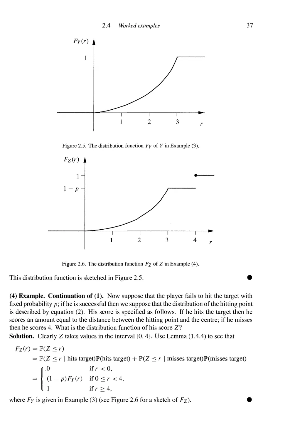
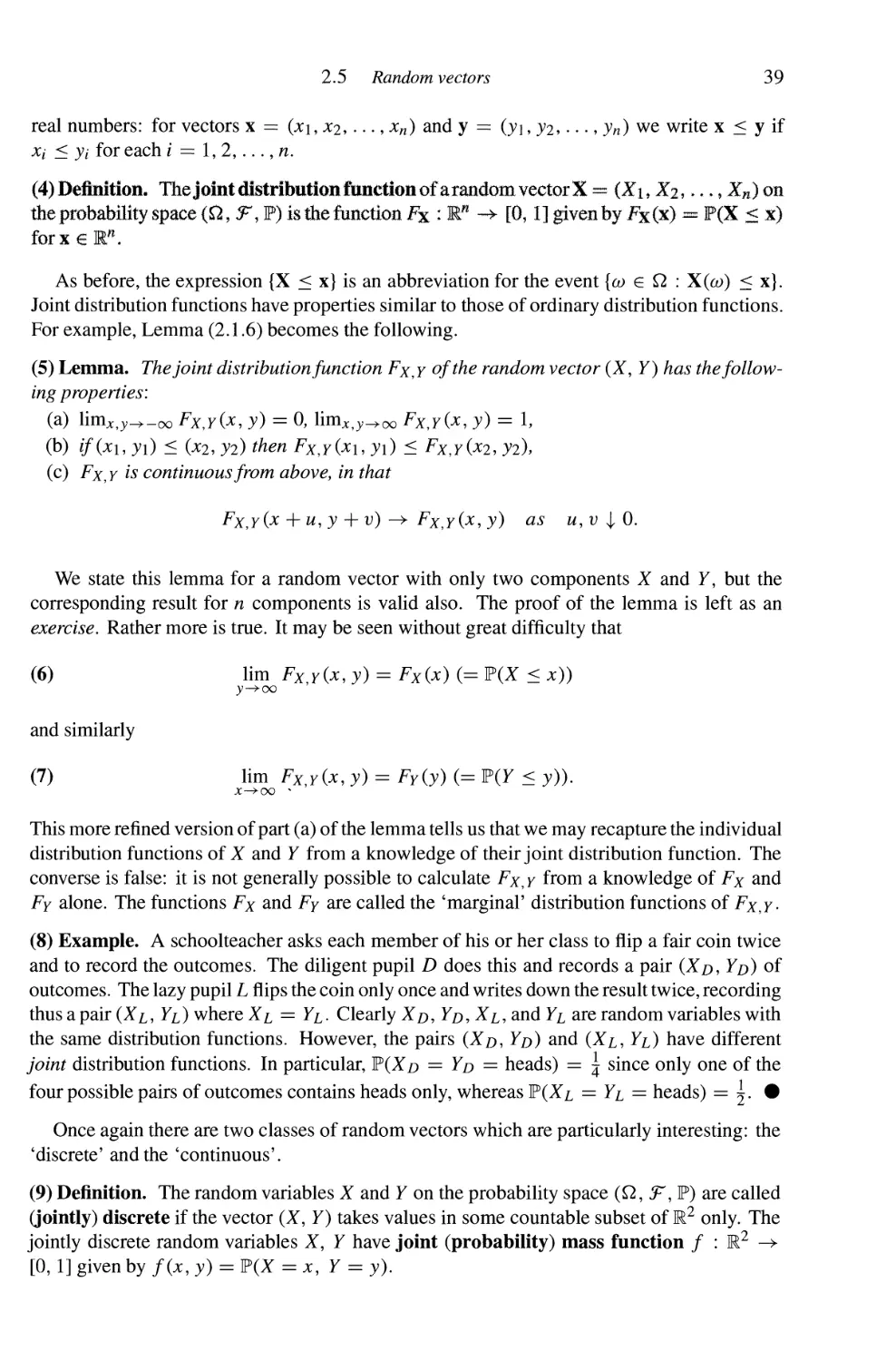
2.4 Worked examples 35
2.5 Random vectors 38
2.6 Monte Carlo simulation 41
2.7 Problems 43
3 Discrete random variables
3.1 Probability mass functions 46
3.2 Independence 48
3.3 Expectation 50
3.4 Indicators and matching 56
3.5 Examples of discrete variables 60
3.6 Dependence 62
3.7 Conditional distributions and conditional expectation 67
3.8 Sums of random variables 70
3.9 Simple random walk 71
3.10 Random walk: counting sample paths 75
3.11 Problems 83

X
Contents
4 Continuous random variables
4.1 Probability density functions 89
4.2 Independence 91
4.3 Expectation 93
4.4 Examples of continuous variables 95
4.5 Dependence 98
4.6 Conditional distributions and conditional expectation 104
4.7 Functions of random variables 107
4.8 Sums of random variables 113
4.9 Multivariate normal distribution 115
4.10 Distributions arising from the normal distribution 119
4.11 Sampling from a distribution 122
4.12 Coupling and Poisson approximation 127
4.13 Geometrical probability 133
4.14 Problems 140
5 Generating functions and their applications
5.1 Generating functions 148
5.2 Some applications 156
5.3 Random walk 162
5.4 Branching processes 171
5.5 Age-dependent branching processes 175
5.6 Expectation revisited 178
5.7 Characteristic functions 181
5.8 Examples of characteristic functions 186
5.9 Inversion and continuity theorems 189
5.10 Two limit theorems 193
5.11 Large deviations 201
5.12 Problems 206
6 Markov chains
6.1 Markov processes 213
6.2 Classification of states 220
6.3 Classification of chains 223
6.4 Stationary distributions and the limit theorem 227
6.5 Reversibility 237
6.6 Chains with finitely many states 240
6.7 Branching processes revisited 243
6.8 Birth processes and the Poisson process 246
6.9 Continuous-time Markov chains 256
6.10 Uniform semigroups 266
6.11 Birth-death processes and imbedding 268
6.12 Special processes 274
6.13 Spatial Poisson processes 281
6.14 Markov chain Monte Carlo 291
6.15 Problems 296

Contents
7 Convergence of random variables
7.1 Introduction 305
7.2 Modes of convergence 308
7.3 Some ancillary results 318
7.4 Laws of large numbers 325
7.5 The strong law 329
7.6 The law of the iterated logarithm 332
7.7 Martingales 333
7.8 Martingale convergence theorem 338
7.9 Prediction and conditional expectation 343
7.10 Uniform integrability 350
7.11 Problems 354
8 Random processes
8.1 Introduction 360
8.2 Stationary processes 361
8.3 Renewal processes 365
8.4 Queues 367
8.5 The Wiener process 370
8.6 Existence of processes 371
8.7 Problems 373
9 Stationary processes
9.1 Introduction 375
9.2 Linear prediction 377
9.3 Autocovariances and spectra 380
9.4 Stochastic integration and the spectral representation 387
9.5 The ergodic theorem 393
9.6 Gaussian processes 405
9.7 Problems 409
10 Renewals
10.1 The renewal equation 412
10.2 Limit theorems 417
10.3 Excess life 421
10.4 Applications 423
10.5 Renewal-reward processes 431
10.6 Problems 437
11 Queues
11.1 Single-server queues 440
11.2 M/M/l 442
11.3 M/G/l 445
11.4 G/M/l 451
11.5 G/G/l 455

Xll
Contents
11.6 Heavy traffic 462
11.7 Networks of queues 462
11.8 Problems 468
12 Martingales
12.1 Introduction 471
12.2 Martingale differences and Hoeffding's inequality 476
12.3 Crossings and convergence 481
12.4 Stopping times 487
12.5 Optional stopping 491
12.6 The maximal inequality 496
12.7 Backward martingales and continuous-time martingales 499
12.8 Some examples 503
12.9 Problems 508
13 Diffusion processes
13.1 Introduction 513
13.2 Brownian motion 514
13.3 Diffusion processes 516
13.4 First passage times 525
13.5 Barriers 530
13.6 Excursions and the Brownian bridge 534
13.7 Stochastic calculus 537
13.8 The ltd integral 539
13.9 Ito's formula 544
13.10 Option pricing 547
13.11 Passage probabilities and potentials 554
13.12 Problems 561
Appendix I. Foundations and notation 564
Appendix II. Further reading 569
Appendix III. History and varieties of probability 571
Appendix IV. John Arbuthnot's Preface to Of the laws of chance (1692) 573
Appendix V. Table of distributions 576
Appendix VI. Chronology 578
Bibliography 580
Notation 583
Index 585

1
Events and their probabilities
Summary. Any experiment involving randomness can be modelled as a
probability space. Such a space comprises a set Q of possible outcomes of the
experiment, a set F of events, and a probability measure P. The definition and
basic properties of a probability space are explored, and the concepts of
conditional probability and independence are introduced. Many examples involving
modelling and calculation are included.
1.1 Introduction
Much of our life is based on the belief that the future is largely unpredictable. For example,
games of chance such as dice or roulette would have few adherents if their outcomes were
known in advance. We express this belief in chance behaviour by the use of words such as
'random' or 'probability', and we seek, by way of gaming and other experience, to assign
quantitative as well as qualitative meanings to such usages. Our main acquaintance with
statements about probability relies on a wealth of concepts, some more reasonable than others.
A mathematical theory of probability will incorporate those concepts of chance which are
expressed and implicit in common rational understanding. Such a theory will formalize these
concepts as a collection of axioms, which should lead directly to conclusions in agreement with
practical experimentation. This chapter contains the essential ingredients of this construction.
1.2 Events as sets
Many everyday statements take the form 'the chance (or probability) of A is /?', where A is
some event (such as 'the sun shining tomorrow', 'Cambridge winning the Boat Race', ...)
and p is a number or adjective describing quantity (such as 'one-eighth', 'low', ...). The
occurrence or non-occurrence of A depends upon the chain of circumstances involved. This
chain is called an experiment or trial', the result of an experiment is called its outcome. In
general, we cannot predict with certainty the outcome of an experiment in advance of its
completion; we can only list the collection of possible outcomes.
(1) Definition. The set of all possible outcomes of an experiment is called the sample space
and is denoted by Q.

2
1.2 Events and their probabilities
(2) Example. A coin is tossed. There are two possible outcomes, heads (denoted by H) and
tails (denoted by T), so that Q = {H, T}. We may be interested in the possible occurrences of
the following events:
(a) the outcome is a head;
(b) the outcome is either a head or a tail;
(c) the outcome is both a head and a tail (this seems very unlikely to occur);
(d) the outcome is not a head. •
(3) Example. A die is thrown once. There are six possible outcomes depending on which of
the numbers 1,2, 3,4, 5, or 6 is uppermost. Thus Q = {1,2,3,4,5,6}. We may be interested
in the following events:
(a) the outcome is the number 1;
(b) the outcome is an even number;
(c) the outcome is even but does not exceed 3;
(d) the outcome is not even. •
We see immediately that each of the events of these examples can be specified as a subset
A of the appropriate sample space Q. In the first example they can be rewritten as
(a) A = {H}, (b) A = {H}U{T},
(c) A = {H}n{T}, (d) A = {H}C,
whilst those of the second example become
(a) A = {1}, (b) A = {2,4,6},
(c) A = {2,4,6} n {1,2, 3}, (d) A = {2,4,6}c.
The complement of a subset A of Q is denoted here and subsequently by Ac; from now on,
subsets of Q containing a single member, such as {H}, will usually be written without the
containing braces.
Henceforth we think of events as subsets of the sample space Q. Whenever A and B are
events in which we are interested, then we can reasonably concern ourselves also with the
events AUB, AHB, and Ac, representing 'A or B\ 'A and B\ and 'not A' respectively. Events
A and B are called disjoint if their intersection is the empty set 0; 0 is called the impossible
event. The set Q is called the certain event, since some member of Q will certainly occur.
Thus events are subsets of Q, but need all the subsets of Q be events? The answer is no, but
some of the reasons for this are too difficult to be discussed here. It suffices for us to think of
the collection of events as a subcollection F of the set of all subsets of Q. This subcollection
should have certain properties in accordance with the earlier discussion:
(a) if A, B e F then AU B e F md An B e F;
(b) if A e FthenAc e F\
(c) the empty set 0 belongs to !F.
Any collection <F of subsets of Q which satisfies these three conditions is called afield. It
follows from the properties of a field F that
n
if AUA2,..., An e 3=^ then (Ja.gF;

1.2 Events as sets
3
Typical notation
Q
CO
A
Ac
ADB
AUB
A\B
AAB
A^B
0
Q
Set jargon
Collection of objects
Member of Q
Subset of Q
Complement of A
Intersection
Union
Difference
Symmetric difference
Inclusion
Empty set
Whole space
Probability jargon
Sample space
Elementary event, outcome
Event that some outcome in A occurs
Event that no outcome in A occurs
Both A and B
Either A or B or both
A, but not B
Either A or B, but not both
If A, then B
Impossible event
Certain event
Table 1.1. The jargon of set theory and probability theory.
that is to say, F is closed under finite unions and hence under finite intersections also (see
Problem (1.8.3)). This is fine when Q is a finite set, but we require slightly more to deal with
the common situation when Q is infinite, as the following example indicates.
(4) Example. A coin is tossed repeatedly until the first head turns up; we are concerned
with the number of tosses before this happens. The set of all possible outcomes is the set
Q = {co\, 0)2, C03,...}, where cot denotes the outcome when the first i — 1 tosses are tails
and the /th toss is a head. We may seek to assign a probability to the event A, that the first
head occurs after an even number of tosses, that is, A = {0)2, 0)4,0)6,...}. This is an infinite
countable union of members of Q and we require that such a set belong to F in order that we
can discuss its probability. •
Thus we also require that the collection of events be closed under the operation of taking
countable unions. Any collection of subsets of Q with these properties is called a a-field.
(5) Definition. A collection F of subsets of Q is called a a-field if it satisfies the following
conditions:
(a) 0Gf;
(b) if Ax, A2,... e F then |JSi Ai e F>
(c) if A e FthenAc e F.
It follows from Problem (1.8.3) that a-fields are closed under the operation of taking
countable intersections. Here are some examples of a-fields.
(6) Example. The smallest a-field associated with Q is the collection F = {0, Q}. •
(7) Example. If A is any subset of Q then F = {0, A, Ac, Q} is a a-field. •
(8) Example. The power set of Q, which is written {0, 1}^ and contains all subsets of Q, is
obviously a a-field. For reasons beyond the scope of this book, when Q is infinite, its power
set is too large a collection for probabilities to be assigned reasonably to all its members. •

4
1.3 Events and their probabilities
To recapitulate, with any experiment we may associate a pair (Q, ^), where Q is the
set of all possible outcomes or elementary events and F is a a-field of subsets of Q which
contains all the events in whose occurrences we may be interested; henceforth, to call a set
A an event is equivalent to asserting that A belongs to the a-field in question. We usually
translate statements about combinations of events into set-theoretic jargon; for example, the
event that both A and B occur is written as A n B. Table 1.1 is a translation chart.
Exercises for Section 1.2
1. Let {A( : i e 1} be a collection of sets. Prove 'De Morgan's Laws'f:
(i>)c=n^ (o)c=i>?-
i i i i
2. Let A and B belong to some a-field T. Show that ^contains the sets A H B, A \ B, and A A B.
3. A conventional knock-out tournament (such as that at Wimbledon) begins with 2n competitors
and has n rounds. There are no play-offs for the positions 2, 3, ..., 2n — 1, and the initial table of
draws is specified. Give a concise description of the sample space of all possible outcomes.
4. Let .Tbe a a-field of subsets of Q and suppose that B e F. Show that % = {An B : A e &} is a
a -field of subsets of B.
5. Which of the following are identically true? For those that are not, say when they are true.
(a) A U (B n C) = (A U B) n (A U C);
(b) A n (B n c) = (A n B) n c-
(c) (AUB)HC = AU(BH C);
(d) A \ (B n C) = (A \ B) U (A \ C).
1.3 Probability
We wish to be able to discuss the likelihoods of the occurrences of events. Suppose that we
repeat an experiment a large number Af of times, keeping the initial conditions as equal as
possible, and suppose that A is some event which may or may not occur on each repetition.
Our experience of most scientific experimentation is that the proportion of times that A occurs
settles down to some value as Af becomes larger and larger; that is to say, writing N(A) for
the number of occurrences of A in the N trials, the ratio N(A)/N appears to converge to a
constant limit as Af increases. We can think of the ultimate value of this ratio as being the
probability P(A) that A occurs on any particular trialj; it may happen that the empirical ratio
does not behave in a coherent manner and our intuition fails us at this level, but we shall not
discuss this here. In practice, Af may be taken to be large but finite, and the ratio N(A)/N
may be taken as an approximation to P(A). Clearly, the ratio is a number between zero and
one; if A = 0 then N(0) = 0 and the ratio is 0, whilst if A = Q then N(Q) = N and the
t Augustus De Morgan is well known for having given the first clear statement of the principle of mathematical
induction. He applauded probability theory with the words: "The tendency of our study is to substitute the
satisfaction of mental exercise for the pernicious enjoyment of an immoral stimulus".
i:This superficial discussion of probabilities is inadequate in many ways; questioning readers may care to
discuss the philosophical and empirical aspects of the subject amongst themselves (see Appendix III).

1.3 Probability
5
ratio is 1. Furthermore, suppose that A and B are two disjoint events, each of which may or
may not occur at each trial. Then
N(A U B) = N(A) + N(B)
and so the ratio N(A U B)/N is the sum of the two ratios N(A)/N and N(B)/N. We now
think of these ratios as representing the probabilities of the appropriate events. The above
relations become
P(AU£) = P(A) + P(£), P(0) = O, P(fi) = l.
This discussion suggests that the probability function P should be finitely additive, which is
to say that
(n \ n
1=1 / i=l
a glance at Example (1.2.4) suggests the more extensive property that P be countably additive,
in that the corresponding property should hold for countable collections A i, A2,... of disjoint
events.
These relations are sufficient to specify the desirable properties of a probability function P
applied to the set of events. Any such assignment of likelihoods to the members of & is called
a probability measure. Some individuals refer informally to P as a 'probability distribution',
especially when the sample space is finite or countably infinite; this practice is best avoided
since the term 'probability distribution' is reserved for another purpose to be encountered in
Chapter 2.
(1) Definition. A probability measure P on (Q> SP) is a function P : SF ~* [0,1] satisfying
(a) P(0)=OI P(n)«l;
(b) if At, A2,. *. is a collection of disjoint members of 3% in that A* Pi Aj = 0for all pairs
U j satisfying i # j, then
(DO \ OO
1=1 / *=i
The triple (fll, F, P), comprising a set Q, a <r-field F of subsets of Q, and a probability
measure F on (Q, F), is called a probability space,
A probability measure is a special example of what is called a measure on the pair (Q, F).
A measure is a function /x : F —► [0, 00) satisfying /x(0) = 0 together with (b) above. A
measure /x is a probability measure if /x(£2) = 1.
We can associate a probability space (Q, !F, P) with any experiment, and all questions
associated with the experiment can be reformulated in terms of this space. It may seem
natural to ask for the numerical value of the probability P(A) of some event A. The answer
to such a question must be contained in the description of the experiment in question. For
example, the assertion that a fair coin is tossed once is equivalent to saying that heads and
tails have an equal probability of occurring; actually, this is the definition of fairness.

6 1.3 Events and their probabilities
(2) Example. A coin, possibly biased, is tossed once. We can take Q = {H, T} and F =
{0, H, T, Q], and a possible probability measure P : F —► [0, 1] is given by
P(0) = O, P(H) = />, P(T) = l-p, P(fi) = l,
where /? is a fixed real number in the interval [0, 1]. If p = \, then we say that the coin is
fair, or unbiased. •
(3) Example. A die is thrown once. We can take Q = {1, 2, 3,4, 5, 6}, ¥ = {0, l}fi, and
the probability measure P given by
P(A) = ]T /?,- for any A c fi,
where p\, P2, • • •, P6 are specified numbers from the interval [0, 1] having unit sum. The
probability that / turns up is /?/. The die is fair if pt = ^ for each /, in which case
P(A) = \\A\ for any A c fi,
where | A| denotes the cardinality of A. •
The triple (£2, ^, P) denotes a typical probability space. We now give some of its simple
but important properties.
(4) Lemma.
(a) P(AC) = 1 - P(A),
(b) ifB^A then F(B) = P(A) + F(B \ A) > P(A),
(c) P(A U B) = P(A) + P(£) - P(A H B),
(d) more generally, if A\, A2, ..., An are events, then
P(UA<) =^P(A«)-XJP(A,-nA7-)+ X] P(A«nA7-nAik)-...
V=l / / i<j i<j<k
+ (-ir+1P(AinA2n...nA^)
where, for example, 2Z/</ 5Mm5 ^v^r flW unordered pairs (/, 7) wz7/z / / 7.
Proof.
(a) A U Ac = Q and A n Ac = 0, so P(A U Ac) = P(A) + P(AC) = 1.
(b) B = A U (5 \ A). This is the union of disjoint sets and therefore
P(£) = P(A)+P(£\A).
(c) A U B = A U (B \ A), which is a disjoint union. Therefore, by (b),
P(A U B)= P(A) + F(B \ A) = P(A) + P(£ \ (A n B))
= P(A) + P(fi)-P(An5).
(d) The proof is by induction on rc, and is left as an exercise (see Exercise (1.3.4)). ■

1.3 Probability
1
In Lemma (4b), B \ A denotes the set of members of B which are not in A. In order to
write down the quantity ¥(B \ A), we require that B \ A belongs to !F, the domain of P; this is
always true when A and B belong to !F, and to prove this was part of Exercise (1.2.2). Notice
that each proof proceeded by expressing an event in terms of disjoint unions and then applying
P. It is sometimes easier to calculate the probabilities of intersections of events rather than
their unions; part (d) of the lemma is useful then, as we shall discover soon. The next property
of P is more technical, and says that P is a continuous set function; this property is essentially
equivalent to the condition that P is countably additive rather than just finitely additive (see
Problem (1.8.16) also).
(5) Lemma. Let A\, A2,... be an increasing sequence of events, so that A\ c A2 ^ A3 c
• • •, and write A for their limit.
A = [ J At = lim At.
Then P(A) = lim^oo P(A,-).
Similarly, ifB\,B2,... is a decreasing sequence of events, so that B\ ^ #2 ^ #3 ^ •
then
B = C\Bi= lim Bi
/ = 1
satisfies F(B) = lim;-^ P(#;).
Proof. A = A\ U (A2 \ Ai) U (A3 \ A2) U • • • is the union of a disjoint family of events.
Thus, by Definition (1),
P(A) = P(Ai) + ^P(Al-+i\Al-)
/=1
n-\
:P(Ai)+ lim V[P(A/+i)-P(A;)]
/=1
= lim P(A„).
n->oo
To show the result for decreasing families of events, take complements and use the first part
{exercise). ■
To recapitulate, statements concerning chance are implicitly related to experiments or
trials, the outcomes of which are not entirely predictable. With any such experiment we can
associate a probability space (Q, F, P) the properties of which are consistent with our shared
and reasonable conceptions of the notion of chance.
Here is some final jargon. An event A is called null if P(A) = 0. If P(A) = 1, we say
that A occurs almost surely. Null events should not be confused with the impossible event
0. Null events are happening all around us, even though they have zero probability; after all,
what is the chance that a dart strikes any given point of the target at which it is thrown? That
is, the impossible event is null, but null events need not be impossible.

8
1.4 Events and their probabilities
Exercises for Section 1.3
1. Let A and B be events with probabilities P(A) = |andP(£) = \. Showthat^ < P(APi£) < j,
and give examples to show that both extremes are possible. Find corresponding bounds for P(A U B).
2. A fair coin is tossed repeatedly. Show that, with probability one, a head turns up sooner or later.
Show similarly that any given finite sequence of heads and tails occurs eventually with probability
one. Explain the connection with Murphy's Law.
3. Six cups and saucers come in pairs: there are two cups and saucers which are red, two white, and
two with stars on. If the cups are placed randomly onto the saucers (one each), find the probability
that no cup is upon a saucer of the same pattern.
4. Let A\, A2,..., An be events where n > 2, and prove that
P(0A') =X)P(A|)-XJP(AinA7-)+ Y, nAiHAjHAk)
i=\ i i<j i<j<k
+ (-if+1P(A] n A2 n • • • n An).
In each packet of Corn Flakes may be found a plastic bust of one of the last five Vice-Chancellors
of Cambridge University, the probability that any given packet contains any specific Vice-Chancellor
being ^, independently of all other packets. Show that the probability that each of the last three
Vice-Chancellors is obtained in a bulk purchase of six packets is 1 — 3(|)6 + 3(|)6 -(5)6.
5. Let Ar, r > 1, be events such that P(Ar) = 1 for all r. Show that P(f|^i Ar) = 1.
6. You are given that at least one of the events Ar, 1 < r < n, is certain to occur, but certainly no
more than two occur. If P(Ar) = p, and P(Ar Pi As) = q,r / s, show that p > l/n and q < 2/n.
7. You are given that at least one, but no more than three, of the events Ar, 1 < r < n, occur, where
n > 3. The probability of at least two occurring is \. If P(Ar) = p, P(Ar n As) = q, r / s, and
P(Ar Pi As Pi At) = x, r < s < t, show that p > 3/(2n), and q < A/n.
1.4 Conditional probability
Many statements about chance take the form 'if B occurs, then the probability of A is /?',
where B and A are events (such as 'it rains tomorrow' and 'the bus being on time' respectively)
and p is a likelihood as before. To include this in our theory, we return briefly to the discussion
about proportions at the beginning of the previous section. An experiment is repeated Af times,
and on each occasion we observe the occurrences or non-occurrences of two events A and
B. Now, suppose we only take an interest in those outcomes for which B occurs; all other
experiments are disregarded. In this smaller collection of trials the proportion of times that A
occurs is N(A n B)/N(B), since B occurs at each of them. However,
N(AHB) _ N(AHB)/N
N(B) ~ N(B)/N
If we now think of these ratios as probabilities, we see that the probability that A occurs, given
that B occurs, should be reasonably defined as P(A n B)/F(B).
Probabilistic intuition leads to the same conclusion. Given that an event B occurs, it is the
case that A occurs if and only ifADB occurs. Thus the conditional probability of A given B

1.4 Conditional probability
9
should be proportional to P(A HB), which is to say that it equals aF(A n B) for some constant
a = a(#). The conditional probability of Q given # must equal 1, and thus a¥(Q n B) = 1,
yielding a = 1/P(#).
We formalize these notions as follows.
(1) Definition. If p(B) > 0 then the conditional probability that A occurs given that B
occurs is defined to be
P(B)
We denote this conditional probability by P(A | B), pronounced 'the probability of A given
B\ or sometimes 'the probability of A conditioned (or conditional) on B\
(2) Example. Two fair dice are thrown. Given that the first shows 3, what is the probability
that the total exceeds 6? The answer is obviously \, since the second must show 4, 5, or
6. However, let us labour the point. Clearly Q = {1, 2, 3, 4, 5, 6}2, the sett of all ordered
pairs (/, j) for i, j e {1, 2,..., 6}, and we can take F to be the set of all subsets of Q, with
P(A) = I A|/36 for any A c Q. Let B be the event that the first die shows 3, and A be the
event that the total exceeds 6. Then
B = {(3, b) : 1 < b < 6}, A = {(a, b):a + b>6}, AHB = {(3,4), (3, 5), (3, 6)},
and
F(AHB) \AHB\ 3
P(A | B) = — = = -. •
V ' F(B) \B\ 6
(3) Example. A family has two children. What is the probability that both are boys, given
that at least one is a boy? The older and younger child may each be male or female, so there
are four possible combinations of sexes, which we assume to be equally likely. Hence we can
represent the sample space in the obvious way as
Q = {GG, GB, BG, BB}
where P(GG) = P(BB) = P(GB) = P(BG) = \. From the definition of conditional
probability,
P(BB | one boy at least) = P(BB | GB U BG U BB)
_ P(BB n (GB U BG U BB))
P(GB U BG U BB)
P(BB) 1
P(GB U BG U BB) 3
A popular but incorrect answer to the question is \. This is the correct answer to another
question: for a family with two children, what is the probability that both are boys given that
the younger is a boy? In this case,
P(BB | younger is a boy) = P(BB | GB U BB)
_ P(BB n (GB U BB)) _ P(BB) _ 1
P(GB U BB) " P(GB U BB) " 2"
tRemember that A x B = {(a, b) : a e A, b e B} and that A x A = A2.

10
1.4 Events and their probabilities
The usual dangerous argument contains the assertion
P(BB | one child is a boy) = P(other child is a boy).
Why is this meaningless? [Hint: Consider the sample space.] •
The next lemma is crucially important in probability theory. A family B\, B2,..., Bn of
events is called a partition of the set Q if
n
B( n Bj■ = 0 when i ^ j, and |^J Bt = Q.
1=1
Each elementary event co e Q belongs to exactly one set in a partition of Q.
(4) Lemma* For any events A and B such thai 0 < P(B) < 1»
P(A) = P(A I B)W(B) + P(A I #C)P(£C).
More generally, let B\, 2¾ ,^iBnbe a partition ofQ such that P($0 > 0,/for #21 *\ 7¾^
P(A)«J]P(A |Bf)P(fli).
Proof. A = (AHB)U(An Bc). This is a disjoint union and so
P(A) = P(A n B) + P(A n £c)
= P(A I £)P(£) + P(A I ^C)P(^C).
The second part is similar (see Problem (1.8.10)). ■
(5) Example. We are given two urns, each containing a collection of coloured balls. Urn I
contains two white and three blue balls, whilst urn II contains three white and four blue balls.
A ball is drawn at random from urn I and put into urn II, and then a ball is picked at random
from urn II and examined. What is the probability that it is blue? We assume unless otherwise
specified that a ball picked randomly from any urn is equally likely to be any of those present.
The reader will be relieved to know that we no longer need to describe (Q, !F, P) in detail;
we are confident that we could do so if necessary. Clearly, the colour of the final ball depends
on the colour of the ball picked from urn I. So let us 'condition' on this. Let A be the event
that the final ball is blue, and let B be the event that the first one picked was blue. Then, by
Lemma (4),
P(A) = P(A I B)F(B) + P(A I £C)P(£C).
We can easily find all these probabilities:
P(A I B) = P(A I urn II contains three white and five blue balls) = |,
P(A I Bc) = P(A I urn II contains four white and four blue balls) = ±,
F(B) = l, P(£c) = |.

1.4 Conditional probability
11
Hence
^) = 1-5 + 2-5 = 1- •
Unprepared readers may have been surprised by the sudden appearance of urns in this book.
In the seventeenth and eighteenth centuries, lotteries often involved the drawing of slips from
urns, and voting was often a matter of putting slips or balls into urns. In France today, aller aux
urnes is synonymous with voting. It was therefore not unnatural for the numerous Bernoullis
and others to model births, marriages, deaths, fluids, gases, and so on, using urns containing
balls of varied hue.
(6) Example. Only two factories manufacture zoggles. 20 per cent of the zoggles from factory
I and 5 per cent from factory II are defective. Factory I produces twice as many zoggles as
factory II each week. What is the probability that a zoggle, randomly chosen from a week's
production, is satisfactory? Clearly this satisfaction depends on the factory of origin. Let A
be the event that the chosen zoggle is satisfactory, and let B be the event that it was made in
factory I. Arguing as before,
P(A) = P(A | B)F(B) + P(A | BC)¥(BC)
_ 4 2,19 1 _ 51
— 5 ' 3 -1" 20 ' 3 ~~ 60'
If the chosen zoggle is defective, what is the probability that it came from factory I? In our
notation this is just ¥(B | Ac). However,
PrB I ac) = P(Z?nAC) = nA°' B)nB) = U_ = * m
P(AC) P(AC) i_5i 9'
This section is terminated with a cautionary example. It is not untraditional to perpetuate
errors of logic in calculating conditional probabilities. Lack of unambiguous definitions and
notation has led astray many probabilists, including even Boole, who was credited by Russell
with the discovery of pure mathematics and by others for some of the logical foundations of
computing. The well-known 'prisoners' paradox' also illustrates some of the dangers here.
(7) Example. Prisoners' paradox. In a dark country, three prisoners have been incarcerated
without trial. Their warder tells them that the country's dictator has decided arbitrarily to free
one of them and to shoot the other two, but he is not permitted to reveal to any prisoner the
fate of that prisoner. Prisoner A knows therefore that his chance of survival is \. In order
to gain information, he asks the warder to tell him in secret the name of some prisoner (but
not himself) who will be killed, and the warder names prisoner B. What now is prisoner As
assessment of the chance that he will survive? Could it be \\ after all, he knows now that
the survivor will be either A or C, and he has no information about which? Could it be \\
after all, according to the rules, at least one of B and C has to be killed, and thus the extra
information cannot reasonably affect As earlier calculation of the odds? What does the reader
think about this? The resolution of the paradox lies in the situation when either response (B
or C) is possible.
An alternative formulation of this paradox has become known as the Monty Hall problem,
the controversy associated with which has been provoked by Marilyn vos Savant (and many
others) in Parade magazine in 1990; see Exercise (1.4.5). •

12
1.4 Events and their probabilities
Exercises for Section 1.4
1. Prove that P(A | B) = P(£ | A)P(A)/P(£) whenever P(A)P(£) / 0. Show that, if P(A | B) >
P(A), thenP(5 | A) > P(5).
2. For events Ai, A2,..., An satisfying P(Aj n A2 0 • • • Pi An_\) > 0, prove that
p(Ai n A2 n • • • n An) = P(Ai)P(A21 aop(A3 | ax n A2) • • • p(A„ | ax n a2 n. •. n a„_i).
3. A man possesses five coins, two of which are double-headed, one is double-tailed, and two are
normal. He shuts his eyes, picks a coin at random, and tosses it. What is the probability that the lower
face of the coin is a head?
He opens his eyes and sees that the coin is showing heads; what is the probability that the lower
face is a head?
He shuts his eyes again, and tosses the coin again. What is the probability that the lower face is
a head?
He opens his eyes and sees that the coin is showing heads; what is the probability that the lower
face is a head?
He discards this coin, picks another at random, and tosses it. What is the probability that it shows
heads?
4. What do you think of the following 'proof by Lewis Carroll that an urn cannot contain two balls
of the same colour? Suppose that the urn contains two balls, each of which is either black or white;
thus, in the obvious notation, P(BB) = P(BW) = P(WB) = P(WW) = \. We add a black ball, so
that P(BBB) = P(BBW) = P(BWB) = P(BWW) = \. Next we pick a ball at random; the chance
that the ball is black is (using conditional probabilities) \-\ + \-\ + \-\ + \-\ = \- However, if
there is probability | that a ball, chosen randomly from three, is black, then there must be two black
and one white, which is to say that originally there was one black and one white ball in the urn.
5. The Monty Hall problem: goats and cars, (a) Cruel fate has made you a contestant in a game
show; you have to choose one of three doors. One conceals a new car, two conceal old goats. You
choose, but your chosen door is not opened immediately. Instead, the presenter opens another door
to reveal a goat, and he offers you the opportunity to change your choice to the third door (unopened
and so far unchosen). Let p be the (conditional) probability that the third door conceals the car. The
value of p depends on the presenter's protocol. Devise protocols to yield the values p = ^, p = |.
Show that, for a e [^, |], there exists a protocol such that p — a. Are you well advised to change
your choice to the third door?
(b) In a variant of this question, the presenter is permitted to open the first door chosen, and to reward
you with whatever lies behind. If he chooses to open another door, then this door invariably conceals
a goat. Let p be the probability that the unopened door conceals the car, conditional on the presenter
having chosen to open a second door. Devise protocols to yield the values p = 0, p = 1, and deduce
that, for any a e [0, 1], there exists a protocol with p = a.
6. The prosecutor's fallacyt. Let G be the event that an accused is guilty, and T the event that
some testimony is true. Some lawyers have argued on the assumption that P(G | T) = ¥(T \ G).
Show that this holds if and only if P(G) = F(T).
7. Urns. There are n urns of which the rth contains r — 1 red balls and n — r magenta balls. You
pick an urn at random and remove two balls at random without replacement. Find the probability that:
(a) the second ball is magenta;
(b) the second ball is magenta, given that the first is magenta.
fThe prosecution made this error in the famous Dreyfus case of 1894.

1.5 Independence 13
1.5 Independence
In general, the occurrence of some event B changes the probability that another event A
occurs, the original probability P(A) being replaced by P(A | B). If the probability remains
unchanged, that is to say P(A | B) = P(A), then we call A and B 'independent'. This is
well defined only if F(B) > 0. Definition (1.4.1) of conditional probability leads us to the
following.
(1) Definition. Events A and B are called independent if
P(AflS) = P(A)P(B).
Mote generally, a family {A* : i e 1} is called independent if
\i€J / i€J
for all finite subsets J of L
Remark. A common student error is to make the fallacious statement that A and B are
independent if A D B = 0.
If the family {A/ : i e 1} has the property that
it n Aj) = P(A;)P(A;) for all i jk j
then it is called pairwise independent. Pairwise-independent families are not necessarily
independent, as the following example shows.
(2) Example. Suppose Q — {abc, acb, cab, cba, bca, bac, aaa, bbb, ccc}, and each of the
nine elementary events in Q occurs with equal probability ^. Let A& be the event that the £th
letter is a. It is left as an exercise to show that the family {A i, A2, A3} is pairwise independent
but not independent. #
(3) Example (1.4.6) revisited. The events A and B of this example are clearly dependent
because P(A | B) = f and P(A) = =¾. •
(4) Example. Choose a card at random from a pack of 52 playing cards, each being picked
with equal probability ^. We claim that the suit of the chosen card is independent of its rank.
For example,
P(king) = ^, P(king | spade) = ^.
Alternatively,
P(spade king) = ± = ±- ± = P(spade)P(king). •
Let C be an event with P(C) > 0. To the conditional probability measure P( • | C)
corresponds the idea of conditional independence. Two events A and B are called conditionally
independent given C if
(5) P(A n B I C) = P(A I C)F(B \ C);
there is a natural extension to families of events. [However, note Exercise (1.5.5).]

14
1.6 Events and their probabilities
Exercises for Section 1.5
1. Let A and B be independent events; show that Ac, B are independent, and deduce that Ac, Bc
are independent.
2. We roll a die n times. Let A/y be the event that the /th and yth rolls produce the same number.
Show that the events {Ay : 1 < i < j < n] are pairwise independent but not independent.
3. A fair coin is tossed repeatedly. Show that the following two statements are equivalent:
(a) the outcomes of different tosses are independent,
(b) for any given finite sequence of heads and tails, the chance of this sequence occurring in the first
m tosses is 2~m, where m is the length of the sequence.
4. Let Q = {1, 2,..., p] where p is prime, ^be the set of all subsets of Q, and P(A) = | A\/p for
all A e T. Show that, if A and B are independent events, then at least one of A and B is either 0 or
Q.
5. Show that the conditional independence of A and B given C neither implies, nor is implied by,
the independence of A and B. For which events C is it the case that, for all A and B, the events A and
B are independent if and only if they are conditionally independent given C?
6. Safe or sorry? Some form of prophylaxis is said to be 90 per cent effective at prevention during
one year's treatment. If the degrees of effectiveness in different years are independent, show that the
treatment is more likely than not to fail within 7 years.
7. Families. Jane has three children, each of which is equally likely to be a boy or a girl independently
of the others. Define the events:
A = {all the children are of the same sex},
B = {there is at most one boy},
C = {the family includes a boy and a girl}.
(a) Show that A is independent of B, and that B is independent of C.
(b) Is A independent of C?
(c) Do these results hold if boys and girls are not equally likely?
(d) Do these results hold if Jane has four children?
8. Galton's paradox. You flip three fair coins. At least two are alike, and it is an evens chance that
the third is a head or a tail. Therefore P(all alike) = j • Do you agree?
9. Two fair dice are rolled. Show that the event that their sum is 7 is independent of the score shown
by the first die.
1.6 Completeness and product spaces
This section should be omitted at the first reading, but we shall require its contents later. It
contains only a sketch of complete probability spaces and product spaces; the reader should
look elsewhere for a more detailed treatment (see Billingsley 1995). We require the following
result.
(1) Lemma. If !F and $ are two a-fields of subsets ofQ then their intersection !F H fy is
a cr-field also. More generally if {Ft : i e 1} is a family of a-fields of subsets ofQ then
$ = f)iei ^i ^ a &-field also.

1.6 Completeness and product spaces
15
The proof is not difficult and is left as an exercise. Note that the union F U $ may not be a
a -field, although it may be extended to a unique smallest a-field written a (!F U $), as follows.
Let {%>[ : i e 1} be the collection of all a-fields which contain both & and $ as subsets; this
collection is non-empty since it contains the set of all subsets of Q. Then $ = f\-G/ % is the
unique smallest a-field which contains F U $.
(A) Completeness. Let (£2, 5\ P) be a probability space. Any event A which has zero
probability, that is P(A) = 0, is called null. It may seem reasonable to suppose that any subset
B of a null set A will itself be null, but this may be without meaning since B may not be an
event, and thus F(B) may not be defined.
(2) Definition. A probability space (Q,!F,F) is called complete if all subsets of null sets
are events.
Any incomplete space can be completed thus. Let J\f be the collection of all subsets of
null sets in & and let $ = cr(!F U J\f) be the smallest a-field which contains all sets in &
and tSf. It can be shown that the domain of P may be extended in an obvious way from F to
gl; (ft, #, P) is called the completion of (Q, £\ P).
(B) Product spaces. The probability spaces discussed in this chapter have usually been
constructed around the outcomes of one experiment, but instances occur naturally when we need
to combine the outcomes of several independent experiments into one space (see Examples
(1.2.4) and (1.4.2)). How should we proceed in general?
Suppose two experiments have associated probability spaces (Q\, ^i, Pi) and (Q2, $2, ^2)
respectively. The sample space of the pair of experiments, considered jointly, is the collection
ftix^2 = {(co\,o)2) : co\ e Q\, coi e Q2} of ordered pairs. The appropriate a-field of events
is more complicated to construct. Certainly it should contain all subsets of Q \ x Q2 of the form
A\ x A2 = {{a\, ai) : a\ e A\, ai e A2} where Ai and A2 are typical members of 5i and 5¾
respectively. However, the family of all such sets, !Fi x 5¾ = {A\ x A2 : A\ e Fi, A2 e £2},
is not in general a a-field. By the discussion after (1), there exists a unique smallest a-field
$ = cr(!Fi x 5¾) of subsets of Q\ x ^2 which contains 5i x 5¾. All we require now is a
suitable probability function on (Q\ x £^, $)• Let P12 : !F\ x 5¾ -> [0, 1] be given by:
(3) Pi2(Ai x A2) = Pi(Ai)P2(A2) for Ai € 5i, A2 e F2.
It can be shown that the domain of Pi2 can be extended from £1 x 5¾ to the whole of
fy = a(!Fi x 5¾). The ensuing probability space (Q\ x ^2, $, P12) is called the product
space of (Q \, !F\, Pi) and (^2, F2, ^2)• Products of larger numbers of spaces are constructed
similarly. The measure Pi2 is sometimes called the 'product measure' since its defining
equation (3) assumed that two experiments are independent. There are of course many other
measures that can be applied to (Q\ x Q2, $)•
In many simple cases this technical discussion is unnecessary. Suppose that Q\ and Q2
are finite, and that their a-fields contain all their subsets; this is the case in Examples (1.2.4)
and (1.4.2). Then % contains all subsets of Q\ x ^2-

16
1.7 Events and their probabilities
1.7 Worked examples
Here are some more examples to illustrate the ideas of this chapter. The reader is now equipped
to try his or her hand at a substantial number of those problems which exercised the pioneers
in probability. These frequently involved experiments having equally likely outcomes, such
as dealing whist hands, putting balls of various colours into urns and taking them out again,
throwing dice, and so on. In many such instances, the reader will be pleasantly surprised to
find that it is not necessary to write down (Q, F, P) explicitly, but only to think of Q as being
a collection [a)\, (02,..., &>#} of possibilities, each of which may occur with probability 1/N.
Thus, P(A) = \A\/N for any A c. Q. The basic tools used in such problems are as follows.
(a) Combinatorics: remember that the number of permutations of n objects is n\ and that
the number of ways of choosing r objects from n is (").
(b) Set theory: to obtain P(A) we can compute P(AC) = 1 — P(A) or we can partition A
by conditioning on events B{, and then use Lemma (1.4.4).
(c) Use of independence.
(1) Example. Consider a series of hands dealt at bridge. Let A be the event that in a given
deal each player has one ace. Show that the probability that A occurs at least once in seven
deals is approximately \.
Solution. The number of ways of dealing 52 cards into four equal hands is 52!/(13!)4. There
are 4! ways of distributing the aces so that each hand holds one, and there are 48!/(12!)4 ways
of dealing the remaining cards. Thus
4!48!/(12!)4 1
P(A) = -—f- ~ —.
52!/(13!)4 10
Now let Bt be the event that A occurs for the first time on the /th deal. Clearly B( D Bj = 0,
i ^ j. Thus
7
P(A occurs in seven deals) = F(B\ U ■ • ■ U B7) = ^ P(^) using Definition (1.3.1).
1
Since successive deals are independent, we have
F(Bi) = P(AC occurs on deal 1, Ac occurs on deal 2,
..., Ac occurs on deal /-1, A occurs on deal /)
= p(Ac)/"1P(A) using Definition (1.5.1)
~ (1 - ±\-1 ±
— y \o) io-
Thus
*—1
P(A occurs in seven deals) = ^ P(#;) -^(^) IT
1 1
Can you see an easier way of obtaining this answer?
(2) Example. There are two roads from A to B and two roads from B to C. Each of the four
roads has probability p of being blocked by snow, independently of all the others. What is
the probability that there is an open road from A to C?

1.7 Worked examples
17
Solution.
P(open road) = P((open road from A to B) D (open road from B to C))
= P(open road from A to B)P(open road from B to C)
using the independence. However, p is the same for all roads; thus, using Lemma (1.3.4),
P(open road) = (l - P(no road from A to B))2
= {1 — P ((first road blocked) n (second road blocked))}
= {1 — P(first road blocked)P (second road blocked)}
using the independence. Thus
(3) P(open road) =(1- p2)2.
Further suppose that there is also a direct road from A to C, which is independently blocked
with probability p. Then, by Lemma (1.4.4) and equation (3),
P(open road) = P(open road | direct road blocked) • p
+ P(open road | direct road open) -(1-/7)
= (l-p2)2'P + l-(l-p). •
(4) Example. Symmetric random walk (or 'Gambler's ruin'). A man is saving up to buy
a new Jaguar at a cost of N units of money. He starts with k units where 0 < k < N, and
tries to win the remainder by the following gamble with his bank manager. He tosses a fair
coin repeatedly; if it comes up heads then the manager pays him one unit, but if it comes up
tails then he pays the manager one unit. He plays this game repeatedly until one of two events
occurs: either he runs out of money and is bankrupted or he wins enough to buy the Jaguar.
What is the probability that he is ultimately bankrupted?
Solution. This is one of many problems the solution to which proceeds by the construction
of a linear difference equation subject to certain boundary conditions. Let A denote the event
that he is eventually bankrupted, and let B be the event that the first toss of the coin shows
heads. By Lemma (1.4.4),
(5) P*(A) = Fk(A | B)F(B) + Fk(A \ BC)¥(BC),
where P& denotes probabilities calculated relative to the starting point k. We want to find
Pfc(A). Consider P&(A | B). If the first toss is a head then his capital increases to k + 1 units
and the game starts afresh from a different starting point. Thus P&(A \ B) = P&+i (A) and
similarly Fk(A \ Bc) = P*_i (A). So, writing pk = P*(A), (5) becomes
(6) pk = \{pk+\ + pk-i) if 0 < k < N,
which is a linear difference equation subject to the boundary conditions p0 = I, pN = 0.
The analytical solution to such equations is routine, and we shall return later to the general

18 1.7 Events and their probabilities
method of solution. In this case we can proceed directly. We put bk = Pk — Pk-\ to obtain
bk = bk-\ and hence bk = b\ for all k. Thus
Pk = b\+ pk-i = 2b\ + pk-2 = '- = kb\ + po
is the general solution to (6). The boundary conditions imply that po = l,b\ = —l/N, giving
(7) P*(A) = 1-^-
As the price of the Jaguar rises, that is as N -> oo, ultimate bankruptcy becomes very likely.
This is the problem of the 'symmetric random walk with two absorbing barriers' to which we
shall return in more generality later. •
Remark. Our experience of student calculations leads us to stress that probabilities lie
between zero and one; any calculated probability which violates this must be incorrect.
(8) Example. Testimony. A court is investigating the possible occurrence of an unlikely event
T. The reliability of two independent witnesses called Alf and Bob is known to the court:
Alf tells the truth with probability a and Bob with probability fi, and there is no collusion
between the two of them. Let A and B be the events that Alf and Bob assert (respectively)
that T occurred, and let x = ¥(T). What is the probability that T occurred given that both
Alf and Bob declare that T occurred?
Solution. We are asked to calculate P(T | A n B), which is equal to P(T HAH B)/F(A n B).
Now P(r n A n B) = P(A n B \ T)F(T) and
p(A n B) = P(A n b I T)¥(T) + P(A n b I rc)P(rc).
We have from the independence of the witnesses that A and B are conditionally independent
given either T or Tc. Therefore
P(A H B I T) = P(A | T)F(B | T) = a0,
P(A H B | Tc) = P(A | TC)F(B | Tc) = (1- a)(l - £),
so that
aBr
¥(T | A H B) = .
a0T + (l-a)(l-0)(l-T)
As an example, suppose that a = ft = ^ and r = 1/1000. ThenP(T | AHB) = 81/1080,
which is somewhat small as a basis for a judicial conclusion.
This calculation may be informative. However, it is generally accepted that such an
application of the axioms of probability is inappropriate to questions of truth and belief. •
(9) Example. Zoggles revisited. A new process for the production of zoggles is invented,
and both factories of Example (1.4.6) install extra production lines using it. The new process
is cheaper but produces fewer reliable zoggles, only 75 per cent of items produced in this new
way being reliable.
Factory I fails to implement its new production line efficiently, and only 10 per cent of its
output is made in this manner. Factory II does better: it produces 20 per cent of its output by
the new technology, and now produces twice as many zoggles in all as Factory I.

1.7 Worked examples
19
Is the new process beneficial to the consumer?
Solution. Both factories now produce a higher proportion of unreliable zoggles than before,
and so it might seem at first sight that there is an increased proportion of unreliable zoggles
on the market.
Let A be the event that a randomly chosen zoggle is satisfactory, B the event that it came
from factory I, and C the event that it was made by the new method. Then
P(A) = ±P(A | B) + |P(A | Bc)
= \ (^P(A | B n C) + ^P(A | B n Cc))
+ \ Uf(A |5cnc) + fP(A i bcncc))
— I (1. 3,_9_ 4\ , 2 /± 3,4 19 \ _ 523 ^ 51
~~ 3 \J0 ' 4 "*" 10 ' 5/ "*" 3 ^5 ' 4 "*" 5 ' 20/ ~~ 600 ^ 60'
so that the proportion of satisfactory zoggles has been increased. #
(10) Example. Simpson's paradoxt. A doctor has performed clinical trials to determine
the relative efficacies of two drugs, with the following results.
Success
Failure
Women
Drug I Drug II
200 10
1800 190
Men
Drug I Drug II
19 1000
1 1000
Which drug is the better? Here are two conflicting responses.
1. Drug I was given to 2020 people, of whom 219 were cured. The success rate was
219/2020, which is much smaller than the corresponding figure, 1010/2200, for drug II.
Therefore drug II is better than drug I.
2. Amongst women the success rates of the drugs are 1/10 and 1/20, and amongst men
19/20 and 1/2. Drug I wins in both cases.
This well-known statistical paradox may be reformulated in the following more general
way. Given three events A, B, C, it is possible to allocate probabilities such that
(11) P(A | B H C) > P(A \ BCHC) and P(A | B n Cc) > P(A | Bc n Cc)
but
(12) P(A | B) < P(A | Bc).
tThis paradox, named after Simpson (1951), was remarked by Yule in 1903. The nomenclature is an
instance of Stigler's law of eponymy: "No law, theorem, or discovery is named after its originator". This law
applies to many eponymous statements in this book, including the law itself. As remarked by A. N. Whitehead,
"Everything of importance has been said before, by somebody who did not discover it".

20
1.7 Events and their probabilities
Dx
D3
D2
D4
a e
R\
R2
Figure 1.1. Two unions of rectangles illustrating Simpson's paradox.
We may think of A as the event that treatment is successful, B as the event that drug I is given
to a randomly chosen individual, and C as the event that this individual is female. The above
inequalities imply that B is preferred to Bc when C occurs and when Cc occurs, but Bc is
preferred to B overall.
Setting
a =P(An#nC),
c = P(A n #c n C),
e = P(A n B n Cc),
g = F(AnBcn cc),
and expanding (11)-(12), we arrive at the (equivalent) inequalities
(13) ad>bc, eh>fg, (a + e)(d + h) < (b + f)(c + g),
subject to the conditions a, b, c,..., h > 0 and a + b + c + - - + h = 1. Inequalities (13)
are equivalent to the existence of two rectangles R\ and /?2, as in Figure 1.1, satisfying
area(Di) > area(Z>2), area(Z>3) > area(D4), area(/?i) < area(/?2)-
b = P(AC n^nc),
d = P(AC n bc n C),
/ = p(ac n b n cc),
/¾ = p(Ac n bc n cc),
Many such rectangles may be found, by inspection, as for example those with a = ^, b = ^,
c = ^, d = j-, e = jq, f = jq, g = jq, h = jq. Similar conclusions are valid for finer
partitions {C/ : i e 1} of the sample space, though the corresponding pictures are harder to
draw.
Simpson's paradox has arisen many times in practical situations. There are many well-
known cases, including the admission of graduate students to the University of California at
Berkeley and a clinical trial comparing treatments for kidney stones. •
(14) Example. False positives. A rare disease affects one person in 105. A test for the
disease shows positive with probability ^ when applied to an ill person, and with probability
Y^q when applied to a healthy person. What is the probability that you have the disease given
that the test shows positive?
Solution. In the obvious notation,
P(ill | +) =
P(+ | ill)P(ill)
P(+ | ill)P(ill) + P(+ | healthy)P(healthy)
99
-22- . 10-5
100 1U
1
_22_ . io-5 + J-n - 10-5)
100 1U ^ 100 ^1 1U *
99+105-l 1011'
The chance of being ill is rather small. Indeed it is more likely that the test was incorrect. •

1.8 Problems
21
Exercises for Section 1.7
1. There are two roads from A to B and two roads from B to C. Each of the four roads is blocked by
snow with probability p, independently of the others. Find the probability that there is an open road
from A to B given that there is no open route from A to C.
If, in addition, there is a direct road from A to C, this road being blocked with probability p
independently of the others, find the required conditional probability.
2. Calculate the probability that a hand of 13 cards dealt from a normal shuffled pack of 52 contains
exactly two kings and one ace. What is the probability that it contains exactly one ace given that it
contains exactly two kings?
3. A symmetric random walk takes place on the integers 0,1,2,...,^ with absorbing barriers at 0
and N, starting at k. Show that the probability that the walk is never absorbed is zero.
4. The so-called 'sure thing principle' asserts that if you prefer x to y given C, and also prefer x to
y given Cc, then you surely prefer x to y. Agreed?
5. A pack contains m cards, labelled 1, 2,..., m. The cards are dealt out in a random order, one
by one. Given that the label of the &th card dealt is the largest of the first k cards dealt, what is the
probability that it is also the largest in the pack?
1.8 Problems
1. A traditional fair die is thrown twice. What is the probability that:
(a) a six turns up exactly once?
(b) both numbers are odd?
(c) the sum of the scores is 4?
(d) the sum of the scores is divisible by 3?
2. A fair coin is thrown repeatedly. What is the probability that on the nth throw:
(a) a head appears for the first time?
(b) the numbers of heads and tails to date are equal?
(c) exactly two heads have appeared altogether to date?
(d) at least two heads have appeared to date?
3. Let ^and $ be a-fields of subsets of Q.
(a) Use elementary set operations to show that ^is closed under countable intersections; that is, if
A i, A2,... are in 5% then so is p|z- A;.
(b) Let H = FH $ be the collection of subsets of Q lying in both ^and $. Show that H is a a-field.
(c) Show that T\J $, the collection of subsets of Q lying in either .Tor % is not necessarily a a-field.
4. Describe the underlying probability spaces for the following experiments:
(a) a biased coin is tossed three times;
(b) two balls are drawn without replacement from an urn which originally contained two ultramarine
and two vermilion balls;
(c) a biased coin is tossed repeatedly until a head turns up.
5. Show that the probability that exactly one of the events A and B occurs is
P(A) + P(£)-2P(An#).
6. Prove that P(A U B U C) = 1 - P(AC | Bc n CC)P(5C | CC)P(CC).

22
1.8 Events and their probabilities
7. (a) If A is independent of itself, show that P(A) is 0 or 1.
(b) If P(A) is 0 or 1, show that A is independent of all events B.
8. Let ^be a or-field of subsets of Q, and suppose P : T-+ [0, 1] satisfies: (i) F(Q) = 1, and (ii) P
is additive, in that P(A U B) - P(A) + P(£) whenever A n B = 0. Show that P(0) = 0.
9. Suppose (Q, F, P) is a probability space and B e ^satisfies P(£) > 0. Let Q : F-+ [0, 1] be
defined by Q(A) = P(A | 5). Show that (Q, F, Q) is a probability space. If C e .Tand Q(C) > 0,
show that Q(A | C) = P(A | 5 n C); discuss.
10. Let B\, B2, ... be a partition of the sample space Q, each 5/ having positive probability, and
show that
00
P(A) = ^P(A I Bj)F(Bj).
./=1
11. Prove Boole's inequalities:
(J A;) <£>(A;), P(n^/) >1-EP(A')-
7 = 1 ' i = l \ = 1 ' i=\
12. Prove that
p(flA') = Ep(A') - Ep<A«u aj) + E p(A'u aj u Ak)
1 ' / i<j i<j<k
(-l)"P(AiUA2U...UA„).
13. Let A\, A2,..., An be events, and let Af& be the event that exactly k of the A/ occur. Prove the
result sometimes referred to as Waring's theorem:
n-k /, A
P(A« = ^-^( £^+/, where 5/= ^ P^ n A;2 n • • • n A,.).
/=0 \ / /1 <h<—<i;
Use this result to find an expression for the probability that a purchase of six packets of Corn Flakes
yields exactly three distinct busts (see Exercise (1.3.4)).
14. Prove Bay es's formula: if A\, A2,..., An is a partition of Q, each A/ having positive probability,
then
¥(B I A/)P(A/)
P(A/ I B) = ^„ ' JJ JJ .
J YJlnB I A;)P(A;)
15. A random number N of dice is thrown. Let A/ be the event that N = i, and assume that
P(A;) = 2~l, i > 1. The sum of the scores is 5. Find the probability that:
(a) N = 2 given 5 = 4;
(b) 5 = 4 given N is even;
(c) N = 2, given that 5 = 4 and the first die showed 1;
(d) the largest number shown by any die is r, where 5 is unknown.
16. Let A\, A2,... be a sequence of events. Define
n — U m' n — I I n

1.8 Problems 23
Clearly Cn c An c #„. The sequences (¾} and {C^} are decreasing and increasing respectively
with limits
lim Bn = B = f] Bn = f] \J Am, \imCn = C = [jCn =\J f] Am.
n n m>n n n m>n
The events B and C are denoted lim sup^^^ An and lim inf^-xx) An respectively. Show that
(a) B = {co e Q \ co e An for infinitely many values of n},
(b) C = {co e Q : co e An for all but finitely many values of n).
We say that the sequence {An} converges to a limit A = lim An if B and C are the same set A. Suppose
that An -* A and show that
(c) A is an event, in that A e T,
(d) P(A„) -* P(A).
17. In Problem (1.8.16) above, show that B and C are independent whenever Bn and Cn are
independent for all n. Deduce that if this holds and furthermore An -* A, then P(A) equals either zero or
one.
18. Show that the assumption that P is countably additive is equivalent to the assumption that P is
continuous. That is to say, show that if a function P : T -+ [0, 1] satisfies P(0) = 0, F(Q) = 1, and
P(A U B) = P(A) + F(B) whenever A, B € ^and A n B = 0, then P is countably additive (in the
sense of satisfying Definition (1.3.1b)) if and only if P is continuous (in the sense of Lemma (1.3.5)).
19. Anne, Betty, Chloe, and Daisy were all friends at school. Subsequently each of the (2) = 6
subpairs meet up; at each of the six meetings the pair involved quarrel with some fixed probability
p, or become firm friends with probability 1 — p. Quarrels take place independently of each other.
In future, if any of the four hears a rumour, then she tells it to her firm friends only. If Anne hears a
rumour, what is the probability that:
(a) Daisy hears it?
(b) Daisy hears it if Anne and Betty have quarrelled?
(c) Daisy hears it if Betty and Chloe have quarrelled?
(d) Daisy hears it if she has quarrelled with Anne?
20. A biased coin is tossed repeatedly. Each time there is a probability p of a head turning up. Let pn
be the probability that an even number of heads has occurred after n tosses (zero is an even number).
Show that /?o = 1 and that pn = p(l — pn-\) + (1 — P)Pn-\ if n > 1- Solve this difference equation.
21. A biased coin is tossed repeatedly. Find the probability that there is a run of r heads in a row
before there is a run of s tails, where r and s are positive integers.
22. A bowl contains twenty cherries, exactly fifteen of which have had their stones removed. A
greedy pig eats five whole cherries, picked at random, without remarking on the presence or absence
of stones. Subsequently, a cherry is picked randomly from the remaining fifteen.
(a) What is the probability that this cherry contains a stone?
(b) Given that this cherry contains a stone, what is the probability that the pig consumed at least one
stone?
23. The 'menages' problem poses the following question. Some consider it to be desirable that men
and women alternate when seated at a circular table. If n couples are seated randomly according to
this rule, show that the probability that nobody sits next to his or her partner is
You may find it useful to show first that the number of ways of selecting k non-overlapping pairs of
adjacent seats is (2n^h)2n(2n - k)~x.

24
1.8 Events and their probabilities
24. An urn contains b blue balls and r red balls. They are removed at random and not replaced. Show
that the probability that the first red ball drawn is the (k + l)th ball drawn equals ^4¾-1) I(r^).
Find the probability that the last ball drawn is red.
25. An urn contains a azure balls and c carmine balls, where ac / 0. Balls are removed at random
and discarded until the first time that a ball (B, say) is removed having a different colour from its
predecessor. The ball B is now replaced and the procedure restarted. This process continues until the
last ball is drawn from the urn. Show that this last ball is equally likely to be azure or carmine.
26. Protocols. A pack of four cards contains one spade, one club, and the two red aces. You deal
two cards faces downwards at random in front of a truthful friend. She inspects them and tells you
that one of them is the ace of hearts. What is the chance that the other card is the ace of diamonds?
Perhaps \l
Suppose that your friend's protocol was:
(a) with no red ace, say "no red ace",
(b) with the ace of hearts, say "ace of hearts",
(c) with the ace of diamonds but not the ace of hearts, say "ace of diamonds".
Show that the probability in question is ^.
Devise a possible protocol for your friend such that the probability in question is zero.
27. Eddington's controversy. Four witnesses, A, B, C, and D, at a trial each speak the truth with
probability ^ independently of each other. In their testimonies, A claimed that B denied that C declared
that D lied. What is the (conditional) probability that D told the truth? [This problem seems to have
appeared first as a parody in a university magazine of the 'typical' Cambridge Philosophy Tripos
question.]
28. The probabilistic method. 10 per cent of the surface of a sphere is coloured blue, the rest is red.
Show that, irrespective of the manner in which the colours are distributed, it is possible to inscribe a
cube in S with all its vertices red.
29. Repulsion. The event A is said to be repelled by the event B if P(A | B) < P(A), and to be
attracted by B if P(A | B) > P(A). Show that if B attracts A, then A attracts B, and Bc repels A.
If A attracts B, and B attracts C, does A attract C?
30. Birthdays. If m students born on independent days in 1991 are attending a lecture, show that the
probability that at least two of them share a birthday is p = 1 - (365).'/{(365 - m)\ 365m}. Show
that p > \ when m = 23.
31. Lottery. You choose r of the first n positive integers, and a lottery chooses a random subset L of
the same size. What is the probability that:
(a) L includes no consecutive integers?
(b) L includes exactly one pair of consecutive integers?
(c) the numbers in L are drawn in increasing order?
(d) your choice of numbers is the same as L?
(e) there are exactly k of your numbers matching members of L?
32. Bridge. During a game of bridge, you are dealt at random a hand of thirteen cards. With an
obvious notation, show that P(4S, 3H, 3D, 3C) ~ 0.026 and P(4S, 4H, 3D, 2C) ~ 0.018. However
if suits are not specified, so numbers denote the shape of your hand, show that P(4, 3, 3, 3) ~ 0.11
and P(4, 4, 3, 2)-0.22.
33. Poker. During a game of poker, you are dealt a five-card hand at random. With the convention
that aces may count high or low, show that:
P(l pair) ~ 0.423, P(2 pairs) ~ 0.0475, P(3 of a kind) ~ 0.021,
P(straight) ~ 0.0039, P(flush) ~ 0.0020, P(full house) ~ 0.0014,
P(4 of a kind) ~ 0.00024, P(straight flush) ~ 0.000015.

1.8 Problems
25
34. Poker dice. There are five dice each displaying 9, 10, J, Q, K, A. Show that, when rolled:
P(l pair) :
P(no 2 alike) :
P(5ofakind) :
- 0.46,
- 0.093,
- 0.0008.
P(2 pairs) :
P(full house) :
- 0.23,
- 0.039,
P(3ofakind) :
P(4ofakind) :
-0.15,
-0.019,
35. You are lost in the National Park of Bandrikaf. Tourists comprise two-thirds of the visitors to
the park, and give a correct answer to requests for directions with probability |. (Answers to repeated
questions are independent, even if the question and the person are the same.) If you ask a Bandrikan
for directions, the answer is always false.
(a) You ask a passer-by whether the exit from the Park is East or West. The answer is East. What is
the probability this is correct?
(b) You ask the same person again, and receive the same reply. Show the probability that it is correct
is£.
(c) You ask the same person again, and receive the same reply. What is the probability that it is
correct?
(d) You ask for the fourth time, and receive the answer East. Show that the probability it is correct
• 27
is 70.
(e) Show that, had the fourth answer been West instead, the probability that East is nevertheless
correct is ^.
36. Mr Bayes goes to Bandrika. Tom is in the same position as you were in the previous problem,
but he has reason to believe that, with probability 6, East is the correct answer. Show that:
(a) whatever answer first received, Tom continues to believe that East is correct with probability 6,
(b) if the first two replies are the same (that is, either WW or EE), Tom continues to believe that East
is correct with probability 6,
(c) after three like answers, Tom will calculate as follows, in the obvious notation:
96 116
P(East correct | EEE) = , P(East correct | WWW)
11 - 26 9 + 26
Evaluate these when 6 = ^.
37. Bonferroni's inequality. Show that
n \ n
r<k
38. Kounias's inequality. Show that
p(0 Ar\ <mini]Tp(Ar)- £ F(Ar n Ak) I .
V=l ' U=l r.r^k J
39. The n passengers for a Bell-Air flight in an airplane with n seats have been told their seat numbers.
They get on the plane one by one. The first person sits in the wrong seat. Subsequent passengers sit
in their assigned seats whenever they find them available, or otherwise in a randomly chosen empty
seat. What is the probability that the last passenger finds his seat free?
f A fictional country made famous in the Hitchcock film 'The Lady Vanishes'.

2
Random variables and their distributions
Summary. Quantities governed by randomness correspond to functions on the
probability space called random variables. The value taken by a random
variable is subject to chance, and the associated likelihoods are described by a
function called the distribution function. Two important classes of random
variables are discussed, namely discrete variables and continuous variables.
The law of averages, known also as the law of large numbers, states that the
proportion of successes in a long run of independent trials converges to the
probability of success in any one trial. This result provides a mathematical
basis for a philosophical view of probability based on repeated
experimentation. Worked examples involving random variables and their distributions are
included, and the chapter terminates with sections on random vectors and on
Monte Carlo simulation.
2.1 Random variables
We shall not always be interested in an experiment itself, but rather in some consequence
of its random outcome. For example, many gamblers are more concerned with their losses
than with the games which give rise to them. Such consequences, when real valued, may
be thought of as functions which map Q into the real line R, and these functions are called
' random t variables'.
(1) Example. A fair coin is tossed twice: Q = {HH, HT, TH, TT}. For co e Q, let X(co) be
the number of heads, so that
X (HH) = 2, X (HT) = X (TH) = 1, X (TT) = 0.
Now suppose that a gambler wagers his fortune of £ 1 on the result of this experiment. He
gambles cumulatively so that his fortune is doubled each time a head appears, and is annihilated
on the appearance of a tail. His subsequent fortune W is a random variable given by
W(UU) = 4, W(UT) = W(TU) = W(TT) = 0. •
f Derived from the Old French word randon meaning 'haste'.

2.1 Random variables
27
Fx(x) i
i
3
4
1 ,
4 *
1
1
1
2
X
Figure 2.1. The distribution function /^ of the random variable X of Examples (1) and (5).
After the experiment is done and the outcome co e Q is known, a random variable X : Q -+
R takes some value. In general this numerical value is more likely to lie in certain subsets
of R than in certain others, depending on the probability space (Q,!F,F) and the function X
itself. We wish to be able to describe the distribution of the likelihoods of possible values of
X. Example (1) above suggests that we might do this through the function f : R —► [0, 1]
defined by
f(x)= probability that X is equal to x,
but this turns out to be inappropriate in general. Rather, we use the distribution function
F : R -> R defined by
F(x) = probability that X does not exceed x.
More rigorously, this is
(2) F(x) = R(A(x))
where A(x) c ^2 is given by A(x) = {co e Q : X(co) < x). However, P is a function on the
collection T of events; we cannot discuss P(A(jc)) unless A(x) belongs to !F, and so we are
led to the following definition.
(3) Definition* A random variable is a function X : Q -> S with the property that {co £ Q :
X(a)) < x} € & for each x eR, Such a function is said to be ^-measurable,
If you so desire, you may pay no attention to the technical condition in the definition
and think of random variables simply as functions mapping Q into R. We shall always use
upper-case letters, such as X, Y, and Z, to represent generic random variables, whilst
lowercase letters, such as x, y, and z, will be used to represent possible numerical values of these
variables. Do not confuse this notation in your written work.
Every random variable has a distribution function, given by (2); distribution functions are
very important and useful.
(4) Definition* The distribution function of a random variable X is the function F : E -^
[0,1] given by F(x) = F(X < x).
This is the obvious abbreviation of equation (2). Events written as {co e Q : X(co) < x]
are commonly abbreviated to {co : X(co) < x] or {X < x}. We write Fx where it is necessary
to emphasize the role of X.

28
2.1 Random variables and their distributions
Fw(x)l
1 H
3 ,
4 *
i
1
4
X
Figure 2.2. The distribution function Fvy of the random variable W of Examples (1) and (5).
(5) Example (1) revisited. The distribution function Fx of X is given by
Fx(x)
0 if jc < 0,
\ if 0 < jc < 1,
\ if 1 < x < 2,
1 ifjc>2,
and is sketched in Figure 2.1. The distribution function Fw of W is given by
f0 if x < 0,
Fw(x) = | I ifO < jc <4,
11 if jc > 4,
and is sketched in Figure 2.2. This illustrates the important point that the distribution function
of a random variable X tells us about the values taken by X and their relative likelihoods,
rather than about the sample space and the collection of events. #
(6) Lemma. A distribution function F has the following properties:
(a) lim F{x) = 0, lim F(x) = 1,
x->—oo x->oo
(b) ifx < y then F(x) < F(y),
(c) F is right-continuous, that is, F(x + h)
F(x) as h | 0.
Proof.
(a) LetZ^ = {oj e Q : X{co) < —n] = {X < —n}. The sequence #i, #2, • • • is decreasing
with the empty set as limit. Thus, by Lemma (1.3.5), F(Bn) -> P(0) = 0. The other
part is similar.
(b) Let A(jc) = {X < jc}, A(jc, y) = {x < X < y}. Then A(y) = A(x) U A(x, y) is a
disjoint union, and so by Definition (1.3.1),
P(A(y)) = P(A(jc)) + P(A(jc,y))
giving
F(y) = F(x) + P(jc < X < y) > F{x).
(c) This is an exercise. Use Lemma (1.3.5).

2.1 Random variables
29
Actually, this lemma characterizes distribution functions. That is to say, F is the distribution
function of some random variable if and only if it satisfies (6a), (6b), and (6c).
For the time being we can forget all about probability spaces and concentrate on random
variables and their distribution functions. The distribution function F of X contains a great
deal of information about X.
(7) Example. Constant variables. The simplest random variable takes a constant value on
the whole domain Q. Let c eR and define X :: Q —► R by
X(co) = c for all co eQ.
The distribution function F(x) = F(X < x) is the step function
0 x < c,
1 X > c.
Slightly more generally, we call X constant {almost surely) if there exists c e R such that
P(X = c) = l. •
(8) Example. Bernoulli variables. Consider Example (1.3.2). Let X : Q -> R be given by
X(H)=l, X(T) = 0.
Then X is the simplest non-trivial random variable, having two possible values, 0 and 1. Its
distribution function F(x) = P(X < x) is
F(x) =
0 x < 0,
1-/? 0 <x < 1,
1 x> 1.
X is said to have the Bernoulli distribution sometimes denoted Bern(/?). •
(9) Example. Indicator functions. A particular class of Bernoulli variables is very useful
in probability theory. Let A be an event and let I a '• ^ —► R be the indicator function of A;
that is,
f 1 if co e A,
10 if (¾) g Ac.
Then /a is a Bernoulli random variable taking the values 1 and 0 with probabilities P(A) and
P(AC) respectively. Suppose {#; : i e 1} is a family of disjoint events with A c (J.G/ B(.
Then
(10) /a = ^^,,
an identity which is often useful. •

30
2.2 Random variables and their distributions
(11) Lemma. Let F be the distribution function of X. Then
(a) P(X > x) = 1 - F(x),
(b) P(jc < X < y) = F(y) - F(x),
(c) P(X =x) = F(x) - lim F(j).
Proof, (a) and (b) are exercises.
(c) Let Bn = {x — l/n < X <x} and use the method of proof of Lemma (6). ■
Note one final piece of jargon for future use. A random variable X with distribution function
F is said to have two 'tails' given by
Ti(x) = P(X > x) = 1 - F(x), T2(x) = P(X < jc) = F(-jc),
where jc is large and positive. We shall see later that the rates at which the 7} decay to zero
as x —► oo have a substantial effect on the existence or non-existence of certain associated
quantities called the 'moments' of the distribution.
Exercises for Section 2.1
1. Let X be a random variable on a given probability space, and let a el. Show that
(i) aX is a random variable,
(ii) X — X = 0, the random variable taking the value 0 always, and X + X = 2X.
2. A random variable X has distribution function F. What is the distribution function of Y = aX+b,
where a and b are real constants?
3. A fair coin is tossed n times. Show that, under reasonable assumptions, the probability of exactly
k heads is i^){\)n■ What is the corresponding quantity when heads appears with probability p on
each toss?
4. Show that if F and G are distribution functions and 0 < A < 1 then kF + (1 — k)G is a distribution
function. Is the product FGa distribution function?
5. Let F be a distribution function and r a. positive integer. Show that the following are distribution
functions:
(a) F(x)r,
(b) \-{l-F(x)V,
(c) F(x) + {l-F(x)}\og{l-F(x)},
(d) {F(x)-l}* + exp{l-F(x)}.
2.2 The law of averages
We may recall the discussion in Section 1.3 of repeated experimentation. In each of N
repetitions of an experiment, we observe whether or not a given event A occurs, and we write
N(A) for the total number of occurrences of A. One possible philosophical underpinning of
probability theory requires that the proportion N(A)/N settles down as N —► oo to some
limit interpretable as the 'probability of A'. Is our theory to date consistent with such a
requirement?
With this question in mind, let us suppose that A\, A2, -.. is a sequence of independent
events having equal probability P(At) = p, where 0 < p < 1; such an assumption requires of

2.2 The law of averages
31
course the existence of a corresponding probability space (Q, !F, P), but we do not plan to get
bogged down in such matters here. We think of A; as being the event 'that A occurs on the /th
experiment'. We write Sn = YTi=\ ^At, the sum of the indicator functions of A\, A2,..-, An\
Sn is a random variable which counts the number of occurrences of At for 1 < / < rc (certainly
Sn is a function of Q, since it is the sum of such functions, and it is left as an exercise to show
that Sn is ^F-measurable). The following result concerning the ratio n~lSn was proved by
James Bernoulli before 1692.
(1) Theorem. It is the case that n~x Sn converges to p as n —>- 00 in the sense that, for all
€ >0,
P(p - ^ < n~lSn < p + e) -> 1 flj n -> 00.
There are certain technicalities involved in the study of the convergence of random variables
(see Chapter 7), and this is the reason for the careful statement of the theorem. For the time
being, we encourage the reader to interpret the theorem as asserting simply that the proportion
n~lSn of times that the events A\, A2,..., An occur converges as n —► 00 to their common
probability p. We shall see later how important it is to be careful when making such statements.
Interpreted in terms of tosses of a fair coin, the theorem implies that the proportion of heads
is (with large probability) near to ^. As a caveat regarding the difficulties inherent in studying
the convergence of random variables, we remark that it is not true that, in a 'typical' sequence
of tosses of a fair coin, heads outnumber tails about one-half of the time.
Proof. Suppose that we toss a coin repeatedly, and heads occurs on each toss with probability
p. The random variable Sn has the same probability distribution as the number Hn of heads
which occur during the first n tosses, which is to say that F(Sn = k) = F(Hn = k) for all k.
It follows that, for small positive values of 6,
'Q^> /7 + 6^= J2 P(#*=*)-
k>n{p+e)
We have from Exercise (2.1.3) that
and hence
(2)
f(Hn=k)=[" )pK(l-p)"-k for 0<fc<n,
l-s.±,+*)-±§K-,r
k=m
where m = \n(p + 6)], the least integer not less than n(p + e). The following argument is
standard in probability theory. Let X > 0 and note that ekk > eXn(p+e) if k > m. Writing
q = 1 - p, we have that
(^Sn >p + e)<J2 ^-"C-Wl Cj)pkqn-k
k=m
^~AneE(lW^e~v)n~
*=0
. e-Xm {pekq + qe-kP)n,

32
2.2 Random variables and their distributions
by the binomial theorem. It is a simple exercise to show that ex < x + ex for x e R. With
the aid of this inequality, we obtain
■(^Sn>p + ^<e-^[pe^2+qe"2Py
(3)
\n /
< X2n—Xne
We can pick X to minimize the right-hand side, namely X = ^€, giving
(4) P(-$i > P + t) <e~4ne2 for e>0,
an inequality that is known as 'Bernstein's inequality'. It follows immediately that F(n~l Sn >
p + e) —► 0 as rc —► oo. An exactly analogous argument shows that ¥(n~lSn < p — e) —► 0
as rc —► oo, and thus the theorem is proved. ■
Bernstein's inequality (4) is rather powerful, asserting that the chance that Sn exceeds its
mean by a quantity of order n tends to zero exponentially fast as n -> oo; such an inequality
is known as a Targe-deviation estimate'. We may use the inequality to prove rather more than
the conclusion of the theorem. Instead of estimating the chance that, for a specific value of
n, Sn lies between n(p — e) and n(p + e), let us estimate the chance that this occurs for all
large n. Writing An = {p — € < n~{Sn < p + 6}, we wish to estimate P(P|^m An). Now
the complement of this intersection is the event U^L™ ^«» anc* the probability of this union
satisfies, by the inequalities of Boole and Bernstein,
(oo \ oo oo
U An ) - S P(A») - S 2e_'"e2 ->" ° aS m ->■ °°'
giving that, as required,
(6) P ( p — € < —Sn < p + 6 for all n > m ) —► 1 as m —>- oo.
V « /
Exercises for Section 2.2
1. You wish to ask each of a large number of people a question to which the answer "yes" is
embarrassing. The following procedure is proposed in order to determine the embarrassed fraction of
the population. As the question is asked, a coin is tossed out of sight of the questioner. If the answer
would have been "no" and the coin shows heads, then the answer "yes" is given. Otherwise people
respond truthfully. What do you think of this procedure?
2. A coin is tossed repeatedly and heads turns up on each toss with probability p. Let Hn and Tn be
the numbers of heads and tails in n tosses. Show that, for 6 > 0,
2p - 1 - 6 < -(Hn -Tn) <2p-l+€) -+ I as n -> oo.
3. Let {Xr : r > 1} be observations which are independent and identically distributed with unknown
distribution function F. Describe and justify a method for estimating F(x).

2.3 Discrete and continuous variables 33
2.3 Discrete and continuous variables
Much of the study of random variables is devoted to distribution functions, characterized by
Lemma (2.1.6). The general theory of distribution functions and their applications is quite
difficult and abstract and is best omitted at this stage. It relies on a rigorous treatment of
the construction of the Lebesgue-Stieltjes integral; this is sketched in Section 5.6. However,
things become much easier if we are prepared to restrict our attention to certain subclasses
of random variables specified by properties which make them tractable. We shall consider in
depth the collection of 'discrete' random variables and the collection of 'continuous' random
variables.
(1) Definition. The random variable X is called discrete if it takes values in some countable
subset {x\, X2,. -}, only, of It The discrete random variable X has (probability) mass
function / : R -* [0,1J given by f(x) - P(X = x).
We shall see that the distribution function of a discrete variable has jump discontinuities
at the values x\,X2,... and is constant in between; such a distribution is called atomic, this
contrasts sharply with the other important class of distribution functions considered here.
(2) Definition. The random variable X is called continuous if its distribution function can
be expressed as
F(x)= I f(u)du x el,
for some integrable function f : M -* [0, oo) called the (probability) density function of X.
The distribution function of a continuous random variable is certainly continuous (actually
it is 'absolutely continuous'). For the moment we are concerned only with discrete variables
and continuous variables. There is another sort of random variable, called 'singular', for a
discussion of which the reader should look elsewhere. A common example of this phenomenon
is based upon the Cantor ternary set (see Grimmett and Welsh 1986,orBillingsley 1995). Other
variables are 'mixtures' of discrete, continuous, and singular variables. Note that the word
'continuous' is a misnomer when used in this regard: in describing X as continuous, we are
referring to a property of its distribution function rather than of the random variable (function)
X itself.
(3) Example. Discrete variables. The variables X and W of Example (2.1.1) take values in
the sets {0, 1, 2} and {0,4} respectively; they are both discrete. •
(4) Example. Continuous variables. A straight rod is flung down at random onto a horizontal
plane and the angle co between the rod and true north is measured. The result is a number
in Q = [0, 2tv). Never mind about F for the moment; we can suppose that F contains
all nice subsets of Q, including the collection of open subintervals such as (a, b), where
0 < a < b < 2ix . The implicit symmetry suggests the probability measure P which satisfies
P((a, b)) — (b — a)/(2n); that is to say, the probability that the angle lies in some interval is
directly proportional to the length of the interval. Here are two random variables X and Y:
X(cd) = cq, Y(0)) = (j02.

34
2.3 Random variables and their distributions
Fx(x) i
1
<l
-1
^^^
1 ^
2ix x
Figure 2.3. The distribution function Fx of the random variable X in Example (5).
Notice that Y is a function of X in that Y — X2. The distribution functions of X and Y are
0 y <0,
Vy/(27r) 0<v<4;r2,
11 v > 4tt2.
0 x <0,
Fx(jc) = { jc/(2tt) 0 < jc < 2tt, Fy(v)
1 JC > 27T,
To see this, let 0 < x < In and 0 < v < 47r2. Then
Fx(jc) = ¥({co eQ:0< X(co) < x})
= F({(o e Q : 0 < co < x}) = x/(2n),
FY(y) = F({oj:Y(oj)<y})
= F({co : co2 < y}) = F({co : 0 < co < ^/y}) = P(X < y/y)
= Vy/(2n).
The random variables X and Y are continuous because
where
Fx(x) =
fx(u) =
/y(u) =
/ fx(u)du,
J—oo
Fv(y) = / fy(u)du,
J—oo
1/(2tt)
ifO < u <2tt,
0 otherwise,
M"2/(47T) if 0 < m < 47T2,
0 otherwise.
(5) Example. A random variable which is neither continuous nor discrete. A coin is
tossed, and a head turns up with probability p (= l—q). If a head turns up then a rod is flung on
the ground and the angle measured as in Example (4). Then £2 = {T}U{(H, x) : 0 < x < 2n},
in the obvious notation. Let X :: Q —► R be given by
X(T) = -1,
X((H,x))=x.
The random variable X takes values in {—1} U [0, 2jt) (see Figure 2.3 for a sketch of its
distribution function). We say that X is continuous with the exception of a 'point mass (or
atom)sX— 1'. #

2.4 Worked examples
35
Exercises for Section 2.3
1. Let X be a random variable with distribution function F, and let a = (am : — oo < m < oo)
be a strictly increasing sequence of real numbers satisfying a-m -> — oo and am -> oo as m -> oo.
Define G(jc) = P(X < am) when am_\ < x < am, so that G is the distribution function of a discrete
random variable. How does the function G behave as the sequence a is chosen in such a way that
supm \am — am-\ | becomes smaller and smaller?
2. Let X be a random variable and let g : R -> R be continuous and strictly increasing. Show that
Y = g(X) is a random variable.
3. Let X be a random variable with distribution function
( 0 if jc <0,
P(X <jc} = \ x ifO< jc < 1,
I 1 if x> 1.
Let F be a distribution function which is continuous and strictly increasing. Show that Y = F~l (X)
is a random variable having distribution function F. Is it necessary that F be continuous and/or strictly
increasing?
4. Show that, if f and g are density functions, and 0 < A < 1, then Xf + (1 — A)g is a density. Is
the product /g a density function?
5. Which of the following are density functions? Find c and the corresponding distribution function
F for those that are.
, CX~~ X > 1,
(a) /(*) =
0 otherwise,
(b) f(x) = cex(l+ex)-2, x Gl
2.4 Worked examples
(1) Example. Darts. A dart is flung at a circular target of radius 3. We can think of the
hitting point as the outcome of a random experiment; we shall suppose for simplicity that the
player is guaranteed to hit the target somewhere. Setting the centre of the target at the origin
of R2, we see that the sample space of this experiment is
£2 = {(x,v):x2 + v2<9}.
Never mind about the collection F of events. Let us suppose that, roughly speaking, the
probability that the dart lands in some region A is proportional to its area \A\. Thus
(2) P(A) = |A|/(9tt).
The scoring system is as follows. The target is partitioned by three concentric circles C\, C2,
and C3, centered at the origin with radii 1, 2, and 3. These circles divide the target into three
annuli A\, A2, and A3, where
Ak = {(x,y):k-1 <Jx2 + y2 <k}.

36
2.4 Random variables and their distributions
Fx{x)i
1
4
9 ~
1
9
•
1
1
•
1
2
i
3
X
Figure 2.4. The distribution function Fx of X in Example (1).
We suppose that the player scores an amount k if and only if the dart hits A*. The resulting
score X is the random variable given by
X(co) = k whenever co e A&.
What is its distribution function?
Solution. Clearly
P(X = k) = F(Ak) = \Ak\/(9n) = %(2k-l), for /:=1,2,3,
and so the distribution function of X is given by
[0 if r < 1,
Fx(r)=¥(X <r)= I ±|/J2 if 1 < r < 3,
I 1 ifr >3,
where |/J denotes the largest integer not larger than r (see Figure 2.4). #
(3) Example. Continuation of (1). Let us consider a revised method of scoring in which the
player scores an amount equal to the distance between the hitting point co and the centre of
the target. This time the score Y is a random variable given by
Y(co) = ^ + /, if co=(x,y).
What is the distribution function of Yl
Solution. For any real r let Cr denote the disc with centre (0, 0) and radius r, that is
Cr = {(x,v):x2 + v2<r}.
Then
FY{r) = F(Y <r) = F(Cr) = \r2 if 0 < r < 3.

2.4 Worked examples
37
Figure 2.5. The distribution function Fy of Y in Example (3).
Fzir) ,
1-
1-/7-
L
l
1
1
2
1
3
•—
4
r
Figure 2.6. The distribution function Fz of Z in Example (4).
This distribution function is sketched in Figure 2.5.
(4) Example. Continuation of (1). Now suppose that the player fails to hit the target with
fixed probability p\ if he is successful then we suppose that the distribution of the hitting point
is described by equation (2). His score is specified as follows. If he hits the target then he
scores an amount equal to the distance between the hitting point and the centre; if he misses
then he scores 4. What is the distribution function of his score Z?
Solution. Clearly Z takes values in the interval [0, 4]. Use Lemma (1.4.4) to see that
FZ(r) = nZ<r)
= P(Z < r | hits target)P(hits target) + P(Z < r
,0 ifr<0,
(1 -p)FY(r) ifO <r < 4,
1 if r > 4,
misses target)P(misses target)
where Fy is given in Example (3) (see Figure 2.6 for a sketch of Fz)- •

38
2.5 Random variables and their distributions
Exercises for Section 2.4
1. Let X be a random variable with a continuous distribution function F. Find expressions for the
distribution functions of the following random variables:
(a) X2, (b) y/x,
(c)sinX, (d)G_1(X),
(e)F(X), (f)G-[(F(X)\
where G is a continuous and strictly increasing function.
2. Truncation. Let X be a random variable with distribution function F, and let a < b. Sketch the
distribution functions of the 'truncated' random variables Y and Z given by
{a if X < a,
X ifa<X<b, Z =
b \fX>b,
Indicate how these distribution functions behave as a -> — oo, b -> oo.
2.5 Random vectors
Suppose that X and Y are random variables on the probability space (Q,!F,F). Their
distribution functions, /¾ and Fy, contain information about their associated probabilities. But
how may we encapsulate information about their properties relative to each otherl The key
is to think of X and Y as being the components of a 'random vector' (X,Y) taking values in
R2, rather than being unrelated random variables each taking values in R.
(1) Example. Tontine is a scheme wherein subscribers to a common fund each receive an
annuity from the fund during his or her lifetime, this annuity increasing as the other subscribers
die. When all the subscribers are dead, the fund passes to the French government (this was
the case in the first such scheme designed by Lorenzo Tonti around 1653). The performance
of the fund depends on the lifetimes L\, L2,.. •, Ln of the subscribers (as well as on their
wealths), and we may record these as a vector (L\, L2,..., Ln) of random variables. •
(2) Example. Darts. A dart is flung at a conventional dartboard. The point of striking
determines a distance R from the centre, an angle 0 with the upward vertical (measured
clockwise, say), and a score S. With this experiment we may associate the random vector
(/?, 0, 5), and we note that 5 is a function of the pair (/?, 0). •
(3) Example. Coin tossing. Suppose that we toss a coin n times, and set Xi equal to 0
or 1 depending on whether the /th toss results in a tail or a head. We think of the vector
X = (X\, X2, ■ ■., Xn) as describing the result of this composite experiment. The total
number of heads is the sum of the entries in X. •
An individual random variable X has a distribution function Fx defined by Fx(x) =
P(X < x) for jc e R. The corresponding 'joint' distribution function of a random vector
(X\, X2,. • •, Xn) is the quantity P(Xi < x\, X2 < X2,. •., Xn < x„), a function of n real
variables x\, X2, ■. •, xn. In order to aid the notation, we introduce an ordering of vectors of
X if\X\<b,
0 ]f\X\>b.

2.5 Random vectors
39
real numbers: for vectors x = (jci, *2,..., xn) and y = (yi, y2, • • •, y«) we write x < y if
*; 5 yi for each / = 1,2,...,«.
(4) Definition. The joint distribution Sanction of a random vector X = (Xu Xi, •..»-¾) on
the probability space (Q, :F, F) is the function Fx : R* -+ [0,1] given by F%(x) « P(X < jc)
forx€lR*.
As before, the expression {X < x} is an abbreviation for the event {co e Q : X(co) < x}.
Joint distribution functions have properties similar to those of ordinary distribution functions.
For example, Lemma (2.1.6) becomes the following.
(5) Lemma. The joint distribution function Fx,y of the random vector (X, Y) has the
following properties:
(a) lirn^^-oo Fx,y(x, y) = 0, lirn^^oo Fx,y(x, y) = 1,
(b) if(x\, yi) < (x2, yi) then Fx,y(xuyi) < Fx,y(x2, yi),
(c) Fxj is continuous from above, in that
Fx,y(x + u,y + v) -+ Fx,y(x,y) as u, v | 0.
We state this lemma for a random vector with only two components X and 7, but the
corresponding result for n components is valid also. The proof of the lemma is left as an
exercise. Rather more is true. It may be seen without great difficulty that
(6) lim Fx,y(x, y) = Fx(x) (= P(X < x))
y—^oo
and similarly
(7) lim Fx,y(x, y) = FY(y) (= F(Y < y)).
x—^oo -
This more refined version of part (a) of the lemma tells us that we may recapture the individual
distribution functions of X and Y from a knowledge of their joint distribution function. The
converse is false: it is not generally possible to calculate Fxj from a knowledge of Fx and
Fy alone. The functions Fx and Fy are called the 'marginal' distribution functions of Fxj.
(8) Example. A schoolteacher asks each member of his or her class to flip a fair coin twice
and to record the outcomes. The diligent pupil D does this and records a pair (Xd, Yd) of
outcomes. The lazy pupil L flips the coin only once and writes down the result twice, recording
thus a pair (Xl,Yl) where Xi = Yi. Clearly Xd,Yd,Xl, and Yi are random variables with
the same distribution functions. However, the pairs (Xd, Yd) and (Xl, Yl) have different
joint distribution functions. In particular, F(Xd = Yd = heads) = \ since only one of the
four possible pairs of outcomes contains heads only, whereas ¥(Xl = Yl = heads) = \. #
Once again there are two classes of random vectors which are particularly interesting: the
'discrete' and the 'continuous'.
(9) Definition. The random variables X and Y on the probability space (Q, !F, P) are called
(jointly) discrete if the vector (X, Y) takes values in some countable subset of R2 only. The
jointly discrete random variables X, Y have joint (probability) mass function f : R2 -+
[0, 1] given by /(*, y) = F(X=x,Y = y).

40
2.5 Random variables and their distributions
(10) Definition. The random variables X and Y on the probability space (Q, &, P) are called
(jointly) continuous if their joint distribution function can be expressed as
fx fy
Fx,y(x, y) = I I f(u,v)dudv x,y eR,
for some integrable function f : R2 -> [0, oo) called thejoint (probability) density function
of the pair (X, Y).
We shall return to such questions in later chapters. Meanwhile here are two concrete
examples.
(11) Example. Three-sided coin. We are provided with a special three-sided coin, each
toss of which results in one of the possibilities H (heads), T (tails), E (edge), each having
probability ^. Let Hn, Tn, and En be the numbers of such outcomes in n tosses of the coin.
The vector (Hn, Tn, En) is a vector of random variables satisfying Hn + Tn + En = n. If the
outcomes of different tosses have no influence on each other, it is not difficult to see that
IV '
»((Hn,Tn,En) = (hj,e)) = ^(^
for any triple (h, t, e) of non-negative integers with sum n. The random variables Hn,Tn, En
are (jointly) discrete and are said to have (jointly) the trinomial distribution. #
(12) Example. Darts. Returning to the flung dart of Example (2), let us assume that no
region of the dartboard is preferred unduly over any other region of equal area. It may then
be shown (see Example (2.4.3)) that
r2 0
■p(R <r) = —, P(0<6>) = —, for 0 <r < p, 0 <0 <2jt,
pz 2jt
where p is the radius of the board, and furthermore
R(R < r, 0 < 9) = R(R < r)P(0 < 0).
It follows that
f f f(u,v)
Ju=0 Jv=0
FR,®(r,0)= I I f(u,v)dudv
where
f(u, v) = —T, 0 < u < p, 0 <v <2tt.
npz
The pair (R, 0) is (jointly) continuous.

2.6 Monte Carlo simulation
41
Exercises for Section 2.5
1. A fair coin is tossed twice. Let X be the number of heads, and let W be the indicator function of
the event {X = 2}. Find F(X = x, W = w) for all appropriate values of x and w.
2. Let X be a Bernoulli random variable, so that F(X = 0) = 1 - p, F(X = 1) = p. Let Y = 1 - X
and Z = AT. Find P(X = jc, F = y) and F(X = x, Z = z) for jc, y, z € {0, 1}.
3. The random variables X and F have joint distribution function
(0 if jc < 0,
(1 _,-x) Q + itan-ly) if*>0.
Show that X and F are (jointly) continuously distributed.
4. Let X and Y have joint distribution function F. Show that
F(a < X < b, c < Y < d) = F(b, d) - F(a, d) - F(b, c) + F(a, c)
whenever a < b and c < d.
5. Let X, Y be discrete random variables taking values in the integers, with joint mass function f.
Show that, for integers x,y,
f(x, y) = F(X>x,Y<y)-F(X>x + l,Y< y)
-F(X>x,Y<y-l) + F(X>x + l,Y<y-l).
Hence find the joint mass function of the smallest and largest numbers shown in r rolls of a fair die.
6. Is the function F(x, y) = 1 — e~xy, 0 < jc, y < oo, the joint distribution function of some pair
of random variables?
2.6 Monte Carlo simulation
It is presumably the case that the physical shape of a coin is one of the major factors relevant
to whether or not it will fall with heads uppermost. In principle, the shape of the coin may
be determined by direct examination, and hence we may arrive at an estimate for the chance
of heads. Unfortunately, such a calculation would be rather complicated, and it is easier to
estimate this chance by simulation, which is to say that we may toss the coin many times and
record the proportion of successes. Similarly, roulette players are well advised to observe
the behaviour of the wheel with care in advance of placing large bets, in order to discern
its peculiarities (unfortunately, casinos are now wary of such observation, and change their
wheels at regular intervals).
Here is a related question. Suppose that we know that our coin is fair (so that the chance of
heads is ^ on each toss), and we wish to know the chance that a sequence of 50 tosses contains
a run of outcomes of the form HTHHT. In principle, this probability may be calculated
explicitly and exactly. If we require only an estimate of its value, then another possibility is
to simulate the experiment: toss the coin 5(W times for some N, divide the result into Af runs
of 50, and find the proportion of such runs which contain HTHHT.
It is not unusual in real life for a specific calculation to be possible in principle but extremely
difficult in practice, often owing to limitations on the operating speed or the size of the memory
of a computer. Simulation can provide a way around such a problem. Here are some examples.

42
2.6 Random variables and their distributions
(1) Example. Gambler's ruin revisited. The gambler of Example (1.7.4) eventually won
his Jaguar after a long period devoted to tossing coins, and he has now decided to save up
for a yacht. His bank manager has suggested that, in order to speed things up, the stake on
each gamble should not remain constant but should vary as a certain prescribed function of
the gambler's current fortune. The gambler would like to calculate the chance of winning the
yacht in advance of embarking on the project, but he finds himself incapable of doing so.
Fortunately, he has kept a record of the extremely long sequence of heads and tails
encountered in his successful play for the Jaguar. He calculates his sequence of hypothetical fortunes
based on this information, until the point when this fortune reaches either zero or the price of
the yacht. He then starts again, and continues to repeat the procedure until he has completed
it a total of N times, say. He estimates the probability that he will actually win the yacht by
the proportion of the N calculations which result in success.
Can you see why this method will make him overconfident? He might do better to retoss
the coins. •
(2) Example. A dam. It is proposed to build a dam in order to regulate the water supply,
and in particular to prevent seasonal flooding downstream. How high should the dam be?
Dams are expensive to construct, and some compromise between cost and risk is necessary.
It is decided to build a dam which is just high enough to ensure that the chance of a flood
of some given extent within ten years is less than 10-2, say. No one knows' exactly how
high such a dam need be, and a young probabilist proposes the following scheme. Through
examination of existing records of rainfall and water demand we may arrive at an acceptable
model for the pattern of supply and demand. This model includes, for example, estimates for
the distributions of rainfall on successive days over long periods. With the aid of a computer,
the 'real world' situation is simulated many times in order to study the likely consequences
of building dams of various heights. In this way we may arrive at an accurate estimate of the
height required. •
(3) Example. Integration. Letg : [0, 1] -> [0, 1] be a continuous but nowhere differentiable
function. How may we calculate its integral I = f0 g(x)dx! The following experimental
technique is known as the 'hit or miss Monte Carlo technique'.
Let (X, Y) be a random vector having the uniform distribution on the unit square. That is,
we assume that P((X, Y) e A) = \ A\, the area of A, for any nice subset A of the unit square
[0, l]2; we leave the assumption of niceness somewhat up in the air for the moment, and shall
return to such matters in Chapter 4. We declare (X, Y) to be 'successful' if Y < g(X). The
chance that (X, Y) is successful equals I, the area under the curve y = g(x). We now repeat
this experiment a large number N of times, and calculate the proportion of times that the
experiment is successful. Following the law of averages, Theorem (2.2.1), we may use this
value as an estimate of I.
Clearly it is desirable to know the accuracy of this estimate. This is a harder problem to
which we shall return later. #
Simulation is a dangerous game, and great caution is required in interpreting the results.
There are two major reasons for this. First, a computer simulation is limited by the degree
to which its so-called 'pseudo-random number generator' may be trusted. It has been said
for example that the summon-according-to-birthday principle of conscription to the United
States armed forces may have been marred by a pseudo-random number generator with a bias

2.7 Problems
43
for some numbers over others. Secondly, in estimating a given quantity, one may in some
circumstances have little or no idea how many repetitions are necessary in order to achieve an
estimate within a specified accuracy.
We have made no remark about the methods by which computers calculate 'pseudo-random
numbers'. Needless to say they do not flip coins, but rely instead on operations of sufficient
numerical complexity that the outcome, although deterministic, is apparently unpredictable
except by an exact repetition of the calculation.
These techniques were named in honour of Monte Carlo by Metropolis, von Neumann, and
Ulam, while they were involved in the process of building bombs at Los Alamos in the 1940s.
2.7 Problems
1. Each toss of a coin results in a head with probability p. The coin is tossed until the first head
appears. Let X be the total number of tosses. What is F(X > m)? Find the distribution function of
the random variable X.
2. (a) Show that any discrete random variable may be written as a linear combination of indicator
variables.
(b) Show that any random variable may be expressed as the limit of an increasing sequence of discrete
random variables.
(c) Show that the limit of any increasing convergent sequence of random variables is a random
variable.
3. (a) Show that, if X and Y are random variables on a probability space (Q, T, P), then so are
X + F, XF, and min{X, Y}.
(b) Show that the set of all random variables on a given probability space (Q, T, P) constitutes a
vector space over- the reals. If £2 is finite, write down a basis for this space.
4. Let X have distribution function
(0 if x < 0,
±x ifO<Jt<2,
1 if x > 2,
and let Y = X2. Find
(a) P(^ < X < |), (b) P(l < X < 2),
(c) P(F < X), (d) F(X < 27),
(e) F(X + Y < |), (f) the distribution function of Z = y/x.
5. Let X have distribution function
if x < —1,
p if - 1 < x < 0,
/? + 2*P if 0 < x < 2,
if x > 2.
Sketch this function, and find: (a) F(X = -1), (b) F(X = 0), (c) F(X > 1).
6. Buses arrive at ten minute intervals starting at noon. A man arrives at the bus stop a random
number X minutes after noon, where X has distribution function
( 0 if x < 0,
F(X < x) = I jc/60 if 0 < x < 60,
I 1 if x > 60.
F(x) =

44
2.7 Random variables and their distributions
What is the probability that he waits less than five minutes for a bus?
7. Airlines find that each passenger who reserves a seat fails to turn up with probability jq
independently of the other passengers. So Teeny Weeny Airlines always sell 10 tickets for their 9 seat
aeroplane while Blockbuster Airways always sell 20 tickets for their 18 seat aeroplane. Which is more
often over-booked?
8. A fairground performer claims the power of telekinesis. The crowd throws coins and he wills
them to fall heads up. He succeeds five times out of six. What chance would he have of doing at least
as well if he had no supernatural powers?
9. Express the distribution functions of
X+ = max{0, X}, X~ = -min{0, X], \X\=X+ + X~, -X,
in terms of the distribution function F of the random variable X.
10. Show that Fx (x) is continuous at x = xq if and only if F(X = xq) = 0.
11. The real number m is called a median of the distribution function F whenever lim^f m F(y) <
2 < F(m). Show that every distribution function F has at least one median, and that the set of
medians of F is a closed interval of R.
12. Show that it is not possible to weight two dice in such a way that the sum of the two numbers
shown by these loaded dice is equally likely to take any value between 2 and 12 (inclusive).
13. A function d : S x S -> R is called a metric on S if:
(i) d(s, t) = d(t, s) > 0 for all s, t G S,
(ii) d(s, t) = 0 if and only if s = t, and
(iii) d(s, t) < d(s, u) + d(u, t) for all s,t,u e S.
(a) Levy metric. Let F and G be distribution functions and define the Levy metric
dL(F,G) = infL >0: G(jc-6)-6 < F(x) < G(x + 6) + 6 for all A
Show that a\ is indeed a metric on the space of distribution functions.
(b) Total variation distance. Let X and Y be integer-valued random variables, and let
dTy(X, Y) = J2\nX =k)- P(F = *)|.
k
Show that djy satisfies (i) and (iii) with S the space of integer-valued random variables, and that
djy(X, Y) = 0 if and only if F(X = Y) = 1. Thus djy is a metric on the space of equivalence
classes of S with equivalence relation given by X ~ Y if F(X = Y) = 1. We call djy the total
variation distance.
Show that
dTY(X, Y) = 2 sup \F(X gA)- F(Y g A)|.
Acz
14. Ascertain in the following cases whether or not F is the joint distribution function of some pair
(X, Y) of random variables. If your conclusion is affirmative, find the distribution functions of X and
Y separately.
e-x-y ifx,y>0,
otherwise.
e~x-xe~y ifO<Jt<.y,
e-y-ye~y if0<y<jc,
otherwise.
(a)
(b)
F(x, y) =
F(x, y) =

2.7 Problems
45
15. It is required to place in order n books B\, B2,..., Bn on a library shelf in such a way that readers
searching from left to right waste as little time as possible on average. Assuming that each reader
requires book 2¾ with probability pi, find the ordering of the books which minimizes P(T > k) for
all k, where T is the (random) number of titles examined by a reader before discovery of the required
book.
16. Transitive coins. Three coins each show heads with probability | and tails otherwise. The first
counts 10 points for a head and 2 for a tail, the second counts 4 points for both head and tail, and the
third counts 3 points for a head and 20 for a tail.
You and your opponent each choose a coin; you cannot choose the same coin. Each of you tosses
your coin and the person with the larger score wins £1010. Would you prefer to be the first to pick a
coin or the second?
17. Before the development of radar and inertial navigation, flying to isolated islands (for example,
from Los Angeles to Hawaii) was somewhat 'hit or miss'. In heavy cloud or at night it was necessary
to fly by dead reckoning, and then to search the surface. With the aid of a radio, the pilot had a good
idea of the correct great circle along which to search, but could not be sure which of the two directions
along this great circle was correct (since a strong tail wind could have carried the plane over its target).
When you are the pilot, you calculate that you can make n searches before your plane will run out of
fuel. On each search you will discover the island with probability p (if it is indeed in the direction of
the search) independently of the results of other searches; you estimate initially that there is probability
a that the island is ahead of you. What policy should you adopt in deciding the directions of your
various searches in order to maximize the probability of locating the island?
18. Eight pawns are placed randomly on a chessboard, no more than one to a square. What is the
probability that:
(a) they are in a straight line (do not forget the diagonals)?
(b) no two are in the same row or column?
19. Which of the following are distribution functions? For those that are, give the corresponding
density function f.
[ 0 otherwise.
(b) F(x) = \ \
I 0 otherwise.
(c) F(x) = ex/(ex + e~x), x e R.
(d) F(x) = e~x2 + ex/(ex + e~x), xeR.
20. (a) If U and V are jointly continuous, show that P(C/ = V) = 0.
(b) Let X be uniformly distributed on (0, 1), and let Y = X. Then X and Y are continuous, and
F(X = Y) = 1. Is there a contradiction here?

3
Discrete random variables
Summary. The distribution of a discrete random variable may be specified via
its probability mass function. The key notion of independence for discrete
random variables is introduced. The concept of expectation, or mean value,
is defined for discrete variables, leading to a definition of the variance and the
moments of a discrete random variable. Joint distributions, conditional
distributions, and conditional expectation are introduced, together with the ideas of
covariance and correlation. The Cauchy-Schwarz inequality is presented. The
analysis of sums of random variables leads to the convolution formula for mass
functions. Random walks are studied in some depth, including the reflection
principle, the ballot theorem, the hitting time theorem, and the arc sine laws
for visits to the origin and for sojourn times.
3.1 Probability mass functions
Recall that a random variable X is discrete if it takes values only in some countable set
{x\,X2,...}. Its distribution function F(x) = F(X < x) is a jump function; just as important
as its distribution function is its mass function.
(1) Definition* The (probability) mass ftinctiontof a discrete random variable X is the
function / : R -* [0,1] men hJ /(*) = F<^ = ■*)•
The distribution and mass functions are related by
F(x) = T /(*/), f(x) = F(x) - lim F(y).
(2) Lemma. The probability mass function f : R —► [0, 1] satisfies:
(a) the set ofx such that f(x) / 0 is countable,
(b) J2i f(xi) — 1> where x\, X2, ■.. are the values ofx such that f(x) / 0.
Proof. The proof is obvious.
This lemma characterizes probability mass functions.
tSome refer loosely to the mass function of X as its distribution.

3.1 Probability mass functions
47
(3) Example. Binomial distribution. A coin is tossed n times, and a head turns up each time
with probability p (= 1 — q). Then Q = {H, T}w. The total number X of heads takes values
in the set {0, 1, 2,... ,n} and is a discrete random variable. Its probability mass function
f(x) = P(X = x) satisfies
/00 = 0 if x i {0,1,2,...,/i}.
Let 0 < & < rc, and consider /(/:). Exactly (^) points in Q give a total of k heads; each of
these points occurs with probability pkqn~k, and so
f(k)=(f\pkqn-k if 0<k<n.
The random variable X is said to have the binomial distribution with parameters n and /?,
written bin(rc, p). It is the sum X = Y\ + F2 H h i« of rc Bernoulli variables (see Example
(2.1.8)). •
(4) Example. Poisson distribution. If a random variable X takes values in the set {0,1,2,...}
with mass function
/(*) = —*"\ /: = 0,1,2,...,
where X > 0, then X is said to have the Poisson distribution with parameter X. #
Exercises for Section 3.1
1. For what values of the constant C do the following define mass functions on the positive integers
1,2,...?
(a) Geometric: f(x) = C2~x.
(b) Logarithmic: f(x) = C2~x/x.
(c) Inverse square: f(x) = Cx~2.
(d) 'Modified' Poisson: f(x) = C2x/x\.
2. For a random variable X having (in turn) each of the four mass functions of Exercise (1), find:
(i) F(X > 1),
(ii) the most probable value of X,
(iii) the probability that X is even.
3. We toss n coins, and each one shows heads with probability p, independently of each of the
others. Each coin which shows heads is tossed again. What is the mass function of the number of
heads resulting from the second round of tosses?
4. Let Sfc be the set of positive integers whose base-10 expansion contains exactly k elements (so
that, for example, 1024 e S4). A fair coin is tossed until the first head appears, and we write T for
the number of tosses required. We pick a random element, N say, from 5y, each such element having
equal probability. What is the mass function of Nl
5. Log-convexity, (a) Show that, if X is a binomial or Poisson random variable, then the mass
function f(k) = F(X = k) has the property that f(k-l)f(k + l)< f(k)2.
(b) Show that, if f(k) = 90/(7tk)4, k > 1, then f(k- l)f(k + 1) > f(k)2.
(c) Find a mass function / such that f(k)2 = f(k - l)f(k + 1), k > 1.

48
3.2 Discrete random variables
3.2 Independence
Remember that events A and B are called 'independent' if the occurrence of A does not
change the subsequent probability of B occurring. More rigorously, A and B are independent
if and only if P(A n B) = P(A)P(#). Similarly, we say that discrete variables X and Y are
'independent' if the numerical value of X does not affect the distribution of Y. With this in
mind we make the following definition.
(1) Definition. Discrete variables X and Y are independent if the events {X = x} and
{Y = y} are independent for all x and 3?,
Suppose X takes values in the set {x\, X2,. • •} and Y takes values in the set {vi, V2, • • • }•
Let
Ai = {X = Xil Bj = {Y = yj}.
Notice (see Problem (2.7.2)) that X and Y are linear combinations of the indicator variables
I A,, hj, in that
X = ^T,XiIAl and Y = Y1 yJIeJ •
i J
The random variables X and Y are independent if and only if Az- and Bj are independent for
all pairs i, j. A similar definition holds for collections {X\, X2,..., Xn] of discrete variables.
(2) Example. Poisson flips. A coin is tossed once and heads turns up with probability
p = 1 — q. Let X and Y be the numbers of heads and tails respectively. It is no surprise that
X and Y are not independent. After all,
p(x = y = l) = 0, p(x = i)P(y = l) = /7(1 - p).
Suppose now that the coin is tossed a random number Af of times, where Af has the Poisson
distribution with parameter X. It is a remarkable fact that the resulting numbers X and Y of
heads and tails are independent, since
P(X = x, Y = y) = P(X = x, Y = y \ N = x + y)F(N = x + y)
= (x+y)P*q>-^e-^=(Xpnxp)ye-\
\ x ) (x + y)\ x\y\
However, by Lemma (1.4.4),
P(X = x) = ]T>(X = x I N = n)F(N = n)
n>x v 7
a similar result holds for 7, and so
P(X =x, Y = y) = F(X = jc)P(F = v). •
If X is a random variable and g : R -► R, then Z = g(X), defined by Z(&>) = g(X(co)),
is a random variable also. We shall need the following.

3.2 Independence
49
(3) Theorem. If X and Y are independent and g, h : R —► R, ^/zerc g(X) arcd /z(F) are
independent also.
Proof. Exercise. See Problem (3.11.1). ■
More generally, we say that a family {Xi : i e 1} of (discrete) random variables is
independent if the events {Xi = jc/}, i e I, are independent for all possible choices of the set
[xt : i e 1} of the values of the Xz-. That is to say, {Xi : i e 1} is an independent family if
and only if
F(Xi = xi for all i e J) = j~]P(X,- = *,-)
ieJ
for all sets {xi : i e 1} and for all finite subsets J of I. The conditional independence
of a family of random variables, given an event C, is defined similarly to the conditional
independence of events; see equation (1.5.5).
Independent families of random variables are very much easier to study than dependent
families, as we shall see soon. Note that pairwise-independent families are not necessarily
independent.
Exercises for Section 3.2
1. Let X and Y be independent random variables, each taking the values — 1 or 1 with probability
j, and let Z = XY. Show that X, Y, and Z are pairwise independent. Are they independent?
2. Let X and Y be independent random variables taking values in the positive integers and having
the same mass function f(x) = 2~x for x = 1,2, Find:
(a) P(min{X, Y] < jc), (b) P(F > X),
(c) F(X = Y), (d) F(X > kY), for a given positive integer k,
(e) F(X divides F), (f) F(X = rY), for a given positive rational r.
3. Let X i, X2, X3 be independent random variables taking values in the positive integers and having
mass functions given by P(XZ- = jc) = (1 — Pi)pf~ for x = 1, 2,..., and i = 1, 2, 3.
(a) Show that
p(x1 < x2 < x3) = JL-ttW-tt)^2
(1 -P2P3)(1 - PIP2P3)
(b) FindP(X! < X2 < X3).
4. Three players, A, B, and C, take turns to roll a die; they do this in the order ABCABCA
(a) Show that the probability that, of the three players, A is the first to throw a 6, B the second, and
C the third, is 216/1001.
(b) Show that the probability that the first 6 to appear is thrown by A, the second 6 to appear is thrown
by B, and the third 6 to appear is thrown by C, is 46656/753571.
5. Let Xr, 1 < r < n, be independent random variables which are symmetric about 0; that is,
Xr and —Xr have the same distributions. Show that, for all x, F(Sn > x) = F(Sn < —x) where
Is the conclusion necessarily true without the assumption of independence?

50
3.3 Discrete random variables
3.3 Expectation
Let x\, X2, • • •, xn be the numerical outcomes of N repetitions of some experiment. The
average of these outcomes is
N ^
i
In advance of performing these experiments we can represent their outcomes by a sequence
X\, X2, . • •, Xjy of random variables, and we shall suppose that these variables are discrete
with a common mass function f. Then, roughly speaking (see the beginning of Section 1.3),
for each possible value x, about Nf(x) of the X( will take that value x. So the average m is
about
X X
where the summation here is over all possible values of the Xz-. This average is called the
'expectation' or 'mean value' of the underlying distribution with mass function f.
(1) Definition. The mean ralue, or expectation, or expected value of the random variable
X with mass function f is defined to be
x:f(x)>0
whenever this sum is absolutely convergent.
We require absolute convergence in order that E(X) be unchanged by reordering the jcz- . We
can, for notational convenience, write E(X) = J2x xf(x)- This appears to be an uncountable
sum; however, all but countably many of its contributions are zero. If the numbers f(x) are
regarded as masses f(x) at points x then E(X) is just the position of the centre of gravity; we
can speak of X as having an 'atom' or 'point mass' of size f(x) at x. We sometimes omit the
parentheses and simply write EX.
(2) Example (2.1.5) revisited. The random variables X and W of this example have mean
values
E(X) = ^xP(X = *) = 0-1 + 1.±+2-5 = 1,
X
E(W) = ]TjcP(W=jc) = ()- 1+4.^ = 1. •
X
If X is a random variable and g : R -* R, then Y = g(X), given formally by Y(co) =
g(X(co)), is a random variable also. To calculate its expectation we need first to find its
probability mass function fy. This process can be complicated, and it is avoided by the
following lemma (called by some the 'law of the unconscious statistician'!).

3.3 Expectation 51
(3) Lemma. IfX has mass function f andg ; E ~~* 3¾ then
E(g(X)) = J2g(x)f(x)
X
whenever this sum is absolutely convergent
Proof. This is Problem (3.11.3). ■
(4) Example. Suppose that X takes values —2, —1,1,3 with probabilities 5,^,5,^
respectively. The random variable Y = X2 takes values 1,4,9 with probabilities |, \, | respectively,
and so
E(7) = ^2xF(Y = *) = 1.1+4.i+9-1 = -^.
Alternatively, use the law of the unconscious statistician to find that
E(7) = E(X2) = ^x2P(X = *) = 4.i + 1-^ + 1.i+9-§ = ^. •
Lemma (3) provides a method for calculating the 'moments' of a distribution; these are
defined as follows.
(5) Definition* Ifk is a positive integer, the Mhmomentm&ofX is defined to be mt = E(Xk),
The Mi central moment 0¾ is 0¾ = E((X -m\)k),
The two moments of most use are m\ = E(X) and 0¾ = E((X — EX)2), called the mean (or
expectation) and variance of X. These two quantities are measures of the mean and dispersion
of X; that is, m\ is the average value of X, and 02 measures the amount by which X tends to
deviate from this average. The mean m \ is often denoted \x, and the variance of X is often
denoted var(X). The positive square root a = Vvar(X) is called the standard deviation, and
in this notation 02 = a2. The central moments {a/} can be expressed in terms of the ordinary
moments {m/}. For example, a\ = 0 and
cr2 = 5^0 -m\)2f{x)
X
= £V/(*) - 2m, £*/(*) + m?£ f{x)
X XX
= mi — mx,
which may be written as
var(X) = E((X - EX)2) = E(X2) - (EX)2.
Remark. Experience with student calculations of variances causes us to stress the following
elementary fact: variances cannot be negative. We sometimes omit the parentheses and write
simply var X. The expression E(X)2 means (E(X))2 and must not be confused with E(X2).

52
3.3 Discrete random variables
(6) Example. Bernoulli variables. Let X be a Bernoulli variable, taking the value 1 with
probability p (= 1 — q). Then
E(X) = ^xf(x) = 0-q + l-p = p,
X
E(X2) = ^x2f(x) = 0-q + l-p = p,
X
var(X) = E(X2) - E(X)2 = pq.
Thus the indicator variable I a has expectation P(A) and variance P(A)P(AC). #
(7) Example. Binomial variables. Let X be bin(rc, p). Then
E(X) = J2kf(k) = J2k(l)pk<ln~'C-
To calculate this, differentiate the identity
multiply by jc to obtain
*=o *
Y^kr\xk=nx(\+x)n-\
and substitute x = p/q to obtain E(X) = np. A similar argument shows that the variance of
X is given by var(X) = npq. •
We can think of the process of calculating expectations as a linear operator on the space of
random variables.
(8) Theorem* The expectation operator E has the following properties:
(a) ifX>QthenE(X)>0,
<b) if a, b<zR then E(aX + bY) = aE(X) + ME(7),
(c) the random variable 1, taking the value I always, has expectation E(l) = 1.
Proof, (a) and (c) are obvious.
(b) Let AX={X = jc}, By = {Y = y}. Then
iX + bY = ^(ax + by)IAx
x,y
and the solution of the first part of Problem (3.11.3) shows that
E(aX + bY) = ^(ax + by)F(Ax PI By).
x,y

3.3 Expectation 53
However,
5>(A, nBy) = F Iax n (U^)) = p^ n ") = p^>
and similarly J^x p(A* n By) = p(#;y), wnicn gives
E(aX + bY) = J2axYlP(A* n By)+ Y2by YlP(A* n By>
x y y x
= a^2xF(Ax) + b^2yF(By)
x y
= aE(X)+bE(Y). M
Remark. It is not in general true that E(XY) is the same as E(X)E(F).
(9) Lemma. If X and Y are independent then E(XY) = E(X)E(F).
Proof. Let Ax and By be as in the proof of (8). Then
XY = ^2xyIAxnBy
x,y
and so
E(XY) = ^2xyF(Ax)F(By) by independence
x,y
= ^xP(AJ^vP(^) =E(X)E(Y).
(10) Definition. X and Y are called uncorrelated if E(XY) = E(X)E(F).
Lemma (9) asserts that independent variables are uncorrelated. The converse is not true,
as Problem (3.11.16) indicates.
(11) Theorem. For random variables X and Y,
(a) var(aX) = a1 vzr(X)fora e R,
(b) var(X + Y) = var(X) + var(F) ifX and Y are uncorrelated.
Proof, (a) Using the linearity of E,
var(aX) = E{(aX - E(aX))2} = E{a2(X - EX)2}
= a2E{(X-EX)2} =a2var(X).
(b) We have when X and Y are uncorrelated that
var(X + Y) = E{(X + Y - E(X + Y))2}
= eUx - EX)2 + 2(XY - E(X)E(Y)) + (Y - EY)2~\
= var(X) + 2[E(XY) - E(X)E(Y)] + var(F)
= var(X)+var(F). ■

54
3.3 Discrete random variables
Theorem (11a) shows that the variance operator 'var' is not a linear operator, even when it
is applied only to uncorrected variables.
Sometimes the sum S = ^2xf(x) does not converge absolutely, and the mean of the
distribution does not exist. If S = — oo or S = +oo, then we can sometimes speak of the
mean as taking these values also. Of course, there exist distributions which do not have a
mean value.
(12) Example. A distribution without a mean. Let X have mass function
f(k) = Ak~2 for £ = ±1,±2,...
where A is chosen so that ]£/(&) = 1. The sum J2k kf(k) = A IZk^o ^~l does not converge
absolutely, because both the positive and the negative parts diverge. •
This is a suitable opportunity to point out that we can base probability theory upon the
expectation operator E rather than upon the probability measure P. After all, our intuitions
about the notion of 'average' are probably just as well developed as those about quantitative
chance. Roughly speaking, the way we proceed is to postulate axioms, such as (a), (b), and
(c) of Theorem (8), for a so-called 'expectation operator' E acting on a space of 'random
variables'. The probability of an event can then be recaptured by defining P(A) = E(/a).
Whittle (2000) is an able advocate of this approach.
This method can be easily and naturally adapted to deal with probabilistic questions in
quantum theory. In this major branch of theoretical physics, questions arise which cannot
be formulated entirely within the usual framework of probability theory. However, there still
exists an expectation operator E, which is applied to linear operators known as observables
(such as square matrices) rather than to random variables. There does not exist a sample space
Q, and nor therefore are there any indicator functions, but nevertheless there exist analogues
of other concepts in probability theory. For example, the variance of an operator X is defined
by var(X) = E(X2) - E(X)2. Furthermore, it can be shown that E(X) = tr(UX) where tr
denotes trace and U is a non-negative definite operator with unit trace.
(13) Example. Wagers. Historically, there has been confusion amongst probabilists between
the price that an individual may be willing to pay in order to play a game, and her expected
return from this game. For example, I conceal £2 in one hand and nothing in the other, and
then invite a friend to pay a fee which entitles her to choose a hand at random and keep the
contents. Other things being equal (my friend is neither a compulsive gambler, nor particularly
busy), it would seem that £1 would be a 'fair' fee to ask, since £1 is the expected return to
the player. That is to say, faced with a modest (but random) gain, then a fair 'entrance fee'
would seem to be the expected value of the gain. However, suppose that I conceal £210 in one
hand and nothing in the other; what now is a 'fair' fee? Few persons of modest means can be
expected to offer £29 for the privilege of playing. There is confusion here between fairness
and reasonableness: we do not generally treat large payoffs or penalties in the same way as
small ones, even though the relative odds may be unquestionable. The customary resolution
of this paradox is to introduce the notion of 'utility'. Writing u(x) for the 'utility' to an
individual of £x, it would be fairer to charge a fee of \ (u (0) + u (210)) for the above prospect.
Of course, different individuals have different utility functions, although such functions have
presumably various features in common: u(0) = 0, w is non-decreasing, u(x) is near to x for
small positive x, and u is concave, so that in particular u(x) < xu(\) when x > 1.

3.3 Expectation
55
The use of expectation to assess a 'fair fee' may be convenient but is sometimes
inappropriate. For example, a more suitable criterion in the finance market would be absence of
arbitrage; see Exercise (3.3.7) and Section 13.10. And, in a rather general model of financial
markets, there is a criterion commonly expressed as 'no free lunch with vanishing risk'. #
Exercises for Section 3.3
1. Is it generally true that E(l/X) = 1/E(X)? Is it ever true that E(l /X) = 1/E(X)?
2. Coupons. Every package of some intrinsically dull commodity includes a small and exciting
plastic object. There are c different types of object, and each package is equally likely to contain any
given type. You buy one package each day.
(a) Find the mean number of days which elapse between the acquisitions of the j th new type of object
and the (j + l)th new type.
(b) Find the mean number of days which elapse before you have a full set of objects.
3. Each member of a group of n players rolls a die.
(a) For any pair of players who throw the same number, the group scores 1 point. Find the mean and
variance of the total score of the group.
(b) Find the mean and variance of the total score if any pair of players who throw the same number
scores that number.
4. St Petersburg paradoxf. A fair coin is tossed repeatedly. Let T be the number of tosses until
the first head. You are offered the following prospect, which you may accept on payment of a fee. If
T = k, say, then you will receive £2 . What would be a 'fair' fee to ask of you?
5. Let X have mass function
r {x(x + i)rl if* = 1,2,...,
f(x) = i
[ 0 otherwise,
and let «El. For what values of a is it the case$ that E(Xa) < oo?
6. Show that var(a + X) = var(X) for any random variable X and constant a.
7. Arbitrage. Suppose you find a warm-hearted bookmaker offering payoff odds of tt (k) against
the &th horse in an rc-horse race where Y%=\ {^W + I}-1 < 1- Show that you can distribute your
bets in such a way as to ensure you win.
8. You roll a conventional fair die repeatedly. If it shows 1, you must stop, but you may choose to
stop at any prior time. Your score is the number shown by the die on the final roll. What stopping
strategy yields the greatest expected score? What strategy would you use if your score were the square
of the final roll?
9. Continuing with Exercise (8), suppose now that you lose c points from your score each time you
roll the die. What strategy maximizes the expected final score if c — ^ ? What is the best strategy if
c = l?
f This problem was mentioned by Nicholas Bernoulli in 1713, and Daniel Bernoulli wrote about the question
for the Academy of St Petersburg.
$If a is not integral, than K(Xa) is called the fractional moment of order a of X. A point concerning
notation: for real a and complex x = re10, xa should be interpreted as rael6a, so that \xa | = ra. In particular,
E(\Xa\) = E(\X\a).

56
3.4 Discrete random variables
3.4 Indicators and matching
This section contains light entertainment, in the guise of some illustrations of the uses of
indicator functions. These were defined in Example (2.1.9) and have appeared occasionally
since. Recall that
f 1 if co e A,
1 0 if^G Ac,
andE/A = P(A).
(1) Example. Proofs of Lemma (1.3.4c, d). Note that
I a + Iac = Iaua^ = Iq = 1
and that I a n b — IaIb- Thus
Ia\jb = 1 - I(aub)c = 1 - Iacdbc
= l-IAdBc = 1-(1-IA)(1-IB)
= I a + h — I a h •
Take expectations to obtain
P(A U5) = P(A) + P(B) - P(A H B).
More generally, if B = (J"=1 ^z then
/5 = 1-^-^^
z = l
multiply this out and take expectations to obtain
(2) pfij a A = J2 p(A«) " I] p(A* n a7-) + • ■ - + (-ir+1P(Ai n • • • n a,).
This very useful identity is known as the inclusion-exclusion formula. •
(3) Example. Matching problem. A number of melodramatic applications of (2) are
available, of which the following is typical. A secretary types n different letters together with
matching envelopes, drops the pile down the stairs, and then places the letters randomly in
the envelopes. Each arrangement is equally likely, and we ask for the probability that exactly
r are in their correct envelopes. Rather than using (2), we shall proceed directly by way of
indicator functions. (Another approach is presented in Exercise (3.4.9).)
Solution. Let L \, L2,..., Ln denote the letters. Call a letter good if it is correctly addressed
and bad otherwise; write X for the number of good letters. Let A* be the event that Lz- is
good, and let /z- be the indicator function of Az-. Let j\,..., jr, h+\, • • •, kn be a permutation
of the numbers 1,2,..., n, and define
(4) 5 = ^/,.,-.-/,-,(1-/^)-..(1-4,,)

3.4 Indicators and matching
57
where the sum is taken over all such permutations jt . Then
0 ifX^r,
S .
r\(n-r)\ ifX = r.
To see this, let Ltx,..., L[m be the good letters. Ifm ^r then each summand in (4) equals
0. If m = r then the summand in (4) equals 1 if and only if j\,..., jr is a permutation of
ii,...,ir and kr+\,..., kn is a permutation of the remaining numbers; there are r\(n — r)!
such pairs of permutations. It follows that /, given by
(5) I l
r\ (n — r)\
is the indicator function of the event {X = r} that exactly r letters are good. We take
expectations of (4) and multiply out to obtain
E^>=E D-1^ (n 7 rY(I^ • • ■ b1^ - • ■ 7^>
n s=0 \ S /
by a symmetry argument. However,
(n — r — s)\
(6) E^.-y^.../^ ) =
nl
since there are n\ possible permutations, only (n — r — s)\ of which allocate LZl,..., Ljr,
Licr+1,..., Lkr+5 to their correct envelopes. We combine (4), (5), and (6) to obtain
P(X = r) = E(/) = l .MS)
r\(n — r)\
= l T(-iy(n-r)ni(-^-
v ; s=0 V 7
1 U~r 1
1/1 1 (-ir~r\ r
= — ( H + -— for r < n - 2 and n > 2.
r! V2! 3! (n - r)\ J
In particular, as the number rc of letters tends to infinity, we obtain the possibly surprising
result that the probability that no letter is put into its correct envelope approaches e~l . It is
left as an exercise to prove this without using indicators. #
(7) Example. Reliability. When you telephone your friend in Cambridge, your call is routed
through the telephone network in a way which depends on the current state of the traffic. For
example, if all lines into the Ascot switchboard are in use, then your call may go through
the switchboard at Newmarket. Sometimes you may fail to get through at all, owing to a
combination of faulty and occupied equipment in the system. We may think of the network
as comprising nodes joined by edges, drawn as 'graphs' in the manner of the examples of

58
3.4 Discrete random variables
Figure 3.1. Two networks with source s and sink t.
Figure 3.1. In each of these examples there is a designated 'source' s and 'sink' t, and we
wish to find a path through the network from s to t which uses available channels. As a
simple model for such a system in the presence of uncertainty, we suppose that each edge e is
'working' with probability pe, independently of all other edges. We write p for the vector of
edge probabilities pe, and define the reliability /?(p) of the network to be the probability that
there is a path from s to t using only edges which are working. Denoting the network by G,
we write Re (p) for R(p) when we wish to emphasize the role of G.
We have encountered questions of reliability already. In Example (1.7.2) we were asked
for the reliability of the first network in Figure 3.1 and in Problem (1.8.19) of the second,
assuming on each occasion that the value of pe does not depend on the choice of e.
Let us write
1 if edge e is working,
0 otherwise,
XP
the indicator function of the event that e is working, so that Xe takes the values 0 and 1 with
probabilities \—pe and pe respectively. Each realization X of the Xe either includes a working
connection from s to t or does not. Thus, there exists a structure function f taking values 0
and 1 such that
(8)
ax)
1 if such a working connection exists,
0 otherwise;
thus f (X) is the indicator function of the event that a working connection exists. It is
immediately seen that /?(p) = E(f (X)). The function f may be expressed as
(9)
ax) = i-Y\i{7T
not working}
=i-n i-n*«
where sx is a typical path in G from s to t, and we say that jx is working if and only if every
edge in n is working.
For instance, in the case of the first example of Figure 3.1, there are four different paths
from s to t. Numbering the edges as indicated, we have that the structure function is given by
(10)
aX) = 1 - (1 - XiX3)(l - XxXA)(l - X2X3)(1 - X2X4).
As an exercise, expand this and take expectations to calculate the reliability of the network
when pe = p for all edges e. #

3.4 Indicators and matching
59
(11) Example. The probabilistic methodf. Probability may be used to derive non-trivial
results not involving probability. Here is an example. There are 17 fenceposts around the
perimeter of a field, exactly 5 of which are rotten. Show that, irrespective of which these 5
are, there necessarily exists a run of 7 consecutive posts at least 3 of which are rotten.
Our solution involves probability. We label the posts 1, 2,..., 17, and let 4 be the indicator
function that post k is rotten. Let /¾ be the number of rotten posts amongst those labelled
k + 1, k + 2,..., k + 7, all taken modulo 17. We now pick a random post labelled K, each
being equally likely. We have that
17 1 17 7 7
E(RK) = J2 yjVk+\ + 4+2 + --- + 4+7) = ^ yjh = ^ •5-
k=\ 7=1
Now yj > 2, implying that F(Rk > 2) > 0. Since Rk is integer valued, it must be the case
that F(RK > 3) > 0, implying that Rk > 3 for some k. •
Exercises for Section 3.4
1. A biased coin is tossed n times, and heads shows with probability p on each toss. A run is a
sequence of throws which result in the same outcome, so that, for example, the sequence HHTHTTH
contains five runs. Show that the expected number of runs is 1 + 2(n — l)p(l — p). Find the variance
of the number of runs.
2. An urn contains n balls numbered 1,2,..., n. We remove k balls at random (without replacement)
and add up their numbers. Find the mean and variance of the total.
3. Of the 2n people in a given collection of n couples, exactly m die. Assuming that the m have
been picked at random, find the mean number of surviving couples. This problem was formulated by
Daniel Bernoulli in 1768.
4. Urn R contains n red balls and urn B contains n blue balls. At each stage, a ball is selected at
random from each urn, and they are swapped. Show that the mean number of red balls in urn R after
stage k is \n{\ + (1- 2/n)k}. This 'diffusion model' was described by Daniel Bernoulli in 1769.
5. Consider a square with diagonals, with distinct source and sink. Each edge represents a component
which is working correctly with probability p, independently of all other components. Write down an
expression for the Boolean function which equals 1 if and only if there is a working path from source
to sink, in terms of the indicator functions X[ of the events {edge i is working} as i runs over the set
of edges. Hence calculate the reliability of the network.
6. A system is called a 'k out of rC system if it contains n components and it works whenever k or
more of these components are working. Suppose that each component is working with probability
p, independently of the other components, and let Xc be the indicator function of the event that
component c is working. Find, in terms of the Xc, the indicator function of the event that the system
works, and deduce the reliability of the system.
7. The probabilistic method. Let G = (V, E) be a finite graph. For any set W of vertices and any
edge e G E, define the indicator function
f 1 if e connects W and Wc,
Iw(e) = {
[ 0 otherwise.
Set Nw = Y^ezE !w(e)- Show that there exists W c V such that Nw > ^\E\.
tGenerally credited to Erdos.

60
3.5 Discrete random variables
8. A total of n bar magnets are placed end to end in a line with random independent orientations.
Adjacent like poles repel, ends with opposite polarities join to form blocks. Let X be the number of
blocks of joined magnets. Find E(X) and var(X).
9. Matching, (a) Use the inclusion-exclusion formula (3.4.2) to derive the result of Example
(3.4.3), namely: in a random permutation of the first n integers, the probability that exactly r retain
their original positions is
1/1 1 (-l)n~r
- — +
r!\2! 3! (n -r)!
(b) Let dn be the number of derangements of the first n integers (that is, rearrangements with no
integers in their original positions). Show that dn+\ = ndn + ndn_\ for n > 2. Deduce the result of
part (a).
3.5 Examples of discrete variables
(1) Bernoulli trials. A random variable X takes values 1 and 0 with probabilities p and q
(= 1 — /?), respectively. Sometimes we think of these values as representing the 'success' or
the 'failure' of a trial. The mass function is
/(0) = 1-p, /(1) = p,
and it follows that EX = p and var(X) = p(l - p). #
(2) Binomial distribution. We perform n independent Bernoulli trials X\, X2,.. •, Xn and
count the total number of successes Y = X\ + X2 + • • • + Xn. As in Example (3.1.3), the
mass function of Y is
n^ kn n\n-k
f(k) = \k)p (1~P) ' * = 0,1,...,/1.
Application of Theorems (3.3.8) and (3.3.11) yields immediately
EF = np, var(F) = np(\ - p)\
the method of Example (3.3.7) provides a more lengthy derivation of this. #
(3) Trinomial distribution. More generally, suppose we conduct n trials, each of which
results in one of three outcomes (red, white, or blue, say), where red occurs with probability
/?, white with probability q, and blue with probability 1 — p — q. The probability of r reds,
w whites, and n — r — w blues is
prqw(l-p-q)n-r-w.
r\w\(n — r — w)\
This is the trinomial distribution, with parameters n, /?, and q. The 'multinomial distribution'
is the obvious generalization of this distribution to the case of some number, say t, of possible
outcomes. #

3.5 Examples of discrete variables
61
(4) Poisson distribution. A Poisson variable is a random variable with the Poisson mass
function
Xk
f(k) = -r-e-X, k = 0,1,2,...
kl
for some X > 0. It can be obtained in practice in the following way. Let Y be a bin(n, p)
variable, and suppose that n is very large and p is very small (an example might be the number
Y of misprints on the front page of the Grauniad, where n is the total number of characters
and p is the probability for each character that the typesetter has made an error). Now, let
n —>► oo and p —► 0 in such a way that E(F) = np approaches a non-zero constant X. Then,
for*; = 0,1,2,...,
Check that both the mean and the variance of this distribution are equal to X. Now do Problem
(2.7.7) again {exercise). •
(5) Geometric distribution. A geometric variable is a random variable with the geometric
mass function
/(*) = /7(1 -p)k~\ k = 1,2,...
for some number p in (0, 1). This distribution arises in the following way. Suppose that
independent Bernoulli trials (parameter p) are performed at times 1,2, Let W be the time
which elapses before the first success; W is called a waiting time. Then P( W > k) = (1 — p)k
and thus
P(W = k) = F(W >k-l)- ¥(W >k) = p{\ - p)k~l.
The reader should check, preferably at this point, that the mean and variance are p~l and
(1 — p)p~2 respectively. •
(6) Negative binomial distribution. More generally, in the previous example, let Wr be the
waiting time for the rth success. Check that Wr has mass function
P(Wr =k)=r~ Jpr(l - p)k~r, k = r, r + 1,...;
it is said to have the negative binomial distribution with parameters r and p. The random
variable Wr is the sum of r independent geometric variables. To see this, let X\ be the waiting
time for the first success, X2 the further waiting time for the second success, X3 the further
waiting time for the third success, and so on. ThenXi, X2,... are independent and geometric,
and
Wr = Xi+X2 + ..- + Xr.
Apply Theorems (3.3.8) and (3.3.11) to find the mean and the variance of Wr. •

62
3.6 Discrete random variables
Exercises for Section 3.5
1. De Moivre trials. Each trial may result in any of t given outcomes, the ith outcome having
probability pi. Let N[ be the number of occurrences of the z th outcome in n independent trials. Show
that
¥(Nt = nt for 1 < i < 0 = -^ : P*1 P? " ' P?
for any collection n\,n2,... ,nt of non-negative integers with sum n. The vector N is said to have
the multinomial distribution.
2. In your pocket is a random number N of coins, where N has the Poisson distribution with
parameter A. You toss each coin once, with heads showing with probability p each time. Show that
the total number of heads has the Poisson distribution with parameter Xp.
3. Let X be Poisson distributed where F(X = n) = pn(X) = Xne~x/n\ for n > 0. Show that
P(X <n) = l-$pn(x)dx.
4. Capture-recapture. A population of b animals has had a number a of its members captured,
marked, and released. Let X be the number of animals it is necessary to recapture (without re-release)
in order to obtain m marked animals. Show that
p(x=n)=-(fl-iv*-flW(*-iy
b \m — 1 I \n — m I / \n — \l
and find EX. This distribution has been called negative hypergeometric.
3.6 Dependence
Probability theory is largely concerned with families of random variables; these families will
not in general consist entirely of independent variables.
(1) Example. Suppose that we back three horses to win as an accumulator. If our stake is £ 1
and the starting prices are a, /3, and y, then our total profit is
W = (a+ 1)(0+ 1)(/+ l)/i/2/3-l
where // denotes the indicator of a win in the ith race by our horse. (In checking this expression
remember that a bet of £B on a horse with starting price a brings a return of £B(a + 1),
should this horse win.) We lose £1 if some backed horse fails to win. It seems clear that the
random variables W and /1 are not independent. If the races are run independently, then
P(W = -l) = P(/i/2/3 =0),
but
P(W = -1 I /1 = 1) = P(/2/3 = 0)
which are different from each other unless the first backed horse is guaranteed victory. #
We require a tool for studying collections of dependent variables. Knowledge of their
individual mass functions is little help by itself. Just as the main tools for studying a random

3.6 Dependence 63
variable is its distribution function, so the study of, say, a pair of random variables is based
on its 'joint' distribution function and mass function.
(2) Definition, The joint distribution function F : M2 -* [0,1] of X and 7, where X and
Y are discrete variables, is given by
F(x, y) - P(X < x md Y < y).
Their joint mass function f : M2 -» [G, 1] is given by
/(*, y) = P(X = jc and F = y).
Joint distribution functions and joint mass functions of larger collections of variables are
defined similarly. The functions F and f can be characterized in much the same way (Lemmas
(2.1.6) and (3.1.2)) as the corresponding functions of a single variable.We omit the details.
We write Fx,y and fx,y when we need to stress the role of X and Y. You may think of the
joint mass function in the following way. If Ax = {X = x] and By = {Y = y}, then
f(x,y) = F(AxnBy).
The definition of independence can now be reformulated in a lemma.
(3) Lemma. The discrete random variables X and Y are independent if and only if
<4) fxj(x,y) = fx(x)fr(y) forallx.yem.
More generally, X and Y are independent if and only iffxjix, y) can befactorized as the
product g(x)h(y) of a function ofx atone and a Junction ofy alone.
Proof. This is Problem (3.11.1). ■
Suppose that X and Y have joint mass function fxj and we wish to check whether or
not (4) holds. First we need to calculate the marginal mass functions fx and fy from our
knowledge of fx,Y- These are found in the following way:
fX(x) = P(X = x) = v([J({X = X] H {Y = y})\
= ^2F(X=x,Y = y) = ^2 fx,Y(x, y),
y y
and similarly fy(y) = X!* fxj(x, y). Having found the marginals, it is a trivial matter to
see whether (4) holds or not.
Remark. We stress that the factorization (4) must hold for all x and y in order that X and Y
be independent.
(5) Example. Calculation of marginals. In Example (3.2.2) we encountered a pair X, Y of
variables with a joint mass function
f(x,y) = ?-J?-e-a-fi for x,y = 0,1,2,...
xi yl

64
3.6 Discrete random variables
! r!
where a, /3 > 0. The marginal mass function of X is
and so X has the Poisson distribution with parameters. Similarly Y has the Poisson distribution
with parameter /3. It is easy to check that (4) holds, whence X and Y are independent. #
For any discrete pair X, Y, a real function g(X, Y) is a random variable. We shall often
need to find its expectation. To avoid explicit calculation of its mass function, we shall use
the following more general form of the law of the unconscious statistician, Lemma (3.3.3).
(6) Lemma. E(g(X, Y)) = £^ g(x, y)fxj{x, y).
Proof. As for Lemma (3.3.3). ■
For example, E(XY) = ^2X xyfxj(x, y). This formula is particularly useful to
statisticians who may need to find simple ways of explaining dependence to laymen. For instance,
suppose that the government wishes to announce that the dependence between defence
spending and the cost of living is very small. It should not publish an estimate of the joint mass
function unless its object is obfuscation alone. Most members of the public would prefer to
find that this dependence can be represented in terms of a single number on a prescribed scale.
Towards this end we make the following definitiont-
(7) Definition. The covariance of X and Y is
cov(X, Y) = E[(X - EX)(Y - EF)].
The correlation (coefficient) of X and Y is
cov(X, Y)
P(X, Y) = =
Vvar(X) • var(F)
as long as the variances are non-zero.
Note that the concept of covariance generalizes that of variance in that cov(X, X) = var(X).
Expanding the covariance gives
cov(X, Y) = E(XY) - E(X)E(Y).
Remember, Definition (3.3.10), that X and Y are called uncorrelated if cov(X, Y) = 0. Also,
independent variables are always uncorrelated, although the converse is not true. Covariance
itself is not a satisfactory measure of dependence because the scale of values which cov(X, Y)
may take contains no points which are clearly interpretable in terms of the relationship between
X and Y. The following lemma shows that this is not the case for correlations.
(8) Lemma. The correlation coefficient p satisfies \p(X, Y)\ < 1 with equality if and only if
¥(aX + bY = c) = 1 for some a,b,c e R.
tThe concepts and terminology in this definition were formulated by Francis Galton in the late 1880s.

3.6 Dependence 65
The proof is an application of the following important inequality.
(9) Theorem. Cauchy-Schwarz inequality. For random variables X and Y,
{E(XY)}2 < E(X2)E(F2)
with equality if and only if¥(aX = bY) = 1 for some real a and b, at least one of which is
non-zero.
Proof. We can assume that E(X2) and E(F2) are strictly positive, since otherwise the result
follows immediately from Problem (3.11.2). For a, b e R, let Z = aX — bY. Then
0 < E(Z2) = a2E(X2) - 2abE(XY) + b2E(Y2).
Thus the right-hand side is a quadratic in the variable a with at most one real root. Its
discriminant must be non-positive. That is to say, if b ^ 0,
E(XF)2 - E(X2)E(F2) < 0.
The discriminant is zero if and only if the quadratic has a real root. This occurs if and only if
E((aX - bY)2) = 0 for some a and b,
which, by Problem (3.11.2), completes the proof. ■
Proof of (8). Apply (9) to the variables X - EX and F - EF. ■
A more careful treatment than this proof shows that p = +1 if and only if F increases
linearly with X and p = —1 if and only if F decreases linearly as X increases.
(10) Example. Here is a tedious numerical example of the use of joint mass functions. Let
X and F take values in {1, 2, 3} and {—1, 0, 2} respectively, with joint mass function f where
f(x, y) is the appropriate entry in Table 3.1.
x = 1
x = 2
x = 3
fy
y = -l y = 0 y = 2
1 3 2
18 18 18
18 u 18
u 18 18
3 7 8
18 18 18
fx
6
18
5
18
7
18
Table 3.1. The joint mass function of the random variables X and Y. The indicated row and
column sums are the marginal mass functions fx and fy ■
A quick calculation gives
E(XF) = ^xv/(x,v) = 29/18,
x,y
E(X) = J>/x(x) = 37/18, E(F) = 13/18,
X
var(X) = E(X2) - E(X)2 = 233/324, var(F) = 461/324,
cov(X,F) =41/324, p(X, Y) =41/Vl07413. •

66
3.6 Discrete random variables
Exercises for Section 3.6
1. Show that the collection of random variables on a given probability space and having finite
variance forms a vector space over the reals.
2. Find the marginal mass functions of the multinomial distribution of Exercise (3.5.1).
3. Let X and Y be discrete random variables with joint mass function
C
f(x, y) = , x, y = 1, 2, 3,
(x + y-l)(x+y)(x + y + iy
Find the marginal mass functions of X and F, calculate C, and also the covariance of X and Y.
4. Let X and Y be discrete random variables with mean 0, variance 1, and covariance p. Show that
E(max{X2, Y2}) < 1 + ^/l - p2.
5. Mutual information. Let X and Y be discrete random variables with joint mass function f.
(a) Show that Eflog /iffl) > E(log/y(X)).
(b) Show that the mutual information
= E hog J
f(X, Y) \
fx(X)fY(Y)j
satisfies I > 0, with equality if and only if X and Y are independent.
6. Voter paradox. Let X, Y, Z be discrete random variables with the property that their values are
distinct with probability 1. Let a = F(X >Y),b = F(Y > Z), c = P(Z > X).
(a) Show that rmn{a, b, c] < |, and give an example where this bound is attained.
(b) Show that, if X, Y, Z are independent and identically distributed, then a = b = c = ^.
(c) Find min{<2, b, c] and supp min{a, b, c} when F(X = 0) = 1, and Y, Z are independent with
P(Z = 1) = P(y = -1) = p, P(Z = -2) = F(Y = 2) = I - p. Here, sup^ denotes the
supremum as p varies over [0, 1].
[Part (a) is related to the observation that, in an election, it is possible for more than half of the voters
to prefer candidate A to candidate B, more than half B to C, and more than half C to A.]
7. Benford's distribution, or the law of anomalous numbers. If one picks a numerical entry at
random from an almanac, or the annual accounts of a corporation, the first two significant digits, X,
F, are found to have approximately the joint mass function
/(*, y) = log10 (l + 757^) . 1<^<9, 0<3;<9.
Find the mass function of X and an approximation to its mean. [A heuristic explanation for this
phenomenon may be found in the second of Feller's volumes (1971).]
8. Let X and Y have joint mass function
j\k\
where a is a constant. Find c, F(X = j), F(X + Y = r), and E(X).

3.7 Conditional distributions and conditional expectation
67
3.7 Conditional distributions and conditional expectation
In Section 1.4 we discussed the conditional probability ¥(B | A). This may be set in the more
general context of the conditional distribution of one variable Y given the value of another
variable X\ this reduces to the definition of the conditional probabilities of events A and B if
X = IA andF = /fl.
Let X and Y be two discrete variables on (£2, F, P).
(1) Definition, The conditional distribution function of Y given X = xy written i*y jjK* f *)>
is defined by
F7\x(y\x)^¥(Y<y\X^x)
for any x such that F(X = x) > 0. The conditional (probability) mass function of Y given
X = x, written /yjx(< | x), is defined by
(2) fflx(y\x)^W(Y = y\X=x)
for any # such that F(X = *) > 0.
Formula (2) is easy to remember as fy\x = fxj/fx- Conditional distributions and mass
functions are undefined at values of x for which ¥(X = x) = 0. Clearly X and Y are
independent if and only if fy \x = fy-
Suppose we are told that X = x. Conditional upon this, the new distribution of Y has
mass function fy\x(y I x), which we think of as a function of y. The expected value of this
distribution, ]T yfy\x(y I x), is called the conditional expectation of Y given X = x and is
written \[r(x) = E(T | X = x). Now, we observe that the conditional expectation depends on
the value x taken by X, and can be thought of as a function \//(X) of X itself.
(3) Definition. Let ^0) = E(Y | X = x). Then ^(X) is called the conditional expectation
of Y given X, written as E(Y | X).
Although 'conditional expectation' sounds like a number, it is actually a random variable.
It has the following important property.
(4) Theorem, The conditional expectation i?(X) = E(F j X) satisfies
E(f(X)) = ECO.
Proof. By Lemma (3.3.3),
EOA(X)) = X>(*)/x(*) = 5Zy/F|x(y I *)/*(*)
= 5>/*jr(*'>0 = 2>M>0 =E(7). ■
x,y y
This is an extremely useful theorem, to which we shall make repeated reference. It often
provides a useful method for calculating E(F), since it asserts that
E(Y) = Y,E(Y I x = x)¥(x = *)•

68
3.7 Discrete random variables
(5) Example. A hen lays N eggs, where N has the Poisson distribution with parameter k.
Each egg hatches with probability p (= 1 — q) independently of the other eggs. Let K be the
number of chicks. FindE(X | N), E(K), mdE(N | K).
Solution. We are given that
Mn) = ^e~\ fK\N(k | n) = (j Vd ~ PT~k •
Therefore
t(n) = E(K\N = n) = £*/*|aK* I "> = Pn'
k
Thus E(K | N) = i/(N) = pN and
E(K) = EOA(AO) = P^(N) = pk.
To find E(N | K) we need to know the conditional mass function fy\K of N given K.
However,
fN\K(n\k)=F(N = n\K = k)
_ F(K = k\ N = n)F(N = n)
~ F(K = k)
{nk)pk(l-p)n-kW/n\)e-^
Em>k(mk)Pk(l ~ P)m-k^m/m\)e-
ifn>k
-e
Hence
(qk)n-k
(n-k)V
(qk)n~k
E(N \K = k) = J^nq ) 1 e~qX = k + qk,
, (n-k)\
n>k
giving E(N | K) = K + qk. •
There is a more general version of Theorem (4), and this will be of interest later.
(6) Theorem. The conditional expectation i//(X) = E(Y | X) satisfies
(7) E(i,(X)g(X))=E(Yg(X))
for any function gfor which both expectations exist.
Setting g(x) = 1 for all x, we obtain the result of (4). Whilst Theorem (6) is useful in its
own right, we shall see later that its principal interest lies elsewhere. The conclusion of the
theorem may be taken as a definition of conditional expectation—as a function iJ/(X) of X
such that (7) holds for all suitable functions g. Such a definition is convenient when working
with a notion of conditional expectation more general than that dealt with here.
Proof. As in the proof of (4),
E(ir(X)g(X)) = ][>(*)£(*)/x(*) = ^yg(x)fY\x(y I x)fx(x)
x x,y
^yg(x)fx,Y(x,y) =E(Yg(X)).
x,y

3.7 Conditional distributions and conditional expectation
69
Exercises for Section 3.7
1. Show the following:
(a) E(aY + bZ\X) = aE(Y | X) + bE(Z | X) for a, b e R,
(b) E(F | X) > 0 if Y > 0,
(c) E(l | X) = 1,
(d) if X and Y are independent then E(7 | X) = E(7),
(e) ('pull-through property') E(Yg(X) \ X) = g(X)E(Y \ X) for any suitable function g,
(f) ('tower property') E{E(F \X,Z)\X} = E(Y \ X) = E{E(Y \ X) \ X, Z}.
2. Uniqueness of conditional expectation. Suppose that X and Y are discrete random variables,
and that </> (X) and ^ (X) are two functions of X satisfying
E^(X)g(X)) =E(f(X)g(X)) =E(Yg(X))
for any function g for which all the expectations exist. Show that (j)(X) and ijf(X) are almost surely
equal, in that P(0(X) = ir(X)) = 1.
3. Suppose that the conditional expectation of Y given X is defined as the (almost surely) unique
function i/r(X) such that E(ilr(X)g(X)) = E(Yg(X)) for all functions g for which the expectations
exist. Show (a)-(f) of Exercise (1) above (with the occasional addition of the expression 'with
probability 1').
4. How should we define var(7 | X), the conditional variance of Y given XI Show that var(7) =
E(var(F | X)) + var(E(F | X)).
5. The lifetime of a machine (in days) is a random variable T with mass function f. Given that the
machine is working after t days, what is the mean subsequent lifetime of the machine when:
(a) f(x) = (N + l)"1 for x e {0, 1,..., Af},
(b) f(x) = 2~xforx = 1,2,....
(The first part of Problem (3.11.13) may be useful.)
6. Let X\, X2,... be identically distributed random variables with mean /x, and let N be a random
variable taking values in the non-negative integers and independent of the X(. Let S = X\ + X2 +
h XN. Show that E(5 | N) = fiN, and deduce that E(5) = /xE(A^).
7. A factory has produced n robots, each of which is faulty with probability ¢. To each robot a test
is applied which detects the fault (if present) with probability 8. Let X be the number of faulty robots,
and Y the number detected as faulty. Assuming the usual independence, show that
E(X I Y) = {n4>(\ -8) + (1- 0)F}/(1 - ¢8).
8. Families. Each child is equally likely to be male or female, independently of all other children.
(a) Show that, in a family of predetermined size, the expected number of boys equals the expected
number of girls. Was the assumption of independence necessary?
(b) A randomly selected child is male; does the expected number of his brothers equal the expected
number of his sisters? What happens if you do not require independence?
9. Let X and Y be independent with mean /x. Explain the error in the following equation:
'E(X \X + Y=z) = E(X\X = z-Y)=E(z-Y)=z-ti'.
10. A coin shows heads with probability p. Let Xn be the number of flips required to obtain a run of
n consecutive heads. Show that E(Xn) = Ylk=\ P~k-

70
3.8 Discrete random variables
3.8 Sums of random variables
Much of the classical theory of probability concerns sums of random variables. We have seen
already many such sums; the number of heads in n tosses of a coin is one of the simplest
such examples, but we shall encounter many situations which are more complicated than
this. One particular complication is when the summands are dependent. The first stage in
developing a systematic technique is to find a formula for describing the mass function of the
sum Z = X + Y of two variables having joint mass function f(x, y).
(1) Theorem. We have that F(X + Y = z) = ^f(x,z-x).
X
Proof. The union
{X + Y = z} = \J({X = x} H {Y = z - x})
X
is disjoint, and at most countably many of its contributions have non-zero probability.
Therefore
P(X + F = z) = ^2F(X = x, Y = z-x) = ^2f(x,z-x). m
X X
If X and ¥ are independent, then
x y
The mass function of X + Y is called the convolution of the mass functions of X and Y,
and is written
(2) fx+y = /x*/k.
(3) Example (3.5.6) revisited. Let X\ and X2 be independent geometric variables with
common mass function
f(k) = p(l-p)k-\ £=1,2,....
By (2), Z = X\ + X2 has mass function
P(Z = z) = Y, p(*i = k)F(X2 = z-k)
k
k=\
= (z-l)p2(l-p)z-\ z = 2,3,...
in agreement with Example (3.5.6). The general formula for the sum of a number, r say, of
geometric variables can easily be verified by induction. #

3.9 Simple random walk
71
Exercises for Section 3.8
1. Let X and Y be independent variables, X being equally likely to take any value in {0, 1, ..., ra},
and Y similarly in {0, 1, ..., n}. Find the mass function of Z = X + Y. The random variable Z is
said to have the trapezoidal distribution.
2. Let X and Y have the joint mass function
fix, y) = , x, y = 1, 2, 3,
(x + y-lXx+y)(x + y+iy
Find the mass functions of U = X + Y and V = X — Y.
3. Let X and Y be independent geometric random variables with respective parameters a and p.
Show that
P(X + Y = z) = -^- {(1 - 0)2"1 -(1- a)z~l}.
a — P K J
4. Let {Xr : 1 < r < rc} be independent geometric random variables with parameter p. Show that
Z = Ylr=\ Xr has a negative binomial distribution. [Hint: No calculations are necessary.]
5. Pepys's problemf. Sam rolls 6n dice once; he needs at least n sixes. Isaac rolls 6(n + 1) dice;
he needs at least n + 1 sixes. Who is more likely to obtain the number of sixes he needs?
6. Let N be Poisson distributed with parameter A. Show that, for any function g such that the
expectations exist, E(Ng(N)) = XEg(N + 1). More generally, if S = ^=1 xr> where {Xr : r > 0}
are independent identically distributed non-negative integer-valued random variables, show that
E(Sg(S)) =XE(g(S + X0)X0).
3.9 Simple random walk
Until now we have dealt largely with general theory; the final two sections of this chapter
may provide some lighter relief. One of the simplest random processes is so-called 'simple
random walk'J; this process arises in many ways, of which the following is traditional. A
gambler G plays the following game at the casino. The croupier tosses a (possibly biased)
coin repeatedly; each time heads appears, he gives G one franc, and each time tails appears
he takes one franc from G. Writing Sn for G's fortune after n tosses of the coin, we have
that Sw+i = Sn + Xn+\ where Xn+\ is a random variable taking the value 1 with some fixed
probability p and —1 otherwise; furthermore, Xn+\ is assumed independent of the results of
all previous tosses. Thus
n
(1) Sn = S0 + J2Xi>
i=\
f Pepys put a simple version of this problem to Newton in 1693, but was reluctant to accept the correct reply
he received.
^Karl Pearson coined the term 'random walk' in 1906, and (using a result of Rayleigh) demonstrated the
theorem that "the most likely place to find a drunken walker is somewhere near his starting point", empirical
verification of which is not hard to find.

72
3.9 Discrete random variables
so that Sn is obtained from the initial fortune So by the addition of n independent random
variables. We are assuming here that there are no constraints on G's fortune imposed externally,
such as that the game is terminated if his fortune is reduced to zero.
An alternative picture of' simple random walk' involves the motion of a particle—a particle
which inhabits the set of integers and which moves at each step either one step to the right,
with probability p, or one step to the left, the directions of different steps being independent of
each other. More complicated random walks arise when the steps of the particle are allowed
to have some general distribution on the integers, or the reals, so that the position Sn at time
n is given by (1) where the X( are independent and identically distributed random variables
having some specified distribution function. Even greater generality is obtained by assuming
that the X; take values in Rd for some d > 1, or even some vector space over the real numbers.
Random walks may be used with some success in modelling various practical situations, such
as the numbers of cars in a toll queue at 5 minute intervals, the position of a pollen grain
suspended in fluid at 1 second intervals, or the value of the Dow-Jones index each Monday
morning. In each case, it may not be too bad a guess that the in + l)th reading differs from the
nth by a random quantity which is independent of previous jumps but has the same probability
distribution. The theory of random walks is a basic tool in the probabilist's kit, and we shall
concern ourselves here with 'simple random walk' only.
At any instant of time a particle inhabits one of the integer points of the real line. At time
0 it starts from some specified point, and at each subsequent epoch of time 1, 2,... it moves
from its current position to a new position according to the following law. With probability
p it moves one step to the right, and with probability q = 1 — p it moves one step to the left;
moves are independent of each other. The walk is called symmetric if p = q = ^. Example
(1.7.4) concerned a symmetric random walk with 'absorbing' barriers at the points 0 and N.
In general, let Sn denote the position of the particle after n moves, and set So = a. Then
n
(2) Sn =a + J2X>
i=\
where X\, X2,... is a sequence of independent Bernoulli variables taking values +1 and — 1
(rather than +1 and 0 as before) with probabilities p and q.
We record the motion of the particle as the sequence {(n, Sn) : n > 0} of Cartesian
coordinates of points in the plane. This collection of points, joined by solid lines between
neighbours, is called the path of the particle. In the example shown in Figure 3.2, the particle
has visited the points 0, 1, 0, —1, 0, 1, 2 in succession. This representation has a confusing
aspect in that the direction of the particle's steps is parallel to the v-axis, whereas we have
previously been specifying the movement in the traditional way as to the right or to the left.
In future, any reference to the x-axis or the v-axis will pertain to a diagram of its path as
exemplified by Figure 3.2.
The sequence (2) of partial sums has three important properties.
(3) Lemma. The simple random walk is spatially homogeneous; that is
¥{Sn = j I S0 = a) = F(Sn = j + b I So = a + b).
Proof. Both sides equal ^(Ya xi = J ~ a)-
m

3.9 Simple random walk
73
n (time)
Figure 3.2. A random walk Sn.
(4) Lemma. The simple random walk is temporally homogeneous; that is
nSn =j\S0=a) = nSm+n = j \ Sm = a).
Proof. The left- and right-hand sides satisfy
LHS = P [ ^ X/ = 7 - a J =
(m+n
Y^ Xi!= j - a J = RHS.
ira+1
(5) Lemma. The simple random walk has the Markov property; that is
nSm+n = j I So, Si,..., Sm) = nSm+n = j I Sm), n>0.
Statements such as P(5 = j \ X,Y) = P(5 = j \ X) are to be interpreted in the obvious
way as meaning that
F(S = j\X=x, Y = y) = F(S = j \X = x) for all x and y\
this is a slight abuse of notation.
Proof. If one knows the value of Sm, then the distribution of Sm+n depends only on the
jumps Xm+\,..., Xm+n, and cannot depend on further information concerning the values of
So, S\,..., Sm-\. ■
This 'Markov property' is often expressed informally by saying that, conditional upon
knowing the value of the process at the mth step, its values after the mth step do not depend
on its values before the mth step. More colloquially: conditional upon the present, the future
does not depend on the past. We shall meet this property again later.

74
3.9 Discrete random variables
(6) Example. Absorbing barriers. Let us revisit Example (1.7.4) for general values of p.
Equation (1.7.5) gives us the following difference equation for the probabilities {/?&} where
Pk is the probability of ultimate ruin starting from k:
(7) Pk = P- Pk+\ + q ■ Pk-\ if l<k<N-l
with boundary conditions p0 = 1, pN = 0. The solution of such a difference equation
proceeds as follows. Look for a solution of the form pk = 0k. Substitute this into (7) and
cancel out the power 0k~l to obtain pO2 — 0 + q = 0, which has roots 0\ = 1, 62 = q/p. If
p ^ \ then these roots are distinct and the general solution of (7) is pk = A\0k + A2®\ for
arbitrary constants A\ and Ai. Use the boundary conditions to obtain
(q/p)k ~ (q/p)N
Pk~ I~(q/P)N '
If p = \ then 0\ = 62 = 1 and the general solution to (7) is pk = A\ + A2k. Use the
boundary conditions to obtain pk = 1 — (k/N).
A more complicated equation is obtained for the mean number D& of steps before the
particle hits one of the absorbing barriers, starting from k. In this case we use conditional
expectations and (3.7.4) to find that
(8) Dk= /7(1 + Z>*+i) +?(1 + Z)*-i) if \<k<N-l
with the boundary conditions Do = D^ = 0. Try solving this; you need to find a general
solution and a particular solution, as in the solution of second-order linear differential equations.
This answer is
(9) Dk =
1
q - p
k-Nj1-^1
1 - (q/pV
ifp*l
[ k(N-k) if p
1
2*
(10) Example. Retaining barriers. In Example (1.7.4), suppose that the Jaguar buyer has
a rich uncle who will guarantee all his losses. Then the random walk does not end when the
particle hits zero, although it cannot visit a negative integer. Instead P(Sw+i = 0 \ Sn = 0) = q
and P(5w+i = 1 \ Sn = 0) = p. The origin is said to have a 'retaining' barrier (sometimes
called 'reflecting').
What now is the expected duration of the game? The mean duration Fk, starting from k,
satisfies the same difference equation (8) as before but subject to different boundary conditions.
We leave it as an exercise to show that the boundary conditions are Fn = 0, pFo = 1 + pF\,
and hence to find Fk. •
In such examples the techniques of 'conditioning' are supremely useful. The idea is that
in order to calculate a probability P(A) or expectation E(F) we condition either on some
partition of Q (and use Lemma (1.4.4)) or on the outcome of some random variable (and use
Theorem (3.7.4) or the forthcoming Theorem (4.6.5)). In this section this technique yielded
the difference equations (7) and (8). In later sections the same idea will yield differential
equations, integral equations, and functional equations, some of which can be solved.

3.10 Random walk: counting sample paths
75
Exercises for Section 3.9
1. Let T be the time which elapses before a simple random walk is absorbed at either of the absorbing
barriers at 0 and N, having started at k where 0 < k < N. Show that P(T < oo) = 1 and E(Tk) < oo
for all A: > 1.
2. For simple random walk S with absorbing barriers at 0 and N, let W be the event that the particle
is absorbed at 0 rather than at N, and let p^ = F(W \ Sq = k). Show that, if the particle starts at
k where 0 < k < N, the conditional probability that the first step is rightwards, given W, equals
ppk+\ I Pk- Deduce that the mean duration J& of the walk, conditional on W, satisfies the equation
PPk+lh+l ~ Pkh + (Pk ~ ppk+\)h-\ = ~Pk, forO < k < N.
Show that we may take as boundary condition Jq = 0. Find J& in the symmetric case, when p = \.
3. With the notation of Exercise (2), suppose further that at any step the particle may remain where
it is with probability r where p + q + r = 1. Show that J& satisfies
PPk+lJk+l ~ (1 -r)Pkh + qPk-\h-\ = ~Pk
and that, when p = q/p / 1,
1 1 \1f k , Ns 2NpN(l-pk)\
Jk = 1 w < Hp + p ) ji— ) ■
p — q pK - p" I I - p™ J
4. Problem of the points. A coin is tossed repeatedly, heads turning up with probability p on each
toss. Player A wins the game if m heads appear before n tails have appeared, and player B wins
otherwise. Let pmn be the probability that A wins the game. Set up a difference equation for the pmn •
What are the boundary conditions?
5. Consider a simple random walk on the set {0, 1, 2,..., N] in which each step is to the right with
probability p or to the left with probability q = 1 — p. Absorbing barriers are placed at 0 and N.
Show that the number X of positive steps of the walk before absorption satisfies
E(X) = \{Dk-k + N(l-pk)}
where D& is the mean number of steps until absorption and p^ is the probability of absorption at 0.
6. (a) "Millionaires should always gamble, poor men never" [J. M. Keynes].
(b) "If I wanted to gamble, I would buy a casino" [P. Getty].
(c) "That the chance of gain is naturally overvalued, we may learn from the universal success of
lotteries" [Adam Smith, 1776].
Discuss.
3.10 Random walk: counting sample paths
In the previous section, our principal technique was to condition on the first step of the walk
and then solve the ensuing difference equation. Another primitive but useful technique is
to count. Let X\, X2,... be independent variables, each taking the values —1 and 1 with
probabilities q = 1 — p and p, as before, and let
n
(1) Sn=a + YJXi
/=1

76
3.10 Discrete random variables
be the position of the corresponding random walker after n steps, having started at So —a.
The set of realizations of the walk is the set of vectors s = (so, s\,...) with so = a and
Si+{ —si = ±1, and any such vector may be thought of as a 'sample path' of the walk, drawn
in the manner of Figure 3.2. The probability that the first n steps of the walk follow a given path
s = (so, s\,..., sn) is prql where r is the number of steps of s to the right and I is the number
to the leftt; that is to say, r = \{i : si+\ — si = 1}| and I = \{i : sv+i — S( = —1}|. Any event
may be expressed in terms of an appropriate set of paths, and the probability of the event is the
sum of the component probabilities. For example, ~P(Sn = b) = ^2r Mrn(a, b)prqn~r where
Mrn(a, b) is the number of paths (so,s\,... ,sn) with so = a, sn = b, and having exactly r
rightward steps. It is easy to see that r +1 = n, the total number of steps, and r —I = b — a,
the aggregate rightward displacement, so that r = \(n-\-b — a) and I = ^(n — b + a). Thus
(2) F(Sn=b)=( n \pfr+b-a) ±in-b+a)t
\±(n + b -a)J
since there are exactly (") paths with length n having r rightward steps and n — r leftward
steps. Formula (2) is useful only if |(n + b — a) is an integer lying in the range 0, 1,..., n;
otherwise, the probability in question equals 0.
Natural equations of interest for the walk include:
(a) when does the first visit of the random walk to a given point occur; and
(b) what is the furthest rightward point visited by the random walk by time nl
Such questions may be answered with the aid of certain elegant results and techniques for
counting paths. The first of these is the 'reflection principle'. Here is some basic notation. As
in Figure 3.2, we keep a record of the random walk S through its path {(n, Sn) : n > 0}.
Suppose we know that So = a and Sn = b. The random walk may or may not have visited
the origin between times 0 and n. Let Nn (a, b) be the number of possible paths from (0, a) to
(n,b), and let N^(a, b) be the number of such paths which contain some point (k, 0) on the
x-axis.
(3) Theorem. The reflection principle. If a, b > 0 then N„(a, b) = Nn(—a, b).
Proof. Each path from (0, —a) to (n, b) intersects the x-axis at some earliest point (k, 0).
Reflect the segment of the path with 0 < x < k in the x-axis to obtain a path joining
(0, a) to (n, b) which intersects the x-axis (see Figure 3.3). This operation gives a one-one
correspondence between the collections of such paths, and the theorem is proved. ■
We have, as before, a formula for Af„ (a, b).
(4) Lemma. Nn(a,b) = I x
\^(n + b — a) j
Proof. Choose a path from (0, a) to (n, b) and let a and fi be the numbers of positive and
negative steps, respectively, in this path. Then a + /3 = n and a — fi = b — a, so that
a — I(rc-f£ — a). The number of such paths is the number of ways of picking a positive
steps from the n available. That is
n
(5) Nn(a,b)=x i-ii,^. ,
\aj ^(n+b-a)
fThe words 'right'and 'left'are to be interpreted as meaning in the positive and negative directions
respectively, plotted along the j-axis as in Figure 3.2.

3.10 Random walk: counting sample paths
Figure 3.3. A random walk; the dashed line is the reflection of the first segment of the walk.
The famous 'ballot theorem' is a consequence of these elementary results; it was proved
first by W. A. Whitworth in 1878.
(6) Corollary t. Ballot theorem. Ifb>0 then the number of paths from (0, 0) to (n, b)
which do not revisit the x-axis equals (b/n)Nn (0, b).
Proof. The first step of all such paths is to (1, 1), and so the number of such path is
^-1(1,6)-^-1(1^) = ^-1(1^)-^-1(-1^)
by the reflection principle. We now use (4) and an elementary calculation to obtain the required
result. ■
As an application, and an explanation of the title of the theorem, we may easily answer
the following amusing question. Suppose that, in a ballot, candidate A scores a votes and
candidate B scores /3 votes where a > /3. What is the probability that, during the ballot, A was
always ahead of Bl Let X; equal 1 if the /th vote was cast for A, and — 1 otherwise. Assuming
that each possible combination of a votes for A and /3 votes for B is equally likely, we have
that the probability is question is the proportion of paths from (0, 0) to (a + ft, a — /3) which
do not revisit the x-axis. Using the ballot theorem, we obtain the answer (a — P)/(a + /3).
Here are some applications of the reflection principle to random walks. First, what is the
probability that the walk does not revisit its starting point in the first n steps? We may as well
assume that So = 0, so that S\ 7^ 0,..., Sn 7^ 0 if and only if S\S2 • • • Sn ^ 0.
(7) Theorem. IfS0 = 0 then, for n > 1
(8)
and therefore
nSiS2 • • • Sn ^ 0, Sn = b) = l-^-¥(Sn = b),
n
(9)
nSiS2"'Sn^0) = -E\Sn\.
n
f Derived from the Latin word 'corollarium' meaning 'money paid for a garland' or 'tip'
hied::.'
taat:* u univ,.

78
3.10 Discrete random variables
Proof. Suppose that So = 0andS„ = b(> 0). The event in question occurs if and only ifthe
path of the random walk does not visit the x-axis in the time interval [1, «]. The number of
such paths is, by the ballot theorem, (b/n)Nn (0, b), and each such path has ^(n+b) rightward
steps and \(n — b) leftward steps. Therefore
P(SlS2 • • • Sn* 0, Sn = b) = -Nn(0, b)p^n+b)q^n-b) = -F(Sn = b)
n n
as required. A similar calculation is valid if b < 0. ■
Another feature of interest is the maximum value attained by the random walk. We write
Mn = max{S/ : 0 < i < n] for the maximum value up to time n, and shall suppose that
So = 0, so that Mn > 0. Clearly Mn > Sn, and the first part of the next theorem is therefore
trivial.
(10) Theorem. Suppose that So = 0. Then, for r > 1,
nSn=b) ifb>r,
(q/p)r-bF(Sn =2r-b) if b < r.
(11) P(M„ >r, Sn=b)=l , ,
It follows that, for r > 1,
r-\
(12) HMn > r) = F(Sn >r)+ J^ {q/pf^HSn = 2r - b)
b=—oo
oo
= F(Sn = r) + J2 il + (4/P)C~r]V(Sn = c),
c=r+\
yielding in the symmetric case when p = q = \ that
(13) F(Mn >r) = 2F(Sn > r + 1) + P(S„ = r),
which is easily expressed in terms of the binomial distribution.
Proof of (10). We may assume that r > 1 and b < r. Let N„(0, b) be the number of paths
from (0, 0) to (n, b) which include some point having height r, which is to say some point
(i,r) with 0 < i < n\ for such a path n, let (in, r) be the earliest such point. We may
reflect the segment of the path with in < x < n in the line y = r to obtain a path nf joining
(0, 0) to (n, 2r — b). Any such path nf is obtained thus from a unique path n, and therefore
Nrn (0, b) = Nn (0, 2r - b). It follows as required that
P(M„ > r, Sn = b) = Nrn(0, b)p^n+b)q^n-b)
= (q/p)r-bNn(0, 2r - b)p^n+2r-b)q^n-2r+b)
= (q/Py-bnsn = 2r-b). M

3.10 Random walk: counting sample paths
79
What is the chance that the walk reaches a new maximum at a particular time? More
precisely, what is the probability that the walk, starting from 0, reaches the point b (> 0) for
the time time at the nth step? Writing /&(«) for this probability, we have that
fb(n) = F(Mn-i = Sn-i =b-h Sn=b)
= p[nMn-l > b - 1, Sn-i = b - 1) - P(M„_! > ft, Sn-l = & " 1)]
= p[F(Sn-i =b-\)- (q/p)¥(Sn-i = b + 1)] by (11)
= -F(Sn = b)
n
by a simple calculation using (2). A similar conclusion may be reached if b < 0, and we
arrive at the following.
(14) Hitting time theorem. The probability fb(n) that a random walk S hits the point b for
the first time at the nth step, having started from 0, satisfies
(15) fb(n) = ^nSn=b) if /i>1.
n
The conclusion here has a close resemblance to that of the ballot theorem, and particularly
Theorem (7). This is no coincidence: a closer examination of the two results leads to another
technique for random walks, the technique of 'reversal'. If the first n steps of the original
random walk are
{0,Si,S2,... ,Sn}= 0,Xi,X!+X2,... ,J2Xi\
then the steps of the reversed walk, denoted by 0, T\, ... , Tn, are given by
{0, TU 7i,... , Tn} =\ 0, Xn, Xn + Xn-u •.. , £>/ .
Draw a diagram to see how the two walks correspond to each other. The X( are independent
and identically distributed, and it follows that the two walks have identical distributions even
if p zfz i. Notice that the addition of an extra step to the original walk may change every step
of the reversed walk.
Now, the original walk satisfies Sn = b (> 0) and S1S2-' Sn ^ 0 if and only if the reversed
walk satisfied Tn = b and Tn — Tn-i = X\ H h X[ > 0 for all i > 1, which is to say that
the first visit of the reversed walk to the point b takes place at time n. Therefore
(16) nS\S2'"Sn 7^0, Sn =b) = fb(n) if b > 0.
This is the 'coincidence' remarked above; a similar argument is valid if b < 0. The technique
of reversal has other applications. For example, let /x& be the mean number of visits of the
walk to the point b before it returns to its starting point. If So = 0 then, by (16),
00 00
(17) V>b = Yl ^1^2 '-Sn^O, Sn=b) = Y^ fb(n) = F(Sn = b for some /1),
n—\ n=\

80
3.10 Discrete random variables
the probability of ultimately visiting b. This leads to the following result.
(18) Theorem. If p = | and So = 0, for any b (^ 0) the mean number /x^ of visits of the
walk to the point b before returning to the origin equals 1.
Proof. Let fy = F(Sn = b for some n > 0). We have, by conditioning on the value of Si,
that fa = \(fb+\ + fb-\) for b > 0, with boundary condition /o = 1. The solution of this
difference equation is /& = Ab + B for constants A and B. The unique such solution lying
in [0, 1] with /o = 1 is given by fy = 1 for all b > 0. By symmetry, /& = 1 for b < 0.
However, fy = /x& for fc ^ 0, and the claim follows. ■
The truly amazing implications of this result appear best in the language of fair games. A
perfect coin is tossed until the first equalization of the accumulated numbers of heads and tails.
The gambler receives one penny for every time that the accumulated number of heads exceeds
the accumulated number of tails by m. The "fair entrance fee" equals 1 independently ofm.'
(Feller 1968, p. 367).
We conclude with two celebrated properties of the symmetric random walk.
(19) Theorem. Arc sine law for last visit to the origin. Suppose that p = \ and So = 0. The
probability that the last visit to 0 up to time 2n occurred at time 2k is P(S2& = 0)F(S2n-2k = 0).
In advance of proving this, we note some consequences. Writing ain (2k) for the probability
referred to in the theorem, it follows from the theorem that ain (2k) = U2kU2n-2k where
u2k = nS2k =0) = [^)2
-2k
In order to understand the behaviour of uik for large values of k, we use Stirling's formula:
(20) n\ ~ nne n-j2ixn as n -► oo,
which is to say that the ratio of the left-hand side to the right-hand side tends to 1 as n —► oo.
Applying this formula, we obtain that U2k ~ l/^/rck as k -^ oo. This gives rise to the
approximation
Ot2n(2k) ~ ,
Tt^/k(n — k)
valid for values of k which are close to neither 0 nor n. With Tin denoting the time of the last
visit to 0 up to time 2«, it follows that
1 fxn 1 2
P(72* < 2xn) ~ Y^ ——= ~ / —-== du = - sin-1 y/x,
j~ 7T-s/k(n — k) Ju=0 Tt^/u(n — u) ft
which is to say that T2n/(2n) has a distribution function which is approximately (2/tt) sin-1 +Jx
when n is sufficiently large. We have proved a limit theorem.
The arc sine law is rather surprising. One may think that, in a long run of 2n tosses of a
fair coin, the epochs of time at which there have appeared equal numbers of heads and tails
should appear rather frequently. On the contrary, there is for example probability ^ that no
such epoch arrived in the final n tosses, and indeed probability approximately \ that no such
epoch occurred after the first In tosses. One may think that, in a long run of 2n tosses of a

3.10 Random walk: counting sample paths
81
fair coin, the last time at which the numbers of heads and tails were equal tends to be close to
the end. On the contrary, the distribution of this time is symmetric around the midpoint.
How much time does a symmetric random walk spend to the right of the origin? More
precisely, for how many values of k satisfying 0 < k < In is it the case that Sk > 0?
Intuitively, one might expect the answer to be around n with large probability, but the truth is
quite different. With large probability, the proportion of time spent to the right (or to the left)
of the origin is near to 0 or to 1, but not near to \. That is to say, in a long sequence of tosses
of a fair coin, there is large probability that one face (either heads or tails) will lead the other
for a disproportionate amount of time.
(21) Theorem. Arc sine law for sojourn times. Suppose that p = \ and So = 0. The
probability that the walk spends exactly 2k intervals of time, up to time 2n, to the right of the
origin equals F(S2k = QW(S2n-2k ~ 0).
We say that the interval (k, k + 1) is spent to the right of the origin if either Sk > 0 or
S&+1 > 0. It is clear that the number of such intervals is even if the total number of steps is
even. The conclusion of this theorem is most striking. First, the answer is the same as that
of Theorem (19). Secondly, by the calculations following (19) we have that the probability
that the walk spends 2xn units of time or less to the right of the origin is approximately
(2/7r)sin_1 */x.
Proof of (19). The probability in question is
«2/1 (2*) = nSlk = 0)P(%+l&+2 "'S2n^0\S2k=0)
= nS2k=0)nSlS2-'-S2n-2k^0).
Now, setting m = n — /:, we have by (8) that
m Oh m Oh / 0 \/l\ ^m
(22) PCS.fc-WO) = *E ^(^ = 2*) = 2£ ^:,)(2)
k=\ k=\
- 2 (-\2m V* \( 2m~l \-(2m~ l\\
\V ^LU+*-l/ \m+k)\
In passing, note the proof in (22) that
(23) P(5i S2 • • • S2m ^ 0) = F(S2m = 0)
for the simple symmetric random walk.
Proof of (21). Let p2n(2k) be the probability in question, and write u2m = ¥(S2m = 0) as
before. We are claiming that, for all m > 1,
(24) ftm (2k) = u2ku2m-2k if 0<k<m.

82
3.10 Discrete random variables
First,
nS\S2 • • • S2m > 0) = P(5i = 1, S2 > 1,... , S2m > 1)
= £P(Si > 0, S2 > 0,... , S2m-x > 0),
where the second line follows by considering the walk Si — 1, S2 — 1,... , S2m — 1 • Now
S2m-i is an odd number, so that S2m_i > 0 implies that S2m > 0 also. Thus
P(SiS2 • • • S2m > 0) = |P(Si > 0, S2 > 0,... , S2m > 0),
yielding by (23) that
\u2m = P(SiS2 • • • S2m > 0) = 3)82*1 (2m),
and (24) follows for k = m, and therefore for k = 0 also by symmetry.
Let n be a positive integer, and let T be the time of the first return of the walk to the origin.
If S2n = 0 then T < 2n\ the probability mass function f2r = ¥(T = 2r) satisfies
P(S2„ = 0) = £>(S2„ = 0 I T = 2r)F(T = 2r) = £>(S2„_2r = 0)P(7 = 2r),
r=\ r=\
which is to say that
n
(25) u2n = / u2n-2rf2r.
r=\
Let 1 < k < n — 1, and consider fi2n(2k). The corresponding event entails that T = 2r
for some r satisfying 1 < r < n. The time interval (0, T) is spent entirely either to the right
or the left of the origin, and each possibility has probability \. Therefore,
k n—k
(26) 02/1(2*) = J2 l2nT = 2r)p2n_2r{2k - 2r) + £ 2P(r = 2r)£2„_2r(2£).
r=l r=\
We conclude the proof by using induction. Certainly (24) is valid for all k if m = 1. Assume
(24) is valid for all k and all m < n.
From (26),
& «—&
rU2k-2rU2n-2k + 2 5J flru2kU2n-2k-2r
r=l r=\
= 2U2n-2kU2k + 2U2kU2n-2k = U2kU2n-2k
by (25), as required. ■

3.11 Problems
83
Exercises for Section 3.10
1. Consider a symmetric simple random walk S with Sq = 0. Let T = min{n > 1 : Sn = 0} be the
time of the first return of the walk to its starting point. Show that
p(r=2")=^(2r)2~"
and deduce that E(Ta) < oo if and only if a < \. You may need Stirling's formula: n\ ~
2. For a symmetric simple random walk starting at 0, show that the mass function of the maximum
satisfies F(Mn = r) = F(Sn = r) + F(Sn = r + 1) for r > 0.
3. For a symmetric simple random walk starting at 0, show that the probability that the first visit to
S2n takes place at time 2k equals the product F(S2k = 0)F(S2n-2k = 0), for 0 < & < rc.
3.11 Problems
1. (a) Let X and Y be independent discrete random variables, and let g, h : R -> R. Show that g(X)
and h(Y) are independent.
(b) Show that two discrete random variables X and Y are independent if and only if /jy(xj) =
/xW/y(y)foraUx,yGR.
(c) More generally, show that X and Y are independent if and only if fx,y(x, y) can be factorized
as the product g(x)h(y) of a function of x alone and a function of y alone.
2. Show that if var(X) = 0 then X is almost surely constant; that is, there exists a e R such that
P(X = a) = 1. (First show that if E(X2) = 0 then F(X = 0) = 1.)
3. (a) Let X be a discrete random variable and let g : R -> R. Show that, when the sum is absolutely
convergent,
E(g(X)) = J2g(*)nX=x).
x
(b) If X and Y are independent and g, h : R -> R, show that E(g(X)h(Y)) = E(g(X))E(h(Y))
whenever these expectations exist.
4. Let Q = {o)\, o>2, &>3}, with P(o>i) = F(co2) = F(co3) = |. Define X, Y, Z : Q -> R by
X(<oi) = l, X(o>2) = 2, X(o>3)=3,
y(a>i) = 2, F(o>2) = 3, 7(0)3) = 1,
Z(o)i) = 2, Z(o>2) = 2, Z(o>3) = 1.
Show that X and F have the same mass functions. Find the mass functions of X + Y, XY, and X/Y.
Find the conditional mass functions fy\z and fz\Y-
5. For what values of k and a is / a mass function, where:
(a) /(w) = k/{n(n + 1)}, w = 1, 2, ...,
(b) f(n) = kna, n = 1, 2, ... (zeta or Zipf distribution)'?

84
3.11 Discrete random variables
6. Let X and Y be independent Poisson variables with respective parameters A and /x. Show that:
(a) X + Y is Poisson, parameter A + /x,
(b) the conditional distribution of X, given X + Y = n, is binomial, and find its parameters.
7. If X is geometric, show that F(X = n + k\X>n)= F(X = k) for k,n> I. Why do you think
that this is called the 'lack of memory' property? Does any other distribution on the positive integers
have this property?
8. Show that the sum of two independent binomial variables, bin(ra, p) and bin(rc, p) respectively,
is bin(ra + n, p).
9. Let N be the number of heads occurring in n tosses of a biased coin. Write down the mass function
of N in terms of the probability p of heads turning up on each toss. Prove and utilize the identity
£
2ilx2iyn-2i = \{(x + y)n + (y-x)"}
in order to calculate the probability pn that N is even. Compare with Problem (1.8.20).
10. An urn contains N balls, b of which are blue and r (= N — b) of which are red. A random sample
of n balls is withdrawn without replacement from the urn. Show that the number B of blue balls in
this sample has the mass function
This is called the hyper geometric distribution with parameters N, b, and n. Show further that if N, b,
and r approach oo in such a way that b/N -> p and r/N -> 1 — p, then
P(fl=*)-* (£)/(1-/>)"-*
You have shown that, for small n and large N, the distribution of B barely depends on whether or not
the balls are replaced in the urn immediately after their withdrawal.
11. Let X and Y be independent b'm(n, p) variables, and let Z = X + Y. Show that the conditional
distribution of X given Z = N is the hypergeometric distribution of Problem (3.11.10).
12. Suppose X and Y take values in {0, 1}, with joint mass function f(x, y). Write /(0, 0) = a,
/(0, 1) = b, /(1, 0) = c, /(1, 1) = d, and find necessary and sufficient conditions for X and Y to
be: (a) uncorrected, (b) independent.
13. (a) If X takes non-negative integer values show that
E(X) = ]T>(X > n).
n=0
(b) An urn contains b blue and r red balls. Balls are removed at random until the first blue ball is
drawn. Show that the expected number drawn is (b + r + 1)/(b + 1).
(c) The balls are replaced and then removed at random until all the remaining balls are of the same
colour. Find the expected number remaining in the urn.

3.11 Problems
85
14. Let X\, X2, ■.., Xn be independent random variables, and suppose that X& is Bernoulli with
parameter p&. Show that Y = X\ + X2 + • • • + Xn has mean and variance given by
n n
E(F) = £>*, var(F) = ^^(1 - pk).
1 1
Show that, for E(F) fixed, var(F) is a maximum when p\ = p2 = • • • = pn- That is to say, the
variation in the sum is greatest when individuals are most alike. Is this contrary to intuition?
15. Let X = (X\, X2, ..., Xn) be a vector of random variables. The covariance matrix V(X) of X is
defined to be the symmetric n by n matrix with entries (vij : 1 < i, j < n) given by V(j = cov(X/ ,Xj).
Show that |V(X)| = 0 if and only if the X{ are linearly dependent with probability one, in that
¥{a\X\ + ^2¾ H 1- cinXn = b) = 1 for some a and b. (|V| denotes the determinant of V.)
16. Let X and F be independent Bernoulli random variables with parameter \. Show that X + Y and
|X - Y\ are dependent though uncorrected.
17. A secretary drops n matching pairs of letters and envelopes down the stairs, and then places the
letters into the envelopes in a random order. Use indicators to show that the number X of correctly
matched pairs has mean and variance 1 for all n > 2. Show that the mass function of X converges to
a Poisson mass function as n —> 00.
18. LetX = (X\, X2, •.., Xn) be a vector of independent random variables each having the Bernoulli
distribution with parameter p. Let f : {0, 1}" -> R be increasing, which is to say that /(x) < /(y)
whenever jc/ < ;yz- for each i.
(a) Leu(p) = E(/(X)). Show that e(p!) < e(p2) if Pi < P2-
(b) FKG inequalityf. Let f and g be increasing functions from {0, 1}" into R. Show by induction
on n that cov(/(X), g(X)) > 0.
19. Let R(p) be the reliability function of a network G with a given source and sink, each edge of
which is working with probability p, and let A be the event that there exists a working connection
from source to sink. Show that
r(p) = J2ia(co)pn^(i-pT
-N(co)
where co is a typical realization (i.e., outcome) of the network, N((o) is the number of working edges
of co, and m is the total number of edges of G.
Deduce that Rf(p) = cov(/^, A0/{p(l - p)}, and hence that
R(p)(l - R(p)) , mR(p)(l - R(p))
< R (p) <
p(I-p) ~ V /K1-/0
20. Let /? (p) be the reliability function of a network G, each edge of which is working with probability
P-
(a) Show that R(p\p2) < R(p\)R(pi) if 0 < pi, p2 < 1.
(b) Show that R(pY) < R(p)Y for all 0 < p < 1 and y > 1.
21. DNA fingerprinting. In a certain style of detective fiction, the sleuth is required to declare "the
criminal has the unusual characteristics ...; find this person and you have your man". Assume that
any given individual has these unusual characteristics with probability 10-7 independently of all other
individuals, and that the city in question contains 107 inhabitants. Calculate the expected number of
such people in the city.
fNamed after C. Fortuin, P. Kasteleyn, and J. Ginibre (1971), but due in this form to T. E. Harris (1960).

86
3.11 Discrete random variables
(a) Given that the police inspector finds such a person, what is the probability that there is at least
one other?
(b) If the inspector finds two such people, what is the probability that there is at least one more?
(c) How many such people need be found before the inspector can be reasonably confident that he
has found them all?
(d) For the given population, how improbable should the characteristics of the criminal be, in order
that he (or she) be specified uniquely?
22. In 1710, J. Arbuthnot observed that male births had exceeded female births in London for 82
successive years. Arguing that the two sexes are equally likely, and 2-82 is very small, he attributed
this run of masculinity to Divine Providence. Let us assume that each birth results in a girl with
probability p = 0.485, and that the outcomes of different confinements are independent of each other.
Ignoring the possibility of twins (and so on), show that the probability that girls outnumber boys in In
live births is no greater than („)pnqn{q/(q — p)}, where q = 1 - p. Suppose that 20,000 children
are born in each of 82 successive years. Show that the probability that boys outnumber girls every
year is at least 0.99. You may need Stirling's formula.
23. Consider a symmetric random walk with an absorbing barrier at N and a reflecting barrier at 0
(so that, when the particle is at 0, it moves to 1 at the next step). Let a&O) be the probability that
the particle, having started at k, visits 0 exactly j times before being absorbed at N. We make the
convention that, if k = 0, then the starting point counts as one visit. Show that
N -k f 1 V-1
^-) = -^(1-^) - j>i.o<k<N.
24. Problem of the points (3.9.4). A coin is tossed repeatedly, heads turning up with probability p
on each toss. Player A wins the game if heads appears at least m times before tails has appeared n
times; otherwise player B wins the game. Find the probability that A wins the game.
25. A coin is tossed repeatedly, heads appearing on each toss with probability p. A gambler starts
with initial fortune k (where 0 < k < N)\ he wins one point for each head and loses one point for
each tail. If his fortune is ever 0 he is bankrupted, whilst if it ever reaches N he stops gambling to buy
a Jaguar. Suppose that p < \- Show that the gambler can increase his chance of winning by doubling
the stakes. You may assume that k and N are even.
What is the corresponding strategy if p > ^ ?
26. A compulsive gambler is never satisfied. At each stage he wins £ 1 with probability p and loses
£1 otherwise. Find the probability that he is ultimately bankrupted, having started with an initial
fortune of £k.
27. Range of random walk. Let {Xn : n > 1} be independent, identically distributed random
variables taking integer values. Let Sq = 0, Sn = Y^i=\ %i- The range Rn of Sq, S\,..., Sn is the
number of distinct values taken by the sequence. Show that F(Rn = Rn-\ + 1)= P(^l ^2- • • Sn / 0),
and deduce that, as n -> oo,
-E(Rn) -> F(5;t / 0 for all k > 1).
n
Hence show that, for the simple random walk, n~lE(Rn) -> \p — q\ as n -> oo.
28. Arc sine law for maxima. Consider a symmetric random walk S starting from the origin, and
let Mn = maxjS; : 0 < i < n}. Show that, for i = 2k, 2k + 1, the probability that the walk reaches
M2n for the first time at time i equals ^(¾ = 0)F(S2n-2k = 0)-
29. Let S be a symmetric random walk with Sq = 0, and let Nn be the number of points that have
been visited by S exactly once up to time n. Show that E(Nn) = 2.

3.11 Problems
87
30. Family planning. Consider the following fragment of verse entitled 'Note for the scientist'.
People who have three daughters try for more,
And then its fifty-fifty they'll have four,
Those with a son or sons will let things be,
Hence all these surplus women, QED.
(a) What do you think of the argument?
(b) Show that the mean number of children of either sex in a family whose fertile parents have
followed this policy equals 1. (You should assume that each delivery yields exactly one child
whose sex is equally likely to be male or female.) Discuss.
31. Let p > 1, let p\, P2, • • • denote the prime numbers, and let N(l), N(2), ... be independent
random variables, N(i) having mass function F(N(i) = k) = (1 - yt)yf f°r ^ - 0> where yt = P{
for all i. Show that M = YlfZi Pi is a random integer with mass function P(M = m) = Cm~P
for m > 1 (this may be called the Dirichlet distribution), where C is a constant satisfying
oo / 1 \ , oo 1
c-n '-4 - e
i.i \ p; / \».i ™
32. N + 1 plates are laid out around a circular dining table, and a hot cake is passed between them in
the manner of a symmetric random walk: each time it arrives on a plate, it is tossed to one of the two
neighbouring plates, each possibility having probability \. The game stops at the moment when the
cake has visited every plate at least once. Show that, with the exception of the plate where the cake
began, each plate has probability \/N of being the last plate visited by the cake.
33. Simplex algorithm. There are (^) points ranked in order of merit with no matches. You seek to
reach the best, B. If you are at the y'th best, you step to any one of the j - 1 better points, with equal
probability of stepping to each. Let ry be the expected number of steps to reach B from the j th best
vertex. Show that ry = Sj(=i ^-1 • Give an asymptotic expression for the expected time to reach B
from the worst vertex, for large m, n.
34. Dimer problem. There are n unstable molecules in a row, m\, mi,... ,mn. One of the n — 1
pairs of neighbours, chosen at random, combines to form a stable dimer; this process continues until
there remain Un isolated molecules no two of which are adjacent. Show that the probability that m\
remains isolated is T,nrZ^(-l)r/r\ -* e"1 as n —> oo. Deduce that lim^-xx) n lEUn = e 2.
35. Poisson approximation. Let {Ir : 1 < r < n} be independent Bernoulli random variables with
respective parameters {pr : 1 < r < n} satisfying pr < c < 1 for all r and some c. Let A = Ylr=\ Pr
and X = J2r=\ xr- Show that
P(X = k) = < 1 + O A max pr -\ max pr
k\ \ r X
36. Sampling. The length of the tail of the rth member of a troop of N chimeras is xr. A random
sample of n chimeras is taken (without replacement) and their tails measured. Let Ir be the indicator
of the event that the rth chimera is in the sample. Set
. N - N , N
Xr = xrIr, Y=-Y/Xr, * = T7 Y>r, °2 = - Y>r - xf.
r=\ r—l r=\
Show that E(7) = /x, and var(F) = (N - n)cr2/{n(N - 1)}.

88 3.11 Discrete random variables
37. Berkson's fallacy. Any individual in a group G contracts a certain disease C with probability
y; such individuals are hospitalized with probability c. Independently of this, anyone in G may be
in hospital with probability a, for some other reason. Let X be the number in hospital, and Y the
number in hospital who have C (including those with C admitted for any other reason). Show that the
correlation between X and Y is
1 — yp a + yc — aye
where p — a + c — ac.
It has been stated erroneously that, when p(X, Y) is near unity, this is evidence for a causal
relation between being in G and contracting C.
38. A telephone sales company attempts repeatedly to sell new kitchens to each of the N families
in a village. Family i agrees to buy a new kitchen after it has been solicited K[ times, where the K(
are independent identically distributed random variables with mass function f(n) = F(K( = n). The
value oo is allowed, so that /(oo) > 0. Let Xn be the number of kitchens sold at the nth round of
solicitations, so that Xn = J2iL\ I{K-=n}- Suppose that N is a random variable with the Poisson
distribution with parameter v.
(a) Show that the Xn are independent random variables, Xr having the Poisson distribution with
parameter vf(r).
(b) The company loses heart after the T\h round of calls, where T = inf {n : Xn = 0}. Let
S = X\ + X2 H + Xt be the number of solicitations made up to time T. Show further that
E(5) = vE(F(T)) where F(k) = /(1) + /(2) + --- + /(*).
39. A particle performs a random walk on the non-negative integers as follows. When at the point n
(> 0) its next position is uniformly distributed on the set {0, 1, 2,..., n + 1}. When it hits 0 for the
first time, it is absorbed. Suppose it starts at the point a.
(a) Find the probability that its position never exceeds a, and prove that, with probability 1, it is
absorbed ultimately.
(b) Find the probability that the final step of the walk is from 1 to 0 when a = I.
(c) Find the expected number of steps taken before absorption when a = I.
40. Let G be a finite graph with neither loops nor multiple edges, and write dv for the degree of
the vertex v. An independent set is a set of vertices no pair of which is joined by an edge. Let
a(G) be the size of the largest independent set of G. Use the probabilistic method to show that
a(G) > Y^v l/(dv + 1)- [This conclusion is sometimes referred to as Turdn's theorem.]

4
Continuous random variables
Summary. The distribution of a continuous random variable may be specified
via its probability density function. The key notion of independence is explored
for continuous random variables. The concept of expectation and its
consequent theory are discussed in depth. Conditional distributions and densities
are studied, leading to the notion of conditional expectation. Certain specific
distributions are introduced, including the exponential and normal
distributions, and the multivariate normal distribution. The density function following
a change of variables is derived by the Jacobian formula. The study of sums
of random variables leads to the convolution formula for density functions.
Methods for sampling from given distributions are presented. The method of
coupling is discussed with examples, and the Stein-Chen approximation to
the Poisson distribution is proved. The final section is devoted to questions of
geometrical probability.
4.1 Probability density functions
Recall that a random variable X is continuous if its distribution function F(x) = ¥(X < x)
can be written ast
(1) F(x)= / f(u)du
*>=/-
oo
for some integrable f : R —► [0, oo).
(2) Definition, The ftmction f is called the (probability) density function of the continuous
random variable X.
The density function of F is not prescribed uniquely by (1) since two integrable functions
which take identical values except at some specific point have the same integrals. However,
if F is differentiable at u then we shall normally set f(u) = F'(u). We may write fx(u) to
stress the role of X.
f Never mind what type of integral this is, at this stage.

90
4.1 Continuous random variables
(3) Example (2.3.4) revisited. The random variables X and Y have density functions
fxW
(277-)-1 if0<JC<27T, f y-\/(4n) ifO<V<47T2
/r(>0 = ,
0 otherwise, I 0 otherwise.
These density functions are non-zero if and only if x e [0, 2jt] and y e [0, An2]. In such
cases in the future, we shall write simply fx(x) = (2tt)~1 for 0 < x <2n, and similarly for
fy, with the implicit implication that the functions in question equal zero elsewhere.
Continuous variables contrast starkly with discrete variables in that they satisfy P(X =
x) = 0 for all x e K; this may seem paradoxical since X necessarily takes some value.
Very roughly speaking, the resolution of this paradox lies in the observation that there are
uncountably many possible values for X\ this number is so large that the probability of X
taking any particular value cannot exceed zero.
The numerical value f(x) is not a probability. However, we can think of f(x) dx as the
element of probability P(jc < X < x + dx), since
P(* < X < x + dx) = F(x + dx) - F(x) ~ f(x) dx.
From equation (1), the probability that X takes a value in the interval [a, b] is
rb
P(c
(a <X <b)= f f(x)dx.
J a
Intuitively speaking, in order to calculate this probability, we simply add up all the small
elements of probability which contribute. More generally, if B is a sufficiently nice subset of
R (such as an interval, or a countable union of intervals, and so on), then it is reasonable to
expect that
(4) F(XeB)= f f(x)dx,
and indeed this turns out to be the case.
We have deliberately used the same letter f for mass functions and density functions!
since these functions perform exactly analogous tasks for the appropriate classes of random
variables. In many cases proofs of results for discrete variables can be rewritten for continuous
variables by replacing any summation sign by an integral sign, and any probability mass f(x)
by the corresponding element of probability f(x)dx.
(5) Lemma. IfX has density function f then
(a) f™OQf(x)dx = l,
(b) P(X =x)= Ofor all xeM,
(c) ¥(a < X < b) = J* f{x) dx.
Proof. Exercise. ■
f Some writers prefer to use the letter p to denote a mass function, the better to distinguish mass functions
from density functions.

4.2 Independence
91
Part (a) of the lemma characterizes those non-negative integrable functions which are
density functions of some random variable.
We conclude this section with a technical note for the more critical reader. For what sets B
is (4) meaningful, and why does (5a) characterize density functions? Let % be the collection
of all open intervals in R. By the discussion in Section 1.6, % can be extended to a unique
smallest a-field £ = o($) which contains #; £ is called the Borelcr-field and contains Borel
sets. Equation (4) holds for all B e <£. Setting FX(B) = F(X e B), we can check that
(R, <£, Fx) is a probability space. Secondly, suppose that f : R —► [0, oo) is integrable and
J^q f(x) dx = l. For any B e <£, we define
F(B) = [ f(x)dx.
JB
Then (R, &, P) is a probability space and / is the density function of the identity random
variable X : R -> R given by X(x) = x for any x e R. Assiduous readers will verify the
steps of this argument for their own satisfaction (or see Clarke 1975, p. 53).
Exercises for Section 4.1
1. For what values of the parameters are the following functions probability density functions?
_l
(a) f(x) = C{jc(1 — x)} 2, 0 < x < 1, the density function of the 'arc sine law'.
(b) /(jc) = Cexp(-jc - e~x), x e R, the density function of the 'extreme-value distribution'.
(c) f(x) = C(l +jt2)-m, x e R.
2. Find the density function of Y = aX, where a > 0, in terms of the density function of X. Show
that the continuous random variables X and —X have the same distribution function if and only if
/*(*) = /*(-*) for all* e R.
3. If f and g are density functions of random variables X and Y, show that af + (1 - a)g is a
density function for 0 < a < 1, and describe a random variable of which it is the density function.
4. Survival. Let X be a positive random variable with density function f and distribution function
F. Define the hazard function H(x) = — log[l — F(x)] and the hazard rate
r(x) = lim -F(X < x + h | X > jc), jc > 0.
/40 /z
Show that:
(a) r(x) = H\x) = /(*)/{! - F(x)},
(b) If r(x) increases with x then H(x)/x increases with x,
(c) H(x)/x increases with x if and only if [1 - F(x)]a < 1 — F(ax) for all 0 < a < 1,
(d) If H(x)/x increases with jc, then H(x + y) > //(jc) + //(y) for all jc, 3; > 0.
4.2 Independence
This section contains the counterpart of Section 3.2 for continuous variables, though it
contains a definition and theorem which hold for any pair of variables, regardless of their types
(continuous, discrete, and so on). We cannot continue to define the independence of X and Y
in terms of events such as {X = x] and [Y = y], since these events have zero probability and
are trivially independent.

92
4.2 Continuous random variables
(1) Definition. Random variables X and F are called independent if
(2) {X < #} and {It < y] are independent events for all x, y e R.
The reader should verify that discrete variables satisfy (2) if and only if they are independent
in the sense of Section 3.2. Definition (1) is the general definition of the independence of any
two variables X and Y, regardless of their types. The following general result holds for the
independence of functions of random variables. Let X and Y be random variables, and let
g, h : R —► R. Then g(X) and h(Y) are functions which map Q into R by
g(X)(a>) = g(X(a>)), h(Y)(co) = h(Y(co))
as in Theorem (3.2.3). Let us suppose that g(X) and h(Y) are random variables. (This holds
if they are ^-measurable; it is valid for instance if g and h are sufficiently smooth or regular
by being, say, continuous or monotonic. The correct condition on g and h is actually that, for
all Borel subsets B of R, g~[ (B) and h~l (B) are Borel sets also.) In the rest of this book,
we assume that any expression of the form lg(X)', where g is a function and X is a random
variable, is itself a random variable.
(3) Theorem. IfX and Y are independent, then so are g(X) andh(Y).
Move immediately to the next section unless you want to prove this.
Proof. Some readers may like to try and prove this on their second reading. The proof does not
rely on any property such as continuity. The key lies in the requirement of Definition (2.1.3)
that random variables be ^-measurable, and in the observation that g(X) is ^-measurable if
g : R —► R is Borel measurable, which is to say that g~l (B) e <£, the Borel a-field, for all
B e £. Complete the proof yourself (exercise). ■
Exercises for Section 4.2
1. I am selling my house, and have decided to accept the first offer exceeding £K. Assuming
that offers are independent random variables with common distribution function F, find the expected
number of offers received before I sell the house.
2. Let X and Y be independent random variables with common distribution function F and density
function f. Show that V = max{X, Y} has distribution function P(V < x) = F(x)2 and density
function fy(x) = 2f(x)F(x),x eR. Find the density function of U = min{X, Y}.
3. The annual rainfall figures in Bandrika are independent identically distributed continuous random
variables {Xr :r > 1}. Find the probability that:
(a) X{ < X2 < X3 < X4,
(b) X\ > X2 < X3 < X4.
4. Let {Xr :r > 1} be independent and identically distributed with distribution function F satisfying
F(y) < 1 for all y, and let Y(y) = mm{k : X^ > y}. Show that
lim ¥(Y(y) < EY(y)) = 1 - e~l.

4.3 Expectation 93
4.3 Expectation
The expectation of a discrete variable X is EX = Ylx X^(X — x)- This is an average of the
possible values of X, each value being weighted by its probability. For continuous variables,
expectations are defined as integrals.
(1) Definition. The expectation of a continuous random variable X with density fiinction f
is given by
/00
xf(x)dx
-00
whenever this integral exists*
There are various ways of defining the integral of a function g : R -> R, but it is not
appropriate to explore this here. Note that usually we shall allow the existence of f g(x) dx
only if f \g(x)\dx < oo.
(2) Examples (2.3.4) and (4.1.3) revisited. The random variables X and Y of these examples
have mean values
pin p4n2 r^
E(X)= —dx = n, E(Y)= y^-dy = ^7T2. •
Jo 2tt Jo 4tt 5
Roughly speaking, the expectation operator E has the same properties for continuous
variables as it has for discrete variables.
(3) Theorem, If X and g(X) are continuous random variables then
/00
g(x)fx(x)dx.
-oo
We give a simple proof for the case when g takes only non-negative values, and we leave
it to the reader to extend this to the general case. Our proof is a corollary of the next lemma.
(4) Lemma. IfX has density function f with f(x) — 0 when x < 0, and distribution function
F, then
EX= / [I- F(x)]dx.
Jo
Proof.
^oo />oo />oo />oo
/ [l-F(x)]dx= F(X>x)dx= / f(y)dydx.
J0 Jo Jo Jy=x
Now change the order of integration in the last term.
Proof of (3) when g > 0. By (4),
EGKX)) = /,°°P(g(X) > x)dx = r (j fx(y)dy\dx
where B = [y : g(y) > x}. We interchange the order of integration here to obtain
poo pg(y) poo
Efe(X)) = dx fx(y)dy = / g(y)fx(y)dy.
Jo Jo Jo

94
4.3 Continuous random variables
(5) Example (2) continued. Lemma (4) enables us to find E(Y) without calculating /y, for
p 2tt p 2n „ 2
E(F) = E(X2) = / x2fx(x) d* = / — dx = \ix2. •
Jo Jo 2tt
We were careful to describe many characteristics of discrete variables—such as moments,
covariance, correlation, and linearity of E (see Sections 3.3 and 3.6)—in terms of the operator
E itself. Exactly analogous discussion holds for continuous variables. We do not spell out
the details here but only indicate some of the less obvious emendations required to establish
these results. For example, Definition (3.3.5) defines the &th moment of the discrete variable
Xtobe
(6) mk=E(Xk)-
we define the &th moment of a continuous variable X by the same equation. Of course, the
moments of X may not exist since the integral
E(Xk)= f xkf(x)dx
may not converge (see Example (4.4.7) for an instance of this).
Exercises for Section 4.3
1. For what values of a is E(|X|a) finite, if the density function of X is:
(a) f(x) = e~x forx > 0,
(b) f(x) = C(l + x2)~m for x € R?
If a is not integral, then E(|X|a) is called the fractional moment of order a of X, whenever the
expectation is well defined; see Exercise (3.3.5).
2. Let X\, X2,..., Xn be independent identically distributed random variables for which E(XJ~ )
exists. Show that, if m < n, then E(Sm/Sn) = m/n, where Sm = X\ + X2 H + Xm.
3. Let X be a non-negative random variable with density function f. Show that
f
Jo
E(Xr)= / rxr~lF(X >x)dx
for any r > 1 for which the expectation is finite.
4. Show that the mean /x, median m, and variance a2 of the continuous random variable X satisfy
(/x - m)2 < a2.
5. Let X be a random variable with mean /x and continuous distribution function F. Show that
/a roo
F(x)dx= / [1 - F(x)]dx,
-00 Ja
if and only if a = jjl.

4.4 Examples of continuous variables
95
4.4 Examples of continuous variables
(1) Uniform distribution. The random variable X is uniform on [a, b] if it has distribution
function
r 0 if x < a,
F(x) =
if a < x <
b — a
1 if x > b.
Roughly speaking, X takes any value between a and b with equal probability. Example (2.3.4)
describes a uniform variable X. #
(2) Exponential distribution. The random variable X is exponential with parameter X (> 0)
if it has distribution function
(3) F(x) = 1 -e~k\ jc>0.
This arises as the 'continuous limit' of the waiting time distribution of Example (3.5.5) and
very often occurs in practice as a description of the time elapsing between unpredictable
events (such as telephone calls, earthquakes, emissions of radioactive particles, and arrivals
of buses, girls, and so on). Suppose, as in Example (3.5.5), that a sequence of Bernoulli trials
is performed at time epochs 8,28,38,... and let W be the waiting time for the first success.
Then
F(W > kS) = (1- p)k and EW = 8/p.
Now fix a time t. By this time, roughly k = t/8 trials have been made. We shall let 8 | 0. In
order that the limiting distribution lim^^o ^(W > t) be non-trivial, we shall need to assume
that p i 0 also and that p/8 approaches some positive constant X. Then
F(W > t) = P ( W > (-) 8 ) ~ (1 - X8)t/8
e-xt
which yields (3).
The exponential distribution (3) has mean
POO
= [1-.
JO
EX= J [I- F(x)]dx = -.
Further properties of the exponential distribution will be discussed in Section 4.7 and Problem
(4.11.5); this distribution proves to be the cornerstone of the theory of Markov processes in
continuous time, to be discussed later. #
(4) Normal distribution. Arguably the most important continuous distribution is the normal^
(or Gaussian) distribution, which has two parameters /x and a2 and density function
1 ( (X-V)2\
/(*) = , T exp —2— , -oo < x < oo.
Vina2 V 2or )
fProbably first named 'normal' by Francis Galton before 1885, though some attribute the name to C. S.
Peirce, who is famous for his erroneous remark "Probability is the only branch of mathematics in which good
mathematicians frequently get results which are entirely wrong".

96
4.4 Continuous random variables
It is denoted by N(ii, a2). If /x = 0 and a2 = 1 then
£( \ * -lx2
f(x) = . e 2A , —oo < x < oo,
V2tt
is the density of the standard normal distribution. It is an exercise in analysis (Problem
(4.11.1)) to show that f satisfies Lemma (4.1.5a), and is indeed therefore a density function.
The normal distribution arises in many ways. In particular it can be obtained as a continuous
limit of the binomial distribution bin(rc, p) as n —► oo (this is the 'de Moivre-Laplace limit
theorem'). This result is a special case of the central limit theorem to be discussed in Chapter
5; it transpires that in many cases the sum of a large number of independent (or at least not too
dependent) random variables is approximately normally distributed. The binomial random
variable has this property because it is the sum of Bernoulli variables (see Example (3.5.2)).
Let X be N(/jl, a2), where a > 0, and let
(5) r = ^.
a
For the distribution of Y,
P(F <y) = P((X - [i)la <y)= P(X < ya + /x)
= i r+\x ((x-^)2\ dx
aV2tt J-oo V 2or2 /
/111 J—OO
-hv2
e z dv by substituting x = vo + /x.
Thus7isA^(0, 1). Routine integrations (see Problem (4.11.1)) show that EY = 0,var(F) = 1,
and it follows immediately from (5) and Theorems (3.3.8), (3.3.11) that the mean and variance
of the N(ijl, a2) distribution are /x and a2 respectively, thus explaining the notation.
Traditionally we denote the density and distribution functions of Y by 0 and 0:
(j)(v) = —f=e-*v\ <D(;y) =F(Y <y)= / cj){v)dv. •
/2tt
-OO
(6) Gamma distribution. The random variable X has the gamma distribution with parameters
X,t > 0, denotedt F(X,t),if it has density
f(x) = —ktxt~le~Xx, x> 0.
r(t)
Here, F(t) is the gamma function
/•OO
T(t) = / xt-le~xdx.
Jo
tDo not confuse the order of the parameters. Some authors denote this distribution r(t, X).

4.4 Examples of continuous variables 97
If t = 1 then X is exponentially distributed with parameter X. We remark that if X = \,
t = \d, for some integer d, then X is said to have the chi-squared distribution x2(d) with d
degrees of freedom (see Problem (4.11.12)). #
(7) Cauchy distribution. The random variable X has the Cauchy distribution t if it has density
function
f^ = ~7T~i—5T' -oo < x < oo.
7T(1 + XL)
This distribution is notable for having no moments and for its frequent appearances in
counterexamples (but see Problem (4.11.4)). #
(8) Beta distribution. The random variable X is beta, parameters a, b > 0, if it has density
function
fix) = xa-\l - x)b~\ 0 < x < 1.
We denote this distribution by fi(a, b). The 'beta function'
-£*
B(a,b)= I xa~\\ - x)b~l dx
is chosen so that f has total integral equal to one. You may care to prove that B(a,b) =
T(a)T(b)/T(a + b). If a = b = 1 then X is uniform on [0, 1]. •
(9) Weibull distribution. The random variable X is Weibull, parameters a, f$ > 0, if it has
distribution function
F(x) = 1 - exp(-ax^), x > 0.
Differentiate to find that
f(x) = aftx1*'1 exp(-ax^), x > 0.
Set ^ = 1 to obtain the exponential distribution. #
Exercises for Section 4.4
1. Prove that the gamma function satisfies F(t) = (t — l)T(t — 1) for t > 1, and deduce that
T{n) = (n — 1)! for n = 1, 2, Show that r(^) = s/tt and deduce a closed form for F(n + ^)
forw = 0, 1,2, ....
2. Show, as claimed in (4.4.8), that the beta function satisfies B(a, b) = T(a)T(b)/ T(a + b).
3. Let X have the uniform distribution on [0, 1]. For what function g does Y = g(X) have the
exponential distribution with parameter 1?
4. Find the distribution function of a random variable X with the Cauchy distribution. For what
values of a does |X| have a finite (possibly fractional) moment of order al
5. Log-normal distribution. Let Y = ex where X has the N(0, 1) distribution. Find the density
function of Y.
•jThis distribution was considered first by Poisson, and the name is another example of Stigler's law of
eponymy.

98
4.5 Continuous random variables
6. Let X be N(n, a2). Show that E{(X - fi)g(X)} = cr2E(g'(X)) when both sides exist.
7. With the terminology of Exercise (4.1.4), find the hazard rate when:
(a) X has the Weibull distribution, F(X > x) = exp(-ajt^-1), x > 0,
(b) X has the exponential distribution with parameter A,
(c) X has density function af + (1 - a)g, where 0 < a < 1 and f and g are the densities of
exponential variables with respective parameters A and /x. What happens to this last hazard rate
r(x) in the limit as x —>> oo?
8. Mills's ratio. For the standard normal density 0(jt), show that 0'(jc) + x¢(x) = 0. Hence show
that
1 1 1 - <D(jc) 1 1 3
t < < H—= , jc > 0.
4.5 Dependence
Many interesting probabilistic statements about a pair X, 7 of variables concern the way X
and F vary together as functions on the same domain Q.
(1) Definition. The joint distribution function of X and Y k the function F : E2 --> [0,1]
given by
If X and F are continuous then we cannot talk of their joint mass function (see Definition
(3.6.2)) since this is identically zero. Instead we need another density function.
(2) Definition, The random variables X and F are (jointly) continuous with joint
(probability) density function f : R2 -> [0, oo) if
F(x, y)= I I f(u, v) du dv for each x9 y € R.
Jy=—DO «/»=—00
If F is sufficiently differentiable at the point (x,y), then we usually specify
d2
/(^) = T-r-^(*.:y).
axay
The properties of joint distribution and density functions are very much the same as those of
the corresponding functions of a single variable, and the reader is left to find them. We note
the following facts. Let X and F have joint distribution function F and joint density function
f. (Sometimes we write Fxj and fxj to stress the roles of X and F.)
(3) Probabilities.
P(a < X < b, c <Y <d) = F{b, d) - F(a, d) - F(b, c) + F(a, c)
, y) dxdy.
pa rb
= / / fix,
Jy=c Jx=a

4.5 Dependence 99
Think of/(jc, y)dxdy as the element of probability ¥(x < X < x+dx, y < Y < y+dy),
so that if B is a sufficiently nice subset of R2 (such as a rectangle or a union of rectangles and
so on)then
(4) P((X, Y)eB) = jj f(x, y) dx dy.
We can think of (X, Y) as a point chosen randomly from the plane; then P((X, 7) e #) is the
probability that the outcome of this random choice lies in the subset B.
(5) Marginal distributions. The marginal distribution functions of X and Y are
FxM = P(X <x) = F(x, oo), FY(y) = P(F < y) = F(oo, y),
where F(jc, cxd) is shorthand for lim^oo F(x, y); now,
Fx(x)= I i f(u,y)dy\du
and it follows that the marginal density function of X is
/oo
Hx,y)dy.
-oo
Similarly, the marginal density function of y is
/oo
f(x,y)dx.
-oo
(6) Expectation. If g : M2 —>- R is a sufficiently nice function (see the proof of Theorem
(4.2.3) for an idea of what this means) then
/oo />oo
/ g(x,y)f(x,y)dxdy;
-oo «/—OO
in particular, setting g(x, y) = ax + by,
E(aX + bY) = aEX + bEY.
(7) Independence. The random variables X and y are independent if and only if
F(x, y) = Fx(x)FY(y) for all x, y e R,
which, for continuous random variables, is equivalent to requiring that
f(x,y) = fx(x)fY(y)

100
4.5 Continuous random variables
whenever F is differentiable at (x, y) (see Problem (4.14.6) also) where f, fx, fy are taken
to be the appropriate derivatives of F, Fx and Fy.
(8) Example. Buffon's needle. A plane is ruled by the lines y = n (n = 0, ±1, ±2, ...) and
a needle of unit length is cast randomly on to the plane. What is the probability that it intersects
some line? We suppose that the needle shows no preference for position or direction.
Solution. Let (X, Y) be the coordinates of the centre of the needle and let 0 be the angle,
modulo 7r, made by the needle and the x-axis. Denote the distance from the needle's centre
and the nearest line beneath it by Z = Y — \Y\, where |_]KJ is the greatest integer not greater
than Y. We need to interpret the statement 'a needle is cast randomly', and do this by assuming
that:
(a) Z is uniformly distributed on [0, 1], so that fz(z) = 1 if 0 < z < 1,
(b) 0 is uniformly distributed on [0, tt], so that /e(0) = \/n if 0 < 6 <n,
(c) Z and 0 are independent, so that fz,®(z, 0) = fz(z)f®(0).
Thus the pair Z, 0 has joint density function f(z,0) = 1 /tt for 0 < z < 1, 0 < 0 <tt. Draw
a diagram to see that an intersection occurs if and only if (Z, 0) e B where/? c [0, l]x[0, tv]
is given by
B = {(z,0) :z < jsintfor 1 -z< ^sin0}.
Hence
P(intersection) = // f(z, 0)dzd0 = - I * dz+ dz)d0 = -.
JJb * Jo \Jo Jl-^sin0 / tt
Buff on t designed the experiment in order to estimate the numerical value of n. Try it if you
have time. •
(9) Example. Bivariate normal distribution. Let f : R2 -* R be given by
(10) f(x, y) = 7L= exp (- l (x2 - 2pxy + y2)
2nj\-p2 V 2(1 -P)
where p is a constant satisfying — 1 < p < 1. Check that f is a joint density function by
verifying that
/oo />oo
/ f(x,y)dxdy = l\
-oo J—oo
f is called the standard bivariate normal density function of some pair X and Y. Calculation of
its marginals shows that X and Y are N(0, 1) variables (exercise). Furthermore, the covarianc.
cov(X, Y) = E(XY) - E(X)E(F)
is given by
/oo />oo
/ xyf(x,y)dxdy = p\
-oo J—oo
tGeorges LeClerc, Comte de Buffon. In 1777 he investigated the St Petersburg problem by flipping a coi:
2084 times, perhaps the first recorded example of a Monte Carlo method in use.

4.5 Dependence
101
you should check this. Remember that independent variables are uncorrelated, but the converse
is not true in general. In this case, however, if p = 0 then
fix, y)
1
-½2
e z
1
e zJ
fxMfY(y)
and so X and Y are independent. We reach the following important conclusion. Standard
bivariate normal variables are independent if and only if they are uncorrelated.
The general bivariate normal distribution is more complicated. We say that the pair X, Y has
the bivariate normal distribution with means /xi and /X2, variances erf and a|, and correlation
p if their joint density function is
f(x,y)
1
2jTa\a2y/l — p2
where o\, oi > 0 and Q is the following quadratic form
2
exp[-iQ(*,30]
Q(x,y) =
1
(1 - P2)
X — jJL\
2p
/xi
01
cr2
y-v>2\(y-v>i
cr2
Routine integrations (exercise) show that:
(a) X is N(/jL\ , (jj2) and Y is N(/X2, a|),
(b) the correlation between X and Y is p,
(c) X and Y are independent if and only if p = 0.
Finally, here is a hint about calculating integrals associated with normal density functions.
It is an analytical exercise (Problem (4.11.1)) to show that
f
e 2X dx = \J2tx
and hence that
fix) = 4=e-^2
/2ix
is indeed a density function. Similarly, a change of variables in the integral shows that the
more general function
/(*) =
1
aV27r
exp
\ (x — [L
~2
a
is itself a density function. This knowledge can often be used to shorten calculations. For
example, let X and Y have joint density function given by (10). By completing the square in
the exponent of the integrand, we see that
cov(X,Y) = ffXyf(X,y)dxdy
= / y—f=e~*y2 I / xg(x, y)dx jdy

102
4.5 Continuous random variables
where
( , 1 ( 1 (x - py)2
g(x,y) = : exp -- — ^-
j2jz(l-p2) V 2 (1 - p2)
is the density function of the N(py, 1 — p2) distribution. Therefore f xg(x, y) dx is the mean,
py, of this distribution, giving
cov(X, Y) = p I y2^=e~2y2 dy.
J V27T
However, the integral here is, in turn, the variance of the N(0, 1) distribution, and we deduce
that cov(X, Y) = p, as was asserted previously. #
(11) Example. Here is another example of how to manipulate density functions. Let X and
Y have joint density function
/(*> y) = - exp ( -y ), 0 < x, y < oo.
y \ y/
Find the marginal density function of Y.
Solution. We have that
f°° f°° 1 ( x\
fy(y)= f(x,y)dx= -exp I-y -- ) dx =e y, y > 0,
J-oo Jo y \ y)
and hence Y is exponentially distributed. •
Following the final paragraph of Section 4.3, we should note that the expectation operator
E has similar properties when applied to a family of continuous variables as when applied to
discrete variables. Consider just one example of this.
(12) Theorem. Cauchy-Schwarz inequality. For any pair X, Y of jointly continuous
variables, we have that
{E(XY)}2 < E(X2)E(F2),
with equality if and only if¥(aX = bY) = 1 for some real a and b, at least one of which is
non-zero.
Proof. Exactly as for Theorem (3.6.9). ■
Exercises for Section 4.5
1. Let
f(x, y) = -j= exp{-|x| - \x2y2}, ijel.
Show that f is a continuous joint density function, but that the (first) marginal density function
g{x) = /^ f(x,y) dy is not continuous. Let Q = {qn : n > 1} be a set of real numbers, and define
oo
fQ(.x,y) = Yl^)ttf(.x-q„,y).
n=\

4.5 Dependence
103
Show that /q is a continuous joint density function whose first marginal density function is
discontinuous at the points in Q. Can you construct a continuous joint density function whose first marginal
density function is continuous nowhere?
2. Buffon's needle revisited. Two grids of parallel lines are superimposed: the first grid contains
lines distance a apart, and the second contains lines distance b apart which are perpendicular to those
of the first set. A needle of length r (< min{a, b}) is dropped at random. Show that the probability it
intersects a line equals r(2a + 2b — r)/{nab).
3. Buffon's cross. The plane is ruled by the lines y = n, for n = 0, ±1,..., and on to this plane
we drop a cross formed by welding together two unit needles perpendicularly at their midpoints. Let
Z be the number of intersections of the cross with the grid of parallel lines. Show that E(Z/2) = 2/tt
and that
3-x/2 4
var(Z/2) = =.
71 7lL
If you had the choice of using either a needle of unit length, or the cross, in estimating 2/tt, which
would you use?
4. Let X and Y be independent random variables each having the uniform distribution on [0, 1]. Let
U = min{X, Y] and V = max{X, Y}. Find E(U), and hence calculate cov(£/, V).
5. Let X and Y be independent continuous random variables. Show that
E(g(X)h(Y)) =E(g(X))E(h(Y)),
whenever these expectations exist. If X and Y have the exponential distribution with parameter 1, find
E{exp(i(X + K))}.
6. Three points A, B, C are chosen independently at random on the circumference of a circle. Let
b(x) be the probability that at least one of the angles of the triangle ABC exceeds xtt . Show that
- (3jc - 1)2 ifi<jc<A,
3(1 -x)2 if^<Jc<l.
Hence find the density and expectation of the largest angle in the triangle.
7. Let {Xr : 1 < r < n} be independent and identically distributed with finite variance, and define
X = n~] Ylr=\ xr- Show that cov(Z, Xr - X) = 0.
8. Let X and Y be independent random variables with finite variances, and let U = X + Y and
V = XY. Under what condition are U and V uncorrected?
9. Let X and Y be independent continuous random variables, and let U be independent of X and Y
taking the values ±1 with probability \. Define S = UX and T = UY. Show that S and T are in
general dependent, but S2 and T2 are independent.

104
4.6 Continuous random variables
4.6 Conditional distributions and conditional expectation
Suppose that X and Y have joint density function f. We wish to discuss the conditional
distribution of Y given that X takes the value x. However, the probability P(F < y \ X = x)
is undefined since (see Definition (1.4.1)) we may only condition on events which have strictly
positive probability. We proceed as follows. If fx(x) > 0 then, by equation (4.5.4),
w„ i ., r \ HY <y, x <X <x+dx)
P(F < y \x < X < x + dx) = ~ y = = -
V ~ y ' ~ ~ ; P(jc < X < x + dx)
fv=-oof(X>V^dxdv
-L
fx(x)dx
f(x,v)
'„=-00 fx(x)
dv.
As dx | 0, the left-hand side of this equation approaches our intuitive notion of the probability
that Y < y given that X = x, and it is appropriate to make the following definition.
(1) Definition, The conditional distribution function of Y given X = x is the function
Fy\x(' I x) given by
fy fix, v)
for any x such that fx(x) > 0. It is sometimes denoted P(F <y\X=x).
Remembering that distribution functions are integrals of density functions, we are led to
the following definition.
(2) Definition. The conditional density function of Fy\x, written fy\xf is given by
for any x such that fx(x) > 0.
Of course, fx(x) = /^ f(x, y) dy, and therefore
f(x,y)
fy\x(y I x) =
f-QOf(x,y)dy'
Definition (2) is easily remembered as fy\x = fxj/fx- Here is an example of a conditional
density function in action.
(3) Example. Let X and Y have joint density function
fx,Y(x,y) = -, 0<y <x <1.
x
Show for yourself (exercise) that
fx(x) = l if 0<x<l, fr\x(y\x) = - if 0<y<x<l,
x

4.6 Conditional distributions and conditional expectation 105
which is to say that X is uniformly distributed on [0, 1] and, conditional on the event {X = x],
Y is uniform on [0, x]. In order to calculate probabilities such as P(X2 + Y2 < I \ X = x),
say, we proceed as follows. If x > 0, define
A(x) = {y e R : 0 < y < x, x1 + y2 < l};
clearly A(x) = [0, min{x, Vl — *2}]- Also,
F(X2 + Y2<l\X = x)= [ fY\x(y\x)dy
JA(x)
= - minjjc, v 1 — x2} = minjl, yx~2 — l}.
Next, let us calculate P(X2 + Y2 < 1). Let A = {(jc, y) : 0 < y < x < 1, x2 + y2 < 1}.
Then
(4) P(X2 + F2<1) = [[ fx,Y(x,y)dxdy
J J A
= / /xW / fr\x(y I x)dydx
Jx=0 JyeA(x)
= f minjl, Vjc-2 - l} Jjc = log(l + V2). •
Jo
From Definitions (1) and (2) it is easy to see that the conditional expectation of Y given X
can be defined as in Section 3.7 by E(F | X) = i//(X) where
/oo
y/yixCyl*)^;
-OO
once again, E(F | X) has the following important property
(5) Theorem, The conditional expectation i?(X) = E(Y j X) satisfies
E(f(X)) = E(F).
We shall use this result repeatedly; it is normally written as E(E(F | X)) = E(F), and it
provides a useful method for calculating E(F) since it asserts that
/oo
E(F | X=x)fx(x)dx.
-oo
The proof of (5) proceeds exactly as for discrete variables (see Theorem (3.7.4)); indeed the
theorem holds for all pairs of random variables, regardless of their types. For example, in
the special case when X is continuous and Y is the discrete random variable Ib , the indicator
function of an event B, the theorem asserts that
/oo
P(B\X=x)fx(x)dx,
-OO

106
4.6 Continuous random variables
of which equation (4) may be seen as an application.
(7) Example. Let X and Y have the standard bivariate normal distribution of Example (4.5.9).
Then
fylx(y I*) = fx.yix,yyMX) =^2J_p2)^{JW^%)
is the density function of the N(px, 1 — p2) distribution. Thus E(F | X = x) = px, giving
thatE(F | X) = pX. •
(8) Example. Continuous and discrete variables have mean values, but what can we say about
variables which are neither continuous nor discrete, such as X in Example (2.3.5)? In that
example, let A be the event that a tail turns up. Then
E(X)=E(E(X\IA))
= E(X | IA = 1)P(/A = 1) + E(X | IA = 0)P(/A = 0)
= E(X | tail)P(tail) + E(X | head)P(head)
= —l>q-\-jT'p = np — q
since X is uniformly distributed on [0, 2jt ] if a head turns up. •
(9) Example (3) revisited. Suppose, in the notation of Example (3), that we wish to calculate
E(F). By Theorem (5),
E(F)= J E(F | X = x)fx(x)dx = J \xdx = \
Jo Jo
since, conditional on [X = x], Y is uniformly distributed on [0, x]. #
There is a more general version of Theorem (5) which will be of interest later.
(10) Theorem. The conditional expectation ij/(X) = E(F | X) satisfies
(11) E(ir(X)g(X)) = E(Yg(X))
for any function gfor which both expectations exist.
As in Section 3.7, we recapture Theorem (5) by setting g(x) = 1 for all x. We omit the
proof, which is an elementary exercise. Conclusion (11) may be taken as a definition of the
conditional expectation of Y given X, that is as a function \J/ (X) such that (11) holds for all
appropriate functions g. We shall return to this discussion in later chapters.
Exercises for Section 4.6
1. A point is picked uniformly at random on the surface of a unit sphere. Writing 0 and 3> for its
longitude and latitude, find the conditional density functions of 0 given ¢, and of 3> given 0.
2. Show that the conditional expectation f(X) = E(Y | X) satisfies E(f(X)g(X)) = E(Yg(X)),
for any function g for which both expectations exist.
3. Construct an example of two random variables X and Y for which E(Y) = oo but such that
E(Y | X) < oo almost surely.

4.7 Functions of random variables
107
4. Find the conditional density function and expectation of Y given X when they have joint density
function:
(a) f(x, v) = X2e~xy for 0 < x < y < oo,
(b) f(x, y) = xe-x(y+]Uorx,y>0.
5. Let Y be distributed as bin(n, X), where X is a random variable having a beta distribution on
[0, 1] with parameters a and b. Describe the distribution of Y, and find its mean and variance. What
is the distribution of Y in the special case when X is uniform?
6. Let {Xr : r > 1} be independent and uniformly distributed on [0, 1]. Let 0 < x < 1 and define
N = min{n > 1 : Xx + X2 H \-Xn > x}.
Show that ¥(N > n) = xn/n\, and hence find the mean and variance of N.
7. Let X and Y be random variables with correlation p. Show that E(var(F | X)) < (1 - p2) var Y.
8. Let X, y, Z be independent and exponential random variables with respective parameters A, /x, v.
Find P(X < y < Z).
9. Let X and y have the joint density f(x, y) = cx(y - x)e~y, 0 < x < y < oo.
(a) Find c.
(b) Show that:
/x|K(* I y) = 6*(y - x)y~3, 0 < x < y,
fY\x(y \x) = (y- x)ex~y, 0 < x < y < oo.
(c) Deduce that E(X | Y) = \Y and E(Y \ X) = X + 2.
10. Let {Xr : r > 0} be independent and identically distributed random variables with density
function f and distribution function F. Let N = mm{n > 1 : Xn > Xq] and M = min{n > 1 :
Xo > X\ > • > Xn_! < X„}. Show that XN has distribution function F + (1 - F) log(l - F),
and find F(M = m).
4.7 Functions of random variables
Let X be a random variable with density function f, and let g : R —► R be a sufficiently nice
function (in the sense of the discussion after Theorem (4.2.3)). Then y = g(X) is a random
variable also. In order to calculate the distribution of Y, we proceed thusf:
P(y <y) = F(g(X) <y) = F(g(X) € (-oo, y])
= F(Xeg-\-oo,y])= f f(x)dx.
Jg 1(-oo,y]
Example (2.3.4) contains an instance of this calculation, when g(x) = x2.
(1) Example. Let X be N(0, 1) and let g(x) = x2. Then Y = g(X) = X2 has distribution
function
P(y <y) = P(X2 <y) = ¥(-y/y < X < ^/y)
= ¢(750-^(-V50 = 24>(V50-i ify>o,
flf A cRthen^_1A = {xeR: g(x) e A}.

108
4.7 Continuous random variables
by the fact that <&(x) = 1 — 0(—x). Differentiate to obtain
fY(y) = 2-^0(^) = -^0,/50 = -J=^3
dy jy ^/Irty
for v > 0. Compare with Example (4.4.6) to see that X1 is r(^, ^), or chi-squared with one
degree of freedom. See Problem (4.14.12) also. •
(2) Example. Let g(x) = ax + b for fixed a, b e R. Then 7 = g(X) = aX + b has
distribution function
P(F <y) =F(aX + b <y)
*(X < (y-b)/a) ifa >0,
'(*> (y-b)/a) if a < 0.
Differentiate to obtain fy(y) = \a\ lfx((y — b)/a). •
More generally, if X\ and X2 have joint density function f, and g, h are functions mapping
R2 to R, then what is the joint density function of the pair Y\ = g(X\, X2), Y2 = h(X\, X2)l
Recall how to change variables within an integral. Let y\ = y\(x[,x2), yi = y2(x\,x2)
be a one-one mapping T : (x\,x2) t-> (yi, yi) taking some domain D c R2 onto some
range R c M2. The transformation can be inverted as x\ = x\(y\, y2), *2 = x2(y\, J2); the
Jacobian'f of this inverse is defined to be the determinant
dx\ dx2
dy\ dy\
dx\ dx2
dy2 dy2
dx\ 8x2 dx\ dx2
dyi dy2 dy2 dy\
which we express as a function J = J(y\, y2). We assume that these partial derivatives are
continuous.
(3) Theorem. If g :
&, and T maps the set A c D onto the set B c R then
II g(x\,x2)dx\dx2 = // g(xi(yi,y2),x2(yi,y2))\J(y},y2)\dyidy2.
(4) Corollary* If X\, Xt have joint density function /, then the pair Fj, Y% given by (Y\, Yi) =
T(X\, X2) has joint density function
/Fj,F2(J1J2) =
f (xi(yi> yz)* xziyi, 3¾)) I«/ (yi > %) I V<yt> n) w in the range of 7\
0
otherwise.
A similar result holds for mappings of R" into R". This technique is sometimes referred
to as the method of change of variables.
tlntroduced by Cauchy (1815) ahead of Jacobi (1841), the nomenclature conforming to Stigler's law.

4.7 Functions of random variables
109
Proof of Corollary. Let A c D, B c tf be typical sets such that T(A) = B. Then
(Xi, X2) e A if and only if (Yl ,Y2) e B. Thus
P((7i, 72) € £) = P((Xi, X2) € A) = [J f(xi,X2)dxidx2
= // /(^1(^1,^2),^2(3^1,^2))1^(^1,^2)1^1^2
by Example (4.5.4) and Theorem (3). Compare this with the definition of the joint density
function of Y\ and Y2,
F((Y{, Y2) e B)= jj fYlj2 (vi, y2) dyx dy2 for suitable sets B c R2,
to obtain the result. ■
(5) Example. Suppose that
X\ = aYx + bY2, X2 = cYi + dY2,
where ad — be / 0. Check that
fY1,Y2(yuy2) = \ad-bc\fXl,x2(ay\ + by2, cy\ +dy2). •
(6) Example. If X and Y have joint density function /, show that the density function of
U = XY is
/00
/(^,^/^)1^1-1^.
-00
Solution. Let T map (x, y) to (w, u) by
u = xy, v = x.
The inverse T~[ maps (w, u) to (x, y)by x = v, y = u/v, and the Jacobian is
J(u, v) =
Thus futv(u, v) = f(v, u/v)\v\ l. Integrate over v to obtain the result. #
(7) Example. Let X\ and X2 be independent exponential variables, parameter X. Find the
joint density function of
7, =XX+X2, Y2 = X{/X2,
and show that they are independent.
dx
du
dx
3^
d_l
du
dy
dv
1
V

110
4.7 Continuous random variables
Solution. Let T map (x\,X2) to (yi, V2) by
yi=x\+x2, yi = x\/x2, xuX2,y\,y2>Q-
The inverse T~x maps (y\, V2) to (x\, ^2) by
*i = yiyiliX + J2), ^2 = y\/(\ + 3¾)
and the Jacobian is
J(yuy2) = -yi/d+y2)2,
giving
fYuY2(yuy2) = fx1,x2{yiy2/(l + y2),y\/(l + )^))-—^-
(1 + V2)z
However, X\ and X2 are independent and exponential, so that
fx1,x2(xux2) = fx1(x1)fx2(x2) = *V*<*1+*2> if xux2 > 0,
whence
tfe-^yi
fy1,Y2(y\,y2) = ——}—^- if yuy2>0
(1 + nr
is the joint density function of Y\ and 72- However,
fYlj2(yuy2) = [X2yie-^]
(1+J2)2
factorizes as the product of a function of y\ and a function of V2; therefore, by Problem
(4.14.6), they are independent. Suitable normalization of the functions in this product gives
fYl(yi) = ^2yie-xy\ fy2{y2) =
(1+J2)2
(8) Example. Let X\ and X2 be given by the previous example and let
X = X\, S = X\ + X2.
By Corollary (4), X and S have joint density function
f(x,s) = X2e~Xs if 0<x<s.
This may look like the product of a function of x with a function of s, implying that X and S
are independent; a glance at the domain of f shows this to be false. Suppose we know that
S = s. What now is the conditional distribution of X, given S = si
Solution.
P(X
< x I S = s) = I f(u, s)du I I f(u, s) du
J — OO I J—OQ
xX2e~Xs x
—=—— = - if 0 < x < s.
sXze~As s

4.7 Functions of random variables
111
Therefore, conditional on S = s, the random variable X is uniformly distributed on [0, s].
This result, and its later generalization, is of great interest to statisticians. #
(9) Example. A warning. Let X\ and X2 be independent exponential variables (as in
Examples (7) and (8)). What is the conditional density function of X\ + X2 given X\ = Z2?
'Solution' 1. Let Yx = X\ + X2 and Y2 = X\/X2. Now X\ = X2 if and only if Y2 = 1.
We have from (7) that Y\ and Y2 are independent, and it follows that the conditional density
function of Y\ is its marginal density function
(10) fY1(yi) = *?yie-kyi for vi >0.
'Solution' 2. Let Y\ = X\ + X2 and Y3 = X\ — X2. It is an exercise to show that
/ki,k3(3^1,3^3) = \x2e~kyi for \y-$\ < y\, and therefore the conditional density function
of Y\ given F3 is
fY1\Y3(y\ I 3>3) = Xe~x^-^ for \y3\ < yi.
Now X\ = X2 if and only if Y3 = 0, and the required conditional density function is therefore
(11) fY1\Y3(yi I 0) = Xe~^ for vi > 0.
Something is wrong: (10) and (11) are different. The error derives from the original
question: what does it mean to condition on the event [X\ = X2}, an event having probability 0?
As we have seen, the answer depends upon how we do the conditioning—one cannot condition
on such events quite so blithely as one may on events having strictly positive probability. In
Solution 1, we are essentially conditioning on the event [X\ < X2 < (1 + h)X\] for small h,
whereas in Solution 2 we are conditioning on [X\ < X2 < X\ + h}\ these two events contain
different sets of information. #
(12) Example. Bivariate normal distribution. Let X and Y be independent random
variables each having the normal distribution wth mean 0 and variance 1. Define
(13) U=cr\X,
(14) V =a2pX + cT2^l-p2Y.
where a\, &2 > 0 and |p | < 1. By Corollary (4), the pair U, V has joint density function
(15) /(«, v) = 1/ exp[-i Q(u, v)]
2no\02^\ — p
where
Q(u,v) =
(I-P2)
2
02
We deduce that the pair U, V has a bivariate normal distribution.
This fact may be used to derive many properties of the bivariate normal distribution without
having recourse to unpleasant integrations. For example, we have that
E(UV) = axa2{pE(X2) + y 1 - p2E(XY)} = axa2p

112
4.7 Continuous random variables
whence the correlation coefficient of U and V equals p.
Here is a second example. Conditional on the event [U = u}, we have that
V = °—u^o1yJ\-p1.
o\ v
Hence E(V | U) = (cr2p/cri)U, and var(V | U) = a22(l - p2). •
The technology above is satisfactory when the change of variables is one-one, but a problem
can arise if the transformation is many-one. The simplest examples arise of course for one-
dimensional transformations. For example, if y = x2 then the associated transformation
T : x i-> x2 is not one-one, since it loses the sign of x. It is easy to deal with this complication
for transformations which are piecewise one-one (and sufficiently smooth). For example, the
above transformation T maps (—oo, 0) smoothly onto (0, oo) and similarly for [0, oo): there
are two contributions to the density function of Y = X2, one from each of the intervals (—oo, 0)
and [0, oo). Arguing similarly but more generally, one arrives at the following conclusion, the
proof of which is left as an exercise.
Let /i, /2,..., /w be intervals which partition R (it is not important whether or not these
intervals contain their endpoints), and suppose that Y = g(x) where g is strictly monotone
and continuously differentiable on every /z-. For each i, the function g : It —► R is invertible
on g(It), and we write hi for the inverse function. Then
n
(16) fY(y) = J2fx(hi(y))\h'i(y)\
i=l
with the convention that the /th summand is 0 if hi is not defined at y. There is a natural
extension of this formula to transformations in two and more dimensions.
Exercises for Section 4.7
1. Let X, 7, and Z be independent and uniformly distributed on [0, 1 ]. Find the joint density function
of XY and Z2, and show that F(XY < Z2) = §.
2. Let X and Y be independent exponential random variables with parameter 1. Find the joint density
function of U = X + Y and V = X/(X + 7), and deduce that V is uniformly distributed on [0,1].
3. Let X be uniformly distributed on [0, \n\ Find the density function of Y = sin X.
4. Find the density function of Y = sin-1 X when:
(a) X is uniformly distributed on [0, 1],
(b) X is uniformly distributed on [—1, 1].
5. Let X and Y have the bivariate normal density function
•^*' ^ = "—a 9 exP \ - ™—2T<*2" 2pxy + y2) r •
iTT^Jl-p2 I 2(1 -pZ) J
Show that X and Z = (Y — pX)/y/\ — p2 are independent N(0, 1) variables, and deduce that
F(X > 0, Y > 0) = - + — sin"1 p.
4 27T

4.8 Sums of random variables
113
6. Let X and Y have the standard bivariate normal density function of Exercise (5), and define
Z = max{X, Y}. Show that E(Z) = V(l - p)/n, and E(Z2) = 1.
7. Let X and 7 be independent exponential random variables with parameters A and /x. Show that
Z = min{X, 7} is independent of the event {X < Y}. Find:
(a) F(X = Z),
(b) the distributions of U = max{X - 7, 0}, denoted (X - 7)+, and V = max{X, 7} - min{X, 7},
(c) F(X < t < X + 7) where r > 0.
8. A point (X, 7) is picked at random uniformly in the unit circle. Find the joint density of R and
X, where R2 = X2 + 72.
9. A point (X, 7, Z) is picked uniformly at random inside the unit ball of M3. Find the joint density
of Z and R, where R2 = X2 + 72 + Z2.
10. Let X and 7 be independent and exponentially distributed with parameters A and /x. Find the
joint distribution of S = X + 7 and R = X/(X + 7). What is the density of #?
11. Find the density of 7 = a/(l + X2), where X has the Cauchy distribution.
12. Let (X, 7) have the bivariate normal density of Exercise (5) with 0 < p < 1. Show that
[1 - <D(fl)][l - <D(c)] < P(X > fl, 7 > « < [1 - <D(fl)][l - <D(c)] + ^(^-^)^
where c = (b — pa)/'y/l — p2, d = (a — pb)/^/\ — p2, and (j) and 3> are the density and distribution
function of the Af(0, 1) distribution.
13. Let X have the Cauchy distribution. Show that 7 = X~l has the Cauchy distribution also. Find
another non-trivial distribution with this property of invariance.
14. Let X and 7 be independent and gamma distributed as T(A, a), F(A, ^) respectively. Show that
W = X + Y and Z = X/(X + 7) are independent, and that Z has the beta distribution with parameters
a, p.
4.8 Sums of random variables
This section contains an important result which is a very simple application of the change of
variable technique.
(1) Theorem. IfX and Y have joint density function f then X + 7 has density function
/oo
f(x,z-x)dx.
-oo
Proof. Let A = {(x, y) : x + y < z}. Then
/>/> />oo pz—u
F(X + Y <z)= f(u,v)dudv= / dudw
«/«/ A Ju=—oo Jv=—oo
poo pz
= / f(x,y-x)dydx
Jx=—oo J y=—oo
by the substitution x=w,y = u+w. Reverse the order of integration to obtain the result. ■

114
4.8 Continuous random variables
If X and Y are independent, the result becomes
/00 /»00
fx(x)fr(z ~x)dxv* I fx(z- y)fy(y)dy.
-00 /—00
The function fx+Y is called the convolution of fx and fy, and is written
(2) fx+Y = fx*fv.
(3) Example. Let X and F be independent N(0, 1) variables. Then Z = X + Y has density
function
= —j=e 4^ / e i dv
2^/jt J-oo V27T
by the substitution v = (x — \z)\/2. Therefore,
2^/JT
showing that Z is N(0, 2). More generally, if X is N(/xi, a2) and F is N(/j,2, o\), and X and
F are independent, then Z = X + F is N(fi\ + /X2, a2 + a|). You should check this. #
(4) Example (4.6.3) revisited. You must take great care in applying (1) when the domain of
f depends on x and y. For example, in the notation of Example (4.6.3),
fx+y(z)= f -dx, 0<z<2,
J a *
where A = {x : 0 < z — x < x < 1} = [^z, min{z, 1}]. Thus
log 2 0<z<l,
fx+y(z) = ,
log(2/z) 1 < z < 2.
(5) Example. Bivariate normal distribution. It is required to calculate the distribution of
the linear combination Z = aUf + bVf where the pair U\ V has the bivariate normal density
function of equation (4.7.15). Let X and F be independent random variables, each having
the normal distribution with mean 0 and variance 1, and let U and V be given by equations
(4.7.13) and (4.7.14). It follows from the result of that example that the pairs (U, V) and
(Uf, Vf) have the same joint distribution. Therefore Z has the same distribution as aU + bV,
which equals {ao\ + boip)X + boiY ^J\ — p2. The distribution of the last sum is easily found
by the method of Example (3) to be N(0, a2 a2 + laboxoip + &2a|). •

4.9 Multivariate normal distribution
115
Exercises for Section 4.8
1. Let X and Y be independent variables having the exponential distribution with parameters X and
/jL respectively. Find the density function of X + Y.
2. Let X and Y be independent variables with the Cauchy distribution. Find the density function of
aX + fiY where aft / 0. (Do you know about contour integration?)
3. Find the density function of Z = X + Y when X and Y have joint density function f(x,y) =
\(x + y)e-(x+y\ x,y>0.
4. Hypoexponential distribution. Let {Xr : r > 1} be independent exponential random variables
with respective parameters [kr : r > 1} no two of which are equal. Find the density function of
Sn = Y£=i xr- [Hint: Use induction.]
5. (a) Let X, Y, Z be independent and uniformly distributed on [0, 1]. Find the density function of
X + Y + Z.
(b) If {Xr : r > 1} are independent and uniformly distributed on [0, 1], show that the density of
J2r=\ Xr at any point x e (0, n) is a polynomial in x of degree n — 1.
6. For independent identically distributed random variables X and Y, show that U = X + Y and
V = X - Y are uncorrected but not necessarily independent. Show that U and V are independent if
X and Y are N(0, 1).
7. Let X and 7 have a bivariate normal density with zero means, variances a2, r2, and correlation
p. Show that:
(a) E(X \Y) = —Y,
x
(b) var(X | Y) = a2(l - p2),
(c) E(X | X + Y = z) =
(a2 + pcrr)z
a2 + 2pox + r2
(d) var(X | X + Y = z) =
(7212(1-/)2)
r2 + 2/)(71 + a2
8. Let X and F be independent N(0, 1) random variables, and let Z = X + y. Find the distribution
and density of Z given that X > 0 and y > 0. Show that
E(Z | X > 0, y > 0) = 2v/27tt.
4.9 Multivariate normal distribution
The centerpiece of the normal density function is the function exp(—jc2), and of the bivariate
normal density function the function exp(—x2 — bxy — y2) for suitable b. Both cases feature
a quadratic in the exponent, and there is a natural generalization to functions of n variables
which is of great value in statistics. Roughly speaking, we say that X\, X2,..., Xn have the
multivariate normal distribution if their joint density function is obtained by 'rescaling' the
function exp(— J^. xf — 2 Y^i<j bijXiXj) of the n real variables x\, X2,..., xn. The exponent
here is a 'quadratic form', but not all quadratic forms give rise to density function. A quadratic
form is a function Q : Rn -* R of the form
(1) g(x) = ^2 aijxixj = xAx

116
4.9 Continuous random variables
where x = (x\, X2,..., xn), xf is the transpose of x, and A = (a^) is a real symmetric matrix
with non-zero determinant. A well-known theorem about diagonalizing matrices states that
there exists an orthogonal matrix B such that
(2) A = BAB7
where A is the diagonal matrix with the eigenvalues X\, X2,..., Xn of A on its diagonal.
Substitute (2) into (1) to obtain
(3) 6(x) = yAy7 = 5>>f
i
where y = xB. The function Q (respectively the matrix A) is called a positive definite
quadratic form (respectively matrix) if Q(x) > 0 for all vectors x having some non-zero
coordinate, and we write Q > 0 (respectively A > 0) if this holds. From (3), Q > 0 if and
only if Xt > 0 for all i. This is all elementary matrix theory. We are concerned with the
following question: when is the function f : Rn —► R given by
f(x) = Kexp(-\Q(x)), XGf,
the joint density function of some collection of n random variables? It is necessary and
sufficient that:
(a) f(x) > 0 for all x gR",
(b) fRnf(x)dx=h
(this integral is shorthand for /• • • f f(x\,..., xn) dx\ • ■ • dxn).
It is clear that (a) holds whenever K > 0. Next we investigate (b). First note that Q must be
positive definite, since otherwise f has an infinite integral. If Q > 0,
f f(x)dx= f Kexp(-±Q(x))dx
= J^Kexp(-±y£kiyf^dy
by (4.7.3) and (3), since |/| = 1 for orthogonal transformations
/00
exp(-%kiyf)dyi
I ~°°
= Ky/(2jt)n/(kik2'"kn) = aV(2tt)V|A|
where |A| denotes the determinant of A. Hence (b) holds whenever K = -^(2^)~"|A|.
We have seen that
/(x) = Vwexp("^xAx/)'
x e
is a joint density function if and only if A is positive definite. Suppose that A > 0 and that
X = (Xi, X2, ..., Xn) is a sequence of variables with joint density function f. It is easy
to see that each Xi has zero mean; just note that fix) = /(—x), and so (X\,..., Xn) and

4.9 Multivariate normal distribution
111
(—X\,..., —Xn) are identically distributed random vectors; however, E|Xz| < oo and so
E(X[) = E(—Xi), giving E(Xz) = 0. The vector X is said to have the multivariate normal
distribution with zero means. More generally, if Y = (Y\, Y2,. •., Yn) is given by
Y = X + il
for some vector [L = (/xj, /X2, ..., /½) of constants, then Y is said to have the multivariate
normal distribution.
(4) Definition. The vector X = (X\, X2,..., Xn) has the multivariate normal distribution
(or multinormal distribution), written N(fi, V), if its joint density function is
f(x) = . exp[-i(x - fi)Y~\x - il)'], x € R",
where V is a positive definite symmetric matrix.
We have replaced A by V-1 in this definition. The reason for this lies in part (b) of the
following theorem.
(5) Theorem. IfX is N(fi, V) then
(a) E(X) = [L, which is to say that E(Xz) = /xz for all i,
(b) V = (vtj) is called the covariance matrix, because vtj = cov(Xz, Xj).
Proof. Part (a) follows by the argument before (4). Part (b) may be proved by performing
an elementary integration, and more elegantly by the forthcoming method of characteristic
functions; see Example (5.8.6). ■
We often write
V = E((X - fi)\X - it))
since (X — fi)f(X — fi) is a matrix with (/, y')th entry (Xz — /xz)(Xy — /xy).
A very important property of this distribution is its invariance of type under linear changes
of variables.
(6) Theorem. IfX = (Xu X2,..., Xn) is N(0, V) and Y = (Yx, Y2,..., Ym) is given by
Y = XDfor some matrix D of rank m < n, then Y is N(0, DrVD).
Proof when m = n. The mapping T : x i-> y = xD is a non-singular and can be inverted as
T~l : y i-> x = yD_1. Use this change of variables in Theorem (4.7.3) to show that, if A,
B c Rn and B = T(A), then
P(Y eB)= [ f(x)dx = [ 1 exp(-\xY-lx')dx
J A J A y/(27t)n\V\
= [ t l exp(-^yW~1y/)Jy
where W = DrVD as required. The proof for values of m strictly smaller than n is more
difficult and is omitted (but see Kingman and Taylor 1966, p. 372). ■
A similar result holds for linear transformations of N(/i, V) variables.

118
4.9 Continuous random variables
There are various (essentially equivalent) ways of defining the multivariate normal
distribution, of which the above way is perhaps neither the neatest nor the most useful. Here is
another.
(7) Definition. The vector X = (X{, X2,..., Xn) of random variables is said to have the
multivariate normal distribution whenever, for all a e ~Rn, the linear combination Xa' =
a\X\ + a2X2 H + anXn has a normal distribution.
That is to say, X is multivariate normal if and only if every linear combination of the
Xt is univariate normal. It often easier to work with this definition, which differs in one
important respect from the earlier one. Using (6), it is easy to see that vectors X satisfying
(4) also satisfy (7). Definition (7) is, however, slightly more general than (4) as the following
indicates. Suppose that X satisfies (7), and in addition there exists aef and b eR such that
a^O and P(Xa' = b) = 1, which is to say that the X( are linearly related; in this case there
are strictly fewer than n 'degrees of freedom' in the vector X, and we say that X has a singular
multivariate normal distribution. It may be shown (see Exercise (5.8.6)) that, if X satisfies (7)
and in addition its distribution is non-singular, then X satisfies (4) for appropriate [i and V.
The singular case is, however, not covered by (4). If (8) holds, then 0 = var(Xa') = aVa',
where V is the covariance matrix of X. Hence V is a singular matrix, and therefore possesses
no inverse. In particular, Definition (4) cannot apply.
Exercises for Section 4.9
1. A symmetric matrix is called non-negative (respectively positive) definite if its eigenvalues are
non-negative (respectively strictly positive). Show that a non-negative definite symmetric matrix V
has a square root, in that there exists a symmetric matrix W satisfying W2 = V. Show further that W
is non-singular if and only if V is positive definite.
2. If X is a random vector with the N(fi,\) distribution where V is non-singular, show that Y =
(X - /fc)W-1 has the N(0,1) distribution, where I is the identity matrix and W is a symmetric matrix
satisfying W2 = V. The random vector Y is said to have the standard multivariate normal distribution.
3. Let X = (X\, X2, • • •, Xn) have the N(/jl,Y) distribution, and show that Y = a\X\ + a2X2 +
- — +anXn has the (univariate) N(/x, a2) distribution where
n n
/x = ^fljECX,-), cr2 = J2af ™(xi) + 2^aI-fl/cov(XI-, Xj).
i=\ i=\ i<j
4. Let X and Y have the bivariate normal distribution with zero means, unit variances, and correlation
p. Find the joint density function of X + Y and X - Y, and their marginal density functions.
5. Let X have the N(0, 1) distribution and let a > 0. Show that the random variable Y given by
Y=(X if\X\<a
I -X if |X| >a
has the N(0, 1) distribution, and find an expression for p(a) = cov(X, Y) in terms of the density
function 0 of X. Does the pair (X, Y) have a bivariate normal distribution?
6. Let {Yr : 1 < r < n] be independent N(0, 1) random variables, and define Xj = Y%=1 cjr^r,
1 < r < n, for constants Cjr. Show that
E(Xj\Xk)=(^^)xk.
V 2^rckr J

4.10 Distributions arising from the normal distribution
119
What is var(Xy- | Xk)l
7. Let the vector (Xr : 1 < r < n) have a multivariate normal distribution with covariance matrix
V = (v(j). Show that, conditional on the event J2\ Xr = x, X\ has the N(a, b) distribution where
a = (ps/t)x,b = s2(l - p2), and 52 = vu,t2 = J2ijvij^P = J2ivn/(st)-
8. Let X, Y, and Z have a standard trivariate normal distribution centred at the origin, with zero
means, unit variances, and correlation coefficients p\, P2, and p3. Show that
F(X > 0, Y > 0, Z > 0) = - + —{sin-1 px + sin-1 p2 + sin-1 p3}.
8 An
9. Let X, Y, Z have the standard trivariate normal density of Exercise (8), with p\ = p (X, Y). Show
that
E(Z | X, Y) = {(p3 - pxpi)X + (p2 - plP3)Y}/(l - p2),
var(Z | X, Y) = {l - p\ - p2 - p\ + 2pxp1p3]l{\ - p\).
4.10 Distributions arising from the normal distribution
This section contains some distributional results which have applications in statistics. The
reader may omit it without prejudicing his or her understanding of the rest of the book.
Statisticians are frequently faced with a collection X\, X2, • • •, Xn of random variables
arising from a sequence of experiments. They might be prepared to make a general assumption
about the unknown distribution of these variables without specifying the numerical values
of certain parameters. Commonly they might suppose that X\, X2,..., Xn is a collection
of independent N{pL,a2) variables for some fixed but unknown values of /x and a2; this
assumption is sometimes a very close approximation to reality. They might then proceed to
estimate the values of /x and a2 by using functions ofX\,X2,...,Xn. For reasons which are
explained in statistics textbooks, they will commonly use the sample mean
n
n 1
as a guess at the value of /x, and the sample variance^
1 n —
s2 = —- T(Xi - x)2
n — 1 ^
as a guess at the value of a2; these at least have the property of being 'unbiased' in that
E(X) = pi and E(S2) = a2. The two quantities X and S2 are related in a striking and
important way.
(1) Theorem. If X\, X2, •. • are independent N(pi, a2) variables then X and S2 are
independent. We have that X is N([jl, a2/n) and (n — \)S2/a2 is x2(n — 1).
tin some texts the sample variance is defined with n in place of (n — 1).

120 4.10 Continuous random variables
Remember from Example (4.4.6) that x2(^) denotes the chi-squared distribution with d
degrees of freedom.
Proof. Define Yt = (X/ — /x)/a, and
n ^ a
From Example (4.4.5), F/ is Af(0, 1), and clearly
1
The joint density function of Y\, Y2, ..., Yn is
1
f^-Tm^-^y
1
This function f has spherical symmetry in the sense that, if A = (a^) is an orthogonal rotation
ofR* and
n n n
(2) Yi^Zjaj, and £lf = £z,2,
7=1 1 1
then Zi, Z2,..., Z„ are independent N(0, 1) variables also. Now choose
(3)
zi = ^l> = ^r.
It is left to the reader to check that Z\ is Af(0, 1). Then let Z2, Z3,..., Z„ be any collection
of variables such that (2) holds, where A is orthogonal. From (2) and (3),
(4)
2 1 n v 1
ft
i=l v 1
Now, Zi is independent of Z2, Z3, ..., Z„, and so by (3) and (4), Y is independent of the
random variable (n - \)S2/a2. By (3) and Example (4.4.4), Y is N(0, \/n) and so X is
N(fJL, cr2/n). Finally, (/1 - l)S2/a2 is the sum of the squares of n — 1 independent Af(0, 1)
variables, and the result of Problem (4.14.12) completes the proof. ■

4.10 Distributions arising from the normal distribution
121
We may observe that a is only a scaling factor for X and S (= vS2). That is to say
n — 1 9 9
U = —^-S2 is x\n - 1)
which does not depend on a, and
y = ^(X-/x) is N(0,l)
a
which does not depend on a. Hence the random variable
V
y/U/(n - 1)
has a distribution which does not depend on a. The random variable T is the ratio of two
independent random variables, the numerator being N(0, 1) and the denominator the square
root of in — 1)_1 times ax2(« — 1) variable; T is said to have the t distribution with n — 1
degrees of freedom, written tin — 1). It is sometimes called 'Student's t distribution' in
honour of a famous experimenter at the Guinness factory in Dublin. Let us calculate its
density function. The joint density of U and V is
dye-^u1^-1 l . 9
f(u, v) = — exp(-^z)
r(£r) V2tt
where r = n — 1. Then map (w, u) to (s, t) by s = u, t = v^/r/u. Use Corollary (4.7.4) to
obtain
fuj(s, t) = y/sjrf(s, t^s]~r)
and integrate over s to obtain
r(i(r+ 1))/ *v"(r+1)
as the density function of the t(r) distribution.
Another important distribution in statistics is the F distribution which arises as follows.
Let U and V be independent variables with the x2(r) and X2(s) distributions respectively.
Then
U/r
V/s
is said to have the F distribution with r and s degrees of freedom, written F(r,s). The
following properties are obvious:
(a) F-lisF(s,r),
(b) T2is F(l, r) if T is t(r).
As an exercise in the techniques of Section 4.7, show that the density function of the F(r, s)
distribution is
f(X)-rr&r + s)) <r*l*)*-x x>0
sT{\r)T{\s) [l + (rx/j)]5<r+i>'
In Exercises (5.7.7, 8) we shall encounter more general forms of the x2, t, and F
distributions; these are the (so-called) 'non-central' versions of these distributions.

122
4.11 Continuous random variables
Exercises for Section 4.10
1. Let X\ and X<i be independent variables with the x2(m) and X2(n) distributions respectively.
Show that X\ + Xj has the x2(m + n) distribution.
2. Show that the mean of the t(r) distribution is 0, and that the mean of the F(r, s) distribution is
s/(s - 2) if s > 2. What happens if s < 2?
3. Show that the t(l) distribution and the Cauchy distribution are the same.
4. Let X and Y be independent variables having the exponential distribution with parameter 1. Show
that X/Y has an F distribution. Which?
5. Use the result of Exercise (4.5.7) to show the independence of the sample mean and sample
variance of an independent sample from the N(/x, a2) distribution.
6. Let {Xr : 1 < r < n] be independent N(0, 1) variables. Let ^ e [0, n] be the angle
between the vector (X\, X2,... ,Xn) and some fixed vector in Rn. Show that ^ has density
/(^) = (sin \l/)n~2/B(^, ^n — ^), 0 < \j/ < tt, where B is the beta function.
4.11 Sampling from a distribution
It is frequently necessary to conduct numerical experiments involving random variables with
a given distribution*f\ Such experiments are useful in a wide variety of settings, ranging from
the evaluation of integrals (see Section 2.6) to the statistical theory of image reconstruction.
The target of the current section is to describe a portfolio of techniques for sampling from
a given distribution. The range of available techniques has grown enormously over recent
years, and we give no more than an introduction here. The fundamental question is as follows.
Let F be a distribution function. How may we find a numerical value for a random variable
having distribution function Fl
Various interesting questions arise. What does it mean to say that a real number has a non-
trivial distribution function? In a universe whose fundamental rules may be deterministic, how
can one simulate randomness? In practice, one makes use of deterministic sequences of real
numbers produced by what are called 'congruential generators'. Such sequences are sprinkled
uniformly over their domain, and statistical tests indicate acceptance of the hypothesis that
they are independent and uniformly distributed. Strictly speaking, these numbers are called
'pseudo-random' but the prefix is often omitted. They are commonly produced by a suitable
computer program called a 'random number generator'. With a little cleverness, such a
program may be used to generate a sequence ¢/1,(/2,-.. of (pseudo-)random numbers which
may be assumed to be independent and uniformly distributed on the interval [0, 1 ]. Henceforth
in this section we will denote by U a random variable with this distribution.
A basic way of generating a random variable with given distribution function is to use the
following theorem.
(1) Theorem. Inverse transform technique. Let F be a distribution function, and let U be
uniformly distributed on the interval [0, 1].
(a) If F is a continuous function, the random variable X = F~](U) has distribution
function F.
tSuch experiments are sometimes referred to as 'simulations'.

4.11 Sampling from a distribution
123
(b) Let F be the distribution function of a random variable taking non-negative integer
values. The random variable X given by
X = k if and only if F(k - 1) < U < F(k)
has distribution function F.
Proof. Part (a) is Problem (4.14.4a). Part (b) is a straightforward exercise, on noting that
F(F(k - 1) < U < F(k)) = F(k) - F(k - 1).
This part of the theorem is easily extended to more general discrete distributions. ■
The inverse transform technique is conceptually easy but has practical drawbacks. In
the continuous case, it is required to know or calculate the inverse function F-1; in the
discrete case, a large number of comparisons may be necessary. Despite the speed of modern
computers, such issues remain problematic for extensive simulations.
Here are three examples of the inverse transform technique in practice. Further examples
may be found in the exercises at the end of this section.
(2) Example. Binomial sampling. Let U\, U2, • • •, Un,... be independent random variables
with the uniform distribution on [0, 1]. The sequence Xk = I{uk<p] of indicator variables
contains random variables having the Bernoulli distribution with parameter p. The sum
S = J2k=\ Xk has the b'm(n, p) distribution. #
(3) Example. Negative binomial sampling. With the Xk as in the previous example, let Wr
be given by
Wr
= min J n : Yj Xk = r },
I k=\ '
the 'time of the rth success'. Then Wr has the negative binomial distribution; see Example
(3.5.6). •
(4) Example. Gamma sampling. With the Uk as in Example (2), let
Xk = -- log Uk.
A
It is an easy calculation (or use Problem (4.14.4a)) to see that the X^ are independent
exponential random variables with parameter X. It follows that S = YTk=\ ^k has the V(a, n)
distribution; see Problem (4.14.10). #
Here are two further methods of sampling from a given distribution.
(5) Example. The rejection method. It is required to sample from the distribution having
density function/. Let us suppose that we are provided with a pair (U, Z) of random variables
such that:
(i) U and Z are independent,
(ii) U is uniformly distribution on [0, 1], and
(iii) Z has density function fz, and there exists a e R such that f(z) < afz(z) for all z.

124
4.11 Continuous random variables
We note the following calculation:
, , fxF(aUfz(Z)<f(Z)\Z = z)fz(z)dz
P(Z < x\ aUfz(Z) < /(Z)) = J~™ )— ^- .
V _ | j-jy )) f™00F(aUfz(Z)<f(Z)\Z = z)fz(z)dz
Now,
HaUfz(Z) < f(Z) \Z = Z)=¥(U < f(z)/{afz(z)}) = -^-
whence
*(Z<x\aUfz(Z)<f(Z))= [X f(z)dz.
J—oo
That is to say, conditional on the event E = {aUfz(Z) < f(Z)}, the random variable Z has
the required density function f.
We use this fact in the following way. Let us assume that one may use a random number
generator to obtain a pair (U, Z) as above. We then check whether or not the event E occurs.
If E occurs, then Z has the required density function. If E does not occur, we reject the pair
(U, Z), and use the random number generator to find another pair (U\ Z') with the properties
(i)-(iii) above. This process is iterated until the event corresponding to E occurs, and this
results in a sample from the given density function.
Each sample pair (U, Z) satisfies the condition of E with probability a. It follows by the
independence of repeated sampling that the mean number of samples before E is first satisfied
is a~l.
A similar technique exists for sampling from a discrete distribution. #
(6) Example. Ratio of uniforms. There are other 'rejection methods' than that described in
the above example, and here is a further example. Once again, let f be a density function
from which a sample is required. For a reason which will become clear soon, we shall assume
that f satisfies f(x) = 0 if x < 0, and f(x) < min{l, x~2} if jc > 0. The latter inequality
may be relaxed in the following, but at the expense of a complication.
Suppose that U\ and 6¾ are independent and uniform on [0, 1], and define R = U2/U1.
We claim that, conditional on the event E = {U\ < \ff{U2/U\)}, the random variable R
has density function f. This provides the basis for a rejection method using uniform random
variables only. We argue as follows in order to show the claim. We have that
P(£ n {R < x}) = // du] du2
iirnio,!]2
where T = {(u\, ui) ' u\ < V/(M2/wi), W2 < xu\}. We make the change of variables
s = U2/u\, t = u\, to obtain that
F(En{R<x})= / tdtds=\\ f(s)ds,
Js=0 Jt=0 JO
from which it follows as required that
¥(R<x\E)= I f(s) ds.
Jo

4.11 Sampling from a distribution
125
In sampling from a distribution function F, the structure of F may itself propose a workable
approach.
(7) Example. Mixtures. Let F\ and /¾ be distribution functions and let 0 < a < 1. It is
required to sample from the 'mixed' distribution function G = aF\ + (1 —a)F2. This may
be done in a process of two stages:
(i) first toss a coin which comes up heads with probability a (or, more precisely, utilize the
random variable I{u<a} where U has the usual uniform distribution),
(ii) if the coin shows heads (respectively, tails) sample from F\ (respectively, /¾).
As an example of this approach in action, consider the density function
1
g(x) = ——= + 3x(l-x), 0<x < 1,
7TV 1 — X1
and refer to Theorem (1) and Exercises (4.11.5) and (4.11.13). #
This example leads naturally to the following more general formulation. Assume that the
distribution function G may be expressed in the form
G(x) =E(F(x,Y)), x Gl,
where Y is a random variable, and where F(-, y) is a distribution function for each possible
value y of Y. Then G may be sampled by:
(i) sampling from the distribution of Y, obtaining the value y, say,
(ii) sampling from the distribution function F(-, y).
(8) Example. Compound distributions. Here is a further illustrative example. Let Z have
the beta distribution with parameters a and b, and let
pk = E ((j)z*d " Z)n~k\ , k = 0, 1, 2, ... ,/i.
It is an exercise to show that
pk oc yAT(a+k)r(n + b -k), /: = 0,1,2,...,/2,
where F denotes the gamma function; this distribution is termed a negative hypergeometric
distribution. In sampling from the mass function (/?& : k = 0, 1, 2, ..., n) it is convenient to
sample first from the beta distribution of Z and then from the binomial distribution bin(/z, Z);
see Exercise (4.11.4) and Example (2). #
Exercises for Section 4.11
1. Uniform distribution. If U is uniformly distributed on [0, 1], what is the distribution of X =
Lrcf/J + l?
2. Random permutation. Given the first n integers in any sequence Sq, proceed thus:
(a) pick any position Pq from {1, 2,... , n] at random, and swap the integer in that place of Sq with
the integer in the nth place of Sq, yielding S\.

126
4.11 Continuous random variables
(b) pick any position Pi from {1, 2, ... , n — 1} at random, and swap the integer in that place of S\
with the integer in the (n - l)th place of S\, yielding 52,
(c) at the (r - l)th stage the integer in position Pr-\, chosen randomly from {1, 2,..., n — r + 1},
is swapped with the integer at the (n — r + l)th place of the sequence 5r_i.
Show that Sn_\ is equally likely to be any of the n\ permutations of {1, 2,... , n}.
3. Gamma distribution. Use the rejection method to sample from the gamma density r (A, t) where
t (> 1) may not be assumed integral. [Hint: You might want to start with an exponential random
variable with parameter l/t.]
4. Beta distribution. Show how to sample from the beta density £ (a, P) where a, ft > 1. [Hint:
Use Exercise (3).]
5. Describe three distinct methods of sampling from the density f(x) = 6jc(1 — x), 0 < x < 1.
6. Aliasing method. A finite real vector is called a probability vector if it has non-negative entries
with sum 1. Show that a probability vector p of length n may be written in the form
1 n
p = —r ]LV"
n — 1 ^-'
r=\
where each vr is a probability vector with at most two non-zero entries. Describe a method, based on
this observation, for sampling from p viewed as a probability mass function.
7. Box-Muller normals. Let U\ and 6¾ be independent and uniformly distributed on [0, 1], and
let Tt = 2£/,- - 1. Show that, conditional on the event that R = ^/7^2 + T22 < 1,
X = ^--2 log/?2, 7 = ^-2 log/?2,
are independent standard normal random variables.
8. Let U be uniform on [0, 1] and 0 < q < 1. Show that X = 1 + [log U/\ogq} has a geometric
distribution.
9. A point (X, Y) is picked uniformly at random in the semicircle x2 + v2 < 1, x > 0. What is the
distribution of Z = Y/Xl
10. Hazard-rate technique. Let X be a non-negative integer-valued random variable with h(r) =
f>(X = r | X > r). If {¢// : i > 0} are independent and uniform on [0, 1], show that Z = mm{n :
Un < h(n)} has the same distribution as X.
11. Antithetic variables. Let g(x\, *2,... ,xn) be an increasing function in all its variables, and
let {f/r : r > 1} be independent and identically distributed random variables having the uniform
distribution on [0, 1]. Show that
cov{g(Ui, U2,... , Un),g(l - UX, 1 - I/2,... , 1 - Un)} < 0.
[Hint: Use the FKG inequality of Problem (3.10.18).] Explain how this can help in the efficient
estimation of I = f0 g(x) dx.
12. Importance sampling. We wish to estimate I = J g(x)fx(x) dx = E(g(X)), where either it
is difficult to sample from the density fx, or g(X) has a very large variance. Let fy be equivalent
to fx, which is to say that, for all x, fx(x) = 0 if and only if fy(x) = 0. Let {F/ : 0 < i < n] be
independent random variables with density function fy, and define
ly g(Yr)fx(Yr)
«£? fr(Yr) '

4.12 Coupling and Poisson approximation
127
g(Y)fx(Y)
fr(Y)
Show that:
(a) E(7) = I =
(b) var(7) = -
n [ V -fr^F)
(c) J -^> / as rc -> oo. (See Chapter 7 for an account of convergence.)
The idea here is that fy should be easy to sample from, and chosen if possible so that var J is
much smaller than n~l[E(g(X)2) — I2]. The function fy is called the importance density.
13. Construct two distinct methods of sampling from the arc sin density
2
/(*) = , 0<jc<1.
71 V 1 - X2
4.12 Coupling and Poisson approximation
It is frequently necessary to compare the distributions of two random variables X and Y.
Since X and Y may not be defined on the same sample space Q, it is in general impossible
to compare X and Y themselves. An extremely useful and modern technique is to construct
copies X' and Y' (of X and Y) on the same sample space Q, and then to compare X' and Y'.
This approach is known as coupling^, and it has many important applications. There is more
than one possible coupling of a pair X and Y, and the secret of success in coupling is to find
the coupling which is well suited to the particular application.
Note that any two distributions may be coupled in a trivial way, since one may always find
independent random variables X and Y with the required distributions; this may be done via
the construction of a product space as in Section 1.6. This coupling has little interest, precisely
because the value of X does not influence the value of Y.
(1) Example. Stochastic ordering. Let X and Y be random variables whose distribution
functions satisfy
(2) Fx(x) < Fy (x) for all x e R.
In this case, we say that X dominates Y stochastically and we write X >st Y. Note that X
and Y need not be defined on the same probability space.
The following theorem asserts in effect that X >st Y if and only if there exist copies of X
and Y which are 'pointwise ordered'.
(3) Theorem. Suppose that X >st Y. There exists a probability space (Q, JF, P) and two
random variable X' and Y' on this space such that.
(a) X' and X have the same distribution,
(b) Y' and Y have the same distribution,
(c) P(X' > Yf) = 1.
f The term 'coupling' was introduced by Frank Spitzer around 1970. The coupling method was developed by
W. Doeblin in 1938 to study Markov chains. See Lindvall (1992) for details of the history and the mathematics
of coupling.

128
4.12 Continuous random variables
Proof. Take Q = [0, 1], F the Borel a-field of Q, and let P be Lebesgue measure, which is
to say that, for any sub-interval I of Q, P(/) is defined to be the length of I.
For any distribution function F, we may define a random variable Zp on (Q, !F, P) by
ZF(co) = inf{z : co < F(z)}, co e Q.
Note that
(4) co < F(z) if and only if ZpioS) < z.
It follows that
P(ZF <z) = P([0, F(z)]) = F(z),
whence Z/7 has distribution function F.
Suppose now that X >st 7 and write G and // for the distribution functions of X and
Y. Since G(x) < H(x) for all jc, we have from (4) that Zh < Zq. We set X7 = Zg and
Y' = ZH. ■•
Here is a more physical coupling.
(5) Example. Buffon's weldings. Suppose we cast at random two of Buffon's needles
(introduced in Example (4.5.8)), labelled N\ and N2. Let X (respectively, Y) be the indicator
function of a line-crossing by N\ (respectively, N2). Whatever the relationship between A^i
and N2, we have that P(X = 1) = P(K = 1)= 2/n. The needles may however be coupled
in various ways.
(a) The needles are linked by a frictionless universal joint at one end.
(b) The needles are welded at their ends to form a straight needle with length 2.
(c) The needles are welded perpendicularly at their midpoints, yielding the Buffon cross of
Exercise (4.5.3).
We leave it as an exercise to calculate for each of these weldings (or 'couplings') the
probability that both needles intersect a line. •
(6) Poisson convergence. Consider a large number of independent events each having small
probability. In a sense to be made more specific, the number of such events which actually
occur has a distribution which is close to a Poisson distribution. An instance of this remarkable
observation was the proof in Example (3.5.4) that the bin(rc, X/n) distribution approaches the
Poisson distribution with parameter X, in the limit as n —>- 00. Here is a more general result,
proved using coupling.
The better to state the result, we introduce first a metric on the space of distribution functions.
Let F and G be the distribution functions of discrete distributions which place masses fn and
gn at the points xn, for n > 1, and define
(7) dTw(F,G) = J2\fk-8kl
k>\
The definition of djy(F, G) may be extended to arbitrary distribution functions as in Problem
(7.11.16); the quantity djv(F, G) is called the total variation distance^ between F and G.
tSome authors define the total variation distance to be one half of that given in (7).

4.12 Coupling and Poisson approximation 129
For random variables X and Y, we define djv(X, Y) = djv(Fx, Fy). We note from Exercise
(4.12.3) (see also Problem (2.7.13)) that
(8) drv(X, Y) = 2 sup|P(X e A)-F(Y e A)\
AOS
for discrete random variables X, Y.
(9) Theoremt. Let {Xr : 1 < r < n] be independent Bernoulli random variables with
respective parameters {pr : 1 < r < n], and let S = Ylr=\ %r- Then
dTV(S,P)<2j2Pr
r2
r=l
where P is a random variable having the Poisson distribution with parameter X = Y^=\ Pr-
Proof. The trick is to find a suitable coupling of S and P, and we do this as follows. Let
(Xr, Yr), 1 < r < n, be a sequence of independent pairs, where the pair (Xr, Yr) takes values
in the set {0, 1} x {0, 1, 2,...} with mass function
[ 1 - Pr if x = y = 0,
e~P>- -\+pr ifjc = 1, y = 0,
P?
>(Xr=x, Yr=y) =
„~Pr if jc = 1, y > 1.
yy-
It is easy to check that Xr is Bernoulli with parameter pr, and Yr has the Poisson distribution
with parameter/?,..
We set
n n
S = J2Xr, /> = !>,
r=\ r=\
noting that P has the Poisson distribution with parameter X = Ylr=i Pr '•> c^- Problem (3.11.6a).
Now,
|P(5 = k)- P(P = k)\ = |P(5 = k, P ^k)- P(S ^ ifc, P = k)\
<F(S = k, S ^ P) + P(P =k, S ^ P),
whence
dTW(S, P) = ]T|P(S = k)-F(P=k)\< 2F(S ^ P).
k
We have as required that
n
P(S ^ P) < F(Xr ^ Yr for somer) < ]Tp(Xr ^ yr)
r=\
= ^{^"Pr-l+Pr+P(IV>2)}
r=l
= J2prd-e-n<itpl
r=l r=l
tProved by Lucien Le Cam in 1960.

130
4.12 Continuous random variables
(10) Example. Set pr = X/n for 1 < r < n to obtain the inequality djy(S, P) < 2X2/n,
which provides a rate of convergence in the binomial-Poisson limit theorem of Example
(3.5.4). •
In many applications of interest, the Bernoulli trials Xr are not independent. Nevertheless
one may prove a Poisson limit theorem so long as they are not 'too dependent'. A beautiful
way of doing this is to use the so-called 'Stein-Chen method', as follows.
As before, we suppose that {Xr : 1 < r < n] are Bernoulli random variables with
respective parameters pr, but we make no assumption concerning their independence. With
S = Ylr=\ Xr, we assume that there exists a sequence V\, V2,..., Vn of random variables
with the property that
(11) F(Vr = k - 1) = ¥(S = k \ Xr = I), 1 < k < n.
[We may assume that pr 7^ 0 for all r, whence F(Xr = 1) > 0.] We shall see in the
forthcoming Example (14) how such Vr may sometimes be constructed in a natural way.
(12) Theorem. Stein-Chen approximation. Let P bea random variable having the Poisson
distribution with parameter X = Ylr=\ Pr' The total variation distance between S and P
satisfies
n
djw(S, P) < 2(1 A AT1) ]TprE\S - Vr\.
r=\
Recall that x A y = min {x, v}. The bound for dj\ (X, Y) takes a simple form in a situation
where P(5 > Vr) = 1 for every r. If this holds,
n n n
J2P^\S -Vr\=J2 pr{E(S) - E(Vr)) = X2 - £prE(Vr).
r=\ r=\ r=\
By (11),
n n
prE(Vr) = pr ]T(£ - 1)P(5 = k\Xr = l) = ^(k - l)P(Xr = 1 I 5 = A:)P(5 = A:)
k=\ k=\
n
= J2(k ~ l)E(*r I S = kMS = k)'
k=\
whence
n n
J^ Pr^iVr) = Y,(k ~ ^kF(S = k)= E(^2) - E(S)-
r=\ k=\
It follows by Theorem (12) that, in such a situation,
(13) ^tvCS, P) < 2(1 A X~l)(X - var(5)).
Before proving Theorem (12), we give an example of its use.
(14) Example. Balls in boxes. There are m balls and n boxes. Each ball is placed in a box
chosen uniformly at random, different balls being allocated to boxes independently of one

4.12 Coupling and Poisson approximation
131
another. The number S of empty boxes may be written as S = Y^r=\ %r where Xr is the
indicator function of the event that the rth box is empty. It is easy to see that
Pr = nXr = 1) =
n-\
whence X = npr = n{\ — n~x)m. Note that the Xr are not independent.
We now show how to generate a random sequence Vr satisfying (11) in such a way that
Y^r pr^\S — Vr\ is small. If the rth box is empty, we set Vr = S — 1. If the rth box is not
empty, we take the balls therein and distribute them randomly around the other n — l boxes; we
let Vr be the number of these n — l boxes which are empty at the end of this further allocation.
It becomes evident after a little thought that (11) holds, and furthermore Vr < S. Now,
E(S2) = J2E^XJ^ = X>(X'2) + 2^E(X;X;)
i,j i i<j
= E(5)+ /1(/1- l)E(XiX2),
where we have used the facts that XJ = X{ andE(X;X/) = E(XiX2)for/ ^ j. Furthermore,
'/z-2N
whence, by (13),
E(XiX2) = P(boxes 1 and 2 are empty) =
dTv(S, P) < 2(1 A AT1) | X2 - n(n - 1) I 1
Proof of Theorem (12). Let g : {0, 1, 2,...} -► R be bounded, and define
Ag = sup{|g(r + l)-g(r)|},
r
so that
(15) l*(/)-s(*)l<|/-*|-A*.
We have that
i n
(16) |E{X*(S+ 1) - Sg(S)}\ = £{/vEs(S+ 1) -E(Xrg(S))}
K=\
i n
= \J2pr-E{g(S+l)-g(Vr + 1)}
r=l
< Agj2prns-vr
by (11)
by (15).
r=l

132
4.12 Continuous random variables
Let A be a set of non-negative integers. We choose the function g = gA in a special way
so that gA (0) = 0 and
(17) XgA(r + \)-rgA(r) = IA(r) - P(P € A), r > 0.
One may check that gA is given explicitly by
(18) gA(r + 1) = ^{HiP <r}H{Pe A}) - P(P < r)P(P € A)), r > 0.
A bound for AgA appears in the next lemma, the proof of which is given later.
(19) Lemma. We have that AgA < IaA"1.
We now substitute r = S in (17) and take expectations, to obtain by (16), Lemma (19), and
(8), that
dTw(S,P) =2 sup^Se A)
A
A)\ <2(lAk-l)^PrE\S-Vrl
r=l
Proof of Lemma (19). Let gj = g{j} for j > 0. From (18),
gj(r + l)
\ex '
r\ e
~X
r Xke~x
k=0
k\
r\ex
= -»E
°° Xke~x
k=r+\
k\
if
r <j,
Kr >j,
implying that gj(r + 1) is negative and decreasing when r < j, and is positive and decreasing
when r > j. Therefore the only positive value of gj (r + 1) — gj (r) is when r = j, for which
«,-o + i)-&-0) = — Eir + EiT-y
<-(,-D =
1 -e~
when j > 1. If j = 0, we have that g; (r + 1) — g/ (r) < 0 for all r.
Since gA(r + 1) = X1/gA £/'(r + 1)> ^ follows from the above remarks that
\-e~x
gA{r + \)-gA{r)< forall r > 1.
Finally, — gA = gAc, and therefore AgA < A *(1 — e A). The claim of the lemma follows
on noting that X~l(l - e~x) < 1 aAT1. ■

4.13 Geometrical probability
133
Exercises for Section 4.12
1. Show that X is stochastically larger than Y if and only if E(u(X)) > E(u(Y)) for any non-
decreasing function u for which the expectations exist.
2. Let X and Y be Poisson distributed with respective parameters A and /x. Show that X is
stochastically larger than Y if X > /x.
3. Show that the total variation distance between two discrete variables X, Y satisfies
dTV(X, Y) = 2 sup |P(X € A) - P(F € A)|.
ACM
4. Maximal coupling. Show for discrete random variables X, Y that F(X = Y) < 1 - \djy(X, Y),
where djy denotes total variation distance.
5. Maximal coupling continued. Show that equality is possible in the inequality of Exercise
(4.12.4) in the following sense. For any pair X, Y of discrete random variables, there exists a pair X\
Y' having the same marginal distributions as X, Y such that F(Xf = Yf) = 1 - jdjy(X, Y).
6. Let X and Y be indicator variables with EX = p,EY = q. What is the maximum possible value
of P(X = F), as a function of p, ql Explain how X, Y need to be distributed in order that P(X = Y)
be: (a) maximized, (b) minimized.
4.13 Geometrical probability
In many practical situations, one encounters pictures of apparently random shapes. For
example, in a frozen section of some animal tissue, you will see a display of shapes; to undertake
any serious statistical inference about such displays requires an appropriate probability model.
Radio telescopes observe a display of microwave radiation emanating from the hypothetical
'Big Bang'. If you look at a forest floor, or at the microscopic structure of materials, or at
photographs of a cloud chamber or of a foreign country seen from outer space, you will see
apparently random patterns of lines, curves, and shapes.
Two problems arise in making precise the idea of a line or shape 'chosen at random'. The
first is that, whereas a point in Rn is parametrized by its n coordinates, the parametrizations
of more complicated geometrical objects usually have much greater complexity. As a
consequence, the most appropriate choice of density function is rarely obvious. Secondly, the
appropriate sample space is often too large to allow an interpretation of 'choose an element
uniformly at random'. For example, there is no 'uniform' probability measure on the line,
or even on the set of integers. The usual way out of the latter difficulty is to work with the
uniform probability measure on a large bounded subset of the state space.
The first difficulty referred to above may be illustrated by an example.
(1) Example. Bertrand's paradox. What is the probability that an equilateral triangle, based
on a random chord of a circle, is contained within the circle? This ill-posed question leads us
to explore methods of interpreting the concept of a 'random chord'. Let C be a circle with
centre O and unit radius. Let X denote the length of such a chord, and consider three cases,
(i) A point P is picked at random in the interior of C, and taken as the midpoint of AB.
Clearly X > V3 if and only if OP < \. Hence P(X > V3) = (\)2 = \.

134
4.13 Continuous random variables
(ii) Pick a point P at random on a randomly chosen radius of C, and take P as the midpoint
of AB. Then X > V3 if and only if OP < \. Hence P(X > V3) = \.
(iii) A and B are picked independently at random on the circumference of C. Then X > V3
if and only if B lies in the third of the circumference most distant from A. Hence
P(X > V3) = 3. •
The different answers of this example arise because of the differing methods of interpreting
'pick a chord at random'. Do we have any reason to prefer any one of these methods above
the others? It is easy to show that if the chord L is determined by n and 0, where n is the
length of the perpendicular from O to L, and 0 is the angle L makes with a given direction,
then the three choices given above correspond to the joint density function for the pair (n, 0)
given respectively by:
(i) Mp,0)=2P/jt,
(ii) f2(p,0) = l/n,
(iii) f3(p,0) = 2/{x2y/l-p2},
forO < p < 1,0 <0 <n. (See Example (4.13.1).)
It was shown by Poincare that the uniform density of case (ii) may be used as a basis
for the construction of a system of many random lines in the plane, whose probabilities are
invariant under translation, rotation, and reflection. Since these properties seem desirable for
the distribution of a single 'random line', the density function /2 is commonly used. With
these preliminaries out of the way, we return to Buffon's needle.
(2) Example. Buffon's needle: Example (4.5.8) revisited. A needle of length L is cast 'at
random' onto a plane which is ruled by parallel straight lines, distance d (> L) apart. It is
not difficult to extend the argument of Example (4.5.8) to obtain that the probability that the
needle is intersected by some line is 2L/(nd). See Problem (4.14.31).
Suppose we change our viewpoint; consider the needle to be fixed, and drop the grid of
lines at random. For definiteness, we take the needle to be the line interval with centre at O,
length L, and lying along the x-axis of R2. 'Casting the plane at random' is taken to mean the
following. Draw a circle with centre O and diameter d. Pick a random chord of C according
to case (ii) above (re-scaled to take into account the fact that C does not have unit radius), and
draw the grid in the unique way such that it contains this random chord. It is easy to show that
the probability that a line of the grid crosses the needle is 2L/(rtd)\ see Problem (4.14.31b).
If we replace the needle by a curve S having finite length L(S), lying inside C, then the
mean number of intersections between S and the random chord is 2L(S)/(jzd). See Problem
(4.14.31c).
An interesting consequence is the following. Suppose that the curve S is the boundary of
a convex region. Then the number I of intersections between the random chord and S takes
values in the set {0, 1, 2, 00}, but only the values 0 and 2 have strictly positive probabilities.
We deduce that
L(S)
P(the random chord intersects S) = lE(I) = .
7 z ixd
Suppose further that Sf is the boundary of a convex subset of the inside of S, with length
L (Sf). If the random chord intersects Sf then it must surely intersect S, whence the conditional
probability that it intersects Sf given that it intersects S is L(Sf)/L(S). This conclusion may
be extended to include the case of two convex figures which are either disjoint or overlapping.
See Exercise (4.13.2). •

4.13 Geometrical probability 135
Figure 4.1. Two intersecting circles with radii a and x . The centre of the second circle lies
on the first circle. The length of the emboldened arc is 2x cos-1 (x/2a).
We conclude with a few simple illustrative and amusing examples. In a classical branch of
geometrical probability, one seeks to study geometrical relationships between points dropped
at random, where 'at random' is intended to imply a uniform density. An early example was
recorded by Lewis Carroll: in order to combat insomnia, he solved mathematical problems in
his head (that is to say, without writing anything down). On the night of 20th January 1884
he concluded that, if points A, B, C are picked at random in the plane, the probability that
ABC is an obtuse triangle is ^jt/{^jt — \V?>}. This problem is not well posed as stated. We
have no way of choosing a point uniformly at random in the plane. One interpretation is to
choose the points at random within some convex figure of diameter d, to obtain the answer
as a function of d, and then take the limit as d -> oo. Unfortunately, this can yield different
answers depending on the choice of figure (see Exercise (4.13.5)).
Furthermore, Carroll's solution proceeded by constructing axes depending on the largest
side of the triangle ABC, and this conditioning affects the distribution of the position of the
remaining point. It is possible to formulate a different problem to which Carroll's answer is
correct. Other examples of this type may be found in the exercises.
A useful method for tackling a class of problems in geometrical probability is a technique
called Crofton 's method. The basic idea, developed by Crofton to obtain many striking results,
is to identify a real-valued parameter of the problem in question, and to establish a differential
equation for the probability or expectation in question, in terms of this parameter. This vague
synopsis may be made more precise by an example.
(3) Example. Two arrows A and B strike at random a circular target of unit radius. What is
the density function of the distance X between the points struck by the arrows?
Solution. Let us take as target the disk of radius a given in polar coordinates as {(r, 0) : r < a}.
We shall establish a differential equation in the variable a. Let f(-,a) denote the density
function of X.
We have by conditional probability that
(4)
f(x, a+8a) = fo(x,a+8a)Fa+8a(R0) + fi (x,a+8a)Fa+Sa(Ri) + f2(x, a + 8a)Fa+8a(R2),
where /¾ be the event that exactly i arrows strike the annulus {(r, 0) : a < r < a + 8a},
fi (x, a + 8a) is the density function of X given the event /¾, and Fy is the probability measure
appropriate for a disk of radius y.

136
4.13 Continuous random variables
Conditional on Rq, the arrows are uniformly distributed on the disk of radius a, whence
fo(x, a + 8a) = f(x,a). By considering Figure 4.1, we have thatt
f\(x, a + 8a) = —-r cos M—)+o(l), as 8a —► 0,
and by the independence of the arrows,
( a Y 48a
K+8a(Ro) = —— = 1 + o(8a),
\a + oa J a
A 8a
Wa+8a(R\) = + <>(Sfl), Fa+8a(R2) = <>(Sfl).
a
Taking the limit as 8a —► 0, we obtain the differential equation
df 4 8jc i / x \
(5) -^(x, a) = —f(x, a) + ^ cos"1 ( —) .
da a na^ \2a/
Subject to a suitable boundary condition, it follows that
[a 8xw _i / x \
f(x,a)= I cos ( — ) du
Jo ?r V2w/
«4'
2<2.
The last integral may be verified by use of a symbolic algebra package, or by looking it up
elsewhere, or by using the fundamental theorem of calculus. Fans of unarmed combat may
use the substitution 6 = cos-1 {x/(2u)}. The required density function is f(x, 1). •
We conclude with some amusing and classic results concerning areas of random triangles.
Triangles have the useful property that, given any two triangles T and Tf, there exists an
affine transformation (that is, an orthogonal projection together with a change of scale) which
transforms T into T. Such transformations multiply areas by a constant factor, leaving many
probabilities and expectations of interest unchanged. In the following, we denote by |ABC|
the area of the triangle with vertices A, B, C.
(6) Example. Area of a random triangle. Three points P, Q, R are picked independently at
random in the triangle ABC. Show that
(7) E|PQR| = ^|ABC|.
Solution. We proceed via a sequence of lemmas which you may illustrate with diagrams.
(8) Lemma. Let Q\ and G2 be the centres of gravity of ABM and AMC, where M is the
midpoint of BC. Choose P at random in the triangle ABM, and Q at random (independently
ofP) in the triangle AMC. Then
(9) E|APQ| = E|AGiG2| = ||ABC|.
tSee Subsection (10) of Appendix I for a reminder about Landau's O/o notation.

4.13 Geometrical probability 137
Proof. Elementary; this is Exercise (4.13.7). ■
(10) Lemma. Choose P and Q independently at random in the triangle ABC. Then
(11) E|APQ| = ^|ABC|.
Proof. By the property of affine transformations discussed above, there exists a real number
a, independent of the choice of ABC, such that
(12) E|APQ| =a|ABC|.
Denote ABM by T{ and AMC by T2, and let Qj be the event that {P e 7}, Q e 7}}, for
i,j e {1,2}. Using conditional expectation and the fact that P(C//) = \ for each pair i, j,
E|APQ| = X>(|APQ| | Cij)¥(Cij)
ij
= a|ABM|P(Cii) + a|AMC|P(C22) + i|ABC|(P(Ci2) + P(C2i)) by (9)
= ±a|ABC| + £.§|ABC|.
We use (12) and divide by |ABC| to obtain a = ^, as required. ■
(13) Lemma. Let P and Q be chosen independently at random in the triangle ABC, and R
be chosen independently ofP and Q at random on the side BC. Then
E|PQR| = ±|ABC|.
Proof. If the length of BC is a, then |BR| is uniformly distributed on the interval (0, a).
Denote the triangles ABR and ARC by Si and S2, and let Dtj = {P g 5,-, Q G Sj] for
i, j e {1,2}. Let x > 0, and let Px and Ex denote probability and expectation conditional on
the event {|BR| = x}. We have that
x2 (a — x\ x(a — x)
Fx(Du) = -j, FX(D22) = , Fx(Dl2) = Fx(D2l) = \
aL \ a ) aL
By conditional expectation,
ExIPQRI = £>,(|PQR| | A7)F(A7)-
By Lemma (10),
E,(|PQR| | Dn) = ^E,|ABR| = 1 • HABC|,
and so on, whence
(4 /jc\3 4 /a-x\3 2x(a-x)]

138
4.13 Continuous random variables
Averaging over |BR| we deduce that
E|PQR| = - f Ex\PQR\dx = dABC|. ■
a Jo 9
We may now complete the proof of (7).
Proof of (7). By the property of affine transformations mentioned above, it is sufficient to
show that E|PQR| = ^ | ABC| for any single given triangle ABC. Consider the special choice
A = (0, 0), B = (*, 0), C = (0, x), and denote by Fx the appropriate probability measure
when three points P, Q, R are picked from ABC. We write A(x) for the mean area EX|PQR|.
We shall use Crofton's method, with x as the parameter to be varied. Let A be the trapezium
with vertices (0, *), (0, x + 8x), (* + <5*, 0), (*, 0). Then
x2 1 68x
P*+5*(P, Q, R € ABC) = (x^8x)2 \ = 1 - — + o(S*)
and
Px+5x({P, Q € ABC} H {R € A}) = — + o(S*).
x
Hence, by conditional expectation and Lemma (13),
68x\ 1 1 9 6 8x
A(x + 8x) = A(x) 1 H xl + o(5*),
* / 9 2 *
leading, in the limit as 5* -> 0, to the equation
dA _ 6A 1
dx x 3
with boundary condition A(0) = 0. The solution is A(x) = ^*2. Since |ABC| = \x2, the
proof is complete. ■ •
Exercises for Section 4.13
With apologies to those who prefer their exercises better posed ...
1. Pick two points A and B independently at random on the circumference of a circle C with centre
O and unit radius. Let n be the length of the perpendicular from O to the line AB, and let 0 be the
angle AB makes with the horizontal. Show that (11, 0) has joint density
/0,,0) = --1=, 0<p<l, 0<0<2tt.
11 v 1 - P
2. Let S\ and S2 be disjoint convex shapes with boundaries of length b(S\), £(¾)^ as illustrated
in the figure beneath. Let b(H) be the length of the boundary of the convex hull of S\ and 52,
incorporating their exterior tangents, and b(X) the length of the crossing curve using the interior
tangents to loop round S\ and 52- Show that the probability that a random line crossing S\ also
crosses 52 is {b(X) — b(H)}/b(S\). (See Example (4.13.2) for an explanation of the term 'random
line'.) How is this altered if S\ and 52 are not disjoint?

4.13 Geometrical probability
139
sA : )x\ (•:"/. /]¾
The circles are the shapes S\ and S2. The shaded regions are denoted A and B, and b(X) is
the sum of the perimeter lengths of A and B.
3. Let S\ and S2 be convex figures such that S2 ^ ^1 • Show that the probability that two independent
random lines X\ and A2, crossing S\, meet within S2 is ^\^2\/b(S\)2, where IS2I is the area of S2
and b(S{) is the length of the boundary of S\. (See Example (4.13.2) for an explanation of the term
'random line'.)
4. Let Z be the distance between two points picked independently at random in a disk of radius a.
Show that E(Z) = 128a/(457r), and E(Z2) = a2.
5. Pick two points A and B independently at random in a ball with centre O. Show that the probability
that the angle AOB is obtuse is |. Compare this with the corresponding result for two points picked
at random in a circle.
6. A triangle is formed by A, B, and a point P picked at random in a set S with centre of gravity G.
Show that E|ABP| = |ABG|.
7. A point D is fixed on the side BC of the triangle ABC. Two points P and Q are picked independently
at random in ABD and ADC respectively. Show that E|APQ| = |AGiG2| = \ |ABC|, where Gi and
G2 are the centres of gravity of ABD and ADC.
8. From the set of all triangles that are similar to the triangle ABC, similarly oriented, and inside
ABC, one is selected uniformly at random. Show that its mean area is y^|ABC|.
9. Two points X and Y are picked independently at random in the interval (0, a). By varying a,
show that F(z, a) = F(\X - Y\ < z) satisfies
dF 2 2z
— + -F = -^, 0<z<a,
da a aL
and hence find F(z, a). Let r > 1, and show that mr(a) = E(|X — Y\r) satisfies
i-""■}•
Hence findmr(a).
10. Lines are laid down independently at random on the plane, dividing it into polygons. Show that
the average number of sides of this set of polygons is 4. [Hint: Consider n random great circles of a
sphere of radius R; then let R and n increase.]
11. A point P is picked at random in the triangle ABC. The lines AP, BP, CP, produced, meet BC,
AC, AB respectively at L, M, N. Show that E|LMN| = (10 - tt2)|ABC|.
12. Sylvester's problem. If four points are picked independently at random inside the triangle ABC,
show that the probability that no one of them lies inside the triangle formed by the other three is |.
13. If three points P, Q, R are picked independently at random in a disk of radius a, show that E | PQR | =
35a2/(487T). [You may find it useful that £ £ sin3 x sin3 _y sin |jc — y| dx dy = 357T/128.]
dmr
da

140
4.14 Continuous random variables
14. Two points A and B are picked independently at random inside a disk C. Show that the probability
that the circle having centre A and radius |AB| lies inside C is ^.
15. Two points A and B are picked independently at random inside a ball S. Show that the probability
that the sphere having centre A and radius |AB| lies inside S is ^.
4.14 Problems
1. (a) Show that /^, e~x dx = *Jjf, and deduce that
tt ^ l i (x ~ ^ \
j (x) = —■== exp < =— > , — GO < X < OO,
is a density function if a > 0.
(b) Calculate the mean and variance of a standard normal variable.
(c) Show that the Af (0, 1) distribution function 3> satisfies
(jc_1 - Jt"3)<?"2*2 < V2tt[1 - <&(*)] < x~le~2x2, x > 0.
These bounds are of interest because 3> has no closed form.
(d) Let X be N(0, 1), and a > 0. Show that F(X > x + a/x | X > jc) -> e"a as jc -> 0.
2. Let X be continuous with density function f(x) — C(x — x2), where a < x < /3 and C > 0.
(a) What are the possible values of a and /??
(b) What is C?
3. Let X be a random variable which takes non-negative values only. Show that
oo oo
^(/-1)/A/ <X<^//A/,
i=l i=l
where Aj = {i — 1 < X < /}. Deduce that
oo oo
i=l i=l
4. (a) Let X have a continuous distribution function F. Show that
(i) F(X) is uniformly distributed on [0, 1],
(ii) - log F(X) is exponentially distributed,
(b) A straight line I touches a circle with unit diameter at the point P which is diametrically opposed
on the circle to another point Q. A straight line QR joins Q to some point R on /. If the angle PQR
between the lines PQ and QR is a random variable with the uniform distribution on [- ^tt, \h\
show that the length of PR has the Cauchy distribution (this length is measured positive or negative
depending upon which side of P the point R lies).
5. Let X have an exponential distribution. Show that F(X >s+x\X>s)= ¥(X > x), for
x, s > 0. This is the 'lack of memory' property again. Show that the exponential distribution is the
only continuous distribution with this property. You may need to use the fact that the only non-negative
monotonic solutions of the functional equation g(s + t) = g(s)g(t) for s, t > 0, with g(0) = 1, are
of the form g(s) = e^s. Can you prove this?

4.14 Problems
141
6. Show that X and Y are independent continuous variables if and only if their joint density function
f factorizes as the product f(x, y) = g(x)h(y) of functions of the single variables x and y alone.
7. Let X and Y have joint density function f(x,y) = 2e~x~y, 0 < x < y < oo. Are they
independent? Find their marginal density functions and their covariance.
8. Bertrand's paradox extended. A chord of the unit circle is picked at random. What is the
probability that an equilateral triangle with the chord as base can fit inside the circle if:
(a) the chord passes through a point P picked uniformly in the disk, and the angle it makes with a
fixed direction is uniformly distributed on [0, 2n),
(b) the chord passes through a point P picked uniformly at random on a randomly chosen radius, and
the angle it makes with the radius is uniformly distributed on [0, In).
9. Monte Carlo. It is required to estimate J = /0 g(x)dx where 0 < g(x) < 1 for all x, as
in Example (2.6.3). Let X and Y be independent random variables with common density function
f(x) = 1 if 0 < x < 1, f(x) = 0 otherwise. Let U = I{y<g(X)}ithe indicator function of the event
that7<g(X),andletV = g(X), W = ±{g(X)+g(l-X)}. Show that E(U) = E(V) = E(W) = J,
and that var(W) < var(V) < var(f/), so that, of the three, W is the most 'efficient' estimator of J.
10. Let X\, X2, • • •, Xn be independent exponential variables, parameter A. Show by induction that
S = X] + X2 H h Xn has the T(A, n) distribution.
11. Let X and Y be independent variables, T(A, m) and T(X, n) respectively.
(a) Use the result of Problem (4.14.10) to show that X + Y is T(A, m + n) when m and n are integral
(the same conclusion is actually valid for non-integral m and n).
(b) Find the joint density function of X + Y and X/(X + 7), and deduce that they are independent.
(c) If Z is Poisson with parameter kt, and m is integral, show that P(Z < m) = F(X > 0-
(d) If 0 < m < n and B is independent of Y with the beta distribution with parameters m and n - ra,
show that YB has the same distribution as X.
12. Let X\, X2, • • •, Xn be independent Af (0, 1) variables.
(a) Show that Xf is x2(l)-
(b) Show that x\ + x\ is x2(2) by expressing its distribution function as an integral and changing
to polar coordinates.
(c) More generally, show that x\ + x\^ \- X% is y}(n).
13. Let X and Y have the bivariate normal distribution with means /jl\, /X2, variances af, a^, and
correlation p. Show that
(a) E(X\Y)=fil+pal(Y-fi2)/cr2,
(b) the variance of the conditional density function fx\y is var(X | Y) = af(l — p2).
14. Let X and Y have joint density function f. Find the density function of Y/X.
15. Let X and Y be independent variables with common density function f'. Show that tan-1 (Y/X)
has the uniform distribution on (—\tt, ^tt) if and only if
l
00 1
f(x)f(xy)\x\dx = ——-—^-, y e ]
Verify that this is valid if either f is the N(0, 1) density function or f(x) = a(l + x4) 1 for some
constant a.
16. Let X and Y be independent N(0, 1) variables, and think of (X, Y) as a random point in the plane.
Change to polar coordinates (R, 0) given by R2 = X2 + 72, tan 0 = Y/X; show that /?2 is x2(2),
tan 0 has the Cauchy distribution, and R and 0 are independent. Find the density of R.
Find E(X2/R2) and
min{|X|,|7|}
max{|X|,|7|}

142
4.14 Continuous random variables
17. If X and Y are independent random variables, show that U = min{X, 7} and V = max{X, 7}
have distribution functions
Fu(u) = 1 - {1 - Fx(u)}{\ - FY(u)}, Fv(v) = Fx(v)FY(v).
Let X and Y be independent exponential variables, parameter 1. Show that
(a) U is exponential, parameter 2,
(b) V has the same distribution as X + ^7. Hence find the mean and variance of V.
18. Let X and Y be independent variables having the exponential distribution with parameters X and
fi respectively. Let U = min{X, 7}, V = max{X, 7}, and W = V - U.
(a) Find P(f/ = X) = F(X < Y).
(b) Show that U and W are independent.
19. Let X and Y be independent non-negative random variables with continuous density functions
on (0, oo).
(a) If, given X + Y = u, X is uniformly distributed on [0, u] whatever the value of u, show that X
and Y have the exponential distribution.
(b) If, given that X + Y = u, X/u has a given beta distribution (parameters a and ft, say) whatever
the value of u, show that X and 7 have gamma distributions.
You may need the fact that the only non-negative continuous solutions of the functional equation
g(s + t) = g(s)g(t) for s, t > 0, with g(0) = 1, are of the form g(s) = e^s. Remember Problem
(4.14.5).
20. Show that it cannot be the case that U = X + Y where U is uniformly distributed on [0, 1] and X
and 7 are independent and identically distributed. You should not assume that X and 7 are continuous
variables.
21. Order statistics. LetXj, X2,..., Xn be independent identically distributed variables with a
common density function f. Such a collection is called a random sample. For each co e Q, arrange the
sample values Xi(co),..., Xn(co) in non-decreasing order X^(co) < X(2)(co) < • < X^(co), where
(1), (2),..., (n) is a (random) permutation of 1, 2,..., n. The new variables X^, Xy,),..., X^
are called the order statistics. Show, by a symmetry argument, that the joint distribution function of
the order statistics satisfies
P(X(1) <yU...,Xin) <yn)=n\F(X1 < yu ..., Xn < yn, X{ < X2 < • • ■ < Xn)
= / •• pi<yi L(x\, ...,xn)n\f(x])-'-f(xn)dxi • • • dxn
*n<yn
where L is given by
( 1 ifxx <x2 < ••• < xn,
L(x) = <
t 0 otherwise,
and x = (jq, *2,..., *«). Deduce that the joint density function of X(i), .., ^) is g(y) =
n\L(y)f(y{)---f(yn).
22. Find the marginal density function of the &th order statistic X(&) of a sample with size n:
(a) by integrating the result of Problem (4.14.21),
(b) directly.
23. Find the joint density function of the order statistics of n independent uniform variables on [0, T].
24. Let X\, X2,. • •, Xn be independent and uniformly distributed on [0, 1], with order statistics
X(1),X(2),...,X(n).
(a) Show that, for fixed k, the density function of nX^ converges as n -> 00, and find and identify
the limit function.

4.14 Problems
143
(b) Show that log X^ has the same distribution as - Y^=k ' 1 ^i> wnere tne ?i are independent
random variables having the exponential distribution with parameter 1.
(c) Show that Z\, Z^, •.., Zn, defined by Z& = (X^/X^+i))* for k < n and Zn = (X^)n, are
independent random variables with the uniform distribution on [0, 1].
25. Let X\, X2, X^ be independent variables with the uniform distribution on [0, 1]. What is the
probability that rods of lengths X\, X2, and X3 may be used to make a triangle? Generalize your
answer to n rods used to form a polygon.
26. Let X\ and X2 be independent variables with the uniform distribution on [0, 1]. A stick of unit
length is broken at points distance X\ and X2 from one of the ends. What is the probability that the
three pieces may be used to make a triangle? Generalize your answer to a stick broken in n places.
27. Let X, Y be a pair of jointly continuous variables.
(a) Holder's inequality. Show that if p, q > 1 and p~l + q~l = 1 then
E|AY| < {E\XP\}1/p{E\Yq\}l/q.
Setp = q = 2to deduce the Cauchy-Schwarz inequality E(XY)2 < E(X2)E(Y2).
(b) Minkowski's inequality. Show that, if p > 1, then
{E(|X + Y\P)}1/P < {E\XP\}l/p + {E\Yp\}l/p.
Note that in both cases your proof need not depend on the continuity of X and Y\ deduce that the same
inequalities hold for discrete variables.
28. Let Z be a random variable. Choose X and Y appropriately in the Cauchy-Schwarz (or Holder)
inequality to show that g(p) = log E| Zp | is a convex function of p on the interval of values of p such
that E|Z^| < 00. Deduce Lyapunov's inequality:
{E|Zr|}1/r > {EIZ^I}1^ whenever r > s > 0.
You have shown in particular that, if Z has finite rth moment, then Z has finite sth moment for all
positive s < r.
29. Show that, using the obvious notation, E{E(X \Y,Z)\Y}= E(X | Y).
30. Motor cars of unit length park randomly in a street in such a way that the centre of each car, in
turn, is positioned uniformly at random in the space available to it. Let m(x) be the expected number
of cars which are able to park in a street of length x. Show that
1 fx
m{x + 1) = - / \m(y) + m(x - y) + 1} dy.
x JO
It is possible to deduce that m(x) is about as big as \x when x is large.
31. Buffon's needle revisited: Buffon's noodle.
(a) A plane is ruled by the lines y = nd (n = 0, ±1,...). A needle with length L (< d) is cast
randomly onto the plane. Show that the probability that the needle intersects a line is 2L/(7td).
(b) Now fix the needle and let C be a circle diameter d centred at the midpoint of the needle. Let
A be a line whose direction and distance from the centre of C are independent and uniformly
distributed on [0, 2tt] and [0, ^d] respectively. This is equivalent to 'casting the ruled plane at
random'. Show that the probability of an intersection between the needle and A is 2L/(jtd).
(c) Let S be a curve within C having finite length L(S). Use indicators to show that the expected
number of intersections between S and Xis2L(S)/(7rd).
This type of result is used in stereology, which seeks knowledge of the contents of a cell by studying
its cross sections.

144
4.14 Continuous random variables
32. Buffon's needle ingested. In the excitement of calculating n, Mr Buffon (no relation)
inadvertently swallows the needle and is X-rayed. If the needle exhibits no preference for direction in the
gut, what is the distribution of the length of its image on the X-ray plate? If he swallowed Buffon's
cross (see Exercise (4.5.3)) also, what would be the joint distribution of the lengths of the images of
the two arms of the cross?
33. Let X], X2,..., Xn be independent exponential variables with parameter A, and let X^ <
X(2) < • • • < ^(n) be their order statistics. Show that
7l = rtXa), Yr = (n + 1 - r)(X{r) - X(r_1}), 1 < r < n
are also independent and have the same joint distribution as the Xj.
34. Let X(i), X(2), • • ■, X^ be the order statistics of a family of independent variables with common
continuous distribution function F. Show that
Yn={F(X(n))}n, Yr = l (r) 1 , Kr<n,
are independent and uniformly distributed on [0, 1]. This is equivalent to Problem (4.14.33). Why?
35. Secretary/marriage problem. You are permitted to inspect the n prizes at a fete in a given order,
at each stage either rejecting or accepting the prize under consideration. There is no recall, in the sense
that no rejected prize may be accepted later. It may be assumed that, given complete information, the
prizes may be ranked in a strict order of preference, and that the order of presentation is independent
of this ranking. Find the strategy which maximizes the probability of accepting the best prize, and
describe its behaviour when n is large.
36. Fisher's spherical distribution. Let R2 = X2 + Y2 + Z2 where X, Y, Z are independent normal
random variables with means A, /x, v, and common variance a2, where (A, /x, v) / (0, 0, 0). Show
that the conditional density of the point (X, Y, Z) given R = r, when expressed in spherical polar
coordinates relative to an axis in the direction e = (A, /x, v), is of the form
f-(0,0) = eacos0 sin (9, 0 <0 < tt, 0 < $ <2tt,
4tt sinh a
where a = r\e\.
37. Let 0 be the Af(0, 1) density function, and define the functions Hn, n > 0, by /¾ = 1, and
(-\)nHn(j) = cj)^n\ the rcth derivative of ¢. Show that:
(a) Hn (x) is a polynomial of degree n having leading term xn, and
f°° (0 ifra/rc,
/ Hm(x)Hn(xW(x)dx = <
J-00 [ n\ itm = n.
00 tn
(b) V Hn{x)~ = exp(tx - \t2).
^-^ n\ z
n=0
38. Lancaster's theorem. Let X and Y have a standard bivariate normal distribution with zero
means, unit variances, and correlation coefficient p, and suppose U = u(X) and V = v(Y) have finite
variances. Show that \p(U\V)\ < \p\. [Hint: Use Problem (4.14.37) to expand the functions u and
v. You may assume that u and v lie in the linear span of the Hn.]
39. Let X(i), X(2), ..., X(„) be the order statistics of n independent random variables, uniform on
[0, 1]. Show that:
(a) E(Xm) = —^-, (b) cov(X(r), X(s)) = r(" ~ 5 + f r <

4.14 Problems
145
40. (a) Let X, Y, Z be independent N(0, 1) variables, and set R = \/x2 + Y2 + Z2. Show that
X2/R2 has a beta distribution with parameters ^ and 1, and is independent of R2.
(b) Let X, Y, Z be independent and uniform on [-1, 1] and set R = V'X2 + Y2 + Z2. Find the
density ofX2/R2 given that /?2 < 1.
41. Let 0 and 3> be the standard normal density and distribution functions. Show that:
(a) <D(jc) = 1 - O(-jc),
(b) f(x) = 2¢(x)<&(Xx), — oo < x < oo, is the density function of some random variable (denoted
by F), and that |7| has density function 20.
(c) Let X be a standard normal random variable independent of Y, and define Z = (X+A | Y \)/ y 1 + X2.
Write down the joint density of Z and \Y\, and deduce that Z has density function f.
42. The six coordinates (Xj, 7;), 1 < / < 3, of three points A, B, C in the plane are independent
N(0, 1). Show that the the probability that C lies inside the circle with diameter AB is |.
43. The coordinates (X;, Yt, Z(), 1 < / < 3, of three points A, B, C are independent N(0, 1). Show
1 V3
that the probability that C lies inside the sphere with diameter AB is .
3 4tt
44. Skewness. Let X have variance a2 and write ra& = E(X^). Define the skewness of X by
skw(X) = E[(X - mi)3]/a3. Show that:
(a) skw(X) = (mi, — 3m\m2 + 2my/cr,
(b) skw(Sn) = skw(X])/^/n, where Sn = Y^=i %r is a sum of independent identically distributed
random variables,
(c) skw(X) = (1- 2p)//s/npq, when X is bin(n, p) where p + q = 1,
(d) skw(X) = 1/VX, when X is Poisson with parameter A,
(e) skw(X) = 2/aA, when X is gamma T(A, t), and t is integral.
45. Kurtosis. Let X have variance a2 and E(X^) = ra&. Define the kurtosis of X by kur(X) =
E[(X - m{)4]/a4. Show that:
(a) kur(X) = 3, when X is Af (/x, a2),
(b) kur(X) = 9, when X is exponential with parameter A,
(c) kur(X) = 3 + A-1, when X is Poisson with parameter A,
(d) kur(Src) = 3 + {kur(Xi) - 3}/n, where Sn = Y^=\ %r is a sum of independent identically
distributed random variables.
46. Extreme value. Fisher-Gumbel-Tippett distribution. LetXr, 1 < r < n, be independent and
exponentially distributed with parameter 1. Show that X^ = max{Xr : 1 < r < n] satisfies
lim F(X(n\ - \ogn < x) = exp(-e~x).
Hence show that Jo°°U — exP(—e~x)} dx — y where y is Euler's constant.
47. Squeezing. Let S and X have density functions satisfying b(x) < fs(x) < a(x) and fs(x) <
fx(x). Let U be uniformly distributed on [0, 1] and independent of X. Given the value X, we
implement the following algorithm:
if Ufx(X) >a(X), reject X;
otherwise: if Ufx(X) < b(X), accept X;
otherwise: if Ufx(X) < fs(X), accept X;
otherwise: reject X.
Show that, conditional on ultimate acceptance, X is distributed as S. Explain when you might use this
method of sampling.

146
4.14 Continuous random variables
48. Let X, Y, and {Ur : r > 1} be independent random variables, where:
F(X = x) = (e- l)e~x, F(Y = y) = forx,y = 1,2,...,
(e- l)y\
and the Ur are uniform on [0, 1]. Let M = max{£/i, U2,..., Uy}, and show that Z = X - M is
exponentially distributed.
49. Let U and V be independent and uniform on [0, 1]. Set X = —a~l log U and Y = - log V
where a > 0.
(a) Show that, conditional on the event Y > \{X — a)2, X has density function f(x) = ^2/jre~2x
for x > 0.
(b) In sampling from the density function /, it is decided to use a rejection method: for given a > 0,
we sample U and V repeatedly, and we accept X the first time that Y > j(X — a)2. What is the
optimal value of a?
(c) Describe how to use these facts in sampling from the N(0, 1) distribution.
50. Let S be a semicircle of unit radius on a diameter D.
(a) A point P is picked at random on D. If X is the distance from P to S along the perpendicular to
D, show E(X) = tt/4.
(b) A point Q is picked at random on S. If Y is the perpendicular distance from Q to D, show
E(7) = 2/tt.
51. (Set for the Fellowship examination of St John's College, Cambridge in 1858.) A large quantity
of pebbles lies scattered uniformly over a circular field; compare the labour of collecting them one by
one:
(i) at the centre O of the field,
(ii) at a point A on the circumference.'
To be precise, if Lq and La are the respective labours per stone, show that E(Lq) = \a and
E(La) = 32a/(9tt) for some constant a.
(iii) Suppose you take each pebble to the nearer of two points A or B at the ends of a diameter. Show
in this case that the labour per stone satisfies
4a f 16 17 r 1 r\ 2
E(LAB) = — jy - y V2 + - log(l + V2) J - 1.13 x -a.
(iv) Finally suppose you take each pebble to the nearest vertex of an equilateral triangle ABC inscribed
in the circle. Why is it obvious that the labour per stone now satisfies E(Labc) < ^<(Lo)?
Enthusiasts are invited to calculate E(Labc)-
52. The lines L, M, and N are parallel, and P lies on L. A line picked at random through P meets M
at Q. A line picked at random through Q meets N at R. What is the density function of the angle @
that RP makes with LI [Hint: Recall Exercise (4.8.2) and Problem (4.14.4).]
53. Let A denote the event that you can form a triangle with three given parts of a rod R.
(a) R is broken at two points chosen independently and uniformly. Show that P(A) = ^.
(b) R is broken in two uniformly at random, the longer part is broken in two uniformly at random.
Show that P(A) = log(4/e).
(c) R is broken in two uniformly at random, a randomly chosen part is broken into two equal parts.
Show that P(A) = \.
(d) In case (c) show that, given A, the triangle is obtuse with probability 3 - 2\f2.
54. You break a rod at random into two pieces. Let R be the ratio of the lengths of the shorter to the
longer piece. Find the density function /r, together with the mean and variance of R.
55. Let R be the distance between two points picked at random inside a square of side a. Show that

4.14 Problems
Ul
E(R2) = \a2, and that R2/a2 has density function
■AJr +7t ifO < r < 1,
f(r) = '
4Vr- 1 - 2 - r + 2 sin"1 Vr* - 2 sin-1 y/\ - r~] if 1 < r < 2.
56. Show that a sheet of paper of area A cm2 can be placed on the square lattice with period 1 cm in
such a way that at least [A] points are covered.
57. Show that it is possible to position a convex rock of surface area S in sunlight in such a way that
its shadow has area at least |s.
58. Dirichlet distribution. Let {Xr : 1 < r < k + 1} be independent r(A, f5r) random variables
(respectively).
(a) Show that Yr = Xr/(X\ + \- Xr), 2 < r < k + 1, are independent random variables.
(b) Show that Zr = Xr/(X\ -\ \- X^i), 1 < r < k, have the joint Dirichlet density
r(fr+■ -- + ^+1) ft-ifa-i, #. A-ia _ _ 7,y%+i-i
59. Hotelling's theorem. Let Xr = (X]r, Xir,..., Xmr), 1 < r < n, be independent multivariate
normal random vectors having zero means and the same covariance matrix V = (vij)- Show that the
two random variables
n * n n n—\
Sij = 2^ XirXjr ~- 2^ Xir /^ Xjr, Ttj = ^ XirXjr,
r=\ r=\ r=\ r=\
are identically distributed.
60. Choose P, Q, and R independently at random in the square S(a) of side a. Show that E|PQR| =
\\a2/144. Deduce that four points picked at random in a parallelogram form a convex quadrilateral
with probability (|)2.
61. Choose P, Q, and R uniformly at random within the convex region C illustrated beneath. By
considering the event that four randomly chosen points form a triangle, or otherwise, show that the
mean area of the shaded region is three times the mean area of the triangle PQR.
62. Multivariate normal sampling. Let V be a positive-definite symmetric n x n matrix, and L
a lower-triangular matrix such that V = I/L; this is called the Cholesky decomposition of V. Let
X = (X\,X2, ■ •., Xn) be a vector of independent random variables distributed as N(0, 1). Show that
the vector Z = ft + XL has the multivariate normal distribution with mean vector ft and covariance
matrix V.
63. Verifying matrix multiplications. We need to decide whether or not AB = C where A, B, C are
given nxn matrices, and we adopt the following random algorithm. Let x be a random {0, 1}"-valued
vector, each of the 2n possibilities being equally likely. If (AB - C)x = 0, we decide that AB = C,
and otherwise we decide that AB / C. Show that
, xf=l ifAB = C,
Pfthe decision is correct) < ■,
I > \ ifAB/C.
Describe a similar procedure which results in an error probability which may be made as small as
desired.

5
Generating functions and their applications
Summary. A key method for studying distributions is via transforms such as the
probability generating function of a discrete random variable, or the moment
generating function and characteristic function of a general random variable.
Such transforms are particularly suited to the study of sums of independent
random variables, and their areas of application include renewal theory, random
walks, and branching processes. The inversion theorem tells how to obtain
the distribution function from knowledge of its characteristic function. The
continuity theorem allows us to use characteristic functions in studying limits
of random variables. Two principal applications are to the law of large numbers
and the central limit theorem. The theory of large deviations concerns the
estimation of probabilities of 'exponentially unlikely' events.
5.1 Generating functions
A sequence a = {at : i = 0, 1, 2,...} of real numbers may contain a lot of information. One
concise way of storing this information is to wrap up the numbers together in a 'generating
function'. For example, the (ordinary) generating function of the sequence a is the function
Ga defined by
oo
(1) Ga is) = V^ ats1 for s e R for which the sum converges.
z=0
The sequence a may in principle be reconstructed from the function Ga by setting at =
Ga (0)//!, where /^ denotes the ith derivative of the function f. In many circumstances it
is easier to work with the generating function Ga than with the original sequence a.
(2) Example. De Moivre's theorem. The sequence an = (cos 6 + i sin0)n has generating
function
oo 1
Ga(s) = T[s(cos0 + ism0)]n = - ^. . m
^^L J 1 — s(cos6 + i smO)
n=0
if |s| < 1; here i = y/—l. It is easily checked by examining the coefficient of sn that
oo
[l -s(cos0 + i sin6)]Y2sn[cos(n6) +/sin(/z0)] = 1
n=0

5.1 Generating functions 149
when | si < 1. Thus
oo 1
V^[cos0z<9) + i sin(/z0)l =
^^ L J 1-s(cos0+/sin0)
n=0
if |si < 1. Equating the coefficients of sn we obtain the well-known fact that cos(rc0) +
i sin0z#) = (cos0 + i sin0)". •
There are several different types of generating function, of which Ga is perhaps the simplest.
Another is the exponential generating function Ea given by
OO /
Ea(S
for s eR for which the sum converges.
i=0
Whilst such generating functions have many uses in mathematics, the ordinary generating
function (1) is of greater value when the ai are probabilities. This is because 'convolutions'
are common in probability theory, and (ordinary) generating functions provide an invaluable
tool for studying them.
(4) Convolution. The convolution of \hz real sequences a = [at : i > 0}and& = {b( : i > 0}
is the sequence c = {q : i > 0} defined by
(5) cn = a0bn + a\bn-\ H h anb0;
we write c = a * b. If a and b have generating functions Ga and G&, then the generating
function of c is
oo oo , n \
gc(s) = J2c»sn = J2(T,a'b»-nsn
(6)
n=0 n=0 \*=0
oo oo
z=0 «=z
Thus we learn that, if c = a * b, then Gc(s) = Ga(s)Gb(s); convolutions are numerically
complicated operations, and it is often easier to work with generating functions.
(7) Example. The combinatorial identity
2
£"
may be obtained as follows. The left-hand side is the convolution of the sequence at = ("),
i =0, 1,2 with itself. However, Ga(s) = £• (fjs1 = (1 + s)n, so that
Ga*a(s) = Ga(s)2 = (l+s)2n = J2 (^V ■
Equating the coefficients of sn yields the required identity. #

150
5.1 Generating functions and their applications
(8) Example. Let X and Y be independent random variables having the Poisson distribution
with parameters X and /x respectively. What is the distribution of Z = X + Yl
Solution. We have from equation (3.8.2) that the mass function of Z is the convolution of
the mass functions of X and Y, fz = fx * fy- The generating function of the sequence
{fx(i):i>0}is
to ll
and similarly Gy(s) = e^s~l\ Hence the generating function Gz of {/z (/) : i > 0} satisfies
Gz(s) = Gx(s)Gy(s) = exp[(A+ ^)(^-1)1, which we recognize from (9) as the generating
function of the Poisson mass function with parameter X + /x. #
The last example is canonical: generating functions provide a basic technique for dealing
with sums of independent random variables. With this example in mind, we make an important
definition. Suppose that X is a discrete random variable taking values in the non-negative
integers {0, 1, 2,...}; its distribution is specified by the sequence of probabilities f{i) =
P(X = i).
(10) Definition. The (probability) generating function of the random variable X is defined
to be the generating function G(s) = E(sx) of its probability mass function.
Note that G does indeed generate the sequence {/(/) : i' > 0} since
E(sx) = £V>(* = i) = X>'/(0
i i
by Lemma (3.3.3). We write Gx when we wish to stress the role of X. If X takes values
in the non-negative integers, its generating function Gx converges at least when |.s| < 1 and
sometimes in a larger interval. Generating functions can be defined for random variables taking
negative as well as positive integer values. Such generating functions generally converge for
values of s satisfying a < \s\ < ft for some a, ft such that a < 1 < p. We shall make
occasional use of such generating functions, but we do not develop their theory systematically.
In advance of giving examples and applications of the method of generating functions, we
recall some basic properties of power series. Let G(s) = J^ aisl where a = {at : i > 0} is
a real sequence.
(11) Convergence. There exists a radius of convergence R (> 0) such that the sum converges
absolutely if |,si < R and diverges if |,s| > R. The sum is uniformly convergent on sets of the
form {s : \s\ < R'} for any Rf < R.
(12) Differentiation. Ga (s) may be differentiated or integrated term by term any number of
times at points s satisfying \s\ < R.
(13) Uniqueness. If Ga(s) = Gb(s) for \s\ < Rf where 0 < Rf < R then an = bn for all n.
Furthermore
(14) an = -Gin\0).
n\

5.1 Generating functions
151
(15) Abel's theorem. If at > 0 for all i and Ga(s) is finite for M < 1, then lirn^i Ga(s) =
X^o au whether the sum is finite or equals +oo. This standard result is useful when the
radius of convergence R satisfies R = 1, since then one has no a priori right to take the limit
as s f 1 •
Returning to the discrete random variable X taking values in {0, 1, 2,...} we have that
GO) = ^0° */p(x = 0, so that
(16) G(0)=P(X = 0), G(l) = l.
In particular, the radius of convergence of a probability generating function is at least 1. Here
are some examples of probability generating functions.
(17) Examples.
(a) Constant variables. If P(X = c) = 1 then G(s) = E(sx) = sc.
(b) Bernoulli variables. If P(X = 1) = /? and P(X = 0) = 1 - p then
G(s)=E(sx) = (l-p) + ps.
(c) Geometric distribution. If X is geometrically distributed with parameter p, so that
P(X = k) = p(l - p)k~x for A; > 1, then
oo
G(s) = E(sx) = Tskp(l - p)k~x = ^ -.
(d) Poisson distribution. If X is Poisson distributed with parameter X then
00 )^
G(s) = E(sx) = J2sk~e~X = *M5"1}- •
k=o
Generating functions are useful when working with integer-valued random variables.
Problems arise when random variables take negative or non-integer values. Later in this chapter
we shall see how to construct another function, called a 'characteristic function', which is
very closely related to Gx but which exists for all random variables regardless of their types.
There are two major applications of probability generating functions: in calculating
moments, and in calculating the distributions of sums of independent random variables. We begin
with moments.
(18) Theorem. IfX has generating function G(s) then
(a) E(X) = G'(l),
(b) more generally, E[X(X - l)... (X - A: + 1)] = G{k\l).
Of course, G^ (1) is shorthand for lirn^i G^ (s) whenever the radius of convergence of G
is 1. The quantity E[X(X — 1) • • • (X — k + 1)] is known as the kth factorial moment of X.
Proof of (b). Take s < 1 and calculate the kth derivative of G to obtain
G(k)(s) = ]TY-*/(/ - 1) • • • (i - k + 1)/(/) = E[sx~kX(X - 1) • • • (X - k + 1)].

152 5.1 Generating functions and their applications
Let s f 1 and use Abel's theorem (15) to obtain
G{k)(s) -> ^/(/ - 1) • • • (i - k + 1)/(/) = E[X(X _ l)... (X - ifc + l)].
z
In order to calculate the variance of X in terms of G, we proceed as follows:
(19) var(X) = E(X2) - E(X)2 = E(X(X - 1) + X) - E(X)2
= E(X(X - 1)) + E(X) - E(X)2 = G"(\) + G'(l) - G'(l)2.
Exercise. Find the means and variances of the distributions in (17) by this method.
(20) Example. Recall the hypergeometric distribution (3.11.10) with mass function
fb\/N-b\ //N^
^ \kj\n-k)l\n
Then G(s) = ^2k sk f(k), which can be recognized as the coefficient of xn in
Q(s,x) = (1+^(1 +x)N-b/(N\
Hence the mean Gf(l) is the coefficient of xn in
-^(l,x)=xb(l +
as
*"/Q
and so Gr(l) = bn/N. Now calculate the variance yourself (exercise). •
If you are more interested in the moments of X than in its mass function, you may prefer
to work not with Gx but with the function Mx defined by Mx(t) = Gx(ef). This change of
variable is convenient for the following reason. Expanding Mx(t) as a power series in t, we
obtain
°° °° °° (tk)n
(21) MX (t) = J^ e^X = ^) = EE^P(I=^
k=0 k=0 n=0
oo n / OO \ oo n
„=0 ' Xk=0 7 n=0
the exponential generating function of the moments E(X°), E(Xl),... of X. The function Mx
is called the moment generating function of the random variable X. We have assumed in (21)
that the series in question converge. Some complications can arise in using moment generating
functions unless the series J^n tnE(Xn)/n\ has a strictly positive radius of convergence.
(22) Example. We have from (9) that the moment generating function of the Poisson
distribution with parameter X is M(t) = exp[X(ef — 1)]. •

5.1 Generating functions
153
We turn next to sums and convolutions. Much of probability theory is concerned with sums
of random variables. To study such a sum we need a useful way of describing its distribution in
terms of the distributions of its summands, and generating functions prove to be an invaluable
asset in this respect. The formula in Theorem (3.8.1) for the mass function of the sum of two
independent discrete variables, F(X + Y = z) = ^2X P(X = x)F(Y = z — x), involves a
complicated calculation; the corresponding generating functions provide a more economical
way of specifying the distribution of this sum.
(23) Theorem, ffX and Y are independent then Gx*y($) = Gx (s)Gy(s),
Proof. The direct way of doing this is to use equation (3.8.2) to find that fz = fx * fy, so
that the generating function of {/z(0 : * > 0} is the product of the generating functions of
{fx(i) ' i > 0} and [fY(i) : i > 0}, by (4). Alternatively, g(X) = sx and h(Y) = sY are
independent, by Theorem (3.2.3), and so E(g(X)h(Y)) = E(g(X))E(h(Y)), as required. ■
(24) Example. Binomial distribution. Let X\, X2,... , Xn be independent Bernoulli
variables, parameter p, with sum S = X\ + X2 + • • • + Xn. Each Xt has generating function
G(s) = qs° + psl = q + ps, where q = 1 — p. Apply (23) repeatedly to find that the
bin (rc, p) variable S has generating function
Gs(s) = [G(s)]n = (q + ps)n.
The sum Si + S2 of two independent variables, bin(rc, p) and bin(m, p) respectively, has
generating function
GSl+s2{s) = GSl(s)Gs2(s) = (<! + Ps)m+n
and is thus bin(m + n, p). This was Problem (3.11.8). #
Theorem (23) tells us that the sum S = X\ + X2 + • • • + Xn of independent variables
taking values in the non-negative integers has generating function given by
Gs = GxxGx2 - - - Gxn.
If n is itself the outcome of a random experiment then the answer is not quite so simple.
(25) Theorem. If X\, X2, ... is a sequence of independent identically distributed random
variables with common generating function Gx, and N (> 0) is a random variable which is
independent of the Xt and has generating function G^, then S = X\ + X2 + • • • + X^ has
generating function given by
(26) Gs(s) = GN(Gx(s)).
This has many important applications, one of which we shall meet in Section 5.4. It is an
example of a process known as compounding with respect to a parameter. Formula (26) is
easily remembered; possible confusion about the order in which the functions G# and Gx
are compounded is avoided by remembering that if ¥(N = n) = 1 then Gn(s) = sn and
Gs(s) = Gx(s)n. Incidentally, we adopt the usual convention that, in the case when N = 0,
the sum X\ + X2 H + Xjy is the 'empty' sum, and equals 0 also.

154
5.1 Generating functions and their applications
Proof. Use conditional expectation and Theorem (3.7.4) to find that
Gs(s) = E(ss) = E(E(ss | N)) = ^EO5 | N = n)¥(N = n)
n
= ]TE(>Xl+-+x")P(Ar = n)
n
= ^2E(sXl) • • • E(sXn)F(N = n) by independence
n
= J2Gx(s)nnN = n) = GN(Gx(s)). ■
n
(27) Example (3.7.5) revisited. A hen lays N eggs, where N is Poisson distributed with
parameter X. Each egg hatches with probability p, independently of all other eggs. Let K be
the number of chicks. Then K = X\ + X2 + • • • + Xn where X\, X2,... are independent
Bernoulli variables with parameter p. How is K distributed? Clearly
00 Xn
GN(s) = Tsn—e-x = ex{s-l\ Gx(s) =q + ps,
*-^ n\
and so Gk(s) = Gm(Gx(s)) = eXp^s~l\ which, by comparison with Gn, we see to be the
generating function of a Poisson variable with parameter kp. #
Just as information about a mass function can be encapsulated in a generating function, so
may joint mass functions be similarly described.
(28) Definition. The joint (probability) generating function of variables X\ and X2 taking
values in the non-negative integers is defined by
There is a similar definition for the joint generating function of an arbitrary family of
random variables. Joint generating functions have important uses also, one of which is the
following characterization of independence.
(29) Theorem. Random variables X\ and X2 are independent if and only if
Gx1,x2(s\,s2) = GXl(si)Gx2(s2) far all s\ and s2.
X X
Proof. If X\ andX2 are independent then so are g(X\) = sxx and/^(¾) = s2 2; then proceed
as in the proof of (23). To prove the converse, equate the coefficients of terms such as s1^ to
deduce after some manipulation that P(Xj = /, X2 = j) = F(X\ = /)P(X2 = j). ■
So far we have only considered random variables X which take finite values only, and
consequently their generating functions Gx satisfy Gx(l) = 1. In the near future we shall
encounter variables which can take the value +00 (see the first passage time To of Section
5.3 for example). For such variables X we note that Gx(s) = E(sx) converges so long as
\s\ < 1, and furthermore
(30) lim Gx(s) = VP(X = ifc) = 1 - P(X = 00).
We can no longer find the moments of X in terms of Gx', of course, they all equal +00. If
P(X = 00) > 0 then we say that X is defective with defective distribution function Fx.

5.1 Generating functions
155
Exercises for Section 5.1
1. Find the generating functions of the following mass functions, and state where they converge.
Hence calculate their means and variances.
(a) f(m) = (n+™-l)pn(l - prjorm >0.
(b) f(m) = {m(m + I)}'1, for m > 1.
(c) /(m) = (l -p)p|m|/(l+p), form = ..., -1,0, 1,....
The constant p satisfies 0 < p < 1.
2. Let X (> 0) have probability generating function G and write t(n) = F(X > n) for the 'tail'
probabilities of X. Show that the generating function of the sequence {t(n) : n > 0} is T(s) =
(1 -G(s))/(l -s). Show that E(X) = T(l) and var(Z) = 27^(1) + 7(1) - T(l)2.
3. Let Gxj(s, t) be the joint probability generating function of X and Y. Show that Gx(s) =
GXj(s, 1) and Gy(0 = Gx,y(1, t). Show that
d2
E(XY)= ——Gx,Y(s,t)
ds dt
s=t=\
4. Find the joint generating functions of the following joint mass functions, and state for what values
of the variables the series converge.
(a) f(j,k) = (1 -a)(P-a)aJpk-J-\forO<k <j\ where 0 <a < l,a < p.
(b) f(j, k) = (e- De-W+VkJ/jl, for j, k>0.
(c) f(j,k) = {kj)pj+k(l - p)k~j/[k\og{l/(l -p)}],for0<; <k, k> 1, where 0 < p < 1.
Deduce the marginal probability generating functions and the covariances.
5. A coin is tossed n times, and heads turns up with probability p on each toss. Assuming the usual
independence, show that the joint probability generating function of the numbers H and T of heads
and tails is G//^(jc, v) = {px + (1- p)y}n. Generalize this conclusion to find the joint probability
generating function of the multinomial distribution of Exercise (3.5.1).
6. Let X have the binomial distribution bin(rc, U), where U is uniform on (0, 1). Show that X is
uniformly distributed on {0, 1, 2, ..., n}.
7. Show that
G(x, y,z, w) = \(xyzw + xy + yz + zw + zx + yw + xz + 1)
is the joint generating function of four variables that are pairwise and triplewise independent, but are
nevertheless not independent.
8. Let pr > 0 and ar e R for 1 < r < n. Which of the following is a moment generating function,
and for what random variable?
n n
(a) M(t) = 1 + ]T Prtr, (b) M(t) = J2 Preart.
r=\ r=\
9. Let G\ and G^ be probability generating functions, and suppose that 0 < a < 1. Show that
G1G2, and aG\ +(1- a)G2 are probability generating functions. Is G(as)/G(a) necessarily a
probability generating function?

156
5.2 Generating functions and their applications
5.2 Some applications
Generating functions provide a powerful tool, particularly in the presence of difference
equations and convolutions. This section contains a variety of examples of this tool in action.
(1) Example. Problem of the pointsf. A coin is tossed repeatedly and heads turns up with
probability p on each toss. Player A wins if m heads appear before n tails, and player B wins
otherwise. We have seen, in Exercise (3.9.4) and Problem (3.11.24), two approaches to the
problem of determining the probability that A wins. It is elementary, by conditioning on the
outcome of the first toss, that the probability pmn, that A wins, satisfies
(2) pmn = PPm-hn + qPm,n-\, for m, /I > 1,
where p + q = 1. The boundary conditions are pmo = 0, pon = 1 for m, rc > 0. We may
solve equation (2) by introducing the generating function
oo oo
G(x,y)=J2Y,P>nnXmyn
m=0 n=0
subject to the convention that /?oo = 0. Multiplying throughout (2) by xmyn and summing
over m, n > 1, we obtain
(3) G(x, y)-J^ Pm0^m ~ £ Pony"
m—\ n=\
oo
= px J2 Pm-hnXm lyH+qy J2 Pm,n-\Xmyn \
m,n=l m,n=\
and hence, using the boundary conditions,
G(x, y) - = pxG(x, y) + qy I G(x, y) - J , \y\ < 1.
l -y V i -y/
Therefore,
v(l -qy)
(4) G(x,y) =
(1 -30(1 -px-qyY
from which one may derive the required information by expanding in powers of x and y and
finding the coefficient of xmyn. A cautionary note: in passing from (2) to (3), one should be
very careful with the limits of the summations. #
(5) Example. Matching revisited. The famous (mis)matching problem of Example (3.4.3)
involves the random placing ofn different letters into n differently addressed envelopes. What
is the probability pn that no letter is placed in the correct envelope? Let M be the event that
tFirst recorded by Pacioli in 1494, and eventually solved by Pascal in 1654. Our method is due to Laplace.

5.2 Some applications
157
the first letter is put into its correct envelope, and let N be the event that no match occurs.
Then
(6) pn = P(A0 = ¥(N I MC)P(MC),
where P(MC) = 1 — n~l. It is convenient to think of an = F(N | Mc) in the following way.
It is the probability that, given n — 2 pairs of matching white letters and envelopes together
with a non-matching red letter and blue envelope, there are no colour matches when the letters
are inserted randomly into the envelopes. Either the red letter is placed into the blue envelope
or it is not, and a consideration of these two cases gives that
(7) an = -Pn-2 +(1 J otn-\.
n — \ \ n — 1/
Combining (6) and (7) we obtain, for n > 3,
(8) Pn = (l - ^) an = (l - -^ f
Pn-2 +11 ~ Un-\
n — 1 \ n — 1
1 )( rPn-2 + Pn-l ) = ~Pn-2 + ( 1 ) Pn-1,
n J \n — 1 / n \ n J
a difference relation subject to the boundary conditions p\ = 0, /?2 = \. We may solve this
difference relation by using the generating function
oo
(9) G{s) = YJPnSn.
n=\
We multiply throughout (8) by nsn~l and sum over all suitable values of n to obtain
oo oo oo
Y^ns"-lpn = sJ2s"~2Pn-2 + S J^(n ~ l)s"~2Pn-l
/?=3 n=3 n=3
which we recognize as yielding
G\s) -pi- 2p2s = sG(s) + s[G'(s) - Pl]
or (1 — s)Gf(s) = sG(s) + s, since p\ = 0 and p2 = \. This differential equation is easily
solved subject to the boundary condition G(0) = 0 to obtain G(s) = (1 — s)~le~s — 1.
Expanding as a power series in s and comparing with (9), we arrive at the conclusion
nm (-1)" (_!)/»-! (-1) , ,
(10) pn = ^ + 7 TT7"f""f_rr+ 1' for n - !'
n\ in — 1)! 1!
as in the conclusion of Example (3.4.3) with r = 0. #

158
5.2 Generating functions and their applications
(11) Example. Matching and occupancy. The matching problem above is one of the
simplest of a class of problems involving putting objects randomly into containers. In a general
approach to such questions, we suppose that we are given a collection A = {A/ : 1 < i < n}
of events, and we ask for properties of the random number X of these events which occur (in
the previous example, At is the event that the /th letter is in the correct envelope, and X is
the number of correctly placed letters). The problem is to express the mass function of X in
terms of probabilities of the form P(A^ n Ai2 n • • • n Mm)- We introduce the notation
sm= J2 P^nA^n-nA/j,
ll<l2<"'<lm
the sum of the probabilities of the intersections of exactly m of the events in question. We
make the convention that So = 1. It is easily seen as follows that
(12) 5m=EpV
the mean value of the (random) binomial coefficient (*): writing Nm for the number of
sub-families of A having size m, all of whose component events occur, we have that
Sm= J^ WAnlAl2'-lAlm)=MNm),
h<"'<im
whereas Nm = (*). It follows from (12) that
(13) sm = T/(lm)nx = i).
i=o ^m'
We introduce the generating functions
n n
Gs(x) = J2 xms™> G*w = J2x'F(-x = ')•
ra=0 /=0
and we then multiply throughout (13) by xm and sum over m, obtaining
Gs(x) = J^nX = i) ^^(l) = X^1 +*yV(X = i) = Gxd +*).
Hence Gx(x) = Gs(x — 1), and equating coefficients of xl yields
(14) P(X = 0 = ^(-1)-^(7 JSj for 0<i<n.
j=i
This formula, sometimes known as 'Waring's theorem', is a complete generalization of certain
earlier results, including (10). It may be derived without using generating functions, but at
considerable personal cost. #

5.2 Some applications
159
(15) Example. Recurrent events. Meteorites fall from the sky, your car runs out of fuel,
there is a power failure, you fall ill. Each such event recurs at regular or irregular intervals; one
cannot generally predict just when such an event will happen next, but one may be prepared
to hazard guesses. A simplistic mathematical model is the following. We call the happening
in question //, and suppose that, at each time point 1, 2,..., either H occurs or H does not
occur. We write X\ for the first time at which H occurs, X\ = min{n : H occurs at time n],
and Xm for the time which elapses between the (ra — l)th and rath occurrence of //. Thus
the rath occurrence of H takes place at time
(16) rm = Xi+x2 + --- + xm.
Here are our main assumptions. We assume that the 'inter-occurrence' times X\, X2,... are
independent random variables taking values in {1, 2,...}, and furthermore that X2, X3,...
are identically distributed. That is to say, whilst we assume that mter-occurrence times are
independent and identically distributed, we allow the time to the first occurrence to have a
special distribution.
Given the distributions of the Xi, how may we calculate the probability that H occurs at
some given time? Define un = P(// occurs at time n). We have by conditioning on X\ that
n
(17) un = J2 nHn I Xi = 1 )P(Xi = i),
1=1
where Hn is the event that H occurs at time n. Now
P(//„ I Xi = i) = F(Hn-i+i I Xi = 1) = FiHn-i+i I Hi),
using the 'translation invariance' entailed by the assumption that the Xi, i > 2, are independent
and identically distributed. A similar conditioning on X2 yields
m-l
(18) P(/Zm I //1) = J^ p(#m I Hi, X2 = j)¥(X2 = j)
./=1
m-\
= J2nHm-j\Hx)nx2 = j)
./■=1
for ra > 2, by translation invariance once again. Multiplying through (18) by xm~x and
summing over ra, we obtain
00 00
(19) J2xm~lF(H« I H^ = ®(xX2)J2X"~lF(Hn I "A*
m=2 n=\
so that GH(x) = £m=i Jcm-]P(//m I Hi) satisfies GH(x) - 1 = F(x)GH(x), where F(x)
is the common probability generating function of the inter-occurrence times, and hence
(20) GH(x)= \
1 - F(x)

160
5.2 Generating functions and their applications
Returning to (17), we obtain similarly that U(x) = Yl^Li xtlun satisfies
D(x)
(21) U(x) = D(x)GH(x) =
1 - F(x)
where D(x) is the probability generating function of X\. Equation (21) contains much of the
information relevant to the process, since it relates the occurrences of H to the generating
functions of the elements of the sequence X\, X2, We should like to extract information
out of (21) about un = F(Hn), the coefficient of xn in U(x), particularly for large values of n.
In principle, one may expand D(x)/[1 — F(x)] as a polynomial in x in order to find un,
but this is difficult in practice. There is one special situation in which this may be done with
ease, and this is the situation when D(x) is the function D = D* given by
(22) D*(x) = l ~ F{X\ for |x|<l,
/x(l -x)
and /x = E(X2) is the mean inter-occurrence time. Let us first check that D* is indeed a
suitable probability generating function. The coefficient of xn in D* is easily seen to be
(1 — f\ — fi — - — — fn)/n<, where ft = P(X2 = 0- This coefficient is non-negative since
the fi form a mass function; furthermore, by L'Hopital's rule,
*tl /X(l — X) x^\ —/jL
since F'{\) = /jl, the mean inter-occurrence time. Hence D*(jc) is indeed a probability
generating function, and with this choice for D we obtain that U = U* where
(23) U\x) = *
/x(l — x)
from (21). Writing U*(x) = J^n unxn we ^nc^ mat un = A6"1 ^or a^ n- That is to say, for
the special choice of D*, the corresponding sequence of the u* is constant, so that the density
of occurrences of H is constant as time passes. This special process is called a stationary
recurrent-event process.
How relevant is the choice of D to the behaviour of un for large n? Intuitively speaking, the
choice of distribution of X\ should not affect greatly the behaviour of the process over long
time periods, and so one might expect that un -* /x_1 asrc -* 00, irrespective of the choice of
D. This is indeed the case, so long as we rule out the possibility that there is 'periodicity' in
the process. We call the process non-arithmetic if gcd{rc : P(X2 = n) > 0} = \; certainly the
process is non-arithmetic if, for example, P(X2 = 1) > 0. Note that gcd stands for greatest
common divisor.
(24) Renewal theorem. If the mean inter-occurrence time jjl is finite and the process is non-
arithmetic, then un = F(Hn) satisfies un —>> /x_1 as n —>> 00.
Sketch proof. The classical proof of this theorem is a purely analytical approach to the
equation (21) (see Feller 1968, pp. 335-8). There is a much neater probabilistic proof using
the technique of 'coupling'. We do not give a complete proof at this stage, but merely a
sketch. The main idea is to introduce a second recurrent-event process, which is stationary

5.2 Some applications
161
and independent of the first Let X = [Xt : i > 1} be the first and inter- occurrence times
of the original process, and let X* = {X* : i > 1} be another sequence of independent
random variables, independent of X, such that X|, X^,... have the common distribution of
X2, X3,..., and X* has probability generating function D*. Let Hn and /f * be the events that
H occurs at time n in the first and second process (respectively), and let T = min{n : Hn n H*
occurs} be the earliest time at which H occurs simultaneously in both processes. It may be
shown that T < 00 with probability 1, using the assumptions that /x < 00 and that the
processes are non-arithmetic; it is intuitively natural that a coincidence occurs sooner or later,
but this is not quite so easy to prove, and we omit a rigorous proof at this point, returning to
complete the job in Example (5.10.21). The point is that, once the time T has passed, the
non-stationary and stationary recurrent-event processes are indistinguishable from each other,
since they have had simultaneous occurrences of H. That is to say, we have that
un = F(Hn I T < n)F(T < n) + F(Hn | T > n)F(T > n)
= F(H* I T < n)F(T < n) + ¥(Hn | T > n)F(T > n)
since, if T <n, then the two processes have already coincided and the (conditional) probability
of Hn equals that of H*. Similarly
M* = F(H* I T < n)F(T < n) + P(#* | T > n)F(T > n),
so that \un — u*\ < F(T > n) —>- 0 as n —► 00. However, u* = /x_1 for all n, so that
un —► /^-1 as n —>- 00. ■
Exercises for Section 5.2
1. Let X be the number of events in the sequence A\, A2, ..., An which occur. Let Sm = E(m),
the mean value of the random binomial coefficient (m), and show that
F(X > i) = ^T(-l)J~l (j~l) sj> for !<'<«»
where Sm = V ( J ~ )F(X > j), for 1 < m < n.
z-^ \ m — 1 J
j=m \ /
2. Each person in a group of n people chooses another at random. Find the probability:
(a) that exactly k people are chosen by nobody,
(b) that at least k people are chosen by nobody.
3. Compounding.
(a) Let X have the Poisson distribution with parameter Y, where Y has the Poisson distribution with
parameter /x. Show that Gx+y(x) = exp{/x(jtex — 1)}.
(b) Let X\, X2, • • • be independent identically distributed random variables with the logarithmic
mass function
f(k) = ^-, k>\,
JK Hog(l/p)
where 0 < p < I. If N is independent of the Xf and has the Poisson distribution with parameter
/x, show that Y = S/=i %i nas a negative binomial distribution.

162
5.3 Generating functions and their applications
4. Let X have the binomial distribution with parameters n and p, and show that
E( l \ 1-(1 -/7)-+1
\+XJ (n + l)p
Find the limit of this expression as n -> oo and p -> 0, the limit being taken in such a way that
np -> A where 0 < A < oo. Comment.
5. A coin is tossed repeatedly, and heads turns up with probability p on each toss. Let hn be
the probability of an even number of heads in the first n tosses, with the convention that 0 is an
even number. Find a difference equation for the hn and deduce that they have generating function
±{(l+2ps-s)-l + (l-s)-1}.
6. An unfair coin is flipped repeatedly, where P(H) = p = 1 - q. Let X be the number of flips
until HTH first appears, and Y the number of flips until either HTH or THT appears. Show that
E(sx) = (p2qs3)/(l - s + pqs2 - pq2s3) and find E(sY).
7. Matching again. The pile of (by now dog-eared) letters is dropped again and enveloped at
random, yielding Xn matches. Show that F(Xn = j) = (j + 1)P(X„+1 = j + 1). Deduce that the
derivatives of the Gn(s) = E(sXn) satisfy G'n+l = Gn, and hence derive the conclusion of Example
(3.4.3), namely:
1/1 1 (-1)""
r\ \2\ 3! (n-r)\
8. Let X have a Poisson distribution with parameter A, where A is exponential with parameter /x.
Show that X has a geometric distribution.
9. Coupons. Recall from Exercise (3.3.2) that each packet of an overpriced commodity contains a
worthless plastic object. There are four types of object, and each packet is equally likely to contain
any of the four. Let T be the number of packets you open until you first have the complete set. Find
E(sT)?mdF(T = k).
5.3 Random walk
Generating functions are particularly valuable when studying random walks. As before, we
suppose that X\, X2,... are independent random variables, each taking the value 1 with
probability p, and — 1 otherwise, and we write Sn = ^= 1 ^ tne sequence S = {Si : i > 0}
is a simple random walk starting at the origin. Natural questions of interest concern the
sequence of random times at which the particle subsequently returns to the origin. To describe
this sequence we need only find the distribution of the time until the particle returns for the
first time, since subsequent times between consecutive visits to the origin are independent
copies of this.
Let po(n) = F(Sn = 0) be the probability of being at the origin after n steps, and let
/o(«) = P(5i 7^ 0,... , Sn-\ ^ 0, Sn = 0) be the probability that the first return occurs
after n steps. Denote the generating functions of these sequences by
00 00
Ms) = J2 P^n>U> F°W = E /o(«)5".
Fo is the probability generating function of the random time To until the particle makes its
first return to the origin. That is Fo(s) = E(sT°). Take care here: To may be defective, and so
it may be the case that Fq(1) = P(7b < 00) satisfies Fq(1) < 1.

5.3 Random walk
163
(1) Theorem. We have that:
(a) ft(j) = l + ft(j)F0(j),
(b) P0(s) = (l-4pqs2)-12,
(c) F0(s) = l-(l-4pqs2)12.
Proof, (a) Let A be the event that Sn = 0, and let /¾ be the event that the first return to the
origin happens at the kth step. Clearly the /¾ are disjoint and so, by Lemma (1.4.4),
n
P(A) = £>(A \Bk)F(Bk).
k=\
However, P(Z?&) = fo(k) and P(A | Bk) = po(n — k) by temporal homogeneity, giving
n
(2) po(n) = J^ Po(n ~ k)fo(k) if n > 1.
k=\
Multiply (2) by sn, sum over n remembering that po(0) = 1, and use the convolution property
of generating functions to obtain Po(s) = 1 + Po(s)Fo(s).
(b) Sn = 0 if and only if the particle takes equal numbers of steps to the left and to the right
during its first n steps. The number of ways in which it can do this is (fj and each such way
occurs with probability (pq)n^2, giving
(3) P0(n)=(?\pq)n'2.
We have that po(n) = 0 if n is odd. This sequence (3) has the required generating function
(c) This follows immediately from (a) and (b). ■
(4) Corollary.
(a) The probability that the particle ever returns to the origin is
YtMn) = F0(l) = l-\p-q\.
n=\
(b) If eventual return is certain, that is Fo(l) = 1 and p = ^, then the expected time to the
first return is
00
We call the process persistent (or recurrent) if eventual return to the origin is (almost)
certain; otherwise it is called transient. It is immediately obvious from (4a) that the process
is persistent if and only if p = \. This is consistent with our intuition, which suggests that if
p > 2 or p < 2, then the particle tends to stray a long way to the right or to the left of the
origin respectively. Even when p = | the time until first return has infinite mean.

164
5.3 Generating functions and their applications
Proof, (a) Let s f 1 in (lc), and remember equation (5.1.30).
(b) Eventual return is certain if and only if p = |. But then the generating function of the
time To to the first return is Fq(s) = 1 — (1 — sz) 2 and E(7b) = lirn^i Fq(s) = 00. ■
Now let us consider the times of visits to the point r. Define
fr(n) = nSi ^r,..., Sn-i ^r, Sn = r)
to be the probability that the first such visit occurs at the nth step, with generating function
(5) Theorem. We have that:
(a) Fr(s) = [Fl(s)]rforr>l,
(b) Fl(s) = [l-(l-4pqs2)12]/(2qs).
Proof, (a) The same argument which yields (2) also shows that
n-\
/r(/0 = £/r-l("-*)/i(*) if r>l.
k=l
Multiply by sn and sum over n to obtain
Fr(s) = Fr-i(s)Fi(s) = Fi(s)r.
We could have written this out in terms of random variables instead of probabilities, and then
used Theorem (5.1.23). To see this, let Tr = min{n : Sn = r] be the number of steps taken
before the particle reaches r for the first time (7> may equal +00 if r > 0 and p < \ or if
r < 0 and p > |). In order to visit r, the particle must first visit the point 1; this requires T\
steps. After visiting 1 the particle requires a further number, T\j say, of steps to reach r; T\j
is distributed in the manner of Tr-\ by 'spatial homogeneity'. Thus
{00 if T\ = 00,
Ti + Thr if 7i <oo,
and the result follows from (5.1.23). Some difficulties arise from the possibility that T\ = 00,
but these are resolved fairly easily (exercise).
(b) Condition on X\ to obtain, for rc > 1,
P(Ji =/1) = F(Ti = n I X\ = 1)/7 + F(Ti = n \ X\ = -\)q
= 0-/? + P(first visit to 1 takes n — \ steps | So = —1) • <7
by temporal homogeneity
= P(T2 = n — l)q by spatial homogeneity
= qflin - 1).
Therefore f\(n) = ^/2(¾ — 1) if n > 1, and /i(l) = p. Multiply by sn and sum to obtain
F\(s) = ps +sqF2(s) = ps + qsF\(s)2

5.3 Random walk
165
by (a). Solve this quadratic to find its two roots. Only one can be a probability generating
function; why? (Hint: Fi (0) = 0.) ■
(6) Corollary. The probability that the walk ever visits the positive part of the real axis is
Fi(l) = = min{l, p/q}.
2q
Knowledge of Theorem (5) enables us to calculate Fo(s) directly without recourse to (1).
The method of doing this relies upon a symmetry within the collection of paths which may be
followed by a random walk. Condition on the value of X\ as usual to obtain
Mn) = qfi(n-\) + pf-i(n-\)
and thus
F0(s) = qsFi(s) + psF-i(s).
We need to find F-1 (s). Consider any possible path n that the particle may have taken to arrive
at the point —1 and replace each step in the path by its mirror image, positive steps becoming
negative and negative becoming positive, to obtain a path n * which ends at +1. This operation
of reflection provides a one-one correspondence between the collection of paths ending at
—1 and the collection of paths ending at +1. If P(7r; p, q) is the probability that the particle
follows tx when each step is to the right with probability p, then P(7r; p,q) = P(7r*; q, p)\
thus
l-jl-Apqs2)1*
F-\{s) = ,
2ps
giving that Fo(s) = 1-(1- 4pqsz) 2 as before.
We made use in the last paragraph of a version of the reflection principle discussed in
Section 3.10. Generally speaking, results obtained using the reflection principle may also be
obtained using generating functions, sometimes in greater generality than before. Consider
for example the hitting time theorem (3.10.14): the mass function of the time 7¾ of the first
visit of S to the point b is given by
\b\
F(Tb = n) =—F(Sn = b) if n > 1.
n
We shall state and prove a version of this for random walks of a more general nature. Consider
a sequence X\, X2,... of independent identically distributed random variables taking values
in the integers (positive and negative). We may think of Sn = X\ + X2 H h Xn as being
the nth position of a random walk which takes steps X/; for the simple random walk, each Xt
is required to take the values ±1 only. We call a random walk right-continuous (respectively
left-continuous) if F(Xt < 1) = 1 (respectively P(X/ > —1) = 1), which is to say that
the maximum rightward (respectively leftward) step is no greater than 1. In order to avoid
certain situations of no interest, we shall consider only right-continuous walks (respectively
left-continuous walks) for which F(Xt = 1) > 0 (respectively F(Xt = — 1) > 0).
(7) Hitting time theorem. Assume that S is a right-continuous random walk, and let 7¾ be
the first hitting time of the point b. Then
b
F(Tb = /1) = -F(Sn = b) for b,n>l.
n

166
5.3 Generating functions and their applications
For left-continuous walks, the conclusion becomes
b
(8) HT-b =/i) = -P(S„ = -b) for b, n > 1.
ft
Proof. We introduce the functions
1 oo
G(z) = E(z~Xl) = J2 z~nnXi = n), Fb{z) = E(zT") = £z"P(7i = n).
n=-oo n=0
These are functions of the complex variable z. The function G(z) has a simple pole at the
origin, and the sum defining Fb(z) converges for |z| < 1.
Since the walk is assumed to be right-continuous, in order to reach b (where b > 0) it
must pass through the points 1,2,... ,b — 1. The argument leading to (5 a) may therefore be
applied, and we find that
(9) Fb(z) = Fl(z)b for b > 1.
The argument leading to (5b) may be expressed as
Fife) = E(zTl) = E(E(zTl | Xi)) = E(zl+Tj) where J = 1 - Xi
since, conditional onXj, the further time required to reach 1 has the same distribution as
T\-x1 • Now 1 - X\ > 0, and therefore
Fife) = zE(Fi_Xl(z)) = zE^ife)1"^) = zFi(z)G(Fi(z)),
yielding
(10) z = 7^-
G(iu)
where
(11) w = w{z) = Fl{z).
Inverting (10) to find F\(z), and hence Fb(z) = F\(z)b, is a standard exercise in complex
analysis using what is called Lagrange's inversion formula.
(12) Theorem. Lagrange's inversion formula. Let z = w/f(w) where w/f(w) is an
analytic function ofw on a neighbourhood of the origin. If g is infinitely differentiable, then
(13) g(w(z)) = g(0) + T-
OO , r m-\
n!Z
[g\u)f(u)n]
dun
u=0
We apply this as follows. Define w = F\(z) and f(w) = wG(w), so that (10) becomes
z = w/f(w). Note that f(w) = E(wl~Xl) which, by the right-continuity of the walk, is a
power series in w which converges for |iu| < 1. Also /(0) = P(Xi = 1) > 0, and hence

5.3 Random walk 167
w If (w) is analytic on a neighbourhood of the origin. Wesetg(w) = wb {= F\(z)b = Fb(z),
by (9)). The inversion formula now yields
oo 1
(14) Fb(z) = g(w(z)) = g(0) + T^znDn
where
n=\
Dn = ^--^\buh-\nG(u)n\
dun~l L J
We pick out the coefficient of zn in (14) to obtain
w=0
(15) ¥(Tb =/i) = — Dn for n > 1.
Now G(w)'1 = E?=-oo M"I,p(^ = 0, so that
= b(n-l)T(Sn=b),
jn-l / n \
dun~
\ i=—oo
u=0
which may be combined with (15) as required.
Once we have the hitting time theorem, we are in a position to derive a magical result
called Spitzer's identity, relating the distributions of the maxima of a random walk to those
of the walk itself. This identity is valid in considerable generality; the proof given here uses
the hitting time theorem, and is therefore valid only for right-continuous walks (and mutatis
mutandis for left-continuous walks and their minima).
(16) Theorem. Spitzer's identity. Assume that S is a right-continuous random walk, and let
Mn = maxfS; : 0 < i <n] be the maximum of the walk up to time n. Then, for \s\, \t\ < 1,
(OO \ 00 .
JVE(SM'0 j = J2 -tK^(SSn)
where S„ = max{0, Sn] as usual.
This curious and remarkable identity relates the generating function of the probability
generating functions of the maxima Mn to the corresponding object for S+. It contains full
information about the distributions of the maxima.
Proof. Writing fj(n) = P(7) = n) as in Section 3.10, we have that
n
(18) F(Mn=k) = J2fkU)nTi >n-j) for k > 0,
since Mn = k if the passage to k occurs at some time j (< n), and in addition the walk does
not rise above k during the next n — j steps; remember that T\ = oo if no visit to 1 takes
place. Multiply throughout (18) by sktn (where 1^1, \t\ < 1) and sum over k, n > 0 to obtain
00 00/00 vOO /1_J7fA\
XyE(*M") = xy (xyp(M„=*>) = xy **« (—[zt1) >
n=0 k=0 \z=0 ' k=0 ^ '

168 5.3 Generating functions and their applications
by the convolution formula for generating functions. We have used the result of Exercise
(5.1.2) here; as usual, Fk(t) = E(tTk). Now Fk(t) = F\ (t)h, by (9), and therefore
oo
(19) ]TVe(sm») = d(s,o
n=0
where
1-Fi(0
(20) D(s, t) =
(1-0(1 -sF.it))
We shall find D(s, t) by finding an expression for dD/dt and integrating with respect to t.
By the hitting time theorem, for n > 0,
n
(21) /iP(7i = n) = F(Sn = 1) = X>(ri = JWSn-j = 0),
i=o
as usual; multiply throughout by tn and sum over rc to obtain that tF[ (t) = F\ (t)Po(t). Hence
(22) -log[l -sF.it)] = ~S iV = -^Fi(OPo(Oyy*i(0*
at 1 — sF\(t) t —
&=0
OO k
= -^7^(0^0(0
*=1
by (9). Now Fk(t)Po(t) is the generating function of the sequence
n
£>(7* = 7)P(5„_7- = 0) = F(Sn = k)
j=o
as in (21), which implies that
iog[i - sf. (0] = - J2 tn~l E ^p(^ = *)•
Hence
« oo oo
0
~dt
n=\ k=\
-log/)(M) = --log(l - 0 + — log[l - Fi(0] - -log[l -sFi(t)]
at at at at
OO/OO OO v
= E^"1 (l - Ep(^ = *) + E^p(^ = kn
n=\ ^ k=\ k=\ '
OO , 00 v oo
^^r1 P(5„ <0) + £Vp(S„ = *)) = JV_1E(j#).
n=\ ^ fc=l ' n=\
Integrate over t, noting that both sides of (19) equal 1 when t = 0, to obtain (17).

5.3 Random walk
169
For our final example of the use of generating functions, we return to simple random walk,
for which each jump equals 1 or —1 with probabilities p and q = 1 — p. Suppose that we are
told that S2n = 0, so that the walk is 'tied down', and we ask for the number of steps of the
walk which were not within the negative half-line. In the language of gambling, L2n is the
amount of time that the gambler was ahead of the bank. In the arc sine law for sojourn times,
Theorem (3.10.21), we explored the distribution of L2n without imposing the condition that
52« = 0. Given that S2n = 0, we might think that L2n would be about n, but, as can often
happen, the contrary turns out to be the case.
(23) Theorem. Leads for tied-down random walk. For the simple random walk 5,
F(L2n = 2k | S2n =0) = , k = 0, 1, 2,... , n.
n + 1
Thus each possible value of L2n is equally likely. Unlike the related results of Section 3.10,
we prove this using generating functions. Note that the distribution of L2n does not depend
on the value of p. This is not surprising since, conditional on {S2n = 0}, the joint distribution
of 5o, 5i,... , S2n does not depend on p (exercise).
Proof. Assume \s\, \t\ < 1, and define G2n(s) = E(sL2n | S2n = 0), F0(s) = E(sT°), and
the bivariate generating function
oo
H(s,t) = Xy"P(S2„ = 0)G2„(s).
n=0
By conditioning on the time of the first return to the origin,
n
(24) G2n(s) = ^E(sL2» I S2n = 0, T0 = 2r)P(7b = 2r \ S2n = 0).
r=\
We may assume without loss of generality that p = q = ^, so that
E(sL>" | S2n = 0, T0 = 2r) = G2n-2r(s){\ + \s2r),
since, under these conditions, L2r has (conditional) probability \ of being equal to either 0 or
2r Also
F(ro = 2,|^ = o) = P(ro = 2r)F(^-2- = 0\
v ns2n = 0)
so that (24) becomes
„ , . ST- [G2n-2r(s)r(S2n-2r = 0)][£(1 + S2r)F(T0 = 2r)]
G2n{s) = \ ns^^o) •
r=\
Multiply throughout by t2nF(S2n = 0) and sum over n > 1, to find that
H(s, t)-\ = \H(s, t)[F0(t) + F0(st)].

170 5.3 Generating functions and their applications
Hence
2 _ 2[y/l -s2t2-VT=?)
= y t2nnsm = o) (———=-)
after a little work using (lb). We deduce that G2n(s) = J2k=o(n + l)~ls2h, and the proof is
finished. ■
Exercises for Section 5.3
1. For a simple random walk S with Sq = 0 and p = I — q < ^, show that the maximum
M = max{5„ : n > 0} satisfies P(M > r) = (p/q)r for r > 0.
2. Use generating functions to show that, for a symmetric random walk,
(a) 2kf0(2k) = F(S2k-2 = 0) for k > 1, and
(b) P(5i52 • ■ • S2n / 0) = P(S2„ = 0) for n > 1.
3. A particle performs a random walk on the corners of the square ABCD. At each step, the probability
of moving from corner c to corner d equals pccj, where
PAB = PBA = PCD = PDC = <*, PAD = PDA = PBC = PCB = P,
and a,/J>0, a + /J = l. Let Gj^(s) be the generating function of the sequence (paaM '• n ^ 0),
where paa(h) is tne probability that the particle is at A after n steps, having started at A. Show that
GAW = 2{l^+l-b8-«|Vr
Hence find the probability generating function of the time of the first return to A.
4. A particle performs a symmetric random walk in two dimensions starting at the origin: each
step is of unit length and has equal probability | of being northwards, southwards, eastwards, or
westwards. The particle first reaches the line x + y = m at the point (X, Y) and at the time T'. Find
the probability generating functions of T and X — Y, and state where they converge.
5. Derive the arc sine law for sojourn times, Theorem (3.10.21), using generating functions. That
is to say, let L2n be the length of time spent (up to time In) by a simple symmetric random walk to
the right of its starting point. Show that
P(L2„ = 2k) = F(S2k = 0)F(S2n_2k =0) forO <k<n.
6. Let {Sn : n > 0} be a simple symmetric random walk with Sq = 0, and let T = min{n > 0 :
Sn = 0}. Show that
E(min{7\ 2m}) = 2E|52m| = 4raP(S2m = 0) form > 0.
7. Let Sn = Ylr=o Xr be a left-continuous random walk on the integers with a retaining barrier
at zero. More specifically, we assume that the Xr are identically distributed integer-valued random
variables with X\ > -1, ¥(X\ = 0) / 0, and
s =(Sn + Xn+{ ifS„>0,
U+l {Sn + X^+1 ifSn=0.

5.4 Branching processes
111
Show that the distribution of Sq may be chosen in such a way that E(zSn) = E(zs°) for all n, if and
only if E(X\) < 0, and in this case
(1 - z)E(Xl)E(zx^)
E(zSn)
1-E(z*i)
8. Consider a simple random walk starting at 0 in which each step is to the right with probability
p (= I - q). Let 7¾ be the number of steps until the walk first reaches b where b > 0. Show that
E(Tb \Tb<oo)=b/\p-q\.
5.4 Branching processes
Besides gambling, many probabilists have been interested in reproduction. Accurate models
for the evolution of a population are notoriously difficult to handle, but there are simpler
non-trivial models which are both tractable and mathematically interesting. The branching
process is such a model. Suppose that a population evolves in generations, and let Zn be the
number of members of the nth generation. Each member of the nth generation gives birth to
a family, possibly empty, of members of the (n + l)th generation; the size of this family is a
random variable. We shall make the following assumptions about these family sizes:
(a) the family sizes of the individuals of the branching process form a collection of
independent random variables;
(b) all family sizes have the same probability mass function f and generating function G.
These assumptions, together with information about the distribution of the number Zq of
founding members, specify the random evolution of the process. We assume here that Zq = 1.
There is nothing notably human about this model, which may be just as suitable a description
for the growth of a population of cells, or for the increase of neutrons in a reactor, or for the
spread of an epidemic in some population. See Figure 5.1 for a picture of a branching process.
Z0 = l
Zi =2
Z2 = 4
Z3
Figure 5.1. The family tree of a branching process.
We are interested in the random sequence Zo, Z\,... of generation sizes. Let Gn(s) =
E(sZn) be the generating function of Zn.
(1) Theorem. It is the case that Gm+n(s) = Gm(Gn(s)) = Gn(Gm(s)), and thus Gn(s) =
G(G(... (GO))...)) is the n-fold iterate ofG.
Proof. Each member of the (m + n)th generation has a unique ancestor in the mth generation.
Thus
Zm+n = X\ + X2 H h Xzm

172
5.4 Generating functions and their applications
where X; is the number of members of the (m + n)th generation which stem from the i th
member of the mth generation. This is the sum of a random number Zm of variables. These variables
are independent by assumption (a); furthermore, by assumption (b) they are identically
distributed with the same distribution as the number Zn of the nth-generation offspring of the
first individual in the process. Now use Theorem (5.1.25) to obtain Gm+n (s) = Gm (Gxx (s))
where Gxx (s) = Gn(s). Iterate this relation to obtain
Gn(s) = Gi(Gn-i(s)) = Gi(Gi(G„-2(*))) = Gi(Gi(... (Gi(*))...))
and notice that G\ (s) is what we called G(s). ■
In principle, Theorem (1) tells us all about Zn and its distribution, but in practice Gn(s)
may be hard to evaluate. The moments of Zn, at least, may be routinely computed in terms
of the moments of a typical family size Z\. For example:
(2) Lemma. Let /x = E(Zi) and a2
E(Zn) = ^n,
var(Zi). Then
I nC
var(Z„) =
no
,2
o\iin - \)iin-
/f/X^l.
Proof. Differentiate Gn(s) = G(Gn-\(s)) once ats
iteration, E(ZW) = \in. Differentiate twice to obtain
/x — 1
= 1 to obtain E(Z„)
/xE(Z„_i); by
G"n(\) = G"(l)Gfn_x{\)2 + G'dJG^d)
and use equation (5.1.19) to obtain the second result. ■
(3) Example. Geometric branching. Suppose that each family size has the mass function
f(k) = qph, for k > 0, where q = 1 — p. Then G(s) = q(l — ps)~l, and each family size
is one member less than a geometric variable. We can show by induction that
n — (n — l)s
Gn(s) =
n + 1 — ns
q[pn~qn-
ps(p'
lW-i
qn~1)]
pn+i _ qn+\
tip = q =
if p^q.
ps(pn-q")
This result can be useful in providing inequalities for more general distributions. What can
we say about the behaviour of this process after many generations? In particular, does it
eventually become extinct, or, conversely, do all generations have non-zero size? For this
example, we can answer this question from a position of strength since we know Gn(s) in
closed form. In fact
P(Z„=0) = G„(0) =
n + 1
q(pn
qn)
I p
n+]
1n+\
Let n —>- oo to obtain
P(Z„ = 0) -^ P(ultimate extinction) =
1
if p = q,
ifp^q.
if p <
q/p tfp>q-

5.4 Branching processes
173
We have used Lemma (1.3.5) here surreptitiously, since
(4) {ultimate extinction} = [J{Zn = 0}
n
and An = {Zn = 0} satisfies An c An+\. •
We saw in this example that extinction occurs almost surely if and only if/x = E(Zi) = /?/#
satisfies E(Zj) < 1. This is a very natural condition; it seems reasonable that if E(Zn) =
E(Zi)" < 1 then Z„ = 0 sooner or later. Actually this result holds in general.
(5) Theorem* As n -* oo, P(2# = 0) -* F(ultimate extinction) = 17, swy, wfere if is the
smallest non-negative root of the equation $ = GO?), ^&#> 17 = 1 1/^ < 1» ami r? < 1
if fjt, > I. If ti *z 1 then rf ^ 1 so long as the family-size distribution has strictly positive
variance,
Proof f. Let r\n = F(Zn = 0). Then, by (1),
Vn = Gn(0) = G(G„_i(0)) = Gfe-i).
In the light of the remarks about equation (4) we know that rjn f rj, and the continuity of G
guarantees that rj = G(rj). We show next that if \[r is any non-negative root of the equation
s = G(s) then rj < \[r. Note that G is non-decreasing on [0, 1] and so
m = G(0) < GW) = if.
Similarly
and hence, by induction, rjn < \[r for all n, giving rj < \J/. Thus rj is the smallest non-negative
root of the equation s = G(s).
To verify the second assertion of the theorem, we need the fact that G is convex on [0, 1].
This holds because
G"(s) = E[Zi(Zi-l)sZl-2]>0 if s>0.
So G is convex and non-decreasing on [0, 1] with G(l) = 1. We can verify that the two
curves y = G(s) and y = s generally have two intersections in [0, 1], and these occur at
s = rj and s = 1. A glance at Figure 5.2 (and a more analytical verification) tells us that
these intersections are coincident if /x = G'{\) < 1. On the other hand, if /x > 1 then these
two intersections are not coincident. In the special case when /x = 1 we need to distinguish
between the non-random case in which 02 = 0, G(s) = s, and rj = 0, and the random case
in which 02 > 0, G(s) > s for 0 < s < 1, and rj = 1. ■
tThis method of solution was first attempted by H. W. Watson in 1873 in response to a challenge posed by
F. Galton in the April 1 edition of the Educational Times. For this reason, a branching process is sometimes
termed a 'Galton-Watson process'. The correct solution in modern format was supplied by J. F. Steffensen in
1930; I. J. Bienayme and J. B. S. Haldane had earlier realized what the extinction probability should be, but
failed to provide the required reasoning.

5.4
Generating functions and their applications
Figure 5.2. A sketch of G{s) showing the roots of the equation G(s) = s.
We have seen that, for large n, the nth generation is empty with probability approaching
r\. However, what if the process does not die out? If E(Zi) > 1 then r\ < 1 and extinction is
not certain. Indeed E(ZW) grows geometrically as n —► oo, and it can be shown that
P(ZW -> oo | non-extinction) = 1
when this conditional probability is suitably interpreted. To see just how fast Zn grows, we
define Wn = Zn/E(Zn) where E(ZW) = iin, and we suppose that /x > 1. Easy calculations
show that
E(Wn) = 1, var(^)
a2(l-/x-")
/x2-/x
a
/x^-/x
as n
oo,
and it seems that Wn may have some non-trivial limitf, called W say. In order to study W,
define gn(s) = E(sw«). Then
8n(s) = E(s
ZnH~n
) = G„(^")
and (1) shows that gn satisfies the functional recurrence relation
gn(s) = Gign-iis1^)).
Now, as n —► oo, we have that W„ ->■ W and gnO) ->■ g(s) = E(^w), and we obtain
(6) *(*) = Gigis1^))
tWe are asserting that the sequence {Wn} of variables converges to a limit variable W. The convergence of
random variables is a complicated topic described in Chapter 7. We overlook the details for the moment.

5.5 Age-dependent branching processes
175
by abandoning some of our current notions of mathematical rigour. This functional equation
can be established rigorously (see Example (7.8.5)) and has various uses. For example,
although we cannot solve it for g, we can reach such conclusions as 'if E(Zj) < oo then W
is continuous, apart from a point mass of size r\ at zero'.
We have made considerable progress with the theory of branching processes. They are
reasonably tractable because they satisfy the Markov condition (see Example (3.9.5)). Can
you formulate and prove this property?
Exercises for Section 5.4
1. Let Zn be the size of the nth generation in an ordinary branching process with Zq = I, E(Z\) = /x,
and var(Zj) > 0. Show that E(ZnZm) = /jLn~mE(Z%l) for m < n. Hence find the correlation
coefficient p(Zm, Zn) in terms of /x.
2. Consider a branching process with generation sizes Zn satisfying Zq = 1 and f(Z\ = 0) = 0.
Pick two individuals at random (with replacement) from the nth generation and let L be the index of
the generation which contains their most recent common ancestor. Show that P(L = r) = E(Z~1) -
E(z7+\) for 0 < r < n. What can be said if F(ZX = 0) > 0?
3. Consider a branching process whose family sizes have the geometric mass function f(k) = qpk,
k > 0, where p + q = 1, and let Zn be the size of the nth generation. Let T = min{n : Zn = 0} be
the extinction time, and suppose that Zq = 1. Find F(T — n). For what values of p is it the case that
E(T) < oo?
4. Let Zn be the size of the nth generation of a branching process, and assume Zq = 1. Find an
expression for the generating function Gn of Zn, in the cases when Z\ has generating function given
by:
(a) G(s) = 1 -a{\ -s)P, 0 < a, p < 1.
(b) G(s) = f~l{P(f(s))}, where P is a probability generating function, and f is a suitable function
satisfying /(1) = 1.
(c) Suppose in the latter case that f(x) = xm and P(s) = s{y — (y — l)s}-1 where y > 1. Calculate
the answer explicitly.
5. Branching with immigration. Each generation of a branching process (with a single progenitor)
is augmented by a random number of immigrants who are indistinguishable from the other members
of the population. Suppose that the numbers of immigrants in different generations are independent
of each other and of the past history of the branching process, each such number having probability
generating function H(s). Show that the probability generating function Gn of the size of the nth
generation satisfies Gn+\ (s) = Gn(G(s))H(s), where G is the probability generating function of a
typical family of offspring.
6. Let Zn be the size of the nth generation in a branching process with E(szi) = (2 — s)~l
and Zq = 1. Let Vr be the total number of generations of size r. Show that E(Vi) = z^r2, and
E(2V2 - V3) = \n2 - ^tt4.
5.5 Age-dependent branching processes
Here is a more general model for the growth of a population. It incorporates the observation
that generations are not contemporaneous in most populations; in fact, individuals in the same
generation give birth to families at different times. To model this we attach another random
variable, called 'age', to each individual; we shall suppose that the collection of all ages is
a set of variables which are independent of each other and of all family sizes, and which

176
5.5 Generating functions and their applications
j r^m
0 Z(0) = 1
1 Z(l) = l
2 Z(2) = 2
3 Z(3) = 4
|- 4 Z(4) = 5
5
Z(5l) = 6
Time
Figure 5.3. The family tree of an age-dependent branching process; • indicates the birth of an
individual, and o indicates the death of an individual which has no descendants.
are continuous, positive, and have the common density function fj. Each individual lives
for a period of time, equal to its 'age', before it gives birth to its family of next-generation
descendants as before. See Figure 5.3 for a picture of an age-dependent branching process.
Let Z(t) denote the size of the population at time t\ we shall assume that Z(0) = 1. The
population-size generating function Gt (s) = E(sz^) is now a function of t as well. As usual,
we hope to find an expression involving Gt by conditioning on some suitable event. In this
case we condition on the age of the initial individual in the population.
nt />00
(1) Theorem. Gt(s) = / G(Gt-u(s))fT(u)du + I sfT(u)du.
Proof. Let T be the age of the initial individual. By the use of conditional expectation,
/>00
(2) Gt{s) = E(sZ{t)) = E(ECsZ(0 \T))= E(sm | T = u)fT(u)du.
Jo
If T = u, then at time u the initial individual dies and is replaced by a random number N of
offspring, where Af has generating function G. Each of these offspring behaves in the future
as their ancestor did in the past, and the effect of their ancestor's death is to replace the process
by the sum of Af independent copies of the process displaced in time by an amount u. Now if
u > fthenZ(f) = landEOZ('} \ T = u) =s, whilst if u < fthenZ(f) = Y\ +y2 + - • - + Ftv
is the sum of N independent copies of Z(t — u) and so E(sz^ \ T = u) = G(Gt-u(s)) by
Theorem (5.1.25). Substitute into (2) to obtain the result. ■
Unfortunately we cannot solve equation (1) except in certain special cases. Possibly the
most significant case with which we can make some progress arises when the ages are
exponentially distributed. In this case, fr(t) = Xe~kt for t > 0, and the reader may show
{exercise) that
(3)
dt
Gt(s) = X[G(Gt(s)) - Gt(s)].

5.5 Age-dependent branching processes
111
It is no mere coincidence that this case is more tractable. In this very special instance, and in
no other, Z(t) satisfies a Markov condition; it is called a Markov process, and we shall return
to the general theory of such processes in Chapter 6.
Some information about the moments of Z(t) is fairly readily available from (1). For
example,
m(t) = E(Z(0) = lim —Gt(s)
s^l OS
satisfies the integral equation
pt poo
(4) m(t) = /x I m(t — u)fr(u)du + I fr(u)du where /x = G'(l).
We can find the general solution to this equation only by numerical or series methods. It is
reasonably amenable to Laplace transform methods and produces a closed expression for the
Laplace transform of m. Later we shall use renewal theory arguments (see Example (10.4.22))
to show that there exist 8 > 0 and /3 > 0 such that m{t) ~ 8e^ as t —► oo whenever /x > 1.
Finally observe that, in some sense, the age-dependent process Z(t) contains the old
process Zn. We say that Zn is imbedded in Z(t) in that we can recapture Zn by aggregating
the generation sizes of Z(t). This imbedding enables us to use properties of Zn to derive
corresponding properties of the less tractable Z(t). For instance, Z(t) dies out if and only if
Zn dies out, and so Theorem (5.4.5) provides us immediately with the extinction probability of
the age-dependent process. This technique has uses elsewhere as well. With any non-Markov
process we can try to find an imbedded Markov process which provides information about the
original process. We consider examples of this later.
Exercises for Section 5.5
1. Let Zn be the size of the nth generation in an age-dependent branching process Z(t), the lifetime
distribution of which is exponential with parameter X. If Z (0) = 1, show that the probability generating
function Gt(s) of Z(t) satisfies
^Gt(s) = X{G(Gt(s))-Gt(s)}.
Show in the case of 'exponential binary fission', when G(s) = s2, that
se~^
Gt(s) = j-
1 -5(1 - e~kt)
and hence derive the probability mass function of the population size Z(t) at time t.
2. Solve the differential equation of Exercise (1) when k = I and G(s) = ^(1 + s2), to obtain
2s + t(l-s)
2 + f(l — s)
Hence find F(Z(t) > k), and deduce that
F(Z(t)/t > x | Z(t) > 0) -> e~2x as t -> oo.

178
5.6 Generating functions and their applications
5.6 Expectation revisited
This section is divided into parts A and B. All readers must read part A before they proceed
to the next section; part B is for people with a keener appreciation of detailed technique. We
are about to extend the definition of probability generating functions to more general types
of variables than those concentrated on the non-negative integers, and it is a suitable moment
to insert some discussion of the expectation of an arbitrary random variable regardless of its
type (discrete, continuous, and so on). Up to now we have made only guarded remarks about
such variables.
(A) Notation
Remember that the expectations of discrete and continuous variables are given respectively
by
(1) EX = ]Tx/(x) if X has mass function f,
(2) EX = fXfix)dx if X has density function/.
We require a single piece of notation which incorporates both these cases. Suppose X has
distribution function F. Subject to a trivial and unimportant condition, (1) and (2) can be
rewritten as
(3) EX = V x dF(x) where dF(x) = F(x) - lim F(y) = f(x),
f dF
(4) EX = / xdF(x) where dF(x) = —dx = f(x)dx.
J dx
This suggests that we denote EX by
(5) EX
= I xdF or I xdF(x)
whatever the type of X, where (5) is interpreted as (3) for discrete variables and as (4) for
continuous variables. We adopt this notation forthwith. Those readers who fail to conquer
an aversion to this notation should read dF as f(x) dx. Previous properties of expectation
received two statements and proofs which can now be unified. For instance, (3.3.3) and (4.3.3)
become
/■
(6) if g : R -> R then E(g(X)) = / g(x)dF.
(B) Abstract integration
The expectation of a random variable X is specified by its distribution function F. But F
itself is describable in terms of X and the underlying probability space, and it follows that
EX can be thus described also. This part contains a brief sketch of how to integrate on a
probability space (£2, P, P). It contains no details, and the reader is left to check up on his
or her intuition elsewhere (see Clarke 1975 or Williams 1991 for example). Let (Q, F, P) be
some probability space.

5.6 Expectation revisited
179
(7) The random variable X : Q —► R is called simple if it takes only finitely many distinct
values. Simple variables can be written in the form
X = YtxiIAl
/=i
for some partition A\, A2,... , AnofQ and some real numbers x\, X2,..., xn; we define the
integral of X, written EX or E(X), to be
E(X) = ^*/P(A/).
/=i
(8) Any non-negative random variable X : Q —► [0, 00) is the limit of some increasing
sequence {Xn} of simple variables. That is, Xn(co) f X(co) for all co e Q. We define the
integral of X, written E(X), to be
E(X) = lim E(Xn).
n->oo
This is well defined in the sense that two increasing sequences of simple functions, both
converging to X, have the same limit for their sequences of integrals. The limit E(X) can be
+00.
(9) Any random variable X : Q —► R can be written as the difference X = X+ — X~ of
non-negative random variables
X+(a)) =max{XO),0}, X~(co) = - min{X(co), 0}.
If at least one of E(X+) and E(X~) is finite, then we define the integral of X, written E(X),
to be
E(X) =E(X+)-E(X").
(10) Thus, E(X) is well defined, at least for any variable X such that
E|X| =E(X+ + X") < 00.
(11) In the language of measure theory E(X) is denoted by
E(X) = / X(co)d¥ or E(X) = / X(^)P(J^).
The expectation operator E defined in this way has all the properties which were described in
detail for discrete and continuous variables.
(12) Continuity of E. Important further properties are the following. If {Xn} is a sequence
of variables with Xn(co) -+ X(co) for all co e Q then
(a) (monotone convergence) if Xn(co) > 0 and Xn(co) < Xn+i(co) for all n and 00, then
E(Xn) -+ E(X),

180
5.6 Generating functions and their applications
(b) (dominated convergence) if \Xn(co)\ < Y(co) for all n and oo, and E|F| < oo, then
E(Xn) -> E(X),
(c) (bounded convergence, a special case of dominated convergence) if \Xn(co)\ < c for
some constant c and all n and co then E(Xn) -+ E(X).
Rather more is true. Events having zero probability (that is, null events) make no contributions
to expectations, and may therefore be ignored. Consequently, it suffices to assume above that
Xn (a)) -+ X (co) for all co except possibly on some null event, with a similar weakening
of the hypotheses of (a), (b), and (c). For example, the bounded convergence theorem is
normally stated as follows: if {Xn} is a sequence of random variables satisfying Xn -+ X
a.s. and \Xn\ < c a.s. for some constant c, then E(Xn) -> E(X). The expression 'a.s.' is an
abbreviation for 'almost surely', and means 'except possibly on an event of zero probability'.
Here is a useful consequence of monotone convergence. Let Z\, Z2, ... be non-negative
random variables with finite expectations, and let X = X!Si %i- We nave ^Y monotone
convergence applied to the partial sums of the Zz- that
00
(13) E(X) = ^E(Zf),
i=\
whether or not the summation is finite.
One further property of expectation is called Fatou's lemma: if {Xn} is a sequence of
random variables such that Xn > Y a.s. for all n and some Y with E\Y| < 00, then
(14) Efliminf Xn) < liminf E(Xn).
This inequality is often applied in practice with Y = 0.
(15) Lebesgue-Stieltjes integral. Let X have distribution function F. The function F gives
rise to a probability measure jjlf on the Borel sets of R as follows:
(a) define /x/r((<2, b]) = F(b) — F(a),
(b) as in the discussion after (4.1.5), the domain of /x/r can be extended to include the Borel
a -field <£, being the smallest a-field containing all half-open intervals (a, b].
So (R, £, /jLf) is a probability space; its completion (see Section 1.6) is denoted by the
triple (R, Xf, /xf), where Xf is the smallest a-field containing £ and all subsets of /x/r-
null sets. If g : R -+ R (is Xf -measurable) then the abstract integral f gdpbp is called the
Lebesgue-Stieltjes integral of g with respect to /x/r, and we normally denote it by f g(x) dF
or f g(x) dF(x). Think of it as a special case of the abstract integral (11). The purpose of
this discussion is the assertion that if g : R -+ R (and g is suitably measurable) then g(X) is
random variable and
E(g(X)) = J g(x)dF,
and we adopt this forthwith as the official notation for expectation. Here is a final word of
caution. If g(x) = Is(x)h(x) where Ib is the indicator function of some KR then
f g(x)dF= f h(x)dF.
We do not in general obtain the same result when we integrate over B\ = [a, b] and #2 = (a, b)
unless F is continuous at a and b, and so we do not use the notation fa h(x)dF unless there
is no danger of ambiguity.

5.7 Characteristic functions
181
Exercises for Section 5.6
1. Jensen's inequality. A function u : R -> R is called convex if for all real a there exists A,
depending on a, such that u(x) > u(a)+X(x-a)fora\\x. (Draw a diagram to illustrate this definition.)
Show that, if u is convex and X is a random variable with finite mean, then E(u(X)) > u(E(X)).
2. Let X\, X2,... be random variables satisfying EQT)?^ |X/|) < 00. Show that
, OO V OO
E(Ex0 = ^E(X/)-
3. Let {Xn} be a sequence of random variables satisfying Xn < Y a.s. for some Y with E|F| < 00.
Show that
E I lim sup Xn I > lim supE(X„).
\ n-+oo J n-+oo
4. Suppose that EIXr I < 00 where r > 0. Deduce that jcrP(|X| > x) -> Oas x -> 00. Conversely,
suppose thatxrP(|X| > x) -> 0 as x -> 00 where r > 0, and show that E\XS\ < 00 for 0 < s < r.
5. Show that E|X| < oo if and only if the following holds: for all 6 > 0, there exists 8 > 0, such
that E(|X|/A) < 6 for all A such that P(A) < 8.
5.7 Characteristic functions
Probability generating functions proved to be very useful in handling non-negative integral
random variables. For more general variables X it is natural to make the substitution s = el
in the quantity Gx(s) = E(sx).
(1) Definition. The moment generating function of a variable X is the fuECtion M : E ->
[0, oo) given by M{t) = M(etX)f
Moment generating functions are related to Laplace transformsf since
M(t)= f etxdF(x)= f etxf(x)dx
if X is continuous with density function f. They have properties similar to those of probability
generating functions. For example, if M(t) < oo on some open interval containing the origin
then:
(a) EX = M'(0), E(Xk) = M<*>(0);
(b) the function M may be expanded via Taylor's theorem within its circle of convergence,
k=0
which is to say that M is the 'exponential generating function' of the sequence of
moments of X;
tNote the change of sign from the usual Laplace transform of f, namely f(t) — J e tx f(x) dx.

182
5.7 Generating functions and their applications
(c) if X and Y are independent thenf Mx+yif) = Mx(t)My(t).
Moment generating functions provide a very useful technique but suffer the disadvantage
that the integrals which define them may not always be finite. Rather than explore their
properties in detail we move on immediately to another class of functions that are equally
useful and whose finiteness is guaranteed.
(2) Definition* The characteristic function of X is the function $ : R ~» C defined by
0(0 =* E(eitX) where i = V^T.
We often write (j)x for the characteristic function of the random variable X. Characteristic
functions are related to Fourier transforms, since 0(0 = f eltx dF(x). In the notation of
Section 5.6, 0 is the abstract integral of a complex-valued random variable. It is well defined
in the terms of Section 5.6 by 0(0 = E(cos^X) + iE(sintX). Furthermore, 0 is better
behaved than the moment generating function M.
(3) Theorem. The characteristic function 0 satisfies:
(a) 0(0) = 1, |0(O| < 1 for all t,
(b) 0 is uniformly continuous on R,
(c) 0 is non-negative definite, which is to say that £]• k <j)(tj — tk)zjZk > 0 for all real
t\, t2, • • • ,tn and complex z\, Z2, • • • , zn-
Proof, (a) Clearly 0(0) = E(l) = 1. Furthermore
Mt)\<j\eitx\dF = jdF = l.
(b) We have that
10(^+/0-0(01 = \E(ei(t+h)x - eitX)\ <E\eitX(eihx - 1)| <E(Y(h))
whereF(/0 = \eihx-l\. However, |Y(h)\ < 2mdY(h) -+ Oas/z -► 0,andsoE(F(/z)) -* 0
by bounded convergence (5.6.12).
(c) We have that
j* j*
^0¾ - tk)zjZk = Y2 [Zj exp(itjx)][zke*p(-itkx)]dF
j,k J
= l(^zj-exp(/^) )>0.
Theorem (3) characterizes characteristic functions in the sense that 0 is a characteristic
function if and only if it satisfies (3a), (3b), and (3c). This result is called Bochner's theorem,
for which we offer no proof. Many of the properties of characteristic functions rely for their
proofs pn a knowledge of complex analysis. This is a textbook on probability theory, and will
•jThis is essentially the assertion that the Laplace transform of a convolution (see equation (4.8.2)) is the
product of the Laplace transforms.

5.7 Characteristic functions
183
not include such proofs unless they indicate some essential technique. We have asserted that
the method of characteristic functions is very useful; however, we warn the reader that we
shall not make use of them until Section 5.10. In the meantime we shall establish some of
their properties.
First and foremost, from a knowledge of $x we can recapture the distribution of X. The
full power of this statement is deferred until the next section; here we concern ourselves only
with the moments of X. Several of the interesting characteristic functions are not very well
behaved, and we must move carefully.
(4) Theorem.
E|X*| < oo ifk is even,
'j exists men <
(b) IfE\Xk\ < oothen-\
(a) If 6^(0) exists then , . .
1 El**"1! < oo ifk is odd
andso^k)(0) = ikE(Xk).
Proof. This is essentially Taylor's theorem for a function of a complex variable. For the
proof, see Moran (1968) or Kingman and Taylor (1966). ■
One of the useful properties of characteristic functions is that they enable us to handle sums
of independent variables with the minimum of fuss.
(5) Theorem, IfX and Y are independent then $x+y{t) = $j(0$r(0*
Proof. We have that
0X+F(O = E(e^x^) = E(eitXeitY).
Expand each exponential term into cosines and sines, multiply out, use independence, and put
back together to obtain the result. ■
(6) Theorem. If ayb € 1 and Y = aX + b then #(0 - e^xiat).
Proof. We have that
(MO = E(eitiaX+b)) = E(eitbei{at)x)
= eitbE(ei(at)X) = eit^x(at). ■
We shall make repeated use of these last two theorems. We sometimes need to study
collections of variables which may be dependent.
(7) Definition. The joint characteristic function of X and Y is the function (fix, y ' ^2 -* ^
given by $xj(s, 0 = E(eisXeltY).
Notice that $x,y(s,t) = (j)sx+tY(\)- As usual we shall be interested mostly in independent
variables.
tSee Subsection (10) of Appendix I for a reminder about Landau's O/o notation.

184
5.7 Generating functions and their applications
(8) Theorem. Random variables X and Y are independent if and only if
0X,f(s,O = <t>x(s)<pY(t) for alls and t.
Proof. If X and Y are independent then the conclusion follows by the argument of (5). The
converse is proved by extending the inversion theorem of the next section to deal with joint
distributions and showing that the joint distribution function factorizes. ■
Note particularly that for X and Y to be independent it is not sufficient that
(9) 4xy(t, t) = ¢x(t)¢Y(t) for all t.
Exercise. Can you find an example of dependent variables which satisfy (9)?
We have seen in Theorem (4) that it is an easy calculation to find the moments of X by
differentiating its characteristic function ¢x(t) at t = 0. A similar calculation gives the 'joint
moments' E(XJYk) of two variables from a knowledge of their joint characteristic function
0x,fO, 0 (see Problem (5.12.30) for details).
The properties of moment generating functions are closely related to those of characteristic
functions. In the rest of the text we shall use the latter whenever possible, but it will be
appropriate to use the former for any topic whose analysis employs Laplace transforms; for
example, this is the case for the queueing theory of Chapter 11.
(10) Remark. Moment problem. If I am given a distribution function F, then I can calculate
the corresponding moments mk(F) = /^ xk dF{x), k = 1, 2,..., whenever these integrals
exist. Is the converse true: does the collection of moments (nik(F) : k = 1,2,...) specify F
uniquely? The answer is no: there exist distribution functions F and G, all of whose moments
exist, such that F ^ G but ntk(F) = ntk(G) for all k. The usual example is obtained by using
the log-normal distribution (see Problem (5.12.43)).
Under what conditions on F is it the case that no such G exists? Various sets of conditions
are known which guarantee that F is specified by its moments, but no necessary and sufficient
condition is known which is easy to apply to a general distribution. Perhaps the simplest
sufficient condition is that the moment generating function of F, M(t) = /^ etx dF(x), be
finite in some neighbourhood of the point t = 0. Those familiar with the theory of Laplace
transforms will understand why this is sufficient.
(11) Remark. Moment generating function. The characteristic function of a distribution is
closely related to its moment generating function, in a manner made rigorous in the following
theorem, the proof of which is omitted. [See Lukacs 1970, pp. 197-198.]
(12) Theorem. Let M(t) = E(etX), t e R, and 0(0 = E(eitX), t e C, be the moment
generating function and characteristic function, respectively, of a random variable X. For
any a > 0, the following three statements are equivalent:
(a) \M(t)\ < oofor \t\ < a,
(b) (j) is analytic on the strip |Im(z)| < a,
(c) themomentsmk = E(X*) existfork = 1,2,... and satisfy \imsupk_>00{\mk\/k\} <
If any of these conditions hold for a > 0, the power series expansion for M(t) may be
extended analytically to the strip |Im(f) \ < a, resulting in a function M with the property that
0(0 = M{it). [See Moran 1968, p. 260.]

5.7 Charade ristic functions 185
Exercises for Section 5.7
1. Find two dependent random variables X and Y such that Qx+Y (0 = ¢x (O0y (0 for all t.
2. If 0 is a characteristic function, show that Re{l — 0(0} > ^ReU — 0(20}, and deduce that
1-10(201 <8{1-|0(O|}.
3. The cumulant generating function Kx(0) of the random variable X is defined by Kx(0) =
logE(e0X), the logarithm of the moment generating function of X. If the latter is finite in a
neighbourhood of the origin, then Kx has a convergent Taylor expansion:
OO j
Kx{9) = Y^-kn{X)en
n=\
and kn(X) is called the nth cumulant (or semi-invariant) of X.
(a) Express k\ (X), ^(X), and /¾ (X) in terms of the moments of X.
(b) If X and F are independent random variables, show that kn (X + Y) = kn (X) + kn (Y).
4. Let X be /V(0, 1), and show that the cumulants of X are k2(X) = 1, km (X) = 0 for m / 2.
5. The random variable X is said to have a lattice distribution if there exist a and £ such that X takes
values in the set L(a, b) = {a + bm : m = 0, ±1,...}. The span of such a variable X is the maximal
value of b for which there exists a such that X takes values in L(a, b).
(a) Suppose that X has a lattice distribution with span b. Show that |0x(27r/Z?)| = 1, and that
|0x(OI < IforO <t <27T/b.
(b) Suppose that |0x(#)l = 1 for some #/0. Show that X has a lattice distribution with span
Ink/6 for some integer k.
6. Let X be a random variable with density function f. Show that |0x(OI -> 0 as f -> ±oo.
7. LetX], X2,..., Xn be independent variables, Xt beingAf(/x/, l),andlet7 = Xjf+X^H hX2.
Show that the characteristic function of Y is
4>Y(t)=(i-Lr/2^\^-2it/
where 0 = /x2 + /x^ H h /x2. The random variables 7 is said to have the non-central chi-squared
distribution with n degrees of freedom and non-centrality parameter 0, written x2(n;0).
8. Let X be /V(/x, 1) and let Y be x2W, and suppose that X and Y are independent. The random
variable T = X/^/Y/n is said to have the non-central t-distribution with n degrees of freedom and
non-centrality parameter /x. If U and V are independent, U being x2(m',&) and V being x2(n)> then
F = (U/m)/(V/n) is said to have the non-central F-distribution with m and rc degrees of freedom
and non-centrality parameter 0, written F(m,n;0).
(a) Show that T2 is F(l, w; /x2).
(b) Show that
E(F)= V ifw>2.
ra(rc — 2)
9. Let X be a random variable with density function f and characteristic function 0. Show, subject
to an appropriate condition on /, that
OO
/oo ] roo
f(x)2dx = — \Ht)\2dt.
-OO ^ J— OO

186
5.8 Generating functions and their applications
10. If X and Y are continuous random variables, show that
/oo roo
<t>x(y)fY(y)e-itydy = / 0y(x - t)fx(x)dx.
-oo J —oo
11. Tilted distributions, (a) Let X have distribution function F and let x be such that M(x) =
E(ezX) < oo. Show that Fz(x) = M(r)-1 /*^ e7^ </F(;y) is a distribution function, called a 'tilted
distribution' of X, and find its moment generating function.
(b) Suppose X and Y are independent and E(ezX),E(ezY) < oo. Find the moment generating function
of the tilted distribution of X + Y in terms of those of X and Y.
5.8 Examples of characteristic functions
Those who feel daunted by i = V—T should find it a useful exercise to work through this
section using M(t) = E(etX) in place of 0(0 = E(eltX). Many calculations here are left as
exercises.
(1) Example. Bernoulli distribution. If X is Bernoulli with parameter p then
0(0 = E(eitX) = eit0 • q + ein • p = q + peil\ %
(2) Example. Binomial distribution. If X is bin(rc, p) then X has the same distribution as
the sum of n independent Bernoulli variables Y\, Y2,... ,Yn. Thus
(t*x(t) = 0Ki(O0k2(O • • • M) = (q + ^,7)n. •
(3) Example. Exponential distribution. If f(x) = Xe Xx for x > 0 then
/•00
0(0= / et^ke-^dx.
Jo
This is a complex integral and its solution relies on a knowledge of how to integrate around
contours in R2 (the appropriate contour is a sector). Alternatively, the integral may be evaluated
by writing eltx = cos(tx) + i sin(tx), and integrating the real and imaginary part separately.
Do not fall into the trap of treating i as if its were a real number, even though this malpractice
yields the correct answer in this case:
0(0
X -it
(4) Example. Cauchy distribution. If f(x) = 1/{jt(1 + x1)} then
I /.00 eitx
IX J-oo 1 +XZ

5.8 Examples of characteristic functions
187
Treating i as a real number will not help you to avoid the contour integral this time. Those
who are interested should try integrating around a semicircle with diameter [—R,R] on the
real axis, thereby obtaining the required characteristic function (j)(t) = e~^. Alternatively,
you might work backwards from the answer thus: you can calculate the Fourier transform of
the function e~^', and then use the Fourier inversion theorem. #
(5) Example. Normal distribution. If X is N(0, 1) then
/oo y
-=exp(itx- \x2)dx.
-oo v 2tc
Again, do not treat i as a real number. Consider instead the moment generating function of X
/oo ^
—=exp(sx - \x2)dx.
-oo V2tc
Complete the square in the integrand and use the hint at the end of Example (4.5.9) to obtain
1 2
M(s) = e?s . We may not substitute s = it without justification. In this particular instance
the theory of analytic continuation of functions of a complex variable provides this justification,
see Remark (5.7.11), and we deduce that
0(0 = e-^\
By Theorem (5.7.6), the characteristic function of the N(/x, a2) variable Y = oX + /x is
cj)Y{t) = elt^(j)x(<yt) = expdfjit - \<y2t2). •
(6) Example. Multivariate normal distribution. If X\, X2,. ■ ■ , Xn has the multivariate
normal distribution N(0, V) then its joint density function is
f(x) = expt-^xV-V).
J J(2n)n\Y\ 2
The joint characteristic function of X\, X2,... , Xn is the function 0(t) = E(e'tx ) where
t = (t\,t2,... ,tn) and X = (X\, X2,. ■. ,Xn). One way to proceed is to use the fact that
tX' is univariate normal. Alternatively,
(7) ¢(1)=( exp(/txr- ixy-VWx.
As in the discussion of Section 4.9, there is a linear transformation y = xB such that
xV-V = 2>y7?
j
just as in equation (4.9.3). Make this transformation in (7) to see that the integrand factorizes
into the product of functions of the single variables y\, y2,... ,yn. Then use (5) to obtain
0(0 =exp(-^tVt/).

188
5.8 Generating functions and their applications
It is now an easy exercise to prove Theorem (4.9.5), that V is the covariance matrix of X, by
using the result of Problem (5.12.30). #
(8) Example. Gamma distribution. If X is F(X, s) then
f°° 1
cj){t) = I Xsxs~l txp(itx — Xx)dx.
Jo 1»
As in the case of the exponential distribution (3), routine methods of complex analysis give
X
0(0 =
X-it
Why is this similar to the result of (3)? This example includes the chi-squared distribution
because a x2(d) variable isT(^,^d) and thus has characteristic function
$(t) = (l-2ityd/2.
You may try to prove this from the result of Problem (4.14.12). #
Exercises for Section 5.8
1. If 0 is a characteristic function, show that ¢, 02, |0|2, Re(0) are characteristic functions. Show
that |0| is not necessarily a characteristic function.
2. Show that
P(X >x)< mf{e~txMx(t)\,
t>0
where Mx is the moment generating function of X.
3. Let X have the F(X, m) distribution and let Y be independent of X with the beta distribution
with parameters n and m — n, where m and n are non-negative integers satisfying n < m. Show that
Z = XY has the F(X, n) distribution.
4. Find the characteristic function of X2 when X has the N(/x, a2) distribution.
5. Let X\, X2, • • • be independent N(0, 1) variables. Use characteristic functions to find the
distribution of: (a)X2, (b) £5f=1 X?, (c)Xi/X2, (d)XxX2, (e) XXX2 + X3X4.
6. Let X[, X2, .. •, Xn be such that, for all a\,a2,... ,an € R, the linear combination a\X\ +
a2X2-\ h anXn has a normal distribution. Show that the joint characteristic function of the Xm is
exp(/ tfi' — 2 tVt7), for an appropriate vector [i and matrix V. Deduce that the vector (X[, X2,..., Xn)
has a multivariate normal density function so long as V is invertible.
7. Let X and Y be independent Af(0, 1) variables, and let U and V be independent of X and Y. Show
that Z = (UX + VY)/\/u2 + V2 has the Af(0, 1) distribution. Formulate an extension of this result
to cover the case when X and Y have a bivariate normal distribution with zero means, unit variances,
and correlation p.
8. Let X be exponentially distributed with parameter X. Show by elementary integration that
E(eitX) = X/(X-it).
9. Find the characteristic functions of the following density functions:
(a) f(x)= ^-Wforjt eR,
(b) /(*) = \\x\e~\x\ forx eR.

5.9 Inversion and continuity theorems
189
10. Is it possible for X, Y, and Z to have the same distribution and satisfy X = U(Y + Z), where
U is uniform on [0, 1], and 7, Z are independent of U and of one another? (This question arises in
modelling energy redistribution among physical particles.)
11. Find the joint characteristic function of two random variables having a bivariate normal distribution
with zero means. (No integration is needed.)
5.9 Inversion and continuity theorems
This section contains accounts of two major ways in which characteristic functions are useful.
The first of these states that the distribution of a random variable is specified by its characteristic
function. That is to say, if X and Y have the same characteristic function then they have
the same distribution. Furthermore, there is a formula which tells us how to recapture the
distribution function F corresponding to the characteristic function ¢. Here is a special case
first.
(1) Theorem. IfX is continuous with density function f and characteristic function (j) then
oo
«=i/_
v—it x,
oo
/(*) = —/ e-"xHt)dt
at every point x at which f is differentiate.
Proof. This is the Fourier inversion theorem and can be found in any introduction to Fourier
transforms. If the integral fails to converge absolutely then we interpret it as its principal value
(see Apostol 1974, p. 277). ■
A sufficient, but not necessary condition that a characteristic function ¢ be the characteristic
function of a continuous variable is that
f
\<f>(t)\dt < oo.
The general case is more complicated, and is contained in the next theorem.
(2) Inversion theorem. Let X have distribution function F and characteristic function ¢.
Define F : M-> [0,1] by
F(x) = l\F(x) + \imF(y)\
Then
~F(b)-~F(a)= lim / — ¢(0 dt.
*iV e—iat p~ibt
N-+oo.J_m 2nit
Proof. See Kingman and Taylor (1966). ■
(3) Corollary* Random variables X and Y have the same characteristic function if and only
if they have the same distribution function.
Proof. If (j)X = ¢7 then, by (2),
Fx(b) - Fx(a) = FY(b) - FY(a).

190
5.9 Generating functions and their applications
Let a -+ — oo to obtain Fx(b) = Fy(b)\ now, for any fixed x e R, let b | x and use
right-continuity and Lemma (2.1.6c) to obtain Fx(x) = Fy(x). ■
Exactly similar results hold for jointly distributed random variables. For example, if X
and Y have joint density function f and joint characteristic function 0 then whenever f is
differentiable at (jc, v)
x, y) = -L [[ e-isxe-ityMs, t) ds dt
4ttz JJR2
/(■
and Theorem (5.7.8) follows straightaway for this special case.
The second result of this section deals with a sequence X\, X2, ... of random variables.
Roughly speaking it asserts that if the distribution functions F\, F2,... of the sequence
approach some limit F then the characteristic functions 0i, 02, • • • of the sequence approach
the characteristic function of the distribution function F.
(4) Definition. We say that the sequence F\, /¾,... of distribution functions converges to
the distribution function F, written Fn -+ F, if F(x) — limw_»oo Fn(x) at each point x where
F is continuous.
The reason for the condition of continuity of F at x is indicated by the following example.
Define the distribution functions Fn and Gn by
{0 if x < n~l, f 0 if x < —n~\
« Gn(x) = { ,
1 if x > n~, I 1 if x > -n~.
We have as n -+ 00 that
Fn(x)^F(x) if* ^0, F„(0)->0,
Gn(x) -+ F(x) for all x,
where F is the distribution function of a random variable which is constantly zero. Indeed
limw-^oo Fn(x) is not even a distribution function since it is not right-continuous at zero. It is
intuitively reasonable to demand that the sequences {Fn} and {Gn} have the same limit, and
so we drop the requirement that Fn (x) -> F(x) at the point of discontinuity of F.
(5) Continuity theorem* Suppose that F\> F2,».. is a sequence of distribution functions
with corresponding characteristic functions 0i» 02» ■ * -
(a) IfFn -+ F/arsome distributionfunction F'with characteristicj"unction <j>> then <j>n(t) -»
0(£)/ara#t
(b) Conversely, if$(t) = lir&«~*oo 0«(O exists #^<i 1* continuous at t = 0, fften 0 & /Ae
characteristic function of some distribution function F, and Fn -»> F.
Proof. As for (2). See also Problem (5.12.35). ■
(6) Example. Stirling's formula. This well-known formulat states that n\ ~ nne~n^2ixn
as n -+ 00, which is to say that
—= —► 1 as n -+ 00.
nne~n\l2ixn
tDue to de Moivre.

5.9 Inversion and continuity theorems
A more general form of this relation states that
191
(7)
t^e-tJl-Kt
1 as t -> oo
where T is the gamma function, F(t) = /0°° xt~xe~x dx. Remember that F(t) = (t — 1)! if t
is a positive integer; see Example (4.4.6) and Exercise (4.4.1). To prove (7) is an 'elementary'
exercise in analysis, (see Exercise (5.9.6)), but it is perhaps amusing to see how simply (7)
follows from the Fourier inversion theorem (1).
Let Y be a random variable with the T(l, t) distribution. ThenX — (Y — t)/y/i has density
function
(8) ft(x) = —— </i(xVt + t)f~l exp[-(x</i + t)], -y/i < x < oo,
and characteristic function
<p,(u) = E(eiuX) = exp(-iuVt) (1 - -=
Now ft(x) is differentiable with respect to x on (—-%/F, oo). We apply Theorem (1) at x = 0
to obtain
(9)
/r(0)
2JT./-C
4>t(u)du.
However, /,(0) = t^^e^/T{t) from (8); also
fa (u) = exp
= exp
i- I l 14,
iu\Jt — t log ( 1 — . -
\A / J
.3.-1
-lUy/t - t[ -—- + '— +0(WV 2)
y/t 2t
= exp[-^u2+ 0(u3t 2)]_>-e iu as t -> oo.
Taking the limit in (9) as t -+ oo, we find that
/ 1 ,-i -A 1 f°°
lim 1 2e )= lim — / fa(u)du
^ooVr(f) / ^°° In Loo
iroo/ \
= — / lim 0f(w) dw
= -LfV^« 1
27T J-oo
/2tt
as required for (7). A spot of rigour is needed to justify the interchange of the limit and the
integral sign above, and this may be provided by the dominated convergence theorem. •

192
5.9 Generating functions and their applications
Exercises for Section 5.9
1. Let Xn be a discrete random variable taking values in {1, 2,..., n], each possible value having
probability n~l. Show that, as n -> oo, F(n~lXn < y) -> y, for 0 < y < 1.
2. Let Xrc have distribution function
FnW =x K- -, 0 < x < 1.
2ft 7T
(a) Show that F^ is indeed a distribution function, and that Xn has a density function.
(b) Show that, as n -> oo, F^ converges to the uniform distribution function, but that the density
function of Fn does not converge to the uniform density function.
3. A coin is tossed repeatedly, with heads turning up with probability p on each toss. Let N be the
minimum number of tosses required to obtain k heads. Show that, as p | 0, the distribution function
of 2Np converges to that of a gamma distribution.
4. If X is an integer-valued random variable with characteristic function ¢, show that
1 fn
F(X =k) = — / e~itk(j){t) dt.
2tt J-n
What is the corresponding result for a random variable whose distribution is arithmetic with span X
(that is, there is probability one that X is a multiple of A, and A is the largest positive number with this
property)?
5. Use the inversion theorem to show that
/
00 sin(at) sin(bt) , .,,
— dt = 7i min{<2, b}.
tL
6. Stirling's formula. Let fn(x) be a differentiable function on R with a a global maximum at
a > 0, and such that f£° exp{fn(x)}dx < oo. Laplace's method of steepest descent (related to
Watson's lemma and saddlepoint methods) asserts under mild conditions that
/•OO PCX)
/ txp{fn(x)}dx ~ / exp{fn(a) + A(jc — a) f„(a)} dx as n -> oo.
Vo JO
By setting /w(jc) = rclogjt — jc, prove Stirling's formula: n\ ~ nne~n\/2nn.
7. Let X = (Xj, X2,..., Xn) have the multivariate normal distribution with zero means, and
covariance matrix V = (v(j) satisfying |V| > 0 and V[j > 0 for all i, j. Show that
d2f
1L
dxt dxj
1 d2f
2~dx}
ifi #./,
if/ = /',
and deduce that P(max£<„ X^ < u) > Ylk=l ^(xk < u)-
8. Let X\,X2 have a bivariate normal distribution with zero means, unit variances, and correlation
p. Use the inversion theorem to show that
d 1
-P(Xi > 0, X2 > 0) =
dp ' 277V1 - p2'
Hence find P(Xi > 0, X2 > 0).

5.10 Two limit theorems
193
5.10 Two limit theorems
We are now in a position to prove two very celebrated theorems in probability theory, the 'law
of large numbers' and the 'central limit theorem'. The first of these explains the remarks of
Sections 1.1 and 1.3, where we discussed a heuristic foundation of probability theory. Part of
our intuition about chance is that if we perform many repetitions of an experiment which has
numerical outcomes then the average of all the outcomes settles down to some fixed number.
This observation deals in the convergence of sequences of random variables, the general theory
of which is dealt with later. Here it suffices to introduce only one new definition.
(1) Definition. If X, X\, X2,... is a sequence of random variables with respective
distribution functions F, F\, F2,..., we say that Xn converges in distributiont to X, written
Xn -> X, if Fn -> Fasn^ 00.
This is just Definition (5.9.4) rewritten in terms of random variables.
(2) Theorem. Law of large numbers. Let X%, X%, < *. be a sequence of independent
identically distributed random variables with finite means /£* Their partial SUMS Sft —
Xi+X2 + ~* + Xn satisfy
—Sn -¥ p, as n ~~± 00»
n
Proof. The theorem asserts that, as n -+ 00,
nn~lSn <x)-
0 if x < /jL,
1 if x > /x.
The method of proof is clear. By the continuity theorem (5.9.5) we need to show that the
characteristic function of n~lSn approaches the characteristic function of the constant
random variable /x. Let § be the common characteristic function of the X/, and let cj)n be the
characteristic function of n~lSn. By Theorems (5.7.5) and (5.7.6),
(3) Mt) = frx(t/n)}n.
The behaviour of §x (t/n) for large n is given by Theorem (5.7.4) as ¢x(t) — 1 + z7/x + o(t).
Substitute into (3) to obtain
£+-G)}"
0„(f) =i + ^_+ol-l| -► elTfl as n -+ 00.
However, this limit is the characteristic function of the constant /x, and the result follows. ■
So, for large n, the sum Sn is approximately as big as nyu. What can we say about the
difference S„ — npP. There is an extraordinary answer to this question, valid whenever the X[
have finite variance:
(a) Sn — nfi is about as big as *Jn,
f Also termed weak convergence or convergence in law. See Section 7.2.

194
5.10 Generating functions and their applications
(b) the distribution of (Sn — n/j,)/^/n approaches the normal distribution as n —► oo
irrespective of the distribution of the Xz.
(4) Central limit theorem. Let Xi, X2,... be a sequence of independent identically
distributed random variables with finite mean /i and finite non-zero variance a2, and let Sn =
Xjt + X2 + • • • + Xn, Then
Sn —* nfM d /rt ..
^ iV(0,1) as n-+ 00.
VW2
Note that the assertion of the theorem is an abuse of notation, since N(0, 1) is a distribution
and not a random variable; the above is admissible because convergence in distribution involves
only the corresponding distribution functions. The method of proof is the same as for the law
of large numbers.
Proof. First, write Y( = (Xz — /x)/<r, and let §y be the characteristic function of the Y{. We
have by Theorem (5.7.4) that (j)y{t) = 1 — It2 + o(t2). Also, the characteristic function \//n
of
Sn -n^
satisfies, by Theorems (5.7.5) and (5.7.6),
*2
%(t) = {Mf/v^r = ^-^+°^)}
e 2' as n -> 00.
The last function is the characteristic function of the N(0, 1) distribution, and an application
of the continuity theorem (5.9.5) completes the proof. ■
Numerous generalizations of the law of large numbers and the central limit theorem are
available. For example, in Chapter 7 we shall meet two stronger versions of (2), involving
weaker assumptions on the Xz and more powerful conclusions. The central limit theorem
can be generalized in several directions, two of which deal with dependent variables and
differently distributed variables respectively. Some of these are within the reader's grasp.
Here is an example.
(5) Theorem. Let Xi, X2,... be independent variables satisfying
EX/ = 0, var(X;) = erf, E|X3| < 00,
and such that
1 n
j]Pe|X?|->>() as n^oo,
cr(n) j=i
where 0 (n)2 = var(£?=i X;) = J^]=i °f- Then
1 n
1 x—^ D
-—£*;-► tf (0,1).

5.10 Two limit theorems
195
Proof. See Loeve (1977, p. 287), and also Problem (5.12.40). ■
The roots of central limit theory are at least 250 years old. The first proof of (4) was found
by de Moivre around 1733 for the special case of Bernoulli variables with p = \. General
values of p were treated later by Laplace. Their methods involved the direct estimation of
sums of the form
£
l]Pkqn k where p + q = l.
k:
k<np+x^/npq
The first rigorous proof of (4) was discovered by Lyapunov around 1901, thereby confirming
a less rigorous proof of Laplace. A glance at these old proofs confirms that the method of
characteristic functions is outstanding in its elegance and brevity.
The central limit theorem (4) asserts that the distribution function of Sn, suitably normalized
to have mean 0 and variance 1, converges to the distribution function of the N(0, 1)
distribution. Is the corresponding result valid at the level of density functions and mass functions?
Broadly speaking the answer is yes, but some condition of smoothness is necessary; after all,
if Fn (x) —► F(x) as rc —► oo for all x, it is not necessarily the case that the derivatives satisfy
F„(x) —► F'(x). [See Exercise (5.9.2).] The result which follows is called a 'local central
limit theorem' since it deals in the local rather than in the cumulative behaviour of the random
variables in question. In order to simplify the statement of the theorem, we shall assume that
the Xt have zero mean and unit variance.
(6) Local central limit theorem. Let X\, X2,... be independent identically distributed
random variables with zero mean and unit variance, and suppose further that their common
characteristic function (j) satisfies
POO
(7) / W(t)\rdt< 00
OO
for some integer r > 1. The density function gnofUn = (X\ + X2 + • • • + Xn)/^/n exists
for n > r, and furthermore
1 1 2
(8) gn(x) ~+ , e 2* as n ^ 00, uniformly in x e R.
V2tt
A similar result is valid for sums of lattice-valued random variables, suitably adjusted to
have zero mean and unit variance. We state this here, leaving its proof as an exercise. In place
of (7) we assume that the Xz- are restricted to take the values a,a ± h,a ±2h,..., where
h is the largest positive number for which such a restriction holds. Then Un is restricted to
values of the form x = (na + kh)/^/n for k = 0, ±1, For such a number x, we write
gn(x) = F(Un = x) and leave gn(y) undefined for other values of v. It is the case that
(9) —gn(x) -+ , e~*x as rc -* 00, uniformly in appropriate*.
h J2n
Proof of (6). A certain amount of analysis is inevitable here. First, the assumption that \cj)\r
is integrable for some r > 1 implies that |0|" is integrable for rc > r, since 10(01 5 1; hence
gn exists and is given by the Fourier inversion formula
1 r
■w-sl
(10) 8n(x) = — e-"xirn(t)dt,

196
5.10 Generating functions and their applications
where ij/n(t) = (j){t/s/n)n is the characteristic function of Un. The Fourier inversion theorem
is valid for the normal distribution, and therefore
(11)
where
i i 9I 1 I r°° . 1 9
gn(x) - ^=e-*x < — / e-'tx[p(t/yfc)n - e-*1 }dt
<In
1 f°°
It suffices to show that In —► Oasn —► 00. We have from Theorem (5.7.4) that cj)(t) =
1 - \t2 + o(£2) as £ -> 0, and therefore there exists 8 (> 0) such that
(12) |0(OI <e~^2 if |;| < 8.
Now, for any a > 0, ^(t/^/n)n -+ e~2f as rc —► 00 uniformly in t e [—a, a] (to see this,
investigate the proof of (4) slightly more carefully), so that
/a
as n -+ 00,
-a
for any a. Also, by (12),
JC 12 /^12
' l^fr/V*)" - e~2l \dt<2 2e~f dt
a<\t\<8y/n Ja
which tends to zero as a -+ 00.
It remains to deal with the contribution to In arising from \t\ > 8^/n. From the fact that
gn exists for n > r, we have from Exercises (5.7.5) and (5.7.6) that |0(Orl < 1 for £ ^ 0,
and |0(Or| -> 0 as £ -+ ±00. Hence |0(f)| < 1 for * ^ 0, and |0(f)| -> 0 as £ -+ ±00, and
therefore 77 = sup{|0(f)| • 1*1 > 8} satisfies r\ < 1. Now, forrc > r,
(15) / |0(^/Vw)n - e'S I d* < r]n-r / |0(*A/fl)|r dt + 2 I e-2f dt
J\t\>8y/n J—00 i/fSV"
/00 />oo
i0(w)rdw+2 / ^2^
-00 Jo*Jn
-+0 as n -+ 00.
Combining (13)-(15), we deduce that
/>oo
lim In <4 e~^ dt -+ 0 as a —»> 00,
*-»oo ya
so that /„ —► 0 as n -+ 00 as required. ■
(16) Example. Random walks. Here is an application of the law of large numbers to the
persistence of random walks. A simple random walk performs steps of size 1, to the right
or left with probability p and 1 — p. We saw in Section 5.3 that a simple random walk is
persistent (that is, returns to its starting point with probability 1) if and only if it is symmetric

5.10 Two limit theorems
197
(which is to say that p = 1 — p = ^). Think of this as saying that the walk is persistent if and
only if the mean value of a typical step X satisfies E(X) = 0, that is, each step is 'unbiased'.
This conclusion is valid in much greater generality.
Let X\, X2, • • • be independent identically distributed integer-valued random variables,
and let Sn = X\ + X2 H \-Xn. We think of Xi as being the i th jump of a random walk, so
that Sn is the position of the random walker after n jumps, having started at So = 0. We call
the walk persistent (or recurrent) if F(Sn = 0 for some n > 1) = 1 and transient otherwise.
(17) Theorem. The random walk is persistent if the mean size of jumps is 0.
The converse is valid also: the walk is transient if the mean size of jumps is non-zero
(Problem (5.12.44)).
Proof. Suppose that E(X/) = 0 and let Vt denote the mean number of visits of the walk to
the point i,
• 00 \ 00
Vi = E\{n >0:Sn= i}\ = e( J^ I{Sn=i} ) = £>(S„ = 0,
where I a is the indicator function of the event A. We shall prove first that Vo = 00, and from
this we shall deduce the persistence of the walk. Let T be the time of the first visit of the walk
to i, with the convention that T = 00 if i is never visited. Then
00 00 00
Vi = J2F(Sn = 0 = E LP(5« =' 1T = {^T =f)
n=0 n=0 t=0
00 00
*=0 n=t
since Sn ^ i for n < T. Now we use the spatial homogeneity of the walk to deduce that
00
(18) Vt = J2 V0¥(T = t) = V0¥(T < 00) < V0.
*=o
The mean number of time points n for which \Sn\ < K satisfies
00 K
V>(|S„| < K) = J^ yi < (2K + i)Vb
n=0 i=-K
by (18), and hence
(19) Vo
1 00
* 2FT-i^mSnl ~ K)-
+ 'n=0
Now we use the law of large numbers. For 6 > 0, it is the case that F(|5„ | < ne) -* 1 as
1
2
n -* 00, so that there exists m such that F(|5„| < ne) > I for n > m. If n€ < K then
P(|S„| <ne) <P(|5n| < AT), so that
(20) ¥(\Sn\ <K)>\ for m < n < K/e.

198
5.10 Generating functions and their applications
Substituting (20) into (19), we obtain
V0> V F(\Sn\<K)> m-\ .
"2AT + 1 ^, 2(2# + l)W /
m<n<K/e x 7
This is valid for all large ^, and we may therefore let K -> oo and 6 | 0 in that order, finding
that Vb = oo as claimed.
It is now fairly straightforward to deduce that the walk is persistent. Let Til) be the time
of the first return to 0, with the convention that T(l) = oo if this never occurs. If T{\) < oo,
we write Til) for the subsequent time which elapses until the next visit to 0. It is clear from
the homogeneity of the process that, conditional on {T(l) < oo}, the random variable Til)
has the same distribution as T(l). Continuing likewise, we see that the times of returns to
0 are distributed in the same way as the sequence T\,T\ + Tz,..., where T\, T2, •.. are
independent identically distributed random variables having the same distribution as T(l).
We wish to exclude the possibility that P(7\l) = 00) > 0. There are several ways of doing
this, one of which is to make use of the recurrent-event analysis of Example (5.2.15). We shall
take a slightly more direct route here. Suppose that /3 = P(7\l) = 00) satisfies/3 > 0, and let
1 = min{/ : Tt = 00} be the earliest i for which 7} is infinite. The event {I = i} corresponds
to exactly i -1 returns to the origin. Thus, the mean number of returns is J^\ 0'~~ 1)P( J = 0-
However, / = / if and only if 7} < 00 for 1 < j < i and T[ = 00, an event with probability
(\-py-xp. Hence the mean number of returns toO is ££^¢-1)(1 - P)l~x P = (1-£)/£,
which is finite. This contradicts the infiniteness of Vo, and hence /3 = 0. ■
We have proved that a walk whose jumps have zero mean must (with probability 1) return
to its starting point. It follows that it must return infinitely often, since otherwise there exists
some Tt which equals infinity, an event having zero probability. #
(21) Example. Recurrent events. The renewal theorem of Example (5.2.15) is one of the
basic results of applied probability, and it will recur in various forms through this book. Our
'elementary' proof in Example (5.2.15) was incomplete, but we may now complete it with the
aid of the last theorem (17) concerning the persistence of random walks.
Suppose that we are provided with two sequences X\, X2,... and X*, X|,... of
independent identically distributed random variables taking values in the positive integers {1,2,...}.
Let Yn = Xn - X* and Sn = £?=1 Yt = £?=1 Xt - J%=1 Xf. Then S = {Sn : n > 0}
may be thought of as a random walk on the integers with steps Y\, Y2,...; the mean step size
satisfies E(Y\) = E(Xi) - E(Xp = 0, and therefore this walk is persistent, by Theorem (17).
Furthermore, the walk must revisit its starting point infinitely often (with probability 1), which
is to say that YH=i %i — 1lH=i X* for infinitely many values of n.
What have we proved about recurrent-event processes? Consider two independent recurrent-
event processes for which the first occurrence times, X\ and X*, have the same distribution as
the inter-occurrence times. Not only does there exist some finite time T at which the event H
occurs simultaneously in both processes, but also: (i) there exist infinitely many such times
T, and (ii) there exist infinitely many such times T even if one insists that, by time T, the
event H has occurred the same number of times in the two processes.
We need to relax the assumption that X\ and X* have the same distribution as the inter-
occurrence times, and it is here that we require that the process be non-arithmetic. Suppose
that X\ = u and X\ = v. Now Sn = S\ + Y^=2 Yi ^s a random walk with mean jump size

5.10 Two limit theorems
199
0 and starting point Si = u — v. By the foregoing argument, there exist (with probability 1)
infinitely many values of n such that Sn = u — v, which is to say that
n n
(22) J2Xi=HX*>
i=2 i=2
we denote these (random) times by the increasing sequence N\,N2,
The process is non-arithmetic, and it follows that, for any integer x, there exist integers r
and s such that
(23) y(r, s\ x) = P((X2 + X3 + • • • + Xr) - (X| + X* + • • • + X*) = x) > 0.
To check this is an elementary exercise (5.10.4) in number theory. The reader may be satisfied
with the following proof for the special case when /3 = P(X2 = 1) satisfies /3 > 0. Then
P(X2 + X3 + • • • + Xx+X =x)> F(Xi = 1 for 2 < i < x + l) = fix > 0
if x > 0, and
P(-X|-X5 **X|+1 =x)>¥(Xf = lfor2<i < |jc| + l) = yS|x| >0
if x < 0, so that (23) is valid with r=x + l,s = l and r = 1, ,s = |jc| + 1 in these two
respective cases. Without more ado we shall accept that such r, s exist under the assumption
that the process is non-arithmetic. We set x = —(u — v), choose r and s accordingly, and
write y = y(r,s\ x).
Suppose now that (22) occurs for some value of n. Then
n+r—1 n+s — \ ,n+r—\ n+s — 1 ^
£ xi- £ xf = (xl-x*l) + ( J2 xi- J2 xn
i=\ i=\ \i=n+l i=n+\ '
which equals (u — v) —(u — v) =0 with strictly positive probability (since the contents of the
final parentheses have, by (23), strictly positive probability of equalling —(u — v)). Therefore,
for each n satisfying (22), there is a strictly positive probability y that the (n + r — l)th
recurrence of the first process coincides with the (n + s — 1) th recurrence of the second. There
are infinitely many such values Nt for n, and one of infinitely many shots at a target must
succeed! More rigorously, define M\ = N\, and M/+i = min{Nj : Nj > Mi + max{r, s}};
the sequence of the Mz- is an infinite subsequence of the Nj satisfying Mz-+i — Mz > max{r, s}.
Call Mz a failure if the (Mz + r — l)th recurrence of the first process does not coincide with
the (Mi +5" — l)th of the second. Then the events F\ = {Mi is a failure for 1 < i < 1} satisfy
P(F/+i) = P(M/+i is a failure | f»P(f» = (1 - y)P(F7),
so that P(f1/) = (1 — y)1 -* 0 as I -* oo. However, {F/ : / > 1} is a decreasing sequence
of events with limit {Mz is a failure for all /}, which event therefore has zero probability. Thus
one of the M/ is not a failure, with probability 1, implying that some recurrence of the first
process coincides with some recurrence of the second, as required.

? (:) •
\k—kn\<lx^/n
k:
\k—n\<Xy/n
~2" / -i=e-2M du,
J-x ■s/Itt
Cx \ 12
-en / -^e-l" du.
J-X V27T
200 5.10 Generating functions and their applications
The above argument is valid for all 'initial values' u and i; for X\ and X*, and therefore
for all choices of the distribution of Xi and X*:
P(coincident recurrences) = Y^ P(coincident recurrences | Xi = w, X* = v)
u,v xP(Xi = u)F(X* = v)
= J] 1 • P(^i = k)P(X* = u) = 1.
In particular, the conclusion is valid when X* has probability generating function D* given
by equation (5.2.22); the proof of the renewal theorem is thereby completed. •
Exercises for Section 5.10
1. Prove that, for x > 0, as n -> oo,
(a)
(b)
2. It is well known that infants born to mothers who smoke tend to be small and prone to a range of
ailments. It is conjectured that also they look abnormal. Nurses were shown selections of photographs
of babies, one half of whom had smokers as mothers; the nurses were asked to judge from a baby's
appearance whether or not the mother smoked. In 1500 trials the correct answer was given 910 times.
Is the conjecture plausible? If so, why?
3. Let X have the r(l, s) distribution; given that X = x, let Y have the Poisson distribution with
parameter x. Find the characteristic function of 7, and show that
Y-E(Y) D
, -=> #(0, 1) as s -* oo.
V^arTF)
Explain the connection with the central limit theorem.
4. Let Xi, X2,... be independent random variables taking values in the positive integers, whose
common distribution is non-arithmetic, in that gcd{« : P(Xj = h) > 0} = 1. Prove that, for all
integers x, there exist non-negative integers r = r(x), s = s(x), such that
P(Xi + • • • + Xr ~ Xr+i Xr+s = x) > 0.
5. Prove the local central limit theorem for sums of random variables taking integer values. You
may assume for simplicity that the summands have span 1, in that gcd{ |jc| : P(X = x) > 0} = 1.
6. Let Xi, X2, ... be independent random variables having common density function f(x) =
l/{2|jt|(log \x\)2} for |jc| < e~l. Show that the X£- have zero mean and finite variance, and that the
density function fn of Xi + X2 + • • • + Xn satisfies fn(x) —> 00 as x —> 0. Deduce that the X; do
not satisfy the local limit theorem.
7. First-passage density. Let X have the density function f(x) = V27rx_3exp(-{2x}_1), x > 0.
Show that 0(/5) = E(e~sX) = e~^2s, s > 0, and deduce that X has characteristic function
, —n ^ OV*} iff >0,
0(0
-{
exp{-(l + i)VJ*T} iff <0.

5.11 Large deviations
201
[Hint: Use the result of Problem (5.12.18).]
8. Let {Xr : r > 1} be independent with the distribution of the preceding Exercise (7). Let
Un = n~l YH=\ xr, and Tn = n~lUn. Show that:
(a) F(Un < c) -> 0 for any c < oo,
(b) Tn has the same distribution as X\.
9. A sequence of biased coins is flipped; the chance that the rth coin shows a head is 0r, where 0r
is a random variable taking values in (0, 1). Let Xn be the number of heads after n flips. Does Xn
obey the central limit theorem when:
(a) the 0r are independent and identically distributed?
(b) 0r = 0 for all r, where 0 is a random variable taking values in (0, 1)?
5.11 Large deviations
The law of large numbers asserts that, in a certain sense, the sum Sn ofn independent identically
distributed variables is approximately rc/x, where /x is a typical mean. The central limit theorem
implies that the deviations of Sn from rc/x are typically of the order */n, that is, small compared
with the mean. Now, Sn may deviate from rc/x by quantities of greater order than <Jn, say na
where a > j, but such 'large deviations' have probabilities which tend to zero as n —► oo.
It is often necessary in practice to estimate such probabilities. The theory of large deviations
studies the asymptotic behaviour of F(\Sn —n[i\ > na) as n -^- oo, for values of a satisfying
a > ^; of particular interest is the case when a = 1, corresponding to deviations of Sn from
its mean rc/x having the same order as the mean. The behaviour of such quantities is somewhat
delicate, depending on rather more than the mean and variance of a typical summand.
Let X\, X2, ■ • • be a sequence of independent identically distributed random variables with
mean /x and partial sums Sn = X\ + X2 H + Xn. It is our target to estimate F(Sn > na)
where a > /x. The quantity central to the required estimate is the moment generating function
M(t) = E(etX) of a typical X/, or more exactly its logarithm A(t) = log M(t). The function
A is also known as the cumulant generating function of the Xt (recall Exercise (5.7.3)).
Before proceeding, we note some properties of A. First,
Mf(0)
(1) A(0) = log M(0) = 0, Ar(0) = —— = /x if M'(0) exists.
Secondly, A(t) is convex wherever it is finite, since
M(t)M"(t) - M'(t)2 E(etX)E(X2etX) - E(XetX)2
(2) A"(0 =
M(t)2 M(t)2
which is non-negative, by the Cauchy-Schwarz inequality (4.5.12) applied to the random
variables Xe?tX and e?tX. We define the Fenchel-Legendre transform of A(t) to be the
function A* (a) given by
(3) A*(a) = sup{a*-A(0}, oeR.
teR
The relationship between A and A* is illustrated in Figure 5.4.

202 5.11 Generating functions and their applications
(a) The case /x > 0. (b) The case /x = 0.
Figure 5.4. A sketch of the function A(r) = log M(t) in the two cases when A'(0) = /x > 0
and when A'(0) = /x = 0. The value of A*(a) is found by maximizing the function ga(t) =
at — A(r), as indicated by the arrows. In the regular case, the supremum is achieved within
the domain of convergence of M.
(4) Theorem. Large deviations*)*. Let X\, X2,... be independent identically distributed
random variables with mean \jl, and suppose that their moment generating function M(t) =
E(etX) is finite in some neighbourhood of the origin t = 0. Let a be such that a > /x and
¥(X > a) > 0. Then A* (a) > 0 and
(5) - logP(S„ > na) -> -A* (a) as n -> 00.
n
Thus, under the conditions of the theorem, ¥(Sn > na) decays exponentially in the manner
of e~nA*(a). We note that F(Sn > na) = 0 if P(X > a) = 0. The theorem may appear to
deal only with deviations of Sn in excess of its mean; the corresponding result for deviations
of Sn below the mean is obtained by replacing X( by — X/.
Proof. We may assume without loss of generality that /x = 0; if /x ^ 0, we replace Xi
by Xi — /j,, noting in the obvious notation that Ax(t) = Ax-^(t) + fit and A*x(a) =
A^_ (a — /x). Assume henceforth that /x = 0.
We prove first that A* (a) > 0 under the assumptions of the theorem. By the remarks after
Definition (5.7.1),
( eat \ ( 1 + at + o(0 \
at - A(0 = log ) = log [ ~—-—-^r-
for small positive t, where a2 = var(X); we have used here the assumption that M(t) < 00
near the origin. For sufficiently small positive t, 1 + at + o(t) > 1 + \o2t2 + o(t2), whence
A* (a) > 0by(3).
f A version of this theorem was first published by Cramer in 1938 using different methods. Such theorems
and their ramifications have had a very substantial impact on modern probability theory and its applications.

5.11 Large deviations
203
We make two notes for future use. First, since A is convex with A'(0) = E(X) = 0, and
since a > 0, the supremum of at — A(t) over t e R is unchanged by the restriction t > 0,
which is to say that
(6) A*(a) = sup[at - A(t)}, a > 0.
(See Figure 5.4.) Secondly,
(7) A is strictly convex wherever the second derivative A" exists.
To see this, note that var(X) > 0 under the hypotheses of the theorem, implying by (2) and
Theorem (4.5.12) that A"(t) > 0.
The upper bound for F(Sn > na) is derived in much the same way as was Bernstein's
inequality (2.2.4). For t > 0, we have that etSn > enatI{sn>na}, so that
nSn > na) < e~natE(etSn) = {e-atM(t)}n = <r"(«'-A(0).
This is valid for all t > 0, whence, by (6),
(8) - logP(^ > na) <- sup{at - A(t)} = -A*(a).
More work is needed for the lower bound, and there are two cases which we term the
regular and non-regular cases. The regular case covers most cases of practical interest, and
concerns the situation when the supremum defining A* (a) in (6) is achieved strictly within
the domain of convergence of the moment generating function M. Under this condition, the
required argument is interesting but fairly straightforward. Let T = sup{t : M(t) < oo],
noting that 0 < T < oo. Assume that we are in the regular case, which is to say that there
exists r e (0, T) such that the supremum in (6) is achieved at r; that is,
(9) A*(a)=flT-A(r),
as sketched in Figure 5.4. Since at — A(t) has a maximum at r, and since A is infinitely
differentiable on (0, T), the derivative of at — A(t) equals 0 at t = r, and therefore
(10) Ar(r) = a.
Let F be the common distribution function of the Xt. We introduce an ancillary distribution
function F, sometimes called an 'exponential change of distribution' or a 'tilted distribution'
(recall Exercise (5.8.11)), by
(11) dF(u) = -^-dF(u)
Mix)
which some may prefer to interpret as
Mix) J_00

204 5.11 Generating functions and their applications
Let X{, X2,... be independent random variables having distribution function F, and write
Sn = X\+X2-i \-Xn. We note the following properties of the X;. The moment generating
function of the X; is
(12) M(t) = / etu dF(u) = / —— dF(u) = -j—1.
J-00 J-00 M{x) Mix)
The first two moments of the X/ satisfy
nXi) = M'(0) = ^-^ = A'(r) = a by (10),
Mix)
(13) var(Xi) = E(X?) - E(X;)2 = M"(0) - M'(0)2
= A"(t) e (0, 00) by (2) and (7).
Since 5W is the sum of n independent variables, it has moment generating function
/Affr + rA" = E(.(^) = _J_ /~ ^,
V M(r) 7 Af(r)" Af(r)" J-oo
where Fn is the distribution function of Sn. Therefore, the distribution function Fn of 5W
satisfies
(14) dFn(u) = -^-dFniu).
Mix)n
Let b > a. We have that
/•00
¥(Sn > na)= / rfFn(w)
/•00
= / M(T)n^"™rfFn(w) by (14)
> M(T)ne-rn6 / dFn(u)
Jna
> e-n{rb-Mr))¥ina <Sn< nb).
Since the X; have mean a and non-zero variance, we have by the central limit theorem
applied to the X; that P(5W > na) —► ^ as n —► 00, and by the law of large numbers that
¥(sn <nb)^ 1. Therefore,
- logP(S„ > na) > -ixb - A(r)) + - logP(rca <Sn< nb)
n n
— ixb — A(r)) as n -> 00
-ixa - A(r)) = -A*(a) as b J, a, by (9).
This completes the proof in the regular case.

5.11 Large deviations
205
Finally, we consider the non-regular case. Let c be a real number satisfing c > a, and write
Zc = min{Z, c}, the truncation of the random variable Z at level c. Since ¥(XC < c) = 1,
we have that Mc(t) = E(etXC) < etc for t > 0, and therefore M(t) < oo for all t > 0. Note
that E(XC) < E(X) = 0, and E(XC) -> 0 as c -> oo, by the monotone convergence theorem.
Since P(X > a) > 0, there exists b e (a,c) such that P(X > &) > 0. It follows that
Ac(t) = log Mc(t) satisfies
at - Ac(t) <at - \og{etbF(X > b)} -> -oo as t -> oo.
We deduce that the supremum of at — Ac(t) over values t > 0 is attained at some point
r = rc e (0, oo). The random sequence Xcx, Xc2, ... is therefore a regular case of the large
deviation problem, and a > E(XC), whence
(15) -logP(^Xfc > na j -> -Ac*(a) as rc ^ oo,
by the previous part of this proof, where
(16) Ac*(a) = sup{<^ - Ac'(0} = ax - Ac{x).
NowAc(0 = E(e'xc)isnon-decreasingincwhen£ > 0, implying that Ac* is non-increasing.
Therefore there exists a real number A°°* such that
(17) Ac*(a)|A°°* as c foo.
Since Ac*(a) < oo and Ac*(a) > -Ac(0) = 0, we have that 0 < A°°* < oo.
Evidently S„ > £?=1 Xc, whence
1 1 / n \
-logP(4, >rca)> -logPf ]T*- >na).
and it therefore suffices by (15)-(17) to prove that
(18) A°°* < A*(a).
Since A°°* < Ac*(a), the set Ic = {t > 0 : at - Ac(t) > A00*} is non-empty. Using
the smoothness of Ac, and aided by a glance at Figure 5.4, we see that Ic is a non-empty
closed interval. Since Ac(t) is non-decreasing in c, the sets Ic are non-increasing. Since the
intersection of nested compact sets is non-empty, the intersection f]c>a Ic contains at least
one real number f. By the monotone convergence theorem, Ac(£) —► A(f) as c -+ oo,
whence
flf - A(f) = lim {af - Ac*(0} > A°°*
so that
as required in (18).
A*(a) = sup{at-A(t)} > Ac

206
5.12 Generating functions and their applications
Exercises for Section 5.11
1. A fair coin is tossed n times, showing heads Hn times and tails Tn times. Let Sn = Hn — Tn.
Show that
1
ifO <a < 1.
What happens if a
2.
as n
Show that
nsn
> 1?
-> oo, where 0 < a
>
<
an)1/" -*
T\/n
1 and
>/d+-
x/O
r„ =
1*-
i
a)1+fl(l -
4
+ a)1+a<
■ 2^|> 4^^
-a)]
(l-
(:)
[-a
a)]~a
Find the asymptotic behaviour of Tn /n where
v^ nk
A::
A:>«(l+fl)
where a > 0.
3. Show that the moment generating function of X is finite in a neighbourhood of the origin if and
only if X has exponentially decaying tails, in the sense that there exist positive constants A and /x such
that P(|X| > a) < ixe~Xa for a > 0. [Seen in the light of this observation, the condition of the large
deviation theorem (5.11.4) is very natural].
4. Let Xj, X2,... be independent random variables having the Cauchy distribution, and let Sn =
Xi + X2 + • • • + Xn. Find F(Sn > an).
5.12 Problems
1. A die is thrown ten times. What is the probability that the sum of the scores is 27?
2. A coin is tossed repeatedly, heads appearing with probability p on each toss.
(a) Let X be the number of tosses until the first occasion by which three heads have appeared
successively. Write down a difference equation for f(k) = P(X = k) and solve it. Now write
down an equation for E(X) using conditional expectation. (Try the same thing for the first
occurrence of HTH).
(b) Let N be the number of heads in n tosses of the coin. Write down G^(s). Hence find the
probability that: (i) N is divisible by 2, (ii) N is divisible by 3.
3. A coin is tossed repeatedly, heads occurring on each toss with probability p. Find the probability
generating function of the number T of tosses before a run of n heads has appeared for the first time.
4. Find the generating function of the negative binomial mass function
/(*)=(*~11V(l-p)*-r, k = r,r + l,...,

5.12 Problems
207
where 0 < p < 1 and r is a positive integer. Deduce the mean and variance.
5. For the simple random walk, show that the probability po(2n) that the particle returns to the origin
at the (2n)th step satisfies p$(2n) ~ (4pq)n /y/irn, and use this to prove that the walk is persistent if
and only if p = ^- You will need Stirling's formula: n\ ~ nn 2e~n +J7m.
6. A symmetric random walk in two dimensions is defined to be a sequence of points {(Xn, Yn) :
n > 0} which evolves in the following way: if (Xn, Yn) = (jc, y) then (Xn+\, Yn+\) is one of the
four points (jc ± 1, y), (x, y ± 1), each being picked with equal probability |. If (Xq, Yq) = (0, 0):
(a) show that E(X% + Y%) = n,
(b) find the probability po(2n) that the particle is at the origin after the (2n)th step, and deduce that
the probability of ever returning to the origin is 1.
7. Consider the one-dimensional random walk {Sn} given by
( Sn + 2 with probability p,
t Sn - 1 with probability q = 1 - p,
where 0 < p < 1. What is the probability of ever reaching the origin starting from Sq = a where
a >0?
8. Let X and Y be independent variables taking values in the positive integers such that
F(X = k\X + Y =n)= (?)p*(l -P)n~k
for some p and all 0 < k < n. Show that X and Y have Poisson distributions.
9. In a branching process whose family sizes have mean /x and variance o , find the variance of Zn,
the size of the rcth generation, given that Zq = 1.
10. Waldegrave's problem. A group {A\, A2,..., Ar} of r (> 2) people play the following game.
Ai and A>i wager on the toss of a fair coin. The loser puts £1 in the pool, the winner goes on to play
A3. In the next wager, the loser puts £1 in the pool, the winner goes on to play A4, and so on. The
winner of the (r — l)th wager goes on to play A\, and the cycle recommences. The first person to
beat all the others in sequence takes the pool.
(a) Find the probability generating function of the duration of the game.
(b) Find an expression for the probability that A& wins.
(c) Find an expression for the expected size of the pool at the end of the game, given that A& wins.
(d) Find an expression for the probability that the pool is intact after the nth spin of the coin.
This problem was discussed by Montmort, Bernoulli, de Moivre, Laplace, and others.
11. Show that the generating function Hn of the total number of individuals in the first n generations
of a branching process satisfies Hn(s) = sG(Hn_\(s)).
12. Show that the number Zn of individuals in the nth generation of a branching process satisfies
F(Zn > N I Zm = 0) < Gm(0)N for n < m.
13. (a) A hen lays N eggs where N is Poisson with parameter A. The weight of the nth egg is
Wn, where Wj, W2,... are independent identically distributed variables with common probability
generating function G(s). Show that the generating function Gw of the total weight W = J2i=\ ^i
is given by Gy/(s) = exp{—X + XG(s)}. W is said to have a compound Poisson distribution. Show
further that, for any positive integral value of n, Gyy(s)l/n is the probability generating function of
some random variable; W (or its distribution) is said to be infinitely divisible in this regard.
(b) Show that if H(s) is the probability generating function of some infinitely divisible distribution
on the non-negative integers then H(s) = exp{—X + XG(s)} for some X (> 0) and some probability
generating function G(s).

208
5.12 Generating functions and their applications
14. The distribution of a random variable X is called infinitely divisible if, for all positive integers n,
there exists a sequence Y^n\ F2 , ..., Yn of independent identically distributed random variables
such that X and Y[n) + Y^n) -\ \- Y^n) have the same distribution.
(a) Show that the normal, Poisson, and gamma distributions are infinitely divisible.
(b) Show that the characteristic function 0 of an infinitely divisible distribution has no real zeros, in
that 0(0 / 0 for all real/.
15. Let X\, X2, ■ • ■ be independent variables each taking the values 0 or 1 with probabilities 1 - p and
p, where 0 < p < 1. Let N be a random variable taking values in the positive integers, independent
of the X(, and write S = X\ + X2 H \- Xjy. Write down the conditional generating function of N
given that S = N, in terms of the probability generating function G of N. Show that N has a Poisson
distribution if and only ifE(xN)P = ¥,{xN \ S = N) for all p and x.
16. If X and Y have joint probability generating function
Y Y U ~(Pl +Pl))n
Gx,y(s, t) = E(sxtY) = ;Pl P2) where P1 + p2 < 1,
{1 -(P1-S + P20}*
find the marginal mass functions of X and Y, and the mass function of X + Y. Find also the conditional
probability generating function Gx\y(s I y) =E(sx | F = );)ofX given that Y = y. The pair X, Y
is said to have the bivariate negative binomial distribution.
17. If X and Y have joint probability generating function
Gx,y(s, t) = exp{a(s -1) + P(t -1) + yfcf - 1)}
find the marginal distributions of X, Y, and the distribution of X + Y, showing that X and Y have the
Poisson distribution, but that X + Y does not unless y = 0.
18. Define
/•00
I(a,b)= / exp(—a m — fc u )du
JO
for a,b > 0. Show that
(a) /(a, b) = fl_1/(l, afc), (b) dl/db = -21(1, ab),
(c) I(a,b) = ^e~2ab/(2a).
(d) If X has density function (d/V*)<?~c/*~^ for jc > 0, then
EO 'X) = dJ—— exp(~2^c(g + 0), t>-g.
(e) If X has density function (27Tjc3)-2 e_1/(2^) for x > 0, then X has moment generating function
given by E(e~tX) = exp{- V27}, / > 0. [Note that E(Xn) = 00 for w > 1.]
19. Let X, y, Z be independent Af(0, 1) variables. Use characteristic functions and moment
generating functions (Laplace transforms) to find the distributions of
(a) U = X/Y,
(b) V = X~2,
(c) W = XYZ/VX2Y2 + Y2Z2 + Z2X2.
20. Let X have density function f and characteristic function ¢, and suppose that /^ |0 (01 dt < 00.
Deduce that
1 f°°
f(x) = — / e-ltxM)dt.
Ik J-00
21. Conditioned branching process. Consider a branching process whose family sizes have the
geometric mass function f(k) = qpk, k > 0, where /x = /?/g > 1. Let Zn be the size of the rcth

5.12 Problems
209
generation, and assume Zq = 1. Show that the conditional distribution of Zn/ ixn, given that Zn > 0,
converges as n -> oo to the exponential distribution with parameter 1 - /x_1.
22. A random variable X is called symmetric if X and - X are identically distributed. Show that X
is symmetric if and only if the imaginary part of its characteristic function is identically zero.
23. Let X and F be independent identically distributed variables with means 0 and variances 1. Let
0(0 be their common characteristic function, and suppose that X + F and X - Y are independent.
Show that 0(20 = 0(O30(~O> and deduce that X and F are N(0, 1) variables.
More generally, suppose that X and F are independent and identically distributed with means 0
and variances 1, and furthermore that E(X - Y | X + F) = 0 and var(X - F | X + F) = 2. Deduce
that (/)(5)2 = (//CO2 - 4>(s)(f)ff(s), and hence that X and F are independent Af(0, 1) variables.
24. Show that the average Z = n~l YH=\ %i °f w independent Cauchy variables has the Cauchy
distribution too. Why does this not violate the law of large numbers?
25. Let X and F be independent random variables each having the Cauchy density function f(x) =
{tt(1 +jt2)r1,andletZ= \{X + Y).
(a) Show by using characteristic functions that Z has the Cauchy distribution also.
(b) Show by the convolution formula that Z has the Cauchy density function. You may find it helpful
to check first that
f(x)f(y-x) = f(X)~!rAf(y2~X) +g(y){xf(x) + (y-x)f(y-x)}
n(4 + yz)
where g(y) = 2/{ny(4 + y2)}.
26. Let X\, X2,..., Xn be independent variables with characteristic functions 0i, 02, ..., 0«.
Describe random variables which have the following characteristic functions:
(a) 01(002(0 --0^(0, (b)|0i(OI2,
(c) Ei Pjtj(0 where Pj > 0 and £1 Pj = 1, (d) (2 - 0!(0)"1,
(e) /0°° fa(ut)e-u du.
27. Find the characteristic functions corresponding to the following density functions on (—00, 00):
(a) l/cosh(7rjc), (b) (1 - cosx)/(ttx2),
(c)exp(-x-e~x), (d) ±e"H
Show that the mean of the 'extreme-value distribution' in part (c) is Euler's constant y.
28. Which of the following are characteristic functions:
(a) 0(0 = 1 - |f I if |f I < U 0(0 = 0 otherwise,
(b) 0(0 = (1 + t4)-1, (c) 0(0 = exp(-;4),
(d)0(O = cos t, (e)0(O = 2(1 -cos t)/t2.
29. Show that the characteristic function 0 of a random variable X satisfies 11 - 0(01 < E|fX|.
30. Suppose X and F have joint characteristic function 0(5, 0- Show that, subject to the appropriate
conditions of differentiability,
dm+n(b
"E(XmF")= ~
dsmdtn
s=t=0
for any positive integers m and n.
31. If X has distribution function F and characteristic function 0, show that for t > 0
(a) f x2dF < -^[1 -Re 0(0],
(b) P |X| > - < - / [1 - Re 0(u)] dv.
rK/„'"

210
5.12 Generating functions and their applications
32. Let X\, X2,... be independent variables which are uniformly distributed on [0, 1]. Let Mn =
max{Xi, X2,..., Xn] and show that n{\ — Mn) —> X where X is exponentially distributed with
parameter 1. You need not use characteristic functions.
33. If X is either (a) Poisson with parameter A, or (b) r(l, A), show that the distribution of Y\ =
(X - EX)/VvarX approaches the N(0, 1) distribution as A -> 00.
(c) Show that
n2 nn\ 1
1 + rc + —- h '—r ~^ ^ as rc ^ 00.
2! rc! / 2
34. Coupon collecting. Recall that you regularly buy quantities of some ineffably dull commodity.
To attract your attention, the manufacturers add to each packet a small object which is also dull, and in
addition useless, but there are n different types. Assume that each packet is equally likely to contain
any one of the different types, as usual. Let Tn be the number of packets bought before you acquire
a complete set of n objects. Show that n~^(Tn — n log n) —> T, where T is a random variable with
distribution function P(T < x) = exp(-e-x), -00 < x < 00.
35. Find a sequence (0W) of characteristic functions with the property that the limit given by 4>(t) =
lim^^oo (j)n it) exists for all t, but such that 4> is not itself a characteristic function.
36. Use generating functions to show that it is not possible to load two dice in such a way that the
sum of the values which they show is equally likely to take any value between 2 and 12. Compare
with your method for Problem (2.7.12).
37. A biased coin is tossed N times, where N is a random variable which is Poisson distributed
with parameter A. Prove that the total number of heads shown is independent of the total number of
tails. Show conversely that if the numbers of heads and tails are independent, then N has the Poisson
distribution.
38. A binary tree is a tree (as in the section on branching processes) in which each node has exactly
two descendants. Suppose that each node of the tree is coloured black with probability p, and white
otherwise, independently of all other nodes. For any path tt containing n nodes beginning at the root
of the tree, let B(tt) be the number of black nodes in it, and let Xn (k) be the number of such paths n
for which B(tt) > k. Show that there exists pc such that
E{Xntfn)}-4
and show how to determine the value pc.
Prove that
HXntfn) > 1)
0 if P>Pc,
00 if ft < pc,
0 if P>PC
1 if P<Pc
39. Use the continuity theorem (5.9.5) to show that, as n -> 00,
(a) if Xn is bin(n, X/n) then the distribution of Xn converges to a Poisson distribution,
(b) if Yn is geometric with parameter p = X/n then the distribution of Yn/n converges to an
exponential distribution.
40. Let X[, X2, ... be independent random variables with zero means and such that E|X? | < 00 for
all j. Show that Sn = X\ + X2 H \-Xn satisfies Sn/^var(Sn) ^> N(0, 1) as n -> 00 if
n
£E|X?|=o({var(S„)}-2).
./=1
The following steps may be useful. Let <r? = var(Xy), a(n)2 = var(5^), pj = E|X?|, and 0y
and \jrn be the characteristic functions of Xj and Sn/cr(n) respectively.

5.12 Problems
211
(i) Use Taylor's theorem to show that 10,-(0 - 1| < It2 erf and 10,-(/) - 1 + \oft2\ < \t\3Pj for
(ii) Show that | log(l + z) — z| < |z|2 if |z| < \, where the logarithm has its principal value,
(iii) Show that a? < Pj, and deduce from the hypothesis that maxi<,-<„ Oj /o(n) -> 0 as n -> oo,
implying that max !<_,-<„ \4>j(t/o(n)) — 11 —> 0.
(iv) Deduce an upper bound for I log 4>;(t /a (n)) — lt2af/a(n)2 Land sum to obtain that log i/n(0 ->
I J Z J I
41. Let X\, X2,... be independent variables each taking values +1 or -1 with probabilities ^ and
A. Show that
3
Y^ kXk -^ #(0, 1) as w -* 00.
42. Normal sample. Let Xi, X2,..., Xn be independent N(/x,a2) random variables. Define X =
n~] Ya %i anc* %i = Xi — X. Find the joint characteristic function of X, Zj, Z2,..., Zn, and hence
prove that X and S2 = (n - 1)_1 Si (¾ - X)2 are independent.
43. Log-normal distribution. Let X be N(0, 1), and let Y = ex; F is said to have the log-normal
distribution. Show that the density function of Y is
f(x) = —7=exp{-A(logjt)2}, x > 0.
x^/2tt
For \a\ < 1, define fa(x) = {l +a sin(27T logx)}f(x). Show that fa is a density function with finite
moments of all (positive) orders, none of which depends on the value of a. The family {fa : \a\ < 1}
contains density functions which are not specified by their moments.
44. Consider a random walk whose steps are independent and identically distributed integer-valued
random variables with non-zero mean. Prove that the walk is transient.
45. Recurrent events. Let {Xr : r > 1} be the integer-valued identically distributed intervals
between the times of a recurrent event process. Let L be the earliest time by which there has been an
interval of length a containing no occurrence time. Show that, for integral a,
r saF(Xi > a)
E(sL) - [
1 - J2ar=l srF(Xx = r)'
46. A biased coin shows heads with probability p (= 1 - q). It is flipped repeatedly until the first
time Wn by which it has shown n consecutive heads. Let E(sWn) = Gn(s). Show that Gn =
psGn-\/{\ — qsGn_\), and deduce that
(1 - ps)pnsn
Gn(s)
1 -s + qpnsn+x'
47. In n flips of a biased coin which shows heads with probability p (= I — q), let Ln be the length
of the longest run of heads. Show that, for r > 1,
1 + Y sn¥(Ln <r) = P " ^,.
^ l-s+ qprsr+l
48. The random process {Xn : n > 1} decays geometrically fast in that, in the absence of external
input, Xn+\ = ^Xn. However, at any time n the process is also increased by Yn with probability

212 5.12 Generating functions and their applications
^, where {Yn : n > 1} is a sequence of independent exponential random variables with parameter A.
Find the limiting distribution of Xn as n -> oo.
49. Let G(s) = E(sx) where X > 0. Show that E{(X + 1)-1} = /J G(s)ds, and evaluate this
when X is (a) Poisson with parameter A, (b) geometric with parameter p, (c) binomial bin(rc, /?), (d)
logarithmic with parameter p (see Exercise (5.2.3)). Is there a non-trivial choice for the distribution
of X such that E{(X + l)"1} = {E(X + l)}"1?
50. Find the density function of Y^?=\ %r, where {Xr : r > 1} are independent and exponentially
distributed with parameter A, and N is geometric with parameter p and independent of the Xr.
51. Let X have finite non-zero variance and characteristic function 0(0- Show that
1 d^
is a characteristic function, and find the corresponding distribution.
52. Let X and Y have joint density function
f(x,y) = \{\+xy(x2-y2)}, \x\ < 1, |y| < 1.
Show that 0x(O0y (0 = 0x+y (0> and that X and Y are dependent.

6
Markov chains
Summary. A Markov chain is a random process with the property that,
conditional on its present value, the future is independent of the past. The Chapman-
Kolmogorov equations are derived, and used to explore the persistence and
transience of states. Stationary distributions are studied at length, and the er-
godic theorem for irreducible chains is proved using coupling. The reversibility
of Markov chains is discussed. After a section devoted to branching processes,
the theory of Poisson processes and birth-death processes is considered in
depth, and the theory of continuous-time chains is sketched. The technique
of imbedding a discrete-time chain inside a continuous-time chain is exploited
in different settings. The basic properties of spatial Poisson processes are
described, and the chapter ends with an account of the technique of Markov chain
Monte Carlo.
6.1 Markov processes
The simple random walk (5.3) and the branching process (5.4) are two examples of sequences
of random variables that evolve in some random but prescribed manner. Such collections are
calledt 'random processes'. A typical random process X is a family {Xt : t e T] of random
variables indexed by some set T. In the above examples T = {0, 1, 2, ...} and we call the
process a 'discrete-time' process; in other important examples T = K or T = [0, oo) and we
call it a 'continuous-time' process. In either case we think of a random process as a family of
variables that evolve as time passes. These variables may even be independent of each other,
but then the evolution is not very surprising and this very special case is of little interest to us
in this chapter. Rather, we are concerned with more general, and we hope realistic, models
for random evolution. Simple random walks and branching processes shared the following
property: conditional on their values at the nth step, their future values did not depend on
their previous values. This property proved to be very useful in their analysis, and it is to the
general theory of processes with this property that we turn our attention now.
Until further notice we shall be interested in discrete-time processes. Let {Xo, X\, ...} be
a sequence of random variables which take values in some countable set S, called the state
tSuch collections are often called 'stochastic' processes. The Greek verb 'azoxot^o^aC means 'to shoot
at, aim at, guess at', and the adjective 'aioxotoTLKog' was used, for example by Plato, to mean 'proceeding
by guesswork'.

214
6.1 Markov chains
spaced. Each Xn is a discrete random variable that takes one of N possible values, where
N = 15|; it may be the case that N = oo.
(1) Definition* The process X is a Markov chain! if it satisfies the Markov condition:
W(Xn = s | X0 = xo, Xi = xu * • • , X*~l = x*~i) = P(X„ = 5 I X^l - *B-i)
for all n > 1 and all $, jci ,. *. , xH_i € S.
A proof that the random walk is a Markov chain was given in Lemma (3.9.5). The reader
can check that the Markov property is equivalent to each of the stipulations (2) and (3) below:
for each s e S and for every sequence {jcz- : i > 0} in S,
(2) FyXn+\ = s J Xni = xni, Xn2 = xn2, Xnk = xnk) = FyXn+\
for all n\ < ni < •
(3) F(Xm+n = s | X0 = xo, X\ = x\, ... , Xm=xm) = P(Xm+„
for any m, n > 0.
We have assumed that X takes values in some countable set S. The reason for this is
essentially the same as the reason for treating discrete and continuous variables separately.
Since S is assumed countable, it can be put in one-one correspondence with some subset Sf
of the integers, and without loss of generality we can assume that S is this set Sf of integers.
If Xn = i, then we say that the chain is in the '/th state at the nth step'; we can also talk of
the chain as 'having the value i', 'visiting i', or 'being in state i', depending upon the context
of the remark.
The evolution of a chain is described by its 'transition probabilities' P(Xw+i = j \ Xn = /);
it can be quite complicated in general since these probabilities depend upon the three quantities
n,i, and j. We shall restrict our attention to the case when they do not depend on n but only
upon i and j.
(4) Definition. The chain X is called homogeneous if
¥(Xn+i =j\Xn = i) = P(Xi =j\X0 = i)
for all n,i, j. The transition matrix P = (/¾) is the |5| x |5| matrix of transition
probabilities
Pij =P(X„+i =j \Xn = i).
Some authors write pjt in place of /¾ here, so beware; sometimes we write pij for ptj.
Henceforth, all Markov chains are assumed homogeneous unless otherwise specified; we
assume that the process X is a Markov chain, and we denote the transition matrix of such a
chain by P.
tThere is, of course, an underlying probability space (Q, F, P), and each Xn is an F-measurable function
which maps £2 into S.
^The expression 'stochastically determined process' was in use until around 1930, when Khinchin suggested
this more functional label.
— S I ^fljfc — xnk
• - < rik <n,
— s \ X m = xm

6.1 Markov processes
215
(5) Theorem. The transition matrix P is a stochastic matrix, which is to say that:
(a) P has non-negative entries, or pij > Ofor all i, j,
(b) P has row sums equal to one, or ^- pij = 1 for all i.
Proof. An easy exercise. ■
We can easily see that (5) characterizes transition matrices.
Broadly speaking, we are interested in the evolution of X over two different time scales,
the 'short term' and the 'long term'. In the short term the random evolution of X is described
by P, whilst long-term changes are described in the following way.
(6) Definition. The w-step transition matrix P(m, m + n) = (pij (m,m + n)) is the matrix
of w-step transition probabilities pij(m, m+ri) = F(Xm+n = j \Xm=i).
By the assumption of homogeneity, P(m, m + 1) = P. That P(m, m + n) does not depend
on m is a consequence of the following important fact.
(7) Theorem, Chapman-l^oliiiogoroTeqiiations^
Pij(mfm + n + r)*z ^PikQn,m+n)p$(m + n,m-i~n + r)>
k
Therefore, P(m, m + n ~f r) = ^{m, m 4~ nJF(m + nim + n^r% and P(m> m + n) = F^>
the nth power of If.
Proof. We have as required that
Pij(m,m+n + r) = F(Xm+n+r = j | Xm = i)
= ^^^(^ra+rc+r = j, Xm+n = k | Xm = i)
k
= £>(Xm+/I+r = j | Xm+n =k, Xm = i)¥(Xm+n =k\Xm=i)
k
= 2_^^m+n+r = J I Xm+n = k)F(Xm+n = k | Xm = /),
where we have used the fact that P(A n B \ C) = P(A | B n C)¥(B | C), proved in Exercise
(1.4.2), together with the Markov property (2). The established equation may be written in
matrix form as P(m, m + n + r) = P(m, m + n)P(m + n,m + n + r), and it follows by
iteration that P(m, m + n) = Pn. ■
It is a consequence of Theorem (7) that P(m, m+n) = P(0, rc), and we write henceforth Pn
for P(m, m + n), and /¾ (rc) for pij (m,m + «). This theorem relates long-term development
to short-term development, and tells us how Xn depends on the initial variable Xo. Let
/X; = P(XW = /) be the mass function of Xw, and write fi^ for the row vector with entries
(8) Lemma. jK,(m+n) = i«,(m)P„, and hence jK.(n) = /i(0)Pn.

216 6.1 Markov chains
Proof. We have that
(m+n)
/X
J
= F(Xm+n = j) = ^P(Xm+„ =j\Xm= i)F(Xm = i)
i
i
and the result follows from Theorem (7). ■
Thus we reach the important conclusion that the random evolution of the chain is determined
by the transition matrix P and the initial mass function /i^°\ Many questions about the chain
can be expressed in terms of these quantities, and the study of the chain is thus largely reducible
to the study of algebraic properties of matrices.
(9) Example. Simple random walk. The simple random walk on the integers has state space
S = {0, ±1, ±2, ...} and transition probabilities
Pij = i
p
q = \-
. 0
if 7 = / + 1,
~P if; = /-1,
otherwise.
The argument leading to equation (3.10.2) shows that
Pij(n) =
n
\{n + j-i)
ph("+j-i)q\{n-j+i) ifn + j_i is even5
0 otherwise.
(10) Example. Branching process. As in Section 5.4, S = {0, 1, 2,...} and /¾ is the
coefficient of s-i in G(s)1. Also, /¾ (n) is the coefficient of s-i in Gn(s)1. #
(11) Example. Gene frequencies. One of the most interesting and extensive applications of
probability theory is to genetics, and particularly to the study of gene frequencies. The problem
may be inadequately and superficially described as follows. For definiteness suppose the
population is human. Genetic information is (mostly) contained in chromosomes, which are
strands of chemicals grouped in cell nuclei. In humans ordinary cells carry 46 chromosomes,
44 of which are homologous pairs. For our purposes a chromosome can be regarded as an
ordered set of n sites, the states of which can be thought of as a sequence of random variables
Ci, C2, ... ,Cn. The possible values of each d are certain combinations of chemicals, and
these values influence (or determine) some characteristic of the owner such as hair colour or
leg length.
Now, suppose that A is a possible value of C\, say, and let Xn be the number of individuals
in the nth generation for which C\ has the value A. What is the behaviour of the sequence
X\, X2, ... ,Xn,...l The first important (and obvious) point is that the sequence is random,
because of the following factors.
(a) The value A for C\ may affect the owner's chances of contributing to the next generation.
If A gives you short legs, you stand a better chance of being caught by a sabre-toothed
tiger. The breeding population is randomly selected from those born, but there may be
bias for or against the gene A.

6.1 Markov processes
111
(b) The breeding population is randomly combined into pairs to produce offspring. Each
parent contributes 23 chromosomes to its offspring, but here again, if A gives you short
legs you may have a smaller (or larger) chance of catching a mate.
(c) Sex cells having half the normal complement of chromosomes are produced by a special
and complicated process called 'meiosis'. We shall not go into details, but essentially the
homologous pairs of the parent are shuffled to produce new and different chromosomes
for offspring. The sex cells from each parent (with 23 chromosomes) are then combined
to give a new cell (with 46 chromosomes).
(d) Since meiosis involves a large number of complex chemical operations it is hardly
surprising that things go wrong occasionally, producing a new value for C\, A say. This
is a 'mutation'.
The reader can now see that if generations are segregated (in a laboratory, say), then we
can suppose that X\, X2,... is a Markov chain with a finite state space. If generations are
not segregated and X(t) is the frequency of A in the population at time t, then X(t) may be a
continuous-time Markov chain.
For a simple example, suppose that the population size is N, a constant. If Xn = i, it may
seem reasonable that any member of the (n + 1 )th generation carries A with probability i/N,
independently of the others. Then
w=P(X.+1=;|I,=0=Q(i);(l-if";.
Even more simply, suppose that at each stage exactly one individual dies and is replaced
by a new individual; each individual is picked for death with probability l/N. If Xn = i, we
assume that the probability that the replacement carries A is i/N. Then
PU
i(N-i)
N2
ifj = i±l,
i(N-i) . .
1-2~1VT- l{J=l>
0 otherwise.
(12) Example. Recurrent events. Suppose that X is a Markov chain on S, with Xo = i. Let
7(1) be the time of the first return of the chain to /: that is, 7(1) = min{n > 1 : Xn = /}, with
the convention that 7(1) = 00 if Xn ^ /for all n > 1. Suppose that you tell me that 7(1) = 3,
say, which is to say that Xn ^ i forn = 1, 2, and X3 = i. The future evolution of the chain
{X3, X4,...} depends, by the Markov property, only on the fact that the new starting point
X3 equals/, and does not depend further on the values of Xo, X\, X2. Thus the future process
{X3, X4,...} has the same distribution as had the original process {Xo, X\,...} starting from
state /. The same argument is valid for any given value of 7(1), and we are therefore led to
the following observation. Having returned to its starting point for the first time, the future
of the chain has the same distribution as had the original chain. Let 7(2) be the time which
elapses between the first and second return of the chain to its starting point. Then 7(1) and
7(2) must be independent and identically distributed random variables. Arguing similarly
for future returns, we deduce that the time of the nth return of the chain to its starting point
may be represented as 7(1) + 7(2) H h Tin), where 7(1), 7(2), ... are independent
identically distributed random variables. That is to say, the return times of the chain form a

218
6.1 Markov chains
'recurrent-event process'; see Example (5.2.15). Some care is needed in order to make this
argument fully rigorous, and this is the challenge of Exercise (5).
A problem arises with the above argument if 7(1) takes the value oo with strictly positive
probability, which is to say that the chain is not (almost) certain to return to its starting point.
For the moment we overlook this difficulty, and suppose not only that P(7\l) < oo) = 1, but
also that /x = E(7\l)) satisfies /x < oo. It is now an immediate consequence of the renewal
theorem (5.2.24) that
pain) = ¥(Xn = i \ Xo = i) -> — as n -> oo
/x
so long as the distribution of 7(1) is non-arithmetic; the latter condition is certainly satisfied
if, say, pa > 0. •
(13) Example. Bernoulli process. Let S = {0, 1, 2,...} and define the Markov chain Y by
Y0 = 0 and
P(F„+1 = s + 1 | Yn = s) = p, P(F„+1 =s\Yn=s) = l-p,
for all n > 0, where 0 < p < 1. You may think of Yn as the number of heads thrown in n
tosses of a coin. It is easy to see that
n x J-i(^ - r,\n-J+l
F(Ym+n = j\Ym = i)=l_ . JpJ-l(l - p)n-J+l, 0<j-i<n.
Viewed as a Markov chain, Y is not a very interesting process. Suppose, however, that the
value of Yn is counted using a conventional digital decimal meter, and let Xn be the final digit
of the reading, Xn = Yn modulo 10. It may be checked that X = {Xn : n > 0} is a Markov
chain on the state space S' = {0, 1, 2,... , 9} with transition matrix
P =
/1-/7 p 0 ... 0 \
I 0 1 - p p •. 0 J
\ p 0 0 ... 1-/7/
There are various ways of studying the behaviour of X. If we are prepared to use the
renewal theorem (5.2.24), then we might argue as follows. The process X passes through the
values 0, 1, 2,... , 9, 0, 1,... sequentially. Consider the times at which X takes the value /,
say. These times form a recurrent-event process for which a typical inter-occurrence time T
satisfies
{1 with probability 1 — p,
1 + Z with probability p,
where Z has the negative binomial distribution with parameters 9 and p. Therefore E(T) =
1 + pE(Z) = 1 + /7(9//7) = 10. It is now an immediate consequence of the renewal theorem
that F(Xn = i) -+ ^ for i = 0, 1, ... , 9, as n -+ 00. •
(14) Example. Markov's other chain (1910). Let Y\, F3, F5,... be a sequence of
independent identically distributed random variables such that
(15) F(Y2M = -1) = F(Y2k+i = 1) = ^ k = 0,1,2,...,

6.1 Markov processes
219
and define Y2k = %-i%+i, for A; = 1,2, You may check that Y2, F4, ... is a
sequence of independent identically distributed variables with the same distribution (15). Now
^(Y2kY2k+x) = E(F2*-i^+i) = E(F2*-i) = 0, and so (by the result of Problem (3.11.12))
the sequence Y\, Y2, . . . is pairwise independent. Hence ptjin) = F(Ym+n = j \ Ym = i)
satisfies pij (n) = ^ for all n and i, j = ± 1, and it follows easily that the Chapman-Kolmogorov
equations are satisfied.
Is Y a Markov chain? No, because ¥(Y2k+\ = 11^ = -1) = ^, whereas
nYik+x = \\Y2k = -1, Y2k-i = 1) = 0.
Thus, whilst the Chapman-Kolmogorov equations are necessary for the Markov property,
they are not sufficient; this is for much the same reason that pairwise independence is weaker
than independence.
Although Y is not a Markov chain, we can find a Markov chain by enlarging the state space.
Let Zn = (Yn, Yn+\), taking values in S = {—1, +1}2. It is an exercise to check that Z is a
(non-homogeneous) Markov chain with, for example,
, , x f i if n even,
P(Zn+l = (1, 1) \Zn = (1, 1)) = { 2
I 1 if n odd.
This technique of 'imbedding' Y in a Markov chain on a larger state space turns out to be
useful in many contexts of interest. #
Exercises for Section 6.1
1. Show that any sequence of independent random variables taking values in the countable set S is
a Markov chain. Under what condition is this chain homogeneous?
2. A die is rolled repeatedly. Which of the following are Markov chains? For those that are, supply
the transition matrix.
(a) The largest number Xn shown up to the nth roll.
(b) The number Nn of sixes in n rolls.
(c) At time r, the time Cr since the most recent six.
(d) At time r, the time Br until the next six.
3. Let {Sn : n > 0} be a simple random walk with Sq = 0, and show that Xn = \Sn\ defines a
Markov chain; find the transition probabilities of this chain. Let Mn = max(¾ : 0 < k < n], and
show that Yn = Mn — Sn defines a Markov chain. What happens if Sq / 0?
4. Let X be a Markov chain and let {nr : r > 0} be an unbounded increasing sequence of positive
integers. Show that Yr = XUr constitutes a (possibly inhomogeneous) Markov chain. Find the
transition matrix of Y when nr = 2r and X is: (a) simple random walk, and (b) a branching process.
5. Let X be a Markov chain on S, and let I : Sn -> {0, 1}. Show that the distribution of
Xn, Xn+{,..., conditional on {I(X\, ..., Xn) = 1} n {Xn = /}, is identical to the distribution
of Xn, Xn+\, ... conditional on {Xn = /}.
6. Strong Markov property. Let X be a Markov chain on S, and let T be a random variable taking
values in {0, 1,2,...} with the property that the indicator function I{T=n}, of the event that T = n, is
a function of the variables X\, X2,..., Xn. Such a random variable T is called a stopping time, and
the above definition requires that it is decidable whether or not T = n with a knowledge only of the
past and present, Xq, X\,..., Xn, and with no further information about the future.
Show that
F(XT+m =j\Xk=xkfor0<k<T,XT= i) = F(XT+m = j \ XT = i)

220
6.2 Markov chains
for m > 0, /, j e 5, and all sequences (x&) of states.
7. Let X be a Markov chain with state space S, and suppose that h : 5 -> T is one-one. Show that
y„ = /7(¾) defines a Markov chain on 7\ Must this be so if h is not one-one?
8. Let X and Y be Markov chains on the set Z of integers. Is the sequence Zn = Xn +1^ necessarily
a Markov chain?
9. Let X be a Markov chain. Which of the following are Markov chains?
(a) Xm+r for r > 0.
(b) X2m for m > 0.
(c) The sequence of pairs (Xn, Xn+\) for n > 0.
10. Let X be a Markov chain. Show that, for 1 < r < n,
F(Xr = k | Xt = xt for i = 1, 2,..., r - 1, r + 1 ..., n)
= F(Xr =k\Xr-i=xr_{, Xr+] =xr+i).
11. Let {Xn : n > 1} be independent identically distributed integer-valued random variables. Let
Sn = Y,nr=i Xr, with S0 = 0, Yn = Xn + X^_! with X0 = 0, and Zn = J2nr=0 Sr- Which of the
following constitute Markov chains: (a) Sn, (b) Yn, (c) Zn, (d) the sequence of pairs (Sn, Zn)l
12. A stochastic matrix P is called doubly stochastic if ^- /?^- = 1 for all j. It is called sub-stochastic
if Y^i Pij < 1 f°r aU 7- Show that, if P is stochastic (respectively, doubly stochastic, sub-stochastic),
then P" is stochastic (respectively, doubly stochastic, sub-stochastic) for all n.
6.2 Classification of states
We can think of the development of the chain as the motion of a notional particle which jumps
between the states of the state space S at each epoch of time. As in Section 5.3, we may be
interested in the (possibly infinite) time which elapses before the particle returns to its starting
point. We saw there that it sufficed to find the distribution of the length of time until the
particle returns for the first time, since other interarrival times are merely independent copies
of this. However, need the particle ever return to its starting point? With this question in mind
we make the following definition.
(1) Definition. State i is called persistent (or recurrent) if
W(Xn s= i for some n > I j Jo = 0 — 1,
which is to say that the probability of eventual return to /, having started from i, is L If this
probability is strictly less than 1, the state i is called transient.
As in Section 5.3, we are interested in the first passage times of the chain. Let
fij(n) = P(Xi ^ j, X2 ^ j,... , Xn-i ^ j, Xn = j\X0 = i)
be the probability that the first visit to state j, starting from i, takes place at the nth step.
Define
oo
(2) fij=Y,fij(n)

6.2 Classification of states
221
to be the probability that the chain ever visits j, starting from i. Of course, j is persistent
if and only if fjj = 1. We seek a criterion for persistence in terms of the rc-step transition
probabilities. Following our random walk experience, we define the generating functions
oo oo
Pij(s) = JV/^/i), Fij(s) = JV/yto,
n=0 n=0
with the conventions that /?//(0) = fy/, the Kronecker delta, and ///(0) = 0 for all i and j.
Clearly fy = Ftj (I). We usually assume that \s\ < 1, since Ptj(s) is then guaranteed to
converge. On occasions when we require properties of Pij(s) as s f 1, we shall appeal to
Abel's theorem (5.1.15).
(3) Theorem.
(a) Pu(s) = l+Fii(s)Pii(s).
(b) Pij(s) = Fij(s)Pjj(s)ifi^j.
Proof. The proof is exactly as that of Theorem (5.3.1). Fix /, j e S and let Am = {Xm = j]
and Bm be the event that the first visit to j (after time 0) takes place at time m; that is,
Bm = [Xr jz j for 1 < r < m, Xm = j}. The Bm are disjoint, so that
m
P(Am | X0 = i) = ^P(Am H Br | X0 = i).
r=\
Now, using the Markov condition (as found in Exercises (6.1.5) or (6.1.6)),
P(Am H Br I X0 = i) = P(Am | Br, X0 = i)¥(Br \ X0 = i)
= F(Am\Xr = j)F(Br\X0 = i).
Hence
m
Pij On) = ^2 ftj (r)pjj (m-r), m = 1, 2, ... .
r=\
Multiply throughout by sm, where \s\ < 1, and sum over m (> 1) to find that Pjj (s) — 8(j =
Ftj (s) Pjj (s) as required. ■
(4) Corollary.
(a) State j is persistent if^n Pjj (n) = oo, and if this holds then ]TW p^ (n) = oofor all i
such that fjj > 0.
(b) State j is transient if^n Pjj(n) < oo, and if this holds then ^n ptj (n) < oofor all i.
Proof. First we show that j is persistent if and only if J^n Pjj W = °°- From (3a),
Pf^s) = if \s\ < 1.
JJ l-Fjj(s)
Hence, as s t 1, Pjj(s) —> oo if and only if fjj = Fjj (I) = 1. Now use Abel's theorem
(5.1.15) to obtain lim^i Pjj(s) = J2n Pjj(n) anc* our claim is shown. Use (3b) to complete
the proof. ■

222
6.2 Markov chains
(5) Corollary. If j is transient then p\j (n) —> 0 as n —> oofor all i.
Proof. This is immediate from (4). ■
An important application of Theorem (4) is to the persistence of symmetric random walk;
see Problem (5.12.5).
Thus each state is either persistent or transient. It is intuitively clear that the number N(i)
of times which the chain visits its starting point i satisfies
(6) F(N(i) = oo) = j
1 if i is persistent,
0 if i is transient,
since after each such visit, subsequent return is assured if and only if fa = 1 (see Problem
(6.15.5) for a more detailed argument).
Here is another important classification of states. Let
Tj = min{n > 1 : Xn = j]
be the time of the first visit to j, with the convention that 7} = oo if this visit never occurs;
¥(Tt = oo | Xo = i) > 0 if and only if i is transient, and in this case E(7J \ Xo = i) = oo.
(7) Definition. The mean recurrence time /x, of a state i is defined as
^2n nfu (n) if i is persistent,
fit = E(7i | Xo = i) = ,
oo if i is transient.
Note that /x* may be infinite even if i is persistent.
(8) Definition* For a persistent state i,
anil if/ii ss= oo
i is called .
non-null (or positive) if m < oo.
There is a simple criterion for nullity in terms of the transition probabilities.
(9) Theorem. A persistent state is null if and only if pu(n) —> 0 as n —> oo; if this holds
then pjt(n) —> Ofor all j.
Proof. We defer this until note (a) after Theorem (6.4.17). ■
Finally, for technical reasons we shall sometimes be interested in the epochs of time at
which return to the starting point is possible.
(10) Definition. The period d(i) of a state i is defined by d(i) = gcd{n : pu(n) > 0},
the greatest common divisor of the epochs at which return is possible. We call i periodic if
d(i) > 1 and aperiodic if d(i) = 1.
This to say, pa (n) = 0 unless n is a multiple of d(i), and d(/) is maximal with this property.
(11) Definition. A state is called ergodic if it is persistent, non-null, and aperiodic.

6.3 Classification of chains 223
(12) Example. Random walk. Corollary (5.3.4) and Problem (5.12.5) show that the states
of the simple random walk are all periodic with period 2, and
(a) transient, if p ^ ^,
(b) null persistent, if p = ^. #
(13) Example. Branching process. Consider the branching process of Section 5.4 and
suppose that ¥(Z\ = 0) > 0. Then 0 is called an absorbing state, because the chain never
leaves it once it has visited it; all other states are transient. #
Exercises for Section 6.2
1. Last exits. Let l[j (n) = F(Xn = j\ X& / / for 1 < k < n \ Xq = /), the probability that the
chain passes from i to j in n steps without revisiting i. Writing
oo
n=\
show that Ptj(s) = Pa(s)Lij(s) if i / j. Deduce that the first passage times and last exit times
have the same distribution for any Markov chain for which Pa (s) = Pjj(s) for all i and j. Give an
example of such a chain.
2. Let X be a Markov chain containing an absorbing state s with which all other states i communicate,
in the sense that pis(n) > 0 for some n = n(i). Show that all states other than s are transient.
3. Show that a state i is persistent if and only if the mean number of visits of the chain to i, having
started at i, is infinite.
4. Visits. Let Vj = |{n > 1 : Xn = j}\ be the number of visits of the Markov chain X to j, and
define raj = P(V) = oo | X0 = /). Show that:
1 if i is persistent,
(a) mi = ,
0 if i is transient,
f W>(Tj < oo | X0 = i) if j is persistent, t . r „ _
[0 if 7 is transient,
5. Symmetry. The distinct pair i, j of states of a Markov chain is called symmetric if
P(7) < 7} | X0 = i) = P(7} < 7} | X0 = 7),
where 7} = min{n > I : Xn = i}. Show that, if Xq = / and /, j is symmetric, the expected number
of visits to j before the chain revisits i is 1.
6.3 Classification of chains
We consider next the ways in which the states of a Markov chain are related to one other. This
investigation will help us to achieve a full classification of the states in the language of the
previous section.
(1) Definition. We say i communicates with j, written i -+ j, if the chain may ever visit
state j with positive probability, having started from i. That is, i —► j if /¾ (m) > 0 for some
m > 0. We say i and j intercommunicate if i —► j and j —► i, in which case we write
i o j.

224
6.3 Markov chains
If i zfz j\ then i —► j if and only if fa > 0. Clearly i —► / since /?*•/ (0) = 1, and it follows
that *> is an equivalence relation (exercise: if / *> 7 and j 0 k, show that / ok). The state
space S can be partitioned into the equivalence classes of 0. Within each equivalence class
all states are of the same type.
(2) Theorem. Ifioj then:
(a) i and j have the same period,
(b) i is transient if and only if j is transient,
(c) i is null persistent if and only if j is null persistent.
Proof, (b) If i *> j then there exist m,n > 0 such that a = ptj(m)pji(n) > 0. By the
Chapman-Kolmogorov equations (6.1.7),
pn(m + r + n) > Pij(m)pjj(r)pji(n) = apjj(r),
for any non-negative integer r. Now sum over r to obtain
]T pjj (r) < 00 if ]T /?,-,■ (r) < 00.
r r
Thus, by Corollary (6.2.4), j is transient if i is transient. The converse holds similarly and (b)
is shown.
(a) This proof is similar and proceeds by way of Definition (6.2.10).
(c) We defer this until the next section. A possible route is by way of Theorem (6.2.9), but we
prefer to proceed differently in order to avoid the danger of using a circular argument. ■
(3) Definition. A set C of states is called:
(a) closed if /¾ = 0 for all i e C, j ¢ C,
(b) irreducible if i *> j for all i, j e C.
Once the chain takes a value in a closed set C of states then it never leaves C subsequently. A
closed set containing exactly one state is called absorbing; for example, the state 0 is absorbing
for the branching process. It is clear that the equivalence classes of ^> are irreducible. We
call an irreducible set C aperiodic (or persistent, null, and so on) if all the states in C have this
property; Theorem (2) ensures that this is meaningful. If the whole state space S is irreducible,
then we speak of the chain itself as having the property in question.
(4) Decomposition theorem. The state space S can be partitioned uniquely as
S = T U C\ U C2 U • • •
where T is the set of transient states, and the C[ are irreducible closed sets of persistent states.
Proof. Let C\, C2,... be the persistent equivalence classes of 0. We need only show that
each Cr is closed. Suppose on the contrary that there exist i e Cr, j ¢ Cr, such that /¾ > 0.
Now j -/> i, and therefore
F(Xn ^ i for all n > 1 | X0 = i) > P(Xi = j \ X0 = i) > 0,
in contradiction of the assumption that i is persistent.
■

6.3 Classification of chains
225
The decomposition theorem clears the air a little. For, on the the one hand, if Xq g Cr,
say, the chain never leaves Cr and we might as well take Cr to be the whole state space. On
the other hand, if Xo e T then the chain either stays in T for ever or moves eventually to one
of the Ck where it subsequently remains. Thus, either the chain always takes values in the set
of transient states or it lies eventually in some irreducible closed set of persistent states. For
the special case when S is finite the first of these possibilities cannot occur.
(5) Lemma. If S is finite, then at least one state is persistent and all persistent states are
non-null
Proof. If all states are transient, then take the limit through the summation sign to obtain the
contradiction
1
lim Y\pij(n) = 0
by Corollary (6.2.5). The same contradiction arises by Theorem (6.2.9) for the closed set of
all null persistent states, should this set be non-empty. ■
(6) Example. Let S = {1, 2, 3, 4, 5, 6} and
P =
2
3
4
1
4
0
0 0 0 0\
0 0 0 0
0 0 0 0
\o o o o
0 0
0
The sets {1,2} and {5, 6} are irreducible and closed, and therefore contain persistent non-null
states. States 3 and 4 are transient because 3^4^6 but return from 6 is impossible. All
states have period 1 because pail) > 0 for all i. Hence, 3 and 4 are transient, and 1, 2, 5,
and 6 are ergodic. Easy calculations give
/ii(«) =
Pu
ifn = 1,
Pn{P2i)n-2P2x = \(i)n-2\ if/i>2,
and hence p,\ = ^2n nf\\(n) = 3. Other mean recurrence times can be found similarly. The
next section gives another way of finding the /x/ which usually requires less computation. #
Exercises for Section 6.3
1. Let X be a Markov chain on {0, 1, 2, ...} with transition matrix given by poj = aj for j > 0,
pa = r and pij-\ = 1 —r for / > 1. Classify the states of the chain, and find their mean recurrence
times.
2. Determine whether or not the random walk on the integers having transition probabilities ptl-+2 =
p, ptj-) = I — p, for all i, is persistent.

226
6.3 Markov chains
3. Classify the states of the Markov chains with transition matrices
/l-2p 2p 0 \
(a) p 1 - 2p p ,
\ 0 2p l-2p/
/ 0 p 0 l-pN
(b) i-p 0 p 0
w 0 \-p 0 p
V p o \-p o
In each case, calculate p;y (rc) and the mean recurrence times of the states.
4. A particle performs a random walk on the vertices of a cube. At each step it remains where it is
with probability \, or moves to one of its neighbouring vertices each having probability \. Let v and
w be two diametrically opposite vertices. If the walk starts at v, find:
(a) the mean number of steps until its first return to v,
(b) the mean number of steps until its first visit to w,
(c) the mean number of visits to w before its first return to v.
5. Visits. With the notation of Exercise (6.2.4), show that
(a) if/ -> j and / is persistent, then raj = rjji = 1,
(b) r)ij = 1 if and only if P(7) < oo | X0 = /) = P(7) < oo | X0 = j) = 1.
6. First passages. Let 7^ = min{rc > 0 : Xn e A}, where X is a Markov chain and A is a subset
of the state space S, and let t]j = P(7^ < oo | Xq = j). Show that
v ike5
Show further that if x = (xj : j e S) is any non-negative solution of these equations then xj > r)j for
ally.
7. Mean first passage. In the notation of Exercise (6), let pj = E(7^ | Xq = y). Show that
(0 ifjeA,
Pj = \ l + YlPJkPk ifJ^A,
v keS
and that if x = (xj : j e S) is any non-negative solution of these equations then Xj > pj for all j.
8. Let X be an irreducible Markov chain and let A be a subset of the state space. Let Sr and Tr
be the successive times at which the chain enters A and visits A respectively. Are the sequences
{Xsr '- r > 1}, {Xjr : r > 1} Markov chains? What can be said about the times at which the chain
exits A?
9. (a) Show that for each pair /, j of states of an irreducible aperiodic chain, there exists N = N(i, j)
such that pij (r) > 0 for all r > N.
(b) Show that there exists a function f such that, if P is the transition matrix of an irreducible aperiodic
Markov chain with n states, then pij (r) > 0 for all states /, 7, and all r > f(n).
(c) Show further that /(4) > 6 and f(n) >(n-l)(n-2).
[Hint: The postage stamp lemma asserts that, for a, b coprime, the smallest n such that all integers
strictly exceeding n have the form aa + fib for some integers a, ft > 0 is (a — \)(b — 1).]
10. An urn initially contains n green balls and n + 2 red balls. A ball is picked at random: if it is
green then a red ball is also removed and both are discarded; if it is red then it is replaced together

6.4 Stationary distributions and the limit theorem
227
with an extra red and an extra green ball. This is repeated until there are no green balls in the urn.
Show that the probability the process terminates is \/(n + 1).
Now reverse the rules: if the ball is green, it is replaced together with an extra green and an extra
red ball; if it is red it is discarded along with a green ball. Show that the expected number of iterations
until no green balls remain is Yll=\ (2j + 1) = n(n + 2). [Thus, a minor perturbation of a simple
symmetric random walk can be non-null persistent, whereas the original is null persistent.]
6.4 Stationary distributions and the limit theorem
How does a Markov chain Xn behave after a long time n has elapsed? The sequence {Xn}
cannot generally, of course, converge to some particular state s since it enjoys the inherent
random fluctuation which is specified by the transition matrix. However, we might hold out
some hope that the distribution of Xn settles down. Indeed, subject to certain conditions this
turns out to be the case. The classical study of limiting distributions proceeds by algebraic
manipulation of the generating functions of Theorem (6.2.3); we shall avoid this here,
contenting ourselves for the moment with results which are not quite the best possible but which
have attractive probabilistic proofs. This section is in two parts, dealing respectively with
stationary distributions and limit theorems.
(A) Stationary distributions. We shall see that the existence of a limiting distribution for
Xn, as n —► oo, is closely bound up with the existence of so-called 'stationary distributions'.
(1) Definition. The vector k is called a stationary distribution of the chain if n has entries
(ttj : j € S) such that:
(a) ftj > 0 for all j\ and J2j xj = U
(b) it = ri2, which is to say that #/ = J2i niPt) f°r a& h
Such a distribution is called stationary for the following reason. Iterate (lb) to obtain
TtV2 = (jtP)P = nV = k, and so
(2) 7tPn = n for all n > 0.
Now use Lemma (6.1.8) to see that if Xo has distribution n then Xn has distribution n for all
n, showing that the distribution of Xn is 'stationary' as time passes; in such a case, of course,
it is also the limiting distribution of Xn as n —► oo.
Following the discussion after the decomposition theorem (6.3.4), we shall assume
henceforth that the chain is irreducible and shall investigate the existence of stationary distributions.
No assumption of aperiodicity is required at this stage.
(3) Theorem. An irreducible chain has a stationary distribution w if and only if alt the states
are non-null persistent; in this case, n is the unique stationary distribution and is given by
tti =sr jxj1 for each i € S, "where fit is the mean recurrence time ofi.
Stationary distributions n satisfy n = 7tP. We may display a root x of the matrix equation
x = xP explicitly as follows, whenever the chain is irreducible and persistent. Fix a state k
and let pi (k) be the mean number of visits of the chain to the state i between two successive

228
6.4 Markov chains
visits to state k\ that is, ptik) = E(Nt \ Xo = k) where
oo
Ni = ^I{Xn=i}n{Tk>n)
n=\
and Tk is the time of the first return to state k, as before. Note that Nk = 1 so that pk(k) = 1,
and that
Pi(k) = £>(X„ = U Tk > n | X0 = k).
n=\
We write p(k) for the vector (pt(k) : i e S). Clearly Tk = Y^i&s ^'> smce tne ^me between
visits to k must be spent somewhere; taking expectations, we find that
(4) M* = X>(*),
ieS
so that the vector p(k) contains terms whose sum equals the mean recurrence time /x&.
(5) Lemma. For any state k of an irreducible persistent chain, the vector p(k) satisfies
Pi(k) < oo for alii, and furthermore p(k) = p(k)P.
Proof. We show first that pi (k) < oo when i ^ k. Write
/*,■(/!) =P(X„= i, Tk >n\X0 = k),
the probability that the chain reaches i in n steps but with no intermediate return to its starting
point k. Clearly fkk (m + n) > hi (m)fik (n)\ this holds since the first return time to k equals
m + n if: (a) Xm = i, (b) there is no return to k prior to time m, and (c) the next subsequent
visit to k takes place after another n steps. By the irreducibility of the chain, there exists n
such that fk (n) > 0. With this choice of n, we have that Iki (m) < fkk Qn + n)/fk (n), and so
oo 1 oo 1
Piik) = V hiQn) < —— V fkk(m + ri) < ——- < oo
as required.
For the second statement of the lemma, we argue as follows. We have that pi (k) =
££Li lki(n). Now lki(X) = pu, and
hiin) = J^ Hxn = «', Xn-i =j,Tk>n\X0 = k)= ]T lkj(n - l)Pji forn > 2,
by conditioning on the value of Xn-\. Summing over n > 2, we obtain
Pi(k) = pki + ]T [y^hjin - 1) Jpji = pk(k)pkt + ]T Pj(k)pjt
j:j^k\>2 ' j:j^k
since pk (k) = 1. The lemma is proved. ■

6.4 Stationary distributions and the limit theorem
229
We have from equation (4) and Lemma (5) that, for any irreducible persistent chain, the
vector p(k) satisfies p(k) = p(k)P, and furthermore that the components of p(k) are non-
negative with sum /x&. Hence, if /x& < oo, the vector n with entries m — pt (k)/fik satisfies
n = TtV and furthermore has non-negative entries which sum to 1; that is to say, n is a
stationary distribution. We have proved that every non-null persistent irreducible chain has a
stationary distribution, an important step towards the proof of the main theorem (3).
Before continuing with the rest of the proof of (3), we note a consequence of the results
so far. Lemma (5) implies the existence of a root of the equation x = xP whenever the chain
is irreducible and persistent. Furthermore, there exists a root whose components are strictly
positive (certainly there exists a non-negative root, and it is not difficult—see the argument
after (8)—to see that this root may be taken strictly positive). It may be shown that this root
is unique up to a multiplicative constant (Problem (6.15.7)), and we arrive therefore at the
following useful conclusion.
(6) Theorem. If the chain is irreducible and persistent, there exists a positive root x of the
equation x = xP, which is unique up to a multiplicative constant. The chain is non-null if
^1 xt < oo and null if^t xt = oo.
Proof of (3). Suppose that n is a stationary distribution of the chain. If all states are transient
then pij (n) -> 0, as n -> oo, for all i and j by Corollary (6.2.5). From (2),
(7) icj = 2_jni Pij (n) ""* 0 as n —► oo, for all/ and j,
i
which contradicts (la). Thus all states are persistent. To see the validity of the limit in (7)t,
let F be a finite subset of S and write
]T Tti pij (n) <^ ni Pij (") + ]C ni
i i&F iiF
—► 2_\ ni as n ~^ °°' smce F is finite
-> 0 as F f S.
We show next that the existence of n implies that all states are non-null and that Tti = /x^-1
for each i. Suppose that Xo has distribution n, so that P(Xo = /) = Tti for each i. Then, by
Problem (3.11.13a),
oo oo
Ttjiij = 5>(2} > n | Xo = JW(X0 = J) = J2 F(TJ >n> x° = J)-
n=\ n=\
However, P(7} > 1, X0 = j) = P(X0 = j), and for n > 2
P(7} > /i, X0 = j) = P(X0 = 7, Xm ^ j for 1 < m < n - 1)
= P(Xm ^ j for 1 < m < n - 1) - P(Xm ^ j for 0 < m < n - 1)
= F(Xm ^ j for 0 < m < n - 2) - F(Xm ^jforO<m<n-l)
by homogeneity
= an-2 - an-\
f Actually this argument is a form of the bounded convergence theorem (5.6.12) applied to sums instead of
to integrals. We shall make repeated use of this technique.

230
6.4 Markov chains
where an = P(Xm ^ j for 0 < m <n). Sum over n to obtain
iijlij = P(X0 = j) + P(X0 ^ i) - lim fln = 1 - lim fl„.
However, an —► P(Xm 7^ 7 for all m) = 0 as n —► 00, by the persistence of 7 (and
surreptitious use of Problem (6.15.6)). We have shown that
(8) JTjflj = 1,
so that jjij = n~l < 00 if ixj > 0. To see that txj > 0 for all j, suppose on the contrary that
Ttj = 0 for some j. Then
0 = ix j = 2_. KiPij (n) > JXiPij (n) for all i and n,
i
yielding that ixt = 0 whenever i —► j. The chain is assumed irreducible, so that m = 0 for
all i in contradiction of the fact that the ixt have sum 1. Hence /xy < 00 and all states of the
chain are non-null. Furthermore, (8) specifies tvj uniquely as /x~ .
Thus, if n exists then it is unique and all the states of the chain are non-null persistent.
Conversely, if the states of the chain are non-null persistent then the chain has a stationary
distribution given by (5). ■
We may now complete the proof of Theorem (6.3.2c).
Proof of (6.3.2c). Let C (/) be the irreducible closed equivalence class of states which contains
the non-null persistent state i. Suppose that Xo e C(i). Then Xn e C(i) for all n, and (5)
and (3) combine to tell us that all states in C(i) are non-null. ■
(9) Example (6.3.6) revisited. To find /xi and /X2 consider the irreducible closed set C =
{1,2}. If Xo e C, then solve the equation n = jcPc for n = (tt\ , 712) in terms of
\4 4
to find the unique stationary distribution n = (^, |), giving that /xi = 7rj~1 = 3 and /X2 =
jr~l = |. Now find the other mean recurrence times yourself (exercise). •
Theorem (3) provides a useful criterion for deciding whether or not an irreducible chain is
non-null persistent: just look for a stationary distribution*f\ There is a similar criterion for the
transience of irreducible chains.
(10) Theorem. Let s e S be any state of an irreducible chain. The chain is transient if and
only if there exists a non-zero solution {yj : j ^ s], satisfying \yj\ < 1 for all j, to the
equations
(11) yt = ^2 PiJyJ* l ^s-
f We emphasize that a stationary distribution is a left eigenvector of the transition matrix, not a right
eigenvector.

6.4 Stationary distributions and the limit theorem
231
Proof. The chain is transient if and only if s is transient. First suppose s is transient and
define
(12) n (n) = P(no visit to s in first n steps \ Xo = i)
= P(Xm ^ s for 1 < m < n \ X0 = i).
Then
*i(l) = ^2 PiJ> X[(jl + *) = ]C PiJrj(n">'
Furthermore, X((n) > rz(« + 1), and so
tz- = lim xt (n) = P(no visit to s ever \ Xo = i) = 1 — fs
n-+oo
satisfies (11). (Can you prove this? Use the method of proof of (7).) Also tz > 0 for some/,
since otherwise fs = 1 for all i ^ s, and therefore
fss = Pss + 2_^ Psi fis = 2_^ Psi — *
z:/^ z
by conditioning on X\; this contradicts the transience of 5".
Conversely, let y satisfy (11) with \yt\ < 1. Then
17,1 < J^ PijW - H PiJ=*iW>
\yt\< ^^-^(1) = ^(2),
and so on, where the xtin) are given by (12). Thus \yt\ < xt(n) for all n. Let n —► oo to
show that tz = lim^^oo tz (rc) > 0 for some /, which implies that 5" is transient by the result
of Problem (6.15.6). ■
This theorem provides a necessary and sufficient condition for persistence: an irreducible
chain is persistent if and only if the only bounded solution to (11) is the zero solution. This
combines with (3) to give a condition for null persistence. Another condition is the following
(see Exercise (6.4.10)); a corresponding result holds for any countably infinite state space S.
(13) Theorem. Let s e S be any state of an irreducible chain on S = {0, 1, 2,...}. The
chain is persistent if there exists a solution {yj : j ^ s] to the inequalities
(14) yt > J2 Pijyj> l ^
such that yt —> oo as i —>> oo.
(15) Example. Random walk with retaining barrier. A particle performs a random walk
on the non-negative integers with a retaining barrier at 0. The transition probabilities are
po,o = q, Pv+i = P for/ > 0, Pu-i = q for/ > 1,

232
6.4 Markov chains
where p + q = 1. Let p = p/q.
(a) lfq<p, take s = 0 to see that yj = 1 — y0_y satisfies (11), and so the chain is transient.
(b) Solve the equation n = nV to find that there exists a stationary distribution, with
Ttj■ = pJ (1 — p), if and only if q > p. Thus the chain is non-null persistent if and only
ifq > p.
(c) lfq = p = \, take s = 0 in (13) and check that yj = j, j > 1, solves (14). Thus the
chain is null persistent. Alternatively, argue as follows. The chain is persistent since
symmetric random walk is persistent (just reflect negative excursions of a symmetric
random walk into the positive half-line). Solve the equation x = xP to find that jcz- = 1
for all i provides a root, unique up to a multiplicative constant. However, ^- jcz- = oo
so that the chain is null, by Theorem (6).
These conclusions match our intuitions well. •
(B) Limit theorems. Next we explore the link between the existence of a stationary distribution
and the limiting behaviour of the probabilities ptj in) as n -> oo. The following example
indicates a difficulty which arises from periodicity.
(16) Example. If S = {1,2} and pn = pi\ = 1, then
0 if n is odd,
pn(n) = P22(n) , .
1 if n is even.
Clearly pa (n) does not converge as n —► oo; the reason is that both states are periodic with
period 2. •
Until further notice we shall deal only with irreducible aperiodic chains. The principal
result is the following theorem.
(17) Theorem. For an irreducible aperiodic chain, we have that
Pij(n) ~> — as n --> oo, for alii and j.
We make the following remarks.
(a) If the chain is transient or null persistent then ptj (n) —► 0 for all i and j, since jjlj = oo.
We are now in a position to prove Theorem (6.2.9). Let C(i) be the irreducible closed
set of states which contains the persistent state i. If C(i) is aperiodic then the result is
an immediate consequence of (17); the periodic case can be treated similarly, but with
slightly more difficulty (see note (d) following).
(b) If the chain is non-null persistent then ptj(n) —► Ttj = /x"1, where n is the unique
stationary distribution by (3).
(c) It follows from (17) that the limit probability, lim^^oo ptj (n), does not depend on the
starting point Xo = i; that is, the chain forgets its origin. It is now easy to check that
¥(Xn = y) = ]T P(X0 = i)pij(/!)-►— as n -► oo
by Lemma (6.1.8), irrespective of the distribution of Xq.

6.4 Stationary distributions and the limit theorem
233
(d) If X = {Xn} is an irreducible chain with period d, then Y = [Yn = Xnd : n > 0} is an
aperiodic chain, and it follows that
d
Pjjind) = ¥(Yn = j | Y0 = j) -+ — as n -+ oo.
/x/
Proof of (17). If the chain is transient then the result holds from Corollary (6.2.5). The
persistent case is treated by an important technique known as 'coupling' which we met first in
Section 4.12. Construct a 'coupled chain' Z = (X, Y), being an ordered pair X = {Xn : n >
0}, Y = [Yn : n > 0} of independent Markov chains, each having state space S and transition
matrix P. Then Z = [Zn = (Xn, Yn) : n > 0} takes values in S x S, and it is easy to check
that Z is a Markov chain with transition probabilities
Pij,kl = P(Z„+l = (k, l)\Zn = (i, j))
= P(X„+i =k\Xn= i)F(Yn+i =l\Yn= j) by independence
= PikPjh
Since X is irreducible and aperiodic, for any states i, j,k,l there exists Af = N(i, j,k,l)
such that Pik(n)pji(n) > 0 for all n > N; thus Z also is irreducible (see Exercise (6.3.9) or
Problem (6.15.4); only here do we require that X be aperiodic).
Suppose that X is non-null persistent. Then X has a unique stationary distribution k, by
(3), and it is easy to see that Z has a stationary distribution v = (vz-y- : /, j e S) given by
vij = TtiJTj', thus Z is also non-null persistent, by (3). Now, suppose that Xo = i and Fo = j,
so that Zq = (i, j)- Choose any state s e S and let
T = min{n > 1 : Zn = (s, s)}
denote the time of the first passage of Z to (s, s); from Problem (6.15.6) and the persistence
of Z, P(r < oo) = 1. The central idea of the proof is the following observation. lfm<n
and Xm = Ym, then Xn and Yn are identically distributed since the distributions of Xn and Yn
depend only upon the shared transition matrix P and upon the shared value of the chains at the
mth stage. Thus, conditional on {T <n},Xn and Yn have the same distribution. We shall use
this fact, together with the finiteness of T, to show that the ultimate distributions of X and Y
are independent of their starting points. More precisely, starting from Zo = (Xo, Ko) — (h j),
pik(n)=F(Xn=k)
= F(Xn =k, T <n)+ F(Xn =k, T > n)
= F(Yn =k, T < n) +P(X^ =k, T > n)
because, given that T <n,Xn and Yn are identically distributed
<F(Yn=k)+F(T >n)
= pjk(n)+F(T>n).
This, and the related inequality with i and j interchanged, yields
\Pik(n)- Pjk(n)\ <P(r >n) -+ 0 as n -+ oo

234
6.4 Markov chains
because F(T < oo) = 1; therefore,
(18) Pik(n) — Pjk(n) -+ 0 as n -+ oo for all /, j, and k.
Thus, if lim^^oo ptkin) exists, then it does not depend on /. To show that it exists, write
(19) Ttk - Pjk(n) = ^2Tti(ptkin) - pjkin)) -+Q as n ^ oo,
i
giving the result. To see that the limit in (19) follows from (18), use the bounded convergence
argument in the proof of (7); for any finite subset F of S,
^Tti\pik{n) - pjk(n)\ < ^2\pik(n) - Pjk(n)\ + 2^^-
i i&F i$F
-+ 2 2_. ^i as n —► °°
which in turn tends to zero as F f S.
Finally, suppose that X is null persistent; the argument is a little trickier in this case. If Z
is transient, then from Corollary (6.2.5) applied to Z,
F(Zn = (j, j) | Z0 = (/, /)) = pij (n)2 -+0 as n -+ oo
and the result holds. If Z is non-null persistent then, starting from Zo = (/, /), the epoch T(f
of the first return of Z to (/, /) is no smaller than the epoch 7} of the first return of X to /;
however, E(7}) = oo and E(7^?) < oo which is a contradiction. Lastly, suppose that Z is
null persistent. The argument which leads to (18) still holds, and we wish to deduce that
Pij (n) -+ 0 as n -+ oo for all i and j.
If this does not hold then there exists a subsequence n\ ,ri2,... along which
(20) pij (nr) -+ a j as r -+ oo for all / and 7,
for some a, where the ay are not all zero and are independent of / by (18); this is an application
of the principle of 'diagonal selection' (see Billingsley 1995, Feller 1968, p. 336, or Exercise
(5)). Equation (20) implies that, for any finite set F of states,
Y,aJ=}^L^Pij(jlr)-1
and so a = J] ■ otj satisfies 0 < a < 1. Furthermore
Y2pik(nr)pkj < PijQtr + 1) = ^PikPkj(nr)\
k£F k
let r -+ 00 here to deduce from (20) and bounded convergence (as used in the proof of (19))
that
^otkPkj <Y,P^aJ =aJ>
k&F k

6.4 Stationary distributions and the limit theorem
235
and so, letting F | 5, we obtain J]& akPkj < Uj for each j e S. However, equality must
hold here, since if strict inequality holds for some j then
k k,j j
which is a contradiction. Therefore
^ a*/?*/ = otj for each 7 e S,
k
giving that n = {ctj/a : j e S] is a stationary distribution for X\ this contradicts the nullity
ofXby(3). ■
The original and more general version of the ergodic theorem (17) for Markov chains does
not assume that the chain is irreducible. We state it here; for a proof see Theorem (5.2.24) or
Example (10.4.20).
(21) Theorem. For any aperiodic state j of a Markov chain, Pjjin) —>- iij as n —>- 00.
Furthermore, ifi is any other state then pij in) —»> fij /l^j as n ^ 00.
(22) Corollary. Let
1 n
Tij(n) = - Y^Pij(m)
m=\
be the mean proportion of elapsed time up to the nth step during which the chain was in state
j, starting from i. If j is aperiodic, tij(n) —> fij/fJLj as n —> 00.
Proof. Exercise: prove and use the fact that, as n —► 00, n~l Ya xi —► x if xn —► x. ■
(23) Example. The coupling game. You may be able to amaze your friends and break the ice
at parties with the following card 'trick'. A pack of cards is shuffled, and you deal the cards
(face up) one by one. You instruct the audience as follows. Each person is to select some card,
secretly, chosen from the first six or seven cards, say. If the face value of this card is m (aces
count 1 and court cards count 10), let the next m — \ cards pass and note the face value of the
mth. Continuing according to this rule, there will arrive a last card in this sequence, face value
X say, with fewer than X cards remaining. Call X the 'score'. Each person's score is known
to that person but not to you, and can generally be any number between 1 and 10. At the end
of the game, using an apparently fiendishly clever method you announce to the audience a
number between 1 and 10. If few errors have been made, the majority of the audience will
find that your number agrees with their score. Your popularity will then be assured, for a short
while at least.
This is the 'trick'. You follow the same rules as the audience, beginning for the sake of
simplicity with the first card. You will obtain a 'score' of Y, say, and it happens that there is a
large probability that any given person obtains the score Y also; therefore you announce the
score Y.
Why does the game often work? Suppose that someone picks the mith card, m2th card,
and so on, and you pick the n\ (= l)th, ri2th, etc. If m = ntj for some i and j, then the two
of you are 'stuck together' forever after, since the rules of the game require you to follow the

236
6.4 Markov chains
same pattern henceforth; when this happens first, we say that 'coupling' has occurred. Prior
to coupling, each time you read the value of a card, there is a positive probability that you will
arrive at the next stage on exactly the same card as the other person. If the pack of cards were
infinitely large, then coupling would certainly take place sooner or later, and it turns out that
there is a good chance that coupling takes place before the last card of a regular pack has been
dealt.
You may recognize the argument above as being closely related to that used near the
beginning of the proof of Theorem (17). •
Exercises for Section 6.4
1. The proof copy of a book is read by an infinite sequence of editors checking for mistakes. Each
mistake is detected with probability p at each reading; between readings the printer corrects the
detected mistakes but introduces a random number of new errors (errors may be introduced even if no
mistakes were detected). Assuming as much independence as usual, and that the numbers of new errors
after different readings are identically distributed, find an expression for the probability generating
function of the stationary distribution of the number Xn of errors after the nth editor-printer cycle,
whenever this exists. Find it explicitly when the printer introduces a Poisson-distributed number of
errors at each stage.
2. Do the appropriate parts of Exercises (6.3.1)-(6.3.4) again, making use of the new techniques at
your disposal.
3. Dams. Let Xn be the amount of water in a reservoir at noon on day n. During the 24 hour period
beginning at this time, a quantity Yn of water flows into the reservoir, and just before noon on each
day exactly one unit of water is removed (if this amount can be found). The maximum capacity of
the reservoir is K, and excessive inflows are spilled and lost. Assume that the Yn are independent
and identically distributed random variables and that, by rounding off to some laughably small unit of
volume, all numbers in this exercise are non-negative integers. Show that (Xn) is a Markov chain, and
find its transition matrix and an expression for its stationary distribution in terms of the probability
generating function G of the Yn.
Find the stationary distribution when Y has probability generating function G(s) = p(l - qs)~l.
4. Show by example that chains which are not irreducible may have many different stationary
distributions.
5. Diagonal selection. Let (xi(n) : i, n > 1) be a bounded collection of real numbers. Show that
there exists an increasing sequence n\,ri2,... of positive integers such that limr^oo X[ (nr) exists for
all i. Use this result to prove that, for an irreducible Markov chain, if it is not the case that ptj (n) -> 0
as n -> oo for all i and j, then there exists a sequence (nr : r > 1) and a vector a (/ 0) such that
Pij (nr) —> aj as r ^ oo for all i and j.
6. Random walk on a graph. A particle performs a random walk on the vertex set of a connected
graph G, which for simplicity we assume to have neither loops nor multiple edges. At each stage it
moves to a neighbour of its current position, each such neighbour being chosen with equal probability.
If G has Y] (< oo) edges, show that the stationary distribution is given by ttv = dv/(2rj), where dv is
the degree of vertex v.
7. Show that a random walk on the infinite binary tree is transient.
8. At each time n = 0, 1, 2,... a number Yn of particles enters a chamber, where {Yn : n > 0}
are independent and Poisson distributed with parameter A. Lifetimes of particles are independent and
geometrically distributed with parameter p. Let Xn be the number of particles in the chamber at time
n. Show that X is a Markov chain, and find its stationary distribution.
9. A random sequence of convex polygons is generated by picking two edges of the current polygon
at random, joining their midpoints, and picking one of the two resulting smaller polygons at random

6.5 Reversibility
237
to be the next in the sequence. Let Xn + 3 be the number of edges of the nth polygon thus constructed.
Find E(Xn) in terms of Xq, and find the stationary distribution of the Markov chain X.
10. Let s be a state of an irreducible Markov chain on the non-negative integers. Show that the chain
is persistent if there exists a solution y to the equations y/ > J2j-j^s Pij yj J / s, satisfying yi -> oo.
11. Bow ties. A particle performs a random walk on a bow tie ABCDE drawn beneath on the left,
where C is the knot. From any vertex its next step is equally likely to be to any neighbouring vertex.
Initially it is at A. Find the expected value of:
(a) the time of first return to A,
(b) the number of visits to D before returning to A,
(c) the number of visits to C before returning to A,
(d) the time of first return to A, given no prior visit by the particle to E,
(e) the number of visits to D before returning to A, given no prior visit by the particle to E.
A D
cxi
B E
A B
12. A particle starts at A and executes a symmetric random walk on the graph drawn above on the
right. Find the expected number of visits to B before it returns to A.
6.5 Reversibility
Most laws of physics have the property that they would make the same assertions if the
universal clock were reversed and time were made to run backwards. It may be implausible
that nature works in such ways (have you ever seen the fragments of a shattered teacup
reassemble themselves on the table from which it fell?), and so one may be led to postulate a
non-decreasing quantity called 'entropy'. However, never mind such objections; let us think
about the reversal of the time scale of a Markov chain.
Suppose that {Xn : 0 < n < N} is an irreducible non-null persistent Markov chain, with
transition matrix P and stationary distribution n. Suppose further that Xn has distribution n
for every n. Define the 'reversed chain' Y by Yn = Xjsr-n for 0 < n < N. We first check as
follows that Y is a Markov chain.
(1) Theorem. The sequence Y is a Markov chain with ¥{Yn+\ = j \ Yn = i) = (tcj/tcOpji.
Proof. We have as required that
P(r„+i = in+\ | Yn = in, Yn-\ = in-[, ..., Y0 = i0)
_ F(Yk =ik, 0 < k < n + 1)
P(r*=i*, 0 <k<n)
_ ^(XN-n-\ = in+1, XN-n = in, • • • , ^/V = *o)
~ nXN-n =in,---, XN=i0)
_ ^in+l Pin+lJn PinJn-l ' ' ' PilJo _ ^hi+l Pin+lJn .
71 in Phi Jn-l " ' Ph ,*0 ^hi

238
6.5 Markov chains
We call the chain Y the time-reversal of the chain X, and we say that X is reversible if X
and Y have the same transition probabilities.
(2) Definition. Let X = [Xn : 0 < n < N] be an irreducible Markov chain such that Xn has
the stationary distribution n for all rc. The chain is called reversible if the transition matrices
of X and its time-reversal Y are the same, which is to say that
(3) txtptj = icjpji for all ij.
Equations (3) are called the detailed balance equations, and they are pivotal to the study of
reversible chains. More generally we say that a transition matrix P and a distribution X are in
detailed balance if A; ptj = Xj pji for all i, j e S. An irreducible chain X having a stationary
distribution n is called reversible in equilibrium if its transition matrix P is in detailed balance
with n. It may be noted that a chain having a tridiagonal transition matrix is reversible in
equilibrium; see Exercise (1) and Problem (6.15.16c).
The following theorem provides a useful way of finding the stationary distribution of an
irreducible chain whose transition matrix P is in detailed balance with some distribution X.
(4) Theorem. Let P be the transition matrix of an irreducible chain X, and suppose that
there exists a distribution n such that TCiptj = TCjpji for all i, j e S. Then n is a stationary
distribution of the chain. Furthermore, X is reversible in equilibrium.
Proof. Suppose that n satisfies the conditions of the theorem. Then
i i i
and so n = ;rP, whence n is stationary. The reversibility in equilibrium of X follows from
the definition (2). ■
Although the above definition of reversibility applies to a Markov chain defined on only
finitely many time points 0, 1, 2,..., N, if is easily seen to apply to the infinite time set
0, 1, 2, It may be extended also to the doubly-infinite time set..., —2, —1, 0, 1, 2,
In the last case it is necessary to note the following fact. Let X = [Xn : —oo < n <oo}bea
Markov chain with stationary distribution n. In order that Xn have distribution n for all n, it
is not generally sufficient that Xo has distribution n.
(5) Example. Ehrenfest model of diffusiont. Two containers A and B are placed adjacent
to each other and gas is allowed to pass through a small aperture joining them. A total of m
gas molecules is distributed between the containers. We assume that at each epoch of time
one molecule, picked uniformly at random from the m available, passes through this aperture.
Let Xn be the number of molecules in container A after n units of time has passed. Clearly
[Xn] is a Markov chain with transition matrix
i i
/7/,1+1 = 1 , pij_i = — if 0<i<m.
m m
Rather than solve the equation n = nV to find the stationary distribution, we note that such
a reasonable diffusion model should be reversible in equilibrium. Look for solutions of the
detailed balance equations ixtpij = KjPji to obtain ix\ = (™)(^)m:- •
tOriginally introduced by Paul and Tatiana Ehrenfest as the 'dog-flea model'.

6.5 Reversibility
239
Here is a way of thinking about reversibility and the equations ixtptj = KjPji- Suppose
we are provided with a Markov chain with state space S and stationary distribution n. To this
chain there corresponds a 'network' as follows. The nodes of the network are the states in S,
and arrows are added between certain pairs of nodes; an arrow is added pointing from state
i to state j whenever ptj > 0. We are provided with one unit of material (disease, water,
or sewage, perhaps) which is distributed about the nodes of the network and allowed to flow
along the arrows. The transportation rule is as follows: at each epoch of time a proportion ptj
of the amount of material at node i is transported to node j. Initially the material is distributed
in such a way that exactly m of it is at node i, for each i. It is a simple calculation that
the amount at node i after one epoch of time is ]T, TTjpjt, which equals m, since n = jcF.
Therefore the system is in equilibrium: there is a 'global balance' in the sense that the total
quantity leaving each node equals the total quantity arriving there. There may or may not be a
'local balance', in the sense that, for all i, j, the amount flowing from i to j equals the amount
flowing from j to i. Local balance occurs if and only if ntptj = XjPji f°r all i, j, which is to
say that P and n are in detailed balance.
Exercises for Section 6.5
1. A random walk on the set {0, 1, 2, ..., b] has transition matrix given by poo = 1 ~~ ^0> Pbb =
1 — /X£, ptj+i = A/ and pt+ij = /x/+i for 0 < i < b, where 0 < A/,/x/ < 1 for all i, and
Xt + /x/ = 1 for 1 < i < b. Show that this process is reversible in equilibrium.
2. Kolmogorov's criterion for reversibility. Let X be an irreducible non-null persistent aperiodic
Markov chain. Show that X is reversible in equilibrium if and only if
Pj\hPhh ' ' ' PJn-\JnPjnj\ = Pj\jnPjnjn-\ ' ' ' Pjlh
for all n and all finite sequences 71,./2,..., jn of states.
3. Let X be a reversible Markov chain, and let C be a non-empty subset of the state space S. Define
the Markov chain Y on S by the transition matrix Q = {q\j) where
J Ppij ifieC and; ¢ C,
lJ \ ptj otherwise,
for i / 7, and where ^ is a constant satisfying 0 < f$ < 1. The diagonal terms qa are arranged so that
Q is a stochastic matrix. Show that Y is reversible in equilibrium, and find its stationary distribution.
Describe the situation in the limit as f3 | 0.
4. Can a reversible chain be periodic?
5. Ehrenfest dog-flea model. The dog-flea model of Example (6.5.5) is a Markov chain X on the
state space {0, 1,..., m] with transition probabilities
i i
Pi i+l = 1 , pt ;_i = —, for 0 < i < m.
m ' m
Show that, if Xq = i,
k(*.-y) = (<-y)(i-£)"->0 as^oo.
6. Which of the following (when stationary) are reversible Markov chains?
/ 1 — Oi Oi \
(a) The chain X = {Xn} having transition matrix P = I 1 where a + p > 0.

240
6.6 Markov chains
(b) The chain Y = {Yn} having transition matrix P :
0 p l-p\
1 - p 0 p where 0 < p < 1.
V P I-P 0 J
(c) Zn = (Xn, Yn), where Xn and Yn are independent and satisfy (a) and (b).
7. Let Xn, Yn be independent simple random walks. Let Zn be (Xn, Yn) truncated to lie in the
region Xn > 0, Yn > 0, Xn + Yn < a where a is integral. Find the stationary distribution of Zn.
8. Show that an irreducible Markov chain with a finite state space and transition matrix P is reversible
in equilibrium if and only if P = DS for some symmetric matrix S and diagonal matrix D with strictly
positive diagonal entries. Show further that for reversibility in equilibrium to hold, it is necessary but
not sufficient that P has real eigenvalues.
9. Random walk on a graph. Let G be a finite connected graph with neither loops nor multiple
edges, and let X be a random walk on G as in Exercise (6.4.6). Show that X is reversible in equilibrium.
6.6 Chains with finitely many states
The theory of Markov chains is much simplified by the condition that S be finite. By Lemma
(6.3.5), if S is finite and irreducible then it is necessarily non-null persistent. It may even be
possible to calculate the rc-step transition probabilities explicitly. Of central importance here
is the following algebraic theorem, in which i = \f—\.. Let TV denote the cardinality of S.
(1) Theorem (Perron-Frobenius). If P is the transition matrix of a finite irreducible chain
with period d then:
(a) X\ = \ is an eigenvalue ofV,
(b) the d complex roots of unity
M
: ft)0, X2
'Xd
CO
d-\
where oo = e2ni/d,
are eigenvalues off*,
(c) the remaining eigenvalues A^+i,... , Xn satisfy \Xj\ < 1.
If the eigenvalues X\,... , Xn are distinct then it is well known that there exists a matrix
B such that P = B_1 AB where A is the diagonal matrix with entries X\,... ,Xn. Thus
P" =8-^*8:
(x\
0
B
0
x2
V o o
0
%7
B.
The rows of B are left eigenvectors of P. We can use the Perron-Frobenius theorem to explore
the properties of P" for large n. For example, if the chain is aperiodic then d = 1 and
P" -► B
/1 0
0 0
Vo 0
0
o/
B as
oo.
When the eigenvalues of the matrix P are not distinct, then P cannot always be reduced to
the diagonal canonical form in this way. The best that we may be able to do is to rewrite P in

6.6 Chains with finitely many states
241
its 'Jordan canonical form' P
B-1 MB where
/Ji o
M =
0 J2
0 0
0
0
J3
v •:
/
and Ji, J2,... are square matrices given as follows. Let X\,
eigenvalues of P and let k( be the multiplicity of Xi. Then
*2,
, Xm be the distinct
J,- =
(Xi
0
0
V;
1
0
0
1
*«■
0
0
1
is a ki x kj matrix with each diagonal term Xi, each superdi
/
agonal term 1, and all other terms
0. Once again we have that P" = B-1M"B, where M" has quite a simple form (see Cox and
Miller (1965, p. 11% et seq.) for more details).
(2) Example. Inbreeding. Consider the genetic model described in Example (6.1.1 lc) and
suppose that C\ can take the values A or a on each of two homologous chromosomes. Then
the possible types of individuals can be denoted by
AA, Aa (= aA), aa,
and mating between types is denoted by
AA x AA, AA x Aa, and so on.
As described in Example (6.1.11c), meiosis causes the offspring's chromosomes to be selected
randomly from each parent; in the simplest case (since there are two choices for each of two
places) each outcome has probability |. Thus for the offspring of AA x Aa the four possible
outcomes are
AA, Aa, AA, Aa
andP(AA) = F(Aa) = \. For the cross Aa x Aa,
It
P(AA) = P(flfl) = ^P(Aa) = \.
Clearly the offspring of A A x A A can only be A A, and those of aa x aa can only be aa.
We now construct a Markov chain by mating an individual with itself, then crossing a single
resulting offspring with itself, and so on. (This scheme is possible with plants.) The genetic
types of this sequence of individuals constitute a Markov chain with three states, A A, Aa,aa.
In view of the above discussion, the transition matrix is
'! ? ?\
4 2 4 I
P =
,0 0 1
and the reader may verify that
/ l °
p" = U - (|r
\ 0 0
(5)"
\ - (*)"+1
1
1
1
2
0
0
0
0
0
1
2
1
as n
00.
Thus, ultimately, inbreeding produces a pure (A A or a a) line for which all subsequent
offspring have the same type. In like manner one can consider the progress of many different
breeding schemes which include breeding with rejection of unfavourable genes, back-crossing
to encourage desirable genes, and so on. #

242
6.6 Markov chains
Exercises for Section 6.6
The first two exercises provide proofs that a Markov chain with finitely many states has a stationary
distribution.
1. The Markov-Kakutani theorem asserts that, for any convex compact subset C of Rn and any
linear continuous mapping T of C into C, T has a fixed point (in the sense that T(x) = x for some
x e C). Use this to prove that a finite stochastic matrix has a non-negative non-zero left eigenvector
corresponding to the eigenvalue 1.
2. Let Tbeamxn matrix and let veM'1. Farkas's theorem asserts that exactly one of the following
holds:
(i) there exists x e Rm such that x > 0 and xT = v,
(ii) there exists yel" such that yv' < 0 and Ty' > 0.
Use this to prove that a finite stochastic matrix has a non-negative non-zero left eigenvector
corresponding to the eigenvalue 1.
3. Arbitrage. Suppose you are betting on a race with m possible outcomes. There are n bookmakers,
and a unit stake with the /th bookmaker yields ty if the yth outcome of the race occurs. A vector
x = (x\, X2,... , xn), where xr e (-oo, oo) is your stake with the rth bookmaker, is called a betting
scheme. Show that exactly one of (a) and (b) holds:
(a) there exists a probability mass function p = (pi, P2» • • • » Pm) such that J2T=\ fij Pj = 0 f°r a^
values of i,
(b) there exists a betting scheme x for which you surely win, that is, Xw=l xitij > 0 f°r an< J-
4. Let X be a Markov chain with state space S = {1, 2, 3} and transition matrix
where 0 < p < 1. Prove that
(a\n <Z2n a3n \
a3n a\n a2n J
a2n a3n a\n )
where a\n + coa2n + (o2a?,n = (1 - p + pa))n, co being a complex cube root of 1.
5. Let P be the transition matrix of a Markov chain with finite state space. Let I be the identity
matrix, U the \S\ x \S\ matrix with all entries unity, and 1 the row |5|-vector with all entries unity.
Let n be a non-negative vector with J2ini = 1- Show that nV = n if and only if n (I - P + U) = 1.
Deduce that if P is irreducible then ;r = l(I-P + U)-1.
6. Chess. A chess piece performs a random walk on a chessboard; at each step it is equally likely
to make any one of the available moves. What is the mean recurrence time of a corner square if the
piece is a: (a) king? (b) queen? (c) bishop? (d) knight? (e) rook?
7. Chess continued. A rook and a bishop perform independent symmetric random walks with
synchronous steps on a 4 x 4 chessboard (16 squares). If they start together at a corner, show that the
expected number of steps until they meet again at the same corner is 448/3.
8. Find the rc-step transition probabilities pij (n) for the chain X having transition matrix

6.7 Branching processes revisited 243
6.7 Branching processes revisited
The foregoing general theory is an attractive and concise account of the evolution through time
of a Markov chain. Unfortunately, it is an inadequate description of many specific Markov
chains. Consider for example a branching process {Zo, Zj,...} where Zo = 1. If there
is strictly positive probability P(Zi = 0) that each family is empty then 0 is an absorbing
state. Hence 0 is persistent non-null, and all other states are transient. The chain is not
irreducible but there exists a unique stationary distribution n given by tto = 1, 777 = 0 if
i > 0. These facts tell us next to nothing about the behaviour of the process, and we must
look elsewhere for detailed information. The difficulty is that the process may behave in one
of various qualitatively different ways depending, for instance, on whether or not it ultimately
becomes extinct. One way of approaching the problem is to study the behaviour of the process
conditional upon the occurrence of some event, such as extinction, or on the value of some
random variable, such as the total number ^- Z/ of progeny. This section contains an outline
of such a method.
Let f and G be the mass function and generating function of a typical family size Z\:
/(*) = P(Zi = *), G(*)=E(*Zl).
Let T = inf{n : Zn = 0} be the time of extinction, with the convention that the infimum of
the empty set is +00. Roughly speaking, if T = 00 then the process will grow beyond all
possible bounds, whilst if T < 00 then the size of the process never becomes very large and
subsequently reduces to zero. Think of {Zn} as a fluctuating sequence which either becomes
so large that it escapes to 00 or is absorbed at 0 during one of its fluctuations. From the results
of Section 5.4, the probability P(T < 00) of ultimate extinction is the smallest non-negative
root of the equation s = G(s). Now let
En = {n < T < 00}
be the event that extinction occurs at some time after n. We shall study the distribution of Zn
conditional upon the occurrence of En. Let
Opf = nZn = j I En)
be the conditional probability that Zn = j given the future extinction of Z. We are interested
in the limiting value
oJTj = lim opj(n),
if this limit exists. To avoid certain trivial cases we assume henceforth that
0 </(0) +/(1) <1, /(0) >0;
these conditions imply for example that 0 < F(En) < 1 and that the probability rj of ultimate
extinction satisfies 0 < rj < 1.

244 6.7 Markov chains
(1) Lemma. If E(Zi) < oo then lim^-^oo oPj(n) = ottj exists. The generating function
J
satisfies the functional equation
(2) G*(ri-lG(srjj) = mGn(s) + 1 - m
where r\ is the probability of ultimate extinction andm = Gf(r]).
Note that if /x = EZ\ < 1 then r\ = 1 and m = /x. Thus (2) reduces to
G"(G(s)) = fiG*(s) + l- fi.
Whatever the value of /x, we have that Gf(j]) < 1, with equality if and only if /x = 1.
Proof. Fors e [0, 1), let
Gnn(s)=E(sz» \En) = J2oPj(n)sj
j
yS F(En) r,-Gn(P)
where G^C?) =E(sZn) as before, since
P(Z„ = j, En) = F(Zn = j and all subsequent lines die out)
= F(Zn=j)VJ if 7>1,
and F(En) = F(T < oo) - F(T < n) = rj - G„(0). Let
„,. V-Gn(s) V - G(s)
Hn(s) = 77^7 > h(s) = , 0<s<r],
so that
(3) Gnn(s) = l-Hn(sr1).
Note that Hn has domain [0, rj) and G% has domain [0, 1). By Theorem (5.4.1),
Hn(s) = h(Gn-i(s))
Hn-i(s) h(Gn-i(0))'
However, Gn-\ is non-decreasing, and h is non-decreasing because G is convex on [0, rj),
giving that Hn(s) > Hn-\{s) for 5" < ^. Hence, by (3), the limits
lim G£(,s) = G7^) and lim Hn(srj) = H(srj)

6.7 Branching processes revisited
245
exist for s e [0,1) and satisfy
(4) Gn(s) = 1 -H{sri) if 0<s<l.
Thus the coefficient 0¾ of s-i in G77" (s) exists for all 7 as required. Furthermore, if 0 < s < rj,
r,-Gn(G(s)) r,-G(Gn(f») v - Gn+i(s)
(5) Hn(G(s))
V-Gn(0) v-Gn(P) I7-G„+i(0)
h(Gn(0))Hn+l(s).
As « -+ 00, G„ (0) t *7 and so
A(G„(0)) -> lim ^ ~ G(^} = G'fo).
s\r] r\ — s
Let n -+ 00 in (5) to obtain
(6) H(G(s)) = G'{ri)H(s) if 0 < s < rj
and (2) follows from (4). ■
(7) Corollary, ///x 7^ 1, then J^j 0¾ = 1.
If\x = 1, £/z£ft 0¾ = Ofor all j.
Proof. We have that /x = 1 if and only if G'(rj) = 1. If /x 7^ 1 then G'fa) 7^ 1 and letting s
increase to r\ in (6) gives lim^ His) = 0; therefore, from (4), lirn^i Gn(s) = 1, or
^0¾ = 1-
j
If/x = 1 then G'fa) = 1, and (2) becomes Gn(G(s)) = Gn(s). However, G(s) > s for all
s < 1 and so Gn(s) = Gn (0) = 0 for all s < 1. Thus 0nj = 0 for all j. ■
So long as /x 7^ 1, the distribution of Zn, conditional on future extinction, converges as
n -+ 00 to some limit {0¾} which is a proper distribution. The so-called 'critical' branching
process with /x = 1 is more difficult to study in that, for j > 1,
P(ZW = ^)-^0 because extinction is certain,
P(Z„ = 7 I E„) -> 0 because Zn -+ 00, conditional on En.
However, it is possible to show, in the spirit of the discussion at the end of Section 5.4, that
the distribution of
Yn = —^- where a2 = varZi,
no1
conditional on En, converges as n -+ 00.
(8) Theorem. If/x = 1 and G"{\) < 00 then Yn = Zn/(na2) satisfies
W(Yn < y I En) -+ 1 - e~2y, as n -+ 00.
Proof. See Athreya and Ney (1972, p. 20). ■
So, if/x = 1, the distribution of Yn, given En, is asymptotically exponential with parameter
2. In this case, the branching process is called critical; the cases /x < 1 and /x > 1 are called
subcritical and supercritical respectively. See Athreya and Ney (1972) for further details.

246
6.8 Markov chains
Exercises for Section 6.7
1. Let Zn be the size of the nth generation of a branching process with Zq = 1 and P(Zj = k) = 2~k
for k > 0. Show directly that, as n -> oo, P(Z„ < 2yrc | Z„ > 0) -> 1 - e"2^, y > 0, in agreement
with Theorem (6.7.8).
2. Let Z be a supercritical branching process with Zq = 1 and family-size generating function G.
Assume that the probability 77 of extinction satisfies 0 < r\ < 1. Find a way of describing the process
Z, conditioned on its ultimate extinction.
3. Let Zw be the size of the nth generation of a branching process with Zq = 1 and F(Z\ = k) = gp^
for & > 0, where p + q = 1 and p > \- Use your answer to Exercise (2) to show that, if we condition
on the ultimate extinction of Z, then the process grows in the manner of a branching process with
generation sizes Zn satisfying Zo = 1 and F(Z\ = k) = pqk fork > 0.
4. (a) Show that E(X | X > 0) < E(X2)/E(X) for any random variable X taking non-negative
values.
(b) Let Zn be the size of the nth generation of a branching process with Zq = 1 and P(Zj = k) = grp*
for & > 0, where p > \- Use part (a) to show that E(Zn/fin \ Zn > 0) < 2p/(/? - q), where
(c) Show that, in the notation of part (b), E(Zn/fin \ Zn > 0) -> p/(p - g) as rc -> 00.
6.8 Birth processes and the Poisson process
Many processes in nature may change their values at any instant of time rather than at certain
specified epochs only. Such a process is a family {X(t) : t > 0} of random variables indexed
by the half-line [0, 00) and taking values in a state space S. Depending on the underlying
random mechanism, X may or may not be a Markov process. Before attempting to study any
general theory of continuous-time processes we explore one simple but non-trivial example
in detail.
Given the right equipment, we should have no difficulty in observing that the process of
emission of particles from a radioactive source seems to behave in a manner which is not totally
predictable. If we switch on our Geiger counter at time zero, then the reading N(t) which it
shows at a later time t is the outcome of some random process. This process {N(t) : t >0]
has certain obvious properties, such as:
(a) N(0) = 0, and N(t) e {0, 1, 2,...},
(b) if j <? then NO) < N(t),
but it is not so easy to specify more detailed properties. We might use the following description.
In the time interval (t,t + h) there may or may not be some emissions. If h is small then the
likelihood of an emission is roughly proportional to h\ it is not very likely that two or more
emissions will occur in a small interval. More formally, we make the following definition of
a Poisson process*)*.
tDeveloped separately but contemporaneously by Erlang, Bateman, and Campbell in 1909, and named after
Poisson by Feller before 1940.

6.8 Birth processes and the Poisson process
247
(1) Definition. A Poisson process with intensity X is a process N = {N(t) : t > 0} taking
values in S = {0,1,2,...} such that:
(a) N(0) *= 0; if j < r then iV(s) < ]V<r).
1Xh + o(h) if jw =5=1,
o(fc) if m > 1,
l-Xft + o(A) ifw = 0t
(c) if $ < *, the number N(t) — N(s) of emissions in the interval ($, t] is independent of
the times of emissions daring [0, s].
We speak of N(t) as the number of 'arrivals' or 'occurrences' or 'events', or in this example
'emissions', of the process by time t. The process N is called a 'counting process' and is one
of the simplest examples of continuous-time Markov chains. We shall consider the general
theory of such processes in the next section; here we study special properties of Poisson
processes and their generalizations.
We are interested first in the distribution of N(t).
(2) Theorem. N(t) has the Poisson distribution with parameter Xt; that is to say,
»(N(t)=j) = ^y-e-x\ 7=0,1,2,....
Proof. Condition N(t + h) on N(t) to obtain
F(N(t + h) = j) = ]T F(N(t) = i)F(N(t + /0 = ./1 N(t) = i)
i
= ]T F(N(t) = i)F((j - i) arrivals in (t, t + h])
i
= F(N(t) = j - l)P(one arrival) + F(N(t) = y)P(no arrivals) + o(h).
Thus pj(t) = F(N(t) = j) satisfies
Pjit + h) = Xhpj-i(t) + (1- Xh)Pj(t) + o(h) if j ^ 0,
p0(t + h) = (1 - Xh)p0(t) + o(h).
Subtract pj (t) from each side of the first of these equations, divide by h, and let h | 0 to
obtain
(3) Pj(t) = Xpj-l(t)-Xpj(t) if j^O;
likewise
(4) Po(t) = -Xp0(t).
The boundary condition is
1 if 7=0,
(5) /.(0) ==5/0= ,

248
6.8 Markov chains
Equations (3) and (4) form a collection of differential-difference equations for the pj (t). Here
are two methods of solution, both of which have applications elsewhere.
Method A. Induction. Solve (4) subject to the condition po(0) = 1 to obtain po(t) = e~Xt.
Substitute this into (3) with j = 1 to obtain p\ it) — Xte~Xt and iterate, to obtain by induction
that
&t)J it
Pj(f)=j\6'
Method B. Generating functions. Define the generating function
oo
G(s,t) = J2PJ^sJ =E(sN(t^'
j=o
Multiply (3) by sJ and sum over j to obtain
dG
-=X(s-l)G
with the boundary condition G(s, 0) = 1. The solution is, as required,
(6) G(M) =^-^ = «-*'?—*'■
j=0
This result seems very like the account in Example (3.5.4) that the binomial bin(«, p)
distribution approaches the Poisson distribution if n —► oo and np —► X. Why is this no
coincidence?
There is an important alternative and equivalent formulation of a Poisson process which
provides much insight into its behaviour. Let To, T\,... be given by
(7) 7b = 0, Tn=mf{t:N(t)=n}.
Then Tn is the time of the nth arrival. The interarrival times are the random variables
Xi,X2,... given by
(8) Xn = Tn — Tn-\.
From knowledge of N, we can find the values of X\, X2,. • • by (7) and (8). Conversely, we
can reconstruct Af from a knowledge of the Xt by
n
(9) Tn = J2 X*> N^ = maX^ : Tn < '}•
1
Figure 6.1 is an illustration of this.
(10) Theorem. The random variables Xj, X2>*.« are independent, each having the
exponential distribution with parameter X.

6.8 Birth processes and the Poisson process
249
N(t) j
5-
4-
2
1-
i
f
1 i i ii
7i r2 r3 r4 t5
t
x] x2
x3
x4
x5
Figure 6.1. A typical realization of a Poisson process N(t).
There is an important generalization of this result to arbitrary continuous-time Markov
chains with countable state space. We shall investigate this in the next section.
Proof. First consider X\\
P(Xi > t) = F(N(t) =0)= e~Xt
and so X\ is exponentially distributed. Now, conditional on X\,
F(X2 > t | X\ = t\) = P(no arrival in (t\, t\ + t] \ X\ = t\).
The event [X\ = t\] relates to arrivals during the time interval [0, *i], whereas the event
{no arrival in (t\ ,t\ + t]} relates to arrivals after time t\. These events are independent, by
(lc), and therefore
F(X2 > t | X\ = t\) = P(no arrival in (t\, t\ + t]) = e~Xt.
Thus X2 is independent of X\, and has the same distribution. Similarly,
F(Xn+] > t I Xi = tu • • • , Xn=tn)= P(no arrival in (T, T + t])
where T = t\ + t2 + • • • + tn, and the claim of the theorem follows by induction on n. ■
It is not difficult to see that the process N, constructed by (9) from a sequence X\, X2,...,
is a Poisson process if and only if the Xz- are independent identically distributed exponential
variables (exercise: use the lack-of-memory property of Problem (4.14.5)). If the Xi form
such a sequence, it is a simple matter to deduce the distribution of N(t) directly, as follows.
In this case, Tn = Ya %i is T(X, n) and N(t) is specified by the useful remark that
N(t) > j if and only if 7} < f.

250
6.8 Markov chains
Therefore
V(W) = j) = P(7} < t < 7}+i) = P(7} <t)- P(7}+1 < t)
-xt
J]-
using the properties of gamma variables and integration by parts (see Problem (4.14.1 lc)).
The Poisson process is a very satisfactory model for radioactive emissions from a sample
of uranium-235 since this isotope has a half-life of 7 x 108 years and decays fairly slowly.
However, for a newly produced sample of strontium-92, which has a half-life of 2.7 hours,
we need a more sophisticated process which takes into account the retardation in decay rate
over short time intervals. We might suppose that the rate X at which emissions are detected
depends on the number detected already.
(11) Definition. A birth process with intensities Xo, X\,... is a process [N(t) : t > 0}
taking values in S = {0, 1, 2,...} such that:
(a) N(0) > 0; if s < t then N(s) < N(t),
[ Xnh + o(h) if m = 1,
o(h) if m > 1,
1— Xnh + o(h) ifm = 0,
(c) ifs < t then, conditional on the value of N (s), the increment N(t) — N(s) is independent
of all arrivals prior to s.
(b) F(N(t +h)=n+m\ N(t) = n) =
Here are some interesting special cases.
(a) Poisson process. Xn = X for all n. •
(b) Simple birth. Xn = nX. This models the growth of a population in which living individuals
give birth independently of one another, each giving birth to a new individual with probability
Xh + o(h) in the interval (t, t + h). No individuals may die. The number M of births in the
interval (t, t + h) satisfies:
m
(M = m\ N(t) = n) =( )(Xh)m(l - Xh)n~m + o(h)
( X—nXh+oQi) ifra = 0,
J nXh +o(h) if m = 1,
I o(h) if m > 1.
(c) Simple birth with immigration. Xn = nX + v. This models a simple birth process which
experiences immigration at constant rate v from elsewhere. •
Suppose that N is a birth process with positive intensities Xo, X\,
for the Poisson process. Define the transition probabilities
Let us proceed as
Pij(t) = F(N(s +t) = j\ N(s) = i) = F(N(t) = j | N(0) = /);
now condition N(t + h) on N(t) and let h | 0 as we did for (3) and (4), to obtain the so-called

6.8 Birth processes and the Poisson process
251
(12) Forward system of equations: /?••(*) = kj-\pij-\(t) — kjPij(t) for j > /,
with the convention that A_i = 0, and the boundary condition ptj (0) = 8(j. Alternatively we
might condition N(t + h) on N(h) and let h | 0 to obtain the so-called
(13) Backward system of equations: p[At) = kipi+\j(t) — \tpij(t) for j > /,
with the boundary condition ptj (0) = <5/y.
Can we solve these equations as we did for the Poisson process?
(14) Theorem. The forward system has a unique solution, which satisfies the backward
system.
Proof. Note first that pijit) = 0 if j < /. Solve the forward equation with j = i to
obtain pa(t) = e~klt. Substitute into the forward equation with j = i + 1 to find pi,i+\(t).
Continue this operation to deduce that the forward system has a unique solution. To obtain
more information about this solution, define the Laplace transformst
/•OO
Pij(0)= / e~etpijit) dt.
Jo
Transform the forward system to obtain
(o + Xj)Pij(6) = Sij+kj-ipij-iiey,
this is a difference equation which is readily solved to obtain
^ 1 A/ A/4-i A/
(15) Pa(0) = — J— for j>i.
Fl,y Xj 6 + Xi 0 + Xi+l 0 + kj J ~
This determines ptj (t) uniquely by the inversion theorem for Laplace transforms.
To see that this solution satisfies the backward system, transform this system similarly to
obtain that any solution 7¾ (t) to the backward equation, with Laplace transform
POO
TCijiO) = / e~et7Tij(t)dt,
Jo
satisfies
(0 + ki)nij(0) = Sij + kilti+ijm.
The p^, given by (15), satisfy this equation, and so the ptj satisfy the backward system. ■
We have not been able to show that the backward system has a unique solution, for the very
good reason that this may not be true. All we can show is that it has a minimal solution.
(16) Theorem. If {pij(t)} is the unique solution of the forward system, then any solution
{xij (f)} of the backward system satisfies p^ (t) < siij (t) for all /, j, t.
Proof. See Feller (1968, pp. 475-477). ■
fSee Section F of Appendix I for some properties of Laplace transforms.

252
6.8 Markov chains
There may seem something wrong here, because the condition
(17) Y^Pij(f) = l
j
in conjunction with the result of (16) would constrain {/¾ (t)} to be the unique solution of the
backward system which is a proper distribution. The point is that (17) may fail to hold. A
problem arises when the birth rates Xn increase sufficiently quickly with n that the process TV
may pass through all (finite) states in bounded time, and we say that explosion occurs if this
happens with a strictly positive probability. Let 7^ = lim^oo Tn be the limit of the arrival
times of the process.
(18) Definition. We call the process N honest if P^oo = oo) = 1 for all t, and dishonest
otherwise.
Equation (17) is equivalent to P^oo > t) = 1, whence (17) holds for all t if and only if N
is honest.
(19) Theorem. The process N is honest if and only ifYln Xn^ — °°-
This beautiful theorem asserts that if the birth rates are small enough then N(t) is almost
surely finite, but if they are sufficiently large that J2 ^n X converges then births occur so
frequently that there is positive probability of infinitely many births occurring in a finite
interval of time; thus N(t) may take the value +oo instead of a non-negative integer. Think
of the deficit 1 — J2j Pij (*) as tne probability P(!Too < t) of escaping to infinity by time t,
starting from i.
Theorem (19) is a immediate consequence of the following lemma.
(20) Lemma. Let X\, X2, • - - be independent random variables, Xn having the exponential
distribution with parameter Xn-\, and let Tqq = ^T,n Xn. We have that
f 0 ifT,nKl =°°>
P(r00<oo)= ;ff »
I 1 '/ E* V < co-
Proof. We have by equation (5.6.13) that
(00 \ 00 1
If Hn K{ < °° then E(^oo) < 00, whence P^ = 00) = 0.
In order to study the atom of 7^ at 00 we work with the bounded random variable e~T°°,
defined as the limit as n —► 00 of e~Tn. By monotone convergence (5.6.12),
E(e-T») = e([] e-A = Bm e([] e~A
N
= lim 1 T IE(e—X/?) by independence
N->oo L l
n=\
N 1 r °° 1-1
n=\ ' vz-1 vn=\

6.8 Birth processes and the Poisson process
253
The last productt equals oo if J2n ^n l = oo, implying in turn that E(e T°°) = 0. However,
e-Too > o? and therefore P^oo = oo) = F(e~T°° = 0) = 1 as required. ■
In summary, we have considered several random processes, indexed by continuous time,
which model phenomena occurring in nature. However, certain dangers arise unless we
take care in the construction of such processes. They may even find a way to the so-called
'boundary' of the state space by exploding in finite time.
We terminate this section with a brief discussion of the Markov property for birth processes.
Recall that a sequence X = {Xn : n > 0} is said to satisfy the Markov property if, conditional
on the event {Xn = i], events relating to the collection {Xm : m > n] are independent
of events relating to {Xm : m < n}. Birth processes have a similar property. Let N be a
birth process and let T be a fixed time. Conditional on the event {N(T) = /}, the evolution
of the process subsequent to time T is independent of that prior to T; this is an immediate
consequence of (1 lc), and is called the 'weak Markov property'. It is often desirable to make
use of a stronger property, in which T is allowed to be a random variable rather than merely
a constant. On the other hand, such a conclusion cannot be valid for all random T, since if T
'looks into the future' as well as the past, then information about the past may generally be
relevant to the future (exercise: find a random variable T for which the desired conclusion is
false). A useful class of random times are those whose values depend only on the past, and
here is a formal definition. We call the random time T a stopping time for the process N if, for
all t > 0, the indicator function of the event {T < t} is a function of the values {N(s) : s < t]
of the process up to time t\ that is to say, we require that it be decidable whether or not T has
occurred by time t knowing only the values of the process up to time t. Examples of stopping
times are the times T\, T2,... of arrivals; examples of times which are not stopping times are
T4 — 2, ^(T\ + T2), and other random variables which 'look into the future'.
(21) Theorem. Strong Markov property. Let N be a birth process and let T be a stopping
time for N. Let A be an event which depends on {N(s) : s > T] and B be an event which
depends on {N(s) : s < T}. Then
(22) P(A I N(T) = i, B) = P(A | N(T) = i) for alii.
Proof. The following argument may be made rigorous. The event B contains information
about the process Af prior to T; the 'worst' such event is one which tells everything. Assume
then that B is a complete description of {N(s) : s < T} (problems of measurability may
in general arise here, but these are not serious in this case since birth processes have only
countably many arrivals). Since B is a complete description, knowledge of B carries with it
knowledge of the value of the stopping time T, which we write as T = T(B). Therefore
p(A I N(T) = i, B) = P(A I N(T) = i, B, T = T(B)).
The event {N(T) = i}DBn{T = T (B)} specifies: (i) the value of T, (ii) the value of N(T),
and (iii) the history of the process up to time T; it is by virtue of the fact that T is a stopping
time that this event is defined in terms of {N(s) : s < T(B)}. By the weak Markov property,
since T is constant on this event, we may discount information in (iii), so that
p(A I N(T) = i, B) = P(A I N(T) = i, T = T(B)).
f See Subsection (8) of Appendix I for some notes about infinite products.

254
6.8 Markov chains
Now, the process is temporally homogeneous, and A is defined in terms of {N(s) : s > T};it
follows that the (conditional) probability of A depends only on the value of N(T), which is
to say that
P(A | N(T) =i, T = T(B)) = P(A | N(T) = i)
and (22) follows.
To obtain (22) for more general events B than that given above requires a small spot of
measure theory. For those readers who want to see this, we note that, for general B,
p(A | N(T) = i, B) = E(IA I N(T) = i, B)
= e|e(/a I N(T) = i, B, H) I N(T) = /, #1
where// = {N(s) : s <T}. The inner expectation equals P( A \ N(T) = i), by the argument
above, and the claim follows. ■
We used two properties of birth processes in our proof of the strong Markov property:
temporal homogeneity and the weak Markov property. The strong Markov property plays an
important role in the study of continuous-time Markov chains and processes, and we shall
encounter it in a more general form later. When applied to a birth process N, it implies that
the new process N\ defined by N'(t) = N(t + 7)- N(T), t > 0, conditional on {N(T) = i}
is also a birth process, whenever T is a stopping time for N; it is easily seen that this new
birth process has intensities A,z-, A,z-+i, In the case of the Poisson process, we have that
N'(t) = N(t + T) - N(T) is a Poisson process also.
(23) Example. A Poisson process N is said to have 'stationary independent increments',
since: (a) the distribution of N(t) — N(s) depends only on t — s, and (b) the increments
{N(ti) — N(st) : i = 1,2,...,«} are independent if si < t\ < S2 < ti < • • • < tn. this
property is nearly a characterization of the Poisson process. Suppose that M = {M(t) : t > 0}
is a non-decreasing right-continuous integer-valued process with M(0) = 0, having stationary
independent increments, and with the extra property that M has only jump discontinuities of
size 1. Note first that, for u, v > 0,
EM(u + v) = EM(u) + E[M(u + v) - M(u)] = EM(u) + EM(v)
by the assumption of stationary increments. Now EM(w) is non-decreasing in u, so that there
exists X such that
(23) EM(u) =Xu, u> 0.
Let T = sup{t : M(t) = 0} be the time of the first jump of M. We have from the right-
continuity of M that M(T) = 1 (almost surely), so that T is a stopping time for M. Now
(24) EM(s) = E{E(M(s) |D}.
Certainly E(M(s) \T) = 0ifs <T, and for s > t
E(M(s) \T = t)= E(M(t) | T = t) + E(M(s) - M(t) \T = t)
= 1 + e(m(s) - M(t) I M(t) = 1, M(u) = 0 for u < v)
= 1+EMCs-f)

6.8 Birth processes and the Poisson process
255
by the assumption of stationary independent increments. We substitute this into (24) to obtain
EM(s) = J [l+EM(s -t)]dF(t)
Jo
where F is the distribution function of T. Now EM(s) = Xs for all s, so that
f
Jo
(25) Xs = F(s) + X / (s-t) dF(t),
an integral equation for the unknown function F. One of the standard ways of solving such
an equation is to use Laplace transforms. We leave it as an exercise to deduce from (25) that
F{t) = 1 — e~Xt, t > 0, so that T has the exponential distribution. An argument similar to
that used for Theorem (10) now shows that the 'inter-jump' times of M are independent and
have the exponential distribution. Hence M is a Poisson process with intensity X. •
Exercises for Section 6.8
1. Superposition. Flies and wasps land on your dinner plate in the manner of independent Poisson
processes with respective intensities X and /x. Show that the arrivals of flying objects form a Poisson
process with intensity X + /x.
2. Thinning. Insects land in the soup in the manner of a Poisson process with intensity A, and each
such insect is green with probability p, independently of the colours of all other insects. Show that
the arrivals of green insects form a Poisson process with intensity Xp.
3. Let Tn be the time of the nth arrival in a Poisson process N with intensity X, and define the excess
lifetime process E(t) = 7}v(r)H-l ~~ ** being the time one must wait subsequent to t before the next
arrival. Show by conditioning on T\ that
F(E(t) > x) = e~x{t+x) + [ F(E(t - u) > x)Xe~Xu du.
Jo
Solve this integral equation in order to find the distribution function of E (t). Explain your conclusion.
4. Let B be a simple birth process (6.8.11b) with #(0) = /; the birth rates are Xn = nX. Write
down the forward system of equations for the process and deduce that
P(B(0 =k) = (k~_ )) e~m (1 " e-Xt)k-J, k > /.
Show also that E(B(t)) = leXt and var(5(0) = Ie2Xt(l - e~Xt).
5. Let B be a process of simple birth with immigration (6.8.11c) with parameters X and v, and
with #(0) = 0; the birth rates are Xn = nX + v. Write down the sequence of differential-difference
equations for pn(t) = f(B(t) = n). Without solving these equations, use them to show that m(t) =
E(B(t)) satisfies m\t) = Xm(t) + v, and solve for m(t).
6. Let iVbea birth process with intensities Xq, X\,..., and let N(0) = 0. Show that pn(t) =
f>(N(t) = n) is given by
kn ,-=o j=okJ~kl
provided that X[ / Xj whenever i / j.

256
6.9 Markov chains
7. Suppose that the general birth process of the previous exercise is such that Yl Ki^ < °°-
Show that Xnpn(t) -> /(0 as « -> oo where f is the density function of the random variable
T = sup{r : N(t) < oo}. Deduce that E(N(t) \ N(t) < oo) is finite or infinite depending on the
convergence or divergence of J2n nk~1.
Find the Laplace transform of f in closed form for the case when Xn = (n + ^)2, and deduce an
expression for f.
6.9 Continuous-time Markov chains
Let X = {X(t) : t > 0} be a family of random variables taking values in some countable state
space S and indexed by the half-line [0, oo). As before, we shall assume that S is a subset
of the integers. The process X is called a (continuous-time) Markov chain if it satisfies the
following condition.
(1) Definition. The process X satisfies the Markov property if
P(X(r„) = j | X(h) = II, .. . , X(ttt-i) = ln-l) ** V(X{tn) ** j | X(f„-l) * iV-l)
for all jf, ii,..., in-i e S and any sequence t\ <ti < *>> <tn of times.
The evolution of continuous-time Markov chains can be described in very much the same
terms as those used for discrete-time processes. Various difficulties may arise in the analysis,
especially when S is infinite. The way out of these difficulties is too difficult to describe in
detail here, and the reader should look elsewhere (see Chung 1960, or Freedman 1971 for
example). The general scheme is as follows. For discrete-time processes we wrote the rc-step
transition probabilities in matrix form and expressed them in terms of the one-step matrix P.
In continuous time there is no exact analogue of P since there is no implicit unit length of
time. The infinitesimal calculus offers one way to plug this gap; we shall see that there exists
a matrix G, called the generator of the chain, which takes over the role of P. An alternative
way of approaching the question of continuous time is to consider the imbedded discrete-time
process obtained by listing the changes of state of the original process.
First we address the basics.
(2) Definition. The transition probability pij (s, t) is defined to be
Pij(s, t) = F(X(t) = j | X(s) = i) for s < t.
The chain is called homogeneous if ptj(s, t) = pij(0, t — s) for all i, j,s,t, and we write
Pij(t-s) for pij (s, t).
Henceforth we suppose that X is a homogeneous chain, and we write P^ for the |5| x |5|
matrix with entries pijit). The family {Vt \ t > 0} is called the transition semigroup of the
chain.
(3) Theorem. The family {Ft : t > 0} is a stochastic semigroup; that is, it satisfies the
following:
(a) Po = I, the identity matrix,
(b) Pr is stochastic, that is Pf has non-negative entries and row sums 1>
(e) the Chapman-Kolmogorov equations, T*s+t = P^3P| if $, t > 0,

6.9 Continuous-time Markov chains
257
Proof. Part (a) is obvious.
(b) With 1 a row vector of ones, we have that
(P,i')« = X>«;(0 = w([J{X(t) = j] x(0) = A = l.
j j
(c) Using the Markov property,
Pij(s + t)=F(X(s + t) = j\X(0) = i)
= J2¥(X(S + 0 = 7 | X(s) = k, X(0) = i)F(X(s) = k | X(0) = i)
k
= Y^ pik(s)pkj(t) as for Theorem (6.1.7). ■
k
As before, the evolution of X(t) is specified by the stochastic semigroup {P^} and the
distribution of X (0). Most questions about X can be rephrased in terms of these matrices and
their properties.
Many readers will not be very concerned with the general theory of these processes, but will
be much more interested in specific examples and their stationary distributions. Therefore,
we present only a broad outline of the theory in the remaining part of this section and hope
that it is sufficient for most applications. Technical conditions are usually omitted, with the
consequence that some of the statements which follow are false in general; such statements are
marked with an asterisk. Indications of how to fill in the details are given in the next section.
We shall always suppose that the transition probabilities are continuous.
(4) Definition. The semigroup {P^} is called standard if Pt -> I as t ^ 0, which is to say
that pa (t) -> 1 and pij (t) -> 0 for i ^ j as t \, 0.
Note that the semigroup is standard if and only if its elements /¾ (t) are continuous
functions of t. In order to see this, observe that pij (t) is continuous for all t whenever the semigroup
is standard; we just use the Chapman-Kolmogorov equations (3c) (see Problem (6.15.14)).
Henceforth we consider only Markov chains with standard semigroups of transition
probabilities.
Suppose that the chain is in state X(t) = i at time t. Various things may happen in the
small time interval (t, t + h):
(a) nothing may happen, with probability pa (h) + o(h), the error term taking into account
the possibility that the chain moves out of i and back to i in the interval,
(b) the chain may move to a new state j with probability ptj (h) +o(h).
We are assuming here that the probability of two or more transitions in the interval (t,t+h)
is o(h); this can be proved. Following (a) and (b), we are interested in the behaviour of ptj (h)
for small h\ it turns out that pij (h) is approximately linear in h when h is small. That is, there
exist constants [gij : i, j e S} such that
(5) pij(h) ^ gijh if i # j, puih) ~ I + gab.
Clearly gij > 0 for i ^ j and gu < 0 for all /; the matrixt G = (gij) is called the
tSome writers use the notation q\} in place of gtJ-, and term the resulting matrix Q the '^-matrix' of the
process.

258
6.9 Markov chains
generator of the chain and takes over the role of the transition matrix P for discrete-time
chains. Combine (5) with (a) and (b) above to find that, starting from X(t) = i,
(a) nothing happens during (t, t + h) with probability 1 + gnh + o(h),
(b) the chain jumps to state j (^ i) with probability gijh + o(h).
One may expect that ]T • ptj (t) = 1, and so
1 = ^^)-1+^¾
j J
leading to the equation
(6*) ^, Sij = 0 for all i, or Gl' = 0',
j
where 1 and 0 are row vectors of ones and zeros. Treat (6) with care; there are some chains
for which it fails to hold.
(7) Example. Birth process (6.8.11). From the definition of this process, it is clear that
gn = -A./, gi,i+\ = A./, gij = 0 if j < i or j > i + 1.
Thus
G =
(-A.o Ao 0 0 0 ...\
0 -A.i X\ 0 0 ...
0 0 -X2 X2 0 ...
V ; = ; ; ; •■./
Relation (5) is usually written as
(8)
lim-(P*-I) = G,
h\0 h
and amounts to saying that Pt is differentiable at t = 0. It is clear that G can be found from
knowledge of the P^. The converse also is usually true. We argue roughly as follows. Suppose
that X(0) = i, and condition X(t + h) on X(t) to find that
Pij (t + h) = J2 Pik(f)pkj(h)
- Pij(t)(l + gjjh) + Y, Pik(t)gkjh by (5)
= Pij(t)+hJ2Pik(t)gkj,
giving that
- [pijit+h) - Pij(t)] ~YPik(t)gkj = (PtG)ij.
Let h | 0 to obtain the forward equations. We write Yft for the matrix with entries p\ ■ (t).

6.9 Continuous-time Markov chains
259
(9*) Forward equations. We have that P£ = Ft G, w&fc& & fc> <say /to
k
A similar argument, by conditioning X(t + h) on X (/*), yields the backward equations.
(10*) Backward equations. We have that Pj = GP*> which is to say that
Pij (0 =* Yl SikPkj ^ ^r aK *> ^ € ^
A
These equations are general forms of equations (6.8.12) and (6.8.13) and relate {P^} to G.
Subject to the boundary condition Po = I, they often have a unique solution given by the
infinite sum
oo n
(ii*) p, = Tf- Gn
n=0
of powers of matrices (remember that G° = I). Equation (11) is deducible from (9) or (10) in
very much the same way as we might show that the function of the single variable p(t) = egt
solves the differential equation p'(t) = gp(t). The representation (11) for P^ is very useful
and is usually written as
(12*) Pt^etQ or P*=eip(rG)+
where eA is the natural abbreviation for ^«io( Vn-)A" whenever A is a square matrix.
So, subject to certain technical conditions, a continuous-time chain has a generator G which
specifies the transition probabilities. Several examples of such generators are given in Section
6.11. In the last section we saw that a Poisson process (this is Example (7) with Xt = X for
all i > 0) can be described in terms of its interarrival times; an equivalent remark holds here.
Suppose that X(s) = i. The future development of X(s + t), for t > 0, goes roughly as
follows. Let U = inf[t > 0 : X(s + t) ^ i} be the further time until the chain changes its
state; U is called a 'holding time'.
(13*) Claim, The random variable U is exponentially distributed with parameter ~-~gu<
Thus the exponential distribution plays a central role in the theory of Markov processes.
Sketch proof. The distribution of U has the 'lack of memory' property (see Problem (4.14.5))
because
¥(U >x + y\U>x) = ¥(U > x+y\X(t+x) = i)
= F(U>y) if x,y>0
by the Markov property and the homogeneity of the chain. It follows that the distribution
function Fv ofU satisfies 1 - Fu(x+y) = [l-Fu(x)][l-Fu(y)], and so l-Fv{x) = e~Xx
where X = F'v (0) = —gu. ■
Therefore, if X(s) = /, the chain remains in state i for an exponentially distributed time
U, after which it jumps to some other state j.

260
6.9 Markov chains
(14*} Claim* The probability that the chain jumps to j (# i) is ^gij/gu-
Sketch proof. Roughly speaking, suppose that x < U < x + h and suppose that the chain
jumps only once in (x, x + h]. Then
P(jumps to j | it jumps) ~ PlJ ^-^ as A|0. ■
1 - Pa (h) ga
(15) Example. Consider a two-state chain X with 5 = {1, 2}; X jumps between 1 and 2 as
time passes. There are two equivalent ways of describing the chain, depending on whether
we specify G or we specify the holding times:
(a) X has generator G =
(b) if the chain is in state 1 (or 2), then it stays in this state for a length of time which is
exponentially distributed with parameter a (or ft) before jumping to 2 (or 1).
The forward equations (9), Yft = P^G, take the form
//,,(0 = -a/>n(0 + Api2(0
and are easily solved to find the transition probabilities of the chain {exercise). #
We move on to the classification of states; this is not such a chore as it was for discrete-time
chains. It turns out that for any pair i, j of states
(16) either /¾ (0 = 0 for all t > 0, or ptj (t) > 0 for all t > 0,
and this leads to a definition of irreducibility.
(17) Definition. The chain is called irreducible if for any pair i, j of states we have that
Pi jit) > 0 for some t.
Any time t > 0 will suffice in (17), because of (16). The birth process is not irreducible,
since it is non-decreasing. See Problem (6.15.15) for a condition for irreducibility in terms of
the generator G of the chain.
As before, the asymptotic behaviour of X(t) for large t is closely bound up with the
existence of stationary distributions. Compare their definition with Definition (6.4.1).
(18)Definition. Tlievector^igastationarydistribiitioiiofthecJiainif^ > 0,¾¾ = h
and m sss w1>t for all t > 0.
If X(0) has distribution fi^ then the distribution fi^ of X(t) is given by
(19) p('>=/i<0>P,.
If ^(°) = fi, a stationary distribution, then X(t) has distribution fi for all t. For discrete-time
chains we found stationary distributions by solving the equations n = jcF; the corresponding
equations n = 7iYt for continuous-time chains may seem complicated but they amount to a
simple condition relating n and G.
(—a a \
p -p r

6.9 Continuous-time Markov chains
261
(20*) Claim* We have that % = rnFtfor all t if and only ifnG = 0.
Sketch proof. From (11), and remembering that G° = I,
for all n > 1
for all t
for all t
for alH. ■
This provides a useful collection of equations which specify stationary distributions,
whenever they exist. The ergodic theorem for continuous-time chains is as follows; it holds exactly
as stated, and requires no extra conditions.
(21) Theorem- Let X be irreducible with a standard semigroup {P*} of transition
probabilities,
(a) If there exists a stationary distribution m then it is unique and
Pij (t) -> &j as t -+ oo > for all i and f
(b) If there is no stationary distribution then ptj (t) -+ Oast -+ oo, for all i and j«
Sketch proof. Fix h > 0 and let Yn = X(nh). Then Y = {Yn} is an irreducible aperiodic
discrete-time Markov chain; Y is called a skeleton of X. If Y is non-null persistent, then it
has a unique stationary distribution nh and
Pijinh) = V(Yn = j \Y0 = i) -+ tt-1 as n -+ oo;
otherwise ptjinh) -+ Oasn -+ oo. Use this argument for two rational values h\ and /^2
and observe that the sequences [nh\ : n > 0}, {nhi : n > 0} have infinitely many points in
common to deduce that nhl = nh2 in the non-null persistent case. Thus the limit of ptj it)
exists along all sequences [nh : n > 0} of times, for rational h\ now use the continuity of
Pij (t) to fill in the gaps. The proof is essentially complete. ■
As noted earlier, an alternative approach to a continuous-time chain X is to concentrate
on its changes of state at the times of jumps. Indeed one may extend the discussion leading
to (13) and (14) to obtain the following, subject to conditions of regularity not stated here.
Let Tn be the time of the nth change in value of the chain X, and set To = 0. The values
Zn = X(Tn+) of X immediately after its jumps constitute a discrete-time Markov chain Z
with transition matrix htj = gij/gi, when gi = —ga satisfies gi > 0; if gi = 0, the chain
remains forever in state i once it has arrived there for the first time. Furthermore, if Zn = j,
the holding time Tn+\ — Tn has the exponential distribution with parameter gj. The chain Z
is called the jump chain of X. There is an important and useful converse to this statement,
which illuminates the interplay between X and its jump chain. Given a discrete-time chain Z,
one may construct a continuous-time chain X having Z as its jump chain; indeed many such
chains X exist. We make this more formal as follows.
TtG = 0 & 7tGn = 0
^y-7tGn = o
^-f n\
oo n
&jzY-Gn=Jz
^ n\
n=0
O JtVt = Tt

262
6.9 Markov chains
Let S be a countable state space, and let H = (h[j) be the transition matrix of a discrete-
time Markov chain Z taking values in S. We shall assume that ha = 0 for all i e S; this is
not an essential assumption, but recognizes the fact that jumps from any state i to itself will
be invisible in continuous time. Let gi, i e S, be non-negative constants. We define
(22) 8U = \ .f. .
[ -gt if i =./.
We now construct a continuous-time chain X as follows. First, let X (0) = Zo. After a holding
time Uo having the exponential distribution with parameter gz0, the process jumps to the state
Z\. After a further holding time U\ having the exponential distribution with parameter gzx,
the chain jumps to Z2, and so on.
We argue more fully as follows. Conditional on the values Zn of the chain Z, let Uo, U\,...
be independent random variables having the respective exponential distributions with
parameters gZoigZn--, and set Tn = Uo + U\ H h Un. We now define
{Zn ifTn<t< Tn+\ for some n,
00 otherwise.
The special state denoted cxd is introduced in case ^ = lim^^oo 7^ satisfies 7^ < t < 00.
The time 7^ is called the explosion time of the chain X, and the chain is said to explode if
P(7oo < °°) > 0- It may be seen that X is a continuous-time chain on the augmented state
space S U {00}, and the generator of X, up to the explosion time Too, is the matrix G = (gij)-
Evidently Z is the jump chain of X. No major difficulty arises in verifying these assertions
when S is finite.
The definition of X in (23) is only one of many possibilities, the others imposing different
behaviours at times of explosion. The process X in (23) is termed the minimal process, since
it is 'active' for a minimal interval of time. It is important to have verifiable conditions under
which a chain does not explode.
(24) Theorem. The chain X constructed above does not explode if any of the following three
conditions holds:
(a) S is finite;
(b) sup,- gt < 00;
(c) X(0) = i where i is a persistent state for the jump chain Z.
Proof. First we prove that (b) suffices, noting in advance that (a) implies (b). Suppose that
gi < y < 00 for all i. The nth holding time Un of the chain has the exponential distribution
with parameter gzn. If gzn > 0, it is an easy exercise to show that Vn = gznUn has the
exponential distribution with parameter 1. If gzn = 0> then Un = 00 almost surely. Therefore,
yToo =
00 if gzn = 0 for some n,
00 00
Y^ yUn > Y^ Vn otherwise.
n=\ n=\
It follows by Lemma (6.8.20) that the last sum is almost surely infinite; therefore, explosion
does not occur.

6.9 Continuous-time Markov chains
263
Suppose now that (c) holds. If gi = 0, then X(t) = i for all t, and there is nothing to
prove. Suppose that gi > 0. Since Zo = i and i is persistent for Z, there exists almost surely
an infinity of times No < N\ < • • • at which Z takes the value i. Now,
giToo > ^2giUNt
and we may once again appeal to Lemma (6.8.20). ■
(25) Example. Let Z be a discrete-time chain with transition matrix H = (htj) satisfying
ha = 0 for all i e S, and let N be a Poisson process with intensity X. We define X by
X(t) = Zn if Tn < t < Tn+\ where Tn is the time of the nth arrival in the Poisson process
(and To = 0). The process X has transition semigroup Pt = (pij(t)) given by
Pij(t)=¥(X(t)=j\X(P) = i)
oo
= £>(X(f) = j, N(t) = n | X(0) = i)
n=0
oo
: V y—^e-XtnZn = j\Z0 = i) = Ye ,
^^ n! ^^ n!
«=o «=o
We note that
n=0
whence P^ =exm~l). •
The interplay between a continuous-time chain X and its jump chain Z provides a basic
tool for the study of the former. We present just one example of this statement; others may be
found in the exercises. We call the state i
persistent for X if P(the set {t : X(t) = i] is unbounded I X(0) = /) = 1,
(26)
transient for X if P(the set {£ : X(t) = i] is unbounded | X(0) = i) = 0.
(27) Theorem. Consider the chain X constructed above.
(a) 7jfgz- = 0, the state i is persistent for the continuous-time chain X.
(b) Assume that gi > 0. State i is persistent for the continuous-time chain X if and only
if it is persistent for the jump chain Z. Furthermore, i is persistent if the transition
probabilities pn(t) = F(X(t) = i \ X(0) = i) satisfy /0°° pa(t)dt = oo, and is
transient otherwise.
Proof. It is trivial that i is persistent if gi = 0, since then the chain X remains in the state i
once it has first visited it.
Assume gi > 0. If i is transient for the jump chain Z, there exists almost surely a last
visit of Z to /; this implies the almost sure boundedness of the set {t : X(t) = /}, whence
i is transient for X. Suppose i is persistent for Z, and X(0) = i. It follows from Theorem

264
6.9 Markov chains
(24c) that the chain X does not explode. By the persistence of /, there exists almost surely an
infinity of values n with Zn = i. Since there is no explosion, the times Tn of these visits are
unbounded, whence i is persistent for X.
Now, the integrand being positive, we may interchange limits to obtain
poo poo
/ Piiit) dt = / E(/{X(o=i} | *(0) = i) dt
Jo Jo
E
E
[/:
I{X(t)=i}dt
X(0) = i
Y^UnI{Zn=i]
■n=0
Z0 = i
where {Un : n > 1} are the holding times of X. The right side equals
oo 1 oo
^E(C/o I X(0) = i)hn(n) = -^/1,-,-(/1)
where hu(n) is the appropriate n-step transition probability of Z. By Corollary (6.2.4), the
last sum diverges if and only if i is persistent for Z. ■
Exercises for Section 6.9
1. Let A/x > 0 and let X be a Markov chain on {1,2} with generator
G =
X
-X
(a) Write down the forward equations and solve them for the transition probabilities pij(t), i, j =
1,2.
(b) Calculate G" and hence find S«^=o(^/w')^"- Compare your answer with that to part (a).
(c) Solve the equation jcG
as t —> oo.
0 in order to find the stationary distribution. Verify that pij (t) -^ ttj
2. As a continuation of the previous exercise, find:
(a) F(X(t) = 2 | X(0) = 1, X(3t) = 1),
(b) F(X(t) = 2 | X(0) = 1, X(3t) = 1, X(4t) = 1).
3. Jobs arrive in a computer queue in the manner of a Poisson process with intensity A. The central
processor handles them one by one in the order of their arrival, and each has an exponentially distributed
runtime with parameter /x, the runtimes of different jobs being independent of each other and of the
arrival process. Let X(t) be the number of jobs in the system (either running or waiting) at time t,
where X(0) = 0. Explain why X is a Markov chain, and write down its generator. Show that a
stationary distribution exists if and only if A < /x, and find it in this case.
4. Pasta property. Let X = {X(t) : t > 0} be a Markov chain having stationary distribution
n. We may sample X at the times of a Poisson process: let N be a Poisson process with intensity
A, independent of X, and define Yn = X(Tn+), the value taken by X immediately after the epoch
Tn of the nth arrival of N. Show that Y = {Yn : n > 0} is a discrete-time Markov chain with the
same stationary distribution as X. (This exemplifies the 'Pasta' property: Poisson arrivals see time
averages.)

6.9 Continuous-time Markov chains
265
[The full assumption of the independence of N and X is not necessary for the conclusion. It suffices
that {N(s) : s > t} be independent of {X(s) : s < t], a property known as 'lack of anticipation'. It is
not even necessary that X be Markov; the Pasta property holds for many suitable ergodic processes.]
5. Let X be a continuous-time Markov chain with generator G satisfying gi = —ga > 0 for all /.
Let Ha = inf{r > 0 : X(t) e A}be the hitting time of the set A of states, and let rjj = F(Ha < oo |
X(0) = j) be the chance of ever reaching A from j. By using properties of the jump chain, which
you may assume to be well behaved, show that J2k gjkVk = 0 for j ¢. A.
6. In continuation of the preceding exercise, let /xy = E(Ha I -X"(0) = j). Show that the vector fi
is the minimal non-negative solution of the equations
fij=0 ifjeA, 1+^^/^=0 ifJiA.
keS
7. Let X be a continuous-time Markov chain with transition probabilities pij (t) and define F[ =
inf{t > T\ : X(t) = i} where T\ is the time of the first jump of X. Show that, if ga ^ 0, then
F(Fi < oo | X(0) = i) = 1 if and only if/ is persistent.
8. Let X be the simple symmetric random walk on the integers in continuous time, so that
Pi,i+\ W = Pi,i-\ (h) = \kh + o(h).
Show that the walk is persistent. Let T be the time spent visiting m during an excursion from 0. Find
the distribution of T.
9. Let i be a transient state of a continuous-time Markov chain X with X(0) = i. Show that the
total time spent in state i has an exponential distribution.
10. Let X be an asymmetric simple random walk in continuous time on the non-negative integers
with retention at 0, so that
_ J kh + o(h) ify =/ + 1, i >0,
PlJ 1 nh+o(h) if y =i - 1, i > 1.
Suppose that X(0) = 0 and X > /x. Show that the total time Vr spent in state r is exponentially
distributed with parameter X — /x.
Assume now that X(0) has some general distribution with probability generating function G.
Find the expected amount of time spent at 0 in terms of G.
11. Let X = {X (t) : t > 0} be a non-explosive irreducible Markov chain with generator G and unique
stationary distribution n. The mean recurrence time /x& is defined as follows. Suppose X(0) = k,
and let U = inf{s : X(s) / k). Then fik = E(inf {t > U : X(t) = k}). Let Z = {Zn : w > 0} be the
imbedded 'jump chain' given by Zq = X(0) and Zn is the value of X just after its nth jump.
(a) Show that Z has stationary distribution ji satisfying
Kkgk
7*k = =^ ,
where gi = — gz-z-, provided J2i ^iSi < °°- When is it the case that n = jcl
(b) Show that 7rz = l/if^igi) if /x/ < oo, and that the mean recurrence time /x& of the state k in the
jump chain Z satisfies /x& = /x& ^- 7rzgz if the last sum is finite.
12. Let Z be an irreducible discrete-time Markov chain on a countably infinite state space S, having
transition matrix H = (h(j) satisfying ha = 0 for all states i, and with stationary distribution v.
Construct a continuous-time process X on S for which Z is the imbedded chain, such that X has no
stationary distribution.

266
6.10 Markov chains
6.10 Uniform semigroups
This section is not for lay readers and may be omitted; it indicates where some of the difficulties
lie in the heuristic discussion of the last section (see Chung (1960) or Freedman (1971) for
the proofs of the following results).
Perhaps the most important claim is equation (6.9.5), that ptjih) is approximately linear
in h when h is small.
(1) Theorem. If{Pt}isa standard stochastic semigroup then there exists an\S\ x |5| matrix
G = (gij) such that, as t ^ 0,
(a) Pij(t) = gtjt + o(t)fori ^ j,
(b) pa(t) = l+gut+o(t).
Also, 0 < g^ <ooifi^j, andO > gu > —oo. The matrix G is called the generator of the
semigroup {Pt}.
Equation (lb) is fairly easy to demonstrate (see Problem (6.15.14)); the proof of (la) is
considerably more difficult. The matrix G has non-negative entries off the diagonal and
non-positive entries (which may be —oo) on the diagonal. We normally write
(2) G = lim-(P,-1).
ao t
If S is finite then
Gl' = lim -(P, - 1)17 = lim -(P,l7 - 17) = 0'
t\o t t\o t
from (6.9.3b), and so the row sums of G equal 0. If S is infinite, all we can assert is that
j
In the light of Claim (6.9.13), states i with gu = —oo are called instantaneous, since the
chain leaves them at the same instant that it arrives in them. Otherwise, state i is called stable
if0>gu>—oo and absorbing if gu = 0.
We cannot proceed much further unless we impose a stronger condition on the semigroup
{Pj} than that it be standard.
(3) Definition. We call the semigroup {Ft} uniform if P* —► 1 uniformly as t | 0, which is
to say that
(4) pn(t) -► 1 as t \, 0, uniformly in i e S.
Clearly (4) implies that pij(t) -* 0 for i ^ j, since pij(t) < 1 — pn(t). A uniform
semigroup is standard; the converse is not generally true, but holds if S is finite. The uniformity
of the semigroup depends upon the sizes of the diagonal elements of its generator G.
(5) Theorem. The semigroup {Y*t} is uniform if and only ifsupi{—gu} < oo.
We consider uniform semigroups only for the rest of this section. Here is the main result,
which vindicates equations (6.9.9)-(6.9.11).

6.10 Uniform semigroups
267
(6) Theorem. Kolmogorov's equations. If'{P^} is a uniform semigroup with generator G,
then it is the unique solution to the:
(7) forward equation: V[ = P^G,
(8) backward equation: Vft = GVt,
subject to the boundary condition Po = I. Furthermore
(9) P, = etG and Gl' = 0'.
The backward equation is more fundamental than the forward equation since it can be
derived subject to the condition that Gl/ = 0', which is a weaker condition than that the
semigroup be uniform. This remark has some bearing on the discussion of dishonesty in
Section 6.8. (Of course, a dishonest birth process is not even a Markov chain in our sense,
unless we augment the state space {0, 1, 2, ...} by adding the point {oo}.) You can prove (6)
yourself. Just use the argument which established equations (6.9.9) and (6.9.10) with an eye
to rigour; then show that (9) gives a solution to (7) and (8), and finally prove uniqueness.
Thus uniform semigroups are characterized by their generators; but which matrices are
generators of uniform semigroups? Let M be the collection of |S| x |5| matrices A = 0¾)
for which
||A|| = supT^ \aij\ satisfies ||A|| < oo.
(10) Theorem. A e M is the generator of a uniform semigroup Ft = etA if and only if
a^ >0 for i ^ j, and /_.aij = 0 for alii.
Next we discuss irreducibility. Observation (6.9.16) amounts to the following.
(11) Theorem. If{l*t} is standard (but not necessarily uniform) then:
(a) pu(t) > 0 for all t > 0.
(b) Levy dichotomy: Ifi ^ j, either pijit) = 0 for all t > 0,
or pij (t) > Ofor all t > 0.
Partial proof, (a) {P^} is assumed standard, so pu(t) —► 1 as t | 0. Pick h > 0 such
that pu(s) > 0 for all s < h. For any real t pick n large enough so that t < hn. By the
Chapman-Kolmogorov equations,
pu(t) > pn(t/n)n > 0 because t/n < h.
(b) The proof of this is quite difficult, though the method of (a) can easily be adapted to
show that if a = inf{t : pij it) > 0} then /¾ (t) > 0 for all t > a. The full result asserts that
either a = 0 or a = oo. ■
(12) Example (6.9.15) revisited. If a, p > 0 and S = {1, 2}, then

268
6.11 Markov chains
is the generator of a uniform stochastic semigroup {P^} given by the following calculation.
Diagonalize G to obtain G = BAB-1 where
-p I J' \ o 0
Therefore
oo {n
P-E^"=B E^A« B-
n=0 \n=0 /
_ 1 ( ah(t) + P a[\- h(t)] \
~ a + p\Ptt-h(t)] a + ph(t) )
where h(t) = e~t{-cc+^\ Let t -> oo to obtain
P* -► ( ! P P I where p
.1-P P) a + P
and so
7 x f 1 — p if i = 1,
v 7 1 p if/ =2,
irrespective of the initial distribution of X(0). This shows that n = (1 — p, p) is the limiting
distribution. Check that tiG = 0. The method of Example (6.9.15) provides an alternative
and easier route to these results. •
(13) Example. Birth process. Recall the birth process of Definition (6.8.11), and suppose
that Xi > 0 for all i. The process is uniform if and only if sup,-{—gu] = sup,-{A;} < oo, and
this is a sufficient condition for the forward and backward equations to have unique solutions.
We saw in Section 6.8 that the weaker condition £]• X~[ = oo is necessary and sufficient for
this to hold. •
6.11 Birth-death processes and imbedding
A birth process is a non-decreasing Markov chain for which the probability of moving from
state n to state n +1 in the time interval (t, t+h) is Xnh + o(h). More realistic continuous-time
models for population growth incorporate death also. Suppose then that the number X(t) of
individuals alive in some population at time t evolves in the following way:
(a) X is a Markov chain taking values in {0, 1, 2,...},
(b) the infinitesimal transition probabilities are given by
(1) F(X(t + h)=n+m\ X(t) = n) =
r Xnh +0(/¾) if m = 1,
jjLnh-\-o(h) if m = -1,
I o(/z) if \m\ > 1,

6.11 Birth-death processes and imbedding
269
(c) the 'birth rates' ko, k\,... and the 'death rates' /xo, /xi,... satisfy ki > 0, /x* > 0,
Then X is called a birth-death process. It has generator G = (gtj : /, 7 > 0) given by
/-A.0
/X]
0
0
Xo
-(Xi +/xi)
/X2
0
0
M
-(X2 + /X2)
/X3
0
0
A2
-(X3 + /X3)
0 ...
0 ...
0 ...
k3 ...
The chain is uniform if and only if sup,- {ki + /x/} < 00. In many particular cases we have that
ko = 0, and then 0 is an absorbing state and the chain is not irreducible.
The transition probabilities pijit) = F(X(t) = j \ X(0) = i) may in principle be
calculated from a knowledge of the birth and death rates, although in practice these functions
rarely have nice forms. It is an easier matter to determine the asymptotic behaviour of the
process as t -> 00. Suppose that kt > Oand/x; > 0 for all relevant i. A stationary distribution
it would satisfy itQ = 0 which is to say that
— koTCo + \A\1X\ = 0,
^-1^-1 - (kn + /x„)7r„ + iin+\Ttn+\ = 0 if n > 1.
A simple induction f yields that
(2)
kok[•••kn-[
/X1/X2-" /X„
-xo,
n > 1.
Such a vector n is a stationary distribution if and only if J2n xn = \\ this may happen if and
only if
(3)
E
n=0
kok\-••kn-\
/X1/X2--/X,,
< OO,
where the term n = 0 is interpreted as 1; if this holds, then
(4)
*° = [T,
kok\
^-1
\n=0
/Xl/X2---/X„
We have from Theorem (6.9.21) that the process settles into equilibrium (with stationary
distribution given by (2) and (4)) if and only if the summation in (3) is finite, a condition
requiring that the birth rates are not too large relative to the death rates.
Here are some examples of birth-death processes.
(5) Example. Pure birth. The death rates satisfy /x„ = 0 for all n.
f Alternatively, note that the matrix is tridiagonal, whence the chain is reversible in equilibrium (see Problem
(6.15.16c)). Now seek a solution to the detailed balance equations.

270
6.11 Markov chains
(6) Example. Simple death with immigration. Let us model a population which evolves in
the following way. At time zero the size X(0) of the population equals I. Individuals do not
reproduce, but new individuals immigrate into the population at the arrival times of a Poisson
process with intensity X > 0. Each individual may die in the time interval (t, t + h) with
probability fih + o(h), where /x > 0. The transition probabilities of X(t) satisfy
Pij(h) = F(X(t + h) = j \X(t) = i)
{P(y — i arrivals, no deaths) + o(h) if j >i,
P(/ — j deaths, no arrivals) + o(h) if j < /,
since the probability of two or more changes occurring during the interval (t, t + h) is o(h).
Therefore
pii+x (h) = Xh(l - fjihY + o(h) = Xh + o(ft),
piti-i(h) = i(fj,h)(l -/x/0'_1(l -A.fc)+o(fc) = 0»fc + o(fc),
Pij(h) = o(/0 if \j -i\ > 1,
and we recognize X as a birth-death process with parameters
(7) Xn =X, fin= nil.
It is an irreducible continuous-time Markov chain and, by Theorem (6.10.5), it is not uniform.
We may ask for the distribution of X it) and for the limiting distribution of the chain as t -^ oo.
The former question is answered by solving the forward equations; this is Problem (6.15.18).
The latter question is answered by the following. #
(8) Theorem. In the limit ast^> oo, X(t) is asymptotically Poisson distributed with
parameter p = X/fi. That is,
on
F(X(t) =n)-+ —e~p, n = 0, 1, 2,... .
v 7 n\
Proof. Either substitute (7) into (2) and (4), or solve the equation tiG = 0 directly. ■ #
(9) Example. Simple birth-death. Assume that each individual who is alive in the
population at time t either dies in the interval (t,t + h) with probability fih + o(h) or splits into two
in the interval with probability Xh + o(h). Different individuals behave independently of one
another. The transition probabilities satisfy equations such as
ptj+i (h) = P(one birth, no deaths) + o(h)
= i(Xh)(\ -Xh){-\\ -fjLhY+o(h)
= (ik)h+o(h)
and it is easy to check that the number X(t) of living individuals at time t satisfies (1) with
Xn = nX, jJLn = njji.

6.11 Birth-death processes and imbedding
111
We shall explore this model in detail. The chain X = {X(t)} is standard but not uniform. We
shall assume that X(0) = I > 0; the state 0 is absorbing. We find the distribution of X(t)
through its generating function.
(10) Theorem. The generating function ofX(t) is
'kt(l -s) + s\J
G(s, t) = E(sX{t))
ifft = X,
Xt(l -s) + \
fi(l - s) - (fi - Xs)e-t^-^\I
iffi^k.
X(l -s)-(fi- We-W-ri j
Proof. This is like Proof B of Theorem (6.8.2). Write pj(t) = F(X(t) = j) and condition
X(t + h) on X(t) to obtain the forward equations
Pj(f) = X(j ~ l)Pj-i(t) - (X + fi)jpj(f) + fi(j + l)pj+i(t) if j > 1,
Po(t) = P>pi(t).
Multiply the y'th equation by s-> and sum to obtain
oo oo oo
J2sJp'jW =ksl £o' - d^"2w-i(o - (a+/x)^7^_1^(o
7=0 j = \ j=0
oo
Put G(s, t) = J2™ sjPj(t) = ^(sX{t)) to obtain
dG 2dG / dG dG
(11) — = Xs2 — - (X + fi)s— +
fiat as as as
dG
= (Xs -fi)(s- 1) —
ds
with boundary condition G(s, 0) = s1. The solution to this partial differential equation is
given by (10); to see this either solve (11) by standard methods, or substitute the conclusion
of(10)into(ll). ■
Note that X is honest for all X and /x since G(\,t) = 1 for all t. To find the mean and
variance of X(t), differentiate G:
I2IXt ifA = /x,
^^v-^-i] if,^.
X — /x
Write p = X/fi and notice that
0 if p < 1,
E(X(0) ,
OO if yO > 1.

272
6.11 Markov chains
(12) Corollary. The extinction probabilities rj(t) = ¥(X(t) = 0) satisfy, as t —► oo,
1 ifp<h
P ifp> I-
Proof. We have that rj(t) - G(0, t). Substitute s = 0 in G(s, t) to find rj(t) explicitly. ■
The observant reader will have noticed that these results are almost identical to those
obtained for the branching process, except in that they pertain to a process in continuous time.
There are (at least) two discrete Markov chains imbedded in X.
(A) Imbedded random walk. We saw in Claims (6.9.13) and (6.9.14) that if X (s) = n, say, then
the length of time T = inf{t > 0 : X(s -\-t) ^ n] until the next birth or death is exponentially
distributed with parameter — gnn = n(X + /x). When this time is complete, X moves from
state n to state n + M where
P(Af = l) = _^±l = _^> P(Af = -1)- M
gnn A + /X X + /X
Think of this transition as the movement of a particle from the integer n to the new integer
n + M, where M = ±1. Such a particle performs a simple random walk with parameter
p = x/(X + /x) and initial position I. We know already (see Example (3.9.6)) that the
probability of ultimate absorption at 0 is given by (12). Other properties of random walks (see
Sections 3.9 and 5.3) are applicable also.
(B) Imbedded branching process. We can think of the birth-death process in the following way.
After birth an individual lives for a certain length of time which is exponentially distributed
with parameter X + /x. When this period is over it dies, leaving behind it either no individuals,
with probability /x/(X + /x), or two individuals, with probability X/(X + /x). This is just an
age-dependent branching process with age density function
(13) fT(u) = (X + /x)e-(A+^)M, u > 0,
and family-size generating function
(14) G(s) =
/x + Xs2
/x + X
in the notation of Section 5.5 (do not confuse G in (14) with G(s, t) = E(sx^)). Thus if
I = 1, the generating function G(s, t) = E(sx^) satisfies the differential equation
(15) — = XG2 - (X + /x)G + /x.
dt
After (11), this is the second differential equation for G(s, t). Needless to say, (15) is really
just the backward equation of the process; the reader should check this and verify that it has the
same solution as the forward equation (11). Suppose we lump together the members of each
generation of this age-dependent branching process. Then we obtain an ordinary branching
process with family-size generating function G(s) given by (14). From the general theory,

6.11 Birth-death processes and imbedding
273
the extinction probability of the process is the smallest non-negative root of the equation
s = G(s), and we can verify easily that this is given by (12) with / = 1. •
(16) Example. A more general branching process. Finally, we consider a more general type
of age-dependent branching process than that above, and we investigate its honesty. Suppose
that each individual in a population lives for an exponentially distributed time with parameter
X say. After death it leaves behind it a (possibly empty) family of offspring: the size N of this
family has mass function f(k) = F(N = k) and generating function G#. Let X(t) be the
size of the population at time t; we assume that X(0) = 1. From Section 5.5 the backward
equation for G(s, t) = E(sx^) is
— = X(GN(G)-G)
Ot
with boundary condition G (s, 0) = s; the solution is given by
[G{s,t) du
(17) / —— = Xt
Js GN(u)-u
provided that Gjq(u) — u has no zeros within the domain of the integral. There are many
interesting questions about this process; for example, is it honest in the sense that
J2HX(t) = j) = l7
/=o
(18) Theorem. The process X is honest if and only if
f[ du
(19) I diverges for all € > 0.
}\-€ Gn(u) -u
Proof. See Harris (1963, p. 107).
If condition (19) fails then the population size may explode to +oo in finite time.
(20) Corollary. X is honest if E(N) < oo.
Proof. Expand Gn(u) — u about u = 1 to find that
GN(u) -u = [E(A0 - 1](m -1) + o(m - 1) as u f 1.

274
6.12 Markov chains
Exercises for Section 6.11
1. Describe the jump chain for a birth-death process with rates Xn and /½.
2. Consider an immigration-death process X, being a birth-death process with birth rates Xn = X
and death rates /½ = rc/x. Find the transition matrix of the jump chain Z, and show that it has as
stationary distribution
1 'i + ^W'
2{n\) V P,
where p = A//x. Explain why this differs from the stationary distribution of X.
3. Consider the birth-death process X with Xn = nX and /½ = rc/x for all n > 0. Suppose X(0) = 1
and let rj(t) = F(X(t) = 0). Show that rj satisfies the differential equation
//(0 + (A +/x)/^0 = M + A/?(02.
Hence find /?(0, and calculate F(X(t) = 0 | X(u) =0)for0<t<u.
4. For the birth-death process of the previous exercise with X < /x, show that the distribution of
X(t), conditional on the event {X(t) > 0}, converges as t -> oo to a geometric distribution.
5. Let X be a birth-death process with Xn = rcA and /½ = rc/x, and suppose X(0) = 1. Show that
the time T at which X(t) first takes the value 0 satisfies
E(T \T <oo) = {
1 ( x x
-log if A > fi.
H \X-fi,
.7
What happens when X = /x?
6. Let X be the birth-death process of Exercise (5) with X / /x, and let Vr (f) be the total amount
of time the process has spent in state r > 0, up to time t. Find the distribution of Vi(oo) and the
generating function J2r sr^(Vr(t))> Hence show in two ways that E(Vi(oo)) = [max{A, /x}]-1.
Show further that E(Vr(oo)) = Xr-lr-{[max{X, /x}]"r.
7. Repeat the calculations of Exercise (6) in the case X = /x.
6.12 Special processes
There are many more general formulations of the processes which we modelled in Sections
6.8 and 6.11. Here is a very small selection of some of them, with some details of the areas
in which they have been found useful.
(1) Non-homogeneous chains. We may relax the assumption that the transition probabilities
pij (s, t) = F(X(t) = j | X(s) = i) satisfy the homogeneity condition ptj (s, t) = ptj(0, t —
s). This leads to some very difficult problems. We may make some progress in the special
case when X is the simple birth-death process of the previous section, for which Xn = nX and
jjcn = n/j,. The parameters X and /x are now assumed to be non-constant functions of t. (After
all, most populations have birth and death rates which vary from season to season.) It is easy
to check that the forward equation (6.11.11) remains unchanged:
dG dG
— = [Ht)s-fi(t)](s-l) — .
dt ds

6.12 Special processes
275
The solution is
G(s,t)
1 +
/ X(u)er{u)du
s -I Jo ,
where I = X(0) and
y(t) = j [/x(w) — X(u)\du.
Jo
The extinction probability ¥(X(t) = 0) is the coefficient of s° in G(s, t), and it is left as an
exercise for the reader to prove the next result.
(2) Theorem. F(X(t) = 0) -► 1 if and only if
^ du —► oo as T —► oo.
./0
(3) A bivariate branching process. We advertised the branching process as a feasible model
for the growth of cell populations; we should also note one of its inadequacies in this role.
Even the age-dependent process cannot meet the main objection, which is that the time of
division of a cell may depend rather more on the size of the cell than on its age. So here is a
model for the growth and degradation of long-chain polymers f.
A population comprises particles. Let N(t) be the number of particles present at time t,
and suppose that N(0) = 1. We suppose that the N(t) particles are partitioned into W(t)
groups of size N\, Afc,... , Nw such that the particles in each group are aggregated into a
unit cell. Think of the cells as a collection of W(t) polymers, containing N\,N2,... , Nw
particles respectively. As time progresses each cell grows and divides. We suppose that each
cell can accumulate one particle from outside the system with probability Xh + o(h) in the
time interval (t,t -\-h). As cells become larger they are more likely to divide. We assume
that the probability that a cell of size N divides into two cells of sizes M and N — M, for
some 0 < M < N, during the interval (t, t + h), is fi(N — \)h + o(h). The assumption that
the probability of division is a linear function of the cell size Af is reasonable for polymer
degradation since the particles are strung together in a line and any of the N — l 'links' between
pairs of particles may sever. At time t there are N(t) particles and W(t) cells, and the process
is said to be in state X(t) = (N(t), W(t)). During the interval (t,t + h) various transitions
for X(t) are possible. Either some cell grows or some cell divides, or more than one such
event occurs. The probability that some cell grows is XWh + o(h) since there are W chances
of this happening; the probability of a division is
ti(N\ +--- + ^- W)h + o(h) = ii(N - W)h + 0(/1)
since there are Af — W links in all; the probability of more than one such occurrence is o(h).
Putting this information together results in a Markov chain X(t) = (N(t), W(t)) with state
space {1, 2,... }2 and transition probabilities
F(X(t + h) = (/1, w) + e I X(t) = (/1, w))
Xwh + o(h)
li(n — w)h +o(/0
1 — [w(X — /x) + \in\h + o(h)
o(h)
if 6 = (1,0),
if* = (0,1),
if € = (0,0),
otherwise.
fin physical chemistry, a polymer is a chain of molecules, neighbouring pairs of which are joined by bonds.

276
6.12 Markov chains
Write down the forward equations as usual to obtain that the joint generating function
G(x,y;t)=E(xNWywW)
satisfies the partial differential equation
dG dG r ,3G
—- = fix(y - 1) — + y[X(x -1)- /x(v - 1)] —
dt dx L ay
with G(x, y; 0) = xv. The joint moments of Af and W are easily derived from this
equation. More sophisticated techniques show that N(t) -> oo, W(t) -> oo, and N(t)/W(t)
approaches some constant as t —► oo.
Unfortunately, most cells in nature are irritatingly non-Markovian! •
(4) A non-linear epidemic. Consider a population of constant size N + 1, and watch the
spread of a disease about its members. Let X(t) be the number of healthy individuals at time
t and suppose that X(0) = N. We assume that if X(t) = n then the probability of a new
infection during (t, t + h) is proportional to the number of possible encounters between ill
folk and healthy folk. That is,
F(X(t + h) = n - 1 | X(t) =n)= Xn(N + 1 - n)h + o(fc).
Nobody ever gets better. In the usual way, the reader can show that
G(s, t) = E(sX(t)) = ]TVp(X(f) = n)
n=0
satisfies
dG ( dG d2G\
with GO?, 0) = sN. There is no simple way of solving this equation, though a lot of information
is available about approximate solutions. •
(5) Birth-death with immigration. We saw in Example (6.11.6) that populations are not
always closed and that there is sometimes a chance that a new process will be started by an
arrival from outside. This may be due to mutation (if we are counting genes), or leakage (if
we are counting neutrons), or irresponsibility (if we are counting cases of rabies).
Suppose that there is one individual in the population at time zero; this individual is the
founding member of some birth-death process Af with fixed but unspecified parameters.
Suppose further that other individuals immigrate into the population in the manner of a Poisson
process I with intensity v. Each immigrant starts a new birth-death process which is an
independent identically distributed copy of the original process Af but displaced in time according
to its time of arrival. Let To (= 0), T\, T2,... be the times at which immigrants arrive, and
let X\, X2, ... be the interarrival times Xn = Tn — Tn-\. The total population at time t is the
aggregate of the processes generated by the /(0 + 1 immigrants up to time t. Call this total
Y(t) to obtain
/(0
(6) Y(t) = J2Ni(t-Ti)

6.12 Special processes 277
where N\,N2, ... are independent copies of N = No. The problem is to find how the
distribution of Y depends on the typical process N and the immigration rate v; this is an
example of the problem of compounding discussed in Theorem (5.1.25).
First we prove an interesting result about order statistics. Remember that I is a Poisson
process and Tn = inf{t : I(t) = n} is the time of the nth immigration.
(7) Theorem. The conditional joint distribution ofT\,T2,... ,Tn, conditional on the event
{I(t) = n}, is the same as the joint distribution of the order statistics of a family of n
independent variables which are uniformly distributed on [0, t].
This is something of a mouthful, and asserts that if we know that n immigrants have arrived
by time t then their actual arrival times are indistinguishable from a collection of n points
chosen uniformly at random in the interval [0, t].
Proof. We want the conditional density function of T = (7i, T2, ... , Tn) given that I(t) = n.
First note that X\, X2, ... , Xn are independent exponential variables with parameter v so that
/x(x) = vn expf -v ]T Xi \
/=i
Make the transformation X i-> T and use the change of variable formula (4.7.4) to find that
/T(t) = vne~vtn if t\ < t2 < • • • < tn-
LetC cl". Then
(8) P(T e C\ I(t) =n) = -^-^ -,
but
(9)
P(/(0 =nzmdT eC)= f ¥(l(t) = n\T = t)fy(t)dt
= f F(l(t)=n\Tn = tn)fy(t)dt
and
(10) P(/(0 =n\Tn=tn)= F(Xn+i >t-tn)= e-*'-^
so long as tn <t. Substitute (10) into (9) and (9) into (8) to obtain
P(T g C I I(t) =n)= f L(i)n\rn dt
where
11 if t\ < t2 < - - - < tn,
0 otherwise.
We recognize g(t) = L(t)n\ t~n from the result of Problem (4.14.23) as the joint density
function of the order statistics of n independent uniform variables on [0, t]. ■

278
6.12 Markov chains
We are now ready to describe Y(t) in terms of the constituent processes Ni.
(11) Theorem. If N(t) has generating function Giy(s,t) = E(sN^) then the generating
function G(s,t) = E(sY^) satisfies
G(s,t) = Gn(s, t)txpl v / [Gn(s, u) - l]du J.
Proof. Let U\, U2,... be a sequence of independent uniform variables on [0, t]. By (6),
E(sy(0) = E(sNo(t)+Nl(t~Tl)+"'+Nl{t~Tl))
where I = I(t). By independence, conditional expectation, and (7),
(12) E(jy('>) = E(sNo(t))E{E(sN^-T^-+Nl{t-Tl) I /)}
= GN(sjm{E(sN^t-Ul)+''-+N^-Uf) I /)}
= G;v(j,0E{E(^l(f-l/l))/}.
However,
(13) E(sNl{t-Ul)) = E{E(sNl{t-Ul) I Ui)}
[f 1
= I -Giy(s,t — u)du = H(s,t), and
Jo t
00 ( \k
(14) E(H') = Y Hki^- e~vt = e^H-x\
k=o
Substitute (13) and (14) into (12) to obtain the result. ■ •
(15) Branching random walk. Another characteristic of many interesting populations is
their distribution about the space that they inhabit. We introduce this spatial aspect gently,
by assuming that each individual lives at some point on the real line. (This may seem a
fair description of a sewer, river, or hedge.) Let us suppose that the evolution proceeds as
follows. After its birth, a typical individual inhabits a randomly determined spot X in R for
a random time T. After this time has elapsed it dies, leaving behind a family containing N
offspring which it distributes at points X + Y\, X + Y2,... , X + Y^ where Y\, Y2, • • • are
independent and identically distributed. These individuals then behave as their ancestor did,
producing the next generation offspring after random times at points X + Yt + Y(j, where Y\j
is the displacement of the y'th offspring of the /th individual, and the Yfj are independent and
identically distributed. We shall be interested in the way that living individuals are distributed
about R at some time t.
Suppose that the process begins with a single newborn individual at the point 0. We require
some notation. Write Gn(s) for the generating function of a typical family size N and let F
be the distribution function of a typical Y. Let Z(x,t) be the number of living individuals at
points in the interval (—00, x] at time t. We shall study the generating function
G(s;x,t) =E(*Z(*'°).

6.12 Special processes 27 9
Let T be the lifetime of the initial individual, N its family size, and Y\, Yi,... ,YN the
positions of its offspring. We shall condition Z on all these variables to obtain a type of
backward equation. We must be careful about the order in which we do this conditioning,
because the length of the sequence Y\, Y2, ... depends on N. Hold your breath, and note
from Problem (4.14.29) that
G{s; jc, t) = EJE[E(EOz I T, N, Y)\T,N)\T]\.
Clearly
Z(x, t) - 1 ^N
zo,o) if r>t,
EtiZiix-Y^t-T) if T<t,
where the processes Z\, Z2,... are independent copies of Z. Hence
- f G{s;x,0) if T > t,
E{sz \T,N,Y) = \ „
\U?=iG(s;x-Yi,t-T) ifT<t.
Thus, if T < t then
E[E(E(.yz I T, N, Y)\T,N)\T]=E
.(/.
-G„(J_
OO
G(s;x- y,t-T)dF{y)
■00
G(^;x-v,^-r)JF(v)
Now breathe again. We consider here only the Markovian case when T is exponentially
distributed with some parameter /x. Then
G(s;x,t)= I fze~^uGN( J G{s; x - y,t - u) dF{y)\ du + e~^G{s; jc,0).
Substitute v = t — u inside the integral and differentiate with respect to t to obtain
— +flG = fiGNU G{s; x-y,t) dF{y)Y
It is not immediately clear that this is useful. However, differentiate with respect to s at s = 1
to find that m(x, t) = E(Z(jc, t)) satisfies
dm f°°
h /xra = /xE(A0 / m(x - v, 0 dF(y)
3^ J-00
which equation is approachable by Laplace transform techniques. Such results can easily be
generalized to higher dimensions. •
(16) Spatial growth. Here is a simple model for skin cancer. Suppose that each point (jc, y)
of the two-dimensional square lattice I? = {(jc, y) : jc, y = 0, ±1, ±2,...} is a skin cell.
There are two types of cell, called &-cells {benign cells) and m-cells {malignant cells). Each
cell lives for an exponentially distributed period of time, parameter ft for &-cells and parameter

280
6.12 Markov chains
/jL for m-cells, after which it splits into two similar cells, one of which remains at the point
of division and the other displaces one of the four nearest neighbours, each chosen at random
with probability \. The displaced cell moves out of the system. Thus there are two competing
types of cell. We assume that m-cells divide at least as fast as &-cells; the ratio k = /x//3 > 1
is the 'carcinogenic advantage'.
Suppose that there is only one m-cell initially and that all other cells are benign. What
happens to the resulting tumour of malignant cells?
(17) Theorem. If k = 1, the m-cells die out with probability 1, but the mean time until
extinction is infinite. If/c > 1, there is probability k~1 that the m-cells die out, and probability
1 — k~1 that their number grows beyond all bounds.
Thus there is strictly positive probability of the malignant cells becoming significant if and
only if the carcinogenic advantage exceeds one.
Proof. Let X(t) be the number of m-cells at time t, and let T0 (= 0), 7i, Tz,... be the
sequence of times at which X changes its value. Consider the imbedded discrete-time process
X = {Xn}, where Xn = X(Tn+) is the number of m-cells just after the nth transition; X is
a Markov chain taking values in {0, 1, 2,...}. Remember the imbedded random walk of the
birth-death process, Example (6.11.9); in the case under consideration a little thought shows
that X has transition probabilities
/X + yft K + 1 K + 1
Therefore Xn is simply a random walk with parameter p = k/(k + 1) and with an absorbing
barrier at 0. The probability of ultimate extinction from the starting point X(0) = 1 is /c_1.
The walk is symmetric and null persistent if /c == 1 and all non-zero states are transient if
k> 1. ■
If/c = 1, the same argument shows that the m-cells certainly die out whenever there is a
finite number of them to start with. However, suppose that they are distributed initially at the
points of some (possibly infinite) set. It is possible to decide what happens after a long length
of time; roughly speaking this depends on the relative densities of benign and malignant cells
over large distances. One striking result is the following.
(18) Theorem. If k = 1, the probability that a specified finite collection of points contains
only one type of cell approaches one as t —>> oo.
Sketch proof. If two cells have a common ancestor then they are of the same type. Since
offspring displace any neighbour with equal probability, the line of ancestors of any cell performs
a symmetric random walk in two dimensions stretching backwards in time. Therefore, given
any two cells at time t, the probability that they have a common ancestor is the probability
that two symmetric and independent random walks Si and S2 which originate at these points
have met by time t. The difference Si — S2 is also a type of symmetric random walk, and, as
in Theorem (5.10.17), Si — S2 almost certainly visits the origin sooner or later, implying that
P(Si (t) = S2 (t) for some 0 = 1. ■ •
(19) Example. Simple queue. Here is a simple model for a queueing system. Customers
enter a shop in the manner of a Poisson process, parameter X. They are served in the order of

6.13 Spatial Poisson processes
281
their arrival by a single assistant; each service period is a random variable which we assume
to be exponential with parameter /x and which is independent of all other considerations. Let
X(t) be the length of the waiting line at time t (including any person being served). It is easy
to see that X is a birth-death process with parameters Xn = X for rc > 0, /x„ = /x for rc > 1.
The server would be very unhappy indeed if the queue length X(t) were to tend to infinity as
t —► oo, since then he or she would have very few tea breaks. It is not difficult to see that the
distribution of X (t) settles down to a limit distribution, as t -> oo, if and only if X < /x, which
is to say that arrivals occur more slowly than departures on average (see condition (6.11.3)).
We shall consider this process in detail in Chapter 11, together with other more complicated
queueing models. #
Exercises for Section 6.12
1. Customers entering a shop are served in the order of their arrival by the single server. They
arrive in the manner of a Poisson process with intensity X, and their service times are independent
exponentially distributed random variables with parameter /x. By considering the jump chain, show
that the expected duration of a busy period B of the server is (/x — A)-1 when X < /x. (The busy
period runs from the moment a customer arrives to find the server free until the earliest subsequent
time when the server is again free.)
2. Disasters. Immigrants arrive at the instants of a Poisson process of rate v, and each independently
founds a simple birth process of rate X. At the instants of an independent Poisson process of rate 5,
the population is annihilated. Find the probability generating function of the population X(t), given
thatX(O) =0.
3. More disasters. In the framework of Exercise (2), suppose that each immigrant gives rise to a
simple birth-death process of rates X and /x. Show that the mean population size stays bounded if and
only if 8 > X — /x.
4. The queue M/G/oo. (See Section 11.1.) An ftp server receives clients at the times of a Poisson
process with parameter A, beginning at time 0. The /th client remains connected for a length Sj
of time, where the 5/ are independent identically distributed random variables, independent of the
process of arrivals. Assuming that the server has an infinite capacity, show that the number of clients
being serviced at time t has the Poisson distribution with parameter X /J[l — G(x)] dx, where G is
the common distribution function of the Sf.
6.13 Spatial Poisson processes
The Poisson process of Section 6.8 is a cornerstone of the theory of continuous-time Markov
chains. It is also a beautiful process in its own right, with rich theory and many applications.
While the process of Section 6.8 was restricted to the time axis R+ = [0, oo), there is a useful
generalization to the Euclidean space Rd where d > 1.
We begin with a technicality. Recall that the essence of the Poisson process of Section 6.8
was the set of arrival times, a random countable subset of R+. Similarly, a realization of a
Poisson process on Rd will be a countable subset IT of Rd. We shall study the distribution of
n through the number | IT n A | of its points lying in a typical subset A of Rd. Some regularity
will be assumed about such sets A, namely that there is a well defined notion of the 'volume'
of A. Specifically, we shall assume that A e £d, where £d denotes the Borel a-field of Rd,
being the smallest a-field containing all boxes of the form Yli=\ (^ ^1- Members of £d are
called Borel sets, and we write | A | for the volume (or Lebesgue measure) of the Borel set A.

282
6.13 Markov chains
(1) Definition. The random countable subset II of Md is called a Poisson process with
(constant) Intensity k if, for all A € Bdy the random variables N(A) = |I1 n A| satisfy:
(a) N(A) has the Poisson distribution with parameter k\A\, and
(b) if Au Ai,,.., An are disjoint sets in £dy then JV(Ai), iVCAa), <.., iV(AB) are
independent random variables.
We often refer to the counting process N as being itself a Poisson process if it satisfies (a)
and (b) above. In the case when k > 0 and \A\ = oo, the number |11 n A\ has the Poisson
distribution with parameter oo, a statement to be interpreted as P(|n fl A| = oo) = 1.
It is not difficult to see the equivalence of (1) and Definition (6.8.1) when d = 1. That is,
if d = 1 and N satisfies (1), then
(2) M(f) = N([0,t]), t>0,
satisfies (6.8.1). Conversely, if M satisfies (6.8.1), one may find a process N satisfying (1)
such that (2) holds. Attractive features of the above definition include the facts that the origin
plays no special role, and that the definition may be extended to sub-regions of Rd as well as
to a-fields of subsets of general measure spaces.
There are many stochastic models based on the Poisson process. One-dimensional
processes were used by Bateman, Erlang, Geiger, and Rutherford around 1909 in their
investigations of practical situations involving radioactive particles and telephone calls. Examples in
two and higher dimensions include the positions of animals in their habitat, the distribution
of stars in a galaxy or of galaxies in the universe, the locations of active sites in a chemical
reaction or of the weeds in your lawn, and the incidence of thunderstorms and tornadoes. Even
when a Poisson process is not a perfect description of such a system, it can provide a relatively
simple yardstick against which to measure the improvements which may be offered by more
sophisticated but often less tractable models.
Definition (1) utilizes as reference measure the Lebesgue measure on Rd, in the sense that
the volume of a set A is its Euclidean volume. It is useful to have a definition of a Poisson
process with other measures than Lebesgue measure, and such processes are termed 'non-
homogeneous'. Replacing the Euclidean element kdx with the element k(x) dx, we obtain
the following, in which A (A) is given by
(3) A(A) = J k(x)dx, A e &d.
J A
(4) Definition. Let d > 1 and let X : Md ->• E be a non-negative measurable function such
that A (A) < oo for aE bounded A. The random countable subset n of Ud is called a non*
homogeneous Poisson process with intensity function k if, for all A € Bd, the random
variables N(A) « jn n A\ satisfy:
(a) N(A) has the Poisson distribution with parameter A(A)> and
(b) if Ai, A2,. ♦., Att are disjoint sets in £d? then N(Ai), N{A2),..., N(An) are
independent random variables.
We call the function A(A), A e 3Bd, the mean measure of the process FL We have
constructed A as the integral (3) of the intensity function k\ one may in fact dispense altogether
with the function k, working instead with measures A which 'have no atoms' in the sense that
A({x}) = Oforallxe Rd.

6.13 Spatial Poisson processes
283
Our first theorem states that the union of two independent Poisson processes is also a
Poisson process. A similar result is valid for the union of countably many independent
Poisson processes.
(5) Superposition theorem. Let IT and IT' be independent Poisson processes on Rd with
respective intensity functions X' and X". The set IT = IT U IT' is a Poisson process with
intensity function X = Xf + X,f.
Proof. Let N'(A) = |IT n A\ and N"(A) = \T\" n A\. Then N'(A) and N"(A) are
independent Poisson-distributed random variables with respective parameters A'(A) and A"(A), the
integrals (3) of Xf and X". It follows that the sum 5(A) = N'(A) + N"(A) has the Poisson
distribution with parameter A'(A) + A"(A). Furthermore, if A\, A2, ... are disjoint, the
random variables S(A\), S(A2), ... are independent. It remains to show that, almost surely,
S(A) = |n H AI for all A, which is to say that no point of 117 coincides with a point of IT'.
This is a rather technical step, and the proof may be omitted on a first read.
Since Rd is a countable union of bounded sets, it is enough to show that, for every bounded
A c Rd9 A contains almost surely no point common to IT and IT'. Let n > 1 and, for
k = (jfci, jfc2,..., kd) e Zd, let Bk(n) = YlLi(ki2~n> (¾ + 1)2"*]; cubes of this form are
termed n-cubes or n-boxes. Let A be a bounded subset of Rd, and A be the (bounded) union
of all #k(0) which intersect A. The probability that A contains a point common to IT and IT'
is bounded for all n by the probability that some Bk(n) lying in A contains a common point.
This is no greater than the mean number of such boxes, whence
P(IT n IT' n A 7^ 0) < ]T F(N\Bk(n)) > 1, N"(Bk(n)) > 1)
k:#k(rc)CA
= V^ (1 _ e-^'{Bk{n))\^ _ e-K"(Bk(n))\
k:Bk(n)cJ
< J2 A/(^k(n))A//(^k(n)) since 1 - e~x < x for x > 0
k:#k(rc)CA
< max _{A'(*k(/i))} Y A"(Bk(n))
\i\Bk{n)C.A
= Mn{A)A"(A)
where
Mn(A)= max _A'(Bk(n)).
k:Bk(n)QA
It is the case that Mn (A) -* 0 as n -* oo. This is easy to prove when X7 is a constant function,
since then Mn (A) a |2?k(«)| = 2-^^. It is not quite so easy to prove for general X''. Since we
shall need a slightly more general argument later, we state next the required result.
(6) Lemma. Let /x be a measure on the pair (Rd, £d) which has no atoms, which is to say
thatfJL({y}) = 0 for ally e Rd. Let n > 1, and Bk(n) = Yl1=i(ki2~n > (ki + l)2~nl k e %d-
For any bounded set A, we have that
max /ji(Bk(n)) —> 0 as n —> oo.
k:Bk(n)£A

284
6.13 Markov chains
Returning to the proof of the theorem, it follows by Lemma (6) applied to the set A that
Mn(A) —► 0 as n —► oo, and the proof is complete. ■
Proof of Lemma (6). We may assume without loss of generality that A is a finite union of
0-cubes. Let
Mn(A)= max fi(Bk(n)),
k:flk0z)CA
and note that Mn > Mn+\. Suppose that Mn(A) yV 0. There exists 8 > 0 such that
Mn(A) > 8 for all n, and therefore, for every n > 0, there exists an rc-cube B^{n) c A with
li(Bk(n)) > 8. We colour an m-cube C black if, for all n > m, there exists an rc-cube C c C
such that /x(C') > 8. Now A is the union of finitely many translates of (0, \]d, and for at
least one of these, Bo say, there exist infinitely many n such that /¾ contains some rc-cube B'
with ii{B') > 8. Since /x() is monotonic, the 0-cube Bo is black. By a similar argument,
#o contains some black 1-cube B\. Continuing similarly, we obtain an infinite decreasing
sequence Bo, B\, ... such that each Br is a black r-cube. In particular, fi(Br) > 8 for all r,
whereas t
^hm fi(Br) = fi(n Br) = /x({y}) = 0
by assumption, where y is the unique point in the intersection of the Br. The conclusion of
the theorem follows from this contradiction. ■
It is possible to avoid the complication of Lemma (6) at this stage, but we introduce the
lemma here since it will be useful in the forthcoming proof of Renyi's theorem (17). In
an alternative and more general approach to Poisson processes, instead of the 'random set'
IT one studies the 'random measure' N. This leads to substantially easier proofs of results
corresponding to (5) and the forthcoming (8), but at the expense of of extra abstraction.
The following 'mapping theorem' enables us to study the image of a Poisson process n
under a (measurable) mapping f : Rd -* Rs. Suppose that n is a non-homogeneous Poisson
process on Rd with intensity function X, and consider the set /(IT) of images of n under f.
We shall need that /(IT) contains (with probability 1) no multiple points, and this imposes a
constraint on the pair X, f. The subset B c Rs contains the images of points of n lying in
f~l B, whose cardinality is a random variable having the Poisson distribution with parameter
A(f~l B). The key assumption on the pair X, f will therefore be that
(7) A(/"1{y}) = 0 forallyer,
where A is the integral (3) of X.
(8) Mapping theorem. Let IT be a non-homogeneous Poisson process on Rd with intensity
function X, and let f : Rd —► Rs satisfy (7). Assume further that
(9) fi(B) = A(f~lB) = f X(x)dx, B e Xs,
Jf-iB
satisfies jjl(B) < oo for all bounded sets B. Then f(Tl) is a non-homogeneous Poisson
process on Rs with mean measure jjl.
tWe use here a property of continuity of general measures, proved in the manner of Lemma (1.3.5).

6.13 Spatial Poisson processes
285
Proof. Assume for the moment that the points in /(11) are distinct. The number of points
of f(J\) lying in the set B (c Rs) is |n H f~lB\, which has the Poisson distribution with
parameter /x(B), as required. If B\, B2, ... are disjoint, their pre-images f~lB\, /"^2, ...
are disjoint also, whence the numbers of points in the Bi are independent. It follows that
/(11) is a Poisson process, and it remains only to show the assumed distinctness of /(11).
The proof of this is similar to that of (5), and may be omitted on first read.
We shall work with the set n n U of points of n lying within the unit cube U = (0, l]d of
Rd. This set is a Poisson process with intensity function
x (x)=( X(x) ifx^>
I 0 otherwise,
and with finite total mass A(U) = fv X(x) dx. (This is easy to prove, and is in any case a
very special consequence of the forthcoming colouring theorem (14).) We shall prove that
f (Tin U) is a. Poisson process on Rs with mean measure
V<u(B) = / Xu(x)dx.
Jf-iB
A similar conclusion will hold for the set /(11 n Uk) where Uk = k + U for k e Zd, and
the result will follow by the superposition theorem (5) (in a version for the sum of countably
many Poisson processes) on noting that the sets /(11 n Uk) are independent, and that, in the
obvious notation,
yW(*)= I \YjXUk{x)\dx= f X(x)dx.
V ^^7 J Jf-1 B
Write ff = n n [/, and assume for the moment that the points /(IT) are almost surely
distinct. The number of points lying in the subset B of Rs is III7 n f~lB\, which has the
Poisson distribution with parameter /Xf/ (B) as required. If B\, #2, • • • are disjoint, their pre-
images f~lB\, /_1#2, • • • are disjoint also, whence the numbers of points in the Bi are
independent. It follows that /(117) is a Poisson process with mean measure /Xf/.
It remains to show that the points in /(117) are almost surely distinct under hypothesis (7).
The probability that the small box Bk = YU=i(ki2~n^ (ki + 1)2""] of Rs contains two or
more points of /(117) is
1 - e~^ - fike~^ < 1 - (1 + /xk)(l - /xk) = fil,
where /xk = /X(/(#k), and we have used the fact that e~x > 1 — x for x > 0. The mean
number of such boxes within the unit cube Us = (0, If is no greater than
]T/x£ < Mn ^/xk = MnfZu(Us)
k k
where
Mn = max /xk —> 0 as n —► 00
k
by hypothesis (7) and Lemma (6). Now fA<u(Us) < A(U) < 00, and we deduce as in the
proof of Theorem (5) that Us contains almost surely no repeated points. Since Rs is the union

286
6.13 Markov chains
of countably many translates of Us to each of which the above argument may be applied, we
deduce that Rs contains almost surely no repeated points of /(IT). The proof is complete. ■
(10) Example. Polar coordinates. Let n be a Poisson process on R2 with constant rate X,
and let f : R2 -> R2 be the polar coordinate function f(x,y) = (r, 0) where
= V*2 + y2, 0 = \suTl(y/x).
It is straightforward to check that (7) holds, and we deduce that /(IT) is a Poisson process on
R2 with mean measure
fx(B) = I Xdx dy = J XrdrdO,
Jf-iB
where S = f(R2) is the strip {(r, 0) : r > 0, 0 < 0 < In}. We may think of /(11) as a
Poisson process on the strip S having intensity function Xr. •
We turn now to one of the most important attributes of the Poisson process, which unlocks
the door to many other useful results. This is the so-called 'conditional property', of which
we saw a simple version in Theorem (6.12.7).
(11) Theorem. Conditional property. Let Tlbea non-homogeneous Poisson process on Rd
with intensity function X, and let A be a subset oj?Rd such that 0 < A (A) < oo. Conditional on
the event that \ n H A \ = n, the n points of the process lying in A have the same distribution as
n points chosen independently at random in A according to the common probability measure
A(B)
v A(A)
Since
(12) Q(B)= f ^-dx,
Jb A(A)
the relevant density function is X(x)/A(A) for x e A. When IT has constant intensity X, the
theorem implies that, given |n n A\ = n, the n points in question are distributed uniformly
and independently at random in A.
Proof. Let A\, A2,..., Ak be a partition of A. It is an elementary calculation that, if n\ +
«2 H h/i* = /1,
(13) ¥(N(Ai) = /11, N(A2) =n2,..., N(Ak) = nk \ N(A) = n)
_Y\inN(Ai) = ni)
¥(N(A) = n)
nI-A(Ai),,i«"A(Ai)/»i!-
by independence
A(A)ne~A^/n\
n\! n2\ - -•«&!
i)niQ(A2)n>---Q(Ak)nk.

6.13 Spatial Poisson processes
287
The conditional distribution of the positions of the n points is specified by this function of
Ai, A2,..., An.
We recognize the multinomial distribution of (13) as the joint distribution of n points
selected independently from A according to the probability measure Q. It follows that the
joint distribution of the points in IT n A, conditional on there being exactly n of them, is the
same as that of the independent sample. ■
The conditional property enables a proof of the existence of Poisson processes and aids
the simulation thereof. Let X > 0 and let Ai, A2,... be a partition of Rd into Borel sets of
finite Lebesgue measure. For each i, we simulate a random variable N( having the Poisson
distribution with parameter X \ A/1. Then we sample n independently chosen points in A/, each
being uniformly distributed on A/. The union over i of all such sets of points is a Poisson
process with constant intensity X. A similar construction is valid for a non-homogeneous
process. The method may be facilitated by a careful choice of the A/, perhaps as unit cubes
ofRd.
The following colouring theorem may be viewed as complementary to the superposition
theorem (5). As in the latter case, there is a version of the theorem in which points are marked
with one of countably many colours rather than just two.
(14) Colouring theorem. Let Ylbea non-homogeneous Poisson process on Rd with intensity
function X. We colour the points of U in the following way A point of IT at position x
is coloured green with probability y (x); otherwise it is coloured scarlet (with probability
a(x) = 1 — y(x)). Points are coloured independently of one another. Let F and S be the sets
of points coloured green and scarlet, respectively. Then F and S are independent Poisson
processes with respective intensity functions y(x)X(x) anda(x)X(x).
Proof. Let A c Rd with A(A) < 00. By the conditional property (11), if |IT n A\ = n,
these points have the same distribution as n points chosen independently at random from A
according to the probability measure Q(B) = A(B)/A(A). We may therefore consider n
points chosen in this way. By the independence of the points, their colours are independent
of one another. The chance that a given point is coloured green is y = fA y (x) dQ, the
corresponding probability for the colour scarlet being a = 1 - y = fA cr(x) dQ. It follows
that, conditional on |n n A\ = n, the numbers Ng and Ns of green and scarlet points in A
have, jointly, the binomial distribution
p(AL = gt ^=5-1 N(A) = n) = —'—y8<Ts, where g-\- s = n.
g\s\
The unconditional probability is therefore
(g + sV- , VA(A)S+^"A(A)
g\s\ (g + s)\
_ (yA(A)ye-YA^ (aA(A))^^A(^
" g\ ^
which is to say that the numbers of green and scarlet points in A are independent. Furthermore
they have, by (12), Poisson distributions with parameters
yA(A)= / y(x)A(A)dQ= / y(x)X(x)dx,
J A J A
aA(A)= / a(x)A(A)dQ= / a(x)X(x)dx.
J A J A

288
6.13 Markov chains
Independence of the counts of points in disjoint regions follows trivially from the fact that
n has this property. ■
(15) Example. The Alternative Millennium Dome contains n zones, and visitors are required
to view them all in sequence. Visitors arrive at the instants of a Poisson process on R+ with
constant intensity X, and the rth visitor spends time Xr,s in the sth zone, where the random
variables XriS, r > 1, 1 < s < n, are independent.
Let t > 0, and let Vs(t) be the number of visitors in zone s at time t. Show that, for fixed
t, the random variables Vs(t), 1 < s < n, are independent, each with a Poisson distribution.
Solution. Let T\ < T2 < • • • be the times of arrivals of visitors, and let c\, C2, -.., cn, 8 be
distinct colours. A point of the Poisson process at time x is coloured cs if and only if
(16) x + y^xv<t <x+y^xv
-1
where X\, X2, ..., Xn are the times to be spent in the zones by a visitor arriving at time x.
If (16) holds for no s, we colour the point at x with the colour <5; at time t, such a visitor has
either not yet arrived or has already departed. Note that the colours of different points of the
Poisson process are independent, and that a visitor arriving at time x is coloured cs if and only
if this individual is in zone s at time t.
The required independence follows by a version of the colouring theorem with n + 1
available colours instead of just two. •
Before moving to other things, we note yet another characterization of the Poisson process.
It turns out that one needs only check that the probability that a given region is empty is given
by the Poisson formula. Recall from the proof of (5) that a box is a region of Rd of the form
Bk(n) = nf=i (ki2~n, (kt + 1)2""] for some k e Zd and n > 1.
(17) Renyi's theorem. Let IT be a random countable subset ofRd, and let X : Rd —► R be a
non-negative integrable function satisfying A (A) = fA X(x) dx < 00 for all bounded A. If
(18) P(n n A = 0) = e
-A(A)
for any finite union A of boxes, then n is a Poisson process with intensity function X.
Proof. Let n > 1, and denote by I^in) the indicator function of the event that B^in) is
non-empty. It follows by (18) that the events Ik(n), k e Zd, are independent.
Let A be a bounded open set in Rd, and let Kn (A) be the set of all k such that #k(^) c A.
Since A is open, we have that
(19) N(A) = |nn A\ = lim Tn(A) where Tn(A) = V" /k(/i);
n->oo *—*
keJC„(A)
note that, by the nesting of the boxes B^(n), this is a monotone increasing limit. We have also
that
(20) A (A) = lim V A(£k(/z)).
n->oo *-^
keJC„(A)

6.13 Spatial Poisson processes
289
The quantity Tn(A) is the sum of independent variables, and has probability generating
function
(21) E(sT"{A)) = Y[ Is + (1 - s)e-MBk<n))}.
k£Xn(A)
We have by Lemma (6) that A(B^(n)) —► 0 uniformly in k e <Kn(A), as n —► oo. Also, for
fixed s e [0, 1), there exists ¢(8) satisfying ¢(8) f 1 as 8 | 0 such that
(22) e-V-s)<* < j + (l _ jy-« < ^-(i-*)*(*)« if o < a < 8.
[The left inequality holds by the convexity of e~x, and the right inequality by Taylor's theorem.]
It follows by (19), (21), and monotone convergence, that
E(sN{A)) = lim FT {* + (!- s)e-A(Bk(n))} for 0 < s < 1,
keJC„(A)
and by (20) and (22) that, for fixed s e [0, 1),
e-{ls)K{A) < E(^(A)} < g-(l-^)A(A) f()r aU g > Q>
We take the limit as 8 \, 0 to obtain the Poisson distribution of N(A).
It remains to prove the independence of the variables N(A\), N(A2), ... for disjoint
A\, A2, This is an immediate consequence of the facts that Tn(A\), Tn(A2),... are
independent, and Tn(Ai) —► N(Ai) as n —>- 00. ■
There are many applications of the theory of Poisson processes in which the points of a
process have an effect elsewhere in the space. A well-known practical example concerns the
fortune of someone who plays a lottery. The player wins prizes at the times of a Poisson process
n on R+, and the amounts won are independent identically distributed random variables.
Gains are discounted at rate a. The total gain G(t) by time t may be expressed in the form
G(t) = Y^ ^~TWT,
TeTl,T<t
where Wt is the amount won at time T (e IT). We may write
G(t)= ^r(t-T)WT
TeTl
where
r(u)
0 if u < 0,
au ifu> 0.
Such sums may be studied by way of the next theorem. We state this in the special case
of a homogeneous Poisson process on the half-line R+, but it is easily generalized. The
one-dimensional problem is sometimes termed shot noise, since one may think of the sum
as the cumulative effect of pulses which arrive in a system, and whose amplitudes decay
exponentially.

290
6.13 Markov chains
(23) Theorem*)*. Let n be a Poisson process on R with constant intensity X, let r : R —> R
be a smooth function, and let {Wx : x e Tl] be independent identically distributed random
variables, independent of Tl. The sum
xeTl, x>0
has characteristic function
E(eWG^) = expK C (E(eWWr{s)) - l) ds
where W has the common distribution of the Wx. In particular,
E(G(0) = A.E(W) / r(s)ds.
Proof. This runs just like that of Theorem (6.12.11), which is in fact a special case. It is
left as an exercise to check the details. The mean of G(t) is calculated from its characteristic
function by differentiating the latter at 0 = 0. ■
A similar idea works in higher dimensions, as the following demonstrates.
(24) Example. Olbers's paradox. Suppose that stars occur in R3 at the points {Rz- : i > 1}
of a Poisson process with constant intensity X. The star at Rz- has brightness #;, where the B{
are independent and identically distributed with mean /3. The intensity of the light striking
an observer at the origin O from a star of brightness B, distance r away, is (in the absence
of intervening clouds of dust) equal to cB/r2, for some absolute constant c. Hence the total
illumination at O from stars within a large ball S with radius a is
la - 2^ IR.I2*
Conditional on the event that the number Na of such stars satisfies Na =n,we have from the
conditional property (11) that these n stars are uniformly and independently distributed over
S. Hence
Wa \Na) = Nac/3^ f T^dV.
Js |r|2
\S\
Now E(Na) = k\S\, whence
EIa =Xcfi [ —dV = XcP(4jza).
Js |r|2
The fact that this is unbounded as a -* oo is called 'Olbers's paradox', and suggests that
the celestial sphere should be uniformly bright at night. The fact that it is not is a problem
whose resolution is still a matter for debate. One plausible explanation relies on a sufficiently
fast rate of expansion of the Universe. #
tThis theorem is sometimes called the Campbell-Hardy theorem. See also Exercise (6.13.2).

6.14 Markov chain Monte Carlo
291
Exercises for Section 6.13
1. In a certain town at time t = 0 there are no bears. Brown bears and grizzly bears arrive as
independent Poisson processes B and G with respective intensities ft and y.
(a) Show that the first bear is brown with probability /3/(/3 + y).
(b) Find the probability that between two consecutive brown bears, there arrive exactly r grizzly
bears.
(c) Given that B(\) = 1, find the expected value of the time at which the first bear arrived.
2. Campbell-Hardy theorem. Let n be the points of a non-homogeneous Poisson process on Rd
with intensity function A. Let S = J]XGn S(x) wnere S *s a smooth function which we assume for
convenience to be non-negative. Show that E(S) = fRd g(u)A(u) dii and var(S) = fRd g(u)2X(u)du,
provided these integrals converge.
3. Let n be a Poisson process with constant intensity A on the surface of the sphere of M3 with radius
1. Let P be the process given by the (X, Y) coordinates of the points projected on a plane passing
through the centre of the sphere. Show that P is a Poisson process, and find its intensity function.
4. Repeat Exercise (3), when n is a homogeneous Poisson process on the ball {(x\, X2, x^) : x\ +
*f+JC3 - !)•
5. You stick pins in a Mercator projection of the Earth in the manner of a Poisson process with
constant intensity A. What is the intensity function of the corresponding process on the globe? What
would be the intensity function on the map if you formed a Poisson process of constant intensity A of
meteorite strikes on the surface of the Earth?
6. Shocks. The rth point Tr of a Poisson process N of constant intensity A on R+ gives rise to an
effect Xre~a(J~Tr^ at time t > 7>, where the Xr are independent and identically distributed with
finite variance. Find the mean and variance of the total effect S(t) = J2r=\ Xre~a^~Tr^ in terms of
the first two moments of the Xr, and calculate cov(SO), 5(0)-
What is the behaviour of the correlation p(S(s), S(t)) as s -> oo with t — s fixed?
7. Let Af be a non-homogeneous Poisson process on R+ with intensity function A. Find the joint
density of the first two inter-event times, and deduce that they are not in general independent.
8. Competition lemma. Let{Afr(0 : r > 1} be a collection of independent Poisson processes on IR+
with respective constant intensities {Ar : r > 1}, such that J2r ^r = A < oo. Set N(t) = J2r Nr(t),
and let I denote the index of the process supplying the first point in N, occurring at time T. Show that
F(/ = i, T >t) = P(/ = i)F(T >t)= —e~Xt, i > 1.
6.14 Markov chain Monte Carlo
In applications of probability and statistics, we are frequently required to compute quantities
of the form f& g(0)jx(0) dO or X^G@ g(Q)jr(Q), where g : 0 —► R and n is a density or mass
function, as appropriate. When the domain 0 is large and n is complicated, it can be beyond
the ability of modern computers to perform such a computation, and we may resort to 'Monte
Carlo' methods (recall Section 2.6). Such situations arise surprisingly frequently in areas as
disparate as statistical inference and physics. Monte Carlo techniques do not normally yield
exact answers, but instead give a sequence of approximations to the required quantity.

292
6.14 Markov chains
(1) Example. Bayesian inference. A prior mass function n(6) is postulated on the discrete
set 0 of possible values of 0, and data x is collected. The posterior mass function jx{0 \ x) is
given by
fjX 1 0)7T(0)
It is required to compute some characteristic of the posterior, of the form
E(g(0)\x) = J2s(0)n(0\x).
0
Depending on the circumstances, such a quantity can be hard to compute. This problem arises
commonly in statistical applications including the theory of image analysis, spatial statistics,
and more generally in the analysis of large structured data sets. #
(2) Example. Ising modelt. We are given a finite graph G = (V, E) with vertex set V and
edge set E. Each vertex may be in either of two states, — 1 or 1, and a configuration is a vector
0 = [0V : v e V} lying in the state space 0 = {—1, 1}v. The configuration 0 is assigned the
probability
7r(0) = ^exp{ J2 0»M
v=fiw, V"
where the sum is over all pairs v, w of distinct neighbours in the graph G (the relation '
denoting adjacency), and Z is the appropriate normalizing constant, or 'partition function',
Z = £]exp J2 0»M-
0e& v^w, v~w
For t, u e V, the chance that t and u have the same state is
0:0t=0u 0
The calculation of such probabilities can be strangely difficult. #
It can be difficult to calculate the sums in such examples, even with the assistance of
ordinary Monte Carlo methods. For example, the elementary Monte Carlo method of Section
2.6 relied upon having a supply of independent random variables with mass function jr. In
practice, 0 is often large and highly structured, and jx may have complicated form, with the
result that it may be hard to simulate directly from n. The 'Markov chain Monte Carlo'
(McMC) approach is to construct a Markov chain having the following properties:
(a) the chain has n as unique stationary distribution,
(b) the transition probabilities of the chain have a simple form.
Property (b) ensures the easy simulation of the chain, and property (a) ensures that the
distribution thereof approaches the required distribution as time passes. Let X = {Xn : n > 0} be
such a chain. Subject to weak conditions, the Cesaro averages of g(Xr) satisfy
1 n — \
-5>(X,.)->X)s(0)7r(0).
n
r=0
tThis famous model of ferromagnetism was proposed by Lenz, and was studied by Ising around 1924.

6.14 Markov chain Monte Carlo
293
The convergence is usually in mean square and almost surely (see Problem (6.15.44) and
Chapter 7), and thus the Cesaro averages provide the required approximations.
Although the methods of this chapter may be adapted to continuous spaces 0, we consider
here only the case when 0 is finite. Suppose then that we are given a finite set 0 and a mass
function n = (jti : i e 0), termed the 'target distribution'. Our task is to discuss how to
construct an ergodic discrete-time Markov chain X on 0 with transition matrix P = (pij),
having given stationary distribution 7t, and with the property that realizations of the X may
be readily simulated.
There is a wide choice of such Markov chains. Computation and simulation is easier
for reversible chains, and we shall therefore restrict out attention to chains whose transition
probabilities ptj satisfy the detailed balance equations
(3) JTkPkj = XjPjk, j, k e 0;
recall Definition (6.5.2). Producing a suitable chain X turns out to be remarkably
straightforward. There are two steps in the following simple algorithm. Suppose that Xn = i, and it is
required to construct Xn+\.
(i) Let H = (hjj : i, j e 0) be an arbitrary stochastic matrix, called the 'proposal matrix'.
We pick Y e 0 according to the probabilities P(F = j \ Xn = i) = htj.
(ii) Let A = 0¾ : i, j e 0) be a matrix with entries satisfying 0 < atj < 1; the a-^ are
called 'acceptance probabilities'. Given that Y = j, we set
X
n+\
j with probability a^,
Xn with probability 1 — a^.
How do we determine the matrices H, A? The proposal matrix H is chosen in such a way
that it is easy and cheap to simulate according to it. The acceptance matrix A is chosen in
such a way that the detailed balance equations (3) hold. Since pij is given by
hi j atj if/ 7^ 7,
1 - ^2 hikaik if/ = 7»
(4) Pij = { 1 _
k:k&
the detailed balance equations (3) will be satisfied if we choose
'xjhji*
(5) au = 1 A
where x Ay = min{x, y] as usual. This choice of A leads to an algorithm called the Hastings
algorithm^. It may be considered desirable to accept as many proposals as possible, and
this may be achieved as follows. Let (t(j) be a symmetric matrix with non-negative entries
satisfying aijtij < 1 for all i, j e 0, and let a^ be given by (5). It is easy to see that one may
choose any acceptance probabilities af.. given by aff. = a^ tfj. Such a generalization is termed
Hastings's general algorithm.
While the above provides a general approach to McMC, further ramifications are relevant
in practice. It is often the case in applications that the space 0 is a product space. For example,
tOr the Metropolis-Hastings algorithm; see Example (8).

294
6.14 Markov chains
it was the case in (2) that B = {—1, 1}v where V is the vertex set of a certain graph; in the
statistical analysis of images, one may take S = Sv where S is the set of possible states of
a given pixel and V is the set of all pixels. It is natural to exploit this product structure in
devising the required Markov chain, and this may be done as follows.
Suppose that S is a finite set of 'local states', that V is a finite index set, and set B = Sv.
For a given target distribution n on B, we seek to construct an approximating Markov chain
X. One way to proceed is to restrict ourselves to transitions which flip the value of the
current state at only one coordinate v e V\ this is called 'updating at v\ That is, given that
Xn = i = (iw : w e V), we decide that Xn+\ takes a value in the set of all j = (jw : w e V)
such that jw = iw whenever w ^ v. This may be achieved by following the above recipe in
a way specific to the choice of the index v.
How do we decide on the choice of vl Several ways present themselves, of which the
following two are obvious examples. One way is to select v uniformly at random from V at
each step of the chain X. Another is to cycle through the elements of V is some deterministic
manner.
(6) Example. Gibbs sampler, or heat bath algorithm. As in Example (2), take S = Sv
where the 'local state space' S and the index set V are finite. For i = (iw : w e V) e B and
v € V, let StiV = {j e B : jw = iw for w ^ v}. Suppose that Xn = i and that we have
decided to update at v. We take
(7) hij = =-^- , j e B/,v,
which is to say that the proposal Y is chosen from B/, v according to the conditional distribution
given the other components iw, w ^ v.
We have from (5) that atj = 1 for all j e B/?v, on noting that B,> = By?v if j e B/?v.
Therefore Fv(Xn+\ = j \ Xn = i) = h^ for j e B/?v, where Fv denotes the probability
measure associated with updating at v.
We may choose the value of v either by flipping coins or by cycling through V in some
pre-determined manner. •
(8) Example. Metropolis algorithm. If the matrix H is symmetric, equation (5) gives a^ =
1 a (jTj/jTi), whence pij = hij{\ a (ttj/tti)} for i ^ j.
A simple choice for the proposal probabilities hij would be to sample the proposal
'uniformly at random' from the set of available changes. In the notation of Example (6), we might
take
if j ^i, j e e,>,
hij =
|0,>|-1
0 if 7
The accuracy of McMC hinges on the rate at which the Markov chain X approaches its
stationary distribution n. In practical cases, it is notoriously difficult to decide whether or not
Xn is close to its equilibrium, although certain theoretical results are available. The choice of
distribution a of Xo is relevant, and it is worthwhile to choose a in such a way that Xo has
strictly positive probability of lying in any part of the set B where n has positive weight. One
might choose to estimate J2e 8(0)^(0) by n~l Yl!?=M~{ 8(Xr) for some large 'mixing time'
M. We do not pursue here the determination of suitable M.

6.14 Markov chain Monte Carlo
295
This section closes with a precise mathematical statement concerning the rate of
convergence of the distribution otVn to the stationary distribution n. We assume for simplicity that
X is aperiodic and irreducible. Recall from the Perron-Frobenius theorem (6.6.1) that P has
T = |®| eigenvalues k\, A.2,..., A 7 such that X\ = 1 and |A/ | < 1 for j' ^ 1. We write A2
for the eigenvalue with second largest modulus. It may be shown in some generality that
P* = 1*' + 0(nm-l\k2\n),
where I is the identity matrix, n' is the column vector (m : i e ®), and m is the multiplicity
of A.2. Here is a concrete result in the reversible case.
(9) Theorem. Let X be an aperiodic irreducible reversible Markov chain on the finite state
space ®, with transition matrix P and stationary distribution n. Then
(10) J2 \P*W ~ Kk\ < |0| • l*2ln sup{|ur(z)| :re®}, i e ®, n > 1,
where vr(i) is the ith term of the rth right-eigenvector \r of P.
We note that the left side of (10) is the total variation distance (see equation (4.12.7))
between the mass functions pi.(n) and n.
Proof. Let T = |®| and number the states in ® as 1, 2,..., T. Using the notation and
result of Exercise (6.14.1), we have that P is self-adjoint. Therefore the right
eigenvectors vi, V2,..., \t corresponding to the eigenvalues A. 1, A.2,..., A.7, are real. We may take
vi, V2,... , vr to be an orthonormal basis of RT with respect to the given scalar product. The
unit vector e&, having 1 in its £th place and 0 elsewhere, may be written
T T
(11) e* = ]P(e*, vr)vr = ^}Tvr(k)7Tk\r.
r=\ r=\
Now P*e* = (pik(n), p2k(n)J..., pTk(n))', and P"vr = A^vr. We pre-multiply (11) by P"
and deduce that
T
Pikin) = ^2vr(k)7tkknrvr(i).
r=\
Now vi = 1 and A] = 1, so that the term of the sum corresponding to r = 1 is simply 7T&. It
follows that
T
k r=2 k
By the Cauchy-Schwarz inequality,
£>*M*)I< /£>*M*)I2 = 1,
k V k
and (10) follows.
■

296
6.15 Markov chains
Despite the theoretical appeal of such results, they are not always useful when P is large,
because of the effort required to compute the right side of (10). It is thus important to establish
readily computed bounds for |A.2|, and bounds on \ptk(n) — 7r&|, which do not depend on the
\j. We give a representative bound without proof.
(12) Theorem. Conductance bound. We have under the assumptions of Theorem (9) that
1 - 2^ < A2 < 1 - i^2 where
ty = inf
{l>W/l>'-: B - e' ° < £*' - si
li€B ' ieB ieB >
Exercises for Section 6.14
1. Let P be a stochastic matrix on the finite set 0 with stationary distribution jr. Define the inner
product (x, y) = J2ke@xkyk7tk^ and let/2(^:) = {x e M® : (x, x) < oo}. Show, in the obvious
notation, that P is reversible with respect to 7t if and only if (x, Py) = (Px, y) for all x, y e l2(n).
2. Barker's algorithm. Show that a possible choice for the acceptance probabilities in Hastings's
general algorithm is
br = m± ,
*; mgij+njgji'
where G = (gtj) is the proposal matrix.
3. Let S be a countable set. For each j e S, the sets Ay&, k e S, form a partition of the interval
[0, 1]. Let g : S x [0, 1] -> S be given by g(j, u) = k if u e Ajk. The sequence {Xn : n > 0} of
random variables is generated recursively by Xn+\ = g(Xn, £/n+l)> n — 0> where {Un : n > 1} are
independent random variables with the uniform distribution on [0, 1~|. Show that X is a Markov chain,
and find its transition matrix.
4. Dobrushin's bound. Let U = (ust) be a finite \S\ x \T\ stochastic matrix. Dobrushins ergodic
coefficient is defined to be
d(U) = \ sup ^T\uit -Ujt\.
iJeSteT
(a) Show that, if V is a finite \T\ x \U\ stochastic matrix, then d(JU\) < d(\])d{\).
(b) Let X and Y be discrete-time Markov chains with the same transition matrix P, and show that
]T|P(X„ =k)- ¥(Yn = k)\ < d(V)n ^|P(X0 = k)
k k
■P(F0=*)|
6.15 Problems
1. Classify the states of the discrete-time Markov chains with state space S = {1, 2, 3,4} and
transition matrices
(a)
2
o
i
(b)
/0 \ \
\ 0 0
1 0 0
Vo o l
2
3
0
o/

6.15 Problems
297
In case (a), calculate /34(^), and deduce that the probability of ultimate absorption in state 4, starting
from 3, equals |. Find the mean recurrence times of the states in case (b).
2. A transition matrix is called doubly stochastic if all its column sums equal 1, that is, if J2i Pij = 1
for all j e S.
(a) Show that if a finite chain has a doubly stochastic transition matrix, then all its states are non-null
persistent, and that if it is, in addition, irreducible and aperiodic then pjj (n) —^ N~] as n -> 00,
where N is the number of states.
(b) Show that, if an infinite irreducible chain has a doubly stochastic transition matrix, then its states
are either all null persistent or all transient.
3. Prove that intercommunicating states of a Markov chain have the same period.
4. (a) Show that for each pair i, j of states of an irreducible aperiodic chain, there exists N = N(i, j)
such that pij (n) > 0 for all n > N.
(b) Let X and Y be independent irreducible aperiodic chains with the same state space S and transition
matrix P. Show that the bivariate chain Zn = (Xn, Yn), n > 0, is irreducible and aperiodic.
(c) Show that the bivariate chain Z may be reducible if X and Y are periodic.
5. Suppose {Xn : n > 0} is a discrete-time Markov chain with Xq = i. Let N be the total number
of visits made subsequently by the chain to the state j. Show that
f 1-fn if « = 0,
F(N = n) = \ JlJ ,
and deduce that ¥(N = 00) = 1 if and only if ftj = fjj = 1.
6. Let i and j be two states of a discrete-time Markov chain. Show that if i communicates with j,
then there is positive probability of reaching j from i without revisiting i in the meantime. Deduce
that, if the chain is irreducible and persistent, then the probability ftj of ever reaching j from i equals
1 for all i and j.
7. Let {Xn : n > 0} be a persistent irreducible discrete-time Markov chain on the state space S with
transition matrix P, and let x be a positive solution of the equation x = xP.
(a) Show that
qijin) = -l-pjiin), 1, j e S, n > 1,
defines the rc-step transition probabilities of a persistent irreducible Markov chain on S whose
first-passage probabilities are given by
gijin) = —lji(n), i / j, n > 1,
where ///(«) = ^(Xn = i,T > n \ Xq = j) and T = min{m > 0 : Xm = j}.
(b) Show that x is unique up to a multiplicative constant.
(c) Let 7) = min{rc > 1 : Xn = j} and define htj = P(7) < Tt \ X0 = i). Show that *,■/*;_/ = Xjhjt
for all/, j e S.
8. Renewal sequences. The sequence u = {un : n > 0} is called a 'renewal sequence' if
n
«0 = 1. un =Y^fiUn~i for«>l,
/=1
for some collection f = {fn : n > 1} of non-negative numbers summing to 1.
(a) Show that u is a renewal sequence if and only if there exists a Markov chain X on a countable
state space S such that un = F(Xn = s \ Xq = s), for some persistent s e S and all n > 1.

298
6.15 Markov chains
(b) Show that if u and v are renewal sequences then so is {unvn : n > 0}.
9. Consider the symmetric random walk in three dimensions on the set of points {(x, y, z) : x, y, z =
0, ±1, ±2, ...}; this process is a sequence {X„ : n > 0} of points such that P(Xrt+] = Xn + e) = ^
for € = (±1, 0, 0), (0, ±1, 0), (0, 0, ±1). Suppose that X0 = (0, 0, 0). Show that
^.-,0,0,0,,.(^ £ ^Gf(2;) e (^
v 7 i+j+k=n K J J v 7 \ / ljrjjrk=n v 7
and deduce by Stirling's formula that the origin is a transient state.
10. Consider the three-dimensional version of the cancer model (6.12.16). If k = 1, are the empires
of Theorem (6.12.18) inevitable in this case?
11. Let X be a discrete-time Markov chain with state space S = {1, 2}, and transition matrix
1 — a a
p i-p
Classify the states of the chain. Suppose that a/3 > 0 and a/3 / 1. Find the rc-step transition
probabilities and show directly that they converge to the unique stationary distribution as n —^ oo.
For what values of a and /3 is the chain reversible in equilibrium?
12. Another diffusion model. N black balls and N white balls are placed in two urns so that each
contains N balls. After each unit of time one ball is selected at random from each urn, and the two
balls thus selected are interchanged. Let the number of black balls in the first urn denote the state
of the system. Write down the transition matrix of this Markov chain and find the unique stationary
distribution. Is the chain reversible in equilibrium?
13. Consider a Markov chain on the set S = {0, 1, 2, ...} with transition probabilities ptj+\ = a(,
PiO = 1 — at, i > 0, where (ai : i > 0) is a sequence of constants which satisfy 0 < ai < 1 for all i.
Let bo = l,b( = aoa\ • • • ai_\ for i > 1. Show that the chain is
(a) persistent if and only if b( —^ 0 as i -> oo,
(b) non-null persistent if and only if J2i fy < oo,
and write down the stationary distribution if the latter condition holds.
Let A and f3 be positive constants and suppose that at = \ — Ai~@ for all large i. Show that the
chain is
(c) transient if /3 > 1,
(d) non-null persistent if /3 < 1.
Finally, if ft = 1 show that the chain is
(e) non-null persistent if A > 1,
(f) null persistent if A < 1.
14. Let X be a continuous-time Markov chain with countable state space S and standard semigroup
{Vt}. Show that ptj(t) is a continuous function of t. Let g(t) = -logpu(t); show that g is a
continuous function, g(0) = 0, and g(s +1) < g(s) + g(t). We say that g is 'subadditive', and a well
known theorem gives the result that
lim = A exists and a = sup < oo.
no t t>0 t
Deduce that ga = Hm^o t~] {pa (t) - 1} exists, but may be -oo.
15. Let X be a continuous-time Markov chain with generator G = (g/y) and suppose that the transition
semigroup Pt satisfies Vt = exp(^G). Show that X is irreducible if and only if for any pair i, j of
states there exists a sequence k\, Jc2, ..., kn of states such that gt^x g^ ?&2 • • • g^ j ^ 0.

6.15 Problems
299
16. (a) Let X = {X(t) : — oo < t < oo} be a Markov chain with stationary distribution jt, and
suppose that X(0) has distribution n. We call X reversible if X and Y have the same joint
distributions, where Y(t) = X(—t).
(i) If X(t) has distribution n for all t, show that Y is a Markov chain with transition probabilities
pf. (t) = (jij /Tti)pji(t), where the pji(t) are the transition probabilities of the chain X.
(ii) If the transition semigroup {Vt} of X is standard with generator G, show that Ttigtj = Jtjgji
(for all i and j) is a necessary condition for X to be reversible,
(iii) If P? = exp(/G), show that X(t) has distribution it for all t and that the condition in (ii) is
sufficient for the chain to be reversible.
(b) Show that every irreducible chain X with exactly two states is reversible in equilibrium.
(c) Show that every birth-death process X having a stationary distribution is reversible in equilibrium.
17. Show that not every discrete-time Markov chain can be imbedded in a continuous-time chain.
More precisely, let
P = ( , ) for some 0 < a < 1
\ 1 — of a J
be a transition matrix. Show that there exists a uniform semigroup {Pt} of transition probabilities in
continuous time such that Pj = P, if and only if ^ < a < 1. In this case show that {Pt} is unique and
calculate it in terms of a.
18. Consider an immigration-death process X(t), being a birth-death process with rates Xn = X,
fin = n\ju. Show that its generating function G(s, t) = E(s ^) is given by
G(s, t) = {1 + (s - \)e-^}! exp{p(s - 1)(1 - e~^)}
where p — Xj \i and X(0) = I. Deduce the limiting distribution of X(t) as t —► oo.
19. Let N be a non-homogeneous Poisson process on K+ = [0, oo) with intensity function X. Write
down the forward and backward equations for N, and solve them.
Let N(0) = 0, and find the density function of the time T until the first arrival in the process. If
X(t) = c/(l + t), show that E(7") < oo if and only if c > 1.
20. Successive offers for my house are independent identically distributed random variables X\,
X2, ..., having density function f and distribution function F. Let Y\ = Zj, let F2 be the first offer
exceeding Y\, and generally let Yn+[ be the first offer exceeding Yn. Show that Y\, Y2, ... are the times
of arrivals in a non-homogeneous Poisson process with intensity function X(t) = /(0/0 - F(t)).
The Y[ are called 'record values'.
Now let Z[ be the first offer received which is the second largest to date, and let Z2 be the second
such offer, and so on. Show that the Z/ are the arrival times of a non-homogeneous Poisson process
with intensity function X.
21. Let Af be a Poisson process with constant intensity X, and let Y\, Y2, ... be independent random
variables with common characteristic function <fi and density function f. The process Af*(0 =
Y\ +Y2 + • • • + YN(t) is called a compound Poisson process. Yn is the change in the value of Af* at
the nth arrival of the Poisson process N. Think of it like this. A 'random alarm clock' rings at the
arrival times of a Poisson process. At the nth ring the process Af* accumulates an extra quantity Yn.
Write down a forward equation for Af* and hence find the characteristic function of N*(t). Can you
see directly why it has the form which you have found?
22. If the intensity function A of a non-homogeneous Poisson process Af is itself a random process,
then Af is called a doubly stochastic Poisson process (or Cox process). Consider the case when
X(t) = A for all t, and A is a random variable taking either of two values X\ or X2, each being picked
with equal probability j. Find the probability generating function of N(t), and deduce its mean and
variance.
23. Show that a simple birth process X with parameter A is a doubly stochastic Poisson process with
intensity function X(t) = XX{t).

300
6.15 Markov chains
24. The Markov chain X = {X(t) : t > 0} is a birth process whose intensities ^(t) depend also on
the time t and are given by
F(X(t + h) = k + 1 I X(t) = k)= +M h + o(h)
1 + \it
as h I 0. Show that the probability generating function G(s, 0 = E(sx^) satisfies
dG S"1 f^ 9G1
G + /X5— >, 0 < s < 1.
3^ 1 + /x£ [ ^5
Hence find the mean and variance of X(t) when X(0) = I.
25. (a) Let X be a birth-death process with strictly positive birth rates Aq, k\, ... and death rates
\jl\ , /^2, Let ?7; be the probability that X(t) ever takes the value 0 starting from X(0) = /. Show
that
fyty+i - (Ay + /^-)¾ + ^-^--1 = 0, j > 1,
and deduce that 77/ = 1 for all i so long as Y1T ej = °° where ej = MlM2 * * * Mj/(^1 ^2 • • * ^)-
(b) For the discrete-time chain on the non-negative integers with
0" + i)2 A J2
PJJ+l= ,-2./,-. n2 and ^^-
2'
y'2 + (;' +1)2 7'7 y'2+ (;' + !)
find the probability that the chain ever visits 0, starting from 1.
26. Find a good necessary condition and a good sufficient condition for the birth-death process X of
Problem (6.15.25a) to be honest.
27. Let X be a simple symmetric birth-death process with Xn = /½ = «A., and let T be the time until
extinction. Show that
¥(T <x I X(0) = 1)= '
\+\xy
and deduce that extinction is certain if P(X(0) < 00) = I.
Show that P(A.77/ < x \ X(0) = I) -+ e~xlx as I -> 00.
28. Immigration-death with disasters. Let X be an immigration-death-disaster process, that is, a
birth-death process with parameters A./ = A, /x/ = //x, and with the additional possibility of 'disasters'
which reduce the population to 0. Disasters occur at the times of a Poisson process with intensity 8,
independently of all previous births and deaths.
(a) Show that X has a stationary distribution, and find an expression for the generating function of
this distribution.
(b) Show that, in equilibrium, the mean of X(t) is X/(8 + jjl).
29. With any sufficiently nice (Lebesgue measurable, say) subset B of the real line K is associated a
random variable X(B) such that
(i) X(B) takes values in {0, 1, 2, ...},
(ii) if B\, B2, ..., Bn are disjoint then X(B\), X(B2), ..., X(Bn) are independent, and furthermore
X(BlUB2) = X(Bl) + X(B2),
(iii) the distribution of X(B) depends only on B through its Lebesgue measure ('length') \B\, and
nx(B) > l)
> 1 as 5 ^ 0.
f>(X(B) = 1) ' '
Show that X is a Poisson process.

6.15 Problems
301
<
30. Poisson forest. Let N be a Poisson process in Rz with constant intensity X, and let R(\) < R(2)
• • • be the ordered distances from the origin of the points of the process.
(a) Show that R}^, R%y • • • are me Pomts of a Poisson process on K+ = [0, oo) with intensity Xtz .
(b) Show that R^ has density function
„ N 27tXr(X7tr2)k-le-XjTr2
fir) = , r > 0.
31. Let X be a n-dimensional Poisson process with constant intensity X. Show that the volume of
the largest (n-dimensional) sphere centred at the origin which contains no point of X is exponentially
distributed. Deduce the density function of the distance R from the origin to the nearest point of
X. Show that E(/?) = r'(1 /'n)/'{n(Xc)1'ln} where c is the volume of the unit ball of Rn and T is the
gamma function.
32. A village of N + 1 people suffers an epidemic. Let X(t) be the number of ill people at time t,
and suppose that X(0) = 1 and X is a birth process with rates Xi = Xi (N + 1 — /). Let T be the
length of time required until every member of the population has succumbed to the illness. Show that
1 N 1
E(d = ~y——
and deduce that
2(log^V + y) 2
v ) X(N + l) v
where y is Euler's constant. It is striking that E(T) decreases with N, for large N.
33. A particle has velocity V(t) at time t, where V(t) is assumed to take values in {n + ^ : n > 0}.
Transitions during (t, t + h) are possible as follows:
(v + \)h + o{h) if w = v + 1,
(y(* + A) = w I y(*) = u) = <{ l-2vh+ o(h) ifw = v,
(v- \)h + o(h) ifw = v-l.
Initially V(0) = f Let
(a) Show that
G(s,t) = J2sn¥(V(t) =n +
n=0
dG 99G
= (l-s)2---(\-s)G
dt ds
and deduce that G(s,t) = {1 +(1 - s)t}~[.
(b) Show that the expected length mn(T) of time for which V = n + ^ during the time interval [0, T]
is given by
rT
n(T) = J F(V(t)=n + l)dt
and that, for fixed k, ra&(r) — log T -> — J2i=i ' 1 as T ^ oo.
(c) What is the expected velocity of the particle at time tl
34. A random sequence of non-negative integers {Xn : n > 0} begins Xq = 0, X\ = 1, and is
produced by
Xn + Xn-\ with probability ^,
L«+l — i 1
\Xn - Xn_\ | with probability £.

302
6.15 Markov chains
Show that Yn = (Xn_i, Xn) is a transient Markov chain, and find the probability of ever reaching
(1, 1) from (1,2).
35. Take a regular hexagon and join opposite corners by straight lines meeting at the point C. A
particle performs a symmetric random walk on these 7 vertices, starting at A. Find:
(a) the probability of return to A without hitting C,
(b) the expected time to return to A,
(c) the expected nmber of visits to C before returning to A,
(d) the expected time to return to A, given that there is no prior visit to C.
36. Diffusion, osmosis. Markov chains are defined by the following procedures at any time n:
(a) Bernoulli model. Two adjacent containers A and B each contain m particles; m are of type I and
m are of type II. A particle is selected at random in each container. If they are of opposite types
they are exchanged with probability a if the type I is in A, or with probability /3 if the type I is in
B. Let Xn be the number of type I particles in A at time n.
(b) Ehrenfest dog-flea model. Two adjacent containers contain m particles in all. A particle is
selected at random. If it is in A it is moved to B with probability or, if it is in B it is moved to A
with probability ft. Let Yn be the number of particles in A at time n.
In each case find the transition matrix and stationary distribution of the chain.
37. Let X be an irreducible continuous-time Markov chain on the state space S with transition
probabilities pjk(t) and unique stationary distribution jt, and write ¥(X(t) = j) = aj(t). If c(x) is a
concave function, show that d(t) = J2jeS 7tjciajit)l7tj) increases to c(l) as t -> oo.
38. With the notation of the preceding problem, let Uk(t) = F(X(t) = k \ X(0) = 0), and suppose
the chain is reversible in equilibrium (see Problem (6.15.16)). Show that uo(2t) = ]T ■ (^o/^j^j (02>
and deduce that «o(0 decreases to ttq as t -> oo.
39. Perturbing a Poisson process. Let n be the set of points in a Poisson process on Rd with
constant intensity X. Each point is displaced, where the displacements are independent and identically
distributed. Show that the resulting point process is a Poisson process with intensity X.
40. Perturbations continued. Suppose for convenience in Problem (6.15.39) that the displacements
have a continuous distribution function and finite mean, and that d = 1. Suppose also that you are
at the origin originally, and you move to a in the perturbed process. Let Lr be the number of points
formerly on your left that are now on your right, and Rl the number of points formerly on your right
that are now on your left. Show that E(Lr) = E(RjJ if and only if a = jjl where /x is the mean
displacement of a particle.
Deduce that if cars enter the start of a long road at the instants of a Poisson process, having
independent identically distributed velocities, then, if you travel at the average speed, in the long run
the rate at which you are overtaken by other cars equals the rate at which you overtake other cars.
41. Ants enter a kitchen at the instants of a Poisson process N of rate A; they each visit the pantry
and then the sink, and leave. The rth ant spends time Xr in the pantry and Yr in the sink (and Xr + Yr
in the kitchen altogether), where the vectors Vr = (Xr, Yr) and Vs are independent for r ^ s. At
time t = 0 the kitchen is free of ants. Find the joint distribution of the numbers A(t) of ants in the
pantry and B(t) of ants in the sink at time t. Now suppose the ants arrive in pairs at the times of the
Poisson process, but then separate to behave independently as above. Find the joint distribution of the
numbers of ants in the two locations.
42. Let {Xr : r > 1} be independent exponential random variables with parameter X, and set Sn =
J2nr=[Xr. Show that:
(a) Yfc = Sk/Sn, 1 < k < n — 1, have the same distribution as the order statistics of independent
variables {£/& : 1 < k < n — 1} which are uniformly distributed on (0, 1),
(b) Z& = Xk/Sn, 1 < k < n, have the same joint distribution as the coordinates of a point
(U\, ... ,Un) chosen uniformly at random on the simplex Ylr=l Ur = *' Ur — ^ ^or a^ r-

6.15 Problems
303
43. Let X be a discrete-time Markov chain with a finite number of states and transition matrix
P = (ptj) where pq > 0 for all i, j. Show that there exists X e (0, 1) such that \ptj (n) - 7tj \ < Xn,
where n is the stationary distribution.
44. Under the conditions of Problem (6.15.43), let V( (n) = Y%=0 hxr=i) ^e me number of visits of
the chain to i before time n. Show that
E
1
-Vi(n)-7ti
0 as n -> oo.
Show further that, if f is any bounded function on the state space, then
/2—1
E
r=0 ieS
0.
45. Conditional entropy. Let A and B = (Bq, B\, ..., Bn) be a discrete random variable and
vector, respectively. The conditional entropy of A with respect to B is defined as H(A \ B) =
E(E{- log f(A | B) | B}) where f(a \ b) = P(A = 0 | B = b). Let X be an aperiodic Markov chain
on a finite state space. Show that
H(Xn+\ I Xq,X\
Xn) = H(Xn+\ I Xn),
and that
H(Xn+i I Xn) -+ ~ Y^ ni^2 Pij log Pij
00,
if X is aperiodic with a unique stationary distribution 7T.
46. Coupling. Let X and Y be independent persistent birth-death processes with the same parameters
(and no explosions). It is not assumed that Xq = Yq. Show that:
(a) for any A c R, |P(X* gA)- P(F, e A)| ^ 0 as f ^ 00,
(b) if P(X0 < Y0) = 1, then E[g(Xt)] < E[g(Yt)] for any increasing function g.
47. Resources. The number of birds in a wood at time tis a continuous-time Markov process X. Food
resources impose the constraint 0 < X(t) < n. Competition entails that the transition probabilities
obey
Pk,k+1 W = Hn - k)h + o(h), Pk,k-l W = l^kh + o(h).
Find E(sx^), together with the mean and variance of X(t), when X(0) = r. What happens as
t -+ 00?
48. Parrando's paradox. A counter performs an irreducible random walk on the vertices 0, 1, 2 of
the triangle in the figure beneath, with transition matrix
/ 0 po qo \
P = Ui 0 Pl \
\P2 a2 0 /
where pt + qt = 1 for all i. Show that the stationary distribution n has
1 - q2P\
TtQ
q\PQ-q2P\ -qoP2
with corresponding formulae for 7t\, 7t2-

304 6.15 Markov chains
1
Suppose that you gain one peseta for each clockwise step of the walk, and you lose one peseta
for each anticlockwise step. Show that, in equilibrium, the mean yield per step is
Wo i\ 3(2P0PlP2~ POPl - P\P2- P2P0 + P0 + Pi + P2~ 1)
^ 3-qiPo- qoP] - Q0P2
-q\PQ-q2P\ -qoP2
Consider now three cases of this process:
A. We have pi = j — a for each /, where a > 0. Show that the mean yield per step satisfies y\ < 0.
B. We have that po = jq — a, P\ = P2 = \~ a, where a > 0. Show that y& < 0 for sufficiently
small a.
C. At each step the counter is equally likely to move according to the transition probabilities of
case A or case B, the choice being made independently at every step. Show that, in this case,
PO = jq — a, pi = p2 = ^ — a. Show that yc > 0 for sufficiently small a.
The fact that two systematically unfavourable games may be combined to make a favourable game is
called Parrando's paradox. Such bets are not available in casinos.
49. Cars arrive at the beginning of a long road in a Poisson stream of rate X from time £ = 0 onwards.
A car has a fixed velocity V > 0 which is a random variable. The velocities of cars are independent
and identically distributed, and independent of the arrival process. Cars can overtake each other freely.
Show that the number of cars on the first x miles of the road at time t has the Poisson distribution with
parameter AE[V-1 min{x, Vt}].
50. Events occur at the times of a Poisson process with intensity X, and you are offered a bet based
on the process. Let t > 0. You are required to say the word 'now' immediately after the event which
you think will be the last to occur prior to time t. You win if you succeed, otherwise you lose. If no
events occur before t you lose. If you have not selected an event before time t you lose.
Consider the strategy in which you choose the first event to occur after a specified time s, where
0 < s < t.
(a) Calculate an expression for the probability that you win using this strategy.
(b) Which value of s maximizes this probability?
(c) If Xt > 1, show that the probability that you win using this value of s is e~l.
51. A new Oxbridge professor wishes to buy a house, and can afford to spend up to one million pounds.
Declining the services of conventional estate agents, she consults her favourite internet property page
on which houses are announced at the times of a Poisson process with intensity X per day. House
prices may be assumed to be independent random variables which are uniformly distributed over the
interval (800,000, 2,000,000). She decides to view every affordable property announced during the
next 30 days. The time spent viewing any given property is uniformly distributed over the range (1,2)
hours. What is the moment generating function of the total time spent viewing houses?

7
Convergence of random variables
Summary. The many modes of convergence of a sequence of random variables
are discussed and placed in context, and criteria are developed for proving
convergence. These include standard inequalities, Skorokhod's theorem, the
Borel-Cantelli lemmas, and the zero-one law. Laws of large numbers,
including the strong law, are proved using elementary arguments. Martingales are
defined, and the martingale convergence theorem proved, with applications.
The relationship between prediction and conditional expectation is explored,
and the condition of uniform integrability described.
7.1 Introduction
Expressions such as 'in the long run' and 'on the average' are commonplace in everyday
usage, and express our faith that the averages of the results of repeated experimentation show
less and less random fluctuation as they settle down to some limit.
(1) Example. Buffon's needle (4.5.8). In order to estimate the numerical value of n, Buffon
devised the following experiment. Fling a needle a large number n of times onto a ruled
plane and count the number Sn of times that the needle intersects a line. In accordance with
the result of Example (4.5.8), the proportion Sn/n of intersections is found to be near to the
probability 2/tt. Thus Xn = 2n/Sn is a plausible estimate for n\ this estimate converges as
n —>• oo, and it seems reasonable to write Xn -> n as n -> oo. •
(2) Example. Decimal expansion. Any number y satisfying 0 < y < 1 has a decimal
expansion
y = 0-yiy2--- = Y^yjl0~J>
./=1
where each yj takes some value in the set {0, 1, 2,... , 9}. Now think of yj as the outcome of
a random variable Yj where {Yj} is a family of independent variables each of which may take
any value in {0, 1, 2,... , 9} with equal probability ^. The quantity
j:yj io-

306
7.1 Convergence of random variables
is a random variable taking values in [0, 1]. It seems likely that Y is uniformly distributed on
[0, 1], and this turns out to be the case (see Problem (7.11.4)). More rigorously, this amounts
to asserting that the sequence {Xn} given by
n
Xn = J2YjW~J
converges in some sense as n -> oo to a limit Y, and that this limit random variable is
uniformly distributed on [0, 1]. •
In both these examples we encountered a sequence {Xn} of random variables together with
the assertion that
(3) Xn -> X as n -> oo
for some other random variable X. However, random variables are real-valued functions on
some sample space, and so (3) is a statement about the convergence of a sequence of functions.
It is not immediately clear how such convergence is related to our experience of the theory of
convergence of sequences {xn} of real numbers, and so we digress briefly to discuss sequences
of functions.
Suppose for example that /i(-), /2(-),--- is a sequence of functions mapping [0, 1] into
R. In what manner may they converge to some limit function /?
(4) Convergence pointwise. If, for all x e [0,1], the sequence [fn(x)} of real numbers
satisfies fn(x) -> f(x) as n -> 00 then we say that fn->f pointwise. #
(5) Norm convergence. Let V be a collection of functions mapping [0, 1] into R, and assume
V is endowed with a function || • || : V -> R satisfying:
(a) 11/11 >0foraU/eV,
(b) || /1| = 0 if and only if / is the zero function (or equivalent to it, in some sense to be
specified),
(c) ||fl/|| = |a|- 11/11 for all a eR,feV,
(d) ||/ + g|| < 11/11 + \\g\\ (this is called the triangle inequality).
The function || • || is called a norm. If {fn} is a sequence of members of V then we say that
fn~>f with respect to the norm || • || if
II/n - /11 -> 0 as n -> 00.
Certain special and important norms are given by the Lp norm
\\g\\P = (j \g(*)\pdx
for p > 1 and any function g satisfying \\g\\p < 00. •
(6) Convergence in measure. Let € > 0 be prescribed, and define the 'distance' between
two functions g, h : [0, 1] -> R by
d€(g,h) = I dx
Je
^ip

7.1 Introduction
307
where E = {u e [0, 1] : \g(u) — h(u)\ > €}. We say that fn->f in measure if
d€(fn, f) -* 0 as n -> oo for all € > 0. •
The convergence of {fn} according to one definition does not necessarily imply its
convergence according to another. For example, we shall see later that:
(a) if /„ —>> f pointwise then /n —>• / in measure, but the converse is not generally true,
(b) there exist sequences which converge pointwise but not with respect to || • || i, and vice
versa.
In this chapter we shall see how to adapt these modes of convergence to suit families of
random variables. Major applications of the ensuing theory include the study of the sequence
(7) Sn = Xi + X2 + • • ■ + Xn
of partial sums of an independent identically distributed sequence {X;}; the law of large
numbers of Section 5.10 will appear as a special case.
It will be clear, from our discussion and the reader's experience, that probability theory is
indispensable in descriptions of many processes which occur naturally in the world. Often
in such cases we are interested in the future values of the process, and thus in the long-
term behaviour within the mathematical model; this is why we need to prove limit theorems
for sequences of random variables. Many of these sequences are generated by less tractable
operations than, say, the partial sums in (7), and general results such as the law of large numbers
may not be enough. It turns out that many other types of sequence are guaranteed to converge;
in particular we shall consider later the remarkable theory of 'martingales' which has important
applications throughout theoretical and applied probability. This chapter continues in Sections
7.7 and 7.8 with a simple account of the convergence theorem for martingales, together with
some examples of its use; these include the asymptotic behaviour of the branching process
and provide rigorous derivations of certain earlier remarks (such as (5.4.6)). Conditional
expectation is put on a firm footing in Section 7.9.
All readers should follow the chapter up to and including Section 7.4. The subsequent
material may be omitted at the first reading.
Exercises for Section 7.1
1. Letr > 1, and define ||X||r = {E|Zr|}1/r. Show that:
(a) ||cX||r = |c|.||X||rforceR,
(b) ||X + F||r <||X||r + ||y||r,
(c) ||X||r = Oifand only ifP(X = 0) = 1.
This amounts to saying that || • ||r is a norm on the set of equivalence classes of random variables on a
given probability space with finite rth moment, the equivalence relation being given by X ~ Y if and
onlyifP(Z = Y) = 1.
2. Define (X, Y) = E(XY) for random variables X and Y having finite variance, and define ||X|| =
y/(X,X). Show that:
(a) (aX + bY, Z) = a(X, Z) + b(Y, Z),
(b) ||X + Y\\2 + ||X - Y\\2 = 2(\\X\\2 + ||F||2), the parallelogram property,
(c) if {Xt ,Xj)=0 for all i / j then
II n II2 n

308
7.2 Convergence of random variables
3. Let € > 0. Let g, h : [0, 1] -> R, and define de(g, A) = /£ rfjc where £ = {u e [0, 1] :
\g(u) — h(u)\ > e}. Show that d€ does not satisfy the triangle inequality.
4. Levy metric. For two distribution functions F and G, let
d(F, G) = inf {<$ > 0 : F(x - 8) - 8 < G(x) < F(x + 8) + 5 for all jc e R}.
Show that d is a metric on the space of distribution functions.
5. Find random variables X, X\, X2,... such that E(\Xn - X\2) -+ 0 as /i —>- oo, but E|X,71 = oo
for all ?z.
7.2 Modes of convergence
There are four principal ways of interpreting the statement 'Xn -+ X as n -+ oo'. Three of
these are related to (7.1.4), (7.1.5), and (7.1.6), and the fourth is already familiar to us.
(1) Definition. Let Xf X\, Xt,,,. be random variables on some probability space (Q, P, P),
We say:
(a) Xn -* X almost surely, written Xn ^+ X, if {m € Q : Xn(a>) -+ X(co) &&n -+ oo}
is an event whose probability is 1,
(b) Xn -> X to **th meaa, where r > 1, written Xn ^+ Xy if E|X£ | < oo for all n and
E(\Xn - X\r) -+0 as n -+ oo,
p
(c) Xn -+ X 10 probability, written Z^ -> X, if
P(1¾ — X| > c) -> 0 as w -> oo for all e > 0,
(d) X» --* X fa dfetribtitioii, writtenf Xn -» X, if
F(X« <x)-+ P(X <x) as n -+ oo
for all points * at which the function FjK*) = P(X < x) is continuous.
It is appropriate to make some remarks about the four sections of this potentially bewildering
definition.
(a) The natural adaptation of Definition (7.1.4) is to say that Xn -+ X pointwise if the set
A = {co e Q : Xn(co) -+ X(co) as n -+ oo} satisfies A = £2. Such a condition is of little
interest to probabilists since it contains no reference to probabilities. In part (a) of (1) we do
not require that A is the whole of Q, but rather that its complement Ac is a null set. There are
several notations for this mode of convergence, and we shall use these later. They include
Xn -+ X almost everywhere, or Xn —+ X,
Xn -+ X with probability 1, or Xn -+ X w.p. 1.
tMany authors avoid this notation since convergence in distribution pertains only to the distribution function
of X and not to the variable X itself. We use it here for the sake of uniformity of notation, but refer the reader
to note (d) below.

7.2 Modes of convergence
309
(b) It is easy to check by Minkowski's inequality (4.14.27) that
(E|
Yr\)x'r = (J \y\rdFY^j
defines a norm on the collection of random variables with finite rth moment, for any value of
r > 1. Rewrite Definition (7.1.5) with this norm to obtain Definition (lb). Here we shall only
consider positive integral values of r, though the subsequent theory can be extended without
difficulty to deal with any real r not smaller than 1. Of most use are the values r = 1 and
r = 2, in which cases we write respectively
Xn -> X, or Xn -> X in mean, or l.i.m. Xn = X,
Xn -> X, or Xn -> X in mean square, or Xn —'-> X.
(c) The functions of Definition (7.1.6) had a common domain [0, 1]; the Xn have a common
domain £2, and the distance function d€ is naturally adapted to become
d€(Y, Z) = P(|7 - Z\ > €) = f dW>
Je
where E = {co e Q : |F(&>) — Z(co)\ > €}. This notation will be familiar to those readers
with knowledge of the abstract integral of Section 5.6.
(d) We have seen this already in Section 5.9 where we discussed the continuity condition.
Further examples of convergence in distribution are to be found in Chapter 6, where we
saw, for example, that an irreducible ergodic Markov chain converges in distribution to its
unique stationary distribution. Convergence in distribution is also termed weak convergence
or convergence in law. Note that if Xn -> X then Xn -> X' for any X' which has the same
distribution as X.
It is no surprise to learn that the four modes of convergence are not equivalent to each
other. You may guess after some reflection that convergence in distribution is the weakest,
since it is a condition only on the distribution functions of the Xn; it contains no reference
to the sample space Q and no information about, say, the dependence or independence of the
Xn. The following example is a partial confirmation of this.
(2) Example. Let X be a Bernoulli variable taking values 0 and 1 with equal probability
\. Let X\, X2,... be identical random variables given by Xn = X for all n. The Xn are
certainly not independent, but Xn -> X. Let Y = 1 — X. Clearly Xn -> Y also, since X and
Y have the same distribution. However, Xn cannot converge to Y in any other mode because
\Xn - Y\ = 1 always. •
Cauchy convergence. As in the case of sequences of real numbers, it is often convenient to
work with a definition of convergence which does not make explicit reference to the limit. For
example, we say that the sequence {Xn : n > 1} of random variables on the probability space
(Q, !F, P) is almost surely Cauchy convergent if the set of points co of the sample space for
which the real sequence {Xn (co) : n > 1} is Cauchy convergent is an event having probability
1, which is to say that
f({co e Q : Xm(co) — Xn(co) -^0asm,n^ 00}) = 1.

310
7.2 Convergence of random variables
(See Appendix I for a brief discussion of the Cauchy convergence of a sequence of real
numbers.) Now, a sequence of reals converges if and only if it is Cauchy convergent. Thus,
for any co e £2, the real sequence {Xn(co) : n > 1} converges if and only if it is Cauchy
convergent, implying that {Xn : n > 1} converges almost surely if and only if it is almost
surely Cauchy convergent. Other modes of Cauchy convergence appear in Exercise (7.3.1)
and Problem (7.11.11).
Here is the chart of implications between the modes of convergence. Learn it well.
Statements such as
(Xn -½ X) => (Xn % X)
mean that any sequence which converges in probability also converges in distribution to the
same limit.
(3) Theorem. The following implications hold:
^ (Xn^X)^(Xn^X)
(Xn -4 X) #
for any r > 1. Also, ift>$>\ then
(Xn 4 X) *» (Xn 4 X).
No other implications hold in general^
The four basic implications of this theorem are of the general form 'if A holds, then B holds'.
The converse implications are false in general, but become true if certain extra conditions are
imposed; such partial converses take the form 'if B holds together with C, then A holds'.
These two types of statement are sometimes said to be of the 'Abelian' and 'Tauberian' types,
respectively; these titles are derived from the celebrated theory of the summability of series.
Usually, there are many possible choices for appropriate sets C of extra conditions, and it is
often difficult to establish attractive 'corrected converses'.
(4) Theorem,
t> F
(a) IfXn -> c> where c is constant, then Xn -** c,
F r
(b) If Xn -> X andP(\Xn\ < k) = 1 for all n and some k, then Xn -* X for all r > h
(c) IfPn(e) = F(|Xn — X\> €) satisfies J^n Pn{€) < oc for all € > 0> then Xn -^ X.
You should become well acquainted with Theorems (3) and (4). The proofs follow as a
series of lemmas. These lemmas contain some other relevant and useful results.
Consider briefly the first and principal part of Theorem (3). We may already anticipate
some way of showing that convergence in probability implies convergence in distribution, since
both modes involve probabilities of the form P(F < y) for some random variable Y and real
y. The other two implications require intermediate steps. Specifically, the relation between
convergence in rth mean and convergence in probability requires a link between expectations
and distributions. We have to move very carefully in this context; even apparently 'natural'
|But see (14).

7.2 Modes of convergence 311
as P
statements may be false. For example, if Xn —> X (and therefore Xn -> X also) then it
does not necessarily follow that EXn -> EX (see (9) for an instance of this); this matter is
explored fully in Section 7.10. The proof of the appropriate stage of Theorem (3) requires
Markov's inequality (7).
p D
(5) Lemma. lfXn—>X then Xn —> X. The converse assertion fails in general^.
p
Proof. Suppose Xn -> X and write
F„(x) = HXn < *), F(x) = F(X < x),
for the distribution functions of Xn and X respectively. If € > 0,
Fn(x) = F(Xn <x) = F(Xn <x, X < x + €) + F(Xn <x, X > x + e)
<F(x+e)+F(\Xn-X\ >€).
Similarly,
F(x -e) = F(X < x - €) = F(X <x-€, Xn < x) + F(X <x-€, Xn > x)
<Fn(x) + F(\Xn-X\>€).
Thus
F{x -€)- F(\Xn -X\>€)< Fn(x) < F(x + €) + F(\Xn - X\ > €).
Let n —>• oo to obtain
F(x — €) < liminf Fn(x) < limsup Fn(x) < F(x + €)
n—>oo n_>OQ
for all € > 0. If F is continuous at x then
F(x - €) t F(jc) and F(x + e) | F(x) as e | 0,
and the result is proved. Example (2) shows that the converse is false. ■
(6) Lemma.
(a) Ifr > s > 1 and Xn -4 X then Xn -4 X.
(b) IfXn X X then Xn -½ X.
The converse assertions fail in general
This includes the fact that convergence in rth mean implies convergence in probability.
Here is a useful inequality which we shall use in the proof of this lemma.
(7) Lemma. Markov's inequality, IfX is any random variable with finite mean then
P(| J| > a) <-L-i foranya>0.
fButsee(14).

312 7.2 Convergence of random variables
Proof. Let A = [\X\ > a}. Then \X\ > al^ where I a is the indicator function of A. Take
expectations to obtain the result. ■
Proof of Lemma (6).
(a) By the result of Problem (4.14.28),
[E(\Xn - X\s)]l/S <[E(\Xn-X\r)]l/r
and the result follows immediately. To see that the converse fails, define an independent
sequence {Xn} by
{n with probability n~^^r+s\
_1 , , X
0 with probability 1 — n 2^r^s\
It is an easy exercise to check that
E\Xsn\ = rc^~r) -> 0, E\Xrn\ = /ia(r-j) -> oo.
(b) By Markov's inequality (7),
F(\Xn -X\>€)< -^ for all € > 0
and the result follows immediately. To see that the converse fails, define an independent
sequence {Xn} by
(9) X
-(:
3 with probability n 2,
with probability 1 — n~2.
Then F(\X\ > e) = n~2 for all large n, and so Xn -> 0. However, E|X „|=«—> oo. ■
(10) Lemma. Let An(e) = {\Xn - X\ > e] andBm(e) = |Jn>m An(e). Then:
(a) Xn —-> X if and only if P(Bm(e)) —>■ 0 as m —> oo, for all e > 0,
(b) Xn^+Xif £„ P(A„(€)) < oo/or a// e > 0,
3. S P
(c) //1¾ —> X £/zen Xn -+ X, but the converse fails in general
Proof.
(a) Let C = {co e Q : Xn(co) -+ X(co) as n -+ 00} and let
00
A{e) = [co e Q : co e An(e) for infinitely many values of n} = O |^J An(e).
m n=m
Now Xn(co) -+ X(co) if and only if co ¢ A(e) for all € > 0. Hence F(C) = 1 implies
P(A(e)) = 0 for all e > 0. On the other hand, if F(A(e)) = 0 for all e > 0, then
F(CC) =f([Ja(€)\ = p( (J Aim'1)) since A(e) £ A(c') if € > ef
00
< ^P(A(m-1)) =0.

7.2 Modes of convergence
313
It follows that F(C) = 1 if and only if F(A(€)) = 0 for all e > 0.
In addition, {Bm(e) : m > 1} is a decreasing sequence of events with limit A(e) (see
Problem (1.8.16)), and therefore F(A(€)) = 0 if and only if F(Bm(e)) -+ 0 as m -+ oo.
(b) From the definition of Bm(e),
oo
P(B«(€))< £>(An(e))
n=m
and so P(#m(e)) -> 0 as m -+ oo whenever J2n ^(An(€)) < oo.
(c) We have that An(e) c 5^(^), and therefore P(|Xn - X\ > €) = F(An(€)) -+ 0
whenever F(Bn(e)) -+ 0. To see that the converse fails, define an independent sequence {Xn}
by
{1 with probability n ~1,
_■.
0 with probability \—n .
p
Clearly Xn -+ 0. However, if 0 < € < 1,
F(Bm(€)) = 1 - lim P(X„ = 0 for all n such that m < n < r) by Lemma (1.3.5)
r—>-oo v 7
= 1-11 111 ) • • • by independence
1- lim
m ) \ m -\-\
m — 1 m m -\- 1 M
m^oo \ m m + \ m +2 M + \
m — 1
= 1 — lim = 1 for all m,
M^oo M + 1
and so {Xn} does not converge almost surely.
(12) Lemma. There exist sequences which:
(a) converge almost surely but not in mean,
(b) converge in mean but not almost surely.
Proof.
(a) Consider Example (9). Use (10b) to show that Xn —+ 0.
(b) Consider Example (11).
This completes the proof of Theorem (3), and we move to Theorem (4).
Proof of Theorem (4).
(a) We have that
F(\Xn -c\ > €) =F(Xn <c-e)+F(Xn > c + €) -+ 0 if Xn ^ c.
(b) If Xn -+ X and F(\Xn\ < k) = 1 then F(\X\ < k) = 1 also, since
F(\X\ <k + e)= lim F(\Xn\ <k + e) = l

314
7.2 Convergence of random variables
for all € > 0. Now, let An(e) = [\Xn — X\ > e}7 with complement An{e)c. Then
\Xn-X\r <€rIAni€)c + (2k)rIAn(€)
with probability 1. Take expectations to obtain
E(\Xn - X\r) < er + [(2k)r - er]F(An(e)) -+ er as n -+ oo.
Let € | 0 to obtain that X„ -4 X.
(c) This is just (10b). ■
p
Note that any sequence {Xn} which satisfies Xn —> X necessarily contains a subsequence
[Xni : 1 < i < oo} which converges almost surely.
p
(13) Theorem. If Xn -+ X, there exists a non-random increasing sequence of integers
n\, W2, • • • such that XHl —+ X as i -+ oo.
p
Proof. Since Xn -+ X, we have that
F(\Xn - X\ > €) -+ 0 as n -+ oo, for all € > 0.
Pick an increasing sequence n\, ni,... of positive integers such that
p(ixni -x\ >r1)<r2.
For any € > 0,
J2 n\Xni -X\>€)< J^ F(\xnt ~x\> *~l) < °°
i>€~1 i>€~1
and the result follows from (1 Ob). ■
We have seen that convergence in distribution is the weakest mode of convergence since
it involves distribution functions only and makes no reference to an underlying probability
space (see Theorem (5.9.4) for an equivalent formulation of convergence in distribution which
involves distribution functions alone). However, assertions of the form 'Xn -+ X' (orequiva-
lently 'Fn -+ F\ where Fn and F are the distribution functions of Xn and X) have important
and useful representations in terms of almost sure convergence.
(14) Skorokhod's representation theorem. If{Xn] and X, with distribution functions {Fn}
and F, are such that
Xn -+ X {or, equivalently, Fn -+ F) as n -+ oo
then there exists a probability space (£2\ !Ff, P') and random variables {Yn} and Y, mapping
Qf into R, such that:
(a) {Yn} and Y have distribution functions {Fn} and F,
(b) Yn -^+ Y as n -+ oo.

7.2 Modes of convergence
315
Therefore, although Xn may fail to converge to X in any mode other than in distribution,
there exists a sequence {Yn} such that Yn is distributed identically to Xn for every n, which
converges almost surely to a copy of X. The proof is elementary.
Proof. Let Q' = (0, 1), let !F' be the Borel a-field generated by the intervals of Q' (see the
discussion at the end of Section 4.1), and let P' be the probability measure induced on !F' by
the requirement that, for any interval I = (a, b) c Q\ F'(I) = (b — a)\ F' is called Lebesgue
measure. For co e £2', define
Yn(co) = inf{x : co < Fn(x)},
Y(co) = inf{x :co < F(x)}.
Note that Yn and Y are essentially the inverse functions of Fn and F since
co < Fn(x) O Yn(co) <x,
(15) 0)<F(X)0 Y(Q))<X.
It follows immediately that Yn and Y satisfy (14a) since, for example, from (15)
W(Y<y) = f((0,F(y)]) = F(y).
To show (14b), proceed as follows. Given € > 0 and co e Q\ pick a point x of continuity of
F such that
Y(co) -€ <x < Y(co).
We have by (15) that F(x) < co. However, Fn(x) -^ F(x) as n -^ oo and so Fn(x) < co for
all large n, giving that
Y(co) - e < x < Yn(co) for all large n\
now let n -^ oo and € \, 0 to obtain
(16) lim inf Yn (co) > Y (co) for all co.
n^-oo
Finally, if co < co! < 1, pick a point x of continuity of F such that
r(a/) <x < Y(co')+€.
We have by (15) that co < co' < F(x), and so co < Fn(x) for all large n, giving that
^ (co) < x < Y(cof) + € for all large n\
now let n -» oo and € | 0 to obtain
(17) lim sup y„ (co) < Y(cof) whenever^ < co'.
Combine this with (16) to see that Yn (co) -^ Y (co) for all points co of continuity of Y. However,
Y is monotone non-decreasing and so that set D of discontinuities of Y is countable; thus
F'(D) = 0 and the proof is complete. ■

316
7.2 Convergence of random variables
We complete this section with two elementary applications of the representation theorem
(14). The results in question are standard, but the usual classical proofs are tedious.
(18) Theorem. IfXn -> X and g :I->Mw continuous then g(Xn) -> g(X).
Proof. Let {Yn} and Y be given as in (14). By the continuity of g,
{cd : g(Yn(a>)) ^ g(Y(a>))} D [co : Yn{a>) ^ Y(a>)),
as D
and so g(Yn) —> g(F) as n -> oo. Therefore g(Fn) -* g(T); however, g(Fn) and g(Y)
have the same distributions as g(Xn) and g(X). ■
(19) Theorem. The following three statements are equivalent.
(a) Xn ^ X.
(b) E(g(Xn)) —> E(g(X)) for all bounded continuous functions g.
(c) E(g(Xn)) —>• E(g(X)) for all functions g of the form g(x) = f(x)I[a,b](x) where f is
continuous on [a, b] and a and b are points of continuity of the distribution function of
the random variable X.
Condition (b) is usually taken as the definition of what is called weak convergence. It is
not important in (c) that g be continuous on the closed interval [a,b]. The same proof is valid
if g in part (c) is of the form g(x) = f(x)I(a,b)(x) where f is bounded and continuous on the
open interval (a,b).
Proof. First we prove that (a) implies (b). Suppose that Xn -> X and g is bounded and
continuous. By the Skorokhod representation theorem (14), there exist random variables
Y, Y\, Y2,... having the same distributions as X, X\, X2, •.. and such that Yn —-> Y.
Therefore g(Yn) —> g(Y) by the continuity of g, and furthermore the g(Yn) are uniformly
bounded random variables. We apply the bounded convergence theorem (5.6.12) to deduce that
E(g(Yn)) -► E(g(Y)), and (b) follows since E(g(Yn)) = E(g(Xn)) and E(g(Y)) = E(g(X)).
We write C for the set of points of continuity of Fx • Now Fx is monotone and has therefore
at most countably many points of discontinuity; hence Cc is countable.
Suppose now that (b) holds. For (c), it suffices to prove that E(h(Xn)) -^- E(h(X)) for
all functions h of the form h(x) = /Cx)/(-oo,fc](*)> where f is bounded and continuous,
and b e C; the general result follows by an exactly analogous argument. Suppose then that
h(x) = f(x)I(-ootb](x) as prescribed. The idea is to approximate to h by a continuous
function. For 8 > 0, define the continuous functions h' and hn by
*'(*) =
ti\x) =
[ 0
(x)
b-x\
l + —j-\h(b)
l + X-^)hib)
b-x\
ifx ¢. (b,b + S),
ifx 6 (b,b + S),
ifx e (b-S,b),
ifx 6 [b,b + S),
otherwise.

7.2 Modes of convergence 317
It may be helpful to draw a picture. Now
\E(h(Xn) - hf(Xn))\ < |E(ft"(Xn))|, |E(A(X) - ti(X))\ < |E(ft"(X))|
so that
\E(h(Xn)) - E(h(X))\ < \E(h"(Xn))\ + |E(ft"(X))| + |E(ft'(Xn)) - E(ft'(X))|
-> 2\E(h"(X))\ as n^oo
by assumption (b). We now observe that
|E(fc"(X))| < \h(b)\F(b-8 <X<b + 8)^0 as <5|0,
by the assumption that P(X = b) =0. Hence (c) holds.
Suppose finally that (c) holds, and that b is such that P(X = b) = 0. By considering the
function f(x) = 1 for all x, we have that, if a e C,
(20) P(X„ < b) > F(a < Xn < b) -+ F(a < X < b) as n -+ oo
-> P(X < fe) as a -> -oo through C.
A similar argument, but taking the limit in the other direction, yields for V e C
(21) P(X„ > b') > P(fc' <Xn<c) if c > b'
-+ F(bf < X < c) as n -+ oo, if c e C
-+ P(X >b') as c -+ oo through C.
It follows from (20) and (21) that, \ib,b' e C and b < b\ then for any e > 0 there exists
TV such that
P(X < b) - € < P(X„ <b)< F(Xn < bf) < P(X <b') + €
for all n > N. Take the limits as n -+ oo and € | 0, and b' ^ b through C, in that order, to
obtain that P(X„ < b) -+ P(X < b) as n -> oo if £ e C, the required result. ■
Exercises for Section 7.2
1. (a) Suppose Xn -+ X where r > 1. Show that E|X£ | -+ E\Xr |.
(b) Suppose X„ -> X. Show that E(X„) -+ E(X). Is the converse true?
2
(c) Suppose Xn -+ X. Show that var(X„) -+ var(X).
p
2. Dominated convergence. Suppose \Xn\ < Z for all n, where E(Z) < oo. Prove that if Xw —> X
then X„ -► X.
3. Give a rigorous proof that E(XY) = E(X)E(F) for any pair X, Y of independent non-negative
random variables on (Q, !F, P) with finite means. [Hint: For k > 0, n > 1, define Xn = &/n if
k/n < X < (k + 1)//7, and similarly for Yn. Show that Xn and Yn are independent, and Xn < X,
and F„ < Y. Deduce that EX„ -+ EX and EF„ -> EF, and also E(X„F„) -> E(XF).]

318
7.3 Convergence of random variables
4. Show that convergence in distribution is equivalent to convergence with respect to the Levy metric
of Exercise (7.1.4).
5. (a) Suppose that Xn —> X and Yn —> c, where c is a constant. Show that XnYn —> cX, and that
Xn/yn -^X/cifc^O.
DP 9
(b) Suppose that Xn —> 0 and yn —> F, and let g : Ir -> K be such that g(x, y) is a continuous
p
function of y for all jc, and g(x, y) is continuous at x = 0 for all y. Show that g(Xn, Fn) —*
S(0, F).
[These results are sometimes referred to as 'Slutsky's theorem(s)'.]
6. Let X\, X2, ... be random variables on the probability space (Q, !F, P). Show that the set
A = {co e Q : the sequence Xn(co) converges} is an event (that is, lies in 3^), and that there exists a
random variable X (that is, an ^-measurable function X : £2 -> K) such that Xn(co) -+ X(co) for
co e A.
7. Let {Xn} be a sequence of random variables, and let {cw} be a sequence of reals converging to the
limit c. For convergence almost surely, in rth mean, in probability, and in distribution, show that the
convergence of Xn to X entails the convergence of cnXn XqcX.
8. Let {Xn} be a sequence of independent random variables which converges in probability to the
limit X. Show that X is almost surely constant.
9. Convergence in total variation. The sequence of discrete random variables Xn, with mass
functions fn, is said to converge in total variation to X with mass function f if
Xj/rcC*) -/Ml ^0 as rc ^ 00.
X
Suppose Xn -+ X in total variation, and u : IR -+ R is bounded. Show that E(u(Xn)) —^ E(w(Z)).
10. Let{Zr : r > 1} be independent Poisson variables with respective parameters {Xr : r > 1}. Show
that J2?Li Xr converges or diverges almost surely according as Ylr^=l ^r converges or diverges.
7.3 Some ancillary results
Next we shall develop some refinements of the methods of the last section; these will prove
to be of great value later. There are two areas of interest. The first deals with inequalities and
generalizes Markov's inequality, Lemma (7.2.7). The second deals with infinite families of
events and the Borel-Cantelli lemmas; it is related to the result of Theorem (7.2.4c).
Markov's inequality is easily generalized.
(1) Theorem. Let h : R -^- [0, 00) be a non-negative function. Then
?(h(X) >a)< v n for alia > 0.
Proof. Denote by A the event [h(X) > a], so that h(X) > al&- Take expectations to obtain
the result. ■
We note some special cases of this.
(2) Example. Markov's inequality. Set h(x) = \x\. •

7.3 Some ancillary results 319
(3) Example!. Chebyshov's inequality. Set h(x) = x2 to obtain
E(X2)
F(|X| > a) < —-^- if a > 0.
This inequality was also discovered by Bienayme and others. #
(4) Example. More generally, let g : [0, oo) —>> [0, oo) be a strictly increasing non-negative
function, and set h(x) = g(\x\) to obtain
P(|X| > a) < V5 "' if a > 0. •
Theorem (1) provides an upper bound for the probability F(h(X) > a). Lower bounds are
harder to find in general, but pose no difficulty in the case when h is a uniformly bounded
function.
(5) Theorem. Ifh : R —>• [0, M] is a non-negative function taking values bounded by some
number M, then
x E(h(X))-a
F(h(X) > a) > -^--^-11 whenever 0 <a < M.
K K J ~ J ~ M-a
Proof. Let A = [h(X) > a] as before and note that h(X) < MI a + aI&o. •
The reader is left to apply this result to the special cases (2), (3), and (4). This is an
appropriate moment to note three other important inequalities. Let X and Y be random
variables. t
(6) Theorem. Holder's inequality. If p,q > 1 and p~] + q~x then
E\XY\ < (E|X/7|)1//7(E|F^|)1/^.
(7) Theorem. Minkowski's inequality. If p > 1 then
[E(\X + Y\p)]l/P < (EIX^I)1^ + (EIF^I)1^.
Proof of (6) and (7). You did these for Problem (4.14.27). ■
(8) Theorem. E(\X + Y\?) < CP[E\XP\ +E\YP\]wher* p > 0 and
Cp =
1 if0<p<l,
2P~l ifP>\.
f Our transliteration of Me6E.iuieB (Chebyshov) is at odds with common practice, but dispenses with the
need for clairvoyance in pronunciation.

320
7.3 Convergence of random variables
Proof. It is not difficult to show that \x + y\p < Cp[\x\p + \y\p] for all x, y e R and p > 0.
Now complete the details. ■
Inequalities (6) and (7) assert that
lixrili <lixiyy|l, if^-1 +^-1 = 1,
\\X + Y\\p<\\X\\p + \\Y\\p ifp>h
where || • \\p is the Lp norm \\X\\P = (E\XP\)^P.
Here is an application of these inequalities. It is related to the fact that if xn -+ x and
yn -> y then xn + yn -> x + y.
(9) Theorem.
(a) IfXn -¾ XandYn^+ Y then Xn + Yn ^+ X + Y.
(b) IfXn -4 XandYn^Y then Xn + Yn^ X + Y.
(c) IfXn ^ XandYn^Y then Xn + Yn ^+ X + F.
(d) /£ w n<9^ m general true that Xn + Yn -+ X + Y whenever Xn -+ X and Yn -+ Y.
Proof. You do it. You will need either (7) or (8) to prove part (b). ■
Theorem (7.2.4) contains a criterion for a sequence to converge almost surely. It is a
special case of two very useful results called the 'Borel-Cantelli lemmas'. Let A\, A2,...
be an infinite sequence of events from some probability space (Q, !F, P). We shall often
be interested in finding out how many of the An occur. Recall (Problem (1.8.16)) that the
event that infinitely many of the An occur, sometimes written {An infinitely often} or {An i.o.},
satisfies
00
{An i.o.} = limsupA^ = f] [J Am.
n^°° n m=n
(10) Theorem. Borel-Cantelli lemmas. Let A = f\ {J^=n Am be the event that infinitely
many of the An occur. Then:
(a) F(A) = 0 if EnF(An) < 00,
(b) F(A) = 1 if ^2n F(An) = 00 and A\, A2,... are independent events.
It is easy to see that statement (b) is false if the assumption of independence is dropped.
Just consider some event E with 0 < F(E) < 1 and define An = E for all n. Then A = E
and F(A) = F(E).
Proof.
(a) We have that A c (Jm=n Am f°r a11 n' anc* so
00
F(A) < ]T F(Am) -+ 0 as n -+ 00,
m=n
whenever ^2n F(An) < 00.
(b) It is an easy exercise in set theory to check that
^c=urK

7.3 Some ancillary results
321
However,
P( Pi A™) "A™ P( H A™) by Lemma (1.3.5)
\jn=n ' \jn=n '
oo
= ]~| [l — P(Am)] by independence
m=n
oo
< Y[ exp[-P(Am)] since 1 - x < e~x if x > 0
m=n
= expf-JTp(Am))=0
whenever ^ P(A„) = oo. Thus
F(AC) = lim P [ 1 A' = 0,
ft->-00
xm=n
(fU)
giving F(A) = 1 as required.
(11) Example. Markov chains. Let {Xn} be a Markov chain with Xo = / for some state i.
Let An = {Xn = i} be the event that the chain returns to i after n steps. State / is persistent
if and only if F(An i.o.) = 1. By the first Borel-Cantelli lemma,
P(Ani.o.) = 0 if ]Tp(A„) <oo
n
and it follows that i is transient if ^2n pa (n) < oo, which is part of an earlier result, Corollary
(6.2.4). We cannot establish the converse by this method since the An are not independent. #
If the events A\, A2,.. • of Theorem (10) are independent then F(A) equals either 0 or 1
depending on whether or not J2 P(^«) converges. This is an example of a general theorem
called a 'zero-one law'. There are many such results, of which the following is a simple
example.
(12) Theorem. Zero-one law. Let A\, A2,... be a collection of events, and let A be the
smallest a-field of subsets ofQ which contains all of them. If A e A is an event which is
independent of the finite collection Ai, A2,... , An for each value ofn, then
either F(A) = 0 or F(A) = 1.
Proof. Roughly speaking, the assertion that A belongs to A means that A is definable in terms
of A1, A2, Examples of such events include B\, #2, and #3 defined by
00
Bi=A7\A9, B2 = A3UA6UA9U---, B3 = \J |~| Am.

322
7.3 Convergence of random variables
A standard result of measure theory asserts that if A e A then there exists a sequence of events
{Cn} such that
(13) Cn e An and F(A AC„)^0 as n -+ oo
where An is the smallest a-field which contains the finite collection A\, A2,... ,An. But A
is assumed independent of this collection, and so is independent of Cn for all n. From (13),
(14) F(AHCn) -+ F(A).
However, by independence,
F(A n Cn) = F(A)F(Cn) -+ F(A)2
which may be combined with (14) to give F(A) = F(A)2, and so F(A) is 0 or 1. ■
Read on for another zero-one law. Let X\, X2, • • • be a collection of random variables on
the probability space (Q, !F, P). For any subcollection {Xi : i e I}, write a{Xt : i e I) for
the smallest a-field with respect to which each of the variables Xi (i e I) is measurable. This
a-field exists by the argument of Section 1.6. It contains events which are 'defined in terms
of {Xi : i e /}'. Let Mn = cr(Xn+u Xn+2,... )• Then Mn 5 Mn+\ 2 ■ • •; write
<^oo == [ J Ji-n'
n
Jioo is called the tail a-field of the Xn and contains events such as
[Xn >0i.O.},
lim sup Xn = 00 },
^ Xn converges \,
n '
the definitions of which need never refer to any finite subcollection {Xi, X2,. •. ,Xn}. Events
in J^oo are called tail events.
(15) Theorem. Kolmogorov'szero-one law. IfX\,X2,... are independent variables then
all events H e Jfoo satisfy either F(H) = 0 or F(H) = 1.
Such a a-field J^ is called trivial since it contains only null events and their complements.
You may try to prove this theorem using the techniques in the proof of (12); it is not difficult.
(16) Example. Let X\, X2, •.. be independent random variables and let
H\ = \co e Q \ ^2 Xn (co) converges
^ n
H2 = \(d e £1 \ lim sup Xn (co) = 00
Each Hi has either probability 0 or probability 1. •
We can associate many other random variables with the sequence Xi, X2,. •.; these include
Y\ = 2(¾ + X6), Y2 = limsupX^, Y3 = Yx + Y2.
n^oo

7.3 Some ancillary results
323
We call such a variable Y a tail function if it is J£x> -measurable, where Moo is the tail o-
field of the Xn. Roughly speaking, Y is a tail function if its definition includes no essential
reference to any finite subsequence Xi, X2,... ,Xn. The random variables Y\ and F3 are not
tail functions; can you see why F2 w a tail function? More rigorously (see the discussion after
Definition (2.1.3)) Y is a tail function if and only if
{co e Q : F (<») <y} e Moo for all yei
Thus, if J^oo is trivial then the distribution function Fy(y) = F(Y < y) takes the values 0
and 1 only. Such a function is the distribution function of a random variable which is constant
(see Example (2.1.7)), and we have shown the following useful result.
(17) Theorem. Let Y be a tail function of the independent sequence Xi, X2, There exists
k satisfying —00 < £ < 00 such that P(F = k) = 1.
Proof. Let k = inf{y : P(F < y) = 1}, with the convention that the infimum of an empty set
is +00. Then
fO if y<k,
P(Y <y) = \ ' M
1 1 if y>k.
(18) Example. Let X\, X2, ... be independent variables with partial sums Sn = YTi=\ %i-
Then
Z\ = lim inf —Sn, Z2 = lim sup —Sn
"^°° n ri^oo n
are almost surely constant (but possibly infinite). To see this, note that ifm<n then
1 I m 1 n
Sn = -Y/Xi + - V Xt = Sn(l) + 5„(2), say.
n n *—f n ^-^
i=\ i=m+l
However, ^(1) -^ 0 pointwise as n -^- 00, and so Z\ and Z2 depend in no way upon the
values of X\, X2,... , Xm. It follows that the event
1
-Sn converges
n
{Zi = Z2}
has either probability 1 or probability 0. That is, n lSn converges either almost everywhere
or almost nowhere; this was, of course, deducible from (15) since {Z\ = Z2} 6 ^oo- •
Exercises for Section 7.3
p
1. (a) Suppose that Xn —> X. Show that {Xn} is Cauchy convergent in probability in that, for all
e > 0, P(|Xn — Xm I > e) -+ 0 as n, m -+ 00. In what sense is the converse true?
(b) Let {Xn} and {Yn} be sequences of random variables such that the pairs (X/, Xy) and (F/, Yj)
p
have the same distributions for all i, j. If Xn —> X, show that Yn converges in probability to
some limit Y having the same distribution as X.
2. Show that the probability that infinitely many of the events {An : n > 1} occur satisfies
¥(An i.o.) > limsup,^^ P(A„).

324
7.3 Convergence of random variables
3. Let {Sn : n > 0} be a simple random walk which moves to the right with probability p at each
step, and suppose that So = 0. Write Xn = Sn — Sn_\.
(a) Show that {Sn = 0 i.o.} is not a tail event of the sequence {Xn}.
(b) Show that ¥(Sn = 0 i.o.) = 0 if p / \.
(c) Let Tn = Sn/^/n, and show that
{liminf Tn < -x\ H {limsup Tn > x\
is a tail event of the sequence {Xn}, for all * > 0, and deduce directly that ¥(Sn = 0 i.o.) = 1 if
4. Hewitt-Savage zero-one law. Let X\, X2, ... be independent identically distributed random
variables. The event A, defined in terms of the Xn, is called exchangeable if A is invariant
under finite permutations of the coordinates, which is to say that its indicator function I a satisfies
IA (X\, Z2, ..., Xn, ...) = 1& (Xix, X(2,..., X[n, Xn+\, ...) for all n > 1 and all permutations
(/1,12,..., in) of (1, 2,..., n). Show that all exchangeable events A are such that either P(A) = 0
orP(A) = 1.
5. Returning to the simple random walk S of Exercise (3), show that {Sn = 0 i.o.} is an exchangeable
event with respect to the steps of the walk, and deduce from the Hewitt-Savage zero-one law that it
has probability either 0 or 1.
6. Weierstrass's approximation theorem. Let f : [0, 1] -+ K be a continuous function, and let
Sn be a random variable having the binomial distribution with parameters n and x. Using the formula
E(Z) = E(ZIA) + E(ZIAc) with Z = f(x) - f(n~x Sn) and A = {^-15n - jc| > 8], show that
lim sup
n^°°0<x<l
f(x)-J2f(k/n)(n)xHl-xr-k
= 0.
You have proved Weierstrass's approximation theorem, which states that every continuous function
on [0, 1] may be approximated by a polynomial uniformly over the interval.
7. Complete convergence. A sequence X\, X2, ... of random variables is said to be completely
convergent to X if
5^P(|X„ - X\ > e) < 00 for all € > 0.
n
Show that, for sequences of independent variables, complete convergence is equivalent to a.s.
convergence. Find a sequence of (dependent) random variables which converges a.s. but not completely.
8. Let X\, X2, •.. be independent identically distributed random variables with common mean \jl
and finite variance. Show that
(;)", t.. ™>
n \ s-^ p 9
l<i<j<n
9. Let (¾ : n > 1} be independent and exponentially distributed with parameter 1. Show that
Pflimsup—— = 1 ) = 1.
V n^oo log ft J
10. Let {Xn : n > 1} be independent Af(0, 1) random variables. Show that:
(a) P (limsup J^L = V2 ) = 1,

7.4 Laws of large numbers
325
r o ify;„p(Xi >an) < oo,
(b) nxn > an La) = .f^npy
11. Construct an example to show that the convergence in distribution of Xn to X does not imply the
convergence of the unique medians of the sequence Xn.
12. (i) Let {Xr : r > 1} be independent, non-negative and identically distributed with infinite mean.
Show that lim sup^^ Xr/r = oo almost surely.
(ii) Let {Xr} be a stationary Markov chain on the positive integers with transition probabilities
Pjk =
J if* = ; + l,
7+2
2
iffc = 1.
(a) Find the stationary distribution of the chain, and show that it has infinite mean.
(b) Show that lim sup^^ Xr/r < 1 almost surely.
13. Let {Xr : 1 < r < n] be independent and identically distributed with mean jjl and finite variance
a2. Let X = n~l YPr=\ xr- Show that
r=l /
N'
J2&r ~ X)2
1
converges in distribution to the Af (0, 1) distribution as n —► oo.
7.4 Laws of large numbers
Let {Xn} be a sequence of random variables with partial sums Sn = Y^=i %i- We are
interested in the asymptotic behaviour of Sn as n -> oo; this long-term behaviour depends
crucially upon the sequence {X*}. The general problem may be described as follows. Under
what conditions does the following convergence occur?
(1) an -> S as n -> oo
where a = {an} and b = {bn} are sequences of real numbers, S is a random variable, and the
convergence takes place in some mode to be specified.
(2) Example. Let Xi, X2,... be independent identically distributed variables with mean /x
and variance a2. By Theorems (5.10.2) and (5.10.4), we have that
Sn D Sn /X*Jn D
► /x and —— > N(0, 1).
n a^/n a
There may not be a unique collection a,b, S such that (1) occurs. #
The convergence problem (1) can often be simplified by setting an — 0 for all n, whenever
the Xt have finite means. Just rewrite the problem in terms of X't = Xt — EX/ and S'n =
Sn — E5n •

326
7.4 Convergence of random variables
The general theory of relations such as (1) is well established and extensive. We shall restrict
our attention here to a small but significant part of the theory when the Xi are independent and
identically distributed random variables. Suppose for the moment that this is true. We saw in
Example (2) that (at least) two types of convergence may be established for such sequences,
so long as they have finite second moments. The law of large numbers admits stronger forms
than that given in (2). For example, notice that n~lSn converges in distribution to a constant
limit, and use Theorem (7.2.4) to see that n~lSn converges in probability also. Perhaps we
can strengthen this further to include convergence in rth mean, for some r, or almost sure
convergence. Indeed, this turns out to be possible when suitable conditions are imposed on
the common distribution of the Xi. We shall not use the method of characteristic functions of
Chapter 5, preferring to approach the problem more directly in the spirit of Section 7.2.
We shall say that the sequence {Xn} obeys the 'weak law of large numbers' if there exists a
1 P 1 a. s
constant/z such that ft ~ Sn -> /x. If the stronger result n Sn ——> /x holds, then we call it the
'strong law of large numbers'. We seek sufficient, and if possible necessary, conditions on the
common distribution of the Xi for the weak and strong laws to hold. As the title suggests, the
weak law is implied by the strong law, since convergence in probability is implied by almost
sure convergence. A sufficient condition for the strong law is given by the following theorem.
(3) Theorem, Let X\, Xzf * + . be independent identically distributed random variables with
E(Xf) < oc and E(Xi) = /*. Then
1 = 1
This strong law holds whenever the Xi have finite second moment. The proof of mean
square convergence is very easy; almost sure convergence is harder to demonstrate (but see
Problem (7.11.6) for an easy proof of almost sure convergence subject to the stronger condition
thatE(Xf) < oo).
Proof. To show mean square convergence, calculate
= E(^(Sn-ESnf
1 n
= ^2 1^
£var(X>)
var(X*) by independence and Theorem (3.3.11)
l
= - var(Xi) -> 0 as n -> oo,
n
since var(Xi) < oo by virtue of the assumption that E(X^) < oo.
Next we show almost sure convergence. We saw in Theorem (7.2.13) that there necessarily
exists a subsequence n\, n2,... along which n~xSn converges to /x almost surely; we can
find such a subsequence explicitly. Write Hi = i2 and use Chebyshov's inequality, Example
(7.3.3), to find that
1 le .2 , \ ^ var(^2) var(*0
^1^ -m\>€\< -^- = -^2--

7.4 Laws of large numbers
327
Sum over i and use Theorem (7.2.4c) to find that
(4) -^ Sp —> ijl as i -> oo.
We need to fill in the gaps in this limit process. Suppose for the moment that the X\ are
non-negative. Then {Sn} is monotonic non-decreasing, and so
St2 <Sn< S(/+i)2 if i2<n< (i + 1)2.
Divide by n to find that
,. , n25,-a < -Sn < ^5(,-+1)2 if i'z</i<(« + l)
0 + 1)Z ft zz
1 _ 1_ 1 _ .. .o .. ..2.
now let n -> oo and use (4), remembering that i2/(i + 1)2 -> 1 as / -> oo, to deduce that
(5) -¾ —■> /x as n -> oo
n
as required, whenever the Xt are non-negative. Finally we lift the non-negativity condition.
For general X/, define random variables X+, X~ by
X+(<w) = mzx{Xn(a)), 0}, X"((w) = -min{X^(a;), 0};
then X+ and X~ are non-negative and
Xn = X+ - X", E(Xn) = E(X+) - E(X").
Furthermore, X+ < \Xn\ and X" < |X„|, so that E((X+)2) < oo andE((Xf)2) < oo. Now
apply (5) to the sequences {X+} and {X~} to find, by Theorem (7.3.9a), that
i4-i(sx-ix)
1 1
E(X]h)-E(Xp=E(Xi) as n-> oo. ■
Is the result of Theorem (3) as sharp as possible? It is not difficult to see that the condition
E(X2) < oo is both necessary and sufficient for mean square convergence to hold. For almost
sure convergence the weaker condition that
(6) E|Xi|<oo
will turn out to be necessary and sufficient, but the proof of this is slightly more difficult and
is deferred until the next section. There exist sequences which satisfy the weak law but not
the strong law. Indeed, the characteristic function technique (see Section 5.10) can be used to
prove the following necessary and sufficient condition for the weak law. We offer no proof,
but see Laha and Rohatgi (1979, p. 320), Feller (1971, p. 565), and Problem (7.11.15).

328 7.4 Convergence of random variables
(7) Theorem. The independent identically distributed sequence {Xn}, with common
distribution function F, satisfies
n
P
1
n ^-'
i=\
for some constant \i, if and only if one of the following conditions (8) or (9) holds:
(8) nP(|Xi| > n) -> 0 and I xdF->jji as n -> oo,
J[—n, n]
(9) £/ze characteristic function (j){t) of the Xj is differentiate at t = 0 and 0'(O) = z/z.
Of course, the integral in (8) can be rewritten as
xdF = E(Xi | |Xi| < /i)P(|Xi| < /i) = E(Xi/{|Xl|<n}).
I.
[-/2,/2]
Thus, a sequence satisfies the weak law but not the strong law whenever (8) holds without
(6); as an example of this, suppose the Xj are symmetric (in that Xi and — Xi have the same
distribution) but their common distribution function F satisfies
1
1 — F(x) ~ as x -> oo.
xlogx
Some distributions fail even to satisfy (8).
(10) Example. Let the Xj have the Cauchy distribution with density function
1
7T(1 + XZ)
Then the first part of (8) is violated. Indeed, the characteristic function of Un = n~lSn is
-1*1
^(0 = ^(0-^(0
exp
n
and so Un itself has the Cauchy distribution for all values of n. In particular, (1) holds with
bn = n, an = 0, where S is Cauchy, and the convergence is in distribution. #
Exercises for Section 7.4
1. Let X2, X3,... be independent random variables such that
F(Xn =n)= F(Xn = -n) = —1 , F(Xn = 0) = 1
2n log n n log n
Show that this sequence obeys the weak law but not the strong law, in the sense that n~x YT\ Xi
converges to 0 in probability but not almost surely.
2. Construct a sequence {Xr : r > 1} of independent random variables with zero mean such that
rc_1 Y^=\ Xr —► — oo almost surely, as n —► 00.
3. Let Af be a spatial Poisson process with constant intensity X in Rd, where d > 2. Let S be the
ball of radius r centred at zero. Show that N(S)/\S\ -> A almost surely as r -> 00, where |5| is the
volume of the ball.

7.5 The strong law 329
7.5 The strong law
This section is devoted to the proof of the strong law of large numbers.
(1) Theorem* Strong taw of large 0imibers* Let Xu ^2,. •. be independent identically
distributed random variables. Then
«2 ./illume
for some constant fi, if and only ifE\X\ \ < oa In this case 11 = EXi,
The traditional proof of this theorem is long and difficult, and proceeds by a generalization
of Chebyshov's inequality. We avoid that here, and give a relatively elementary proof which
is an adaptation of the method used to prove Theorem (7.4.3). We make use of the technique
of truncation, used earlier in the proof of the large deviation theorem (5.11.4).
Proof. Suppose first that the Xi are non-negative random variables with E|Xi | = E(Xi) <
00, and write /x = E(X\). We 'truncate' the Xn to obtain a new sequence {Yn} given by
(2) Yn = XnI{X„<n} =
Note that
Xn if Xn < n,
0 if Xn>n.
J>(X„ ^ Yn) = £>(*„ > n) < E(Xi) < 00
n n
by the result of Problem (4.14.3). Of course, P(X„ > n) = P(Xi > n) since the X,- are
identically distributed. By the first Borel-Cantelli lemma (7.3.10a),
P(Xn 7^ Yn for infinitely many values of n) = 0,
and so
1 n
(3) - ^(Xi - Yt) ^>0 as n -> 00;
^ • i
thus it will suffice to show that
1 n
(4) -Ey«
a.s.
—> /x as n -> 00.
1=1
We shall need the following elementary observation. If a > 1 and/?& = [^^ J, the integer part
of ak, then there exists A > 0 such that
1 A
(5) y -^- < -pr for m > 1.
k=m Pk Vm

330 7.5 Convergence of random variables
This holds because, for large m, the convergent series on the left side is 'nearly' geometric
with first term /3~2. Note also that
(6) > a as k -> oo.
fa
Write Sn = YTi=\ ^- F°r ot > \,e > 0, use Chebyshov's inequality to find that
°° / 1 \ 1 °° 1
n=l VP* y € 11=1 ^
-j OO . fin
= —j- y~] —2 E var(^*) by independence
A °° 1
A v-^ 1 «
^ 71E 7IE^ )
1 = 1
by changing the order of summation and using (5).
Let Btj = {j - 1 < Xt < j}, and note that F(Bij) = F(B\j). Now
oo 1 oo -j i
(8) E^E^ = E^EE^2/^) b^2)
«=i «=i j=i
oo . i
^E^E^B«)
i=l .7=1
°° 2
< ]T./2P(£i;-)t < 2[E(Xi) + 1] < oo.
j=i J
Combine (7) and (8) and use Theorem (7.2.4c) to deduce that
(9) J_[^_E(^„)]^>0 as n-K».
Pn
Also,
E(Yn) = E(XnI{Xn<n}) = E(Xi/{Xl<n}) "> E(Xi) = n
as n -> oo, by monotone convergence (5.6.12). Thus
1 1 Pn
—E(S'fin) = — J]E(F0->/x as n->oo
1 = 1
(remember the hint in the proof of Corollary (6.4.22)), yielding from (9) that
(10) ~rsk -^/^ as n -> °°;
Pn

7.5 The strong law
331
this is a partial demonstration of (4). In order to fill in the gaps, use the fact that the Yi are
non-negative, implying that the sequence {Sfn} is monotonic non-decreasing, to deduce that
(id -1.¾< 1¾<^ if „„<„, <„„+,.
Let m -> oo in (11) and remember (6) to find that
(12) a~l/jL < liminf —S'm < limsup —S'm < a/z almost surely.
This holds for all a > 1; let a | 1 to obtain (4), and deduce by (3) that
1 n
a.s.
(13) - > Xt —-> /x as n -> oo
n f-f
«=i
whenever the X( are non-negative. Now proceed exactly as in the proof of Theorem (7.4.3)
in order to lift the non-negativity condition. Note that we have proved the main part of the
theorem without using the full strength of the independence assumption; we have used only
the fact that the X( are pairwise independent.
In order to prove the converse, suppose that n~x YTi=\ %i ~~> A6- Then n~lXn —-> 0 by
the theory of convergent real series, and the second Borel-Cantelli lemma (7.3.10b) gives
Y^F(\xn\ >n)<oo,
n
since the divergence of this sum would imply that F(n~l \Xn \ > 1 i.o.) = 1 (only here do we
use the full assumption of independence). By Problem (4.14.3),
oo oo
E|*i|<l+£>(|Xi|>n) = l+£>(|X„|>n),
n=l n=\
and hence E | X \ \ < oo, which completes the proof of the theorem. ■
Exercises for Section 7.5
1. Entropy. The interval [0, 1] is partitioned into n disjoint sub-intervals with lengths p\, /?2, • • •,
pn, and the entropy of this partition is defined to be
h = -^AlogA'.
Let X\, X2, •. • be independent random variables having the uniform distribution on [0, 1], and let
Zm(i) be the number of the X\, X2, . • •, Xm which lie in the /th interval of the partition above. Show
that
i=\
satisfies m_1 log Rm —^ —h almost surely asm -> 00.
2. Recurrent events. Catastrophes occur at the times T\, ^, ... where 7} = X\+X2~\ \-X( and
theZ/ are independent identically distributed positive random variables. LetA^(0 = max{« : Tn < t]
be the number of catastrophes which have occurred by time t. Prove that if E(X\) < 00 then
N(t) -* 00 and N(t)/t -+ l/E(Xi) as t -+ 00, almost surely.
3. Random walk. Let X\, X2, ■ ■. be independent identically distributed random variables taking
values in the integers Z and having a finite mean. Show that the Markov chain S = {Sn} given by
Sn = Y!\ xi is transient if E(Xi) ^ 0.

332
7.6 Convergence of random variables
7.6 The law of the iterated logarithm
Let Sn = X\ + X2 + - • • + Xn be the partial sum of independent identically distributed
variables, as usual, and suppose further that E(X;) = 0 and var(X;) = 1 for all i. To date, we
have two results about the growth rate of {Sn}.
1
Law of large numbers'. -Sn -> 0 a.s. and in mean square.
n
Central limit theorem: —=Sn -> 7V(0, 1).
y/n
Thus the sequence Un = Sn/*fn enjoys a random fluctuation which is asymptotically regularly
distributed. Apart from this long-term trend towards the normal distribution, the sequence
{Un} may suffer some large but rare fluctuations. The law of the iterated logarithm is an
extraordinary result which tells us exactly how large these fluctuations are. First note that, in
the language of Section 7.3,
U = lim sup =
n^oo y^loglogft
is a tail function of the sequence of the X(. The zero-one law, Theorem (7.3.17), tells us that
there exists a number k, possibly infinite, such that F(U = k) = 1. The next theorem asserts
that£ = 1.
(1) Theorem. Law of the iterated logarithm. If X\t X2,. ♦. are independent identically
distributed random variables with mean 0 and variance 1 then
pflims^p * =^1) = 1.
^ ra-*oo ^2/3 log log ft J
The proof is long and difficult and is omitted (but see the discussion in Billingsley (1995)
or Laha and Rohatgi (1979)). The theorem amounts to the assertion that
An = {Sn > c-v/2nloglogn}
occurs for infinitely many values of n if c < 1 and for only finitely many values of n if c > 1,
with probability 1. It is an immediate corollary of (1) that
pfliminf— Sn =-1 ) = 1;
y n^oo ^2n log log n J
just apply (1) to the sequence — Xi, — X2,
Exercise for Section 7.6
1. A function (j){x) is said to belong to the 'upper class' if, in the notation of this section, P(5W >
(j)(n)+Jn i.o.) = 0. A consequence of the law of the iterated logarithm is that *Ja log log x is in the
upper class for all a > 2. Use the first Borel-Cantelli lemma to prove the much weaker fact that
(j){x) = V'a log x is in the upper class for all a > 2, in the special case when the X/ are independent
Af(0, 1) variables.

7.7 Martingales
333
7.7 Martingales
Many probabilists specialize in limit theorems, and much of applied probability is devoted to
finding such results. The accumulated literature is vast and the techniques multifarious. One
of the most useful skills for establishing such results is that of martingale divination, because
the convergence of martingales is guaranteed.
(1) Example. It is appropriate to discuss an example of the use of the word 'martingale' which
pertains to gambling, a favourite source of probabilistic illustrations. We are all familiar with
the following gambling strategy. A gambler has a large fortune. He wagers £1 on an evens
bet. If he loses then he wagers £2 on the next play. If he loses on the nth play then he wagers
£2n on the next. Each sum is calculated so that his inevitable ultimate win will cover his lost
stakes and profit him by £1. This strategy is called a 'martingale'. Nowadays casinos do
not allow its use, and croupiers have instructions to refuse the bets of those who are seen to
practise it. Thackeray's advice was to avoid its use at all costs, and his reasoning may have
had something to do with the following calculation. Suppose the gambler wins for the first
time at the TVth play. TV is a random variable with mass function
P(7V = n) = (\)n
and so F(N < oo) = 1; the gambler is almost surely guaranteed a win in the long run.
However, by this time he will have lost an amount £L with mean value
oo
E(L) = J](^r (1 +2 + -..+ 2n~2) = oo.
n=\
He must be prepared to lose a lot of money! And so, of course, must the proprietor of the
casino.
The perils of playing the martingale are illustrated by the following two excerpts from the
memoirs of G. Casanova recalling his stay in Venice in 1754 (Casanova 1922, Chapter 7).
Playing the martingale, continually doubling my stake, I won every day during the rest
of the carnival. I was fortunate enough never to lose the sixth card, and if I had lost
it, I should have been without money to play, for I had 2000 sequins on that card. I
congratulated myself on having increased the fortune of my dear mistress.
However, some days later:
I still played the martingale, but with such bad luck that I was soon left without a sequin.
As I shared my property with my mistress, I was obliged to tell her of my losses, and
at her request sold all her diamonds, losing what I got for them; she had now only 500
sequins. There was no more talk of her escaping from the convent, for we had nothing
to live on.
Shortly after these events, Casanova was imprisoned by the authorities, until he escaped to
organize a lottery for the benefit of both himself and the French treasury in Paris. Before it
became merely a spangle, the sequin was an Italian gold coin. #
In the spirit of this diversion, suppose a gambler wagers repeatedly with an initial capital So,
and let Sn be his capital after n plays. We shall think of So, S\,... as a sequence of dependent
random variables. Before his (n + l)th wager the gambler knows the numerical values of
Sq, S\,... , Sn, but can only guess at the future Sn+ i ,.... If the game is fair then, conditional

334
7.7 Convergence of random variables
upon the past information, he will expect no change in his present capital on average. That is
to sayt,
(2) E(5n+i | So, Si,..- ,Sn) = Sn.
Most casinos need to pay at least their overheads, and will find a way of changing this equation
to
E(S„+i | So, Si,... ,Sn)<Sn-
The gambler is fortunate indeed if this inequality is reversed. Sequences satisfying (2) are
called 'martingales', and they have very special and well-studied properties of convergence.
They may be discovered within many probabilistic models, and their general theory may be
used to establish limit theorems. We shall now abandon the gambling example, and refer
disappointed readers to How to gamble if you must by L. Dubins and L. Savage, where they
may find an account of the gamblers' ruin theorem.
(3) Definition. A sequence {Sn : n > 1} in a martitigale with respect to the sequence
{Xn :n> 1} if, far all i* > 1:
(a) E\Sn\ < oo,
(b) £(^+11^,^2,.-.^^) = 5^
Equation (2) shows that the sequence of gambler's fortunes is a martingale with respect to
itself. The extra generality, introduced by the sequence {Xn} in (3), is useful for martingales
which arise in the following way. A specified sequence {Xn} of random variables, such as
a Markov chain, may itself not be a martingale. However, it is often possible to find some
function 0 such that {Sn = <j)(Xn) : n > 1} is a martingale. In this case, the martingale
property (2) becomes the assertion that, given the values of X\, X2,... , Xn, the mean value
of Sn+\ = (j)(Xn+\) is just £„ = 0(X„); thatis,
(4) E(5„+i \Xu...,Xn) = Sn.
Of course, this condition is without meaning unless Sn is some function, say <t>n, of X\,... , Xn
(that is, Sn = <j)n (X\, ... , Xn)) since the conditional expectation in (4) is itself a function of
X\,... , Xn. We shall often omit reference to the underlying sequence {Xn}, asserting merely
that {Sn} is a martingale.
(5) Example. Branching processes, two martingales. Let Zn be the size of the nth
generation of a branching process, with Zq = 1. Recall that the probability r\ that the process
ultimately becomes extinct is the smallest non-negative root of the equation s = G(s), where
G is the probability generating function of Z\. There are (at least) two martingales associated
with the process. First, conditional on Zn = zn, Zn+i is the sum of zn independent family
sizes, and so
E(Z„ + i I Zn =Zn) =ZnV
f Such conditional expectations appear often in this section. Make sure you understand their meanings. This
one is the mean value of Sn+i, calculated as though So,... > $n were already known. Clearly this mean value
depends on So, ... , Sn; so it is a function of So,... , Sn. Assertion (2) is that it has the value Sn. Any detailed
account of conditional expectations would probe into the guts of measure theory. We shall avoid that here, but
describe some important properties at the end of this section and in Section 7.9.

7.7 Martingales 335
where /x = Gf(l) is the mean family size. Thus, by the Markov property,
E(Z„+i | Zi, Z2, ... , Zn) = Znfi.
Now define Wn = Zn/E(Zn) and remember that E(Zn) = /j/1 to obtain
E(Wn+l |Zi,... ,Zn) = Wn,
and so {W„} is a martingale (with respect to {Zn}). It is not the only martingale which
arises from the branching process. Let Vn = r}Zn where r\ is the probability of ultimate
extinction. Surprisingly perhaps, {V^} is a martingale also, as the following indicates. Write
Zn+\ = X[ + X2 H h Xzn in terms of the family sizes of the members of the nth generation
to obtain
E(V„+i I Zi,... , Zn) = E(ri^+-+Xz^ I Zi,... , Zn)
= ]~]E(?7*' I Zi,... , Zn) by independence
i=\
Zn ^n
=n e^)=n g(^=vzn=vn,
since r\ = G(rj). These facts are very significant in the study of the long-term behaviour of
the branching process. •
(6) Example. Let X\, X2,.. • be independent variables with zero means. We claim that the
sequence of partial sums Sn = X\ + X2 + • • • + Xn is a martingale (with respect to {Xn}).
For,
E(Sn+l I Xi 9Xn)=E(Sn+Xn+l \ XU . . . , Xn)
= E(Sn I Xi ,Xn)+E(Xn+i I Xi ,¾)
= Sn +0, by independence. #
(7) Example. Markov chains. Let Xq, X\,... be a discrete-time Markov chain taking
values in some countable state space S with transition matrix P. Suppose that \jr : S —>► R is
a bounded function which satisfies
(8) £/>i,K/') = ^(0 forall/eS.
We claim that Sn = i/s(Xn) constitutes a martingale (with respect to {Xn}). For,
E(Sn+i I Xi,... , Xn) = E(ir(Xn+i) \Xu...9Xn)
= E(\ls(Xn+\) \Xn) by the Markov property
= YPXnJ^^
= ^(Xn) = Sn by (8). •

336
7.7 Convergence of random variables
(9) Example. Let X\, X2,... be independent variables with zero means, finite variances,
and partial sums Sn = YTi=\ %i- Define
Tn=S2n = (±Xif.
\'=1
Then
E(rn+i 1 xu... , Xn) = E(S„2 + 2SnXn+l + x2n+l \xu...,xn)
= Tn+ 2E(Xn+l)E(Sn I XU ... , Xn) + E(Xl+l)
by independence
= Tn+E(Xl+l)>Tn.
Thus {7^} is not a martingale, since it only satisfies (4) with > in place of =; it is called a
'submartingale', and has properties similar to those of a martingale. •
These examples show that martingales are all around us. They are extremely useful because,
subject to a condition on their moments, they always converge; this is 'Doob's convergence
theorem' and is the main result of the next section. Martingales are explored in considerable
detail in Chapter 12.
Finally, here are some properties of conditional expectation. You need not read them now,
but may refer back to them when necessary. Recall that the conditional expectation of X given
Y is defined by
E(X I Y) = i/r(Y) where ^00 = E(X \ Y = y)
is the mean of the conditional distribution of X given that Y = y. Most of the conditional
expectations in this chapter take the form E(X | Y), the mean value of X conditional on the
values of the variables in the random vector Y = (Y\, Y2,... , Yn). We stress that E(X | Y)
is a function of Y alone. Expressions such as 'E(X | Y) = Z' should sometimes be qualified
by 'almost surely'; we generally omit this qualification.
(10) Lemma.
(a) E(Xi + X2 I Y) = E(Xi | Y) + E(X2 \ Y).
(b) E(Xg(Y) I Y) = g(Y)E(X | Y) for (measurable) functions g : Rn -* R.
(c) E(X I h(Y)) = E(X I Y) ifh : Rn -* Rn is one-one.
Sketch proof.
(a) This depends on the linearity of expectation only.
(b) E(Xg(Y) I Y = y) = g(y)E(X | Y = y).
(c) Roughly speaking, knowledge of Y is interchangeable with knowledge of h(Y), in that
Y(co) = y if and only if h(Y(co)) = h(y), for any co e Q. ■
(11) Lemma. Tower property. E[E(X | Yi, Y2) | Yi] = E(X \ Yi).
Proof. Just write down these expectations as integrals involving conditional distributions to
see that the result holds. It is a more general version of Problem (4.14.29). ■

7.7 Martingales
337
Sometimes we consider the mean value E(X | A) of a random variable X conditional upon
the occurrence of some event A having strictly positive probability. This is just the mean of
the corresponding distribution function Fx\a(x) = ^(X < x | A). We can think of E(X | A)
as a constant random variable with domain A c 12; it is undefined at points co e Ac. The
following result is an application of Lemma (1.4.4).
(12) Lemma. If{Bt : 1 <i < n} is a partition of A then
n
E(X | A)F(A) = Y2E(X I BiW(Bi)'
You may like the following proof:
Sometimes we consider mixtures of these two types of conditional expectation. These are
of the form E(X | Y, A) where X, Y\,... , Yn are random variables and A is an event. Such
quantities are defined in the obvious way and have the usual properties. For example, (11)
becomes
(13) E(X | A) = E[E(X I Y, A) I A].
We shall make some use of the following fact soon. If, in (13), A is an event which is defined
in terms of the Yt (such as A = {Y\ < 1} or A = {\Y2Y3 - F4I > 2}) then it is not difficult to
see that
(14) E[E(X I Y) I A] = E[E(X | Y, A) | A];
just note that evaluating the random variable E(X | Y, A) at a point co e Q yields
= E(X\Y)(co) if co e A
E(X I Y,A)(co){
is undefined if co ¢ A.
The sequences {Sn} of this section satisfy
(15) E|5„| <oo, E(5„+i I Xi ,Xn) = Sn.
(16) Lemma. If{Sn] satisfies (15) then:
(a) E(^m+„ I Xi,... ,Xm) = Smforallm,n > 1,
(b) E(Sn) =E(Si)foralln.
Proof.
(a) Use (11) with X = Sm+n, Yi = (Xi,... , Xm), and Y2 = (Xm+i,..., Xm+W_i) to
obtain
E(5m+n I Xi,... , Xm) = E[E(5,m+„ I Xi,... , Xm+„_i) I Xi,... , XmJ
= E(5'm+W_i I Xi,... , Xm)
and iterate to obtain the result.
(b) E(Sn) = E(E(Sn I Xi)) = E(5i) by (a). ■
For a more satisfactory account of conditional expectation, see Section 7.9.

338
7.8 Convergence of random variables
Exercises for Section 7.7
1. Let X\, X2,... be random variables such that the partial sums Sn = X\ + X2 + ■ - ■ + Xn
determine a martingale. Show that E(X(Xj) = 0 if i / j.
2. Let Zn be the size of the nth generation of a branching process with immigration, in which the
family sizes have mean \jl (/ 1) and the mean number of immigrants in each generation is m. Suppose
that E(Zo) < 00, and show that
is a martingale with respect to a suitable sequence of random variables.
3. Let Xq , X\, X2, ... be a sequence of random variables with finite means and satisfying E(Xn+\ \
Xq, X\, ..., Xn) = aXn + bXn_\ for n > 1, where 0 < a, b < 1 and a + b = 1. Find a value of a
for which 5^ = aXn + Xn_\, n > 1, defines a martingale with respect to the sequence X.
4. Let Xn be the net profit to the gambler of betting a unit stake on the nth play in a casino; the
Xn may be dependent, but the game is fair in the sense that E(Xn+i | X\, X2, ..., Xn) = 0 for all
n. The gambler stakes Y on the first play, and thereafter stakes fn (X\, X2, ..., Xn) on the (n + l)th
play, where /1,/2,--- are given functions. Show that her profit after n plays is
ft
S>z = 22Xi/i-l(X\, X2, ..., X/_i),
1=1
where /0 = F. Show further that the sequence S = {Sn} satisfies the martingale condition E(Sn+\ \
X\, X2, ..., Xn) = Sn, n > 1, if Y is assumed to be known throughout.
7.8 Martingale convergence theorem
This section is devoted to the proof and subsequent applications of the following theorem. It
receives a section to itself by virtue of its wealth of applications.
(1) Tfieorein. If {Sn} is a martingale with E(S^) < M < oofor some M and all n, then there
exists a random variable S such that Sn converges to S almost surely and in mean square.
This result has a more general version which, amongst other things,
(i) deals with submartingales,
(ii) imposes weaker moment conditions,
(iii) explores convergence in mean also,
but the proof of this is more difficult. On the other hand, the proof of (1) is within our
grasp, and is only slightly more difficult than the proof of the strong law for independent
sequences, Theorem (7.5.1); it mimics the traditional proof of the strong law and begins with
a generalization of Chebyshov's inequality. We return to the theory of martingales in much
greater generality in Chapter 12.
(2) Theorem. Doob-Kolmogorov inequality. If {Sn} is a martingale with respect to {Xn}
then
P( max \St\ > e ) < -^-E(^) whenever e > 0.
\\<i<n ) €z

7.8 Martingale convergence theorem 339
Proof of (2). Let A0 = Q, Ak = {\St | < € for all i < k], and let ft = A*_i n {\Sk\ > €} be
the event that \Si\ >e for the first time when i = k. Then
(y*
A*U(|Jft )=£>.
Therefore
(3) E(S2) = ^£(¾2¾) +E(^2/AJ > ^E(^2/^).
However,
E(^2/5,)=E((^-^+^)2/^)
= E((Sn - Si)2IBl) + 2E((5n - Si)SiIBl) + E(S?/fll)
= a + f$ + y, say.
Note that a > 0 and y > e2P(ft), because |S,-1 > e if ft occurs. To deal with £, note that
E((Sn-Si)SiIBl)=E[SilBMSn-Si | Xi ,X/)] by Lemma (7.7.10b)
= 0 by Lemma (7.7.16a),
since ft concerns X\,... , X; only, by the discussion after (7.7.4). Thus (3) becomes
E(S2) > YVP(ft) = €2F[ max |$| > € )
i=i
and the result is shown. ■
Proof of (1). First note that Sm and (Sm+n — Sm) are uncorrelated whenever m, n > 1, since
E(5'm(»S'm+w — Sm)J = K[SmK(Sm+n — Sm \ X\ , . . . , Xm)J = 0
by Lemma (7.7.16). Thus
(4) E(S2+„) = E(S2J + E((5m+n " Sm)2)-
It follows that {E(S2)} is a non-decreasing sequence, which is bounded above, by the
assumption in (1); hence we may suppose that the constant M is chosen such that
ECS2) \ M as n -* oo.
We shall show that the sequence {Sn(co) : n > 1} is almost-surely Cauchy convergent
(see the notes on Cauchy convergence after Example (7.2.2)). Let C = {co e Q : {Sn(co)}

340
7.8 Convergence of random variables
is Cauchy convergent}. For co e C, the sequence Sn(co) converges as n —>► oo to some limit
S(co), and we shall show that F(C) = 1. Note that
C = jve > 0, 3m such that \Sm+t - Sm+j\ < € for all/,./ > l|.
By the triangle inequality
l^m+i ~ bm+j | < |om-f./ — om\ -\- lom+j — om\,
so that
C = jve > 0, 3m such that \Sm+i - Sm\ < € for all i > l|
=n u{^+< -Smi < € f°r ai1 f - ^-
The complement of C may be expressed as
CC = \J f]{\Sm+i -Sm\>€fov some i > 1} = (J p| Am(€)
where Am(e) = {\Sm+i — Sm\ > € for some / > 1}. Now Am{e) c Am(€') if € > e', so that
P(Cc)=limP(r|Am(€)) <lim lim P(Am(e)).
e|0 \' ' / e^Om-xx)
In order to prove that F(CC) = 0 as required, it suffices to show that F(Am(€)) ->► 0 as
m —>► oo for all € > 0. To this end we shall use the Doob-Kolmogorov inequality.
For a given choice of m, define the sequence Y = {Yn : n > 1} by Yn = Sm+n — Sm. It
may be checked that Y is a martingale with respect to itself:
E(rn+i | Fi, ... , Yn) = E[E(Yn+] | Xi Xm+n) 1^,...,^]
= E(Yn |Fi,... ,Yn) = Yn
by Lemma (7.7.11) and the martingale property. We apply the Doob-Kolmogorov inequality
(2) to this martingale to find that
P(l£n+i " Sm\ > € for some \<i <n)< —E((Sm+n - Sm)2).
Letting n —>► oo and using (4) we obtain
F(Am(€))<^{M-E(S2j),
and hence F(Am(€)) —>► 0 as m —>► oo as required for almost-sure convergence. We have
proved that there exists a random variable S such that Sn —> S.

7.8 Martingale convergence theorem
341
It remains only to prove convergence of Sn to S in mean square. For this we need Fatou's
lemma (5.6.13). It is the case that
E((Sn - S)2) = E(Hminf(Sn - SmfJ < liminf E((5„ - Sm)2)
= M - E(S2) -* 0 as n -* oo,
and the proof is finished. ■
Here are some applications of the martingale convergence theorem.
(5) Example. Branching processes. Recall Example (7.7.5). By Lemma (5.4.2), Wn =
Zn/E(Zn) has second moment
E(W2) = 1+ \ * } if /x^l
/x(/x- 1)
wherea2 = var(Zi). Thus,if/x^ 1, there exists a random variable W such that Wn —-> W,
and so Wn ->► W also; their characteristic functions satisfy <t>wn(t) -> <t>w(t) by Theorem
(5.9.5). This makes the discussion at the end of Section 5.4 fully rigorous, and we can rewrite
equation (5.4.6) as
(j)w(^t) = G((j)w(t)). •
(6) Example. Markov chains. Suppose that the chain Xo, X\,... of Example (7.7.7) is
irreducible and persistent, and let 4r be a bounded function mapping S into R which satisfies
equation (7.7.8). Then the sequence {Sn}, given by Sn = x//(Xn), is a martingale and satisfies
the condition E(S2) < M for some M, by the boundedness of \jr. For any state /, the event
[Xn = i} occurs for infinitely many values of n with probability 1. However, {Sn = VKO} 2
[Xn = i} and so
Sn —> VKO for all /,
which is clearly impossible unless 4r(i) is the same for all i. We have shown that any bounded
solution of equation (7.7.8) is constant. #
(7) Example. Genetic model. Recall Example (6.1.11), which dealt with gene frequencies
in the evolution of a population. We encountered there a Markov chain Xq,X\, ... taking
values in {0, 1,... , TV} with transition probabilities given by
,N-j
(8)
Then
*/ = **-+> =;•!*. = ^ = 0(0(1 ~h)
E(X„+i | X0,... , X„) = E(X„+i | Xn) by the Markov property

342
7.8 Convergence of random variables
by (8). Thus Xo, X\,... is a martingale. Also, let Yn be defined by Yn = Xn(N — Xn), and
suppose that N > 1. Then
E(rn+i | X0, • • • , Xn) = E(Yn+i | Xn) by the Markov property
and
E(rn+i | xn = i) = J2^N ~rtPiJ = W ~0(1 - ^-1)
j
by (8). Thus
(9) E(F„+i | X0, •.. , Xn) = Yn(\ - TV"1),
and we see that {Yn} is not itself a martingale. However, set Sn = Yn/(1 — N~])n to obtain
from (9) that
E(Sn+\ | Xo,..., Xn) = Sn;
we deduce that {Sn} is a martingale.
The martingale {Xn} has uniformly bounded second moments, and so there exists an X
such that Xn —> X. Unlike the previous example, this chain is not irreducible. In fact, 0 and
TV are absorbing states, and X takes these values only. Can you find the probability P(X = 0)
that the chain is ultimately absorbed at 0? The results of the next section will help you with
this.
Finally, what happens when we apply the convergence theorem to {Sn}? •
Exercises for Section 7.8
1. Kolmogorov's inequality. Let Xj, X2, ... be independent random variables with zero means
and finite variances, and let Sn = X\ + X2 + • • • + Xn. Use the Doob-Kolmogorov inequality to
show that
\ 1 n
max |5/| > € ) < -~ y\ar(X7) fore > 0.
\<i<n J ez r-f
-j- / J=l
2. Let Xi, X2,... be independent random variables such that Y^n n~2 var(X^) < 00. Use
Kolmogorov's inequality to prove that
V^ ^' ~ ^(Xj) a.s.
h ] "
for some finite random variable F, and deduce that
1
as n —> 00,
Y^(Xi - EXi) "^ ° as n -► °°-
ni=l
(You may find Kronecker's lemma to be useful: if (an) and (bn) are real sequences with bn t °° and
J2t ai/bt < 00, then b~x YH=\ ai ~> ® as n ~> °°-)
3. Let S be a martingale with respect to X, such that E(S%) < K < 00 for some K e K. Suppose
that \3.r(Sn) -> 0 as n -> 00, and prove that S — lim^^oo Sn exists and is constant almost surely.

7.9 Prediction and conditional expectation
343
7.9 Prediction and conditional expectation
Probability theory is not merely an intellectual pursuit, but provides also a framework for
estimation and prediction. Practical men and women often need to make decisions based on
quantities which are not easily measurable, either because they lie in the future or because of
some intrinsic inaccessibility; in doing so they usually make use of some current or feasible
observation. Economic examples are commonplace (business trends, inflation rates, and so
on); other examples include weather prediction, the climate in prehistoric times, the state of
the core of a nuclear reactor, the cause of a disease in an individual or a population, or the
paths of celestial bodies. This last problem has the distinction of being amongst the first to be
tackled by mathematicians using a modern approach to probability.
At its least complicated, a question of prediction or estimation involves an unknown or
unobserved random variable Y, about which we are provided with the value of some
(observable) random variable X. The problem is to deduce information about the value of Y from a
knowledge of the value of X. Thus we seek a function h(X) which is (in some sense) close
to Y\ we write Y = h(X) and call Y an 'estimator' of Y. As we saw in Section 7.1, there are
many different ways in which two random variables may be said to be close to one another—
pointwise, in rth mean, in probability, and so on. A particular way of especial convenience is
to work with the norm given by
(1) \\U\\2 = jE(U2),
so that the distance between two random variables U and V is
(2) \\U-V\\2 = ^E{(U-V)2};
The norm || • ||2 is often called the L2 norm, and the corresponding notion of convergence is
of course convergence in mean square:
(3) \\Un - U\\2 -* 0 if and only if Un -¾ U.
This norm is a special case of the 'Lp norm' given by \\X\\P = {E\Xp\}l/p where p > 1.
We recall that || • H2 satisfies the triangle inequality:
(4) l|tf + V||2<||iy||2 + l|V||2.
With this notation, we make the following definition.
(5) Definition. Let X and Y be random variables on (ft, F, P) such that E(F2) < 00. The
minimum mean-squared-error predictor (or best predictor) of Y given X is the function
Y = h(X) of X for which \\Y - Y\\2 is a minimum.
We shall commonly use the term 'best predictor' in this context; the word 'best' is only
shorthand, and should not be interpreted literally.
Let H be the set of all functions of X having finite second moment:
(6) H = {h(X) :/*mapsMtoM, E(h(X)2) < 00}.
The best (or minimum mean-squared-error) predictor of Y is (if it exists) a random variable
Y belonging to H such that E((F - ?)2) < E((F - Z)2) for all Z e H. Does there exist

344
7.9 Convergence of random variables
such a F? The answer is yes, and furthermore there is (essentially) a unique such Y in H. In
proving this we shall make use of two properties of H, that it is a linear space, and that it is
closed (with respect to the norm || • H2); that is to say, for Zi, Z2,... e H and a\, «22,... e R,
(7) aiZi+a2Z2 + '-+anZneH, and
(8) if \\Zm — Zn H2 -> 0 as m, n ->► 00, there exists Z e H such that Z„ —> Z.
(See Exercise (7.9.6a).) More generally, we call a set H of random variables a closed linear
space (with respect to || • H2) if ||X||2 < 00 for all X e H, and H satisfies (7) and (8).
(9) Theorem. Let H be a closed linear space (with respect to || • H2) of random variables. Let
Y be a random variable on (Q, !F,F) with finite variance. There exists a random variable Y
in H such that
(10) \\Y-Y\h < \\Y-Z\\2 forallZeH,
and which is unique in the sense that F(Y = Y) = IforanyY e H with \\Y — Y\\2 = \\Y — Y\\2.
Proof. Let d = inf{||F — Z\\2 : Z e H], and find a sequence Z\, Z2,... in H such that
lim^oo IIY — Zn H2 = d. Now, for any A, B e H, the 'parallelogram rule' holds|:
(11) ||A - B\\l = 2[\\Y - A\\\ -2\\Y- I (A + B)\\ + ||F - B\\2^
to show this, just expand the right side. Note that \{A + B) e H since H is a linear space.
Setting A = Zn, B = Zm, we obtain using the definition of d that
\\Zm-Zn\\l<2(\\Y-Zm\\j-2d+\\Y-Zn\\ty-*0 as m,n-+oo.
Therefore \\Zm — Zn \\2 ->► 0, so that there exists Y e H such that Zn —* Y\ it is here that
we use the fact (8) that H is closed. It follows by the triangle inequality (4) that
\\Y-Y\\2<\\Y-Zn\\2+\\Zn-Y\\2-+d as n -* 00,
so that Y satisfies (10).
Finally, suppose that Y e H satisfies || Y - Y \\2 = d. Apply (11) with A = 7, B = ?, to
obtain
\\Y -Y\\l = 4[d2 - \\Y - z(Y + Y)\\l] <4(d2-d2) =0.
Hence E((F - Y)2) = 0 and so P(F = F) = 1. ■
(12) Example. Let Y have mean /x and variance a2. With no information about Y, it is
appropriate to ask for the real number h which minimizes \\Y — h\\2. Now \\Y - h\\2 =
E((F - h)2) = a2 + (/x - h)2, so that /x is the best predictor of Y. The set H of possible
estimators is the real line R. •
t||Z||2 denotes {||Z||2}2.

7.9 Prediction and conditional expectation
345
(13) Example. Let X\, X2, •.. be uncorrected random variables with zero means and unit
variances. It is desired to find the best predictor of Y amongst the class of linear combinations
of the X(. Clearly
e( (y-J2aiXl) ) =E(y2) -2^fl,-E(XlT) + J2a?
= E(Y2) + YX* ~ E(W]2 " £e(X,T)2.
1 i
This is a minimum when at = E(X/ F) for all /, so that Y = ^- X/E(X/ F). (Exercise: Prove
that EC?2) < 00.) This is seen best in the following light. Thinking of the X( as orthogonal
(that is, uncorrected) unit vectors in the space H of linear combinations of the X/, we have
found that Y is the weighted average of the X/, weighted in proportion to the magnitudes of
their 'projections' onto Y. The geometry of this example is relevant to Theorem (14). •
(14) Projection theorem. Let H be a closed linear space (with respect to || • H2) of random
variables, and let Y satisfy E(F2) < 00. Let M e H. The following two statements are
equivalent:
(15) E((F - M)Z) = 0 for all Z e H,
(16) \\Y -M\\2<\\Y -Z\\2 forallZeH.
Here is the geometrical intuition. Let L2(£2, !F, P) be the set of random variables on
(Q,!F,F) having finite second moment. Now H is a linear subspace of L2(£2, !F, P); think
of H as a hyperplane in a vector space of very large dimension. If Y ¢ H then the shortest
route from Y to H is along the perpendicular from Y onto H. Writing Y for the foot of
this perpendicular, we have that Y — Y is perpendicular to any vector in the hyperplane H.
Translating this geometrical remark back into the language of random variables, we conclude
that(F-F,Z) =0forallZ e H, where (U, V) is the scalar product in L2( ft, F, P) defined
by {U, V) = E(UV). These remarks do not of course constitute a proof of the theorem.
Proof. Suppose first that M e H satisfies (15). Then, for M' e H,
E((F - M'j1) = E((F -M + M - Mf)2)
= E((F - M)2) + E((M - M')2)
by (15), since M - Mf e H\ therefore ||F - M\\2 <\\Y - Mf\\2 for all Mf e H.
Conversely, suppose that M satisfies (16), but that there exists Z e H such that
E((Y-M)Z) =d>0.
We may assume without loss of generality that E(Z2) = 1; otherwise replace Z by Z/^/E(Z2),
noting that E(Z2) ^ 0 since F(Z = 0) ^ 1. Writing M' = M + dZ, we have that
E((Y - M'j1) = E((F -M + M - M'j1)
= E((Y - Mj1) - 2dE((Y - M)Z) + d2E(Z2)
= E((Y -M)1) -d1,
in contradiction of the minimality of E((F — M)1). ■

346
7.9 Convergence of random variables
It is only a tiny step from the projection theorem (14) to the observation, well known to
statisticians, that the best predictor of Y given X is just the conditional expectation E(F | X).
This fact, easily proved directly (exercise), follows immediately from the projection theorem.
(17) Theorem. Let X and Y be random variables, and suppose that E(Y2) < oo. The best
predictor ofY given X is the conditional expectation E(Y | X).
Proof. Let H be the closed linear space of functions of X having finite second moment.
Define \//(x) =E(Y \ X = x). Certainly ^(X) belongs to H, since
E(^(X)2) = E(E(F I X)2) < E(E(F2 | X)) = E(Y2),
where we have used the Cauchy-Schwarz inequality. On the other hand, for Z = h (X) e H,
E([F - 1r(X)]Z) = E(Yh(X)) - E(E(Y | X)h(X))
= E(Yh(X)) - E(E(Yh(X) | X))
= E(Yh(X)) - E(Yh(X)) = 0,
using the elementary fact that E(Yh(X) \ X) = h(X)E(Y | X). Applying the projection
theorem, we find that M = f(X) (= E(Y | X)) minimizes ||F - M\\2 for M e H, which is
the claim of the theorem. ■
Here is an important step. We may take the conclusion of (17) as a definition of the
conditional expectation E(F | X): if E(F2) < oo, the conditional expectation E(Y \ X) of Y
given X is defined to be the best predictor of Y given X.
There are two major advantages of defining conditional expectation in this way. First, it is
a definition which is valid for all pairs X, Y such that E(F2) < oo, regardless of their types
(discrete, continuous, and so on). Secondly, it provides a route to a much more general notion
of conditional expectation which turns out to be particularly relevant to the martingale theory
of Chapter 12.
(18) Example. Let X = {Xi : i e 1} be a family of random variables, and let H be the
space of all functions of the X; with finite second moments. If E(F2) < oo, the conditional
expectation E(Y \ X/, i eI)ofY given the X; is defined to be the function M = if/ (X) e H
which minimizes the mean squared error || Y — M\\2 over all M in H. Note that ^/(X) satisfies
(19) E([F - if(X)]Z) = 0 for all Z e H,
and f(X) is unique in the sense that P(^(X) = N) = 1 if ||F - f(X)\\2 = \\Y - N\\2 for any
N e H. We note here that, strictly speaking, conditional expectations are not actually unique',
this causes no difficulty, and we shall therefore continue to speak in terms of the conditional
expectation. #
We move on to an important generalization of the idea of conditional expectation, involving
'conditioning on a a-field'. Let Y be a random variable on (Q, !F, P) having finite second
moment, and let $ be a sub-a-field of F. Let H be the space of random variables which
are ^-measurable and have finite second moment. That is to say, H contains those random
variables Z such that E(Z2) < oo and {Z < z} € ^ for all z £ 1^. It is not difficult to see that
H is a closed linear space with respect to || • ||2- We have from (9) that there exists an element

7.9 Prediction and conditional expectation
347
M of H such that || Y - M\\2 < || Y - Z\\2 for all Z e H, and furthermore M is unique (in the
usual way) with this property. We call M the 'conditional expectation of Y given the a-field
#', written E(Y | §>).
This is a more general definition of conditional expectation than that obtained by
conditioning on a family of random variables (as in the previous example). To see this, take $ to
be the smallest a-field with respect to which every member of the family X = {X( : i e 1}
is measurable. It is clear that E(F | $) = E(F | X;, i e I), in the sense that they are equal
with probability 1.
We arrive at the following definition by use of the projection theorem (14).
(20) Definition. Let (Q, !F, P) be a probability space, and let Y be a random variable
satisfying E(F2) < oo. If $ is a sub-a-field of !F, the conditional expectation E(F | §>) is a
^-measurable random variable satisfying
(21) E([y - E(Y | %)]Z) = 0 for all Z e H,
where H is the collection of all ^-measurable random variables with finite second moment.
There are certain members of H with particularly simple form, being the indicator functions
of events in $. It may be shown without great difficulty that condition (21) may be replaced
by
(22) E([F - E(Y | gl)]/G) = 0 for all G e %.
Setting G = £2, we deduce the important fact that
(23) E(E(F |£))=E(F).
(24) Example. Doob's martingale. (Though some ascribe this to Levy.) Let Y have finite
second moment, and let Xi, X2,... be a sequence of random variables. Define
Yn=E(Y\XuX2,...,Xn).
Then {Yn} is a martingale with respect to {Xn}. To show this it is necessary to prove that
E|r„| < ooandE^+i | XUX2,... , Xn) = Yn. Certainly E|rn| < oo, since E(y„2) < oo.
For the other part, let Hn be the space of functions of Xi, X2,... ,Xn having finite second
moment. We have by (19) that, for Z e Hn,
0 = E((F - Yn)Z) = E((F - F„+i + Yn+l - Yn)Z)
= E((Yn+i-Yn)Z) since Z e Hn c Hn+i.
Therefore Yn = E(Yn+] \ Xu X2,... , Xn).
Here is a more general formulation. Let Y be a random variable on (Q, F, P) with E(F2) <
oo, and let {§>„ : n > 1} be a sequence of a-fields contained in y and satisfying %n c $>n+\
for all n. Such a sequence {§>„} is called a. filtration', in the context of the previous paragraph
we might take %n to be the smallest a-field with respect to which Xi, X2,... , Xn are each
measurable. We define Yn = E(F | %). As before {Yn} satisfies E|F„| < oo and E(Yn+\ \
$n) = Yn\ such a sequence is called a 'martingale with respect to the filtration {%Y. •

348
7.9 Convergence of random variables
This new type of conditional expectation has many useful properties. We single out one
of these, namely the pull-through property, thus named since it involves a random variable
being pulled through a paranthesis.
(25) Theorem. Let Y have finite second moment and let §, be a sub-a-field of the a-field !F.
Then E(XY | gO = XE(Y \ fy) for all ^-measurable random variables X with finite second
moments.
Proof. Let X be g> -measurable with finite second moment. Clearly
Z = E(XY | gO - XE(Y | gO
is ^-measurable and satisfies
Z = X[Y- E(Y | £)] - [XY - E(XY | go]
so that, for G e g>,
E(Z/G) = E([r - E(F | gt)]X/G) - E([XY - E(XY | g0]/G) = 0,
the first term being zero by the fact that XIq is ^-measurable with finite second moment, and
the second by the definition of E(XY | §>). Any ^.-measurable random variable Z satisfying
E(Z/G) = 0 for all G e % is such that P(Z = 0) = 1 (just set G\ = {Z > 0}, G2 = {Z < 0}
in turn), and the result follows. ■
In all our calculations so far, we have used the norm || • ||2, leading to a definition of
E(F I $) for random variables Y with E(F2) < 00. This condition of finite second moment is
of course too strong in general, and needs to be replaced by the natural weaker condition that
E|F| < 00. One way of doing this would be to rework the previous arguments using instead
the norm || • || 1. An easier route is to use the technique of 'truncation' as in the following
proof.
(26) Theorem. Let Y be a random variable on (Q, !F, P) with E\Y\ < 00, and let fybe a
sub-o -field of T'. There exists a random variable Z such that:
(a) Z is ^-measurable,
(b) E|Z| < 00,
(c) E((F - Z)IG) = 0 for all G eg,
Z is unique in the sense thatJorany Z! satisfying (a), (b), and(c), we have thatF(Z = Z') = 1.
The random variable Z in the theorem is called the 'conditional expectation of Y given g>',
and is written E(F | g>). It is an exercise to prove that
(27) E(XY I gl) = XE(Y \ go
for all g>-measurable X, whenever both sides exist, and also that this definition coincides
(almost surely) with the previous one when Y has finite second moment. A meaningful value
can be assigned to E(F | g>) under the weaker assumption on Y that either E(F+) < 00 or
E(y-) < 00.

7.9 Prediction and conditional expectation
349
Proof. Suppose first that Y > 0 and E|F| < oo. Let Yn = min{F, n}, so that Yn t Y as
n ^ oo. Certainly E(F^) < oo, and hence we may use (20) to find the conditional expectation
E(Yn | §>), a ^-measurable random variable satisfying
(28) E([Yn - E(Yn | $)]IG) = 0 for all G e £.
Now Yn < Y„+i, and so we may take E(Y„ | §>) < E(Yn+\ | §>); see Exercise (7.9.4iii).
Hence lim„^ooIE(F„ | $) exists, and we write E(F | §>) for this limit, a ^.-measurable random
variable. By monotone convergence (5.6.12) and (23), E(YnIG) t ^(YIG), and
E[E(F„ I £)/G] t E[E(F I gl)/G] = E[E(YIG | £)] = E(F/G),
so that, by (28), E([F - E(F | gl)]/G) = 0 for all G e §>.
Next we lift in the usual way the restriction that Y be non-negative. We express Y as
Y = F+ — Y~ where Y+ = max{F, 0} and Y~ = — min{F, 0} are non-negative; we define
E(Y | %) = E(F+ | %) - E(F" | %). It is easy to check that E(F | %) satisfies (a), (b), and
(c). To see the uniqueness, suppose that there exist two ^-measurable random variables Z\
and Z2 satisfying (c). Then E((Zi - Z2)IG) = E((F - Y)IG) = 0 for all G e % Setting
G = {Z\> Z2} and G = {Z\ < Z2} in turn, we find that P(Zi = Z2) = 1 as required. ■
Having defined E(F | $), we can of course define conditional probabilities also: if A e !F,
we define ¥(A \ %) = E(IA I §>). It may be checked that P(0 | gl) = 0, P(fi | gl) = 1 a.s.,
and P(IJ/ Ai I $) — Yli ^(^** \ %) a.s. for any sequence {At : i > 1} of disjoint events in ^.
It looks as though there should be a way of defining P(- | §>) so that it is a probability
measure on (Q, F). This turns out to be impossible in general, but the details are beyond the
scope of this book.
Exercises for Section 7.9
1. Let Y be uniformly distributed on [—1, 1] and let X = Y2.
(a) Find the best predictor of X given F, and of Y given X.
(b) Find the best linear predictor of X given Y, and of Y given X.
2. Let the pair (X, Y) have a general bivariate normal distribution. Find E(F | X).
3. Let X\, X2,..., Xn be random variables with zero means and covariance matrix V = (1¾ )> and
let F have finite second moment. Find the linear function h of the X( which minimizes the mean
squared error E{(F - h{X\,..., Xn))2}.
4. Verify the following properties of conditional expectation. You may assume that the relevant
expectations exist.
(i) E{E(F|£)} = E(F).
(ii) E(aY + $Z\%) = aE(Y \ %) + £E(Z | %) for a, P e R.
(iii) E(F I £) > 0 if F > 0.
(iv) E(F I £) = E{E(F I #) I fr} if fr C #.
(v) E(F I g) = E(F) if Y is independent of IG for every G e g.
(vi) Jensen's inequality. g{E(F | $)} < E{g(F) | $} for all convex functions g.
(vii) If Yn -¾ F and |F„ | < Z a.s. where E(Z) < 00, then E(F„ | £) -¾ E(F | %).
(Statements (ii)-(vi) are of course to be interpreted 'almost surely'.)
5. Let X and F have joint mass function f(x,y) = {x(x + 1)}-1 for x = y = 1,2, Show that
E(F I X) < 00 while E(F) = 00.

350
7.10 Convergence of random variables
6. Let (Q, T, P) be a probability space and let $ be a sub-a-field of T. Let H be the space of
^-measurable random variables with finite second moment.
(a) Show that H is closed with respect to the norm || • ||2-
(b) Let Y be a random variable satisfying E(F2) < oo, and show the equivalence of the following
two statements for any M e H:
(i) E{(F - M)Z] = 0 for all Z e H,
(ii) E{(F - M)IG] = 0 for all GeJ.
7.10 Uniform integrability
Suppose that we are presented with a sequence [Xn : n > 1} of random variables, and we are
p
able to prove that Xn -+ X. Convergence in probability tells us little about the behaviour of
E(Xn), as the trite example
{n with probability n ~[,
0 otherwise,
p
shows; in this special case, Yn -+ 0 but E(Yn) = 1 for all n. Should we wish to prove that
E(Xn) -+ E(X), or further that Xn X X (which is to say that E\Xn - X\ -+ 0), then an
additional condition is required.
p
We encountered in an earlier Exercise (7.2.2) an argument of the kind required. If Xn -+ X
and \Xn\ < Y for some Y such that E\Y\ < oo, then Xn -+ X. This extra condition, that
[Xn} be dominated uniformly, is often too strong an assumption in cases of interest. A weaker
condition is provided by the following definition. As usual I a denotes the indicator function
of the event A.
(1) Definition. A sequence X\, X2,... of random variables is said to be uniformly
integrable if
(2) supE(\Xn\I{\Xn\>a}) ^0 as a -+ 00.
n
Let us investigate this condition briefly. A random variable Y is called 'integrable' if
E\Y\ < 00, which is to say that
E(|r|/{|y|>fl})= f \y\dFY(y)
J\y\>a
tends to 0 as a -+ 00 (see Exercise (5.6.5)). Therefore, a family [Xn : n > 1} is 'integrable'
if
E(\Xn\I[Xn>a}) ^0 as a -+ 00
for all n, and is 'uniformly integrable' if the convergence is uniform in n. Roughly speaking, the
condition of integrability restricts the amount of probability in the tails of the distribution, and
uniform integrability restricts such quantities uniformly over the family of random variables
in question.

7.10 Uniform integrability 351
The principal use of uniform integrability is demonstrated by the following theorem.
p
(3) Theorem. Suppose that X\, X2, •.. is a sequence of random variables satisfying Xn -+
X. The following three statements are equivalent to one another.
(a) The family [Xn : n > 1} is uniformly integrable.
(b) E\Xn\ < 00 for all n, E\X\ < 00, and Xn -+ X.
(c) E\Xn\ < 00 for all n, andE\Xn\ -> E\X\ < 00.
In advance of proving this, we note some sufficient conditions for uniform integrability.
(4) Example. Suppose \Xn\ < Y for all n, where E\Y\ < 00. Then
\Xn\I{\Xn\>a] < \Y\h\Y\>a}>
so that
SUpE(\Xn\I{lXn\>a}) <E(\Y\I{\Y\>a})
n
which tends to zero as a -+ 00, since E| Y\ < 00. •
(5) Example. Suppose that there exist 8 > 0 and K < 00 such that E(\X„ |1+<5) < K for all
n. Then
E(\Xn\I{]Xn]>a}) < ±E(\Xn\MI{lXn]>a})
< 1e(|XJ1+5) < - ^ 0
ad a6
as a -+ 00, so that the family is uniformly integrable. #
Turning to the proof of Theorem (3), we note first a preliminary lemma which is of value
in its own right.
(6) Lemma. A family {Xn : n > 1} is uniformly integrable if and only if both of the following
hold:
(a) sup„E|X„| < 00,
(b) for all € > 0, there exists 8 > 0 such that, for all n, E(\Xh\Ia) < € for any event A
such that P(A) < 8.
The equivalent statement for a single random variable X is the assertion that E\X\ < 00 if
and only if
(7) sup E(\X\IA) ^0 as 8^0;
A:F(A)<8
see Exercise (5.6.5).
Proof of (6). Suppose first that {Xn} is uniformly integrable. For any a > 0,
E\Xn\=EQXn\I[Xn<a})+M\Xn\I[xn>a}),

352
7.10 Convergence of random variables
and therefore
supE|X„| < a + supE(|^|/{x,>a}).
n n
We use uniformintegrability to find that sup„ E\Xn\ < oo. Next,
(8) E(\Xn\IA) = E(\Xn\IAnBn(a))+V(\Xn\lAnBH(ay)
where Bn(a) = {\Xn\ > a}. Now
E(\Xn\IAnBn(a)) <E(\Xn\IBn(a))
and
^(\Xn\IAnBn(ay) < aE(IA) = aF(A).
Let € > 0 and pick a such that E(|Xn\lBn{a)) < ^ f°r aU ^- We have from (8) that
E(\Xn\IA) < \e +a¥(A), which is smaller than € whenever P(A) < e/{2a).
Secondly, suppose that (a) and (b) hold; let e > 0 and pick 8 according to (b). We have
that
E\Xn\ >E(\Xn\IBn(a)) > a¥(Bn(a))
(this is Markov's inequality) so that
1
supF(Bn(a)) < -supE|X„| < oo.
n CI n
Pick a such that a~l sup„ E\Xn\ < 8, implying that F(Bn(a)) < 8 for all n. It follows from
(b) that E(\Xn |lBn(a)) < e for all n, and hence (¾} is uniformly integrable. ■
Proof of Theorem (3). The main part is the statement that (a) implies (b), and we prove this
first. Suppose that the family is uniformly integrable. Certainly each member is integrable,
p
so that E\Xn\ < oo for all n. Since Xn —>• X, there exists a subsequence [Xnk : k > 1} such
that Xnk -¾ X (see Theorem (7.2.13)). By Fatou's lemma (5.6.13),
(9) E\X\ =E(liminf \X„k\) < liminf E|X„J < supE|X„|,
k^oo k^oo n
which is finite as a consequence of Lemma (6).
To prove convergence in mean, we write, for e > 0,
(10) E\Xn -X\= E(\Xn - X\I{lXn-X\<,} + \Xn - X\I{]Xn-x\>,})
<€+E(\Xn\IAn)+E(\X\IAn)
where An = {\Xn — X\ > e}. Now F(An) -> 0 in the limit as n -> oo, and hence
E(\Xn\IAn) -> Oasn -> oo, by Lemma (6). Similarly E(\X\IAfl) -> Oasn -> oo, by (7), so
that lim sup^^ E\Xn - X\ < e. Let e | 0 to obtain that Xn -> X.
That (b) implies (c) is immediate from the observation that
|E|Xn|-E|X|| <E\Xn-X\,

7.10 Uniform integrability 353
and it remains to prove that (c) implies (a). Suppose then that (c) holds. Clearly
(11) E(|Xn|/{|X|1|>fl}) = E\Xn\ - E(u(Xn))
where u(x) = \x\I(-a,a)(x). Now u is a continuous bounded function on (—a, a) and Xn ->
X\ hence
E(u(Xn)) -> E(u(X)) = E(\X\I{m<a})
if a and —a are points of continuity of the distribution function Fx of X (see Theorem
(7.2.19) and the comment thereafter). The function Fx is monotone, and therefore the set A
of discontinuities of Fx is at most countable. It follows from (11) that
(12) E(|Xn|/{|X|1|>fl}) -► E|X| - E(\X\I{m<a}) = E(|X|/{|X|>fl})
if a ¢ A. For any € > 0, on the one hand there exists b ¢ A such that E(|X|/{|X|>&}) < e;
with this choice ofb, there exists by (12) an integer N such that E(\Xn\I{\xn\>b}) < 2e for all
n > N. On the other hand, there exists c such that E(|X^|/{|x^|>c}) < 2^ for all k < N, since
only finitely many terms are involved. If a > max{&, c}, we have that E(\Xn\I{\xn\>a}) < 2^
for all n, and we have proved that {Xn} is uniformly integrable. ■
The concept of uniform integrability will be of particular value when we return in Chapter
12 to the theory of martingales. The following example may be seen as an illustration of this.
(13) Example. Let F be a random variable on (^, F, P) with E|F| < oo,andlet{§>„ : n > 1}
be a filtration, which is to say that % is a sub-a-field of !F, and furthermore % c %n+\ for
all n. Let Xn = E(Y | $n). The sequence [Xn : n > 1} is uniformly integrable, as may be
seen in the following way.
It is a consequence of Jensen's inequality, Exercise (7.9.4vi), that
\Xn\ = \E(Y\9.n)\<V(\Y\\9.n)
almost surely, so that E(\Xn\I{lXn\>a}) < E(ZnI{Zn>a}) where Zn = E(\Y\ \ %). By the
definition of conditional expectation, E{(|F| — Zn)I{zn>a}} = 0, so that
(14) E(\Xn\I{lXn\>a}) <E(\Y\I{Zn>a]).
We now repeat an argument used before. By Markov's inequality,
P(Zn > a) < a-lE(Zn) = a~lE\Y\,
and therefore ¥(Zn > a) -^- Oasa -^ oo, uniformly in n. Using (7), we deduce that
E(|F|/{zn>a}) -^ Oasa -^ oo, uniformly inn, implying that the sequence {Xn} is uniformly
integrable. •
We finish this section with an application.
(15) Example. Convergence of moments. Suppose that X\, X2,... is a sequence satisfying
Xn -^ X, and furthermore sup„ E(|X„|a) < 00 for some a > 1. It follows that
(16) E(X%) -* E(X?)

354
7.11 Convergence of random variables
for any integer ft satisfying 1 < fi < a. This may be proved either directly or via Theorem
(3). First, if /3 is an integer satisfying 1 < fi < a, then {X% : n > 1} is uniformly integrable
by (5), and furthermore X% -+ X@ (easy exercise, or use Theorem (7.2.18)). If it were the
case that xf -+ X@ then Theorem (3) would imply the result. In any case, by the Skorokhod
representation theorem (7.2.14), there exist random variables Y, Y\, Y2,... having the same
distributions as X, X\, X2,... such that y£ -+ Y^. Thus E(y£) -+ E(Y?) by Theorem (3).
However, E(YJ?) = E(X^) and E(F^) = E(X^), and the proof is complete. •
Exercises for Section 7.10
1. Show that the sum {Xn + Yn} of two uniformly integrable sequences {Xn} and {Yn} gives a
uniformly integrable sequence.
2. (a) Suppose that Xn -+ X where r > 1. Show that {|X^|r : n > 1} is uniformly integrable, and
deduce that E(Xrn) -+ E(Xr) if r is an integer.
(b) Conversely, suppose that {\Xn\r : n > 1} is uniformly integrable where r > 1, and show that
r . P
Xn —> X 11 Xn —> X.
3. Let g : [0, 00) -+ [0, 00) be an increasing function satisfying g(x)/x -+ 00 as x -+ 00. Show
that the sequence {Xn : n > 1} is uniformly integrable if sup^ E{g(|Xn|)} < 00.
4. Let {Zn : rc > 0} be the generation sizes of a branching process with Zq = 1, E(Zj) = 1,
var(Zj) / 0. Show that {Zn : n > 0} is not uniformly integrable.
P P P
5. Pratt's lemma. Suppose that Xn < Yn < Zn where Xn -+ X, Yn -+ Y, and Zn -+ Z. If
E(X„) -* E(X) andE(Z„) -> E(Z), show that E(Yn) -+ E(F).
6. Let {Xn : n > 1} be a sequence of variables satisfying E(supw \Xn\) < 00. Show that {Xn} is
uniformly integrable.
7.11 Problems
1. Let Xn have density function
7T(1 +rcZ.XZ)
With respect to which modes of convergence does Xn converge as n -+ 00?
2. (i) Suppose that Xn -¾ X and Yn ^+ Y, and show that Xn + In -¾ X + F. Show that the
corresponding result holds for convergence in rth mean and in probability, but not in distribution.
(ii) Show that if Xn ^-+ X and Yn —+ Y then XnYn —+ XY'. Does the corresponding result hold
for the other modes of convergence?
3. Let g : R -> R be continuous. Show that g(Xn) ^+ g(X) if Xn ^+ X.
4. Let Y\, Y2,... be independent identically distributed variables, each of which can take any value
in {0, 1,...,9} with equal probability ^. Let Xn = Y%=i ^i 10-' • Show by the use of characteristic
functions that Xn converges in distribution to the uniform distribution on [0, 1]. Deduce that Xn -—> Y
for some Y which is uniformly distributed on [0, 1].

7.11 Problems
355
5. Let N(t) be a Poisson process with constant intensity on R.
(a) Find the covariance of N(s) and N(t).
(b) Show that N is continuous in mean square, which is to say that E({N(t + h) — N(t)}2) -+ 0 as
h -+0.
(c) Prove that N is continuous in probability, which is to say that F(\N(t +h) — N(t)\ > e) -+ Oas
h -+ 0, for all e > 0.
(d) Show that N is differentiable in probability but not in mean square.
6. Prove that n~x Y%=\ %i ~^ ® whenever the X; are independent identically distributed variables
with zero means and such that E(X^) < oo.
7. Show that Xn -¾ X whenever J2n E(\xn - X\r) < oo for some r > 0.
8. Show that if Xn -+ X then aXn + b ^> aX + b for any real a and 6.
9. If X has zero mean and variance a2, show that
a2
P(X > 0 < -^ o for t > °-
a2 + f2
p
10. Show that X„ -+ 0 if and only if
0 as n -+ oo.
1 + |X„|
11. The sequence (¾} is said to be mean-square Cauchy convergent if E{(Xn — Xm) } -+ 0 as
m, n -+ oo. Show that (¾} converges in mean square to some limit X if and only if it is mean-square
Cauchy convergent. Does the corresponding result hold for the other modes of convergence?
12. Suppose that {Xn} is a sequence of uncorrelated variables with zero means and uniformly bounded
variances. Show that n~x Y^l=\ %i —-> 0.
13. Let X\, X2,. • • be independent identically distributed random variables with the common
distribution function F, and suppose that F(x) < 1 for all x. Let Mn = max{Xi, X2, ..., Xn} and
suppose that there exists a strictly increasing unbounded positive sequence a\, 02> • • • sucn that
F(Mn/an < x) -+ //(*) for some distribution function //. Let us assume that H is continuous
with 0 < //(1) < 1; substantially weaker conditions suffice but introduce extra difficulties.
(a) Show that n[\ — F(anx)] -+ — log H(x) as n -+ 00 and deduce that
l-Ffa,*) log //OO
^ xf x > 0.
1-F(fln) log//(1)
l-F(fjc) log/J(jc)
1-F(0 ~* log//(1)
(c) Set x = x\X2 and make the substitution
log//(e*)
#(*) = —
log//(1)
to find that g(x + y) = g(x)g(y), and deduce that
exp(—ax~P) if jc > 0,
(b) Deduce that if x > 0
as f -+ 00.
//(*) = ,
' 0 if x < 0,

356
7.11 Convergence of random variables
for some non-negative constants a and ft.
You have shown that H is the distribution function of F_1, where Y has a Weibull distribution.
14. Let X\, X2,. •., Xn be independent and identically distributed random variables with the Cauchy
distribution. Show that Mn = max{Xi, X2, • •., Xn} is such that 7rMn/n converges in distribution,
the limiting distribution function being given by H(x) = e~l/xifx > 0.
15. Let X\, X2, . • • be independent and identically distributed random variables whose common
1 P
characteristic function 0 satisfies 0'(O) = i/i. Show that n~ YTj=\ Xj ~^ I1-
16. Total variation distance. The total variation distance djy (X, Y) between two random variables
X and Y is defined by
dTW(X, Y) = sup |E(k(X)) - E(w(Y))|
u\\\u\\oo = \
where the supremum is over all (measurable) functions u : K —^ K such that ||w||oo = supx \u(x)\
satisfies ||w||oo = 1-
(a) If X and Y are discrete with respective masses fn and gn at the points xn, show that
dTW(X, Y) = ^\fn-gn\ = 2 sup |P(X e A) - P(F e A)|.
(b) If X and F are continuous with respective density functions f and g, show that
/00
\f(x)-g(x)\dx = 2 sup|P(X e A)-P(F e A)|.
-00 ACE
(c) Show that djy(Xn, X) —^ 0 implies that Xn —^ X in distribution, but that the converse is false.
(d) Maximal coupling. Show that P(X / F) > jdTy(X, F), and that there exists a pair X', F'
having the same marginals for which equality holds.
(e) If X/, Yj are independent random variables, show that
(n n x n
;—1 7 — 1 / 7 — 1
17. Let g : K —► K be bounded and continuous. Show that
fc=0
18. Let Xn and Fm be independent random variables having the Poisson distribution with parameters
n and m, respectively. Show that
(Xn -n)-(Ym-m) d
z > /V(0, 1) as m, n —> 00.
\J Xn + FOT
19. (a) Suppose that X \, X2,... is a sequence of random variables, each having a normal distribution,
and such that Xn —► X. Show that X has a normal distribution, possibly degenerate,
(b) For each n > 1, let (Xn, yn) be a pair of random variables having a bivariate normal distribution
Suppose thi
distribution.
and such that Xn —► X. Show that X has a normal distribution, possibly degenerate.
(Xn, Yn) be a pair
P P
Suppose that Xn —► X and yn —► F, and show that the pair (X, F) has a bivariate normal

7.11 Problems
357
20. Let X\, X2, •. • be random variables satisfying var(Z^) < c for all n and some constant c. Show
that the sequence obeys the weak law, in the sense that n~l ]Tj (X; — EX;) converges in probability
to 0, if the correlation coefficients satisfy either of the following:
(i) p(X;,X;)<0forall//y,
(ii) p(Xi,Xj)^0 3S\i-j\^>OO.
21. Let X\, X2,. • • be independent random variables with common density function
(0 if|*|<2,
j*;2 log |jc|
if |jc| >2,
where c is a constant. Show that the X; have no mean, but n ] Y%=\ X; ^ 0 as rc —^ 00. Show that
convergence does not take place almost surely.
22. Let Xn be the Euclidean distance between two points chosen independently and uniformly from
the ^-dimensional unit cube. Show that E(Xn)/*/n -> 1/V6 as n -> 00.
23. Let Xi, X2,... be independent random variables having the uniform distribution on [—1, 1].
Show that
n
E^1
> Inn I —► A as n —> 00.
'/=1
24. Let X\, X2, ... be independent random variables, each X& having mass function given by
p(xt = *) = p(xt =-*) = ^jL
P(Xt = l)=P(Xt = -1) = ^f1-"^) if*>l.
Show that % = Ya xi satisfies l/„/Vn -¾ iV(0, 1) but \ar(U„/Jn) —> 2 as /7 —► oo.
25. Let Xi, X2,... be random variables, and let A^i, N2,... be random variables taking values in
P
the positive integers such that Nk —► 00 as k —> 00. Show that:
(i) if Xn —► X and the Xn are independent of the Nk, then Xjqk —► X as & —► 00,
as P
(ii) if Xn -1^ X then X^k —► X as A; —>- 00.
26. Stirling's formula.
(a) Let <2(£, n) = nk/(k - 1)! for 1 <k<n + l. Use the fact that 1 - x < e~x if* > 0 to show that
g{n-k,n) ^e_kl/(2n) .f^Q
a(n + 1, n)
(b) Let X\, X2, • • • be independent Poisson variables with parameter 1, and let Sn = X\ H \- Xn.
Define the function g : K —>- K by
( -x if0>;c > -M,
g(x) = { ~ ~
I 0 otherwise,
where M is large and positive. Show that, for large n,

358
7.11 Convergence of random variables
where k = \Mn^l J. Now use the central limit theorem and (a) above, to deduce Stirling's
formula:
n\en
: ^1 as n -+ oo.
n 2 ^/2tt
27. A bag contains red and green balls. A ball is drawn from the bag, its colour noted, and then it
is returned to the bag together with a new ball of the same colour. Initially the bag contained one
ball of each colour. If Rn denotes the number of red balls in the bag after n additions, show that
Sn = Rn I\n + 2) is a martingale. Deduce that the ratio of red to green balls converges almost surely
to some limit as n -+ oo.
28. Anscombe's theorem. Let {X; : i > 1} be independent identically distributed random variables
with zero mean and finite positive variance a2, and let Sn = J2\ X(. Suppose that the integer-valued
random process M(t) satisfies t~x M{t) -+ 6 as t -+ oo, where 6 is a positive constant. Show that
— —> N(0, 1) and —. v J —> N(0, 1) as t -+ oo.
You should not assume that the process M is independent of the X[.
29. Kolmogorov's inequality. Let X\, Xi, ... be independent random variables with zero means,
andS„ = Xi+X2-\ \-Xn. LetM„ = max \<k<n \Sk\ and show mat E (Sn 7A^) > c2P(A^) where
A# = {Mk_i < c < Mk) and c > 0. Deduce Kolmogorov's inequality:
max 15*1 >c) < -^, c> 0.
\<k<n J Cl
30. Let X\, X2, . •. be independent random variables with zero means, and let Sn = X\ + X2 +
• • • + Xn. Using Kolmogorov's inequality or the martingale convergence theorem, show that:
(i) J2?Zi xi converges almost surely if Y%L\ E(xl"> < °°»
(ii) if there exists an increasing real sequence (bn) such that bn -+ 00, and satisfying the inequality
YT=\ ^xl)lbl < °°.men Kx Y%L\ xk -¾ °as n -+ °°-
31. Estimating the transition matrix. The Markov chain Xq, X\, ... , Xn has initial distribution
fi = P(Xq = i) and transition matrix P. The log-likelihood function A.(P) is defined as A.(P) =
logt/XoPXo.XiPXi.Xz ' ' ' Pxn-l>Xn)- Sh°W that:
(a) A.(P) = log fx0 + J]/,/ N(j log p/y where Af/y is the number of transitions from i to y,
(b) viewed as a function of the p;y, A.(P) is maximal when ptj = pij where /?;y = Ny /J2k Nik,
(c) if X is irreducible and ergodic then ptj —+ ptj as n -+ 00.
32. Ergodic theorem in discrete time. Let X be an irreducible discrete-time Markov chain, and let
/JLi be the mean recurrence time of state i. Let V( (n) = J2r=o hxr=i] ^e me number of visits to i up
to n — 1, and let f be any bounded function on S. Show that:
(a) «-1V/(«) —^ /^r as /7 —► 00,
(b) if /ii < 00 for all i, then
£/(*r)-> £/(/)//*,• as;
W r=0 i€5
33. Ergodic theorem in continuous time. Let X be an irreducible persistent continuous-time Markov
chain with generator G and finite mean recurrence times /ij.
I ft as 1
(a) Show that - / Iix(s)=i)ds —+ as t -+ 00;
t Jo J Vjgj

7.11 Problems 359
(b) deduce that the stationary distribution n satisfies tcj = l/(/xyg/);
(c) show that, if f is a bounded function on S,
1 f*
- f(X(s))ds -^VV/jfO') as^^oo.
t Jo i
34. Tail equivalence. Suppose that the sequences {Xn : n > 1} and {Yn : n > 1} are fcw/ equivalent,
which is to say that Y%L\ v(xn ^ Yn) < oo. Show that:
(a) J2nL\ Xn and X^j Yn converge or diverge together,
(b) Y1%L\ (¾ ~~ Yn) converges almost surely,
(c) if there exist a random variable Zand a sequence an such that an t ooanda"1 J2"=i %r —> Z,
then
1 n
35. Three series theorem. Let{Zw : rc > 1} be independent random variables. Show that J2^Li ^«
converges a.s. if, for some a > 0, the following three series all converge:
(a) J2nF(\Xn\>a),
(b) J2n™(XnI{\Xn\<a}),
(C) £„E(Z„/{|Zn|<a}).
[The converse holds also, but is harder to prove.]
36. Let {Xn : n > 1} be independent random variables with continuous common distribution function
F. We call Z^ a record value for the sequence if Z& > Xr for 1 < r < k, and we write /# for the
indicator function of the event that Z& is a record value.
(a) Show that the random variables /# are independent.
(b) Show that Rm = XX=1 ^r sausfies ^m/^ogm —^ 1 as m —► oo.
37. Random harmonic series. Let {Zw : /7 > 1} be a sequence of independent random variables
with F(Xn = 1) = P(Xn = —I) = j. Does the series J2r=l %r/r converge a.s. as n -> oo?

8
Random processes
Summary. This brief introduction to random processes includes elementary
previews of stationary processes, renewal processes, queueing processes, and
the Wiener process (Brownian motion). It ends with a discussion of the Kol-
mogorov consistency conditions.
8.1 Introduction
Recall that a 'random process' X is a family {Xt : t e T} of random variables which
map the sample space £2 into some set S. There are many possible choices for the index
set T and the state space S, and the characteristics of the process depend strongly upon
these choices. For example, in Chapter 6 we studied discrete-time (T = {0, 1, 2,...}) and
continuous-time (T = [0, oo)) Markov chains which take values in some countable set S.
Other possible choices for T include Rn and IT, whilst S might be an uncountable set such
as R. The mathematical analysis of a random process varies greatly depending on whether
S and T are countable or uncountable, just as discrete random variables are distinguishable
from continuous variables. The main differences are indicated by those cases in which
(a) r = {0, 1,2, ...JorT = [0, oo),
(b) S = ZorS = R.
There are two levels at which we can observe the evolution of a random process X.
(a) Each Xt is a function which maps £2 into S. For any fixed co e £2, there is a corresponding
collection {Xt(co) : t e T] of members of S\ this is called the realization or sample
path of X at co. We can study properties of sample paths.
(b) The Xt are not independent in general. If S c R and t = (t\, t2,... , tn) is a vector
of members of T, then the vector (Xh, Xt2,... , Xtn) has joint distribution function
Ft : Rn -+ [0, 1] given by Ft(x) = F(Xh < x\,... , Xtn < xn). The collection
{Ft}, as t ranges over all vectors of members of T of any finite length, is called the
collection of finite-dimensional distributions (abbreviated to fdds) of X, and it contains
all the information which is available about X from the distributions of its component
variables Xt. We can study the distributional properties of X by using its fdds.
These two approaches do not generally yield the same information about the process in
question, since knowledge of the fdds does not yield complete information about the properties
of the sample paths. We shall see an example of this in the final section of this chapter.

8.2 Stationary processes
361
We are not concerned here with the general theory of random processes, but prefer to
study certain specific collections of processes which are characterized by one or more special
properties. This is not a new approach for us. In Chapter 6 we devoted our attention to
processes which satisfy the Markov property, whilst large parts of Chapter 7 were devoted to
sequences [Sn} which were either martingales or the partial sums of independent sequences. In
this short chapter we introduce certain other types of process and their characteristic properties.
These can be divided broadly under four headings, covering 'stationary processes', 'renewal
processes', 'queues', and 'diffusions'; their detailed analysis is left for Chapters 9, 10,11, and
13 respectively.
We shall only be concerned with the cases when T is one of the sets Z, {0, 1, 2,...}, R, or
[0, oo). If T is an uncountable subset of R, representing continuous time say, then we shall
usually write X(t) rather than Xt for ease of notation. Evaluation of X(t) at some co e Q
yields a point in S, which we shall denote by X(t\ co).
8.2 Stationary processes
Many important processes have the property that their finite-dimensional distributions are
invariant under time shifts (or space shifts if T is a subset of some Euclidean space Rn, say).
(1) Definition. The process X = {X(t) : t > 0}, taking values in 3R, is called strongly
stationary if the families
iX(tl)iX(t2),...,X(tH)} and [Ift+DJfe + li^.Jfe+W
have the same joint distribution for all *i, &,,., Jn and h > 0.
Note that, if X is strongly stationary, then X(t) has the same distribution for all t.
We saw in Section 3.6 that the covariance of two random variables X and Y contains some
information, albeit incomplete, about their joint distribution. With this in mind we formulate
another stationarity property which, for processes with var(X (t)) < oo, is weaker than strong
stationarity.
(2) Definition. The process X = {X(t) : t > 0} is called weakly (or second-order or
covariance) stationary if, for all t\y ftj, and h > 0,
E(X(h)) = 1(1(¾)) and cov(X(*D, 1(¾)) = cov(X(ti + h), X(% + h)).
Thus, X is weakly stationary if and only if it has constant means, and its autocovariance
function
(3) c(t, t + h)= cov(X(0, X(t + h))
satisfies
c(t, t + h) = c(0, h) for all t,h>0.
We emphasize that the autocovariance function c(s, t) of a weakly stationary process is a
function of t — s only.

362
8.2 Random processes
Definitions similar to (1) and (2) hold for processes with T = R and for discrete-time
processes X = {Xn : n > 0}; the autocovariance function of a weakly stationary discrete-
time process X is just a sequence {c(0, m) : m > 0} of real numbers.
Weak stationarity interests us more than strong stationarity for two reasons. First, the
condition of strong stationarity is often too restrictive for certain applications; secondly, many
substantial and useful properties of stationary processes are derivable from weak stationarity
alone. Thus, the assertion that X is stationary should be interpreted to mean that X is weakly
stationary. Of course, there exist processes which are stationary but not strongly stationary
(see Example (5)), and conversely processes without finite second moments may be strongly
stationary but not weakly stationary.
(4) Example. Markov chains. Let X = {X(t) : t > 0} be an irreducible Markov chain
taking values in some countable subset S of R and with a unique stationary distribution n.
Then (see Theorem (6.9.21))
F(X(t) = j \X(0) = i) -> Ttj as t -> oo
for all i, j e S. The fdds of X depend on the initial distribution jm,(0) of X(0), and it is not
generally true that X is stationary. Suppose, however, that fi^ = n. Then the distribution
fi^ of X(t) satisfies /i^ = nVt = n from equation (6.9.19), where {Pt} is the transition
semigroup of the chain. Thus X(t) has distribution n for all t. Furthermore, if 0 < s < s + t
and h > 0, the pairs (X(s), X(s + t)) and (X(s + h), X(s + t + h)) have the same joint
distribution since:
(a) X(s) and X(s + h) are identically distributed,
(b) the distribution of X (s + h) (respectively X (s +1 + h)) depends only on the distribution
of X(s) (respectively X(s + t)) and on the transition matrix P&.
A similar argument holds for collections of the X (u) which contain more than two elements,
and we have shown that X is strongly stationary. #
(5) Example. Let A and B be uncorrected (but not necessarily independent) random
variables, each of which has mean 0 and variance 1. Fix a number A e [0, n] and define
(6) Xn — A cos(An) + B sin (An).
Then EXn = 0 for all n and X = {Xn} has autocovariance function
c(m, m + n) = E(XmXm+n)
= e([A cos(Ara) + B sin (Am)] [A cos{A(m + n)} + B sin{A(m + n)}]\
= E(A2 cos(Ara) cos{A(m + n)} + B2 sin(Ara) sin{A(m + n)})
= cos(An)
since E(AB) = 0. Thus c(m, m + n) depends on n alone and so X is stationary. In general
X is not strongly stationary unless extra conditions are imposed on the joint distribution of A
and B\ to see this for the case A = \n, simply calculate that
{Xo, XUX2, X3,...} = {A, B, -A, -B,...}

8.2 Stationary processes
363
which is strongly stationary if and only if the pairs (A, B), (B, —A), and (—A, —B) have the
same joint distributions. It can be shown that X is strongly stationary for any A if A and B
are /V(0, 1) variables. The reason for this lies in Example (4.5.9), where we saw that normal
variables are independent whenever they are uncorrected. •
Two major results in the theory of stationary processes are the 'spectral theorem' and the
'ergodic theorem'; we close this section with a short discussion of these. First, recall from
the theory of Fourier analysis that any function f :R-+R which
(a) is periodic with period In (that is, f(x + In) = f(x) for all x),
(b) is continuous, and
(c) has bounded variation,
has a unique Fourier expansion
oo
f(x) = \a§ + ^2[^n cos(nx) + bn sin(nx)]
/i=l
which expresses f as the sum of varying proportions of regular oscillations. In some sense to
be specified, a stationary process X is similar to a periodic function since its autocovariances
are invariant under time shifts. The spectral theorem asserts that, subject to certain conditions,
stationary processes can be decomposed in terms of regular underlying oscillations whose
magnitudes are random variables; the set of frequencies of oscillations which contribute to
this combination is called the 'spectrum' of the process. For example, the process X in (5)
is specified precisely in these terms by (6). In spectral theory it is convenient to allow the
processes in question to take values in the complex plane. In this case (6) can be rewritten as
(7) Xn=Rt(Yn) where Yn = CeiXn-
here C is a complex-valued random variable and i = yf—Y. The sequence Y = {Yn} is
stationary also whenever E(C) = 0 and E(CC) < oo, where C is the complex conjugate of
C (but see Definition (9.1.1)).
The ergodic theorem deals with the partial sums of a stationary sequence X = {Xn : n > 0}.
Consider first the following two extreme examples of stationarity.
(8) Example. Independent sequences. LetX = {Xn : n > 0} be a sequence of independent
identically distributed variables with zero means and unit variances. Certainly X is stationary,
and its autocovariance function is given by
f 1 ifrc = 0,
c(m,m + n) = E(XmXm+n) = \
[ 0 if n ^ 0.
The strong law of large numbers asserts that n~l Yl]=i %j —> 0. •
(9) Example. Identical sequences. Let Y be a random variable with zero mean and unit
variance, and let X = {Xn : n > 0} be the stationary sequence given by Xn = Y for all n.
Then X has autocovariance function c(m,m + n) = E(XmXm+n) — 1 for all n. It is clear
that n~x YTj=\ Xj ~~> Y since each term in the sum is Y itself. •
These two examples are, in some sense, extreme examples of stationarity since the first deals
with independent variables and the second deals with identical variables. In both examples,

364
8.2 Random processes
however, the averages n~l J2]=\ Xj converge as n -> oo. In the first case the limit is constant,
whilst in the second the limit is a random variable with a non-trivial distribution. This indicates
a shared property of 'nice' stationary processes, and we shall see that any stationary sequence
X = {Xn : n > 0} with finite means satisfies
1 n
n ^-f J
for some random variable Y. This result is called the ergodic theorem for stationary sequences.
A similar result holds for continuous-time stationary processes.
The theory of stationary processes is important and useful in statistics. Many sequences
{xn : 0 < n < TV} of observations, indexed by the time at which they were taken, are suitably
modelled by random processes, and statistical problems such as the estimation of unknown
parameters and the prediction of the future values of the sequence are often studied in this
context. Such sequences are called 'time series' and they include many examples which are
well known to us already, such as the successive values of the Financial Times Share Index,
or the frequencies of sunspots in successive years. Statisticians and politicians often seek to
find some underlying structure in such sequences, and to this end they may study 'moving
average' processes F, which are smoothed versions of a stationary sequence X,
r
Yn — / J &i Xn—i >
/=0
where ao, «i, • •. > <*r are constants. Alternatively, they may try to fit a model to their
observations, and may typically consider 'autoregressive schemes' F, being sequences which
satisfy
r
/=1
where {Zn} is a sequence of uncorrected variables with zero means and constant finite
variance.
An introduction to the theory of stationary processes is given in Chapter 9.
Exercises for Section 8.2
1. Flip-flop. Let {Xn} be a Markov chain on the state space S = {0, 1} with transition matrix
v (I-ol a \
V P i-PJ'
where a + /3 > 0. Find:
(a) the correlation p(Xm, Xm+n), and its limit as m —► oo with n remaining fixed,
(b) 1^-,00^-^=1^ = 1).
Under what condition is the process strongly stationary?
2. Random telegraph. Let {N(0 : t > 0} be a Poisson process of intensity X, and let Tq be
an independent random variable such that ¥(T0 = ±1) = \. Define T(t) = T0(-l)N{t). Show
that {T(t) : t > 0} is stationary and find: (a) p(T(s), T(s + t)), (b) the mean and variance of
X(t) = StQT(s)ds.

8.3 Renewal processes
365
3. Korolyuk-Khinchin theorem. An integer-valued counting process {N(t) : t >0] with N(0) =
0 is called crudely stationary if Pk(s, t) = ¥(N(s -\-t) — N(s) = k) depends only on the length t and
not on the location s. It is called simple if, almost surely, it has jump discontinuities of size 1 only.
Show that, for a simple crudely stationary process N, lim^o £_1P(Af(0 > 0) = E(N(l)).
8.3 Renewal processes
We are often interested in the successive occurrences of events such as the emission of
radioactive particles, the failures of light bulbs, or the incidences of earthquakes.
(1) Example. Light bulb failures. This is the archetype of renewal processes. A room is
lit by a single light bulb. When this bulb fails it is replaced immediately by an apparently
identical copy. Let X; be the (random) lifetime of the /th bulb, and suppose that the first bulb
is installed at time t = 0. Then Tn = X\ + X2 + • • • + Xn is the time until the nth failure
(where, by convention, we set 7¾ = 0), and
N(t) = max{n : Tn < t}
is the number of bulbs which have failed by time t. It is natural to assume that the Xi are
independent and identically distributed random variables. •
(2) Example. Markov chains. Let {Yn : n > 0} be a Markov chain, and choose some
state i. We are interested in the time epochs at which the chain is in the state i. The times
0 < T\ < T2 < " • of successive visits to i are given by
T\ = min{n > 1 : Yn = i],
Tm+\ = min{n > Tm : Yn = i] for m > 1;
they may be defective unless the chain is irreducible and persistent. Let {Xm : m > 1} be
given by
Xm = Tm - Tm-i for m > 1,
where we set To = 0 by convention. It is clear that the Xm are independent, and that
X2, ^3, •. • are identically distributed since each is the elapsed time between two successive
visits to i. On the other hand, X\ does not have this shared distribution in general, unless the
chain began in the state Yq = i. The number of visits to i which have occurred by time t is
given by N(t) = max{n : Tn < t}. •
Both examples above contain a continuous-time random process TV = {N(t) : t > 0},
where Nit) represents the number of occurrences of some event in the time interval [0, t).
Such a process /V is called a 'renewal' or 'counting' process for obvious reasons; the Poisson
process of Section 6.8 provides another example of a renewal process.
{3) Definition. A renewal proeess N = {N{f) : t > 0} is a process for which
N(t) - maxftt : Tn < t]
where
7b = 0, Tn**Xi+X2 + -- + Xn for n>l,
and the Xm are independent identically distributed non-negative random variables.

366
8.3 Random processes
-D(s)-
C(s)-
E(s)-
TN{s) S TN{s)+i Time
Figure 8.1. Excess, current, and total lifetimes at time s.
This definition describes TV in terms of an underlying sequence {Xn}
knowledge about this sequence we can construct it from TV; just define
In the absence of
(4)
Tn = inf {f : N(t) = n}, X„ = Tn - Tn-X.
Note that the finite-dimensional distributions of a renewal process TV are specified by the
distribution of the Xm. For example, if the Xm are exponentially distributed then TV is a
Poisson process. We shall try to use the notation of (3) consistently in Chapter 10, in the sense
that {N(t)}, {Tn}, and {Xn} will always denote variables satisfying (4).
It is sometimes appropriate to allow X\ to have a different distribution from the shared
distribution of X2, X3, ...; in this case TV is called a delayed (or modified) renewal process.
The process TV in (2) is a delayed renewal process whatever the initial Fo; if Yo = i then TV is
an ordinary renewal process.
Those readers who paid attention to Claim (6.9.13) will be able to prove the following little
result, which relates renewal processes to Markov chains.
(5) Theorem. Poisson processes are the only renewal processes which are Markov chains.
If you like, think of renewal processes as a generalization of Poisson processes in which
we have dropped the condition that interarrival times be exponentially distributed.
There are two principal areas of interest concerning renewal processes. First, suppose that
we interrupt a renewal process TV at some specified time s. By this time, N(s) occurrences
have already taken place and we are awaiting the (TV(s) + l)th. That is, s belongs to the
random interval
h = [Tn(s), Tn(s)+i)-
Here are definitions of three random variables of interest.
(6) The excess (or residual) lifetime of Is: E(s) = 7^)+1 — s.
(7) The current lifetime (or age) of Is: C(s) = s — Tn(s).
(8) The total lifetime of Is: D(s) = E(s) + C(s).
We shall be interested in the distributions of these random variables; they are illustrated in
Figure 8.1.
It will come as no surprise to the reader to learn that the other principal topic concerns the
asymptotic behaviour of a renewal process N(t) as t -> 00. Here we turn our attention to the
renewal function m(t) given by
(9)
m(t) =E(TV(0).

8.4 Queues
367
For a Poisson process TV with intensity A, Theorem (6.8.2) shows that m(t) = Xt. In general,
m is not a linear function of t\ however, it is not too difficult to show that m is asymptotically
linear, in that
-m(t) -> — as t -> oo, where /x = E(Xi).
t /jl
The 'renewal theorem' is a refinement of this result and asserts that
h
m(t + h) — m(t) ->
as t -> oo
/x
subject to a certain condition on X\.
An introduction to the theory of renewal processes is given in Chapter 10.
Exercises for Section 8.3
1. Let (fn : n > 1) be a probability distribution on the positive integers, and define a sequence
(un : n > 0) by uq = 1 and ww = Y%=1 frun-r, n > 1. Explain why such a sequence is called a
renewal sequence, and show that w is a renewal sequence if and only if there exists a Markov chain U
and a state 5 such that un = P(£/n = s | Uq = s).
2. Let [Xj : i > 1} be the inter-event times of a discrete renewal process on the integers. Show
that the excess lifetime Bn constitutes a Markov chain. Write down the transition probabilities of the
sequence [Bn] when reversed in equilibrium. Compare these with the transition probabilities of the
chain U of your solution to Exercise (1).
3. Let (un : n > 1) satisfy uq = 1 and un = J2r=l frun-r foxn > 1, where (fr : r > 1) is a
non-negative sequence. Show that:
(a) vn = pnun is a renewal sequence if p > 0 and YlnLi Pn fn = 1>
(b) as n —* oo, pnun converges to some constant c.
4. Events occur at the times of a discrete-time renewal process Af (see Example (5.2.15)). Let un be
the probability of an event at time n, with generating function U(s), and let F(s) be the probability
generating function of a typical inter-event time. Show that, if \s\ < 1:
^E(Af(r))sr
r=0
F(s)U(s)
1 -s
and
t=0
N(t)+k
k
U(s)k
for k > 0.
5. Prove Theorem (8.3.5): Poisson processes are the only renewal processes that are Markov chains.
8.4 Queues
The theory of queues is attractive and popular for two main reasons. First, queueing models
are easily described and draw strongly from our intuitions about activities such as shopping
or dialling a telephone operator. Secondly, even the solutions to the simplest models use
much of the apparatus which we have developed in this book. Queues are, in general, non-
Markovian, non-stationary, and quite difficult to study. Subject to certain conditions, however,
their analysis uses ideas related to imbedded Markov chains, convergence of sequences of
random variables, martingales, stationary processes, and renewal processes. We present a
broad account of their theory in Chapter 11.

368
8.4 Random processes
Customers arrive at a service point or counter at which a number of servers are stationed.
[For clarity of exposition we have adopted the convention, chosen by the flip of a coin, that
customers are male and servers are female.] An arriving customer may have to wait until one
of these servers becomes available. Then he moves to the head of the queue and is served;
he leaves the system on the completion of his service. We must specify a number of details
about this queueing system before we are able to model it adequately. For example,
(a) in what manner do customers enter the system?
(b) in what order are they served?
(c) how long are their service times?
For the moment we shall suppose that the answers to these questions are as follows.
(a) The number Nit) of customers who have entered by time Ms a renewal process. That
is, if Tn is the time of arrival of the nth customer (with the convention that 7¾ = 0) then
the interarrival times Xn = Tn — Tn-\ are independent and identically distributed.
(b) Arriving customers join the end of a single line of people who receive attention on a
'first come, first served' basis. There are a certain number of servers. When a server
becomes free, she turns her attention to the customer at the head of the waiting line. We
shall usually suppose that the queue has a single server only.
(c) Service times are independent identically distributed random variables. That is, if Sn
is the service time of the nth customer to arrive, then {Sn} is a sequence of
independent identically distributed non-negative random variables which do not depend on the
arriving stream N of customers.
It requires only a little imagination to think of various other systems. Here are some
examples.
(1) Queues with baulking. If the line of waiting customers is long then an arriving customer
may, with a certain probability, decide not to join it.
(2) Continental queueing. In the absence of queue discipline, unoccupied servers pick a
customer at random from the waiting melee.
(3) Airline check-in. The waiting customers divide into several lines, one for each server.
The servers themselves enter and leave the system at random, causing the attendant customers
to change lines as necessary.
(4) Last come, first served. Arriving documents are placed on the top of an in-tray. An
available server takes the next document from the top of the pile.
(5) Group service. Waiting customers are served in batches. This is appropriate for lift queues
and bus queues.
(6) Student discipline. Arriving customers jump the queue, joining it near a friend
We shall consider mostly the single-server queues described by (a), (b), and (c) above.
Such queues are specified by the distribution of a typical interarrival time and the distribution
of a typical service time; the method of analysis depends partly upon how much information
we have about these quantities.
The state of the queue at time t is described by the number Q(t) of waiting customers
(Q(t) includes customers who are in the process of being served at this time). It would be
unfortunate if Q(t) -> oo as t —> oo, and we devote special attention to finding out when
this occurs. We call a queue stable if the distribution of Q(t) settles down as t -> oo in
some well-behaved way; otherwise we call it unstable. We choose not to define stability more
precisely at this stage, wishing only to distinguish between such extremes as
(a) queues which either grow beyond all bounds or enjoy large wild fluctuations in length,

8.4 Queues
369
(b) queues whose lengths converge in distribution, as t —> oo, to some 'equilibrium
distribution'.
Let S and X be a typical service time and a typical interarrival time, respectively; the ratio
_ E(S)
P ~ E(X)
is called the £ra#zc intensity.
(7) Theorem. Le£ Q — (2(0 : * > 0} be a queue with a single server and traffic intensity p.
(a) Ifp < 1 then Q is stable.
(b) If p > 1 £/ze/2 Q is unstable.
(c) If p — \ and at least one of S and X has strictly positive variance then Q is unstable.
The conclusions of this theorem are intuitively very attractive. Why?
A more satisfactory account of this theorem is given in Section 11.5.
Exercises for Section 8.4
1. The two tellers in a bank each take an exponentially distributed time to deal with any customer;
their parameters are X and \x respectively. You arrive to find exactly two customers present, each
occupying a teller.
(a) You take a fancy to a randomly chosen teller, and queue for that teller to be free; no later switching
is permitted. Assuming any necessary independence, what is the probability p that you are the
last of the three customers to leave the bank?
(b) If you choose to be served by the quicker teller, find p.
(c) Suppose you go to the teller who becomes free first. Find p.
2. Customers arrive at a desk according to a Poisson process of intensity X. There is one clerk, and
the service times are independent and exponentially distributed with parameter /i. At time 0 there is
exactly one customer, currently in service. Show that the probability that the next customer arrives
before time t and finds the clerk busy is
X + (1
3. Vehicles pass a crossing at the instants of a Poisson process of intensity X; you need a gap of
length at least a in order to cross. Let T be the first time at which you could succeed in crossing to
the other side. Show that E(T) = {eaX - \)/X, and find E(e6T).
Suppose there are two lanes to cross, carrying independent Poissonian traffic with respective rates
X and ii. Find the expected time to cross in the two cases when: (a) there is an island or refuge between
the two lanes, (b) you must cross both in one go. Which is the greater?
4. Customers arrive at the instants of a Poisson process of intensity X, and the single server has
exponential service times with parameter jjl. An arriving customer who sees n customers present
(including anyone in service) will join the queue with probability (n + l)/(n + 2), otherwise leaving
for ever. Under what condition is there a stationary distribution? Find the mean of the time spent in
the queue (not including service time) by a customer who joins it when the queue is in equilibrium.
What is the probability that an arrival joins the queue when in equilibrium?
5. Customers enter a shop at the instants of a Poisson process of rate 2. At the door, two
representatives separately demonstrate a new corkscrew. This typically occupies the time of a customer and
the representative for a period which is exponentially distributed with parameter 1, independently of
arrivals and other demonstrators. If both representatives are busy, customers pass directly into the

370
8.5 Random processes
shop. No customer passes a free representative without being stopped, and all customers leave by
another door. If both representatives are free at time 0, show the probability that both are busy at time
tis2_2e-2t+4_e-5t.
8.5 The Wiener process
Most of the random processes considered so far are 'discrete' in the sense that they take values
in the integers or in some other countable set. Perhaps the simplest example is simple random
walk {Sn}, a process which jumps one unit to the left or to the right at each step. This random
walk {Sn} has two interesting and basic properties:
(a) time-homogeneity, in that, for all non-negative m and n, Sm and Sm+n — Sn have the
same distribution (we assume So = 0); and
(b) independent increments, in that the increments SUl — Smi (i > 1) are independent
whenever the intervals (mi, nt\ are disjoint.
What is the 'continuous' analogue of this random walk? It is reasonable to require that such a
'continuous' random process has the two properties above, and it turns out that, subject to some
extra assumptions about means and variances, there is essentially only one such process which
is called the Wiener process. This is a process W = {W(t) : t > 0}, indexed by continuous
time and taking values in the real line R, which is time-homogeneous with independent
increments, and with the vital extra property that W(t) has the normal distribution with mean
0 and variance cr2t for some constant a2. This process is sometimes called Brownian motion,
and is a cornerstone of the modern theory of random processes. Think about it as a model for
a particle which diffuses randomly along a line. There is no difficulty in constructing Wiener
processes in higher dimensions, leading to models for such processes as the Dow-Jones index
or the diffusion of a gas molecule in a container. Note that W(0) = 0; the definition of a
Wiener process may be easily extended to allow more general starting points.
What are the finite-dimensional distributions of the Wiener process Wl These are easily
calculated as follows.
(1) Lemma. The vector of random variables W(t\), W(t\),..., W(tn) has the multivariate
normal distribution with zero means and covariance matrix (v-tj) where v-tj — a2 min{^-, tj}.
Proof. By assumption, W(t() has the normal distribution with zero mean and variance a2t[.
It therefore suffices to prove that cov(W(s), W(t)) = a2 min{s, t}. Now, if s < t, then
E(W(s)W(t)) = E(W(s)2 + W(s)[W(t) - W(s)]) = E(W(s)2) + 0,
since W has independent increments and E(W(s)) = 0. Hence
cow(W(s), W(t)) = var(WO)) = a2s. ■
A Wiener process W is called standard if W(0) = 0 and a2 = 1. A more extended
treatment of Wiener processes appears in Chapter 13.

8.6 Existence of processes
371
Exercises for Section 8.5
1. For a Wiener process W with W (0) = 0, show that
11 f~s
F(W(s) > 0, W(t) > 0) = - + — sin-1 J- for s < t.
Calculate ¥(W(s) > 0, W(t) > 0, W(u) > 0) when s < t < u.
2. Let W be a Wiener process. Show that, for s < t < u, the conditional distribution of W(t) given
W(s) and W(u) is normal
Deduce that the conditional correlation between W(t) and W(u), given W(^) and W(v), where s <
t < u < v, is
(i> — w)0 — s)
(v — t)(u — s)
3. For what values of a and b is aW\ + &W2 a standard Wiener process, where Wi and W2 are
independent standard Wiener processes?
4. Show that a Wiener process W with variance parameter a2 has finite quadratic variation, which
is to say that
n-\
J2iw(U + !)'/«) - W(7'/")}2 -^4 a2J as n -* 00.
5. Let W be a Wiener process. Which of the following define Wiener processes?
(a) -W(t), (b) V7W(1), (c) W(2t) - W(t).
8.6 Existence of processes
In our discussions of the properties of random variables, only scanty reference has been made
to the underlying probability space (Q, !F, P); indeed we have felt some satisfaction and relief
from this omission. We have often made assumptions about hypothetical random variables
without even checking that such variables exist. For example, we are in the habit of making
statements such as 'let X\, X2, ... be independent variables with common distribution
function F', but we have made no effort to show that there exists some probability space on which
such variables can be constructed. The foundations of such statements require examination.
It is the purpose of this section to indicate that our assumptions are fully justifiable.
First, suppose that (Q, !F, P) is a probability space and that X = {Xt : t e T] is some
collection of random variables mapping Q into R. We saw in Section 8.1 that to any vector
t = (t\,t2, ... , tn) containing members of T and of finite length there corresponds a joint
distribution function Ft; the collection of such functions Ft, as t ranges over all possible
vectors of any length, is called the set of finite-dimensional distributions, or fdds, of X. It is
clear that these distribution functions satisfy the two Kolmogorov consistency conditions:
(1) F{tu_JnJn+l)(xu ... ,xn,xn+\) -* ^,...,^)(^1, ...,-½) as xn+i -* 00,

372
8.6 Random processes
(2) if n is a permutation of (1, 2,... , n) and ny denotes the vector jry = 0>jr(i)> • • • > )>jr(n))
for any n-vector y, then Fni(nx) = Ft(x) for all x, t, jr, and n.
Condition (1) is just a higher-dimensional form of (2.1.6a), and condition (2) says that the
operation of permuting the Xt has the obvious corresponding effect on their joint distributions.
So fdds always satisfy (1) and (2); furthermore (1) and (2) characterize fdds.
(3) Theorem. Let T be any set, and suppose that to each vectort = (t\,t2, ... ,tn) containing
members of T and of finite length, there corresponds a joint distribution function Ft. If the
collection {Ft} satisfies the Kolmogorov consistency conditions, there exists a probability
space (Q, !F, P) and a collection X = {Xt : t e T] of random variables on this space such
that {Ft} is the set of fdds ofX.
The proof of this result lies in the heart of measure theory, as the following sketch indicates.
Sketch proof. Let £2 = Mr, the product of T copies of R; the points of Q are collections
y = {yt ; t e T) of real numbers. Let !F = <Sr, the a-field generated by subsets of the form
YiteT Bt for Borel sets Bt all but finitely many of which equal R. It is a fundamental result in
measure theory that there exists a probability measure P on (Q, F) such that
P(jy e Q : yh < xu yt2 < x2, • •. , ytn < -½}) = FtW
for all t and x; this follows by an extension of the argument of Section 1.6. Then (Q, !F, P) is
the required space. Define Xt : £2 —>► R by Xt(y) = yt to obtain the required family {Xt}. ■
We have seen that the fdds are characterized by the consistency conditions (1) and (2). But
how much do they tell us about the sample paths of the corresponding process XI A simple
example is enough to indicate some of the dangers here.
(4) Example. Let U be a random variable which is uniformly distributed on [0, 1]. Define
two processes X = {Xt : 0 < t < 1} and Y = {Yt : 0 < t < 1} by
f 1 if U = t9
Xt=0 for all*, Yt = \
[ 0 otherwise.
Clearly X and Y have the same fdds, since ¥(U = t) = 0 for all t. But X and Y are different
processes. In particular F(Xt = 0 for all t) = 1 and ¥(Yt = 0 for all 0 = 0. •
One may easily construct less trivial examples of different processes having the same fdds;
such processes are called versions of one another. This complication should not be overlooked
with a casual wave of the hand; it is central to any theory which attempts to study properties
of sample paths, such as first-passage times. As the above example illustrates, such properties
are not generally specified by the fdds, and their validity may therefore depend on which
version of the process is under study.
For the random process {X(t) : t e T], where T = [0, oo) say, knowledge of the fdds
amounts to being given a probability space of the form (Rr, <Sr, P), as in the sketch proof of
(3) above. Many properties of sample paths do not correspond to events in <Sr. For example,
the subset of Q given by A = {co e Q : X(t) = 0 for all t e T] is an uncountable intersection
of events A = (~)teT{X(t) = 0}, and may not itself be an event. Such difficulties would be
avoided if all sample paths of X were continuous, since then A is the intersection of {X(t) = 0}
over all rational t e T\ this is a countable intersection.

8.7 Problems
373
(5) Example. Let W be the Wiener process of Section 8.5, and let T be the time of the first
passage of W to the point 1, so that S = inf{t : W(t) = 1}. Then
0<s<t
is a set of configurations which does not belong to the Borel a-field &°'°°\ If all sample
paths of W were continuous, one might write
0<s<t
s rational
the countable intersection of events. As the construction of Example (4) indicates, there are
versions of the Wiener process which have discontinuous sample paths. One of the central
results of Chapter 13 is that there exists a version with continuous sample paths, and it is with
this version that one normally works. #
It is too restrictive to require continuity of sample paths in general; after all, processes
such as the Poisson process most definitely do not have continuous sample paths. The most
which can be required is continuity from either the left or the right. Following a convention,
we go for the latter here. Under what conditions may one assume that there exists a version
with right-continuous sample paths? An answer is provided by the next theorem; see Breiman
(1968, p. 300) for a proof.
(6) Theorem. Let {X(t) : t > 0} be a real-valued random process. Let D be a subset of
[0, oo) which is dense in [0, oo). If:
p
(i) X is continuous in probability from the right, that is, X(t + h) —>► X(t) as h \, 0, for
all t, and
(ii) at any accumulation point a of D, X has finite right and left limits with probability 1,
that is lim/40 X(a + h) and lim/^o X(a + h) exist, a.s.,
then there exists a version Y of X such that:
(a) the sample paths of Y are right-continuous,
(b) Y has left limits, in that lim/^o Y(t -\-h) exists for all t.
In other words, if (i) and (ii) hold, there exists a probability space and a process Y defined
on this space, such that Y has the same fdds as X in addition to properties (a) and (b). A
process which is right-continuous with left limits is called cadlag by some (largely French
speakers), and a Skorokhod map or R-process by others.
8.7 Problems
1. Let {Zn} be a sequence of uncorrelated real-valued variables with zero means and unit variances,
and define the 'moving average'
r
Yn = / jWjZn—ii
i=0
for constants aQ,a\,... ,ar. Show that Y is stationary and find its autocovariance function.

374
8.7 Random processes
2. Let {Zn} be a sequence of uncorrected real-valued variables with zero means and unit variances.
Suppose that {Yn} is an 'autoregressive' stationary sequence in that it satisfies Yn = oiYn_\ + Zn,
—oo < n < oo, for some real a satisfying |a| < 1. Show that Y has autocovariance function
c(m) =a'm'/(l -a2).
3. Let {Xn} be a sequence of independent identically distributed Bernoulli variables, each taking
values 0 and 1 with probabilities 1 — p and p respectively. Find the mass function of the renewal
process N(t) with interarrival times {Xn}.
4. Customers arrive in a shop in the manner of a Poisson process with parameter X. There are
infinitely many servers, and each service time is exponentially distributed with parameter /x. Show
that the number Q(t) of waiting customers at time t constitutes a birth-death process. Find its
stationary distribution.
5. Let X(t) = Y cos(9t) + Z sin(9t) where Y and Z are independent N(0, 1) random variables, and
let X(t) = R cos(6t + ^) where R and *I> are independent. Find distributions for R and ^ such that
the processes X and X have the same fdds.
6. Bartlett's theorem. Customers arrive at the entrance to a queueing system at the instants of
an inhomogeneous Poisson process with rate function X(t). Their subsequent service histories are
independent of each other, and a customer arriving at time s is in state A at time s + t with
probability p(s, t). Show that the number of customers in state A at time t is Poisson with parameter
Jloo X(u)p(u, t — u) du.
7. In a Prague teashop (U Mysaka), long since bankrupt, customers queue at the entrance for a
blank bill. In the shop there are separate counters for coffee, sweetcakes, pretzels, milk, drinks, and
ice cream, and queues form at each of these. At each service point the customers' bills are marked
appropriately. There is a restricted number Af of seats, and departing customers have to queue in order
to pay their bills. If interarrival times and service times are exponentially distributed and the process
is in equilibrium, find how much longer a greedy customer must wait if he insists on sitting down.
Answers on a postcard to the authors, please.

9
Stationary processes
Summary. The theory of stationary processes, with discrete or continuous
parameter, is developed. Autocovariances and spectral distributions are
introduced. A theory of stochastic integration is developed for functions integrated
against a stochastic process, and this theory is used to obtain a
representation of a stationary process known as the spectral theorem. A result of major
importance is the ergodic theorem, which explains the convergence of
successive averages of a stationary process. Ergodic theorems are presented for
weakly and strongly stationary processes. The final section is an introduction
to Gaussian processes.
9.1 Introduction
Recall that a process X is strongly stationary whenever its finite-dimensional distributions
are invariant under time shifts; it is (weakly) stationary whenever it has constant means
and its autocovariance function is invariant under time shifts. Section 8.2 contains various
examples of such processes. Next, we shall explore some deeper consequences of stationarity,
in particular the spectral theorem and the ergodic theorem!.
A special class of random processes comprises those processes whose joint distributions
are multivariate normal; these are called 'Gaussian processes'. Section 9.6 contains a brief
account of some of the properties of such processes. In general, a Gaussian process is not
stationary, but it is easy to characterize those which are.
We shall be interested mostly in continuous-time processes X = {X(t) : —oo < t < oo},
indexed by the whole real line, and will indicate any necessary variations for processes with
other index sets, such as discrete-time processes. It is convenient to suppose that X takes
values in the complex plane C. This entails few extra complications and provides the natural
setting for the theory. No conceptual difficulty is introduced by this generalization, since
any complex-valued process X can be decomposed as X = X\ + 1X2 where X\ and X2 are
real-valued processes. However, we must take care when discussing the finite-dimensional
distributions (fdds) of X since the distribution function of a complex-valued random variable
C = R + il is no longer a function of a single real variable. Thus, our definition of strong
f The word 'ergodic' has several meanings, and probabilists tend to use it rather carelessly. We conform to
this custom here.

376
9.1 Stationary processes
stationarity requires revision; we leave this to the reader. The concept of weak stationarity
concerns covariances; we must note an important amendment to the real-valued theory in this
context. As before, the expectation operator E is defined by E(R + il) = E(R) + iE(I).
(1) Definition. The covariance of two complex-valued random variables C\ and Ci is defined
to be
cov(Ci, C2) = E((Ci - ECi)(C2-EC2))
where z denotes the complex conjugate of z.
This reduces to the usual definition (3.6.7) when C\ and C2 are real. Note that the operator
'cov' is not symmetrical in its arguments, since
COV(C2, C\) = cov(Ci, C2).
Variances are defined as follows.
(2) Definition. The variance of a complex-valued random variable C is defined to be
var(C) = cov(C, C).
Decompose C into its real and imaginary parts, C = R + il, and apply (2) to obtain
var(C) = var(7?) + var(7). We may write
var(C) =E(|C -EC|2).
We do not generally speak of complex random variables as being 'uncorrelated', preferring
to use a word which emphasizes the geometrical properties of the complex plane.
(3) Definition. Complex-valued random variables C\ and C2 are called orthogonal if they
satisfy cov(Ci, C2) = 0.
If X = X\ + /¾ is a complex-valued process with real part Xi and imaginary part X2
then X denotes the complex conjugate process of X, that is, X = X\ — 1X2.
(4) Example. Functions of the Poisson process. Let TV be a Poisson process with intensity
A. Let a be a positive number, and define X(t) = N(t + a) — N(t), for t > 0. It is easily
seen (exercise) from the definition of a Poisson process that X is a strongly stationary process
with mean E(X(t)) = Xa and autocovariance function
0 if h > a,
X(a — h) if h < a,
where t,h > 0.
Here is a second example based on the Poisson process. Let fi = e2jT^m be a complex rath
root of unity, where ra > 2, and define Y(t) = fiZJrN^ where Z is a random variable that is
independent of TV with mass function F(Z = j) = 1/ra, for 1 < j < ra. Once again, it is
left as an exercise to show that Y is a strictly stationary (complex-valued) process with mean
E(Y(t)) = 0. Its autocovariance function is given by the following calculation:
E(nt)7(rno) = E(pN^N{t+h)) = E((mN{t^N(t+h)~N{t))
= E0m)) since )8)8 = 1
= exp[Xh0- 1)] for t, h > 0,
where we have used elementary properties of the Poisson process. •
c(t, t + h)= E(X(t)X(t + h)) - (Xa)2 = j

9.2 Linear prediction
311
Exercises for Section 9.1
1. Let..., Z_i, Zq, Z\, Z2, ... be independent real random variables with means 0 and variances
1. and let a, /3 e K. Show that there exists a (weakly) stationary sequence {W^} satisfying 1¾ =
aW^_i + j3Wn-2 + Zn, n = ..., —1, 0, 1, ..., if the (possibly complex) zeros of the quadratic
equation z2 — olz — /3 = 0 are smaller than 1 in absolute value.
2. Let U be uniformly distributed on [0, 1] with binary expansion U = J2fZ\ Xi2~l - Show that
the sequence
oo
Vn = ^2xi+n2-it n>0,
/=1
is strongly stationary, and calculate its autocovariance function.
3. Let {Xn : n = ..., — 1, 0, 1, ...} be a stationary real sequence with mean 0 and autocovariance
function c(m).
(i) Show that the infinite series YlnLo an %n converges almost surely, and in mean square, whenever
(ii) Let
oo
Yn = J2«kXn-k> « = ...,-1,0,1,...
k=0
where Ylk^=0 \ak\ < °°- Fmcl an expression for the autocovariance function cy of Y, and show
that
oo
]P \cy{m)\ < oo.
m=—oo
4. Let X = {Xn : rc > 0} be a discrete-time Markov chain with countable state space S and stationary
distribution jt, and suppose that Xq has distribution n. Show that the sequence {f(Xn) : rc > 0} is
strongly stationary for any function f : S —^ K.
9.2 Linear prediction
Statisticians painstakingly observe and record processes which evolve in time, not merely for
the benefit of historians but also in the belief that it is an advantage to know the past when
attempting to predict the future. Most scientific schemes (and many non-scientific schemes)
for prediction are 'model' based, in that they make some specific assumptions about the
process, and then use past data to extrapolate into the future. For example, in the statistical
theory of 'time series', one often assumes that the process is some combination of general
trend, periodic fluctuations, and random noise, and it is common to suppose that the noise
component is a stationary process having an autocovariance function of a certain form.
Suppose that we are observing a sequence {xn} of numbers, the number xn being revealed
to us at time n, and that we are prepared to accept that these numbers are the outcomes of a
stationary sequence {Xn} with known mean EXn = /x and autocovariance function c(m) =
cov(X„, Xn+m). We may be required to estimate the value of Xr+k (where k > 1), given
the values Xr, Xr-\,..., Xr-S. We saw in Section 7.9 that the 'best' (that is, the minimum
mean-squared-error) predictor of Xr+& given Xr, Xr-\,..., Xr-S is the conditional mean
M = E(Xr+k | Xr, Xr-\,..., Xr-S)\ that is to say, the mean squared error E((F — Xr+k)2)

378
9.2 Stationary processes
is minimized over all choices of functions Y of Xr, Xr-\,..., Xr-S by the choice Y — M.
The calculation of such quantities requires a knowledge of the finite-dimensional distributions
(fdds) of X which we do not generally possess. For various reasons, it is not realistic to
attempt to estimate the fdds in order to estimate the conditional mean. The problem becomes
more tractable, and its solution more elegant, if we restrict our attention to linear predictors
of Xr+k, which is to say that we seek the best predictor of Xr+k amongst the class of linear
functions of Xr, Xr-\,..., Xr-S.
(1) Theorem. Let X be a real stationary sequence with zero mean and autocovariance
function c(m). Amongst the class of linear functions of the subsequence Xr, Xr-\,..., Xr-S, the
best predictor of Xr+k (where k > 1) is
s
(2) Xr+k = ^ ajXr-j
/=0
where the a\ satisfy the equations
s
(3) J]flic(|«-y|) = c(fc + y) for 0<j<s.
i=0
Proof. Let H be the closed linear space of linear functions of Xr, Xr-\,..., Xr-S. We have
from the projection theorem (7.9.14) that the element M of H for which E((Xr+k - M)2) is
a minimum is the (almost surely) unique M such that
(4) E((Xr+k - M)Z) = 0 for all Z e H.
Certainly Xr-j e H for 0 < j < s. Writing M = X!/=o aixr-i and substituting Z = Xr-j
in (4), we obtain
s
E(Xr+kXr„j) = E(MXr-j) = J2aiE(Xr-iXr-j),
/=0
whence (3) follows by the assumption of zero mean. ■
Therefore, if we know the autocovariance function c, then equation (3) tells us how to find
the best linear predictor of future values of the stationary sequence X. In practice we may not
know c, and may instead have to estimate it. Rather than digress further in this direction, the
reader is referred to the time series literature, for example Chatfield (1989).
(5) Example. Autoregressive scheme. Let {Zn} be a sequence of independent variables with
zero means and unit variances, and let {Yn} satisfy
(6) Yn =aYn-i + Zn, -oo < n < oo,
where a is a real number satisfying \a\ < 1. We have from Problem (8.7.2) that Y is stationary
with zero mean and autocovariance function c(m) = E(YnYn+m) given by
a\m\
(7) c(m) = «, —oo < m < oo.
1 — az

9.2 Linear prediction
379
Suppose we wish to estimate Yr+k (where k > 1) from a knowledge of Yr, Yr~\,..., Yr-S.
The best linear predictor is Yr+k = 2Z/=o a* ^-/ where the a\ satisfy equations (3):
s
J2^~jl =ak+j9 0<j<s.
/=0
A solution is ao = ak, <z/ = 0 for i > 1, so that the best linear predictor is Yr+k = akYr. The
mean squared error of prediction is
E((Yr+k - Yr+k)2) = var(Fr+* - akYr)
= var(Fr+^) - 2a*cov(yr+*, Yr) + a2k var(Fr)
I _ a2k
= c(0)-2akc(k) + a2kc(0) = -, by (7). •
1 — az
(8) Example. Let Xn = (—l)nXo where Xo is equally likely to take each of the values —1
and +1. It is easily checked in this special case that X is stationary with zero mean and
au toco variance function c(m) = (—l)mE(Xg) = (— l)m, —oo < m < oo. The best linear
predictor of Xr+k (where k > 1) based on Xr, Xr-\,..., Xr-S is obtained by solving the
equations
s
^,.(-1)1^1 = (-l)k+J, 0<j<s.
/=0
A solution is ao = (—1)-7, at =■ 0 for i > 1, so that Xr+k = (—l)kXr, and the mean squared
error of prediction is zero. •
Exercises for Section 9.2
1. Let X be a (weakly) stationary sequence with zero mean and autocovariance function c(m).
(i) Find the best linear predictor Xn+\ ofXn+\ given Xn.
(ii) Find the best linear predictor Xn+i of Xn+\ given Xn and Xn-\.
(iii) Find an expression for D = E{(Xn+i — Xn+\)2} — E{(Xn+i — Z„+i)2}, and evaluate this
expression when:
(a) Xn = cos(nU) where U is uniform on [—7r, it],
(b) X is an autoregressive scheme with c(k) = a'*' where |a| < 1.
2. Suppose |<z| < 1. Does there exist a (weakly) stationary sequence {Xn : —oo < n < oo} with
zero means and autocovariance function
c(k)
( 1 if* = 0,
V^-2 ifl*l = l.
0 if|*|>l.
Assuming that such a sequence exists, find the best linear predictor Xn of Xn given Xn_i,
Z„_2, ..., and show that the mean squared error of prediction is (1 + a2)~l. Verify that {Xn} is
(weakly) stationary.

380 9.3 Stationary processes
9.3 Autocovariances and spectra
Let X = {X(t) : —oo < t < oo} be a (weakly) stationary process which takes values in the
complex plane C. It has autocovariance function c given by
c(s, s + t) = co\(X(s), X(s + t)) for s,t eR
where c(s, s +1) depends on t alone. We think of c as a complex-valued function of the single
variable t, and abbreviate it to
c(t) = c(s, s +t) for any s.
Notice that the variance of X(t) is constant for all t since
(1) var(X(0) = cov(X(0, X(t)) = c(0).
We shall sometimes assume that the mean value E(X(t)) of X equals zero; if this is not true,
then define X\t) = X (t) — E(X (t)) to obtain another stationary process with zero means and
the same autocovariance function.
Autocovariances have the following properties.
(2) Theorem. We have that:
(a) c(-t) = c~(t),
(b) c is a non-negative definite function, which is to say that
^c(tk - tj)zjZk >0
for all real t\, t2,.. • ,tn and all complex z\, Z2, ■ ■ ■ ,zn>
Proof.
(a) c(-t) = co\(X(t), X(0)) = cov(X(0),X(0) = clfj.
(b) This resembles the proof of Theorem (5.7.3c). Just write
Y^c{tk - tj)zjZk = ^cov(z;-X(f/),z*X(f*)) = cov(Z, Z) > 0
j,k j,k
where Z = J2jZjX(tj). ■
Of more interest than the autocovariance function is the 'autocorrelation function' (see
Definition (3.6.7)).
(3) Definition. The autocorrelation function of a weakly stationary process X with
autocovariance function c(t) is defined by
cov(X(0), X(Q) __ c(t)
P{t) ~ Vw(X(0))var(X(*)) ~ c(0)
whenever c(0) = var(Z(/)) > 0.

9.3 Autocovariances and spectra
381
Of course, p{t) is just the correlation between X(s) and X(s + t), for any s.
Following the discussion in Section 8.2, we seek to assess the incidence of certain regular
oscillations within the random fluctuation of X. For a weakly stationary process this is often
a matter of studying regular oscillations in its autocorrelation function.
(4) Theorem. Spectral theorem for autocorrelation tactions. The autocorrelation
junction p(t) of a weakly stationary process X with strictly positive variance is the characteristic
function of some distribution function F whenever pit) is continuous at t = (X That is to say,
/00
eitX4F(X).
-00
Proof. This follows immediately from the discussion after Theorem (5.7.3), and is a simple
application of Bochner's theorem. Following (2), we need only show that p is uniformly
continuous. Without loss of generality we can suppose that E(X(t)) = 0 for all t. Let c(t) be
the autocovariance function of X, and use the Cauchy-Schwarz inequality (3.6.9) to obtain
\c(t + h) - c(t)\ = \E(X(0)[X(t+h)-X(t)])\
<E(\X(0)\\X(f + h)-X(t)\)
<^E(\X(0)\2M\X(t + h)-X(t)\2)
= Jc(0)[2c(0)-c(h)-c(-h)].
Therefore c is uniformly continuous whenever it is continuous at h = 0. Thus p(t) =
c(t)/c(0) is uniformly continuous as claimed, and the result follows. ■
Think of equation (5) as follows. With any real A we may associate a complex-valued
oscillating function gx which has period 2n/\k\ and some non-negative amplitude fx, say:
gx(t) = Aeia;
in the less general real-valued theory we might consider oscillations of the form g[(t) =
fx cos(tX) (see equations (8.2.6) and (8.2.7)). With any collection Ai, A2,... of frequencies
we can associate a mixture
(6) gx(t) = J2fjeitXj
J
of pure oscillations, where the f indicate the relative strengths of the various components. As
the number of component frequencies in (6) grows, the summation may approach an integral
/00
fWeiadk
-OO
where f is some non-negative function which assigns weights to the A. The progression from
(6) to (7) is akin to the construction of the abstract integral (see Section 5.6). We have seen
many expressions which are similar to (7), but in which f is the density function of some
continuous random variable. Just as continuous variables are only a special subclass of the

382
9.3 Stationary processes
larger family of all random variables, so (7) is not the most general limiting form for (6); the
general form is
/00
eiadF(k)
-00
where F is a function which maps R into [0, oo) and which is right-continuous, non-decreasing,
and such that F(—oo) = 0; we omit the details of this, which are very much the same as in
part B of Section 5.6. It is easy to see that F is a distribution function if and only if g(0) = 1.
Theorem (4) asserts that p enjoys a decomposition in the form of (8), as a mixture of pure
oscillations.
There is an alternative view of (5) which differs slightly from this. If A is a random variable
with distribution function F, then #a(0 = eltA is a pure oscillation with a random frequency.
Theorem (4) asserts that p is the mean value of this random oscillation for some special
distribution F. Of course, by the uniqueness theorem (5.9.3) there is a unique distribution
function F such that (5) holds.
(9) Definition, If the autocorrelation function p satisfies
/oo
eitkdF(X)
-CO
then F is called the spectral distribution function of the process. The spectral density
function is the density function which corresponds to the distribution function F whenever
this density exists.
For a given autocorrelation function p, we can find the spectral distribution function by the
inversion techniques of Section 5.9.
In general, there may be certain frequency bands which make no contribution to (5). For
example, if the spectral distribution function F satisfies F(X) = 0 for all A < 0, then only
positive frequencies make non-trivial contributions. If the frequency band (A — e, A+e) makes
a non-trivial contribution to (5) for all € > 0, then we say that A belongs to the 'spectrum' of
the process.
(10) Definition. The spectrum of X is the set of all real numbers A with the property that
F(X + €) - F(X - €) > 0 for all € > 0
where F is the spectral distribution function.
If X is a discrete-time process then the above account is inadequate, since the autocorrelation
function p now maps Z into C and cannot be a characteristic function unless its domain is
extended. Theorem (4) remains broadly true, but asserts now that p has a representation
/oo
einXdF(X)
-OO
for some distribution function F and all integral n. No condition of continuity is appropriate
here. This representation (11) is not unique because the integrand gxin) — einX is periodic

9.3 Autocovariances and spectra
383
in k, which is to say that gx+2n(n) = gx(n) for all n. In this case it is customary to rewrite
equation (11) as
oo „
P(n)= T / einXdF(k),
,_^J((2k-l)n,(2k+l)n]
&=-oo *
yielding the usual statement of the spectral theorem for discrete-time processes:
(12) p(n) = I einXdF(k)
(/i) = [ einX
J(-7T,7T]
for some appropriate distribution function F obtained from F and satisfying F(—tt) = 0 and
F(n) = 1. A further simplification is possible if X is real valued, since then p(n) = p(—n),
so that
(13)
cos(nk) dF(k).
/(-77-,77-]
p(n) = \[P{n) + p(-n)] = [ \{eink + e~inX) dF(k) by (12)
■/-
Furthermore cos(nA) = cos(—nk), and it follows that p may be expressed as
(14) p(n) = J cos(nk)dG(k)
for some distribution function G of a symmetric distribution on [—n,7t]. We note that the
validity of (14) for some such G is both necessary and sufficient for p to be the autocorrelation
function of a real-valued stationary sequence. The necessity of (14) has been shown. For its
sufficiency, we shall see at the beginning of Section 9.6 that all symmetric, non-negative
definite functions p with p(0) = 1 are autocorrelation functions of stationary sequences
whose fdds are multivariate normal.
Equations (12)-(14) express p as the Fourier transform of some distribution function.
Fourier transforms may be inverted in the usual way to obtain an expression for the spectral
distribution in terms of p. One such expression is the following.
(15) Theorem. Let p be the auto correlation function of a stationary sequence. If the function
F in (12) is differentiable with derivative f, then
-j oo
(16) f(X) = 2^ X! *~''"Vn)
n=—oo
at every point k at which f is differentiable.
For real-valued sequences, (16) may be written as
-j oo
(17) /W = 27 X P(n)cos(nX), 7t<X<n.

384
9.3 Stationary processes
As in the discussion after Theorem (5.9.1) of characteristic functions, a sufficient (but not
necessary) condition for the existence of the spectral density function f is
oo
(18) J2 i^wi <o°-
(19) Example. Independent sequences. Let X = [Xn : n > 0} be a sequence of
independent variables with zero means and unit variances. In Example (8.2.8) we found that the
autocorrelation function is given by
f 1 ifn = 0,
pin) =
10 if/i ^0.
In order to find the spectral density function, either use (15) or recognize that
p(n) = j* eM-±-dX
to see that the spectral density function is the uniform density function on [—n, tt]. The
spectrum of X is the interval [—n, n]. Such a sequence X is sometimes called 'discrete white
noise'. #
(20) Example. Identical sequences. Let Y be a random variable with zero mean and unit
variance, and let X = {Xn : n > 0} be the stationary sequence given by Xn = Y for all n.
In Example (8.2.9) we calculated the autocorrelation function as pin) = 1 for all n, and we
recognize this as the characteristic function of a distribution which is concentrated at 0. The
spectrum of X is the set {0}. #
(21) Example. Two-state Markov chains. Let X = {X(t) : t > 0} be a Markov chain with
state space 5 = (1,2}. Suppose, as in Example (6.9.15), that the times spent in states 1 and 2
are exponentially distributed with parameters a and fi respectively where aft > 0. That is to
say, X has generator G given by
°-(7 -V
In our solution to Example (6.9.15) we wrote down the Kolmogorov forward equations and
found that the transition probabilities
are given by
Pijit) = F(Xit) = j | X(0) = i), 1 < i, j < 2,
a + ft a + P
/722(0 = 1 - P2l(t) =
J?_ , P r-t{a+&)
a+fi a+P

9.3 Autocovariances and spectra
385
in agreement with Example (6.10.12). Let t -> oo to find that the chain has a stationary
distribution n given by
P a
Suppose now that X(0) has distribution n. As in Example (8.2.4), X is a strongly stationary
process. We are going to find its spectral representation. First, find the autocovariance
function. If t > 0, then a short calculation yields
e(x(0)X(o) = ]£fE(x(o | x(0) = i)izi = Y^tJPvMm
i ij
= (la + P)2 afi t(a+0)
(a + P)2 (a + P)2
and so the autocovariance function c(t) is given by
c(0 = E(X(0)X(f)) ~ E(X(0))E(X(0) = !_n,2e~ ] if *^°-
^u -\- p)
Hence c(0) = ap/(a + P)2 and the autocorrelation function p is given by
p(,) = ^ =*-'<«+» if ;>0.
c(0)
The process X is real valued, and so p is symmetric; thus
(22) p(0 = *-"l(a+/°.
The spectral theorem asserts that p is the characteristic function of some distribution. We may
use the inversion theorem (5.9.2) to find this distribution; however, this method is long and
complicated and we prefer to rely on our experience. Compare (22) with the result of Example
(5.8.4), where we saw that if Y is a random variable with the Cauchy density function
7T(1 + Az)
then Y has characteristic function 0(0 = e~''L Thus p(t) = 0(£(a + ft)), and p is the
characteristic function of (a + P)Y (see Theorem (5.7.6)). By Example (4.7.2) the density
function of A = (a + P)Y is
1 ( A \ a+p
a + P \<x + PJ 7T[(a + P)z + Az]
and this is the spectral density function of X. The spectrum of X is the whole real line R. #
(23) Example. Autoregressive scheme. Let {Zn} be uncorrected random variables with
zero means and unit variances, and suppose that
Xn = aXn-\ + Zn, —oo < n < oo,

386
9.3 Stationary processes
where a is real and satisfies \a\ < 1. We saw in Problem (8.7.2) that X has autocorrelation
function
p(n) = a^, — oo < n < oo.
Use (16) to find the spectral density function fx of X:
oo
n=-oc
\-al \-al
/2 = -00
2tt|1 -aeix\2 In (I - 2a cos A + a2)'
More generally, suppose that the process Y satisfies
r
Yn = Y2ctjYn-j + Zn, -oo < n <
-71 < X < 71.
OO
where a\, 012, • • • , &r are constants. The same techniques can be applied, though with some
difficulty, to find that Y is stationary if the complex roots 61,62,--- , 6r of the polynomial
A{z) = zr - viz*'1 ar=0
satisfy \6j\ < 1. If this holds then the spectral density function fy of Y is given by
MA.) = 0 ^-T. -7T < A < 7T,
where a2 = var(Fo)- •
Exercises for Section 9.3
1. Let Xn = Acos(nX) + 5 sin(rcA) where A and 5 are uncorrected random variables with zero
means and unit variances. Show that X is stationary with a spectrum containing exactly one point.
2. Let U be uniformly distributed on (—7r, 7r), and let V be independent of U with distribution
function F. Show that Xn = ei(U-Vn) dennes a stationary (complex) sequence with spectral distribution
function F.
3. Find the autocorrelation function of the stationary process {X(t) : — 00 < t < 00} whose spectral
density function is:
(i) N(0, 1), (ii) /(jc) = ^~|x|, -00 < x < 00.
4. Let X1, X2, ... be a real-valued stationary sequence with zero means and autocovariance function
c(m). Show that
lA \ /* /sin(rcA/2)\2
-Vx/ =c(0) / — ^f(A)
"jzf V A-^] V«sin(V2)>/
where F is the spectral distribution function. Deduce that n~x Y^j=\ %j —~* ® ^ anc* only ^
F(0) - F(O-) = 0, and show that
c(0){F(0) - F(0-)} = lim -Vc(y).
j=0

9.4 Stochastic integration and the spectral representation
387
9.4 Stochastic integration and the spectral representation
Let X = {X(t) : —oo < t < oo} be a stationary process which takes values in C, as before.
In the last section we saw that the autocorrelation function p enjoys the representation
/oo
eitkdF(k)
-OO
as the characteristic function of some distribution function F whenever p is continuous at
t = 0. This spectral representation is very useful in many contexts, including for example
statistical analyses of sequences of data, but it is not the full story. Equation (1) is an analytical
result with limited probabilistic content; of more interest to us is the process X, and (1) leads us
to ask whether X itself enjoys a similar representation. The answer to this is in the affirmative,
but the statement of the result is complicated and draws deeply from abstract theory.
Without much loss of generality we can suppose that X (t) has mean 0 and variance 1 for all
t. With each such stationary process X we can associate another process S called the 'spectral
process' of X, in much the same way as the spectral distribution function F is associated with
the autocorrelation function p.
(2) Spectral theorem. If X is a stationary process with zero mean, unit variance, continuous
autocorrelation function, and spectral distribution function F, there exists a complex-valued
process S = {S(X) : —oo < A < oo} such that
/oo
eiadS(X).
-oo
Furthermore S has orthogonal increments in the sense that
E([S(v) - S(u)][S(t) - ~S(s)]) = 0 if u<v <s <t,
and in addition E(\S(v) — S(u)\2) = F(v) — F(u) ifu < v.
The discrete-time stationary process X = {Xn : —oo < n <oo} has a spectral
representation also. The only significant difference is that the domain of the spectral process may be
taken to be (—n, tt].
(4) Spectral theorem. IfX is a discrete-time stationary process with zero mean, unit variance,
and spectral distribution function F, there exists a complex-valued process S = {S(X) :
—7i < A < n) such that
(5) Xn= [ einXdS(X).
</(-7r,7r]
Furthermore S has orthogonal increments, and
(6) E(\S(v) - S(u)\2) = F(v)- F(u) for u<v.
A proof of (4) is presented later in this section. The proof of (2) is very similar, Fourier
sums being replaced by Fourier integrals; this proof is therefore omitted. The process S in (3)
and (5) is called the spectral process of X.

388
9.4 Stationary processes
Before proving the above spectral representation, we embark upon an exploration of the
'stochastic integral', of which (3) and (5) are examples. The theory of stochastic integration
is of major importance in modern probability theory, particularly in the study of diffusion
processes.
As amply exemplified by the material in this book, probabilists are very often concerned
with partial sums YTi=\ %i an(^ weighted sums YTi=\ ai^i °f sequences of random variables.
If X is a continuous-time process rather than a discrete-time sequence, the corresponding
objects are integrals of the form f£ a(u) dX(u)\ how should such an integral be defined? It is
not an easy matter to discuss the 'stochastic integral' before an audience some of whom have
seen little or nothing beyond the Riemann integral. There follows such an attempt.
Let S = {S(t) : t G 1) be a complex-valued continuous-time random process on the
probability space (Q, !F, P), and suppose that S has the following properties:
(7) E(\S(t)\2) < oo for all*,
(8) E(\S(t + h)-S(t)\2)-*0 as h | 0, for all*,
(9) the process S has orthogonal increments in that
E([S(v) - S(u)][S(t) - ~S(s)]) = 0 whenever u < v < s < t.
Condition (7) is helpful, since we shall work with random variables with finite second
moments, and with mean-square convergence. Condition (8) is a continuity assumption which
will be useful for technical reasons. Condition (9) will be of central importance in
demonstrating the existence of limits necessary for the definition of the stochastic integral.
Let G(t) be defined by
f E(\S(t) -S(0)|2) if; >0,
(10) G(t) = \ V/ '
I -£(15(0 -S(0)|2) if; <0.
It is an elementary calculation that
(11) E(\S(t)-S(s)\2) = G(t)-G(s), for s<t.
To see that this holds when 0 < s < t, for example, we argue as follows:
G(t) = E(\[S(t) - S(s)] + [S(s) - S(0)]\2)
= E(\S(t) - S(s)\2) + E(\S(s) - S(0)\2)
+ E([S(t) - S(s)](S(s) - S(0)] + [5(0 - S(s)][S(s) - S(0)])
= E(\S(t)-S(s)\2) + G(s)
by the assumption of orthogonal increments. It follows from (11) that G is monotonic non-
decreasing, and is right-continuous in that
(12) Git + h) -> G{t) as h | 0.
The function G is central to the analysis which follows.

9.4 Stochastic integration and the spectral representation
389
Let a\ < ci2 < - - - < an, and let ci, C2,... ,cn-\ be complex numbers. Define the step
function 0 on R by
{0 if t < a\ or t > <zn,
C/ 110/ < £ < 0/ + 1,
and define the integral /(0) of 0 with respect to 5 by
/oo n~l
Ht)dS(t) = J2^(aj+i) - S(aj)];
this is a finite sum, and therefore there is no problem concerning its existence.
Suppose that 0i and ¢2 are step functions of the type given above. We may assume, by a
suitable 'refinement' argument, that 0i and ¢2 are of the form
0! (t) = ¢2(0 = 0 if t<a\ort>an,
01 (0 = Cj, 02(0 = dj if a,j < t < 0/+1,
for some a\ < ai < • • • < an. Then, using the assumption of orthogonal increments,
E(/(0,)7(¾)) = ^c^E([5(fl;-+i) - S(aj)][S(ak+i) -S(ak)])
= J2^H\S(aj+i)-S(aj)\2)
J
= X>^[G(a;+i) - G(ay)] by (11),
which may be written as
/00
MO'foitjdGit).
-OO
It is now immediate by expansion of the squares that
/00
Wi(t)-<k(t)\2dG(t),
-OO
which is to say that 'integration is distance preserving' in the sense that
(16) ||/(0l) -/(02)112 =1101-0211,
where the first norm is given by
(17) \\U-V\\2 = y/E(\U - V\2) for random variables U, V,
and the second by
(18) \\f-g\\= Jj°° 1/(0 - g(t)\2dG(t) for suitable f,g : R -> C.

390
9.4 Stationary processes
We are ready to take limits. Let 0 : R -> C and let {0^} be a sequence of step functions
such that ||0,2 — 0|| -> 0 as n -> oo. Then
110/i -0m II < Il0/i -011 + 110m - 011 -> 0 as m, n -> oo,
whence it follows from (16) that the sequence {7(0,0} is mean-square Cauchy convergent,
and hence convergent in mean square (see Problem (7.11.11)). That is, there exists a random
variable 7(0) such that 7(0«) -—* 7(0"); we call 7(0) the integral of 0 with respect to S,
writing
/oo
Vr(0<*S(f).
-OO
Note that the integral is not defined uniquely, but only as any mean-square limit of 7(0n); any
two such limits I\ and h are such that P(7i = I2) = 1.
For which functions 0 do there exist approximating sequences {0„} of step functions? The
answer is those (measurable) functions for which
/00
IV(0I2dG(t) <oo.
-OO
To recap, for any given function 0 : R -> C satisfying (20), there exists a random variable
/00
-00
defined as above. Such integrals have many of the usual properties of integrals, for example:
(a) the integral of the zero function is zero,
(b) 7((x0! +£02) =(*7(0i)+£7(02) for a, 0 e C,
and so on. Such statements should be qualified by the phrase 'almost surely', since integrals
are not defined uniquely; we shall omit this qualification here.
Integrals may be defined on bounded intervals just as on the whole of the real line. For
example, if 0 : R -> C and {a, b) is a bounded interval, we define
00
f f(t)dS(t)= f xlrab(t)dS(t)
J(a,b) J—00
where 0^(0 = 0(07^,^(0-
The above exposition is directed at integrals f i/s(t)dS(t) where 0 is a given function
from R to C. It is possible to extend this definition to the situation where 0 is itself a random
process. Such an integral may be constructed very much as above, but at the expense of adding
certain extra assumptions concerning the pair (0, S); see Section 13.8.
Proof of Theorem (4). Let Hx be the set of all linear combinations of the Xj, so that Hx is
the set of all random variables of the form YTj=1 aj ^m(j) for <zi, 02, • • • ,a>n e ^ arjd integers
n, m (1), m (2),... ,m(n). The space Hx is a vector space over C with a natural inner product
given by
(22)
(U,V)2 = E(UV).

9.4 Stochastic integration and the spectral representation
391
The closure Hx of Hx is defined to be the space Hx together with all limits of mean-square
Cauchy-convergent sequences in Hx-
Similarly, we let Hf be the set of all linear combinations of the functions /„ : R -> C
defined by fn(x) = einx for — oo < x < oo. We impose an inner product on Hf by
(23) (u, v) = J u{X)v{X)dF(X) for u,v e HF,
and we write Hf for the closure of Hf, being the space Hf together with all Cauchy-
convergent sequences in H f (a sequence {un} is Cauchy convergent if {un—um,un—um) -> 0
as m, n —>• oo).
The two spaces Hx and Hf are Hilbert spaces, and we place them in one-one
correspondence in the following way. Define the linear mapping /x : Hf -> Hx by /x(/y) = Xj, so
that
(n \ n
it is seen easily that \x is one-one, in a formal sense. Furthermore,
</*(/»), ja(/m)>2 = (¾. *m>2 = / e!("-ffl)ArfF(X) = (/„, fm)
J(-7Z,7Z)
by equations (9.3.12) and (23); therefore, by linearity, {/jl(u), /x(iOh = (w, v) for u, v e Hf,
so that /x is 'distance preserving' on Hf. The domain of /x may be extended to Hf in the
natural way: if u e Hf, u = lim^oo un where un e Hf, we define /jl(u) = lim^oo m(««)
where the latter limit is taken in the usual sense for Hx- The new mapping /x from Hf to Hx
is not quite one-one, since mean-square limits are not defined uniquely, but this difficulty is
easily avoided (/x is one-one when viewed as a mapping from equivalence classes of functions
to equivalence classes of random variables). Furthermore it may easily be checked that /x is
distance preserving on Hp, and linear in that
(n v n
; — i / 1 — 1
j = l
for (31, (32, ... ,an G C, «1, «2, • • • , un G Hp.
The mapping /x is sometimes called an isometric isomorphism. We now define the process
S = {S(X) : -7i < A < n] by
(24) S(A) = /x(4) for - tt < A < tt,
where /^ : R —>• {0, 1} is the indicator function of the interval (—tt, A.]. It is a standard result
of Fourier analysis that 4 e #f, so that /x(4) is well defined. We introduce one more piece
of notation, defining Jap to be the indicator function of the interval (a, /?]; thus Jap = Ip — Ia.
We need to show that X and S are related (almost surely) by (5). To this end, we check first
that S satisfies conditions (7)-(9). Certainly E(\S(X)\2) < oo since S(X) e Hx- Secondly,
E(\S(X + h)- S(X)\2) = {S(X + /0- S(k), S(X + h)- S(X))2

392
9.4 Stationary processes
by linearity and the isometry of /z. Now (A,a+/?, Jx,x+h) -> 0 as /z | 0, and (8) has been
verified. Thirdly, ifu<v<s<t, then
(5(u) - 5(ii), S(t) - S(s))2 = (Juv, Jst) = 0
since JUv(x)Jst(x) = 0 for all x. Thus S has orthogonal increments. Furthermore, by (23),
E(\S(v) - S(u)\2) = (Juv, Juv) = f dF(X) = F(v) - F(u)
J(u,v]
since F is right-continuous; this confirms (6), and it remains to check that (5) holds.
The process S satisfies conditions (7)-(9), and it follows that the stochastic integral
IW)= f ir(k)dS(k)
J (-71,71]
is defined for a broad class of functions \jr : (—n, tt] -> C. We claim that
(25) 7(V0 = /z(V0 (almost surely) for \J/ e Hp.
The result of the theorem will follow immediately by the choice i/s = fn, for which (25)
implies that (almost surely) I(fn) = /x(/n) = Xn, which is to say that
f einX dS(X) = Xn
J (-71,71]
as required.
It remains to prove (25), which we do by systematic approximation. Suppose first that \jr
is a step function,
{0 if x < a\ orx > an,
Cj 11 Clj < X < 0/ + 1,
where — n < a\ < ai < • • • < an < n and c\, C2,... ,cn e C. Then
n n
/«0 = X>;[S(^+i) - S(aj)] = J2cJ^J«j^ by (24)
= v(j2cJJaJ'aJ+i) =^W by (26).
Hence I (iff) = /x(t/t) for all step functions if/. More generally, if if/ e H p and {^j/n} is a
sequence of step functions converging to \J/, then /x(V^) -> MV0- By me definition of the
stochastic integral, it is the case that I(\/rn) -> /(^), and it follows that /(^) = /x(V0> which
proves (25). ■

9.5 The ergodic theorem
393
Exercises for Section 9.4
1. Let S be the spectral process of a stationary process X with zero mean and unit variance. Show
that the increments of S have zero means.
2. Moving average representation. Let X be a discrete-time stationary process having zero means,
continuous strictly positive spectral density function f, and with spectral process S. Let
Show that..., y_ i, Yq , Y\, ... is a sequence of uncorrected random variables with zero means and
unit variances.
Show that Xn may be represented as a moving average Xn = YlTL-oo aj'^n-j where the aj are
constants satisfying
oo
y/2nf{X) = ^2 aJe~iJX foTke(-7t,7tl
./=-00
3. Gaussian process. Let X be a discrete-time stationary sequence with zero mean and unit
variance, and whose fdds are of the multivariate-normal type. Show that the spectral process of X has
independent increments having normal distributions.
9.5 The ergodic theorem
The law of large numbers asserts that
1 n
(1) _^Xy^/X
./=1
whenever {Xj} is an independent identically distributed sequence with mean /x; the
convergence takes place almost surely. This section is devoted to a complete generalization of the law
of large numbers, the assumption that the Xj be independent being replaced by the assumption
that they form a stationary process. This generalization is called the 'ergodic theorem' and
it has more than one form depending on the type of stationarity—weak or strong—and the
required mode of convergence; recall the various corresponding forms of the law of large
numbers!-
It is usual to state the ergodic theorem for discrete-time processes, and we conform to this
habit here. Similar results hold for continuous-time processes, sums of the form YTi %j being
replaced by integrals of the form f£ X (t) dt. Here is the usual form of the ergodic theorem.
(2) Theorem* Ergodic theorem for strongly stationary processes. Let X = {Xn : n > 1}
be a strongly stationary process such thatE\X\ \ < oo. There exists a random variable Y with
the same mean as the Xn such that
— > Xj ~h>> Y a>s. and in mean.
f The original weak ergodic theorem was proved by von Neumann, and the later strong theorem by Birkhoff.

394
9.5 Stationary processes
The proof of this is difficult, as befits a complete generalization of the strong law of large
numbers (see Problem (9.7.10)). The following result is considerably more elementary.
(3) Theorem* Ergodic theorem for weakly stationary processes, IfX = {Xn : n > 1} is
a (weakly) stationary process, there exists a random variable Y such thatEY = EXi and
1 n
We prove the latter theorem first. The normal proof of the 'strong ergodic theorem' (2) is
considerably more difficult, and makes use of harder ideas than those required for the 'weak
ergodic theorem' (3). The second part of this section is devoted to a discussion of the strong
ergodic theorem, together with a relatively straightforward proof.
Theorems (2) and (3) generalize the laws of large numbers. There are similar
generalizations of the central limit theorem and the law of the iterated logarithm, although such results
hold only for stationary processes which satisfy certain extra conditions. We give no details
of this here, save for pointing out that these extra conditions take the form 6Xm and Xn are
"nearly independent" when \m — n\ is large'.
We give two proofs of (3). Proof A is conceptually easy but has some technical
difficulties; we show that n~l YT\ Xj is a mean-square Cauchy-convergent sequence (see Problem
(7.11.11)). Proof B uses the spectral representation of X; we sketch this here and show that
it yields an explicit form for the limit Y as the contribution made towards X by 'oscillations
of zero frequency'.
Proof A. Recall from (7.11.11) that a sequence {Yn} converges in mean square to some limit
if and only if {Yn} is mean-square Cauchy convergent, which is to say that
(4) E(\Yn - Ym\2) -> 0 as m,n^oo.
A similar result holds for complex-valued sequences. We shall show that the sequence
[n~l Yy[ Xj} satisfies (4) whenever X is stationary. This is easy in concept, since it involves
expressions involving the autocovariance function of X alone; the proof of the mean-square
version of the law of large numbers was easy for the same reason. Unfortunately, the
verification of (4) is not a trivial calculation.
For any complex-valued random variable Z, define
= yjn\z\2)\
the function || • || is a norm (see Section 7.2) when viewed as a function on the collection
of equivalence classes of random variables with finite second moment and with Y ~ Z if
P(F = Z) = 1. We wish to show that
(5) \\(X)n-(X)m\\^0 as rc,m^oo
where
(X)n = -J2Xj
nj=>

9.5 The ergodic theorem
[Physicists often use the notation (•) to denote expectation.] Set
/jln = inf HA4X1 + A2X2 H \-XnXn\
where the infimum is calculated over all vectors X = (X\, X2,.
negative entries with sum 1. Clearly /jln > /jln+i and so
395
, Xn) containing non-
/x = lim /jln = inf lln
exists. If m < n then
where
|<X)„ + <X)m||=2
T,kJxJ
\ (- + -) ifl<y<m,
2 \m n '
1
In
if m < j < n,
and so
||<X)„ + <X)m||>2/z.
It is not difficult to deduce (see Exercise (7.1.2b) for the first line here) that
II(X)n - (X)m ||2 = 2||(X)n ||2 + 2||(X)m ||2 - ||(X)n + (X)m ||2
<2||<X)J2 + 2||<X)m||2-4/z2
= 2|||(X),||2-/x2|+2|||(X)m||2-/x2|
and (5) follows as soon as we can show that
(6) \\{X)n\\ -> /x as n -> 00.
The remaining part of the proof is devoted to demonstrating (6).
Choose any e > 0 and pick TV and X such that
||A.lXl + A.2X2 + •••+*/, Xtf|| </X + €
where Xt > 0 and Y^\ ^/ = 1- Define the moving average
Yk = X\Xk +^2X^+1 H \-Xfi[Xk+N-\\
it is not difficult to see that Y = {Yk} is a stationary process (see Problem (8.7.1)). We shall
show that
(7)
where
\\(Y)n - (X)n\\ ^ 0 as n -+00
(Y)n=l-j:Yj.
j=i

396 9.5 Stationary processes
Note first that, by the triangle inequality (7.1.5),
(8) ll(r>nll<ll^ill<^ + € for all n
since || Yn \\ = \\ Y\ || for all n. Now
(Y)n = Ai (X)hn + X2(X)2,n + .-• + kN(X)N,n
where
-j k+n-l
(X)k,n = ~ V Xjl
n *-t
now use the facts that {X)i,n = {X)n,l—k\ =X2~\-^3-\ hA^, and the triangle inequality
to deduce that
\\(Y)n ~ (X)n\\ <J2^jW(X)j,n ~ (X)l,nl
./=2
However, by the triangle inequality again,
II W,> - Wl,nll = -|(X;- + - • - + Xj+n-l) " (Xi + • • • + Xn)\\
n\\ ii
= l-1 (Xn+i +••• + Xj+n-l) ~ (Xl + • • • + Xj-x) I
2/
<— IIXiH
n
since ||X„|| = ||Xi|| for all n. Therefore,
\\(Y)n - (X)n\\ < J2^j — \\Xi\\<— ||X,||;
j =2
let n -+ oo to deduce that (7) holds. Use (8) to obtain
n<\\{X)n\\<\\(X)n -<r)„|| + ||<r>„||
< ||(X)„ - (Y)n\\ +/x + € -> /jL + € as n -> oo.
Now € was arbitrary, and we let € | 0 to obtain (6).
Since (X)„ -¾ Y, we have that (X)„ -X Y, which implies that E{X)n -+ EY. However,
E{X)n =EXU whence EY =EX\. ■
Sketch proof B. Suppose that E(Xn) = 0 for all n. The process X has a spectral representation
J ( — 71,71
einkdS{X).
Now,
>„ = - J^ Xj = f -T e'7A dS(X)= f gn (
(9) (X)n = - > Xj = / - > evA dS(X) = I gn (X) dS(X)

9.5 The ergodic theorem
397
where
(10) gn(k) =
1 if A. = 0,
ik 1 _ ink
jr- if A ^0.
n 1 — el
We have that |gn(A)| < 1 for all n and A, and, as n -> oo,
1 if A. = 0,
(11) &i(A) -> g(A) = ,
5 5 I 0 if A. ^0.
It can be shown that
I gn(X)dS(X)^>[ g(X)dS(X) as n -> oo,
«/( —7T,7T] «/( —7T,7T]
implying that
m.s.
/
i/( — 7T,7r]
(X), —* I gW dS(X) = 5(0) - 5(0-),
by the right-continuity of 5, where 5(0-) = lim^o S(y). This shows that (X)n converges
in mean square to the random magnitude of the discontinuity of 5(A) at A = 0 (this quantity
may be zero); in other words, (X)n converges to the 'zero frequency' or 'infinite wavelength'
contribution of the spectrum of X. This conclusion is natural and memorable, since the average
of any oscillation having non-zero frequency is zero. ■
The second proof of Theorem (3) is particularly useful in that it provides an explicit
representation for the limit in terms of the spectral process of X. It is easy to calculate the first
two moments of this limit.
(12) Lemma. If X is a stationary process with zero means and auto covariance function c(m)
then the limit variable Y = lim^^ooj^-1 YTj=\ %j} satisfies
E(Y) = 0, E(|F|Z)= lim f ^c(y).
l
A similar result holds for processes with non-zero means.
Proof. We have that (X)n -¾ Y, and so (X)n -X Y by Theorem (7.2.3). The result of
Exercise (7.2.1) implies that E((X)„) -> E(Y) as n -> oo; however, E((X)„) = E(X\) = 0
for all n.
In order to prove the second part, either use Exercise (7.2.1) again and expand E((X)^) in
terms of c (see Exercise (2)), or use the method of Proof B of (3). We use the latter method.
The autocovariance function c(m) satisfies
1 n f
-Yc(j) = c(0) / gnWdF{\)
-> c(0) / g(X)dF(X) as n -> oo
= c(0)[F(0) - F(0-)]

398
9.5 Stationary processes
where g,j and g are given by (10) and (11), F is the spectral distribution function, and F(0—) =
lim^^o F(y) as usual. We can now use (9.4.6) and the continuity properties of S to show that
c(0)[F(0) - F(0-)] = E(|5(0) - S(0-)\2) = E(|F|2). ■
We turn now to the strong ergodic theorem (2), which we shall first rephrase slightly. Here
is some terminology and general discussion.
A vector X = (Xj, X2,...) of real-valued random variables takes values in the set of real
vectors of the form x = (x \, X2,...). We write RT for the set of all such real sequences, where
T denotes the set {1, 2,...} of positive integers. The natural a-field for RT is the product
£T of the appropriate number of copies of the Borel a-field <£ of subsets of R. Let Q be a
probability measure on the pair (RT, !BT). The triple (RT, <Sr, Q) is our basic probability
space, and we make the following crucial definitions.
There is a natural 'shift operator' r mapping RT onto itself, defined by r(x) = x' where
xf = (X2, X3,...); that is, the vector x = (x\, X2, • •.) is mapped to the vector (X2, X3,...).
The measure Q is called stationary if and only if Q(A) = Q(r _1 A) for all A e &T (remember
that r-1 A = {x e RT : r(x) e A}). IfQ is stationary, we call the shift r 'measure preserving'.
Stationary measures correspond to strongly stationary sequences of random variables, as the
following example indicates.
(13) Example. Let X = (Xi, X2,...) be a strongly stationary sequence on the probability
space (ft, F, P). Define the probability measure Q on (RT, <&r) by Q(A) = P(X e A) for
A e &T. Now X and r(X) have the same fdds, and therefore
Q(r_1A) = P(r(X) e A)= P(X e A) = Q(A)
for all (measurable) subsets A of RT.
We have seen that every strongly stationary sequence generates a stationary measure on
(RT, <Sr). The converse is true also. Let Q be a stationary measure on (RT, <Sr), and define
the sequence Y = (Y\, Y2,...) of random variables by Yn(x) = xn, the nth component of the
real vector x. We have from the stationarity of Q that, for A e <Sr,
Q(Y eA) = Q(A) = Q(t~1A) = Q(r(Y) e A)
so that Y and r (Y) have the same fdds. Hence Y is a strongly stationary sequence. •
There is a certain special class of events in !BT called invariant events.
(14) Definition. An event A in <Sr is called invariant if A = r-1 A.
An event A is invariant if
(15) xeA if and only if r(x) e A,
for any x e RT. Now (15) is equivalent to the statement'x e A if and only if rrt(x) e A for all
n > 0'; remembering that rrt(x) = fe+i, -^«+2» • • •)» we see therefore that the membership
by x of an invariant event A does not depend on any finite collection of the components of x.
Here are some examples of invariant events:
Ai = |x : limsupx,2 < 3 i,
A2 = {x : the sequence n~lxn converges},
A3 = {x : xn = 0 for all large n}.

9.5 The ergodic theorem
399
We denote by I the set of all invariant events. It is not difficult to see (Exercise (1)) that I is
a a-field, and therefore I is a sub-a-field of £T, called the invariant a-field.
Finally, we need the idea of conditional expectation. Let U be a random variable on
(RT, <Sr, Q) with finite mean E(U); here, E denotes expectation with respect to the measure
Q. We saw in Theorem (7.9.26) that there exists an I-measurable random variable Z such
thatE|Z| < ooandE((/7-Z)/G) = 0forallG e I; Z is usually denoted by Z = E(C/ | I)
and is called the conditional expectation of U given I.
We are now ready to restate the strong ergodic theorem (2) in the following way.
(16) Ergodic theorem. Let Qbe a stationary probability measure on (RT, <Sr), and let Y
be a real-valued random variable on the space (RT, <Sr, Q). Let Y\, Y2,... be the sequence
of random variables defined by
(17) rl-(x) = r(rI""1(x)) for xeRT.
IfY has finite mean, then
1 n
(18) - 7 Y[ -> E(F I I) a.s. and in mean,
n *-^
i=i
The sequence Y = (Y\, Y2, •..) is of course strongly stationary: since Q is stationary,
Q{(Y2, Y3,...) e A) = Q(r(Y) e A) = Q(Y e r~lA) = Q(Y e A) for A e £T.
The above theorem asserts that the average of the first n values of Y converges as n -^ 00,
the limit being the conditional mean of Y given I; this is a conclusion very similar to that of
the strong law of large numbers (7.5.1).
To understand the relationship between Theorems (2) and (16), consider the situation
treated by (2). Let X\, X2, • • • be a strongly stationary sequence on (Q, !F, P), and let Q
be the stationary measure on (RT, <&r) defined by Q(A) = P(X e A) for A e <&r. We
define Y : RT -+ R by Y(x) = x\ for x = (x\, x2,...) e RT, so that Yt in (17) is given
by Yt(x) — X[. It is clear that the sequences {Xn : n > 1} and [Yn : n > 1} have the same
joint distributions, and it follows that the convergence of n~l J2\ Yi entails the convergence
ofn-'E"*.--
(19) Definition. The stationary measure Q on (RT, £T) is called ergodic if each invariant
event has probability either 0 or 1, which is to say that Q(A) = 0 or 1 for all A e I.
Ergodic stationary measures are of particular importance. The simplest example of such a
measure is product measure.
(20) Example. Independent sequences. Let S be a probability measure on (R, <£), and
let Q = S>T, the appropriate product measure on (RT, &T). Product measures arise in the
context of independent random variables, as follows. Let X\, X2, •. • be a sequence of
independent identically idstributed random variables on a probability space (Q, !F, P), and let
g(A) = F(X\ e A) for A e <&. Then S is a probability measure on (R, <&). The probability
space (RT, <&r, S>T) is the natural space for the vector X = (Xi, X2,...); that is, S>T(A) =
P(X g A) for A e &T.

400
9.5 Stationary processes
Suppose that A (e <Sr) is invariant. Then, for all n, A belongs to the a-field generated
by the subsequence (Xn, Xn+\,...), and hence A belongs to the tail a-field of the X*. By
Kolmogorov's zero-one law (7.3.15), the latter a-field is trivial, in that all events therein have
probability either 0 or 1. Hence all invariant events have probability either 0 or 1, and therefore
the measure Sr is ergodic. •
The conclusion (18) of the ergodic theorem takes on a particularly simple form when the
measure Q is ergodic as well as stationary. In this case, the random variable E(F | I) is (a.s.)
constant, as the following argument demonstrates. The conditional expectation E(Y | I) is
I-measurable, and therefore the event Ay = {E(F | I) < y] belongs to I for all y. However,
I is trivial, in that it contains only events having probability 0 or 1. Hence E(F | I) takes
almost surely the value sup{v : Q(Ay) = 0}. Taking expectations, we find that this value is
E(F), so that the conclusion (18) becomes
(21)
in the ergodic case.
1 n
E(F) a.s. and in mean
i=\
Proof of ergodic theorem (16). We give full details of this for the case when Q is ergodic,
and finish the proof with brief notes describing how to adapt the argument to the general case.
Assume then that Q is ergodic, so that E(F | I) = E(F). First we prove almost-sure
convergence, which is to say that
(22)
It suffices to prove that
1 n
7 = 1
E(F) a.s.
(23)
if E(F) < 0 then lim sup
n^-oo
U»
< 0 a.s.
To see that (23) suffices, we argue as follows. Suppose that (23) holds, and that Z is a
(measurable) function on (RT, <Sr, Q) with finite mean, and let e > 0. thenF' = Z—E(Z)—€
and Y" = -Z + E(Z) — e have negative means. Applying (23) to Y' and Y" we obtain
E(Z)
€ < lim inf
\-J2Zi\ < lim sup -^ Z,
< E(Z) ■
a.s.,
where Z; is the random variable given by Z;(x) = Z{xl l(x)). These inequalities hold for
all € > 0, and therefore
lim inf
- y^ Z,- | = lim sup \ - Y^ Z/
= E(Z) a.s.
as required for almost-sure convergence.

9.5 The ergodic theorem
401
Turning to the proof of (23), suppose that E(F) < 0, and introduce the notation Sn =
Ya=\ Yi- Now $n < Mn where Mn = max{0, S\, S2, • • • , Sn] satisfies Mn < Mn+\. Hence
Sn < Moo where Moo = lim^oo Mn. Therefore
(24) limsup I -Sn } < limsup | -Moo } ,
and (23) will be proved once we know that Moo < 00 a.s. It is easily seen that the event
{Moo < 00} is an invariant event, and hence has probability either 0 or 1; it is here that we
use the hypothesis that Q is ergodic. We must show that Q(Moo < 00) = 1, and to this end
we assume the contrary, that Q(Moo = 00) = 1.
Now,
(25) M„+i = max{0, Su S2, • • • , Sn+i)
= max{0, S\ +max{0, S2-S\,... , Sn+\ - S\}}
= max{0, S\ + Mfn}
where M'n = max{0, S\,Sf2,... , S'J, and 5j = £/= 1 Yi+\. It follows from (25) that
M„+i =M^+max{-M,;,F},
since S\ = Y. Taking expectations and using the fact that E(M'n) = E(Mn), we find that
(26) 0 < E(Af„+i) - E(Af„) = E(max{-M^, Y}).
If Mn t 00 a.s. then M'n t 00 a.s., implying that max{—M'n, Y) | Y a.s. It follows by (26)
(and dominated convergence) that 0 < E(F) in contradiction of the assumption that E(F) < 0.
Our initial hypothesis was therefore false, which is to say that Q(Moo < 00) = 1, and (23) is
proved.
Having proved almost-sure convergence, convergence in mean will follow by Theorem
(7.10.3) once we have proved that the family [n~xSn : n > 1} is uniformly integrable. The
random variables Y\, F2, • • • are identically distributed with finite mean; hence (see Exercise
(5.6.5)) for any e > 0, there exists 8 > 0 such that, for all /,
(27) E(\Yi\IA) < € for all A satisfying Q(A) < 8.
Hence, for all n,
1 n
E(\n-lSn\IA)<-J2H\Yi\lA)<€
/=l
whenever Q(A) < 8. We deduce by an appeal to Lemma (7.10.6) that {n~lSn : n > 1} is a
uniformly integrable family as required.
This completes the proof in the ergodic case. The proof is only slightly more complicated
in the general case, and here is a sketch of the additional steps required.

402
9.5 Stationary processes
1. Use the definition of I to show that E(Y | I) = E(Yt | I) for all i.
2. Replace (23) by the following statement: on the event {E(F | I) < 0}, we have that
1
lim sup { — V^ Yi
n^oo n f—'
<0
except possibly for an event of probability 0. Check that this is sufficient for the required
result by applying it to the random variables
Y' = Z - E(Z | I) - €, Y" = -Z + E(Z | I) - 6,
where € > 0.
3. Moving to (26), prove that E(Mfn | I) = E(Mn | I), and deduce the inequality
E(max{-M'n,Y]\l) > 0.
4. Continuing from (26), show that [Mn —>• oo} = [Mfn -^- oo}, and deduce the inequality
E(y | I) > 0 on the event [Mn -^ oo}. This leads us to the same contradiction as in
the ergodic case, and we conclude the proof as before. ■
Here are some applications of the ergodic theorem.
(28) Example. Markov chains. Let X = {Xn} be an irreducible ergodic Markov chain with
countable state space S, and let n be the unique stationary distribution of the chain. Suppose
that X(0) has distribution n\ the argument of Example (8.2.4) shows that X is strongly
stationary. Choose some state k and define the collection I = [In : n > 0} of indicator
functions by
1 if Xn = k,
7» ■ „ i .
0 otherwise.
Clearly I is strongly stationary. It has autocovariance function
c(n, n + m) = cov(/„, In+m) = 7tk[pkk(m) - nk], m > 0,
where pkk(m) = F(^m = k \ Xo = k). The partial sum Sn = Yl]Zo h *s me number of
visits to the state k before the nth jump, and a short calculation gives
-E(Sn) = 7ik for all n.
n
It is a consequence of the ergodic theorem (2) that
1 a.s.
— Sn —> S as n —> oo,
n
where S is a random variable with mean E(S) = E(/o) = 7T&- Actually S is constant in that
P(5 = 7tk) = 1; just note that c(n, n + m) ^ 0 as m ^ oo and use the result of Problem
(9.7.9). •
(29) Example. Binary expansion. Let X be uniformly distributed on [0,1]. The random
number X has a binary expansion
oo
X = 0'XiX2-' = J2xj2~j

9.5 The ergodic theorem
403
where Xi, X2,... is a sequence of independent identically distributed random variables, each
taking one of the values 0 or 1 with probability \ (see Problem (7.11.4)). Define
(30) Yn=0-XnXn+i..- for n>\
and check for yourself that Y = {Yn : n > 1} is strongly stationary. Use (2) to see that
1 n 1
- > Yi —> - as n -> oo.
n
j=i
Generalize this example as follows. Let g : R -+ R be such that:
(a) g has period 1, so that g(x + 1) = g(x) for all x,
(b) g is uniformly continuous and integrable over [0,1],
and define Z = [Zn : n > 1} by Zn = g(2n~lX) where X is uniform on [0, 1] as before. The
process Y, above, may be constructed in this way by choosing g(x) = x modulo 1. Check
for yourself that Z is strongly stationary, and deduce that
-f^-1*)^ f g{x)dx
Can you adapt this example to show that
l n rl
n~i Jo
as n ~^ °°-
^ /n ^
as n -^ oo
for any fixed positive irrational number n ? #
(31) Example. Range of random walk. Let Xi, X2,... be independent identically
distributed random variables taking integer values, and let Sn = X\ + X2 + • • • + Xn; think
of Sn as being the position of a random walk after n steps. Let Rn be the range of the walk
up to time n, which is to say that Rn is the number of distinct values taken by the sequence
Si, ,¾,... ,Sn. It was proved by elementary means in Problem (3.11.27) that
(32) -E(/?„) -► P(no return) as n -+ 00
n
where the event {no return} = {Sk ^ 0 for all k > 1} is the event that the walk never revisits
its starting point So = 0.
Of more interest than (32) is the fact that
(33) ~Rn -^ F(no return),
n
and we shall prove this with the aid of the ergodic theorem (16).
First, let /V be a positive integer, and let Z& be the number of distinct points visited by
S(k-\)N+\. S(&-i)w+2, • • • , SkN', clearly Z\, Z2,... are independent identically distributed

404
9.5 Stationary processes
variables. Now, if KN < n < (K + l)N, then \Rn - RKN\ < N and RKN <Z\+Z2 +
■■- + ZK. Therefore
-Rn < -ttv;(Rkn + N)< —(Zi + Z2 + • • • + ZK) + -
n KN KN K
^+ — E(Zi) as K -+ oo
N V u
by the strong law of large numbers. It is easily seen that Z\ — Rn, and therefore, almost
surely,
(34) lim sup I -Rn I < —E(RN) -+ P(no return)
n^oo [n \ N
as TV -+ oo, by (32). This is the required upper bound.
For the lower bound, we must work a little harder. Let V& be the indicator function of the
event that the position of the walk at time k is not revisited subsequently; that is,
_ f 1 if Sj-^ Sk for all j > k,
I 0 otherwise.
The collection of points Sk for which V& = 1 is a collection of distinct points, and it follows
that
(35) Rn>Vl + V2 + ... + vn.
On the other hand, V& may be represented as Y(Xk+\, Xk+2, • • •) where Y : RT -+ {0, 1} is
defined by
1 if xi + ••• + */ 7^0 for all/ > 1,
y(*i,*2,...)= . n fU •
0 otherwise.
The Xj are independent and identically distributed, and therefore Theorem (16) may be applied
to deduce that
-(V1 + V2 + --- + V*) ^>E(Vi).
n
Note that E(V\) = P(no return).
It follows from (35) that
liminf | —Rn \ > P(no return) a.s.,
which may be combined with (34) to obtain the claimed result (33).
•

9.6 Gaussian processes
405
Exercises for Section 9.5
1. Let T = {1, 2, ...} and let I be the set of invariant events of (Rr, BT). Show that I is a a -field.
2. Assume that X\, X2,... is a stationary sequence with autocovariance function c(m). Show that
Assuming that y-1 Y^jZo ^ (/) ^ cr2 as y ^ 00, show that
varf - > Xj ) —► a as n —► oo.
3. Let Xi, X2,... be independent identically distributed random variables with zero mean and unit
variance. Let
00
Yn=YlaiXn+i for n - l
i=0
where the at are constants satisfying Y^i af < °°- Use the martingale convergence theorem to show
that the above summation converges almost surely and in mean square. Prove that n~l Ya=\ ^i ~^ 0
a.s. and in mean, as n -> 00.
9.6 Gaussian processes
Let X = {X(t) : —00 < t < 00} be a real-valued stationary process with autocovariance
function c(t); in line with Theorem (9.3.2), c is a real-valued function which satisfies:
(a) c(-t) = c(t),
(b) c is a non-negative definite function.
It is not difficult to see that a function c : R -» R is the autocovariance function of some
real-valued stationary process if and only if c satisfies (a) and (b). Subject to these conditions
on c, there is an explicit construction of a corresponding stationary process.
(1) Theorem. If c : R -> R and c satisfies (a) and (b) above, there exists a real-valued
strongly stationary process X with autocovariance function c.
Proof. We shall construct X by defining its finite-dimensional distributions (fdds) and then
using the Kolmogorov consistency conditions (8.6.3). For any vector t = (*i, *2> • • • , tn) of
real numbers with some finite length n, let Ft be the multivariate normal distribution function
with zero means and covariance matrix V = (vjk) with entries Vjk = c(tk — tj) (see Section
4.9).
The family {Ft : t e Rn, n = 1, 2,...} satisfies the Kolmogorov consistency conditions
(8.6.3) and so there exists a process X with this family of fdds. It is clear that X is strongly
stationary with autocovariance function c. ■
A result similar to (1) holds for complex-valued functions c : R -^- C, (a) being replaced
by the property that
(2)
c(-t) = c(t).

406
9.6 Stationary processes
We do not explore this here, but choose to consider real-valued processes only. The process X
which we have constructed in the foregoing proof is an example of a (real-valued) 'Gaussian
process'.
(3) Definition. A real-valued continuous-time process X is called a Gaussian process if each
finite-dimensional vector (X(t\), Xfo), • • • ,X(tn)) has the multivariate normal distribution
N(fi(t), V(t)) for some mean vector ft and some covariance matrix V which may depend on
t = (t\,t2,... ,tn).
The X (tj) may have a singular multivariate normal distribution. We shall often restrict our
attention to Gaussian processes with E(X (t)) = 0 for all t\ as before, similar results are easily
found when this fails to hold.
A Gaussian process is not necessarily stationary.
(4) Theorem. The Gaussian process X is stationary if and only ifE(X(t)) is constant for
all t and the covariance matrix V(t) in Definition (3) satisfies V(t) = V(t + h) for all t and
h > 0, where t + h = (t\ + h, t2 + h,... ,tn + h).
Proof. This is an easy exercise. ■
It is clear that a Gaussian process is strongly stationary if and only if it is weakly stationary.
Can a Gaussian process be a Markov process? The answer is in the affirmative. First, we
must rephrase the Markov property (6.1.1) to deal with processes which take values in the real
line.
(5) Definition* The continuous-time process X, taking values ia E, is called a Markov process
if the following fields:
(6) W(X(tn) < x | X{h) ~xu..., X(tn-i) = *„-i) - V(X(fn) < * | X(fe-i) - *„~i)
for all x, xu %2, *»< * %n-\» a&d all increasing sequences *i <&<•**< fo of times.
(7) Theorem. The Gaussian process X is a Markov process if and only if
(8) E(X(tn) | X(ti) = jci X(tn-i) = xn-i) = E(X(tn) | X(tn-i) = xn-i)
for all x\, X2,... , xn-\ and all increasing sequences t\ < t2 < • • • < tn of times.
Proof. It is clear from (5) that (8) holds whenever X is Markov. Conversely, suppose that X
is Gaussian and satisfies (8). Both the left- and right-hand sides of (6) are normal distribution
functions. Any normal distribution is specified by its mean and variance, and so we need only
show that the left- and right-hand sides of (6) have equal first two moments. The equality of
the first moments is trivial, since this is simply the assertion of (8). Also, if 1 < r < n, then
E(YXr) = 0 where
(9) Y = Xn - E(Xn | XU ... , Xn_i) =Xn- E(Xn \ Xn_i)
and we have written Xr = X(tr) for ease of notation; to see this, write
E(YXr) = E(XnXr - E(XnXr | Xi X„_i))
= E(XnXr)-E(XnXr)=0.

9.6 Gaussian processes
407
However, Y and X are normally distributed, and furthermore E(T) = 0; as in Example (4.5.9),
Y and Xr are independent. It follows that Y is independent of the collection Xi, X2,... , Xn-i,
using properties of the multivariate normal distribution.
Write Ar = {Xr = xr} and A = A\ H A2 fl • • • H A«-i. By the proven independence,
E(F2 I A) = E(Y2 I An-i), which may be written as var(X„ | A) = var(X„ | An-\), by (9).
Thus the left- and right-hand sides of (6) have the same second moment also, and the result is
proved. ■
(10) Example. A stationary Gaussian Markov process. Suppose X is stationary, Gaussian
and Markov, and has zero means. Use the result of Problem (4.14.13) to obtain that
c(0)E[X(s + 0 I X(s)] = c(t)X(s) whenever t > 0,
where c is the autocovariance function of X. Thus, if 0 < s < s +t then
c(0)E[X(0)X(s + 0] = c(0)eFe(X(0)X(s + 0 | X(0), X(s))\
= c(0)E[X(0)E(X(s + 0 I X(s))]
= c(t)E(X(0)X(s))
by Lemma (7.7.10). Thus
(11) c(0)c(s + 0 = c(s)c(t) for s, t > 0.
This is satisfied whenever
(12) c(t) = c(0)e~altl.
Following Problem (4.14.5) we can see that (12) is the general solution to (11) subject to some
condition of regularity such as that c be continuous. We shall see later (see Problem (13.12.4))
that such a process is called a stationary Ornstein-Uhlenbeckprocess. #
(13) Example. The Wiener process. Suppose that a2 > 0 and define
(14) c(s, t) = a2 min^, t} whenever s, t > 0.
We claim that there exists a Gaussian process W = {W(t) : t > 0} with zero means such that
W(0) = 0andcov(W(5'), W(t)) = c(s,t). By the argument in the proof of (1), it is sufficient
to show that the matrix V(t) with entries (vjk), where Vjk = c(tk, tj), is positive definite for
all t = (t\, t2, • • • ,t„). In order to see that this indeed holds, let z\, zi,... , zn be complex
numbers and suppose that 0 = £q < h < • • • < tn. It is not difficult to check that
J2 c(tk, tj)zjZk = cr2 ^2(tj - tj-l)\J2
M=i j=i
Zk
k=j
2
>0
whenever one of the zj is non-zero; this guarantees the existence of W. It is called the Wiener
process; we explore its properties in more detail in Chapter 13, noting only two facts here.

408 9.6 Stationary processes
(15) Lemma. The Wiener process W satisfies E(W(t)2) = a21 for all t > 0.
Proof. E(W(t)2) = cov(W(f), W(t)) = c(t, t) = a2t. ■
(16) Lemma. The Wiener process W has stationary independent increments, that is:
(a) the distribution ofW{t) — W(s) depends ont — s alone,
(b) the variables W(tj) — W(sj), 1 < j < n, are independent whenever the intervals (sj, tj]
are disjoint.
Proof. The increments of W are jointly normally distributed; their independence follows as
soon as we have shown that they are uncorrected. However, if u<v<s<t,
E([W(v) - W(u)][W(t) - W(s)]) = c(v, t) - c(v, s) + c(u, s) - c(u, t)
= a2(v — v + u — u) =0
by (14).
Finally, W(t) — W(s) is normally distributed with zero mean, and with variance
E([W(t) - W(s)]2) = E(W(t)2) - 2c(s, t) + E(W(s)2)
= a2(t-s) if s<t. ■•
Exercises for Section 9.6
1. Show that the function c(s, t) = min{s, t] is positive definite. That is, show that
n
Y^ c(tk,tj)zjlk > 0
for all 0 < ^i < t2 < • • • < tn and all complex numbers z\, Z2, • • • > Zn at least one of which is
non-zero.
2. Let X\, X2,... be a stationary Gaussian sequence with zero means and unit variances which
satisfies the Markov property. Find the spectral density function of the sequence in terms of the
constant p = cov(Xi, X2).
3. Show that a Gaussian process is strongly stationary if and only if it is weakly stationary.
4. Let X be a stationary Gaussian process with zero mean, unit variance, and autocovariance function
c(t). Find the autocovariance functions of the processes X2 = {X(t)2 : —00 < t < 00} and
X3 = {X(t)3 : -00 < t < 00}.

9.7 Problems
409
9.7 Problems
1. Let..., X_], Xq, X\, ... be uncorrected random variables with zero means and unit variances,
and define
oo
Yn = Xn + a ^2 Pl~XXn-i for - oo < n < oo,
/=1
where a and /? are constants satisfying | /31 < 1, |/3 — a| < 1. Find the best linear predictor of Yn+\
given the entire past Yn, Yn-\,
2. Let {Y& : — oo < & < oo} be a stationary sequence with variance ay, and let
r
Xn = ^2akYn_k, -oo < n < oo,
fc=0
where ao,a\,... ,ar are constants. Show that X has spectral density function
2
/xW = ^/y(A)|G^)|2
where /y is the spectral density function of F, &% = var(Zj), and Ga(z) = J2k=o akZ -
Calculate this spectral density explicitly in the case of 'exponential smoothing', when r = oo,
ak =^(1 — /x), and 0 < /i < 1.
3. Suppose that Yn+\ = aYn + f5Yn-\ is the best linear predictor of Yn+\ given the entire past
Yn, Yn-\,... of the stationary sequence {F& : —oo < k < oo}. Find the spectral density function of
the sequence.
4. Recurrent events (5.2.15). Meteorites fall from the sky at integer times T\, ^, ... where Tn =
X\ + X2 H h Xn. We assume that the X/ are independent, X2, X3,... are identically distributed,
and the distribution of X\ is such that the probability that a meteorite falls at time n is constant for
all n. Let Yn be the indicator function of the event that a meteorite falls at time n. Show that {Yn} is
stationary and find its spectral density function in terms of the characteristic function of X^.
5. Let X = {Xn : n > 1} be given by Xn = cos()z£/) where U is uniformly distributed on [—it, it].
Show that X is stationary but not strongly stationary. Find the autocorrelation function of X and its
spectral density function.
6. (a) Let N be a Poisson process with intensity A, and let a > 0. Define X(t) = N(t + a) — N(t)
for t > 0. Show that X is strongly stationary, and find its spectral density function.
(b) Let W be a Wiener process and define X = {X(t) : t > 1} by X(f) = W(t) - W(t - 1).
Show that X is strongly stationary and find its autocovariance function. Find the spectral density
function of X.
7. Let Z\, Z2, ... be uncorrected variables, each with zero mean and unit variance.
(a) Define the moving average process X by Xn = Zn + aZn_\ where a is a constant. Find the
spectral density function of X.
(b) More generally, let Yn = S/=o ai^n-i^ where clq = \ and a\, ..., ar are constants. Find the
spectral density function of Y.
8. Show that the complex-valued stationary process X = {X(t) : —00 < t < 00} has a spectral
density function which is bounded and uniformly continuous whenever its autocorrelation function p
is continuous and satisfies Jq°° \p(t)\ dt < 00.
9. Let X = {Xn : n > 1} be stationary with constant mean \jl = E(Xn) for all n, and such that
cov(Xq, Xn) -> 0 as ?z -> 00. Show that ft-1 ]C/=i ^' —~^ M-
10. Deduce the strong law of large numbers from an appropriate ergodic theorem.

410
9.7 Stationary processes
11. Let Q be a stationary measure on (RT, BT) where T = {1, 2, ...}. Show that Q is ergodic if and
only if
1 n
- Y^ Y[ -+ E(F) a.s. and in mean
for all F : RT -> R for which E(F) exists, where F; : RT -> R is given by F; (x) = F(r/_1 (x)). As
usual, r is the natural shift operator on RT.
12. The stationary measure Q on (Mr, <Sr) is called strongly mixing if Q(A (~)T~nB) ^ Q(A)Q(B)
as « —>- oo, for all A, Z? e <Sr; as usual, T = {1, 2, ...} and r is the shift operator on RT. Show that
every strongly mixing measure is ergodic.
13. Ergodic theorem. Let (Q, !F, P) be a probability space, and let T : Q -+ Q be measurable and
measure preserving (i.e., F(T~l A) = P(A) for all A e !F). Let X : Q -+ R be a random variable,
and let X,- be given by X/ (<w) = X(Ti~l(co)). Show that
1 n
- Y^ X/ -^ E(X I I) a.s. and in mean
n ^-f
where I is the a-field of invariant events of T.
If T is ergodic (in that P(A) equals 0 or 1 whenever A is invariant), prove that E(X \ I) = E(X)
almost surely.
14. Consider the probability space (Q, 5% P) where Q = [0, 1), & is the set of Borel subsets, and P
is Lebesgue measure. Show that the shift T : Q -+ Q defined by T(x) = 2x (mod 1) is measurable,
measure preserving, and ergodic (in that P(A) equals 0 or 1 if A = T~l A).
Let X : Q -+ R be the random variable given by the identity mapping X{co) = co. Show that the
proportion of 1 's, in the expansion of X to base 2, equals ^ almost surely. This is sometimes called
'Borel's normal number theorem'.
15. Let g : R -+ R be periodic with period 1, and uniformly continuous and integrable over [0, 1].
Define Zn = g(X + (n — l)a), n > 1, where X is uniform on [0, 1] and a is irrational. Show that,
as n -+ oo,
1 n fl
- \^ Zj -+ / g(u) du a.s.
nj=[ ^°
16. Let X = {X(t) : t > 0} be a non-decreasing random process such that:
(a) X(0) = 0, X takes values in the non-negative integers,
(b) X has stationary independent increments,
(c) the sample paths {X(t, co) : t > 0} have only jump discontinuities of unit magnitude.
Show that X is a Poisson process.
17. Let X be a continuous-time process. Show that:
(a) if X has stationary increments and m(t) = E(X(t)) is a continuous function of t, then there exist
a and /? such that m(t) = a + fit,
(b) if X has stationary independent increments and v(t) = var(X(£) — X(0)) is a continuous function
of t then there exists a2 such that var(X(s + f) — X(s)) = a2^ for all s.
18. A Wiener process W is called standard if W(0) = 0 and W(l) has unit variance. Let W be a
standard Wiener process, and let a be a positive constant. Show that:
(a) a W(t/a2) is a standard Wiener process,
(b) W(t + a) — W(a) is a standard Wiener process,
(c) the process V, given by V(t) = tW(\/t) for t > 0, V(0) = 0, is a standard Wiener process,
(d) the process W(l) — W(\ — t) is a. standard Wiener process on [0, 1].

9.7 Problems
411
19. Let W be a standard Wiener process. Show that the stochastic integrals
X(t) = I dW(u), Y(t) = I e~{t~u)dW(u), t > 0,
JO Jo
are well defined, and prove that X(t) = W (t), and that Y has autocovariance function cov (Y (s), Y (t)) =
^e-\s-t\ _ e-s-t^ s <t
20. Let W be a standard Wiener process. Find the means of the following processes, and the
autocovariance functions in cases (b) and (c):
(a) X(t) = \W(t)\,
(b) Y(t) = ew('\
(c) Z(0 = /o W(u)du.
Which of these are Gaussian processes? Which of these are Markov processes?
21. Let Wbea standard Wiener process. Find the conditional joint density function of W(¾) and
W(t3) given that W(t\) = W(t4) = 0, where t\ < t2 < t3 < t4.
Show that the conditional correlation of Wfa) and Wfo) is
/(*4-*3)(*2-~fl)"
P \l (t4-t2)(t3-ti)'
22. Empirical distribution function. Let U\, U2, ... be independent random variables with the
uniform distribution on [0, 1]. Let Ij(x) be the indicator function of the event {Uj < x], and define
Fn(x) = -\lj(x), 0<*<1.
J=l
The function Fn is called the 'empirical distribution function' of the Uj.
(a) Find the mean and variance of Fn (x), and prove that +Jn(Fn (x) — x) —* Y(x) as « ->- 00, where
y(*) is normally distributed.
(b) What is the (multivariate) limit distribution of a collection of random variables of the form
{-s/n{Fn{xi) — xi) : 1 < i < k}, where 0 < x\ < x2 < • • • < Xk < 1?
(c) Show that the autocovariance function of the asymptotic finite-dimensional distributions of
+Jn(Fn(x) —x), in the limit as n —► 00, is the same as that of the process Z(t) = W(t) — tW(\),
0 < t < 1, where W is a standard Wiener process. The process Z is called a 'Brownian bridge'
or 'tied-down Brownian motion'.

10
Renewals
Summary. A renewal process is a recurrent-event process with independent
identically distributed interevent times. The asymptotic behaviour of a
renewal process is described by the renewal theorem and the elementary renewal
theorem, and the key renewal theorem is often useful. The waiting-time
paradox leads to a discussion of excess and current lifetimes, and their asymptotic
distributions are found. Other renewal-type processes are studied, including
alternating and delayed renewal processes, and the use of renewal is illustrated
in applications to Markov chains and age-dependent branching processes. The
asymptotic behaviour of renewal-reward processes is studied, and Little's
formula is proved.
10.1 The renewal equation
We saw in Section 8.3 that renewal processes provide attractive models for many natural
phenomena. Recall their definition.
(1) Definition. A renewal process TV = {N(t) : t > 0} is a process such that
N(t) = max{n : Tn < t)
where 7¾ = 0, Tn = X\ + Xi + • • • + Xn for n > 1, and {X[} is a sequence of independent
identically distributed non-negativet random variables.
We commonly think of a renewal process N(t) as representing the number of occurrences
of some event in the time interval [0, t]; the event in question might be the arrival of a person
or particle, or the failure of a light bulb. With this in mind, we shall speak of Tn as the 'time
of the nth arrival' and Xn as the 'nth interarrival time'. We shall try to use the notation of (1)
consistently throughout, denoting by X and T a typical interarrival time and a typical arrival
time of the process TV.
When is TV an honest process, which is to say that N(t) < oo almost surely (see Definition
(6.8.18))?
(2) Theorem. ¥(N(t) < oo) = 1 for all t if and only if E(X0 > 0.
|But soon we will impose the stronger condition that the X; be strictly positive.

10.1 The renewal equation
413
This amounts to saying that TV is honest if and only if the interarrival times are not
concentrated at zero. The proof is simple and relies upon the following important observation:
(3) N(t) > n if and only if Tn < t.
We shall make repeated use of (3). It provides a link between N(t) and the sum Tn of
independent variables; we know a lot about such sums already.
Proof of (2). Since the X; are non-negative, if E(Xi) = 0 then P(X/ = 0) = 1 for all i.
Therefore
F(N(t) = oo) = 1 for all t > 0.
Conversely, suppose that E(Xi) > 0. There exists € > 0 such that P(Xi > €) = 8 > 0. Let
At = {Xi > €}, and let A = {Xj > € i.o.} = lim sup A/ be the event that infinitely many of
the Xi exceed e. We have that
p(ac) = p/\j p| a{\ <]Cn!^(1~5)n~m = ]C0 = a
^ m n>m ' m m
Therefore, by (3),
F(N(t) = oo) = ¥(Tn < t for all n) < P(AC) = 0. ■
Thus TV is honest if and only if Xi is not concentrated at 0. Henceforth we shall assume
not only that P(Xi = 0) < 1, but also impose the stronger condition that P(Xi = 0) = 0.
That is, we consider only the case when the Xi are strictly positive in that P(Xi > 0) = 1.
It is easy in principle to find the distribution of N(t) in terms of the distribution of a typical
interarrival time. Let F be the distribution function of Xi, and let /¾ be the distribution
function of 7&.
Jo
(4) Lemmaf. We have that F\ = F and Fk+\ (x) = Fk(x — y) dF(y)for k > 1.
Jo
Proof. Clearly F\ = F. Also TM = Tk + Xk+\, and Theorem (4.8.1) gives the result when
suitably rewritten for independent variables of general type. ■
(5) Lemma. We have that F(N(t) = k) = Fk(t) - Fk+\(t).
Proof. {N(t) =k} = {N(t) >k}\ {N(t) > k + 1}. Now use (3). ■
We shall be interested largely in the expected value of N(t).
(6) Definition* The renewal function m is given by m(t) = E(N(t)),
Again, it is easy to find m in terms of the /¾.
f Readers of Section 5.6 may notice that the statement of this lemma violates our notation for the domain
of an integral. We adopt the convention that expressions of the form ja g(y) dF(y) denote integrals over the
half-open interval (a, b], with the left endpoint excluded.

414 10.1 Renewals
oo
(7) Lemma. We have thatm(t) = ^jP /¾(t).
k=i
Proof. Define the indicator variables
1 if7i<f,
0 otherwise.
Then N(t) = J^LX Ik and so
(OO v oo oo
k=\ ' k=\ k=\
An alternative approach to the renewal function is by way of conditional expectations and
the 'renewal equation'. First note that m is the solution of a certain integral equation.
(8) Lemma. The renewal function m satisfies the renewal equation,
(9) m(t) = F(t) + [ m(t- x) dF(x).
Jo
Proof. Use conditional expectation to obtain
m(t) = E(N(t)) = E(E[N(t) | Xi]);
but, on the one hand,
E(N(t) | Xi = x) = 0 if t < x
since the first arrival occurs after time t. On the other hand,
E(N(t) \Xi =x) = l+E(N(t -x)) if t>x
since the process of arrivals, starting from the epoch of the first arrival, is a copy of TV itself.
Thus
/»00 pt
m(t)= / E(N(t)\Xi=x)dF(x)= / [1 + m(t - x)]dF(x). ■
Jo Jo
We know from (7) that
oo
m(t) = J2Fk(t)
k=\
is a solution to the renewal equation (9). Actually, it is the unique solution to (9) which is
bounded on finite intervals. This is a consequence of the next lemma. We shall encounter a
more general form of (9) later, and it is appropriate to anticipate this now. The more general
case involves solutions /x to the renewal-type equation
= H(f) + I »
Jo
(10) fji(t) = H(t)+ /x(t-x)dF(x), t>0,
Jo
where H is a uniformly bounded function.

10.1 The renewal equation
415
(11) Theorem. The function jjl, given by
/jL(t) = H(t)+ H(t -x)dm(x),
Jo
is a solution of the renewal-type equation (10). If H is bounded on finite intervals then /x is
bounded on finite intervals and is the unique solution #/(10) with this property^.
We shall make repeated use of this result, the proof of which is simple.
Proof. If h : [0, oo) —>> R, define the functions h * m and h * F by
(h*m)(t)= / h(t-x)dm(x), (h * F)(t) = / h(t -x)dF(x),
Jo Jo
whenever these integrals exist. The operation * is a type of convolution; do not confuse it
with the related but different convolution operator of Sections 3.8 and 4.8. It can be shown
that
(h * m) * F = h * (m * F),
and so we write h * m * F for this double convolution. Note also that:
(12) m = F + m* F by (9),
(13) Fk+1=Fk*F = F* Fk by (4).
Using this notation, /x can be written as /x = H + H *m. Convolve with F and use (12) to
find that
jjL*F = H*F + H*m*F = H*F + H*(m — F)
= H *m = /x — H,
and so /x satisfies (10).
If H is bounded on finite intervals then
I /"
sup \ H(
0<t<T\Jo
sup |/x(0l < sup \H(t)\+ sup |/ H(t — x)dm(x)
0<t<T 0<t<T
<[l+m(r)] sup |if(0l<oo,
0<t<T
and so /x is indeed bounded on finite intervals; we have used the finiteness of m here (see
Problem (10.6.1b)). To show that /x is the unique such solution of (10), suppose that /xi is
another bounded solution and write 8(t) = /x(0 — /xi(0; 5 is a bounded function. Also
8 = 8 * F by (10). Iterate this equation and use (13) to find that 8 = 8 * Fk for all k > 1,
which implies that
\8(t)\ < Fk{t) sup \8(u)\ for all fc > 1.
0<u<t
f Think of the integral in (11) as J H (t — x)m'(x) dx if you are unhappy about its present form.

416
10.1 Renewals
Let k -> oo to find that \8(t)\ = 0 for all t, since
Fk(t) = ¥(N(t) > k) -> 0 as k -> oo
by (2). The proof is complete. ■
The method of Laplace-Stieltjes transforms is often useful in renewal theory (see Definition
(15) of Appendix I). For example, we can transform (10) to obtain the formula
li* (0) = 1^- for 0 ^ 0,
an equation which links the Laplace-Stieltjes transforms of/z, //, and F. In particular, setting
H = F9 we find from (8) that
F* (G^\
(14) m*(6) = K }
i-F*(oy
a formula which is directly derivable from (7) and (13). Hence there is a one-one
correspondence between renewal functions m and distribution functions F of the interarrival times.
(15) Example. Poisson process. This is the only Markovian renewal process, and has
exponentially distributed interarrival times with some parameter A. The epoch /& of the kth arrival
is distributed as T(A, k)\ Lemma (7) gives that
m(t)=} —— ds= \ds=\t.
Alternatively, just remember that N(t) has the Poisson distribution with parameter Xt to obtain
the same result. •
Exercises for Section 10.1
1. Prove that E(eeN^) < oo for some strictly positive 9 whenever E(X\) > 0. [Hint: Consider
the renewal process with interarrival times Xrk = el{xk>t} f°r some suitable €.]
2. Let Af be a renewal process and let W be the waiting time until the length of some interarrival
time has exceeded s. That is, W = inf{£ : C(t) > s}, where C(t) is the time which has elapsed (at
time t) since the last arrival. Show that
{0 if x < s,
1 - F(s) + Jq Fw(x - u) dF(u) \fx > s,
where F is the distribution function of an interarrival time. If Af is a Poisson process with intensity A,
show that
w
A-i
E(euw) = 7r-jV- for<9<A,
X-9e^-e">s
and E(W) = (eks — \)/X. You may find it useful to rewrite the above integral equation in the form of
a renewal-type equation.
3. Find an expression for the mass function of N(t) in a renewal process whose interarrival times
are: (a) Poisson distributed with parameter X, (b) gamma distributed, r(A, b).
4. Let the times between the events of a renewal process Af be uniformly distributed on (0, 1). Find
the mean and variance of N(t) for 0 < t < 1.

10.2 Limit theorems
411
10.2 Limit theorems
We study next the asymptotic behaviour of N(t) and its renewal function m (t) for large values
of t. There are four main results here, two for each of TV and m. For the renewal process TV
itself there is a law of large numbers and a central limit theorem; these rely upon the relation
(10.1.3), which links TV to the partial sums of independent variables. The two results for m
deal also with first- and second-order properties. The first asserts that m(t) is approximately
linear in t\ the second asserts that the gradient of m is asymptotically constant. The proofs
are given later in the section.
How does N(t) behave when Ms large? Let/x = E(Xi) be the mean of a typical interarrival
time. Henceforth we assume that /z < oo.
1 as 1
(1) Theorem. -N(t) —> — as t -> oo.
t /JL
(2) Theorem. Ifcr2 = var(Xi) satisfies 0 < a < oo, then
N(t) - tjii d
y^v^
TV(0, I) as t -+ oo.
It is not quite so easy to find the asymptotic behaviour of the renewal function.
1 1
(3) Elementary renewal theorem* - m(t) ~> — as t -> oo,
t fi
The second-order properties of m are hard to find, and we require a preliminary definition.
(4) Definition. Call a random variable X and its distribution Fx arithmetic with span A
(> 0) if X takes values in the set {mA : m = 0, ± 1,...} with probability 1, and A is maximal
with this property.
If the interarrival times of TV are arithmetic, with span A say, then so is 7& for each k. In
this case m(t) may be discontinuous at values of t which are multiples of A, and this affects
the second-order properties of m.
{5) Renewal theorem. lfX\ is not arithmetic then
h
(6) m(t + h) — m(t) -» <— as t -» oo far all h.
Ii
IfX\ is arithmetic with span X, then (6) holds whenever h is a multiple ofX>
It is appropriate to make some remarks about these theorems before we set to their proofs.
Theorems (1) and (2) are straightforward, and use the law of large numbers and the central
limit theorem for partial sums of independent sequences. It is perhaps surprising that (3) is
harder to demonstrate than (1) since it concerns only the mean value of N(t); it has a suitably
probabilistic proof which uses the method of truncation, a technique which proved useful in
the proof of the strong law (7.5.1). On the other hand, the proof of (5) is difficult. The usual
method of proof is largely an exercise in solving integral equations, and is not appropriate for
inclusion here (see Feller 1971, p. 360). There is an alternative proof which is short, beautiful,

418
10.2 Renewals
and probabilistic, and uses 'coupling' arguments related to those in the proof of the ergodic
theorem for discrete-time Markov chains. This method requires some results which appear
later in this chapter, and so we defer a sketch of the argument until Example (10.4.21). In
the case of arithmetic interarrival times, (5) is essentially the same as Theorem (5.2.24), a
result about integer-valued random variables. There is an apparently more general form of
(5) which is deducible from (5). It is called the 'key renewal theorem' because of its many
applications.
In the rest of this chapter we shall commonly assume that the interarrival times are not
arithmetic. Similar results often hold in the arithmetic case, but they are usually more complicated
to state.
(7) Key renewal theorem. If g : [0, oo) -> [0, oo) is such that:
(a) g(t) > 0 for all t,
(b) f™g(t)dt<oo,
(c) g is a non-increasing function,
then
ff 1 fc
/ g(t -x)dm(x) -> -
Jo I1 Jo
g(x) dx as t -+ oo
whenever X\ is not arithmetic.
In order to deduce this theorem from the renewal theorem (5), first prove it for indicator
functions of intervals, then for step functions, and finally for limits of increasing sequences
of step functions. We omit the details.
Proof of (1). This is easy. Just note that
(8) Tm) <t <TN{t)+l for all*.
Therefore, if N(t) > 0,
TN(t) < t ^ 7V(Q+l L + 1
N(t) ~ N(t) N(t) + 1 V N(t)/
Ast -+ oo, N(t) —+ oo, and the strong law of large numbers gives
ul < lim f ) < /x almost surely.
Proof of (2). This is Problem (10.5.3). ■
In preparation for the proof of (3), we recall an important definition. Let M be a random
variable taking values in the set {1, 2,...}. We call the random variable M a stopping time
with respect to the sequence X( of interarrival times if, for all m > 1, the event [M < m)
belongs to the a-field of events generated by X\, X2,... , Xm. Note that M = N(t) + 1 is a
stopping time for the Xt, since
{M <m} = {N(t) <m- 1} = l]TXi > f|

10.2 Limit theorems
419
which is an event defined in terms of X\, X2,... ,Xm. The random variable N(t) is not a
stopping time.
(9) Lemma. Wald's equation. Let X\, X2, . . . be independent identically distributed
random variables with finite mean, and let M be a stopping time with respect to the X( satisfying
E(M) < 00. Then
,M .
E(J2Xi) = E(Xi)E(M).
\=l '
Applying Wald's equation to the sequence of interarrival times together with the stopping
time M = N(t) + 1, we obtain
(10) E(r,v(o+i) = /4^(0 + 1].
Wald's equation may seem trite, but this is far from being the case. For example, it is not
generally true that E(TN(tj) = /xm(0; the forthcoming Example (10.3.2) is an example of
some of the dangers here.
Proof of Wald's equation (9). The basic calculation is elementary. Just note that
M 00
Yl Xi =yJL,XihM>ih
/=1 /=1
so that (using dominated convergence or Exercise (5.6.2))
M
E
HXi) = I]E(^7{M>/}) = ^E(X,-)P(M > i) by independence,
/=1 ' /=1 /=1
since {M > i] = {M < z —1}C, an event definable in terms of X\, X2,..., X(-\ and therefore
independent of X(. The final sum equals
E(Xi) ]TP(Af > i) = E(Xi)E(M).
/=1
Proof of (3). Half of this is easy. We have from (8) that t < 7^)+1; take expectations of
this and use (10) to obtain
m(t) 1 1
t /x t
Letting t —>• 00, we obtain
1 1
(11) liminf -mit) > -.
t^oo t \X
We may be tempted to proceed as follows in order to bound m(t) above. We have from (8)
that 7w(f) < t, and so
(12) t > E(TN(t)) = E(7tf(,)+i - XN(t)+i) = ii[m(t) + 1] - E(XN(tnl).

420
10.2 Renewals
The problem is that X^{t)+\ depends on N(t), and so E(X^(?)+i) ^ /x in general. To cope
with this, truncate the X( at some a > 0 to obtain a new sequence
f Xj ifXf <a,
yd I J J '
j \ a if Xj > a.
Now consider the renewal process Na with associated interarrival times {X?}. Apply (12) to
Na, noting that fia = E(Xp < a, to obtain
(13) t >/jLa[E(Na(t)) + l]-a.
However, XJ < Xj for all j, and so Na(t) > N(t) for all t. Therefore
E(Na(t)) >E(N(t)) =m(t)
and (13) becomes
Let t —>• oo to obtain
m(t) 1 a — iia
—^ < —: + ■
1 1
limsup-m(0 < —;
now let a —>► oo and use monotone convergence (5.6.12) to find that /jLa -^ /x, and therefore
1 1
limsup -m(t) < —.
t^OQ t /X
Combine this with (11) to obtain the result. ■
Exercises for Section 10.2
1. Planes land at Heathrow airport at the times of a renewal process with interarrival time distribution
function F. Each plane contains a random number of people with a given common distribution and
finite mean. Assuming as much independence as usual, find an expression for the rate of arrival of
passengers over a long time period.
2. Let Z\, Z2,... be independent identically distributed random variables with mean 0 and finite
variance a2, and let Tn = YH=\ ^i- Let M be a finite stopping time with respect to the Z/ such that
E(M) < 00. Show that var(rM) = E(M)a2.
3. Show that E(TN^+k) = fi(m(t)+k) forallfc > 1, butthatitis not generally true that E(TN^) =
lim(t).
4. Show that, using the usual notation, the family {N{t)/t : 0 < t < 00} is uniformly integrable.
How might one make use of this observation?
5. Consider a renewal process Af having interarrival times with moment generating function M, and
let T be a positive random variable which is independent of N. Find E(sN^T^) when:
(a) T is exponentially distributed with parameter v,
(b) Af is a Poisson process with intensity X, in terms of the moment generating function of T. What
is the distribution of N(T) in this case, if T has the gamma distribution F(v, b)l

10.3 Excess life
All
10.3 Excess life
Suppose that we begin to observe a renewal process TV at some epoch t of time. A certain
number Nit) of arrivals have occurred by then, and the next arrival will be that numbered
Nit) + 1. That is to say, we have begun our observation at a point in the random interval
It = [TM(t), 7^(0+1 )> the endpoints of which are arrival times.
(1) Definition.
(a) The excess lifetime at t is E(t) = TN^+\ - t.
(b) The current lifetime (or age) at t is C(t) = t — 7^).
(c) The total lifetime at t is D(t) = E(t) + C(t) = XN{t)+i.
That is, E(t) is the time which elapses before the next arrival, C(t) is the elapsed time
since the last arrival (with the convention that the zeroth arrival occurs at time 0), and D(t)
is the length of the interarrival time which contains t (see Figure 8.1 for a diagram of these
random variables).
(2) Example. Waiting time paradox. Suppose that N is a Poisson process with parameter
A. How large is E(E(t))l Consider the two following lines of reasoning.
(A) N is a. Markov chain, and so the distribution of E(t) does not depend on the arrivals
prior to time t. Thus E(t) has the same mean as £(0) = X\, and so E(E(t)) = A-1.
(B) If t is fairly large, then on average it lies near the midpoint of the interarrival interval It
which contains it. That is
E(E(t)) ~ -E(7tf(0+1 - TN{t)) = -E(XN{t)+l) = —.
These arguments cannot both be correct. The reasoning of (B) is false, in that Xn^+i does
not have mean A-1; we have already observed this after (10.2.12). In fact, X^(?)+i is a very
special interarrival time; longer intervals have a higher chance of catching t in their interiors
than small intervals. In Problem (10.6.5) we shall see that E(XN(t)+i) = (2 — e~Xt)/X. For
this process, E(t) and C(t) are independent for any t\ this property holds for no other renewal
process with non-arithmetic interarrival times. •
Now we find the distribution of the excess lifetime E(t) for a general renewal process.
(3) Theorem. The distribution function of the excess life E(t) is given by
F(E(t) <y) = F(t + y)- / [l-F(t + y- x)] dm(x).
Jo
Proof. Condition on X\ in the usual way to obtain
F(E(t) > y) =E[F(E(t) > y\Xx)l
However, you will see after a little thought that
F(E(t -x) > y) if jc < t,
0 if t < x < t + y,
>(E(t) >y\Xi=y) =
I 1 if x > t + y,

422
10.3 Renewals
since E(t) > y if and only if no arrivals occur in (t, t + y]. Thus
/»00
F(E(t) > y)= F(E(t) >y\Xi=x)dF(x)
Jo
ft /»00
= / F(E(t-x)>y)dF(x)+ / dF(x).
JO Jt+y
So/x(0 = P(E(f) > y) satisfies (10.1.10) with H(t) = 1 - F(t + y)\ use Theorem (10.1.11)
to see that
Jo
/x(0 = 1 - F(t + y) + / [l-F(t + y- x)] dm(x)
as required.
(4) Corollary. The distribution of the current life C(t) is given by
J(C(0 >y) =
0 (/> > t,
pt-y
1 - F(t) +/ [1 - F(r - x)] dm(x) ify < t.
Jo
Proof. It is the case that C(t) > y if and only if there are no arrivals in it — y, t]. Thus
F(C(t) >y)= F(E(t -y) > y) if y < t
and the result follows from (3). ■
Might the renewal process TV have stationary increments, in the sense that the distribution
of N(t + s) — N(t) depends on s alone when s > 0? This is true for the Poisson process but
fails in general. The reason is simple: generally speaking, the process of arrivals after time
t depends on the age t of the process to date. When t is very large, however, it is plausible
that the process may forget the date of its inception, thereby settling down into a stationary
existence. Thus turns out to be the case. To show this asymptotic stationarity we need to
demonstrate that the distribution of N(t + s) — N(t) converges as t -^ oo. It is not difficult
to see that this is equivalent to the assertion that the distribution of the excess life E(t) settles
down as t -^ oo, an easy consequence of the key renewal theorem (10.2.7) and Lemma (4.3.4).
(5) Theorem. If X\ is not arithmetic and \x = E(Xi) < oo then
1 fy
P(£(0 <y) -+ - / [l-F(x)]dx as t
V> Jo
oo.
Some difficulties arise if Xi is arithmetic. For example, if the Xj are concentrated at the value
1 then, as n -+ oo,
1 ifc = ±,
0 ifc:
F(E(n + c) < \) -+ \
4-

10.4 Applications
423
Exercises for Section 10.3
1. Suppose that the distribution of the excess lifetime E(t) does not depend on t. Show that the
renewal process is a Poisson process.
2. Show that the current and excess lifetime processes, C(t) and E(t), are Markov processes.
3. Suppose that X\ is non-arithmetic with finite mean /i.
(a) Show that E(t) converges in distribution as t -> oo, the limit distribution function being
H(x) = [ -[l-F(y)]dy.
JO V*
(b) Show that the rth moment of this limit distribution is given by
JO fi(r + 1)
assuming that this is finite.
(c) Show that
E(E(t)r)=E({(Xi-t)+}r)+ J h{t-x)dm{x)
Jo
for some suitable function h to be found, and deduce by the key renewal theorem that E(E(t)r) —►
E(Zj+ )/{fJL(r + 1)} as t —► oo, assuming this limit is finite.
4. Find an expression for the mean value of the excess lifetime E(t) conditional on the event that
the current lifetime C(t) equals x.
5. Let M(t) = N(t) + 1, and suppose that X\ has finite non-zero variance a2.
(a) Show that var(rM(r) - fiM(t)) = o2(m(t) + 1).
(b) In the non-arithmetic case, show that \ar(M(t))/t -> a2/'\j? as t -> oo.
10.4 Applications
Here are some examples of the ways in which renewal theory can be applied.
(1) Example. Counters, and their dead periods. In Section 6.8 we used an idealized Geiger
counter which was able to register radioactive particles, irrespective of the rate of their arrival.
In practice, after the detection of a particle such counters require a certain interval of time in
order to complete its registration. These intervals are called 'dead periods'; during its dead
periods the counter is locked and fails to register arriving particles. There are two common
types of counter.
Type 1. Each detected arrival locks the counter for a period of time, possibly of random
length, during which it ignores all arrivals.
Type 2. Each arrival locks the counter for a period of time, possibly of random length,
irrespective of whether the counter is already locked or not. The counter registers only those
arrivals that occur whilst it is unlocked.
Genuine Geiger counters are of Type 1; this case might also be used to model the process in
Example (8.3.1) describing the replacement of light bulbs in rented property when the landlord

424
10.4 Renewals
Arrival
process
Dead
periods
Detection
process
Xi X2
. L°.i '■-
Xi
x3
Lx
x2
x4
,
X5
L2
x3
x6
Time
Time
Figure 10.1. Arrivals and detections by a Type I counter; • indicates an undetected arrival,
and o indicates a detected arrival.
is either mean or lazy. We consider Type 1 counters briefly; Type 2 counters are harder to
analyse, and so are left to the reader.
Suppose that arrivals occur as a renewal process A with renewal function m and interarrival
times X\,X2,... having distribution function F. Let Ln be the length of the dead period
induced by the nth detected arrival. It is customary and convenient to suppose that an additional
dead period, of length Lo, begins at time t = 0; the reason for this will soon be clear. We
suppose that {Ln} is a family of independent random variables with the common distribution
function Fi, where Ll(0) = 0. Let N(t) be the number of arrivals detected by the Type 1
counter by time t. Then A is a stochastic process with interarrival times X\, X2,... where
Xn+\ = Ln + En and En is the excess life of A at the end of the nth dead period (see Figure
10.1). The process A is not in general a renewal process, because the Xt need be neither
independent nor identically distributed. In the very special case when A is a Poisson process,
the En are independent exponential variables and TV is a renewal process; it is easy to construct
other examples for which this conclusion fails.
It is not difficult to find the elapsed time X\ until the first detection. Condition on Lq to
obtain
~ ~ rx
F(Xi <x) = E(P(Xi < x I L0)) = / P(L0 + £0 < x I L0 = /) dFL(l).
Jo
However, Eq = E(Lo), the excess lifetime of A at Lo, and so
~ fx
(2) F(Xi<x)= P(L(/) <x-l)dFL(l).
Jo
Now use Theorem (10.3.3) and the integral representation
m(t) = F(t)+ Fit -x)dm(x),
Jo
which follows from Theorem (10.1.11), to find that
(3)
F(Xi < x) = J"YT[1 - F(x - y)]dm(y)) dFL(l)
-f
Jo
[l-F(x-y)]FL(y)dm(y).

10.4 Applications
425
Figure 10.2. An alternating renewal process.
If A is a Poisson process with intensity A, equation (2) becomes
?-x{x~l))dFL(l).
P(Xi < x)
f
Jo
(1
A is now a renewal process, and this equation describes the common distribution of the
interarrival times.
If the counter is registering the arrival of radioactive particles, then we may seek an estimate
A of the unknown emission rate A of the source based upon our knowledge of the mean length
E(L) of a dead period and the counter reading N(t). Assume that the particles arrive in the
manner of a Poisson process, and let yt = N(t)/t be the density of observed particles. Then
1
1
Yt
E(Xi) E(L)+A"
for larger,
and so A ~ A where
A =
Yt
1 - ytE(L)
(4) Example. Alternating renewal process. A machine breaks down repeatedly. After the
nth breakdown the repairman takes a period of time, length Yn, to repair it; subsequently the
machine runs for a period of length Zn before it breaks down for the next time. We assume
that the Ym and the Zn are independent of each other, the Ym having common distribution
function Fy and the Zn having common distribution function /¾. Suppose that the machine
was installed at time t = 0. Let N(t) be the number of completed repairs by time t (see
Figure 10.2). Then A is a renewal process with interarrival times X\, X2,... given by
Xn = Zn-\ +Yn and with distribution function
F(x)
Jo
Fy(x -y)dFz(y).
Let pit) be the probability that the machine is working at time t.

426
10.4 Renewals
(5) Lemma. We have that
p(t) = 1 - Fz{t) + I p(t- x) dF(x)
Jo
Jo
and hence
p{t) = I - Fz(t) + I [l-Fz(t-x)]dm(x)
where m is the renewal function of N.
Proof. The probability that the machine is on at time t satisfies
pit) = P(on at t) = P(Z0 > t) + P(on at t, Z0 < t)
= P(Z0 > t) + E[P(on at t, Z0 < t \ Xi)]
= P(Z0 > t) + / P(on ?Xt\X\=x) dF(x)
Jo
since P(on at t, Z0 < t \ X\ > t) = 0
= P(Zo>0+/ p(t-x)dF(x).
Jo
Now use Theorem (10.1.11). ■
(6) Corollary. If X\ is not arithmetic then pit) -> (1 + p)-1 as t ^ oo, where p =
E(F)/E(Z) is the ratio of the mean lengths of a typical repair period and a typical working
period.
Proof. Use the key renewal theorem (10.2.7). ■#
(7) Example. Superposition of renewal processes. Suppose that a room is illuminated by
two lights, the bulbs of which fail independently of each other. On failure, they are replaced
immediately. Let TVi and N2 be the renewal processes describing the occurrences of bulb
failures in the first and second lights respectively, and suppose that these are independent
processes with the same interarrival time distribution function F. Let /V be the superposition
of these two processes; that is, N(t) = N\ (t) + N2O) is the total number of failures by time
t. In general TV is not a renewal process. Let us assume for the sake of simplicity that the
interarrival times of iVi and N2 are not arithmetic.
(8) Theorem. TV is a renewal process if and only if N\ and N2 are Poisson processes.
Proof. It is easy to see that TV is a Poisson process with intensity 2A whenever TVi and TV2
are Poisson processes with intensity A. Conversely, suppose that TV is a renewal process, and
write {Xn(l)}, {Xn(2)}, and {Xn} for the interarrival times of TVi, TV2, and TV respectively.
Clearly X\ = min{Xi(l), X\ (2)}, and so the distribution function F of X\ satisfies
(9) 1 - F(y) = [1- F(y)f.
Let E\(t), E2(t), and E(t) denote the excess lifetimes of TV], TV2, and TV respectively at time
t. Clearly, E(t) = min{E[(t), £2(OK and so
F(E(t)>y)=F(El(t)>y)
2

10.4 Applications
All
Let t -> oo and use Theorem (10.3.5) to obtain
(10) i [ [1 - F(x)]dx = \( f [1 - F(x)]dx)
where /x = E(Xi) and /x = E(Xi (1)). Differentiate (10) and use (9) to obtain
1 [1 - F(y)] = -^[1 - F(y)] f°°[l - F(x)]dx
Jy
/X /Z2 Jy
= l[l-F(y)f
/x
(this step needs further justification if F is not continuous). Thus
l-F(y) = -% / [1-F(*)]d*
M Jy
which is an integral equation with solution
F(y) = l-cxp(-^yY ■•
(11) Example. Delayed renewal process. The Markov chain of Example (8.3.2) indicates
that it is sometimes appropriate to allow the first interarrival time X\ to have a distribution
which differs from the shared distribution of X2, X3,
(12) Definition. LetXj, X2,... be independent positive variables such that X2, X3,... have
the same distribution. Let
n
To = 0, Tn = J2xi> Nd(0 = max{n : Tn < t}.
1
Then A^d is called a delayed (or modified) renewal process.
Another example of a delayed renewal process is provided by a variation of the Type 1
counter of (1) with particles arriving in the manner of a Poisson process. It was convenient
there to assume that the life of the counter began with a dead period in order that the process TV
of detections be a renewal process. In the absence of this assumption TV is a delayed renewal
process. The theory of delayed renewal processes is very similar to that of ordinary renewal
processes and we do not explore it in detail. The renewal equation (10.1.9) becomes
Jo
md(t) = Fd(t)+ m(t -x)dF6(x)
where Fd is the distribution function of X\ and m is the renewal function of an ordinary
renewal process TV whose interarrival times are X2, X3, It is left to the reader to check
that
(13) m6(t) = F6(t) + / m6(t - x) dF(x)
/'
Jo

428 10.4 Renewals
and
oo
(14) m6(t) = J2Fk(t)
k=l
where Fd is the distribution function of 7& = X\ + X2 + • • • + Xk and F is the shared
distribution function of X2, X3,
With our knowledge of the properties of m, it is not too hard to show that md satisfies the
renewal theorems. Write /x for £(¾).
(15) Theorem. We have that:
(a) -md(t) -> — as t -> 00.
t jJL
(b) If X2 is not arithmetic then
d d n
(16) m (t + h) — m (t) -> — as t -> 00 for any h.
/x
7fX2 is arithmetic with span X then (16) remains true whenever h is a multiple ofk.
There is an important special case for the distribution function Fd.
(17) Theorem. The process Nd has stationary increments if and only if
(18) Fd(y) = - [y[l-F(x)]dx.
M Jo
If Fd is given by (18), then Afd is called a stationary (or equilibrium) renewal process. We
should recognize (18) as the asymptotic distribution (10.3.5) of the excess lifetime of the
ordinary renewal process Af. So the result of (17) is no surprise since Afd starts off with this
'equilibrium' distribution. We shall see that in this case md(t) = t/jji for all t > 0.
Proof of (17). Suppose that Afd has stationary increments. Then
md(s + t) = E([Nd(s + t) - Nd(s)] + 7Vd(s))
= E(Nd(t))+E(Nd(s))
= md(t)+md(s).
By monotonicity, md(t) = ct for some c > 0. Substitute into (13) to obtain
Fd(t) = c f [1- F(x)]dx
Jo
and let t -> 00 to obtain c — \//jl.
Conversely, suppose that Fd is given by (18). Substitute (18) into (13) and use the method
of Laplace-Stieltjes transforms to deduce that
(19) md(t) = -.
/x

10.4 Applications
429
Now, Nd has stationary increments if and only if the distribution of Ed(t), the excess lifetime
of 7Vd at t, does not depend on t. But
F(Ed(t) > y) = ^F(Ed(t) > y, Nd(t) = k)
k=o
= F(Ed(t) >y, Nd(t)=0)
+ V / F(Ed(t) > y, Nd(t) =k\Tk=x) dFd(x)
= 1 - Fd(t + y) + j [l-F(t + y- x)]d(Y, **(*))
= l-Fd(t + y)+ f [l-F(t + y-x)]dmd(x)
Jo
from (14). Now substitute (18) and (19) into this equation to obtain the result. ■ #
(20) Example. Markov chains. Let Y = {Yn : n > 0} be a discrete-time Markov chain with
countable state space S. At last we are able to prove the ergodic theorem (6.4.21) for F, as
a consequence of the renewal theorem (16). Suppose that Fo = i and let j be an aperiodic
state. We can suppose that j is persistent, since the result follows from Corollary (6.2.5) if j
is transient. Observe the sequence of visits of Y to the state j. That is, let
7b = 0, Tn+\ = mm{k > Tn : Yk = j} for n > 0.
T\ may equal +00; actually F(T\ < 00) = fy. Conditional on the event {T\ < 00}, the
inter-visit times
Xn = Tn- Tn-\ for n > 2
are independent and identically distributed; following Example (8.3.2), Nd(t) — max{n :
Tn <t) defines a delayed renewal process with a renewal function md(t) = J2n=i Pti (n) f°r
integral t. Now, adapt (16) to deal with the possibility that the first interarrival time X\ = T\
equals infinity, to obtain
f"
Pijin) = m in) — m in — 1) -> — as n -> 00
where /z/ is the mean recurrence time of j. #
(21) Example. Sketch proof of the renewal theorem. There is an elegant proof of the
renewal theorem (10.2.5) which proceeds by coupling the renewal process TV to an independent
delayed renewal process /Vd; here is a sketch of the method. Let TV be a renewal process with
interarrival times {Xn} and interarrival time distribution function F with mean /x. We suppose
that F is non-arithmetic; the proof in the arithmetic case is easier. Let 7Vd be a stationary
renewal process (see (17)) with interarrival times {Yn}, where Y\ has distribution function
_ l r
P> k
Fd(y) = ~ f\l-F(x)]dx

430
10.4 Renewals
and Y2, Y3,... have distribution function F\ suppose further that the Xt are independent of
the Y(. The idea of the proof is as follows.
(a) For any € > 0, there must exist an arrival time Ta = Y^t %i of N and an arrival time
rf = E? ?i of ^d such that \Ta~Tg\< e.
(b) If we replace Xa+\, Xa+2,. • • by F^+i, F&+2, -in the construction of TV, then the
distributional properties of TV are unchanged since all these variables are identically
distributed.
(c) But the Yf are the interarrival times of a stationary renewal process, for which (19) holds;
this implies that md(t + h) — md(t) = h//ji for aHt,h. However, m(t) and md(t) are
nearly the same for large t, by the previous remarks, and so m(t + h) — m(t) ~ hf/x for
large t.
The details of the proof are slightly too difficult for inclusion here (see Lindvall 1977). •
(22) Example. Age-dependent branching process. Consider the branching process Z(t)
of Section 5.5 in which each individual lives for a random length of time before splitting into
its offspring. We have seen that the expected number m(t) = E(Z(t)) of individuals alive at
time t satisfies the integral equation (5.5.4):
fit poo
(23) m(t) = v m(t -x)dFT(x)+ dFT(x)
where Ft is the distribution function of a typical lifetime and v is the mean number of offspring
of an individual; we assume for simplicity that Fj is continuous. We have changed some of
the notation of (5.5.4) for obvious reasons. Equation (23) reminds us of the renewal-type
equation (10.1.10) but the factor v must be assimilated before the solution can be found using
the method of Theorem (10.1.11). This presents few difficulties in the supercritical case. If
v > 1, there exists a unique fi > 0 such that
fiOO y
*r08)= / e-PxdFT(x) = -;
Jo v
this holds because the Laplace-Stieltjes transform Fj{6) is a strictly decreasing continuous
function of 6 with
F*(0) = 1, f£(6)-*0 as 6>->oo.
Now, with this choice of /?, define
F(t) = v I e~Px dFT(x), g(t) = e~^m(t).
Jo
Multiply through (23) by e~Pf to obtain
(24) g(t)=h(t)+ f g(t-x)dF(x)
Jo
where
h{t) =e-^[l- FT(t)];
(24) has the same general form as (10.1.10), since our choice for ft ensures that F is the
distribution function of a positive random variable. The behaviour of g(t) for large t may be
found by applying Theorem (10.1.11) and the key renewal theorem (10.2.7). •

10.5 Renewal-reward processes
431
Exercise for Section 10.4
1. Find the distribution of the excess lifetime for a renewal process each of whose interarrival times is
the sum of two independent exponentially distributed random variables having respective parameters
A and /jL. Show that the excess lifetime has mean
1 Xe-(x+^ + ii
- H -.
\i A. (A. + ii)
10.5 Renewal-reward processes
Renewal theory provides models for many situations in real life. In practice, there may be
rewards and/or costs associated with such a process, and these may be introduced as follows.
Let{(X/, Rt) : i > 1} be independent and identically distributed pairs of random variables
such that X( > 0. For a typical pair (X, R), the quantity X is to be interpreted as an interarrival
time of a renewal process, and the quantity R as a reward associated with that interarrival time;
we do not assume that X and R are independent. Costs count as negative rewards. We now
construct the renewal process TV by N(t) = sup{n : Tn < t} where Tn = X\ + Xi -\ \-Xn,
and the 'cumulative reward process' C by
N(t)
c(t) = j2Rt-
i=i
The reward function is c(t) = EC(t). The asymptotic properties of C(t) and c(t) are given
by the following analogue of Theorems (10.2.1) and (10.2.3).
(1) Renewal-reward theorem. Suppose that 0 < EX < oo and E\R\ < oo. Then:
Cit) a.s. ER
(2) — ^- as t-, oo,
™ c(t) ER
(3) > as t -> oo.
t EX
Proof. We have by the strong law of large numbers and Theorem (10.2.1) that
C(f) _ E?=i Ri N(t) a.s. ER
(4)
N(t) t EX
We saw prior to Lemma (10.2.9) that N(t) + 1 is a stopping time for the sequence {X; :
i > 1}, whence it is a stopping time for the sequence of pairs {(Xi, Ri) : i > 1}. By a
straightforward generalization of Wald's equation (10.2.9),
JV(0+i v
c(t)=E( J^ Rj)-E(RN(tHl) = E(N(t) + l)E(R)-E(RN(tH1).

432
10.5 Renewals
The result will follow once we have shown that t~lE(R^^j+\) -> 0 as £ -> oo.
By conditioning on X\, as usual, we find that r(t) = E(/?^(o+i) satisfies the renewal
equation
(5)
r(t) = //(0+ f r(t-x)dF(x),
Jo
where F is the distribution function of X, H(t) = E(RI[x>t}), and (X, R) is a typical
interarrival-time/reward pair. We note that
(6) #(0->0 as^->oo, \H(t)\ <E\R\ <oo.
By Theorem (10.1.11), the renewal equation (5) has solution
0
r(t) = H(t)+ I H(t-x)dm(x)
Jo
where m(t) = E(N(t)). By (6), for € > 0, there exists M(e) < oo such that \H(t)\ < € for
t > M(€). Therefore, when t > M(€),
r(t) I 1 I ff~M Cf 1
— < -{1//(01+ / |//(f-jc)|dm(jc) + / |//(f-jc)|dm(jc)}
MM </o Jt-M J
< -]e+ em(J-M)+E|tf|(m(0 -m(f - M))\
€
-> as t -> oo,
EX
by the renewal theorems (10.2.3) and (10.2.5). The result follows on letting € 4- 0. ■
The reward process C accumulates rewards at the rate of one reward per interarrival time. In
practice, rewards may accumulate in a continuous manner, spread over the interval in question,
in which case the accumulated reward C(t) at time t is obtained by adding to C(t) that part of
/?iV(0+i arising from the already elapsed part of the interval in progress at time t. This makes
no effective difference to the conclusion of the renewal-reward theorem so long as rewards
accumulate in a monotone manner. Suppose then that the reward C(t) accumulated at time t
necessarily lies between C(t) and C(t) + RN(t)+\. We have as in (4) that
7(C(t) + RN(t)+l) = -j^i ► ^-
Taken with (4), this implies that
C{t) a.s. ER
(7) — — — as,-oo.
One has similarly that c(t) = E(C(0) satisfies c(t)/t -> ER/EX as t -> oo.

10.5 Renewal-reward processes
433
(8) Example. A vital component of an aeroplane is replaced at a cost b whenever it reaches
the given age A. If it fails earlier, the cost of replacement is a. The distribution function of
the usual lifetime of a component of this type is F, which we assume to have density function
f. At what rate does the cost of replacing the component accrue?
Let X\,X2,... be the runtimes of the component and its replacements. The X( may be
assumed independent with common distribution function
F(x) if x < A,
if x > A.
A
EX = I [1 - F(x)]dx.
By Lemma (4.3.4), the mean of the Xt is
-I
The cost of replacing a component having runtime X is
[a ifZ<A,
S(X) =
[bifX>A,
whence ES = aF(A) + b[\ - F(A)].
By the renewal-reward theorem (1), the asymptotic cost per unit time is
(9) E5 = aF(A) + b[l-F(A)]
EX fo[l-F(x)]dx
One may choose A to minimize this expression. •
We give two major applications of the renewal-reward theorem, of which the first is to
passage times of Markov chains. Let X = {X(t) : t > 0} be an irreducible Markov chain in
continuous time on the countable state space S, with transition semigroup {Pt} and generator
G = (gij). For simplicity we assume that X is the minimal process associated with its jump
chain Z, as discussed prior to Theorem (6.9.24). Let U = inf{t : X(t) ^ X(0)} be the first
'holding time' of the chain, and define the 'first passage time' of the state i by F/ = inf{£ >
U : X(t) = i}. We define the mean recurrence time of i by /z* = E(F/ | X(0) = i). In
avoid to avoid a triviality, we assume |5| > 2, implying by the irreducibility of the chain that
gi = -gn > 0 for each/.
(10) Theorem. Assume the above conditions, and let X(0) = i. If \±t < oo, the proportion
of time spent in state i, and the expectation of this amount, satisfy, as t -> oo,
(11) - / I{X(s)=i)ds
t Jo
(12) - / pu(s)ds-
l^igi
it""1
l^igi
1
We note from Exercise (6.9.1 lb) that the limit in (11) and (12) is the stationary distribution
of the chain.

434
10.5 Renewals
Proof. We define the pairs (Pr, Qr), r > 0, of times as follows. First, we let Pq = 0 and
<2o = inf {t : X(t) ^ i], and more generally
Pr = M{t > Pr-\ + Qr-l : X(t) = l],
Qr =mi{s >0:X(Pr+s)^i}.
That is, Pr is the time of the rth passage of X into the state i, and Qr is the subsequent
holding time in state i. The Pr may be viewed as the times of arrivals in a renewal process
having interarrival times distributed as Ft conditional on X(0) = i, and we write N(t) =
sup{r : Pr < t] for the associated renewal process. With the interarrival interval (Pr, Pr+i)
we associate the reward Qr.
We have that
x N(t)-i x t N(t)
(13) " £ Qr < " / /(X(,)^}^ <Tfir-
Applying Theorem (1), we identify the limits in (11) and (12) as E(Qo)/E(P\). Since Qo has
the exponential distribution with parameter g/, and P\ is the first passage time of i, we see
that E(Go)/E(Pi) = (gi^i)~l as required. ■
Another important and subtle application of the renewal-reward theorem is to queueing.
A striking property of this application is its degree of generality, and only few assumptions
are required of the queueing system. Specifically, we shall assume that:
(a) customers arrive one by one, and the nth customer spends a 'waiting time' Vn in the
system before departing!;
(b) there exists almost surely a finite (random) time T (> 0) such that the process beginning
at time T has the same distribution as the process beginning at time 0; the time T is
called a 'regeneration point';
(c) the number Q(t) of customers in the system at time t satisfies <2(0) = Q(T) = 0.
From (b) follows the almost-sure existence of an infinite sequence of times 0 = To < T\ <
T2 < • ■ • each of which is a regeneration point of the process, and whose interarrival times
Xt = Tt — Ti-\ are independent and identically distributed. That is, there exists a renewal
process of regeneration points.
Examples of such systems are multifarious, and include various scenarios described in
Chapter 11: a stable G/G/l queue where the 7} are the times at which departing customers
leave the queue empty, or alternatively the times at which an arriving customer finds no one
waiting; a network of queues, with the regeneration points being stopping times at which the
network is empty.
Let us assume that (a), (b), (c) hold. We call the time intervals [7)_i, 7/) cycles of the
process, and note that the processes Pi = [Q(t) : 7)_i < t < Ti}, i > 1, are independent
and identically distributed. We write TV* for the number of arriving customers during the
cycle [7/_i, 7}), and N = N], T = T\. In order to avoid a triviality, we assume also that
the regeneration points are chosen in such a way that TV/ > 0 for all i. We shall apply the
renewal-reward theorem three times, and shall assume that
(14) ET < 00, E7V < 00, E(7Vr) < 00.
f This waiting time includes any service time.

10.5 Renewal-reward processes
435
(A) Consider the renewal process with arrival times To,T\,T2, The reward associated
with the interarrival time Xt = 7} — 7/_i is taken to be
Ri= I Q(u)du.
rT
The R( have the same distribution as R = R\ — J0 Q(u) du; furthermore Q(u) < N when
0 < u < T, whence ER <E(NT) < oo by (14). By the renewal-reward theorem (1) and
the discussion before (7),
1 /"
- I Q(u)du
t Jo
_ ER
(15) - J Q(u) du —> — as t -> oo.
The ratio E(R)/E(T) is termed the 'long run average queue length' and is denoted by L.
(B) Consider now another renewal-reward process with arrival times To,T\,T2, The
reward associated with the interarrival time X( is taken to be the number N( of customers who
arrive during the corresponding cycle. By the renewal-reward theorem and the discussion
prior to (7), we have from hypothesis (14) that the number N(t) of arrivals by time t satisfies
(16) > as t -> oo.
t ET
The ratio E(N)/E(T) is termed the 'long run rate of arrival' and is denoted by A.
(C) Consider now the renewal-reward process with interarrival times N\, N2,..., the reward
St associated with the interarrival time Nj being the sum of the waiting times of customers
arriving during the /th cycle of the queue. The mean reward is ES = E(^\ Vi)\ this is no
larger than E(NT) which by (14) is finite. Applying the renewal-reward theorem and the
discussion prior to (7), we have that
1 A_. a.s. ES
(17) -X>
.► as n -> 00.
n ^ EN
i=\
The ratio E(S)/E(N) is termed the 'long run average waiting time' and is denoted by W.
(18) Little's theorem. Under the assumptions above, we have that L = XW.
Proof. We have that
L _ ER ET EN _ E/Qr Q(u) du
XW ~ ET ' EN ' ES ~ Ej^i Vi
so that the result will follow once we have shown that
(19) E(yyvi)=E([ Q(u)du
1 / vo
Each side of this equation is the mean amount of customer time spent during the first cycle of
the system: the left side of (19) counts this by customer, and the right side counts it by unit of
time. The required equality follows. ■

436
10.5 Renewals
(20) Example. Cars arrive at a car wash in the manner of a Poisson process with rate v.
They wait in a line, while the car at the head of the line is washed by the unique car-wash
machine. There is space in the line for exactly K cars, including any car currently being
washed, and, when the line is full, arriving cars leave and never return. The wash times of
cars are independent random variables with distribution function F and mean 6.
Let pi denote the proportion of time that there are exactly i cars in the line, including any
car being washed. Since the queue length is not a Markov chain (unless wash times are
exponentially distributed), one should not talk of the system being 'in equilibrium'. Nevertheless,
using renewal theory, one may see that there exists an asymptotic proportion pt of time.
We shall apply Little's theorem to the smaller system comprising the location at the head
of the line, that is, the car-wash machine itself. We take as regeneration points the times at
which cars depart from the machine leaving the line empty.
The 'long run average queue length' is L = 1 — po, being the proportion of time that the
machine is in use. The 'long run rate of arrival' A is the rate at which cars enter this subsystem,
and this equals the rate at which cars join the line. Since an arriving car joins the line with
probability 1 — pk, and since cars arrive in the manner of a Poisson process with parameter
v, we deduce that X = v(l — p%). Finally, the 'long run average waiting time' W is the mean
time taken by the machine to wash a car, so that W = 6.
We have by Little's theorem (18) that L = X W which is to say that 1 — po = v(l — px)0-
This equation may be interpreted in terms of the cost of running the machine, which is
proportional to 1 — po, and the disappointment of customers who arrive to find the line full,
which is proportional to vpK- •
Exercises for Section 10.5
1. If X{t) is an irreducible persistent non-null Markov chain, and u(-) is a bounded function on the
integers, show that
1 ft
i(X(s))ds —> y^7tju(i),
ieS
where n is the stationary distribution of X(t).
2. Let M(t) be an alternating renewal process, with interarrival pairs {Xr, Yr : r > 1}. Show that
1 rf
7 / u{
t Jo
1 ft
7 Jo /{M(
a.s. EXi
,)iseven}^^EZi+EFi as f-► 00.
3. Let C(s) be the current lifetime (or age) of a renewal process N(t) with a typical interarrival time
X. Show that
r(.A a.s. E(Z2)
C(s) as —> as t —> oo.
2E(X)
t Jo
Find the corresponding limit for the excess lifetime.
4. Let j and k be distinct states of an irreducible discrete-time Markov chain X with stationary
distribution n. Show that
P(7/ <Tk\X0 = k) = —
where 7/ = min{n > 1 : Xn — i] is the first passage time to the state i. [Hint: Consider the times of
return to j having made an intermediate visit to k.]

10.6 Problems
437
10.6 Problems
In the absence of indications to the contrary, {Xn : n > 1} denotes the sequence of interarrival times
of either a renewal process N or a. delayed renewal process Afd. In either case, Fd and F are the
distribution functions of X\ and X2 respectively, though Fd / F only if the renewal process is
delayed. We write /1 = E(X2), and shall usually assume that 0 < /1 < 00. The functions m and m
denote the renewal functions of N and Afd. We write Tn = Y%=\ %i» me time °f me ^m arrival.
1. (a) Show that F(N(t) -* 00 as t -> 00) = 1.
(b) Show that m(t) < 00 if /x / 0.
(c) More generally show that, for all k > 0, E(N(t)k) < 00 if \i / 0.
2. Let u(0 = E(A^(02). Show that
•■!'
JO
v(t) = m(t) + 2 J m(t - s) dm(s).
Find v(t) when N is a Poisson process.
3. Suppose that a2 = var(Zi) > 0. Show that the renewal process Af satisfies
N(t) - (Jill) d ._,. n
> A^(0, 1), as f ^ 00.
0cr2//x3
4. Find the asymptotic distribution of the current life C (t) of Af as t —► 00 when Z^ is not arithmetic.
5. Let N be a Poisson process with intensity X. Show that the total life D (t) at time t has distribution
function P(D(f) < jc) = 1 - (1 + Amin{J, x})e~Xx for* > 0. Deduce that E (/)(0) = (2-e~Xt)/X.
6. A Type 1 counter records the arrivals of radioactive particles. Suppose that the arrival process
is Poisson with intensity X, and that the counter is locked for a dead period of fixed length T after
each detected arrival. Show that the detection process Af is a renewal process with interarrival time
distribution F(x) = 1 - e~x^~T) if x > T. Find an expression for ¥(N(t) > k).
7. Particles arrive at a Type 1 counter in the manner of a renewal process N; each detected arrival
locks the counter for a dead period of random positive length. Show that
nXi<x)= [ [l-F(x-y)]FL(y)dm(y)
JO
where Fi is the distribution function of a typical dead period.
8. (a) Show that m(t) = \xt — ^(1 — e~2Xt) if the interarrival times have the gamma distribution
r(A,2).
(b) Radioactive particles arrive like a Poisson process, intensity X, at a counter. The counter fails to
register the rcth arrival whenever n is odd but suffers no dead periods. Find the renewal function
m of the detection process N.
9. Show that Poisson processes are the only renewal processes with non-arithmetic interarrival times
having the property that the excess lifetime E(t) and the current lifetime C(t) are independent for
each choice of t.
10. Let N\ be a Poisson process, and let A^2 be a renewal process which is independent of N\ with
non-arithmetic interarrival times having finite mean. Show that N(t) = N\ (t) + A^(0 is a renewal
process if and only if A^2 is a Poisson process.
11. Let N be a renewal process, and suppose that F is non-arithmetic and that a2 = var(Z^) < 00.
Use the properties of the moment generating function F*(—9) of X\ to deduce the formal expansion
m*m = -/- + ° ~? +0(1) as 9 -+0.
9 ix 2jx1

438
10.6 Renewals
Invert this Laplace-Stieltjes transform formally to obtain
m(t) = —| = h o(l) as t —^ oo.
jJL 2\il
Prove this rigorously by showing that
m(t) = --FE(t)+ / [1- FE(t-x)]dm(x),
V> Jo
where F% is the asymptotic distribution function of the excess lifetime (see Exercise (10.3.3)), and
applying the key renewal theorem. Compare the result with the renewal theorems.
12. Show that the renewal function rad of a delayed renewal process satisfies
md(t) = Fd(t) + f md(t-x)dF(x).
Jo
Show that vd(t) = E(Nd(t)2) satisfies
vd(t) = md(t) + 2 / md(t - x) dm(x)
Jo
where m is the renewal function of the renewal process with interarrival times X2, X3,
13. Let m (t) be the mean number of living individuals at time t in an age-dependent branching process
with exponential lifetimes, parameter X, and mean family size v (> 1). Prove that m(t) = /g(v_1)^
where I is the number of initial members.
14. Alternating renewal process. The interarrival times of this process are Zq, Y\, Z\, Y2,...,
where the Y/ and Zy are independent with respective common moment generating functions My and
Mz. Let p(t) be the probability that the epoch t of time lies in an interval of type Z. Show that the
Laplace-Stieltjes transform p* of p satisfies
p*(0) = —— .
y 1 -MY(-0)Mz(-0)
15. Type 2 counters. Particles are detected by a Type 2 counter of the following sort. The incoming
particles constitute a Poisson process with intensity X. The jth particle locks the counter for a length
Yj of time, and annuls any after-effect of its predecessors. Suppose that Y\, Y2, ... are independent of
each other and of the Poisson process, each having distribution function G. The counter is unlocked
at time 0.
Let L be the (maximal) length of the first interval of time during which the counter is locked.
Show that H{t) = P(L > t) satisfies
H{t) = e~xt[\ - G(t)] + j H(t- x)[l - G(x)]Xe~Xx dx.
Jo
Solve for H in terms of G, and evaluate the ensuing expression in the case G(x) = 1 — e~^x where
\i >0.

10.6 Problems
439
16. Thinning. Consider a renewal process N, and suppose that each arrival is 'overlooked' with
probability q, independently of all other arrivals. Let M(t) be the number of arrivals which are
detected up to time t/p where p = 1 — q.
(a) Show that M is a renewal process whose interarrival time distribution function Fp is given by
Fp(x) = J^rL] Pqr~l Fr(x/p), where Fn is the distribution function of the time of the nth
arrival in the original process N.
(b) Find the characteristic function of Fp in terms of that of F, and use the continuity theorem to
show that, as p | 0, Fp (s) -> 1 — e~s^ for s > 0, so long as the interarrival times in the original
process have finite mean jjl. Interpret!
(c) Suppose that p < 1, and M and N are processes with the same fdds. Show that N is a Poisson
process.
17. (a) A PC keyboard has 100 different keys and a monkey is tapping them (uniformly) at random.
Assuming no power failure, use the elementary renewal theorem to find the expected number of
keys tapped until the first appearance of the sequence of fourteen characters 'W. Shakespeare'.
Answer the same question for the sequence 'omo'.
(b) A coin comes up heads with probability p on each toss. Find the mean number of tosses until the
first appearances of the sequences (i) HHH, and (ii) HTH.
18. Let N be a stationary renewal process. Let s be a fixed positive real number, and define X(t) —
N(s + t) — N(t) for t > 0. Show that X is a strongly stationary process.
19. Bears arrive in a village at the instants of a renewal process; they are captured and confined at a
cost of $c per unit time per bear. When a given number B bears have been captured, an expedition
(costing $d) is organized to remove and release them a long way away. What is the long-run average
cost of this policy?

11
Queues
Summary. A queue may be specified by its arrival process and its queueing
and service disciplines. Queues with exponentially distributed interarrival and
service times are the easiest to study, since such processes are Markov chains.
Imbedded Markov chains allow an analysis when either the interarrival or the
service times are exponentially distributed. The general case may be studied
using the theory of random walks via Lindley's equation. Open and closed
networks of Markovian queues may be studied via their stationary distributions.
11.1 Single-server queues
As summarized in Section 8.4, with each queue we can associate two sequences [Xn : n > 1}
and {Sn : n > 1} of independent positive random variables, the Xn being interarrival times with
common distribution function Fx and the Sn being service times with common distribution
function Fs. We assume that customers arrive in the manner of a renewal process with
interarrival times {Xn}, the nth customer arriving at time Tn = X\ + X2 + • • • + Xn. Each
arriving customer joins the line of customers who are waiting for the attention of the single
server. When the nth customer reaches the head of this line he is served for a period of
length Sn, after which he leaves the system. Let Q(t) be the number of waiting customers at
time t (including any customer whose service is in progress at t)\ clearly Q(0) = 0. Thus
Q = {Q(t) : t > 0} is 3. random process whose finite-dimensional distributions (fdds) are
specified by the distribution functions Fx and /¾. We seek information about Q. For example,
we may ask:
(a) When is Q a Markov chain, or when does Q contain an imbedded Markov chain?
(b) When is Q asymptotically stationary, in the sense that the distribution of Q(t) settles
down as t -> 00?
(c) When does the queue length grow beyond all bounds, in that the server is not able to
cope with the high rate of arrivals?
The answers to these and other similar questions take the form of applying conditions to the
distribution functions Fx and Fs; the style of the analysis may depend on the types of these
distributions functions. With this in mind, it is convenient to use a notation for the queueing
system which incorporates information about Fx and Fs. The most common notation scheme
describes each system by a triple A/B/s, where A describes Fx, B describes Fs, and s is the

11.1 Single-server queues
441
number of servers. Typically, A and B may each be one of the following:
D(d) = almost surely concentrated at the value d (D for 'deterministic'),
M(A) = exponential, parameter A (M for 'Markovian'),
r(A, k) = gamma, parameters A and k,
G = some general distribution, fixed but unspecified.
(1) Example. M(X)/M(fi)/l. Interarrival times are exponential with parameter A and service
times are exponential with parameter /z. Thus customers arrive in the manner of a Poisson
process with intensity A. The process Q = {Q(t)} is a continuous-time Markov chain with
state space {0, 1, 2,...}; this follows from the lack-of-memory property of the exponential
distribution. Furthermore, such systems are the only systems whose queue lengths are
homogeneous Markov chains. Why is this? •
(2) Example. M(A)/D( 1)/1. Customers arrive in the manner of a Poisson process, and each
requires a service time of constant length 1. The process Q is not a Markov chain, but we
shall see later that there exists an imbedded discrete-time Markov chain {Qn : n > 0} whose
properties provide information about Q. •
(3) Example. G/G/l. In this case we have no special information about Fx or /¾. Some
authors denote this system by GI/G/1, reserving the title G/G/l to denote a more complicated
system in which the interarrival times may not be independent. #
The notation M(A) is sometimes abbreviated to M alone. Thus Example (1) becomes
M/M/l; this slightly unfortunate abbreviation does not imply that Fx and Fs are the same. A
similar remark holds for systems described as G/G/l.
Broadly speaking, there are two types of statement to be made about the queue Q:
(a) 'time-dependent' statements, which contain information about the queue for finite values
of t\
(b) 'limiting' results, which discuss the asymptotic properties of the queue as t -> oo.
These include conditions for the queue length to grow beyond all bounds.
Statements of the former type are most easily made about M(A)/M(/x)/l, since this is the only
Markovian system; such conclusions are more elusive for more general systems, and we shall
generally content ourselves with the asymptotic properties of such queues.
In the subsequent sections we explore the systems M/M/l, M/G/l, G/M/l, and G/G/l, in
that order. For the reader's convenience, we present these cases roughly in order of increasing
difficulty. This is not really satisfactory, since we are progressing from the specific to the
general, so we should like to stress that queues with Markovian characteristics are very special
systems and that their properties do not always indicate features of more general systems.
Here is a final piece of notation.
(4) Definition. The traffic intensity p of a queue is defined as p = E(S)/E(X), the ratio of
the mean of a typical service time to the mean of a typical interarrival time.
We assume throughout that neither E(S) nor E(X) takes the value zero or infinity.
We shall see that queues behave in qualitatively different manners depending on whether
p < 1 or p > 1. In the latter case, service times exceed interarrival times, on average, and

442
11.2 Queues
the queue length grows beyond all bounds with probability 1; in the former case, the queue
attains an equilibrium as t -> oo. It is a noteworthy conclusion that the threshold between
instability and stability depends on the mean values of Fx and Fs alone.
11.2 M/M/l
The queue M(A)/M(/x)/l is very special in that Q is a continuous-time Markov chain.
Furthermore, reference to (6.11.1) reminds us that Q is a birth-death process with birth and death
rates given by
{/x if n > 1,
0 if n = 0.
The probabilities pn(t) = P(Q(0 = n) satisfy the Kolmogorov forward equations in the
usual way:
(1) -j-=*.Pn-l(f)-(X. + ll)Pn(t)+lipn+l(t) for n > 1,
at
(2) ^ = -^0(0+^1(0,
at
subject to the boundary conditions pn(0) = 8on, the Kronecker delta. It is slightly tricky to
solve these equations, but routine methods provide the answer after some manipulation. There
are at least two possible routes: either use generating functions or use Laplace transforms with
respect to t. We proceed in the latter way here, and define the Laplace transform! of pn by
/»00
%(0)= / e-0tpn{t)dt.
Jo
(3) Theorem. We have that pn(0) = 6>_1[1 - a(0)]a(0)n where
(A + fi + 0) - 7(^ + ^ + 0)2 - 4A/x
(4) a(0)
2/jl
The actual probabilities pn(t) can be deduced in terms of Bessel functions. It turns out
that/7,,(0 = Kn{t) - Kn+i(t) where
Kn(t) = f (X/^)2nns-le-s{x+^In(2s^xil)ds
Jo
and In(x) is a modified Bessel function (see Feller 1971, p. 482), defined to be the coefficient
of zn in the power series expansion of txp[^x(z + z~1)]. See Exercise (5) for another
representation of pn (t).
fDo not confuse pn with the Laplace-Stieltjes transform p„(0) = J0 e dt dpn(t).

11.2 M/M/l
443
Proof. Transform (1) and (2) to obtain
(5) /jipn+i - (X +/x + 6)pn + Xpn-i = 0 for n > 1,
(6) fipi-& + 0)po = -l,
where we have used the fact (see equation (14) of Appendix I) that
1
e 0t —- dt = 0% — <$o>z, for all n.
dt
Equation (5) is an ordinary difference equation, and standard techniques (see Appendix I)
show that it has a unique solution which is bounded as 6 —>• oo and which is given by
(7) pn(0) = Po(0)a(0)n
where a is given by (4). Substitute (7) into (6) to deduce that pb(0) = [1 - a(0)]/0 and the
proof is complete. Alternatively, /?b(#) niay be calculated from the fact that *]Tn Pn(t) = 1,
implying that £n pn(0) = 0-1. ■
The asymptotic behaviour of Q (t) as t —>► oo is deducible from (3), but more direct methods
yield the answer more quickly. Remember that Q is a Markov chain.
(8) Theorem* Let ps X/jube the traffic intensity.
(a) If p < 1, then V(Q(t) — n) -^ (1 — p)pn = nn for n > 0, where m is the unique
stationary distribution.
(b) If p > 1, there is no stationary distribution, and¥(Q(t) =¾ #) --» 0 for all n.
The result is very natural. It asserts that the queue settles down into equilibrium if and
only if interarrival times exceed service times on average. We shall see later that if p > 1
then P(Q(0 —> °° as * —> oo) = 1, whilst if p = 1 then the queue length experiences wild
oscillations with no reasonable bound on their magnitudes.
Proof. The process Q is an irreducible chain. Let us try to find a stationary distribution, as
done in greater generality at (6.11.2) for birth-death chains. Let t ->► oo in (1) and (2) to find
that the mass function n is a stationary distribution if and only if
TT/i+i -(1 + p)7Tn + pnn-i =0 for n > 1,
7l\ — pjto = U.
(The operation of taking limits is justifiable by (6.9.20) and the uniformity of Q.) The general
solution to (9) is
A + Bpn if p ^1,
A-\-Bn ifp = l,
where A and B are arbitrary constants. Thus the only bounded solution to (9) with bounded
sum is
Bpn ifp < 1,
0 ifp>l.
Hence, ifp < \,nn = (1 — p)pn is a stationary distribution, whilst if p > 1 then there exists
no stationary distribution. By Theorem (6.9.21), the proof is complete. ■

444
11.2 Queues
There is an alternative derivation of the asymptotic behaviour (8) of Q, which has other
consequences also. Let Un be the epoch of time at which the nth change in Q occurs. That is
to say
U0 = 0, Un+i = inf[t > Un : Q(t) ^ Q(Un+)}.
Now let Qn = Q(Un+) be the number of waiting customers immediately after the nth change
in Q. Clearly {Qn : n > 0} is a random walk on the non-negative integers, with
Qn+\ =
Qn + 1 with probability
Qn — 1 with probability
A + /z 1 + p
/x 1
A + /z 1 +p'
whenever (¾ > 1 (see paragraph A after (6.11.12) for a similar result for another birth-death
process). When Qn = 0 we have that
P(G„+i = i| 2,=0) = 1,
so that the walk leaves 0 immediately after arriving there; it is only in this regard that the walk
differs from the random walk (6.4.15) with a retaining barrier. Look for stationary distributions
of the walk in the usual way to find (exercise) that there exists such a distribution if and only
if p < 1, and it is given by
(10) tto = ±(1-p), 7Tn = ^-P2)Pn~l for n>\.
Follow the argument of Example (6.4.15) to find that
non-null persistent if p < 1,
null persistent if p = 1,
[GnJis
transient if p > 1.
Equation (10) differs from the result of (8) because the walk {Qn} and the process Q behave
differently at the state 0. It is possible to deduce (8) from (10) by taking account of the times
which elapse between the jumps of the walk (see Exercise (11.2.6) for details). It is clear now
that Qn —► oo almost surely as n —>► oo if p > 1, whilst {Qn} experiences large fluctuations
in the symmetric case p = 1.
Exercises for Section 11.2
1. Consider a random walk on the non-negative integers with a reflecting barrier at 0, and which
moves rightwards or leftwards with respective probabilities p/(l + p) and 1/(1 + p); when at 0, the
particle moves to 1 at the next step. Show that the walk has a stationary distribution if and only if
p < 1, and in this case the unique such distribution n is given by ttq = ^(l—p),7tn = ^(1—p2)p"-1
f or n > 1.
2. Suppose now that the random walker of Exercise (1) delays its steps in the following way. When
at the point n, it waits a random length of time having the exponential distribution with parameter
6n before moving to its next position; different 'holding times' are independent of each other and of
further information concerning the steps of the walk. Show that, subject to reasonable assumptions
on the 0n, the ensuing continuous-time process settles into an equilibrium distribution v given by
vn = Cjtn/0n for some appropriate constant C.

11.3 M/G/l
445
By applying this result to the case when 6q = X,6n = X+/x for n > 1, deduce that the equilibrium
distribution of the M(A)/M(/x)/l queue is vn = (1 — p)pn, n > 0, where p = X/fi < 1.
3. Waiting time. Consider a M(A)/M(/x)/l queue with p = X/\jl satisfying p < 1, and suppose that
the number 2(0) of people in the queue at time 0 has the stationary distribution itn = (1 — p)pn,
n > 0. Let W be the time spent by a typical new arrival before he begins his service. Show that the
distribution of Wis given by P(W < x) = l-pe~x^~xUorx > 0, and note that P(W = 0) = 1-p.
4. A box contains / red balls and j lemon balls, and they are drawn at random without replacement.
Each time a red (respectively lemon) ball is drawn, a particle doing a walk on {0, 1, 2, ...} moves
one step to the right (respectively left); the origin is a retaining barrier, so that leftwards steps from
the origin are suppressed. Let 7t(n; /, j) be the probability that the particle ends at position n, having
started at the origin. Write down a set of difference equations for the 7t(n;i, j), and deduce that
7t(n; /, j) = A(n; i, j) — A(n + 1; /, j) for i < j + n
where A(n; i, j) = Q /(j?).
5. Let Q be aM(A)/M(/t)/l queue with g(0) = 0. Show that pn(t) = P(fi(f) = n) satisfies
where the 7t(n;i, j) are given in the previous exercise.
6. Let 2(0 be the length of an M(A)/M(/x)/l queue at time £, and let Z = {Zw} be the jump chain
of 2- Explain how the stationary distribution of Q may be derived from that of Z, and vice versa.
7. Tandem queues. Two queues have one server each, and all service times are independent and
exponentially distributed, with parameter /x/ for queue i. Customers arrive at the first queue at the
instants of a Poisson process of rate X (< min{/xi, /12}), and on completing service immediately enter
the second queue. The queues are in equilibrium. Show that:
(a) the output of the first queue is a Poisson process with intensity X, and that the departures before
time t are independent of the length of the queue at time t,
(b) the waiting times of a given customer in the two queues are not independent.
11.3 M/G/l
M/M/l is the only queue which is a Markov chain; the analysis of other queueing systems
requires greater ingenuity. If either interarrival times or service times are exponentially
distributed then the general theory of Markov chains still provides a method for studying the
queue. The reason is that, for each of these two cases, we may find a discrete-time Markov
chain which is imbedded in the continuous-time process Q. We consider M/G/l in this section,
which is divided into three parts dealing with equilibrium theory, the 'waiting time' of a typical
customer, and the length of a typical 'busy period' during which the server is continuously
occupied.
(A) Asymptotic queue length. Consider M(A)/G/1. Customers arrive in the manner of a
Poisson process with intensity X. Let Dn be the time of departure of the nth customer from the
system, and let Q(Dn) be the number of customers which he leaves behind him in the system
on his departure (really, we should write Q(Dn+) instead of Q(Dn) to make clear that the
departing customer is not included). Then Q(D) = {Q(Dn) : n > 1} is a sequence of random

446
11.3 Queues
variables. What can we say about a typical increment Q(Dn+\) — Q(Dn)l If Q(Dn) > 0,
the (n + l)th customer begins his service time immediately at time Dn\ during this service
time of length Sn+\, a random number, Un say, of customers arrive and join the waiting line.
Therefore the (n + l)th customer leaves Un + Q(Dn) — 1 customers behind him as he departs.
That is,
(1)
Q(Dn+i) = Un + Q(Dn) - 1 if Q(Dn)>0.
If Q(Dn) = 0, the server must wait for the (n + l)th arrival before she| sets to work again.
When this service is complete, the (n + l)th customer leaves exactly Un customers behind
him where Un is the number of arrivals during his service time, as before. That is,
(2)
Q(Dn+i) = Un if Q(A,)=0.
Combine (1) and (2) to obtain
(3)
where h is defined by
G(D„+i) = Un + Q(Dn) - h(Q(Dn))
h(x) =
1 if x > 0,
0 if*<0.
Equation (3) holds for any queue. However, in the case of M(X)/G/\ the random variable Un
depends only on the length of time Sn+\, and is independent of Q(Dn), because of the special
properties of the Poisson process of arrivals. We conclude from (3) that Q(D) is a Markov
chain.
(4) Theorem. The sequence Q(D) is a Markov chain with transition matrix
\
Mo ^1 ^2 • • •
/<$0 ^1 ^2
<5o S\ 82
0 80 Si
0 0 80
\ i i i
/
where
8j=E
frW _
xs
and S is a typical service time.
The quantity 8j is simply the probability that exactly j customers join the queue during a
typical service time.
Proof. We need to show that P# is the correct transition matrix. In the notation of Chapter 6,
POj = P(G(Ai+i) = J I Q(A,) = 0) = E(F(Un = j I S))
f Recall the convention of Section 8.4 that customers are male and servers female.

11.3 M/G/l
447
where S = Sn+\ is the service time of the (n + l)th customer. Thus
as required, since, conditional on S, Un has the Poisson distribution with parameter XS.
Likewise, if i > 1 then
Pij = E(F(Un =j-i + l\S)) =
8j-i+i if;-/ + 1 >0,
0 if j -/ + 1 <0.
This result enables us to observe the behaviour of the process Q = {Q(t)} by evaluating
it at the time epochs D\, D2,... and using the theory of Markov chains. It is important to
note that this course of action provides reliable information about the asymptotic behaviour
of Q only because Dn —>► 00 almost surely as n —>► 00. The asymptotic behaviour of Q(D)
is described by the next theorem.
(5) Theorem. Let p =» AE(5) fee fe £ro$?c intensity,
(a) if p < 1, fft^fl 0(i>) & ergodic with a unique stationary distribution wf having
generating function
n \ V^* i /1 w w Ms(X(s-l))
GW = ^,^ = (1 _ p)(, _ !)___
w/iere M5 i^ ^^ moment generating function of a typical service time.
(b) If p > I, then Q(D) is transient.
(c) If p = 1, then Q(D) is null persistent
Here are some consequences of this theorem.
(6) Busy period. A busy period is a period of time during which the server is continuously
occupied. The length B of a typical busy period behaves similarly to the time Bf between
successive visits of the chain Q(D) to the state 0. Thus
if p < 1 then E(B) < 00,
if p = 1 then E(B) = 00, F(B = 00) = 0,
if p > 1 then F(B = 00) > 0.
See the forthcoming Theorems (17) and (18) for more details about B.
(7) Stationarity of Q. It is an immediate consequence of (5) and Theorem (6.4.17) that
Q(D) is asymptotically stationary whenever p < 1. In this case it can be shown that Q is
asymptotically stationary also, in that F(Q(t) = n) -» nn as t -> 00. Roughly speaking, this
is because Q(t) forgets more and more about its origins as t becomes larger.
Proof of (5). The sequence Q(D) is irreducible and aperiodic. We proceed by applying
Theorems (6.4.3), (6.4.10), and (6.4.13).

448 11.3 Queues
(a) Look for a root of the equation n = jiVq. Any such n satisfies
j+i
(8) 7ij = 7t08j + ]P Mj-i + l, for J > °-
/=1
First, note that if ttq (> 0) is given, then (8) has a unique solution n. Furthermore, this solution
has non-negative entries. To see this, add equations (8) for j = 0, 1,... , n and solve for
7tn+] to obtain
n
(9) 7tn+i80 = 7to€n + ]P m€n-i+i for n > 0
1=1
where
en = 1 — <50 — S\ — • • • — 8n > 0 because ^ fy = 1-
From (9), 7Tn+\ > 0 whenever m > 0 for all i < n, and so
(10) nn > 0 for all n
if tto > 0, by induction. Return to (8) to see that the generating functions
GO) = Ylnis3> AW = Y18JS^
j j
satisfy
G(s) = 7T0A(S) + -[GO) - tt0]AO)
s
and therefore
TTqO - l)AO)
(11) GO) =
s - AO)
The vector n is a stationary distribution if and only if ttq > 0 and lim5|i GO) = 1- Apply
L'Hopital's rule to (11) to discover that
tto = 1- A'(l) >0
is a necessary and sufficient condition for this to occur, and thus there exists a stationary
distribution if and only if
(12) A'(l) < 1.
However,
= E(eXS(s-l)) = Ms(Hs- 1))

11.3 M/G/l
449
where Ms is the moment generating function of S. Thus
(13) A'(l) = XMfs(0) = XE(S) = p
and condition (12) becomes p < 1. Thus Q(D) is non-null persistent if and only if p < 1. In
this case, G(s) takes the form given in (5a).
(b) Recall from Theorem (6.4.10) that Q(D) is transient if and only if there is a bounded
non-zero solution {yj : j > 1} to the equation
oo
(14) yi = X>y«,
i=i
oo
(15) yj = Y^Siyj+i-\ for j>2.
/=o
If p > 1 then A(s) satisfies
0<A(0)<1, A(l) = l, A'(l) > 1,
from (13). Draw a picture (or see Figure 5.1) to see that there exists a number b e (0,1) such
that A(b) = b. By inspection, yj = 1 — W solves (14) and (15), and (b) is shown.
(c) Q(D) is transient if p > 1 and non-null persistent if and only if p < 1. We need only
show that Q(D) is persistent if p = 1. But it is not difficult to see that {yj : j ^ 0} solves
equation (6.4.14), when yj is given by yj = j for j > 1, and the result follows. ■
(B) Waiting time. When p < 1 the imbedded queue length settles down into an equilibrium
distribution n. Suppose that a customer joins the queue after some large time has elapsed.
He will wait a period W of time before his service begins; W is called his waiting time (this
definition is at odds with that used by some authors who include the customer's service time
in W). The distribution of W should not vary much with the time of the customer's arrival
since the system is 'nearly' in equilibrium.
(16) Theorem. The waiting time W has moment generating function
Mw(s) =
X + s -XMs(s)
when the imbedded queue is in equilibrium.
Proof. The condition that the imbedded queue be in equilibrium amounts to the supposition
that the length Q(D) of the queue on the departure of a customer is distributed according to
the stationary distribution n. Suppose that a customer waits for a period of length W and then
is served for a period of length S. On departure he leaves behind him all those customers who
have arrived during the period, length W + S, during which he was in the system. The number
Q of such customers is Poisson distributed with parameter A( W + S), and so
E(sQ) =E(E(sQ I W,S))
= E(eHW+S){s~l))
= E(exw(s-l))E(eXS{s-])) by independence
= Mw(X(s-l))Ms(X(s-l)).
However, Q has distribution n given by (5a) and the result follows. ■

450
11.3 Queues
(C) Busy period: a branching process. Finally, put yourself in the server's shoes. She may
not be as interested in the waiting times of her customers as she is in the frequency of her tea
breaks. Recall from (6) that a busy period is a period of time during which she is continuously
occupied, and let B be the length of a typical busy period. That is, if the first customer arrives
at time T\ then
B = M{t > 0 : Q(t + T\) = 0};
The quantity B is well defined whether or not Q(D) is ergodic, though it may equal +oo.
(17) Theorem. The moment generating function Mb of B satisfies the functional equation
MB(s) = Ms(s-X + XMB(s)).
It can be shown that this functional equation has a unique solution which is the moment
generating function of a (possibly infinite) random variable (see Feller 1971, pp. 441, 473).
The server may wish to calculate the probability
P(£ < oo) = lim P(£ < x)
that she is eventually free. It is no surprise to find the following, in agreement with (6).
(18) Theorem. We have that
( = 1 ifp<l9
P(£<oo) JJ-
{ < 1 ifp>\.
This may remind you of a similar result for the extinction probability of a branching process.
This is no coincidence; we prove (17) and (18) by methods first encountered in the study of
branching processes.
Proof of (17) and (18). Here is an imbedded branching process. Call customer C2 an
'offspring' of customer C\ if C2 joins the queue while C\ is being served. Since customers arrive
in the manner of a Poisson process, the numbers of offspring of different customers are
independent random variables. Therefore, the family tree of the 'offspring process' is that of a
branching process. The mean number of offspring of a given customer is given in the notation
of the proof of (5) as /z = A'(l), whence /z = p by (13). The offspring process is ultimately
extinct if and only if the queue is empty at some time later than the first arrival. That is,
¥(B < 00) = P(Z„ = 0 for some n),
where Zn is the number of customers in the nth generation of the process. We have by Theorem
(5.4.5) that r\ = ¥(Zn = 0 for some n) satisfies
rj = 1 if and only if /x < 1.
Therefore F(B < 00) = 1 if and only if p < 1, as required for (18).
Each individual in this branching process has a service time; B is the sum of these service
times. Thus
z
(19) B = S + J2BJ

11.4 G/M/l
451
where S is the service time of the first customer, Z is the number of offspring of this customer,
and Bj is the sum of the service times of the j th such offspring together with all his descendants
in the offspring process (this is similar to the argument of Problem (5.12.11)). The two terms
on the right side of (19) are not independent of each other; after all, if S is large then Z is
likely to be large as well. However, condition on S to obtain
Mfl(5)=E^E{expL^ + ^fiAl 51})
and remember that, conditional on Z, the random variables B\, B2,... , #z are independent
with the same distribution as B to obtain
MB(s) = E(esSGFoixS){MB(s)})
where Gp0(At) is the probability generating function of the Poisson distribution with parameter
/x. Therefore
MB(s)=E(eS{s-x+XMB{s)))
as required. ■
Exercises for Section 11.3
1. Consider M(A)/D(d)/1 where p = Xd < 1. Show that the mean queue length at moments of
departure in equilibrium is jp(2 — p)/(l — p).
2. Consider M(A)/M(/x)/l, and show that the moment generating function of a typical busy period
is given by
(k + fl-s)- y/Q, + lL- S)2 ~ 4A/X
MB(s) =
for all sufficiently small but positive values of 5.
3. Show that, for a M/G/l queue, the sequence of times at which the server passes from being busy
to being free constitutes a renewal process.
11.4 G/M/l
The system G/M(/x)/l contains an imbedded discrete-time Markov chain also, and this chain
provides information about the properties of Q(t) for large t. This section is divided into two
parts, dealing with the asymptotic behaviour of Q(t) and the waiting time distribution.
(A) Asymptotic queue length. This time, consider the epoch of time at which the nth customer
joins the queue, and let Q (An) be the number of individuals who are ahead of him in the system
at the moment of his arrival. The quantity Q(An) includes any customer whose service is in
progress; more specifically, Q(An) = Q(Tn —) where Tn is the instant of the nth arrival. The
argument of the last section shows that
(1) Q(An+i) = Q(An) + l-Vn

452
11.4 Queues
where Vn is the number of departures from the system during the interval [Tn, Tn+\) between
the nth and (n + l)th arrival. This time, Vn depends on Q(An) since not more than Q(An) + 1
individuals may depart during this interval. However, service times are exponentially
distributed, and so, conditional upon Q(An) and Xn+\ = Tn+\ — Tn, the random variable Vn has
a truncated Poisson distribution
(2) F(Vn = d | Q(An) = q, Xn+l = x) =
Uixf
d\
-fix
ifd<q,
Y^^-e-v* ifd = q + l.
;!
m>q
Anyway, given Q(An), the random variable Vn is independent of the sequence Q(A\), Q(A2),
..., Q(An-\), and so Q(A) = {Q(An) : n > 1} is a Markov chain.
(3) Theorem. The sequence Q(A) is a Markov chain with transition matrix
(
1 -ao
- ao - «1
ao — oi\ — oil
ao
a\
012
0
«0
Oi\
0
0
(XQ
\
where
aj=E
Oixy
-\lX
and X is a typical interarrival time.
The quantity otj is simply the probability that exactly j events of a Poisson process occur
during a typical interarrival time.
Proof. This proceeds as for Theorem (11.3.4). ■
(4) Theorem. Let p = {/iE(X)}^1 be the traffic intensity,
(a) If p < 1, then Q(A) is ergodic with a unique stationary distribution % given by
7tj = (1 — t})t}J for j > 0
where if is the smallest positive mot oft} = Mxifiifl — I)) and Mj is the moment
generating function ofX.
(b) Ifp > 1, then Q(A) is transient
(c) Ifp =s= 1, then 0(A) is null persistent.
If p < 1 then Q(A) is asymptotically stationary. Unlike the case of M/G/l, however, the
stationary distribution n given by (4a) need not be the limiting distribution of Q itself; to see
an example of this, just consider D(l)/M/1.
Proof. Let Qd be an M(/x)/G/l queue whose service times have the same distribution as the
interarrival times of Q (the queue Qd is called the dual of Q, but more about that later). The
traffic intensity pa of Qd satisfies
(5)
PPd = 1.

11.4 G/M/l
453
From the results of Section 11.3, Qd has an imbedded Markov chain Qd(D), obtained from
the values of Qd at the epochs of time at which customers depart. We shall see that Q(A)
is non-null persistent (respectively transient) if and only if the imbedded chain Qd(D) of Qd
is transient (respectively non-null persistent) and the results will follow immediately from
Theorem (11.3.5) and its proof.
(a) Look for non-negative solutions n to the equation
(6) n = tzVa
which have sum nV — 1. Expand (6), set
(7) yj = no + 7ri H + ttj-\ for j > 1,
and remember that J^j aj = 1 to obtain
oo
(8) y\ = ^otiyt,
i=\
oo
(9) yj = J2°tiyj+i-\ for j > 2.
i=0
These are the same equations as (11.3.14) and (11.3.15) for Qd- As in the proof of Theorem
(11.3.5), it is easy to check that
(10) yj = i- vj
solves (8) and (9) whenever
oo
Ms) = J2aJsJ
satisfies Ar(\) > 1, where r\ is the unique root in the interval (0, 1) of the equation A(s) = s.
However, write A in terms of Mx, as before, to find that A(s) = Mx(ft(s — 1)), giving
A\l) = pd = -.
P
Combine (7) and (10) to find the stationary distribution for the case p < 1. If p > 1 then
Pd < 1 by (5), and so (8) and (9) have no bounded non-zero solution since otherwise Qd(D)
would be transient, contradicting Theorem (11.3.5). Thus Q(A) is non-null persistent if and
only if p < 1.
(b) To prove transience, we seek bounded non-zero solutions {yj : j > 1} to the equations
.7 + 1
(11) yj = ^ytaj-t+i for j > 1.
/=1
Suppose that {yj} satisfies (11), and that y\ > 0. Define n = {ttj : j > 0} as follows:
7To = y\ao, 7T\ =y\(l -ao), ttj = yj -yj-\ for j > 2.

454
11.4 Queues
It is an easy exercise to show that n satisfies equation (11.3.8) with the 8j replaced by the
aj throughout. But (11.3.8) possesses a non-zero solution with bounded sum if and only if
Pd < 1, which is to say that Q(A) is transient if and only if p = l/pj > 1.
(c) Q(A) is transient if and only if p > 1, and is non-null persistent if and only if p < 1.
If p = 1 then Q(A) has no choice but null persistence. ■
(B) Waiting time. An arriving customer waits for just as long as the server needs to complete
the service period in which she is currently engaged and to serve the other waiting customers.
That is, the nth customer waits for a length Wn of time:
Wn = Z* + Z2 + Z3 + '•' + ZQiAn) if Q(An)>0
where Z* is the excess (or residual) service time of the customer at the head of the queue, and
Z2, Z3,..., Zg(A„) are the service times of the others. Given Q(An), the Z/ are independent,
but Z* does not in general have the same distribution as Z2, Z3, In the case of G/M(/x)/l,
however, the lack-of-memory property helps us around this difficulty.
(12) Theorem. The waiting time W of an arriving customer has distribution
ifx < 0,
-1?.
F(W <x) - , n ,
where r\ is given in (4a), when the imbedded queue is in equilibrium.
Note that W has an atom of size 1 — r\ at the origin.
Proof. By the lack-of-memory property, Wn is the sum of Q(An) independent exponential
variables. Use the equilibrium distribution of Q(A) to find that
/x(l — r\)
Mw(s) = (\-rj) + ri- ^
/x(l -rj)-s
which we recognize as the moment generating function of a random variable which either
equals zero (with probability 1 — rj) or is exponentially distributed with parameter /x(l - rj)
(with probability rj). ■
Finally, here is a word of caution. There is another quantity called virtual waiting time,
which must not be confused with actual waiting time. The latter is the actual time spent by
a customer after his arrival; the former is the time which a customer would spend if he were
to arrive at some particular instant. The equilibrium distributions of these waiting times may
differ whenever the stationary distribution of Q differs from the stationary distribution of the
imbedded Markov chain Q(A).
Exercises for Section 11.4
1. Consider G/M(/x)/l, and let aj = E((fiX)Je~^x/j\) where X is a typical interarrival time.
Suppose the traffic intensity p is less than 1. Show that the equilibrium distribution n of the imbedded
chain at moments of arrivals satisfies
00
nn = ^a/7r„+l-_i forrc > 1.
/=0

11.5 G/G/l
455
Look for a solution of the form nn = 6n for some 6, and deduce that the unique stationary distribution
is given by 7tj = (1 — rf)r]J for j > 0, where 77 is the smallest positive root of the equation s =
Mx(ji(s-1)).
2. Consider a G/M(/x)/l queue in equilibrium. Let 77 be the smallest positive root of the equation
x = Mx(fi(x -1)) where Mx is the moment generating function of an interarrival time. Show that
the mean number of customers ahead of a new arrival is 77(1 — 77)-1, and the mean waiting time is
7^(1-77))-1.
3. Consider D(l)/M(/x)/l where jjl > 1. Show that the continuous-time queue length Q(t) does not
converge in distribution as t -> oo, even though the imbedded chain at the times of arrivals is ergodic.
11.5 G/G/l
If neither interarrival times nor service times are exponentially distributed then the methods
of the last three sections fail. This apparent setback leads us to the remarkable discovery that
queueing problems are intimately related to random walk problems. This section is divided
into two parts, one dealing with the equilibrium theory of G/G/l and the other dealing with
the imbedded random walk.
(A) Asymptotic waiting time. Let Wn be the waiting time of the nth customer. There is a
useful relationship between Wn and Wn+\ in terms of the service time Sn of the nth customer
and the length Xn+\ of time between the nth and the (n + l)th arrivals.
(1) Theorem. Lindley's equation. We have that
Wn+i=max{0,Wn + Sn-Xn+1}.
Proof. The nth customer is in the system for a length Wn + Sn of time. If Xn+\ > Wn + Sn
then the queue is empty at the (n + l)th arrival, and so Wn+\ = 0. If Xn+\ < Wn + Sn then
the (n + l)th customer arrives while the nth is still present, but only waits for a period of
length Wn + Sn — Xn+\ before the previous customer leaves. ■
We shall see that Lindley's equation implies that the distribution functions
Fn(x)=F(Wn<x)
of the Wn converge as n -^ oo to some limit function F(x). Of course, F need not be a proper
distribution function; indeed, it is intuitively clear that the queue settles down into equilibrium
if and only if F is a distribution function which is not defective.
(2) Theorem. Let Fn(x) = F(Wn < x). Then
[0 ifx < 0,
Fn+i(jc)=| fx
\ Fn(x-y)dG(y) ifx>0,
I J—oo
where G is the distribution function ofUn = Sn — X„+i. Thus the limit F(x) = lim^^oo Fn (x)
exists.

456
11.5 Queues
Note that [Un : n > 1} is a collection of independent identically distributed random variables.
Proof. Ifx > Othen
/00
nWn + Un<x\Un=y)dG(y)
-00
-f
J—c
^(Wn < x — y) dG(y) by independence,
and the first part is proved. We claim that
(3) Fn+\ (x) < Fn(x) for all x and n.
If (3) holds then the second result follows immediately; we prove (3) by induction. Trivially,
F2(x) < F\(x) because F\(x) = 1 for all x > 0. Suppose that (3) holds for n = k — 1, say.
Then, for x > 0,
Fk+l(x) - Fk(x) = f [Fk(x-y)-Fk-](x-y)]dG(y)<0
J—oo
by the induction hypothesis. The proof is complete. ■
It follows that the distribution functions of {Wn} converge as n —>• oo. It is clear, by
monotone convergence, that the limit F(x) satisfies the Wiener-Hopf equation
F(x) = J F(x- y) dG(y) for x > 0;
this is not easily solved for F in terms of G. However, it is not too difficult to find a criterion
for F to be a proper distribution function.
(4) Theorem* Let p = E(S)/E(X) be the traffic intensity
(a) Ifp < I, then F is a non-defective distribution Junction.
(b) Ifp > 1, then Fix) = 0 for all x.
(c) If f> s= 1 andvaz(U) > 0, then F(x) = 0 for all x.
An explicit formula for the moment generating function of F when p < 1 is given in
Theorem (14) below. Theorem (4) classifies the stability of G/G/1 in terms of the sign of
1 — p; note that this information is obtainable from the distribution function G since
(5)
/oo
udG(u) <0
-oo
where U is a typical member of the Ui. We call the process stable when p < 1.
The crucial step in the proof of (4) is important in its own right. Use Lindley's equation
(1) to see that:
Wi =0,
W2 = max{0, W\ + Ux} = max{0, U\),
W3 = max{0, W2 + U2] = max{0, U2, U2 + U\],

11.5 G/G/l
457
and in general
(6) Wn+i = max{0, Un, Un + Un-U ... , Un + Un-\ + • • • + U\\
which expresses Wn+\ in terms of the partial sums of a sequence of independent identically
distributed variables. It is difficult to derive asymptotic properties of Wn+\ directly from (6)
since every non-zero term changes its value as n increases from the value k, say, to the value
k + 1. The following theorem is the crucial observation.
(7) Theorem. The random variable Wn+\ has the same distribution as
W'n+] = max{0, Uu Ux + U2,... , Ux + U2 + • • ■ + Un}.
Proof. The vectors (U\, U2,... ,Un) and (Un, Un-\,... , U\) are sequences with the same
joint distribution. Replace each Ut in (6) by Un+\-i. ■
That is to say, Wn+\ and W^+1 are different random variables but they have the same
distribution. Thus
F(x) = lim F(Wn <x)= lim P(W' < x).
Furthermore,
(8) Wn<W'n+x foralln>l,
a monotonicity property which is not shared by {Wn}. This property provides another method
for deriving the existence of F in (2).
Proof of (4). From (8), the limit W = lim^oo W'n exists almost surely (and, in fact, point-
wise) but may be +oo. Furthermore,
(9) W'= max{0, Ei,E2,...}
where
n
j = l
andF(x) =F(W <x). Thus
F(x) = P(£„ < x for all n) if x > 0,
and the proof proceeds by using properties of the sequence (¾} of partial sums, such as the
strong law (7.5.1):
(10) -¾ -¾ E(C/) as n -+ oo.
n
Suppose first that E(C/) < 0. Then
P(En > 0 for infinitely many n) = P ( -En - E(U) > \E(U)\ i.o.) = 0

458
11.5 Queues
by (10). Thus, from (9), W is almost surely the maximum of only finitely many terms, and
so P(W < oo) = 1, implying that F is a non-defective distribution function.
Next suppose that E(U) > 0. Pick any x > 0 and choose N such that
2x
N >
E(U)
For n > N,
(¾ > x) = P ( -Sn - E(U) >-- E(U)
,n n
>P( -¾ -E(U) > -^E(U) ).
Let n —>• oo and use the weak law to find that
P(W > *) > P(En > jc) -> 1 for all jc.
Therefore W almost surely exceeds any finite number, and so F(Wf < oo) = 0 as required.
In the case when E(U) = 0 these crude arguments do not work and we need a more precise
measure of the fluctuations of En; one way of doing this is by way of the law of the iterated
logarithm (7.6.1). Ifvartf/) > 0 and E(Uf) < oo, then {£„} enjoys fluctuations of order
0(^ log log n) in both positive and negative directions with probability 1, and so
P(£n — x f°r some n) = 1 for all x.
There are other arguments which yield the same result. ■
(B) Imbedded random walk. The sequence £ = (¾ : n > 0} given by
n
(11) S0 = 0, £„ = ]T] £// for n > 1,
.7 = 1
describes the path of a particle which performs a random walk on M, jumping by an amount
Un at the nth step. This simple observation leads to a wealth of conclusions about queueing
systems. For example, we have just seen that the waiting time Wn of the nth customer has
the same distribution as the maximum Wn of the first n positions of the walking particle. If
E(U) < 0 then the waiting time distributions converge as n -^- oo, which is to say that the
maximum displacement W = lim Wn is almost surely finite. Other properties also can be
expressed in terms of this random walk, and the techniques of reflection and reversal which
we discussed in Section 3.10 are useful here.
The limiting waiting time distribution is the same as the distribution of the maximum
W =max{0, Si,S2,...},
and so it is appropriate to study the so-called 'ladder points' of S. Define an increasing
sequence L(0), L(l),... of random variables by
L(0) = 0, Lin + 1) = min{m > L(n) : Ew > SL(„)};

11.5 G/G/l
459
that is, L(n + 1) is the earliest epoch m of time at which £m exceeds the walk's previous
maximum £/,0)- The L(n) are called ladder points; negative ladder points of £ are defined
similarly as the epochs at which £ attains new minimum values. The result of (4) amounts to
the assertion that
fO ifE(C/)<0,
Pfthere exist infinitely many ladder points) = {
I 1 ifE(U) > 0.
The total number of ladder points is given by the next lemma.
(12) Lemma. Let rj = P(£n > Ofor some n > 1) be the probability that at least one ladder
point exists. The total number A of ladder points has mass function
P(A =1) = (1- t])r]1 for I > 0.
Proof. The process £ is a discrete-time Markov chain. Thus
P(A > I + 1 | A > /) = rj
since the path of the walk after the /th ladder point is a copy of £ itself. ■
Thus the queue is stable if r\ < 1, in which case the maximum W' of £ is related to the
height of a typical ladder point. Let
be the difference in the displacements of the walk at the (j — l)th and y'th ladder points.
Conditional on the value of A, {Yj : 1 < j < A} is a collection of independent identically
distributed variables, by the Markov property. Furthermore,
A
(13) r = £L(A) = £>;
this leads to the next lemma, relating the waiting time distribution to the distribution of a
typical Yj.
(14) Lemma. If the traffic intensity p satisfies p < 1, the equilibrium waiting time distribution
has moment generating function
1 -X]
Mw(s)
1 - T]My(s)
where My is the moment generating function of Y.
Proof. We have that p < 1 if and only if r\ < 1. Use (13) and (5.1.25) to find that
Mw(s) = GA(MY(s)).
Now use the result of Lemma (12).

460
11.5 Queues
Lemma (14) describes the waiting time distribution in terms of the distribution of Y.
Analytical properties of Y are a little tricky to obtain, and we restrict ourselves here to an elegant
description of Y which provides a curious link between pairs of 'dual' queueing systems.
The server of the queue enjoys busy periods during which she works continuously; in
between busy periods she has idle periods during which she drinks tea. Let I be the length of
her first idle period.
(15) Lemma. Let L = min{m > 0; Sm < 0} be the first negative ladder point ofH. Then
I = -¾.
That is, I equals the absolute value of the depth of the first negative ladder point. It is of
course possible that £ has no negative ladder points.
Proof. Call a customer lucky if he finds the queue empty as he arrives (customers who arrive
at exactly the same time as the previous customer departs are deemed to be unlucky). We
claim that the (L + l)th customer is the first lucky customer after the very first arrival. If this
holds then (15) follows immediately since I is the elapsed time between the Lth departure
and the (L + l)th arrival:
L L
' = £*;+!-£*; =-¾.
.7 = 1 .7 = 1
To verify the claim remember that
(16) Wn = max{0, Vn] where Vn = max{Un-\, Un-\ + Un-2, • • • , ^n-i}
and note that the nth customer is lucky if and only if Vn < 0. Now
Vn > £/i_i > 0 for 2 < n < L,
and it remains to show that Vl+\ < 0. To see this, note that
UL + Ul-\ + • ■ ■ + Uh-k = El - ^L-k-\ < SL < 0
whenever 0 < k < L. Now use (16) to obtain the result. ■
Now we are ready to extract a remarkable identity which relates 'dual pairs' of queueing
systems.
(17) Definition. If Q is a queueing process with interarrival time distribution Fx and
service time distribution Fs, its dual process Qa is a queueing process with interarrival time
distribution Fs and service time distribution Fx •
For example, the dual of M(A)/G/1 is G/M(A)/1, and vice versa; we made use of this fact
in the proof of (11.4.4). The traffic densities p and pa of Q and Q^ satisfy ppa = 1; the
processes Q and Qa cannot both be stable except in pathological instances when all their
interarrival and service times almost surely take the same constant value.
(18) Theorem. Let S and Sj be the random walks associated with the queue Q and its dual
<2d- Then — S and Sj are identically distributed random walks.

11.5 G/G/l
461
Proof. Let Q have interarrival times {Xn} and service times {Sn}; £ has jumps of size Un =
Sn - Xn+\ (n > 1). The reflected walk — £, which is obtained by reflecting £ in the x-axis,
has jumps of size— Un = Xn+\—Sn(n > 1) (see Section 3.10 for more details of the reflection
principle). Write {Sfn} and [Xrn) for the interarrival and service times of Q&\ Ed has jumps of
size U'n — X'n — S'l (n > 1), which have the same distribution as the jumps of — £. ■
This leads to a corollary.
(19) Theorem. The height Y of the first ladder point of E has the same distribution as the
length /d of a typical idle period in the dual queue.
Proof. From (15), —1^ is the height of the first ladder point of — Ed, which by (18) is distributed
as the height Y of the first ladder point of E. ■
Here is an example of an application of these facts.
(20) Theorem. Let Q be a stable queueing process with dual process Qd- Let W be a typical
equilibrium waiting time of Q and 1^ a typical idle period of Qd- Their moment generating
functions are related by
Mw(s) = 1~J ,.
l-r]MId(s)
where rj = F(W > 0).
Proof. Use (14) and (19). ■
An application of this result is given in Exercise (2). Another application is a second
derivation of the equilibrium waiting time distribution (11.4.12) of G/M/1; just remark that
the dual of G/M/1 is M/G/1, and that idle periods of M/G/1 are exponentially distributed
(though, of course, the server does not have many such periods if the queue is unstable).
Exercises for Section 11.5
1. Show that, for a G/G/l queue, the starting times of the busy periods of the server constitute a
renewal process.
2. Consider a G/M(/x)/l queue in equilibrium, together with the dual (unstable) M(/x)/G/l queue.
Show that the idle periods of the latter queue are exponentially distributed. Use the theory of duality
of queues to deduce for the former queue that: (a) the waiting-time distribution is a mixture of an
exponential distribution and an atom at zero, and (b) the equilibrium queue length is geometric.
3. Consider G/M(/x)/l, and let G be the distribution function of S — X where S and X are typical
(independent) service and interarrival times. Show that the Wiener-Hopf equation
F(x) = J F(x- y) dG(y), x > 0,
J—oo
for the limiting waiting-time distribution F is satisfied by F(x) = 1 — r]e~^l~^x, x > 0. Here, r\
is the smallest positive root of the equation x = Mx((jl(x — 1)), where Mj is the moment generating
function of X.

462
11.7 Queues
11.6 Heavy traffic
A queue settles into equilibrium if its traffic intensity p is less than 1; it is unstable if p > 1. It
is our shared personal experience that many queues (such as in doctors' waiting rooms and at
airport check-in desks) have a tendency to become unstable. The reason is simple: employers
do not like to see their employees idle, and so they provide only just as many servers as are
necessary to cope with the arriving customers. That is, they design the queueing system so
that p is only slightly smaller than 1; the ensuing queue is long but stable, and the server
experiences 'heavy traffic'. As p t 1 the equilibrium queue length Qp becomes longer and
longer, and it is interesting to ask for the rate at which Qp approaches infinity. Often it turns
out that a suitably scaled form of Qp is asymptotically exponentially distributed. We describe
this here for the M/D/l system, leaving it to the readers to amuse themselves by finding
corresponding results for other queues. In this special case, Qp ~ Z/(l — p) as p t 1 where
Z is an exponential variable.
(1) Theorem. Let p = Xd be the traffic intensity of the M(X)/D(d)/l queue, and let Qp be
a random variable with the equilibrium queue length distribution. Then (1 — p) Qp converges
in distribution as p t 1 to the exponential distribution with parameter 2.
Proof. Use (11.3.5) to see that Qp has moment generating function
(2) Mp(s) = — — if p<l.
exp[s — p(es — 1)] — 1
The moment generating function of (1 — p)Qp is Mp((l — p)s), and we make the
appropriate substitution in equation (2). Now let p t 1 and use L'Hopital's rule to deduce that
Mp((l-p)s) -+2/(2 -s). M
Exercise for Section 11.6
1. Consider the M(A)/M(/x)/l queue with p = X/fi < 1. Let Qp be a random variable with the
equilibrium queue distribution, and show that (1 — p)Qp converges in distribution as p \ 1, the limit
distribution being exponential with parameter 1.
11.7 Networks of queues
A customer departing from one queue may well be required to enter another. Under certain
circumstances, this customer may even, at a later stage, be required to re-enter the original
queue. Networks of queues provide natural models for many situations in real life, ranging
from the manufacture of components in complex industrial processes to an application for a
visa for travel to another country.
We make concrete our notion of a queueing network as follows. There is a finite set S of
'stations' labelled s\, S2,... ,sc. At time t, station i contains Qiit) individuals, so that the
state of the system may be represented as the vector Q(t) = (Q\ (t), Qiit),..., Qc(t)). We
assume for simplicity that the process Q is Markovian, taking values in the set Jsf — {n =
(n\, ri2, • • • , nc) : nt = 0, 1, 2,... for 1 < i < c] of sequences of non-negative integers. The
migration of customers between stations will be described in a rather general way in order to
enable a breadth of applications.

11.7 Networks of queues
463
We begin with a little notation. We write e& = (0, 0,..., 0, 1, 0,..., 0) for the row vector
of length c with 1 in the k\h position and 0 elsewhere.
Assume that Q(t) = n. Three types of event may occur in the short time interval (t,t + h),
at rates given by the following. For i ^ j,
Q(t + h)
n — e* + e;- with probability kij&(rii)h + o(/z),
n + ey with probability Vjh + o(/z),
n - e/ with probability /x/</>/(n/)/z + o(/z),
where k-tj, Vj, /x/ are constants and the ¢( are functions such that & (0) = 0 and (j>t (n) > 0
for n > 1. We assume for later use that ku = 0 for all /. Thus a single customer moves
from station / to station j at rate A/;-0/(n/), a new arrival occurs at station j at rate v/, and a
single customer departs the system from station / at rate /x/0/ (nt). Note that departures from
a station may occur at a rate which depends on the number of customers at that station.
Queueing networks defined in this rather general manner are sometimes termed 'migration
processes' or 'Jackson networks'. Here are some concrete instances. First, the network is
termed a 'closed migration process' if Vj = /xj = 0 for all j, since in this case no arrival from
or departure to the outside world is permitted. If some Vj or /z/ is strictly positive, the network
is termed an 'open migration process'. Closed migration processes are special inasmuch as
they are restricted to a subset of Jsf containing vectors n having constant sum.
(3) Example. Suppose that each station i has r servers, and that each customer at that station
requires a service time having the exponential distribution with parameter yi. On departing
station /, a customer proceeds to station j (^ i) with probability ptj, or departs the
system entirely with probability qt = 1 — Ylyj^i Pij- Assuming the usual independence, the
corresponding migration process has parameters given by </>/(n) = min{n, r}, ktj = ytPij,
:0. •
(4) Example. Suppose that customers are invisible to one another, in the sense that each
proceeds around the network at rates which do not depend on the positions of other customers.
In this case, we have ¢( (n) = n. •
(A) Closed migration processes. We shall explore the equilibrium behaviour of closed
processes, and we assume therefore that Vj = /Xj = 0 for all j. The number of customers is
constant, and we denote this number by N.
Consider first the case N = I, and suppose for convenience that ty (1) = 1 for all j. When
at station /, the single customer moves to station j at rate ktj. The customer's position is a
continuous-time Markov chain with generator H = (/¾) given by
(5) htj =
It has an equilibrium distribution a = (at : i e S) satisfying ocH = 0, which is to say that
(6) ]P oijkji = a/ ]P kij for i e S,

464
11.7 Queues
and we assume henceforth that a satisfies these equations. We have as usual that ott > 0 for
all i whenever this chain is irreducible, and we suppose henceforth that this is the case. It is
the case that ^- a; = 1, but this will be irrelevant in the following.
The equilibrium distribution in the case of a general closed migration process is given in
the following theorem. We write J^n for the set of all vectors in Jsf having sum N. Any empty
product is to be interpreted as 1.
(7) Theorem. The equilibrium distribution of an irreducible closed migration process with
N customers is
(8) 7r(n) = BN f[ \ —^ , neMN,
where Bn is the appropriate normalizing constant.
Note the product form of the equilibrium distribution in (8). This does not imply the
independence of queue lengths in equilibrium since they are constrained to have constant sum
TV and must therefore in general be dependent.
Proof. The process has at most one equilibrium distribution, and any such distribution y —
(y(n) : n e J^n) satisfies the equations
(9) Yl y(n ~ e< + *j)kJi4j(nJ + *) = X(n) ^] A,70/(n/), n e JfN.
ij ij
This is a complicated system of equations. If we may solve the equation 'for each f, then
we obtain a solution to (9) by summing over i. Removing from (9) the summation over /, we
obtain the 'partial balance equations'
(10) ]T y(n - e/ + e;-)Ay/0y(n;- + 1) = y(n) ]T Xtj fr(m), n e ^, i e S,
where Jsf^ is the subset of <N containing all vectors n with nt > 1. It suffices to check that (8)
satisfies (10). With n given by (8), we have that
aj4>i(nt)
;r(n-e/ + e/) =7r(n)-
arfjOij + 1)
whence n satisfies (10) if and only if
<X/0f(fl|)
j J J j
The latter equation is simply (6), and the proof is complete.
„r<n \.u ■ Xji<t>j(-ni+1) = E*yfcto>' n 6 "*>{6 s-
(11) Example. A company has exactly K incoming telephone lines and an ample number of
operators. Calls arrive in the manner of a Poisson process with rate v. Each call occupies
an operator for a time which is exponentially distributed with parameter A, and then lasts a
further period of time having the exponential distribution with parameter /x. At the end of this

11.7 Networks of queues
465
time, the call ceases and the line becomes available for another incoming call. Arriving calls
are lost if all K channels are already in use.
Although the system of calls is a type of open queueing system, one may instead consider
the lines as customers in a network having three stations. That is, at any time t the state vector
of the system may be taken to be n = (n\, n2, ^3) where n\ is the number of free lines, n2 is
the number of calls being actively serviced by an operator, and n?, is the number of calls still
in operation but no longer utilizing an operator. This leads to a closed migration process with
transition rates given by
A.12 = v, 0i(n) = /{„>i},
A23 = A., 02 (w) = n,
A31 = /x, 4>?>(n) = n,
where I{n>\) is the indicator function that n > 1. It is an easy exercise to show from (6) that
the relative sizes of a 1, (^2,^3 satisfy a 1 : «2 ' #3 = v~l : A-1 : /x_1, whence the equilibrium
distribution is given by
1 1 1
(12) 7t(ni,n2, nj) = B • — • — • — n\ + n2 + n3 = K,
Vni A"2ft2! iJLn3m\
for an appropriate constant B. #
(B) Open migration processes. We turn now to the general situation in which customers
may enter or leave the system. As in the case of a closed migration process, it is valuable to
consider first an auxiliary process containing exactly one customer. We attach another station,
labelled 00, to those already in existence, and we consider the following closed migration
process on the augmented set S U {00} of stations. There is a unique customer who, when at
station /, moves to station j (^ i) at rate:
[ Xij if 1 < /, j < c,
fit ifj = oo,
Vj if/ = 00.
We assume henceforth that this auxiliary process is irreducible. Let J be its generator. The
chain has a unique stationary distribution ft = (Pi, fc,..., Pc, Poo) which satisfies ft J = 0.
In particular,
PooVt + J2 &XJl = & ( M + J2 XiJ ) for * e S-
jeS ^ jeS '
Note that fy > 0 for / e S U {00}. We set at = fii/fioo, to obtain a vector a = {at : i e S)
with strictly positive entries such that
(13)
Vi + ^2 aJ^l'i = ai ( /^ + ^2 ^J ) f°r i e S'
We shall make use of this vector oc in very much the same way as we used equation (6) for
closed migration processes. We let
a = E
n=0
n;=iW

466 11.7 Queues
(14) Theorem. Assume that the above auxiliary process is irreducible, and that Dt < oo for
all i e S. The open migration process has equilibrium distribution
c
(15) 7r(n) = J^7T;(ft;), II G thf,
/=1
where
Proof. The distribution y = (y (n) : n e Jf) is an equilibrium distribution if yG = 0 where
G = (g (n, n') : n, n' e Jsf) is the generator of the Markov chain Q, which is to say that
(16)
]T y(n - e;)g(n - e,-, n) + ]T y(n - e,- +e,-)g(n - e,- +e/, n) + ]T y(n + e;-)g(n + ey-, n)
i iJ J
= /(n) I ^g(n,n-e,-) + ^g(n,n-e/+ey-) + ^g(n,n + ey-) J .
These are solved by y if it satisfies the 'partial balance equations'
(17) y(n - e,-)g(n - e,-, n) + ]T y(n - e,- + e;-)g(n - e,- + e,-, n)
;'
= y(n) lg(n,n-e;) + ^g(n,n-e;+ey-) J , i e S,
together with the equation
(18) J2 y (n + e;)#(n +e;"'n) = /(°) XI <^(n'n + e^-
We now substitute (15) into (17) and divide through by 7r(n) to find that n satisfies (17) by
reason of (13). Substituting n into (18), we obtain the equation
J2aJ^ = lLvJ>
j j
whose validity follows by summing (13) over i. ■
Equation (15) has the important and striking consequence that, in equilibrium, the queue
lengths at the different stations are independent random variables. Note that this equilibrium
statement does not apply to the queueing process itself: the queue processes Qt (•), i e S, are
highly dependent on one another.
It is a remarkable fact that the reversal in time of an open migration process yields another
open migration process.

11.7 Networks of queues
467
(19) Theorem. Let Q = (Q(0 : — oo < t < oo) be an open migration process and assume
that, for all t, Q(t) has distribution n given by Theorem (14). Then Q'(t) = Q(—t) is an open
migration network with parameters
, Oii Aj j , , Vi ,
Oi{ Oi[
where a satisfies (13).
Proof. It is a straighforward exercise in conditional probabilities (see Problem (6.15.16)) to
show that Qf is a Markov chain with generator Gf = (gf(m, n) : m, n e Jsf) given by
,, , , n(n-ei + e;-)g(n - e,+ey, n)
7r(n) -7
/, , 7r(n-e;)g(n-e;,n)
g (n, n - e,-) = — = ^faim),
7r(n)
7r(n + e/)g(n + e/,n) ,
g (n, n + e,-) = ^-- * vj9
7r(n) 7
as required. ■
Here is one noteworthy consequence of this useful theorem. Let Q be an open migration
network in equilibrium, and consider the processes of departures from the network from the
various stations. That is, let Dl it) be the number of customers who depart the system from
station i during the time interval [0, t]. These departures correspond to arrivals at station i in
the reversed process Q'. However, such arrival processes are independent Poisson processes,
with respective parameters v[ — oli /x/ . It follows that the departure processes are independent
Poisson processes with these parameters.
Exercises for Section 11.7
1. Consider an open migration process with c stations, in which individuals arrive at station j at
rate vy, individuals move from i to j at rate kyfa (rc;), and individuals depart from i at rate /x/0/ («/),
where «/ denotes the number of individuals currently at station i. Show when 0/(«/) = n\ for all i
that the system behaves as though the customers move independently through the network. Identify
the explicit form of the stationary distribution, subject to an assumption of irreducibility, and explain
a connection with the Bartlett theorem of Problem (8.7.6).
2. Let Q be an M(X)/M(/jl)/s queue where X < s/x, and assume Q is in equilibrium. Show that
the process of departures is a Poisson process with intensity A, and that departures up to time t are
independent of the value of 2(0-
3. Customers arrive in the manner of a Poisson process with intensity A in a shop having two servers.
The service times of these servers are independent and exponentially distributed with respective
parameters \jl\ and /^. Arriving customers form a single queue, and the person at the head of the
queue moves to the first free server. When both servers are free, the next arrival is allocated a server
chosen according to one of the following rules:
(a) each server is equally likely to be chosen,
(b) the server who has been free longer is chosen.
Assume that X < jjl\ + (jL2, and the process is in equilibrium. Show in each case that the process of
departures from the shop is a Poisson process, and that departures prior to time t are independent of
the number of people in the shop at time t.

468
11.8 Queues
4. Difficult customers. Consider an M(A)/M(/x)/l queue modified so that on completion of service
the customer leaves with probability 8, or rejoins the queue with probability 1—5. Find the distribution
of the total time a customer spends being served. Hence show that equilibrium is possible if A < 8/1,
and find the stationary distribution. Show that, in equilibrium, the departure process is Poisson, but if
the rejoining customer goes to the end of the queue, the composite arrival process is not Poisson.
5. Consider an open migration process in equilibrium. If there is no path by which an individual
at station k can reach station j, show that the stream of individuals moving directly from station j to
station k forms a Poisson process.
11.8 Problems
1. Finite waiting room. Consider M(A)/M(/x)/& with the constraint that arriving customers who
see N customers in the line ahead of them leave and never return. Find the stationary distribution of
queue length for the cases k = 1 and k = 2.
2. Baulking. Consider M(A)/M(/x)/l with the constraint that if an arriving customer sees n customers
in the line ahead of him, he joins the queue with probability p(n) and otherwise leaves in disgust.
(a) Find the stationary distribution of queue length if p(n) = (n + 1)_1.
(b) Find the stationary distribution n of queue length if p(n) = 2~n, and show that the probability
that an arriving customer joins the queue (in equilibrium) is /x(l — tcq)/X.
3. Series. In a Moscow supermarket customers queue at the cash desk to pay for the goods they want;
then they proceed to a second line where they wait for the goods in question. If customers arrive in the
shop like a Poisson process with parameter X and all service times are independent and exponentially
distributed, parameter \jl\ at the first desk and \±2 at the second, find the stationary distributions of
queue lengths, when they exist, and show that, at any given time, the two queue lengths are independent
in equilibrium.
4. Batch (or bulk) service. Consider M/G/l, with the modification that the server may serve up to m
customers simultaneously. If the queue length is less than m at the beginning of a service period then she
serves everybody waiting at that time. Find a formula which is satisfied by the probability generating
function of the stationary distribution of queue length at the times of departures, and evaluate this
generating function explicitly in the case when m = 2 and service times are exponentially distributed.
5. Consider M(A)/M(/x)/l where X < /i. Find the moment generating function of the length B of a
typical busy period, and show that E(B) = (jjl — X)~l and var(Z?) = (X + \i)l(\i — A)3. Show that
the density function of B is
fB{x) = ^Ee-(^)xI^lxyfxii) for* > 0
where I\ is a modified Bessel function.
6. Consider M(A)/G/1 in equilibrium. Obtain an expression for the mean queue length at departure
times. Show that the mean waiting time in equilibrium of an arriving customer is ^XE(S )/(1 — p)
where S is a typical service time and p = XE(S).
Amongst all possible service-time distributions with given mean, find the one for which the mean
waiting time is a minimum.
7. Let Wt be the time which a customer would have to wait in a M(A)/G/1 queue if he were to arrive
at time t. Show that the distribution function F(x; t) = ¥(Wt < x) satisfies
dF dF
— = — - XF + X¥(Wt + S<x)
ot ox
where S is a typical service time, independent of Wt.

11.8 Problems
469
Suppose that F(x,t) —^ H(x) for all x as t —^ oo, where H is a distribution function satisfying
0 = h — XH + AP(f/ + S < x) for * > 0, where U is independent of S with distribution function H,
and /z is the density function of H on (0, oo). Show that the moment generating function Mjj of U
satisfies
Mjj (6) =
A + 6>-AMs(6>)
where p is the traffic intensity. You may assume that P(5 = 0) = 0.
8. Consider a G/G/1 queue in which the service times are constantly equal to 2, whilst the interarrival
times take either of the values 1 and 4 with equal probability j. Find the limiting waiting time
distribution.
9. Consider an extremely idealized model of a telephone exchange having infinitely many channels
available. Calls arrive in the manner of a Poisson process with intensity X, and each requires one
channel for a length of time having the exponential distribution with parameter /x, independently of
the arrival process and of the duration of other calls. Let Q(t) be the number of calls being handled
at time t, and suppose that 2(0) = /.
Determine the probability generating function of Q(t), and deduce E(Q(t)), P(Q(0 = 0), and
the limiting distribution of Q(t) as t -> oo.
Assuming the queue is in equilibrium, find the proportion of time that no channels are occupied,
and the mean length of an idle period. Deduce that the mean length of a busy period is (ex^ — l)/X.
10. Customers arrive in a shop in the manner of a Poisson process with intensity X, where 0 < X < 1.
They are served one by one in the order of their arrival, and each requires a service time of unit length.
Let Q(t) be the number in the queue at time t. By comparing Q(t) with Q(t + 1), determine the
limiting distribution of Q{t) as t —► oo (you may assume that the quantities in question converge).
Hence show that the mean queue length in equilibrium is A(l — jX)/(l — X).
Let W be the waiting time of a newly arrived customer when the queue is in equilibrium. Deduce
from the results above that E(W) = \x/{\ - X).
11. Consider M(A)/D( 1)/1, and suppose that the queue is empty at time 0. Let T be the earliest time
at which a customer departs leaving the queue empty. Show that the moment generating function Mj
of T satisfies
log (l - 0 + logMr(s) = (s - X)(l - MT(s)),
and deduce the mean value of T, distinguishing between the cases X < 1 and X > 1.
12. Suppose X < \i, and consider a M(A)/M(/x)/l queue Q in equilibrium.
(a) Show that Q is a reversible Markov chain.
(b) Deduce the equilibrium distributions of queue length and waiting time.
(c) Show that the times of departures of customers form a Poisson process, and that Q(t) is
independent of the times of departures prior to t.
(d) Consider a sequence of K single-server queues such that customers arrive at the first in the manner
of a Poisson process, and (for each j) on completing service in the j th queue each customer moves
to the (j + l)th. Service times in the y'th queue are exponentially distributed with parameter /xy,
with as much independence as usual. Determine the (joint) equilibrium distribution of the queue
lengths, when X < /ij for all j.
13. Consider the queue M(X)/M(fi)/k, where k > 1. Show that a stationary distribution n exists if
and only if X < kfi, and calculate it in this case.
Suppose that the cost of operating this system in equilibrium is
oo
Ak + B^2(n -k + l)7tn,
n=k
the positive constants A and B representing respectively the costs of employing a server and of the
dissatisfaction of delayed customers.

470
11.8 Queues
Show that, for fixed /x, there is a unique value A* in the interval (0, /x) such that it is cheaper to
have k = 1 than k = 2 if and only if A < A*.
14. Customers arrive in a shop in the manner of a Poisson process with intensity X. They form a
single queue. There are two servers, labelled 1 and 2, server i requiring an exponentially distributed
time with parameter m to serve any given customer. The customer at the head of the queue is served
by the first idle server; when both are idle, an arriving customer is equally likely to choose either.
(a) Show that the queue length settles into equilibrium if and only if A < \jl\ +/^2-
(b) Show that, when in equilibrium, the queue length is a time-reversible Markov chain.
(c) Deduce the equilibrium distribution of queue length.
(d) Generalize your conclusions to queues with many servers.
15. Consider the D(l)/M(/x)/l queue where \jl > 1, and let Qn be the number of people in the
queue just before the nth arrival. Let Q^ be a random variable having as distribution the stationary
distribution of the Markov chain {Qn}- Show that (1 — ii )Qp converges in distribution as /i | 1,
the limit distribution being exponential with parameter 2.
16. Taxis arrive at a stand in the manner of a Poisson process with intensity r, and passengers
arrive in the manner of an (independent) Poisson process with intensity it. If there are no waiting
passengers, the taxis wait until passengers arrive, and then move off with the passengers, one to each
taxi. If there is no taxi, passengers wait until they arrive. Suppose that initially there are neither
taxis nor passengers at the stand. Show that the probability that n passengers are waiting at time t is
(7r/T)2ne~(n+T>}tIn(2t^/7rT), where In(x) is the modified Bessel function, i.e., the coefficient of zn
in the power series expansion of &xp{jx(z + z-1)}.
17. Machines arrive for repair as a Poisson process with intensity X. Each repair involves two stages,
the /th machine to arrive being under repair for a time X( + Y(, where the pairs (X(, Yt), i = 1, 2, ...,
are independent with a common joint distribution. Let U(t) and V(t) be the numbers of machines in
the Z-stage and F-stage of repair at time t. Show that U(t) and V (t) are independent Poisson random
variables.
18. Ruin. An insurance company pays independent and identically distributed claims {Kn : n > 1}
at the instants of a Poisson process with intensity X, where XE(K\) < 1. Premiums are received at
constant rate 1. Show that the maximum deficit M the company will ever accumulate has moment
generating function
E(e9M) = (l-p)fl
k + 0-kE(eeK)'
19. (a) Erlang's loss formula. Consider M(A)/M(/x)/s with baulking, in which a customer departs
immediately if, on arrival, he sees all the servers occupied ahead of him. Show that, in equilibrium,
the probability that all servers are occupied is
Ps/sl
Ej=0pVi!
where p =X/jjl.
(b) Consider an M(A)/M(/x)/oo queue with channels (servers) numbered 1,2, On arrival, a
customer will choose the lowest numbered channel that is free, and be served by that channel. Show
in the notation of part (a) that the fraction pc of time that channel c is busy is pc — p{nc-\ — 7tc) for
c > 2, and p\ — Tt\.

12
Martingales
Summary. The general theory of martingales and submartingales has many
applications. After an account of the concentration inequality for martingales,
the martingale convergence theorem is proved via the upcrossings inequality.
Stopping times are studied, and the optional stopping theorem proved. This
leads to Wald's identity and the maximal inequality. The chapter ends with a
discussion of backward martingales and continuous-time martingales. Many
examples of the use of martingale theory are included.
12.1 Introduction
Random processes come in many forms, and their analysis depends heavily on the
assumptions that one is prepared to make about them. There are certain broad classes of processes
whose general properties enable one to build attractive theories. Two such classes are Markov
processes and stationary processes. A third is the class of martingales.
(1) Definition. A sequence Y = {Yn : n > 0} is a martingale with respect to the sequence
X = {Xn : n > 0} if, for all n > 0,
(a) E|r„|<oo,
(b) E(IVfi | Xo, Xi,,., , Xn) *= Yn*
A warning note: conditional expectations are ubiquitous in this chapter. Remember that
they are random variables, and that formulae of the form E(A | B) = C generally hold only
'almost surely'. We shall omit the term 'almost surely' throughout the chapter.
Here are some examples of martingales; further examples may be found in Section 7.7.
(2) Example. Simple random walk. A particle jumps either one step to the right or one
step to the left, with corresponding probabilities p and q (= 1 — p). Assuming the usual
independence of different moves, it is clear that the position Sn = X\ + X2 H h Xn of the
particle after n steps satisfies E\Sn\ < n and
E(5„+i I Xi, X2, . • • , Xn) = Sn + (p - q),
whence it is easily seen that Yn = Sn — ft(.p — q) defines a martingale with respect to X. 0
(3) Example. The martingale. The following gambling strategy is called a martingale. A
gambler has a large fortune. He wagers «£1 on an evens bet. If he loses then he wagers £2

472
12.1 Martingales
on the next bet. If he loses the first n plays, then he bets £2n on the (n + l)th. He is bound
to win sooner or later, say on the Tth bet, at which point he ceases to play, and leaves with
his profit of 2T — (1 + 2 + 4 + • • • + 2r_1). Thus, following this strategy, he is assured an
ultimate profit. This sounds like a good policy.
Writing Yn for the accumulated gain of the gambler after the nth play (losses count negative),
we have that Y0 = 0 and \Yn\ < 1 + 2 H + 2n~] = 2n - 1. Furthermore, Yn+\ = Yn if the
gambler has stopped by time n + 1, and
f Yn-2n with probability J>,
1 Yn + 2n with probability \,
otherwise, implying that E(yn+i I Y\,Y2,... ,Yn) = Yn. Therefore Y is a martingale (with
respect to itself).
As remarked in Example (7.7.1), this martingale possesses a particularly disturbing feature.
The random time T has a geometric distribution, F(T = n) = (^)n for n > 1, so that the
mean loss of the gambler just before his ultimate win is
oo
^(^(1+2 + --- + 2^2)
n=l
which equals infinity. Do not follow this strategy unless your initial capital is considerably
greater than that of the casino. •
(4) Example. De Moivre's martingale. About a century before the martingale was
fashionable amongst Paris gamblers, Abraham de Moivre made use of a (mathematical)
martingale to answer the following 'gambler's ruin' question. A simple random walk on the set
{0, 1, 2,... , TV} stops when it first hits either of the absorbing barriers at 0 and at TV; what is
the probability that it stops at the barrier 0?
Write X\, X2,. • • for the steps of the walk, and Sn for the position after n steps, where
So = k. Define Yn = (q/p)Sn where p = F(X( = 1), p + q = 1, and 0 < p < 1. We claim
that
(5) E(Yn+i\XuX2,...,Xn) = Yn for all n.
If Sn equals 0 or TV then the process has stopped by time n, implying that 5^+1 = Sn and
therefore Yn+\ = Yn. If on the other hand 0 < Sn < TV, then
E(r„+i I Xu X2, ■ •. , Xn) = E((q/p)s"+x»^ I XU X2, • •. , Xn)
= (q/p)Sn[p(q/p) + q(q/pyl] = Yn,
and (5) is proved. It follows, by taking expectations of (5), that E(F„+i) = E(Yn) for all n,
and hence E\Yn\ =E\Yo\ = (q/p)k for all n. In particular Y is a martingale (with respect to
the sequence X).
Let T be the number of steps before the absorption of the particle at either 0 or N. De
Moivre argued as follows: E(Yn) = (q/p)k for all n, and therefore E(Yt) = (q/p)k- If
you are willing to accept this remark, then the answer to the original question is a simple
consequence, as follows. Expanding E(F^), we have that
E(YT) = {q/pfpu + (q/p)Nd ~ Pk)

12.1 Introduction
473
where pk = P(absorbed at 0 | So = k). However, E(Yt) = (q/p)k by assumption, and
therefore
Pk-PN h
Pk = -, JT Where P = VlP
1 — p/v
(so long as p ^ 1), in agreement with the calculation of Example (3.9.6).
This is a very attractive method, which relies on the statement that E(Yj) = E(Fo) for a
certain type of random variable T. A major part of our investigation of martingales will be
to determine conditions on such random variables T which ensure that the desired statements
are true. •
(6) Example. Markov chains. Let X be a discrete-time Markov chain taking values in the
countable state space S with transition matrix P. Suppose that if/ : S —>• S is bounded and
harmonic, which is to say that
X] PijtU) = ^(0 for a11 * e S.
It is easily seen that Y = {i/s(Xn) : n > 0} is a martingale with respect to X: simply use the
Markov property in order to perform the calculation:
E(if(Xn+i) | Xl9 X2, • • • , Xn) = E(iKXn+i) \Xn) = J2Pxn,jfU) = t(Xn).
More generally, suppose that ^ is a right eigenvector of P, which is to say that there exists
A (^ 0) such that
J2PijisU) = W(i), i e S.
Then
E(xKXn+i) | XUX2, ... , Xn) = W(Xn),
implying that X~n\//(Xn) defines a martingale so long as E\\jr(Xn)\ < oo for all n. •
Central to the definition of a martingale is the idea of conditional expectation, a subject
developed to some extent in Chapter 7. As described there, the most general form of conditional
expectation is of the following nature. Let Y be a random variable on the probability space
(Q, !F, P) having finite mean, and let §> be a sub-a-field of !F. The conditional expectation
of Y given §>, written E(Y | §>), is a ^-measurable random variable satisfying
(7) E([Y - E(F | gl)]/G) = 0 for all events G e #,
where Iq is the indicator function of G. There is a corresponding general definition of a
martingale. In preparation for this, we introduce the following terminology. Suppose that
3? = {5¾^ 5^,...} is a sequence of sub-a-fields of !F; we call & a filtration if !Fn C 5^+1
for all n. A sequence Y = {Yn : n > 0} is said to be adapted to the filtration & if Yn is
!Fn -measurable for all n. Given a filtration ^, we normally write 5^ = rimn-»oo &n for the
smallest a-field containing !Fn for all n.

474
12.1 Martingales
(8) Definition. Let & be a filtration of the probability space (Q, !F, P), and let Y be a sequence
of random variables which is adapted to &. We call the pair (Y, &) = {(Yn, 5^) : n > 0} a
martingale if, for all n > 0,
(a) E|rn| <oo,
(b) E(rn+i I Fn) = Yn.
The former definition (1) is retrieved by choosing !Fn = cr(Xo, X\,... , Xn), the smallest
a-field with respect to which each of the variables Xq, X\,... , Xn is measurable. We shall
sometimes suppress reference to the filtration &, speaking only of a martingale Y.
Note that, if Y is a martingale with respect to &, then it is also a martingale with respect
to % where % = cr(Yo, Y\,... , Yn). A further minor point is that martingales need not be
infinite in extent: a finite sequence {(Yn, !Fn) : 0 < n < N} satisfying the above definition is
also termed a martingale.
There are many cases of interest in which the martingale condition E(Yn+\ | !Fn) = Yn
does not hold, being replaced instead by an inequality: E(Yn+\ \ !Fn) > Yn for all n, or
E(Fn+i | Fn) < Yn for all n. Sequences satisfying such inequalities have many of the
properties of martingales, and we have special names for them.
(9) Definition. Let 3? be a filtration of the probability space (Q, !F, P), and let Y be a sequence
of random variables which is adapted to &. We call the pair (Y, &) a submartingale if, for
all n > 0,
(a) E(F+) < oo,
(b) E(F„+i | Fn) > Yn,
or a supermartingale if, for all n > 0,
(c) E(F-) < oo,
(d) E(F„+i | Fn) < Yn.
Remember that X+ = max{0, X} and X~ = - min{0, X}, so that X = X+ - X~ and
\X\ = X+ + X~. The moment conditions (a) and (c) are weaker than the condition that
E|yn| < oo. Note that Y is a martingale if and only if it is both a submartingale and a
supermartingale. Also, Y is a submartingale if and only if —Y is a supermartingale.
Sometimes we shall write that (Yn, 5^) is a (sub/super)martingale in cases where we mean
the corresponding statement for (F, &).
It can be somewhat tiresome to deal with sub(/super)martingales and martingales separately,
keeping track of their various properties. The general picture is somewhat simplified by the
following result, which expresses a submartingale as the sum of a martingale and an increasing
'predictable' process. We shall not make use of this decomposition in the rest of the chapter.
Here is a piece of notation. We call the pair (S, &) = {(Sn, !Fn) : n > 0} predictable if Sn
is yn-\-measurable for all n > 1. We call a predictable process (S, &) increasing if So = 0
and F(Sn < Sn+i) = 1 for all n.
(10) Theorem. Doob decomposition. A submartingale (Y, &) with finite means may be
expressed in the form
(11) Yn = Mn + Sn
where (M, &) is a martingale, and (S, &) is an increasing predictable process. This
decomposition is unique.

12.1 Introduction
475
The process (S, 3T) in (11) is called the compensator of the submartingale (F, 3T). Note
that compensators have finite mean, since 0 < Sn <Y+ — Mn, implying that
(12) E|5„| <E(y+) + E|Mn|.
Proof. We define M and S explicitly as follows: Mo = Yo, So = 0,
Mn+l -Mn = Yn+l - E(Yn+l | Fn), Sn+l -Sn= E(Yn+l \ Fn) - Yn,
for n > 0. It is easy to check (exercise) that (M, 3T) and (S, 3T) satisfy the statement of
the theorem. To see uniqueness, suppose that Yn = Mn + Sn is another such decomposition.
Then
Yn+l -Yn = (Mn+] - M'n) + (S'n+l - Sfn)
= (Mn+l-Mn) + (5n+i -Sn).
Take conditional expectations given !Fn to obtain Sn+l — S'n = Sn+\ - Sn, n > 0. However,
S'Q = So = 0, and therefore Sfn = Sn, implying that M'n = Mn. (Most of the last few
statements should be qualified by 'almost surely'.) ■
Exercises for Section 12.1
1. (i) If (F, #) is a martingale, show that E(Yn) = E(F0) for all n.
(ii) If (F, 3^) is a submartingale (respectively supermartingale) with finite means, show that E(Yn) >
E(F0) (respectively E(Yn) < E(F0)).
2. Let (F, 3^) be a martingale, and show that E(Yn+m \ &n) = Yn for all n, m > 0.
3. Let Zn be the size of the nth generation of a branching process with Zq = 1, having mean family
size \jl and extinction probability r\. Show that Zn\ju~n and r\Zn define martingales.
4. Let {Sn : n > 0} be a simple symmetric random walk on the integers with Sq = k. Show that Sn
and S^ — nart martingales. Making assumptions similar to those of de Moivre (see Example (12.1.4)),
find the probability of ruin and the expected duration of the game for the gambler's ruin problem.
5. Let (F, 3) be a martingale with the property that E(F^) < oo for all n. Show that, for i < j < k,
E{(Yk - Yj)Yi] = 0, and E{(F^ - Yj)2 \ ^} = E(Y2 \ £•) - E(F;2 | ^). Suppose there exists K
such that E(F^) < K for all n. Show that the sequence {Yn} converges in mean square as n -> oo.
6. Let F be a martingale and let u be a convex function mapping K to K. Show that {u(Yn) : n > 0}
is a submartingale provided that E(w(F„)+) < oo for all n.
Show that \Yn\, Y%, and F+ constitute submartingales whenever the appropriate moment
conditions are satisfied.
7. Let F be a submartingale and let u be a convex non-decreasing function mapping K to M. Show
that [u(Yn) : /7 > 0} is a submartingale provided that E(w(F^)+) < oo for all n.
Show that (subject to a moment condition) F+ constitutes a submartingale, but that | Yn \ and Y%
need not constitute submartingales.
8. Let X be a discrete-time Markov chain with countable state space S and transition matrix P.
Suppose that \/r : S -+ K is bounded and satisfies ]C/'eS Pij^U) — ^(i) for some A > 0 and all
i e 5. Show that X~n\j/(Xn) constitutes a supermartingale.
9. Let C/7 (5) be the probability generating function of the size Zn of the nth generation of a branching
process, where Zq = 1 and var(Zj) > 0. Let Hn be the inverse function of the function Gn, viewed
as a function on the interval [0, 1], and show that Mn = {Hn (s)}Zn defines a martingale with respect
to the sequence Z.

476
12.2 Martingales
12.2 Martingale differences and Hoeffding's inequality
Much of the theory of martingales is concerned with their behaviour as n —>► oo, and
particularly with their properties of convergence. Of supreme importance is the martingale
convergence theorem, a general result of great power and with many applications. Before
giving an account of that theorem (in the next section), we describe a bound on the degree of
fluctuation of a martingale. This bound is straightforward to derive and has many important
applications.
Let (F, *F) be a martingale. The sequence of martingale differences is the sequence D =
{Dn : n > 1} defined by Dn = Yn - Yn-\, so that
n
(1) Yn = Y0 + J2Di'
Note that the sequence D is such that Dn is !Fn-measurable, E\Dn | < oo, and
(2) E(Dn+i | ^,) = 0 for all n.
(3) Theorem. Hoeffding's inequality. Let (Y, &) be a martingale, and suppose that there
exists a sequence K\, K2, ... of real numbers such that F(\Yn — Yn-\ \ < Kn) = 1 for all n.
Then
n\Yn - Y0\ >x)< 2exJ-liX2/JTK?)> x > °-
That is to say, if the martingale differences are bounded (almost surely) then there is only
a small chance of a large deviation of Yn from its initial value Fo-
Proof. We begin with an elementary inequality. If ^ > 0, the function g (d) = e^d is convex,
whence it follows that
(4) e*d < \(l -d)e~* + \(l+ d)e^ if \d\<\.
Applying this to a random variable D having mean 0 and satisfying P(|D| < 1) = 1, we
obtain
(5) E(e*D) < ±(<T* + **) < e^\
by a comparison of the coefficients of \//2n for n > 0.
Moving to the proof proper, it is a consequence of Markov's inequality, Theorem (7.3.1),
that
(6) F(Yn -Y0>x)< e~6xE(ee(Yn~Yo))
for 6 > 0. Writing Dn = Yn — Yn-\, we have that
E^OiYn-Yo^ =E(ee(Yn.1-Y0)e0Dny

12.2 Martingale differences and Hoeffding 's inequality
All
By conditioning on !Fn-i, we obtain
(7) E(ee{Yn-Yo) | !Fn-\) = e6^-1-™^60" | Fn-\)
where we have used the fact that Yn-\ — Yq is !Fn-\-measurable, in addition to (5) applied to
the random variable Dn/Kn. We take expectations of (7) and iterate to find that
E(e^r"~Io)) < E(^l/"-1~1'o;)exp(^z^z) < expl ^]T A?Y
Therefore, by (6),
P(T„ - Y0 > x) < exp( -Ox + \02 ]T Kf\
for all 0 > 0. Suppose x > 0, and set 0 = x /Y^i=\ K? (trus *s me value which minimizes
the exponent); we obtain
nYn -Y0>x)< exp(-±x2/J2 K?)> x > 0.
The same argument is valid with Yn — 1¾ replaced by Yq — Yn, and the claim of the theorem
follows by adding the two (identical) bounds together. ■
(8) Example. Large deviations. Let X\, X2,... be independent random variables, X(
having the Bernoulli distribution with parameter p. We set Sn = X\ + X2 + • • • + Xn and
Yn = Sn — np to obtain a martingale Y. It is a consequence of Hoeffding's inequality that
F(\Sn - np\ > xojn) < 2exp(-^x2/M) for x > 0,
where /x = max{p, 1 — p}. This is an inequality of a type encountered already as Bernstein's
inequality (2.2.4), and explored in greater depth in Section 5.11. #
(9) Example. Bin packing. The bin packing problem is a basic problem of operations
research. Given n objects with sizes x\,X2,. >> ,xn, and an unlimited collection of bins each
of size 1, what is the minimum number of bins required in order to pack the objects? In the
randomized version of this problem, we suppose that the objects have independent random
sizes Xi, X2,... having some common distribution on [0, 1]. Let Bn be the (random) number
of bins required in order to pack X\, X2,... , Xn efficiently; that is, Bn is the minimum number
of bins of unit capacity such that the sum of the sizes of the objects in any given bin does not
exceed its capacity. It may be shown that Bn grows approximately linearly in n, in that there
exists a positive constant /3 such that n~l Bn -» fi a.s. and in mean square as n -» 00. We
shall not prove this here, but note its consequence:
(10) -E(Bn) -+ 0 as n -+ 00.
n

478
12.2 Martingales
The next question might be to ask how close Bn is to its mean value E(Bn), and Hoeffding's
inequality may be brought to bear here. For i < n, let Yt = E(Bn | 5^), where !F( is the
a-field generated by X\, X2,. • • ,X(. It is easily seen that (Y, &) is a martingale, albeit one
of finite length. Furthermore Yn = Bn, and Fo = E(Bn) since 5¾ is the trivial a-field {0, Q}.
Now, let #„ (i) be the minimal number of bins required in order to pack all the objects except
thezth. Since the objects are packed efficiently, we must have Bn(i) < Bn < Bn(i) + l. Taking
conditional expectations given !F(-\ and !F(, we obtain
E(Bn(i) I ^-_i) < Yt-i < E(Bn(i) I Ft-i) + 1,
E(Bn(i) I Tt) < Yt < E(Bn(i) I ft) + 1.
However, E(Bn(i) | 5^-i) = E(Bn(i) \ ^-), since we are not required to pack the /th object,
and hence knowledge of X( is irrelevant. It follows from (11) that | Yt - Yt- \ \ < 1. We may
now apply Hoeffding's inequality (3) to find that
(12) F(\Bn -E(Bn)\ >x)< 2exp(-±x2/n), x > 0.
For example, setting x = en, we see that the chance that Bn deviates from its mean by en (or
more) decays exponentially in n as n —>► 00. Using (10) we have also that, as n —>► 00,
(13) FQBn -M >en) < 2exp{-^€2n[l + o(l)]}. •
(14) Example. Travelling salesman problem. A travelling salesman is required to visit
n towns but may choose his route. How does he find the shortest possible route, and
how long is it? Here is a randomized version of the problem. Let P\ = (U\, V\), /¾ =
(U2, V2),... , Pn = (Un, Vn) be independent and uniformly distributed points in the unit
square [0, l]2; that is, suppose that U\,U2,... ,Un,V\,V2,... , Vn are independent random
variables each having the uniform distribution on [0, 1 ]. It is required to tour these points using
an aeroplane. If we tour them in the order /^(1), ^-(2), • • • , Pjr(n), for some permutation n
of {1, 2,... , n}, the total length of the journey is
/1-1
din) = ^1/^(,-+1) - Pm\ + \P„(n) - PjriDl
i=\
where | • | denotes Euclidean distance. The shortest tour has length Dn = min^ d(n). It turns
out that the asymptotic behaviour of Dn for large n is given as follows: there exists a positive
constant r such that Dn/^/n —>► r a.s. and in mean square. We shall not prove this, but note
the consequence that
1
(15) —-E(Dn)-^ r as n ->► 00.
<s/n
How close is Dn to its mean? As in the case of bin packing, this question may be answered
in part with the aid of Hoeffding's inequality. Once again, we set Yt = E(Dn | 5^) for i < n,
where 5^- is the a-field generated by P\, P2,... , Pi. As before, (F, &) is a martingale, and
Yn = Dn,Y0 = E(Dn).

12.2 Martingale differences and Hoeffding 's inequality
479
Let Dn (i) be the minimal tour-length through the points P\, P2,... , P;_i, P;+i,... , Pn,
and note that E(D„(/) | Pi) = E(Dn(i) \ £5_i). The vital inequality is
(16) Dn(i) <Dn< Dn(i) + 2Z/, i < /1 - 1,
where Z; is the shortest distance from Pi to one of the points P/+i, P/+2, ... , /V It is
obvious that D„ > Dn(/) since every tour of all n points includes a tour of the subset
Pi,... , P/_i, P;+i,... , Pn- To obtain the second inequalityof (16), we argue as follows.
Suppose that Pj is the closest point to Pi amongst the set {P/+i, P/+2, • ■ • , Pn}- One way
of visiting all n points is to follow the optimal tour of P\,... , Pi-\, Pi+\,... , Pn, and on
arriving at Pj we make a return trip to Pi. The resulting trajectory is not quite a tour, but it
can be turned into a tour by not landing at Pj on the return but going directly to the next point;
the resulting tour has length no greater than Dn (i) + 2Z/.
We take conditional expectations of (16) to obtain
E(Dn(i) I #-1) < Yt-i < E(Dn(i) I Ft-i) + 2E(Zi | ^-_i),
E(Dn(i) I £■) < F; < E(Dn(f) I ^-) + 2E(Zi \ ^),
and hence
(17) \Yi-Yi-\\ <2max{E(Z; 1^-),¾¾ I ^-1)}, / </1 - 1.
In order to estimate the right side here, let Q e [0, l]2, and let Zi(Q) be the shortest distance
from Q to the closest of a collection of n — i points chosen uniformly at random from the unit
square. If Zi(Q) > x then no point lies within the circle C(x, Q) having radius x and centre
at Q. Note that \fl is the largest possible distance between two points in the square. Now,
there exists c such that, for all x e (0, \/2], the intersection of C(x, Q) with the unit square
has area at least ex2, uniformly in Q. Therefore
(18) P(Z;(Q) > x) < (1 - cx2)n~\ 0 < x < V2.
Integrating over x, we find that
*V2 rV2 „ q
E(Z/(j2)) < / (1 - C*2)*-1" dx < / e-™2(n-i) dx <
Jo Jo
\/n — i
for some constant C; {exercise). Returning to (17), we deduce that the random variables
E(Zt I F{) and E(Z,- | ^-1) are smaller than C/y/n-i, whence |F/ - F,_i | < 2C/V^ - i
for / < n — 1. For the case / = n, we use the trivial bound |F„ — Yn-\ I < 2^2, being twice
the length of the diagonal of the square.
Applying Hoeffding's inequality, we obtain
(19) F(\Dn-EDn\ >x)< 2exp ( —^ —J
\ 2(8 + nr/4c2//)/
< 2exp(-Ax2/logn), x > 0,

480 12.2 Martingales
for some positive constant A. Combining this with (15), we find that
F(\Dn - x<s/n\ > ejn) < 2exp(-Be2n/logn), e > 0,
for some positive constant B and all large n. •
(20) Example. Markov chains. Let X = {Xn : n > 0} be an irreducible aperiodic Markov
chain on the finite state space S with transition matrix P. Denote by n the stationary distribution
of X, and suppose that Xo has distribution n, so that X is stationary. Fix a state s e S, and let
N(n) be the number of visits of X\, X2,... , Xn to s. The sequence TV is a delayed renewal
process and therefore n~lN(n) —> tts as n —> 00. The convergence is rather fast, as the
following (somewhat overcomplicated) argument indicates.
Let 5¾ = {0, ^} and, for 0 < m < n, let Fm = a(X\,X2,..., Xm). Set Ym =
E(N(n) I Fm) for m > 0, so that (Fm, Fm) is a martingale. Note that Yn = N(n) and
Fo =E(N(n)) = nns by stationarity.
We write N(m,n) = N(n) — N(m), 0 < m < n, the number of visits to s by the
subsequence Xm+\, Xm+2, • • • ,^- Now
Ym = E(N(m) I Fm) + E(N(m, n) \ Fm) = N(m) + E(N(m, n) \ Xm)
by the Markov property. Therefore, if m > 1,
Ym ~ Ym-\ = [N(m) - N(m - 1)] + [E(N(m, n) \ Xm) - E(N(m - 1, n) \ XOT_i)]
= E(N(m — l,/i) I Xm) - E(N(m - 1, n) \ Xm_i)
since A^(m) — N(m — I) = 8xm,s, the Kronecker delta. It follows that
\Ym ~ Ym-\\ < max
t,ueS
E(N(m -l,n)\Xm=t) - E(N(m - 1, n) \ Xm-i = u)
= max \Dm(t,u)\
t,ueS
where, by the time homogeneity of the process,
(21) Dm(t, u) = E(N(n -m + l)\X\=t)- E(N(n -m + l)\X0 = u).
It is easily seen that
E(N(n - m + 1) | X\ = t) < Sts + E(Ttu) + E(N(n -m + l)\X0 = u),
where E(Txy) is the mean first-passage time from state x to state y; just wait for the first
passage to u, counting one for each moment which elapses. Similarly
E(N(n -m + l)\X0 = u) < E(Tut) + E(N(n -m + l)\X\=t).
Hence, by (21), \Dm(t, u)\ < 1 + mzx{E(Ttu), E(Tut)}, implying that
(22) |Fm-Fm_l| <l+/x

12.3 Crossings and convergence 481
where /x = max{E(Txy) : x,y e S}; note that /z < oo since S is finite. Applying Hoeffding's
inequality, we deduce that
F(\N(n) - nns\ > x) < 2exp (~2 *+1)) > * > 0.
Setting x = ne,wc obtain
.2
(23)
(|^(n)-^|>,)<2exp (-^^), €>0.
a large-deviation estimate which decays exponentially fast as n —>> oo. Similar inequalities
may be established by other means, more elementary than those used above. •
Exercises for Section 12.2
1. Knapsack problem. It is required to pack a knapsack to maximum benefit. Suppose you have n
objects, the ith object having volume V/ and worth W/, where V\, V2,. •., Vn, W\, W2,..., Wn are
independent non-negative random variables with finite means, and W( < M for all i and some fixed
M. Your knapsack has volume c, and you wish to maximize the total worth of the objects packed in
it. That is, you wish to find the vector z\, Z2, • • •, zn of 0's and 1 's such that J2\ Zi V/ < c and which
maximizes Ya Zi W(. Let Z be the maximal possible worth of the knapsack's contents, and show that
P(|Z-EZ| > jc) <2exp{-x2/(2^M2)}for^; > 0.
2. Graph colouring. Given n vertices v\, V2,..., vn, for each 1 < i < j < n we place an edge
between V( and Vj with probability p; different pairs are joined independently of each other. We call
V( and Vj neighbours if they are joined by an edge. The chromatic number x of the ensuing graph is
the minimal number of pencils of different colours which are required in order that each vertex may
be coloured differently from each of its neighbours. Show that P(|/ — Ex \ > x) < 2 exp{—^x2/n}
for x > 0.
12.3 Crossings and convergence
Martingales are of immense value in proving convergence theorems, and the following famous
result has many applications.
(1) Martingale convergence theorem* Let (F, $F) be a submartingale and suppose that
E(F^) < Mfor some M and all n. There exists a random variable Yqq such that Yn —* Yoo
as n --> oo. We have in addition that:
(i) Yqo has finite mean ifE\Yo\ < oo, and
(ii) Yn -»- Yoo tf the sequence {Yn :n > 0} is uniformly integrabte*
It follows of course that any submartingale or supermartingale (F, &) converges almost
surely if it satisfies E\Yn\ < M.
The key step in the classical proof of this theorem is 'Snell's upcrossings inequality'.
Suppose that y = {yn : n > 0} is a real sequence, and [a, b] is a real interval. An up-
crossing of [a, b] is defined to be a crossing by y of [a, b] in the upwards direction. More
precisely, we define T\ = min{n : yn < a}, the first time that y hits the interval (—oo, a], and

482 12.3 Martingales
T2 = min{n > T\ : yn > b}, the first subsequent time when y hits [b, 00); we call the interval
[T\, T2] an upcrossing of [a,b]. In addition, let
T2u-\ = min{n > Tlk-2 ' yn < a\, T2k = min{n > T2k-\ '• yn > b],
for k > 2, so that the upcrossings of [a, b] are the intervals [T2k-i, Tik\ for /: > 1. Let
Un (a, b\ y) be the number of upcrossings of [a, b] by the subsequence yo,y\, •• • ,yn, and let
U(a,b; y) = lim^^oo Un(a,b;y)be the total number of such upcrossings by y.
(2) Lemma. IfU(a,b;y) < 00 for all rationals a and b satisfying a < b, then lim^^oo yn
exists (but may be infinite).
Proof. If A = liminf^^oo yn and/x = limsup^^^ yn satisfy A < /z then there exist rationals
a, b such that A < a < b < /x. Now yn < a for infinitely many n, and yn > b similarly,
implying that U(a, b; y) = 00, a contradiction. Therefore k = /jl. ■
Suppose now that (F, &) is a submartingale, and let Un (a, b\ Y) be the number of
upcrossings of [a, b] by Y up to time n.
(3) Theorem. Upcrossings inequality. Ifa < b then
EUn(a, b; Y) < .
b — a
Proof. Setting Zn = (Yn — a)+, we have by Exercise (12.1.7) that (Z, &) is a non-negative
submartingale. Upcrossings by Yof[a, b] correspond to upcrossings by Z of [0, b — a], so
that Un(a, b; Y) = Un(Q, b - a; Z).
Let [T2k-\, T2k], k > 1, be the upcrossings by Z of [0, b — a], and define the indicator
functions
f 1 if i e (Tzk-i, T2k\ for some k,
I 0 otherwise.
Note that It is 5^ _i-measurable, since
{/« = 1} = \J{T2k-i <i-l}\ {T2k < * - 1},
k
an event which depends on Yq, Y\,... , F/-i only. Now
/ n
(4) (b - a)Un(0, b-a;Z)< E( £(Z,- - Z;_,)/,
\=i
since each upcrossing of [0, b — a] contributes an amount of at least b — ato the summation.
However
(5) E((Zt - Zi-i)Ii) = E(E[(Z,- - Zi-i)Ii I J7-1]) = E(/;[E(Z; | ^_0 - Z/_i])
< E[E(Zf I *5_i) - Zi-i] = E(Zf) - E(Z;_j)
where we have used the fact that Z is a submartingale to obtain the inequality. Summing over
i, we obtain from (4) that
(b - a)Un(0, b-a;Z)< E(Z„) - E(Z0) < E(Z„)
and the lemma is proved. ■

12.3 Crossings and convergence
483
Proof of Theorem (1). Suppose (Y, &) is a submartingale and E(F+) < M for all n. We
have from the upcrossings inequality that, if a < b,
b — a
so that U(a, b\ Y) = lim^oo Un(a, b\ Y) satisfies
M+ \a\
EU(a,b;Y) = lim EUn(a, b\ Y) < ' '
n^oo b — a
for all a < b. Therefore U(a, b; Y) < oo a.s. for all a < b. Since there are only countably
many rationals, it follows that, with probability l,U(a,b; Y) < oo for all rational a and b. By
Lemma (2), the sequence Yn converges almost surely to some limit Foo. We argue as follows
to show that P(|Foo| < oo) = 1. Since \Yn\ = 2F+ - Yn and E(Yn | 5¾) > F0, we have that
E(\Yn\ | 5¾) = 2E(r+ | 5¾) - E(Yn | %) < 2E(F+ | <F0) - Y0-
By Fatou's lemma,
(6) E(|Foo| I 5¾) = Ejliminf \Yn\ % ) < liminf E(\Yn\ I 5¾) < 2Z - F0
where Z = lim inf„^oo E(F+ | 5¾). However E(Z) < M by Fatou's lemma, so that Z < oo
a.s., implying that E(| Foo | | %) < ^^ a.s. Hence P(| Foo I < oo | 5¾) = 1, and therefore
P(|Foo| < oo) = E[p(|Foo| < oo | 5¾)] = 1.
IfE|F0| < oo, we may take expectations of (6) to obtain E | Foo I < 2M-E(F0) < oo. That
uniform integrability is enough to ensure convergence in mean is a consequence of Theorem
(7.10.3). ■
The following is an immediate corollary of the martingale convergence theorem.
(7) Theorem. If(Y, Sr)is either a non-negative supermartingale or a non-positive
submartingale, then Foo = lim^^oo Yn exists almost surely.
Proof. If F is a non-positive submartingale then E(F+) = 0, whence the result follows from
Theorem (1). For a non-negative supermartingale F, apply the same argument to — F. ■
(8) Example. Random walk. Consider de Moivre's martingale of Example (12.1.4), namely
Yn = (q/p)Sn where Sn is the position after n steps of the usual simple random walk. The
sequence {F„} is a non-negative martingale, and hence converges almost surely to some finite
limit F as n -^- oo. This is not of much interest if p = q, since Yn = 1 for all n in this case.
Suppose then that p ^ q. The random variable Yn takes values in the set {pk : k = 0, ± 1,...}
where p = q/p. Certainly Yn cannot converge to any given (possibly random) member of this
set, since this would necessarily entail that Sn converges to a finite limit (which is obviously
false). Therefore Yn converges to a limit point of the set, not lying within the set. The only
such limit point which is finite is 0, and therefore Yn -» Oa.s. Hence, Sn -» — ooa.s.if/? < q,

484
12.3 Martingales
andS,j -+ ooa.s. if p > q. Note that Yn does not converge in mean, since E(Yn) = E(Fo) 7^ 0
for all n. •
(9) Example. Doob's martingale (though some ascribe the construction to Levy). Let Z be
a random variable on (Q, !F, P) such that E|Z| < oo. Suppose that & = {5^), !F\,...} is
a filtration, and write 5^ = limn-»oo !Fn for the smallest a-field containing every yn. Now
define Yn = E(Z | !Fn). It is easily seen that (Y, &) is a martingale. First, by Jensen's
inequality,
E|F„| = E|E(Z I <Fn)\ < E{E(|Z| | Fn)} = E|Z| < oo,
and secondly
E(F„+i | Fn) = E[E(Z | Fn+i) | Fn] = E(Z | Fn)
since 5^ c 5^+1. Furthermore {F„} is a uniformly integrable sequence, as shown in Example
(7.10.13). It follows by the martingale convergence theorem that Foo = lim«^ co Yn exists
almost surely and in mean.
It is actually the case that Foo = E(Z | Foo), so that
(10) E(Z | Fn) -+ E(Z | Foo) a.s. and in mean.
To see this, one argues as follows. Let TV be a positive integer. First, Yn I a -+ Foo I a a.s. for all
A e !Fn- Now {YhIa '• n > TV} is uniformly integrable, and therefore E(Yn I a) -+ E(Foo/a)
for all A e !FN. On the other hand E(YnIA) = E(YNIA) = E(ZIA) for all n > TV and
all A e !Fn, by the definition of conditional expectation. Hence E(Z/a) = E(Foo/a) for
all A e !Fn- Letting TV -+ oo and using a standard result of measure theory, we find that
E((Z - Foo)/a) = 0 for all A e 5^, whence Foo = E(Z | 5^).
There is an important converse to these results.
(11) Lemma. Let (F, &) be a martingale. Then Yn converges in mean if and only if there
exists a random variable Z with finite mean such that Yn = E(Z | !Fn). IfYn -+ Foo, then
Yn=E(Yoo 1¾).
If such a random variable Z exists, we say that the martingale (F, &) is closed.
Proof. In the light of the previous discussion, it suffices to prove that, if (F, &) is a martingale
which converges in mean to Foo, then Yn = E(Foo 1^)- For any positive integer TV and event
A e !Fn, it is the case that E(F„/a) -+ E(Foo/a); just note that YuIa -+ Y^Ia since
E|(F„-Foo)/aI <E|F„-Foo| -+0 as n -+ oo.
On the other hand, E(YnIA) = E(Fat/a) for n > TV and A e 5^, by the martingale property.
It follows that E(Foo/a) = E(YNIA) for all A e !FN, which is to say that YN = E(Foo | 5w)
as required. ■ •
(12) Example. Zero-one law (7.3.12). Let Xq, X\,... be independent random variables,
and let T be their tail a-field; that is to say, T = p|n Jin where J£n = cr(Xn, Xn+\,...).
Here is a proof that, for all A eT, either F(A) = 0 or F(A) = 1.
Let A e T and define Yn = E(/A | Fn) where Fn = cr(XuX2,..., Xn). Now A e T c
^oo = lim^-^oo Fn, and therefore Yn -+ E(IA \ 5^) = I a a.s. and in mean, by (11). On

12.3 Crossings and convergence 485
the other hand Yn = E(Ia \ Fn) = F(^), since A (e T) is independent of all events in !Fn.
Hence P(A) = I a almost surely, which is to say that I a is almost surely constant. However,
IA takes values 0 and 1 only, and therefore either F(A) = 0 or F(A) = 1. •
This completes the main contents of this section. We terminate it with one further result
of interest, being a bound related to the upcrossings inequality. For a certain type of process,
one may obtain rather tight bounds on the tail of the number of upcrossings.
(13) Theorem. Dubins's inequality. Let (Y, &) be a non-negative supermartingale. Then
(14) V{Un(a, b;Y)>j}< (|);E(min{l, Y0/a})
for 0 < a < b and j > 0.
Summing (14) over j, we find that
(15) EUn(a, b; Y) < —— E(min{l, Y0/a}),
b — a v '
an inequality which may be compared with the upcrossings inequality (3).
Proof. This is achieved by an adaptation of the proof of the upcrossings inequality (3), and
we use the notation of that proof. Fix a positive integer j. We replace the indicator function
li by the random variable
f a~l(b/a)k~l if/ e (T2k-u T2k] for some k < j,
i ^~ 1
[ 0 otherwise.
Next we let Xo, X\,... be given by Xo = min{l, Yo/a},
n
(16) Xn = X0 + ]T JiiYt - Yt-i), n > 1.
i=\
If 72/ 5 n, then
j
Xn > Xo + J2a~l(b/a^~l(YT^ ~ F^-i)'
k=\
However, Yj2k > b and YT<2k+1 < a, so that
(17) YTM - ^YT2k+1 > 0,
implying that
Xn>Xo+a-\b/a)j-lYT2j-a-lYTl, if T2j < n.
IfFo^^thenTi = OandXo— a~xYjx = 0; on the other hand, if Fo > athcnXo—a~lYr1 =
1 - cTxYtx > 0. In either case it follows that
(18) Xn > (b/a)j if T2j < n.

486 12.3 Martingales
Now Y is a non-negative sequence, and hence Xn > Xo — a~l Yjx > 0 by (16) and (17). Take
expectations of (18) to obtain
(19) E(Xn) > (b/ayF(Un(a, b; Y) > j),
and it remains to bound E(Xn) above. Arguing as in (5) and using the supermartingale
property, we arrive at
n
1=1
The conclusion of the theorem follows from (19). ■
(20) Example. Simple random walk. Consider de Moivre's martingale Yn = (q/p)Sn of
Examples (12.1.4) and (8), with p < q. ByTheorem(13),P(C/n(a,fe; Y) > j) < (a/by. An
upcrossing of [a, b] by Y corresponds to an upcrossing of [log a, log b] by S (with logarithms
to the base q/p). Hence
F(Un(0, r; S) > j) = F{Un(l, (q/p)r; Y) > j} < (p/q)rj, j > 0.
Actually equality holds here in the limit as n -^- oo: P(£/(0, r; S) > j) = (p/q)rJ for positive
integers r; see Exercise (5.3.1). •
Exercises for Section 12.3
1. Give a reasonable definition of a downcrossing of the interval [a, b] by the random sequence
(a) Show that the number of downcrossings differs from the number of upcrossings by at most 1.
(b) If (Y, 3^ is a submartingale, show that the number Dn(a,b; Y) of downcrossings of [a, b] by Y
up to time n satisfies
E{(Yn-b)+]
EDn(a,b;Y) <
b — a
2. Let (Y, 3^) be a supermartingale with finite means, and let Un (a, b\ Y) be the number of
upcrossings of the interval [a, b] up to time n. Show that
EUn(a, b\ Y) <
b — a
Deduce that EUn(a, b\ Y) < a/(b — a) if Y is non-negative and a > 0.
3. Let X be a Markov chain with countable state space S and transition matrix P. Suppose that X is
irreducible and persistent, and that \/r : S -> S is a bounded function satisfying J2jeS Pij^U) - VKO
for i e S. Show that \j/ is a constant function.
4. Let Z\, Z2, ... be independent random variables such that:
an with probability \n~^,
Zn = < 0 with probability 1 — n~2,
-an with probability jn 2,
where a\ = 2 and an = ^YTj=\ ay Show that Yn = YTj=\ Zj defines a martingale. Show that
Y = lim Yn exists almost surely, but that there exists no M such that E\Yn\ < M for all n.

12.4 Stopping times
487
12.4 Stopping times
We are all called upon on occasion to take an action whose nature is fixed but whose timing
is optional. Commonly occurring examples include getting married or divorced, employing a
secretary, having a baby, and buying a house. An important feature of such actions is that they
are taken in the light of the past and present, and they may not depend on the future. Other
important examples arise in considering money markets. The management of portfolios is
affected by such rules as: (a) sell a currency if it weakens to a predetermined threshold, (b) buy
government bonds if the exchange index falls below a given level, and so on. (Such rules are
often sufficiently simple to be left to computers to implement, with occasionally spectacular
consequences!.)
A more mathematical example is provided by the gambling analogy. A gambler pursues a
strategy which we may assume to be based upon his experience rather than his clairvoyance.
That is to say, his decisions to vary his stake (or to stop gambling altogether) depend on the
outcomes of the game up to the time of the decision, and no further. A gambler is able to
follow the rule 'stop when ahead' but cannot be expected to follow a rule such as 'stop just
before a loss'.
Such actions have the common feature that, at any time, we have sufficient information
to decide whether or not to take the action at that time. The usual way of expressing this
property in mathematical terms is as follows. Let (Q, F, P) be a probability space, and let
3? = {5x), 5^,...} be a filtration. We think of Tn as representing the information which is
available at time n, or more precisely the smallest a-field with respect to which all observations
up to and including time n are measurable.
(1) Definition. A random variable T taking values in {0, 1, 2,...} U {oo} is called a stopping
time (with respect to the filtration &) if {T = n] e Fn for all n > 0.
Note that stopping times T satisfy
(2) {T >n} = {T < n}c e Fn for all n,
since & is a filtration. They are not required to be finite, but may take the value oo. Stopping
times are sometimes called Markov times. They were discussed in Section 6.8 in the context
of birth processes.
Given a filtration & and a stopping time T, it is useful to introduce some notation to
represent information gained up to the random time T. We denote by 5r the collection of all
events A such that A n [T < n} e 5^ for all n. It is easily seen that 5r is a a-field, and we
think of 5t as the set of events whose occurrence or non-occurrence is known by time T.
(3) Example. The martingale (12.1.3). A fair coin is tossed repeatedly; let T be the time of
the first head. Writing Xt for the number of heads on the /th toss, we have that
{T = n} = {Xn = 1, Xj = 0 for 1 < j < n) e Fn
where !Fn = a(X\, X2,..., Xn). Therefore T is a stopping time. In this case T is finite
almost surely. #
f At least one NYSE crash has been attributed to the use of simple online stock-dealing systems programmed
to sell whenever a stock price falls to a given threshold. Such systems can be subject to feedback, and the rules
have been changed to inhibit this.

488
12.4 Martingales
(4) Example. First passage times. Let & be a filtration and let the random sequence X be
adapted to &, so that Xn is !Fn -measurable. For each (sufficiently nice) subset B of R define
the first passage time of X to B by Tb = min{n : Xn e B} with Tb = oo if Xn £ B for all n.
It is easily seen that Tb is a stopping time. •
Stopping times play an important role in the theory of martingales, as illustrated in the
following examples. First, a martingale which is stopped at a random time T remains a
martingale, so long as T is a stopping time.
(5) Theorem. Let (Y, *F) be a submartingale and let T be a stopping time (with respect to
&). Then (Z, 3r)1 defined by Zn = Ytau, is a submartingale.
Here, as usual, we use the notation x Ay = min{x, y}. If (Y, &) is a martingale, then it is
both a submartingale and a supermartingale, whence YjAn constitutes a martingale, by (5).
Proof. We may write
/2—1
(6) Zn = Y,YihT=t) + YnI[T>nh
t=0
whence Zn is !Fn -measurable (using (2)) and
n
E(Z+)<^E(r+)<oo.
f=0
Also, from (6), Zn+\ — Zn = (Yn+\ — Yn)I{T>n}, whence, using (2) and the submartingale
property,
E(Z„+i - Zn | Fn) = E(Yn+l - Yn | Fn)I{T>n} > 0. ■
One strategy open to a gambler in a casino is to change the game (think of the gambler as
an investor in stocks, if you wish). If he is fortunate enough to be playing fair games, then he
should not gain or lose (on average) at such a change. More formally, let (X, &) and (Y, &)
be two martingales with respect to the filtration &. Let T be a stopping time with respect to
&', T is the switching time from X to Y, and Xj is the 'capital' which is carried forward.
(7) Theorem. Optional switching. Suppose that Xj = Yj on the event [T < oo}. Then
Xn ifn < T,
Yn ifn > T,
Zn =
defines a martingale with respect to &.
Proof. We have that
(8) Zn = XnI{n<T} + YnI{n>j}\
each summand is ^-measurable, and hence Zn is .^-measurable. Also E|ZW| < E|Xn| +
E\Yn\ < oo. By the martingale property of X and Y,
(9) Zn = E(Xn+l | Fn)I[n<T] + E(F^+i | Fn)I[n>T}
= E(Xn+\I{n<T} + Yn+\I{n>T} | Fn),

12.4 Stopping times
489
since T is a stopping time. Now
(10) Xn+\I{n<T} + Yn+iI{n>T] = Zn+\ + Xn+iI{n+\=T} - Yn+\I{n+\=T}
= Zn+\ + (Xt - YT)I{n+\=T}
whence, by (9) and the assumption that Xj = YT on the event {T < oo}, we have that
Zn = E(Zn+i | 5^), so that (Z, &) is a martingale. ■
'Optional switching' does not disturb the martingale property. 'Optional sampling' can be
somewhat more problematical. Let (F, &) be a martingale and let T\, T2,... be a sequence
of stopping times satisfying T\ < T2 < • • • < 00. Let Zo = 3¾ and Zn = Yjn, so that the
sequence Z is obtained by 'sampling' the sequence Y at the stopping times 7). It is natural to
set J£n = !Fjn, and to ask whether (Z, 9t) is a martingale. The answer in general is no. To
see this, use the simple example when Yn is the excess of heads over tails in n tosses of a fair
coin, with T\ = min{n : Yn = 1}; for this example EFo = 0 but EYTl = 1. The answer is,
however, affirmative if the 7} are bounded.
(11) Optional sampling theorem. Let (Y, &) be a submartingale.
(a) IfT is a stopping time and there exists a deterministic N (< 00) such thatF(T < N) = 1,
thenE(Y+) < 00 andE(YT | 5¾) > 1¾.
(b) If T\ < T2 < • • • is a sequence of stopping times such that P(7) < Nj) = 1 for
some deterministic real sequence Nj, then (Z, 9t), defined by (Zo, Jfo) — (Yo, %)>
(Zj, Jij) = (Yjj, Ftj ), w a submartingale.
If (F, ^) is a martingale, then it is both a submartingale and a supermartingale; Theorem
(11) then implies that E(YT | 5¾) = 5¾ for any bounded stopping time T, and furthermore
(Yt , 5t ) is a martingale for any increasing sequence T\,T2,... of bounded stopping times.
Proof. Part (b) may be obtained without great difficulty by repeated application of part (a),
and we therefore confine outselves to proving (a). Suppose F(T < N) = 1. Let Zn — Yj/\n,
so that (Z, &) is a submartingale, by (5). Therefore E(Z^) < 00 and
(12) E(ZN I 5¾) > Zo = F0,
and the proof is finished by observing that Zyv = Ytan = Yt a.s. ■
Certain inequalities are of great value when studying the asymptotic properties of
martingales. The following simple but powerful 'maximal inequality' is an easy consequence of the
optional sampling theorem.
(13) Theorem. Let (Y, &) be a martingale. For x > 0,
(14) P( max Ym > x ) < —^ and P( max \Ym\ > x] < EMm
\0<m<n J X \0<m<n J X
Proof. Let x > 0, and let T = min{m : Ym > x] be the first passage time of Y above the
level x. Then T a n is a bounded stopping time, and therefore E(Yq) — EiYj^n) = E(Yn)
by Theorem (1 la) and the martingale property. Now E(YTAn) = E(YTI{T<n) + YnI{T>n}).
However,
E(YTI{T<n}) > xE(I{T<n}) = xF(T < n)

490 12.4 Martingales
since Yj > x, and therefore
(15) E(Yn) = E(YTAn) > xF(T < n) + E(YnI{T>n}),
whence
xF(T <n) <E(YnI{T<n}) <E(Y+)
as required for the first part of (14). As for the second part, just note that (-Y, &) is a
martingale, so that
<E(17)
max {-Ym} > x ) < — for x > 0,
0<m<n ) X
which may be added to the first part. ■
We shall explore maximal inequalities for submartingales and supermartingales in the
forthcoming Section 12.6.
Exercises for Section 12.4
1. If T\ and T2 are stopping times with respect to a filtration 5% show that T\ + T2, maxfT], ^),
and min{Ti, ^} are stopping times also.
2. Let X\, X2, .. • be a sequence of non-negative independent random variables and let N(t) =
max{n : X\ + Z2 H hX« < ^}. Show that N(t) + 1 is a stopping time with respect to a suitable
filtration to be specified.
3. Let (F, 3^) be a submartingale and x > 0. Show that
max Fm >* ] < -E(F+).
$><m<n J X
4. Let (F, ,£) be a non-negative supermartingale and x > 0. Show that
max Fm > x
< -E(F0).
0<m<n J X
5. Let (F, ^) be a submartingale and let S and T be stopping times satisfying 0 < S < T < N for
some deterministic N. Show that EF0 < EF5 < EFr < EYN.
6. Let (¾} be a simple random walk with Sq = 0 such that 0 < p = ¥(S[ = 1) < ^. Use de
Moivre's martingale to show that E(supm Sm) < p/(l - 2p). Show further that this inequality may
be replaced by an equality.
7. Let ^be a filtration. For any stopping time T with respect to 5% denote by Tj the collection of
all events A such that, for all n, A D {T < n] e Tn. Let S and T be stopping times.
(a) Show that 3-rj is a a-field, and that T is measurable with respect to this a-field.
(b) If A e 5^, show that A n {S < T] e FT.
(c) Let S and T satisfy S < T. Show that 5¾ c ¥T.

12.5 Optional stopping
491
12.5 Optional stopping
If you stop a martingale (T, &) at a fixed time n, the mean value E(Yn) satisfies E(Yn) = E(Yq).
Under what conditions is this true if you stop after a random time T\ that is, when is it the case
that E(Yt) — E(Yo)l The answer to this question is very valuable in studying first-passage
properties of martingales (see (12.1.4) for example). It would be unreasonable to expect such
a result to hold generally unless T is required to be a stopping time.
Let T be a stopping time which is finite (in that F(T < oo) = 1), and let (Y, &) be a
martingale. Then Ia«^ lasn^ oo, so that YjAn -+ Yj a.s. It follows (as in Theorem
(7.10.3)) that E(F0) = E(YTAn) -> E(YT) so long as the family {YTAn : n > 0} is uniformly
integrable.
The following two theorems provide useful conditions which are sufficient for the
conclusion E(F0) = E(YT).
(1) Optional stopping theorem. Let (Y$ $?) be a martingale and let T be a stopping time.
ThenE(YT)=K(Yo)if>
(a) PCT < oo) = 1,
(b) E|IVI < oo, and
(c) E(YnI{T>n}) -> 0 as n --> oo,
(2) Theorem, Let (Y> SF) be a martingale and let The a stopping time. If the Yn are uniformly
integrable and ¥(T < oo) = 1 then YT = 1(7^ [ FT) andYo = E(YT | 5¾). In particular
E(%) = E<$W
Proof of (1). It is easily seen that Yj = YjAn + (Yj — Yn)I{T>n}- Taking expectations and
using the fact that E(YTAn) = E(F0) (see Theorem (12.4.11)), we find that
(3) E(YT) =E(Y0) +E(YTI[T>n}) -E(YnI[T>n]).
The last term tends to zero as n -+ oo, by assumption (c). As for the penultimate term,
oo
E(YTI{T>n]) = J2 ^&ThT=k))
k=n + \
is, by assumption (b), the tail of the convergent series E(Yj) — J2k ^(*W{r=Jfc}); therefore
E(YTI{T>n}) -+ 0 as n -> oo, and (3) yields E(YT) = E(F0) in the limit as n -> oo. ■
Proof of (2). Since (F, &) is uniformly integrable, we have by Theorems (12.3.1) and
(12.3.11) that the limit Fqo = lim^oo Yn exists almost surely, and Yn = E(Foo | !Fn).
It follows from the definition (12.1.7) of conditional expectation that
(4) E(YnIA)=E(YOQIA) for all A G^.
Now, if A e !FT then A n {T = n} e !Fn, so that
E(YTIA) = J2E(YnlAn{T=n}) = J^ E(Y™IAH{T =n}) = E(F0O/A),
n n
whence Yj — E(Foo | 5r). Secondly, since 5¾ c Ft,
E(YT | F0) = E(E(Foo I FT) | F0) = E^ | 5¾) - Y0. ■

492
12,5 Martingales
(5) Example. Markov chains. Let X be an irreducible persistent Markov chain with
countable state space S and transition matrix P, and let \jr : S —>• R be a bounded function satisfying
X] Pij^U) = ^(0 for all i e S.
Then \J/(Xn) constitutes a martingale. Let 7} be the first passage time of X to the state /, that
is, Tt = min{n : Xn = /}; it is easily seen that 7} is a stopping time and is (almost surely)
finite. Furthermore, the sequence {x//(Xn)} is bounded and therefore uniformly integrable.
Applying Theorem (2), we obtain E(\J/(XT)) = E(\J/(Xo)), whence E(^(X0)) = fii) for all
states i. Therefore if/ is a constant function. #
(6) Example. Symmetric simple random walk. Let Sn be the position of the particle after n
steps and suppose that So = 0. Then Sn = YTi=\ ^i where X\, X2,. •. are independent and
equally likely to take each of the values +1 and —1. It is easy to see as in Example (12.1.2)
that {Sn} is a martingale. Let a and b be positive integers and let T = min{n : Sn — —a or
Sn = b} be the earliest time at which the walk visits either —a orb. Certainly T is a stopping
time and satisfies the conditions of Theorem (1). Let pa be the probability that the particle
visits —a before it visits b. By the optional stopping theorem,
(7) E(ST) = (-a)Pa + b(l - pa), E(%) = 0;
therefore pa = b/(a + b), which agrees with the earlier result of equation (1.7.7) when the
notation is translated suitably. The sequence {Sn} is not the only martingale available. Let
{Yn} be given by Yn = S„ — n\ then {Yn} is a martingale also. Apply Theorem (1) with T
given as before to obtain E(T) = ab. #
(8) Example. De Moivre's martingale (12.1.4). Consider now a simple random walk {Sn}
withO < So < N, for which each step is rightwards with probability p where 0 < p = 1— q <
1. We have seen that Yn = (q/p)s" defines a martingale, and furthermore the first passage
time T of the walk to the set {0, TV} is a stopping time. It is easily checked that conditions
(la)-(lc) of the optional stopping theorem are satisfied, and hence E((q/p)Sl) = E((q/p)s°).
Therefore pk = P(*SV = 0 \ So = k) satisfies pk + (q/p)N(l — pk) = (q/p)h, whence pk
may be calculated as in Example (12.1.4). •
When applying the optional stopping theorem it is sometimes convenient to use a more
restrictive set of conditions.
(9) Theorem. Let (F, &) be a martingale, and let Tbe a stopping time. Then E{Yj) =E(Yo)
if the following hold:
(a) P(r < 00) = 1, E71 < 00, and
(b) there exists a constant c such that E(| Yn+\ — Yn | | !Fn) < c for all n < T.
Proof. By the discussion prior to (1), it suffices to show that the sequence {Ytau • n > 0}
is uniformly integrable. Let Zn = \Yn — Yn-\ \ for n > 1, and W = Z\ + Z2 + • • • + Zj.
Certainly \YT/Kn\ < \Yo\ + W for all n, and it is enough (by Example (7.10.4)) to show that
E(W) < 00. We have that
00
do) w = Y^ZihT>i\-
1=1

12.5 Optional stopping
493
Now
®(Zil{T>i] | *7-l) = I{T>i]®(Zi I ^-l) < d[T>ih
since {T > /} = {T <i - 1}C e ^_i. Therefore E(Z;/{r>;}) < cP(7 > /), giving by (10)
that
oo
(11) E(W) <c^P(r >/) = cE(T) < oo. ■
/=1
(12) Example. Wald's equation (10.2.9). Let X\, X2,... be independent identically
distributed random variables with finite mean /x, and let Sn = YTi=\ %i- ^ *s easv t0 see
that Yn — Sn — n/x constitutes a martingale with respect to the filtration (¾} where !Fn =
cr(YuY2,... ,Yn). Now
E(|rn+i - rn| | Fn) = E\Xn+l - /x| = E\X{ - /z| < oo.
We deduce from (9) that E(Yt) = E(Yq) — 0 for any stopping time T with finite mean,
implying that
(13) E(ST) = /xE(D,
a result derived earlier in the context of renewal theory as Lemma (10.2.9).
If the Xi have finite variance a2, it is also the case that
(14) var(Fr) = <?2E(T) ifE(T) < oo.
It is possible to prove this by applying the optional stopping theorem to the martingale Zn —
F2 — ncr2, but this is not a simple application of (9). It may also be proved by exploiting
Wald's identity (15), or more simply by the method of Exercise (10.2.2). •
(15) Example. Wald's identity. This time, let X\, X2,... be independent identically
distributed random variables with common moment generating function M(t) — E(etX); suppose
that there exists at least one value of t (^ 0) such that 1 < M(t) < oo, and fix t accordingly.
Let Sn = X\ + X2 H h Xn, define
(16) Y0 = l, Yn = ^-- for /i>l,
M(t)n
and let !Fn = cr(X\, X2,... , Xn). It is clear that (F, &) is a martingale. When are the
conditions of Theorem (9) valid? Let T be a stopping time with finite mean, and note that
(17) E(|rn+1 - Yn\ | Fn) = YnE H^— - lh < ~^MetX + M(t)) = 2Yn.
Suppose that T is such that
(18)
\Sn\<C for n < T,

494
12.5 Martingales
C is a constant.
Now M(t) >
etSn
Yn =
M(t)n
1,
<
and
e\t\c
M(t)n
< eltlc for n < T,
giving by (17) that condition (9b) holds. In summary, if T is a stopping time with finite mean
such that (18) holds, then
(19) E{etSTM(t)~T} = 1 whenever M(t)>l,
an equation usually called Wald's identity.
Here is an application of (19). Suppose the X( have strictly positive variance, and let
T = min{n : Sn < —a or Sn > b} where a, b > 0; T is the 'first exit time' from the
interval (—a,b). Certainly \Sn\ < max{a,&} if n < T. Furthermore ET < oo, which
may be seen as follows. By the non-degeneracy of the X/, there exist M and e > 0 such that
P(|Sm I > a + b) > €. If any of the quantities \Sm\, \S2M — Sm\, • • • , \SkM — S(&-1)mI exceed
a+b then the process must have exited (—a, b) by time kM. ThereforeP(r > kM) < (\—€)k,
implying that
oo oo
E(T) = J2^(T >i) <Mj2^(T>kM) < oo.
i=\ k=0
We conclude that (19) is valid. In many concrete cases of interest, there exists 0 (^ 0) such
that M{6) = 1. Applying (19) with t = 0, we obtain E(e0Sr) = 1, or
VanSr < -a) + mnST > b) = 1
where
na = E(eeST | ST < -a), m = E(eeST | ST > b),
and therefore
(20) P(Sr < -a) = m~ , ¥(ST >b)= ~ ^
m -r\a m~ Va
When a and b are large, it is reasonable to suppose that r\a ~ e~0a and r]t> — eeb, giving the
approximations
e9b _ ^ I — e~0a
(21) F(St < -a) - ^r -^- , F(St > b)
These approximations are of course exact if S is a simple random walk and a and b are positive
integers. •
(22) Example. Simple random walk. Suppose that {Sn} is a simple random walk whose
steps {Xi} take the values 1 and —1 with respective probabilities p and q (= 1 — p). For
positive integers a and b, we have from Wald's identity (19) that
(23) e-atE(M(tyTI{sT=-a}) + ebtE(M(tyT I{ST=b}) = 1 if M(t) > 1

12.5 Optional stopping 495
where T is the first exit time of (—a, b) as before, and M(t) = pel + qe~l.
Setting M(t) = s~l, we obtain a quadratic for e\ and hence ef = k\(s) or ef = a2(s)
where
1 + y/\ - 4pqs2 1 - y/\ - 4pqs2
MW = z , *>2KS) = .
2ps 2ps
Substituting these into equation (23), we obtain two linear equations in the quantities
(24) P&) = E(sTI{ST=-a}), Ps(s) = E(sTI{ST=b}),
with solutions
Al An, (Al An, ) Al An.
P, (S) = l 2V l V- Pry(s) — I ?
riK*} ,a+b ,a+b ' r2K>) ,a+b ,a+b'
Al An, Al An
which we add to obtain the probability generating function of T,
(25) E(sT) = Pi(s) + P2(s), 0 < s < 1.
Suppose we let a —>• oo, so that T becomes the time until the first passage to the point b.
From (24), P\ (s) —>• 0 as a —>• oo if 0 < s < 1, and a quick calculation gives P2(s) —>> Fb(s)
where
in agreement with Theorem (5.3.5). Notice that Fb(l) = (min{l, p/q})b. •
Exercises for Section 12.5
1. Let (F, #) be a martingale and T a stopping time such that ¥(T < oo) = 1. Show that E(Fr) =
E(Fq) if either of the following holds:
(a) E(sup„ \YTAn\) < oo, (b) E(\YTAn\l+s) < c for some c, 8 > 0 and all n.
2. Let (F, 57) be a martingale. Show that (YjAn, !Fn) is a uniformly integrable martingale for any
finite stopping time T such that either:
(a) E\Yt\ < ooandE(|F^|/(7>„}) -> 0 as n -> oo, or
(b) {Fft} is uniformly integrable.
3. Let (F, 57) be a uniformly integrable martingale, and let S and T be finite stopping times satisfying
S < T. Prove that YT = E(Fqo I Ft) and that Ys = E(Fr | £$), where Foo is the almost sure limit
as n -> oo of F^.
4. Let {Sn : n > 0} be a simple symmetric random walk with 0 < Sq < N and with absorbing
barriers at 0 and N. Use the optional stopping theorem to show that the mean time until absorption is
E{S0(N - S0)h
5. Let {Sn : n > 0} be a simple symmetric random walk with So = 0. Show that
= cos{X[Sn-l(b-a)]}
n (cos X)n
constitutes a martingale if cos X / 0.

496
12.6 Martingales
Let a and b be positive integers. Show that the time T until absorption at one of two absorbing
barriers at — a and b satisfies
_T cos{±X(b-a)} it
E({cos \)~L) = -j-^ -, 0 < X <
cos{±A(6 + a)}' b + a
6. Let {Sn : n > 0} be a simple symmetric random walk on the positive and negative integers, with
Sq = 0. For each of the three following random variables, determine whether or not it is a stopping
time and find its mean:
U = min{n > 5 : Sn = Sn-5 + 5}, V = U - 5, W = min{n : Sn = 1}.
7. Let Sn = a + J2r=1 ^r be a simple symmetric random walk. The walk stops at the earliest time T
when it reaches either of the two positions 0 or K where 0 < a < K. Show that Mn = J2r=0 $r — \ S%
is a martingale and deduce that ^(Y^=o ^) — |(^2 _ a2)a + a-
8. Gambler's ruin. Let X( be independent random variables each equally likely to take the values
±1, and let T = min{n : Sn e {—a, b}}. Verify the conditions of the optional stopping theorem
(12.5.1) for the martingale S„—n and the stopping time T.
12.6 The maximal inequality
In proving the convergence of a sequence X\, X2,... of random variables, it is often useful
to establish an inequality of the form
P(max{Xi, X2, • •. , Xn} > x) < An(x),
and such an inequality is sometimes called a maximal inequality. The bound An(x) usually
involves an expectation. Examples of such inequalities include Kolmogorov's inequality in
the proof of the strong law of large numbers, and the Doob-Kolmogorov inequality (7.8.2)
in the proof of the convergence of martingales with bounded second moments. Both these
inequalities are special cases of the following maximal inequality for submartingales. In order
to simplify the notation of this section, we shall write X* for the maximum of the first n + \
members of a sequence Xo, X\,..., so that X* = max{X; : 0 < i < n}.
(1) Theorem. Maximal inequality.
(a) IfiY,^) is a submartingale, then
W(Yn >*)< -^-1 for x>0.
(b) If(Y, &) is a supermartingale an<iE|Yol < °°> then
nY:>X)<EiY0)+xm«n for *>0.
These inequalities may be improved somewhat. For example, a closer look at the proof in
case (a) leads to the inequality
(2) F(Y* >x)< ±-E(Y+I{y*>x}) for x > 0.

12.6 The maximal inequality 497
Proof. This is very similar to that of Theorem (12.4.13). Let T = min{n : Yn > x] where
x > 0, and suppose first that (Y, 3T) is a submartingale. Then (F+, 3T) is a non-negative
submartingale with finite means by Exercise (12.1.7), and T = min{n : Y+ > x} since x > 0.
Applying the optional sampling theorem (12.4.1 lb) with stopping times T\ = T A n, 7¾ = n,
we obtain E(Y^An) < E(F+). However,
E(YTAn) = ®(Y?I{T<n}) +E(Y + I{T>n})
>x¥(T <n)+E(Y+I{T>n})
whence, as required,
(3) x¥(T <n)< E(r+(1 - I[T>n}))
= E(r+/{r<n})<E(yII+).
Suppose next that (Y, 3T) is a supermartingale. By optional sampling E(Fo) > ^(FrArc).
Now
E(FrA„) = E(Fr/{r<„} + F„/{r>„})
>xF(T <n)-E(F~),
whence xP(7 < n) < E(y0) + E(F~). ■
Part (a) of the maximal inequality may be used to handle the maximum of a
submartingale, and part (b) may be used as follows to handle its minimum. Suppose that (F, 3T) is a
submartingale with finite means. Then (— F, 3T) is a supermartingale, and therefore
(4) Ffminy,<-x)<E(F"+)-E(r0) for * > 0,
\0<k<n / X
by (lb). Using (la) also, we find that
( \ 2E(F+) - E(F0) 3
PI max \Yk\ >x)< —-^- — < -supE|F*|.
\0<k<n / X X fr
Sending n to infinity (and hiding a minor 'continuity' argument), we deduce that
(5) P(sup|r*| >* ) <-supE|r*|, for x > 0.
\ k ) x k
A slightly tighter conclusion is valid if (F, 3T) is a martingale rather than merely a
submartingale. In this case, (\Yn |, 3Tn) is a submartingale, whence (la) yields
(6) P(sup|F^| >x) < -supE|F*|, for x > 0.
V * J * k
(7) Example. Doob-Kolmogorov inequality (7.8.2). Let (Y, 3T) be a martingale such that
E(F„2) < oo for all n. Then (Y„, !Fn) is a submartingale, whence
(8) P( max |F*| > x) = pf max F,2 > x2) < --^1
\0<k<n J \0<k<n J X2

498 12.6 Martingales
for x > 0, in agreement with (7.8.2). This is the major step in the proof of the convergence
theorem (7.8.1) for martingales with bounded second moments. #
(9) Example. Kolmogorov's inequality. Let X\, X2,... be independent random variables
with finite means and variances. Applying the Doob-Kolmogorov inequality (8) to the
martingale Yn= Sn- E(Sn) where Sn = X\ + X2 H + Xn, we obtain
(10) P( max 1¾ - E(Sk)\ > x) < -^ var(5n) for x > 0.
\\<k<n J X1
This powerful inequality is the principal step in the usual proof of the strong law of large
numbers (7.5.1). See Problem (7.11.29) for a simple proof not using martingales. •
The maximal inequality may be used to address the question of convergence in rth mean
of martingales.
(11) Theorem. Let r > 1, and let (Y, !F) be a martingale such that sup„ E\Y„\ < 00. Then
Yn -> ^00 where Foo is the (almost sure) limit ofYn.
This is not difficult to prove by way of Fatou's lemma and the theory of uniform integrability.
Instead, we shall make use of the following inequality.
(12) Lemma. Let r > 1, and let (F, £*) be a non-negative submartingale such that E(y£) <
00 for all n. Then
(13) e(f;) < e((y*Y) < (^-) ^K)-
Proof. Certainly Yn < Y*, and therefore the first inequality is trivial. Turning to the second,
note first that
E((r„*)r) < E((F0 + Ki + • • • + Yn)r) < 00.
Now, integrate by parts and use the maximal inequality (2) to obtain
/»00 /»00
E((i-nT) = / rxr~xV(Y* >x)dx< / rxr-2E(YnIlYn*>x])dx
Jo Jo
= e(Yn J " rxr~l dx\ = -^—x E(Yn(Y:)r-1).
We have by Holder's inequality that
E(Yn{Y;y-x) < m{Yrn)]"rm((Y:)r)f-l)lr-
Substituting this, and solving, we obtain
[E(y;n]1/r<^Y[iE(rnr)]1/r. ■
Proof of Theorem (11). Using the moment condition, Y^ = lim^^oo Yn exists almost surely.
Now (I Yn I, J^n) is a non-negative submartingale, and hence E (sup^ | Y^ \r) < 00 by Lemma (12)
and monotone convergence (5.6.12). Hence {Y£ : k > 0} is uniformly integrable (Exercise
(7.10.6)), implying by Exercise (7.10.2) that F& -> Foo as required. ■

12.7 Backward martingales and continuous-time martingales
499
12.7 Backward martingales and continuous-time martingales
The ideas of martingale theory find expression in several other contexts, of which we consider
two in this section. The first of these concerns backward martingales. We call a sequence
§, = {fyn ; n > 0} of a-fields decreasing if %n D %n+\ f°r aU n.
(1) Definition. Let % be a decreasing sequence of a-fields and let F be a sequence of random
variables which is adapted to %. We call (F, $) a backward (or reversed) martingale if, for
all n > 0,
(a) E|F„| <oo,
(b) E(Yn |gi„+i) = r„+i.
Note that {(Yn,%) : n = 0, 1, 2,...} is a backward martingale if and only if the reversed
sequence {(Yn,$n) : n = ... , 2, 1, 0} is a martingale, an observation which explains the use
of the term.
(2) Example. Strong law of large numbers. Let X\, X2,... be independent identically
distributed random variables with finite mean. Set Sn = X\ + X2 + • • • + Xn and let
% = a(Sn, Sn+i,...). Then, using symmetry,
(3) E(Sn I £n+i) = E(Sn I Sn+i) = nE(Xi \ Sn+1) = /i-^±
since Sn+\ - E(5n+i | Sn+\) = (n + l)E(Xi | Sn+\). Therefore Yn = Sn/n satisfies
E(Yn I fyn+i) = y«+i, whence (F, §>) is a backward martingale. We shall see soon that
backward martingales converge almost surely and in mean, and therefore there exists Foo such
that Yn -^ Foo a.s. and in mean. By the zero-one law (7.3.15), F^ is almost surely constant,
and hence F^ = E(X\) almost surely. We have proved the strong law of large numbers. #
(4) Backward-martingale convergence theorem. Let (F, §,) be a backward martingale.
Then Yn converges to a limit F^ almost surely and in mean.
It is striking that no extra condition is necessary to ensure the convergence of backward
martingales.
Proof. Note first that the sequence ... , Yn, Yn-\, ... , Y\, Yq is a martingale with respect to
the sequence ... , %, %-\,... , %\, $0, and therefore Yn = E(Fo | %) for all n. However,
E|Fo| < 00, and therefore {Yn} is uniformly integrable by Example (7.10.13). It is therefore
sufficient to prove that Yn converges almost surely. The usual way of doing this is via an
upcrossings inequality. Applying (12.3.3) to the martingale Yn, Yn-\,... , Fo, we obtain that
wit ( u v^ ^ E((Y0-a)+)
EUn(a, b\ Y) <
b — a
where Un(a, b; F) is the number of upcrossings of [a, b] by the sequence Yn, Fn-i, • • • > ^0-
We let n -^ 00, and follow the proof of the martingale convergence theorem (12.3.1) to obtain
the required result. ■
Rather than developing the theory of backward martingales in detail, we confine ourselves
to one observation and an application. Let (F, %>) be a backward martingale, and let T be
a stopping time with respect to % that is, {T = n] e % for all n. If T is bounded,

500
12.7 Martingales
say P(T < N) = I for some fixed N, then the sequence Z#, Zn-\ , • • • , Zo defined by
Zn = IV vn is a martingale with respect to the appropriate sequence of a-fields (remember
that x v y = max{x, y}). Hence, by the optional sampling theorem (12.4.1 la),
(5) E(YT | &N) = YN.
(6) Example. Ballot theorem (3.10.6). Let X\, X2,... be independent identically
distributed random variables taking values in {0, 1, 2,...}, and let Sn = X\ + X2 H h Xn.
We claim that
(7) F(Sk > k for some l<k<N\SN = b)= min{l, b/N},
whenever b is such that F(Sn = b) > 0. It is not immediately clear that this implies the
ballot theorem, but look at it this way. In a ballot, each of N voters has two votes; he or she
allocates both votes either to candidate A or to candidate B. Let us write X; for the number
of votes allocated to A by the /th voter, so that X; equals either 0 or 2; assume that the X; are
independent. Now ,¾ > k for some 1 < lc < N if and only if B is not always in the lead.
Equation (7) implies
(8) P(# always leads | A receives a total of 2a votes)
= 1 - P(S* > k for some 1 < k < N \ Sn = 2a)
2a p — q
N ~ p + q
if 0 < a < \ N, where p = 2 N - 2a is the number of votes received by B, and q = 2a is the
number received by A. This is the famous ballot theorem discussed after Corollary (3.10.6).
In order to prove equation (7), let % = a(Sn, Sn+\,...), and recall that (Sn/n, %) is a
backward martingale. Fix N, and let
{max{£ : Sk > k and 1 < k < N} if this exists,
1 otherwise.
This may not look like a stopping time, but it is. After all, for 1 < n < N,
{T = n} = {Sn >n, Sk <kforn <k < AT},
an event defined in terms of Sn, Sn+\, ... and therefore lying in the a-field % generated by
these random variables. By a similar argument, {T = 1} e %\.
We may assume that Sn = b < N, since (7) is obvious if b > N. Let A = (¾ > k
for some 1 < k < N}. We have that Sn < N; therefore, if A occurs, it must be the case
that ST > T and ST+\ < T + 1. In this case Xr+i = ST+\ - ST < 1, so that Xr+i = 0
and therefore St /T = 1. On the other hand, if A does not occur then 7 = 1, and also
ST = Si = 0, implying that ST/T = 0. It follows that ST/T = IA if SN < N, where IA is
the indicator function of A. Taking expectations, we obtain
SN=b)=F(A\SN=b) if b<N.
El-Sr

12.7 Backward martingales and continuous-time martingales
501
Finally, we apply (5) to the backward martingale (Sn/n, $n) to obtain
(^ST \sN = bj=E (^SN \sN=bj =
The last two equations may be combined to give (7).
TV
In contrast to the theory of backward martingales, the theory of continuous-time martingales
is hedged about with technical considerations. Let (Q, F, P) be a probability space. A
filtration is a family & — {!Ft : t > 0} of sub-a-fields of F satisfying ^cff whenever
s < t. As before, we say that the (continuous-time) process Y = {Y(t) : t > 0} is adapted
to & if Y(t) is S^-measurable for all t. If Y is adapted to &, we call (Y, &) a martingale if
E\Y(t)\ < ooforallf,andE(y(0 | Fs) = Y(s) whenever^ < t. A random variable T taking
values in [0, 00] is called a stopping time (with respect to the filtration &) if {T < t] e !Ft
for all t > 0.
Possibly the most important type of stopping time is the first passage time T(A) = inf{t :
Y(t) e A} for a suitable subset A of M. Unfortunately T(A) is not necessarily a stopping
time. No problems arise if A is closed and the sample paths Yl(co) — {(t, Y(t; 00)) : t > 0} of
Y are continuous, but these conditions are over-restrictive. They may be relaxed at the price
of making extra assumptions about the process Y and the filtration &. It is usual to assume
in addition that:
(a) (fi, ^, P) is complete,
(b) 5¾ contains all events A of !F satisfying P(A) = 0,
(c) & is right-continuous in that !Ft = 5^+ for all t > 0, where 5^+ = f\>o ^v+e-
We shall refer to these conditions as the 'usual conditions'. Conditions (a) and (b) pose little
difficulty, since an incomplete probability space may be completed, and the null events may
be added to 5¾. Condition (c) is not of great importance if the process Y has right-continuous
sample paths, since then Y(t) = lim^o Y(t + e) is 5^+-measurable.
Here are some examples of continuous-time martingales.
(9) Example. Poisson process. Let {N(t) : t > 0} be a Poisson process with intensity A,
and let 5^ be the a-field generated by {N(u) : 0 < u < t}. It is easily seen that
U(t) = N(t) - kt,
V(t) = U(t)2 -kt,
W(t) = exp[-0N(t) + kt(l - e~e)l
constitute martingales with respect to ^.
There is a converse statement. Suppose iV = {N(t) : t > 0} is an integer-valued non-
decreasing process such that, for all 6,
Wit) = exp[-0N(t) + kt{\ - e~e)]
is a martingale. Then, if s < t,
E(exp{-0[JV(O - N(s)]} I Si) = E (^- txp[-k(t - s)(l - e~e)]
= cxp[-k(t - s)(l -e~0)]

502
12.7 Martingales
by the martingale condition. Hence TV has independent increments, N(t) - N(s) having the
Poisson distribution with parameter X(t - s). •
(10) Example. Wiener process. Let {W(t) : t > 0} be a standard Wiener process with
continuous sample paths, and let 3^ be the a-field generated by {WXw) : 0 < u < t}. It is
easily seen that W(t), W(t)2 - t, and exp[# W(t) - \62t] constitute martingales with respect
to &. Conversely it may be shown that, if W(t) and W(t)2 — t are martingales with continuous
sample paths, and W(0) = 0, then W is a standard Wiener process; this is sometimes called
'Levy's characterization theorem'. •
Versions of the convergence and optional stopping theorems are valid in continuous time.
(11) Convergence theorem. Let (F, 3T)bea martingale with right-continuous sample paths.
IfE\Y(t)\ < M for some M and all t, then Foo = lim^oo Y(t) exists almost surely. If in
addition, (Y, <F) is uniformly integrable then Y(t) -> Yqq.
Sketch proof. For each m > 1, the sequence {(Y(n2~m), F^-m) : n > 0} constitutes a
discrete-time martingale. Under the conditions of the theorem, these martingales converge as
n -> oo. The right-continuity property of Y may be used to fill in the gaps. ■
(12) Optional stopping theorem. Let (Y, &) be a uniformly integrable martingale with
right-continuous sample paths. Suppose that S and T are stopping times such that S < T.
ThenE(Y(T) \ 5¾) = Y(S).
The idea of the proof is to 'discretize' Y as in the previous proof, use the optional stopping
theorem for uniformly integrable discrete-time martingales, and then pass to the continuous
limit.
Exercises for Section 12.7
1. Let X be a continuous-time Markov chain with finite state space S and generator G. Let rj =
{r](i) : i e S} be a root of the equation Grjf = 0. Show that r](X(t)) constitutes a martingale with
respect to Tt = a({X(u) : u < t}).
2. Let N be a Poisson process with intensity A and Af(0) = 0, and let Ta = min{t : N(t) = a],
where a is a positive integer. Assuming that E{exp(i//Ta)} < oo for sufficiently small positive \j/, use
the optional stopping theorem to show that var(7^) = a\~2.
3. Let Sm = J2?=i %r, m < n, where the Xr are independent and identically distributed with finite
mean. Denote by U\, U2, • • • ,Un the order statistics of n independent variables which are uniformly
distributed on (0, t), and set Un+\ = t. Show that Rm = Sm/Um+i, 0 < m < n, is a backward
martingale with respect to a suitable sequence of a-fields, and deduce that
F(Rm > 1 for some m < n | Sn = y) < min{_y/£, !}•

12.8 Some examples
503
12.8 Some examples
(1) Example. Gambling systems. In practice, gamblers do not invariably follow simple
strategies, but they vary their manner of play according to a personal system. One way of
expressing this is as follows. For a given game, write Yq,Y\, ... for the sequence of capitals
obtained by wagering one unit on each play; we allow the F; to be negative. That is to say,
let Fo be the initial capital, and let Yn be the capital after n gambles each involving a unit
stake. Take as filtration the sequence & given by 5^ — cr(Yo,Yi, ... ,Yn). A general betting
strategy would allow the gambler to vary her stake. If she bets Sn on the nth play, her profit
is Sn(Yn — Yn-\), since Yn — Yn-\ is the profit resulting from a stake of one unit. Hence the
gambler's capital Zn after n plays satisfies
n
(2) Zn = Z„_! + Sn(Yn - Yn-i) = Fo + J2 Si(Yi ~ y'-i)'
where Fo is the gambler's initial capital. The Sn must have the following special property. The
gambler decides the value of Sn in advance of the nth play, which is to say that Sn depends
only on Fo, F],... , Yn-\, and therefore Sn is &n-\-measurable. That is, (S, &) must be a
predictable process.
The sequence Z given by (2) is called the transform of F by S. If F is a martingale, we
call Z a martingale transform.
Suppose (F, &) is a martingale. The gambler may hope to find a predictable process
(S, &) (called a system) for which the martingale transform Z (of F by S) is no longer a
martingale. She hopes in vain, since all martingale transforms have the martingale property.
Here is a version of that statement.
(3) Theorem. Let (S, &) be a predictable process, and let Z be the transform of Y by S.
Then:
(a) if(Y, &) is a martingale, then (Z, &) is a martingale so long as E\Zn \ < oo for all n,
(b) if (Y, &) is a submartingale and in addition Sn > Ofor all n, then (Z, 3?) is a sub-
martingale so long as E(Z+) < oo for all n.
Proof. From (2),
E(Z„+1 | Fn) -Zn= E[Sn+i(Yn+l - Yn) | Fn]
= Sn+1[E(Yn+i\Fn)-Yn].
The last term is zero if F is a martingale, and is non-negative if F is a submartingale and
Sn+\ > 0. ■
A number of special cases are of value.
(4) Optional skipping. At each play, the gambler either wagers a unit stake or skips the round;
S equals either 0 or 1.
(5) Optional stopping. The gambler wagers a unit stake on each play until the (random) time
T, when she gambles for the last time. That is,
, 1 ifn< T,
1 0 if/t > T,

504
12.8 Martingales
and Zn = Ytau- Now {T = n} = {Sn = 1, Sn+\ = 0} e !Fn, so that T is a stopping
time. It is a consequence of (3) that (IVah, ^) is a martingale whenever F is a martingale,
as established earlier.
(6) Optional starting. The gambler does not play until the (T + l)th play, where T is a
stopping time. In this case Sn = 0 for n < T. •
(7) Example. Likelihood ratios. Let X\, X2, ... be independent identically distributed
random variables with common density function f. Suppose that it is known that /(•) is
either /?(•) or #(•), where p and q are given (different) densities; the statistical problem is to
decide which of the two is the true density. A common approach is to calculate the likelihood
ratio
= p(Xl)p(X2)'-p(Xn)
n q(Xl)q(X2)---q(Xn)
(assume for neatness for q(x) > 0 for all x), and to adopt the strategy:
(8) decide pifYn > a, decide q if Yn < a,
where a is some predetermined positive level.
Let 5^ =or(Xi,X2,... ,X„). If/ = q, then
E(yn+1 I Fn) = YnE(^^) = Yn f°° ^q(x)dx = Yn
\q(Xn+i)J J-ooq(x)
since p is a density function. Furthermore
E|rn| = / —— ^r(Xi)--.^rfe)(ixi ••• dx„ = 1.
JMn q(xi)q(x2)-'-q(xn)
It follows that (F, 5^) is a martingale, under the assumption that q is the common density
function of the X(. By an application of the convergence theorem, the limit Foo = lim^oo Yn
exists almost surely under this assumption. We may calculate Foo explicitly as follows:
*"-=t*ra
the sum of independent identically distributed random variables. The logarithm function is
concave, so that
■(*(»*(■»-•
by Jensen's inequality, Exercise (5.6.1). Applying the strong law of large numbers (7.5.1),
we deduce that n~l log Yn converges almost surely to some point in [—00, 0), implying that
Yn —-> Foo = 0. (This is a case when the sequence Yn does not converge to Foo in mean, and
I^E(Foo 1¾).)
The fact that Yn —> 0 tells us that Yn < a for all large n, and hence the decision rule (8)
gives the correct answer (that is, that f = q) for all large n. Indeed the probability that the
outcome of the decision rule is ever in error satisfies F(Yn > a for any n>\)< a~], by the
maximal inequality (12.6.6). •

12.8 Some examples
505
(9) Example. Epidemics. A village contains N + 1 people, one of whom is suffering from
a fatal and infectious illness. Let S(t) be the number of susceptible people at time t (that is,
living people who have not yet been infected), let /(0 be the number of infectives (that is,
living people with the disease), and let D(t) = N + 1 — S(t) — I(t) be the number of dead
people. Assume that (S(t), /(0, D(t)) is a (trivariate) Markov chain in continuous time with
transition rates
(s — 1, / + 1, d) at rate Xsi,
1 (s, i — I, a + 1) at rate /zz;
that is to say, some susceptible becomes infective at rate Xsi, and some infective dies at rate
/z/, where s and / are the numbers of susceptibles and infectives. This is the model of (6.12.4)
with the introduction of death. The three variables always add up to N + 1, and therefore we
may suppress reference to the dead, writing (s,i) for a typical state of the process. Suppose
we can find i[r = {\jr(s, i) : 0 < s + / < iV + 1} such that Gi/r' = 0, where G is the generator
of the chain; think of ^ as a row vector. Then the transition semigroup Pt = etG satisfies
oo 1
P,f = f' + Y —tnGnf = f,
whence it is easily seen (Exercise (12.7.1)) that Y(t) = i/s(S(t), I(t)) defines a continuous-
time martingale with respect to the filtration !Ft = a({S(u), I(u) : 0 < u < t}).
Now Gijr1 = 0 if and only if
(10) Xsix//(s -1,/ + 1)- (Xsi + /jLi)is(s, /) + /jli^(s, i — I) = 0
for all relevant i and s. If we look for a solution of the form \//(s, i) = a(s)P(i), we obtain
(11) Xsa(s - 1))8(/ + 1)- (X.s + fjb)a(s)P(i) + fjia(s)fi(i - 1) = 0.
Viewed as a difference equation in the /3(i), this suggests setting
(12) P(i) = Bl for some B.
With this choice and a little calculation, one finds that
(13) a(s) = n (—15¾—)
k=s+l x /
will do. Withsuchchoicesforaand^,theprocess^(5'(0, /(0) — oi(S(t))fi(I(t)) constitutes
a martingale.
Two possibilities spring to mind. Either everyone dies ultimately (that is, S(0 = 0 before
I(t) = 0) or the disease dies off before everyone has caught it (that is, /(0 = 0 before
S(j) = 0). Let T = inf{t : 5(0/(0 — 0} be the time at which the process terminates.
Clearly T is a stopping time, and therefore
E(^(5(D, /(D)) = V(S(0), /(0)) = a(N)P(l) = B,

506
12.8 Martingales
which is to say that
(14) E|*'<" || iXBk~x^k~B))\=B
eIbw n (/-
\ k=S(T) + l ^
for all B. From this equation we wish to determine whether S(T) = 0 or I(T) = 0,
corresponding to the two possibilities described above.
We have a free choice of B in (14), and we choose the following values. For 1 < r < N,
define Br = /x/(Ar + /z), so that XrBr - /x(l - Br) = 0. Substitute B = Br in (14) to obtain
(15) E[B?™-N f] fk-JL)\=Br
(remember that I(T) = 0 if S(T) ^ 0). Put r = N to get F(S(T) = N) = BN. More
generally, we have from (15) that pj = F(S(T) = j) satisfies
N-r (N-r)(N-r-l) (N-r)lrl
(16) PN + lmPN-1 + n(n-db? PN~2 + •" •+ l^rf=rpr = B"
for 1 < r < N. From these equations, po = F(S(T) = 0) may in principle be calculated. #
(17) Example. Our final two examples are relevant to mathematical analysis. Let f :
[0, 1] -^ R be a (measurable) function such that
/'
Jo
(18) / \f(x)\dx <oo;
Jo
that is, f is integrable. We shall show that there exists a sequence [fn : n > 0} of step
functions such that fn (x) -^ f(x) as n -^ oo, except possibly for an exceptional set of values
of x having Lebesgue measure 0.
Let X be uniformly distributed on [0, 1], and define Xn by
(19) Xn = k2~n if kl~n < X < (k + 1)2-"
where k and n are non-negative integers. It is easily seen that Xn t X as n -» oo, and
furthermore 2n(Xn — Xn-\) equals the nth term in the binary expansion of X.
Define Y = f(X)mdYn =E(Y \ Fn) where Fn =a(X0,Xu... ,Xn). NowE|/(X)| <
oo by (18), and therefore (F, &) is a uniformly integrable martingale (see Example (12.3.9)).
It follows that
(20) Yn-+YOQ= E(F | Foo) a.s. and in mean,
where 5^ = cr(X0, Xi, X2, ...) = cr(X). Hence Foo = E(/(X) | X) = /(X), and in
addition
(21) Yn = E(F | Fn) = E(F | X0, Xi, ... , Xn) = / /(m)2w du = fn(X)
j xn

12.8 Some examples 507
where fn : [0, 1] -> R is the step function defined by
fXn+2-n
fn(x)=2n / f(u)du,
Jxn
xn being the number of the form k2~n satisfying xn < x < xn + 2~n. We have from (20) that
fn(X) —>• /(X) a.s. and in mean, whence fn(x) —>• f(x) for almost all x, and furthermore
I \ fn(x) — f (x)\ dx-^ 0 as n^oo. #
Jo
(22) Example. This time let / : [0, 1] -» M be Lipschitz continuous, which is to say that
there exists C such that
(23) \f(x)-f(y)\<C\x-y\ for all*, y e [0, 1].
Lipschitz continuity is of course somewhere between continuity and differentiability: Lipschitz-
continuous functions are necessarily continuous but need not be differentiable (in the usual
sense). We shall see, however, that there must exist a function g such that
-i
f(x) -/(0)= / g(u)du, xe[0, 1];
Jo
the function g is called the Radon-Nikodym derivative of f (with respect to Lebesgue
measure).
As in the last example, let X be uniformly distributed on [0, 1], define Xn by (19), and let
(24) Zn = 2n[f(Xn + 2~n) - f(Xn)].
It may be seen as follows that (Z, &) is a martingale (with respect to the filtration &n =
cr(Xo, X\,... , Xn)). First, we check that E(Z„+i | !Fn) = Zn. To this end note that,
conditional on Xo, X\,... , Xn, it is the case that Xn+\ is equally likely to take the value Xn
or the value Xn + 2~n~[. Therefore
E(Zn+i | Fn) = \2n+l[f{Xn+2-n-x) - f(Xn)]
+ l2*+1 [f(Xn + 2-n) - f(Xn + 2-*-1)]
- 2n[/(Xn +2-n)- /(¾)] = Zn.
Secondly, by the Lipschitz continuity (23) of /, it is the case that \Zn | < C, whence (Z, ^)
is a bounded martingale.
Therefore Zn converges almost surely and in mean to some limit Zoo, and furthermore Zn =
E(Zoo | 3=n) by Lemma (12.3.11). Now Zoo is ^*oo-measurable where 5^ — limn->oo -^ —
cr(Xo, Xj, X2,...) = <j(X), which implies that Zoo is a function of X, say Zoo = g(X). As
in equation (21), the relation
Zn=E(s(X)|X0,Xi,... ,Xn)

508 12.9 Martingales
becomes
v i q— n
f(Xn+2-n)-f(Xn)= I H g(u)du.
This is an ('almost sure') identity for Xn, which has positive probability of taking any value
of the form k2~n for 0 < k < 2n. Hence
Kk+V)2-n
f((k+l)2-n)-f(k2-n) = / g(u)du,
whence, by summing,
fix)-/(0)= r g(u)du
Jo
for all x of the form k2~n for some n > 1 and 0 < k < 2n. The corresponding result for
general x e [0, 1 ] is obtained by taking a limit along a sequence of such 'dyadic rationals'. #
12.9 Problems
1. Let Zn be the size of the nth generation of a branching process with immigration in which the
mean family size is /x (/ 1) and the mean number of immigrants per generation is m. Show that
Yn=yTn{zn-mX-^-\
defines a martingale.
2. In an age-dependent branching process, each individual gives birth to a random number of
offspring at random times. At time 0, there exists a single progenitor who has N children at the subsequent
times B\ < B2 <"< Bj^; his family may be described by the vector (N, B\, B2, ..., B^). Each
subsequent member* of the population has a family described similarly by a vector (N(x), B\(x), ...,
Bn(x) 0*0) having the same distribution as (N, B\,..., B^) and independent of all other individuals'
families. The number N(x) is the number of his offspring, and B[(x) is the time between the births
of the parent and the /th offspring. Let {Bnj : r > 1} be the times of births of individuals in the nth
generation. Let Mn(6) = ]Tr e~eBn^r, and show that Yn = Mn(6)/E(M\ (6))n defines a martingale
with respect to &n = o({Bm,r : m <n, r > 1}), for any value of 6 such that EM\ (6) < 00.
3. Let (F, #) be a martingale with EYn = 0 and E(F^) < 00 for all n. Show that
A E(F„2)
max Yb > x ) < =-^—=-, x > 0.
\<k<n J ~ E(Y%)+x2
4. Let (F, 3^ be a non-negative submartingale with Fq = 0, and let {cn} be a non-increasing sequence
of positive numbers. Show that
\ 1 n
max ckYk >x) < -Y]ckE(Yk - Yk_{), x > 0.
Such an inequality is sometimes named after subsets of Hajek, Renyi, and Chow. Deduce Kol-
mogorov's inequality for the sum of independent random variables. [Hint: Work with the martingale
Zn =cnYn- YH=x ckE(Xk I ^-0 + ELlfo-1 - <*)r*-i where Xk = Yk - Yk^ .]

12.9 Problems
509
5. Suppose that the sequence {Xn : n > 1} of random variables satisfies E(Xn \ X\, X2,..., Xn_\)
= 0 for all n, and also £j£=i E(\Xk\r)/kr < 00 for some r e [1, 2]. Let Sn = E?=l Z< where
Z/ = X///, and show that
max \Sm+k-Sm\>x) <—E(\Sm+n-Sm\r), x > 0.
Deduce that Sn converges a.s. as n —>- 00, and hence that n~l J2\ %k ~~* 0- [Hint: In the case
1 < r < 2, prove and use the fact that h (u) = \u\r satisfies h(v) — h (u) < (v — u)hf(u)+2h((v — u)/2).
Kronecker's lemma is useful for the last part.]
6. Let X\, X2, ... be independent random variables with
with probability (2n)~l,
with probability 1 — n~\
with probability (2rc)-1.
Let Y\ = X\ and for n > 2
X„ ifF„_!=0,
nFn-l|X„| ifrn_i#0.
Show that yn is a martingale with respect to &n = a (Fj, Y2, ..., Yn). Show that yn does not converge
almost surely. Does Yn converge in any way? Why does the martingale convergence theorem not
apply?
7. Let X[, X2,... be independent identically distributed random variables and suppose that M(t) =
E(etX*) satisfies M(t) = 1 for some t > 0. Show that P(S& > x for some A;) < e~tx foxx > 0 and
such a value of £, where S^ = X\ + X2 + 1-¾.
8. Let Zn be the size of the nth generation of a branching process with family-size probability
generating function G(s), and assume Zq = I. Let f be the smallest positive root of G(s) = 5.
Use the martingale convergence theorem to show that, if 0 < f < 1, then ¥(Zn -> 0) = f and
P(Z„->oo) = l-£.
9. Let (F, ,£) be a non-negative martingale, and let Y* = max{F& : 0 < k < n}. Show that
E(F^)<^T{l+E(F^(logFw)+)}.
[Hint: alog+ b < a log+ a + b/e ifa,b>0, where log+ x = max{0, log*}.]
10. Let X = {X(t) : t > 0} be a birth-death process with parameters A./, /x/, where A/ = 0 if and
only if 1 = 0. Define h(0) = 0, h{\) = 1, and
My) = 1 + 2^ t-7 r-' 7 > 2-
Show that h(X(t)) constitutes a martingale with respect to the filtration !Ft = a({X(u) : 0 < u < t}),
whenever Eh(X(t)) < 00 for all t. (You may assume that the forward equations are satisfied.)
Fix n, and let m < n; let it (m) be the probability that the process is absorbed at 0 before it reaches
size n, having started at size m. Show that n(m) = 1 — {h(m)/h(n)}.

510
12.9 Martingales
11. Let (F, 3) be a submartingale such that E(F+) < M for some M and all n.
(a) Show that Mw = limm^oo E(F^_m | 5^) exists (almost surely) and defines a martingale with
respect to &.
(b) Show that Yn may be expressed in the form Yn = Xn — Zn where (X, 3) is a non-negative
martingale, and (Z, 3) is a non-negative supermartingale. This representation of F is sometimes
termed the 'Krickeberg decomposition'.
(c) Let (F, 3) be a martingale such that E|F^| < Af for some Af and all n. Show that F may be
expressed as the difference of two non-negative martingales.
12. Let £Yn be the assets of an insurance company after n years of trading. During each year it
receives a total (fixed) income of £P in premiums. During the nth year it pays out a total of £Cn in
claims. Thus Yn+\ = Yn + P — Cn+\- Suppose that C\, C2, ... are independent N(/jL, a2) variables
and show that the probability of ultimate bankruptcy satisfies
^(Yn < 0 for some n) < exp
13. Polya's urn. A bag contains red and blue balls, with initially r red and b blue where rb > 0. A
ball is drawn from the bag, its colour noted, and then it is returned to the bag together with a new ball
of the same colour. Let Rn be the number of red balls after n such operations.
(a) Show that Yn = Rn/(n +r + b) is a. martingale which converges almost surely and in mean.
(b) Let T be the number of balls drawn until the first blue ball appears, and suppose that r = b = \.
Show thatE{(T + 2)_1 } = \.
(c) Suppose r = b = 1, and show that F(Yn > | for some n) < |.
14. Here is a modification of the last problem. Let {An : n > 1} be a sequence of random variables,
each being a non-negative integer. We are provided with the bag of Problem (12.9.13), and we add
balls according to the following rules. At each stage a ball is drawn from the bag, and its colour noted;
we assume that the distribution of this colour depends only on the current contents of the bag and not
on any further information concerning the An. We return this ball together with An new balls of the
same colour. Write Rn and Bn for the numbers of red and blue balls in the urn after n operations, and
let 3rn = <j({Rk, B^ : 0 < k < n}). Show that Yn = Rn/(Rn + Bn) defines a martingale. Suppose
R0 = Bq = 1, let T be the number of balls drawn until the first blue ball appears, and show that
solongas^(2 + ^=1 At)~ = 00 a.s.
15. Labouchere system. Here is a gambling system for playing a fair game. Choose a sequence
jci, X2, • • •, xn of positive numbers.
Wager the sum of the first and last numbers on an evens bet. If you win, delete those two numbers;
if you lose, append their sum as an extra term xn+\ (= x\ + xn) at the right-hand end of the sequence.
You play iteratively according to the above rule. If the sequence ever contains one term only, you
wager that amount on an evens bet. If you win, you delete the term, and if you lose you append it to
the sequence to obtain two terms.
Show that, with probability 1, the game terminates with a profit of J21 *i, and that the time until
termination has finite mean.
This looks like another clever strategy. Show that the mean size of your largest stake before
winning is infinite. (When Henry Labouchere was sent down from Trinity College, Cambridge, in
1852, his gambling debts exceeded <£6000.)
2(P - fi)Y0
•

12.9 Problems
511
16. Here is a martingale approach to the question of determining the mean number of tosses of a coin
before the first appearance of the sequence HHH. A large casino contains infinitely many gamblers
G\, G2, .. •, each with an initial fortune of $1. A croupier tosses a coin repeatedly. For each n,
gambler Gn bets as follows. Just before the nth toss he stakes his $1 on the event that the nth toss
shows heads. The game is assumed fair, so that he receives a total of $p_1 if he wins, where p is the
probability of heads. If he wins this gamble, then he repeatedly stakes his entire current fortune on
heads, at the same odds as his first gamble. At the first subsequent tail he loses his fortune and leaves
the casino, penniless. Let Sn be the casino's profit (losses count negative) after the nth toss. Show
that Sn is a martingale. Let N be the number of tosses before the first appearance of HHH; show that
N is a stopping time and hence find E(iV).
Now adapt this scheme to calculate the mean time to the first appearance of the sequence HTH.
17. Let {(¾ Yjf) : k > 1} be a sequence of independent identically distributed random vectors such
that each Xk and Yk takes values in the set {-1, 0, 1, 2, ...}. Suppose that E(Xi) = E(Fi) = 0
and E(X\Y\) = c, and furthermore X\ and Y\ have finite non-zero variances. Let Uq and Vq
be positive integers, and define (Un+\, Vn+\) = (Un, Vn) + (Xn+i, Fw+i) for each n > 0. Let
T = min{n : UnVn = 0} be the first hitting time by the random walk (Un, Vn) of the axes of R2.
Show that E(T) < 00 if and only if c < 0, and that E(T) = -E(U0V0)/c in this case. [Hint: You
might show that Un Vn — en is a martingale.]
18. The game 'Red Now' may be played by a single player with a well shuffled conventional pack of
52 playing cards. At times n = 1, 2, ..., 52 the player turns over a new card and observes its colour.
Just once in the game he must say, just before exposing a card, "Red Now". He wins the game if the
next exposed card is red. Let Rn be the number of red cards remaining face down after the nth card
has been turned over. Show that Xn = Rn/(52 — n), 0 < n < 52, defines a martingale. Show that
there is no strategy for the player which results in a probability of winning different from ^.
19. A businessman has a redundant piece of equipment which he advertises for sale, inviting "offers
over .£1000". He anticipates that, each week for the foreseeable future, he will be approached by
one prospective purchaser, the offers made in week 0, 1, ... being <£1000Zq, <£1000Xi ,..., where
Xq, X\, ... are independent random variables with a common density function f and finite mean.
Storage of the equipment costs £ 1000c per week and the prevailing rate of interest is a (> 0) per
week. Explain why a sensible strategy for the businessman is to sell in the week T, where T is a
stopping time chosen so as to maximize
fi(T) = E (1 +a)~TXT - ^2(l+a)-nc \.
Show that this problem is equivalent to maximizing E{(1 + a)~TZj) where Zn = Xn + c/a.
Show that there exists a unique positive real number y with the property that
rOO
ay= F(Zn >y)dy,
Jy
and that, for this value of y, the sequence Vn = (1 + a)~n max{Zn, y} constitutes a supermartingale.
Deduce that the optimal strategy for the businessman is to set a target price r (which you should
specify in terms of y) and sell the first time he is offered at least this price.
In the case when f(x) = 2x~3 for x > 1, and c = a = ^, find his target price and the expected
number of weeks he will have to wait before selling.
20. Let Z be a branching process satisfying Zq = 1, E(Zj) < 1, and F(Z[ > 2) > 0. Show that
E(sup„ Zn) < rj/(rj — 1), where r\ is the largest root of the equation x = G(x) and G is the probability
generating function of Z\.

512
12.9 Martingales
21. Matching. In a cloakroom there are K coats belonging to K people who make an attempt to
leave by picking a coat at random. Those who pick their own coat leave, the rest return the coats and
try again at random. Let N be the number of rounds of attempts until everyone has left. Show that
EN = K and var(N) < K.
22. Let Wbea standard Wiener process, and define
M(t) = / W(u)du- lW(t)3.
Show that M(t) is a martingale, and deduce that the expected area under the path of W until it first
reaches one of the levels a (> 0) or b (< 0) is — ^ab(a + b).
23. Let W = (W\, W2, ..., Wd) be a J-dimensional Wiener process, the W( being independent
one-dimensional Wiener processes with W((0) = 0 and variance parameter a2 = d~x. Let R(t)2 =
Wi(t)2 + W2(t)2 H h Wd(t)2, and show that R(t)2 - t is a martingale. Deduce that the mean
time to hit the sphere of Rd with radius a is a2.
24. Let W be a standard one-dimensional Wiener process, and let a, b > 0. Let T be the earliest
time at which W visits either of the two points — a, b. Show that F(W(T) = b) = a/'(a + b) and
E(7") = ab. In the case a = b, find E(e~sT) for s > 0.

13
Diffusion processes
Summary. An elementary description of the Wiener process (Brownian motion)
is presented, and used to motivate an account of diffusion processes based on
the instantaneous mean and variance. This leads to the forward and backward
equations for diffusions. First-passage probabilities of the Wiener process
are explored using the reflection principle. Interpretations of absorbing and
reflecting barriers for diffusions are presented. There is a brief account of
excursions, and of the Brownian bridge. The ltd calculus is summarized, and
used to construct a class of diffusions which are martingales. The theory of
financial mathematics based on the Wiener process is described, including
option pricing and the Black-Scholes formula. Finally, there is a discussion
of the links between diffusions, harmonic functions, and potential theory.
13.1 Introduction
Random processes come in many types. For example, they may run in discrete time or
continuous time, and their state spaces may also be discrete or continuous. In the main, we
have so far considered processes which are discrete either in time or space; our purpose in this
chapter is to approach the theory of processes indexed by continuous time and taking values
in the real line R. Many important examples belong to this category: meteorological data,
communication systems with noise, molecular motion, and so on. In other important cases,
such random processes provide useful approximations to the physical process in question:
processes in population genetics or population evolution, for example.
The archetypal diffusion process is the Wiener process W of Example (9.6.13), a Gaussian
process with stationary independent increments. Think about W as a description of the motion
of a particle moving randomly but continuously about R. There are various ways of defining
the Wiener process, and each such definition has two components. First of all, we require
a distributional property, such as that the finite-dimensional distributions are Gaussian, and
so on. The second component, not explored in Chapter 9, is that the sample paths of the
process {W(t; co) : t > 0}, thought of as random functions on the underlying probability
space (Q, !F, P), are almost surely continuous. This assumption is important and natural, and
of particular relevance when studying first passage times of the process.

514
13.2 Diffusion processes
Similar properties are required of a diffusion process, and we reserve the term 'diffusion'
for a process {X(t) : t > 0} having the strong Markov property and whose sample paths are
almost surely continuous.
13.2 Brownian motion
Suppose we observe a container of water. The water may appear to be motionless, but this is
an illusion. If we are able to approach the container so closely as to be able to distinguish
individual molecules then we may perceive that each molecule enjoys a motion which is unceasing
and without any apparent order. The disorder of this movement arises from the frequent
occasions at which the molecule is repulsed by other molecules which are nearby at the time.
A revolutionary microscope design enabled the Dutch scientist A. van Leeuwenhoek (1632—
1723) to observe the apparently random motion of micro-organisms dubbed 'animalcules', but
this motion was biological in cause. Credit for noticing that all sufficiently tiny particles enjoy
a random movement of physical origin is usually given to the botanist R. Brown (1773-1858).
Brown studied in 1827 the motion of tiny particles suspended in water, and he lent his name
to the type of erratic movement thus observed. It was a major thrust of mathematics in the
20th century to model such phenomena, and this has led to the mathematical object termed
the 'Wiener process', an informal motivation for which is presented in this section.
Brownian motion takes place in continuous time and continuous space. Our first attempt
to model it might proceed by approximating to it by a discrete process such as a random walk.
At any epoch of time the position of an observed particle is constrained to move about the
points {(a8, b8, c8) : a, b, c = 0, ±1, ±2, ...} of a three-dimensional 'cubic' lattice in which
the distance between neighbouring points is 8; the quantity 8 is a fixed positive number which
is very small. Suppose further that the particle performs a symmetric random walk on this
lattice (see Problem (6.13.9) for the case 8 — 1) so that its position Sn after n jumps satisfies
P(Sn+i=Sn+«0 = 5 if * = (±1, 0,0), (0,+1, 0),(0, 0,+1).
Let us concentrate on the x coordinate of the particle, and write Sn — {S\, S„, S„). Then
^-s$ = I>
as in Section 3.9, where {Xt} is an independent identically distributed sequence with
nXt = kS)
6
I if fc = +1,
| iffc = 0.
We are interested in the displacement S„ — S^ when n is large; the central limit theorem
(5.10.4) tells us that the distribution of this displacement is approximately 7V(0, ^n82). Now
suppose that the jumps of the random walk take place at time epochs r, 2r, 3r, ... where
r > 0; r is the time between jumps and is very small, implying that a very large number of
jumps occur in any 'reasonable' time interval. Observe the particle after some time t (> 0)

13.2 Brownian motion
515
has elapsed. By this time it has experienced n = \t/r\ jumps, and so its x coordinate S](t)
is such that S[(t) — Sl(0) is approximately N(0, ^t82/r). At this stage in the analysis we
let the inter-point distance 8 and the inter-jump time r approach zero; in so doing we hope
that the discrete random walk may approach some limit whose properties have something in
common with the observed features of Brownian motion. We let 8 | 0 and r | 0 in such a
way that ^82/r remains constant, since the variance of the distribution of S[ (t) — S[ (0) fails
to settle down to a non-trivial limit otherwise. Set
(1) \82/r = a2
where a2 is a positive constant, and pass to the limit to obtain that the distribution of S](t) —
S] (0) approaches 7V(0, o2t). We can apply the same argument to the y coordinate and to the z
coordinate of the particle to deduce that the particle's position S(t) — (S] (t), S2(t), S3(t)) at
time t is such that the asymptotic distribution of the coordinates of the displacement S(t) — S(0)
is multivariate normal whenever 8, r | 0, and (1) holds; furthermore, it is not too hard to see
that S] (t), S2(t), and S3(t) are independent of each other.
We may guess from the asymptotic properties of this random walk that an adequate model
for Brownian motion will involve a process X — {X(t) : t > 0} taking values in R3 with a
coordinate representation X(t) = (X](t), X2(t), X3(t)) such that:
(a) X(0) = (0, 0,0), say,
(b) X[, X2, and X3 are independent and identically distributed processes,
(c) X[(s+t)-X[(s)isN(0, a2t) for any s,t > 0,
(d) X] has independent increments in that X](v)—X](u) and Xl (t)—Xl (s) are independent
whenever u < v < s < t.
We have not yet shown the existence of such a process X; the foregoing argument only
indicates certain plausible distributional properties without showing that they are attainable.
However, properties (c) and (d) are not new to us and remind us of the Wiener process of
Example (9.6.13); we deduce that such a process X indeed exists, and is given by X(t) =
(Wl (0, W2(t), W3(t)) where W\ W2, and W3 are independent Wiener processes.
This conclusion is gratifying in that it demonstrates the existence of a random process
which seems to enjoy at least some of the features of Brownian motion. A more detailed and
technical analysis indicates some weak points of the Wiener model. This is beyond the scope
of this text, and we able only to skim the surface of the main difficulty. For each co in the
sample space Q, {X(r; co) : t > 0} is a sample path of the process along which the particle
may move. It can be shown that, in some sense to be discussed in the next section,
(a) the sample paths are continuous functions of t,
(b) almost all sample paths are nowhere differentiable functions of t.
Property (a) is physically necessary, but (b) is a property which cannot be shared by the
physical phenomenon which we are modelling, since mechanical considerations, such as
Newton's laws, imply that only particles with zero mass can move along routes which are
nowhere differentiable. As a model for the local movement (over a short time interval) of
particles, the Wiener process is poor; over longer periods of time the properties of the Wiener
process are indeed very similar to experimental results.
A popular improved model for the local behaviour of Brownian paths is the so-called
Ornstein-Uhlenbeck process. We close this section with a short account of this. Roughly, it is
founded on the assumption that the velocity of the particle (rather than its position) undergoes
a random walk; the ensuing motion is damped by the frictional resistance of the fluid. The

516
13.3 Diffusion processes
result is a 'velocity process' with continuous sample paths; their integrals represent the sample
paths of the particle itself. Think of the motion in one dimension as before, and write Vn for
the velocity of the particle after the nth jump. At the next jump the change Vn+\ — Vn in the
velocity is assumed to have two contributions: the frictional resistance to motion, and some
random fluctuation owing to collisions with other particles. We shall assume that the former
damping effect is directly proportional to Vn, so that Vn+\ = Vn + Xn+\; this is the so-called
Langevin equation. We require that:
E(Xn+i | Vn) = ~PVn : frictional effect,
\ar(Xn+\ | Vn) = cr2 : collision effect,
where f$ and a2 are constants. The sequence {Vn} is no longer a random walk on some
regular grid of points, but it can be shown that the distributions converge as before, after
suitable passage to the limit. Furthermore, there exists a process V — {V(t) : t > 0} with
the corresponding distributional properties, and whose sample paths turn out to be almost
surely continuous. These sample paths do not represent possible routes of the particle, but
rather describe the development of its velocity as time passes. The possible paths of the particle
through the space which it inhabits are found by integrating the sample paths of V with respect
to time. The resulting paths are almost surely continuously differentiable functions of time.
13.3 Diffusion processes
We say that a particle is 'diffusing' about a space W1 whenever it experiences erratic and
disordered motion through the space; for example, we may speak of radioactive particles
diffusing through the atmosphere, or even of a rumour diffusing through a population. For the
moment, we restrict our attention to one-dimensional diffusions, for which the position of the
observed particle at any time is a point on the real line; similar arguments will hold for higher
dimensions. Our first diffusion model is the Wiener process.
(1) Definition* A Wiener process W = {W(t) : t > 0}» starting from W(0) = w> say, is a
real-valued Gaussian process such that:
(a) W has independent increments (see Lemma (9*6.16)),
(b) W(s +i) — W(s) is distributed as N(0, u2t) for all $,t > 0 where a2 is a positive
constant,
(c) the sample paths of W are continuous*
Clearly (la) and (lb) specify the finite-dimensional distributions (fdds) of a Wiener process
W, and the argument of Theorem (9.6.1) shows there exists a Gaussian process with these
fdds. In agreement with Example (9.6.13), the autocovariance function of W is given by
c(s, t) = E([W(s) - W(0)][W(t) - W(0)])
= E([W(s) - W(0)]2 + [W(s) - W(0)][W(t) - W(s)])
= a2s + 0 if 0 < s < t,
which is to say that
(2) c(s,t) = a2min{s,t} for all s, t > 0.

13.3 Diffusion processes
517
The process W is called a standard Wiener process if a2 — 1 and W(0) = 0. If W is
non-standard, then W\ (t) — (W(t) — W(0))/cr is standard. The process W is said to have
'stationary' independent increments since the distribution of W(s + t) — W(s) depends on t
alone. A simple application of Theorem (9.6.7) shows that W is a Markov process.
The Wiener process W can be used to model the apparently random displacement of
Brownian motion in any chosen direction. For this reason, W is sometimes called 'Brownian
motion', a term which we reserve to describe the motivating physical phenomenon.
Does the Wiener process exist? That is to say, does there exist a probability space (Q, !F, P)
and a Gaussian process W thereon, satisfying (la, b, c)? The answer to this non-trivial question
is of course in the affirmative, and we defer to the end of this section an explicit construction
of such a process. The difficulty lies not in satisfying the distributional properties (la, b) but
in showing that this may achieved with continuous sample paths.
Roughly speaking, there are two types of statement to be made about diffusion processes
in general, and the Wiener process in particular. The first deals with sample path properties,
and the second with distributional properties.
Figure 13.1 is a diagram of a typical sample path. Certain distributional properties of
continuity are immediate. For example, W is 'continuous in mean square' in that
E([W(s + t) - W(s)]2) -> 0 as t -> 0;
this follows easily from equation (2).
Let us turn our attention to the distributions of a standard Wiener process W. Suppose we
are given that W(s) — x, say, where s >0 and igI. Conditional on this, W(t) is distributed
as N(x, t - s) for t > s, which is to say that the conditional distribution function
F(t, y\s,x) = F(W(t) < y | W(s) = x)
has density function
(3) f(t,y\s,x) = -?-F(t,y\s,x)
dy
which is given by
(4) /(^^^) = 72^yexp("lr^)' -oo<^<o°-
This is a function of four variables, but just grit your teeth. It is easy to check that f is the
solution of the following differential equations.
(5) Forward diffusion equation:
(6) backward diffusion equation:
We ought to specify the boundary conditions for these equations, but we avoid this at the
moment. Subject to certain conditions, (4) is the unique density function which solves (5) or
df = 1 B2f
8t 2 By1 *
Bf _ 1 B2f
Bs '^" 2dx2*

518 13.3 Diffusion processes
Figure 13.1. A typical realization of a Wiener process W. This is a scale drawing of a
sample path of W over the time interval [0, 1]. Note that the path is continuous but very
spiky. This picture indicates the general features of the path only; the dense black portions
indicate superimposed fluctuations which are too fine for this method of description. Any
magnification of part of the path would reveal fluctuations of order comparable to those of the
original path. This picture was drawn with the aid of a computer, using nearly 90,000 steps of
a symmetric random walk and the scaling method of Section 13.2.

13.3 Diffusion processes
519
(6). There is a good reason why (5) and (6) are called the forward and backward equations.
Remember that W is a Markov process, and use arguments similar to those of Sections 6.8
and 6.9. Equation (5) is obtained by conditioning W(t + h) on the value of Wit) and letting
h \, 0; (6) is obtained by conditioning W(t) on the value of W(s + h) and letting h | 0.
You are treading in Einstein's footprints as you perform these calculations. The derivatives in
(5) and (6) have coefficients which do not depend on x, y, s, t\ this reflects the fact that the
Wiener process is homogeneous in space and time, in that:
(a) the increment W(t) — W(s) is independent of W(s) for all t > s,
(b) the increments are stationary in time.
Next we turn our attention to diffusion processes which lack this homogeneity.
The Wiener process is a Markov process, and the Markov property provides a method for
deriving the forward and backward equations. There are other Markov diffusion processes to
which this method may be applied in order to obtain similar forward and backward equations;
the coefficients in these equations will not generally be constant. The existence of such
processes can be demonstrated rigorously, but here we explore their distributions only. Let
D = {D(t) : t > 0} denote a diffusion process. In addition to requiring that D has (almost
surely) continuous sample paths, we need to impose some conditions on the transitions of
D in order to derive its diffusion equations; these conditions take the form of specifying the
mean and variance of increments D(t +h) — D(t) of the process over small time intervals
(t, t + h). Suppose that there exist functions a(t,x),b(t,x) such that:
F(\D(t+h)-D(t)\ > e\D(t) = x) = 0(¾) for all € > 0,
E(D(t +h)- D(t) | D(t) = x) = a(t, x)h + o(h),
E([D(t + h) - D(t)f | D(t) =x)= b{t, x)h + o(h).
The functions a and b are called the 'instantaneous mean' (or 'drift') and 'instantaneous
variance' of D respectively. Subject to certain other technical conditions (see Feller 1971, pp.
332-335), if s < t then the conditional density function of D(t) given D(s) = x,
f(t, y\s,x) = —P(D(0 < y \ D(s) = x),
satisfies the following partial differential equations.
(7) Forward equation: ^ = -¾^ y)f] + A ^ [b(t9 y)fl
at ay 2 oyl
(8) Backward equation: •— = — a($, x)- ^b(s, x)itt>
It is a noteworthy fact that the density function f is specified as soon as the instantaneous
mean a and variance b are known; we need no further information about the distribution of
a typical increment. This is very convenient for many applications, since a and b are often
specified in a natural manner by the physical description of the process.
(9) Example. The Wiener process. If increments of any given length have zero means and
constant variances then
a(t,x) = 0, b(t,x) = a2,

520
13.3 Diffusion processes
for some a2 > 0. Equations (7) and (8) are of the form of (5) and (6) with the inclusion of a
factor a2. •
(10) Example. The Wiener process with drift. Suppose a particle undergoes a type of
one-dimensional Brownian motion, in which it experiences a drift at constant rate in some
particular direction. That is to say,
a(t,x) = m, b(t,x) = a2,
for some drift rate m and constant a2. The forward diffusion equation becomes
df 3/1 292/
— = —m —a —-
dt dy 2 dy2
and it follows that the corresponding diffusion process D is such that D(t) = crW(t) + mt
where W is a standard Wiener process. #
(11) The Ornstein-Uhlenbeck process. Recall the discussion of this process at the end
of Section 13.2. It experiences a drift towards the origin of magnitude proportional to its
dislacement. That is to say,
a(t,x) = — fix, b(t,x) = a ,
and the forward equation is
df d n l 0d2f
See Problem (13.8.4) for one solution of this equation. #
(12) Example. Diffusion approximation to the branching process. Diffusion models are
sometimes useful as continuous approximations to discrete processes. In Section 13.2 we saw
that the Wiener process approximates to the random walk under certain circumstances; here
is another example of such an approximation. Let {Zn} be the size of the nth generation of
a branching process, with Zq = 1 and such that E(Zi) = /x and var(Zi) = a2. A typical
increment Zn+i — Zn has mean and variance given by
E(Z„+i -Zn\Zn=x) = bi- l)x,
var(Z„+i - Zn | Zn = x) = o2x\
these are directly proportional to the size of Zn. Now, suppose that the time intervals
between successive generations become shorter and shorter, but that the means and variances of
the increments retain this proportionality; of course, we need to abandon the condition that
the process be integer-valued. This suggests a diffusion model as an approximation to the
branching process, with instantaneous mean and variance given by
a(t,x) = ax, b(t,x) = bx,

13.3 Diffusion processes
521
and the forward equation of such a process is
df d id2
(13) i = -aYy{yf) + 2b^{yf)-
Subject to appropriate boundary conditions, this equation has a unique solution; this may be
found by taking Laplace transforms of (13) in order to find the moment generating function
of the value of the diffusion process at time t. •
(14) Example. A branching diffusion process. The next example is a modification of the
process of (6.12.15) which modelled the distribution in space of the members of a branching
process. Read the first paragraph of (6.12.15) again before proceeding with this example. It
is often the case that the members of a population move around the space which they inhabit
during their lifetimes. With this in mind we introduce a modification into the process of
(6.12.15). Suppose a typical individual is born at time s and at position x. We suppose that
this individual moves about R until its lifetime T is finished, at which point it dies and divides,
leaving its offspring at the position at which it dies. We suppose further that it moves according
to a standard Wiener process W, so that it is at position x + W(t) at time s + t whenever
0 < t < T. We assume that each individual moves independently of the positions of all the
other individuals. We retain the notation of (6.12.15) whenever it is suitable, writing TV for
the number of offspring of the initial individual, W for the process describing its motion, and
T for its lifetime. This individual dies at the point W(T).
We no longer seek complete information about the distribution of the individuals around
the space, but restrict ourselves to a less demanding task. It is natural to wonder about the
rate at which members of the population move away from the place of birth of the founding
member. Let M(t) denote the position of the individual who is furthest right from the origin
at time t. That is,
M(t) = sup{x : Z\(t,x) > 0}
where Z\(t,x) is the number of living individuals at time t who are positioned at points in
the interval [x, oo). We shall study the distribution function of M(t)
F(t,x) = F(M(t) <x),
and we proceed roughly as before, noting that
J/»oo
' F(M(t) <x\T =s)fT(s)ds
o
where fy is the density function of T. However,
P(M(0 < x | T = s) = F(W(t) <x) if s > t,
whilst, if s < t, use of conditional probabilities gives
P(M(0 < x | T = s)
= XI / P(M(0 < x | T = s, N = n, W(s) = w)¥(N = n)fW{s)(w) dw

522
13.3 Diffusion processes
where fw(s) is the density function of W(s). However, if s < t, then
F(M(t) <x\T = s, N = n, W(s) = w) = [F(M(t - s) < x - w)]n,
and so (15) becomes
pt poo
(16) F(t,x)= I I GN[F(t — s,x — w)]fw(s)(w>)fT(s)dwds
Js=0 Jw=—oo
/00
fr(s)ds.
We consider here only the Markovian case when T is exponentially distributed, so that
fT(s) = fie-^ for s>0.
Multiply throughout (16) by e^, substitute t — s = u and x — w = v within the integral, and
differentiate with respect to t to obtain
o^1
fiF + —J =nj GN(F(t, v))fW(0)(x - v)e^ dv
+ /x / / GN(F(u,v)) ( — fW(t-u)(x-v) )e^udvdu
Ju=oJv=-oo \ot
+ ^F(W(t)<x).
Now differentiate the same equation twice with respect to x, remembering that fw(s)(w)
satisfies the diffusion equations and that 8(v) = fw(0)(x ~ v) needs to be interpreted as the
Dirac 8 function at the point v — x to find that
dF l d2F
(17) ^ + -=^^) + --
Many eminent mathematicians have studied this equation; for example, Kolmogorov and
Fisher were concerned with it in connection with the distribution of gene frequencies. It is
difficult to extract precise information from (17). One approach is to look for solutions of the
form F(t,x) = \l/(x — ct) for some constant c to obtain the following second-order ordinary
differential equation for \jr:
(18) V" + 2ci/sf + 2fiHW) = 0
where H(\jr) = Gn(i/s) — ^- Solutions to (18) yield information about the asymptotic
distribution of the so-called 'advancing wave' of the members of the process. #
Finally in this section, we show that Wiener processes exist. The difficulty is the
requirement that sample paths be continuous. Certainly there exist Gaussian processes with
independent normally distributed increments as required in (la, b), but there is no reason in
general why such a process should have continuous sample paths. We shall show next that
one may construct such a Gaussian process with this extra property of continuity.

13.3 Diffusion processes
523
Let us restrict ourselves for the moment to the time interval [0, 1], and suppose that X is a
Gaussian process on [0, 1] with independent increments, such that X(0) = 0, and X(s +1) —
X(s) is N(0, t) for s, t > 0. We shall concentrate on a certain countable subset Q of [0, 1],
namely the set of 'dyadic rationals', being the set of points of the form ml~n for some n > 1
and 0 < m < 2n. For each n > 1, we define the process Xn (t) by Xn (t) = X (t) if t = ml~n
for some integer ra, and by linear interpolation otherwise; that is to say,
Xn(t) = X(m2-n) + 2n(t - m2-n)[X((m + 1)2"") - X(m2~n)]
ifm2~n < t < (m + \)2~n. Thus Xn is a piecewise-linear and continuous function comprising
2n line segments. Think of Xn+\ as being obtained from Xn by repositioning the centres of
these line segments by amounts which are independent and normally distributed. It is clear
that
(19) Xn(t) -+ X{t) for t e Q,
since, if t e Q, then Xn (t) = X (t) for all large n. The first step is to show that the convergence
in (19) is (almost surely) uniform on Q, since this will imply that the limit function Xis (almost
surely) continuous on Q. Now
n
(20) Xn(t) = Y^Zj(t)
where Zj(t) = Xj(t) — Xj-\(t) and Xo(t) = 0. This series representation for Xn converges
uniformly on Q if
oo
(21) V sup |Z/(01 < oo.
J=iteQ
We note that Z/ (0 = 0 for values of t having the form m2~J where m is even. It may be seen
by drawing a diagram that
sup |Z/(01 =max{|Z;-(m2";*)| : m = 1, 3,... , V - 1}
teQ
and therefore
(22) pfsup |Z;(0l > x) < J^ H\Zj(m2-J)\ > x).
Kt^Q / modd
Now
Zj(2-j) = X(2~j) - i[X(0) + X(2~j+l)]
= ±[X(2~J) - X(0)] - \[X{2-i+x) - X{2~J)\
and therefore EZ/(2_;) = 0 and, using the independence of increments, var(Z/(2_-7')) =
2~J~l; a similar calculation is valid for Zj(m2~J') for m — 1, 3,... , 2J: — 1. It follows by
the bound in Exercise (4.4.8) on the tail of the normal distribution that, for all such m,
F(\Zj(m2-J)\ >x)< -^e~x22J, x > 0.

524
13.3 Diffusion processes
Setting x = Cy/j2~J log 2, we obtain from (22) that
p(sup|Z/(OI > x ) < 2j~l = .
\teQ J c^/j log 2
Choosing c > 1, the last term is summable in j, implying by the Borel-Cantelli lemma
(7.3.10a) that
sup \Zj(t)\ > c
teQ
for only finitely many values of j (almost surely). Hence
y^ sup \Zj(t)\ < oo almost surely,
and the argument prior to (21) yields that X is (almost surely) continuous on Q.
We have proved that X has (almost surely) continuous sample paths on the set of dyadic
rationals; a similar argument is valid for other countable dense subsets of [0, 1]. It is quite
another thing for X to be continuous on the entire interval [0,1], and actually this need not be
the case. We can, however, extend X by continuity from the dyadic rationals to the whole of
[0,1]: for; g [0, 1], define
Y(t) = \imX(s),
s->t
seQ
the limit being taken as s approaches t through the dyadic rationals. Such a limit exists almost
surely for all t since X is almost surely continuous on Q. It is not difficult to check that the
extended process Y is indeed a Gaussian process with covariance function cov(Y(s), Y(t)) =
tiring, t}, and, most important, the sample paths of Y are (almost surely) continuous.
Finally we remove the 'almost surely' from the last conclusion. Let Q' be the subset of
the sample space Q containing all co for which the corresponding path of Y is continuous
on R. We now restrict ourselves to the smaller sample space Q\ with its induced a-field
and probability measure. Since F(Q') = 1, this change is invisible in all calculations of
probabilities. Conditions (la) and (lb) remain valid in the restricted space.
This completes the proof of the existence of a Wiener process on [0, 1]. A similar argument
can be made to work on the time interval [0, oo), but it is easier either: (a) to patch together
continuous Wiener processes on [n, n +1] for n = 0, 1,..., or (b) to use the result of Problem
(9.7.18c).
Exercises for Section 13.3
1. Let X = {X(t) : t > 0} be a simple birth-death process with parameters Xn = nk and \in = nji.
Suggest a diffusion approximation to X.
2. Bartlett's equation. Let D be a diffusion with instantaneous mean and variance a(t, x) and
b(t, x), and let M(t, 6) = E(eeD^), the moment generating function of D(t). Use the forward
diffusion equation to derive Bartlett's equation:
dM / 3\ l 9 ( d \
=ea[t, — )M + -62b [t, — ]M
dt \ dOJ 2 \ dOJ
/7log2
V v

13.4 First passage times
525
where we interpret
d \ ^ dnM
— M =}yn(t)
7 n
if g(t,x) = J2Zo Yn(t)*n-
3. Write down Bartlett's equation in the case of the Wiener process D having drift m and
instantaneous variance 1, and solve it subject to the boundary condition D(0) = 0.
4. Write down Bartlett's equation in the case of an Ornstein-Uhlenbeck process D having
instantaneous mean a(t, x) = —x and variance b(t, x) = 1, and solve it subject to the boundary condition
D(0) = 0.
5. Bessel process. If W\ (t), W2(t), W^(t) are independent Wiener processes, then R(t) defined as
R2 = W2 + W% + W2 is the three-dimensional Bessel process. Show that R is a Markov process. Is
this result true in a general number n of dimensions?
6. Show that the transition density for the Bessel process defined in Exercise (5) is
f(t,y\s,x) = -^F(R(t)<y\R(s)=x)
y/x \ ( (y -x)2 \ ( (y-\-x)2
J27t{t-s) [eXP y 2{t - s) J eXP y 2(t - s)
7. If W is a Wiener process and the function g : K -> K is continuous and strictly monotone, show
that g(W) is a continuous Markov process.
8. Let W be a Wiener process. Which of the following define martingales?
(a) eaW^\ (b) cW(t/c2), (c) tW(t) - Jq W(s)ds.
9. Exponential martingale, geometric Brownian motion. Let W be a standard Wiener process
and define S(t) = eatJrbw^\ Show that:
(a) S is a Markov process,
(b) S is a martingale (with respect to the filtration generated by W) if and only if a + ^b2 = 0, and
in this case E(S(t)) = 1.
10. Find the transition density for the Markov process of Exercise (9a).
13.4 First passage times
We have often been interested in the time which elapses before a Markov chain visits a
specified state for the first time, and we continue this chapter with an account of some of the
corresponding problems for a diffusion process.
Consider first a standard Wiener process W. The process W\ given by
(1) Wi(t) = W(t + T)-W(T), t>0,
is a standard Wiener process for any fixed value of T and, conditional on W(T), W\ is
independent of {W(s) : s < T}\ the Poisson process enjoys a similar property, which in
Section 6.8 we called the 'weak Markov property'. It is a very important and useful fact that
this holds even when T is a random variable, so long as T is a stopping time for W. We
encountered stopping times in the context of continuous-time martingales in Section 12.7.

526
13.4 Diffusion processes
(2) Definition. Let !Ft be the smallest a-field with respect to which W(s) is measurable for
each s < t. The random variable T is called a stopping time for W if {T < t} e Tt for all t.
We say that W has the 'strong Markov property' in that this independence holds for all
stopping times T. Why not try to prove this? Here, we make use of the strong Markov property
for certain particular stopping times T.
(3) Definition. The first passage time T(x) to the point x e R is given by
T(x) = inf{t : W(t) =x}.
The continuity of sample paths is essential in order that this definition make sense: a Wiener
process cannot jump over the value x, but must pass through it. The proof of the following
lemma is omitted.
(4) Lemma. The random variable T(x) is a stopping time for W.
(5) Theorem. The random variable T(x) has density function
Clearly T(x) and T(—x) are identically distributed. For the case when x = 1 we
encountered this density function and its moment generating function in Problems (5.12.18)
and (5.12.19); it is easy to deduce that T(x) has the same distribution as Z~2 where Z is
7V(0, x~2). In advance of giving the proof of Theorem (5), here is a result about the size of
the maximum of a Wiener process.
(6) Theorem. The random variable M(t) = max{ W(s) :0<^ <() has the same
distribution as \W(t)\. Thus M(t) has density function
jM{t){m) = J — exp
V 7lt
You should draw your own diagrams to illustrate the translations and reflections used in
the proofs of this section.
Proof of (6). Suppose m > 0, and observe that
(7) T(m) <t if and only if M(t) > m.
Then
F(M(t) >m)= F(M(t) > m, W(t) - m > 0) + F(M(t) > m, W(t) - m < 0).
However, by (7),
F(M(t) > m, W(t) - m < 0) = F(W(t) - W(T(m)) < 0 | T(m) < t)F(T(m) < t)
= F(W(t) - W(T(m)) > 0 | Tim) < t)F(T(m) < t)
= F(M(t) >m, W(t) -m > 0)
(-¾ • m>-°-

13.4 First passage times 527
since W(t) — W(T(m)) is symmetric whenever t > T(m) by the strong Markov property;
we have used sample path continuity here, and more specifically that F(W(T(m)) = m) = 1.
Thus
F(M(t) > m) = 2F(M(t) > m, W(t) > m) = 2F(W(t) > m)
since W(t) < M(t). Hence F(M(t) > m) = F(\W(t)\ > m) and the theorem is proved on
noting that | W(t) | is the absolute value of an iV(0, t) variable. ■
Proof of (5). This follows immediately from (7), since if x > 0 then
F(T(x) <t)= F(M(t) >x) = F(\W(t)\ > x)
[Y r°° ( m2\
= ivtjx exH-^Jdm
= f07htxv{-Xi)dy
by the substitution y = x t/m2
We are now in a position to derive some famous results about the times at which W returns
to its starting point, the origin. We say that' W has a zero at time f if W(t) = 0, and we write
cos-1 for the inverse trigonometric function, sometimes written arc cos.
(8) Theorem. Suppose 0 < to < t\. The probability that a standard Wiener process W has
a zero in the time interval (to, t\), is (2/tt) cos-1 ^to/t\.
Proof. Let E(u,v) denote the event
E(u, v) = {W(t) = 0 for some t e (u, v)}.
Condition on W(to) to obtain
/oo
P(E(to,ti) | W(t0) = w)f0(w)dw
-OO
r°
= 2 F(E(to,ti)\W(to) = w)f0(w)dw
J-oo
by the symmetry of W, where fo is the density function of W(to)- However, if a > 0,
F(E(t0, ti) | W(t0) = -a) = F(T(a) <t\-t0\ W(0) = 0)
by the homogeneity of W in time and space. Use (5) to obtain that
r>00 rti-t0
F(E(toJ\)) = 2 / / fTia)(t)M-a)dtda
Ja=0 Jt=0
l fh~to _3 r°° r l 2/t
— —7= / t 2 i a exp — -« -
n^fto Jt=0 Ja=0 L 2 V
= V^ fh~t0 dt
n Jo (t + to)Vi
dadt
2 _, ff\ o
= — tan . / 1 by the substitution t = tos
n y to
= — cos ' <s/to/t\ as required.
71

528
13.4 Diffusion processes
The result of (8) indicates some remarkable properties of the sample paths of W. Set fa = 0
to obtain
P(there exists a zero in (0, t) \ W(0) = 0) = 1 for all t > 0,
and it follows that
T(0) =inf{f > 0: W(t) = 0}
satisfies T(0) = 0 almost surely. A deeper analysis shows that, with probability 1, W has
infinitely many zeros in any non-empty time interval [0, t]; it is no wonder that W has non-
differentiable sample paths! The set Z = {t : W(t) = 0} of zeros of W is rather a large set; in
fact it turns out that Z has Hausdorff dimension ^ (see Mandelbrot (1983) for an introduction
to fractional dimensionality).
The proofs of Theorems (5), (6), and (8) have relied heavily upon certain symmetries of the
Wiener process; these are similar to the symmetries of the random walk of Section 3.10. Other
diffusions may not have these symmetries, and we may need other techniques for investigating
their first passage times. We illustrate this point by a glance at the Wiener process with drift.
Let D = {D(t) : t > 0} be a diffusion process with instantaneous mean and variance given
by
a(t,x)=m, b(t,x) = l,
where m is a constant. It is easy to check that, if D(0) = 0, then D(t) is distributed as
N(mt, t). It is not so easy to find the distributions of the sizes of the maxima of D, and we
take this opportunity to display the usefulness of martingales and optional stopping.
(9) Theorem. Let U(t) = e-2mD{t\ Then U = [U(t) : t > 0} is a martingale.
Our only experience to date of continuous-time martingales is contained in Section 12.7.
Proof. The process D is Markovian, and so U is a Markov process also. To check that the
continuous-martingale condition holds, it suffices to show that
(10) E(U(t + s) | U(t)) = U(t) for all s, t > 0.
However,
E(e-2mD(t+s) | D{s) = d)
E(exp{-2m[D(J + s) - D(t)] - 2rnd) \ D(t) = d)
e-2mdE(exp{-2m[D(t + s) - D(t)]})
e-2mdE(e~2mD(s))
because D is Markovian with stationary independent increments. Now, E(e~2mD^) —
M(—2m) where M is the moment generating function of an N(ms,s) variable; this
function M is given in Example (5.8.5) as M(u) = emsu+2su\ Thus E(e-2mD{s)) = 1 and so (10)
follows from (11). ■
We can use this martingale to find the distribution of first passage times, just as we did in
Example (12.5.6) for the random walk. Let x, y > 0 and define
T(x, -y) = inf{t : either D(t) = x or D(t) = -y]
(11)
E(U(t+s)\U(t) =e~2md)

13.4 First passage times
529
to be the first passage time of D to the set {x, — y}. It is easily shown that T(x, — y) is a
stopping time which is almost surely finite.
(12) Theorem. E(U[T(x, -y)]) = 1 for all x, y > 0.
Proof. This is just an application of a version of the optional stopping theorem (12.7.12). The
process U is a martingale and T(x, —y) is a stopping time. Therefore
E(U[T(x,-y)]) = E(U (0)) = 1. ■
(13) Corollary. Ifm<0 andx > 0, the probability that D ever visits the point x is
F(D(t) = x for some t) = e2mx.
Proof. By Theorem (12),
1 = e-2mxF(D[T(x, -y)] = x) + e2my{\ - F(D[T(x, -y)] = x)}.
Let y -+ oo to obtain
F(D[T(x,-y)]=x) -> e2mx
so long as m < 0. Now complete the proof yourself. ■
The condition of Corollary (13), that the drift be negative, is natural; it is clear that if m > 0
then D almost surely visits all points on the positive part of the real axis. The result of (13)
tells us about the size of the maximum of D also, since if x > 0,
|maxD(0 > x \ = {D(t) = x for some t],
and the distribution of M = max{D(0 : t > 0} is easily deduced.
(14) Corollary. If m < 0 then M is exponentially distributed with parameter —2m.
Exercises for Section 13.4
1. Let W be a standard Wiener process and let X (t) = exp{i0W(t) + \02t} where i = >/—T. Show
that X is a martingale with respect to the filtration given by &t = o>({W(u) : u < t}).
2. Let T be the (random) time at which a standard Wiener process W hits the 'barrier' in space-time
given by y = at-\-b wherea < 0, b > 0;thatis, T = inf{t : W(t) = at-\~b). Use the result of Exercise
(1) to show that the moment generating function of T is given byE(^r) = exp{-b(^a2-2xjf+a)}
for if/ < ^a2. You may assume that the conditions of the optional stopping theorem are satisfied.
3. Let W be a standard Wiener process, and let T be the time of the last zero of W prior to time t.
Show thatP(7 < u) = (2/n) sin-1 Jujt, 0 <u <t.

530
13.5 Diffusion processes
13.5 Barriers
Diffusing particles are rarely allowed to roam freely, but are often restricted to a given part
of space; for example, Brown's pollen particles were suspended in fluid which was confined
to a container. What may happen when a particle hits a barrier? As with random walks, two
simple types of barrier are the absorbing and the reflecting, although there are various other
types of some complexity.
We begin with the case of the Wiener process. Let w > 0, let W be a standard Wiener
process, and consider the shifted process w + W(t) which starts at w. The Wiener process
Wa absorbed at 0 is defined to be the process given by
, w + W(t) iff < T,
(1) W\t) = {
1 " iff > 7\
-I."
where T = inf{f : w + W(t) = 0} is the hitting time of the position 0. The Wiener process
Wr reflected at 0 is defined as the process Wr(t) = \w + W(t)\.
Viewing the diffusion equations (13.3.7)-(13.3.8) as forward and backward equations, it
is clear that Wa and Wl satisfy these equations so long as they are away from the barrier.
That is to say, Wa and Wr are diffusion processes. In order to find their transition density
functions, we might solve the diffusion equations subject to suitable boundary conditions. For
the special case of the Wiener process, however, it is simpler to argue as follows.
(2) Theorem. Let f(t,y) denote the density function of the random variable W(t), and let
Wa and Wr be given as above.
(a) The density function of Wa(t) is
f\t, y) = f(t, y-w)- fit, y + w), y > 0.
(b) The density function of Wr it) is
fit, y) = fit, y-w) + fit, y + w), y > 0.
The function fit, y) is the 7V(0, t) density function,
(3) /(f,y) = -^=exp(-^2/0-
V27Tf
Proof. Let I be a subinterval of (0, oo), and let Ir = [x e R : — x e 1} be the reflection of I
in the point 0. Then
P(Wa(f) el)= F({w + Wit) e 1} n [T > t})
= F(w + Wit) el)- F({w + Wit) e 1} n [T < t})
= F(w + Wit) el)- F(w + Wit) e /r)
using the reflection principle and the strong Markov property. The result follows.
The result of part (b) is immediate from the fact that Writ) = \w + W(t)\. ■

13.5 Barriers
531
We turn now to the absorption and reflection of a general diffusion process. Let D =
{D(t) : t > 0} be a diffusion process; we write a and b for the instantaneous mean and
variance functions of D, and shall suppose that b(t,x) > 0 for all x (> 0) and t. We make a
further assumption, that D is regular in that
(4) F(D(t) = y for some t | D(0) = x) = I for all x, y > 0.
Suppose that the process starts from D(0) = d say, where d > 0. Placing an absorbing
barrier at 0 amounts to killing D when it first hits 0. The resulting process Da is given by
f D(t) if T > t,
lo ifr<^,
where T = inf{t : D(t) = 0}; this formulation requires D to have continuous sample paths.
Viewing the diffusion equations (13.3.7)-(13.3.8) as forward and backward equations, it
is clear that they are satisfied away from the barrier. The presence of the absorbing barrier
affects the solution to the diffusion equations through the boundary conditions.
Denoteby /a(f, y) the density function of Da(0; wemightwrite fa(t, y) = fa(t, y | 0, d)
to emphasize the value of Da(0). The boundary condition appropriate to an absorbing barrier
atOis
(5) /^,0)=0 foralH.
It is not completely obvious that (5) is the correct condition, but the following rough argument
may be made rigorous. The idea is that, if the particle is near to the absorbing barrier, then
small local fluctuations, arising from the non-zero instantaneous variance, will carry it to the
absorbing barrier extremely quickly. Therefore the chance of it being near to the barrier but
unabsorbed is extremely small.
A slightly more rigorous justification for (5) is as follows. Suppose that (5) does not hold,
which is to say that there exist e, r\ > 0 and 0 < u < v such that
(6) f*(t, y) > t] for 0 < y < €, u < t < v.
There is probability at least r\ dx that 0 < D*(t) < dx whenever u < t < v and 0 < dx < €.
Hence the probability of absorption in the time interval (t, t + dt) is at least
(7) r]dxF(D\t + dt) - Da(0 < -dx | 0 < Da(0 < dx).
The instantaneous variance satisfies b(t,x) > fi for 0 < x < €, u < t < v, for some
P > 0, implying that Da(t + dt) — Da(t) has variance at least fi dt, under the condition that
0< Da(t) <dx. Therefore,
F(D*(t + dt) - Da(0 < -y Vdi | 0 < Da(0 < dx) > 8
forsomey,<5 > 0. Substituting^ = y \fdt in (7), we obtain P (t < T < t-\-dt) > (t]y8)^/dt,
implying by integration that P(w < T < v) = oo, which is clearly impossible. Hence (5)
holds.

532
13.5 Diffusion processes
(8) Example. Wiener process with drift. Suppose that a(t, x) = m and b(t, x) = 1 for all
t and x. Put an absorbing barrier at 0 and suppose D(0) = d > 0. We wish to find a solution
g(t, y) to the forward equation
(9)
subject to the
(10)
(11)
boundary
— = — m
dt
conditions
g(f, 0)
g(0, y)
dg 1 92g
dy 2 dy2'
= 0,
= Sd(y),
y >
t>0,
y>0,
where 8d is the Dirac 8 function centred at d. We know from Example (13.3.10), and in any
case it is easy to check from first principles, that the function
,-^ 1 ( (y-x-mt)2
(12) g(t,y\x) = -==txp[-yy
2nt \ 2t
satisfies (9), for all possible 'sources' x. Our target is to find a linear combination of such
functions g(-, • \ x) which satisfies (10) and (11). It turns out that
(13) /a(f, y) = g(t, y\d)- e~2mdg(t, y | -d), y > 0,
is such a function; assuming the solution is unique (which it is), this is therefore the density
function of Da(t). We may think of it as a mixture of the function g(, • | d) with source d
together with a corresponding function from the 'image source' —d, being the reflection of d
in the barrier at 0.
It is a small step to deduce the density function of the time T until the absorption of the
particle. At time t, either the process has been absorbed, or its position has density function
given by (13). Hence
f°° » fmt + d\ w (mt-d\
F(T < t) = 1 - / f*(t, y)dy = l-&l — J + e~2md^ I — )
by (12) and (13), where O is the 7V(0, 1) distribution function. Differentiate with respect to t
to obtain
d { (d + mt)2\
It is easily seen that
f 1 ifm <0,
P(absorption takes place) = F(T < oo) = { _9 •
I e Lma if m > 0.
Turning to the matter of a reflecting barrier, suppose once again that D is a regular diffusion
process with instantaneous mean a and variance b, starting from D(0) = d > 0. A reflecting
barrier at the origin has the effect of disallowing infinitesimal negative jumps at the origin

13.5 Barriers
533
and replacing them by positive jumps. A formal definition requires careful treatment of the
sample paths, and this is omitted here. Think instead about a reflecting barrier as giving rise
to an appropriate boundary condition for the diffusion equations. Let us denote the reflected
process by Dr, and let fr(t, y) be its density function at time t. The reflected process lives on
[0, oo), and therefore
/»00
/ f(t,y)dy=l for all*.
Jo
Differentiating with respect to t and using the forward diffusion equation, we obtain at the
expense of mathematical rigour that
0=-1 fiUy)dy
/•oo Qfr r°° / a 192 \
This indicates that the density function fr(t,y) of Dx(t) is obtained by solving the forward
diffusion equation
dg d n2 ,
37=-^^ + 2 3^^
subject to the boundary condition
(15) [ag-~(bg)
= 0 for t > 0,
y=0
as well as the initial condition
(16) g(0,y) = 8d(y) for y>0.
(17) Example. Wiener process with drift. Once again suppose that a(t,x) = m and
b(t,x) = 1 for all x, t. This time we seek a linear combination of the functions g given
in (12) which satisfies equations (15) and (16). It turns out that the answer contains an image
at —d together with a continuous line of images over the range (—oo, —d). That is to say, the
solution has the form
fit, y) = git, y\d) + Agit, y\-d)+ f B(x)g(t, y\x)dx
J—oo
for certain A and B(x). Substituting this into equation (15), one obtains after some work that
(18) A = e-2md, B(x) = -2me2mx. •

534
13.6 Diffusion processes
Exercise for Section 13.5
1. Let D be a standard Wiener process with drift m starting from D(0) = d > 0, and suppose that
there is a reflecting barrier at the origin. Show that the density function fr(t, y) of D(t) satisfies
fit, y) -+ 0 as t -+ oq if m > 0, whereas fr(t, y) -+ 2\m\e~2^y for y > 0, as t -+ oo if m < 0.
13.6 Excursions and the Brownian bridge
This section is devoted to properties of the Wiener process conditioned on certain special
events. We begin with a question concerning the set of zeros of the process. Let W = {W(t) :
t > 0} be a Wiener process with W(0) = w, say, and with variance-parameter a2 = 1. What
is the probability that W has no zeros in the time interval (0, v] given that it has none in the
smaller interval (0, w]? The question is not too interesting if w ^ 0, since in this case the
probability in question is just the ratio
P(no zeros in (0, v] \ W(0) = w)
P(no zeros in (0, u] \ W(0) = w)
each term of which is easily calculated from the distribution of maxima (13.4.6). The difficulty
arises when w = 0, since both numerator and denominator in (1) equal 0. In this case, it may
be seen that the required probability is the limit of (1) as w -+ 0. We have that this limit
equals limw^o{gw(v)/gw(u)} where gw(x) is the probability that a Wiener process starting
at w fails to reach 0 by time x. Using symmetry and Theorem (13.4.6),
[~2~ [^ ! ?
gw(x) = J— I cxp(—jm/x)dm,
V nx Jo
whence gw(v)/gw(u) -+ +Ju/v as w -+ 0, which we write as
(2) F(W ^ 0 on (0, v] | W ^ 0 on (0, u], W(0) =0) = ^/u/v, 0 < u < v.
A similar argument results in
(3) F(W > 0 on (0, v] \ W > 0 on (0, w], W(0) =0) = y/ujv, 0 < u < v,
by the symmetry of the Wiener process.
An 'excursion' of W is a trip taken by W away from 0. That is to say, if W(u) = W(v) =0
and Wit) 7^ 0 for u < t < v, then the trajectory of W during the time interval [u, v] is called
an excursion of the process; excursions arc positive if W > 0 throughout (u, v), and negative
otherwise. For any time t > 0, let t — Z(t) be the time of the last zero prior to t, which is
to say that Zit) = supfs : W(t — s) = 0}; we suppose that W(0) = 0. At time t, some
excursion is in progress whose current duration is Zit).
(4) Theorem. Let Yit) = ^/Z(t)sign{ W(t)}, andFt = a({Y(u) : 0 < u < t}). Then (Y, F)
is a martingale, called the excursions martingale.

13.6 Excursions and the Brownian bridge
535
Proof. Clearly Z(t) < t, so that E\Y(t)\ < sft. It suffices to prove that
(5) E(Y(t) | F,) = Y(s) for * < t.
Suppose s < t, and let A be the event that W(u) = 0 for some u e [s,t]. With a slight abuse
of notation,
E(Y(t) | *;) = E(Y(t) | *;, A)P(A | Fs) + e(f(o | F„ Ac)F(Ac i yj.
Now,
(6) E(Y(t)\Fs,A)=0
since, on the event A, the random variable F(0 is symmetric. On the other hand,
(7) E(Y(t) | Fs, Ac) = y/t-s + Z(s)si&i{W(s)}
since, given !FS and Ac, the current duration of the excursion at time t is (t — s) + Z(^), and
sign{W(r)} = sign{W(5')}. Furthermore P(Ac | !FS) equals the probability that W has strictly
the same sign on (s — Z(s), t] given the corresponding event on (s — Z(s), s], which gives
P(AC|^)= / Z^ by (3).
Combining this with equations (6) and (7), we obtain E(Y(t) \ Fs) = Y(s) as required. ■
(8) Corollary. The probability that the standard Wiener process W has a positive excursion
of total duration at least a before it has a negative excursion of total duration at least b is
Vb/(ja~ + Vb).
Proof. Let T = inf{t : Y(t) > ja or Y(t) < -Vb], the time which elapses before W
records a positive excursion of duration at least a or a negative excursion of duration at least
b. It may be shown that the optional stopping theorem for continuous-time martingales is
applicable, and hence E(Y(T)) = E(F(0)) = 0. However,
E(Y(T)) = 7ija~ -(1- n)Vb
where n is the required probability. ■
We turn next to the Brownian bridge. Think about a sample path of W on the time interval
[0, 1] as the shape of a random string with its left end tied to the origin. What does it look like
if you tie down its right end also? That is to say, what sort of process is {W(t) : 0 < t < 1}
conditioned on the event that W(l) = 0? This new process is called the 'tied-down Wiener
process' or the 'Brownian bridge'. There are various ways of studying it, the most obvious of
which is perhaps to calculate the fdds of W conditional on the event {W(l) e (—rj, t])}, and
then take the limit as r\ | 0. This is easily done, and leads to the next theorem.
(9) Theorem. Let B = {B(t) : 0 < t < 1} be a process with continuous sample paths and
the same fdds as {W(t) : 0 < t < 1} conditioned on W(0) = W(l) = 0. The process B is a
diffusion process with instantaneous mean a and variance b given by
(10) a(t,x) = —, b(t,x) = l, xeR, 0 < f < 1.

536
13.6 Diffusion processes
Note that the Brownian bridge has the same instantaneous variance as W, but its
instantaneous mean increases in magnitude as t -> 1 and has the effect of guiding the process to its
finishing point B{\) = 0.
Proof. We make use of an elementary calculation involving conditional density functions.
Let W be a standard Wiener process, and suppose that 0 < u < v. It is left as an exercise
to prove that, conditional on the event {W(v) = y}, the distribution of W(u) is normal with
mean yu/v and variance u(v — u)/v. In particular,
(11) E(W(u) I W(0) = 0, W(v) = y) = —,
1 ' v
, o i \ /yu\2 u(v — u)
(12) E(W(u)2\ W(0) = 0, W(v) =y) = (— J +— -.
Returning to the Brownian bridge B, after a little reflection one sees that it is Gaussian and
Markov, since W has these properties. Furthermore the instantaneous mean is given by
xh
E(B(t +h)- B(t) | B(t) =x) =
by (11) with y = —x,u = h, v = 1 — t; similarly the instantaneous variance is given by the
following consequence of (12):
E(\B(t +h)- B(t)\2 | B(t) =x)=h+ o(h). M
An elementary calculation based on equations (11) and (12) shows that
(13) co\(B(s), B(t)) = min{s, t} -st, 0 < s, t < 1.
Exercises for Section 13.6
1. Let W be a standard Wiener process. Show that the conditional density function of W(t), given
that W(u) > 0 for 0 < u < t, is g(x) = (x/t)e~x2^2t\ x > 0.
2. Show that the autocovariance function of the Brownian bridge is c(s, t) = min{s, t] — st, 0 <
s,t < 1.
3. Let W be a standard Wiener process, and let W(t) = W(t)-tW(l). Show that {W(t) : 0 < t < 1}
is a Brownian bridge.
4^ If W is a Wiener process with W(0) = 0, show that W(t) = (1 - t)W(t/(\ -t))for0<t<\,
W(l) = 0, defines a Brownian bridge.
5. Let 0 < s < t < 1. Show that the probability that the Brownian bridge has no zeros in the
interval (s, t) is (2/tt) cos-1 ^(t - s)/[t{\ - s)].

13.7 Stochastic calculus
537
13.7 Stochastic calculus
We have so far considered a diffusion process! D = [Dt : t > 0} as a Markov process with
continuous sample paths, having some given 'instantaneous mean' /x(t,x) and 'instantaneous
variance' o2(t, x). The most fundamental diffusion process is the standard Wiener process
W = {Wt : t > 0}, with instantaneous mean 0 and variance 1. We have seen in Section 13.3
how to use this characterization of W in order to construct more general diffusions. With this
use of the word 'instantaneous', it may seem natural, after a quick look at Section 13.3, to
relate increments of D and W in the infinitesimal form
(1) dDt = pit, Dt)dt +cr(t, Dt)dWt,
or equivalently its integrated form
(2) Dt-D0= [ /x(s, Ds)ds + f cr(s, Ds)dWs.
Jo Jo
The last integral has the form f0 x//(s)dWs where if/ is a random process. Whereas we saw in
Section 9.4 how to construct such an integral for deterministic functions \jr, this more general
case poses new problems, not least since a Wiener process is not differentiable. This section
contains a general discussion of the stochastic integral, the steps necessary to establish it
rigorously being deferred to Section 13.8.
For an example of the infinitesimal form (1) as a modelling tool, suppose that Xt is the price
of some stock, bond, or commodity at time t. How may we represent the change dXt over
a small time interval (t,t + dt)? It may be a matter of observation that changes in the price
Xt are proportional to the price, and otherwise appear to be as random in sign and magnitude
as are the displacements of a molecule. It would be plausible to write dXt = bXt dWt, or
Xt — Xo = f0 bXs dWs, for some constant b. Such a process X is called a geometric Wiener
process, or geometric Brownian motion; see Example (13.9.9) and Section 13.10.
We have already constructed certain representations of diffusion processes in terms of W.
For example we have from Problem (13.12.1) that tW\/t and aWt/a2 are Wiener processes.
Similarly, the process Dt = yut + a Wt is a Wiener process with drift. In addition, Ornstein-
Uhlenbeck processes arise in a multiplicity of ways, for example as the processes Ut given
by:
Ui(t)=e~fitW(e2fit - 1), U2(t) =e~PtW(e2Pt), U3(t) = W(t) - 0 f e-^f-s)W(s)ds.
Jo
(See Problem (13.12.3) and Exercises (13.7.4) and (13.7.5).) Expressions of this form enable
us to deduce sample path properties of the process in question from those of the underlying
Wiener process. For example, since W has continuous sample paths, so do the Uj.
It is illuminating to start with such an expression and to derive a differential form such
as equation (1). Let X be a process which is a function of a standard Wiener process W,
that is, Xt = f(Wt) for some given f. Experience of the usual Newton-Leibniz chain rule
would suggest that dXt = f'(Wt) dWt but this turns out to be incorrect in this context. If f
is sufficiently smooth, a formal application of Taylor's theorem gives
Xt+8t -Xt = f'(Wt)(8Wt) + \f\Wt){8Wtf + ■•■
fFor notational convenience, we shall write Xt or X(t) interchangeably in the next few sections.

538
13.7 Diffusion processes
where 8Wt = Wt+&t — Wt. In the usual derivation of the chain rule, one uses the fact that
the second term on the right side is o(8t). However, (8Wt)2 has mean 8t, and something new
is needed. It turns out that 8t is indeed an acceptable approximation for (8Wt)2, and that the
subsequent terms in the Taylor expansion are insignificant in the limit as 8t -> 0. One is
therefore led to the formula
(3) dXt = f\Wt) dWt + \f"(Wt) dt.
Note the extra term over that suggested by the usual chain rule. Equation (3) may be written
in its integrated form
Xt-X0= [ f'(Ws)dWs+ f \f"{Ws)ds.
Jo Jo
Sense can be made of this only when we have a proper definition of the stochastic integral
/o f'(Ws) dWs. Equation (3) is a special case of what is known as Ito's formula, to which we
return in Section 13.9.
Let us next work with a concrete example in the other direction, asking for an non-rigorous
interpretation of the stochastic integral f0 Ws dWs. By analogy with the usual integral, we
take t = nS where 8 is small and positive, and we partition the interval (0, t] into the intervals
(j8, (j + l)8],0 < j < n. Following the usual prescription, we take some Oj e [j8, (j + l)8]
and form the sum In = J^]Zo w6j (W(j+DS ~ WjS).
In the context of the usual Riemann integral, the values Wj&, Wqj , and W(j+[)8 would be
sufficiently close to one another for /„ to have a limit as n -> oo which is independent of
the choice of the Oj. The Wiener process W has sample paths with unbounded variation, and
therein lies the difference.
Suppose that we take Oj = j8 for each j. It is easy to check that
n—l n—\
2/„ = £(^5+1)« - Wfs) - J^Wu+W - wJsf = Wf - W* - Zn
7=0 y=0
where Zn = YljZo (^(7+1)« - Wj$)2. It is the case that
(4) E((Z„ - tf) -»■ 0 as n -> 00,
which is to say that Zn -> t in mean square (see Exercise (13.7.2)). It follows that In ->
\{W2 — t) in mean square as n -> oo, and we are led to the interpretation
(5) f WsdW =\{wf-t).
Jo
This proposal is verified in Example (13.9.7).
The calculation above is an example of what is called an ltd integral. The choice of the Oj
was central to the argument which leads to (5), and other choices lead to different answers.
In Exercise (13.7.3) is considered the case when Oj = (j + 1)8, and this leads to the value
\(Wf +1) for the integral. When Oj is the midpoint of the interval [j8, (j + 1)8], the answer
is the more familiar Wf, and the corresponding integral is termed the Stratonovich integral.

13.8 The ltd integral
539
Exercises for Section 13.7
1. Doob's Z>2 inequality. Let W be a standard Wiener process, and show that
e( max \WS\2) <4E(W?).
\0<s<t /
2. Let W be a standard Wiener process. Fix t > 0, n > 1, and let 5 = f//7. Show that Zn =
]C7=o(^(/+l)<$ "~ ^J^1 satisfies ^n -> t in mean square as n -> oo.
3. Let W be a standard Wiener process. Fix t > 0, n > 1, and let 5 = f/«. Let Vj = Wj$ and
Ay = Vj+\ — Vy. Evaluate the limits of the following as n -> oo:
(a) Il(n)=J2jVjAj,
(b) /2W=E;V/+iA;-,
(c) /3(«) = E/ j(V/+i +Vy-)Ay,
(d) /4(/1) =E;W0.+ ,)aA;,
4. Let W be a standard Wiener process. Show that U(t) = e~^tW(e2^t) defines a stationary
Ornstein-Uhlenbeck process.
5. Let W be a standard Wiener process. Show that Ut = Wt — /3 /0 e~^^~s^Ws ds defines an
Ornstein-Uhlenbeck process.
13.8 The ltd integral
Our target in this section is to present a definition of the integral /0°° \//sdWs, where if/ is a
random process satisfying conditions to be stated. Some of the details will be omitted from
the account which follows.
Integrals of the form /0°° 0(s) dSs were explored in Section 9.4 for deterministic functions
0, subject to the following assumptions on the process S:
(a) E(|^|2) < oo for all*,
(b) EQSt+h - St\2) -> 0 as h | 0, for all t,
(c) S has orthogonal increments.
It was required that 0 satisfy /0°° |0O)|2 dG(s) < oo where G(t) = E(\St - S0\2).
It is a simple exercise to check that conditions (a)-(c) are satisfied by the standard Wiener
process W, and that G(t) = t in this case. We turn next to conditions to be satisfied by the
integrand if/.
Let W = {Wt : t > 0} be a standard Wiener process on the complete probability space
(Q, !F, P). Let Ft be the smallest sub-a-field of !F with respect to which the variables Ws,
0 < s < t, are measurable and which contains the null events Jsf = {A e !F : F(A) = 0}.
We write & = {!Ft : t > 0} for the consequent filtration.
A random process 4r is said to be measurable if, when viewed as a function x//t (co) of both
t and the elementary event co e £2, it is measurable with respect to the product a-field <£ 0 !F;
here, <£ denotes the Borel a-field of subsets of [0, oo). The measurable process \J/ is said to
be adapted to the filtration & if t//> is !Ft -measurable for all t. It will emerge that adapted
processes may be integrated against the Wiener process so long as they satisfy the integral

540
13.8 Diffusion processes
condition
r»00
|2
(1) El/ Wtfdt \<oo,
and we denote by A the set of all adapted processes satisfying (1). It may be shown that A is
a Hilbert space (and is thus Cauchy complete) with the normt
(2) \\n = jn m2dt
We shall see that /0°° \jrs dWs may be defined^ for \jr e A.
We follow the scheme laid out in Section 9.4. The integral /0°° \jrs dWs is first defined for
a random step function i/rt = J2j Cjhaj,aJ+1](t) where the aj are constants and the C/ are
random variables with finite second moments which are !Faj -measurable. One then passes to
limits of such step functions, finally checking that any process satisfying (1) may be expressed
as such a limit. Here are some details.
Let 0 = ao < a\ < ■ - ■ < an = t, and let Co, C\,... , Cn-\ be random variables with
finite second moments and such that each C/ is !Faj -measurable. Define the random variable
<$>t by
^ f 0 if t < Oor t > an,
We call the function 0 a 'predictable step function'. The stochastic integral /(0) of 0 with
respect to W is evidently to be given by
n-\
(3) lW) = J2Cj(Waj+1-Wa}).
j=o
It is easily seen that I(a(j)1 + yS02) = al(^) + ^/(02) for two predictable step functions
0*,02 and a,p el.
The following 'isometry' asserts the equality of the norm ||0|| and the L2 norm of the
integral of ¢. As before, we write \\UW2 = y/E\U2\ where U is a random variable.
(4) Lemma. If ¢ is a predictable step function, ||/(0)||2 = 11011-
Proof. Evidently,
(5)
•/2—1 /2 — 1
//2-1
(At — 1 At — 1 \
./=0 t=0 ^
= e(J2Cf(Waj+l -Waj)2+2 ]T CiC^Waj+i - Waj)(Wak+1 - Wak)\.
7=0 0<j<k<n-l '
f Actually || • || is not a norm, since ||^r || = 0 does not imply that ^ = 0. It is however a norm on the set of
equivalence classes obtained from the equivalence relation given by t/^ ~ 0 if F(xf/ = ¢) = 1.
^Integrals over bounded intervals are defined similarly, by multiplying the integrand by the indicator function
of the interval in question. That \j/ be adapted is not really the 'correct' condition. In a more general theory
of stochastic integration, the process W is replaced by a so-called semimartingale, and the integrand if/ by a
locally bounded predictable process.

13.8 The ltd integral 541
Using the fact that Cj is !Faj -measurable,
Hcf(Waj+1 - Wajf) = E[E(CJ(Waj+1 - Wajf | Faj)] = E(Cf)(aj+l - aj).
Similarly, by conditioning on !Fak, we find that the mean of the final term in (5) equals 0.
Therefore,
E(|/(0)|2) = £E(C?)(<y+i - aj) = e(J°° W(t)\2dt\ = ||0||2. ■
Next we consider limits of sequences of predictable step functions. Let \jr e A. It may
be shown that there exists a sequence 0 = {¢^} of predictable step functions such that
||0(h) _ 0.|| _> o as n -> oo. We prove this under the assumption that i/r has continuous
sample paths, although this continuity condition is not necessary.
(6) Theorem. Letx/s e A be a process with continuous sample paths. There exists a sequence
0 = {¢^} of predictable step functions such that ||0^ — \jr || -> 0 as n -> oo.
Proof. Define the predictable step function
\ n I \fssds for — < t < J ' ~, 1 < j < nz,
! J{j-D/n n n
0 otherwise.
By a standard use of the Cauchy-Schwarz inequality,
^0'+l)/« , . „ I rj/n I2 rj/n
\®n)\2dt =n\ / i/rsds\ < /
Jj/n \J{j-i)/n I A;-1)/h
Hence
(7)
Now,
(8)
/0'+i)/« . . _ I /•;/« I2 /•.//«
|0r}|2^=n/ i/rsds\ </ 1^1^ fory>l.
.,/« \J(j-i)/n I A;-1)/h
/•OO /»00
/ |0<n)|2<fo< / 1^,12^ forT>0.
JT JT-(2/n)
poo pT /»oo
/ |0<»> -ifs\2ds= |0<»> -tsfdS+ \^n) - irs|2<fc.
Jo Jo </r
Using the continuity of the sample paths of if/, \fy ~ V^ I -> 0 as n -> oo, uniformly on the
interval [0, T], whence the penultimate term in (8) tends to 0 as n -> oo. Since \x + y\2 <
2(|jc|2 + |y|2)forx,y e R, the last term in (8) is by (7) no greater than 4 f™_{2/n) \fs\2ds.
We let n -> oo and then T -> oo in (8). Since x/s e A, it is the case that /0°° \\f/s |2 ds < oo
almost surely, and therefore
J/* 00
l<A^ — ^ |2 <i^ —> 0 almost surely, as n -> oo.
o

542 13.8 Diffusion processes
By the same argument used to bound the last term in (8),
/»00 /»00
0< / \tin)-1rs\2ds<4 / \1rs\2ds,
and it follows by the dominated convergence theorem that ||0^ — \Js || -> 0 as n -> oo. ■
Let if/ e A and let 0 = {¢^} be a sequence of predictable step functions converging in
A to \jr. Since 0« — 0^ is itself a predictable step function, we have that
||/(0«) - /(0<»>)||2 = ||/(0(m) " 0(n))||2
= ||0(m) -0(n)|| by Lemma (4)
< ||0(m) -^11 + ||0(,l) -^11 by the triangle inequality
-> 0 as m, n -> oo.
Therefore the sequence /(0^) is mean-square Cauchy convergent, and hence converges in
mean square to some limit random variable denoted I (0). It is not difficult to show as follows
that P(/(0) = /(/))) = 1 for any other sequence p of predictable step functions converging
in A to ^. We have by the triangle inequality that
11/(0) " /(P)||2 < 11/(0) " /(0^)112 + 11/(0^) " Kp{n))\\2 + ||/(p(,°) " /(/>)ll2.
The first and third terms on the right side tend to 0 as n -> oo. By Lemma (4) and the linearity
of the integral operator on predictable step functions, the second term satisfies
11/(0^) - I(p{n))\\2 = 11/(0^ " P{n))\\2 = \Win) ~ P{n)\\
<M{n)-n + \\P{n)-n
which tends to zero as n -> oo. Therefore ||/(0) — /(/))112 = 0, implying as claimed that
P(/(0) = /(p)) = l.
The (almost surely) unique such quantity /(0) is denoted by /(^), which we call the ltd
integral of the process \jr. It is usual to denote I (\jr) by /0°° \jrs d Ws, and we adopt this notation
forthwith. We define f0 \jrs dWs to be /0°° i/fsI(0,t](s) dWs.
With the (ltd) stochastic integral defined, we may now agree to write
(9) dXt=n(t9Xt)dt + cr(t9Xt)dWt
as a shorthand form of
(10)
Xt =X0+ f n(s,Xs)ds+ f a(s,Xs)dWs.
Jo Jo
A continuous process X defined by (9), by which we mean satisfying (10), is called an ltd
process, or a diffusion process, with infinitesimal mean and variance /z(£, x) and a (t, x)2. The
proof that there exists such a process is beyond our scope. Thus we may define diffusions via
stochastic integrals, and it may be shown conversely that all diffusions previously considered
in this book may be written as appropriate stochastic integrals.

13.8 The ltd integral
543
It is an important property of the above stochastic integrals that they define martingalest-
Once again, we prove this under the assumption that \f/ has continuous sample paths.
(11) Theorem. Let 4r e A be a process with continuous sample paths. The process Jt =
J0 4ru dWu is a martingale with respect to the filtration &.
Proof. Let 0 < s < t and, for n > 1, let ao, a\,..., an be such that 0 = ao < a\ < • • • <
am = s < am+\ < • • • < an = t for some m. We define the predictable step function
/2—1
j=o
with integral
4n) = / ^uU) dWu = J^ ^ (Waj+lAv - WajAv), V > 0,
Jo j=0
wherex Ay = min{x, y}. Now,
/2—1
E(/,(n) | Fs) = J>(^(Wflj+1 - Waj) | Fs)
j=o
where
E(iraj(Waj+1 -Waj)\ <FS) = isaj(Waj+1 - Waj) if j < m,
and
E(iraj(Waj+1 - Waj) | Fs) = E[E(^(W^+1 - Waj) | ^) | Fs] = 0 if j > m,
since Waj+1 — Waj is independent of fFaj and has zero mean. Therefore,
(12) E(Jt{n) | Fs) = jW.
We now let n -> oo and assume that max/ \aj+\ — aj\ -> 0. As shown in the proof of
Theorem (6),
\\1rin)I(0,s]-1rI(0,s]\\^0 and U(n)I{0,t] ~ V^(0,,]II -> 0,
whence /^ -> f£ x//u dWu and /, -> /J ^M JWM in mean square. We let n -> oo in (12),
and use the result of Exercise (13.8.5), to find that E(Jt | !FS) = Js almost surely. It follows
as claimed that / is a martingale. ■
There is a remarkable converse to Theorem (11) of which we omit the proof.
(13) Theorem. Let M be a martingale with respect to the filtration &. There exists an
adapted random process if/ such that
Mt = M0+ f fudWu, t>0.
Jo
fin the absence of condition (1), we may obtain what is called a 'local martingale', but this is beyond the
scope of this book.

544
13.9 Diffusion processes
Exercises for Section 13.8
In the absence of any contrary indication, W denotes a standard Wiener process, and !Ft is the smallest
a-field containing all null events with respect to which every member of {Wu : 0 < u < t] is
measurable.
1. (a) Verify directly that / s dWs = tWt - / Wsds.
JO JO
(b) Verify directly that f WJdWs = \wf - J Wsds.
J WsdWs\ ) = / E(W*)ds.
(c) Show that E
2. Let Xt = /q Ws ds. Show that X is a Gaussian process, and find its autocovariance and
autocorrelation function.
3. Let (Q, T, P) be a probability space, and suppose that Xn —> X as n -> oo. If % c y, show
thatE(Zw | 81) ^ E(X | 81).
4. Let i/q and 1/^2 be predictable step functions, and show that
E{/(^1)/(^2)} =E(7°° ^1(0^2(0^),
whenever both sides exist.
5. Assuming that Gaussian white noise Gt = dWt/dt exists in sufficiently many senses to appear
as an integrand, show by integrating the stochastic differential equation dXt = — fiXt dt + dWt that
Xt = Wt-p f e-W-s)Wsds,
Jo
ifX0 =0.
6. Let \j/ be an adapted process with ||^|| < 00. Show that ||/(V0ll2 = 11^ II-
13.9 Ito's formula
The 'stochastic differential equation', or 'SDE',
(1) dX = fi(t9 X) dt + cr(t, X) dW
is a shorthand for the now well-defined integral equation
Xt=X0+ f fi(s,Xs)ds+ [ a(s,Xs)dWs,
Jo Jo
solutions to which are called ltd processes, or diffusions. Under rather weak conditions on /x,
a, and Xo, it may be shown that the SDE (1) has a unique solution which is a Markov process
with continuous sample paths. The proof of this is beyond our scope.
We turn to a central question. If X satisfies the SDE (1) and Yt = f(t,Xt) for some given
f : [0, 00) x R -> R, what is the infinitesimal formula for the process Yl

13.9 ltd's formula
545
(2) Theorem. Ito's formula. If dX = fjb(t, X) dt + cr(t, X) dW and Yt = f(t, Xt), where
f is twice continuously differentiable on [0, oo) x R, then Y is also an ltd process, given by\
(3) dY = [fx(t, X)fi(t, X) + /,(f, X) + yxx(t, X)a2(t, X)] dt + fx(t, X)cr(t, X) dW.
This formula may be extended to cover multivariate diffusions. We do not prove Ito's
formula at the level of generality of (2), instead specializing to the following special case
when X is the standard Wiener process. The differentiability assumption on the function f
may be weakened.
(4) Theorem. Ito's simple formula. Let f(s, w) be thrice continuously differentiable on
[0, oo) x R, and let W be a standard Wiener process. The process Yt = ft(t, Wt) is an ltd
process with
dY = [ft(t, W) + ±fww(t, W)] dt + fw(t, W)dW.
Sketch proof. Let n > 1, 8 — tin, and write Ay = W(j+\)$ — Wj$. The idea is to express
f(t, Wt) as the sum
(5) f(t, Wt) - /(0, Wo) = JJf(U + !)5' wU+Dt) ~ fU8> Wu+i)8)]
/2 — 1
+ YXfW, WU+1)8) - f(j8, Wj8)]
j=o
and to use Taylor's theorem to study its behaviour as n -> oo. We leave out the majority of
details necessary to achieve this, presenting instead the briefest summary.
By (5) and Taylor's theorem, there exist random variables 0j e [jS, (j + 1)8] and Qj e
[Wjs, W(j+i)&] such that
n—l n—\
(6) f(t, Wt) - /(0, Wo) = J2 MOj, WU+1)S)8 + J2 fwUS, WjS)Aj
7=0 7=0
n—l n—l
+ ^/^0"«, Wj8)AJ + l^fwwwUS, ^;)A;3.
j=o j=o
We consider these terms one by one, as n -> oo.
(i) It is a consequence of the continuity properties of f and W that
n-\ „t
Yft(0j,W(j+1)s)8^ / Ms,Ws)ds.
(ii) Using the differentiability of f, one may see that YTjZq fw(j8, Wjs)Aj converges in
mean square as n -^ oo to the ltd integral f0 fw(s, Ws)dWs.
tHere ft(t, X) and fx(t, X) denote the derivatives of f with respect to its first and second arguments
respectively, and evaluated at (t, Xt).

546 13.9 Diffusion processes
(iii) We have that E(A?) = 8, and A? and A2 are independent for j ^ k. It follows after
some algebra that
/2 — 1 /2—1
y=o j=o
This implies the convergence of the third sum in (6) to the integral \ Jq fww (s, Ws) ds.
(iv) It may be shown after some work that the fourth term in (6) converges in mean square
to zero as n -> oo, and the required result follows by combining (i)-(iv). ■
(7) Example, (a) Let dX = /z(7, X) dt + cr(t, X) dW and let Y = X2. By Theorem (2),
dY = (2/xX + a2) dt + 2aX dW = cr(t, X)2 dt + 2X dX.
(b) Let Yt = W2. Applying part (a) with /z = 0 and a = 1 (or alternatively using Ito's simple
formula (4)), we find that dY = dt + 2WdW. By integration,
[ WsdWs = \(Yt-Y0-t) = \(W}-t)
Jo
in agreement with formula (13.7.5). •
(8) Example. Product rule. Suppose that
dX = fjii (t, X) dt + a\ {t, X) dW, dY = /jL2(t, Y) dt + cr2(t, Y) dW,
in the notation of Ito's formula (2). We have by Example (7) that
d(X2) = cr\ (t, X)2 dt + 2X dX,
d(Y2) = a2(t, Y)2dt + 2F dY,
d((X + F)2) = (ai(t, X) + cr2(f, Y)f dt + 2{X + Y)(dX + dY).
Using the representation XY = \{{X + Y)2 — X2 — Y2}, we deduce the product rule
d(XY) = XdY + YdX + cr\(t, X)cr2(t, Y)dt.
Note the extra term over the usual Newton-Leibniz rule for differentiating a product. •
(9) Example. Geometric Brownian motion. Let Yt = exp(/z£ +aWt) for constants /x, a.
Ito's simple formula (4) yields
dY = (fi + \a2)Y dt + oY dW',
so that Y is a diffusion with instantaneous mean a(t, y) = (/x + \o2)y and instantaneous
variance b(t, y) = a2y2. As indicated in Example (12.7.10), the process Y is a martingale if
and only if /x + \o2 = 0. •

13.10 Option pricing
547
Exercises for Section 13.9
In the absence of any contrary indication, W denotes a standard Wiener process, and Tt is the smallest
a-field containing all null events with respect to which every member of {Wu : 0 < u < t] is
measurable.
1. Let X and Y be independent standard Wiener processes. Show that, with R? = Xf + Y2,
f* Xs [* Ys
Zt = —dXs+ — dYs
Jo Rs Jo Rs
is a Wiener process. [Hint: Use Theorem (13.8.13).] Hence show that R2 satisfies
R2 = 2 I RsdWs+2t.
Jo
Generalize this conclusion to n dimensions.
2. Write down the SDE obtained via Ito's formula for the process Yt = Wf, and deduce that
E(Wr4) = 3t2.
3. Show that Yt = tWt is an ltd process, and write down the corresponding SDE.
4. Wiener process on a circle. Let Yt = eiw*. Show that Y = Xx + iX2 is a process on the unit
circle satisfying
dX\ = -\x{dt-X2dW, dX2 = -\x2dt + X\dW.
5. Find the SDEs satisfied by the processes:
(a) Xt = Wt/(l+t),
(b) Xt = sin Wt,
(c) [Wiener process on an ellipse] Xt = a cos Wt,Yt = b sin Wt, where ab / 0.
13.10 Option pricing
It was essentially the Wiener process which Bachelier proposed in 1900 as a model for the
evolution of stock prices. Interest in the applications of diffusions and martingales to stock
prices has grown astonishingly since the fundamental work of Black, Scholes, and Merton in
the early 1970s. The theory of mathematical finance is now well developed, and is one of the
most striking modern applications of probability theory. We present here one simple model
and application, namely the Black-Scholes solution for the pricing of a European call option.
Numerous extensions of this result are possible, and the reader is referred to one of the many
books on mathematical finance for further details (see Appendix II).
The Black-Scholes model concerns an economy which comprises two assets, a 'bond' (or
'money market account') whose value grows at a continuously compounded constant interest
rate r, and a 'stock' whose price per unit is a stochastic process £ = (^:^0} indexed by
time t. It is assumed that any quantity, positive or negative real valued, of either asset may
be purchased at any timet. Writing Mt for the cost of one unit of the bond at time t, and
fNo taxes or commissions are payable, and the possession of stock brings no dividends. The purchase of
negative quantities of bond or stock is called 'short selling' and can lead to a 'short position'.

548
13.10 Diffusion processes
normalizing so that Mo = 1, we have that
(1) dMt = rMt dt or Mt = ert.
A basic assumption of the Black-Scholes model is that S satisfies the stochastic differential
equation
(2) dSt = St{ii dt + a dWt) with solution St = exp((/z - \a2)t + crWt),
where W is a standard Wiener process and we have normalized by setting ,¾ = 1. That is
to say, S is a geometric Brownian motion (13.9.9) with parameters /x, a; in this context, a is
usually called the volatility of the price process.
The market permits individuals to buy so-called 'forward options' on the stock, such
products being termed 'derivatives'. One of the most important derivatives, the 'European call
option', permits the buyer to purchase one unit of the stock at some given future time and at
some predetermined price. More precisely, the option gives the holder the right to buy one
unit of stock at time T, called the 'exercise date', for the price K, called the 'strike price';
the holder is not required to exercise this right. The fundamental question is to determine
the 'correct price' of this option at some time t satisfying t < T. The following elucidation
of market forces leads to an interpretation of the notion of 'correct price', and utilizes some
beautiful mathematicsf.
We have at time T that:
(a) if St > K, a holder of the option can buy one unit of the stock for K and sell immediately
for St , making an immediate profit of St — K,
(b) if St < K,it would be preferable to buy K/St (> 1) units of the stock on the open
market than to exercise the option.
It follows that the value 0^ of the option at time T is given by 07 = max{SV — K,0] =
(St — K)+. The discounted value of 0r at an earlier time t is e~r{?~f\ST — K)+, since an
investment at time t of this sum in the bond will be valued at 0^ at the later time T. One might
naively suppose that the value of the option at an earlier time is given by its expectation; for
example, the value at time 0 might be ¢0 = E(e~rT(St — K)+). The financial market does
not operate in this way, and this answer is wrong. It turns out in general that, in a market
where options are thus priced according to the mean of their discounted value, the buyer of
the option can devise a strategy for making a certain profit. Such an opportunity to make a
risk-free profit is called an arbitrage opportunity and it may be assumed in practice that no
such opportunity exists. In order to define the notion of arbitrage more properly¢, we discuss
next the concept of 'portfolio'.
Let !Ft be the a-field generated by the random variables {Su : 0 < u < t}. A portfolio
is a pair a = {at : t > 0}, fi = {fit ' t > 0} of stochastic processes which are adapted to
the filtration & = {5^ : t > 0}. We interpret the pair (a, f$) as a time-dependent portfolio
comprising at units of stock and fit units of the bond at time t. The value at time t of the
portfolio (a, fi) is given by the value function
(3) Vt(a,P)=atSt+PtMt,
fit would in practice be a mistake to adhere over rigidly to strategies based on the mathematical facts
presented in this section and elsewhere. Such results are well known across the market and their use can be
disadvantageous, as somp have found out to their cost.
:j:Such a concept was mentioned for a discrete system in Exercise (6.6.3).

13.10 Option pricing
549
and the portfolio is called self-financing if
(4) dVt(a,P)=atdSt+PtdMt,
which is to say that changes in value may be attributed to changes in the market only and
not to the injection or withdrawal of funds. Condition (4) is a consequence of the modelling
assumption implicit in (2) that S is an ltd integral. It is is explained slightly more fully via
the following discretization of time. Suppose that € > 0, and that time is divided into the
intervals In = [ne, (n + \)e). We assume that prices remain constant within each interval In.
We exit interval In-\ having some portfolio («(„_i)e, P(n_i)€). At the start of In this portfolio
has value vn = a(n-])€Sn€ + P(n_i)€Mn€. The self-financing of the portfolio implies that the
value at the end of In equals vn, which is to say that
(5)
Now,
(6) vn+\ -vn= an€S(n+\)€ + pn€M(n+i)€ - a{n-\)€Sn€ - ^n_\)€Mn€
= «/ie (5(,,+1)€ — Sn€)+ f}n€(M{n+\)€ - Mn€)
by (5). Condition (4) is motivated by passing to the limit e | 0.
We say that a self-financing portfolio (a, ft) replicates the given European call option if its
value Vt(&, P) at time T satisfies Vt(oc, f$) = (St — K)+ almost surely.
We now utilize the assumption that the market contains no arbitrage opportunities. Let
t < T, and suppose that two options are available at a given time t. Option I costs c\ per unit
and yields a (strictly positive) value $ at time T\ Option II costs C2 per unit and yields the
same value 0 at time T. We may assume without loss of generality that c\ > C2- Consider
the following strategy: at time t, buy — ci units of Option I and c\ units of Option II. The total
cost is {—C2)c\ -\-c\C2 = 0, and the value at time T is (—C2)0 + ci0 — (ci — c2)0- If c\ > C2,
there exists a strategy which yields a risk-free profit, in contradiction of the assumption of no
arbitrage. Therefore c\ = C2.
Assume now that there exists a self-financing portfolio (a, f$) which replicates the European
call option. At time t (< T) we may either invest in the option, or we may buy into the portfolio.
Since their returns at time T are equal, they must by the argument above have equal cost at
time t. That is to say, in the absence of arbitrage, the 'correct value' of the European call
option at time t is Vt (a, f$). In order to price the option, it remains to show that such a portfolio
exists, and to find its value function.
First we calculate the value function of such a portfolio, and later we shall return to the
question of its existence. Assume that (a, ft) is a self-financing portfolio which replicates the
European call option. It would be convenient if its discounted value function e~rt Vt were a
martingale, since it would follow that e~rtVt = E(e~rTVT I Pi) where VT = (ST - K)+.
This is not generally the case, but the following clever argument may be exploited. Although
e~rt Vt is not a martingale on the probability space (Q, !F, P), it turns out that there exists an
alternative probability measure Q on the measurable pair (Q, !F) such that e~rt Vt is indeed a
martingale on the probability space (Q, !F,Q). The usual proof of this statement makes use
of a result known as the Cameron-Martin-Girsanov formula which is beyond the scope of
this book. In the case of the Black-Scholes model, one may argue directly via the following
'change of measure' formula.

550
13.10 Diffusion processes
(7) Theorem. Let B = {Bt : 0 < t < T] be a Wiener process with drift 0 and instantaneous
variance a2 on the probability space (Q, F, P), and let v el. Define the random variable
A — exp
2
V V
a2 T 2a2'
and the measure Q by Q(A) = E(A/a). Then Q is a probability measure and, regarded
as a process on the probability space (Q, !F, Q), B is a Wiener process with drift v and
instantaneous variance a2.
Proof. That Q is a probability measure is a consequence of the fact that
= E(A) = e-v2T/(2^)E(e(v/**)BT) = e-v*T/(2**)e±(v/a^T = {
The distribution of B under Q is specified by its finite-dimensional distributions (we recall
the discussion of Section 8.6). Let 0 = to < t\ < — • < tn = T and xo, x\,..., xn = x eR.
The notation used in the following is informal but convenient. The process B has independent
normal increments under the measure P. Writing {Bti e dxi\ for the event that xi < Bti <
xi + dxi, we have that
(Bh € dx\, Bt2 e dx2,..., Btn e dxn)
= E ^exp ( -^BT - ^2TJ hBtledXl}n...n{Btn
GdXr,
IWjlnaHti-ti-i) V\ loHh-ti-x) ) 'J
It follows that, under Q, the sequence Btl, Bh,..., Btn is distributed in the manner of a
Wiener process with drift v and instantaneous variance a2. Since this holds for all sequences
h, h, • • •, tn and since B has continuous sample paths, the claim of the theorem follows. ■
With W the usual standard Wiener process, and v e R, there exists by Theorem (7) a
probability measure Qy under which aW is a. Wiener process with drift v and instantaneous
variance a2. Therefore, under Qy, the process W given by a Wt — — vt + a Wy is a standard
Wiener process. By equation (2) and the final observation of Example (13.9.9), under Qy the
process
e~rtSt = exp((/x - \o2 - r)t +aWt) = exp((/x - \o2 - r + v)t + crWt)
is a diffusion with instantaneous mean and variance a(t, x) = (/x—r+v)x and/?(£,x) = a2x2.
By Example (12.7.10), it is a martingale under Qy if /x — r + v = 0, and we set v = r — /x
accordingly, and write Q = Qy. The fact that there exists a measure Q under which e~rt St is
a martingale is pivotal for the solution to this problem and its generalizations

13.10 Option pricing
551
It is a consequence that, under Q, e rt Vt constitutes a martingale. This may be seen as
follows. By the product rule of Example (13.9.8),
(8) d(e-rtVt) =e~rt dVt -re~rtVtdt
= e~rtat dSt - re~rtatSt dt + e~rtpt(dMt - rMt) by (4) and (3)
= ate-rtSt((/j, -r)dt + odWt) by (1) and (2)
= ate~rtSt(-v dt + a dWt),
where v = r — /x as above. Under Q, a W is a Wiener process with drift v and instantaneous
variance a2, whence aW = —vt + crW is a. Wiener process with drift 0 and instantanteous
variance a2. By (8),
Jo
e-rtVt = V0+ / aue-ruSucrdWu
Jo
which, by Theorem (13.8.11), defines a martingale under Q. Now Vt equals the value of the
European call option at time t and, by the martingale property,
(9) Vt = ert(e~rtVt) = ertEQ(e-rTVT \ Ft)
where Eq denotes expectation with respect to Q. The right side of (9) may be computed via the
result of Exercise (13.10.1), leading to the following useful form of the valuef of the option.
(10) Theorem. Black-Scholes formula. Lett < 7\ The value at timet of the European call
option is
(11) **(di(r, St)) - tf e~'<r-'>*(<fe(f, St))
where <J> is the N(Q, 1) distribution function and
io$(x/K) + (r + y2)(T -t) t / f ,
o^/T — t
Note that the Black-Scholes formula depends on the price process through r and o2 and
not through the value of /x. A similar formula may be derived for any adapted contingent
claim having finite second moment.
The discussion prior to the theorem does not constitute a full proof, since it was based
on the assumption that there exists a self-financing strategy which replicates the European
call option. In order to prove the Black-Scholes formula, we shall show the existence of a
self-financing replicating strategy with value function (11). This portfolio may be identified
from (11), since (11) is the value function of the portfolio (a, f$) given by
(13) at = <D(di(f, St)), pt = -Ke-rT$>(d2(t, St)).
fThe value given in Theorem (10) is sometimes called the 'no arbitrage value' or the 'risk-neutral value' of
the option.

552
13.10 Diffusion processes
Let § (t, x), x/s (t, x) be smooth functions of the real variables t, x, and consider the portfolio
denoted (§, V0 which at time t holds i-(t,St) units in stock and \//(t, St) units in the bond.
This portfolio has value function Wt(i-, V0 — w(t, St) where
(14) w(j, x) = %(t, x)x + fit, x)ert.
(15) Theorem. Le£ §, V>" &e s^c/* £/za£ the function w given by (14) is twice continuously
differentiable. The portfolio (§, ^) w self-financing if and only if
(16) ^+^,=0,
(17) %<j2x%+x&+^+,=0,
where fx, ft denote derivatives with respect to x, t.
Proof. We apply Ito's formula (13.9.2) to the function w of equation (14) to find via (2) that
dw(t, St) = wx(t, S,)dSt + {w,(t, St) + \o2S2wxx{t, St)}dt
whereas, by (4) and (1), (§, \/r) is self-financing if and only if
(18) dw(t, St) = %(t, St) dSt + rf(t, St)ert dt.
Equating coefficients of the infinitesimals, we deduce that (£, \j/) is self-financing if and only
if § = wx and rij/ert = wt + ^a2x2wxx, which is to say that:
(20) rfert = %tx + irter1 + r^ert + \o2x2£xxx + 2¾ + irxxen).
(19) ?=H^ + ^/(,
Differentiating (19) with respect to x yields
(21) 0 = $xxx+Sx + 1rxxert,
which may be inserted into (20) to give as required that
Theorem (15) leads to the following characterization of value functions of self-financing
portfolios.
(22) Corollary. Black-Scholes equation. Suppose that w(t,x) is twice continuously
differentiable. Then w(t, St) is the value function of a self-financing portfolio if and only if
(23) \a1x1wxx + rxwx + wt — rw = 0.
The Black-Scholes equation provides a means for finding self-financing portfolios which
replicate general contingent claims. One 'simply' solves equation (23) subject to the boundary
condition imposed by the particular claim in question. In the case of the European call option,

13.10 Option pricing
553
the appropriate boundary condition is w(7\ x) = (x — K)+. It is not always easy to find the
solution, but there is a general method known as the 'Feynman-Kac formula', not discussed
further here, which allows a representation of the solution in terms of a diffusion process.
When the solution exists, the claim is said to be 'hedgeable', and the self-financing portfolio
which replicates it is called the 'hedge'.
Proof. Assume that w satisfies (23), and set
§ = wx, if/ = e~rt(w - xwx).
It is easily checked that the portfolio (§, \jr) has value function w(t, St) and, via (23), that the
pair §, \jr satisfy equations (16) and (17).
Conversely, if wit, St) is the value of a self-financing portfolio then w(t, x) = i=(t, x)x +
x//(t,x)ert for some pair §, \j/ satisfying equations (16) and (17). We compute wx and compare
with (16) to find that § = wx. Setting if/ — e~rt (w — xwx),wt substitute into (17) to deduce
that equation (23) holds. ■
Proof of Theorem (10). Finally we return to the proof of the Black-Scholes formula, showing
first that the portfolio (a, ft), given in equations (13), is self-financing. Set
a(t, x) = <b(di(t, x)), P(t, x) = -Ke-rT<$>(d2(t, x)),
where d\ and d2 are given in (12). We note from (12) that
(24) d\ = d\ - 21og(x//0 -2r(T-t),
and it is straightforward to deduce by substitution that the pair a, fi satisfy equations (16) and
(17). Therefore, the portfolio (a, /3) is self-financing. By construction, it has value function
Vt((x, P) given in (11).
We may take the limit in (11) as t \ T. Since
f -oo if ST < K,
di(t,St)-+\
I oo if St > K,
for/ = 1, 2, we deduce that VT(a9 fi) = (ST -K)+ whenever 5r ^ K. NowP(^r = K) = 0,
and therefore Vt(ol, fi) — (St — K)+ almost surely. It follows as required that the portfolio
(a, P) replicates the European call option. ■
Exercises for Section 13.10
In the absence of any contrary indication, W denotes a standard Wiener process, and Ft is the smallest
a-field containing all null events with respect to which every member of {Wu : 0 < u < t} is
measurable. The process St = exp((/x — ^oz) + oWt) is a geometric Brownian motion, and r > 0
is the interest rate.
1. (a) Let Z have the N(y, r2) distribution. Show that
/ 7 4-x v-4-ir2 /log(fl//0 + y \ f\og(a/K) + y\
E((aeZ - K)+) = aey+2v <J> I *K ' }^Y + T j - KQ> f *W Y J
where <$> is the A^(0, 1) distribution function.

554
13.11 Diffusion processes
(b) Let Q be a probability measure under which aW is a Wiener process with drift r — /x and
instantaneous variance a2. Show for 0 < t < T that
EQ((ST - K)+ | Ft) = Ste'W-'^idiit, St)) - K<3>(d2(t, St))
where
\og(x/K) + (r + lo2)(T - t) .
di(t,x) = . 2 —, d2(t,x) =di(t,x)-cry/T-t.
o<jT — t
2. Consider a portfolio which, at time t, holds §(f, 5) units of stock and \j/(t, S) units of bond, and
assume these quantities depend only on the values of Su for 0 < u < t. Find the function i/r such that
the portfolio is self-financing in the three cases:
(a) £(f,S) = 1 for all f, S,
(b) Ht, S) = St,
(c) £(f,S)= f Svdv.
JO
3. Suppose the stock price St is itself a Wiener process and the interest rate r equals 0, so that a
unit of bond has unit value for all time. In the notation of Exercise (2), which of the following define
self-financing portfolios?
(a) £(f, S) = x/s(t, S) = 1 for all t, S,
(b) i;(t,S) = 2St, f(t,S) = -S}-t,
(c) £(f, S) = -t, x/s(t, S) = Jq Ss ds,
(d) $(t, S) = fQ Ss ds, is(t, S) = - & Sjds.
4. An 'American call option' differs from a European call option in that it may be exercised by the
buyer at any time up to the expiry date. Show that the value of the American call option is the same
as that of the corresponding European call option, and that there is no advantage to the holder of such
an option to exercise it strictly before its expiry date.
5. Show that the Black-Scholes value at time 0 of the European call option is an increasing function
of the initial stock price, the exercise date, the interest rate, and the volatility, and is a decreasing
function of the strike price.
13.11 Passage probabilities and potentials
In this final section, we study in a superficial way a remarkable connection between probability
theory and classical analysis, namely the relationship between the sample paths of a Wiener
process and the Newtonian theory of gravitation.
We begin by recalling some fundamental facts from the theory of scalar potentials. Let us
assume that matter is distributed about regions of Rd. According to the laws of Newtonian
attraction, this matter gives rise to a function <j) : Rd —>► R which assigns a potential 0(x) to
each point x — {x\, X2, ■ ■ ■, Xd) 6 Rd■ In regions of space which are empty of matter, the
potential function <$> satisfies
(1) Laplace's equation'. V <j> — 0,
where the Laplacian V20 is given by
*,-£*.

13.11 Passage probabilities and potentials
555
It is an important application of Green's theorem that solutions to Laplace's equation are
also solutions to a type of integral equation. We make this specific as follows. Let x lie in the
interior of a region R of space which is empty of matter, and consider a ball B contained in R
with radius a and centre x. The potential ¢) (x) at the centre of B is the average of the potential
over the surface £ of B. That is to say, 0 (x) may be expressed as the surface integral
(3) 0(x)= f ^jdS.
Jyex Ana1
Furthermore, § satisfies (3) for all such balls if and only if 0 is a solution to Laplace's equation
(1) in the appropriate region.
We turn now to probabilities. Let W(f) — (W\(t), W2(t),..., Wd(t)) be a d-dimensional
Wiener process describing the position of a particle which diffuses around Rd, so that the
Wt are independent one-dimensional Wiener processes. We assume that W(0) — w and that
the Wt have variance parameter a2. The vector W(f) contains d random variables with joint
density function
(4) /w(o(x) = ^^exp(-^|x-W|^ xeK«.
Let H, J be disjoint subsets of Rd which are 'nice' in some manner which we will not make
specific. Suppose the particle starts from W(0) — w, and let us ask for the probability that it
visits some point of H before it visits any point of J. A particular case of this question might
arise as follows. Suppose that w is a point in the interior of some closed bounded connected
domain D of Rd, and suppose that the surface dD which bounds D is fairly smooth (if D is a
ball then 3D is the bounding spherical surface, for example). Sooner or later the particle will
enter dD for the first time. If dD = H U J for some disjoint sets H and J, then we may ask
for the probability that the particle enters d D at a point in H rather than at a point in J (as an
example, take D to be the ball of radius 1 and centre w, and let H be a hemisphere of D).
In the above example, the process was bound (almost surely) to enter H U J at some time.
This is not true for general regions H, J. For example, the hitting time of a point in R2
is almost surely infinite, and we shall see that the hitting time of a sphere in R3 is infinite
with strictly positive probability if the process starts outside the sphere. In order to include
all eventualities, we introduce the hitting time Ta = inf{t : W(0 e A] of the subset A of
Rd, with the usual convention that the infimum of the empty set is oo. We write Pw for the
probability measure which governs the Wiener process W when it starts from W(0) = w.
(5) Theorem* Let H and J be disjoint 'nice' subsets^ ofWd suck that Hi) J is closed, and
let p(w) =: Fw(Th < Tj). The function p satisfies Laplace's equation, V2p(w) = 0, at all
points w $ H U J, with the boundary conditions
J 1 ifwsH,
P 10 ifweJ.
fWe do not explain the condition that H and J be 'nice', but note that sets with smooth surfaces, such as
balls or Platonic solids, are nice.

556
13.11 Diffusion processes
Proof. Let w £ H U J. Since H U J is assumed closed, there exists a ball B contained
in Rd \ (H U J) with centre w. Let a be the radius of B and £ its surface. Let T =
inf{t : WO) 6 E)be the first passage time of W to the set E. The random variable T is
a stopping time for W, and it is not difficult to see as follows that FW(T < oo) = 1. Let
At = {|W(0 - WO" - 1)| < 2a} and note that Pw (A i) < 1, whence
pw(r > n) < pw(Ai n a2 n.. • n An)
= Pw (A i)" by independence
—>• 0 as n —>> oo.
We now condition on the hitting point W(T). By the strong Markov property, given W(T),
the path of the process after time T is a Wiener process with the new starting point W(T). It
follows that the (conditional) probability that W visits H before it visits J is p(W(T)), and
we are led to the following formula:
(6) />(w) = f Pw(7/, < Tj | WOO = y)fw(y)ds
JyGE
where /w is the conditional density function of W(T) given W(0) = w. Using the spherical
symmetry of the density function in (4), we have that W(T) is uniformly distributed on S,
which is to say that
/w(y) = 7-^-2 forallyeE,
Ana1
and equation (6) becomes
(7) />(w)= f P^dS.
This integral equation holds for any ball B with centre w whose contents do not overlap H U J,
and we recognize it as the characteristic property (3) of solutions to Laplace's equation (1).
Thus p satisfies Laplace's equation. The boundary conditions are derived easily. ■
Theorem (5) provides us with an elegant technique for finding the probabilities that W visits
certain subsets of Rd. The principles of the method are simple, although some of the ensuing
calculations may be lengthy since the difficulty of finding explicit solutions to Laplace's
equation depends on the boundary conditions (see Example (14) and Problem (13.12.12), for
instance).
(8) Example. Take d = 2, and start a two-dimensional Wiener process W at a point W(0) =
w G R2. Let H be a circle with radius e (> 0) and centre at the origin, such that w does not
lie within the inside of H. What is the probability that W ever visits H ?
Solution. We shall need two boundary conditions in order to find the appropriate solution
to Laplace's equation. The first arises from the case when w g //. To find the second, we
introduce a second circle J, with radius R and centre at the origin, and suppose that R is much
larger than e. We shall solve Laplace's equation in polar coordinates,
r dr \ dr ) r2 dO2

13.11 Passage probabilities and potentials
557
in the region e < r < R, and use the boundary conditions
1 ifwe#,
(10) />(w) = , n .f
10 if W G J.
Solutions to equation (9) having circular symmetry take the form
p(w) = Alogr + B if w = (r, 0),
where A and B are arbitrary constants. We use the boundary conditions to obtain the solution
\og(r/R)
^*(w) = i ) ,Jv *<r<R,
and we deduce by Theorem (5) that Pw(7// < Tj) = pr(w).
In the limit as R —>> oo, we have that Tj —>> oo almost surely, whence
M(w)^Pw(r// < oo) = l.
We conclude that W almost surely visits any €-neighbourhood of the origin regardless of its
starting point. Such a process is called persistent (or recurrent) since its sample paths pass
arbitrarily closely to every point in the plane with probability 1. #
(11) Example. We consider next the same question as Example (8) but in three dimensions.
Let H be the sphere with radius € and centre at the origin of M3. We start a three-dimensional
Wiener process W from some point W(0) = w which does not lie within H. What is the
probability that W visits HI
Solution. As before, let J be a sphere with radius R and centre at the origin, where R is much
larger than e. We seek a solution to Laplace's equation in spherical polar coordinates
(12) — r2/ ) + -——[ sin0-^ + —;=-—£ = 0,
dr \ drj sin0 90V SO J sin20 30:
subject to the boundary conditions (10). Solutions to equation (12) with spherical symmetry
have the form
(13) p(w) = _ + fl if w = (r,0,0).
r
We use the boundary conditions (10) to obtain the solution
Let/?
—>
00
to obtain
pR(w) =
by Theorem (5) that
M(w)->P(7/j <
r-1
€-1
OO) :
-R-1
-/J-1'
r > €.

558
13.11 Diffusion processes
That is to say, W ultimately visits H with probability e/r. It is perhaps striking that the answer
is directly proportional to €.
We have shown that the three-dimensional Wiener process is not persistent, since its
sample paths do not pass through every €-neighbourhood with probability 1. This mimics the
behaviour of symmetric random walks; recall from Problems (5.12.6) and (6.15.9) that the
two-dimensional symmetric random walk is persistent whilst the three-dimensional walk is
transient. #
(14) Example. Let £ be the surface of the unit sphere in R3 with centre at the origin, and let
H = {(r,0,0) :r = 1, 0 < 6> < \n)
be the upper hemisphere of E. Start a three-dimensional Wiener process W from a point
W(0) = w which lies in the inside of S. What is the probability that W visits H before it
visits J = £ \ H, the lower hemisphere of E?
Solution. The function p(w) = Pw(7# < Tj) satisfies Laplace's equation (12) subject to
the boundary conditions (10). Solutions to (12) which are independent of 0 are also solutions
to the simpler equation
dr V drj sinOdO \ 80J
We abandon the calculation at this point, leaving it to the reader to complete. Some knowledge
of Legendre polynomials and the method of separation of variables may prove useful. •
We may think of a Wiener process as a continuous space-time version of a symmetric
random walk, and it is not surprising that Wiener processes and random walks have many
properties in common. In particular, potential theory is of central importance to the theory of
random walks. We terminate this chapter with a brief but electrifying demonstration of this.
Let G = (V, E) be a finite connected graph with vertex set V and edge set E. For simplicity
we assume that G has neither loops nor multiple edges. A particle performs a random walk
about the vertex set V. If it is at vertex v at time n, then it moves at time n + 1 to one of the
neighbours of v, each such neighbour being chosen with equal probability, and independently
of the previous trajectory of the particle. We write Xn for the position of the particle at time
n, and Fw for the probability measure governing the Xn when Xo = w.
For A c V, we define the passage time Ta = inf{n : Xn e A}. Let H and J be disjoint
non-empty sets of vertices. We see by conditioning on X\ that the function
(15) p(w)=Fw(TH <Tj)
satisfies the difference equation
p(w) = ]T FW(X{ = x)p(x) for w £ H U J.
xgV
This expresses p(w) as the average of the /?-values of the neighbours of w:
(16) p(w) = V p(x) for w i H U J,
diw) t-'
7 x\x~w

13.11 Passage probabilities and potentials
559
where d(w) is the degree of the vertex w and we write x ~ w to mean that x and u; are
neighbours. Equation (16) is the discrete analogue of the integral equation (7). The boundary
conditions are given as before by (10).
Equations (16) have an interesting interpretation in terms of electrical network theory. We
may think of G as an electrical network in which each edge is a resistor with resistance 1
ohm. We connect a battery into the network in such a way that the points in H are raised
to the potential 1 volt and the points in J are joined to earth. It is physically clear that this
potential difference induces a potential <j)(w) at each vertex w, together with a current along
each wire. These potentials and currents satisfy a well-known collection of equations called
Kirchhoff's laws and Ohm's law, and it is an easy consequence of these laws (exercise) that 0
is the unique solution to equations (16) subject to (10). It follows that
(17) ¢(10) = p(w) for all w e V.
This equality between first passage probabilities and electrical potentials is the discrete
analogue of Theorem (5).
As a beautiful application of this relationship, we shall show that random walk on an infinite
connected graph is persistent if and only if the graph has infinite resistance when viewed as
an electrical network.
Let G = (V, E) be an infinite connected graph with countably many vertices and finite
vertex degrees, and let 0 denote a chosen vertex of G. We may turn G into an (infinite)
electrical network by replacing each edge by a unit resistor. For u,v e V, let d(u, v) be the
number of edges in the shortest path joining u and v, and define An = {v e V : d(0, v) = n}.
Let Rn be the electrical resistance between 0 and the set An. That is to say, 1 /Rn is the current
which flows in the circuit obtained by setting 0 to earth and applying a unit potential to the
vertices in An. It is a standard fact from potential theory that Rn < Rn+\, and we define the
resistance of G to be the limit R(G) = lim^^oo Rn-
(18) Theorem. A random walk on the graph G is persistent if and only if R(G) — oo.
Proof. Since G is connected with finite vertex degrees, a random walk on G is an irreducible
Markov chain on the countable state space V. It suffices therefore to show that the vertex 0
is a persistent state of the chain. We write Px for the law of the random walk started from
Xo =x.
Let (j)n be the potential function in the electrical network obtained from G by earthing 0
and applying unit potential to all vertices in An. Note that 0 < <t>n(x) < 1 for all vertices x
(this is an application of what is termed the maximum principle). We have from the above
discussion that <j)n(x) = Fx(T&n < To), where Ta denotes the first hitting time of the set A.
Now 7a,7 is at least the minimum distance from i to A„, which is at least n — d(0, x), and
therefore Fx(TAn -^- ooas/i^ oo) = 1 for all x. It follows that
(19) 4>n(x) -+ Px(7b = oo) as n -+ oo.
Applying Ohm's law to the edges incident with 0, we have that the total current flowing
out of 0 equals
J2 (t)n(x) = -~.
x:x~0

560
13.11 Diffusion processes
We let n —>• oo and use equation (19) to find that
(20) J>(7b = 00) = -^
where l/oo is interpreted as 0.
We have by conditioning on X\ that
F0(Xn = 0 for some n > 1) = —— Y" Fx(To < 00)
jc:jc~0
= 1 — y Fx(t0 = 00) = 1
1
J(0)*~^o </(0)/?(G)
The claim follows.
(21) Theorem. Persistence of two-dimensional random walk. Symmetric random walk on
the two-dimensional square lattice Z2 is persistent.
Proof. It suffices by Theorem (18) to prove that R(l?) = 00. We construct a lower bound
for Rn in the following way. For each r < n, short out all the points in Ar (draw your own
diagram), and use the parallel and series resistance laws to find that
1 1 1
Rn > 7 +
4 12 8n-4
This implies that Rn -^ 00 as n -^ 00, and the result is shown. ■
(22) Theorem. Transience of three-dimensional random walk. Symmetric random walk
on the three-dimensional cubic lattice I? is transient.
Proof. It is a non-trivial and interesting exercise to prove that R{I?) < 00. See the solution
of Problem (6.15.9) for another method of proof. ■
Exercises for Section 13.11
1. Let G be the closed sphere with radius € and centre at the origin of Mr where d > 3. Let W be a
J-dimensional Wiener process starting from W(0) = w ¢ G. Show that the probability that W visits
G is (€/r)d~2, where r = |w|.
2. Let G be an infinite connected graph with finite vertex degrees. Let An be the set of vertices x
which are distance n from 0 (that is, the shortest path from x to 0 contains n edges), and let Nn be
the total number of edges joining pairs x, y of vertices with x e An, y e An+\. Show that a random
walk on G is persistent if J2i Nj~ = 00.
3. Let G be a connected graph with finite vertex degrees, and let Hbea connected subgraph of G.
Show that a random walk on H is persistent if a random walk on G is persistent, but that the converse
is not generally true.

13.12 Problems
561
13.12 Problems
1. Let W be a standard Wiener process, that is, a process with independent increments and continuous
sample paths such that W(s +1) — W(s) is N(0, t) for t > 0. Let a be a positive constant. Show that:
(a) aW(t/a2) is a standard Wiener process,
(b) W(t + a) - W(a) is a standard Wiener process,
(c) the process V, given by V(t) = tW(l/t) for f > 0, V(0) = 0, is a standard Wiener process.
2. Let X = {X(t) : f > 0} be a Gaussian process with continuous sample paths, zero means, and
autocovariance function c(s, t) = u(s)v(t) foxs <t where u and i> are continuous functions. Suppose
that the ratio r(t) = u(t)/v(t) is continuous and strictly increasing with inverse function r_1. Show
that W(t) = X(r-1 (0)/^(r_1 (0) is a standard Wiener process on a suitable interval of time.
If c(s, t) = s{\ — t) for s < t < 1, express X in terms of W.
3. Let /? > 0, and show that U(t) = e~PtW(e2Pt — 1) is an Ornstein-Uhlenbeck process if W is a
standard Wiener process.
4. Let V = {V(0 : t > 0} be an Ornstein-Uhlenbeck process with instantaneous mean a(t, x) =
—fix where f$ > 0, with instantaneous variance b(t, x) = a2, and with U(0) = u. Show that V(t) is
N(ue-Pf, a2(l - e_2^)/(2£)). Deduce that V(0 is asymptotically 7V(0, ja2/^) as t -> oo, and
show that V is strongly stationary if V(0) is N(0, \o2/ft).
Show that such a process is the only stationary Gaussian Markov process with continuous
autocovariance function, and find its spectral density function.
5. Let D = {D(t) : t > 0} be a diffusion process with instantaneous mean a(t, x) = ax and
instantaneous variance b(t, x) = fix where a and ft are positive constants. Let D(0) = d. Show that
the moment generating function of D(t) is
2ad6eat
M(t, 6) = exp <
J6(l -eat) + 2a)
Find the mean and variance of D(t), and show that F(D(t) = 0) -> e~2dcl^ as t -+ oo.
6. Let D be an Ornstein-Uhlenbeck process with D(0) = 0, and place reflecting barriers at — c and
d where c, d > 0. Find the limiting distribution of D as t -+ oo.
7. Let Xq, X\,... be independent N(0, 1) variables, and show that
t l~2~x^ sin(kt)
w(t) = —x0 + V - E —^¾
defines a standard Wiener process on [0, n].
8. Let W be a standard Wiener process with W(0) = 0. Place absorbing barriers at — b and b, where
& > 0, and let W3- be W absorbed at these barriers. Show that Wa(t) has density function
y/lTtt ,^ It \
k=—oo v y
which may also be expressed as
n=l
where <zn = &-1 sm(jnjt) and Xn = n27t2/(8b2).

562
13.12 Diffusion processes
Hence calculate P(supo<5<? | W(s)\ > b) for the unrestricted process W.
9. Let D be a Wiener process with drift ra, and suppose that D(0) = 0. Place absorbing barriers at
the points x = — a and x = b where a and b are positive real numbers. Show that the probability pa
that the process is absorbed at —a is given by
Pa
e2mb _ j
e2m{a+b) _ j '
10. Let W be a standard Wiener process and let F (u, v) be the event that W has no zero in the interval
(w, i>).
(a) If ab > 0, show that P(F(0, t) | W(0) = a, W(t) = b) = 1 - e~2^/'.
(b) If W(0) = 0 and 0 < J0 < 'l < *2> show that
Wcv, ^1/7/, ,^ sin-1 vV*2
sin x VPl
(c) Deduce that, if W(0) = 0 and 0 < tx < t2, then P(F(0, t2) \ F(0, ^i)) = v^iT^.
11. Let VK be a standard Wiener process. Show that
P sup \W(s)\ >w)< 2P(|W(0I >w)<—~ for w > 0.
Set t = 2" and w = 22"/3 and use the Borel-Cantelli lemma to show that t~{W(t) -+ 0 a.s. as
t -+ oo.
12. Let W be a two-dimensional Wiener process with W(0) = w, and let F be the unit circle. What
is the probability that W visits the upper semicircle G of F before it visits the lower semicircle H?
13. Let W\ and W2 be independent standard Wiener processes; the pair W(f) = (W\(t), W2(t))
represents the position of a particle which is experiencing Brownian motion in the plane. Let / be
some straight line in M2, and let P be the point on / which is closest to the origin O. Draw a diagram.
Show that
(a) the particle visits /, with probability one,
(b) if the particle hits / for the first time at the point R, then the distance PR (measured as positive or
negative as appropriate) has the Cauchy density function f(x) = d/{Tt(d2+x2)}, -oo < x < oo,
where d is the distance OP,
(c) the angle POR is uniformly distributed on [— jTt, ^tt]-
14. Let 0(^ + iy) = u(x, y) + iv(x, y) be an analytic function on the complex plane with real part
u(x, y) and imaginary part v(x, y), and assume that
\ 9 / \ 9
du\ ( du\
dx) +{dy) L
Let (W\, W2) be the planar Wiener process of Problem (13) above. Show that the pair u(W\, W2),
v(W[, W2) is also a planar Wiener process.
15. Let M(t) = maxo<5<? W(s), where W is a standard Wiener process. Show that M(t) — W(t)
has the same distribution as M(t).
16. Let W be a standard Wiener process, (iel, and let Z = {t : W(t) = u}. Show that Z is a null
set (i.e., has Lebesgue measure zero) with probability one.
17. Let M(t) = maxo<5<? W(s), where W is a standard Wiener process. Show that M(t) is attained
at exactly one point in [0, t], with probability one.

13.12 Problems
563
18. Sparre Andersen theorem. Let sq = 0 and sm = Y^T=\ xj* where (xj : 1 < j < n) is a given
sequence of real numbers. Of the n\ permutations of (xj : 1 < j < n), let Ar be the number of
permutations in which exactly r values of (sm : 0 < m < n) are strictly positive, and let Br be the
number of permutations in which the maximum of (sm : 0 < m < n) first occurs at the rth place.
Show that Ar = Br for 0 < r < n. [Hint: Use induction on n.]
19. Arc sine laws. For the standard Wiener process W, let A be the amount of time u during the
time interval [0, t] for which W(u) > 0; let L be the time of the last visit to the origin before t;
and let R be the time when W attains its maximum in [0, t]. Show that A, L, and R have the same
distribution function F(x) = (2/tt) sin-1 y/x/t for 0 < x < t. [Hint: Use the results of Problems
(13.12.15)-(13.12.18).]
20. Let W be a standard Wiener process, and let Ux be the amount of time spent below the level x
(> 0) during the time interval (0, 1), that is, Ux = /0 I{w(t)<x} dt. Show that Ux has density function
fuxM = —, n , exp -^- , 0 < u < 1.
7ly/u{\ — u) \ 2u I
Show also that
J sup{£ < 1 : Wt = x] if this set is non-empty,
Vx -— \
[ 1 otherwise,
has the same distribution as Ux.
21. Letsign(;t) = 1 if x > 0 and sign(x) = -1 otherwise. Show that Vt = Jq sign(Ty5) dWs defines
a standard Wiener process if W is itself such a process.
22. After the level of an industrial process has been set at its desired value, it wanders in a random
fashion. To counteract this the process is periodically reset to this desired value, at times 0, T, 2T,
If Wt is the deviation from the desired level, t units of time after a reset, then {Wt : 0 < t < T} can
be modelled by a standard Wiener process. The behaviour of the process after a reset is independent
of its behaviour before the reset. While Wt is outside the range (—a, a) the output from the process
is unsatisfactory and a cost is incurred at rate C per unit time. The cost of each reset is R. Show that
the period T which minimises the long-run average cost per unit time is T*, where
^ a ( a2\
R = C . exp dt.
h vWO \ 2tJ
23. An economy is governed by the Black-Scholes model in which the stock price behaves as a
geometric Brownian motion with volatility a, and there is a constant interest rate r. An investor likes
to have a constant proportion y (e (0, 1)) of the current value of her self-financing portfolio in stock
and the remainder in the bond. Show that the value function of her portfolio has the form Vt = f{t)Sj
where f(t) = cexp{(l — y){\yo2 + r)t] for some constant c depending on her initial wealth.
24. Let u(t, x) be twice continuously differentiable in x and once in t, for x el and t e [0, T]. Let
W be the standard Wiener process. Show that u is a solution of the heat equation
du 1 d u
~dt ~ 29^
if and only if the process Ut =u(T — t, Wt), 0 < t < T, has zero drift.

Appendix I
Foundations and notation
Summary. Here is a digest of topics with which many readers will already be
familiar, and which are necessary for a full understanding of the text.
(A) Basic notation
The end of each example or subsection is indicated by the symbol •; the end of each proof is
indicated by ■.
The largest integer which is not larger than the real number x is denoted by |* J, and the
smallest integer not smaller than x by |~x]. We use the following symbols:
R = the real numbers (—oo, oo),
Z = the integers {... , -2, -1, 0, 1, 2,...},
C = the complex plane {x + iy : x, y el}.
Here are two 'delta' functions.
1 iff =7,
0 iff ^7.
Dirac 8 function: If x e R, the symbol 8X represents a notional function with the properties
(a) 8x(y) = 0 if y^x,
/oo
g(y)8x(y) dy = g(x) for all integrable g : R -> R.
-oo
(B) Sets and counting
In addition to the union and intersection symbols, U and D, we employ the following notation:
set difference: A\ B = {x e A : x ¢ B},
symmetric difference: A A B = (A \ B) U (B \ A) = {x e A U B : x £ A n B}.
The cardinality \A\ of a set A is the number of elements contained in A. The complement of
A is denoted by Ac.
The binomial coefficient (") is the number of distinct combinations of r objects that can be
drawn from a set containing n distinguishable objects. The following texts treat this material
in more detail: Halmos (1960), Ross (1998), and Rudin (1976).
Kronecker 8: If i and j belong to some set S, define 8(j

Appendix I. Foundations and notation
565
(C) Vectors and matrices
The symbol x denotes the row vector (x\, X2,...) of finite or countably infinite length. The
transposes of vectors x and matrices V are denoted by x' and V' respectively. The determinant
of a square matrix V is written as | V|.
The following books contain information about matrices, their eigenvalues, and their
canonical forms: Lipschutz (1974), Rudin (1976), and Cox and Miller (1965).
(D) Convergence
(1) Limits inferior and superior. We often use inferior and superior limits, and so we review
their definitions. Given any sequence {xn : n > 1} of real numbers, define
gm = inf xn, hm = supx„.
n>m n>m
Then gm < gm+\ and hm > hm+\ for all m, whence the sequences {gm} and {hm} converge
as m -+ oo. Their limits are denoted by 'liminf^^oo xn9 and 'lim sup^^^ xn' respectively.
Clearly, lim inf^^oo x„ < lim sup^^^ xn. The following result is very useful.
(2) Theorem. The sequence {xn} converges if and only if lim inf^^oo xn = lim sup^^^ xn.
(3) Cauchy convergence. The criterion of convergence (for all € > 0, there exists TV such
that \xn — x | < € if n > N) depends on knowledge of the limit x. In many practical instances
it is convenient to use a criterion which does not rely on such knowledge.
(4) Definition. The sequence {xn} is called Cauchy convergent if, for all e > 0, there exists
/V such that \xm — xn\ < € whenever m, n > N.
(5) Theorem. A real sequence converges if and only if it is Cauchy convergent.
(6) Continuity of functions. We recall that the function g : R -» R is continuous at the point
x if g(x + h) -^ g(x) as h -^- 0. We often encounter functions which satisfy only part of this
condition.
(7) Definition. The function g : R -+ R is called:
(i) right-continuous if g(x + h) -+ g(x) as h | 0 for all x,
(ii) left-continuous if g(x + h) -+ g(x) as h t 0 for all x.
The function g is continuous if and only if g is both right- and left-continuous.
If g is monotone then it has left and right limits, lim/^o g(x +^), lini/40 g(* + &), at all
points x; these may differ from g(x) if g is not continuous at x. We write
g(x+) = limg(x + h), g(x-) = limg(x + ¾).
/z|0 h'fO

566 Appendix I. Foundations and notation
(8) Infinite products. We make use of the following result concerning products of real
numbers.
(9) Theorem. Let pn = YY!=i(l + *()•
(a) If xi > Ofor all i, then pn -+ oo as n -+ oo if and only ifYli xi — °°-
(b) If— I < X( < Ofor all i, then pn -+ 0 if and only ifYli \xi\ — °°-
(10) Landau's notation. Use of the O/o notation! is standard. If f and g are two functions
of a real variable x, then we say that:
f(x) = o(g(x)) as x -> oo if lim f(x)/g(x) = 0,
f(x) = 0(g(x)) as x -+ oo if \f(x)/g(x)\ < C for all large x and some constant C.
Similar definitions hold as x | 0, and for real sequences {f(n)}, {g(n)} as n -» oo.
(11) Asymptotics. We write
f(x) ~ g(x) asx -^ oo if lim f(x)/g(x) = 1,
x^-oo
with a similar definition as x | 0, and for sequences {f(n)}, {g(n)} as n -+ oo. When we
write f(x) ~ g(^), we mean that /(x) is approximately equal to g(x), perhaps in some
limiting sense.
For more details about the topics in this section see Apostol (1974) or Rudin (1976).
(E) Complex analysis
We make use of elementary manipulation of complex numbers, the formula eltx = cos(tx) +
i sin(^x), and the theory of complex integration. Readers are referred to Phillips (1957),
Nevanlinna and Paatero (1969), and Rudin (1986) for further details.
(F) Transforms
An integral transform of the function g : R -+ R is a function g of the form
/oo
K(0,x)g(x)dx,
-OO
for some 'kernel' K. Such transforms are very useful in the theory of differential equations.
Perhaps most useful is the Laplace transform.
(12) Definition. The Laplace transform of g is defined to be the function
/oo
e~6xg(x)dx where 0 e C
-oo
whenever this integral exists.
f Invented by Paul Bachmann in 1894.

Appendix I. Foundations and notation
567
As a special case of the Laplace transform of g, set 9 = iX for real A to obtain the Fourier
transform
/00
e-ikxg(x)dx.
-00
Often, we are interested in functions g which are defined on the half-line [0, oo), with Laplace
transform
/•OO
8(0)= / e-exg(x)dx.
Jo
Such a transform is called 'one-sided'. We often think of 'g as a function of a real variable 9.
Subject to certain conditions (such as existence and continuity) Laplace transforms have
the following important properties.
(13) Inversion. The function g may be retrieved from knowledge ofgby the 'inversion
formula'.
/OO
g(x - y)h(y) dy thenk{9) = f(9)h(9).
-OO
(15) Differentiation. IfG : [0, oo) -> R and g = dG/dx then 9G{9) = £(0) + G(0).
It is sometimes convenient to use a variant of the Laplace transform.
(16) Definition. The Laplace-Stieltjes transform of g is defined to be
/OO
e-°xdg(x) where 9 e C
-oo
whenever this integral exists.
We do not wish to discuss the definition of this integral (it is called a 'Lebesgue-Stieltjes'
integral and is related to the integrals of Section 5.6). You may think about it in the following
way. If g is differentiable then its Laplace-Stieltjes transform g* is defined to be the Laplace
transform of its derivative gf, since in this case dg (x) = gf(x) dx. Laplace-Stieltjes transforms
g* always receive an asterisk in order to distinguish them from Laplace transforms. They have
properties similar to (13), (14), and (15). For example, (14) becomes the following.
/OO
-oo
(17) Convolution. //*(*) = g(x - y) dh(y) then k*(9) = g*(6>)/z*(6>).
J—oo
Fourier-Stieltjes transforms may be defined similarly.
More details are provided by Apostol (1974) and Hildebrand (1962).
(G) Difference equations
The sequence {ur : r > 0} is said to satisfy a difference equation if
m
(18) ^atun+m-i = fin), n > 0,
/=0

568
Appendix I. Foundations and notation
for some fixed sequence ao,a\,... ,am and given function f'. If a§am ^ 0, the difference
equation is said to be of order m. The general solution of this difference equation is
r mi-I
Un = YlYl CijK30? + Pn
i=\ j=0
where 6\, 02, • • • , 0r are the distinct roots of the polynomial equation
m
;=o
mi being the multiplicity of the root 0;, and {pn : n > 0} is any particular solution to (18). In
general there are m arbitrary constants, whose determination requires m boundary conditions.
More details are provided by Hall (1983).
(H) Partial differential equations
Let a = a(x, y, u), b = b(x, y, u), and c = (x, y, u) be 'nice' functions of M3, and suppose
that u(x, y) satisfies the partial differential equation
du du
(19) a— +b— =c.
dx dy
The solution u = u(x,y) may be thought of as a surface (j)(x,y,u) = 0 where (j)(x,y,u) =
u — u(x,y). The normal to <j) at the point (x, y, u(x, y)) lies in the direction
(du du
, , 1
dx dy
Consider a curve {x(t), y(t),u(t) : t e R} in M3 defined by x = a, y = b, u = c. The
direction cosines of this curve are proportional to the vector (a,b,c), whose scalar product
with V0 satisfies
du du
V0.(<2, b, c) = —a b h c = 0,
dx dy
so that the curve is perpendicular to the normal vector V0. Hence any such curve lies in the
surface <j){x,y,u) = 0, giving that the family of such curves generates the solution to the
differential equation (19).
For more details concerning partial differential equations, see Hildebrand (1962), Piaggio
(1965), or O'Neil (1999).

Appendix II
Further reading
This list is neither comprehensive nor canonical. The bibliography lists books which are useful
for mathematical background and further exploration.
Probability theory. Ross (1998), Hoel et al (1971 a), Grimmett and Welsh (1986), and Stirza-
ker (1994,1999) are excellent elementary texts. There are many fine advanced texts, including
Billingsley (1995), Breiman (1968), Chung (1974), Kallenberg (1997), and Shiryayev (1984).
The probability section of Kingman and Taylor (1966) provides a concise introduction to the
modern theory, as does Ito (1984). Moran (1968) is often useful at our level.
The two volumes of Feller's treatise (Feller 1968, 1971) are essential reading for incipient
probabilists; the first deals largely in discrete probability, and the second is an idiosyncratic
and remarkable encyclopaedia of the continuous theory. Blom et al (1994) give a modern
collection of problems of discrete probability in the spirit of Feller. The book of Stoyanov
(1997) provides many cautionary examples.
The Stein-Chen method of proving distributional limits is discussed at length by Barbour
etal. (\992).
Markov chains. We know of no account of discrete-time Markov chains that is wholly
satisfactory at this level, though various treatments have attractions. Billingsley (1995) proves
the ergodic theorem by the coupling argument; Cox and Miller (1965) and Karlin and Taylor
(1975) contain many examples; Ross (1996) is clear and to the point; Norris (1997) is an
attractive and slightly more sophisticated account; Kemeny et al (1976) deal extensively with
links to potential theory. Chung (1960) and Freedman (1971b) are much more advanced and
include rigorous treatments of the continuous-time theory; these are relatively difficult books.
Bremaud (1998) includes a pleasant selection of recent applications of the theory.
Other random processes. Our selection from the enormous list of books on these topics is
necessarily ruthless. Karlin and Taylor (1975,1981), Cox and Miller (1965), and Ross (1996)
each look at several kinds of random processes and applications in an accessible way.
Time series, stationarity, and extensions thereof, are well covered by Brockwell and Davis
(1987) and by Daley and Vere-Jones (1988).
Apart from by Cox (1962), renewal theory is seldom treated in isolation, and is often
considered in conjunction with Markov chains and point processes; see Ross (1996), Feller
(1971), and Karlin and Taylor (1975, 1981).
Queueing theory is treated in the above books also, in the form of examples involving
Markov chains and renewal processes. Examples of excellent books dedicated to queues

570
Appendix II. Further reading
include Kelly (1979), Wolff (1989), and Asmussen (1987).
Martingale theory was expounded systematically by Doob (1953). The fine book of
Williams (1991) provides an invaluable introduction to measure theory (for the probabilist)
and to martingales in discrete time. Other fairly accessible books include those by Neveu
(1975), Hall and Heyde (1980), and Kopp (1984).
Diffusion processes in general, and the Wiener process in particular, are often considered
by authors in the context of continuous-parameter martingales and stochastic integration. Of
the torrent of bulky volumes, we mention Revuz and Yor (1999), 0ksendal (1998), Williams
(1979), and Rogers and Williame (1987). There are many books on financial mathematics, at
several levels, and we mention only Baxter and Rennie (1996), Bingham and Kiesel (1998),
Bjork (1998), and Nielsen (1999).

Appendix III
History and varieties of probability
History
Mathematical probability has its origins in games of chance, principally in games with dice and
cards. Early calculations involving dice were included in a well-known and widely distributed
poem entitled De Vetula, written in France around 1250 AD, (possibly by Richard de Fournival,
a French cleric). Dice and cards continued as the main vessels of gambling in the fifteenth
and sixteenth centuries, during which mathematics flowered as part of the Renaissance. A
number of Italian mathematicians of this period (including Galileo) gave calculations of the
number and proportion of winning outcomes in various fashionable games. One of them (G.
Cardano) went so far as to write a book, On games of chance, sometime shortly after 1550.
This was not published however until 1663, by which time probability theory had already had
its official inauguration elsewhere.
It was around 1654 that B. Pascal and P. de Fermat generated a celebrated correspondence
about their solutions of the problem of the points. These were soon widely known, and C.
Huygens developed these ideas in a book published in 1657, in Latin. Translations into Dutch
(1660) and English (1692) soon followed. The preface by John Arbuthnot to the English
version (see Appendix IV) makes it clear that the intuitive notions underlying this work were
similar to those commonly in force nowadays.
These first simple ideas were soon extended by Jacob (otherwise known as James) Bernoulli
in Ars conjectandi (1713) and by A. de Moivre in Doctrine of chances (1718, 1738, 1756).
These books included simple versions of the weak law of large numbers and the central limit
theorem. Methods, results, and ideas were all greatly refined and generalized by P. Laplace
in a series of books from 1774 to 1827. Many other eminent mathematicians of this period
wrote on probability: Euler, Gauss, Lagrange, Legendre, Poisson, and so on.
However, as ever harder problems were tackled by ever more powerful mathematical
techniques during the nineteenth century, the lack of a well-defined axiomatic structure was
recognized as a serious handicap. In 1900, D. Hilbert included this as his sixth problem, and
in his 1933 book Grundbegriffe der Wahrscheinlichkeitsrechnung, written to aid roof repairs
of his dacha, A. Kolmogorov provided the axioms which today underpin most mathematical
probability.

572
Appendix III. History and varieties of probability
Varieties
It is necessary to have an interpretation of probability, for this is what suggests appropriate
axioms and useful applications. The oldest interpretations of probability are as:
(a) an indication of relative frequency, and
(b) an expression of symmetry or fairness.
These views were natural given the origins of the subject. A well-made die is symmetrical
and is equally likely to show any face; an ill-made die is biased and in the long run shows its
faces in different relative frequencies. (Recall Ambrose Bierce's definition of 'dice': dice are
small polka-dotted cubes of ivory constructed like a lawyer to lie upon any side, commonly
the wrong one.)
However, there are many chance events which are neither repeatable nor symmetrical, and
from earliest times probabilists have been alert to the fact that applications might be sought
in fields other than gambling. G. Leibniz considered the degree to which some statement
had been proved, and many later authors concerned themselves with the theory of testimony.
Indeed, Daston (1988) has argued that legal questions and concepts were among the primary
catalysts for the development of probability; mathematicians simply used the obvious and
natural symmetries of fair games to model the far more slippery concepts of equity and fair
(judicial) expectation. Such ideas lead to more complicated interpretations of probability such
as:
(c) to what extent some hypothesis is logically implied by the evidence, and
(d) the degree of belief of an individual that some given event will occur.
This last interpretation is commonly known as 'subjective probability', and the concept is
extremely fissiparous. Since different schools of thought choose different criteria forjudging
possible reasons for belief, a wide variety of axiomatic systems have come into being.
However, by a happy chance, in many cases of importance, the axioms can be reasonably
reduced to exactly the axioms (1.3.1) with which we have been concerned. And systems not
so reduced have in general proved very intractable to extensive analysis.
Finally we note that (a)-(d) do not exhaust the possible intepretations of probability theory,
and that there remain areas where interpretations are as yet unagreed, notably in quantum
mechanics. The reader may pursue this in books on physics and philosophy; see Kriiger et al.
(1987).

Appendix IV
John Arbuthnot's Preface to
Of the laws of chance (1692)
It is thought as necessary to write a Preface before a Book, as it is judg'd civil, when you
invite a Friend to Dinner, to proffer him a Glass of Hock beforehand for a Whet: And this
being maim'd enough for want of a Dedication, I am resolv'd it shall not want an Epistle to
the Reader too. I shall not take upon me to determine, whether it is lawful to play at Dice or
not, leaving that to be disputed betwixt the Fanatick Parsons and the Sharpers; I am sure it
is lawful to deal with Dice as with other Epidemic Distempers; and I am confident that the
writing a Book about it, will contribute as little towards its Encouragement, as Fluxing and
Precipitates do to Whoring.
It will be to little purpose to tell my Reader, of how great Antiquity the playing at Dice is.
I will only let him know that by the AleceLudus, the Antients comprehended all Games, which
were subjected to the determination of mere Chance; this sort of Gaming was strictly forbid
by the Emperor Justinian, Cod. Lib. 3. Tit. 43. under severe Penalties; and Phocius Nomocan.
Tit. 9. Cap. 27. acquaints us, that the Use of this was altogether denied the Clergy of that time.
Seneca says very well, Aleator quantd in arte est melior tantd est nequior; That by how much
the one is more skilful in Games, by so much he is the more culpable; or we may say of this,
as an ingenious Man says of Dancing, That to be extraordinary good at it, is to be excellent
in a Faultf; therefore I hope no body will imagine I had so mean a Design in this, as to teach
the Art of Playing at Dice.
A great part of this Discourse is a Translation from Mons. Huygen 's Treatise, De ratiociniis
in ludoAlece; one, who in his Improvements of Philosophy, has but one Superior^, and I think
few or no Equals. The whole I undertook for my own Divertisement, next to the Satisfaction
of some Friends, who would now and then be wrangling about the Proportions of Hazards in
some Cases that are here decided. All it requir'd was a few spare Hours, and but little Work
for the Brain; my Design in publishing it, was to make it of general Use, and perhaps persuade
a raw Squire, by it, to keep his Money in his Pocket; and if, upon this account, I should incur
the Clamours of the Sharpers, I do not much regard it, since they are a sort of People the world
is not bound to provide for.
You will find here a very plain and easy Method of the Calculation of the Hazards of Game,
which a man may understand, without knowing the Quadratures of Curves, the Doctrine
f An apophthegm of Francis Bacon who attributes it to Diogenes.
$Isaac Newton.

574 Appendix IV. John Arbuthnot's Preface to 'Of the laws of chance' (1692)
of Series's, or the Laws of Concentripetation of Bodies, or the Periods of the Satellites of
Jupiter; yea, without so much as the Elements of Euclid. There is nothing required for the
comprehending the whole, but common Sense and practical Arithmetick; saving a few Touches
of Algebra, as in the first Three Propositions, where the Reader, without suspicion of Popery,
may make use of a strong implicit Faith; tho' I must confess, it does not much recommend it
self to me in these Purposes; for I had rather he would enquire, and I believe he will find the
Speculation not unpleasant.
Every man's Success in any Affair is proportional to his Conduct and Fortune. Fortune
(in the sense of most People) signifies an Event which depends on Chance, agreeing with
my Wish; and Misfortune signifies such an one, whose immediate Causes I don't know, and
consequently can neither foretel nor produce it (for it is no Heresy to believe, that Providence
suffers ordinary matters to run in the Channel of second Causes). Now I suppose, that all
a wise Man can do in such a Case is, to lay his Business on such Events, as have the most
powerful second Causes, and this is true both in the great Events of the World, and in ordinary
Games. It is impossible for a Die, with such determin'd force and direction, not to fall on
such a determin'd side, only I don't know the force and direction which makes it fall on such
a determin'd side, and therefore I call that Chance, which is nothing but want of Art; that
only which is left to me, is to wager where there are the greatest number of Chances, and
consequently the greatest probability to gain; and the whole Art of Gaming, where there is
any thing of Hazard, will be reduc'd to this at last, viz. in dubious Cases to calculate on which
side there are most Chances; and tho' this can't be done in the midst of Game precisely to an
Unit, yet a Man who knows the Principles, may make such a conjecture, as will be a sufficient
direction to him; and tho' it is possible, if there are any Chances against him at all, that he
may lose, yet when he chuseth the safest side, he may part with his Money with more content
(if there can be any at all) in such a Case.
I will not debate, whether one may engage another in a disadvantageous Wager. Games
may be suppos'd to be a tryal of Wit as well as Fortune, and every Man, when he enters the
Lists with another, unless out of Complaisance, takes it for granted, his Fortune and Judgment,
are, at least, equal to those of his Play-Fellow; but this I am sure of, that false Dice, Tricks
of Leger-de-main, &c. are inexcusable, for the question in Gaming is not, Who is the best
Jugler?
The Reader may here observe the Force of Numbers, which can be successfully applied,
even to those things, which one would imagine are subject to no rules. There are very few
things which we know, which are not capable of being reduc'd to a Mathematical Reasoning;
and when they cannot, it's a sign our Knowledge of them is very small and confus'd; and
where a mathematical reasoning can be had, it's as great a folly to make use of any other,
as to grope for a thing in the dark, when you have a Candle standing by you. I believe the
Calculation of the Quantity of Probability might be improved to a very useful and pleasant
Speculation, and applied to a great many Events which are accidental besides those of Games;
only these Cases would be infinitely more confus'd, as depending on Chances which the most
part of Men are ignorant of; and as I have hinted already, all the Politicks in the World are
nothing else but a kind of Analysis of the Quantity of Probability in casual Events, and a good
Politician signifies no more, but one who is dextrous at such Calculations; only the Principles
which are made use of in the Solution of such Problems, can't be studied in a Closet, but
acquir'd by the Observation of Mankind.
There is likewise a Calculation of the Quantity of Probability founded on Experience, to
be made use of in Wagers about any thing; it is odds, if a Woman is with Child, but it shall

Appendix IV. John Arbuthnot's Preface to 'Of the laws of chance' (1692) 575
be a Boy; and if you would know the just odds, you must consider the Proportion in the Bills
that the Males bear to the Females: The Yearly Bills of Mortality are observ'd to bear such
Proportion to the live People as 1 to 30, or 26; therefore it is an even Wager, that one out of
thirteen, dies within a Year (which may be a good reason, tho' not the true, of that foolish
piece of superstition), because, at this rate, if 1 out of 26 dies, you are no loser. It is but 1
to 18 if you meet a Parson in the Street, that he proves to be a Non-Juror^, because there
is but 1 of 36 that are such. It is hardly 1 to 10, that a Woman of Twenty Years old has her
Maidenhead^, and almost the same Wager, that a Town-Spark of that Age has not been clap 'd.
I think a Man might venture some odds, that 100 of the Gens d'arms beats an equal Number
of Dutch Troopers; and that an English Regiment stands its ground as long as another, making
Experience our Guide in all these Cases and others of the like nature.
But there are no casual Events, which are so easily subjected to Numbers, as those of
Games; and I believe, there the Speculation might be improved so far, as to bring in the
Doctrine of the Series's and Logarithms. Since Gaming is become a Trade, I think it fit the
Adventurers should be put upon the Square; and therefore in the Contrivance of Games there
ought to be strict Calculation made use of, that they mayn't put one Party in more probability
to gain them another; and likewise, if a Man has a considerable Venture; he ought to be allow'd
to withdraw his Money when he pleases, paying according to the Circumstances he is then
in: and it were easy in most Games to make Tables, by Inspection of which, a Man might
know what he was either to pay or receive, in any Circumstances you can imagin, it being
convenient to save a part of one's Money, rather than venture the loss of it all.
I shall add no more, but that a Mathematician will easily perceive, it is not put in such a
Dress as to be taken notice of by him, there being abundance of Words spent to make the more
ordinary sort of People understand it.
f A 'Non-Juror' is one who refused to take an oath of allegiance to William and Mary in 1688.
$Karl Pearson has suggested that this may be a reference to a short-lived Company for the Assurance of
Female Chastity.

Appendix V
Table of distributions
Bernoulli
Uniform (discrete)
Binomial bin(n, p)
Geometric
Poisson
Negative binomial
Hypergeometric
Uniform (continuous)
Exponential
Normal N(fjL, a2)
Gamma F(X, r)
Cauchy
Beta £ (a, 6)
Doubly exponential
Rayleigh
Laplace
mass/density function
/(1) = /7, f(P)=q = l-p
n~l
(nk)pka -pf~k
P(\-P)k~]
e~xXk/k\
dziyo-jo*-"
(bk)(Nn:bk) b N-b
0 'P »'q~ »
(b-a)-1
Xe~Xx
1 \ (x-ix)2\
vwc"pi ^ J
—Uxx~Xe-Xx
r(T)
1
n(\+x2)
r(a)T(b)
exp(—x — e~x)
-±x2
xe 2X
\Xe~^
domain
{0,1}
{1,2,...,«}
{0, 1,... ,/i}
k = 1,2,...
£ = 0, 1,2,...
k = n, n + 1, ...
{0, 1,2, ..., b A n)
[a,b]
[0,oo)
R
[0,oo)
R
[0,1]
R
[0,oo)
R
mean
P
\(n + \)
np
P~l
X
np
np
\(a + b)
k~]
/x
rr-1
-
a
a+b
Kf
V 2
0
fThe letter y denotes Euler's constant.

Appendix V. Table of distributions
577
variance
pq
^(n2 -1)
np{\ - p)
(\~P)P~2
X
n(i-p)p~2
npq{N — n)
N -\
±(b-a)2
x~2
a2
tX~2
-
ab{a + b)2
a + b+\
y
2-n-
2
2A2
skewness
q- P
«fpq
0
1 -2p
«Jnp{\ - p)
2-p
VI ~P
i
A~2
2-p
V*(i - P)
q- p IN -1 /N ~2n\
JWpq \ N -n\N -2 J
0
2
0
i
2r~2
-
2(a - 6)
fl+6 + 2
1.29857...
2^/n(n — 3)
(4 - jt)3/2
0
characteristic function
q + /?<?*'
g,7(l -g,-nr)
n{\ -elt)
{\- p + pe[t)n
P
e~lt - 1 + p
exp{X(eu - 1)}
( p V
\e-it -l + pj
-^-^-F(-/i, -6; TV - b - n + 1; elt)-\
eibt _ £iat
it(b ~ a)
X
X- it
eilit-\o2t2
( Mr
\X-itJ
e-W
M(a,a + b,it)-f
r(l-it)
1 + V2Jrir(l - 4>(-i0)e~5'2t
A2
A.2 + «2
tF(fl, fr; c; z) is Gauss's hypergeometric function and M {a, a+b, it) is a confluent hypergeometric function.
The N(0, 1) distribution function is denoted by ¢.

Appendix VI
Chronology
A subset of the mathematicians, scientists and others mentioned in this book.
Pythagoras 6th century BC
Plato 428-348 BC
Diogenes 400-320 BC
Euclid 325-265 BC
Seneca 4 BC-65
LucaPacioli 1445-1514
Gerolamo Cardano 1501-1576
Gerardus Mercator 1512-1594
Francis Bacon 1561-1626
Galileo Galilei 1564-1642
Pierre de Fermat 1601-1665
Blaise Pascal 1623-1662
Christiaan Huygens 1629-1695
Lorenzo Tonti 1630-1695
Antony van Leeuwenhoek 1632-1723
Samuel Pepys 1633-1703
Isaac Newton 1642-1727
Gottfried von Leibniz 1646-1716
William of Orange 1650-1702
Jacob [James] Bernoulli 1654-1705
Guillaume de L'Hopital 1661-1704
John Arbuthnot 1667-1735
Abraham de Moivre 1667-1754
Pierre de Montmort 1678-1719
Brook Taylor 1685-1731
Nicholas Bernoulli 1687-1759
James Stirling 1692-1770
Daniel Bernoulli 1700-1782
Thomas Bayes 1701-1761
Leonhard Euler 1707-1783
Georges Buffon 1707-1788
Edward Waring 1734-1798
Joseph-Louis Lagrange 1736-1813
Pierre-Simon de Laplace 1749-1827
Adrien-Marie Legendre 1752-1833
Heinrich Olbers 1758-1840
Thomas Malthus 1766-1834
Jean Fourier 1768-1830
Robert Brown 1773-1858
Carl Friedrich Gauss 1777-1855
Simeon Poisson 1781-1840
Friedrich Wilhelm Bessel 1784-1846
Georg Ohm 1789-1854
Augustin-Louis Cauchy 1789-1857
George Green 1793-1841
Irenee-Jules Bienayme 1796-1878
Niels Abel 1802-1829
Carl Jacobi 1804-1851
Johann Dirichlet 1805-1859
Augustus De Morgan 1806-1871
William Makepeace Thackeray 1811-1863
Pierre Laurent 1813-1854
James Sylvester 1814-1897
George Boole 1815-1864
Karl Weierstrass 1815-1897
Pafnuti Chebyshov 1821-1894
Joseph Bertrand 1822-1900
Francis Galton 1822-1911
Leopold Kronecker 1823-1891
Gustav Kirchhoff 1824-1887
Georg Bernhard Riemann 1826-1866
Morgan Crofton 1826-1915
Henry Watson 1827-1903
Henry Labouchere 1831-1912
Lewis Carroll [Charles Dodgson]
1832-1898
Rudolf Lipschitz 1832-1903
John Venn 1834-1923

Chronology
579
Simon Newcomb 1835-1909
Paul Bachmann 1837-1920
Josiah Willard Gibbs 1839-1903
Charles Peirce 1839-1914
William Whitworth 1840-1905
Ambrose Bierce 1842-1914
Rayleigh [John Strutt] 1842-1919
Hermann Schwarz 1843-1921
Georg Cantor 1845-1918
Vilfredo Pareto 1848-1923
Ferdinand Georg Frobenius 1849-1917
Jules Henri Poincare 1854-1912
Thomas Stieltjes 1856-1894
Andrei A. Markov 1856-1922
Alexander Liapunov 1857-1918
Karl Pearson 1857-1936
Ernesto Cesaro 1859-1906
Alfred Dreyfus 1859-1935
Otto Holder 1859-1937
Alfred Whitehead 1861-1947
David Hilbert 1862-1943
Hermann Minkowski 1864-1909
Johan Jensen 1869-1925
Ernest Rutherford 1871-1937
George Udny Yule 1871-1951
EmileBorel 1871-1956
Paul Langevin 1872-1946
Bertrand Russell 1872-1970
Johan Steffensen 1873-1961
Henri Lebesgue 1875-1941
Francesco Cantelli 1875-1966
William Gosset [Student] 1876-1937
Tatiana Ehrenfest 1876-1964
Edmund Landau 1877-1938
Godfrey H. Hardy 1877-1947
Agner Erlang 1878-1929
Pierre Fatou 1878-1929
Guido Fubini 1879-1943
Albert Einstein 1879-1955
Paul Ehrenfest 1880-1933
Evgenii Slutsky 1880-1948
Norman Campbell 1880-1949
Sergei Bernstein 1880-1968
Oskar Perron 1880-1975
Arthur Eddington 1882-1944
Hans Geiger 1882-1945
Harry Bateman 1882-1946
John Maynard Keynes 1883-1946
Paul Levy 1886-1971
Johann Radon 1887-1956
George Polya 1887-1985
WilhelmLenz 1888-1957
Sydney Chapman 1888-1970
Ronald Fisher 1890-1962
Emil Gumbel 1891-1966
Stefan Banach 1892-1945
Carlo Bonferroni 1892-1960
John B. S. Haldane 1892-1964
Paul Getty 1892-1976
Harald Cramer 1893-1985
Alexander Khinchin 1894-1959
Norbert Wiener 1894-1964
Heinz Hopf 1894-1971
Harold Hotelling 1895-1973
Joseph Berkson 1899-1982
Salomon Bochner 1899-1982
George Uhlenbeck 1900-1988
Ernst Ising 1900-1998
Abraham Wald 1902-1950
George Zipf 1902-1950
Paul Dirac 1902-1984
John von Neumann 1903-1957
Andrei Kolmogorov 1903-1987
William Feller 1906-1970
Eugene Lukacs 1906-1987
Stanislaw Ulam 1909-1984
Paul Turan 1910-1976
Garrett Birkhoff 1911-1996
Paul Erdos 1913-1996
Mark Kac 1914-1984
Wassily Hoeffding 1914-1991
Wolfgang Doeblin 1915-1940
Leonard Jimmie Savage 1917-1971
Patrick Moran 1917-1988
Richard Feynman 1918-1988
Alfred Renyi 1921-1970
Pieter Kasteleyn 1924-1996
Lucien Le Cam 1924-2000
John Kemeny 1926-1992
Frank Spitzer 1926-1992
Roland Dobrushin 1929-1995
Radha Laha 1930-1999

Bibliography
Apostol, T. M. (1974). Mathematical analysis (2nd edn). Addison-Wesley, Reading, MA.
Ash, R. B. and Doleans-Dade, C. A. (2000). Probability and measure theory (2nd edn).
Academic Press, San Diego.
Asmussen, S. (1987). Applied probability and queues. Wiley, New York.
Athreya, K. B. and Ney, P. E. (1972). Branching processes. Springer, Berlin.
Barbour, A. D., Hoist, L., and Janson, S. (1992). Poisson approximation. Clarendon Press,
Oxford.
Baxter, M. and Rennie, A. (1996). Financial calculus. Cambridge University Press,
Cambridge.
Billingsley, P. (1995). Probability and measure (3rd edn). Wiley, New York.
Bingham, N. H. and Kiesel R. (1998). Risk neutral valuation. Springer, Berlin.
Bjork, T. (1998). Arbitrage theory in continuous time. Oxford University Press, Oxford.
Blom, G., Hoist, L., and Sandell, D. (1994). Problems and snapshots from the world of
probability. Springer, Berlin.
Breiman, L. (1968). Probability. Addison-Wesley, Reading, MA, reprinted by SIAM, 1992.
Bremaud, P. (1998). Markov chains. Springer, Berlin.
Brockwell, P. and Davis, R. (1987). Time series: theory and methods. Springer, Berlin.
Casanova de Seingalt (Giacomo Girolamo) (1922). Memoirs (trans. A. Machen), Vol. IV.
Casanova Society, London.
Chatfield, C. (1989). The analysis of time series (5th edn). Chapman and Hall, London.
Chung, K. L. (1960). Markov chains with stationary transition probabilities. Springer, Berlin.
Chung, K. L. (1974). A course in probability theory (2nd edn). Academic Press, New York.
Chung, K. L. and Williams, R. J. (1990). Introduction to stochastic integration. Birkhauser,
Boston.
Clarke, L. E. (1975). Random variables. Longman, London.
Cox, D. R. (1962). Renewal theory. Longman, London.
Cox, D. R. and Miller, H. D. (1965). The theory of stochastic processes. Chapman and Hall,
London.
Cox, D. R. and Smith, W. L. (1961). Queues. Chapman and Hall, London.
Daley, D. J. and Vere-Jones, D. (1988). An introduction to the theory of point processes.
Springer, Berlin.
Daston, L. (1988). Classical probability in the enlightenment. Princeton University Press,
NJ.
Doob, J. L. (1953). Stochastic processes. Wiley, New York.

Bibliography
581
Dubins, L. and Savage, L. (1965). How to gamble if you must. McGraw-Hill, New York,
reprinted by Dover, 1976.
Dudley, R. M. (1989). Real analysis and probability. Wadsworth & Brooks/Cole, Pacific
Grove, CA.
Feller, W. (1968). An introduction to probability theory and its applications, Vol. 1 (3rd edn).
Wiley, New York.
Feller, W. (1971). An introduction to probability theory and its applications, Vol. 2 (2nd edn).
Wiley, New York.
Freedman, D. (197 la). Brownian motion and diffusion. Holden-Day, San Francisco, reprinted
by Springer, 1983.
Freedman, D. (1971b). Markov chains. Holden-Day, San Francisco, reprinted by Springer,
1983.
Grimmett, G. R. and Stirzaker, D. R. (2001). One thousand exercises in probability. Oxford
University Press, Oxford.
Grimmett, G. R. and Welsh, D. J. A. (1986). Probability, an introduction. Clarendon Press,
Oxford.
Hald, A. (1990). A history of probability and statistics and their applications before 1750.
Wiley, New York.
Hald, A. (1998). A history of mathematical statistics from 1750 to 1930. Wiley, New York.
Hall, M. (1983). Combinatorial theory (2nd edn). Wiley, New York.
Hall, P. and Heyde, C. C. (1980). Martingale limit theory and its application. Academic
Press, New York.
Halmos, P. R. (1960). Naive set theory. Van Nostrand, Princeton, NJ.
Hildebrand, F B. (1962). Advanced theory of calculus. Prentice-Hall, Englewood Cliffs, NJ.
Hoel, P. G., Port, S. C, and Stone, C. J. (1971a). Introduction to probability theory. Houghton
Mifflin, Boston.
Hoel, P. G., Port, S. C, and Stone, C. J. (1971b). Introduction to stochastic processes.
Houghton Mifflin, Boston,
ltd, K. (1984). Introduction to probability theory. Cambridge University Press, Cambridge.
Kallenberg, O. (1997). Foundations of modern probability. Springer, Berlin.
Karlin, S. and Taylor, H. M. (1975). A first course in stochastic processes (2nd edn). Academic
Press, New York.
Karlin, S. and Taylor, H. M. (1981). A second course in stochastic processes. Academic
Press, New York.
Kelly, F P (1979). Reversibility and stochastic networks. Wiley, New York.
Kemeny, J. G., Snell, J. L., and Knapp, A. W. (1976). Denumerable Markov chains. Springer,
New York.
Kingman, J. F C. and Taylor, S. J. (1966). Introduction to measure and probability. Cambridge
University Press, Cambridge.
Kopp, P. E. (1984). Martingales and stochastic integrals. Cambridge University Press,
Cambridge.
Kriiger, L. et al, eds (1987). The probabilistic revolution, (2 vols). MIT Press, Cambridge,
MA.
Laha, R. G. and Rohatgi, V K. (1979). Probability theory. Wiley, New York.
Lindvall, T. (1992). Lectures on the coupling method. Wiley, New York.

582
Bibliography
Lipschutz, S. (1974). Linear algebra, Schaum Outline Series. McGraw-Hill, New York.
Loeve, M. (1977). Probability theory, Vol. 1 (4th edn). Springer, Berlin.
Loeve, M. (1978). Probability theory, Vol. 2 (4th edn). Springer, Berlin.
Lukacs, E. (1970). Characteristic functions (2nd edn). Griffin, London.
Mandelbrot, B. (1983). The fractal geometry of nature. Freeman, San Francisco.
Moran, P. A. P. (1968). An introduction to probability theory. Clarendon Press, Oxford.
Nevanlinna, R. and Paatero, V (1969). Introduction to complex analysis. Addison-Wesley,
Reading, MA.
Neveu, J. (1975). Discrete parameter martingales. North-Holland, Amsterdam.
Nielsen, L. T. (1999). Pricing and hedging of derivative securities. Oxford University Press,
Oxford.
Norris, J. R. (1997). Markov chains. Cambridge University Press, Cambridge.
0ksendal, B. (1998). Stochastic differential equations (5th edn). Springer, Berlin.
O'Neil, P. V (1999). Beginning partial differential equations. Wiley, New York.
Parzen, E. (1962). Stochastic processes. Holden-Day, San Francisco.
Phillips, E. G. (1957). Functions of a complex variable. Oliver and Boyd, Edinburgh.
Piaggio, H. T. H. (1965). Differential equations. Bell, London.
Prabhu, N. U. (1998). Queues, insurance, dams, and data (2nd edn). Springer, New York.
Revuz, D. and Yor, M. (1999). Continuous martingales and Brownian motion (3rd edn).
Springer, Berlin.
Rogers, L. C. G. and Williams, D. (1987). Diffusions, Markov processes, and martingales,
Vol. 2. Wiley, New York.
Ross, S. (1996). Stochastic processes (2nd edn). Wiley, New York.
Ross, S. (1998). A first course in probability (5th edn). Prentice-Hall, New York.
Rudin, W (1976). Principles of mathematical analysis (3rd edn). McGraw-Hill, New York.
Rudin, W. (1986). Real and complex analysis (3rd edn). McGraw-Hill, New York.
Shiryayev, A. N. (1984). Probability. Springer, Berlin.
Stigler, S. M. (1980). Stigler's law ofeponymy. Trans. N. Y Acad. Sci. 39,147-157. Reprinted
in Statistics on the table, by Stigler, S. M. (1999), Harvard University Press.
Stigler, S. M. (1986). The history of statistics. Harvard University Press.
Stirzaker, D. R. (1994). Elementary probability. Cambridge University Press, Cambridge.
Stirzaker, D. R. (1999). Probability and random variables. Cambridge University Press,
Cambridge.
Stoyanov, J. (1997). Counterexamples in probability (2nd edn). Wiley, New York.
Whittle, P. (2000). Probability via expectation (4th edn). Springer, New York.
Williams, D. (1979). Diffusions, Markov processes, and martingales, Vol. 1. Wiley, New
York.
Williams, D. (1991). Probability with martingales. Cambridge University Press, Cambridge.
Wolff, R. W. (1989). Stochastic modelling and the theory of queues. Prentice-Hall, New York.

Notation
bin(n, p)
c(n), c(t)
cov(X, Y)
/» Jj' A/
/r|x(y I*)
fit)
f*g
binomial distribution
autocovariances
co variance
total variation distance
probabilities
mass or density functions
conditional mass or density
joint mass or density
derivative of f
convolution
g Laplace transform
g* Laplace-Stieltjes transform
i v^T
i, j,k,l,m,n,r,s indices
m(-), md(-) mean renewal functions
max(v), min(A) maximum, minimum
P, Pi, Pij, pit), ptit) probabilities
max{x,0}, — min{— x,0}
integer part of x
least integer not less than x
variance
complex conjugate
cardinality of set A
complement of set A
transpose of A
r i~ v
X1 , X
w
w
var(X)
z
\A\
Ac
A'
A'
B(a, b)
C(t), D(t), E(t)
F(r, s)
F(x),Fx(x)
Fy\x(y I x)
Fx,Y(x,y)
G(s),Gx(s)
H, T
Ia
J
Mx(t)
matrix with entries a'--(t)
beta function
current, total, excess life
F distribution
distribution functions
conditional distribution
joint distribution
generating functions
head, tail
indicator of the event A
Jacobian
moment generating function
NQi.cr')
N(t)
(2(0
normal distribution
Poisson or renewal process
queue length
X, Y, Z, X(a>) random variables
X.Y.W
V(X)
|V|
W(t), wt,
w,wn
X
A, B, T, %
£
Sij
S(t)
ri
x2(0
¢x(t)
IX
l^i
it
a
p(n)
P(X, Y)
Y
CO
r(0
r(A,o
Q
*(x)
C
E
E(- \F)
P,Q
R
Z
0
Ml
random vectors
covariance matrix
determinant of V
W(0 Wiener processes
waiting times
sample mean
, Jf, 1 a-fields
Borel a-field
Kronecker delta
Dirac delta
probability of extinction
chi-squared distribution
characteristic function
mean
mean recurrence time
stationary distribution
standard deviation
autocorrelation
correlation between X and Y
Euler's constant
elementary event
gamma function
gamma distribution
sample space
normal distribution function
complex plane
expectation
conditional expectation
probability measures
real numbers
integers
empty set
norm

Index
Abbreviations used in this index: c.f. characteristic function; distn distribution; eqn equation;
fn function; m.g.f. moment generating function; p.g.f. probability generating function; pr.
process; r.v. random variable; r.w. random walk; s.r.w. simple random walk; thm theorem.
Abel's theorem 151, 221
absolute convergence 50
absolutely continuous 33
absorbing barrier: in diffusion pr.
530, 531,561, 562; in r.w. 18,
72,74
absorbing state 224, 266
abstract integral 178
acceptance probability 293
adapted: process 539, 543;
sequence 473, 501
additive probability measure 5
affine transformation 136
age-dependent branching process
176, 273, 430, 438, 508;
honest 273; Malthusian
parameter 430; mean 177
age of renewal process 366, 421
airlines 25, 44
alarm clock 299
algorithm 293, 294, 296
aliasing method 126
almost sure convergence 180, 308
almost surely (a.s.) 7
alternating renewal pr. 425, 436,
438
alternative measure 549
American call option 554
ancestors in common 175
ancillary distn 203
anomalous numbers 66
Anscombe's theorem 358
antithetic variable 126
ants 302
aperiodic: set 224; state 222
arbitrage 55, 242, 548, 551
Arbuthnot, J. 86, 573
arc sine distn, sampling from 127
arc sine laws for r.w.: maxima
86, 91; sojourns 81, 170; visits
80, 83
arc sine laws for Wiener pr. 529,
563
arithmetic r.v. 192, 417, 422, 428
arrows 135
atom 34, 50
atomic 33
autocorrelation function 380;
spectral thm for 381
autocovariance function 361, 380;
non-negative definite 380
autoregressive scheme 364, 378,
385
autoregressive sequence 374,
spectral density of 386
auxiliary pr. 465
average 50, 93; moving 363, 373,
393
B
backward equations: birth pr.
251; birth-death pr. 272;
diffusion pr. 519; Markov pr.
259,267; Wiener pr. 517
backward martingale 499
balance equations 238, 293
ballot theorem 77, 500
balls in boxes 130
Bandrika 25, 92
bankruptcy, see gambler's ruin
Barker's algorithm 296
barriers, absorbing/reflecting
in diffusion 530, 531, 533;
absorbing/retaining in r.w. 74;
hitting by Wiener pr. 529
Bartlett: equation 524; thm 374
batch service 468
baulking 369, 468, 470
Bayes's formula 22
Bayesian inference 292
bears 291, 439
Benford's distn 66
Berkeley 20
Berkson's fallacy 88
Bernoulli: Daniel 55, 59; James
31; Nicholas 55
Bernoulli distn 29, 60; c.f. 186;
distn 29, 60; moments 52, 60;
p.g.f. 151; sampling from 123;
sum of 47, 60, 85, 129, 153
Bernoulli: model 302; pr. 218;
renewal pr. 374
Bernoulli's theorem 31
Bernstein's inequality 32, 203,
477
Bertrand's paradox 133, 141
Bessel: function 442, 468, 470;
process 512, 525
best predictor 343, 346, 378
beta: distn 97; -binomial 107;
sampling from 126
betting scheme 242
bin packing 477
binary expansion 377, 402, 410
binary fission 177
binary tree 210, r.w. on 236
binomial distn 47, 60; c.f. 186;
distn 47, 60; limits 61, 130,
195, 210; moments 52, 60;
p.g.f. 153; sampling from 123;
sum of 84, 153
birth process 250, 255;
dishonest 252, 267; forward
and backward eqns 251;
generator 258; honest 252;

586
Index
immigration 255; minimal
251; non-homogeneous 300;
uniform 268; see also simple
birth
birth-death process 269;
backward eqn 272; coupled
303; extinction 272, 275,
300, 509; forward eqn 271;
generator 269; immigration
276; martingale 509;
non-homogeneous 274; queue
281, 442; stationary distn 269;
uniform 269; see also simple
birth-death
birthdays 24, 42
bivariate: branching pr. 275;
negative binomial distn 208;
normal distn 100, 106, 111,
112, 114, 118, 141, 349; p.g.f.
154,
Black-Scholes: eqn 552; formula
551; model 547, 563; value
554
boat race 1
Bochner's theorem 182, 381
bond 547
Bonferroni's inequality 25
books 45
Boole's inequalities 22
Borel: field 91; 180, 315,398;
measurable 92; normal number
thm 410; paradox 106; set 91,
281, 372
Borel-Cantelli lemmas 320
bounded convergence 180, 229
bow tie 237
Box-Muller normals 126
boxes 281
boys 9, 86
branching process 171;
age-dependent 176, 273, 430,
438, 508; bivariate 275; busy
period 450; conditioned 177,
208, 243, 246; convergence
509; critical 245; diffusion
521; diffusion approximation
520; dishonest 273; explosion
273; extinction 173; family
tree 171; geometric 172;
honest 273; imbedded 177,
272, 450; immigration
175, 338, 508; Malthusian
parameter 430; Markov 216;
martingale 334, 475, 508, 509;
moments 172, 207; p.g.f. 171;
r.w. 278; stationary distn 245;
sub/supercritical 245; total
population 207; transition
matrix 216; variance 172, 207
bridge 24
Brownian bridge 411, 535;
autocovariance 536; zeros 536,
Brownian motion 370, 514;
geometric 525, 537, 546; tied
down 411
Buffon's: cross 103; needle
100, 103, 134, 143, 144, 305;
noodle 143; weldings 128
busy period 281; in M/G/l 447;
branching pr. 450
c
cadlag 373
cake 87
call option: American 554,
European 548, 552, 554
Campbell-Hardy theorem 290,
291
cancer 280, 298
canonical form 241
Cantelli, see Borel-Cantelli
capture-recapture 62
car wash 436
cardinality 6, 564
cards 16, 24, 25, 235
Carroll, Lewis 12, 135
Casanova 333
casino 71, 75, 333, 338, 472, 488,
511
Cauchy complete 540
Cauchy convergence 309, 323,
565; in m.s. 355
Cauchy distn 97, 140, 146, 385;
c.f. 186; maximum 356;
moments 97; sampling from
126; sum of 115, 206, 209,
328
Cauchy-Schwarz inequality 65,
102
cells 275
central limit thm 194, 200, 417,
515
central moments 51
certain event 2
Cesaro average 292
chain, see Markov
chain rule 538
chamber 236
change: exponential 203; of
measure 549; of variables 108,
112
Chapman-Kolmogorov eqns 215,
256
characteristic function 182;
autocorrelation fn 381;
Bernoulli distn 186; binomial
distn 186; Cauchy distn
186; central limit thm
194; chi-squared distn
188; continuity thm 190;
exponential distn 186;
extreme-value distn 209; first
passage distn 200; gamma
distn 188; infinitely divisible
208; inversion 189; joint 183,
209; law of large numbers
328; m.g.f. 184; moments 183;
multinormal distn 187; normal
187; positive definite 182; sum
of independent r.v. 183
Chebyshov's inequality 319
cherries 23
chess 242
chicks 68, 154
chimeras 87
chi-squared (x2) distn 97, 119;
c.f. 188; non-central 185; sum
of 122, 141
Cholesky decomposition 147
chromatic number 481
circle 133, 138, 141, 146, 556
classification: Markov chain 224;
Markov pr. 260; of states 220,
222
closed: set 224; linear space 344;
martingale 484; migration pr.
464
coins: double 12; fair 5, 6, 14,
80, 81; first head 3, 8,43,
487; gambler's 26; patterns
162, 206, 511; transitive 45;
unbiased 6; see Poisson flips
colouring: of graph 481; sphere
24; Poisson c. thm 287
communicating states 223, 297
compensator 475
competition lemma 291
complement 2, 564
complete convergence 324
complete probability space 15
complex: pr. 388; r.v. 182, 363,
376,
compound: distns 125;
immigration 277; Poisson pr.
299; Poisson distn 207
compounding 153, 161
conditional: branching pr. 177,
208, 243, 246; density 104,
111; distn 67, 104; entropy
303; expectation 67, 105, 336,
346, 348; independence 13,14,

Index
587
49; mass fn 67; probability 9,
22; probability mass fn 67; c.
property of Poisson pr. 277,
286; s.r.w. 75; variance 69;
Wiener process 371, 535, 536;
with respect to a -field 346,
473
conductance bound 296
congruential generator 122
constant r.v. 29
continuity 565; distn fns 28, 190;
of expectation 179; marginals
102; of probability measures
7, 23; sample paths 516, 541,
543; thm 190; of Wiener pr.
516, 522, 524
continuous r.v. 33, 89; examples
33, 95; expectation 93;
independence 99; jointly 40,
99; limits of discrete r.v. 43,
179; moments 94
continuous-time martingale 501
convergence 306, 308, 310;
almost sure (a.s.) 308;
bounded 180, 229; Cauchy
309, 323; c.f. 190; complete
324; in distn 190, 193, 308;
dominated 180, 317; in law
193, 309; martingale 338,
481, 498, 502; in mean 309; in
mean square 309; in measure
306; moments 353; monotone
179; in norm 306; pointwise
306; in probability 308; radius
of 150; in rth mean 308; in
total variation 318; weak 193,
309, 316
convex: fn 181, 475; rock 147
convolution 70, 415; integral 114;
Laplace 182; sequences 70,
149; c. thm 567
Corn Flakes 8, 22
correlation coefficient 64;
bivariate normal distn 101
countably additive 5, 23
counters 423; dead period 423,
437; Geiger 246, 423; types
423; type 2 438
counting process 365
coupling 127, 133; birth-death
pr. 303; game 235; Markov
chains 233; maximal 133, 356;
Poisson 129; renewal pr. 160,
429
coupons 55, 162, 210
co^ariance 64; bivariate normal
distn 101; complex r.v. 376;
matrix 85, 117; Poisson pr.
355; stationary 361
Cox process 299
Cp inequality 319
criterion: Kolmogorov 239;
persistence 231, 237;
non-nullity 227; transience
230
critical branching process 245
Crofton's method 135
crudely stationary 365
cubic lattice 514, 560
cumulants 185
cups and saucers 8
current life 366, 421; Markov 423
customer: arriving 451; departing
445, 467; difficult 468;
invisible 463; lucky 460
cycle 434
D
dam 42, 236
darts 35
de Moivre: martingale 472, 483,
486, 492; de M. thm 148; trial
62
de Moivre-Laplace theorem 96,
195
De Morgan laws 4
dead period 423, 437
death pr.: birth 269,
birth-immigration 276,
immigration 270
decimal expansion 47, 305, 354
decomposition: Cholesky 147;
Doob 474; Krickeberg 510;
Markov chain 224
decreasing a-fields 499
defective distn 154
degradation of polymer 275
degrees of freedom 97
delayed renewal 366, 427, 438
density 33, 89; arc sine 80, 127;
beta 97; bivariate normal
100, 111; Cauchy 97, 385;
chi-squared 97; conditional
104, 111; Dirichlet, 87, 147;
exponential 95; extreme value
145; F(r,s) 121; first passage
200, 526; Fisher's spherical
144; gamma 96; Gaussian 95;
joint 40, 98; log-normal 97,
211; marginal 99; maximum
355; maximum of Wiener pr.
526; multinomial 117; normal
95; spectral 382; standard
normal 96; Student's t 121;
uniform 95; Weibull 97
departure pr. 445, 467
derangement 60
derivative 548
detailed balance 238, 293
diagonal: d. form 116; Jordan
form 241; d. selection 234,
236
dice 14, 49, 55; weighted or
loaded 44, 210
difference eqn 17, 23, 60, 74, 75,
567
differences 564; martingale 476
differential-difference eqns 248
difficult customers 468
diffusion 516, 544; absorbing
barrier 531; approximation
for branching pr. 520; Bessel
pr. 512, 525; branching 521;
Ehrenfest model 238, 239,
302; first passage 526, 529;
forward and backward eqns
519; geometric 528; Ito
process 544; maximum 526,
529; models 59, 238, 298,
302; Ornstein-Uhlenbeck pr.
407, 515, 537, 539; osmosis
302; potential theory 555;
reflecting barrier 533; regular
531; stopping time 526, 529;
Wiener pr. 516-519; zeros
527, 528
diligent pupil 39
dimer problem 87
Dirac delta function 564
Dirichlet distn 87, 147
disasters 281, 300
discontinuous marginal 102
discounting 549
discrete r.v. 33; independent of
48, 53, 63, 154; sum of 70,
153
dishonest: birth pr. 252, 267;
branching pr. 273
disjoint events 2, 5
distance preserving 389
distribution: ancillary 203; arc
sine 80, 127; arithmetic 192,
417; atomic 33; Benford 66;
Bernoulli 29, 60; beta 97;
beta-binomial 107; binomial
47, 60; bivariate normal
100, 111; Cauchy 97, 385;
c.f. 182; chi-squared 97;
compound 125; conditional
67, 104; convergence 308;
current life 421, 422; defective

588
Index
154; Dirichlet 87, 147;
empirical 411; excess life
421; expectation 50, 93;
exponential 9; F(r,s) 121;
finite-dimensional 360, 371;
first passage 200, 526; function
27; gamma 96; Gaussian 95;
geometric 61; hypergeometric
84; hypoexponential 115;
indicator 29; infinitely divisible
207, 208; inverse square 47,
54; joint 39, 63, 98; lattice
185; logarithmic 47, 161;
log-normal 97, 211; marginal
39, 99; maximum 355; mixed
125; modified Poisson 47;
moments 51, 94; multinomial
62; multinomial 117; negative
binomial 61; normal 95;
Poisson 47; spectral 382;
standard normal 96; stationary
227; Student's t 121; tails 30;
target 293; tilted 186, 203;
trinomial 40, 60; trivariate
normal 119; uniform 95;
variance 51, 94; waiting time
61, 95; Weibull 97; zeta/Zipf
83
DNA fingerprinting 85
Dobrushin: bound, ergodic
coefficient 296
dog-flea model 238, 239, 302
dominated convergence 180, 317
Doob's: convergence theorem
481; decomposition 474; L^
inequality 539; martingale 347,
484
Doob-Kolmogorov inequality
338, 342, 497
doubly stochastic: matrix 220,
297; Poisson pr. 299
downcrossings inequality 486
drift 519; of Ornstein-Uhlenbeck
pr. 520; of Wiener pr. 520,
528, 532, 533, 550, 551
drug 19
drunken walker 71
dual queue 453, 461
Dubins's inequality 485
duration of play 74
dyadic rationals 508, 524
E
earthing 559
Eddington's controversy 24
editors 236
eggs: hatching 68, 154; weight
207
Ehrenfest model 238, 239, 302
eigenvector 295, 335, 473, 492
Einstein, A. 519
electrical network, resistance 559
elementary: event 4; renewal thm
417
embarrassment 32
empires 298
empirical: distn 411; ratio 4, 8,
30
entrance fee 55, 80
entropy 331; conditional 303;
mutual 66
epidemic 276, 301, 505
equilibrium, see stationary
equivalence class 44, 224, 307,
540
ergodic: coefficient 296; measure
399; state 222; e. thm for
Markov chain 235, 358, 402,
429; Markov pr. 261, 358;
stationary measure 399; e. thm
for stationary pr. 363, 393,
394, 410
Erlang's loss formula 470
estimation 32, 42,119, 305, 343,
358,411,425
Euler's constant 209
European call option 548, 552,
554
event 2; certain e. 2;
complement of 2; disjointness
2; elementary e. 4;
exchangeability 324; field 2;
impossible e. 2; independence
13; intersection of 2;
invariance 398; null e. 7, 15,
539; recurrence 159, 198, 211,
217, 331, 409; sequence of
7, 22; a-field of 3, 14, 21;
tail 322, 324; uncountable
intersection of 372; union of
2
excess life 255, 366, 421; Markov
property 423; reversed 367
excess service 454
exchangeable 324
excursions: martingale 534; of
s.r.w. 80; of Wiener pr. 534
exercise date 548
expectation 50; abstract 179;
conditional 67, 105, 336, 346,
348; continuity of 179; of
continuous r.v. 93; of discrete
r.v. 51; of functions of r.v. 50,
64, 93, 99; linearity of 52, 99;
notation 178; e. operator 52,
179; tail integral 93, 94; tail
sum 84, 140
expected value, see expectation
experiment 1
explosion: of birth pr. 252; of
Markov pr. 262; of branching
pr. 273
exponential change of distn 203
exponential distn 95; c.f. 186;
holding time 259; in Poisson
process 248; lack-of-memory
property 140; limit in
branching pr. 177; limit of
geometric distn 210; heavy
traffic 462; distn of maximum
210, 355; mean 95; waiting
time 95; in Markov pr. 259;
order statistics 144; sum of
109, 115, 141, 212, 252
exponential generating fn 149,
181
exponential martingale 525, 528
exponential smoothing 409
extinction: of birth-death pr. 272,
275, 300, 509; of branching pr.
173; of non-homogeneous pr.
274
extreme value distn 91, 145, 355;
c.f. and mean 209
F
^-measurable 27, 92
F(r,s) distn 121; non-central 185
factorial moments 151
fair: coins 5, 6, 80; dice 6, 55;
fee 54, 80; game 80; price 55;
wager 54
fairness 5
fallacy: Berkson 88; prosecutor
12
false positives 20
families 9, 14, 69
family: planning 87; f. size p.g.f.
171; uniformly integrable 351
Farkas's theorem 242
Fatou's lemma 180
fdds 360, 371
Feller minimal solution 251
Fenchel-Legendre transform 201
ferromagnetism 292
Feynman-Kac formula 553
field 2; Borel, 91, 180, 315,
398; a- 3, 14, 21; tail f. 322;
triviality 323
filtration 347, 353, 473, 487, 488,
490, 501, 539, 543
fingerprinting 85

Index
589
finite: Markov chain 225; waiting
room 468
finitely additive 5
first exit of r.w. 494
first passage 487; of diffusion pr.
526, 529; distn 200, 526; of
Markov chain 220, 226, 433;
mean 226; of martingale 488;
p.g.f. in s.r.w. 164; of r.w. 79,
83, 164, 495; stopping time
488, 501; of Wiener pr. 526
Fisher: eqn 522; spherical distn
144; -Tippett-Gumbel distn
145
FKG inequality 85
flip-flop 364
forward eqns: of birth pr. 251; of
simple birth-death pr. 271; of
diffusion pr. 519; of Markov
pr. 259, 267; of Wiener pr. 517
forward option 548
Fourier: inversion 189, 383;
series 363; transform 182, 383,
567
fractional: dimensionality 528;
moments 55, 94
functional eqn 140; for
age-dependent pr. 176; for
branching pr. 171, 174;
for busy period 450; for
conditional branching pr. 244
G
Galton, F. 64, 95; paradox 14;
G.-Watson pr. 173
gambler's ruin 17, 42, 74, 472,
475, 496
gambling 71; advice 75, 333;
martingales 333, 338, 471,
488; systems 503
gamma distn 96; c.f. 188; and
Poisson distn 141; sampling
from 123, 126; sum of 141
gaps: Poisson 369; recurrent
events 211; renewal 416
Gaussian pr. 393, 406, 523;
Markov property 406;
stationary 393, 406, 408; white
noise 544
Gaussian distn 95, see normal
Geiger counter 246, 423
gene frequency 216, 341, 523;
inbreeding 241
generating fn 148; for branching
pr. 171; for compound distn
153; cumulant g.f. 185, 201;
exponential g.f. 149, 181;
for first passage time 164;
for independent r.v.s 153,
154; joint 154; for Markov
chain 221; moment g.f. 181;
probability g.f. 150; of random
sum 153; of r.w. 162; of sum
153
generator 256, 258; of birth pr.
258, 268; of birth-death pr.
269; of Markov chain 258; of
semigroup 266; of two-state
chain 267, 384
genetic 216, 241, 513; g.
martingale model 341
geometric: branching pr. 172;
Brownian motion 525, 537,
546; Wiener pr. 528, 537
geometric distn 47, 61;
lack-of-memory property
84; moments 61; p.g.f. 151;
sampling from 126; sum of 61,
70,71
Gibbs sampler 294
global balance 239
goat 12
graph 59; colouring 481; r.w. on
g. 236, 240, 558
Green's theorem 555
H
half life 250
Hall, Monty 12
harmonic fn 473
Hastings algorithm 293, 296
Hawaii 45
Hajek-Renyi-Chow inequality
508
hazard rate 91, 98; technique 126
heat bath 294
heat eqn 563
Heathrow 420
heavy traffic 462
hedge 553
hen, see eggs
Hewitt-Savage zero-one law 324
Hilbert space 391, 540
hit or miss Monte Carlo 42
hitting time theorem 79, 165
Hoeffding's inequality 476
Holder's inequality 143, 319
holding time 259, 261, 433, 444
homogeneous: diffusion pr. 370;
Markov chain 214; Markov pr.
256; r.w. 72
honest: birth pr. 252; branching
pr. 273; renewal pr. 412
horses 62
Hotelling's theorem 147
house 92, 299, 304
hypergeometric distn 84; p.g.f.
152; moments 152; negative
62, 125
hypoexponential distn 115
I
idle period 460
images 532
imbedding 219, 256, 265, 299;
in birth-death pr. 272; of
branching pr. 177, 272;
jump chain 261, 265, 274; in
Markov chain 299; in queues
441,444, 445, 449, 450, 451,
453, 458; of r.w. 272, 444, 458
immigration: birth pr. 250, 255;
birth-death pr. 276; branching
pr. 175, 338; death pr. 270,
274, 299; with disasters 281,
300; Poisson pr. 276
importance sampling 126
impossible event 2
inbreeding 241
inclusion-exclusion principle 6, 8,
22, 56
increasing pr. 475
increments: independent 254,
370, 515, 516; orthogonal 387,
388; stationary 254, 408, 422,
428; in Wiener pr. 408, 516
independent 13, 92; c.f.
184; conditionally 13, 14;
continuous r.v.s 92, 99;
discrete r.v.s 48, 53, 63, 92,
154; events 13, 14; family of
r.v.s 49; functions of r.v.s 49,
83, 92; increments 254, 370,
408, 515, 516; Markov chains
233; mean and variance of
normal sample 119, 122, 211;
normal r.v.s 101; pairwise 13,
14, 155; p.g.f. 154; set 88;
triplewise 155
indicator r.v. 29, 56; linear
combinations of 43, 48;
matching 56; moments 52;
structure fn 58
inequality: Bernstein 32;
Bonferroni 25; Boole 22;
Cp 319; Cauchy-Schwarz
65, 102; Chebyshov
319; Doob-Kolmogorov
338, 342, 497; Doob L2
539; downcrossings 486;
Dubins 485; FKG 85;

590
Hajek-Renyi-Chow 508;
Hoeffding 476; Holder
143, 319; Jensen 181, 349;
Kolmogorov 342, 358, 498,
508; Kounias 25; Lyapunov
143; Markov 311, 318;
maximal 489, 490, 496;
Minkowski 143, 319; triangle
306, 343; upcrossings 482, 486
infinitely divisible distn 207, 208
inspection paradox 421, 437
instantaneous: mean and variance
519; state 266
insurance 470, 510
integral: abstract 178; Ito 538,
542; Lebesgue-Stieltjes 180;
Monte Carlo 42, 141; Riemann
538; stochastic 388,411, 538;
Stratonovich 538; surface i.
555; transforms 566
intensity: of birth pr. 250; of
Poisson pr. 282; traffic i. 369,
441
interarrival time 248, 368, 374,
412
invariant: event 398; a-field 399,
405
inverse distn 35
inverse square distn 47, 54
inverse transform technique 122
inversion theorem: c.f. 189;
Fourier 189, 383; Lagrange
166
invisible customers 463
irreducible chain and set 224,
232; of Markov pr. 260, 298
Ising model 292
isometric isomorphism 391, 540
iterated logarithm 332
Ito: formula 538, 545; integral
538, 542; process 542, 544;
product rule 546; simple
formula 545
j
Jackson network 463
Jacobian 108
Jaguar 17, 42, 74, 86
jargon 3
Jensen's inequality 181, 349
joint: c.f. 183, 209; density 40,
98; distn 39, 63, 98; mass fn
39, 63; moments 209, p.g.f.
154, 155; transformed r.v.s
108, 112
Jordan form 241
Index
jump chain 261; imbedded 265,
274, 445
K
Keynes, J. M. 75
key renewal theorem 418
killing 531
Kirchhoff's laws 559
knapsack problem 481
Kolmogorov: consistency
conditions 371, 405; criterion
239; -Doob inequality 338,
342, 497; eqns 267; -Fisher
eqn 522; inequality 342, 358,
498, 508; zero-one law 322,
400
Korolyuk-Khinchin theorem 365
Kounias's inequality 25
Krickeberg decomposition 510
Kronecker: delta fn 221, 564;
lemma 342
kurtosis 145
L
L2'. inequality 539; norm 343
Lp norm 343
Labouchere system 510
lack of anticipation 265
lack-of-memory property: of
exponential distn 140; of
geometric distn 84; of holding
time 259
ladders 458, 459, 461
Lagrange's formula 166
Lancaster's theorem 144
Langevin eqn 516
Laplace: convolution 567; -de
Moivre thm 96, 195; L. eqn
554, 556, 557; method of
steepest descent 192; -Stieltjes
transform 416, 567; transform
181, 442, 566
large deviations 32, 202, 477
last exits 223
lattice: cubic 514, 560; distn 185;
square 279, 560
law: of anomalous numbers 66;
arc sine 80, 81, 83, 86, 170,
529, 563; convergence in
193, 309; De Morgan 4; of
iterated logarithm 332; of large
numbers 193, 326; strong 326,
329; of unconscious statistician
50, 64, 83, 93, 99; weak 193,
326; zero-one 321, 322, 324,
400, 484
lazy: landlord 424; pupil 39
leads in tied down r.w. 169
Lebesgue measure 281, 300, 315
Lebesgue-Stieltjes integral 180
left-continuous r.w. 165
Legendre polynomial 558
level sets of Wiener pr. 562
Levy: characterization 502;
dichotomy 267; martingale
347, 484; metric 44, 308, 318
life: current 366, 421, 423;
excess 255, 366, 421, 423;
total 366, 421
light bulbs 365, 412, 426
likelihood ratio 358, 504
limit: binomial 84,
binomial-Poisson 61, 130,
210; branching 174; central
limit theorem 194; diffusion
515; 1. distns 35, 308; ergodic
393, 394; events 7, 23;
extreme-value 145; gamma
192; geometric-exponential 95,
210; immigration-death 270;
lim inf 23, 565; lim sup 23,
565; local central 1. thm 195;
Markov chain 232; martingale
481; Poisson 85, 87, 129; r.v.
43, 179; r.w. 483; renewal 160,
412
Lindley's eqn 455
linear fn of normal r.v. 117, 118
Lipschitz continuity 507
Little's theorem 435
local: balance 239; central limit
thm 195
locked counter 423, 437
logarithmic distn 47, 161
logarithm iterated 332
log-convex 47
log-likelihood 358
log-normal distn 97, 211
long run average waiting time
435
Los Alamos 43
lottery 24
lucky customer 460
Lyapunov's inequality 143
M
machine 470
magnets 60
Malthusian parameter 430
mapping theorem 284
marginal: bivariate normal 100;
density 99; discontinuous 102;
distn 39, 99; of multinomial

Index
591
distn 66; order statistics 142;
mass fn 63
Marilyn vos Savant 11
Markov chain in continuous time
256; backward eqns 259,
267; Chapman-Kolmogorov
eqns 256; classification
260, 263; ergodic thm 261,
358; explosion 262; first
passage 433; forward eqns
259, 267; generator 258;
holding time 259, 261, 433;
homogeneous 256; irreducible
260, 298; jump chain 261,
265, 274; Kolmogorov
eqns 267; martingale 501,
543; mean recurrence time
265, 433; minimal 262;
non-homogeneous 274,
300; renewal pr. 366, 416;
reversible 299, 469; sampled
264; skeleton 261; stationary
distn 260; transition matrix
256; two-state 260, 264, 267,
384; visits 265, 433
Markov chain in discrete time
214; Chapman-Kolmogorov
eqn 215; classification of
220, 222; coupled 233;
decomposition of 224; ergodic
thm 235, 358, 402, 429;
finite 225; first passage of
220, 226; generating fns 221;
homogeneous 214; imbedded
219, 265, 274, 299, 446, 452;
limit thm for 232; martingale
335, 341, 473, 480, 486,
492; mean first passage 226;
mean recurrence time 222;
M.'s other chain 218; renewal
297, 421; reversed M.c. 237;
reversible 238; stationary distn
for 227; transition matrix 214;
two-state 239, 298, 364; visits
by 223, 226, 297, 303
Markov chain Monte Carlo 292
Markov condition 214
Markov inequality 311, 318
Markov-Kakutani theorem 242
Markov process: Gaussian 406,
408; stationary 227, 260, 407,
408
Markov property 214, 256; of
branching pr. 216; of r.w. 73,
216; strong 219, 253,526;
weak 253, 525
Markov renewal pr. 366, 416
Markov time 487, see stopping
time
Markovian queue 280, 369, 442,
468, 470
marriage problem 144
martingale 333, 471, 474, 543;
backward 499; birth-death
pr. 509; branching pr. 334,
475, 508, 509; closed 484;
continuous parameter 501,
502, 512, 528, 534, 543, 546,
551; convergence of 338, 481,
498, 502; de Moivre m. 472,
483, 486, 492; m. differences
476; diffusion pr. 542; Doob's
m. 347, 484; epidemic 505;
exponential m. 525, 528;
excursions of 534; gambling
333, 338, 471, 475, 496, 503,
511; genetic model 341; ltd
integral 543; Levy m. 347,
484; Markov chain 335, 341,
473, 480, 486, 492; optional
stopping 488, 491, 503; partial
sum of 335; m. representation
543; reversed m. 499; s.r.w.
471, 472, 475, 483, 486, 490,
492, 494, 496; stochastic
integral 543; submartingale
474; supermartingale 474, 475,
486; m. transform 503; with
respect to filtration 474
mass, centre of 50
mass function 46; conditional 67;
joint 39, 63; marginal 63
matching 56, 60, 85, 156, 158,
162, 512
matrix: covariance 85, 117;
doubly stochastic 220,
297; multiplication 147;
proposal 293; stochastic 215;
sub-stochastic 220; transition
214; tridiagonal 238, 269
maximal: coupling 133, 356;
inequality 489, 490, 496
maximum of: drifting Wiener
pr. 529; r.w. 78, 83, 167, 170,
219; uniforms 210; Wiener pr.
526, 529, 562
maximum principle 559
maximum r.v. 355
mean 50; Bernoulli 52; binomial
52; branching pr. 172, 177;
Cauchy 97; continuous
r.v. 93; convergence 309;
discrete r.v. 51; exponential
95; extreme value 209; first
passage 226; geometric distn
61; hypergeometric 152;
indicator function 56; landlord
424; measure 282; negative
binomial 61, 206; normal 96;
Poisson 61; recurrence time
222, 265, 433; waiting time
455, 468, 469
mean-square convergence 309;
Cauchy 355
measurable: Borel- 92, ¥- 27, 92;
process 539; r.v. 27
measure: alternative 549;
Borel 90; change of 549;
convergence in 306; ergodic
399; Lebesgue281, 300, 315,
507; mean 282; preserving
398; probability 5; product 15,
399; stationary 398; strongly
mixing 410
median 44, 94
melodrama 56
menages 23
Mercator projection 291
meteorites 159, 291, 409
metric 44; Levy 44, 308, 318;
total variation 44, 128
Metropolis algorithm 293, 294
migration pr. 463; closed m.p. in
equilibrium 464; departures
from 467; open m.p. in
equilibrium 466, 467, 468;
reversal of 467
Mills's ratio 98
minimal: solution 251, 265; m.
pr. 262
Minkowski's inequality 143, 319
misprints 236
mixing 294; strong 410
mixture 125
modified renewal pr. 366, 427,
438
moments 51, 94; of branching
pr. 172; central 51; c.f. 183,
184; convergence of 353;
factorial 151; fractional 55,
94; m. generating fn 152, 181;
joint 209; problem 184, 211;
renewal pr. 416, 437, 438
monotone convergence 179
Monte Carlo 42, 100, 141, 292
Monty Hall 12
Moscow 468
moving average pr. 364, 373,
377, 393, 409; spectral density
of 409
multinomial distn 62; marginals
66; p.g.f. 155
multinomial distn 117, 370;
c.f. 187, 188; covariance
matrix 117, 188; mean 117;

592
sampling from 147; singular
118; standard 118; transformed
117
Murphy's law 8
mutual information 66
N
needle, Buffon's 100, 103, 104,
143, 144, 305,
negative binomial distn 61;
bivariate 208; moments 61;
p.g.f. 155, 206; sampling from
123
negative hypergeometric distn 62,
125
Newton, I. 71, 554
no arbitrage 551
non-central distns 185
non-homogeneous: birth pr. 300;
birth-death pr. 274; Poisson pr.
282, 291, 299
non-linear: birth pr., epidemic
276
non-null state 222
noodle, Buffon's 143
norm 306, 540; of complex r.v.
389; convergence in 306;
equivalence class 540; Li 343;
Lp 343
normal distn 95, 140; bivariate
100, 106, 111, 112, 114, 118,
141, 349; central limit theory
194, 200; c.f. 187; correlation
101; covariance 101; linear
transformation 117, 118;
Mills's ratio 98; moments
96; multivariate 117; sample
119, 122, 211; sampling
from 126, 146; square 107;
standard 96; sum of 114; sum
of squares 141, 193; trivariate
119; uncorrelated 101
normal number theorem 410
null: event 7, 15, 539; state 222
o
O/o notation 566
occupancy 158
Ohm's law 559
Olbers's paradox 290
open migration pr. 466
optimal: packing 477, 481;
replacement 433; reset time
563
optimal stopping: dice 55;
marriage 144
Index
optional: sampling 489; skipping
503; starting 504; switching
488
optional stopping 488, 491, 502,
503; diffusion 529; martingale
491, 502
order statistics 142; exponential
144; general 144; Poisson pr.
277; uniform 142, 144, 302
Ornstein-Uhlenbeck pr. 407, 515,
537, 539; drift 520; reflected
561
orthogonal: increments 387,
388, 539; polynomials 144;
complex-valued r.v.s 376
osmosis 302
outcome 1
P
pairwise independent: events 13,
14; r.v.s 49
paradox: Bertrand 133, 141;
Borel 106; Carroll 12; Galton
14; inspection 421, 437;
Olbers 290; Parrando 303;
prisoners 11; Simpson 19;
St Petersburg 55; voter 66;
waiting time 421
parallel lines 146
parallelogram 147; property 307;
rule 344
parking 143
Parrando's paradox 303
partial balance 464, 466
partition: event 337; function
292; sample space 10, 22; state
space 224
Pasta property 264
path of r.w. 72, 76
patterns 162, 206, 439, 511
pawns 45
Pearson, K. 71
Pepys's problem 71
periodic state 222
Perron-Frobenius thm 240, 295
persistent: chain 225; r.w. 163,
197, 207, 559; state 220, 263;
Wiener pr. 557
pig 23
point mass 34, 50
points, problem of 75, 86, 156
pointwise convergence 306
Poisson: approximation 87;
convergence 128; coupling
129; flips 48, 62, 208, 210;
traffic 302, 304, 369
Poisson distn 47, 61; compound
207; and gamma distn 141;
limit of binomial distn 61,
130, 210; m.g.f. 152; modified
47; moments 61; p.g.f. 151;
sum of 84, 150, 318; truncated
452
Poisson pr. 247; age 421;
characterization of 410,
501; colouring thm 287;
compound P. 299; conditional
property 277, 286; continuity
in m.s. 355; covariance
355; differentiability 355;
doubly stochastic 299;
excess life 255; forest 301;
gaps 369; intensity fn 282;
Markov renewal pr. 416;
mapping thm 284; martingales
501; mean measure 282;
non-homogeneous 282, 291,
299, 374; perturbed 302; p.g.f.
248; renewal 366, 416; Renyi's
thm 288; sampling 264; spatial
282; superposed 255, 283;
thinned 255; total life 437;
traffic 302, 304, 369
poker 24, 25; p. dice 25
Polya's urn 358, 510
polymer 275,
portfolio 548, 554; replicating
549, 553; self-financing 549
positive definite 116, 118, 408
positive state, see non-null
postage stamp lemma 226
posterior distn 292
potential theory: diffusion 555;
r.w. 559
power: series 150; series
approximation 356; set 3
Pratt's lemma 354
predictable: sequence 474; step
fn 540, 542, 544
predictor; best 343, 346; linear
378; minimum m.s. 343
prior distn 292
prisoners' paradox 11
probabilistic method 24, 59
probability: conditional 9;
continuity of p. measure
7; convergence 7, 308; p.
density fn 33, 89; p. distn fn
27; extinction of branching
pr. 173; p. mass fn 46; p.
measure 5; p.g.f. 150; product
p. measure 15; cx-additivity 5;
p. space 5, 6; transition p. 214,
256; p. vector 126

Index
593
product: measure and space 15,
399; rule 546
projection: of r.w. 207; p.
theorem 345
proof reading 236
proportion, see empirical ratio
proportional investor 563
proposal matrix 293
prosecutor's fallacy 12
protocol 12, 24
pseudo-random number 42, 122
pull-through property 69, 336,
348
pupils 39
Q
Q -matrix 257
quadratic form 115; non-negative
definite, positive definite 116
quadratic variation 371
quantum theory 54
queue: batch 468; baulking 369,
468,470; busy period 281,
447, 450; costs 469; departure
pr. 445, 467; difficult customer
468; discipline 368; D/M/l
455, 470; dual q. 453, 460,
461; Erlang loss formula
470; finite waiting room 468;
G/G/l 455, 461, 469; G/M/l
451,454,455,461; heavy
traffic 462; idle period 460;
imbedded branching pr. 450;
imbedded Markov pr. 446,
452; imbedded r.w. 444, 458;
Jackson network 463; ladder
point 458, 459, 461; Lindley
eqn 455; lucky customer 460;
M/D/l 451,462,469; M/G/l
281,445,451,461, 468;
M/G/oo 281; migration system
463; M/M/l 281, 442, 445,
451,462,468,469; M/M/Jfc
374, 467, 469, 470; networks
463; notation 440; reflection
461; reversed 467; series 468,
469; simple 280; stability
368; supermarket 468; tandem
445; taxicabs 470; telephone
exchange 464, 469; traffic
intensity 369, 441; virtual
waiting 454, 468; waiting time
61, 369,445,449, 454,459,
469
R
R-process 373
rth mean convergence 308
radioactivity 246, 423, 425
Radon-Nikodym derivative 507
random: bias 201; binomial
coefficient 161; chord 133;
dead period 437; harmonic
series 359; integers 301; line
134; r. parameter of distn 107,
125, 155, 161, 162; pebbles
146; permutation 125; polygon
236; process 360; rock 147;
rod 143, 146; sample 142;
subset 282; sum 69, 71, 153,
212; telegraph 364; triangle
136
random sample 142; normal 119;
order statistics 142
random variable 27; arc sine
80; arithmetic 192, 417;
Bernoulli 29, 60; beta 97;
binomial 47, 60; bivariate
normal 100; Cauchy 97;
c.f. 182; chi-squared 97;
complex 182; compound
125, 153, 161; constant 29;
continuous 33, 89; correlated
64; defective 154; density
33, 89; dependent 62, 98;
discrete 33; distribution 27;
expectation 179; exponential
95; F(r,s) 121; measurability
of 27, 92; function of 34, 50,
92; gamma 96; generating
fn of 150, 152; geometric
47, 61; hypergeometric
84; independent 48, 53,
92; indicator 29; infinitely
divisibility 208; log-normal
97, 211; m.g.f. 152, 181;
moments 51, 94; multinomial
62; multinomial 117, 370;
negative binomial 61; normal
95; orthogonal 376; p.g.f.
150; Poisson 47, 61; simple
179; singular 33; spectral
representation for 387;
standard normal 96; Student's
t 121; sums of 70, 153;
symmetric 49, 91, 209; tails of
30; tilted 186, 203; truncated
38, 329, 349; uncorrelated 53,
84, 115; uniform 95; waiting
time 61, 95; Weibull 97; zeta
83
random vector 38
random walk 71, 162; asymmetric
75; with barriers 74; on
binary tree 236; branching
278; classification of 223;
conditional 75; on cube 226;
diffusion limit of 515; first
exit 494; first passage 164;
first visit 83; on graph 236,
240, 302, 558, 559, 560;
homogeneous 72; imbedded in
birth-death pr. 272; imbedded
in queue 444, 458; leads 169;
Markov 73; martingale 495;
maximum 78, 83, 167, 170;
path 72, 76; persistent 163,
197; potential theory 559;
projected 170; range 86,
403; reflected 460; reflection
principle 76, 165; retaining
barrier 231; returns to origin
79, 83, 163; reversed 79, 239,
457; simple 71, 72, 74, 162,
216, 471, 472, 483, 486; on
square 170; symmetric 17,
21; three dimensional 298,
560; tied down 169; transient
163, 331; truncated 240; two
dimensional 170, 207, 240,
511, 560; visits 77, 80, 86,
165; zeros of 162
range of r.w. 86, 403
rate of convergence 295, 303
ratio 4, 8, 30; of uniforms 124
realization 76, 360; of Wiener pr.
518
record: times 92; values 107,
299, 359
recurrence eqn, see difference eqn
recurrence time 222, 433
recurrent, see persistent
recurrent event 159, 198, 211,
217, 331, 409
Red Now 511
reflecting barrier 530, 533
reflection: in diffusion 530, 533;
of Ornstein-Uhlenbeck pr.
561; principle 76, 165; in
queues 461; in r.w. 74, 460;
of Wiener pr. 526, 530, 533,
534
regeneration 434
regular diffusion 531
rejection method 123
reliability 57
renewal: age 366, 421;
alternating 425, 436, 438;
Bernoulli 374; Blackwell thm
417; central limit thm 437;
counters 423; coupling 429;
current life 366, 421; delayed
366, 427, 438; elementary
r. thm 417; r. equation 414;
excess life 366, 421; function

594
Index
366, 413, 438; gaps 416;
honesty 412; key r. thm 418;
law of large numbers; Markov
r. 366, 416; r. process 365,
367, 412; r.-reward thm 431; r.
sequence 297, 367; stationary
r. pr. 428; stopping time 418;
sum/superposed 426, 437; r.
thm 160, 198, 367,417,429;
thinning 439; total life 366,
421; r.-type eqn 414, 416, 430
Renyi's theorem 288
repairman 425
replication 549
repulsion 24
residual: life 366; service 454
resistance 559
resources 303
retaining barrier 74
reversed: chain 237, 367;
martingale 499; migration pr.
467; r.w. 79, 457
reversible: chain 238, 240, 263,
293; Markov pr. 299, 469; r.w.
239
reward fn 431
right-continuous 28; filtration
501; martingale 502; r.w. 164
risk-neutral 551
rod 143, 146
ruin 470, 510, see also gambler's
ruin
runs 59, 69, 211
s
a-field 3, 14, 21; conditioning on
346; decreasing sequence of
499; increasing sequence of
347, 473; invariant 399; tail
322; trivial 323
St John's College 146
St Petersburg paradox 55, 100
sample: s. mean 119; normal
119, 122, 211; ordered s. 142;
s. path 76, 360, s. space 1; s.
variance 119
sampling 87, 122; optional 489;
with and without replacement
84
sampling from distn 122; arc sine
127; beta 126; binomial, 123;
Cauchy 126; gamma 123, 126;
geometric 126; multinomial
147; negative binomial 123;
normal 126, 146; uniform 125
schoolteacher 39
second-order stationary 361
secretary problems 56, 85, 144,
487
self-financing portfolio 549
semigroup 256; generator 258,
266; standard 257, 266;
stochastic 256, 266; transition
256; uniform 266
semi-invariant 185
sequence: of events 7, 23; of
heads and tails 8, 14; renewal
297, 367; of step fns 506;
typical 31
series of queues 468
shift operator 398, 410
shocks 291
shorting 547, 560
shot noise 289
simple birth 250, 255
simple birth-death 270, 274;
extinction 272, 274, 300;
non-homogeneous 274; p.g.f.
271
simple immigration-death pr. 270
simple: process 365; queue 280;
r.v. 179; r.w. 71, 72, 74, 162,
216, 471, 472, 483, 486
simplex 302; s. algorithm 87
Simpson's paradox 19
simulation 122, see sampling
singular: multivariate normal
distn 118; r.v. 33
skeleton 261
skewness 145
Skorokhod: map 373; thm 314
sleuth 85
Slutsky's theorem 318
smoothing 409
Snell's inequality 481
snow 16, 21
space: closed 344; complete 15;
Hilbert s. 391, 540; probability
s. 5, 6; product s. 15, 399;
state s. 213, 214; sample s. 1;
vector s. 43, 66
span of r.v.s 185, 192, 417
Sparre Andersen theorem 563
spectral: decomposition of 2-state
Markov chain 385; density
382; distribution 382; process
387; representation 387; s. thm
363, 381, 387
spectrum 363, 382
sphere 24, 106, 144, 291, 512,
555, 557, 558, 560
Spitzer, F. 127; identity 167
square lattice 279, 560
squeezing 145
stable: queue 368, 461, 461; state
266
standard: bivariate normal
distn 100; s. deviation 51;
multinormal distn 118; normal
distn 96; s. semigroup 257,
261, 266; s. Wiener pr. 370,
410, 517
stars 290
state: absorbing 223, 266;
aperiodic 222; classification
of 222; closed set 224;
communicating 223;
ergodic 222; finite s. space;
instantaneous 266; irreducible
set of 224; Markov chain
214; null 222; period(ic) 222;
persistent 220, 263; recurrent
220; space 213, 214; stable
266; symmetric 223; transient
220, 263
stationary distn: of birth-death
pr. 269; of branching pr. 244;
of closed migration pr. 464; of
Markov chain 227; of Markov
pr. 260; of open migration pr.
466; of queue length 443, 445,
447, 452, 454, 462, 469; of
r.w. 231, 444; waiting time
445, 449, 454, 455, 461
stationary excess life 422, 423
stationary increments 254, 408,
422, 428
stationary Markov process:
continuous 260; discrete-time
227
stationary measure 398
stationary process 361; best
predictor 378; ergodic thm
393, 394; Gaussian 393,
408; Gaussian Markov 407;
spectral representation thm
387; strongly 361; weakly 361;
stationary recurrent events 160;
renewal 428, 429
Stein-Chen approximation 130
stereology 143
Stigler's law, 19
Stirling's formula 80, 83, 190,
192, 298, 357
stochastic: differential eqn 544;
s. domination 127; doubly s.
220; s. integral 388, 411, 542;
s. matrix 215; s. ordering 127,
133; s. pr. 213; s. semigroup
256, 266
stock 547

Index
595
stopped martingale 488
stopping: optimal 55, 144;
optional 488, 491,502, 503;
s. time 219, 253,420,490; s.
time for martingale 487, 501;
s. time for renewal pr. 418; s.
time for Wiener pr. 526
strategy 45, 55, 144, 304, 511
Stratonovich integral 538
strike price 548
strong law of large numbers 326,
329, 355, 409, 499
strong mixing 410
strongly stationary 361; ergodic
thm 393
strong Markov property 219, 253,
526
strontium 250
structure function 58
Student's t distn 121; non-central
185
subadditive function 298
subcritical branching 245
submartingale 474
sum of dependent r.v.s 70, 113
sum of independent r.v.s 70, 153;
Bernoulli 47, 60, 85, 129, 153;
binomial 84, 153; Cauchy
115, 206, 209, 328; c.f. 183;
chi-squared 122, 141; distn
of 70; exponential 109, 115,
141, 212, 252; gamma 141;
geometric 61, 70, 71; normal
114; p.g.f. 153; Poisson 84,
150, 318; randoms. 69, 71,
153, 212; renewals 426, 437;
uniform 71, 115; variance 53
sunspots 364
supercritical branching pr. 245
supermartingale 474
superposed: Poisson pr. 255, 283;
renewal pr. 426, 437
sure thing principle 21
survival 59, 91
Sylvester's problem 139
symmetric: difference 564; r.v.
49, 91,209; r.w. 17, 21, 72,
80, 86, 170, 280, 298, 492,
495; spectral distn 383; state
223
system 503; Labouchere 510
T
t, Student's 121
tail: equivalent 359; event 322,
324; fn 323; integral 93, 94;
a-field 322; sum 84, 140
tail of distn 30; p.g.f. 155
tandem queue 445
target distn 293
taxis 470
Taylor's theorem 181, 183, 537,
545
telekinesis 44
telephone: exchange 464, 469;
sales 88
testimony 18
Thackeray, W. M. 333
thinning 255; of renewal pr. 439
three series theorem 359
three-dimensional r.w.: transience
298, 560; Wiener pr. limit 515
three-dimensional Wiener pr. 515,
555, 557
tied-down: r.w. 169; Wiener pr.
411,535
tilted distn 186, 203
time-reversed chain 237
time-reversible chain 238, 240,
263, 293, 299, 469
time series 364, 377
Tontine 38
total life 366, 421
total variation distance 44, 128,
133, 318, 356
tower property 69, 143, 336
traffic: gaps 369; heavy 462;
intensity 369, 441; Poissonian
302, 304
transform: Fenchel-Legendre
201; Fourier 182, 567; Laplace
181, 566; Laplace-Stieltjes
416, 567; martingale 503
transient: chain 225; diffusion pr.
558; queue 443, 444, 447, 452;
r.w. 163, 197, 211, 298, 331,
559; state 220, 263; Wiener pr.
558
transition: matrix 214;
probabilities 214, 256;
semigroup 256
transitive coins 45
trapezoidal distn 71
travelling salesman 478
trial 1; Bernoulli, 60, 95; clinical
19, 20; deMoivre62
triangle inequality 306, 343, 396
trinomial distn 40, 60
triplewise independent 155
trivariate normal distn 119
trivial a-fleld 323
truncated 329, 348; Poisson 452;
r.v. 38; r.w. 240
tumour 280
Turan's theorem 88
two-dimensional: r.w. 170, 207,
240, 511, 560; Wiener pr. 556,
562
two-state: Markov chain 239,
298, 364; Markov pr. 260, 267,
384
type 2 counter 438
u
U Mysaka 374
unbiased 6, 119
uncle, rich 74
unconscious statistician 50, 64,
83, 93, 99
uncorrected: normal r.v.s 101;
r.v.s 53, 64, 84, 115, 345
uniform birth pr. 268
uniform: distn 95; 111, 384;
maximum 210; order statistics
142, 144, 277, 302; sampling
from 125; sum of 71, 115
uniform integrability 350
uniform stochastic semigroup 266
uniqueness theorem 189
upcrossings inequality 482, 486
upper class fn 332
uranium 250
urn 11, 12, 24; Poly a u. 358, 510
usual conditions 501
utility 54
V
value function 548, 551, 554
variance 51, 94; Bernoulli 52;
binomial 52; branching pr.
172, 207; complex r.v. 376;
conditional 69; geometric
61; hypergeometric 152;
indicator fn 52; negative
binomial 61; non-linearity
of 54; non-negativity of 51;
normal 96; normal sample
119; Poisson 61; of sums 53
vector space 43, 66
versions 372
Vice-Chancellor 8, 22
virtual waiting time 454, 468
visits: by Markov chain 223, 226,
265, 297, 303, 433; by r.w. 77,
80, 86, 165
volatility 548
vos Savant, M. 11
voter paradox 66

596
Index
W
wagers 54
waiting room 468
waiting time: distn 61, 95; for
a gap 369, 416; in G/G/l
455, 469; in G/M/l 454; in
M/G/l 449; in M/M/l 445;
paradox 421; stationary distn
of 445, 449, 454, 455, 461,
469; virtual 454, 468
Wald's: eqn 419, 431, 493;
identity 493, 494
Waldegrave's problem 207
Waring's theorem 22, 158
warning 111
weak convergence 193, 309, 316
weak law of large numbers 193,
326
weak Markov property 253, 525
weakly stationary 361; ergodic
thm for 394
Weibull distn 97, 98, 356
Weierstrass's theorem 324
white noise: discrete 384;
Gaussian 544
Wiener-Hopf eqn 456, 462
Wiener process 370, 407, 516;
absorbing barrier for 530,
561; arc sine laws 529,
563; backward eqns for
517; characterization 502;
on circle 547; conditional
371, 535, 536; continuity
of 516, 522, 524; with drift
520, 528, 532, 533, 551; on
ellipse 547; excursions 534;
existence of 523; first passage
526; forward eqns for 517;
geometric 525, 537; hitting
barrier 529; homogeneous
370; integrated 411, 512, 537,
544; level sets of 562; Levy
characterization thm 502;
martingales 512; maximum
of 526, 529, 562; positive
536; quadratic variation 371;
realization of 518, reflected
526, 530, 533, 534; standard
370, 410, 516; stopping time
526; in three dimensions 555,
557; tied down 411, 535; in
two dimensions 556, 562;
zeros of 527, 534, 562
Wimbledon 4
X
X-ray 144
Y
Yule, G. U. 19
Z
zero-one law 321, 484;
Hewitt-Savage 324;
Kolmogorov 322, 400
zeros: Brownian bridge 536; of
r.w. 162; of Wiener pr. 527,
534, 562
zeta, Zipf distn 83
zoggles 11, 18

The third edition of this successful text gives an introduction to probability and
many practical applications. The authors have four main aims:
• to provide a thoro
the reader a nat
• to discuss imp
• to cover a ranj
• to impart to th(
"' mt straightforward act
. for tlje subject u^bu.
"^ rocesses in dep
ut less ror":- *
Lvour of a
~~ t- of basic probability, giving
y oppressive technicalities;
»v e*an*j^es;
ea work. i
The book begins with the basickleas common to most undergr
mathematics, statistics and the sciences:JAoncludes with
graduate level. Highlights oft1 1J"
and f^Jnv chain Mqf
calcun^^B's formula
markets, m addition ther
that are entertaining and
in the comittHkin volume
FROM REVIEWS OF PREVIOUS EDITIONS
I believe this book will be most valuable to postgraduates and research workers
in mathematics and statistics needing a quick but thorough introduction to
probability, and to advanced undergraduates specialising in probability.
R. L. Smith Bulletin of the London Mathematical Society
This is definitely one of my favourites as a textbook.
P. A. L. Embrechts Short Book Reviews
ISBN 0-19-857223-9