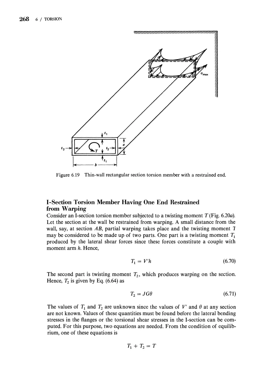
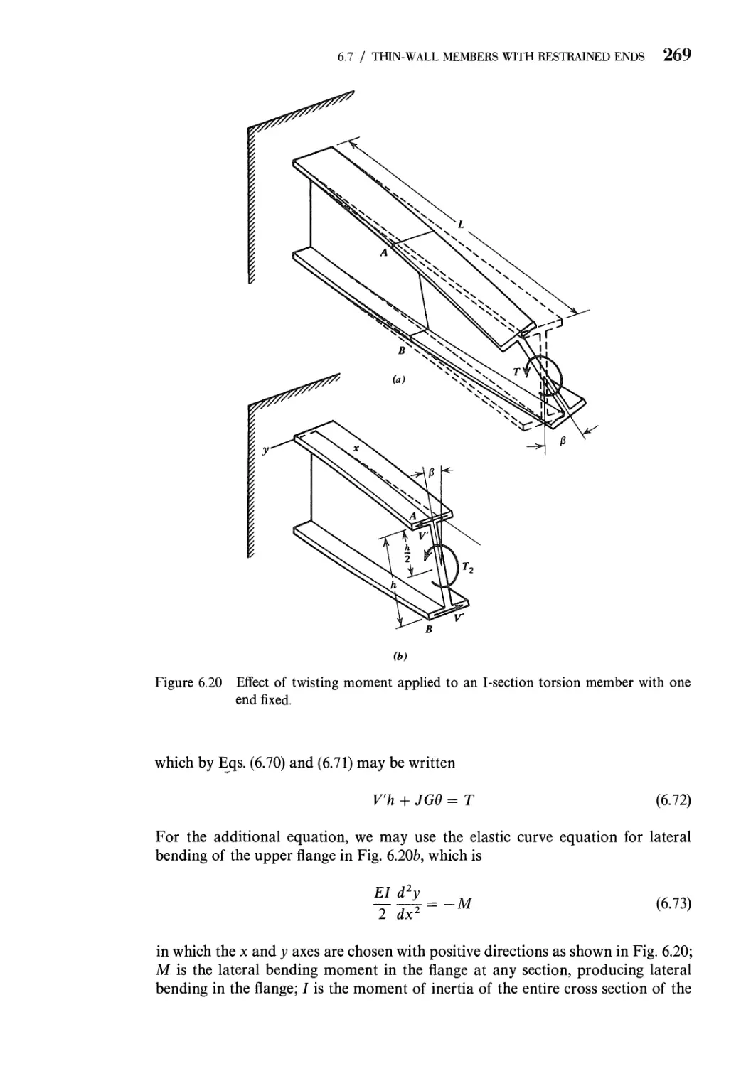
/


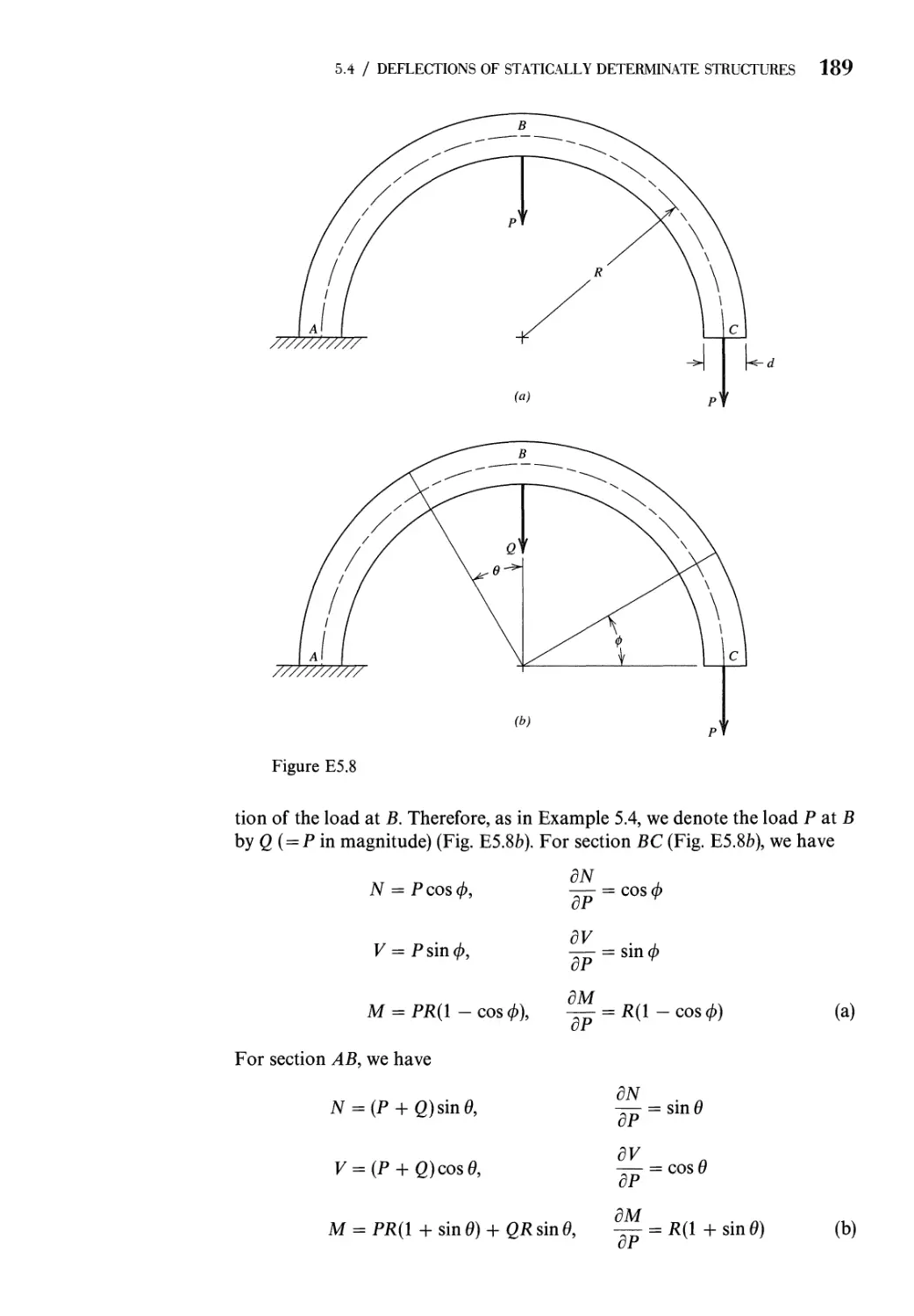


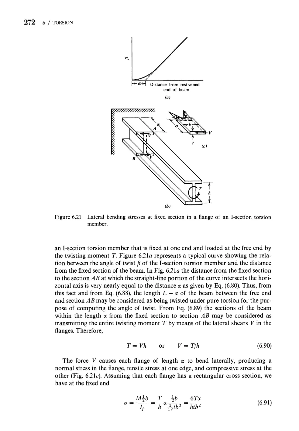


Автор: Boresi A. P. Schmidt R. J.
Теги: mathematics mathematical physics higher mathematics john wiley and sons advanced mechanics of materials
ISBN: 0-471-55157-0


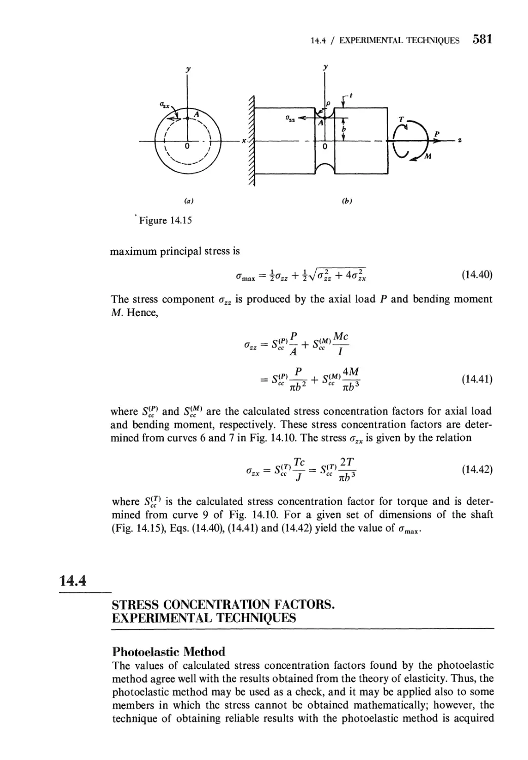
Текст
Fifth Edition
ADVANCED
MECHANICS
OF
MATERIALS
ARTHUR P. BORESI
Professor and Head
Civil and Architectural Engineering
The University of Wyoming at Laramie
RICHARD J. SCHMIDT
Associate Professor
Civil and Architectural Engineering
The University of Wyoming at Laramie
OMAR M. SIDEBOTTOM
Professor Emeritus
Theoretical and Applied Mechanics
The University of Illinois at Champaign-Urbana
JOHN WILEY & SONS, INC.
New York Chichester Brisbane Toronto Singapore
Recognizing the importance of preserving what has been written,
it is a policy of John Wiley & Sons, Inc. to have books of enduring
value published in the United States printed on acid-free paper, and we
exert our best efforts to that end.
acquisitions editor Charity Robey
MARKETING MANAGER Susan Elbe
production supervisor Nancy Prinz
designer Kevin Murphy
manufacturing manager Andrea Price
copy editing supervisor Deborah Herbert
This book was set in Times Roman by Polyglot Compositors and
printed and bound by Hamilton Printing. The cover was printed
by Hamilton Printing.
Copyright © 1932, by Fred B. Seely, Copyright © 1952,1978,1985,1993
by John Wiley & Sons, Inc.
All rights reserved. Published simultaneously in Canada.
Reproduction or translation of any part of
this work beyond that permitted by Sections
107 and 108 of the 1976 United States Copyright
Act without the permission of the copyright
owner is unlawful. Requests for permission
or further information should be addressed to
the Permissions Department, John Wiley & Sons.
Library of Congress Cataloging in Publication Data:
Boresi, Arthur P. (Arthur Peter), 1924-
Advanced mechanics of materials/Arthur P. Boresi, Richard J.
Schmidt, Omar M. Sidebottom.
p. cm.
Includes bibliographical references and index.
ISBN 0-471-55157-0
1. Strength of materials. I. Schmidt, Richard J. (Richard Joseph),
1954- . II. Sidebottom, Omar M. (Omar Marion) III. Title.
TA405.B66 1993
620.Г12—dc20 92-30349
CIP
Printed in the United States of America
10 9 8 7 6 5 4
To Our Students
and
To Our Wives
Jean, Pat, and Charlotte
PREFACE
This fifth edition represents a major revision of the fourth edition. However, as
in previous editions, the blend of analysis, qualified approximations, and
judgements based on practical experience is maintained. Each topic is developed from
basic principles so that the applicability and limitations of the methods employed
are clear. Introductory statements in each chapter serve as guidelines for the
reader to the topics that are discussed. The topics are divided into three major
parts: Part I—Fundamental Concepts; Part II—Classical Topics in Advanced
Mechanics; and Part III—Selected Advanced Topics.
Part I, Chapters 1-5, includes topics from elasticity, plasticity, and energy
methods that are important in the remainder of the book. In Chapter 1, the role
and the limits of design are discussed. Basic concepts of one-dimensional load-
stress, load-deflection, and stress-strain diagrams are introduced. A discussion of
the tension test and associated material properties is presented, followed by an
introduction to failure theories. These concepts are followed, in Chapter 2, by the
theories of stress and strain, and by strain measurements (strain rosettes) and,
in Chapter 3, by the theory of linear stress-strain-temperature relations. The
discussion of anisotropic materials has been expanded, and example problems on
orthotropic material behavior are given. Student problems for anisotropic
materials are also included. Chapter 4 contains much new material related to inelastic
(nonlinear) behavior and a broader treatment of yield criteria, including elastic-
plastic behavior of beams, strain-hardening effects in bars, and residual stresses in
elastic-plastic bars after unloading. The application of energy methods, Chapter 5,
is expanded to include an in-depth discussion of the dummy-load method used by
structuraLengineers and its relation to the Castigliano method. Additional worked
examples and many new problems have been added. (In this edition, problems have
been placed at the end of each Chapter, rather than at the end of each section.)
Part II, Chapters 6-12, treats some classical topics of advanced mechanics.
Torsion is treated in Chapter 6, including new examples and problems. In
addition, a finite difference solution of the rectangular cross section bar is presented.
An example of limit analysis and residual stresses in a circular cross section shaft
is also included. In Chapters 7 to 9, the three topics of unsymmetrical bending,
shear center, and curved beams are examined on a rigorous basis, and limitations
on existing analyses are indicated. A presentation of beams on elastic foundations,
plus new problems and references, is given in Chapter 10. Some minor
clarifications for the thick-wall cylinder and many new student problems are given in
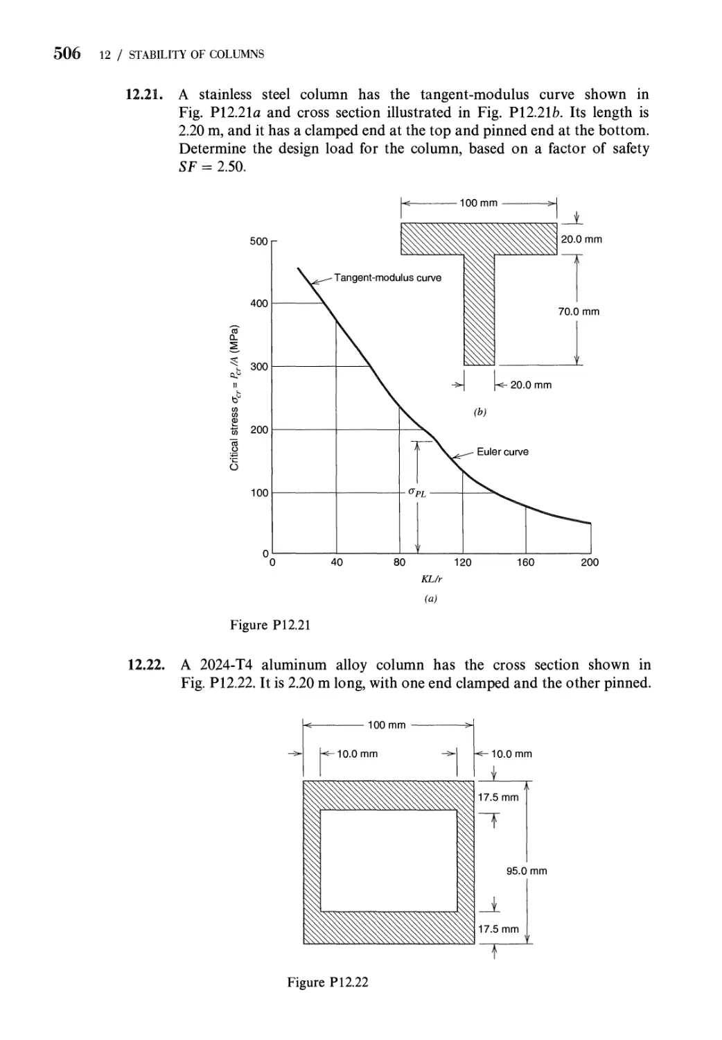
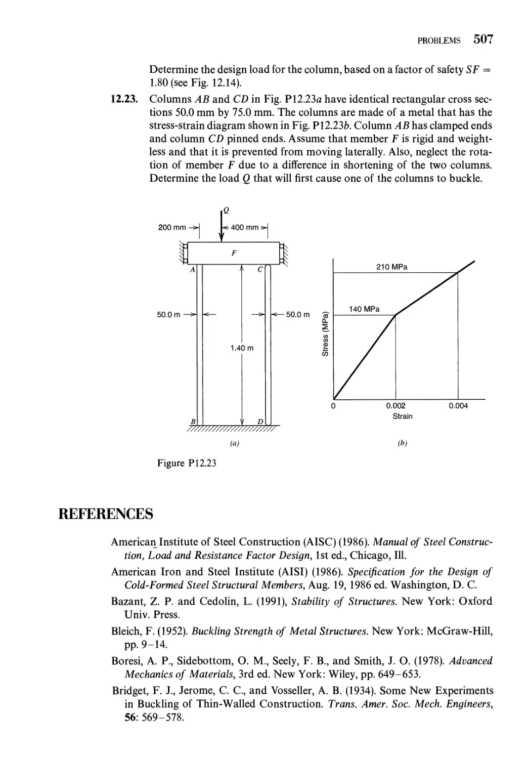
Chapter 11. In Chapter 12, the topic of stability of columns is expanded
considerably, and a wide range of practical example problems and student exercises is
included.
Viii PREFACE
Part III, Chapters 13-19, presents the more advanced topics of flat plates, stress
concentrations, fracture mechanics, fatigue, creep (time-dependent deformations),
contact stresses, and the finite element method. The linear theory of flat plates is
given in Chapter 13, including some illustrative problems and a collection of
student exercises. The level is appropriate as an introduction for master-level students
and for practicing engineers. Chapter 14 collects, in an integrated manner, material
on stress concentrations previously presented in parts of Chapters 3, 12, and 13 of
the fourth edition. New examples and exercise problems have been added, as well
as some new charts of stress concentration factors for rectangular cross section
beams. The topic of fracture mechanics is introduced in Chapter 15; it includes
material previously given in Chapters 3 and 12 of the fourth edition and a brief
discussion of other factors, such as elastic-plastic fracture, crack-growth analysis, load
spectra and stress history, testing, and experimental data interpretation. A number
of up-to-date books and papers are referenced. Progressive fracture(fatigue) is
discussed in Chapter 16, including additional problems and references. An extended
discussion of creep is presented in Chapter 17, including creep of metals and non-
metals (concrete, asphalt, and wood). Chapter 18, contact stresses, is essentially
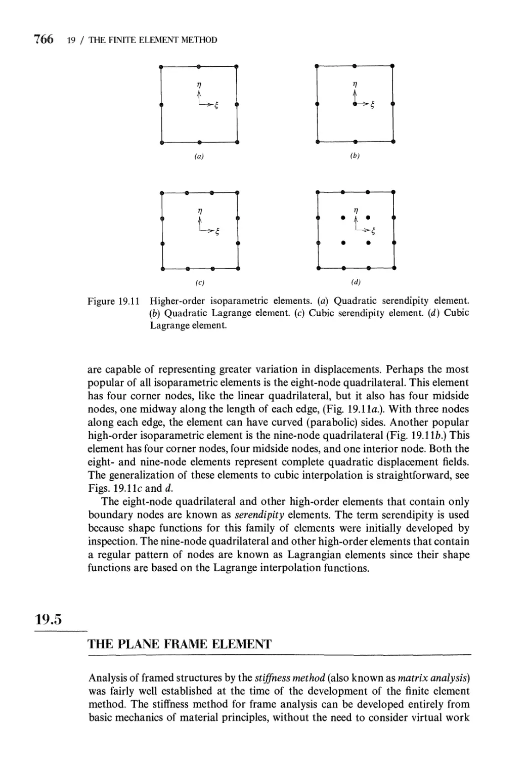
unchanged from Chapter 14 of the fourth edition. Chapter 19, the finite element
method, is a completely rewritten treatment of Chapter 15 of the fourth edition.
It includes discussions of the constant strain triangular element, the bilinear
rectangular element, the linear isoparametric quadrilateral element, and the plane
frame element. Example problems and exercise problems are included.
As a result of the new material and problems that have been added, this
edition is larger than its predecessors. Consequently, it provides a greater choice
of topics for study. It also has the advantage that the book can be used over a
lifetime of practice, as a reference to topics of lasting importance in engineering.
The book contains more material than can be covered in a one-quarter or a one-
semester course. It is, however, with the proper selection of topics, suitable for a
one-semester (one-quarter) course at either the senior level or the first-semester
graduate level, for a two-semester (two- or three-quarter) course sequence, or as a
reference work in several courses in mechanics.
The computer program listings in the fourth edition have been omitted from the
current edition. However, revised versions of the programs from the fourth edition
and new programs for applications in this edition are available on request from one
of the authors (R. J. Schmidt, Department of Civil and Architectural Engineering,
Box 3295, University of Wyoming, Laramie, WY 82071).
We thank Charity Robey, Wiley engineering editor, for her expert help and
advice during the development of this edition. We also greatly appreciate the help of
Suzanne Ingrao, with the difficult task of galley and page proof editing. We thank
the reviewers of the preliminary format and content of the fifth edition for their
constructive criticism and suggestions for improving the fourth edition. These
reviewers are Stanley Chen, Arizona State University; Donald DaDeppo, University
of Arizona; D. W. Haines, Manhattan College; Loren D. Lutes, Texas A. & M.
University; Esmet M. Kamil, Pratt Institute; and Thomas A. Lenox, U.S. Military
Academy, West Point, NY. We thank especially the reviewers of the draft
manuscript for their helpful suggestions. These reviewers are J. A. M. Boulet, University
of Tennessee-Knoxville; Ray W. James, Texas A. & M. University; A. P. Moser,
Utah State University; William A. Nash, University of Massachusetts-Amherst;
and Sam Y. Zamrik, Pennsylvania State University. We also acknowledge the
contribution of Travis Finch for the artwork in Figs. 12.12 and 18.1.
PREFACE ix
Finally, we welcome comments, suggestions, questions, and corrections from the
reader. They may be sent to Arthur P. Boresi, Department of Civil and Architectural
Engineering, Box 3295, University of Wyoming, Laramie, WY 82071.
Arthur P. Boresi
Richard J. Schmidt
Omar M. Sidebottom
October 1992
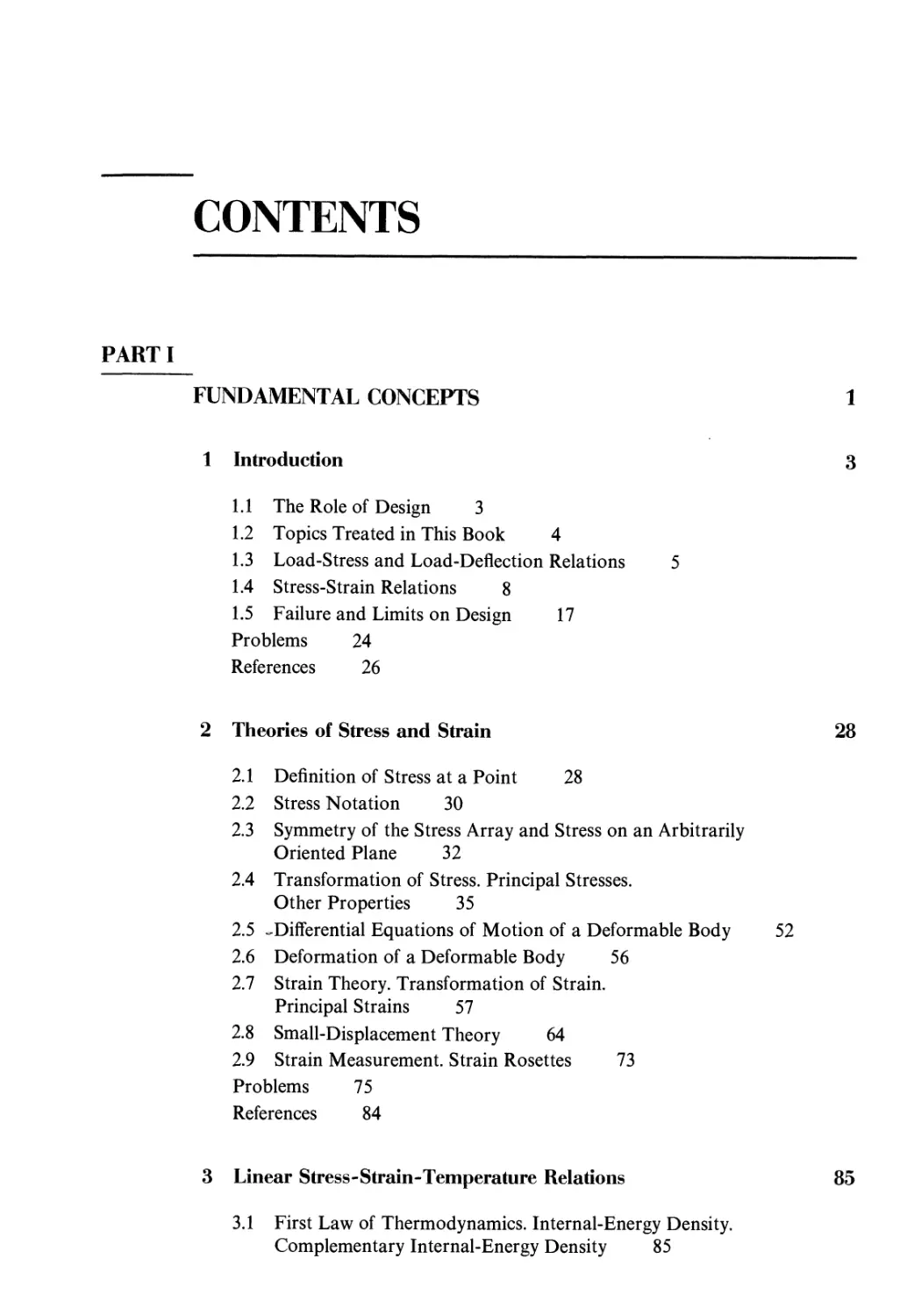
CONTENTS
PARTI
FUNDAMENTAL CONCEPTS 1
1 Introduction 3
1.1 The Role of Design 3
1.2 Topics Treated in This Book 4
1.3 Load-Stress and Load-Deflection Relations 5
1.4 Stress-Strain Relations 8
1.5 Failure and Limits on Design 17
Problems 24
References 26
2 Theories of Stress and Strain 28
2.1 Definition of Stress at a Point 28
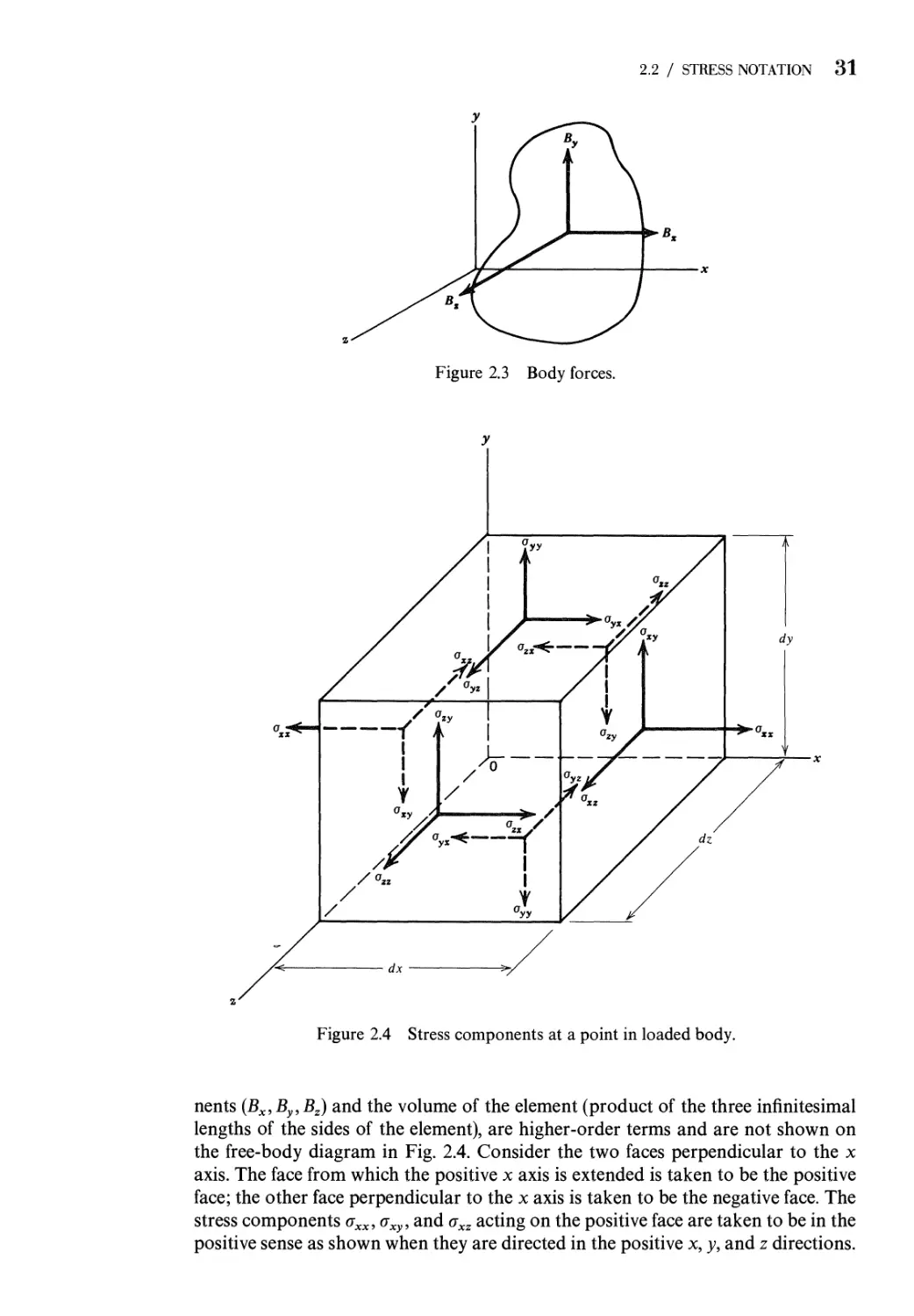
2.2 Stress Notation 30
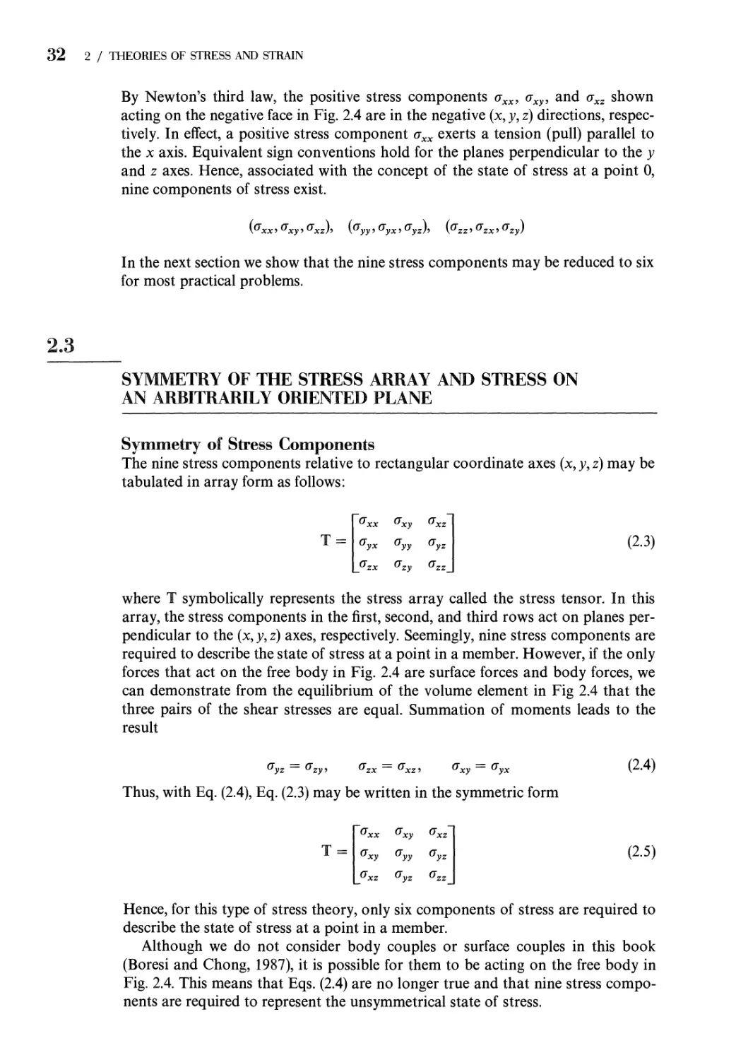
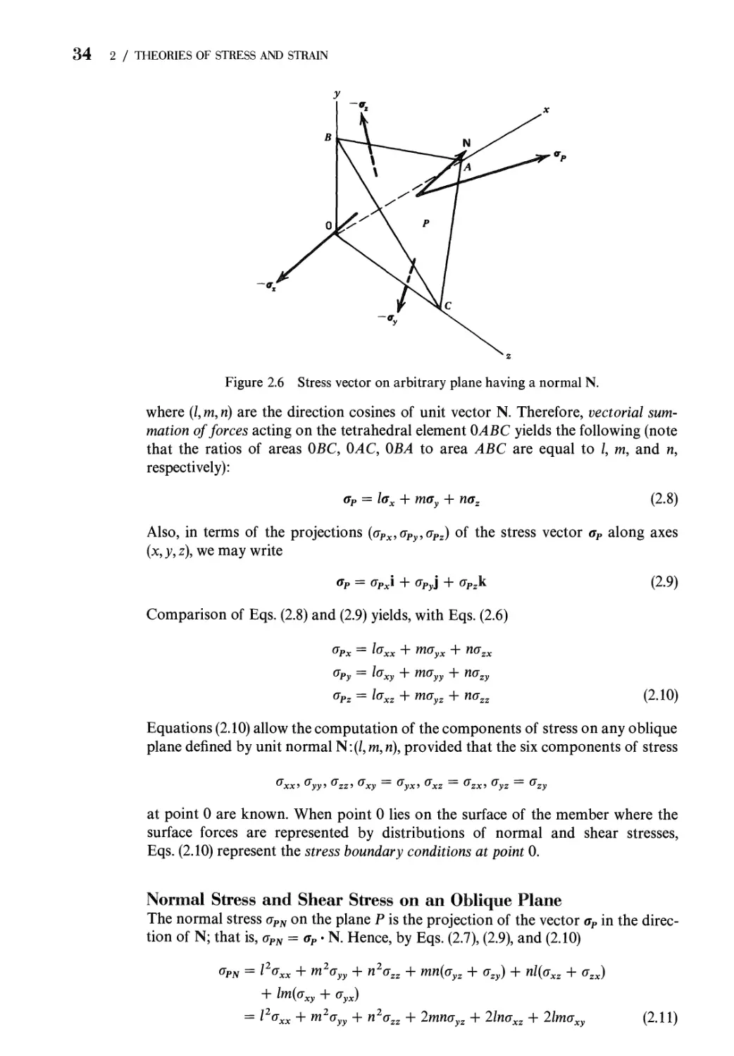
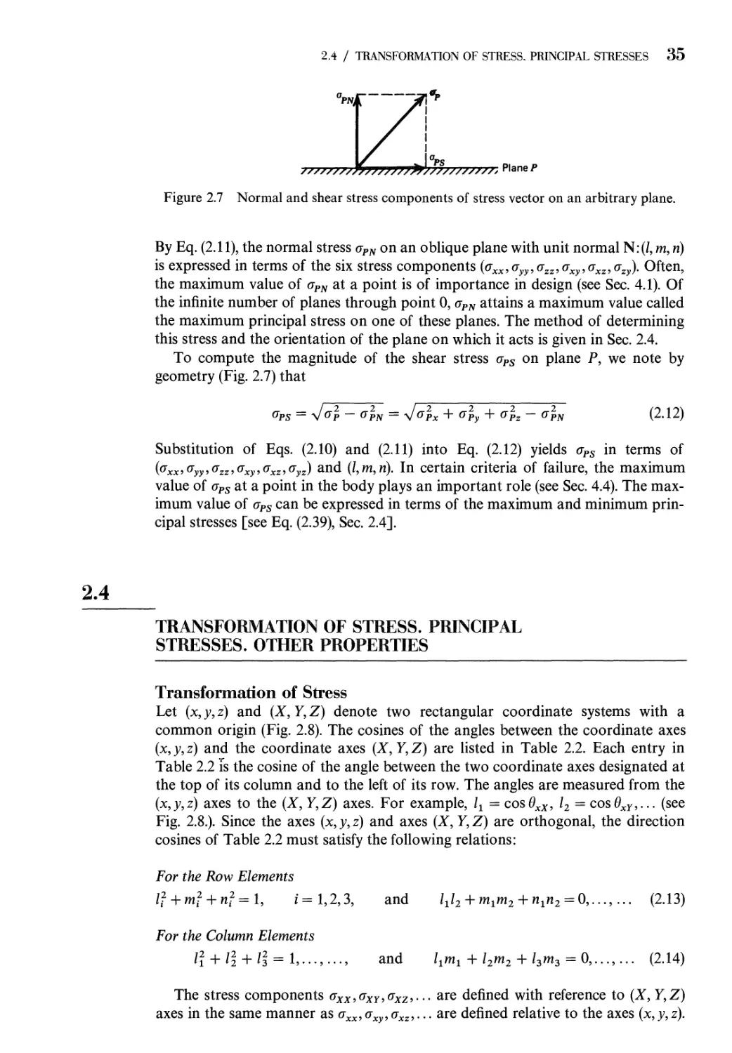
2.3 Symmetry of the Stress Array and Stress on an Arbitrarily
Oriented Plane 32
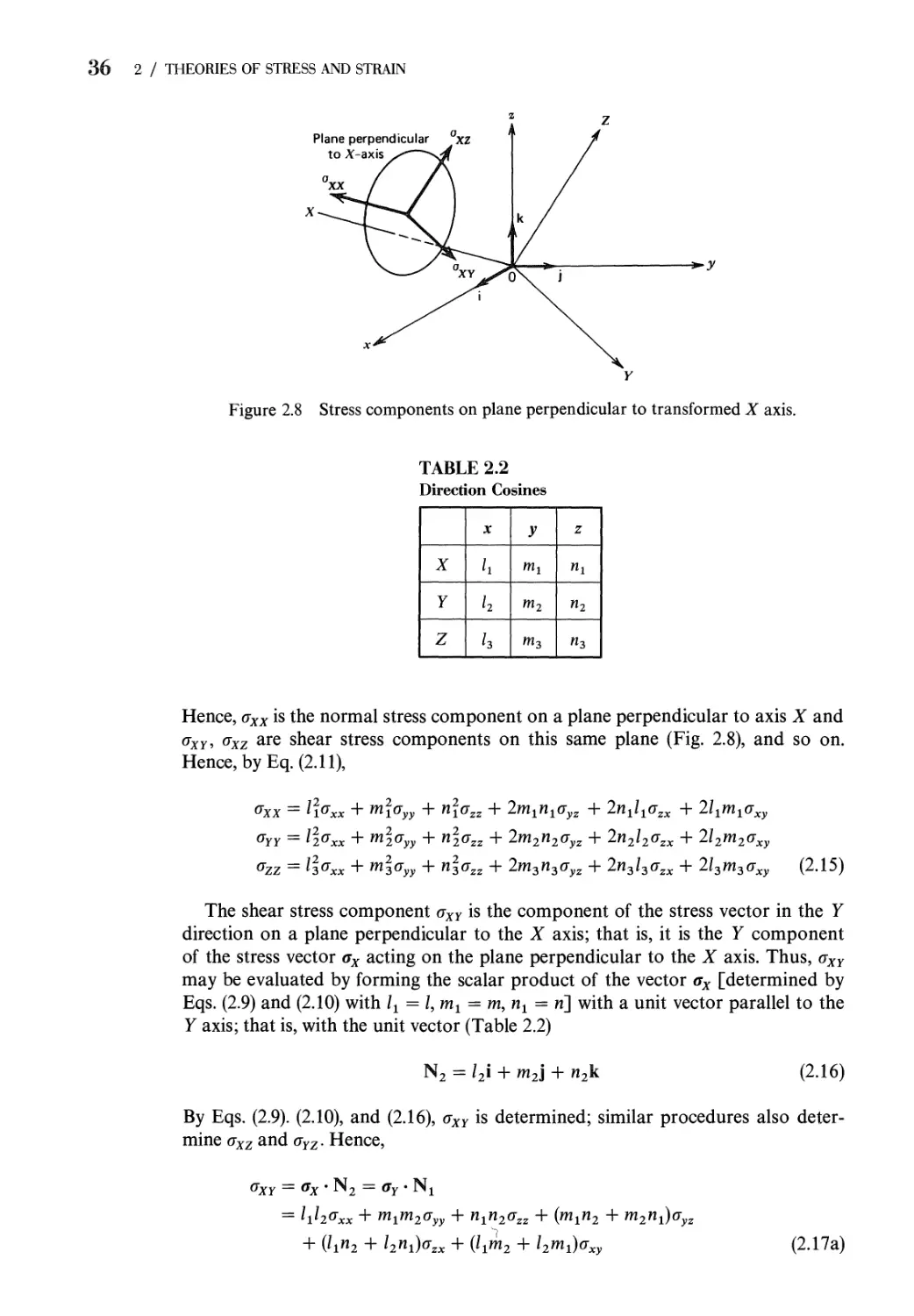
2.4 Transformation of Stress. Principal Stresses.
Other Properties 35
2.5 -Differential Equations of Motion of a Deformable Body 52
2.6 Deformation of a Deformable Body 56
2.7 Strain Theory. Transformation of Strain.
Principal Strains 57
2.8 Small-Displacement Theory 64
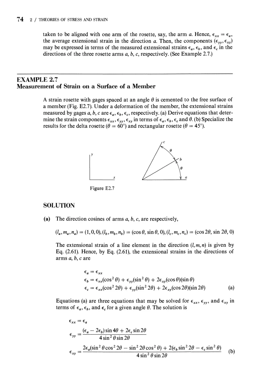
2.9 Strain Measurement. Strain Rosettes 73
Problems 75
References 84
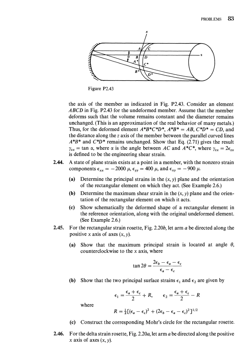
3 Linear Stress-Strain-Temperature Relations 85
3.1 First Law of Thermodynamics. Internal-Energy Density.
Complementary Internal-Energy Density 85
xii contents
3.2 Hooke's Law: Anisotropic Elasticity 90
3.3 Hooke's Law: Isotropic Elasticity 92
3.4 Equations of Thermoelasticity for Isotropic
Materials 99
3.5 Hooke's Law: Orthotropic Materials 101
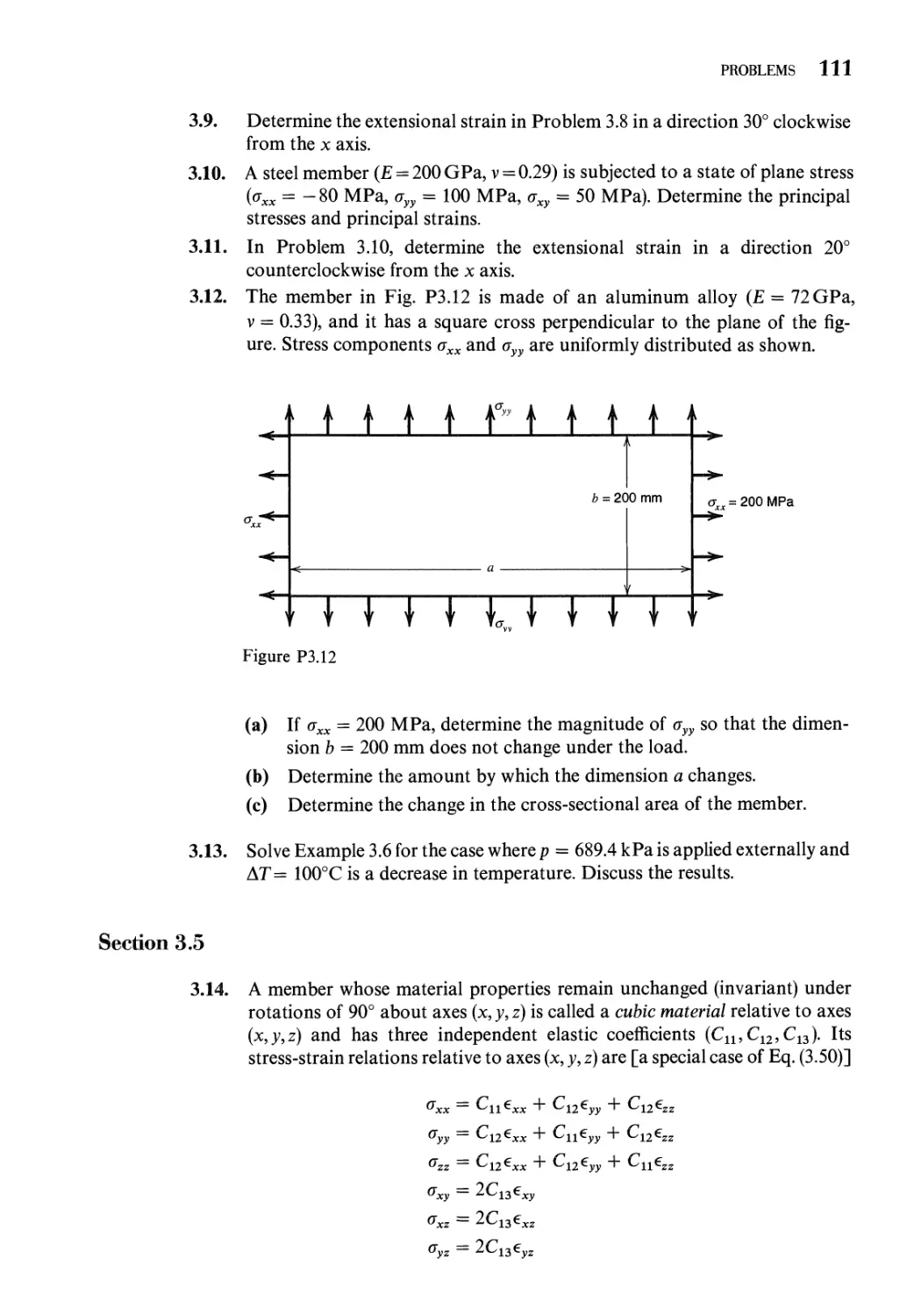
Problems 110
References 112
4 Inelastic Material Behavior 113
4.1 Limitations of the Use of Uniaxial Stress-Strain Data 113
4.2 Nonlinear Material Response 116
4.3 Yield Criteria: General Concepts 126
4.4 Yielding of Ductile Metals 130
4.5 Alternative Yield Criteria 140
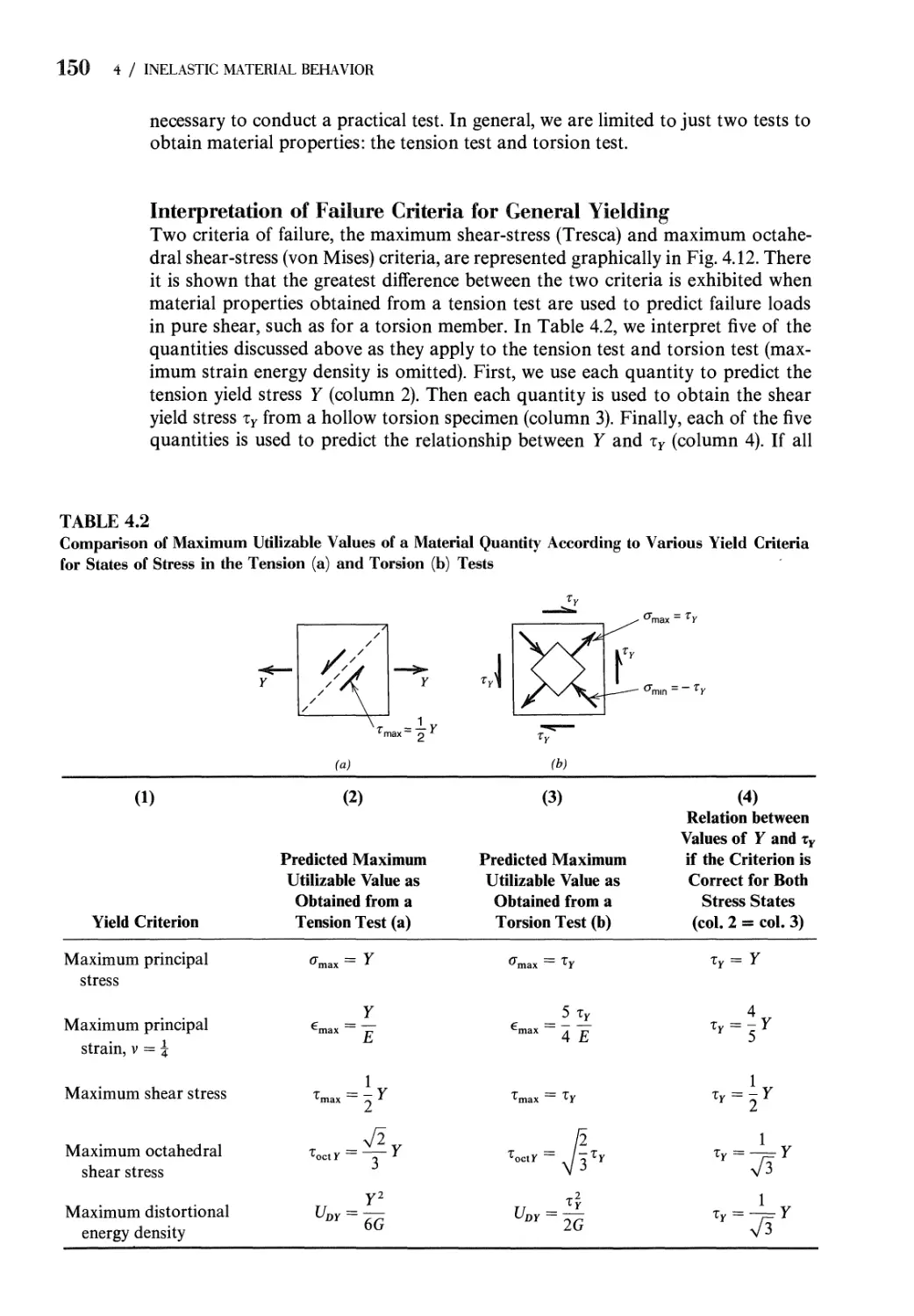
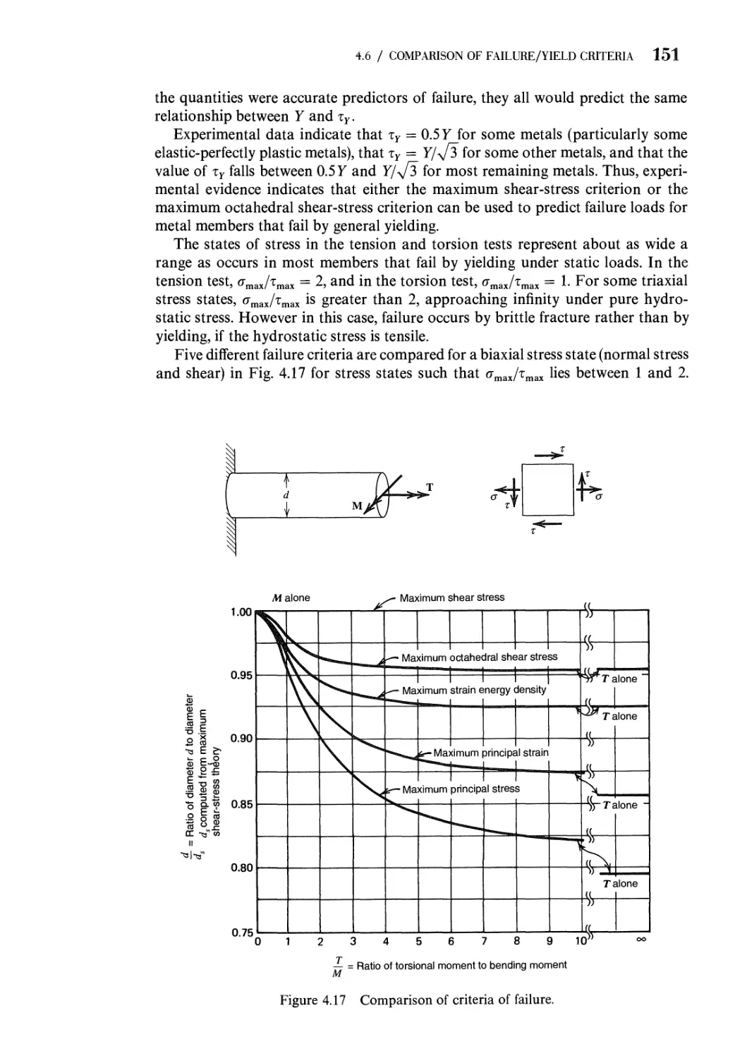
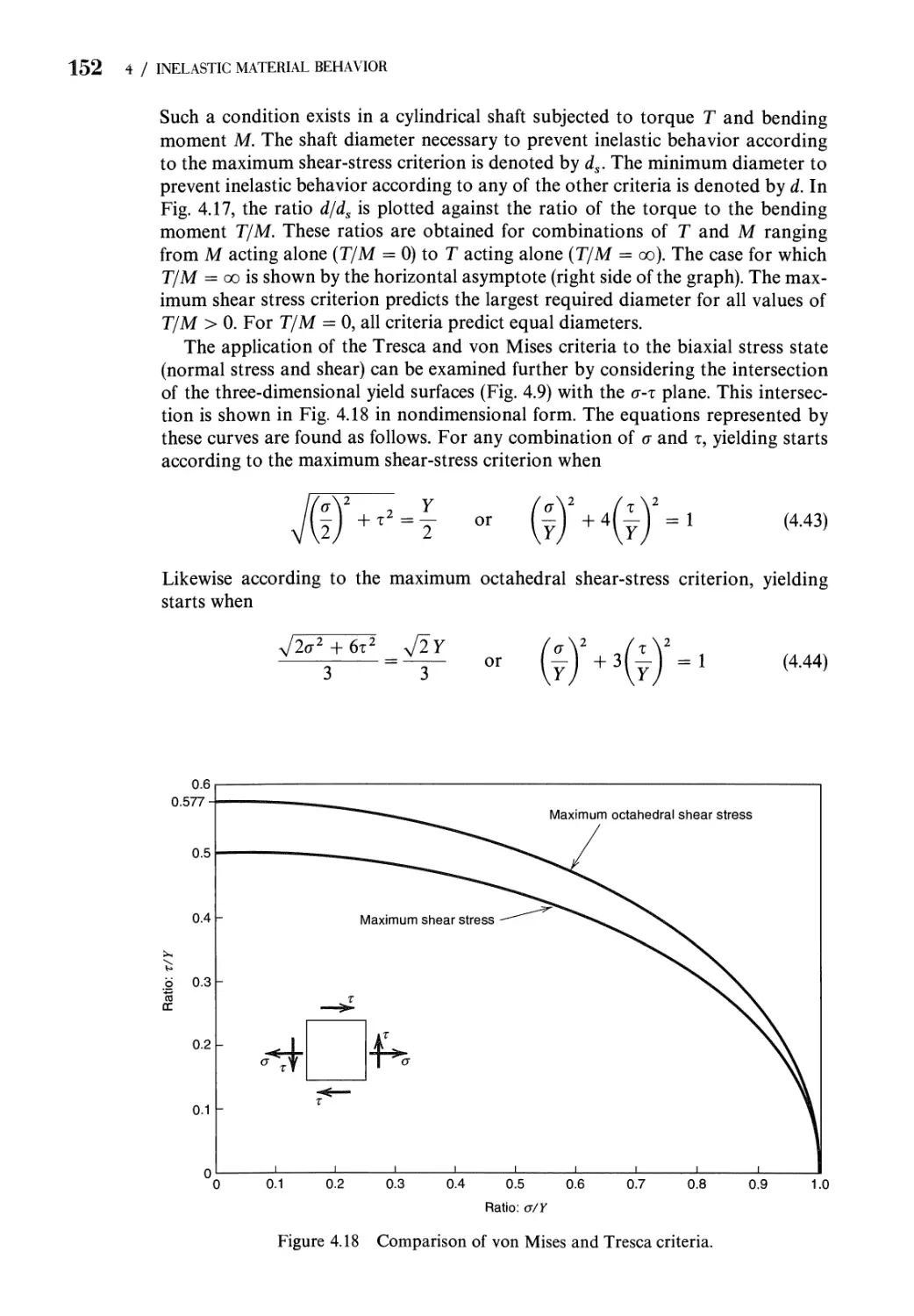
4.6 Comparison of Failure Criteria for General Yielding 144
Problems 154
References 162
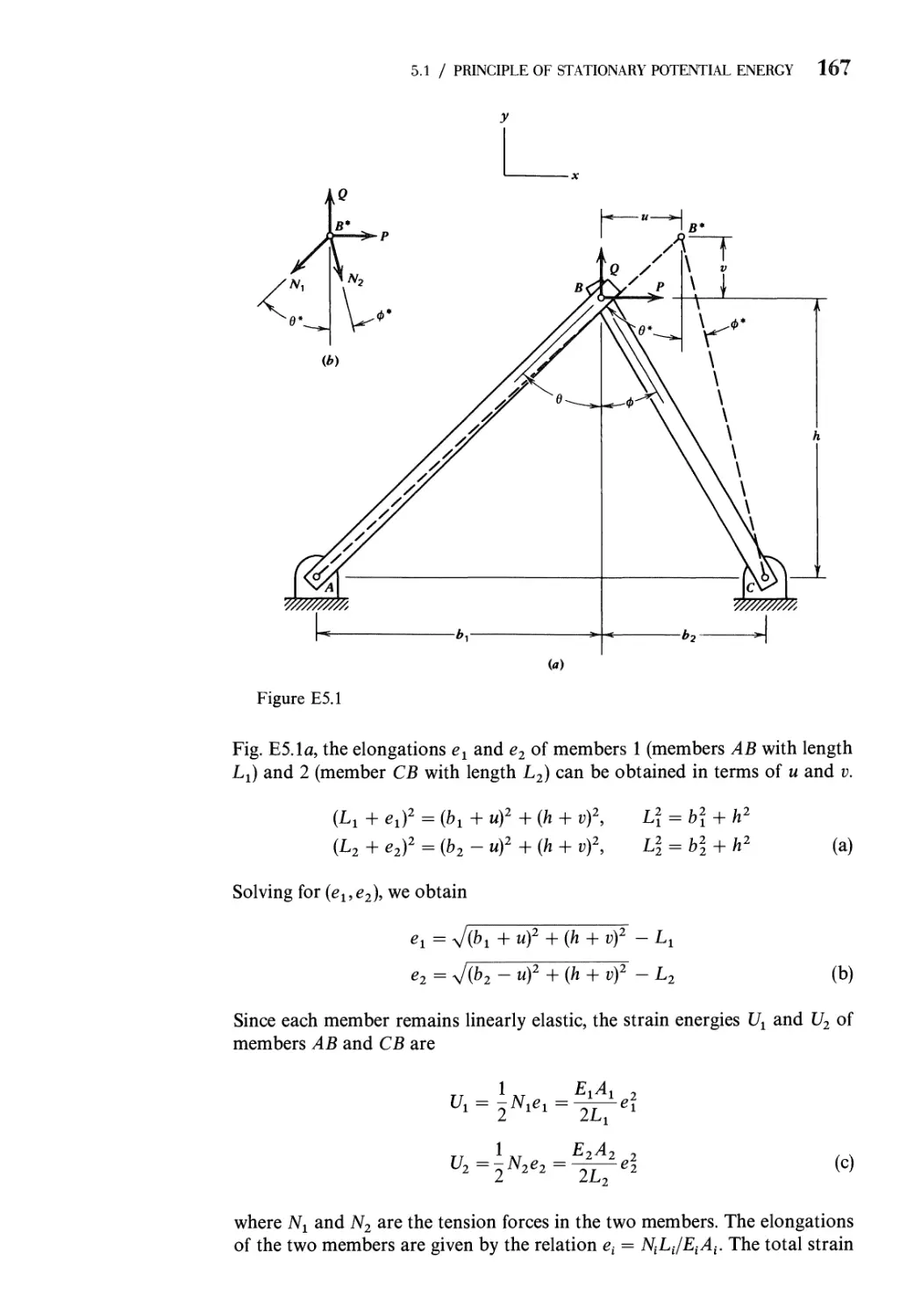
5 Applications of Energy Methods 163
5.1 Principle of Stationary Potential Energy 163
5.2 Castigliano's Theorem on Deflections 169
5.3 Castigliano's Theorem on Deflections for Linear
Load-Deflection Relations 173
5.4 Deflections of Statically Determinate Structures 179
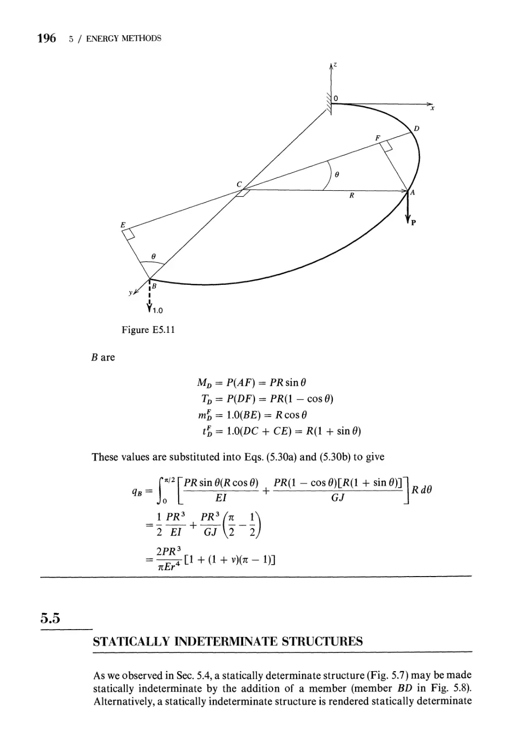
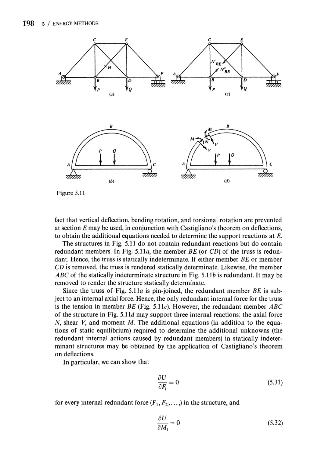
5.5 Statically Indeterminate Structures 196
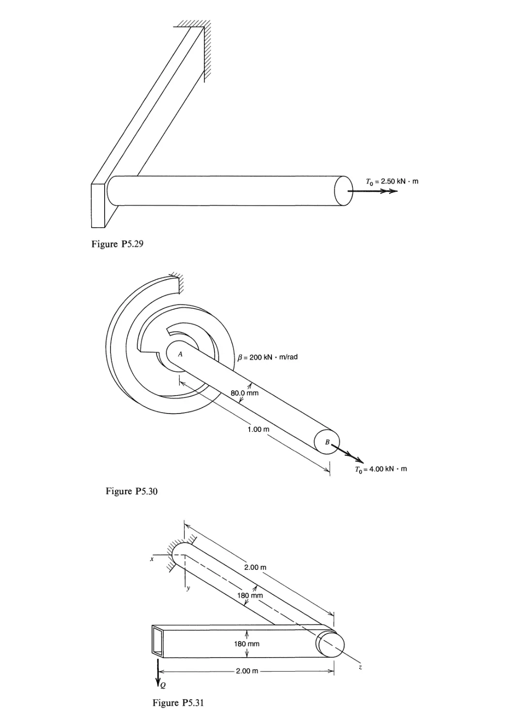
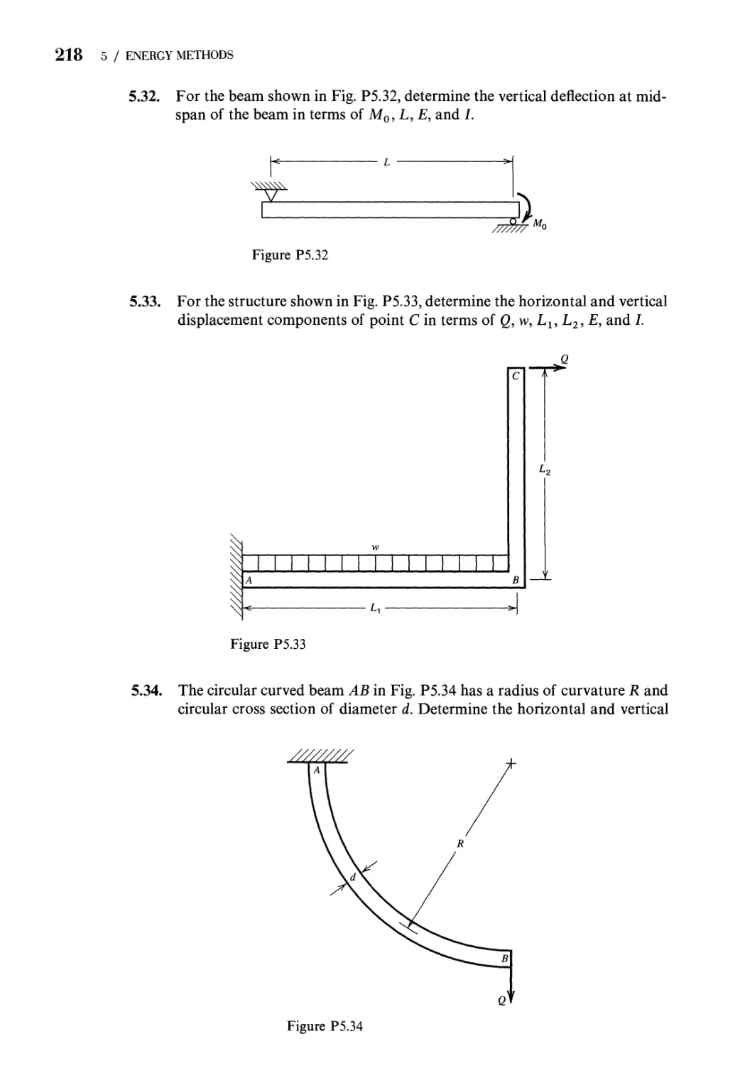
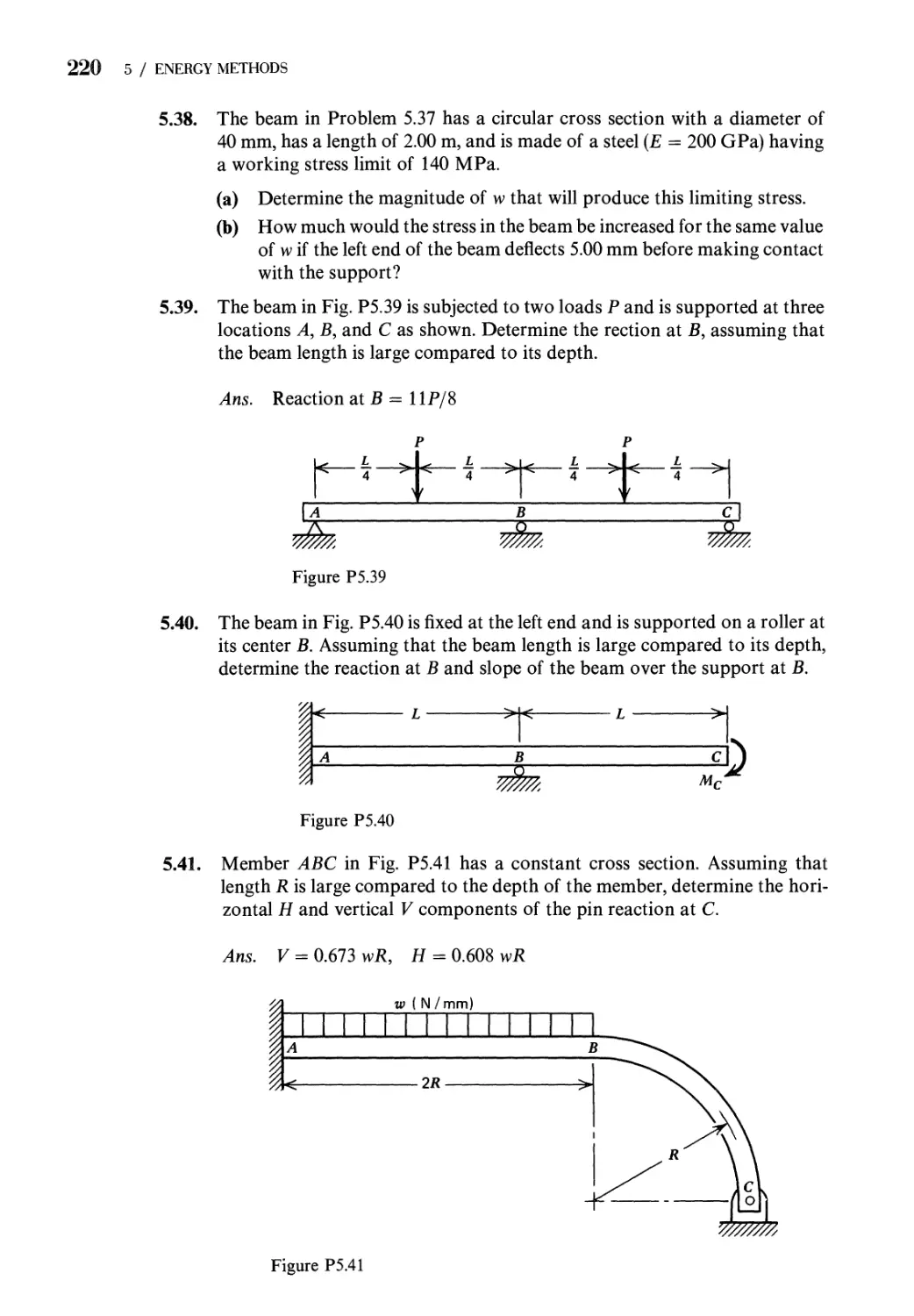
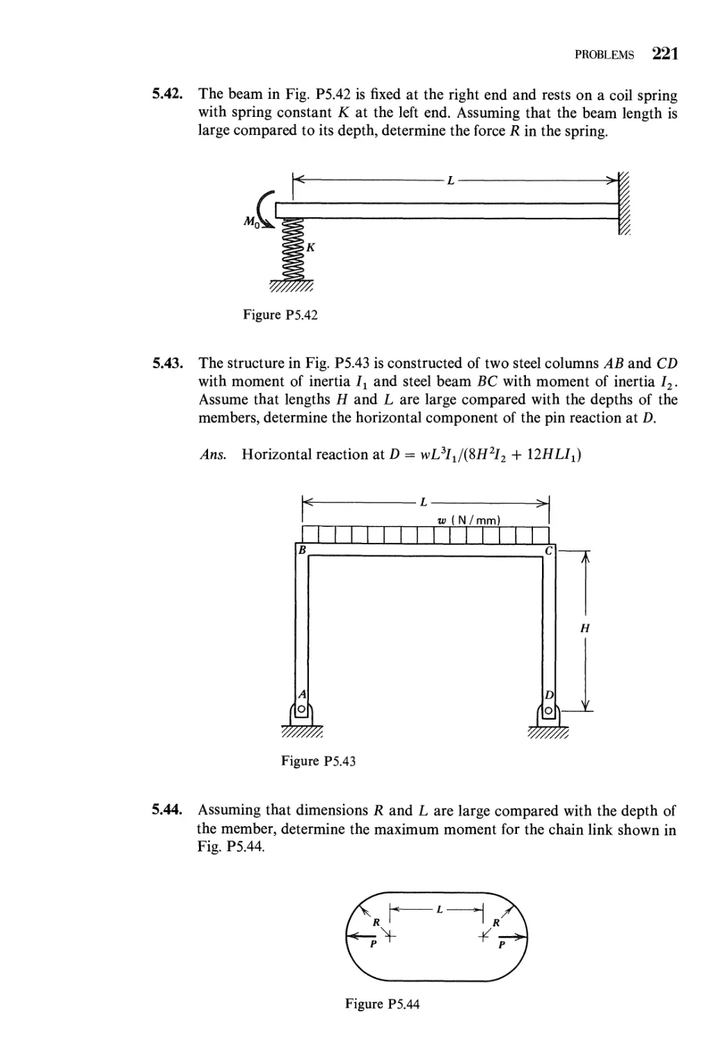
Problems 208
References 232
PART II
CLASSICAL TOPICS IN ADVANCED MECHANICS 235
6 Torsion 237
6.1 Torsion of a Prismatic Bar of Circular
Cross Section 237
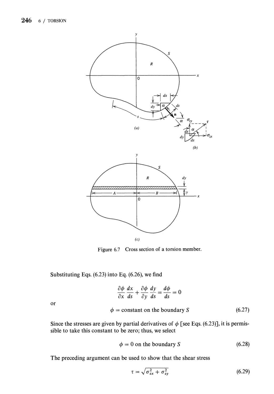
6.2 Saint-Venant's Semiinverse Method 243
6.3 Linear Elastic Solution 248
6.4 The Prandtl Elastic-Membrane (Soap-Film) Analogy 253
6.5 Narrow Rectangular Cross Section 257
contents xiii
6.6 Hollow Thin-Wall Torsion Members. Multiply Connected
Cross Section 260
6.7 Thin-Wall Torsion Members with Restrained Ends 266
6.8 Numerical Solution of the Torsion Problem 274
6.9 Fully Plastic Torsion 277
Problems 283
References 291
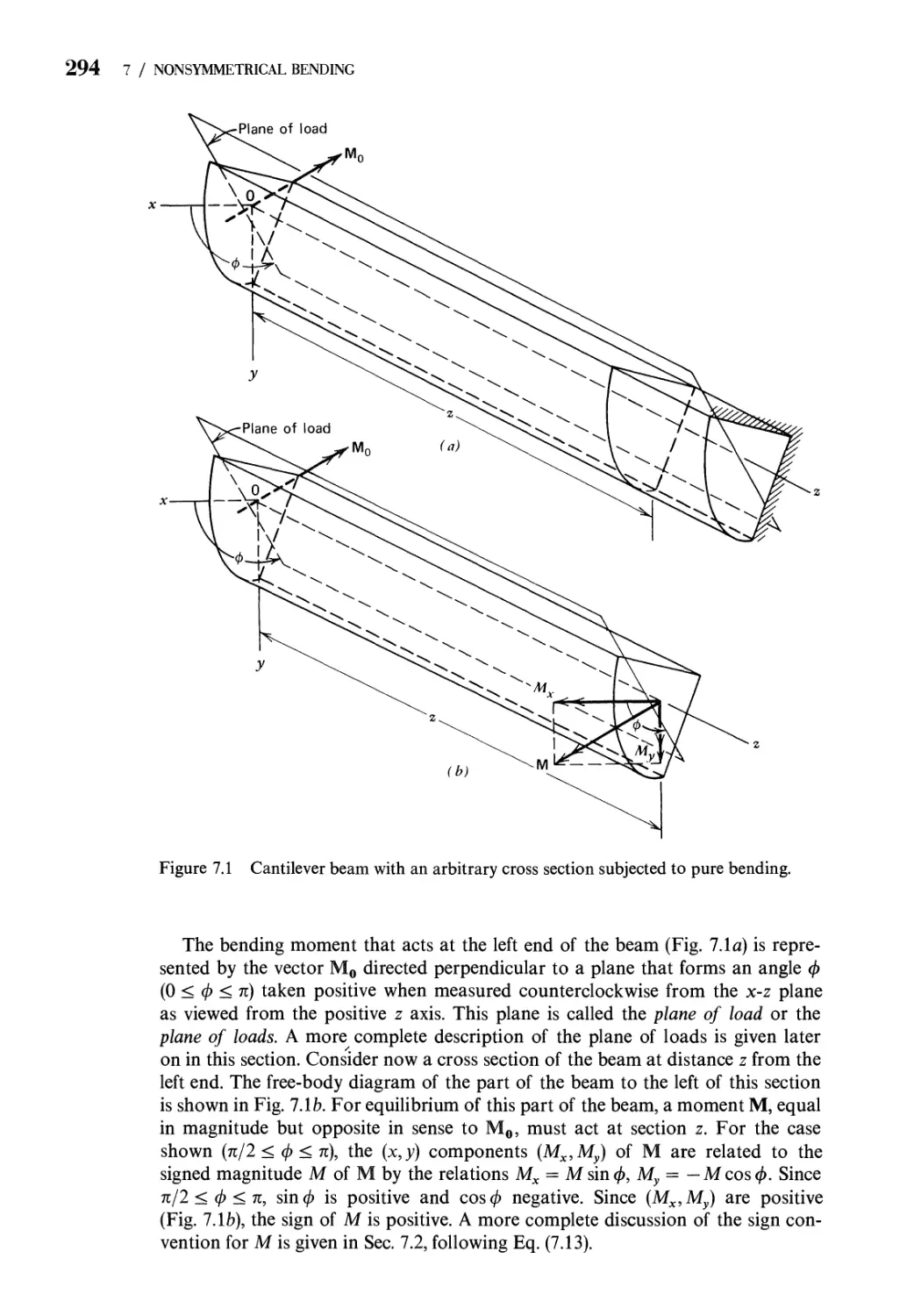
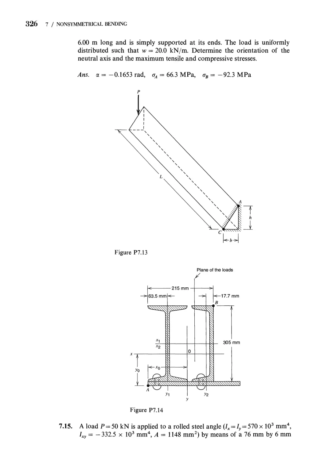
7 Nonsymmetrical Bending of Straight Beams 293
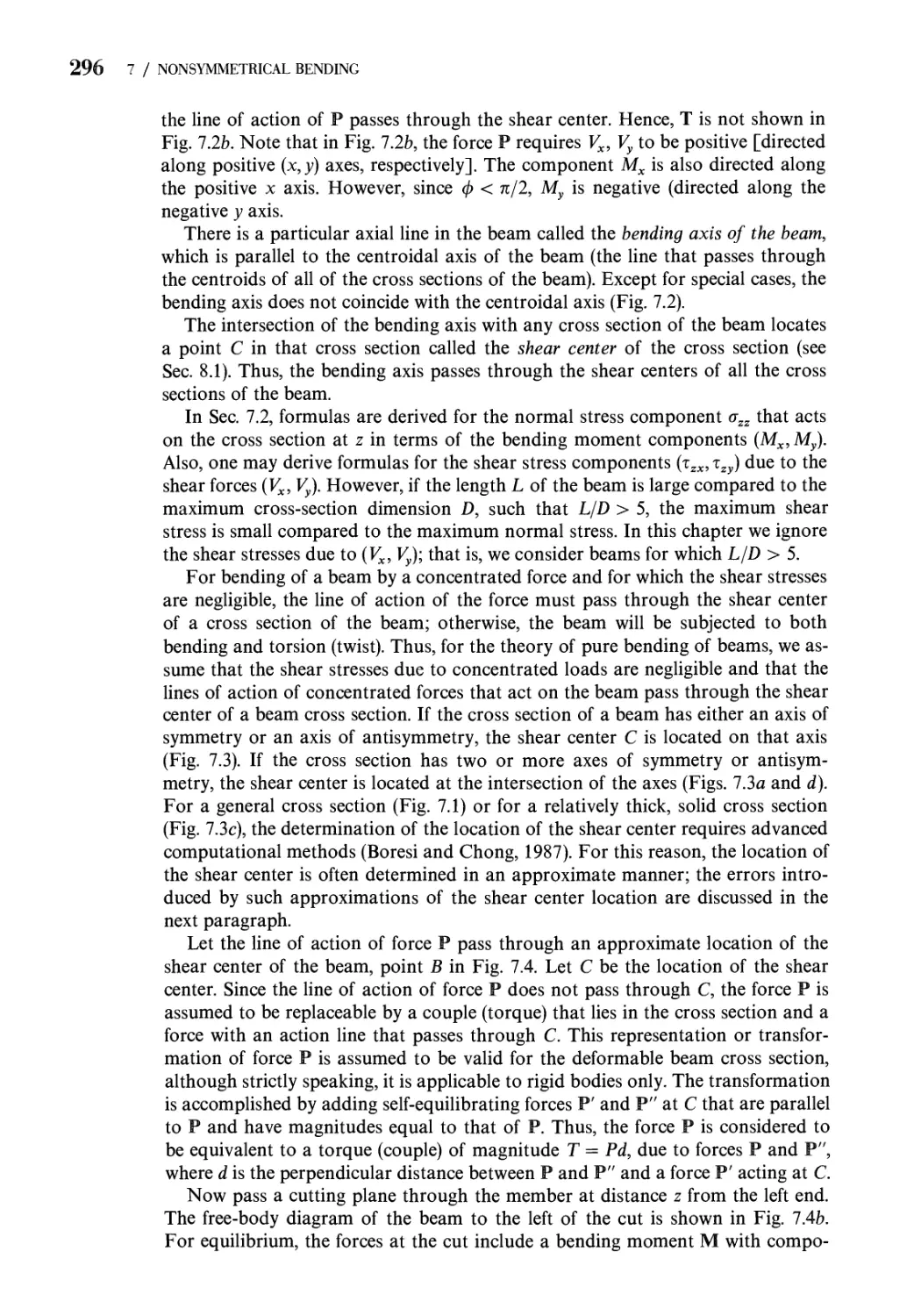
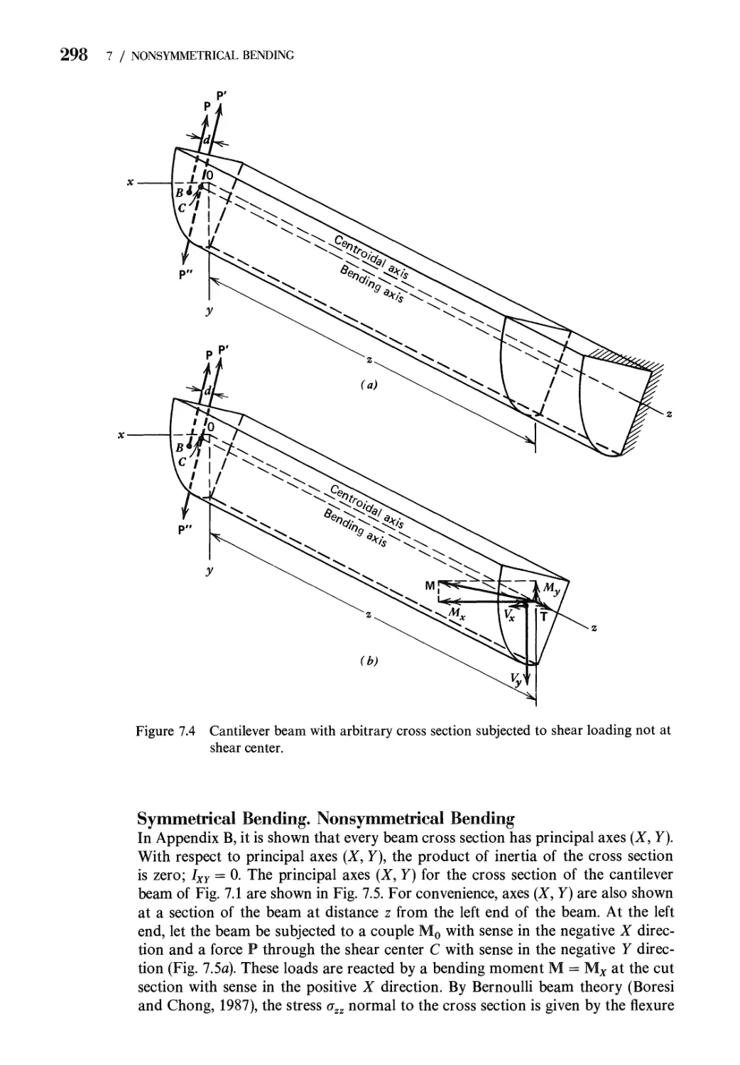
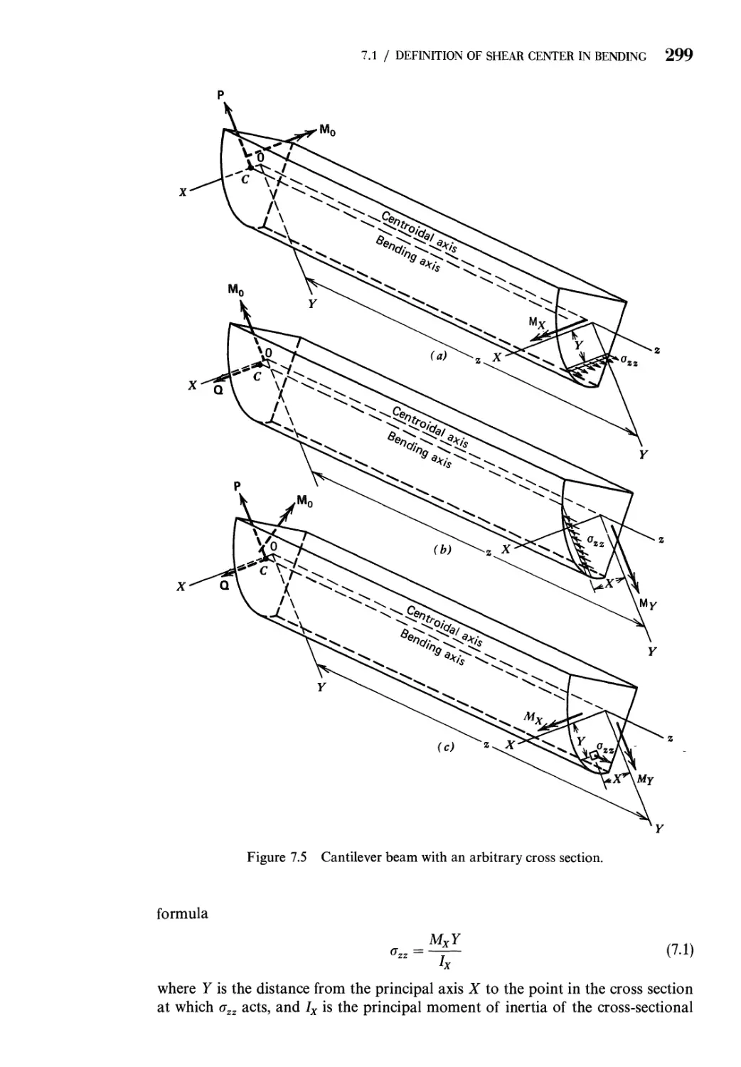
7.1 Definition of Shear Center in Bending. Symmetrical and
Nonsymmetrical Bending 293
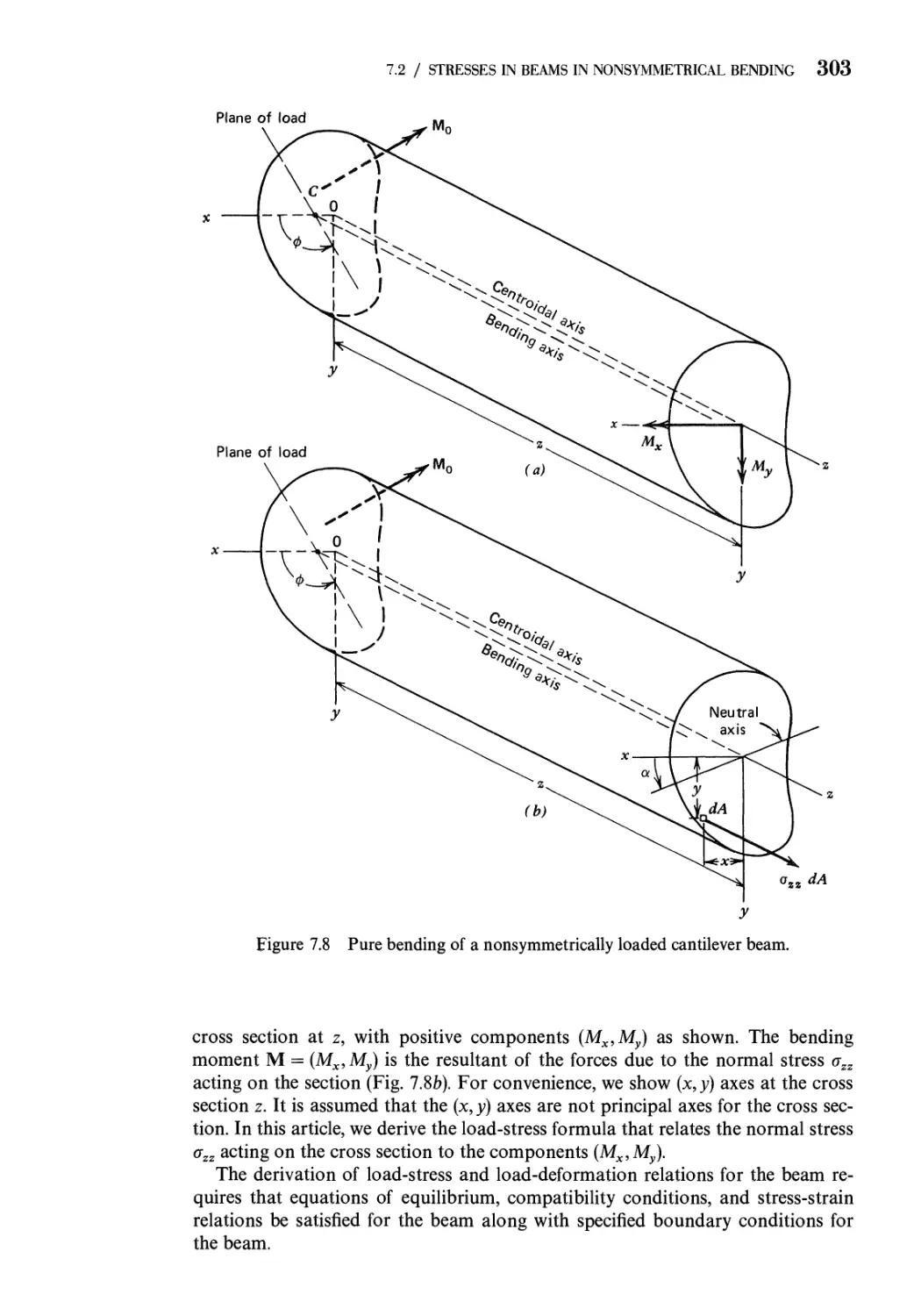
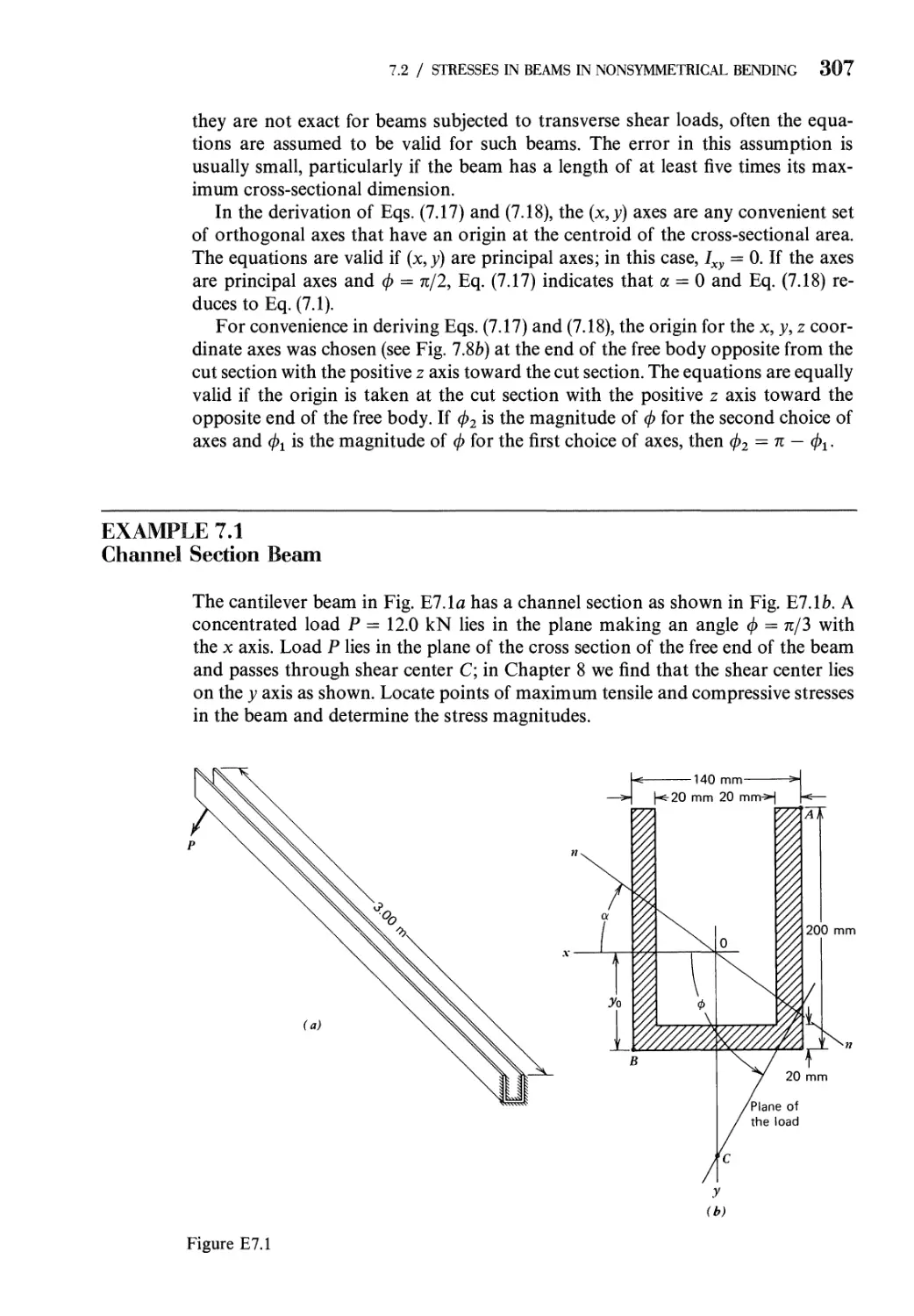
7.2 Bending Stresses in Beams Subjected to Nonsymmetrical
Bending 302
7.3 Deflections of Straight Beams Subjected to Nonsymmetrical
Bending 312
7.4 Effect of Inclined Loads 316
7.5 Fully Plastic Load for Nonsymmetrical Bending 318
Problems 320
References 330
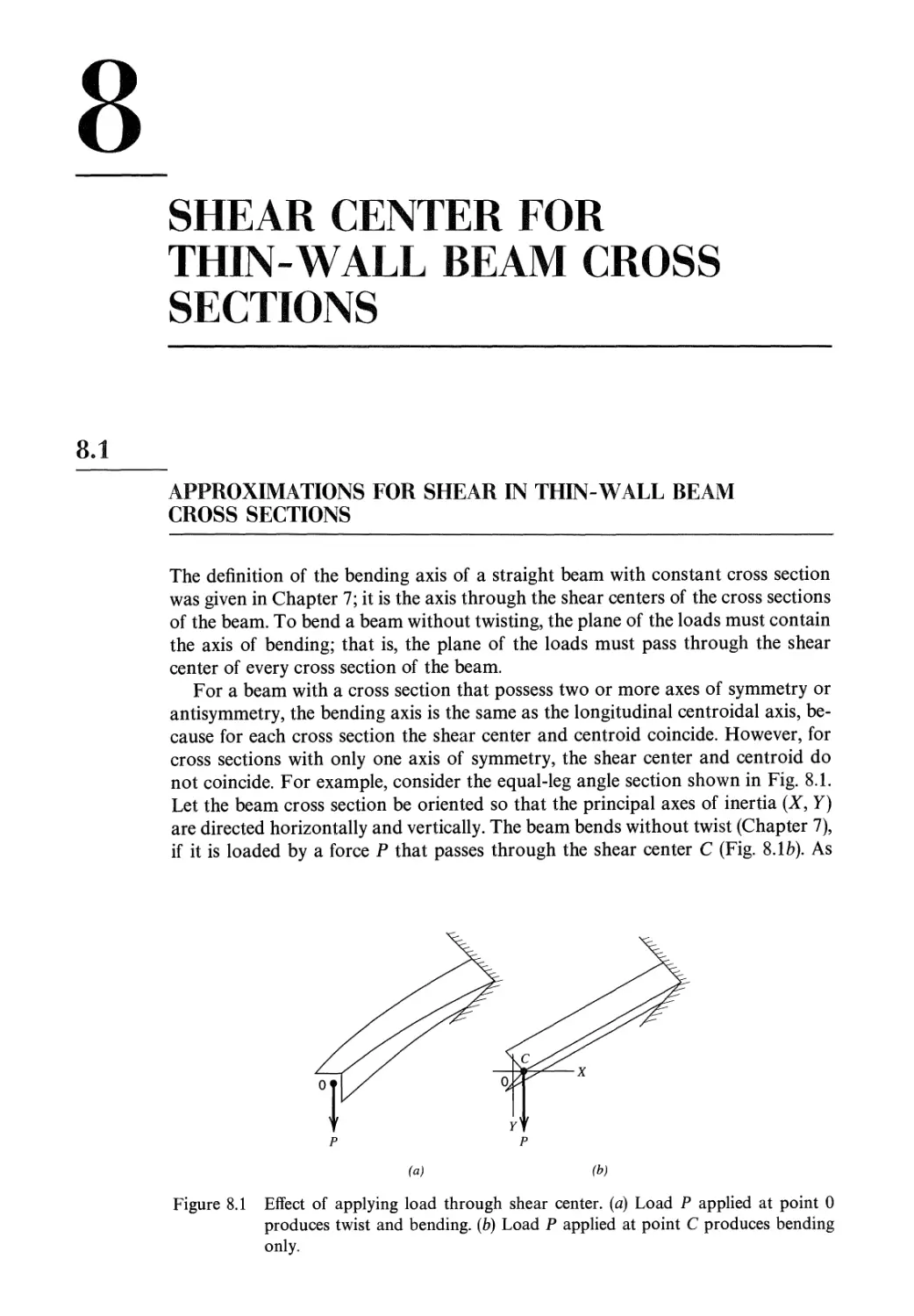
8 Shear Center for Thin-Wall Beam Cross Sections 331
8.1 Approximations for Shear in Thin-Wall Beam
Cross Sections 331
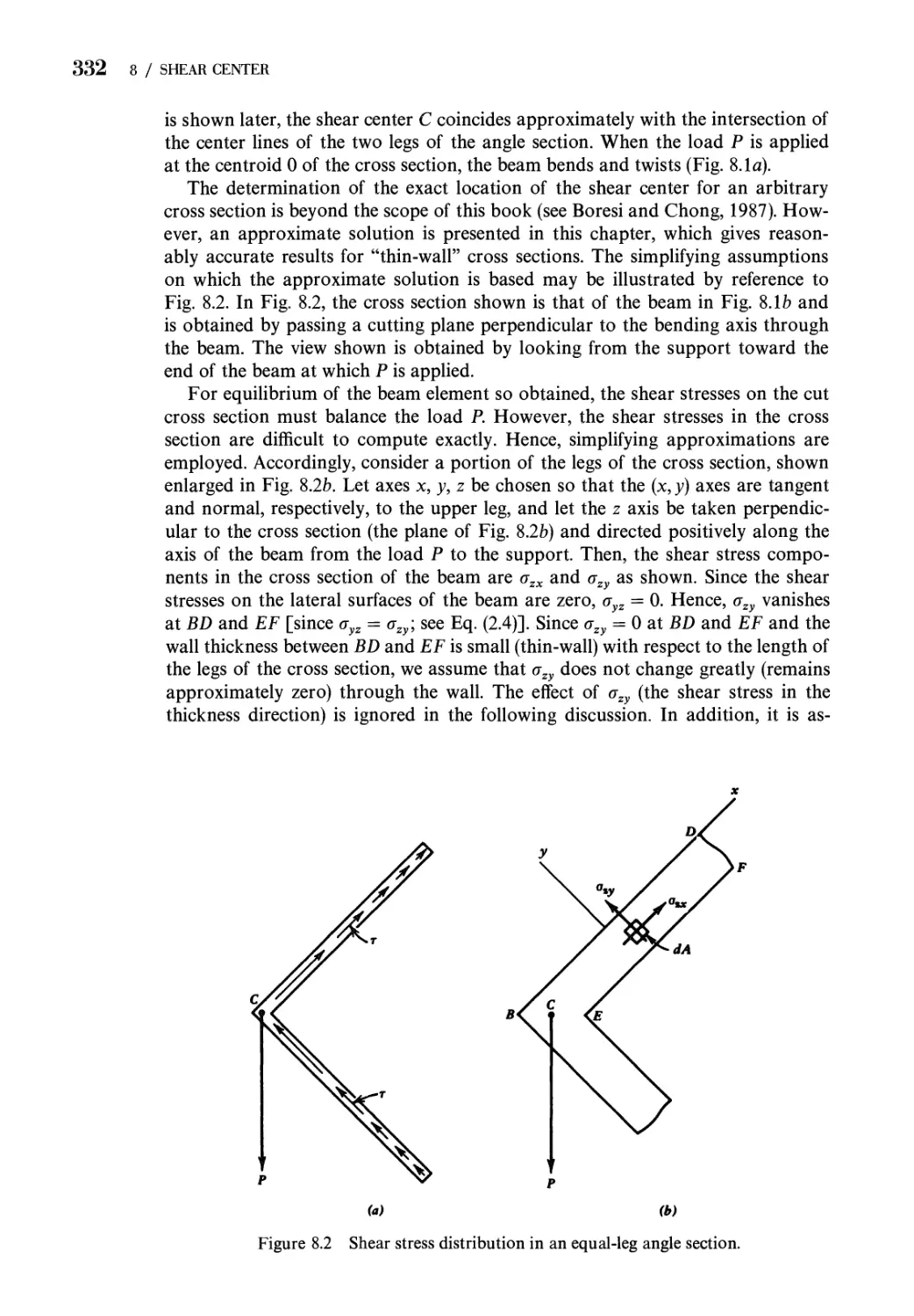
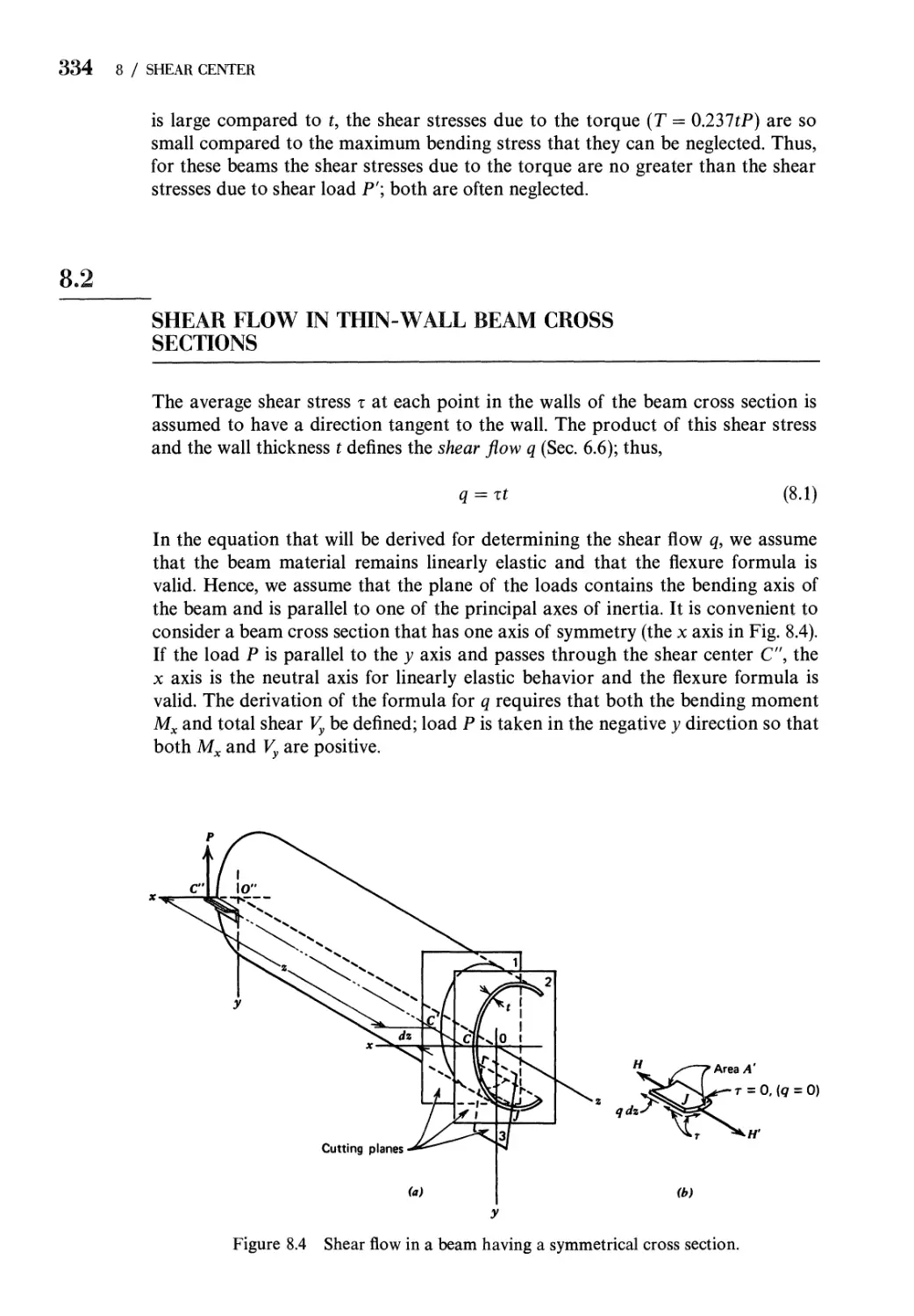
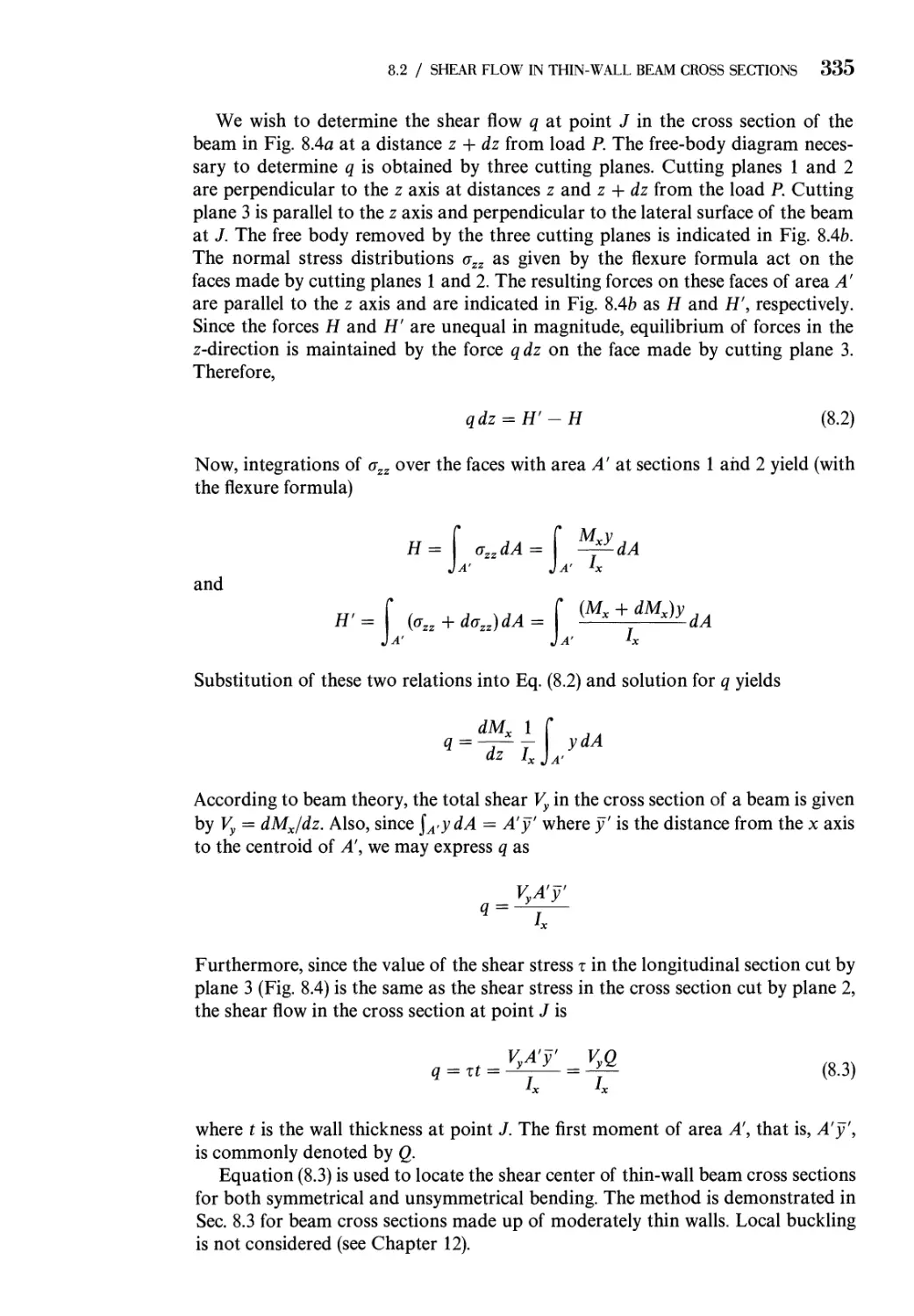
8.2 Shear Flow in Thin-Wall Beam Cross Sections 334
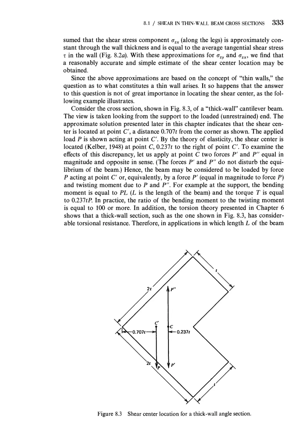
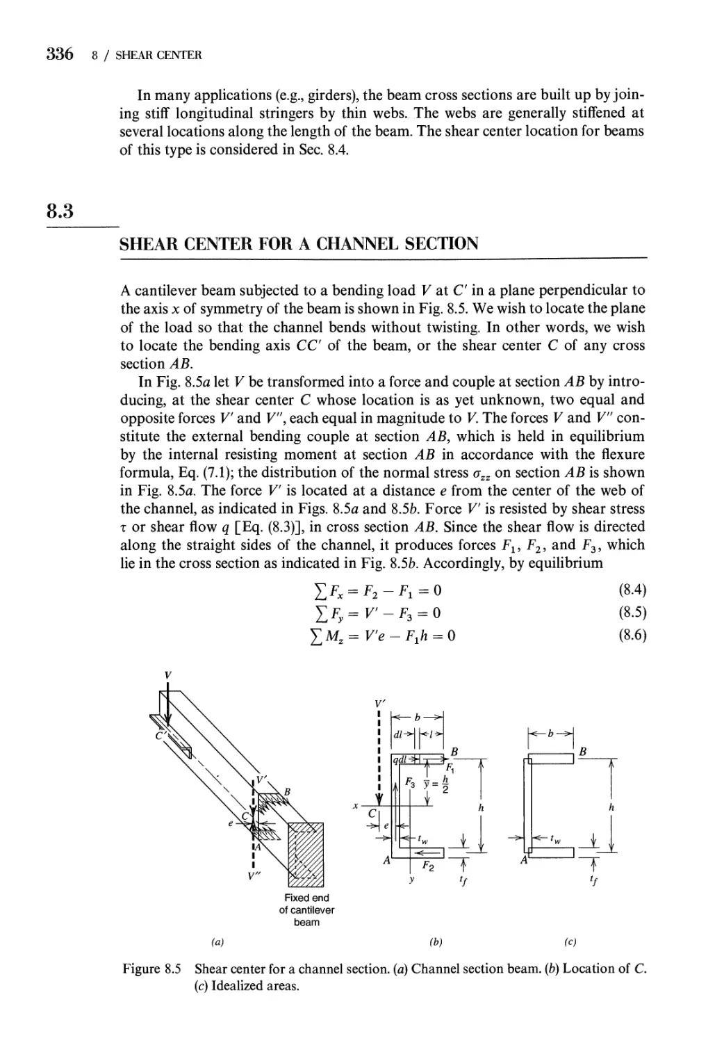
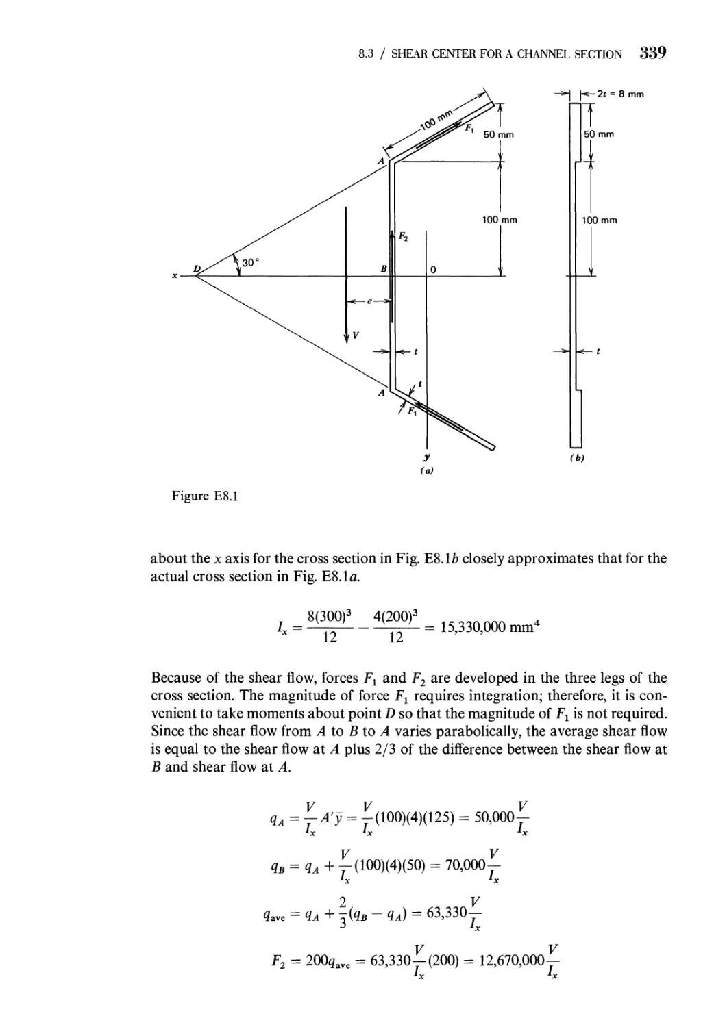
8.3 Shear Center for a Channel Section 336
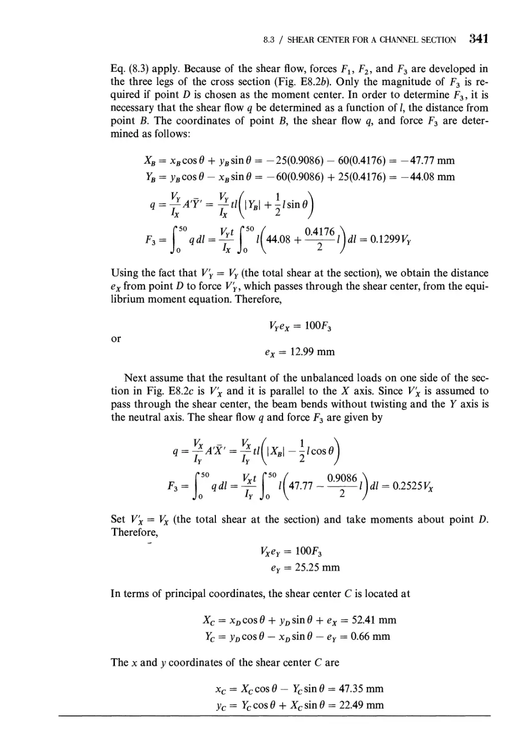
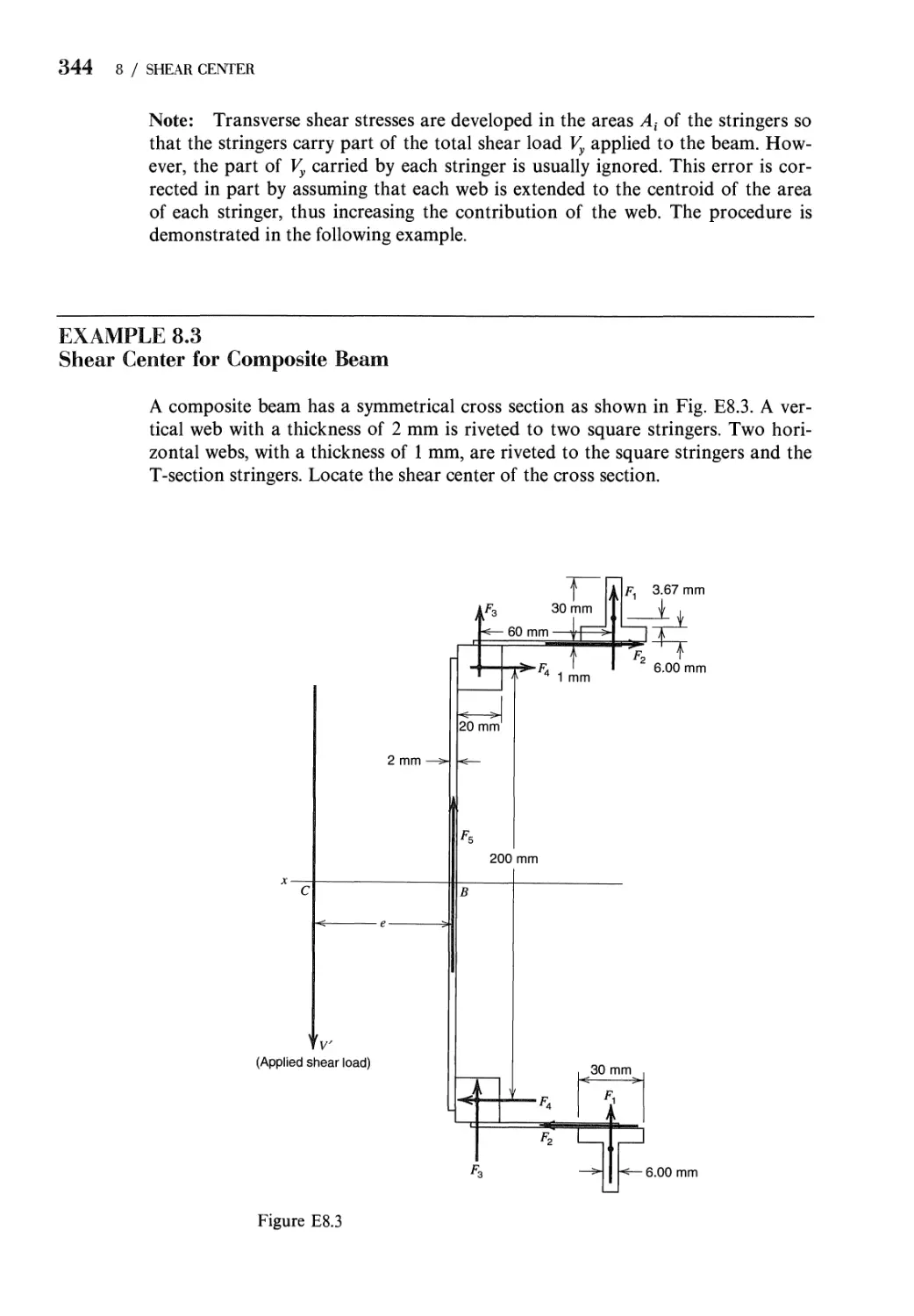
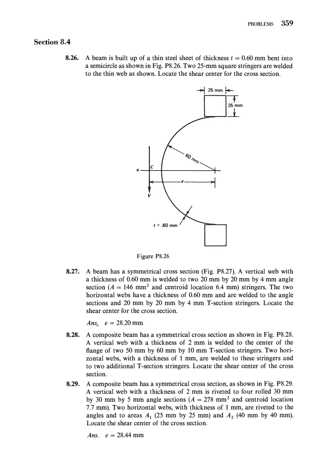
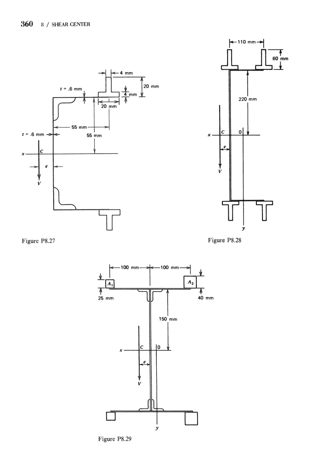
8.4 Shear Center of Composite Beams Formed from Stringers and
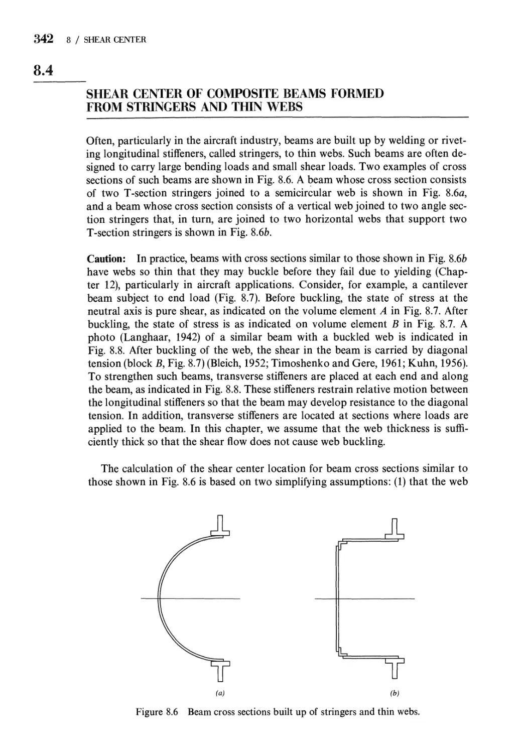
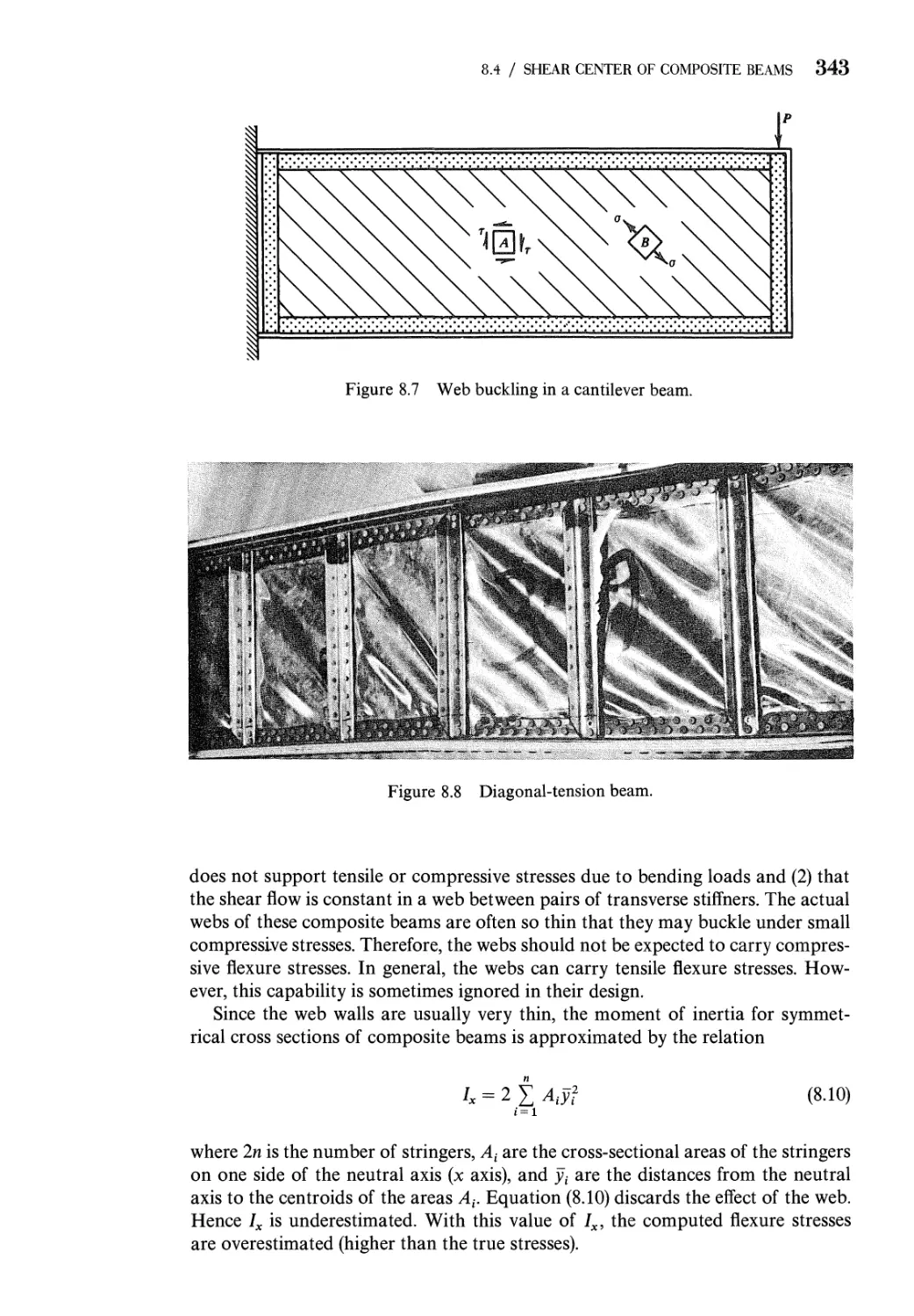
Thin Webs 342
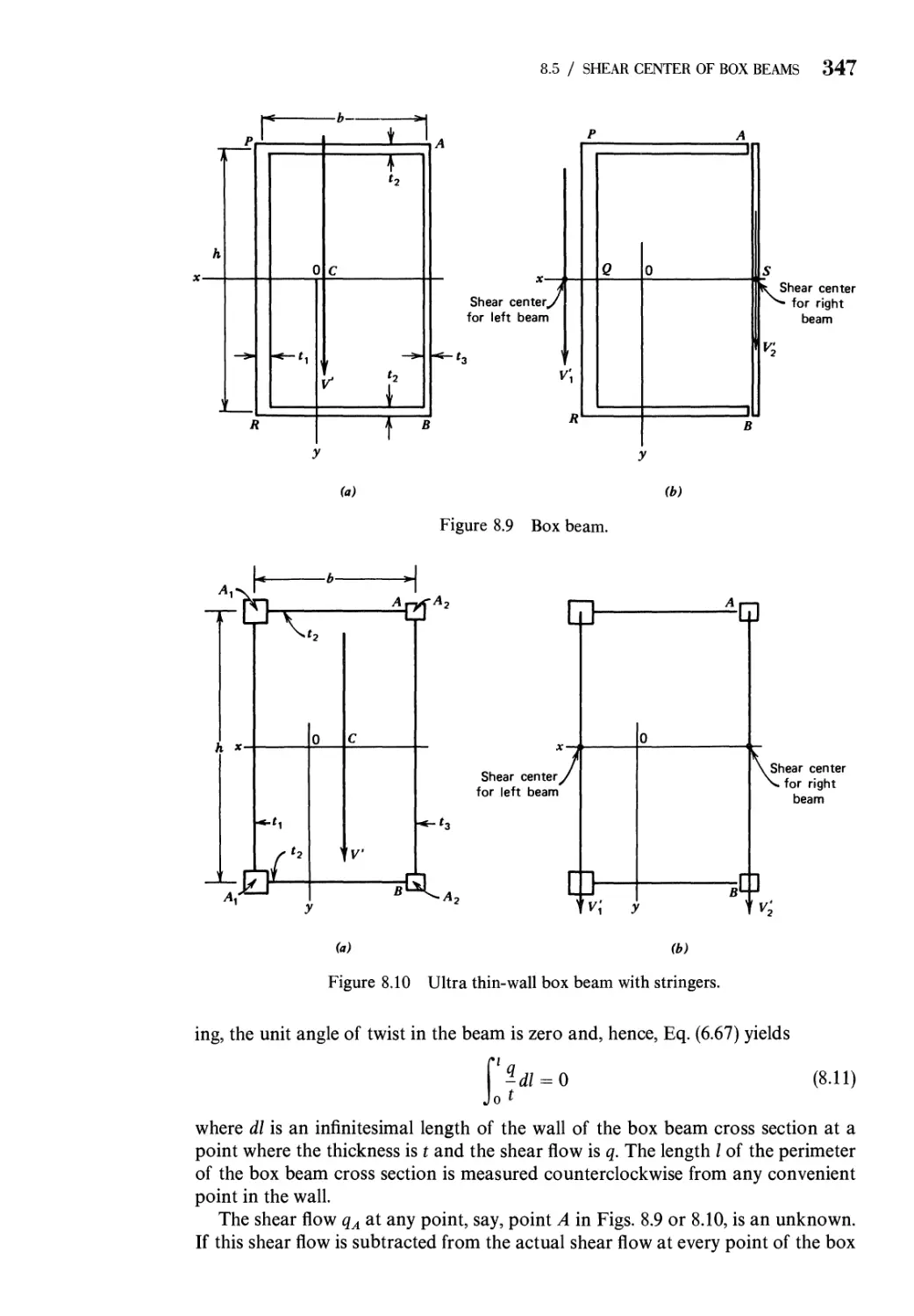
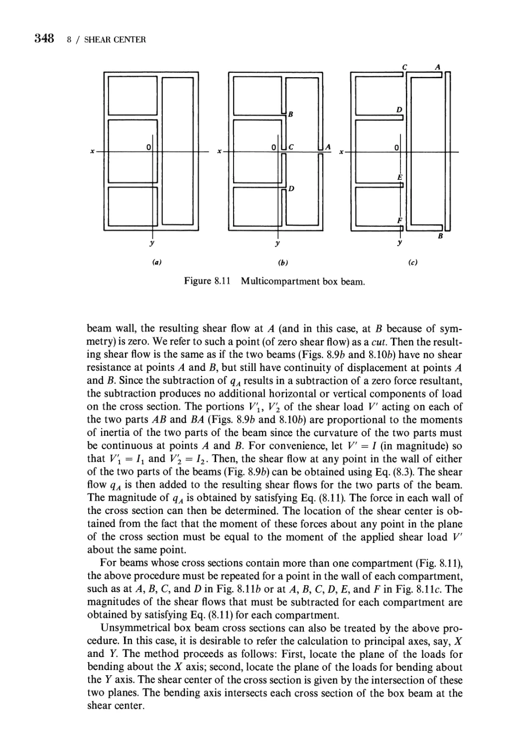
8.5 Shear Center of Box Beams 346
Problems 350
References 361
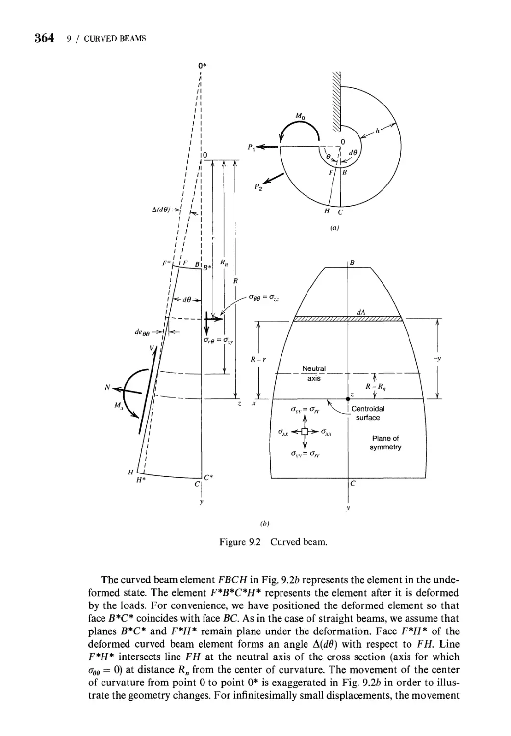
9 Curved Beams 362
9.1 Introduction 362
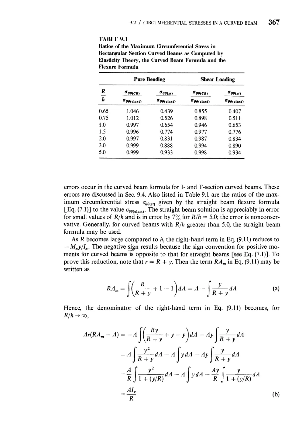
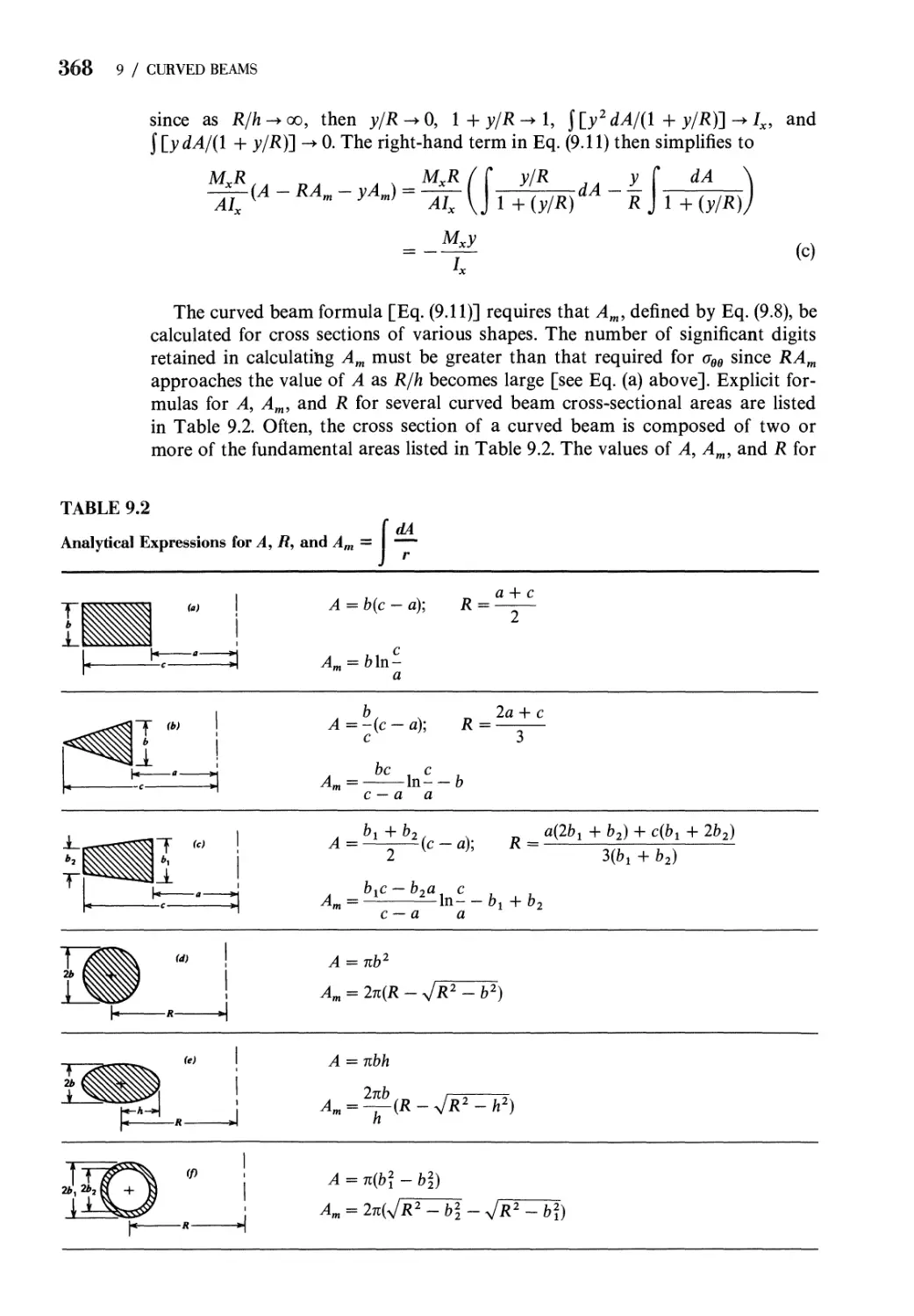
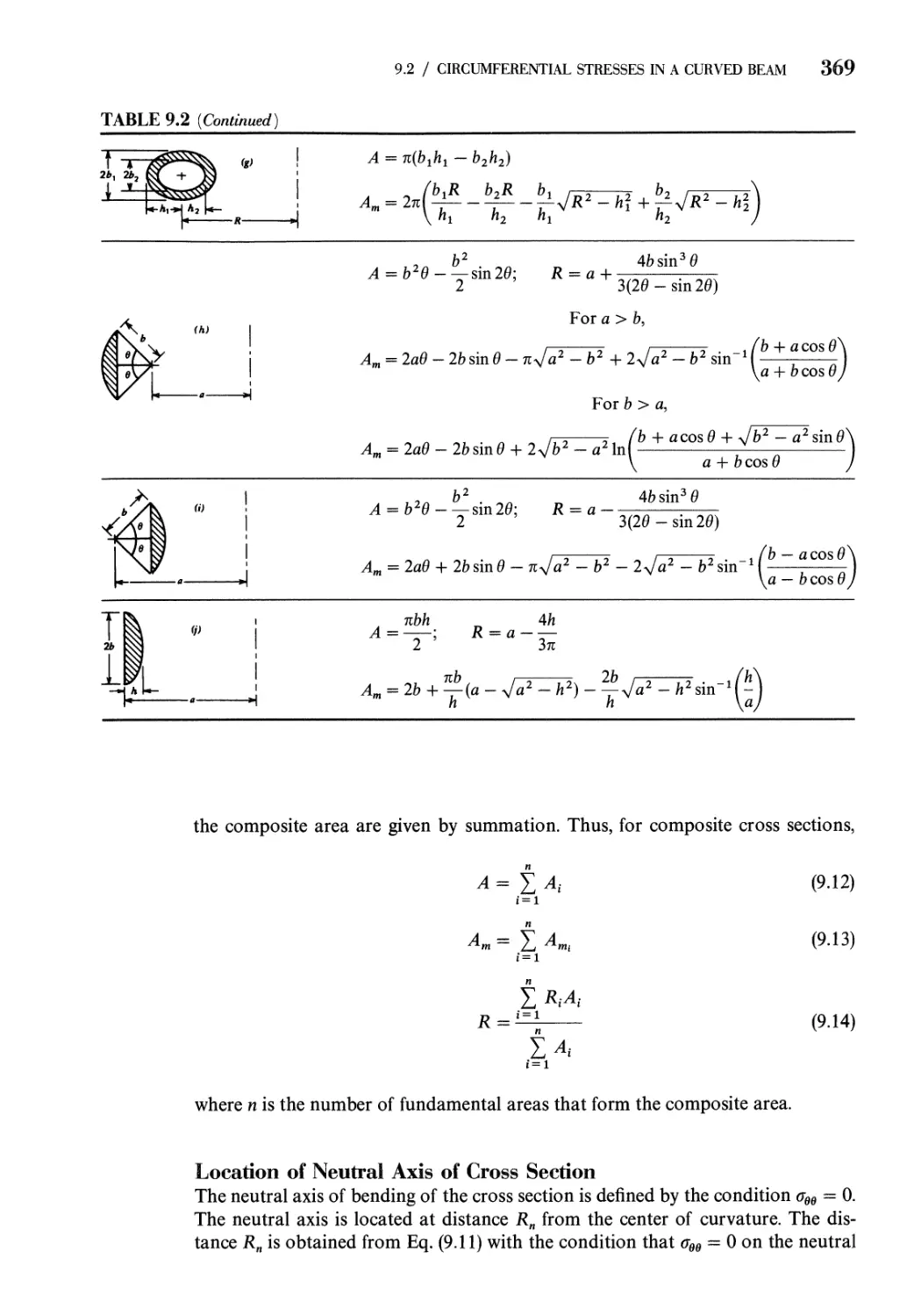
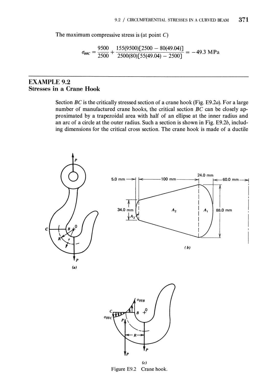
9.2 Circumferential Stresses in a Curved Beam 363
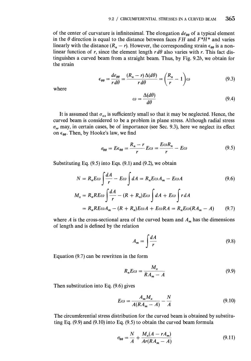
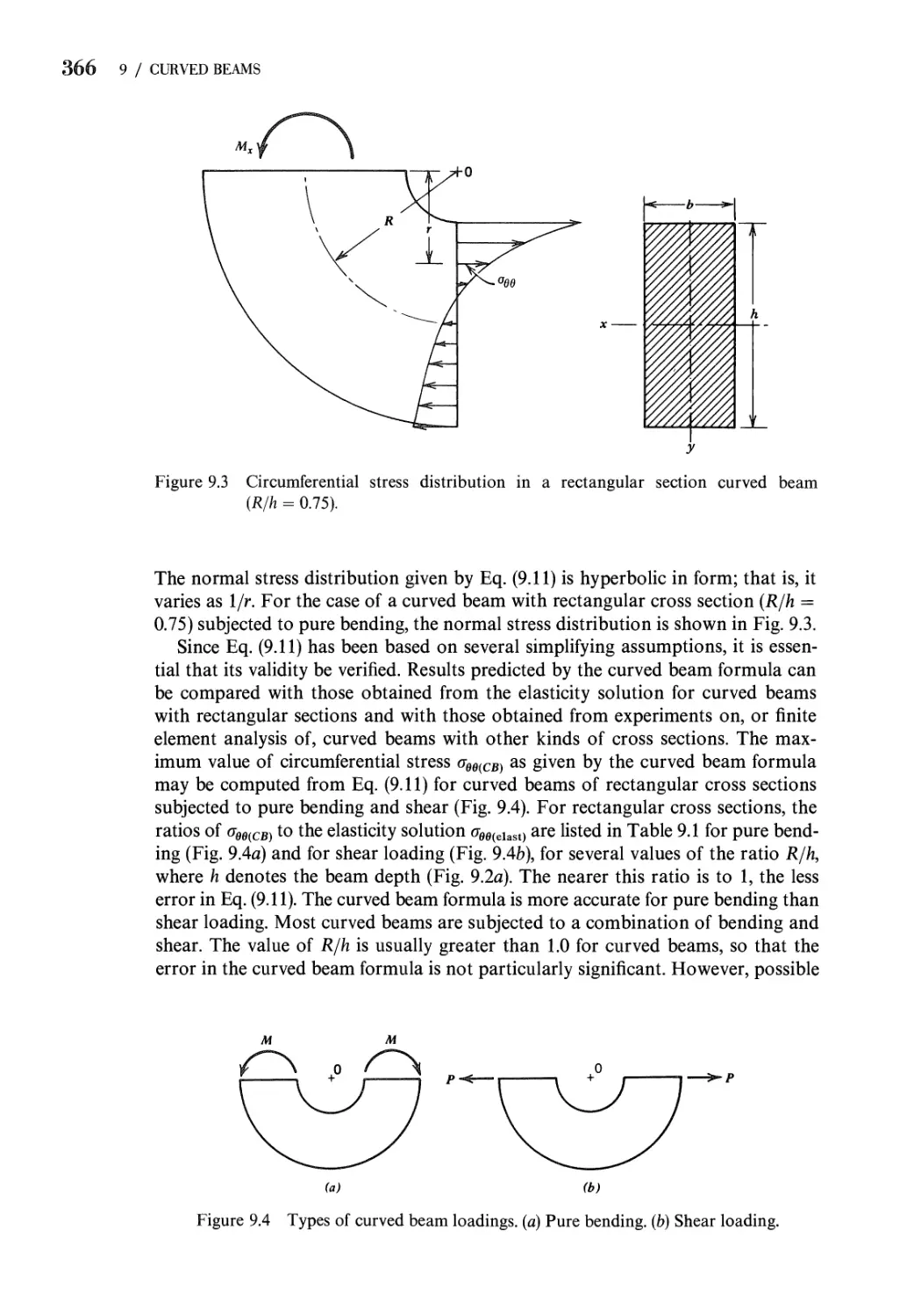
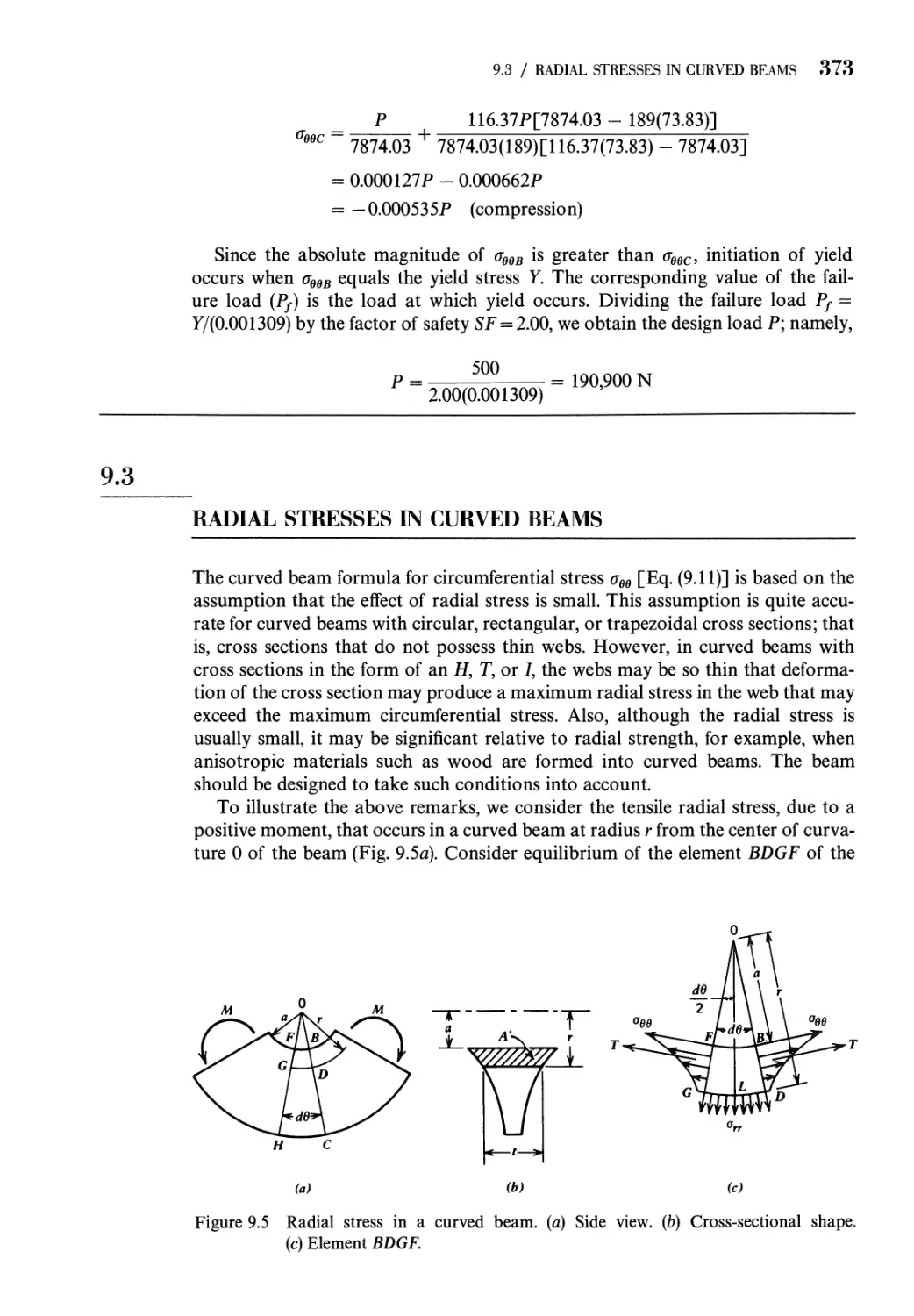
9.3 Radial Stresses in Curved Beams 373
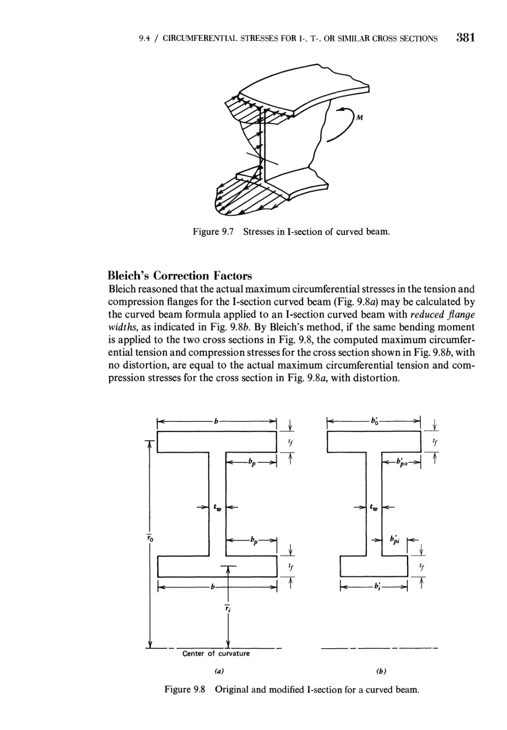
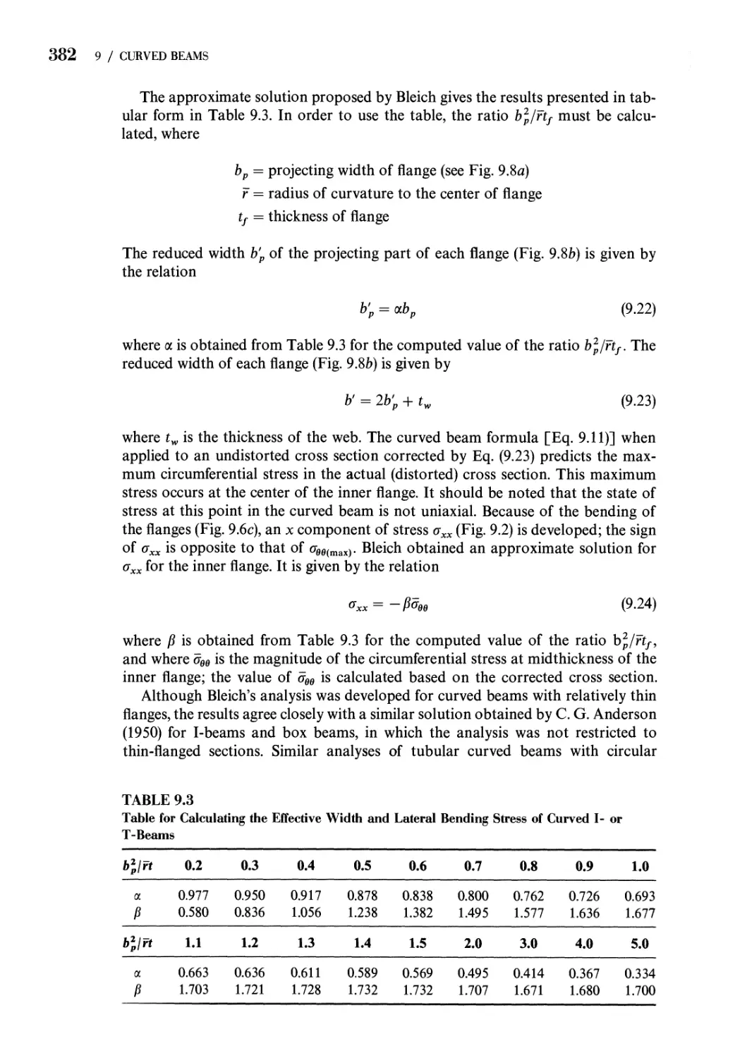
9.4 Correction of Circumferential Stresses in Curved Beams
Having I-, T-, or Similar Cross Sections 379
9.5 Defections of Curved Beams 385
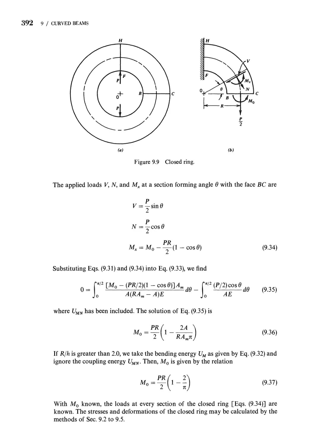
9.6 Statically Indeterminate Curved Beams. Closed Ring Subjected
to a Concentrated Load 391
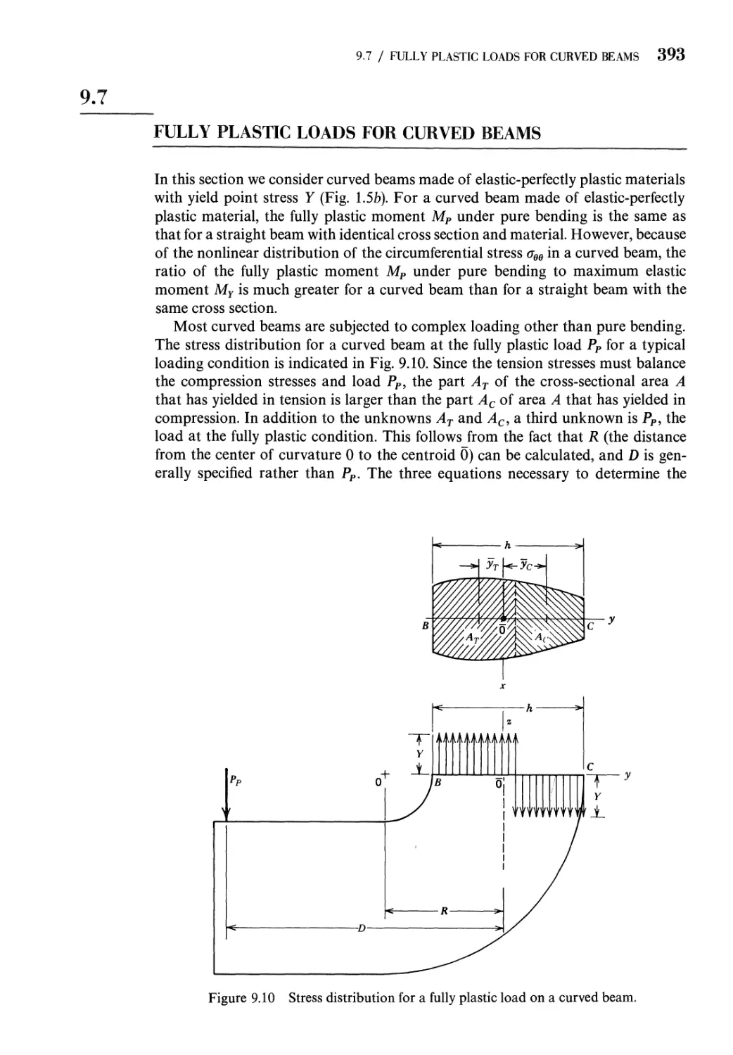
9.7 Fully Plastic Loads for Curved Beams 393
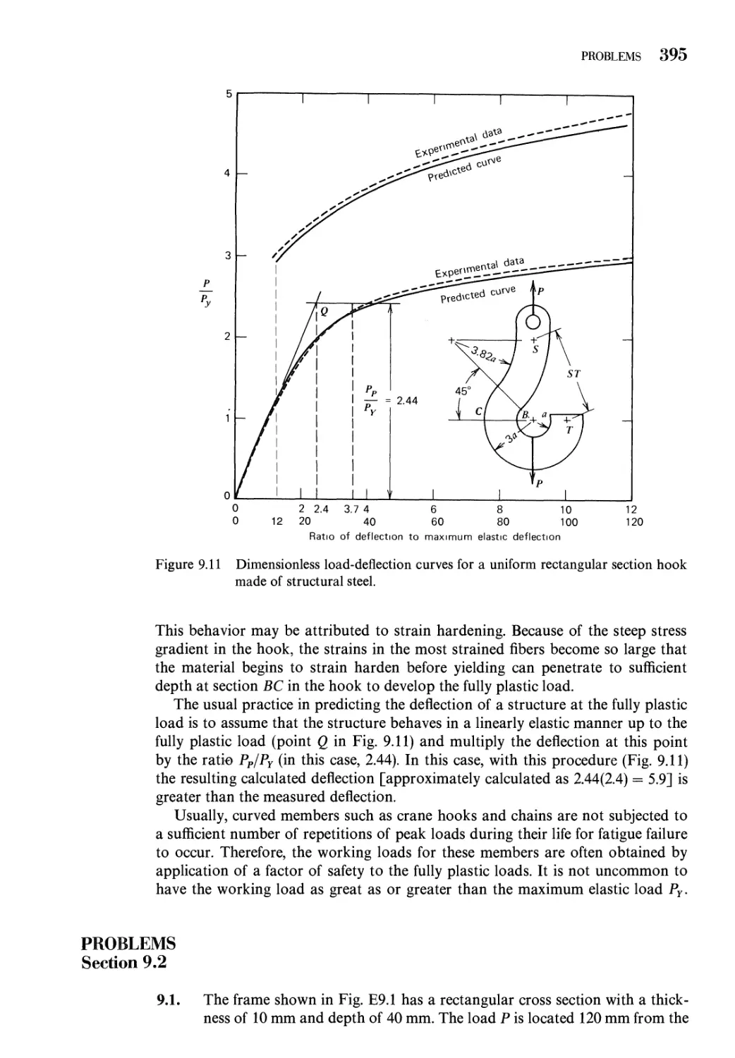
Problems 395
References 403
10 Beams on Elastic Foundations 404
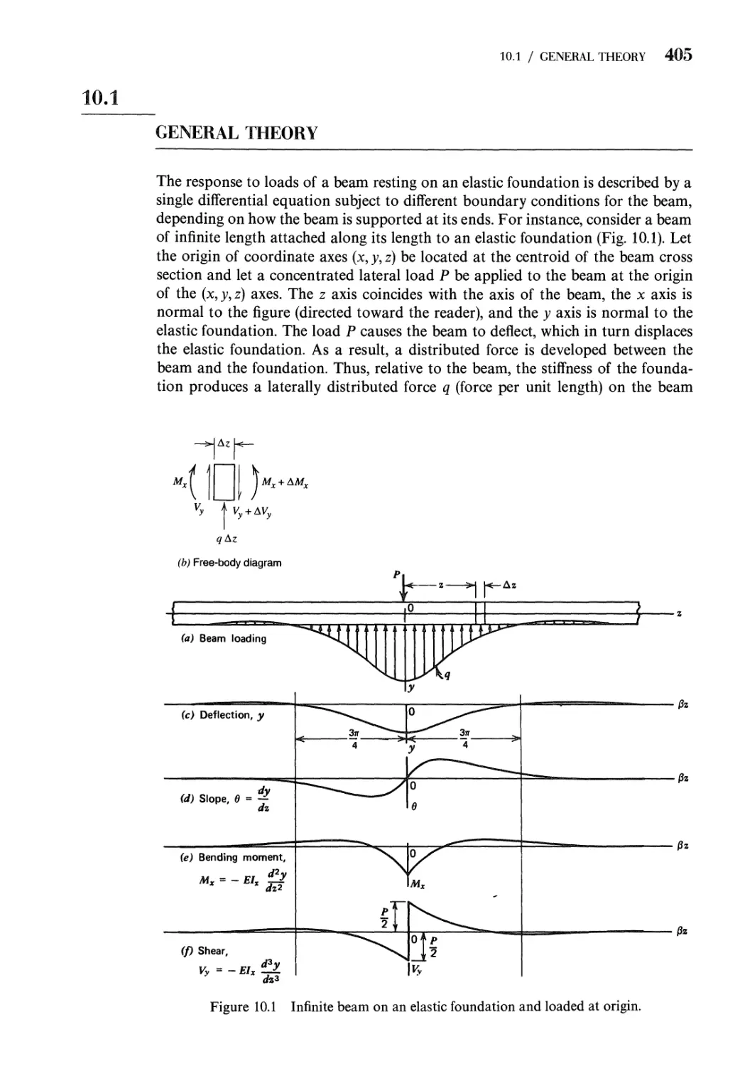
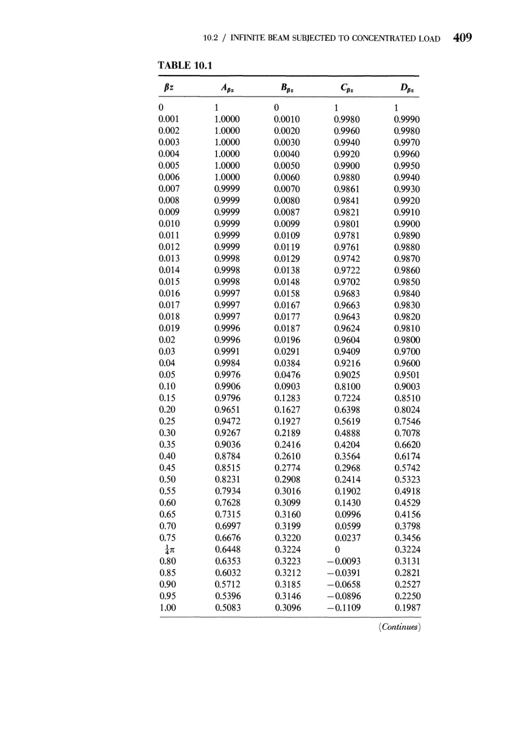
10.1 General Theory 405
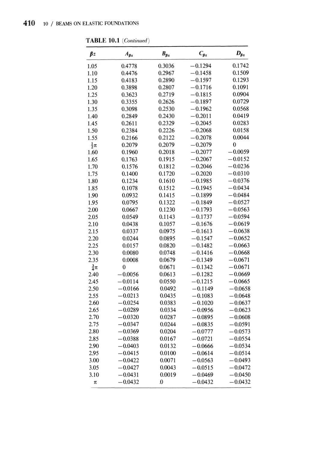
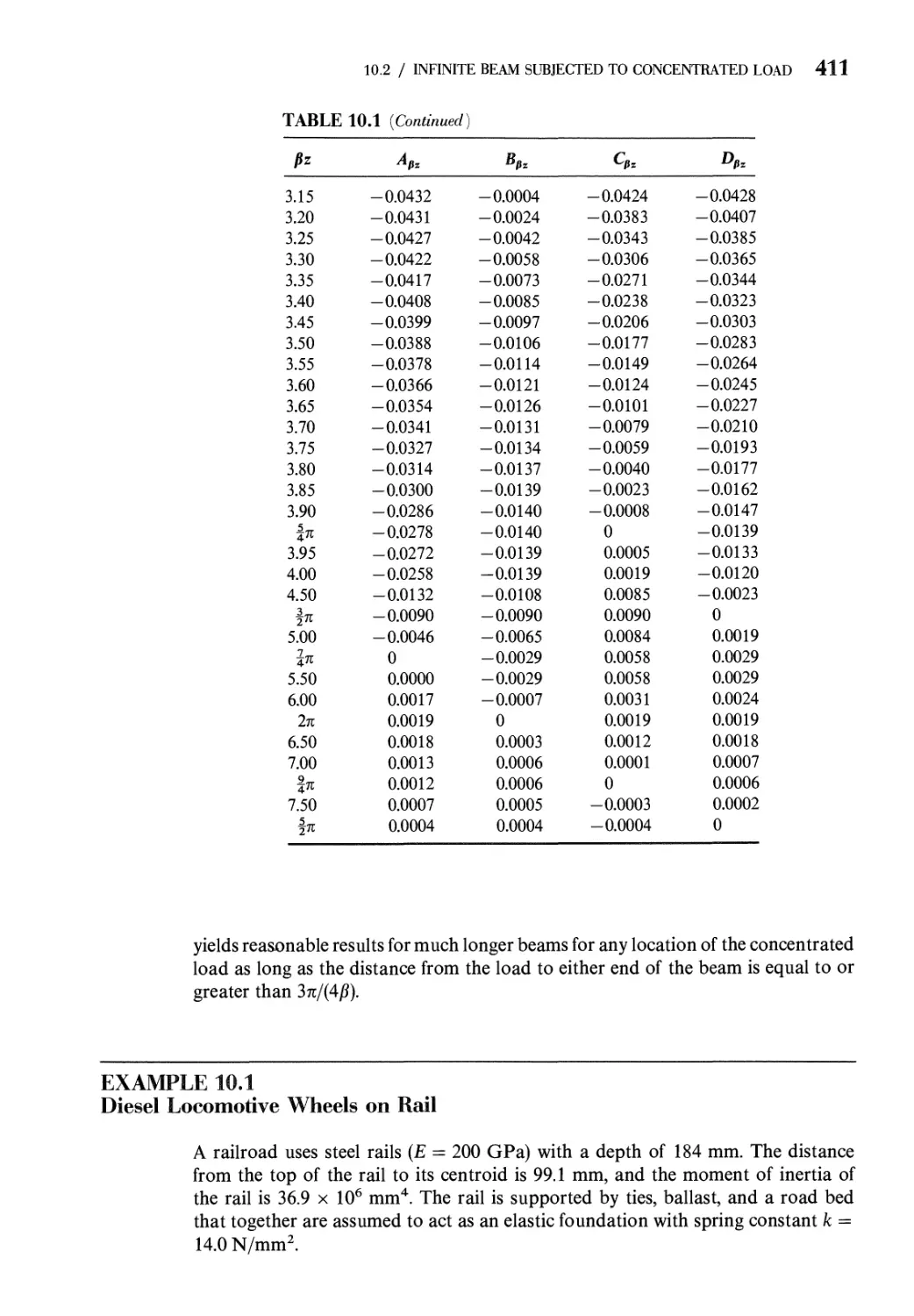
10.2 Infinite Beam Subjected to a Concentrated Load:
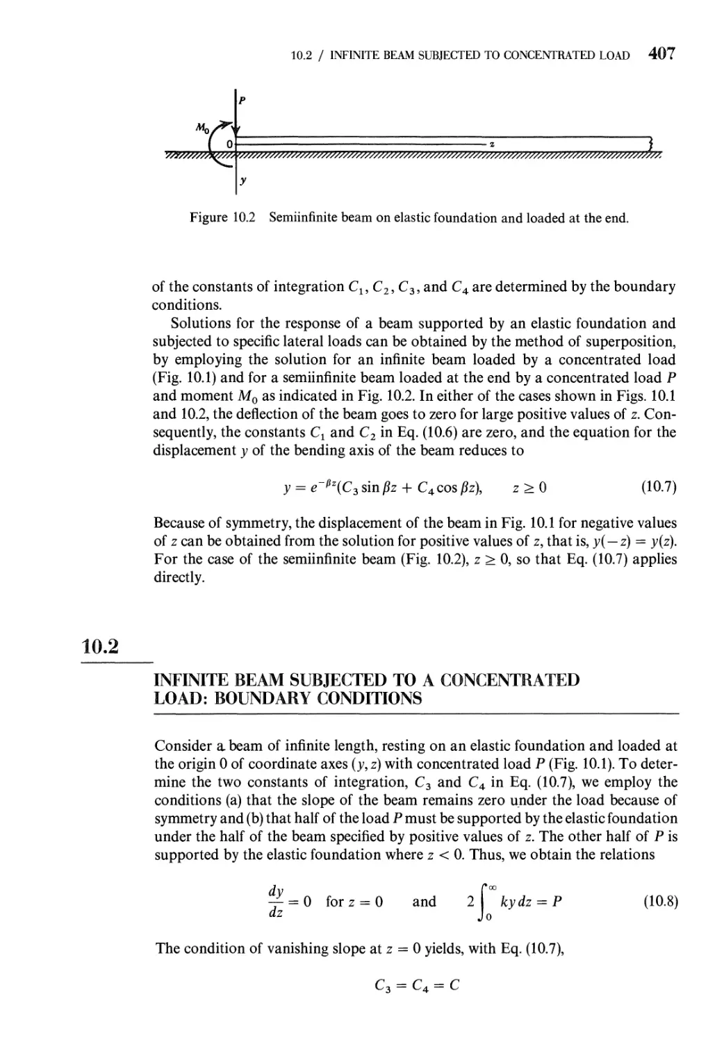
Boundary Conditions 407
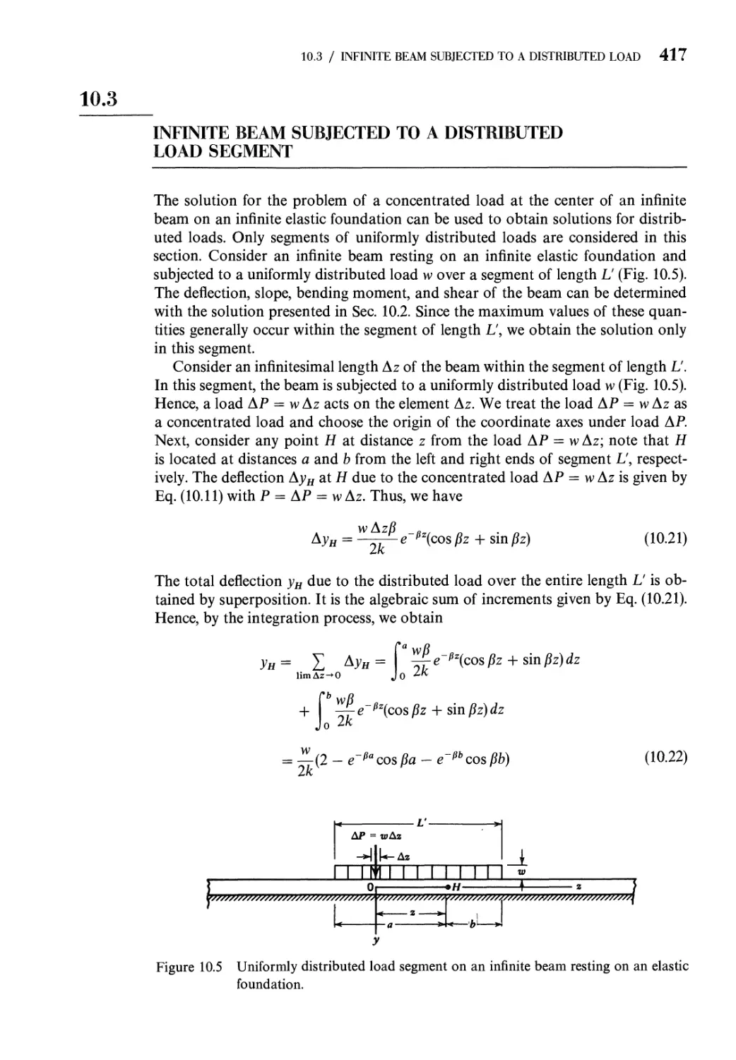
10.3 Infinite Beam Subjected to a Distributed Load Segment 417
10.4 Semiinfinite Beam Subjected to Loads at Its End 421
10.5 Semiinfinite Beam with Concentrated Load near
Its End 422
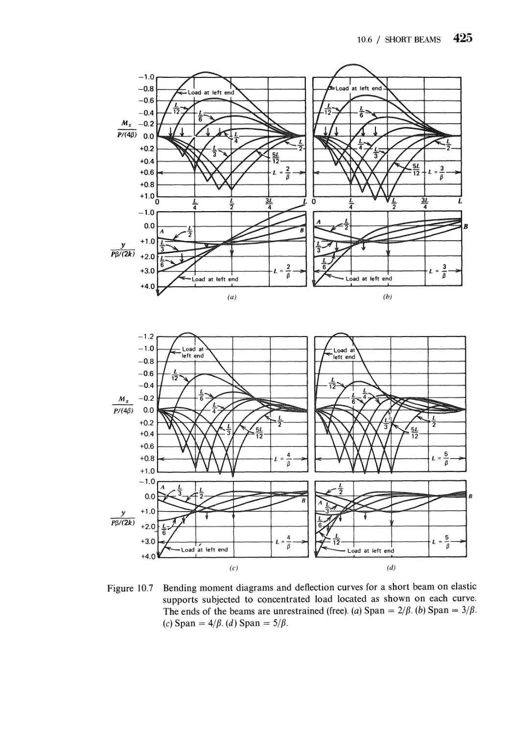
10.6 Short Beams 424
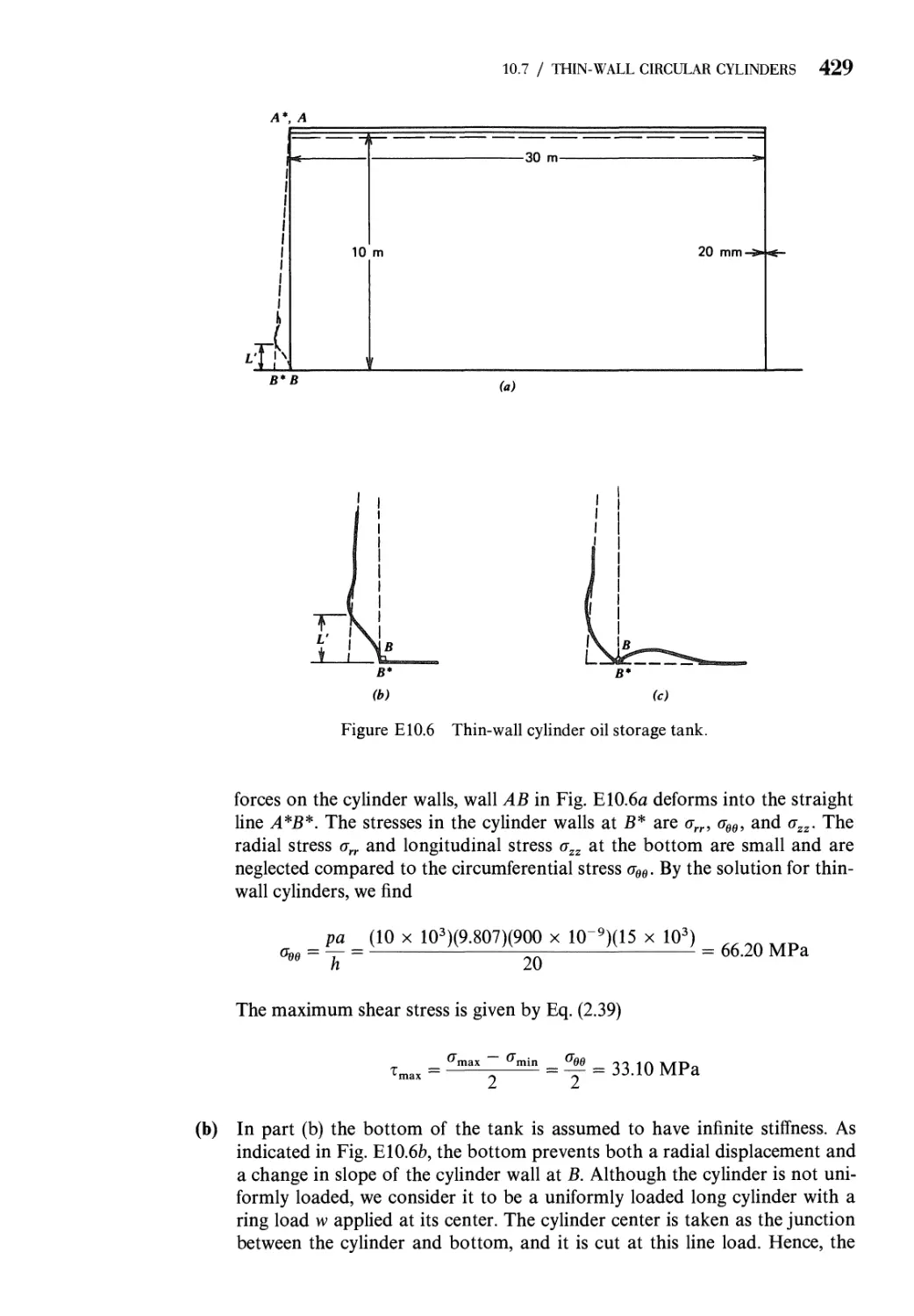
10.7 Thin-Wall Circular Cylinders 426
Problems 432
References 439
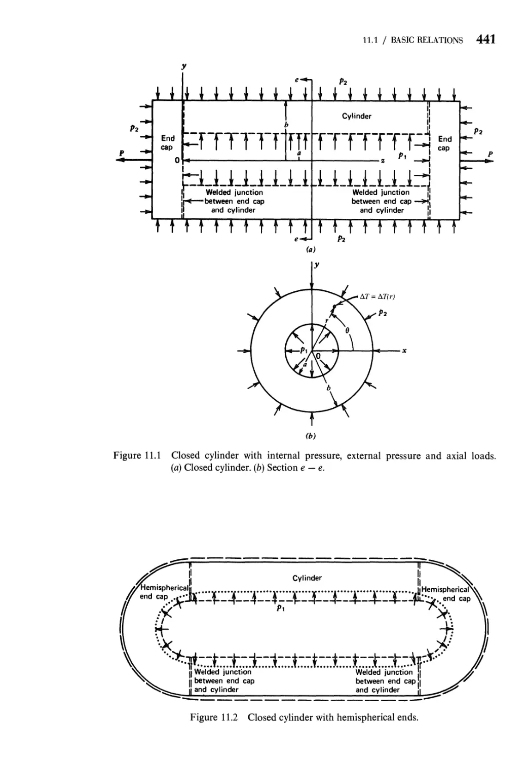
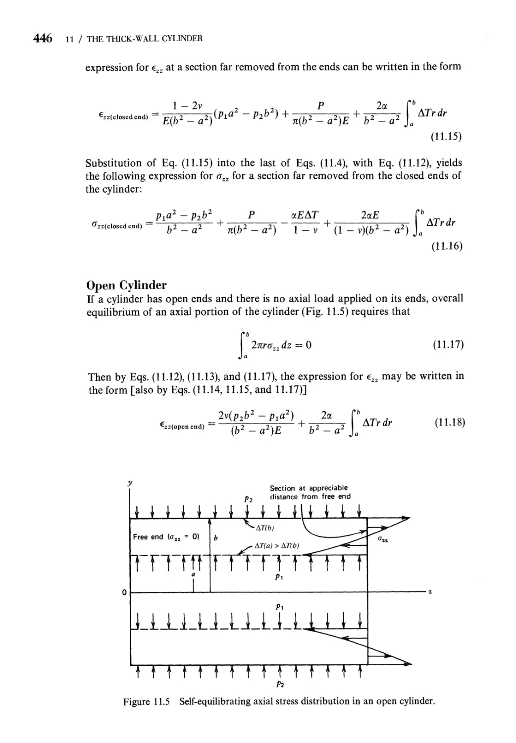
11 The Thick-Wall Cylinder 440
11.1 Basic Relations 440
11.2 Stress Components for a Cylinder with Closed Ends 444
11.3 Stress Components and Radial Displacement for Constant
Temperature 447
11.4 Criteria of Failure 451
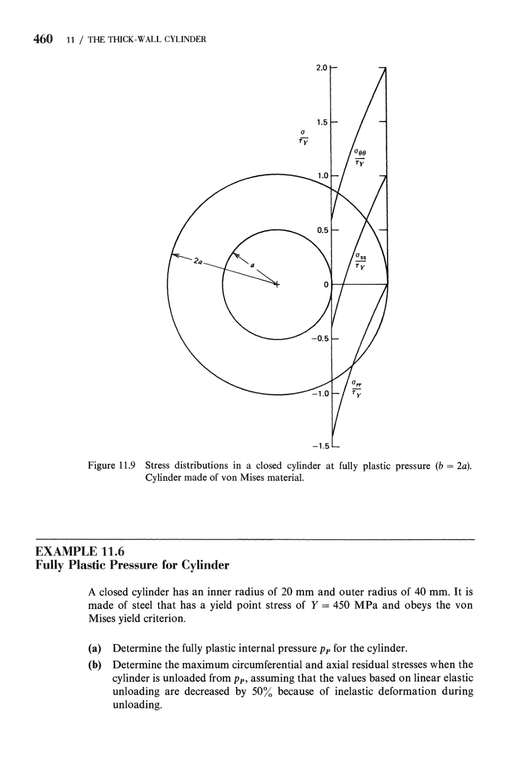
11.5 Fully Plastic Pressure. Autofrettage 457
11.6 Cylinder Solution for Temperature Change Only 462
Problems 465
References 468
12 Elastic and Inelastic Stability of Columns 469
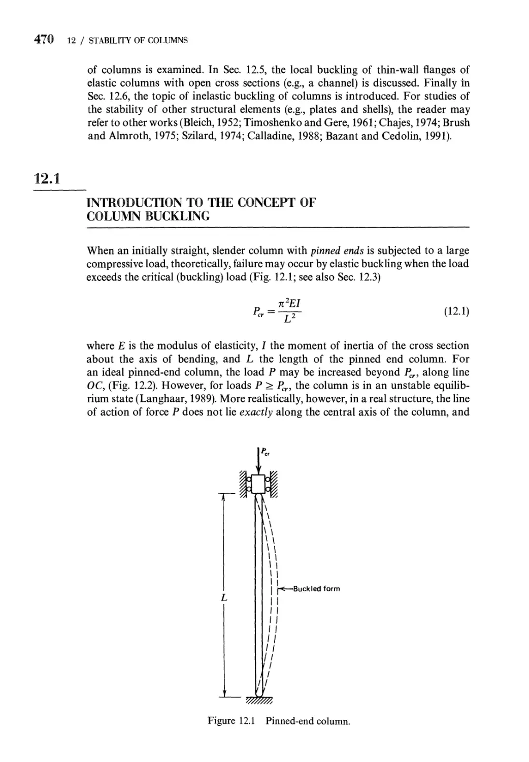
12.1 Introduction to the Concept of Column Buckling 470
12.2 Deflection Response of Columns to Compressive
Loads 472
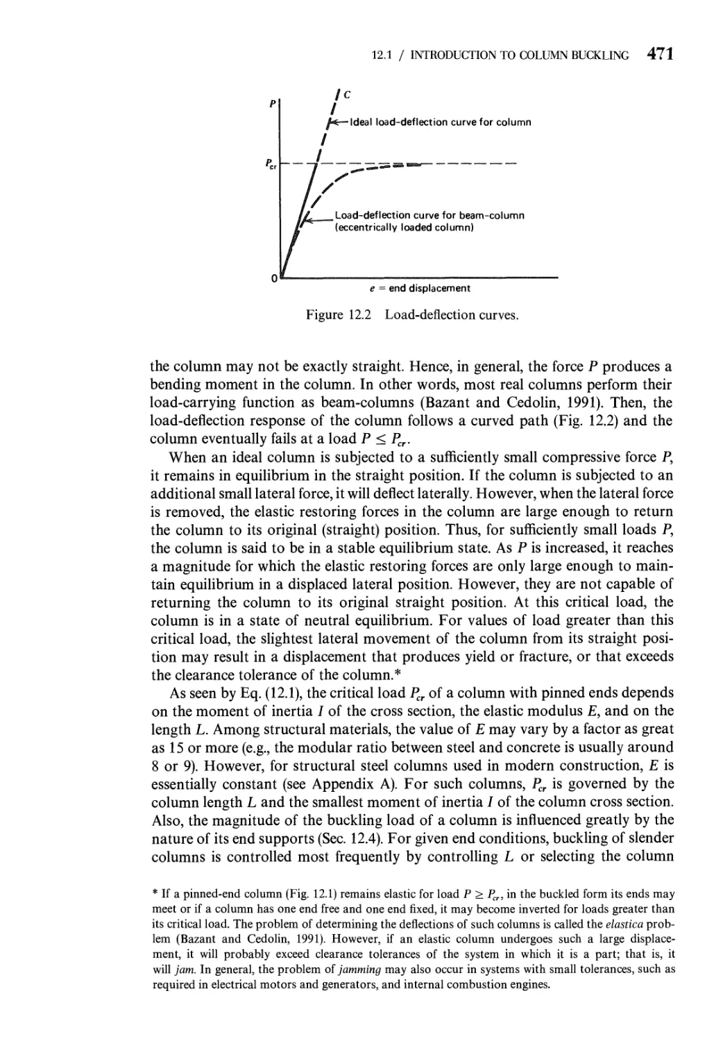
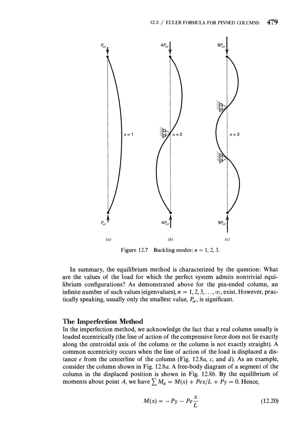
12.3 The Euler Formula for Columns with Pinned Ends 475
12.4 Euler Buckling of Columns with General End
Constraints 484
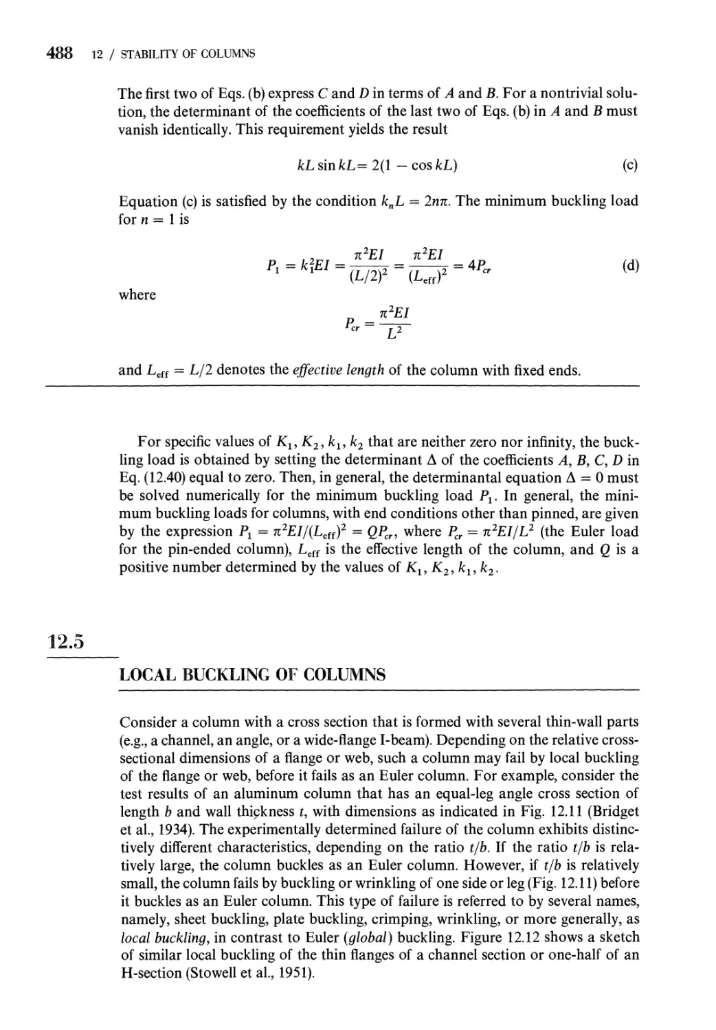
12.5 Local Buckling of Columns 488
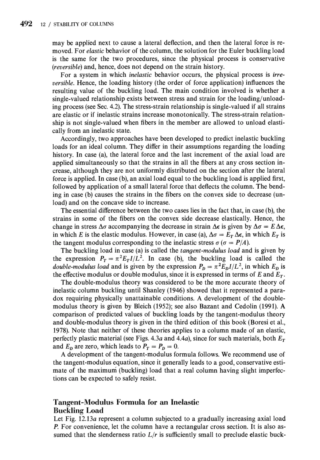
12.6 Inelastic Buckling of Columns 490
Problems 500
References 507
CONTENTS XV
PART III
SELECTED ADVANCED TOPICS 509
13 Flat Plates 511
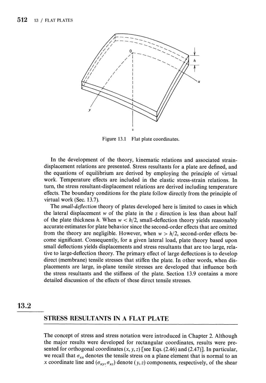
13.1 Introduction 511
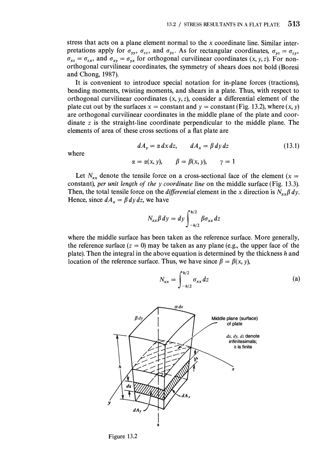
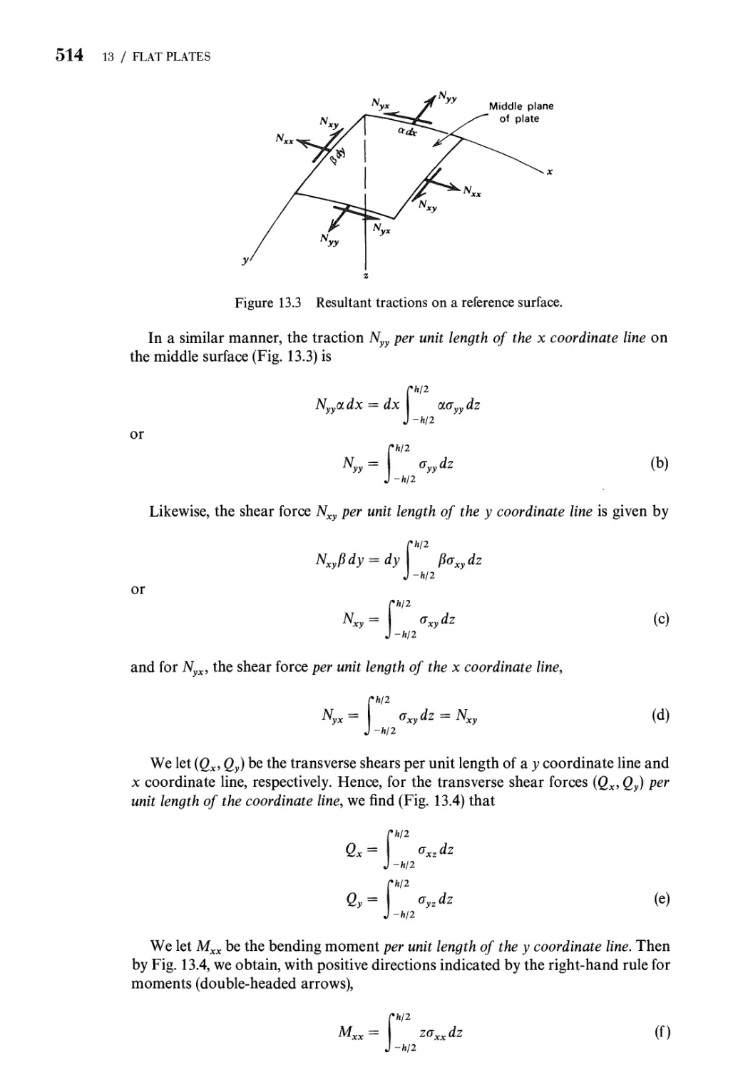
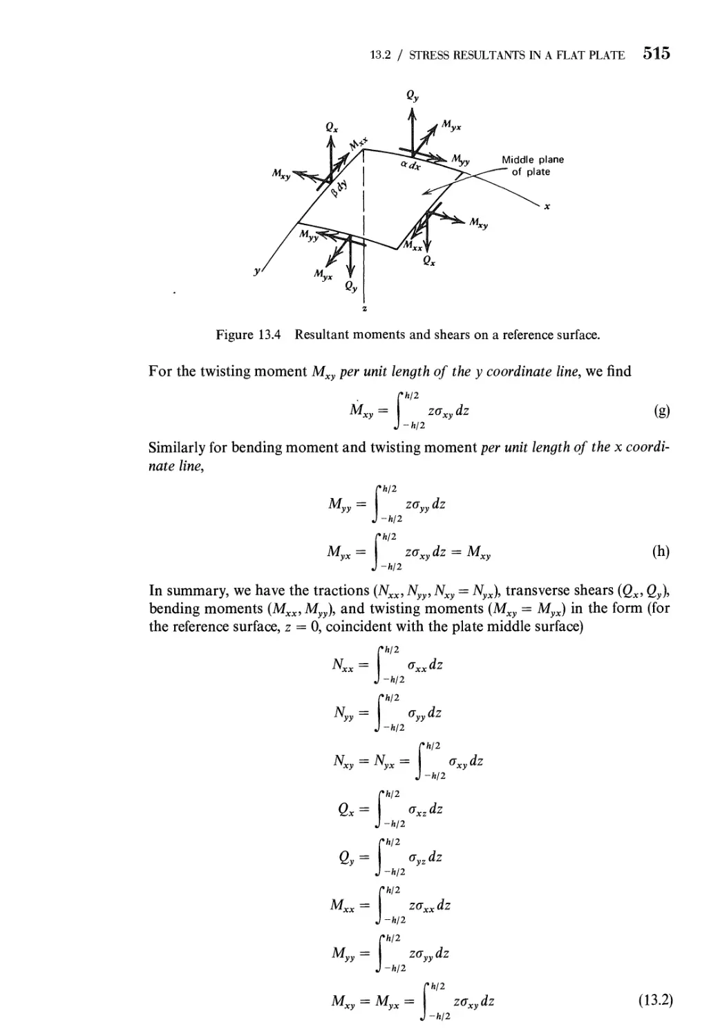
13.2 Stress Resultants in a Flat Plate 512
13.3 Kinematics: Strain-Displacement Relations for Plates 516
13.4 Equilibrium Equations for Small-Displacement Theory of
Flat Plates 521
13.5 Stress-Strain-Temperature Relations for Isotropic
Elastic Plates 523
13.6 Strain Energy of a Plate 526
13.7 Boundary Conditions for Plates 527
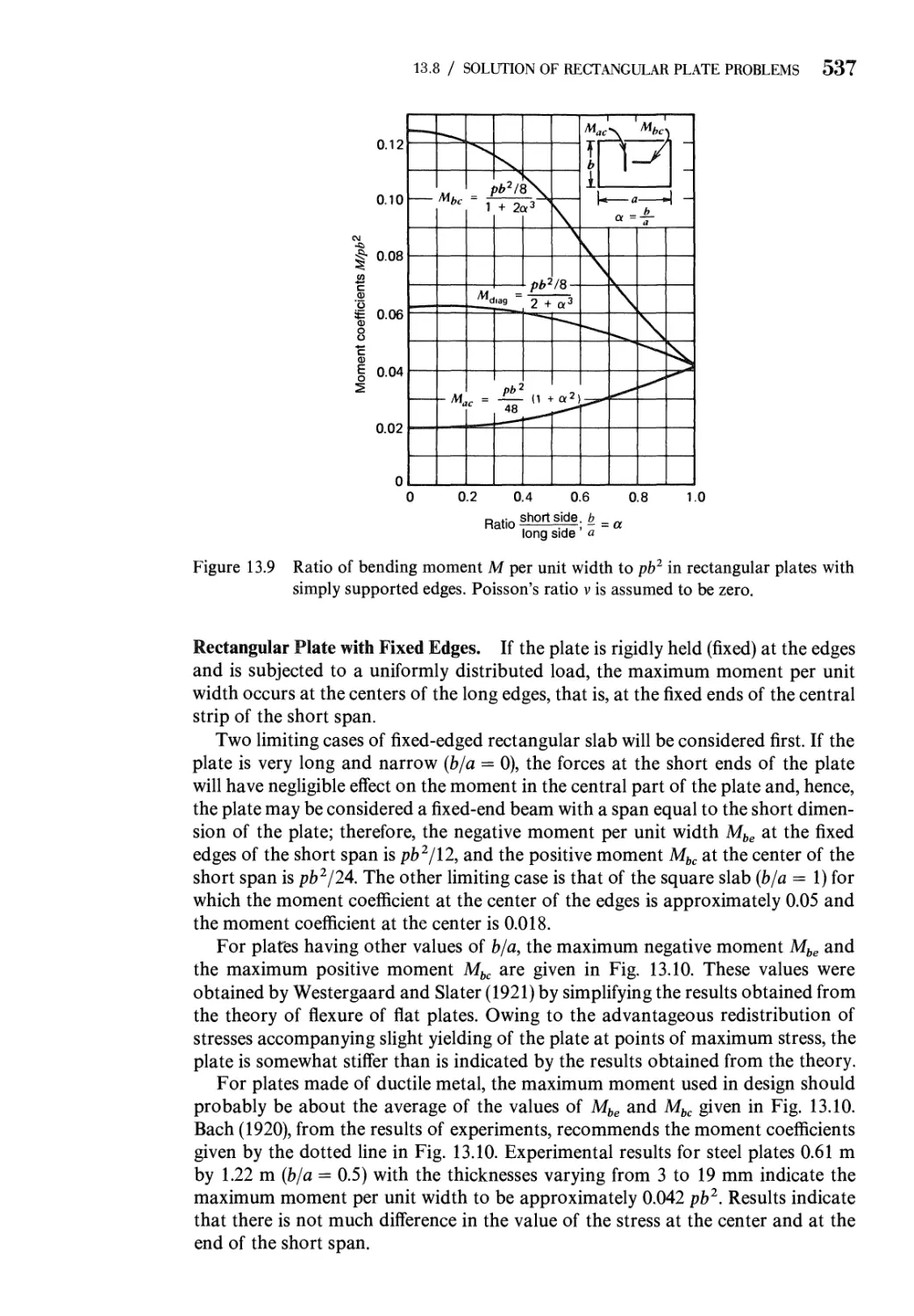
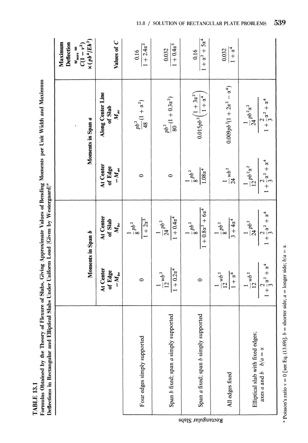
13.8 Solution of Rectangular Plate Problems 531
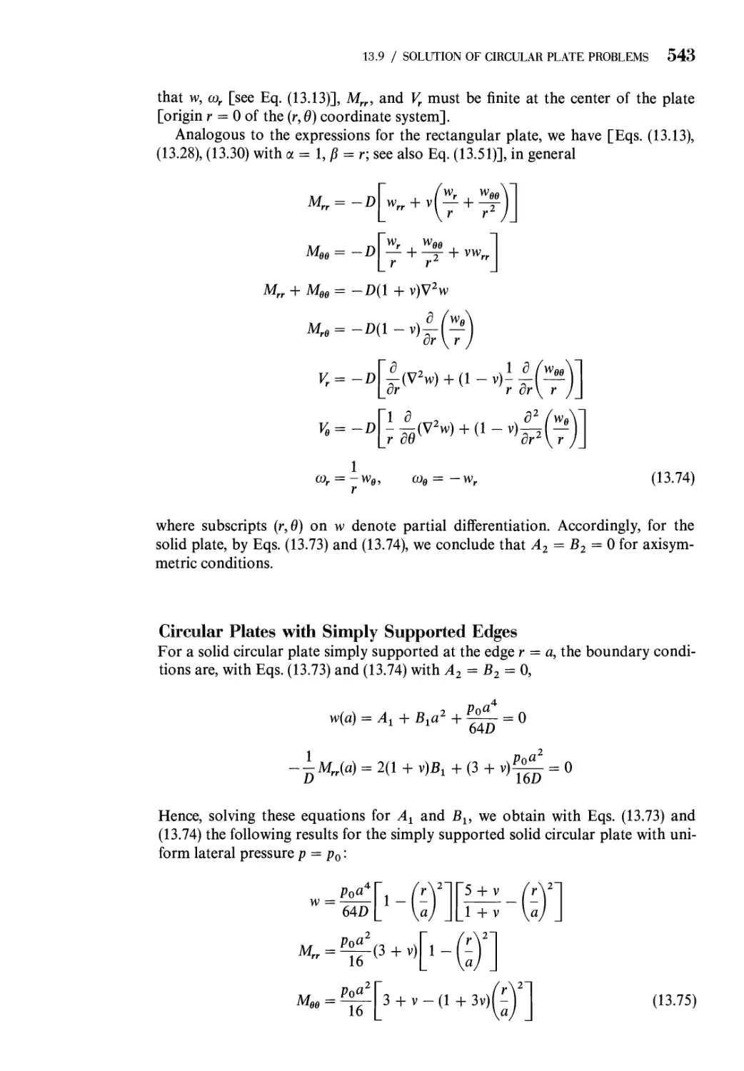
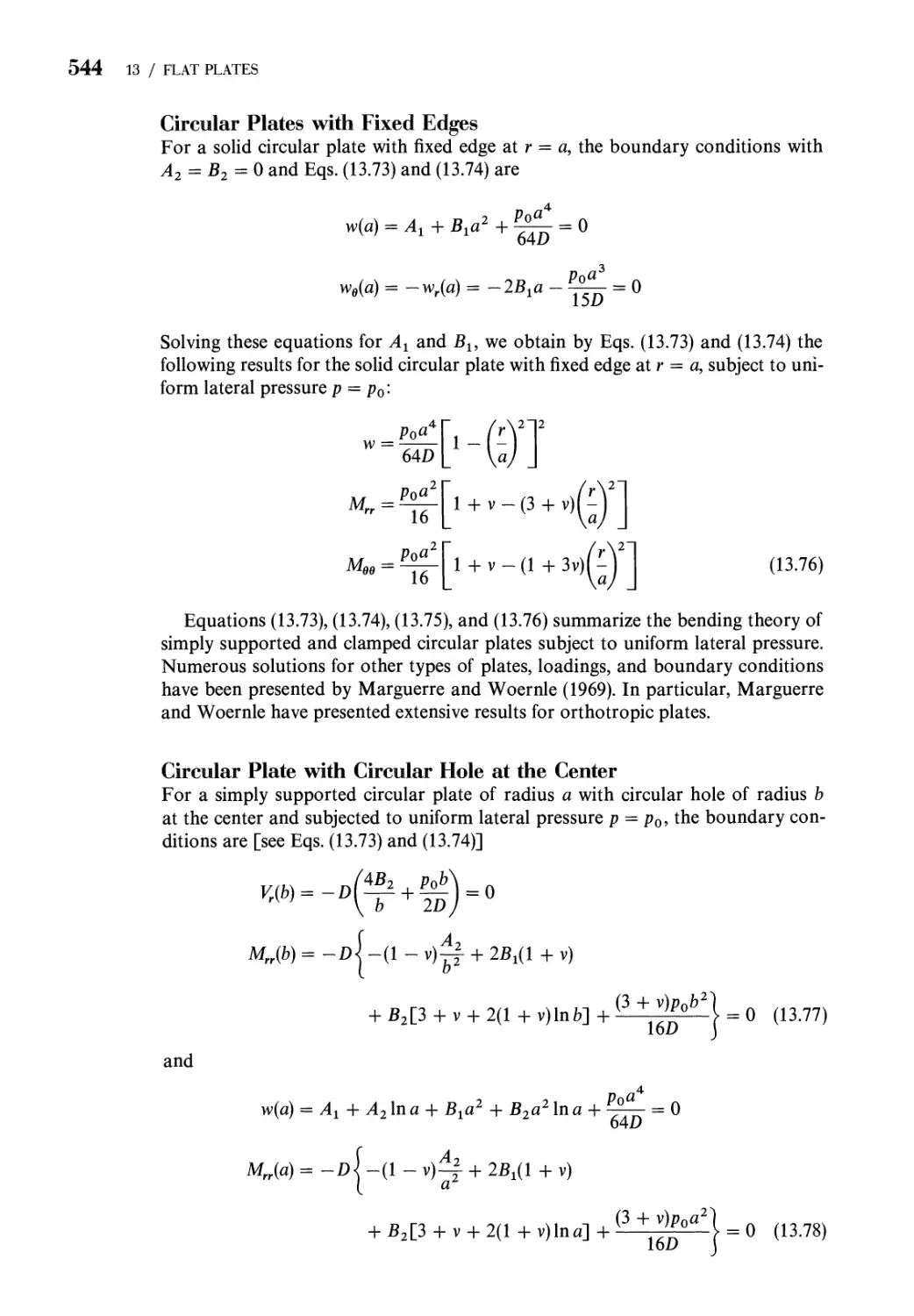
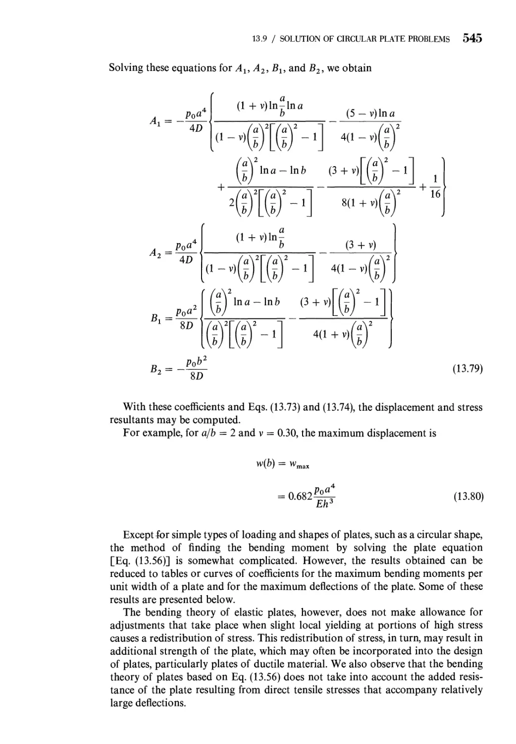
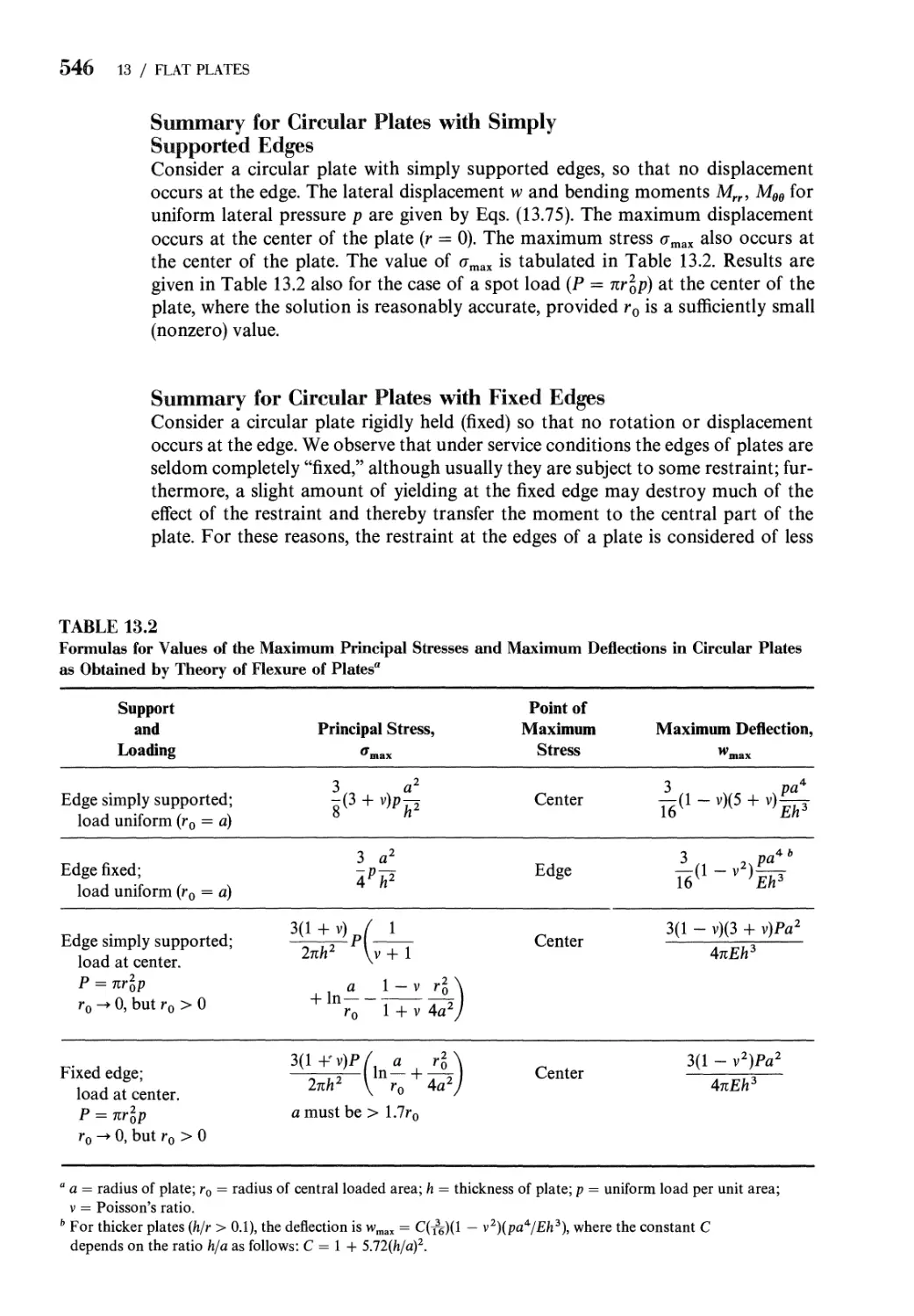
13.9 Solution of Circular Plate Problems 542
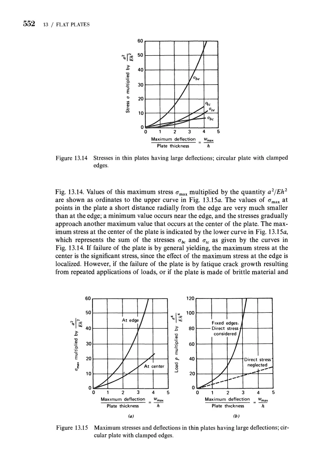
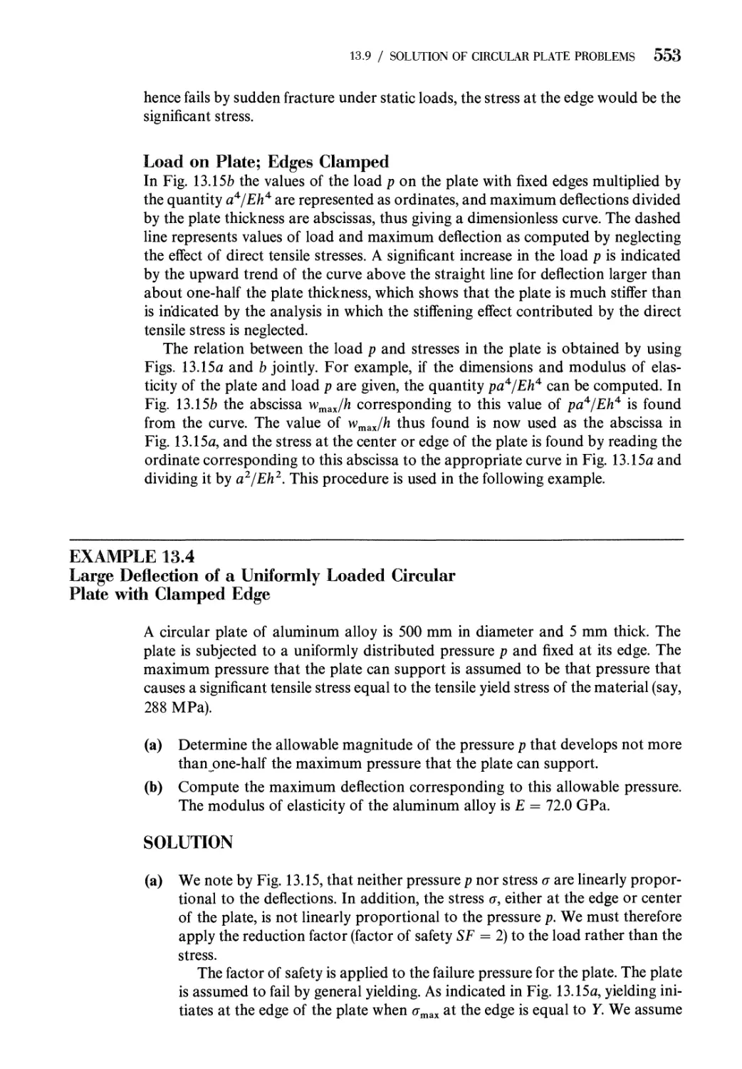
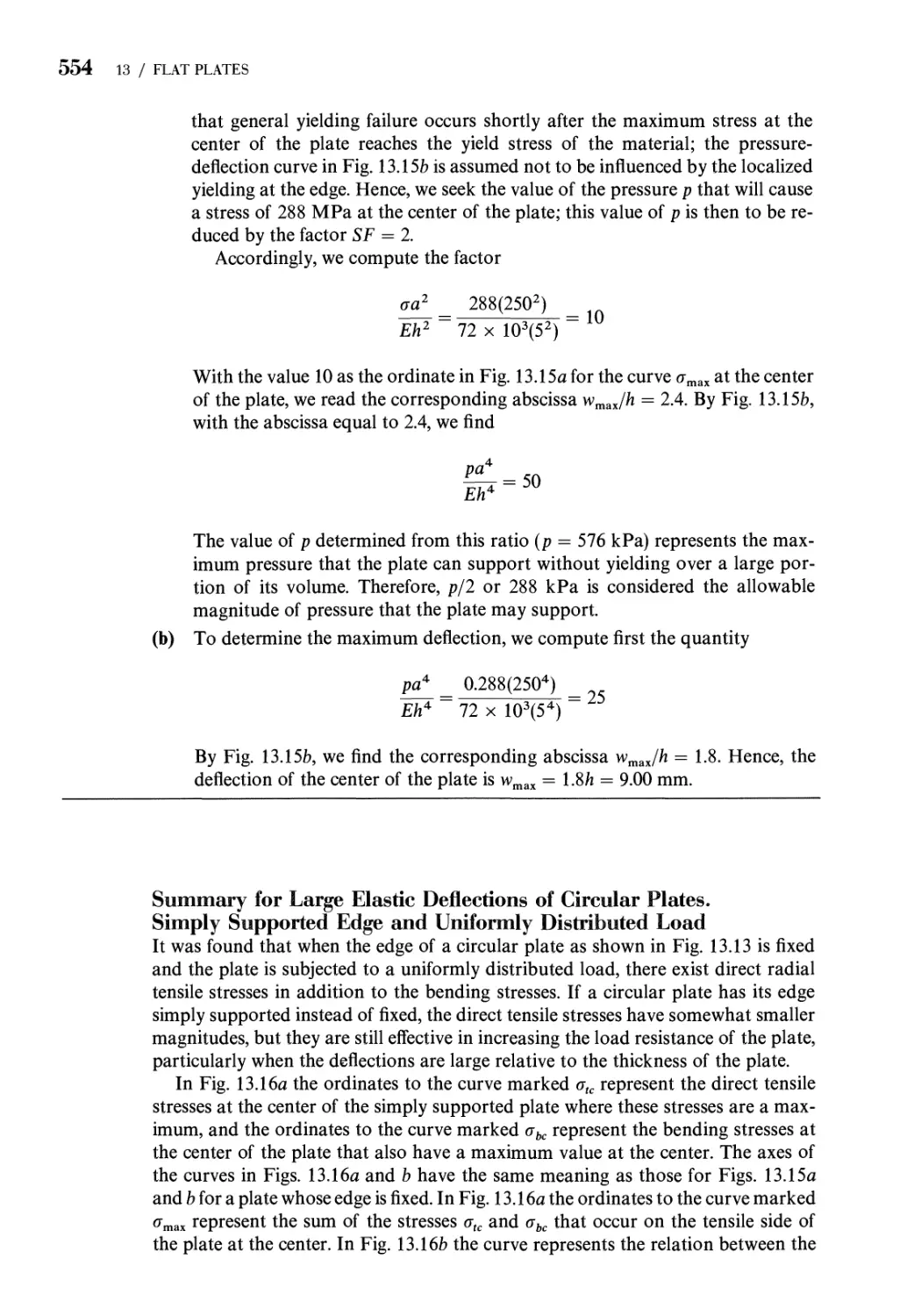
Problems 555
References 559
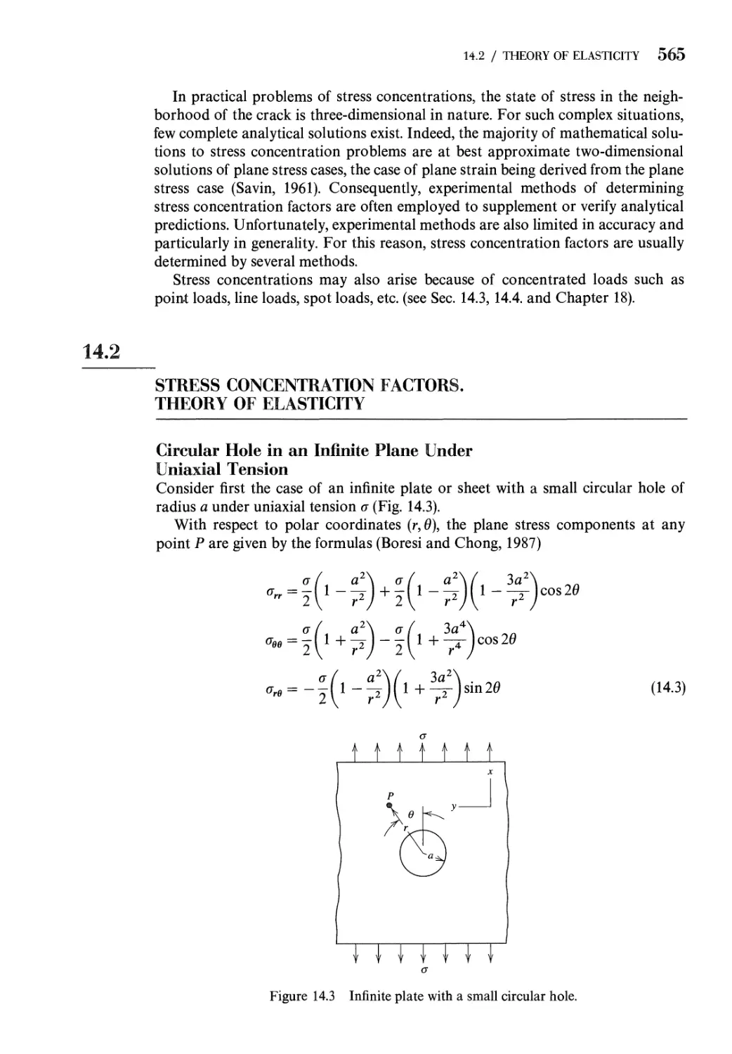
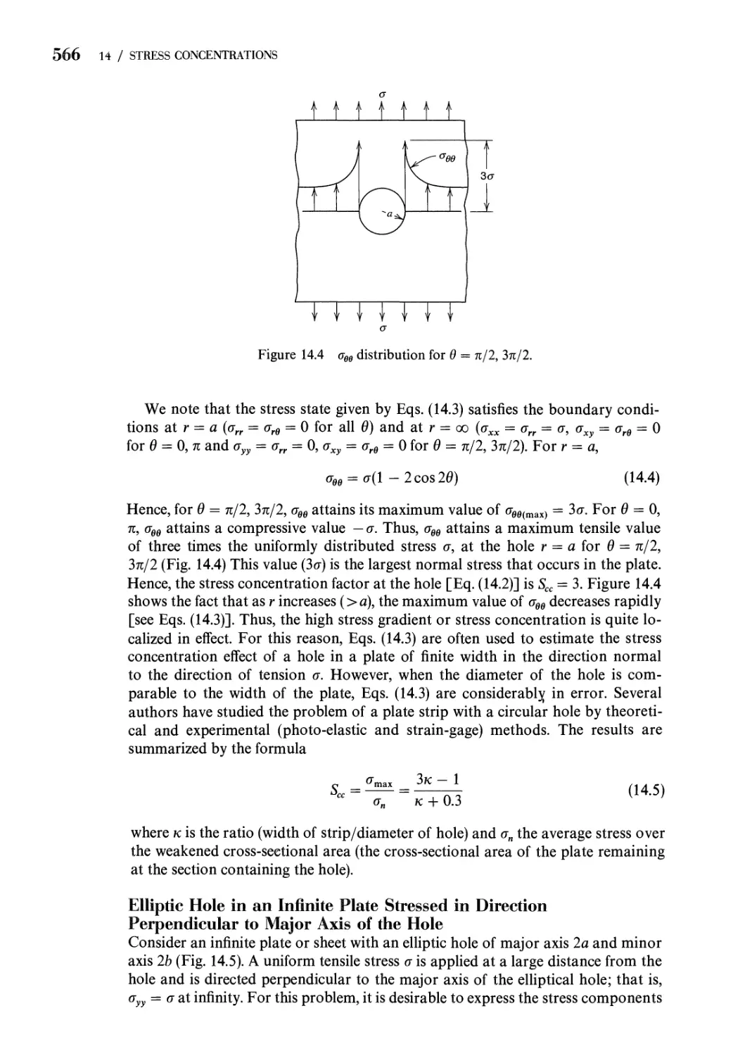
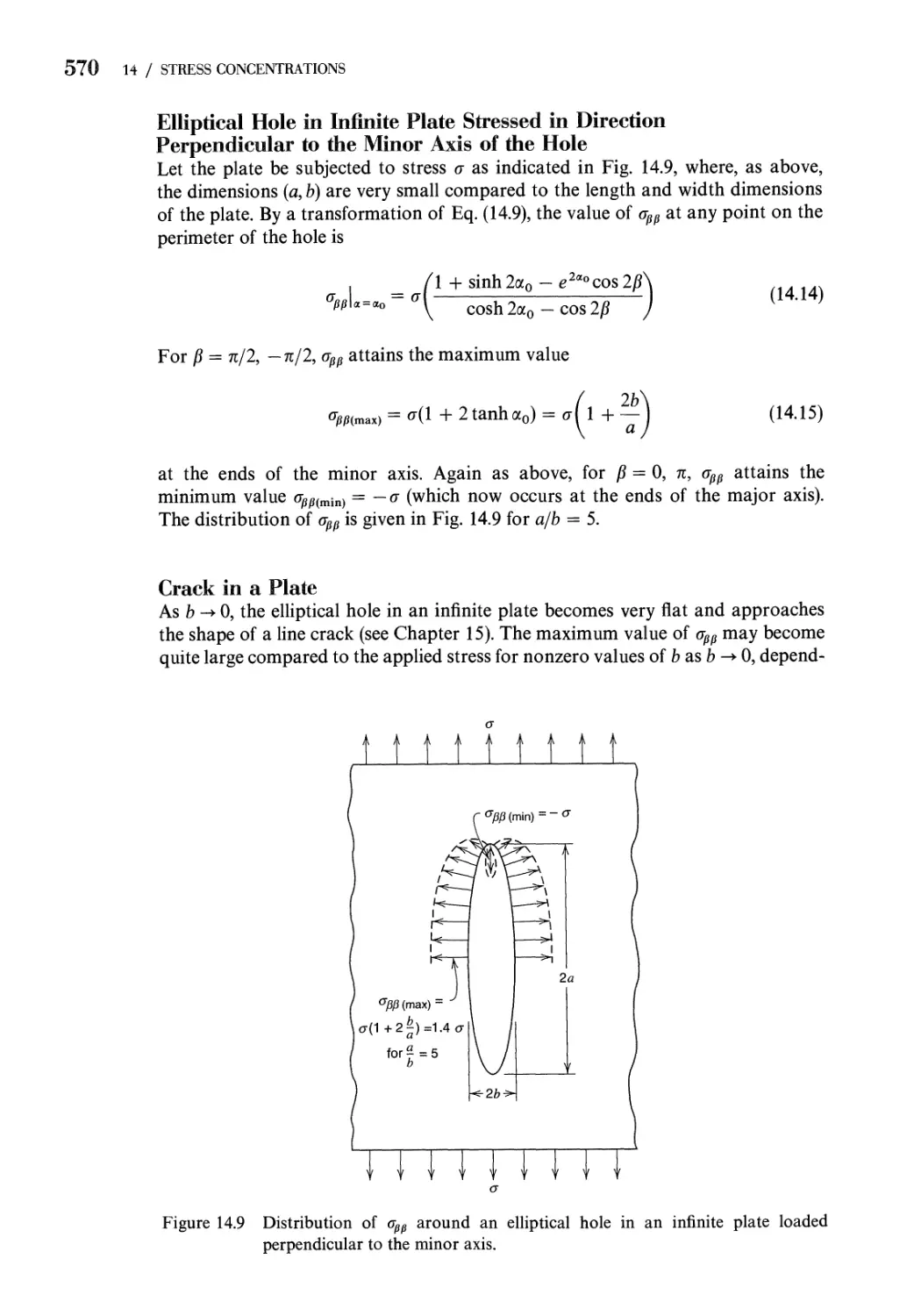
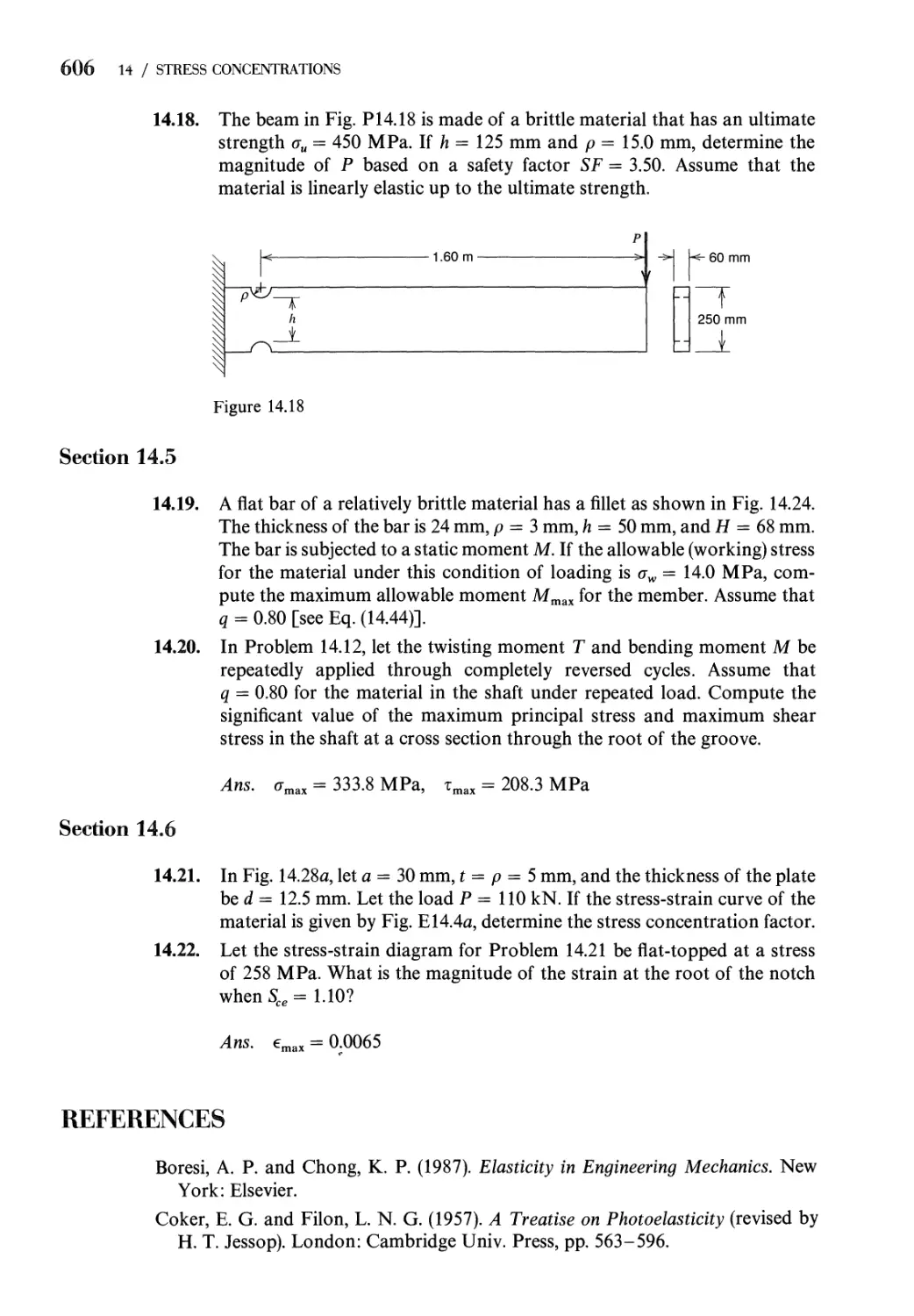
14 Stress Concentrations 560
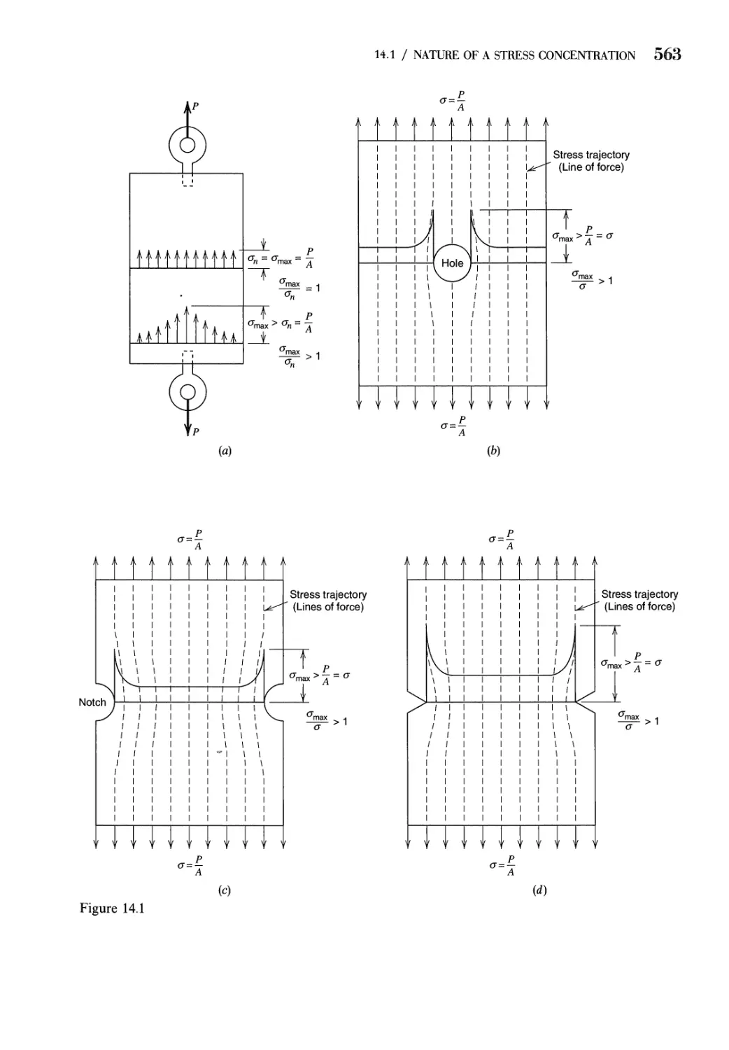
14.1 Nature of a Stress Concentration Problem. Stress
Concentration Factor 562
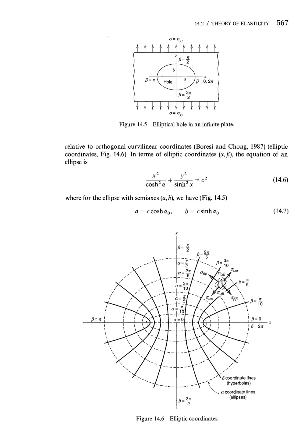
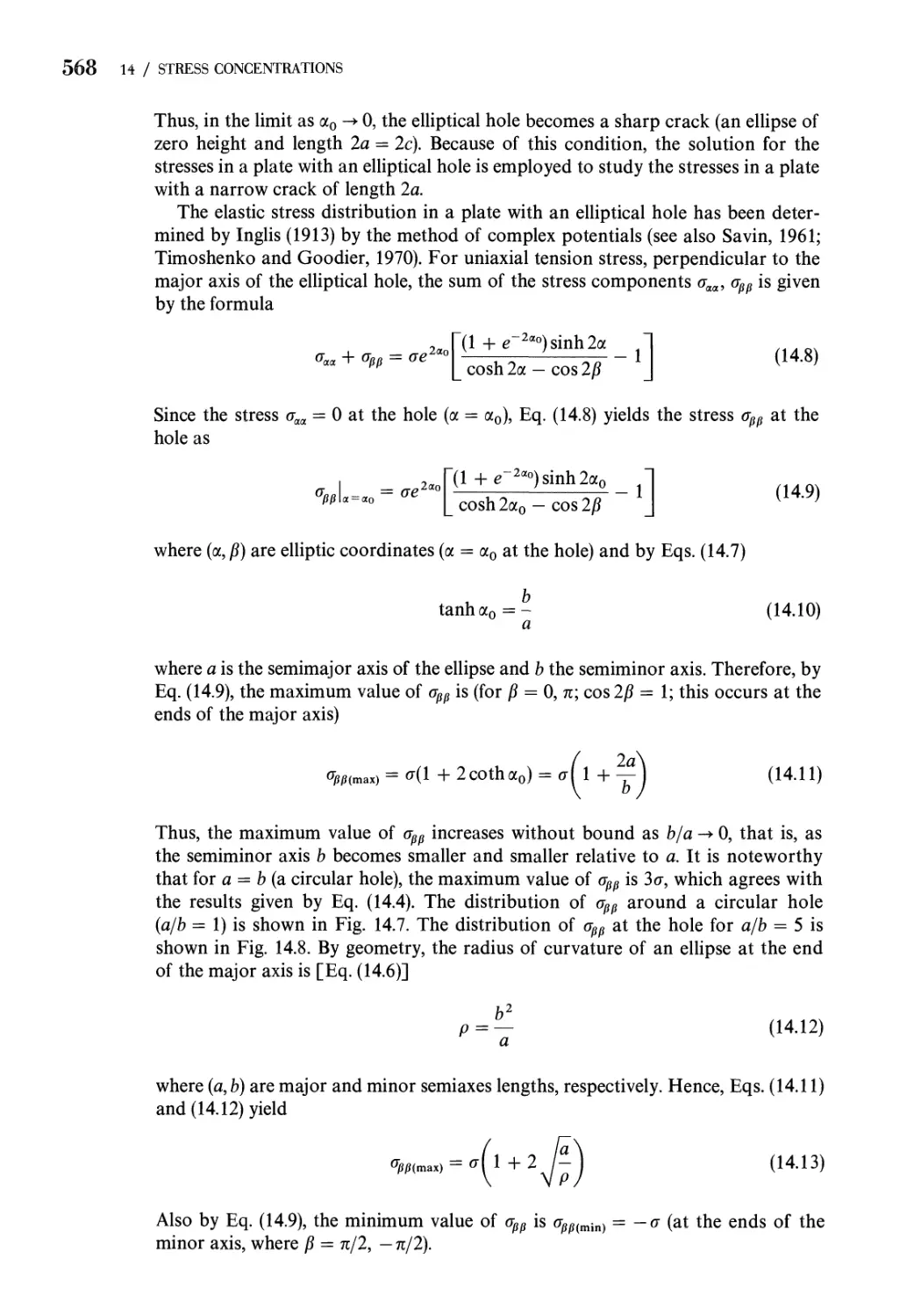
14.2 Stress Concentration Factors. Theory of Elasticity 565
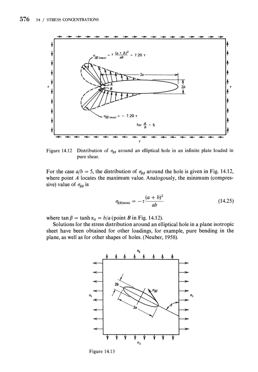
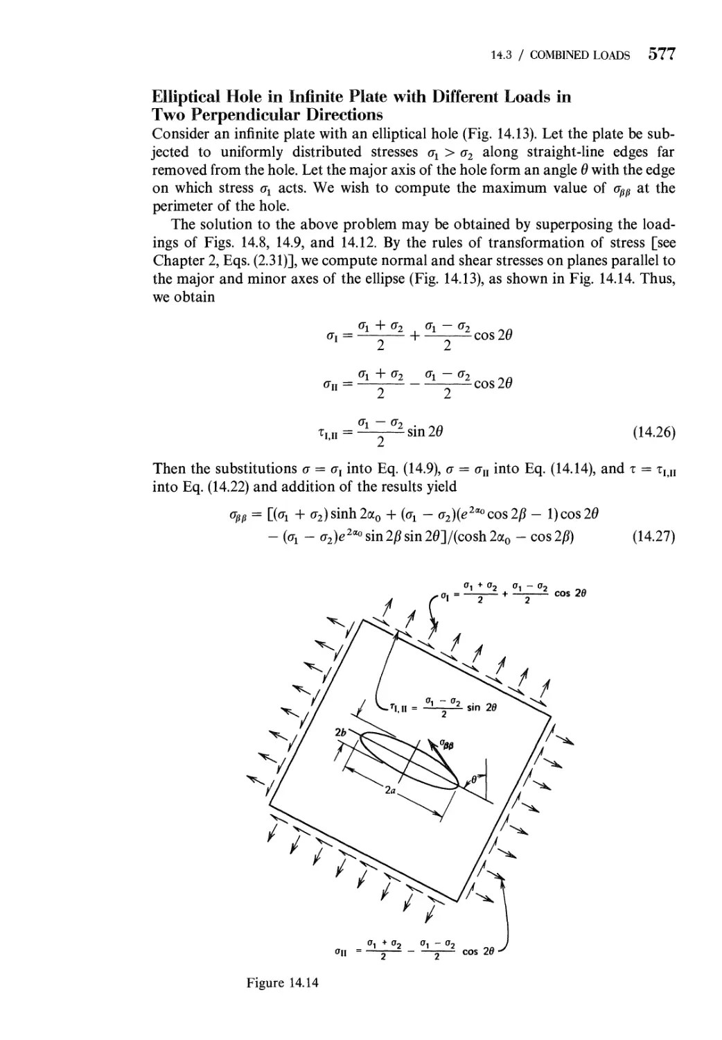
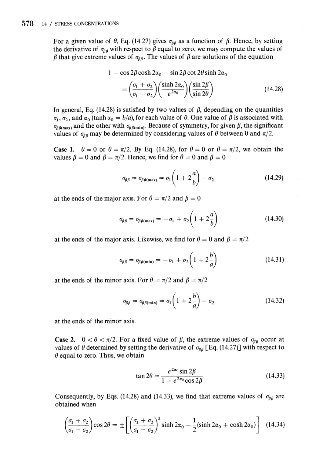
14.3 Stress Concentration Factors. Combined Loads 574
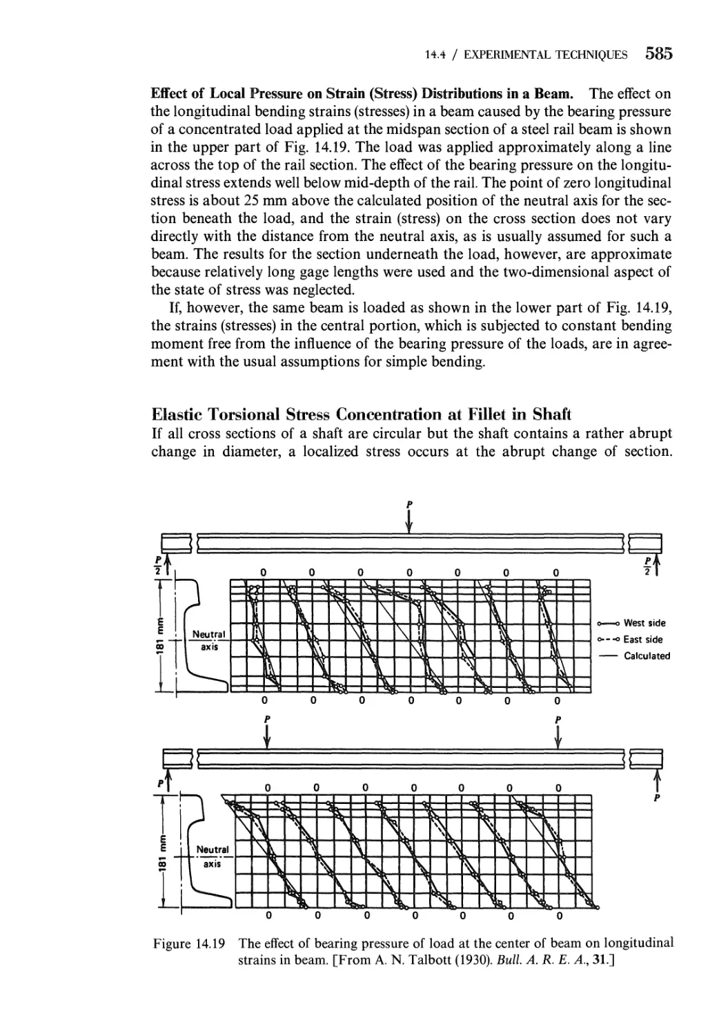
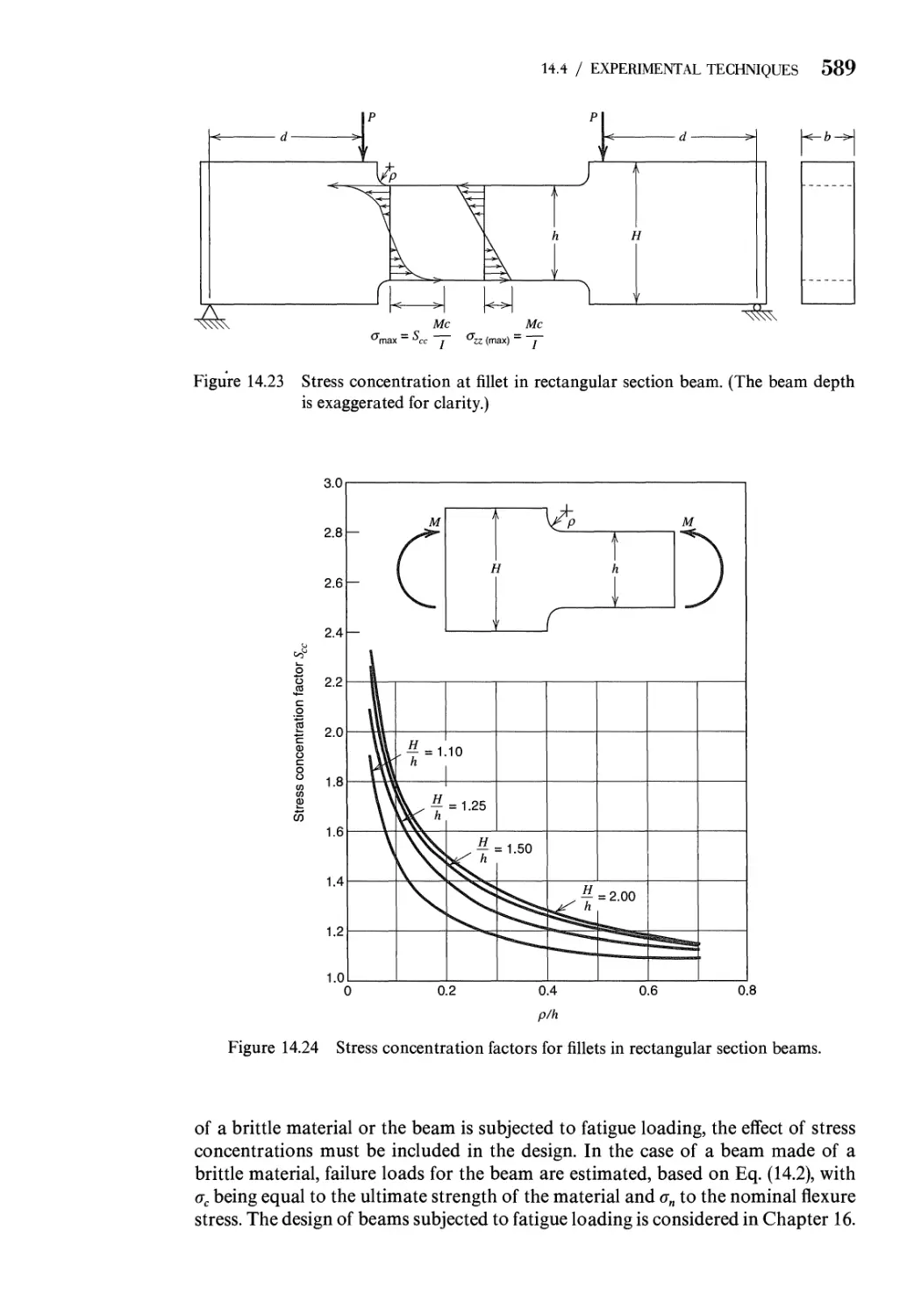
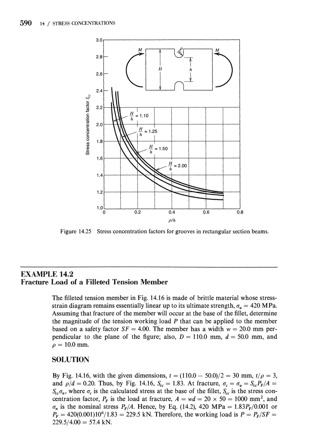
14.4 Stress Concentration Factors. Experimental Techniques 581
14.5 Effective Stress Concentration Factors 591
14.6 Effective Stress Concentration Factors. Inelastic Strains 598
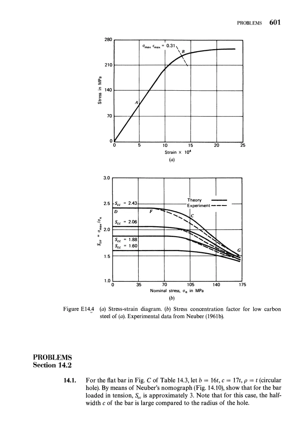
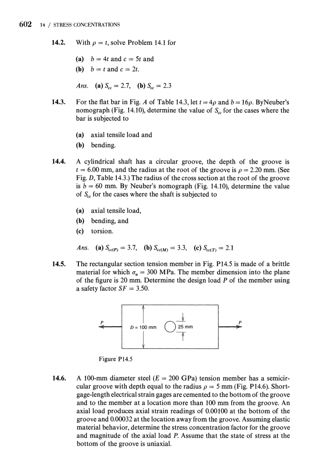
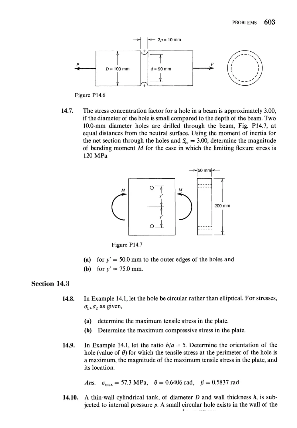
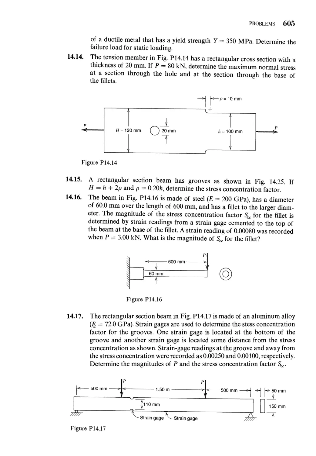
Problems 601
References 606
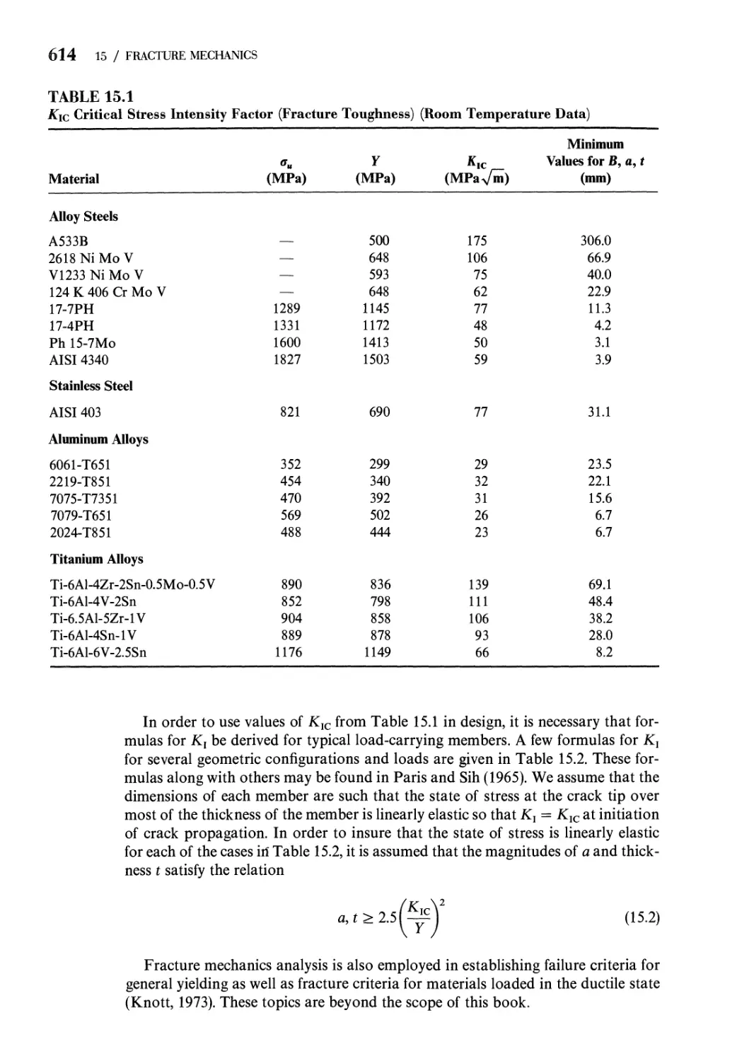
15 Fracture Mechanics 608
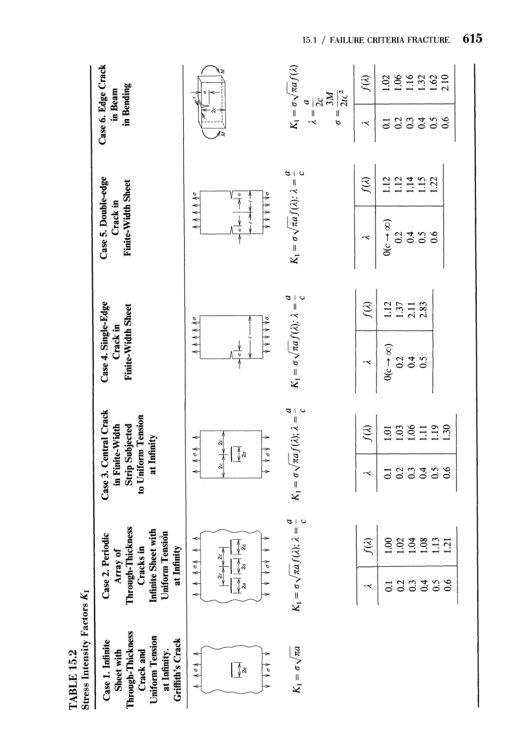
621
15.1
15.2
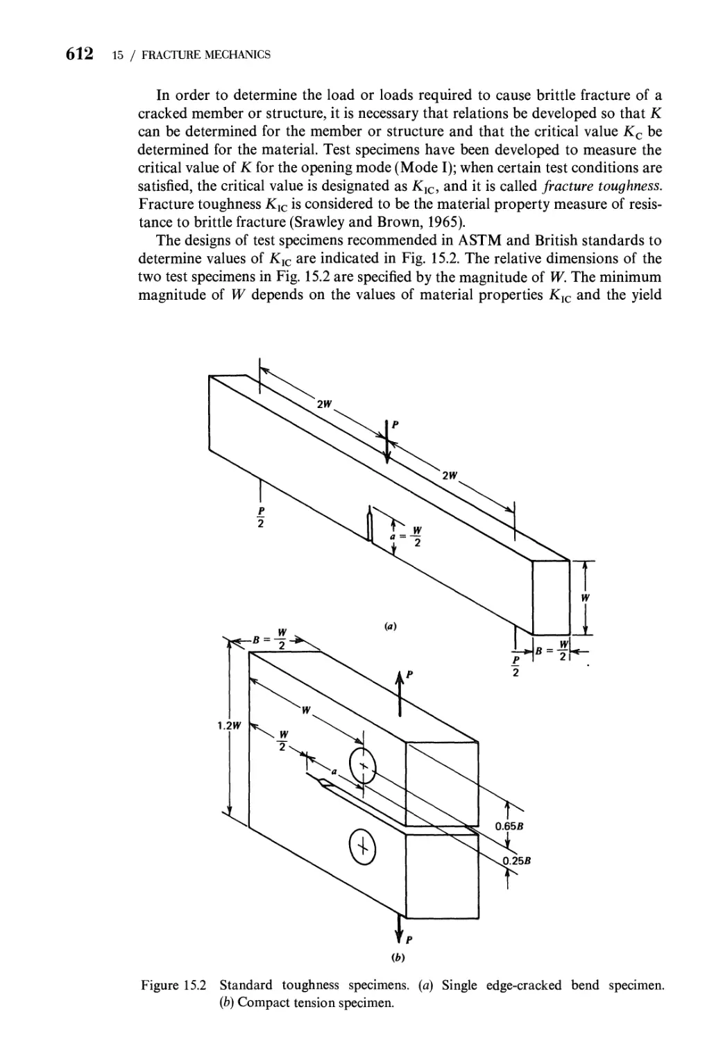
15.3
15.4
Prob
Refer
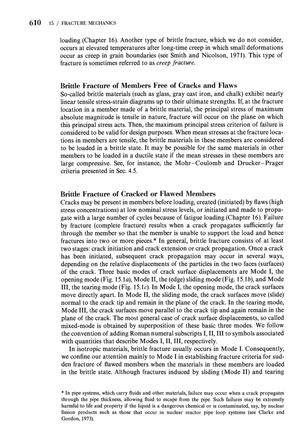
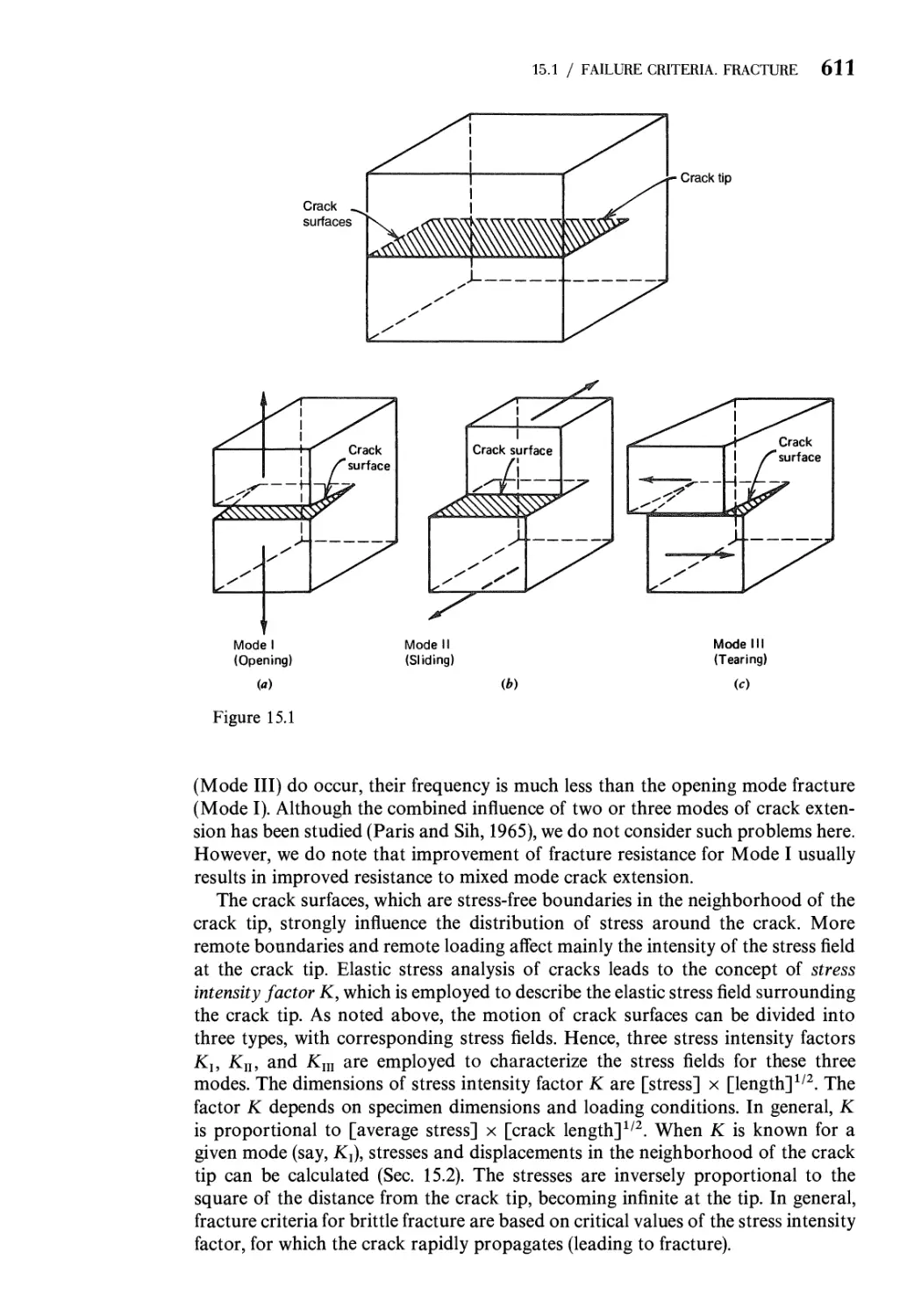
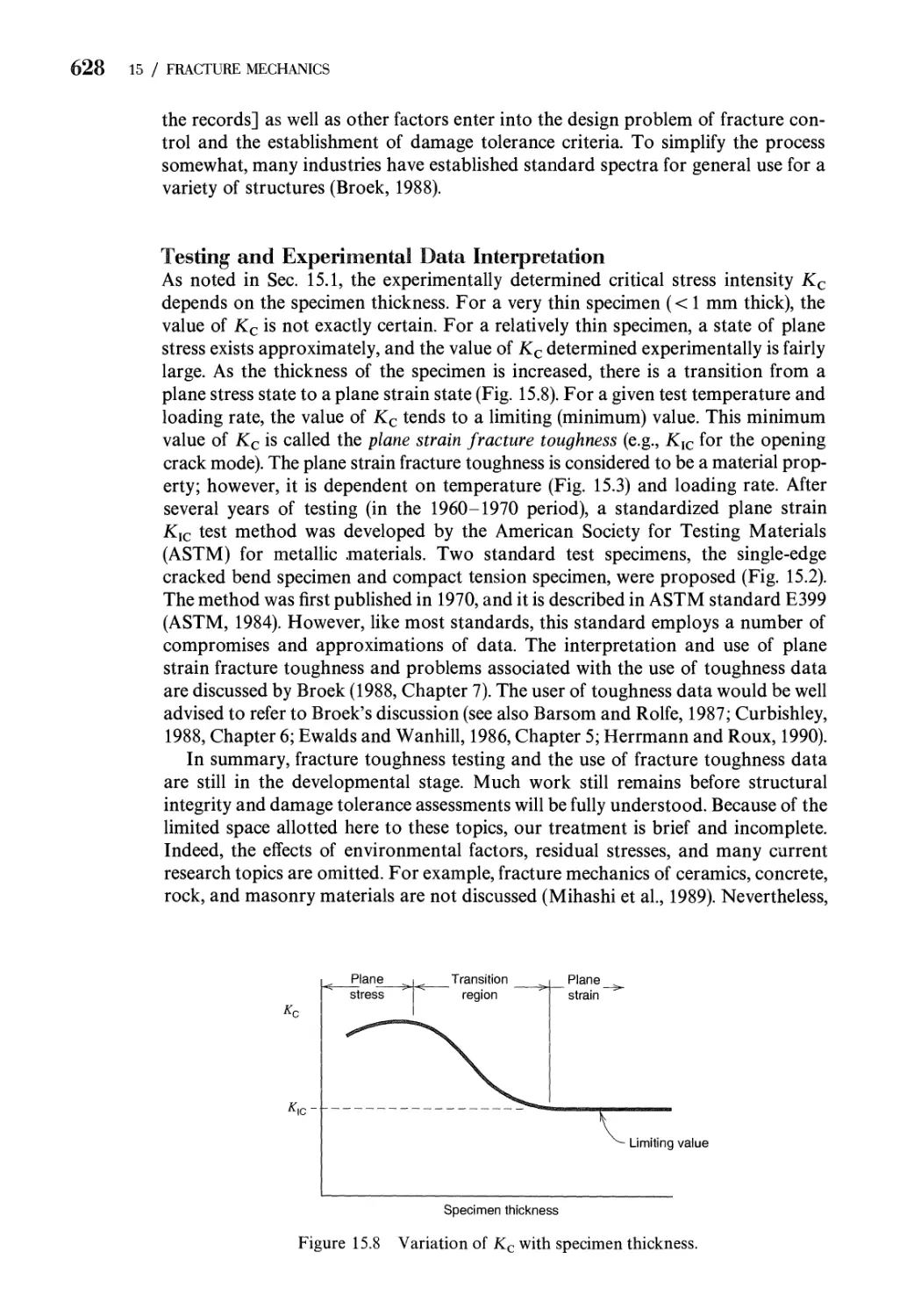
Failure Criteria. Fracture 608
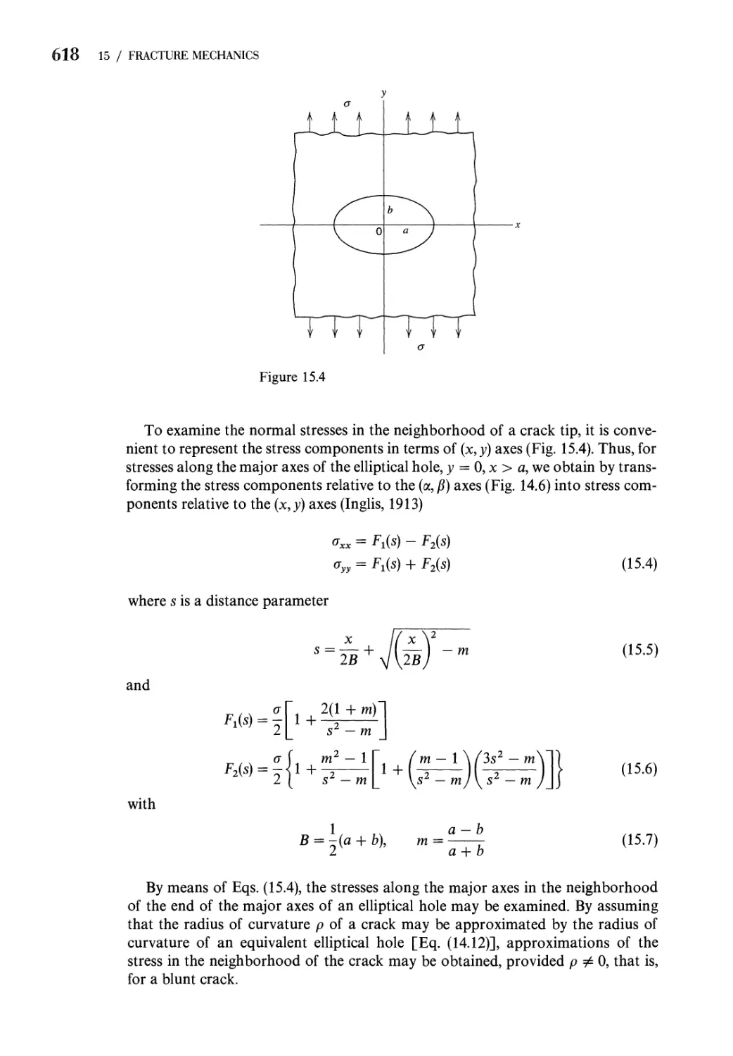
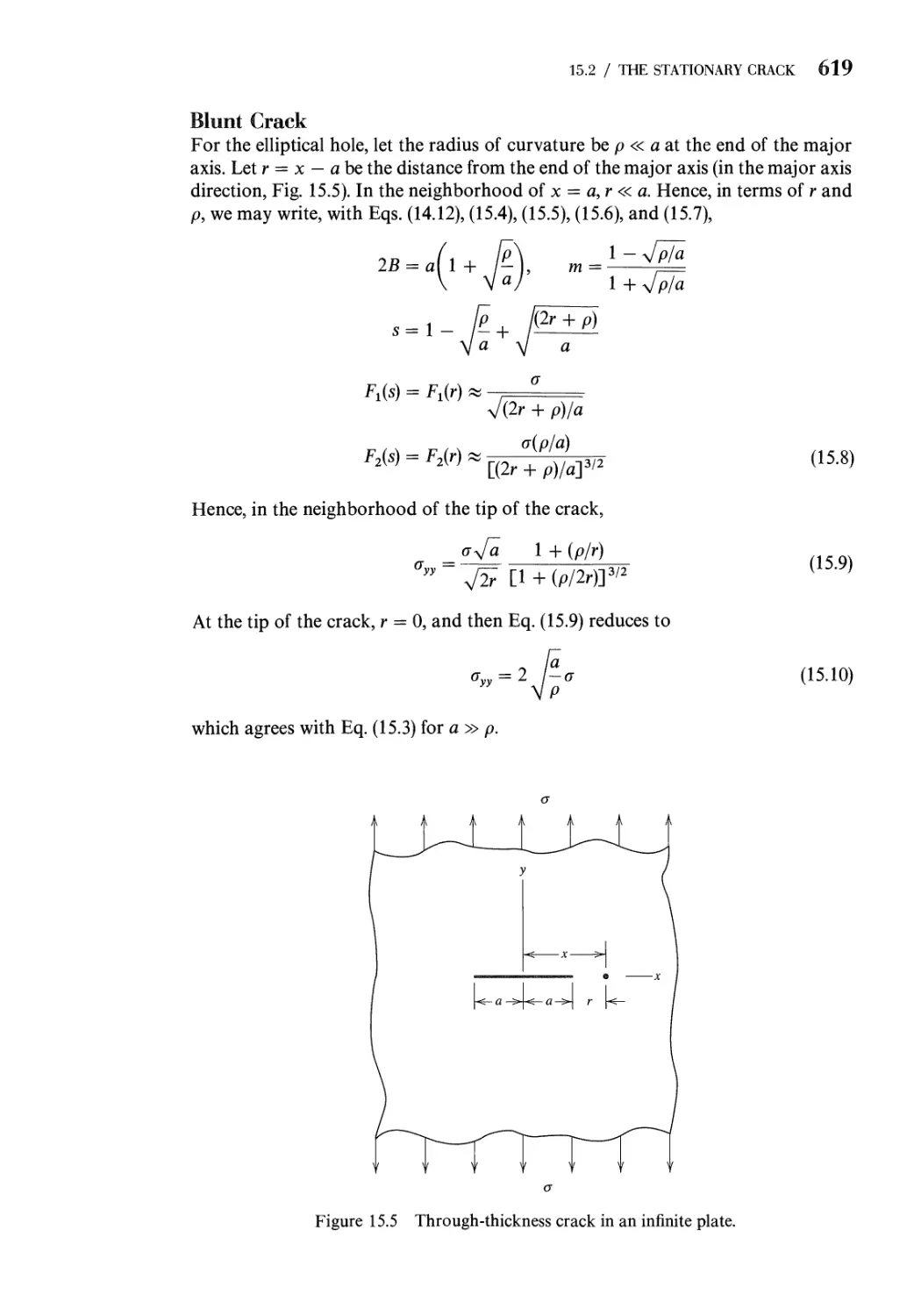
The Stationary Crack 617
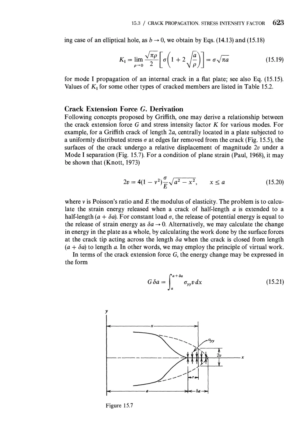
Crack Propagation. Stress Intensity Factor
Fracture: Other Factors 626
lems 629
ences 631
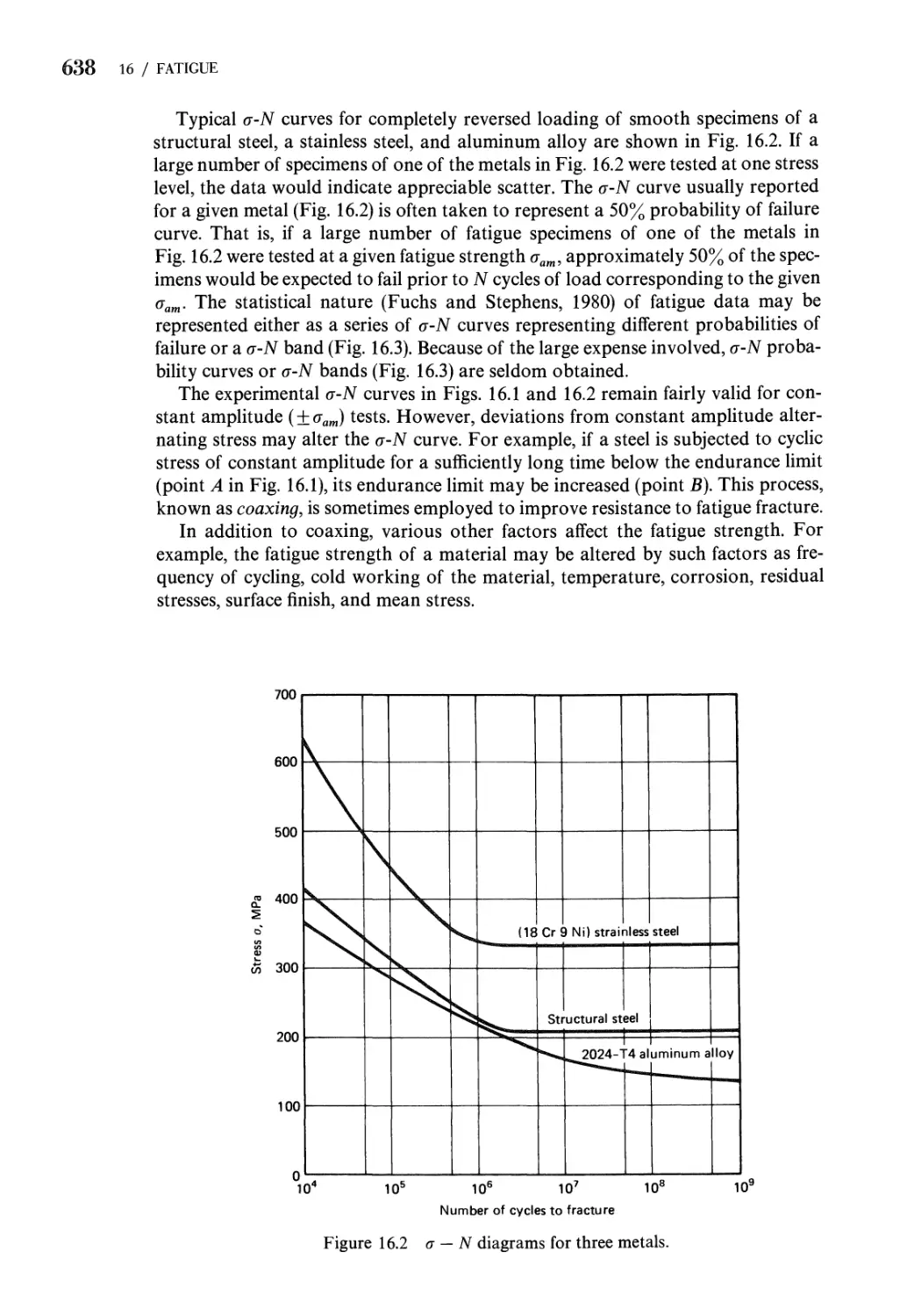
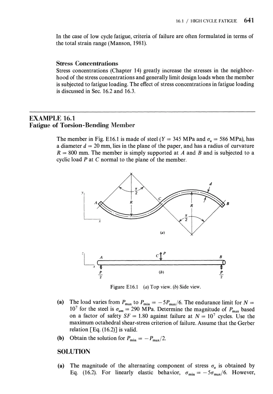
16 Fatigue: Progressive Fracture 634
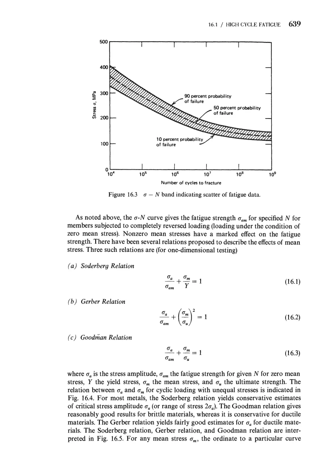
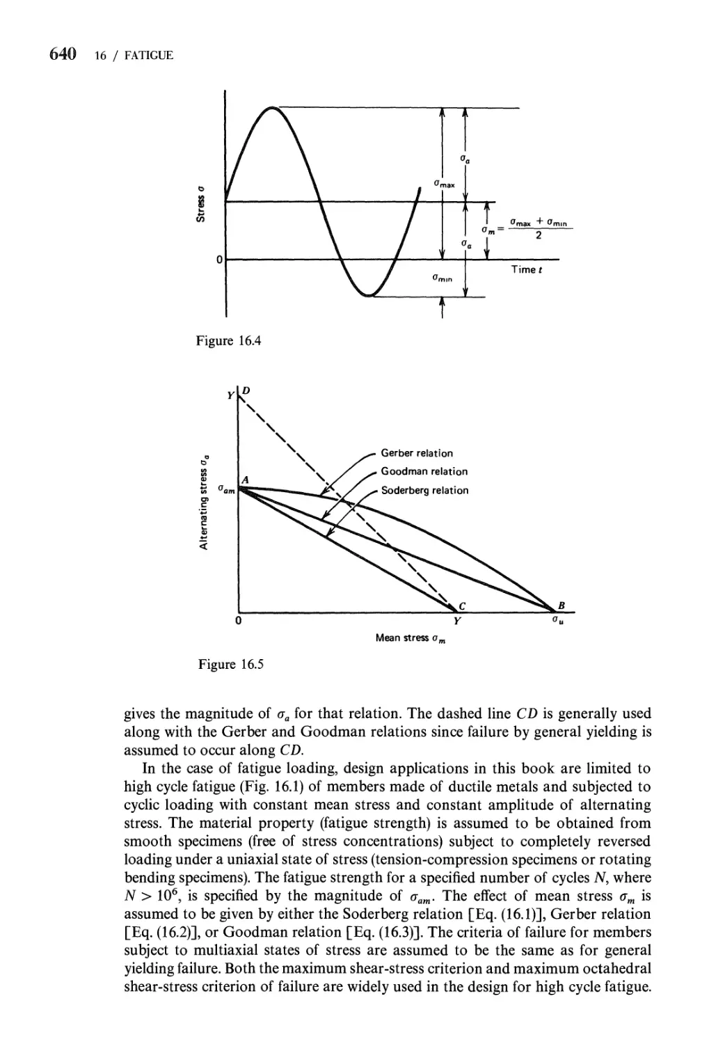
16.1 Progressive Fracture (High Cycle Fatigue for Number of
Cycles N > 106) 635
XVI CONTENTS
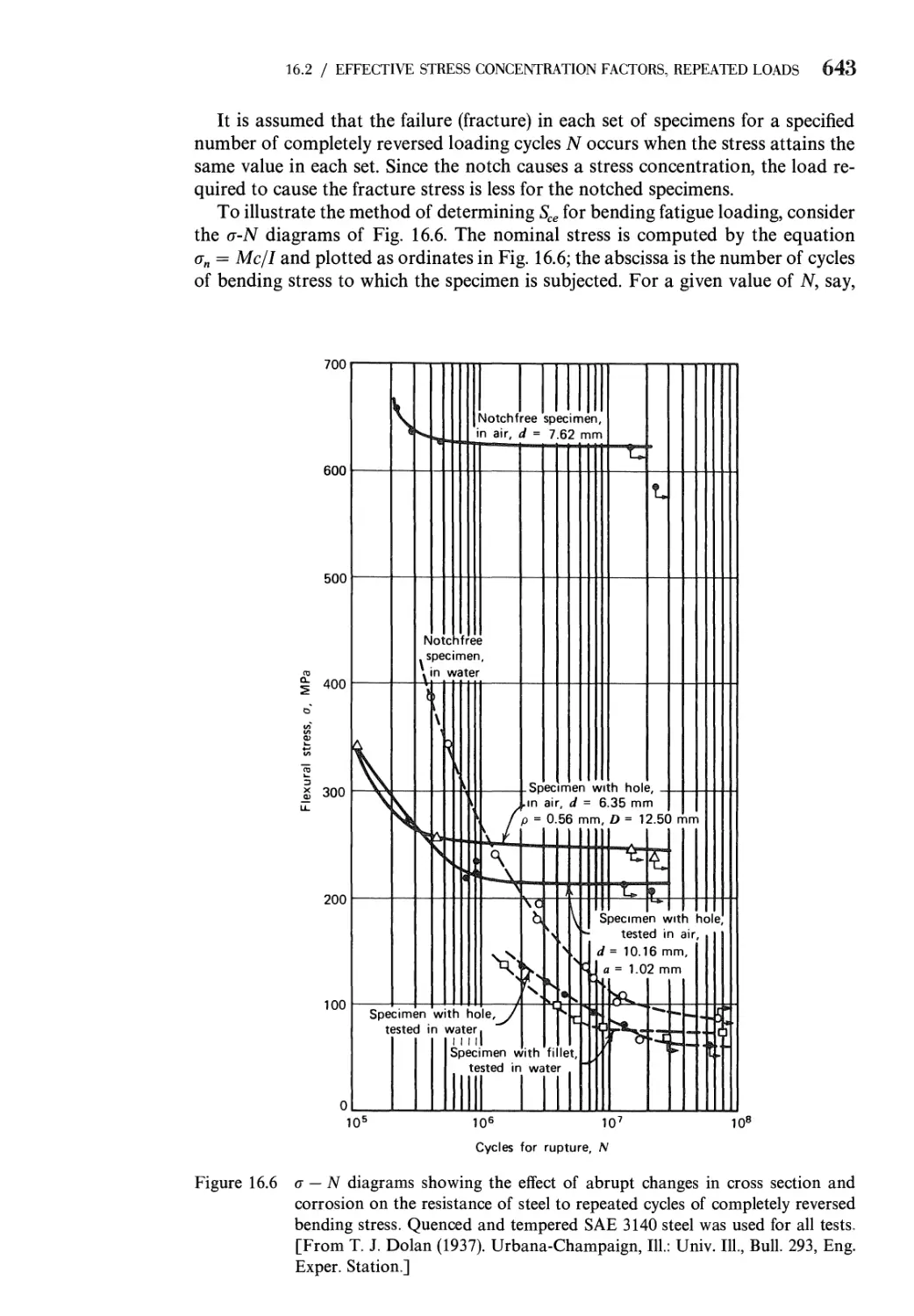
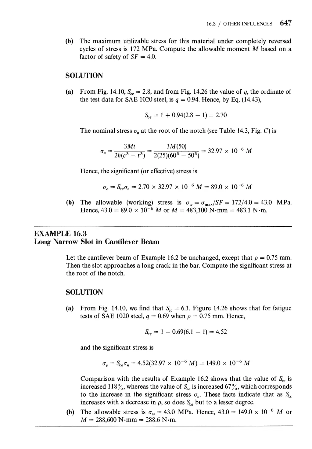
16.2 Effective Stress Concentration Factors: Repeated Loads 642
16.3 Effective Stress Concentration Factors: Other Influences 644
Problems 649
References 653
17 Creep. Time-Dependent Deformation 655
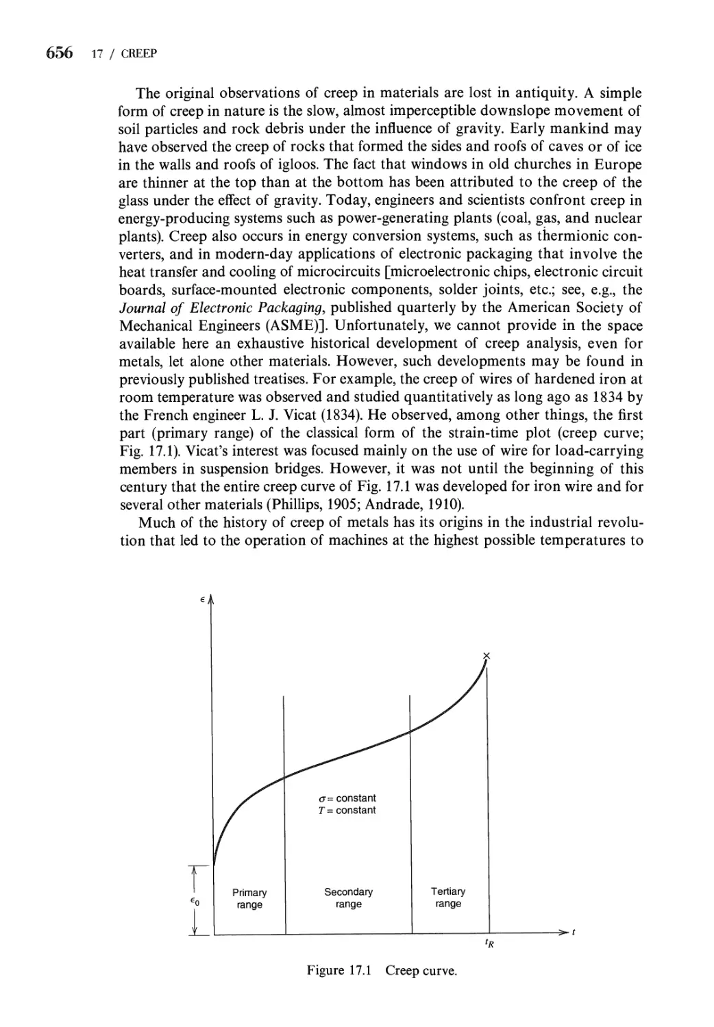
17.1 Definition of Creep. The Creep Curve 655
17.2 The Tension Creep Test for Metals 657
17.3 One-Dimensional Creep Formulas for Metals Subjected to
Constant Stress and Elevated Temperature 658
17.4 One-Dimensional Creep of Metals Subjected to Variable Stress
and Temperature 663
17.5 Creep Under Multiaxial States of Stress 673
17.6 Flow Rule for Creep of Metals Subjected to Multiaxial
States of Stress 677
17.7 A Simple Application of Creep of Metals 682
17.8 Creep of Nonmetals 683
References 688
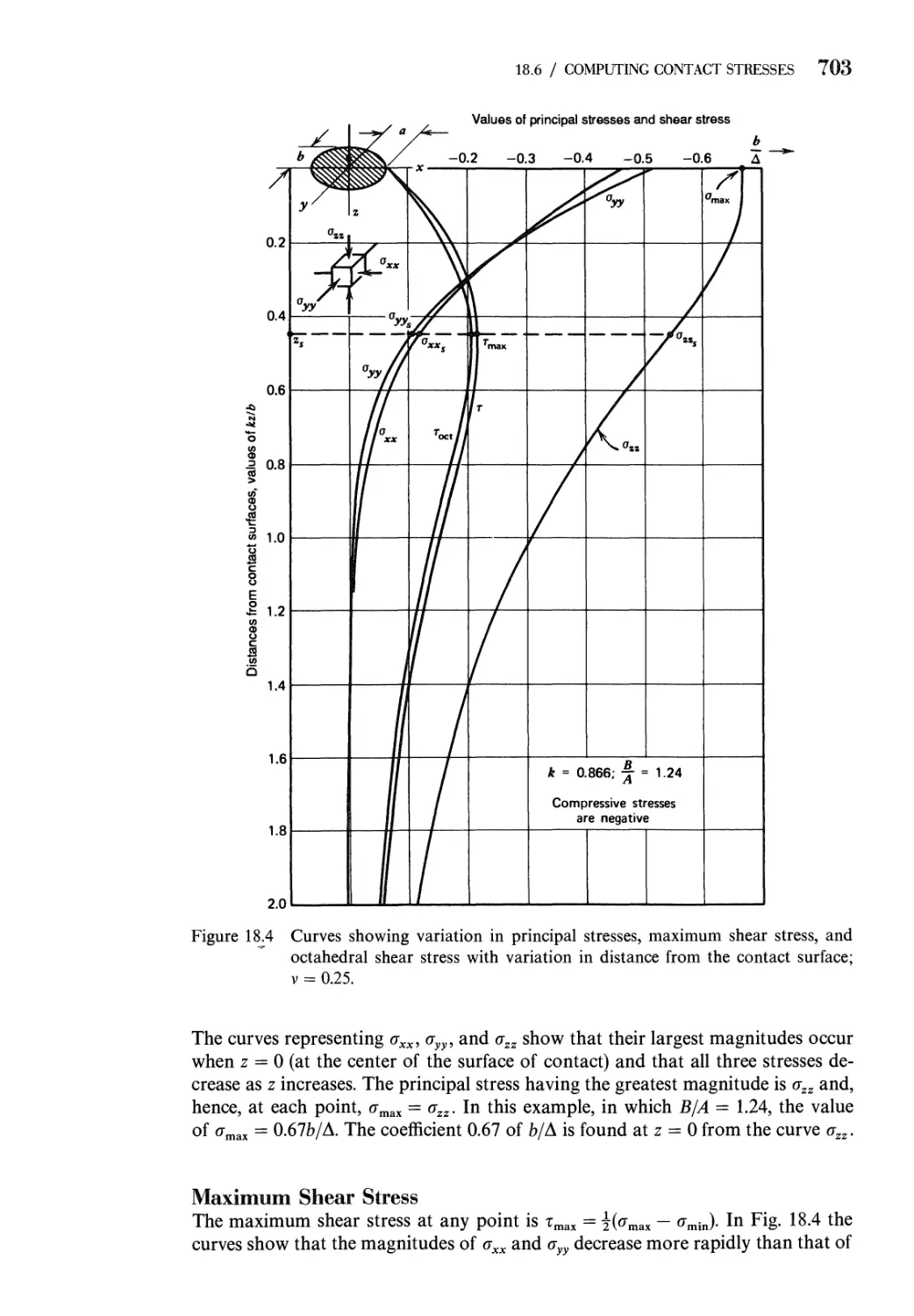
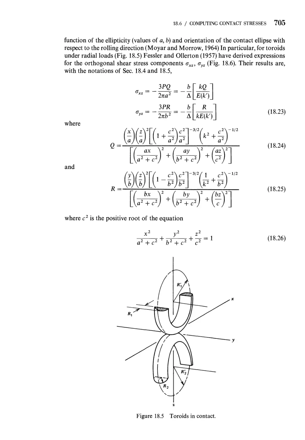
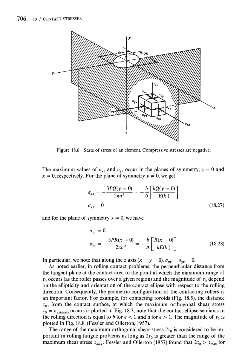
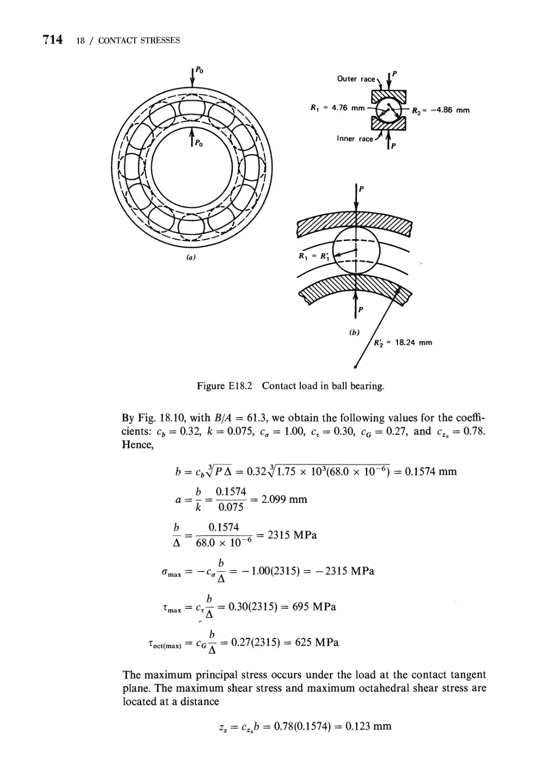
18 Contact Stresses 692
18.1 Introduction 692
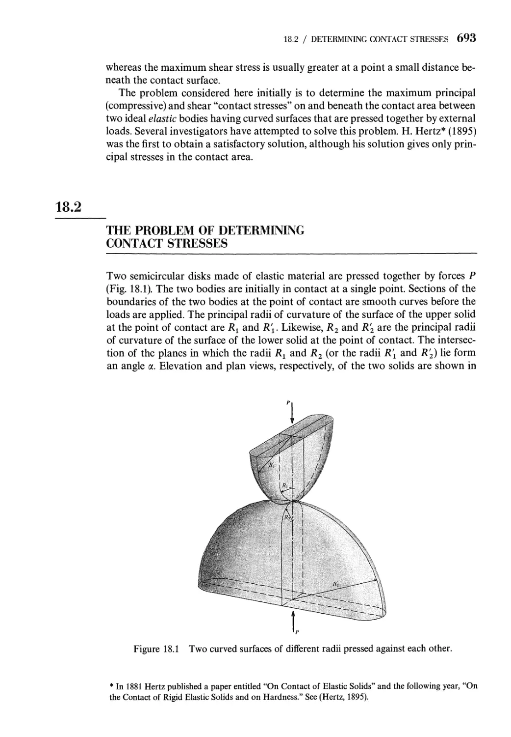
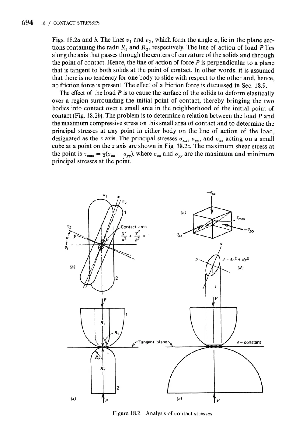
18.2 The Problem of Determining Contact Stresses 693
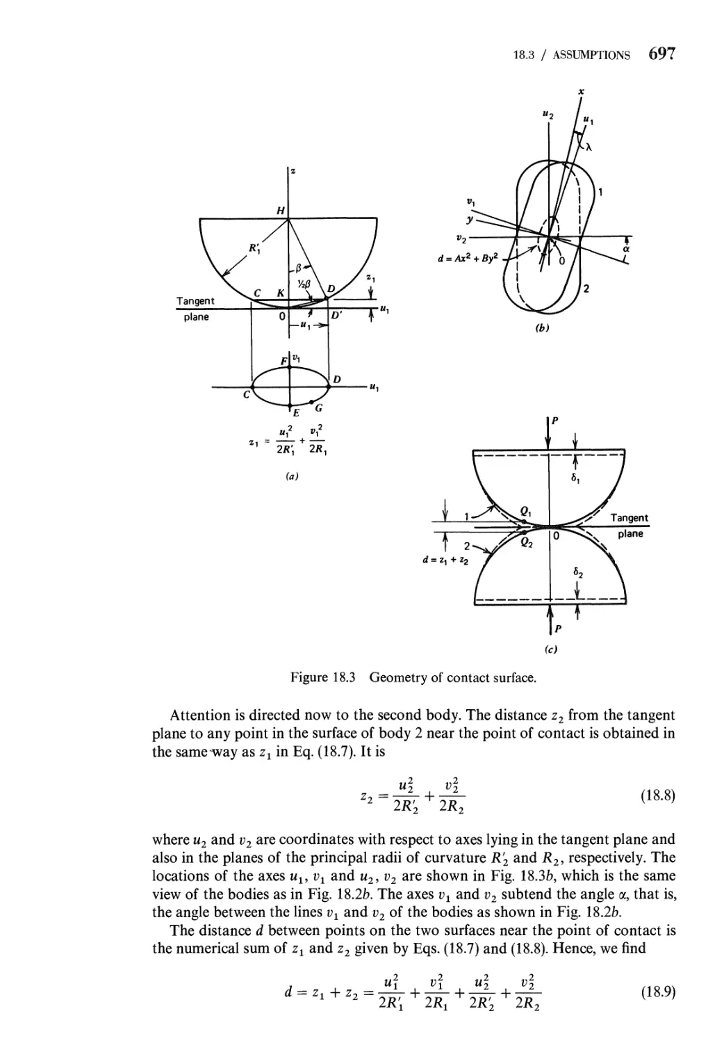
18.3 Geometry of the Contact Surface 695
18.4 Notation and Meaning of Terms 700
18.5 Expressions for Principal Stresses 701
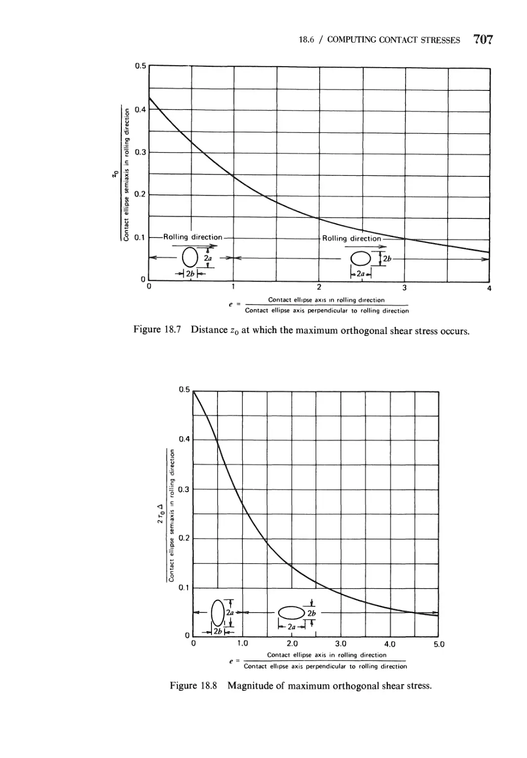
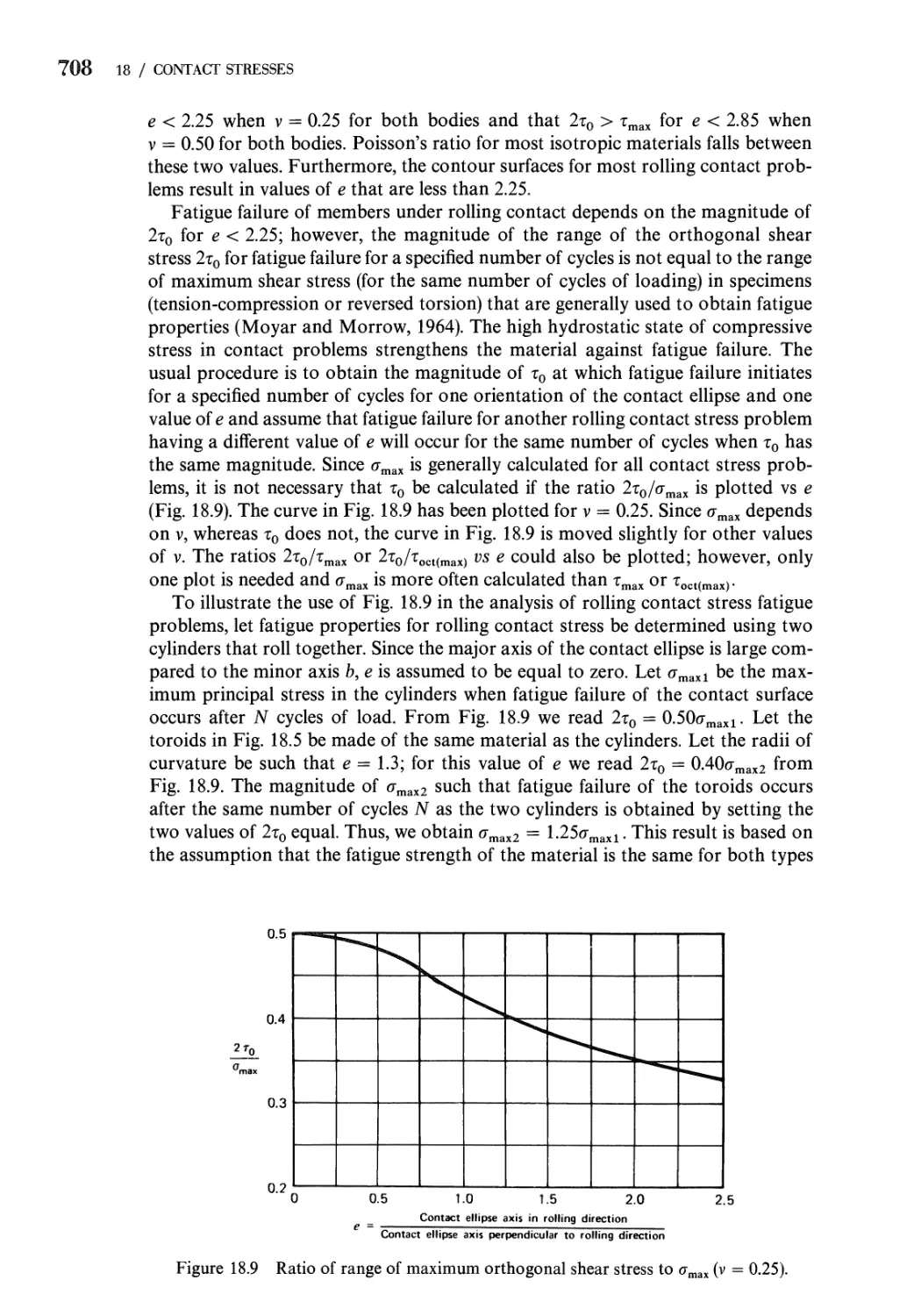
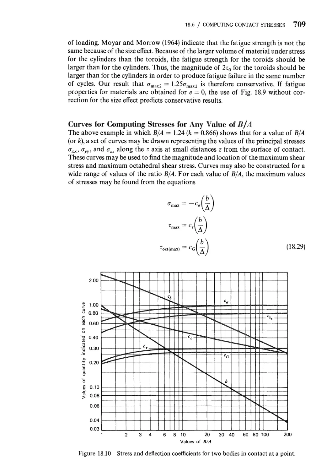
18.6 Method of Computing Contact Stresses 702
18.7 Deflection of Bodies in Point Contact 711
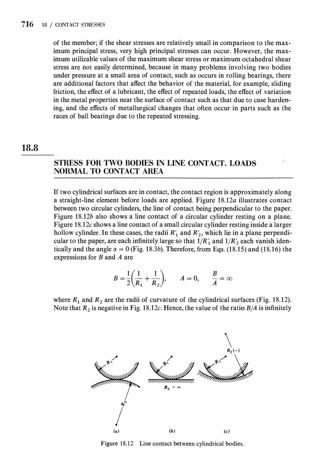
18.8 Stress for Two Bodies in Line Contact. Loads Normal to
Contact Area 716
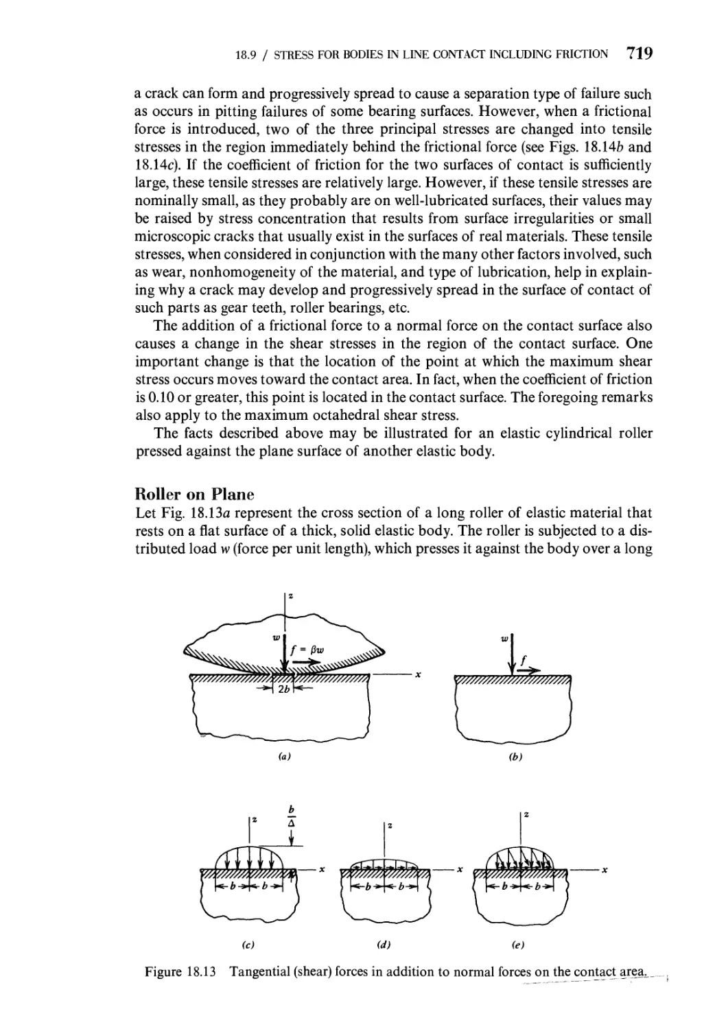
18.9 Stresses for Two Bodies in Line Contact. Loads Normal and
Tangent to Contact Area 718
Problems 727
References 731
19 The Finite Element Method 732
19.1 Introduction 732
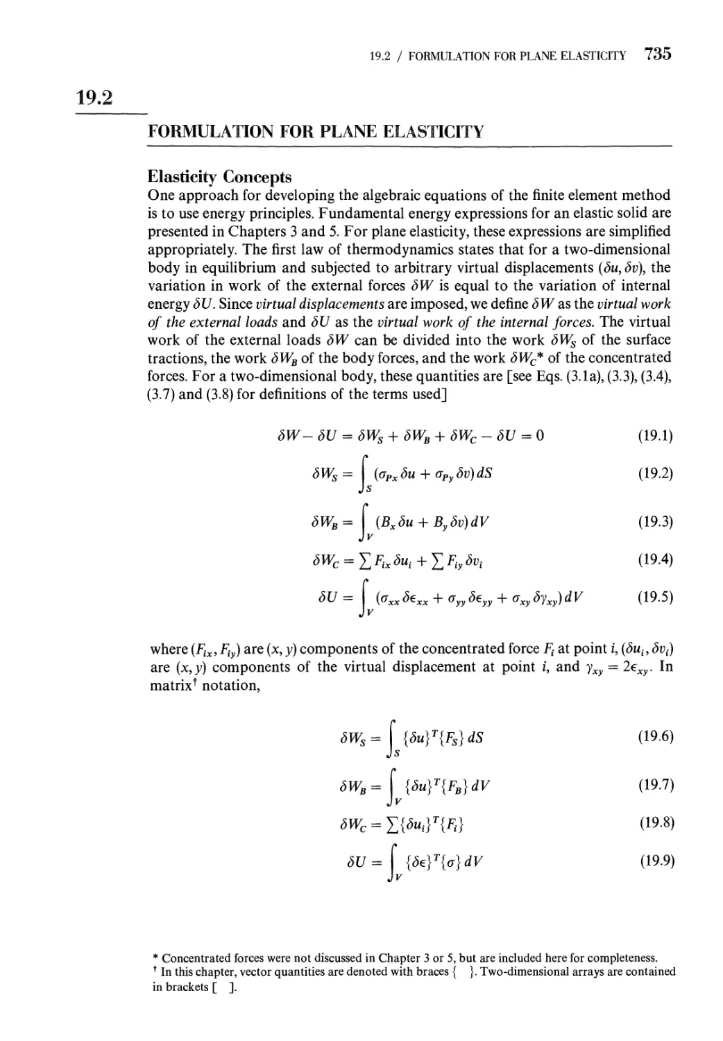
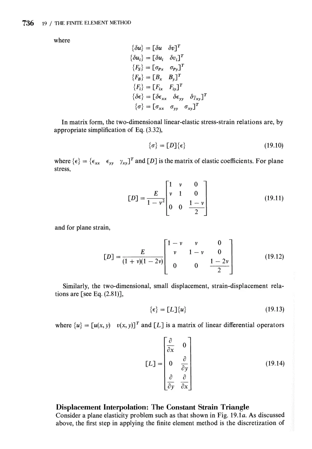
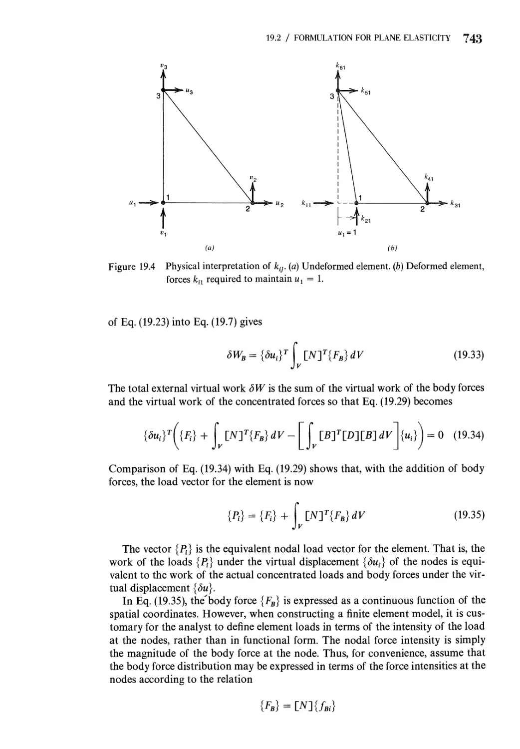
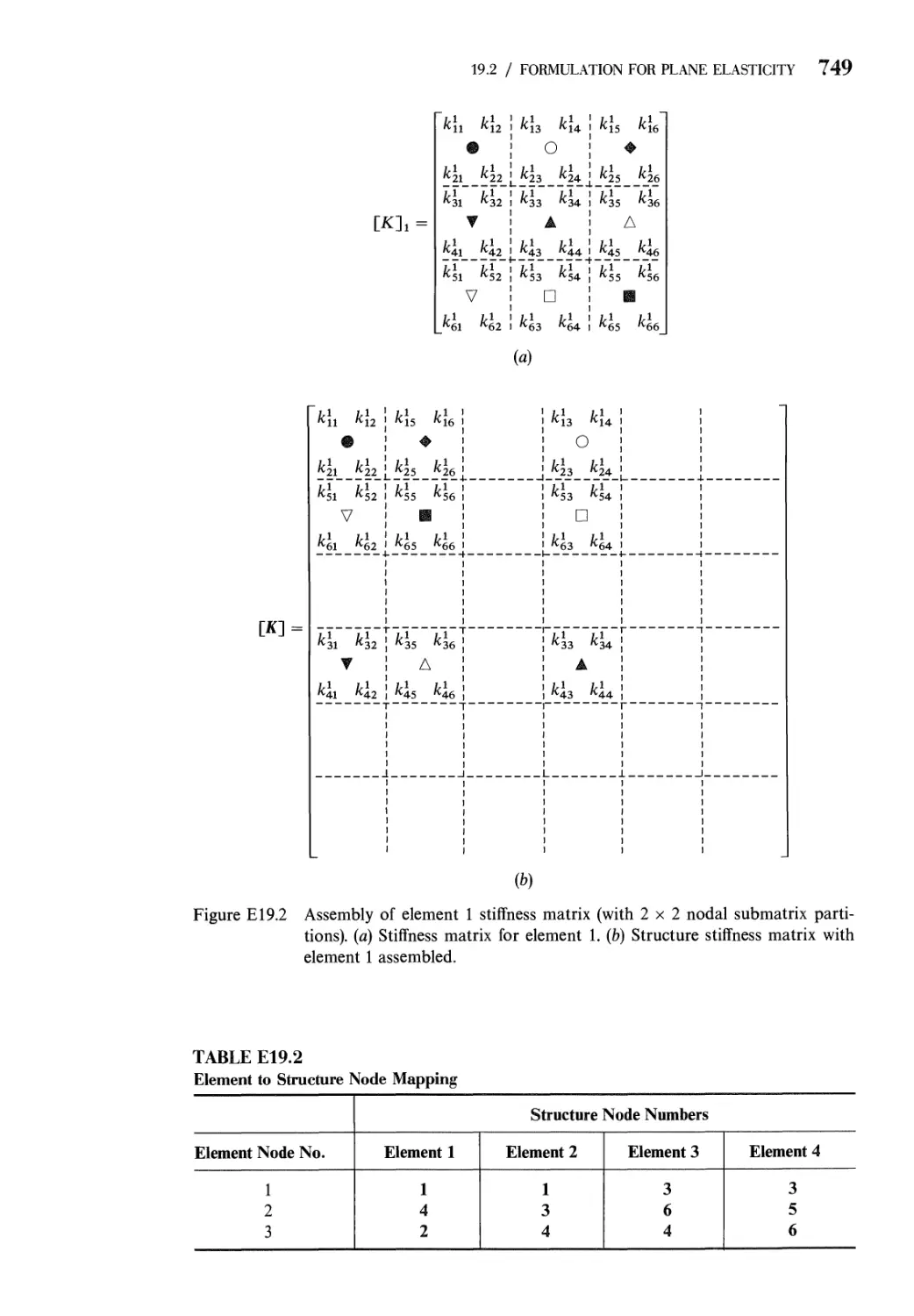
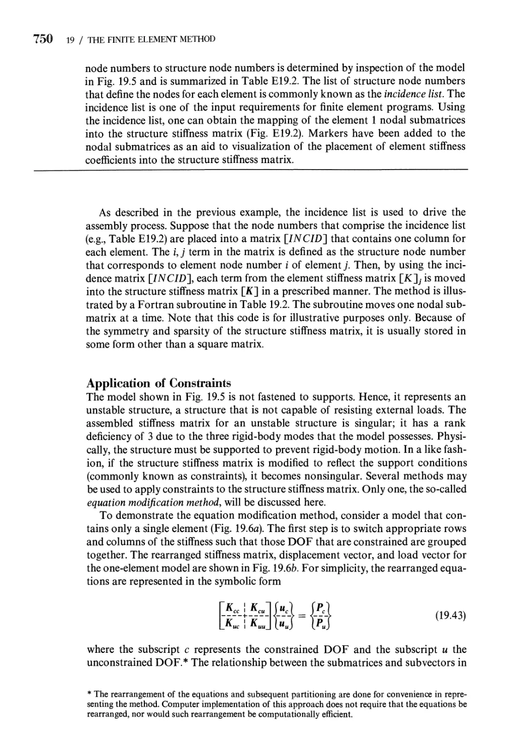
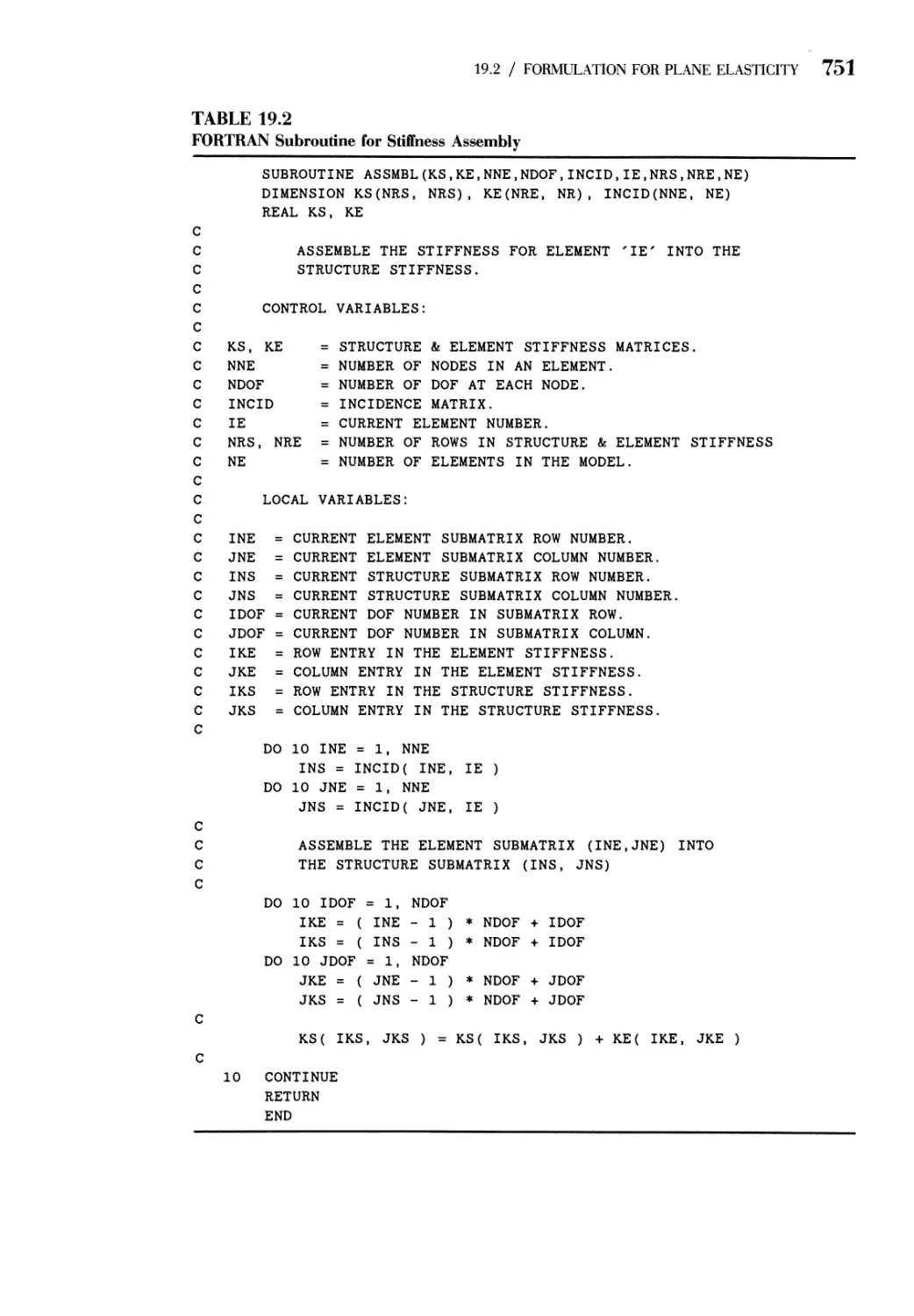
19.2 Formulation for Plane Elasticity 735
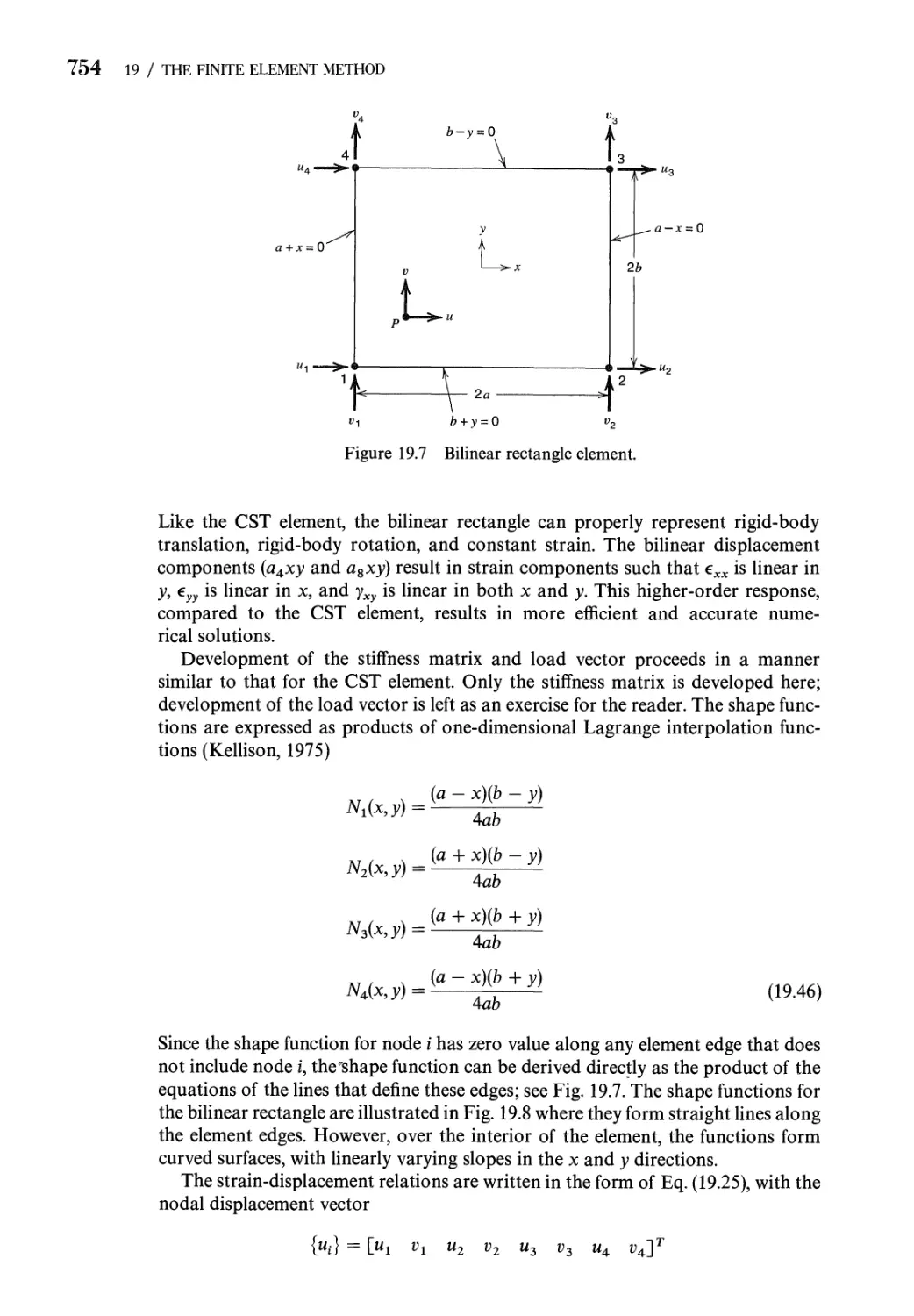
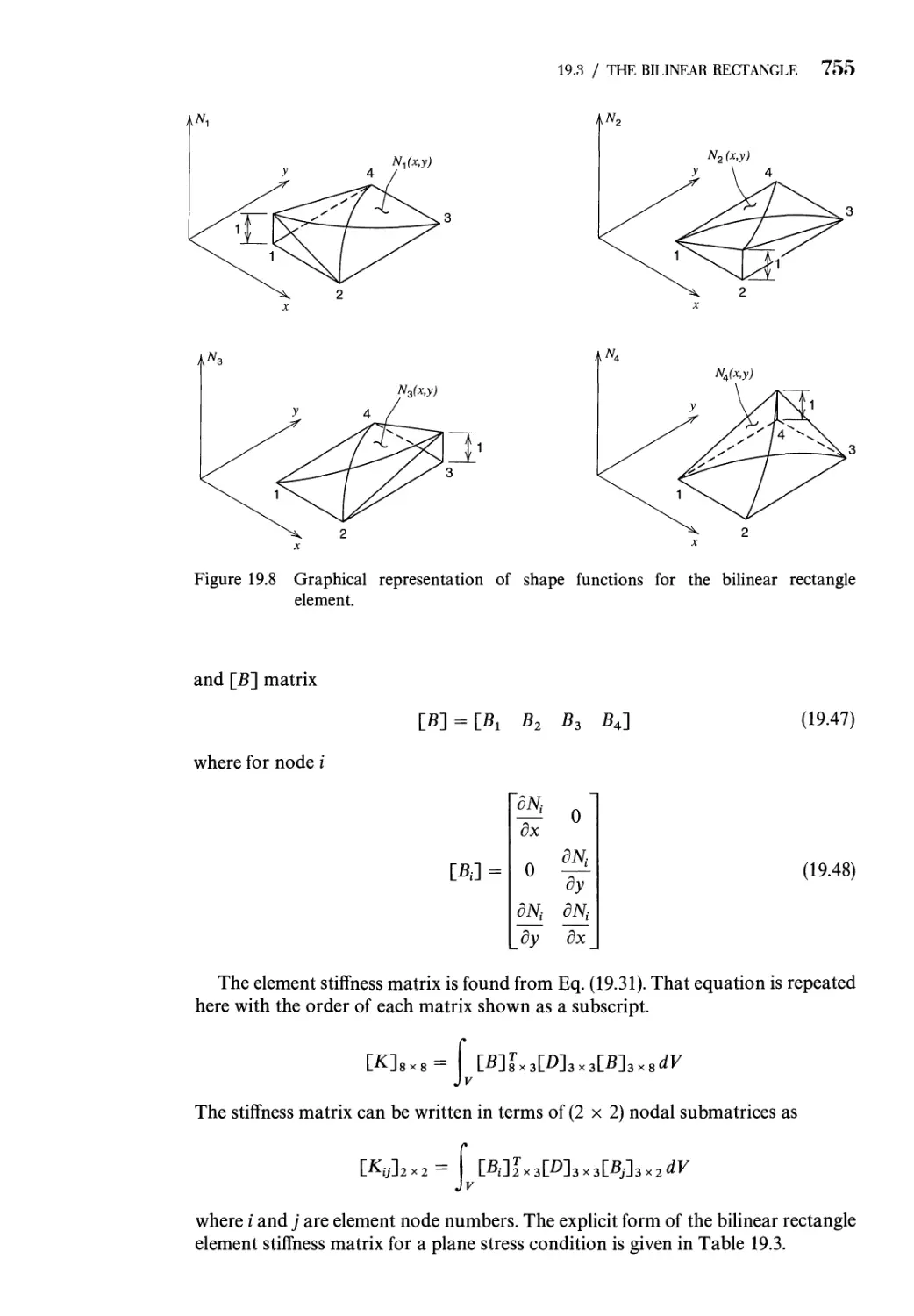
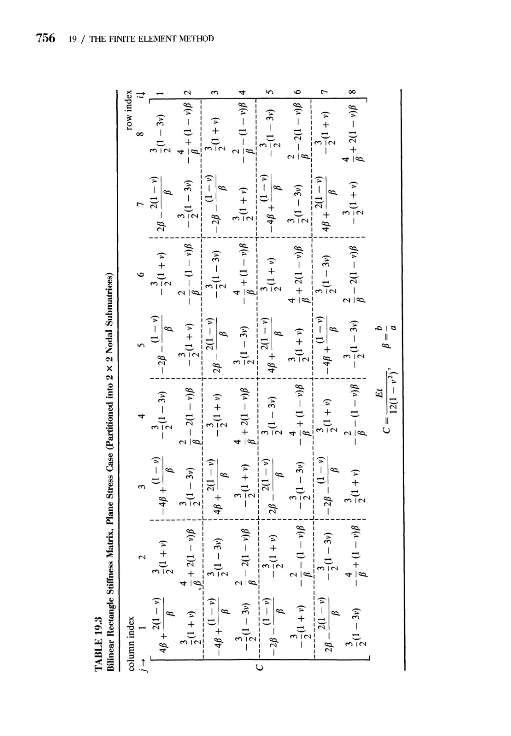
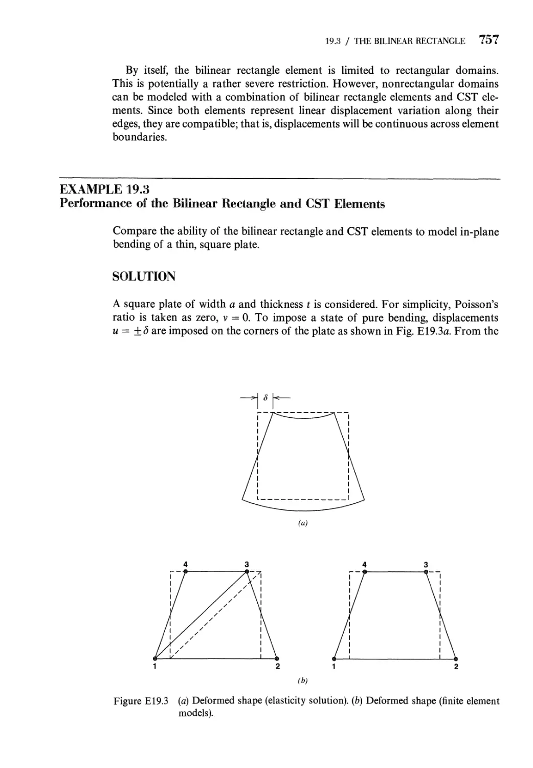
19.3 The Bilinear Rectangle 753
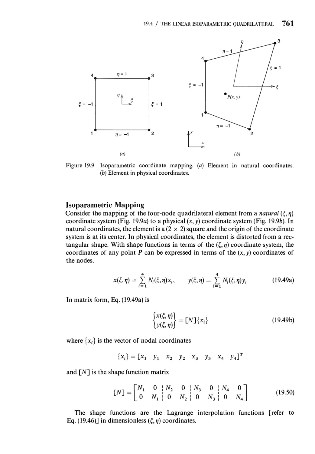
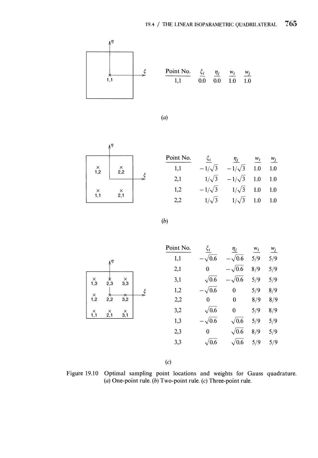
19.4 The Linear Isoparametric Quadrilateral 760
contents xvii
19.5
19.6
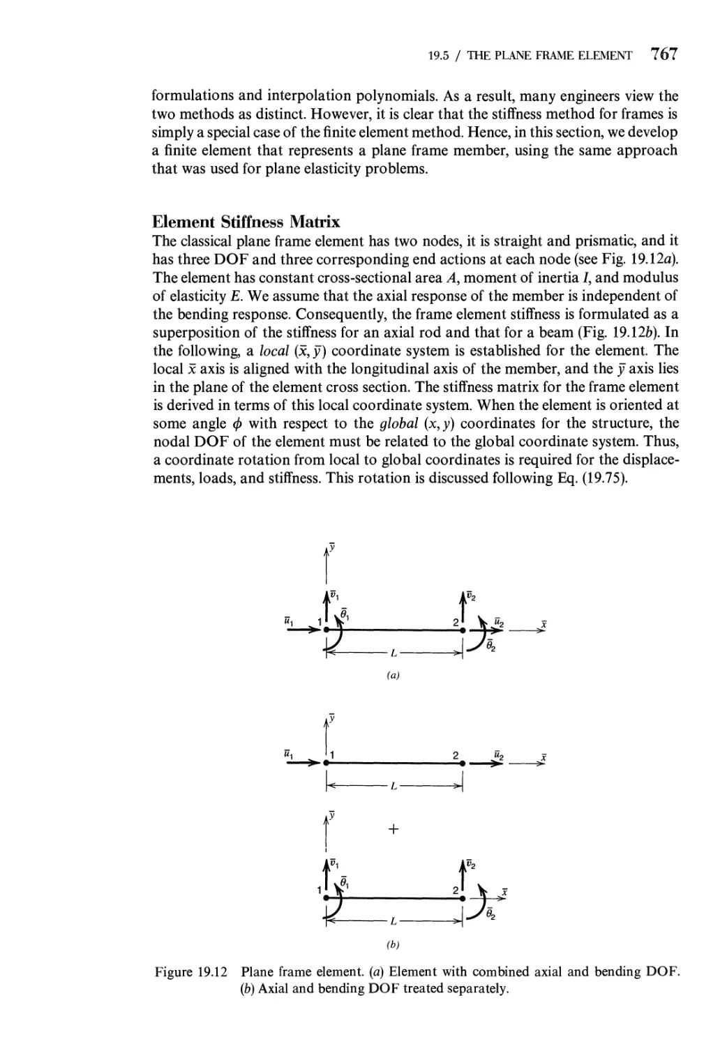
The Plane Frame Element
Closing
Problems
References
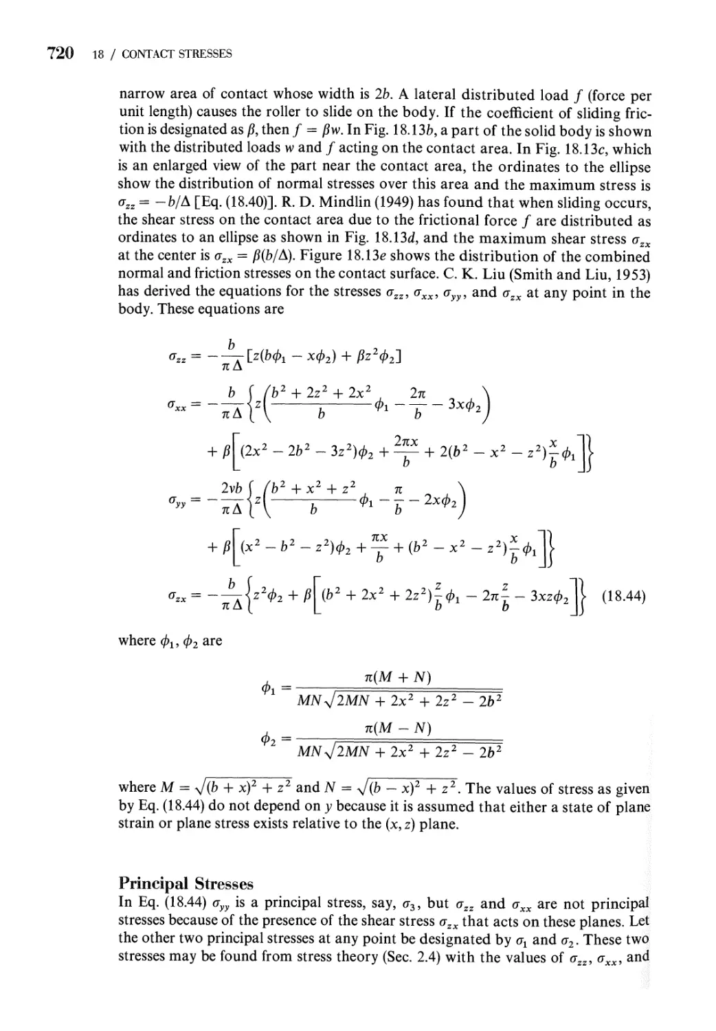
Remarks
779
782
775
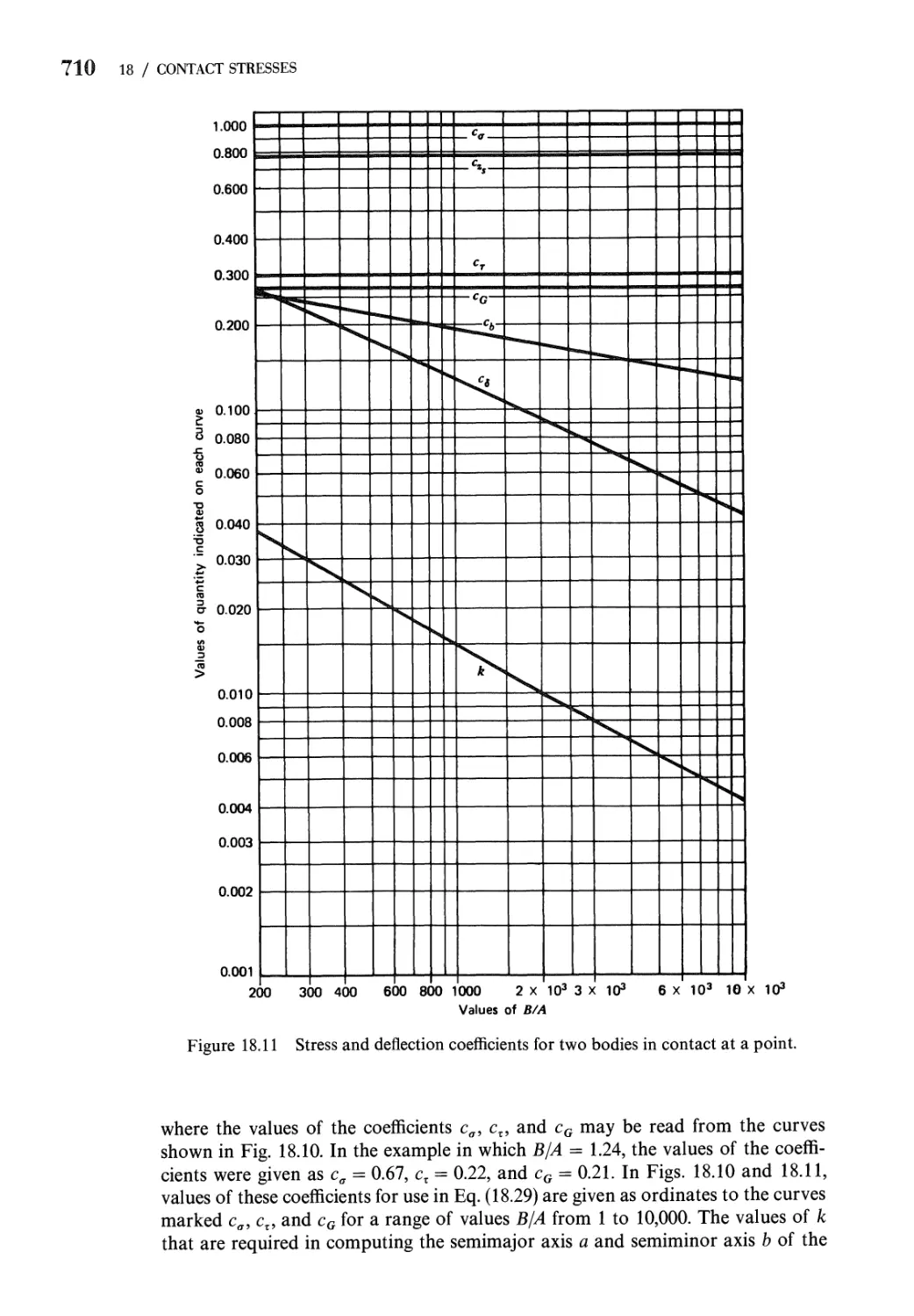
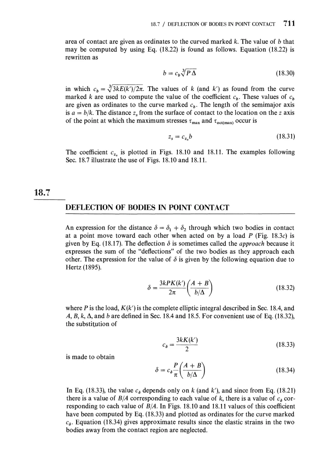
766
Appendix A Average Mechanical Properties of Selected Materials
Appendix В Second Moment (Moment of Inertia) of a Plane Area
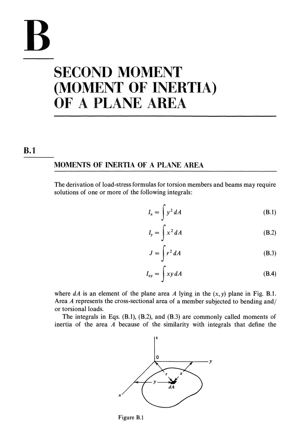
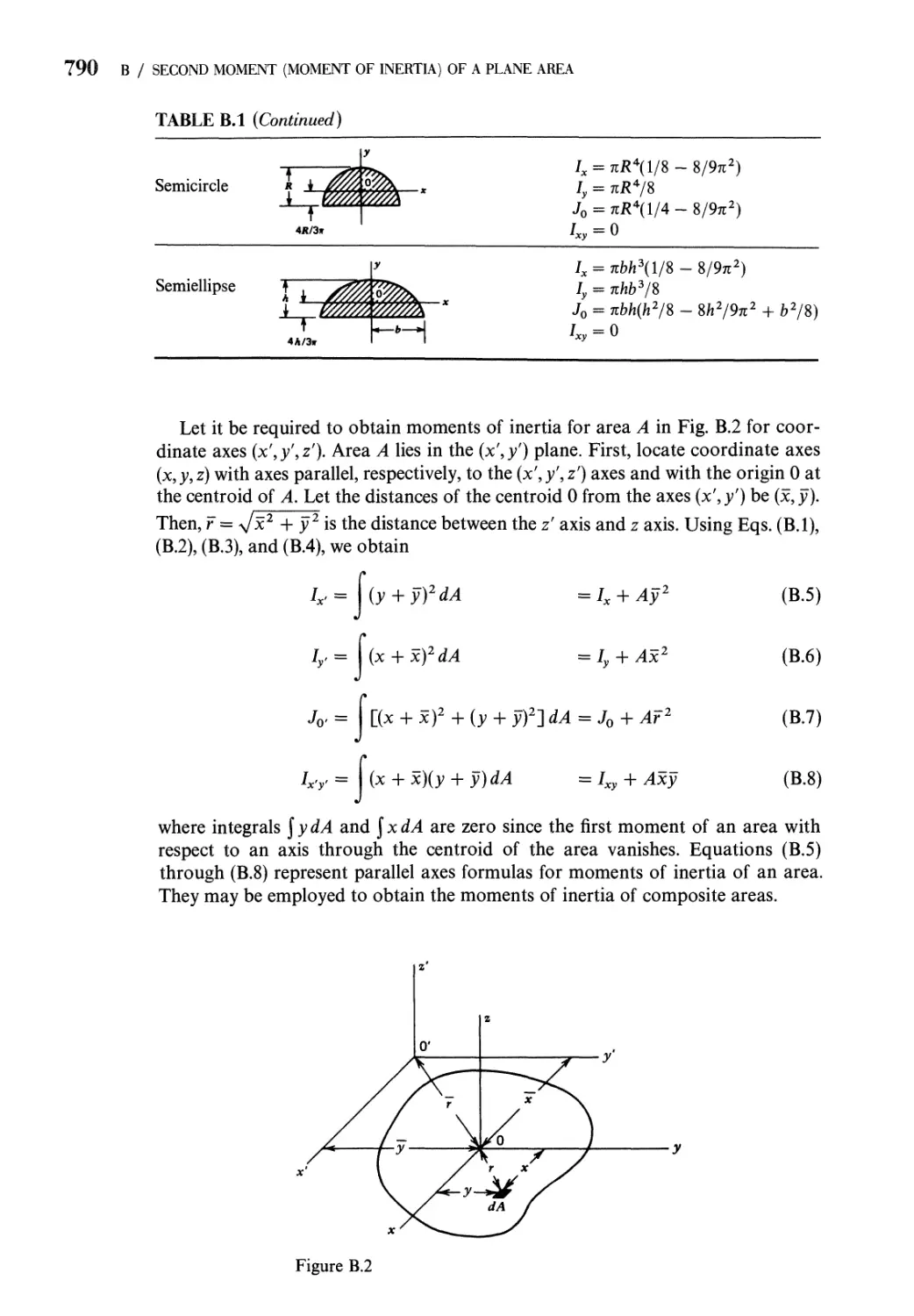
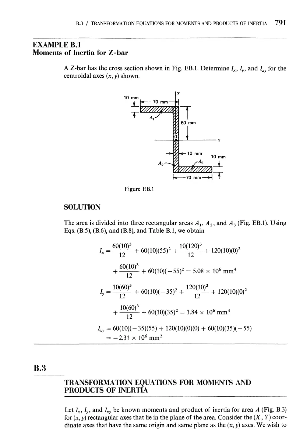
B.l Moments of Inertia of a Plane Area 788
B.2 Parallel Axis Theorem 789
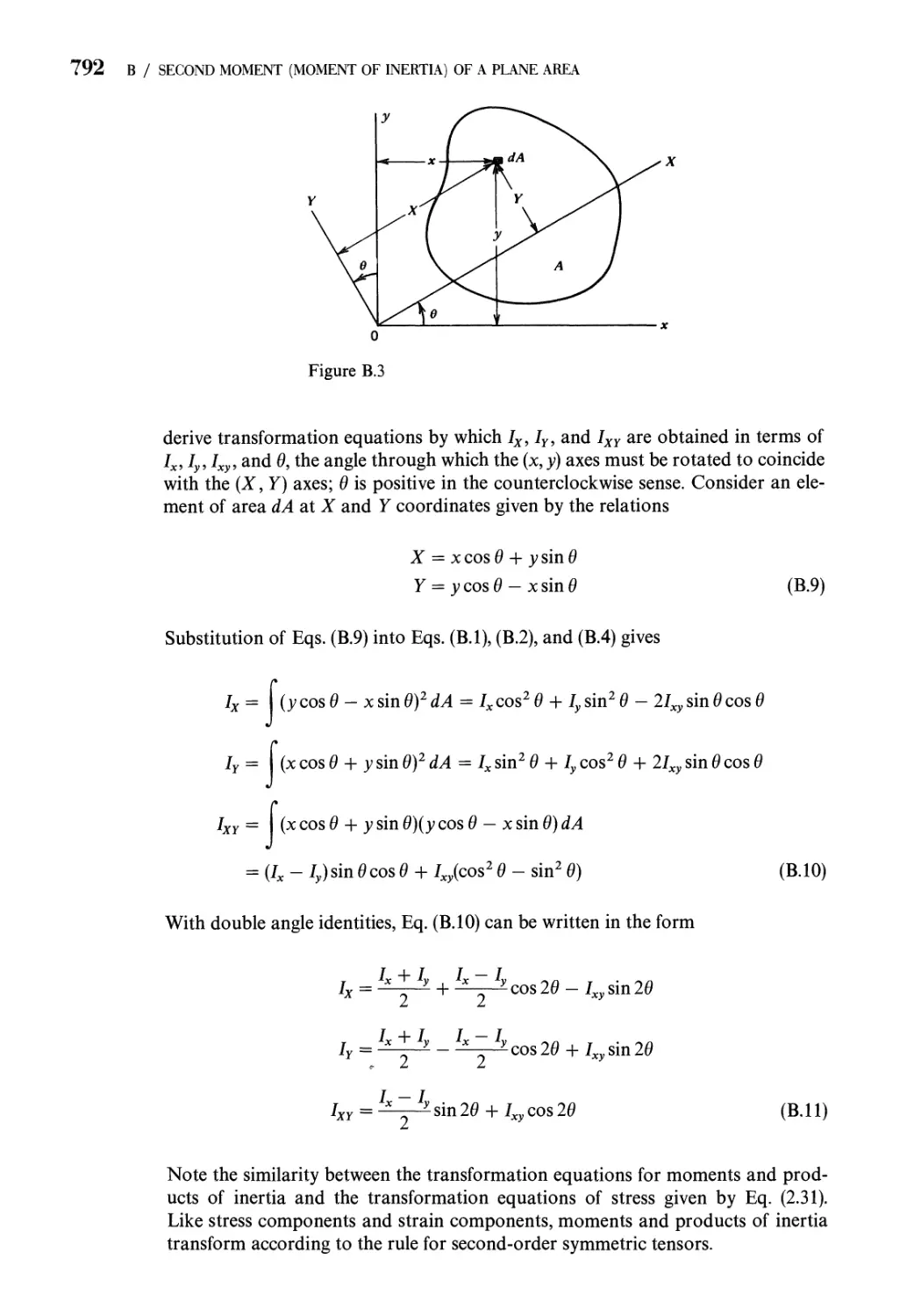
B.3 Transformation Equations for Moments and
Products of Inertia 791
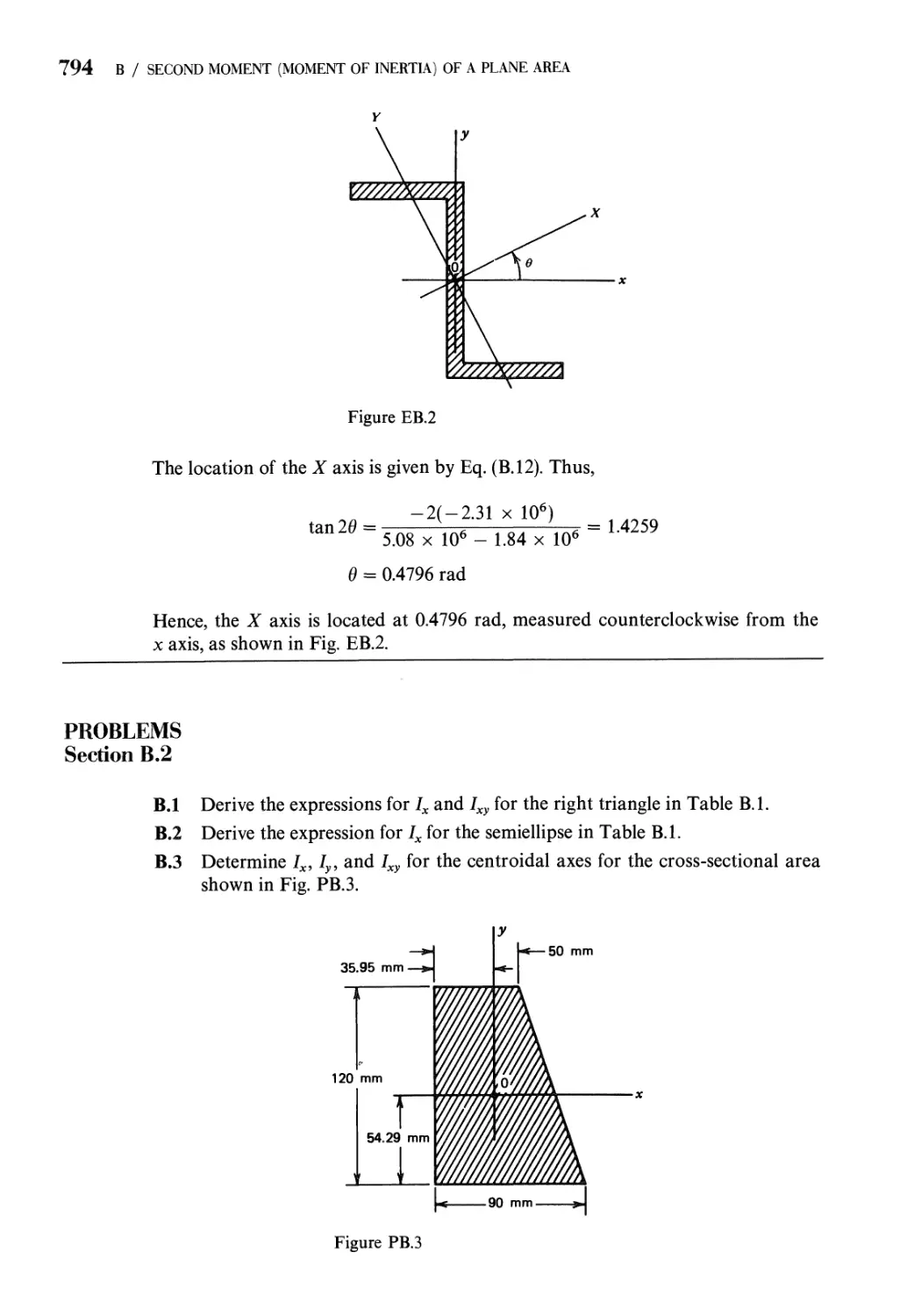
Problems 794
785
788
Author Index
Subject Index
797
801
PARTI
FUNDAMENTAL
CONCEPTS
In Part I of this book, Chapters 1 to 5, we introduce and develop fundamental topics
that are important in the remainder of the book. In Chapter 1, we emphasize basic
material properties and their use in design. Theories of stress and strain are
presented in Chapter 2, and linear stress-strain-temperature relations are
introduced in Chapter 3. Inelastic material behavior is discussed in Chapter 4 and finally,
energy methods are treated in Chapter 5.
INTRODUCTION
In this chapter, we present general concepts and definitions that are fundamental to
many of the topics discussed in this book. The chapter serves also as a brief guide
and introduction to the remainder of the book. The reader may find it fruitful to
refer to this chapter, from time to time, in conjunction with the study of topics in
other chapters.
THE ROLE OF DESIGN
This book emphasizes the methods of mechanics of materials and applications to
the analysis and design of components of structural/machine systems. As such, it
is directed to aeronautical, civil, mechanical, and nuclear engineers, as well as to
specialists in the field of theoretical and applied mechanics. As engineers, we are
problem solvers. The problems that we solve encompass practically all fields of
human activity. We solve problems related to buildings, transportation (including
automotive, rail, water, air and outer-space travel), water systems (e.g., dams and
pipelines), manufacturing, specialized medical equipment, communication systems,
computers, hazardous wastes, etc. These problems are generally encountered in the
design, manufacture, and construction of engineering systems. Ordinarily, these
systems are not built or manufactured before the design process is completed. The
design process usually involves the development of many drawings and/or CAD
files to describe the final system. One of the major purposes of the design process is
to analyze or evaluate various design alternatives before a final design is selected.
One of the simplest objectives of the analysis is to ensure that all components of the
system will fit together and function properly. More complicated analysis involves
the evaluation of forces in the proposed design to ensure that each component of the
system functions properly (for instance, safely withstands loads or does not undergo
excessive displacements). This analysis is essential in the process of refining the
design to meet required conditions such as adequate strength, minimum weight, and
minimum cost of production.
The process of refining the design can be very complicated and extremely time-
consuming. For example, consider the design of a space vehicle, such as the shuttle.
After the shuttle's mission or use has been established, the designer must decide on
the shape of the vehicle and the materials to be used. The designer must analyze the
vehicle's structure to determine if it is strong and stiff enough to withstand the
aerodynamic and thermal loads to which it will be subjected. The designer must
4 1 / INTRODUCTION
analyze the skin and individual component parts of the structure to determine how
these loads will be carried and safely transmitted from part to part. This first analysis
usually reveals evidence that a redesign of some members in the structure may
provide a more efficient and safer distribution of load and perhaps a more cost-
effective design. Unfortunately, the designer may also discover that improvements in
one part of the system may require changes in another part and possible problems in
still other parts. Thus, the designer may be faced with one or more iterations between
analysis and design to ensure that the entire system will function properly. This type
of iteration is a common feature of design (Cross, 1989; de Neufville, 1990).
Considerations other than resistance to and transfer of loads, such as those of
form or appearance, cost, ease of manufacturing, time constraints, etc., may influence
or even control the design. Indeed, these factors may not only govern the design of
an individual component but also may have a strong influence on the design of a
more general engineering system, such as an office building. However,
considerations of this kind are secondary to the topics treated in this book.
The term design as used in this book is not limited to the detailed calculations
required to determine the proper dimensions of a member; rather, this term is used
in a broader sense that emphasizes the relation of the methods of mechanics of
materials to the concepts and philosophy of a rational design code or specification.
In particular, emphasis is placed on the development of equations, formulas, or
methods by which detailed analyses can be performed. Thus, this text provides an
analytical foundation that is fundamental to the design process. Readers interested
in the general concepts and methods of design may refer to the books by Cross
A989) and de Neufville A990).
13
TOPICS TREATED IN THIS BOOK
This book is intended for advanced undergraduate and graduate engineering
students, as well as practicing engineers. The topics treated are separated into three
groups: Part I, Fundamental Concepts; Part II, Classical Topics in Advanced
Mechanics of Materials; Part III, Selected Advanced Topics. Part I treats general
concepts that pertain to the entire book, theories of stress and strain, linear stress-
strain-temperature relations, yield criteria for multiaxial stress states, and energy
methods. These topics are intended to be read sequentially, more or less. However,
depending on the background of the reader, some of these topics may be bypassed.
Part II presents several chapters on classical applications of the methods of
mechanics of materials, namely, torsion, nonsymmetrical bending of beams, shear
center for thin-wall beam cross sections, curved beams, beams on elastic
foundations, thick-wall cylinders, and buckling of columns. These chapters may be treated
in any order, except that the chapter on shear centers should be studied after the
chapters on torsion and nonsymmetrical bending of beams. Part III introduces
chapters on selected advanced topics, namely, flat plates, stress concentration
factors, contact stresses, fracture mechanics, high cycle fatigue, time-dependent
deformation/creep, and finite element methods. Each of these chapters may be
treated independently, more or less.
1.3 / LOAD-STRESS AND LOAD-DEFLECTION RELATIONS 5
LOAD-STEESS AND LOAD-DEFLECTION RELATIONS
For most of the members considered in this book we derive relations, in terms of
known loads and known dimensions of the member, for either the distributions of
normal and shear stresses on a cross section of the member or for stress components
that act at a point in the member. For a given member subjected to prescribed loads,
the derivation of load-stress relations depends on satisfaction of the following
requirements.
1. The equations of equilibrium (or equations of motion for bodies not in
equilibrium)
2. The compatibility conditions (continuity conditions) that require deformed
volume elements in the member to fit together without overlap or tearing
3. The constitutive relations
Two different methods are used to satisfy requirements 1 and 2: the method of
mechanics of materials and the method of general continuum mechanics. Often,
load-stress and load-deflection relations have not been derived in this book by
general continuum mechanics methods, either because the beginning student does
not have the necessary background or because of the complexity of the general
solutions. Instead, the method of mechanics of materials is used to obtain either
exact solutions or reliable approximate solutions. In the method of mechanics of
materials, the load-stress relations are derived first. They are then used to obtain
load-deflection relations for the member.
A simple member such as a circular shaft of uniform cross section may be
subjected to complex loads that produce a multiaxial state of stress in the shaft.
However, such complex loads can be reduced to several simple types of load, such as
axial, bending, and torsion. Each type of load, when acting alone, produces mainly
one stress component, which is distributed over the cross section of the shaft. The
method of mechanics of materials can be used to obtain load-stress relations for
each type of load. If the deformations of the shaft that result from one type of load
do not influence the magnitudes of the other types of loads and if the material
remains linearly elastic for the combined loads, the stress components due to each
type of load can be added together (i.e., the method of superposition may be used).
In a complex member, each load may have a significant influence on each
component of the state of stress. Then, the method of mechanics of materials
becomes cumbersome, and the use of the method of continuum mechanics may be
more appropriate.
Method of Mechanics of Materials
The method of mechanics of materials is based on simplified assumptions related to
the geometry of deformation (requirement 2) so that strain distributions for a cross
section of the member can be determined. A basic assumption is that plane sections
before loading remain plane after loading. The assumption can be shown to be exact
for axially loaded members of uniform cross sections, for slender straight torsion
members having uniform circular cross sections, and for slender straight beams of
6 1 / INTRODUCTION
uniform cross sections subjected to pure bending. The assumption is approximate
for other beam problems. The method of mechanics of materials is used in this book
to treat several advanced beam topics (Chapters 7 to 10). In a similar way, we assume
that lines normal to the middle surface of an undeformed plate remain straight and
normal to the middle surface after the load is applied. This assumption is used to
simplify the plate problem in Chapter 13.
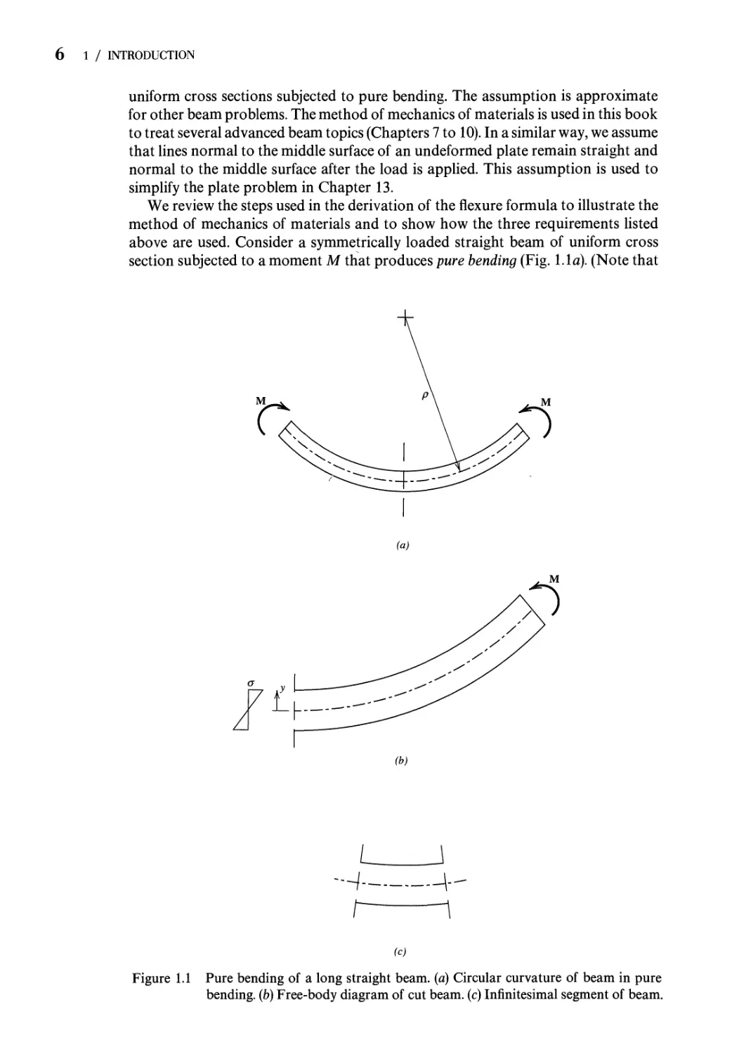
We review the steps used in the derivation of the flexure formula to illustrate the
method of mechanics of materials and to show how the three requirements listed
above are used. Consider a symmetrically loaded straight beam of uniform cross
section subjected to a moment M that produces pure bending (Fig. 1.1a). (Note that
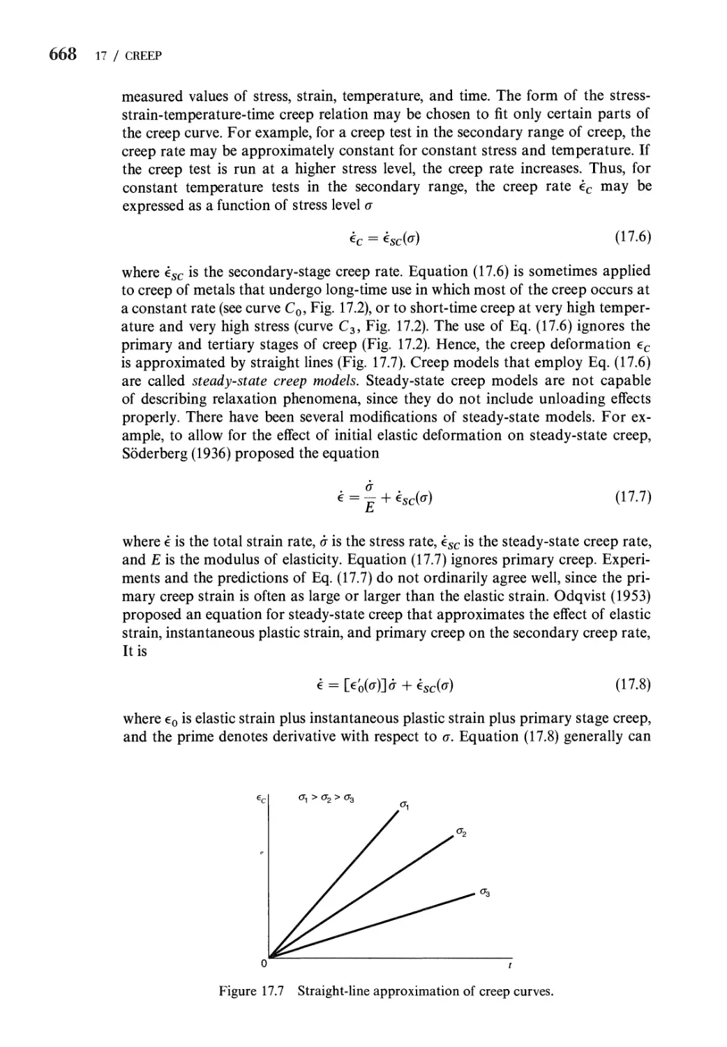
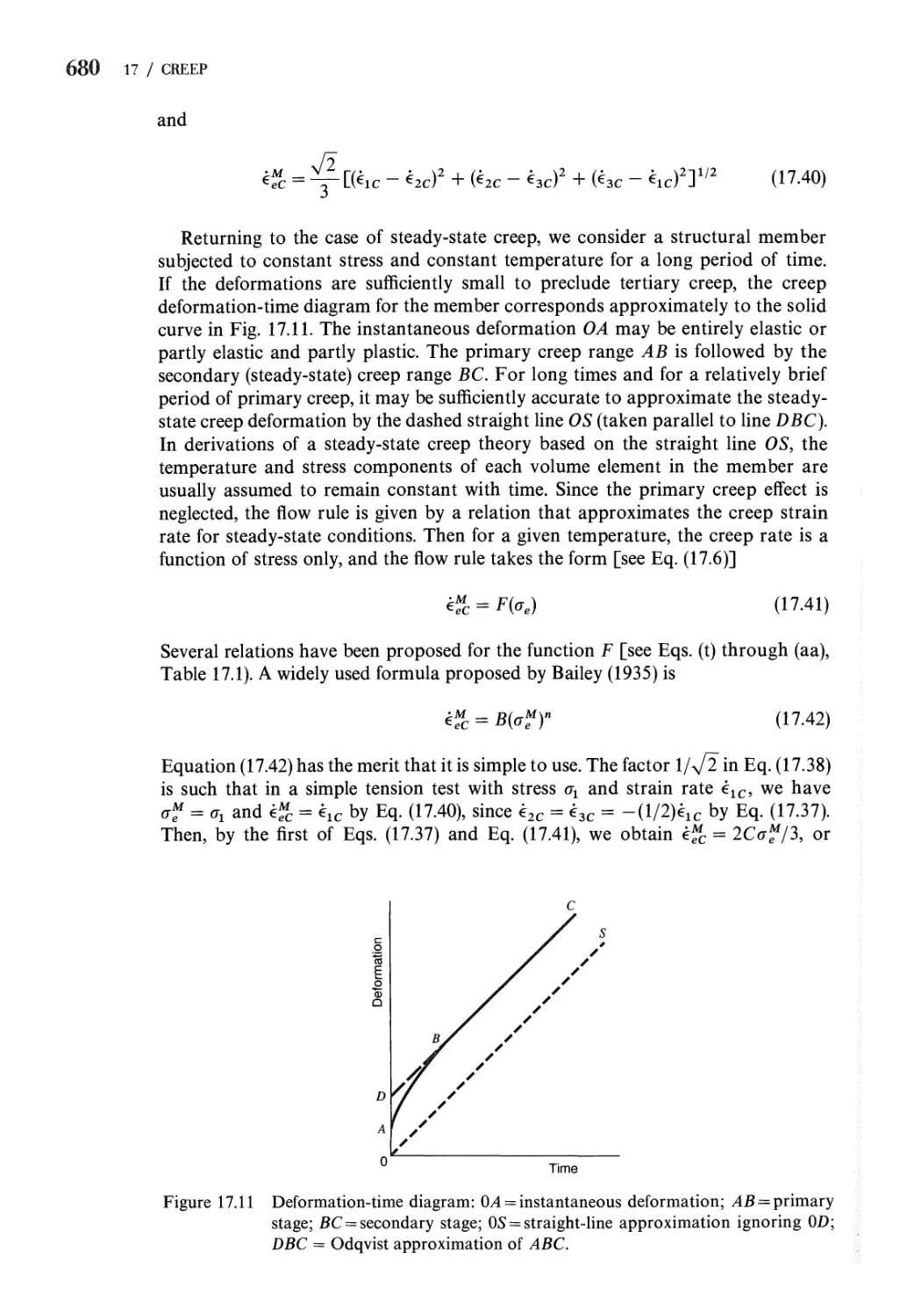
(a)
L 1
H \-
г 1
(c)
Figure 1.1 Pure bending of a long straight beam, (a) Circular curvature of beam in pure
bending, (b) Free-body diagram of cut beam, (c) Infinitesimal segment of beam.
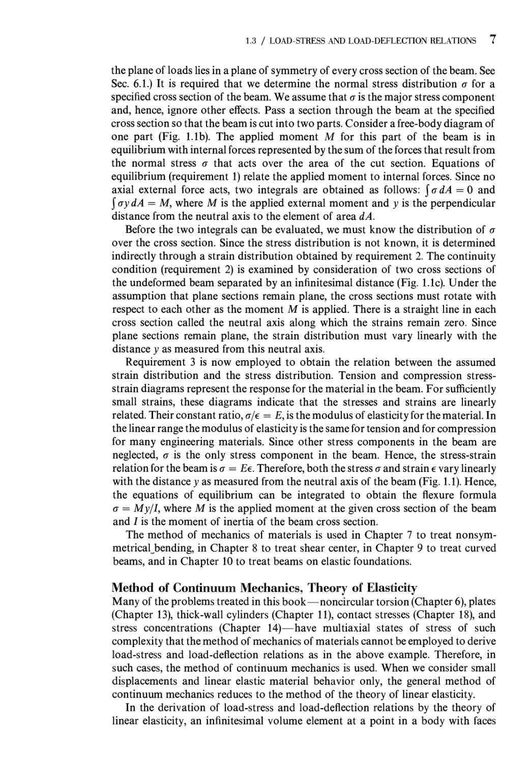
1.3 / LOAD-STRESS AND LOAD-DEFLECTION RELATIONS 7
the plane of loads lies in a plane of symmetry of every cross section of the beam. See
Sec. 6.1.) It is required that we determine the normal stress distribution a for a
specified cross section of the beam. We assume that о is the major stress component
and, hence, ignore other effects. Pass a section through the beam at the specified
cross section so that the beam is cut into two parts. Consider a free-body diagram of
one part (Fig. Lib). The applied moment M for this part of the beam is in
equilibrium with internal forces represented by the sum of the forces that result from
the normal stress о that acts over the area of the cut section. Equations of
equilibrium (requirement 1) relate the applied moment to internal forces. Since no
axial external force acts, two integrals are obtained as follows: §adA = 0 and
§<jydA = M, where M is the applied external moment and у is the perpendicular
distance from the neutral axis to the element of area dA.
Before the two integrals can be evaluated, we must know the distribution of a
over the cross section. Since the stress distribution is not known, it is determined
indirectly through a strain distribution obtained by requirement 2. The continuity
condition (requirement 2) is examined by consideration of two cross sections of
the undeformed beam separated by an infinitesimal distance (Fig. Lie). Under the
assumption that plane sections remain plane, the cross sections must rotate with
respect to each other as the moment M is applied. There is a straight line in each
cross section called the neutral axis along which the strains remain zero. Since
plane sections remain plane, the strain distribution must vary linearly with the
distance у as measured from this neutral axis.
Requirement 3 is now employed to obtain the relation between the assumed
strain distribution and the stress distribution. Tension and compression stress-
strain diagrams represent the response for the material in the beam. For sufficiently
small strains, these diagrams indicate that the stresses and strains are linearly
related. Their constant ratio, a/e = E, is the modulus of elasticity for the material. In
the linear range the modulus of elasticity is the same for tension and for compression
for many engineering materials. Since other stress components in the beam are
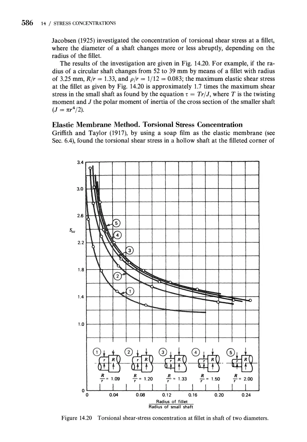
neglected, о is the only stress component in the beam. Hence, the stress-strain
relation for the beam is a = Ее. Therefore, both the stress о and strain e vary linearly
with the distance у as measured from the neutral axis of the beam (Fig. 1.1). Hence,
the equations of equilibrium can be integrated to obtain the flexure formula
a = My/I, where M is the applied moment at the given cross section of the beam
and J is the moment of inertia of the beam cross section.
The method of mechanics of materials is used in Chapter 7 to treat nonsym-
metricaljDending, in Chapter 8 to treat shear center, in Chapter 9 to treat curved
beams, and in Chapter 10 to treat beams on elastic foundations.
Method of Continuum Mechanics, Theory of Elasticity
Many of the problems treated in this book—noncircular torsion (Chapter 6), plates
(Chapter 13), thick-wall cylinders (Chapter 11), contact stresses (Chapter 18), and
stress concentrations (Chapter 14)—have multiaxial states of stress of such
complexity that the method of mechanics of materials cannot be employed to derive
load-stress and load-deflection relations as in the above example. Therefore, in
such cases, the method of continuum mechanics is used. When we consider small
displacements and linear elastic material behavior only, the general method of
continuum mechanics reduces to the method of the theory of linear elasticity.
In the derivation of load-stress and load-deflection relations by the theory of
linear elasticity, an infinitesimal volume element at a point in a body with faces
8 1 / INTRODUCTION
normal to the coordinate axes is often employed. Requirement 1 is represented by
the differential equations of equilibrium (Chapter 2). Requirement 2 is represented
by the differential equations of compatibility (Chapter 2). The material response
(requirement 3) for linearly elastic behavior is determined by one or more
experimental tests that define the required elastic coefficients for the material. In this
book we consider mainly isotropic materials for which only two elastic coefficients
are needed (Chapter 3). These coefficients can be obtained from a tension specimen if
both axial and lateral strains are measured for every load applied to the specimen.
Requirement 3 is represented therefore by the isotropic stress-strain relations
developed in Chapter 3. If the differential equations of equilibrium and the differential
equations of compatibility can be solved subject to specified stress-strain relations
and specified boundary conditions, the states of stress and displacements for every
point in the member are obtained.
Deflections by Energy Methods
Certain structures are made up of members whose cross sections remain essentially
plane during the deflection of the structures. The deflected position of a cross
section of a member of the structure is defined by three orthogonal displacement
components of the centroid of the cross section and by three orthogonal rotation
components of the cross section. These six components of displacement and
rotation of a cross section of a member are readily calculated by energy methods. For
small displacements and small rotations and for linearly elastic material behavior,
Castigliano's theorem is recommended as a method for the computation of the
displacements and rotations. The method is employed in Chapter 5 for structures
made up of axially loaded members, beams, and torsion members, and in Chapter 9
for curved beams.
1.4
STRESS-STRAIN RELATIONS
In Chapter 2, the state of stress at a point is defined by six stress components. The
transformation of the stress components under a rotation of coordinate axes is
developed, and equations of equilibrium (or equations of motion for accelerated
bodies) are derived. The analogous theory of deformation, based on geometric
concepts, is presented and strain-displacement relations, transformation of the
strain components under a rotation of coordinate axes, and strain compatibility
relations are derived.
To derive load-stress and load-deflection relations for specified structural
members, the stress components must be related to the strain components.
Consequently, in Chapter 3 we discuss linear stress-strain-temperature relations.
These relations may be employed in the study of linearly elastic material behavior.
In addition, they may be employed in plasticity theories to describe the linearly
elastic part of the total response of materials. More generally, nonlinear (inelastic)
stress-strain relations are required for the plastic part of material behavior.
Unfortunately, these relations take on different forms, depending on the material
behavior during plastic response. In this book, we consider only the limiting case of
1.4 / STRESS-STRAIN RELATIONS 9
fully plastic loads for low-carbon structural steel. At the fully plastic load, stress
components are assumed to be independent of the strain components and remain
constant with increasing strain.
Since experimental studies are required to determine material properties (e.g.
elastic coefficients for linearly elastic materials), the study of stress-strain relations is,
in part, empirical. To obtain needed isotropic elastic material properties, we employ
a tension specimen (Fig. 1.2). If lateral as well as longitudinal strains are measured
for linearly elastic behavior of the tension specimen, the resulting stress-strain data
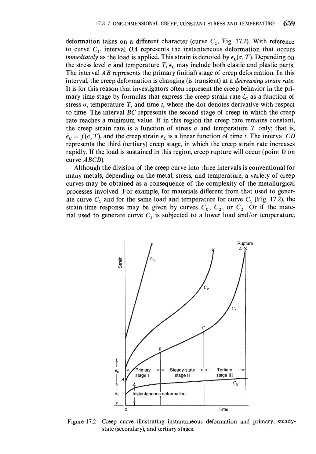
represent the material response for obtaining the needed elastic constants for the
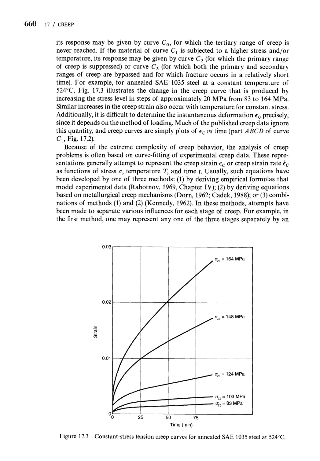
material. The main structure of the stress-strain-temperature relations, however, is
studied theoretically by means of the first law of thermodynamics (Chapter 3).
The stress-strain-temperature relations presented in Chapter 3 are limited mainly
to small strains and small rotations. The reader interested in large strains and large
rotations may refer to the works of Green and Adkins A960).
Elastic and Inelastic Response of a Solid
Initially, we review the results of a simple tension test of a circular cylindrical bar
that is subjected to an axially directed tensile load P (Fig. 1.2). It is assumed that the
load is monotonically increased slowly (so-called static loading) from its initial value
of zero to its final value, since the material response depends not only on the
magnitude of the load, but also on other factors, such as the rate of loading, load
cycling, etc. It is customary in engineering practice to plot the tensile stress о in the
bar as a function of the strain e of the bar. In engineering practice, it is also
a
-£> = 10.0mm
(a)
(b)
Figure 1.2 Circular cross section tension specimen, (a) Undeformed specimen: Gage length
L; diameter D. (b) Deformed specimen: Gage length elongation e.
10 1 / INTRODUCTION
customary to assume that the stress о is uniformly distributed over the cross-
sectional area of the bar and that it is equal in magnitude to P/A0, where A0 is the
original cross-sectional area of the bar. Similarly, the strain e is assumed to be
constant over the gage length L and equal to AL/L = e/L, where AL = e (Fig. 1.2b) is
the change or elongation in the original gage length L (the distance J К in Fig. 1.2a).
For these assumptions to be valid, the points J and К must be sufficiently far from
the ends of the bar (a distance of one or more diameters D from the ends). However,
according to the definition of stress (Sec. 2.1), the true stress is ot = P/At, where At is
the true cross-sectional area of the bar when the load P acts. (The bar undergoes
lateral contraction everywhere as it is loaded, with a corresponding change in cross-
sectional area.) The difference between a = P/A0 and ot = P/At is small, provided
that the elongation e and, hence, the strain e are sufficiently small (Sec. 2.8). If the
elongation is large, At may differ significantly from A0. In addition, the
instantaneous or true gage length when load P acts is Lt = L + e (Fig. 1.2b). Hence, like At,
the true gage length Lt changes with the load P. Corresponding to the true stress ot,
we may define the true strain et as follows: In the tension test, assume that the load P
is increased from zero (where e = 0 also) by successive infinitesimal increments dP.
With each incremental increase dP in load P, there is a corresponding infinitesimal
increase dLt in the instantaneous gage length Lt. Hence, the infinitesimal increment
det of the true strain et due to dP is
<fe,=^ (i.i)
Integration of Eq. A.1) from L to Lt yields the true strain et. Thus, we have
^е, = 1п(^) = 1п(^^) = 1пA+€) A.2)
In contrast to the engineering strain e, the true strain et is not linearly related to the
elongation e of the original gage length L.
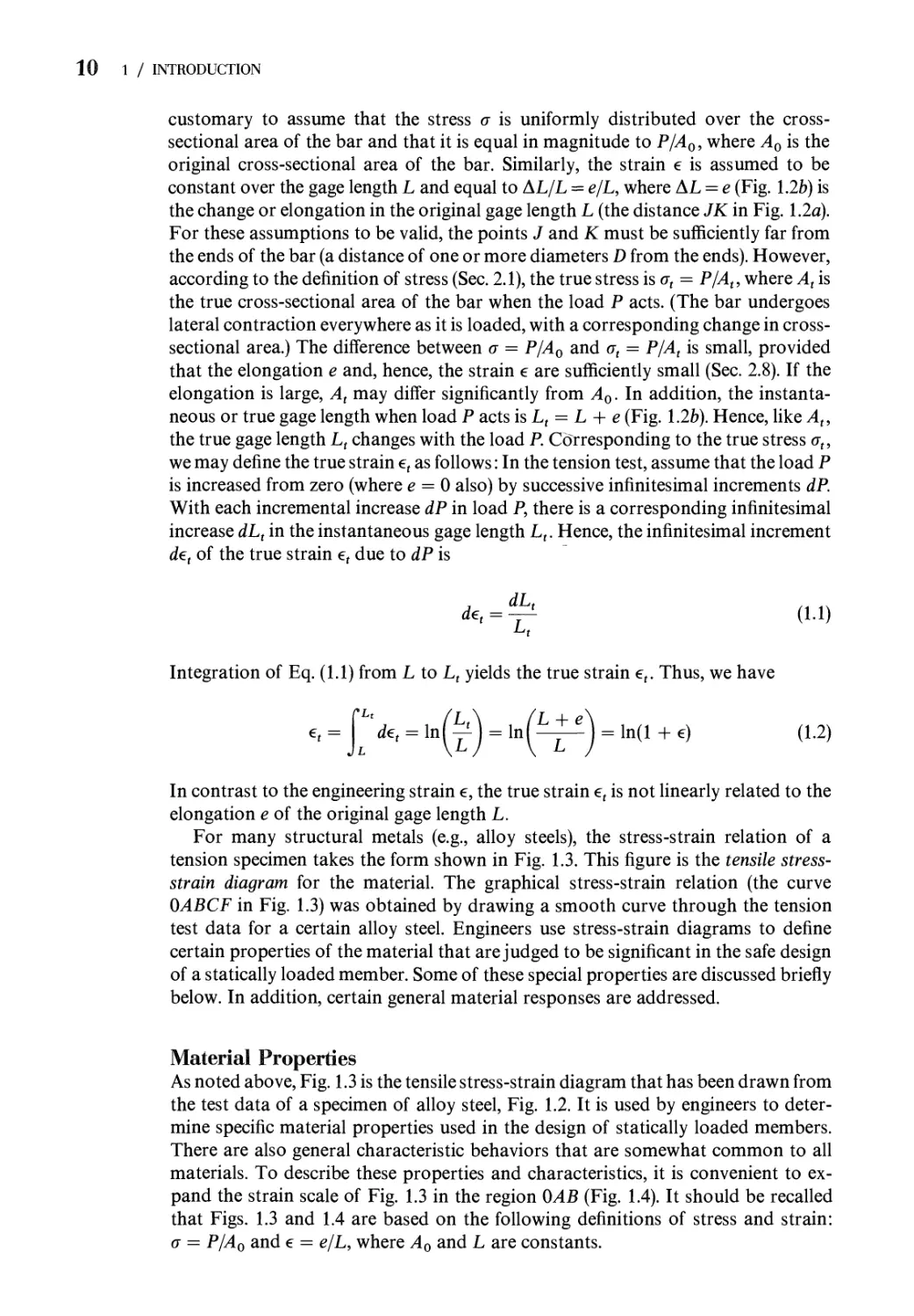
For many structural metals (e.g., alloy steels), the stress-strain relation of a
tension specimen takes the form shown in Fig. 1.3. This figure is the tensile stress-
strain diagram for the material. The graphical stress-strain relation (the curve
OABCF in Fig. 1.3) was obtained by drawing a smooth curve through the tension
test data for a certain alloy steel. Engineers use stress-strain diagrams to define
certain properties of the material that are judged to be significant in the safe design
of a statically loaded member. Some of these special properties are discussed briefly
below. In addition, certain general material responses are addressed.
Material Properties
As noted above, Fig. 1.3 is the tensile stress-strain diagram that has been drawn from
the test data of a specimen of alloy steel, Fig. 1.2. It is used by engineers to
determine specific material properties used in the design of statically loaded members.
There are also general characteristic behaviors that are somewhat common to all
materials. To describe these properties and characteristics, it is convenient to
expand the strain scale of Fig. 1.3 in the region OAB (Fig. 1.4). It should be recalled
that Figs. 1.3 and 1.4 are based on the following definitions of stress and strain:
a = P/A0 and e = e/L, where A0 and L are constants.
1.4 / STRESS-STRAIN RELATIONS 11
500
2
b* 400
300
200
100
/в
♦л
с
°и
У
F
0.05
0.10 0.15
Strain, e
0.20 eF 0.25
Figure 1.3 Engineering stress-strain diagram for tension specimen of alloy steel.
300
Af
A- Offset^
[ 4
i
/
/
'к 1
Y
,
S
-B
0 0.002 0.004 0.006 0.008 0.010 0.012
1 | | Strain, e
- es —*"H ee
Figure 1.4 Engineering stress-strain diagram for tension specimen of alloy steel (expanded
strain scale).
12 1 / INTRODUCTION
Consider a tensile specimen (bar) subjected to a strain e under the action of a load
P. If upon removal of the load P, the strain in the bar returns to zero as the load P
goes to zero, the material in the bar is said to have been strained within the elastic
limit or the material has remained perfectly elastic. If under loading the strain is
linearly proportional to the load P (part OA in Figs. 1.3 and 1.4), the material is said
to be strained within the limit of linear elasticity. The maximum stress for which
the material remains perfectly elastic is frequently referred to simply as the elastic
limit aEL, whereas the stress at the limit of linear elasticity is referred to as the
proportional limit gpl (point A in Figs. 1.3 and 1.4). Ordinarily, oEL is larger than gpl.
The properties of elastic limit and proportional limit, although important from a
theoretical viewpoint, are not of practical importance for materials like alloy steels.
This is due to the fact that the transitions from elastic to inelastic behavior and from
linear to nonlinear behavior are so gradual that these limits are very difficult to
determine from the stress-strain diagram (part OAB of the curves in Figs. 1.3
and 1.4).
When the load produces a stress a that exceeds the elastic limit (e.g., the stress
at point J in Fig. 1.4), the strain does not disappear upon unloading (curve JL in
Fig. 1.4) A permanent strain OL remains. For simplicity, it is assumed that the
unloading occurs along the straight line JK, with a slope equal to that of the straight
line OA. For this reason, the strain OK is called the offset strain es. The strain that
is recovered when the load is removed is called the elastic strain ee. Hence, the total
strain e at point J is the sum of the offset strain and elastic strain, or € = es + ee.
Yield Strength. The value of stress associated with point J, Fig. 1.4, is called the
yield strength and is denoted by <jys or simply by YS. In practice, a value of the offset
strain is chosen and the yield strength is determined as the stress associated with the
intersection of the curve OAB and the straight line J К drawn from the offset strain
value, with a slope equal to that of line OA (Fig. 1.4). The value of the offset strain is
arbitrary. However, a commonly agreed upon value of offset is 0.002 or 0.2% strain,
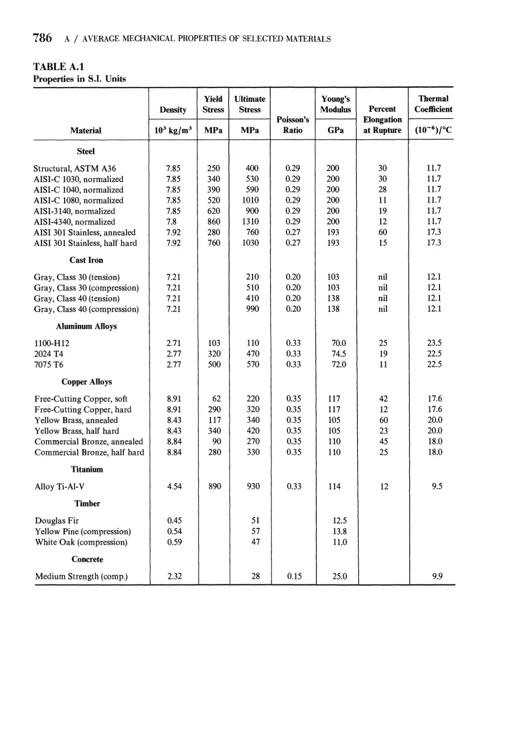
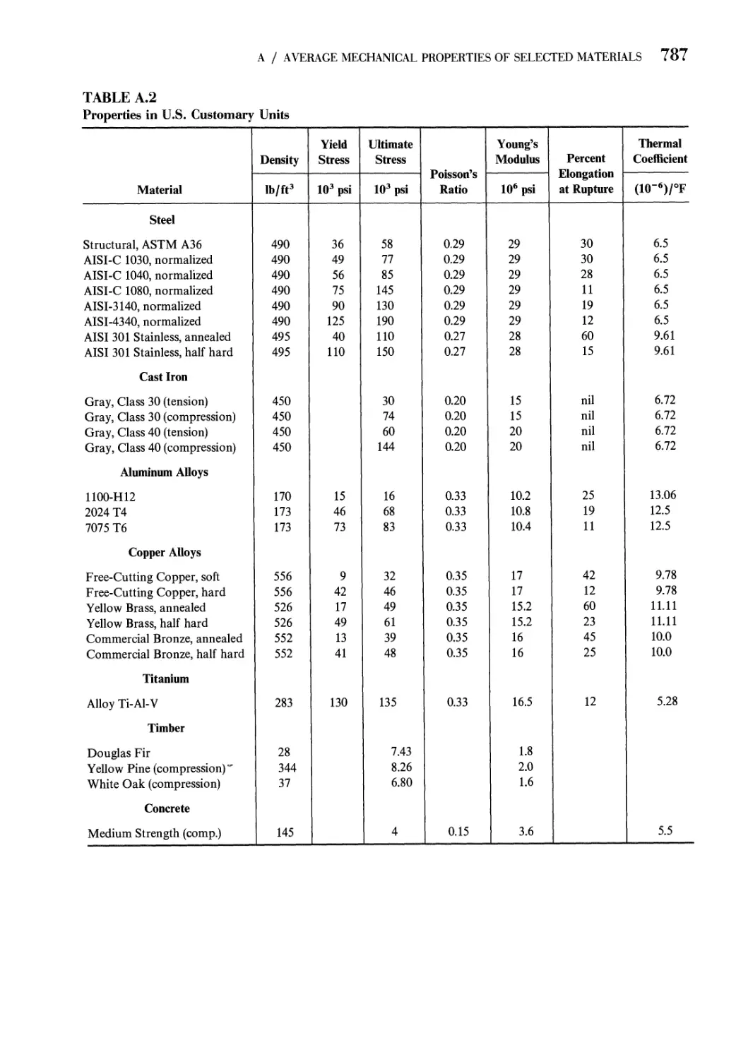
as shown in Fig. 1.4. Typical values of yield strength for several structural materials
are listed in Appendix A, for an offset of 0.2%. For materials with stress-strain
curves like that of alloy steels (Figs. 1.3 and 1.4), the yield strength is used to predict
the load that initiates inelastic behavior (yield) in a member.
Ultimate Tensile Strength. Another important property determined from the
stress-strain diagram is the ultimate tensile strength or ultimate tensile stress au. It
is defined as the maximum stress attained in the engineering stress-strain diagram,
and in Fig. 1.3 it is the stress associated with point C. As seen from Fig. 1.3, the
stress increases continuously beyond the elastic region 0A, until point С is reached.
This increase is because the material is hardening (gaining strength) because of
the straining, at a faster rate than it is softening (losing strength) because of the
reduction in cross-sectional area. At point C, the strain hardening effect is balanced
by the effect of the area reduction. From point С to point F, the weakening effect of
the area reduction controls, and the engineering stress decreases, until the specimen
ruptures at point F.
Modulus of Elasticity. In the straight-line region 0A of the stress-strain diagram,
the stress is proportional to strain, that is, a = Ee. The constant of proportionality E
is called the modulus of elasticity. It is also referred to as Young's modulus.
Geometrically, it is equal in magnitude to the slope of the stress-strain relation in
the region 0A (Fig. 1.4).
1.4 / STRESS-STRAIN RELATIONS 13
Percent Elongation. The value of the elongation eF of the gage length L at rupture
(point F, Fig. 1.3) divided by the gage length L (in other words, the value of strain eF
at rupture) multiplied by 100 is referred to as the percent elongation of the tensile
specimen. The percent elongation is a measure of the ductility of the material. From
Fig. 1.3, we see that the percent elongation of the alloy steel is approximately 23%.
An important structural metal, mild or structural steel, has a distinct stress-strain
curve as shown in Fig. 1.5a. The portion OAB of the stress-strain diagram is shown
expanded in Fig. 1.5b. The stress-strain diagram for structural steel usually exhibits a
so-called upper yield point, with stress aYU, and a lower yield point, with stress aYL.
This is because the stress required to initiate yield in structural steel is larger than
500
л 300
о.
tf
CO
CO
200
100
A j
\B
С
1
о
\
и
I
F
0.12 0.16
Strain, e
(a)
0.24
0.28
§_ 200
b"
CO
CO
Ф
Й 100
1
A
Да
/
/
<T
J
YU
GYL
1 \
\
= Y
'
0 0.002 0.004 0.006
Strain, e
(b)
£ 200
b"
со
со
CD
cS ioo
A
#x
£nN\
h
,
<?YL
\
»
= Y
'
0 0.002 0.004 0.006
Strain, e
(c)
Figure 1.5 Engineering stress-strain diagram for tension specimen of structural steel.
(a) Stress-strain diagram, (b) Diagram for small strain (e < 0.007). (c) Idealized
diagram for small strain (e < 0.007).
14 1 / INTRODUCTION
the stress required to continue the yielding process. At the lower yield the stress
remains essentially constant for increasing strain until strain hardening causes the
curve to rise (Fig. 1.5a). The constant or flat portion of the stress-strain diagram may
extend over a strain range of 10 to 40 times the strain at the yield point. Actual test
data indicate that the curve from A to В bounces up and down as sketched in
Fig. 1.5b. However, for simplicity, the data are represented by a horizontal straight
line.
Yield Point for Structural Steel. The upper yield point is usually ignored in design,
and it is assumed that the stress initiating yield is the lower yield point stress,
oYL. Consequently, for simplicity, the stress-strain diagram for the region OAB is
idealized as shown in Fig. 1.5c. Also for simplicity, we shall refer to the yield point
stress as the yield point and denote it by the symbol 7. Recall that the yield strength
(or yield stress) for alloy steel, and for materials such as aluminum alloys that have
similar stress-strain diagrams, was denoted by YS (Fig. 1.4). However, for simplicity
when there is no danger of confusion, we will also denote the yield strength by the
symbol Y.
Modulus of Resilience. Another property easily determined from the stress-strain
diagram is the modulus of resilience. It is a measure of energy absorbed by a material
up to the time it yields under load and is represented by the area under the stress-
strain diagram to the yield point (the shaded area OAH in Fig. 1.5c). In Fig. 1.5c, this
area is given by icryLeyL. Since eYL = <rYL/E, and with the notation Y = aYL, we may
express the modulus of resilience as follows:
1 Y2
Modulus of resilience = - — A.3)
2 E
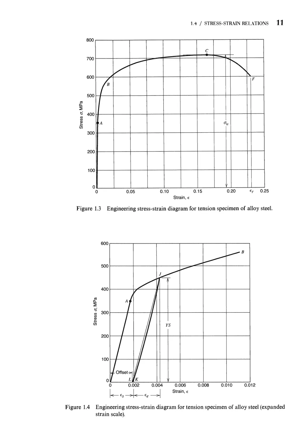
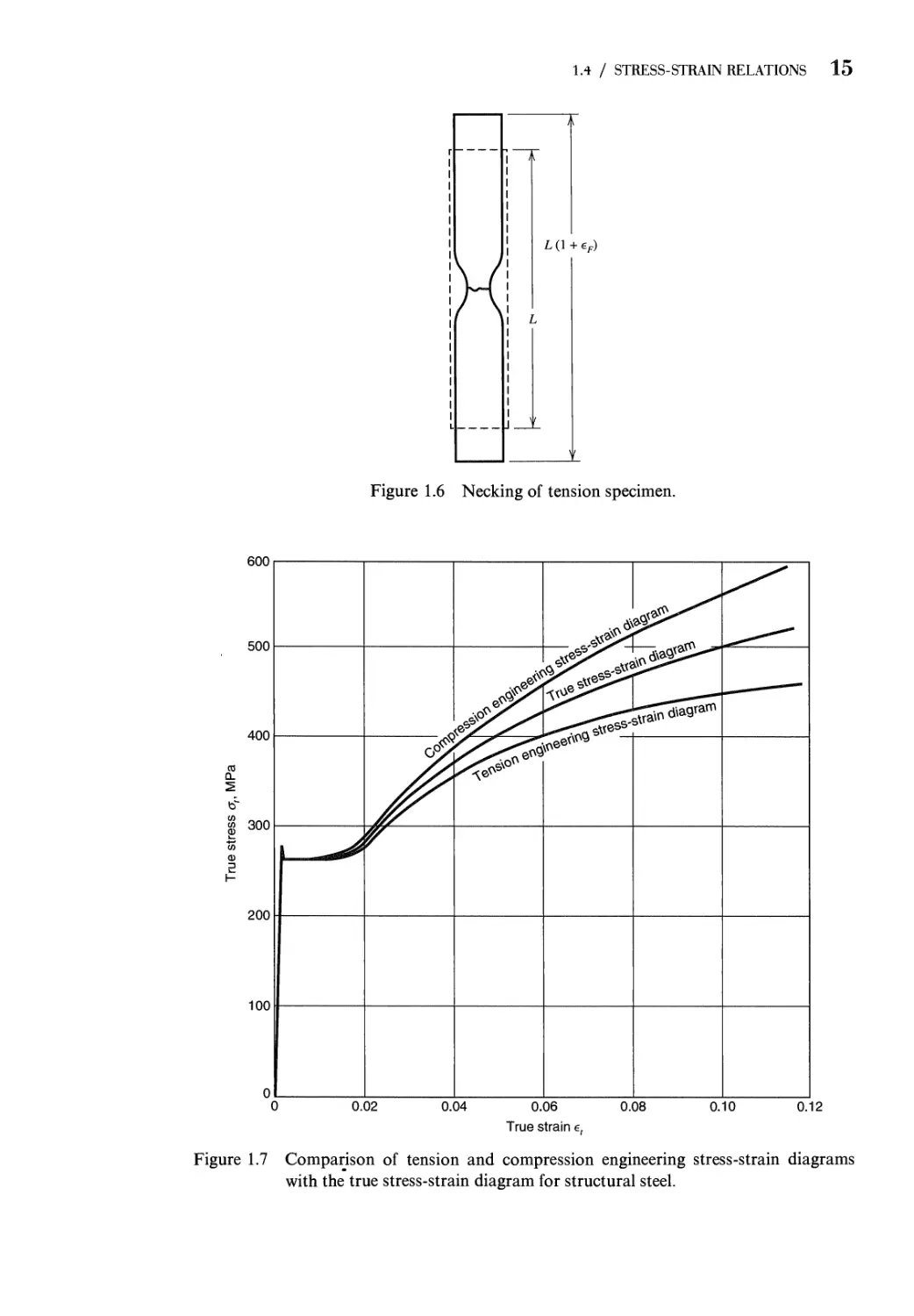
Necking of a Mild Steel Tension Specimen. As noted above, the stress-strain curve
for a mild steel tension specimen first reaches a local maximum called the upper yield
or plastic limit erF[/, after which it drops to a local minimum (the lower yield point Y)
and runs approximately (in a wavy fashion) parallel to the strain axis for some range
of strain. For mild steel, the lower yield point stress Y is assumed to be the stress
at which yield is initiated. After some additional strain, the stress rises gradually;
a relatively small change in load causes a significant change in strain. In this
region (ВС in Fig. 1.5a), substantial differences exist in the stress-strain diagrams,
depending on whether area A0 or At is used in the definition of stress. With area A0,
the curve first rises rapidly and then slowly, turning with its concave side down and
attaining a maximum value <ju, the ultimate strength, before turning down rapidly to
fracture (point F, Fig. 1.5a). Physically, after au is reached, the so-called necking of
the bar occurs, Fig. 1.6. This necking is a drastic reduction of the cross-sectional
area of the bar in the region where the fracture ultimately occurs. If the load P is
referred to the true cross-sectional area At and, hence, at = P/At9 the true stress-
strain curve differs considerably from the engineering stress-strain curve in the
region ВС (Figs. 1.5a and 1.7). In addition, the engineering stress-strain curves
for tension and compression differ considerably in the plastic region (Fig. 1.7),
because of the fact that in tension the cross-sectional area decreases with
increasing load, whereas in compression it increases with increasing load. However, as
can be seen from Fig. 1.7, little differences exist between the curves for small strains
(с, < 0.01).
1.4 / STRESS-STRAIN RELATIONS 15
H
L(l+eF)
Figure 1.6 Necking of tension specimen.
600
$ 300
c$
•tires'
^s^— ■
******
0.04 0.06 0.08
True strain e,
0.10
0.12
Figure 1.7 Comparison of tension and compression engineering stress-strain diagrams
with the true stress-strain diagram for structural steel.
16 1 / INTRODUCTION
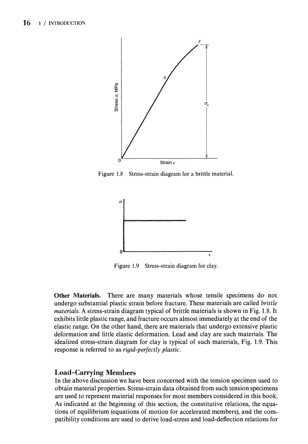
Figure 1.8 Stress-strain diagram for a brittle material.
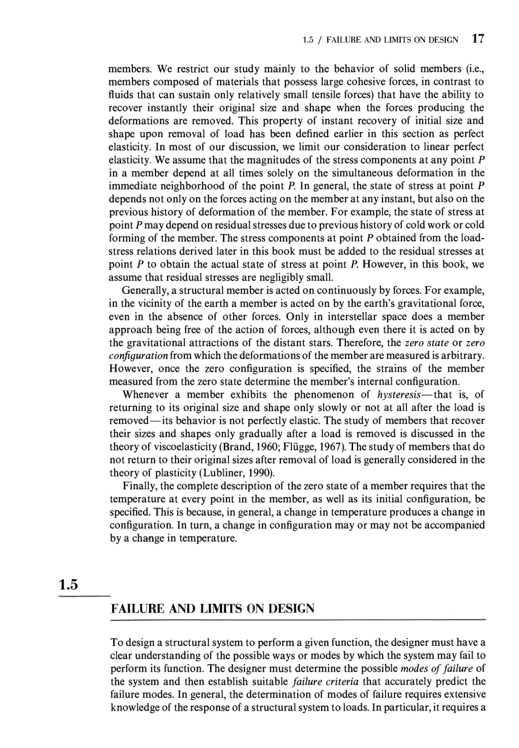
0I— , .
e
Figure 1.9 Stress-strain diagram for clay.
Other Materials. There are many materials whose tensile specimens do not
undergo substantial plastic strain before fracture. These materials are called brittle
materials. A stress-strain diagram typical of brittle materials is shown in Fig. 1.8. It
exhibits little plastic range, and fracture occurs almost immediately at the end of the
elastic range. On the other hand, there are materials that undergo extensive plastic
deformation and little elastic deformation. Lead and clay are such materials. The
idealized stress-strain diagram for clay is typical of such materials, Fig. 1.9. This
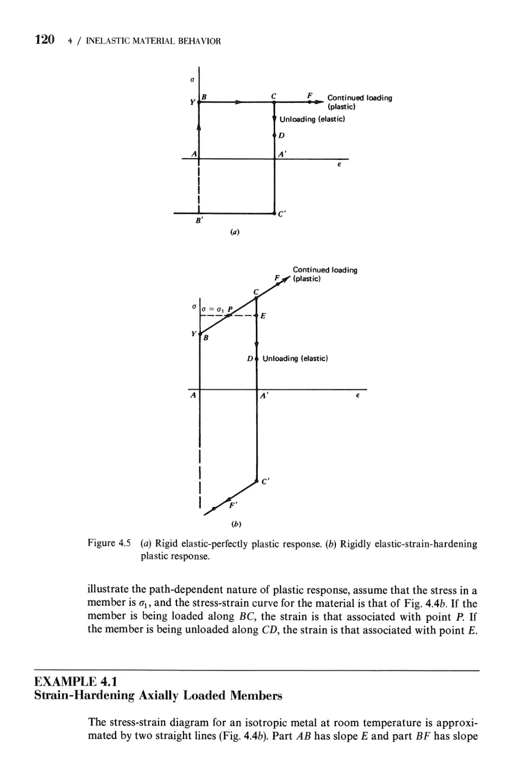
response is referred to as rigid-perfectly plastic.
Load-Carrying Members
In the above discussion we have been concerned with the tension specimen used to
obtain material properties. Stress-strain data obtained from such tension specimens
are used to represent material responses for most members considered in this book.
As indicated at the beginning of this section, the constitutive relations, the
equations of equilibrium (equations of motion for accelerated members), and the
compatibility conditions are used to derive load-stress and load-deflection relations for
1.5 / FAILURE AND LIMITS ON DESIGN 17
members. We restrict our study mainly to the behavior of solid members (i.e.,
members composed of materials that possess large cohesive forces, in contrast to
fluids that can sustain only relatively small tensile forces) that have the ability to
recover instantly their original size and shape when the forces producing the
deformations are removed. This property of instant recovery of initial size and
shape upon removal of load has been defined earlier in this section as perfect
elasticity. In most of our discussion, we limit our consideration to linear perfect
elasticity. We assume that the magnitudes of the stress components at any point P
in a member depend at all times solely on the simultaneous deformation in the
immediate neighborhood of the point P. In general, the state of stress at point P
depends not only on the forces acting on the member at any instant, but also on the
previous history of deformation of the member. For example, the state of stress at
point P may depend on residual stresses due to previous history of cold work or cold
forming of the member. The stress components at point P obtained from the load-
stress relations derived later in this book must be added to the residual stresses at
point P to obtain the actual state of stress at point P. However, in this book, we
assume that residual stresses are negligibly small.
Generally, a structural member is acted on continuously by forces. For example,
in the vicinity of the earth a member is acted on by the earth's gravitational force,
even in the absence of other forces. Only in interstellar space does a member
approach being free of the action of forces, although even there it is acted on by
the gravitational attractions of the distant stars. Therefore, the zero state or zero
configuration from which the deformations of the member are measured is arbitrary.
However, once the zero configuration is specified, the strains of the member
measured from the zero state determine the member's internal configuration.
Whenever a member exhibits the phenomenon of hysteresis—that is, of
returning to its original size and shape only slowly or not at all after the load is
removed—its behavior is not perfectly elastic. The study of members that recover
their sizes and shapes only gradually after a load is removed is discussed in the
theory of viscoelasticity (Brand, 1960; Fltigge, 1967). The study of members that do
not return to their original sizes after removal of load is generally considered in the
theory of plasticity (Lubliner, 1990).
Finally, the complete description of the zero state of a member requires that the
temperature at every point in the member, as well as its initial configuration, be
specified. This is because, in general, a change in temperature produces a change in
configuration. In turn, a change in configuration may or may not be accompanied
by a change in temperature.
FAILURE AND LIMITS ON DESIGN
To design a structural system to perform a given function, the designer must have a
clear understanding of the possible ways or modes by which the system may fail to
perform its function. The designer must determine the possible modes of failure of
the system and then establish suitable failure criteria that accurately predict the
failure modes. In general, the determination of modes of failure requires extensive
knowledge of the response of a structural system to loads. In particular, it requires a
18 1 / INTRODUCTION
comprehensive stress analysis of the system. Since the response of a structural
system depends strongly on the material used, so does the mode of failure. In turn,
the mode of failure of a given material also depends on the manner or history of
loading, such as the number of cycles of load applied at a particular temperature.
Accordingly, suitable failure criteria must account for different materials, different
loading histories, as well as factors that influence the stress distribution in the
member.
A major part of this book is concerned with A) stress analysis, B) material
behavior under load, and C) the relationship between the mode of failure and a
critical parameter associated with failure. The critical parameter that signals the
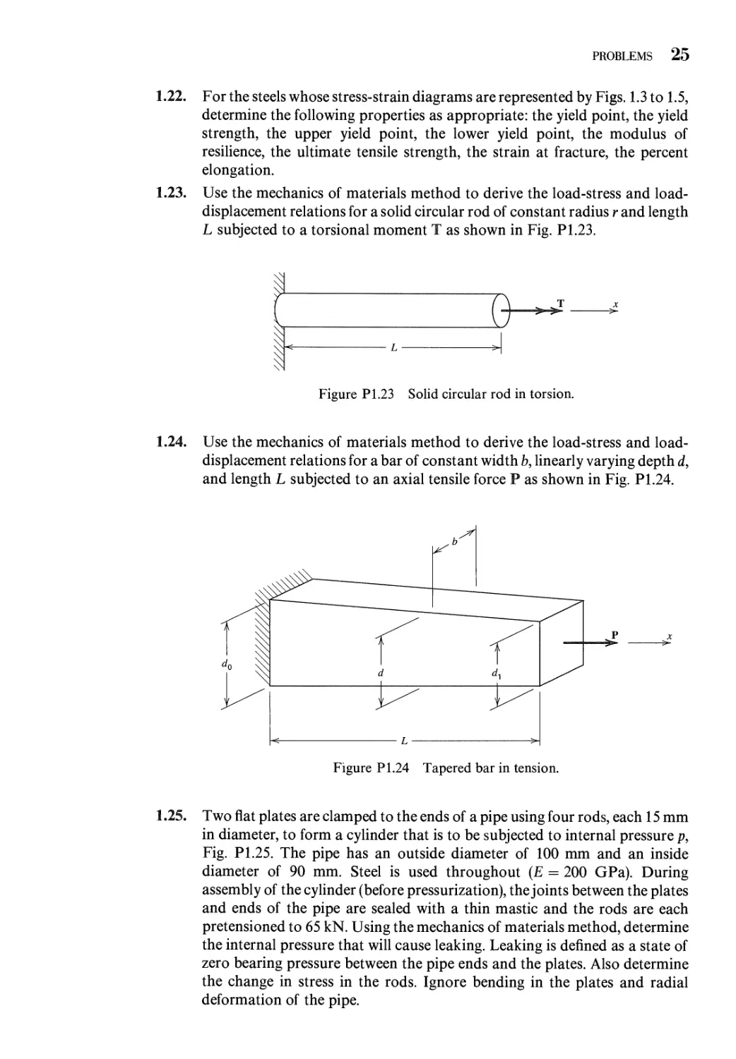
onset of failure might be stress, strain, displacement, load, number of load cycles, or
a combination of these. The discussion in this book is restricted to situations in
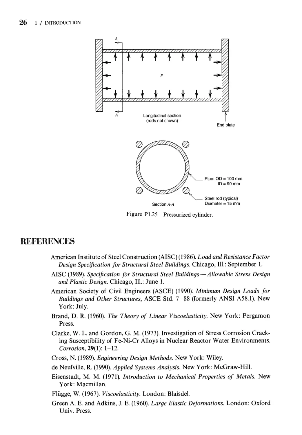
which failure of a system is related to only a single critical parameter. In addition, we
will examine the accuracy of the theories presented in the text with regard to their
ability to predict system behavior. In particular, limits on design will be introduced
utilizing factors of safety or reliability-based concepts that provide a measure of
safety against failure.
Historically, limits on the design of a system have been established using a factor
of safety. A factor of safety SF can be defined as
SF = |^ A.4)
where R„ is the nominal resistance (the critical parameter associated with failure)
and Rw is the safe working magnitude of that same parameter. The letter R is used to
represent the resistance of the system to failure. Generally, the magnitude of Rn is
based on theory or experimental observation. The factor of safety is chosen on the
basis of experiments or experience with similar systems made of the same material
under similar loading conditions. Then the safe working parameter jRw is
determined from Eq. A.4). The factor of safety must account for unknowns, including
variability of the loads, differences in material properties, deviations from the
intended geometry, and our ability to predict the critical parameter.
Generally, a design inequality is employed to relate load effects to resistance. The
design inequality is defined as
N Л
lQ^fF d.5)
where each Q, represents the effect of a particular working (or service-level) load,
such as internal pressure or temperature change, and N denotes the number of load
types considered.
More recently, design philosophies based on reliability concepts (Salmon and
Johnson, 1990) have been developed. It has been recognized that a single factor of
safety is inadequate to account for all the unknowns mentioned above.
Furthermore, each of the particular load types will exhibit its own statistical variability.
Consequently, appropriate load and resistance factors are applied to both sides
of the design inequality. So modified, the design inequality of Eq. A.5) may be
reformulated as
fttft^M, A.6)
1.5 / FAILURE AND LIMITS ON DESIGN 19
where the yt are the load factors for load effects Qt and ф is the resistance factor for
the nominal capacity Rn. The statistical variation of the individual loads is
accounted for in yh whereas the variability in resistance (associated with material
properties, geometry, and analysis procedures) is represented by ф. The use of this
approach, known as limit-states design, is more rational than the factor-of-safety
approach and produces a more uniform reliability throughout the system.
A limit state is a condition in which a system, or component, ceases to fulfill its
intended function. This definition is essentially the same as the definition of failure
used earlier in this text. However, some prefer the term limit state because the term
failure tends to imply only some catastrophic event (brittle fracture), rather than
an inability to function properly (excessive elastic deflections or brittle fracture).
Nevertheless, the term failure will continue to be used in this book in the more
general context.
EXAMPLE 1.1
Design of a Tension Rod
A steel rod is used as a tension brace in a structure. The structure is subjected to dead
load, live load, and snow load. The effect of each of the individual loads on the
tension brace is D = 25 kN, L = 60 kN, and W = 30 kN. Select a circular rod of
appropriate size to carry these loads safely. Use steel with a yield strength of 250
MPa. Make the selection using (a) factor-of-safety design and (b) limit-states design.
SOLUTION
For simplicity in this example, the only limit state that will be considered is yielding
of the cross section. Other limit states, including fracture of the member at the
connections to the remainder of the structure, are ignored.
(a) In factor-of-safety design (also known as allowable stress or working stress
design), the load effects are added without load factors. Thus, the total service-
level load is
YQt = D + L + W= 115 kN = 115,000 N (a)
The nominal resistance (capacity) of the tension rod is
Rn = YAg = B50 MPa)Ag (b)
where Ag is the gross area of the rod. In the design of tension members for steel
structures, a factor of safety of 5/3 is used (AISC, 1989). Hence, the design
inequality is
115,000 <^ (c)
which yields Ag > 161 mm2. A rod of 32-mm diameter, with a cross-sectional
area of 804 mm2, is adequate.
20 1 / INTRODUCTION
(b) In limit-states design, the critical load effect is determined by examination of
several possible load combination equations. These equations represent the
condition in which a single load quantity is at its maximum lifetime value,
whereas the other quantities are taken at an arbitrary point in time. The
relevant load combinations for this situation are specified (ASCE, 1990) as
IAD (d)
1.2D + 1.6L (e)
1.2D + 0.5L + 13W (f)
For the given load quantities, combination (e) is critical. The total load effect is
YjtQi = 126 kN = 126,000 N (g)
In the design of tension members for steel structures, a resistance factor of
ф = 0.9 is used (AISC, 1986). Hence, the limit-states design inequality is
126,000 < 0.9B50,4,) (h)
which yields Ag > 560 mm2. A rod of 28-mm diameter, with a cross-sectional
area of 616 mm2, is adequate.
Discussion
The objective of this example has been to demonstrate the use of different design
philosophies through their respective design inequalities, Eqs. A.5) and A.6). For the
conditions posed, the limit-states approach produces a more economical design
than the factor-of-safety approach. This can be attributed to the recognition in
the load factor equations (d-f) that it is highly unlikely both live load and wind
load would reach their maximum lifetime values at the same instant. Different
combinations of dead load, live load, and wind load, which still give a total service-
level load of 115 kN, could produce different factored loads and thus different area
requirements for the rod under limit-states design.
Modes of Failure
When a structural member is subjected to loads, its response depends not only on
the type of material from which it is made but also on the environmental conditions
and the manner of loading. Depending on how the member is loaded, it may fail by
excessive deflection, which results in the member being unable to perform its design
function; it may fail by plastic deformation (general yielding), which may cause a
permanent, undesirable change in shape; it may fail because of a fracture (break),
which depending on the material and the nature of loading may be of a ductile type
preceded by appreciable plastic deformation or of a brittle type with little or no prior
plastic deformation. Materials such as glass, ceramics, rocks, plain concrete, and
cast iron are examples of materials that fracture in a brittle manner under normal
environmental conditions and the slow application of tension load. In uniaxial
compression, they also fracture in a brittle manner, but the nature of the fracture is
quite different from that in tension. Depending on a number of conditions such as
1.5 / FAILURE AND LIMITS ON DESIGN 21
environment, rate of load, nature of loading, and presence of cracks or flaws,
structural metals may exhibit ductile or brittle fracture.
One type of loading that may result in brittle fracture of ductile metals is that of
repeated loads. For example, consider a uniaxially loaded bar with a smooth surface
that is subjected to repeated cycles of load. The bar may fail by fracture (usually, in a
brittle manner). Fracture of a structural member under repeated loads is commonly
called fatigue fracture or fatigue failure. Fatigue fracture may start by the initiation
of one or more small cracks, usually in the neighborhood of the maximum critical
stress in the member. Repeated cycling of the load causes the crack or cracks to
propagate until the structural member is no longer able to carry the load across the
cracked region, and the member ruptures.
Another manner in which a structural member may fail is that of elastic or plastic
instability. In this failure mode, the structural member may undergo large
displacements from its design configuration when the applied load reaches a critical value,
the so-called buckling load (or instability load). This type of failure may result in
excessive displacement or loss of ability (because of yielding or fracture) to carry
the design load. In addition to the above failure modes, a structural member may fail
because of environmental corrosion (chemical action).
To elaborate on the modes of failure of structural members, we discuss more fully
the following categories of failure modes:
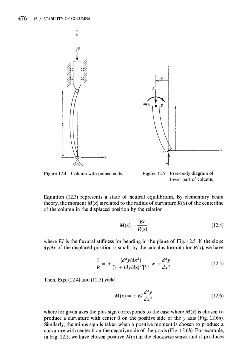
1. Failure by excessive deflection
(a) Elastic deflection
(b) Deflection due to creep
2. Failure by general yielding
3. Failure by fracture
(a) Sudden fracture of brittle materials
(b) Fracture of cracked or flawed members
(c) Progressive fracture (fatigue)
These failure modes and their associated failure criteria are most meaningful for
simple structural members (e.g., tension members, columns, beams, circular cross
section torsion members). For more complicated two- and three-dimensional
problems, the significance of such simple failure modes is open to question.
Manyof these modes of failure for simple structural members are well-known to
engineers. However, under unusual conditions of load or environment, other types
of failure may occur. For example, in nuclear reactor systems, cracks in pipe loops
have been attributed to stress-assisted corrosion cracking, with possible side effects
attributable to residual welding stresses (Clarke and Gordon, 1973; Hakala et al,
1990; Scott and Tice, 1990).
The physical action in a structural member leading to failure is usually a
complicated phenomenon, and in the following discussion the phenomena are
necessarily oversimplified, but they nevertheless retain the essential features of the
failures.
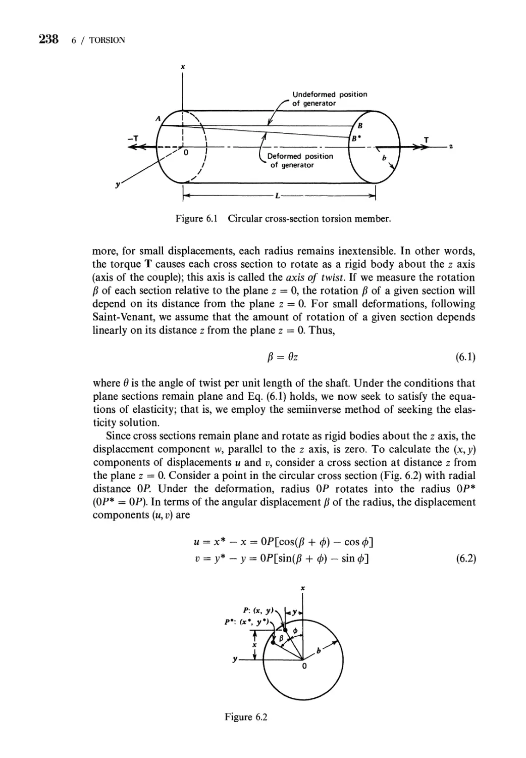
1. Failure by Excessive Elastic Deflection. The maximum load that may be applied
to a member without causing it to cease to function properly may be limited by the
permissible elastic strain or deflection of the member. Elastic deflection that may
22 1 / INTRODUCTION
cause damage to a member can occur under these different conditions:
(a) Deflection under conditions of stable equilibrium, such as the stretch of a
tension member, the angle of twist of a shaft, and the deflection of an end-
loaded cantilever beam. Elastic deflections, under conditions of equilibrium,
are computed in Chapter 5.
(b) Buckling, or the rather sudden deflection associated with unstable equilibrium
and often resulting in total collapse of the member. This occurs, for example,
when an axial load, applied gradually to a slender column, exceeds the Euler
load. See Chapter 12.
(c) Elastic deflections that are the amplitudes of the vibration of a member
sometimes are associated with failure of the member resulting from
objectionable noise, shaking forces, collision of moving parts with stationary
parts, etc., which result from the vibrations.
When a member fails by elastic deformation, the significant equations for design
are those that relate loads and elastic deflection. For example, the equations, for the
three members mentioned under (a) are e = PL/AE, 0 = TL/GJ, and S = WL3/3EI.
It is noted that these equations contain the significant property of the material
involved in the elastic deflection, namely, the modulus of elasticity E (sometimes
called the stiffness) or the shear modulus G = £/[2A + v)], where v is Poisson's
ratio. The stresses caused by the loads are not the significant quantities; that is, the
stresses do not limit the loads that can be applied to the member. In other words, if a
member of given dimensions fails to perform its load-resisting function because of
excessive elastic deflection, its load-carrying capacity is not increased by making the
member of stronger material. As a rule, the most effective method of decreasing the
deflection of a member is by changing the shape or increasing the dimensions of its
cross section, rather than by making the member of a stiffer material.
2. Failure by General Yielding. Another condition that may cause a member to fail
is general yielding. General yielding is inelastic deformation of a considerable
portion of the member, distinguishing it from localized yielding of a relatively small
portion of the member. The following discussion of yielding addresses the behavior
of metals at ordinary temperatures, that is, at temperatures that do not exceed the
recrystallization temperature. Yielding at elevated temperatures (creep) is discussed
in Chapter 17.
Polycrystalline metals are composed of extremely large numbers of very small
units called crystals or grains. The crystals have slip planes on which the resistance
to shear stress is relatively small. Under elastic loading, before slip occurs, the crystal
itself is distorted due to stretching or compressing of the atomic bonds from their
equilibrium state. If the load is removed, the crystal returns to its undistorted shape
and no permanent deformation exists. When a load is applied that causes the yield
strength to be reached, the crystals are again distorted but, in addition, defects in the
crystal, known as dislocations (Eisenstadt, 1971), move in the slip planes by breaking
and reforming atomic bonds. After removal of the load, only the distortion of the
crystal (due to bond stretching) is recovered. The movement of the dislocations
remains as permanent deformation.
After sufficient yielding has occurred in some crystals at a given load, these
crystals will not yield further without an increase in load. This is due to the
formation of dislocation entanglements that make motion of the dislocations more
1.5 / FAILURE AND LIMITS ON DESIGN 23
and more difficult. A higher and higher stress will be needed to push new
dislocations through these entanglements. This increased resistance that develops
after yielding is known as strain hardening or work hardening. Strain hardening is
permanent. Hence, for strain-hardening metals, the plastic deformation and increase
in yield strength are both retained after the load is removed.
When failure occurs by general yielding, stress concentrations usually are not
significant because of the interaction and adjustments that take place between
crystals in the regions of the stress concentrations. Slip in a few highly stressed
crystals does not limit the general load-carrying capacity of the member, but merely
causes readjustment of stresses that permit the more lightly stressed crystals to take
higher stresses. The stress distribution approaches that which occurs in a member
free from stress concentrations. Thus, the member as a whole acts substantially as an
ideal homogeneous member, free from abrupt changes of section.
It is important to observe that if a member that fails by yielding is replaced by one
with a material of a higher yield stress, the mode of failure may change to that of
elastic deflection, buckling, or excessive mechanical vibrations. Hence, the entire
basis of design may be changed when conditions are altered to prevent a given mode
of failure.
3. Failure by Fracture. Some members cease to function satisfactorily because
they break (fracture) before either excessive elastic deflection or general yielding
occurs. Three rather different modes or mechanisms of fracture that occur especially
in metals are discussed briefly below.
(a) Sudden Fracture of Brittle Material. Some materials—so-called brittle
materials—function satisfactorily in resisting loads under static conditions until
the material breaks rather suddenly with little or no evidence of plastic
deformation. Ordinarily, the tensile stress in members made of such materials is
considered to be the significant quantity associated with the failure, and the
ultimate strength ou is taken as the measure of the maximum utilizable strength
of the material (Fig. 1.8).
(b) Fracture of Flawed Members. A member made of a ductile metal and
subjected to static tensile loads will not fracture in a brittle manner so long as the
member is free of flaws (cracks, notches, or other stress concentrations) and the
temperature is not unusually low. However, in the presence of flaws, ductile
materials may experience brittle fracture at normal temperatures. The flaw often
contributes to development of a high hydrostatic tension stress (hydrostatic
stress is discussed in Chapter 2). Yielding of ductile metals is not influenced
significantly by hydrostatic stress so plastic deformation may be small or
nonexistent even though fracture is impending. Thus, yield strength is not the
critical material parameter when failure occurs by brittle fracture. Instead, notch
toughness, the ability of a material to absorb energy in the presence of a notch (or
other flaw), is the parameter that governs the failure mode. Dynamic loading and
low temperatures also increase the tendency of a material to fracture in a brittle
manner. Failure by brittle fracture is discussed in Chapter 15.
(c) Progressive Fracture (Fatigue). If a metal that ordinarily fails by general
yielding under a static load is subjected to repeated cycles of stress, it may fail by
fracture without visual evidence of yielding, provided that the repeated stress is
greater than a value called the fatigue strength. Under such conditions, minute
24 1 / INTRODUCTION
cracks start at one or more points in the member, usually at points of high
localized stress such as at abrupt changes in section, and gradually spread by
fracture of the material at the edges of the cracks where the stress is highly
concentrated. The progressive fracture continues until the member finally breaks.
This mode of failure is usually called a fatigue failure, but it is better designated as
failure by progressive fracture resulting from repeated loads. (See Chapter 16.)
The quantity usually considered most significant in failure by progressive
fracture is localized tensile stress (although the fatigue crack sometimes occurs on the
plane of maximum shear stress), and the maximum utilizable strength of the
material is considered to be the stress {fatigue strength) corresponding to a given
"life" (number of repetitions of stress). If the material has an endurance limit (fatigue
strength for infinite life) and a design for so-called infinite life is desired, then the
endurance limit is the limiting resistance value or maximum utilizable strength of
the material (Chapter 16).
PROBLEMS
1.1. What requirements control the derivation of load-stress relations?
1.2. Describe the method of mechanics of materials.
1.3. How are stress-strain-temperature relations for a material established?
1.4. Explain the differences between elastic response and inelastic response of a
solid.
1.5. What is a stress-strain diagram?
1.6. Explain the difference between elastic limit and proportional limit.
1.7. Explain the difference between the concepts of yield point and yield stress.
1.8. What is offset strain?
1.9. How does the engineering stress-strain diagram differ from the true stress-
strain diagram?
1.10. What are modes of failure?
1.11. What are failure criteria? How are they related to modes of failure?
1.12. What is meant by the term factor of safety? How are factors of safety used in
design?
1.13. What is a design inequality?
1.14. How is the usual design inequality modified to account for statistical
variability?
1.15. What is a load factor? A load effect? A resistance factor?
1.16. What is a limit-states design?
1.17. What is meant by the phrase "failure by excessive deflection?"
1.18. What is meant by the phrase "failure by yielding?"
1.19. What is meant by the phrase "failure by fracture?"
1.20. Discuss the various ways that a structural member may fail.
1.21. Discuss the failure modes, critical parameters, and failure criteria that may
apply to the design of a downhill snow ski.
PROBLEMS 25
1.22. For the steels whose stress-strain diagrams are represented by Figs. 1.3 to 1.5,
determine the following properties as appropriate: the yield point, the yield
strength, the upper yield point, the lower yield point, the modulus of
resilience, the ultimate tensile strength, the strain at fracture, the percent
elongation.
1.23. Use the mechanics of materials method to derive the load-stress and load-
displacement relations for a solid circular rod of constant radius r and length
L subjected to a torsional moment T as shown in Fig. P1.23.
Figure PI.23 Solid circular rod in torsion.
1.24. Use the mechanics of materials method to derive the load-stress and load-
displacement relations for a bar of constant width b, linearly varying depth d,
and length L subjected to an axial tensile force P as shown in Fig. P1.24.
Figure P1.24 Tapered bar in tension.
1.25. Two flat plates are clamped to the ends of a pipe using four rods, each 15 mm
in diameter, to form a cylinder that is to be subjected to internal pressure p,
Fig. P1.25. The pipe has an outside diameter of 100 mm and an inside
diameter of 90 mm. Steel is used throughout (E = 200 GPa). During
assembly of the cylinder (before pressurization), the joints between the plates
and ends of the pipe are sealed with a thin mastic and the rods are each
pretensioned to 65 kN. Using the mechanics of materials method, determine
the internal pressure that will cause leaking. Leaking is defined as a state of
zero bearing pressure between the pipe ends and the plates. Also determine
the change in stress in the rods. Ignore bending in the plates and radial
deformation of the pipe.
26 1 / INTRODUCTION
V//////X//.
/|\ m Ж /Л А Ж Я\
W W W W W W W
А Longitudinal section
(rods not shown)
4
T
End plate
Pipe:OD= 100 mm
ID = 90 mm
Section A-A
Figure P1.25 Pressurized cylinder.
Steel rod (typical)
Diameter = 15 mm
REFERENCES
American Institute of Steel Construction (AISC) A986). Load and Resistance Factor
Design Specification for Structural Steel Buildings. Chicago, 111.: September 1.
AISC A989). Specification for Structural Steel Buildings—Allowable Stress Design
and Plastic Design. Chicago, 111.: June 1.
American Society of Civil Engineers (ASCE) A990). Minimum Design Loads for
Buildings and Other Structures, ASCE Std. 7-88 (formerly ANSI A58.1). New
York: July.
Brand, D. R. A960). The Theory of Linear Viscoelasticity. New York: Pergamon
Press.
Clarke, W. L. and Gordon, G. M. A973). Investigation of Stress Corrosion
Cracking Susceptibility of Fe-Ni-Cr Alloys in Nuclear Reactor Water Environments.
Corrosion, 29A): 1-12.
Cross, N. A989). Engineering Design Methods. New York: Wiley.
de Neufville, R. A990). Applied Systems Analysis. New York: McGraw-Hill.
Eisenstadt, M. M. A971). Introduction to Mechanical Properties of Metals. New
York: Macmillan.
Fliigge, W. A967). Viscoelasticity. London: Blaisdel.
Green A. E. and Adkins, J. E. A960). Large Elastic Deformations. London: Oxford
Univ. Press.
REFERENCES 27
Hakala, J., Hanninen, H., and Asltonen, P. A990). Stress Corrosion and Thermal
Fatigue. Nucl Eng. Design, 119B, 3): 389-398.
Lubliner, J. A990). Plasticity Theory. New York: Macmillan.
Salmon, C. G. and Johnson, J. E. A990). Steel Structures—Design and Behavior,
3rd ed. New York: Harper & Row.
Scott, P. M. and Tice, D. R. A990). Stress Corrosion in Low-Alloy Steels. Nucl Eng.
Design, 119B, 3): 399-414.
THEORIES OF STRESS
AND STRAIN
In Chapter 1, we presented general concepts and definitions that are fundamental
to many of the topics discussed in this book. In this chapter, we develop theories
of stress and strain that are essential for the analysis of the behavior of a
structural or mechanical system subjected to loads. The relations developed are used
throughout the remainder of the book.
DEFINITION OF STRESS AT A POINT
Consider a general body subjected to forces acting on its surface (Fig. 2.1). Pass a
fictitious plane Q through the body, cutting the body along surface A (Fig. 2.2).
Designate one side of plane Q as positive and the other side as negative. The
portion of the body on the positive side of Q exerts a force on the portion of the body
on the negative side. This force is transmitted through the plane Q by direct contact
of the parts of the body on the two sides of Q. Let the force that is transmitted
through an incremental area A A of A by the part on the positive side Q be denoted
by AF. In accordance with Newton's third law, the portion of the body on the
negative side of Q transmits through area A A a force — AF.
The force AF may be resolved into components AFN and AFS, along unit normal
N and unit tangent S, respectively, to the plane Q. The force AFN is called the normal
{perpendicular) force on area A A and AFS is called the shear (tangential) force on
A A. The forces AF, AFN, and AFS depend on the area A A and the orientation of
plane Q. The magnitudes of the average forces per unit area are AF/AA, AFN/AA,
and AFS/AA. These ratios are called the average stress, average normal stress, and
average shear stress, respectively, acting on area A A. The concept of stress at a
point is obtained by letting A A become an infinitesimal. Then the forces AF, AFN,
and AFS approach zero, but usually the ratios AF/АЛ, A¥N/AA, and AFS/A^
approach limits different from zero. The limiting ratio of AF/AA as A A goes to
zero defines the stress vector a. Thus, the stress vector a is given by
The stress vector a (also called the traction vector) always lies along the limiting
direction of the force vector AF, which in general is neither perpendicular nor
tangent to the plane Q.
2.1 / DEFINITION OF STRESS AT A POINT 29
,v;
Figure 2.1 A general loaded body cut by plane Q.
-^\ v\l \"'
A
V-
4AF
Figure 2.2 Force transmitted through incremental area of cut body.
30 2 / THEORIES OF STRESS AND STRAIN
2,2
Similarly, the limiting ratios of A¥N/AA and AFS/A^4 define the normal stress
vector aN and the shear stress vector as that act at a point in the plane Q. These
stress vectors are defined by the relations
ffN = hm -r-j, as = hm —- B.2)
ДЛ-^O &A AA^O
ЛАТЫ unit vectors associated with % and as are perpendicular and tangent,
respectively, to the plane Q.
STRESS NOTATION
We use free-body diagrams to specify the state of stress at a point and to obtain
relations between various stress components. In general a free-body diagram may
be a diagram of a complete member, a portion of the member obtained by passing
a cutting plane through the member, or a boxlike volume element of the member.
The loads that act on any of these free bodies can be divided into two types as
follows:
1. Surface forces, which are forces that act on the surface of the free body
2. Body forces, which are forces that act throughout the volume of that portion
of the member considered in the free-body diagram
Examples of surface forces are contact forces and distributed loads. Concentrated
loads and reactions at a point are considered contact forces. Distributed loads may
be either line loads with dimensions of force per unit length or surface loads with
dimensions of force per unit area (dimensions of pressure or stress). Distributed
loads on beams are often indicated as loads per unit length. Examples of surface
loads are pressure exerted by a fluid in contact with the body and normal and shear
stresses that act on a cut section of the body.
Examples of body forces are gravitational forces, magnetic forces, and inertia
forces. Since the body force is distributed throughout the volume of the free body,
it is convenient to define body force per unit volume. We use the notation В or
(Bx9By,Bz) for body force per unit volume, where В stands for body and subscripts
(x, y, z) denote components in the (x, v, z) directions, respectively, of the rectangular
coordinate system (x,y,z) (see Fig. 2.3).
Consider now a free-body diagram of a box-shaped volume element at a point
0 in a member, with sides parallel to the (x, y, z) axes (Fig. 2.4). For simplicity, we
show the volume element with one corner at point 0 and assume that the stress
components are uniform (constant) throughout the volume element. The surface
forces are represented by the product of the stress components (Fig. 2.4) and the
areas* on which they act. Body forces, represented by the product of the compo-
* The reader must multiply each stress component by an appropriate area before applying equations of
force equilibrium. For example, axx must be multiplied by the area dy dz.
2.2 / STRESS NOTATION 31
Figure 2.3 Body forces.
Figure 2.4 Stress components at a point in loaded body.
nents (Bx, By, Bz) and the volume of the element (product of the three infinitesimal
lengths of the sides of the element), are higher-order terms and are not shown on
the free-body diagram in Fig. 2.4. Consider the two faces perpendicular to the x
axis. The face from which the positive x axis is extended is taken to be the positive
face; the other face perpendicular to the x axis is taken to be the negative face. The
stress components axx, axy, and oxz acting on the positive face are taken to be in the
positive sense as shown when they are directed in the positive x, y, and z directions.
32 2 / THEORIES OF STRESS AND STRAIN
2.3
By Newton's third law, the positive stress components axx, oxy, and oxz shown
acting on the negative face in Fig. 2.4 are in the negative (x, y, z) directions,
respectively. In effect, a positive stress component oxx exerts a tension (pull) parallel to
the x axis. Equivalent sign conventions hold for the planes perpendicular to the у
and z axes. Hence, associated with the concept of the state of stress at a point 0,
nine components of stress exist.
(°xx > Gxy > Gxz\ (&УУ' °yx> °yz)> (azz > <*zx, ^zy)
In the next section we show that the nine stress components may be reduced to six
for most practical problems.
SYMMETRY OF THE STRESS ARRAY AND STRESS ON
AN ARBITRARILY ORIENTED PLANE
Symmetry of Stress Components
The nine stress components relative to rectangular coordinate axes (x, y, z) may be
tabulated in array form as follows:
T =
"xx ®xy "jc:
Oyx ®yy Oy:
CTZX Ozy Gz:
B.3)
where T symbolically represents the stress array called the stress tensor. In this
array, the stress components in the first, second, and third rows act on planes
perpendicular to the (x, v, z) axes, respectively. Seemingly, nine stress components are
required to describe the state of stress at a point in a member. However, if the only
forces that act on the free body in Fig. 2.4 are surface forces and body forces, we
can demonstrate from the equilibrium of the volume element in Fig 2.4 that the
three pairs of the shear stresses are equal. Summation of moments leads to the
result
B.4)
Thus, with Eq. B.4), Eq. B.3) may be written in the symmetric form
^ xx ^ xy ®x:
®xy ®yy Uy:
axz oyz crz.
B-5)
Hence, for this type of stress theory, only six components of stress are required to
describe the state of stress at a point in a member.
Although we do not consider body couples or surface couples in this book
(Boresi and Chong, 1987), it is possible for them to be acting on the free body in
Fig. 2.4. This means that Eqs. B.4) are no longer true and that nine stress
components are required to represent the unsymmetrical state of stress.
2.3 / SYMMETRY OF STRESS, STRESS ON AN ARBITRARY PLANE 33
TABLE 2.1
Stress Notations (Symmetric Stress Components)
I
II
III
Gxx
°x
011
ayy
Oy
<?22
azz
°z
^33
®xy Gyx
T = T
'"xy ^yx
°\2 = °2\
Gxz = <*zx
^xz = ^zx
CT13 = CT31
Gyz = °zy
Tyz ~ 1zy
CT23 = <732
The stress notation described above is widely used in engineering practice. It is
the notation used in this book,* row I of Table 2.1. Two other frequently used
symmetric stress notations are also listed in Table 2.1. The symbolism indicated in row
III is employed where index notation is used (Boresi and Chong, 1987).
Stresses Acting on Arbitrary Planes
The stress vectors ax, ay, and az on planes that are perpendicular, respectively, to
the x, y, and z axes are
°y = <V + Gyyl + <Vk
az = azxi + azyi + azzk B.6)
where i, j, and к are unit vectors relative to the (x, y, z) axes (see Fig. 2.5 for ax). Now
consider the stress vector aP on an arbitrary oblique plane P through point 0 of a
member (Fig. 2.6). For clarity, the plane P is shown removed from point 0. The unit
normal vector to plane P is
N = /i + m\ + nk B.7)
Figure 2.5 Stress vector and its components acting on a plane perpendicular to the x axis.
* Equivalent notations are used for other orthogonal coordinate systems (see Sec. 2.5.).
34 2 / THEORIES OF STRESS AND STRAIN
Figure 2.6 Stress vector on arbitrary plane having a normal N.
where (/, m, n) are the direction cosines of unit vector N. Therefore, vectorial
summation of forces acting on the tetrahedral element OABC yields the following (note
that the ratios of areas OBC, (L4C, OB A to area ABC are equal to /, m, and n,
respectively):
Op = lax + may + naz B.8)
Also, in terms of the projections {oPx,(JPy,ePz) of the stress vector aP along axes
(x, y, z), we may write
o-p = o-P;ci + <7P)j + о>гк B.9)
Comparison of Eqs. B.8) and B.9) yields, with Eqs. B.6)
Opx = loxx + mGyx + nazx
aPy = loxy + moyy + nazy
<7Fz = loxz + m<7yz + nazz B.10)
Equations B.10) allow the computation of the components of stress on any oblique
plane defined by unit normal N:(/, m, n), provided that the six components of stress
Gxx> Gyy, °zz> Gxy = Gyx> Gxz = Gzx> Gyz = Gzy
at point 0 are known. When point 0 lies on the surface of the member where the
surface forces are represented by distributions of normal and shear stresses,
Eqs. B.10) represent the stress boundary conditions at point 0.
Normal Stress and Shear Stress on an Oblique Plane
The normal stress gpn on the plane P is the projection of the vector aP in the
direction of N; that is, aPN = eP • N. Hence, by Eqs. B.7), B.9), and B.10)
°pn = l2°xx + ™2vyy + n2azz + mn(ayz + ozy) + nl{oxz + ozx)
+ ЩОху + Gyx)
= l2axx + m2ayy + n2ozz + 2mnoyz + 2lnaxz + 2lmaxy B.11)
2.4 / TRANSFORMATION OF STRESS, PRINCIPAL STRESSES 35
Figure 2.7 Normal and shear stress components of stress vector on an arbitrary plane.
By Eq. B.11), the normal stress aPN on an oblique plane with unit normal N:(/, m, n)
is expressed in terms of the six stress components ((Txx,Gyy9azzi(Txy,<Txz9azy). Often,
the maximum value of aPN at a point is of importance in design (see Sec. 4.1). Of
the infinite number of planes through point 0, aPN attains a maximum value called
the maximum principal stress on one of these planes. The method of determining
this stress and the orientation of the plane on which it acts is given in Sec. 2.4.
To compute the magnitude of the shear stress aPS on plane P, we note by
geometry (Fig. 2.7) that
aPS = yjoj, - <j2pn = V^p* + (Tpy + сг|г - о™ B.12)
Substitution of Eqs. B.10) and B.11) into Eq. B.12) yields oPS in terms of
{pxx,uyy9GzziGxy,(TXZ9ayz) and (l,m,ri). In certain criteria of failure, the maximum
value of <tps at a point in the body plays an important role (see Sec. 4.4). The
maximum value of aPS can be expressed in terms of the maximum and minimum
principal stresses [see Eq. B.39), Sec. 2.4].
TRANSFORMATION OF STRESS. PRINCIPAL
STRESSES. OTHER PROPERTIES
Transformation of Stress
Let (x, y, z) and (X, Y, Z) denote two rectangular coordinate systems with a
common origin (Fig. 2.8). The cosines of the angles between the coordinate axes
(x, y, z) and the coordinate axes (X, Y, Z) are listed in Table 2.2. Each entry in
Table 2.2 Is the cosine of the angle between the two coordinate axes designated at
the top of its column and to the left of its row. The angles are measured from the
(x,y,z) axes to the (X, Y,Z) axes. For example, lx = cosOxX, l2 = cos6xY,... (see
Fig. 2.8.). Since the axes (x, y, z) and axes (X, Y, Z) are orthogonal, the direction
cosines of Table 2.2 must satisfy the following relations:
For the Row Elements
lf + mf + nf = l, i= 1,2,3, and lj2 + mim2 + ^1n2 = 0,...,... B.13)
For the Column Elements
l* + ll + ll = 1,...,..., and l1m1 + l2m2 + /3m3 = 0,...,... B.14)
The stress components oXX9gxy,oxz,... are defined with reference to (X, Y,Z)
axes in the same manner as axx, cr <rxzi... are defined relative to the axes (x,y, z).
36 2 / THEORIES OF STRESS AND STRAIN
Plane perpendicular
to X-axis
Figure 2.8 Stress components on plane perpendicular to transformed X axis.
TABLE 2.2
Direction Cosines
X
Y
Z
X
h
h
h
У
m1
m2
Щ
z
"i
«2
«3
Hence, <jxx is the normal stress component on a plane perpendicular to axis X and
aXY, oxz are shear stress components on this same plane (Fig. 2.8), and so on.
Hence, by Eq. B.11),
°xx = 1\<*хх + m\<*yy + n\axz + 2m1n1ffyz + 2щ\&хх + Ihm^a^
Gyy ■■
l\oxx + m\ayy + w|cr2Z + 2m2n2G + 2n2l2azx + 2l2m2ax,
<*zz = li0"** + ™зЧу + "зЧ* + 2m3n3oyz + 2n3l3azx + 2l3m3axy B.15)
The shear stress component rjxy is the component of the stress vector in the Y
direction on a plane perpendicular to the X axis; that is, it is the Y component
of the stress vector ax acting on the plane perpendicular to the X axis. Thus, aXY
may be evaluated by forming the scalar product of the vector ax [determined by
Eqs. B.9) and B.10) with lx = l,mx = m, n1 = n\ with a unit vector parallel to the
Y axis; that is, with the unit vector (Table 2.2)
N2 = l2\ + m2j + n2k
B.16)
By Eqs. B.9). B.10), and B.16), oXY is determined; similar procedures also
determine oxz and aYZ • Hence,
GXY = ax-N2 = ayN1
= IJiGxx + m1m2ayy + n1n2a„ + (m^a + т2п^)оу,
+ (/^2 + ^K* + A^2 + \2m^)oxy
B.17a)
2.4 / TRANSFORMATION OF STRESS, PRINCIPAL STRESSES 37
oxz = ax . N3 = /i/gff,, + т^вуу + и^з^ + (т±п3 + т^о^
+ (/^з + hn^a^ + (/^3 + /3WiK:
(TrZ =
•N,
: Уз^х* + m2m3ayy + n2n3azz + (m2n3 + m3n2)ayi
+ (/2«з + *зК* + P2W3 + hmiiOxj
B.17b)
B.17c)
Equations B.15) and B.17) determine the stress components relative to rectangular
axes (X, Y, Z) in terms of the stress components relative to rectangular axes (x, y, z);
that is, they determine how the stress components transform under a rotation of
rectangular axes. A set of quantities that transform according to this rule is called
a second-order symmetrical tensor. Later it will be shown that strain components
(see Sec. 2.7) and moments and products of inertia (see Sec. B.3) also transform
under rotation of axes by similar relationships; hence, they too are second-order
symmetrical tensors.
Principal Stresses
It may be shown that for any general state of stress at any point 0 in a body, there
exist three mutually perpendicular planes at point 0 on which the shear stresses
vanish. The remaining normal stress components on these three planes are called
principal stresses. Correspondingly, the three planes are called principal planes, and
the three mutually perpendicular axes that are normal to the three planes (hence,
that coincide with the three principal stress directions) are called principal axes.
Thus, by definition, principal stresses are directed along principal axes that are
perpendicular to the principal planes. A cubic element subjected to principal stresses
is easily visualized, since the forces on the surface of the cube are normal to the
faces of the cube. More complete discussions of principal stress theory are present
elsewhere (Boresi and Chong, 1987). Here we merely sketch the main results.
Principal Values and Directions
Since the shear stresses vanish on principal planes, the stress vector on principal
planes is given by eP = aN, where a is the magnitude of the stress vector <rP and N
the unit normal to a principal plane. Let N = l\ + mj + nk relative to rectangular
axes (x, y, z) with associated unit vectors i, j, k. Thus, (/, m, n) are the direction
cosines of the unit normal N. Projections of o> along (x, y, z) axes are oPx = al,
oPy =am, opz = an. Hence, by Eq. B.10), we obtain
1(gxx -g) + maxy + naxz = 0
laxy + m(oyy — a) + noy.
= 0
laxz + mo■ + n(azz — о) = О
B.18)
Since Eqs. B.18) are linear homogeneous equations in (/,m,w) and the trivial
solution / = m = n — 0 is impossible because I2 + m2 + n2 = 1 [law of direction
cosines, Eq. B.13)], it follows from the theory of linear algebraic equations that
Eqs. B.18) are consistent if and only if the determinant of the coefficients of (/, m, n)
vanishes identically. Thus, we have
<*xz
• <* Gyz
B.19)
38 2 / THEORIES OF STRESS AND STRAIN
or, expanding the determinant, we obtain
where
о-3 - Ito2 - /2<7 - J3 = 0
*1 = Gxx + О + Ozl
B.20)
u = ~
<*xx
°ху
Gxy
<Jyy
°xx
°xz
<*xz
<*zz
Oyy
Gyz
Gyz
<*zz
0"v*O^ — O^G„.
h =
<fxx
axy
<*xz
axy
Oyy
Vyz
Ъ
ff3
Ъ
B.21)
The three roots @i,02,<73) of Eq. B.20) are the three principal stresses at point 0.
The magnitudes and directions of al5 <r2, and cr3 for a given member depend only
on the loads being applied to the member and cannot be influenced by the choice
of coordinate axes (x, y, z) used to specify the state of stress at point 0. This means
that Il9 ll9 and J3 given by Eqs. B.21) are invariants of stress and must have the
same magnitudes for all choices of coordinate axes (x, y, z). Relative to principal
axes, the stress invariants may be written in terms of the principal stresses as
lx = g1 + <j2 + o-3
h = — °i02 — °2аъ — <?1°ъ
h - о^въ
When (а19а2,оъ) have been determined, the direction cosines of the three
principal axes are obtained from Eqs. B.18) by setting о in turn equal to (о19а29оъ\
respectively, and observing the direction cosine condition /2 + m2 + w2 = lfor
each of the three values of <r. See Example 2.1.
In special cases, two principal stresses may be numerically equal. Then,
Eqs. B.18) show that the associated principal directions are not unique. In these
cases, any two mutually perpendicular axes that are perpendicular to the unique
third principal axis will serve as principal axes with corresponding principal planes.
If all three principal stresses are equal, then ox — <r2 = tr3 at point 0, and all planes
passing through point 0 are principal planes. In this case, any set of three mutually
perpendicular axes at point 0 will serve as principal axes. This stress condition is
known as a state of hydrostatic stress, since it is the condition that exists in a fluid
in static equilibrium.
EXAMPLE 2.1
Principal Stresses and Principal Directions
<7xy = 15,
The state of stress at a point in a body is given by axx = —10, <jyy = 30.
and GZZ = axz = oyz = 0; see Fig. E2.1a. Determine the principal stresses and
orientation of the principal axes at the point.
2.4 / TRANSFORMATION OF STRESS, PRINCIPAL STRESSES 39
-A/
°zy
6
A
л
(a)
(b)
Figure E2.1
SOLUTION
By Eq. B.21) the three stress invariants are
/j = 20, /2 = 525, and /3 = 0
Substituting the invariants into Eq. B.20) and solving for the three roots of this
equation, we obtain the principal stresses
gx — 35, a2 — 0, and a3 = —15
To find the orientation of the first principal axis in terms of its direction cosines
ll9 ml9 and nl9 we substitute ox = 35 into Eq. B.18) for o. The direction cosines
40 2 / THEORIES OF STRESS AND STRAIN
must also satisfy Eq. B.13). Thus, we have
-45/i + 15m! = 0 (a)
15/i - 5m1 = 0 (b)
-35^=0 (c)
\\ + m\ + n\ = 1 (d)
Only two of the first three of these equations are independent. Equation (c) gives
щ =0
Simultaneous solution of Eqs. (b) and (d) yields the result
*1 — 10
or
lx = ±0.3162
Substituting into Eq. (b) for /l9 we obtain
Wl = +0.9487
where the order of the + and — signs corresponds to those of lx. Note also that
Eq. (a) is satisfied with these values of ll9 ml9 and n1. Thus, the first principal axis
is directed along unit vector Nl5 where
N± = 0.3162i + 0.9487J or (e)
Nx = -0.31621 - 0.9487J (f)
where i and j are unit vectors along the x and у axes, respectively.
The orientation of the second principal axis is found by substitution of
о = 02 = 0 into Eq. B.18), which yields
l2 = 0 and m2 = 0
Proceeding as for al9 we then obtain
n2 = ±l
from which
where к is a unit vector along the z axis.
The orientation of the third principal axis is found in a similar manner.
/3 = ±0.9487
m3 = +0.3162
To establish a definite sign convention for the principal axes, we require them to
form a right-handed triad. If Nx and N2 are unit vectorsithat define the directions
2.4 / TRANSFORMATION OF STRESS, PRINCIPAL STRESSES 41
of the first two principal axes, then the unit vector N3 for the third principal axis
is determined by the right-hand rule of vector multiplication. Thus, we have
N3 = Nx x N2
or
N3 = (m^ - m2nx)\ + (/2И! - 1^2I + (/хт2 - l2m^k (g)
In our example, if we arbitrarily select N^ from Eq. (e) and N2 = +k, we obtain N3
from Eq. (g) as:
N3=0.9487i-0.3162j
The principal stresses at = 35 and оъ = —15 and their orientations (the
corresponding principal axes) are illustrated in Fig. E2.1b. The third principal axis is
normal to the x-y plane shown and is directed toward the reader. The
corresponding principal stress is o2 = 0. Since all the stress components associated with the
z direction (crzz, axz, and ayz) are zero, this stress state is said to be a state of plane
stress in the x-y plane (see the discussion below on plane stress).
Octahedral Stress
Let (X, Y, Z) be principal axes. Consider the family of planes whose unit normals
satisfy the relation I2 = m2 = n2 = % with respect to the principal axes (X, Y,Z).
There are eight such planes (the octahedral planes, Fig. 2.9) that make equal angles
with respect to the (X, 7, Z) directions. Therefore, the normal and shear stress
components associated with these planes are called the octahedral normal stress ooci and
octahedral shear stress ioct. By Eqs. B.10), B.11), and B.12), we obtain
tfoa = i(oi + <*г + о"з) = kh
9i02ct = (oi - <r2J + fa - o3J + (<t2 - <r3J = 2I\ + 6/2 B.22)
kY
@,1,0)
X
A,0,0)
z/
Figure 2.9 Octahedral plane for I = m = n = l/л/З, relative to principal axes (X, Y, Z).
42 2 / THEORIES OF STRESS AND STRAIN
since for the principal axes oxx = o^, <jyy = <j2, oZ2 = ff3, and %у = oy2 = <7ZX = 0.
[See Eqs. B.21).] It follows that since (Il9I2,I3) are invariants under rotation of
axes, we may refer Eqs. B.22) to arbitrary (x,y,z) axes by replacing Ilf I2, I3 by
their general forms as given by Eqs. B.21). Thus for arbitrary (x9y,z) axes,
9т2ос1 = (axx - oyyJ + {oxx - azzJ + (ayy - azzJ + 6<r2xy + 6a2xz + 6a2z B.23)
The octahedral normal and shear stresses play a role in certain failure criteria
(Sec. 4.4).
Mean and Deviator Stress
Experiments indicate that yielding and plastic deformation of many metals are
essentially independent of the mean normal stress crm, where
__ °xx + by + °zz __ в"! + G2 + ^3 _ 1 r
B.24)
Comparing Eqs. B.22), B.23), and B.24), we note that the mean normal stresss am
is equal to <7oct. Most plasticity theories postulate that plastic behavior of materials
is related primarily to that part of the stress tensor that is independent of om.
Therefore, the stress array [Eq. 2.5] is rewritten in the following form:
T = Tm + Td
where T symbolically represents the stress array, Eq. B.5), and
B.25)
<тт О 0
0 om 0
0 0 am
B.26a)
and
2oxx — crv1
2o\„
2cr_„ — <rvv — ax.
B.26b)
The array Tm is called the mean stress tensor. The array Td is called the deviator
stress tensor, since it is a measure of the deviation of the state of stress from a
hydrostatic stress state, that is, from the state of stress that exists in an ideal
(frictionless fluid).
Let (x,y,z) be the transformed axes that are in the principal stress directions.
Then,
vxx = <*n
■°2,
:ъ>
"TV ^YZ "vj
0
2.4 / TRANSFORMATION OF STRESS, PRINCIPAL STRESSES 43
and Eq. B.25) is simplified accordingly. Application of Eqs. B.21) to Eq. B.26b)
yields the following stress invariants for Td:
Л =0
J2=h+ ill = ±K*i - °2? + fe - еъ? + (*3 " ^iJ]
«'З = *3 + 3M*2 + 27-* 1
= ^Boi - <72 - (T3)BG2 - a3 - oi)B<73 - oi - <r2) B.27)
The principal directions for Td are the same as those for T. It can be shown that
since Jx = 0, Td represents a state of pure shear. The principal values of the deviator
Si = <V
2G! -
(cr2-
^11
- G2- <73 _
3
- 0з) + (°2 "
3
- °i)_jl(?3j
>i~
-*i)
-^2).
■ 0-3) + (
3
@ -
-_(*
fa ~ 02)
О-з) - (°"l -
3
J" g) + (<72
O2)
-^3)
S3 = <r3 - om = ^ ^-y^ ^ = -^ ^y^ ^ B.28)
Since St + S2 + S3 = 0, only two of the principal stresses (values) of Td are
independent. Many of the formulas of the mathematical theory of plasticity are often
written in terms of the stress invariants of the deviator stress tensor Тл.
Plane Stress
In a large class of important problems, certain approximations may be applied to
simplify the three-dimensional stress array [see Eq. B.3)]. For example, simplifying
approximations can be made in analyzing the deformations that occur in a thin
flat plate subjected to in-plane forces. We define a thin plate to be a prismatic
member (e.g., a cylinder) of a very small length or thickness h. Accordingly, the
middle surface of the plate, located halfway between its ends (faces) and parallel to
them, may be taken as the (x, y) plane. The thickness direction is then coincident
with the direction of the z axis. If the plate is not loaded on its faces, ozz =
ozx = azy = 0 on its lateral surfaces (z = ± h/2). Consequently, since the plate is
thin, as aiirst approximation, it may be assumed that
°zz = °zX = <rzy = 0 B.29)
throughout the plate thickness.
Furthermore, it is assumed that the remaining stress components axx, ayy, and
oxy are independent of z. With these approximations, the stress array reduces to a
function of the two variables (x, y). Then it is called a plane stress array or the
tensor of plane stress.
Consider a transformation from the (x, y, z) coordinate axes to the (X, Y, Z)
coordinate axes for the condition that the z axis and Z axis remain coincident
under the transformation. Then, for a state of plane stress in the (x,y) plane,
Table 2.3 gives the direction cosines between the axes in a transformation from
the (x,y) coordinate axes to the (X,Y) coordinate axes (Fig. 2.10). Hence, with
44 2 / THEORIES OF STRESS AND STRAIN
TABLE 2.3
X
Y
Z
X
lx = cos 9
l2 = _ sin#
/3 = 0
У
mx = sin в
m2 = cos 6
m3 = 0
z
«i=0
«2=0
n3 = l
Figure 2.10 Location of transformed axes for plane stress.
Table B.3) and Fig. B.10), Eqs. B.15) and B.17) yield
°xx = Gxx cos2 0 + ayy sm2 0 + ^°xy sm $ cos ^
Gyy = <rxx sin2 0 + ayy cos2 0 — 2oxy sin 0 cos 0
aXY = --(<jxx — Gyy) sin 6 cos 0 + crXJ,(cos2 0 — sin2 0) B.30)
By means of trigonometric double angle formulas, Eq. B.30) may be written in
the form
GXX = l(°xx + Gyy) + li^xx ~ Gyy)COs26 + Gxy SU1 26
gYy = ife + by) - U°xX ~ Gyy) cos 2в - axy sin 2d
Gxy = ~~ i(gXx — Gyy) sin26 + oxy cos 26 B.31)
Equations B.30) or B.31) expresss the stress components oxx, oyy, and <jxy in the
(X, Y) coordinate system in terms of the corresponding stress components axx, ayy,
and oxy in the (x,y) coordinate system for the plane transformation defined by
Fig. B.10) and Table 2.3.
Mohr's Circle in Two Dimensions
In the form of Eq. B.31), the plane transformation of stress components is
particularly suited for graphical interpretation. Stress components oxx and <jxy act on
face BE in Fig. B.11) that is located at a positive angle 6 (counterclockwise) from
face ВС on which stress components axx and axy act. The variation of the stress
components gxx and aXY with 6 may be depicted graphically by constructing a
diagram in which axx and oXY are coordinates. For each plane BE, there is a point
on the diagram whose coordinates correspond to values of <jxx and oXY.
Rewriting the first of Eqs. B.31) by moving the first term on the right side to the
left side and squaring both sides of the resulting equation, squaring both sides of
2.4 / TRANSFORMATION OF STRESS, PRINCIPAL STRESSES 45
Figure 2.11 Stress components on plane perpendicular to transformed X axis for plane
stress.
the last of Eq. B.31), and adding, we obtain
l°xx ~ i(°xx + oyyj]2 + {oXY - 0J = \{axx -
GyyJ + °ly
()
Equation B.32) is the equation of a circle in the axx, oXY plane whose center С has
coordinates
ftfac* + <*yy)> 0]
and whose radius R is given by the relation
Gyy) + Gx
B.33)
B.34)
Consequently, the geometrical representation of the first and third of Eqs. B.31) is
a circle (Fig. 2.12). This stress circle is frequently called Mohfs circle in honor of
Otto Mohr, who first employed it to study plane stress problems. It is necessary to
take the positive direction of the aXY axis downward so that the positive direction
of в in both Figs. 2.11 and 2.12 is counterclockwise.
Since axx, Gyy, and oxy are known quantities, the circle in Fig. 2.12 can be
constructed using Eqs. B.33) and B.34). The interpretation of Mohr's circle of stress
requires that one known point be located on the circle. When 0 = 0 (Fig. 2.10), the
first and third of Eqs. B.31) give
°xx
and
°XY = °x:
B.35)
which are coordinates of point P in Fig. 2.12.
Principal stresses ox and a2 are located at points Q and Q' in Fig. 2.12 and occur
when в = в1 and 0t + я/2, measured counterclockwise from line CP. The two
magnitudes of в are given by the third of Eqs. B.31) since oXY = 0 when в = 9± and
BY + я/2. Note that in Fig. 2.12, we must rotate through angle 26 from line CP,
which corresponds to a rotation of в from plane ВС in Fig. 2.10. [See also
Eqs. B.31)] Thus, by Eqs. B.31), for <jxy = 0, we obtain (see also Fig. 2.12)
tan 20 ■
2(TY1
B.36)
Solution of Eq. B.36) yields the values в = в1 and 0± + я/2.
46 2 / THEORIES OF STRESS AND STRAIN
aXY{0-O) ~ °xy
°XY
Figure 2.12 Mohr's circle for plane stress.
The magnitudes of the principal stresses from Mohr's circle of stress are
"xx "Г" ®yy
~ 2
■~ 2
+ Vi(^xx - byf + <?
— V 4(°"jcx "" ^yy) + °"xy
B.37)
and are in agreement with the values predicted by the procedure outlined earlier in
this section.
Another known point on Mohr's circle of stress can be located although it is not
needed for the interpretation of the circle. When в = я/2, the first and third of
Eqs. B.31) give
°xx = Gy}
and oXY = -°xy
B.38)
These coordinates locate point P' in Fig. 2.12, which is on the opposite end of the
diameter from point P.
Note that Example 2.1 could also have been solved by means of Mohr's circle.
EXAMPLE 2.2
Mohr's Circle in Two Dimensions
A piece of chalk is subjected to combined loading consisting of a tensile load P and
torque T (Fig. E2.2a). The chalk has an ultimate strength au as determined in a
simple tensile test. The load P remains constant at such a value that it produces a
2.4 / TRANSFORMATION OF STRESS, PRINCIPAL STRESSES 47
tensile stress 0.51 au on any cross section. The torque T is increased gradually
until fracture occurs on some inclined surface.
Assuming that fracture takes place when the maximum principal stress at
reaches the ultimate strength eru, determine the magnitude of the torsional shear
stress produced by torque T at fracture and determine the orientation of the fracture
surface.
SOLUTION
Take the x and у axes with their origin at a point on the surface of the chalk as
shown in Fig. E2.2a. Then a volume element taken from the chalk at the origin of
the axes will be in plane stress (Fig. E22b) with oxx = 0.51 <ju, a = 0, and axv
у у
^
- Fracture surface -»<х-
(л)
зь
-^%
°хУ = ~0.70ou
~**~M H—^o„= 0.51 aM
aXY(e=0) = -0.7Qou
Figure E2.2
48 2 / THEORIES OF STRESS AND STRAIN
unknown. The magnitude of the shear stress axy can be determined from the
condition that the maximum principal stress a1 [given by Eq. B.37)] is equal to au;
thus,
ou = 0.255 <ru 4- V@.255o-uJ + <7^
axy = 0.700 uu
Since the torque acting on the right end of the piece of chalk is
counterclockwise, the shear stress exy acts down on the front face of the volume element
(Fig. E2.2b) and is therefore negative. Thus,
axy= - 0.700 au
In other words, oxy actually acts downward on the right face of Fig. E2.2& and
upward on the left face. We determine the location of the fracture surface first using
Mohr's circle of stress and then using Eq. B.36). As indicated in Fig. E2.2c, the
center С of Mohr's circle of stress lies on the axx axis at distance 0.255 au from
the origin 0 [see Eq. B.33)]. The radius R of the circle is given by Eq. B.34);
R = 0.745 au. When 0 = 0, the stress components GXx(e = o) — axx = 0-51 0"„ апс*
°ху(в = о) = Vxy = - 0.700 GU locate point P on the circle. Point Q representing the
maximum principal stress is located by rotating clockwise through angle 26l from
point P; therefore, the fracture plane is perpendicular to the X axis, which is located
at an angle 0t clockwise from the x axis. The angle Qx can also be obtained from
Eq. B.36), as the solution of n
tanei=2^=_2^700O=_27452
oxx 0.51 au
Thus,
вх = -0.6107 rad
Since в1 is negative, the X axis is located clockwise through angle 0X from the x
axis. The fracture plane is at angle ф from the x axis. It is given as
ф = ^-\в1\ = 0.9601 rad
The magnitude of ф depends on the magnitude of P. If P = 0, the chalk is
subjected to pure torsion and ф = я/4. If P/A = au (A is the cross-sectional area), the
chalk is subjected to pure tension (Г =0) and ф = я/2.
Mohr's Circles in Three Dimensions*
As discussed in Chapter 4, the failure of load-carrying members is often associated
with either the maximum normal stress or the maximum shear stress at the point in
the member where failure is initiated. The maximum normal stress is equal to the
maximum of the three principal stresses gu a2, and <r3. In general, we will order the
* In the early history of stress analysis, Mohr's circles in three dimensions were used extensively.
However, today, they are used principally as a heuristic device.
2.4 / TRANSFORMATION OF STRESS, PRINCIPAL STRESSES 49
principal stresses so that ox > a2 > оъ. Then, o1 is the maximum (signed) principal
stress and оъ the minimum principal stress (see Fig. 2.13.) Procedures have been
presented for determining the values of the principal stresses for either the general
state of stress or for plane stress. For plane stress states, two of the principal stresses
are given by Eqs. B.37) the third being gzz = 0.
Even though the construction of Mohr's circle of stress was presented for plane
stress (azz = 0), the transformation equations given by either Eqs. B.30) or B.31) are
not influenced by the magnitude of azz but require only that azx = azy = 0
(Problem 2.2). Therefore, in terms of the principal stresses, Mohr's circle of stress can be
constructed by using any two of the principal stresses, thus giving three Mohr's
circles for any given state of stress. Consider any point in a stressed body for which
values of al9 o2, and <r3 are known. For any plane through the point, let the N axis be
normal to the plane and the S axis coincide with the shear component of the stress
for the plane. If we choose aNN and vNS as coordinate axes in Fig. 2.13, three Mohr's
circles of stress can be constructed. As will be shown later, the stress components <rNN
and aNS for any plane passing through the point locates a point either on one of the
three circles in Fig. 2.13 or in one of the two shaded areas. The maximum shear stress
tmax for the point is equal to the maximum value of aNS and is equal in magnitude to
the radius of the largest of the three Mohr's circles of stress. Hence,
J max w mm
lmax — VNS (max) -
B.39)
where amax = ot and amin = оъ (Fig. 2.13).
N аз >
°NS imsx\ ~ T?
Figure 2.13 Mohr's circles in three dimensions.
50 2 / THEORIES OF STRESS AND STRAIN
Once the state of stress at a point is expressed in terms of the principal stresses,
three Mohr's circles of stress can be constructed as indicated in Fig. 2.13. Consider
plane P whose normal relative to the principal axes has direction cosines /, m, and n.
The normal stress aNN on plane P is by Eq. B.11)
aNN = \1(j1 + m2<j2 + n2a3 B.40)
Similarly, the square of the shear stress aNS on plane P is, by Eqs. B.10) and B.12),
a2NS = \2o\ + m2a2 + n2o\ - a2N B.41)
For known values of the principal stresses ou cr2, and a3 and of the direction cosines
/, m, and n for plane P, graphical techniques can be developed to locate the point in
the shaded area of Fig. 2.13 whose coordinates (aNN, gns) are the normal and shear
stress components acting on plane P. However, we recommend the procedure in
Sec. 2.3 to determine magnitudes for aNN and aNS. In the discussion to follow, w^
show that the coordinates ((tnn,gns) locate a point in the shaded area of Fig. 2.13.
Since
I2 + m2 + n2 = 1 B.42)
Eqs. B.40), B.41), and B.42) are three simultaneous equations in I2, m2, and n2.
Solving for /2, m2, and n2 and noting that I2 > 0, m2 > 0, and n2 > 0, we obtain
/2 _ °*s + (GNN — °)(%N - °з) > q
(oi - ^X^i ~ 03)
m2 = °NS + (°NN - g"l)(gjVN ~ °l) > q
n2 = aNS + fajy - gQfajy - (T2) > ^
(or3 - ajfa ~ a2)
Ordering the principal stresses such that ax > o2 > оъ, we may write Eqs. B.43) in
the form
GNS + @NN ~ 02)(*NN ~ ^з) ^ 0
°NS + (% - ^зЖ* - Oi) ^ 0
These inequalities may be rewritten in the form
4s + (%N-^4-^-) <7(^3-o-iJ = ^
2 / ~4V
els + Un - ^Ц^У > -M - a2J = t2 B.44)
2.4 / TRANSFORMATION OF STRESS, PRINCIPAL STRESSES 51
where xx = i|<r2 ~~ 031 > T2 == il°3 ~ °il» тз = il°i — 021 are the maximum (extreme)
magnitudes of the shear stresses in three-dimensional principal stress space and
@i,02,03) are tne signed principal stresses (see Fig. 2.13). The inequalities of
Eqs. B.44) may be interpreted graphically as follows: Let (crNNi(TNS) denote the
abscissa and ordinate, respectively, on a graph (Fig. 2.13). Then, an admissible state
of stress must lie within a region bounded by three circles obtained from Eqs. B.44)
where the equalities are taken (the shaded region in Fig. 2.13).
EXAMPLE 2.3
Three-Dimensional State of Stress
Let the state of stress at a point be given by axx =120 MPa, cr^ = 55 MPa,
0ZZ = -85 MPa, axy = -55 MPa, oyz = 33 MPa, and ozx = -75 MPa. Determine
the three principal stresses and the directions associated with them.
SOLUTION
Substituting the given stress components into Eq. B.20), we obtain
<t3 - 90o-2 - 18,014(j + 471,680 = 0
The three principal stresses are the three roots of this equation. They are
©i = 176.80 MPa, <x2 = -110.86 MPa, аъ = 24.06 MPa
The direction cosines for any one of the principal stress directions are given by
substituting the given principal stress into Eqs. B.18). Substitution of gx into
Eqs. B.18) gives
A20 - 176.80)/! - 55m1 - 15nx = 0
-55/i + E5 - 176.80)m! + 33nx = 0
-75/! + 33mx + (-85 - 176.80)лх = 0 (a)
where ll,m1, and nx are the direction cosines for the cr1 direction. Only two of these
equations- are independent; in addition, the direction cosines must satisfy the
equation
If + mf + nf = 1, i = 1, 2, or 3 (b)
The simultaneous solution of any two of Eqs. (a) along with Eq. (b) gives
/i = 0.8372, m1 = -0.4587, щ = -0.2977
In a similar manner, we obtain sets of direction cosines for a2 and a3.
/2 = 0.2872, m2 = -0.0944, n2 = 0.9532
/3 = 0.4657, m3 = 0.8834, n3 = -0.0521
52 2 / THEORIES OF STRESS AND STRAIN
2Л>
DIFFERENTIAL EQUATIONS OF MOTION OF A
DEFORMABLE BODY
In previous sections, we determined the stress components needed to specify the
state of stress at a point 0 in a deformed body for a given set of orthogonal
coordinate axes (x,y,z). We derived transformation equations that define the state of
stress at point 0 for any other set of orthogonal axes (X, Y, Z) rotated with respect
to (x, y, z). We derived relations that give at point 0 the principal stresses and their
directions, the maximum shear stress, the octahedral normal and shear stresses,
and the hydrostatic and deviatoric states of stress.
In this section, we derive differential equations of motion of a deformable solid
body (differential equations of equilibrium if the deformed body has zero
acceleration). These equations are needed when the theory of elasticity is used to derive
load-stress and load-deflection relations for a member. We consider a general
deformed body and choose a differential volume element at point 0 in the body as
indicated in Fig. 2.14. The form of the differential equations of motion depends on
the type of orthogonal coordinate axes employed. We choose rectangular
coordinate axes (x, y, z) whose directions are parallel to the edges of the volume element.
In this book, we restrict our consideration mainly to small displacements and,
therefore, do not distinguish between coordinate axes in the deformed state and in the
undeformed state (Boresi and Chong, 1987). Six cutting planes bound the volume
element shown as a free-body diagram in Fig. 2.15. In general, the state of stress
changes with the location of point 0. In particular, the stress components
undergo changes from one face of the volume element to another face. Body forces
(Bx, By, Bz) are included in the free-body diagram.
To write the differential equations of motion, each stress component must be
multiplied by the area on which it acts and each body force must be multiplied by
the volume of the element since (Bx,By,B2) have dimensions of force per unit
volume. The equations of motion for the volume element in Fig. 2.15 are then
obtained by summation of these forces and summation of moments. In Sec. 2.3 we
Figure 2.14 General deformed body.
2.5 / DIFFERENTIAL EQUATIONS OF MOTION 53
"*У ' Э2
Figure 2.15 Stress components showing changes from face to face along with body force per
unit volume including inertial forces.
have already used summation of moments to obtain the stress symmetry
conditions [Eqs. B.4)]. Summation of forces in the x direction gives*
5o"YY dGvy. do71c „
-^ + -^ + -^ + Bx = 0
dx dy dz
where axx, oyx = axy, and axz — azx are stress components in the x direction and Bx
is the body force per unit volume in the x direction including inertial (acceleration)
forces. Summation of forces in the у and z directions yields similar results. The
three equations of motion are thus
doxx do dozx
ox dy oz
~oxv doyy dozy
dx
dx dy dz
B.45)
We use Eqs. B.45) in the treatment of torsion of noncircular sections (Chapter 6).
As noted earlier, the form of the differential equations of motion depends on the
coordinate axes; Eqs. B.45) were derived for rectangular coordinate axes. In this
book we need differential equations of motion in terms of cylindrical coordinates
and plane polar coordinates. These are not derived here; instead, we present the
* Note axx on the left face of the element goes to axx + daxx = axx + (daxx/dx)dx on the right face of
the element, with similar changes for the other stress components (Fig. 2.15).
54 2 / THEORIES OF STRESS AND STRAIN
most general form from the literature (Boresi and Chong, 1987, pp. 218-222) and
show how the general form can be reduced to desired forms. The equations of
motion relative to orthogonal curvilinear coordinates (x,y,z) (see Fig. 2.16), are
д(Ру<Гхх) д(уиоух) d(ap(Tzx) да
дх + ду dz +УGухду
doc дВ п dy п „
д(РУ°Ху) д(У*Оуу) dfafozy) <V
дх ду dz zy dz
dp ду doc _ _
+ уаху--асгг--усхх- + фВу = 0
d(Pyoxz) d(yaayz) д{фгг) ду
дх ду dz z dx
d]__ R fa
zdy P°xxdz ™yydz
+ <wyz£ - (Igxx— - aayy-£ + фВх = 0 B.46)
where (a, /?, y) are metric coefficients that are functions of the coordinates (x, y, z).
They are defined by
ds2 = oc2 dx2 + P2 dy2 + y2 dz2 B.47)
where ds is the differential arc length representing the diagonal of a volume element
(Fig. 2.16) with edge lengths a dx, ft dy, and у dz, and where (Bx, By, Bz) are the
components of body force per unit volume including inertial forces. For rectangular
coordinates, oc = ft = у = 1 and Eqs. B.46) reduce to Eqs. B.45).
Specialization of Equations B.46)
Commonly employed orthogonal curvilinear systems in three-dimensional
problems are the cylindrical coordinate system (г, в, z) and spherical coordinate system
(г, в, ф); in plane problems, the plane polar coordinate system (г, в) is frequently
used. We will now specialize Eqs. B.46) for these systems.
Figure 2.16 Orthogonal curvilinear coordinates.
2.5 / DIFFERENTIAL EQUATIONS OF MOTION 55
(a) Cylindrical Coordinate System (r, 0, z). In Eqs. B.46), we let x = г, у = в,
z — z. Then the differential length ds is defined by the relation
ds2 = dr2 + r2 de2 + dz2 B.48)
A comparison of Eqs. B.47) and B.48) yields
a = 1, 0 = r, y = l B.49)
Substituting Eq. B.49) into Eqs. B.46), we obtain the differential equations of
motion
darr 1 довг dozr arr - oee
1 + 1 1_ и — у
or г до dz r
дагв 1 давв dozQ 2агв
a$. + i&£ + a*.+ ^ 0 A50)
дг г дв dz r
where (<rrr,(jeeiazz,are,arz,(Tez) represent stress components defined relative to
cylindrical coordinates (r,d,z). We use Eqs. B.50) in Chapter 11 to derive load-
stress and load-deflection relations for thick-wall cylinders.
(b) Spherical Coordinate System (#*, 0, ф). In Eqs. B.46), we let x = г, у = в, z = ф,
where r is the radial coordinate, в the colatitude, and ф the longitude. Since the
differential length ds is defined by
ds2 = dr2 + r2de2 + r2 sin2 вdф2 B.51)
comparison of Eqs. B.47) and B.51) yields
a=l, p = r, y = rsin0 B.52)
Substituting Eq. B.52) into Eqs. B.46), we obtain the differential equations of
motion
darr 1 довг 1 даЛг 1,. im n л
dr r dd rsmd dф r
¥ + -8-W + J-nlt + V* + ZofccotO) + В, = О B.53)
dr r dd rsmd dф r v
where (crrr, (%, <r^, оге,огф,аеф) are defined relative to spherical coordinates (r, 0, ф).
(c) Plane Polar Coordinate System (r,0). In plane-stress problems relative to
(x, y) coordinates, azz = <jxz = oyz = 0, and the remaining stress components are
56 2 / THEORIES OF STRESS AND STRAIN
functions of (x, y) only (Sec. 2.4). Letting x = г, у = в, z = z in Eqs. B.50) and noting
that ozz = arz = 0-0z = (d/dz) = 0, we obtain from Eq. B.50)
dorr 1 давг , ffrr-% >
or г од r
or г до г
^6
DEFORMATION OF A DEFORMABLE BODY
In the first four sections of this chapter, we examined the six stress components that
define the state of stress at a point in a loaded member, derived the transformation
equations of stress, and derived expressions for the maximum principal stress,
maximum shear stress, and maximum octahedral shear stress at a point. These
relations are of interest throughout most of the book. Differential equations of
equilibrium (differential equations of motion for members being accelerated) were
derived in Sec. 2.5. These are needed in chapters in which the theory of elasticity
is used to derive load-stress and load-deflection relations. Additionally, differential
equations of compatibility, needed in the theory of elasticity, are derived in
Sec. 2.8; the derivation employs small displacement approximations and the
associated strain-displacement relations. Although small displacements are considered
in most applications of this book, more general finite strain-displacement relations
are derived in this chapter so that the reader may better understand the
approximations that lead to the strain-displacement relations of small-displacement
theory.
In the derivation of strain-displacement relations for a member, we consider the
member first to be unloaded (undeformed and unstressed) and next to be loaded
(stressed and deformed). We let R represent the closed region occupied by the
undeformed member and R* the closed region occupied by the deformed member.
Asterisks are used to designate quantities associated with the deformed state of
members throughout the book.
Let (x,y9z) be rectangular coordinates (Fig. 2.17). A particle P is located at the
general coordinate point (x, y, z) in the undeformed body. Under a deformation, the
particle moves to a point (x*, y*9 z*) in the deformed state defined by the equations
x* = x*(x,y,z)
y* = y*(x,y,z)
z* = z*(x,y,z) B.55)
where the values of (x,y,z) are restricted to region R and (x*,y*,z*) are restricted
to region R*. Equations B.55) define the final location of a particle P that lies at a
given point {x9y,z) in the undeformed member. It is assumed that the functions
(x*, y*,z*) are continuous and differentiable in the independent variables (x,y,z),
since a discontinuity of these functions would imply a rupture of the member.
Mathematically, this means that Eqs. B.55) may be solved for single-valued solu-
2.7 / STRAIN THEORY AND TRANSFORMATIONS, PRINCIPAL STRAINS 57
Figure 2.17 Location of general point P in undeformed and deformed body.
tions of (x, y, z); that is,
x = x(x*,y*,z*)
у = y(x*,y*,z*)
z = z(x*,y*,z*)
B.56)
Equations B.56) define the initial location of a particle P that lies at point
(x*, y*9 z*) in the deformed member. Functions (x, y, z) are continuous and differen-
tiable in the independent variables (x*,y*,z*).
When (x*,y*9z*) are used as independent variables [Eq. B.56)], the point of
view is that of the Eulerian or spatial coordinate method. When (x, y, z) are used as
independent variables, the point of view is that of the Lagrangian or material
coordinate method. It may be shown that for classical, small-displacement theories of
elasticity and plasticity, it is not necessary to distinguish between the variables
(x*,y*,z*) and (x,y,z). We employ material coordinates in this book.
STRAIN THEORY. TRANSFORMATION OF STRAIN.
PRINCIPAL STRAINS*
The theory of stress of a continuous medium rests solely on Newton's laws. As
will be shown in this section, the theory of strain rests solely on geometric
concepts. Both the theories of stress and strain are, therefore, independent of material
behavior and, as such, are applicable to the study of all materials. Furthermore,
although the theories of stress and strain are based on different physical concepts,
* The theory presented in this article includes quadratic terms in the displacement components (u, v, w)
and in the engineering strain eE. One may discard all quadratic terms in u, v, w, and eE and directly
obtain the theory of strain for small deformations. (See Sec. 2.8.)
58 2 / THEORIES OF STRESS AND STRAIN
mathematically, they are equivalent, as will become evident in the following
discussion.
Strain of a Line Element
When a body is deformed, the particle at point P:(x,y,z) passes to the point
P*:(x*,y*,z*) (Fig. 2.18). Also, the particle at point Q:(x + dx, у + dy, z + dz)
passes to the point Q*:(x* + dx*, y* + dy*, z* + dz*), and the infinitesimal line
element PQ = ds passes into the line element P*Q* = ds*. We define the
engineering strain eE of the line element PQ = ds as
ds* — ds
ds
B.57)
Therefore, by the definition, e£ > —1. Equation B.57) is employed widely in
engineering.
By Eqs. B.55), we obtain the total differential
. . dx* dx* dx*
dx* = ——dx + ——dy + ^r—dz
ox dy dz
B.58)
with similar expressions for dy*, dz*. Noting that
x* = x + и
у* = у + v
z* = z + w
B.59)
у ^.- —
-(//, v, w)
Q: (x + dx,у + dy, z + dz)
P: (x, y, z)
Figure 2.18 Line segment PQ in undeformed and deformed body.
2.7 / STRAIN THEORY AND TRANSFORMATIONS, PRINCIPAL STRAINS 59
where (u,v,w) denote the (x,y,z) components of the displacement of P to P*, and
also noting that
(dsJ = (dxJ + (dyJ + (dzJ
(ds*J = {dx*J + (dy*J + (dz*J
B.60)
we findf [retaining quadratic terms in derivatives of (u, v, w)]
M--
-1
12 _ /2
+ /me^ + /w€x
+ mkyx + m2ew + mn€yz + ntezx + nmeZ), + n2€Z2
■ l2exx + m2evv + n2ezz + 2/mexv + 2/n€xz + 2mwev,
B.61)
where M is called the magnification factor and
: = <^ + 2
it
aw l Г/5м\:
a7 + 2Lv^J
cbc/ \^/ \dx.
' " dy + 2
/&Л2 /awVl
fevY fewy
+Ы+Ы.
1 /du du du du dv dv dw dw
2\dx dy dx dy dx dy dx dy
1 (dw du du du dv dv dw dw\
2\dx dz dx dz dx dz dx dz J
dv du du dv dv dw dw\
€yz = €zy = l\jty +lte*ltyTz+YyTz+lty~dz~)
\(dw
= с = _ .
B.62)
are the finite strain-displacement relations* and where
dx
ds9
ds'
dz
ds
B.63)
are the direction cosines of line element ds.
We may interpret the quantities exx, eyy, ezz physically, by considering line
elements ds that lie parallel to the (x, y, z) axes, respectively. For example, let the
line element ds (Fig. 2.18) lie parallel to the x axis. Then / = 1, m = n = 0, and
f Although one may compute e£ directly from Eq. B.57), it is mathematically simpler to form the
quantity M = mds*/dsJ - 1] = i[(l + €Ef - 1] = eE + |e|. Then one may compute eE from Eq. B.61).
For small €E (Sec. 2.8), eE £ M. A more detailed derivation of Eq. B.61) is given by Boresi and Chong
A987, Sec. 2-6).
% In small displacement theory, the quadratic terms in Eqs. B.62) are neglected. Then, Eqs. B.62) reduce
to Eqs. B.81).
60 2 / THEORIES OF STRESS AND STRAIN
Eq. B.61) yields
Mx = €Ex + \<e\x = €xx B.61a)
where Mx and eEx denote the magnification factor and the engineering strain of the
element ds (parallel to the x direction). Hence, exx, physically, is the magnification
factor of the line element at P that lies initially in the x direction. In particular, if
the engineering strain is small (eEx « 1), we obtain the result €xx « eEx: namely, that
exx is approximately equal to the engineering strain for small strains. Similarly, for
the cases where initially ds lies parallel to the у axis and then the z axis, we obtain
Щ = €Ey + 2€Ey = €yy
К = 4z + Ы, = *zz B.61b)
Thus, (exx,€yy,ezz) physically represent the magnification factors for line elements
that initially lie parallel to the (x, y, z) axes, respectively.
To obtain a physical interpretation of the components exy, exz, eyz, it is
necessary to determine the rotation between two line elements initially parallel to the
(x, y) axes, (x, z) axes, and (y, z) axes, respectively. To do this, we first determine the
final direction of a single line element under the deformation. Then, we use this
result to determine the rotation between two line elements.
Final Direction of Line Element
As a result of the deformation, the line element ds: (dx, dy, dz) deforms into the line
element ds*: (dx*,dy*,dz*). By definition, the direction cosines of ds and ds* are
dx
ds'
I* = ,
ds*'
ively, we may write
dx* ds
ds ds*'
ds'
ds*
. dy* ds
m* = — —,
ds ds*
dz
ds
* dz*
n =
ds*
# dz* ds
ds ds*
B.64)
B.65)
By Eqs. B.58) and B.59), we find
dx* ( ди\ ди ди
ds \ dx) dy dz
dy* dv ( dv\ dv
ds dx \ dy) dz
dz* dw. dw / dw\
17 = &/ + ^тЧ1+^Г BM)
and by Eq. B.57)
ds 1
Is* ~ 1 + €F
B.67)
2.7 / STRAIN THEORY AND TRANSFORMATIONS, PRINCIPAL STRAINS 61
Hence, Eqs. B.65), B.66), and B.67) yield
/ ди\1 ди ди
(l+e£)m*= —-/ + 1 + — )m + — n
ox \ cyj oz
Equations B.68) represent the final direction cosines of line element ds when it
passes into the line element ds* under the deformation.
Rotation Between Two Line Elements
(Definition of Shear Strain)
Next, let us consider two infinitesimal line elements PA and PB of lengths ds±
and ds2 emanating from point P. For simplicity, let PA be perpendicular to PB^
(Fig. 2.19). Let the direction cosines of lines PA and PB be (ll9ml9 щ) and (l2, m2, n2\
respectively. By the deformation, line elements PA, PB are transformed into line
elements P*A*, P*B*, with direction cosines (/*,mf,n*) and (/f,mf ,nf),
respectively. Since РЛ is perpendicular to PB, by the definition of scalar product of vectors
cos— = lj2 + mlm2 + n1n2 = 0 B.69)
Similarly, the angle в* between P*A* and P*B* is defined by
cos 0* = /f /f + mjm? + nf wf B.70)
Figure 2.19 Line segments iM and P# before and after deformation.
This restriction is not necessary but is used for simplicity. See Boresi and Chong A987).
62 2 / THEORIES OF STRESS AND STRAIN
In turn, (/f,mf,wf) and {I*,™***1*) are expressed in terms of {li,m1,n1) and
(J2,m2,rc2), respectively, by means of Eq. B.68). Hence, by Eqs. B.68), B.69), and
B.701 we mav write with Eqs. B.62)
B.70), we may write with Eqs. B.62)
У12 = A +Cbi)A + e£2)cos0*
= 2/i/26xx + 2m1m2eyy + 2w1tt2ezz + 2(^2 + l2^i)^
+ 2(m1n2 + rn2n1)eyz + 2(/1n2 + l2ni)€xz B.71)
where y12 is defined to be the engineering shear strain between line elements PA and
PB as they are deformed into Р*Л* and P*£* (Fig. 2.19). J
To obtain a physical interpretation of exy, we now let PA and PB be oriented
initially parallel to axes (x,y), respectively. Hence, /x = 1, = 0 and /, =
7l2 = Уху = ^xy B'72)
In other words, 2exy represents the engineering shear strain between two line
elements initially parallel to the (x, y) axes, respectively. Similarly, we may consider
PA and PB to be oriented initially parallel to the (y, z) axes and then to the (x, z)
axes to obtain similar interpretations for eyz9 exz. Thus,
У*, = 2еХу, yy* = 2€yz> yxz = 2exz B.73)
represent the engineering shear strains between two line elements initially parallel
to the (x, у), (у, z) and (x, z) axes, respectively.
If the strains e£1, e£2 are small and the rotations are small (e.g., 0* « я/2),
Eq. B.71) yields the approximation
712 = A + €*!)A + €£2)COS0* * | - 0* B.74)
and the engineering shear strain becomes approximately equal to the change in
angle between line elements PA and PB.
Other results analogous to those of stress theory (Sec. 2.3 and 2.4) also hold.
For example, the symmetric array
^xx ^xy ex
xy УУ У
_^xz *-yz ^z.
B.75)
is the strain tensor. Under a rotation of axes, the components of the strain tensor
(€xx,€xy,exz,...) transform in exactly the same way as the stress tensor [Eqs. B.15)
and B.17)]. [Compare Eqs. B.5) and B.75). Also compare Eqs. B.11) and B.61)].
To show this transformation, consider again axes (x, y, z) and (X, 7, Z), as in
Sec. 2.4, Fig. 2.8 (also Fig. 2.18), and Table 2.2. The strain components €xx, eXY,
exz,..., are defined with reference to axes (X, Y, Z) in the same manner as exx, €xy,
€xz,..., are defined relative to axes (x, y, z). Hence, €xx is the extensional strain of a
line element at point P (Fig. 2.18) that lies in the direction of the X axis, and €XY
and €xz are shear components between line elements that are parallel to axes (X, Y)
and (X,Z), respectively, and so on for eyy, ezz, eyz. Hence, if we let element ds lie
2.7 / STRAIN THEORY AND TRANSFORMATIONS, PRINCIPAL STRAINS 63
parallel to the X axis, Eq. B.61), with Table 2.2, yields
*xx = l2i*xx + ™\€yy + n\ezz + 2lx
W>l^xy ~J~ 2\\tl\€.xz + 2т1и1еу2 B.76a)
Similarly for the line elements that lie parallel to axes Y and Z, respectively, we
have
€yy = ll€xx + ^2^ + nhzz + 2l2m2€xy + 2l2n2exz + 2m2n2€yz B.76b)
€zz = 'Nxx + тзе^ + nl*zz + 2l3m3exy + 2l3n3€xz + 2m3n3€yz B.76c)
Similarly, if we take line elements РЛ and PB parallel, respectively to axes X
and 7 (Fig. 2.19), Eqs. B.71) and B.73) yield the result
Ьху = cXY = lj2€xx + т^гбу, + nxn2zzz + (/^ + l2m^
+ (m^ + manje^ + (J^ + /2"i)^z
B.76d)
In a similar manner, we find
bvz = eYZ = Уз*хх + т2тъ€уу + n2n3€zz + (/2m3 + /3m2)ex;
+ (w2n3 + m3n2)eyz + (/2w3 + l3n2)exz
Ьхг = 4Z = /l'3€xx + ^1^3^ + «l^zz + 0l™3 + k^l)^
+ (т^з + ШзИ^е^ + (ltn3 + ^wjc^
B.76e)
B.76f)
where (ll,m1,ni), (l2,m2,n2) and (/3,m3,w3) are the direction cosines of axes X, 7,
and Z, respectively.
Equations B.76) represent the transformation of the strain tensor (€xx,eyy,...,
eyz) under a rotation from axes (x, y, z) to axes (X, Y, Z). (See Figs. 2.18 and 2.19 and
also Fig. 2.8.)
Principal Strains
Under a deformation of a body (Sec. 2.6), any infinitesimal sphere in the body is
deformed into an ellipsoid, called the strain ellipsoid. The principal axes of the
strain ellipsoid have the directions of the principal axes of strain (see below) at the
center of the ellipsoid in the deformed member. The radii of the infinitesimal sphere
that pass into the principal axes of the strain ellipsoid are initially perpendicular to
each other, and they coincide with the principal axes of strain in the undeformed
body. Hence, through any point in an undeformed member, there exist three
mutually perpendicular line elements that remain perpendicular under the deformation.
The strains of these three line elements are called the principal strains at the point.
We denote them by (€£1,e£2,e£3) and the corresponding principal values of the
magnification factor M = e£ + ie| are denoted by (M1,M2,M3). By analogy with
stress theory (Sec. 2.4), the principal values of the magnification factor are the three
roots of the determinantal equation
•M
M
e*z
€У*
= 0
B.77a)
64 2 / THEORIES OF STRESS AND STRAIN
where
M3 -IXM2 -
M = eE + ie|
h = €xx + €yy + 6;
■/, = 0
с I *
fcXJC
*-xy
~УУ '
^*y
eyy
^-zz
*-xx
*xz
zxz
*zz
€yy
*-yz
*-yz
€zz
B.77b)
B.78)
are the strain invariants [see Eqs. B.19), B.20), B.21)]. Because of the symmetry of
the determinant of Eq. B.77a), the roots Mt:i = 1, 2, 3 are always real. Also since
eEi > — 1, Mt > — 1.
The three principal strain directions associated with the three principal strains
(€E1,€E2,€E3), Eq. B.77b), are obtained as the solution for (/,m,n) of the equations
l(exx - M) + mexy + nexz = 0
kxy + m(€yy - M) + neyz = 0
kxz + meyz + n(ezz - M) = 0
I2 + m2 + n2 = 1 B.79)
Recall that only two of the first three of Eqs. B.79) are independent. The solution
M = Mx yields the direction cosines for eE = €E1 and so on for M = M2(eE = eE2),
M = M3(eE = e£3).
If (x9y,z) axes are principal strain axes, exx = Ml5 ey
:M,
: = M3, ev =
exz = eyz = 0 an(ltne expressions for the strain invariants Ix, I2, h to reduce to
7t = M1 + M2 + M3
72 = -м1м2 - м1м3 - м2м3
I3 = м,м2м3
B.80)
2.8
SMALL-DISPLACEMENT THEORY
The deformation theory developed in Sec. 2.6 and 2.7 is purely geometrical and the
associated equations are exact. In the small-displacement theory, the quadratic
terms in Eqs. B.62) are discarded. Then
du dv dw
2.8 / SMALL-DISPLACEMENT THEORY 65
are the strain-displacement relations for small-displacement theory. Then, the
magnification factor reduces to
M s €e B.82)
The above approximations, which are the basis for small-displacement theory,
imply that the strains and rotations (excluding rigid-body rotations) are small
compared to unity. The latter condition is not necessarily satisfied in the deformation
of thin flexible bodies, such as rods, plates, and shells. For these bodies the
rotations may be large. Consequently, the small-displacement theory must be used with
caution: It is usually applicable for massive (thick) bodies, but it may give results
that are seriously in error when applied to thin flexible bodies.
Strain Compatibility Relations
The six strain components are determined by Eqs. B.81) if the three displacement
components (u,v,w) are known. However, the three displacement components
(w, v, w) cannot be determined by the integration of Eqs. B.81) if the six strain
components are chosen arbitrarily. That is, certain relationships (the so-called strain
compatibility relations) among the six strain components must exist in order that
Eqs. B.81) may be integrated to obtain the three displacement components. To
illustrate this point, for simplicity, consider the case of plane strain relative to the
(x, y) plane. This state of strain is defined by the condition that the displacement
components (u,v) are functions of (x,y) only and w = constant. Then Eqs. B.81)
yield
du dv du dv
€xx = te' €yy = d? xy = Ту + Jx~
*xz = cyz = ezz = 0 (a)
The strain compatibility condition is obtained by elimination of the two
displacement components (u,v) from the three nonzero strain-displacement relations in
Eqs. (a). This can be done by differentiation and addition as follows. Note that by
differentiation, Eqs. (a) yield
(b)
oy~ oxoy- ox~ ox~ vy
and
?Я2^ Я3*/ Я3я
(с)
дхду дхду2 ' дх2 ду
Addition of the right-hand sides of Eqs. (b) shows that the right-hand side of
Eq. (c) is obtained. Therefore, the relation
дЧис д\у_ = 2d2€xy
ду2 дх2 дхду К }
д2ехх д3и
ду2
дхду2
2д2еху =
5
дъи
д2еуу
дх2
-=--!--
d3v
дх2 ду
dh
among the three strain components exists. This result, valid for small strains, is
known as the strain compatibility relation for plane strain. In the general case, a
66 2 / THEORIES OF STRESS AND STRAIN
similar elimination of (w, v, w) from Eqs. B.81) yields the results (Boresi and Chong,
1987; Sec. 2-16)
d2eyy d2exx =2S2€xy
дх2 ду2 дхду
d2ezz | g2€» = 2^xz
dx2 dz2 dxdz
d2€zz d2€yy = 2d2eyz
dy2 dz2 dydz
d2e d2€ d2€ d2e
u ^zz , ^ ^xy ^ *-yz . v *-zx
dxdy dz2 dzdx dydz
d2e d2e d2e d2e
dxdz dy2 dydz dxdy
d2g*x + ^4z = ^Ч, + гч, B g3)
dydz cbc2 dxdy dxdz
Equations B.83) are known as the strain compatibility equations of
small-displacement theory. It may be shown that if the strain components (€xx,eyy,€zzi€xyn€xz,€yz)
satisfy Eqs. B.83), there exist displacement components (u,v,w) that are
solutions of Eqs. B.81). More fully, in the small-displacement theory, the functions
(exx,€yyi€zz,exy,€xz,€yz) are possible components of strain if, and only if, they
satisfy Eqs. B.83). For large displacement theory, the equivalent results are given by
MurnahanA951).
Strain-Displacement Relations for Orthogonal
Curvilinear Coordinates
More generally, the strain-displacement relations [Eqs. B.62)] may be written for
orthogonal curvilinear coordinates (Fig. 2.16). The derivation of the expressions
for (exxieyy,€zz,€xy,€xz,€yz) is a routine problem (Boresi and Chong, 1987). For
small-displacement theory, the results are
1 (du v da w da
a\dx p dy у dz
_ 1 (dv w dp и dp
€yy~J\dy + JT + afa
1 /dw и dy v dy
y\dz a dx P dyt
_ 1 /1 du 1 dv v dp и da
€xy = 2\p lfy + aT~^Tc~^pJy,
1 /1 dw 1 du и da w dy
2\a dx у dz ay dz ay dx
l/l dw 1 dv w dy v dp .
€yz = 2 \p ~fy + у Tz ~ Jy Ту ~ Ту ~fe)
2.8 / SMALL-DISPLACEMENT THEORY 67
where (и, v, w) are the projections of the displacement vector of point (x, y, z) on the
tangents to the respective coordinate lines at that point and (a, /?, y) are the metric
coefficients of the coordinate system [Eq. B.47)]. Equations B.84) are easily
specialized for particular coordinates. For cylindrical coordinates x = r, y = 0, z — z
and then a = 1, p = г, у = 1; for spherical coordinates, x = г, у = 0 = colatitude,
z = ф = longitude and then a = 1, P = г, у = r sin в (see Sec. 2.5), etc.
Thus, we obtain for
Cylindrical Coordinates
du и 1 dv dw
e = —, €вв = I — ezz = —-
or г г од dz
1 du dv v du dw
dv 1 dw
Уе,=2ев2 =-- + -— B.85)
dz г d0
Spherical Coordinates
du и 1 dv и v 1 dw
err = —, e00 = - + - —, €фф = - + -cot в + —— t-7
<3r r r du ^ r r rsmv дф
1 du dv v 1 du dw w
Угв = 2er0 = — — + — , угф = 2er(x = ; — —— + —
r du dr r v v rsmu дф дг г
1 (dw \ 1 dt? ,. _ „
У0Ф = 2е0ф = - — - WCot0 + —7-х хг B-86)
v v r\du J rsmu дф
Polar Coordinates
du и 1 dv „ 1 du dv v ._ 0_.
€rr = т> €°° = - + -^, Угв = 2er0 = - — + B.87)
dr r r du r du dr r
EXAMPLE 2.4
Three-Dimensioflal State of Strain
The parallelopiped in Fig. E2.4 is deformed into the shape indicated by the dashed
straight lines (small displacements). The displacements are given by the
following relations: и = C±xyz, v = C2xyz, and w = C3xyz. (a) Determine the state of
strain at point E when the coordinates of point E* for the deformed body are
A.504,1.002,1.996). (b) Determine the normal strain at E in the direction of line
ЕЛ. (c) Determine the shear strain at E for the undeformed orthogonal lines EA
and EF.
SOLUTION
The magnitudes of Cl9 C2, and C3 are obtained from the fact that the
displacements of point E are known as follows: uE = 0.004 m, vE = 0.002 m, and
68 2 / THEORIES OF STRESS AND STRAIN
-1.000 m
Figure E2.4
-0.004 m. Thus,
0.004
и = —-— xyz
0.002
-xyz
0.004
w= ^—xyz
(a) The strain components for the state of strain at point E are given by
Eqs. B.81). At point E,
du 0.004
€xx dx ' 3
yz = 0.00267, €yy = 0.00200, ezz = -0.00200
\fdv du\ 1/0.002 0.004 \ ллл^
yx, = 2eX), = 0.00583, yxz = 2exz = -0.00007
yyz = 2eyz = -0.00300
(b) Let the X axis lie along the line from E to A. The direction cosines of EA are
lx = 0, mx = -1Д/5, and wx = -2/>/5. Equations B.61) and B.82) give the
magnitude for exx. Thus,
*xx = ^™i + eZ2nf + l€yzm1n1
0.00200 0.00200D) 0.00300B)
= -0.00240
2.8 / SMALL-DISPLACEMENT THEORY 69
(с) Let the Y axis lie along the line from E to F. The direction cosines of EF
are 12 = — 1, m2 = 0, and n2 = 0. The shear strain yXY = 2eXY is given by
Eq. B.76d). Thus,
Уху = 2exy = 2exyl2m1 4- 2exz/2tti
_ (O.QQ533) (-0.00007)B)
V5 V?
= 0.00232
EXAMPLE 2.5
State of Strain in Torsion-Tension Member
A straight torsion-tension member with a solid circular cross section has a length
L = 6 m and radius R = 10 mm. The member is subjected to tension and torsion
loads that produce an elongation AL = 10 mm and a rotation of one end of the
member with respect to the other end of я/3 rad. Let the origin of the (г, 0, z)
cylindrical coordinate axes lie at the centroid of one end of the member, with the z axis
extending along the centroidal axis of the member. The deformations of the
member are assumed to occur under conditions of constant volume. The end z = 0 is
constrained so that only radial displacements are possible there, (a) Determine the
displacements for any point in the member and the state of strain for a point on
the outer surface, (b) Determine the principal strains for the point where the state
of strain was determined.
SOLUTION
The change in radius AR for the member is obtained from the condition of
constant volume. Thus,
%R2L= n(R + ARJ(L + AL)
102F x 103) = A0 + ARJF010)
AR = -0.00832 mm
(a) The displacements components
u= -0.000832r(mm)
v = 0.0001745rz (mm)
w = 0.001667z (mm)
satisfy the displacement boundary conditions at z = 0. The strain components
at the outer radius are given by Eqs. B.85). They are (rounded to six decimal
places)
ди и 1 dv
€rr = ^= -0.000832, €(W = - + - — = -0.000832
or г г дв
dw 1 du dv v
€zz = -=- = 0.001667, yrQ = 2ere = -^ + -z = 0
oz г дв or r
du dw л dv 1 dw A„AI_
y<> = 2e~ - &+-^ - °' *■ =2e- = &+-г ж = a001745
70 2 / THEORIES OF STRESS AND STRAIN
(b) The three principal strains are the three roots of a cubic equation,
Eq. B.77b), where the three invariants of strain are defined by Eqs. B.78).
Choose the (x, y, z) coordinate axes at the point on the outer surface of the
member where the strain components have been determined in part (a). Let
x = г, у = в, and z = z. From Eqs. B.78),
-0.000832 - 0.000832 + 0.001667 ~ 0
€ee€zz + €гв + €rz + €0z
h = *гг + *ee + ezz =
I2 = — €rr€ee — €rr€z,
= -(-0.000832X-0.000832) - (-0.000832)@.001667)
/0001745 V
-(-0.000832)@.001667) + (~ J
= +2.838 x 10
-0.000832
0
0
0
-0.000832
0.001745
0
0.001745
2
0.001667
1.785 x 10~9
Substitution of these results into Eq. B.77b) gives the following cubic
equation in e(= M):
€3 - 2.838 x 10~6e - 1.785 x 10~9 = 0
One principal strain, err = —0.000832, is known. Factoring out this root,
we find
e2 - 0.000832c - 2.146 x 10~6 = 0
Solution of this quadratic equation yields the remaining two principal strains.
Thus, the three principal strains are
€t = 0.001939
€, = -0.000832
EXAMPLE 2.6
Mohr's Circle for Plane Strain
A state of plane strain at a point in a body is given, with respect to the (x, y) axes,
as exx = 0.00044, e^ = 0.00016, and exy = -0.00008. Determine the principal
strains in the (x, y) plane, the orientation of the principal axes of strain, the
maximum shear strain, and the strain state on a block rotated by an angle of в' = 25°
measured counterclockwise with respect to the reference axes.
2.8 / SMALL-DISPLACEMENT THEORY 71
SOLUTION
Since the components of strain form a symmetric second-order tensor, they are
transformed in precisely the same way as stresses. Thus, plane strain states can be
represented by Mohr's circle in the same way as plane stress states. By analogy to
the development for plane stress, Mohr's circle for plane strain is defined by the
equation, [see Eq. B.32)]
fox - ifex + ^)]2 + (€XY - 0J = i(eXJC - eyyJ + e2xy (a)
Equation (a) is the equation of a circle in the (exx, eXY) plane with center coordinates
Й(€« + €„Х0] (b)
and radius
R = Vifex - *yyJ + e2xy (c)
The orientation of the principal axes of strain is given by the angle 9, where
tan 20= 2y (d)
and в is measured with respect to the reference x axis, positive in the
counterclockwise sense. The principal strains are
ti'^^^ + Vi^-^+ti, (e)
e2J^ + e,y)_ji{exx_ej2+e2y (f)
The maximum shear strain is simply the radius of the circle as given by Eq. (c).
For the data given, the state of strain may be expressed as exx = 440 ju, eyy =
160/г, and e^ = — 80 ^, where ц = 10~6. This representation of strain is known
as microstrain. The Mohr's circle for this data is shown in Fig. E2.6a. By Eq. (b)
and (c), the center of the circle is located at point С with coordinates C00 fi, 0)
and its radius is R = 161 pi. By Eqs. (e) and (f), the principal strains are
€г = 300 fi + 161/* = 461 j* (g)
e2 = 300/г- 161 ц = 139 ^ (h)
On Mohr's circle, they correspond to points Q and Q\ respectively. The reference
strain state is plotted at points P(€xx,exy) and P'(eyy, — exy). Note that the positive
€XY axis is directed downward, as is done with the plane stress case. By Eq. (d) the
principal axis corresponding to €t in the body is located at an angle of в = —14.87°
with respect to the x axis. On Mohr's circle, this corresponds to an angle 26 =
-29.74° from line CP to line CQ.
The maximum value of shear strain is €XY{max) = R = 161 /г. It occurs at an
orientation of +45° from the principal axis for €х (±90° from line CQ on Mohr's
circle). Note that this is the maximum shear strain using the tensor definition
of strain. The maximum engineering shear strain is УхУ(тах) = 2eXY{max) = 322 \i
[Eq. B.73)]. The strain state on a block at 6' = 25° E0° on Mohr's circle) is
identified by points S(€'xx,€'xy) and S'(eyy, —€xy). By geometry of the circle, the strain
72 2 / THEORIES OF STRESS AND STRAIN
0
*xl
■<- e2= 139// —&-
G'
P'fc^-e^
'
Ji^rr. e'xy)
/ / ^4
/ / )
^\*=161/* / 20, ^"'
/
\ ' /
w„,-«V
с -461Д
\P(exx> exy)
\q
exy (max)
= 161//
Y
(a)
Deformed
Undeformed
Reference orientation
Principal strain orientation
(b)
Figure E2.6 (a) Mohr's circle for plane strain, (b) Deformed element in three different
orientations.
quantities are
€'xx= ОС + RcosB0' - 26) = 329p
€'yy = OC- RcosB6' - IB) = 271 ц
e'xy = -#sinB0' - IB) = -295 ц
In Fig. E2.6b, the deformed shape of an element in the reference orientation is
shown. Also illustrated is the deformed shape in the principal orientation, that is
at an angle of В = —14.87° with respect to the x axis. Notice that in this
orientation, the deformed element is not distorted, since the shear strain is zero. Finally,
the deformed shape at 6' = 25° with respect to the reference orientation is shown.
2.9 / STRAIN MEASUREMENT. STRAIN ROSETTES 73
STRAIN MEASUREMENT. STRAIN ROSETTES
For members of complex shape subjected to loads, it may be mathematically
impractical or impossible to derive analytical load-stress relations. Then, either
numerical or experimental methods are used to obtain approximate results.
Numerical methods (finite element methods) are treated in Chapter 19. Several
experimental methods are used, the most common one being the use of strain gages.
Strain gages are used to measure extensional strains on the free surface of a
member or the axial extension/contraction of a bar. They cannot be used to
measure the strain at an interior point of a member. To measure interior strains
(or stresses), other techniques such as photoelasticity may be used, although this
method has been largely superseded by modern numerical techniques.
Nevertheless, photoelastic methods are still useful when augmented with modern computer
data-acquisition techniques (Kobayashi, 1987). Additional experimental
procedures are also available. They include holographic, Moire, and laser speckle inter-
ferometry techniques. These specialized methods lie outside of the scope of this
text (see Kobayashi, 1987). We shall discuss only the use of electrical resistance
(bonded) strain gages. Electric strain gages are used to obtain average extensional
strain over a given gage length. These gages are made of very fine wire or metal
foil and are glued to the surface of the member being tested. When forces are applied
to the member, the gage elongates or contracts with the member. The change in
length of the gage alters its electrical resistance. The change in resistance can be
measured and calibrated to indicate the average extensional strain that occurs over
the gage length. To meet various requirements, gages are made in a variety of gage
lengths, varying from 4 to 150 mm (approximately 0.15 to 6 in), and are designed
for different environmental conditions.
A minimum of three extensional strain measurements in three different
directions at a point on the surface of a member is required to determine the average
state of strain at that point. Consequently, it is customary to cluster together three
gages to form a strain rosette that may be cemented to the free surface of a member.
Two common forms of rosettes are the delta rosette (with three gages spaced
at 60° angles) and the rectangular rosette (with three gages spaced at 45° angles),
Fig. 2.20. From the measurement of extensional strains along the gage arm
directions (directions a, b, с in Fig. 2.20), one can determine the strain components
(€xx,€yy,€xy) at the point, relative to the (x,y) axes. Usually, one of the axes is
(a) (b)
Figure 2.20 Rosette strain gages, (a) Delta rosette, (b) Rectangular rosette.
74 2 / THEORIES OF STRESS AND STRAIN
taken to be aligned with one arm of the rosette, say, the arm a. Hence, exx = €a,
the average extensional strain in the direction a. Then, the components (еУ)),еху)
may be expressed in terms of the measured extensional strains ea, eb, and ec in the
directions of the three rosette arms a, b, c, respectively. (See Example 2.7.)
EXAMPLE 2.7
Measurement of Strain on a Surface of a Member
A strain rosette with gages spaced at an angle 0 is cemented to the free surface of
a member (Fig. E2.7). Under a deformation of the member, the extensional strains
measured by gages a, b, с are ea, eb, ec, respectively, (a) Derive equations that
determine the strain components exx, eyy, exy in terms of efl, eb, ec and 0. (b) Specialize the
results for the delta rosette @ = 60°) and rectangular rosette @ = 45°).
Figure E2.7
SOLUTION
(a) The direction cosines of arms a, b, c, are respectively,
(la,ma,na) = A,0,0), (lb,mb, nb) = (cos в, sin в, 0), {lc, mc, nc) = (cos 26, sin 20,0)
The extensional strain of a line element in the direction (/, m, n) is given by
Eq. B.61). Hence, by Eq. B.61), the extensional strains in the directions of
arms a, b, с are
*a = exx
€b = exx(cos2 6) + eyy(sin2 0) + 2eX),(cos 0)(sin 0)
£c = e**(cos2 20) + e^sin2 20) + 2eXJ,(cos 20)(sin 20) (a)
Equations (a) are three equations that may be solved for €xx, eyy, and €xy in
terms of €a,eb, and ec for a given angle 0. The solution is
*-xx *-a
(€a - 2eb)sin40 + 2ecsin20
4 sin2 0 sin 20
2€a(sin2 0cos2 20 - sin2 20 cos2 0) + 2(eb sin2 20 - ec sin2 0)
4 sin2 0 sin 20
(b)
PROBLEMS 75
(b) For 0 = 60°, cos0 = 1/2, sin0 = л/З/2, cos 20 = -1/2, and sin 20 = V3/2.
Therefore, for 0 = 60°, Eqs. (b) yield
_ 2(€b + €c) ~ €a
€УУ з
€b ~~ €c / ч
e-=^r (c)
For 0 = 45°, cos0 = 1Д/2, sin0 = 1Д/2, cos 20 = 0, and sin 20 = 1.
Therefore, for 0 = 45°, Eqs. (b) yield
e« = *„> €yy = €c, eXJ, = €b - i(ee + ec) (d)
PROBLEMS
Sections 2.1-2.4
2.1. Let the state of stress at a point be specified by the following stress
components: oxx = oyy = ozz = 0, oxy = —15 MPa, oyz = 65 MPa, and
azx = — 55 MPa. Determine the principal stresses, direction cosines for the
three principal stress directions, and maximum shear stress.
2.2. Consider a state of stress in which the nonzero stress components are oxx,
ayy, crzz, and oxy. Note that this is not a state of plane stress since ozz Ф 0.
Consider another set of coordinate axes (X, Y, Z), with the Z axis
coinciding with the z axis and the X axis located counterclockwise through angle 0
from the x axis. Show that the transformation equations for this state of
stress are identical to Eq. B.30) or B.31) for plane stress.
2.3. Let the state of stress at a point be specified by the following stress
components: oxx = 110 MPa, ayy = -86 MPa, ozz = 55 MPa, axy = 60 MPa,
and oyz = azx = 0. Determine the principal stresses, direction cosines of
the principal stress directions, and maximum shear stress.
Ans. oi = 126.9 MPa, o2 = -102.9 MPa, оъ = 55.0 MPa
/x = 0.9625, m1 = 0.2717, nt = 0
l2 = 0.2717, m2 = -0.9625, n2 = 0
/3=0, m3 = 0, n3 = -1
%s(max)= П4.9 MPa
2.4. Solve Problem 2.3 using the results of Problem 2.2
2.5. Let the state of plane stress be specified by the following stress components:
gxx = 90 MPa, ay, = -10 MPa, oxy = 40 MPa. Let the X axis lie in the (x, y)
plane and be located at 0 = я/6 clockwise from the x axis. The
direction cosines for the X axis are / = cos( — я/6) = 0.8660, m = sin( — я/6) =
—0.5000, n = 0. Determine the normal and shear stresses on a plane
perpendicular to the X axis; use Eqs. B.10), B.11), and B.12).
Ans. <jxx = 30.36 MPa, aXY = 63.30 MPa
76 2 / THEORIES OF STRESS AND STRAIN
In Problems 2.6 through 2.9, the Z axis for the transformed axes coincides with the z
axis for the volume element on which the known stress components act.
2.6. The nonzero stress components are oxx = 200 MPa, oyy = 100 MPa, and
axy = — 50 MPa. Determine the principal stresses and maximum shear
stress. Determine the angle between the X axis and the x axis when the
X axis is in the direction of the principal stress with largest absolute
magnitude.
2.7. The nonzero stress components are axx = — 90 MPa, oyy = 50 MPa, and
axy = 60 MPa. Determine the principal stresses and maximum shear stress.
Determine the angle between the X axis and the x axis when the X axis is in
the direction of the principal stress with largest absolute magnitude.
Ans. oi = 72.2 MPa, o2 = -112.2 MPa, <r3 = 0, tmax = 92.2 MPa.
X axis located 0.3543 rad clockwise from x axis.
2.8. The nonzero stress components are axx = 80 MPa, ozz = — 60 MPa, and
oxy = 30 MPa. Determine the principal stresses and maximum shear
stress. Determine the angle between the X axis and the x axis when the
X axis is in the direction of the principal stress with largest absolute
magnitude.
2.9. The nonzero stress components are oxx =150 MPa, oyy = 70 MPa, ozz =
— 80 MPa, and axy = — 45 MPa. Determine the principal stresses and
maximum shear stress. Determine the angle between the X axis and the x axis
when the X axis is in the direction of the principal stress with largest absolute
magnitude.
Ans. oi = 170.2 MPa, a2 = 49.8 MPa, a3 = -80 MPa,
Tmax = 125.1 MPa. X axis located 0.4221 rad clockwise from the x axis.
2.10. Using transformation equations of plane stress, determine oxx and oXY for
the X axis located 0.5000 rad clockwise from the x axis. The nonzero stress
components are given in Problem 2.6.
2.11. Using transformation equations of plane stress, determine oxx and oXY for
the X axis located 0.1500 rad counterclockwise from the x axis. The nonzero
stress components are given in Problem 2.7.
Ans. <jxx-= -69.1 MPa, oXY = 78.0 MPa
2.12. Using transformation equations of stress (see Problem 2.2), determine <jxx
and oXY for the X axis located 1.00 rad clockwise from the x axis. The nonzero
stress components are given in Problem 2.8.
2.13. Using transformation equations of stress (see Problem 2.2), determine axx
and aXY for the X axis located 0.70 rad counterclockwise from the x axis. The
nonzero stress components are given in Problem 2.9.
Ans. gxx = 72.5 MPa, oXY = -All MPa
2.14. Solve Problem 2.10 using Mohr's circle of stress.
2.15. Solve Problem 2.11 using Mohr's circle of stress.
PROBLEMS 77
2.16. Solve Problem 2.12 using Mohr's circle of stress.
2.17. Solve Problem 2.13 using Mohr's circle of stress.
2.18. A volume element at the free surface is shown in Fig. P2.18. The state of
stress is plane stress with axx =100 MPa. Determine the other stress
components.
°nn
Figure P2.18
2.19. Determine the unknown stress components for the volume element in
Fig. P2.19.
Am. crxx = 26.67 MPa, avv = 172.50 MPa
oxx= 120 MPa
Figure P2.19
2.20. Determine the unknown stress components for the volume element in
Fig. P2.20.
78 2 / THEORIES OF STRESS AND STRAIN
У
oxx= 120 MPa
axx = 40 MPa
\. аху1
в ^*bC /
/ ^ч^\ахк= 50 MPa
_,
°*У 1
Figure P2.20
2.21. Determine the unknown stress components for the volume element in
Fig. P2.21.
Ans. gxx = -109.18 MPa, oxy = -10.01 MPa
Figure P2.21
PROBLEMS 79
In Problems 2.22 through 2.26, determine the principal stresses, maximum shear
stress, and octahedral shear stress.
2.22. The nonzero stress components are oxx = —100 MPa, oyy — 60 MPa, and
crxy = -50 MPa.
2.23. The nonzero stress components are crxx = 180 MPa, oyy = 90 MPa, and
oxy = 50 MPa.
Ans. (Ti = 202.3 MPa, a2 = 67.7 MPa, оъ = 0, tmax = 101.1 MPa,
2.24. The nonzero stress components are oxx = —150 MPa, ayy = —70 MPa,
(Tzz = 40 MPa, and oxy = -60 MPa.
2.25. The nonzero stress components are oxx = 80 MPa, ayy = — 35 MPa, ozz =
-50 MPa, and axy = 45 MPa.
Ans. oi = 95.5 MPa, o2 = -50.5 MPa, <x3 = -50 MPa,
tmax = 73.0 MPa, toct = 68.7 MPa
2.26. The nonzero stress components are oxx = 95 MPa, oyy = 0, <rzz = 60 MPa,
and cxy = — 55 MPa.
2.27. Let the state of stress at a point be given by axx = —120 MPa, ayy = 140 MPa,
azz = 66 MPa, axy = 45 MPa, oyz = -65 MPa, and azx = 25 MPa.
Determine the three principal stresses and directions associated with the three
principal stresses.
Ans. oj = 180.2 MPa, a2 = 40.1 MPa, a3 = -134.3 MPa
/j = 0.0913, mx = 0.8740, щ = -0.4773
/2 = 0.2584, m2 = 0.4422, n2 = 0.8589
/3 = 0.9598, m3 = -0.2062, n3 = -0.1904
2.28. Let the state of stress at a point be given by axx = 0, <jyy = 100 MPa, azz = 0,
oxy = -60 MPa, oyz = 35 MPa, and <yzx = 50 MPa. Determine the three
principal stresses.
2.29. Let the state of stress at a point be given by axx =120 MPa, oyy = - 55 MPa,
(TZ2 = -85 MPa, oxy = -55 MPa, ayz = 33 MPa, and azx = -75 MPa.
Determine the three principal stresses and maximum shear stress.
Ans. a, = 162.5 MPa, a2 = -114.1 MPa, оъ = -68.4 MPa, imax =
138.3 MPa
2.30. Let the state of stress at a point be given by gxx — — 90 MPa, ayy =
-60 MPa, gzz = 40 MPa, oxy = 70 MPa, oyz = -40 MPa, and ozx =
— 55 MPa. Determine the three principal stresses and maximum shear stress.
2.31. Let the state of stress at a point be given by oxx = —150 MPa, oyy = 0,
gzz = 80 MPa, oxy = -40 MPa, oyz = 0, and ozx = 50 MPa. Determine the
three principal stresses and maximum shear stress.
Ans. ъ = 91.2 MPa, o2 = 8.28 MPa, оъ = -169.5 MPa,
т_ = 130.3 MPa
80 2 / THEORIES OF STRESS AND STRAIN
2.32. (a) Solve Example 2.1 using Mohr's circle and show the orientation of
the volume element on which the principal stresses act.
(b) Determine the maximum shear stress and show the orientation of the
volume element on which it acts.
2.33. At a point on the flat surface of a member, load-stress relations give the
following stress components relative to the (x, y9 z) axes, where the z axis is
perpendicular to the surface: oxx = 240 MPa, ayy =100 MPa, oxy = — 80 MPa,
<*zz = °xz = Oyz = 0-
(a) Determine the principal stresses using Eq. B.20), and then again using
Eqs. B.36) and B.37).
(b) Determine the principal stresses using Mohr's circle and show the
orientation of the volume element on which these principal stresses act.
(c) Determine the maximum shear stress and maximum octahedral shear
stress.
Sections 2.5-2.8
2.34. The tension member in Fig. P2.34 has the following dimensions: L = 5 m,
b = 100 mm, and h = 200 mm. The (x,y,z) coordinate axes are parallel
to the edges of the member, with origin 0 located at the centroid of the
left end. Under the deformation produced by load P, the origin 0 remains
located at the centroid of the left end and the coordinate axes remain
parallel to the edges of the deformed member. Under the action of load P,
the bar elongates 20 mm. Assume that the volume of the bar remains
constant with exx = e^.
(a) Determine the displacements for the member and the state of strain
at point Q, assuming that the small-displacement theory holds.
(b) Determine ezz at point Q based on the assumption that displacements
are not small.
\,
/
X
л-
/
1
}0
V-
L/2 —
~7
/
~-Q
1
b
i
4
♦a
s-
71 p
)
У
Figure P2.34
2.35. In many practical engineering problems, the state of strain is approximated
by the condition that the normal and shear strains for some direction, say, the
z direction, are zero, that is, €zz = ezx = ezy = 0 (plane strain). In Chapter 3,
it is shown that analogously, ezx = ezy = 0, but ezz Ф 0 for members made of
isotropic materials and loaded such that the state of stress may be
approximated by the condition ozz = ozx = ozy = 0 (plane stress). Assume that
€xx, eyy, and exy for the (x,y) coordinate axes shown in Fig. P2.35 are
known. Let the (X, Y) coordinate axes be defined by a counterclockwise
rotation through angle 9 as indicated in Fig. P2.35. Analogous to the
PROBLEMS 81
transformation for plane stress, show that the transformation equations
of plane strain are exx = eXJCcos2 в + €yy sin2 в + 2exy sin в cos в and eXY =
— exx sin в cos 0 + e sin 9 cos 0 + e^cos2 в — sin2 0). [See Eq. B.30).]
Figure P2.35
2.36. The square plate in Fig. P2.36 is loaded so that the plate is in a state of
plane strain (ezz = ezx = ezy = 0).
(a) Determine the displacements for the plate given the deformations
shown and the strain components for the (x, y) coordinate axes.
(b) Determine the strain components for the (X, Y) axes.
Figure P2.36
2.37. The square plate in Fig. P2.37 is loaded so that the plate is in a state of
plane strain (ezz = eZJC = ezy = 0.)
2.5 mm
Straight lines
Figure P2.37
82 2 / THEORIES OF STRESS AND STRAIN
(a) Determine the displacements for the plate for the deformations shown
and the strain components for the (x, y) coordinate axes.
(b) Determine the strain components for the (X, Y) axes.
Ans. (а) и = -0.0020* - 0.0030};, v = 0.0010* + 0.0025};, €xx =
ey = 0.0025, yxy = 2exy = -0.0020;
(b) exx = -0.00174, eyy = 0.00224, yXY = 2eXY = 0.00290
-0.0020,
2.38. Determine the orientation of the (X, Y) coordinate axes for principal
directions in Problem 2.37. What are the principal strains?
2.39. The plate in Fig. P2.39 is loaded so that a state of plane strain (ezz = ezx —
ezy = 0) exists.
(a) Determine the displacements for the plate for the deformations shown
and the strain components at point B.
(b) Let the X axis extend from point 0 through point B. Determine €xx
at point B.
Ans. (a) (dimensions in m) и = 0.000661xy, v = О.ООШЗху, ехх = 0.00200,
eyy = 0.00200, yxy = 2exy = 0.00500;
(Ь)€Х
: 0.00400
V
^A*>
3.C
---^ч
. —.
) m
-1.5 m-H
b^-3 mm
o36mm
L^r^"Straight lines
CI v
о* с
Figure P2.39
2.40. The nonzero strain components at a point in a loaded member are exx =
0.00180, €yy = -0.00108, and yxy = 2exy = -0.00220. Using the results of
Problem 2.35, determine the principal strain directions and principal strains.
2.41. Solve for the principal strains in Problem 2.40 by using Eqs. B.77b) and
B.78).
Ans. ex = 0.00217, e2 = -0.00145, e3 = 0
2.42. Determine the principal strains at point E for the deformed parallelepiped
in Example 2.4.
2.43. When solid circular torsion members are used to obtain material properties
for finite strain applications, an expression for the engineering shear strain yzx
is needed, where the (x, z) plane is a tangent plane and the z axis is parallel to
PROBLEMS 83
Figure P2.43
the axis of the member as indicated in Fig. P2.43. Consider an element
ABCD in Fig. P2.43 for the undeformed member. Assume that the member
deforms such that the volume remains constant and the diameter remains
unchanged. (This is an approximation of the real behavior of many metals.)
Thus, for the deformed element A*B*C*D*, A*B* = AB, C*D* = CD, and
the distance along the z axis of the member between the parallel curved lines
A*B* and C*D* remains unchanged. Show that Eq. B.71) gives the result
yzx = tan a, where a is the angle between AC and A*C*, where yzx = 2ezx
is defined to be the engineering shear strain.
2.44. A state of plane strain exists at a point in a member, with the nonzero strain
components exx = -2000 /л, eyy = 400 ц, and exy = -900 fi.
(a) Determine the principal strains in the (x, y) plane and the orientation
of the rectangular element on which they act. (See Example 2.6.)
(b) Determine the maximum shear strain in the (x, y) plane and the
orientation of the rectangular element on which it acts.
(c) Show schematically the deformed shape of a rectangular element in
the reference orientation, along with the original undeformed element.
(See Example 2.6.)
2.45. For the rectangular strain rosette, Fig. 2.20/?, let arm a be directed along the
positive x axis of axes (x, y).
(a) Show that the maximum principal strain is located at angle в,
counterclockwise to the x axis, where
♦ ™ 2eb - ea - ec
tan 26 =
(b) Show that the two principal surface strains €x and €2 are given by
€i = —— + K? e2 _ —_ к
where
^=i№a-€cJ + B€b-€a-€cJ]1/2
(c) Construct the corresponding Mohr's circle for the rectangular rosette.
2.46. For the delta strain rosette, Fig. 2.20a, let arm a be directed along the positive
x axis of axes (x, y).
84 2 / THEORIES OF STRESS AND STRAIN
(a) Show that the maximum principal strain is located at angle 0,
counterclockwise to the x axis, where
2ea - eb - ec
(b) Show that the two principal surface strains e1 and e2 are given by
€a + €b + €c €a + €b + €c
€1 = ~ + ^5 62 = 3 K
where
* = HBe.-e»-ecJ + 3(eb-ecJ]1'2
(c) Construct the corresponding Mohr's circle for the delta rosette.
2.47. Let the arm a of a delta rosette, Fig. 2.20a, be directed along the positive x
axis of axes (x,y). From measurements, ea = 2450 \i, eb = 1360 fi, and €c =
— 1310/г. Determine the two principal surface strains, the direction of the
principal axes, and the associated maximum shear strain exy.
2.48. Let the arm a of a rectangular rosette, Fig. 2.20b, be directed along the
positive x axis of axes (x, y). Using Mohr's circle of strain, show that 2eXY =
yXY = 2eb ~€a- ec.
REFERENCES
Boresi, A. P. and Chong, K. P. A987). Elasticity in Engineering Mechanics. New
York: Elsevier.
Kobayashi, A. S. (ed.) A987). Handbook on Experimental Mechanics. Englewood
Cliffs, N. J.: Prentice-Hall.
Murnahan, F. D. A951). Finite Deformation of an Elastic Solid. New York: Wiley.
LINEAR
STRESS-STRAIN-
TEMPERATURE
RELATIONS
In Chapter 2, we presented separate theories for stress and strain. These theories
are based on the concept of a general continuum. Consequently, these theories are
applicable to all continua. In particular, the theory of stress is based solely on the
concept of force and the associated concept of force per unit area. Similarly, the
theory of strain is based on geometrical concepts of infinitesimal line extensions
and rotations between two infinitesimal lines. However, to relate the stress at a
point in a material to the corresponding strain at that point, material properties
are required. These properties enter into the stress-strain-temperature relations as
material coefficients. The theoretical basis for these relations is the first law of
thermodynamics.
In this chapter, we employ the first law of thermodynamics to derive linear
stress-strain-temperature relations. In addition, certain concepts, such as
complementary strain energy, that have application to nonlinear problems are introduced.
These relations and concepts are utilized in many applications presented in
subsequent chapters of this book.
FIRST LAW OF THERMODYNAMICS.
INTERNAL-ENERGY DENSITY. COMPLEMENTARY
INTERNAL-ENERGY DENSITY
The derivation of load-stress and load-deflection relations requires stress-strain
relations that relate the components of the strain tensor to components of the
stress tensor. The form of these relations depends on material behavior. In this
book, we treat mainly materials that are isotropic, that is, at any point they have
the same properties in all directions. Stress-strain relations for linearly elastic
isotropic materials are well known and are presented in Sec. 3.4. Stress-strain
relations may be treated theoretically by the use of the first law of thermodynamics, a
precise statement of the law of conservation of energy. It is noted that the total
amount of internal energy in a system is generally indeterminate. Hence, only
changes of internal energy are measurable. These changes are determined by the
86 3 / LINEAR STRESS-STRAIN-TEMPERATURE RELATIONS
first law of thermodynamics. If electromagnetic effects are disregarded, this law is
described as follows:
The work that is performed on a mechanical system by external forces plus
the heat that flows into the system from the outside equals the increase of
internal energy plus the increase of kinetic energy.
Symbolically, the first law of thermodynamics is expressed by the equation
3W + 3H = SU + SK
C.1)
where SW is the worked performed on the system by external forces, SH the heat
that flows into the system, SU the increase in internal energy, and SK the increase
in kinetic energy.
To apply the first law of thermodynamics, we consider a loaded member in
equilibrium. The deflections are assumed to be known. They are specified by known
displacement components (u, v, w) for each point in the deflected member; positive u,
v, and w are components of displacement of a point in the positive direction of
rectangular orthogonal coordinate axes (x, y, z), respectively. We allow each point
to undergo infinitesimal increments (variations) in the displacement components
(u, v, w) indicated by (Su, Sv, Sw). The stress components at every point of the
member are considered to be unchanged under variations of the displacements. These
displacement variations are arbitrary, except that two or more particles cannot
occupy the same point in space, nor can a single particle occupy more than one
position (the member does not tear). In addition, displacements of certain points
in the member may be specified (e.g., at a fixed support); such specified
displacements are referred to as forced boundary conditions (Langhaar, 1989). By Eq. B.81),
the variations of the strain components resulting from variations (Su, Sv, Sw) are
Eevv =
Sev
Se^ =
dEu)
dx
dEv)
; dy '
d(Sw)
dz '
Sex
3ev
dCv) dCu)
dx
d(Sw)
dy
d{Sv)
'~dz~
fez* = :
d(Sw) d(Su)
dx dz
C.2)
These equations are used later in the analysis.
To introduce force quantities, consider an arbitrary volume V of the deformed
member enclosed by a closed surface S. We assume that the member is in static
equilibrium following the displacement variations (Su, Sv, Sw). Therefore, the part
of the member considered in volume V is in equilibrium under the action of
surface forces (represented by stress distributions on surface S) and by body forces
(represented by distributions of body forces per unit volume Bxi By, and Bz in
volume V).
For adiabatic conditions (no net heat flow into V) and static equilibrium
(SK = 0), the first law of thermodynamics states that, during the displacement
variations (Su, Sv, Sw), the variation in work of the external forces SW is equal
3.1 / FIRST LAW OF THERMODYNAMICS, STRAIN ENERGY DENSITY 87
to the variation of internal energy 3U for each volume element. Hence, for V,
we have
SW = SU
C.1a)
It is convenient to divide SW into two parts: the work of the surface forces 5WS
and the work of the body forces 3WB. At point P of surface S, consider an
increment of area dS. The stress vector aP acting on dS has components aPx, aPy, and
gPz defined by Eqs. B.10). The surface force is equal to the product of these stress
components and dS. The work 5WS is equal to the sum of the work of these forces
over the surface S. Thus,
SWS = <jPxSudS + aPydvdS+ <jPzSwdS
JS JS JS
[(<jxxl + oyxm 4- azxn)Su + (<jxyl + oyym + azyn)Sv
+ ((jxzl + oyzm + azzn) dW] dS C.3)
For a volume element dV in volume V, the body forces are given by products of
dV and the body force components per unit volume (Bx,By,Bz). The work 3WB of
the body forces that act throughout V is
SWR
(Bxdu + BySv + Bzdw)dV
C.4)
The variation of work SW of the external forces that act on volume V with
surface S is equal to the sum of SWS and SWB. The surface integral in Eq. C.3) may
be converted into a volume integral by use of the divergence theorem (Boresi and
Chong, 1987). Thus,
SW= SWS + SWB =
— (oxxdu + oxydv + <jxz5w)
0?
+ —(oyx5u + OyySv + ayzdw)
+ ^r(°"zjc<$w + gzvSv + (Jzzdw)
dz
+ Bxdu + Bvdv +
BzSw\
dV
With Eqs. C.2) and B.45), Eq. C.5) reduces to
C.5)
SW=
fe^xx + Oyyfeyy + Gzz^zz + 2axySex.
+ 2ayzd€yz + 2a2Xd€zx)dV
C.6)
88 3 / LINEAR STRESS-STRAIN-TEMPERATURE RELATIONS
The internal energy U for volume V is expressed in terms of the internal energy
per unit volume, that is, in terms of the internal-energy density U0. Thus,
U =
and the variation of internal energy becomes
dU = 5U0dV C.7)
= [ dU0c
Substitution of Eqs. C.6) and C.7) into Eq. C.1a) gives the variation of the internal-
energy density 3U0 in terms of the stress components and the variation in strain
components. Thus,
&Uo = tf** fexx + <jyy deyy + ozz dezz + 2oxy dexy + 2axz d€xz + 2ayz deyz C.8)
This equation is used later in the derivation of expressions that relate the stress
components to the strain energy density U0 [see Eqs. C.11)].
Elasticity and Internal-Energy Density
The strain-energy density U0 is a function of certain variables; we need to
determine these variables. For elastic material behavior, the total internal energy U in
a loaded member is equal to the potential energy of the internal forces (called the
elastic strain energy). Each stress component is related to the strain components;
therefore, the internal-energy density U0 at a given point in the member can be
expressed in terms of the six components of the strain tensor. If the material is
nonhomogeneous (has different properties at different points in the member), the
function U0 depends on location (x, y, z) in the member as well. The strain-energy
density U0 also depends on the temperature T (see Sec. 3.4). Generally, small elastic
deformations do not cause significant changes in temperature (Boley and Weiner,
1960). Consequently, thermal stress problems may be treated approximately with
the assumption that the time rate of change of temperature is sufficiently slow so
that transient inertial effects may be ignored. Then, the stress distribution at any
instant is the same as if the temperature distribution at that instant were
maintained constant (Sec. 3.4).
Since the strain-energy density function U0 generally depends on the strain
components, the coordinates, and the temperature, we may express it as function
of these variables. Thus,
xx •> ^-yy> *-zz? ^-xy> 'xz' ^yz> *"> Уч *">
T) C.9)
Then, if the displacements (u, v9 w) undergo a variation (Su, dv, dw), the strain
components take variations de^, deyy, dezz, Sexy, 5exz, and'Eey2, and the function U0
takes on the variation
dU0. dU0 dU0 dU0 , 5l/0 .5l/0
д£хх деуу dezz деху cexz deyz
3.1 / FIRST LAW OF THERMODYNAMICS, STRAIN ENERGY DENSITY 89
Therefore, since Eqs. C.8) and C.10) are valid for arbitrary variations Eu, Sv, Sw),
comparison yields for rectangular coordinate axes (x, v, z)
:dU0
2 d€™'
dUn
Gyy=^
1 dU0
2 dexv_
dUo
2 d€v.
C.11)
Elasticity and Complementary Internal-Energy Density
In many members of engineering structures, there may be one dominant
component of the stress tensor; call it a. This situation may arise in axially loaded
members, simple columns, beams, or torsional members. Then the strain-energy density
U0 [Eq. C.9)] depends mainly on the associated strain component e; consequently,
for a given temperature T, a depends mainly on e.
By Eq. C.11), (T = dU0/de and, therefore, U0 = ^ade. It follows that U0 is
represented by the area under the stress-strain diagram (Fig. 3.1) The rectangular area
@,0), @, e), (c, e), (<r, 0) is represented by the product ae. Hence, this area is given by
<T€ = U0 + C0
C.12)
where C0 is called the complementary internal-energy density or complementary
strain energy density. C0 is represented by the area above the stress-strain curve and
below the horizontal line from (<7,0) to (o-,e). Hence by Fig. 3.1,
C.13)
dC0
' da
C.14)
The above graphical interpretation of the complementary strain energy is
applicable only for the case of a single nonzero component of stress. However, an
analytical generalization for several nonzero components of stress has been given by
A. M. Legendre (Boresi and Chong, 1987). To achieve this generalization, we
(o, 0)\-r-l 1-
(o, e)
Figure 3.1
90 3 / LINEAR STRESS-STRAIN-TEMPERATURE RELATIONS
3.2
assume that Eqs. C.11) may be integrated to obtain the strain components as
functions of the stress components. Thus, we obtain
€xx = /lfacx» Oyy> °zz> Gxy, °xz> Gyz)
€yy = J2(°"xx, Oyy > <*zz» <7Xy> Gxz, Oyz)
*yz = U(?xx> Oyy> Ozz, Oxyi °xz, Oyz) C-15)
where fu f2,..., /6 denote functions of the stress components. Substitution of
Eqs. C.15) into Eqs. C.9) yields U0 as a function of the six stress components. Then
direct extension of Eq. C.12) yields
®xx*~xx ' Vyy^yy + °zz*zz + 2(Txy€xy + 2<7XZ€XZ + 2ffyz€yz C.16)
By Eqs. C.15) and C.16), the complementary energy density C0 may be expressed
in terms of the six stress components. Hence, differentiating Eq. C.16) with respect
to aXX9 noting by the chain rule of differentiation that
dU0 = dU0 дехх [ 3U0 деуу [ dU0 dezz
д<?хх дехх дахх деуу daxx dezz doxx
d*xy d<*xx fexz d<?xx feyz d<*xx
and employing Eq. C.11), we find
xx л
oax.
C.18)
Similarly, taking derivatives of Eq. C.16) with respect of the other stress
components (ayy, ozz, axy, <jxz, oyz\ we obtain the generalization of Eq. C.14).
дС0 дС0 дС0
xy 2dax; €xz 2dax; €yz 2 dayz {5Л*>
Because of their relationship to Eqs. C.11), Eqs. C.19) are said to be conjugate
to Eqs. C.11). Equations C.19) are known also as the Legendre transform of
Eqs. C.11).
HOOKE'S LAW: ANISOTROPIC ELASTICITY
In the one-dimensional case, for a linear elastic material the stress a is proportional
to the strain e; that is, a = £e, where the proportionality factor E is called the
3.2 / HOOKE'S LAW: ANSIOTROPIC ELASTICITY 91
modulus of elasticity of the material. The modulus of elasticity is a property of
the material. Thus, for the one-dimensional case, only one material property is
required to relate stress and strain for linear elastic behavior. The relation a = Ее
is known as Hooke's law. More generally in the three-dimensional case, Hooke's
law asserts that each of the stress components is a linear function of the
components of the strain tensor; that is, [with yxy, yxz, yyz, see Eq. B.73)],
o\
°yy
G,
= Cnexx + C12€yy + C13ezz + Сыуху + C15yxz + C16yyz
= Cll^xx + С 22* yy + ^23 €zz + ^24-Уху + ^islxz + ^2бУ/
__ = C3lexx + СЪ2€уу + C33€zz + C34yxy + C35yxz + C36yyz
axy = С 41* xx + Q2€yy + C*3€zz + ^44?xy + C^xz + QeTyz
^xz = C51exx + С52€уу + C53eZ2 + C54yxy + С55уХ2 + C56yyz
<*yz = C61exx + C62€yy + C63€zz + C64yXJ, + C65yxz + C66yyz C.20)
exhibit such stress-strain relations involving a number of independent elastic
coefficients are said to be anisotropic. (See also Sec. 3.5.)
In reality, Eq. C.20) is no law, but merely an assumption that is reasonably
accurate for many materials subjected to small strains. For a given temperature,
time, and location in the body, the coefficients Ctj are constants that are
characteristics of the material.
Equations C.11) and C.20) yield
r)TJ
~-°- = axx = Cnexx + C12€yy + C13ezz + Cl4yxy + C15yxz + C16yyz
Oe.yy
ATT
-z-~ = °yz = C61€xx + C62€yy + C63ezz + C64yxy + C65yxz + C66yyz C.21)
®lyz
Hence, the appropriate differentiations of Eqs. C.21) yield
d2Un
Jo
д€ххдеУу
-™*—c -c
0€xxd€zz
d2Uo -c _c
Ям Ям ~ °56 " C65
d2U0
C.22)
These equations show that C12 = C2i, C13 = C31,..., C£fc = Cki,
that is, the elastic coefficients Ctj = Cjt are symmetrical in the subscripts i, j.
Therefore, there are only 21 distinct C's. In other words, the general anisotropic linear
elastic material has 21 elastic coefficients. In view of the preceding relation, the
strain energy density of a general anisotropic material is [by integration of
92 3 / LINEAR STRESS-STRAIN-TEMPERATURE RELATIONS
Eqs. C.21); see Boresi and Chong, 1987]
U0 = jCn€xx + jC12€xx€yy + '' • + 2^1бУххУуг
+ jCl2€xx€yy + lC22€y)> + •••+■ 1С2еУууУу2
+ 2^13€xx€zz + I^23eyy€zz "I +" ^ЪбУггУуг
+
+ \C16yxxyyz + \C26yyyyyz + • • • + iC66?y2z C.23)
In this form, Eq. C.23) is important in the study of crystals (Nye, 1957).
HOOKE'S LAW: ISOTROPIC ELASTICITY
Isotropic Materials. Homogeneous Materials
If the constituents of the material of a solid member are distributed sufficiently
randomly, any part of the member will display essentially the same material
properties in all directions. If a solid member is composed of such randomly oriented
constituents, it is said to be isotropic. Accordingly, if a material is isotropic, its
physical properties at a point are invariant under a rotation of axes. A material is said
to be elastically isotropic if its characteristic elastic constants are invariant under
any rotation of coordinates.
If the material properties are identical for every point in a member, the member
is said to be homogeneous. In other words, homogeneity implies that the physical
properties of a member are invariant under a translation. Alternatively, a member
whose material properties change from point to point is said to be nonhomoge-
neous. For example, since the elastic constants are functions of temperature, a
member subjected to a nonuniform temperature distribution is nonhomogeneous.
Accordingly, the property of nonhomogeneity is a scalar property; that is, it
depends only on the location of a point in the member, not on any direction at the
point. Consequently, the material in a member may be nonhomogeneous, but
isotropic. For example, consider a flat sandwich plate formed by a layer of aluminum
bounded by layers of steel. If the point considered is in a steel layer, the material
properties have certain values that are generally independent of direction. That is,
the steel is essentially isotropic. If the point considered is in the aluminum, the
material properties differ from those of steel. Therefore, taken as a complete body,
the sandwich plate exhibits nonhomogeneity. However, at any point in the
sandwich plate, the properties are essentially independent of direction.*
* An exception occurs at the boundaries between the aluminum layer and steel layers. Here, the
sandwich plate is anisotropic in nature.
3.3 / HOOKED LAW: ISOTROPIC ELASTICITY 93
Analogously, a member may be anisotropic, but homogeneous. For example, the
physical properties of a crystal depend on direction in the crystal, but the
properties vary little from one point to another (Nye, 1957).
If an elastic member is composed of isotropic materials, the strain energy
density depends only on the principal strains (which are invariants), since for
isotropic materials the elastic constants are invariants under arbitrary rotations [see
Eq.C.25)].
Strain Energy Density of Isotropic Elastic Materials
The strain energy density of an elastic isotropic material depends only on the
principal strains (€1,€2,€3). Accordingly, if the elasticity is linear, Eq. C.23) yields
U0 = -21Спе1 + 2'C12€1e2 + 2^13€1€3 + 2^12ele2 + 1^22€2 + ^23€2e3
+ iC^ea + iC23e2€3 + iC33ei C.24)
We note that a strain energy density function U0 exists for either adiabatic or
isothermal (constant temperature) deformations. However, the numerical values of
the elastic coefficients Ctj differ in these two cases (Nye, 1957).
By symmetry, the naming of the principal axes is arbitrary. Hence, Cn — C22 =
C33 = Cl9 and C12 = С23 = C13 = C2. Consequently, Eq. C.24) contains only two
distinct coefficients. For linear elastic isotropic materials, the strain energy density
may be expressed in the form
U0 = iX{€l + e2 + e3J + G(£? + €22 + €|) C.25)
where X = C2 and G = (C1 — C2)/2 are elastic coefficients called Lame's elastic
coefficients. If the material is homogeneous and temperature is constant
everywhere, X and G are constants at all points. In terms of the strain invariants [see
Eq. B.78)], Eq. C.25) may be written in the following form:
U0 = ЦХ + G)I\ + 2GT2 C.26)
Returning to orthogonal curvilinear coordinates (x, y, z) and introducing the
general definitions of 7Х and J2 from Eq. B.78), we obtain
U0 = №xx + by + €«J + G(€L + e2yy + e2zz + 2e2xy + 2e2xz + 2€%) C.27)
where (€xx,€yy,€zz,€xy,€xz,€yz) are strain components relative to orthogonal
coordinates {x,y,z); see Eqs. B.84). Equations C.11) and C.27) now yield Hooke's law
for a linear elastic isotropic material in the form (for orthogonal curvilinear
coordinates x, v, z):
Gxx = Xe + 2Gexx, uyy = Xe + 2Geyy, azz = Xe + 2Gezz
<jxy = 2G€xy, oxz = 2Gexz, ayz = 2Geyz C.28)
where e = exx + eyy + ezz = Ix is the classical small-displacement volumetric strain
(also called cubical strain; see Boresi and Chong, 1987). Thus, we have shown that
94 3 / LINEAR STRESS-STRAIN-TEMPERATURE RELATIONS
for isotropic linear elastic materials, the stress-strain relations involve only two
elastic constants. An analytic proof of the fact that no further reduction is possible
on a theoretical basis can be constructed (Jeffreys, 1957).
By means of Eqs. C.28), we find [with Eqs. B.21) and B.78)]
h = (ЗА + 2G)!,
I2 = ~XCX + 4G)Ij + 4G2I2
/3 = X2(X + 2G)I\ - 4XG2JJ2 + 8G3/3 C.29)
which relate the stress invariants, Il9 J2, /3 to the strain invariants Tl9 /2, /3.
Inverting Eqs. C.28), we obtain
*xx = -^(Gxx - V°yy - VGzz)
€yy = ~^(°уу ~~ V°xx ~ V<5^
where
£zz=-^zz-
1
€xy~2G0xy
1
€xz~2G°xz
1
€yz ~ 9G Gyz
GCA + 2G)
" V<7XJC - Vffyy)
l+v
l + v
l+v
X
V = — —
C.30)
£ = — ■ -, v = C.31)
X + G ' 2(A + G) V }
are elastic coefficients called Young's modulus and Poisson's ratio, respectively.
Alternatively, Eqs. C.28) may be written in terms of E and v as follows:
[A ~ v)ex:c + v{eyy + €„)]
[A - v)€„ + v(exx + €„)]
[A - v)e2Z + v(€xx + €„)]
"= A + v)(l -
E
°yy " A + v)(l -
E
ff"~U + v)(l-
E
-2v)
-2v)
-2v)
0
TT7e*" °,J" = rT7e,B A32)
Substitution of Eqs. C.30) into Eq. C.27) yields the strain-energy density U0 in
3.3 / HOOKE'S LAW: ISOTROPIC ELASTICITY 95
terms of stress quantities. Thus, we obtain
Uo = 2E ^ + °2yy + °2zz ~ lv(°xxGyy + °xx°zz + 0yy°zz)
+ 2A + v)« + o2xz + o2yzj]
= ^[/i + 2(l+v)J2]
C.33)
If the axes (x, y, z) are directed along the principal axes of strain, then exy =
€xz = eyZ = 0- Hence, by Eq. C.32), axy = axz = oyz = 0. Therefore, the axes (x, y, z)
must also lie along the principal axes of stress. Consequently, for an isotropic
material, the principal axes of stress are coincident with the principal axes of strain.
When we deal with isotropic materials, no distinction need be made between principal
axes of stress and principal axes of strain. Such axes are called simply principal axes.
EXAMPLE 3.1
Flat Plate Bent Around a Circular Cylinder
A flat rectangular plate lies in the (x,y) plane (Fig. E3.1a). The plate, of uniform
thickness h = 2.00 mm, is bent around a circular cylinder (Fig. E3.1b) with the у
axis parallel to the axis of the cylinder. The plate is made of an isotropic
aluminum alloy (E = 72.0 GPa and v = 0.33). The radius of the cylinder is 600 mm.
(a) Assuming that plane sections, x = constant for the undeformed plate, remain
plane after deformation, determine the maximum circumferential stress <%(max) in
the plate for linearly elastic behavior, (b) The reciprocal of the radius of curvature
R for a beam subject to pure bending is the curvature к = 1/R = M/EI. For the
plate, derive a formula for the curvature к = 1/R in terms of the applied moment
M per unit width and the flexural rieiditv D = Eh3/[12A - v2)] of the plate.
(a)
(b)
Figure E3.1
96 3 / LINEAR STRESS-STRAIN-TEMPERATURE RELATIONS
SOLUTION
(a) We assume that the middle surface of the plate remains unstressed and the
stress through the thickness is negligible. Hence, the flexure formula is valid
for the bending of the plate. Therefore, авв = ayy = 0 for the middle surface
and orr = 0 throughout the plate thickness h. Equations C.30) yield the results
err = евв = €yy — 0 in the middle surface of the plate. Since the length of the
plate in the у direction is large compared to the thickness h, the plate deforms
approximately under conditions of plane strain; that is, €yy « 0 throughout
the plate thickness. Equations C.30) give
л l v
throughout the plate thickness. Thus, for plane strain relative to the (r, 0) plane
<*yy = v°ee (a)
With Eqs. C.30), Eq. (a) yields
1 v A-v2)
€вв = £ °вв ~lL<Jyy = £ °вв ^
The relation between the radius of curvature R of the deformed plate and
евв may be determined by the geometry of deformation of a plate segment
(Fig. E3.1c). By similar triangles, we find from Fig. E3.1c that
(c)
Rd6
~R~~
2dee
€00(max)
2^00(max)
h
h
~2R
Rd9
Equations (b) and (c) yield the result
Eh 72.0 x 10³B)
2(l-v2)£ 2A -0.332)F01)
= 134 MPa (d)
(b) In plate problems, it is convenient to consider a unit width of the plate
(y direction) and let M be the moment per unit width. The moment of inertia
for this unit width is / = bh3/12 = h3/12. Since %,(max) = M(h/2)/I, this
relation may be used with Eq. (d) to give
1 _ ^(max)B)(l - v2) = MhA2) 2A - v2) = M
R Eh 2h3 Eh D U
where
Fh3
° = Ж^) (f)
is called the flexure rigidity of the plate. (See Chapter 13.)
3.3 / HOOKE'S LAW: ISOTROPIC ELASTICITY 97
EXAMPLE 3.2
The Simple Tension Test
In Sec. 1.4, the axial tension test and its role in the determination of material
properties were discussed. The axial tension test in the linear elastic range of stress-
strain may be used to interpret the Lame coefficients X and G. For example,
consider a prismatic bar subjected to the following state of stress relative to the axes
(x,y9z), with the z axis directed along the longitudinal axis of the bar:
°xx = <7yy = vxy = <*xz = <*yz = 0, ozz = о = constant (a)
For this state of stress to exist, the stresses on the lateral surface of the bar must
be zero. On the ends of the bar, the normal stress is о and the shear stress is zero.
In other words, the state of stress in the bar is one of simple tension.
Equations C.28) yield Xe + 2Gexx = Xe + 2Geyy = exy = exz = eyz = 0. Solving
these equations for the strain components, we obtain
Xo (X + G)o
(b)
xx yy [2GCA + 2G)]' zz [GCA + 2G)]
It follows from Eqs. (b) that
Су:* evv X <7
eZ2 ezz [2(Я + С)] " E
where the quantities
(c)
= GCX + 2G) X
(X + G) ' V [2A + G)] K }
are Young's modulus of elasticity and Poisson's ratio, respectively. See Sec. 1.4
for a further discussion of the modulus of elasticity. In terms of E and v, Eq. (b)
becomes
va a
"¥' e- = £ (e)
Solving Eqs. (d) for the Lame coefficients, X and G, in terms of E and v, we obtain
- E (f)
[(l + v)(l-2v)]' [2A +v)]
The Lame coefficient G is also called the shear modulus of elasticity. It may be given
a direct physical interpretation (see Example 3.3). The Lame coefficient X has
no direct physical interpretation. However, if the first of Eqs. C.32) is written in
the form of Eq. (g), the coefficient E(l — v)/[(l + v)(l — 2v) can be called the axial
modulus, since it relates the axial strain component exx to its associated axial
98 3 / LINEAR STRESS-STRAIN-TEMPERATURE RELATIONS
E(l ~ v)
-(l + v)(l-2v)€
vE
A + v)(l - 2v)
(tyy + ezz)
(g)
Similarly, the Lame coefficient к = vE/[(l + v)(l — 2v)] may be called the
transverse modulus, since it relates the strain components €yy, ezz (which act transversely
to axx) to the axial stress oxx. The second and third equations of Eqs. C.32) may
be written in a form similar to Eq. (g), with the same interpretation.
EXAMPLE 3.3
The Pure Shear Test
The pure shear test may be characterized by the stress state axx = ayy = azz —
oxy = oxz = 0, and oyz = x — constant. For this state of stress, Eqs. C.28) yield the
strain components
Jyz G
(a)
where у is used to represent engineering shear strain because of its convenient
geometric interpretation [see Eq. B.73)]. These formulas show that a rectangular
parallelepiped ABCD (Fig. E3.3) whose faces are parallel to the coordinate planes
is sheared in the yz plane so that the right angle between the edges of the
parallelepiped parallel to the у and z axes decreases by the amount yyz. For this reason,
the coefficient G is called the shear modulus of elasticity. A pure shear state of stress
can be obtained quite accurately by the torsion of a hollow circular cylinder with
very thin walls (see Chapter 6).
Figure E3.3
EXAMPLE 3.4
Elimination of Friction Effect in the Uniaxial
Compression Test
In a uniaxial compression test, the effect of friction between the test specimen and
the testing machine platens restrains the ends of the specimen and prevents them
3.4 / THERMOELASTICITY FOR ISOTROPIC MATERIALS 99
3.4
from expanding freely in the lateral directions. This restraint may lead to erroneous
measurement of the specimen strain. One way to eliminate this effect is to design
the specimen and machine platens so that A) the specimen and the end of the
platens in contact with the specimen have the same cross sections, and B) a certain
relation exists between the material properties of the specimen and the platens.
To illustrate this point, let quantities associated with the specimen be denoted
by subscript s and those associated with the platens be denoted by subscript p. Let
P be the load applied to the specimen through the end platens. Because the cross-
sectional shapes of the specimen and the platens are the same, we denote the areas
by A. Let coordinate z be taken along the longitudinal axis of the specimen and
coordinate x be perpendicular to axis z. Then, under a machine load P, the
longitudinal strains in the specimen and platens are, respectively,
P P
{€zz)s = (E^~Y fcz)* = (^4) (a)
The associated lateral strains are
v P v P
(*xx)s = - vs(ezz)s = -Tjtjy (€xx)P = ~ vP(€zz)p = - 7]TJ) <b)
If the lateral strains in the specimen and platens are equal, they will expand
laterally the same amount, thus eliminating friction that might be induced by the
tendency of the specimen to move laterally relative to the platens. By Eq. (b), the
requirement for friction to be nonexistent is that (exx)s = (exx)p, or
^ = ^ (c)
In addition to identical cross sections of specimen and platens, the moduli of
elasticity and Poisson's ratios must satisfy Eq. (c). To reduce or eliminate the effect of
friction on the tests results, it is essential to select the material properties of the
platens to satisfy Eq. (c) as closely as possible.
EQUATIONS OF THERMOELASTICITY FOR
ISOTROPIC MATERIALS
Consider an unconstrained member made of an isotropic elastic material in an
arbitrary zero configuration. Let the uniform temperature of the member be
increased by a small amount AT. Since the material is isotropic, all infinitesimal
line elements in the volume undergo equal expansions. Furthermore, all line
elements maintain their initial directions. Therefore, the strain components due to
the temperature change AT are, with respect to rectangular Cartesian coordinates
{x,y,z),
■■a AT, €>xy = €'xz = €'zy = 0 C.34)
100 3 / LINEAR STRESS-STRAIN-TEMPERATURE RELATIONS
*-xx ^xx
xy ^xyi
a AT,
€yy €yy
*-xz ^xz?
-a AT,
<z = ezz
€yz €yz
where a denotes the coefficient of thermal expansion of the material. For a non-
homogeneous member, a may be a function of coordinates and of temperature;
that is, a = <x(x, y, z, AT).
Now let the member be subjected to forces that induce stresses axx, <?yy,..., ayz
at point 0 in the member. Accordingly, if €XX9€yy9...,€yz denote the strain
components at point 0 after the application of the forces, the change in strain produced
by the forces is represented by the equations
aAT
C.35)
In general, AT may depend on the location of point 0 and time t. Hence AT =
AT(x,y,z, t). Substitution of Eq. C.35) into Eqs. C.28) yields
oxx = Xe + 2Gexx — с AT, ayy = Xe + 2Geyy — с AT
(Tzz = Xe + 2GeZ2 - с AT
oxy = 2Gexy, axz = 2Gexz, oyz = 2Geyz C.36)
where
Eol
c = C2 + 2G)a = —— C.37)
Similarly, substitution of Eqs. C.36) into Eqs. C.30) yields
exx = £ I>xx - v(cryy + <jzJ] + a AT
€yy = £ \<*уу ~ Л°хх + <*и)] + a AT
1
*zz = ~б fa* - v(°xx + ffyy)] + a AT
A+v) A + v) A+v) ,-_
€xy = ^ °xy> *xz = £ 0"xz» €yz - £ ^yz L5.;>5J
Finally, substituting Eqs. C.38) into Eqs. C.26) or C.27), we find that
U0 = (iX + G)I\ + 2Gl2 - ch AT + fca(ATJ C.39)
In terms of the strain components [see Eqs. B.78)], we obtain
U0 = Wxx + £yy + <U2 + G(e2xx + e2yy + e2zz + 2e2xy + 2e2xz + 2e2z)
- c(€xx + €w + ezz) AT + fca(ATJ C.40)
Equations C.36) and C.38) are the basic stress-strain relations of classical ther-
moelasticity for isotropic materials. For temperature changes AT, the strain energy
density is modified by a temperature-dependent term that is proportional to the
3.5 / HOOKE'S LAW: ORTHOTROPIC MATERIALS 101
volumetric strain e = It = exx + eyy + ezz and by a term proportional to (ATJ
[Eqs. C.39) and C.40)].
We find by Eqs. C.38) and C.40)
Uo=^Ul + 2(l+v)I2-] C.41)
and
Uo = 2E ^** + °*y + a" ~ Ъ^°хх°уу + °xx°zz + V«)
+ 2A + v)« + a2xz + <£)] C.42)
in terms of stress components. Equation C.42) does not contain AT explicitly.
However, the temperature distribution may affect the stresses. Note Eqs. C.41)
and C.42) are identical to the results in Eq. C.33).
HOOKE'S LAW: ORTHOTROPIC MATERIALS
An important class of materials, called orthotropic materials, is discussed in this
section. Materials such as wood, laminated plastics, cold rolled steels, reinforced
concrete, various composite materials, and even forgings can be treated as ortho-
tropic. Orthotropic materials possess three orthogonal planes of material
symmetry and three corresponding orthogonal axes called the orthotropic axes. In
some materials, for example, forged materials, these axes may vary from point to
point. In other materials, for example, fiber-reinforced plastics and concrete
reinforced with steel bars, the orthotropic directions remain constant as long as the
fibers and steel reinforcing bars maintain constant directions. In any case, for
an elastic orthotropic material, the elastic coefficients Ctj [Eq. C.20)] remain
unchanged at a point under a rotation of 180° about any of the orthotropic axes.
Let the (x, y, z) axes denote the orthotropic axes for an orthotropic material and
let the (x, y) plane be a plane of material symmetry. Then, under the coordinate
transformation x -» x, у -* у, and z ^ —z, called a reflection with respect to the
(x, y) plane, the elastic coefficients Ctj remain invariant. The direction cosines for
this transformation (see Table 2.2) are defined by
/x = m2 = 1, n3 = — 1, l2 = l3 = mx = m3 = пх = n2 = 0 C.43)
Substitution of Eqs. C.43) into Eqs. B.15), B.17) and B.76) reveals that for a
reflection with respect to the (x, y) plane,
GXX = Gxx> GYY = Gyy> GZZ = Gzzi GXY = Gxy> °XZ = —°xz> °YZ = ~Gyz C-44)
and
*xx = €**> €yy = сУу> €zz = ezz, yXY = yxy, yXz = - Ух» Iyz = - lyz C.45)
Since the Ctj are constant under the transformation of Eq. C.43), the first of
102 3 / LINEAR STRESS-STRAIN-TEMPERATURE RELATIONS
Eqs. C.20) yields
°XX — Qlejnf + Cl2€YY + Cl3€ZZ + ^14-7 XY + ^15?XZ + С1бУYZ C.46)
Substitution of Eqs. C.44) and C.45) into Eq. C.46) yields
°xx = <?xx = Cnexx + Cl2eyy + C13ezz + C14yxy - C15yxz - C16yyz C.47)
Comparison of the first of Eqs. C.20) with Eq. C.47) yields the conditions C15 =
— C15 and C16 = — C16, or C15 = C16 = 0. Similarly, considering <туу, <rzz, %y,
axz, <ryz, we find that C25 = C26 = C35 = C36 = C45 = C46 = 0. Thus, the
coefficients for a material whose elastic properties are invariant under a reflection with
respect to the (x,y) plane (i.e., for a material that possesses a plane of elasticity
symmetry) are summarized by the matrix
"Cu
Cl2
c13
C14
0
0
c12
C22
C23
^24
0
0
A general orthotropic material has two additional planes of elastic material
symmetry, in this case, the (x,z) and (y9z) planes. Consider the (x,z) plane. Let x -* x,
у -> — y,z-*z. Then, proceeding as above, noting that lx = n3 = 1, m2 = — 1, /2 =
/3 = mi = m3 = Wj = n2 = 0, we find C14 = C24 = C34 = C56 = 0. Then, the
matrix of Eq. C.48) reduces to
"Cu
Ci2
c13
0
0
0
c12
^22
С2з
0
0
0
c13
^23
С33
0
0
0
0
0
0
c44
0
0
0
0
0
0
C55
0
A reflection with respect to the (y,z) plane does not result in further reduction in
the number of elastic coefficients Ctj. The matrix of coefficients in Eq. C.49)
contains nine elastic coefficients. Consequently, the stress-strain relations for the most
general orthotropic material contain nine elastic coefficients relative to the ortho-
tropic axes (x, y, z). Equations C.20) are simplified accordingly. It should be noted,
however, that this simplification occurs only when the orthotropic axes are used as
the coordinate axes for which the Cu are defined. The resulting equations are
°xx — C\l€xx + Cl2€yy + Q3 €zz
Gyy = C12€xx + C22€yj, + C23ezz
°zz — Cl3€xx + ^23€yy + C33 €zz
°xy — САгАУху
<*xz = QsTxz
S« = C66^z C.50)
Cu
^23
C33
^34
0
0
c14
С 24
^34
^44
0
0
0
0
0
0
c55
c56
0
0
0
0
c5
C6
C.48)
C-49)
3.5 / HOOKE'S LAW: ORTHOTROPIC MATERIALS 103
The stress-strain relations for orthotropic materials in terms of orthotopic moduli
of elasticity and orthotropic Poisson's ratios may be written in the form
*-xx
€yy =
€zz =
*-xy
€» =
€У* =
1
X°"~
v
yxy
1
й:'-*
l
щ:*-
i
ж>
v
V -
Ey°yy
1
Яу
l
— ~2^xy
1
>J 1 XZ
1
~2Jyz
vzx
Xa"
~x°-
+x°-
C.51)
where Ex, Ey, Ez denote the orthotropic moduli of elasticity and Gxy, Gxz, Gyz
denote the orthotropic shear moduli in the orthotropic coordinate system (x, y, z).
The term vxy is a Poisson ratio that characterizes the strain in the у direction
produced by the stress in the x direction, with similar interpretations for the other
Poisson ratios vxz,vyz9...,vzy. For example, by Eq. C.51), for a tension specimen
of orthotropic material subjected to a uniaxial stress ozz = о in the z direction, the
axial strain in the z direction is eZ2 = <r/Ez and the laterial strains in the x and у
directions are exx = — vzxo/Ez and eyy = — vzya/Ez. (See Example 3.2 for the
analogous isotropic tension test.)
Because of the symmetry of the coefficients in the stress-strain relations, we have
by Eqs. C.51) the identities
Vxz=V5£
EY Er
C.52)
EXAMPLE 3.5
Stress-Strain Relations for Orthotropic Materials: The Plane Stress Case
Consider an orthotropic body with orthotropic axes (x, y, z) subjected to a plane
stress state relative to the (x, y) plane. Let a rectangular region in the body be
subjected to extensional stress oxx, Fig. Е3.5<я. By Eq. C.51), the strain components are
= Gxx
€xx Ex
V О
€ = — V € =
Ex
-vxz-7r- (a)
where vxy and vxz are orthotropic Poisson ratios.
104 3 / LINEAR STRESS-STRAIN-TEMPERATURE RELATIONS
Contraction
(a)
(c)
VT § r T T
Contraction
4|||
у Extension
(b)
| | Deformed shape
i_ j Undeformed shape
Orthotopic material axes
Figure E3.5 Orthotropic material, (a) Applied stress oxx. (b) Applied stress oyy. (c) Applied
stress axv.
Consider next the case where the rectangular region is subjected to an exten-
sional stress oyy, Fig. E3.5b. By Eqs. C.51), the strain components are
Ey
(b)
where vyx and vyz are orthotropic Poisson ratios.
For a combination of stresses (axx, ayy), the addition of Eqs. (a) and (b) yields
^xx
€yy —
°xx V
Ex
yx^yy
Ey
Vxy^xx . ®yy
Lx by
vxzax
x Vyz<*yy
(c)
3.5 / HOOKED LAW: ORTHOTROPIC MATERIALS 105
Solving the first two of Eqs. (c) for (axx, vyy) in terms of the in-plane strains (exx,€yy).
we obtain
Ex
(e + v e )
v-xjc ' vyx^-yy/
1 — V V
x vxy yyx
Ev
(Vxytxx + О (d)
1 — V V
x rxy vyx
Finally, consider the element subjected to shear stress axy, Fig. E3.5c. By Eqs. C.51),
we have
axy = 2Gxyexy = Gxyyxy (e)
where Gxy is the orthotropic shear modulus in the (x, y) plane and yxy is the
engineering shear strain in the (x, y) plane. Thus, for the orthotropic material in a state
of plane stress, we have the stress-strain relations [by Eqs. (d) and (e)]
Ex
" V-xx ' *yx*-y)
1 — V V
x ¥xyvyx
\Уху^хх ' €yy)
1 — V V
A vxy vyx
<*xy = 1Gxy€xy = Gxyyxy (f)
With these stress-strain relations, the theory for plane stress orthotropic problems
follows in the same manner as for plane stress problems for isotropic materials.
EXAMPLE 3.6
Composite Thin-Wall Cylinder Subjected to Pressure and
Temperature Increase
In Chapter 11, we consider the problem of thermal stresses in thick-wall cylinders.
However, there are many situations in which the cylinder wall thickness t is small
compared with the mean radius jRm of the cylinder. In these instances, certain
approximations may be used to simplify the analysis. For example, consider a
composite cylinder of length L formed from an inner cylinder of aluminum with
outer radius R and thickness tA, and an outer cylinder of steel with inner radius
R and thickness ts (Fig. ЕЗ.ба); tA « R, ts « R. The composite cylinder is
supported snugly in an upright, unstressed state between rigid supports. An inner
pressure p is applied to the cylinder (Fig. ЕЗ.бЬ), and the entire assembly is
subjected to a uniform temperature change AT. Determine the stresses in both the
aluminum and the steel cylinders for the case tA = ts = t = 0.02 jR. For aluminum,
EA = 69 GPa, vA = 0.333, and <xA = 21.6 x 10~6 per °C. For steel, Es = 207 GPa,
vs = 0.280, and as = 10.8 x 10 per °C. Subscripts Л and S refer to aluminum
and steel, respectively.
106 3 / LINEAR STRESS-STRAIN-TEMPERATURE RELATIONS
Г
L A$
V/////////////////////////
U
(a)
(c)
A I L
"I I f
Figure E3.6 (a) Composite cylinder, (b) Cross section A-A. (c) Longitudinal section B-B.
{d) Cylinder element.
SOLUTION
Since both cylinders are very thin, we may assume that the stresses in the tangential
direction в, авА and aes in the aluminum and steel, respectively, are constant
through the thicknesses tA and ts, Fig. ЕЗ.бс. Also, it is sufficiently accurate to use
the approximation R — t = R. From the free-body diagram of Fig. ЕЗ.бс, we have
YjF = 2pRL — 2aestL — 2aeAtL = 0. Hence,
<*ba + °es = ( j )P = 50p
(a)
Since ordinarily the radial stress or in the cylinder is very small (of the order p)
compared with both the tangential stress ae and the longitudinal stress crL, we
assume that <jr is negligible. Therefore, the cylinder is subjected approximately to a
state of plane stress (oL,ae\ Fig. E3.6J. Hence, for plane stress, the strain-stress-
3.5 / HOOKES LAW: ORTHOTROPIC MATERIALS 107
temperature relations for each cylinder are
E4 — °l ~~ V(Te + Ea(AT)
Eee = (тв — vaL + Ea(AT) (b)
Equations (b) hold for all points in the cylinder, provided that the ends are free to
expand radially. The cylinder is restrained from expanding longitudinally, since the
end walls are rigid. Then, eL = 0. Also at radial distance R (the interface between
the aluminum and the steel sleeves), the radial displacement is и and the tangential
strain is e0 = [2n(R + u) — InR^/lnR = u/R. Assuming that t is so small that this
strain is the same throughout the aluminum and the steel sleeves, we have by
Eqs. (b)
4a = -Et(°la ~ Woa) + ocA(AT) = 0
EA
4s = -£r(°Ls - Vs<tes) + %(АГ) = О
4a = 4s = тг(%4 - Va°la) + MAT) = — (oes - vs<rLs) + as(AT) (c)
Also from the given data, 3EA = Es and aA = 2as. Therefore, with Eqs. (a) and (c),
we may write
1 50 2
°la + з°es ~ у P + ^Esas(AT) = 0
<7LS - O.28<70s + Esas(AT) = 0
3E0p - aes) - gla + 2Esas(AT) = aes - 0.28<rLS + Esas(AT) = 0 (d)
By the first two of Eqs. (d) and with Esas = 2.236 MPa per °C, we find that
^ = уР-1.491(АГ)-^ю
aLS = O.28<t0S - 2.236(AT) (e)
Substitution of Eqs. (e) into the last of Eqs. (d) yields for the tangential stress in the
steel cylinder
aes = 37.16p + 0.8639(AT) (f)
By Eqs. (a) and (f), we find the tangential stress in the aluminum cylinder to be
авА == 50p - 37.16p - 0.8639(AT) = 12.84p - 0.8639(AT)
and by Eqs. (e) and (f), we find the longitudinal stresses in the aluminum and steel
cylinders, respectively,
aLA = 4.28p - 1.779(AT)
<rLS = lOAOp - 1.994(AT)
108 3 / LINEAR STRESS-STRAIN-TEMPEMTURE RELATIONS
Thus, for p = 689.4 kPa and AT = 100°C
aeA= -77.4 MPa
aes = 112 MPa
aLA= -175 MPa
EXAMPLE 3.7
Douglas Fir Stress-Strain Relations
Wood is generally considered to be an orthotropic material. For example, a typical
douglas fir strain-stress relationship [see Eqs. C.51) and C.52)] is, relative to
material axes (x, y, z),
106 x €xx = 87.0 (Txx - 34.8 Uyy - 43.5 ozz
106 x eyy = -34.Saxx + 1305.0<7yy - 609.0ozz
Ю6 x €zz = -43.5 axx - 609.0 oyy + 1740.0 gzz
Ю6 x exy= 696.0 ffx,
106x€xz= 290.0 axz
106 xeyz = 3045.0 oyz (a)
where the x axis is longitudinal, the у axis radial in the tree, and the z axis tangent
to the growth rings of the tree. The unit of stress is MPa.
At a point in a douglas fir log, the nonzero components of stress are
<rXJC = 7MPa, ayy = 2.1 MPa, azz = - 2.8 MPa, ^=1.4MPa (b)
(a) Determine the orientation of the principal axes of stress.
(b) Determine the strain components.
(c) Determine the orientation of the principal axes of strain.
SOLUTION
(a) Since axz — oyz = 0, the z axis is a principal axis of stress and ozz = — 2.8 MPa
is a principal stress. Therefore, the orientation of the principal axes in the (x, y)
plane is given by [Eq. B.36)]
tan 29= l0^ =^ = 0.5714 (c)
(axx - ayy) 4.9
Equation (c) yields 20 = 29.74° or 209.74° and в = 14.9° or 104.9°. The
maximum principal stress a1 = 7.37 MPa, in the (x, y) plane, occurs in the
3.5 / HOOKE'S LAW: ORTHOTROPIC MATERIALS 109
62= 104.9° cr1 = 7.37 M Pa
(a)
У\ €1 = 0.00445
Figure E3.7 (a) Principal stress axes, (b) Principal strain axes.
direction 6 = 14.9°, and the minimum principal stress a2 = 1.73 MPa occurs
in the direction 6 = 104.9° (Fig. E3.7a).
(b) By Eqs. (a) and (b), we have
exx = 657.72 x 1(Г6, €yy = 4202.1 x 10~6, ezz = -6455 x 10
€xy = 974.4 x 10, exz = eyz = 0. (d)
(c) Since €xz = eyz = 0, the z axis is also a principal axis of strain. The
orientation of the principal axes of strain in the (x, y) plane is given by
tan 26 =
2ev
K^xx yy)
1948.8
-3544.38)
= -0.5498
(e)
Hence, 26 = -28.80° or 151.20°, and 6 = -14.40° or 75.60°. The maximum
principal strain et = 0.00445, in the (x, y) plane, occurs in the direction 6 =
75.60°, and the minimum principal strain e2 = 0.00041 occurs in the direction
6 = —14.40° (Fig. E3.7b). Thus, the principal axes of stress and strain do not
coincide as they do for an isotropic material.
110 3 / LINEAR STRESS-STRAIN-TEMPERATURE RELATIONS
PROBLEMS
Sections 3.1-3.4
3.1. A square plate with 800-mm sides parallel to the x and у axes has a uniform
thickness h = 10 mm and is made of an isotropic steel (E = 200 GPa and
v = 0.29). The plate is subjected to a uniform state of stress. If gzz = gzx =
ozy = 0 (plane stress), gxx = Gt = 500 MPa, and eyy = 0 for the plate,
determine ayy — g2 and the final dimensions of the plate, assuming linearly elastic
conditions.
3.2. The plate in Problem 3.1 is subjected to plane strain (ezz = ezx = ezy = 0). If
axx = ax = 500 MPa and exx = 2eyy, determine the magnitude of oyy = g2
and gzz = <j3 , assuming linearly elastic conditions.
Ans. Gyy = 311.2 MPa, gzz = 254.4 MPa
3.3. A triaxial state of principal stress acts on the faces of a unit cube. Show that
these stresses will not produce a volume change if v = 1/2. The material is a
linearly elastic isotropic material. If v Ф 1/2, show that the condition
necessary for the volume to remain unchanged is for gx + o2 + <x3 = 0.
3.4. A member is made of an isotropic linearly elastic aluminum alloy (E =
72.0 GPa and v = 0.33). Consider a point in the free surface that is tangent
to the (x,y) plane. If <7XJC = 250 MPa, Gyy = -50 MPa, and oxy= -150 MPa,
determine the directions for strain gages at that point to measure two of the
principal strains. What are the magnitudes of these principal strains?
Ans. €j = 0.00485 at 0.3927 rad clockwise from x axis,
€2= -0.00299
3.5. A member made of isotropic bronze (E = 82.6 GPa and v = 0.35) is
subjected to a state of plane strain (ezz = ezx = €zy = 0). Determine azz, €xx, eyyn
and yxy = 2exy, if oxx = 90 MPa, ayy = - 50 MPa, and axy = 70 MPa.
3.6. Solve Problem 3.1 for the condition that exx = 2eyy
Ans. ayy = 345.0 MPa, exx = 0.00200, eyy = 0.00100,
ezz = -0.00123, Lx = 801.60 mm, Ly = 800.80 mm,
Lz = 9.99 mm
3.7. A rectangular rosette, Fig. 2.20b, is cemented to the free surface of a
member made of an aluminum alloy 7075 T6 (see Appendix A). Under load, the
strain readings are ea = exx = 0.00250, eb = 0.00140, ec = €yy = -0.00125.
(a) Determine the principal stresses. Note that the stress components on
the free surface are zero.
(b) Show the orientation of the volume element on which the principal
stresses in the plane of the rosette act.
(c) Determine the maximum shear stress ттах.
(d) Show the orientation of the volume element on which ттах acts.
3.8. The nonzero stress components at a point in a steel member (E — 200 GPa,
v = 0.29) are gxx = 80 MPa, Gyy = 120 MPa, and Gxy = 50 MPa. Determine
the principal strains.
PROBLEMS 111
Determine the extensional strain in Problem 3.8 in a direction 30° clockwise
from the x axis.
A steel member (E = 200 GPa, v = 0.29) is subjected to a state of plane stress
(°xx = -80 MPa, ayy = 100 MPa, axy = 50 MPa). Determine the principal
stresses and principal strains.
In Problem 3.10, determine the extensional strain in a direction 20°
counterclockwise from the x axis.
The member in Fig. P3.12 is made of an aluminum alloy (E = 72 GPa,
v = 0.33), and it has a square cross perpendicular to the plane of the
figure. Stress components oxx and oyy are uniformly distributed as shown.
i
\
^■1Чгчг4гФФ
t 1
A
b = 200 mm
>
f\\\\\a\\\
f
П
I
<rxx
f
Figure P3.12
(a) If oxx = 200 MPa, determine the magnitude of ayy so that the
dimension b = 200 mm does not change under the load.
(b) Determine the amount by which the dimension a changes.
(c) Determine the change in the cross-sectional area of the member.
3.13. Solve Example 3.6 for the case where p = 689.4 kPa is applied externally and
AT= 100°C is a decrease in temperature. Discuss the results.
Section 3.5
3.14. A member whose material properties remain unchanged (invariant) under
rotations of 90° about axes (x, y, z) is called a cubic material relative to axes
(x,y9z) and has three independent elastic coefficients (Си,С12,С13). Its
stress-strain relations relative to axes (x, y, z) are [a special case of Eq. C.50)]
®xx = Cu€xx + Cl2€yy + Cl2€zz
Gyy = Q2€jcjc + Cll€yy + Cl2€zz
Gzz = Ci2€jcjc + Cl2€yy + Ql€zz
Gxy = 2C13€xy
oxz = 2C13exz
ayz — 2C13eyz
3.9.
3.10.
3.11.
3.12.
112 3 / LINEAR STRESS-STRAIN-TEMPERATURE RELATIONS
Although in practice aluminum is often assumed to be an isotropic material
(E = 69 GPa, v = 0.333), it is actually a cubic material with Cn = 103 GPa,
C12 = 55 GPa, C13 = 27.6 GPa. At a point in an aluminum body, the strain
components are exx = 0.0003, eyy = 0.0002, ezz = 0.0001, €xy = 0.00005, and
Zxz = Zyz = 0.
(a) Determine the orientation of the principal axes of strain.
(b) Determine the stress components.
(c) Determine the orientation of the principal axes of stress.
(d) Calculate the stress components and determine the orientation of the
principal axes of strain and stress under the assumption that the
aluminum is isotropic.
3.15. A birch wood has the following strain-stress relations [see Eqs. C.51) and
C.52)] relative to orthotropic axes (x, y, z)\
Ю6 x exx = 72.50 axx - 36.25 ayy - 36.25 azz
Ю6 x eyy = -36.25 axx + 942.5 <yyy - 652.5 azz
106 x €zz = - 36.25 oxx - 652.5 <ryy - 1450.0 azz
Ю6 x exy = 507.5 axy
106 x €xz = 543.8 axz
106 x eyz = 2175.0 <ryx
where the x axis is longitudinal to the grain, the у axis radial in the tree,
and the z axis tangent to the growth rings of the tree. The unit of stress is
MPa. At a point in a birch log, the components of stress are oxx = 7 MPa,
ayy = 2.1 MPa, <7ZZ = -2.8 MPa, oxy = 1.4 MPa, and axz = ayz = 0.
(a) Determine the orientation of the principal axes of stress.
(b) Determine the strain components.
(c) Determine the orientation of the principal axes of strain.
REFERENCES
Boley, B. A. and Weiner, J. H. A960). Theory of Thermal Stresses. New York: Wiley.
Boresi, A. P. and Chong, K. P. A987). Elasticity in Engineering Mechanics. New
York: Elsevier.
Jeffreys, H. A957). Cartesian Tensors. London: Cambridge Univ. Press.
Langhaar, H. L. A989). Energy Methods in Applied Mechanics. Malabar, Florida:
Krieger.
Nye, J. F. A957), Physical Properties of Crystals. London: Oxford Univ. Press.
INELASTIC MATERIAL
BEHAVIOR
In Chapter 1, we discussed the behavior of engineering materials subjected to
uniaxial tension or compression. Various concepts related to elastic and inelastic
response were introduced. The experimental stress-strain diagram was examined
and various material properties for the uniaxial stress state were defined. The
concept of failure was introduced as it applies to members subjected to a single
(uniaxial) stress component. For a member subjected to a single, dominant stress
component, appropriate uniaxial failure criteria may be applied. However, when a
member is subjected to a multiaxial state of stress in which a single stress component
does not dominate, failure criteria must account for the multiaxial nature of the
stress state.
In this chapter, we examine certain criteria that are used to predict the initiation
of the inelastic response of materials under multiaxial stress states. We use the term
inelastic to denote material response characterized by a stress-strain diagram that is
nonlinear and that retains a permanent strain or returns slowly to an unstrained
state on complete unloading. The term plastic is used in certain descriptive
expressions, such as fully plastic load. The term plasticity is used to describe the inelastic
behavior of a material that retains a permanent set on complete unloading.
In this chapter, we concentrate on criteria for the initiation of yield of ductile
metals, for example, structural steel. However, we will examine the inelastic behavior
of some other materials as well. In Sec. 4.1, we discuss the limitations on the use
of material properties obtained from the uniaxial stress-strain curve. In Sec. 4.2,
we present a general discussion of nonlinear material behavior. This discussion
establishes the perspective from which the remainder of the chapter is developed.
The general concept of a yield criterion is treated"in Sec. 4.3. The concept of a yield
surface is introduced and presented in graphical form to facilitate interpretation of
the yield criterion. In Sec. 4.4, specific yield criteria for ductile metals are developed
and compared. The physical significance of these criteria is emphasized. In Sec. 4.5,
yield criteria for other materials, including concrete, rock, and soil, are discussed.
Various yield and failure criteria are compared and evaluated in Sec. 4.6.
LIMITATIONS ON THE USE OF UNIAXIAL
STRESS-STRAIN DATA
As discussed in Chapter 1, tension or compression tests are used to obtain material
properties under uniaxial conditions. These tests are usually run at room
temperature in testing machines that have head speeds in the range of 0.20 to 10 mm/min.
114 4 / INELASTIC MATERIAL BEHAVIOR
The material properties determined under these conditions are often employed
in a wide range of designs. However, in practice structural members are
sometimes subjected to loads at lower or higher temperature than room temperature.
In addition, loads may be applied at rates outside the range used in conventional
tension or compression tests. Standard tension or compression tests employ a
standard test specimen* to ensure a uniaxial stress state. In practice, the shape of the
member, as well as the type of loading, may create a state of stress that is biaxial
or triaxial. Such conditions place limitations on the use of material properties
obtained from uniaxial tests. These limitations are discussed briefly below.
Eate of Loading
The rate at which load is applied can have a significant effect on the resulting stress-
strain behavior of the material. Consider a material that responds in a ductile
manner in a standard tension test. For such a material, the stress-strain curve will
generally have an elastic range, followed by an inelastic region. Generally, the total
strain e can be separated into two parts: the elastic strain ee and inelastic (or plastic)
strain €p, where ee = a/E and ep = e — ee. If a tension test is run at a high rate of
loading, the magnitude of inelastic strain that precedes fracture may be reduced
considerably, relative to that under normal load rates. Then the material response
is less ductile. Also, a high load rate increases both the apparent yield strength Y
and apparent modulus of elasticity E. If the loading rate is very high, say, several
orders of magnitude higher than 10 mm/min, the inelastic strain ep that precedes
fracture may be eliminated almost entirely (see Sec. 1.4). Under these conditions,
the material response may be characterized as brittle (see Fig. 1.8), although in the
standard tension test the material responds in a ductile manner. Conversely, if the
rate of loading is very low compared with that of the standard tension test,
properties such as yield stress Y may be lowered (Morkovin and Sidebottom, 1947).
Temperature Lower than Room Temperature
If a metal tension specimen is tested at a temperature substantially below room
temperature, it may fail in a brittle manner, even though it responds in a ductile
manner in the standard tension test. If, in addition to the low temperature, the
specimen is subjected to a very high rate of loading, the brittle response of the metal
is amplified further. As a consequence, the strain that precedes failure is reduced
more than when only one of these effects is present. Hence, if ductile behavior is
required in a member, care must be employed in selecting an appropriate material
when low temperature is combined with high load rates.
Temperature Higher than Room Temperature
If a metal is subjected to temperatures above the recrystallization temperature, the
strain under a sustained, constant load will continue to increase until fracture occurs
(the metal is said to be sensitive to load duration). This phenomenon is known as
creep. The topic of creep is treated in Chapter 17.
* See ASTM Specification A370-77, Annual Book of ASTM Standards, Vol. 01.01, American Society for
Testing and Materials, Philadelphia, PA 19103.
4.1 / LIMITS ON THE USE OF STRESS-STRAIN DATA 115
Effect of Unloading and Load Reversal
Consider the case of a tension specimen loaded into the inelastic range. Then, let the
tension load be gradually removed and continue to load the specimen in
compression as shown in Fig. 4.1. In an ideal model, it is assumed that the stress-strain
relation for the material follows the path OABCD. However, actual test data for
an annealed high-carbon steel indicate deviations from this path (Sidebottom
and Chang, 1952). Two observations regarding these deviations are made. First,
the actual unloading path does not follow the ideal linear elastic unloading path.
Second, the subsequent yield strength in compression is reduced below the original
value — Y for the virgin material. The term Bauschinger effect is used to
characterize this behavior.
The Bauschinger effect can also occur during simple cyclic loading in tension (or
compression) without stress reversal (Lubahn and Felgar, 1961). Modern theories of
plasticity attempt to account for the Bauschinger effect. For instance, the change in
compressive yield strength due to tension hardening is often modeled by
maintaining an elastic stress range of 27 (see Fig. 4.1). However, the deviation from the ideal
unload path BCD is often ignored.
о ^ i00
I I I
Loading Sequence:
i о • Tension-compression
I A A Compression-tension
I I I
I I I
I I I
I I I
i I I
I I i
i I i
I i i
i I I
i. j. _i
I i I
I i I
I I I
-ill
I I I
I I i
I ! ! °«
l l l
I l I
l l l
-III
l l l
l l l
г т -i ■&
! i i *
! ! ! л*
I I I Д
—-Г™ Т-.Д-У — -
I I • I ^J
! iAl^^
U^\ I I I I I
: L*B !
I A^^rf I >
6i pi
£ i A i
[ i jf i
/i # i
6 L. JP i.
f l / l
л ' / '
A 4/ l
I ]
/ 1
-J. -
' '
»7 ! !
*/! ! : 2
,4 \ i !
/ I I I
7 r r -t J
/i i i
/i i i
/ i i i
/i i i
/i i i
/ill
/ill
f Г T 1 "
1 1 1 .
1 1 1
I
Y
1 1 1
1 1 1
1 1 1
1 1 1
1 1 1 1 1 1 1
-0.004 -0.003 -0.002 -0.001 0.000 0.001 0.002 0.003
Strain
Figure 4.1 Tension and compression stress-strain diagrams for annealed high-carbon steel
for initial and reversed loading. (From Sidebottom and Chang, 1952.)
4 / INELASTIC MATERIAL BEHAVIOR
Multiaxial States of Stress
Inelastic behavior can occur under multiaxial stress in a load-carrying member,
even if none of the individual stress components exceeds the uniaxial yield stress
for the material. The implication is that, under multiaxial stress states, the initiation
of yielding is governed by some quantity other than the individual stress
components themselves. Thus, it is necessary to combine the components of stress into an
effective uniaxial stress. This effective stress is then compared with some material
property, usually the uniaxial yield stress, by appropriate yield criteria to predict the
beginning of inelastic response. The concept of yield criteria is discussed more
completely in Sec. 4.3, 4.4, and 4.5.
NONLINEAR MATERIAL RESPONSE
As noted in Sec. 1.4 and 4.1, the shape of a tension stress-strain curve depends on
the material itself and the test conditions. However, when the load is applied and
removed slowly, certain features of the stress-strain curve are similar for all
structural materials. For example, if the load is sufficiently small, the relation between
stress and strain is linearly elastic; that is, the stress-strain curve is a straight line
(line segment О A in Fig. 4.1). The stress associated with loading and unloading
increases or decreases, respectively, along this straight-line path. As the load is
increased to a sufficiently large value, the stress-strain curve becomes nonlinear. The
material response may be classified as elastic, plastic, viscoelastic, viscoplastic, or
fracture, depending on its response to the loading condition.
If the unloading path coincides with the loading path, the process is reversible and
the material is said to be elastic (Fig. 4.2a). If the unloading path does not follow the
loading path, the behavior is said to be inelastic. A material that behaves in a plastic
manner does not return to an unstrained state after the load is released (Fig. 4.2b). If,
after load removal, the material response continues to change with time, its response
is said to be viscoelastic or viscoplastic. Upon removal of load, the stress-strain
response of a viscoelastic material follows a path (AB, Fig. 4.2c) that is different from
the loading path. But in time, after complete unloading, the material will return to an
unstrained state (along path BO, Fig. 4.2c). Likewise, the initial unloading response
of a viscoplastic material (AB, Fig. 4.2d) is different from its loading response, and
after complete unloading, the response will also change with time. However, some
permanent strain will remain (ОС, Fig. 4.2d).
In practice, fracture may occur at various stress levels. The material response up
to fracture may be almost linear and fracture may occur at relative small inelastic
strains (Fig. 1.8). Conversely, the material response prior to fracture may be highly
nonlinear, with large inelastic strains (Figs. 1.3 and 1.5). Fracture may occur due to
slow crack growth caused by a large number of load repetitions at stress levels below
the yield point, a process known as fatigue (Chapter 16). Fracture may also occur
because of sufficiently high stress levels that cause microcracks to propagate rapidly
(to increase in size rapidly until rupture occurs; see Chapter 15).
In the remainder of this chapter, we limit our discussion to failure of materials
that undergo elastic, plastic, or fracture response.
4.2 / NONLINEAR MATERIAL RESPONSE 117
(a)
Permanent 1
Strain "*1
(b)
(c)
(d)
Figure 4.2 Types of nonlinear response, (a) Nonlinear elastic, (b) Plastic, (c) Viscoelastic.
_ (d) Viscoplastic.
Models of Uniaxial Stress-Strain Curves
In a uniaxial tension test, the transition from linear elastic response to inelastic
(nonlinear) response may be abrupt (Fig. 4.3a) or gradual (Fig. 4.3b). For an abrupt
transition, the change is identified by the kink in the stress-strain curve. The stress
level at this point is called the yield stress Y* In the case of a gradual transition,
the yield stress is arbitrarily defined as that stress which corresponds to a given
permanent strain es (usually, es = 0.002) that remains upon unloading along a
straight-line path BB' parallel to AA' (Fig. 43b).
* In this chapter, the quantity Y represents yield stress, yield point, and yield strength without further
distinction.
118 4 / INELASTIC MATERIAL BEHAVIOR
о
Y
A
В
A Loading
^^C^,^^
(a)
€
Figure 4.3 Experimental stress-strain curves. In (b), line BB' is parallel to line AA', which is
tangent to curve ABC at A.
Actual stress strain curves, such as that in Fig. 4.3a, are difficult to use in
mathematical solutions of complex problems. Therefore, idealized models of material
response are used in analysis. For example, the uniaxial stress-strain curve shown
in Fig. 4.3a may be modeled as shown in Fig. 4.4a, including unloading. Since
part ВС of the idealized curve in Fig. 4.4a is parallel to the strain axis (the stress
remains constant with increasing strain), the material response is said to be elastic-
perfectly plastic. For materials that strain harden in the initial nonlinear region, as
does alloy steel, the stress continues to increase with increasing strain, (region AB
in Fig. 4.1), although at a slower rate than in the elastic region (part О A in Fig. 4.1).
The stress-strain curve for such a material might be idealized with a bilinear curve
(region ABC, Fig. 4.4b). Such material response is referred to as elastic-linear strain
hardening. For this idealized stress-strain diagram, the yield stress Y is the stress at
point В (Fig. 4.4b), not the stress at a specified set es. Finally, we recall that the real
response of a material might not follow the assumed idealized stress-strain curve
upon unloading. Some metals exhibit a Bauschinger effect, such as that exhibited by
curves A'H in Figs. 4.4a and 4.4b and curve BD in Fig. 4.1.
Sometimes, the deformation imposed on a material may be so large that the
elastic strain (point В in Fig. 4.4) is a small fraction of the total strain (say, the strain
associated with point F, Fig. 4.4). In such cases, the elastic strain may have a
negligible effect on the analysis. If the elastic strain is neglected, further idealizations
(Fig. 4.5) of the stress-strain curves of Fig. 4.4 are possible. For the idealization of
Fig. 4.5a, the material response is said to be rigid-perfectly plastic. The response
shown in Fig. 4.5b is called rigid-strain hardening. In general, material response for
which the elastic strain may be neglected is said to be simply rigid-plastic.
4.2 / NONLINEAR MATERIAL RESPONSE 119
(b)
Figure 4.4 Idealized stress-strain curves, (a) Elastic-perfectly plastic response, (b) Elastic-
strain-hardening response.
There exists an essential difference between nonlinear elastic response and
plastic response of a material. In nonlinear elastic response there is always a unique
relation between stress and strain throughout the load history; that is, for each
value of stress, there is one and only one value of strain (Fig. 4.2a). However, for
plastic response, there may be more than one value of strain for each value of
stress. Specifically, if a plastic material is loaded into the inelastic region and then
unloaded (Fig. 4.4b), a given value of stress may correspond to two values of
strain, one for application of the load and one for removal of the load. This fact
implies that the strain value for a given stress is path-dependent; that is, the strain
can be determined uniquely, only if the stress and history of loading (the load path)
are known. In contrast, elastic material response is path-independent, in that for a
given stress the same value of strain is obtained during loading or unloading. To
120 4 / INELASTIC MATERIAL BEHAVIOR
Continued loading
Fjf (plastic)
° = °i L*
Unloading (elastic)
F'
(b)
Figure 4.5 (a) Rigid elastic-perfectly plastic response, (b) Rigidly elastic-strain-hardening
plastic response.
illustrate the path-dependent nature of plastic response, assume that the stress in a
member is ou and the stress-strain curve for the material is that of Fig. 4.4b. If the
member is being loaded along ВС, the strain is that associated with point P. If
the member is being unloaded along CD, the strain is that associated with point E.
EXAMPLE 4.1
Strain-Hardening Axially Loaded Members
The stress-strain diagram for an isotropic metal at room temperature is
approximated by two straight lines (Fig. 4.4b). Part AB has slope E and part BF has slope
4.2 / NONLINEAR MATERIAL RESPONSE 121
PE, where E is the modulus of elasticity and /? the strain-hardening factor for the
metal. The intersection of the two lines defines the yield stress Y and yield strain
ey = Y/E. The stress-strain relations in the region ЛВ and BF are, respectively,
<7 = £e,
<j = A - jff)Y + pEe,
€ < €r (elastic stress-strain)
e > ey (inelastic stress-strain)
(a)
(b)
(a) Determine the constants /?, Y, E, and eY for the annealed high-carbon steel of
Fig. 4.1.
(b) Consider the pin-joined structure in Fig. E4.1a. Each member has cross
(b)
300
250
%, 200
a.
§ 150
_i
100
50
E J
, I
F^
i I
G_^ **
I I I I
gj.,
I I I I I
6.0 9.0
Deflection, и (mm)
12.0 15.0
Figure E4.1 {a) Pin-joined structure, (b) Free-body diagram, (c) Load-deflection plot.
122 4 / INELASTIC MATERIAL BEHAVIOR
section area 645 mm2 and is made of the steel of Fig. 4.1. A load P = 170 kN
is applied. Compute the deflection u.
(c) Repeat part (b) for P = 270 kN and P = 300 kN.
(d) Use the results of parts (b) and (c) to plot a load-deflection graph for the
structure.
SOLUTION
(a) By Fig. 4.1, E = 211A GPa, Y = 252.6 MPa, pE = 16.9 GPa (or p = 0.0799),
and ey = Y/E = 0.001195. Equations (a) and (b) become
G = 21 l,400e MPa, e < 0.001195 (elastic stress-strain) (c)
о = 232.4 + 16,900e MPa, € > 0.001195 (inelastic stress-strain) (d)
(b) By the geometry of the structure shown in Fig. E4.1a, cos в = 0.8. By
equilibrium of joint D (Fig. E4.1fr), we find the force in members AD and CD to be
F = P/Bcos0) = 106.25 kN. Therefore, the stress in members AD and CD is
a = 164.73 MPa < 252.6 MPa. Thus, for this load, the members are deformed
elastically. By Eq. (c), the strain in members AD and CD is e = 0.000779.
Since the length of members AD and CD is L = 3.0 m, their elongation is
e = eL = 2.338 mm. Hence, и = e/cos 9 = 2.922 mm.
(c) For P = 270 kN, F = 168.75 kN, a = 261.63 MPa (> 252.6 MPa). Hence,
bars AB and CD are strained inelastically. Therefore, by Eq. (d), e = 0.001730,
and e = eL = 5.189 mm. Hence, и = e/cos0 = 6.486 mm. For P = 300 kN,
F = 187.5 kN and о = 290.7 MPa (> 252.6 MPa). By Eq. (d), the strain in the
bars is e = 0.003450, the elongation of the bars is e = eL = 10.349 mm, and
the deflection is и = e/cos 0 = 12.936 mm.
(d) A summary of the load deflection data is given in Table E4.1, and the data are
plotted in Fig. E4.1c. The yield load (point F) is located by the intersection of
the extensions of lines 0E and GH. Note that the ratio of the slope of line
FGH to the slope of line 0EF is p = 0.0799.
TABLE E4.1
Load-Deflection Data
Load F (kN)
0
170
270
300
Deflection и (mm)
0.0
2.922
6.486
12.936
Point (Fig. E4.1c)
0
E
G
H
EXAMPLE 4.2
Eiastic-Perfeetly Plastic Structure
The structure in Fig. E4.2a consists of a rigid beam AB and five rods placed
symmetrically about line CD. A load P is applied to the beam as shown. The
members are made of an elastic-perfectly plastic steel (E = 200 GPa), and they each
y/ZZZA^Z^
2.0 m ////Ж//////*
'Л
>A
V
V/.
V4///////M/////-
(a)
1™MN к FG к CD hFHJ k^RS
<b)
-
/ ' F
7 . 1 !*V
С К
ъ*~>—-—° / !
/ 1
/ 1 p
Y / j
' 1 1 1 J/l 1 I 1 \v
p
1
2 3 4
Displacement of bar AB (mm)
(c)
PCD = 271Q kN
i
PMN= 19.44 kN
PFn = 5.56 kN
i_t
PflS=19.44kN
FH/=5.56kN
(d)
Figure E4.2 (a) Rod-supported beam, (b) Free-body diagram of beam, (c) Load-
displacement diagram, {d) Residual forces in bars.
124 4 / INELASTIC MATERIAL BEHAVIOR
have a cross section area of 100 mm2. Members CD, FG, and HJ have a yield
point stress equal to Yx = 500 MPa, and members MN and RS have a yield point
equal to Y2 = 250MPa.
(a) Ignoring the weight of the beam, determine the magnitude of load P and
the corresponding displacement of beam AB for P = PY, the load for which
yield first occurs in the structure.
(b) Repeat part (a) for P = PP, the fully plastic load, that is, the load for which all
members are yielded.
(c) Construct the load-displacement diagram for beam AB.
(d) The fully plastic load PP is gradually removed. Determine the residual forces
that remain in the members of the structure.
SOLUTION
The load P produces elongations in the five members equal to the displacement of
the beam. Since equilibrium can be maintained by the single member CD, the four
other members may be considered redundant. However, since the members
undergo equal elongations, the redundancy of the structure will not pose any problem.
(a) Yield Load PY. By inspection, yield is initiated first in members MN and RS.
Yield is initiated in these members when the stress in them reaches the yield
point stress Y2. At this stress level, the load is P = PY. The corresponding load
in members MN and RS is
p1 = pMN = pRS = y2A = 25, 000 N = 25.0 kN (a)
The elongation of members MN and RS at initiation of yield is eMN = eRS =
PiLMn/(EA) = 1-25 mm. The displacement of the beam А В and the
elongation of the other three members are also equal to 1.25 mm. The strain in
members FG and HJ is 0.00125, and the stress is 250 MPa (<500 MPa).
Therefore, bars FG and HJ are elastic. The strain in bar CD is 0.000625, and
its stress is 125 MPa (< 500 MPa). Therefore, it is also elastic. Hence, the axial
forces in members FG, HJ, and CD are
P2 = Peg = Phj=^^ = 25.0 kN (b)
Р3 = Рсв=^£Е=П.5Ш (с)
The equilibrium force equation in the direction parallel to the members gives,
with Eqs. (a-c),
PY = 2P, + 2P2 + P3 = 112.5 kN (d)
and the corresponding beam displacement is 1.25 mm.
(b) Fully Plastic Load PP. Since members FG and HJ are shorter than member
CD, they yield next. Also, the axial forces in members MN and RS will
4.2 / NONLINEAR MATERIAL RESPONSE 125
remain constant as P is increased in magnitude beyond PY. Yield occurs in
members FG and HJ when the stress in them reaches the yield stress Yt =
500 MPa. The load in each of these members is then
P4 = PFG = PHJ = yxA = 50.0 kN (e)
The elongation of these members at yield is eFG = eHJ = P4LFG/(EA) =
2.50 mm. The displacement of beam AB and the elongation of all the other
members are also 2.50 mm. The strain of member CD is 0.00125 and,
therefore, the stress is 250 MPa (< 500 MPa). Hence, bar CD is elastic. Therefore, the
force in member CD is
£^ = 25.0kN (f)
The force equilibrium equation in the direction parallel to the members gives,
with Eqs. (a), (e), and (f),
P = 2P1 + 2P4 + P5 = 175.0 kN (g)
and the corresponding beam displacement is 2.50 mm.
The fully plastic load PP occurs when yield is initiated in member CD. The
loads in members MN, RS, FG, and HJ remain unchanged as P is increased
beyond 175.0 kN. When member CD reaches yield, the axial force is
P6 = pCD = y2A = 50.0 kN (h)
Also, when member CD reaches yield, its elongation is eCD = P6LCD/(EA) =
5.00 mm. The displacement of the beam, and that of all the other members, is
5.00 mm. The force equilibrium equation in the direction parallel to the
members gives, with Eqs. (a), (e), and (h), the fully plastic load
PP = 2PX + 2P4 + P6 = 200.0 kN (i)
and the beam displacement is 5.00 mm.
Load-Displacement Diagram. The load-displacement diagram for beam AB
is plotted in Fig. E4.2c. Point A corresponds to displacement 1.25 mm and
the load PY. Point В occurs at the elastic-plastic load that initiates yield in
members FG and HJ, with corresponding displacement 2.50 mm. Point С
occurs at the fully plastic load PP that initiates yield in member CD, with
corresponding displacement 5.00 mm. The load-displacement curve is horizontal
at the fully plastic load PP.
Residual Forces. Let the fully plastic load PP be unloaded gradually from a
displacement greater than 5.00 mm, say, 5.50 mm as indicated in Fig. E4.2c.
Assume that the materials in the members respond elastically upon unloading.
Then, the displacement of the beam will follow the path KJ, parallel to line
0A At the beginning of unloading, the stress in members MN and RS is equal
to the yield stress Y2 = 250 MPa. We assume that the material in these two
members remains linearly elastic as the stress in the members goes to zero and
126 4 / INELASTIC MATERIAL BEHAVIOR
also remains linearly elastic to —250 MPa in compression (i.e., there is no
Bauschinger effect). Hence, the members will remain elastic for an increment
of elongation Ae on unloading equal to twice the elongation at point A; that
is, for an elongation Ae = 2A.25) = 2.50 mm. The actual increment of
elongation as the structure unloads from point К to point J is AeVJ, and it is given
by the similarity of triangles OAU and JKV in Fig. E4.2c. Thus, AeVJ/200.0 =
1.25/112.5, or AeVJ = 2.222 mm. Since AeVJ is less than 2.50 mm, all tension
members unload elastically. The increment in load AP for each member for
unloading is, therefore, APMN = APRS = APFG = APHJ = EA(AeVJ)/LMN =
44.44 kN and APCD = EA(AeVJ)/LCD = 22.22 kN. At zero load, the residual
forces in the members are equal to the axial forces in the members at the fully
plastic load PP minus the load increments AP. Thus,
JWesiduai) = ^(residual) = 25.0 - 44.44 = -19.44 kN (compression)
JWesiduai) = JWesiduai) = 50.0 - 44.44 = 5.56 kN (tension)
^(residual) = 50.0 - 22.22 = 27.78 kN (tension)
The residual forces are shown in Fig. E4.2d.
4.3
YIELD CRITERIA: GENERAL CONCEPTS
The previous discussion of failure criteria has been limited to uniaxial stress states.
However, more generally, we must apply failure criteria to multiaxial states of stress.
We consider failure to occur at the initiation of inelastic material behavior through
either yielding or fracture. In general, a complete plasticity theory has three
components: a yield criterion (or yield function) that defines the initial inelastic
response of the material, a flow rule that relates the plastic strain increments to the
stress increments after initiation of the inelastic response, and a hardening rule that
predicts changes in the yield surface (a geometrical representation of the yield
criterion) due to the plastic strain (Mendelson, 1983). Since we limit ourselves to
predicting initiation of inelastic behavior, we consider only the first component of
plasticity theory: the yield criterion.
The primary objective of this section is to extend the concept of yield criteria to
multiaxial stress states. The basis for this extension is the definition of an effective (or
equivalent) uniaxial stress that is a particular combination of the components of the
multiaxial stress state. It is postulated that yielding is initiated in a multiaxial stress
state when this effective stress reaches a limiting value (assumed to be some function
of the uniaxial yield stress). The same concept may be used to predict failure by
fracture, provided that an appropriate failure criterion can be established. In the
following, we examine various yield criteria and discuss their ability to predict the
initiation of inelastic response of various materials subjected to multiaxial stress
states. Unfortunately, no single yield criterion has been established that accurately
predicts yielding (or fracture) for all materials. However, the initiation of yield in
ductile metals can be predicted reasonably well by either the maximum shear-stress
4.3 / YIELD CRITERIA: GENERAL CONCEPTS 127
criterion or the maximum octahedral shear-stress criterion (the latter being
equivalent to the distortional energy criterion).
A yield criterion can be any descriptive statement that defines conditions under
which yielding will occur. It may be expressed in terms of specific quantities, such as
the stress state, the strain state, a strain energy quantity, or others. A yield criterion is
usually expressed in mathematical form by means of a yield function f(otj, 7), where
atj defines the state of stress and 7 is the yield strength in uniaxial tension (or
compression). The yield function is defined such that the yield criterion is satisfied
when /(аи, 7) = 0. When f(Gip Y) < 0, the stress state is elastic. The condition
f((?ij, Y) > 0 is undefined. To develop a yield function, the components of the
multiaxial stress state are combined into a single quantity known as the effective
stress ae. The effective stress is then compared with the yield stress Y, in some
appropriate form, to determine if yield has occurred.
To help illustrate the nature of a yield criterion, the concept of a yield surface is
used widely (Lubliner, 1990). A yield surface is a graphical representation of a yield
function. For a three-dimensional stress state, the yield surface is plotted in principal
stress space, also known as Haigh-Westergaard stress space. That is, the yield
surface is plotted using principal stresses ax, cr2, <x3 as coordinates of three mutually
perpendicular axes. In the following paragraphs, various yield criteria and their
associated yield functions are discussed.
Maximum Principal Stress Criterion
To illustrate the concept of a yield criterion, consider the maximum principal stress
criterion, often called Rankine's criterion. This criterion states that yielding begins at
a point in a member when the maximum principal stress reaches a value equal to the
tensile (or compressive) yield stress Y. For example, assume that a single nonzero
principal stress <jx acts at a point in the member (Fig. 4.6a). According to Rankine's
criterion, yielding will occur when gx reaches the value Y. Next consider the case
where principal stresses oy and a2 (|oi| >\a2\) both act at the point as shown in
Fig. 4.6Ъ. Rankine's criterion again predicts that yielding will occur when ax = 7,
regardless of the fact that o2 also acts at the point. In other words, the maximum
principal stress criterion ignores the effects of the other principal stresses.
If ax = — a2 — g, the shear stress т is equal in magnitude to о and occurs on 45°
diagonal planes (Fig. 4.6c). Such a state of stress occurs in a cylindrical bar subjected
to torsion. Thus, if the maximum principal stress criterion (oi = a = 7) is to be valid
for a particular material under arbitrary loading, the shear yield stress ту of the
г г t
(a) (b) (c)
Figure 4.6 Uniaxial and biaxial stress states.
128 4 / INELASTIC MATERIAL BEHAVIOR
material must be equal to the tensile yield stress Y. For ductile metals, the shear yield
stress ty is much less than the tensile yield stress У. It is evident that, for ductile
metals, the maximum principal stress criterion is not applicable. However, for
brittle materials that fail by brittle fracture rather than yielding, the maximum
principal stress criterion may adequately predict tension fracture. In fact, the maximum
principal stress criterion is often used in conjunction with other criteria to predict
failure of brittle materials such as concrete (Chen and Han, 1988).
The maximum principal stress criterion can be expressed by the yield function
/=тах(К|>2|,|(Хз1)-У DЛ)
where the principal stresses are not ordered. From Eq. D.1), we see that the effective
stress is oe = maxfloil, \o2\, \аъ\).
The corresponding yield surface is defined by the locus of stress states that satisfy
the yield criterion (/ = 0). Hence, the yield surface for the maximum principal stress
criterion is defined by the relations.
a, = + У, <r2 = ± У, <r3 = ± Y D.2)
The yield surface consists of six planes, perpendicular to the principal stress
coordinates axes (see Fig. 4.7).
Maximum Principal Strain Criterion
The maximum principal strain criterion, also known as St. Venant's criterion, states
that yielding begins when the maximum principal strain at a point reaches a value
equal to the yield strain €y = Y/E. For example, yielding in the block of Fig. 4.6a
begins when e1 = eY, which corresponds to ax = У Under biaxial stress (Fig. 4.6b),
the maximum principal strain in an isotropic material is ex = (aJE) — v((r2/E). For
the stress state shown in Fig. 4.6b, where o2 is positive (tensile), yielding will begin
for a value of ox > Y. If a2 is negative (compressive), the maximum value of at that
Figure 4.7 Maximum principal stress yield surface.
4.3 / YIELD CRITERIA: GENERAL CONCEPTS 129
o2 -
0-3 -
- V0"!
- VGX
- VG3 = ± Y
- Va2 = ± Y
D.4b)
D.4c)
can be applied without causing yielding is less than 7. The maximum principal
strain criterion does not accurately predict yielding of ductile metals but may show
improved ability, relative to the maximum principal stress criterion, to predict
fracture of brittle materials.
Even though the maximum principal strain criterion predicts yielding in terms
of strain magnitudes, we still express its yield function in terms of stress. Writing
the first of Eqs. C.30) in terms of principal stresses, we have
*i ==^((Ti ~ Vff2~ ™з) D-3)
Assuming that ex is the principal strain with the largest magnitude, we equate \€t\
with €y and obtain the yield function
Л = l°i — vcr2 — vcr3l — Y = 0 or g1 — v(T2 — v«r3 = ±Y D.4a)
If we assume that the principal strains are unordered, either e2 or e3 may have the
largest magnitude. Then we obtain the additional possibilities
fl = \°2 - VOi ~ VG3| - Y = 0
h = кз - voi - vcr2| - 7 = 0
Hence, the effective stress oe may be defined as
oe = max | «г,- — vgj — vcrfe| D.5)
and the yield function as
f = ae-Y D.6)
The yield surface for the maximum principal strain criterion for a biaxial stress state
(a3 = 0) is shown in Fig. 4.8. The yield surface ABCD illustrates that under biaxial
tension (or biaxial compression), individual principal stresses greater then Y can
occur without causing yielding.
Strain Energy Density Criterion
The strain energy density criterion, proposed by Beltrami (Mendelson, 1983), states
that yielding at a point begins when the strain energy density at the point equals the
strain energy density at yield in uniaxial tension (or compression). Written in terms
of principal stresses, strain energy density is [Eq. C.33)]
U° = IE C<7' + ^2 + о-з ~ 2v(oi<72 + ахаъ + ff2(T3)] > 0 D.7)
By Eq. D.7), the strain energy density at yield in a uniaxial tension test (oi = Y,
<?2 — °з — 0) is
130 4 / INELASTIC MATERIAL BEHAVIOR
o0 - vo, = Y
ал - vcr2 = -Y
Figure 4.8 Maximum principal strain yield surface for biaxial stress state (cr3 = 0); / = 0
along the perimeter ABCD.
Thus, the strain energy density criterion states that yield is initiated when the strain
energy density U0, Eq. D.7), for any stress state equals U0Y, Eq. D.8).
We again consider the stress states depicted in Fig. 4.6, but apply the strain energy
density criterion for yielding U0 = U0Y. For uniaxial tension (Fig. 4.6a), yielding is
predicted to occur when ax = Y, as it should. For a biaxial stress state in which
o^ = <72 = cr (Fig. 4.66), yielding is predicted to occur when 2<j2(\ - v) = Y2. If we
assume that Poisson's ratio for the material is zero (v = 0), then yielding occurs
when о = Y/yfl. If the biaxial stress state is ox = -a2 = a (Fig 4.6c), a state of
pure shear exists and yielding is again predicted to occur when о = Y/yfl,
provided that v = 0.
The yield function for the strain energy density criterion is obtained by setting U0,
Eq. D.7), equal to U0Y, Eq. D.8), to obtain
g\ + a\ + <j\ - 2v(g1o2 + oi<73 + <72G3) - Y2 = 0
Hence, the yield function has the form
/ =
where the effective stress is
= \ja\ + o\ + a\ — 2v(<71G2 + ахаъ + o2(j^)
D.9)
D.10)
D.11)
4.4
YIELDING OF DUCTILE METALS
Thus far, we have considered yield criteria that are based on point-wise values of
stress or strain. However, in engineering, experimentally measured inelastic
deformations (strains) are determined over gage lengths that are of finite length.
4.4 / YIELDING OF DUCTILE METALS 131
The engineering approach to defining inelastic deformation differs from that of the
metallurgist who treats inelastic deformation as a microscopic quantity associated
with the slip of crystals. Nevertheless, these engineering measurements and certain
metallurgical concepts are employed to establish criteria to predict the inception of
yielding. For example, it is well known in metallurgy that certain metal crystals have
slip planes along which the resistance to shear force is relatively small. Thus, for such
metals, yield criteria are based on limiting values of shear stress. Two such criteria
are presented in the following discussion.
Maximum Shear-Stress (Tresca) Criterion
The maximum shear-stress criterion, also known as the Tresca criterion, states that
yielding begins when the maximum shear stress at a point equals the maximum
shear stress at yield in uniaxial tension (or compression). For a multiaxial stress
state, the maximum shear stress is ттах = (<rmax — om{n)/2, where amax and <rmin
denote the maximum and minimum ordered principal stress components,
respectively. In uniaxial tension (ax = a, o2 = оъ = 0), the maximum shear stress is ттах =
a/2. Since yield in uniaxial tension must begin when ax = Y, the shear stress
associated with yielding is predicted to be ty = Y/2. Thus, the yield function for the
maximum shear-stress criterion may be defined as
/ = "-.-у С4-12)
where the effective stress is
we "max
D.13)
The magnitudes of the extreme values of the shear stresses are [see Eq. B.44) and
Fig. 2.13]
№2 ~ 0-3!
xi=—2—
T3=^^ D.14)
The maximum shear stress tmax is the largest of (т15т2,т3). If the principal stresses
are unordered, yielding under a multiaxial stress state can occur for any one of the
following conditions:
o-2 - 0-3 = ± Y
ff3 - 0i = ± Y
0i-g2 = ±Y D.15)
By Eq. D.15), the yield surface for the maximum shear-stress criterion is a regular
hexagon in principal stress space (Fig. 4.9). For a biaxial stress state (<r3 = 0), the
yield surface takes the form of an elongated hexagon in the (<ти <т2) plane (Fig. 4.10).
The Tresca criterion exhibits good agreement with experimental results for
certain ductile metals. This can be anticipated by reexamination of the metallurgical
basis for yielding. The movement of dislocations along slip planes, which is
132 4 / INELASTIC MATERIAL BEHAVIOR
Hydrostatic axis
Distortional energy density
criterion (von Mises)
Figure 4.9 Yield surface in principal stress space.
von Mises ellipse (octahedral
shear-stress criterion)
\ Y
Tresca hexagon (maximum \. ^/y
shear-stress criterion) ^к//
-Y // \
° = ~Y\I
о
a,-G2 = -Y
2 = -Y
o2
0
V45-
-Y
cr2=Y
^X—'°л
/ CT1
Jy
тл=| [Eq.D.12)]
4=^ [Eq.D
.26)]
a, = Y
Figure 4.10 Yield surfaces for biaxial stress state (a3 = 0). For points A and B, al
— <j2 = о (pure shear).
responsible for permanent deformation, is a shear-related phenomenon. Thus, the
maximum shear-stress (Tresca) criterion has some physical basis. However, for a
state of pure shear, such as occurs in a torsion test, the shear yield stress xY of some
ductile metals is found to be approximately 15% higher than the value predicted by
the Tresca criterion. Thus, the Tresca criterion is conservative for these metals.
4.4 / YIELDING OF DUCTILE METALS 133
Nevertheless, since it is fairly accurate and computationally simple to use, the
maximum shear-stress criterion is a reasonable choice for most ductile metals.
Distortional Energy Density (von Mises) Criterion
The distortional energy density criterion, often attributed to von Mises, states that
yielding begins when the distortional strain energy density at a point equals the
distortional strain energy density at yield in uniaxial tension (or compression). The
distortional strain energy density is that energy associated with a change in the
shape of a body. The total strain energy density U0 (Eq. 4.7) can be broken into two
parts: one part that causes volumetric change Uv and one that causes distortion UD.
The appropriate manipulations of Eq. D.7) give
fa + <T2 + <T3J fa - Q2J + fa - <T3J + fa - OjJ
Uo = __ + __ D.16)
where К is the bulk modulus (K = £/[3A - 2v)]) and G the shear modulus (G =
£/[2A + v)]). The first term on the right side of Eq. D.16) is Uv, the strain energy
density associated with pure volume change. The second term is the distortional
strain energy density
TT - (СГ* ~~ G^ + (g2 - °зJ + fa - °iJ (АА1Л
Ud_ __ D.i/)
At yield under a uniaxial stress state fa = a, a2 = оъ = 0), UD = UDY = Y2/6G.
Thus, for a multiaxial stress state, the distortional energy density criterion states that
yielding is initiated when the distortional energy density UD given by Eq. D.17)
equals F2/6G.
The distortional energy density criterion can be expressed in an alternate form as
follows. By Eqs. D.17) and B.27), the distortional energy density UD can be written in
terms of the second deviator stress invariant J2 as
U» = ^J2 D-18)
where
h = ±[(*i - °2? + fa - *зJ + fa - *iJ] D.19a)
Relative to the general (x,y,z) axes, J2 can be expressed in terms of the stress
invariants It and I2 [see Eqs. B.21) and B.27)]
J2 = l2+\1\ D.19b)
At yield in uniaxial tension (or compression), ox = + Y, o2 = a3 — 0- Then,
J2=iY> D.20)
Therefore, by Eqs. D.19a) and D.20), we may write the yield function for the
distortional energy density (von Mises) criterion as
/ = 4C(oi - oiJ + fe - *зJ + (?ъ - ^iJ] " *Г2 D-21)
134 4 / INELASTIC MATERIAL BEHAVIOR
A more compact form for the yield function is
/ = *2 - Y2 D.22)
where the effective stress is
<je = ViCte - Gi? + te - <r3J + (<r3 - fflJ] = V3J2 D.23)
Also, noting the relationship between J2 and the octahedral shear stress,
Eqs. B.27) and B.22), we can rewrite the yield function, Eq. D.21), for the von Mises
yield criterion in the alternate form
f = ^-\Y D.24)
Thus, according to Eq. D.24), when / = 0, the octahedral shear stress at a point
reaches the value (>J2/3)Y= 0.471 У, and yielding occurs. This result agrees with that
obtained by Eq. D.21). For this reason, the distortional energy density (von Mises)
criterion is also referred to as the maximum octahedral shear-stress criterion.
For a three-dimensional stress state, the yield surface for the von Mises criterion
forms a cylinder that circumscribes the Tresca hexagon, (Fig. 4.9). For a biaxial
stress state (a3 = 0), the von Mises yield surface reduces to an ellipse in the ol-o2
plane (Fig. 4.10).
As with the Tresca criterion, the von Mises criterion is fairly accurate in
predicting initiation of yield for certain ductile metals. The von Mises criterion is
more accurate for some materials than the Tresca criterion in predicting yield under
pure shear. A state of pure shear exists for a principal stress state ax = — o2 = cr,
a3 — 0 (Fig. 4.6c). With this stress state, Eq. D.22) predicts that yield occurs under
pure shear when
За2 = Y2 D.25)
For this stress state, the maximum shear stress is tmax = |oi — a2\/2 = o. Therefore,
at yield о = ттах = ту. Substitution of this value for a into the von Mises criterion,
Eq. D.25), gives the shear stress at yield as
ту = 4= = 0.577 Y D.26)
л/3
as compared to ту = У/2, which is predicted by the Tresca criterion, Eqs. D.12) and
D.13). Thus, the von Mises criterion predicts that the pure-shear yield stress is
approximately 15% greater than that predicted by the Tresca criterion (see also
Fig. 4.10).
If the principal stresses are known, the Tresca criterion is easier to apply than the
von Mises criterion. However, since the von Mises yield function is continuously
differentiable, that is, its yield surface has a unique outward normal at all points
(Figs. 4.9 and 4.10), it is preferred in plasticity studies in which plastic flow and
strain hardening are considered. Materials that behave according to either the von
Mises or Tresca criterion are often called J2 materials, since the effective stress can
be written solely in terms of this invariant. (Chen and Han, 1988; p. 75)
4.4 / YIELDING OF DUCTILE METALS 135
Effect of Hydrostatic Stress, The яг-Plane
Examination of the yield functions for the Tresca and von Mises yield criteria
indicates that the hydrostatic stress, om = (ai + a2 + <r3)/3, has no influence on the
initiation of yielding. This agrees with experimental evidence that indicates certain
ductile metals do not yield under very high hydrostatic stress.* This independence of
hydrostatic stress permits us to examine just a cross section of the Tresca and von
Mises yield surfaces.
Consider an arbitrary stress state represented by point B(ou(т2,(т3) that lies on
line M in principal stress space (Fig. 4.11). The vector OB, which represents this
stress state, can be decomposed into two components: OA that lies along the
hydrostatic axis [line L with direction cosines: A/V3, l/лД l/VJ)] and AB that lies in a
plane normal to line L. Vector OA represents the hydrostatic component of the
stress state and vector AB represents its deviatoric component. Since hydrostatic
stress has no influence on yielding, it is sufficient to discuss the yield surfaces only in
terms of the deviatoric component (vector AB). The plane that contains point В and
is normal to the hydrostatic axis also contains all other points that represent stress
states with the same hydrostatic stress. Such a plane is known as a deviatoric plane.
Now consider a second stress state represented by point D that also lies on line M
and differs from point В only in its hydrostatic stress component. With respect to
yielding, point D is identical to point B; they represent identical deviatoric stress
states. Therefore, line M must be parallel to line L, the hydrostatic axis. The fact that
the generator line M is parallel to the hydrostatic axis implies that all possible stress
states may be viewed in terms of only their deviatoric components. Thus, only a
Hydrostatic axis
(а1 = сг2 = (Тз)
Deviatoric plane
Deviatoric plane
Figure 4.11
* However, hydrostatic tension can contribute to brittle fracture in otherwise ductile metals.
136 4 / INELASTIC MATERIAL BEHAVIOR
single deviatoric plane is needed to study the yield criteria. As our reference plane, we
choose the deviatoric plane for which ox = a2 = a3 = 0 (hence, om = 0). This
reference plane is known as the n-plane (Lubliner, 1990; Sec. 3.3).
Figure 4.12 shows the я-plane as the plane of the paper with the three,
orthogonal, principal stress axes oblique to the plane. The Tresca and von Mises yield
surfaces form a regular hexagon and circle, respectively, on the тс-plane.
Representation of the Tresca and von Mises yield surfaces on the я-plane is of fundamental
importance in the theory of plasticity (which includes flow rules and hardening
rules in addition to yield criteria). To construct these surfaces, we must determine
the lengths of the line segments OB and 0Л (or ОС), see Fig. 4.12. Consider the
uniaxial stress state (o19g2 = <t3 = 0) and unit vectors i, j, and к along axes <rl9 a2,
and <r3, respectively. The vector that represents this stress state is Oji. This vector
may be decomposed into two perpendicular components: one component oL that
lies along the hydrostatic axis L, with unit vector n = ^=(i + j + k), and a second
component o% that lies in the 7i-plane.
By geometry, oL = ох\ • n = ajy[b. Since o\ = о\ + о\, we find an = л/Щ to
be the length of the projection of c^i on the я-plane. Similar results are obtained
for stress states (<r2, ox = оъ = 0) and (cr3, ax = o2 = 0). Thus, the components of a
general stress state {gx,g2,o?) have projections on the 7i-plane: %/foi, Vf<72, -s/i<73.
The stress state {px = Y,a2 = оъ — 0) represents the initiation of yield in a
uniaxial tension test for both the Tresca and von Mises criteria. For this case, the
length of the projection on the 7c-plane is VfT and the stress state lies at a common
point on both yield surfaces, point A in Fig. 4.12. By inspection, the intersection of
the von Mises cylinder (Fig. 4.9) with the 7i-plane is a circle of radius V! Y.
von Mises circle
Pure shear. s
Uniaxial stress
Tresca hexagon
Uniaxial stress
Pure shear
Uniaxial stress
Figure 4.12 Yield surfaces in the л>р1апе.
4.4 / YIELDING OF DUCTILE METALS 137
Next consider a state of yield under pure shear according to the Tresca criterion
(oj_ = — 03 = y/2, a2 = 0). The projections of the components of this stress state
on the 7r-plane are 0£ for ct and 0D for 03. Line segments 0D and 0E are each of
length Vfoi = V|(Y/2) = ^=У. We note that 0D = 0£ = 0Л/2. The sum of the two
vector projections gives the projection of the pure shear-stress state OB, where
OB = 2@D) cos 30 = Y/y/2. The point Л lies on the Tresca yield surface. For
pure shear, the von Mises criterion predicts that yield is initiated at point C, where
ОС = >/§У. The ratio ОС/OB is 1.15. This fact confirms the earlier statement
that the von Mises criterion predicts yield at a shear stress that is 15% higher than
that predicted by the Tresca criterion.
In general, uniaxial stress states exist along the projections of the @1,02,03)
coordinate axes on the я-plane. Pure shear-stress states exist along the lines labeled
S in Fig. 4.12, for which one principal stress is zero and the other two principal
stresses are equal in magnitude but of opposite sign.
The values of the principal stresses that produce yielding in pure shear can
be found as follows. A close-up view of a portion of the я-plane from Fig. 4.12 is
shown in Fig. 4.13. The pure shear-stress state (ox = — 03, o2 = 0) can be
transformed back to principal stress coordinates using the law of sines. For the Tresca
criterion, yield occurs at point B; lines 0D and 0E have length Y/y/б. Hence,
the principal stresses are
Figure 4.13 Geometry of yielding in pure shear.
138 4 / INELASTIC MATERIAL BEHAVIOR
and the shear yield stress is ту = У/2. Similarly for the von Mises criterion, yield
occurs at point C, lines OF and OG have length (\fl/3)Y9 the principal stresses are
Y Y
and the shear yield stress is ty = Y/yfb.
EXAMPLE 4.3
Comparison of Tresca and Von Mises Criteria
When the loads that act on a member reach their working values, the nonzero stress
components at the critical point in the member where yield is initiated are axx =
100 MPa, Gyy = -14.0 MPa, and axy = 50.0 MPa. The load-stress relations are
linear so that the factor of safety SF [see Eq. A.4)] can be applied to either the loads
or stress components. The member material has a yield stress У = 300 MPa.
(a) Assuming that the material is a Tresca material, determine the factor of
safety SF against yield.
(b) Assuming that the material is a von Mises material, determine the factor of
safety SF against yield.
(c) Determine which criterion, Tresca or von Mises, is more conservative.
(d) Illustrate the stress state and factors of safety in the 7i-plane for the material.
SOLUTION
(a) Tresca (Maximum Shear-Stress) Criterion. This criterion is defined by Eq. D.12),
with ттах = У/2 = (crmax — <rmin)/2. To determine amax and (Tmin, we compute the
principal stresses (a±, o2, <j3 ) at the point. With the given data and Eqs. B.20)
and B.21), the principal stresses are the roots of a3 — 86a2 — 3900ff = 0. The
roots are A18.8,0,-32.8). Hence, <xmax = 118.8 MPa and amin = -32.8 MPa.
When the loads are increased by the factor of safety SF, the principal stresses
are also increased by the factor SF. Consequently, ттах = У/2 = 300/2 =
SF{(Tmax - amin)/2 = SFA18.8 + 32.8)/2. Therefore, SF = 1.98, if the material
obeys the Tresca (maximum shear-stress) criterion.
(b) von Mises (Maximum Octahedral Shear-Stress) Criterion. By Eq. D.21),
including the factor of safety SF, we have
У = ^L[A18.8J + C2.8J + (-32.8 - 118.8J]1/2 (a)
Hence, SF = 2.17 if the material obeys the von Mises criterion.
(c) The same design loads are applied to the member in parts (a) and (b). If the
Tresca criterion is applicable, the design loads are increased by a factor of 1.98
to initiate yield. However, if the von Mises criterion is applicable, the design
4.4 / YIELDING OF DUCTILE METALS 139
loads are increased by a factor 2.17 to initiate yield. Thus, the Tresca criterion is
more conservative; it predicts yield initiation at smaller loads than the von
Mises criterion.
(d) Illustration in the n-Plane. To illustrate this solution, we simply project each
of the principal stress components onto the 7i-plane, sum the projected
vectors, and determine the length of the resultant. The factors of safety are
determined by comparing this length to the radial distances from the origin to the
appropriate yield surfaces. As an alternative, we may work with the principal
values of the deviatoric stress. Both approaches are considered.
In Fig. E4.3a, the projections of the components of principal stress are
shown. Vector OA is the projection of ax and has length Vf °i = 97.0 MPa.
Likewise, vector AB is the projection of a3 and has length y/%<r3 = — 26.78 MPa.
The sum of these two projections is vector OB that has length 112.8 MPa. If
the mean stress, om = 26.67 MPa, is subtracted from each of the principal
stress components, the principal values (S1,S2,S3) of the deviator stress are
obtained as (90.13 MPa, -28.67 MPa, -61.47 MPa) [see Eq. B.28)]. The
deviator stress components (S1,S2,S3) are projected in the same way as the
principal stress components. The projections are illustrated in Fig. E4.3b as
vectors 0E, EF, and FB, respectively. The sum of the three projections is
vector OB, which is identical to that in Fig. E43a.
By inspection, we see that the stress state illustrated by vector OB is elastic,
since it is within the boundary of the two yield surfaces under consideration.
For the Tresca criterion, the factor of safety against yield is the ratio of the
lengths of vectors ОС and OB. The extension of vector OB to the Tresca
hexagon defines point C, the point at which yielding would occur if the given stress
(a)
Figure E4.3 (a) Principal stress projections.
140 4 / INELASTIC MATERIAL BEHAVIOR
von Mises circle
(b)
Figure E4.3 (b) Deviatoric stress projections.
state is increased proportionally. Vector ОС has length 223.2 MPa. Hence, the
factor of safety against yield for the Tresca criterion is SF = 223.3/112.8 =
1.98. For the von Mises criterion, the factor of safety is the ratio 0D/0B. The
length of vector 0D is simply the radius of the von Mises circle that is Vf У=
244.95 MPa. Thus, for the von Mises criterion, SF = 244.95/112.8 = 2.17.
45
ALTERNATIVE YIELD CRITERIA
Interest in predicting the initiation of yielding is not limited to ductile metals.
Many other materials used in engineering applications exhibit inelastic (yielding)
behavior that is distinct from that of ductile metals. Thus, suitable yield criteria for
these materials are needed. Some of these materials include soil, rock, concrete, and
anisotropic composites. A brief discussion of yield criteria* for these materials
follows in this section.
Mohr-Coulomb Yield Criterion
The yield behavior of many cohesive materials, including rock and concrete, has
been observed to depend on hydrostatic stress. Specifically, an increase in hydro-
* The term yield is not entirely appropriate to describe the behavior of some of these materials in that
their nonlinear response is often brittle unless relatively high confining pressure (hydrostatic
compression) is applied.
4.5 / ALTERNATIVE YIELD CRITERIA 141
static compressive stress produces an increased ability of some materials to resist
yield. Also, these materials may exhibit different yield stresses in tension and
compression. The Mohr-Coulomb yield criterion is a generalization of the Tresca
criterion that accounts for the influence of hydrostatic stress. The yield function
is written in terms of the stress state and two material properties: the cohesion с
and angle of internal friction ф.
For principal stresses in the order a1> g2> аъ, the Mohr-Coulomb yield
function is (Lubliner, 1990)
/ = ox — a3 + fa + a3) sin ф — 2c cos ф D.27)
For unordered principal stresses, the yield function becomes
/ = max [сг; — Gj + (ot + <Fj) sin ф~\ — 2c cos ф D.28)
If we impose uniaxial tension until yield occurs (аг = YT, a2 = <r3 = 0), we can
derive the yield stress in tension from Eq. D.27) as
- 2CC0S* D.29)
1 + sin ф
Similarly, if we impose uniaxial compression with a stress state of (ax — a2 = 0,
cr3 = — Yc), the yield stress in compression is
yc=2cC0St D.30)
Equations D.29) and D.30) can be solved to obtain с and ф in terms of YT
and Yc as
D.31)
D.32)
If a material such as concrete is being studied and strength parameters YT and Yc
are known, Eqs. D.31) and D.32) can be used to find the properties с and ф needed
by the Mohr-Coulomb yield function, Eq. D.28).
The yield surface for the Mohr-Coulomb criterion has the form of an irregular
hexagonal pyramid. The axis of the pyramid is the hydrostatic axis. The geometry
of the pyramid depends on с and ф. The three-dimensional Mohr-Coulomb yield
surface is shown in Fig. 4.14a and its intersection with the я-plane is shown in
Fig. 4.14b. Compressive stress axes are used, as is common in studies of cohesive
materials. Enforcing the yield criterion (/ = 0) expressed in Eq. D.27), we obtain
a plane in the sextant a1> a2> a3. The other five planes are obtained by
enforcing the yield criterion in Eq. D.28) for the remaining principal stress ordering.
Instead of writing equations for the six planes, the geometry of the irregular
hexagon can be defined by two characteristic lengths, rc and rr, in the я-plane. These
142 4 / INELASTIC MATERIAL BEHAVIOR
Drucker-Prager
Mohr-Coulomb
Hydrostatic axis
Mohr-Coulomb
(b)
Figure 4.14 Mohr-Coulomb and Drucker-Prager yield surfaces, (a) In principal stress
space, (b) Intersection with the rc-plane.
lengths have the form (Chen and Han, 1988)
2V6ccos$ j6Yc(l — sin</>)
c 3 — sin ф 3 — sin ф
2у/бссоБф *f6YT(l + Бтф)
T 3 + sin ф 3 + sin ф
D.33)
4.5 / ALTERNATIVE YIELD CRITERIA 143
For a frictionless material (ф = 0), the Mohr-Coulomb criterion reduces to the
Tresca criterion, and с = tf, the yield stress in pure shear.
Draeker-Prager Yield Criterion
The Drucker-Prager yield criterion is a generalization of the von Mises criterion
that includes the influence of hydrostatic stress. The yield function can be written
in the form (Chen and Han, 1988)
f = oJt + л/Л - К D.34)
where a and К are coefficients dependent on the cohesion с and the angle of
internal friction ф. Viewed in principal stress space, the Drucker-Prager yield
surface is a right circular cone. The size of the cone can be adjusted to match the
Mohr-Coulomb pyramid by selecting appropriate values for a and K. The cone
circumscribes the Mohr-Coulomb pyramid, as shown in Fig. 4.14, when a and К
are determined from
2si„4, к= бссовф D35)
V3 C — sin ф) л/з"C — sin ф)
For these coefficients, the Drucker-Prager criterion provides an outer bound on
the Mohr-Coulomb yield surface; the radius of the cone as it intersects the %-
plane is rc, see Fig. 4.14b. The Drucker-Prager yield surface can be linked more
closely to the tension strength by using a and К from
-- 281ПФ К= *СС°8Ф D.36)
УЗ C + sin ф) лДC + sin ф)
In this case, the cone has radius rT in the 7i-plane, (Fig. 4.14b). For a frictionless
material (ф = 0), the Drucker-Prager criterion reduces to the von Mises criterion.
Hill's Criterion for Orthotropic Materials
The foregoing criteria for yielding are limited to isotropic materials. Yield behavior
of anisotropic materials depends on the direction of the imposed stresses, relative
to the material axes. Therefore, a criterion that predicts yielding of anisotropic
materials must account for the different material properties in the various material
directions. For orthotropic materials, materials that have three mutually
orthogonal material directions, the yield criterion proposed by Hill A950) is quite
effective. Hill's criterion is a generalization of the von Mises criterion. The yield
function has the form
/ = F(°22 - ^ззJ + G(a33 - anJ + H{on - a22J
+ Ца223 + a\2) + M(a213 + a23l) + N(a22 + a221) - 1 D.37)
where subscripts 1, 2, and 3 are the material directions and the coefficients F, G, Я,
L, M, and N are obtained from uniaxial load tests. If we denote the three tensile
144 4 / INELASTIC MATERIAL BEHAVIOR
yield stresses corresponding to the 1, 2, and 3 directions as X, У, and Z,
respectively, and the shear yield stresses as S12, S13, and S23,tne coefficients in Eq. D.37)
can be written as
J_ JL 1_
J_ J 1_
~Z*+~X*~Y*
J_ _1 1_
■i-, 2M = -^-, 2iV=-^ D.38)
^23 ^13 ^ 12
It is implicitly assumed in Hill's criterion that the yield stresses X, 7, and Z are the
same in either tension or compression, and that yielding is insensitive to
hydrostatic stress. For an isotropic material, the yield function coefficients reduce to
6F = 6G = 6H = L = M = N D.39)
and the yield function in Eq. D.37) reduces to the von Mises yield function,
Eq. D.21).
Since Hill's criterion is written for a specific reference coordinate system, that is,
the principal material directions, we cannot change the reference coordinates
without changing the function itself. Thus, Hill's criterion cannot be illustrated in the
form of a yield surface in principal stress space for an arbitrary stress state.
46
COMPARISON OF FAILURE CRITERIA FOR
GENERAL YIELDING
The yield criteria presented in the previous sections merely define methods for
combining the individual components of a multiaxial stress state into an effective,
uniaxial stress. The uniaxial stress is then compared to a material property, often
the yield strength, to determine whether yielding has occurred. Depending on the
type of member under consideration, the initiation of yielding might or might not
provide an accurate measure for the limiting strength of the member. In this book,
we define the failure load for the general yielding mode of failure as the load for
which the load-deflection curve for the member becomes nonlinear. Since the effect
of stress concentrations on the overall shape of the load-deflection curve for
ductile materials is small (Smith and Sidebottom, 1969), we ignore this effect.
This definition of failure load leads to a lower-bound load for the general
yielding mode of failure. For members made of an elastic-perfectly plastic material, the
fully plastic load is an upper bound for the general yielding mode of failure. The
fully plastic load is the load at which the entire cross section has yielded.
IF
2G
IE
2L
4.6 / COMPARISON OF FAILURE/YIELD CRITERIA 145
For example, consider the nondimensional load-strain curves for two simple
structural members in Fig. 4.15. Member A is an axially loaded tension member
and member В is a beam with a rectangular cross section subjected to pure bending.
The members are made of the same material that, for simplicity, we take to be
elastic-perfectly plastic. For member A, let PY denote the yield load, that is, the axial
load that causes the stress at some point in the member to reach the yield stress Y.
For member Б, let MY denote the yield moment, that is, the moment for which a
point on the outer fibers of the beam reaches the yield stress Y. Thus, for members
of rectangular cross section of width b and depth h, loads PY and MY are
bh2
D.40)
These loads are defined in this book as the failure loads for general yielding.
Now consider the fully plastic loads for these members. Let e be the strain in
member A (at any point) and in member Б at a point on the outer fibers. Also, let
€y be the strain associated with the initiation of yield (ey = Y/E). Then the load-
strain curve for member A is OCD and for member В is OCF.
Since member A has a uniform distribution of stress over its cross section and
the material is elastic-perfectly plastic, member A cannot support any load greater
than PY. Thus, the load Py, which initiates yielding, is also the fully plastic load
Pp. Hence, for member A, the fully plastic load is
pp = Ybh = PY
D.41)
1.5
1.0
I
b
i
0
Member В
^ " |F
C/ ' D
/j ^-Member A I
/ I °
1.0 5.0 L
e/eY
Member A Member I
P M
r
H
Figure 4.15 Nondimensional load-strain curves for members A and B.
146 4 / INELASTIC MATERIAL BEHAVIOR
The behavior of member В is substantially different from that of member A.
Since M = MY produces yielding only on the outer fibers of the beam while fibers
in the interior of the beam have not yielded, the beam is capable of supporting
substantially larger values of bending moment. Thus, the load-strain curve OCF for
member В continues to rise until all fibers through the beam cross section have
yielded in either tension or compression. At that instant, the moment is M = MP,
where
bh2
MP = Y— = 1.5My D.42)
for a rectangular cross section.* Thus, we see that for member A, initiation of
yielding and extensive yielding occur at the same load level P = PY = PP. However, for
member B, initiation of yielding occurs at M = My, whereas extensive yielding
occurs for M = MP = 1.5 MY.
In general, we assume that failure occurs when yielding is initiated at some point
in a simple structural member. Thus, for the simple members of Fig. 4.15, failure
occurs for loads corresponding to point С on the load-strain diagrams. However,
current practice of plastic collapse design employs the concept of a fully plastic
load. Therefore, we occasionally calculate fully plastic loads for simple structural
members. The concept of fully plastic loads loses its meaning when the material in
the member is capable of strain hardening (see Fig. 4.3b). For materials that strain-
harden, a load corresponding to the fully plastic load (as defined above) is often
calculated and serves as a lower bound on the actual member capacity when strain
hardening is taken into account.
EXAMPLE 4.4
Partial Yielding due to Pure Bending
The rectangular beam identified as member В in Fig. 4.15 is subjected to pure
bending such that M = 1.25MY. The material is elastic-perfectly plastic. Determine the
extent to which the cross section has yielded.
SOLUTION
A short segment of the beam and the distribution of bending stress are shown in
Fig. E4.4. First, consider only the portion of the cross section that is in
compression. The internal force associated with the elastic stress distribution is shown as PE
and has magnitude
PE = iYby (a)
This force acts at a distance e = § у from the neutral axis of the beam. Likewise,
the internal force associated with the plastic stress distribution is shown as PP and
* Note that MP = l.5MY only for beams of rectangular cross section. In general, MP = fMY, where /
is known as the shape factor for the cross section, / = Z/S, Z is the plastic section modulus, and S is
the elastic section modulus.
4.6 / COMPARISON OF FAILURE/YIELD CRITERIA 147
Figure E4.4
has magnitude
П[2-у
(b)
It acts at a distance p = y/2 + h/4 from the neutral axis of the beam. Since the
beam cross section is symmetric about the neutral axis, forces PE and PP act at
the same relative locations on the tension side of the cross section but with
opposite sense. Next, moment equilibrium is enforced to balance the applied moment
against the internal force couples.
1.25My = 2ePE + 2pPP
(c)
For a beam of rectangular cross section, MY = bh2Y/6, Eq. D.40). Therefore,
Eqs (a-c) yield
У =
h _ 1 /.
JS~72V.
(d)
Hence, the elastic portion of the cross section has depth 2y = O.lOlh and is
centered on the neutral axis. The remaining 29.3% of the beam cross section has
yielded.
Comparison of Failure Criteria
We noted in Sec. 4.4 that a large volume of experimental evidence indicates that
the Tresca (maximum shear-stress) and von Mises (distortional energy density or
maximum octahedral shear-stress) criteria are valid for the general yielding mode
of failure for ductile materials. We now examine the critical values for these two
criteria and the other criteria discussed in Sec. 4.3.
A typical stress-strain curve for a tensile specimen of ductile steel is shown in
Fig. 4.16. When the specimen starts to yield, the following six quantities attain their
critical values at the same load PY.
1. The maximum principal stress (сттах = PY/A) reaches the tensile strength (yield
stress) Y of the material.
2. The maximum principal strain (emax = omaJE) reaches the value €y = Y/E.
148 4 / INELASTIC MATERIAL BEHAVIOR
Figure 4.16 Typical stress-strain diagram for ductile steel.
3. The strain energy density U0 absorbed by the material per unit volume reaches
the value U0Y = Y2/2E [from Eq. D.8)].
4. The maximum shear stress (tmax = PY/2A) reaches the Tresca shear strength
xY = 7/2.
5. The distortional energy density UD absorbed by the material reaches a value
UDY = Y2/6G [from Eq. D.17) with gx = 7; all other stresses are zero].
6. The maximum octahedral shear stress roct reaches the value iocty = y/2Y/3 =
0.4717 [see Eq. D.24)].
These six quantities, as determined from a simple tension test, are summarized in
Table 4.1. Note that the maximum octahedral shear stress and distortional energy
density, though different physical quantities, represent the same yield criterion, the
von Mises criterion.
The six critical values in Table 4.1 occur simultaneously in a specimen that is
loaded to yield in uniaxial tension. Hence, it is impossible to determine from a
tension test which one of the six quantities is the best indicator of inelastic behavior
for multiaxial stress states. However, in a biaxial or triaxial state of stress, these six
quantities do not occur simultaneously.
Significance of Failure Criteria
A rational procedure for design requires that a general mode of failure be
considered (e.g., failure by yielding or fracture). For a given mode of failure, each
criterion of failure identifies a quantity that causes failure. That is, failure occurs when
the value of the quantity reaches its critical value. Thus, we must choose a quantity,
such as stress or strain, that can be associated with the initiation of failure. We
must determine a critical value of the selected quantity that limits the loads; that
is, a suitable test of the material must be made to determine the critical value. This
critical value is frequently referred to as the maximum utilizable strength of the
material. In most cases, a tension test is considered to be a suitable test for
determining the critical or maximum value of this quantity. Ideally, we would like to test
a material in the same state of stress that it will experience in the actual member.
If this were feasible, there would be no need for failure criteria. If we were able to
test the member under actual conditions, we would know its failure limit directly.
Such an approach is not always necessary or economical.
4.6 / COMPARISON OF FAILURE/YIELD CRITERIA 149
TABLE 4.1
Quantity
Critical Value in
Terms of Tension Test
1. Maximum principal stress
4
y~*4 h»»r
2. Maximum principal strain
4
- Unit length
3. Strain energy density
U
£:
-1 J_
4. Maximum shear stress
H p~T* H1
5. Distortional energy density
4
6. Octahedral shear stress
¥■
Y = PY/A
eY = Y/E
U0Y = Y2/2E
xY = PY/2A = 7/2
Y2 E
UDY = —, G =
m 6G' 2A + v)
ioct =G2/3O = 0.4717
It is important to understand how criteria of failure fit into a rational design
process. A single failure criterion that applies to all conditions in which load-
resisting members are used is desirable. Unfortunately, this is too much to expect
when we consider the radically different material types, modes of failure (ranging
from ductile yielding to brittle fracture), and the simplifying conditions that are
150 4 / INELASTIC MATERIAL BEHAVIOR
necessary to conduct a practical test. In general, we are limited to just two tests to
obtain material properties: the tension test and torsion test.
Interpretation of Failure Criteria for General Yielding
Two criteria of failure, the maximum shear-stress (Tresca) and maximum
octahedral shear-stress (von Mises) criteria, are represented graphically in Fig. 4.12. There
it is shown that the greatest difference between the two criteria is exhibited when
material properties obtained from a tension test are used to predict failure loads
in pure shear, such as for a torsion member. In Table 4.2, we interpret five of the
quantities discussed above as they apply to the tension test and torsion test
(maximum strain energy density is omitted). First, we use each quantity to predict the
tension yield stress Y (column 2). Then each quantity is used to obtain the shear
yield stress ту from a hollow torsion specimen (column 3). Finally, each of the five
quantities is used to predict the relationship between Y and ту (column 4). If all
TABLE 4.2
Comparison of Maximum Utilizable Values of a Material Quantity According to Various Yield Criteria
for States of Stress in the Tension (a) and Torsion (b) Tests
Maximum principal
stress
Maximum principal
strain, v = \
Maximum shear stress
Maximum octahedral
shear stress
Maximum distortional
energy density
(a)
A)
Yield Criterion
B)
Predicted Maximum
Utilizable Value as
Obtained from a
Tension Test (a)
C)
Predicted Maximum
Utilizable Value as
Obtained from a
Torsion Test (b)
D)
Relation between
Values of Y and xY
if the Criterion is
Correct for Both
Stress States
(col. 2 = col. 3)
.= Y
Y2
5 iy
4 ¥
ToctF — <yTY
UnY = -
zY=Y
Ту = тУ
xY=-7=rY
V3
6G
2G
">/3"
4.6 I COMPARISON OF FAILURE/YIELD CRITERIA 151
the quantities were accurate predictors of failure, they all would predict the same
relationship between Y and ту.
Experimental data indicate that ту = 0.5Y for some metals (particularly some
elastic-perfectly plastic metals), that ту = Y/y/3 for some other metals, and that the
value of Ty falls between 0.5 У and Y/y/3 for most remaining metals. Thus,
experimental evidence indicates that either the maximum shear-stress criterion or the
maximum octahedral shear-stress criterion can be used to predict failure loads for
metal members that fail by general yielding.
The states of stress in the tension and torsion tests represent about as wide a
range as occurs in most members that fail by yielding under static loads. In the
tension test, сгтах/ттах = 2, and in the torsion test, сгтах/ттах = 1. For some triaxial
stress states, сгтах/ттах is greater than 2, approaching infinity under pure
hydrostatic stress. However in this case, failure occurs by brittle fracture rather than by
yielding, if the hydrostatic stress is tensile.
Five different failure criteria are compared for a biaxial stress state (normal stress
and shear) in Fig. 4.17 for stress states such that 0-тах/ттах lies between 1 and 2.
Ж
»■
ст л
f.
■ Maximum shear stress
2 3
T
4 5 6 7 8 9 10"
Ratio of torsional moment to bending moment
Figure 4.17 Comparison of criteria of failure.
152 4 / INELASTIC MATERIAL BEHAVIOR
Such a condition exists in a cylindrical shaft subjected to torque T and bending
moment M. The shaft diameter necessary to prevent inelastic behavior according
to the maximum shear-stress criterion is denoted by ds. The minimum diameter to
prevent inelastic behavior according to any of the other criteria is denoted by d. In
Fig. 4.17, the ratio d/ds is plotted against the ratio of the torque to the bending
moment T/M. These ratios are obtained for combinations of T and M ranging
from M acting alone (T/M = 0) to T acting alone (T/M = oo). The case for which
T/M = oo is shown by the horizontal asymptote (right side of the graph). The
maximum shear stress criterion predicts the largest required diameter for all values of
T/M > 0. For T/M = 0, all criteria predict equal diameters.
The application of the Tresca and von Mises criteria to the biaxial stress state
(normal stress and shear) can be examined further by considering the intersection
of the three-dimensional yield surfaces (Fig. 4.9) with the o-x plane. This
intersection is shown in Fig. 4.18 in nondimensional form. The equations represented by
these curves are found as follows. For any combination of о and т, yielding starts
according to the maximum shear-stress criterion when
+ т^=-
Y) +Hf
1
D.43)
Likewise according to the maximum octahedral shear-stress criterion, yielding
starts when
—3 = ^T or у +3Ы=1
D.44)
0 577 -
0 5
0.4
>ч
Ratio: т/
о
СО
0.2
0.1
**
Maximum shear stress -"""
^т
т
f»
Maximum octahedral shear stress
i i i i I
0.1 0.2 0.3 0.4 0.5 0.6 0.7 0.8 0.9 1.0
Ratio: a/Y
Figure 4.18 Comparison of von Mises and Tresca criteria.
4.6 / COMPARISON OF FAILURE/YIELD CRITERIA 153
EXAMPLE 4.5
Cylindrical Steel Shaft Subjected to Torsion and Bending
A circular cylindrical shaft is made of steel with a yield stress Y = 700 MPa. The
shaft is subjected to a static bending moment M = 13.0 kN*m and a static torsional
moment T = 30.0 kN-m (Fig. 4.17). Also, for the steel the modulus of elasticity is
E = 200 GPa and Poisson's ratio is v = 0.29. Employing a factor of safety of SF =
2.60, determine the minimum required safe diameter for the shaft.
SOLUTION
Assuming that the failure is by yield initiation, we note that either the maximum
octahedral shear-stress (or equivalently, the distortional energy) criterion or
maximum shear-stress criterion is applicable.
For the octahedral shear-stress criterion we obtain by Eqs. D.24) and D.44)
т0С1(тах) = ^У = ^2<72 + 6т2 (a)
which simplifies to
7 = V<72 + 3t2 (b)
Yielding in the shaft will occur when the loads M and T are increased by the safety
factor. Thus, a = (SF)Mc/I = 32(SF)M/nd3 and т = (SF)Tc/J = 16(SF)T/nd3.
Substitution into Eq. (b) yields
(c)
Y = Jo
or
^min
Thus, with numerical values, i
2 + 3l2 :
/16SF
"\ nY
we get
4nn :
nd3
-V4M2
-V4M
' + 3T
= 103 mm
2 + 3T2
_\l/3
')
Hence, by the octahedral shear-stress criterion a minimum shaft diameter of
103 mm is required to prevent inelastic action.
Alternatively, if the maximum shear-stress criterion is employed, the yield
condition becomes [Eq. D.43)]
or
, /32SF ;„, . „Л1/э
min V nY
Thus, with numerical values, we get
Jm2 + t2)
dmin = Ю7 mm
154 4 / INELASTIC MATERIAL BEHAVIOR
A diameter not less than 107 mm would be required to prevent initiation of
yielding of the shaft. We observe that the properties E and v of the steel do not enter
into the computations. Note that the ratio of diameters 103/107 = 0.963 agrees
with Fig. 4.17 for T/M = 30/13 = 2.31.
Other Factors to Be Considered
Failure criteria do not account for all conditions that the engineer must consider
in the problem of failure, even for failure by yielding of ductile materials subjected
to static loads at ordinary temperatures. Recall that our definition of failure is
limited to the initiation of yielding. It was shown that a beam has reserve capacity
above the bending moment that causes first yield. In fact, for a rectangular cross
section, the collapse moment is 50% higher than the yield moment. In other cases,
some localized yielding may occur without destroying the usefulness of a member.
This yielding causes a readjustment of stresses that may permit an appreciable
increase in the loads on the member (Smith and Sidebottom, 1969).
In conclusion, we remark that although the capacity of a material to work-
harden will permit higher applied loads to be incorporated into a design, present-
day design specifications usually do not take work hardening into account. Hence,
the so-called plastic design concept is based on the fully plastic load for an elastic-
perfectly plastic material. As we have learned, it is relatively simple to calculate
fully plastic loads for simple frame members, like beams. However, for more
complicated massive parts or members, the calculation of fully plastic loads becomes
extremely difficult because of the effect of the more general (triaxial) states of stress
on general yielding. Also for thin-wall members, fully plastic loads might not be
reached. Instead, instability (local buckling) may occur after the initiation of
yielding, which complicates determination of ultimate load capacity of the member
(see Chapter 12). Finally, in many instances, the uncertainty in the magnitudes of
the loads applied to structures or mechanisms is quite large. Consequently, factors
of safety (or load factors) are also large; see Eqs. A.4) and A.6). This leads to
conservative, but relatively crude, approximations of behavior.
PROBLEMS
Sections 4.1-4,2
4.1. In Example 4.1, add a member BD of the same material and cross section
as members AD and CD. Determine the loads P required to cause
deflections и = 2.00, 4.00, 4.481, and 8 mm. Plot the load-deflection curve for the
structure.
4.2. In Example 4.1, let j5 = 0. Determine the load PPC for which the stress in
members AD and CD of the truss first reaches the yield stress Y. This load
PPC is called the plastic collapse load of the truss. At this load, for an elastic-
perfectly plastic material (/? = 0), the truss becomes unable to sustain any
load above PPC and continues to deflect. This deflection will continue
unabated, unless the material begins to strain harden after the initial region
of a perfectly plastic response (see Fig. 1.5).
4.3. In Problem 4.1, assume that /? = 0 and compute the plastic collapse load PPC
of the three bar truss (see Problem 4.2 for a discussion of plastic collapse
load).
PROBLEMS 155
4.4. The members AD and CF in Fig. P4.4 are made of elastic-perfectly plastic
structural steel, and member BE is made of 7075-T6 aluminum alloy (see
Appendix A for properties). The members each have a cross-sectional area of
100 mm2. Determine the load P = PY that initiates yield of the structure and
the fully plastic load PP for which all the members yield.
,
///////,
D
1.5 m
V////
///
'A y/
/////A////.
k E
1.2
>m
i a\ I b[
J 5 T ft
I
Figure P4.4
Г
"p
У/////Л
F
y//////
4.5. Two steel rods of equal length are supported and loaded as shown in
Fig. P4.5. Rod ЛВ is elastic-perfectly plastic and has yield strength YAB =
250 MPa. Rod ВС is assumed to remain elastic. Both rods have cross-
sectional area A — 25 mm2 and E = 200 GPa. A horizontal load P is
applied at B. Load P is initially zero and increases to 20 kN. From that point,
the load is slowly cycled: 20 kN to -20 kN to 20 kN. Construct a load P
vs displacement и curve for the system.
Section 4.3
-1.0 m-
Figure P4.5
4.6. Show that the maximum principal stress theory of failure predicts that
ти = aU9 where ou is the fracture stress obtained in a tension test of a
brittle material and xu is the fracture shear stress obtained in a torsion test of
the same material.
4.7. The design loads of a member made of a brittle material produce the
following nonzero stress components at the critical section in the member:
gxx = -60 MPa, oyy = 80 MPa, and axy = 70 MPa. The ultimate strength
of the material is 460 MPa. Determine the factor of safety used in the
design.
(a) Apply the maximum principal stress criterion.
(b) Apply the maximum principal strain criterion and use v :
= 0.20.
156 4 / INELASTIC MATERIAL BEHAVIOR
4.8. A brittle material has an ultimate strength ou = 590 MPa. A member made
of this material is subjected to its design loads. At the critical point in the
member, the nonzero stress components are axx = 160 MPa and axy =
60 MPa. Determine the factor of safety used in the design. Use the
maximum principal stress criterion.
Section 4.4
4.9. A member is subjected to its design loads. The nonzero stress components at
the point of maximum stress are axx = 150 MPa and axy = 65 MPa. The
yield stress of the material is Y = 450 MPa.
(a) Determine the factor of safety used in the design, assuming that the
material is a Tresca material.
(b) Repeat part (a), assuming that the material is a von Mises material.
4.10. A member made of steel (E = 200 GPa and v = 0.29) is subjected to a state
of plane strain (e2Z = exz = eyz = 0) when the design loads are applied. At
the critical point in the member, three of the stress components are <jxx =
60 MPa, oyy = 240 MPa, and axy = -80 MPa. The material has a yield
stress Y = 490 MPa. Based on the maximum shear-stress criterion,
determine the factor of safety used in the design.
4.11. At the critical point in a member, the three principal stresses are nonzero.
The yield point stress for the material is Y. If two of the principal stresses are
equal, say, <y2 = ff3, show that the factor of safety based on the maximum
shear-stress criterion is equal to the factor of safety based on the maximum
octahedral shear-stress criterion.
Section 4.6
4.12. The rectangular beam considered in Example 4.4 is subjected to pure
bending with a moment M = /Шу, where /? varies from 1.0 to 1.5 (note that
at f$ = 1.5, M = Mp). The material is elastic-perfectly plastic. As p varies
from 1.0 to 1.5, the dimension у (Fig. E4.4) varies from h/2 to 0, where у
locates the boundary between the elastic and plastic regions of the beam.
Develop a general relationship between ft and the dimension y. Plot your
relationship.
4.13. Compute the fully plastic moments for an elastic-perfectly plastic beam
subjected to pure bending (see member B, Fig. 4.15) for the different cross
sections shown in Fig. P4.13. Show that the ratio / of the fully plastic
moment MP to the yield moment MY (f = MP/MY) is as given in Fig. P4.13.
Note that the factor / is called the shape factor of the beam for the fully
plastic state. The section at which M = MP occurs is called a plastic hinge,
since the parts of the beam on either side of this section can rotate relative to
one another, whereas the moment at the section remains unchanged. Thus,
the so-called plastic hinge acts like an ordinary hinge with a constant amount
of friction. A plastic hinge can also be developed in the presence of bending
and axial loads, shear and bending loads, and axial and shear loads.
Accordingly, more generally, plastic hinges can form in structures (e.g., in a
frame) under different load combinations (see Chapter 5; Smith and Side-
bottom, 1965; Hodge, 1959; Mendelson, 1983).
к-—I
|~-*-1
1
(а)
(Ь)
(с)
(d)
PROBLEMS 157
/=1.50
/=-
/=1.70
/= 2.00
/=1.80
(е)
Figure P4.13 Plastic moments for various beam cross sections.
4.14. Consider a cantilever beam of rectangular cross section of width b and depth
h. A lateral force P is applied at the free end of the beam (Fig. P4.14). The
beam material is elastic-perfectly plastic (Fig. 4.4a).
^A_
Figure P4.14
158 4 / INELASTIC MATERIAL BEHAVIOR
(a) Determine the load P = PY that causes initial yield in the beam.
(b) Determine the load P = PP that produces a plastic hinge.
(c) Compute the ratio PP/PY.
Note: When the plastic hinge is produced at the wall section A of the
beam, the beam is able to rotate freely about section A, with no increase in
load P. In other words, the beam is said to collapse plastically. Also, it
continues to rotate (kinematically) as a mechanism about point A. For this
reason, in the study of structures the term mechanism or kinematic
mechanism is used to describe this process.
4.15. Consider the indeterminate beam of Fig. P4.15. Let the beam material be
elastic-perfectly plastic (Fig. 4.4a). Also let the cross section be rectangular
with width b and depth h. Treat the internal moment at A as the redundant.
Under sufficiently high load F, the moment at A will reach its limiting
value MP, the fully plastic moment. Thus, the redundant moment is known.
-LI2-
-LI2-
Figure P4.15
(a) Determine the magnitude of the force P = PPC that will cause a
second hinge to form at B.
(b) Construct a moment diagram for the beam for load P = PPC. The load
PPC is called the plastic collapse load for the member.
(c) Draw a sketch of the deformed shape of the beam for P = PPC.
Note: The elastic segments of the beam rotate about a plastic hinge as rigid
bodies. For this reason, the response of the beam at P = PPC is like a
mechanism that rotates kinematically about hinges. Therefore, the term
mechanism or kinematic mechanism is used in plastic collapse analysis (limit
analysis) to describe this process.
4.16. A shaft has a diameter of 20 mm and is made of an aluminum alloy with yield
stress Y = 330 MPa. The shaft is subjected to an axial load P = 50.0 kN.
(a) Determine the torque T that can be applied to the shaft to initiate
yielding.
(b) Determine the torque T that can be applied to the shaft if the shaft
is designed with a factor of safety SF = 1.75 for both P and T against
initiation of yielding.
Use the maximum octahedral shear-stress criterion of failure.
4.17. A low-carbon steel shaft is designed with a diameter of 30 mm. It is
subjected to an axial load P = 30.0 kN, a moment M = 150 N-m, and a torque
PROBLEMS 159
T = 250 N-m. If the yield point for the steel is Y = 280 MPa, determine
the factor of safety used in the design of the shaft based on the maximum
shear-stress criterion of failure, assuming that failure occurs at initiation
of yielding.
Ans. SF = 2.05
4.18. A closed end thin-wall cylinder of titanium alloy Ti-6AL-4B (Y = 800 MPa)
has an inside diameter of 38 mm and a wall of thickness of 2 mm. The
cylinder is subjected to an internal pressure p = 22.0 MPa and axial load
P — 50.0 kN. Determine the torque T that can be applied to the cylinder if
the factor of safety for design is SF = 1.90. The design is based on the
maximum shear-stress criterion of failure, assuming that failure occurs at
initiation of yielding.
4.19. A load P = 30.0 kN is applied to the crank pin of the crank shaft in Fig. P4.19
to rotate the shaft at constant speed. The crank shaft is made of a ductile steel
with a yield stress Y = 276 MPa. Determine the diameter of the crank shaft if
it is designed using the maximum shear-stress criterion for initiation of
yielding and the factor of safety is SF = 2.00.
Ans. d = 89.2 mm
250 mm
Figure P4.19
4.20. Solve Problem 4.19 using the maximum octahedral shear-stress criterion of
failure.
4.21. The shaft in Fig. P4.21 is supported in flexible bearings at A and D, and
two gears В and С are attached to the shaft at the locations shown. The
gears are acted on by tangential forces as shown by the end view. The shaft
is made of a ductile steel having a yield stress Y = 290 MPa. If the factor
of safety for the design of the shaft is SF = 1.85, determine the diameter
Figure P4.21
160 4 / INELASTIC MATERIAL BEHAVIOR
of the shaft using the maximum shear-stress criterion for the initiation of
yielding failure.
Arts, d = 35.7 mm
4.22. Let the 6.00-kN load on the smaller gear of Problem 4.21 be horizontal
instead of vertical. Determine the diameter of the shaft.
4.23. The 100-mm diameter bar shown in Fig. P4.23 is made of a ductile steel that
has a yield stress Y = 420 MPa. The free end of the bar is subjected to a load
P making equal angles with the positive directions of the three coordinate
axes. Using the maximum octahedral shear-stress criterion of failure,
determine the magnitude of P that will initiate yielding.
Ans. P = 149.5 kN
Figure P4.23
Figure P4.24
4.24. The shaft in Fig. P4.24 has a diameter of 20 mm and is made of a ductile steel
(Y = 400 MPa). It is subjected to a combination of static loads as follows:
axial load P = 25.0 kN, bending moment Mx = 50.0 N-m, and torque T =
120 N-m.
(a) Determine the factor of safety for a design based on the maximum
octahedral shear-stress criterion of failure.
(b) Determine the factor of safety for a design based on the maximum
shear-stress criterion of failure.
(c) Determine the maximum and minimum principal stresses and
indicate the direction that they act at point В shown.
Ans. (a) SF = 2.05, (b) SF = 1.91,
(c) *max = 176.3 MPa, <7min = - 33.1 MPa,
в= -0.4088 rad
4.25. Let the material properties for the shaft in Problem 4.24 be obtained by
using a hollow torsion specimen. The shear yield stress is found to be xY =
200 MPa. Re-solve parts (a) and (b).
PROBLEMS 161
4.26. The member in Fig. P4.26 has a diameter of 20 mm and is made of a ductile
metal. Static loads P and Q are parallel to the у axis and z axis, respectively.
Determine the magnitude of the yield stress Y of the material if yielding is
impending.
Ans. Y = 502.6 MPa based on maximum shear-stress criterion of failure
< 150 mm -
200 mm
Figure P4.26
4.27. A 50-mm diameter structural steel shaft is subjected to a torque T = 1.20
kN«m and an axial load P. A hollow torsion specimen made of the same steel
indicated a shear yield point ty = 140 MPa. If the shaft is designed for a
factor of safety SF = 2.00, determine the magnitude of P based on
(a) the maximum shear-stress criterion of failure and
(b) the maximum octahedral shear-stress criterion of failure
4.28. A solid aluminum alloy G = 320 MPa) shaft extends 200 mm from a bearing
support to the center of a 400-mm diameter pully (Fig. P4.28). The belt
tensions 7i and T2 vary in magnitude with time. Their maximum values are
7i = 1800 N and T2 = 180 N. If the maximum values of the belt tensions are
applied only a few times during the life of the shaft, determine the required
diameter of the shaft if the factor of safety is SF = 2.20.
Ans. d = 32.97 mm based on the maximum shear-stress criterion of failure.
4.29. A closed thin-wall tube has a mean radius of 40.0 mm and wall thickness of
4.00 mm. It is subjected to an internal pressure of 11.0 MPa. The axis of the
tube lies along the z axis. In addition to internal pressure, the tube is
subjected to an axial load P = 80.0 kN, bending moments Mx = 660 N*m
and My = 480 N«m, and torque T = 3.60 kN-m. If yielding is impending in
the tube, determine the yield stress Y of the material based on the maximum
shear-stress criterion of failure.
162 4 / INELASTIC MATERIAL BEHAVIOR
Figure P4.28
4.30. Solve Problem 4.29 by using the maximum octahedral shear-stress criterion
of failure.
Ans. Y = 216.6 MPa
EEFEEENCES
Chen, W. F. and Han, D. J. A988). Plasticity for Structural Engineers. New York:
Springer-Verlag.
Hill, R. A950). The Mathematical Theory of Plasticity. New York: Oxford Univ.
Press.
Hodge, P. G. Jr., A959). Plastic Analysis of Structures. New York: McGraw-Hill.
Lubahn, J. D. and Felgar, R. P. A961). Plasticity and Creep of Metals. New York:
Wiley.
Lubliner, J. A990). Plasticity Theory. New York: Macmillan.
Mendelson, A. A983). PLASTICITY: Theory and Application. Malabar, Florida:
Krieger.
Morkovin, D. and Sidebottom, O. A947). 'The effects of Non-Uniform Distribution
of Stress on the Yield Strength of Steel.' Urbana Champaign, III: Eng. Exp.
Station, Univ. Ill, Bull. 373.
Sidebottom, O. M. and Chang, С A952). Influence of the Bauschinger Effect on
Inelastic Bending of Beams.' In Proceedings of the 1st U.S. National Congress
of Applied Mechanics, ASME, Chicago, III, June 11-16, pp. 631-639.
Smith, J. O. and Sidebottom, О. М. A965). Inelastic Behavior of Load-Carrying
Members. New York: Wiley.
Smith, J. O. and Sidebottom, О. М. A969). Elementary Mechanics of Deformable
Bodies. New York: Macmillan.
APPLICATIONS OF
ENERGY METHODS
Energy methods are used widely to obtain solutions to elasticity problems and
determine deflections of structures and machines. Since energy is a scalar
quantity, energy methods are sometimes called scalar methods. In this chapter, energy
methods are employed to obtain elastic deflections of statically determinate
structures and to determine redundant reactions and deflections of statically
indeterminate structures. The applications of energy methods in this book are limited
mainly to linearly elastic material behavior and small displacements. However, in
Sec. 5.1 and 5.2, energy methods are applied to two nonlinear problems to
demonstrate their generality.
Castigliano's theorem on deflections is restricted to small displacements. It is
used to obtain elastic deflections and determine redundant reactions. In
applications to linearly elastic material behavior, the theorem is generally expressed in
terms of the total strain energy of the structure. For the determination of the
deflections of structures, two energy principles are presented: A) the principle of
stationary potential energy and B) Castigliano's theorem on deflections. The general
proofs of these principles are not presented in this book. Instead, the reader is
referred to proofs given by H. L. Langhaar A989).
In the application of the principle of stationary potential energy and of
Castigliano's theorem on deflection to problems of structures it is assumed that
every plane cross section of each member of a structure before deformation remains
plane after deformation. Therefore, the displacement of a given cross section of a
member is specified by three components of the displacement of the centroid of its
cross section and by three angles that define the rotation of the plane of the cross
section. Rectangular coordinate axes (x, y, z) are chosen for each member, with the z
axis directed along the axis of the member and (x, y) axes taken as the principal
axes of the cross section (see Appendix B). The principal axes (x, y) maintain the
same orientation for every cross section of each straight member of the structure;
that is, the member is prismatic.
PRINCIPLE OF STATIONARY POTENTIAL ENERGY
We employ the concept of generalized coordinates (x1,x2,...,xn) to describe the
shape of a structure in equilibrium (Langhaar, 1989; Sec. 1.2). Since plane cross
sections of the members are assumed to remain plane, the changes of the generalized
164 5 / ENERGY METHODS
coordinates denote the translation and rotation of the cross section of the member.
If a finite number of coordinates suffices to specify the configuration of the system,
the system is said to possess a finite number of degrees of freedom. If a finite
number of coordinates cannot specify the system configuration, the system is said to
have infinitely many degrees of freedom. In this chapter we consider applications
in which a finite number of degrees of freedom, equal to the number of generalized
coordinates, specifies the configuration of the system.
Consider a system with a finite number of degrees of freedom that has the
equilibrium configuration (x1,x2,...,xn). A virtual (imagined) displacement is
imposed such that the new configuration is(x1 + Sx1,x2 + Sx2,..., хи + Sxn), where
(Sx1,Sx2,.,.,Sxn) is the virtual displacement.* The virtual work 3W
corresponding to the virtual displacement is given by
SW = Q.Sx, + Q2Sx2 + --- + QnSxn E.1)
where (Ql9 Q2,..., Qn) are components of the generalized load. They are functions
of the generalized coordinates. Let Qt be defined for a given cross section of the
structure; Qt is a force if Sxt is a translation of the cross section, and Qt is a moment
(or torque) if Sxt is a rotation of the cross section.
The virtual work S W corresponding to virtual displacement of a mechanical
system may be separated into the sum
dW = dWe + dWt E.2)
where 3We is the virtual work of the external forces and SW{ the virtual work of the
internal forces.
Analogous to the expression for SW in Eq. E.1), under a virtual displacement
(dx i, Sx2,..., Sxn), we have
SWe = P^x, + P2Sx2 + ••• + PnSxn E.3)
where (Pj, P2,..., P„) are functions of the generalized coordinates (xx, x2,..., xn). By
analogy to the Qt in Eq. E.1), the functions (Pl5 P2,..., P„) are called the components
of generalized external load. If the generalized coordinates (xl,x2,...,xn) denote
displacements and rotations that occur in a member or structure (system), the
variables (P1,P2,...,P„) may be identified as the components of the prescribed
external forces and couples that act on the system.
Now imagine that the virtual displacement takes the system completely around
any closed path. At the end of the closed path, we have Sxx = 3x2 = ••• = 3xn = 0.
Hence, by Eq. E.3), 3We = 0. In our applications, we consider only systems that
undergo elastic behavior. Then the virtual work 3Wt of the internal forces is equal
to the negative of the virtual change in the elastic strain energy SU, that is,
3Wt=-3U E.4)
* Note that the virtual displacement must not violate the essential boundary conditions (support
conditions) for the structure.
5.1 / PRINCIPLE OF STATIONARY POTENTIAL ENERGY 165
where U = U(xl9x2,...,xn) is the total strain energy of the system. Since the
system travels around a closed path, it returns to its initial state and, hence, 3U = 0.
Consequently, by Eq. E.4), 5Wt = 0. Accordingly, the total virtual work 3W
[Eq. E.2)] also vanishes around a closed path. The condition 3W = 0 for virtual
displacements that carry the system around a closed path indicates that the system is
conservative. The condition S W = 0 is known as the principle of stationary potential
energy.
For a conservative system (e.g., elastic structure loaded by conservative external
forces), the virtual change in strain energy SU of the structure under the virtual
displacement (dxl9Sx2,...,Sxn) is
STT dU s dU . dU s
SU = ^dXl +—dx2 + ••• +1—dxn E.5
дх± дх2 дхп
Then, Eqs. E.1) through E.5) yield the result
Q1dx1 + Q23x2 + ..- + QJxn = P1dxl + P2Sx2 + ••• + P„<5xn
ai/. eu £ ai/ s
_ -—^! -—&C2 T~5X»
Ш^ ^X2 OX„
fii = ^i-|^, i=l,2,...,n E.6)
For any system in static equilibrium with finite degrees of freedom, the vanishing
of the components Qt of the generalized force is sufficient for equilibrium.
Therefore, by Eq. E.6), an elastic system with n degrees of freedom is in equilibrium if
(Langhaar, 1989; Sec. 1.9)
dU_
dxt'
i=l,2,...,w E.7)
The relation given in Eq. E.7) is sometimes referred to as Castigliano's first
theorem. For a structure, the strain energy U is obtained as the sum of the strain
energies of the members of the structure. Note the similarity between Eqs. E.7) and
Eqs. C.11):
As a simple example, consider a uniform bar loaded at its ends by an axial load
P. Let the bar be made of a nonlinear elastic material with the load-elongation
curve indicated in Fig. 5.1. The area below the curve represents the total strain
energy U stored in the bar, that is, U = \P de, then by Eq. E.7), P = dU/де, where
P is the generalized external force and e the generalized coordinate. If the load-
elongation data for the bar are plotted as a stress-strain curve (see Fig. 3.1), the
area below the curve is the strain energy density U0 stored in the bar. Then, U0 =
Jcrde and, by Eqs. C.11), о = dU0/de.
Equation E.7) is valid for nonlinear elastic (conservative) problems in which
the nonlinearity is due either to finite geometry changes or material behavior, or
both. The following example problem indicates the application of Eq. E.7) for finite
geometry changes.
166 5 / ENERGY METHODS
Y;/;;/;s;s;;/;///s///;s/j///s/T77.
Elongation, e
Figure 5.1 Nonlinear elastic load-elongation curve.
EXAMPLE 5.1
Equilibrium of Simple Linear Elastic Pin-Joined Truss
Two members AB and CB of lengths Lx and L2, respectively, of a pin-joined truss
are attached to a rigid foundation at points A and C, as shown in Fig. E5.1a. The
cross-sectional area of member ЛВ is Ax and that of member CB is A2. The
corresponding moduli of elasticity are Ex and E2. Under the action of horizontal and
vertical forces P and Q, pin В undergoes finite horizontal and vertical displacement
with components и and v, respectively (Fig. E5.1a). The bars AB and CB remain
linearly elastic.
(a) Derive formulas for P and Q in terms of и and v.
(b) Let E1AJL1 =KX = 2.00 N/mm and E2A2/L2 = K2 = 3.00 N/mm, and let
b± = /i = 400 mm and b2 = 300 mm. For и = 30 mm and v = 40 mm,
determine the values of P and Q using the formulas derived in part (a).
(c) Consider the equilibrium of the pin В in the displaced position B* and verify
the results of part (b).
(d) For small displacement components и and v (u,v « LliL2), linearize the
formulas for P and Q derived in part (a).
SOLUTION
(a) For this problem the generalized external forces are Px = P and P2 = Q
and the generalized coordinates are x1 = и and x2 = v. For the geometry of
5.1 / PRINCIPLE OF STATIONARY POTENTIAL ENERGY 167
Figure E5.1
Fig. E5.1a, the elongations ex and e2 of members 1 (members А В with length
Lx) and 2 (member CB with length L2) can be obtained in terms of и and v.
(L, + e,J = (b, + uJ + {h + vJ, Ll = bl + h2
(L2 + e2f = (b2 - uJ + (h + i;J,
L2 = b| + /i2
(a)
Solving for (e1,e2), we obtain
e1 = V(&! + wJ + (Л + uJ - Li
e2 = V(b2 - uJ + (h + vJ - L2
(b)
Since each member remains linearly elastic, the strain energies их and U2 of
members AB and CB are
Ц
1
£2A
U2=2N^=2L
2^2 7
(С)
where N1 and iV2 are the tension forces in the two members. The elongations
of the two members are given by the relation et = ЩЬ^Е^. The total strain
168 5 / ENERGY METHODS
energy U for the structure is equal to the sum Ux + U2 of the strain energies
of the two members; therefore by Eqs. (c),
,E1AL
2hx
el+^el (d)
The magnitudes of P and Q are obtained by differentiation of Eq. (d) with
respect to и and v, respectively [see Eq. E.7)]. Thus,
p _ dU = EiAiei dei E2A2e2 де2
ди Lx ди L2 ди
dU Е1А1е1 дех
dv Lj dv L2 dv
(e)
The partial derivatives of ey and e2 with respect to и and v are obtained from
Eqs. (b). Taking the derivatives and substituting in Eqs. (e), we find
p = £^i(bi + u) Vfo + uf + (h + vf - L,
Li V(bi + uf + (h + vf
E2A2(b2 - u) V(b2 - uf + (h + vf - L2
L2 V(b2 - uf + (h + vf
E.A^h + v) V(bi + uf + (h + vf - Lx
Li V(bi + wJ + № + u):
£2А2(Л + и) V(b2 ~ wJ + № + tfJ - L2
(f)
L2 V(b2 - uf + (Л + i>J
(b) Substitution of the values K1,K2,b1,b2,h,Ll,L2,u, and f into Eqs. (f) gives
P = 43.8 N
Q = П2.4 N (g)
(c) The values of P and Q may be verified by determining the tension forces Nx
and N2 in the two members, determining directions of the axes of the two
members for the deformed configuration, and applying equations of
equilibrium to a free-body diagram of pin B*. Elongations ex = 49.54 mm and
e2 = 16.24 mm are given by Eqs. (b). The tension forces ]\\ and N2 are
JVX = e.K, = 99.08 N
jV2 = e2K2 = 48.72 N
Angles 0* and ф* for the directions of the axes of the two members for the
deformed configurations are found to be 0.7739 and 0.5504 rad, respectively.
The free-body diagram of pin B* is shown in Fig. E5.1b. The equations of
5.2 / CASTIGLIANO'S THEOREM ON DEFLECTIONS 169
equilibrium are
£FX = 0 = P - Nx sin0* + iV2sin<£*; hence, P = 43.8 N
£Fy = 0 = Q - iViCosfl* - iV2cos(£*; hence, g = 112.4N
These values of P and Q agree with those of Eqs. (g).
(d) If displacements и and v are very small compared to b1 and b2, and, hence,
with respect to L1 and L2, simple approximate expressions for P and g may
be obtained. For example, we find by the binomial expansion to linear terms
in и and v that
7(b2_uJ + № + l)J=L2_^ + ^
With these approximations, Eqs. (f) yield the linear relations
Е.АлЪл „ , ч E2A2b2 „ , ч
p = -J7f-L(M + M + 3 2(M - M
EAAAh „ , ч E2A2h / , , ч
e = -J7y-(b1M + м + -73Ч-М + м
^1 ^2
If these equations are solved for the displacements w and t>, the resulting
relations are identical to those derived by means of Castigliano's theorem on
deflections for linearly elastic materials (Sec. 5.3 and 5.4).
5.2
CASTIGLIANO'S THEOREM ON DEFLECTIONS ■
The derivation of Castigliano's theorem on deflections is based on the concept of
complementary energy С of the system. Consequently, the theorem is sometimes
called the "principle of complementary energy." The complementary energy С is
equal to the strain energy U in the case of linear material response. However, for
nonlinear material response, complementary energy and strain energy are not
equal. For example, the complementary energy С of a nonlinear elastic tension
member subject to an axial load is equal in magnitude to the area OAB above the
load-elongation curve OB (see Fig. 5.1 and also Fig. 3.1 and Sec. 3.1), whereas the
strain energy U is equal to the area OBC below the curve OB. Hence, for this case,
С Ф1].
In the derivation of Castigliano's theorem, the complementary energy С is
regarded as a function of generalized forces (F1,F2,...,i^) that act on a system
5 / ENERGY METHODS
\ ^nx\
ttH
з L
t
42
Figure 5.2
that is mounted on rigid supports (say the beam in Fig. 5.2). The
complementary energy С depends also on distributed loads that act on the beam (Fig. 5.2), as
well as the weight of the beam. However, these distributed forces do not enter
explicitly into consideration in the derivation. In addition, the beam may be
subjected to temperature effects (e.g., thermal strains; see Boresi and Chong, 1987;
Chapter 4).
Castigliano's theorem may be stated generally as follows (Langhaar, 1989;
Sec. 4.10):
I/ an elastic system is supported so that rigid-body displacements of the system
are prevented, and if certain concentrated forces of magnitudes F1,F2,...,Fp
act on the system, in addition to distributed loads and thermal strains, the
displacement component qt of the point of application of the force Ft, is
determined by the equation
dC_
1,2,. ...p
E.8)
Note the similarity of Eqs. E.8) and C.19). The relation given by Eq. E.8) is
sometimes referred to as Castigliano's second theorem. With reference to Fig. 5.2, the
displacement qt at the location of Ft in the direction of F1 is given by the relation
qi = dC/dFt.
The derivation of Eq. E.8) is based on the assumption of small displacements;
therefore, Castigliano's theorem is restricted to small displacements of the
structure. The complementary energy С of a structure composed of m members may
be expressed by the relation
IC<
E.9)
where Ct denotes the complementary energy of the ith member (Langhaar, 1989,
Sec. 4.10; Charlton, 1959, Chapter V).
Castigliano's theorem on deflections may be extended to compute the rotation
of line elements, in a system subjected to couples. For example, consider again a
beam that is supported on rigid supports and subjected to external concentrated
forces of magnitudes Fu F2,..., Fp (Fig. 5.3). Let two of the concentrated forces
(F1,F2) be parallel, lie in a principal plane of the cross section, have opposite
senses, and act perpendicular to the ends of a line element of length b in the beam
(Fig. 5.3a). Then, Eq. E.8) shows that the rotation в (Fig. 5.3b) of the line segment
due to the deformations is given by the relation
" b dFx + b W2
(a)
5.2 / CASTIGLIANO'S THEOREM ON DEFLECTIONS 171
F, F2
11
l-**-4
-Segment
a
<*)
шт.
Fy F2
LA
Segment in displaced position
Figure 5.3 (a) Beam before deformation, (b) Beam after deformation.
where we have employed the condition of small displacements. To interpret this
result, we employ the chain rule of partial differentiation of the complementary
function С with respect to a scalar variable S. Considering the magnitudes of Fx
and F2 to be functions of S, we have by the chain rule
dC _ dC dF± dC dF2
~dS~W1~dS+W2'dS
(b)
In particular, we take the variable S equal to F1 and F2, that is, S = Ft = F2 = F,
where F denotes the magnitudes of Fx and F2. Then, dF1/dS = dF2/dS = 1, and
we obtain by Eq. (b)
dC
dC dC
■ + -
dF dFt dF2
Consequently, Eqs. (a) and (c) yield
1 dC
blF
(c)
(d)
and since ^he equal and opposite forces Fl9 F2 constitute a couple of magnitude
M = bF, Eq. (d) may be written in the form в = дС/дМ. More generally, for couples
Mt and rotations 6i9 we may write
dC
1,2,.
E.10)
Hence, Eq. E.10) determines the angular displacement 9t of the arm of a couple of
magnitude Mt that acts on an elastic structure. The sense of 6t is the same as that
of the couple Mj.
While Eqs. E.8) and E.10) are restricted to small displacements, they may be
applied to structures that possess nonlinear elastic material behavior (Langhaar,
1989; Charlton, 1959). The following example problem indicates the application
of Eq. E.8) for nonlinear elastic material behavior.
172 5 / ENERGY METHODS
EXAMPLE 5.2
Equilibrium of Simple Nonlinear Elastic Pin-Joined Truss
Let the two members of the pin-joined truss in Fig. E5.1 be made of a nonlinear
elastic material whose stress-strain diagram is approximated by the relation e =
e0 sinh(cr/cr0), where €0 and a0 are material constants. The truss is subjected to
known loads P and Q. By means of Castigliano's theorem on deflections,
determine the small displacement components и and v. Let P = 10.0 kN, Q = 30.0 kN,
(T0 = 70.0 MPa, e0 = 0.001, bt = h = 4O0 mm, b2 = 300 mm, and A, = A2 = 300 mm2.
Show that the values for и and v so obtained agree with those obtained by a direct
application of equations of equilibrium and the consideration of the geometry of
the deformed truss.
SOLUTION
Let Nx and N2 be the tensions in members AB and CB. From the equilibrium
conditions for pin B, we find
N2 =
Li(Qb2 + Ph)
Kb, + b2)
L2(Qh - Ph)
Kb, + ь2)
(a)
The complementary energy С for the truss is equal to the sum of the
complementary energies for the two members. Thus,
С = d + C2 =
e, dNi +
(b)
With ex = €,ЬХ and e2 = e2L2, Eq. (b) becomes
dN. 4- I
L^oSinh-—dN, 4
L2€0sinh 2 dN2
о ^2°"o
(c)
The displacement components и and v are obtained by substitution of Eq. (c) into
Eq. E.8). Thus, we find
dC r ( • и Nl \dNl r ( ■ и N2 \
dP
A^oJ dP
\dN7
A2g0J dP
dC r ( ' u #1 \dNl r ( • и N2 '
JdQ
(d)
The partial derivatives of N1 and N2 with respect to P and Q are obtained by
means of Eqs. (a). Taking derivatives and substituting into Eqs. (d), we obtain
L?€° sinh Ll{Qb2 + Pk)
b, + b2
Lxb2€0
L22€0_sihh_L2(Qb1-Ph)
A1a0h(b1 + b2) b, 4 b2 A2eQh{bx 4 b2)
sinh LlFb? + Ph\ + , ЬЬ*« .sinh ^ ~Ph\ (e)
/i(&i + b2) А^оЦЬ, 4 Ь2) h(bt 4 Ь2) Л2оьМЬ1 + b2)
5.3 / CASTIGLIANO'S THEOREM, LINEAR RESPONSE 173
5.3
Substitution of values for P, Q, a0,e0,b1,b2, h, Au and A2 gives
и = 0.4709 mm
v = 0.8119 mm (f)
An alternate method of calculating и and v is as follows: Determine tensions Nx
and N2 in the two members by Eqs. (a); next, determine elongations ex and e2 for
the two members and use these values of et and e2 along with geometric relations
to calculate values for и and v. Equations (a) give Nx = 26.268 kN and N2 =
14.286 kN. Elongations e1 and e2 are given by the relations
ex = L^shm —— = 565.68@.001) sinli '4 = 0.9071 mm
AxGq 300G0)
e2 = L2e0sinh--^- = 500.00@.001) sinh—^—— = 0.3670 mm
A2a0 300G0)
With ex and e2 known, values of и and v are given by the following geometric
relations:
e, cos ф — e2 cos в
1 ^ 2 0.4709 mm
sin в cos ф + cos в sin ф
ex sin ф + e2 cos 0
sin 0 cos ф + cos 0 sin ф
0.8119 mm
These values of и and v agree with those of Eqs. (f). Thus, Eq. E.8) gives the correct
values of и and v for this problem of nonlinear material behavior.
CASTIGLIANO'S THEOREM ON DEFLECTIONS FOR
LINEAR LOAD-DEFLECTION RELATIONS
In the remainder of this chapter and in Chapter 9, we limit our consideration to
linear elastic material behavior and small displacements. Consequently, the
resulting load-deflection relation for either a member or structure is linear, the strain
energy U is equal to the complementary energy C, and the principle of
superposition applies. Then, Eqs. E.8) and E.10) may be written
dU .in
qi=W, i=l,2,...,p С5-11)
dU
"Mi
i = 1,2 s E.12)
whereG = L/(F1,F2,...,Fp,M1,M2,...,Ms).
174 5 / ENERGY METHODS
By Eq. C.7), the strain energy U is
T0dV E.13)
where U0 is the strain energy density. In this chapter we restrict ourselves to linear
elastic, isotropic, homogeneous materials for which the strain energy density is
[see Eq. C.33)]
U° = 2£^*X + °1уУ + °^ ~ 'Ё^(Тхх<ТУУ + ayyG'* + °zzGxx)
+ 2^« + ^2x + 0 E.14)
With load-stress formulas derived for the members of the structure, U0 may be
expressed in terms of the loads that act on the structure. Then, Eq. E.13) gives U
as a function of the loads. Equations E.11) and E.12) can then be used to obtain
displacements at the points of applications of the concentrated forces or the
rotations in the direction of the concentrated moments. Three types of loads are
considered in this chapter for the various members of a structure as follows: A) axial
loading, B) bending of beams, and C) torsion. In practice, it is convenient to obtain
the strain energy for each type of load acting alone and then add together these
strain energies to obtain the total strain energy I/, instead of using load-stress
formulas and Eqs. E.13) and E.14) to obtain U.
Strain Energy UN for Axial Loading
The equation for the total strain energy UN due to axial loading is derived for the
tension members shown in Figs. 5.4a and Fig. 5Ad. In general, the cross-sectional
area A of the tension member may vary slowly with axial coordinate z. The line of
action of the loads (the z axis) passes through the centroid of every cross section
of the tension member. Consider two sections ВС and DF of the tension member
in Fig. 5.4a at distance dz apart. After the loads are applied, these sections are
displaced to B*C* and D*F* (shown by the enlarged free-body diagram in Fig. 5.4b)
and the original length dz has elongated an amount dez. For linear elastic material
behavior, dez varies linearly with N as indicated in Fig. 5.4c. The shaded area below
the straight line is equal to the strain energy dUN for the segment dz of the tension
member. The total strain energy UN for the tension member becomes
UN =\dUN =
E.15)
Noting that dez = ezz dz and assuming that the cross-sectional area varies slowly,
we have ezz = azz/E [see Eq. C.30)], and azz = N/A, where A is the cross-sectional
area of the member at section z. Then, we write Eq. E.15) in the form
UN =
L N2
dz E.16)
5.3 / CASTIGLIANO'S THEOREM, LINEAR RESPONSE 175
ШШШ^
dz
IP
(a)
Figure 5.4 Strain energy due to axial loading of member.
At abrupt changes in material properties, load, and cross section, the values of E,
N, and A change abruptly. Then, we must account approximately for these changes
by writing UN in the form (see Fig. 5 Ad)
Vn
lEiAi
dz +
x2
2E?A-
■dz +
-dz
E.16a)
where an abrupt change in load occurs at Lx and an abrupt change in cross-
sectional area occurs at L2. The subscripts 1, 2, 3 refer to properties in parts 1,
2, 3 of the member (Fig. 5 Ad).
Strain Energies UM and Us for Beams
Consider a beam of uniform cross section, as in Fig. 5.5a (or a beam with slowly
varying cross section). We take (x,y,z) axes with origin at the centroid of the
cross-section and with the z axis along the axis of the beam, the у axis down, and
the x axis normal to the plane of the paper. The (x,y) axes are assumed to be
principal axes for each cross section of the beam (see Appendix B). The loads P, Q,
and R are assumed to lie in the (y9z) plane. The flexure formula
Mxy
I,
E.17)
176 5 / ENERGY METHODS
(с) (е)
Figure 5.5 Strain energy due to bending and shear.
is assumed to hold, where Mx is the internal bending moment with respect to the
principal x axis, Ix is the moment of inertia of the cross section at z about the x axis,
and у is measured from the (x, z) plane. Consider two sections ВС and DF of the
unloaded beam at distance dz apart. After the loads are applied to the beam, plane
sections ВС and DF are displaced to B*C* and D*F* and are assumed to remain
plane. An enlarged free-body diagram of the deformed beam segment is shown in
Fig. 5.5b. Due to MX9 plane Z)*F* is rotated through angle йф with respect to JS*C*.
For linear elastic material behavior, йф varies linearly with Mx as indicated in
Fig. 5.5c. The shaded area below the straight line is equal to the strain energy dUM
due to bending of the beam segment dz. An additional strain energy dUs due to the
shear Vy is considered later. The strain energy UM for the beam due to Mx becomes
М^ф
E.18)
Noting that dф = dejy, dez = ezz dz, and assuming that ezz = ozzjE and azz =
Mxy/Ix, we may write Eq. E.18) in the form
Ml
2EL
dz
E.19)
where in general Mx is a function of z. Equation E.19) represents the strain energy
due to bending about the x axis. A similar relation is valid for bending about the у
axis for loads lying in the (x, z) plane. For abrupt changes in material £, moment
Mx9 or moment of inertia Ix, the value of UM may be computed following the
same procedure as for UN [Eq. E.16a)].
Equation E.19) is exact for pure bending but is only approximate for shear
loading as indicated in Fig. 5.5a. However, more exact solutions and experimental
data indicate that Eq. E.19) is fairly accurate, except for relatively short beams. An
exact expression for the strain energy Us due to shear loading of a beam is difficult
to obtain. Consequently, an approximate expression for Us is often used. When
corrected by an appropriate coefficient, the use of this approximate expression often
5.3 / CASTIGLIANO'S THEOREM, LINEAR RESPONSE 177
leads to fairly reliable results. The correction coefficients for various beam cross
sections are discussed later.
Because of the shear Vy (Fig. 5.5b), shear stresses azy are developed in each cross
section; the magnitude of ozy is zero at both the top and bottom of the beam since the
beam is not subjected to shear loads on the top or bottom surfaces. We define an
average value of ozy as т = Vy/A. We assume that this average shear stress acts over
the entire beam cross section (Fig. 5.5d) and, for convenience, assume that the beam
cross section is rectangular with thickness b. Because of the shear, the displacement
of face D*F* with respect to face B*C* is dey. For linear elastic material behavior,
dey varies linearly with Vy, as indicated in Fig. 5.5e. The shaded area below the
straight line is equal to the strain energy dU's for the beam segment dz. A correction
coefficient к is now defined such that the exact expression for the shear strain energy
dUs of the element is equal to к dU's. Then, the shear strain energy Us for the beam
due to shear Vv is
Us =
\vydey E.20)
Noting that dey = ydz and assuming that у = x/G and т = Vy/A, we may write
Eq. E.20) in the form
kV2
Equation E.21) represents the strain energy for shear loading of a beam. The value
of Vy is generally a function of z. Also, the cross-sectional area A may vary slowly
with z. For abrupt changes in material E, shear Vy or cross-sectional area A, the value
of Us may be computed following the same procedure as for UN [Eq. E.16a)].
An exact expression of Us may be obtained, provided the exact shear stress
distribution ozy is known. Then substitution into Eq. E.14) to obtain U0 (for azy,
the only nonzero stress component) and then substitution into Eq. E.13) yields Us.
However, the exact distribution of ozy is often difficult to obtain, and approximate
distributions are used. For example, consider a segment dy of thickness b of a beam
cross section. In the engineering theory of beams, the stress component azy is
assumed to be uniform over thickness b. With this assumption (Popov, 1990)
«п-Щ E-22)
where Q is the first moment about the x axis of the area above the line of length b
with ordinate y. Generally, azy is not uniform over thickness b. Nevertheless, if for a
beam of rectangular cross section, one assumes that azy is uniform over b, it may be
shown that к = 1.20.
Exact values of к are not generally available. Fortunately, in practical problems,
the shear strain energy Us is often small compared to UM. Hence, for practical
problems, the need for exact values of Us is not critical. Consequently, as an
expedient approximation, the correction coefficient к in Eq. E.21) may be obtained
as the ratio of the shear stress at the neutral surface of the beam calculated using
Eq. E.22) to the average shear stress Vy/A. For example, by this procedure, the
178 5 / ENERGY METHODS
magnitude of к for the rectangular cross section is
VyQ A Qbh (bh/2)(h/4)h
к=#К = Т^^Ш^=1-50 ()
12е
This value is larger and hence more conservative than the more exact value 1.20.
Nevertheless, since the more precise value is known, we recommend that к = 1.20 be
used for rectangular cross sections. Approximate values of k, calculated by this
method are listed in Table 5.1 for several beam cross sections. For I-sections,
channels, and box-sections, к = 1.00, provided that the area A in Eq. E.21) is taken
as the area of the web for these cross sections.
Strain Energy Ut for Torsion
The strain energy UT for a torsion member with circular cross section (Fig. 5.6a) may
be derived as follows. Let the z axis lie along the centroidal axis of the torsion
member. Before torsional loads Tx and T2 are applied, sections ВС and DF are a
distance dz apart. After the torsional loads are applied, these sections become
sections B*C* and D*F*, with section D*F* rotated relative to section B*C*
through the angle dp, as shown in the enlarged free-body diagram of the element of
length dz (Fig. 5.6b). For linear elastic material behavior, dp varies linearly with T
(Fig. 5.6c). The shaded area below the inclined straight line is equal to the torsional
strain energy dUT for the segment dz of the torsion member. Hence, the total
torsional strain energy UT for the torsional member becomes
UT =
dUT= \\Tdp E.24)
Noting that bdp = ydz and assuming that у = т/G and т = Tb/J (b is the radius
and J the polar moment of inertia of the cross section), we may write Eq. E.24) in
TABLE 5.1
Correction Coefficients for Strain
due to Shear
Beam Cross Section
Rectangle0
Solid circularb
Thin-wall circular5
I-section, channel, box-section0
a Exact value.
b Calculated by Eq. E.23).
Energy
к
1.20
1.33
2.00
1.00
c The area A for the I-section, channel, or
box-section is the area of the web hb, where h
is the section depth and b the web thickness.
The load is applied perpendicular to the axis
of the beam and in the plane of the web.
5.4 / DEFLECTIONS OF STATICALLY DETERMINATE STRUCTURES 179
B I 'д*
w
Figure 5.6 Strain energy due to torsion.
the form
UT
2GJ
dz
E.25)
Equation E.25) represents the strain energy for a torsion member with circular cross
section. The unit angle of twist 9 for a torsion member of circular cross section is
given by в = T/GJ. Torsion of noncircular cross sections is treated in Chapter 6.
Equation E.25) is valid for other cross sections if the unit angle of twist в for a given
cross section replaces T/GJ in Eq. E.25). For abrupt changes in material E,
torsional load T or polar moment of inertia J, the value of UT may be computed
following the same procedure as for UN [Eq. E.16a)].
Deflections of Statically Determinate Structures
In the analysis of many engineering structures, the equations of static equilibrium
are both necessary and sufficient to solve for unknown reactions and for internal
actions in the members of the structure. For example, the simple structure shown in
Fig. E5.1 is such a structure, since the equations of static equilibrium are sufficient
to solve for the tensions Nl9 and N2 in members AB and CB, respectively.
Structures for which the equations of static equilibrium are sufficient to determine the
unknown tensions, shears, etc., uniquely are said to be statically determinate
structures. Implied in the expression "statically determinate" is the condition that the
180 5 / ENERGY METHODS
Figure 5.7 Statically determinate pin-joined truss.
deflections due to the loads are so small that the geometry of the initially unloaded
structure remains essentially unchanged and the angles between members are
essentially constant. If these conditions were not true, the internal tensions, etc.,
could not be determined without including the effects of the deformation and, hence,
they could not be determined solely upon the basis of the equations of equilibrium.
The truss shown in Fig. 5.7 is a statically determinate truss. A physical
characteristic of a statically determinate structure is that every member is essential for
the proper functioning of the structure under the various loads to which it is
subjected. For example, if member AC were to be removed from the truss of Fig. 5.7,
the truss would be unable to support the loads; it would collapse.
Often, additional members are added to structures in order to stiffen the structure
(reduce deflections), to strengthen the structure (increase its load-carrying capacity),
or to provide alternate load paths (in the event of failure of one or more members).
For example, for such purposes an additional diagonal member BD may be added to
the truss of Fig. 5.7; see Fig. 5.8. Since the equations of static equilibrium are just
sufficient for the analysis of the truss of Fig. 5.7, they are not adequate for the
analysis of the truss of Fig. 5.8. Accordingly, the truss of Fig. 5.8 is said to be a
statically indeterminate structure. The analysis of statically indeterminate structures
requires additional information (additional equations) beyond that obtained from
the equations of static equilibrium.
Figure 5.8 Statically indeterminate pin-joined truss.
5.4 / DEFLECTIONS OF STATICALLY DETERMINATE STRUCTURES 181
In this section, the analysis of statically determinate structures is discussed.
The analysis of statically indeterminate structures is presented in Sec. 5.5.
The strain energy U for a structure is equal to the sum of the strain energies of
its members. The loading for the jth member of the structure is assumed to be such
that the strain energy Ц for that member is
Uj=UNj
+ UMJ + Us j + V
Tj
E.26)
where UNj, UMj, USj, and UTj are given by Eqs. E.16), E.19), E.21), and E.25),
respectively. In the remainder of this chapter the limitations placed on the member
cross section in the derivation of each of the components of the strain energy are
assumed to apply. For instance, each beam is assumed to undergo bending about
a principal axis of the beam cross section (see Appendix В and Chapter 7);
Eqs. E.19) and E.21) are valid only for bending about a principal axis. For
simplicity, we consider bending about the x axis (taken to be a principal axis) and let
MX = M and Vy = V.
With the total strain energy U of the structure known, the deflection qt of the
structure at the location of a concentrated force Ft in the direction of Ft is [see
Eq.E.11)]
4i =
dU_
= 1
EjAj dFt
M, dM: 1
Ejlj dFt
^L^dz
GjAj dFt
T: dT:
GjJj dFt
dz
E.27)
and the angle (slope) change 9t of the structure at the location of a concentrated
moment Mt in the direction of Mt is [see Eq. E.12)]
в-ди
в'-щ
= l
' Nj dNj
ЕЛ, dM: Z +
Mj dMj
dz +
J GjJj BMt
dz
E.28)
where m is the number of members in the structure. Use of Castigliano's theorem
on deflections, as expressed in Eqs. E.27) and E.28), to determine deflections or
rotations at the location of a concentrated force or moment is outlined in the
following procedure:
1. Write an expression for each of the internal actions (axial force, shear, moment,
and torque) in each member of the structure in terms of the applied external
loads.
182 5 / ENERGY METHODS
2. To determine the deflection qt of the structure at the location of a concentrated
force Ft and in the directed sense of Fb differentiate each of the internal action
expressions with respect to Ft. Similarly, to determine the rotation 9t of the
structure at the location of a concentrated moment Mt and in the directed
sense of Mh differentiate each of the internal action expressions with respect
toMf.
3. Substitute the expressions for internal actions obtained in Step 1 and the
derivatives obtained in Step 2 into Eq. E.27) or E.28) and perform the
integration. The result is a relationship between the deflection qt (or rotation в-)
and the externally applied loads.
4. Substitute the magnitudes of the external loads into the result obtained in Step 3
to obtain a numerical value for the displacement qt or rotation в{.
Curved Beams Treated as Straight Beams
The strain energy due to bending [see Eq. E.19)] was derived by assuming that the
beam is straight. The magnitude of UM for curved beams is derived in Chapter 9,
where it is shown that the error in using Eq. E.19) to determine UM is negligible as
long as the radius of curvature of the beam is more than twice its depth. Consider the
curved beam in Fig. 5.9 whose strain energy is the sum of UN, Us, and UM, each of
which is caused by the same load P. If the radius of curvature R of the curved beam is
large compared to the beam depth, the magnitudes of UN and Us will be small
compared to UM and can be neglected. We assume that UN and Us can be neglected
when the ratio of length to depth is greater than 10. The resulting error is often less
than 1% and will seldom exceed 5%. A numerical result is obtained in Example 5.7.
Figure 5.9
EXAMPLE 5.3
End Load on a Cantilever Beam
Determine the deflection under load P of the cantilever beam shown in Fig. E5.3.
Assume that the beam length L is more than five times the beam depth h.
Figure E5.3 End-loaded cantilever beam.
5.4 / DEFLECTIONS OF STATICALLY DETERMINATE STRUCTURES 183
SOLUTION
Since L > 5h, the strain energy Us is small and will be neglected. Therefore, the
total strain energy is [Eq. E.19)]
Ml
dz
Jo 2EIX
By Castigliano's theorem, the deflection qP is [Eq. E.8)]
qP = -
dU
Jo EIX
dMx
dz
dP In Eh dP
By Fig. E5.3, Mx = Pz. Therefore, dMJdP = z, and by Eq. (b), we find
qP-
L Pz2 л PL3
dz ■■
EL
mx
(a)
■(b)
(c)
This result agrees with elementary beam theory.
EXAMPLE 5.4
Cantilever Beam Loaded in Its Plane
The cantilever beam in Fig. E5.4 has a rectangular cross section and is subjected to
equal loads P at the free end and at the center as shown.
Q = P
Ш
Figure E5.4
*-l
—I
(a) Determine the deflection of the free end of the beam.
(b) What is the error in neglecting the strain energy due to shear if the beam
length L is five times the beam depth Kt Assume that the beam is made of
steel (E = 200 GPa and G = 77.5 GPa).
SOLUTION
(a) To determine the dependencies of the shear V and moment M on the end load
P, it is necessary to distinguish between the loads at A and B. Let the load
at В be designated by Q. The moment and shear functions are continuous from
184 5 / ENERGY METHODS
A to В and from В to C. From A to B, we have
dV л
V = P, Л — = 1
M = Pz, .-.—- = z
dP
dM
From В to C, we have
where we have chosen point Б as the origin of coordinate z for the length from
В to C. Equation E.27) gives (with Q = P)
qP =
*L/2 1 IP fL/2 Pz fL/2 2 4P
L/2PBz + L/2)/ L\ , 1.8PL 7PL3
_0 —£7— ^+2)^ = ^4- + Тб£7 (а)
(b) Since the beam has a rectangular section, A — hh and / = bh3/12.
Equation (a) can be rewritten as follows:
EbqP _ 1.8LE 7A2)L3
~P~~ Gfc + 16Л3
_ 1.8E)B00) 7A2)E3)
77.5 + 16
= 23.23 + 656.25
= 679.48
23.23A00)
Error in neglecting shear term = = 3.42 %
Alternatively, one could have used the approximate value k = 1.50
[Eq. E.23)]. Then the estimate of shear contribution would have been
increased by the ratio 1.50/1.20 = 1.25. Overall the shear contribution would
still remain small.
EXAMPLE 5.5
A Shaft-Beam Mechanism
A shaft AB is attached to the beam CDFH; see Fig. E5.5. A torque of 2.00 kN-m
is applied to the end В of the shaft. Determine the rotation of section B. The shaft
and beam are made of an aluminum alloy for which E = 72.0 GPa and G =
27.0 GPa. Neglect the strain energy of the hub DF.
5.4 / DEFLECTIONS OF STATICALLY DETERMINATE STRUCTURES 185
t
<- 200 mm ->
\C *1
Figure E5.5 Shaft-beam mechanism.
т= 2.00 kN ■ m
SOLUTION
Since the beam is slender, the strain energy due to shear is neglected. Hence, the total
strain energy of the mechanism is
f4
U = UM+UT = 2\
'Ml
2EL
dz +
о 2GJ
dz
The pin reactions at С and H have the same magnitude, but opposite sense.
Therefore, moment equilibrium yields the result
H = C = 0.001 T
By Castigliano's theorem, the angular rotation at В is
л dU
dT
= 2
>4Q0 мх дмх
о EIX dT
Л 800 jp
By Fig. E5.5 and Eq. (b), we have
T = 2,000,000 N-mm, Mx = Cz1 = 2000zx
(b)
(c)
(d)
Therefore, Eqs. (c) and (d) yield, with Ix = C0)D0K/12 = 160,000 mm4 and J =
7гF0L/64 = 636,000 mm4, 6B = 0.101 rad.
EXAMPLE 5.6
Uniformly Loaded Cantilever Beam
The cantilever beam in Fig. E5.6a is subjected to a uniformly distributed load w.
Determine the deflection of the free end. Neglect the shear strain energy Us.
186 5 / ENERGY METHODS
IT
-L-
(a)
I
I
Figure E5.6 Uniformly loaded cantilever beam.
SOLUTION
Since there is no force acting at the free end, we introduce the fictitious force P,
(Fig. E5.65). See the discussion that follows Example 5.8. Hence, the deflection qP
at the free end is given by [see Eq. E.8)]
qP =
fL Mx dMx
dz
The bending moment Mx due to P and w is
and
dMx
дР
(a)
(b)
(c)
Substitution of Eqs. (b) and (c) into Eq. (a) yields
1
qP =
EL
L wL3
(Pz+iwz2)|p = 0z<*z= —
This result agrees with elementary beam theory.
(d)
EXAMPLE 5.7
Curved Beam Loaded in Its Plane
The curved beam in Fig. E5.7 has a 30-mm square cross section and radius of
curvature R = 65 mm. The beam is made of a steel for which E = 200 GPa and
v = 0.29.
5.4 / DEFLECTIONS OF STATICALLY DETERMINATE STRUCTURES 187
Figure E5.7
(a) If P = 6.00 kN, determine the deflection of the free end of the curved beam
in the direction of P.
(b) What is the error in the deflection if UN and Us are neglected?
SOLUTION
The shear modulus for the steel is G = £/[2A + v)] = 77.5 GPa.
(a) It is convenient to use polar coordinates. For a cross section of the curved
beam located at angle в from the section on which P is applied (Fig. E5.7),
iV = Pcos0,
V = PsmO,
M = PR{l-cos0),
dN
JP
dV_
dp
3M
~дР
= sin 9
= RA -cos0)
(a)
Substitution into Eq. E.27) gives
t%3n'2 PcosO
<1p
EA
(cos 6)Rde +
Г
kP sin 0
GA
(sin 0)Rd6
Cn/2PR(l-cos6)
EI
R(l-cos 9)Rde
(b)
188 5 / ENERGY METHODS
Using the trigonometric identities cos2 в=|+icos 20 and sin2 в =^—|cos 20,
we find that
PR f3*/2 1 2PR Г3я/2
Яр=~Ёа\0 li + icos2B)de+^GA~\0 B-icos20)d0
PR3
Зл/2
A -2cos0 + i + icos 20)d6
о
3nPR 12Cn)PR
qp"JEA+ AGA +
/9тг \РЯ3
(т+2Ьг
ЗтгF5)F000) 1.2Cтг)F5)F000)
" 4B00 х 103)C0J 4G7,500)C0)
+ /9тг+2\ F5KF000)A2)
4 ;B00 х 103)C0L
= 0.0051 + 0.0158 + 1.1069 = 1.1278
Again, as in Example 5.4, we could have used the value к = 1.50, with a
resulting slight overall change in the shear contribution.
(b) In case UN and Us are neglected,
qP = 1.1069 mm
and the percentage error in the deflection calculation is
A.1278 - 1.1069I00
1.1278
= 1.85%
This error is small enough to be neglected for most engineering applications.
The ratio of length to depth for this beam is ЗяF5)/[2C0)] = 10.2.
EXAMPLE 5.8
Semicircular Cantilever Beam
The semicircular cantilever beam in Fig. E5.8a has a radius of curvature R and a
circular cross section of diameter d. It is subjected to loads of magnitude P at points
В and С
(a) Determine the vertical deflection at С in terms of P, modulus of elasticity E,
shear modulus G, radius of curvature R, area of the cross section A, and
moment of inertia of the cross section /.
(b) Let P = 150 N, R = 200 mm, d = 20.0 mm, E = 200 GPa, and G = 77.5 GPa.
Determine the effect of neglecting the strain energy Us due to shear.
SOLUTION
(a) Since we wish to determine the vertical deflection at C, the contribution to the
total strain energy of the load at С must be distinguished from the contribu-
5.4 / DEFLECTIONS OF STATICALLY DETERMINATE STRUCTURES 189
77777777777
A
(a)
7777/777777
Figure E5.8
1 ~^~*"-\ "\
T
/^ ф
\/ V
(b)
N \
\\\
\ \ \
/\ \ \
v\
\ \ \
\ 1
с 1
pT
tion of the load at B. Therefore, as in Example 5.4, we denote the load P at В
by Q ( = P in magnitude) (Fig. E5.8b). For section ВС (Fig. E5.8&), we have
N = P cos (
F = Psind
ap
дМ
M = PRA - cos ф\ — = ДA - cos ф)
(a)
For section ЛВ, we have
JV = (P + Q)sin0,
F = (P + Q)cos0,
M = PRA + sin 0) + QR sin 0,
<3iV
ap
ap
"ар"
= sin#
= cos0
= PA +sin0)
(b)
190 5 / ENERGY METHODS
Substitution of Eqs. (a) and (b) into Eq. E.27) yields, with к = 1.33,
1c =
(•я/2 р
COS*
-Яйф +
71/2 1.33P sin2 ф
о ЕА
71/2 PR2{1-cos фJ
Rd<j>
Rd(j) +
RdQ
о EI
'*/21.33(P + <2)cos2e
о 6Л
>7t/2PP(l + sin fl) + QR sine
о
GA
(«I* (P + Q) Sin2 в
0
EA
RdO
EI
P(l + sin0)Pd0
Integration yields, if we note that Q = P,
Ъ% PR Ъ% 1.33PP
: 4 £4+~4
G4
.7ti \PP3
(с)
(d)
The three terms on the right-hand side of Eq. (d) are the contributions of the
axial force, shear, and moment, respectively, to the displacement qc.
(b) For P = 150 N, R = 200 mm, d = 20.0 mm (hence, A = 314 mm2 and / =
7850 mm4), E = 200 GPa, and G = 77.5 GPa, Eq. (d) yields
qc = 0.0011 + 0.0039 + 4.9666 = 4.97 mm
where 0.0011 is due to the axial force, 0.0039 is due to shear, and 4.9666 is due
to moment. The contributions of axial load and shear are very small. Since
R/d = 200/20 = 10, this result confirms the statement at the end of Sec. 5.4.
Dummy Load Method and Dummy Unit Load Method
As illustrated in the preceding examples, Castigliano's theorem on deflections, as
expressed in Eqs. E.27) and E.28), is useful for the determination of deflections and
rotations at the locations of concentrated forces and moments. Frequently, it is
necessary to determine the deflection or rotation at a location that has no
corresponding external load (see Example 5.6). For example, we might want to know the
rotation at the free end of a cantilever beam that is subjected to concentrated loads
at midspan and at the free end, but no concentrated moment at the free end (as is
the case in Example 5.4). Castigliano's theorem on deflections can be applied in
these situations as well. The modified procedure is as follows:
1. Apply a fictitious force Ft (or fictitious moment M,) at the location and in the
direction of the displacement qt (or rotation вг) to be determined.
2. Write an expression for each of the internal actions (axial force, shear, moment,
and torque) in each member of the structure in terms of the applied external
forces and moments, including the fictitious force (or moment).
3. To determine the deflection qt of the structure at the location of a fictitious
force Ft and in the sense of Ft, differentiate each of the internal action expres-
5.4 / DEFLECTIONS OF STATICALLY DETERMINATE STRUCTURES 191
sions with respect to Ft. Similarly, to determine the rotation 6t of the structure
at the location of a fictitious moment Mt and in the sense of Mb differentiate
each of the internal action expressions with respect to Mt.
4. Substitute the expressions for the internal actions obtained in Step 2 and the
derivatives obtained in Step 3 into Eq. E.27) or E.28) and perform the
integration. The result is a relationship between the deflection qt (or rotation 9t) and
the externally applied loads, including the fictitious force Ft (or moment Mt).
5. Since, in fact, the fictitious force (or moment) does not act on the structure, set
its value to zero in the relation obtained in Step 4. Then substitute the
numerical values of the external loads into this result to obtain numerical value for
the displacement qt (or rotation в{).
The above procedure is known as the dummy load method. The name derives from
the procedure. A fictitious (or dummy) load is applied, its effect on internal actions
is determined, and then it is removed. If the procedure is limited to small deflections
of linear elastic structures (consisting of tension members, compression members,
beams, and torsion bars), then the derivatives of the internal actions with respect
to the fictitious loads are equivalent to the internal actions that result from a unit
force (or unit moment) applied at the point of interest. When the method is used in
this manner, it is referred to as the dummy unit load method. The net effect of this
procedure is that it eliminates the differentiation in Eqs. E.27) and E.28). The
internal actions (axial, shear, moment, and torque, respectively) in member j due to
a unit force at location i may be represented as
щ
' dF,'
'dF,'
dMj
"Ж'
8Jj
8F,
E.29a)
Similarly, the internal actions in member j due to a unit moment at location i may
be represented as
. J_ |.M __ J_
' дМ{' ji 6Mt9
ВЫ:
1 дМ- Jl dMt
In the dummy unit load approach, Eq. E.27) and E.28) take the form
-^5- E.29b)
m
N-n^
EjAj
GJAJ
GJAJ
'Mjmjij _l
ж +
Г TtF-
(MjmV CTjt% •
ttdz+mdz.
E.30a)
E.30b)
The use of this technique is illustrated in the following examples.
EXAMPLE 5.9
Cantilever Beam Deflections and Rotations
The cantilever beam in Fig. E5.9 has a rectangular cross section and is subjected to
a midspan load P as shown.
192 5 / ENERGY METHODS
L/2 I LIZ |FA
г+4*
r
Мл
Figure E5.9
(a) Determine the vertical deflection and rotation of the free end of the beam by
the dummy load method.
(b) Show that the same results are obtained by the dummy unit load method.
Neglect strain energy due to shear.
SOLUTION
(a) The first step in the dummy load method is to apply a fictitious load FA and
a fictitious moment MA at point A as shown in Fig. E5.9. Next, we write the
moment expressions for the two intervals of the beam.
Interval A~B
Interval B~C
MAB = MA + FAz (a)
MBC = MA + FA(z + ^) + Pz (b)
Differentiation of Eqs. (a) and (b) with respect to the fictitious force and
moment yields
Interval А-В
8Млв r
ж=г (c)
5M,„ .
Interval B-C
(d)
dMBC _ L
Ш,
ВС
1 (f)
To find the vertical deflection at point A, we substitute Eqs. (a), (b), (c), and (e)
into Eq. E.27) and perform the integration.
5.4 / DEFLECTIONS OF STATICALLY DETERMINATE STRUCTURES 193
4 a =
™2MA + FA(z)
EI
(z)dz +
■^ + ^ЗД + РЙ/ LV (g)
2EI
= MA^\ + FJ^) + P
*\3EI
5L
'-)
4SEI
(h)
Since, in fact, the fictitious loads FA and MA do not exist, they are set to zero.
Then Eq. (h) yields the deflection of point A as
4a
5PL3
4SEI
(i)
To find the rotation of the section at A, we substitute Eqs. (a), (b), (d), and (f)
into Eq. E.28) and perform the integration.
CL'2MA + FA(z^L/2) + P(z)i
Jo
eA
*L'2 MA + FA(z)
EI
(l)dz +
EI
= MA
±\+Рт+р(.
EI
\2Elj \SEI
L(l)dz (J)
(k)
Again, the fictitious loads FA and MA are set to zero. Then Eq. (k) yields the
rotation of the section at A as
PL2
' 8EI
A)
(b) In the dummy unit load method, FA and MA are set to unity. Then the internal
moment M due to the real force at В and the internal moments mF and mM
[see Eqs. E.29a) and E.29b)] due to the unit force and unit moment at A are
Interval А-В
Interval B-C
MAB = 0
mAB = 1.0(z):
тмлп = 1.0
MBC = Pz
mFBC = l.o(z + -) = z + -
mgc = 1.0
(m)
(n)
(o)
(P)
(q)
W
The deflection at point A is obtained by the substitution of Eqs. (m), (n), (p),
and (q) into Eq. E.30a). The result is [see Eq. (i)]
Qa =
Ll2Pz(_ L\
EiY + 2 Г
о
5PL3
48£/
(s)
(t)
194 5 / ENERGY METHODS
The rotation of the section at A is obtained by the substitution of Eqs. (m),
(o), (p), and (r) into Eq. E.30b). The result is [see Eq. A)]
о EI
PL2
8£/
(l)dz
(u)
(v)
Thus, the equivalence of the dummy load approach with the dummy unit load
approach is demonstrated for this example.
EXAMPLE 5.10
Pin-Connected Structure
The pin-connected structure in Fig. E5.10 is made of an aluminum alloy for which
E = 72.0 GPa. The magnitudes of the loads are P = 10 kN and Q = 5 kN.
Members ВС, CD, and DE each have cross-sectional areas of 900 mm2. The remaining
members have cross-sectional areas of 150 mm2. Determine the rotation of
member BE caused by the loads P and Q.
Figure E5.10
SOLUTION
To determine the rotation of member BE by energy methods, a moment M must
be acting on member BE. Let M be an imaginary counterclockwise moment
represented by a couple with equal and opposite forces M/L(L = BE = 2.5 x 103 mm)
applied perpendicular to BE at points В and E as indicated in Fig. E5.10.
Equations of equilibrium give the following values for the axial forces in the members
of the structure.
NAl
з(а + 2Р)
5M
"Jl9
dNAB
dM
_5_
3L
5.4 / DEFLECTIONS OF STATICALLY DETERMINATE STRUCTURES 195
Nbc = -^(Q + P),
NBD = Q,
_ 5P AM
4P 5M
dNRl
dM
dNBD
dM
dNBE
dM
dNCD
=
0
5
4
3L
dM 3L
After the partial derivatives dNj/дМ have been taken, the magnitude of M in the
Nj is set to zero. The values of Nj and dNj/дМ are then substituted into Eq. E.28)
to give
= « NjLj dNj = NabLab dNAB Nbc
BE j^EjAjdM F*- ЯЛ/Г FA
EA
dNBC
dM ' EABC dM
+
NBDLBD dNBD
EARTi dM
+ '■
NKWLRv dNRl
EAn
dM
+ 2
yCD^CD
EAC
dM
4B5,000)B000)
3G2,000)A50)
2D)A0,000)B000)
3B500)
5A0,0Q0)B500) Г 4
3G2,000)A50) [~ 3B500)
3G2,000)(900)
-0.00672 rad
5
3B500)
-0.004115 - 0.002058 - 0.000549
The negative sign for 6BE indicates that the angle change is clockwise; that is, the
angle change has a sign opposite to that assumed for M.
EXAMPLE 5.11
Curved Beam Loaded Perpendicular to Its Plane
The semicircular curved beam of radius R in Fig. E5.11 has a circular cross section
of radius r. The curved beam is fixed at 0 and lies in the {x, y) plane with center of
curvature at С on the x axis. Load P parallel to the z axis acts at a section n/2 from
the fixed end. Determine the z component of the deflection of the free end. Assume
that R/r is sufficiently large for Us to be negligible.
SOLUTION
To find the z component of the deflection of the free end of the curved beam, a
dummy unit load parallel to the z axis is applied at В as indicated in Fig. E5.ll;
the curved beam is indicated by its centroidal axis in order to simplify the figure.
Consider a section D of the curved beam at an angle в measured from section A
at the load P. The internal moment and torque at section D due to forces at A and
196 5 / ENERGY METHODS
Figure E5.ll
В are
MD = P(AF) = PR sin в
TD = P(DF) = PJRA - cos в)
mFD= l.O(BE) = Rcos0
tFD = 1.0(DC + CE) = P(l + sine)
These values are substituted into Eqs. E.30a) and E.30b) to give
<1b-
7Г/2
PR sin 9{R cos 0) P£(l - cos 0)[RA
о
1 PR3
£/
GJ
+ sin0)]1R
d0
PR3
2 EI
2PR3
GJ \2 2)
4 [1 + A + V)GT - 1)]
5.5
STATICALLY INDETERMINATE STRUCTURES
As we observed in Sec. 5.4, a statically determinate structure (Fig. 5.7) may be made
statically indeterminate by the addition of a member (member BD in Fig. 5.8).
Alternatively, a statically indeterminate structure is rendered statically determinate
5.5 / STATICALLY INDETERMINATE STRUCTURES 197
if certain members, internal actions, or supports are removed. For example, the
truss in Fig. 5.8 is rendered statically determinate if member BD (or equally well
member AC) is removed. Such a member in a statically indeterminate structure is
said to be redundant, since after its removal the structure will remain in static
equilibrium under arbitrary loads. In general, statically indeterminate structures
contain one or more redundant members or supports.
Generally in the analysis of structures, internal actions in each member of the
structure must be determined. For statically indeterminate structures, the
equations of static equilibrium are not sufficient to determine these internal actions. For
example, in Fig. 5.10a, the propped cantilever beam has four unknown support
reactions, whereas there are only three equations of equilibrium for a planar
structure. If the support at В were removed, the beam would function as a simple
cantilever beam. Hence, we may consider the support at В to be redundant and, if it
is removed, the beam is rendered statically determinate. Since the choice of the
redundant is arbitrary, the moment at the wall (point A) could be considered the
redundant.
If we consider the support at В to be redundant, additional information is
required to determine the magnitude of the reaction R (see Fig. 5.10c). As we shall
see, the fact that the support at В prevents the tip of the beam from displacing
vertically may be used, in conjunction with Castigliano's theorem on deflections, to
obtain the additional equation needed to determine the redundant reaction R.
Likewise, the three support reactions at A (or E) for member ABCDE in
Fig. 5.10b can be chosen as the redundants. Hence, either the support at A or E (but
not both) may be removed to render the structure statically determinate. Let us
assume that the support reactions at E are chosen as the redundants (Fig. 5.10d).
The three redundant reactions are a vertical force VE, which prevents vertical
deflection at E; a bending moment ME, which prevents bending rotation of the section
at E; and a torque TE, which prevents torsional rotation of the section at E. The
i I 1 1 I 1 1 1 I 1 I 11
m
J>
1111111 1TTT
(a)
(c)
Ф)
Figure 5.10
198 5 / ENERGY METHODS
syyvv
С
IB
\p
*H >
£
Ф)
Figure 5.11
fact that vertical deflection, bending rotation, and torsional rotation are prevented
at section E may be used, in conjunction with Castigliano's theorem on deflections,
to obtain the additional equations needed to determine the support reactions at E.
The structures in Fig. 5.11 do not contain redundant reactions but do contain
redundant members. In Fig. 5.11a, the member BE (or CD) of the truss is
redundant. Hence, the truss is statically indeterminate. If either member BE or member
CD is removed, the truss is rendered statically determinate. Likewise, the member
ABC of the statically indeterminate structure in Fig. 5.11b is redundant. It may be
removed to render the structure statically determinate.
Since the truss of Fig. 5.11a is pin-joined, the redundant member BE is
subject to an internal axial force. Hence, the only redundant internal force for the truss
is the tension in member BE (Fig. 5.11c). However, the redundant member ЛВС
of the structure in Fig. 5.1Ы may support three internal reactions: the axial force
N, shear V9 and moment M. The additional equations (in addition to the
equations of static equilibrium) required to determine the additional unknowns (the
redundant internal actions caused by redundant members) in statically indeter-
minant structures may be obtained by the application of Castigliano's theorem
on deflections.
In particular, we can show that
= o
E.31)
for every internal redundant force (Fl5F2,...,) in the structure, and
dU
dM:
0
E.32)
5.5 / STATICALLY INDETERMINATE STRUCTURES 199
for every internal redundant moment (M1,M2,...,) in the structure. Equations
E.31) and E.32) are readily verified for the structures in Fig. 5.10. The beam in
Fig. 5.10a has a redundant external reaction R at В that produces an internal shear
at section В equal to R. Since the deflection at point В is zero, Eq. E.27) gives qR =
dU/dR = 0, which agrees with Eq. E.31). The structure in Fig. 5.10b has three
internal redundant reactions (VE,ME,TE) at section E, as indicated in Fig. 5.10d.
Since the deflection and rotations at E remain zero as the structure is loaded,
Eqs. E.27) and E.28) yield the results dU/dVE = dU/dME = dU/dTE = 0, which
agree with Eqs. E.31) and E.32).
It is not directly apparent that Eqs. E.31) and E.32) are valid for the internal
redundant reactions in the structures in Fig. 5.11. To show that they are valid, let
NBE be the redundant internal action for the pin-joined truss (Fig. 5.11a). Pass a
section through some point H of member BE and apply equal and opposite
tensions N'BE and NBE, as indicated in Fig. 5.11c. Since the component of the
deflection of point H along member BE is not zero, it is not obvious that
dU
■sir- = ° E-33)
In order to prove that Eq. E.33) is valid, it is necessary to distinguish between
tensions NBE and NBE. The displacement of point H in the direction of NBE is given
by [see Eq. E.27)]
dU
q«°°=jN^ E-34)
and in the direction of NBE, the displacement is given by
dU
These displacements qN>BE and qN^E are collinear, have equal magnitudes, but have
opposite senses. Hence, by Eqs. E.34) and E.35) we have
8U Шг = * E-36)
dNBE dN'iE
The reduction of Eq. E.36) to Eq. E.33) then follows by the same technique
employed in the reduction of Eq. (a) of Sec. 5.2 to Eq. (d) of Sec. 5.2, since N'BE =
NBE — NBE. In a similar manner, it may be shown for the structure in Fig. 5.1 lb that
dU dU dU л /г„„ч
m=W = m = 0 E37)
where iV, V, and M are the internal reactions for any given section of member ABC.
Note: In the application of Eqs. E.31) and E.32) to the system with redundant
supports or redundant members, it is assumed that the unloaded system is stress-
free. Consequently, redundant supports exert no force on the structure initially.
200 5 / ENERGY METHODS
(a) Unloaded
я
xA.
(c) Loaded
t
Чу
Ш
a
шт.
i-
t
{b) Unloaded
47
(d) Loaded
Figure 5.12 Effect of support settlement or thermal expansion or contraction on redundant
supports of loaded beams, (a) Unloaded, (b) Unloaded, (c) Loaded, (d) Loaded.
However, in certain applications, these conditions do not hold. For example,
consider the beam in Fig. 5.10. Initially, the right end of the beam may be lifted off the
support, or the end support may exert a force on the beam because of either
support settlement or thermal expansion or contraction. As a result, the end of the
beam (in the absence of the redundant support) may be raised a distance qx above
the location of the support before the beam is loaded (Fig. 5.12a) or it may be a
distance q2 below the support location (Fig. 5.12b).
If the displacement magnitudes qx or q2 of the end of the beam (in the absence
of the support) are known, we may compute the reaction R for the loaded beam
(Figs. 5.12c and d) by the relations
«i =
~dR
q2 =
dU_
M
E.38)
where the minus sign indicates that displacement qx and force R have opposite
senses.
If known residual stresses (say, due to fabrication processes) are present in a
structure before it is loaded, the total stresses in the structure after it is loaded may
be computed in two steps. First, we assume that the structure is stress-free when
unloaded, and we calculate the redundant reactions by means of Eqs. E.31) and
E.32). Stresses are calculated for the known loads and known reactions. Next, we
superimpose these calculated stresses on the residual stresses to determine the total
stresses in the structure.
EXAMPLE 5.12
Statically Indeterminate Cantilever Beam
The beam in Fig. E5.12a is fixed at the left end, simply supported at the right end,
and subjected to a concentrated load P at the center.
(a) Determine the magnitude of the reaction R (Fig. E5.12b) at the right end.
(b) Determine the deflection of the beam under load P.
(c) If the simple support at the right end settles a vertical distance PL3/32EI,
determine the new magnitude of the reaction R.
5.5 / STATICALLY INDETERMINATE STRUCTURES 201
J^
я
(a)
Figure E5.12
f
Jl
(b)
z*Ar
SOLUTION
(a) Since the vertical displacement of the beam at the simple support is zero,
Eq. E.31) gives (with z measured to the left from R)
dU_
-~-(z)dz +
L Rz~P(z~-L/2)
EI
R =
5P
(z)dz
0 = |(L/2K + |[L3 - (L/2K] - |[L3 - (L/2K]
pr
+ ^[L2-(L/2J]
(b) Reaction R is treated as independent of P in determining the deflection of
the beam under load P. Therefore, the strain energy for the right half of the
beam is independent of P. With z measured to the left from P, we have
qP =
fL/2 Pz - R{z + L/2), ч , PL3
-(z)az =
5RL3
7PL3
EI
24EI 4SEI 768£/
(c) The vertical displacement at the simple support has a sense opposite to the
sense of R; therefore, Eq. E.31) gives (with z measured to the left from R)
dU_
dR
PL3
32EI
L>2Rz_
n EI
(z)dz +
L Rz ~ P(z ~ L/2)
EI
(z)dz
Hence,
PL3
32
RL3
—
3
5PL3
48
or
n 1P
R =—-
32
202 5 / ENERGY METHODS
EXAMPLE 5.13
Statically Indeterminate System
Determine the reactions at С for member ABC in Fig. E5.13a and the deflection
of point В in the direction of P. Assume UN and Us are so small that they can
be neglected.
Figure E5.13
SOLUTION
(b)
The support at С allows rotation but prevents displacements. Our first problem is
to determine the redundant reactions Q and H (Fig. E5.135) at C. Since the у
displacement at С is zero, Eq. E.31) gives
dU_
= 0 =
[QRsine~HR(\ -cosfl)]
EI
№ ~ P)s + 2HK]
EI
R(sme)RdO
sds
J% 8\ ^„ 8P л
%+3 +2H-T = °
4.2375Й + 2H - 2.6667P = 0
Since the z displacement at С is zero, Eq. E.31) gives
[niQRsin0~HR(\ -cos0)]
(a)
Ж л
EI
: [(g - P)s + 2HR-]
EI
[-R(l -cos0)]Pd0
2#ds
5.5 / STATICALLY INDETERMINATE STRUCTURES 203
or
2Q + Я^у + 8 J - 4P = 0
or
2Q + 12.7124Я - 4P = 0 (b)
The simultaneous solution of Eqs. (a) and (b) gives
Q = 0.5193P
Я = 0.2329P
In the application of Castigliano's theorem to determine the deflection of the
point B, we must differentiate the strain energy in member ABC with respect to the
load at B; that is, with respect to P. However, since Я and Q, the reactions at C,
are expressed in terms of the load P, the chain rule must be used. That is,
_ dU dU dH dU dQ
qp~ dP+dHJp+^Qjp (c)
Boundary conditions at С require that dU/дН = 0 and dU/dQ = 0 and Eq. (c) is
simplified accordingly. Also, for the released structure [Fig. 5.13(b)], the load at В
does not cause bending moment in the curved part ВС so that we need consider
only the strain energy of the part AB. Thus,
dU
qp = Jp =
*2R№-P)s + 2HRlr
0 Ы (-S)dS
Following substitution for Q and Я in terms of P,
pr>3
fc. = 0.3503 —
Notice that the above argument is applicable to indeterminate structures in
general. That is, the boundary condition requirement that dU/дН = 0 and dU/dQ = 0
can be used to simplify the expression for strain energy in the structure. Only the
strain energy in the released structure due to the applied load needs to be
considered. (See also Example 5.12.)
EXAMPLE 5.14
Statically Indeterminate Truss
The inverted king post truss in Fig. E5.14 is constructed of a 160-mm deep by
60-mm wide rectangular steel beam ABC (EAC = 200 GPa and YAC = 240 MPa), a
15-mm diameter steel rod ADC (EDC = 200 GPa and YDC = 500 MPa), and a
40 mm by 40 mm white oak compression member BD (EBD = 12.4 GPa and YBD =
29.6 MPa). Determine the magnitude of the load P that can be applied to the king
post truss if all parts are designed using a factor of safety SF = 2.00. Neglect
stress concentrations.
204 5 / ENERGY METHODS
~4^
p
Y
^ S—-*J
J-
0.5 m
Figure E5.14
SOLUTION
Let member BD be the redundant member of the king post truss. We will include
strain energy UN for both member BD and member ADC; however, UN and Us for
the beam are so small compared to UM that they can be neglected. Let the
compression load in member BD be NBD. Equations of equilibrium at joint D give
The bending moment in the beam at distance s from either С or Л is
-ff-ь»
Equation E.31) gives
dU
= 0 = NBDLBD 2NDCLDC dNDC
dNBD
+ 2
fLBC M
о
dM
ds
500 Nj
ЬПпЛ]
+ 2
<BD [ 2(V4.25 x 103)D.25)JVBD
P
2000 \~2
NRl
Ejrhi
-y*
which can be simplified to give
500 3EACL
AClAC ,
V4.25(8.5 x 10³) 3EACIAC
EBDABD 4 x 10⁹ EncAjyc 4 x 10⁹
But ABD = 40D0) = 1600 mm2, ADC = reA5J/4 = 176.7 mm2, and
IAC = 60A60K/12 = 20.48 x 106 mm4.
NBD\l+-
(a)
5.5 / STATICALLY INDETERMINATE STRUCTURES 205
These along with other given values when substituted in Eq. (a) give
P = 2.601А/Щ,
The axial loads in members BD and ADC and the maximum moment in member
ABC can now be written as functions of P.
NBD = 0.384P(N)
NDC = 0.793P(N)
Mmax = 616P(N • mm)
Since the working stress for each member is half the yield stress for the member, a
limiting value of P is obtained for each member. For compression member BD
YBD _ 29.6 _ NBD _ Q.384P
2 " 2 ~ ABD~ 1600
P= 61,700 N
For tension member ADC
YDC _ 500 _ NDC _ 0.797P
2 ~~Y~~J^~ 176.7
P = 55,700 N
For beam ABC
YAC _ 240 = Mmaxc = 616P(80)
2 2 IAC 20.48 x 10⁶
P = 49,900 N
Thus, the design load for the king post truss is 49.9 kN.
EXAMPLE 5.15
Spring-Supported I-Beam
An aluminum alloy I-beam (depth = 100 mm, J = 2.45 x 106 mm4, E = 72.0 GPa)
has a length of 6.8 m and is supported by seven springs (K = 110 N/mm) spaced
at distance / = 1.10 m center to center along the beam (Fig. E5.15a). A load P =
12.0 kN is applied at the center of the beam over the center spring. Determine the
load carried by each spring, the deflection of the beam under the load, the
maximum bending moment, and the maximum bending stress in the beam.
SOLUTION
It is assumed that the springs are attached to the beam so that the springs can
develop tensile as well as compressive forces. Because of symmetry, there are only
four unknown spring forces: А, В, С, D. A free-body diagram of the beam with
springs attached is shown in Fig. E5.15b. Let the loads В, С, and D carried by the
springs be redundant reactions. The magnitudes of these redundants are obtained
206 5 / ENERGY METHODS
\P= 12.0 kN
r-i
a \b \c Id Ic \b \a
Figure E5.15
using Eq. E.31)
Ф)
dU _ dU _ dU _ л
~dB~Jc~~dD~
(a)
The strain energy U for the beam and springs (if we neglect Us for the beam) is
given by the relation
17 = 2
ЛЕ1
dz + 2
2*M2
, 2Ё7
dz + 2
'M2
2£/
dz
+ \2Х + 2К" + Ж/ + Ж
(b)
The moments in the three integrals are functions of the reaction A, which can be
eliminated from Eq. (b) by the equilibrium force equation for the у direction.
P D
A=--B-C--
2 2
(c)
The moments for the three segments of the beam are
0<z< /
M = Az
\<z<2\
P n „ D
— z — Bz — Cz — —z
2 2
P D
M = Az + B(z-l) =-z~Bl-Cz- -z
2/ < z < 3/
M = Az + B(z-l) + C(z - 21) =^-z-Bl- 2CI - ~z (d)
5.5 / STATICALLY INDETERMINATE STRUCTURES 207
Substitution of Eqs. (b-d) into the first of Eqs. (a) gives
— -0- —
dB~ ~ EI
i /p j)
z — Bz — Cz ~ — z \( — z)dz
2
2
+ Ё7
2 2
%2l/P D
^ lz„Bl^Cz--z)(-l)dz
ni/p D
\-z - Bl - 2CI - -z){-l)dz
2i \2 2
2 /P n ^ D\, ,ч 2B
which can be simplified to give
0 = 12BEI + 6CEI + WEI - 3PEI ~ 13PK13 + UBKl3
+ 23CK13 + 13DKI3 (e)
Substitution of Eqs. (b-d) into the second and third of Eqs. (a) gives, after
simplification,
0 = 6BEI + 12CEI + 3DEI - 3PEI - 23PK13 + 23BK13
+ 40CK/3 + 23DK13 (f)
0 = 6BEI + 6CEI + 9DEI - 3PEI - 27PK/3 + 26PK/3
+ 46CK13 + 271Ж/3 (g)
Equations (e-g) are three simultaneous equations in the three unknowns, В, С, and
D. Their magnitudes depend on the magnitudes of £, /, and K. Using the values
specified in the problem, we have
0 = В + 1.0622C + 0.5838D - 0.5838P
0 = В + 1.8015C + 0.8804D - 0.8804P
0 = 5+ 1.6019C + 1.1389D - 0.9213P (h)
The solutions of Eqs. (h) and (c) are
,4 = -0.0379P = -455N
В = 0.1014Р = 1217 N
С = 0.2578Р = 3094 N
D = 0.3573P = 4288 N
The maximum deflection of the beam is the deflection under the load P, which
is equal to the deflection of the spring at D.
D 4288 „оло
^ = K=W = 38-98mm
Mmax = 3L4 + 21B + 1С = 4.58 x 10⁶ N- mm
<W = ^^ = 93.5MPa
208 5 / ENERGY METHODS
Except for the simplifying assumptions that the shear introduced negligible
error in the flexure formula and contributed negligible strain energy, the above
solution is exact. A simple approximate solution of the same problem is presented
in Chapter 10.
PROBLEMS
Sections 5.1-5.4
5.1.
5.2.
Determine the horizontal component of deflection of the free end of the
curved beam described in Example 5.7. Assume that UN and Us are so small
that they can be neglected.
For the pin-connected structure in Fig. E5.10, determine the component of
the deflection of point E in the direction of force P.
Ans. qP = 25.60 mm
5.3. Find the vertical deflection of point С in the truss shown in Fig. P5.3. All
members have the same cross section and are made of the same material.
Figure P5.3
5.4. The beam in Fig. P5.4 has the central half of the beam enlarged so that the
moment of inertia I is twice the value for each end section. Determine the
deflection at the center of the beam.
Ans. qmax = 65wL4/F144£J)
5.5. Member ABC in Fig. P5.5 has a uniform symmetrical cross section and
depth that is small compared to L and R. Determine the component of the
deflection of point С in the direction of load P.
PROBLEMS 209
■т-^
Figure P5.4
w (N/mm)
И
*-*-
Figure P5.5
Member OAB in Fig. P5.6 lies in one plane and has the shape of two
quadrants of a circle. Assuming that Us and UN can be neglected, determine the
vertical component of the deflection of point B.
Ans. Vertical qB — ———- (down)
EI
Figure P5.6
Determine the horizontal deflection of point В for the member in Fig. P5.6.
Determine the change in slope of the cross section at point В for the member
in Fig. P5.6.
Ans. 6B = nRMB/EI
5 / ENERGY METHODS
5.9. Determine the x and у components of the deflection of point В of the
semicircular beam in Fig. P5.9. The depth of the beam is small compared
with R.
Figure P5.9
5.10. Determine the vertical component of the deflection of point С for the
semicircular beam in Problem 5.9.
Arts. Vertical qc = PR3 ( 1 + - )/EI (down)
5.11. The structure in Fig. P5.ll is made up of a cantilever beam AB(E1Jl,Al)
and two identical rods ВС and CD(E2,A2). Let Ax be large compared with
A2 and Lx be large compared with the beam depth.
Figure P5.ll
(a) Determine the component of the deflection of point С in the direction
of load P.
(b) If Et = E2 = E, the beam and rods have solid circular cross sections
with radii r± and r2, respectively, and L1 = L2 = 25rti determine the
ratio of rx to r2 such that the beam and rods contribute equally to qP.
PROBLEMS 211
5.12. Beam ABC in Fig. P5.12 is simply supported and subjected to a linearly
varying distributed load as shown. Determine the deflection of the center of
the beam.
Ans. qB = wL4/120EI
Figure P5.12
5.13. Member ABC in Fig. P5.13 has a circular cross section with radius r. It has a
right angle bend at В and is loaded by a load P perpendicular to the plane of
ABC. Determine the component of deflection of point С in the direction
of P. Assume that Lx and L2 are each large compared to r.
i^-
W
■*i-
\y
Figure P5.13
5.14. Member ABC in Fig. P5.14 lies in the plane of the paper, has a uniform
circular cross section, and is subjected to torque T0, also in the plane of the
Figure P5.14
212 5 / ENERGY METHODS
paper, as shown. Determine the displacement of point С perpendicular to the
plane of ABC. G = £/2A + v).
Ans. qc = T0DR2 + 4R2v - kR2v + 4LR + 2L2)/4EI
5.15. For the member in Problem 5.14, determine the rotation of the section at С
in the direction of T0.
5.16. Member ABC in Fig. P5.16. lies in the plane of the paper, has a uniform
circular cross section, and is subjected to a uniform load w (N/mm) that acts
perpendicular to the plane of ABC. Determine the deflection of point С
perpendicular to ABC, if length L is large compared with the diameter of the
member. G = £/2A + v)
Ans. qc = wL4A3 + 6v)/12£/
'A
cu I
Figure P5.16
5.17. Member ABC in Fig. P5.17 lies in the (x, y) plane, has a uniform circular cross
section, and is subjected to loads P perpendicular to the (x,y) plane.
Determine the deflection of point С in the z direction, if R and L are large
compared with the diameter of the member.
Figure P5.17
PROBLEMS 213
5.18. The semicircular member in Fig. P5.18 lies in the (x,y) plane and has a
circular cross section with radius r. The member is fixed at A and is subjected
to torque T0 at the free end at B. Determine the angle of twist of the cross
section at B. G = £/2A + v).
Ans. eB = 2T0RB + v)/Er4
Figure P5.18
5.19. For the semicircular member in Problem 5.18, determine the x, y, and z
components of the deflection of point B.
5.20. A bar having a circular cross section is fixed at the origin 0 as shown in
Fig. P5.20 and has right angle bends at points A and B. Length ®A lies
along the z axis; length AB is parallel to the x axis; length ВС is parallel
to the у axis. Determine the x, y, and z components of the deflection of
point C. Moment Mc is a couple lying in a plane parallel to the (x, y) plane.
G = £/2A + v).
Ans. и = 0, v = MCL2/2EI, w = -MCL2E + 2v)/2£/
Figure P5.20
5.21. A stepped tension member has two sections of length 1.00 m, each section
being circular in cross section with diameters of 120 mm and 80.0 mm,
respectively; see Fig. P5.21. The member is made of an aluminum alloy that
5 / ENERGY METHODS
к = 200 MN/m
Figure P5.21
5.22.
has a yield stress Y = 330 MPa and a modulus of elasticity E = 72.0 GPa.
A spring slides freely over the bottom half of the member and bears on an
end plate at the bottom end. The spring has a constant к = 200 MN/m.
The member was designed using a safety factor of 1.80 for general yielding.
Determine the deflection of the free end of the spring caused by the
maximum allowable load Pmax.
The beam ABC in Fig. P5.22 is made of steel (E = 200 GPa) and has a
rectangular cross section, 70.0 mm by 50.0 mm. Member BD is made of an
aluminum alloy (E = 72.0 GPa) and has a circular cross section of diameter
10.0 mm. Determine the vertical deflection under the load Q = 8.50 kN.
\\^N\\N
< 800 mm -
//////)//
Q = 8.50 kN
70.0 mm В
Figure P5.22
PROBLEMS 215
5.23. The beam ABC in Fig. P5.23 is made of steel (E = 200 GPa). It has a hollow
circular section, with outer diameter 180 mm and inner diameter 150 mm.
The spring has a constant к = 2.00 MN/m. A moment M0 = 40.0 kN-m is
applied at C. Determine the rotation of the cross section at C.
/^
< 1.00 m >|
OA
У///////
Figure P5.23
180 mm в
""I ^
3
<; к = 2.00 MN/m M0 = 40.0 kN ■ m
5.24. The beam in Fig. P5.24 is made of brass (E = 83.0 GPa) and has a square
cross section with a dimension of 10.0 mm. The identical coil springs have
constant к = 30.0 kN/m. A load Q = 250 N is applied at midspan (a =
100 mm). Determine the deflection at midspan.
Q = 250 N
-J 10.0 n
__i L
\\\w
Figure P5.24
5.25. Let the location of the load a = 150 mm in Problem 5.24. Determine the
deflection under Q.
5.26. The beam in Fig. P5.26 is made of an aluminum alloy (E = 72.0 GPa) and
has a rectangular cross section with external dimensions 80.0 m by 100 mm
and a wall thickness of 10.0 mm. The identical springs have constant к =
300 kN/m. A couple M0 is applied at distance a from the left end. Let M0 =
15.0 kN«m and a = 1.50 m. Determine the rotation of the section where M0
is applied.
Г
M0=15.0kN • m
/////
/7777
Figure P5.26
216 5 / ENERGY METHODS
5.27. In Problem 5.26, let a = 2.5 m. Determine the rotation at the section where
M0 is applied.
5.28. A structure is fabricated by welding together three lengths of I-shape
members (Y = 250 MPa, E = 200 GPa, and G = 77.5 GPa), as shown in
Fig. P5.28. The members have cross-section properties /x = 695 x 106 mm4,
/, = 20.9 x 106 mm4, Sx = 2705 x 103 mm3, Sy = 228 x 103 mm3, depth =
515.6 mm, and area = 18190 mm2. The structure was designed with a
safety factor of 2.00 for general yielding.
Figure P5.28
(a) Determine the maximum allowable load Q.
(b) For this load, what is the deflection at the point where Q is applied?
(c) Determine the error in neglecting the strain energy due to axial load,
due to shear.
5.29. A structure (Fig. P5.29) is made by welding a circular cross-section steel
shaft (E = 200 GPa, G = 77.5 GPa), of length 1.2 m and diameter 60.0 mm,
to a rectangular cross-section steel beam of length 1.5 m and cross-section
dimensions 70.0 mm by 30.0 mm. A torque T0 = 2.50 kN-m is applied to the
free end of the shaft as shown. Determine the rotation of the free end of the
shaft.
5.30. A circular cross-section shaft AB, with diameter 80.0 mm and length 1.0 m,
is made of an aluminum alloy (G = 27.0 GPa); see Fig. P5.30. It is attached
at point A to a torsional spring (/? = 200 kN-m per rad). A torque T0 =
4.00 kN-m is applied at the free end B. Determine the rotation of the shaft
at£.
5.31. A rectangular box-section beam is welded to a 180-mm diameter shaft
(Fig. P5.31). The box-section has external dimensions 100 mm by 180 mm
and a wall thickness of 20.0 mm. Both members are made of an aluminum
alloy (E = 72.0 GPa and G = 27.0 GPa). For a load Q = 16.0 kN, determine
the vertical deflections at the free ends of the beam and shaft.
щш
TQ = 2.50 kN ■ m
$*&*■
Figure P5.29
/?=200kN -m/rad
T0 = 4.00kN ■ m
Figure P5.30
Figure P5.31
218 5 / ENERGY METHODS
5.32. For the beam shown in Fig. P5.32, determine the vertical deflection at mid-
span of the beam in terms of M0, L, E, and I.
~
///?///
i)
Figure P5.32
5.33. For the structure shown in Fig. P5.33, determine the horizontal and vertical
displacement components of point С in terms of Q, w, Ll,L2, £, and /.
^
1
s
\|
w
1 1 1 1 1 1 1 1 1 1 1 II II
A
< ч
С
в
J
L
\
2
*"■
Figure P5.33
5.34. The circular curved beam AB in Fig. P5.34 has a radius of curvature R and
circular cross section of diameter d. Determine the horizontal and vertical
/////////
Figure P5.34
PROBLEMS 219
displacement components of point В in terms of E, R, d, and load Q. Neglect
the strain energy due to axial load and shear.
5.35. Determine the rotation of the section at В in Problem 5.34.
Section 5.5
5.36. Let tension member EF be added to the structure in Fig. E5.10 as indicated
in Fig. P5.36. Member EF is made of the same material and has the same
cross-sectional area as member ЛВ. The loads, material, and cross-sectional
dimensions are indicated in Example 5.10. Determine the axial force in
member EF and deflection of point E in the direction of force P.
4 m
Figure P5.36
5.37. The beam in Fig. P5.37 is fixed at the right end and simply supported at
the left end. Determine the reaction R at the left end, assuming that length
L of the beam is large compared with its depth.
Ans. R = 3wL/8
w (N/mm)
Ш
Figure P5.37
220 5 / ENERGY METHODS
5.38. The beam in Problem 5.37 has a circular cross section with a diameter of
40 mm, has a length of 2.00 m, and is made of a steel (E = 200 GPa) having
a working stress limit of 140 MPa.
(a) Determine the magnitude of w that will produce this limiting stress.
(b) How much would the stress in the beam be increased for the same value
of w if the left end of the beam deflects 5.00 mm before making contact
with the support?
5.39. The beam in Fig. P5.39 is subjected to two loads P and is supported at three
locations A, B, and С as shown. Determine the rection at B, assuming that
the beam length is large compared to its depth.
Ans. Reaction at В = 1 IP/8
И—т
>K
e
Figure P5.39
5.40. The beam in Fig. P5.40 is fixed at the left end and is supported on a roller at
its center B. Assuming that the beam length is large compared to its depth,
determine the reaction at В and slope of the beam over the support at B.
->K
Mr
Figure P5.40
5.41. Member ABC in Fig. P5.41 has a constant cross section. Assuming that
length R is large compared to the depth of the member, determine the
horizontal H and vertical V components of the pin reaction at C.
Ans. V = 0.673 wR, H = 0.608 wR
mm
Figure P5.41
PROBLEMS 221
5.42. The beam in Fig. P5.42 is fixed at the right end and rests on a coil spring
with spring constant К at the left end. Assuming that the beam length is
large compared to its depth, determine the force R in the spring.
Figure P5.42
5.43. The structure in Fig. P5.43 is constructed of two steel columns AB and CD
with moment of inertia I± and steel beam ВС with moment of inertia I2.
Assume that lengths H and L are large compared with the depths of the
members, determine the horizontal component of the pin reaction at D.
Ans. Horizontal reaction at D = wLiI1l{m2I2 + IIHLI^
w (N/mm)
Figure P5.43
5.44. Assuming that dimensions jR and L are large compared with the depth of
the member, determine the maximum moment for the chain link shown in
Fig. P5.44.
Figure P5.44
222 5 / ENERGY METHODS
5.45. Member ABCD in Fig. P5.45 lies in the plane of the paper. If length L is
large compared with the depth of the member, determine the pin reaction
V at D and the horizontal displacement qH of the pin at D.
Ans. F=81P/128, qH = 9PL3/64EI
УЛ
3L
2
F
■H-i
Figure P5.45
5.46. Let the pin at D for member ABCD in Problem 5.45 be prevented from
displacing horizontally as load P is applied. Determine pin reactions V and H
atD.
5.47. The structure in Fig. P5.47 is made up of a steel (E = 200 GPa) rectangular
beam ABC with depth h = 40.0 mm and width b = 30.0 mm and two wood
(E = 10.0 GPa) pin-connected members BD and CD with 25.0-mm square
cross sections. If load P = 9.00 kN is applied to the beam at C, determine
the reaction V at support D and the maximum stresses in the steel beam and
wood members.
Ans. V = 13.09 kN, (Tbeam = 92.1 MPa, (repression member =13.1 MPa
1
г
F
-300 mm-
-300 mm
Figure P5.47
PROBLEMS 223
5.48. Member ЛВС in Fig. P5.48 has a uniform circular cross section with radius
r that is small compared with R. Determine the pin reaction V at С and
horizontal component of the displacement of point B.
Figure P5.48
5.49. Member ABC in Fig. P5.49 has a right angle bend at B, lies in the (x, z)
plane, and has a circular cross section with diameter d that is small
compared with either length Lx or length L2. The reaction at С prevents
deflection in the у direction only. Determine the reaction V at С when the moment
M0 is applied at С
Ans. V = M0[3L| + 6L!L2A + v)]/[2L? + 2L\ + 61^A + v)]
4c Li %
ш 7/4B—
СШ\ >УМ0
Figure P5.49
5.50. Member AB in Fig. P5.50 is a quadrant of a circle lying in the (x,z) plane,
has a circular cross section of radius r, which is small compared with R,
and is supported by a spring (spring constant K) at B, whose action line is
parallel to the у axis. Determine the force in the spring when torque T0 is
applied at В with action line parallel to the negative z axis.
5.51. The structure in Fig. P5.51 has a uniform circular cross section with
diameter d, which is small compared with either H or L. The structure is fixed at
0 and С and lies in the (x, z) plane. The load P is parallel to the у axis.
Determine the magnitudes of the moment and torque at 0 and C.
Ans. M0 = MC = PH/2, T0 = TC = PL2/{8[L + 2ЯA + v)]}
224 5 / ENERGY METHODS
Figure P5.51
5.52. Each of the three members of the structure in Fig. P5.52 is made of a ductile
steel (E = 200 GPa, v = 0.29) with yield stress Y = 420 MPa. Member 0A
has a diameter of 100 mm, is fixed at 0, and is welded to beam AB, which has
a rectangular cross section with a depth of 75.0 mm and width of 50.0 mm.
Tension member ВС has a circular cross section with a diameter of 7.50 mm.
All the members are unstressed when P = 0. Determine the value of P based
on a factor of safety of SF = 2.00 against initiation of yielding. Neglect
stress concentrations.
5.53. Member BCD and tension member BD in Fig. P5.53 are made of materials
having the same modulus of elasticity. Member BCD has a constant
moment of inertia J, has a cross-sectional area that is large compared to
area A of tension member BD, and has depth that is small compared to L.
Determine the axial force N in member BD.
Ans. N = 3PAL2/(96I + 16лД AL2)
PROBLEMS 225
'///////#///////.
Figure P5.52
Figure P5.53
5.54.
5.55.
Member BCDF in Fig. P5.54 has the same moment of inertia / at every
section. Determine the internal reactions ND, VD, and MD at section D.
Length L is large compared with the depth of the member.
Member BCD in Fig. P5.55 has the same moment of inertia J at every
section. Determine the internal actions NB,VB, and MB at section B. Radius R
is large compared with the member's depth.
Am. NB = 0, VB = 8w#/Ctc2 + 6tt - 24)
MB = -2nR2w/Cn2 + бтг - 24)
226 5 / ENERGY METHODS
Li
Figure P5.54
*Nn
^
XP
w (N/mm)
KLww
£Ж
Figure P5.55
5.56. The beam in Fig. P5.56 is supported by three identical springs with spring
constant k. It is subjected to a uniformly distributed load w. Determine
the force in each spring in terms of w, k, L, E, and /.
1*
77777
H—
Figure
MM
P5.56
MM
L
~ 2
| | | | | | | | |
В
" " —•■^y— ■— —
//77//
H^
1 1 1 1 1 1 1
L
2
MM
a|
H
5.57. Show that the reaction at the roller support for the beam in Fig. Pb.57 is
equal to 5Q/2.
~ш
Figure P5.57
PROBLEMS 227
5.58. Determine the force in the spring (Fig. P5.58) in terms of w, L, к, Е,
and J.
Figure P5.58
5.59. Show that the vertical reaction at the roller support for the curved member
in Fig. P5.59 is equal to 2Q/Cn - 8).
Figure P5.59
5.60. Determine the reaction at В for the beam in Fig. P5.60 in terms of w, Ll9
L2, E, and J.
ч^\
ч&\
\\\4s\
Figure P5.60
5.61. Determine the reaction at the roller support for the structure in Fig. P5.61,
in terms of Q, R, E, and /.
5.62. In Problem 5.57, determine the vertical deflection at the point where Q is
applied.
5.63. In Problem 5.59, determine the horizontal deflection at the point where load
Q is applied.
5.64. In Problem 5.61, determine the vertical deflection at the point where load Q
is applied.
228 5 / ENERGY METHODS
feib^
Figure P5.61
5.65. For the structure in Fig. P5.65, determine the force in the spring in terms of
M0, /c, L, £, and J.
i)
Figure P5.65
5.66. An I-beam is made of steel (E = 200 GPa) and is 5.0 m long (Fig. P5.66).
It has cross section properties 4 = 24.0 x 106 mm4, Iy = 1.55 x 106 mm4,
depth = 203.2 mm, flange width = 101.6 mm, and area = 3490 mm2. The
helical support spring has a constant к = 1.00 MN/m. For the case where
Q = 30.0 kN, determine the force in the spring and the maximum bending
stress in the beam.
t=±
Ж
~Z$7?
Figure P5.66
5.67. For the structure in Fig. P5.67, derive a formula for the force in the bar in
terms of w, Eu J, and Lx for the beam and E2, A2, and L2 for the bar.
5.68. The beam in Problem 5.67 is made of steel (E = 200 GPa). It has a
rectangular cross section with dimensions 90.0 mm deep, 30.0 mm wide, and a
length Lx = 2.00 m. The rod is made of an aluminum alloy (E = 72.0 GPa).
It has a diameter of 5.00 mm and a length L2 = 4.00 m. Determine the
tension in the bar in terms of load w.
PROBLEMS 229
//////{{//////
^
Figure P5.67
5.69. A shaft ЛВ is attached to member CDFH at A and fixed to a wall at В
(Fig. P5.69). The shaft has a diameter of 60.0 mm and the parts CD and FH
of member CDFH have square cross sections 40 mm by 40 mm. The
massive hub DF may be considered as rigid. A torque of magnitude 3.00 kN-m
is applied to the midsection of the shaft as shown. All members are made
of steel (E = 200 GPa and G = 77.5 GPa).
Figure P5.69
(a) Determine the maximum bending stress in members CD and FH.
(b) Determine the maximum shear stress in the shaft.
230 5 / ENERGY METHODS
5.70. In Fig. P5.70, the shaft is attached to a torsional spring at one end and
fixed to a rigid wall at the other end. The shaft has an 80.0-mm diameter
and shear modulus G = 77.5 GPa. The torsional spring constant is /? =
200 kN-m/rad. A torque of magnitude 5.00 kN-m is applied to the
midsection of the shaft as shown. Determine the maximum shear stress in the
shaft.
Figure P5.70
5.71. A rectangular box-beam, 100 mm by 200 mm and with a wall thickness of
10.0 mm, is welded to a shaft of diameter 180 mm, (Fig. P5.71). Determine
the vertical reaction at the roller support. (E = 200 GPa and G = 77.5 GPa
for all members.)
Figure P5.71
PROBLEMS 231
5.72. A steel torsion member has a length of 3.00 m and diameter of 120 mm
(E = 200 GPa and G = 77.5 GPa). It is fixed to a rigid wall at one end.
A steel beam of rectangular cross section 120 mm by 30.0 mm is welded
perpendicularly to the torsion member at its midsection (Fig. P5.72). The
beam is supported by a roller located 2.00 mm from the welded section. The
free end of the member is subjected to a torque T — 16.0 kN*m. Determine
the reaction at the roller.
r=16.0kN-m
Figure P5.72
5.73. A beam ABC is fixed at its ends A and С (Fig. P5.73). Show that the shear V
and moment M at С are given by the relations V = Q(L3 — 3a2L 4- 2a3)/L3
and M = Q(aL2 - 2a2L + a3)/L\
Figure P5.73
5.74. The beam in Problem 5.73 has a circular cross section of diameter d —
150 mm and length L = 2.00 m. For a — L/3, determine the magnitude
of load Q that produces a maximum bending stress of 100 MPa.
5.75. The L-shaped beam ABCD in Fig. P5.75 has a constant cross section along
its length. Show that the horizontal and vertical reactions H and V,
respectively, of the pin at D are given by the expressions H = 9Q/22 and V =
4С/П.
232 5 / ENERGY METHODS
- >|<—
£>p|
//)///////
Figure P5.75
5.76. The L-shaped beam in Fig. P5.75 has a square cross section, 80.0 mm by
80.0 mm, and a length 3L = 2400 mm.
(a) Determine the magnitude of load Q that produces a maximum bending
stress of 120 MPa in the beam.
(b) The beam is made of steel (E = 200 GPa). Determine the vertical
deflection of the beam at point С
5.77. Consider the indeterminate beam of Example 5.12 (Fig. E5.12). Let the
beam material be elastic-perfectly plastic (Fig. 4.4a). Let the cross section
be rectangular with width b and depth h.
(a) Determine the magnitude of the force P = PY that causes yielding to
initiate and locate the section at which it occurs.
(b) Determine the magnitude of the force P = PP that causes a plastic
hinge to form at the wall support.
(c) Determine the magnitude of the force P = PPC that causes the beam
to form a plastic hinge to occur at the section under load P. The load
PPC is called the plastic collapse load for the member.
(d) Construct a moment diagram for the beam for load PPC.
(e) Draw a sketch of the deformed shape of the beam for P = PPC.
Note: The elastic segments of the beam rotate about a plastic hinge as
rigid bodies. For this reason, the response of the beam at P = PPC is like
a mechanism that rotates kinematically about hinges. Therefore, the term
mechanism or kinematic mechanism is used in plastic collapse analysis (limit
analysis) to describe this process.
REFERENCES
Boresi, A. P. and Chong, K. P. A987). Elasticity in Engineering Mechanics. New
York: Elsevier.
PROBLEMS 233
Charlton, Т. М. A959). Energy Principles in Applied Statics. London: Blackie and
Son, Ltd.
Langhaar, H. L. A989). Energy Methods in Applied Mechanics. Malabar, Florida:
Krieger.
Popov, E. P. A990). Engineering Mechanics of Solids. Englewood Cliffs, N. J.:
Prentice Hall.
PART II
CLASSICAL
TOPICS
IN
ADVANCED
MECHANICS
In Part II of this book, Chapters 6 to 12, we discuss topics that are considered
classical subjects in advanced mechanics. In Chapter 6 the torsion of bars is treated.
In Chapter 7 we present nonsymmetrical bending of straight beams. The concept
of shear center is developed in Chapter 8. In Chapter 9 curved beam theory is
discussed. Beams on elastic foundations are examined in Chapter 10, and thick-wall
cylinders are studied in Chapter 11. Column buckling is explored in Chapter 12.
TORSION
In this chapter, we treat the problem of torsion of prismatic bars with noncircular
cross sections. First, we treat the case in which each torsion member is made of a
linearly elastic isotropic material. The last section of the chapter treats fully plastic
torsion. For prismatic bars with circular cross sections, the torsion formulas are
readily derived by the method of mechanics of materials. However, for noncircular
cross sections, more general methods are required. In the following sections we
treat noncircular cross sections by several methods, one of which is the semiinverse
method of Saint-Venant (Boresi and Chong, 1987). General relations are derived
that are applicable for both the linear elastic torsion problem and the fully plastic
torsion problem. In order to aid in the solution of the resulting differential
equation for some linear elastic torsion problems, the Saint-Venant solution is used in
conjunction with the Prandtl elastic-membrane (soap-film) analogy.
In spirit, the semiinverse method of Saint-Venant is, in part, comparable to the
mechanics of materials method in that certain assumptions, based on an
understanding of the mechanics of the problem, are introduced initially. However, these
assumptions are not so specific as to attempt to meet all the requirements of the
problem. Rather, sufficient freedom is allowed so that the equations describing the
torsion boundary value problem of solids may be employed to determine the
solution more completely. For the case of circular cross sections, the method of Saint-
Venant leads to an exact solution (subject to appropriate boundary conditions) for
the torsion problem. Because of its importance in engineering, the torsion problem
of circular cross sections is discussed first.
TORSION OF A PRISMATIC BAR OF CIRCULAR
CROSS SECTION
Consider a solid cylinder with cross sectional area A and length L. Let the
cylinder be subjected to a twisting couple T applied at the right end (Fig. 6.1). An
equilibrating torque acts on the left end. The vectors that represent the torque are
directed along the z axis, the centroidal axis of the shaft (Fig. 6.1). Under the action
of the torque, an originally straight generator of the cylinder AB will deform into
a helical curve AB*. However, because of the radial symmetry of the circular cross
section and because a deformed cross section must appear to be the same from both
ends of the torsion member, plane cross sections of the torsion member normal to
the z axis remain plane after deformation and all radii remain straight. Further-
238 6 / TORSION
Undeformed position
/~ of generator
Figure 6.1 Circular cross-section torsion member.
more, for small displacements, each radius remains inextensible. In other words,
the torque T causes each cross section to rotate as a rigid body about the z axis
(axis of the couple); this axis is called the axis of twist. If we measure the rotation
P of each section relative to the plane z = 0, the rotation ft of a given section will
depend on its distance from the plane z = 0. For small deformations, following
Saint-Venant, we assume that the amount of rotation of a given section depends
linearly on its distance z from the plane z = 0. Thus,
£ = 0z
F.1)
where 9 is the angle of twist per unit length of the shaft. Under the conditions that
plane sections remain plane and Eq. F.1) holds, we now seek to satisfy the
equations of elasticity; that is, we employ the semiinverse method of seeking the
elasticity solution.
Since cross sections remain plane and rotate as rigid bodies about the z axis, the
displacement component w, parallel to the z axis, is zero. To calculate the (x,y)
components of displacements и and v, consider a cross section at distance z from
the plane z = 0. Consider a point in the circular cross section (Fig. 6.2) with radial
distance OP. Under the deformation, radius OP rotates into the radius OP*
(OP* = OP). In terms of the angular displacement ft of the radius, the displacement
components (w, v) are
и = x* — x = 0P[cos(/? + ф) — cos ф~]
v = у* _ у = 0P[sin(£ + ф) - sin ф]
F.2)
p*
1
P. (x, y)<
(x*, y*K
x I *
I I
j 1_|—
0,
*yA
LtJ
Figure 6.2
6.1 / TORSION OF A CIRCULAR PRISMATIC BAR 239
Expanding cos(/? + ф) and sin(/? + ф) and noting that x = OP cos ф, у = OP sin ф,
we may write Eqs. F.2) in the form
и = x(cos ft — 1) — ysin^
v = x sin /? + y(cos /? — 1) F.3)
Restricting the displacement to be small, we obtain (since then sin /? « /?, cos /? « 1),
with the assumption that w = 0,
u=-y0, v = xfi, w = 0 F.4)
to first degree terms in /?. Substitution of Eq. F.1) into Eq. F.4) yields
и = — 9yz, v = Qxz, w = 0 F.5)
On the basis of the foregoing assumptions, Eqs. F.5) represent the displacement
components of a point in a circular shaft subjected to a torque T.
Substitution of Eqs. F.5) into Eqs. B.81) yields the strain components (if we
ignore temperature effects)
*** = Cyy = €" = €xy = 0> 2ezx = Угх=~ 0У, Ztzy = 7zy = OX F.6)
Since the strain components are derived from admissible displacement
components, compatibility is automatically satisfied (See Sec. 2.8. See also Boresi and
Chong, 1987; Sec. 2.16). With Eqs. F.6), Eqs. C.32) yield the stress components for
linear elasticity
(Txx = (Tyy = ozz = oxy = 0, azx = —OGy, ozy = 6Gx F.7)
Equations F.7) satisfy the equations of equilibrium, provided the body forces are
zero [Eqs. B.45)].
To satisfy the boundary conditions, Eqs. F.7) must yield no forces on the lateral
surface of the bar; on the ends, they must yield stresses such that the net moment
is equal to T and the resultant force vanishes. Since the direction cosines of the unit
normal to the lateral surface are (Z,m,0) (see Fig. 6.3), the first two of Eqs. B.10)
are satisfied identically. The last of Eqs. B.10) yields
hzx + mozy = 0 F.8)
X
N: (I, m. 0) I
Figure 6.3
240 6 / TORSION
By Fig. 6.3,
I = COS ф = T , WM ~ — ,
b b
Substitution of Eqs. F.7) and F.9) into Eqs. F.8) yields
m = sin ф — :
F.9)
Therefore, the boundary conditions on the lateral surface are satisfied.
On the ends, the stresses must be distributed so that the net moment is T.
Therefore, summation of moments on each end with respect to the z axis yields (Fig. 6.4)
£mz = T = {xazy - yozx)dA
Substitution of Eqs. F.7) into Eq. F.10) yields
T=G9
{x2 + y2)dA = G9\ r2dA
I
F.10)
F.11)
Since the last integral is the polar moment of inertia (J = nb4/2) of the circular
cross section, Eq. F.11) yields
9 =
GJ
F.12)
which relates the angular twist 9 per unit length of the shaft to the magnitude T of
the applied torque.
Since compatibility and equilibrium are satisfied, Eqs. F.7) represent the
solution of the elasticity problem. However, in applying torsional loads to most torsion
members of circular cross section, the distributions of azx and azy on the ends
probably do not satisfy Eqs. F.7). In these cases, it is assumed that azx and ozy undergo
a redistribution with distance from the ends of the bar until, at a distance of a few
bar diameters from the ends, the distributions are essentially given by Eqs. F.7).
This concept of redistribution of the applied end stresses with distance from the
ends is known as the Saint-Venant principle (Boresi and Chong, 1987).
Figure 6.4
6.1 / TORSION OF A CIRCULAR PRISMATIC BAR 241
Figure 6.5
Since the solution of Eqs. F.7) indicates that azx and azy are independent of z,
the stress distribution is the same for all cross sections. Thus, the stress vector т for
any point P in a cross section is given by the relation
т= -6Gy\ + eGx\ F.13)
The stress vector т lies in the plane of the cross section, and it is perpendicular
to the radius vector г joining point P to the origin 0. By Eq. F.13), the magnitude
of ris
т = OGyJx2 + y2 = 6Gr F.14)
Hence, т is a maximum for r = b; that is, т attains a maximum value of 6Gb.
Substitution of Eq. F.12) into Eq. F.14) yields the result
Tr
т = у F.15)
which relates the magnitude т of the shear stress to the magnitude T of the torque.
The above result holds also for cylindrical bars with hollow circular cross sections
(Fig. 6.5), with inner radius a and outer radius b; for this cross section J =
ж(Ь4 - a4)/2 mda<r<b.
The analysis for the torsion of noncircular cross sections proceeds in much the
same fashion as for circular cross sections. However, in the case of noncircular
cross sections, Saint-Venant assumed more generally that w is a function of (x, y),
the cross-section coordinates. Then, the cross section does not remain plane but
warps; thaf is, different points in the cross section, in general, undergo different
displacements in the z direction.
EXAMPLE 6.1
Shaft with Hollow Circular Cross Section
A steel shaft has a hollow circular cross section (see Fig. 6.5), with radii a = 22 mm
and b — 25 mm. It is subjected to a twisting moment T = 500 m»N.
(a) Determine the maximum shear stress in the shaft.
(b) Determine the angle of twist per unit length.
242 б / torsion
SOLUTION
(a) The polar moment of inertia of the cross section is J = n(b4 — a4)/2 =
tcB54 - 224)/2 = 245,600 mm4 = 24.56 x 10~8 m4. Hence, by Eq. F.15),
?max = Tb/J = 500 x 0.025/24.56 x 10~8 = 50.9 MPa.
(b) By Eq. F.12), with G = 11 GPa, в = T/GJ = 500/G7 x 109 x 24.56 x 10"8) =
0.0264 rad/m.
EXAMPLE 6.2
Circular Cross-Section Drive Shaft
Two pulleys, one at В and one at C, are driven by a motor through a stepped, steel
drive shaft (G = 77 GPa) ABC, as shown in Fig. E6.2. Each pulley absorbs a torque
of 113 m*N. The stepped shaft has two lengths AB = Lt = 1 m long and ВС =
L2 = 1.27 m long. The shafts are made of steel (Y = 414 MPa). Let the safety factor
be SF = 2.0 for yield by the maximum shear-stress criterion.
(a) Determine suitable diameter dimensions dx and d2 for the two shaft lengths.
(b) With the diameters selected in part (a), calculate the total angle of twist Д. of
the shaft.
Pulley Pulley
А В С
Motor
(•
i
< ьл >
\d2
t
< L2
1
1
1
ZH
l
I
—H
Figure E6.2 Circular cross-section shaft.
SOLUTION
Since each pulley removes 113 m«N, shaft AB must transmit a torque 7\ =
226 m«N, and shaft ВС must transmit a torque T2 = 113 m-N. Also, the
maximum permissible shear stress in either shaft length is [by Eq. D.12)] ттах =
Ty/SF = 0.257= 103.5 MPa.
(a) By Eq. F.15), we have ттах = 2T/(nr\). Consequently, we have rx =
[2Т/(тгттах)]A/3) = [2 x 226/(л х 103.5 x 10⁶)]1/3 = 0.0112 m. Hence, the
diameter d1 = 2rx = 0.0224 m = 22.4 mm. Similarly, we find d2 = 2r2 =
2 x 0.00886 m = 0.0177 m = 17.7 mm. Since these dimensions are not
standard sizes, we choose dY — 25.4 mm and d2 = 19.05 mm, since these sizes
A.0 and 0.75 in., respectively) are available in U.S. customary units.
(b) By Eq. F.12), the unit angle of twist in the shaft length AB is 0X = TJiGJi) =
2TJ(Gnrt) = B x 226)/G7 x 109 x % x 0.01274) = 0.07183 rad/m.
Similarly, we obtain 62 = 0.1135 rad/m. Therefore, the total angle of twist is Д. =
1.0 x 0.07183 + 1.27 x 0.1135 = 0.216 rad = 12.4°.
6.2 / SAINT-VENANTS SEMIINVERSE METHOD 243
SAINT-VENANT'S SEMIINVERSE METHOD
Consider a torsion member with a uniform cross section of general shape as shown
in Fig. 6.6. Axes (x,y,z) are taken as for the circular cross section (Fig. 6.1). The
applied shear stress distribution on the ends (o2X,cFzy) produces a torque T. In
general, any number of stress distributions on the end sections may produce a
torque T. According to Saint-Venant's principle, the stress distribution on sections
sufficiently far removed from the ends depends principally on the magnitude of T
and not on the stress distribution on the ends. Thus, for sufficiently long torsion
members, the end stress distribution does not aflfect the stress distributions in a
large part of the member.
Saint-Venant's semiinverse method starts by an approximation of the
displacement components due to torque T. This approximation is based on observed
geometric changes in the deformed torsion member.
Geometry of Deformation
As with circular cross sections, Saint-Venant assumed that every straight torsion
member with constant cross section (relative to axis z) has an axis of twist, about
which each cross section rotates approximately as a rigid body. Let the z axis in
Fig. 6.6 be the axis of twist.
For the torsion member in Fig. 6.6, let OA and OB be line segments in the cross
section for z = 0, which coincide with the x and у axes, respectively. After
deformation, by rigid-body displacements, we may translate the new position of 0, that is,
0* back to coincide with 0, align the axis of twist along the z axis, and rotate the
deformed torsion member until the projection of 0*4* on the (x, y) plane coincides
with the x axis. Because of the displacement (w displacement) of points in each cross
section, 0*4* does not, in general, lie in the (x,y) plane. However, the amount of
warping is small for small displacements; therefore, line 04 and curved line 0*Л*
are shown as coinciding in Fig. 6.6. Experimental evidence indicates also that the
Undeformed end section
Deformed end section
P (x, y, z) J j
Figure 6.6 Torsion member.
244 б / torsion
distortion (warping) of each cross section is essentially the same. Furthermore,
experimental evidence indicates that the cross-sectional dimensions of the torsion
member are not changed significantly by the deformations, particularly for small
displacements. In other words, deformation in the plane of the cross section is
negligible. Hence, the projection of 0*B* on the (x,y) plane coincides
approximately with the у axis, indicating that exy (yxy = 2exy) is approximately zero [see
Sec. 2.7; particularly, Eq. B.74).].
Consider a point P with coordinates (x, y, z) in the undeformed torsion
member (Fig. 6.6). Under deformation, P goes into P*. The point P, in general, is
displaced by an amount w parallel to the z axis because of the warping of the cross
section and by amounts и and v parallel to the x and у axes, respectively. The cross
section in which P lies rotates through an angle /? with respect to the cross at the
origin. This rotation is the principal cause of the (u, v) displacements of point P.
These observations led Saint-Venant to assume that /? = 6z, where в is the angle of
twist per unit length and therefore that the displacement components take the form
и = — 6yz, v = Oxz, w = 9ф(х,у) F.16)
where ф is the warping function [compare Eqs. F.16) for the general cross section
with Eqs. F.5) for the circular cross section]. The function ф(х,у) may be
determined such that the equations of elasticity are satisfied. Since we have assumed
continuous displacement components (w,u,w), the small-displacement
compatibility conditions [Eqs. B.83)] are automatically satisfied.
The state of strain at a point in the torsion member is given by substitution of
Eqs. F.16) into Eqs. B.81) to obtain
:0
2€- = У- = в(^-У
2€zy = yzy = e[-^ + x) F.17)
If the equation for yzx is differentiated with respect to y, the equation for yzy is
differentiated with respect to x, and the second of these resulting equations is subtracted
from the first, the warping function ф may be eliminated to give the relation
^_^k=_20 F.18)
dy ox
If the torsion problem is formulated in terms of (yZJC, yzy\ Eq. F.18) is a geometrical
condition (compatibility condition) to be satisfied for the torsion problem.
Stresses at a Point and Equations of Equilibrium
For torsion members made of isotropic materials, stress-strain relations for either
elastic [the first of Eqs. F.17) and Eqs. C.32)] or inelastic conditions indicate that
GXX = ffyy = Gzz = Oxy = ° FЛ9)
6.2 / SAINT-VENANT'S SEMIINVERSE METHOD 245
The stress components (azx, ozy) are nonzero. If body forces and acceleration terms
are neglected, these stress components may be substituted into Eqs. B.45) to obtain
equations of equilibrium for the torsion member.*
^ = 0 F.20)
dz
^ = 0 F.21)
dz
dGvz d<7xz л . _ ллч
—^ + -^ = 0 F.22)
ду ox
Equations F.20) and F.21) indicate that ozx = oxz and ozy = oyz are independent
of z. These stress components must satisfy Eq. F.22), which expresses a necessary
and sufficient condition for the existence of a stress function ф(х,у) (the so-called
Prandtl stress function) such that
дф
,,-% **>
Thus, the torsion problem is transformed into the determination of the stress
function ф. Boundary conditions put restrictions on ф.
Boundary Conditions
Since the lateral surface of a torsion member is free of applied stress, the resultant
shear stress т in the cross section of the torsion member, on the surface S of the
cross section, must be directed tangent to the surface (Figs. 6.1a and b). The two
shear stress components ozx and azy that act on the cross-sectional element with
sides dx, dy, and ds may be written in terms of т (Fig. 6.7b) in the form
gzx = т sin a
azy = т cos a F.24)
where according to Fig. 6.7a,
dx dy /r _ _4
sm a = —, cos a = — F.25)
ds ds
Since the component of т in the direction of the normal n to the surface S is zero,
projections of azx and azy in the normal direction (Fig. 6.7b) yield, with Eq. F.25)
<jzx cos a — ozy sin a = 0
•4-4-*
* This approach was taken by Prandtl. See Sec. 7.3, Boresi and Chong A987).
6 / TORSION
(с)
Figure 6.7 Cross section of a torsion member.
Substituting Eqs. F.23) into Eq. F.26), we find
дф dx дф dy dф
dx ds dy ds ds
or
ф = constant on the boundary S
F.27)
Since the stresses are given by partial derivatives of ф [see Eqs. F.23)], it is
permissible to take this constant to be zero; thus, we select
ф — 0 on the boundary S
The preceding argument can be used to show that the shear stress
' = y/<rL + <*l
F.28)
F.29)
6.2 / SAINT-VENANTS SEMIINVERSE METHOD 247
at any point in the cross section is directed tangent to the contour ф = constant
through the point.
The distributions of azx and ozy on a given cross section must satisfy the
following equations:
Emz = t =
ozxdxdy =
ozy dx dy —
dxdy
dx
dxdy
{xozy-yozx)dxdy
дф дф\. л
x—+ у — dxdy
ох ду J
F.30)
F.31)
F.32)
In satisfying the second equilibrium equation, consider the strip across the cross
section of thickness dy as indicated in Fig. 6.7c. Since the stress function does not
vary in the у direction for this strip, the partial derivative can be replaced by the
total derivative. For the strip, Eq. F.31) becomes
dy
^—dx = dy
ox
dx
dx = dy
Ф(В)
ф(А)
dyW(B) - ф{А)~] = 0
F.33)
since ф is equal to zero on the boundary. The same is true for every strip so that
Y,Fy = 0 is satisfied. In a similar manner, Eq. F.30) is verified. In Eq. F.32),
consider the term
x —— dx dy
ox
which becomes for the strip in Fig. 6.7c
-dy
x-r-dx = —dy
dx
xdф
F.34)
ф(А)
Evaluating the latter integral by parts and noting that ф(В) = ф(А) — 0, we obtain
ГФ(В)
-dy
ф(А)
xdф = — dyi хф\вА
dx) = dy
)dx
F.35)
Summing for the other strips and repeating the process using strips of thickness dx
for the other term in Eq. F.32), we obtain the relation
T = 2
фdxdy
F.36)
The stress function ф can be considered to represent a surface over the cross section
of the torsion member. This surface is in contact with the boundary of the cross
248 б / torsion
6.3
section [see Eq. F.28)]. Hence, Eq. F.36) indicates that the torque is equal to twice
the volume between the stress function and the plane of the cross section.
Note: Equations F.18), F.23), F.28), and F.36), as well as other equations in this
section, have been derived for torsion members that have uniform cross sections
that do not vary with z, that have simply connected cross sections, that are made
of isotropic materials, and that are loaded so that deformations are small. These
equations are used to obtain solutions for torsion members; they do not depend on
any assumption as to material behavior except that the material is isotropic;
therefore, they are valid for any specified material response (elastic or inelastic).
Two types of typical material response are considered in this chapter:
linearly elastic response and elastic-perfectly plastic response (Fig. 4.4a). The linearly
elastic response leads to the linearly elastic solution of torsion, whereas the elastic-
perfectly plastic response leads to the fully plastic solution of torsion of a bar
for which the entire cross section yields. The material properties associated with
various material responses are determined by appropriate tests. Usually, as noted
in Chapter 4, we assume that the material properties are determined by either a
tension test or torsion test of a cylinder with thin-wall annular cross section.
LINEAR ELASTIC SOLUTION
Stress-strain relations for linear elastic behavior of an isotropic material are given
by Hooke's law [see Eqs. C.32)]. By Eqs. C.32) and F.23), we obtain
dy
дф
Substitution of Eqs. F.37) into Eq. F.18) yields
д2ф д2
—Z_ _|
dx2 dy
+ _r=_2G0 F.38)
If the unit angle of twist в is specified for a given torsion member and ф satisfies
the boundary condition indicated by Eq. F.28), then Eq. F.38) uniquely determines
the stress function ф(х,у). Once ф has been determined, the stresses are given by
Eqs. F.23) and the torque is given by Eq. F.36). The elasticity solution of the
torsion problem for many practical cross sections requires special methods (Boresi and
Chong, 1987) for determining the function ф and is beyond the scope of this book.
As indicated in the following paragraphs, an indirect method may be used to obtain
solutions for certain types of cross sections, although it is not a general method.
6.3 / LINEAR ELASTIC SOLUTION 249
Let the boundary of the cross section for a given torsion member be specified
by the relation
F(x9y) = 0
F.39)
Furthermore, let the torsion member be subjected to a specified unit angle of twist
and define the stress function by the relation
ф = BF(x,y)
F.40)
where Б is a constant. This stress function is a solution of the torsion problem,
provided F(x,y) = 0 on the lateral surface of the bar and d2F/dx2 + d2F/dy2 =
constant. Then, the constant В may be determined by substituting Eq. F.40) into
Eq. F.38). With В determined, the stress function ф for the torsion member is
uniquely defined by Eq. F.40). This indirect approach may, for example, be used
to obtain the solutions for torsion members whose cross sections are in the form
of a circle, an ellipse, or an equilateral triangle.
Elliptical Cross Section
Let the cross section of a torsion member be bounded by an ellipse (Fig. 6.8). The
stress function ф for the elliptical cross section may be written in the form
/x2 y2
F.41)
since F(x,y) = x2/h2 + y2/b2 - 1 = 0 on the boundary [Eq. F.39)]. Substituting
Eq. F.41) into Eq. F.38), we obtain
h2b2G9
~h2 + b2
F.42)
in terms of the geometrical parameters (h, b), shear modulus G, and unit angle of
twist 6. With ф determined, the shear stress components for the elliptical cross
(
X*
1
1
1
\
\
b
A.
Figure 6.8 Ellipse.
250 6 / TORSION
°zx
°zy
дф 2By 2h2G6y
~lfy~Jrr~~h2 + b2
дф 2Bx 2b2G6x
~~~dx~~ P~~/i2 + b2
section are, by Eqs. F.23),
F.43)
F.44)
The maximum shear stress ттах occurs at the boundary nearest the centroid of the
cross section. Its value is
_ 2b2hoe
Tmax - Gzy(x = h) ~ p + ^2 @.4DJ
The torque T for the elliptical cross-section torsion member is obtained by
substituting Eq. F.41) into Eq. F.36). Thus, we obtain
T =
h2
\X4A + 2^\
dA = ™Iy + ™Ix-2BA
y2dA-2B
Determination of Ix, Iy and A in terms of (b, h) allows us to write
T=-nBhb F.46)
The torque may be expressed in terms of either ттах or в by means of Eqs. F.42),
F.45), and F.46). Thus,
2T _ T(b2 + h2)
nbh2' ~ Gnb3h3
W=-TT2> в= L,3b3; F-47)
where Gnb3h3/(b2 + h2) = GJ is called the torsional rigidity (stiffness) of the
section and the torsional constant for the cross section is J = nb3h3/(b2 + h2).
Equilateral Triangle Cross Section
Let the boundary of a torsion member be an equilateral triangle (Fig. 6.9). The
stress function is given by the relation
Proceeding as for the elliptical cross section, we find
__15УЗГ 15УЗГ
F.49)
where G/i4/i 5 y[b = GJ is called the torsional rigidity of the section. Hence, the
torsional constant for the cross section is J = /*4/A5л/3).
6.3 / LINEAR ELASTIC SOLLTION 251
Figure 6.9 Equilateral triangle.
Rectangular Cross Sections
The indirect method outlined above fails for rectangular cross sections. Special
methods (Boresi and Chong, 1987), which are beyond the scope of this book, are
required to obtain the torsion solution for rectangular cross sections. We merely
summarize some of the results here. Consider the rectangular cross section shown
in Fig. 6.10. Relations between the cross-sectional dimensions, T, tmax, and в take
the form
k1G{2b)BhK
k2Bb)BhJ
F.50)
where imax is the maximum shear stress at the center of the long side at the
boundary. Values of the parameters kt and k2 are tabulated in Table 6.1 for several
values of the ratio b/h. In Eq. F.50), the factor /c1GBfe)B/iK = GJ is the torsional
rigidity of the section. The torsional constant for the cross section is J = k1Bb)BhK.
Alternatively, by Eq. F.50), tmax may be expressed in terms of в as ттах = 2G6hk3,
where k3 = k1/k2.
•*- A->
0
У
t
b
Y
A
b
1
Figure 6.10
Rectangle.
252 б / torsion
TABLE 6.1
Torsional Parameters for Rectangular Cross Sections
bjh
k2
1
0.141
0.208
1.5
0.196
0.231
2
0.229
0.246
2.5
0.249
0.256
3
0.263
0.267
4
0.281
0.282
6
0.299
0.299
10
0.312
0.312
oo
0.333
0.333
Other Cross Sections
There are many torsion members whose cross sections are so complex that exact
analytical solutions are difficult to obtain. However, approximate solutions may
be obtained by Prandtl's membrane analogy (see Sec. 6.4). An important class of
torsion members are those with thin walls. Included in the class of thin-walled
torsion members are open and box sections. Approximate solutions for these types
of section are obtained in Sec. 6.5 and 6.6 by means of the Prandtl membrane
analogy.
EXAMPLE 6.3
Rectangular Section Torsion Member
The rectangular section torsion member in Fig. E6.3 has a width of 40 mm. The
first 3.00-m length of the torsion member has a depth of 60 mm, and the
remaining 1.50-m length has a depth of 30 mm. The torsion member is made of steel
for which G = 77.5 GPa. For Tx = 750 N-m and T2 = 400 N-m, determine the
maximum shear stress in the torsion member. Determine the angle of twist of the
free end. The support at the left end prevents rotation of this cross section but
does not prevent warping.
^^ 40 mm T,
1 1 у t у
60 mm 30 mm
Figure E6.3
SOLUTION
For the left portion of the torsion member,
h 20
From Table 6.1, we find kt =0.196 and k2 = 0.231. For the right portion of the
6.4 / THE PRANDTL ELASTIC-MEMBRANE ANALOGY 253
torsion member,
- = — = 1 33
h 15
Linear interpolation between the values 1 and 1.5 in Table 6.1 gives k1 = 0.178
and k2 = 0.223. The torque in the left portion of the torsion member is T =
Ti + T2 = 1.15 kN«m; the maximum shear stress in this portion of the torsion
member is
T 1,150,000 елпж,п
51.9 MPa
max k2Bb)Bhf 0.231F0)D0)
The torque in the right portion of the torsion member is equal to T2 = 400 N-m;
the maximum shear stress in this portion of the torsion member is
400,000 _01^
= 49.8 MPa
0.223D0)C0J
Hence, the maximum shear stress occurs in the left portion of the torsion member
and is equal to 51.9 MPa.
The angle of twist /? is equal to the sum of the angles of twist for the left and
right portions of the torsion member. Thus,
1,150,000C000) 400,000A500) лллл, ,
= 0.0994 rad
0.196G7,500)F0)D0K 0.178G7,500)D0)C0K
6.4
THE PRANDTL ELASTIC-MEMBRANE (SOAP-FILM)
ANALOGY
In this section, we consider a solution of the torsion problem by means of an
analogy proposed by Prandtl A903). The method is based on the similarity of the
equilibrium equation for a membrane subjected to lateral pressure and the
torsion (stress function) equation [Eq. F.38)]. Although this method is of historical
interest, it is rarely used today to obtain quantitative results. It is discussed here
primarily from a heuristic viewpoint, in that it is useful in the visualization of the
distribution of shear-stress components in the cross section of a torsion member.
To set the stage for our discussion, consider an opening in the (x, y) plane that
has the same shape as the cross section of the torsion bar to be investigated. Cover
the opening with a homogeneous elastic membrane, such as a soap film, and apply
pressure to one side of the membrane. The pressure causes the membrane to bulge
out of the (x, y) plane, forming a curved surface. If the pressure is small, the slope
of the membrane will also be small. Then, the lateral displacement z(x,y) of the
membrane and the Prandtl torsion stress function ф(х9 у) satisfy the same
equation in (x, y). Hence, the displacement z(x, y) of the membrane is mathematically
254 б / torsion
equivalent to the stress function ф(х,у), provided that z(x,y) and ф(х,у) satisfy the
same boundary conditions. This condition requires the boundary shape of the
membrane to be identical to the boundary shape of the cross section of the
torsion member. In the following discussion, we outline the physical and
mathematical procedures that lead to a complete analogy between the membrane
problem and the torsion problem.
As noted above, the Prandtl membrane analogy is based on the equivalence of
the torsion equation, [Eq. F.38), repeated here for convenience]
д2ф д2ф
and the membrane equation (to be derived in the next paragraph)
F.51)
d2z fiz_
^T + ^2
p
~s
F.52)
where z denotes the lateral displacement of an elastic membrane subjected to a
lateral pressure p in terms of force per unit area and an initial (large) tension S
(Fig. 6.11) in terms of force per unit length.
For the derivation of Eq. F.52), consider an element ABCD of dimensions dx,
dy of the elastic membrane shown in Fig. 6.11. The net vertical force due to the
tension S acting along edge AD of the membrane is (if we assume small
displacements so that sin a « tan a)
dz
— Sdy sin a « — Sdytana = —Sdy~-
dx
and, similarly, the net vertical force due to the tension S (assumed to remain
constant for sufficiently small values of p) acting along edge ВС is
Sdytm[ ol + j-dx
$dy^\z
dz_
dx
dx
Plan
view
Figure 6.11
6.4 / THE PRANDTL ELASTIC-MEMBRANE ANALOGY 255
Similarly for edges А В and DC, we obtain
_ . dz д ( dz 1
— Sax—-, Sdx — \z + —ay
dy oy\ oy
Consequently, the summation of force in the vertical direction yields for the
equilibrium of the membrane element dx dy
J2z i л J2*
>—-jdxdy + S-r-i
dxz dy2
S-^dxdy + S-r-^dxdy + pdxdy = 0
d2z Pz_
~ёх* + др~ s
2+П=-7 F'52)
By comparison of Eqs. F.51) and F.52), we arrive at the following analogous
quantities:
г = сф, | = clGB F.53)
о
where с is a constant of proportionality. Hence,
z * a 2Ges /«™
JTs^lGe' Ф=~Г* F'54)
Accordingly, the membrane displacement z is proportional to the Prandtl stress
function ф, and since the shear-stress components azx, ozy are equal to the
appropriate derivatives of ф with respect to x and у [see Eqs. F.23)], it follows that the
stress components are proportional to the derivatives of the membrane
displacement z with respect to the coordinates (x, y) in the flat plate to which the
membrane is attached (Fig. 6.11). In other words, the stress components at a point (x,y)
of the bar are proportional to the slopes of the membrane at the corresponding
point (x, y) of the membrane. Consequently, the distribution of shear stress
components in the cross section of the bar is easily visualized by forming a mental
image of the slope of the corresponding membrane. Furthermore, for simply
connected cross sections,* since z is proportional to ф, by Eqs. F.36) and F.54), we
note that the twisting moment T is proportional to the volume enclosed by the
membrane and the (x,y) plane (Fig. 6.11). For the multiply connected cross
section, additional conditions arise (Sec. 6.6; see also Boresi and Chong, 1987).
Although rarely used today, recommended experimental techniques for the use
of the membrane analogy are reported in a paper by Thorns and Masch A965).
The experimental technique requires that p/S be determined for the membrane.
*A region R is simply connected if every closed curve Within it or on its boundary encloses only
points in R. For example, the solid cross section in Fig. 6.7a (region R) is simply connected (as are all
the cross sections in Sec. 6.3), since any closed curve in R or on its boundary contains only points in R.
However, a region JR between two concentric circles is not simply connected (see Fig. 6.5), since its inner
boundary r = a encloses points not in R. A region or cross section that is not simply connected is called
multiply connected.
256 6 / TORSION
The procedure usually followed is to machine a circular hole in the plate in
addition to the cross section of interest. If the same membrane is used for both
openings, the values of p/S are the same for both openings, and the corresponding
values of G0 are the same for the corresponding torsion members [see Eqs. F.54)].
Since the relations among T, в, and т for a torsion member with a solid circular
cross section are given by Eqs. F.12) and F.15), measurements obtained on the
two elastic membranes may be used to compare torques and shear stresses for the
two corresponding torsion members for the same unit angle of twist. In particular,
then the ratio of the two volumes between the membrane surfaces and flat plate is
equal to the ratio of the torques of the two corresponding torsion members. The
ratio of the maximum slopes of the two membrane surfaces is equal to the ratio of
the maximum shear stresses in the two corresponding torsion members.
Another important aspect of the elastic membrane analogy is that, without
performing experiments, valuable deductions can be made by merely visualizing
the shape that the membrane must take. For example, if a membrane covers holes
machined in a flat plate, the corresponding torsion members have equal values of
GO; therefore, the stiffnesses [see Eqs. F.47), F.49), and F.50)] of torsion members
made of materials having the same G are proportional to the volumes between the
membranes and flat plate. For cross sections with equal area, one can deduce that
a long narrow rectangular section has the least stiffness and the circular section
has the greatest stiffness.
Important conclusions may also be drawn with regard to the magnitude of the
shear stress and hence to the cross section for minimum shear stress. Consider
the angle section shown in Fig. 6.12a. At the external corners А, В, С, Е, and F, the
membrane has zero slope and the shear stress is zero; therefore, external corners
do not constitute a design problem. However, at the reentrant corner at D (shown
as a right angle in Fig. 6.12a), the corresponding membrane would have an infinite
slope, which indicates an infinite shear stress in the torsion member. In practical
problems, the magnitude of the shear stress at D would be finite, but would be
very large compared to that at other points in the cross section.
Remark on Reentrant Corners
If a torsion member with cross section shown in Fig. 6.12a is made of a ductile
material and it is subjected to static loads, the material in the neighborhood of D
yields and the load is redistributed to adjacent material, so that the stress
concentration at point D is not particularly important. If, on the other hand, the material
is brittle or the torsion member is subjected to fatigue loading, the shear stress at D
limits the load-carrying capacity of the member. In such a case, the maximum
shear stress in the torsion member may be reduced by removing some material as
В
(a) Poor (b) Better (c) Best
Figure 6.12 Angle section of a torsion member, (a) Poor, (b) Better, (c) Best.
6.5 / NARROW RECTANGULAR CROSS SECTION 257
shown in Fig. 6.12b. However, preferably, the member should be redesigned to
alter the cross section (Fig. 6.12c). The maximum shear stress would then be about
the same for the two cross sections shown in Figs. 6.12b and с for a given unit
angle of twist; however, a torsion member with the cross section shown in
Fig. 6.12c would be stiffer for a given unit angle of twist.
NARROW RECTANGULAR CROSS SECTION
The cross sections of many members of machines and structures are made up of
narrow rectangular parts. These members are used mainly to carry tension,
compression, and bending loads. However, they may be required also to carry
secondary torsional loads. For simplicity, we use the elastic membrane analogy to
obtain the solution of a torsion member whose cross section is in the shape of a
narrow rectangle.
Consider a bar subjected to torsion. Let the cross section of the bar be a solid
rectangle with width 2h and depth 2b, where b » h (Fig. 6.13). The associated
membrane is shown in Fig. 6.14.
Figure 6.13
tinnm г—x
Figure 6.14
258 б / torsion
Except for the region near x = ± b, the membrane deflection is approximately
independent of x. Hence, if we assume that the membrane deflection is
independent of x and parabolic with respect to y, the displacement equation of the
membrane is
:)"]
l) I <«5>
where z0 is the maximum deflection of the membrane. Note that Eq. F.55)
satisfies the condition z = 0 on the boundaries у = ±h. Also, if p/S is a constant in
Eq. F.52), the parameter z0 may be selected so that Eq. F.55) represents a solution
of Eq. F.52). Consequently, Eq. F.55) is an approximate solution of the
membrane displacement. By Eq. F.55) we find
d2z d*z
дх2 ду
2 -т-я-2- —JT F'56)
By Eqs. F.56), F.52), and F.53), we may write -2z0/h2 = -2cG6 and Eqs. F.55)
becomes
ф = G0h:
Consequently, Eqs. F.23) yield
-r
F.57)
azx = -^ = - 2GBy9 azy=-^ = 0 F.58)
and we note that the maximum value of azx is
Tmax = 2G0h, fory=±h F.59)
Equations F.36) and F.57) yield
T = 2
where
ф dx dy = ~ GdBh){2hf = GJO F.60)
J = iBb)B/iK F.61)
is the torsional constant and GJ is the torsional rigidity.
In summary, we note that the solution is approximate and, in particular, the
boundary condition for x = ±b is not satisfied. From Eqs. F.59) and F.60) we
obtain
3T 2Th n ЪТ
max Bb)BhJ J ' GBb)BhK GJ
Note that Eqs. F.62) agree with Eqs. F.50) since, from Table 6Л,к1 = к2 = з.
F.62)
6.5 / NARROW RECTANGULAR CROSS SECTION 259
Cross Sections Made Up of Long Narrow Rectangles
Many rolled composite sections are made up of joined long narrow rectangles.
For these cross sections, it is convenient to define the torsional constant J by the
relation
J = c\£Bbi)Bhi? F.63)
where С is a correction coefficient. If bt > 10ht for each rectangular part of the
composite cross section (see Table 6.1), С « 1. For many rolled sections, bt may be
less than 10ht for one or more of the rectangles making up the cross section. In this
case, it is recommended that С = 0.91. When n = 1 and b > Ю/i, С = 1 and
Eq. F.63) is identical to Eq. F.61). For n > 1, Eqs. F.62) take the form
^^ "max л (С сл\
W = ——, в = — F.64)
where hmax is the maximum value of the ht.
Cross-sectional properties for typical torsion members are given in the manual
published by the American Institute of Steel Construction, Inc. A983). The
formulas for narrow rectangular cross sections may also be used to approximate
narrow curved members. See Example 6.4.
EXAMPLE 6.4
Torsion of a Member with Narrow Semi Circular Cross Section
Consider a torsion member of narrow semicircular cross section (Fig. E6.4), with
constant thickness 2h and mean radius a. The mean circumference is 2b = %a. We
consider the member to be equivalent to a slender rectangular member of
dimension 2h x na. Then, for a twisting moment T applied to the member, by Eqs. F.62),
Figure E6.4
260 6 / TORSION
6.6
we approximate the maximum shear stress and angle of twist per unit length
as follows:
where
Hence,
Also,
T ЪТ
~~GJ~ SnGah3'
Alternatively, we may express в in terms of tmax as
^max
2Gh'
''max
J
''max
Й
2Th
~~T~'
ЪТ
4nah2'
T
ЪТ
HOLLOW THIN-WALL TORSION MEMBERS.
MULTIPLY CONNECTED CROSS SECTION
In general, the solution for a torsion member with a multiply connected cross
section is more complex than that for the solid (simply connected cross section)
torsion member. For simplicity, we refer to the torsion member with a multiply
connected cross section as a hollow torsion member. The complexity of the
solution can be illustrated for the hollow torsion member in Fig. 6.15. No shear stresses
act on the lateral surface of the hollow region of the torsion member; therefore,
the stress function and the membrane must have zero slope over the hollow region
[see Eqs. F.23) and Sec. 6.4]. Consequently, the associated elastic membrane may
be given a zero slope over the hollow region by machining a flat plate to the
dimensions of the hollow region and displacing the plate a distance zl9 as shown
in Fig. 6.15. However, the distance zx is not known. Furthermore, only one value
of zx is valid for specified values of p and S.
The solution for torsion members having thin-wall noncircular sections is
based on the following simplifying assumption. Consider the thin-wall torsion
member in Fig. 6.16a. The plateau (region of zero slope) over the hollow area and
the resulting membrane are shown in Fig. 6.166. If the wall thickness is small
compared to the other dimensions of the cross section, sections through the
membrane, made by planes parallel to the z axis and perpendicular to the outer
boundary of the cross section, are approximately straight lines. It is assumed that
these intersections are straight lines. Because the shear stress is given by the slope
of the membrane, this simplifying assumption leads to the condition that the
shear stress is constant through the thickness. However, the shear stress around
6.6 / HOLLOW THIN-WALL MEMBERS, MULTIPLY CONNECTED SECTION 261
UVht^J
77777ft -T ' fl/////
(b) Intersection of (x, г)—plane with membrane
Figure 6.15 Membrane for hollow torsion member, (a) Hollow section, (b) Intersection of
(x, z) plane with membrane.
X
(b) Membrane
>
Figure 6.16 Membrane for thin-wall hollow torsion member, (a) Thin-wall hollow section.
(b) Membrane.
the boundary is not constant, unless the thickness t is constant. This is
apparent by Fig. 6.16b since т = дф/дп, where n is normal to a membrane contour
curve z = constant. Hence, by Eqs. F.54) and Fig. 6.16b, т = BG6S/p)dz/dn =
BGfJS/p)tana. Finally, by Eq. F.53).
т = - tan a = - sin a (since a is assumed to be small) F.65)
с с
262 6 / TORSION
The quantity q = xt, with dimensions force/length, is commonly referred to in
the literature as shear flow. As indicated in Fig. 6.16b, the shear flow is constant
around the cross section of a thin-wall hollow torsion member and is equal to ф.
Since ф is proportional to z [Eq. F.53)], by Eq. F.36), the torque is proportional
to the volume under the membrane. Thus, we have approximately (z1 = сф^
2Az
T = 2Аф1 = - = 2Aq = lAxt F.66)
с
in which A is the area enclosed by the mean perimeter of the cross section (see the
area enclosed by the dot-dashed line in Fig. 6.16a). A relation between т, G, 6, and
the dimensions of the cross section may be derived from the equilibrium
conditions in the z direction. Thus,
£fz = pA - J) Ssinadl = 0,
and by Eqs. F.65) and F.53),
-4)i;dl = J~ = 2G6 F.67)
A J cS
where / is the length of the mean perimeter of the cross section and S is the tensile
force per unit length of the membrane.
Equations F.66) and F.67) are based on the simplifying assumption that the
wall thickness is sufficiently small so that the shear stress may be assumed to be
constant through the wall thickness. For the cross section considered in the
following illustrative problem, the resulting error is negligibly small when the wall
thickness is less than one-tenth of the minimum cross-sectional dimension.
EXAMPLE 6.5
Hollow Thin-Wall Circular Torsion Member
A hollow circular torsion member has an outside diameter of 22.0 mm and inside
diameter of 18.0 mm, with mean diameter D = 20.0 mm and t/D = 0.10.
(a) Let the shear stress at the mean diameter be т = 70.0 MPa. Determine T and
в using Eqs. F.66) and F.67) and compare these values with values obtained
using the elasticity theory. G = 77.5 GPa.
(b) Let a cut be made through the wall thickness along the entire length of the
torsion member and let the maximum shear stress in the resulting torsion
member be 70.0 MPa. Determine T and 9.
SOLUTION
(a) The area A enclosed by the mean perimeter is
kD2
A=-—= ЮОтс mm2
4
6.6 / HOLLOW THIN-WALL MEMBERS, MULTIPLY CONNECTED SECTION 263
The torque is given by Eq. F.66)
T = 2Axt = 2A00тг)G0)B) = 87,960 N-mm = 87.96 N-m
Because the wall thickness is constant, Eq. F.67) gives
^ ~ = ЧтШ^ = 0-0000903 rad/mm
2GA 2G7,500)A00тг) '
Elasticity values of T and в are given by Eqs. F.15) and F.12). Thus, with
J = -^B24 - 184) = 40407Г mm4
we find that
and
xJ 70D040тг)
T = — = — = 88,840 N-mrn = 88.84 N-m
r 10
т 70
в = vr = ппкгымъ = 0-0000903 rad/mm
Gr 77,500A0)
The approximate solution agrees with the elasticity theory in the prediction
of the unit angle of twist and yields torque that differs by only 1%. Note
that the approximate solution assumes that the shear stress was uniformly
distributed, whereas the elasticity solution indicates that the maximum shear
stress is 10% greater than the value at the mean diameter, since the elasticity
solution indicates that т is proportional to r. Note that for a thin tube J «
2nR3t = 4000л; mm4, where R is the mean radius and t the wall thickness
(see Problem 6.17).
(b) When a cut is made through the wall thickness along the entire length of the
torsion member, the torsion member becomes equivalent to a long narrow
rectangle, for which the theory of Sec. 6.5 applies. Thus, with h = 1 and
b = 10n
т 70
л mav 0.0004515 rad/mm
2Gh 2G7,500)A)
т = Шг^ = 8A0*)(l)-G0) = 5865 N_mm = 5_865 N.m
Hence, after the cut, the torque is 6.7% of the torque for part (a), whereas the
unit angle of twist is 5 times greater than that for part (a). However, the
maximum shear stress is essentially unchanged.
264 6 / TORSION
(a) Membrane
zzzzzz
(b) Section aa through membrane
Figure 6.17 Multicompartment hollow thin-wall torsion member, (a) Membrane, (b)
Section a-a through membrane.
Hollow Thin-Wall Torsion Member Having Several
Compartments
Thin-wall hollow torsion members may have two or more compartments.
Consider the torsion member whose cross section is shown in Fig. 6.11a. Section a-a
through the membrane is shown in Fig. 6.17b. The plateau over each compartment
is assumed to have a different elevation zt. If there are N compartments, there
are N + 1 unknowns to be determined. For a specified torque T, the unknowns
are the N values for the qt and the unit angle of twist 0, which is assumed to be the
same for each compartment. The N + 1 equations are given by the equation
N
I
2.E^
F.68)
and N additional equations similar to Eq. F.67)
2GAt
ф
-dl,
1,2,
,N
F.69)
where At is the area bounded by the mean perimeter for the ith compartment, q'
the shear flow for the compartment adjacent to the ith compartment where dl is
located, t the thickness where dl is located, and lt the length of the mean perimeter
for the ith compartment. We note that q' is zero at the outer boundary. The
maximum shear stress occurs where the membrane has the greatest slope, that is, where
(qt — q')/t takes on its maximum value for the N compartments.
6.6 / HOLLOW THIN-WALL MEMBERS, MULTIPLY CONNECTED SECTION 265
EXAMPLE 6.6
Two Compartment Hollow Thin-Wall Torsion Member
A hollow thin-wall torsion member has two compartments with cross-sectional
dimensions as indicated in Fig. E6.6. The material is an aluminum alloy for which
G = 26.0 GPa. Determine the torque and unit angle of twist if the maximum shear
stress, at locations away from stress concentrations, is 40.0 MPa.
Figure E6.6
SOLUTION
Possible locations of the maximum shear stress are in the outer wall of
compartment 1 where tx = 4.5 mm, in the outer wall of compartment 2 where t2 = 3.0 mm,
and the wall between the two compartments where t3 = 1.5 mm. To determine the
correct location, we must determine the ratio of qt to q2. First, we write the three
equations given by Eq. F.68) and Eqs. F.69).
T = 2{A1q1 + A2q2) = 7200 q1 + 2S21q2
1
2GA,
1
Ji h \ ?20(
7200G
180<ь + 60^ - q2)
4.5
1.5
2G^,
[_t2 h J 900:
900tcG
'30tc<?2 60й2 - qj
3.0
1.5
(a)
(b)
(c)
Since the unit angle of twist given by Eq. (b) is equal to that given by Eq. (c), the
ratio of <ji to q2 is found to be
— = 1.220
42
266 6 / TORSION
This ratio is less than tjt2\ therefore, the maximum shear stress does not occur in
the walls with thickness tx = 4.5 mm. Let us assume that it occurs in the wall with
thickness t2.
q2 = W2 = 40.0C) = 120.0 N/mm (d)
ql = 1.220A20.0) = 146.4 N/mm (e)
qt — q2 = 26.4 N/mm
т, = — = 1^1 = 32.5 МРа, т2 = — = 40.0 MPa,
1 tx 4.5 h
T3=ii^ii=176Mpa
The magnitudes of q1 and g2 given by Eqs. (d) and (e) were based on the
assumption that т2 = ттах = 40.0 MPa; it is seen that the assumption is valid. These
values for qt and q2 may be substituted into Eqs. (a) and (b) to determine T and
0. Thus,
T = 7200A46.4) + 2827A20.0) = 1,393,000 N-mm = 1.393 kN-m
в- l
7200B6,000)
180A46.4) 60B6.4)
45 + 1.5
= 0.0000369 rad/mm = 0.0369 rad/m
6.7
THIN-WALL TORSION MEMBERS WITH
RESTRAINED ENDS
Torsion members with noncircular cross sections warp when subjected to
torsional loads. However, if a torsion member is fully restrained by a heavy support
at one end, warping at the end section is prevented. Hence, for a torsion
member with a noncircular cross section, a normal stress distribution that prevents
warping occurs at the restrained end. In addition, a shear stress distribution is
developed at the restrained end to balance the torsional load.
Consider the I-section torsion member (Fig. 6.18) constrained against warping
at the wall. At a section near the wall (Fig. 6.18a), the torsional load is transmitted
mainly by lateral shear force V in each flange. This shear force produces lateral
bending of each flange. As a result, on the basis of a linear bending theory, a linear
normal stress distribution is produced at the wall. In addition, the shear stress
distribution in each flange, at the wall, is similar to that for shear loading of a
rectangular beam. At small distances away from the wall (Fig. 6.18b), partial warping
occurs, and the torsional load is transmitted partly by the shear forces V < V
induced by warping restraint and partly by Saint Venant's torsional shear. At
greater distances from the wall (Fig. 6.18c), the effect of the restrained end
diminishes rapidly, and the torque is transmitted mainly by torsional shear stresses.
6.7 / THIN-WALL MEMBERS WITH RESTRAINED ENDS 267
Figure 6.18 General effect of torsional load on I-section torsion member, (a) Lateral shear
mainly, (b) Partly lateral shear and partly torsional shear, (c) Torsional shear
mainly.
These remarks are illustrated further by a solution for an I-section torsion member
presented later in this section.
Thin-wall hollow torsion members with restrained ends (see Fig. 6.19) may also
warp under torsion. However, in contrast to torsion members with simply
connected cross sections, noncircular thin-wall hollow torsion members may, under
certain conditions, twist without warping. A solution presented by von Karman
and Chien- A946) for constant-thickness hollow torsion members indicates that a
torsion member with equilateral polygon cross section does not warp. By contrast
if tt = t2, the rectangular section hollow torsion member (a # b) in Fig. 6.19 tends
to warp when subjected to torsion loads and, hence, to develop a normal stress
distribution at a restrained end. As a generalization of the von Karman-Chien
solution, a solution presented by Smith, Thomas, and Smith A970) indicates that the
torsion member in Fig. 6.19 does not warp if bt± = at2. In addition, they
presented a solution for the case when a/b = 3/8, tt = b/32, and t2 — b/16. They
found that the normal stress distribution at the end was nonlinear as indicated in
Fig. 6.19 with crmax = 0.0114T, where amax has the units of MPa and T the units of
N*m. For hollow torsion members with rectangular sections of constant thickness,
similar normal stress distributions at a restrained end are predicted in the papers
by von Karman and Chien A946) and Smith et al. A970). Readers are referred to
these two papers for thin-wall hollow torsion members with restrained ends.
268 6 / TORSION
Figure 6.19 Thin-wall rectangular section torsion member with a restrained end.
I-Section Torsion Member Having One End Restrained
from Warping
Consider an I-section torsion member subjected to a twisting moment T (Fig. 6.20a).
Let the section at the wall be restrained from warping. A small distance from the
wall, say, at section AB, partial warping takes place and the twisting moment 7
may be considered to be made up of two parts. One part is a twisting moment Tx
produced by the lateral shear forces since these forces constitute a couple with
moment arm h. Hence,
Tt = V'h F.70)
The second part is twisting moment T2, which produces warping on the section.
Hence, T2 is given by Eq. F.64) as
T2 = JG6 F.71)
The values of Tt and T2 are unknown since the values of V and в at any section
are not known. Values of these quantities must be found before the lateral bending
stresses in the flanges or the torsional shear stresses in the I-section can be
computed. For this purpose, two equations are needed. From the condition of
equilibrium, one of these equations is
7; + T2 = T
6.7 / THIN-WALL MEMBERS WITH RESTRAINED ENDS 269
(b)
Figure 6.20 Effect of twisting moment applied to an I-section torsion member with one
end fixed.
which by Eqs. F.70) and F.71) may be written
V'h + JG0=T F.72)
For the additional equation, we may use the elastic curve equation for lateral
bending of the upper flange in Fig. 6.20b, which is
in which the x and у axes are chosen with positive directions as shown in Fig. 6.20;
M is the lateral bending moment in the flange at any section, producing lateral
bending in the flange; I is the moment of inertia of the entire cross section of the
270 6 / TORSION
beam with respect to the axis of symmetry in the web, so that \l closely
approximates the value of the moment of inertia of a flange cross section. However,
Eq. F.73) does not contain either of the desired quantities V and 6. These
quantities are introduced into Eq. F.73) as follows: In Fig. 6.20b the lateral deflection of
the flange at section ЛВ is
y = \? F-74)
Differentiation of Eq. F.74) twice with respect to x gives
F.75)
F.76)
d2y _ h d2p
dx2 2 dx2
and, since dfi/dx = 6, Eq. F.75) may be written
d2y _hdO
dx2 2 dx
The substitution of this value of d2y/dx2 into Eq. F.73) gives
EIhde лл <ыъ
Tdx-=-M FJ7)
In order to introduce V into Eq. F.77), use is made of the fact that dM/dx = V.
Thus, by differentiating both sides of Eq. F.77) with respect to x, we obtain
Elh d2B
4 dx
2 = -V F.78)
Equations F.72) and F.78) are simultaneous equations in V and 6. The value of
V obtained from Eq. F.78) is substituted into Eq. F.72), which then becomes
Elh2 d26
+ 0 = — F.79)
For convenience let
2\IJG
so that Eq. F.79) may be written
4JG dx2 JG
a = ~ l~ F.80)
d29 T
The solution of this equation is
: Aex/a + Be~x/a + ^- F.82)
JG
6.7 / THIN-WALL MEMBERS WITH RESTRAINED ENDS 271
Appropriate boundary conditions in terms of в or dO/dx are needed to determine
values of the constants A and В in Eq. F.82). At the fixed end where x = 0, в =
d(l/dx = B/h)(dy/dx) = 0 (since the slope is zero). At the free end where x = L,
dO/dx = 0 [see Eq. F.77)], since at the free end the bending moment M in the
flange is zero. The values of A and В are determined from these two conditions and
are substituted in Eq. F.82), which gives the angle of twist per unit length
T
Jg
/«) J
i-cosh(t"rri F-83)
cosh(L/a4 '
The total angle of twist at the free end is
edx = J-7(b- atanh-j F.84)
The twisting moment T2 at any section of the beam is obtained by substitution of
the value of в from Eq. F.83) into Eq. F.71). Thus,
cosh(L — x)/a
cosh(L/a)
F.85)
The maximum torsional shear stress at any section is computed by substituting
this value of T2 into Eq. F.64). The lateral bending moment M in the flanges of
the beam at any section is obtained by substituting dd/dx from Eq. F.83) into
Eq. F.77), which gives
T sinh(L-x)/a
M = ~Ta \,r , I 6'86
h cosh(L/a)
Note that Eq. F.86) shows that the maximum value of M occurs at the fixed end,
for x = 0, and is
Mmax = --atanh- F.87)
h a
Except for relatively short beams, the length L is large as compared with the value
of a, and the value of tanh (L/a) is approximately equal to 1 when L/oc > 2.5. In
Eqs. F.84) and F.87) the substitution of tanh(L/a) = 1 gives
„ T(L - a)
f-V-2 F-88)
Mmax = ^ F.89)
The approximate values of /? and Mmax obtained from Eqs. F.88) and F.89)
lead to the following procedure for solving for the angle of twist and the
maximum longitudinal stresses resulting from a twisting moment in an I-section
torsion member with one section restrained from warping. Let Fig. 6.21b represent
272 б / torsion
«о.
Г*~<*-Н Distance from restrained
end of beam
(a)
Figure 6.21 Lateral bending stresses at fixed section in a flange of an I-section torsion
member.
an I-section torsion member that is fixed at one end and loaded at the free end by
the twisting moment T. Figure 6.21a represents a typical curve showing the
relation between the angle of twist /? of the I-section torsion member and the distance
from the fixed section of the beam. In Fig. 6.21a the distance from the fixed section
to the section AB at which the straight-line portion of the curve intersects the
horizontal axis is very nearly equal to the distance a as given by Eq. F.80). Thus, from
this fact and from Eq. F.88), the length L — a of the beam between the free end
and section AB may be considered as being twisted under pure torsion for the
purpose of computing the angle of twist. From Eq. F.89) the sections of the beam
within the length a from the fixed section to section AB may be considered as
transmitting the entire twisting moment T by means of the lateral shears V in the
flanges. Therefore,
T=Vh or V = T/h F.90)
The force V causes each flange of length a to bend laterally, producing a
normal stress in the flange, tensile stress at one edge, and compressive stress at the
other (Fig. 6.21c). Assuming that each flange has a rectangular cross section, we
have at the fixed end
М\Ъ __T_ \Ь 6Ta
F.91)
6.7 / THIN-WALL MEMBERS WITH RESTRAINED ENDS 273
The value for a is given by Eq. F.80), in which E and G are the tensile and shear
moduli of elasticity, respectively, / is the moment of inertia of the entire section
with respect to a centroidal axis parallel to the web, and J is an equivalent
torsional constant of the section. Values of a calculated by this equation come close
to values obtained from actual tests. For a section made up of slender,
approximately rectangular elements, such as a rolled-steel channel, angle, or I-section, J
is given by Eq. F.63) if it is noted that bt in this article replaces 2h{ in Eq. F.63)
and tt replaces 2ht in Eq. F.63). All equations in this article have been derived for
I-sections, but they apply as well to channels or Z-sections.
Various Loads and Supports for Beams in Torsion
The solution of Eq. F.81) given by Eq. F.82) is for the particular beam shown
in Fig. 6.20. However, solutions of the equation have been obtained for beams
loaded and supported as shown in Figs. А, В, С, and D in Table 6.2 by arranging
the particular solution of the differential equation to suit the conditions of
loading and support for each beam. The values of the maximum lateral bending
moment Mmax given in Table 6.2 may be used in Eq. F.91) to compute the maximum
TABLE 6.2
Beams Subjected to Torsion
Type of Loading
and Support
Maximum Lateral Bending
Moment in Flange
Angle of Twist of Beam
of Length L
<t
J-
Mmax = —tanh^
Та
2a'
->2.5
T ( L
-.——[ L — 2atanh —
JG\ 2a
= jG(L-2a)
Error is small if —- > 2.5
2a
Mm
Ta( L
2a
2a T
Та
= 2Plf
— is large
2a
■^-^ri -r — atanh^-)
2JG \4 4a/
T (L t L\
— I — — a tan n — I
(H
T
2JG
Error is small if — > 2.5
4a
Mm
Ta_
T
Ta
-,if
- is large
L _ Л
coth —
t = 2L(L
JG\2
T (h
atanh —
2a/
JGV2
Error is small if — > 2.5
2a
6 / TORSION
TABLE 6.2 {Continued)
Beams Subjected to Torsion
Type of Loading
and Support
Maximum Lateral Bending
Moment in Flange
Angle of Twist of Beam
of Length L
«бра:
X-U-^L^
M,
sinh
Та
Та
= 2h>*
^and^>2
a a
Error is small
—-sinh
a
sinh —
a
a
Approximate value
. 1 T (L u LN
0 = ~ T77bг-atanh:—
2JG\2 2a
1 T (L \
= 2lG\^-a)
Error is small
L
if — > 2.5
' 2a
lateral bending stress in the beam. The formulas in Table 6.2 where I-sections
are shown may also be used for channels or Z-sections.
NUMERICAL SOLUTION OF THE TORSION PROBLEM
Considerable literature has been devoted to the Saint-Venant torsion problem of
homogeneous, isotropic bars. However, studies of nonhomogeneous, anisotropic
torsion members are less numerous. In modern aircraft structures, aerospace
and industrial applications, laminated or anisotropic torsion members are used
widely. For simple cross-sectional shapes, analytic solutions have been developed
(Arutyunyan and Abramyan, 1963; Arutyunyan et al., 1988). For complicated,
irregular cross sections, exact analytic solutions are difficult if not impossible to
obtain. For such cases, both for homogeneous and isotropic, and for
nonhomogeneous and anisotropic members, numerical or approximate solutions must be
sought. The most commonly employed numerical techniques are finite element
and finite difference methods (Noor and Anderson, 1975; Zienkiewicz and Taylor,
1989; Boresi and Chong, 1991). (See also Chapter 19 of this book.) Here for
simplicity, we consider the finite difference solution of a homogeneous, isotropic
torsion member with a square cross section R, boundary C, and dimension a
(Fig. 6.22). We recall that Prandtl's formulation of the torsion problem for a
homogeneous, isotropic material is [see Sec. 6.2 and 6.3; Eqs. F.28) and F.38)]
V20 = -2GB
ф = 0
on Я
on С
F.92)
6.8 / NUMERICAL SOLUTION OF THE TORSION PROBLEM 275
J
1
\
1
1
J
3
2
Д1
к
1ki,i ka.i I л
[1 [2 C
R
-e a >■
Figure 6.22 Square cross section
where ф is the Prandtl stress function, С the bounding curve of the bar cross
section jR, G the shear modulus of the material, and в the angle of twist per unit length
of the bar. To solve Eqs. F.92) by the finite difference method, we must
approximate V2</> by a finite difference formula. For this purpose, we employ the following
second-order finite difference formula [Boresi and Chong, 1991, Eq. C.48)],
1
(v Ф)и * jpWi-uj + <^+i,; - 4Фи + Фи-i + Фи+i)
F.93)
where h is the mesh dimension and (j, j) denote the node point in R (Fig. 6.22). By
symmetry, we need consider only a quarter of region R. Figure 6.22 shows a 4 x 4
square mesh subdivision with mesh dimension h = a/4. Numbering the node points
as in Fig. 6.22, we need consider only three values of фи} at the node points A,1),
B,1), and B,2), respectively. Then, by Eqs. F.92) and F.93), and with Fig. 6.22,
we have
i = l,; = 2:
F2,i + ^2,1 - 4FU + ¥1Л + F2I = -2G9h2
F2,2 + ?2,2 ~ 4F2>1 + Fu +0 = ~2G6h2
F2tl +0 - 4F2J + F2I +0 = -2G0h2 F.94)
276 6 / TORSION
Collecting terms in Eqs. F.94), we have
-4FU+4F2>1 = -2GBh2
Fi,i - 4F2;1 + 2F2>2 = -2G0h2
2F2,i ~ 4F2>2 = -IGBh2 F.95)
*u = '
Ггл =
F2,2 =
-2.250Geh2
1.75OG0/!2
1.375G0/J2
The solution of Eqs. F.95) is
F.96)
Next, we determine the maximum shear stress azy — — дф/дх that occurs at the
point x = a/2, у = 0. Using a fourth-order backward-difference formula (Boresi
and Chong, 1991; Table 3.3.2), we have the approximation
j£). = iFfi^ ~ i2Fi~3j + nF'~2j ~ 96F'~1J + 50F,j) F-97)
Thus, for i = 3, j = 1, that is, for x = a/2, у = 0, we have by Eq. F.97)
K)max = -(|£K1 * 2^@ - 32F2a + 72FM - 96F2>1 + 0) F.98)
Substitution of Eq. F.96) into Eq. F.98) yields
KLax ~ 2.583G0/* = O.646G0a F.99)
The exact solution (Boresi and Chong, 1987; Sec. 7.10) yields {azy)max = O.675G0a.
If we take a finer mesh, we obtain a better approximation. For example, with h =
a/8, we find (oJ,)max = O.666G0a.
It can be shown (see Boresi and Chong, 1991; Chapter 3) that the error in the
derivative of the stress function ф [and hence in (ozy)max] is proportional to h2.
Thus, if 5 denotes the error for a mesh size h, we may write 3 = Ch2, where С is
a constant. This fact can be used to extrapolate to a better approximation, given
values for h = a/4 and a/8. For example, let h = а/n, where n is the number of
segments into which a is divided. Let hx = a/n1 and h2 — a/n2, n2> nl9 be two mesh
sizes for which the approximate values Sl9 S2 of {azy)max have been determined. Let
di and S2 be the errors in St, S2 compared with the exact value (o"zy)max. Then, we
can obtain a better approximation by the equations
<5i = Chi = C~2 = (o-Z3?)max - Si
and
a2
32 = Chi = C^ = ((Tzy)max - S2
6.9 / FULLY PLASTIC TORSION 277
Solving for (aZ),)max, we obtain the result
/ ч njS2 - n21S1
feyLax = 2 J J ' F.100)
For nx = 4, Si = O.646G0a, and n2 = 8, S2 = O.666G0a, Eq. F.100) yields the
approximate (crZy)max = O.673G0a. This value is only 0.3% lower than the exact value
O.675G0a.
Explicit closed-form analytical solutions of the torsion problem for complex
irregular cross sections are not generally available. However, approximate
solutions by the finite difference method are still feasible, although the generation of
the approximating finite difference equations becomes more difficult.* The
application of finite difference methods to irregular boundaries requires finite difference
formulas for nonuniform mesh dimensions. The use of finite difference methods
for irregular boundaries is discussed by Boresi and Chong A991).
FULLY PLASTIC TORSION
Consider a torsion member made of an elastic-perfectly plastic material, that is, one
whose shear stress-strain diagram is flat-topped at the shear yield stress xY. As the
torque is gradually increased, yielding starts at one or more places on the boundary
of the cross section and spreads inward with increasing torque. Finally, the entire
cross section becomes plastic at the limiting, fully plastic torque. The torsion
analysis for the limiting torque or fully plastic torque is considered in this article.
Equations F.23) and F.29) are valid for both the elastic and plastic regions"
of each cross section of a torsion member. At the fully plastic torque, the
resultant shear stress is т = xY at every point in the cross section. Thus, Eqs. F.23) and
F.29) give
*+*-(£)■♦(£)'-'' <w>
Equation F.101) uniquely determines the stress function ф(х,у) for a given torsion
member for fully plastic conditions. Since the unit angle of twist does not appear
in Eq. F.101), the deformation (twist) of the torsion member is not specified at the
fully plastic torque.
Now we consider a procedure by which Eq. F.101) may be used to construct
the stress function surface for the cross section of a given torsion member at fully
plastic torque. Equation F.28) indicates that ф = 0 on the boundary, and Eq. F.101)
indicates that the absolute value of the maximum slope of ф everywhere in the
* It is shown in Chapter 19 that the inherent difficulties of the finite difference method in dealing with
irregular boundaries or satisfying complicated boundary conditions can be circumvented by the use of
finite element methods.
278 б / torsion
h 2a *\
T
^Л—Boundary 0 = 0
2a
-~~J()ontour curve
|"*of constant ф
I hary
J f
Figure 6.23 Stress function surface for a fully plastic square cross section.
cross section is a constant equal to ту; therefore, the magnitude of ф at a point is
equal to ту times its distance from the nearest boundary, measured along the
perpendicular from the point to the nearest boundary. The contour curves of constant
ф are perpendicular to the direction of maximum slope and, hence, are parallel to
the nearest boundary.
Consider the problem of constructing the stress function ф for a square cross
section with sides 2a, as indicated in Fig. 6.23. At a given point P, the resultant shear
stress is iy and is directed along a contour curve of constant ф; the elevation of the
stress function at point P is equal to ту times its perpendicular distance to the
nearest boundary. The stress function ф for the square cross section is a pyramid
of height xYa\ this condition suggested to Nadai A950) the so-called sand-heap
analogy because sand poured on a flat plate with the same dimensions as the cross
section of the torsion member tends to form a pyramid similar to that indicated in
Fig. 6.23.
The fully plastic torque TP for the square cross section can be obtained by means
of Eq. F.36), which indicates that the torque is equal to twice the volume under the
stress function. Since the volume of a pyramid is equal to one-third of the area of
the base times the height, we have
TP = 2^BaJxYa] = fiya3 F.102)
The fully plastic torques for a few common cross sections are listed in Table 6.3 and
are compared with the maximum elastic solutions for these cross sections. We see
by Table 6.3 that the load-carrying capacity for the cross sections considered are
greatly increased when we make it possible for yielding to spread throughout the
cross sections.
Expressions for the fully plastic torques for a number of common structural
sections have been derived (see Table 6.4, p. 280). We remark that the expressions
in Table 6.4 are not exact. When the cross section has a reentrant corner as
indicated in Fig. 6.24, the correct stress surface is as shown in Fig. 6.24a and not as in
Fig. 6.24b. Since the expressions in Table 6.4 are based on the assumption that
Fig. 6.4b is correct, these expressions are not exact for sections with reentrant
corners. Finally, we note that the expressions for TP in the second column of Table 6.4
hold for each of the two cross sections in the first column. Since the cross sections
in Table 6.4 are made up of long narrow rectangular sections, the error in the
expressions in Table 6.4 is small; furthermore, the error makes the expressions
conservative. The maximum elastic torques are not given in Table 6.4 because of the
6.9 / FULLY PLASTIC TORSION 279
TABLE 6.3
ву, Ту, Тр, and Tp/Ty for Five Common Cross Sections
Section
Maximum Elastic
Torque TY and
Unit Angle of Twist 0r
Fully Plastic
Torque TP
T
Ratio-^
TY
Square
TY = 1.664туя3
1.475tv
2Ga
-ty a
1.605
Rectangle
Ту = 3.936туа3
1.074tv
2Ga
Ty = -tYba2
2Ga
20
-Ту а
AxYba2
1.69
1.50
Equilateral triangle
TY =
ву =
15лД
Ga
ТуйГ
2V3
27
TyflJ
1.67
Circle
rr il 3
Ty = -iyfl3
Ga
1.33
influence on initial yielding of the high stress-concentration factors at reentrant
corners. In summary, Table 6.4 has limited applicability to the design of such
sections in an actual structure for two reasons. First, failure by buckling, at least for
thin sections, is likely to be the basis for design. Second, torsion of such sections
is more often a secondary action that is usually accompanied by primary action,
which produces bending or normal stresses.
In the calculation of the fully plastic torque for a hollow torsion member,
the method of analysis is similar to that for elastic torsion of the hollow torsion
member, since the stress function ф(х,у) is flat-topped (has zero slope) over the
hollow region of the torsion member. Sadowsky A941) has extended Nadai's sand-
heap analogy to hollow torsion members. In order to simplify the analysis, only
hollow torsion members of constant wall thickness are considered. For such
torsion members, the fully plastic torque TP is obtained by subtracting from the fully
280 6 / TORSION
TABLE 6.4
TP for Common Structural Sections
Section
Fully Plastic Torque TP
Hi HH
Ш
ti
"•ч!+*-г'
hH
S
••НИИ
>±i
|«—.—»j t (_._цТ
-L "Г"
?-;<
[=Lbi±I
7=jT"
atj + bt\--^- t\t
Л
ii
D3:
Рчт
af| + bff
2 !±_,2,
Ш
I
ral
1
<w
«0
Figure 6.24 Stress function surfaces for a fully plastic angle section, (a) Correct plastic-
stress surface, (b) Incorrect plastic-stress surface.
plastic torque TPS of a solid torsion member having the boundary of the outer
cross section, the fully plastic torque TPH of a solid torsion member having a cross
section identical to the hollow region. That is, for such members
F.103)
6.9 / FULLY PLASTIC TORSION 281
EXAMPLE 6.7
Limit Analysis and Residual Stress in a Circular
Cross-Section Shaft
A bar with circular cross section of radius b is subjected to a twisting moment T,
which is increased until the bar is fully yielded.
(a) Determine the angle of twist 6Y per unit length of the bar at initiation of yield.
(b) Determine the angle of twist в > 0Y, as the torque is increased beyond the
torque TY that initiates yield to radius bY.
(c) Determine the elastic torque TE, plastic torque TP, and elastic-plastic torque
TEP (the sum of TE and TP) for part (b) above.
(d) Determine the limiting (fully plastic) torque TL.
(e) After the limiting torque is reached, it is removed (released), and the torsion
member springs back. As a result, residual stresses remain in the bar.
Determine the residual stress distribution in the bar.
SOLUTION
As in Sec. 6.9, we consider a circular cross-section torsion member made of an
elastic-perfectly plastic material, that is, one whose shear stress-strain diagram is
flat-topped at the shear yield stress xY (similar to Fig. 4.4a for tensile stress). As the
torque is increased, yielding occurs when the shear stress т on the boundary of the
cross section reaches the value ту, (Fig. E6.7a).
(a) When the shear stress reaches the value xY at r = b, the corresponding torque
is, by Eq. F.15),
T, = ^f (a)
(see Table 6.3). As the torque is increased beyond the value TY, yielding
spreads inward into the cross section of the member (Fig. E6.7b), so that the
region from r == bY to r = b has yielded fully. The angle of twist per unit length
of the bar at initiation of yield (Fig. E6.7a) is, by Eq. F.14),
*-a (ь)
(b) As the torque increases beyond TY, the angle of twist в per unit length
increases, that is, 9 > 6Y, and the section yields to radius bY (Fig. E6.7b). Since
the cross section is elastic to the radius bY, by Eq. F.14),
Dividing Eq. (c) by b, we find, with Eq. (b),
9 = ^1 (d)
282 б / torsion
(a)
(b)
(c)
Figure E6.7 Solid circular cross section, (a) Yield at r = b.{b) Yield at r = bY. (c) Residual
shear stress.
(c) Likewise, the twisting moment TE due to the shear stress up to r = bY, that is,
in the elastic core, by Eq. F.15) with J = nby/2, is
T„ =
KTybY
(e)
The torque TP due to the stress in the yielded (plastic) region of the bar
(r > bY) is
'b 2
rxYBnrdr) = -7iTY(b3 — by)
(f)
The total elastic-plastic moment TEP is, by Eqs. (e) and (f),
1
ТЕР=ТЕ+ТР = -жту [b3--b
(g)
(d) The fully plastic or limiting moment TL is given by Eq. (g), letting bY -> 0. Thus.
2
TL = ^KTYb3
(h)
PROBLEMS 283
This result agrees with that of Table 6.3. Dividing Eq. (h) by Eq. (a), we obtain
TL=~TY (i)
Thus, the limiting moment TL is 4/3 times larger than the torque that initiates
yield [recall the relation MP = 1.5My for bending of a rectangular beam,
Eq.D.42)].
(e) When the limiting torque TL is released, the bar springs back (unwinds) elas-
tically, and the shear stress-strain curve will follow a path similar to CA' in
Fig. 4.4a. Since the limiting torque is TL = 4ГУ/3, the elastic stress recovery
at r = b is 4ту/3. Hence, since the shear stress is initially ту at r = b, a residual
shear stress ту/3 in the opposite sense of ту remains at r = b. However, at the
center of the cross section (r = 0), the residual stress remains ту, in the original
sense, as shown in Fig. E6.7c. Since the recovery is elastic, the shear stress
varies linearly from r = 0 to r = b. Hence, the residual shear stress is zero at
r = 3b/4.
PROBLEMS
Sections 6.1-6.3
6.1. Derive the relation for the shear stress distribution on the x axis for the
equilateral triangle in Fig. 6.9.
6.2. Derive Eqs. F.49) for the equilateral triangle.
6.3. A square shaft may be used to transmit power from a farm tractor to farm
implements. A 25.0-mm square shaft is made of a steel having a yield stress
of Y = 380 MPa. Determine the torque that can be applied to the shaft
based on a factor of safety of SF = 2.00 by using the octahedral shear
stress criterion of failure.
6.4. A square shaft has 42.0-mm sides and the same cross-sectional area as
shafts having circular and equilateral triangular cross sections. If each
shaft is subjected to a torque of 1.00 kN-m, determine the maximum shear
stress for each of the three shafts.
Ans. isquare = 64.89 MPa, icircle = 47.82 MPa, Ttriangle = 76.86 MPa
6.5. The shafts in Problem 6.4 are made of a steel for which G = 77.5 GPa.
Determine the unit angle of twist for each shaft.
6.6. The left-hand section of the torsion member in Fig. E6.3 is 2.00 m long,
and the right-hand section is 1.00 m long. It is made of an aluminum alloy
for which G = 27.1 GPa. Determine the magnitude of T2 if Tt = 350 N-m
and the maximum shear stress is 45.0 MPa. Neglect stress concentrations at
changes in section. Determine the angle of twist of the free end. The
support at the left end prevents rotation of this cross section but does not
prevent warping of the cross section.
Ans. T2 = 361.3 N-m, angle of twist = 0.1391 rad
284 б / torsion
6.7. A torsion member has an elliptical cross section with major and minor
dimensions of 50.0 mm and 30.0 mm, respectively. The yield stress of the
material in the torsion member is Y = 400 MPa. Determine the maximum
torque that can be applied to the torsion member based on a factor of
safety of SF = 1.85 using the maximum shear stress criterion of failure.
6.8. A steel bar has a rectangular cross section 12.7 mm wide and 38.1 mm
deep. The bar is subjected to a twisting moment T = 135.7 N»m. The shear
yield stress of the material is 82.7 MPa.
(a) By Eq. F.50), calculate the maximum shear stress in the bar and show
in a diagram where it occurs.
(b) Calculate the shear stress in the bar at the center of the short side.
Ans. (а) ттах = 82.7 MPa, (b) т = 27.6 MPa
6.9. A bar of steel has a tensile yield stress Y = 345 MPa and shear yield stress
iy = 207 MPa. The bar has a rectangular cross section, and it is subjected
to a twisting moment T = 565 N«m. The working stress limit of the bar is
two-thirds %. If the width of the cross section of the bar is 2h = 19 mm,
determine the length lb of the cross section (Fig. 6.10).
6.10. A rectangular bar has a cross section such that b/h = k, and it is subjected
to a twisting moment T. A cylindrical bar of diameter d is also subjected to
T. Show that the maximum shear stresses in the two bars are equal,
provided d = ЗЛ4Щкк2I/3 and the bars remain elastic.
6.11. The depth 2b of a rectangular cross section torsion bar is 38.1 mm
(Fig. 6.10). Determine the required width 2h so that the maximum shear
stress produced in it is the same as that in a cylindrical bar 51 mm in
diameter, both bars being subjected to the same twisting moment.
6.12. Two bars, one with a square cross section and one with a circular cross
section, have equal cross-sectional areas. The bars are subjected to equal
twisting moments. Determine the ratio of the maximum shear stresses in
the two bars, assuming that they remain elastic.
ЛПй. Tmax(squarebar) l.-JU ^max(circularbar)
6.13. A stepped steel shaft ABC has lengths AB = Lx = 1.0 m and ВС = L2 =
1.27 m, with diameters dx = 25.4 mm and d2 = 19.05 mm, respectively. The
steel has a yield stress Y = 450 MPa and shear modulus G — 11 GPa. A
twisting moment is applied at the stepped section B. Ends A and С are fixed.
(a) Determine the value of T that first causes yielding.
(b) For this value of T, determine the angle of rotation pB at section B.
6.14. Consider a hollow elliptic cylinder with its outer elliptic surface defined by
(x/hJ + (y/bJ = 1 and inner elliptic surface defined by [x/(fc/i)]2 +
[уЦЩ]2 = 1. Show that
(h2 + b2)T 2T
в ~ nh3b3(l - k4)G Tmax " nbh2(l - /c4)
PROBLEMS 285
and
IT
' %hb\\ - k4
IT
' nbh3(l-k4):
Hint: By the theory of hollow torsional members (Boresi and Chong,
1987), the twisting moment T is related to ф by the relation
T =
2ф dA + 2K1A1, where ф = А
Kx is the value of ф on the inner elliptic surface, Аг is the area bounded by
the inner ellipse and R is the solid region bounded by the inner and outer
ellipses.
Sections 6.4-6.6
6.15. Find the maximum shear stress and unit angle of twist of the bar having
the cross section shown in Fig. P6.15 when subjected to a torque at its ends
of 600 N-m. The bar is made of a steel for which G = 77.5 GPa.
Figure P6.15
6.16. An aluminum alloy extruded section (Fig. P6.16) is subjected to a torsional
load. Determine the maximum torque that can be applied to the member if
the maximum shear stress is 75.0 MPa. Neglect stress concentrations at
changes in section.
Ans. Г = 665.4 N-m
6.17. For a thin-wall circular cross-section tube, show that the polar moment of
inertia J of the cross section is approximately J = 2nR3t, where R is the
mean radius of the tube and t is the wall thickness. Determine the percent
error in J as t increases from 0.001 R to 0.2 R
286 6 / TORSION
V»»/s/////»//;/x
-« 100 mm-
i
6.18. A thin-wall torsion member subjected to torque T has the cross section
shown in Fig. P6.18. The wall thickness t is constant throughout the
section. By the theory of Sec. 6.6, in terms of T, b, and t,
Figure P6.18
(a) derive formulas for the shear stress in the outer walls and the interior
web and
(b) derive a formula for the unit angle of twist. Disregard the effects of
stress concentrations at interior corners.
6.19. Remove the interior web in the cross section of Fig. P6.18. Derive
formulas for the shear stress and unit angle of twist of the section. Ignore the
effects of stress concentrations.
6.20. For the cross section in Problem 6.19, make a slit lengthwise along the
member so as to form an open cross section. Derive formulas for the shear
stress and unit angle of twist. Compare the results to those obtained in
Problem 6.19.
6.21. A thin-wall brass tube (G = 27.6 GPa) has an equilateral triangular cross
section. The mean length of one side of the triangle is 25.4 mm and the
PROBLEMS 287
wall thickness 2.54 mm. The tube is subjected to a twisting moment T =
20 m«N. Determine the maximum shear stress and angle of twist per unit
length of the tube.
Ans. ттах = 14.1 MPa, 9 = 0.0696 rad/m
6.22. An aluminum (G = 26.7 GPa) torsion bar has the cross section shown
in Fig. P6.22. The bar is subjected to a twisting moment T = 1356 m«N.
100 mm >■
12 mm
■<- 10 mm
1
12 mm
Figure P6.22
(a) Determine the maximum shear stress ттах and angle of twist per unit
length.
(b) At what location in the cross section does ттах occur? Ignore stress
concentrations.
6.23. Compare the shear stress and the unit angle of twist for three thin-wall
sections: a circular tube, a square tube, and an equilateral triangle. The
three sections have equal wall thicknesses and equal perimeters.
AYIS. TSqUare = l.Z/ Tcjrcie, ^triangle 1.00 ^circle? ^square l.OZ t/cjrcje,
^triangle L.l^t Ccircle
6.24. A steel (G = 79 GPa) torsion bar is subjected to twisting moments T =
226 m-N at its ends (Fig. P6.24). The bar is 1.2 m long.
(a) Determine the angle of twist of one end relative to the other end.
(b) Determine the maximum shear stress and its location in the section.
200 mm
288 б / torsion
т
12 mm
Figure P6.24
6.25. (a) Compare the twisting moments required to give the same angle of
twist per unit length to the two sections shown in Fig. P6.25.
(b) Compare the twisting moments required to cause the same maximum
shear stress. Ignore the effect of stress concentrations.
t~zn
i i
т i т
(a)
(b)
Figure P6.25
6.26. The hollow circular and square thin-wall torsion members in Fig. P6.26
have identical values for b and t. Neglecting the stress concentrations at
K\\4\4V%444SS%\
Figure P6.26
PROBLEMS 289
the corners of the square, determine the ratio of the torques and unit angle
of twists for the two torsion members, for equal shear stresses in each.
6.27. A hollow thin-wall brass tube has an equilateral triangular cross section.
The mean length of each side of the triangle is 40.0 mm. The wall thickness
is 4.00 mm. Determine the torque and unit angle of twist for an average
shear stress of 20.0 MPa, and for G = 31.1 GPa.
Ans. T = 110.8 N-m, 0 = 0.0559 rad/m
6.28. A hollow rectangular thin-wall steel torsion member has the cross section
shown in Fig. P6.28. The steel has a yield stress Y = 360 MPa and shear
modulus of elasticity of G = 77.5 GPa. Determine the maximum torque
that may be applied to the torsion member, based on a factor of safety of
SF = 2.00 for the octahedral shear stress criterion of failure. What is the
unit angle of twist when the maximum torque is applied?
-150 mm-
7zzzzzzzzzzm
5 mm \Л
J
9 mm—э-Kd
Figure P6.28
6.29. The hollow thin-wall torsion member of Fig. P6.29 has uniform thickness
walls. Show that walls ВС, CD, and CF are stress-free.
4SS\SSSSS\SSSyy,SSS\SSSS\UCT
SSSSSSSSSSSS\SV\SS4\\S\SSSS4SS
Figure P6.29
6.30. The aluminum (G = 27.1 GPa) hollow thin-wall torsion member in
Fig. P6.30 has the dimensions shown. Its length is 3.00 m. If the member
is subjected to a torque T= 11.0 kN-m, determine the maximum shear
stress and angle of twist.
290 6 / TORSION
Section 6.7
-80 mm
5 mm
5 mm
Figure P6.30
6.31. A wide-flange steel (E = 200 GPa and G = 77.5 GPa) I-beam has a depth
of 300 mm, web thickness of 15 mm, flange width of 270 mm, flange
thickness of 20 mm, and length of 8.00 m. The I-beam is fixed at one end and free
at the other end. A twisting moment T = 7.00 kN-m is applied at the free
end. Determine the maximum normal stress and maximum shear stress in
the I-beam and the angle of rotation ft of the free end of the I-beam.
6.32. The I-beam in Fig. P6.32 is an aluminum alloy (E = 72.0 GPa and G =
27.1 GPa) extruded section. It is fixed at the wall and attached rigidly to
the thick massive plate at the other end. Determine the magnitude of P for
<rmax = 160 MPa.
Arts. P = 1.095 kN
И—60 mm—И I
wzzzzzzzzzi.
Figure P6.32
REFERENCES 291
6.33. Let the thick plate in Problem 6.32 be subjected to a torque T = 150 N-m
directed along the axis of the I-beam. Determine the maximum shear stress
and angle of twist /? of the plate.
Section 6.8
6.34. (a)
(b)
(c)
(d)
By the finite difference method, determine the maximum shear stress
for a solid rectangular torsion member subjected to a twisting
moment T. The cross section of the member has dimensions a x 2a. Use
a mesh dimension of h = a/4.
Repeat part (a), using a mesh dimension h = a/S.
Compare the results of parts (a) and (b) with the results obtained in
Sec. 6.8.
Use Eq. F.100) to obtain an improved estimate of maximum shear
stress.
Section 6.9
6.35. Derive the relation for the fully plastic torque for a rectangular cross
section having dimensions 2a by 2b.
6.36. Derive the relation for the fully plastic torque for the cross sections in the
first row of Table 6.4.
6.37. A rectangular section torsion member has dimensions of 100 mm by
150 mm and is made of a steel for which the shear yield point is zY =
100.0 MPa. Determine TP for the cross section and the ratio of TP to TY,
where TY is the maximum elastic torque.
6.38. A rectangular hollow torsion member has external dimensions of 200 mm
by 400 mm. The cross section has a uniform thickness of 30 mm. For a
material that has a shear stress ту = 120 MPa, determine the fully plastic
torque.
Am. TP = 455.0 kN-m
6.39. Repeat Example 6.7 for a hollow circular cross section with outer radius
2Tand inner radius a.
REFERENCES
American Institute of Steel Construction, Inc. (AISC) A983). Torsion Analysis of
Steel Members. Chicago, 111.
Arutyunyan, N. Kh. and Abramyan, B. L. A963). Torsion of Elastic Bodies.
Moscow: Fizmatgiz (in Russian).
Arutyunyan, N. Kh., Abramyan, B. L., and Naumov, V. E. A988). Torsion of
Inhomogeneous Shafts.' In Mechanics of Deformable Solids (A. Yu. Ishlinskii,
ed.). New York: Allerton Press, Chapter 4.
292 б / torsion
Boresi, A. P. and Chong, K. P. A987). Elasticity in Engineering Mechanics. New
York: Elsevier.
Boresi, A. P. and Chong, K. P. A991). Approximate Solution Methods in
Engineering Mechanics. New York: Elsevier.
Nadai, A. A950). Theory of Flow and Fracture of Solids, Vol. 1. New York:
McGraw-Hill.
Noor, A. K. and Anderson, С. М. A975). 'Mixed Isoparametric Elements for
Saint-Venant Torsion'. In Computer Methods Applied Mechanics and
Engineering, Vol. 6 (J. H. Argyris, W. Prager, and A. M. O. Smith, eds.) Amsterdam:
North-Holland, pp. 195-218.
Prandtl, L. A903). 'Zur Torsion von prisma atischen Staben.' Physik Ziet., 4:
758-770.
Sadowsky, M. A. A941). 'An Extension of the Sand Heap Analogy in Plastic
Torsion Applicable to Cross-Sections Having One or More Holes.' J. App. Meek,
8 D): A166-A168.
Smith, F. A., Thomas, F. M., and Smith, J. O. A970). 'Torsional Analysis of Heavy
Box Beams in Structures.' J. Structural Div., ASCE 96 (ST3): 613-635 (Proc.
Paper 7165).
Thorns, R. L. and Masch, F. D. A965). 'Membrane Analogy Studies Employing
Visible Contour Lines.' In Developments in Theoretical and Applied Mechanics,
Vol. 2 (W. A. Shaw, ed.). New York: Pergamon Press, pp. 545-555.
von Karman, T. and Chien, W. Z. A946). 'Torsion with Variable Twist.' J. Aero.
Sci., 13, A0): 503-510.
Zienkiewicz, О. С and Taylor, R. С A989). The Finite Element Method, 4th ed.,
Vol. 1. New York: McGraw-Hill.
NONSYMMETRICAL
BENDING OF STRAIGHT
BEAMS
In this chapter we assume that there is a plane in which the forces that act on a
beam lie. This plane is called the plane of loads. In addition, we assume that the
plane of loads passes through a point (the shear center) in the beam cross section,
so that there is no twisting (torsion) of the beam; that is, the resulting forces that
act on any cross section of the beam consist only of bending moments and shear
forces. The net torque is zero. For cross sections that have two or more axes of
symmetry, the shear center is located at the intersection of the axes. For cross
sections with one axis of symmetry, the shear center lies on the axis. Similarly, for
a cross section with two axes of antisymmetry, the shear center is located at the
point of intersection of the axes. For general cross sections, the theory of elasticity
may be used to locate the shear center of a cross section (Boresi and Chong, 1987).
However, in Chapter 8 the methods of mechanics of materials are used to locate
the shear center approximately. We introduce the concepts of symmetrical and
nonsymmetrical bending of straight beams and the plane of loads in Sec. 7.1. In
Sec. 7.2, we develop formulas for stresses in beams subjected to nonsymmetrical
bending. In Sec. 7.3, deflections of beams are computed. In Sec. 7.4, the effect of
an inclined load relative to a principal plane is examined. Finally, in Sec. 7.5, a
method is presented for computing fully plastic loads for cross sections in
nonsymmetrical bending.
DEFINITION OF SHEAR CENTER IN BENDING.
SYMMETRICAL AND NONSYMMETRICAL BENDING
The straight cantilever beam shown in Fig. 7.1 has a cross section of arbitrary
shape. It is subjected to pure bending by the end couple M0. Let the origin 0 of
the coordinate system (x, y, z) be chosen at the centroid of the beam cross section
at the left end of the beam, with the z axis directed along the centroidal axis of
the beam, and the (x,y) axes taken in the plane of the cross section. Generally,
the orientation of the (x,y) axis is arbitrary. However, we often choose the (x,y)
axes so that the moments of inertia of the cross section Ix, Iy, and Ixy are easily
calculated, or we may take them to be principal axes of the cross section (see
Appendix B).
294 7 / NONSYMMETRICAL BENDING
Figure 7.1 Cantilever beam with an arbitrary cross section subjected to pure bending.
The bending moment that acts at the left end of the beam (Fig. 7.1a) is
represented by the vector M0 directed perpendicular to a plane that forms an angle ф
@ < ф < %) taken positive when measured counterclockwise from the x-z plane
as viewed from the positive z axis. This plane is called the plane of load or the
plane of loads. A more complete description of the plane of loads is given later
on in this section. Consider now a cross section of the beam at distance z from the
left end. The free-body diagram of the part of the beam to the left of this section
is shown in Fig. 7.1b. For equilibrium of this part of the beam, a moment M, equal
in magnitude but opposite in sense to M0, must act at section z. For the case
shown (я/2 < ф < n), the (x,y) components (Mx,My) of M are related to the
signed magnitude M of M by the relations Mx = Msin$, My = — Mcos0. Since
n/2 < ф <n, sin$ is positive and cos$ negative. Since (Mx,My) are positive
(Fig. 7.1b), the sign of M is positive. A more complete discussion of the sign
convention for M is given in Sec. 7.2, following Eq. G.13).
7.1 / DEFINITION OF SHEAR CENTER IN BENDING 295
Shear Loading of a Beam. Shear Center Defined
Let the beam shown in Fig. 7.2a be subjected to a concentrated force P that lies in
the end plane (z = 0) of the beam cross section. The vector representing P lies in a
plane that forms angle ф @ < ф < n), taken positive when measured
counterclockwise from the z-x plane as viewed from the positive z axis. This plane is called
the plane of the load. Consider a cross section of the beam at distance z from the
left end. The free-body diagram of the part of the beam to the left of this section
is shown in Fig. 7.2b. For equilibrium of this part of the beam, a moment M, with
components Mx and My9 shear components Vx and Vy, and in general, a twisting
moment T (with vector directed along the positive z axis) must act on the section
at z. However, if the line of action of force P passes through a certain point С
(the shear center) in the cross section, T = 0. In this discussion, we assume that
Figure 7.2 Cantilever beam with an arbitrary cross section subjected to shear loading.
296 7 / NONSYMMETRICAL BENDING
the line of action of P passes through the shear center. Hence, T is not shown in
Fig. 7.2b. Note that in Fig. 7.2b, the force P requires Vx, Vy to be positive [directed
along positive (x,y) axes, respectively]. The component Mx is also directed along
the positive x axis. However, since ф < л/2, My is negative (directed along the
negative у axis.
There is a particular axial line in the beam called the bending axis of the beam,
which is parallel to the centroidal axis of the beam (the line that passes through
the centroids of all of the cross sections of the beam). Except for special cases, the
bending axis does not coincide with the centroidal axis (Fig. 7.2).
The intersection of the bending axis with any cross section of the beam locates
a point С in that cross section called the shear center of the cross section (see
Sec. 8.1). Thus, the bending axis passes through the shear centers of all the cross
sections of the beam.
In Sec. 7.2, formulas are derived for the normal stress component ozz that acts
on the cross section at z in terms of the bending moment components (Mx,My).
Also, one may derive formulas for the shear stress components (tzx, %zy) due to the
shear forces (Vx, Vy). However, if the length L of the beam is large compared to the
maximum cross-section dimension D, such that L/D > 5, the maximum shear
stress is small compared to the maximum normal stress. In this chapter we ignore
the shear stresses due to (Vx, Vy); that is, we consider beams for which L/D > 5.
For bending of a beam by a concentrated force and for which the shear stresses
are negligible, the line of action of the force must pass through the shear center
of a cross section of the beam; otherwise, the beam will be subjected to both
bending and torsion (twist). Thus, for the theory of pure bending of beams, we
assume that the shear stresses due to concentrated loads are negligible and that the
lines of action of concentrated forces that act on the beam pass through the shear
center of a beam cross section. If the cross section of a beam has either an axis of
symmetry or an axis of antisymmetry, the shear center С is located on that axis
(Fig. 7.3). If the cross section has two or more axes of symmetry or
antisymmetry, the shear center is located at the intersection of the axes (Figs. 7.3a and d).
For a general cross section (Fig. 7.1) or for a relatively thick, solid cross section
(Fig. 7.3c), the determination of the location of the shear center requires advanced
computational methods (Boresi and Chong, 1987). For this reason, the location of
the shear center is often determined in an approximate manner; the errors
introduced by such approximations of the shear center location are discussed in the
next paragraph.
Let the line of action of force P pass through an approximate location of the
shear center of the beam, point В in Fig. 7.4. Let С be the location of the shear
center. Since the line of action of force P does not pass through C, the force P is
assumed to be replaceable by a couple (torque) that lies in the cross section and a
force with an action line that passes through C. This representation or
transformation of force P is assumed to be valid for the deformable beam cross section,
although strictly speaking, it is applicable to rigid bodies only. The transformation
is accomplished by adding self-equilibrating forces P' and P" at С that are parallel
to P and have magnitudes equal to that of P. Thus, the force P is considered to
be equivalent to a torque (couple) of magnitude T = Pd, due to forces P and P",
where d is the perpendicular distance between P and P" and a force P' acting at C.
Now pass a cutting plane through the member at distance z from the left end.
The free-body diagram of the beam to the left of the cut is shown in Fig. 7.4/?.
For equilibrium, the forces at the cut include a bending moment M with compo-
Axis of symmetry
7.1 / DEFINITION OF SHEAR CENTER IN BENDING 297
Axis of symmetry
Axis of symmetry
J
. Axis of symmetry
to"
(b)
Axis of antisymmetry
Axis of symmetry
Axis of antisymmetry
0
(c)
(d)
Figure 7.3 (a) Equilateral triangle section, (b) Open channel section, (c) Angle section.
(d) Z-section.
nents Mx and My, torque of magnitude T = Pd, and shears Vx and Vy. The normal
stress distribution ozz due to Mx and My can be calculated by the formulas
derived in Sec. 7.2. The shear stresses due to Vx and Vy are considered to be negligible
(L/D > 5). The shear stress due to torque T may be computed by the methods
presented in Chapter 6. Cross sections with thick walls (Fig. 7.3c) require large
torques if the maximum shear stress due to the torque is to be significant. For
such cross sections, an approximate location of the shear center will suffice,
since shear stresses due to T are small compared to the maximum value of <jzz,
provided Pz is large compared to Pd. However, caution must be used for cross
sections made of connected narrow rectangular walls such as the open channel
cross section shown in Fig. 7.3b, since, as noted in Chapter 6, such cross sections
have little resistance to torsional loads. For these kinds of cross sections, an
accurate estimate of the location of the shear center is necessary. Such problems are
treated in Chapter 8.
In this chapter, unless the shear center is located by intersecting axes of
symmetry or antisymmetry, its location is approximated. The reader should have a
better understanding of such approximations after studying Chapter 8.
298 7 / NONSYMMETRICAL BENDING
Figure 7.4 Cantilever beam with arbitrary cross section subjected to shear loading not at
shear center.
Symmetrical Bending. Nonsymmetrical Bending
In Appendix B, it is shown that every beam cross section has principal axes (X, Y).
With respect to principal axes (X, Y), the product of inertia of the cross section
is zero; IXY = 0. The principal axes (X, Y) for the cross section of the cantilever
beam of Fig. 7.1 are shown in Fig. 7.5. For convenience, axes (X, Y) are also shown
at a section of the beam at distance z from the left end of the beam. At the left
end, let the beam be subjected to a couple M0 with sense in the negative X
direction and a force P through the shear center С with sense in the negative Y
direction (Fig. 7.5a). These loads are reacted by a bending moment M = Mx at the cut
section with sense in the positive X direction. By Bernoulli beam theory (Boresi
and Chong, 1987), the stress ozz normal to the cross section is given by the flexure
7.1 / DEFINITION OF SHEAR CENTER IN BENDING 299
Figure 7.5 Cantilever beam with an arbitrary cross section.
formula
MXY
Iy
G.1)
where Y is the distance from the principal axis X to the point in the cross section
at which ozz acts, and Ix is the principal moment of inertia of the cross-sectional
300 7 / NONSYMMETRICAL BENDING
area relative to the X axis. Equation G.1) shows that ozz is zero for Y = 0 (the X
axis). Consequently, the X axis is called the neutral axis of bending of the cross
section, that is, the axis for which ozz = 0. We define the bending moment
component Mx as positive when the sense of the vector representing Mx is in the
positive X direction. Since Mx is related to azz by Eq. G.1), ozz is a tensile stress for
positive values of Y and a compressive stress for negative values of Y. In addition
to causing a bending moment component Mx, load P produces a positive shear VY
at the cut section. It is assumed that the maximum shear stress xZY resulting from
VY is small compared to the maximum value of ozz. Hence, since this chapter treats
bending effects only, we neglect shear stresses in this chapter.
Likewise, if a load Q (applied at the shear center C) directed along the positive
X axis and a moment M0 directed along the negative Y axis are applied to the left
end of the beam (Fig. 7.5b), they are reacted by a bending moment M = MY
directed along the positive Y axis. The normal stress distribution azz, due to the
component MY, is also given by the flexure formula. Thus,
G.2)
where X is the distance from the principal axis Y to the point in the cross section
at which ozz acts, and IY is the principal moment of inertia of the cross-sectional
area relative to the Y axis. The negative sign arises from the fact that a positive MY
produces compressive stresses on the positive side of the X axis. Now for X = 0
(the Y axis), ozz = 0. Hence, in this case, the Y axis is the neutral axis of bending of
the cross section, that is, the axis for which azz = 0. In either case [Eq. G.1) or
G.2)], the beam is subjected to symmetrical bending. (Bending occurs about a
neutral axis in the cross section that coincides with the corresponding principal axis.)
In Fig. 7.5c, the beam is subjected to moment M0 with components in the
negative directions of both axis (X, Y), as well as concentrated forces P and Q acting
through the shear center C. These loads result in a bending moment M at the
cut section with positive components (MX,MY). For this loading, the stress ozz
normal to the cross section may be obtained by the superposition of Eqs. G.1) and
G.2). Thus,
MXY
h
G.3)
In this case, the moment M = (MX,MY) is not parallel to either of the principal
axes (X, Y). Hence the bending of the beam occurs about an axis that is not
parallel to either the X or Y axis. When the axis of bending does not coincide with
a principal axis direction, the bending of the beam is said to be nonsymmetrical.
The determination of the neutral axis of bending of the cross section for
nonsymmetrical bending is discussed in Sec. 7.2.
Plane of Loads. Symmetrical and Nonsymmetrical Loading
Often, a beam is loaded by forces that lie in a plane which coincides with a plane
of symmetry of the beam, (Fig. 7.6). In this figure, the y-axis is an axis of symmetry
for the cross section; it is a principal axis. Hence, if axes (x, y) are principal axes
for the cross section, the beams in Figs. 7.6a and b undergo symmetrical bending;
7.1 / DEFINITION OF SHEAR CENTER IN BENDING 301
Plane of loads
Plane of loads
Figure 7.6 Plane of loads coincident with the plane of symmetry of the beam, {a) Couple
loads, (b) Lateral loads.
that is, bending about a principal axis of a cross section, since the moment vector
in Fig. 7.6a and the force vectors in Fig. 7.6b are parallel to principal axes. (See the
discussion above in the section entitled "Symmetrical Bending. Nonsymmetrical
Bending.") We further observe that since the shear center lies on the у axis, the
plane of the load contains the axis of bending of the beam. It is shown later in this
chapter that if the plane of loads does not coincide with a plane of symmetry of
the beam, the beam may still deform symmetrically (bend about a principal axis),
provided that the plane of loads contains the bending axis and is parallel to one of
the principal planes [the (x,z) and (y,z) planes in Fig. 7.6].
Consider next two beams with cross sections shown in Fig. 7.7. Since a
rectangular cross section (Fig. 7.7a) has two axes of symmetry that pass through its cen-
troid 0, the shear center С coincides with the centroid 0. Let the intersection of
the plane of the loads and the plane of the cross section be denoted by line L-L,
which forms angle ф @ < ф < n) measured counterclockwise from the x-z plane
302 7 / NONSYMMETRICAL BENDING
7.2
Intersection of
plane of the loads l
with plane of
cross section
Intersection of
plane of the loads
with plane of
cross s
Figure 7.7 Unsymmetrically loaded beams, (a) Rectangular cross section, (b) Channel cross
section.
and passes through the shear center C. Since the plane of loads contains point
C, the bending axis of the rectangular beam lies in the plane of the loads. If the
angle ф equals 0 or я/2, the rectangular beam will undergo symmetrical bending.
For other values of ф, the beam undergoes nonsymmetrical bending; that is,
bending for which the neutral axis of bending of the cross section does not coincide
with either of the principal axes (X, Y).
In the case of a general channel section (Fig. 7.7b), the principal axes (X, Y) are
located by a rotation through angle в (positive в is taken counterclockwise) from
the (x,y) axes as shown. The value of в is determined by Eq. (B.12) in Appendix B.
Although the plane of loads contains the shear center С (and hence, the bending
axis of the beam), it is not parallel to either of the principal planes (X,z), (Y,z).
Hence, in general, the channel beam (Fig. 7.76) undergoes nonsymmetrical
bending. However, for the two special cases, ф = 0 от ф = 9 + я/2, the channel beam
does undergo symmetrical bending.
BENDING STRESSES IN BEAMS SUBJECTED TO
NONSYMMETRICAL BENDING
Let a cutting plane be passed through a straight cantilever beam at section z. The
free-body diagram of the beam to the left of the cut is shown in Fig. 7.8a. The
beam has constant cross section of arbitrary shape. The origin 0 of the coordinate
axes is chosen at the centroid of the beam cross section at the left end of the beam
with the z axis taken parallel to the beam. The left end of the beam is subjected
to a bending couple M0 that is equilibrated by bending moment M acting on the
7.2 / STRESSES IN BEAMS IN NONSYMMETRICAL BENDING 303
Plane of load
Figure 7.8 Pure bending of a nonsymmetrically loaded cantilever beam.
cross section at z, with positive components (Mx,My) as shown. The bending
moment M = (Mx,My) is the resultant of the forces due to the normal stress ozz
acting on the section (Fig. 7.8b). For convenience, we show (x, y) axes at the cross
section z. It is assumed that the (x, y) axes are not principal axes for the cross
section. In this article, we derive the load-stress formula that relates the normal stress
gzz acting on the cross section to the components (Mx,My).
The derivation of load-stress and load-deformation relations for the beam
requires that equations of equilibrium, compatibility conditions, and stress-strain
relations be satisfied for the beam along with specified boundary conditions for
the beam.
304 7 / NONSYMMETRICAL BENDING
Equations of Equilibrium
Application of the equations of equilibrium to the free body in Fig. 7.8b yields
(since there is no net resultant force in the z direction)
0= ozzdA
Mx= yazzdA
M=-
xozzdA G.4)
where dA denotes an element of area in the cross section and the integration is
performed over the area A of the cross section. The other three equilibrium equations
are satisfied identically, since ozz is the only nonzero stress component. To evaluate
the integrals in Eq. G.4), it is necessary that the functional relation between azz
and (x,y) be known. The determination of azz as a function of (x,y) is achieved
by considering the geometry of deformation and the stress-strain relations.
Geometry of Deformation
We assume that plane sections of an unloaded beam remain plane after the beam
is subjected to pure bending. Consider two plane cross sections perpendicular to
the bending axis of an unloaded beam such that the centroids of the two sections
are separated by a distance Az. These two planes are parallel since the beam is
straight. These planes rotate with respect to each other when moments Mx and
My are applied. Hence, the extension ezz of longitudinal fibers of the beam
between the two planes can be represented as a linear function of (x, y), namely
ezz = a" + b"x + c"y G.5)
where a", b'\ and c" are constants. Since the beam is initially straight, all fibers
have the same initial length Az so that the strain ezz can be obtained by dividing
Eq. G.5) by Az. Thus,
ezz = a' + b'x + c'y G.6)
where ezz = ezz/Az, a' = a"/Az, b' = b"/Az, and c' = c"/Az.
Stress-Strain Relations
According to the theory of pure bending of straight beams, the only nonzero
stress component in the beam is crzz. For linearly elastic conditions, Hooke's law
states
°zz = Eezz GJ)
Eliminating ezz between Eqs. G.6) and G.7), we obtain
°"zz = a + bx + cy G.8)
where a = Ea\ b = Eb\ and с = Ее'.
7.2 / STRESSES IN BEAMS IN NONSYMMETRICAL BENDING 305
Load-Stress Relation for Nonsymmetrical Bending
Substitution of Eq. G.8) into Eqs. G.4) yields
0 =
MY
M,
(a + bx + cy) dA = a
dA + b
xdA + с
ydA
(ay + bxy + cy2)dA = a
(ax + bx2 + cxy)d,4 =
3/<L4 + b
xy<£4 + с
ldA
xdA — b
x2dA-c\xydA G.9)
Since the z axis passes through the centroid of each cross section of the end beam,
j x dA = J" у dA = 0. The other integrals in Eqs. G.9) are defined in Appendix B.
Equations G.9) simplify to
0 = aA
Mx = blxy + clx
Mv = -bL- cL,
G.10)
where Ix and Iy are the centroidal moments of inertia of the beam cross section
with respect to the x and у axes, respectively, and Ixy is the centroidal product of
inertia of the beam cross section. Solving Eqs. G.10) for the constants a, b, and c,
we obtain
a = 0 (because А Ф 0)
MyJx + Mx/xy
J/ -J2
_ MJy + My/xy
c~ // -/2
лхАу -1 xy
G.11)
The substitution of Eqs. G.11) into Eq. G.8) gives the normal stress distribution
crzz on a given cross section of a beam subjected to unsymmetrical bending in
the form
MyIx + MxIxy\ t (MxIy + Mylxy t
Uy - К
IJy ~ II
G.12)
Equation G.12) is not the most convenient form for the determination of the
maximum value of the flexural stress ozz. Also, Eq. G.12) does not lend itself readily to
visualization of the bending behavior of the beam. A more convenient, and a more
visually meaningful, form follows.
Before the location of the points of maximum tensile and compressive stresses
in the cross section are determined, it is useful to locate the neutral axis. For this
purpose, it is desirable to express the neutral axis orientation in terms of the angle
ф between the plane of the loads and the x axis; ф is measured positive
counterclockwise (Fig. 7.7). The magnitude of ф is generally in the neighborhood of
n/2 @ < ф < %). The bending moments Mx and My can be written in terms of ф
as follows:
Mx = M sin ф
M = —M cos ф
G.13)
306 7 / NONSYMMETRICAL BENDING
in which M is the signed magnitude of moment M at the cut section. The sign of
M is positive if the x projection of the vector M is positive; it is negative if the x
projection of M is negative. Since the (x, y) axes are chosen for the convenience of
the one making the calculations, they are chosen so that the magnitude of Mx is
not zero. Therefore, by Eqs. G.13),
M
cot<£ = - —y- G.14)
lvlx
Neutral Axis
The neutral axis of the cross section of a beam subjected to unsymmetrical bending
is defined as the axis in the cross section for which gzz = 0. Thus, by Eq. G.12), the
equation of the neutral axis of the cross section is
MJXV + MVL
y = u +mi'* = ***' <7-15)
iy±x±y ' lvxyxxy
where a is the angle between the neutral axis of bending and the x axis; a is
measured positive counterclockwise (Fig. 7.8), and
tana^ + ff G.16)
MxIy + MyIxy
Since x — у = 0 satisfies Eq. G.15), the neutral axis passes through the centroid of
the section. The right side of Eq. G.16) can be expressed in terms of the angle ф by
using Eq. G.14). Thus,
tana=^-_4cot^
1у-1хуС01ф
More Convenient Form for the Flexure Stress crzz
Elimination of My between Eqs. G.12) and G.16) results in a more convenient
form for the normal stress distribution ozz for beams subjected to nonsymmetrical
bending; namely
Ayy-xtanoO
4-4, tan a
where tan a is given by Eq. G.17). Once the neutral axis is located on the cross
sections at angle a as indicated in Fig. 7.8b, points in the cross section where the
tensile and compressive flexure stresses are maxima are easily determined. The
coordinates of these points can be substituted into Eq. G.18) to determine the magnitudes
of these stresses. If Mx is zero, Eq. G.12) may be used instead of Eq. G.18) to
determine magnitudes of these stresses, or axes (x, y) may be rotated by я/2 to obtain
new reference axes (x', y').
Note: Equations G.17) and G.18) have been derived by assuming that the beam
is subjected to pure bending. These equations are exact for pure bending. Although
7.2 / STRESSES IN BEAMS IN NONSYMMETRICAL BENDING 307
they are not exact for beams subjected to transverse shear loads, often the
equations are assumed to be valid for such beams. The error in this assumption is
usually small, particularly if the beam has a length of at least five times its
maximum cross-sectional dimension.
In the derivation of Eqs. G.17) and G.18), the (x,y) axes are any convenient set
of orthogonal axes that have an origin at the centroid of the cross-sectional area.
The equations are valid if (x,y) are principal axes; in this case, Ixy = 0. If the axes
are principal axes and ф = n/2, Eq. G.17) indicates that a = 0 and Eq. G.18)
reduces to Eq. G.1).
For convenience in deriving Eqs. G.17) and G.18), the origin for the x, y, z
coordinate axes was chosen (see Fig. 7.8b) at the end of the free body opposite from the
cut section with the positive z axis toward the cut section. The equations are equally
valid if the origin is taken at the cut section with the positive z axis toward the
opposite end of the free body. If ф2 is the magnitude of ф for the second choice of
axes and ф1 is the magnitude of ф for the first choice of axes, then ф2 = n — ф1.
EXAMPLE 7.1
Channel Section Beam
The cantilever beam in Fig. E7.1a has a channel section as shown in Fig. El ЛЬ. А
concentrated load P = 12.0 kN lies in the plane making an angle ф = я/3 with
the x axis. Load P lies in the plane of the cross section of the free end of the beam
and passes through shear center C; in Chapter 8 we find that the shear center lies
on the у axis as shown. Locate points of maximum tensile and compressive stresses
in the beam and determine the stress magnitudes.
у
(b)
Figure E7.1
308 7 / NONSYMMETRICAL BENDING
SOLUTION
Several properties of the cross-sectional area are needed (see Appendix B).
A = 10,000 mm2, Ix = 39.69 x 106 mm4
y0 = 82.0 mm, Iy = 30.73 x 106 mm4
4, = o
The orientation of the neutral axis for the beam is given by Eq. G.17).
a = -0.6407 rad
The negative sign indicates that the neutral axis n-n, which passes through the cen-
troid (x = у = 0), is located clockwise 0.6407 rad from the x axis (Fig. 7.1b). The
maximum tensile stress occurs at point A, whereas the maximum compressive
stress occurs at point B. These stresses are given by Eq. G.18) after Mx has been
determined. From Fig. E7.1a
M = -3.00P= -36.0 kN-m
Mx = Msin<£ = -31.18 kN-m
Mx(yA-xAtma)
°A = J
-31,180,QOO[-118 - (-70)(-0.7457)]
39,690,000
= 133.7 MPa
-31,180,000[82-70(-0.7457)] _ лъжп
*= ^ш =-105-4 MPa
EXAMPLE 7.2
Angle-Beam
Plates are welded together to form the 120 mm by 80 mm by 10 mm angle-section
beam shown in Fig. E7.2a. The beam is subjected to a concentrated load P —
4.00 kN as shown. The load P lies in the plane making an angle ф = 2п/3 with
the x axis. Load P passes through shear center C; in Chapter 8 we find that the
shear center is located at the intersection of the two legs of the angle section.
Determine the maximum tensile and compressive bending stresses at the section of the
beam where the load is applied.
(a) Solve the problem using the load-stress relations derived for nonsymmetrical
bending.
(b) Solve the problem using Eq. G.3).
7.2 / STRESSES IN BEAMS IN NONSYMMETRICAL BENDING 309
Plane of the load
(b)
Figure E7.2
SOLUTION
(a) Several properties of the cross-sectional area are needed (see Appendix B).
A = 1900 mm2, Ix = 2.783 x 106 mm4
x0 = 19.74 mm, J, = 1.003 x 106 mm4
y0 = 39.74 mm, Ixy = -0.973 x 106 mm4
310 7 / NONSYMMETRICAL BENDING
The orientation of the neutral axis for the beam is given by Eq. G.17). Thus,
1ху-1хсогф
tana =
Iy — Ixy cot ф
-0.973 x 10⁶ - 2.783 x 10⁶(- 0.5774)
" 1.003 x 10⁶ - (-0.973 x 10⁶)(-0.5774)=
a = 0.9626 rad
1.4363
The positive sign indicates that the neutral axis n-n, which passes through the
centroid (x — у = 0), is located counterclockwise 0.9628 rad from the x axis
(Fig. El.2b). The maximum tensile stress occurs at point A, whereas the
maximum compressive stress occurs at point B. These stresses are given by
Eq. G.18) after Mx has been determined. From Fig. E7.2a
M= 1.2P = 4.80kN-m
Mx = Msin<£ = 4.80 x 10³@.8660) = 4.157 kN-m
Мх{уА-хА\ши)
a — —
4-Z^tana
_ 4.157 x 10⁶[39.74 - (-60.26)A.4363)]
" 2.783 x 10⁶ - (-0.973 x 10⁶)A.4363)
= 125.6 MPa
_ 4.157 x 10⁶[- 80.26 - 19.74A.4363)]
°B " 2.783 x 10⁶ - (-0.973 x 10⁶)A.4363)
= -108.0 MPa
(b) To solve the problem using Eq. G.3), it is necessary that the principal axes for
the cross section be determined. The two values of the angle в between the x
axis and the principal axes are given by Eq. (B.12). Thus, we obtain
24v 2(-0.973 x 10⁶)
tan20 = ~T^h = -2.783 x 10'-1.003 x 10' = "»33
B1 = 0.4150 rad @2 = -1.156 rad)
The principal X and Y axes are shown in Fig. E7.2b. Thus [see Eq. (B.10)
Appendix B]
Ix = Ix cos2 04 + Iy sin2 Qx - 2Ixy sin 0X cos 0X = 3.212 x 106 mm4
IY = IX + Iy-Ix = 0.574 x 106 mm4
Note that now angle ф is measured from the X axis and not from the x axis
as for part (a). Hence,
ф=^-в1 = 1.6794 rad
7.2 / STRESSES IN BEAMS IN NONSYMMETRICAL BENDING 311
Angle a', which determines the orientation of the neutral axis, is now
measured from the X axis (Fig. El.2b), and is given by Eq. G.17). Hence, we find
, , 4cot0 3.212 x 10⁶(-0.1090)
tana = = —— -~2 = 0.6098
IY 0.574 x 10⁶
a' = 0.5476 rad
which gives the same orientation for the neutral axis as for part (a), that is,
a = a' + Q1
= 0.5476 + 0.4150
= 0.9626 rad.
To use Eq. G.3) relative to axes (X, Y), the X and Y coordinates of points
A and В are needed. They are [Eq. (B.9)]
XA = xAcos01 + yAsm0l = -60.26@.9151) + 39.74@.4032) = -39.12 mm
YA = &COS0! - л* sin 0! = 39.74@.9151) - (-60.26)@.4032) = 60.66 mm
and
XB = 19.74@.9151) - 80.26@.4032) = -14.30 mm
YB = -80.26@.9151) - 19.74@.4032) = -81.41 mm
The moment components are
Мх = Мътф = 4.80 x 10³@.9941) = 4.772 kN-m
My = -Mcoscj) = -4.80 x 10³(-0.1084) = 520 N-m
The stresses at A and В are calculated using Eq. G.3).
MXYA MYXA
<*в
h h
4.772 x 10⁶F0.66)
3.212 x 106
= 125.6 MPa
MXYB MYXB
h Iy
4.772 x 10⁶(-81.41)
" 3.212 x 106
= -108.0 MPa
0.520 x 10⁶(-39.12)
0.574 x 10⁶
0.520 x 10⁶(-14.30)
0.574 x 10⁶
These values for oA and oB agree with the values calculated in part (a).
7 / NONSYMMETRICAL BENDING
DEFLECTIONS OF STRAIGHT BEAMS SUBJECTED TO
NONSYMMETRICAL BENDING
Consider a straight beam subjected to transverse shear loads and moments. The
transverse shear loads lie in a plane and the moment vectors are normal to that
plane. The neutral axes of all cross sections of the beam have the same orientation
as long as the beam material remains linearly elastic. The deflections of the beam
will be in a direction perpendicular to the neutral axis. It is relatively simple to
determine the component of the deflection parallel to an axis, say, the у axis. The
total deflection is easily determined once one component has been determined.
Consider the intersection of the (y, z) plane with the beam in Fig. 7.8. A side view
of this section of the deformed beam is shown in Fig. 7.9. Before deformation, the
lines FG and HJ were parallel and distance Az apart. In the deformed beam, the
two straight lines FG and HJ represent the intersection of the (y, z) plane with two
planes perpendicular to the axis of the beam, a distance Az apart at the neutral
surface. Since plane sections remain plane and normal to the axis of the beam, the
extensions of FG and HJ meet at the center of curvature 0'. The distance from 0'
to the neutral surface is the radius of curvature Ry of the beam in the (y9z) plane.
Since the center of curvature lies on the negative side of the у axis, Ry is negative.
Figure 7.9 Deflection of a nonsymmetrically loaded beam.
7.3 / DEFLECTIONS OF BEAMS IN NONSYMMETRICAL BENDING 313
We assume that the deflections are small so that 1/Ry £ d2v/dz2, where v is the у
component of displacement. Under deformation of the beam, a fiber at distance у
below the neutral surface elongates an amount ezz = (Az)ezz. Initially, the length of
the fiber is Az. By the geometry of similar triangles,
Az (Az)ez.
~R~~ у
Dividing by Az, we obtain
1
where
1
;5?
G.19)
For linearly elastic behavior, Eqs. G.18) and G.12), with x = 0, and Eq. G.7) yield
Mv
£D -I tan a)
MxIy + MyIxy
E(IxIy - 1%)
which, with Eq. G.19), yields
a v
1?
MY
E(Ix-Ixy Ып ос)
ЕЦх*у * xy)
G.20)
Note the similarity of Eq. G.20) to the elastic curve equation for symmetrical
bending. The only difference is that the term / has been replaced by (Ix — Ixy tan a).
The solution of the differential relation Eq. G.20) gives the у component of the
deflection v at any section of the beam. As is indicated in Fig. 7.10, the total
deflection of the centroid at any section of the beam is perpendicular to the neutral
axis. Therefore,
и = — v tan a
G.21)
Figure 7.10 Components of deflection of a nonsymmetrically loaded beam.
314 7 / NONSYMMETRICAL BENDING
and the total displacement is
д = V«2 + v2 = G.22)
EXAMPLE 7.3
Channel Section Simple Beam
Let the channel section beam in Fig. E7.1 be loaded as a simple beam with a
concentrated load P = 35.0 kN acting at the center of the beam. Determine the
maximum tensile and compressive stresses in the beam if ф = 5п/9. If the beam is
made of an aluminum alloy (E = 72.0 GPa), determine the maximum deflection of
the beam.
SOLUTION
Amalogous to the solution of Example 7.1, we have
Ix ± 39,690,000 5тг _„
tana = --±cot<£ = - „ ' '„ cot—- = 0.2277
Iy ^ 30,730,000 9
a = 0.2239 rad
PL 35.0C.00)
M = — = \ }- = 26.25 kN-m
4 4
Mx = Msin^ = 25.85 kN-m
_ 25,850,000[82 - (-70)@.2277)]
nsion ~ 39,690,000
25,850,000[-118 - 70@.2277)]
J compression
39,690,000
= 63.8 MPa
= -87.2 MPa
Since the deflection of the center of a simple beam subjected to a concentrated
load in the center is given by the relation PL3/48£/, the у component of the
deflection of the center of the beam is
_ PL3 sin ф _ 35,000C000Ksin57i/9
V~ 48£/x " 48G2,000)C9,690,000) " * mm
The lateral deflection is
и = -и tan a = -6.78@.2277) = -1.54 mm
Finally, the total deflection is
S = Vw2 + v2 = 6.95 mm
7.3 / DEFLECTIONS OF BEAMS IN NONSYMMETRICAL BENDING 315
EXAMPLE 7.4
Cantilever I-Beam
A cantilever beam has a length of 3 m with cross section indicated in Fig. E7.4.
The beam is constructed by welding two 40 mm by 40 mm steel (E = 200 GPa)
bars longitudinally to the S-200 x 27 steel I-beam (Ix = 24 x 106 mm4 and Iy =
1.55 x 106 mm4). The bars and I-beam have the same yield stress, Y = 300 MPa.
The beam is subjected to a concentrated load P at the free end at an angle ф =
я/3 with the x axis. Determine the magnitude of P necessary to initiate yielding
in the beam and the resulting deflection of the free end of the beam.
, 120 mm
Plane of the loads
Figure E7.4
SOLUTION
Values of Ixi Iy, and Ixy for the composite cross section can be obtained using the
procedure outlined in Appendix B.
Ix = 56.43 x 106 mm4, Iy = 18.11 x 106 mm4
Lv = 22.72 x 106 mm4
The orientation of the neutral axis for the beam is given by Eq. G.17). We find
/„ - 1хсогф 22.72 x 10⁶ - 56.43 x 10⁶@.5774)
tana =
Iy - 1хусогф 18.11 x 10⁶ - 22.72 x 10⁶@.5774)
a = -1.023 rad
= -1.9759
The orientation of the neutral axis n — n is indicated in Fig. E7.4. The maximum
tensile stress occurs at point A; the magnitude of the stress is obtained using
Eq. G.18).
316 7 / NONSYMMETRICAL BENDING
7.4
M = -3P
Mx = Msin^ = -2.598P
C^ = I =
/x-/„tana
p_ 7(/x -Ixy tan g)
(-2.598 x 10³)(yA-xAtm<x)
- 30Q[56.43 x 10⁶ - 22.72 x 1Q6(-1.9759)] _
" -2.598 x 10³[-120 -(-91)(-1.9759)] ~ '
Since the deflection of the free end of a cantilever beam subjected to symmetrical
bending is given by the relation PyL3/3EI, the у component of the deflection of
the free end of the beam is
PL3 sin ф
3E(IX-Ixytm<x)
39.03 x 103C x 103K@.8660)
~ 3B00 x 103)[56.43 x 10⁶ - 22.72 x 10⁶(-1.9759)] ~ ' mm
Hence,
и = — v tan a = 34.25 mm
and the total displacement of the free end of cantilever beam is
S = yju2 + v2 = 38.39 mm
EFFECT OF INCLINED LOADS
Some common rolled sections such as I-beams and channels are designed so that
Ix is many times greater than Iy and Ixy = 0. Equation G.17) indicates that the
angle a may be large even though ф is nearly equal to n/2. Thus, the neutral axis
of such I-beams and channels is steeply inclined to the horizontal axis (the x
axis) of symmetry when the plane of the loads deviates slightly from the vertical
plane of symmetry. As a consequence, the maximum flexure stress and maximum
deflection may be quite large. These rolled sections should not be used as beams
unless the lateral deflection is prevented. If lateral deflection of the beam is
prevented, nonsymmetrical bending cannot occur.
In general, however, I-beams and channels make poor long-span cantilever
beams. The following example illustrates this fact.
7.4 / EFFECT OF INCLINED LOADS 317
EXAMPLE 7.5
An Unsuitable Beam
An S-610 x 134 I-beam (Ix = 937 x 106 mm4 and Iy = 18.7 x 106 mm4) is
subjected to a bending moment M in a plane with angle ф = 1.5533 rad; the plane of
the loads is Г (л/180 rad) clockwise from the (y,z) plane of symmetry. Determine
the neutral axis orientation and the ratio of the maximum tensile stress in the
beam to the maximum tensile stress for symmetrical bending.
SOLUTION
The cross section of the I-beam with the plane of the loads is indicated in Fig. E7.5.
The orientation of the neutral axis for the beam is given by Eq. G.17).
tana :
-1хсогф 937 x 106@.01746)
I
18.7 x 10⁶
a = -0.7188 rad
-0.8749
The orientation of the neutral axis is indicated in Fig. E7.5. If the beam is
subjected to a positive bending moment, the maximum tensile stress is located at
point A. By Eqs. G.13) and G.18),
MT
^
:Msin(£ = 0.9998M
0.9998M[305 - 90.5(-0.8749)]
937 x 106
: 4.099 x 10~7M
(a)
r 181 mm -.
v^^^~Г
305 mm
A\SMjXSVa>
Figure E7.5
318 7 / NONSYMMETRICAL BENDING
When the plane of the loads coincides with the у axis (Fig. E7.5), the beam is
subjected to symmetrical bending and the maximum bending stress is
о л =
My _ 305M
~4~ ~ 937 x 106
= 3.255 x 10~7M
(b)
7.5
The ratio of the stress aA given by Eq. (a) to that given by Eq. (b) is 1.259. Hence,
the maximum stress in the I-beam is increased 25.9% when the plane of the loads
is merely 1° from the symmetrical vertical plane.
FULLY PLASTIC LOAD FOR NONSYMMETRICAL
BENDING
A beam of general cross section (Fig. 7.11) is subjected to pure bending. The
material in the beam has a flat-top stress-strain diagram with yield point Y in both
tension and compression (Fig. 4.4a). At the fully plastic load, the deformations of
the beam are unchecked and continue (until possibly the material begins to strain
harden). The fully plastic load is the upper limit for failure loads (Sec. 4.6) since the
deformations of the beam at the outset of any strain hardening generally exceed
design limits for the deformations.
In contrast to the direct calculation of fully plastic load in symmetrical bending
(Sec. 4.6), an inverse method is required to determine the fully plastic load for a
Plane of the loads
Figure 7.11 Location of a neutral axis for fully plastic bending of a nonsymmetrically
loaded beam.
7.5 / FULLY PLASTIC LOAD FOR NONSYMMETRICAL BENDING 319
beam subjected to nonsymmetrical bending. Although the plane of the loads is
generally specified for a given beam, the orientation and location of the neutral axis,
when the fully plastic moment is developed at a given section of the beam, must be
determined by trial and error. The analysis is begun by assuming a value for the
angle a (Fig. 7.11). The neutral axis is inclined to the x axis by the angle a, but
does not necessarily pass through the centroid as in the case of linearly elastic
conditions. The location of the neutral axis is determined by the condition that it
must divide the cross-sectional area into two equal areas. This follows from the fact
that since the yield point stress is the same for tension and compression, the area
AT that has yielded in tension must be equal to the area Ac that has yielded in
compression. In other words, the net resultant tension force on the section must be
equal to the net resultant compression force.
The yield point stress Y is uniform over the area AT that has yielded in tension;
the resultant tensile force PT = YAT is located at the centroid CT of AT. Similarly,
the resultant compressive force Pc = YAC is located at the centroid Cc of Ac. The
fully plastic moment MP is given by
YAd
MP = YATd = — G.23)
where A is the total cross-sectional area and d is the distance between the centroids
CT and Cc as indicated in Fig. 7.11. A plane through the centroids CT and. Cc is the
plane of the loads for the beam. In case the calculated angle ф (Fig. 7.11) does not
correspond to the plane of the applied loads, a new value is assumed for a and the
calculations are repeated. Once the angle ф (Fig. 7.11) corresponds to the plane of
the applied loads, the magnitude of the fully plastic load is calculated by setting
the moment due to the applied loads equal to MP given by Eq. G.23).
EXAMPLE 7.6
Fully Plastic Moment for Unsymmetrical Bending
A steel beam has the cross section shown in Fig. E7.6. The beam is made
of a steel having a yield point stress Y = 280 MPa. Determine the fully plastic
moment for the condition that the neutral axis passes through point B. Determine
the orientation of the neutral axis and the plane of the loads.
SOLUTION
The neutral axis must divide the cross section into two equal areas since the area
that has yielded in tension AT must equal the area that has yielded in compression
Ac. The neutral axis bisects edge AC. Therefore,
30 л e
tana = 20 =
a = 0.9828 rad
320 7 / NONSYMMETRICAL BENDING
-Plane of the loads
-40 mm-
60 mm
Figure E7.6
The plane of the loads passes through the centroids of area ABD and BCD. The
centroids of these areas are located at (^, -10) for ABD and (-^, 10) for BCD.
20/3-(-20/3)
tan/? = lo-(-io) =0-6667
p = 0.5880 rad
ф = - + p = 2.1588 rad
The fully plastic moment MP is equal to the product of the force on either of the
two areas (AT or Ac) and the distance d between the two centroids.
20\2
20 - — 1 + C0 - 10J = 24.04 mm
MP = ATYd = iD0)C0)B80)B4.04) = 4.039 x 10⁶ N-mm
= 4.039 kN-m
Since the orientation of the neutral axis is known a priori, iteration is not
necessary in this example.
PROBLEMS
Section 7.1-7.2
7.1. A timber beam 250 mm wide by 300 mm deep by 4.2 m long is used as a
simple beam on a span of 4 m. It is subjected to a concentrated load P at
the midsection of the span. The plane of the loads makes an angle ф =
PROBLEMS 321
5я;/9 with the horizontal x axis. The beam is made of yellow pine with
a yield stress Y = 25.0 MPa. If the beam has been designed with a factor
of safety SF = 2.50 against initiation of yielding, determine the magnitude
of P and orientation of the neutral axis.
The plane of the loads for the rectangular section beam in Fig. P7.2
coincides with a diagonal of the rectangle. Show that the neutral axis for the
beam cross section coincides with the other diagonal.
Figure P7.2
In Fig. P7.3 let b = 300 mm, h = 300 mm, t = 25.0 mm, L = 2.50 m, and
P = 16.0 kN. Calculate the maximum tensile and compressive stresses in
the beam, and determine the orientation of the neutral axis.
Figure P7.3
7 / NONSYMMETRICAL BENDING
7.4. In Fig. P7.3 let b = 200 mm, h = 300 mm, t = 25.0 mm, L = 2.50 m, and
P = 16.0 kN. Calculate the maximum tensile and compressive stresses in
the beam and determine the orientation of the neutral axis.
Ans. azz(ten) = 98.6 MPa, Gzz(com) = -81.9 MPa
7.5. In Fig. P7.5 let b = 150 mm, t = 50.0 mm, h = 150 mm, and L = 2.00 m.
The beam is made of a steel that has a yield point stress Y = 240 MPa.
Using a factor of safety of SF = 2.00, determine the magnitude of P if ф =
2%I9 from the horizontal x axis.
Figure P7.5
7.6. A simple beam is subjected to a concentrated load P = 4.00 kN at the mid-
length of a span of 2.00 m. The beam cross section is formed by nailing
together two 50.0 mm by 150 mm boards as indicated in Fig. P7.6. The plane
of the loads passes through the centroid of the two boards as indicated.
Determine the maximum flexure stress in the beam and orientation of the
neutral axis.
Ans. <rzz(max) = 4.17 MPa, a = 1.3522 rad
7.7. Solve Problem 7.6 if ф = 1.900 rad.
7.8. A C-180 x 15 [mm] [kg/m] rolled steel channel (Ix = 8.87 x 106 mm4,
depth = 178 mm, width = 53 mm, xB = 13.7 mm) is used as a simply
supported beam as, for example, a purlin in a roof (Fig. P7.8). If the slope of
the roof is 1/2 and the span of the purlin is 4 m, determine the maximum
tensile and compressive stresses in the beam caused by a uniformly
distributed vertical load of 1.00 kN/m.
A™. <rzz(ten) = 48.4 MPa, <7zz(com) = -105.2 MPa
PROBLEMS 323
Plane of the load
100 mm
150 mm
Figure P7.6
13.7 mm
Plane of the
Figure P7.8
7.9. Two rolled steel angles (IXl = 391 x 103 mm4, Iyi = 912 x 103 mm4, IXiyi =
349 x 103 mm4, and A = 1148 mm2) are welded to a 200 mm by 10 mm
steel plate to form a composite Z-bar (Fig. P7.9). The Z-bar is a simply
supported beam used as a purlin in a roof of slope \. The beam has a span of
4.00 m. The yield stress of the steel in the plate and angles is Y = 300 MPa.
The beam has been designed using a factor of safety of SF = 2.50 against
initiation of yielding. If the plane of the loads is vertical, determine the
magnitude of the maximum distributed load that can be applied to the beam.
324 7 / NONSYMMETRICAL BENDING
Figure P7.9
7.10. A steel Z-bar is used as a cantilever beam having a length of 2.00 m. When
viewed from the free end toward the fixed end of the beam, the cross section
has the orientation and dimensions shown in Fig. P7.10. A concentrated
load P = 14.0 kN acts at the free end of the beam at an angle ф = 1.25 rad.
Determine the maximum flexure stress in the beam.
Ans. Ix = 39.36 x 106 mm4, Iy = 9.84 x 106 mm4,
Ixy = 14.40 x 106 mm4, a = 0.2557 rad, azz{max) = 76.6 MPa
у
Figure P7.10
7.11. An extruded bar of aluminum alloy has the cross section shown in
Fig. P7.ll. A 1.00-m length of this bar is used as a cantilever beam. A
concentrated load P = 1.25 kN is applied at the free end and makes an angle
of ф = 5n/9 with the x axis. The view in Fig. P7.ll is from the free end
toward the fixed end of the beam. Determine the maximum tensile and
compressive stresses in the beam.
PROBLEMS 325
1
40
\
Tim
i
■< 30 mm >■
Ш
Ш
Ш
Ш
HUl
УУ/Л
0 mm
10
J.
10 mm
T
iHi
— 50 n
у l
Ш
10 mm
t
Figure P7.11
7.12. An extruded bar of aluminum alloy has the cross section shown in
Fig. P7.12. A 2.10-m length of this bar is used as a simple beam on a span
of 2.00 m. A concentrated load P = 5.00 kN is applied at midlength of the
span and makes an angle of ф = 1.40 rad with the x axis. Determine the
maximum tensile and compressive stresses in the beam.
Ans. x0 = 28.0 mm, y0 = 35.0 mm, Ix = 1.330 x 106 mm4
Iy = 917 x 103 mm4
Ixy = 30.0 x 103 mm4
-0.2153 rad, o\, = 81.5MPa,
-75.8 MPa
10 mm —>
t
30 mm
■< 60 mm —
r -1
■ошштж
1
t
l
1 ,pn
u
0
Ш
1
ж
-S-*0-^
■<—10mm
В \
10 mm ;
T
70
J.
10 mm N
^
mm
(
t
Figure P7.12
7.13. A cantilever beam has a right triangular cross section and is loaded by a
concentrated load P at the free end (Fig. P7.13). Solve for the stresses at
points A and С at the fixed end if P = 4.00 kN, h = 120 mm, b = 75.0 mm,
and L =1.25 m.
7.14. A girder that supports a brick wall is built up of an S-310 x 47 I-beam
(A1 = 6030 mm2, IXl = 90.7 x 106 mm4, Iyi = 3.90 x 106 mm4), a C-310 x 31
channel (A2 = 3930 mm2, IX2 = 53.7 x 106 mm4, Iy2 = 1.61 x 106 mm4), and
a cover plate 300 mm by 10 mm riveted together (Fig. P7.14). The girder is
326 7 / NONSYMMETRICAL BENDING
6.00 m long and is simply supported at its ends. The load is uniformly
distributed such that w = 20.0 kN/m. Determine the orientation of the
neutral axis and the maximum tensile and compressive stresses.
Am. a = -0.1653 rad, oA = 66.3 MPa, oB = -92.3 MPa
Figure P7.13
Plane of the loads
Уо
-215 mm-
63.5 mm
^Шр^ Ч^Ш
^
и^^^?^..^оШ
L4\m\\\\\\\\\^^
^$
УА
У2
Figure P7.14
7.15. A load P = 50 kN is applied to a rolled steel angle (Ix = Iy = 570 x 103 mm4,
Ixy = —332.5 x 103 mm4, A = 1148 mm2) by means of a 76 mm by 6 mm
PROBLEMS 327
plate riveted to the angle (Fig. P7.15). The action line of load P coincides
with the centroidal axis of the plate. Determine the maximum stress at
a section, such as A A, of the angle. Hint: Resolve the load P into a load
(equal to P) at the centroid of the angle and a bending couple.
Plane of the load
Figure P7.15
7.16. The beam shown in Fig. P7.16 has a cross section of depth 60 mm and
width 30 mm. The load P and reactions R% and R2 all lie in a plane that
forms an angle of 20° counterclockwise from the у axis. Determine the
point in the beam at which the maximum tensile flexural stress acts and
the magnitude of that stress.
p = з.оо kN
< 700 mm
Figure P7.16
7.17. A beam has a square cross section (Fig. P7.17).
(a) Determine an expression for amax in terms of M, h, and ф.
(b) Compare values of <rmax for ф = 0, 15, and 45°.
7.18. Consider the beam shown in Fig. P7.18.
(a) Derive an expression for crmax in terms of M, h, and ф.
(b) Compare values of <rmax for ф = 0, 30, 45, 60, and 90°.
7.19. An I-beam has the cross section shown in Fig. P7.19. The design flexural
stress is limited to 120 MPa. Determine the allowable bending moment M.
328 7 / NONSYMMETRICAL BENDING
< b = h >
,-L
Figure P7.17
Figure P7.18
к— 100 mm —H
100 mm
140 mm
к— 200 mm —И
Figure P7.19
Figure P7.20
7.20. A T-beam has the cross section shown in Fig. P7.20. The design
flexural stress is limited to 150 MPa. Determine the allowable bending
moment M.
7.21. A beam has an isosceles triangular cross section (Fig. P7.21). The
maximum flexural stress is limited to 90 MPa. Determine the magnitude of the
allowable bending moment M.
7.22. A circular cross section shaft is mounted in bearings that develop shear
reactions only (Fig. P7.22). Determine the location and magnitude of the
maximum flexural stress in the beam.
PROBLEMS 329
Figure P7.22
7.23. A wood beam of rectangular cross section 200 mm by 100 mm is simply
supported at its ends (Fig. P7.23). Determine the location and magnitude
of the maximum flexural stress in the beam.
Figure P7.23
Section 7.3
7.24. Determine the deflection of the beam in Problem 7.1 if E = 12.0 GPa for
the yellow pine.
7.25. The beam in Problem 7.3 is made of 7075-T6 aluminum alloy for which
E = 71.7 GPa. Determine the deflection of the free end of the beam.
Ans. v = 13.81 mm, и = —7.86 mm, 3 = 15.89 mm
330 7 / NONSYMMETRICAL BENDING
7.26. The beam in Problem 7.4 is made of 7075-T6 aluminum alloy for which
E = 71.7 GPa. Determine the deflection of the free end of the beam.
7.27. The beam in Problem 7.6 is made of yellow pine for which E = 12.0 GPa.
Determine the deflection at the center of the beam.
Ans. v = 0.33 mm, и = —1.49 mm, S = 1.53 mm
7.28. Determine the deflection of the center of the beam in Problem 7.8. E =
200 GPa.
7.29. If the beam in Problem 7.9 is subjected to a distributed load of w =
6.5 kN/m, determine the deflection at the center of the beam. E = 200 GPa.
Ans. v = 1.58 mm, и = 8.25 mm, S = 8.40 mm
7.30. Determine the deflection of the beam in Problem 7.10. E = 200 GPa.
7.31. Determine the deflection of the free end of the beam in Problem 7.11. E —
72.0 GPa.
Ans. v = 33.16 mm, и = 6.25 mm, S = 33.74 mm
7.32. Determine the deflection of the midspan of the beam in Problem 7.12. E =
72.0 GPa.
7.33. Determine the deflection of the free end of the beam in Problem 7.13. E =
200 GPa.
Ans. v = 4.82 mm, и = —3.86 mm, д = 6.18 mm
Section 7.5
7.34. The cantilever beam in Problem 7.11 is made of a low-carbon steel that
has a yield stress Y = 200 MPa.
(a) Determine the fully plastic load PP for the beam for the condition
that a = 0.
(b) Determine the fully plastic load PP for the beam for the condition that
a = я/6.
7.35. The cantilever beam in Problem 7.13 is made of a mild steel that has a yield
point stress Y = 240 MPa. Determine the fully plastic load PP for the
condition that a = 0.
Ans. PP = 21.21 kN at ф = 1.2679 rad
REFERENCES
Boresi, A. P. and Chong, K. P. A987). Elasticity in Engineering Mechanics. New
York: Elsevier.
SHEAR CENTER FOR
THIN-WALL BEAM CROSS
SECTIONS
APPROXIMATIONS FOR SHEAR IN THIN-WALL BEAM
CROSS SECTIONS
The definition of the bending axis of a straight beam with constant cross section
was given in Chapter 7; it is the axis through the shear centers of the cross sections
of the beam. To bend a beam without twisting, the plane of the loads must contain
the axis of bending; that is, the plane of the loads must pass through the shear
center of every cross section of the beam.
For a beam with a cross section that possess two or more axes of symmetry or
antisymmetry, the bending axis is the same as the longitudinal centroidal axis,
because for each cross section the shear center and centroid coincide. However, for
cross sections with only one axis of symmetry, the shear center and centroid do
not coincide. For example, consider the equal-leg angle section shown in Fig. 8.1.
Let the beam cross section be oriented so that the principal axes of inertia (X, Y)
are directed horizontally and vertically. The beam bends without twist (Chapter 7),
if it is loaded by a force P that passes through the shear center С (Fig. 8.1b). As
p p
(a) (b)
Figure 8.1 Effect of applying load through shear center, (a) Load P applied at point 0
produces twist and bending, (b) Load P applied at point С produces bending
only.
332 8 / SHEAR CENTER
is shown later, the shear center С coincides approximately with the intersection of
the center lines of the two legs of the angle section. When the load P is applied
at the centroid 0 of the cross section, the beam bends and twists (Fig. 8.1a).
The determination of the exact location of the shear center for an arbitrary
cross section is beyond the scope of this book (see Boresi and Chong, 1987).
However, an approximate solution is presented in this chapter, which gives
reasonably accurate results for "thin-wall" cross sections. The simplifying assumptions
on which the approximate solution is based may be illustrated by reference to
Fig. 8.2. In Fig. 8.2, the cross section shown is that of the beam in Fig. 8.1b and
is obtained by passing a cutting plane perpendicular to the bending axis through
the beam. The view shown is obtained by looking from the support toward the
end of the beam at which P is applied.
For equilibrium of the beam element so obtained, the shear stresses on the cut
cross section must balance the load P. However, the shear stresses in the cross
section are difficult to compute exactly. Hence, simplifying approximations are
employed. Accordingly, consider a portion of the legs of the cross section, shown
enlarged in Fig. 8.2b. Let axes x, y, z be chosen so that the (x, y) axes are tangent
and normal, respectively, to the upper leg, and let the z axis be taken
perpendicular to the cross section (the plane of Fig. 8.2b) and directed positively along the
axis of the beam from the load P to the support. Then, the shear stress
components in the cross section of the beam are azx and azy as shown. Since the shear
stresses on the lateral surfaces of the beam are zero, oyz = 0. Hence, azy vanishes
at BD and EF [since oyz = ozy\ see Eq. B.4)]. Since ozy = 0 at BD and EF and the
wall thickness between BD and EF is small (thin-wall) with respect to the length of
the legs of the cross section, we assume that azy does not change greatly (remains
approximately zero) through the wall. The effect of azy (the shear stress in the
thickness direction) is ignored in the following discussion. In addition, it is as-
(a) (b)
Figure 8.2 Shear stress distribution in an equal-leg angle section.
8.1 / SHEAR IN THIN-WALL BEAM CROSS SECTIONS 333
sumed that the shear stress component ozx (along the legs) is approximately
constant through the wall thickness and is equal to the average tangential shear stress
т in the wall (Fig. 8.2a). With these approximations for ozy and azx, we find that
a reasonably accurate and simple estimate of the shear center location may be
obtained.
Since the above approximations are based on the concept of "thin walls," the
question as to what constitutes a thin wall arises. It so happens that the answer
to this question is not of great importance in locating the shear center, as the
following example illustrates.
Consider the cross section, shown in Fig. 8.3, of a "thick-wall" cantilever beam.
The view is taken looking from the support to the loaded (unrestrained) end. The
approximate solution presented later in this chapter indicates that the shear
center is located at point C, a distance 0.707t from the corner as shown. The applied
load P is shown acting at point С By the theory of elasticity, the shear center is
located (Kelber, 1948) at point C, 0.23It to the right of point С. То examine the
effects of this discrepancy, let us apply at point С two forces P' and P" equal in
magnitude and opposite in sense. (The forces P' and P" do not disturb the
equilibrium of the beam.) Hence, the beam may be considered to be loaded by force
P acting at point С or, equivalently, by a force P' (equal in magnitude to force P)
and twisting moment due to P and P". For example at the support, the bending
moment is equal to PL (L is the length of the beam) and the torque T is equal
to 0.231tP. In practice, the ratio of the bending moment to the twisting moment
is equal to 100 or more. In addition, the torsion theory presented in Chapter 6
shows that a thick-wall section, such as the one shown in Fig. 8.3, has
considerable torsional resistance. Therefore, in applications in which length L of the beam
Figure 8.3 Shear center location for a thick-wall angle section.
8 / SHEAR CENTER
is large compared to t, the shear stresses due to the torque (T = 0.237tP) are so
small compared to the maximum bending stress that they can be neglected. Thus,
for these beams the shear stresses due to the torque are no greater than the shear
stresses due to shear load P'; both are often neglected.
SHEAR FLOW IN THIN-WALL BEAM CROSS
SECTIONS
The average shear stress % at each point in the walls of the beam cross section is
assumed to have a direction tangent to the wall. The product of this shear stress
and the wall thickness t defines the shear flow q (Sec. 6.6); thus,
q — xt
(8.1)
In the equation that will be derived for determining the shear flow q, we assume
that the beam material remains linearly elastic and that the flexure formula is
valid. Hence, we assume that the plane of the loads contains the bending axis of
the beam and is parallel to one of the principal axes of inertia. It is convenient to
consider a beam cross section that has one axis of symmetry (the x axis in Fig. 8.4).
If the load P is parallel to the у axis and passes through the shear center C", the
x axis is the neutral axis for linearly elastic behavior and the flexure formula is
valid. The derivation of the formula for q requires that both the bending moment
Mx and total shear Vy be defined; load P is taken in the negative у direction so that
both Mx and Vy are positive.
Area/1'
r = 0, [q = 0)
Cutting planes
Figure 8.4 Shear flow in a beam having a symmetrical cross section.
8.2 / SHEAR FLOW IN THIN-WALL BEAM CROSS SECTIONS 335
We wish to determine the shear flow q at point J in the cross section of the
beam in Fig. 8.4a at a distance z + dz from load P. The free-body diagram
necessary to determine q is obtained by three cutting planes. Cutting planes 1 and 2
are perpendicular to the z axis at distances z and z + dz from the load P. Cutting
plane 3 is parallel to the z axis and perpendicular to the lateral surface of the beam
at J. The free body removed by the three cutting planes is indicated in Fig. 8.4b.
The normal stress distributions ozz as given by the flexure formula act on the
faces made by cutting planes 1 and 2. The resulting forces on these faces of area A'
are parallel to the z axis and are indicated in Fig. 8.4b as H and Я', respectively.
Since the forces H and #' are unequal in magnitude, equilibrium of forces in the
z-direction is maintained by the force qdz on the face made by cutting plane 3.
Therefore,
qdz = H' -H
8.2)
Now, integrations of azz over the faces with area A' at sections 1 and 2 yield (with
the flexure formula)
and
Я' =
H ■
о ГЛ А =
{ozz + dazz)dA =
Mxy
dA
(Mx + dMx)y
dA
Substitution of these two relations into Eq. (8.2) and solution for q yields
dMx 1
<? =
dz L
ydA
According to beam theory, the total shear Vy in the cross section of a beam is given
by Vy = dMJdz. Also, since \AydA = A'y' where y' is the distance from the x axis
to the centroid of A\ we may express q as
VyA'y'
Furthermore, since the value of the shear stress т in the longitudinal section cut by
plane 3 (Fig. 8.4) is the same as the shear stress in the cross section cut by plane 2,
the shear flow in the cross section at point J is
q = xt =
VyA'y1
УД
(8.3)
where t is the wall thickness at point J. The first moment of area A', that is, A'y',
is commonly denoted by Q.
Equation (8.3) is used to locate the shear center of thin-wall beam cross sections
for both symmetrical and unsymmetrical bending. The method is demonstrated in
Sec. 8.3 for beam cross sections made up of moderately thin walls. Local buckling
is not considered (see Chapter 12).
8 / SHEAR CENTER
In many applications (e.g., girders), the beam cross sections are built up by
joining stiff longitudinal stringers by thin webs. The webs are generally stiffened at
several locations along the length of the beam. The shear center location for beams
of this type is considered in Sec. 8.4.
SHEAR CENTER FOR A CHANNEL SECTION
A cantilever beam subjected to a bending load V at С in a plane perpendicular to
the axis x of symmetry of the beam is shown in Fig. 8.5. We wish to locate the plane
of the load so that the channel bends without twisting. In other words, we wish
to locate the bending axis CC of the beam, or the shear center С of any cross
section AB.
In Fig. 8.5a let V be transformed into a force and couple at section AB by
introducing, at the shear center С whose location is as yet unknown, two equal and
opposite forces V and V", each equal in magnitude to V. The forces V and V"
constitute the external bending couple at section AB, which is held in equilibrium
by the internal resisting moment at section AB in accordance with the flexure
formula, Eq. G.1); the distribution of the normal stress ozz on section AB is shown
in Fig. 8.5a. The force V is located at a distance e from the center of the web of
the channel, as indicated in Figs. 8.5a and 8.5b. Force V is resisted by shear stress
т or shear flow q [Eq. (8.3)], in cross section AB. Since the shear flow is directed
along the straight sides of the channel, it produces forces Fl9 F2
lie in the cross section as indicated in Fig. 8.5b. Accordingly, by equilibrium
1^ = ^2-^=0
£F,= V-F, = 0
(8.4)
(8.5)
(8.6)
c4
ИЭ;
F3 y = i
±\
ГМ
rh I-
*и> ]f_
(a)
(b)
(c)
Figure 8.5 Shear center for a channel section, (a) Channel section beam, (b) Location of C.
(c) Idealized areas.
8.3 / SHEAR CENTER FOR A CHANNEL SECTION 337
TABLE 8.1
Locations of Shear Centers for Sections Having One Axis of Symmetry
Figure A
e b { 3ft2
2 + Yb + ~V[1+ir + W
ft Г 3ft2
„ ft 2^/ 2ft, 4b?
2 + 3ft + X V-lt + y?
»1, *
Figure С
1 -
Ь\
2 + —1 + -^-
ьх <ь
^
Figure D
3-
2bx
+ Ь b2 +P
Figure E
e _2{sin9-9cos9)
Д ~ 0 - sin 9 cos 0
For semicircle, 9 = — and
2
= 4/тг
Figure F
И + *ЦЬ + Л)'♦■**♦*(£
ъъ_
R
-^+4УК
For bi = 0:
b (b
L 4+2^+2U
R лЬ
For b = 0:
2^71 /
-4-4
+ 12|
,Rj
338 8 / SHEAR CENTER
The magnitude of the load V is assumed to be known. Therefore, the
determination of the distance e from the center line of the web to the shear center requires
only that the force Fl ( = F2) be determined.
To determine Fl9 it is convenient to think of the beam cross section as made up
of line segments (Fig. 8.5a) with specified thicknesses. Since the forces Fl9 F2, F3
are assumed to lie along the center line of the walls, the cross section is idealized as
three narrow rectangles of lengths fr, h, and b as indicated in Fig. 8.5c; note that the
actual and idealized cross-sectional areas are equal since the three areas overlap.
However, the moments of inertia of the actual and idealized cross sections differ
from each other slightly. The moment of inertia of the idealized area is
This result may be simplified further by neglecting the third term, since for the usual
channel section tf is small compared to b or h. Thus, we write
Ix = ^twh3+^tfbh2 (8.7)
The force Fx may be found from the shear flow equation
fb
Ft
V,
qdl =
0 h
\rdl = Y^L\bldl = ^lL (8.8)
о 2ix Jo 4ix
where q is given by Eq. (8.3). The distance e to the shear center of the channel
section is determined by substituting Eqs. (8.7) and (8.8) into Eq. (8.6) with the
magnitude of V set equal to that of Vy. Thus, we find
* 1 twh
3 tfb
(8.9)
Because of the assumptions employed and approximations used, Eq. (8.9) gives
an approximate location of the shear center for channel sections. The error is small
for thin-wall sections. The approximate locations of the shear center for several
other thin-wall sections with an axis of symmetry are given in Table 8.1.
EXAMPLE 8.1
Shear Center for Channel with Sloping Flanges
A 4-mm thickness plate of steel is formed into the cross section shown in Fig. E8.1a.
Locate the shear center for the cross section.
SOLUTION
For simplicity in finding the moment of inertia, we approximate the actual cross
section (Fig. Е8.1я) by the cross section shown in Fig. E8.1b. The moment of inertia
8.3 / SHEAR CENTER FOR A CHANNEL SECTION 339
IT
(b)
Figure E8.1
about the x axis for the cross section in Fig. E&Ab closely approximates that for the
actual cross section in Fig. E8.1a.
8C00K 4Г200K
h = Л-^ 4^- = 15,330,000 mm4
12
12
Because of the shear flow, forces Fx and F2 are developed in the three legs of the
cross section. The magnitude of force Fx requires integration; therefore, it is
convenient to take moments about point D so that the magnitude of Ft is not required.
Since the shear flow from A to В to A varies parabolically, the average shear flow
is equal to the shear flow at A plus 2/3 of the difference between the shear flow at
В and shear flow at A.
Ча = гА'У = J (Ю0)D)A25) = 50,000^
*x *x *x
qB = Ял + у (Ю0)D)E0) = 70,000^
*x *x
2 V
<?ave = 4Л + з^В - Qa) = 63,330 y-
F2 = 200gave = 63,330—B00) = 12,670,000^
340 8 / SHEAR CENTER
With point D as the moment center, the clockwise moment of V must equal the
counterclockwise moment of F2. Thus, we have A73.2 — e) V = 173.2 F2, and
hence, e = 30.1 mm.
EXAMPLE 8.2
Shear Center for Unequal-Leg Channel
A beam has an unsymmetrical section whose shape and dimensions are as shown
in Fig. E8.2a. Locate the shear center.
SOLUTION
Centroidal x and у axes are chosen that are parallel to the sides of the thin-wall
legs of the cross section. The origin 0 of the coordinates axes is located at xD =
25.0 mm and yD — 40.0 mm. To apply the theory to unsymmetrical sections, we use
principal X and Y axes. As indicated in Appendix B, the principal axes may be
described in terms of Ix, Iy, and Ixy. These values are Ix = 1.734 x 106 mm4, /,, =
0.876 x 106 mm4, and Ixy = -0.500 x 106 mm4. The angle в between the x axis
and X axis is obtained by the relation [Eq. (B.12)]
2/
tan 20= ^
-2(-0.500 x 10⁶)
L - L 1.734 x 10⁶ - 0.876 x 10⁶
1.166
from which в = 0.4308 rad. Since в is positive, the X axis is located
counterclockwise from the x axis. By using the equations in Appendix B, we find the principal
moments of inertia to be Ix = 1.964 x 106 mm4, and IY = 0.646 x 106 mm4. The
principal axes are shown in Figs. E8.26 and с
The shear center С is located by considering two separate cases of loading
(without twisting) in two orthogonal planes of the loads. The intersection of these
two planes of loads determines the shear center C. Thus, assume that the resultant
V'Y of unbalanced loads on one side of the section in Fig. E8.2b is parallel to the
Y axis. Since V'Y is assumed to pass through the shear center, the beam bends
without twisting and the X axis is the neutral axis; hence, the flexure formula and
1
100
>
yD'-
—*~
* \
mm
{
i
| D
= 40 mm
xD = 25 mm ->-
50 mm U-
1 "T
t = 4 mm
0
■<r-
У
(a)
p^M'
(b)
(c)
Figure E8.2
8.3 / SHEAR CENTER FOR A CHANNEL SECTION 341
Eq. (8.3) apply. Because of the shear flow, forces Flt F2, and F3 are developed in
the three legs of the cross section (Fig. E8.26). Only the magnitude of F3 is
required if point D is chosen as the moment center. In order to determine F3, it is
necessary that the shear flow q be determined as a function of /, the distance from
point B. The coordinates of point B, the shear flow q, and force F3 are
determined as follows:
XB = xBcos9 + yBsin9 = -25@.9086) - 60@.4176) = -47.77 mm
YB = yBcos9- xBsin9 = -60@.9086) + 25@.4176) = -44.08 mm
q = ^A'T = ^tl(\YB\+±lsm9
F3 =
50
qdl =
VYt
•so / 0 4176
/( 44.08 + -^y-Z) dl = 0.1299VY
Using the fact that VY = VY (the total shear at the section), we obtain the distance
ex from point D to force VY, which passes through the shear center, from the
equilibrium moment equation. Therefore,
VYex = 100F3
or
ex = 12.99 mm
Next assume that the resultant of the unbalanced loads on one side of the
section in Fig. E8.2c is V'x and it is parallel to the X axis. Since V'x is assumed to
pass through the shear center, the beam bends without twisting and the Y axis is
the neutral axis. The shear flow q and force F3 are given by
к, vY ( 1
A'X' = -±tl |XB|--/cos<
h h V °l 2
50
Vyt
X^
Г50У_„ 0.9086
о
I \ 47.77 - —— /) dl = 0.2525 Vx
Set V'x = Vx (the total shear at the section) and take moments about point D.
Therefore,
VxeY = 100F3
In terms of principal coordinates, the shear center С is located at
Xc = xD cos в + yD sin 0 + ex = 52.41 mm
Yc = yD cos в — xD sin 9 — eY = 0.66 mm
The x and у coordinates of the shear center С are
xc = Xc cos в — Yc sin в = 47.35 mm
уc = Yc cos в + Xc sin 9 = 22.49 mm
8 / SHEAR CENTER
SHEAR CENTER OF COMPOSITE BEAMS FORMED
FROM STRINGERS AND THIN WEBS
Often, particularly in the aircraft industry, beams are built up by welding or
riveting longitudinal stiffeners, called stringers, to thin webs. Such beams are often
designed to carry large bending loads and small shear loads. Two examples of cross
sections of such beams are shown in Fig. 8.6. A beam whose cross section consists
of two T-section stringers joined to a semicircular web is shown in Fig. 8.6a,
and a beam whose cross section consists of a vertical web joined to two angle
section stringers that, in turn, are joined to two horizontal webs that support two
T-section stringers is shown in Fig. 8.6b.
Caution: In practice, beams with cross sections similar to those shown in Fig. 8.6b
have webs so thin that they may buckle before they fail due to yielding
(Chapter 12), particularly in aircraft applications. Consider, for example, a cantilever
beam subject to end load (Fig. 8.7). Before buckling, the state of stress at the
neutral axis is pure shear, as indicated on the volume element A in Fig. 8.7. After
buckling, the state of stress is as indicated on volume element В in Fig. 8.7. A
photo (Langhaar, 1942) of a similar beam with a buckled web is indicated in
Fig. 8.8. After buckling of the web, the shear in the beam is carried by diagonal
tension (block B, Fig. 8.7) (Bleich, 1952; Timoshenko and Gere, 1961; Kuhn, 1956).
To strengthen such beams, transverse stiffeners are placed at each end and along
the beam, as indicated in Fig. 8.8. These stiffeners restrain relative motion between
the longitudinal stiffeners so that the beam may develop resistance to the diagonal
tension. In addition, transverse stiffeners are located at sections where loads are
applied to the beam. In this chapter, we assume that the web thickness is
sufficiently thick so that the shear flow does not cause web buckling.
The calculation of the shear center location for beam cross sections similar to
those shown in Fig. 8.6 is based on two simplifying assumptions: A) that the web
&
r
\l
T
(a) (b)
Figure 8.6 Beam cross sections built up of stringers and thin webs.
8.4 / SHEAR CENTER OF COMPOSITE BEAMS 343
Figure 8.7 Web buckling in a cantilever beam.
Figure 8.8 Diagonal-tension beam.
does not support tensile or compressive stresses due to bending loads and B) that
the shear flow is constant in a web between pairs of transverse stiffners. The actual
webs of these composite beams are often so thin that they may buckle under small
compressive stresses. Therefore, the webs should not be expected to carry
compressive flexure stresses. In general, the webs can carry tensile flexure stresses.
However, this capability is sometimes ignored in their design.
Since the web walls are usually very thin, the moment of inertia for
symmetrical cross sections of composite beams is approximated by the relation
4 = 2 £ Atf (8.10)
£=1
where 2n is the number of stringers, At are the cross-sectional areas of the stringers
on one side of the neutral axis (x axis), and yt are the distances from the neutral
axis to the centroids of the areas At. Equation (8.10) discards the effect of the web.
Hence Ix is underestimated. With this value of Ix, the computed flexure stresses
are overestimated (higher than the true stresses).
344 8 / SHEAR CENTER
Note: Transverse shear stresses are developed in the areas At of the stringers so
that the stringers carry part of the total shear load Vy applied to the beam.
However, the part of Vy carried by each stringer is usually ignored. This error is
corrected in part by assuming that each web is extended to the centroid of the area
of each stringer, thus increasing the contribution of the web. The procedure is
demonstrated in the following example.
EXAMPLE 8.3
Shear Center for Composite Beam
A composite beam has a symmetrical cross section as shown in Fig. E8.3. A
vertical web with a thickness of 2 mm is riveted to two square stringers. Two
horizontal webs, with a thickness of 1 mm, are riveted to the square stringers and the
T-section stringers. Locate the shear center of the cross section.
T
v
(Applied shear load)
- 60 mm -
20 mm
f 4 1 mm
^T
F1 3.67 mm
6.00 mm
A
Figure E8.3
8.4 / SHEAR CENTER OF COMPOSITE BEAMS 345
SOLUTION
The centroid of each T-section is located 9.67 mm from its base. The distance from
the x axis to the centroid of each T-section is
y2 = 100 + 10 + 1 + 9.67 = 120.67 mm
The approximate value of Ix [Eq. (8.10)] is
Ix = 2AJI + 2A2y\ = 2D00)A00J + 2C24)A20.67J
= 17.44 x 106 mm4
In these calculations, the shear flow qx is assumed to be constant from the
centroid of the T-section to the centroid of the square stringers. The magnitude of qx
is[Eq.(8.3)]
qi = YiA>y' = ^C24)A20.67) = 39.10 x 10³^
where Vy is the total shear at the section. The forces Fl9 F2, and F3 are given by
the relations
F, = (9.67 + 0.5)^ = 397.6 x 10³^
F2 = 60^! =2.346 x 10⁶^
F3 = A0 + 0.5)^ = 410.5 x 10³^
The shear flow q2 is also assumed to be constant between centroids of the square
stringers. Hence,
Ч2 = Qi + yD00)A00) = 79.10 x 10³^
The forces F4 and F5 are given by the relations
F4 = A0 + \)q2 = 870.1 x 10³^
-*x
F5 = 200q2 = 15.82 x 10⁶-^.
-*x
These forces with V (Fig. E8.3) must satisfy equilibrium in the у direction, that is,
XF,= F'-2F!-2F3-F5=0
346 8 / SHEAR CENTER
Hence,
_ 2C97.6 x 103Fy) + 2D10.5 x 103Fy) + 15.82 x 10⁶^
_ 17.44 x 10⁶ ~~ y
Thus, the applied shear load V is equal to the total internal shear Vy in the
section. The moment equilibrium equation for moments about point В determines
the shear center location. Thus,
£MB = V'e + 2FXG1) + 2F3A1) - F2B21) - F4B00) = 0
e = [2.346 x 10⁶B21) + 870.1 x 10³B00) - 2C97.6 x 103)G1)
-2D10.5 x 103)A1)]/17.44 x 106
e = 35.95 mm
This estimate of the location of the shear center С (Fig. E8.3) may be in error by
several percent because of the simplifying assumptions. Hence, if the transverse
bending loads are placed at C, they may introduce a small torque load in addition
to bending loads. In most applications, the shear stresses resulting from this small
torque are relatively insignificant (Chapter 6). In addition, it is questionable that
the beam can be manufactured to precise dimensions and that the loads can be
placed with great accuracy. Thus, the need for greater accuracy in our
computations is also questionable.
8.5
SHEAR CENTER OF BOX BEAMS
Another class of practical beams is the box beam (with boxlike cross section)
(Fig. 8.9). Box beams ordinarily have thin walls. However, they usually have walls
sufficiently thick so that the walls will not buckle when subjected to elastic
compressive stresses developed by bending. Box beams may be composed of several
legs of different thickness (Fig. 8.9) or they may be a composite of longitudinal
stringers and very thin webs (Fig. 8.10). The beams in Figs. 8.9 and 8.10 are
one-compartment, box beams. In general, box beams may contain two or more
compartments.
For convenience, let the x axis be an axis of symmetry in Figs. 8.9 and 8.10. Let
the beams be subjected to symmetrical bending. Hence, let the plane of the loads
be parallel to the у axis and let it contain the shear center C. The determination
of the location of the shear center requires that the shear stress distribution in the
cross section be known. However, the shear stress distribution cannot be obtained
using Eq. (8.3) alone, since area A' is not known. (A is the area of the wall from
a point of interest in the wall to a point in the wall where q = 0.) Consequently,
an additional equation, Eq. F.67), along with Eq. (8.3), is required to obtain the
shear stress distribution for a cross section of a box beam. Since there is no twist-
8.5 / SHEAR CENTER OF BOX BEAMS 347
X
~i
Shear center,
for left beam
a
V\
N Shear center
.. - for right
beam
(a)
Figure 8.9 Box beam.
(b)
-гЪ
-LrhL
x:
*<
Ш
Ar-ucA2
Cf
В
Я.,
Shear center
for left beam
(a) (b)
Figure 8.10 Ultra thin-wall box beam with stringers.
ing, the unit angle of twist in the beam is zero and, hence, Eq. F.67) yields
i
(8.11)
where dl is an infinitesimal length of the wall of the box beam cross section at a
point where the thickness is t and the shear flow is q. The length / of the perimeter
of the box beam cross section is measured counterclockwise from any convenient
point in the wall.
The shear flow qA at any point, say, point A in Figs. 8.9 or 8.10, is an unknown.
If this shear flow is subtracted from the actual shear flow at every point of the box
348 8 / SHEAR CENTER
С А
1 11
1 D1
II
0
1 E1
F\
III
11
ll
0
Jg
Jc L
^D 1
у у у
(a) (b) (с)
Figure 8.11 Multicompartment box beam.
beam wall, the resulting shear flow at A (and in this case, at В because of
symmetry) is zero. We refer to such a point (of zero shear flow) as a cut. Then the
resulting shear flow is the same as if the two beams (Figs. 8.9b and 8.10Z>) have no shear
resistance at points A and B, but still have continuity of displacement at points A
and B. Since the subtraction of qA results in a subtraction of a zero force resultant,
the subtraction produces no additional horizontal or vertical components of load
on the cross section. The portions V'l9 V'2 of the shear load V acting on each of
the two parts AB and BA (Figs. 8.9b and 8.10b) are proportional to the moments
of inertia of the two parts of the beam since the curvature of the two parts must
be continuous at points A and B. For convenience, let V = I (in magnitude) so
that V\ = 11 and V'2 = I2 ■ Then, the shear flow at any point in the wall of either
of the two parts of the beams (Fig. 8.9b) can be obtained using Eq. (8.3). The shear
flow qA is then added to the resulting shear flows for the two parts of the beam.
The magnitude of qA is obtained by satisfying Eq. (8.11). The force in each wall of
the cross section can then be determined. The location of the shear center is
obtained from the fact that the moment of these forces about any point in the plane
of the cross section must be equal to the moment of the applied shear load V
about the same point.
For beams whose cross sections contain more than one compartment (Fig. 8.11),
the above procedure must be repeated for a point in the wall of each compartment,
such as at A, B, C, and D in Fig. 8.116 or at A, B, C, D, E, and F in Fig. 8.11c. The
magnitudes of the shear flows that must be subtracted for each compartment are
obtained by satisfying Eq. (8.11) for each compartment.
Unsymmetrical box beam cross sections can also be treated by the above
procedure. In this case, it is desirable to refer the calculation to principal axes, say, X
and Y. The method proceeds as follows: First, locate the plane of the loads for
bending about the X axis; second, locate the plane of the loads for bending about
the Y axis. The shear center of the cross section is given by the intersection of these
two planes. The bending axis intersects each cross section of the box beam at the
shear center.
8.5 / SHEAR CENTER OF BOX BEAMS 349
EXAMPLE 8.4
Shear Center for Box Beam
For the box beam in Fig. 8.9, let b = 300 mm, h = 500 mm, t1 = 20 mm, and t2 =
t3 = 10 mm. Determine the location of the shear center for the cross section.
SOLUTION
The moment of inertia for the x axis is Ix = 687.9 x 106 mm4. Cuts are taken at
points A and В to divide the beam into two parts (Fig. 8.9b). For convenience, let
the magnitude of the shear load V for the box beam be equal to the magnitude of
lx so that V\ = Ixl and V'2 = Ix2. The shear flow q is determined at points P, Q,
and S for the two parts of the cut beam cross section (Fig. 8.9b) as follows (with
V\ = Vl9 V2 = V2):
qp = Yl^iL = (bt2) = 300A0)B50) = 750.0 kN/mm
(h \h
<1q = <1p + I ~h J- = 1,375.0 kN/mm
<ls =
= 312.5 kN/mm
The senses of the shear flows oppose those of V\ and V'2. For the left part of the
beam (Fig. E8.4a), the shear flow increases linearly from zero at В to qP at R and
decreases linearly from qP at P to zero at A. The shear flow changes parabolically
from qP at R to qQ at Q and back to qP at P. For the right of the beam, the shear
flow changes parabolically from zero at В to qs at S and back to zero at A. Now,
we add qA (assumed positive in a counterclockwise direction) to the value of q at
% = %
(a)
(b)
Figure E8.4
350 8 / SHEAR CENTER
every point in the cross section (Fig. E8.46), and we require that Eq. (8.11) be
satisfied. Starting at P, we find that
Qa ~ 4p ~ ^(Qq - Qp)
0 = 135.0^ - G50.0 + | x 625.0J5 - C75.0K0
+ (|x 312.5M0-C75.0K0
qA = 305.6 kN/mm
This value of qA must be added to the values computed for the cross section with
the cuts to give the shear flow (Fig. ESAb). The equilibrium moment equation for
moments about point В gives
0 = Ve - D44.4 + ^625 )E00)C00) _ ^l(i77.76)E00)
+ ^^A22.24)E00)
139.57 x 10⁹N-mm __
e = —^ ^— = 202.9 mm
687.9 x 10⁶ N
The shear center С lies on the x axis at a point 202.9 mm to the left of the center
line of the right leg of the box section.
PROBLEMS
Section 8.3
8.1. Locate the shear center for the hat section beam shown in Fig. A of
Table 8.1 by deriving the expression for e.
8.2. Verify the relation for e for the cross section shown in Fig. В of Table 8.1.
8.3. Locate the shear center for an unsymmetrical I-beam shown in Fig. С of
Table 8.1 by deriving the expression for e.
8.4. Show that the shear center for the cross section in Fig. D of Table 8.1 is
located at distance e as shown.
8.5. Derive the relation for e for the circular arc cross section shown in Fig. E
of Table 8.1.
8.6. Derive the relation for e for the helmet cross section shown in Fig. F of
Table 8.1
8.7. An extruded bar of aluminum alloy has the cross section shown in Fig. P8.7.
Locate the shear center for the cross section.
PROBLEMS 351
h
40 mm
30 mm
m
4^
<—-^ t = 3 mm
Figure P8.7
Note: Small differences in the value of e may occur because of differences
in the approximations of Ix.
8.8. A 2.50-mm thick plate of steel is formed into the cross section shown in
Fig. P8.8. Locate the shear center for the cross section.
Ans. e = 37.14 mm
50 mm
р«-^-4|
-50 mm-
7
25 mr
25 mm
1-е-25 mm-»-)
Figure P8.8
352 8 / SHEAR CENTER
8.9. A rolled steel channel has the dimensions shown in Fig. P8.9. Locate the
shear center for the cross section.
23.2 mm
200 i
«—104 тт-Ы 13.5 mm
(-s-96.8 mm-aJ 1
T
It-
Figure P8.9
8.10. A beam has the cross section shown in Fig. P8.10. Locate the shear center
for the cross section.
Am. в = -0.4215 rad, ex = 45.50 mm, eY = 126.88
100 mm
5 mm ■
PROBLEMS 353
8.11. An extruded bar of aluminum alloy has the cross section shown in
Fig. P8.ll. Locate the shear center for the cross section.
- 30 mm >H— 30 mm
T
20 mm
V4f
3 mm
L^O
T
30 mm
■ 3 mm
3 mm
Figure P8.11
8.12. A 4-mm thick plate of steel is formed into the cross section shown in
Fig. P8.12. Locate the shear center for the cross section.
Am. e = 28.50 mm
Y-
125 mmU-50 mm-a-J
tF3
50 mm
|0 \
V%
N
Figure P8.12
8.13. A 5-mm thick plate of steel is formed into the cross section shown in
Fig. P8.13. Locate the shear center for the cross section.
354 8 / SHEAR CENTER
Figure P8.13
8.14. A 5-mm thick plate of steel is formed into the semicircular shape shown in
Fig. P8.14. Locate the shear center for the cross section.
Ans. e = 318.31 mm
250 mm
Figure P8.14
8.15. The horizontal top-most and bottom-most arms of the extruded bar of
Fig. P8.7 are removed. Locate the shear center for the modified section.
PROBLEMS 355
8.16. An aluminum alloy extrusion has the cross section shown in Fig. P8.16.
The member is to be used as a beam with the x axis as the neutral axis.
Locate the shear center for the cross section.
- 50 mm -
t= 10 mm-
- 70 mm >•
120 mm
Figure P8.16
8.17. Locate the shear center for the beam cross section shown in Fig. P8.17.
Both flanges and the web have thickness t = 3.00 mm.
n [<— 50 mm —И
Figure P8.17
8.18. Locate the shear center for the beam cross section shown in Fig. P8.18.
The walls of the cross section have constant thickness t = 2.50 mm.
356 8 / SHEAR CENTER
-50 mm
-\
100 mm
50 mm
Figure P8.18
8.19. Locate the shear center for the beam cross section shown in Fig. P8.19.
The walls of the cross section have constant thickness t = 2.00 mm.
50 mm
,1
Figure P8.19
8.20. Locate the shear center for the beam cross section shown in Fig. P8.20.
The walls of the cross section have constant thickness t = 2.00 mm.
-25 mm
~i
1
Figure P8.20
8.21. Locate the shear center for the beam cross section shown in Fig. P8.21.
The walls of the cross section have constant thickness t = 2.00 mm.
PROBLEMS 357
Figure P8.21
8.22. Locate the shear center for the beam cross section shown in Fig. P8.22.
The walls of the cross section have constant thickness t = 2.00 mm.
80 mm >|< 60 mm-И
Figure P8.22
8.23. Locate the shear center for the beam cross section shown in Fig. P8.23.
The walls of the cross section have constant thickness t = 2.50 mm.
Г
80 mm
Figure P8.23
8.24. For the beam cross section shown in Fig. P8.24, b » t. Show that the
moment of inertia L = 5.609b31 and locate the shear center for the cross section.
358 8 / SHEAR CENTER
Figure P8.24
8.25. The channel shown in Fig. P8.25 is subjected to nonsymmetric bending.
The associated shear forces, which act through the shear center, are Vx =
-2400 N and Vy = 1800 N. Determine the distribution of the shear stress
throughout the cross section. Make a sketch, to scale, of the shear-stress
distribution in the channel walls.
100 mm
I
| 2.5 mm
t
0
I
Figure P8.25
PROBLEMS 359
Section 8.4
8.26. A beam is built up of a thin steel sheet of thickness t = 0.60 mm bent into
a semicircle as shown in Fig. P8.26. Two 25-mm square stringers are welded
to the thin web as shown. Locate the shear center for the cross section.
t = .60 mm
Figure P8.26
8.27. A beam has a symmetrical cross section (Fig. P8.27). A vertical web with
a thickness of 0.60 mm is welded to two 20 mm by 20 mm by 4 mm angle
section (A = 146 mm2 and centroid location 6.4 mm) stringers. The two
horizontal webs have a thickness of 0.60 mm and are welded to the angle
sections and 20 mm by 20 mm by 4 mm T-section stringers. Locate the
shear center for the cross section.
Ans^ e = 28.20 mm
8.28. A composite beam has a symmetrical cross section as shown in Fig. P8.28.
A vertical web with a thickness of 2 mm is welded to the center of the
flange of two 50 mm by 60 mm by 10 mm T-section stringers. Two
horizontal webs, with a thickness of 1 mm, are welded to these stringers and
to two additional T-section stringers. Locate the shear center of the cross
section.
8.29. A composite beam has a symmetrical cross section, as shown in Fig. P8.29.
A vertical web with a thickness of 2 mm is riveted to four rolled 30 mm
by 30 mm by 5 mm angle sections (A = 278 mm2 and centroid location
7.7 mm). Two horizontal webs, with thickness of 1 mm, are riveted to the
angles and to areas Ax B5 mm by 25 mm) and A2 D0 mm by 40 mm).
Locate the shear center of the cross section.
Ans. e = 28.44 mm
360 8 / SHEAR CENTER
t = .6 mm -
J 4 mm
20 mm
-e 55 mm-
1°
U-110 mm-sJ
LJ
60 mm
220 mm
ou
T
1
Figure P8.27
Figure P8.28
i_,
r
00 mm-
25 mm
СГ
-100 mm
-i
ТГТ
T
40 mm
150 i
JL
Figure P8.29
REFERENCES 361
Section 8.5
8.30. For the box beam in Fig. 8.9, let b = 100 mm, h = 200 mm, tx = 20 mm,
t2 = 10 mm, and t3 = 5 mm. Determine the location of the shear center for
the cross section.
8.31. For the box beam in Fig. 8.10, let b = 200 mm, h = 400 mm, t1 = t2 = t3 =
1 mm, and Ax = ЪА2 = 900 mm2. Determine the location of the shear
center for the cross section.
Ans. e = 83.33 mm
8.32. Let t1 = 2 mm with other dimensions from Problem 8.31 remaining
unchanged. Determine the location of the shear center.
REFERENCES
Bleich, F. A952). Buckling Strength of Metal Structures. New York: McGraw-Hill,
pp. 337-343.
Boresi, A. P. and Chong, K. P. A987) Elasticity in Engineering Mechanics. New
York: Elsevier, Chap. 7.
Kelber, С. С A948). Numerical Determination of the Shear Center Coordinates
of Heavy L-Shaped Sections. Champaign/Urbana, 111: Univ. 111., Dept. of
Theoretical and Appl. Mech., M. S. Thesis.
Kuhn P. A956). Stresses in Aircraft and Shell Structures. New York: McGraw-Hill.
Langhaar, H. L. A942). Theoretical and Experimental Investigations of Thin-
Webbed Plate-Girder Beams. San Diego, Calif.: Consolidate Aircraft Corp.,
Rept. SG-895, Sept. 1.
Timoshenko, S. and Gere, J. M. A961). Theory of Elastic Stability: New York:
McGraw-Hill, pp. 360-439.
CURVED BEAMS
INTRODUCTION
The flexure formula [Eq. G.1)] is accurate for symmetrically loaded straight beams
subjected to pure bending. It is also generally used to obtain approximate results
for the design of straight beams subjected to shear loads, when the plane of loads
contains the shear center and is parallel to a principal axis of the beam; the
resulting errors in the computed stresses are small enough to be negligible as long as the
beam length is at least five times the maximum cross-sectional dimension. In
addition, the flexure formula is reasonably accurate in the analysis of curved beams
for which the radius of curvature is more than five times the beam depth.
However, for curved beams the error in the computed stress predicted by the flexure
formula increases as the ratio of the radius of curvature of the beam to the depth
of the beam decreases in magnitude. Hence, as this ratio decreases, one needs a
more accurate solution for curved beams.
Timoshenko and Goodier A970) have presented a solution based on the theory
of elasticity for the linear elastic behavior of curved beams of rectangular cross
sections for the loading shown in Fig. 9.1a. They used polar coordinates and
obtained relations for the radial stress arr, the circumferential stress авв, and the
shear stress ore (Fig. 9.1b). However, most curved beams do not have rectang-
(a) (b)
Figure 9.1 Rectangular section curved beam, (a) Curved beam loading, (b) Stress
components.
9.2 / CIRCUMFERENTIAL STRESSES IN A CURVED BEAM 363
ular cross sections. Therefore, in the following we present an approximate curved
beam solution that is generally applicable to all symmetrical cross sections. This
solution is based on two simplifying assumptions: A) plane sections before
loading remain plane after loading and B) the radial stress arr and shear stress агв are
sufficiently small so that the state of stress is essentially one-dimensional. The
resulting formula for the circumferential stress овв is the curved beam formula.
CIRCUMFERENTIAL STRESSES IN A CURVED BEAM
Consider the curved beam shown in Fig. 9.2a. The cross section of the beam has
a plane of symmetry and the polar coordinates (r, Q) lie in the plane of symmetry,
with origin at 0, the center of curvature of the beam. We also assume that the
applied loads lie in the plane of symmetry. A positive moment is defined as one that
causes the radius of curvature at each section of the beam to increase in
magnitude. Thus, the applied loads on the curved beams in Figs. 9.1 and 9.2a cause
positive moments. We wish to determine an approximate formula for the
circumferential stress distribution om on section ВС. A free-body diagram of an element FBCH
of the beam is shown in Fig. 9.2b (see Fig. 9.2a). The normal traction N, at the
centroid of the cross section, the shear V, and moment Mx acting on face FH are
shown in their positive directions. These forces must be balanced by the resultants
due to the normal stress oee and shear stress orQ that act on face ВС. The effect of
the shear stress orQ on the computation of авв is usually small, except for curved
beams with yery thin webs. However, since ordinarily, practical curved beams are
not designed with thin webs because of the possibility of failure by excessive
radial stresses (see Sec. 9.3), neglecting the effect of ore on the computation of oee is
reasonable.
Let the z axis be normal fo face ВС (Fig. 9.26). By equilibrium of forces in the
z direction and of moments about the centroidal x axis, we find
1FZ =
IMX-
qdA-N = 0
aeg(R-r)dA-Mx = 0
N = oeedA
Mx
oee(R-r)dA
(9.1)
(9.2)
where R is the distance from the center of curvature of the curved beam to the
centroid of the beam cross section and r locates the element of area dA from the
center of curvature. The integrals of Eqs. (9.1) and (9.2) cannot be evaluated until
Oqq is expressed in terms of r. The functional relationship between авв and r is
obtained from the assumed geometry of deformation and stress-strain relations for
the material.
364 9 / CURVED BEAMS
(b)
Figure 9.2 Curved beam.
The curved beam element FBCH in Fig. 9.2b represents the element in the unde-
formed state. The element F*B*C*H* represents the element after it is deformed
by the loads. For convenience, we have positioned the deformed element so that
face B*C* coincides with face ВС. As in the case of straight beams, we assume that
planes B*C* and F*H* remain plane under the deformation. Face F*H* of the
deformed curved beam element forms an angle A(d6) with respect to FH. Line
F*H* intersects line FH at the neutral axis of the cross section (axis for which
<%0 = 0) at distance Rn from the center of curvature. The movement of the center
of curvature from point 0 to point 0* is exaggerated in Fig. 9.2b in order to
illustrate the geometry changes. For infinitesimally small displacements, the movement
9.2 / CIRCUMFERENTIAL STRESSES IN A CURVED BEAM 365
of the center of curvature is infinitesimal. The elongation deee of a typical element
in the 0 direction is equal to the distance between faces FH and F*H* and varies
linearly with the distance (Rn — r). However, the corresponding strain евв is a
nonlinear function of r, since the element length r d6 also varies with r. This fact
distinguishes a curved beam from a straight beam. Thus, by Fig. 9.2b, we obtain for
the strain
where
deee=(Rn-r)A(de)
rdQ rd9
A(d6)
^-1]<d
(9.3)
(9.4)
It is assumed that oxx is sufficiently small so that it may be neglected. Hence, the
curved beam is considered to be a problem in plane stress. Although radial stress
arr may, in certain cases, be of importance (see Sec. 9.3), here we neglect its effect
on €00. Then, by Hooke's law, we find
I = Eta,
Rn
r EcoRn
— Eco = -
Eco
(9.5)
Substituting Eq. (9.5) into Eqs. (9.1) and (9.2), we obtain
mdA
N = R„Eco
— Eco dA = RnEcoAn
Eco A
iVL
: RnREco
■■ RnREcoA,
dA
(R + Rn)Eco
dA + Eco
rdA
(9.6)
(R + R„)EcoA + EcoRA = RnEco(RAm ~ A) (9.7)
where A is the cross-sectional area of the curved beam and Am has the dimensions
of length and is defined by the relation
dA
r
(9.8)
Equation (9.7) can be rewritten in the form
R„Eco =
MY
RAW
(9.9)
Then substitution into Eq. (9.6) gives
Eco-
AmMY
N
A(RAm -A) A
(9.10)
The circumferential stress distribution for the curved beam is obtained by
substituting Eq. (9.9) and (9.10) into Eq. (9.5) to obtain the curved beam formula
N Mx{A-rAm)
A Ar(RAm ~ A)
(9.11)
366 9 / CURVED BEAMS
:Г~Л
Figure 9.3 Circumferential stress distribution in a rectangular section curved beam
(R/h = 0.75).
The normal stress distribution given by Eq. (9.11) is hyperbolic in form; that is, it
varies as 1/r. For the case of a curved beam with rectangular cross section (R/h =
0.75) subjected to pure bending, the normal stress distribution is shown in Fig. 9.3.
Since Eq. (9.11) has been based on several simplifying assumptions, it is
essential that its validity be verified. Results predicted by the curved beam formula can
be compared with those obtained from the elasticity solution for curved beams
with rectangular sections and with those obtained from experiments on, or finite
element analysis of, curved beams with other kinds of cross sections. The
maximum value of circumferential stress oee{CB) as given by the curved beam formula
may be computed from Eq. (9.11) for curved beams of rectangular cross sections
subjected to pure bending and shear (Fig. 9.4). For rectangular cross sections, the
ratios of <7вв{св) to the elasticity solution o-00(elast) are listed in Table 9.1 for pure
bending (Fig. 9.4a) and for shear loading (Fig. 9.4b), for several values of the ratio R/h,
where h denotes the beam depth (Fig. 9.2a). The nearer this ratio is to 1, the less
error in Eq. (9.11). The curved beam formula is more accurate for pure bending than
shear loading. Most curved beams are subjected to a combination of bending and
shear. The value of R/h is usually greater than 1.0 for curved beams, so that the
error in the curved beam formula is not particularly significant. However, possible
M M
(a) (b)
Figure 9.4 Types of curved beam loadings, (a) Pure bending, (b) Shear loading.
9.2 / CIRCUMFERENTIAL STRESSES IN A CURVED BEAM 367
TABLE 9.1
Ratios of the Maximum Circumferential Stress in
Rectangular Section Curved Beams as Computed by
Elasticity Theory, the Curved Beam Formula and the
Flexure Formula
R
h
0.65
0.75
1.0
1.5
2.0
3.0
5.0
Pure Bending
авв(СВ)
°00(elast)
1.046
1.012
0.997
0.996
0.997
0.999
0.999
aee(st)
^eeCelast)
0.439
0.526
0.654
0.774
0.831
0.888
0.933
Shear Loading
°O0(CB)
°00(elast)
0.855
0.898
0.946
0.977
0.987
0.994
0.998
a00(st)
ff00(elast)
0.407
0.511
0.653
0.776
0.834
0.890
0.934
errors occur in the curved beam formula for I- and T-section curved beams. These
errors are discussed in Sec. 9.4. Also listed in Table 9.1 are the ratios of the
maximum circumferential stress omst) given by the straight beam flexure formula
[Eq. G.1)] to the value (Tee{elasty The straight beam solution is appreciably in error
for small values of R/h and is in error by 7% for R/h = 5.0; the error is nonconser-
vative. Generally, for curved beams with R/h greater than 5.0, the straight beam
formula may be used.
As R becomes large compared to h, the right-hand term in Eq. (9.11) reduces to
— Mxy/Ix. The negative sign results because the sign convention for positive
moments for curved beams is opposite to that for straight beams [see Eq. G.1)]. To
prove this reduction, note that r = R + y. Then the term RAm in Eq. (9.11) may be
written as
RAm
R
R + y
+ l-l)dA = A
R + y
-dA
(a)
Hence, the denominator of the right-hand term in Eq. (9.11) becomes, for
R/h -»oo,
Ry
R + y
2
Ar(RAm-A)=-A
= A
_A [_f___
~R]l+(y/R)
+ у - y)dA- Ay
R + y
-dA
R + y
-dA- A
ydA — Ay
R + y
-dA
dA- A
h-т.
i + (y/R)
-dA
368 9 / CURVED BEAMS
since as R/h^oo, then y/R^O, 1 + у/Д-► 1, J [y2 dA/(l + y/R)] -> IX9 and
J [y dA/(l + y/R)] -> 0. The right-hand term in Eq. (9.11) then simplifies to
^(A-RAm-yAn)^
Alx
MXR(
Ah L
Ky
4
up)"
* <L4 '
i + (y/R),
(c)
The curved beam formula [Eq. (9.11)] requires that Am, defined by Eq. (9.8), be
calculated for cross sections of various shapes. The number of significant digits
retained in calculating Am must be greater than that required for oee since RAm
approaches the value of A as R/h becomes large [see Eq. (a) above]. Explicit
formulas for A, Am, and R for several curved beam cross-sectional areas are listed
in Table 9.2. Often, the cross section of a curved beam is composed of two or
more of the fundamental areas listed in Table 9.2. The values of A, Am, and R for
TABLE 9.2
Analytical Expressions for A, R, and Am
-Jt
A = b(c- a); R =
Am = b\n-
a 4- с
* ь, л п 2а + с
A=-(c-a); R=—T-
c 3
А ЬС 1 C U
Am = \n--b
с — a a
I. b=!=q
bt + bz, aBbl + b2) + c(b, + 2b2)
A=^-^-^ « = w^bj
Am = b^halnc__bi+b2
с — a a
A = nb2
Am = 2n(R - s/R2-b2)
A = nbh
h
A = n(b\ - b\)
Am = 2n(y/R2 - b\ - ^R2 ~ b2)
9.2 / CIRCUMFERENTIAL STRESSES IN A CURVED BEAM 369
TABLE 9.2 {Continued)
A = nipyhi — b2h2)
^ = 2*^-^-^V£^ + k/£^
h
h
л ,,„ Ь2 . „л 4bsin30
,4 = Ь2в - --sin20; Я = a + —— г—г
2 3B0-sm 20)
For a > b,
Am = 2a0 - 2bsin0 - nja2-b2 + 2^Ja2-b2 sm-1!^-^
\a + b
COS0
COS0
For b > a,
Am = 2a0 - 2bsin0 + 2Vb2-fl2ln
b + acos0 + Vb2 -fl2s
a + b cos 0
Л
*2
A L2n Ь2 . лл п 4Ьsin3 0
A = b20 - —-sin20; Я = a - —— —-
2 3B0-sin 20)
Am = 2a6 + 2b sin 0 - n^ja2 - b2 - 2^ja2 -b2si
b — a cos (
a — b cos t
2b |§}
A =-
nbh
R = a--
4h
"Зя
nb ,
2b
Am = 2b + — (a - Vfl2 - /i2) - — >Д»2-Л28Ш
the composite area are given by summation. Thus, for composite cross sections,
A=£a, (9.12)
i = l
Am=t Ami (9.13)
1=1
R = '-
z*
(9-14)
where n is the number of fundamental areas that form the composite area.
Location of Neutral Axis of Cross Section
The neutral axis of bending of the cross section is defined by the condition aee = 0.
The neutral axis is located at distance R„ from the center of curvature. The
distance JR„ is obtained from Eq. (9.11) with the condition that <твв = О on the neutral
370 9 / CURVED BEAMS
surface r = Rn. Thus, Eq. (9.11) yields
Rn
AMV
AmMx + N(A - RAJ
For pure bending, N = 0, and then Eq. (9.15) yields
Rn^
(9.15)
(9.16)
EXAMPLE 9.1
Stress in Curved Beam Portion of a Frame
The frame shown in Fig. E9.1 has a square cross section 50.0 mm by 50.0 mm. The
load P is located 100 mm from the center of curvature of the curved beam portion
of the frame. The radius of curvature of the inner surface of the curved beam is
a = 30 mm. For P = 9.50 kN, determine the values for the maximum tensile and
compressive stresses in the frame.
Figure E9.1
SOLUTION
The circumferential stresses <твв are calculated using Eq. (9.11). Required values for
A, Am) and R for the curved beam are calculated using the equations in row (a) of
Table 9.2. For the curved beam a = 30 mm and с = 80 mm.
A = b(c-a) = 50(80 - 30) = 2500 mm2
Am = bln~ = 50 In— = 49.04 mm
a 30
a + с 80 + 30
R
= 55 mm
2 2
Hence, the maximum tensile stress is (at point B)
= P MX{A - rAm) _ 9500 155(9500)[2500 - 30D9.04)]
°ввв А + Ar(RAm -A)~ 2500 + 2500C0)[55D9.04) - 2500]
= 106.2 MPa
9.2 / CIRCUMFERENTIAL STRESSES IN A CURVED BEAM
The maximum compressive stress is (at point C)
9500 155(9500)[2500 - 80D9.04)]
371
°eec '•
2500 + 2500(80)[55D9.04) - 2500]
-49.3 MPa
EXAMPLE 9.2
Stresses in a Crane Hook
Section ВС is the critically stressed section of a crane hook (Fig. E9.2a). For a large
number of manufactured crane hooks, the critical section ВС can be closely
approximated by a trapezoidal area with half of an ellipse at the inner radius and
an arc of a circle at the outer radius. Such a section is shown in Fig. E9.2b,
including dimensions for the critical cross section. The crane hook is made of a ductile
5.0 mm
24.0 mm
60.0 mm
88.0 mm
(b)
(a)
(O
Figure E9.2 Crane hook.
372 9 / CURVED BEAMS
steel that has a yield stress of Y = 500 MPa. Assuming that the crane hook is
designed with a factor of safety of SF = 2.00 against initiation of yielding, determine
the maximum load P that can be carried by the crane hook.
Note: An efficient algorithm to analyze crane hooks has been developed by Wang
A985).
SOLUTION
The circumferential stresses om are calculated using Eq. (9.11). To calculate values
of A, R, and Am for the curved beam cross section, we divide the cross section into
basic areas Al9A2, and A3 (Fig. E9.2b).
For area Au a = 84 mm. Substituting this dimension along with other given
dimensions into Table 9.2, row (j), we find
Ax = 1658.76 mm2, Rt = 73.81 mm, Ami = 22.64 mm (a)
For the trapezoidal area A29 a = 60 + 24 = 84 mm and с = a + 100 = 184 mm.
Substituting these dimensions along with other given dimensions into Table 9.2,
row (c), we find
A2 = 6100.00 mm2, R2 = 126.62 mm, Am2 = 50.57 mm (b)
For area A3, в = 0.5721 rad, b = 31.40 mm, and a = 157.60 mm. When these
values are substituted into Table 9.2, row (h), we obtain
A3 = 115.27 mm2, R3 = 186.01 mm, Атъ = 0.62 mm (c)
Substituting values of Ai9 Rt, and Ami from Eqs. (a), (b), and (c) into Eqs. (9.12),
(9.13), and (9.14), we calculate
A = 6100.00 + 115.27 + 1658.76 = 7874.03 mm2
Am = 50.57 + 0.62 + 22.64 = 73.83 mm
6100.00A26.62) + 115.27A86.01) + 1658.76G3.81)
7874.03
= 116.37 mm
As indicated in Fig. E9.2c, the circumferential stress distribution авв is due to the
normal load N = P and moment Mx = PR. The maximum tension and
compression values of oeB occur at points В and C, respectively. For points В and C,
by Fig. E9.2b, we find
rB — 60 mm
rc = 60 + 24 + 100 + 5 = 189 mm
Substituting the required values into Eq. (9.11), we find
P 116.37P[7874.03 - 60G3.83)]
°евв ~ 7874.03 + 7874.03F0)[116.37G3.83) - 7874.03]
= 0.000127P + 0.001182P
= 0.001309P (tension)
9.3 / RADIAL STRESSES IN CURVED BEAMS 373
P 116.37P[7874.Q3 - 189G3.83)]
°eec ~ 7874.03 + 7874.03A89)[116.37G3.83) - 7874.03]
= 0.000127P - 0.000662P
= -0.000535P (compression)
Since the absolute magnitude of аввв is greater than aeec, initiation of yield
occurs when aeeB equals the yield stress Y. The corresponding value of the
failure load (Pf) is the load at which yield occurs. Dividing the failure load Pf =
7/@.001309) by the factor of safety SF = 2.00, we obtain the design load P; namely,
P = 529 = 190,900 N
2.00@.001309)
9.3
RADIAL STRESSES IN CURVED BEAMS
The curved beam formula for circumferential stress oee [Eq. (9.11)] is based on the
assumption that the effect of radial stress is small. This assumption is quite
accurate for curved beams with circular, rectangular, or trapezoidal cross sections; that
is, cross sections that do not possess thin webs. However, in curved beams with
cross sections in the form of an Я, T, or /, the webs may be so thin that
deformation of the cross section may produce a maximum radial stress in the web that may
exceed the maximum circumferential stress. Also, although the radial stress is
usually small, it may be significant relative to radial strength, for example, when
anisotropic materials such as wood are formed into curved beams. The beam
should be designed to take such conditions into account.
To illustrate the above remarks, we consider the tensile radial stress, due to a
positive moment, that occurs in a curved beam at radius r from the center of
curvature 0 of the beam (Fig. 9.5a). Consider equilibrium of the element BDGF of the
(a) (b) (c)
Figure 9.5 Radial stress in a curved beam, (a) Side view, (b) Cross-sectional shape.
(c) Element BDGF.
374 9 / CURVED BEAMS
beam shown enlarged in the free-body diagram in Fig. 9.5c. The faces BD and GF,
which subtend the infinitesimal angle d6, have the area A shown shaded in
Fig. 9.5b. The distribution of авв on each of these areas produces a resultant
circumferential force T (Fig. 9.5c) given by the expression
T= oeedA
(9.17)
The components of the circumferential forces along line OL are balanced by the
radial stress orr acting on the area tr d6, where t is the thickness of the cross section
at the distance r from the center of curvature 0 (Fig. 9.5b). Thus for equilibrium in
the radial direction along OL, £Fr = 0 = orrtrdQ — 2T sm(d6/2) = (arrtr — T)d6,
since for infinitesimal angle d6/2, sin(dB/2) = d6/2. Thus, the tensile stress due to
the positive moment is
tr
(9.18)
The force T is obtained by substitution of Eq. (9.11) into Eq. (9.17). Thus,
T=A
dA +
MY
rdA
MxAm
RAm-A
A + A(RAm-A) x
r A(RAm - A) J
dA
where
A' =
dA
and
A =
dA
(9.19)
(9.20)
Substitution of Eq. (9.19) into Eq. (9.18) yields the relation for the radial stress. For
rectangular cross-section curved beams subjected to shear loading (Fig. 9.4Ь), а
comparison of the resulting approximate solution with the elasticity solution
indicates that the approximate solution is conservative. Furthermore, for such beams
it remains conservative to within 6% for values of R/h > 1.0 even if the term
involving N in Eq. (9.19) is discarded. Consequently, if we retain only the moment
term in Eq. (9.19), the expression for the radial stress may be approximated by the
formula,
_ AAm AAm
"~ trA(RAm-A) x
(9.21)
to within 6% of the elasticity solution for rectangular cross-section curved beams
subjected to shear loading (Fig. 9.4b).
EXAMPLE 9.3
Radial Stress in T-Section
The curved beam in Fig. E9.3 is subjected to a load P = 120 kN. The dimensions
of section ВС are also shown. Determine the circumferential stress at В and radial
stress at the junction of the flange and web at section ВС.
9.3 / RADIAL STRESSES IN CURVED BEAMS 375
- 24 mm
?i
-120 mm-
Figure E9.3
SOLUTION
The magnitudes of A, Am, and R are given by Eqs. (9.12); (9.13), and (9.14),
respectively. They are
A = 48A20) + 120B4) = 8640 mm2
48A20)(96)+120B4)A80)
R = 864Ю = 124° mm
120 240
Am = 120In—- + 24In-— = 77.93 mm
72 120
The circumferential stress is given by Eq. (9.11). It is
120,000 364.0A20,000)[8640 - 72G7.93)]
8640 + 8640G2)[124.0G7.93) - 8640]
13.9 + 207.8 = 221.7 MPa
376 9 / CURVED BEAMS
The radial stress at the junction of the flange and web is given by Eq. (9.21), with
r = 120 mm and t = 24 mm. Magnitudes of A' and A'm are
A' = 48A20) = 5760 m2
120
A'm=1201n—= 61.30 mm
72
Substitution of these values in Eq. (9.21) gives
= 364.0A20,000)[8640F1.30) - 5760G7.93)]
°rr 24A20)(8640)[124.0G7.93) - 8640] ' *
Hence, the magnitude of this radial stress is appreciably less than the maximum
circumferential stress {\оеев\ > \овес\) and may not be of concern for the design
engineer. However, in the solution of this problem, the effect of the stress
concentration at the fillet joining the flange to the web has not be considered. This stress
concentration increases the magnitude of the radial stress at the junction. However,
the increase in stress is localized. Hence, it is not significant for curved beams made
of ductile metal and subjected to static loads. However, for curved beams made of
brittle materials or for curved beams of ductile material subjected to repeated loads,
the localized stresses are significant. The effects of stress concentrations at fillets
are considered in Chapter 14.
Curved Beams Made from Anisotropic Materials
Typically, the radial stresses developed in curved beams of stocky (rectangular,
circular, etc.) cross sections are small enough that they can be neglected in analysis
and design. However, some anisotropic materials may have low strength in the
radial direction. Such materials include fiber-reinforced composites (fiberglass)
and wood. For these materials, the relatively small radial stress developed in a
curved beam may control the design of the beam due to the corresponding
relatively low strength of the material in the radial direction. Hence, it may be
important to properly account for radial stresses in curved beams of certain materials.
When radial stresses exceed allowable stress limits, design changes are necessary.
Possible changes to the beam include increasing the radius of curvature,
modifying the cross section proportions, or adding mechanical reinforcement (deformed
bars or lag bolts in the case of curved wood beams).
EXAMPLE 9.4
Radial Stress in Glulam Beam
A glued laminated timber (glulam) beam is used in a roof system. The beam has a
simple span of 15 m and the middle half of the beam is curved with a mean radius
of 10 m. The beam depth and width are both constant: d = 0.800 m and b =
0.130 m. Dead load is 2400 N/m and snow load is 4800 N/m. The geometry of
the beam and assumed loading are shown in Fig. E9.4.
9.3 / RADIAL STRESSES IN CURVED BEAMS 377
7200N/m
w w w ф w w ' w w w
I
Figure E9.4
(a) Determine the maximum circumferential and radial stresses in the beam.
(b) Compare the maximum circumferential stress to that obtained from the
straight beam flexure formula.
(c) Compare the maximum circumferential and radial stresses to the allowable
stress limits for Douglas fir: cr00(allow) = 15.8 MPa, (rrr(al,ow) = 0.119 MPa
(AITC, 1985)
SOLUTION
(a) The maximum bending moment occurs at midspan and has magnitude Mx =
w/2/8 = 202,500 N-m. Circumferential stress авв is calculated using Eq. (9.11).
For the curved beam described
а = Я-- = 9.6т
2
c = r + -= 10.4 m
2
/4 = 0.13 x 0.80 = 0.104 m2
Am = 0.13 ln^ = 0.0104056
9.6
The maximum circumferential stress occurs at the inner edge of the beam
r = a. It is
_ MX(A - aAm) _ 2Q2,500[0.104 - 9.6@.0104056)]
(%(max) ~ Aa{RAm - A) ~ 0.104(9.6)[10.0@.0104056) - 0.104]
= 15.0 MPa
378 9 / CURVED BEAMS
The maximum radial stress crrr(max) is calculated using Eq. (9.21). However,
the location at which <rrr(max) occurs is unknown. Thus, we must maximize 6rr
with respect to r. For a rectangular cross section, the quantities in Eq. (9.21) are
t
d
A
A'
Am
A'm
= b = width of cross
section
= с — а = depth of cross section
= M
== b(r - a)
= Mn-
a
= bln-
a
Substitution of these expressions into Eq. (9.21) gives
= Mxpln(r/a)-(r-q)ln(c/aI
°rr b L rdlR\n(c/a) - d-] J K)
Maximizing arr with respect to r, we find that <rrr(max) occurs at
r = aexpi 1 —-In-) (b)
\ d aj
We evaluate Eq. (b) for the particular cross section of this example to obtain
r = 9.987 m. At that location, the radial stress is, by Eq. (a),
_ 202,500
.80 In (9.987/9.6) - [(9.987 - 9.6) In A0.4/9.6)]"
9.987@.80)[10.0InA0.4/9.6) - 0.80]
= 0.292 MPa (c)
An approximate formula for computing radial stress in curved beams of
rectangular cross section is (AITC, 1985; p. 218)
(d)
IRbd
Using this expression, we determine the radial stress to be arr = 0.292 MPa.
The approximation of Eq. (d) is quite accurate in this case! In fact, for
rectangular curved beams with R/d > 3, the error in Eq. (d) is less than 3%.
However, as R/d becomes small, the error grows substantially and Eq. (d) is
unconservative.
(b) Using the curved beam formula, Eq. (9.11), we obtain the maximum
circumferential stress as ствв^тах) = 15.0 MPa. Using the straight beam
flexure formula, Eq. G.1), with Ix = bd3/12 = 0.005547 m4, we obtain aQd =
202,500@.40)/0.005547 = 14.6 MPa. Thus, the straight beam flexure formula
9.4 / CIRCUMFERENTIAL STRESSES FOR К Т-, OR SIMILAR CROSS SECTIONS 379
is within 3% of the curved beam formula. One would generally consider the
flexure formula adequate for this case, in which R/d = 12.5.
(c) The maximum circumferential stress is just within its limiting value; the
beam is under stressed just 5%. However, the maximum radial stress is 245%
over its limit. It would be necessary to modify beam geometry or add
mechanical reinforcement to make this design acceptable.
9.4
CORRECTION OF CIRCUMFERENTIAL STRESSES
IN CURVED BEAMS HAVING I-, T-, OR SIMILAR
CROSS SECTIONS
If the curved beam formula is used to calculate circumferential stresses in curved
beams having thin flanges, the computed stresses are considerably in error and the
error is nonconservative. The error arises because the radial forces developed in
the curved beam causes the tips of the flanges to deflect radially, thereby distorting
the cross section of the curved beam. The resulting effect is to decrease the
stiffness of the curved beam, to decrease the circumferential stresses in the tips of the
flanges, and to increase the circumferential stresses in the flanges near the web.
Consider a short length of a thin-flanged I-section curved beam included
between faces ВС and FH that form an infinitesimal angle dO as indicated in
Fig. 9.6a. If the curved beam is subjected to a positive moment Mx, the
circumferential stress distribution results in a tensile force T acting on the inner flange and
a compressive force С acting on the outer flange, as shown. The components of
these forces in the radial direction are TdB and CdO. If the cross section of the
curved beam did not distort, these forces would be uniformly distributed along
each flange, as indicated in Fig. 9.6b. However, the two portions of the tension and
compression flanges act as cantilever beams fixed at the web. The resulting
bending due to cantilever beam action causes the flanges to distort, as indicated in
Fig. 9.6c.
The effect of the distortion of the cross section on the circumferential stresses in
the curved beam can be determined by examining the portion of the curved beam
ABCD in Fig. 9.6d. Sections AC and BD are separated by angle в in the unloaded
beam. When the curved beam is subjected to a positive moment, the center of
curvature moves from 0 to 0*, section AC moves to A*C*, section BD moves to B*D*,
and the included angle becomes в*. If the cross section does not distort, the inner
tension flange А В elongates to length A*B*. Since the tips of the inner flange move
radially inward relative to the undistorted position (Fig. 9.6c), the circumferential
elongation of the tips of the inner flange is less than that indicated in Fig. 9.6d.
Therefore, aee in the tips of the inner flange is less than that calculated using the
curved beam formula. In order to satisfy equilibrium, it is necessary that авв for
the portion of the flange near the web be greater than that calculated using the
curved beam formula. Now consider the outer compression flange. As indicated
in Fig. 9.6d, the outer flange shortens from CD to C*D* if the cross section does
not distort. Because of the distortion (Fig. 9.6c), the tips of the compressive flange
move radially outward, requiring less compressive contraction. Therefore, the
magnitude of oee in the tips of the compression outer flange is less than that calculated by
380 9 / CURVED BEAMS
(d)
Figure 9.6 Distortion of cross section of an I-section curved beam.
the curved beam formula, and the magnitude of om in the portion of the
compression flange near the web is larger than that calculated by the curved beam
formula.
The resulting circumferential stress distribution is indicated in Fig. 9.7. Since
in developing the curved beam formula we assume that the circumferential stress is
independent of x (Fig. 9.2), corrections are required if the formula is to be used in
the design of curved beams having I- or T-cross sections and similar cross sections.
There are two approaches that can be employed in the design of these curved
beams. One approach is to prevent the radial distortion of the cross section by
welding radial stiffeners to the curved beams. If distortion of the cross section is
prevented, the use of the curved beam formula is appropriate. A second approach,
suggested by H. Bleich A933), is discussed below.
9.4 / CIRCUMFERENTIAL STRESSES FOR К Т-, OR SIMILAR CROSS SECTIONS 381
Figure 9.7 Stresses in I-section of curved beam.
Bleich's Correction Factors
Bleich reasoned that the actual maximum circumferential stresses in the tension and
compression flanges for the I-section curved beam (Fig. 9.8a) may be calculated by
the curved beam formula applied to an I-section curved beam with reduced flange
widths, as indicated in Fig. 9.8b. By Bleich's method, if the same bending moment
is applied to the two cross sections in Fig. 9.8, the computed maximum
circumferential tension and compression stresses for the cross section shown in Fig. 9.8b, with
no distortion, are equal to the actual maximum circumferential tension and
compression stresses for the cross section in Fig. 9.8a, with distortion.
-« b ^»
<„
< u
* bp-^
T~
\
</
•f
t
-e b'Q э»
-
*»
U *\
■<г-Ьр0
Hi
>.
\
'/
1
'/
\
Center of curvature
(a) (b)
Figure 9.8 Original and modified I-section for a curved beam.
382 9 / CURVED BEAMS
The approximate solution proposed by Bleich gives the results presented in
tabular form in Table 9.3. In order to use the table, the ratio bl/rtf must be
calculated, where
bp = projecting width of flange (see Fig. 9.8a)
r = radius of curvature to the center of flange
tf = thickness of flange
The reduced width b'p of the projecting part of each flange (Fig. 9.8b) is given by
the relation
b'p = «bp (9.22)
where a is obtained from Table 9.3 for the computed value of the ratio bl/rtf. The
reduced width of each flange (Fig. 9.8b) is given by
b' = 2b'p + tw (9.23)
where tw is the thickness of the web. The curved beam formula [Eq. 9.11)] when
applied to an undistorted cross section corrected by Eq. (9.23) predicts the max-
mum circumferential stress in the actual (distorted) cross section. This maximum
stress occurs at the center of the inner flange. It should be noted that the state of
stress at this point in the curved beam is not uniaxial. Because of the bending of
the flanges (Fig. 9.6c), an x component of stress <тхх (Fig. 9.2) is developed; the sign
of <7XX is opposite to that of oee{max). Bleich obtained an approximate solution for
oxx for the inner flange. It is given by the relation
<rxx=-№eo (9-24)
where /? is obtained from Table 9.3 for the computed value of the ratio b^/Ft/,
and where авв is the magnitude of the circumferential stress at midthickness of the
inner flange; the value of oee is calculated based on the corrected cross section.
Although Bleich's analysis was developed for curved beams with relatively thin
flanges, the results agree closely with a similar solution obtained by С G. Anderson
A950) for I-beams and box beams, in which the analysis was not restricted to
thin-flanged sections. Similar analyses of tubular curved beams with circular
TABLE 9.3
Table for Calculating the Effective Width and Lateral Bending Stress of Curved I- or
T-Beams
ЬЦП
a
b2Plrt
0.2
0.977
0.580
1.1
0.3
0.950
0.836
1.2
0.4
0.917
1.056
1.3
0.5
0.878
1.238
1.4
0.6
0.838
1.382
1.5
0.7
0.800
1.495
2.0
0.8
0.762
1.577
3.0
0.9
0.726
1.636
4.0
1.0
0.693
1.677
5.0
a 0.663 0.636 0.611 0.589 0.569 0.495 0.414 0.367 0.334
P 1.703 1.721 1.728 1.732 1.732 1.707 1.671 1.680 1.700
9.4 / CIRCUMFERENTIAL STRESSES FOR I-, T-, OR SIMILAR CROSS SECTIONS 383
and rectangular cross sections have been made by T. von Karman A911) and by
S. Timoshenko A923). An experimental investigation by D. C. Broughton, M. E.
Clark, and H. T. Corten A950) showed that another type of correction is needed if
the curved beam has extremely thick flanges and thin webs. For such beams each
flange tends to rotate about a neutral axis of its own in addition to the rotation
about the neutral axis of the curved beam cross section as a whole. Curved beams
for which the circumferential stresses are appreciably increased by this action
probably fail by excessive radial stresses.
Note: The radial stress can be calculated using either the original or the modified
cross section.
EXAMPLE 9.5
Bleich Correction Factors for T- Section
A T-section curved beam has the dimensions indicated in Fig. E9.5a and is
subjected to pure bending. The curved beam is made of a steel having a yield stress
7 = 280 MPa.
E
E E
о Е
-100 mm-
f [-«— 72.1 mm^^j
1
Center of curvature
(a)
Center of curvature
(b)
Figure E9.5 (a) Original section, (b) Modified section.
(a) Determine the magnitude of the moment that indicates yielding in the curved
beam if Bleich's correction factors are not used.
(b) Use Bleich's correction factors to obtain a modified cross section. Determine
the magnitude of the moment that initiates yielding for the modified cross
section and compare with the result of part (a)
SOLUTION
(a) The magnitudes of A, Am, and R for the original cross section are given by
Eqs. (9.12), (9.13), and (9.14), respectively, as follows: A = 4000 mm2, Am =
44.99 mm, and R = 100.0 mm. By comparison of the stresses at the locations
384 9 / CURVED BEAMS
r = 180 mm and r = 60 mm, we find that the maximum magnitude of авв
occurs at the outer radius (r = 180 mm). See Eq. (9.11). Thus,
°00(max) ~
Mx[4000 - 180D4.99)]
4000A80)[100.0D4.99) - 4000]
= 1-1.141 x KT5MJ
where Mx has the units of N-mm. Since the state of stress is assumed to be
uniaxial, the magnitude of Mx to initiate yielding is obtained by setting авв =
- Y. Thus,
Mx = , 4A?*°4ex = 24,540,000 N-mm = 24.54 kN-m
x 1.141 x КГ5
(b) The dimensions of the modified cross section are computed by Bleich's
method; hence h2pl?tf must be calculated. It is
ftf 70B0)
Linear interpolation in Table 9.3 yields a = 0.651 and fi = 1.711. Hence, by
Eqs. (9.22) and (9.23), the modified flange width is b'p = abp = 0.651D0) =
26.04 mm and h' = 2b'p + tw = 2B6.04) + 20 = 72.1 mm (Fig. E9.5&). For this
cross section, by means of Eqs. (9.12), (9.13), and (9.14), we find
A = 72.1B0) + 20A00) = 3442 mm2
711B0)G0) +20A00)A30) =
3442
Am = 72.1 ln~ + 20 ln^ = 36.96 mm
60 80
Now by means of Eq. (9.11), we find that the maximum magnitude of авв
occurs at the inner radius of the modified cross section. Thus, with r = 60 mm,
Eq. (9.11) yields
. _ ^[3442-60C6.96)] =1363xl0-5^
<щтах) 3442F0)[104.9C6.96) - 3442]
The magnitude of Mx that causes yielding can be calculated by means of
either the maximum shear-stress criterion of failure or the maximum
octahedral shear-stress criterion of failure. If the maximum shear-stress criterion is
used, the maximum principal stress must be computed. The minimum
principal stress is oxx. Hence, by Eqs. (9.11) and (9.24), we find
= - ",[3442-70C6.96)] l8.15xlO-M,
3442G0)[104.9C6.96) - 3442]
-Равв = -1.711(8.15 x КГ6МХ) = -1.394 x КГ5МХ
9.5 / DEFLECTIONS OF CURVED BEAMS 385
9.5
and
— ^тах <7min _ _ — °flfl(max) ~~ °xx
2 " 2 " 2
Mx = 10,140,000 N-mrn = 10.14 kN-m
A comparison of the moment Mx as determined in parts (a) and (b) above
indicates that the computed Mx required to initiate yielding is reduced by
58.8% because of the distortion of the cross section. Since the yielding is highly
localized, its effect is not of concern unless the curved beam is subjected to
fatigue loading. If the second principal stress oxx is neglected, the moment Mx
is reduced by 16.5% because of the distortion of the cross section. The
distortion is reduced if the flange thickness is increased.
DEFLECTIONS OF CURVED BEAMS
A convenient method for determining the deflections of a linearly elastic curved
beam is by the use of Castigliano's theorem (Chapter 5). For example, the
deflections of the free end of the curved beam in Fig. 9.2a are given by the relations
dU
SPi -Щ (9.25)
Ф =Шо (9'26)
where SPl is the component of the deflection of the free end of the curved beam in
the direction of load Pl9 ф the angle of rotation of the free end of the curved beam
in the direction of M0, and U the total elastic strain energy in the curved beam.
The total strain energy U [see Eq. E.13)] is equal to the integral of the strain energy
density U0 over the volume of the curved beam [see Eqs. C.33) and E.14)].
Consider the strain energy density U0 for a curved beam (Fig. 9.2) Because of
the symmetry of loading relative to the (y, z) plane, axy = axz = 0, and since the
effect of the transverse normal stress axx (Fig. 9.2b) is ordinarily neglected, the
formula for the strain energy density U0 reduces to the form
Uo = 2E °2» + 2Ё°"~1 ""*• + 2G ^
where the radial normal stress <тгг, the circumferential normal stress <твв, and the
shear stress агв are, relative to the (x,y,z) axes of Fig. 9.2b, arr = <туу, aee = <rzz, and
агв = ayz. In addition, the effect of arr is often small for curved beams of practical
dimensions. Hence, the effect of orr is often discarded from the expression for
U0. Then,
1 2 ! 2
Uo = 2Eaee + 2GGre
386 9 / CURVED BEAMS
The stress components <yee and are, respectively, contribute to the strain energies
UN and Us because of the normal traction N and shear V (Fig. 9.2b). In addition,
(% contributes to the bending strain energy UM, as well as to the strain energy UMN
because of a coupling effect between the moment M and traction N, as we shall see in
the derivation below.
Ordinarily, it is sufficiently accurate to approximate the strain energies Us and
UN that are due to shear V and traction N, respectively, by the formulas for straight
beams (see Sec. 5.3). However, the strain energy UM due to bending must be
modified. To compute the strain energy due to bending, consider the curved beam
shown in Fig. 9.2b. Since the strain energy increment dU for a linearly elastic
material undergoing small displacement is independent of the order in which loads
are applied, let the shear load V and normal load N be applied first. Next, let
the moment be increased from zero to Mx. The strain energy increment due to
bending is
dUM = iMx A(dO) = iMxcodd
(9.27)
where A(dO), the change in d9, and со = A(d6)/d6 are due to Mx alone. Hence, w is
determined from Eq. (9.10) with N = 0. Consequently, Eqs. (9.27) and Eq. (9.10)
yield (with N = 0)
dUM =
AJAl
2A(RAm - A)E
de
(9.28)
During the application of Mx, additional work is done by N because the cen-
troidal (middle) surface (Fig. 9.2b) is stretched an amount deee. Let the
corresponding strain energy increment due to the stretching of the middle surface be denoted
by dUMN. This strain energy increment dUMN is equal to the work done by N as it
moves through the distance deee. Thus,
dUMN = Nde** = N€aRRdO
(9.29)
where deee and евв refer to the elongation and strain of the centroidal axis,
respectively. The strain €вв is given by Eq. (9.3) with r = R. Thus, Eq. (9.3) (with r = R)
and Eqs. (9.29), (9.9), and (9.10) (with N = 0) yield the strain energy increment dUMN
due to coupling of the moment Mx and traction N.
N
dUMN = —
Mx
AmMr
RAm
A(RAm - A)
EA
(9.30)
By Eqs. E.16), E.21), (9.28), and (9.30), the total strain energy U for the curved
beam is obtained in the form
C/ =
kV2R
2AG
d0 +
N2R
2АЁ
d0 +
AmMl
2A(RAm - A)E
dB-
MXN
EA
dd (9.31)
Equation (9.31) is an approximation, since it is based on the assumptions that plane
sections remain plane and that the effect of the radial stress crrr on U is negligible.
It might be expected that the radial stress increases the strain energy. Hence,
9.5 / DEFLECTIONS OF CURVED BEAMS 387
TABLE 9.4
Ratios of Deflections in Rectangular Section Curved Beams as Computed by
Elasticity Theory and by Approximate Strain-Energy Solution
(!)
w
0.65
0.75
1.0
1.5
2.0
3.0
5.0
Neglecting
Pure Bending
G4
\°elast/
0.923
0.974
1.004
1.006
1.004
1.002
1.000
uMN
Shear Loading
(Jl.)
V^elast/
1.563
1.381
1.197
1.085
1.048
1.021
1.007
Including UMN
Pure Bending
V^elast/
0.697
0.807
0.914
0.968
0.983
0.993
0.997
Shear Loading
V^elast/
1.215
1.123
1.048
1.016
1.008
1.003
1.001
Eq. (9.31) yields a low estimate of the actual strain energy. However, if Mx and N
have the same sign, the coupling UMNi the last term in Eq. (9.31), is negative.
Ordinarily, UMN is small and, in many cases, it is negative. Hence, we recommend that
UMN, the coupling strain energy be discarded from Eq. (9.31) when it is negative.
The discarding of UMN from Eq. (9.31) raises the estimate of the actual strain energy
when UMN is negative, and compensates to some degree for the lower estimate due
to discarding orr.
The deflection <5elast of rectangular cross section curved beams has been given by
Timoshenko and Goodier A970) for the two types of loading shown in Fig. 9.4. The
ratio of the deflection Sv given by Castigliano's theorem and the deflection <5elast is
presented in Table 9.4 for several values of R/h. The shear coefficient к [see Eqs.
E.21) and E.23)] was taken to be 1.5 for the rectangular section, and Poisson's ratio
v was assumed to be 0.30.
Note: The deflection of curved beams is much less influenced by the curvature of
the curved beam than is the circumferential stress авв. If R/h is greater than 2.0,
the strain energy due to bending can be approximated by that for a straight beam.
Thus, for Д/Л > 2.0, for computing deflections the third and fourth terms on the
right-hand side of Eq. (9.31) may be replaced by
UM
Ml
2EL
Rd0
(9.32)
In particular, we note that the deflection of a rectangular cross section curved beam
with R/h = 2.0 is 7.7% greater when the curved beam is assumed to be straight than
when it is assumed to be curved.
Cross Sections in the Form of an I, T, etc.
As discussed in Sec. 9.4, the cross sections of curved beams in the form of an I, T,
etc. undergo distortion when loaded. One effect of the distortion is to decrease the
388 9 / CURVED BEAMS
stiffness of the curved beam. As a result, deflections calculated on the basis of the
undistorted cross section are less than the actual deflections. Therefore, the
deflection calculations should be based on modified cross sections determined by Bleich's
correction factors (Table 9.3). The strain energy terms UN and UM for the curved
beams should also be calculated using the modified cross section. We recommend
that the strain energy Us be calculated with к = 1.0, and with the cross-sectional
area A replaced by the area of the web Aw = th, where t is the thickness of the
web and h the curved beam depth. Also, as a working rule, we recommend that
the coupling energy UMN be neglected if it is negative, and that it be doubled if
it is positive.
EXAMPLE 9.6
Deformations in a Curved Beam Subjected to
Pure Bending
The curved beam in Fig. E9.6 is made of an aluminum alloy (E = 72.0 GPa), has a
rectangular cross section with a thickness of 60 mm, and is subjected to a pure
bending moment M = 24.0 kN-m.
,^o
r\
(a)
Figure E9.6
(a) Determine the angle change between the two horizontal faces where M is
applied.
(b) Determine the relative displacement of the centroids of the horizontal faces
of the curved beam.
SOLUTION
Required values for A, Am, and R for the curved beam are calculated using
equations in row (a) of Table 9.2.
Л = 60A50) = 9000 mm2
250
Am = 60In—- = 54.98 mm
R = 100 + 75 = 175 mm
9.5 / DEFLECTIONS OF CURVED BEAMS 389
(a) The angle change between the two faces where M is applied is given by
Eq. (9.26). As indicated in Fig. E9.6a, the magnitude of Mx at any angle в is
Mx = M. Thus, by Eq. (9.26), we obtain
Л^ (l)dB
0 A(RAm - А)Е
54.98B4,000,000)я
9000[175E4.98) - 9000]G2,000)
: 0.01029 rad
(b) In order to determine the deflection of the curved beam, a load P must be
applied as indicated in Fig. E9.6fr. In this case, Mx = M + PR sin в and
dU/дР = Rsin9. Then the deflection is given by Eq. (9.25), in which the
integral is evaluated with P — 0. Thus, the relative displacement is given by
the relation
Л dU
dp = Jp
AmMx
(R sin в) d9
p=o
о A(RAm - A)E
54.98B4,00Q,000)A75)B)
p ~ 9000[175E4.98) - 9000]G2,000) " ' mm
EXAMPLE 9.7
Deflections in a Press
A press (Fig. E9.7a) has the cross section shown in Fig. E9.7b. It is subjected to a
load P = 11.2 kN. The press is made of steel with E = 200 GPa, and v = 0.30.
Determine the separation of the jaws of the press due to the load.
SOLUTION
The press is made up of two straight members and a curved member. We compute
the strain energies due to bending and shear in the straight beams, without
modification of the cross sections. The moment of inertia of the cross section is Ix =
181.7 x 103 mm4. We choose the origin of the coordinate axes at load P, with z
measured from P toward the curved beam. Then the applied shear V and moment
Mx at a section in the straight beam are
V = P
Mx = Pz
In the curved beam portion of the press, we employ Bleich's correction factor to
obtain a modified cross section. With the dimensions in Fig. E9.7&, we find
M = J£!_ = 0.643
rtf 35A0)
390 9 / CURVED BEAMS
(a)
II
FT
-10 mm
TTU-34.7 mm-J
(b)
(c)
Figure E9.7 {a) Curved beam, (b) Original section, (c) Modified section.
A linear interpolation in Table 9.3 yields the result a = 0.822. The modified cross
section is shown in Fig. E9.7c. Equations (9.12), (9.13), and (9.14) give
A = 34.7A0) + 10D0) = 747 mm2
34.7A0)C5) + 10D0)F0)
747
80 40
Am = 101n- + 34.71n- = 16.9 mm
With в defined as indicated in Fig. E9.7a, the applied shear V, normal load JV, and
moment Mx for the curved beam are
V = Pcos6
N = Psin6
Mx = PA00 + Rsind)
9.6 / STATICALLY INDETERMINATE CURVED BEAMS 391
Summing the strain energy terms for the two straight beams and the curved
beam and taking the derivative with respect to P [Eq. (9.25)], we compute the
increase in distance 3P between the load points as
100
p
0 AwV
•100 pz2
о Ж"^
: Pcos29
Rd8 +
71 Psin2 в
RdQ
+
'P(m + RfsuLO?Am_dQ
I o A(RAm - A)E
The shear modulus is G = £/[2A + v)] = 76,900 MPa. Hence,
c 2A1,200)A00) 2A1,200)A00K
• + :
76,900E00) 3B00,000)A81,700)
11,200D8.4O1 11,200D8.4O1
500G6,900)B) 747B00,000)B)
16.9A1,200) f/1AA42_ , ,ЛОАМП
——-ГA00J7Г
>,ooo) |_ '
+ D8.4J- + 2A00)D8.4)B)
747[48.4A6.9)-747]B00,000)[v ' x ''2
3P = 0.058 + 0.205 + 0.022 + 0.006 + 0.972 = 1.263 mm
9.6
STATICALLY INDETERMINATE CURVED BEAMS.
CLOSED RING SUBJECTED TO A
CONCENTRATED LOAD
Many loaded curved members, such as closed rings and chain links, are statically
indeterminate (see Sec. 5.5). For such members, equations of equilibrium are not
sufficient to determine all the internal resultants (V,N,MX) at a section of the
member. The additional relations needed to solve for the loads are obtained using
Castigliano's theorem with appropriate boundary conditions. Since closed rings
are commonly used in engineering, we present the computational procedure for
a closed ring.
Consider a closed ring subjected to a central load P (Fig. 9.9a). From the
condition of symmetry, the deformation of each quadrant of the ring is identical. Hence,
we need consider only one quadrant. The quadrant (Fig. 9.9b) may be considered
fixed at section FH with a load P/2 and moment M0 at section ВС. Because of the
symmetry of the ring, as the ring deforms, section ВС remains perpendicular to
section FH. Therefore, by Castigliano's theorem, we have for the rotation of face ВС
4>ec = ^- = 0 (9.33)
392 9 / CURVED BEAMS
(a) (b)
Figure 9.9 Closed ring.
The applied loads V, N, and Mx at a section forming angle 9 with the face ВС are
V
N
MT
P .
= — sin (
2
P
= —cos
2
= M0-
РЯ
A -cos0)
(9.34)
Substituting Eqs. (9.31) and (9.34) into Eq. (9.33), we find
0 =
^2IM0~(PR/2)A- cos 9)-] Am
A(RAm - A)E
d9-
nl2(P/2)cos9
AE
d9 (9.35)
where UMN has been included. The solution of Eq. (9.35) is
M,
2A
= ™Л
° 2 V RAmn
(9.36)
If R/h is greater than 2.0, we take the bending energy UM as given by Eq. (9.32) and
ignore the coupling energy UMN. Then, M0 is given by the relation
Mt
2 \ n
(9.37)
With M0 known, the loads at every section of the closed ring [Eqs. (9.34)] are
known. The stresses and deformations of the closed ring may be calculated by the
methods of Sec. 9.2 to 9.5.
9.7 / FULLY PLASTIC LOADS FOR CURVED BEAMS 393
FULLY PLASTIC LOADS FOR CURVED BEAMS
In this section we consider curved beams made of elastic-perfectly plastic materials
with yield point stress Y (Fig. 1.5b). For a curved beam made of elastic-perfectly
plastic material, the fully plastic moment MP under pure bending is the same as
that for a straight beam with identical cross section and material. However, because
of the nonlinear distribution of the circumferential stress oee in a curved beam, the
ratio of the fully plastic moment MP under pure bending to maximum elastic
moment MY is much greater for a curved beam than for a straight beam with the
same cross section.
Most curved beams are subjected to complex loading other than pure bending.
The stress distribution for a curved beam at the fully plastic load PP for a typical
loading condition is indicated in Fig. 9.10. Since the tension stresses must balance
the compression stresses and load PP, the part AT of the cross-sectional area A
that has yielded in tension is larger than the part Ac of area A that has yielded in
compression. In addition to the unknowns AT and Ac, a third unknown is PP, the
load at the fully plastic condition. This follows from the fact that R (the distance
from the center of curvature 0 to the centroid 0) can be calculated, and D is
generally specified rather than PP. The three equations necessary to determine the
Figure 9.10 Stress distribution for a fully plastic load on a curved beam.
394 9 / CURVED BEAMS
three unknowns AT, Ac, and PP are obtained from the equations of equilibrium
and the fact that the sum of AT and Ac must equal the cross-sectional area A,
that is,
A = AT + Ac (9.38)
The equilibrium equations are (Fig. 9.10)
£ Fz = 0 = ATY - ACY - PP (9.39)
£ Mx = 0 = PPD - ATYyT - AcYyc (9.40)
In Eq. (9.40), yT and yc locate the centroids of AT and Лс, respectively, as measured
from the centroid 0 of the cross-sectional area of the curved beam (Fig. 9.10). Let
M be the moment, about the centroid axis x, resulting from the stress distribution
on section ВС (Fig. 9.10). Then,
M = PPD = ATYyT + AcYyc (9.41)
The most convenient method of solving Eqs. (9.38), (9.39), and (9.40) for the
magnitudes of AT, Ac, and PP is often a trial-and-error procedure, since yT and yc are
not known until AT and Ac are known (McWhorter et al., 1971).
The moment M [Eq. (9.41)] is generally less than the fully plastic moment MP
for pure bending. It is desirable to know the conditions under which M due to
load PP can be assumed equal to MP, since for pure bending AT is equal to Ac,
and the calculations are greatly simplified. For some common sections, M « MP,
when D > h. For example, for D = h, we note that M = 0.94MP for curved beams
with rectangular sections and M = 0.96MP for curved beams with circular
sections. However, for curved beams with T-sections, M may be greater than MP.
Other exceptions are curved beams with I-sections and box sections, for which D
should be greater than 2h in order for M to be approximately equal to MP.
Fully Plastic vs Maximum Elastic Loads for
Curved Beams
A linearly elastic analysis of a load-carrying member is required in order to
predict the load-deflection relation for linearly elastic behavior of the member up to
the load PY that initiates yielding in the member. The fully plastic load is also of
interest since it is often considered to be the limiting load that can be applied to
the member before the deformations become excessively large.
The fully plastic load PP for a curved beam is often more than twice the
maximum elastic load PY. Fracture loads for curved beams that are made of ductile
metals and subjected to static loading may be four to six times PY. Dimension-
less load-deflection experimental data for a uniform rectangular section hook made
of a structural steel are shown in Fig. 9.11. The deflection is defined as the change
in distance ST between points S and T on the hook. The hook does not fracture
even for loads such that P/PY > 5. A computer program written by J. С
McWhorter, H. R. Wetenkamp, and О. М. Sidebottom A971) gave the predicted
curve in Fig. 9.11. The experimental data agree well with predicted results.
As noted in Fig. 9.11, the ratio of PP to PY is 2.44. Furthermore, the load-
deflection curve does not level off at the fully plastic load, but continues to rise.
PROBLEMS 395
О 2 2.4 3.7 4 6 . 8 10 12
О 12 20 40 60 80 100 120
Ratio of deflection to maximum elastic deflection
Figure 9.11 Dimensionless load-deflection curves for a uniform rectangular section hook
made of structural steel.
This behavior may be attributed to strain hardening. Because of the steep stress
gradient in the hook, the strains in the most strained fibers become so large that
the material begins to strain harden before yielding can penetrate to sufficient
depth at section ВС in the hook to develop the fully plastic load.
The usual practice in predicting the deflection of a structure at the fully plastic
load is to assume that the structure behaves in a linearly elastic manner up to the
fully plastic load (point Q in Fig. 9.11) and multiply the deflection at this point
by the ratk> PP/PY (in this case, 2.44). In this case, with this procedure (Fig. 9.11)
the resulting calculated deflection [approximately calculated as 2.44B.4) = 5.9] is
greater than the measured deflection.
Usually, curved members such as crane hooks and chains are not subjected to
a sufficient number of repetitions of peak loads during their life for fatigue failure
to occur. Therefore, the working loads for these members are often obtained by
application of a factor of safety to the fully plastic loads. It is not uncommon to
have the working load as great as or greater than the maximum elastic load PY.
PROBLEMS
Section 9.2
9.1. The frame shown in Fig. E9.1 has a rectangular cross section with a
thickness of 10 mm and depth of 40 mm. The load P is located 120 mm from the
396 9 / CURVED BEAMS
centroid of section ВС. The frame is made of steel having a yield stress of
Y = 430 MPa. The frame has been designed using a factor of safety of SF =
1.75 against initiation of yielding. Determine the maximum allowable
magnitude of P, if the radius of curvature at section ВС is R = 40 mm.
9.2. Solve Problem 9.1 for the condition that R - 35 mm.
Ans. F = 3.174 kN
9.3. The curved beam in Fig. P9.3 has a circular cross section 50 mm in
diameter. The inside diameter of the curved beam is 40 mm. Determine the
stress at В for P = 20 kN.
Figure P9.3
9.4. Let the crane hook in Fig. E9.2 have a trapezoidal cross section as shown
in row (c) of Table 9.2 with (see Fig. P9.4) a = 45 mm, с = 80 mm, bt =
25 mm, and b2 = 10 mm. Determine the maximum load to be carried by
the hook if the working stress limit is 150 MPa.
Ans. P = 7.34 kN
f/\ 25 mm
Ал |
45 mm H
80 mm 9-1
Figure P9.4
9.5. A curved beam is built up by welding together rectangular and elliptical
cross-section curved beams; the cross section is shown in Fig. P9.5. The
center of curvature is located 20 mm from B. The curved beam is subjected
to a positive bending moment Mx. Determine the stresses at points В and
С in terms of Mx.
10 mm
PROBLEMS 397
30 mm
-30 mm Ц*5 H"
15 mm
Figure P9.5
A commercial crane hook has the cross-sectional dimensions shown in
Fig. P9.6 at the critical section that is subjected to an axial load P =
100 kN. Determine the circumferential stresses at the inner and outer radii
for this load. Assume that area Ax is half of an ellipse [see row (j) in
Table 9.2] and area A3 is enclosed by a circular arc.
Ans. оевв = 113.5 MPa, aeec = —43.6 MPa
13.0 mm
,0 mm—>-j
102.0 mm
Figure P9.6
A crane hook has the cross-sectional dimensions shown in Fig. P9.7 at the
critical section that is subjected to an axial load P = 90.0 kN. Determine
13.79 mm
1.59 mm
28.00 mm_
Figure P9.7
398 9 / CURVED BEAMS
the circumferential stresses at the inner and outer radii for this load. Note
that Ax and A3 are enclosed by circular arcs.
9.8. The curved beam in Fig. P9.8 has a triangular cross section with the
dimensions shown. If P = 40 kN, determine the circumferential stresses at В
and C.
Ans. аввв = 297.8 MPa, aeec = -238.1 MPa
Figure P9.8
9.9. A curved beam with a rectangular cross section strikes a 90° arc and is
loaded and supported as shown in Fig. P9.9. The thickness of the beam is
50 mm. Determine the hoop stress aee along line A-A at the inside and
outside radii and at the centroid of the beam.
200 kN
/////////////////////////
- 500 mm >\< 500 mm -
Figure P9.9
Section 9.3
9.10. For the curved beam in Problem 9.5, determine the radial stress in terms of
the moment Mx if the thickness of the web at the weld is 10 mm.
PROBLEMS 399
9.11. In Fig. P9.ll is shown a cast iron frame with a U-shaped cross section. The
ultimate tensile strength of the case iron is au = 320 MPa.
Figure P9.11
(a) Determine the maximum value of P based on a factor of safety SF =
4.00 which is based on the ultimate strength.
(b) Neglecting the effect of stress concentrations at the fillet at the
junction of the web and flange, determine the maximum radial stress when
this load is applied.
(c) Is the maximum radial stress less than the maximum
circumferential stress?
Am. (a) P = 110.8 kN, (b) arr = 42A MPa (c) Yes
Section 9.4
9.12. A T-section curved beam has the cross section shown in Fig. P9.12. The
center of curvature lies 40 mm from the flange. If the curved beam is
subjected to a positive bending moment Mx = 2.50 kN«m, determine the
stresses at the inner and outer radii. Use Bleich's correction factors. What
is the maximum shear stress in the curved beam?
he-40 mm—*-
i T
I 40 mm
j 1
Figure P9.12
400 9 / CURVED BEAMS
9.13. Determine the radial stress at the junction of the web and the flange for
the curved beam in Problem 9.12. Neglect stress concentrations. Use the
Bleich correction.
Ans. orr= 118.1 MPa
9.14. A load P = 12.0 kN is applied to the clamp shown in Fig. P9.14.
Determine the circumferential stresses at points В and C, assuming that the
curved beam formula is valid at that section.
w
i i
he—=н
73 mm
Figure P9.14
9.15. Determine the radial stress at the junction of the web and inner flange of
the curved beam portion of the clamp in Problem 9.14. Neglect stress
concentrations.
Section 9.5
Ans.
69.7 MPa
9.16. The curved beam in Fig. P9.16 is made of a steel (E = 200 GPa) that has
a yield point stress Y = 420 MPa. Determine the magnitude of the
bending moment Mx = MY required to initiate yielding in the curved beam, the
angle change of the free end, and the horizontal and vertical components
of the deflection of the free end.
9.17. Determine the deflection of the curved beam in Problem 9.3 at the point
of load application. The curved beam is made of an aluminum alloy for
which E = 72.0 GPa and G = 27.1 GPa. Let к = 1.3.
Ans. SP = 0.1629 mm
PROBLEMS 401
30 mm
p |-«-60ттэ*| *
Figure P9.16
9.18. The triangular cross-section curved beam in Problem 9.8 is made of steel
(E = 200 GPa, G = 77.5 GPa). Determine the separation of the points of
application of the load. Let к = 1.5.
9.19. Determine the deflection across the center of curvature of the cast iron
curved beam in Problem 9.11 for P = 126 kN. E = 102.0 GPa and G =
42.5 GPa. Let к = 1.0 with the area in shear equal to the product of the
web thickness and the depth.
Ans. 3Q = 0.3447 mm
Section 9.6
9.20. The ring in Fig. P9.20 has an inside diameter of 100 mm, an outside
diameter of 180 mm, and a circular cross section. The ring is made of a steel
having a yield stress Y = 520 MPa. Determine the maximum allowable
magnitude of P if the ring has been designed with a factor of safety SF =
1.75 against initiation of yielding.
402 9 / CURVED BEAMS
9.21. If E = 200 GPa and G = 77.5 GPa for the steel in Problem 9.20, determine
the deflection of the ring for a load P = 60 kN. Let к = 1.3.
Ans. dP = 2.088 mm
9.22. An aluminum alloy ring has a mean diameter of 600 mm and a
rectangular cross section with 200 mm thickness and a depth of 300 mm (radial
direction). The ring is loaded by diametrically opposite radial loads
P = 4.00 MN. Determine the maximum tensile and compressive
circumferential stresses in the ring.
9.23. If E = 72.0 GPa and G = 27.1 GPa for the aluminum alloy ring in
Problem 9.22, determine the separation of the points of application of the loads.
Let к = 1.5.
Am. dP = 8.742 mm
9.24. The link in Fig. P9.24 has a circular cross section and is made of a steel
having a yield point stress of Y = 250 MPa. Determine the magnitude of
P that will initiate yield in the link.
Section 9.7
Figure P9.24
9.25. Let the curved beam in Fig. 9.10 have a rectangular cross section with
depth h and width b. Show that the ratio of the bending moment for fully
plastic load PP to the fully plastic moment for pure bending MP = Ybh2/4
is given by the relation
M AD I AD2 W2
WP~~hyj + ~P W
9.26. Let the curved beam in Problem 9.1 be made of a steel that has a flat top
stress-strain diagram at the yield point stress Y = 430 MPa. From the
answer to Problem 9.1, the load that initiates yielding is equal to PY =
SF{P) = 6.05 kN. Since D = 3h, assume M = MP and calculate PP.
Determine the ratio PP/PY-
Am. PP = 14.33 kN, PP/PY = 2.37
REFERENCES 403
9.27. Let the steel in the curved beam in Example 9.5 have a flat top at the
yield point stress Y = 280 MPa. Determine the fully plastic moment for
the curved beam. Note that the original cross section must be used. The
distortion of the cross section increases the fully plastic moment for a
positive moment.
REFERENCES
American Institute of Timber Construction (AITC) A985). Timber Construction
Manual, 3rd ed. New York: Wiley.
Anderson, C. G. A950). Flexural Stresses in Curved Beams of I- and Box Sections.
Presented to Inst, of Mech. Engineers, London, Nov. 3.
Bleich, H. A933). Die Spannungsverteilung in den Gurtungen gekriimmter Stabe
mit T- und I-formigem Querschnitt. Der Stahlblau, Beilage zur Zeitschrift, Die
Bautechnik, 6A): 3-6.
Broughton, D. C, Clark, M. E., and Corten, H. T. A950). Tests and Theory of
Elastic Stresses in Curved Beams Having I- and T-Sections. Exper. Mech., 8A):
143-155.
McWhorter, J. C, Wetenkamp, H. R., and Sidebottom, О. М. A971). Finite
Deflections of Curved Beams. J. Eng. Mech. Div., Proc. ASCE, 97: 345-358.
Timoshenko, S. A923). Bending Stresses in Curved Tubes of Rectangular Cross-
Section. Trans. ASME, 45: 135-140.
Timoshenko, S. and Goodier, J. A970). Theory of Elasticity, 3rd ed. New York:
McGraw-Hill.
von Karman, T. A911). Zeitschrift des Vereines deutscher Ingenieure, 55: 1889.
Wang, С. С. A985). A Unified Algorithm for Accurately Sizing Straight and
Curved Beam Sections to Allowable Stress Limits. Presented at ASME Des.
Eng. Div. Conf. and Exhibit on Mech. Vibration and Noise, Cincinnati, Ohio,
Sept. 10-13, Paper 85-DET-102.
BEAMS ON ELASTIC
FOUNDATIONS
In certain applications, a beam of relatively small bending stiffness is placed on an
elastic foundation and loads are applied to the beam. The loads are transferred
through the beam to the foundation. The beam and foundation must be designed
to resist the loads without failing. Often, failure occurs in the beam before it occurs
in the foundation. Accordingly, in this chapter we assume that the foundation has
sufficient strength to prevent its own failure. Furthermore, we assume that the
foundation resists the loads transmitted by the beam, in a linearly elastic manner;
that is, the pressure developed at any point between the beam and the foundation
is proportional to the deflection of the beam at that point. This type of foundation
response is referred to as the Winkler foundation or Winkler model (Hetenyi, 1946;
Westergaard, 1948). Other types of foundation models are used, for example, the
Vlasov model (Vlasov and Leont'ev, 1966). However, the Vlasov model is more
complex than the Winkler model. Therefore, we employ the assumption that the
foundation responds linearly with beam deflection. This assumption is fairly
accurate for small deflections. However, if the deflections are large, the resistance of the
foundation generally does not remain linearly proportional to the beam deflection.
For large deflections, the stiffness of the foundation is larger than that for small
deflections and is related in a nonlinear way to the beam deflection. The increased
stiffness due to the nonlinear response of the foundation tends to reduce the
deflections and stresses in the beam compared to those due to a linear foundation
response. Since we consider small displacements, the solution presented in this chapter
for the beam on an elastic foundation is generally conservative for the range of
deflections treated. (However, for certain cases in which the load on the beam is
distributed fairly uniformly, the Winkler model can lead to nonconservative design
values; Vallabhan and Das, 1987). Furthermore, since we consider only a linear
response of the foundation, we drop the term linear in our discussion.
The solution presented in this chapter for beams on elastic foundations can be
used to obtain a simple approximate solution for beams supported by identical
elastic springs that are spaced uniformly along the beam. Extensive surveys of
studies on beams on elastic foundations have been given by Kerr A964), Selvadurai
A979), and Scott A981). Vallabhan and Das A988) and Jones and Xenophontos
A977) have studied the Vlasov model. Design tables based on the Winkler model
have been developed by Iyengar and Ramu A979).
GENERAL THEORY
10.1 / GENERAL THEORY 405
The response to loads of a beam resting on an elastic foundation is described by a
single differential equation subject to different boundary conditions for the beam,
depending on how the beam is supported at its ends. For instance, consider a beam
of infinite length attached along its length to an elastic foundation (Fig. 10.1). Let
the origin of coordinate axes (x, y, z) be located at the centroid of the beam cross
section and let a concentrated lateral load P be applied to the beam at the origin
of the (x, y, z) axes. The z axis coincides with the axis of the beam, the x axis is
normal to the figure (directed toward the reader), and the у axis is normal to the
elastic foundation. The load P causes the beam to deflect, which in turn displaces
the elastic foundation. As a result, a distributed force is developed between the
beam and the foundation. Thus, relative to the beam, the stiffness of the
foundation produces a laterally distributed force q (force per unit length) on the beam
q Az
(b) Free-body diagram
Figure 10.1 Infinite beam on an elastic foundation and loaded at origin.
406 10 / BEAMS ON ELASTIC FOUNDATIONS
(Fig. 10.1a). In the solution of the deflection problem, we shall see that in certain
regions the deflection of the beam may be negative (upwards). Since the beam is
assumed to be attached to the foundation, the foundation may in certain regions
exert a tensile force on the beam.
A free-body diagram of an element Az of the beam is shown in Fig. 10.1b, with
positive sign conventions for the total shear Vy and moment Mx indicated. For the
indicated sign convention and the condition of small displacements, we obtain the
differential relations
EI,
EI,
dy
dz
d2y
4z2~
d3y
cdz3~
в
-ма
'Vy
EL
dz*'
-9
A0.1)
where q is taken to be positive if it pushes up on the beam, that is, q is positive if
it acts in the negative у direction.
For the linearly elastic foundation, the distributed load q is linearly proportional
to the deflection у of the beam; thus,
q = ky
where the spring coefficient к may be written in the form
к = bkQ
A0.2)
A0.3)
in which b is the beam width and k0 the elastic spring constant for the foundation.
The dimensions of k0 are force/length3. Substitution of Eq. A0.2) into the fourth
of Eqs. A0.1) yields the differential equation of the bending axis of the beam on
an elastic foundation.
Щ$--*у
A0.4)
With the notation,
P-
A0.5)
the general solution у of Eq. A0.4) may be expressed as
у = ^Z(CX sin Pz + C2 cos pz) + e~fiz(C3 sin Pz + C4 cos Pz) A0.6)
Equation A0.6) represents the general solution for the response of an infinite beam
on an elastic foundation subjected to a concentrated lateral load. The magnitudes
10.2 / INFINITE BEAM SUBJECTED TO CONCENTRATED LOAD 407
10.2
\y
Figure 10.2 Semiinfinite beam on elastic foundation and loaded at the end.
of the constants of integration C1,C2, C3, and C4 are determined by the boundary
conditions.
Solutions for the response of a beam supported by an elastic foundation and
subjected to specific lateral loads can be obtained by the method of superposition,
by employing the solution for an infinite beam loaded by a concentrated load
(Fig. 10.1) and for a semiinfinite beam loaded at the end by a concentrated load P
and moment M0 as indicated in Fig. 10.2. In either of the cases shown in Figs. 10.1
and 10.2, the deflection of the beam goes to zero for large positive values of z.
Consequently, the constants Cl and C2 in Eq. A0.6) are zero, and the equation for the
displacement у of the bending axis of the beam reduces to
у = e~pz(C3 sin pz + C4 cos jSz), z > 0 A0.7)
Because of symmetry, the displacement of the beam in Fig. 10.1 for negative values
of z can be obtained from the solution for positive values of z, that is, y( — z) = y(z).
For the case of the semiinfinite beam (Fig. 10.2), z > 0, so that Eq. A0.7) applies
directly.
INFINITE BEAM SUBJECTED TO A CONCENTRATED
LOAD: BOUNDARY CONDITIONS
Consider a beam of infinite length, resting on an elastic foundation and loaded at
the origin 0 of coordinate axes {y, z) with concentrated load P (Fig. 10.1). To
determine the two constants of integration, C3 and C4 in Eq. A0.7), we employ the
conditions (a) that the slope of the beam remains zero under the load because of
symmetry and (b) that half of the load P must be supported by the elastic foundation
under the half of the beam specified by positive values of z. The other half of P is
supported by the elastic foundation where z < 0. Thus, we obtain the relations
-p = 0 for z = 0 and 2
dz
kydz = P A0.8)
The condition of vanishing slope at z = 0 yields, with Eq. A0.7),
408 10 / BEAMS ON ELASTIC FOUNDATIONS
Hence, Eq. A0.7) becomes
у = Ce~^z(sin fiz + cos jffz) A0.9)
Substituting Eq. A0.9) into the second of Eqs. A0.8), we obtain
C=2F (iai0)
Consequently, the equation of the deflected axis of the beam is
У = Ц- e~'z(sin £z + cos pz), z > 0 A0.11)
Equation A0.11) holds for positive values of z. The deflections for negative values
of z are obtained by the condition that y( — z) = y(z\ that is, by symmetry. Values
for the slope, moment, and shear are obtained by substitution of Eq. A0.11) into
Eqs . A0.1). Thus, we find
У = ^~А^ z>0 A0.12)
PB2
e = —irB^ z^° A0ЛЗ)
Mx = ^Cpz, z>0 A0.14)
P
where
Vy=--DPz9 z>0 A0.15)
APx = e~*z(sin fiz + cos Kz), BPz = e'pz sin fiz
Cpz = e~Pz{cosfiz - sinjSz), Dpz = e~pzcospz A0.16)
For convenience, values of APz, Bpz, CPz, and Dpz are listed in Table 10.1 for
0 < jSz < 57i/2.
Values of deflection, slope, bending moment, and shear at any point along the
beam are given by Eqs. A0.12), A0.13), A0.14), and A0.15), respectively. By using
the symmetry conditions, y{ — z) — y(z\ Q( — z) = —0(z), MX( — z) = Mx(z), and
Vy( — z)= — Vy(z), these quantities are plotted vs fiz in Figs. 10.1c, d, e, and /. Since
all of these quantities approach zero as fiz becomes large, the above solutions may
be used as approximations for beams of finite length. In particular, in Table 10.1,
we note that Apz = 0 for /?z = Зя/4; therefore, the beam has zero deflection at a
distance Ъ%1{Щ from the load. A beam with a length L = 3n/{2p) loaded at the center
has a maximum deflection 5.5% greater (Hetenyi, 1946) and a maximum bending
moment 1.9% greater than for a beam with infinite length. Although the error in
using the solution for a beam of length L = 3n/Bp) is nonconservative, the error is
not large; therefore, the infinite beam solution yields reasonable results for beams
as short as L = 3n/BP) when loaded at the center. The infinite beam solution also
10.2 / INFINITE BEAM SUBJECTED TO CONCENTRATED LOAD 409
TABLE 10.1
fiz APz Bfiz CPz DPz
0
0.001
0.002
0.003
0.004
0.005
0.006
0.007
0.008
0.009
0.010
0.011
0.012
0.013
0.014
0.015
0.016
0.017
0.018
0.019
0.02
0.03
0.04
0.05
0.10
0.15
0.20
0.25
0.30
0.35
0.40
0.45
0.50
0.55
0.60
0.65
0.70
0.75
i*
0.80
0.85
0.90
0.95
1.00
1
1.0000
1.0000
1.0000
1.0000
1.0000
1.0000
0.9999
0.9999
0.9999
0.9999
0.9999
0.9999
0.9998
0.9998
0.9998
0.9997
0.9997
0.9997
0.9996
0.9996
0.9991
0.9984
0.9976
0.9906
0.9796
0.9651
0.9472
0.9267
0.9036
0.8784
0.8515
0.8231
0.7934
0.7628
0.7315
0.6997
0.6676
0.6448
0.6353
0.6032
0.5712
0.5396
0.5083
0
0.0010
0.0020
0.0030
0.0040
0.0050
0.0060
0.0070
0.0080
0.0087
0.0099
0.0109
0.0119
0.0129
0.0138
0.0148
0.0158
0.0167
0.0177
0.0187
0.0196
0.0291
0.0384
0.0476
0.0903
0.1283
0.1627
0.1927
0.2189
0.2416
0.2610
0.2774
0.2908
0.3016
0.3099
0.3160
0.3199
0.3220
0.3224
0.3223
0.3212
0.3185
0.3146
0.3096
1
0.9980
0.9960
0.9940
0.9920
0.9900
0.9880
0.9861
0.9841
0.9821
0.9801
0.9781
0.9761
0.9742
0.9722
0.9702
0.9683
0.9663
0.9643
0.9624
0.9604
0.9409
0.9216
0.9025
0.8100
0.7224
0.6398
0.5619
0.4888
0.4204
0.3564
0.2968
0.2414
0.1902
0.1430
0.0996
0.0599
0.0237
0
-0.0093
-0.0391
-0.0658
-0.0896
-0.1109
1
0.9990
0.9980
0.9970
0.9960
0.9950
0.9940
0.9930
0.9920
0.9910
0.9900
0.9890
0.9880
0.9870
0.9860
0.9850
0.9840
0.9830
0.9820
0.9810
0.9800
0.9700
0.9600
0.9501
0.9003
0.8510
0.8024
0.7546
0.7078
0.6620
0.6174
0.5742
0.5323
0.4918
0.4529
0.4156
0.3798
0.3456
0.3224
0.3131
0.2821
0.2527
0.2250
0.1987
{Continues)
410 10 / BEAMS ON ELASTIC FOUNDATIONS
TABLE 10.1 [Continued)
Pz
1.05
1.10
1.15
1.20
1.25
1.30
1.35
1.40
1.45
1.50
1.55
in
1.60
1.65
1.70
1.75
1.80
1.85
1.90
1.95
2.00
2.05
2.10
2.15
2.20
2.25
2.30
2.35
J*
2.40
2.45
2.50
2.55
2.60
2.65
2.70
2.75
2.80
2.85
2.90
2.95
3.00
3.05
3.10
л
A»
0.4778
0.4476
0.4183
0.3898
0.3623
0.3355
0.3098
0.2849
0.2611
0.2384
0.2166
0.2079
0.1960
0.1763
0.1576
0.1400
0.1234
0.1078
0.0932
0.0795
0.0667
0.0549
0.0438
0.0337
0.0244
0.0157
0.0080
0.0008
0
-0.0056
-0.0114
-0.0166
-0.0213
-0.0254
-0.0289
-0.0320
-0.0347
-0.0369
-0.0388
-0.0403
-0.0415
-0.0422
-0.0427
-0.0431
-0.0432
%
0.3036
0.2967
0.2890
0.2807
0.2719
0.2626
0.2530
0.2430
0.2329
0.2226
0.2122
0.2079
0.2018
0.1915
0.1812
0.1720
0.1610
0.1512
0.1415
0.1322
0.1230
0.1143
0.1057
0.0975
0.0895
0.0820
0.0748
0.0679
0.0671
0.0613
0.0550
0.0492
0.0435
0.0383
0.0334
0.0287
0.0244
0.0204
0.0167
0.0132
0.0100
0.0071
0.0043
0.0019
.0
c*
-0.1294
-0.1458
-0.1597
-0.1716
-0.1815
-0.1897
-0.1962
-0.2011
-0.2045
-0.2068
-0.2078
-0.2079
-0.2077
-0.2067
-0.2046
-0.2020
-0.1985
-0.1945
-0.1899
-0.1849
-0.1793
-0.1737
-0.1676
-0.1613
-0.1547
-0.1482
-0.1416
-0.1349
-0.1342
-0.1282
-0.1215
-0.1149
-0.1083
-0.1020
-0.0956
-0.0895
-0.0835
-0.0777
-0.0721
-0.0666
-0.0614
-0.0563
-0.0515
-0.0469
-0.0432
%_
0.1742
0.1509
0.1293
0.1091
0.0904
0.0729
0.0568
0.0419
0.0283
0.0158
0.0044
0
-0.0059
-0.0152
-0.0236
-0.0310
-0.0376
-0.0434
-0.0484
-0.0527
-0.0563
-0.0594
-0.0619
-0.0638
-0.0652
-0.0663
-0.0668
-0.0671
-0.0671
-0.0669
-0.0665
-0.0658
-0.0648
-0.0637
-0.0623
-0.0608
-0.0591
-0.0573
-0.0554
-0.0534
-0.0514
-0.0493
-0.0472
-0.0450
-0.0432
10.2 / INFINITE BEAM SUBJECTED TO CONCENTRATED LOAD 411
TABLE 10.1 {Continued)
Pz
3.15
3.20
3.25
3.30
3.35
3.40
3.45
3.50
3.55
3.60
3.65
3.70
3.75
3.80
3.85
3.90
in
3.95
4.00
4.50
in
5.00
in
5.50
6.00
2%
6.50
7.00
in
7.50
**
Л.
-0.0432
-0.0431
-0.0427
-0.0422
-0.0417
-0.0408
-0.0399
-0.0388
-0.0378
-0.0366
-0.0354
-0.0341
-0.0327
-0.0314
-0.0300
-0.0286
-0.0278
-0.0272
-0.0258
-0.0132
-0.0090
-0.0046
0
0.0000
0.0017
0.0019
0.0018
0.0013
0.0012
0.0007
0.0004
%
-0.0004
-0.0024
-0.0042
-0.0058
-0.0073
-0.0085
-0.0097
-0.0106
-0.0114
-0.0121
-0.0126
-0.0131
-0.0134
-0.0137
-0.0139
-0.0140
-0.0140
-0.0139
-0.0139
-0.0108
-0.0090
-0.0065
-0.0029
-0.0029
-0.0007
0
0.0003
0.0006
0.0006
0.0005
0.0004
b.
-0.0424
-0.0383
-0.0343
-0.0306
-0.0271
-0.0238
-0.0206
-0.0177
-0.0149
-0.0124
-0.0101
-0.0079
-0.0059
-0.0040
-0.0023
-0.0008
0
0.0005
0.0019
0.0085
0.0090
0.0084
0.0058
0.0058
0.0031
0.0019
0.0012
0.0001
0
-0.0003
-0.0004
»*_
-0.0428
-0.0407
-0.0385
-0.0365
-0.0344
-0.0323
-0.0303
-0.0283
-0.0264
-0.0245
-0.0227
-0.0210
-0.0193
-0.0177
-0.0162
-0.0147
-0.0139
-0.0133
-0.0120
-0.0023
0
0.0019
0.0029
0.0029
0.0024
0.0019
0.0018
0.0007
0.0006
0.0002
0
yields reasonable results for much longer beams for any location of the concentrated
load as long as the distance from the load to either end of the beam is equal to or
greater than Зя/D/?).
EXAMPLE 10.1
Diesel Locomotive Wheels on Rail
A railroad uses steel rails (E = 200 GPa) with a depth of 184 mm. The distance
from the top of the rail to its centroid is 99.1 mm, and the moment of inertia of
the rail is 36.9 x 106 mm4. The rail is supported by ties, ballast, and a road bed
that together are assumed to act as an elastic foundation with spring constant к =
14.0 N/mm2.
412 10 / BEAMS ON ELASTIC FOUNDATIONS
(a) Determine the maximum deflection, maximum bending moment, and
maximum flexure stress in the rail for a single wheel load of 170 kN.
(b) A particular Diesel locomotive has three wheels per truck equally spaced at
1.70 m. Determine the maximum deflection, maximum bending moment, and
maximum flexure stress in the rail if the load on each wheel is 170 kN.
SOLUTION
The equations for bending moment and deflection require the value of /?. From
Eq. A0.5), we find that
14
= 0.000830 mm"
14B00 x 103)C6.9 x 106)
(a) The maximum deflection and maximum bending moment occur under the
load where APz = Cpz = 1.00. Equations A0.12) and A0.14) give
PP 170 x 103@.000830) c Mfx
У™ = 2k = 2A4) = 5'039 mm
P 170 x 103
M- = 4^ = 4@.000830) = 5L21 Ш'т
- M-C 51-21х1°6(99Л) = 137.5 MPa
Ix 36.9 x 10⁶
(b) The deflection and bending moment at any section of the beam are obtained
by superposition of the effects of each of the three wheel loads. With
superposition, an examination of Figs. 10.1c and e indicates that the maximum
deflection and maximum bending moment occur either under the center wheel or
under one of the end wheels. Let the origin be located under one of the end
wheels. The distance from the origin to the next wheel is z± = 1.7 x 103 mm.
Hence, pzt =0.000830A.7 x 103)= 1.411. The distance from the origin to the
second wheel is z2 = 2A.7x 103) mm. Hence, jfe2 = 0.000830B)A.7 x 103) =
2.822. From Table 10.1, we find
Apzl = 0.2797, CPzl = -0.2018
APz2 = -0.0377, CPz2 = -0.0752
The deflection and bending moment at the origin (under one of the end
wheels) are
Jend = ^OV + А,я1 + APz2) = 5.039A + 0.2797 - 0.0377)
= 6.258 mm
Mend = — (Cpz0 + CPzl + CPz2) = 51.20 x 10⁶A - 0.2018 - 0.0752)
= 37.02 kN-m
10.2 / INFINITE BEAM SUBJECTED TO CONCENTRATED LOAD 413
Now, let the origin be located under the center wheel. The distance between
the center wheel and either of the end wheels isz1 = 1.7 x 103 mm. Therefore,
Center = ^(^zo + 2APsl) = 5.039[1 + 2@.2797)] = 7.858 mm
Mcenter = ^(Cpz0 + 2Cptl) = 51.20 x 10⁶[1 - 2@.2018)]
= 30.54 kN-m
Thus, we find
and
^center = >W = ^.858 mm
Mend = Mmax = 37.02 kN-m
= M^ = 37.02 x 10^(99.1) =
L 36.9 x 10⁶
Beam Supported on Equally Spaced Discrete
Elastic Supports
Long beams are sometimes supported by elastic springs equally spaced along the
beam (Fig. 10.3a). Although coil springs are shown in Fig. 10.3, each spring
support may be due to the resistance of a linearly elastic member or a structure such
as a tension member, straight beam, or curved beam. It is possible to obtain an
exact solution for the spring-supported beam of Fig. 10.3a by energy methods (see
Sec. 5.5, Example 5.15); however, the computational work becomes prohibitive as
the number of springs becomes large.
Alternatively, we may proceed as follows: Let each spring in Fig. 10.3a have
the same constant K. The force R that each spring exerts on the beam is directly
proportional to the deflection у of the beam at the section where the spring is
attached. Thus, we write
R = Ky A0.17)
We assumeJ:hat the load R is distributed uniformly over a spacing /, a distance 1/2
to the right and to the left of each spring. Thus, we obtain the stepped distributed
loading shown in Fig. 10.3b. If the stepped distributed loading is approximated by
a smooth average curve (dashed curve in Fig. 10.3b), the approximate distributed
load is similar to the distributed load q of Fig. 10.1a. Since the dashed curve in
Fig. 10.3b intersects each of the steps near its center, we assume that the dashed
curve does indeed intersect each of the steps directly beneath the spring. Thus, we
assume that an equivalent spring constant к exists, such that
k = j A0.18)
Hence, substitution of Eq. A0.18) into Eq. A0.5) yields an equivalent fi for the
springs. Next, we assume that Eqs. A0.12) through A0.15) are valid for an infinite
414 10 / BEAMS ON ELASTIC FOUNDATIONS
u— / —>U— /—»U— / —>u—
Г
_ / _*Д* - / —*Ы / —»U / —>|
///////^//////////7/////////^///////////^////////^
(a)
-/—*+*—/-
1/2 ¥ 1/2
t4»U
I j I ,1-W
tf>)
Figure 10.3 Infinite beam supported by equally spaced elastic springs.
beam supported by equally spaced elastic supports and loaded in the center.
Obviously, the resulting approximate solution becomes more accurate as the spacing
/ between springs becomes small. However, we note that this approximate solution
becomes greatly in error when the spacing / between springs becomes large. It has
been found that the error in the solution is not excessive if we require that the
spacing I between springs satisfies the condition
/<■
A0.19)
The magnitude of the error for spacing that satisfies Eq. A0.19) is discussed in the
example problem that follows this section.
The approximate solution for a beam of infinite length, with equally spaced
elastic supports, may be used to obtain a reasonable approximate solution for a
sufficiently long finite-length beam. We note that the load exerted by each elastic
spring has been assumed to be distributed over a distance /, the distribution being
uniform over a distance 1/2 to the left and right of the spring (Figs. 10.3a and
b). Hence, consider a beam of length L supported by discrete elastic springs
(Fig. 10.4a). In general, the end springs do not coincide with the ends of the beam
but lie at some distance less than 1/2 from the beam ends. Since the distributed
effect of the end springs is assumed to act over length /, 1/2 to the left and right
of the end springs, we extend the beam of length L to a beam of length L",
where (Fig. 10.4b)
L" = ml
A0.20)
U, / э^ / >L* /
10.2 / INFINITE BEAM SUBJECTED TO CONCENTRATED LOAD 415
P
4*
*ф« / »+*-
-JL/2
_/ ^ / ^
^^TTJ^^Z^Z^
- 172 -
L"/2-
-тТ-'—T—'—T—1~
-I М-* / >H /-
Figure 10.4
and the integer m denotes the number of spring supports. If L" > Зя:/B/?), the
approximate solution for a spring-supported infinite beam yields a reasonably good
approximation for a spring-supported finite beam of length L.
EXAMPLE 10.2
Finite-Length Beam Supported by Seven Springs
An aluminum alloy I-beam (depth = 100 mm, Ix = 2.45 x 106 mm4, E = 72.0 GPa)
has a length L = 6.8 m and is supported by seven springs (K = 110 N/mm) spaced
at distance / = 1.10 m center to center along the beam. A load P — 12.0 kN is
applied at the center of the beam over one of the springs. Using the approximate
solution method described in Sec. 10.2, determine the load carried by each spring,
the deflection of the beam under the load, the maximum bending moment, and
the maximum bending stress in the beam. The exact solution of this problem has
been presented in Example 5.15.
SOLUTION
The magnitude of the factor fi is estimated by means of Eqs. A0.18) and A0.5).
Thus, welftnd
к = * = л /10_, = 0.100 N/mm2
I 1.1 x 10³
0.100
4G2 x 103)B.45 x 106)
By Eqs. A0.19) and A0.20), we see that
/=1.10x 103<^-: n
4p 4@.000614)
:0.000614 mm
1279 mm
L" = 7A.10 x 103) = 7700 mm>^ = ^JlL^ = 7675 mm
v ; 2p 2@.000614)
416 10 / BEAMS ON ELASTIC FOUNDATIONS
Hence, the limiting conditions on I and L" are satisfied. The maximum deflection
and maximum bending moment occur under the load where APz = CPz = 1.00.
Equations A0.12) and A0.14) give
PP 12 x 103@.000614) t%rOA
JW = -zr = ^T77^ - = 36.84 mm
/max 2/c 2@.10)
P 12 x 103
M^ = ^ = 4(aooo6l4) = 4-886xlo6N-mm
<7та1 = %^ = 99.7МРа
The deflection ymax (Ув = У max ш Fig- E5.156) occurs at the origin (at the center
of the beam under the load). The magnitude of pz for the first, second, and third
springs to the right and left of the load are pi = 0.6754, ipi = 1.3508, and 3pl =
2.0262, respectively. From Table 10.1, Apl = 0.7153, A2pi = 0.3094, and Am =
0.0605. The deflections of the springs C, B, and A (see Fig. E5.15b) are given by
Eq. A0.12).
PP
yc = ~-Api = 36.84@.7153) = 26.35 mm
Ув = Ц~А2Р1 = 36.84@.3094) = 11.40 mm
PI
2/cJ
yA = ~:АШ = 36.84@.0605) = 2.23 mm
The reaction for each spring may be computed by means of Eq. A0.17). A
comparison of the approximate solution presented here with the exact solution of
Example 5.15 is given in Table E10.2. Although the reaction at A is considerably in error,
the results in Table El0.2 indicate that the approximate maximum deflection is
5.50% less than the exact deflection, whereas the approximate maximum bending
moment is 6.68% greater than the exact bending moment. These errors in the
maximum deflection and maximum moment are not large when one considers the
simplicity of the present solution compared to that of Example 5.15.
TABLE E10.2
Quantity
Reaction A
Reaction В
Reaction С
Reaction D
Mmax
Утах
Exact Solution
Example 5.15
-454 N
1216 N
3094 N
4288 N
4.580 kN-m
38.98 mm
Approximate Solution
245 N
1254 N
2899 N
4052 N
4.886 kN-m
36.84 mm
10.3 / INFINITE BEAM SUBJECTED TO A DISTRIBUTED LOAD 417
INFINITE BEAM SUBJECTED TO A DISTRIBUTED
LOAD SEGMENT
The solution for the problem of a concentrated load at the center of an infinite
beam on an infinite elastic foundation can be used to obtain solutions for
distributed loads. Only segments of uniformly distributed loads are considered in this
section. Consider an infinite beam resting on an infinite elastic foundation and
subjected to a uniformly distributed load w over a segment of length L (Fig. 10.5).
The deflection, slope, bending moment, and shear of the beam can be determined
with the solution presented in Sec. 10.2. Since the maximum values of these
quantities generally occur within the segment of length L', we obtain the solution only
in this segment.
Consider an infinitesimal length Az of the beam within the segment of length I/.
In this segment, the beam is subjected to a uniformly distributed load w (Fig. 10.5).
Hence, a load AP = wAz acts on the element Az. We treat the load AP = w Az as
a concentrated load and choose the origin of the coordinate axes under load A P.
Next, consider any point H at distance z from the load AP = w Az; note that H
is located at distances a and b from the left and right ends of segment L',
respectively. The deflection AyH at H due to the concentrated load AP = w Az is given by
Eq. A0.11) with P = AP = w Az. Thus, we have
Дуя = e ^z(cos fiz + sin /?z)
A0.21)
The total deflection yH due to the distributed load over the entire length L' is
obtained by superposition. It is the algebraic sum of increments given by Eq. A0.21).
Hence, by the integration process, we obtain
Ун = I &Ун =
HmAz->0
-j-e"Pz(cosPz + sin ($z)dz
о 2fe
'xvfi
~2k
e ^(cos Pz + sin fiz) dz
= -—B-e-pacospa-
bcospb)
A0.22)
AP - wAz
I lltll I I 1 I Ш
Ifsssss/sssssssssssss/s/sssssssssss/ssbss/sssssssssss*
-•H-
Y/SSSS/S/SS/XSSSSfSS/S/SS/S/S////S/S//S///\
*—,£—J
Figure 10.5 Uniformly distributed load segment on an infinite beam resting on an elastic
foundation.
418 10 / BEAMS ON ELASTIC FOUNDATIONS
Values of slope, bending moment, and shear at point H may also be obtained by
superposition. These expressions may be simplified by means of Eqs. A0.16). Thus,
we obtain the results
ya = ^B-DH-D,b) A0.23)
ви=~^(Ан-Ат) A0.24)
Мя = ^2(Я* + В,ь) (Ю.25)
Уи = ^(С„-С„,) A0.26)
Generally, the maximum values of deflection and bending moment are of
greatest interest. The maximum deflection occurs at the center of segment L. The
maximum bending moment may or may not occur at the center of segment L. In
general, the location of the maximum bending moment depends on the magnitude
of PL.
For PL less than or equal to л, the data for Bpz in Table 10.1 indicate that the
maximum bending moment occurs at the center of segment L.
As PL becomes large,
w
0->O, Mx^0, Fy-»0, and j>->- A0.27)
everywhere, except near the ends of segment L. The data in Table 10.1 indicate
that the maximum bending moment occurs when either Pa or pb is equal to я/4.
Intermediate Values of fiLf
For PL greater than n, the location of the maximum bending moment may lie
outside of segment L. (See Problem 10.18 and Example 10.3.) However, the maximum
moment value outside of segment L for the example problem is only 3.0% greater
than the maximum bending moment within segment L. The location of the
maximum bending moment can be obtained by trial and error; however, because of the
small difference, sufficient accuracy can be obtained by taking the location of the
maximum moment to be n/Dp) from either end of the uniformly distributed load
within length L.
10.3 / INFINITE BEAM SUBJECTED TO A DISTRIBUTED LOAD 419
EXAMPLE 10.3
Uniformly Distributed Load on a Segment of Wood Beam
A long wood beam (E = 10.0 GPa) has a rectangular cross section with a depth
of 200 mm and width of 100 mm. It rests on a soil foundation. The spring
constant for the foundation is k0 — 0.040 N/mm3. A uniformly distributed load w =
35.0 N/mm extends over a length L = 3.61 m of the beam (Fig. ЕЮ.За).
Determine the maximum deflection, maximum flexure stress, and maximum pressure
between the beam and foundation. Take the origin of coordinates at the center of
segment L'.
SOLUTION
The magnitude of P is obtained by means of Eqs. A0.3) and A0.5). Thus, we find
k = bk0 = 100@.040) = 4.00 N/mm2
bh3 100B00K
/x="
12
12
: 66.67 x 106 mm4
' 4A0 x 103)F6.67 x 106)
= 0.001107 mm"
The magnitude of PL', needed to determine where the maximum bending moment
occurs, is PL' = 0.001107C.61 x 103) = 4.00. Since pv is greater than л, the
maximum bending moment does not occur at the center of segment L'. With values of
Figure El0.3
420 10 / BEAMS ON ELASTIC FOUNDATIONS
Pa and pb = 4.00 — Pa, values of the quantities у, в, Мх, and Vy may be calculated
by means of Eqs. A0.23), A0.24), A0.25), and A0.26), and the data from Table 10.1.
These quantities are plotted in Figs. E10.3&, c, d, and e, respectively. Values are
also shown for points in the beam outside the distributed load segment where pb =
P(a + L') and a is the distance from H to the nearest edge of the distributed load
(Fig. ЕЮ.За). Equations A0.24) and A0.26), for вн and VH, respectively, are valid
for points away from the distributed load; however, different equations are needed
for yH and MH as indicated in Problem 10.18.
The maximum deflection occurs at the center of segment I/, where Pa = pb =
2.00. Equation A0.23), with DPa = -0.0563 from Table 10.1, gives
)W = £A - ty.) = ~A + 0.0563) = 9.243 mm
The maximum pressure between the beam and foundation occurs at the point of
maximum deflection; thus, we find that the maximum pressure is pmax = ymaxk0 =
9.243@.040) = 0.370 MPa. There are four possible locations at which the largest
bending moment may occur. They are located symmetrically with respect to the
center of segment I/. Relative maximum bending moments occur at locations
where VH = 0. From Table 10.1, it is found that VH = 0 (CPa = Cpb) when Pa = 0.858
and pb = 3.142 and also when Pa = 0.777 and pb = 4.777. These conditions
locate the position of relative maximum bending moments inside segment L and
outside of segment L', respectively. However, the value of the largest bending
moment is located outside of segment L' and is given by the equation indicated in
Problem 10.18. Thus, we find (outside of segment L')
ТБТ^Ра ~ Врь)
— w
AP
35
4@.001107)'
[0.3223 - (-0.0086)] = 2.363 kN-m
This value is 3% greater than the bending moment calculated by means of
Eq. A0.25) with Pa = 0.858 and pb = 3.142. In practice, this difference is not
especially significant.
The corresponding flexure stress is
- _Mmaxc^ 2.363 x 10^A00) ^>544Mpa
Ix 66.67 x 10⁶
If the maximum bending moment is assumed to occur at n/DP) (see the end of
Sec. 10.3), pa = я/4 and pb = 4 — я/4 (inside of segment L'). Substituting these
values for Pa and pb in Eq. A0.25), we find
мн = ^i%a + Bpb) = ,/лпЛ11^2 [0.3224 + (-0.0029)]
402 (B*« + B/») 4@.001107J
= 2.281 kN-m
which is 3.5% less than the largest moment Mmax computed above. Generally, the
value MH for Pa = я/4 and pb = PL' — я/4 gives a good approximation of Mmax.
10.4 / SEMIIFINITE BEAM LOADED AT ITS END 421
10.4
SEMIINFINITE BEAM SUBJECTED TO LOADS
AT ITS END
A semiinfinite beam resting on an infinite linearly elastic foundation is loaded at
its end by a concentrated load P and positive bending moment M0 (Fig. 10.2). The
boundary conditions that determine the two constants of integration C3 and C4
in Eq. A0.7) are
tlxdz2
hl'dz3
= -Vy = P A0.28)
Substitution of Eq. A0.7) into these boundary conditions yields two linear
equations in C3 and C4. Solving these equations for C3 and C4, we obtain
Сз=М^, C4 = 2f-C3 A0.29)
Substituting these into Eq. A0.7), we find
2Be~fiz
у = -!--— [F cos Pz - pM0(cos pz - sin jffz)] A0.30)
Values of slope, bending moment, and shear are obtained by substitution of
Eq. A0.30) into Eqs. A0.1). These equations are simplified with the definitions given
by Eqs. A0.16). Thus, we have
3,^.2^ (ia31)
e=_2P^A^4qkDpz (l032)
Mx=~jBpz + M0Apz A0.33)
Vy = -PCPz-2M0pBpz A0.34)
These results are valid, provided that the beam is attached to the foundation
everywhere along its length.
EXAMPLE 10.4
I-Beam Loaded at Its End
A steel I-beam (E = 200 GPa) has a depth of 102 mm, width of 68 mm, moment
of inertia of 4 = 2.53 x 106 mm4, and length of 4 m. It is attached to a rubber
foundation for which k0 = 0.350 N/mm3. A concentrated load P = 30.0 kN is
422 10 / BEAMS ON ELASTIC FOUNDATIONS
applied at one end of the beam. Determine the maximum deflection, maximum
flexure stress in the beam, and the location of each.
SOLUTION
The spring coefficient к is equal to the product of the beam width and the elastic
spring constant k0 for the foundation; that is, к = 68@.350) = 23.8 N/mm2. From
Eq. A0.5), we find that
23-8 = 0.001852 mm"
14B00,000)B,530,000)
Since
ь = 4ОООтт>0 = 2(оЖЩ = 254Отт
the beam can be considered to be a long beam. Values for deflection у and
moment Mx are given by Eqs. A0.31) and A0.33). The maximum deflection occurs at
the end where load P is applied, since Dfiz is maximum where /?z = 0. The
maximum moment occurs at z = я/4/?, where Bpz is a maximum. Thus, the maximum
deflection is
2PP 2C0,000)@.001852) A rn
У™ = Т = Ш = 46? mm
The location of ymax is at z = 0. The maximum moment is
0.3224P 0.3224C0,000)
Mmax = = ^ ' = -5.22 kN-m
В 0.001852
and, therefore, the maximum stress is
Mmaxc 5,220,000E1)
g"aTS 2,530,000 =1Q5-3MPa
The location of <rmax is at z = n/4fi = 424 mm.
10.5
SEMIINFINITE BEAM WITH CONCENTRATED LOAD
NEAR ITS END
The solution for a semiinfinite beam resting on an infinite linearly elastic
foundation with a concentrated load P near its end may be obtained from the solutions
presented in Sec. 10.2 and 10.4. Consider a beam subjected to load P at distance
a from its end (Fig. 10.6a). Let the beam be extended to infinity to the left as
indicated by the dashed line. For the beam so extended, Eqs. A0.14) and A0.15) give
10.5 / SEMIINFINITE BEAM WITH CONCENTRATED LOAD NEAR ITS END 423
У//////////Л777т>7>
4
-°-\p
%77777777777^7^^^77^77^^^^^^7^77777777777777777777^
(a)
4
(b)
Figure 10.6 Semiinfinite beam on an elastic foundation loaded near its end.
magnitudes for Mx(z=_fl) = РСра/{Щ and Vy{z = _a) = PDpJ2 at distance a to the
left of the origin (Fig. 10.6a). Now let the beam (Fig. 10.6a) be loaded at the left
end (Fig. 10.6b), by loads Q and M with magnitudes
Q =
PDRl
M-.
A0.35)
Since the origin of the coordinate axes is distance a to the right of the loaded
end, the deflection and bending moment for this loading are given by Eqs. A0.31)
and A0.33), respectively, if the coordinate z is replaced by (a + z). Superposing the
two loadings for the two beams in Fig. 10.6 cancels the moment and shear at the
left end. Thus, superposition of the two results yields the solution for a
semiinfinite beam loaded by a concentrated load P at distance a from the left end. Using
Eqs. A0.12), A0.31), and A0.35), we obtain the deflection у for z > -a. Thus, we
find for у the formula
_Pfi
У — ~^rl^pz + 2DpaDp{a + z) H- CpaCp{a+z)~]
A0.36)
Similarly, Eqs. A0.14), A0.33), and A0.35) give the bending moment Mx for z > —a
as follows:
Mx=^lC,z
2DpaBp(u+z) — CpaAp{a+z)]
A0.37)
Since the quantities APz and Cpz in Eqs. A0.36) and A0.37) are symmetrical in z,
for negative values of z ( — a < z < 0), we use the conditions Apz( — z) = Apz(z) and
Cfiz(-z) = CPz(z).
EXAMPLE 10.5
I-Beam Loaded near One End
Let the load in Example 10.4 be moved to a location 500 mm from one end of the
beam. Determine the maximum deflection, maximum flexure stress in the beam,
and the location of each.
424 10 / BEAMS ON ELASTIC FOUNDATIONS
SOLUTION
From Example 10.4, к = 23.8 N/mm2 and j5 = 0.001852 mm. The deflection
у and bending moment Mx are given by Eqs. A0.36) and A0.37). Since pa =
0.001852E00) = 0.9260, Table 10.1 gives Cfia= -0.0782 and 1)^ = 0.2383. Hence,
У = ~yTL^pz + 2DpaDp{a+z) + CpaCp{a+z)]
= U672D4,, + 0A166Dp{a+z) - 0.0782С,(в+ж)]
_ P
= 4,050,000[СЭ - 0.4766%,+z) + 0.0782^(a+z)]
By trial and error, it is found that the maximum deflection ymax occurs at
424 mm from the end of the beam, where z = — 76 mm [/?z = 0.1408 and fi(a + z) =
я/4 = 0.7854]. From Table 10.1, APz = 0.9816, Dp(a+Z) = 0.3224, and Cpia+Z) = 0.
Thus,
ymax = 1.1672[0.9816 + 0.4766@.3224) - 0.0782@)]
= 1.3251 mm
By trial and error, it is found that the maximum bending moment Mmax
occurs at 500 mm from the end of the beam [jSz = 0 and fi(a + z) = 0.9260]. From
Table. 10.1, CPz = 1.0000, Ap{a+Z) = 0.5548, and Bp(a+Z) = 0.3165. Hence,
Mmax = 4,050,000[1.0000 - 0.4766@.3165) + 0.0782@.5548)]
= 3,615,000 N-mm
and, therefore,
_Mmaxc_ 3,615,000E1)
amax" Ix ~ 2,530,000 -7Z9MPa
10.6
SHORT BEAMS
The solutions that have been presented in the foregoing sections are good
approximations for a beam supported by an elastic foundation and with a length greater
than Зя/B/?). However, for beams whose lengths are less than 3n/Bp), so called
short beams, special solutions are required. The reader is referred to the book by
M. Hetenyi A946) for a solution applicable for short beams. For the special case
of a concentrated load located at the center of a short beam, the maximum
deflection ymax and maximum bending moment Mmax occur under the load; their
10.6 / SHORT BEAMS 425
-1.0
-0.8
-0.6
-0.4
Mx -0.2
p/<№ o.o
+0.2
+0.4
+0.6
+0.8
+1.0
I
-1.0
0.0
+ 10
A-Lo
-12^1-
iA
ad at left en
?"^V"e-
Aj*\
d4
/
/ ^4
Уч 3>V
"^^^^L\
^yu§L
-f-
Pp/QM +20
+3.0
+4.0
1 L~J~u*.SS
/JL-*/
ГШ
L^
6 4^
/i.
JL^^x
Oc *J
0 L ¥ >
/"P
/^yC§L
Xl2 "
p^JT
-£=_—*|
?L2L l
4
^3/^JS
6^>
z.
/^2
/4—L
"^%Г \
oad at left e
(<
'
id
i)
,**•***" B
-f-
-4 i
ss__^2.
x6/
t
i/^^-— |_oacj at left end
К —i 1
, -3 >■
L- 0^
(b)
1
/
£
Load a
**"left en
L
___/__,
J \
//'
/ 3
^»^5^
/l2
L
2
-H
Figure 10.7 Bending moment diagrams and deflection curves for a short beam on elastic
supports subjected to concentrated load located as shown on each curve.
The ends of the beams are unrestrained (free), (a) Span = 2/C. (b) Span = 3//?.
(c) Span - 4/jff. (<*) Span = 5/0.
426 10 / BEAMS ON ELASTIC FOUNDATIONS
magnitudes are given by the following equations:
10.7
/max
M„
PP coshj8L + cosj3L + 2
2/c sinh PL + sin PL
P cosh PL — cos pL
"ip sinh pL + sin PL
A0.38)
A0.39)
in which L is the length of the beam. Magnitudes of the deflection у and bending
moment Mx for other locations of the concentrated load are beyond the scope of
the book. However, solutions have been calculated for several load locations for
three short beams and one long beam. The results are presented in Fig. 10.7.
Design tables for finite beams with free ends on a Winkler foundation have
been given by Iyengar and Ramu A979). The cases of simply supported ends and
clamped ends may be treated by appropriate superposition techniques. A solution
for finite beams with elastic end restraints on a Winkler foundation has been given
by Ting A982). This solution can be used to simulate a beam on elastic
foundations with various boundary conditions, including initial settlement of an end of
the beam. The effect of other structural members connected to a beam on a Winkler
foundation can also be assessed by using proper values of the elastic end restraints.
The solution is in a form that can be coded easily into computer language.
THIN-WALL CIRCULAR CYLINDERS
The concept of a beam on an elastic foundation may be used to approximate
the response of thin-wall circular cylinders subjected to loads that are rotation-
ally symmetrical (Fig. 10.8). We use cylindrical coordinates г, 0, z for radial,
circumferential, and axial directions. The dimensions of a long thin-wall cylinder may
be represented by the mean radius a and wall thickness h. Let a long thin-wall
cylinder be subjected to a ring load w having units N/mm, where the length
dimension is measured in the circumferential direction. We show that the response
Figure 10.8 Ring load on a thin-wall cylinder.
10.7 / THIN-WALL CIRCULAR CYLINDERS 427
of the cylinder is similar to that of a corresponding beam on an elastic foundation
subjected to a concentrated load at its center (Sec. 10.2).
In developing an analogy between a thin-wall circular cylinder and a beam on
an elastic foundation, we specify the analogous beam and elastic foundation as
follows: Cut a longitudinal strip from the cylinder of width aA6 (Fig. 10.9b). For
convenience let the width aA6 be unity. We consider this strip of length L and
width а Ав = 1 as a beam. We consider the remainder of the cylinder to act as the
elastic foundation. The spring constant к for the elastic foundation is obtained by
imagining the open-ended cylinder to be subjected to an external pressure p2. This
pressure p2 produces a uniaxial state of stress for which the only nonzero stress
component is авв = ap2/h. Hence, by Hooke's law, the circumferential strain is
евв = овв1Е. In turn, by strain-displacement relations, we can express eQe in terms
of the radial displacement и as follows [see Eqs. B.85)]:
u = eeM = ^ = ^ A0.40)
Since и is constant along the length of the cylinder, the magnitude of к is given
by Eq. A0.27) where и replaces у and w = p2(aA6) = p2, since aAO = 1. Hence,
we have
/c = ^ = ^ A0.41)
U ЙГ
Note that the narrow strip (Fig. 10.9b), which represents the beam on an elastic
foundation, has a different state of stress (and strain) than other beams considered
in this chapter. The beam in Fig. 10.1 was assumed to be free to deform in the x
direction, thus developing anticlastic curvature (Boresi and Chong, 1987). Each of
the two sides of the beam in Fig. 10.9b lies in a radial plane of the cylinder; these
sides are constrained to lie in the same planes after deformation much like a flat
plate (see Chapter 13). Therefore, since the beam cannot deform anticlastically, EIX
in Eq. A0.5) must be replaced by D = £/*3/[12(l - v2)] [see Eq. (f) of Example 3.1].
(b)
,а&в
(a)
Figure 10.9 Thin-wall cylinder.
428 10 / BEAMS ON ELASTIC FOUNDATIONS
Replacing EIX by D and using Eq. A0.41), we express jS in the form
4/3A _ v2\
^=7^ <io-42>
With the value of $ given by Eq. A0.42), the solution for any of the loadings
considered in Sec. 10.2 through 10.5 is applicable for thin-wall circular cylinders
subjected to circumferential line loads. They may also be used to obtain estimates of
the response of a thin-wall cylinder subjected to rotationally symmetric loads that
vary along the axis of the cylinder.
Note: The analogous elastic foundation for the strip taken from a thin-wall
circular cylinder is very stiff compared to the usual elastic foundation. Hence, the
analogy is applicable even for a cylinder with length less than the radius a. If we
assume that v = 0.30, the minimum length L for which the analogy is applicable is
L = ^ = 3.67a /- I L = 0.82afor- = -!-) A0.43)
2p \j a \ a 20/
Generally for thin-wall cylinders, h/a is less than 1/20, and the length L of the
cylinder influenced by the concentrated ring load is less than 0.82a. Often, the beam
analogy can be employed to obtain estimates of the response of noncylindrical
circular shell segments (for instance, conical shells) if the change in radius for a given
length L is small compared to the average radius a in the length L.
EXAMPLE 10.6
Stresses in Storage Tank
A closed end thin-wall cylinder is used as an oil storage tank that rests on one of
its ends (see Fig. E10.6). The tank has a diameter of 30 m, depth of 10 m, and wall
thickness of 20 mm. The tank is made of steel for which E = 200 GPa and v =
0.29. Determine the maximum shear stress in the tank if it is filled with oil having
a mass density of 900 kg/m3 under the following different conditions:
(a) Assume that the bottom of the tank does not influence the circumferential
stress in the cylindrical walls.
(b) Assume that the radial displacement of the junction between the cylinder and
bottom remains zero during loading and that the bottom has infinite
rotational stiffness.
(c) Assume that the radial displacement of the junction between the cylinder and
bottom remains zero and that the bottom plate is sufficiently flexible that the
moment at the junction can be considered to be zero.
SOLUTION
(a) Choose cylindrical coordinates г, в, and z. The pressure in the cylinder
increases linearly with depth. If the bottom does not exert moments or radial
10.7 / THIN-WALL CIRCULAR CYLINDERS 429
Л*
1
'I 1
A
10
)
m
f
20 mm->
(a)
Figure E10.6 Thin-wall cylinder oil storage tank.
forces on the cylinder walls, wall А В in Fig. E 10.6a deforms into the straight
line A*B*. The stresses in the cylinder walls at B* are arr, age, and ozz. The
radial stress arr and longitudinal stress ozz at the bottom are small and are
neglected compared to the circumferential stress aee. By the solution for thin-
wall cylinders, we find
pa _ A0 x 103)(9.807)(900 x 10~9)A5 x 103)
= 66.20 MPa
The maximum shear stress is given by Eq. B.39)
■ = 33.10 MPa
(b) In part (b) the bottom of the tank is assumed to have infinite stiffness. As
indicated in Fig. ЕЮ.бЬ, the bottom prevents both a radial displacement and
a change in slope of the cylinder wall at B. Although the cylinder is not
uniformly loaded, we consider it to be a uniformly loaded long cylinder with a
ring load w applied at its center. The cylinder center is taken as the junction
between the cylinder and bottom, and it is cut at this line load. Hence, the
430 10 / BEAMS ON ELASTIC FOUNDATIONS
bottom of the tank produces a ring load w/2 on the upper half of the long
cylinder and bending moment to prevent rotation of the cut section. The
associated magnitudes of к and /? are given by Eqs. A0.41) and A0.42). Thus,
we find
Eh _ B00 x 103)B0)
~a*~ A5 x 103J
k = ^ = /Kvin3 2; = 0-0178 N/mm2
P = <fcp = Щ-f^l = 0.00235 mm-
H V h2a2 \jB0J(l5 x 103J
Since the cylinder is subject to internal pressure due to the oil, it is not
uniformly loaded as assumed in the proposed solution. For the analogy to be
valid, the minimum uniformly loaded length [Eq. A0.43)] needs to be
L Зл; Зя <лл„
L=2=^ = 4(a00235)=1003mm
which corresponds to the distance L in Figs. E 10.5a and b. Thus, only 10%
of the cylinder height needs to be uniformly loaded; the variation of
pressure over this height is considered small enough to be neglected. The radial
displacement и of the walls of the cylinder away from end effects is given
by Eq. A0.40)
aeea 66.20A5 x 103) л _
и = -^- = ——l——^ = 4.965 mm
E 200 x 103
Since the radial displacement of the bottom plate of the tank is assumed
to be zero, the ring load w causes a radial displacement inward of 4.965 mm.
The magnitude of w is obtained by substituting the known value of и
(equal to v) into Eq. A0.12) for /?z = 0. Hence, by
wp w@.00235) Atxre
u = -f= V^_/ = 4.965 mm
2k 2@.0178)
we find
w = 75.21 N/mm
The maximum bending moment is given by Eq. A0.14) for /?z = 0. Thus,
we obtain
w 75 21
M™ = 4T4@^ = 8001N-mm
and
_Mmaxc_Mmax(ft/2) 8001F) 1200Mp
"'*'■»" / " fc3/12 _ B0J -120'0MPa
The radial stress orr is small and is neglected. Since the radial displacement
of the cylindrical wall at the bottom is the same as for the unloaded cylinder,
the average value of авв through the wall thickness is zero. However, due to
10.7 / THIN-WALL CIRCULAR CYLINDERS 431
bending, the ratio of aQe to azz is proportional to Poisson's ratio [see Eq. (a)
of Example 3.1]. Therefore,
%>(max) = v<rZ2(max) = 0.29A20.0) = 34.8 MPa
The maximum shear stress at the junction between the bottom of the tank
and cylindrical walls of the tank is
t_ = 'T-:'Tmi"=^ = 60.0MPa
which is 81% greater than for part (a).
The radial displacement и for the junction between the bottom of the tank
and cylindrical walls of the tank has been neglected. However, its magnitude
may be computed by the following relation:
w(l - v)a 75.21@.71)A5 x 103)
«ьо«„т = -2ЙП- = 2B00 x 103)B0) = °10°mm
This value is only 2% of the displacement of the unrestrained cylinder wall.
(c) If the bending moment at the junction of the cylindrical walls and tank
bottom is zero, the thin-wall cylinder can be treated as a beam on an elastic
foundation loaded at one end. The bottom of the tank is assumed to prevent
a radial displacement as indicated in Fig. ЕЮ.бс. Let w be the ring load
produced by the bottom of the tank. The radial displacement и is given by
Eq. A0.31) for ^ = 0.
2wp 2w@.00235) A ^c
w = T = -ol7T = 4965mm
w = 18.80 N/mm
The maximum moment occurs at a distance 7i/D/?) = 334 mm from the
bottom and has a magnitude given by Eq. A0.33)
w„ 18.80@.3224) Wft XT
Mma^-jBpz = ~ 0;Q235 ^-2579N.mm
tfzz(max) = -y4 = 20H = '~38-691 MPa
This bending stress causes a circumferential stress <твв1, which is part of the
resultant circumferential stress.
0m = v<r22(max) = 0.29(-38.69) = -11.22 MPa
Another part of the circumferential stress авв2 comes from the fact that the
maximum bending stress occurs at a location (fiz = я/4) where the
displacement is not maximum. The radial displacement given by Eq. A0.31) is
2wp
u = —DPz = 0322Aumax
432 10 / BEAMS ON ELASTIC FOUNDATIONS
Since ommax) = 66,20 MPa is the uniform circumferential stress in the
thin-wall cylinder, when и = 0, the average circumferential stress for и =
0.3224umax is
аев2 = A - 0.3224He(max) = 0.6776F6.20) = 44.86 MPa
The circumferential stress at the point where crzz(min) occurs is
ове = авв1 + авв2 = -11.22 + 44.86 = 33.64 MPa
and
^тах ~ <7min 33.64 -(-38.69) _17„p
Tmax = £ = 2 =
which is 9% greater than for part (a).
If the maximum shear-stress criterion of failure is used, the maximum
shear stress indicates the severity of the loading conditions. If the bottom
of the tank is rigid (one limiting condition), the maximum shear stress is 81%
greater than that for unrestrained cylindrical walls. If the bottom does not
offer any resistance to bending (a second limiting condition), the shear stress
is 9% greater than that for unrestrained cylindrical walls. The actual
condition of loading for most flat bottom tanks would be between the two limiting
conditions but nearer to the condition of a rigid bottom. Some experimental
measurements of the stresses, in what is reportedly the world's largest welded
steel water-storage tank, have been given by James and Raba A991).
PROBLEMS
Section 10.2
10.1. The ballast and roadbed under railroad rails may vary appreciably from
location to location. If the magnitude of к is 50% less than the value in
Example 10.1, determine the percentage increase in the maximum
deflection and maximum bending moment for the rail for the same wheel load.
10.2. A steel I-beam (E = 200 GPa) has a depth of 127 mm, width of 76 mm,
moment of inertia of Ix = 5.12 x 106 mm4, and length of 4 m. It rests on
a hard rubber foundation. The value of the spring constant for the hard
rubber is k0 = 0.270 N/mm3. If the beam is subjected to a concentrated
load, P = 60.0 kN, at the center of the beam, determine the maximum
deflection and maximum flexure stress at the center of the beam.
Ans. 3W = 2.187 mm, amax = 124.4 MPa
10.3. Solve Problem 10.2 if the steel beam is replaced by an aluminum alloy
beam for which E = 72.0 GPa.
10.4. An infinitely long beam rests on an elastic foundation and is loaded by
two equal forces P spaced at a distant L. The beam has bending stiffness
EI and the foundation has a spring constant k.
PROBLEMS 433
(a) Find the distance L such that the deflection у under one of the forces
is the same as the deflection midway between the two forces.
(b) For unit values of P, EI, and k, and with the origin midway between
the two forces, write an expression for the deflection у as a function
of position z. Evaluate your expression for deflection at z — ±L/2.
(c) Plot the expression derived in (b) over the domain —4.0 < f$z < 4.0.
10.5. A steel train rail (E = 200 GPa) has moment of inertia
/ = 36.9 x 106mm4 and rests on a subgrade with к = 14.0 N/mm2. Find
the maximum wheel spacing for the train such that the rail never lifts
from the subgrade between any two sets of wheels.
10.6. A heavy machine has a mass of 60,000 kg. Its mass center is equidistant
from each of four ground supports located at the four corners of a square
1.5 m on a side. Before it is moved to its permanent location, temporary
support must be designed to hold the machine on a level horizontal
surface on the ground. The surface layer of the ground is silt above a thick
layer of inorganic clay. By the theory of soil mechanics, it is estimated that
the spring constant of the soil is k0 = 0.029 N/mm3. The machine is placed
centrally on two long timber beams (E = 12.4 GPa), 200 mm wide and
300 mm deep. The beams are parallel to one another, with centers 1.50 m
apart. Determine the maximum deflection of the beams, maximum flexure
stress in the beams, and minimum required length L for the beams.
Ans- JW = 13.27 mm, <rmax = 14.84 MPa, L > 8.10 m
10.7. A 60-kN capacity hoist may be moved along a steel I-beam (E =
200 GPa). The I-beam has a depth of 152 mm and moment of inertia,
Ix= 11.0 x 106 mm4. The beam is hung from a series of vertical steel rods
(E = 200 GPa) of length 2.50 m, of diameter 18.0 mm, and spaced 500 mm
center to center.
(a) For capacity load at the center of the beam, located under one of
the rods, determine the maximum stress in the beam and the rods.
(b) Does/satisfy Eq. A0.19)?
10.8. After installation of the I-beam of Problem 10.7, it becomes necessary to
lower the I-beam 800 mm. This was done by adding 18.0-mm diameter
aluminum alloy bars (E = 72 GPa) of length 800 mm to the steel bars.
For a 60-kN load at the center of the beam located under one of the
composite bars, determine the maximum stress in the beam and the rods.
Ans. crmax(beam) = 82.8 MPa <7max(rod) = 73.7 MPa
10.9. A long wood beam (E = 12.4 GPa) of depth 200 mm and width 60 mm
is supported by 100 mm rubber cubes placed equidistant along the beam
at I = 600 mm. The cube edges are parallel and perpendicular to the axis
of the beam. The rubber has a spring constant of k0 = 0.330 N/mm3. A
load P is applied to the center of the beam located over one of the rubber
cubes.
434 10 / BEAMS ON ELASTIC FOUNDATIONS
(a) If the wood has a yield stress of Y = 40.0 MPa, determine the
magnitude of P based on a factor of safety SF = 2.50. What is the
maximum pressure developed between the rubber and beam?
(b) Does / satisfy Eq. A0.19)?
10.10. A long 50-mm diameter steel bar {E = 200 GPa and Y = 300 MPa) is
supported by a number of pairs of 2-mm diameter high-strength steel wires
(E — 200 GPa and Y = 1200 MPa). An end view of the beam and wires is
shown in Fig. PI0.10. The pairs of wires are equally spaced at / = 900 mm.
A load P is applied to the center of the long beam at the same location
as one pair of wires.
Figure P10.10
(a) Determine the magnitude of P if both the beam and wires are
designed with factor of safety SF = 2.00.
(b) Does/satisfy Eq. A0.19)?
Ans. (a) P = 5.428 kN, (b) Yes
10.11. A long 40-mm diameter steel beam (E = 200 GPa) is supported by a
number of semicircular curved beams. (See end view in Fig. P10.ll.) The
sss/ss/s/.
Figure P10.ll
PROBLEMS 435
10.12.
curved beams are spaced along the beam with spacing / = 550 mm. Each
curved beam is made of steel, has a circular cross section of diameter
30 mm, and a radius of curvature R = 300 mm. A load P = 3.00 kN is
applied to the center of the long beam located at one of the curved beams.
Determine the maximum stress in the long beam and curved beams.
The beams in Fig. PI0.12 are steel I-beams B03 mm deep, Ix =
24.0 x 106 mm4, E = 200 GPa). If a load P = 90.0 kN is applied to
the center of the long beam located over one of the cross beams,
determine the maximum flexure stess in the long beam and cross beams.
Ans. <7max(long) = 102.6 MPa, am
, = 79.4 MPa
/ - 600 mm
Figure P10.12
H-
^ЗДЛ
10.13. Let the curved beams in Problem 10.11 be made of an aluminum alloy
(E = 72.0 GPa). Determine the maximum stress in the long beam and
curved beams.
10.14. Let the long beam in Problem 10.12 be made of an aluminum alloy (E =
72.0 GPa). Determine the maximum flexure stress in the long beam and
cross beams.
Arts. <7max(cross) = 79.4 MPa, <7max(long) = Ю2.6 MPa
10.15. For the beam on a linearly elastic foundation shown in Fig. 10.1, replace
the concentrated load P by a concentrated (counterclockwise) moment M0
at point 0. The beam has bending stiffness EI and the foundation has a
spring constant к (force/area). Derive analytical expressions for the
deflected shape y(z), rotation 6(z), internal moment M(z), and internal shear
V(z). Sketch each of the four expressions as is done in Fig. 10.1.
Section 10.3
10.16. Let the load of 60.0 kN in Problem 10.2 be uniformly distributed over a
length of 1.00 m. Determine the maximum deflection and maximum
flexure stress in the beam.
436 10 / BEAMS ON ELASTIC FOUNDATIONS
10.17. The long wood beam in Problem 10.9 is subjected to a distributed load
w over length L = 3.00 m. Determine the magnitude of w based on a
factor of safety SF = 2.00.
Ans. w = 123.2 kN/m
10.18. Show that, for point H located outside segment L' (Fig. E10.3), the
following equations are valid: yH = w(Dpa — Dpb)/2k and MH =
~w(Bpa-Bpb)/Dn
Section 10.4
10.19. Let load P be moved to one end of the beam in Problem 10.2. Determine
the maximum deflection and maximum flexure stress in the beam and give
the location of the maximum flexure stress.
10.20. Let the hoist in Problem 10.7 be moved to one end of the beam. Each rod
supporting the I-beam is a spring exerting an influence over length /. If the
end of the beam is 1/2 = 250 mm from the nearest tension rod, determine
the maximum stress in the rods and beam.
Ans. amax(rod) = 149.3 MPa, tfmax(beam) = 60.7 MPa
10.21. A long rectangular section brass beam (E = 82.7 GPa) has a depth of
20 mm, and a width of 15 mm and rests on a hard rubber foundation
(Fig. PI0.21). The value of the spring constant for the hard rubber
foundation is 0.200 N/mm3. If the beam is subjected to a concentrated load P =
700 N at the location shown, determine the maximum deflection of the
beam and maximum flexure stress in the beam.
i_Jh
P
b= 100 mm
Figure P10.21
10.22. Solve Problem 10.21 for b = 200 mm.
Ans.
10.23. A steel I-beam (depth = 102 mm, Ix = 2.53 x 106 mm4, E = 200 GPa) is
long and supported by many springs (K = 100 N/mm) spaced at distance
/ = 500 mm center to center along the beam. A load P = 3.50 kN is
applied to the left end of the beam at a distance of 2.00 m from the first
spring. Determine the maximum flexure stress in the beam and maximum
tension load and maximum compression load in the springs. Hint: M0 =
-PB000-J/2).
PROBLEMS 437
10.24. Solve Problem 10.23 for the case where the steel beam is replaced by an
aluminum alloy beam for which E = 72.0 GPa.
Ans. <7max = 141.1 MPa, compression = 4.23 kN Ast spring),
tension = 720 N Fth spring)
Section 10.5
10.25. Let the load P = 60.0 kN in Problem 10.2 be moved to one of the quarter
points in the beam. Determine the maximum deflection and maximum
flexure stress in the beam and locations for each.
10.26. Let the load P = 60.0 kN in Problem 10.2 be moved to a location 500 mm
from one end of the beam. Determine the maximum deflection and
maximum flexure stress in the beam and locations for each.
Ans. ymax = 3.036 mm at free end, amax = 94.5 MPa under load
10.27. Let the hoist in Problem 10.7 with a capacity load of 60 kN be located
under the second rod from one end. Since each spring is assumed to exert
an influence over a length / = 500 mm, the load acts at distance а = 750 mm
from the end of the beam. Determine the maximum deflection of the beam,
maximum flexure stress in the beam, maximum stress in the rods, and
locations for each.
10.28. Let the hoist in Problem 10.7 with a capacity load of 60 kN be located
under the first rod from one end. Since each spring is assumed to exert an
influence over a length / = 500 mm, the load acts at distance а = 250 mm
from the end of the beam. Determine the maximum deflection of the beam,
maximum flexure stress in the beam, maximum stress in the rods, and
locations for each.
Arts. Ушах = 2.80 mm at free end; ffmaX(beam) = 39.2 MPa at 880 mm from
free end; o"max(rod) = 172.7 MPa under load
10.29. A four-wheel car runs on steel rails (E = 200 GPa). The rails have a depth
of 120 mm. The distance from the top of a rail to its centroid is 69 mm,
and" its moment of inertia is 17.07 x 106 mm4. The rail rests on an elastic
foundation with spring constant к = 12.0 N/mm2. The two wheels on each
side of the car are spaced 2.50 m center to center. If each wheel load is
80.0 kN, determine the maximum deflection and maximum flexure stress
when a car wheel is located at one end of the rail and the other car wheel
on the same rail is 2.50 m from the end.
Section 10.6
10.30. A steel I-beam (E = 200 GPa) has a length of L = 3.00 m, depth of 305 mm,
flange width of 129 mm, and moment of inertia Ix = 95.3 x 106 mm4. The
beam rests on a hard rubber elastic foundation whose spring constant is
438 10 / BEAMS ON ELASTIC FOUNDATIONS
k0 = 0.300 N/mm3. If the beam is subjected to a concentrated load P =
270 kN at its center, determine the maximum deflection and maximum
flexure stress in the beam.
10.31. The magnitude of PL for the beam in Problem 10.30 is 2.532. Determine
the maximum deflection and maximum flexure stress in the beam if the
load is moved to one end of the beam. Use linear interpolation with the
curves in Fig. 10.7.
Ans. ymax = 12.37 mm, amax = 147.2 MPa
Section 10.7
10.32. A steel (E = 200 GPa and v = 0.29) thin-wall cylinder has an inside
diameter of 40 mm and a wall thickness of 1 mm. The cylinder may be
considered fixed where it enters the stiffened end of a pressure vessel. The
residual stress of installation may be considered negligible. Determine
the bending stresses resulting from an internal pressure of 3 MPa.
10.33. A thin-wall cylinder is made of an aluminum alloy (E = 72.0 MPa and
v = 0.33), has an outside diameter of 1 m, and a wall thickness of 5 mm.
A split ring with square cross section 20 mm on a side is tightened on the
cylinder until the stress in the split ring is 100 MPa. Assume that the split
ring applies two line loads separated by the 20-mm dimension of the ring.
Determine the principal stresses at the inner radius of the cylinder below
the centerline of the split ring.
Ans. ozz = 103.0 MPa, oee = -62.1 MPa
10.34. Let the split ring in Problem 10.33 be rounded on the inside surface so as
to apply a line load at the center of the ring. Determine the maximum
principal stresses at the inner radius of the cylinder.
10.35. A closed-end steel cylinder (E = 200 GPa and v = 0.29) has an inside
radius а = 2.00 m, wall thickness h = 10 mm, and hemispherical ends. Since
the state of stress is different for cylinder and hemisphere, their radial
displacements will be different. Show that the length L/2 [see Eq. A0.43)]
is small compared to a so that the short length of the hemisphere can
be considered another cylinder. Determine the shear force w in terms of
internal pressure p± at the junction of the cylinder and hemisphere
(assumed to be another cylinder). Note that the bending moment at the
junction is zero because of symmetry. Determine the maximum bending
stress crzz(bending) ш tne cylinder, axial stress crzz, and circumferential
stress овв at the outside of the cylinder at the location where the
maximum bending stress occurs, and the ratio of the maximum shear stress at
that location to the maximum shear stress in the cylinder at a distance
far from the junction.
Ans. w = 13.73^; <xzz(bending) = 29.17?!; ozz = 129.2px;
om = 174.6?!; ratio = 0.874
REFERENCES 439
REFERENCES
Boresi, A. P. and Chong,.K. P. A987). Elasticity in Engineering Mechanics. New
York: Elsevier.
Hetenyi, M. A946). Beams on Elastic Foundations. Ann Arbor: Univ. of Michigan
Press.
Iyengar, K. T. S. R. and Ramu, S. A. A979). Design Tables for Beams on Elastic
Foundations and Related Problems. London: Elsevier Appl. Sci. Pub., Ltd.
James, R. W. and Raba, G. W. A991). 'Behavior of Welded Steel Water-Storage
Tank.' J. Structural Eng., 117, A): 61-79.
Jones, R. and Xenophontos, J. A977). 'The Vlasov Foundation Model.' Int. J.
Meek Set, 19, F): 317-324.
Kerr, A. D. A964). 'Elastic and Viscoelastic Foundation Models.' J. Appl. Mech.,
Trans. ASME, 31, Series E C): 491-498.
Scott, R. F. A981). Foundation Analysis. Englewood Cliffs, N. J. Prentice Hall.
Selvadurai, A. P. S. A979). Elastic Analysis of Soil Foundation Interaction. London:
Elsevier Appl. Sci. Publ., Ltd.
Ting, B.-Y. A982). 'Finite Beams on Elastic Foundation with Restraints.' J.
Structural Div., 108, (ST 3): 611-621.
Vallabhan, С V. G. and Das, Y. С A987). 'A Note on Elastic Foundations.' IDR
Report, Dept. of Civil Engr., Texas Tech. Univ., Lubbock, Texas.
Vallabhan, С V. G. and Das, Y. С A988). 'Parametric Study of Beams on Elastic
Foundations.' ASCE J. Engr. Mech., 114, A2): 2072-2082.
Vlasov, V. Z. and Leont'ev, N. N. A966). Beams, Plates and Shells on Elastic
Foundations. Washington, D. C: NASA TT F-357 (translated from Russian).
Westergaard, H. M. A948). 'New Formulas for Stresses in Concrete Pavements of
Airfields.' Trans. Amer. Soc. Civil Engineers, 113: 425-444.
THE THICK-WALL
CYLINDER
BASIC RELATIONS
In this section, we derive basic relations for the axisymmetric deformation of a
thick-wall cylinder. Thick-wall cylinders are used widely in industry as pressure
vessels, pipes, gun tubes, etc. In many applications the cylinder wall thickness is
constant, and the cylinder is subjected to a uniform internal pressure pl9 sl uniform
external pressure p2, an axial load P, and a temperature change AT (measured from
an initial uniform reference temperature; see Sec. 3.4) (Fig. 11.1). Often, the
temperature change AT is a function of the radial coordinate r only (Fig. 11.1). Under
such conditions, the deformations of the cylinder are symmetrical with respect to
the axis of the cylinder (axisymmetric). Furthermore, the deformations at a cross
section sufficiently far removed from the junction of the cylinder and its end caps
(Fig. 11.1) are practically independent of the axial coordinate z. In particular, if the
cylinder is open (no end caps) and unconstrained, it undergoes axisymmetric
deformations due to pressures px and p2 and temperature change AT = *AT(r), which are
independent of z. If the cylinder's deformation is constrained by supports or end
caps, then in the vicinity of the supports or junction between the cylinder and end
caps, the deformation and stresses will depend on the axial coordinate z. For
example, consider a pressure tank formed by welding together hemispherical caps
and a cylinder (Fig. 11.2). Under the action of an internal pressure pl9 the tank
deforms as indicated by the dotted inside boundary and the long dashed outside
boundary (the deformations are exaggerated in Fig. 11.2). If the cylinder were not
constrained by the end caps, it would be able to undergo a larger radial
displacement. However, at the junctions between the hemispherical caps and cylinder, the
cylinder displacement is constrained by the stiff hemispherical caps. Consequently,
the radial displacement (hence, the strains and stresses) at cylinder cross sections
near the end cap junctions differs from those at sections far removed from the end
cap junctions. In this section, we consider the displacement, strains, and stresses
at locations far removed from the end caps. The determination of deformations,
strains, and stresses near the junction of the thick-wall end caps and the thick-wall
cylinder lies outside the scope of our treatment. This problem often is treated by
experimental methods, since its analytical solution depends on a general three-
dimensional study in the theory of elasticity (or plasticity). For thin-wall cylinders,
the stress near the end cap junctions may be estimated by the procedure outlined
in Sec. 10.7 (see Problem 10.35).
11.1 / BASIC RELATIONS 441
P2
L±
End
cap
IHHUit
T
trrmitfTr!
Ij Welded junction
jp^—«between end cap
ll and cylinder
il
ttttttttttt
<*HUUit
Cylinder
■rfTfTT-q „
Welded junction {} I
between end cap -w,
and cylinder
TTTTTTTTTT
/>2
<?«*-« P2
(a)
Figure 11.1 Closed cylinder with internal pressure, external pressure and axial loads.
(a) Closed cylinder, (b) Section e — e.
/^ S Cylinder !! л.
x^Hemisphericalj v~v •* ............ у Hemispherical^
ftend cap..<j^ f—A 4 4 ^^-4—4—4—4—t—-p^-..end cap \
I ff -Й I
^\ и Welded junction Welded junction j /?
>^^ и between end cap between end cap | >^
^^^^ || and cylinder and cylinder || ^^^^
Figure 11.2 Closed cylinder with hemispherical ends.
442 11 / THE THICK-WALL CYLINDER
Consequently, the solution presented in this chapter for thick-wall cylinders is
applicable to locations sufficiently far from the end cap junctions where the effects
of the constraints imposed by the end caps are negligible. The solution is also
applicable to thick-wall cylinders that do not have end caps, so-called open cylinders.
Since only axially symmetrical loads and constraints are admitted, the solution is
axisymmetrical, that is, a function only of radial coordinate r.
We use cylindrical coordinates г, в, z for radial, circumferential, and axial
directions (Fig. 11.1). Let the cylinder be loaded as shown in Fig. 11.1. For analysis
purposes, we remove a thin annulus of thickness dz from the cylinder (far removed
from the end junctions) by passing two planes perpendicular to the z axis, a distance
dz apart (Fig. 11.3a). The cylindrical volume element dr(r dO) dz shown in Fig. 11.3b
is removed from the annulus. Because of radial symmetry, no shear stresses act on
the volume element and normal stresses are functions of r only. The nonzero stress
components are principal stresses arr, oQe, and azz. The distributions of these stresses
through the wall thickness are determined by the equations of equilibrium,
compatibility relations, stress-strain-temperature relations, and material response data.
Equation of Equilibrium
We neglect body force components. Hence, the equations of equilibrium for
cylindrical coordinates [Eqs. B.50)] reduce to the single equation
ddrr d
r—- = oee~arr or — (r<xrr) = <% A1.1)
(a) (b)
Figure 11.3 Stresses in thick-wall cylinder, (a) Thin annulus of thickness dz. (The z axis is
perpendicular to the plane of the figure.) (b) Cylindrical volume element of
thickness dz.
11.1 / BASIC RELATIONS 443
Strain-Displacement Relations and
Compatibility Condition
The strain-displacement relations for the thick-walled cylinder [Eqs. B.85)] yield
the three relations for extensional strains (since v = 0)
ди и dw
e- = a? 6- = ? e"=5F AL2)
where и = w(r, z\ w = w(r, z) denote displacement components in the r and z
directions, respectively. At sections far removed from the ends, the dependency on z in
и and w is considered to be small. Hence, at sections far from the ends, the shear
strain components are zero because of radial symmetry; furthermore, we assume
that ezz is constant. Eliminating the displacement и = u(r) from the first two of
Eqs. A1.2), we obtain
deee d
r~dtr = €rr'~€ee' °Г ^(Г€ев) = €rr (П.З)
Equation A1.3) is the strain compatibility condition for the thick-wall cylinder.
Stress-Strain-Temperature Relations
The material of the cylinder is taken to be isotropic and linearly elastic. Since, the
stress-strain-temperature relations are [see Eqs. C.38)]
err = — [arr - v(aee + <7ZZ)] + a AT
tee=^i<ree ~ v(°rr + O] + ocAT
€zz = 7T [eZz ~~ v(arr + °0в)] + a AT = constant A1.4)
E
where £, v, and a denote the modulus of elasticity, Poisson's ratio, and the
coefficient of linear thermal expansion, respectively. The term AT in Eq. A1.4) represents
the change-in temperature measured from a uniform reference temperature
(constant throughout the cylinder initially); see Boresi and Chong A987).
Material Response Data
For a cylinder made of isotropic linearly elastic material, the material response
data are represented by the results of tests required to determine the elastic
constants (modulus of elasticity E and Poisson's ratio v) and the coefficient of linear
thermal expansion a. In order to determine the maximum elastic loads for the
cylinder, the material data must include either the yield stress Y obtained from a
tension test, or the shear yield stress xY obtained from a torsion test of a hollow
thin-wall tube. If the material response indicates that the material has a yield point
(Fig. 1.5b), the value of either the yield point stress Y or shear yield point stress xY
is needed to calculate the fully plastic pressure for the cylinder.
11 / THE THICK-WALL CYLINDER
STRESS COMPONENTS FOR A CYLINDER WITH
CLOSED ENDS
In this section, we obtain expressions for the stress components arr, авв, azz, for a
cylinder with closed ends; the cylinder is subjected to internal pressure pl9 external
pressure p2, axial load P, and temperature change AT (Fig. 11.1).
We may express Eq. A1.3) in terms of <rrr, <%0, azz and their derivatives with
respect to r, by substitution of the first two of Eqs. A1.4) into Eq. A1.3). Since
ezz — constant, the last of Eqs. A1.4) may be used to express the derivative
doZJchin terms of the derivatives of crrr, авв, and AT with respect to r. By means of this
expression, we may eliminate dcrzz/dr from Eq. A1.3) to rewrite Eq. A1.3) in terms
of arr, aeQ, and derivatives of arr, авв, and AT. Since the undifferentiated terms in
a„ and Gee occur in the form orr — aM, Eq. A1.1) may be used to eliminate arr — om.
Hence, we obtain the differential expression
jr(°» + °* +137) = ° <1L5>
Incorporated in Eq. A1.5) is the equation of equilibrium, Eq. A1.1), the strain
compatibility equation, Eq. A1.3), and the stress-strain-temperature relations,
Eqs. A1.4).
Integration of Eq. A1.5) yields the result
aEAT
where 2Q is a constant of integration (the factor 2 is included for simplicity of
form in subsequent expressions). Elimination of the stress component aee between
Eqs. A1.1) and A1.6) yields the following different expression for <jrr:
d , 0 ч aEATr „ .лл _ч
Jr^ ^ = -T^7 + 2Cir AL7)
Integration of Eq. A1.7) yields the result
a£ Г _ , Л а2
<?rr = —
r2(l - v) J
ATrdr + ( 1 - -j ) Q + -f A1.8)
where the integration is carried out from the inner radius a of the cylinder
(Fig. 11.1) to the radius r, and C2 is a second constant of integration. Substitution
of Eq. A1.8) into Eq. A1.6) yields the result
ocE
»» ~ r\\ - v) J
By Eqs. A1.8) and A1.9), we obtain
aEAT / a2\ C2
ATrdr-- - + [l+Z2)Ci--T AL9)
c„ + am = 2Cl-°^- A1.10)
1 — v
11.2 / STRESS IN CYLINDER WITH CLOSED ENDS 445
Equation A1.10) serves as a check on the computations [see Eq. A1.6)]. The
constants of integration Ct and C2 are obtained from the boundary conditions <rrr =
—px at r = a and orr = —p2 at r = b (Fig. 11.1). Substituting these boundary
conditions into Eq. A1.8), we find
Q
1
pxa2 -p2b2 +
aE
1 -\
ATrdr
C2 = -Pla2 A1.11)
Hence, Eq. A1.10) may be written as
orr + о 00 pxa2 — p2b2 ocEAT
b2 -a2
2A - v) A - v)(b2 - a2)
ATrdr A1.12)
To obtain axz, we integrate each term of the last of Eqs. A1.4) over the cross-
sectional area of the cylinder. Thus, we have
b 1
ezz2nrdr = ~
(T-_27ir dr
E
i + <rn
Inrdr + a
ATlnrdr A1.13)
For sections far removed from the end section, ezz is a constant, and the integral of
ozz over the cross-sectional area is equal to the applied loads. Hence, because of
pressures рир2, and axial load P applied to an end plate (Fig. 11.4), overall
equilibrium in the axial direction requires
<Tzz2nrdr = P + %(pla2 — p2b2)
A1.14)
If there is no axial load P applied to the closed ends, P = 0.
Since the temperature change AT does not appear in Eq. A1.14), the effects of
temperature are self-equilibrating. With Eqs. A1.12), A1.13), and A1.14), the
p
P2 —
1 i
» ♦ *
1
И Cylinder
II
End f--r--r
cap | J
h— Pi
1
!
U-i-
i
i
i
* ♦
i
i
i
i
i
\ i t
^4
t '1
1 1
1
P2
Figure 11.4
446 11 / THE THICK-WALL CYLINDER
expression for ezz at a section far removed from the ends can be written in the form
^zz(closed end)
1 -2v
: E(b2 - a2)
(p1a2-p2b2) +
2a
n(b2 - a2)E b2~a2 J
ATrdr
A1.15)
Substitution of Eq. A1.15) into the last of Eqs. A1.4), with Eq. A1.12), yields
the following expression for azz for a section far removed from the closed ends of
the cylinder:
"zz(closed end)
pxa2 -p2b2
olEAT
2aE
b2 - a2 n(b2 -a2) 1 - v A - v)(b2 - a2) J
ATrdr
A1.16)
Open Cylinder
If a cylinder has open ends and there is no axial load applied on its ends, overall
equilibrium of an axial portion of the cylinder (Fig. 11.5) requires that
2nr<j77 dz = 0
A1.17)
Then by Eqs. A1.12), A1.13), and A1.17), the expression for ezz may be written in
the form [also by Eqs. A1.14, 11.15, and 11.17)]
^zz(open end)
2v(p2b2 - Pla2) t 2a
+ -.
(b2 - a2)E b2~a
ATrdr
A1.18)
Free end (o22 = 0)
RTlTfT
Section at appreciable
p7 distance from free end
* * * * * w м w
^AT(b)
AT(a) > AT(b)
Fl T ГТТ
LLi.Li-tiJ_i-L_LL Ц11
P2
Figure 11.5 Self-equilibrating axial stress distribution in an open cylinder.
11.3 / STRESS AND DISPLACEMENT FOR CONSTANT TEMPERATURE 447
and for <fxz, we obtain by Eqs. A1.4), A1.12), and A1.18),
aE ( 2
uzz(openend)
l-v\b2-a2
ATrdr-AT) A1.19)
We note, by Eq. A1.19), that if the temperature change AT = 0, ozz = 0.
However, €2Z Ф 0 [see Eq. A1.18)] when the Poisson ratio v Ф 0. Note that if pj_ =
p2 = p — 0 (temperature change still occurs), Eqs. A1.15) and A1.16) are identical
to Eqs. A1.18) and A1.19), respectively.
STRESS COMPONENTS AND RADIAL DISPLACEMENT
FOR CONSTANT TEMPERATURE
Stress Components
In the absence of temperature change, we set AT = 0. Then Eqs. A1.8), A1.9),
A1.10), A1.11), and A1.16) may be used to obtain the following expressions for the
stress components in a closed cylinder (cylinder with end caps)
pta2 — p2b2 a2b
b2-a2 r2(b2 - a2)
Pi**2 — Pib2 a2b2
b2-a2 + r2(b2 - a2)
Pia2-P2b2 P_
b2-a2 %{b2 - a2)
°rr = —72 -2 ZiiTi 72T(Pi - Pi) (И.20)
(Pl~p2) A1.21)
Gzz = ___^— + = constant A1.22)
2(p1a2 — p2b2)
arr + авв = -^-2 4— = constant A1.23)
For an open cylinder in the absence of axial force P, azz = 0 by Eq. A1.19) with
AT = 0. Since the sum arr + aee and stress ozz are constants through the thickness
of the wall of the closed cylinder, by Eq. A1.13) or Eq. A1.15), we see that ezz is
constant {extension or compression).
Radial Displacement for Closed Cylinder
For no temperature change, AT = 0. Then the radial displacement и for a point
in a thick-wall closed cylinder (cylinder with end caps) may be obtained by the
second of Eqs. A1.2), the second of Eqs. A1.4), and Eqs. A1.20), A1.21), and A1.22).
The resulting expression for и is
W(closedend) ~~
E(b2 - a2)
(l-2v)(Pla2-p2b2)
A + v)a2b2
-3
(Pi-P3)-v- (П.24)
448 И / THE THICK-WALL CYLINDER
Radial Displacement for Open Cylinder
Of special interest are open cylinders (cylinder without end caps), since an open
inner cylinder is often shrunk to fit inside an open outer cylinder to increase the
strength of the resulting composite cylinder. For an open cylinder, in the absence
of temperature changes (AT = 0), Eq. A1.19) yields azz = 0. Hence, proceeding as
for the closed cylinder, we obtain
A
+
- v)(Pia2 -
A + v)a2b<
T1
- Pzb2)
"(Pi ~Pl)
"(openend) - Щ\уг __ д2ч |
П 4- V\a2h2 1
A1.25)
EXAMPLE 11.1
Stresses in Hollow Cylinder
A thick-wall cylinder is made of steel (E = 200 GPa and v = 0.29), has an inside
diameter of 20 mm, and outside diameter of 100 mm. The cylinder is subjected to
an internal pressure of 300 MPa. Determine the stress components arr and авв at
r — a— 10 mm, r = 25 mm, and r = b = 50 mm.
SOLUTION
The external pressure p2 = 0. Equations A1.20) and A1.21) simplify to
a2(r2 - b2)
arr~Plr2(b2-a2)
a\r2 + b2)
a"-pir2{b2-a2)
Substitution of values for r equal to 10 mm, 25 mm, and 50 mm, respectively, into
these equations yields the following results:
Stress r — 10 mm r = 25 mm r = 50 mm
a„ -300.0 MPa -37.5 MPa 0.0
om 325.0 MPa 62.5 MPa 25.0 MPa
EXAMPLE 11.2
Stresses and Deformations in Hollow Cylinder
A thick-wall closed-end cylinder is made of an aluminum alloy (E = 72 GPa and
v = 0.33), has an inside diameter of 200 mm, and an outside diameter of 800 mm.
The cylinder is subjected to an internal pressure of 150 MPa. Determine the
principal stresses, maximum shear stress at the inner radius (r ■= a = 100 mm), and
the increase in the inside diameter due to the internal pressure.
11.3 / STRESS AND DISPLACEMENT FOR CONSTANT TEMPERATURE 449
SOLUTION
The principal stresses are given by Eqs. A1.20), A1.21), and A1.22). For the
conditions that p2 = 0 and r = a, these equations give
a2~b2
orr = Pi ~2 j = ~~Pi = ~150 MPa
L£2-a2
a2 + b2 __ 10Q2 + 40Q2
Lb2-a2 4002-1002
<% = PilTTTI = 15(W ШП2 = 17° MPa
a2 1002
azz = Р1Г2 2 = 15077^2 77^2 = 10 MPa
The maximum shear stress is given by Eq. B.39).
>a.:*min = 170-(-150)=l6()Mpa
The increase in the inside diameter due to the internal pressure is equal to twice
the radial displacement given by Eq. A1.24) for the conditions p2 = P = 0 and
r = a.
U{r=a) = Е(Ь^-а2)Ш " 2v)a2 + A + V)fo2]
150A2QQ)tnn2^D1 ~ 0-66I002 + A + 0.33L002]
72,000D002 - 1002)
= 0.3003 mm
The increase in the inside diameter due to the internal pressure is 0.6006 mm.
EXAMPLE 11.3
Stresses in a Composite Cylinder
Let the cylinder in Example 11.1 be a composite cylinder made by shrinking an
outer cylinder on an inner cylinder. Before assembly, the inner cylinder has inner
and outer radii of a = 10 mm and ct = 25.072 mm, respectively. Likewise, the outer
cylinder has inner and outer radii of c0 = 25.000 mm and b = 50 mm,
respectively. Determine the stress components orr and <твв at r = a = 10 mm, r = 25 mm,
and r = b = 50 mm for the composite cylinder. For assembly purposes, the inner
cylinder is cooled to a uniform temperature Tx and the outer cylinder is heated
to a uniform temperature T2 in order for the outer cylinder to slide freely over the
inner cylinder. It is assumed that the two cylinders will slide freely if we allow
an additional 0.025 mm to the required minimum difference in radii of 0.072 mm.
Determine how much the temperature (in degrees Celsius) must be raised in the
outer cylinder above the temperature in the inner cylinder in order to freely
assemble the two cylinders, a = 0.0000117 per °C.
450 11 / THE THICK-WALL CYLINDER
SOLUTION
After the composite cylinder has been assembled, the change in stresses due to the
internal pressure px = 300 MPa is the same as for the cylinder in Example 11.1.
These stresses are added to the residual stresses in the composite cylinder caused
by shrinking the outer cylinder on the inner cylinder.
The initial difference between the outer radius of the inner cylinder and the inner
radius of the outer cylinder is 0.072 mm. After the two cylinders have been
assembled and allowed to cool to their initial uniform temperature, a shrink pressure ps
is developed between the two cylinders. The pressure ps is an external pressure for
the inner cylinder and an internal pressure for the outer cylinder. The magnitude
of ps is obtained from the fact that the sum of the radial displacement of the inner
surface of the outer cylinder and the radial displacement of the outer surface of the
inner cylinder must equal 0.072 mm. Hence, by Eq. A1.25),
Е^^Ш ~ V)PA + A + V)psfc2]
~ vJl л2чС-A - v)pscf - A 4- v)psa2] = 0.072
Solving for ps, we obtain
ps = 189.1 MPa
The pressure ps produces stresses (so-called residual stresses) in the nonpressurized
composite cylinder. For the inner and outer cylinders, the residual stresses ofr and
g% at the inner and outer radii are given by Eqs. A1.20) and A1.21). For the inner
cylinder, pt = 0, p2 = ps, a = 10 mm, and b = 25 mm. For the outer cylinder px =
ps, p2 = 0, a = 25 mm, and b = 50 mm. The residual stresses are found to be
Residual Stress
<
Inner
r = 10 mm
0
-450.2 MPa
Cylinder
r = 25 mm
-189.1 MPa
-261.1 MPa
Outer Cylinder
r = 25 mm
-189.1 MPa
315.1 MPa
r = 50 mm
0
126.0 MPa
The stresses in the composite cylinder after an internal pressure of 300 MPa has
been applied are obtained by adding these residual stresses to the stresses
calculated in Example 11.1. Thus, we find
Inner Cylinder Outer Cylinder
Stress r = 10 mm r = 25 mm r = 25 mm r = 50 mm
°00
-300.0 MPa
-125.2 MPa
-226.6 MPa
-198.6 MPa
-226.6 MPa 0
377.7 MPa 151.0 MPa
11.4 / CRITERIA OF FAILURE 451
11.4
A comparison of these stresses or the composite cylinder with those for the
solid cylinder in Example 11.1 indicates that the stresses have been changed
greatly. The determination of possible improvements in the design of the open end
cylinder necessitates consideration of particular criteria of failure (see Sec. 11.4).
In order to have the inner cylinder slide easily into the outer cylinder during
assembly, the difference in temperature between the two cylinders is given by the
relation
AT-T.-Ti-??-0*72*0-025- ft097 -331Л-С
1 l m m 25@.0000117)
since for uniform temperatures Tl9 T2, we have orr = авв = <xzz = 0 in each cylinder,
and since then Eqs. A1.2) and A1.4) yield евв = u/r = a AT, where r = cQ = ct.
CRITERIA OF FAILURE
The criterion of failure used in the design of a thick-wall cylinder depends on the
type of material in the cylinder. As discussed in Sec. 4.3, the maximum principal
stress criterion should be used in the design of members made of brittle isotropic
materials if the principal stress of largest magnitude is a tensile stress. Either the
maximum shear-stress or maximum octahedral shear-stress criterion of failure
should be used in the design of members made of ductile isotropic materials (see
Sec. 4.4).
Failure of Brittle Materials
If a thick-wall cylinder is made of a brittle material, the material property
associated with fracture is the ultimate tensile strength au. At the failure loads, the
maximum principal stress in the cylinder is equal to au. If the maximum principal stress
occurs at the constrained ends of the cylinder, it cannot be computed using the
relations derived in Sec. 11.2 and 11.3. At sections far removed from the ends, the
maximum principal stress is either the circumferential stress ствв(г=а) or axial stress
<rzz. If the-cylinder is loaded so that the magnitude of the maximum compressive
principal stress is appreciably larger than the magnitude of the maximum tensile
principal stress, the appropriate criterion of failure to be used in design is
uncertain. Such conditions are not considered in this book.
Failure of Ductile Materials
If excessive elastic deformation is not a design factor, failure of members made of
ductile materials may be initiated as the result of inelastic deformation or fatigue
(only high cycle fatigue is considered in this book; see Chapter 16). Failure of these
members is predicted by either the maximum shear-stress criterion of failure or
the maximum octahedral shear-stress criterion of failure. The failure of the
member may be either a general yielding failure or a fatigue failure at a large number of
stress cycles.
452 И / THE THICK-WALL CYLINDER
General Yielding Failure Thick-wall cylinders, which are subjected to static loads
or peak loads only a few times during the life of the cylinder, are usually designed
for the general yielding limit state. General yielding may be defined to occur when
yielding is initiated in the member at some point other than at a stress
concentration. This definition is used in examples at the end of this section (see also Sec. 4.6).
However, yielding may be initiated in the region of stress concentrations at the
ends of the cylinder or at an opening for pipe connections. Yielding in such regions
in usually highly localized and subsequent general yielding is unlikely. However,
the possibility of failure by fatigue still may exist (see Chapter 16). General yielding
sometimes is considered to occur only after the member has yielded over an
extensive region, such as occurs with fully plastic loads. Fully plastic loads for thick-
wall cylinders are discussed in Sec. 11.5.
Fatigue Failure In practice, a thick-wall cylinder may be subjected to repeated
pressurizations (loading and unloading) that may lead to fatigue failure. Since
fatigue cracks often occur in the neighborhood of stress concentrations, every
region of stress concentration must be considered in the design. In particular, the
maximum shear stress must be determined in the region of stress concentrations,
since fatigue cracking usually originates at a point where either the maximum
shear stress or maximum octahedral shear stress occurs. The equations derived
in Sec. 11.2 and 11.3 cannot be used to compute the design stresses, unless the
maximum stresses occur at sections of the cylinder far removed from end
constraints or other stress concentration regions.
Material Response Data for Design
If a member fails by general yielding, the material property associated with failure
is the yield stress. This fact places a limit either on the value of the maximum shear
stress, if the maximum shear-stress criterion of failure is used, or on the value of
the maximum octahedral shear stress, if the maximum octahedral shear-stress
criterion of failure is used. If the member fails by fatigue, the material property
associated with the failure is the fatigue strength. For high cycle fatigue, both the
maximum shear-stress criterion of failure and maximum octahedral shear-stress
criterion of failure are used widely in conjunction with the fatigue strength (see
Chapter 16, Example 16.1). The yield stress and fatigue strength may be obtained
by tests of either a tension specimen or hollow thin-wall tube. It has been found
that the values of these properties, as determined from tests of a hollow thin-wall
tube in torsion, lead to a more accurate prediction of the material response for
thick-wall cylinders than the values obtained from a tension specimen. This result
is because the critical state of stress in the cylinder is usually at the inner wall of
the cylinder, and for the usual pressure loading it is essentially one of pure shear
(as occurs in the torsion test) plus a hydrostatic state of stress. Since in many
materials a hydrostatic stress does not affect the yielding, the material responds
(yields) as if it were subjected to a state of pure shear. Consequently, if the
material properties are determined by means of a torsion test of a hollow thin-wall
tube, the maximum shear-stress criterion and maximum octahedral shear-stress
criterion predict failure loads that differ by less than 1% for either closed or open
cylinders. The difference in these predictions may be as much as 15.5% if the
material properties are obtained from tension specimen tests (Sec. 4.4). These
conclusions pertain in general to most metals. However, the yield of most plastics is
11.4 / CRITERIA OF FAILURE 453
influenced by the hydrostatic state of stress. Hence, for most plastics, these
conclusions may not generally hold.
The deviatoric state of stress (see Sec. 2.4) in a closed cylinder is identical to that
for pure shear. Hence, the maximum shear-stress and octahedral shear-stress
criteria of failure predict nearly identical factors of safety for the design of a closed
cylinder if the yield stress for the material is obtained from torsion tests of hollow
thin-wall tubes. Let the shear yield stress obtained from a torsion test of a thin-
wall hollow tube specimen be designated as xY. If the maximum shear stress for
the inner radius of a closed cylinder is set equal to zY, the pressure pY required to
initiate yielding is obtained. (The reader is asked to derive the formula for pY in
Problem 11.11.) For the special case of a closed cylinder with internal pressure
only and with dimensions b = 2a, the yield pressure is found to be pY = 0.75 ty;
the corresponding dimensionless stress distribution is shown in Fig. 11.6.
Ideal Residual Stress Distributions for Composite
Open Cylinders
It is possible to increase the strength of a thick-wall cylinder by introducing
beneficial residual stress distributions. The introduction of beneficial residual stresses
can be accomplished in several ways. In particular, there are two common ways of
producing residual stresses in cylinders. One method consists of forming a
composite cylinder from two or more open cylinders. For example, in the case of two
cylinders, the inner cylinder has an outer radius that is slightly larger than the inner
radius of the outer cylinder. The inner cylinder is slipped inside the outer cylinder
after first heating the outer cylinder and/or cooling the inner cylinder. When the
Figure 11.6 Stress distributions in a closed cylinder at initiation of yielding (b = 2a).
454 11 / THE THICK-WALL CYLINDER
cylinders are allowed to return to their initially equal uniform temperatures (say,
room temperature), a pressure (the so-called shrink pressure) is created between the
cylinder surfaces in contact. This pressure introduces residual stresses in the
cylinders. As a result, the strength of the composite cylinder under additional internal
and external pressure loading is increased (Example 11.5). For more than two
cylinders this process is repeated for each cylinder that is added to form the
composite cylinder.
A second method consists of pressurizing a single cylinder until it deforms in-
elastically to some distance into the wall from the inner surface (the process is
called autofrettage). When the pressure is removed, a beneficial residual stress
distribution remains in the cylinder (see Sec. 11.5).
For a composite cylinder formed by two cylinders under a shrink fit and subject
to internal pressure Pi, the most beneficial residual stress distribution is that which
results in the composite cylinder failing (yielding or fracturing) simultaneously at
the inner radii of the inner and outer cylinders. Consider, for example, a composite
cylinder formed by inner and outer cylinders made of a brittle material whose
stress-strain diagram remains linear up to its ultimate strength au. The inner
cylinder has inner radius rx and outer radius 1.5r± + (i.e., the outer radius is slightly
larger than 1.5^). The outer cylinder has an inner radius of 1.5?*! and outer radius
of 3rt. See Fig. 11.7. Fracture of the brittle material occurs when the maximum
principal stress reaches the ultimate strength ou. Since the maximum principal
stress in the composite cylinder is the circumferential stress component %>, for the
most beneficial residual (dimensionless) stress distribution (Fig. 11.7a), failure of
the composite cylinder occurs when om = ou, simultaneously at the inner radii of
the inner and outer cylinders (Fig. 11.76). The ideal residual stress distribution re-
Figure 11.7 Stress distributions in composite cylinder made of brittle material that fails
at inner radius of both cylinders simultaneously, {a) Residual stress
distributions, (b) Total stress distributions.
11.4 / CRITERIA OF FAILURE 455
Figure 11.8 Stress distributions in composite cylinder made of ductile material that fails
at inner radius of both cylinders simultaneously, (a) Residual stress
distributions, (b) Total stress distributions.
quires a specific difference between the inner radius of the outer cylinder and the
outer radius of the inner cylinder, which produces a shrink pressure ps (see
Problem 11.18). This shrink pressure produces a residual stress distribution (Fig. 11.7a)
such that the application of an internal pressure px produces the (dimensionless)
stress distribution of Fig. 11.7b at failure.
If the composite cylinder is made of a ductile metal, either the maximum shear-
stress criterion of failure or maximum octahedral shear-stress criterion of failure
can be used. For example, let the composite cylinder of Fig. 11.8 be made of a
ductile metal. Based on the maximum shear-stress criterion of failure, the ideal residual
stress distribution due to the shrink pressure ps is shown in Fig. 11.8a. (In this case,
the interference fit is different from the cylinder of Fig. 11.7; see Problem 11.17.)
For an internal pressure px at failure of the cylinder, yield occurs simultaneously
at the inner radii of the inner and outer cylinders, and the associated dimensionless
stress distribution is shown in Fig. 11.8b.
EXAMPLE 11.4
Yield Failure of Thick-Wall Cylinder
The thick-wall cylinder in Example 11.1 is made of a ductile steel whose general
yielding failure is accurately predicted by the octahedral shear-stress yield criterion.
Determine the minimum yield stress for the steel for a factor of safety of SF = 1.75.
456 11 / THE THICK-WALL CYLINDER
SOLUTION
The stress components calculated in Example 11.1 are for a cylinder that has been
designed with a factor of safety of SF = 1.75. Yielding impends in the cylinder
when the internal pressure is increased to (SF)p1 = 525 MPa. The yield stress Y for
the steel is obtained by setting the maximum octahedral shear stress in the cylinder
[when the pressure in the cylinder is (SF)p12 equal to the octahedral shear stress
that occurs in a tension specimen made of the steel when the tension specimen axial
stress is Y. The octahedral shear stress in the tension specimen is given by the
relation [see Eqs. B.22) and D.24)],
Toct = \j(Y - 0J + @ - 0J + @ - Yf = ^ (a)
The octahedral shear stress at any point in the thick-wall cylinder is given by the
relation [see Eq. 2.22)]
xoct = - V(<% - O2 + i°rr ~ O2 + i°zz - щвJ (b)
For the open cylinder, the axial stress ozz is zero and the radial and circumferential
stresses are
<r„ = -1.75C00) = -525 MPa
oeQ = 1.75C25) = 568.8 MPa
Substituting these stress components into Eq. (b) and setting Eq. (a) equal to
Eq. (b), we obtain
Y = -=7E68.8 + 525J + E25J 4- E68.8J = 947.5 MPa
V2
EXAMPLE 11.5
Yield of Composite Thick-Wall Cylinder
The inner and outer cylinders of the composite thick-wall cylinder in Example 11.3
are made of the same ductile steel as the cylinder in Example 11.4. Determine the
minimum yield stress for the steel in the composite cylinder for a factor of safety
of SF = 1.75.
SOLUTION
Note: Equations (a) and (b) in Example 11.4 are valid for this problem also.
For the composite open cylinder, it is necessary to consider initiation of yielding
for the inside of the inner cylinder, as well as for the inside of the outer cylinder.
The axial stress <jzz is zero for both cylinders. At the inside of the inner cylinder,
11.5 / FULLY PLASTIC PRESSURE. AUTOFRETTAGE 457
11.5
the radial and circumferential stresses for a pressure (SF)p1 are
arr = A.75)C00) = - 525 MPa
авв = A.75)C25) - 450.2 = 118.6 MPa
Substituting these stress components into Eq. (b) and setting Eq. (a) equal to
Eq. (b), we obtain
Y = -L>/A18.6 + 525J + E25J + A18.6J = 593.3 MPa
At the inside of the outer cylinder, the radial and circumferential stresses for a
pressure (SF)p1 are
orr = -A.75)C7.5) - 189.1 = -254.7 MPa
авв = A.75)F2.5) + 315.1 = 424.5 MPa
Substituting these stress components into Eq. (b) and setting Eq. (a) equal to
Eq. (b), we find
Y = 4-VD24.5 + 254.7J + B54.7J + D24.5J
V2
= 594.3 MPa > 593.3 MPa
For the composite cylinder, the yield stress should be at least Y = 594.3 MPa.
An ideal design for a composite cylinder should cause the required yield stress
to be the same for the inner and outer cylinders. (Note that the above design is
nearly ideal.)
A comparison of the required yield stress for the single cylinder in Example 11.4
and the required yield stress for the composite cylinders indicates the advantage of
the composite cylinder. The yield stress of the single cylinder material must be
59.4% greater than that of the composite cylinder, if both cylinders are subjected
to the same initial pressure and are designed for the same factor of safety against
initiation of yielding.
FULLY PLASTIC PRESSURE. AUTOFRETTAGE
Thick-wall cylinders made of ductile material can be strengthened by introducing
beneficial residual stress distributions. In Sec. 11.3 and 11.4, it was found that
beneficial residual stress distributions may be produced in a composite cylinder formed
by shrinking one cylinder on another. Beneficial residual stress distributions may
also be introduced into a single cylinder by initially subjecting the cylinder to high
internal pressure so that inelastic deformations occur in the cylinder. As a result,
an increase in the load-carrying capacity of the cylinder occurs because of the
458 11 / THE THICK-WALL CYLINDER
beneficial residual stress distributions that remain in the cylinder after the high
pressure is removed. The residual stress distribution in the unloaded cylinder
depends on the depth of yielding produced by the high pressure, the shape of the
inelastic portion of the stress-strain diagram for loading of a tensile specimen of
the material, and the shape of the stress-strain diagram for unloading of the
tensile specimen followed by compression loading of the specimen. If the material in
the cylinder is a strain hardening material, a part (usually, a small part) of the
increase in load-carrying capacity is due to the strengthening of the material,
resulting from strain hardening of the material. If the material exhibits a flat top stress-
strain diagram at the yield point (i.e., elastic-perfectly plastic), all the increase in
load-carrying capacity is due to the beneficial residual stress distribution.
The process of increasing the strength of open and closed cylinders by
increasing the internal pressure until the cylinder is deformed inelastically is called auto-
frettage. The beneficial effect of the autofrettage process increases rapidly with the
spread of inelastic deformation through the wall thickness of the cylinder. Once
yielding has spread through the entire wall thickness, any further improvement
in load-carrying capacity resulting from additional inelastic deformation is due
to strain hardening of the material. The minimum internal pressure px required
to produce yielding through the wall of the cylinder is an important pressure to
be determined, since most of the increase in load-carrying capacity is produced
below this pressure, and the deformation of the cylinder remains small up to this
pressure. For the special case where the stress-strain diagram of the material is
flat-topped at the yield point Y, the internal pressure pt is called the fully plastic
pressure pP.
We derive the fully plastic pressure by assuming that the maximum shear-stress
criterion of failure is valid. If we assume that ozz is the intermediate principal stress
{orr < gzz < (jee) for the cylinder, авв — orr = 2ту, where xY is the shear yield stress.
This result may be substituted into the equation of equilibrium, Eq. A1.1), to obtain
darr = ^dr A1.26)
Integration yields
orr = 2xylnr + С A1.27)
The constant of integration С is obtained from the boundary condition that orr =
— p2 when r = b. Thus, we obtain
orr = -2ту1п--р2 A1.28)
r
the radial stress distribution at the fully plastic pressure pP. The magnitude of pP is
given by Eq. A1.28) since the internal pressure is then px = pP = — orr at r — a.
Thus, we obtain
pP = 2iyln- + p2 A1.29)
a
In practice, p2 is ordinarily taken equal to zero, since for p2 = 0 the required
internal pressure px is smaller than for nonzero p2. The circumferential stress dis-
11.5 / FULLY PLASTIC PRESSURE. AUTOFRETTAGE 459
tribution for the cylinder at the fully plastic pressure is obtained by substituting
Eq. A1.28) into the relation aQe — arr = 2ту to obtain
<твв = 2туA-Ы-)-р2 A1.30)
If the material in the cylinder is a Tresca material, that is, a material satisfying
the maximum shear-stress criterion of failure, xY — Y/2, and the fully plastic
pressure given by Eq. A1.29) is valid for cylinders subjected to axial loads in addition
to internal and external pressures as long as ozz is the intermediate principal stress,
that is, Grr < ozz < oeQ. If the material in the cylinder is a von Mises material, that
is, a material satisfying the maximum octahedral shear-stress criterion of failure
Ty = Y/y/3 (see column 4, Table 4.2), the fully plastic pressure given by Eq. A1.29)
is valid for closed cylinders subjected to internal and external pressures only. For
this loading, the maximum octahedral shear-stress criterion of failure requires that
the axial stress be given by the relation
ozz = A1.31)
The proof of Eq. A1.31) is left to the reader.
In many applications, the external pressure p2 is zero. In this case, the ratio of
the fully plastic pressure pP [Eq. A1.29)] to the pressure pY that initiates yielding in
the cylinder at the inner wall (see Problem 11.11) is given by the relation
^-^ln* (П.32)
pY b — a a
In particular, this ratio becomes large as the ratio b/a becomes large. For b — 2a,
Eq. A1.32) gives pP = 1.85py; dimensionless radial, circumferential, and axial stress
distributions for this cylinder are shown in Fig. 11.9. A comparison of these stress
distributions with those at initiation of yielding (see Fig. 11.6) indicates that
yielding throughout the wall thickness of the cylinder greatly alters the stress
distributions. If the cylinder in Fig. 11.9 unloads elastically, the residual stress distributions
can be obtained by multiplying the stresses in Fig. 11.6 by the factor 1.85 and
subtracting them from the stresses in Fig. 11.9. For instance, the residual
circumferential stress G*0 at the inner radius is calculated to be of0 = — 1.72ту. This
maximum circumferential residual stress can be expressed in terms of the tensile yield
stress 7 as follows: for a Tresca material afQ = —0.867 and for a von Mises
material afe = —0.997. However, one cannot always rely on the presence of this
large compressive residual stress in the unloaded cylinder. In particular, all metals
behave inelastically (due to the Bauschinger effect) when the cylinder is unloaded,
resulting in a decrease in the beneficial effects of the residual stresses. For example,
an investigation (Sidebottom et al, 1976) indicated that the beneficial effect of the
residual stresses at the inside of the cylinder (when b = 2a) is decreased to about
50% of that calculated based on the assumption that the cylinder unloads
elastically. Consequently, the cylinder will respond inelastically rather than elastically
the next time it is loaded to the fully plastic pressure.
460 11 / THE THICK-WALL CYLINDER
Figure 11.9 Stress distributions in a closed cylinder at fully plastic pressure (b = 2a).
Cylinder made of von Mises material.
EXAMPLE 11.6
Fully Plastic Pressure for Cylinder
A closed cylinder has an inner radius of 20 mm and outer radius of 40 mm. It is
made of steel that has a yield point stress of Y = 450 MPa and obeys the von
Mises yield criterion.
(a) Determine the fully plastic internal pressure pP for the cylinder.
(b) Determine the maximum circumferential and axial residual stresses when the
cylinder is unloaded from pP, assuming that the values based on linear elastic
unloading are decreased by 50% because of inelastic deformation during
unloading.
11.5 / FULLY PLASTIC PRESSURE. AUTOFRETTAGE 461
(c) Assuming that the elastic range of the octahedral shear stress has not been
altered by the inelastic deformation, determine the internal pressure px that
can be applied to the cylinder based on a factor of safety SF = 1.80. For
SF = 1.80, compare this result with the pressure p± for a cylinder without
residual stresses.
SOLUTION
(a) The shear yield stress ту for the von Mises steel is obtained using the
octahedral shear-stress yield condition
zY = ^= = 259.8 MPa
V3
The magnitude of pP is given by Eq. A1.29). Thus, we find
pP = 2ту1п- = 2B59.8) In— = 360.21 MPa
a 20
The circumferential and axial stresses at the inner radius for fully plastic
conditions are given by Eqs. A1.30) and A1.31). They are
oee = 2туМ - ln-j = 2B59.8)M - ln^J = 159.4 MPa
^+^= 159,4-3602 = _m4Mpa
(b) Assuming linearly elastic unloading, we compute the circumferential and axial
residual stresses at r = a as
ff*-1591 Mb2 + a2)....l591 360.2D0* + 2Q3)
<т„-159.4 b2_a% -159.4 402_202
= 440.9 MPa
<*- 00.4-^= -100.4-Wg = 220.5 MPa
The actual residual stresses may be as much as 50% less than these computed
values. Thus,
o% = 0.50(- 440.9) = -220.4 MPa
<r?z = 0.50(-220.5) = -110.2 MPa (a)
(c) Yielding is initiated in the cylinder at a pressure (SF)p1 = 1.80рх. If the
residual stresses are neglected, the stresses at the inner radius due to pressure
462 11 / THE THICK-WALL CYLINDER
11.6
{SF)p1 are
orr = ~(SF)(Pl) = -lMPl
b2 4- a2 402 4- 202
o» = (smj-p—j = A-8Q)(piL02!202
= 3.000^ (b)
ozz = (sfkpO^^ = (L8°)^iL022!220a
= 0.6000^!
The actual stresses at the inner radius are obtained by adding the residual
stresses given by Eq. (a) to those given by Eqs. (b). Thus,
orr = —1.80;?!
авв = 3.0000/?! - 220.4 (с)
(т„ = 0.6000р1-110.2
The octahedral shear-stress yield condition requires that
JlY 1
= ~ VW - O2 + {Grr ~ GzzY + fez ~ <*wJ №
3 3
Substituting the values for the stress components given by Eq. (c) into
Eq. (d), we find that
p, = 154.2 MPa
is the working internal pressure for the cylinder that was preloaded to the
fully plastic pressure. Substituting the values for the stress components given
by Eq. (b) into Eq. (d), we obtain the working internal pressure for the
cylinder without residual stresses
Pi = 108.3 MPa
Hence, the working pressure for the cylinder that is preloaded to the fully
plastic pressure is 42.4% greater than the working pressure for the elastic
cylinder without residual stresses.
CYLINDER SOLUTION FOR TEMPERATURE
CHANGE ONLY
Consider the stress distribution in a thick-wall cylinder subjected to uniform
internal and external pressures px and p2, axial load P, and temperature change AT
that depends on the radial coordinate r only. The stress distribution may be ob-
11.6 / SOLUTION FOR TEMPERATURE CHANGE ONLY 463
tained from Eqs. A1.8), A1.9), A1.10), A1.11), and A1.16). The special case of
constant uniform temperature was considered in Sec. 11.3. In this section, the case of
a cylinder subjected to a temperature change AT = T(r), in the absence of
pressures and axial load, is treated. If internal and external pressures and temperature
changes occur simultaneously, the resulting stresses may be obtained by
superposition of the results of this section and Sec. 11.3. As in Sec. 11.3, the results of this
section are restricted to the static, steady-state problem. Accordingly, the steady-
state temperature change AT = T(r) is required input to the problem.
Steady-Steady Temperature Change (Distribution)
The temperature distribution in a homogeneous body in the absence of heat
sources is given by Fourier's heat equation
£V2T=—- A1.33)
in which [I is the thermal diffusivity for the material in the body, where we
consider T = AT to be the temperature change measured from the uniform reference
temperature of the unstressed state, and t is the time. For steady-state conditions,
дТ/dt = 0, and Eq. A1.33) reduces to
V2T = 0 A1.34)
In cylindrical coordinates (r, 6,z), Eq. A1.34) takes the form
d2T 1 dT 1 д2Т д2Т л
drz г дг г1 d6z dz2
Since T is assumed to be a function of r only, Eq. A1.35) simplifies to
^ + г£-о (П.36)
The solution of Eq. A1.36) is
dr2 r dr
T= Q In r + C2 A1.37)
where Q and C2 are constants of integration. With Eq. A1.37), the boundary
conditions T = Tb for r = b and T = Ta for r = a are used to determine Cx and C2.
The solution of Eq. A1.37) then takes the form
T = r?^ln- A1.38)
In (b/a) r
where
464 И / THE THICK-WALL CYLINDER
Stress Components
If Pl = p2 = p = 0, Eq. A1.38) can be used with Eqs. A1.8), A1.9), A1.10), A1.11),
and A1.16) to obtain stress components for steady-state temperature distributions
in a thick-wall cylinder. The results are
(xETn
2A-v) In (b/a)
ocETn
2A -v) In (b/a)
-ln- +
r rl{bl
a2(b2-r2)l b
a2)
ln-
' , b a2(b2 + r2I b
1 - In =—= ^rln-
azz = a,., + a™ =
<xET0
2A-v) In (b/a)
r2(b2
l-21n
a2)
b
2a2
rln-
A1.39)
A1.40)
A1.41)
Thus, the stress distributions for linearly elastic behavior of a thick-wall
cylinder subjected to a steady-state temperature distribution are given by Eqs. A1.39),
A1.40), and A1.41). When T0 = Ta — Tb is positive, the temperature at the inner
radius Ta is greater than the temperature at the outer radius Tb. For the case of
positive T0, dimensionless stress distributions for a cylinder with b = 2a are shown
in Fig. 11.10. Since for this case, the stress components авв and azz are compressive,
a positive temperature difference T0 is beneficial for a cylinder that is subjected to
a combination of internal pressure p1 and temperature since the compressive
stresses due to T0 counteract tensile stresses due to px. The stresses in cylinders
subjected to internal pressure pt, external pressure p2, axial load P, and steady-
state temperature may be obtained as follows: The radial stress is given by adding
Eq. A1.20) to Eq. A1.39), the circumferential stress is given by adding Eq. A1.21)
to Eq. A1.40), and the axial stress is given by adding Eq. A1.22) to Eq. A1.41).
Figure 11.10 Stress distributions in a cylinder subjected to a temperature gradient
(b - 2a).
PROBLEMS
Section 11.3
PROBLEMS 465
11.1. A long closed cylinder has an internal radius a = 100 mm and external
radius b = 250 mm. It is subjected to an internal pressure px = 80.0 MPa
(Pi = 0)- Determine the maximum radial, circumferential, and axial stresses
in the cylinder.
11.2. Determine the radial and circumferential stress distributions for the
cylinder in Problem 11.1
11.3. Consider a 1-m length of the unloaded cylinder in Problem 11.1 at a
location in the cylinder some distance from the ends. What are the dimensions
of this portion of the cylinder after pt = 80.0 MPa is applied? The cylinder
is made of a steel for which E = 200 GPa and v = 0.29.
11.4. A closed cylinder has an inside diameter of 20 mm and outside diameter
of 40 mm. It is subjected to an external pressure p2 = 40 MPa and internal
pressure of px = 100 MPa. Determine the axial stress and circumferential
stress at the inner radius.
Ans. <7ZZ = -20.0 MPa, aM = 60.0 MPa
11.5. A composite aluminum alloy (£ = 72.0 GPa and v=0.33) cylinder is
made up of an inner cylinder with inner and outer diameters of 80 and
120+ mm, respectively, and an outer cylinder with inner and outer
diameters of 120 and 240 mm, respectively. The composite cylinder is
subjected to an internal pressure of 160 MPa. What must the outside diameter
of the inner cylinder be if the circumferential stress at the inside of the
composite cylinder is equal to 130 MPa?
11.6. What must the outside diameter of the inner cylinder be for the composite
cylinder in Problem 11.5 if the maximum shear stress at the inner radius
of the inner cylinder is equal to the maximum shear stress at the inner
radius of the outer cylinder? What are the values for the circumferential
stress at the inside of the composite cylinder and the maximum shear stress?
Ans. Diameter = 120.2271 mm, <?ев(а) —
85.1 MPa, imax = 122.6 MPa
11.7. A-gray cast iron (E = 103 GPa and v = 0.20) cylinder has an outside
diameter of 160 mm and inside diameter of 40 mm. Determine the
circumferential stress at the inner radius of the cylinder when the internal
pressure is 60.0 MPa.
11.8. Let the cast iron cylinder in Problem 11.7 be a composite cylinder made
up of an inner cylinder with inner and outer diameters of 40 and 80 + mm,
respectively, and an outer cylinder with inner and outer diameters of 80
and 160 mm, respectively. What must the outside diameter of the inner
cylinder be if the circumferential stress at the inside of the inner cylinder
is equal to the circumferential stress at the inside of the outer cylinder?
What is the magnitude of the circumferential stress at the inside of the
composite cylinder?
Ans. Diameter = 80.0287 mm, oem = 38.5 MPa
466 11 / THE THICK-WALL CYLINDER
11.9. A hollow steel cylinder (E = 200 GPa, v = 0.3), with an inner diameter of
100 mm and outer diameter of 300 mm, is press-fitted over a solid steel
shaft of diameter 100.125 mm. Determine the maximum principal stress in
the shaft and in the cylinder.
Section 11.4
11.10. (a) Derive the expression for the maximum shear stress in a thick-wall
cylinder subjected to internal pressure pl9 external pressure p2, and
axial load P, assuming that azz is the intermediate principal stress,
that is, orr < ozz < oQQ.
(b) Derive an expression for the limiting value of the axial load P for
which the expression in part (a) is valid.
11.11. Let azz be the intermediate principal stress in a thick-wall cylinder
(orr < ozz < (jee). Using the maximum shear-stress criterion of failure,
derive an expression for the internal pressure pY necessary to initiate
yielding in the cylinder. The shear yield stress for the material is ту.
Ans. pY = TY(b2 — a2)/b2 + p2
11.12. For a closed cylinder subjected to internal pressure px only, show that the
octahedral shear stress ioct at the inner radius is given by the relation ioct =
V2Plb2/[V3(b2 - a2)].
11.13. A closed cylinder is made of a ductile steel that has a yield stress Y =
600 MPa. The inside diameter of the cylinder is 80 mm. Determine the
outside diameter of the cylinder if the cylinder is subjected to an internal
pressure only, of pi = 140 MPa, and the cylinder is designed using a factor of
safety of SF = 1.75 based on the maximum shear-stress criterion of failure.
11.14. Solve Problem 11.13 using the octahedral shear-stress criterion of failure.
11.15. A closed cylinder with inner and outer radii of 60 and 80 mm,
respectively, is subjected to an internal pressure p1 = 30.0 MPa and axial load
P = 650 kN. The cylinder is made of a steel that has a yield stress of Y =
280 MPa. Determine the factor of safety SF used in the design of the
cylinder based on
(a) the maximum shear-stress criterion of failure and
(b) the maximum octahedral shear-stress criterion of failure.
Ans. (a) SF = 1.96, (b) SF = 2.00
11.16. A closed cylinder with inner and outer diameters of 30 and 60 mm,
respectively, is subjected to an internal pressure only. The cylinder is made of a
brittle material having an ultimate strength of au = 160 MPa. The outer
diameter has been gradually reduced as we move away from each end so
that stress concentrations at the ends can be neglected. Determine the
magnitude of px based on a factor of safety of SF = 3.00.
11.17. Two cylinders are slip-fitted together to form a composite open cylinder.
Both cylinders are made of a steel having a yield stress Y = 700 MPa.
PROBLEMS 467
The inner cylinder has inner and outer diameters of 100 and 150+ mm,
respectively. The outer cylinder has inner and outer diameters of 150 and
300 mm, respectively.
(a) Determine the shrink pressure ps and maximum internal pressure рг
that can be applied to the cylinder if it has been designed with a
factor of safety of SF = 1.85 for simultaneous initiation of yielding at
the inner radii of the inner and outer cylinders. Use the maximum
shear-stress criterion of failure.
(b) Determine the outer diameter of the inner cylinder required for the
design. For the steel E = 200 GPa and v = 0.29.
Ans. (a) ps = 91.2 MPa, p± = 247.0 MPa; (b) diameter = 150.292 mm
11.18. Two cylinders are slip-fitted together to form a composite open cylinder.
Both cylinders are made of a brittle material whose stress-strain diagram
is linear up to the ultimate strength uu = 480 MPa. The inner cylinder
has inner and outer radii of 50 and 75 + mm, respectively. The outer
cylinder has inner and outer radii of 75 and 150 mm, respectively. Determine
the shrink pressure ps and maximum internal pressure px that results in
initiation of fracture simultaneously at the inner radii of both cylinders.
Use the maximum principal stress criterion of failure.
Section 11.5
11.19. A thick-wall cylinder has an inside diameter of 180 mm and outside
diameter of 420 mm. It is made of steel having a yield point stress of Y —
460 MPa and obeying the Tresca criterion. Determine the fully plastic
pressure for the cylinder if p2 = 0.
11.20. (a) Determine the working pressure px for the thick-wall cylinder in
Problem 11.19 if it is designed with a factor of safety of SF = 3.00
based on the fully plastic pressure.
(b) What is the factor of safety based on the maximum elastic
pressure pY.
Ans. (a) Pl = 129.9 MPa, (b) SF = 1.45
11.21. A composite open cylinder has an inner cylinder with inner and outer radii
of 20 and 30 mm and is made of a steel with yield point stress 1^ =
400 MPa. The outer cylinder has inner and outer radii of 30 and 60 mm
and is made of a steel with yield point stress Y2 = 600 MPa. Determine the
fully plastic pressure for the composite cylinder if both steels obey the von
Mises criterion.
11.22. The closed cylinder in Example 11.6 is made of a Tresca material instead
of a von Mises material. Obtain the solution for the Tresca material.
Ans. pP = 311.9 MPa, px = 133.5 MPa (including residual stresses)
px = 93.8 MPa (without residual stresses)
468 11 / THE THICK-WALL CYLINDER
Section 11.6
11.23. An unloaded closed cylinder has an inner radius of 100 mm and outer
radius of 250 mm. The cylinder is made of a steel for which a =
0.0000117 per °C, E = 200 GPa, and v = 0.29. Determine the stress
components at the inner radius for a steady-state temperature change with the
temperature at the inner radius 100°C greater than the temperature at the
outer radius.
11.24. Let the steel in the cylinder in Problem 11.23 have a yield stress of Y =
500 MPa. Determine the magnitude of T0 necessary to initiate yielding in
the cylinder based on the
(a) maximum shear-stress criterion of failure and
(b) maximum octahedral shear-stress criterion of failure.
Ans. (a) TQ = 235.3°C (b) T0 = 235.3°C
11.25. The cylinder in Problem 11.23 is subjected to a temperature difference of
T0 = 50°C and an internal pressure p1 = 100 MPa. Determine the stress
components at the inner radius.
11.26. A closed brass (У = 240 MPa, E = 96.5 GPa, v = 0.35, a = 0.000020 per °C)
cylinder has an inside diameter of 70 mm and outside diameter of 150 mm.
It is subjected to a temperature difference T0 = Ta — Tb = 70°C. For this
value of T0,
(a) determine the magnitude pt of internal pressure required to initiate
yield in the cylinder and
(b) the magnitude p2 of external pressure required to initiate yield.
(c) Repeat parts (a) and (b) for the case T0 = 0. Use the maximum shear-
stress criterion of failure.
Ans. (a) Pi = 135.9 MPa, (b) p2 = 51.9 MPa, (c) px=p2 = 93.9 MPa
REFERENCES
Boresi, A. P. and Chong, K. P. A987). Elasticity in Engineering Mechanics. New
York: Elsevier.
Sidebottom, O. M., Chu, S. C, and Lamba, H. S. A976). 'Unloading of Thick-
Walled Cylinders That Have Been Plastically Deformed.' Exper. Mech., 16A2):
454-460.
ELASTIC AND INELASTIC
STABILITY OF COLUMNS
In this chapter, we consider columns subjected to axial compressive loads. The
columns are considered sufficiently slender so that, at a critical compressive load, they
may fail by sudden lateral deflection (buckling), rather than by yielding or
crushing. If this lateral deflection continues to increase, a real column will undergo
plastic deformation and possibly a catastrophic fracture or collapse. For very
slender columns made of elastic-perfectly plastic materials, the critical load
depends primarily on the modulus of elasticity and the properties of the column
cross section. It is independent of the yield stress and ultimate strength. For
moderately slender columns made of an elastic, strain-hardening material such as
high-strength, alloy steels and aluminum alloys, the critical load will also depend
on the inelastic stress-strain relationship of the material (see Sec. 12.6, "Inelastic
Buckling of Columns"). Additionally, residual stresses due to nonuniform cooling
of hot-rolled steel may cause the steel to behave as an elastic, strain-hardening
material. Consequently, the critical load for a column made of such a steel may
also be dependent on the inelastic stress-strain behavior of the material. A large
part of our treatment is devoted to ideal columns. We define an ideal column to
be one that remains elastic, is perfectly straight, is subjected to a compressive load
that lies exactly along its central longitudinal axis, is not subjected to a bending
moment or lateral force, and is weightless and free of residual stresses.
In general, the theoretical study of buckling is referred to as the theory of
stability or theory of buckling. A comprehensive review of the general theory of
buckling has been given by Langhaar A958), including references to many works
through mid-1958. More recently, the book by Bazant and Cedolin A991)
summarizes stfuctural stability studies to 1990. Broadly speaking, the theory of
buckling is the theory of stability of mechanical systems; that is, the theory of buckling
deals principally with conditions for which equilibrium becomes unstable. The
critical load at which a system may become unstable (buckle) may be determined by
several methods. For conservative systems, these methods include A) the
equilibrium method, which leads to an eigenvalue problem, B) the energy method,
C) snap-through theory, D) imperfection theory, and E) the dynamic method. Non-
conservative (dissipative) systems require special attention (see Sec. 12.6, "Inelastic
Buckling of Columns").
In Sec. 12.1, we introduce some basic concepts of column buckling. In Sec. 12.2,
a physical description of the elastic buckling of columns for a range of lateral
deflections, for both ideal and imperfect slender columns, is presented. In Sec. 12.3,
the Euler formula for the critical load for elastic columns with pinned ends is
derived. In Sec. 12.4, the effect of general end constraints on the elastic buckling load
12 / STABILITY OF COLUMNS
of columns is examined. In Sec. 12.5, the local buckling of thin-wall flanges of
elastic columns with open cross sections (e.g., a channel) is discussed. Finally in
Sec. 12.6, the topic of inelastic buckling of columns is introduced. For studies of
the stability of other structural elements (e.g., plates and shells), the reader may
refer to other works (Bleich, 1952; Timoshenko and Gere, 1961; Chajes, 1974; Brush
and Almroth, 1975; Szilard, 1974; Calladine, 1988; Bazant and Cedolin, 1991).
INTRODUCTION TO THE CONCEPT OF
COLUMN BUCKLING
When an initially straight, slender column with pinned ends is subjected to a large
compressive load, theoretically, failure may occur by elastic buckling when the load
exceeds the critical (buckling) load (Fig. 12.1; see also Sec. 12.3)
n2EI
A2.1)
where E is the modulus of elasticity, / the moment of inertia of the cross section
about the axis of bending, and L the length of the pinned end column. For
an ideal pinned-end column, the load P may be increased beyond ^r, along line
ОС, (Fig. 12.2). However, for loads P > Pcr, the column is in an unstable
equilibrium state (Langhaar, 1989). More realistically, however, in a real structure, the line
of action of force P does not lie exactly along the central axis of the column, and
У///У///,
r<—Buckled form
Figure 12.1 Pinned-end column.
12.1 / INTRODUCTION TO COLUMN BUCKLING 471
/C
P
Per
0
e = end displacement
Figure 12.2 Load-deflection curves.
the column may not be exactly straight. Hence, in general, the force P produces a
bending moment in the column. In other words, most real columns perform their
load-carrying function as beam-columns (Bazant and Cedolin, 1991). Then, the
load-deflection response of the column follows a curved path (Fig. 12.2) and the
column eventually fails at a load P < Pcr.
When an ideal column is subjected to a sufficiently small compressive force P,
it remains in equilibrium in the straight position. If the column is subjected to an
additional small lateral force, it will deflect laterally. However, when the lateral force
is removed, the elastic restoring forces in the column are large enough to return
the column to its original (straight) position. Thus, for sufficiently small loads P,
the column is said to be in a stable equilibrium state. As P is increased, it reaches
a magnitude for which the elastic restoring forces are only large enough to
maintain equilibrium in a displaced lateral position. However, they are not capable of
returning the column to its original straight position. At this critical load, the
column is in a state of neutral equilibrium. For values of load greater than this
critical load, the slightest lateral movement of the column from its straight
position may result in a displacement that produces yield or fracture, or that exceeds
the clearance tolerance of the column.*
As seen by Eq. A2.1), the critical load Pcr of a column with pinned ends depends
on the moment of inertia I of the cross section, the elastic modulus E, and on the
length L. Among structural materials, the value of E may vary by a factor as great
as 15 or more (e.g., the modular ratio between steel and concrete is usually around
8 or 9). However, for structural steel columns used in modern construction, E is
essentially constant (see Appendix A). For such columns, Pcr is governed by the
column length L and the smallest moment of inertia / of the column cross section.
Also, the magnitude of the buckling load of a column is influenced greatly by the
nature of its end supports (Sec. 12.4). For given end conditions, buckling of slender
columns is controlled most frequently by controlling L or selecting the column
* If a pinned-end column (Fig. 12.1) remains elastic for load P > Pcr, in the buckled form its ends may
meet or if a column has one end free and one end fixed, it may become inverted for loads greater than
its critical load. The problem of determining the deflections of such columns is called the elastica
problem (Bazant and Cedolin, 1991). However, if an elastic column undergoes such a large
displacement, it will probably exceed clearance tolerances of the system in which it is a part; that is, it
will jam. In general, the problem of jamming may also occur in systems with small tolerances, such as
required in electrical motors and generators, and internal combustion engines.
I<r— Ideal load-deflection curve for column
Load-deflection curve for beam-column
(eccentrically loaded column)
12 / STABILITY OF COLUMNS
cross section to maximize I To maximize J, closed-tube cross sections are
commonly used in column design.
In summary, if an ideal slender elastic column is subjected to a compressive load
P and is further subjected to a lateral disturbance, it can undergo destructive lateral
displacements, when the magnitude of P equals or exceeds Pcr. It may fail by
excessive, yet small, stable elastic deflections (jamming) if P is equal to Pcr. It may
fail by elastic deflections, which may increase indefinitely, if P is increased to values
larger than Pcr. In the latter case, since most real materials cannot withstand the
strains associated with such large deflections without yielding or breaking, a real
column will fail by plastic collapse or fracture when P is significantly larger than
Pcr. In the next section, we consider the deflection response of columns to
compressive loads that vary in magnitude from zero to greater than Pcr.
DEFLECTION RESPONSE OF COLUMNS TO
COMPRESSIVE LOADS
In Sec. 12.1, we noted that a slender pinned-end column can buckle at the load P =
Pcr [Eq. A2.1)], if it is subjected to a lateral disturbance. For this load, the column
may undergo a lateral elastic displacement. If this displacement exceeds the
tolerance limits of the column, the column is said to have failed by excessive lateral
deflection due to elastic buckling. If the compressive load on the column continues to
increase beyond Pcr, the column will continue to deflect laterally, and unless it is
extremely slender (an elastica), it will become completely unstable and undergo
plastic collapse or fracture. Buckling, therefore, is frequently referred to as
structural instability. Furthermore, in this type of failure of slender columns, the
buckling load usually represents the maximum theoretical load that the column can be
expected to resist. This is true even though, at this load, the stress in the column
material is ordinarily less than the compressive proportional limit or yield stress.
Hence, when elastic buckling is the mode of failure of the column, the problem is
one of obtaining an expression for the critical (buckling) load. A brief physical
description of the deflection response of a slender elastic column in the neighborhood
of the critical load is given in the next subsection.
Caution: The effects of temperature (especially elevated temperature) and of time
(such as in long loading periods resulting in creep) on buckling are not considered
in the subsequent discussion. In practice, these effects may be extremely important
(Manson, 1981; Moulin et al, 1989) and usually act to lower the critical load.
Elastic Buckling of an Ideal Slender Column
Consider an ideal slender pinned-end column that is straight, axially loaded, and
made of a homogeneous material. The column will remain straight under any value
of the axial load; that is, it will not bend. At a certain critical load, let a small lateral
force be applied to the column to produce a small lateral deflection. As noted in
Sec. 12.1, if when the lateral load is removed, the column remains in the slightly
bent position (Fig. 12.1), the axial load is the critical load Pcr. If the load is in-
12.2 / RESPONSE OF COLUMNS TO COMPRESSIVE LOADS 473
creased slightly, the lateral deflection of the column increases rapidly; the
deflection (and hence, the strain and stress in the column) is not proportional to the load,
However, the material still acts elastically. This behavior of the column is
represented by the region OAB of the curve in Fig. 12.3a, where A represents the critical
(buckling) load for the ideal slender column. Although the deflection increases in
region AB, segment AB still represents a relatively small deflection [the larger
deflections indicated by BCD (Fig. 12.3a) are discussed in the next subsection]; note
that the magnitude of the deflection S in the sketch is greatly exaggerated. As noted
in Sec. 12.1, the value of the critical load is given by Eq. A2.1). Associated with the
critical load Pcr is a critical stress acr = Pcr/A, where ocr is the average normal stress
in the column due to the load Pcr and A is the cross-sectional area of the column.
Thus, we may write
n2EI Pcr n2E
P.--J?-, ^ = t = (Ea? A12)
where E is the modulus of elasticity of the material, L the length of the column, I
the smallest moment of inertia of the cross section, r the least radius of gyration of
the cross section (r2 = I/A)9 and L/r the slenderness ratio. In order for the column
to remain elastic, ocr must be less than the yield stress of the column material. In
other words, the elastic buckling load has little physical significance, unless it is
reached before the average stress equals or exceeds the yield stress. Equation A2.2)
is called Euler's formula for a column with pinned ends. Further discussion and the
derivation of Eq. A2.2) are given in Sec. 12.3.
Large Deflections. Southwell A941) has shown that a very slender column can
sustain a load greater than Pcr in a bent position, provided that the average stress
is much less than the yield stress. The load-deflection relation for such a column is
similar to the curves BCD in Fig. 12.3. For a real column, the yield stress of the
material is exceeded at some deflection C, and the column yields at an outer fiber due
to combined axial force and bending (Fig. 12.3a). At point C, the load-deflection
Deflection, 5 u' Deflection, 5 0' Deflection, 6
(a) (b) (O
Figure 12.3 Relation between load and deflection for columns.
474 12 / STABILITY OF COLUMNS
curve continues to rise slightly with increasing load, until the critical section of the
column is fully yielded. Then, the load-deflection curve drops, as indicated by the
region near point E, and the column fails, either by plastic collapse or fracture.
Imperfect Slender Columns
Columns that possess deviations from the ideal conditions assumed in the
previous subsection are said to be imperfect columns. Real columns nearly always
possess deviations from perfect (ideal) conditions. It is important, therefore, to
consider the effects of these imperfections on the elastic buckling load. A common
deviation is eccentricity of loading caused by misalignment of load or by initial
crookedness of the column. If the load is slightly eccentric, a slender column will
undergo lateral deflection as soon as a load is applied. This deflection will increase
with increasing load (Fig. 12.2). However, before the load reaches the Euler load
[Eq. A2.2)], the deflection of the column may be very large. Therefore, load-
deflection relations for large deflections are needed to explain the effects of
deviations from ideal conditions. Practically, however, unless a column is extremely
slender, it will fail by yielding or fracture, before such large deflections occur.
An imperfect column may be considered to be equivalent to a straight slender
column with an eccentricity e of load, as shown in the sketch in Fig. 12.3b. For
small eccentricities, O'B'FG represents the load-deflection curve of the column. The
curve O'B'FG approaches the curve OABCD of the ideal column if the material
remains elastic. However, near point F, the yield stress is reached or exceeded. As
for the ideal column, the load-deflection curve continues to rise until the critical
section of the column is fully yielded, then drops (near point #). For a larger
eccentricity, similar behavior occurs (curve 0"B"IJ). For a small eccentricity, the
maximum load within region FH does not differ much from Pcr (Fig. 12.3b).
However, for large eccentricities, the maximum load within region IK may be much less
thanPcr.
For a very slender [large L/r; see Eq. A2.2)] straight column subjected to a
slightly eccentric load, Euler's formula [Eq. A2.2)] may give a fairly accurate
estimate of the critical load. However, for a less slender column in which the critical
stress acr = Pcr/A is only slightly less than the yield stress, the load-deflection curve
is represented more like OABE in Fig. 12.3c instead of OABCD in Figs. 12.3a and
b. This behavior is explained by the fact that at point В only a small amount of
additional lateral deflection is required to cause yielding. The curves O'FH and 0K
in Fig. 12.3c show that a column with an intermediate L/r ratio is much more
sensitive to eccentricity of load than is a very slender column (Fig. 12.3b). Hence,
Euler's formula does not predict accurately the buckling load for eccentrically
loaded columns of intermediate slenderness ratios.
Failure of Slender Columns. In view of the above discussion, the question arises
as to whether it is appropriate to use the term buckling in describing the failure of
a slender column that is loaded eccentrically. For example, if columns whose load-
deflection relations are represented by the curves OABCE, O'BTH, and 0"B"IK
in Fig. 12.3b are used as machine or structural parts, their failure is usually
considered to occur by excessive deflection represented approximately by points B, B\
and B". However, at B, B\ and B'\ the loads are smaller than those required to
cause instability or total collapse (regions CE, FH, and IK). Hence, failure of
eccentrically loaded slender members (the condition that limits the maximum utiliz-
able load) is not a condition of buckling in the usual sense of the term.
12.3 / EULER FORMULA FOR PINNED COLUMNS 475
Failure of Columns of Intermediate Slenderness Ratio. The load-deflection
relations for columns of intermediate slenderness ratios are represented by the curves
in Fig. 12.3c. For such columns, a condition of instability is associated with points
B, F9 and I. At these points, inelastic strain occurs and is followed, after only a small
increase in load, by instability and plastic collapse at relatively small lateral
deflections. These deflections do not differ greatly from the deflections associated with
points B, B', and B" of Fig. 12.3b.
Which Type of Failure Occurs? As noted above, two types of failure of slender
columns are possible, depending on the slenderness ratio L/r, namely, A) failure
by excessive deflection before plastic collapse or fracture and B) failure by plastic
collapse or fracture. For a given value of L/r, it is difficult to determine which
type of failure will occur, except perhaps when L/r is very large. In other words,
for L/r values ordinarily employed in structural columns, the type of column
failure is not easily determined. Furthermore, for responses indicated by curves O'FH
and 0"Ж (Fig. 12.3c), it is uncertain how much of an increase in load is possible,
after inelastic strains occur and before collapse. To complicate matters further,
this increase in load depends on not only the value of L/r, but also the shape of
the cross section and the stress-strain diagram of the material (see Sec. 12.6). Thus,
a wholly rational method, or formula, for the failure of columns is difficult to
achieve. Hence, empirical methods are usually used in conjunction with analysis
to develop workable design criteria (Salmon and Johnson, 1990).
12.3
THE EULER FORMULA FOR COLUMNS WITH
PINNED ENDS
In this section, we derive Euler's formula for the critical load of an axially
compressed column with pinned ends (Fig. 12.4). As noted in the introductory remarks
for this chapter, several methods may be used to determine critical loads of a
conservative system. By way of illustration, we derive the Euler formula using several
of these methods; namely, the equilibrium method, the imperfection method, and
the energy method. We do not demonstrate the snap-through method (since it is
more significant in the study of buckling of shells) or the vibration method (since
it lies outside the scope of this book; see Bazant and Cedolin, 1991). The definitive
study of buckling of columns has been attributed to Euler A933), who studied the
buckling of a column clamped at the bottom and unrestrained at the top (the so-
called flag-pole problem). However, since the problem of a column with pinned
ends occurs frequently in practice, it is called the fundamental problem of buckling
of a column. Hence, we consider it first.
The Equilibrium Method
Consider the pin-ended column of Fig. 12.4. The free-body diagram of the lower
part AB of the column is shown in Fig. 12.5, where positive M(x) is taken in the
clockwise sense. By equilibrium of moments about point A, we have ]T MA =
M(x) + Py = 0, or
M(x)= -Py
A2.3)
12 / STABILITY OF COLUMNS
M(x)
Figure 12.4 Column with pinned ends.
Figure 12.5 Free-body diagram of
lower part of column.
Equation A2.3) represents a state of neutral equilibrium. By elementary beam
theory, the moment M(x) is related to the radius of curvature R(x) of the centerline
of the column in the displaced position by the relation
M(x)
EI
Щх)
A2.4)
where EI is the flexural stiffness for bending in the plane of Fig. 12.5. If the slope
dy/dx of the displaced position is small, by the calculus formula for R(x), we have
1 ^ (d2y/dx2)
R ~ [1 + (dy/dxJ f12
d2y
'dx2
Then, Eqs. A2.4) and A2.5) yield
M(x)=±EIJ ,
cfy
dx2
A2.5)
A2.6)
where for given axes the plus sign corresponds to the case where M(x) is chosen to
produce a curvature with center 0 on the positive side of the у axis (Fig. 12.6a).
Similarly, the minus sign is taken when a positive moment is chosen to produce a
curvature with center 0 on the negative side of the у axis (Fig. 12.6b). For example,
in Fig. 12.5, we have chosen positive M(x) in the clockwise sense, and it produces
12.3 / EULER FORMULA FOR PINNED COLUMNS 477
M(x) = + EIy"
M(x) = -EIy"
(a)
(b)
Figure 12.6 Sign convention for internal moment, (a) Positive moment taken clockwise.
(b) Positive moment taken counterclockwise.
a curvature with center 0 on the positive side of the у axis. Therefore, we take
the plus sign in Eq. A2.6). Thus, by Eqs. A2.3) and A2.6), we obtain, after
dividing by EI,
d2y
where
*?+k2y=0
P
The boundary conditions associated with Eq. A2.7) are
у = 0, for x = 0 and x = L
A2.7)
A2.8)
A2.9)
For arbitrary values of P, Eqs. A2.7) and A2.9) admit only the trivial solution у = 0.
However, nontrivial solutions of Eq. A2.7) exist for specific eigenvalues k, as will
now be shown.
The general solution to Eq. A2.7) is
у = A sin kx + В cos kx
A2.10)
where A and В are constants determined from the boundary conditions [Eq. A2.9)].
Therefore, Eqs. A2.9) and A2.10) yield,
^sin/cL = 0, B = 0 A2.11)
For a nontrivial solution (А ф 0), Eq. A2.11) requires that sin/cL = 0, or
1,2,3,
A2.12)
For each value of n, by Eq. A2.10), for к = kn, there exists an associated nontrivial
solution (eigenfunction)
yn = Ansin-
A2.13)
478 12 / STABILITY OF COLUMNS
From Eq. A2.12), the corresponding Euler loads are
Pn=zn%EJ_^ „ = 1,2,3,... A2.14)
The minimum Pn occurs for n = 1. This is the smallest load for which a nontrivial
solution is possible; that is, it is the critical load for the column. By Eq. A2.12), with
n = 1, we find
n2EI
Pi= — = Zr A2.15)
As noted previously, Eq. A2.15) is the Euler formula for the buckling of a column
with pinned ends [see Eqs. A2.1) and A2.2)]. The buckled shape of the column is,
as given by Eq. A2.13) and shown in Fig. 12.4,
TZX
yx = ^sin-— A2.16)
However, the constant Ax is indeterminant; that is, the maximum amplitude of
the buckled column cannot be determined by this approach. It must be determined
by the theory of the elastica. The interpretation of Eq. A2.14) for higher values of
n follows.
Higher Buckling Loads; n > 1
A slender pinned-end elastic column (one with a large slenderness ratio L/r) has
more than one buckling or critical load, Eq. A2.14). If the column is restrained
from buckling into a single lobe by a lateral stop, it may buckle at a load higher
than Pcr. For example, a column with pinned ends can buckle in the form of a
single sine lobe at the critical load Pcr (Fig. 12.7a). If, however, it is prevented from
bending in the form of one lobe by restraints at its midpoint, the load can increase
until it buckles into two lobes (n = 2; Fig. 12.7b). By Eq. A2.14), for n = 2, the
critical load and critical stress are
%2El P> n2E
P2 = * = 4Pcr, acr{2) = -j- = 477TXT A2.17)
(L/rJ
Similarly, for n — 3,
.к2Е1 _ Р3 л %2Е
Рз = 9Т1- = 9Рсг, осг{Ъ) = -^ = 9^ A2.18)
or for any number of lobes n,
Рк = п^ = пЪ, ^(»» = 5 = (W {12Л9)
The buckling modes for n = 1, 2, and 3 are shown in Fig. 12.7.
12.3 / EULER FORMULA FOR PINNED COLUMNS 479
9Prr
APrr
9Prr
(a) (b) (c)
Figure 12.7 Buckling modes: n — 1, 2, 3.
In summary, the equilibrium method is characterized by the question: What
are the values of the load for which the perfect system admits nontrivial
equilibrium configurations? As demonstrated above for the pin-ended column, an
infinite number of such values (eigenvalues), n = 1,2,3,..., oo, exist. However,
practically speaking, usually only the smallest value, Pcr, is significant.
The Imperfection Method
In the imperfection method, we acknowledge the fact that a real column usually is
loaded eccentrically (the line of action of the compressive force does not lie exactly
along the centroidal axis of the column or the column is not exactly straight). A
common eccentricity occurs when the line of action of the load is displaced a
distance e from the centerline of the column (Fig. 12.8a, c, and d). As an example,
consider the column shown in Fig. 12.8a. A free-body diagram of a segment of the
column in the displaced position is shown in Fig. 12.8b. By the equilibrium of
moments about point A, we have £ MA = M(x) + Pex/L + Py = 0. Hence,
M(x)= -Py-Pe—
A2.20)
480 12 / STABILITY OF COLUMNS
r
Displaced
y>
(a)
(b)
\/7777?
Ш
(c) (d)
Figure 12.8 Eccentrically loaded pinned-end columns.
Thus, by Eqs. A2.6) and A2.20), we obtain M(x) = +EId2y/dx2 ■
or dividing by EI, we obtain
d2y
dx2 ' 'v ' ~ L ' " EI
т /C CX ~ г
+ k2y = —, h2=-
-Py-Pex/L,
A2.21)
The boundary conditions associated with Eq. A2.21) are
у = 0 for x = 0, L
The general solution of Eq. A2.21) is
A2.22)
у = Asinkx + В cos /ex — -
A2.23)
where A and В are constants determined by the boundary conditions. Hence,
12.3 / EULER FORMULA FOR PINNED COLUMNS 481
Eqs. A2.22) and A2.23) yield the solution
/sin kx x\ ,***A,
y^el-T-—---) 12.24
\smkL L)
As the load P increases (Fig. 12.8a), the deflection of the column increases. When
P reaches the value for which kL = nn, n= 1,2,3,..., the deflection given by
Eq. A2.24) becomes infinitely large, since sin kL goes to zero as kL goes to nn. The
term sin/cL becomes zero for the first time when n = 1. Then, P1 = Pcr = n2EI/L2,
the Euler load [Eq. A2.2)]. Thus, we see that the imperfection method yields the
Euler buckling load for the pin-ended column. Other types of eccentricities, such
as those shown in Figs. 12.8c and d, may also be analyzed by the method of
imperfections (see Problems 12.8 and 12.9).
In summary, the imperfection method is characterized by the question: What
is the value of the load for which the deflection of an imperfect system increases
beyond any limit?
The Energy Method
The energy method is based on the first law of thermodynamics; namely, as a
system is moved from one configuration to a second configuration, the work that
external forces perform on a system plus the heat energy that flows into the system
equals the increase of internal energy of the system plus the increase of the kinetic
energy of the system. For a conservative (elastic) system, the increase in internal
energy is equal to the change in strain energy (see Sec. 5.1). Thus, for a conservative
system, the first law of thermodynamics is, in equation form,
SW + SH = SU + SK A2.25)
where SW is the work of the external forces as the system is moved from one
configuration to a second configuration, SH the corresponding heat energy added to
the system SU the corresponding change in the strain energy, and SK the
corresponding change in kinetic energy. See also Sec. 3.1.
Application to Column Buckling. Consider an elastic column that is subjected to
its critical axial load. A slight disturbance will cause the column to "kick out" or
buckle into a new equilibrium position. Dynamically, the elastic column will
vibrate about the buckled position indefinitely. This vibration represents an increase
in kinetic energy. However, for an infinitesimal buckling displacement, the kinetic
energy SK is of a higher order than the energies SW and SU; that is, SK « SW or
SU. In addition we assume an adiabatic system, so that SH = 0. Then, for an adia-
batic elastic column, Eq. A2.25) may be approximated by the condition
SW = SU A2.26)
In the energy approach (Timoshenko and Gere, 1961), it is assumed that the
column may buckle when the load first reaches a value for which SW = SU. If
there exists a family of such loads, the critical load is the minimum load of
the family.
482 12 / STABILITY OF COLUMNS
To solve the problem for the lowest possible load by the Rayleigh method (which
is an approximate solution; Langhaar, 1989), we may reduce the problem to a
single degree of freedom by assuming a simple deflection form, say, y = A sin nx/L.
However, more generally, we may represent the buckled configuration by a Fourier
series that satisfies the end conditions. For example, consider the pin-ended column
subjected to an axial compressive load P, (Fig. 12.9). In the small displacement
theory, it is assumed that the effect of the axial shortening of the column on the
strain energy is of secondary importance. [This assumption is also fairly accurate
for large displacements of the column (Kounadis and Mallis, 1988).] It is further
assumed that the length L of the column remains essentially unchanged when it
buckles. However, in the buckled position the load P is lowered a distance (L — b)
from its buckled position (Fig. 12.9).
Let us assume that the displacement у may be represented by the Fourier series
y{x)= 2, e„sm-
A2.27)
This equation satisfies the end conditions (y = 0 for x = 0, L) for the pin-ended
column. Next consider the change in strain energy from the unbuckled position to
the buckled position. By Eqs. E.19) and A2.6), the strain energy due to bending of
the column is
UM
1
EI(y"fdx
A2.28)
where y" — d2y/dx2. Utilizing the orthogonality condition for the sine series,
. nnx . mnx . л r
sin—— sin—— ax = 0 for m Ф n;
we obtain by integration, with Eqs. A2.27) and A2.28)
7Г4£/
L form = n
UM
1 n*a*
A2.29)
A2.30)
\ Buckled
\ /position
Y
\L
Figure 12.9
12.3 / EULER FORMULA FOR PINNED COLUMNS 483
As noted previously, in the small displacement theory, we ignore the shortening of
the column. Then, initially in the unbuckled position, U = 0. Therefore,
ir*FT °°
4b „ = i
A2.31)
To compute the work done by the load P, we recall that the bar will buckle without
changing its length L significantly. Note also that an element ds of the column is
given by the relation ds2 = dx2 + dy2 or ds = y/l + (y'J dx and, therefore,
ds ■
Vl + {y'f dx
By the binomial expansion,
Vi+(/J = [i + (/J]1/2 = i + Wf
to second-order terms in y'. Therefore,
L-Ьк-
(/Jrfx*i
(y'fdx
Consequently, the work done by force P is
SW=P(L-b) = ~
{y'fdx
or with Eq. A2.27)
n P °°
A2.32)
With Eqs. A2.31) and A2.32), the criterion SW= 3U yields
or
n2EI « wX
: t2 2j и2„2'
JL „=i и а„
n2EI a\ + 24ai + 34af + -
L2 a? + 22a\ + 32af + •
A2.33)
If ax ф 0 and a2 = a3 = a4 = • • • = 0, then P = n2EI/L2. By inspection if any of
the other a's are not zero, P > n2EI/L2. Hence, the minimum buckling load is
p1 = pcr = n2EI/L2, with the corresponding displacement mode у = ^ sin юс/L.
This value of Px and its displacement mode agree with those obtained by the
imperfection method and by the equilibrium method. For a2 Ф 0 and all other a's
zero, we obtain the second mode and the buckling load P2 = 4n2EI/L2 = 4Pcr, as
before. Similarly, for a3 ф 0 and all other a's zero, we get P3 = 9Pcr, and so on for
the other modes.
12 / STABILITY OF COLUMNS
In summary, for an elastic column (or more generally, for any elastic structure),
the energy method seeks an answer to the question: When does the load reach a
value for which the work done by the external forces during the buckling deflection
first equals the increase in the strain energy due to buckling? The equality yields an
expression for the buckling load.
EULER BUCKLING OF COLUMNS WITH GENERAL
END CONSTRAINTS
Consider a straight elastic column (Fig. 12.10) with linearly elastic end restraints.
Let Kl9 K2 denote the elastic constants for the rotational springs, and klt k2 denote
the elastic constants for the extensional springs. Let an axial compressive load P be
applied to the column. Initially, for small values of P, the column remains straight.
When the load increases, a critical value is reached at which any small lateral
disturbance will cause the column to displace laterally (to buckle). In the buckled
position, the potential energy of the column-spring system is
V = \K2{y'2f + ik2(y2J + ^(y'J2 + iM*J
+ iEI\ (y"Jdx-iP
(y'fdx
A2.34)
where yl9y2 denote the displacements at jc = 0 and x = L, respectively, and primes
denote derivatives with respect to x. The displaced equilibrium position of the
column is given by the principle of stationary potential energy (see Sec. 5.1); that
is, by the condition that the first variation SV of V, under a virtual displacement
Sy, vanishes identically (Langhaar, 1989). By Eq. A2.34), we set bV equal to zero.
trl
i Displaced
! / position
Figure 12.10
12.4 / EULER BUCKLING OF COLUMNS WITH GENERAL END CONSTRAINTS 485
Thus, we find
SV = K2y'2 Sy'2 + k2y2 Sy2 + К{у\ Sy\ + kxyx Syx
EI
yy"dx-P
y' by' dx = 0
A2.35)
Integration of Eq. A2.35) by parts yields
(K2y'2 + EIy'i)Sy'2 + (Kxy\ - EIy'[)dy\ + (k2y2 - Ely? - Py'2)Sy2
+ (kiyi + Ely'? + Py'1)Syl + J (Ely"" + Py")Sydx = 0 A2.36)
The necessary and sufficient conditions that SV = 0 are that (see Langhaar,1989)
Ely"" + Py" = 0 A2.37)
and
(K2y'2 + EIy'i)Sy'2 = 0
(Kiri - EMWi = 0
(k2y2 - Ely2 - Py2)by2 = °
(k^+EIy'i' + Py'JSy^O
A2.38)
Equation A2.37) is the Euler equation for the column, and Eqs. A2.38) are the
boundary conditions. Equations A2.38) include both natural boundary conditions and
forced boundary conditions, as demonstrated in the following discussion.
The general solution of Eq. A2.37) is
у = A sin kx + В cos kx + Cx + D
A2.39)
where k2 = P/EI and А, В, С, D are constants.
If У'и У 2 and their first derivatives yi, y'2 are arbitrary (not forced), their
variations 5yl9 5y2, dy'l9 and 3y'2 are also arbitrary (nonzero). Then, Eqs. A2.38) and
A2.39) yield the natural boundary conditions
coskL — —--sinkL )A — ( sinkL +
К
Elk
ikL]B
= 0
л + -в + 1 = о
. Jr Elk3 1T Pk Ir\
sm /cL + —-— cos kL—-— cos /cL 1Л
k2 k2 J
Elk3 Pk \ ( PN
+ 1 cos kL —sin/cL + —-sin/cL B+L- — |C + £> = 0
Р/с £J/c3\ , P „ ^ л
Г-~Г + в + Гс + 2) = 0
A2.40)
486 12 / STABILITY OF COLUMNS
Equations A2.40) are a set of four homogeneous algebraic equations in А, В, С, D.
For a nontrivial solution of Eq. A2.37), the determinant A of the coefficients A, B,
C, D must vanish; that is, A = 0. This equation leads to the critical load (buckling)
condition of the column.
If certain of the end displacements (yi,y2) and end slopes (y\,y'2) of the column
are forced (given), that is, they are not arbitrary, the associated variations must
vanish. These specified conditions are called the forced boundary conditions (also
called geometric, kinematic, or essential boundary conditions). For example, for
pinned ends, we require that yx and y2 be set (forced) equal to zero; that is, we
require
yt = 0 for x = 0
and
у2 = 0 for x = L
A2.41)
Hence, the variations dyx = dy2 = 0. Then, the last two of Eqs. A2.38) are
identically satisfied. The first two of Eqs. A2.38) yield the natural (unforced) boundary
conditions for pinned ends, since y\ and y'2 and hence dy'2 are arbitrary (nonzero).
Also, for pinned ends, Kx = K2 = 0. Therefore, Eqs. A2.8) yield the natural
boundary conditions (since EI ф 0)
= /2 = 0
A2.42)
Equations A2.39), A2.41), and Eq. A2.42) yield В = С = D = 0, and _4sinfcL = 0.
Hence, knL = nn, n = 1,2,3,..., and the critical load (for n = 1) is Pcr = k\EI =
n2EI/L2. This result agrees with that obtained in Sec. 12.3. In the following
examples, columns with other end conditions are treated. See also Table 12.1, where a
summary of column buckling loads and the corresponding modes for several end
conditions are listed.
TABLE 12.1
Comparison of Boundary-Condition Effects
Boundary Conditions
Critical Load
Deflected Shape
Effective Length KL
Simple support-simple
support
Clamped-clamped
Clamped-simple
support
Clamped-free
Clamped-guided
Simple support-guided
n2EI
4n2EI
2.04tt2£/
n2EI
~4lJ~
n2EI
n2EI
_____
0.70L
2L
L
2L
12.4 / EULER BUCKLING OF COLUMNS WITH GENERAL END CONSTRAINTS 487
EXAMPLE 12.1
Column with One End Clamped and the Other End Free
Consider a column clamped at one end (x = 0) and free at the other end (x = L);
see Table 12.1. At x = 0, the forced boundary conditions are
y@) = yi = 0, j/'@) = y\ = 0 (a)
Hence, dy1 = dy\ = 0. Also, at the free end, K2 = k2 = 0. Then, Eqs. A2.38) yield
the natural boundary conditions
y'i = 0, Ely? + Py'2 = 0 (b)
Equations (a) and (b), with Eq. A2.39), yield the results
В 4- £> = 0, L4 + С = 0
A sin kL+ В cos kL= 0, Л cos /cL= 0 (c)
The solution of Eqs. (c) is A = С = 0, D = -B, and cosfeL = 0. The condition
cos kL = 0 yields knL = {In — l)n/2. For n = 1, the eigenvalue is kt = я/2. Hencq,
the minimum buckling load is
p _ hiEI _ ^ ^El ir
where
^ n2El
denotes the critical load of a pinned-end column of length L and where Leff = 2L
denotes the effective length of the clamped-free ended column. The effective length
of a given column is the length of an equivalent column with pinned ends that will
buckle at the same critical load as the given column with its actual end conditions.
The effective length Leff is often denoted by KL, where К is the effective length
factor (Table 12.1).
EXAMPLE 12.2
Column with Clamped (Fixed) Ends
Consider a column with clamped ends (Table 12.1). The specified (forced) boundary
conditions are
for x = 0, yl = y\ = 0; for x = L, y2 = y'2 = 0 (a)
Consequently, the variations Sy1 — Sy2 = 5y\ = by'2 — 0, and Eqs. A2.40) are
satisfied identically. Therefore, there are no natural boundary conditions for this
problem; that is, all the boundary conditions are forced. Equations (a), with
Eq. A2.39), yield
В + D = 0 (or D = -B), kA + С = 0 (or С = -кА)
A(sin kL - kL) + B(cos kL- 1) = 0, ^(cos kh - 1) - В sin kh = 0 (b)
488 12 / STABILITY OF COLUMNS
The first two of Eqs. (b) express С and D in terms of A and B. For a nontrivial
solution, the determinant of the coefficients of the last two of Eqs. (b) in A and В must
vanish identically. This requirement yields the result
kL sin kL= 2A — cos kL) (c)
Equation (c) is satisfied by the condition knL = Inn. The minimum buckling load
for n — 1 is
p -kiE1-^L-^L-AP (d)
Pl-klE1-{LI2f-(Lmf-AP" (d)
where
„ n2EI
and Leff = L/2 denotes the effective length of the column with fixed ends.
For specific values of KlfK2,ki, k2 that are neither zero nor infinity, the
buckling load is obtained by setting the determinant A of the coefficients А, В, С, D in
Eq. A2.40) equal to zero. Then, in general, the determinantal equation A = 0 must
be solved numerically for the minimum buckling load Px. In general, the
minimum buckling loads for columns, with end conditions other than pinned, are given
by the expression Pt = n2EI/(Le{fJ = QPcr, where Pcr = n2EI/L2 (the Euler load
for the pin-ended column), Leff is the effective length of the column, and Q is a
positive number determined by the values of Kl9 K29 ки к2.
12.5
LOCAL BUCKLING OF COLUMNS
Consider a column with a cross section that is formed with several thin-wall parts
(e.g., a channel, an angle, or a wide-flange I-beam). Depending on the relative cross-
sectional dimensions of a flange or web, such a column may fail by local buckling
of the flange or web, before it fails as an Euler column. For example, consider the
test results of an aluminum column that has an equal-leg angle cross section of
length b and wall thickness t, with dimensions as indicated in Fig. 12.11 (Bridget
et al., 1934). The experimentally determined failure of the column exhibits
distinctively different characteristics, depending on the ratio t/b. If the ratio t/b is
relatively large, the column buckles as an Euler column. However, if t/b is relatively
small, the column fails by buckling or wrinkling of one side or leg (Fig. 12.11) before
it buckles as an Euler column. This type of failure is referred to by several names,
namely, sheet buckling, plate buckling, crimping, wrinkling, or more generally, as
local buckling, in contrast to Euler (global) buckling. Figure 12.12 shows a sketch
of similar local buckling of the thin flanges of a channel section or one-half of an
H-section (Stowell et al, 1951).
12.5 / LOCAL BUCKLING OF COLUMNS 489
0 0.01 0.02 0.03 0.04 0.05 0.06 0.07
Wall thickness ratio, •—
b
Figure 12.11 Buckling loads for local buckling and Euler buckling for columns made of
245 TR aluminum (E = 74.5 GPa).
Local buckling of a compressed thin-wall column may not cause immediate
collapse of the column. However, it alters the stress distribution in the system, reduces
the compressive stiffness of the column, and generally leads to collapse at loads less
than the Euler load. The prediction of the occurrence of local buckling has been
studied by a number of authors (see, e.g., Timoshenko and Gere, 1961; Rhodes,
1978). The study of compression of such columns beyond the local buckling load
is less extensive (Rhodes and Harvey, 1976). In a sense, the effect of local buckling
in a column is comparable to the effect of imperfections (Rhodes, 1978). In most
instances, local buckling reduces the collapse load of the column. However, under
certain conditions, load redistribution may not be particularly harmful, in that
additional load may be applied before the strength of the column, as a whole, is
exceeded (Rhodes and Harvey, 1976).
In the design of columns in building structures using hot-rolled steel, local
buckling is controlled by selecting cross sections with t/b ratios such that the critical
stress for local buckling will exceed the yield stress of the material (AISC, 1986).
Hence, local buckling will not occur since the material will yield first. Local
buckling is controlled in cold-formed steel members by the use of effective widths of
490 12 / STABILITY OF COLUMNS
Figure 12.12 Local buckling (wrinkling) of thin flanges of channel section (or half of
bisection; see Stowel et al., 1951).
the various compression elements (leg of an angle, flange of a channel, etc.), which
account for the relatively small t/b ratio. These effective widths are then used to
compute effective (reduced) cross-section properties, A, J, and so forth (AISI, 1986).
12.6
INELASTIC BUCKLING OF COLUMNS
In the previous discussion, we considered mainly elastic buckling of columns. In
this section, we account for the fact that the average stress in the column may
exceed the proportional limit stress of the material before buckling as an Euler column
occurs.
Inelastic Buckling
As noted previously, buckling of columns that have intermediate slenderness ratios
(L/r) is not solely affected by elastic action. For example, let the value of L/r be re-
12.6 / INELASTIC BUCKLING OF COLUMNS 491
latively small, so that the compressive stress in the column reaches the compressive
proportional limit stress or the yield point stress (see Sec. 1.4) of the material before
the load reaches the elastic buckling load. Then, the behavior of the column may
be very similar to that of elastic buckling; that is, the column may undergo a rather
abrupt lateral deflection at a fairly well-defined load. This behavior is called
inelastic or plastic buckling.
The problem of determining the buckling load for a column that does not buckle
before it is strained inelastically may be considered for two kinds of material
behavior. In one case, the material in the column has a flat-top stress-strain curve.
The initial nonzero slope of the compressive stress-strain curve changes abruptly
to zero when the proportional limit stress is reached. Then, the stress-strain curve
becomes horizontal and remains so until relatively large inelastic strains are
developed (Fig. 1.5). For such materials, the proportional limit stress and yield
point stress are essentially equal. Mild steel usually exhibits this type of stress-
strain curve.
A column with a relatively small L/r (less than approximately 100) and made of
structural steel having a yield point usually buckles when the average stress in the
column is slightly less than the proportional limit of the material. When the average
stress in the column is equal to the yield point, it is impossible for the column to
develop a resisting moment until the column has deflected sufficiently to cause the
most highly strained material in the column to strain harden. The column usually
fails by excessive deflection before this happens.
In the second kind of material behavior, the compressive stress-strain curve
changes in slope gradually as the stress is increased above the proportional limit
(Figs. 1.3 and 1.4); aluminum alloys and some heat-treated steels, for example,
exhibit this kind of behavior. Also, residual stresses cause this kind of behavior
in rolled structural steel shapes (see Salmon and Johnson, 1990, p. 308). Inelastic
buckling loads for columns made of this second kind of material behavior are
considered in the following discussion.
Columns made of materials that exhibit this second type of stress-strain
diagram (e.g. aluminum, alloy steels, and rolled structural steel shapes in which
significant residual stresses exist) may have relative dimensions such that before buckling,
small amounts of inelastic strains occur. These inelastic strains, however, may not
be great enough to cause significant damage to the column. In fact, the maximum
inelastic strain in the column, at impending buckling, is often of the same order of
magnitude as that of the elastic strain at the proportional limit of the material.
Usually, it-is much less than the strain corresponding to the yield stress based on a
0.2% offset. By permitting this small amount of inelastic strain, a larger design load
may be justified than if only strains within the elastic range were permitted.
However, when the buckling load is finally reached, the deflection of the column may
increase suddenly and result in a catastrophic collapse.
Two Formulas for Inelastic Buckling of an Ideal Column
The buckling load for a column is the axial load that holds the column in a slightly
deflected position. Since an ideal column will not bend under axial load, a small
lateral force must be applied to produce the initial deflection. This loading
procedure may be carried out in any number of ways. For instance, the loading history
might be A) the lateral force may be applied first, the axial load required to hold
the column in the slightly bent position may be applied next, and the lateral force
is removed; or B) the unknown critical load may be applied first, the lateral force
492 12 / STABILITY OF COLUMNS
may be applied next to cause a lateral deflection, and then the lateral force is
removed. For elastic behavior of the column, the solution for the Euler buckling load
is the same for the two procedures, since the physical process is conservative
(reversible) and, hence, does not depend on the strain history.
For a system in which inelastic behavior occurs, the physical process is
irreversible. Hence, the loading history (the order of force application) influences the
resulting value of the buckling load. The main condition involved is whether a
single-valued relationship exists between stress and strain for the
loading/unloading process (see Sec. 4.2). The stress-strain relationship is single-valued if all strains
are elastic or if inelastic strains increase monotonically. The stress-strain
relationship is not single-valued when fibers in the member are allowed to unload elasti-
cally from an inelastic state.
Accordingly, two approaches have been developed to predict inelastic buckling
loads for an ideal column. They differ in their assumptions regarding the loading
history. In case (a), the lateral force and the last increment of the axial load are
applied simultaneously so that the strains in all the fibers at any cross section
increase, although they are not uniformly distributed on the section after the lateral
force is applied. In case (b), an axial load equal to the buckling load is applied first,
followed by application of a small lateral force that deflects the column. The
bending in case (b) causes the strains in the fibers on the convex side to decrease
(unload) and on the concave side to increase.
The essential difference between the two cases lies in the fact that, in case (b), the
strains in some of the fibers on the convex side decrease elastically. Hence, the
change in stress Act accompanying the decrease in strain Ae is given by Act = E Ae,
in which E is the elastic modulus. However, in case (a), Act = ET Ae, in which ET is
the tangent modulus corresponding to the inelastic stress о {а = Р/Л).
The buckling load in case (a) is called the tangent-modulus load and is given by
the expression PT - n2ETI/L2. In case (b), the buckling load is called the
double-modulus load and is given by the expression PD = n2EDI/L2, in which ED is
the effective modulus or double modulus, since it is expressed in terms of E and ET.
The double-modulus theory was considered to be the more accurate theory of
inelastic column buckling until Shanley A946) showed that it represented a
paradox requiring physically unattainable conditions. A development of the double-
modulus theory is given by Bleich A952); see also Bazant and Cedolin A991). A
comparison of predicted values of buckling loads by the tangent-modulus theory
and double-modulus theory is given in the third edition of this book (Boresi et al,
1978). Note that neither of these theories applies to a column made of an elastic,
perfectly plastic material (see Figs. 4.3a and 4.4a), since for such materials, both ET
and ED are zero, which leads to PT = PD = 0.
A development of the tangent-modulus formula follows. We recommend use of
the tangent-modulus equation, since it generally leads to a good, conservative
estimate of the maximum (buckling) load that a real column having slight
imperfections can be expected to safely resist.
Tangent-Modulus Formula for an Inelastic
Buckling Load
Let Fig. 12.13a represent a column subjected to a gradually increasing axial load
P. For convenience, let the column have a rectangular cross section. It is also
assumed that the slenderness ratio L/r is sufficiently small to preclude elastic buck-
12.6 / INELASTIC BUCKLING OF COLUMNS 493
ling. The load P may therefore attain a value that causes a uniform stress a on the
cross section of the column that is greater than the proportional limit oPL (Sec. 1.4)
of the material The stress-strain diagram for the material is shown in Fig. 12.13d.
In this diagram, о represents the uniformly distributed compressive stress on each
cross section of the column and e the corresponding strain; it is assumed that the
value of the buckling load PT (or buckling stress oT = PT/A) and the
corresponding inelastic strain are represented by a point in the neighborhood of С on the
stress-strain curve. Hence, as previously noted, inelastic buckling involves
relatively small inelastic strains.
The problem is to find the smallest load PT = AoT that will cause the ideal
column to remain in a slightly bent position when a small lateral force is applied
(simultaneously with the last increment of axial load) and then is removed. As
increments of the axial load P are applied to the ideal column, the longitudinal strain
at n-n increases but remains uniformly distributed as shown by the lines
marked 1, 2, 3, and 4 in Fig. 12.13b. As P approaches the value Pr, which we
wish to determine, let a small lateral force be applied simultaneously with the last
increment of load as P attains the value PT. The resulting distribution of strain
is as shown by the line marked 5 in Fig. 12.13b in which the lateral bending is
greatly exaggerated.
The resulting stress distribution on section n-n is shown in Fig. 12.13c by the
sloping line AB and is obtained from Fig. 12.13d by taking the stresses
corresponding to the strains. The assumption that line AB is straight is equivalent to the
assumption that the slope of tangent line to the stress-strain curve, such as that shown
at С in Fig. 12.13d, is constant during the change in strain from e to e + Ae. This
assumption is justified because the increment Ae is small for the small lateral
bending imposed on the column. The slope of the tangent line at any point such as С is
called the tangent modulus at point С and is denoted by ET; the increment of stress
-Ao = ETAe
(a) (b) (c) (d)
Figure 12.13 Strain and stress distribution for tangent-modulus load.
494 12 / STABILITY OF COLUMNS
corresponding to Ae is therefore A<r = ET Ae. The desired value PT of the axial load
P may now be found in the same manner that the Euler load for the beginning of
elastic buckling is usually obtained. Thus, let Fig. 12.13c be a free-body diagram
showing the forces acting on the lower half of the column. Equilibrium of the
column requires that the external bending moment PTy for any cross section shall
be equal and opposite to the resisting moment about the centroidal axis of the cross
section of the internal forces on the section. This fact is expressed by the equation
(Aa/2)I
р^=-ж~ A143)
In Eq. A2.43), let Aa be replaced by £TAe and, in turn, let Ae be replaced by the
expression h/R, which is obtained by relating the strain in the extreme fiber to the
radius of curvature R of the column. Furthermore, for small deflections the
curvature 1/R is given by the expression 1/R = ~d2y/dz2 [see Eq. A2.5)]. With these
substitutions, Eq. A2.43) becomes
1
dz2
ETI-^=~PTy A2.44)
The solution of this differential equation for a column with pinned ends leads to
the buckling load (see the first subsection in Sec. 12.3)
я2£г/ Рт п2Ет ,<«л^
p^~ir or *Ч-ш (ll45)
in which PT is the tangent modulus buckling load. It may be considered either the
smallest load that will hold the ideal column in a slightly bent form or the largest
load under which the ideal column will not bend. This formula is called the tangent-
modulus formula or Engessefs formula*
The solution of the tangent-modulus equation for a column of given material
and dimensions involves a trial-and-error process for the reason that a value of ET
cannot be selected unless PT is known. Furthermore, a stress-strain diagram for the
given material must be available. The method of solution is illustrated in the
following examples. An alternate procedure has been proposed by Rao A991).
EXAMPLE 12.3
Tangent-Modulus Load PT
A pinned-pinned column having a square cross section b = 25.0 mm on a side and
a length of L = 250 mm is loaded axially through special bearing blocks that allow
free rotation when bending of the column starts. The member is made of material
for which the compressive stress-strain curve is shown by OBC in Fig. E12.3. The
tangent modulus for this stress-strain curve is shown by abscissas to the curve
* This theory is due in part to F. R. Shanley A947,1950).
12.6 / INELASTIC BUCKLING OF COLUMNS 495
Tangent-modulus, GPa
100
0.0018
Figure El2.3 Values of tangent modulus for a material not having a yield point.
DEFG on the upper scale. (Point F corresponds to the proportional limit, point В
on curve 0BC.) Compute the load PT.
SOLUTION
By trial and error, we must select from the curves in Fig. El2.3 a set of
corresponding values of stress <jt and tangent modulus ET that will satisfy Eq. A2.45). As a
first trial value, select ET = 31.0 GPa, which from curve DEF corresponds to
aT = pT/A = 262 MPa. For rectangular sections r = b/^JJl = 7.217 mm and
L/r = 34.64. The right side of Eq. A2.45) is
n2ET n2C1 x 103)
(L/rJ
C4.64J
255 MPa
Since the left side of Eq. A2.45) is 262 MPa, a new trial is necessary. For the
second trial assume that ET = 31.6 GPa, which from curve DEF corresponds
to oT = 261 MPa. The right side of Eq. A2.45) is now 260 MPa, which is
sufficiently close to the assumed value. Hence, the buckling load is PT ^ 260B5J =
163,000 N= 163 kN.
496 12 / STABILITY OF COLUMNS
EXAMPLE 12.4
In Example 12.3 the stress at the tangent-modulus load was found to be 260 MPa
which from curve OBC corresponds to a strain of 0.00180. If it is specified that the
strain (or stress) in the column must not exceed the value corresponding to the yield
stress of the material, based on 0.2% offset, will this stress and strain at the tangent
modulus load be within the required limit?
SOLUTION
The yield stress based on 0.2% offset, as shown by the line HI in Fig. E12.3, is
288 MPa, which corresponds to a strain of 0.0034. Therefore, the stress and strain
at the tangent-modulus load are less than values at the yield stress. It should be
pointed out that the stress and strain at which the tangent-modulus load occurs
in nearly all inelastic columns are smaller than the stress and strain values
corresponding to the yield stress. This fact shows that, although the tangent-modulus
formula is obtained on the assumption that some inelastic strain occurs, the
inelastic strains that correspond to this load are smaller than the inelastic strains (the
offset) that are usually assumed to be permissible without causing damage to the
load-resisting behavior of the material or structure.
Direct Tangent-Modulus Method
The iterative method of applying the tangent modulus formula is suitable for
calculating the buckling load for a given column. However, in design, one may wish
to try several different column configurations to meet specifications most efficiently.
Then, the procedure described below is more appropriate.
As noted in Example 12.3, the average tangent-modulus stress aT is determined
by iterating between Eq. A2.45) and interpreted values from Fig. El2.3. This method
is not satisfactory when more than one column configuration must be studied.
Therefore, it is more expedient to determine a tangent-modulus stress curve as a
function of the effective slenderness ratio of the column for stress greater than the
proportional limit stress aPL. For this purpose, consider the compressive stress-
strain diagram for 2024-T4 aluminum alloy, Fig. 12.14b. At several stress values
<rT > <rPL, the corresponding slopes ET of the stress-strain curve are determined
from Fig. 12.14b. Corresponding values of oT and ET are then substituted into
Eq. A2.45) to determine the effective slenderness ratio Leff/r. The values of Leff/r
are then plotted vs oT to obtain a tangent-modulus curve (Fig. 12.14a). The Euler
curve CBG and tangenf modulus curve DB intersect at point В at the proportional
limit stress aPL. The curve DBG can be used to design both elastic and inelastic
columns of 2024-T4 aluminum alloy. However, in practice, the procedure may be
simplified further by approximating the tangent modulus curve DB and part of the
Euler curve by a simpler empirical curve or equation (say, a straight line, a parabola,
etc.); see Salmon and Johnson A990).
Many empirical column formulas are represented in part by one of the following
three types of column equations when the allowable stress design (ASD) method
12.6 / INELASTIC BUCKLING OF COLUMNS 497
300
400
0 50 100 150
Effective slenderness ratio KL/r
(a)
(b)
Figure 12.14 Euler and tangent-modulus critical stress for columns made of 2024-T4
aluminum alloy.
is used:
P ( KI \
ocr = ~=os- Csl 1 (straight-line) A2.46)
"■ cr r-<
¥)'
Pa
(J = —
°GR
(parabola) A2.47)
2 (Gordon-Rankine) A2.48)
A 1 + CGR(KL/r)
where ocr and Pcr denote the critical stress and load for the column, respectively,
and KL = Leff (see Table 12.1), as, aP, <jgr, Cs, Cp, and CGR are empirical positive
constants. These equations are usually referred to by the names in parentheses, and
subscripts S, P, and GR refer to straight-line, parabola, and Gordon-Rankine
formulas, respectively. The constants in Eqs. A2.46), A2.47), and A2.48) may be
determined by fitting the equations to the tangent-modulus stress curve for materials
like aluminum alloys, or by fitting the equations to experimental column buckling
data for materials like structural steel.
For 2024-T4 aluminum alloy, we may approximate the curves of Fig. 12.14a as
follows. The tangent-modulus curve and the portion of the Euler curve of interest
are redrawn in Fig. 12.15. By inspection, the general shape of the tangent-modulus
curve and a portion of the Euler curve may be approximated by a straight line. For
example, the straight-line equation
390
-зм(^)
\ Г I
A2.49)
accurately approximates the curves for 2024-T4 aluminum alloy, provided that the
effective slenderness ratio KL/r < 80, (Fig. 12.15). The Euler formula then may be
498 12 / STABILITY OF COLUMNS
Figure 12.15 Straight-line empirical column formula for columns made of 2024-T4
aluminum alloy.
used for values of KL/r > 80. A straight-line equation is generally used for all
aluminum alloys. However, the magnitudes of <xs, Cs and the limiting value of KL/r
are generally different for each alloy.
Design loads for columns depend on the safety factor used. The magnitude of
the safety factor is specified by design codes, as is the range of KL/r for each column
formula. For example, if a safety factor of 1.80 is used, the design load P for 2024-
T4 aluminum alloy columns is given by the following design formulas:
a = 4 = 216.6 -1.9lf—Y — <80
A \ r J r
408,500 KL
' (KL/rJ' r
>80
A2.50)
A2.51)
Design equations for steel columns are more complex. Generally, with appropriate
constants, a parabolic equation is used for low values of KL/r (say, KL/r < 120),
and the Euler equation is used for KL/r > 120 (Salmon and Johnson, 1990).
EXAMPLE 12.5
Buckling of a 2024-T4 Aluminum Alloy Column
The 2024-T4 aluminum alloy column shown in Fig. El2.5 has a length of 1.00 m
and a solid rectangular cross section 40.0 mm by 75.0 mm. Its compressive stress-
12.6 / INELASTIC BUCKLING OF COLUMNS 499
■(o)
о
Pb
-■£
Figure E12.5
strain diagram is given in Fig. 12.14b. The column is supported at its ends by fric-
tionless pins that allow rotation about the у axis and by rigid walls that prevent
rotation about the z axis and lateral displacement of the ends in the у and z
directions. Determine the design load for buckling of the column, based on a safety
factor SF = 2.50.
SOLUTION
It is first necessary to determine how the column will buckle. The column will
buckle in a direction perpendicular to the axis for which KL/r is a maximum, since
the maximum slenderness ratio results in the smallest buckling load. If the column
buckles in the z direction, about the у axis (Fig. E12.5), it rotates about the pinned
ends (Ky = 1). Hence, the value of (KL/r)y may be computed as follows:
= 21.7 mm
and
KL\ A)A000)
-)y=~2VT = 46-2
(a)
(b)
500 12 / STABILITY OF COLUMNS
If the column buckles in the у direction, about the z axis, it has fixed ends (Kz =
0.50). In this case,
. KL\ @.50)A000) „e
11.5 mm, = ^—-^—-i = 43.5 (c)
12 V г Л 11.5
Thus, the column buckles as a pin-ended column with (KL/r)y = 46.2. With this
value of KL/r, we obtain from Fig. 12.14a, ocr = PJA = 229 MPa and, therefore,
Pcr = 687 kN. The design load is P = PJSF = 687/2.50 = 275 kN.
PROBLEMS
Section 12.3
12.1.
12.2.
An airplane compression strut 2.00 m long has an elliptical cross section
with major and minor diameters of b = 150 mm and a — 50.0 mm,
respectively. Calculate the slenderness ratio for pinned ends. If the member is
made of spruce wood with E = 11.0 GPa, determine the load P that can
be carried by the column based on a factor of safety of SF = 1.50, / ==
nba3/'64, and A = nab/4.
Three pinned-end columns each have a cross-sectional area of 2000 mm2
and length of 750 mm. They are made of 7075-T5 aluminum alloy (E =
72.0 GPa and aPL = 448 MPa). One of the columns has a solid square
cross section. A second column has a solid circular cross section. The third
has a hollow circular cross section with an inside diameter of 30.0 mm.
Determine the critical buckling load for each of the columns.
Ans. Pr
— 491 ъ-tsj p
cr(square) t^a л-а^, -*cr(circle) "
:402 kN,
*cr(hollowcircular) ~ 686 kN
12.3. An aluminum alloy (E = 72.0 GPa) extrusion has the cross section shown
in Fig. P12.3. A 2.00-m length of the extrusion is used as a pin-ended
column.
100 mm
PROBLEMS 501
(a) Determine the minimum radius of gyration for the column cross
and find the slenderness ratio of the column.
(b) Determine the buckling load for the column.
In Fig. PI 2.4, columns А В and CD have pinned ends, are made of an
aluminum alloy (E = 72.0 GPa), and have equal rectangular cross sections
20 mm by 30 mm. Determine the magnitude of P that will first cause one
of the columns to buckle. Assume elastic conditions.
-1.50 m -
- 500 mm
1
\<- 500 mm -Ц-*- 500 mm -4|'
1.00 m
Figure P12.4
In Fig. P12.5, member 0A can be considered rigid and weightless.
Columns ВС and DF are pin-ended with solid circular cross sections of
diameter 10.0 mm. Column ВС is made of structural steel (E = 200 GPa) and
k- 200 mm -*-|
A \\B D\\ A
/////////Л
477777777
500 mm
Figure PI2.5
502 12 / STABILITY OF COLUMNS
column DF is made of an aluminum alloy (E = 72.0 GPa). Determine the
magnitude of Q that will first cause one of the columns to buckle.
12.6. In Fig. P12.6, member CD is a structural steel (E = 200 GPa) pipe with an
outside diameter of 101.6 mm and inside diameter of 90.1 mm. The pipe
has reinforced spherical end caps, so that the pipe acts as a pin-ended
column. The column was used to support the weight (80 kN) of member
AB while it was fixed in the position shown. In this position, the pipe
supports the weight of AB. The exact location of member AB was obtained
when the column had a uniform temperature of 20°C. After fixing
member AB in position, the column temperature was increased uniformly
by the sun and column buckled. Determine the temperature at which
the column buckled. The coefficient of linear thermal expansion is
a = 11.7 x KT6per°C.
Figure P12.6
12.7. A long thin-wall steel (E = 200 GPa, v = 0.29) pressure vessel has a length
of 9.00 m, an inside diameter of 100 mm, and a wall thickness of 2.00 mm.
The ends of the vessel are reinforced hemispheres. The vessel is positioned
between two rigid walls that touch each end of the vessel when the internal
pressure is zero.
(a) Determine the internal pressure that will cause the vessel to buckle
as a column. Assume that local buckling of the thin walls does not
occur.
(b) What is the average axial stress in the vessel when it buckles?
12.8. Determine the Euler load for the column shown in Fig. 12.8c; see the
discussion on the imperfection method in Sec. 12.3.
12.9. Determine the Euler load for the column shown in Fig. 12.8d; see the
discussion on the imperfection method in Sec. 12.3.
PROBLEMS 503
Section 12.4
12.10. A steel (E = 200 GPa) column with a solid circular cross section has
clamped ends, is 2.50 m long, and must support a load of 40.0 kN.
(a) Determine the minimum required diameter using a factor of safety
SF = 2.00.
(b) What is the minimum value for the proportional limit in order for
the column to buckle elastically?
12.11. An aluminum alloy (E = 72.0 GPa) column has the cross section shown in
Fig. PI2.11. It has a length of 9.00 m and is clamped at each end. A support
at midlength of the column prevents deflection in the x direction, but does
not prevent rotation of the section nor deflection in the у direction.
Figure P12.ll
(a) Determine the buckling load.
(b) What is the minimum proportional limit in order for the column to
buckle elastically?
12.12. In Fig. P12.12, bar AB is pinned at A. It can be considered rigid and
weightless. The aluminum (E = 72.0 GPa) columns CD and FH have solid
circular cross sections of diameter 100 mm. Column CD has pinned ends,
and column FH is clamped at the bottom and pinned at the top. When the
load 6 = 0, bar AB is horizontal, and the two columns just are in contact
with AB. Determine the least value of Q that will cause one of the columns
to buckle.
12.13. Solve Problem 12.12 for the case where both columns are made of steel
(E — 200 GPa). What is the minimum required proportional limit to ensure
that the column will buckle elastically?
504 12 / STABILITY OF COLUMNS
к 2.50 m -
k-1.50m-H
"ZZ^ L
\Oa
С I IF
Figure PI2.12
(a)
25
igun
mm->
зР12.
^ iuu mm =*-
Г 1
ж
Ш
w
ш
14
ww/жж
Ш,
)
(b
Ш
)
)
i
Ш
^25
12.5
12.5
\
mm
Tim y
100
nm ^
*
n
'
PROBLEMS 505
12.14. The two structural steel (E = 200 GPa) truss members in Fig. P12.14a are
5.00 m long and have the cross section shown in Fig. PI2.14b. They are
clamped at the bottom and are pinned together at the top. The members
are free to deflect perpendicular to their plane; in which case, they both
bend about the cross-section axis having the maximum moment of inertia.
If they buckle in their plane, they both bend about the axis of minimum
moment of inertia. Determine the magnitude of the load Q that will buckle
the members.
Section 12.5
12.15. Assume that the dimensions of the angle section of the pinned-end column
shown in Fig. 12.11 are t = 0.635 mm, b = 12.0 mm, and L = 559 mm.
Show by Fig. 12.11 that the column fails as a unit by elastic buckling (not
local buckling). Calculate the average stress in the column at the
buckling load and compare it to the stress obtained experimentally (Fig.
12-11).
Section 12.6
12.16. Solve Example 12.3 for a column length of L = 300 mm.
12.17. A column made of the steel whose compressive stress-strain diagram is
shown in Fig. El2.3 has a length of 1.00 m and solid circular cross section.
The column must carry a design load of 810 kN with a factor of safety of
SF = 2.00. Determine the required diameter of the column.
Ans. D = 90.4 mm
12.18. An aluminum alloy has a modulus E = 72.0 GPa and proportional limit
gpl = 310 MPa. The equation a = Ae", where A and n are material
constants, accurately approximates the compressive stress-strain diagram for
small inelastic strains when it is made to coincide with the stress-strain
diagram at the proportional limit and to pass through another test point
whose coordinates are a = 370 MPa and e = 0.00600.
(a) Determine values for A and n.
(b) A rectangular section column with dimensions 40 mm by 60 mm has
fixed ends and is found to buckle at an average stress of PT/A =
345 MPa; find the length L of the column.
12.19. For the aluminum alloy in Problem 12.18, determine two values of the
slenderness ratio such that PT/A — aPL.
Ans. (L/r)max = 47.9 and (L/r)min = 35.0
12.20. A rectangular cross-section F0.0 mm x 90.00 mm) column of 2024-T4
aluminum alloy is 1.00 m long. The top end of the column is pinned. The
bottom of the column has a knife-edge support that runs perpendicular to
the 90.0-mm dimension. The effect of the knife-edge support is to provide
a clamped condition for deflection in the 90.0-mm direction and a pinned
condition in the direction of the 60.0-mm dimension. Use Fig. 12.14 to
determine the buckling load of the column.
506 12 / STABILITY OF COLUMNS
12.21. A stainless steel column has the tangent-modulus curve shown in
Fig. PI2.2la and cross section illustrated in Fig. PI2.2lb. Its length is
2.20 m, and it has a clamped end at the top and pinned end at the bottom.
Determine the design load for the column, based on a factor of safety
SF = 2.50.
300
to 200
160 200
(a)
Figure P12.21
12.22. A 2024-T4 aluminum alloy column has the cross section shown in
Fig. P 12.22. It is 2.20 m long, with one end clamped and the other pinned.
- 100 mm
к-10.0П
-10.0 mm
_L_
Ш
~J
95.0 mm
17.5 mm
T
Figure P12.22
PROBLEMS 507
Determine the design load for the column, based on a factor of safety SF =
1.80 (see Fig. 12.14).
12.23. Columns А В and CD in Fig. PI 2.23a have identical rectangular cross
sections 50.0 mm by 75.0 mm. The columns are made of a metal that has the
stress-strain diagram shown in Fig. PI2.23b. Column AB has clamped ends
and column CD pinned ends. Assume that member F is rigid and
weightless and that it is prevented from moving laterally. Also, neglect the
rotation of member F due to a difference in shortening of the two columns.
Determine the load Q that will first cause one of the columns to buckle.
50.0 m -д
////////////////////////
(a)
(b)
Figure P12.23
REFERENCES
American Institute of Steel Construction (AISC) A986). Manual of Steel
Construction, Load and Resistance Factor Design, 1st ed., Chicago, 111.
American Iron and Steel Institute (AISI) A986). Specification for the Design of
Cold-Formed Steel Structural Members, Aug. 19,1986 ed. Washington, D. C.
Bazant, Z. P. and Cedolin, L. A991), Stability of Structures. New York: Oxford
Univ. Press.
Bleich, F. A952). Buckling Strength of Metal Structures. New York: McGraw-Hill,
pp. 9-14.
Boresi, A. P., Sidebottom, O. M., Seely, F. В., and Smith, J. O. A978). Advanced
Mechanics of Materials, 3rd ed. New York: Wiley, pp. 649-653.
Bridget, F. J., Jerome, C. C, and Vosseller, A. B. A934). Some New Experiments
in Buckling of Thin-Walled Construction. Trans. Amer. Soc. Mech. Engineers,
56: 569-578.
508 12 / STABILITY OF COLUMNS
Brush, D. O. and Almroth, В. О. A975). Buckling of Bars, Plates, and Shells. New
York: McGraw-Hill.
Calladine, C. R. A988). Theory of Shell Structures. Cambridge: Univ. Press.
Chajes, A. A974). Principles of Structural Stability Theory. Englewood Cliffs, N.J.:
Prentice Hall.
Euler, L. A933). Elastic Curves (Des Curvie Elasticis, Lausanne and Geneva)
translated and annotated by W. A. Oldfather, С A. Ellis, and D. M. Brown. Reprinted
from ISIS, No. 58, XXA), 1774. Bruges, Belgium: Saint Catherine Press, Ltd.
Kounadis, A. N. and Mallis, J. A988). On the Accuracy of Various Formulas for
Establishing Large Axial Displacement of Columns. Mech. Structures and
Machines, 16B): 123-146.
Langhaar, H. L. A958). General Theory of Buckling. Appl. Mech. Rev., 11A1):
585-588.
Langhaar, H. L. A989). Energy Methods in Applied Mechanics. Melbourne, Florida:
Kreiger.
Manson, S. S. A981). Thermal Stress and Low-Cycle Fatigue. Melbourne, Florida:
Kreiger.
Moulin, D., Combescure, A., and Acker, D. A989). A Review of Thermal Buckling
Analysis Methods. Nucl. Eng. Design, 116: 255-263.
Rao, B. N. A991). A Simplified Procedure for Determining the Buckling Strength
of Inelastic Columns. Exper. Tech. (Soci. of Exper. Mech.), 15B): 42-44.
Rhodes, J. A978). Secondary Local Buckling in Thin-Walled Sections. Acta Tech-
nica Academiae Scientiarum Hungaricae, 87A-2): 143-153.
Rhodes, J. and Harvey, J. M. A976). Plain Channel Section Struts in Compression
and Bending Beyond the Local Buckling Load. Int. J. Mech. Sci., 8: 511-519.
Salmon, С G. and Johnson, J. E. A990). Steel Structures Design and Behavior,
3rd ed. New York: Harper and Row.
Shanley, F. R. A946). The Column Paradox. J. Aero. Sci., 13A2): 678.
Shanley, F. R. A947). Inelastic Column Theory. J. Aero. Sci., 14E): 261-267.
Shanley, F. R. A950). Applied Column Theory. Trans. Amer. Soci. Civil Engineers,
115: 698-727.
Southwell, R. V. A941). Introduction to the Theory of Elasticity, 2nd ed. London:
Oxford Press, p. 434.
Stowell, E. Z., et al. A951). Buckling Stresses for Flat Plates and Sections. Proc.
Amer. Soc. Civil Engineers, 77G): 31.
Szilard, R. A974). Theory and Analysis of Plates. Englewood Cliffs, N. J.: Prentice
Hall.
Timoshenko, S. and Gere, J. M. A961). Theory of Elastic Stability, 2nd ed. New
York: McGraw-Hill.
PART III
SELECTED
ADVANCED
TOPICS
In Part III, Chapters 13 to 19, we introduce selected advanced topics of interest. In
Chapter 13, the topic of linear plate theory is introduced. The effects of stress
concentrations are discussed in Chapter 14. Fracture mechanics of metals and high
cycle fatigue are treated in Chapters 15 and 16, respectively. Time-dependent
deformation (creep) is addressed in Chapter 17, and contact stress problems are
presented in Chapter 18. Finally, an introduction to and discussion of finite element
applications are given in Chapter 19.
FLAT PLATES
In this chapter, we present the theory of elastic plates and a number of examples.
We develop the basic equations (Sec. 13.1-13.7), and we outline methods of
solution for rectangular plates (Sec. 13.8) and circular plates (Sec. 13.9) subjected to
simple loading.
INTRODUCTION
A flat plate is a structural element or member whose middle surface lies in a flat
plane. The dimension of a flat plate in a direction normal to the plane of its middle
surface is called the thickness of the plate. A plate is characterized by the fact that
its thickness is relatively small compared to the dimensions in the plane of
the middle surface. As a consequence, the bending behavior of a plate depends
strongly on the plate thickness, as compared to the in-plane dimensions of
the plate.
Plates may be classified according to the magnitude of the thickness compared
to the magnitude of the other dimensions and according to the magnitude of the
lateral deflection compared to the thickness. Thus, we may speak of A) relatively
thick plates with small deflections, B) relatively thin plates with small deflections,
C) very thin plates with large deflections, D) extremely thin plates (membranes) that
may undergo either large or small deflections, and so on. There are no sharp lines
of distinction between these classifications; rather there are gradual transition
regions between two categories, in which the response of the plate exhibits some of
the characteristics of both categories.
Additional descriptions are applied to plates. For example, if the distance
between the two surfaces (faces) of the plate is constant, the plate is said to be of
constant thickness; if not, it is said to be of variable thickness. Further descriptions of
a plate pertain, as we shall see, to the manner in which the plate edges are
constrained and to the manner in which the plate material responds to load.
Some attention is given to anisotropic material behavior. However, the
treatment presented here is largely a study of the small-deflection theory of thin
constant thickness isotropic elastic plates with temperature effects included. In the
general development of the theory, (x, y, z) coordinates are taken to be orthogonal
curvilinear plate coordinates, where (x, y) are orthogonal planar curvilinear
coordinates that lie in the middle surface of the plate and the z coordinate is
perpendicular to the middle surface of the plate (Fig. 13.1).
512 13 / FLAT PLATES
Figure 13.1 Flat plate coordinates.
In the development of the theory, kinematic relations and associated strain-
displacement relations are presented. Stress resultants for a plate are defined, and
the equations of equilibrium are derived by employing the principle of virtual
work. Temperature effects are included in the elastic stress-strain relations. In
turn, the stress resultant-displacement relations are derived including temperature
effects. The boundary conditions for the plate follow directly from the principle of
virtual work (Sec. 13.7).
The small-deflection theory of plates developed here is limited to cases in which
the lateral displacement w of the plate in the z direction is less than about half
of the plate thickness h. When w < h/2, small-deflection theory yields reasonably
accurate estimates for plate behavior since the second-order effects that are omitted
from the theory are negligible. However, when w > h/2, second-order effects
become significant. Consequently, for a given lateral load, plate theory based upon
small deflections yields displacements and stress resultants that are too large,
relative to large-deflection theory. The primary effect of large deflections is to develop
direct (membrane) tensile stresses that stiffen the plate. In other words, when
displacements are large, in-plane tensile stresses are developed that influence both
the stress resultants and the stiffness of the plate. Section 13.9 contains a more
detailed discussion of the effects of these direct tensile stresses.
13.2
STRESS RESULTANTS IN A FLAT PLATE
The concept of stress and stress notation were introduced in Chapter 2. Although
the major results were developed for rectangular coordinates, results were
presented for orthogonal coordinates (x, y, z) [see Eqs. B.46) and B.47)]. In particular,
we recall that oxx denotes the tensile stress on a plane element that is normal to an
x coordinate line and (axy9Gxz) denote (y,z) components, respectively, of the shear
13.2 / STRESS RESULTANTS IN A FLAT PLATE 513
stress that acts on a plane element normal to the x coordinate line. Similar
interpretations apply for ayy, <rzz, and ayz. As for rectangular coordinates, oyz = azy,
axz = ^zjo and oxy = ayx for orthogonal curvilinear coordinates (x,y,z). For non-
orthogonal curvilinear coordinates, the symmetry of shears does not bold (Boresi
and Chong, 1987).
It is convenient to introduce special notation for in-plane forces (tractions),
bending moments, twisting moments, and shears in a plate. Thus, with respect to
orthogonal curvilinear coordinates (x,y,z), consider a differential element of the
plate cut out by the surfaces x = constant and у = constant (Fig. 13.2), where (x, y)
are orthogonal curvilinear coordinates in the middle plane of the plate and
coordinate z is the straight-line coordinate perpendicular to the middle plane. The
elements of area of these cross sections of a flat plate are
where
dAy = adx dz, dAx — fidydz
cc = a(x,y), P = $(x,y), y = l
A3.1)
Let Nxx denote the tensile force on a cross-sectional face of the element (x =
constant), per unit length of the у coordinate line on the middle surface (Fig. 13.3).
Then, the total tensile force on the differential element in the x direction is Nxxfidy.
Hence, since dAx — pdy dz, we have
NxJdy = dy
•Й/2
foxxdz
where the middle surface has been taken as the reference surface. More generally,
the reference surface (z = 0) may be taken as any plane (e.g., the upper face of the
plate). Then the integral in the above equation is determined by the thickness h and
location of the reference surface. Thus, we have since ft = /3(x, y),
AL
7i/2
axxdz
(a)
-ft/2
Middle plane (surface)
of plate
Figure 13.2
514 13 / FLAT PLATES
Figure 13.3 Resultant tractions on a reference surface.
In a similar manner, the traction Nyy per unit length of the x coordinate line on
the middle surface (Fig. 13.3) is
iVvva dx = dx
wvv dz
Nm
ovvdz
(b)
-ft/2
Likewise, the shear force Nxy per unit length of the у coordinate line is given by
Г У 2
Nxypdy = dy
foxydz
-ft/2
N„
'ft/2
<jxvdz
-ft/2
and for Nyx, the shear force per unit length of the x coordinate line,
Ph/2
Nvx =
axvdz = AL
(c)
(d)
-ft/2
We let (gx, Qy) be the transverse shears per unit length of а у coordinate line and
x coordinate line, respectively. Hence, for the transverse shear forces (Qx,Qy) per
unit length of the coordinate line, we find (Fig. 13.4) that
Qx =
ГА/2
Gvrdz
-ft/2
'ft/2
avzdz
(e)
We let Mxx be the bending moment per unit length of the у coordinate line. Then
by Fig. 13.4, we obtain, with positive directions indicated by the right-hand rule for
moments (double-headed arrows),
MY =
zaxx dz
(f)
13.2 / STRESS RESULTANTS IN A FLAT PLATE 515
Figure 13.4 Resultant moments and shears on a reference surface.
For the twisting moment Mxy per unit length of the у coordinate line, we find
MY =
'ft/2
z(Txv dz
(g)
Similarly for bending moment and twisting moment per unit length of the x
coordinate line,
Mvv =
Mva
'ft/2
zavv dz
-h/2
h/2
zaxv dz = Mri
(h)
In summary, we have the tractions (Nxx,Nyy, Nxy = Nyx), transverse shears (Qx, Qy),
bending moments (Mxx,Myy), and twisting moments (Mxy = Myx) in the form (for
the reference surface, z = 0, coincident with the plate middle surface)
Nxx =
Nyy =
«h/2
axxdz
-h/2
•A/2
ayydz
-h/2
Nxy = Nyx=\
Qx =
Qy =
"h/2
С
-h/2
"h/2
oxzdz
-h/2
"h/2
oyzdz
-h/2
Г h/2
Kx= zaxxdz
J-h/2
Myy =
Mxy = l
-h/2
zoyy dz
-h/2
MyX =
rh/2
J-h/2
a^dz
zaxv dz
A3.2)
13 / FLAT PLATES
The positive senses of forces and moments are shown in Figs. A3.3) and A3.4).
However, there is no universal agreement between authors on the sign conventions
for the shears (Qx, Qy) and twisting moments (Mxy = Myx)* Special attention must
be paid to the notation Mxx and Myy. For example, Mxx is a resultant moment per
unit length of у coordinate due to the stress component axx; it is not a moment
about the x axis. Similar remarks pertain to Myy. Also, as noted previously, Mxy
and Myx are twisting moments due to shear stresses acting on planes perpendicular
to the x and у axes, respectively (Fig. 13.4).
KINEMATICS: STRAIN-DISPLACEMENT RELATIONS
FOR PLATES
In this section, we let (U, V, W) be the components of the displacement vector, of
any point P in the plate, on tangents to the local coordinate lines at P (Fig. 13.5).
The notation (u,v,w) is reserved for the displacement components of the
corresponding point P' on the middle surface of the plate (Fig. 13.5). Then, by Eqs. B.84),
for orthogonal coordinates [for a flat plate a = <x(x,y), f$ = P(x,y), у = 1; see
Eq. B.47)], we have the small-displacement strain-displacement relations for
point P
lfrr *УУ
yy A ' a
2c
xy
P a a/? a/?
W
a
2eyz = Vz + ^ A3.3)
where the (x,y,z) subscripts on U, V, W, a, and ft denote partial differentiation.
Equations A3.3) are linear strain-displacement relations for the three-dimensional
kinematical problem of the plate. However, the purpose of plate theory is to reduce
the three-dimensional problem to a more tractable two-dimensional problem. The
approximation that is usually used to achieve this reduction is due to Kirchhoff;
namely, it is assumed that the straight-line normals to the undeformed middle
plane (reference plane) of the plate remain straight, inextensional and normal to the
* Here, we follow the convention employed by H. L. Langhaar A989). See also Marguerre and Woernle
A969).
13.3 / KINEMATICS: STRAIN-DISPLACEMENT RELATIONS FOR PLATES 517
dx, dy denote
infinitesimals;
h is finite
Figure 13.5
middle surface under the deformation of the plate. Since under this assumption line
elements normal to the middle surface do not extend and no angular distortion
occurs between normals and the reference surface, it follows that the Kirchhoff
approximation is equivalent to assuming that ezz = exz = €yz = 0 (note these
conditions match those of plane strain). The Kirchhoff assumption is not limited to
problems of small displacements, since it is purely kinematical in form. It does not
depend on material properties. Hence, it may be employed in plasticity studies of
plates, etc. Since exz and eyz are discarded, for an isotropic material, it implies that
<jxz, oyz are zero and, hence, the shears Qx and Qy are zero [(Eq. 13.2)]. If values
of (Qx,Qy) are needed, they are reintroduced into the theory through the
equations of equilibrium (Sec. 13.4). However, some inconsistencies are inevitable when
the Kirchhoff approximation is employed in plates (such as the implied plane
strain condition). It is nevertheless more accurate than the membrane theory
(approximation) of plates, which requires not only Qx and Qy to be zero, but also
that Mxx, Myy, Mxy = Myx vanish.
The Kirchhoff approximation implies that U, V, W are linear functions of z,
irrespective of the magnitude of the displacement. General expressions for (U, V, W)
in terms of the displacement components (u, v, w) of the middle surface are very
complicated for large displacements. The resulting nonlinear relations for the
strains (€xx,€yy, •.. €yz) in terms of (u, v, w) are even more complicated. However, it
is feasible to derive general strain equations in terms of (u, v, w) for any plate, if
we employ the strain-displacement relations for small displacements [Eqs. A3.3)].
Since, by the Kirchhoff approximation, the thickness is not changed by the
deformation (Fig. 13.5), the difference W — w is of second order. Therefore, we make
the approximation W = w. Then by the last two of Eqs. A3.3), we obtain
2eXi
-+UZ
2evz = -?-+V
A3.4)
518 13 / FLAT PLATES
where {x,y,z) subscripts on U, V, and w denote partial differentiation. Since
Kirchhoff's approximation implies that exz = € = 0, Eqs. A3.4) yield
Uz + — = 0,
a
w
A3.5)
Integrations of Eqs. A3.5) yield
U = -~^z + f{x,y)
V=-^z + g(x,y)
A3.6)
The additive functions f(x, y) and g(x, y) are determined by the conditions U = и
and V = v for z = 0. Then, by Eqs. A3.6)
G = и — z-
V = v-z-
W = w
a
A3.7)
where (u, v, w) are functions of (x, y) only. Equation A3.7) determines how, U, V, W
vary through the thickness of the plate in accord with Kirchhoff's approximation
and small-displacement theory. Substitution of Eqs. A3.7) into Eqs. A3.3) yields
1 д (au — zwx\ ay (fiv — zwy\
: = a fa \ a ) + aP\ P )
1 д ffiv — zwy\ Px fau — zw.
ap
€уУ Р ду\ р
ezz = 0
p д fpv — zwy\ a д fau — zw>
yxy = 2exy = - ^y—j2 J + J ^Д ^2—
: 2€xz = 2ev
0
A3.8)
Alternatively, Eqs. A3.8) may be written by separating the z terms as follows:
Ux 0LyV Z
xx ~ a olP a
yy P ар р
д (Wx\ VyWy
cbc \ a
P2
д (wy\ . &w*
A3.9a)
A3.9b)
13.3 / KINEMATICS: STRAIN-DISPLACEMENT RELATIONS FOR PLATES 519
■2ex
p_ д fv\ ad fu
a lhc\jj) +'/jf~dy\a
z Г д /wy\ pxwyl
фД/V P2 J
z Гд (Wx\ ayW*l
ФЛ«/ *2 j
: Ixz = yyZ = 0
A3.9c)
A3.9d)
Equations A3.8) and A3.9) are approximations of Eqs. A3.3) that result from
application of the Kirchhoff approximation. These approximations form the basis
of classical small-displacement plate theory.
Rotation of a Plate Surface Element
To obtain continuity conditions at the junction of two plates, it is sometimes
necessary to compute the rotations of the plate (middle) surface at the junction. As noted
in the theory of deformation (Boresi and Chong, 1987), the small-displacement
rotation (o of a volume element is a vector quantity given by the relation
\ curl q
A3.10)
where q — (U,V,W) is the displacement vector, and the operation curlq = V x q
must be expressed in terms of the appropriate coordinate system (recall that here
we employ orthogonal curvilinear coordinates). The expression for the curl in
curvilinear orthogonal coordinates is (Newell, 1955)
curl q = V x q = -
1
Ф
ai
д
дх
aU
Pi
д
ду
pv
yk
д
Tz
yW
A3.11)
where the displacement vector q is
q=Ui+Vi + Wk
A3.12)
and (i,j,k) denote unit vectors tangent to (x,y,z) coordinate lines, respectively.
With Eqs. A3.7) and A3.11), Eq. A3.10) yields with у = 1 and with z = 0 (after
differentiation)
1
~2a~j]
jL™-&m\
A3.13)
where (cox, coy, coz) are the projections of m along tangents to the (x, y, z) coordinate
lines, respectively.
520 13 / FLAT PLATES
In terms of ((ох9соу\ we may rewrite Eqs. A3.8) and A3.9) in the forms
д jv — zcox\ а д (и 4- zcox
and
wx avf z / Sea, av
£** = — + -Jr-- --^ + -77^
a txP a\ dx jff '
P д fv\ ad fu\ zfda)x pxco,
Уху 2€xy a dx\pj x P ду\а) a\dx fi
-^f-^ + ^ A3.15)
p\ dy a J
For rectangular coordinates, а = Д = 1 and ax = ay = Px = py = 0. Then
Eqs. A3.14) and A3.15) reduce to
dx^ ' "~y" ^~ dyK
exx = ~zz(u + zcoy), ey}; = — (i? - zwx)
■ 2exy = —{v - zcox) + — (u + zcoy) A3.16)
and
<3cov dcov
dt? dw /дох дсаД
G>x = wy, coy=-Wx
A3.17)
A3.18)
where
Alternatively in terms of (u, v, w), we may write
txx = ux- zwxx, eyy = vy~ zwyy
Уху = 2exy = vx + uy- 2zwxy A3.19)
where we recall that (x, y) subscripts on («, v, w) denote partial differentiation.
The strain-displacement relations derived above are employed in the classical
small-displacement theory of plates. For an alternative derivation of these
relations, see Marguerre and Woernle A969).
13.4 / EQUILIBRIUM EQUATIONS FOR SMALL-DISPLACEMENTS 521
EQUILIBRIUM EQUATIONS FOR
SMALL-DISPLACEMENT THEORY OF FLAT PLATES
The equations of equilibrium for a plate may be derived by several methods. For
example, they may be derived A) by considering the equilibrium requirements for
an infinitesimal plate element (dx,dy,dz) (Fig. 13.2), B) by integrating the point-
wise equilibrium equations [Eqs. B.45) or B.46)] through the plate thickness and
employing the definitions of Eqs. A3.2), or C) by a direct application of the
principal of virtual work. In the following derivation, we employ Method 2. Similar
results have been obtained by Mar guerre and Woernle A969) by Methods 1 and 3
for rectangular coordinates.
We consider an element of the plate generated by all normals erected on an
element dxdy of the middle surface. This element may be subjected to external
forces caused by gravity and by external shears and pressures applied to the faces
of the plate. Since the area of the element dx dy of the middle surface is a/? dx dy,
the resultant external force on the element of the plate is denoted by P аД dx dy.
The vector P is the resultant force per unit area of the middle surface. It is a
function of the coordinates (x, y) of the middle surface. The vector P is considered to
act at the middle surface of the plate, and it is resolved into components Px, Py, Pz
along (x, y, z) coordinate lines, respectively. Often, the component Pz is denoted by
p or q, since usually it results from normal pressures on the faces of the plate. In
addition to the external force P ap dx dy, an external couple R afi dx dy may act on
the element of the plate. We consider a couple that results only from shear stresses
on the external faces of the plate. Hence, relative to the midsurface Rz = 0, and
аРЯх=-фаХ2и12
aPRy = фоХ2\тт A3.20)
where (Rx, Ry, Rz) are the (x, y, z) projections of couple R.
To employ Method 2, we use the pointwise equilibrium equations. Thus, for а =
a(x,y), fi = p(x,y\ у = 1, we obtain by Eqs. B.46)
^~)+!^)+!
(jSO + -^{Mxy) + ^z№°xz) + <xyaxy - Px<?yy + Л = 0
P) P\ Pi
~fa(Pa*y) + Y^Gyy) + ~dz^Gyz^ + ^x°xy ~ ay°xx + a^By = °
^(/*0 + Yy{a°yz) + i(aRz) + a№ = ° A3,21)
The force equilibrium equations for Nxx9 Nyy, Nxy, Qx, and Qy are obtained by
integrating the differential equations of equilibrium [Eqs. A3.21)] through the
thickness h of the plate. For example, the first term in the first of Eqs. A3.21) is
d(f$oxx)ldx. Integrating this term with respect to z between the limits — h/2 and
h/2 and utilizing Eqs. A3.2), we obtain
'h'2 д д
T-(P°xx)dz= —
-h/2 Vх и*
'h/2
3<7xxdz = -?-(l}Nxx)
-h/2 dx
522 13 / FLAT PLATES
The second term in Eq. A3.21) is integrated similarly. For the integral of the third
term, we obtain
-Woxz)dz = фХт = *№
-h/2 Cz
The fourth integral obtained from Eq. A3.21) is
С h/2
ocyaxydz = ccyNxy
-h/2
Similarly, the other terms can be integrated.
To obtain the moment equilibrium equations, we multiply Eqs. A3.21) by z and
then integrate through the thickness and employ the definitions of Eq. A3.2).
The complete set of equilibrium equations obtained is thus
^(MJ + yy(*Nxy) + ayNxy - pxNyy + *f$Px + aphBx = 0
-fcW*,) + |;(aiNW + №*> - <h*txx + *fipy + *phBy = о
■fc(fiQx) + yy№y) + °№ + фв2 = о
■^(PMxx) + yy^M*y) + «уМ*у - РхМуу ~ «№* + «PRy = °
дх
(РМху) + —(оМ„) + &М*, - а,Мхх - apQy - аДЯх = О
ду
N =-N
1*ху ■ 1*ух
A3.22)
For rectangular coordinates, а = ft = 1. Then Eqs. A3.22) yield
dNxx dNxv
8Nxy | 0ЛГ„
Sx dy
+ Pv + ЛД, = 0
Шхх . дМх,
- + ■
дх 5);
dMxv dM„
дх ду
-Qx + Ry = 0
Qy-Rx = 0
Nxy = Nyx
A3.23)
Equations A3.22) are exact relations, provided that (x, y, z) are orthogonal
curvilinear plate coordinates for the deformed plate. They are approximations for the
small-displacement theory of plates if (x,j/,z) are orthogonal curvilinear plate
13.5 / STRESS-STRAIN-TEMPERATURE RELATIONS 523
coordinates in the undeformed plate, since Eqs. A3.21) are approximations for such
axes.* Therefore, we shall use them as the equilibrium relations for the small-
displacement theory of plates relative to orthogonal curvilinear plate axes in the
undeformed plate.
The last of Eqs. A3.22) is an identity that follows from Eqs. A3.2). Often, Rx and
Ry are zero; in any case, they may usually be discarded from Eqs. A3.22). However,
if they are retained, we obtain from the third, fourth, and fifth of Eqs. A3.22), by
the elimination of Qx and Q ,
4
8x a
:{0MXX) + jrS<xMxy) + ayMxy - /ixMyy + a$Ry
+ hapBz + apPz = 0 A3.24)
' д fl
:(РМХУ) + —((xMyy) - ocyMxx + pxMxy - apRx
Equation A3.24) is called the moment equilibrium equation of plates. For
rectangular axes, a = /? = 1, and Eq. A3.24) reduces to (if we discard Rx and Ry)
d2Mxx J2Mxy d2Mvv ln л „„^
-jT^ + 2—f + -^ + hBz + Pz = 0 13.25
ox oxoy oy
STRESS-STRAIN-TEMPERATURE RELATIONS FOR
ISOTROPIC ELASTIC PLATES
The preceding equations, derived in Sec. 13.2, 13.3, and 13.4, are independent of
material properties. Hence, they are equally applicable to problems of elasticity,
plasticity, and creep, irrespective of the effects of temperature.
In conventional plate theory, it is assumed that the plate is in a state of plane
stress; that is, oxz = oyz = ozz = 0. For isotropic elastic plates, the relations axz =
uyz = 0 are consistent with the Kirchhoff approximation, which signifies that exz =
eyz = 0. However, the Kirchhoff approximation has been criticized since it includes
the approximation ezz = 0. The condition ezz = 0 conflicts with the assumption
that gzz = 0. The condition ezz = 0 is incorrect; however, the strain ezz has little
effect on the strains €xx, eyy, exy. Thus, the approximation ezz = 0 is merely
expedient. In the stress-strain relations, the condition of plane stress azz = 0 is
commonly used instead of ezz = 0, and this circumstance is often regarded as an
inconsistency. However, in approximations, the significant question is not the
consistency of the assumptions, but rather the magnitude of the error that results,
since nearly all approximations lead to inconsistencies. In plate theory, the values
of €zz and <rzz are not of particular importance. Viewed in this light, the Kirchhoff
approximation merely implies that ezz has small effects on gxx and oyy, and that oxz
and oyz are not significant. We observe further that the Kirchhoff approximation
need not be restricted to linearly elastic plates; it is also applicable to studies of
plasticity and creep of plates, and it is not restricted to small displacements.
* See Appendix 3C of Boresi and Chong A987).
524 13 / FLAT PLATES
For linearly elastic isotropic materials and plane stress relative to the (x,y)
plane (<xzz = oxz = ayz = 0), stress-strain-temperature relations are
E , ч EkAT
2"(€xx + V€yy)
1-V
E
ayy = y.
2Gex
= G7xv
1 -v
EkAT
1 -v
A3.26)
where £ is Young's modulus, v Poisson's ratio, к the coefficient of linear thermal
expansion [we use к instead of a (see Chapter 3) since a is used here as a metric
coefficient; see Eq. A3.1)], G the shear modulus, and AT the temperature change
measured relative to an arbitrary datum. It may be assumed without complication
that к is a function of temperature change AT.
By Eqs. A3.9) and A3.26), <jxx, ayy, oxy may be expressed in terms of u, v, w,
and AT. Then by Eqs. A3.2), the quantities Nxx, Nyy, Nxy, Mxx, Myy, Mxy may be
expressed in terms of w, v, w, and AT. Then the first two of Eqs. A3.22) and
Eq. A3.24) become differential equations in м, v, w. Thus, the equilibrium equations
are expressed in terms of the displacement vector of the reference surface of the
plate. For homogeneous plates, it is convenient to take the reference surface
midway between the plate faces. However, for layered or reinforced plates, some other
reference surface may be more appropriate. Then the integral limits (— h/2, h/2) in
Eqs. A3.2) would be modified accordingly. In the following, we take the reference
surface as the middle surface of the plate. Hence, the faces of the plate are located
aXz = ±h/2.
Although the Kirchhoff approximation implies that Qx, Qy vanish for isotropic
linearly elastic plates, estimates of Qx, Qy may be obtained from the fourth and fifth
of Eqs. A3.22).
Substitution of Eqs. A3.9) into Eqs. A3.26) and then substitution of the results
into Eq. A3.2) yields
AL
Eh
a(l - v2)
vpx <xv va
—— w + ux + -f v + -—v,
1-v
E
kATdz
N _ u+—u +_iLj, + Vy\-
yy a(l - vz) \a a a y J 1 - v
^, i a ^ (u\ P д fv
-h/2
'h/2
kATdz
-h/2
-4;
^4
1 -v
h/2
zk AT dz
h/2
Mv= •
Af,
д /w,
dy\p) a2 a dx\a J apWy
1 -v
/i/2
zkATdz
-h/2
Gh3 ( <xy
A3.27)
13.5 / STRESS-STRAIN-TEMPERATURE RELATIONS 525
where
2A + v)'
Eh3
12A - v2)
A3.27a)
The quantity D is called the flexural rigidity of the plate.
Alternatively, with Eqs. A3.9) and A3.27), we may write
Eh
1-v2
Eh
(exx + ve°yy - T°)
2(^2, + €?,-Г0)
1-v2
iVxy = 2Ghexy = Ghy%, y% = 2e%
Myy=-D(v^ + 1p+Ti
м A ~ v)Z)
A3.28)
where e^, e^, €xy are the strain components in the plate middle surface (z = 0),
T° ■
1+v
Г h/2
kATdz
-h/2
h/2
A3.29)
are the zero-th and first moments of AT with respect to z, and
Kxx = -^r1 + фг™У + W*x
Kyy = ^2rWx-
- wv + wv.
ccxwx pv
кху а ^ wy + wx
A3.30)
are the curvatures of the middle surface relative to the (x, y) axes. Hence,
1 T°
1
y-0
,y Ей ^ xxJ 1+v
T° =2e° =—-AT
A3.31)
526 13 / FLAT PLATES
and
13.6
12a2
12B2
-^r(Myy - vMxx) -
Щ^^оф
a2Tx
"l+v
Д2Т1
~l + v
-xy ргЗ "лху A3.32)
For rectangular coordinates, a = p = 1. Then, the moment curvature relations
[the last three of Eqs. A3.28)] reduce to
Mxx= -DiK^ + VK^ + T1)
Mxy=-(l-v)DKxy A3.33)
where [by Eqs. A3.30)],
kxx = wXJC, Kyy = wyy, кху = wxy A3.34)
Stress Components in Terms of Tractions and Moments
Equations A3.9) and A3.26) lead to the conclusion that axx, ayy, axy vary linearly
through the thickness of the plate; that is, axx = a>+ bz,........ Hence, by
Eqs. A3.2), a = Nxx/h, b = 12Mxx/h3. Similarly, the coefficients in the linear
expressions for ayy and axy are determined. Thus, we find
Nxx 12zMxx
h h3
Nvv 12zM
^vv = ~ +
УУ_
h ' h3
Nxy 12zMY1
h + h3
**, = -? +-ЦТ* A335)
Pure Bending of Plates
If a plate is subjected to bending moments (Mxx,Myy) only, we refer to the plate
problem as one of pure bending of plates. In particular, for pure bending of plates,
Nxx = Nyy = Nxy = Qx = Qy = Mxy = 0 and the preceding equations are
simplified accordingly.
STRAIN ENERGY OF A PLATE
For plane stress theory, the strain energy density of a homogeneous isotropic
elastic plate, referred to orthogonal plate coordinates, is (see Sec. 3.4).
U0=-^- [e2xx + e2yy + 2vexxeyy + 2A - v)e* - 2A + v)^ + eyy)k AT] A3.36)
13.7 / BOUNDARY CONDITIONS FOR PLATES 527
where U0 has the dimensions of energy per unit volume. Since the volume element
of a plate is a/? dx dy dz, the total strain energy U of the plate is
U =
U0cnpdxdydz
A3.37)
The integrations with respect to x and у extend over the middle surface of the plate,
whereas the integration with respect to z extends between the limits — h/2 and h/2.
By Eqs. A3.9), A3.36), and A3.37), we find after integration with respect to z, the
total strain energy
U = UM + Ub+Ut
A3.38)
13.7
where Um, the membrane energy of the plate, is linear in the thickness h, and Ub,
the bending energy of the plate, is cubic in h. The term Ut represents the strain
energy that results from the temperature change AT. Hence, if G and v are taken
independent of z, integration with respect to z yields
Um =
Gh
1-v
Gh3
K4J2 + DJ + 2ve°xxe°yy + 2A - v){e%f\^ dx dy
Ut =
12A - v)
Eh
^HfJ+2#)(I
££ W _ZZ
+ 2A-v)fe)j
a/? dx dy
1-v2
(e°xx + e\
Ж ~ (J? + ffi£\*fl*xdy A3.39)
By means of Eqs. A3.9), with z = 0, and Eqs. A3.30), the strain energy
[Eqs. A3.38) and A3.39)] may be expressed as a function of the middle surface
displacement components (м, v, w). The strain energy is employed in conjunction with
the Rayleigh-Ritz procedure to obtain approximate solutions of plate problems
(Timoshenko and Woinowsky-Krieger, 1959; Szilard, 1974; Ugural, 1981). The
strain energy also serves, by means of variational principals, to determine plate
boundary conditions (Langhaar, 1989). In addition, the differential equations of
equilibrium; in terms of (u, v, w), are obtained from the total potential energy
expression by means of Euler's equation of the calculus of variations. In the next section,
we employ the principle of stationary potential energy to determine boundary
conditions for a plate.
BOUNDARY CONDITIONS FOR PLATES
In this section, we employ the principle of stationary potential energy (Sec. 5.1) to
obtain boundary conditions for the classical theory of plates. For simplicity, we
consider rectangular coordinates (a = /? = 1) and a rectangular plate that lies in the
region 0 < x < a, 0 < у <b (Fig. 13.6). Also, for purposes of demonstration, we
528 13 / FLAT PLATES
Clamped
w = 0
dx
Free
w = 0
dw _ ,
Clamped
Г"
Direction of
line integral
Figure 13.6 Boundary conditions at a reference surface edge.
discard temperature effects and consider the effects of tractions Nxx, Nyyi Nxy to
be negligible compared to the moments Mxx, Myy, Mxy. Furthermore, we recall
that in Kirchhoff plate theory, the effects of Qx, Qy are also discarded.
The principle of stationary potential energy states
SWe = SU
where the first variation SU of the strain energy is
SU ■
SU dxdy
A3.40)
A3.41)
with
SU
(стххд€хх + Oyydtyy + ozz8ezz + 2axySex
г
+ 2(jxzSexz+ 2<ryz Seyz)dz
A3.42)
and for (Px = Py = 0,Pz = p), (RX = Ry = 0), and (BX = By = Bz = 0) (see Sec. 13.4)
SW =
о J
p Sw dx dy
A3.43)
Thus, Eqs. A3.40), A3.41) and A3.43) yield, with the Kirchhoff approximations
€zz — €xz — €yz = 0 (and hence, Sezz = 5exz = Seyz = 0),
(SU — p Sw) dxdy = 0
A3.44)
Since (Nxx,Nyy,Nxy) and temperature effects have been discarded, Eqs. A3.31)
and A3.19) yield e°xx = ux = 0, e% = vy = 0 and 2e% = vx + uy = 0. Hence, by
Eqs. A3.19),
eYY = —zwY
€yy = ~ZWyy,
A3.45)
13.7 / BOUNDARY CONDITIONS FOR PLATES 529
Substitution of Eqs. A3.45) into Eq. A3.42) yields, with Eqs. A3.2) and A3.44),
(Mxx Swxx + Myy Swyy + 2Mxy Swxy + p Sw) dx dy = 0 A3.46)
Now successive integration by parts of Eq. A3.46) yields (Boresi and Chong, 1987)
Y^ <5wx + -~^ dWy )dxdy- fy (Mxx Swx + Mxy Swy) dy
and
+
VdM,
—^l Swx + —^ Swy J dx dy + d> (Mxy Swx + Myy Swy) dx
i
pSwdxdy = 0
d2Mx:
dx2
+ 2
d2Mxv d2Mvx
dx dy dy
+ p J dw dx dy
+ d> Mxxdwx + MxydWy - (—^ + -j51)** W
+ d>
-MxySwx - MyySWy + №& + ^Kw
\dx =
0 A3.47)
where the line integrals are taken along the boundary in a counterclockwise
direction (Fig. 13.6).
We note that the integral over the area of the plate leads to the moment
equilibrium equation [Eq. A3.25), with Bz = 0 and Pz = p].
To be specific, consider the rectangular plate to be clamped along the edges у — 0
and x = 0. Let the edges x = a and у = b be free of forces and moments. Then, we
have the forced boundary conditions
w — 0 and
dw
~dn~
0 for x = 0 and j = 0
A3.48)
where n denotes the normal direction to the edge. Since the variations must satisfy
the forced boundary conditions, we also have
dw
Sw = <$-— = 0 for x = 0 and v = 0
dn
A3.49)
Consequently, Eq. A3.47) reduces to
Mxxdwx + MxydWy - (^ + ^Л*]^р
MXJ, <5wx + Myy 5wy-[ V1
Лс =0 A3.50)
530 13 / FLAT PLATES
The line integrals of Eq. A3.50) lead to additional boundary conditions (natural
conditions) for the free edge after further integration by parts. In this regard, we
note that for x = a, the functions Swx(y) and Sw(y) are independent, where we recall
that wx = dw/дх. However, the functions 3wy — S(dw/dy) and Sw are not
independent for x = a. Hence, the second term of the integral in dy must again be
integrated by parts. Thus, integrating by parts and noting that дМхх/дх + дМху/ду =
Qx [see the fourth of Eqs. [A3.23), with Ry = 0], we obtain
e,
*b
0
Mxx3wx-
and similarly for у = b,
с
MyySwx-
(e-+^H
dy
(<^H
dx
x = a
+ MxySw
y = b
+ Mxy Sw
\x = a,y = b
a,y = b
Hence, for the free edges x = a and у = b, we must have the natural boundary
conditions
AC
Myy = 0,
Qx +
dMxy
dy
■5-ft^-o
for x = a
for у = b
A3.51)
In addition, at the corner of two free edges, we have the additional natural
boundary condition
Mxy = 0 for x = а, у = b
A3.52)
Consequently, at a free edge of a classical plate, say, x = a, the shear Qx and
twisting moment Mxy do not vanish separately, but rather the combination
Qx + дМху/ду = Vx, the so-called Kirchhoff shear, vanishes. Alternatively, we
may express Vx and Vy in the form [with the fourth and fifth of Eqs. A3.23), with
JRY = Rv
= 0]
v=-
:dMx:
dx
dMyi
dy
+ 2
+ 2
dMxy
dy
dMxy
dx
A3.53)
In summary, in terms of the displacement w and its derivatives, we may write [see
Eqs. A3.33)]
Mxx =
Myy =
Mxy =
vx =
v =
-D(wxx + vwyy)
-D(wyy + vwxx)
-(l-v)Dwxy
-D[wxxx + B~ v)wxyy]
-D[wyyy + B - v)wxxy-]
A3.54)
13.8 / SOLUTION OF RECTANGULAR PLATE PROBLEMS 531
Consequently, substitution for Mxx9 Mxy, Myy, in terms of w, in Eq. A3.25) yields,
with Bz = 0 and Pz = p,
V2V2w = V4w = j- A3.55)
where V2V2w = V4w = wxxxx + 2wxxyy + wyyyy. Equation A3.55) is the plate
equation; it is one of the main results of classical plate theory. It is a fourth-order partial
differential equation. Hence, the plate problem is to find solutions of Eq. A3.55)
that satisfy the boundary conditions (clamped, free, simply supported, etc.) at the
edges of the plate. Fortunately, the most important plate shapes are rectangular
and circular, which may be treated most readily.
SOLUTION OF RECTANGULAR PLATE PROBLEMS
A large collection of solved rectangular plate problems has been presented by
Timoshenko and Woinowsky-Krieger A959). [See also Marguerre and Woernle
A969), in which isotropic and orthotropic plate solutions are presented for
rectangular and circular plates for a wide variety of boundary conditions.] Marguerre
and Woernle have presented a systematic treatment that clarifies the effects of
shear deformation and hence clarifies the boundary conditions for the classical
plate, in which shear deformation is discarded. In addition, the treatment by
Marguerre and Woernle emphasizes the orthotropic plate, which is more
interesting and more important practically than the isotropic plate. Naruoka A981)
has presented an extensive bibliography on the theory of plates indexed by author
and subject matter.
In this section, initially, we treat the small displacement theory of simply
supported rectangular plates for certain simple loadings. Thus, initially, we consider
bending effects only, since in the case of small displacements, these effects
dominate. Fourier series methods of solutions are employed. We also present results of
an approximate solution due to Westergaard and Slater A921).
Solution of V2V2w = —. Rectangular Plate
In Sec. 13.7, when bending effects are dominant, we obtained the plate equation
V2V2w = j- A3.56)
where p denotes lateral pressure and D is the flexural rigidity. The plate theory
based on Eq. A3.56) is often referred to as the flexural (or bending) theory of plates.
For this case, the solution of the plate problem requires that the lateral
displacement w satisfies Eq. A3.56) and appropriate boundary conditions. We note that
since V2V2 is an invariant vector operator, Eq. A3.56) holds for all coordinate
532 13 / FLAT PLATES
T
b
T
0
1
*—
U-л
_u
^
Figure 13.7
\vAsj
systems, provided that proper expressions for V2V2 are employed (Boresi and
Chong, 1987).
For simplicity, we consider here a simply supported rectangular plate of
thickness h and in-plane dimensions a and b (Fig. 13.7). Then, we observe that any
function (Levy, 1899)
nny
w(x,y) = Xn{x)sin—
A3.57a)
where n is an integer, satisfies the simple support boundary conditions at у = О
and у = b*
w = 0
Myy = -D(wyy+ vwxx) = 0
Similarly, we may also write w(x, y) in the form
at у = 0, b
w(x,y)= Yn(j)sin-
A3.58a)
which, in turn, satisfies the simple support boundary conditions at x = 0 and x =
a: that is,
w = 0
Mxx= -D{wxx + vwyy) = 0^
at x = 0, a
A3.58b)
For our purposes here, we employ Eq. A3.57a). Thus, substitution into
Eq. A3.56) yields an ordinary fourth-order differential equation for Xn(x). Its solu-
* One advantage of this single-series method (the Levy method) is that the subsequent series solution
[see Eq. A3.63)] converges quite rapidly compared to a double-series representation for w (the Navier
method), that is, a solution form of the type
» " . mnx . nny
W = 2^ 2Lr ^mnSln SHI——
m=in=i a b
13.8 / SOLUTION OF RECTANGULAR PLATE PROBLEMS 533
tion contains four constants of integration, which may be selected to satisfy the
remaining four boundary conditions at the edges x = 0 and x = a (two at x = 0
and two at x — a). However, before this procedure may be carried out, the lateral
pressure p must be expressed in appropriate form. Corresponding to the solution
form [Eq. A3.57a)], we express p in the form
Р(х,У) = Ро L fn(x)sm—-
n = l О
In many practical cases, p may be written in the product form
Р(х,У) = РоЯ*Му)
Then, Eqs. A3.59) and A3.60) yield
P(x,y) = f(x) X p„sin
nny
where
Pn = -
2Po
g{y)suk—dy
. b
Consequently, to satisfy Eq. A3.56), we must generalize w(x,y) to
A3.59)
A3.60)
A3.61)
A3.62)
w(x,y)= £ X„(x)sin
nny
A3.63)
Then substitution of Eqs. A3.61) and A3.63) into Eq. A3.56) yields the set of
ordinary differential equations
^-<"Мт) *]-*"*
n= 1,2,..
A3.64)
for the functions Xn(x). The solution of Eq. A3.64) for the Xn and substitution into
Eq. A3.63) yield the solution of the simply supported rectangular plate subjected
to pressure p [Eq. A3.61)]. The resulting series solution gives good results
(converges well) for a > b, and often for a — b. If a < b, it is better to use the series
form of Eq. A3.58a) or simply interchange the labels a, b, so that again a > b.
In the treatment of Eq. A3.64), for simplicity, we take f{x) = 1. Then, Eq. A3.64)
yields
*n*)-2(£ ™ + тад = |
A3.65)
By the theory of ordinary differential equations, the general solution of
Eq. A3.65) is
nK } D \nnj
1 + (Aln + x^2„)cosh-
+ (Bln + xB2n)sinh-
n = l,2,.
A3.66)
534 13 / FLAT PLATES
The constants Aln, A2n, Bln, B2n are selected to satisfy the four boundary conditions
w = 0
ч /atx = 0,a A3.67)
Mxx=-D(wxx + vwyy) = 0\
Substitution of Eqs. A3.66) into Eq. A3.63) and then substitution of the results into
Eq. A3.67) yield, after considerable algebra (Marguerre and Woernle, 1969),
,.,ч Pn(b\A{. , ППХ ППХ . л ППХ
x"(x) = DL)Y-C0Shir+irsmhir
_l smh—- —- smh——
t nna |\ b b } b
1 + cosh-
1 X( . , nna nna\ . ,
sinh-~ -— smh
_unml\ b bj
nna . , nna , nnx ..
——smh-—cosh-—- \} A3.68)
b b b
With Xn(x) and hence w(x,y) known, Eqs. A3.54) may be used to compute Mxx,
M M V V
EXAMPLE 13.1
Square Plate Subject to SInusoidally Distributed Pressure
A square plate is simply supported on all edges (Fig. 13.7) and is loaded by gravel
such that
. nx . ny
p(x,y) = Posin—sin--, a — b (a)
a b
(a) Determine the maximum deflection and its location.
(b) Determine the maximum values of the moments Mxx, Myy.
(c) Determine the maximum values of the Kirchhoff shear forces Vx, Vy.
SOLUTION
The boundary conditions for simply supported edges are
w = 0, Mxx = 0 for x = 0, a
w = 0, Myy = 0 (oiy = 0,b (b)
Since w = 0 around the plate boundary, d2w/dx2 = 0 for edges parallel to the x
axis and likewise d2w/dy2 = 0 for edges parallel to the у axis. Hence, noting the
expressions for Mxx, Myy in Eq. A3.54), we may rewrite the boundary conditions,
13.8 / SOLUTION OF RECTANGULAR PLATE PROBLEMS 535
Eqs. (b) in the form (note that b = a)
d2w
dx2
d2w
dy2
w — о —— = 0 for x = 0, a
w = 0, i~2- = 0 for у = 0, a (c)
(a) Equations (c) may be satisfied by taking w in the form
. nx . ny
w = w0 sin—sin — (d)
a a
where w0 is a constant that must be chosen to satisfy the plate equation
[Eq. A3.56)], namely, with Eq. (a),
<94w ^ d4w d4w p0 . nx . ny
tt + 2777T + ~TT = TTsm— sin— (e)
дх* дх2ду2 ду* D a a
Substitution of Eq. (d) into Eq. (e) yields
Wo=££ @
By Eq. (d), we see that the maximum deflection of the plate occurs at
x = у = a/2. Thus, the maximum deflection of the plate is
p0a4 a
wmax = w0 = j-^ at x = у = - (g)
(b) To determine the maximum values of moments Mxx, Myy, we find from
Eqs. A3.54) with Eqs. (d) and (f)
p0a A + v) . nx . ny
——5 sin—sin—
4n a a
Mxx = Myy = —2 sin — sin — (h)
It is seen that the maximum values of Mxx and Myy occur at x — у = a/2.
Thus,
p0a2(l + v) a
-An2— *Х = У = 2
MXJc(max) = Myyimax) = j^ at x = у = - (i)
(c) To calculate the Kirchhoff shear forces, we have by Eqs. A3.54) with Eqs. (d)
and (f)
т/ Poa,i ^ ПХ . Пу
Vx = ^(З - v)cos — sin —
4л: а а
Роа,* ^ . nx ny ...
yy = 7- 3 ~ v) sin—cos-i- (j)
An а а
536 13 / FLAT PLATES
We see that the maximum values of Vx, Vy occur along the edges of the plate.
Thus, by Eqs. (j),
^(max) = ^C-v) aty^, x = 0,a
П(тах) = ^C-г) atx = | y = 0,a (k)
Westergaard Approximate Solution for Rectangular Plates.
Uniform Load
The solution of the simply supported rectangular plate subjected to pressure was
indicated above. By the results of the bending (flexural) theory of plates for
uniform pressure, it may be shown that, at the center of the plate, the stress is always
greater in the direction of the shorter span than in the direction of the larger span
(Fig. 13.8). This fact may be made plausible by physical considerations. For
example, consider the two strips EF and GH (Fig. 13.8). The deflections of the two
strips at the center of the plate are, of course, equal. However, the shorter strip
(GH), being the stiffer, carries the greater load, and hence, a greater stress is
developed in it.
Rectangular Plate with Simply Supported Edges. In Fig. 13.9, the bending moment
per unit width across the diagonal at the corner (denoted by Mdiag), the bending
moment per unit width at the center of the strip GH (Fig. 13.8) in the short span b
(denoted by Mbc) and the bending moment per unit width at the center of the strip
EF (Fig. 13.8) in the long span a (denoted by Mac) are plotted.
The curves and equations in Fig. 13.9 were obtained by Westergaard and Slater
A921) with slight modifications in the results obtained from the theory of flexure
of plates. The modifications were made in order to obtain relatively simple
expressions and, in doing so, allowance was made for some redistribution of stress
accompanying slight yielding in the regions of high (and more or less localized)
stresses. Note that the moment coefficient for a square slab (b/a = 1) is 1/24 =
0.0417, and that for a long narrow slab (b/a = 0) the moment coefficient for the
short span is 1/8 = 0.125. The factor 1/8 is the same as for a simply supported
beam. For intermediate values of b/a, the moment coefficient is always greater in
the short span than elsewhere, and its value is intermediate between the limiting
values of 1/24 and 1/8.
G
1 1
г
ь 1
1 , 1
H
Figure 13.8
13.8 / SOLUTION OF RECTANGULAR PLATE PROBLEMS 537
0.12
0.10
J 0.08
В
cien
coeff
с
с
ф
1 0.04
2
0.02
0
™ "_ ре-"* \
1
+ 2a3
-^lT
лА2
/a
p# /и
2 + a3
p*2 м
48^^-i
a2
^•^ %c
T
l->
.
1
r6 " n ^
Ratio
0.4 0.6
short side, b
0.8
long side' a
Figure 13.9 Ratio of bending moment M per unit width to pb2 in rectangular plates with
simply supported edges. Poisson's ratio v is assumed to be zero.
Rectangular Plate with Fixed Edges. If the plate is rigidly held (fixed) at the edges
and is subjected to a uniformly distributed load, the maximum moment per unit
width occurs at the centers of the long edges, that is, at the fixed ends of the central
strip of the short span.
Two limiting cases of fixed-edged rectangular slab will be considered first. If the
plate is very long and narrow (b/a = 0), the forces at the short ends of the plate
will have negligible effect on the moment in the central part of the plate and, hence,
the plate may be considered a fixed-end beam with a span equal to the short
dimension of the plate; therefore, the negative moment per unit width Mbe at the fixed
edges of the short span is pb2/12, and the positive moment Mbc at the center of the
short span is pb2/24. The other limiting case is that of the square slab (b/a = 1) for
which the moment coefficient at the center of the edges is approximately 0.05 and
the moment coefficient at the center is 0.018.
For plates having other values of b/a, the maximum negative moment Mbe and
the maximum positive moment Mbc are given in Fig. 13.10. These values were
obtained by Westergaard and Slater A921) by simplifying the results obtained from
the theory of flexure of flat plates. Owing to the advantageous redistribution of
stresses accompanying slight yielding of the plate at points of maximum stress, the
plate is somewhat stiffer than is indicated by the results obtained from the theory.
For plates made of ductile metal, the maximum moment used in design should
probably be about the average of the values of Mbe and Mbc given in Fig. 13.10.
Bach A920), from the results of experiments, recommends the moment coefficients
given by the dotted line in Fig. 13.10. Experimental results for steel plates 0.61 m
by 1.22 m (b/a = 0.5) with the thicknesses varying from 3 to 19 mm indicate the
maximum moment per unit width to be approximately 0.042 pb2. Results indicate
that there is not much difference in the value of the stress at the center and at the
end of the short span.
538 13 / FLAT PLATES
0.10
E
о
5
0.04
—I
пЪ*1Л
Mbe=T-TZ
■^ы
?
4~
P*"-^ i .
Experimental values
Mbc
К
_ pb2/8
I 3 + 4СГ
4
«V
S
"Щ
N.
*%l 1 •*•«•
long side
Figure 13.10 Ratio of bending moment M per unit width to pb2 in rectangular plates with
fixed edges. Poisson's ratio v is assumed to be zero.
Other Types of Edge Conditions. Formulas obtained by Westergaard and Slater
A921), giving approximate values of the moments per unit width in rectangular
plates, including some of the formulas discussed in the preceding articles, are
shown in Table 13.1. These formulas give results fairly close to those found from
the theory of flexure of slabs, in which for convenience the value of Poisson's
ratio v = 0 has been assumed. The effect of Poisson's ratio is to increase the
bending moment per unit width in the plate. Let Macv and Mbcv represent the values of
the bending moments at the center of a rectangular plate when the material has a
Poisson's ratio v not assumed to be zero. Approximate values of these bending
moments are given by the expressions
Macv = Mac + vMbc
Mbcv = Mbc + vMai
A3.69)
in which Mac and Mbc are values of the bending moments as given in Table 13.1,
or subsequent tables, in which v has been assumed to be zero. In using these
formulas for plates made of ductile material, it should be borne in mind that they give
results that probably err somewhat on the side of safety.
Deflection of Rectangular Plate; Uniformly
Distributed Load
The differential equation for plates has been solved only for relatively simple
shapes of plates and certain simple types of loading. From the solution of this
equation for rectangular plates subjected to uniformly distributed loads, the
maximum deflection wmax at the center of the plate is given by the equation
C(l - v2)
pb4
Eh3
A3.70)
13.8 / SOLUTION OF RECTANGULAR PLATE PROBLEMS 539
Maximum
Deflection
II > t^
a 1 ^"*
X
<3
O*
СЛ
.5
la
£
о
s
a
Ou
C/5
.2
e
I
о
из
s
1
0>
s
3
Along Center
of Slab
Mac
ba
ass
b«
3 л
S£s
5 e
1 & ^
ass
3-s '
ЧО
©
8
+
^
8
+
О
-О
a.
8
+
о
тз
В
о
Си
Си
33
<л
J2?
"Си
В
CD
О
Ь
m
О
о
8
О
+
8
О
+
о
-О
Си
^ I4*
-*
8
О
+
-О
£
-IS
•<*
8
О
+
-г-н
ТЗ
CD
"С
О
О*
3
ел
>>
Си
в
"(Л
а
С
«J
а
СЛ
•о
<и
43
-Сз
Д
аЗ
а
с/э
ЧО
О
■*
8
+
8
+
^ ^
8
со
8
+ +
-о
Си
О
О
-Сз
Си
~ч | ОО
't
8
00
О
-С)
Си
-н |0О
■tf
8
ЧО
+
8
ОО
о
+
ч—1
о
43
CD
о
а
а
35
ел
;>>
Си
_е
'ел
-О
е
Cst
а
СЛ
ТЗ
CD
X!
43
<3
аЗ
Х/1
ГО
О
О
8
+
8
1
8
<N
+
-С)
Си
<3\
о
о
о
<N
-Сз
-О
а.
^н |оо
8
+
СО
-о
£
-IS
8
+
-о
CD
X
43
ел
CD
ьо
тз
CD
<
-Сз
Си
— |<N
8
+
8
(N |со
+
8
ЛЬ
Си
42
8
+
8
М |го
+
,_1
-Сз
Си
*
8
+
8
+
-О
5
-IS
8
+
8
<Ч |m
+
«Г
CD
#
CD
T3 8
8 ii
43 <з
-о
£
ев ^
2 §
3 Q
• ^ ел
Си х
Л ев
И
sq^js ЩпЯищээц
540 13 / FLAT PLATES
where p is the uniformly distributed load per unit of area, b the short span length,
E the modulus of elasticity of the material in the plate, h the plate thickness, v
Poisson's ratio, and С a dimensionless constant whose value depends on the ratio
b/a of the sides of the plate and on the type of support at the edge of the plate.
Several investigators have computed values of the constant С in Eq. A3.70);
some of the values are as follows: For a uniformly loaded square (b/a = 1) plate
simply supported at its edges, С = 0.047; if the plate is very long and narrow
(b/a = 0, approximately), С = 0.16. Thus, the deflection of a long narrow plate
is more than three times that of a square plate having the same thickness as the
narrow plate; in fact, the supports at the short ends of a narrow plate (b/a < |)
have very little effect in preventing deflection at the center of the plate. If all the
edges of a uniformly loaded square plate are fixed, the constant in Eq. A3.70) is
С = 0.016. A comparison of this value of С with the value 0.047 for simply
supported edges shows that if the edges of a square plate are fixed, the deflection at
the center of the plate is about one-third the deflection for simply supported edges.
However, the edges of a plate are seldom if ever rigidly clamped and, therefore,
the deflection at the center of a plate having partial restraint at its edges would be
given by a value of С between 0.016 and 0.047.
Values of the constant С in Eq. A3.70) for various ratios of b/a and various
conditions at the supports are given in Table 13.1. From experiments on plates 0.61 m
by 1.22 m with the edges carefully clamped, the measured deflections on relatively
thin plates (h/b < 0.02) agree very closely up to values of deflections not greater
than about one-half the plate thickness with those given by the formulas for
deflections in Table 13.1. The formulas for deflections in this table give values that are
too large when the direct tensile stresses in the plate are appreciable; this condition
begins when the maximum deflection of the plate reaches a value of about one-half
the thickness of the plate. The stiffening effect of the direct (membrane) tensile
stresses also serves to reduce the bending stresses in the plate.
EXAMPLE 13.2
Water Tank
A water tank 3.60 m deep and 2.70 m square is to be made of structural steel plate.
The sides of the tank are divided into nine panels by two vertical supports (or stiff-
eners) and two horizontal supports; that is, each panel is 0.90 m wide and 1.20 m
high, and the average head of water on a lower panel is 3.00 m (Fig. El3.2).
(a) Determine the thickness of the plate for the lower panels, using a working
stress limit of aw = 124.0 MPa.
(b) Calculate the maximum deflection of the panel.
SOLUTION
The mean pressure on a bottom panel is p = C.00 m)(9.80 kPa/m) = 29.4 kPa. We
assume this pressure to be uniformly distributed over the panel. We also assume
that the edges of the panel are fixed.
13.8 / SOLUTION OF RECTANGULAR PLATE PROBLEMS 541
1
E
-1.20
I
1
F
E
-1.20
E
1.2C
i
-«-0.90 m-Ц-б-0.90 m^*j«e-0.90 m-»-
i i
1 1
1 |
1 |
| |
1 I
| |
1 1
i !
i
i i
i u_
i
i i
i
i i <
—b H
i i
1 i i
J
\
head —
E
о
о
со
'
i
Figure El3.2
(a) For fixed edges, by Fig. 13.10 with b/a = 0.75, we have approximately, using
the experimental curve,
M = 0.042 pb2 = @.042) ( 29.4 x 10³ Дг )@.902m2)
1000
N-m
and hence,
thus
6M /6 1000 _
h= /—= / * =6.96 mm
V 124
(b) To find displacement, we have from Table 13.1, for fixed edges, С =
0.032Д1 + @.75L] = 0.0243. With v = 0.29 and E = 200 GPa, we find
wmax = 0.0243A - 0.292)
2 B9.4 x 103 Pa)(900 mmL
B00 x 109 Pa)F.96 mmK
6.37 mm
This deflection is more than one-half the thickness of the plate. Hence,
direct tensile stress would probably reduce the value of wmax. See Sec. 13.9.
13 / FLAT PLATES
SOLUTION OF CIRCULAR PLATE PROBLEMS
In this section, we consider solutions for circular plates undergoing small elastic
displacements. We also present some results for large elastic deflections of circular
plates; that is, for maximum deflections that are large compared to the plate
thickness h. In the case of large deflections, direct tensile forces (tractions) that,
though small for deflections less than one-half the plate thickness, become
relatively large for deflections greater than the thickness.
Solution of V2V2w = —. Circular Plate
D
For the circular plate with radius a and thickness /i, we employ polar coordinates
with origin at the center of the plate (Fig.13.11). Then, Eq. A3.56) may be written
in the form (Boresi and Chong, 1987)
_ 2 /d1 \d i а2 у a2
V2V2w =-—, + -— + -^ —^ H —
1 dw 1 d2w
+ -*■
dr2 rdr r2 de2J\dr2 г dr г2 дв
= § A3.71)
The general solution of Eq. A3.71) is presented by Marguerre and Woernle
A969). Here, we consider only the axisymmetric case, in which the plate is loaded
and supported symmetrically with respect to the z axis. Then, Eq. A3.71) reduces
to (since dependency on в vanishes),
V2V2w =
dr
\_d_
r dr
d2w 1 dw
dr2 r dr
D
A3.72)
The solution of Eq. A3.72), with p = p0 = constant, is
p r
w = ——- + Ax + A2\nr + Bxr2 + B2r2lnr
64D 12 12
A3.73)
where Au A29 Bl9 B2 are constants of integration. The constants Al9 A2, Bu B2
are determined by the boundary conditions at r = a and the regularity conditions
s^i
WW
t w^:
Figure 13.11
13.9 / SOLUTION OF CIRCULAR PLATE PROBLEMS 543
that w, o)r [see Eq. A3.13)], Mrr, and Vr must be finite at the center of the plate
[origin r — 0 of the (г, 6) coordinate system].
Analogous to the expressions for the rectangular plate, we have [Eqs. A3.13),
A3.28), A3.30) with a = 1, 0 = r; see also Eq. A3.51)], in general
Mrr
-D
Mee=-Di
Lr
Mrr + Мвв = -D(l + v)V2w
wr , Wee ,
r rl
r
c% = -wr
A3.74)
where subscripts (r, 0) on w denote partial differentiation. Accordingly, for the
solid plate, by Eqs. A3.73) and A3.74), we conclude that A2 — B2 = 0 for axisym-
metric conditions.
Circular Plates with Simply Supported Edges
For a solid circular plate simply supported at the edge r = a, the boundary
conditions are, with Eqs. A3.73) and A3.74) with A2 = B2 = 0,
w(a) = A1+B1a2+^ = 0
~M„(a) = 2A + v)*! + C + v)^ = 0
Hence, solving these equations for A1 and Bl9 we obtain with Eqs. A3.73) and
A3.74) the following results for the simply supported solid circular plate with
uniform lateral pressure p = p0:
Po«
A3.75)
544 13 / FLAT PLATES
Circular Plates with Fixed Edges
For a solid circular plate with fixed edge at r = a, the boundary conditions with
A2 = B2 = 0 and Eqs. A3.73) and A3.74) are
w(a) = A1 + B1a2+^~ = 0
we(a) = -wr(a) = ~2Bia - fgL = 0
Solving these equations for Ax and Bu we obtain by Eqs. A3.73) and A3.74) the
following results for the solid circular plate with fixed edge at r = a, subject to
uniform lateral pressure p = p0:
Mrr
Pq0
64D
,Pofl2
16
Mm =
16
[-GJT
1 + v - C + v)
1 + v - A + 3v)
A3.76)
Equations A3.73), A3.74), A3.75), and A3.76) summarize the bending theory of
simply supported and clamped circular plates subject to uniform lateral pressure.
Numerous solutions for other types of plates, loadings, and boundary conditions
have been presented by Marguerre and Woernle A969). In particular, Marguerre
and Woernle have presented extensive results for orthotropic plates.
Circular Plate with Circular Hole at the Center
For a simply supported circular plate of radius a with circular hole of radius b
at the center and subjected to uniform lateral pressure p = p0, the boundary
conditions are [see Eqs. A3.73) and A3.74)]
Mrr(b) = -D\ -A - v)-rf- + 2BXA + v)
+ B2[3 + v + 2A + v)lnb] + C +1^°b2j = 0 A3-77)
and
w(a) = Ax + A2\na + B^2 + B2a2\na + ^- = 0
64D
M» = -D\ -A - v)-i + 2Bf(l + v)
+ B2[3 + v + 2A + v)lna] + C +1^°a2l = 0 A3.78)
13.9 / SOLUTION OF CIRCULAR PLATE PROBLEMS 545
Solving these equations for Al9 A2,B1, and B2, we obtain
A,-
~ AD
PoCT
AD
B,=
A 4- v)ln-lna
b
E-v)lna
A-v)
- 1
4A-v)-
\na-lnb C + v)
Ж
(l + v)ln-
8A + v)
C + v)
0-v,|i
1 I 4A - v)l-
8D
Pob2
W
-) lna-lnb C + v)
Ш
-1
4A + v)
1
+ 16
A3.79)
With these coefficients and Eqs. A3.73) and A3.74), the displacement and stress
resultants may be computed.
For example, for a/b = 2 and v = 0.30, the maximum displacement is
w(b) = wmax
= 0.682
P0a
Eh3
A3.80)
Except lor simple types of loading and shapes of plates, such as a circular shape,
the method of finding the bending moment by solving the plate equation
[Eq. A3.56)] is somewhat complicated. However, the results obtained can be
reduced to tables or curves of coefficients for the maximum bending moments per
unit width of a plate and for the maximum deflections of the plate. Some of these
results are presented below.
The bending theory of elastic plates, however, does not make allowance for
adjustments that take place when slight local yielding at portions of high stress
causes a redistribution of stress. This redistribution of stress, in turn, may result in
additional strength of the plate, which may often be incorporated into the design
of plates, particularly plates of ductile material. We also observe that the bending
theory of plates based on Eq. A3.56) does not take into account the added
resistance of the plate resulting from direct tensile stresses that accompany relatively
large deflections.
546 13 / FLAT PLATES
Summary for Circular Plates with Simply
Supported Edges
Consider a circular plate with simply supported edges, so that no displacement
occurs at the edge. The lateral displacement w and bending moments Mrr, Mee for
uniform lateral pressure p are given by Eqs. A3.75). The maximum displacement
occurs at the center of the plate (r = 0). The maximum stress <7max also occurs at
the center of the plate. The value of <rmax is tabulated in Table 13.2. Results are
given in Table 13.2 also for the case of a spot load (P = nrlp) at the center of the
plate, where the solution is reasonably accurate, provided rQ is a sufficiently small
(nonzero) value.
Summary for Circular Plates with Fixed Edges
Consider a circular plate rigidly held (fixed) so that no rotation or displacement
occurs at the edge. We observe that under service conditions the edges of plates are
seldom completely "fixed," although usually they are subject to some restraint;
furthermore, a slight amount of yielding at the fixed edge may destroy much of the
effect of the restraint and thereby transfer the moment to the central part of the
plate. For these reasons, the restraint at the edges of a plate is considered of less
TABLE 13.2
Formulas for Values of the Maximum Principal Stresses and Maximum Deflections in Circular Plates
as Obtained by Theory of Flexure of Plates"
Support
and
Loading
Edge simply supported;
load uniform (r0 = a)
Edge fixed;
load uniform (r0 = a)
Principal Stress,
ffmax
i***P
3 a2
4P¥
Point of
Maximum
Stress
Center
Edge
Maximum Deflection,
я"-**^
»»-<■
Edge simply supported;
load at center.
P = ™%p
rQ -> 0, but r0 > 0
3A+ vW 1
2nh2 \v + 1
r0 1 + v 4a'
Center
3A - v)C + v)Pa2
_____
Fixed edge;
load at center.
P = nr2p
r0 -> 0, but r0 > 0
2nh2 \ r0 4a2
a must be > 1.7r0
Center
3A - v2)Pa2
4nEh3
a a = radius of plate; r0 = radius of central loaded area; h = thickness of plate; p = uniform load per unit area;
v = Poisson's ratio.
b For thicker plates (h/r > 0.1), the deflection is wmax = C(^)(l - v2)(pa4/Eh3), where the constant С
depends on the ratio h/a as follows: С = 1 + 5.72(/i/aJ.
13.9 / SOLUTION OF CIRCULAR PLATE PROBLEMS 547
importance, particularly if the plate is made of relatively ductile material, than
would be indicated by the results of the theory of flexure of plates with fixed edges.
In general, an actual medium-thick plate with a fixed edge will be intermediate in
stiffness between the plate with a simply supported edge and the plate with an
ideally fixed edge.
Formulas are given in Table 13.2 for the maximum deflection of clamped
circular plates of ideal, elastic material (Morley, 1935). Experiments have verified the
formulas for uniformly distributed loads and a simply supported edge. These
experiments with fixed-edged plates under uniformly distributed loads show that the
formula for the deflection is correct for thin and medium-thick plates [(h/a) < 0.1]
for deflections not larger than about one-half the plate thickness. For thicker plates
the measured values of deflection are much larger than those computed by the
formula. Two reasons for this discrepancy exist: A) lack of ideal fixity at the edge and
B) additional deflection in the thicker plates due to the shear stresses. These
experiments suggested that for thicker {{hia) > 0.1] circular plates with fixed edges
subjected to uniform loads, the values of wmax given in Table 13.2 be multiplied by a
factor that depends on the ratio of the thickness h to the radius r. This factor is С =
1 + 5J2(h/aJ. Experiments on plates with edges securely clamped gave deflections
that agreed closely with values computed by the use of the bending theory formula
and the constant C.
Formulas for deflections by the bending theory give values that are too large for
thin to medium-thick plates when the deflections are larger than about one-half
the plate thickness.
Summary for Stresses and Deflections in Flat Circular
Plates with Central Holes
Circular plates of radius a with circular holes of radius r0 at their center are
commonly used in engineering systems. For example, they occur in thrust-bearing
plates, telephone and loudspeaker diaphragms, steam turbines, diffusers, piston
heads, etc. Several cases of practical importance have been studied by Wahl and
Lobo A930). In all these cases, the maximum stress is given by simple formulas of
the type
^2 ОГ °max — ^2
: = k,*h- or ew = -k- A3-81)
depending on whether the applied load is uniformly distributed over the plate or
concentrated along the edge of the central hole. Likewise, the maximum deflections
are given by simple formulas of the type
pa4 , Pa2
*W or w™ = k2W*
■ ^-ftt or wmax = /c2—-y A3.82)
Wahl and Lobo have calculated numerical values for k± and k2 for several values
of the ratio a/r0 and for a Poisson's ratio of v = 0.30. The cases that they studied
are shown in Fig. 13.12 and the corresponding values of fcx and k2 are tabulated in
Table 13.3. For other solutions for symmetrical bending of circular plates, the
interested reader is referred to Timoshenko and Woinowsky-Krieger A959).
548 13 / FLAT PLATES
Case 1
Case 6
"XT
a H
Case 2
Case 7
Щ===Ц
ИР-ц
/> p
Case 3
Case 8
VJ
Case 4
Case 9
Case 5
Case 10
Figure 13.12
m\ KJsd^t
EXAMPLE 13.3
Circular Plate Fixed at Edges
A mild steel plate (E = 200 GPa, v = 0.29, Y = 315 MPa) has a thickness h =
10 mm and covers a circular opening having a diameter of 200 mm. The plate is
fixed at the edges and is subjected to a uniform pressure p.
(a) Determine the magnitude of the yield pressure pY and deflection wmax at the
center of the plate when this pressure is applied.
(b) Determine a working pressure based on a factor of safety of SF = 2.00
relative to pY.
SOLUTION
(a) The maximum stress in the plate is a radial flexure stress at the outer edge of
the plate given either by Eq. A3.76) and the flexure formula or the appropriate
13.9 / SOLUTION OF CIRCULAR PLATE PROBLEMS 549
ifi
Ъ
со
€S
•Л
1.25
II
1 «ue
D
Case
"З-О'З-СЧ^ ^f со О oo »n 1
О и ю o\ m *-н ^н in со r--
r-- со m - eN T-HoomtNii-H
о" ^ о о о о о о о о
m m О
fn и ю »n oo ,r^,~1t^;r^t^
ri >Л СП н d -^н CN н •<-< О
t О CO M> (N О со Г- (N
CN О "t ^-h l> OS CO СГ\ -н Ю
г- со ^ ^г- -н ©ооечс^т-i
d ^* о о о с5оооо
со tj- уч о
t-~ о on »n со тоо-'-нг^'^н
■^-imas^t-tN osO«nor-
N t* ri и (N О CN ^н ^ O
- О со ^ О M t О М О
тмааи чо cn о г-- со
Г- CS (N (N 'H О ОО CN "-< •-н
O-н'ООО OOOOO
со О «П со Г--
oo t}- in тн t oooor-»nl
oo rn н (s >л h oon \q ю
т-н СО <Ч -н --н О *-ч *-ч О* О*
oo о о> r- ^ о >л
cn cn со m <ч со тг г- ^ r-
r-- о о <n со <N4Doooo«n
ЧО О О -н О ОЮООО
OOOOO OOOOO
«П О со ^t ©
OO t t Tf Н О ^ "П IT) 00
^ © © Г- Г- rJ-^tr-Tj-Tj-
H(NHOO © н © © ©
со со cn - as cn as \
0\ н сон vo чо^^^го
i—i as у* со о о н г] м н
^n^OOO O^fOOO
OOOOO OOOOO
© ЧО CO 0400000s
ЧОСЛ^СОГ- NhM(N>n
Csl^-iTj-corN (S CJ\ t m D
-h^O'OO* OOOOO
и со r~ as о ^ as \
m Tf h- csj н О On
H(S(NmO и ^r in in н
TtOOOO OOOOOO
COCNOOO O-^OOO
OOOOO OOOOO
«neNO m cn г- ^ m
ovococnon h as сч as о
н чО и гн О _< ю СЧ ^-ч -н
нОООО ООООО
и м m Tt >л чо г-- оо on ©
со
со
т—i
ы
<
Н
о
со
о
II
&
о
•-в
03
Св
сю
&
о
СЮ
О
Он
(М
т-ч
СО
г*
его
Uh
С
С
£
о
JS
ел
0>
ев
и
S
0)
н
»
JS
ь-
о
(М
со
со
с
ев
со
СО
т*
^—"
ев
сг
ы
<М
-iS
■о
с
ев
■£
сю
с
0)
о
U
550 13 / FLAT PLATES
equation in Table 13.2
3 a2 _ 3PyA00J _
^a,~4PYh2- 4A0J -I^Py
The magnitude of pY by the maximum shear-stress theory of failure is
obtained by setting <rmax equal to Y
Pr = |: = ~ = 4.20MPa
The maximum deflection of the plate when this pressure is applied is given by
the appropriate equation in Table 13.2. Thus,
= Ап- 2чР^4 = 3A-0.292)D.20)A00L
wmax 16U v ) Eh3 16BQ0 x 10з)A0)з
= 0.361 mm
(b) Let pw be the working pressure; its value is based on py
pY 4.20
p» = S = ioo = 2-10MPa
Summary for Large Elastic Deflections of Circular Plates.
Clamped Edge and Uniformly Distributed Load
Consider a circular plate of radius a and thickness h (Fig. 13.13a). Let the plate be
loaded by lateral pressure p that causes a maximum deflection wmax that is large
compared to the thickness h (Fig. 13.13c). Let the edge of the plate be clamped so
that rotation and radial displacement are prevented (Fig. 13.13b). In Fig. 13.13d a
diametral strip of one unit width is cut from the plate to show the bending moments
per unit of width and the direct tensile forces that act in this strip at the edge and
center of the plate. The direct tensile forces arise from two sources: First, the fixed
support at the edge prevents the edge at opposite ends of a diametral strip from
moving radially, thereby causing the strip to stretch as it deflects. Second, if the
plate is not clamped at its edge but is simply supported as shown in Figs. 13.13e,
/, and #, radial stresses arise out of the tendency for outer concentric rings of the
plate, such as shown in Fig. 13.Ш, to retain their original diameter as the plate
defects. In Fig. 13.13/i the concentric ring at the outer edge is shown cut from the
plate. This ring tends to retain the original outside diameter of the unloaded plate;
the radial tensile stresses acting on the inside of the ring, as shown in Fig. 13.13ft,
cause the ring diameter to decrease, and in doing so they introduce compressive
stresses on every diametral section such as x-x. These compressive stresses in the
circumferential direction sometimes cause the plate to wrinkle or buckle near the
edge, particularly if the plate is simply supported. The radial stresses are usually
larger in the central portion of the plate than near the edge.
Thus, when the plate is deflected more than about one-half the thickness, there
are direct tensile stresses in addition to bending stresses; as will be indicated later,
13.9 / SOLUTION OF CIRCULAR PLATE PROBLEMS 551
(b)
(c)
♦ lte
w
p »«
(d)
Figure 13.13 Thin plates having large deflections in which tension is significant.
the significant values of these stresses occur either at the edge or center of the plate.
Let the bending stresses in a radial plane at the edge and center of the plate be
designated by abe and obci respectively, and let the corresponding direct tensile stresses
be ate and atc, respectively. Values of these stresses for a plate with clamped edges
having a radius a and thickness h and made of a material having a modulus of
elasticity E are given in Fig. 13.14. In Fig. 13.14 the ordinates are values of the stress
multiplied by the quantity a2/Eh2 (to make dimensionless ordinates), and the
abscissas are values of the maximum deflection wmax divided by the thickness h (Pres-
cott, 194g). Note that the dimensionless ordinates and abscissas make it possible
to use the curves for plates of any dimensions, provided that other conditions are
the same. Also note that the bending stress abe at the fixed edge is the largest of
these four stresses. The direct tensile stresses, though small for small deflections
(deflections less than about one-half the plate thickness), become relatively large as the
deflection increases. For example, if the deflection is equal to twice the plate
thickness, the direct tensile stress atc at the center of the plate is equal to the bending
stress abc at the center; if the deflection is four times the thickness, the stress utc is
twice <rbc.
Significant Stress; Edges Clamped
The maximum stress in the plate is at the edge and is the sum of the values of the
bending stress obe and the direct tensile stress ate associated with the curves in
552 13 / FLAT PLATES
L^
533=
i
/
/
u
J
/
/"be
,<<
^
H
'abc I
0 1 2 3 4 5
Maximum deflection u^
Plate thickness
Figure 13.14 Stresses in thin plates having large deflections; circular plate with clamped
edges.
Fig. 13.14. Values of this maximum stress amax multiplied by the quantity a2/Eh2
are shown as ordinates to the upper curve in Fig. 13.15a. The values of omax at
points in the plate a short distance radially from the edge are very much smaller
than at the edge; a minimum value occurs near the edge, and the stresses gradually
approach another maximum value that occurs at the center of the plate. The
maximum stress at the center of the plate is indicated by the lower curve in Fig. 13.15a,
which represents the sum of the stresses оЪс and atc as given by the curves in
Fig. 13.14. If failure of the plate is by general yielding, the maximum stress at the
center is the significant stress, since the effect of the maximum stress at the edge is
localized. However, if the failure of the plate is by fatique crack growth resulting
from repeated applications of loads, or if the plate is made of brittle material and
60
■*>
40
At edge
7
J
f
'AX с
0 1 2 3 <
Maximum deflection
enter I
% 5
wmax
120
I* 100
I ^
£ 80
■D
| 60
^ 30
Q.
E 20
J
10
Plate thickness h
(a)
Figure 13.15 Maximum stresses and deflections in thin plates having large deflections;
circular plate with clamped edges.
^£'
Fixed (
Direct
consic
.--J
jdges. (
ered /
-*"""""
Direct
negle
stress]
cted^
1 2 3
Maximum deflection
Plate thickness
(b)
4
"'max
h
13.9 / SOLUTION OF CIRCULAR PLATE PROBLEMS 553
hence fails by sudden fracture under static loads, the stress at the edge would be the
significant stress.
Load on Plate; Edges Clamped
In Fig. 13.15b the values of the load p on the plate with fixed edges multiplied by
the quantity a4/Eh4 are represented as ordinates, and maximum deflections divided
by the plate thickness are abscissas, thus giving a dimensionless curve. The dashed
line represents values of load and maximum deflection as computed by neglecting
the effect of direct tensile stresses. A significant increase in the load p is indicated
by the upward trend of the curve above the straight line for deflection larger than
about one-half the plate thickness, which shows that the plate is much stiffer than
is indicated by the analysis in which the stiffening effect contributed by the direct
tensile stress is neglected.
The relation between the load p and stresses in the plate is obtained by using
Figs. 13.15a and b jointly. For example, if the dimensions and modulus of
elasticity of the plate and load p are given, the quantity pa4/Eh4 can be computed. In
Fig. 13.15b the abscissa wmaJh corresponding to this value of pa4/Eh4 is found
from the curve. The value of wmax//i thus found is now used as the abscissa in
Fig. 13.15a, and the stress at the center or edge of the plate is found by reading the
ordinate corresponding to this abscissa to the appropriate curve in Fig. 13.15a and
dividing it by a2/Eh2. This procedure is used in the following example.
EXAMPLE 13.4
Large Deflection of a Uniformly Loaded Circular
Plate with Clamped Edge
A circular plate of aluminum alloy is 500 mm in diameter and 5 mm thick. The
plate is subjected to a uniformly distributed pressure p and fixed at its edge. The
maximum pressure that the plate can support is assumed to be that pressure that
causes a significant tensile stress equal to the tensile yield stress of the material (say,
288 MPa).
(a) Determine the allowable magnitude of the pressure p that develops not more
than one-half the maximum pressure that the plate can support.
(b) Compute the maximum deflection corresponding to this allowable pressure.
The modulus of elasticity of the aluminum alloy is E = 72.0 GPa.
SOLUTION
(a) We note by Fig. 13.15, that neither pressure p nor stress a are linearly
proportional to the deflections. In addition, the stress o, either at the edge or center
of the plate, is not linearly proportional to the pressure p. We must therefore
apply the reduction factor (factor of safety SF = 2) to the load rather than the
stress.
The factor of safety is applied to the failure pressure for the plate. The plate
is assumed to fail by general yielding. As indicated in Fig. 13.15a, yielding
initiates at the edge of the plate when (Tmax at the edge is equal to Y. We assume
554 13 / FLAT PLATES
that general yielding failure occurs shortly after the maximum stress at the
center of the plate reaches the yield stress of the material; the pressure-
deflection curve in Fig. 13.15b is assumed not to be influenced by the localized
yielding at the edge. Hence, we seek the value of the pressure p that will cause
a stress of 288 MPa at the center of the plate; this value of p is then to be
reduced by the factor SF = 2.
Accordingly, we compute the factor
aa2 _ 288B502)
£/? ~ 72 x 103E2) "
With the value 10 as the ordinate in Fig. 13.15a for the curve <ттах at the center
of the plate, we read the corresponding abscissa wmax/ft = 2.4. By Fig. 13.15b,
with the abscissa equal to 2.4, we find
^- = 50
Eh4
The value of p determined from this ratio (p = 576 kPa) represents the
maximum pressure that the plate can support without yielding over a large
portion of its volume. Therefore, p/2 or 288 kPa is considered the allowable
magnitude of pressure that the plate may support.
(b) To determine the maximum deflection, we compute first the quantity
pa4 _ 0.288B504)
Ж4 ~ 72 x 103E4) "
By Fig. 13.15b, we find the corresponding abscissa wmax/ft = 1.8. Hence, the
deflection of the center of the plate is wmax = 1.8ft = 9.00 mm.
Summary for Large Elastic Deflections of Circular Plates.
Simply Supported Edge and Uniformly Distributed Load
It was found that when the edge of a circular plate as shown in Fig. 13.13 is fixed
and the plate is subjected to a uniformly distributed load, there exist direct radial
tensile stresses in addition to the bending stresses. If a circular plate has its edge
simply supported instead of fixed, the direct tensile stresses have somewhat smaller
magnitudes, but they are still effective in increasing the load resistance of the plate,
particularly when the deflections are large relative to the thickness of the plate.
In Fig. 13.16a the ordinates to the curve marked otc represent the direct tensile
stresses at the center of the simply supported plate where these stresses are a
maximum, and the ordinates to the curve marked аЪс represent the bending stresses at
the center of the plate that also have a maximum value at the center. The axes of
the curves in Figs. 13.16a and ft have the same meaning as those for Figs. 13.15a
and ft for a plate whose edge is fixed. In Fig. 13.16a the ordinates to the curve marked
°"max represent the sum of the stresses otc and obc that occur on the tensile side of
the plate at the center. In Fig. 13.16ft the curve represents the relation between the
PROBLEMS 555
/
1
/
f
/amax
f
^bc
/°tc
64
56
\* 48
a 40
гз-
ш
I 32
э
E
«. 24
"O
ro
о
-1 16
8
0
Maximum deflection
Plate thickness
(a)
Simply supported edges / J
I I I / I
Direct stress
considered ~""^
I Direct stress i
neglected "Vy
**d?~-
— —
/
/
/
>-
0 12 3^
Maximum deflection
Plate thickness
.---1
\ 5
™max
h
(b)
Figure 13.16 Stresses in thin circular plates having large deflections; edges simply
supported.
load and maximum deflection, and the dashed line represents this relationship if
the direct tensile stresses are neglected in the analysis. The solid curve in Fig. 13.16b,
which rises above the dashed line when the maximum deflection becomes greater
than one-half to one times the thickness of the plate, shows the influence of the
direct tensile stress in increasing the stiffness, especially of relatively thin plates
for which the deflections are likely to be large in comparison with the thickness.
Figures 13.16a and b are used in solving problems in a manner similar to the use
of Figs. 13.15a and b as described in Example 13.4.
Rectangular or Other Shaped Plates with
Large Deflections
The general behavior described for circular plates when the deflections are large
also applies to rectangular, elliptical, or other shapes of plates. Curves giving data
for rectangular plates similar to those given in Figs. 13.15 and 13.16 for circular
plates are given by Ramberg et al. A942).
PROBLEMS
Section 13.8
13.1. Repeat Example 13.1 for the case of a rectangular plate а ф b.
^ ^ ,-,^r, • mjCX • ППУ л 1
13.2. Repeat Example 13.1 for the case p = p0sm sin , where m and n
a a
are integers.
13.3. Repeat Problem 13.2 for the case of a rectangular plate а ф b.
PLATES
4. Determine the twisting moment Mxy and stress axy for the plate of
Example 13.1.
5. Compute the stresses oxx, oyyi oxy for the plate of Example 13.1.
6. Let a simply supported rectangular plate be subjected to load p(x, y) given
in the form of a double trigonometric series
, ч it уг л • mnx • п%У / \
Р(х,У)= L 2- 4«sm sin-=— (a)
m=lи = 1
(Я fe
Let the displacement w(x, y) be represented in terms of a double
trigonometric series
wfc^)= I Z W^sin sin^ (b)
This double-series method was used by Navier (the Navier method; see
also, Timoshenko and Woinowsky-Krieger, 1959) in a lecture presented to
the French Academy in 1820.
(a) Show that
1 л
W = — — (c)
mn 7t4D (m2/a2 + n2/b2J K }
(b) For the case p(x,y) = p0, show by the method of Fourier series that
:4po ГаГЪ
ab
16p0
о J
. mnx . nny . _
sin sin —-— ax ay
a b
(d)
(c) and hence, that
. mnx . nny
sin sin—r-
6D h. L „.«/«.2/л2 , «2/L242 V >
nbD m^! „^ mn(m2/a2 + n2/b2)
(d) and that the maximum deflection is given by
16p0 °2, °°, (_l)(m + »-2)/2
W = -
I I
max 7i6Z) m^i „^ mn(m2/a2 + n2/b2J
v4ws. This series converges extremely rapidly. Using only the first
term for a square plate (a = b), we obtain
wmax^—zz- ^0.0042-
7r6D ~~ D
PROBLEMS 557
13.7. A rectangular steel plate (E = 200 GPa, v = 0.29, Y = 280 MPa) has a
length of 2 m, width of 1 m, and fixed edges. The plate is subjected to a
uniform pressure p = 270 kPa. Assume that the design pressure for the
plate is limited by the maximum stress in the plate; this would be the case
for fatigue loading, for instance. For a working stress limit ow = 7/2,
determine the required plate thickness and maximum deflection.
13.8. If the pressure for the plate in Problem 13.7 is increased, yielding will be
initiated by moment Mbe at the fixed edge of the plate; however, the
pressure-deflection curve for the plate will remain nearly linear until after the
pressure has been increased to initiate yielding due to bending at the center
of the plate. Determine the required plate thickness and maximum
deflection for the plate in Problem 13.7 if the plate has a factor of safety SF =
2.00 against initiation of yielding at the center of the plate.
Ans. h = 22.1 mm, wmax = 3.45 mm
13.9. A square structural steel trap door (E = 200 GPa, v = 0.29, Y = 240 MPa)
has a side length of 1.50 m and thickness of 15 mm. The plate is simply
supported and subjected to a uniform pressure. Determine the yield
pressure pY and maximum deflection when this pressure is applied.
Ans. pY = 74.4 kPa, wmax = 24.1 mm
Section 13.9
13.10. Verify Eq. A3.73).
13.11. With Eqs. A3.73) and A3.74) and the boundary conditions for a solid
circular plate simply supported at the outer edge, r — a, derive the results of
Eqs. A3.75).
13.12. Repeat Problem 13.11 for the case of the solid circular plate with fixed edge
at r = a; that is, derive Eqs. A3.76).
13.13. Derive Eqs. A3.79) and, hence, verify Eq. A3.80).
13.14. The cylinder of a steam engine is 400 mm in diameter, and the maximum
steam pressure is 690 kPa. Find the thickness of the cylinder head that is a
flat steel plate, assuming that the working stress is aw = 82.0 MPa.
Determine the maximum deflection of the cylinder head. The plate has fixed
edges. For the steel, E = 200 GPa and v = 0.29.
13.15. A cast-iron disk valve is a flat circular plate 300 mm in diameter and is
simply supported. The plate is subjected to uniform pressure supplied by a
head of 60 m of water (9.80 kPa/m). Find the thickness of the disk using
a working stress of <rw = 14 MPa. Determine the maximum deflection of
the plate. For cast iron, E = 100 GPa and v = 0.20.
Ans. h = 33.7 mm, wmax = 0.061 mm
13.16. A circular plate is made of steel (E = 200 GPa, v = 0.29, and Y = 276 MPa),
has a radius a = 250 mm, and thickness h = 25 mm. The plate is simply
supported and subjected to a uniform pressure p = 1.38 MPa.
558 13 / FLAT PLATES
(a) Determine the maximum bending stress in the plate and maximum
deflection.
(b) Determine the pressure pY that is required to initiate yielding in
the plate and the factor of safety against initiation of yielding in the
plate.
13.17. A circular steel plate with a central hole is fixed at the central hole and
uniformly loaded as indicated in Case 3 of Fig. 13.12. For the plate, a =
300 mm, r0 = 100 mm, h = 10 mm, p = 100 kPa, E = 200 GPa, and
Y = 290 MPa.
(a) Determine the maximum bending stress and maximum deflection.
(b) What is the factor of safety against initiation of yielding?
Am. (a) <7max = 194 MPa, wmax = 1.19 mm (b) SF = 1.50
13.18. A circular opening in the flat end of a nuclear reactor pressure vessel is
254 mm in diameter. A circular steel plate 2.54 mm thick, with tensile yield
stress Y = 241 MPa, is used as a cover for the opening. When the cover
plate is inserted in the opening, its edges are clamped securely. Determine
the maximum internal pressure to which the vessel may be subjected if it
is limited by the condition that it must not exceed one-third the pressure
that will cause general yielding of the cover plate. E = 200 GPa for steel.
13.19. A circular plate made of aluminum alloy (E = 72.0 GPa and Y = 276 MPa)
is to have a 254-mm diameter. The edge of the plate is clamped and a
pressure of p = 73.8 kPa is applied. Determine the required thickness h of
the plate, so that this pressure G3.8 kPa) is two-thirds of the pressure that
will cause the plate to just reach yield.
Hint: Here, the stress at the edge of the plate is the significant stress,
since no yield of the plate is permitted. Use Figs. 13.15a and b to solve for
h by trial and error, with a value p = |x 73.8 kPa = 110.7 kPa and
о = 276 MPa.
Arts, h = 2.0 mm
13.20. A circular steel plate whose diameter is 2.54 m and thickness is 12.7 mm is
simply supported at its edge and subjected to a uniformly distributed
pressure p. The tensile yield point stress of the steel is 207 MPa. Determine the
pressure pY that produces a maximum stress in the plate equal to the tensile
yield point stress. Determine the maximum deflection for this pressure.
13.21. In Problem 13.20, determine the pressure p that produces a maximum
stress at the center of the plate equal to one-half the yield point stress.
Compare this pressure to that determined in Problem 13.20? Explain
the result.
Ans. p = 14.0 kPa
13.22. Rework Problem 13.18 for the case of a simply supported edge.
13.23. Let the aluminum plate in Problem 13.19 have a thickness of 2.0 mm and
REFERENCES 559
simply supported edges. Determine the magnitude of the internal pressure
p that can be applied to the plate if the pressure is two-thirds the pressure
that will cause the plate to just reach yield.
Ans. p = 154 kPa
REFERENCES
Bach, С A920). Elastizitdt und Festigkeit, 8th ed. Berlin: Springer-Verlag, p. 598.
Boresi, A. P. and Chong, K. P. A987). Elasticity in Engineering Mechanics. New
York: Elsevier.
Langhaar, H. L. A989). Energy Methods in Applied Mechanics. Malabar, Florida:
Krieger.
Levy, M. A899). Comptes Rendes, 129: 535-539.
Marguerre K. and Woernle, H.-T. A969). Elastic Plates. Waltham, Mass.: Blaisdell.
Morley, A. A935). Strength of Materials, 8th ed. London: Longmans, Green.
Naruoka, M. A981). Bibliography on Theory of Plates, 1st ed. Tokyo: Gihodo.
Newell, H. E., Jr. A955). Vector Analysis. New York: McGraw-Hill.
Prescott, J. A946). Applied Elasticity. New York: Dover, pp. 455-469.
Ramberg, W. A., McPherson, A. E., and Levy, S. A942). Normal Pressure Tests of
Rectangular Plates. Rept. 748, Nat. Advisory Comm. for Aero., Washington,
D.C.
Szilard, R. A974). Theory and Analysis of Plates. Englewood Cliffs, N.J.: Prentice-
Hall.
Timoshenko, S. and Woinowsky-Krieger, S. A959). Theory of Plates and Shells,
2nd ed. New York: McGraw-Hill.
Ugural, A. C. A981). Stresses in Plates and Shells. New York: McGraw-Hill.
Wahl, A. M. and Lobo, G. A930). Stresses and Deflections in Flat Circular Plates
with Central Holes. Trans. Amer. Soc. Mech. Eng., 52: 29-43.
Westergaard, H. M. and Slater, W. A. A921). Moments and Stresses in Slabs. Proc.
Amer. Concrete Inst., 17: 415-538.
STRESS CONCENTRATIONS
As noted in previous chapters, the formulas for determining stresses in simple
structural members and machine elements are based on the assumption that the
distribution of stress on any section of a member can be expressed by a
mathematical law or equation of relatively simple form. For example, in a tension
member subjected to an axial load the stress is assumed to be distributed uniformly over
each cross section; in an elastic beam the stress on each cross section is assumed to
increase directly with the distance from the neutral axis; etc.
The assumption that the distribution of stress on a section of a simple member
may be expressed by relatively simple laws may be in error in many cases. The
conditions that may cause the stress at a point in a member, such as a bar or beam, to
be radically different from the value calculated from simple formulas include effects
such as
1. abrupt changes in section such as occur at the roots of the threads of a bolt, at
the bottom of a tooth on a gear, at a section of a plate or beam containing a
hole, at the corner of a keyway in a shaft
2. contact stress at the points of application of the external forces, as, for example,
at bearing blocks near the ends of a beam, at the points of contact of the wheels
of a locomotive and the rail, at points of contact between gear teeth or between
ball bearings and the races
3. discontinuities in the material itself, such as nonmetallic inclusions in steel,
voids in concrete, pitch pockets and knots in timber, or variations in the
strength and stiffness of the component elements of which the member is made,
such as crystalline grains in steel, fibers in wood, aggregate in concrete
4. initial stresses in a member that result, for example, from overstraining and
cold working of metals during fabrication or erection, from heat treatment of
metals, from shrinkage in castings and in concrete, or from residual stress
resulting from welding operations
5. cracks that exist in the member, which may be the result of fabrication, such
as welding, cold working, grinding, or other causes.
The conditions that cause the stresses to be greater than those given by the
ordinary stress equations of mechanics of materials are called discontinuities or
stress raisers. These discontinuities cause sudden increases in the stress (stress
peaks) at points near the stress raisers. The term stress gradient is used to indicate
the rate of increase of stress as a stress raiser is approached. The stress gradient
may have an influence on the damaging effect of the peak value of the stress.
Often, large stresses due to discontinuities are developed in only a small portion
of a member. Hence, these stresses are called localized stresses or simply stress
concentrations. In many cases, particularly in which the stress is highly localized, a
14 / STRESS CONCENTRATIONS 561
mathematical analysis is difficult or impracticable. Then, experimental, numerical,
or mechanical methods of stress analysis are used.
Whether the significant stress (stress associated with structural damage) in a
metal member under a given type of loading is the localized stress at a point, or a
somewhat smaller value representing the average stress over a small area including
the point, depends on the internal state of the metal such as grain type and size,
state of stress, stress gradient, temperature, and rate of straining; all these factors
may influence the ability of the material to make local adjustments in reducing
somewhat the damaging effect of the stress concentration at the point.
The solution for the values of stress concentrations by the theory of elasticity
applied to members with known discontinuities or stress raisers requires in
general- the solution of differential equations that are difficult to solve. However, the
elasticity method has been used with success to evaluate stress concentrations in
members containing changes of section, such as that caused by a circular hole in a
wide plate (see Sec. 14.2). In addition, the use of numerical methods, such as finite
elements (see Chapter 19) has lead to approximate solutions to a wide range of
stress concentration problems. Experimental methods of determining stress
concentrations may also prove of value in cases for which the elasticity method
becomes excessively difficult to apply.
Some experimental methods are primarily mechanical methods of solving for
the significant stress; see, for example, the first three of the list of methods given in
the next paragraph. These three methods tend to give values comparable with the
elasticity method. Likewise the elastic strain (strain-gage) method, when a very
short gage length is used over which the strain is measured with high precision,
gives values of stress concentration closely approximating the elasticity value. In
the other methods mentioned, the properties of the materials used in the models
usually influence the stress concentration obtained, causing values somewhat less
than the elasticity values.
Each experimental method, however, has limitations, but at least one method
usually yields useful results in a given situation. Some experimental methods that
have been used to evaluate stress concentrations are A) photoelastic (polarized
light), B) elastic membrane (soap film), C) electrical analogy, D) elastic strain (strain
gage), E) brittle coating, F) Moire methods, and G) repeated stress, and so on;
see Hetenyi A950); Peterson A974); Kobayashi A988); Doyle and Phillips A989).
In this chapter, we consider large stress gradients that arise in the vicinity of
holes, notches, and cracks in a structural member or solid. In many practical
engineering situations, the failure of a structural member or system is due to the
propagation of a crack or cracks that occur in the presence of large stress gradients.
The state of stress in the neighborhood of such geometrical irregularities is usually
three-dimensional in form, thus increasing the difficulty of obtaining complete
analytical solutions. Generally, powerful mathematical methods are required to
describe the stress concentrations. We present some general concepts and basic
techniques of stress concentrations calculations. For more explicit and more
advanced solutions, the reader should refer to specialized works.
The results for computation of stress gradients play a fundamental role in the
analysis of fracture and the establishment of fracture criteria. In particular, stress
concentrations coupled with repeated loading (fatigue loading; Chapter 16) cause
a large number of the failures in structures. The reason for this fact is fairly clear,
since stress concentrations lead to local stresses that exceed the nominal or average
stress by large amounts.
14 / STRESS CONCENTRATIONS
The concept of a stress concentration factor is often employed by designers to
account for the localized increase in stress at a point, the nominal stress being
multiplied by a stress concentration factor to obtain an estimate of the local stress at
the point. Examples of the use of stress concentration factors are given in the
following sections.
NATURE OF A STEESS CONCENTRATION PROBLEM.
STRESS CONCENTRATION FACTOR
In the tension test of an isotropic homogeneous bar of constant cross-sectional
area A, the stress a is assumed to be uniformly distributed over the cross section,
provided the section is sufficiently far removed from the ends of the bar, where the
load may be applied in a nonuniform manner (Fig. 14.1a). At the end sections,
ordinarily the stress distribution is not uniform. Nonuniformity of stress may also
occur because of geometric changes (holes or notches) in the cross section of a
specimen (Figs. 14.1b and c). This nonuniformity in stress distribution may result in
a maximum stress amax at a section that is considerably larger than the average
stress (<rn = P/A, where P is the total tension load).* The ratio Sc defined as
Sc = ^ A4.1)
is called the stress concentration factor for the section (point); the more abrupt the
cross-sectional area transition in the tension specimen, the larger the stress
concentration factor (Fig. 14.Id).
If <rmax is the calculated value oc of the localized stress as found from the theory
of elasticity, or experimental methods, Sc is given an additional subscript с and is
written Scc. Then, Scc is called the calculated stress concentration factor; it is also
sometimes referred to as a form factor. If, on the other hand, <rmax is the effective
value oe found from tests of the actual material under the conditions of use, as, for
example, under repeated stress by determining first the effective stress oe (fatigue
strength) from specimens that contain the abrupt change in section or notch and
then obtaining the fatigue strength from specimens free from the notch, Sc is given
the additional subscript e. Then, Sce is called the effective or significant stress
concentration factor; the term strength reduction factor is also used, especially in
connection with repeated loads (fatigue). Thus, we may write
(Tc = Scc(Tn and <Je = SceGn A4.2)
* When the dimension of the hole or notch is small compared to the width of the bar, the area A is
considered to be the cross-sectional area of the bar away from the load application region or from the hole
or notch in the member. For bars with relatively small widths, we take A to be the area of the bar at
the hole or notch section. When the width of the bar is large compared to the diameter of the hole, the
difference in the two definitions of A is small.
14.1 / NATURE OF A STRESS CONCENTRATION 563
Jl
AAA
A A
ттттттуУУУт
Stress trajectory
(Line of force)
(b)
Stress trajectory
(Lines of force)
>
AAAAAAAAA
Stress trajectory
(Lines of force)
К
»¥V¥VVVVVY
(d)
564 14 / STRESS CONCENTRATIONS
The significance of values of Sce is discussed in Sec. 14.5. Analytical and
experimental values for Scc are presented in Sec. 14.2,14.3, and 14.4.
The values of calculated stress concentrations given in this chapter are not
meant to be exhaustive, but rather illustrative of the effects of different
discontinuities as computed by the various methods of determining calculated stress
concentrations or localized stresses.
A pictorial representation of stress trajectories (Figs. 14.1Ь, c, d) is often
employed as an approximate model in the physics of solids to explain the nature
of the strain (stress) in the neighborhood of a geometrical discontinuity (crack,
dislocation, etc.) in a solid. This representation is based on the analogy between
magnetic lines of forces and stress trajectories.
For example, analogous to magnetic lines of forces, the stress trajectories,
whose paths must lie in the material, cluster together in passing around a
geometric hole or discontinuity. In doing so, the average spacing between the lines
of force is reduced and, therefore, there results a stress concentration (stress
gradient) or an increase in local stress (more lines of force are squeezed into the
same area). To expand this idea further, consider a geometrical discontinuity
(crack) and sketch the hypothetical local arrangement of atoms around the tip of
the crack (Fig. 14.2). The lines of force may be considered to be transmitted from
one row of atoms to another. Therefore, the transmission of force around the tip
of the crack (say, a small crack in an infinite plate) entails heavy loading and
straining of the bonds (AB, CD, AC, etc.). Smaller loads and strains are carried by bonds
away from the crack (the strain of bond MN is much less than that of AB). For
bonds sufficiently far removed from AB, for example, bond MN, the associated
stress is essentially a= P/A. The conceptual model of Fig. 14.2 leads to the
conclusion that for bond AB to be extended, bonds AC and BD also must be extended.
Hence, the uniaxial loading of the plate causes the region around the crack tip to
have not only a high tensile strain in the у direction but also a high tensile strain
in the x direction. The concept of lines of force also suggests a redistribution of
strain energy from regions above or below the crack (regions R and Q in Fig. 14.2)
to the highly strained region at the crack tip (see also Figs, 14.1Ь, с, d). Also because
of the distortion of rectangular elements (Fig. 14.2), high shear stresses exist in the
neighborhood of a stress concentration.
Figure 14.2 Atomic model of crack in a solid.
14.2 / THEORY OF ELASTICITY 565
In practical problems of stress concentrations, the state of stress in the
neighborhood of the crack is three-dimensional in nature. For such complex situations,
few complete analytical solutions exist. Indeed, the majority of mathematical
solutions to stress concentration problems are at best approximate two-dimensional
solutions of plane stress cases, the case of plane strain being derived from the plane
stress case (Savin, 1961). Consequently, experimental methods of determining
stress concentration factors are often employed to supplement or verify analytical
predictions. Unfortunately, experimental methods are also limited in accuracy and
particularly in generality. For this reason, stress concentration factors are usually
determined by several methods.
Stress concentrations may also arise because of concentrated loads such as
point loads, line loads, spot loads, etc. (see Sec. 14.3,14.4. and Chapter 18).
STEESS CONCENTRATION FACTORS.
THEORY OF ELASTICITY
Circular Hole in an Infinite Plane Under
Uniaxial Tension
Consider first the case of an infinite plate or sheet with a small circular hole of
radius a under uniaxial tension a (Fig. 14.3).
With respect to polar coordinates (r, 0), the plane stress components at any
point P are given by the formulas (Boresi and Chong, 1987)
о
+f(i-£)(i-£W*
о / За4 .
--M+-^-|cos20
1 +-^-Wn20
A4.3)
A A A A A A A
у у у w y w Y
о
Figure 14.3 Infinite plate with a small circular hole.
566 14 / STRESS CONCENTRATIONS
A A A A A A A
у у w у у у у
G
Figure 14.4 <твв distribution for в = я/2, Зя/2.
We note that the stress state given by Eqs. A4.3) satisfies the boundary
conditions at r = a (orr = агв = 0 for all 6) and at r = oo (axx — arr = 0, axy = orQ = 0
for в = 0, я and oyy = <тгг = 0, axy = агв = 0 for в = л/2, Зя/2). For г = a,
cr00 = 0A — 2 cos 20)
A4.4)
Hence, for 9 = я/2, Зя/2, 00e attains its maximum value of o0(max) = З0. For 0 = 0,
я, age attains a compressive value — a. Thus, 000 attains a maximum tensile value
of three times the uniformly distributed stress 0, at the hole r = a for 0 = я/2,
Зя/2 (Fig. 14.4) This value (З0) is the largest normal stress that occurs in the plate.
Hence, the stress concentration factor at the hole [Eq. A4.2)] is Scc = 3. Figure 14.4
shows the fact that as r increases (>a), the maximum value of авв decreases rapidly
[see Eqs. A4.3)]. Thus, the high stress gradient or stress concentration is quite
localized in effect. For this reason, Eqs. A4.3) are often used to estimate the stress
concentration effect of a hole in a plate of finite width in the direction normal
to the direction of tension 0. However, when the diameter of the hole is
comparable to the width of the plate, Eqs. A4.3) are considerably, in error. Several
authors have studied the problem of a plate strip with a circular hole by
theoretical and experimental (photo-elastic and strain-gage) methods. The results are
summarized by the formula
^max
On
Ък -1
к+ 03
A4.5)
where к is the ratio (width of strip/diameter of hole) and a„ the average stress over
the weakened cross-seetional area (the cross-sectional area of the plate remaining
at the section containing the hole).
Elliptic Hole in an Infinite Plate Stressed in Direction
Perpendicular to Major Axis of the Hole
Consider an infinite plate or sheet with an elliptic hole of major axis 2a and minor
axis 2b (Fig. 14.5). A uniform tensile stress 0 is applied at a large distance from the
hole and is directed perpendicular to the major axis of the elliptical hole; that is,
ayy = 0 at infinity. For this problem, it is desirable to express the stress components
14.2 / THEORY OF ELASTICITY 567
±1
2
ууууууууууу
Figure 14.5 Elliptical hole in an infinite plate.
relative to orthogonal curvilinear coordinates (Boresi and Chong, 1987) (elliptic
coordinates, Fig. 14.6). In terms of elliptic coordinates (a,/?), the equation of an
ellipse is
cosh2 a sinh2 a
where for the ellipse with semiaxes (a, b\ we have (Fig. 14.5)
a = с cosh a0, b = с sinh a0
A4.6)
A4.7)
coordinate lines
(hyperbolas)
«coordinate lines
(ellipses)
Figure 14.6 Elliptic coordinates.
568 14 / STRESS CONCENTRATIONS
Thus, in the limit as a0 -> 0, the elliptical hole becomes a sharp crack (an ellipse of
zero height and length 2a = 2c). Because of this condition, the solution for the
stresses in a plate with an elliptical hole is employed to study the stresses in a plate
with a narrow crack of length 2a.
The elastic stress distribution in a plate with an elliptical hole has been
determined by Inglis A913) by the method of complex potentials (see also Savin, 1961;
Timoshenko and Goodier, 1970). For uniaxial tension stress, perpendicular to the
major axis of the elliptical hole, the sum of the stress components aaa, app is given
by the formula
, + <rBt
(l+e^°)sinh2a_n
cosh 2a- cos 2£ J
Since the stress aaa = 0 at the hole (a = a0), Eq. A4.8) yields the stress <jpp at the
hole as
"A + £r2ao)sinh2a0
A4.9)
cosh 2a0 — cos 2/?
where (a, /?) are elliptic coordinates (a = a0 at the hole) and by Eqs. A4.7)
и
tanha0 = ~ A4.10)
where a is the semimajor axis of the ellipse and b the semiminor axis. Therefore, by
Eq. A4.9), the maximum value of opp is (for ft = 0, n; cos 2ft = 1; this occurs at the
ends of the major axis)
%(max) = <r(l + 2cotha0) = oil + -^ J A4.11)
Thus, the maximum value of opp increases without bound as b/a -* 0, that is, as
the semiminor axis b becomes smaller and smaller relative to a. It is noteworthy
that for a = b (a circular hole), the maximum value of opp is 3a, which agrees with
the results given by Eq. A4.4). The distribution of opp around a circular hole
(a/b = 1) is shown in Fig. 14.7. The distribution of opp at the hole for a/b = 5 is
shown in Fig. 14.8. By geometry, the radius of curvature of an ellipse at the end
of the major axis is [Eq. A4.6)]
b2
p=- A4.12)
a
where (a, b) are major and minor semiaxes lengths, respectively. Hence, Eqs. A4.11)
and A4.12) yield
qwma*) = ffM+2 I-J A4.13)
Also by Eq. A4.9), the minimum value of opp is <Jpp{min) = —a (at the ends of the
minor axis, where ft = я/2, — л/2).
14.2 / THEORY OF ELASTICITY 569
AAAAAAAAA
°"f(min)
Figure 14.7 Circumferential stress distribution around an edge of a circular hole in an
infinite plate.
t t t t t t t t t t t t t t t 1 t t t
+ ♦ M M I M M I I M M M
Figure 14.8 Distribution of opp around an elliptical hole in an infinite plate loaded
perpendicular to the major axis.
570 14 / STRESS CONCENTRATIONS
Elliptical Hole in Infinite Plate Stressed in Direction
Perpendicular to the Minor Axis of the Hole
Let the plate be subjected to stress a as indicated in Fig. 14.9, where, as above,
the dimensions (a, b) are very small compared to the length and width dimensions
of the plate. By a transformation of Eq. A4.9), the value of app at any point on the
perimeter of the hole is
1 + sinh2oe0-e2aocos2jS
cosh 2a0 — cos 2/?
A4.14)
For f$ = я/2, — я/2, врр attains the maximum value
%(max) = Ф + 2tanha0) = a I 1 +
2b'
A4.15)
at the ends of the minor axis. Again as above, for p — 0, я, apfi attains the
minimum value amm{n) — — о (which now occurs at the ends of the major axis).
The distribution of app is given in Fig. 14.9 for a/b = 5.
Crack in a Plate
As b -> 0, the elliptical hole in an infinite plate becomes very flat and approaches
the shape of a line crack (see Chapter 15). The maximum value of <jpp may become
quite large compared to the applied stress for nonzero values of b as b -+ 0, depend-
AAAAAAAAA
WA+2£)=1.4<7
YyyvvYvyv
Figure 14.9 Distribution of app around an elliptical hole in an infinite plate loaded
perpendicular to the minor axis.
14.2 / THEORY OF ELASTICITY 571
ing on the nature of the load. For example, for the case of Fig. 14.5, Eq. A4.11)
yields with a/b = 100, (%)max = 201cr, which corresponds to a stress concentration
factor of Scc = 201. For the loading case of Fig. 14.9, with a/b = 100, Eq. A4.15)
yields (%)max = 1-02G or Scc = 1.02. The case b = 0 leads to a special study of
stress singularities. The practical significance of very large stress concentrations is
discussed in Chapter 15.
Ellipsoidal Cavity
In a member subjected to axial tension, the theoretical stress at the edge of an
internal cavity having the shape of an ellipsoid has been obtained by Sadowsky
and Sternberg A949). The stress concentration factors for two special cases of such
an internal discontinuity will be considered; namely for ellipsoids of revolution of
the prolate spheroid type (football shape) and the oblate spheroid type (door-knob
shape). The data for a prolate spheroid are given in Table 14.1. For this case, the
semimajor axis a of the ellipsoid, which is the axis of revolution, is oriented so that
it is perpendicular to the direction of the axial pull in the member, and the semi-
minor axis b always lies in a plane parallel to the axial pull. Dimensions a and b
are considered to be very small compared to the cross-sectional dimensions of the
axial member. If the nominal (average) stress in the member is on, the maximum
stress occurs at the end of the semimajor axis a and has values for various ratios
of b/a as given in Table 14.1.
The ellipsoid of revolution having the shape of the oblate spheroid has its
semiminor axis b, which is the axis of revolution, oriented in the direction of the
uniaxial pull in the member, and the semimajor axis a always lies in a plane
perpendicular to the load. If the nominal (average) stress in the member is an, the
maximum stress occurs at the end of a semimajor axis a and has values for various
ratios of b/a as given in Table 14.2. These values of the calculated maximum elastic
stress show that an internal flaw or cavity of spherical shape such as a gas bubble
(an ellipsoid for which b/a = 1) raises the stress from on to 2.05an; a long, narrow,
stringlike internal flaw or cavity (b/a = 0) oriented in a direction perpendicular to
the load raises the stress from on to 2.83crn; and a very flat, round cavity oriented
so that the flat plane is perpendicular to the load raises the stress from an to values
as high or higher than 13.5on if the material remains elastic; this value is
comparable to the value for a narrow elliptical hole as given by Eq. A4.11).
TABLE 14.1
Stress at End of Semimajor Axis a of Internal Ellipsoidal Cavity of Prolate
Spheroid Shape
Ratio b/a 1.0 0.8 0.6 0.4 0.2 0.1
Calculated stress 2.05<7И 2.Па„ 233<тп 2.52<7„ 2J0an 2.83or„
TABLE 14.2
Stress at End of Semimajor Axis a of Internal Ellipsoidal Cavity of Oblate Spheroid Shape
Ratio b/a 1.0 0.8 0.6 0.4 0.2 0.1
Calculated stress 2.05<т„ 2.50<ти 33a„ 4.0<7„ 1.2an tt.5cn
572 14 / STRESS CONCENTRATIONS
Grooves and Holes
The values of the calculated stress concentration factors for grooves as shown in
Figs. A through D of Table 14.3 may be obtained from the diagram given by Neuber
A958) (Fig. 14.10).
Consider first the construction of Fig. 14.10. For example, let it be assumed that
a member contains the groove shown in Fig. A of Table 14.3 and is subjected to an
axial load P.
Let the calculated stress concentration factor be Scs when the groove is very
shallow. Then from Neuber A958)
1 + 2
A4.16)
TABLE 14.3
Directions for Use of Fig. 14.10 (Neuber) in Finding Calculated Stress Concentration
Factor Sec in Bars
Type of Notch
Type
of
Load
Formula
for
Nominal
Stress
Scale
for
IT
*l*k*
Tension
_p_
2bh
Bending
3M
2b4i
4F
_i
й-i
Ш
Tension
P
bh
Bending
6M
Tension
P
2bh
^h\^J
Bending
3Mt
2h(c3 - t3)
Tension
P
~nb*
m-n~
Bending
4M
rib*
Direct
shear
1.23K
Tib2
Torsional
shear
2T
14.2 / THEORY OF ELASTICITY 573
^—
Scc y^^^^^--—
/*/' y0^' ^—~~~~^
/^ / X /^
//Х1//^^^
/ / / / / У^^^^~Л^
/ / / // /У^^^/~
1 I / / / / /ъ/^/^^~~~
1 / / // /S/^"
/ / / If/ /''/ /^~~~
If/ f//b/^~
I l/'l 1 // /^~
а m \}{\111/7я
^
/
/
/
...
/
/
J
f
f
w
J
/
it..
/
1
n
b
/
/
1
у
Л
A
A IL
ll
>
K/
A/
4
л r
* 7 6 5 4 321 01234567
/3 2 1
vf
Figure 14.10 Neuber's diagram (nomograph) for a calculated stress concentration factor
at the root of a notch.
Let the calculated stress concentration factor be Scd when the groove is very deep.
Then from Neuber A958),
A4.17)
2[(b/p) + l]Vb/p
[(b/p) + 1] arctan Vb/p + V b/p
Let Scc represent the calculated stress concentration for any depth of groove. Then,
according to Neuber, an approximate, and usually quite accurate, value of Scc is
given by the following equation:
1 +
(Scs-i)(Scd-l)
VECS - lJ + (Scd - If
A4.18)
When the groove is very shallow, Eq. A4.18) reduces to 5CC = $cs, and when the
groove is very deep, Eq. A4.18) reduces to Scc = Scd. Curve number 1 in Fig. 14.10
has been plotted by making use of Eqs. A4.16), A4.17), and A4.18). The other
curves were obtained in a similar manner.
To show how Fig. 14.10 is used, assume that p = 6.35 mm, t = 38.0 mm, and
b = 241.0 mm in Fig. A of Table 14.3 and that the bar is subjected to a bending
moment M. From these values, \ft/p = 2.45 and \[bfp = 6.16. As indicated in
Table 14.3, scale / applies for ^ft/p and curve 2 for yfbfp. Thus, to find the value
of the calculated stress concentration factor, we enter Fig. 14.10 with y/b/p =6.16,
proceed vertically upward to curve 2, then horizontally to the left to the axis of
ordinates. We join this point to the point v^/p = 2.45 on the left-hand axis of
abscissas (on which scale / is applicable) by a straight line. This line is tangent to
the circle corresponding to the appropriate calculated stress concentration factor;
thus, Srr = 4.25.
574 14 / STRESS CONCENTRATIONS
ff
о
со
*-
О
ilf
с
с
о
°
tres
ел
3.4
3.2
3.0
28
2.6
24
2.2
20
1.8
1.6
1.4
1.2
1.0
Ratio, —
a
Figure 14.11 Calculated stress concentration factors for semicircular grooves in a
cylindrical member subjected to bending only as obtained for Neuber's diagram.
(From the unpublished results of Moore and Jordan.)
Some values of a calculated stress concentration factor for bending obtained
from Neuber's diagram (Fig. 14.10) as found by Moore and Jordan are given in
Fig. 14.11.
14.3
STRESS CONCENTRATION FACTORS.
COMBINED LOADS
In Sec. 14.2, we discussed stress concentrations for several types of notches for
simple loading of members made of an isotropic material that is assumed to behave
in a linearly elastic manner. Because of the linearity of the response, if these same
conditions prevail when such a member is subjected to more complex loading,
the loads in some cases may be resolved into simple component parts, for which
the results of Sec. 14.2 hold. Then by means of the principle of superposition, the
results may be combined to yield the effect of complex loading.
Infinite Plate with Circular Hole
Consider an infinite plate, with a circular hole, subjected to stress a = at on two
parallel edges far removed from the hole (Fig. 14.3) and to stress g — o2 on the
14.3 / COMBINED LOADS 575
other distant parallel edges. The stress distribution may be derived from Eqs. A4.3)
by superposition. One need merely set a = gx and в = 0 in Eqs. A4.3) to obtain
stresses due to at. Then set о = o2 and 9 = в + n/2 in Eqs. A4.3) to obtain stresses
due to o2 and add the stresses so obtained to those due to gx. Special results
are obtained for о — аг = a2, the case of uniform tension in all directions [then
°00(max) = 2ff] and for a = at = — a2, the case of pure shear [then (твв(тах) = 4cr for
в = ±7i/2]. Thus, for uniform tension Scc = 2 and for uniform shear Scc = 4.
Elliptical Hole in Infinite Plate Uniformly Stressed in
Directions of Major and Minor Axes of the Hole
Analogous to the circular hole case, the stresses for the state of uniform tension о
on the boundary (axx ->■ a for x -> oo and oyy -»• a for у -> оо) may be computed for
the elliptical hole. The results are (Neuber, 1958)
2o-sinh2a ... .m
<T- + ^ = cosh2a-cos2^ (R19)
Again since aaa = 0 for a = a0 (at the hole),
, 2c sinh 2an
Mi«=«o cosh 2oCo_ cos 2p
and
A4.20)
%maX) = 2a(j\ A4.21)
which, for a/b = 1, becomes equal to 2a as derived previously for the circular hole.
Pure Shear Parallel to Major and Minor Axes of the
Elliptical Hole
Let an infinite plate be subjected to uniform shear stress т as shown in Fig. 14.12.
The stress state due to this case of pure shear parallel to the (x,y) axes may be
found by superposition of the two cases for uniform tension a( = т) at /3 = n/4 and
-(j(= -t) at P = 3n/4; see Figs. 14.5 and 14.6 and also Eqs. A4.9) and A4.14).
The value of o^ on the perimeter of the hole (a = a0) may be found in this manner
to be
- ' и A4.22)
cosh 2a0 — cos 2p
By differentiation of арр with respect to P, we may show that the maximum value
of aRR occurs when
A4.23)
a
and the maximum value of grr is
^■'4^-^ A4.24)
tan/? = -
W? is
(cosh ac
sinh с
- tanh a0 = -
, + sinh a0J
x0 cosh a0
b
a
(a
— T —
+ bf
ab
576 14 / STRESS CONCENTRATIONS
Figure 14.12 Distribution of opp around an elliptical hole in an infinite plate loaded in
pure shear.
For the case a/b = 5, the distribution of app around the hole is given in Fig. 14.12,
where point A locates the maximum value. Analogously, the minimum
(compressive) value of typ is
where tan /3 = tanh a0 = b/a (point В in Fig. 14.12).
Solutions for the stress distribution around an elliptical hole in a plane isotropic
sheet have been obtained for other loadings, for example, pure bending in the
plane, as well as for other shapes of holes. (Neuber, 1958).
Figure 14.13
14.3 / COMBINED LOADS 577
Elliptical Hole in Infinite Plate with Different Loads in
Two Perpendicular Directions
Consider an infinite plate with an elliptical hole (Fig. 14.13). Let the plate be
subjected to uniformly distributed stresses ax > <r2 along straight-line edges far
removed from the hole. Let the major axis of the hole form an angle в with the edge
on which stress ot acts. We wish to compute the maximum value of o^ at the
perimeter of the hole.
The solution to the above problem may be obtained by superposing the
loadings of Figs. 14.8, 14.9, and 14.12. By the rules of transformation of stress [see
Chapter 2, Eqs. B.31)], we compute normal and shear stresses on planes parallel to
the major and minor axes of the ellipse (Fig. 14.13), as shown in Fig. 14.14. Thus,
we obtain
<j = — cos 26/
2 2
°i + Gi Qj -°~2 _ 0д
он = —2 2—
т1>д = °'1 "I*72 sin 20 A4.26)
Then the substitutions о = ox into Eq. A4.9), a = <jn into Eq. A4.14), and т = т1П
into Eq. A4.22) and addition of the results yield
% = [(°i + 0)sinh2ao + {ox — a2)(e2a°cos2p — 1) cos 20
- (oi - a2)e2tXo sin 2fi sin 20]/(cosh 2a0 - cos 2Д A4.27)
Figure 14.14
578 14 / STRESS CONCENTRATIONS
For a given value of в, Eq. A4.27) gives a^ as a function of /?. Hence, by setting
the derivative of oPfi with respect to f$ equal to zero, we may compute the values of
ft that give extreme values of <Tpp. The values of ft are solutions of the equation
1 — cos 2jS cosh 2a0 — sin 2Д cot 29 sinh 2a0
A4.28)
Oj + <^2
ffi-^iA e2ao Д sin 20
In general, Eq. A4.28) is satisfied by two values of /?, depending on the quantities
<т15 <72, and a0 (tanh a0 = b/a), for each value of 9. One value of /? is associated with
°/щтах)апс*tne other with %(min). Because of symmetry, for given /?, the significant
values of opp may be determined by considering values of 9 between 0 and я/2.
Case 1. 9 = 0 or 9 = л/2. By Eq. A4.28), for 9 = 0 or 9 = л/2, we obtain the
values P = 0 and P = n/2. Hence, we find for 9 = 0 and /? = 0
%Hmax) = <Ml + 2r)-<72 A4.29)
at the ends of the major axis. For 9 = л/2 and j3 = 0
%(max)=-tfi + <Ml+2r) A4.30)
at the ends of the major axis. Likewise, we find for 9 = 0 and Д = л/2
h
Щ - o/Wmin) = -0-1 + CT2( 1 + 2-1 A4.31)
at the ends of the minor axis. For в — 7c/2 and /? = 7r/2
:о-1A + 2Ч-ст2 A4.32)
at the ends of the minor axis.
Case 2. 0 < в < n/2. For a fixed value of /?, the extreme values of app occur at
values of в determined by setting the derivative of app [Eq. A4.27)] with respect to
в equal to zero. Thus, we obtain
1-е2*0 cos 2£
Consequently, by Eqs. A4.28) and A4.33), we find that extreme values of opp are
obtained when
'fLt^Us2fl= +
(Tj + C2\2 1
sinh2a0 — -(sinh2a0 + cosh2a0)
01-02/ 2
A4.34)
14.3 / COMBINED LOADS 579
e2a°cos2p = e2«°cosh2a0 - 2Г1 * *2Y sinh2 2a0 A4.35)
1 + coth2a0 < /од. + a2\2 < 1 +coth2a0 36
and
provided that
2cotha0
where Eq. A4.36) follows from Eqs. A4.34) and A4.35) and the conditions
-1 <cos20< 1, -1<cos2£<1 A4.37)
By Eqs. A4.34), A4.35), and A4.27), we find the two values of app
G№ = -^Г1Г~тA + coth2a0) A4.38)
2(oi + a2)
3fe - v2J
°P02
2(oi + (T2)
A +coth2a0) A4.39)
Depending on the sign of the applied stresses, the maximum value of app is given
by either the value of appi or app2, depending on which is larger. For example,
assume that the values of <ru a2, and a0 are such that Eq. A4.36) is satisfied. Let
the elliptical hole be oriented at angle в (Fig. 14.13) given by Eq. A4.34). Under
these conditions, the value of opp2 from Eq. A4.39) is never greater than the value
of %(max) given by Eqs. A4.29) and A4.30). However, the stress appi is a tensile
stress when ax + o2 < 0. The values of appi may exceed the maximum tensile stress
that can exist for в = 0 or я/2. Hence, when ox and o2 are both negative
(compressive stresses), a tensile stress appi exists on the perimeter of the elliptical hole. When
в is equal to the value given by Eq. A4.34), with the positive sign, oppi is the largest
tensile stress that exists for any other value of в that may be chosen for this state
of stress [values of al9 <r2, a0 that satisfy Eq. A4.36)]. Consequently the presence
of an elliptical hole in a flat plate (even for the case b/a « 0) may result in a tensile
stress on the perimeter of the hole, even when the plate is subjected to negative
stresses at and a2 (compression) on its edges (Fig. 14.13).
EXAMPLE 14.1
Narrow Elliptical Hole in Plate
Consider an elliptical hole in a plate with ratio a/b = 100 (Fig. 14.13). For this large
value of a/b, the hole appears as a very narrow slit (crack) in the plate. Let
compressive stresses ax = — 20 MPa and a2 = —75 MPa be applied to the plate edges.
(a) Determine the orientation of the hole (value of в) for which the tensile stress
at the perimeter of the hole is a maximum.
(b) Calculate the value of this tensile stress.
(c) Calculate the associated value of /? (location of the point) for which this
tensile stress occurs.
580 14 / STRESS CONCENTRATIONS
SOLUTION
Since a/b = 100, Eq. A4.10) indicates that cotha0 = l/tanha0 = a/b = 100. Hence,
a0 = 0.0100 rad, sinh2a0 = 0.0200, cosh2a0 = 1.000, coth2a0 = 50.0. For these
values of gu <j2, and a0, Eq. A4.36) is satisfied.
(a) The value of в is given by Eq. A4.34). Hence,
-20-75\2
cos 26 ■-
-1 - 0.0200 +
-20 + 75
@.020)
-20-75
-20 + 75
= 0.2607
в = 0.6535 rad
(b) The maximum value of the tensile stress is given by Eq. A4.38). Thus,
(-20 + 75J
2(-20-75)
A + 50) = 812 MPa tension
(c) This tensile stress is located on the perimeter of the hole at a value of p given by
Eq. A4.35)
cos2^1-2f^-?|W = 0.9977
ч-20 + 75/ 1.020
p = 0.0342 rad
This small value of p means that the maximum tensile stress occurs very near
the end of the major axis of the elliptical hole (see Figs. 14.13 and 14.5).
The above computation shows that a slender elliptical hole (long narrow crack)
in a plate may result in a high tensile stress concentration even when the applied
edge stresses are compressive.
Stress Concentration at a Groove in a Circular Shaft
Consider a machine element consisting of a circular shaft in which a
circumferential circular groove (notch) is cut (Fig. 14.15 and Fig. D, Table 14.3). In practice, the
shaft is subjected to an axial force P, bending moment M, and twisting moment
(torque) T. We wish to compute the maximum principal stress in the cross section
of the shaft at the root of the notch. In addition, a shear V may act on the shaft
(Fig. D, Table 14.3). However, this shear has only a small effect on the maximum
stress at the root of the notch (Neuber, 1958). Hence, we do not consider its effect.
The maximum principal stress at the root of the notch occurs at point A in
Fig. 14.15. The stress components at A are <jzz and azx. Hence, by Eq. B.37), the
14.4 / EXPERIMENTAL TECHNIQUES 581
(a)
Figure 14.15
maximum principal
stress
is
^max
= K
z +
W<4
(b)
+ 4°2ZX
A4.40)
The stress component azz is produced by the axial load P and bending moment
M. Hence,
P Mc
P AM
" cc nb2 + cc тгЬ3
A4.41)
where S^ and S^} are the calculated stress concentration factors for axial load
and bending moment, respectively. These stress concentration factors are
determined from curves 6 and 7 in Fig. 14.10. The stress azx is given by the relation
zx cc J " cc тгЬ3
A4.42)
14.4
where S^ is the calculated stress concentration factor for torque and is
determined from curve 9 of Fig. 14.10. For a given set of dimensions of the shaft
(Fig. 14.15), Eqs. A4.40), A4.41) and A4.42) yield the value of <7max.
STRESS CONCENTRATION FACTORS.
EXPERIMENTAL TECHNIQUES
Photoelastic Method
The values of calculated stress concentration factors found by the photoelastic
method agree well with the results obtained from the theory of elasticity. Thus, the
photoelastic method may be used as a check, and it may be applied also to some
members in which the stress cannot be obtained mathematically; however, the
technique of obtaining reliable results with the photoelastic method is acquired
582 14 / STRESS CONCENTRATIONS
? +
s
4
Q. 1
\k\
AAJ
У 4
III
,
j
HI
III
Fillets
,
Iff
P=
Эк
i_
HI
[
CM -
r
*
III
V У Ф
1
Щ
Semicircular grooves
i
\^¥^
Beeuwkes
о Frocht
• Wahl and
1
p У
®
1
Circular hole
. 1 . ,
/
/
/ «,
/o
—-
p
r
I
f-
.--'
®
u
II
- Fillets
/ J
/ /
©
qroove
ircuiar
Semic
_
1
I
\
ft
f
1
II
- Fillet
.[
J
1
1
7S 'JOioej. иоцедиээиоэ ssans
14.4 / EXPERIMENTAL TECHNIQUES 583
only after considerable experience. In particular, special care must be exercised to
obtain trustworthy results when the radius of the notch is very small (Kobayashi,
1988).
Values of the calculated stress concentration factors obtained by the photo-
elastic method for three forms of abrupt changes in section in flat specimens are
shown as reported by Frocht A936) in Fig. 14.16. In each specimen, the stress
distribution is uniform at distant sections on either side of the abrupt change; when
the stress distribution is variable on either side of the abrupt change in section, as
in bending, the calculated stress concentration factor is found to be somewhat
smaller. These curves show that the value of Scc varies with the ratio p/d. However,
iScc also depends on the ratio D/d. For the particular groove, hole, and fillet shown
in Fig. 14.16, the values of p/d and D/d are related by the equation D/d = 1 + 2p/d.
The values of Scc for the hole and groove in Fig. 14.16 can be found also by
Neuber's solution, as obtained from Fig. 14.10 for various values of p/d. These
values obtained from Neuber's nomograph agree satisfactorily with those found by
the photoelastic method. The elasticity solution for the calculated stress
concentration factor for the fillet is achieved by a numerical method that is an approximation.
Hence, the photoelastic method is of special value for this type of discontinuity.
For the fillet in Fig. 14.16 for which t = p, the curve marked t = p gives values of
Scc. For members in which t is not equal to p, the values of Scc will be different as
shown, for example, by the curve marked t = 3p. The influence of t/p on the values
of Scc for a fillet subjected to axial tension and to bending has been studied by
Frocht A936).
The distribution of stress shown in Fig. 14.17 was obtained by Coker and Filon
A957) by the photoelastic method. The maximum stress at the edge of the groove
(a)
(b)
Figure 14.17 Stress distribution at notches found by the photoelastic method. (From
Coker and Filon, 1957.)
584 14 / STRESS CONCENTRATIONS
in Fig. 14.17a is 1.37 times the average stress on the reduced section, that is,
Scc = 1.37, by the photoelastic method. The value as found by using Neuber's
nomograph is Scc = 1.45. In Fig. 14.176 the groove has a much smaller radius
and the plate is much wider. The photoelastic method gives a maximum stress of
7.58 MPa, whereas the nominal or average stress was 1.59 MPa, that is, Scc = 4.77.
The value as found by Neuber's nomograph is Scc = 5.50. The rather sharp notch
gives a high concentration of stress. However, the stress concentration depends on
the relative depth of the notch. For example, if in Fig. 14.17b the notch geometry
and dimensions are kept as shown and the outer width of the plate is reduced to
29.97 mm (the width of the root section is then 9.90 mm), the value of Scc = 2.6 is
obtained from Neuber's solution.
Strain-Gage Method
Two examples are presented to indicate the use of the strain-gage method to
determine calculated stress concentration factors for a hole in a shaft and to determine
the effect of a concentrated load or the strain (stress) distribution in a beam at the
section where the load is applied.
Transverse Hole in a Shaft. By using a specially designed, mechanical strain gage
that measured elastic strains in a 2.54-mm gage length, Peterson and Wahl A936)
obtained elastic stress concentration factors for a shaft containing a transverse hole
and subjected to bending loads. Their results are shown in Fig. 14.18. With the
same instrument, they obtained the stress at a fillet in a large steel shaft tested as a
beam. These values checked closely with the values found by Frocht by the
photoelastic method for fillets of the same proportions (Fig. 14.16).
3.0 r
2.8
2.6
15 2.2
>
1.8
1.6
1
\
\
\
\
\
1 4
>
1
\
\
s
4
4
с
(t НИ.Ч.
)
fF^I
о Points obtained from
strain measurements
on large steel shafts
"""""■—..
—-
0.04 0.08 0.12 0.16 0.20 0.24 0.28 0.32 0.36
2p Hole diameter
>ir:
Shaft diameter
Figure 14.18 Calculated stress concentration factors for a shaft in bending with a
transverse hole as found by elastic strain method. (From Peterson and Wahl
1936.)
14.4 / EXPERIMENTAL TECHNIQUES 585
Effect of Local Pressure on Strain (Stress) Distributions in a Beam. The effect on
the longitudinal bending strains (stresses) in a beam caused by the bearing pressure
of a concentrated load applied at the midspan section of a steel rail beam is shown
in the upper part of Fig. 14.19. The load was applied approximately along a line
across the top of the rail section. The effect of the bearing pressure on the
longitudinal stress extends well below mid-depth of the rail. The point of zero longitudinal
stress is about 25 mm above the calculated position of the neutral axis for the
section beneath the load, and the strain (stress) on the cross section does not vary
directly with the distance from the neutral axis, as is usually assumed for such a
beam. The results for the section underneath the load, however, are approximate
because relatively long gage lengths were used and the two-dimensional aspect of
the state of stress was neglected.
If, however, the same beam is loaded as shown in the lower part of Fig. 14.19,
the strains (stresses) in the central portion, which is subjected to constant bending
moment free from the influence of the bearing pressure of the loads, are in
agreement with the usual assumptions for simple bending.
Elastic Torsional Stress Concentration at Fillet in Shaft
If all cross sections of a shaft are circular but the shaft contains a rather abrupt
change in diameter, a localized stress occurs at the abrupt change of section.
Figure 14.19 The effect of bearing pressure of load at the center of beam on longitudinal
strains in beam. [From A. N. Talbott A930). Bull. A. R. E. A., 31.]
586 14 / STRESS CONCENTRATIONS
Jacobsen A925) investigated the concentration of torsional shear stress at a fillet,
where the diameter of a shaft changes more or less abruptly, depending on the
radius of the fillet.
The results of the investigation are given in Fig. 14.20. For example, if the
radius of a circular shaft changes from 52 to 39 mm by means of a fillet with radius
of 3.25 mm, R/r = 1.33, and p/r = 1/12 = 0.083; the maximum elastic shear stress
at the fillet as given by Fig. 14.20 is approximately 1.7 times the maximum shear
stress in the small shaft as found by the equation т = Tr/J, where T is the twisting
moment and J the polar moment of inertia of the cross section of the smaller shaft
(J = ?rr4/2).
Elastic Membrane Method. Torsional Stress Concentration
Griffith and Taylor A917), by using a soap film as the elastic membrane (see
Sec. 6.4), found the torsional shear stress in a hollow shaft at the filleted corner of
ol I I 1 L_J I I I I I I I I
0 0.04 0.08 0.12 0.16 0.20 0.24
Radius of fillet
Radius of small shaft
Figure 14.20 Torsional shear-stress concentration at fillet in shaft of two diameters.
14.4 / EXPERIMENTAL TECHNIQUES 587
a keyway and also at the center of the flat bottom of the keyway. The external and
internal diameters were 2a = 254 mm and 147 mm, respectively, and the keyway
was 25.4 mm deep and 63.5 mm wide.
Figure 14.21 shows the value of the ratios of the maximum torsional shear stress
at the fillet for various radii r of fillet to the maximum shear stress that would be
developed in the shaft if the shaft had no keyway. In other words, the ordinates
to the curve give the elastic calculated stress concentration factors Scc due to
the keyway.
Ordinates to the dotted line in Fig. 14.21 are the elastic stress concentration
factors for the shear stress at the center of the bottom of the keyway; the stress at
this point is approximately twice as great as would be the maximum shear stress in
the shaft if it had no keyway.
Torsional Stress at Fillet in Angle Section. The torsional shear stress at a sharp
internal corner of a bar subject to torque is infinitely large if the material does not
yield when the stress becomes sufficiently high. If the corner is rounded off by means
of a fillet, the stress is reduced; the amount of reduction corresponding to fillets of
different radii in an angle section was found by Griffith and Taylor A917) by use
of the soap-film method. They used a section 25.4 mm wide (Fig. 14.22) and the
straight portions or arms of the section were long.
The ratios of the maximum shear stress at the fillet to the shear stress in the
straight portion or arm of the angle section for various radii of fillets are given in
Table 14.4. These values show that a small fillet has a large influence in reducing the
stress at the corner, and that practically no advantage is gained by making the
radius of the fillet larger than about 6 mm.
Note: The stress concentration factors given in the foregoing discussions are
for particular forms of discontinuities. Values of stress concentration factors
о
с
ш
с
о
о
о
о
и
О 0.02 0.04 0.06
г
а
г = radius of filet at A
Figure 14.21 Factors of torsional shear-stress concentration at keyway in hollow shaft.
5.0
4.0
3.0
2.0
1 0
——
\>
--.2f
1
essjt
r
53.5
i i 254
mm-J U- mm
/^^
v
О
" /
V у
*—254 mm—■
#N
X
1
147 mrr
TABLE 14.4
Ratio:
Radius r of Fillet, Maximum Stress
mm (see Fig. 14.22) Stress in Arm
2.54 1.89
5.08 1.54
7.62 1.48
10.16 1.44
12.70 1.43
15.24 1.42
17.78 1.41
for many other forms of discontinuities are available in the technical literature
(Peterson, 1974).
Beams with Rectangular Cross Sections
In Chapter 7, the normal stress distribution for elastically loaded beams was
assumed to be given by the flexure formula [Eq. G.1)]. There are many conditions
that arise in practice that produce stress distributions that differ from the one given
by the flexure formula. For example, three such conditions are the following. First,
residual stresses that alter the stress distribution may be present in the beam before
loading. Second, concentrated loads (large loads applied over a small area; see
Chapter 18) cause contact stresses that also alter the distribution of flexure stress
(see Fig. 14.19 and the associated discussion). Third, stress concentrations caused
by abrupt changes in the cross section of the beam produce normal stress
distributions that differ from those predicted by the flexure formula.
Consider a simply supported beam with rectangular cross section loaded as
shown in Fig. 14.23. The portion of the beam between the loads P is subjected to
pure bending with moment M = Pd. For elastic bending, the normal stress
distribution at sections far removed from the stress concentration is given by the
flexure formula. Hence, the nominal value for the flexure stress is on = Mc/I, where
с = /г/2, (Fig. 14.23). The maximum stress at the base of the fillet is given by
Eq. A4.2) as amax = Sccg„ = SccMc/I, where Scc is the stress concentration factor
for bending. The magnitude of Scc depends on the ratio of the radius p of the fillet
to the beam depth h and the ratio of H to h (Fig. 14.23). The magnitude of Scc is
larger for sharp notches, that is, for cases where H is large compared to h and p is
small compared to h. Values of Scc for fillets in rectangular section beams are given
in Fig. 14.24 as functions of H/h and p/h; also, stress concentration factors for
grooves in rectangular section beams are given in Fig. 14.25 as functions of H/h
and p/h.
Design of Beams Having Stress Concentrations. If a beam is made of ductile
material and it is not subjected to a large number of repeated loads (fatigue loading;
see Chapter 16), the effects of stress concentrations are usually disregarded. Then,
the flexure formula is used in the design of the beam. However, if the beam is made
588 14 / STRESS CONCENTRATIONS
L_
25.4 mm
r«—25.4 mm
Figure 14.22
14.4 / EXPERIMENTAL TECHNIQUES 589
Mc Mc
^max = Scc — O"^ (max) = —
"^5^
Figure 14.23 Stress concentration at fillet in rectangular section beam. (The beam depth
is exaggerated for clarity.)
8 2.2
1.2
M
■C
h
к Я
v^ h
i
1
i
10
= 1.25
Я
КГ h
= 1.50
1Л
f
/г
I
r
M
')
я
= 2.00
0.2
0.4
0.6
0.8
Figure 14.24 Stress concentration factors for fillets in rectangular section beams.
of a brittle material or the beam is subjected to fatigue loading, the effect of stress
concentrations must be included in the design. In the case of a beam made of a
brittle material, failure loads for the beam are estimated, based on Eq. A4.2), with
oc being equal to the ultimate strength of the material and <r„ to the nominal flexure
stress. The design of beams subjected to fatigue loading is considered in Chapter 16.
590 14 / STRESS CONCENTRATIONS
Figure 14.25 Stress concentration factors for grooves in rectangular section beams.
EXAMPLE 14.2
Fracture Load of a Filleted Tension Member
The filleted tension member in Fig. 14.16 is made of brittle material whose stress-
strain diagram remains essentially linear up to its ultimate strength, au = 420 MPa.
Assuming that fracture of the member will occur at the base of the fillet, determine
the magnitude of the tension working load P that can be applied to the member
based on a safety factor SF — 4.00. The member has a width w = 20.0 mm
perpendicular to the plane of the figure; also, D = 110.0 mm, d = 50.0 mm, and
p = 10.0 mm.
SOLUTION
By Fig. 14.16, with the given dimensions, t = A10.0 - 50.0)/2 = 30 mm, t/p = 3,
and p/d = 0.20. Thus, by Fig. 14.16, Scc = 1.83. At fracture, oc = au = SCCPF/A =
Sccan, where oc is the calculated stress at the base of the fillet, Scc is the stress
concentration factor, PF is the load at fracture, A = wd = 20 x 50 = 1000 mm2, and
an is the nominal stress PF/A. Hence, by Eq. A4.2), 420 MPa = 1.83PF/0.001 or
PF = 420@.001I06/1.83 = 229.5 kN. Therefore, the working load is P = PF/SF =
229.5/4.00 = 57.4 kN.
14.5 / EFFECTIVE STRESS CONCENTRATION FACTORS 591
EXAMPLE 14.3
Beam with Stress Concentration
The beam in Fig. E14.3 is made of cast iron (au = 250 MPa), a material considered
to be brittle.
P=1.50kN
\jt-p= 10 mm
Я = 200 mm /г = 100 mm
. L_
Figure E14.3
(a) If the design working load is P = 1.50 kN, determine the maximum stress in
the beam at the fillet.
(b) What factor of safety was used in the design of the beam?
SOLUTION
Since H = 200 mm, h = 100 mm, and p = 10 mm, we have H/h = 2.00 and p/h =
0.10. With these values, the stress concentration factor is, by Fig. 14.24, Scc = 1.77.
(a)
(b)
The maximum flexure design stress is <Jmax{D) at the base of the fillet, and
it is given by amax{D) = SccPLc/I = A.77)A500)A400)E0)A2)/[D0)A00K] =
55.8MPa.
To obtain the fracture load PF, the working load P is multiplied by the
factor of safety. Hence, the maximum flexural fracture stress is <7max(F) =
au = Scc(SF)PLc/L Therefore, the factor of safety is SF = auI/(SccPLc) =
B50)D0)A00K/[A.77)A500)A400)E0)A2)] = 4.48. Since the stress-strain
relationship for east iron is essentially linear to fracture, the stress is
proportional to the load. Therefore, the factor of safety could also have been
obtained by dividing au by <ттахф).
14.5
EFFECTIVE STEESS CONCENTRATION FACTORS
Definition of Effective Stress Concentration Factor
As noted in Sec. 14.1 and 14.2, calculated stress concentration factors apply mainly
to ideal, elastic materials, and they depend mainly on the geometry or form of the
abrupt change in section. For these reasons, they are often called form factors.
592 14 / STRESS CONCENTRATIONS
However, in applications involving real materials, the significance of a stress
concentration factor is not indicated satisfactorily by the calculated value. Rather, it is
found through experience that the significant or effective stress value that indicates
impending structural damage (failure) of a member depends on the characteristics
of the material and the nature of the load, as well as the geometry or form of the
stress raiser. Consequently, in practice, the significant (or effective) value of the
stress concentration is obtained by multiplying the nominal stress by a significant
or effective stress concentration factor* Sce. Often, the nominal stress is computed
from an elementary stress formula, such as an = P/A, g„ = Mc/I, etc. Usually, the
magnitude of Sce is less than the magnitude Scc of the calculated stress
concentration factor for a given stress raiser.
The magnitude of Sce is always obtained experimentally, in contrast to the
calculated value Scc. Ordinarily, Sce is obtained by testing two or more samples or sets
of specimens of the actual material. One specimen (or set of specimens) is prepared
without the presence of the discontinuity or stress raiser, so that the nominal stress
is the significant or effective stress. A second specimen (or set of specimens) is
prepared with the discontinuity or stress raiser built in. The second set of specimens
is tested in the same manner as the first set. For simple members, such as axial rods,
beams, or torsion bars, the stress in each set of specimens is usually calculated by
means of elementary formulas.
One may assume that damage (failure) in the two sets of specimens is initiated
when the significant stress quantities in the specimens attain the same critical value.
The loads causing these equal stress quantities are unequal. The damaging stress in
the specimens with the stress raiser is, of course, caused by a smaller load. Hence,
the effective stress concentration factor may be defined as the ratio of these two
loads Sce = PJPe, where P„ is the load that causes failure for the specimens without
the stress concentration (the nominal load) and Pe is the load that causes failure for
the specimens with the stress concentration (the effective load).
Alternatively, one may recognize that the effective stress concentration factor Sce
is usually less than the calculated stress concentration factor Scc. Hence, Sce may be
defined in terms of an effective stress quantity ae that is greater than the nominal
stress quantity cr„ but is less than the calculated localized stress quantity ac.
Consider a condition in which a stress concentration exists in a member. Using the
theory of elasticity or other methods, we may determine the calculated localized
stress ac. By experimental means, the effective stress quantity <re is found. Finally,
the nominal stress quantity on is computed by using an appropriate elementary
stress formula. Then ac may be expressed as the nominal stress plus some
proportion q of the increase in the calculated stress caused by the stress concentration.
That is, ae = on + q{ec — on). This expression can be written in terms of the
nominal stress and the two stress concentration factors.
ив*» = °n + q{SCc<*n ~ <rn)
Thus,
Sce = 1 + q(Scc - 1) A4.43)
and
* The term strength reduction factor is sometimes used. However, one should note that the strength
of the material is not reduced by the stress raiser, but rather the load-carrying capacity of the member
is reduced.
14.5 / EFFECTIVE STRESS CONCENTRATION FACTORS 593
For example, if the stress concentration is caused by a small hole in the center
of a plate subjected to an axial tensile load, then the nominal stress is an = P/A,
and the calculated localized stress quantity ac = 3P/A. Suppose that, under
experimental conditions, yielding around the hole in the plate begins at an effective stress
of oe = 2P/A. For these conditions, the proportion of the increase in calculated
stress is q = (ae — g„)/((tc — cn) = 0.5 and the effective stress concentration factor
is Sce = 2.0.
The ratio q is called the notch sensitivity index of the material for the given form
of discontinuity and the given type of loading. For example, in Eq. A4.43), if q = 0,
Sce = 1, and the material and member are said to be insensitive to the effects of the
stress concentration, whereas if q = l,Sce = Scc, and the member is said to be fully
sensitive to the effects of the stress concentration. The value of Sce (and hence q)
is determined from tests as described above. It has been found from such tests
(Fig. 14.26) that the values of Sce and q depend mainly on the ability of the material
and member to make adjustments or accommodations, such as local yielding, that
reduce the damaging effects of the localized stress. The ability of the material to
make these adjustments or accommodations depends, in turn, on the type of
loading applied to the member (whether static, repeated, impact, etc.); the existence in
the member of initial or residual stresses; the character of the internal structure of
the material; the temperature of the member; the surface finish at the abrupt change
of section; the stress gradient in the region of the stress concentration, etc. These
factors are discussed briefly below.
Static Loads; Ductile Material
At abrupt changes of section in members made of ductile* materials (especially
metals) and subjected to static loads at ordinary temperatures, the localized stresses
at the abrupt change of section are relieved to a large degree by localized yielding
of the material that occurs largely, in metals, as slip across intercrystalline planes
* Static load test — Kriston II
- Fatigue test - SAE 2345 and 4130 steels heat-treated
Fatigue test - SAE 1035 steel as rolled
Fatigue test - SAE 1020 steel as rolled
I I
•( СЖЗ )*
2 3 4 5
Radius of groove, p, mm
Figure 14.26 The influence of radius of groove on notch sensitivity index.
* See Chapter 1; ductile materials exhibit yield stresses and undergo large plastic strains before
fracture.
594 14 / STRESS CONCENTRATIONS
(see Sec. 1.5). Because of this action, the value of q for the conditions specified is
very low and lies usually in the range from 0 to 0.1. However, if the use or function
of the member is such that the amount of inelastic strain required for this relieving
action must be restricted, the value of q may approach 1.0 (Fig. 14.26). If the
temperature of a metal member is very low when subjected to static loads, slip in the
crystals seems to be reduced and is likely to be less effective in relieving the
concentrated stress; hence, the value of q may be as much as 0.5 or even greater.
If the metal member is subjected to static load while at an elevated temperature,
the mechanism (creep, Chapter 17) by which localized yielding occurs may cause
the value of q to vary from nearly zero to nearly unity. This situation arises from
the fact that the creep of metals may be the result of either one or both of two
different inelastic mechanisms, depending on the temperature and stress imposed:
A) Creep may be caused mainly by inter crystalline slip, especially at the lower range
of creep temperatures and relatively high stresses, this type of creep relieves the
stress concentration to a large degree (q = 0, nearly); or B) creep may be due to
viscous flow of the unordered (so-called amorphous) grain boundary material,
especially at higher temperatures and lower stresses, and stress concentration is relieved
very little by such inelastic deformation (q = 1, nearly).
Static Loads; Brittle Material
If a member that contains an abrupt change in cross section is made of a relatively
brittle material and subjected to static loads, q will usually have a value in the range
from 0.5 to unity, except for certain materials that contain many internal stress
raisers inherent in the internal structure of the material such as graphite flakes in
gray cast iron. An external stress raiser in the form of an abrupt change in section
in such a material as gray cast iron has only a small additional influence on the
strength of the member and, hence, the value of q is relatively small.
Repeated Loads
If a member has an abrupt change in section and is subjected to a load that is
repeated many times, the mode of failure is one of progressive fracture, even though
the material is classified as ductile. Under these conditions, the ability of the
material to make adjustments or accommodations by localized yielding is greatly
reduced. This type of fracture, known as fatigue (Chapter 16), is illustrated in
Fig. 14.27. The herringbone gear in Fig. 14.27 has several regions of stress
concentration located at the root of each tooth and at the inside corners of the keyway.
Due to the relative proximity of the keyway to the root of the teeth, a pair of fatigue
cracks developed and joined. Normally, there is little or no evidence of yielding
during fatigue crack growth. In this case, after the fatigue cracks became sufficiently
long, average stress levels in the vicinity of the crack increased above yield. The
subsequent yielding is commonly noticed in rough and noisy operation of the
equipment. The gear was removed from service just prior to complete fracture of
the part. Because of yielding, the cracks remained open.
The minimal influence of yielding under repeated loads leads to a relatively large
value of q, usually between 0.5 and unity. The value of unity is approached
in general for the harder, heat-treated metals (including tools and machine parts)
and the lower value @.5) is approached for metals in their softer condition
(such as structural steel). Furthermore, the internal structure of metals, especially
14.5 / EFFECTIVE STRESS CONCENTRATION FACTORS 595
(a)
Ф)
Figure 14.27 Fatigue cracks due to repeated (fatigue) loading of herringbone gear, (a)
Perspective view of failed gear, (b) End view of fatigue cracks.
596 14 / STRESS CONCENTRATIONS
of steel, has some influence on the value of q. If the pearlitic grain size in steel is
very fine, q is near unity. If the grain size is very coarse, the value of q is less.
Residual Stresses
The presence of initial or residual stresses in a member at an abrupt change in
section also may influence the value of q. If the member is made of ductile metal
and subjected to static loads at room temperature, localized yielding relieves the
effects of residual stresses. Generally, in this case, it is assumed that q is not altered
by the residual stresses. On the other hand, if the member is made of brittle
material and the residual stresses act along the same directions as the load stresses, the
effects of the residual stresses may either add or subtract from the effects of the load
stresses, depending on the relative signs of the load stresses and the residual
stresses. Correspondingly, the magnitude of q is increased or decreased. If, however,
the member is made of a ductile metal and subjected to repeated loads, the influence
of initial or residual stresses is uncertain. The relatively large inelastic deformation
that occurs (in a small volume of the member surrounding the stress concentration)
in low cycle fatigue is assumed generally to negate any effect of residual stress
on the magnitude of q. However, in the case of high cycle fatigue (N > 106,
Chapter 16), inelastic deformation in the region of a stress concentration is
ordinarily minimal and residual stresses are assumed generally to alter the magnitude
of q; the magnitude of q may either increase or decrease, depending on the sign of
the residual stresses.
Very Abrupt Changes in Section. Stress Gradient
Let the change in section of a member be very abrupt; that is, let the hole, fillet, or
groove, etc., forming the abrupt change in section have a very small characteristic
dimension compared to the dimensions of the section, so that the calculated stress
gradient is steep in the region of stress concentration. The value of Scc for such a
stress raiser is large, but the value of Sce found from tests of such members, under
either static or repeated loads, is usually much smaller than Scc; that is, the value of
q is smaller than would be found from tests of members of the same material with
less abrupt changes of section. Figure 14.26 gives the results of tests of specimens
having an abrupt change of section caused by a circumferential groove that show
the foregoing facts. In this figure, the value of q is plotted as ordinates, and the
radius of the groove at the abrupt change of section is plotted as abscissas.
The results of these tests are represented by smooth curves drawn through points
(not shown) representing the test data. The data used for each curve were obtained
by testing specimens of the same material, the specimens being identical except for
the size of the groove radius. The upper curve is for static load tests of specimens
of Kriston (a plastic), which is a very brittle material. The other curves are for
repeated bending-load tests of steels. In these tests, the unpublished results of Moore,
Jordan, and Morkovin, the values of a/p and t/p were kept constant, which means
that the value of Scc was kept constant (see Neuber's nomograph, Fig. 14.10).
However, the groove radius p was varied and all these curves show that when the groove
radius approaches very small values, q is quite small, but when the groove radius
is relatively large, the value of q approaches unity.
The results of these tests indicate that the damaging effects on a member from
notches having small radii at the roots of the notches such as scratches, small holes,
14.5 / EFFECTIVE STRESS CONCENTRATION FACTORS 597
grooves, fillets, or small inclusions, are considerably less than would be indicated
by the large values of the theoretical stress at such stress raisers; in other words, q
(and hence, Sce) is relatively small. Much of the available data for the value of Sce
and q have been obtained by conducting repeated load tests of specimens with
cross sections of relatively small dimensions containing fillets, grooves, holes, etc.,
having small radii. These data furnish valuable information for computing
significant stresses in a member having such discontinuities within the range of
conditions used in the tests, but the values of q are probably unrealistically small for use
in computing Sce by Eq. A4.43) for holes, fillets, grooves, etc., whose radii are
relatively large.
Significance of Stress Gradient
The question naturally arises as to why the value q for a given material under a
given type of loading should depend on the value of the root radius of the notch
when it is small, as indicated by the curves of Fig. 14.26. Much discussion of this
question is found in the technical literature, but no completely satisfactory reason
can be given. A possible explanation is as follows: At one or more points on the
surface of the member at the root of the notch, the stress concentration will have
its highest value, but at nearby points in the member in any direction from the root
of the notch, the values of the stress diminish. For most notches, the highest rate
(stress gradient) at which the stress diminishes occurs at points in a cross section of
the member at the notch root. Let S be the stress gradient at the root of the notch,
that is, S is the slope of a line that is tangent at the root of the notch to the curve
of stress distribution on the cross section at the root of the notch. This slope gives
the rate at which the stress is diminishing at points just underneath the root of the
notch. If S is large, the stress magnitude will diminish rapidly so that the stress at
a point just underneath the root of the notch will be only slightly larger than
the value given at this point by the ordinary (nominal) stress equation.
It may be shown that S for notches such as holes, fillets, and grooves is given
approximately by the following equation:
s = 2.5amax = L5Sccan
P P
From Eq. A4.45), it is seen that, for a given value of nominal stress on and Scc, if p
becomes small, the value of S becomes very large. When p is small and S large, the
magnitude of the concentrated stress diminishes so rapidly that only a very thin
layer of material at the root of the notch is subjected to the stress concentration.
This means that the so-called adjustments or accommodations that take place in
the material and that tend to relieve high stresses can take place more easily since
such a small amount of material is involved. Furthermore, the machining and
polishing of a specimen at the root of the notch will frequency result in an increase of
the ability of the material in this thin layer (by work hardening) to resist stress. The
greater apparent ability of this thin layer of material to resist higher stress plus the
fact that the unchanged material (parent material) under this layer is not required
to resist the highly concentrated stress also help explain why q becomes so much
smaller as p becomes very small.
The foregoing discussion of stress gradient applies mainly to so-called
mechanical notches such as holes and fillets, rather than chemical notches such as corrosion
pits (see Chapter 16).
598 14 / STRESS CONCENTRATIONS
Impact or Energy Loading
If machine parts and structural members are subjected to impact or energy loading,
for example, if a member is required to absorb energy delivered to it by a body
having a relatively large velocity when it comes in contact with the member,
localized stresses have, in general, a large influence in decreasing the load-carrying
capacity of the member. As discussed in Chapter 3 [Eq. C.33) with uxx = a and all
other stress components equal to zero], the energy absorbed per unit volume by
a material when stressed within the elastic strength is <i2/BE); that is, the energy
absorbed by a material is proportional to the square of the stress in the material.
This means that the small portions of a member where the high localized stresses
occur absorb an excessive amount of energy before the main portion of the member
can be stressed appreciably and, hence, before the main portion can be made to
absorb an appreciable share of the energy delivered to the member. As a result, the
small portion where the localized stress occurs is likely to be stressed above the
yield stress of the material. Then the energy required to be absorbed may be great
enough to cause rupture even if the material is relatively ductile. (A familiar method
of breaking a bar of ductile metal is to file a V-notch in one side of the bar to create
a local stress raiser and then clamp one end of the bar in a vise, with the notch close
to the face of the vise, and strike the bar near the other end a sharp blow with a
hammer so that the bar is bent with the notch on the tension side of the bar.)
Tests widely used to measure the effects of a notch under impact loads are the
Charpy and Izod impact tests. However, neither of these notched-bar single-blow
impact tests gives a quantitative value of Sce. These tests are important primarily
in determining whether or not a material of known history of manufacture and
treatment is substantially the same as a similar material that has proved to be
satisfactory in service. There is no satisfactory test or method for determining a value
of q for stress raisers in members subjected to impact loading. The effects of
repeated loads and certain other influences on stress concentration factors are
discussed in Chapter 16.
14.6
EFFECTIVE STRESS CONCENTRATION FACTORS.
INELASTIC STRAINS
Consider a flat plate of width / and thickness d, with symmetrically placed edge
notches of radius p (Fig. 14.28a). The elastic stress concentration factor Scc for this
case may be found from Fig. 14.10 for given values of p, t, and a. The tensile stress-
strain curve for the maferial is shown in Fig. 14.28b. We consider here the problem
of determining the maximum stress amax and maximum strain emax at the roots of
the edge notches for the case where the axial load P produces inelastic
deformation in the material surrounding the notches. Before we present a solution to this
problem, we define certain quantities and state a theorem that is employed in
obtaining this solution.
In Fig. 14.28a, we assume that the stress distribution may be represented by the
curve CD. The nominal stress on the cross section at the notch is on. One of the
quantities we wish to determine is the maximum stress crmax, where in terms of the
14.6 / INELASTIC STRAINS 599
(a) (b) (c)
Figure 14.28 (a) Stress distribution, (b) Stress-strain curve, (c) Strain distribution.
significant stress concentration factor Sce and nominal stress <ти, we have
^тах = Sce(Jn A4.46)
Corresponding to the nominal stress an, we have the nominal strain e„, where
(o>n,€n) are the coordinates of point A in Fig. 14.28b. In general, the strain
distribution across the specimen and maximum strain emax in the specimen are not known;
see curve CD' in Fig. 14.28c. Corresponding to the effective stress concentration
factor Sce, we define a strain concentration factor Ece by the relation
Ece = ^ A4.47)
We wish to determine the values of both <rmax and emax. From curve OAB of
Fig. 14.28b, we note that (<rmax, €max) are the coordinates of point B. For this
purpose, we employ a theorem due to Neuber A961a).
Neuber's Theorem
For relatively sharp notches, the following relation between Sce, Scc, and Ece exists:
Sce-Ece = Si A4.48)
where Sce and Ece are defined by Eqs. A4.46) and A4.47), respectively, and Scc is the
calculated (theoretical) stress concentration factor.
Equation A4.48) holds for o-max above and below the elastic limit of the material.
For example, when crmax is below the elastic limit, Sce = Scc and also Ece = Scc.
Hence, Eq. A4.48) is satisfied identically. When amax is above the elastic limit, Sce <
Scc. Hence, by Eq. A4.48), Ece > Sce. Substituting Eqs. A4.46) and A4.47) into
600 14 / STRESS CONCENTRATIONS
Eq. A4.48), we find
anen A4.49)
J max4- max
Equation A4.49) may be used to determine the values of amax and emax (coordinates
of points B, Fig. 14.28b), since in a typical problem the values of Scc, <7„, and en are
usually available; that is, the load, dimensions of the member, stress-strain curve
of the material, and value of Scc are known or obtainable. Thus, with these values
known, Eq. A4.49) may be written
J max*- max
: constant A4.50)
Equation A4.50) represents a hyperbola in (<r, e) space (Fig. 14.28b). The
intersection of this hyperbola with the stress-strain curve occurs at point В (Fig. 14.28b).
Thus, by plotting Eq. A4.50) in Fig. 14.28b, we locate point В and, hence, we may
read the values of amax and emax as the coordinates of point B. Then, the
substitution of amax and emax values into Eqs. A4.46) and A4.47) yields values of Sce and
Ece, respectively.
EXAMPLE 14.4
Application of Neuber's Theorem
Consider a low carbon steel with the stress-strain diagram shown in Fig. El4.4a.
Let the nominal stress in a notched specimen (Fig. 14.28a) be a„ = 105 МРа. From
Fig. E14.4a, we find e„ = 0.0005. Also, let Scc = 2.43. By Eq. A4.49) we obtain
This curve intersects the stress-strain curve at point В (Fig. E 14.4a). For point B,
we find crmax = 236.3 MPa and emax = 0.0013. Hence, by Eq. A4.46).
<-, _ Omax 236.3
Oce — — = L.l^
(j„ 105
This value of Sce corresponds to the value of the ordinate of point C, (Fig. E 14.4b)
with an abscissa value of an— 105 MPa. Proceeding in a similar manner, we may
plot a continuous curve FCG of values of Sce as shown in Fig. E14.4b. For values
of on < 58 MPa (abscissa of point F), Sce = <xmax/<r„ = 2.43 = Scc. For values of
on > 58 MPa, Sce decreases from the value of 2.43 to 1.5 at point G. In this region
of decreasing value of Sce (from point F to point G), Sce < Scc. In this region, Sce is
the significant (effective) stress concentration factor rather than Scc.
Three other curves for values of Scc equal to 2.06,1.88, and 1.60, respectively, are
also plotted in Fig. E 14.4b, employing the method for Scc = 2.43. In addition,
experimental values obtained by Neuber A961b) are also shown.
PROBLEMS 601
210
140
A
0.31 ч
10 15
Strain X 104
(a)
20
25
3.0
2.5 к
ь£ 2.0
1.0
Sec
D
Sec
SCC
scc
= 2.43
= 2.06
= 1.88
= 1.60
«^
Theory —
txpenment —»——
IT^-*^
С
^4
^
2ll
—
S.G
35 70 105 140
Nominal stress, on in MPa
(b)
Figure El4.4 (a) Stress-strain diagram, (b) Stress concentration factor for low carbon
steel of (a). Experimental data from Neuber A961b).
PROBLEMS
Section 14.2
14.1. For the flat bar in Fig. С of Table 14.3, let b = Ш, с = 17*, p = t (circular
hole). By means of Neuber's nomograph (Fig. 14.10), show that for the bar
loaded in tension, Scc is approximately 3. Note that for this case, the half-
width с of the bar is large compared to the radius of the hole.
602 14 / STRESS CONCENTRATIONS
14.2. With p = t, solve Problem 14.1 for
(a) b = At and с = 5t and
(b) b = t and с = 2t.
Ans. (a)Scc = 2.7, (b) Scc = 2.3
14.3. For the flat bar in Fig. A of Table 14.3, let t = 4p and b = 16p. ByNeuber's
nomograph (Fig. 14.10), determine the value of Scc for the cases where the
bar is subjected to
(a) axial tensile load and
(b) bending.
14.4. A cylindrical shaft has a circular groove, the depth of the groove is
t = 6.00 mm, and the radius at the root of the groove is p = 2.20 mm. (See
Fig. D, Table 14.3.) The radius of the cross section at the root of the groove
is b = 60 mm. By Neuber's nomograph (Fig. 14.10), determine the value
of Scc for the cases where the shaft is subjected to
(a)
(b)
(c)
axial tensile load,
bending, and
torsion.
Ans. (a) SCC{P) = 3.7, (b) Scc(M) = 3.3, (c) SCC{T) = 2.1
14.5. The rectangular section tension member in Fig. P14.5 is made of a brittle
material for which ou — 300 MPa. The member dimension into the plane
of the figure is 20 mm. Determine the design load P of the member using
a safety factor SF = 3.50.
£>=100тт
( J 25 mm
p
Figure P14.5
14.6. A 100-mm diameter steel (E = 200 GPa) tension member has a
semicircular groove with depth equal to the radius p = 5 mm (Fig. P14.6). Short-
gage-length electrical strain gages are cemented to the bottom of the groove
and to the member at a location more than 100 mm from the groove. An
axial load produces axial strain readings of 0.00100 at the bottom of the
groove and 0.00032 at the location away from the groove. Assuming elastic
material behavior, determine the stress concentration factor for the groove
and magnitude of the axial load P. Assume that the state of stress at the
bottom of the groove is uniaxial.
PROBLEMS 603
2p=10mm
Figure PI4.6
14.7. The stress concentration factor for a hole in a beam is approximately 3.00,
if the diameter of the hole is small compared to the depth of the beam. Two
10.0-mm diameter holes are drilled through the beam, Fig. PI4.7, at
equal distances from the neutral surface. Using the moment of inertia for
the net section through the holes and 5CC = 3.00, determine the magnitude
of bending moment M for the case in which the limiting flexure stress is
120 MPa
M
(
V.
Figure
у
1
у'
О J_
P14.7
Section 14.3
14.8.
(a) for y' = 50.0 mm to the outer edges of the holes and
(b) for y' = 75.0 mm.
In Example 14.1, let the hole be circular rather than elliptical. For stresses,
0ivG2 as given,
(a) determine the maximum tensile stress in the plate.
(b) Determine the maximum compressive stress in the plate.
14.9. In Example 14.1, let the ratio b/a = 5. Determine the orientation of the
hole (value of в) for which the tensile stress at the perimeter of the hole is
a maximum, the magnitude of the maximum tensile stress in the plate, and
its location.
Ans.
■ 57.3 MPa, в = 0.6406 rad, p = 0.5837 rad
14.10.
A thin-wall cylindrical tank, of diameter D and wall thickness h, is
subjected to internal pressure p. A small circular hole exists in the wall of the
604 14 / STRESS CONCENTRATIONS
cylinder. By means of Eqs. A4.29) through A4.32), derive expressions for
the maximum stresses aA and aB at the hole, on longitudinal and transverse
sections of the tank, respectively. Assume that the material remains elastic.
14.11. A thin-wall cylindrical pressure vessel, of diameter D and wall thickness h,
is filled with a fluid whose weight density is у (force per unit volume). The
fluid is pressurized until the average pressure in the vessel is p (force per
unit area). Assume that the difference in pressure between the top and
bottom of the tank is small enough to be neglected. The vessel is supported
near its ends on horizontal supports a distance / apart. Design
considerations require that a small circular hole be drilled into the vessel at mid-
span at either the top (point A) or bottom (point B) (Fig. P14.ll).
Show that if the hole is drilled at point A, the maximum stress at the
hole due to the fluid and pressure is aA = EpD/4h) 4- (yl2/Sh\ and if at
point B, <rB = EpD/4h) — (yl2/$h). The weight of the vessel is neglected in
estimating the bending stresses at section AB, and the bending stress is
assumed to be smaller than the circumferential stress.
Section 14.4
Figure P14.ll
14.12. Let the shaft of Problem 14.4 be subjected simultaneously to a bending
moment M = 15.0 kN-m and torsional moment T = 30.0 kN-m. With the
stress concentration factors determined in Problem 14.4, compute
(a) the maximum principal stress,
(b) the maximum shear stress, and
(c) the maximum octahedral shear stress that occur in the shaft at the
root of the groove.
Ans. (a) dmax = 382 MPa, (b) umax = 236 MPa, (c) toct = 205 MPa
14.13. A rectangular section tension member has semicircular grooves as shown
in Fig. P14.13. The thickness of the member is 40 mm. The member is made
h = 40 mm
Figure P14.13
PROBLEMS 605
of a ductile metal that has a yield strength Y = 350 MPa. Determine the
failure load for static loading.
14.14. The tension member in Fig. P14.14 has a rectangular cross section with a
thickness of 20 mm. If P = 80 kN, determine the maximum normal stress
at a section through the hole and at the section through the base of
the fillets.
h^-p=10r
#=120mm ( J0mm
o:
j.
p
Figure P14.14
14.15. A rectangular section beam has grooves as shown in Fig. 14.25. If
H = h + 2p and p — 0.20/z, determine the stress concentration factor.
14.16. The beam in Fig. P14.16 is made of steel (E = 200 GPa), has a diameter
of 60.0 mm over the length of 600 mm, and has a fillet to the larger
diameter. The magnitude of the stress concentration factor Scc for the fillet is
determined by strain readings from a strain gage cemented to the top of
the beam at the base of the fillet. A strain reading of 0.00080 was recorded
when P = 3.00 kN. What is the magnitude of Scc for the fillet?
1' t
60 mm
t
PI
Y
®
Figure PR 16
14.17. The rectangular section beam in Fig. P14.17 is made of an aluminum alloy
(E = 72.0 GPa). Strain gages are used to determine the stess concentration
factor for the grooves. One strain gage is located at the bottom of the
groove and another strain gage is located some distance from the stress
concentration as shown. Strain-gage readings at the groove and away from
the stress concentration were recorded as 0.00250 and 0.00100, respectively.
Determine the magnitudes of P and the stress concentration factor Scc.
x
- 500 mm
77^7~
^Z
110mm
e V
50 mm
Strain gage V strain gage
7ZW"
Figure P14.17
606 14 / STRESS CONCENTRATIONS
14.18. The beam in Fig. PI4.18 is made of a brittle material that has an ultimate
strength ou = 450 MPa. If h = 125 mm and p = 15.0 mm, determine the
magnitude of P based on a safety factor SF = 3.50. Assume that the
material is linearly elastic up to the ultimate strength.
-1.60 m -
-60 mm
Figure 14.18
Section 14.5
14.19. A flat bar of a relatively brittle material has a fillet as shown in Fig. 14.24.
The thickness of the bar is 24 mm, p = 3 mm, h = 50 mm, and H = 68 mm.
The bar is subjected to a static moment M. If the allowable (working) stress
for the material under this condition of loading is aw = 14.0 MPa,
compute the maximum allowable moment Mmax for the member. Assume that
q = 0.80 [see Eq. A4.44)].
14.20. In Problem 14.12, let the twisting moment T and bending moment M be
repeatedly applied through completely reversed cycles. Assume that
q = 0.80 for the material in the shaft under repeated load. Compute the
significant value of the maximum principal stress and maximum shear
stress in the shaft at a cross section through the root of the groove.
Section 14.6
Ans. <rmax = 333.8 MPa, т„
■ 208.3 MPa
14.21. In Fig. 14.28a, let a = 30 mm, t = p = 5 mm, and the thickness of the plate
be d = 12.5 mm. Let the load P = 110 kN. If the stress-strain curve of the
material is given by Fig. El4.4a, determine the stress concentration factor.
14.22. Let the stress-strain diagram for Problem 14.21 be flat-topped at a stress
of 258 MPa. What is the magnitude of the strain at the root of the notch
when S„ = 1.10?
Ans.
= 0.0065
REFERENCES
Boresi, A. P. and Chong, K. P. A987). Elasticity in Engineering Mechanics. New
York: Elsevier.
Coker, E. G. and Filon, L. N. G. A957). A Treatise on Photoelasticity (revised by
H. T. Jessop). London: Cambridge Univ. Press, pp. 563-596.
REFERENCES 607
Doyle, J. F. and Phillips, J. W. A989). Manual on Experimental Stress Analysis.
Bethel, Conn.: Soc. for Experimental Mech.
Frocht, M. M. A936). Photoelastic Studies in Stress Concentrations. Mech.
Eng.: 485.
Frocht, M. M. A948). Photoelasticity, Vols. 1 and 2. New York: Wiley.
Griffith, A. A. and Taylor, G. I. A917). The Use of Soap Films in Solving Torsional
Problems. In Proceedings of the Institute of Mechanical Engineers. London:
Oct-Dec, p. 755.
Hetenyi, M. A950). Handbook of Experimental Stress Analysis, New York: Wiley.
Inglis, С. Е. A913). Stresses in the Plate due to the Presence of Cracks and Sharp
Corners. Trans. Inst. Naval Arch., 60: 219.
Jacobsen, L. S. A925). Torsional-Stress Concentrations in Shafts of Circular Cross-
Section and Variable Diameter. Trans. Amer. Soc. Mech. Eng. 47: 619.
Kobayashi, A. S. A988). Handbook on Experimental Mechanics. Bethel, Conn.: Soc.
for Experimental Mech.
Neuber, H. A958), Kerbspannungslehre, 2nd ed. Berlin: Springer-Verlag.
Neuber, H. A961a). Theory of Stress Concentration for Shear Strained Prismatic
Bodies with Nonlinear Stress-Strain Law. J. Appl. Mech., 28, Series E D):
544-550.
Neuber, H. A961b). Research on the Distribution of Tension in Notched
Construction Parts. WADD Rept. 60-906, Jan.
Peterson, R. E. A974). Stress Concentrations Factors for Design. New York: Wiley.
Peterson, R. E. and Wahl, A. M. A936). Two- and Three-Dimensional Cases of
Stress Concentration, and Comparison with Fatigue Tests. Trans. Amer. Soc.
Mech. Eng., 47: 619; 59: A15-A22.
Sadowsky, M. A. and Sternberg, E. A949). Stress Concentrations Around a Tri-
axial Ellipsoidal Cavity., J. Appl. Meek, 71: 149.
Savin, G. N. A961). Stress Concentrations Around Holes. New York: Pergamon
Press.
Timoshenko, S. P. and Goodier, J. N. A970). Theory of Elasticity, 3rd ed. New
York: McGraw-Hill.
15
FRACTURE MECHANICS
Unexpected failure of weapons, buildings, bridges, ships, trains, airplanes, and
various machines has occurred throughout the industrial world. A number of these
failures have been due to poor design. However, it has been discovered that many
failures have been caused by preexisting flaws in materials that initiate cracks that
grow and lead to fracture. This discovery has, in a sense, lead to the field of study
known as fracture mechanics. The field of fracture mechanics is extremely broad.
It includes applications in engineering, studies in applied mechanics (including
elasticity and plasticity), and materials science (including fracture processes,
fracture criteria, and crack propagation). The successful application of fracture
mechanics requires some understanding of the total field. Unfortunately, this vast
subject cannot be treated fully in the few pages allotted to it here. Therefore, we
have focused mainly on certain fundamental concepts. In particular, we briefly
examine criteria for crack initiation and the three modes of crack extension or
crack propagation (Sec. 15.1). Using the concept of an elliptical hole in a thin flat
plate, we examine the stress distribution at the leading edge of a blunt crack
(Sec. 15.2). By letting the minor axis of the elliptical hole go to zero, we estimate
the stress distribution at the leading edge of a sharp crack and introduce the
concept of stress intensity factor for the opening or tension mode of crack propagation
(Sec. 15.3). Although fracture is influenced by many factors, such as plasticity
(Chapter 4), temperature, corrosion, fatigue (Chapter 16), creep (Chapter 17), etc.,
we restrict our study mainly to linear elastic fracture mechanics (LEFM) of
materials that fracture in a brittle manner. A brief discussion of some of these effects is
given in Sec. 15.4. The reader who is interested in pursuing these topics is referred
to the literature (see, e.g., the following excellent references: Broek, 1985 and 1988;
Barsom and Rolfe, 1987; Ewalds and Wanhill, 1986; Knott 1973; Kanninen and
Popelar, 1984; Liebowitz, 1968-1971). For testing methods in fracture mechanics,
the reader is referred to Ewalds and Wanhill A986) and Curbishley A988).
15.1
FAILURE CRITERIA. FRACTURE
As noted in Chapter 1, failure of a structural system may occur by excessive
deflection, yield, or fracture. Unfortunately, these modes of failure do not occur in a
singular fashion, since prior to failure, say, by fracture, yielding of a member may
occur. Furthermore, a member may undergo considerable deflection before it fails,
say, by extensive yielding. Consequently, failure criteria are usually based on the
15.1 / FAILURE CRITERIA. FRACTURE 609
dominant failure mode. Thus, for yield-dominant failure of ductile metals the
criteria of octahedral shear stress (also distortional strain energy density) and
maximum shear stress seem most appropriate. For fracture-dominant failure, several
types of fracture must be considered. For example, fracture may occur in a
"sudden" manner (brittle materials at ordinary temperatures or structural steels at
low temperatures), it may occur as brittle fracture of cracked or flawed members,
it may occur in progressive stages (so-called fatiguing; Chapter 16) at general levels
of stress below yield, and finally, it may occur with time at elevated temperatures
(creep rupture). In contrast to yield dominant failures, different types of failure
criteria are applicable to different types of fracture-dominant failures.
Material defects are of significance in all kinds of failures. However, different
types of defects influence various modes of failure differently. For example, for
initiation of yielding, the significant defects tend to distort and interrupt crystal
lattice planes and interfere with easy glide of dislocations. These defects are of the
nature of dislocation entanglements, interstitial atoms, out-of-size substitutional
atoms, grain-boundary spacings, bounded precipitate particles, etc. In general,
these defects provide resistance to yielding that is essential to the proper
performance of high-strength metals. On the other hand, little resistance to yielding is
provided by larger defects such as inclusions, porosity, surface scratches, and small
cracks, although such defects may alter the net load-bearing section.
For failure by fracture before extensive yielding of the section (fracture-
dominant failure), the significant defects (size scale) depend principally on the notch
toughness of the material. Notch toughness is a measure of the ability of a
material to absorb energy in the presence of a flaw. Unfortunately, there is no clear
boundary between yielding (ductile-type material) failures and fracture-dominant
(brittle-type material) failures. Indeed, classification of many materials as ductile or
brittle is meaningless unless physical factors such as temperature, state of stress,
rate of loading, and chemical environment are specified. For example, many
materials can be made to behave in a ductile manner for a given set of conditions
and in a brittle manner for another set of conditions. To be more precise, one
should speak of a material being in a brittle or ductile state. However, here too
difficulties arise, since there is not always a clear demarcation between brittle and
ductile states. Nevertheless, it is fortuitous that for an important range of materials
and conditions in either the ductile state or the brittle state, time effects,
temperature, stress gradients, microstructural features, and size effects, for example, are of
secondary importance. For the ductile state, it is possible to postulate failure
criteria based on concepts of macroscopic states of stress that define critical values of
quantities for which yielding begins (Chapter 4).
Under similar circumstances, it is also possible to postulate reasonable failure
criteria based on macroscopic stress concepts for the onset of brittle fracture. In
general, in contrast to materials in the ductile state, failure (fracture) states for
materials in the brittle state are sensitive to both the magnitude and sign of the
mean stress. The fracture states for isotropic materials in the brittle state are
frequently (conveniently) represented by pyramid-like surfaces in principal stress
space, which are cut (limited) by suitable tension (critical value) cutoffs (Liebowitz,
1968; Paul, 1968).
Brittle fracture problems that we consider are subdivided into three types as
follows: A) brittle fracture of members free of cracks and flaws under static loading
conditions, B) brittle fracture originating at cracks and flaws in members under
static loading conditions, and C) brittle fracture resulting from high cycle fatigue
610 15 / FRACTURE MECHANICS
loading (Chapter 16). Another type of brittle fracture, which we do not consider,
occurs at elevated temperatures after long-time creep in which small deformations
occur as creep in grain boundaries (see Smith and Nicolson, 1971). This type of
fracture is sometimes referred to as creep fracture.
Brittle Fracture of Members Free of Cracks and Flaws
So-called brittle materials (such as glass, gray cast iron, and chalk) exhibit nearly
linear tensile stress-strain diagrams up to their ultimate strengths. If, at the fracture
location in a member made of a brittle material, the principal stress of maximum
absolute magnitude is tensile in nature, fracture will occur on the plane on which
this principal stress acts. Then, the maximum principal stress criterion of failure is
considered to be valid for design purposes. When mean stresses at the fracture
locations in members are tensile, the brittle materials in these members are considered
to be loaded in a brittle state. It may be possible for the same materials in other
members to be loaded in a ductile state if the mean stresses in these members are
large compressive. See, for instance, the Mohr-Coulomb and Drucker-Prager
criteria presented in Sec. 4.5.
Brittle Fracture of Cracked or Flawed Members
Cracks may be present in members before loading, created (initiated) by flaws (high
stress concentrations) at low nominal stress levels, or initiated and made to
propagate with a large number of cycles because of fatigue loading (Chapter 16). Failure
by fracture (complete fracture) results when a crack propagates sufficiently far
through the member so that the member is unable to support the load and hence
fractures into two or more pieces.* In general, brittle fracture consists of at least
two stages: crack initiation and crack extension or crack propagation. Once a crack
has been initiated, subsequent crack propagation may occur in several ways,
depending on the relative displacements of the particles in the two faces (surfaces)
of the crack. Three basic modes of crack surface displacements are Mode I, the
opening mode (Fig. 15.1a), Mode II, the (edge) sliding mode (Fig. 15.1b), and Mode
III, the tearing mode (Fig. 15.1c). In Mode I, the opening mode, the crack surfaces
move directly apart. In Mode II, the sliding mode, the crack surfaces move (slide)
normal to the crack tip and remain in the plane of the crack. In the tearing mode,
Mode III, the crack surfaces move parallel to the crack tip and again remain in the
plane of the crack. The most general case of crack surface displacements, so called
mixed-mode is obtained by superposition of these basic three modes. We follow
the convention of adding Roman numeral subscripts I, II, III to symbols associated
with quantities that describe Modes I, II, III, respectively.
In isotropic materials, brittle fracture Usually occurs in Mode I. Consequently,
we confine our attention mainly to Mode I in establishing fracture criteria for
sudden fracture of flawed members when the materials in these members are loaded
in the brittle state. Although fractures induced by sliding (Mode II) and tearing
* In pipe systems, which carry fluids and other materials, failure may occur when a crack propagates
through the pipe thickness, allowing fluid to escape from the pipe. Such failures may be extremely
harmful to life and property if the liquid is a dangerous chemical or is contaminated, say, by nuclear
fission products such as those that occur in nuclear reactor pipe loop systems (see Clarke and
Gordon, 1973).
15.1 / FAILURE CRITERIA. FRACTURE 611
(a) (b) (c)
Figure 15.1
(Mode III) do occur, their frequency is much less than the opening mode fracture
(Mode I). Although the combined influence of two or three modes of crack
extension has been studied (Paris and Sih, 1965), we do not consider such problems here.
However, we do note that improvement of fracture resistance for Mode I usually
results in improved resistance to mixed mode crack extension.
The crack surfaces, which are stress-free boundaries in the neighborhood of the
crack tip, strongly influence the distribution of stress around the crack. More
remote boundaries and remote loading affect mainly the intensity of the stress field
at the crack tip. Elastic stress analysis of cracks leads to the concept of stress
intensity factor K, which is employed to describe the elastic stress field surrounding
the crack tip. As noted above, the motion of crack surfaces can be divided into
three types, with corresponding stress fields. Hence, three stress intensity factors
Kl9 Kn, and Km are employed to characterize the stress fields for these three
modes. The dimensions of stress intensity factor К are [stress] x [length]1/2. The
factor К depends on specimen dimensions and loading conditions. In general, К
is proportional to [average stress] x [crack length]1/2. When К is known for a
given mode (say, Kr), stresses and displacements in the neighborhood of the crack
tip can be calculated (Sec. 15.2). The stresses are inversely proportional to the
square of the distance from the crack tip, becoming infinite at the tip. In general,
fracture criteria for brittle fracture are based on critical values of the stress intensity
factor, for which the crack rapidly propagates (leading to fracture).
612 15 / FRACTURE MECHANICS
In order to determine the load or loads required to cause brittle fracture of a
cracked member or structure, it is necessary that relations be developed so that К
can be determined for the member or structure and that the critical value Kc be
determined for the material. Test specimens have been developed to measure the
critical value of К for the opening mode (Mode I); when certain test conditions are
satisfied, the critical value is designated as Klc, and it is called fracture toughness.
Fracture toughness Klc is considered to be the material property measure of
resistance to brittle fracture (Srawley and Brown, 1965).
The designs of test specimens recommended in ASTM and British standards to
determine values of KIC are indicated in Fig. 15.2. The relative dimensions of the
two test specimens in Fig. 15.2 are specified by the magnitude of W. The minimum
magnitude of W depends on the values of material properties KIC and the yield
Figure 15.2 Standard toughness specimens, (a) Single edge-cracked bend specimen,
(fr) Compact tension specimen.
15.1 / FAILURE CRITERIA. FRACTURE 613
200
150
£ 100
50
-150 -100 -50 0 50
Temperature °C
Figure 15.3 Temperature dependence of Klc for A533B steel.
stress Y of the material. The derivation of К is based on a linear elastic solution.
Therefore, the stress state at the crack tip of the test specimen used to determine
Klc should approximate linear elastic conditions as closely as possible. If the
magnitude of the thickness В = W/2 (Fig. 15.2) is small, appreciable inelastic
deformation occurs at the tip of the crack and the measured value of Kc is larger than
Klc. Values of toughness that exceed Klc are defined as Kc. As В is increased in
magnitude, the measured value of К approaches a minimum value obtained when
the inelastic deformation at the tip of the crack is held to a minimum, that is, for
nearly linear elastic conditions. This will occur when the state of stress at the tip
of the crack over most of the width of the specimen is that associated with plane
strain. In order to insure plane strain conditions over the major length of the crack
tip, it has been recommended (Knott, 1973) that the magnitude of В satisfy the
relation
B>2.5^Y A5.1)
Because of the large size of specimens required to satisfy Eq. A5.1) for some
materials, the expense of specimen preparation and of testing may be large. Wessel
A969) has obtained values of KIC for an A533B steel at several temperatures as
indicated in Fig. 15.3. At temperatures of —150 and 10°C, Eq. A5.1) gives values for В
of 7.4 mm and 242.0 mm, respectively. The large variation of Klc with temperature
indicated in Fig. 15.3 is typical of relatively low-strength structural steels. Nonfer-
rous alloys and very high-strength steels show a rather small variation of Klc with
temperature. Room-temperature values of Klc for several metals are listed in
Table 15.1. Except for the data for A533B steel that were taken from Fig. 15.3, the
other data in Table 15.1 were taken from published papers.*
* H. D. Greenberg, E. T. Wessel, and W. H. Pryle, 1970; E. A. Steigerwald, 1969; W. A. Logsdon, 1975;
F. G. Nelson, P. E. Schilling, and J. G. Faufman, 1972; С N. Freed, 1968.
-500
-250
4
г
^••^
^r^
614 15 / FRACTURE MECHANICS
TABLE 15.1
Kic Critical Stress Intensity Factor (Fracture Toughness) (Room Temperature Data)
Material
Alloy Steels
A533B
2618 Ni Mo V
V1233 Ni Mo V
124 К 406 Cr Mo V
17-7PH
17-4PH
Ph 15-7Mo
AISI 4340
Stainless Steel
AISI 403
Aluminum Alloys
6061-T651
2219-T851
7075-T7351
7079-T651
2024-T851
Titanium Alloys
Ti-6Al-4Zr-2Sn-0.5Mo-0.5V
Ti-6Al-4V-2Sn
Ti-6.5Al-5Zr-lV
Ti-6Al-4Sn-lV
Ti-6Al-6V-2.5Sn
<*«
(MPa)
—
_
—
—
1289
1331
1600
1827
821
352
454
470
569
488
890
852
904
889
1176
Y
(MPa)
500
648
593
648
1145
1172
1413
1503
690
299
340
392
502
444
836
798
858
878
1149
^IC __
(MPaVm)
175
106
75
62
77
48
50
59
77
29
32
31
26
23
139
111
106
93
66
Minimum
Values for B, a, t
(mm)
306.0
66.9
40.0
22.9
11.3
4.2
3.1
3.9
31.1
23.5
22.1
15.6
6.7
6.7
69.1
48.4
38.2
28.0
8.2
In order to use values of KIC from Table 15.1 in design, it is necessary that
formulas for KY be derived for typical load-carrying members. A few formulas for KY
for several geometric configurations and loads are given in Table 15.2. These
formulas along with others may be found in Paris and Sih A965). We assume that the
dimensions of each member are such that the state of stress at the crack tip over
most of the thickness of the member is linearly elastic so that KY = Klc at initiation
of crack propagation. In order to insure that the state of stress is linearly elastic
for each of the cases iri Table 15.2, it is assumed that the magnitudes of a and
thickness t satisfy the relation
a,t>2.5J^Y A5.2)
Fracture mechanics analysis is also employed in establishing failure criteria for
general yielding as well as fracture criteria for materials loaded in the ductile state
(Knott, 1973). These topics are beyond the scope of this book.
15.1 / FAILURE CRITERIA FRACTURE
■a
« e .s
* SI
3 ®$
; .9
«
Q 2 S
О) .1м
1 .s
w ft
53 ©
U | 1 1 .
ri Ь "С I «
« .S w *-*
.£
•I «S 3 -9 tJ § £
Ф ;* .Я си «u r~ «
i (h g .* ■« Si'
, © .a •'-, о» ф д;
( >>ьн М «С ^ ев
^ is ■§) 2 « I 2
1 ^ S u 'S 1 *
■£ в .S <3
i 1 s s g -| и
"'ill Eli
о | | о
Г>*
Г
v_>*
ЛХ1
X
IX
IX
«I«^ Г-
Q Its го Its
Р- LJ
to
II
to
II
to
И- к
*
"<
^
-<
ts
о
о
ЧО
О
(N
О
ЧО
1—1
со
О
CS
со
■*■
О
CS
чо
»Г)
О
о
(N
чо
О
3
^
tS CS ^t" »Г> tN
_H r-i i-H ,-1 (N
* (N t "Л Ю
1 О О О О
о'
^Г
^
-<
cs о-
i-l ГО
1—1 1—I
?
1 о
1—t го
i-i 00
CS CS
О ©
^
^
~<
о
i-H
^
О
ГО
О
CS
о
чо
о
,rH
ГО
О
1—1
1—1
тГ
о
OS
т~|
»/->
о
о
го
4—1
чо
о
^
^
-S
о
о
о
CS
о
1—1
CS
о
^t
о
го
о
00
о
1—1
"sf
о
го
1—1
"
«Г)
О
CS
"
чо
о
616 15 / FRACTURE MECHANICS
EXAMPLE 15.1
Longitudinal Cracks in Pressurized Pipes
General experience in nondestructive testing of pressurized pipes made of various
materials indicates that longitudinal cracks of maximum length of 10 mm may be
present. There is concern that the pipe will undergo sudden fracture. Hence, an
estimate of the maximum allowable pressure is required. Consider two cases, one for
which 17-4PH precipitation hardening steel heat-treated to the properties in
Table 15.1 is used and the other for which Ti-6Al-4Sn-lV titanium alloy heat-
treated to the properties in Table 15.1 is used.
SOLUTION
By fracture mechanics concepts, unstable crack growth (crack propagation) occurs
at a load level for which the potential energy available for crack growth exceeds the
work done in extending the crack (creating additional crack surface). For the
pressurized pipe, the stress state of the crack corresponds to that of Case 1 of
Table 15.2; see also Fig. El5.1. Thus, Kx = o-spm, where a is the crack half-length,
о — pr/t, where p is the internal pressure, r the pipe inner radius, and t the pipe
thickness. By fracture mechanics concepts, K} = Klc for unstable crack growth.
p'Pe ~^J/\ p Д\ >*- Through crack
2a
-LULL
2a
TTTT
Figure El5.1
Case A A7-4PH Precipitation Hardening Steel)
By Table 15.1, XIC = 48 MPa Vm. We find the maximum allowable pressure to be
t Klc 48^1000 t t
Р-^г^ = -^Гг=Шг (а)
If, on the other hand, the pressure p is fixed, the critical value of the ratio t/r is
= 0.0026 lp (b)
critical
15.2 / THE STATIONARY CRACK 617
These results assume that the thickness t is greater than 4.2 mm so that Eq. A5.2) is
satisfied. If the crack half-length is decreased in magnitude, the fracture pressure
given by Eq. (a) increases in magnitude; the computed value is no longer valid for
a < 4.2 mm.
Case В (Ti-6Al-4Sn-tV Titanium Alloy)
By Table 15.1, Klc = 93 MPa Jm. As in Case A, by fracture mechanics
t KK 93V100Q t t
Pmax = - —r= = 7= = /42-
r yjna y/5n r r
This pressure probably would not cause brittle fracture. Even if the thickness t was
equal to or greater than 28 mm, the crack half-length a = 5 mm is much less than
that required B8 mm) to satisfy Eq. A5.2).
15.2
THE STATIONARY CRACK
The solution to the stress concentration problem for an elliptical hole may be used
to obtain an estimate of the stress distribution in the neighborhood of the tip of a
crack (either blunt or sharp). As noted in Sec. 14.2, the tangential stress
component app around an elliptical hole in an infinite plate (sheet) subjected to uniform
tensile stress о in a direction perpendicular to the major axis of the hole depends
on the ratio a/b [Eq. A4.11)]. Hence, as a/b -> oo (the elliptical hole becomes a
crack), the maximum value of app becomes very large. For example, for a/b = 100,
%(max) = 201a; for a/b = 1000, %(max) = 2001а; etc. For sufficiently large ratios of
a/b, the radius p of curvature at the edge of the major axis of the elliptical hole
decreases but remains finite. If we take the radius p very small (but nonzero), the
elliptical hole solution (at the end of the major axis of the hole) is used as the
solution for a blunt crack.
As the ratio b/a -> 0, we consider that p -» 0, and we are led to the case of a sharp
crack of length 2a in an infinite plate with uniform stress о applied at infinity in a
direction perpendicular to the length 2a. The stress distribution in the
neighborhood of a sharp crack tip may be obtained directly from the elliptical hole problem
by considering the case b -► 0.
In terms of p, the stress concentration factor Scc is [Eq. A4.13)]
s,c = %(!nax) = 1+2 fa {153)
Thus, since many geometrical holes, notches, flaws, cracks, etc., may be
approximated by an elliptical hole, it is to be expected that as p -> 0, Scc -► oo. All tabulated
solutions of the crack problem exhibit this behavior. Most of the studies of fracture
mechanics are directed toward the behavior of the stress solution in the
neighborhood of a crack tip, as p ->> 0.
618 15 / FRACTURE MECHANICS
Figure 15.4
To examine the normal stresses in the neighborhood of a crack tip, it is
convenient to represent the stress components in terms of (x, y) axes (Fig. 15.4). Thus, for
stresses along the major axes of the elliptical hole, у = 0, x > a, we obtain by
transforming the stress components relative to the (a, /?) axes (Fig. 14.6) into stress
components relative to the (x,y) axes (Inglis, 1913)
vxx = Fi(s) ~ F2(s)
ayy = F&) + F2(s) A5.4)
where s is a distance parameter
s=e+V(sJ-w
and
™-!ЬЗД1+(?^)(ЭД]}
with
1, ,ч а — b
2 a + b
By means of Eqs. A5.4), the stresses along the major axes in the neighborhood
of the end of the major axes of an elliptical hole may be examined. By assuming
that the radius of curvature p of a crack may be approximated by the radius of
curvature of an equivalent elliptical hole [Eq. A4.12)], approximations of the
stress in the neighborhood of the crack may be obtained, provided p ф 0, that is,
for a blunt crack.
A5.5)
A5.6)
A5.7)
15.2 / THE STATIONARY CRACK 619
Blunt Crack
For the elliptical hole, let the radius of curvature be p « a at the end of the major
axis. Let r = x — a be the distance from the end of the major axis (in the major axis
direction, Fig. 15.5). In the neighborhood of x = a, r « a. Hence, in terms of r and
p, we may write, with Eqs. A4.12), A5.4), A5.5), A5.6), and A5.7),
2B = al 1 +
5= 1 -
FM = Ft(r):
F2(s) = F2(r)'.
1
/p/a
1 + y/p/a
k+ p + P)
' a \/ a
VBr + p)/a
v(p/a)
R2r + p)/aT12
Hence, in the neighborhood of the tip of the crack,
G^fa 1 + (p/r)
УУ V27 [l+(p/2r)]3/2
At the tip of the crack, r = 0, and then Eq. A5.9) reduces to
G=2 —O
VP
which agrees with Eq. A5.3) for a » p.
A5.8)
A5.9)
A5.10)
Figure 15.5 Through-thickness crack in an infinite plate.
620 15 / FRACTURE MECHANICS
Sharp Crack
For the sharp crack, we may estimate the stress distribution from that of the
elliptical hole by letting b -► 0. Then, we have
2B = a, m=l, s = ^+ /Q2_i
and by Eqs. A5.6)
x = r + a, r«a, b = 0 A5.11)
F,(s) = Ft(r) « °
Hence,
2rja
F2{s) = F2{r)Ka- A5.12)
A5.13)
2r
Clearly at the crack tip (r = 0), the stress is singular (ayy -> oo as r -» 0).
Alternatively in terms of x, it may be shown that
v^
.V*5
- 1 A5.14)
Again at the crack tip (x = a), oyy (and <rxx) become infinite. For large values of x,
oyy -> a, and o-XJC -» 0 as expected (Fig. 15.5).
As we shall see in Sec. 15.3 in describing crack propagation, it is conventional
to introduce the combination oyyyJ2r since this factor remains finite as r -► 0. In
addition, a factor % is introduced so that
KY = oyyyjl%r = оурш A5.15)
The factor Kx is called the stress intensity factor. In certain fracture theories, it is
assumed that the material fractures (the crack propagates) if KY exceeds a critical
value
Kx = асу/ш > Klc A5.16)
where oc is the corresponding critical tensile stress. The term stress intensity
factor should not be confused with the term stress concentration factor [Eq. A4.1)],
which represents the ratio between the maximum stress in a region of stress
concentration and the average stress.
The results of this section are of importance in fracture mechanics, failure
theories, and crack propagation studies. See Sec. 15.3. One might question how, in the
15.3 / CRACK PROPAGATION. STRESS INTENSITY FACTOR 621
presence of such a high stress (ayy -» oo, as r -> 0), the material can remain elastic,
permitting the application of linear elastic fracture mechanics. In fact, at the tip
of a sharp crack, it is possible for a state of high hydrostatic stress to exist (in a
sufficiently thick member), whereas the maximum shear stress and distortional
energy density remain low. Thus, yielding may not occur prior to brittle fracture.
CRACK PROPAGATION. STRESS INTENSITY FACTOR
Elastic Stress at the Tip of a Sharp Crack
In Sec. 14.2, we noted that the maximum stress at the ends of an elliptical hole in
an infinite plate may be quite large. For example, when the plate is subjected to
an edge tensile stress о in the direction perpendicular to the major axis of the elliptic
hole, the stress at the edge of the hole is given by Eq. A4.11). Hence, if the ratio
a/b = 100, the value of %(max) is 201<x; if a/b = 1000, стттах) = 2001a; etc. The
elliptical hole becomes very narrow and approaches the shape of an internal line
crack as a/b -> oo. In this case, %(maX) -> oo, and we can no longer utilize the
concept of stress concentration factor in describing the behavior around the crack tip.
Physically, one might expect that when loads are applied to a member that
contains a line crack, the extremely large stress at the tips of the crack will cause the
crack to extend or propagate. Experiments bear out this expectation in that it has
been observed that the crack may* propagate when the load attains a critical
nominal value. In general, under lower values of the applied stress a, the crack may
propagate slowly a short distance and stop, whereas under higher values of a, the
crack may propagate rapidly and continuously until a catastrophic separation of
parts of the member occurs.
For a given member made of a given material, cracks may propagate under
conditions such that the material is in the ductile state or under conditions such that
the material is in the brittle state (Sec. 15.1). If the dimensions of the member are
such that the state of stress over most of the length of the crack tip is plane strain,
the crack will propagate with minimum plastic deformation occurring at the crack
tip. The material in such members is considered to be loaded in the brittle state.
The state of stress outside the small plastic zone is assumed to be characterized by
the elasticity solution presented in Sec. 15.2. In the discussion that follows, we
assume that the materials are loaded in the brittle state.
Investigators have attempted to explain the mechanism of crack propagation in
terms of the distribution of stress in the neighborhood of the crack tip. However,
in addition, to help explain the crack propagation, another concept is required.
Earlier investigators, particularly Griffith, introduced the concept of strain energy
release rate, G. The quantity G represents the amount of strain energy lost by the
member per unit area of the newly formed crack area as the crack propagates.
This strain energy is used up in forming the new surface area of the crack. In other
words, the energy required to form the surface area of the extended crack is
obtained from the strain energy of the body. Since the dimensions of G may be
* The capacity of the material to absorb relatively large amounts of energy per unit volume by plastic
flow before fracture determines the level of nominal stress at which the crack propagates. In mild steel,
a crack may not propagate until catastrophic fracture is imminent.
622 15 / FRACTURE MECHANICS
written \_F/L\ G is referred to as the crack extension force. Hence, for a given
geometry and material, a crack will propagate when the load reaches a level that
produces a critical value GIC of G.
Stress Intensity Factor. Definition and Derivation
To examine the stress distribution near the tip of a crack in a flat plate, consider a
crack of length 2a, which is very small compared to the width and length of the
plate (Fig. 15.6). Let the plate be subjected to uniformly distributed stress in a
direction perpendicular to the crack length 2a. As noted in Sec. 15.2, the elastic stress at
the tip of the crack becomes infinitely large as the radius of curvature p at the tip
goes to zero [Eq. A5.10)]. As shown in Sec. 15.2, [see Eq. A5.15) and Figs. 15.5 and
15.6], the stress oyy along the extension of the major axis (the expected path of
crack propagation) is given by
A5.17)
where r is the distance from the crack tip measured along the x axis and KY the
stress intensity factor for a mode I crack. (See Sec. 15.2 and Fig. 15.1.)
Following Irwin A957), we define the stress intensity factor by means of the
following limit:
Kx = lim
p-0
A5.18)
where p is the radius of curvature at the crack tip (Fig. 15.6), and <rmax, the
maximum stress at the crack tip, is a function of p; see Eqs. A5.9) and A4.13) for the
case of an elliptical hole. Consequently, if we consider the line crack to be the limit-
AAAAAAAAAAAAA
J
N^^ 0
ц__й_^
/
^a-~^
\
r
N.
^—
0
Figure 15.6
15.3 / CRACK PROPAGATION. STRESS INTENSITY FACTOR 623
ing case of an elliptical hole, as b -> 0, we obtain by Eqs. A4.13) and A5.18)
/np
p->0 ^
a 1+2
A5.19)
for mode I propagation of an internal crack in a flat plate; see also Eq. A5.15).
Values of Kx for some other types of cracked members are listed in Table 15.2.
Crack Extension Force G. Derivation
Following concepts proposed by Griffith, one may derive a relationship between
the crack extension force G and stress intensity factor К for various modes. For
example, for a Griffith crack of length 2a, centrally located in a plate subjected to
a uniformly distributed stress a at edges far removed from the crack (Fig. 15.5), the
surfaces of the crack undergo a relative displacement of magnitude 2v under a
Mode I separation (Fig. 15.7). For a condition of plane strain (Paul, 1968), it may
be shown that (Knott, 1973)
2v = 4A - v2)-V«2-*2,
E
x < a
A5.20)
where v is Poisson's ratio and E the modulus of elasticity. The problem is to
calculate the strain energy released when a crack of half-length a is extended to a
half-length (a + da). For constant load a, the release of potential energy is equal to
the release of strain energy as da -> 0. Alternatively, we may calculate the change
in energy in the plate as a whole, by calculating the work done by the surface forces
at the crack tip acting across the length da when the crack is closed from length
(a + 6a) to length a. In other words, we may employ the principle of virtual work.
In terms of the crack extension force G, the energy change may be expressed in
the form
Gda =
avvv dx
A5.21)
-°yy
лч—т
|«ч=— 6а-эн
Figure 15.7
624 15 / FRACTURE MECHANICS
where the plate thickness is taken as unity and, by Eq. A5.14),
ax
ayy = -, a < x < a + da A5.22)
V*2 — a2
and v is given by Eq. A5.20), where we let a -> a + da and a < x < a + Sa. Letting
r = x — a, we may write for sufficiently small r (Fig. 15.7)
2nr ^2nr
2v = 4A - v2)^V2aV<5a-r A5.23)
E
and, hence, with Eq. A5.20) we have
Gda = 2A — v )—-
dr A5.24)
Integration of Eq. A5.24) with the convenient substitution r = Sa sin2 со yields for
plane strain
G = <!^^-(l-v*4 A5.25)
where KY = <tV^* is the stress intensity factor for a Mode I opening (Fig. 15.1,
Table 15.2).
Critical Value of Crack Extension Force
As noted in Sec. 15.1, under certain conditions of loading, a crack in a structural
member may gradually increase in length as the load is increased. This period of
gradual increase in crack length may be followed by a rapid (catastrophic)
propagation of the crack, resulting in complete separation of two parts of the member.
In certain fracture mechanics hypotheses, this rapid propagation of the crack is
associated with a critical crack length ac. Alternatively, since G, the Griffith crack
extension force, is related to the crack length a [Eq. A5.25)], the rapid
propagation of the crack (say for Mode I) may also be associated with GIC, a critical crack
extension force, defined by
01С = A-^2=A-У^ A5.26)
where analogous to GIC, the factor
Klc = о4тшс A5.27)
is called the critical stress intensity factor for Mode I opening of the crack
(Sec. 15.1) . The factor Klc is also referred to as the fracture toughness (Knott,
15.3 / CRACK PROPAGATION. STRESS INTENSITY FACTOR 625
1973). Typical values of Klc for several metals are listed in Table 15.1. These values
have been obtained for elastic (plane strain) conditions according to ASTM
standards and can be used in the design of the members shown in Table 15.2. If the
fracture loads for these members are to be calculated with reasonable accuracy, it
is necessary that the state of stress at the tip of the crack is plane strain over most
of the length of the crack tip. This is insured (Knott, 1973) by specifying that the
crack half-length a (or crack length a when applicable) and thickness t of the
cracked member satisfy the relation [see also Sec. 15.1, Eq. A5.2)]
a, t > 2.5
A5.28)
The magnitude of the right side of Eq. A5.28) for each metal is listed (in millimeters)
in Table 15.1. If the crack half-length a (or crack length a when applicable) is
appreciably less than the value indicated by Eq. A5.28), the computed fracture load may
be greater than the failure load for another mode of failure (yielding failure, for
instance). If the thickness t of the member is small compared to the value given by
the right side of Eq. A5.28), the state of stress approaches plane stress, appreciable
yielding may occur at the crack tip, and the actual fracture load may be as much
as several hundred percent greater than the value calculated using Klc.
EXAMPLE 15.2
Brittle Fracture for Combined Tension and Bending
A hook similar to that shown in Fig. El5.2 is part of a scarifier used to dig up old
road beds before replacing them. Let the tool be made of AISI 4340 steel and
heat-treated to the properties indicated in Table 15.1. The dimensions of the tool
are d = 250 mm, 2c = 60 mm, and the width of the rectangular cross section is
t = 25 mm. Determine the magnitude of the fracture load P for a crack length of
(a) a = 5 mm and (b) a = 10 mm.
2c
T
л
Figure E15.2
SOLUTION
Note that both the width t and crack length a satisfy Eq. A5.28); therefore, the hook
is assumed to be loaded in the brittle state. At a section through the crack, the
hook is subjected to combined axial load (Case 4 of Table 15.2) and bending
JZMiR YOKSEK TEKHOLOji EHSTlTOSO I
626 15 / FRACTURE MECHANICS
(Case 6 of Table 15.2). Since a linear elastic analysis is assumed, the state of stress
for combined loading can be obtained by superposition of the two states of stress
for the two types of loading. Thus,
*/(A) = o-i/iW + ff2/2(A)
(a) When a = 5 mm, A = a/2c = 0.083. From Table 15.2 for Cases 4 and 6, we
obtain MX) = 1.22 and f2{X) = 1.02.
"ЛА)-^1^+11^ш = (МI95Р
This is substituted in the relation
P
(b) When a = 10 mm, Я =
сгДА) =
P
15.4
FRACTURE: OTHER FACTORS
In Sec. 15.1 through 15.3, concepts related to the stationary crack and initiation of
crack propagation in metallic materials were introduced for brittle fracture [linear
elastic fracture mechanics (LEFM)]. As noted, however, many other factors that
influence fracture are being researched today. Many of the factors pertain to
secondary effects. Indeed, as noted by Broek A988), "Too many 'refinements' in
engineering (fracture) solutions pertain to secondary errors; they increase the complexity,
but do not improve the solution." However, some of these factors are of primary
importance. For example, the topics of elastic-plastic fracture mechanics (EPFM;
see Parton and Morozov, 1989), crack-growth analysis (fatigue, variable amplitude
loading, etc.), load spectra and stress histories (statistical models; see Hermann and
Roux, 1990), testing and experimental data interpretation (Broek, 1988; Curbishley,
1988; Ewalds and Wanhill, 1986; Herrmann and Roux, 1990), environmental effects
(Liebowitz, 1968, Vol. Ill, 1971; Parton and Morozov, 1989), surface flaws, and
residual stresses play important roles in fracture. The ultimate uses of the results
of fracture mechanics studies are to control fracture and assess damage tolerances
(Broek, 1988; Kachanov, 1986), and to develop fracture control plans that help to
minimize the potential for brittle fracture (Barsom and Rolfe, 1987).
= afB)yjna
59^/1000
0.0195V5tt
= 0.167
= 24,100 N = 24.1 kN
Р:1.33+^^вР = 0.0205Я
25F0)
59 V1000
0.0205 л/Тбя
2B5)C0J
= 16,200 N = 16.2 kN
15.4 / FRACTURE: OTHER FACTORS 627
Elastic-Plastic Fracture Mechanics
In previous sections of this chapter, we examined conditions in which a crack may
propagate. However, cracks or flaws differ in nature. At one extreme, the fracture
of a crystal grain initiates from a submicroscopic crack produced when two atomic
layers move apart. At the other extreme, the fracture of a pressure vessel may
originate from a crack whose length and width are measured in millimeters
(macroscopic crack and macroscopic fracture). Macroscopic fracture is due to
macroscopic cracks whose dimensions are several orders of magnitude larger than the
largest structural constituent of the material. Consequently, the problem can be
treated as a problem in continuum mechanics. Thus, if we assume that the material
is continuous, homogeneous, isotropic, and linearly elastic, we can use either the
theory of linear elasticity or LEFM to compute the stresses in the neighborhood
of a crack (Sec. 14.3 and 15.2). However, the theory of linear elasticity leads to the
conclusion that the stresses for a sharp crack grow without bound at the crack tip.
Thus, for a real, brittle material, fracture will occur almost instantaneously at a
critical stress. For a real, ductile material, plastic deformation will usually occur
before fracture, and then, LEFM is not applicable. In this case, elastic-plastic
fracture mechanics (EPFM) must be used (see Parton and Morozov, 1989; Liebowitz,
1968, Vol. Ill, 1971, Chapter 2; Broek, 1988, Chapter 4; Clausmeyer et. al, 1991;
Hwang et. al, 1990). The topic of EPFM is beyond the scope of this book.
Crack-Growth Analysis
The initiation of crack growth (crack propagation) is predicted by LEFM at a load
for which the stress intensity factor KY reaches a critical value (Klc for the crack
opening mode, see Sec. 15.3; see also Broek, 1988; Liebowitz, 1968, Vol. Ill, 1971,
Chapter 1; Parton and Morozov, 1989, Chapters 1 and 2). However, crack
initiation and growth are strongly affected by several factors such as repeated loads
(fatigue, see Chapter 16; also Ewald and Wanhill, 1986), high temperatures (creep,
Chapter 17), plasticity, environmental conditions (see Liebowitz, 1968, Vol. Ill,
Broek 1988, Chapters 6 and 7).
Load Spectra and Stress History
As employed in Sec. 15.1 through 15.3, LEFM predicts a critical value of load that
initiates crack propagation. More generally, members of structures are subjected
to load spectra and subsequent stress histories. The word spectra means any
statistical representation of loads or stresses (Herrmann and Roux, 1990). In the
determination of damage due to crack propagation, one must establish reliable
prediction methods to estimate the number of load cycles that will result in a
maximum permissible crack size for a given stress history (Broek, 1988, Chapter 6). The
type of stress histories (constant amplitude, repeated loads, variable amplitude
loads, impulse loads, etc.) and methods of obtaining load spectra [say, records
obtained by strain-gage readings over long periods of time, power spectrum
density analysis, exceedance diagrams* from counts (peak, mean-cross peak, etc.) of
* Exceedance diagrams give the number of times that a quantity, say, stress, exceeds a certain level
during a given time interval. Exceedance diagrams may be for one year of operation or any other
appropriate time, depending on the application. The exceedance diagram may also be for a range of stress (or
load, etc.).
628 15 / FRACTURE MECHANICS
the records] as well as other factors enter into the design problem of fracture
control and the establishment of damage tolerance criteria. To simplify the process
somewhat, many industries have established standard spectra for general use for a
variety of structures (Broek, 1988).
Testing and Experimental Data Interpretation
As noted in Sec. 15.1, the experimentally determined critical stress intensity Kc
depends on the specimen thickness. For a very thin specimen (< 1 mm thick), the
value of Kc is not exactly certain. For a relatively thin specimen, a state of plane
stress exists approximately, and the value of Kc determined experimentally is fairly
large. As the thickness of the specimen is increased, there is a transition from a
plane stress state to a plane strain state (Fig. 15.8). For a given test temperature and
loading rate, the value of Kc tends to a limiting (minimum) value. This minimum
value of Kc is called the plane strain fracture toughness (e.g., Klc for the opening
crack mode). The plane strain fracture toughness is considered to be a material
property; however, it is dependent on temperature (Fig. 15.3) and loading rate. After
several years of testing (in the 1960-1970 period), a standardized plane strain
KIC test method was developed by the American Society for Testing Materials
(ASTM) for metallic materials. Two standard test specimens, the single-edge
cracked bend specimen and compact tension specimen, were proposed (Fig. 15.2).
The method was first published in 1970, and it is described in ASTM standard E399
(ASTM, 1984). However, like most standards, this standard employs a number of
compromises and approximations of data. The interpretation and use of plane
strain fracture toughness and problems associated with the use of toughness data
are discussed by Broek A988, Chapter 7). The user of toughness data would be well
advised to refer to Broek's discussion (see also Barsom and Rolfe, 1987; Curbishley,
1988, Chapter 6; Ewalds and Wanhill, 1986, Chapter 5; Herrmann and Roux, 1990).
In summary, fracture toughness testing and the use of fracture toughness data
are still in the developmental stage. Much work still remains before structural
integrity and damage tolerance assessments will be fully understood. Because of the
limited space allotted here to these topics, our treatment is brief and incomplete.
Indeed, the effects of environmental factors, residual stresses, and many current
research topics are omitted. For example, fracture mechanics of ceramics, concrete,
rock, and masonry materials are not discussed (Mihashi et al, 1989). Nevertheless,
Kc
Л1С
Plane
stress
—>\<—
Transition
region
_ Plane
strain
^~ Limiting
Specimen thickness
Figure 15.8 Variation of Kc with specimen thickness.
PROBLEMS 629
the interested reader may refer to the excellent references cited. In addition, much
of the current research is documented in technical journals devoted exclusively to
fracture mechanics. These include Engineering Fracture Mechanics, International
Journal of Fracture, and Theoretical and Applied Fracture Mechanics. In
addition, other journals contain articles on fracture mechanics, for example, Computer
Methods in Applied Mechanics and Engineering, Experimental Mechanics,
International Journal of Fatigue, and International Journal of Plasticity.
PROBLEMS
Section 15.1
15.1. A circular shaft is made of gray cast iron, which may be considered to be
linearly elastic up to its ultimate strength au = 145 MPa. The shaft is
subjected to a moment M = 5.50 kN-m and torque T = 5.00 kN»m. Determine
the diameter d of the shaft if the factor of safety against brittle fracture
is SF = 4.00.
15.2. A piece of chalk of diameter d is subjected to an axial load P and a torque
T. Assume that the chalk remains linearly elastic up to the ultimate strength
au. The axial load is P = aund2/12. Determine the magnitude of the torque
T that will cause brittle fracture.
Arts. T = nd3Gu/Sy/6
15.3. A 50-mm diameter shaft is made of a brittle material. The shaft is subjected
to a static torque T = 1.20 kN*m. A bending moment M is increased in
magnitude until fracture. The fracture surface is found to make an angle of
1.000 rad with a longitudinal line drawn on the shaft. If the maximum
principal stress criterion of failure is valid for this material and loading,
determine the magnitude of M and ultimate strength au for the material.
15.4. A circular shaft is made of gray cast iron, which may be considered to be
linearly elastic up to its ultimate strength au — 150 MPa. The shaft has a
diameter of 125 mm and is subjected to a bending moment M = 7.50 kN*m.
Determine the maximum value for torque T that can be applied to the shaft
if it has been designed with a factor of safety of 3.00 for both M and T.
Ans. T = 8.98 kN-m
15.5. Let the bending moment for Problem 15.4 be applied by a dead load that
is known to remain constant with time. The variation of torque T with
time is unknown. Determine the limiting value for T if the factor of safety
for M remains 3.00, whereas the factor of safety for T is increased to 5.00.
15.6. A long strip of aluminum alloy 2024-T851 has a width of 150 mm and
thickness of 8.00 mm. An edge crack of length a — 9.00 mm (Case 4 of
Table 15.2) is located at one edge of the strip near the center of its length.
Determine the magnitude of the axial load P that will cause brittle fracture.
Ans. P = 137.3 kN
630 15 / FRACTURE MECHANICS
15.7. The long strip in Problem 15.6 has a double-edge crack with a = 9.00 mm
(Case 5 in Table 15.2). Determine the magnitude of the axial load P that
will cause brittle fracture.
15.8. A 2024-T851 aluminum alloy pipe is used as a tension member. The pipe
has an outside diameter of 100 mm and wall thickness of 8.00 mm. An
inspection of the pipe locates a circumferential through-thickness crack
having a length of 15.0 mm (Case 3 of Table 15.2). If the axial load P
is increased to failure, will the failure be brittle fracture? What is the
failure load?
Ans. Yes. P = 342.7 kN
15.9. Let the tension member in Problem 15.8 be made of AISI 403 stainless
steel. If the axial load P is increased to failure, will the failure be brittle
fracture? What is the lower limit for the failure load?
15.10. A 60.0-mm square beam is made of AISI 4340 steel that has been heat-
treated to give the properties indicated in Table 15.1. On the tension side
of the beam, a transverse crack has a depth of 8.00 mm (Case 6 of
Table 15.2). Determine the magnitude of the moment M that will cause
brittle fracture.
Ans. M = 12.97 kN-m
15.11. A simple beam has a span of 4.00 m, depth of 250 mm, and width of
100 mm. The beam is made of 6061-T651 aluminum alloy and is loaded by
a concentrated load P at midspan. The design load for the beam has been
calculated using a factor of safety of 3.00 and assuming the general yielding
theory of failure. Determine the magnitude of P. An inspection of the beam
located a transverse crack a distance of 1.50 m from one end. The crack
has a depth of 24.0 mm. What is the factor of safety for the beam against
brittle fracture?
Section 15.3
15.12. Solve Example 15.2 for the condition that d = 200 mm and 2c = 50 mm.
15.13. A rectangular section beam has a depth 2c = 150 mm, width t = 25 mm,
and length L = 2.00 m. The beam is loaded as a simply supported beam
with a concentrated load P at the center. A notch is machined into the beam
on the tension side opposite the point of application of P. The depth of
the notch was increased by fatigue loading until a = 15 mm. The beam is
made of 17-7PH precipitation hardening steel heat-treated to yield the
properties indicated in Table 15.1.
(a) Determine whether or not plane strain conditions are satisfied for
the beam.
(b) Determine the fracture load P.
Ans. (a) Conditions are satisfied (b) P = 65.2 kN
REFERENCES 631
15.14. Solve Problem 15.13 if the beam is made of 2024-T851 aluminum alloy.
15.15. A closed-end cylinder is made of 7079-T651 aluminum alloy. The cylinder
has an inside diameter D = 1000 mm, a wall thickness h — 20 mm, and is
subjected to an internal pressure p = 6.00 MPa. Determine the length of
crack Ba) required to cause fracture at this pressure if plane strain
conditions are assumed to be satisfied. The inside of the cylinder is covered with
a thin layer of rubber to prevent leakage. Determine whether or not
conditions are satisfied for a plane strain state of stress.
Ans. 2a = 19.1 mm, yes
15.16. If the crack with length 2a = 19.1 mm is circumferential instead of
longitudinal for the cylinder in Problem 15.15, determine the internal pressure that
will cause fracture.
15.17. A bar of titanium alloy (Ti-6Al-4Sn-lV) has a rectangular cross section
(t = 30 mm and 2c = 300 mm), a length L = 1 m, and is heat-treated to
give the material properties in Table 15.1. The bar is subjected to an axial
load P whose action line is at the centerline of one of the 30-mm edges. If
a transverse edge crack at the center of length L has the minimum length
required for a plane strain state of stress, determine the magnitude of P to
cause brittle fracture.
Ans. P = 656kN
15.18. Solve Problem 15.17 if the action line of load P is at the center of the tip
of the crack.
15.19. In a plane strain compact specimen test (Fig. 15.2), a value of fracture
toughness Kc = 55 MPay/m is estimated. The yield strength of the
material is Y = 689 MPa, and the specimen thickness is 12.7 mm.
(a) Is the value Kc = 55 MPaVin a valid value for Klcl
(b) What is the maximum value of fracture toughness that can be
measured with this specimen?
(c) If the fracture toughness determined in the test is not valid, estimate
the plane strain fracture toughness with an accuracy of 6% or less.
(d) What is the required thickness of the specimen to measure plane
strain fracture toughness for all conditions?
REFERENCES
American Society of Testing Materials (ASTM) A984). Standard Test Method
for Plane-Strain Fracture Toughness of Metallic Materials. In Annual Book
of ASTM Standards, Vol. 03.01, ASTM Std. E399-83. Philadelphia, Pa.:
pp. 519-554.
Barsom, J. M. and Rolfe, S. T. A987). Fracture and Fatigue Control in Structures,
2nd ed. Englewood Cliffs, N. J.: Prentice-Hall.
632 15 / FRACTURE MECHANICS
Broek, D. A985). Elementary Engineering Fracture Mechanics, 4th ed. London:
Martinus Nijhoff.
Broek, D. A988). The Practical Use of Fracture Mechanics. London: Kluwer
Academic Pub.
Clarke, W. L. and Gordon, G. M. A973). Investigation of Stress Corrosion
Cracking Susceptibility of Fe-Ni-Cr Alloys in Nuclear Reactor Water Environments.
Corrosion 29, Part 1: 1-12.
Clausmeyer, H., Kussmaul, K., and Roos, E. A991). Influence of Stress State on the
Failure Behavior of Cracked Components Made of Steel. Appl. Mech. Rev., 44,
B): 77-92.
Curbishley, I. A988). Mechanical Testing: Characterization of High-Temperature
Materials, 3. London: Inst, of Metals.
Ewalds, H. L. and Wanhill, R. J. H. A986). Fracture Mechanics. London: Edward
Arnold.
Freed, С N. A968). A Comparison of Fracture Toughness Parameters for Titanium
Alloys. Eng. Fracture Mech, 1 A): 175-190.
Greenberg, H. D., Wessel, E. Т., and Pryle, W. H. A970). Fracture Toughness of
Turbine Generator Rotor Forgings. Eng. Fracture Mech, 1 D): 653-674.
Herrmann, H. J. and Roux, S. A990). Statistical Models for the Fracture of
Disordered Media. New York: Elsevier.
Hwang, K. C, Yu, S. W., and Yang, W. A990). Theoretical Study of Crack-Tip
Singularity Fields in China, App. Mech. Rev., 43, C).
Inglis, С. Е. A913). Stresses in the Plate due to the Presence of Cracks and Sharp
Corners. Trans. Inst. Naval Arch., 60. 219.
Irwin, G. R. A957). Analyses of Stresses and Strains Near the End of a Crack
Traversing a Plate. J. Appl. Mech., 24: 361-364.
Kachanov, L. M. A986). Introduction to Continuum Damage Mechanics. Hingham,
Mass.: Kluwer Academic Publ.
Kanninen, M. F. and Popelar, С. Н. A984). Advanced Fracture Mechanics, Oxford
Engineering Science Series, Vol. 15. London: Oxford Univ. Press.
Knott, J. F. A973). Fundamentals of Fracture Mechanics. New York: Wiley.
Liebowitz, H. A968). Fracture: An Advanced Treatise, Vol. II. New York: Academic
Press, Chapter 4. (See also Vol. I, 1968, and Vols. Ill through VII, 1971-1972.
Logsdon, W. A. A975). An Evaluation of the Crack Growth and Fracture
Properties of AISI403 Modified 12 Cr. Stainless Steel. Eng. Fracture Mech., 7 A): 23-40.
Mihashi, H., Takahashi, H., and Wittmann, F. A989). Fracture Toughness and
Fracture Energy: Test Methods for Concrete and Rock. Brookfield, Vermont: A. A.
Balkema Publ.
Nelson, F. G., Schilling, P. E., and Faufman. J. G. A972). The Effect of Specimen
Size on the Results of Plane Strain Fracture Toughness Tests. Eng. Fracture
Mech. 4 A): 33-50.
Paris, P. G. and Sih, G. С A965). Stress Analysis of Cracks. In Fracture Toughness
Testing and Its Applications, STP 381. Philadelphia, Pa.: ASTM, p. 30.
Parton, V Z. and Morozov, E. M. A989). Mechanics of Elastic-Plastic Fracture,
2nd ed. (revised). New York: Hemisphere Publ.
REFERENCES 633
Paul, В. A968). Generalized Pyramidal Fracture and Yield Criteria. Internat. J.
Solids and Structures, 4: 175-196.
Smith, A. I. and Nicolson, A. M. A971). Advances in Creep Design. New York:
Halsted Press Div., Wiley.
Srawley, J. E. and Brown, W. F., Jr. A965). Fracture Toughness Methods. In
Fracture Toughness Testing and Its Applications, STP 381. Philadelphia, Pa.:
ASTM, p. 133.
Steigerwald, E. A. A969). Plane Strain Fracture Toughness of High Strength
Materials. Eng. Fracture Mech., 1 C): 473-494.
Wessel, E. T. A969). Practical Fracture Mechanics for Structural Steel. Paper H,
London: UKAEA/Chapman and Hall.
FATIGUE: PROGRESSIVE
FRACTURE
Fatigue has been defined as "the progressive localized permanent structural change
that occurs in a material subjected to repeated or fluctuating strains at stresses
having a maximum value less than the tensile strength of the material" (ASM, 1975).
As noted in Chapter 15, failures occur in many mechanical systems. It has been
estimated that between 50 and 90% of these failures are due to fatigue (Fuchs and
Stephens, 1980). Failures due to fatigue culminate in cracks or fracture after a
sufficient number of fluctuations of load.
Fracture of a structural member due to repeated cycles of load or fluctuating
loads is commonly referred to as a fatigue failure or fatigue fracture. The
corresponding number of load cycles or the time during which the member is subjected
to these loads before fracture occurs is referred to as the fatigue life of the member.
The fatigue life of a member is affected by many factors (ASM, 1975). For example,
it is affected by A) the type of load (uniaxial, bending, torsion), B) the nature of the
load-displacement curve (linear, nonlinear), C) the frequency of load repetitions or
cycling, D) the load history [cyclic load with constant or variable amplitude,
random load, etc. (Gauthier and Petrequin, 1989; Buxbaum et. al, 1991)], E) the
size of the member, F) the material flaws, G) the manufacturing method (surface
roughness, notches), (8) the operating temperatures (high temperature that results
in creep, low temperature that results in brittleness), (9) the environmental operating
conditions (corrosion, see Clarke and Gordon, 1973). In practice, accurate estimates
of fatigue life are difficult to obtain, because for many materials, small changes in
these conditions may strongly affect fatigue life. The designer may therefore be
forced to rely on experience or testing of full-scale members under in-service
conditions. Testing of full-scale members is time-consuming and costly. Therefore, data
from laboratory tests of small material specimens are used to establish fatigue
failure criteria, even though these data may not be sufficient to determine the fatigue
life of the real member. Nevertheless, laboratory tests are useful in determining the
effect of load variables on fatigue life, in comparing the relative fatigue resistance
of various materials and establishing the importance of fabrication methods,
surface finish, environmental effects, etc., on fatigue life predictions (Buch, 1988; Fuchs
and Stephens, 1980).
The total period of fatigue life (total life) may be considered to consist of three
phases: A) initial fatigue damage that produces crack initiation, B) propagation of
a crack or cracks that results in partial separation of a cross section of a member,
until the remaining uncracked cross section is unable to support the applied load,
and C) final fracture of the member. Traditionally, fatigue life data have been
expressed as the number of stress cycles required to initiate a fatigue crack that will
grow large enough to produce fracture (e.g., breaking of a test specimen into two
16.1 / HIGH CYCLE FATIGUE 635
pieces). Alternatively, fatigue data may also be expressed in terms of crack-growth
rate (Fuchs and Stephens, 1980, p. 82). Early investigators of fatigue life assumed
that total fatigue life consisted mainly of the time required to initiate a minute
fatigue crack and that the time required for the crack to grow (propagate) was an
insignificant portion of the total life. However, with the development of more
accurate methods of crack detection and tracking (Skelton, 1988), it was discovered that
microscopic cracks develop very early in the fatigue life and grow at various rates
until fracture occurs. This fact has led to the use of crack initiation and crack-growth
rates to more accurately predict fatigue life (Fuchs and Stephens, 1980; Knott, 1973).
In this chapter, we estimate fatigue life on the basis of experimental fatigue data
(stress-cycle data) of test specimens subject to appropriate conditions, including the
effects of stress concentrations. The reader interested in analytical methods of
fatigue life predictions is referred to the literature (Buch et. al, 1986; Buch, 1988;
Kliman, 1985; Socie, 1977; Fuchs and Stephens, 1980; Weronski and Hejwowski,
1991; see also current journals, e.g., the International Journal of Fatigue).
Ductile Fracture Resulting from Low Cycle
Fatigue Loading
Many current studies of fatigue are devoted to problems of low cycle fatigue of
members made of ductile materials. For such problems, large plastic strains occur
at the section of the member where fracture finally occurs. Consequently, we
consider the material in members that undergo low cycle fatigue to be in a ductile state.
Failure resulting from low cycle fatigue is beyond the scope of this book, and the
reader is referred to the literature (Manson, 1981; Sandor, 1972). Fatigue failures
may occur with only small plastic strains. Such failures are called brittle failures
due to high cycle fatigue. For members made of ductile metals, high cycle fatigue
failure occurs after about 106 cycles.
16.1
PROGRESSIVE FRACTURE (HIGH CYCLE FATIGUE
FOR NUMBER OF CYCLES N > 106) ..'
A basic concept in fracture predictions by fracture mechanics analysis is the
existence of a critical crack size for a given geometry and load. In some practical
applications, the size of the critical crack or defect is so large that the effect can usually
be detected and corrected before the part is put into service or during maintenance
of the part in service. However, most parts contain subcritical cracks or flaws.
These subcritical cracks may, during operation, grow to critical size and cause
catastrophic failures. Several mechanisms of subcritical flaw growth exist. Of
particular importance in practical problems are the mechanisms of fatigue and stress
corrosion cracking. Here we briefly consider fatigue criteria associated with sub-
critical flaw (crack) growth by the mechanism of fatigue. The mechanism of stress
corrosion cracking is left to more specialized works (Clarke and Gordon, 1973;
Fuchs and Stephens, 1980; Chapter 11). However, one should note that fatigue
crack growth processes cannot be fully explained unless effects of environment
(corrosion) are considered.
16 / FATIGUE
Encouraged by the success of linear elastic fracture mechanics (LEFM) in
explaining sudden brittle fracture, several investigators have attempted to describe
subcritical crack growth in terms of LEFM parameters. The objective of the
fracture mechanics approach is essentially to replace uncertainties (i.e., the degree of
ignorance) in conventional design factors by more reliable quantitative parameters
that are more direct measures of the material fracture resistance. Early results seem
to indicate that a material exhibiting high static fracture toughness also gives good
resistance to subcritical crack propagation due to fatigue.
By fatigue failure (progressive fracture), we mean one that occurs after a number
of cycles under alternating stresses, with peak stresses below the ultimate strength
of the material in a simple tension test. We restrict our discussion to ordinary
(room) temperatures. Fatigue fracture at high temperature (thermal fatigue) has
been treated in the literature (Smith and Nicolson, 1971; Manson, 1981). To simplify
our discussion, we further divide our treatment of the fatigue growth of subcritical
cracks into the initiation of cracks as microcracks and the propagation of cracks
as macrocracks to fracture.
For example, consider a smooth shaft rotating in bearings and subjected to loads
that produce bending moments. As the shaft rotates, the maximum fiber stresses
alternate between tension and compression. In turn, these cyclic components at a
surface point set up alternating shear stresses, maximum on 45° planes with the
tension-compression direction. If these stresses locally exceed the elastic limit,
alternating plastic deformation (strain) is produced in the surface grains. Since the plastic
deformation is not fully reversible, at least two effects result: A) a general strain
hardening of the surface grains that localizes the deformation along active slip-
bands inclined roughly at 45° to the direction of the maximum principal stress and
B) a nonreversible flow at the surface producing extrusions that pile up material on
the surface and associated intrusions that act as microcracks along the active slip-
bands. An intrusion initially propagates along an active slip-band as a so-called
stage I crack until it reaches a length sufficiently large with respect to the member
for the crack tip stress field to become dominant. Under continued repeated
loading, the intrusion then propagates as a stage II crack, normal to the maximum
principal (tensile) stress until the member breaks by a fast tensile fracture. During stage
II propagation, striations or ripples occur on portions of the fatigue crack surface
perpendicular to the tensile direction. The growth of the crack from intrusion to
the stage II propagation is a rapidly accelerating process. Hence, the process is
strongly controlled by the initiation of the intrusion. Fairly large amounts of
alternating plastic deformations are required to form intrusions and extrusions on an
initially smooth surface. Consequently, rather large alternating stresses are needed
to precipitate fatigue fracture. It follows that once a crack has been initiated in any
initially smooth surface, it propagates rapidly due to the high stress concentration.
Conventional fatigue (endurance) testing has been concerned primarily with the
testing of specimens with smooth surfaces under conditions of rotating-bending or
uniaxial tension-compression cycling. The results of these tests are presented in the
form of plots of stress (applied alternating stress magnitude ± a) vs the number N
of stress cycles (usually represented as logiV) required to cause fracture. These
plots are called a-N diagrams (also called S-N diagrams in the literature) (Fig. 16.1).
Wohler (Anonymous, 1967) discovered that the steel in the railroad car axles he
tested exhibited a behavior called an endurance limit: a stress level below which a
material can undergo repeated cycling of stress indefinitely and show no evidence
of fracture. However, later investigators found that many materials did not exhibit
16.1 / HIGH CYCLE FATIGUE 637
tD
Q)"
it IK
mpl
ro
Ш
lating £
Item
<
■ Low
у fati
cycl
gue
e_
1
1
V
г
aam
t _J
с
LJ
Jam
[_
^
^j з»>* High cy
1
1
1
1
1
1
1
1
1
1
\ 1
\] 1
cle fatigue
?
Materials with
/~ endurance limit
1 ё
sj
^si
rv.
1 \.
1
1
1
1
1
1
1
1 1
Nw °L
с
Materials without
/~ endurance limit
L |
lit! i_
104
N 106 Ю7
Number of cycles to fracture, JV
a — N diagram
Figure 16.1 о — N diagram.
108
10a
the endurance limit response, but rather continued to exhibit fracture, provided
that the repetition of load was continued for a sufficiently large number of cycles
(Fig. 16.1). Thus in general, under fatigue testing of smooth specimens, materials
exhibit one of two types of responses. In mild steel or certain other steels, an
endurance limit is observed, below which the specimen seems to last indefinitely. On the
other hand, many materials do not exhibit a clear-cut endurance limit, but the rj-N
curves continue downward as N increases. For these materials (e.g., most nonfer-
rous materials), it is customary to define the stress to cause failure in a given
number of cycles (say, N = 108) as the endurance limit stress aL (Fig. 16.1).
The endurance limit aL is an important material property for members subjected
to fatigue loading as long as the number of cycles of loading approaches the
number associated with oL. It should be noted that other fatigue properties for a
given material can be obtained from the a-N curve. Many members are subjected
to fewer cycles than are associated with the endurance limit. For each value of N
in Fig. 16.1, there is a stress <jam, the fatigue strength, where the subscripts am
denote alternating maximum; a specimen subjected to completely reversed cycles of
stress at aam will fracture after N cycles. Note that oam = aL at the endurance limit.
638 16 / FATIGUE
Typical o-N curves for completely reversed loading of smooth specimens of a
structural steel, a stainless steel, and aluminum alloy are shown in Fig. 16.2. If a
large number of specimens of one of the metals in Fig. 16.2 were tested at one stress
level, the data would indicate appreciable scatter. The o-N curve usually reported
for a given metal (Fig. 16.2) is often taken to represent a 50% probability of failure
curve. That is, if a large number of fatigue specimens of one of the metals in
Fig. 16.2 were tested at a given fatigue strength oam, approximately 50% of the
specimens would be expected to fail prior to N cycles of load corresponding to the given
oam. The statistical nature (Fuchs and Stephens, 1980) of fatigue data may be
represented either as a series of o-N curves representing different probabilities of
failure or a o-N band (Fig. 16.3). Because of the large expense involved, o-N
probability curves or o-N bands (Fig. 16.3) are seldom obtained.
The experimental o-N curves in Figs. 16.1 and 16.2 remain fairly valid for
constant amplitude (±oam) tests. However, deviations from constant amplitude
alternating stress may alter the o-N curve. For example, if a steel is subjected to cyclic
stress of constant amplitude for a sufficiently long time below the endurance limit
(point A in Fig. 16.1), its endurance limit may be increased (point B). This process,
known as coaxing, is sometimes employed to improve resistance to fatigue fracture.
In addition to coaxing, various other factors affect the fatigue strength. For
example, the fatigue strength of a material may be altered by such factors as
frequency of cycling, cold working of the material, temperature, corrosion, residual
stresses, surface finish, and mean stress.
100
104 105 106 107 Ю8 109
Number of cycles to fracture
Figure 16.2 a — N diagrams for three metals.
16.1 / HIGH CYCLE FATIGUE 639
300
й 200
m 90 percent probability
of failure
_ 50 percent probability
of failure
10 percent probability y
of failure
104
105 106 107
Number of cycles to fracture
Figure 16.3 a — N band indicating scatter of fatigue data.
As noted above, the a-N curve gives the fatigue strength oam for specified N for
members subjected to completely reversed loading (loading under the condition of
zero mean stress). Nonzero mean stresses have a marked effect on the fatigue
strength. There have been several relations proposed to describe the effects of mean
stress. Three such relations are (for one-dimensional testing)
(a) Soderberg Relation
A6.1)
(b) Gerber Relation
-^ + pl =i
Oat» \ Ou
A6.2)
(c) Goodman Relation
^+^=i
A6.3)
where aa is the stress amplitude, oam the fatigue strength for given N for zero mean
stress, Y the yield stress, am the mean stress, and au the ultimate strength. The
relation between oa and am for cyclic loading with unequal stresses is indicated in
Fig. 16.4. For most metals, the Soderberg relation yields conservative estimates
of critical stress amplitude oa (or range of stress 2aa). The Goodman relation gives
reasonably good results for brittle materials, whereas it is conservative for ductile
materials. The Gerber relation yields fairly good estimates for aa for ductile
materials. The Soderberg relation, Gerber relation, and Goodman relation are
interpreted in Fig. 16.5. For any mean stress am, the ordinate to a particular curve
640 16 / FATIGUE
Figure 16.4
с
1
к
\
\
\
\
U ч/
^- Gerber relation
^ yr Goodman relation
/ у Soderberg relation
^4c
^*^^д
Mean stress om
Figure 16.5
gives the magnitude of aa for that relation. The dashed line CD is generally used
along with the Gerber and Goodman relations since failure by general yielding is
assumed to occur along CD.
In the case of fatigue loading, design applications in this book are limited to
high cycle fatigue (Fig. 16.1) of members made of ductile metals and subjected to
cyclic loading with constant mean stress and constant amplitude of alternating
stress. The material property (fatigue strength) is assumed to be obtained from
smooth specimens (free of stress concentrations) subject to completely reversed
loading under a uniaxial state of stress (tension-compression specimens or rotating
bending specimens). The fatigue strength for a specified number of cycles N, where
N > 106, is specified by the magnitude of Gam. The effect of mean stress <rm is
assumed to be given by either the Soderberg relation [Eq. A6.1)], Gerber relation
[Eq. A6.2)], or Goodman relation [Eq. A6.3)]. The criteria of failure for members
subject to multiaxial states of stress are assumed to be the same as for general
yielding failure. Both the maximum shear-stress criterion and maximum octahedral
shear-stress criterion of failure are widely used in the design for high cycle fatigue.
16.1 / HIGH CYCLE FATIGUE 641
In the case of low cycle fatigue, criteria of failure are often formulated in terms of
the total strain range (Manson, 1981).
Stress Concentrations
Stress concentrations (Chapter 14) greatly increase the stresses in the
neighborhood of the stress concentrations and generally limit design loads when the member
is subjected to fatigue loading. The effect of stress concentrations in fatigue loading
is discussed in Sec. 16.2 and 16.3.
EXAMPLE 16.1
Fatigue of Torsion-Bending Member
The member in Fig. El6.1 is made of steel (Y = 345 MPa and au = 586 MPa), has
a diameter d = 20 mm, lies in the plane of the paper, and has a radius of curvature
R = 800 mm. The member is simply supported at A and В and is subjected to a
cyclic load P at С normal to the plane of the member.
Ф)
Figure El6.1 (a) Top view, (b) Side view.
(a) The load varies from Pmax to Pmin = - 5Pmax/6. The endurance limit for N =
107 for the steel is oam = 290 MPa. Determine the magnitude of Pmax based
on a factor of safety SF = 1.80 against failure at N = 107 cycles. Use the
maximum octahedral shear-stress criterion of failure. Assume that the Gerber
relation [Eq. A6.2)] is valid.
Obtain the solution for Pmin =
(b)
SOLUTION
~ ■* max/ ^"
(a) The magnitude of the alternating component of stress aa is obtained by
Eq. A6.2). For linearly elastic behavior, amin = — 5<7max/6. However,
642 16 / FATIGUE
16.2
0max ~ tfmin = ^a and Gmax = om + oa. Hence, am = <re/ll. Substituting this
value of crm and values of oam and au in Eq. A6.2), we obtain oa = 289 MPa.
Thus, (Tmax = jx^a = 315 MPa and ermin = —263 MPa. This result indicates
that a smooth fatigue specimen cycled between these stress levels would not
fracture before 107 cycles. Since amax is less than У, failure would be by
fatigue and not general yielding.
The load P on member AC В in Fig. El 6.1 can be cycled from Pmax(SF) to
Pmin(SF) through 107 cycles before fracture by fatigue. The reactions at A and
В when Pmax(SF) is applied are equal to Pmax(SF)/2 = 0.90Pmax. The reaction
0.90Pmax produces a moment and torque of equal magnitude at the critical
section at C. Thus,
M = T = 0.90PmaxR = 720Pmax
The bending stress о due to M and shear stress т due to T at С are
^ = Mc = 720PmaxA0)D) Afti„n
/ 7rA0f
Тс = 720PmaxA0)B)
J ttA0L
= 0.458Pm
The magnitude of Pmax is obtained by means of Eq. D.44) when <rmax =
315 MPa is substituted for Y. Thus,
Pmax = 260N and Pmin=-216N
(b) For omin = — 0"max/2, we obtain om = <ra/3. Substitution of this value of cm
along with values for Y and <ju into Eq. A6.2) gives ca = 282 MPa and trmax =
376 MPa. Since <7max is greater than Y, failure of the member occurs by general
yielding and not fatigue. Substitution of values of а, т, and Y into Eqs. D.44)
gives Pmax = 285 N and Pmin = -142 N.
EFFECTIVE STRESS CONCENTRATION FACTORS:
REPEATED LOADS
The value of the stress concentration factor Sce for a notched member subjected to
completely reversed repeated loads (fatigue) is obtained by comparison of data
taken from two sets of test specimens. One set of specimens E to 10 specimens) is
notch-free, the other set notched. The significant stress in the notch-free specimens
is the nominal stress as computed with an elementary stress formula. For the
notched specimens, the nominal stress is again computed with the same elementary
stress formula as for the notch-free specimens. Both sets of specimens are subjected
to the same type of repeated load or fatigue test (say, bending).
16.2 / EFFECTIVE STRESS CONCENTRATION FACTORS, REPEATED LOADS 643
It is assumed that the failure (fracture) in each set of specimens for a specified
number of completely reversed loading cycles N occurs when the stress attains the
same value in each set. Since the notch causes a stress concentration, the load
required to cause the fracture stress is less for the notched specimens.
To illustrate the method of determining Sce for bending fatigue loading, consider
the <r-N diagrams of Fig. 16.6. The nominal stress is computed by the equation
on = Mc/I and plotted as ordinates in Fig. 16.6; the abscissa is the number of cycles
of bending stress to which the specimen is subjected. For a given value of N, say,
600
500
400
S зоо
100
JNotchfree specimen,
in air, d = 7.62 mm
Notchfree
specimen,
-q
Specimen with hole,
tested in air,
d = 10.16 mm,
1.02 mm
106 107
Cycles for rupture, N
Figure 16.6 о — N diagrams showing the effect of abrupt changes in cross section and
corrosion on the resistance of steel to repeated cycles of completely reversed
bending stress. Quenced and tempered SAE 3140 steel was used for all tests.
[From T. J. Dolan A937). Urbana-Champaign, 111.: Univ. 111., Bull. 293, Eng.
Exper. Station.]
644 16 / FATIGUE
16.3
300,000 cycles, the value of Sce is computed by taking the ratio of the failure stress
of the notch-free specimen to the failure stress of the notched specimen. Thus, for
N = 300,000 cycles, by Fig. 16.6, we find
634.4 „ _
Likewise, for N = 107 cycles we find
o 620.6 „ eex
Thus, the value of Sce varies with N. By Fig. 16.6, the value of Sce remains relatively
constant for N > 107, since the curves at N = 107 are changing very slowly. In
fatigue testing, the value of Sce is often based on the endurance limit of the steel
(stress at N = 107).
For the specimen with a transverse hole (Fig. 14.16), the calculated (elastic) stress
concentration factor is Scc = 3.00. However, as shown by the results of fatigue tests
for these specimens, the significant stress concentration factor is Sce = 2.5. Thus,
there is a difference between the value of Sce and Scc, the value of Sce being
smaller. In the following section, additional conditions that influence the value of
SL are discussed.
EFFECTIVE STRESS CONCENTRATION FACTORS:
OTHER INFLUENCES
Corrosion Fatigue
Figure 16.6 shows the damaging effects that mechanical notches such as holes and
fillets and so-called chemical notches such as corrosion pits are likely to have on
the resistance of steel to repeated stress, particularly of alloy steels heat-treated
to give high strength. The effect of corrosion that takes place while the material is
being repeatedly stressed is much more damaging to the fatigue strength of steel
than corrosion that takes place prior to stressing (called stressless corrosion). The
main reason for this fact seems to be that in the absence of stress the products of
the corrosion tend to form a protecting film that excludes the corroding agent from
contacting the metal. If,<however, the rather brittle film is repeatedly stressed in the
presence of the corroding agent, it cracks and allows the corroding agent to continue
to attack the metal underneath the film. The effect of corrosion on the fatigue
strength of steel is shown by the <r-N diagrams in Fig. 16.6. For example, the
quenched and tempered SAE 3140 steel tested indicated an endurance limit of
approximately 620.5 MPa when tested in air (a relatively noncorrosive medium), and
this was reduced to about 68.94 MPa when the specimens were tested in the
presence of water; the presence of a small hole caused little further decrease in fatigue
strength. Also the shape of the a-N diagram for stresses above the endurance limit
was influenced greatly by the corrosion.
16.3 / OTHER INFLUENCES 645
Effect of Range of Stress
In Sec. 16.2, it was assumed that the member or specimen was subjected to repeated
cycles of completely reversed stress, that is, in each stress cycle the stress varied
from a given tensile stress to an equal compressive stress. If a specimen in which
the stress is concentrated is subjected to repeated cycles of stress in which the
stress is not completely reversed, it is convenient to consider the cycle or range of
stress to be made up of a steady stress and a completely reversed (alternating) stress
superimposed on the steady stress (see Sec. 16.1). There is considerable evidence
(Eisenstadt, 1971) indicating that the damaging effect of the stress concentration in
such a repeated cycle of stress is associated only with the completely reversed
(alternating) component of the stress cycle and not with the mean stress in the cycle.
Thus, the stress concentration factor for the particular discontinuity is applied only
to the alternating stress component (see Example 16.4).
Methods of Reducing Harmful Effects of Stress
Concentrations
A problem that frequently arises in engineering is that of reducing the value of a
stress concentration below the minimum value that will cause a fatigue fracture to
occur or of raising the fatigue strength of the material so that fracture is avoided,
rather than that of calculating the effective stress concentration. Some of the
methods that have been employed in an attempt to reduce the damaging effects of
localized stresses are the following:
1. Reducing the value of the stress concentration by decreasing the abruptness of
the change in cross section of the member by use of fillets, etc., either by adding
or removing small amounts of material.
2. Reducing the value of the stress concentration by making the portion of the
member in the neighborhood of the stress concentration less stiff; this may be
done, for example, by removing material in various ways, as indicated in
Fig. 16.7. Sometimes it may be done by substituting a member made of material
with a lower modulus of elasticity, such as replacing a steel nut on a steel
bolt by a bronze nut to reduce the stress concentration at the threads of the
steel bolt.
3. Increasing the fatigue strength of the material by cold-working the portions of
the members where the stress concentrations occur; for example, by the cold
rolling of fillets and bearing surfaces on axles, or by the shot blasting or shot
peening of surfaces of machine parts. The increased fatigue strength of a
member caused by local cold-working of the metal at the region of stress
concentration in some cases may be due primarily to residual compressive stresses
set up in the cold-worked metal by the surrounding elastic material as this
elastic material attempts to return to its original position when the cold-
working tool is removed, especially if the repeated cycle of stress is not
reversed. Likewise, overstraining of the outer fibers of a beam or the inner fibers
of a thick-walled pressure vessel or pipe may create favorable initial (residual)
stresses (see Chapter 11).
4. Increasing the fatigue strength of the material by alloying and heat-treating
portions of steel members that resist the high stress, by case hardening,
nitriding, flame hardening, etc. In such treatments, however, care must be
taken to avoid inducing tensile residual stresses.
646 16 / FATIGUE
(a)
(b)
Figure 16.7 Wheel shrunk on an axle subjected to bending (top half of a symmetric cross
section), (a) Stress concentration at A and B. (b) Stress concentration reduced
by removing material in the vicinity of A and B.
5. Reducing the stress concentration by removing surface scratches, tool marks,
small laps, and similar stress raisers to create a smooth surface by polishing.
6. Reducing the stress concentration by the prevention of minute surface
corrosion pits by protecting the surface from acid fumes or moisture through the use
of a corrosion-resisting covering, as, for example, by encasing the member in
grease or paint.
EXAMPLE 16.2
Slot in Cantilever Beam
A cantilever beam is made of a flat bar of hot-rolled SAE 1020 steel. The beam
contains a slot, Fig. С of Table 14.3, with dimensions b = 10 mm, t = 50 mm, p =
5 mm, h = 25 mm, and с = 60 mm.
Let the beam be subjected at its free end to a large number of completely
reversed cycles of bending moment of maximum amplitude M.
(a) Compute the significant value of the stress at the top or bottom of the slot
(i.e., at the root of the notch) in terms of M; assume q is given by Fig. 14.26.
16.3 / OTHER INFLUENCES 647
(b) The maximum utilizable stress for this material under completely reversed
cycles of stress is 172 MPa. Compute the allowable moment M based on a
factor of safety of SF = 4.0.
SOLUTION
(a) From Fig. 14.10, Scc = 2.8, and from Fig. 14.26 the value of q, the ordinate of
the test data for SAE 1020 steel, is q = 0.94. Hence, by Eq. A4.43),
Sce = 1 + 0.94B.8 - 1) = 2.70
The nominal stress an at the root of the notch (see Table 14.3, Fig. C) is
3Mt 3ME0) __ 4Л ,
'• = TMc^W) = 2B5)F03 - 50^) ° 3197 X 1Г6 М
Hence, the significant (or effective) stress is
ae = Sceon = 2.70 x 32.97 x 10~6 M = 89.0 x 10~6 M
(b) The allowable (working) stress is ow = amJSF = 172/4.0 = 43.0 MPa.
Hence, 43.0 = 89.0 x 10⁻⁶ M or M = 483,100 N-mm = 483.1 N-m.
EXAMPLE 16.3
Long Narrow Slot in Cantilever Beam
Let the cantilever beam of Example 16.2 be unchanged, except that p = 0.75 mm.
Then the slot approaches a long crack in the bar. Compute the significant stress at
the root of the notch.
SOLUTION
(a) From Fig. 14.10, we find that Scc = 6.1. Figure 14.26 shows that for fatigue
tests of SAE 1020 steel, q = 0.69 when p = 0.75 mm. Hence,
Sce = 1 + 0.69F.1 - 1) = 4.52
and the significant stress is
ae = Scean = 4.52C2.97 x 10 M) = 149.0 x 10⁻⁶ M
Comparison with the results of Example 16.2 shows that the value of Scc is
increased 118%, whereas the value of Sce is increased 67%, which corresponds
to the increase in the significant stress oe. These facts indicate that as Scc
increases with a decrease in p, so does Sce but to a lesser degree.
(b) The allowable stress is aw = 43.0 MPa. Hence, 43.0 = 149.0 x 10~6 M or
M = 288,600 N-mm = 288.6 N-m.
648 16 / FATIGUE
EXAMPLE 16.4
Fillet in Bar Subjected to Eange of Load
The filleted tension member in Fig. 14.16 is made of 2024-T4 aluminum alloy
(E = 72.0 GPa, v = 0.33, ou = 470 MPa, Y = 330 MPa, and oam = 190 MPa for
N = 106 cycles). Perpendicular to the figure, the thickness of the member is 10 mm.
The other dimensions are D = 59 mm, d = 50 mm, and t = p = 3.00 mm. The
member is subjected to a tensile load ranging from Pmin = 20.0 kN to Pmax.
Assuming that q = 0.95, determine the magnitude of Pmax to produce fracture of the
tension member in 106 cycles. Also determine <rmax and amin.
SOLUTION
The calculated stress concentration factor Scc for the fillet can be read from the
curve, fillet t = p, in Fig. 14.16, with p/d = 0.06. As read from the curve,
Scc = 1.90
Since q = 0.95, Eq. A4.43) gives
Sce = 1 + 0.95A.9 - 1) = 1.86
Experimental evidence (Smith, 1942) indicates that Sce should be applied only to
the alternating part of the stress. Therefore, it is convenient to work with nominal
values of the stresses as follows: nominal minimum stress <7n(min) = Pmin/A, nominal
maximum stress <тп(тах) = Ртлх/Л, nominal alternating stress ana, nominal mean
stress anm, and nominal fatigue strength Gnam — oaJSce.
Since 2024-T4 aluminum alloy is a ductile metal, we assume that the Gerber
relation, Eq. A6.2), is valid when written in terms of nominal stress values.
*"- + (?»*) =1 (a)
Onam \ <*u
Equation (a) can be interpreted graphically in Fig. 16.5; each ordinate to curve AB
is reduced in magnitude by the factor 1/Sce. Nominal stress relations are defined as
follows:
Pmin 20.0 x 10³ .nn,/m _
^(mi„) = -X = -~50A0Г МРа (Ъ)
tf«m = ffiKmin) + °па (<0
Ршх
^(raax) = —j— = 0n(min) + 2ana (d)
^ = |j = ^=102.2 MPa (e)
Substitution of Eqs. (c) and (e) into Eq. (a) gives
ana = 93.9 MPa
PROBLEMS 649
which when substituted into Eq. (d) gives
(тй(шх) = 40.0 + 2(93.9) = 227.8 MPa = -
max
Pmax = 227.8E0)A0) = 113,900 N = 113.9 kN
The assumption that the effective stress concentration factor should be applied only
to the alternating part of the stress defines the maximum and minimum stresses in
the member at the stress concentration as
tfmax = <*nm + $се<*па = 133.9 + 1.86(93.9) = 308.6 MPa
^rnin = °nm - $ce°na = 0.8 MPa (f)
Since the load cycles between a tensile load of 20.0 kN and a tensile load of
114 kN, the negative sign for <7min may be suspect. The maximum and minimum
stresses given by Eqs. (f) give the correct range in stress at the stress
concentration for linearly elastic conditions; however, the values given by Eqs. (f) can be
only a rough approximation of their true magnitudes. If residual stresses are not
present at the stress concentration, linearly elastic analysis gives the maximum
stress at the stress concentration as SccPmaJA = 432.8 MPa, which exceeds the yield
stress of the material. Plasticity theories and experimental evidence indicate that
plastic deformation in the region of the stress concentration produces residual
stresses that result in a reduction of the mean stress at the stress concentration.
The residual stresses at the stress concentration have a sign opposite to the sign
of the stresses that caused the inelastic deformation. Thus, the residual stresses
decrease the magnitudes of both crmax and amin so that the values given by Eqs. (f)
are realistic.
PROBLEMS
Section 16.1
16.1. A tension member is cycled an indefinitely large number of times from
^min= -10-0 kN to Pmax= 16.0 kN. The member is made of steel
(au = 700 MPa, Y = 450 MPa, and aam = aL = 350 MPa). Using the
Gerber relation, determine the diameter of the rod for a factor of safety
SF = 2.20.
16.2. Let the tension member in Problem 16.1 be cycled an indefinitely large
number of times between Pmin = 0 and Pmax = 16.0 kN. Determine the
diameter of the tension member for a factor of safety SF = 2.20. What
is the mode of failure?
Ans. d = 9.98 mm, general yielding mode of failure
16.3. A cast iron I-beam has a depth of 150 mm, width of 100 mm, and
equal flange and web thicknesses of 20 mm. The beam is subjected to 106
cycles of loading from Mmin = 5.00 kN-m to Mmax. Consider the cast
iron to be a brittle material (au = 200 MPa and aam = 90.0 MPa for
650 16 / FATIGUE
N = 106). Using the Goodman relation, determine Mmax based on a factor
of safety SF = 2.50.
16.4. A thin-wall cylinder is made of 2024-T4 aluminum alloy (au = 430 MPa,
Y = 330 MPa, oam = 190 MPa for N = 106). The cylinder has an inside
diameter of 300 mm and a wall thickness of 8.00 mm. The ends are
strengthened so that fatigue failure is assumed to occur in the cylinder away
from the ends. The pressure in the cylinder is cycled 106 times between
Pmin = -2.00 MPa and pmax = 7.00 MPa. What is the factor of safety
against fatigue failure if design is based on the Gerber relation?
A ns. SF = 2.13
16.5. A shaking mechanism of a machine has a crank shown in Fig. PI6.5. The
crank is made of a stress-relieved cold-worked SAE 1040 steel (ou =
830 MPa, Y = 660 MPa, and oam = oL = 380 MPa). A completely reversed
load P = 500 N is to be applied for up to 108 cycles to the crank pin, normal
to the plane of the crank. Determine the diameter d of the shaft based on
a factor of safety SF = 1.75 using the octahedral shear-stress criterion
of failure.
Figure PI6.5
16.6. The crank in Problem 16.5 has a diameter d = 15.0 mm and is made of
2024-T4 aluminum alloy (<ru = 430 MPa, Y = 330 MPa, oam = 160 MPa
for N = 108). Let the load vary between 0 and Pmax = 500 N for 108 cycles.
Assume that the Gerber relation [Eq. A6.2)] is valid.
(a) Is the design governed by general yielding or fatigue failure?
(b) Determine the magnitude of the safety factor SF used in the design
based on the octahedral shear-stress criterion of failure.
Am. (a) Fatigue failure, (b) SF = 2.03
PROBLEMS 651
16.7. Let the shaft in Problem 4.21 be made of SAE 1040 steel {ou = 830 MPa,
Y = 660 MPa, Gam = oL = 380 MPa). If the shaft is rotated under constant
load an indefinitely large number of times, determine the diameter of the
shaft for a factor of safety SF = 2.00.
16.8. A 30.0-mm diameter shaft is subjected to cyclic combined bending and
torsion loading such that M = 200 P and T = 150 P, where the magnitude
of P varies from Pmin = —0.60 Pmax to Pmax and length is measured in
millimeters. The shaft is made of a stress-relieved cold-worked SAE 1060
steel (<ти = 810 MPa, Y = 620 MPa, aam = aL = 410 MPa). Using a factor
of safety SF = 1.80, determine Pmax for 107 cycles of loading. Use the
octahedral shear-stress criterion of failure and Gerber relation.
Arts. Pmax = 3.12kN
Sections 16.2-16.3
16.9. The crank shaft in Fig. PI6.5 has a diameter d = 13.0 mm. Let a small-
diameter hole be drilled in the crank shaft at a location 50 mm from the
load P (measured along the axis of the shaft). Determine the magnitude of
the completely reversed load P that can be cycled 108 times based on a
factor of safety SF = 1.75. Assume that q = 1.00. Material properties are
given in Problem 16.5.
16.10. The load P in Problem 16.9 is cycled from zero to Pmax. Determine the
magnitude of Pmax for 108 cycles based on a factor of safety SF = 1.75.
Material properties are given in Problem 16.5. Assume that q = 0.90 and
the Gerber relation is valid when expressed in terms of nominal stress
values [see Eq. (a) of Example 16.4]. Since the state of stress at the hole is
uniaxial, we define Scc for the stress concentration as the ratio of <rmax for
the crank shaft with the hole to crmax for the crank shaft without the hole.
Ans. Sce = 2.98, Pmax = 494.1 N
16.11. A crank shaft has a fillet and minimum diameter of 30 mm. The critical
section of the crank shaft is subjected to a bending moment M = 200P and
a torque T — 180P, where P is a completely reversed load. The calculated
stress concentrations for the fillet are S^ = 2.50 for bending and S<P —
200 for torsion. The shaft is made of a stress-relieved cold-worked SAE
1060 steel (E = 200 GPa, v = 0.29, ou = 810 MPa, Y = 620 MPa, and
oam = 410 MPa for 107 cycles). Determine the completely reversed load P
that can be applied 107 times based on a factor of safety of SF = 2.20.
Assume q = 0.85.
16.12. Let the crank shaft in Problem 16.11 be subjected to a range of load from
zero to Pmax. Determine the completely reversed load Pmax that can be
applied 107 times based on a factor of safety SF = 2.20. Assume that the
Gerber relation is valid when expressed in terms of nominal stress values
[see Eq. (a) of Example 16.4]. Use the maximum shear-stress criterion of
failure; therefore, assume that Sce for the fillet is the ratio imax in the crank
shaft with the fillet to ттах in the crank shaft without the fillet.
Ans. Pmax = 1.66 kN
652 16 / FATIGUE
16.13. A tension member has a hole drilled at its center, similar to the member in
Fig. 14.16. The dimensions of the member are w = 20 mm perpendicular
to the figure, D = 60 mm, and p = 5.0 mm. The member is subjected to a
tension load that cycles between Pmin = 30.0 kN and Pmax. The member is
made of 2024-T4 aluminum alloy, with properties E = 72.0 GPa, v = 0.33,
ou = 470 MPa, Y = 330 MPa, and aam = 190 MPa (by testing a smooth
specimen to N = 106 cycles).
16.14.
(a) Determine the magnitude of Pmax to produce general fatigue
fracture of the member in 106 cycles (see Example 16.4). Assume that
fracture occurs at the hole section.
(b) Determine the maximum and minimum stress at the edge of the hole,
assuming that the stress concentration factor need be applied only
to the alternating component of stress (see Example 16.4).
A rectangular cross-section tension member made of a ductile material
(Y = 350 MPa and oam = <jl = 280 MPa at 108 cycles of completely
reversed axial load) has semicircular grooves (Fig. P16.14). The thickness
of the member is 40 mm.
Figure P16.14
(a) Determine the failure load for static loading.
(b) Determine the failure load for 108 cycles of completely reversed
axial load.
16.15. For the member in Problem 16.14, determine Pmax if the member fails in
108 cycles of load from Pmin = 0 to Pmax.
16.16. For the member in Problem 16.14, determine Pmax if the member fails in
108 cycles of load from Pmin = -100 kN to Pmax.
16.17. A rectangular cross-section cantilever beam is made of steel (E = 200 GPa,
<t„ = 590 MPa, and oam = 220 MPa for 106 completely reversed cycles
of load); see Fig. PI6.17. Determine the magnitude of load P to cause
- 500 mm -
\J- p= 12.5 mm
Figure P16.17
REFERENCES 653
failure at 106 cycles of completely reversed load, based on a factor of safety
of 2.20.
16.18. Solve Problem 16.17 for the case where the load is cycled from 0 to Pmax.
(See Example 16.4.)
16.19. The beam in Fig. P16.19 is made of 2024-T4 aluminum alloy (E =
72.0 GPa, Y = 330 MPa, au = 470 MPa, and oan = 170 MPa for 107 cycles
of completely reversed load). The beam is subjected to 107 completely
reversed cycles of load P. If h = 200 mm and p = 25.0 mm, determine the
magnitude of P, based on a factor of safety of 1.80.
"pVt/
T
h
Figure P16.19
-60 mm
250 mm
16.20.
16.21.
Solve Problem 16.19 for the case where P is cycled 107 times from 0 to Pmax.
(See Example 16.4.)
The tension member in Fig. PI6.21 has a thickness of 60 mm. The member
is made of 2024-T4 aluminum alloy. The member is subjected to 106
completely reversed cycles of loading. The fatigue strength for N = 106 is oam =
220 MPa. What is the design load based on a factor of safety SF = 2.20?
REFERENCES
i
~\^t = 3p
:30 mm
1 I
d = 60 mm
Figure P16.21
16.22. Solve Problem 16.21 for the case where the load is cycled between Pmin =
0andPmav.
Anonymous A967). Wdhler's Experiments on the Strength of Materials. Eng.,
207: 10.
American Society for Metals (ASM) A975). Metals Handbook, 8th ed., Vol. 10,
Failure Analysis and Prevention. Metals Park, Ohio: pp. 95-125.
Buch, A. A988). Fatigue Strength Calculation, Materials Science Surveys, No. 6.
Brookfield, Vermont: Trans Tech Publications, Brookfield Publ.
654 16 / FATIGUE
Buch, A., Seeger, Т., and Vormwald, M. A986). Improvement of Fatigue Life
Prediction Accuracy for Various Realistic Loading Spectra by Use of Correction
Factors. Internat. J. Fatigue, 8: 175.
Buxbaum, O., Klatschke, H., and Opperman, H. A991). Effect of Loading Sequence
on the Fatigue Life of Notched Specimens Made from Steel and Aluminum
Alloys. App. Mech. Rev., 44 A).
Clarke, W. L. and Gordon, G. M. A973). Investigation of Stress Corrosion
Cracking Susceptibility of Fe-Ni-Cr Alloys in Nuclear Reactor Water Environments.
Corrosion, 29, Part 1: 1-12.
Eisenstadt, M. M. A971). Introduction to Mechanical Properties of Metals, New
York: Macmillan.
Fuchs, H. O. and Stephens, R. I. A980). Metal Fatigue in Engineering. New York:
Wiley.
Gauthier, J. P. and Petrequin, P. A989). High Cycles Fatigue of Austenitic Stainless
Steels Under Random Loading. Nucl. Eng. Design, 116: 343-353.
Kliman, V. A985). Fatigue Life Estimation Under Random Loading Using Energy
Criterion. Internat. J. Fatigue, 7: 39.
Knott, J. F. A973). Fundamentals of Fracture Mechanics. New York: Wiley.
Manson, S. S. A981). Thermal Stress and Low-Cycle Fatigue. Melbourne, Florida:
Kreiger.
Sandor, B. I. A972). Fundamentals of Cyclic Stress and Strain. Madison, Wis.: Univ.
Wis. Press.
Skelton, R. P. A988). Fatigue Crack Growth. In Mechanical Testing (Curbishley,
I., ed.). Brookfield, Vermont: Inst, of Metals, Chapter 3.
Smith, A. I. and Nicolson, A. M. A971). Advances in Creep Design, New York:
Halsted Press Division of Wiley.
Smith, J. O. A942). Effect of Range of Stress on the Fatigue Strength of Metals.
Urbana-Champaign, III: Univ. Ill, Bull. 334, Eng. Exper. Station.
Socie, D. F. A977). Fatigue Life Prediction Using Local Stress-Strain Concepts.
Exper. Meek, 17 B): 50.
Weronski, A. and Hejwowski, T. A991). Thermal Fatigue of Metals. New York:
Marcel Dekker.
CREEP. TIME-DEPENDENT
DEFORMATION
DEFINITION OF CREEP. THE CREEP CURVE
At ordinary temperatures, say, 0°C to 50°C C2°F to 122°F), and in the absence of
a corrosive environment, a properly designed member will support its static design
load for an unlimited time. However, at so-called elevated temperatures, the life of
the member may be severly limited, even for loads less than the design load. At
elevated temperatures, a sustained load may produce inelastic strain in the material
that increases with time. Hence, the material is said to creep, creep being defined as
time-dependent inelastic strain under sustained load and elevated temperature. If
creep is maintained for a sufficiently long time, excessive deflection (creep-failure)
or fracture (creep-fracture) occurs. The combination of temperature, load, and time
that produces creep and possibly creep-failure or creep-fracture of a member
depends on the material and the environment. Consequently, creep, creep-failure,
and creep-fracture of a member may occur over a wide range of temperature
and load.
Creep will occur in any metal subjected to a sustained load at a temperature
slightly above its recrystallization temperature. At this temperature, the atoms
become quite mobile. As a result, time-dependent alterations of the metal's
structure occur. It is often stated that "elevated temperature" for creep behavior of a
metal begins at about one-half the melting temperature Tm of a metal measured in
degrees Kelvin. However, this is a rule of thumb that greatly oversimplifies a very
complex behavior. The temperature at which a member's function is limited by
creep rather than, say, yield strength is not directly related to Tm. In reality, the
meaning of elevated temperature must be determined individually for each
material on the basis of its behavior. As noted in the American Society for Metals'
Handbook (ASM, 1976), elevated temperature behavior for various metals occurs
over a wide range of temperature, for example, at 2Q5°C D00°F) for aluminum
alloys, 315°C F00°F) for titanium alloys, 370°C G00°F) for low-alloy steels,
540°C A000°F) for austenitic, iron-based high-temperature alloys, 650°C A200°F)
for nickel-based and cobalt-based high-temperature alloys, and 980°C to 1540°C
A800°F to 2800°F) for refractory metals and alloys. Whereas for certain plastics,
asphalt, concrete, lead, and lead alloys, elevated temperatures for creep
behavior may lie in the range of "ordinary temperatures," say, from 0°C to 50°C C2°F
to 122°F).
656 17 / CREEP
The original observations of creep in materials are lost in antiquity. A simple
form of creep in nature is the slow, almost imperceptible downslope movement of
soil particles and rock debris under the influence of gravity. Early mankind may
have observed the creep of rocks that formed the sides and roofs of caves or of ice
in the walls and roofs of igloos. The fact that windows in old churches in Europe
are thinner at the top than at the bottom has been attributed to the creep of the
glass under the effect of gravity. Today, engineers and scientists confront creep in
energy-producing systems such as power-generating plants (coal, gas, and nuclear
plants). Creep also occurs in energy conversion systems, such as thermionic
converters, and in modern-day applications of electronic packaging that involve the
heat transfer and cooling of microcircuits [microelectronic chips, electronic circuit
boards, surface-mounted electronic components, solder joints, etc.; see, e.g., the
Journal of Electronic Packaging, published quarterly by the American Society of
Mechanical Engineers (ASME)]. Unfortunately, we cannot provide in the space
available here an exhaustive historical development of creep analysis, even for
metals, let alone other materials. However, such developments may be found in
previously published treatises. For example, the creep of wires of hardened iron at
room temperature was observed and studied quantitatively as long ago as 1834 by
the French engineer L. J. Vicat A834). He observed, among other things, the first
part (primary range) of the classical form of the strain-time plot (creep curve;
Fig. 17.1). Vicat's interest was focused mainly on the use of wire for load-carrying
members in suspension bridges. However, it was not until the beginning of this
century that the entire creep curve of Fig. 17.1 was developed for iron wire and for
several other materials (Phillips, 1905; Andrade, 1910).
Much of the history of creep of metals has its origins in the industrial
revolution that led to the operation of machines at the highest possible temperatures to
Figure 17.1 Creep curve.
17.2 / TENSION CREEP TEST FOR METALS 657
achieve the greatest thermal efficiencies. One of the first comprehensive studies of
the purposes and techniques of stress analysis and design in creep problems was
made by Bailey A935). In the late 1950s and 60s, a great increase in studies of creep
occurred, due in part to the interest in nuclear reactor power generation and the
high temperatures used in such systems. During this period, several books dealing
with stress analysis of creep were published in various countries. One of these
books (Finnie and Heller, 1959) summarized many of the earlier creep studies and
the associated stress analysis techniques. Other publications during this period
include books by Kachanov A960), Lubahn and Felgar A961), Odqvist A966),
Hult A966), Rabotnov A969), and Penny and Marriott A971). Several surveys
were also published during this period (e.g., ASTM, 1959; ASTM, 1965). A review
of creep of metals under multiaxial states of stress, including an extensive list of
references up to 1971, was given by Boresi and Sidebottom A972). More recently,
the book by Kraus A980) presents an introduction to design problems of creep;
the book by Boyle and Spence A983) treats basic methods of stress analysis of
creep; the book edited by Bernasconi and Piatti A979) covers a wide range of
creep problems from basic concepts to experimental techniques; Cadek A988)
explores high-temperature creep as affected by metallurgical mechanisms (e.g.,
motion of dislocations, dislocation structure, dislocation creep in pure metals, etc.);
the volume edited by Curbishley A988) discusses tensile testing (T. G. F. Gray,
Chapter 1) and creep testing (M. S. Loveday, Chapter 2).
In this chapter, we are concerned mainly with mathematical equations used to
represent creep strain (Fig. 17.1) as a function of stress, temperature, and time, and
the use of these equations to study the effects of creep. Therefore, we assume that
an elevated temperature for a material exists so that the material may creep. A phe-
nomenological approach is taken to describe the physical processes that alter the
metallurgical structure of a material, allowing creep to occur. Furthermore, we do
not attempt to describe in any detail various creep models (viscoelastic, elastic-
plastic, etc.) that have been proposed. Rather, we base our study on the typical creep
curve (plot of strain vs time, Fig. 17.1) and mathematical modeling of the creep
curve. Creep curves are ordinarily obtained by tests of bars subjected to sustained
axial tension (Loveday, 1988). Standards for creep tests have been established by
several technical organizations [International Standards Organization (ISO),
1987; British Standards Institute (BSI), 1987; ASTM, 1983].
In Sec. 17.2, we briefly describe the tension creep test for metals. In Sec. 17.3 and
17.4, we present one-dimensional creep formulas for metals subjected to stress and
elevated temperature. In Sec. 17.5 and 17.6, the creep of metals subjected to
multidimensional states of stress is considered. Some applications to simple problems
in creep of metals are discussed in Sec. 17.7. In Sec. 17.8, a few observations relative
to creep of nonmetals are given.
17.2
THE TENSION CREEP TEST FOR METALS
The creep behavior of various materials is often based on a one-dimensional
(tension) test. Various standards for creep testing specify the geometric design of
test specimens (ASTM, 1983; BSI, 1987; ISO, 1987). Careful control of machined
17 / CREEP
dimensions is specified (Loveday, 1988). During the test, the tension specimen is
subjected to sufficiently high stress a and temperature T to produce time-dependent
inelastic strain (creep). Highly sensitive creep-testing systems have been developed
to measure load (stress) and temperature to ensure accurate creep data over long
periods of time (Loveday, 1988). In the creep test, the strain in the specimen varies
with time. For an appropriate constant stress and elevated temperature, a strain-
time plot (creep curve) is shown in Fig. 17.1. This creep curve exhibits three
distinct ranges. Beginning at time t = 0, the strain is €0 due to the initially loading.
The strain e0 may be partly elastic and partly plastic, depending on the level of
load and temperature. In the first interval of time, the primary range of the creep
curve, the strain rate (the slope of the creep curve), decreases, until it reaches some
minimum rate. During the next interval of time, the secondary range, this
minimum rate is maintained, more or less, until a time at which the strain rate begins
to increase, the beginning of the tertiary range. In the tertiary range, the strain rate
continues to increase under the sustained stress and temperature until, at time t =
tR, the specimen is pulled apart (point x in Fig. 17.1). In the following section,
various formulas that have been used to approximate one-dimensional curves are
discussed.
ONE-DIMENSIONAL CREEP FORMULAS FOR METALS
SUBJECTED TO CONSTANT STRESS AND ELEVATED
TEMPERATURE
As noted in Sec. 17.1, by creep we mean the inelastic strain that occurs when the
relationship between stress, strain, and elevated temperature is time-dependent. In
general, creep behavior is a function of the material, stress, temperature, time, stress
history, and temperature history. Creep behavior includes the phenomenon of
relaxation, which is characterized by the reduction of stress in a member, with time,
while total strain remains constant. It also includes recovery, which is characterized
by the reduction of inelastic strain with time after the stress has been removed (see
Kraus, 1980, Chapter 3). However, the topics of relaxation and recovery lie outside
the scope of our discusssion.
Creep of metals at elevated temperatures is characterized by the fact that most
of the deformation is irreversible; that is, only a small part of the strain is recovered
after removal of load. In addition, the dependence of creep rate on stress is quite
nonlinear. As a consequence, linear theories of viscoelasticity do not ordinarily
apply to metals (Rabotnov, 1969). Thus, the theory of creep of metals, the objective
of which is to describe time-dependent irreversible deformation, is patterned after
the general theory of plasticity. At elevated temperatures, plastic deformation of
metals is usually accompanied by creep. Therefore, in real situations of creep, the
concepts of creep and plasticity intertwine. However, in the representation of creep
data by empirical formulas, creep deformation is separated from plastic, and
likewise elastic, deformation.
For one-dimensional states, the classical creep curve for a material is obtained
from a tensile test at constant stress a and temperature T (Fig. 17.1). As noted in
Sec. 17.1, the creep curve for metals usually exhibits three regions in which the creep
17.3 / ONE-DIMENSIONAL CREEP, CONSTANT STRESS AND TEMPERATURE 659
deformation takes on a different character (curve Cl9 Fig. 17.2). With reference
to curve Cl5 interval О A represents the instantaneous deformation that occurs
immediately as the load is applied. This strain is denoted by e0(a, T). Depending on
the stress level о and temperature T, e0 may include both elastic and plastic parts.
The interval AB represents the primary (initial) stage of creep deformation. In this
interval, the creep deformation is changing (is transient) at a decreasing strain rate.
It is for this reason that investigators often represent the creep behavior in the
primary time stage by formulas that express the creep strain rate ic as a function of
stress a, temperature Г, and time £, where the dot denotes derivative with respect
to time. The interval ВС represents the second stage of creep in which the creep
rate reaches a minimum value. If in this region the creep rate remains constant,
the creep strain rate is a function of stress a and temperature T only; that is,
ec = f(a, Г), and the creep strain ec is a linear function of time t. The interval CD
represents the third (tertiary) creep stage, in which the creep strain rate increases
rapidly. If the load is sustained in this region, creep rupture will occur (point D on
curve ABCD).
Although the division of the creep curve into three intervals is conventional for
many metals, depending on the metal, stress, and temperature, a variety of creep
curves may be obtained as a consequence of the complexity of the metallurgical
processes involved. For example, for materials different from that used to
generate curve Ci and for the same load and temperature for curve C1 (Fig. 17.2), the
strain-time response may be given by curves C0, C2, or C3. Or if the
material used to generate curve Ct is subjected to a lower load and/or temperature,
111 I I L
0 Time
Figure 17.2 Creep curve illustrating instantaneous deformation and primary, steady-
state (secondary), and tertiary stages.
660 17 / CREEP
its response may be given by curve C0, for which the tertiary range of creep is
never reached. If the material of curve Cx is subjected to a higher stress and/or
temperature, its response may be given by curve C2 (for which the primary range
of creep is suppressed) or curve C3 (for which both the primary and secondary
ranges of creep are bypassed and for which fracture occurs in a relatively short
time). For example, for annealed SAE 1035 steel at a constant temperature of
524°C, Fig. 17.3 illustrates the change in the creep curve that is produced by
increasing the stress level in steps of approximately 20 MPa from 83 to 164 MPa.
Similar increases in the creep strain also occur with temperature for constant stress.
Additionally, it is difficult to determine the instantaneous deformation e0 precisely,
since it depends on the method of loading. Much of the published creep data ignore
this quantity, and creep curves are simply plots of ec vs time (part ABCD of curve
Cl9 Fig. 17.2).
Because of the extreme complexity of creep behavior, the analysis of creep
problems is often based on curve-fitting of experimental creep data. These
representations generally attempt to represent the creep strain ec or creep strain rate ic
as functions of stress a, temperature T, and time t. Usually, such equations have
been developed by one of three methods: A) by deriving empirical formulas that
model experimental data (Rabotnov, 1969, Chapter IV); B) by deriving equations
based on metallurgical creep mechanisms (Dorn, 1962; Cadek, 1988); or C)
combinations of methods A) and B) (Kennedy, 1962). In these methods, attempts have
been made to separate various influences for each stage of creep. For example, in
the first method, one may represent any one of the three stages separately by an
0.02
стгг = 164МРа
сггг = 148 MPa
^^^^ сггг=124МРа
— 0-^=103 MPa
_ o^ = 83 MPa
25
50 75
Time (min)
Figure 17.3 Constant-stress tension creep curves for annealed SAE 1035 steel at 524°C.
17.3 / ONE-DIMENSIONAL CREEP, CONSTANT STRESS AND TEMPERATURE 661
empirical formula; or one may represent two stages by a single formula, say, the
primary and secondary stages; or all three stages by a single formula. Alternatively,
in method B), one may consider the effect of a particular creep-producing
mechanism, say, dislocations (Cadek, 1988), on the various stages of creep and attempt to
relate various parameters in the strain-stress-temperature-time relations to the
properties of the dislocations. In Table 17.1, we list a number of formulas that have
been used to represent one-dimensional creep curves. Many of these formulas are
discussed in the references listed in the table. Following Kennedy A962), we
separate the equations into time-, temperature-, and stress-dependent parts. We also
indicate combinations of time, stress, and temperature components. The time-
dependence formulas are sometimes of the form e = e0 + ec, where ec = ePC +
esc + eTC, e is the total strain, e0 is the instantaneous strain, ec is creep strain, and
€po €sc> €тс denote primary, secondary, and tertiary creep, respectively. The
various components of the total strain e are selected to fit creep data at constant
stress and temperature (method 1). If practical interest does not extend to the
tertiary stage, the effects of erc are not included in some of the formulas. Generally,
€0 is a constant, ePC a monotonically decreasing function of time, esc a linear
function of time, and eTC a monotonically increasing function of time, where a dot
denotes derivative with respect to time.
The temperature dependency of creep is often related to thermodynamics and
rate processes of solid-state physics (Dora, 1962; Cadek, 1988). Consequently, the
temperature dependency is often of exponential form. Also, experimental evidence
indicates that the creep rate in the secondary stage of creep increases more rapidly
with temperature increases than does the creep rate in the primary stage of creep.
Finally, since stress is a tensor (Chapter 2), whereas temperature and time are
TABLE 17.1
Empirical One-Dimensional Creep Formulas
Equation Form
References
Equation
Time Dependence
Rational
€c = at/(I + Ы)
Logarithmic
€ = а + Ып@
е = а + ЫпA + ct)
Exponential
e = а + Ы — с ехр( — dt)
ec = at + b[l — exp( — ctj]
€C =
Power
*c =
*c =
btn:
; 1/3 < n <
series
atm
atm
4- btn; m >
+ Un + ctp...
1/2
1,
0
< n
<
1
(Freundenthal, 1936)
(a)
(Phillips, 1905)
Modification of (b)
(McVetty, 1934)
(McVetty, 1934)
(Soderberg, 1936)
(Bailey, 1935)
(de Lacombe, 1939)
(Graham, 1953)
(b)
(c)
(d)
(e)
(f)
(g)
(h)
(continues)
662 17 / CREEP
TABLE 17.1 {Continued)
Equation Form
Combined exponential-power
€C = a{\ + bt1/3)exp(kt) - a
Combined logarithmic-power
€c = a\n(t) + btn + ct
Exponential
€c = flexp(-e/JRT)
ес = а[Гехр(-е/ДТ)]
£c = aTexp(~Q/RT)
Rational
ec = aT2"f(t)
€C = aTf(t)
*c = ЯПа + ln(t)]}
€c = fl(T-a)/\n(t-b)l
Hyperbolic-exponential
ec = aexp(-Q/jRT)sinh(b/JRT)
Other
€c = cftt(T-TTBl
Exponential
^c = qf(t)Q\p(ba)
ic = a exp(fr + со)
ec = o[exp(bcr) ~ 1]
Power
cc = af(t)<jb
€C = atn<7b; 0<n<l, b > 1;
Hyperbolic
ec = a sinh(bo-)
ic = asmh(bo/RT)
Other
ec = aGQxpl f(aJ
References
Time Dependence (continued)
(Andrade, 1910)
(Wyatt, 1953)
Temperature Dependence
Stress Dependence
Bailey-Norton law
(Mott, 1953)
(Dorn, 1962)
(Stowell, 1957)
(Mott and Nabarro, 1948)
(Smith, 1948)
(Larson and Miller, 1952)
(Manson and Haferd, 1954)
(Feltham, 1953)
(Warren, 1967)
(Dorn, 1962)
(Nadai, 1931)
(Soderberg, 1936)
(Dorn, 1962)
(Bailey, 1935)
(Norton, 1929)
(Ludwik, 1908)
(McVetty, 1943)
(Feltham, 1953)
(Kanter, 1938)
Equation
(i)
(J)
(k)
0)
(m)
(n)
(o)
(P)
(q)
W
(s)
(t)
(u)
(v)
(w)
(x)
(У)
(z)
(aa)
Combined Time-Temperature-Stress Dependencies
ec = Texp( — a/T — b + со)
€c = aexp(-A/T)ontk
ec = aexp{ — A/T)sinh(ao)tk
ec = aexp{-A/T) x [sinh(b(r)]m(k
ec = aexp(-A/T)(o/b)c + {o/d)et
(Nadai, 1931)
(Pickel et al, 1971)
(Pickel et al., 1971)
(Pickel et al., 1971)
(Odqvist, 1953)
(bb)
(cc)
(dd)
(ее)
(ff)
: = Ё С{оа\
. = t(V - T)~
(Graham and Walles, 1955) (gg)
17.4 / ONE-DIMENSIONAL CREEP, VARIABLE STRESS AND TEMPERATURE 663
scalars, the introduction of stress dependency into creep formulas is more difficult.
Therefore, more than one function of stress has to be employed, if creep behavior
over a wide range of stress is to be fitted accurately. In general, to model creep
curves (Figs. 17.1 through 17.3), one needs expressions of the form ec = f(t, T,a),
where / is a general function of time t, temperature T, and stress er. It is customary
to assume that the effects of t, T, and g are separable. Then, in general, / may be
taken as a sum of n products of t, T, and a, and ec may be written in the form
eC = t A№(T)W
i = l
Thus, experiments for one-dimensional creep behavior are usually run allowing
only one of the variables (t, T,a) to change (see Fig. 17.3, where о is varied for
constant temperature T and a given time t). The formulas in Table 17.1 reflect the
separation of stress, temperature, and time.
It should be noted that, in practice, the determination of the time dependence
of creep for a complex metal (alloy) that exhibits large structural change with time
at elevated temperature is very difficult. It requires extensive curve-fitting
procedures (see Conway, 1968; 1969; Penny and Marriott, 1971; Kraus, 1980).
Consequently, Eqs. (a) through (j) are not generally applicable. Any one of them may
hold for a certain metal and for certain test conditions. However, many of them are
not conveniently adapted to include effects of temperature and stress.
By combining the time, temperature, and stress representations, Eqs. (bb)
through (gg) in Table 17.1, the entire functional behavior of creep may be
approximated by a single equation. An extensive discussion of the application of Eq. (gg)
is given by Kennedy A962). The successful use of these equations generally requires
numerical methods (Kraus, 1980) such as finite element methods (see Chapter 19).
Many of the formulas in Table 17.1 may be applied to multiaxial stress states
through the use of the concept of effective stress (Sec. 4.3) and the corresponding
concept of effective strain rate (Sec. 17.6). Kennedy A962) also discusses at length
strain-stress-temperature-time relations based on quasi-empirical methods and
metallurgical (microstructure) observations. The distinguishing feature of micro-
structure formulations is that an attempt is made to relate the parameters in the
creep relation to creep-producing microstructure mechanisms such as grain
boundary displacement, slip, and subgrain size (see Cadek, 1988).
In Table 17.1, e denotes total strain, ec creep strain, о stress, T temperature, t
time, In the natural logarithm, exp the exponential e, and a, b, c,..., A, B, C,...
parameters that may be functions of <r, t, T or they may be constants. Time
derivative is denoted by a dot over a symbol (e.g., ec). The notation f(x) denotes a
function of x.
17.4
ONE-DIMENSIONAL CREEP OF METALS SUBJECTED
TO VARIABLE STRESS AND TEMPERATURE
Preliminary Concepts
As indicated by Loveday A988), there are many designs for creep-testing machines.
They differ mainly in the method of measuring deformation and the methods of
664 17 / CREEP
heating and controlling temperature. Several of these machines are of the lever
type that ensures constant load. However, during a constant load creep test, a creep
specimen enlongates and its cross-sectional area decreases. Consequently, the
stress is not truly constant; that is, for a constant applied force, the stress increases
during the test. Some attention has been devoted to the fact that the stress is not
constant, and various machines have been designed to maintain constant stress
(Loveday, 1988).
In the design of these machines, it is assumed that the volume of the creep
specimen remains constant and that the change in cross-sectional area can be
determined from the elongation of the specimen. Lubahn and Felgar A961, Chapter 6)
give an interesting discussion of the difference between constant load and constant
stress creep tests. Also, Andrade A910) found that the elongation of lead wire for
constant load testing was considerably larger than for constant stress loading,
particularly at stress levels near the ultimate strength. He also found that under
constant load, the creep curve for lead wire exhibited three stages of creep (primary,
secondary, and tertiary), whereas for constant stress, the creep curve exhibited only
the primary and secondary stages (Fig. 17.4). Lubahn and Felgar A961, p. 136)
observe that for a metallurgically stable material subject to a tensile creep test at
constant stress, the creep rate continues to decrease indefinitely, this effect being
caused by strain hardening (see Sec. 4.2).
If the load is kept constant, the creep rate will tend to increase after sufficient
creep has occurred, because of the reduction of cross-sectional area of the
specimen. Since the strain-hardening effect tends to decrease with increasing
deformation and the reduction of cross section increases with increasing deformation, a
strain is eventually reached at which the effect of reduction of area dominates, the
strain rate begins to increase rapidly, and the creep curve exhibits an inflection
point (the start of the tertiary stage). This balance between reduction of cross
section and strain hardening is similar to the balance of necking down and strain
hardening in the static tension test (Chapter 1). Therefore, it may be regarded as a
0 100 200 300 400 500
Time (min)
Figure 17.4 Creep tests of lead wire. Initial loads and initial lengths were the same.
(From Andrade, 1910.)
17.4 / ONE-DIMENSIONAL CREEP, VARIABLE STRESS AND TEMPERATURE 665
structural instability that leads to fracture. For many metals this instability occurs
at about the same strain in the creep test, as it does in the tension test. At
temperatures where creep is important, metals are often metallurgical unstable; that is, their
properties change either gradually or abruptly with time. Because of these
metallurgical changes, or the lack of them, the creep rate of a metal may remain constant
for long periods of time, it may increase continuously from the beginning of the
creep test, or it may remain constant for a brief time and then increase rapidly
(even for a constant stress creep test) to fracture. Thus, one should not assume that
all metals always exhibit three distinct regions of primary, secondary, and
tertiary creep.
In machines and structures, ordinarily only small creep strains on the order of
1% or 2% are permitted. In addition, high-strength, heat-resistant alloys fracture
at relatively small deformations. Consequently, much creep testing is restricted to
small strains. For constant stress creep tests of a metallurgically stable metal, creep
strain in the secondary stage appears to vary almost linearly with time (Fig. 17.1);
that is, the creep rate is constant. For this reason, the secondary stage of creep is
referred to as steady-state creep, and straight-line approximations of this stage
are used. However, early published results of tests (Robinson, 1943) that lasted
12 years A00,000 hr) showed that the creep rate changed continuously throughout
this time. Nevertheless, over a particular period of time, experimentally determined
straight-line approximations can be used with sufficient accuracy for many
purposes. More recently, Evans and Wilshire A985) questioned the steady-state ideas
that have dominated theoretical studies of creep for over the past half-century.
Although Evans and Wilshire acknowledge that the concept of steady-state creep
has led to progress, they believe that further development depends on new concepts
based on the view that the steady-state creep condition is not attained even at high
temperatures. These new concepts are based on experimental data obtained using
high-precision constant-stress machines, rather than constant-load machines. Evans
and Wilshire A985) explored the idea that most materials exhibit a minimum
rather than a steady-state creep rate and have developed new formulas and
computer programs to study creep. Their work may be particularly important in the
case of large creep deformations that lead to rupture. However, these concepts and
procedures lie outside the scope of our study here. Therefore, we employ the
concept of steady-state creep and consider mainly the primary and secondary stages
of creep.
Similarity of Creep Curves
The similarity of creep curves has been used by many authors in the development
of phenomenological theories of creep (Boresi and Sidebottom, 1972; Rabotnov,
1969). Similarity of creep curves means that the creep deformation is representable
in the form
ec = F(a)f(t) A7.1)
Thus, for a given temperature, the stress dependency F(a) is separate from the time
dependency f(t). For example, for isothermal conditions a common form of
Eq. A7.1) is the power form [the Bailey-Norton equation; Eq. (x), Table 17.1]
ec = atnGb
A7.2)
666 17 / CREEP
Experimentally, the separation of time and stress dependencies is fairly well
justified for the initial part of the creep curve. Indeed, for many metals, Eq. A7.2) is valid
for the initial part of the creep curve.
A series of creep curves may be considered as a graphical representation of the
equation
c = €(<r,t) A7.3)
with one (c, t) curve for each value of a (Fig. 17.5). Alternatively, the relation among
e, <r, and t may be expressed by plotting о vs € for given times tu t2,... (Fig. 17.6).
Curves of {o,e\ for given times tu t29..., are called isochronous creep curves.
For some materials, isochronous creep curves are similar. Thus, by analogy to
Eq. A7.1), isochronous creep curves may be represented by the relation
о = G(€)g(t) A7.4)
However, the conditions of similarity of isochronous creep curves are very
different from ordinary creep curves; see Eq. A7.1) (see Rabotnov, 1969).
In Eq. A7.4), if we set g@) = 1, then a = G(e) is the instantaneous deformation
relation. In published experimental data on creep, the data for the initial stage of
creep are sometimes unreliable, since the instantaneous strain e0 that occurs on
Figure 17.5 Constant-stress creep-time curves.
Figure 17.6 Isochronous stress-strain diagram.
17.4 / ONE-DIMENSIONAL CREEP, VARIABLE STRESS AND TEMPERATURE 667
applying the load is not recorded accurately. Consequently, creep curves for very
small values of t frequently are not accurate (Evans and Wilshire, 1985). By
selecting g(t) appropriately, we can obtain the instantaneous curve a = G(e) by
extrapolation. However, we have no guarantee that the actual instantaneous curve is
obtained. Rabotnov A969) has represented the function g(t) by the formula
g(t) = , 1 h A7.5)
y w 1 + atb v ;
and from experimental data has estimated that b « 0.3.
By comparison of analytical and experimental creep results, it is found that very
small changes in stress produce a large change in creep rate, and consequently, the
time required to achieve a particular strain. Small differences in micro-structure or
chemical composition of material specimens also greatly affect creep rate.
Consequently, in experiments to determine the time required to attain a given creep strain
at a fixed stress level, the scatter of results for a given set of specimens may be quite
large. However, if we determine experimentally the stress at which a particular
strain is reached in a given time, the scatter is small. On this basis, Rabotnov A969)
noted that there is some experimental evidence of accurately predicted creep
deformation that confirms the similarity of isochronous creep curves [Eq. A7.4)].
However, much experimental evidence does not fully confirm Eq. A7.4). In some
cases, similarity is clearly not valid, but if it exists, it can be used to simplify
calculations.
Temperature Dependency
The effect of temperature on creep response may be summarized by noting that an
increase in temperature results in an increase of creep rate. Hence, at a given stress
level, a given strain is obtained more quickly at higher rather than at lower
temperatures. In general, all creep parameters are affected by temperature. Consequently,
a correlation of the temperature effects on the parameters that occur in the
numerous creep equations that have been proposed (Table 17.1) is not feasible. Physical
concepts are usually employed to predict the temperature dependence of creep
curves (Cadek, 1988; Evans and Wilshire, 1985). The results have been reasonably
successful. Formulas that have been used to predict the temperature dependency of
creep curves of metals are listed in Table 17.1 [Eqs. (k) through (s)]. Ordinarily, in
practice,jthe temperature dependency of creep curves is required mainly for
interpolation over a fairly narrow range of temperatures; extrapolation far outside of
the range is not particularly important to the engineer. In general, it is reasonable
to use a simple formula for temperature dependency, even though the formula may
have no physical relationship to a physically based formula that requires
complicated calculations.
Variable Stress and Temperature
The objective of elementary creep theory based on a phenomenological model is
to determine the strain as a function of time, given stress and temperature as
functions of time. By elementary, we mean theories that include all the results of
one-dimensional creep tests at constant stress and temperature. Alternatively, the
objective is to develop an equation or a system of equations that accurately relate
668 17 / CREEP
measured values of stress, strain, temperature, and time. The form of the stress-
strain-temperature-time creep relation may be chosen to fit only certain parts of
the creep curve. For example, for a creep test in the secondary range of creep, the
creep rate may be approximately constant for constant stress and temperature. If
the creep test is run at a higher stress level, the creep rate increases. Thus, for
constant temperature tests in the secondary range, the creep rate ec may be
expressed as a function of stress level о
*c = *бс(<г) A7-6)
where esc is the secondary-stage creep rate. Equation A7.6) is sometimes applied
to creep of metals that undergo long-time use in which most of the creep occurs at
a constant rate (see curve C0, Fig. 17.2), or to short-time creep at very high
temperature and very high stress (curve C3, Fig. 17.2). The use of Eq. A7.6) ignores the
primary and tertiary stages of creep (Fig. 17.2). Hence, the creep deformation ec
is approximated by straight lines (Fig. 17.7). Creep models that employ Eq. A7.6)
are called steady-state creep models. Steady-state creep models are not capable
of describing relaxation phenomena, since they do not include unloading effects
properly. There have been several modifications of steady-state models. For
example, to allow for the effect of initial elastic deformation on steady-state creep,
Soderberg A936) proposed the equation
€ = | + €5C(ff) A7.7)
where e is the total strain rate, о is the stress rate, esc is the steady-state creep rate,
and E is the modulus of elasticity. Equation A7.7) ignores primary creep.
Experiments and the predictions of Eq. A7.7) do not ordinarily agree well, since the
primary creep strain is often as large or larger than the elastic strain. Odqvist A953)
proposed an equation for steady-state creep that approximates the effect of elastic
strain, instantaneous plastic strain, and primary creep on the secondary creep rate,
It is
€=[€'0(G)]G + €sc(G) A7.8)
where e0 is elastic strain plus instantaneous plastic strain plus primary stage creep,
and the prime denotes derivative with respect to a. Equation A7.8) generally can
Figure 17.7 Straight-line approximation of creep curves.
17.4 / ONE-DIMENSIONAL CREEP, VARIABLE STRESS AND TEMPERATURE 669
be made to agree well with experimental creep curves. The creep model curve
associated with Eq. A7.8) starts at time t = 0 and is a straight line, asymptotic to the
steady-state creep curve (Fig. 17.8).
One may represent the creep curve for constant temperature as a relationship of
the type
€ = /(M)
A7.9)
that is a general form of Eq. A7.1). It is tempting to assume that this relationship
holds true when stress varies with time. However, on the basis of invariance
relative to time, Eq. A7.9) leads to contradictions (Rabotnov, 1969). Models in which
stress, strain, temperature, and time are related functionally as in Eqs. A7.1) and
A7.9) are called aging (time) models. Since these models are applied mainly to
primary and secondary ranges of creep and in these regions the creep rate decreases
(i.e., the resistance to creep increases or the material hardens), they are also called
time-hardening models. In a modified form of aging (time hardening), the creep
strain rate ec is taken as a function of stress and time. In particular, in a form
analogous to Eq. A7.9), the creep rate is taken as
Т = /(М
A7.10)
The time-hardening model of Eq. A7.10) is more logically acceptable than that of
Eq. A7.9), since instantaneous change in stress does not produce an instantaneous
change in creep strain; rather, it produces an instantaneous change in creep strain
rate. Predictions based on the time-hardening model of Eq. A7.10) also agree well
with experiments for small changes in stress levels. The time-hardening model of
Eq. A7.10) is particularly easy to apply for similar creep curves [Eq. A7.1)]. Then,
JWW
A7.11)
If we change the time scale and take f(t) as the independent variable rather than t,
we may write Eq. A7.11) in the form
dec de 1 da
~df=W~Edf
-F{&)
A7.12)
Figure 17.8 Approximation of steady-state creep stage.
670 17 / CREEP
This form is particularly suited to the relaxation problem, since then e = constant
(refer to the first paragraph in Sec. 17.3). For e = constant, Eq. A7.12) yields
For thermally stable materials (i.e., for materials whose structure and properties do
not change under prolonged exposure to test temperatures in the absence of load),
it is natural to assume the existence of an equation of state that relates the creep
rate to the applied stress and accumulated creep strain. Such an assumption
uniquely relates the degree of strain hardening to the amount of plastic
deformation in a manner analogous to the way that work hardening in the theory of
plasticity is related to plastic deformation (Sec. 4.2). Thus, for a strain-hardening
hypothesis, the equation of state is represented as
F(ec,a,€c,T) = 0 A7.14)
Equations of state were employed early in the study of plasticity (Ludwik, 1908;
Nadai, 1931). However, Davenport A938) was one of the first to introduce the
concept of strain hardening. Strain-hardening theory can be checked most simply by
a creep test in which stepwise changes in stress are made (Pickel et al, 1971).
Generally speaking, stepwise changes in stress (load) are easy to make. Also,
theoretical predictions of various hardening theories show wider differences for stepwise
loading than they do for relaxation tests. Consequently, stepwise loading tests serve
as a better check on the accuracy of hardening models than relaxation tests (Boyle
and Spence, 1983).
For example, let us examine creep tests with a stepwise change in stress. To
illustrate the differences between predictions of a time-hardening model and strain-
hardening model, consider two creep curves for two stress levels: <rl9 a2; and at < a2
(Fig. 17.9). Assume that the creep curves can be represented by the relation ec =
aobtn [Eq. A7.2)], a common representation of creep in the primary and secondary
Figure 17.9 Models of creep hardening.
17.4 / ONE-DIMENSIONAL CREEP, VARIABLE STRESS AND TEMPERATURE 671
creep ranges for isothermal conditions. The creep rate form of this equation is
€c = naabt"-1 A7.15)
Equation A7.15) is a time-hardening model of the creep rate, since 0 < n < 1 and
therefore the creep rate decreases (creep resistance hardens) with time.
Equation A7.15) can be written in a form independent of time t by eliminating t between
Eqs. A7.2) and A7.15); then,
Equation A7.16) indicates that the creep strain rate decreases (resistance to creep
strain hardens) with increasing creep strain ec. Thus, Eq. A7.16) is called a strain-
hardening model, since the hardening phase is modeled using the creep parameter
ec. Time- and strain-hardening models can be developed similarly for more
complex creep functions. Equations A7.15) and A7.16) give the same strain rate for
constant stress.
Let us assume that Eq. A7.2) can be applied to varying stress conditions,
although it was developed for constant stress states. For varying stress, we find
that time and strain hardening give different creep rates. For example, let us
subject a metal specimen first to stress o1. The creep is predicted by the lower curve
in Fig. 17.9. At time t = tu let the stress level be increased instantaneously to o2.
Deleting the instantaneous elastic strain (since we plot creep strain ec), we find
that the new creep curve leaves the ax creep curve at point P. Depending on the
hardening model used, predictions for the new curve differ. For example, if the
time-hardening model is used [Eq. A7.15)], the creep rate at point P depends
solely on the time tt and stress level <r2. Hence, by the time-hardening model,
the new creep curve will leave point P with a creep rate of curve u2 at time tx
(point J5) and continue parallel to ВС of curve a2 ■ On the other hand, for a strain-
hardening model, the new creep rate depends on the stress level a2 and
accumulated creep eCA. Hence, by the strain-hardening model, the new creep curve will
leave point P with the creep rate of curve o2 at point A and will continue parallel
to ABC of curve o2. Thus, as observed in Fig. 17.9, appreciable differences in the
two predictions are apparent.
Quite often, strain-hardening models give more accurate predictions of
experimental results for stepwise changes of stress. Unfortunately, strain-hardening
models do not always yield accurate predictions, particularly when several step
changes in stress occur in the same test (Rabotnov, 1969). Furthermore, the strain-
hardening model is unable to accurately predict results due to structural instabilities
(Pickel et al, 1971). Nevertheless, for structurally stable metals, generally
predictions by the strain-hardening model are fairly reliable and the model is relatively
easy to use.
Finally, the equation-of-state approach [Eq. A7.14)] has been used by many
authors to describe various processes in the behavior of metals. As in the theory of
plasticity, it has been assumed that ec is the total plastic strain and ec is therefore
the rate of plastic strain. If one accepts these assumptions, for a fixed temperature
T, Eq. A7.4) may be considered a surface in space with coordinates ec, ec, and a;
then the instantaneous plastic deformation curve should be given by the
intersection of this surface with the plane ec = oo. Rabotnov A969) has shown that this
672 17 / CREEP
procedure is not generally valid, and the problem of instantaneous plastic strain
must be solved by other means. Accordingly, the equation-of-state approach to
hardening [Eq. A7.14)] is best suited to those situations involving structurally
stable metals in which a predominate creep mechanism exists and in which only
instantaneous elastic deformation a/E exists. Then the total strain is € = o/E + ec.
See Evans and Wilshire A985) for another approach to varying stress effects on
creep that does not directly use either time- or strain-hardening models.
A more general hardening hypothesis is that the creep rate depends on stress,
temperature, and a number of parameters (Pi,P2>--->Pjv) which characterize the
creep processes (Rabotnov, 1963). Then, Eq. A7.14) becomes
F(€C9a,T,pt) = 09
1,2,.
,N
A7.17)
The time-hardening hypothesis is characterized by N = 1, рг = t, and the strain-
hardening hypothesis is given by N = 1, px
, By selecting N > 1 and different
Pi, other hardening models may be obtained (Taira, 1962).
In applications, many special forms of Eqs. A7.14) or A7.17) have been used. In
particular, analytical forms have been chosen to represent Eq. A7.14), with the
objective of including the effect of the principal mechanism of creep. Often, the
condition of similarity of creep curves is assumed. Then, for constant temperature,
Eq. A7.14) is represented by [see Eq. A7.1)]
*c = F(a)f
_S(a\
A7.18)
If / is a power function of ec/S, we may write
ес = €сЩст) A7.19)
where j5 is a constant. Integration of Eq. A7.19) yields (Rabotnov, 1969, p. 210)
€C = g(a)t* A7.20)
where n = 1/A + /?). Various forms of g(a) have been used; for example, a power
function
g{a) = Aab; b>~
n
A7.21)
or an exponential function
#(<7) = Bexp(-) A7.22)
Equation A7.22) is not suitable for small values of stress, since g(a) must tend to
zero as о goes to zero. An improvement
g(a) = С
2sinh
A7.23)
17.5 / CREEP UNDER MULTIAXIAL STATES OF STRESS 673
17.5
was suggested by Garofalo A965), but this expression is more complicated to use
in practice.
More generally, to adequately describe both the primary and secondary creep
of metals, it is necessary to broaden Eq. A7.18) into the form
€C = H(ec)h(a) A7.24)
where #(ec) behaves like e^ for small values of ec and tends to a constant for the
secondary range of creep. Rabotnov A969) suggests the form
Я(ес) = €cp + Q A7.25)
where Cx is a constant. For p = 2, Eqs. A7.24) and A7.25) are equivalent to
Andrade's law in the primary range, since creep deformation is then proportional
to the 1/3 power of time [see Eq. (i), Table 17.1].
Techniques for the experimental determination of the constants in creep
equations, such as Eqs. A7.20) through A7.25), are discussed by Conway A968) and
by Evans and Wilshire A985). The creep parameters A and b in Eq. A7.21) or В
and с in Eq. A7.22) generally depend on temperature T; see, for example, Eq. (cc),
Table 17.1. If the temperature range is sufficiently small, b (or c) is practically
constant. However, A (or B) varies considerably with T. To express the effects of
temperature Г, the parameters A and В are often taken in the form
A = ^exp(^J, В = B0exp(^pj A7.26)
where U is activation energy (Cadek, 1988) and R the universal gas constant. Thus,
a general form of the strain hardening law that includes temperature effects is
ёс = €с№)ехр(^) A7.27)
where f(a) and the parameter /? are considered to be independent of
temperature T.
CREEP UNDER MULTIAXIAL STATES OF STRESS
General Discussion
Most engineering systems (machines, structures, aircraft, etc.) operate under multi-
axial stress conditions. Creep tests of members in such systems are very difficult
and expensive to perform. In addition, a large amount of experimental and
analytical data must be accumulated to make meaningful comparisons between
experimental results and analytical predictions. Digital computer representations of
analytical predictions in the form of field maps (Boresi and Sidebottom, 1972) or
674 17 / CREEP
finite element programs (Chapter 19) overcome some of this difficulty by displaying
the entire analytical calculation in a single diagram or map.
Metallurgical models of multiaxial stress creep are lacking. Therefore, models
of multi-axial creep are mainly phenomenological in form (Gooch and How, 1986;
Boyle and Spence, 1983; Kraus, 1980). These models are based mainly on concepts
from the theory of plasticity of metals at normal (room) temperatures, where time
effects are negligible or absent. Multiaxial plasticity theories predict reasonably
accurate results for proportional loading. However, for arbitrary loading paths,
considerable differences between experimental results and analytical predictions
may occur. In addition, experimental data does not absolutely indicate the validity
of any particular theory of plasticity. Since the extension of a single plasticity
theory to creep may proceed in several ways, the number of possible creep models
is quite large. Fortunately, in a number of engineering creep problems, the stress
state ordinarily varies slowly with time. Consequently, different creep models may
predict rather similar results.
The multiaxial creep problem is far more complex than the uniaxial case
because of the fact that one-dimensional quantities (scalars) must now be replaced by
tensor quantities. Hence, instead of a single creep strain ec and strain rate ec, now
a creep strain tensor e-j and creep strain rate tensor Щ (ij = 1,2,3) enter. Thus, the
equation of state becomes a relationship among the creep strain rate tensor e£,
stress tensor Gtj, and hardening parameters that may be scalars or more generally
tensors of any order. When the hardening parameters are scalars, the hardening is
said to be isotropic. Engineering phenomenological models of multiaxial creep
have been based primarily on isotropic hardening assumptions, even though
predictions so obtained may, in some cases, disagree with experiments.
The simplest case of multiaxial creep is that in which the stress state is
homogeneous (constant from point to point) and constant with time. As expected, most
available experimental results are for this case. From this basis, a number of
methods are used to extend the analysis to nonhomogeneous stress states that
vary with time. As noted above, however, the number of possibilities is much
larger than in plasticity theory. Indeed, it is possible to describe a large number
of creep models treating special effects such as steady-state creep (creep
deformation rate constant with constant stress), creep with isotropic hardening, creep
with anisotropic hardening, and so on.
As noted in the one-dimensional creep theory (Sec. 17.3), it is difficult if not
impossible to determine the end of the instantaneous deformation (elastic and
plastic) and the beginning of creep deformation in a creep test. However, the error
introduced into the analysis by this unknown is generally small. Likewise, it is not
possible to distinguish precisely between the primary and secondary stages of
creep. The determination of the transition from the primary to secondary stage of
creep has been attempted in several ways. For example, in the one-dimensional
case, it is often assumed that as creep deformation ec increases, the function H(ec)
in Eq. A7.24) tends to a definite limit that is attained either for a particular value
of €c or as ec -» oo [Eq. A7.25)]. Another method based on metallurgical concepts
is to assume that primary and secondary creep are controlled by different micro-
mechanisms that coexist simultaneously, but independently. In this case, the total
deformation at any time consists of the instantaneous strain e0 (elastic and plastic),
primary creep strain ePC, and secondary creep strain €sc. The primary creep
(transient creep) is described by an equation of state like Eq. A7.14), namely,
17.5 / CREEP UNDER MULTIAXIAL STATES OF STRESS 675
€PC = FP(a,€c, T), which dampens out with time so that ec -> 0. Other elaborate
schemes have been devised. Depending on the scheme employed for the
transition from the primary to secondary stage of creep, the analysis may proceed by
widely differing paths. In engineering problems, issues such as simplicity and
convenience often dictate methods. On this basis, the first method noted above
is used most frequently.
Two cases of steady-state creep are prevalent. Under one set of conditions, strain
hardening may be negligible from the initiation of loading. Under other conditions,
the creep rate becomes constant only after some time as the material becomes fully
strain-hardened and cannot undergo further hardening as creep continues. For
example, if the temperature and stress levels are sufficiently high (as in short-term
creep tests), strain hardening is negligible. However, at relatively low temperatures,
the creep rate may become constant only after long times, steady-state creep being
preceded by a period of strain hardening. The difference in responses in the two
cases is clear under variable loading. If the material does not strain harden, the
instantaneous creep rate depends only on the instantaneous stress. If steady-state
creep is preceded by a transient (primary) period, when a step change in load is
applied in the steady-state region, the steady-state creep rate does not change
instantaneously to a new value, but rather the transient period of the creep curve
is repeated (more or less), until finally after some time the creep rate is again
constant (Fig. 17.10).
<72
ff1
t, t
i_
Figure 17.10 Creep curve for discontinuous stress change.
676 17 / CREEP
For creep under multiaxial states of stress, the effects of strain hardening are
more important, since strain hardening may create anisotropy in the material
relative to subsequent creep after a change in loading path. Consequently, in steady-
state creep, as well as nonsteady creep, under multiaxial stress states, one must
distinguish between conditions of isotropic and anisotropic behavior. These
conditions are influenced by the initial state of the material, strain hardening or
structural changes caused by instantaneous plastic creep (which may occur due to large
instantaneous loads or due to creep if the stresses are nonuniform and become
redistributed), and strain hardening that occurs in the transient creep phase.
As noted above, time-dependent inelastic theories for multiaxial states of stress
are based on idealized models of material behavior. The models are similar to those
used in the theory of plasticity (time-independent, inelastic behavior; Chapter 4).
As noted in Sec. 4.3, the mathematical theory of plasticity is based on three
postulates (assumptions):
1. There exists an initial yield state defined by a point on a yield surface specifying
the states of stress for which plastic flow begins, the yield criterion.
2. There exists a rule relating the increment of the plastic state of strain to a
specified increment in the state of stress, the flow rule.
3. There exists a rule specifying the modification of the yield surface during the
course of the plastic flow, the hardening rule.
In addition, it is often assumed that the yield surfaces are independent of
hydrostatic states of stress.
In the case of time-dependent deformation, the concept of a yield surface has no
meaning. However, Drucker A959) has pointed out that one may speak of surfaces
ф(сгу) = constant in stress space for both time-dependent and time-independent
inelastic behavior. For von Mises and Tresca materials, these surfaces correspond
to the condition ф = oe = constant, where oe denotes the effective stress (Sec. 4.3).
For time-independent inelastic deformation, the surface ae = constant is a yield
surface. For time-dependent inelastic deformation, the surface ae = constant is
interpreted by Drucker as a surface along which the rate of dissipation of energy
is a constant; that is, <теееС, where eeC = deeC/dt is the effective creep strain rate
defined by
teC = ^ V(& - 4J + (^ - %,? + (^ ~ ZC*X? + b{k%f + 6{kCyzf + 6(€^J
A7.28)
where here the superscript С denotes creep.
The mathematical^ theory of inelasticity for time-dependent (creep)
deformations, analogous to plasticity theory, is based on the following three conditions:
1. There exist surfaces for which ф = constant that are independent of
hydrostatic states of stress.
2. There exists a rule relating eeC to ae, temperature, and stress histories, the
creep flow rule.
3. There exists a rule specifying the modification of the surface ф = constant
during the process of inelastic deformation, the creep hardening rule.
17.6 / FLOW RULE FOR CREEP OF METALS 677
Condition A) is generally assumed valid for metals, and isotropic hardening is often
assumed in condition C). The flow rule (condition 2) for uniaxial states of stress is
obtained from the tension test. However, for time-dependent inelastic deformation,
even for the uniaxial case, the flow rule is not known precisely, since the strain rate
is generally a function of not only stress and temperature, but also stress and
temperature histories (Sec. 17.3). We consider the question of selection of a flow rule
in Sec. 17.6.
FLOW MULE FOR CREEP OF METALS SUBJECTED TO
MULTIAXIAL STATES OF STRESS
The flow rule for multiaxial states of stress generally is based on the existence of
a flow rule for the uniaxial state of stress (the tension test or the torsion test of a
thin-wall circular cross-section cylinder; see Chapter 4). Often, the multiaxial flow
rule is obtained from the flow rule for tension specimens by replacing the tensile
stress о by the effective stress ae (Chapter 4) and the tensile creep strain rate ec by
the effective creep strain eeC [Eq. A7.28)].
Since an equation of state does not truly exist for metals that creep, the flow rule
is not known for the uniaxial state of stress. However, as discussed in Sec. 17.4, a
number of approximate flow rules have been proposed. Most of them are based on
a family of constant stress creep curves obtained from tension specimens tested at
the temperature of interest. If a temperature gradient is to be included in the
analysis, a family of constant stress creep curves is obtained at each of two or more
temperatures in the range of interest. The family of constant stress creep curves is
incorporated into the multiaxial flow rule in a number of different ways.
Steady-State Creep
As noted in Sec. 17.5, in the case of multiaxial states of creep, the presence or
absence of strain-hardening effects is most important. This is because strain
hardening that results from creep or plastic deformation produces anisotropic changes
in the material properties that alter subsequent time-dependent deformation
(creep). The effects of anisotropy are well known in rolled members of steel or
aluminum alloy. For example, the elastic properties of such members may vary 10 to
20% between the direction of rolling and the direction transverse to rolling.
However, the creep rate in these directions, for a given stress and temperature, may
vary by a factor of 2 or more. It has also been observed that the effects of
anisotropy due to strain hardening during creep may cause even greater variations in the
creep rate.
If one wishes to describe multiaxial creep in the secondary stage of creep
(steady-state creep stage), one must distinguish between isotropic and anisotropic
creep. In particular, one must be aware of the fact that anisotropy may be produced
by several effects; for example, anisotropy may be caused by the manufacturing
process, strain hardening due to plastic deformation at the instant of loading,
strain hardening due to plastic deformation caused by changes in load during creep,
or by strain hardening that occurs in the primary stage of creep. Anisotropy may
678 17 / CREEP
also arise in steady-state creep, if the creep is of sufficient duration and magnitude
to result in structural (physical) changes in the metal. The study of the effects of
creep under anisotropic conditions lies outside the scope of our study here.
However, it is a topic of current research in metals and composites (Sullivan, 1991;
Ohno, 1990; Pan, 1991).
We restrict our discussion to isotropic creep in which the principal axes of stress
and strain coincide during the creep process. We have seen in Chapters 2 and 3 that
the general state of stress at any point in a body may be characterized by three
principal stresses al9 <r2, and <r3, in three mutually perpendicular principal stress
directions (axes). Likewise, the state of strain at the point may be defined in terms
of three principal strains ex, e2, e3, in three mutually perpendicular principal strain
directions (axes). For linear elastic isotropic material properties, the principal axes
of stress and strain coincide (see Chapter 3). In terms of principal axes, the stress-
strain relations of a linear elastic isotropic material may be written in the form
4 =£i>i -Ф2 + 03)]
е2 = £[>2-Фз + oi)]
€3=^[^3-v(a1 + (T2)] A7.29)
where E is the modulus of elasticity and v Poisson's ratio. In linear elastic theory,
the history of loading is neglected. However, as noted previously, in inelastic
deformations, such as plasticity and creep, the history of loading affects the
deformations. Also, as noted in Sec. 17.5, it is therefore useful to employ creep strain-
rate-stress relations in the study of creep deformation [see Eq. A7.28)].
In general, to derive a creep strain-rate-stress relation (flow rule) for creep
problems, we employ the fact that the deformation in a creep process is largely inelastic.
It has been noted experimentally that inelastic deformation does not involve
volumetric changes, the volumetric change being principally elastic in form.
Accordingly, as in the theory of plasticity, we assume that the volumetric change due
to inelastic (creep) deformation is zero. The total volumetric strain is (Boresi and
Chong, 1987)
e = h - 2/2 + 4/3 A7.30)
where Jl9 J2, and I3 are the strain invariants [see Eq. B.80)]. For small strains,
relative to principal axes, Eq. A7.30) may be approximated as
e * 7, = €l + e2 + €3 A7.31)
since J2,J3 are higher-order terms in the principal strains (el5e2,e3). We may
separate the strain into elastic and inelastic (creep) parts. Thus,
€i+€2 + e3= fo + €2 + €3)elastic + (€Х + e2 + e3)creep A7.32)
By Eq. A7.29),
{e, +€2 + e3)elastic = ~^-(oi + a2 + (j3) A7.33)
17.6 / FLOW RULE FOR CREEP OF METALS 679
With the assumption that the volume change due to creep is zero, the volumetric
creep strain is zero; that is,
(e, + c2 + €3)creep = €1C + e2C + 63c = 0 A7.34)
where the subscript С denotes creep strain.
For isotropic creep deformation in which the stress distribution does not change
with time, it follows that the principal axes of stress and strain remain
coincident and do not rotate during the creep deformation. Then, we can differentiate
Eq. A7.34) with respect to time to obtain
€ic + *2c + ёзс = О A7.35)
as the condition of constant volume under creep deformation. Although Eq. A7.35)
has been obtained on the basis that the principal strain directions do not rotate,
it appears that is also gives good results in certain cases in which the principal strain
directions do rotate (see Pickel et al, 1971, where solid circular bars of SAE 1035
steel were tested in torsion).
A second assumption, analogous to that used in plasticity theory (see Lubahn
and Felgar, 1961, Chapter 8), is that the maximum shear strain rates [i.e., €tj =
(€j — €j)/2] are proportional to the maximum shear stresses [see Eq. D.14)]. Thus,
we write
€1C ~~ €2C €2C ~ €3C 63C ~~ €1C ^/ ,4 /n,n
_ __ _ qx y^ ^ ^ A7,36)
°1 — °2 G2— °3 <?3 ~ <*L
where C(x, y, z, t) is a function of location (x, y, z) in the body and time t. For steady-
state creep, C(x, y, z, t) -> C(x, y, z); that is С remains constant in time. In transient
creep, С will change with time, since the creep strain rates change with time.
Solving Eqs. A7.35) and A7.36) for €1C, €2C, and e3C, we obtain
€ic = fC[>i - ifo + 03)]
*гс = |C[(T2 - i(<73 + aj]
e3c = Kl>3-i(ffi + *2)] A7'3?)
To determine the parameter C, the creep behavior of the material must be known
for given strain rates and stresses. For this purpose, we employ concepts analogous
to plasticity theory (Sec. 4.3) and define an effective stress, an effective strain, and
an effective strain rate. First, we note that the yielding of many metals has been
shown to be predicted by either the Tresca [Eq. D.12)] or von Mises criterion
[Eq. D.22)]. Accordingly, say, for the von Mises criterion, we write for the effective
stress [see Eq. D.23)]
of = -Ufa - <J2f + (a2 - оъУ + (a3 - а^У'2 A7.38)
where superscript M denotes von Mises. Similarly, for the effective strain and
effective strain rate, we write
^c = Ф №1C - e2CJ + fee - e3CJ + fee - elcJ]1/2 A7.39)
680 17 / CREEP
and
^c = ^f№ic - ticJ + fee - €3CJ + fee - €1CJ]1/2 (П.40)
Returning to the case of steady-state creep, we consider a structural member
subjected to constant stress and constant temperature for a long period of time.
If the deformations are sufficiently small to preclude tertiary creep, the creep
deformation-time diagram for the member corresponds approximately to the solid
curve in Fig. 17.11. The instantaneous deformation О A may be entirely elastic or
partly elastic and partly plastic. The primary creep range AB is followed by the
secondary (steady-state) creep range ВС. For long times and for a relatively brief
period of primary creep, it may be sufficiently accurate to approximate the steady-
state creep deformation by the dashed straight line OS (taken parallel to line DBC).
In derivations of a steady-state creep theory based on the straight line OS, the
temperature and stress components of each volume element in the member are
usually assumed to remain constant with time. Since the primary creep effect is
neglected, the flow rule is given by a relation that approximates the creep strain
rate for steady-state conditions. Then for a given temperature, the creep rate is a
function of stress only, and the flow rule takes the form [see Eq. A7.6)]
efc = F(ae) A7.41)
Several relations have been proposed for the function F [see Eqs. (t) through (aa),
Table 17.1). A widely used formula proposed by Bailey A935) is
Ф = B(afY A7-42)
Equation A7.42) has the merit that it is simple to use. The factor l/\/2 in Eq. A7.38)
is such that in a simple tension test with stress gx and strain rate elc, we have
erf = oi and kfc = elc by Eq. A7.40), since e2C = e3C = ~(l/2)elc by Eq. A7.37).
Then, by the first of Eqs. A7.37) and Eq. A7.41), we obtain e™c = ICaf/X or
Figure 17.11 Deformation-time diagram: 0A = instantaneous deformation; AB = primary
stage; ВС = secondary stage; OS = straight-line approximation ignoring 0D;
DBC = Odqvist approximation of ABC.
17.6 / FLOW RULE FOR CREEP OF METALS 681
С = 3e^./BGf). With this value of С and Eq. A7.42), we can write Eq. A7.37) in
the form (flow rule)
e1c = B(^f)"[^-ife + <T3)]
e2c = B(fff)"fe-ife + T1)]
ёзс = B(af)""'[о-з - ifa + <r2)] A7.43)
Alternatively, if we take the Tresca yield criterion, the effective stress and
effective strain rate are defined as [see Eq. D.14) with ox > a2 > <r3]
ате=о1-оъ, €егс = е1С-€зс A7.44)
where superscript Tdenotes Tresca. Then in place of Eq. A7.43), we have
itez + 03)]
±(*i + ^2)] A7.45)
In cases where the order ox > a2 > <r3 is retained during loading, Eq. A7.45) may be
easier to use than Eq. A7.43); see Finnie and Heller A959, Sec. 7.3) for a discussion
of the differences between the results predicted by Eqs. A7.43) and A7.45).
Nonsteady Creep
Multiaxial creep models have been used to predict stresses or deformations of
structural members subjected to prescribed stress or deformation histories and to
prescribed temperature histories, including temperature gradients. Often, the flow
rule for these problems is based on an equation that approximates a family of
constant-stress creep curves, if only one temperature is considered, or that
approximates families of constant stress creep curves over a range of temperatures. As
a generalization of Eq. A7.27), the flow rule takes the form [see also Eqs. (bb)
through (gg), Table 17.1]
eeC = F(ae)G(T^(t) (П.46)
where F(oe\ G(Ta), and ф(?) are functions of effective stress cre, absolute
temperature Ta, and time t, respectively. A number of investigators have used the form [see
Eqs. (x) and (cc), Table 17.1]
€eC = B(jne[e{-A/Ta)]tk, 0<k<l A7.47)
where B, n, A, and к are material constants. Frequently, better accuracy is obtained
by replacing cr" by (sinhforj", where b is an additional material constant [see
Eq. (ее), Table 17.1].
L teC
€lc== __L0i __
J О' e
€2C — ^ ~~Y *-а2 ~~
3C 3 'a1 3 ~~
682 17 / CREEP
Forms such as Eq. A7.47) are ordinarily used for constant stress and
temperature conditions. The effect of varying stress or temperature on the effective strain
rate eeC is included in the creep model by the introduction of a hardening rule. As
noted in Sec. 17.4, two hardening rules, the time-hardening and strain-hardening
[see Eqs. A7.15) and A7.16)] concepts, are commonly used. The time-hardening
rule assumes that the creep strain rate €c depends on stress, temperature, and time.
With the time-hardening rule, the creep strain rate is obtained by taking the time
derivative of Eq. A7.46). For the specific form of Eq. A7.47), we have
eeC = kBanele{-A,Ta)'}t{k'1) A7.48)
The strain-hardening rule states that ec depends on stress, temperature, and strain.
The strain-hardening form is obtained by eliminating time between Eqs. A7.47) and
A7.48). Thus, we get
keC = /c{B(r;[e(-x/Te)]}1/k€g-1)/k A7.49)
Numerous applications of time- and strain-hardening flow rules have been given
in the literature (Rabotnov, 1969; Boresi and Sidebottom, 1972; Boyle and Spence,
1983; Kraus, 1980). Because of the complexity of the creep problem, approximate
solutions are obtained by numerical techniques, such as iteration methods (e.g.,
successive elastic solutions) and finite element methods (Zienkiewicz, 1977; see also
Chapter 19). Boresi and Sidebottom A972) have given several comparisons of
multiaxial flow rules by the method of successive elastic solutions.
Relatively few problems in creep analysis admit closed-form solutions. One such
problem is the steady-state creep of a thick cylinder; other cases include the
problem of the steady-state, small-strain creep of an infinite rectangular plate with a
small circular hole (see Sec. 14.2) and certain steady-state creep problems in the
membrane theory of shells (Boyle and Spence, 1983, Chapter 4; Kraus, 1980,
Chapter 3).
17.7
A SIMPLE APPLICATION OF CREEP OF METALS
One of the simplest problems for which a closed-form solution of creep is possible
is that of a thin-wall metal tube with closed ends, subjected to constant internal
pressure and temperature (see Chapter 11). By equilibrium, the stresses in the radial,
circumferential, and axial directions are
arr = 0, %> = f, *zz=g A7.50)
where r is the inner radius of the tube, h is the tube wall thickness, and (г, в, z) refer
to the radial, circumferential, and axial directions, respectively. For small strains,
the stresses remain constant for constant pressure, since the changes in geometry
are negligible.
17.8 / CREEP OF NONMETALS 683
17.8
Consider a Tresca material. Then, if we use the time-hardening formulation
given by Eq. A7.48), we get
ejc = feB(<7j)"[e(-^r->]t<*-1> A7.51)
Also, by Eqs. A7.50) and the first of Eqs. A7.44), we have
oTe = oj. - cr3 = авв -orr = — A7.52)
By Eqs. A7.45), A7.51), and A7.52), we obtain
*"-*«*- 2 al{h J' 2kB{h)le ]t
4c = Kzc = 0
^ = ^ = -^(?) = -Kx)'Ce<"rJ]te"l> A7'53)
As a result, we see that the tube grows radially in diameter, but maintains its
length. Considering the radial displacement due to creep, uc = геввс, we have
uc — reeec — r
A7.54)
If we assume that initial strain is entirely elastic, the total radial displacement is
u — "elastic + uc> where «elastic *s given by Hooke's law [Eq. A7.29)]
r pr2 ( v\
«elastic = ^elastic = £ l><W> ~ ^zz + O] = ~^~ I 1 ~ ^ ) A7.55)
Hence, the total radial displacement is, after carrying out the integration of
Eq. A7.54),
Summary
Since 0 < к < 1, the creep rate €TeC -► 0 as time t becomes large [see Eq. A7.51)].
The radial displacement и continues to increase with time, and the circumference
of the tube increases. Since the volumetric change is zero, the thickness of the
tube decreases.
CREEP OF NONMETALS
Under appropriate conditions, most materials will creep. For example, nonmetallic
materials such as glass, polymers, portland cement paste, and so on, creep when
subjected to sufficiently high temperatures and stresses. As pointed out by Finnie
684 17 / CREEP
and Heller A959), the mechanical behavior of many nonmetallic materials during
creep is somewhat simpler than that of metals. This has been attributed to the fact
that nonmetallic materials like glass, polymers, and cements are more nearly
isotropic than metals and large creep strains are required to induce anisotropy in
them. The creep of glass and polymers is often treated by the theory of linear visco-
elasticity. The creep behavior of other nonmetals, such as concrete, asphalt, and
wood, is very complex. Nevertheless, one of the first applications of the theory of
linear viscoelasticity was in the study of creep in concrete (Rabotnov, 1969).
Concrete is a material that undergoes an aging process, such that under sustained load
the modulus of elasticity changes with time. Generally, the properties of concrete
depend on its age; that is, property changes occur that are independent of
deformation. Aging is a phenomenon that alters creep of concrete. It is caused mainly by
cement hydration, a process that continues for a long time after the initial
hardening period. Aging changes the rate of creep and, hence, must be accounted for.
This fact increases the difficulty of predicting the creep behavior of concrete.
Aging effects have been discussed by Bazant A977), and Bazant and Prasannan
A989a, b). Asphalt, a widely used pavement material, acts much like a viscoelastic
material. However, the creep behavior of asphalt resembles that of concrete. In the
following, we give a brief description of the creep behavior of asphalt, concrete
and wood.
Asphalt
The early work of Van der Poel A954) discusses asphaltic mixtures and their
applications to road design. A large number of references to 1953 are listed by Van der
Poel. More recently, Bolk A981) published a manual on the creep test, which
summarizes much of the work on the creep of asphalt conducted by The Netherlands
Government Highway Engineering Laboratory. In this study, the representation of
creep behavior was examined from the viewpoint that asphalt possesses elastic,
viscous, and plastic properties dependent on the temperature and duration of
loads. At low temperatures and/or for short duration of load, asphalt behaves in
an almost linear elastic manner. At high temperatures and/or long duration of
loads, asphalt responds in a viscous manner. Asphalt responds plastically at high
levels of loads or under localized high stress (even at low loads). Consequently,
rheological modeling is employed (Hills, 1973) and, for theoretical analyses, the
various rheological components are assumed to be independent of one another. In
a test, it is difficult, if not impossible, to separate the measured deformation into
its rheological components. Also in creep tests, deformation behavior over long
periods of time is of primary interest. Nevertheless, the permanent deformation (the
deformation that remains after reversible deformation is recovered; see Monismith
and Tayeboli, 1988) of asphalt is composed of viscous, plastic, and visco-plastic
components. These effects change in importance with the duration of load and
temperature. For example, during a creep test of asphalt, the binder film that exists
between mineral particles becomes thinner. As a result, mineral particle-to-particle
contact gradually occurs. Because these particles are relatively dry, the shear force
required to maintain a shear strain rate gradually increases; that is, the asphalt
appears to strain-harden (Prendergast, 1992). Ordinarily, creep tests are
performed in a temperature range for which asphalt does not behave as a purely
viscous material, and in these tests, the viscous component of deformation is nonlinear
in time. Thus, even in a well-controlled creep test, the separation of the permanent
17.8 / CREEP OF NONMETALS 685
deformation of asphalt into various linear rheological components is not feasible.
Consequently, in practice, a phenomenological approach is taken, much as in the
case of metals (Bolk, 1981). However, the material constants in the creep rate
equations exhibit a stronger dependency on temperature and time than they do for
metals (see Table 17.1).
The relation of creep to the engineering properties of asphalt (e.g., rutting of
pavements, total deformation, strength, etc.) has been examined extensively (see,
e.g., Bolk, 1981; Eckmann, 1989; Monismith and Tayeboli, 1988). Bolk A981) has
concluded that the correlation between the deformation measured in a creep test
and that measured in a rutting test of asphalt hardly changes when the permanent
strain in the flow rule is replaced by the total strain measured in the creep test.
Hence, for practical purposes, it is sufficient to measure only total strain. The
measurement of the reversible strain is therefore optional. Bolk A981) concluded that
the creep test is a valuable tool for prediction of engineering properties, such as
rutting of asphalt pavements. He also gives recommendations for conducting
uniaxial static creep tests with asphalt test specimens and recommends the logarithmic
flow rule, € = A + В log t, where A and В are material constants determined by
the tests. A relatively low value of В indicates low viscous behavior; a high value
of В suggests mainly viscous behavior.
Concrete
The creep of concrete is affected by a large number of factors. For example, water-
reducing admixtures tend to increase creep rates, as do retarding admixtures and
accelerating admixtures (Mindess and Young, 1981). Many other experimental
variables affect the creep of concrete, for example, paste parameters (porosity, age,
etc.), concrete parameters (aggregate stiffness, aggregate/cement content, volume to
surface ratio), and environmental parameters (applied stress, duration of load,
humidity, etc.). Usually, the creep of concrete is influenced more by paste
properties, since the aggregate tends to retard creep rate. Since creep data on paste are
limited, creep data on concrete are relied on to assess the influence of various
parameters. Concrete is often treated as an isotropic material, and creep flow formulas
similar to those of metals are used to represent concrete creep. For example, creep
dependence on stress and temperature is often represented by the formula
€с = С5ть(Щ A7.57)
where С is a constant, V the activation volume, R the universal gas constant, and
T the absolute temperature [see Eq. (z), Table 17.1]. Equation A7.57) has been
used with success to represent experimental data. Since the parameter Va/RT is
generally small, the creep strain-stress-temperature relation is approximately
linear in the stress range ordinarily used in concrete. From a practical viewpoint, the
creep strain-stress relation in concrete is commonly taken to be
ec = фа A7.58)
where ф is called the specific creep. The concept of specific creep is useful for
comparing the creep of different concrete specimens at different stress levels. A
typical value of ф is approximately 150 /i/MPa, \i = 10~6. Although Eqs. A7.57) or
686 17 / CREEP
A7.58) are frequently used to estimate creep in concrete, many empirical equations
(some simple, some complex) have been used to predict creep in concrete. These
equations are used in the same manner as for metal creep. There is considerable
disagreement regarding a specific equation to represent different aspects of
concrete creep, because of the difficulty in separating effects such as shrinkage from
the more conventional effects. Nevertheless, under the assumption that the initial
instantaneous strain, creep strain, and shrinkage strain are independent and
additive, the American Concrete Institute (ACI, 1991) has developed a simplified creep
equation of the form
,0.6
Cult A7.59)
ee~ B + t0-6 ult
where t denotes time, В is a constant that depends on the age of the concrete
before loading (B is taken to be 10 when the concrete is more than 7 days old before
loading), and Cult is the ultimate creep coefficient. The value of Cult is difficult to
determine, as it may vary considerably (for 40% relative humidity Cult may range
between 1.30 and 4.5). ACI recommends a value of Cult = 2.35, if experimental data
are not available. ACI also recommends certain correction factors to adjust Cult for
different conditions of humidity and age at loading. The interested reader is referred
to the ACI Manual of Concrete Practice (ACI, 1991) for details.
Wood
Hearmon A954) gave one of the early reviews of creep data of wood up to 1953.
More recently, Bodig and Jayne A982) wrote a comprehensive treatise on the
mechanics of wood and wood composites. They approached the creep of wood
from a rheological (flow) point of view, as a study of the time-dependent stress-
strain behavior of materials. Since wood is highly anisotropic, the magnitude of
creep strain depends on a large number of factors. The most critical conditions
include the alignment of the orthotropic axes of wood relative to the load, the
magnitude and type of stress, the rate of load, the duration of load, moisture content,
and temperature. There are many practical situations in which the creep of wood
is particularly important: for example, the deflection of wood beams and other
types of load-carrying wood members under long durations of load; the reduction
of pressure between layers of glulam members due to creep relaxation, resulting in
loss of bonding; creep rupture of wood members at sustained loads less than the
ultimate static load; and so on. In spite of the complexity of wood, many of the
same concepts employed in the study of creep in metals are used, and the study
of creep in wood rests heavily on curve-fitting of experimental data to obtain
approximate flow rules/Because of the nature of the manufacturing process of
wood composites, creep relaxation may strongly affect the serviceability of wood
composites (Bodig and Jayne, 1982). In contrast to creep models of metals that
are described in terms of three stages of creep, Bodig and Jayne consider the
total creep deformation to consist of elastic and viscoelastic parts. For example,
consider a tension specimen subjected to an instantaneously applied load P at
time t0 (Fig. 17.12). The deformation at some later time t1 is taken to be
4 = 4 + 4* + 4 (П.60)
17.8 / CREEP OF NONMETALS 687
Time t
(b)
Figure 17.12 Creep curve, (a) Load-time function, (b) Components of creep.
where Se is the instantaneous elastic deformation due to the instantaneous
application of load, Sde a delayed elastic deformation, and 3V sl viscous component. To
determine the delayed elastic part, one imagines that the load is instantaneously
reduced to zero at time t2. Then, the elastic deformation Se is instantaneously
recovered. As time continues, additional deformation is recovered (Fig. 17.12). Since the
process of recovery is irreversible, a residual deformation remains. The nonre-
coverable (viscous) deformation developed to time t2 is Sv. At time t2, the total
deformation is S2. It consists of the viscous deformation Sv and the delayed elastic
deformation 3de. For a particular time t > t2, Sv can be obtained from the data
(Fig. 17.12). Therefore,
Sde = S2-SV A7.61)
Tests show that for many wood composites, 3V increases linearly with time. By
subtracting the viscous contribution from the total deformation-time curve, the
delayed elastic component can be determined. Guided by this simplistic one-
dimensional model and employing linear rheological models (e.g., linear visco-
elastic models, namely, the Maxwell body, Kelvin body, and Burger body), Bodig
and Jayne A982, Sec. 5.4) derived creep formulas that are the synthesis of linear
viscoelastic models and experimental data. For example, for a beam made of a
flakeboard-veneer composite, they derived the strain-time relation
a ( 1 i_ «,-'/1.2557 t \
€ = W{0M+ 5.48 + 7137J A7'62)
688 17 / CREEP
where о is in lb/in.2 and t in hours. Note that the first term is the instantaneous
elastic strain, the second term is the delayed elastic strain, and the third is the
viscous strain [see Eq. A7.59)]. A similar approach for a multiaxial stress state may
be carried out following the concepts presented in Sec. 17.6.
REFERENCES
American Concrete Institute (ACI) A991). Manual of Concrete Practice, Part I:
Materials and General Properties of Concrete. Detroit, Mich.
American Society for Metals (ASM) A976). Metals Handbook; Failure Analysis and
Prevention, Vol. 10. Metals Park, Ohio: p. 249.
American Society for Testing and Materials (ASTM) A959). Effects of Nonsteady
Load and Temperature Conditions on the Creep of Metals, STP 260.
Philadelphia, Pa.
ASTM A965). Literature Survey on Creep Damage in Metals, STP 391.
Philadelphia, Pa.
ASTM A983). Recommended Practice for Conducting Creep, Creep-Rupture and
Stress-Rupture Tests of Metallic Materials, Std. El39. Philadelphia, Pa.
Andrade, E. N. da С A910). The Viscous Flow in Metals and Allied Phenomena.
Proc. Roy. Soc. Ser. A, 84: 1.
Bailey, R. W. A935). The Utilization of Creep Test Data in Engineering Design.
Proc. Inst. Mech. Eng., 131: 131.
Bazant, Z. P. A977). Viscoelasticity of Solidifying Porous Material — Concrete.
J. Eng. Mech.9 ASCE, 103 F): 1049-1067.
Bazant, Z. P. and Prasannan, S. A989a). Solidification Theory for Concrete Creep
I: Foundation. J. Eng. Meek, ASCE, 115 (8): 1691-1703.
Bazant, Z. P. and Prasannan, S. A989b), Solidification Theory for Concrete Creep
II: Verification and Application. J. Eng. Mech. ASCE, 115 (8): 1704-1725.
Bernasconi, G. and Piatti, G. (eds.) A979). Creep of Engineering Materials and
Structures. Essex, England: Elsevier.
Bodig, J. and Jayne, B. A. A982). Mechanics of Wood and Wood Composites. New
York: Van Nostrand Reinhold.
Bolk, Ir. H. J. N. A981). The Creep Test. The Netherlands: Study Ctr. for Road
Construction.
Boresi, A. P. and Chong, K. P. A987). Elasticity in Engineering Mechanics. New
York: Elsevier.
Boresi, A. P. and Sidebottom, О. М. A972). Creep of Metals Under Multiaxial
States of Stress. Internat. J. Nucl. Eng. and Design, 18: 415-456.
Boyle, J. T. and Spence, J. A983). Stress Analysis for Creep. London: Butterworth.
British Standard Institute (BSI) A987). Methods for Creep and Rupture Testing
of Metals, Tensile Creep Testing, BS3500, Part 6. London.
Cadek, J. A988). Creep in Metallic Materials. New York: Elsevier.
Conway, J. B. A968). Numerical Methods for Creep and Rupture Analysis. New
York: Gordon and Breach.
REFERENCES 689
Conway, J. B. A969). Stress-Rupture Parameters: Origin, Calculation and Use. New
York: Gordon and Breach.
Curbishley, I. (ed.) A988). Mechanical Testing. London: Ins. of Metals.
Davenport, С. С A938). Correlation of Creep and Relaxation Properties of
Copper. J. Appl. Meek, 60: A55 - A60.
de Lacombe, J. A939). A Method of Representing Creep Curves. Rev. Metallurgy,
36: 178.
Dorn, J. E. A962). Progress in Understanding High-Temperature Creep, H. W.
Gillet Mem. Lecture. Philadelphia, Pa.: ASTM.
Drucker, D. С A959). A Definition of Stable Inelastic Material. J. Appl. Mech.
Trans. ASME, 81: 101-106.
Eckmann, B. A989). Exxon Research in Pavement Design—Moebius Software: A
Case Study Reduction of Creep Through Polymer Modification. Proc. Assoc.
Asphalt Paving Technologist, 58: 337-361.
Evans, R. and Wilshire, B. A985). Creep of Metals and Alloys. London: Inst,
of Metals.
Feltham, P. A953). Proc. Phys. Soc, London, 66: 865.
Finnie, I. and Heller, W. R. A959). Creep of Engineering Materials. New York:
McGraw- Hill.
Freundenthal, A. M. A936). Theory of Wide-Span Arches in Concrete and
Reinforced Concrete. Internat. Assoc. Bridge and Structural Engineers, 4: 249.
Garofalo, F. A965). Fundamental of Creep and Creep Rupture in Metals. New York:
MacMillan.
Gooch, D. J. and How, I. M. (eds.) A986). Techniques for Multiaxial Creep Testing.
New York: Elsevier.
Graham, A. A953). The Phenomenological Method in Rheology. Res., 6: 92.
Graham, A. and Walles, K. F. A. A955). Relations Between Long and Short Time
Properties of a Commercial Alloy. J. Iron and Steel Inst., 179: 105-120.
Gray, T. G. F. A988). Tensile Testing. In Mechanical Testing, I., Curbishley, ed.).
London: Inst, of Metals, Chapter 1.
Hearmon, R. F. S. A954). Wood. In Building Materials, Their Elasticity and
Inelasticity, (M. Reiner, ed.). Amsterdam: North Holland, Chapter 5.
Hills, J. F. A973). The Creep of Asphalt Mixes. J. Inst. Petrol, 59 E70): 247-262.
Hult, J. A966). Creep in Engineering Structures. Waltham, Mass.: Blaisdell Publ.
International Standards Organization (ISO) A987). Metallic Materials—
Verifications of Extensometers Used in Uniaxial Testing. Geneva, Switzerland:
DIS 9513.
Kachanov, L. M. A960). Theory of Creep. London: UK Nat. Lending Library for
Sci. and Technol. (translation 1967).
Kanter, J. A938). Problem of Temperature Coefficient of Tensile Creep Rate.
Trans. AIME, 131: 385-418.
Kennedy, A. J. A962). Creep and Stress Relaxation in Metals. London: Oliver and
Boyd.
Kraus, H. A980). Creep Analysis. New York: Wiley.
690 17 / CREEP
Larson, F. R. and Miller, J. A952). A Time-Temperature Relationship for Rupture
and Creep Stresses. Trans. ASME, 74: 765.
Loveday, M. S. A988). Creep Testing. In Mechanical Testing, (I. Curbishley, ed.).
London: Inst, of Metals, Chapter 2.
Lubahn, J. D. and Felgar, R. P. A961). Plasticity and Creep of Metals. New York:
Wiley.
Ludwik, P. A908). Elemente der Technologischen Mechanik: Berlin: Springer-
Verlag.
Manson, S. S. and Haferd, A. M. A954 ). Washington, D.C.: NACA, Tech. Note 3159.
McVetty, P. G. A934). Working Stresses for High Temperature Service, Mech. Eng.,
56: 149.
McVetty, P. G. A943). Creep of Metals at Elevated Temperatures—The
Hyperbolic Sine Relation Between Stress and Creep Rate. Trans. ASME, 65: 761.
Mindess, S. and Young, J. F. A981). Concrete. Englewood Cliffs, N.J.: Prentice-Hall.
Monismith, C. L. and Tayeboli, A. A. A988). Permanent Deformation (Rutting)
Considerations in Asphalt Concrete Pavement Sections. Proc. Assoc. Asphalt
Paving Technologists, 57: 414-463.
Mott, N. F. A953). A Theory of Work-Hardening of Metals II. Phil. Mag., 44: 742.
Mott, N. F. and Nabarro, F. R. N. A948). Dislocation Theory and Transient Creep:
Report on a Conference on the Strength of Solids. Proc. Phys. Soc, London,
Series B, 64: 1-19.
Nadai, A. A931). Plasticity. New York: McGraw-Hill.
Norton, F. H. A929). The Creep of Steel at High Temperature. New York:
McGraw-Hill.
Odqvist, F. K. G. A953). Influence of Primary Creep on Stresses in Structural
Parts. Teckniska Hogskolan—Handlingar, Stockholm F6): 18 pp.
Odqvist, F. K. G. A966). Mathematical Theory of Creep and Creep Rupture, 2nd
ed. A974). London: Clarendon Press.
Odqvist, F. K. G. and Hult, J. A962). Creep Strength of Metallic Structures. Berlin:
Springer-Verlag. (in German).
Ohno, N. A990). Recent Topics In Constitutive Modeling of Cyclic Plasticity and
Viscoplasticity. Appl. Mech. Rev., 43 A1): 283-295.
Pan, T.-Y. A991). Thermal Cycling Induced Plastic Deformation in Solder Joints—
Part 1: Accumulated Deformation in Surface Mount Joints. J. Elec. Packaging,
Trans. ASME, 113A): 8-15.
Penny, R. K. and Marriott, D. L. A971). Design for Creep. New York: McGraw-
Hill.
Phillips, F. A905). The Slow Stretch in India Rubber, Glass and Metal Wire When
Subjected to a Constant Pull. Phil. Mag., 9: 513.
Pickel, T. W., Jr., Sidebottom, О. М., and Boresi, A. P. A971). Evaluation of Creep
Laws and Flow Criteria for Two Metals Subjected to Stepped Load and
Temperature Changes. Exper. Mech., 11 E): 202-209.
Prendergast, J. A992). A European Road Comes to the U.S. Civil Eng., 62 E):
52-54.
REFERENCES 691
Rabotnov, Yu. N. A963). On the Equations of State of Creep. Proc. Joint. Internat.
Conf. Creep, 2: 117-122.
Rabotnov, Yu. N. A969). Creep Problems in Structural Members. Amsterdam:
North-Holland.
Robinson, E. L. A943). 100,000 Hour Creep Test. Meek Eng. 65 C): 166-168.
Smith, С L. A948). A Theory of Transient Creep in Metals. Proc. Phys. Soc, Series
B, London, 61: 201-205.
Sederberg, С R. A936). The Interpretation of Creep Tests for Machine Design.
Trans ASME, 58 (8): 733-743.
Stowell, E. Z. A957). Phenomenological Relation Between Stress, Strain, and
Temperature for Metals at Elevated Temperatures. Washington, D.C.: NACA, Tech.
Note 4000.
Sullivan, J. L. A991). Measurements of Composite Creep. Exper. Mech., 15 E):
32-37.
Taira, S. A962). Lifetime of Structures Subjected to Varying Load and
Temperature. In Creep in Structures. Berlin: Springer-Verlag, pp. 96-124.
Van der Poel, C. A954). Road Asphalt. In Building Materials, Their Elasticity and
Inelasticity, (M. Reiner, ed.). Amsterdam: North Holland, Chapter 9.
Vicat, L. J. A834). Note sur l'allongemont progressif du fil de fer soumis a diverses
tensions. Ann. ponts et chausees, Mem. et Doc. 7 A): 40.
Warren, J. W. L. A967). A Survey of the Mechanics of Uniaxial Creep Deformation
of Metals. London: Aero. Res. Council.
Wyatt, O. H. A953). Transient Creep in Pure Metals. Proc. Phys. Soc, London,
Series B, 66: 459.
Zienkiewicz, О. С A977). The Finite Element Method, 3rd ed. New York:
McGraw-Hill.
CONTACT STRESSES
INTRODUCTION
Contact stresses are caused by the pressure of one solid on another over limited
areas of contact. Most load-resisting members are designed on the basis of stress
in the main body of the member, that is, in portions of the body not affected by the
localized stresses at or near a surface of contact between bodies. In other words,
most failures (by excessive elastic deflection, yielding, and fracture) of members are
associated with stresses and strains in portions of the body far removed from the
points of application of the loads.
In certain cases, however, the contact stresses created when surfaces of two
bodies are pressed together by external loads are the significant stresses; that is, the
stresses on or somewhat beneath the surface of contact are the major cause of
failure of one or both of the bodies. For example, contact stresses may be
significant at the area A) between a locomotive wheel and the railroad rail; B) between a
roller or ball and its race in a bearing; C) between the teeth of a pair of gears in
mesh; D) between the cam and valve tappets of a gasoline engine; etc.
We note that in each of these examples, the members do not necessarily remain
in fixed contact. In fact, the contact stresses are often cyclic in nature and are
repeated a very large number of times, often resulting in a fatigue failure that starts as
a localized fracture (crack) associated with localized stresses. The fact that contact
stresses frequently lead to fatigue failure largely explains why these stresses may
limit the load-carrying capacity of the members in contact and hence may be the
significant stresses in the bodies. For example, a railroad rail sometimes fails as a
result of "contact stresses"; the failure starts as a localized fracture in the form of
a minute transverse crack at a point in the head of the rail somewhat beneath the
surface of contact between the rail and locomotive wheel, and progresses outwardly
under the influence of the repeated wheel loads until the entire rail cracks or
fractures. This fracture is called a transverse fissure failure.
On the other hand, bearings and gear teeth sometimes fail as a result of
formation of pits (pitting) at the surface of contact. The bottom of such a pit is often
located approximately at the point of maximum shear stress. Steel tappets have
been observed to fail by initiation of microscopic cracks at the surface that then
spread and cause flaking. Chilled cast-iron tappets have failed by cracks that start
beneath the surface, where the shear stress is highest, and spread to the surface,
causing pitting failure.
The principal stresses at or on the contact area between two curved surfaces
that are pressed together are greater than at a point beneath the contact area,
18.2 / DETERMINING CONTACT STRESSES 693
whereas the maximum shear stress is usually greater at a point a small distance
beneath the contact surface.
The problem considered here initially is to determine the maximum principal
(compressive) and shear "contact stresses" on and beneath the contact area between
two ideal elastic bodies having curved surfaces that are pressed together by external
loads. Several investigators have attempted to solve this problem. H. Hertz* A895)
was the first to obtain a satisfactory solution, although his solution gives only
principal stresses in the contact area.
THE PROBLEM OF DETERMINING
CONTACT STRESSES
Two semicircular disks made of elastic material are pressed together by forces P
(Fig. 18.1). The two bodies are initially in contact at a single point. Sections of the
boundaries of the two bodies at the point of contact are smooth curves before the
loads are applied. The principal radii of curvature of the surface of the upper solid
at the point of contact are Rx and jR^. Likewise, R2 and R'2 are the principal radii
of curvature of the surface of the lower solid at the point of contact. The
intersection of the planes in which the radii Rx and R2 (or the radii R\ and R'2) lie form
an angle a. Elevation and plan views, respectively, of the two solids are shown in
Figure 18.1 Two curved surfaces of different radii pressed against each other.
* In 1881 Hertz published a paper entitled "On Contact of Elastic Solids" and the following year, "On
the Contact of Rigid Elastic Solids and on Hardness." See (Hertz, 1895).
694 18 / CONTACT STRESSES
Figs. 18.2a and b. The lines vt and v2, which form the angle a, lie in the plane
sections containing the radii Rt and R2, respectively. The line of action of load P lies
along the axis that passes through the centers of curvature of the solids and through
the point of contact. Hence, the line of action of force P is perpendicular to a plane
that is tangent to both solids at the point of contact. In other words, it is assumed
that there is no tendency for one body to slide with respect to the other and, hence,
no friction force is present. The effect of a friction force is discussed in Sec. 18.9.
The effect of the load P is to cause the surface of the solids to deform elastically
over a region surrounding the initial point of contact, thereby bringing the two
bodies into contact over a small area in the neighborhood of the initial point of
contact (Fig. 18.2b). The problem is to determine a relation between the load P and
the maximum compressive stress on this small area of contact and to determine the
principal stresses at any point in either body on the line of action of the load,
designated as the z axis. The principal stresses axx, ayy, and azz acting on a small
cube at a point on the z axis are shown in Fig. 18.2c. The maximum shear stress at
the point is xmax = \{azz - oyy\ where azz and oyy are the maximum and minimum
principal stresses at the point.
(<*) fp (e)
Figure 18.2 Analysis of contact stresses.
18.3 / ASSUMPTIONS 695
The detailed development of the solution of the problem will not be presented
here. However, the main assumptions made in the solution are given so that the
limitations on the use of the results may be understood. A brief discussion is given
to explain and justify the assumptions.
GEOMETRY OF THE CONTACT SURFACE
Fundamental Assumptions
The solution of the problem of the contact stresses in the neighborhood of the
point of contact of two bodies is based on the following two assumptions.
(a) Properties of Materials. The material of each body is homogeneous,
isotropic, and elastic in accordance with Hooke's law, but the two bodies are not
necessarily made of the the same material.
(b) Shape of Surfaces near Point of Contact, Before Loading. If two bodies are
in contact at a point, there is a common tangent plane to the surfaces at the point
of contact. In the solution for contact stresses, an expression for the distance
between corresponding points on the surfaces near the point of contact is required;
corresponding points are points that lie on the surfaces of the bodies and on a line
perpendicular to the common tangent plane. Equations that express the two
distances zl9z2 from corresponding points to the common tangent plane are needed
to determine the deformations of the two bodies near the initial point of contact.
In the analysis, an equation that approximates the total distance d = zx + z2
between corresponding points on any two surfaces is used. This equation is
d = Ax2 + By2 A8.1)
in which x and у are coordinates with respect to the у and x axes with origin at the
point of contact; these coordinates lie in the tangent plane, and A and В are
(positive) constants (Hertz, 1895) that depend on the principal radii of curvature
of the surfaces at the point of contact. The derivation of Eq. A8.1) is discussed later
in this section. Figures 18.2d and e illustrate the fact that the curve representing
Eq. A8.1) for a given value of d is an ellipse. This fact will be important in considering
the shape of the area of contact between the two bodies.
Contact Surface Shape After Loading
When the loads P are applied to the bodies, their surfaces deform elastically near
the point of contact so that a small area of contact is formed. It is assumed that,
as this small area of contact forms, points that come into contact are points on
the two surfaces that originally were equal distances from the tangent plane.
According to Eq. A8.1), such equidistant points on the two surfaces lie on an ellipse.
Hence the boundary line of the area of contact is assumed to be an ellipse whose
696 18 / CONTACT STRESSES
equation is
к2 y2
-Т + Г2 = 1 A8-2)
b2
where x and у are coordinates referred to the same axes as were specified for
Eq. A8.1). The contact area described by Eq. A8.2) is shown in Fig. 18.2b.
Equation A8.1) is of sufficient importance to warrant further discussion of its validity,
particularly since a method of determining the constants Л and В is required in the
solution of the problem of finding contact stresses.
Justification of Eq. A8.1)
In order to obtain Eq. A8.1), an expression is derived first for the perpendicular
distance zt from the tangent plane to any point on the surface of body 1 near the
point of contact, by assuming that the bodies are free from loads and in contact at
a point. A portion of body 1 showing the distance z1 is illustrated in Fig. 18.3a.
Let the points considered lie in the planes of principal radii of curvature. Let ux
and vx be axes in the tangent plane that lie in the planes of principal radii of
curvature of body 1. The distance zt to point С or D is found as follows. From
triangle ODD'
z1=u1taniP = iu1p A8.3)
since the angle p is small. From triangle HKD
^=^m=ut A8-4)
since the radius jRi is approximately equal to HK. Substitution of the value of ft
from Eq. A8.4) into Eq. A8.3) gives
'*=Щ A8'5)
In a similar manner, the distance z1 to the points E and F lying in the plane of
radius Ri is found to be
*~Щ A8-6)
On the basis of these results, it is assumed that the distance zx to any point G not
lying in either plane of principal curvature may be approximated by
^=ж+ж A8Л)
This assumption seems justified by the fact that Eq. A8.7) reduces to Eq. A8.6) for
ux = 0, and Eq. A8.5) for v± = 0. In particular, we note that if zx is constant for all
points G, Eq. A8.7) is an equation for an ellipse.
18.3 / ASSUMPTIONS 697
2R\ 2Я,
(a)
d = Ax2 + By2
Figure 18.3 Geometry of contact surface.
Attention is directed now to the second body. The distance z2 from the tangent
plane to any point in the surface of body 2 near the point of contact is obtained in
the same way as zx in Eq. A8.7). It is
i i
z2 = —^- + —L.
2K.-) Zix-j
A8.8)
where u2 and v2 are coordinates with respect to axes lying in the tangent plane and
also in the planes of the principal radii of curvature R2 and R2, respectively. The
locations of the axes ul9 v± and u2, v2 are shown in Fig. 18.3b, which is the same
view of the bodies as in Fig. 18.2b. The axes vx and v2 subtend the angle a, that is,
the angle between the lines vx and v2 of the bodies as shown in Fig. 18.2b.
The distance d between points on the two surfaces near the point of contact is
the numerical sum of zx and z2 given by Eqs. A8.7) and A8.8). Hence, we find
d = z1 + z2
+ :
2R\ 21*! 2R\
■ +
2Я,
A8.9)
698 18 / CONTACT STRESSES
Equation A8.9) may now be transformed into the form of Eq. A8.1). The first
transformation is the elimination of the coordinates u2 and v2 by the relationships
u2 = мх cos a + t^sma
v2 = — ux sin a + vx cos a
When Eqs. A8.10) are substituted into Eq. A8.9), there results
d = A'u\ + 2H'u1v1 + B'v\
where
2A' ■■
1
+ -
1
R\ R
-cos a 4-
2Я' =
R'i Л3
*n, 1 ! • i 1 i
IB — — + —тшг а + ^^cos2 a
A8.10)
A8.11)
A8.12)
Equation A8.11) is the equation of an ellipse, as shown in Fig. 18.3b, with center
at point 0. To find the equation of the ellipse referred to axes x and y, which
coincide with the major and minor axes of the ellipse, the value of the angle X through
which the axes ut and v1 must be rotated in order to eliminate the product term
u1v1in Eq. A8.11) is required. The transformation is
ux =xcosA — у sin Я
vt = xsinA + ycos/l
A8.13)
If Eqs. A8.13) are substituted into Eq. A8.11) and the value of the angle X taken to
eliminate the product term uxv^ Eq. A8.11) becomes
d = Ax2 + By2
A8.14)
which is identical in form to Eq. A8.1). In the process of making the
transformation, it is found that A and В are the roots of a quadratic equation and have the
following values:
B-U— — — —
~ 4\RX + R2 + ^ + R2
A8.15)
+ 4
1 1
r;~~r\
i
R~2
1
*i R'iJ\R
Rr
A-U— — — —
A8.16)
1 1
R? R?
1
4,R1 R'J\R2
R'o
The constants A and В depend on the principal radii of curvature of the two bodies
at the point of contact and on the angle a between the corresponding planes of the
principal curvatures.
18.3 / ASSUMPTIONS 699
Note: With the definition for radii of curvature in Fig. 18.2, it is possible for the
ratio B/A to be greater than or less than 1. If a = 0 and B/A > 1, the major axis of
the ellipse of contact is along the x axis and is said to be in the direction of rolling
If a = 0 and B/A < 1, the minor axis of the ellipse of contact is along the x axis
(in the direction of rolling). In this latter case, it is convenient to let Яг and R2 be
radii of curvature in the plane of rolling [the x-z plane, Fig. 18.2e] so that
B/A > 1.
Brief Discussion of Solution
It was pointed out earlier in this section that Eq. A8.1) is used to estimate the
displacement of points on the surfaces of the two bodies that eventually lie within the
contact area. In Fig. 18.3c the solid outline shows the two bodies of Fig. 18.1 in
contact at one point, before the loads are applied, and the dashed lines show the
new positions of the two bodies after the loads P are applied and the two bodies
are in contact over an area around the original point of contact 0. The centers of
the bodies move toward each other by amounts of ^ and 32, respectively, which
means that the distance between points on the bodies not affected by the local
deformation near 0 is decreased by an amount 3t + 32 = 3.
Let wt denote the displacement, due to local compression, of point Ql9
Fig. 18.3c. We take wx positive in the direction away from the tangent plane,
assumed to remain immovable during local compression. Similarly, let w2 denote
the displacement, due to local compression, of point Q2, where w2 is taken positive
in the direction away from the tangent plane. These positive directions of w± and
w2 conform to the positive directions of displacement in a small loaded region on
a part of the boundary of a semiinfinite solid, that is, the positive displacement is
directed into the solid. Hence, the distance between two points, such as Qt and Q2
in Fig. 18.3, will diminish by 3 — (wx + w2). If, finally, due to the local compression,
points Qx and Q2 come in contact, we have
S — (wj + w2) = z1 + z2 = d
With the expression for d, given by Eq. A8.14), we may write
Wl + w2 = 3 - Ax2 - By2 A8.17)
Equation A8.17) has been obtained from geometrical considerations only. To
compute the displacements (w1,w2), local deformation at the surface of contact
must be considered. Under the assumption that the surface of contact is very small
compared to the radii of curvatures of the bodies, the solution obtained for
semiinfinite bodies subjected to spot loads may be employed to determine wx + w2
(Timoshenko and Goodier, 1970; Thomas and Hoersch, 1930). Hertz noted that
Eq. A8.17) has the same form as that of the Newtonian potential equation for the
attraction of a homogeneous mass M in the shape of an ellipsoid on a unit of mass
concentrated at a point P some distance from the ellipsoid. This Newtonian
potential function satisfies the same differential equations that are required to be satisfied
by the theory of elasticity. The problem is solved by placing into the potential
equation the stresses at the contact surface instead of the mass, etc., and the
constants are evaluated (Thomas and Hoersch, 1930). The solution is given in terms
of elliptic integrals. The results are summarized in the following sections.
18 / CONTACT STRESSES
NOTATION AND MEANING OF TERMS
The following notation and interpretations of terms are needed for an
understanding of subsequent equations:
P = total force exerted by body 1 on body 2, and vice versa.
El9E2 = tensile (or compressive) moduli of elasticity for bodies 1 and 2.
a = semimajor axis of ellipse of contact.
b = semiminor axis of ellipse of contact.
k = b/a = cosO; к < 1.
к' = Vl-/c2 = sin&
Rl9Rfi = principle values of the radii, respectively, of the surface of body 1 at the
point of contact. The plane sections in which Rl,R,1 lie are perpendicular
to each other. See Fig. 18.1. The signs of Rt and R\ are determined as
follows. If the center of curvature lies inside the body (i.e., if the body
surface is convex at the point of contact), the radius is positive. If the center
of curvature lies outside the body (i.e., if the body surface is concave at
the point of contact), the radius is negative. For example, in Fig. 18.1, the
radii Rl9 R't are positive.
R2, R'2 = same as Rl9 R'lt but for body 2; in Fig. 18.12c, R2 is negative.
a = angle between planes of principal curvatures at point of contact (see
Fig. 18.26).
k(z/b) = relative depth below the surface of contact to a point on the z axis
at which stresses are to be calculated. The depth is expressed in terms
of k(z/b) rather than by z directly so that, in evaluating the integrals
obtained in the mathematical solution of the problem, the term k(z/b)
can conveniently be replaced by a trigonometric function. Thus, cot ф =
k(z/b).
zs = distance from surface to point on z axis at which maximum shear
stress occurs in either body.
In the expressions for the principal stresses, two integrals (called elliptic
integrals) are found that involve ф, в, and k'. These integrals are denoted as F@, k')
and Н(ф, к'). Likewise, two integrals involving k' alone, denoted as K{k') and E(k'\
are required. These elliptic integrals are
18.5 / PRINCIPAL STRESSES 701
K(k') = F\-,k>) =
E(k') = Hl-,k'
я/2
dO
о Vl-/c,2sin20
n/2
Vl -k'2sin2Odd
These integrals have been tabulated and are readily available in most
mathematical handbooks.
EXPRESSIONS FOR PRINCIPAL STRESSES
The analysis involving the assumptions and limitations indicated in Sec. 18.3 yields
the following expressions for the principal stresses axx, ayy, and <rzz at a point on
the z axis. The point is at the distance z from the origin, which lies on the surface
of contact of the two elastic bodies. The stresses act on orthogonal planes
perpendicular to the x, y, and z axes, respectively. The solution of this problem is (Thomas
and Hoersch, 1930)
<r„ = IM(QX + vfli)]
A
o-w = [Af(n, + vo;)]-
<7zz= -
'Mil у
b
A
in which
A8.18)
A8.19)
A8.20)
M =
2k
к'Щк'У
\2 + k2(z/bJ
1 + k2(z/bJ
A + B\ E1
■ + -
A8.20a)
where A and В are constants given by Eqs. A8.15) and A8.16), and where
1-я
2 +к-1Р(ф,к')~Щф,к'I
л, и , , z
л 1 1 п , z
2,Я(фД')-^(ф,/с')
т^Щф,к')-Р(ф,к')
Q; = -1 + „ + fc- [F(& /с') - Я(ф, /с')]
702 18 / CONTACT STRESSES
18.6
Also, v = v1 for a point in body 1 and v = v2 for a point in body 2. We note that
the stresses depend on the variables, A, B, k, k\ vl5 v2, Eu E2, b, and z. The first
four variables depend only on the shape of the surfaces near the point of contact.
Of these four, A and В are found from Eqs. A8.15) and A8.16), and from Sec. 18.4,
k' = y/l — k2. Therefore, one additional equation is needed for determining the
value of k. This equation is
В = A/к2)Е(к') - K(k')
A K(k')-E(k') '
The second group of four variables, vl9v29El9 and E2, depend only on the
properties of the two bodies in contact and are found by tests of the materials. The
variable b, the semiminor axis of the area of contact, depends on the eight variables
previously listed, but it is important to note that it also depends on the load P.
The equation expressing this fact is
3 3f^(PA) = ka A8.22)
Values of the variable z, which represent the distance of a point from the surface
of contact, may be chosen. Then the three principal stresses at any point on the z
axis may be obtained.
METHOD OF COMPUTING CONTACT STRESSES
Principal Stresses
In Sec. 18.5 it is noted that the values of A and В must be computed first, and that
in Eq. A8.21) the ratio B/A determines the value of к (and k'). It should be
remembered that the values of A and В are related to the geometric shape and
configuration of the two bodies. For example, if two cylinders are crossed so that they are
in point contact with their longitudinal axes perpendicular, the value of B/A = 1,
but if these cylinders are arranged so that their longitudinal axes are parallel (line
contact), B/A = oo. With the values of the four quantities А, В, /c, and k' known,
the terms in the brackets in Eqs. A8.18), A8.19), and A8.20) can be evaluated for
a selected value of Poisson's ratio v. Fortunately, the value of v in these bracket
terms has only a small influence on the final values of the stresses. Consequently,
we take a value of v = | to compute these terms. The actual values of v± and v2 of
the two bodies are used later in computing A. Thus, since the terms within the
brackets do not depend strongly on the elastic constants of the two bodies or the
load P, their magnitudes can be computed and tabulated for use as coefficients in
the determination of the ratio b/A. For example, let a value of the ratio B/A = 1.24
be chosen. From Eq. A8.21), к = 0.866 and hence, k' = 0.5. For specified values of
the ratio kz/b, required coefficients can be found for determination of the stresses
at a distance z from the area of contact. The results of these computations are
given in Fig. 18.4, in which the coefficients of b/A are plotted as abscissas, and the
values of kz/b to the point at which the stresses occur are plotted as ordinates.
18.6 / COMPUTING CONTACT STRESSES 703
Figure 18.4 Curves showing variation in principal stresses, maximum shear stress, and
octahedral shear stress with variation in distance from the contact surface;
v = 0.25.
The curves representing axx, ayy, and ozz show that their largest magnitudes occur
when z = 0 (at the center of the surface of contact) and that all three stresses
decrease as z increases. The principal stress having the greatest magnitude is gzz and,
hence, at each point, <jmax = ozz. In this example, in which B/A = 1.24, the value
of amax = 0.61b/A. The coefficient 0.67 of b/A is found at z = 0 from the curve ozz.
Maximum Shear Stress
The maximum shear stress at any point is tmax = i(<rmax — Gmin)- In Fig. 18.4 the
curves show that the magnitudes of oxx and oyy decrease more rapidly than that of
704 18 / CONTACT STRESSES
ozz at points just beneath the surface of contact. Because of this fact, the maximum
shear stress at points just beneath the surface of contact increases in magnitude and
reaches its maximum value \{pZZs — <тУУя) at zs, as shown by the curve marked т.
In this example in which B/A = 1.24, the value of ттах = 0.22Ь/Д, and the depth
kzjb = 0.44, that is, zs = 0.44b/0.866 = 0.51b. The coefficient 0.22 of b/A is the
ordinate to the т curve at the depth zs.
Maximum Octahedral Shear Stress
The octahedral shear stress roct [see, Eq. B.22)] is
The values of Toct have been computed by this equation for several points along the
z axis and are plotted as ordinates to the curved marked toct. In this example, for
B/A = 1.24, the maximum value of the octahedral shear stress тос1(таХ) = 0.21b/A9
and it occurs at the same zs = 0.51b as the maximum shear stress. The coefficient
0.21 of b/A is the ordinate to the Toct curve at zs.
Maximum Orthogonal Shear Stress
As noted above, the maximum shear stress and maximum octahedral shear stress
occur in the interior of the contacting bodies at points located equidistant from the
tangent plane on a line perpendicular to the center of the contacting area. These
maximum values are considered to be the significant stresses in certain failure
criteria associated with initiation of yielding (Chapter 4). Other shear stress
components that are considered to be significant in the fatigue failure of bearings and
other rolling elements (e.g., cylinders) in contact are shear stresses that occur on
planes perpendicular and parallel to the plane tangent to the contact area. For
example, with reference to Figs. 18.2b and d, orthogonal shear stress components
gxz and oyz act on a plane perpendicular to the z axis; they are called orthogonal
shear stresses since they act also on planes x-y and y-z that are perpendicular
(orthogonal) to the plane of contact. These shear stress components are zero on
the z axis, where ттах occurs. We choose the x axis in the direction of rolling and
consider only those problems for which the x axis coincides with either the major
or minor axes of the contacting ellipse. The maximum orthogonal shear stress t0
is defined as о"хг(тах), which occurs at points in the interior of the contacting bodies
located in the (x,z) plane equidistant from the z axis at some distance from the
contacting surface.
Although т0 is always smaller than ттах, т0 for a given point in a contacting body
changes sign as the rolling element (the contact area) approaches and leaves the
region above the point. Therefore, the range of the maximum orthogonal shear
stress is 2t0, and for most applications this range is greater than the range of the
maximum shear stress ттах. Note that oyz{max) may be greater than т0; however,
^z(max) does not change sign during rolling so that the range of ayz is equal to
<Jyz{maX), which is less than 2т0. The range in shear stress is considered to be
important (Moyar and Morrow, 1964) in studies of fatigue failure due to rolling contact.
The location of the point (perpendicular distance to the point from the tangent
plane at the contact area) at which т0 occurs, as well as the magnitude of т0, is a
18.6 / COMPUTING CONTACT STRESSES 705
function of the ellipticity (values of a, b) and orientation of the contact ellipse with
respect to the rolling direction (Moyar and Morrow, 1964) In particular, for toroids
under radial loads (Fig. 18.5) Fessler and Ollerton A957) have derived expressions
for the orthogonal shear stress components gxz, <ryz (Fig. 18.6). Their results are,
with the notations of Sec. 18.4 and 18.5,
where
and
a )\a
3PQ
2na2
3PR
'bib2
i c"
1+-5
kQ "
E(k')
R
kE(k')
3/2,
/c2+-
аг + С
ay
R
Ш-ЙЯ
b2 + c2
2-1-3/2/ J
c2\-l/2
к1 + Ъ~2>
[(?
bx
+
by
+ cLj \b2 + c2
where c2 is the positive root of the equation
2 /&Л2"
+
A8.23)
A8.24)
A8.25)
- + :
+ ^=1
A8.26)
Figure 18.5 Toroids in contact.
706 18 / CONTACT STRESSES
Figure 18.6 State of stress of an element. Compressive stresses are negative.
The maximum values of oxz and oyz occur in the planes of symmetry, у = 0 and
x = 0, respectively. For the plane of symmetry у = 0, we get
3fg(y = 0)
2жа2
~kQ(y = 0)"
E(k')
and for the plane of symmetry x = 0, we have
A8.27)
0
3PR(x = 0)
2тсЬ2
Я(х = 0)"
A8.28)
In particular, we note that along the z axis (x = у = 0), (Txz = ayz = 0.
As noted earlier, in rolling contact problems, the perpendicular distance from
the tangent plane at the contact area to the point at which the maximum range of
т0 occurs (as the roller passes over a given region) and the magnitude of т0 depend
on the ellipticity and orientation of the contact ellipse with respect to the rolling
direction. Consequently, the geometric configuration of the contacting rollers is
an important factor. For example, for contacting toroids (Fig. 18.5), the distance
z0, from the contact surface, at which the maximum orthogonal shear stress
To = ^zx(max) occurs is plotted in Fig. 18.7; note that the contact ellipse semiaxis in
the rolling direction is equal to b for e < 1 and a for e > 1. The magnitude of т0 is
plotted in Fig. 18.8. (Fessler and Ollerton, 1957).
The range of the maximum orthogonal shear stress 2т0 is considered to be
important in rolling fatigue problems as long as 2т0 is greater than the range of the
maximum shear stress ттах. Fessler and Ollerton A957) found that 2т0 > ттах for
18.6 / COMPUTING CONTACT STRESSES 707
0.5
0.3
0.2
rvr
-*|2*h-
Rolling direction "**°~»»
ГТТ>а
0 12 3
Contact ellipse axis in rolling direction
e =
Contact ellipse axis perpendicular to rolling direction
Figure 18.7 Distance z0 at which the maximum orthogonal shear stress occurs.
0.5
E
2 0.2
V
l\
L f
i
\
\
\
vr
/^~
S
1
1.0 2.0 3.0 4.0
Contact ellipse axis in rolling direction
Contact ellipse axis perpendicular to rolling direction
Figure 18.8 Magnitude of maximum orthogonal shear stress.
708 18 / CONTACT STRESSES
e < 2.25 when v = 0.25 for both bodies and that 2т0 > ттах for e < 2.85 when
v = 0.50 for both bodies. Poisson's ratio for most isotropic materials falls between
these two values. Furthermore, the contour surfaces for most rolling contact
problems result in values of e that are less than 2.25.
Fatigue failure of members under rolling contact depends on the magnitude of
2t0 for e < 2.25; however, the magnitude of the range of the orthogonal shear
stress 2t0 for fatigue failure for a specified number of cycles is not equal to the range
of maximum shear stress (for the same number of cycles of loading) in specimens
(tension-compression or reversed torsion) that are generally used to obtain fatigue
properties (Moyar and Morrow, 1964). The high hydrostatic state of compressive
stress in contact problems strengthens the material against fatigue failure. The
usual procedure is to obtain the magnitude of t0 at which fatigue failure initiates
for a specified number of cycles for one orientation of the contact ellipse and one
value of e and assume that fatigue failure for another rolling contact stress problem
having a different value of e will occur for the same number of cycles when т0 has
the same magnitude. Since <7max is generally calculated for all contact stress
problems, it is not necessary that т0 be calculated if the ratio 2т0/егтах is plotted vs e
(Fig. 18.9). The curve in Fig. 18.9 has been plotted for v = 0.25. Since amax depends
on v, whereas t0 does not, the curve in Fig. 18.9 is moved slightly for other values
of v. The ratios 2т0/ттах or 2т0/тос1(тах) vs e could also be plotted; however, only
one plot is needed and (Tmax is more often calculated than ттах or ioct(max).
To illustrate the use of Fig. 18.9 in the analysis of rolling contact stress fatigue
problems, let fatigue properties for rolling contact stress be determined using two
cylinders that roll together. Since the major axis of the contact ellipse is large
compared to the minor axis b, e is assumed to be equal to zero. Let amaxl be the
maximum principal stress in the cylinders when fatigue failure of the contact surface
occurs after N cycles of load. From Fig. 18.9 we read 2t0 = 0.50crmaxl. Let the
toroids in Fig. 18.5 be made of the same material as the cylinders. Let the radii of
curvature be such that e = 1.3; for this value of e we read 2т0 = 0.40<rmax2 from
Fig. 18.9. The magnitude of o-max2 such that fatigue failure of the toroids occurs
after the same number of cycles N as the two cylinders is obtained by setting the
two values of 2т0 equal. Thus, we obtain 0-max2 = 1.25crmaxl. This result is based on
the assumption that the fatigue strength of the material is the same for both types
0.5
0.4
°max
0.3
0 0.5 1.0 1.5 2.0 2.5
_ Contact ellipse axis in rolling direction
Contact ellipse axis perpendicular to rolling direction
Figure 18.9 Ratio of range of maximum orthogonal shear stress to rjmax (v = 0.25).
18.6 / COMPUTING CONTACT STRESSES 709
of loading. Moyar and Morrow A964) indicate that the fatigue strength is not the
same because of the size effect. Because of the larger volume of material under stress
for the cylinders than the toroids, the fatigue strength for the toroids should be
larger than for the cylinders. Thus, the magnitude of 2т0 for the toroids should be
larger than for the cylinders in order to produce fatigue failure in the same number
of cycles. Our result that <7max2 = 1.25amaxl is therefore conservative. If fatigue
properties for materials are obtained for e = 0, the use of Fig. 18.9 without
correction for the size effect predicts conservative results.
Curves for Computing Stresses for Any Value of B/A
The above example in which B/A = 1.24 (k = 0.866) shows that for a value of B/A
(or k), a set of curves may be drawn representing the values of the principal stresses
axx, ayy, and azz along the z axis at small distances z from the surface of contact.
These curves may be used to find the magnitude and location of the maximum shear
stress and maximum octahedral shear stress. Curves may also be constructed for a
wide range of values of the ratio B/A. For each value of B/A, the maximum values
of stresses may be found from the equations
—G)
1 2 3 4 6 8 10 20 30 40 60 80 100 200
Values of B/A
Figure 18.10 Stress and deflection coefficients for two bodies in contact at a point.
710 18 / CONTACT STRESSES
gg-
-V
[^ |^p'cG-
4JII
T4
200 300 400 600 800 1000 2 X 10³ 3 X 10³ 6 X 10³ 10 X 103
Values of B/A
Figure 18.11 Stress and deflection coefficients for two bodies in contact at a point.
where the values of the coefficients cff, cT, and cG may be read from the curves
shown in Fig. 18.10. In the example in which B/A = 1.24, the values of the
coefficients were given as ca = 0.67, cx = 0.22, and cG = 0.21. In Figs. 18.10 and 18.11,
values of these coefficients for use in Eq. A8.29) are given as ordinates to the curves
marked ca,cz, and cG for a range of values B/A from 1 to 10,000. The values of k
that are required in computing the semimajor axis a and semiminor axis b of the
18.7 / DEFLECTION OF BODIES IN POINT CONTACT 711
area of contact are given as ordinates to the curved marked k. The value of b that
may be computed by using Eq. A8.22) is found as follows. Equation A8.22) is
rewritten as
b = cb^P~K A8.30)
in which cb = $3kE(k')/2n. The values of к (and k') as found from the curve
marked к are used to compute the value of the coefficient cb. These values of cb
are given as ordinates to the curve marked cb. The length of the semimajor axis
is a = b/k. The distance zs from the surface of contact to the location on the z axis
of the point at which the maximum stresses rmax and toct(max) occur is
zs = czb A8.31)
The coefficient cZs is plotted in Figs. 18.10 and 18.11. The examples following
Sec. 18.7 illustrate'the use of Figs. 18.10 and 18.11.
DEFLECTION OF BODIES IN POINT CONTACT
An expression for the distance S = dl + S2 through which two bodies in contact
at a point move toward each other when acted on by a load P (Fig. 18.3c) is
given by Eq. A8.17). The deflection S is sometimes called the approach because it
expresses the sum of the "deflections" of the two bodies as they approach each
other. The expression for the value of S is given by the following equation due to
Hertz A895).
-^№)
where P is the load, K(k') is the complete elliptic integral described in Sec. 18.4, and
А, В, к, A, and b are defined in Sec. 18.4 and 18.5. For convenient use of Eq. A8.32),
the substitution of
3kK(k')
C* = -2~
is made to obtain
P (A + B\
3 = c*n{-bir)
In Eq. A8.33), the value cd depends only on к (and k'\ and since from Eq. A8.21)
there is a value of B/A corresponding to each value of k, there is a value of c8
corresponding to each value of B/A. In Figs. 18.10 and 18.11 values of this coefficient
have been computed by Eq. A8.33) and plotted as ordinates for the curve marked
cd. Equation A8.34) gives approximate results since the elastic strains in the two
bodies away from the contact region are neglected.
A8.33)
A8.34)
712 18 / CONTACT STRESSES
EXAMPLE 18.1
Contact Stresses Between Two Semicircular Disks
Let the two semicircular disks in Fig. 18.1 be made of steel (Ег = E2 — 200 GPa
and vt = v2 = 0.29). The radii of curvature of the two surfaces at the point of
contact are Rx = 60 mm, R\ = 130 mm, R2 = 80 mm, and R'2 = 200 mm. The angle a
between the planes of minimum curvature is я/3 rad. If the load P = 4.50 kN,
determine the maximum principal stress, maximum shear stress, and maximum
octahedral shear stress in the disks and state the location of the point where each
of these stresses occur. Determine the approach д for the two disks because of
load P.
SOLUTION
All stress and displacement calculations require first that values be obtained for
B, A, and A; these are given by Eqs. A8.15), A8.16), and A8.20a).
r, If1 1 1 Ml
в = _ —_|___ + 1_— +_
4 V 60 80 130 200/4
1 _ _L _L _ _LY
60 ~ 130 + 80 ~ 200/
160 130Д80 200/ 3
A
A
В
~A
= 0.01255 mm-1
1/1 1 1 1 \ 1Г/ 1 1 1
" 4 \60 + 80 + 130 + 200/ 4 [\60 130 + 80 "
V60 " 130/V80 " 200/Sm2 3"J
= 0.00838 mm
2A - v2) 2[1 - @.29J]
(A + B)E @.01255 + 0.00838)B00 x 103)
= 438 x 10 mm3/N
= 1.50
~200/
The coefficients needed to calculate b, amax, ттах, Toct(max), zS9 and the deflection are
read from Fig. 18.10 for the ratio B/A = 1.50. Hence, by Fig. 18.10 we obtain the
following coefficients: cb = 0.77, ca = 0.72, cT = 0.24, cG = 0.22, cZs = 0.53, and
c8 — 2.10. For known values of cb, P, and A, Eq. A8.30) gives
b = cb$¥A = 0.77^D.5 x 103)D38 x 10~6) = 0.965 mm
from which
b 0.965
A 438 x 10~6
2203 MPa
18.7 / DEFLECTION OF BODIES IN POINT CONTACT 713
Values of amax, ттах, Toct(max), zs, and S are obtained by substituting known values
of the coefficients into Eqs. A8.29), A8.31), and A8.34).
h
amax = -ca-= -0.72B203) = -1586 MPa
W = ct д = 0.24B203) = 529 MPa
Toct(max) = cG- = 0.22B203) = 485 MPa
zs = czb = 0.53@.965) = 0.51 mm
P (A + B\ _ 2.10D.5 x 103)/0.01255 + O.Q0838\
~Cdn\ b/A )~ ж \ 2203 )
= 0.029 mm
The maximum Hertz stress amax = —1586 MPa occurs at the contact surface under
the load. The maximum shear stress and maximum octahedral shear stress occur
at zs = 0.51 mm from the surface of contact.
EXAMPLE 18.2
Contact Stresses in a Steel Ball Bearing
A steel ball bearing consisting of an inner race, an outer race, and 12 balls is shown
in Fig. E18.2 (E = 200 GPa, v = 0.29, and Y= 1600 MPa). A rated load of P0 =
4.2 kN is given in a manufacturer's handbook for this bearing when operated at
3000 rpm. An empirical relation (Allen, 1945) is used to determine the load P on
the topmost ball that bears the largest portion of the load; P = 5P0/n = 1.75 kN
in which n is the number of balls.
(a) At the region of contact between the inner race and topmost ball, determine
the maximum principal stress, maximum shear stress, maximum octahedral
shear stress, dimensions of the area of contact, maximum orthogonal shear
stress, and distance from the point of contact to the point where these stresses
occur.
(b) What is the factor of safety against initiation of yielding based on the
octahedral shear stress criterion of failure?
SOLUTION
(a) Let the ball be designated as body 1 and the inner race as body 2 so i^ = R[ =
4.76 mm, R2 = —4.86 mm, and R'2 = 18.24 mm. We substitute these values in
Eqs. A8.15) and A8.16) to obtain values for A and B. The following results are
obtained:
В = 0.13245 mm'1, A = 0.00216 mm, - = 61.3
A
2 1-v2 2A - 0.292)
" A + В E ~ @.13246 + 0.00216)B00 x 103)
= 68.0 x 10 mm3/N
714 18 / CONTACT STRESSES
Outer race
Л, = 4.76 mm
R0= -4.86 mm
R'2 = 18.24 mm
Figure El8.2 Contact load in ball bearing.
By Fig. 18.10, with В/A = 61.3, we obtain the following values for the
coefficients: cb = 0.32, k = 0.075, ca = 1.00, ct = 0.30, cG = 0.27, and cZs = 0.78.
Hence,
b = cb^fPA = 0.32-^1.75 x 10³F8.0 x 10~6) = 0.1574 mm
b 0.1574
a к: 0.075
b 0.1574
A 68.0 x 10~6
= 2.099 mm
= 2315 MPa
(jmax = -ca- = -1.00B315) = -2315 MPa
imax = cT- = 0.30B315) = 695 MPa
Wax) = cG- = 0.27B315) = 625 MPa
The maximum principal stress occurs under the load at the contact tangent
plane. The maximum shear stress and maximum octahedral shear stress are
located at a distance
zs = czb = 0.78@.1574) = 0.123 mm
18.7 / DEFLECTION OF BODIES IN POINT CONTACT 715
from the contact tangent plane directly under the load. The magnitude of the
maximum orthogonal shear stress is obtained from Fig. 18.8. Since b is in the
direction of rolling, e = b/a = к = 0.075. From Fig. 18.8, we obtain
0.486b 0.486@.1574) ___
T°=^ = 2F8.0 xlO-') = 556MPa
The location of the maximum orthogonal shear stress from the contact
tangent plane is obtained from Fig. 18.7.
z0 = 0.41b = 0.41@.1574) = 0.065 mm
(b) Since contact stresses are not linearly related to load P, the safety factor is not
equal to the ratio of the maximum octahedral shear stress in the specimen used
to obtain material properties and the maximum octahedral shear stress in the
ball bearing. The magnitude of the yield load PY for a single ball may be
obtained from the relation
Ji Ji ь SKI
3 3 UA " ° A
from which
The safety factor SF is equal to the ratio of PY to P
or, PY 3076 i _
P 1750
Significance of Stresses
In the preceding examples, the magnitude of the maximum principal stress is quite
large in comparison with the value of this stress usually found in direct tension,
bending, and torsion. In these problems, as in all contact stress problems, the three
principal stresses at the point of maximum values are all compressive stresses. As
a result, the maximum shear stress and maximum octahedral shear stress are
always less than one-half the maximum principal stress; we recall that for a state
of uniaxial stress (one principal stress), the maximum shear stress is one-half the
principal stress. In fact by a comparison of the values of ca,cx, and cG for various
values of B/A in Figs. 18.10 and 18.11, we see that when B/A = 1, cT = 032ca, and
cG = 0.30cff and when B/A = 100 or larger, cx = 0.30cff and cG = 0.27'ca. Thus, imax
and Toct(max) are always slightly smaller than one-third of the maximum principal
stress <ттах. This fact is of special importance if the maximum shear stress or the
octahedral shear stress is considered to be the cause of structural damage (failure)
18 / CONTACT STRESSES
of the member; if the shear stresses are relatively small in comparison to the
maximum principal stress, very high principal stresses can occur. However, the
maximum utilizable values of the maximum shear stress or maximum octahedral shear
stress are not easily determined, because in many problems involving two bodies
under pressure at a small area of contact, such as occurs in rolling bearings, there
are additional factors that affect the behavior of the material, for example, sliding
friction, the effect of a lubricant, the effect of repeated loads, the effect of variation
in the metal properties near the surface of contact such as that due to case
hardening, and the effects of metallurgical changes that often occur in parts such as the
races of ball bearings due to the repeated stressing.
STRESS FOE TWO BODIES IN LINE CONTACT. LOADS
NORMAL TO CONTACT AREA
If two cylindrical surfaces are in contact, the contact region is approximately along
a straight-line element before loads are applied. Figure 18.12a illustrates contact
between two circular cylinders, the line of contact being perpendicular to the paper.
Figure 18.12b also shows a line contact of a circular cylinder resting on a plane.
Figure 18.12c shows a line contact of a small circular cylinder resting inside a larger
hollow cylinder. In these cases, the radii R\ and R'2, which lie in a plane
perpendicular to the paper, are each infinitely large so that 1/JRi and l/R'2 each vanish
identically and the angle a = 0 (Fig. 18.3b). Therefore, from Eqs. A8.15) and A8.16) the
expressions for В and A are
B = 2\Rl^2} Л = 0' I0
where #x and R2 are the radii of curvature of the cylindrical surfaces (Fig. 18.12).
Note that R2 is negative in Fig. 18.12c. Hence, the value of the ratio B/A is infinitely
(a) (b) (c)
Figure 18.12 Line contact between cylindrical bodies.
18.8 / STRESS FOR BODIES IN LINE CONTACT, NORMAL LOADS 717
large, and from Eq. A8.21) the corresponding value of к approaches zero. However,
к is the ratio of the semiminor axis b of the area of contact to semimajor axis a
[Eq. A8.22)] and, therefore, a must be infinitely large, which is the case of contact
along a line between two bodies. The area of contact, when a distributed load of w
(force per unit length) is applied, is a long narrow rectangle of width 2b in the x
direction and length 2a in the у direction. When к = 0, Eqs. A8.18), A8.19), and
A8.20) for the stresses at points on the z axis at various distances z/b from the
contact surface do not involve elliptic functions. In this case,
2v
[H)
ryi + W/bJ
2 Zl
b\
-z/bJ
L y/l+(z/bJ
1 ~]b
л
'I + (z/bJ
A
A8.35)
A8.36)
A8.37)
The value of b from Eq. A8.22) for the limiting case in which к = 0 is
b =
/2wA
л
A8.38)
in which w is the load per unit length of the contact area. The value of A is
[Eq. A8.20a)]
1
A/2R1) + A/2R2)\ Ex
1-vf
E,
A8.39)
where Rx and R2 are the radii of curvature of the cylindrical surfaces as shown in
Fig. 18.12. The values of the stresses at a point on the line of contact are obtained
from Eqs. A8.35), A8.36), and A8.37) by setting z = 0.
Maximum Principal Stresses: к = 0
It is seen from Eqs. A8.35), A8.36), and A8.37) that the principal stresses axx, <jyy,
and ozz have their maximum numerical value when z/b = 0, that is, at the surface
of contact. These stresses are
b
"A'
<Jyy=-2v\A
b
"A
A8.40)
Maximum Shear Stress: к = 0
The shear stress at any point on the z axis is т = j((txx — ozz). If the expressions for
oxx and gzz from Eq. A8.36) and A8.37) are substituted in this equation for т and
the first derivative of т with respect to z is equated to zero, the value of z (or z/b)
found from the resulting equation is the distance from the contact surface at which
718 18 / CONTACT STRESSES
the greatest value ттах of the shear stress occurs. The value thus found is zjb =
0.7861. At this point, the principal stresses are, from Eqs. A8.35-18.37),
18.9
b\ vb
A *„=-0.9718-
axx = -0.1856( T ), oyy = -0.9718
<7ZZ = -0.78611-1 A8.41)
Hence,
W = K^-O = 0.300^ A8.42)
At zjb = 0.7861, the magnitude of oxx is smaller than that of ayy for values of v
greater than about 0.19.
Maximum Octahedral Shear Stress: к = 0
The maximum octahedral shear stress occurs at the same point as the maximum
shear stress and is found by substituting the values of crxx, ayy, and gzz from
Eq. A8.41) into Eq. B.22). The result is
*oct(max) = 0.27^ A8.43)
We note that the coefficients for determining the quantities crmax, imax, toct(max), and
zs as obtained from Figs. 18.10 and 18.11 for values of B/A greater than about 50
are 1.00,0.30,0.27, and 0.78, respectively, and these are the same coefficients found
for the case of line contact between two bodies. This fact means that when the ratio
B/A is about 50 or larger, the area of contact between the two bodies is very nearly
a long narrow rectangle.
STRESSES FOR TWO BODIES IN LINE CONTACT.
LOADS NORMAL AND TANGENT TO CONTACT AREA
In the preceding sections, the contact stresses in two elastic bodies held in contact
by forces normal to the area of contact were found. Frequently, the normal force
is accompanied by a tangential (frictional) force in the contact area such as occurs
when the teeth of spur gears come into contact or when a shaft rotates in a bearing.
The frictional force that results from the sliding contact lies in the plane of the area
of contact in a direction perpendicular to the normal force. The presence of
frictional force causes the maximum values of the contact stresses in the two elastic
bodies to become substantially larger than those produced by a normal force acting
alone. Furthermore, the presence of a frictional force combined with a normal force
causes certain changes in the nature of the stresses. For example, when a normal
force acts alone, the three principal stresses are compressive stresses at every point
in the body near the contact area, and this fact makes it difficult to understand how
18.9 / STRESS FOR BODIES IN LINE CONTACT INCLUDING FRICTION 719
a crack can form and progressively spread to cause a separation type of failure such
as occurs in pitting failures of some bearing surfaces. However, when a frictional
force is introduced, two of the three principal stresses are changed into tensile
stresses in the region immediately behind the frictional force (see Figs. 18.14b and
18.14c). If the coefficient of friction for the two surfaces of contact is sufficiently
large, these tensile stresses are relatively large. However, if these tensile stresses are
nominally small, as they probably are on well-lubricated surfaces, their values may
be raised by stress concentration that results from surface irregularities or small
microscopic cracks that usually exist in the surfaces of real materials. These tensile
stresses, when considered in conjunction with the many other factors involved, such
as wear, nonhomogeneity of the material, and type of lubrication, help in
explaining why a crack may develop and progressively spread in the surface of contact of
such parts as gear teeth, roller bearings, etc.
The addition of a frictional force to a normal force on the contact surface also
causes a change in the shear stresses in the region of the contact surface. One
important change is that the location of the point at which the maximum shear
stress occurs moves toward the contact area. In fact, when the coefficient of friction
is 0.10 or greater, this point is located in the contact surface. The foregoing remarks
also apply to the maximum octahedral shear stress.
The facts described above may be illustrated for an elastic cylindrical roller
pressed against the plane surface of another elastic body.
Roller on Plane
Let Fig. 18.13a represent the cross section of a long roller of elastic material that
rests on a flat surface of a thick, solid elastic body. The roller is subjected to a
distributed load w (force per unit length), which presses it against the body over a long
(a) (b)
(c) (d) (e)
Figure 18.13 Tangential (shear) forces in addition to normal forces on the contact area^_
720 18 / CONTACT STRESSES
narrow area of contact whose width is 2b. A lateral distributed load / (force per
unit length) causes the roller to slide on the body. If the coefficient of sliding
friction is designated as ft, then / = /?w. In Fig. 18.13b, a part of the solid body is shown
with the distributed loads w and / acting on the contact area. In Fig. 18.13c, which
is an enlarged view of the part near the contact area, the ordinates to the ellipse
show the distribution of normal stresses over this area and the maximum stress is
ozz = -b/A [Eq. A8.40)]. R. D. Mindlin A949) has found that when sliding occurs,
the shear stress on the contact area due to the frictional force / are distributed as
ordinates to an ellipse as shown in Fig. 18.13d, and the maximum shear stress azx
at the center is azx = f$(b/A). Figure 18.13e shows the distribution of the combined
normal and friction stresses on the contact surface. С. К. Liu (Smith and Liu, 1953)
has derived the equations for the stresses crzz, axx, <jyy, and azx at any point in the
body. These equations are
b Г (b2 + 2z2 + 2x2 ± In „ ±
axx^- — z( 01_т_3хф2
Bx2 - 2b2 - 3z2H2 + ^ + 2(b2 -x2- г2)\фх
b b
ff» = -^H ь Ф1-ъ-2х^)
+ p
(x2 - b2
°" = -^аГФ2 + >
z2)<j>2+-^ + (b2-x2~z2)
Z , ^ Z
Я
(b2 + 2x2 + 2z2)-<p1 - 2n- - Зхгф2 \} A8.44)
]}
where фи ф2 are
тг(М + N)
MNyj2MN + 2x2 + 2z2 - 2b2
n(M - N)
MNJ2MN + 2x2 + 2z2 - 2b2
where M = ^J(b + xJ + z2 and N = V(b — xJ + z2. The values of stress as given
by Eq. A8.44) do not depend on у because it is assumed that either a state of plane
strain or plane stress exists relative to the (x, z) plane.
Principal Stresses
In Eq. A8.44) oyy is a principal stress, say, ст3, but <jzz and axx are not principal
stresses because of the presence of the shear stress azx that acts on these planes. Let
the other two principal stresses at any point be designated by ox and o2. These two
stresses may be found from stress theory (Sec. 2.4) with the values of azz, axx, and
18.9 / STRESS FOR BODIES IN LINE CONTACT INCLUDING FRICTION 721
Figure 18.14 Effect of tangential force on principal stresses.
ozx for the point. The principal stresses ou <т2, and оъ for points on the surface*
and at a distance z = b/4 from the surface have been computed by this theory for a
value of friction coefficient of |, and their values have been plotted in Figs. 18.14a,
b, and с Each principal stress has its maximum value in the surface of the body at
a distance of about 03b from the center of the area of contact in the direction of
the frictional force. These maximum values, all of which occur at the same point,
are <j1 = — 1.4b/A, g2 = — 0.12b/A, and <тъ = —0.536/A. These values may be
compared with ox = -b/A, (T2 = —b/A, and a3 = -0.55/A, as found from Eq. A8.40)
* A special method of evaluating Eq. A8.44) may be used when solving for the stresses on the surface
where z = 0 (Smith and Liu, 1953).
722 18 / CONTACT STRESSES
for the normal distributed load w only. This comparison shows that the frictional
force corresponding to a coefficient of friction of ^ increases the maximum principal
stress by 40%. Furthermore, the curves in Fig. 18.14 show that the principal stresses
o2 and <r3 are tension stresses near the edge of the contact area opposite the
direction of the frictional force. The largest magnitudes of these stresses are 0.667(b/A)
and 0.167(b/A), respectively, but these values are sometimes quite large. The
presence of the tensile stresses on the surfaces aids in understanding the occurrence of
fatigue failure by pitting, etc., of bearing surfaces subjected to repeated loads.
Maximum Shear Stress
From the values of maximum and minimum principal stresses at a point in the
surface of contact, the maximum shear stress at the point on the surface is found to be
1/ 1.4b 0.53b\ „AJb\ „n ^
T- = 2V"^" + "A") = "a43W ( }
To determine whether or not this value of the shear stress is the maximum value
occurring in the body, it is necessary to compute the maximum shear stress at all
other points, and especially at points inside the body under the contact area, since
in all previous results presented in this chapter the maximum shear stress was found
to be a subsurface shear stress. The values of shear stress at points on the surface
and from the surface a distance of z = b/4 (where the maximum subsurface shear
occurs) have been computed by making use of the principal stresses in Fig. 18.14
and are represented as ordinates to the curves in Figs. 18.15a, b, and c. There are
three extreme values of shear stresses at each point; they are
4 = iK - <*з)
Ъ = i(oi - 02)
т3 = i((j2 - <73) A8.46)
From Figs. 18.15a and c, we see that the ordinates to the curves representing xt and
т3 at distance z = b/4 from the surface are everywhere smaller than at the surface.
This fact is true of the curves for these values at all distances from the surface.
However, in Fig. 18.15b, the curve for т2 at z = b/4 rises above the curve representing
values of т2 at the surface. Such curves for values of т2 have been plotted for several
different distances from the surface, and it is found that the largest value of т2 is
0.36fr/A. This value occurs at a distance of about b/4 from the surface. Therefore,
the value of x1 = — 0.43b/A as given by Eq. A8.46) is the maximum shear stress,
and it occurs at a point in the contact area about 0.3b from the center of the area.
In Eq. A8.46) the mfaximum value of т2, which always occurs away from the
surface, does not exceed xx until the coefficient of friction has a value less than -fa.
Maximum Octahedral Shear Stress
In Fig. 18.16 the ordinates to the curves represent the values of the octahedral
shear stresses toct that have been computed at each point from Eq. B.22) by
substitution of values of the principal stresses obtained from Fig. 18.14. The maximum
value is ioct(max) = 0.375/A, and this value occurs on the contact area at the same
18.9 / STRESS FOR BODIES IN LINE CONTACT INCLUDING FRICTION 723
Friction coefficient = -r
-4 -3 -2 -1 0 +1 +2 +3 +4
Figure 18.15 Effect of tangential force on maximum shear stresses.
point that the maximum principal stress and maximum shear stresses occur
(Figs. 18.14 and 18.15).
Effect of Magnitude of Friction Coefficient
The magnitude of the coefficient of friction determines the size of the frictional
distributed load / for a given value of w and, therefore, of the values of the maximum
principal stresses, maximum shear stresses, and maximum octahedral shear stress.
The changes in the maximum contact stresses with the coefficient of friction are
724 18 / CONTACT STRESSES
0.4
Friction coefficient = - />
^ ^oct
л. —— At surface
3 / \ ' Л. -At 2-b
/q.3-1 \ Atz
r^ у
1 /
1 /
/ /
/ /
/ /
У I 0.1
_-——^^^ /
' \\
\\
\\
- t\\
* \4
z \\
— V ^
i r"~~"T ~ ^лкл\ i i i
+2 +3 +4
Figure 18.16 Effect of tangential force on octahedral shear stress.
given by Table 18.1. The increases in the maximum values of the tensile and
compressive principal stresses caused by the frictional distributed load are very nearly
proportional to the increases in the friction coefficient. For small values of the
friction coefficient, the values of shear stress are increased only slightly by an increase
in the friction coefficient, whereas there is a small decrease in octahedral shear up
to a friction coefficient of \. For the case of a disk in rolling contact with a cylinder
and for p = -|, Mitsuda A965) has noted that the range of maximum octahedral
shear stress is 26% larger than the range of maximum orthogonal shear stress.
TABLE 18.1
Values of Contact Stresses Between Two Long Cylindrical Bodies Sliding Against Each Other While in
Line Contact (Normal and Friction Forces)
Coefficient of Friction
Kind of Stress and
Its Location
Maximum tensile principal
stress that occurs in
surface at x = —b
Maximum compressive
principal stress that occurs
in the surface between
x = 0 and x = 03b
Maximum shear stress"
Maximum octahedral
shear stress0
0
0
b
A
b
0.300-
A
b
0.272-
A
1
12
Values of Stress in
1
9
Terms of
1
6
b/A Corresponding to
the Above Friction Coefficients
2 b
12A
b
-1.09-
A
0.308-
A
0.265 v
A
2b
9A
-ш£
b
0.310-
A
b
0.255-
A
2b
6A
—I
b
0.339-
A
b
0.277-
A
1
3
2b
ЗА
b
-1.40-
A
b
0.435-
A
b
0.368-
A
a Note that these stresses occur at the surface when the friction coefficient is j^ or larger.
18.9 / STRESS FOR BODIES IN LINE CONTACT INCLUDING FRICTION 725
Range of Shear Stress for One Load Cycle
The magnitude of the maximum shear stress or maximum octahedral shear stress
serves to indicate if yielding has taken place or to determine the factor of safety
against impending yielding. However, in the case of fatigue loading, the range of
shear stress on a given plane in a given direction in that plane is more commonly
used to indicate the severity of a given loading. In the absence of friction, the range
of the orthogonal shear stress for two cylinders in rolling contact is 2т0 =
0.50Ь/Д[т0 = 0"zx(max)]; this range is greater than either the corresponding range
of maximum shear stress @.30b/A) or the corresponding range of octahedral shear
stress @.21b/A).
TABLE 18.2
Principal Stresses at Fixed Point 0 as Contact Surface Moves Relative to 0
Position of Contact Surface
Relative to Fixed Point 0
Direction of Principle
Stresses of Fixed Point 0
(A)-
(В)-
дШ
*-l
-Ч0.55*Н-
/ГТТУТ\
—>| \*- 0.306*
h H
-0.83* '
h—*-4
_J U_0l = -0.67- , a2 = -0.17 -
o, = -0.51 —
o3 = -0.53 -
o3 = -0.50 -
К 60°
if-
Г73"
o3 = 0
-О-
I
—1 —o,
-0.36 *
-1.04*
Д
= 0.05 *
Д
-0.61 *
Д
= 0.67±.o2
= 0, o2 = 0
= -0.37-
= -0.14 -
— *
726 18 / CONTACT STRESSES
The presence of friction has little influence on the range of the orthogonal shear
stress. However, the ranges of shear stress on certain planes increase with the
coefficient of friction; the maximum range is as large as 0.61b/A for f$ = -j.
Furthermore, this range occurs for points at the free surface of the contacting bodies
where fatigue failures are more likely to be initiated.
For rolling cylinders in contact, Smith and Liu A953) have determined the
principal state of stress for a point in the surface of one of the rolling cylinders for
the special case of the coefficient of friction /? = |. The principal stresses are
indicated in Table 18.2 for a volume element located at a point 0 for several
locations of point 0 relative to the contact surface. For each location of point 0, the
shear stress and octahedral shear stress attain maximum values on certain planes
passing through point 0.
The largest values of these maxima [ттах and Toct(maX)] occur for the volume
element located at point 0 in Fig. (D) of Table 18.2. Smith and Liu noted the two
sets of planes on which the largest values of tmax and ioct(max) occur and determined
the magnitude and sense of the shear stress acting on these planes for various
locations of point 0. They also defined the maximum range of shear stress on either set
of planes to be the magnitude of the maximum diameter of the shear stress
envelope. (These maximum ranges were found to be 0.53b/A and 0.63fr/A.) (Smith and
Liu, 1953).
Note that in Figs. (B) of Table 18.2 the maximum shear stress for these two
states of stress occur on the same planes and they are opposite in sign; the range
of shear stress for these planes is 0.676/A. Only four sets of the infinite number of
planes through point 0 [including planes perpendicular to the x and z axes on
which t0 = (Tzx{max) occurs] were investigated; therefore, the range of shear stress
@.67b/A) may not be the largest that occurs. However, the results do indicate that
a tangential component of force at the contact surface increases the probability of
fatigue failure, particularly if the coefficient of friction approaches a value of ^.
EXAMPLE 18.2
Contact Stress in Cylinders with Friction
The fatigue testing machine described in Problem 18.13 has two identical steel
disks (E = 200 GPa and v = 0.29) rolling together. The identical disks have a radius
of curvature of 40 mm and width h = 20 mm. For rolling without friction, a load
P = 24.1 kN produces the following stresses: amax = 1445 МРа, ттах = 433 MPa
and T0ct(max) = 361 MPa. Let the cylinders be subjected to a load P = 24.1 kN and be
rotated at slightly different speeds so that the roller surfaces slide across each other.
If the coefficient of sliding friction is ^, determine <7max(tension), <rmax (compression),
Vax) ana Toct(maX).
SOLUTION
From Table 18.1 the value of the stresses are found as follows:
<7max(tension) = - -
PROBLEMS 727
crmax(compression) = — 1.13 —
= 0.310^-
A
Toct(max) — 0.255 —
The magnitudes of A and b are given by Eqs. A8.39) and A8.38)
2D0)A - 0.292)
200 x 103
= 0.0003664
f2B4.1 x 103 @.0003664) л ef>M
v — = 0.5301 mm
20тг
■= 1447 MPa
A
Therefore, we have the following results:
2
(Tmax(tension) = -A447) = 322 MPa
<7max(compression) = -1.13A447) = -1635 MPa
ттах = 0.310A447) = 449 MPa
Wax) = 0.255A447) = 369 MPa
The friction force (coefficient of sliding friction is ^) increasses the maximum
compression stress by 13.1%, maximum shear stress by 3.7%, and maximum octahedral
shear stress by 2.2%.
PROBLEMS
Section 18.7
18.1. A "steel railway car wheel may be considered a cylinder with a radius of
440 mm. The wheel rolls on a steel rail whose top surface may be considered
another cylinder with a radius of 330 mm. For the steel wheel and steel rail,
E = 200 GPa, v = 0.29, and Y = 880 MPa. If the wheel load is 110 kN,
determine <rmax, ттах, тос1(тах), 2т0, and the factor of safety against
initiation of yielding based on the maximum shear-stress criterion.
18.2. Determine the vertical displacement of the center of the wheel in
Problem 18.1 due to the deflections in the region of contact.
Ans. S = 0.116 mm
18.3. In terms of P compute the maximum principal stress, maximum shear
stress, and maximum octahedral shear stress in two steel balls (E =
200 GPa and v = 0.29) 200 mm in diameter pressed together by a force P.
728 18 / CONTACT STRESSES
18.4. Solve Problem 18.3 for the condition that a single steel ball is pressed
against a thick flat steel plate. (Length in mm)
18.5. Solve Problem 18.3 for the condition that a single steel ball is pressed
against the inside of a thick spherical steel race of inner radius 200 mm.
18.6. A feed roll (a device used to surface-finish steel shafts) consists of two
circular cylindrical steel rollers, each 200 mm in diameter and arranged so
that their longitudinal axes are parallel. A cylindrical steel shaft F0 mm in
diameter) is fed between the rollers in such a manner that its longitudinal
axis is perpendicular to that of the rollers. The total load P between the
shaft and rollers is 4.5 kN. Determine the values of the maximum principal
stress and maximum shear stress in the shaft. Determine the distance from
the plane of contact to the point of maximum shear stress, E = 200 GPa
and v = 0.29.
Ans. (jmax = -1589 MPa, imax = 517 MPa, zs = 0.515 mm
18.7. The longitudinal axes of the two feed rollers in Problem 18.6 are rotated
in parallel planes until they form an angle of тс/6 radians. The steel shaft is
then fed between the two rollers at an angle of я/12 radians with respect
to each of the rollers; again, P = 4.5 kN. Determine the maximum
principal stress, maximum shear stress, and distance from the plane of contact
to the maximum shear stress.
18.8. A cast-iron push rod (E = 117 GPa, v = 0.20) in a valve assembly is
operated by a steel cam (E = 200 GPa, v = 0.29) (Fig. P18.8). The cam is
cylindrical in shape and has a radius of curvature of 5.00 mm at its tip.
The surface of the push rod that contacts the cam is spherical in shape with
Figure PI8.8 Contact load in valve tappet.
PROBLEMS 729
a radius of curvature 4.00 m so that the rod and cam are in point contact.
If the allowable maximum principal stress for cast iron is —1400 MPa,
determine the maximum load P that may act on the rod.
Ans. P = 5.58kN
18.9. A fatigue testing machine used to determine fatigue life under rolling
contact consists of a steel toroid (body 2) rolling on a steel cylinder (body 1),
where Rt = 32 mm, R\ = oo, R2 = 32 mm, and R'2 = 20 mm. For steel,
E = 200 GPa, v = 0.29.
(a) Determine an expression for amax in terms of P.
(b) Fatigue test results indicate that fatigue failure occurs at
approximately N = 109 cycles with amax = —2758 MPa. Determine the
applied load P. Since a = 0 and R1 and R2 He in the x-z plane (see
Fig. 18.5), b (the minor semiaxis of the contact eclipse) is in the
direction of rolling.
18.10. In the fatigue testing machine of Problem 18.9, the same cylinder is used,
but the toroid is replaced by a second toroid, where Rt = oo, R\ = 32 mm,
R2 = 12.8 mm, and R2 — 32 mm. For the same steel properties as in
Problem 18.9,
(a) determine omax for fatigue failure at approximately N = 109 cycles.
Neglect size effects and assume that fatigue failure is governed by the
maximum range 2т0 of the orthogonal shear stress.
(b) Determine the required load P. Since a = 0 and R\ and R'2 lie in the
x-z plane (see Fig. 18.5), a (the major semiaxis of the ellipse) lies in
the direction of rolling.
Ans. P = 2.60 kN
18.11. A hard steel ball (E = 200 GPa, v = 0.29) of diameter 50 mm is pressed
against a thick aluminum plate (E = 72.0 GPa, v = 0.33, and Y =
450 MPa). Determine the magnitude of load PY required to initiate yield
in the aluminum plate according to the maximum octahedral shear-stress
criterion of failure.
18.12. For a safety factor SF = 1.75,
(a) recalculate the required load in Problem 18.11.
(b) For this load, determine the displacement (approach) 5 of the ball
relative to the plate.
Section 18.8
Ans. P = 196 N, S = 0.006 mm
18.13. A fatigue testing machine rolls together two identical steel disks (E =
200 GPa, v = 0.29), with radii 40 mm and thickness h = 20 mm. In terms
of the applied load P, determine <rmax, ттах, toct(max), and т0.
730 18 / CONTACT STRESSES
18.14. Test data for the disks of Problem 18.13 indicate that fatigue failure occurs
at approximately 108 cycles of load for crmax = —1380 MPa.
(a) Determine the corresponding value of load P.
(b) For a fatigue failure at 108 cycles and a factor of safety SF = 2.50,
determine the value of <rmax.
Ans. (a) P = 21.9 kN, (b) amax = - 872 MPa
18.15. The rail in Problem 18.1 wears in service until the top of the rail is flat
with a width h = 100 mm.
(a) For other conditions given in Problem 18.1 remaining constant,
determine the values of omax and imax.
(b) Using the maximum shear-stress criterion of failure, determine the
safety factor SF against initiation of yield.
18.16. A cylindrical steel roller, with diameter 30 mm, is used as a follower on a
steel cam. The surface of the cam at the contact region is cylindrical with
radius of curvature 6 mm. Under no load, the follower and cam are in line
contact over a length of 15 mm. For a value crmax = —1000 MPa,
determine the corresponding applied load P {E = 200 GPa, v = 0.29).
Ans. P = 1.85 kN
Section 18.9
18.17. Two cylindrical steel rollers (E = 200 MPa and v = 0.29), each 80 mm in
diameter and 150 mm long, are mounted on parallel shafts and loaded by
a force P = 80 kN. The two cylinders are rotated at slightly different speeds
so that the roller surfaces slide across each other. If the coefficient of sliding
friction is ft = |, determine the maximum compressive principal stress,
maximum shear stress, and maximum octahedral shear stress.
18.18. The two cylinders in Problem 18.17 are hardened. It is found that fatigue
failures occur in the cylinders after 109 cycles for crmax = —1500 MPa when
/J = 0.
(a) Determine the load P that can be applied to the cylinders to cause
fatigueTailure after 109 cycles (/? = 0).
(b) Determine the load P that can be applied to the cylinders to cause
fatigue failure at approximately 109 cycles for f$ = |. Assume that
°"maxt0 cause fatigue failure is inversely proportional to the range of
shear stress on a given plane and that the maximum range of shear
stress is 0.61b/A for p = %.
Ans. (a) P = 194 kN, (b) P = 55.2 kN
REFERENCES 731
REFERENCES
Allen, R. K. A945), Rolling Bearings. London.: Pitman.
Fessler, H. and Ollerton, E. A957). Contact Stresses in Toroids Under Radial
Loads. Brit. J. Appl. Phys., 8 A0): 387.
Hertz, H. A895). Gesammetlte Werke, Vol. 1. Lepzig. [For an English translation,
see Hertz, H. A896). Miscellaneous Papers. New York: Macmillan.
Mindlin, R. D. A949). Compliance of Elastic Bodies in Contact. J. App. Meek, 16
C): 259.
Mitsuda, T. A965). An Investigation of Pitting and Shelling Failure in Rolling
Contact. Urbana/Champaign, 111.: Univ. 111., Depart. Theoretical and Appl.
Mech., Ph. D. thesis, p. 16 and Table 1.
Moyar, G. J. and Morrow, J. D. A964). Surface Failure of Bearings and Other
Roller Elements. Urbana/Champaign, III: Univ. 111., Eng. Exper. Station,
Bull. 468.
Smith, J. O. and Liu, С. К. A953). Stresses due to Tangential and Normal Loads
on an Elastic Solid with Applications to Some Contact Stress Problems. J. Appl
Mech., 20 B): 157.
Thomas, H. R. and Hoersch, V. A. A930). Stresses due to the Pressure of One
Elastic Solid on Another. Urbana/Champaign, 111.: Univ. 111., Eng. Exper.
Station, June 15, Bull. 212.
Timoshenko, S. and Goodier, J. A970). Theory of Elasticity, 3rd ed., New York:
McGraw-Hill.
THE FINITE ELEMENT
METHOD
INTRODUCTION
The finite element method* is the most powerful numerical technique available
today for the analysis of complex structural and mechanical systems. It is used to
obtain numerical solutions to a wide range of problems. The finite element method
is used to analyze both linear and nonlinear systems. Nonlinear analysis includes
material yielding, creep or cracking; aeroelastic response; buckling and postbuck-
ling response; contact and friction; etc. The finite element method is used for
both static and dynamic analyses. In its most general form, the method is not
restricted to structural (or mechanical) systems. It has been applied to problems in
fluid flow, heat transfer, and electric potential. This versatility is a major reason for
the popularity of the method.
A complete study of finite element methods is beyond the scope of this book. So,
the objective of this chapter is to outline the basic formulation for problems in
linear elasticity. The formulation for plane elasticity is presented first. Then, the use
of the method to analyze framed structures is examined. Finally, accuracy,
convergence, and modeling techniques are discussed. Advanced topics, such as analysis
of plate bending and shell problems, three-dimensional problems, and dynamic
and nonlinear analysis, are left to more specialized texts.
Analytical Perspective
The classical method of analysis in elasticity involves the study of an infinitesimal
element of an elastic body (continuum or domain). Relationships among stress,
strain, and displacement for the infinitesimal element are developed (see
Chapters 1-3) that are usually in the form of differential (or integral) equations that apply
to each point in the body. These equations must be solved subject to appropriate
boundary conditions. In other words, the approach is to define and solve a classical
boundary value problem in mathematics (Boresi and Chong, 1987). Problems in
engineering usually involve very complex shapes and boundary conditions.
Consequently, for such cases, the equations cannot be solved exactly, but must finally be
solved by approximate methods; for example, by truncated series, finite differences,
* The discovery of the method is often attributed to Courant A943). The use of the method in
structural (aircraft) analysis was first reported by Turner et al. A956). The method received its name from
Clough A960).
19.1 / INTRODUCTION 733
numerical integration, etc. All these approximate methods require some form of
discretization of the solution.
By contrast, the formulation of finite element solutions recognizes at the outset
that discretization is likely to be required. The first step in application of the
method is to discretize the domain into an assemblage of a finite number of finite
size elements (or subregions) that are connected at specified node points. The
quantities of interest (usually nodal displacements) are assumed to vary in a particular
fashion over the element. This assumed element behavior leads to relatively simple
integral equations for the individual elements. The integral equations for an
element are evaluated to produce algebraic equations (in the case of static loading) in
terms of the displacements of the node points. The algebraic equations for all
elements are assembled to achieve a system of equations for the structure as a
whole. Appropriate numerical methods are then used to solve this system of
equations.
In summary, using the classical approach, we often are confronted with
differential (or integral) equations that cannot be solved in closed form. This is due to the
complexity of the geometry of the domain or boundary conditions. Consequently,
we are forced to use numerical methods to obtain an approximate solution. These
numerical methods always involve some type of discretization. In the finite element
method, the discretization is performed at the outset. Then, further approximations,
either in the formulation or in the solution may not be necessary.
Sources of Error
There are three sources of error in the finite element method: errors due to
approximation of the domain (discretization error), errors due to approximation of the
element behavior (formulation error), and errors due to use of finite precision
arithmetic (numerical error).
Discretization error is due to the approximation of the domain with a finite
number of elements of fixed geometry. For instance, consider the analysis of a
rectangular plate with a centrally located hole (Fig. 19.1a). Due to symmetry, it is
sufficient to model only one-quarter of the plate. If the region is subdivided into
triangular elements (a triangular mesh or grid), the circular hole is approximated
by a series of straight lines. If a few large triangles are used in a coarse mesh,
(Fig. 19.1b), greater discretization error results than if a large number of small
elements are used in a fine mesh, (Fig. 19.1c). Other geometric shapes may be
chosen fop the elements. For example, with quadrilateral elements that can represent
curved sides, the circular hole is more accurately approximated (Fig. 19.Id). Hence,
discretization error may be reduced by grid refinement. The grid can be refined by
using more elements of the same type but of smaller size (h-refinement, Cook et al,
1989) or by using elements of a different type (p-refinement).
Formulation error results from the use of finite elements that do not precisely
describe the behavior of the continuum. For instance, a particular element might
be formulated on the assumption that displacements vary linearly over the domain.
Such an element would contain no formulation error when used to model a
prismatic bar under constant tensile load; in this case, the assumed displacement
matches the actual displacement. If the same bar were subjected to uniformly
distributed body force, then the actual displacements vary quadratically and
formulation error would exist. Formulation error can be minimized by proper selection of
element type and appropriate grid refinement.
734 19 / THE FINITE ELEMENT METHOD
(a) (b)
(c) (d)
Figure 19.1 Finite element models of plate with centrally located hole, (a) Plate geometry
and loading, (b) Coarse mesh of triangles, (c) Fine mesh of triangles, (d) Mesh
of quadrilaterals with curved edges.
Numerical error is a consequence of round-off during floating-point
computations and the error associated with numerical integration procedures. This source
of error is dependent on the order in which computations are performed in the
program and the use of double or extended precision variables and functions. The
use of bandwidth minimization* can help control numerical error. Generally, in a
well-designed finite element program, numerical error is small relative to
formulation error.
* See Sec. 19.6 for a discussion of bandwidth minimization.
19.2 / FORMULATION FOR PLANE ELASTICITY 735
FORMULATION FOR PLANE ELASTICITY
Elasticity Concepts
One approach for developing the algebraic equations of the finite element method
is to use energy principles. Fundamental energy expressions for an elastic solid are
presented in Chapters 3 and 5. For plane elasticity, these expressions are simplified
appropriately. The first law of thermodynamics states that for a two-dimensional
body in equilibrium and subjected to arbitrary virtual displacements (Su, Sv), the
variation in work of the external forces S W is equal to the variation of internal
energy SU. Since virtual displacements are imposed, we define SW as the virtual work
of the external loads and SU as the virtual work of the internal forces. The virtual
work of the external loads SW can be divided into the work SWS of the surface
tractions, the work SWB of the body forces, and the work SWC* of the concentrated
forces. For a two-dimensional body, these quantities are [see Eqs. C.1a), C.3), C.4),
C.7) and C.8) for definitions of the terms used]
SW- SU = SWS + SWR + SWC - SU = 0
sws =
swB =
(aPx Su + oPy Sv) dS
s
(BxSu + BySv)dV
V
twc = x^x4 + I^^
su =
(axx Sexx + <jyy Seyy
V
"xy^xy)dV
A9.1)
A9.2)
A9.3)
A9.4)
A9.5)
where (Fix, Fiy) are (x, y) components of the concentrated force Ft at point i, (SubSvi)
are (x,y) components of the virtual displacement at point i, and yxy — 2exy. In
matrixf notation,
SWS= {Su}T{Fs}dS
Js
{du}T{FB}dV
«*fc = !{*«№}
su ■
{5e}T{<r}dV
A9.6)
A9.7)
A9.8)
A9.9)
* Concentrated forces were not discussed in Chapter 3 or 5, but are included here for completeness.
f In this chapter, vector quantities are denoted with braces { }. Two-dimensional arrays are contained
in brackets [ ].
736 19 / THE FINITE ELEMENT METHOD
where
{3u} = lSu SvY
{бщ} = [дщ SViy
{FS} = Op* °PyY
{FB} = tBx ВУУ
{Fi} = lFix FiyY
{<5e} = [dexx deyy SyxyY
{&} = fax Gyy <?xy]T
In matrix form, the two-dimensional linear-elastic stress-strain relations are, by
appropriate simplification of Eq. C.32),
W = [D]{€}
A9.10)
where {e} = {exx €yy yxy]T and [D] is the matrix of elastic coefficients. For plane
stress,
[D] =
1-v2
v 0
v 1 0
о о til
A9.11)
and for plane strain,
[D] =
A + v)(l - 2v)
1 - v v 0
v 1 -v 0
1 - 2v
0 0 —-—
A9.12)
Similarly, the two-dimensional, small displacement, strain-displacement
relations are [see Eq. B.81)],
{e} = \;l-]{u}
A9.13)
where {«} = [u(x,y) v{x,yJ]T and [L] is a matrix of linear differential operators
[L] =
p
dx
0
д
[Ту
1
0
д
ду\
д
дх
A9.14)
Displacement Interpolation: The Constant Strain Triangle
Consider a plane elasticity problem such as that shown in Fig. 19.1a. As discussed
above, the first step in applying the finite element method is the discretization of
19.2 / FORMULATION FOR PLANE ELASTICITY 737
the domain into a finite number of elements. Consider triangular elements as shown
in Figs. 19.1b and с If the entire domain is in equilibrium, then too is each element.
Hence, the above virtual work concepts can be applied to an individual triangular
element.
A typical triangular element is shown in Fig. 19.2 with corner nodes 1, 2, and 3
numbered in a counterclockwise order. The (x, y) displacement components at the
nodes are (wi,t>i), (u2,v2), and (u3,v3) as shown. The nodal displacements are the
primary variables (unknowns) that are to be determined in the analysis. In general,
for plane elasticity elements, node i has two degrees of freedom (DOF), щ and vt,
where the subscript identifies the node at which the DOF exist. Quantities that are
continuous over the element (those not associated with a particular node) are
denoted without a subscript. A single triangular element with three nodes has six
nodal DOF. These DOF are ordered according to node numbering as
Ш = [mi »i v2 u3 v3~]T A9.15)
Displacements (w, v) at any point P within the element are continuous functions of
the spatial coordinates (x, y). A fundamental approximation in the finite element
method (that leads to formulation error) is that the displacement (u, v) at any point
P in the element can be written in terms of the nodal displacements. Specifically,
the displacement (u, v) at point P within the element is interpolated from the
displacements of the nodes using interpolation polynomials. The order of the
interpolation depends on the number of DOF in the element. For the three-node
triangular element, the displacement is assumed to vary linearly over the element.
u(x,y) = a1 + a2x + a3y
v(x,y) = a4 + a5x 4- a6y A9.16)
The coefficients a{ are constants (sometimes called generalized displacement
coordinates) that are evaluated in terms of the nodal displacements. Before
making this evaluation, we consider some properties of the linear displacement
approximation.
Figure 19.2 Constant strain triangle element.
738 19 / THE FINITE ELEMENT METHOD
1. Substitution of Eq. A9.16) into Eq. A9.13) yields exx = a2, eyy = a6, and
yxy = аъ 4- a5. Thus, the strain components in the element are constant; hence,
the name constant strain triangle (CST) element. Since the stress-strain
relations are linear [Eq. A9.10)], stress components are also constant in the
element.
2. If a2 = a3 = a5 = a6 = 0, then u(x,y) = a1 and v(x,y) = a4. Constant values
of и and v displacement indicate that the element can represent rigid-body
translation.
3. If аг = a2 = aA = a6 = 0anda3 = — a5, then м(х, у) = a3y and v{x,y) = — a3x.
Thus, for small strains and small rotations, the element can represent rigid-
body rotation.
These three element characteristics ensure that the solution will converge mono-
tonically as the mesh is refined (see Sec. 19.6 for a discussion of convergence).
To express the continuous displacement field in terms of the nodal
displacements, Eq. A9.16) is evaluated at each node. The resulting equations are then solved
for the coefficients at. Consider first the и displacement.
"(*i>)>i) = ai + fl2*i + (*ъУ\ = Mi
и(х2>У2) = al + «2*2 + Я3У2 = «2
Фз»Уз) = ai + а2хъ + аъУъ = "з
In matrix form, these equations are written as
1А-]{а} = {щ) A9.17)
where
W =
У1
У2
Уъ.
{a}-
and
ы
Solution of Eq. A9.17) for {a} and substitution into Eq. A9.16) yields
Ф,У) = 2^4 («i + ftx + y^K
+ 2^(а2 + ^2^ + ?23;)
+ 2д(аз + P*x + y3y)u3
A9.18)
where Л is the area of the triangle
A = H*i(j>2 - Уз) + ^{Уъ - Ух) + *зC>1 - УгЯ
and
«1 = ^2^3 - *зУ2>
«2 = ^3^1 -*l)>3>
а3 = хху2 - х2уи
к=Уг- Уъ*
Pi = Уз- Уи
Рз = У1- Уг>
?1 = *3 - Х2
?2 = Х1 ~~ х3
у3 = х2 - Xi
A9.19)
A9.20)
19.2 / FORMULATION FOR PLANE ELASTICITY 739
Similarly, for the v displacement,
v(x,y) = 2^(<*i + Pix + yiy)vi
+ _^(a2 + p2x + y2y)v2
+ 2A^3 +^^ + 73^)^3
A9.21)
The functions that multiply the nodal displacements in Eqs. A9.18) and A9.21)
are known as shape functions (other common names are interpolation and basis
functions). The shape functions for the CST element are
Nifay) = — («! + &x + yxy)
N2(x,y) = — (a2 + p2x + y2y)
N3(x,y) = — (a3 + p3x + y3y)
A9.22)
Then Eqs. A9.18) and A9.21) take the form
In matrix notation
3 3
Ф,У) = I NiUi9 v(x,y) = X Ntvt
i = l i=l
where
{m} = [N]{iiJ
u] = [u(x,y) v(x,y)]T
~Nt 0 N2 0 N3 0"
0 Nt 0 N2 0 iV3
1X1 =
A9.23)
A9.24)
The shape functions for the CST element are illustrated in Fig. 19.3, where N± = 1
at node 1 and N1 = 0 at nodes 2 and 3. Shape functions N2 and iV3 behave
similarly. Another important characteristic of the shape functions is that
E%j)=i.o
which is a requirement for shape functions so that the element can represent rigid-
body motion.
Element Stiffness Matrix: The Constant Strain Triangle
With the displacement field for the element expressed in terms of the nodal
displacements, the remainder of the formulation involves relatively straightforward
740 19 / THE FINITE ELEMENT METHOD
Figure 19.3 Graphical representation of shape functions for the CST element.
manipulation of the virtual work expressions [Eqs. A9.1), A9.6-19.9)]. Consider
first the strain-displacement relations. Substitution of Eq. A9.23) into Eq. A9.13)
gives the relationship between continuous element strains and nodal displacements
{e} = [L][N]{«j} = [B]{«I.}
where, by Eqs. A9.14) and A9.24),
[B]
A9.25)
~dNx
дх
0
dNt
_dy
0
dN1
17
dNt
дх
dN2
дх
0
dN2
dy
0
dN2
~df
dN2
дх
dN3
дх
0
dN3
dy
0
dN3
dy
dN3
дх
A9.26)
where [B] is partitioned into nodal submatrices. The matrix [Б] is sometimes
called the semidiscretized gradient operator. Since the shape functions for the CST
element are linear in x and у, [Б] contains only constants that depend on the
nodal coordinates.
For simplicity, temporarily assume that no body forces or surface tractions are
applied to the element. However, concentrated loads at node points are permitted.
The virtual work of these loads is [see Eq. A9.8)]
SW = 3Wc = {dui}T{Fi}
Substitution of Eqs. A9.27) and A9.9) into A9.1) leads to
A9.27)
{<4-HFj -
{Se}T{<j}dV = 0
A9.28)
Note that {a} = [/)]{€}, {e} = [J3]{wJ, and {Ee}r = {<5wJT[B]r. Substitution of
these expressions into Eq. A9.28) gives
{4-}T№}
\{5щ
}T[B]r[B][B]{uJ dV = 0
19.2 / FORMULATION FOR PLANE ELASTICITY 741
Since {щ} and {Sut} are nodal quantities, they can be removed from the integral.
Thus,
{ыт[ т
iBYmmdv
Since {дщ} is arbitrary, Eq. A9.29) yields the result
w-
or
where
isymmdv
Ы = о
M
A9.29)
[*] =
[Б]Г[/)][В]^К
A9.30)
A9.31)
The element stiffness matrix [K] relates nodal loads to nodal displacements in a
system of linear algebraic equations; see Eq. A9.30). For the CST element, all terms
in the integral are constants. Hence, for an element of constant thickness t and
area A, the element stiffness matrix is
[K]=^[B]r[Z)][B]
A9.32)
The individual terms in [K] are denoted kij9 where i,j = 1,2,..., 6 are the row and
column positions, respectively. Since the element has six nodal DOF, [K] has order
F x 6). The explicit form of the CST element siffness matrix for a plane stress
condition is given in Table 19.1.
Examination of Eq. A9.30) helps to establish a physical interpretation of the
stiffness coefficients (the individual terms in [K]). Let a unit displacement be
assigned to ux and take all other DOF to be zero. The resulting displacement
vector is
{uj = [1 0 0 0 0 0]r
Substitution of this displacement vector into Eq. A9.30) gives the force vector
required to maintain the deformed shape.
lAij = L^ll ^21 ^31 ^41 &51 ^61J
Hence, an individual stiffness coefficient ktj can be interpreted as the nodal force in
the direction of DOF i that results from a unit displacement in the direction of
DOF j, while all other DOF are set equal to zero. The physical system is
illustrated in Fig. 19.4.
Equivalent Nodal Load Vector: The Constant
Strain Triangle
Assume that body forces are applied to the CST element (surface tractions will be
considered subsequently). The virtual work SWB of the body forces on the element
during an arbitrary virtual displacement {Su} is given by Eq. A9.7). Substitution
.0
■z
CO
X
CJ
ъ
CO
is
I
СЛ
W 4)
J Ы
^ CO
I
It
ЧО
»/->
^f
CO
CN
>ч
X5
1
CN
+
£
>
X
X
1
CN
+
>I
£
£
fS
X
|
CN
+
£
x
>■
X
x
P»
+
CN
+
ro
^
>S
£)
>s
X
+
CN
,м
X
>
1
У*
CN
+
<NfS
=4
^
1
CN
+
*T
X
£
X
>
1
<N
+
£
X
>
to
^
<N
>>
>
1
••—'
CN
+
«S
X
2
X
£
X
>■
1
CN
+
rt
Г4
£
^
> i
1 <N
'-н 1
+
X
Ci
£
X
p„
+
^
CN
£
X
>
1
CN
+
X
>
X
en
X
>
1
CN
+
>>
£
«
=4
x*
>
+
^H
CN
X*
>•
1
CN
+
MM
L_
X
■>
1
T-t
CN
+
X
X
x
>
+
1-4
(N
+
£
4
s£ i
^ ,
>
1
CN
+
X
X
£
X
>
1
CN
+
£
x"
>
Njj
^s
>
1
T-<
CN
+
N2
X
Й
=5
>
+
,__,
<
CN
£
о
<s
>>
>
1
■F-l
CN
+
X
x*
X
>
1
*"
CN
+
£
<
2
£
x4
+
4—1
CN
X
>
CN
+
>%
я
>>
<N
X
>
1
t-H
CN
+
a
>4
~*
X
>
X
X
>
1
CN
+
,-<
£
>s
=4
Я
X
>■
1
l-l
CN
+
>^
Xs
X?
X
>
1
y—t
CN
! +
1 £
^
?>.
1
CN
+
X
ГЧ
^
+
^
CN
m
?s
<s
=4
>■
1
Т-Ч
CN
+
Я
X
f>
X
>^
X
>
1
CN
+
я
>>
X
^.
>.
1
t-H
Iе*
+
*1
Xs
^
>?
>•
1
т-Ц
CN
+
^!
X
>
I
II
I
19.2 / FORMULATION FOR PLANE ELASTICITY 743
I—1*8,
-^-*31
(a)
(b)
Figure 19.4 Physical interpretation of ku. (a) Undeformed element, (b) Deformed element,
forces kn required to maintain ui = 1.
of Eq. A9.23) into Eq. A9.7) gives
SWB = {дщУ
lNY{FB}dV
A9.33)
The total external virtual work 3W is the sum of the virtual work of the body forces
and the virtual work of the concentrated forces so that Eq. A9.29) becomes
{Ч-И {f,} +
iNY{FB}dV-
[B]r[D][B]dF
{«,} =0 A9.34)
Comparison of Eq. A9.34) with Eq. A9.29) shows that, with the addition of body
forces, the load vector for the element is now
{Pi) = m +
lNY{FB}dV
A9.35)
The vector {Pj is the equivalent nodal load vector for the element. That is, the
work of the loads {Pj under the virtual displacement {Зщ} of the nodes is
equivalent to the work of the actual concentrated loads and body forces under the
virtual displacement {Su}.
In Eq. A9.35), the'body force {FB} is expressed as a continuous function of the
spatial coordinates. However, when constructing a finite element model, it is
customary for the analyst to define element loads in terms of the intensity of the load
at the nodes, rather than in functional form. The nodal force intensity is simply
the magnitude of the body force at the node. Thus, for convenience, assume that
the body force distribution may be expressed in terms of the force intensities at the
nodes according to the relation
Ш = [N]{/„}
744 19 / THE FINITE ELEMENT METHOD
where {fBi} is the vector of nodal force intensities. Substitution of this relation
into Eq. A9.35) gives
№} = №}+ [tf]r[N]{/„}d7
Since {fBi} does not vary over the element, that is, they are nodal quantities that
can be removed from the integral,
{Pi} = {F,} + [Q]{fm}
where
Thus, for a CST element,
Щ]
\NY\N~\dV
A9.36)
[fi] =
At
10 10 10
0 10 10 1
10 10 10
0 10 10 1
10 10 10
0 10 10 1
Now suppose that, in addition to concentrated nodal loads and body forces, the
element is subjected to surface tractions along a single edge and that the
continuous load function {Fs} is expressed in terms of the nodal force intensities {fSi}
by use of the shape functions. Since only one edge is loaded, only two of the nodes
have nodal intensities and only these two nodes have equivalent nodal load
components. Hence, for these two nodes, the interpolation equation is
m = тля
where the overbar indicates that only these two element nodes are included in the
equation.
By the same approach as for body forces, the equivalent nodal loads due to
surface traction on one edge are
where
m = mist
[fi]= [iV]T[JV]dS
JS
A9.37)
A9.38)
and the integral is evaluated over the loaded edge, where dS = tds, t = thickness
and s is a coordinate along the loaded edge. The equivalent nodal load vector {Pf}
in Eq. A9.37) is then added to {Pj from Eq. A9.36), but first it must be expanded
from four to six terms to account for the fact that one node does not participate
in the loading.
19.2 / FORMULATION FOR PLANE ELASTICITY 745
EXAMPLE 19.1
Equivalent Nodal Loads for Linear Surface Traction
A horizontally directed, linearly varying surface traction is applied to edge 1-3
of the CST element with nodal intensities as shown in Fig. El9.1. Determine the
vector of equivalent nodal loads for the element.
Figure E19.1
SOLUTION
The surface traction function is interpolated from the nodal intensities at nodes 1
and 3 the corresponding shape functions
fx(y) = Ni/i, + N3f3x
With the coordinates of the nodes, the shape functions are simplified to
(a)
N, = 1
By Eq. A9.38), with ds = dy9
[Sl = t
0
N,N3
By Eqs. (b) and (c),
'b'
JV3=f
0 N<N3
[fi] = f
N
0
N,i
b
3
0
h
6
0
2
1
^3
0
h
3
0
b
6
0
Nl
b
6
0
h
3
0
0
1
0
b
6
0
h
3
N,N3
0
Nl
dy
(b)
(c)
(d)
746 19 / THE FINITE ELEMENT METHOD
and by Eq. (a), the vector of nodal intensities {/Si} is
(e)
With Eqs. (d) and (e), the equivalent nodal load vector {Pf} is obtained from
Eq. A9.37) as
m =
,r/ Jlx . JZx
M — + —
0
tb\ h± + hi
о
(f)
Equation (e) is partitioned to identify the equivalent nodal loads associated with
nodes 1 and 3.
If the vector {Д-} is expanded to include positions for node 2, it becomes
!л} =
tb\
\tb
fix ,
0
0
0
0
Щ
t)
Assembly of the Structure Stiffness Matrix and
Load Vector
To solve a plane elasticity problem by the finite element method, it is necessary to
combine the individual element stiffness matrices [X];- and load vectors {P}j to
form the structure stiffness matrix [Ж] and structure load vector {P}, respectively.
To demonstrate the logic associated with the assembly process, two node numbering
systems for the nodes are used. Let numerals in boldface refer to the nodes of the
structural system and numerals in lightface the nodes for a particular element.
Likewise, lightface [X], {щ}, and {Pj refer to element quantities, whereas boldface [Ж],
{hJ, and {Pi} refer to structure quantities. A specific two-dimensional
discretization is shown in Fig. 19.5 to illustrate the node numbering. For this model, there
are 6 structure nodes but a total of 12 separate element nodes. The assembly
process involves assigning unique identifiers to each of the nodes in the model, using
the structure node numbering, and then combining element stiffness matrices and
load vectors according to the numbering.
For purposes of demonstration, we consider first a mathematically precise, but
computationally inefficient, approach for this assembly. Then, we discuss an
approach that is more appropriate for computer implementation.
19.2 / FORMULATION FOR PLANE ELASTICITY 747
Тз
к
ш
I
2
\
3
^1
Ш
и
d
NN = 6, NE = 4
Figure 19.5 Assembly of CST elements.
For element;, define a matrix [M], with order F x 2NN)*, where NN is the
number of nodes in the structure, to define the mapping from the element DOF
vector {ut}j, with order F x 1), to the structure DOF vector {mJ, with order
BNN x 1).
W;=[M]>J
By Fig. 19.5, the mapping for element 1 takes the form
A9.39)
and
R-h = l>i ^i u2 v2 u3 v32l
{щ} = [щ vt u2 v2 u3 v3 •
v<Y
[ML
100000000000
010000000000
000000100000
000000010000
001000000000
000100000000
By inspection or by Eq. A9.39), the DOF mapping for element 1 is
[mj vx u2 v2 u3 %][*-» I>i vx v4 u2 v2Y
The double-headed arrow indicates the reversibility of the mapping of the
quantities on the left to the quantities on the right. Nodal forces and stiffness coefficients
for element 1 follow the same mapping.
Next, the virtual work expressions for the entire structure are written as the sum
of the virtual work for all elements
NE NE
mj{Fs}jdS
NE
+ S {Ы1
J"=l
WMbdV - £ {6u,}jlKU«th = 0 A9.40)
J'=l
* The matrix [M],- in known as a Boolean connectivity matrix since it contains only ones and zeros.
748 19 / THE FINITE ELEMENT METHOD
where NE is the number of elements in the model. Substitution of Eq. A9.39) into
Eq. A9.40) for each element gives
{^Г£[м]7№Ь + {г«лгЕ[ми
№J{Fs}jdS
+ {дщу x imij
[N2j{FB}jdV - {5щ[
X [М]Т[К],.[М],.
Since {<5u,} is arbitrary, it is eliminated from Eq. A9.41) to obtain
[«]{«,} = {P,}
where
and
[NE
Ы = о
A9.41)
A9.42a)
A9.42b)
NE NE _ Г NE (
W = I IXffttb + Z MI [*№Ь<ю + Z [M]J
[N]J{FB},JF
A9.42c)
In Eqs. A9.41) and A9.42c), matrix [M],-, of order D x 2MV), accounts for the
mapping to the structure nodes of the two nodes in element j that participate in the
surface tractions. If more than one edge on an element is loaded, then Eqs. A9.41)
and A9.42c) are extended accordingly.
The forms of [Ж] and {Fj in Eq. A9.42) are precise but they are not used in
practice. The matrix products involving [M]j, which involve multiplying by 0 or
1, do nothing more than move individual quantities from one position in the
element stiffness matrix or load vector to another in the structure stiffness matrix or
load vector. Although the above development is not practical, it does demonstrate
that the structure stiffness matrix is assembled by successively adding the stiffness
terms from each element into appropriate locations of the structure matrix; the
same is true for the structure load vector. A more direct approach to assembly is
demonstrated in Example 19.2.
EXAMPLE 19.2
Assembly of the Structure Stiffness Matrix
For the model shown in Fig. 19.5, illustrate the assembly of the stiffness matrix for
element 1 into the structure stiffness matrix.
SOLUTION
Since the structure has six nodes, each of which has two DOF, the structure
stiffness matrix is of order A2 x 12). The individual stiffness coefficients are designated
Щ, where now the superscript identifies the element number. With this notation,
the stiffness matrix for element 1 is shown in Fig. El9.2. The mapping of element
19.2 / FORMULATION FOR PLANE ELASTICITY 749
Mr
k1 k1
K31 КЪ2
K51 K5.
V
к1 к1
О
к1 к1
К-9 3 К.1,
^33
к1 к1
^53 ^54
□
к1 к1
«63 «64
к1
«16
«35 «3<
Л
Р if1
/С45 _«_4<
V ~ Р~
«55 «5<
(а)
[К] =
A-1 fr1 к1 к1 fr1 fr1
/си /с12 /с15 /с16 i i к13 /с14 i i
• ! ♦ | | О | |
jlI hi \ к1 к1 \ I P fr1 I !
* 21 «22_ ]_ _ 25 «26 | |__2i_ _ _24_J |
к1 Р ' Р Р ' ' Р Р ' '
к51 к52 I к55 к56 I I к53 к54 I I
V j ■ | | П | |
ul u\ j и 1 hi 1 j bi £Д i i
К61 ^62 К65 «66 I I K63 K64 I I
+ (• 1 4 1
-j---j-r--1--~J-i~'T, [~тг-"ju"~f 7
K^l «32 j к35 к36 j ] КЗЗ к34 j j
т ! л ! ! а ! !
к1 к1 i к1 к1 ! ' Р Р i 1
«•41 «42 | К45 ^46 | | К43 К44 | |
т т ! j 1
1 1 I 1_ J.
(Ь)
Figure El9.2 Assembly of element 1 stiffness matrix (with 2x2 nodal submatrix
partitions), (a) Stiffness matrix for element 1. (b) Structure stiffness matrix with
element 1 assembled.
TABLE E19.2
Element to Structure Node Mapping
Element Node No.
1
2
3
Structure Node Numbers
Element 1
1
4
2
Element 2
1
3
4
Element 3
3
6
4
Element 4
3
5
6
750 19 / THE FINITE ELEMENT METHOD
node numbers to structure node numbers is determined by inspection of the model
in Fig. 19.5 and is summarized in Table El9.2. The list of structure node numbers
that define the nodes for each element is commonly known as the incidence list. The
incidence list is one of the input requirements for finite element programs. Using
the incidence list, one can obtain the mapping of the element 1 nodal submatrices
into the structure stiffness matrix (Fig. El9.2). Markers have been added to the
nodal submatrices as an aid to visualization of the placement of element stiffness
coefficients into the structure stiffness matrix.
As described in the previous example, the incidence list is used to drive the
assembly process. Suppose that the node numbers that comprise the incidence list
(e.g., Table El9.2) are placed into a matrix [INCID] that contains one column for
each element. The i, j term in the matrix is defined as the structure node number
that corresponds to element node number i of element j. Then, by using the
incidence matrix [INCID\ each term from the element stiffness matrix \_K~\j is moved
into the structure stiffness matrix [K] in a prescribed manner. The method is
illustrated by a Fortran subroutine in Table 19.2. The subroutine moves one nodal sub-
matrix at a time. Note that this code is for illustrative purposes only. Because of
the symmetry and sparsity of the structure stiffness matrix, it is usually stored in
some form other than a square matrix.
Application of Constraints
The model shown in Fig. 19.5 is not fastened to supports. Hence, it represents an
unstable structure, a structure that is not capable of resisting external loads. The
assembled stiffness matrix for an unstable structure is singular; it has a rank
deficiency of 3 due to the three rigid-body modes that the model possesses.
Physically, the structure must be supported to prevent rigid-body motion. In a like
fashion, if the structure stiffness matrix is modified to reflect the support conditions
(commonly known as constraints), it becomes nonsingular. Several methods may
be used to apply constraints to the structure stiffness matrix. Only one, the so-called
equation modification method, will be discussed here.
To demonstrate the equation modification method, consider a model that
contains only a single element (Fig. 19.6a). The first step is to switch appropriate rows
and columns of the stiffness such that those DOF that are constrained are grouped
together. The rearranged stiffness matrix, displacement vector, and load vector for
the one-element model are shown in Fig. 19.6b. For simplicity, the rearranged
equations are represented in the symbolic form
where the subscript с represents the constrained DOF and the subscript и the
unconstrained DOF.* The relationship between the submatrices and sub vectors in
* The rearrangement of the equations and subsequent partitioning are done for convenience in
representing the method. Computer implementation of this approach does not require that the equations be
rearranged, nor would such rearrangement be computationally efficient.
19.2 / FORMULATION FOR PLANE ELASTICITY 751
TABLE 19.2
FORTRAN Subroutine for Stiffness Assembly
SUBROUTINE ASSMBL(KS,KE,NNE,NDOF,INCID,IE,NRS,NRE,NE)
DIMENSION KS(NRS, NRS), KE(NRE, NR), INCID(NNE, NE)
REAL KS, KE
С
С ASSEMBLE THE STIFFNESS FOR ELEMENT 'IE' INTO THE
С STRUCTURE STIFFNESS.
С
С CONTROL VARIABLES:
С
С KS, KE = STRUCTURE & ELEMENT STIFFNESS MATRICES.
С NNE = NUMBER OF NODES IN AN ELEMENT.
С NDOF = NUMBER OF DOF AT EACH NODE.
С INCID = INCIDENCE MATRIX.
С IE = CURRENT ELEMENT NUMBER.
С NRS, NRE = NUMBER OF ROWS IN STRUCTURE & ELEMENT STIFFNESS
С NE = NUMBER OF ELEMENTS IN THE MODEL.
С
С LOCAL VARIABLES:
С
С INE = CURRENT ELEMENT SUBMATRIX ROW NUMBER.
С JNE = CURRENT ELEMENT SUBMATRIX COLUMN NUMBER.
С INS = CURRENT STRUCTURE SUBMATRIX ROW NUMBER.
С JNS = CURRENT STRUCTURE SUBMATRIX COLUMN NUMBER.
С IDOF = CURRENT DOF NUMBER IN SUBMATRIX ROW.
С JDOF = CURRENT DOF NUMBER IN SUBMATRIX COLUMN.
С IKE = ROW ENTRY IN THE ELEMENT STIFFNESS.
С JKE = COLUMN ENTRY IN THE ELEMENT STIFFNESS.
С IKS = ROW ENTRY IN THE STRUCTURE STIFFNESS.
С JKS = COLUMN ENTRY IN THE STRUCTURE STIFFNESS.
С
DO 10 INE = 1, NNE
INS = INCID( INE, IE )
DO 10 JNE = 1, NNE
JNS = INCID( JNE, IE )
С
С ASSEMBLE THE ELEMENT SUBMATRIX (INE,JNE) INTO
С THE STRUCTURE SUBMATRIX (INS, JNS)
С
DO 10 IDOF = 1, NDOF
IKE =( INE - 1 ) * NDOF + IDOF
IKS =( INS - 1 ) * NDOF + IDOF
DO 10 JDOF = 1, NDOF
JKE = ( JNE - 1 ) * NDOF + JDOF
JKS = ( JNS - 1 ) * NDOF + JDOF
KS( IKS, JKS ) = KS( IKS, JKS ) + KE( IKE, JKE )
10 CONTINUE
RETURN
END
752 19 / THE FINITE ELEMENT METHOD
7777?~
ku
к 21
hi
k3i
hi
_hi
hi
k22
hi
hi
hi
hi
kl4
k24
^44
^34
ks4
^64
^13
^23
^43
^33
^53
h3
к is
kis
hs
hs
hs
hs
ku
he
h6
^36
^56
he]
I
M
\Vl\
Ull
W3I
{v3.
(a)
(b)
Figure 19.6 Application of constraints by the equation modification method, (a) One-
element model with constraints, (b) Rearranged structure equations.
Eq. A9.43) and those in Fig. 19.6b is determined by their respective positions in the
equations.
The unknown quantities are the displacements {им} of the unconstrained DOF
and the forces {Fc} at the constrained DOF. Rewrite Eq. A9.43) as two separate
submatrix/subvector equations.
lKcc-]{uc} + [KcJ{uu} = {Pc}
A9.44a)
A9.44b)
Since {i#c} is known, it is moved to the load side of Eq. A9.44b) to obtain
№»]{"„} = {PU}-C*UK} A9.45)
Equation A9.45) is the constrained system of equations. If the imposed
constraints {mc} are nonzero, they serve to modify the load vector. If the constraints
are all zero, such as in Fig. 19.6a, then the second term on the right side of
Eq. A9.45) vanishes. In either case, the system of equations is reduced in order by
the number of constrained DOF. If appropriate constraints are applied to render
the structure stable, then [Жцм] will be nonsingular.
Solution of the System of Equations
After assembly of the stiffness matrix and load vector and application of
constraints, the system of linear algebraic equations may be solved. It is common to
represent the solution of Eq. A9.45) in the symbolic form
{«„} = IKUJ-\{PU} - [IJ{.,})
However, inversion of the stiffness matrix \_KUU] is computationally expensive and
can lead to significant numerical error. A more efficient approach, known as
Choleski decomposition, involves triangular factorization of the stiffness matrix.
where [I/] is an upper triangular matrix; that is, each term in the lower triangle of
[17] is zero {Uij = 0, i > j). Factorization of [Kuu] into this form permits direct
19.3 / THE BILINEAR RECTANGLE 753
solution for displacements via two load-pass operations. The first of these, known
as the forward load-pass, yields an intermediate solution vector {y}.
The second operation, known as the backward load-pass, produces the final
displacement vector {иы}.
Шии} = {у}
Upon solution for {«„}, the reactions that result from deformation of the structure
can be found from Eq. A9.44a). The total reactions are obtained by subtracting any
nodal loads that are applied to the constrained DOF. Such loads frequently exist
when element loads, in the form of body forces or surface tractions, are resolved
into equivalent nodal loads.
Details of the equation solving methods and discussions of their advantages
and disadvantages can be found in books that specialize in the finite element method
(see the references at the end of this chapter).
THE BILINEAR RECTANGLE
The constant strain triangle is the simplest element that can be used for plane
elasticity problems. As such, it is an attractive choice for demonstration of the basic
formulation of the finite element method. However, because of its simplicity, the
CST element exhibits relatively poor performance in a coarse mesh (a few large
elements). In order to obtain satisfactory results with the CST element, a very
highly refined mesh (many small elements) is generally needed for all but the most
trivial problems. Alternatively, one may use a different element that is based on
different displacement interpolation functions and that yields better results. The
number of alternatives to the CST element is quite large and no attempt is made
to discuss all of them here. Instead, we examine two alternatives: the bilinear
rectangle and the linear isoparametric quadrilateral. The development of the bilinear
rectangle follows. The linear isoparametric quadrilateral is presented in Sec. 19.4.
Consider a rectangular element of width 2a, height 2b, and with corner nodes
numbered in a counterclockwise order. The (x, y) coordinate axes for the element
are parallel to the 1-2 and 1-4 edges of the element, respectively, and the origin
of the coordinate system is at the centroid of the element (see Fig. 19.7). As with
the CST element, the displacement components (u, v) at any point P are expressed
in terms of the nodal displacements. Since there are four nodes in the element, each
with two nodal DOF, the displacement functions for u(x, y) and v(x, y) each have
four coefficients. Hence, we choose the bilinear functions*
u(x,y) = ax + a2x + a3y + a^xy
v(x,y) = a5 + a6x + a7y + a8xy
* These functions are said to be bilinear functions of (x, y) because the dependency on x and у comes
from the product of two linear expressions, one in x and one in y. The corresponding rectangular
element is said to be bilinear. With the given functions (u, v), the straight edges of the bilinear rectangle
remain straight under deformation (like the CST element). However, the strain components in the
bilinear rectangle element are not constant.
754 19 / THE FINITE ELEMENT METHOD
^■"з
Figure 19.7 Bilinear rectangle element.
Like the CST element, the bilinear rectangle can properly represent rigid-body
translation, rigid-body rotation, and constant strain. The bilinear displacement
components (a4xy and a8xy) result in strain components such that exx is linear in
y, eyy is linear in x, and yxy is linear in both x and y. This higher-order response,
compared to the CST element, results in more efficient and accurate
numerical solutions.
Development of the stiffness matrix and load vector proceeds in a manner
similar to that for the CST element. Only the stiffness matrix is developed here;
development of the load vector is left as an exercise for the reader. The shape
functions are expressed as products of one-dimensional Lagrange interpolation
functions (Kellison, 1975)
N1(x,y) =
N2(x,y) =
N3(x,y) =
N4(x,y) =
(a - x)(b - y)
4ab
(a + x)(b -
(a4
(a-
Aab
■ x)(b 4
Aab
У)
У)
- х)(Ь + у)
Aab
A9.46)
Since the shape function for node i has zero value along any element edge that does
not include node i, the "shape function can be derived directly as the product of the
equations of the lines that define these edges; see Fig. 19.7. The shape functions for
the bilinear rectangle are illustrated in Fig. 19.8 where they form straight lines along
the element edges. However, over the interior of the element, the functions form
curved surfaces, with linearly varying slopes in the x and у directions.
The strain-displacement relations are written in the form of Eq. A9.25), with the
nodal displacement vector
Wi} = [«I VX U2 V2 M3 V3 U4 V4Y
19.3 / THE BILINEAR RECTANGLE 755
Ni(x,y)
N3(x,y)
Figure 19.8 Graphical representation of shape functions for the bilinear rectangle
element.
and [#] matrix
where for node i
т = [вг в2 в3 в4]
A9.47)
№] =
dx
0
dNt
dNt 8Nt
dy dx
A9.48)
The element stiffness matrix is found from Eq. A9.31). That equation is repeated
here with the order of each matrix shown as a subscript.
[K]8x8 =
[Я]8Тх3[#]зкзМзх8^
The stiffness matrix can be written in terms of B x 2) nodal submatrices as
№j]2 x 2 =
№]2Гх3[/>]3хзВДзх2^
where i and j are element node numbers. The explicit form of the bilinear rectangle
element stiffness matrix for a plane stress condition is given in Table 19.3.
756 19 / THE FINITE ELEMENT METHOD
г-н CN
G
в
It
1
^
cn
1
CO |CN
^
^H
rS'
«a.
1
cn
>
+
СП ICN
1
^
1
«a
CN
1
en
1
m I cn
^
1
CO.
i
/-v
^
4-
m its
/ ч.
>
1
«Q.
+
«a.
rfr
«a
>
1
+
1
en
1
en |cn
I
3S:
1
^
1
CN |CQ.
1
^
+
cn |cn
1
«Q.
1
CN
1
CN |«Q.
^>
cn
|
cn |CN
52;
^
1
CN
+
^
+
СП ICN
^_^
>•
+
СП |CN
^
1
«a.
CN
1
_
cn
1
1
СП ICN
1
^
|
CQ.
cnI
1
00.
CN
>
+
СП ICN
1
^
|
«a.
cn'i
+
^
cn
1
СП ICN
>•
1
«Q.
+
1
«a.
>
1
1
CN |QQ,
1
+
СП |CN
«a.
.
1
w
+
"* I «a.
1
cn
1
СП ICN
CQ.
1
CN
+
^
+
СП ICN
1
5S:
"p
1
CN
1
CN |CQ.
^~v
cn
1
СП ICN
1
СП
1
1
СП ICN
1
IS4
1
CQ.
+
I
x-v
^
+
cn |CN
IP
1
«0.
cn'
+
IP
cn
1
^
СП ICN
IP
1
«a.
CNN
1
«so.
CN
IP
+
СП ICN
1
,
1 >
! i
«Q.
| i
1 CQ,
1 CN
! i
«a. i
'p
1
CN
1
CN |«a.
"P4
СП
|
СП ICN
_ _
«a.
^
1
CN
+
>
+
cn ICN
«a.
"P
1
+
^ |«a.
1
^^
cn
1
cn ICN
I
55:
'P
i
1
<n |ca,
1
•—4
+
cn ICN
'p4
+
1—1
СП ICN
1
■*p
1
of
«a.
+
«a.
^f
'P
СП
1
СП ICN
IP
1
«Q.
+
1
"p4
+
w
СП | CN
"P
1
«a
W|
«a,
CN
1
_ __
'p4
СП
1
1
СП ICN
1
/—ч 1
>■
1 1
i«a.
CN 1
| 1
i «a.
1 CN
1
ЗЭ;
"P
1
cn'
+
^- |<aa.
''P
+
СП ICN
1
«a.
>■
1
CN
1
CN |CQ.
^■v
cn
1
СП ICN
1
«a.
''P
1
CN |CQ,
1
^—s
+
СП |CN
«a.
'P
1
+
1
'P
cn
1
ч-Ч
СП ICN
|
^ -H С ' Z^ W
19.3 / THE BILINEAR RECTANGLE 757
By itself, the bilinear rectangle element is limited to rectangular domains.
This is potentially a rather severe restriction. However, nonrectangular domains
can be modeled with a combination of bilinear rectangle elements and CST
elements. Since both elements represent linear displacement variation along their
edges, they are compatible; that is, displacements will be continuous across element
boundaries.
EXAMPLE 19.3
Performance of the Bilinear Rectangle and CST Elements
Compare the ability of the bilinear rectangle and CST elements to model in-plane
bending of a thin, square plate.
SOLUTION
A square plate of width a and thickness t is considered. For simplicity, Poisson's
ratio is taken as zero, v = 0. To impose a state of pure bending, displacements
и = ±д sltq imposed on the corners of the plate as shown in Fig. El9.3a. From the
Figure E19.3 (a) Deformed shape (elasticity solution), (b) Deformed shape (finite element
models).
758 19 / THE FINITE ELEMENT METHOD
theory of elasticity, the displacements are
Axyd
a*
4x2 _
a " J
Differentiation of Eqs. (a) and (b) gives the strain components
4yd
Jxy = 0
(a)
(b)
(c)
The strain energy in the plate is
u = \u0
dV
Eel
-№«
~Etd2
(d)
Two finite element models of the square plate are considered. The first uses two
CST elements and the second, a single bilinear rectangle. As for the elasticity
solution, nodal displacements of щ = ±3 are imposed. The models and their deformed
shapes are shown in Fig. E19.3b. The model of two CST elements is considered
first. Strains in the CST elements can be determined first since the displacement
vector is known.
{M.} = [-<5 0 \3 0 ! -S Old 0]7
(e)
The [B] matrices for the two CST elements are defined by Eq. A9.26). For the
element geometries in Fig. E19.3fr, these matrices are
(f)
LAJcst-i — ~
u
lBjcst-2 ~ ~
CL
0
0
_-l
"-1
0
0
0
-1
0
0 !
0 !
-1 !
! 1
i о
| 0
1
0
-1
0 !
о i
11
0
-1
1
-1
0
1
i о
! 0
1 1
0"
1
-1
0"
1
0
Thus, the strains in the two elements are obtained by Eq. A9.25) as
Г 25 л 2<5Т
Wc
[7 • -ST
(g)
(h)
(i)
19.3 / THE BILINEAR RECTANGLE 759
The structure stiffness for an assembly of two CST elements is
[X]c
Et
0.75
0.0
-0.5
0.0
0.0
-0.25
-0.25
0.25
0.0
0.75
0.25
-0.25
-0.25
0.0
0.0
-0.5
-0.5
0.25
6.75
-0.25
-0.25
0.0
0.0
0.0
0.0
-0.25
-0.25
0.75
0.25
-0.5
0.0
0.0
0.0
-0.25
-6.25
0.25
0.75
0.0
-0.5
0.0
-0.25
0.0
0.0
-0.5
0.0
0.75
0.25
-0.25
-0.25
0.0
0.0
0.0
-0.5
0.25
0.75
-0.25
0.25
-0.5
0.0
0.0
0.0
-0.25
-0.25
0.75
(j)
(k)
from which the product [К]С5Т{щ} gives the nodal forces {Pj
{Pi}csT = Et SI-1.5 0.5 11.5 -0.5 1-1.5 0.5 11.5 -0.5]T
The strain energy in the structure is
UCsT = i{^Y{Pi}csr = iEtd' A)
Next, consider the model with only a single bilinear rectangle shown in Fig. El9.3b.
The [B] matrix for the element is given by Eqs. A9.47) and A9.48) as
mBR =
i
Г я
-2 + '
0
a
[-2 + X
The strains
0
a
-2 + X
a
-2 + y
are obtai
a
-2-y
0
a
—2-x
0 |
a j
2~X\
a !
2-y\
ned by Eq. A9.25) as
{c}br =
4yd
; + у
: + x
+ x
, + y
a
2-X
0 --
4xd'
(m)
(n)
The stiffness matrix for the bilinear rectangle is obtained from Table A9.3), which,
for this problem, becomes
[K]SR = Et
0.5
0.125
-0.25
-0.125
-0.25
-0.125
0.0
0.125
0.125
0.5
0.125
0.0
-0.125
-0.25
-0.125
-0.25
-0.25
0.125
0.5
L-0.125
0.0
-0.125
-0.25
0.125
-0.125
0.0
-0.125
0.5
0.125
-0.25
0.125
-0.25
-0.25
-0.125
0.0
0.125
0.5
0.125
-0.25
-0.125
-0.125
-0.25
-0.125
-0.25
0.125
0.5
0.125
0.0
0.0
-0.125
-0.25
0.125
-0.25
0.125
0.5
-0.125
0.125
-0.25
0.125
-0.25
-0.125
0.0
-0.125
0.5
(o)
760 19 / THE FINITE ELEMENT METHOD
from which the product [К]вк{щ} gives the nodal forces {Pi}BR as
{p.}BR = Etd[-0.5 0 ! 0.5 0 ' -0.5 0 | 0.5 0]r (p)
The strain energy in the element is
UBR = i{ui}T{Pi}BR = Et52 (q)
This example clearly demonstrates that the bilinear rectangle is superior to the CST
element. The bilinear rectangle correctly predicts the normal strains e^ and eyy. In
addition, the bilinear rectangle model stores less strain energy than the CST model.
If we use the elasticity solution as the exact solution, UBR = 1.5£/exact, whereas
UCst = 4.5l/exact. Notice though that both the CST and bilinear rectangle possess
nonzero shear stress where none should exist. This defect, known as parasitic shear,
contributes to excess strain energy in the elements. Although little can be done to
improve the performance of the CST element, a more general formulation of the
bilinear rectangle, known as the linear isoparametric quadrilateral (Sec. 19.4), can
be used to control parasitic shear.
19.4
THE LINEAR ISOPARAMETRIC QUADRILATERAL
Suppose that an analyst wishes to model an irregular domain but wants to avoid
the use of CST elements because of their relatively poor performance. Since the
domain is irregular, the bilinear rectangle element would be inappropriate. Instead,
arbitrarily shaped quadrilateral (four-sided) elements are selected to better fit
boundaries. A quadrilateral element may be formulated directly, as was done above
for the CST and bilinear rectangle elements. However, the necessary integrations
are quite complex. This is due, in part, to the difficulty in defining the limits of
integration. Use of isoparametric elements eliminates this difficulty. Isoparametric
elements are formulated in natural coordinates as square elements and then mapped
to physical coordinates via coordinate interpolation functions, similar to
displacement interpolation functions. Depending on the type of isoparametric element
used, the configuration of the element in physical coordinates can be nonrectan-
gular and can have curved sides. If the shape functions used for coordinate
interpolation are identical to those used for displacement interpolation, then the
element is said to be isoparametric. If coordinate interpolation is of higher order
than displacement interpolation (i.e., more nodes are used to represent the
variation in geometry than the variation in displacements), then the element is called
superparametric. If coordinate interpolation is of lower order than displacement
interpolation (fewer nodes are used to represent the variation in geometry than the
variation in displacements), then the element is called subparametric (Zienkiewicz
and Taylor, 1989, p. 160). Because of their versatility and accuracy, isoparametric
elements have become the mainstay of modern finite element programs.
19.4 / THE LINEAR ISOPARAMETRIC QUADRILATERAL 761
77=1
4 7?=1
£=-1
£ = -1
£ = 1
P(x, y)
77= -1
77= -1
(a)
(b)
Figure 19.9 Isoparametric coordinate mapping, (a) Element in natural coordinates.
(b) Element in physical coordinates.
Isoparametric Mapping
Consider the mapping of the four-node quadrilateral element from a natural ({, n)
coordinate system (Fig. 19.9a) to a physical (x,y) coordinate system (Fig. 19.9b). In
natural coordinates, the element is a B x 2) square and the origin of the coordinate
system is at its center. In physical coordinates, the element is distorted from a
rectangular shape. With shape functions in terms of the (£, rj) coordinate system, the
coordinates of any point P can be expressed in terms of the (x, y) coordinates of
the nodes.
x«,iy) = £ Nt((9ri)xi9 y(i,rj) = X NfatHyt
i=l i = 1
In matrix form, Eq. A9.49a) is
x&ti)'
= [*]{*,}
where {xt} is the vector of nodal coordinates
Ы = I>i yi *i У 2 *з Уз *4 УаУ
and [IV] is the shape function matrix
[IV]
[0 Nx
0 N2
0 IV3 | 0 N4
A9.49a)
A9.49b)
A9.50)
The shape functions are the Lagrange interpolation functions [refer to
Eq. A9.46)] in dimensionless (£,rj) coordinates.
762 19 / THE FINITE ELEMENT METHOD
NM,4)-
(i - 0(i - ч)
*2«,Ч) =
АГз«,Ч) =
JV*«,4) =
4
A + 0A
4
-n)
(i + 0A + v)
(i-
4
-0A
+ 4)
A9.51)
After the element is mapped from natural to physical coordinates, the £ and ?/ axes
need not remain orthogonal.
The principal reason for using isoparametric elements is to avoid integrating in
physical coordinates. However, the general expression for the stiffness matrix,
Eq. A9.31), is expressed in terms of physical coordinates. Therefore, the differential
lengths dx and dy must be expressed in terms of the natural coordinate differentials
d£ and drj. In addition, strain is defined in terms of the derivatives of the shape
functions with respect to physical coordinates. These derivatives are the elements
in the \_B~\ matrix, and they must be converted to derivatives with respect to
natural coordinates.
The differentials (dx,dy) are related to the differentials (d£,drj) by means of
Eq. A9.49a). Thus,
where
, dx JK dx ,
dx = —d£+—dri
d£ drj
dx _ v dNt
dx__ydNi
drj drj
8-1 = удЛУ1
drj drj
A9.52)
The coordinate derivatives are combined in matrix form as
[•/] =
dx
\di
dx
[drj
dy]
di\
By
drj_
A9.53)
where [J] is the Jacobian of the transformation (Courant, 1950).
Equations A9.52) and A9.53) relate the differentials of the two coordinate
systems as
-w<£
A9.54)
19.4 / THE LINEAR ISOPARAMETRIC QUADRILATERAL 763
In a like manner, derivatives of the shape function for node i are related by
1 дх
dNt
= итх
Щ
dN(
drj .
A9.55)
If [J]-1 exists, then the area mapping from (£,rj) coordinates to (x,y)
coordinates is unique and reversible. A physical interpretation of [J] can be obtained by
comparing the area of the element in (x, y) coordinates to that in (£, rj) coordinates.
If the determinate \J\ > 0, then the area of the element is preserved and the
mapping is physically meaningful. In precise terms, \J\ is the differential area ratio
Axy/Aft at any point in the element.
This physical interpretation of [J] leads to a change in the differential volume
for a constant thickness, plane elasticity element from tdxdy to t\J\d£drj. The
limits of integration are — 1 to 1 in £ and — 1 to 1 in ц. So, the integral of any
function F(x, y) can be transformed to natural coordinates in the manner
F(x, y) dx dy =
F(x(£9ri),y(e,ri))\J\dZdri
Element Stiffness Matrix
Equation A9.31) defines the element stiffness matrix for any elasticity element
(using displacement DOF), including the isoparametric linear quadrilateral. A
change in coordinate system from (x, y) to (£, rj), with the modified limits of
integration, leads to the stiffness matrix
[K] = t
-1 J
mTmiB-]\j\de<b,
A9.56)
where [B] is given by Eq. A9.47) and [Д] by Eq. A9.48). From Eqs. A9.48) and
A9.55), the individual terms in [£f], in terms of (£, rj\ are
№«,!/)] =
'j*dNi + j*dNi
0
dN{
+ J\
щ
' drj
0
Jl1 d£ +Jl2dr,
Jndi +Jl2drj_
A9.57)
where J * is the ij term from [J]-1.
It is usually more convenient to work with just a single B x 2) nodal submatrix
of [K] at one time. Hence, we write
[K«] = t
{.B,YLB]lB,-]\J\dZA,
A9.58)
where i and j are node numbers for the element.
764 19 / THE FINITE ELEMENT METHOD
Numerical Integration
Although analytical expressions for the individual terms in Eq. A9.58) can be
developed, they are quite complex and, thus, prone to errors in algebra or computer
programming. As an alternative to direct integration, the required integrals are usually
evaluated numerically within the finite element program. The most commonly used
numerical integration method is Gauss quadrature. The Gauss quadrature method
is more efficient than many other methods, such as the Newton-Cotes methods,
since fewer sampling points are required to obtain a given level of accuracy. In
fact, in one dimension, the use of n sampling points in Gauss quadrature results in
exact integration of a polynomial of order Bn — 1). However, the integration of a
function that is not a polynomial is approximate.
Consider a function F(£, rj) that is to be integrated over the limits of — 1 to 1 in
f and — 1 to 1 in rj. The integral is evaluated numerically by the form
J =
F(£,rj)d£drj = X ImwF(^)
where m and n are the numbers of sampling points in the £ and r\ directions,
respectively. Also, £k and rji are the locations of the /cth and Ith sampling points and wk
and Wj are weights applied to F(£, rj) after it is evaluated at the sampling points.
Usually, m and n are taken as equal, in which case the numerical scheme is
symmetric.
If Gauss quadrature is used to evaluate the nodal submatrix [Ky] in Eq. A9.58),
the integral becomes
iK,jl = tt 1^,№(?;к,г1,тот^У1Ш£ь,т)\ A9.59)
k=l 1 = 1
The accuracy achieved with Gauss quadrature is dependent on the proper
selection of sampling point locations and weights. For elements in natural coordinates,
the optimal sampling point locations and weights are given in Fig. 19.10. Only
symmetric integration and the one-, two-, and three-point rules are considered. Non-
symmetric integration and higher-order integration rules are discussed elsewhere.
The number of integration points used to evaluate Eq. A9.59) influences the
ultimate performance of the element. Full integration is the integration order
needed to exactly integrate the stiffness for an undistorted element. For the linear
quadrilateral, a two-point rule provides full integration. An integration rule less
than that required for full integration is termed reduced integration. Reduced
integration, although not exactly evaluating Eq. A9.59), can often lead to improved
performance of an element, relative to full integration. For instance, reduced
integration of the linear quadrilateral can eliminate the parasitic shear that is a
common defect in the element (see Example 19.3). A more complete discussion of
reduced integration, including justification for its use, can be found in most finite
element textbooks.
High-Order Isoparametric Elements
The concept of isoparametric mapping has been applied to a broad list of element
geometries. Within the scope of plane elasticity problems, elements with more than
four nodes permit greater flexibility in element shape (including curved edges) and
19.4 / THE LINEAR ISOPARAMETRIC QUADRILATERAL 765
f
1,1
£
Point No. &
U oTo
Hi
o.o
1.0 1.0
(a)
у
X
1,2
X
1,1
V
X
2,2
X
2,1
£
Point No.
U
2,1
1,2
2,2
ft
-1Л/3
1/л/З
-1/л/З
i/V3
7/
-i/V3
-1/V3
1/л/З
1/л/З
w,-
1.0
1.0
1.0
1.0
w/
1.0
1.0
1.0
1.0
№)
X
1,3
1,2
X
1,1
i
>
Л
:
2,3
i
2,2
X
2,1
X
3,3
3,2
X
3,1
£
Point No.
U
2,1
зд
1,2
2,2
3,2
1,3
2,3
3,3
ft
-л/Об
0
Va6
-Va6
0
Va6
-Vo^6
0
Va6
ъ
-Vo6
-Vo6
-Va6
0
0
0
Vo^
Va6
V0j6
w£
5/9
8/9
5/9
5/9
8/9
5/9
5/9
8/9
5/9
Wj
5/9
5/9
5/9
8/9
8/9
8/9
5/9
5/9
5/9
(c)
Figure 19.10 Optimal sampling point locations and weights for Gauss quadrature.
(a) One-point rule, (b) Two-point rule, (c) Three-point rule.
766 19 / THE FINITE ELEMENT METHOD
(a)
(b)
(c)
• A •
С
id)
Figure 19.11 Higher-order isoparametric elements, (a) Quadratic serendipity element.
(b) Quadratic Lagrange element, (c) Cubic serendipity element, (d) Cubic
Lagrange element.
19.5
are capable of representing greater variation in displacements. Perhaps the most
popular of all isoparametric elements is the eight-node quadrilateral. This element
has four corner nodes, like the linear quadrilateral, but it also has four midside
nodes, one midway along the length of each edge, (Fig. 19.11a.). With three nodes
along each edge, the element can have curved (parabolic) sides. Another popular
high-order isoparametric element is the nine-node quadrilateral (Fig. 19.11b.) This
element has four corner nodes, four midside nodes, and one interior node. Both the
eight- and nine-node elements represent complete quadratic displacement fields.
The generalization of these elements to cubic interpolation is straightforward, see
Figs. 19.11c and d.
The eight-node quadrilateral and other high-order elements that contain only
boundary nodes are known as serendipity elements. The term serendipity is used
because shape functions for this family of elements were initially developed by
inspection. The nine-node quadrilateral and other high-order elements that contain
a regular pattern of nodes are known as Lagrangian elements since their shape
functions are based on the Lagrange interpolation functions.
THE PLANE FRAME ELEMENT
Analysis of framed structures by the stiffness method (also known as matrix analysis)
was fairly well established at the time of the development of the finite element
method. The stiffness method for frame analysis can be developed entirely from
basic mechanics of material principles, without the need to consider virtual work
19.5 / THE PLANE FRAME ELEMENT 767
formulations and interpolation polynomials. As a result, many engineers view the
two methods as distinct. However, it is clear that the stiffness method for frames is
simply a special case of the finite element method. Hence, in this section, we develop
a finite element that represents a plane frame member, using the same approach
that was used for plane elasticity problems.
Element Stiffness Matrix
The classical plane frame element has two nodes, it is straight and prismatic, and it
has three DOF and three corresponding end actions at each node (see Fig. 19.12a).
The element has constant cross-sectional area A, moment of inertia J, and modulus
of elasticity E. We assume that the axial response of the member is independent of
the bending response. Consequently, the frame element stiffness is formulated as a
superposition of the stiffness for an axial rod and that for a beam (Fig. 19.12b). In
the following, a local (x, y) coordinate system is established for the element. The
local x axis is aligned with the longitudinal axis of the member, and the у axis lies
in the plane of the element cross section. The stiffness matrix for the frame element
is derived in terms of this local coordinate system. When the element is oriented at
some angle ф with respect to the global (x,y) coordinates for the structure, the
nodal DOF of the element must be related to the global coordinate system. Thus,
a coordinate rotation from local to global coordinates is required for the
displacements, loads, and stiffness. This rotation is discussed following Eq. A9.75).
21 Л£ J
-i A^
(a)
11 2 «2 x
I • >= SC
h l >|
f +
(b)
4*
Figure 19.12 Plane frame element, (a) Element with combined axial and bending DOF.
(b) Axial and bending DOF treated separately.
768 19 / THE FINITE ELEMENT METHOD
Consider first the case of the axial rod. There are two nodal DOF associated
with axial response, so the displacement is taken as a linear function
w(x) = a0 + aj3c
The coefficients a0 and ax are evaluated based on the boundary conditions w@) =
йх and u(L) = м2, where L is the element length. The displacement function, in
terms of the nodal displacements, becomes
w(x) = [N]{uJ
where [N] = [1 — x/L x/L] and {щ} = [й]. u2]T.
The only nonzero strain component is €xx, which is written in terms of the
nodal displacements as
€« = KJ{u,}
in which the subscript A indicates axial response and
[Щ
'dNj_ 8N2,
дх дх
■1-Г-1 i
] I L L
The axial stress is written as oxx = Eexx and the variation of internal energy is
SU
A9.60)
Assume that only concentrated nodal loads are applied. Substitution for oxx and
d€xx in Eq. A9.60), and then substitution of Eq. A9.60) into Eq. A9.1), yield
№}r{Fj - {d
Since {Зщ} is arbitrary,
*>>г[л1
lBAYElB^dx
Ш=о
LBAYELBA-]dx
Ы
which leads to the stiffness matrix for the axial rod
KJ = A
lBAYElBA-]dx
For constant E, the integrals are easily evaluated to obtain [Кл] in terms of
A, E, and L.
кл =
Г АЕ
17
AE
_~"T
AE~
~1T
AE
~1Г\
A9.61)
19.5 / THE PLANE FRAME ELEMENT 769
Next consider the bending effect of the frame element. There are four nodal
DOF associated with bending (a lateral translation and a rotation at each node),
so the displacement is written as a cubic polynomial with four coefficients.
v(x) = a0 + axx + a2x2 + a3x3
The coefficients Oq through a3 are evaluated based onthe boundary conditions
Ц0) = vu 0@) = 0l9 v(L) = v2, and 9(L) = в2 in which в = dv/dx. In terms of the
of the nodal displacements, the displacement function is
4x) = m{vt}
where {£,} = lv1 вх v2 02]T, and the shape function matrix [iV] is
IXl = PVi N2 N3 iV4]
for which the individual shape functions are
A9.62)
A9.63a)
N,
N2
N3
= 1-
= x —
X2
= 3 —
5L2
x2
3Z* + 2z7
Л1 x3
2T + 1?
L3
X3
iVA =
• + TT
A9.63b)
These shape functions are illustrated in Fig. 19.13.
The strain energy in a beam subjected to bending is given by Eq. E.19); that is,
U ■■
'M2
2EI
dx
E.19)
If the curvature v" is taken as a generalized strain quantity, the strain-nodal
displacement relation is
where the subscript В represents bending response and
rd2^ d2N2 d2N3 d2N4
[Щ
dx2
dx2
dx2
dx2
Substitution of M = EIv" into Eq. E.19) gives
U ■■
-dx
A9.64a)
A9.64b)
A9.65)
770 19 / THE FINITE ELEMENT METHOD
J4
T~
1 ■
1
.
■<—
L
~^-—- о -x
| 2
>J
Figure 19.13 Beam element shape functions.
from which the first variation of the strain energy is
5U =
(dv)"EIv" dx
In terms of nodal DOF, from Eq. A9.64a), 5U is
3U =
№}г[Вв№[ВД{»1}^
A9.66)
In the manner followed with other elements, only nodal loads are assumed,
Eq. A9.66) is substituted into Eq. A9.1), {dvt} is eliminated, and the bending
stiffness matrix is found to be
[Щ
[BB]r£/[BJdJE
Since EI is constant, integration yields the bending stiffness matrix in terms of E,
I, and L as
[Щ
~ Y1EI
L3
6EI
L2
-12EI
\~u~~~
6EI
L L2
6EI
L2
AEI
~T~
-6Е~Г
L2
2EI
L
-12EI
L3
-6EI
~IF~
\2E~I
L3
-6EI
~u~~
6EI 1
и
2EI
~~L
-6EI\
L2
AEI
T~~
A9.67)
19.5 / THE PLANE FRAME ELEMENT 771
The stiffness matrix for the plane frame element [see Eq. A9.68)] is a
combination of the axial stiffness matrix, Eq. A9.61), and the bending stiffness matrix,
Eq. A9.67). Note that the ordering of the DOF in the element first lists all three
DOF at node 1 and then the three DOF at node 2.
m
AE
о
0
-AE
L
0
0
0
12EI
~U~
6EI
IF
0
-12EI
~U~
6EI
0
6EI
L2
4EI
L
0
-6EI !
L2 !
2EI
-AE
L
0
0
AE
~L
0
0
0
-12EI
L3
-6EI
~u~
0
12EI
L3
-6EI
0
6EI
и
2EI
L 1
0
-6EI
~U~
4EI
T" _
The displacement vector {ut} for the element is
{ttj = [«! Vt 0t U2
and the element end action (load) vector {PJ is
{PJ = [PX1 Pyl Mx Px
02Y
РУ2 М2У
A9.68)
A9.69)
A9.70)
Finally, the relationship between nodal loads and nodal displacements for an
element in local coordinates is given by the familiar form
[£]{«,} = {PJ
A9.71)
Equivalent Nodal Load Vector
As for most other elements, actual loads that are applied over the element must be
converted to equivalent nodal loads. We consider only element loads that affect
beam behavior. Two cases are considered: a distributed load over a portion of the
element and a transverse concentrated force. Equivalent nodal loads for axial
behavior are derived in a like fashion.
For a distributed load along the beam, not necessarily over the full length, the
variation of work 5WD of the load is
5vq(x)dx
A9.72)
where q(x) is the load function that exists over the domain La < x < Lb (see
Fig. 19.14a) and the subscript D denotes a distributed load. Equation A9.62) is
substituted into Eq. A9.72), and the equivalent nodal load vector is obtained as
{PDi}= ГЬ[ЛГГ?(х)«Ёс
J La
A9.73)
772 19 / THE FINITE ELEMENT METHOD
rfm.
(a)
(b)
Figure 19.14 Element loads for beam element, (a) Distributed load, (b) Concentrated
load.
For a concentrated load Pc located at x = Lc along the beam (see Fig. 19.14b) the
Wc = Sv\,=LPc
A9.74)
The variation of displacement Sv at x = Lc is written in terms of the variation of
nodal displacements by Eq. A9.62) with the shape functions evaluated at x = Lc.
The equivalent nodal load vector is
{ра} = Ш1=ьЛ
A9.75)
By Eqs. A9.73) and A9.75), equivalent nodal load vectors for several load patterns
on a beam element were determined and are shown in Fig. 19.15.
Coordinate Rotations
Consider an element in a structure oriented at an angle ф with respect to the global
x axis (Fig. 19.16). To assemble the stiffness matrix and load vector for this element
with those of other elements, all nodal DOF must be defined in terms of the global
coordinate system. For node i, the displacements in the two coordinate systems
are related by
where
ra
cos ф sin ф О
- sin ф cos ф О
0 0 1
A9.76)
For a plane frame element, with two nodes, the displacements are related by
Ы = т{щ} A9.77)
where the rotation (transformation) matrix [T] is
[T] =
~А_!(Л
~о1~я
19.5 / THE PLANE FRAME ELEMENT 773
Яо
IyYYVyI X
9 ! * * * * 9 >-
{P»} =
<1qL
2
qpL2
12
(a)
{Ли} =
L
0
60
gob
2
12
№ + 3g2)
№i + 2q2)
0№ + 7^
60
w
M
{jy =
2
Figure 19.15 Equivalent nodal loads for beam element, (a) Uniformly distributed load.
{b) Linearly distributed load, (c) Concentrated load.
B£i + 3q2)
2
PCL
Figure 19.16 Frame element in global coordinates.
<N СП "*!•
1Г> ЧО
19.6 / CLOSING REMARKS 775
In like manner, element end actions (loads) are rotated by
{Pti = m{Pi} A9.78)
Substitution of Eqs. A9.77) and A9.78) into Eq. A9.71) yields
[Х][Т]Ц} = [Т]{Р£} A9.79)
Premultipling both sides of Eq. A9.79) by [T] and observing that [T] = [Г]г,
since [Г] is an orthogonal matrix, we obtain
Thus, since {щ} and {/>•} are in global coordinates, the stiffness matrix for the plane
frame element, in global coordinates, is
[Х] = [Т]ГЙ[Т] A9.80)
The final form of [!£] is given in Table 19.4. The load vector for the element, in
global coordinates, is obtained from Eq. A9.78) as
{Pi} = [T]r{Pj A9.81)
19.6
CLOSING REMARKS
Requirements for Accuracy
The accuracy of a finite element solution strongly depends on two conditions. First,
it is important that the equations of equilibrium be satisfied throughout the model.
Second, it is also important that compatibility (continuity of displacements) be
maintained. In certain circumstances, these conditions are violated, as noted below.
Equilibrium at the structure nodes is satisfied since the basic system of
equations, Eq. A9.45), is fundamentally a system of nodal equilibrium equations. Thus,
within the accuracy of the equation-solving process (numerical error), the
structure nodes are in equilibrium.
For elements with only displacement DOF, equilibrium along element edges
is generally not satisfied. This is because although displacements might be
continuous across element boundaries, their derivatives are not, and thus, stresses are not
continuous. For instance, consider two constant strain triangle elements, such as
those shown in Fig. 19.17. Nodes 1, 2, and 3 are fully constrained, whereas node 4
has an imposed displacement in the x direction. Hence, element 1 is unstressed,
whereas element 2 has nonzero axx. Because of the stress discontinuity, a
differential element located at the boundary between the two elements does not satisfy
equilibrium in the x direction.
Equilibrium within an element is not satisfied, unless body forces are of
relatively low order or are entirely absent. For a constant strain triangle, the stress
776
19 / THE FINITE ELEMENT METHOD
Figure 19.17 Equilibrium along element edges.
state is constant throughout the element. Thus, equilibrium of a differential
element is satisfied only when body forces are absent [see Eq. B.45)]. Similarly, for
elements that can represent linear stress variation, body forces must be, at most,
constant in magnitude for equilibrium.
Compatibility at the nodes is assured because of the assembly process. That is,
the displacements of adjacent elements are the same at their common nodes.
However, to assure that compatibility is maintained along the common edge between
two adjacent elements, the displacements along that edge, viewed from either
element, must be expressed entirely in terms of the displacement of nodes on that
edge. Elements that maintain compatibility along common edges are known as
conforming elements. Generally, this condition is satisfied for elements that possess
only translational DOF. However, certain plate-bending and shell elements, for
instance, are nonconforming.
Compatibility within an element is assured so long as the displacement
interpolation polynomials are continuous.
Requirements for Convergence
As discussed at the beginning of this chapter, a major source of error in a finite
element solution is the use of approximation functions to describe element
response (formulation error). To reduce formulation error, we successively refine
our finite element models with the expectation that the numerical solution will
converge to the exact solution. Under certain conditions, convergence can be
guaranteed. These conditions are the following:
1. The elements must be complete. That is, the shape function must be a
complete polynomial. For instance, a complete quadratic contains all possible
quadratic terms and omits no linear or constant terms. Inclusion of a few
cubic terms, such as for the quadratic serendipity and Lagrange elements,
does not destroy completeness of the quadratic polynomial.
2. The elements must be compatible. Hence, continuity of displacements must
be assured throughout the entire structural model.
19.6 / CLOSING REMARKS 777
3. The elements must be capable of representing rigid-body motion and constant
strain. For two- and three-dimensional elasticity problems, these are assured
if the displacement field contains at least a complete linear polynomial. For
shell elements, constant strain implies constant curvature and constant twist
[see Eq. A3.30)]. Some shell elements cannot represent rigid-body motion.
Generally, a finite element model is too stiff. That is, displacements converge
from below. A qualitative explanation is as follows. The elements are constrained,
by the shape functions, to deform in a specific (unnatural) manner. This constraint
adds stiffness, relative to the physical system, that results in smaller displacements
when the external influences on the system are loads. If all external loads are zero
and the only external influences on the system are imposed (nonzero)
displacements, additional energy is required to force the model into the imposed deformed
shape.
For isoparametric elements, reduced integration can be used effectively to
soften the element such that its response improves relative to full integration.
Problem 19.1 demonstrates how the use of approximation functions to represent
displacements results in a model that is stiff relative to the actual system.
Modeling Recommendations
As an aid to the application of the finite-element method to analysis of practical
problems in elasticity, the following recommendations are offered. The list is not
exhaustive and the recommendations themselves are not rigid rules that cannot
be violated.
1. Avoid abrupt transitions in element size and geometry. Limit the change in
element stiffness (approximated by E/Ve9 where Ve is the volume of the element)
from one element to the next to roughly a factor of 3.
2. Avoid unnecessary element irregularity. Keep aspect ratios (the length ratio of
the longest side to the shortest side) less than 10:1. Interior angles of
quadrilaterals should be as regular as possible. They should not exceed 150° and they
should not be less than 30°. Midside nodes on quadratic elements should be
within the middle third of the edge.
3. Maintain compatibility between elements. For instance, it is not appropriate
to attach one quadratic quadrilateral to two linear quadrilaterals simply
because they have three nodes in common. Such an assembly would not
maintain compatibility because of the difference in displacement interpolation on
the two sides of the boundary; see Fig. 19.18.
—r
Gap between
~7 elements
(a) (b)
Figure 19.18 Assembly of incompatible elements, (a) Undistorted assembly, {b) Loss of
compatibility under distortion.
в • в ®
1 1 4
778 19 / THE FINITE ELEMENT METHOD
4. Use a fine mesh in regions of high stress gradient (stress concentration); use a
coarse mesh where gradients are low.
5. When Choleski decomposition, or any other band solver, is used, minimize the
bandwidth of the assembled structure stiffness matrix by proper node
numbering. The nonzero entries in the structure stiffness matrix are clustered about the
diagonal in a band. The bandwidth is the number of terms across a row (or
down a column) of the band. The half-bandwidth is the number of terms from
the diagonal out to the edge of the band. The nodal half-bandwidth is
computed as (wmax - nmin + 1), where wmax and nmin are the largest and smallest
structure node numbers in the incidence list for an element. Hence, to minimize
bandwidth, keep the range of node numbers that define the incidences for a
single element as small as possible. Examples of poor and good node
numbering schemes are illustrated in Fig. 19.19.
6. Exploit symmetry in the geometry and loads of the physical system to build
the smallest reasonable model.
The finite element method and its use in engineering practice are evolving
continuously. For instance, not long ago, material and/or geometric nonlinear
analyses were rarely attempted. Today, such analyses are not limited to research but
are performed by practicing engineers as well. The popularity of the finite element
method is due primarily to the greater availability, and affordability, of user-
friendly software that integrates sophisticated analysis capabilities with solid
modeling and computer-aided design (CAD). Unfortunately, user training and
experience are not always equal to the capabilities of the software. Hence, the
danger exists that these powerful analytical tools will be used as black boxes,
without proper understanding of the physical system or algorithms used in the analysis.
There is no substitute for common sense and sound judgment, and one should
remain skeptical of computer-generated results until they can be verified by some
other means.
An effective means for an engineer to gain experience in performing finite
element analysis and develop confidence in a finite element program is to solve a series
of relatively simple benchmark problems. Such problems are specially designed to
f 1
[13
[7
© 4
» (
14
8
i 1
i s
15
9
i (
i 1
16
10
i 1
i ©
17 T
11 [
i •
© © © 6 в 9
1 2 3 4 5 6
(a)
9 а
Тз
]2
® «
i 1
6
5
i i
> <
9
8
i ,
i (
12
11
i <
> 9
15 T
14 T
i 6
1 4 7 10 13 16
(b)
Figure 19.19 Node numbering to minimize bandwidth, (a) Poor numbering scheme, half-
bandwidth = 8. (b) Good numbering scheme, half-bandwidth = 5.
PROBLEMS 779
test the accuracy of the individual elements in the program. However, they can
also be used as a training device for novice users. A reasonable set of benchmark
problems has been proposed by MacNeal and Harder A984, 1985). Additional
problems can be found in (AIAA, 1985).
PROBLEMS
Section 19.2
19.1. A transverse load P is applied to the end of a cantilever beam (Fig. P19.1).
The beam has length L, moment of inertia I, and modulus of elasticity E.
The displaced shape of the beam is assumed to be of the following forms:
1 E, I, L
Figure P19.1
i. v(x) = a0 + axx + a2x2
nx\
ii. v(x) = b( 1 — cos
ill. v(x) = c0 + cxx + c2x2 + c3x3
Consider only strain energy due to bending as given by Eq. A9.65) and the
potential of the load [Q = — Pv(L)~] with respect to the undeformed beam.
(a) To the extent possible, simplify each of the assumed displaced shapes
to account for the boundary conditions.
(b) Calculate the elastic strain energy U and potential Q of the external
load P for each of the assumed displaced shapes.
(c) Solve for the parameters (a0,..., c3) using the principle of stationary
potential energy, where for equilibrium ОТ = SU + <Ш = 0. Hint: The
virtual displacement Sv is first written in terms of a variation in the
parameters (да0,...,дс3). Then simultaneous equations are written
from ОТ = (Ш/адЧ + ■ • • = 0.
(d) Compute values of П and v(L) for each of the assumed displaced
shapes. Compare the values of v(L) to each other and to the
elasticity solution of v(L) = (PL3/3EL
(e) Discuss the results.
19.2. For the constant strain triangle element shown in Fig. PI9.2
(a) Write the shape function for each node.
(b) Evaluate each shape function at point P.
(c) Show, numerically for each shape function, that the value of the shape
function for node i is equal to the ratio APjk/Aijk, where APJk is the
area of triangle Pjk and Aijk the area of the element.
780 19 / THE FINITE ELEMENT METHOD
1@,0)
Figure P19.2
2B,0)
19.3.
19.4.
Section 19.4
For the mesh shown in Fig. 19.5, construct the boolean connectivity matrix
[M] for elements 2, 3, and 4. Refer to Example 19.2.
For the mesh shown in Fig. 19.5, assemble the complete stiffness matrix for
the structure. Use the notation Щ to represent each stiffness coefficient,
where the superscript identifies the element number. Refer to Example 19.2.
19.5. A four-node isoparametric element has nodes at the following (x, y)
coordinates: 1@,0), 2A,0), 3B,2), 4@,1).
(a) Sketch to scale the element and the lines for which <J = ±i, £ = ± J,
Ц = ±i, and rj = +J.
(b) Write the coordinate interpolation functions
x(t,ri) = £ Alltf,!/)*, and y&tf) = t Nt(Z,ti)yt.
(c) Compute the terms in the Jacobian matrix [J] given by Eq. A9.53).
(d) Evaluate the determinate | J\ at £ = 0, ц = 0. Compare this value to
the ratio of the area of the element in (x,y) coordinates to that in
(£, ц) coordinates.
19.6. For the linear isoparametric element shown in Fig. PI9.6, compute \B{\
at the point £ = 0, r\ = 0.
19.7. Using the one-, two-, and three-point Gauss quadrature rules, numerically
evaluate the following integrals. Compare the numerical results to the exact
solutions.
{6x3 -4x2 + 3x-2)dx
(a)
(b)
(c)
I =
1 =
1 =
cosh { d £
e4£
PROBLEMS 781
3A,2)
4@,1)
1@,0) 2A,0)
Figure P19.6
19.8. Using the one-, two-, and three-point symmetric Gauss quadrature rules,
numerically evaluate the following integrals. Compare the numerical
results to the exact solutions.
(a) / =
(b) / =
X
cos £ cos ц d^ drj
sin2 £ cos ц d£ dr\
Section 19.5
19.9. Derive the equivalent nodal load vector for an axial rod element subjected
to a concentrated axial force Pc acting at Lc from node 1, see Fig. PI9.9.
Figure P19.9
19.10. Derive the equivalent nodal load vector for an axial rod subjected to a
uniformly distributed axial force of magnitude q0 acting over the domain
La< x < Lb9 see Fig. P19.10
54
=H
i 1 1 $
x = La x = Lb
^ L J
Figure P19.10
19.11. Derive the equivalent nodal load vector for a beam element subjected
to a concentrated bending moment Mc acting at Lc from node 1; see
Fig.P19.11.
782 19 / THE FINITE ELEMENT METHOD
mc
Figure P19.ll
19.12. Derive the stiffness matrix in local coordinates for a beam on elastic
foundation element. Use the shape functions described in Eq. A9.63b) and a
Winkler model for the foundation. With the addition of the elastic
foundation, the virtual work of the internal forces SU in the element is the
virtual work due to beam bending plus the virtual work due to
foundation deformation. That is,
5U =
Ev)"EIv"dx +
Svkv dx
where к is the foundation modulus [Eq. A0.3)].
REFERENCES
Works Cited in the Chapter
American Institute of Aeronautics and Astronautics (AIAA) A985). Proceedings
Finite Element Standards Forum. AIAA/ASME/ASCE/AHS 26th Structural
Dynamics and Materials Conference, April 15, Orlando, Florida.
Boresi, A. P. and Chong, K. P. A987). Elasticity in Engineering Mechanics. New
York: Elsevier.
Clough, R. W. A960). The Finite Element Method in Plane Stress Analysis.
Proceedings 2nd ASCE Conference on Electronic Computation. Pittsburg, Pa.
pp. 345-378.
Cook, R. D., Malkus, D. S., and Plesha, M. E. A989). Concepts and Applications of
Finite Element Analysis, 3rd ed. New York: Wiley.
Courant, R. A950). Differential and Integral Calculus. New York: Wiley.
Courant, R. A943). Variational Methods for the Solution of Problems of
Equilibrium and Vibrations. Bull. Amer. Math. Soc, 49: 1-23.
Kellison, S. G. A975). Fundamentals of Numerical Analysis, Homewood, 111.
Richard D. Irwin.
MacNeil, R. H. and IJarder, R. L. A984). A Proposed Standard Set of Problems to
Test Finite Element Accuracy. Proceedings AIAA/ASME/ASCE/AHS 25th
Structural Dynamics and Materials Conference, May 14, Palm Springs, Calif.
MacNeil, R. H. and Harder, R. L. A985). A Proposed Standard Set of Problems to
Test Finite Element Accuracy. Finite Elements Anal. Des. 1 A). 3-20.
Turner, M. J., Clough, R. W., Martin, H. C, and Topp, L. J. A956). Stiffness and
Deflection Analysis of Complex Structures. J. Aero. Sc, 25 (9): 805-823.
Zienkiewicz, О. С and Taylor, R. L. A989). The Finite Element Method, 4th ed.
New York: McGraw-Hill.
REFERENCES 783
Texts on the Finite Element Method
Baker, A. J. and Pepper, D. W. A991). Finite Elements 1-2-3. New York:
McGraw-Hill.
Bathe, K.-J. A982). Finite Element Procedures in Engineering Analysis. Englewood
Cliffs, N. J.: Prentice-Hall.
Bickford, W. B. A990). A First Course in the Finite Element Method. Homewood,
111.: Richard D. Irwin.
Burnett, D. S. A987). Finite Element Analysis, from Concepts to Applications.
Reading, Mass.: Addison-Wesley.
Cook, R. D., Malkus, D. S., and Plesha, M. E. A989). Concepts and Applications of
Finite Element Analysis, 3rd ed. New York: Wiley.
Crisfield, M. A. A991). Non-linear Finite Element Analysis of Solids and Structures.
New York: Wiley.
Ghali, A. and Neville, A. M. A989). Structural Analysis, A Unified Classical and
Matrix Approach, 3rd ed. London: Chapman and Hall.
Grandin, H., Jr. A991). Fundamentals of the Finite Element Method. Prospect
Heights, III: Waveland Press.
Hughes, T. J. R. A987). The Finite Element Method, Linear Static and Dynamic
Finite Element Analysis. Englewood Cliffs, N.J.: Prentice-Hall.
Melosh, R. J. A990). Structural Engineering Analysis by Finite Elements. Englewood
Cliffs, N. J.: Prentice-Hall.
Potts, J. F. and Oler, J. W. A989). Finite Element Applications with Microcomputers.
Englewood Cliffs, N.J.: Prentice-Hall.
Przemieniecki, J.S. A968). Theory of Matrix Structural Analysis. New York:
McGraw-Hill.
Rao, S. S. A989). The Finite Element Method in Engineering, 2nd ed. Oxford:
Pergamon Press.
Reddy, J. N. A984). An Introduction to the Finite Element Method. New York:
McGraw-Hill.
Sack, R. L. A989). Matrix Structural Analysis. Boston: PWS-Kent Publ. Co.
Stasa, F. L. A985). Applied Finite Element Analysis for Engineers. New York: Holt,
Rinehart and Winston.
Weaver, "W., Jr. and Gere, J. M. A990). Matrix Analysis of Framed Structures,
3rd ed. New York: Van Nostrand Reinhold.
Zienkiewicz, О. С and Taylor, R. L. A989). The Finite Element Method, 4th ed.
New York: McGraw-Hill.
А
AVERAGE MECHANICAL
PROPERTIES OF
SELECTED MATERIALS
786 А / AVERAGE MECHANICAL PROPERTIES OF SELECTED MATERIALS
TABLE A.l
Properties in S.I. Units
Material
Steel
Structural, ASTM A36
AISI-C 1030, normalized
AISI-C 1040, normalized
AISI-C 1080, normalized
AISI-3140, normalized
AISI-4340, normalized
AISI 301 Stainless, annealed
AISI 301 Stainless, half hard
Cast Iron
Gray, Class 30 (tension)
Gray, Class 30 (compression)
Gray, Class 40 (tension)
Gray, Class 40 (compression)
Aluminum Alloys
1100-H12
2024 T4
7075 T6
Copper Alloys
Free-Cutting Copper, soft
Free-Cutting Copper, hard
Yellow Brass, annealed
Yellow Brass, half hard
Commercial Bronze, annealed
Commercial Bronze, half hard
Titanium
Alloy Ti-Al-V
Timber
Douglas Fir
Yellow Pine (compression)
White Oak (qompression)
Concrete
Medium Strength (сотр.)
Density
103 kg/m3
7.85
7.85
7.85
7.85
7.85
7.8
7.92
7.92
7.21
7.21
7.21
7.21
2.71
2.77
2.77
8.91
8.91
8.43
8.43
8.84
8.84
4.54
0.45
0.54
0.59
2.32
Yield
Stress
MPa
250
340
390
520
620
860
280
760
103
320
500
62
290
117
340
90
280
890
Ultimate
Stress
MPa
400
530
590
1010
900
1310
760
1030
210
510
410
990
no
470
570
220
320
340
420
270
330
930
51
57
47
28
Poisson's
Ratio
0.29
0.29
0.29
0.29
0.29
0.29
0.27
0.27
0.20
0.20
0.20
0.20
0.33
0.33
0.33
0.35
0.35
0.35
0.35
0.35
0.35
0.33
0.15
Young's
Modulus
GPa
200
200
200
200
200
200
193
193
103
103
138
138
70.0
74.5
72.0
117
117
105
105
110
110
114
12.5
13.8
11.0
25.0
Percent
Elongation
at Rupture
30
30
28
11
19
12
60
15
nil
nil
nil
nil
25
19
11
42
12
60
23
45
25
12
Thermal
Coefficient
A0~6)/°C
11.7
11.7
11.7
11.7
11.7
11.7
17.3
17.3
12.1
12.1
12.1
12.1
23.5
22.5
22.5
17.6
17.6
20.0
20.0
18.0
18.0
9.5
9.9
А / AVERAGE MECHANICAL PROPERTIES OF SELECTED MATERIALS 787
TABLE A.2
Properties in U.S. Customary Units
Material
Steel
Structural, ASTM A36
AISI-C 1030, normalized
AISI-C 1040, normalized
AISI-C 1080, normalized
AISI-3140, normalized
AISI-4340, normalized
AISI 301 Stainless, annealed
AISI 301 Stainless, half hard
Cast Iron
Gray, Class 30 (tension)
Gray, Class 30 (compression)
Gray, Class 40 (tension)
Gray, Class 40 (compression)
Aluminum Alloys
1100-H12
2024 T4
7075 T6
Copper Alloys
Free-Cutting Copper, soft
Free-Cutting Copper, hard
Yellow Brass, annealed
Yellow Brass, half hard
Commercial Bronze, annealed
Commercial Bronze, half hard
Titanium
Alloy Ti-Al-V
Timber
Douglas Fir
Yellow Pine (compression)"'
White Oak (compression)
Concrete
Medium Strength (сотр.)
Density
lb/ft3
490
490
490
490
490
490
495
495
450
450
450
450
170
173
173
556
556
526
526
552
552
283
28
344
37
145
Yield
Stress
103 psi
36
49
56
75
90
125
40
110
15
46
73
9
42
17
49
13
41
130
Ultimate
Stress
103 psi
58
77
85
145
130
190
110
150
30
74
60
144
16
68
83
32
46
49
61
39
48
135
7.43
8.26
6.80
4
Poisson's
Ratio
0.29
0.29
0.29
0.29
0.29
0.29
0.27
0.27
0.20
0.20
0.20
0.20
0.33
0.33
0.33
0.35
0.35
0.35
0.35
0.35
0.35
0.33
| 0.15
Young's
Modulus
106 psi
29
29
29
29
29
29
28
28
15
15
20
20
10.2
10.8
10.4
17
17
15.2
15.2
16
16
16.5
1.8
2.0
1.6
3.6
Percent
Elongation
at Rupture
30
30
28
11
19
12
60
15
nil
nil
nil
nil
25
19
11
42
12
60
23
45
25
12
Thermal
Coefficient
(KT6)/°F
6.5
6.5
6.5
6.5
6.5
6.5
9.61
9.61
6.72
6.72
6.72
6.72
13.06
12.5
12.5
9.78
9.78
11.11
11.11
10.0
10.0
5.28
5.5
SECOND MOMENT
(MOMENT OF INERTIA)
OF A PLANE AREA
MOMENTS OF INERTIA OF A PLANE AREA
The derivation of load-stress formulas for torsion members and beams may require
solutions of one or more of the following integrals:
4= \y2dA
4 =
4,
x2dA
J= | r2dA
xydA
(B.l)
(B.2)
(B.3)
(B.4)
where dA is an element of the plane area A lying in the (x,y) plane in Fig. B.l.
Area A represents the cross-sectional area of a member subjected to bending and/
or torsional loads.
The integrals in Eqs. (B.l), (B.2), and (B.3) are commonly called moments of
inertia of the area A because of the similarity with integrals that define the
Figure B.l
В.2 / PARALLEL AXIS THEOREM 789
moment of inertia of bodies in the field of dynamics. Since an area cannot have an
inertia, moment of inertia of an area is a misnomer. We use the term because of
common usage.
The integral represented by Eq. (B.4) is called the product of inertia. Its sign can
be negative. The moment of inertia and product of inertia are given the symbol J
if the axes about which the moments are taken lie in the plane of the area [see
Eqs. (B.l), (B.2), and (B.4)]. When the axis about which the moment is taken is
perpendicular to the area [see Eq. (B.3)], the moment of inertia is given the symbol
J and is called the polar moment of inertia of the area.
PARALLEL AXIS THEOREM
In the application of Eqs. (B.l), (B.2), (B.3), and (B.4) to engineering problems, it is
convenient to know these integrals for coordinate axes at the centroid of area A.
The values of the integrals for a few cross sections are listed in Table B.l. Often,
practical members have cross sections that are composed of two or more simple
cross sections (Table B.l). Moments of inertia for composite areas are obtained by
application of the parallel axis theorem.
TABLE B.l
Moments of Inertia of Common Plane Areas
Ix = bh3/12
Iy = hb3/12
J0 = {bh3 + hb3)/12
4v = 0
Right
Triangle
Ix = bh3/36
Iy = hb3/36
j0 = (bh3 + M>3)/36
Ix=-b2h2/n
Circle
Ix = л£>764 = tlR4/4
Iy = tuD4/64 = nR4/4
j0 = tiD4/32 = тгД4/2
4v = 0
Ellipse
Ix = nbh3/4
Iy = nhb3/4
J0 = nbh(h2 + b2)/4
/™ = 0
(continues)
790 В / SECOND MOMENT (MOMENT OF INERTIA) OF A PLANE AREA
TABLE B.l (Continued)
Semicircle
Ix = тгД4A/8 - 8/97Г2)
Iy = тг#4/8
J0 = rcK4(l/4-8/97i2)
4v = 0
Semiellipse
4 = тгЬ/г3A/8 - 8/9тг2)
Iy = 7c/ifo3/8
J0 = nbh{h2/8 - 8h2/9n2 + b2/8)
4v = 0
Let it be required to obtain moments of inertia for area A in Fig. B.2 for
coordinate axes (x', y', z'\ Area A lies in the (x\y') plane. First, locate coordinate axes
(x, y, z) with axes parallel, respectively, to the (x'9 y\ z') axes and with the origin 0 at
the centroid of A. Let the distances of the centroid 0 from the axes (x',/) be (x9y).
Then, F = yjx2 + y2 is the distance between the z' axis and z axis. Using Eqs. (B.l),
(B.2), (B.3), and (B.4), we obtain
(У + yfdA
= Ix + Ay2
(B.5)
',' =
(x + xJdA =Iy + Ax2 (B.6)
J0. = i [(x + xJ + (y + yfl dA = J0 + Ar2 (B.7)
/,.
(x + x)(y + y)dA
= 4„ + Axy
(B.8)
where integrals J 3; <i^l and j x dA are zero since the first moment of an area with
respect to an axis through the centroid of the area vanishes. Equations (B.5)
through (B.8) represent parallel axes formulas for moments of inertia of an area.
They may be employed to obtain the moments of inertia of composite areas.
I2'
0*
r
z
X >v
/0 }
\ / J
dA
Figure B.2
В.З / TRANSFORMATION EQUATIONS FOR MOMENTS AND PRODUCTS OF INERTIA 791
EXAMPLE B.l
Moments of Inertia for Z-bar
A Z-bar has the cross section shown in Fig. EB.l. Determine Ix, Iy, and Ixy for the
centroidal axes (x, y) shown.
70 mm
-AT
Figure EB.l
SOLUTION
The area is divided into three rectangular areas Al9 A2> and A3 (Fig. EB.l). Using
Eqs. (B.5), (B.6), and (B.8), and Table B.l, we obtain
h =
60A0K , ГЛМЛЧ/ССЧ2 . ЮA20K
12
60A0K
+ 60A0)E5J + -
12
+ 120A0)@J
+ 1 ' + 60A0)(-55J = 5.08 x 106 mm4
10F0K , ^im/ ,.,2 , 120A0K
12
10F0K
12
+ 60A0)(-35J+-
12
+ 120A0)@J
+ 60A0)C5J = 1.84 x 106 mm4
Ixy = 60A0)(-35)E5) + 120A0)@)@) + 60A0)C5)(-55)
= -2.31 x 106mm2
B.3
TRANSFORMATION EQUATIONS FOR MOMENTS AND
PRODUCTS OF INERTIA
Let Ix, Iy, and Ixy be known moments and product of inertia for area A (Fig. B.3)
for (x, y) rectangular axes that lie in the plane of the area. Consider the (X, Y)
coordinate axes that have the same origin and same plane as the (x, y) axes. We wish to
792 В / SECOND MOMENT (MOMENT OF INERTIA) OF A PLANE AREA
Figure B.3
derive transformation equations by which Ix, IY, and IXY are obtained in terms of
Ix, Iy, Ixy, and 0, the angle through which the (x, y) axes must be rotated to coincide
with the (X, Y) axes; 0 is positive in the counterclockwise sense. Consider an
element of area dA at X and Y coordinates given by the relations
X = x cos 0 + у sin 0
Y = у cos 9 — x sin 9
Substitution of Eqs. (B.9) into Eqs. (B.l), (B.2), and (B.4) gives
h= \(y cos 0 ~~ x sm $J dA = Ix cos2 9 + Iy sin2 9 — 2Ixy sin 9 cos 9
(x cos 9 + j; sin 0J *L4 = Ix sin2 0 + 1^ cos2 0 + 2Ixy sin 0 cos 9
(x cos 0 + у sin #)(); cos 0 — x sin 0) *L4
= D - Iy) sin 9 cos 9 + Ixy(cos2 9 - sin2 0)
With double angle identities, Eq. (B.10) can be written in the form
(B.9)
(B.10)
1-v ~T~ iv 1-v- lv
J — x ' У
cos 20 - Lv sin 29
IY = k+Ji _^y^cos20 + /xysin29
IXY = x~~ ysin20 + JL,cos20
(B.ll)
Note the similarity between the transformation equations for moments and
products of inertia and the transformation equations of stress given by Eq. B.31).
Like stress components and strain components, moments and products of inertia
transform according to the rule for second-order symmetric tensors.
В.З / TRANSFORMATION EQUATIONS FOR MOMENTS AND PRODUCTS OF INERTIA 793
Principal Axes of Inertia
There are two values of 9 for which IXY = 0. To determine these values, let IXY = 0.
Then, the third of Eqs. (B.ll) yields
tan20=--^-_ (B.12)
The two values of 9 given by Eq. (B.12) locate two positions of axes (X, Y) that
represent the principal axes of inertia for a given cross-sectional area. In the
discussion that follows, we assume for definitiveness that Ix is greater than Iy. Then, the
maximum moment of inertia, which we take to be Ix and is associated with the X
axis, will occur for the X axis located at the smallest of the two values of 9 from
the x axis; the direction is counterclockwise for a positive value of 9 and clockwise
for a negative value of 9. Since Ix — Iy> 0, if we substitute the value of 9 given by
Eq. (B.12) into the first and second of Eqs. (B.ll), we find that
lx=k±k+ /fe*Y+«
'r = ^- /PV=4 +'i (B-13)
:4 + /, /Ас-/Д2
as the principal moments of inertia for the cross-sectional area A
EXAMPLE B.2
Principal Axes for Z-Bar
Locate the principal axes and determine the principal moments of inertia Ix and
IY for the Z-bar whose dimensions are specified in Fig. EB.l.
SOLUTION
Since 4 = 5.08 x 106 mm4, Iy = 1.84 x 106 mm4, and Ixy = -2.31 x 106 mm4, the
principal values for the moments of inertia are given by Eqs. (B.13).
r 5.08 x 10⁶ + 1.84 x 10⁶
./5.08 x 106 - 1.84 x 10⁶Y , „ „ .42
+ J[ ^ ) +(-2.31xl06J
: 6.281 x 106 mm4
5.08 x 10⁶ + 1.84 x 10⁶
5.08 x 10⁶ - 1.84 x 10⁶\ , „_ ,л6ч2
+ (-2.31 x 10⁶J
2
= 0.639 x 106 mm4
794 В / SECOND MOMENT (MOMENT OF INERTIA) OF A PLANE AREA
Figure EB.2
The location of the X axis is given by Eq. (B.12). Thus,
— 2( —2.31 x 10⁶)
tan 20
5.08 x 10⁶ - 1.84 x 10⁶
в = 0.4796 rad
1.4259
Hence, the X axis is located at 0.4796 rad, measured counterclockwise from the
x axis, as shown in Fig. EB.2.
PEOBLEMS
Section B.2
B.l Derive the expressions for Ix and Ixy for the right triangle in Table B.l.
B.2 Derive the expression for Ix for the semiellipse in Table B.l.
B.3 Determine Ix, Iy, and Ixy for the centroidal axes for the cross-sectional area
shown in Fig. PB.3.
35.95 mm—s»
120
)
mm
t
54.29 mm
Ж
Ж
1
У
U—50 mm
'°у//ш
W/mk
< 90 mm зИ
Figure PB.3
PROBLEMS 795
Ans. Ix = 9.806 x 106 mm4, Iy = 3.982 x 106 mm4
Ixy = -1.634 x 106mm4
Determine Ix, Iy, and Ixy for the centroidal axes for the cross-sectional area
shown in Fig. PB.4.
Ans. Ix = 333.3 x 103 mm4, Iy = 208.3 x 103 mm4, Ixy = 150.0 x 103 mm4
M h1i
Locate principal axes (X, Y) and determine Ix and IY for the cross-sectional
area in Problem B.3.
Ans. Ix = 10.233 x 106 mm4, IY = 3.555 x 106 mm4, в = 0.2557 rad
Locate the principal axes (X, Y) and determine Ix and IY for the cross-
sectional area in Fig. PB.4.
Ans. Ix = 433.3 x 103 mm4, IY = 108.3 x 103 mm4, в = -0.5880 rad
AUTHOR INDEX
Abramyan, B. L., 274, 291
Acker, D., 472, 508
Adkins, J. E., 9, 26
Allen, R. K., 713, 731
Almroth, В. О., 470, 508
American Concrete Institute (ACI), 686, 688
American Institute of Aeronautics and
Astronautics (AIAA), 779, 782
American Institute of Steel Construction
(AISC), 19, 26, 259,291,489, 507
American Institute of Timber Construction
(AITC), 377,403
American Iron and Steel Institute (AISI), 490,
507
American Society of Civil Engineers (ASCE),
20,26
American Society for Metals (ASM), 634, 653,
655, 688
American Society for Testing and Materials
(ASTM), 114, 625, 628, 631, 657, 688
Anderson, С G., 382,403
Anderson, С. М., 274, 292
Andrade, E. N. da C, 656, 662, 664, 688
Arutyunyan, N. Kh., 274, 291
Asltonen, P.,21,27
Bach, C, 537; 559
Bailey, R. W., 657, 661, 662, 665, 680, 688
Baker, A J., 783
Barsom, J. M., 608, 626, 628, 631
Bathe, K.-J., 783
Bazant, Z. P., 469-471,475,492, 507, 684, 688
Bernasconi, G., 657, 688
Bickford, W. В., 783
Bleich, F., 342, 361, 470,492, 507
Bleich, H., 380-382, 403
Bodig, J., 686, 687, 688
Boley,B.A, 88,112
Bolk, Ir. H. J. N., 684, 685, 688
Boresi, A. P., 32, 33, 37, 52, 54, 59, 61, 66, 84,
87, 89,92, 93, 112, 170, 232, 237, 239, 240,
245, 248,251, 255, 274, 275,276, 277, 285,
292, 293,296, 298, 330, 332, 361, 427, 439,
443, 468, 492, 507, 513, 523, 529, 532, 542,
559, 565, 567, 606, 657, 662, 665, 670, 671,
673, 678. 679. 682. 688, 690. 732, 782
Boyle, J. Т., 657, 670, 674, 682, 688
Brand, D. R., 17, 26
Bridget, F. J., 488, 507
British Standards Institute (BSI), 657, 688
Broek, D., 608, 626, 627, 628, 632
Broughton, D. C, 383, 403
Brown, W.F., Jr., 612, 633
Brush, D. O., 470, 508
Buch, A, 634, 654
Burnett, D. S., 783
Buxbaum, O., 634, 654
Cadek, J., 657, 660, 661, 663, 667, 673, 688
Calladine, С R., 470, 508
Cedolin, L., 469-471,475, 492, 507
Chajes, A., 470, 508
Chang, C, 115, 162
Charlton, Т. М., 170, 171,233
Chen,W. F., 128,142,143,162
Chien, W. Z., 267, 292
Chong, K. P., 32, 33, 37, 52, 54, 59, 61, 66, 84,
87, 89,92, 93, 112, 170, 232, 237,239, 240,
245, 248, 251, 255, 274, 275, 276, 277, 285,
292, 293,296, 298, 300, 332, 361,427,439,
443, 468, 513, 519, 523, 532, 542, 559, 565,
567, 606, 678, 688, 732, 782
Chu, S. C, 459,468
Clark, M.E., 21, 26, 383,403
Clarke, W. L., 610, 632, 634, 635, 654
Clausmeyer, H., 627, 632
Clough, R. W., 732, 782
Coker, E. G., 583, 606
Combescure, A., 472, 508
Conway, J. В., 663, 673, 688, 689
Cook, R. D., 733, 782, 783
Corten, H. Т., 383,403
Courant, R., 732, 762, 782
Crisfield, M. A, 783
Cross, N., 4, 26
Curbishley, I., 608, 626, 628, 632, 657, 689
AUTHOR INDEX
Das, Y. C, 404, 439
Davenport, С. С, 670, 689
de Lacombe, J., 661, 689
de Neufville, R., 4, 26
Dolan, T. J., 643
Dorn, J. E., 660, 661, 662, 689
Doyle, J. F., 561,607
Dracker, D. C, 676, 689
Eckmann, В., 685, 689
Eisenstadt, M. M., 22, 26, 645, 654
Euler, L., 475, 508
Evans, R., 665, 667, 672, 673, 689
Ewalds, H. L., 608, 626, 627, 628, 632
Faufman, J. G., 613, 632
Felgar, R. P., 115, 162, 657, 664, 679, 690
Feltham, P., 662, 689
Fessler,H.,705,706,731
Filon, L. N. G., 583, 606
Finnie, I., 657, 681, 683, 684, 689
Flugge,W., 17,26
Freed, С N., 613, 632
Freundenthal, A. M., 661, 689
Frocht, M. M., 583, 584, 607
Fuchs, H. O., 634, 635, 638, 654
Garofalo, F., 673, 689
Gauthier, J. P., 634, 654
Gere, J. M., 342, 361, 470, 481, 489, 508, 783
Ghali, A, 783
Gooch, D. J., 674, 689
Goodier, J. N., 362, 387, 403, 568, 607, 699, 731
Gordon, G. ML, 21, 26, 610, 632, 634, 635, 654
Graham, A., 661, 662, 689
Grandin, H., Jr., 783
Gray, T. G. F., 657, 689
Green, A. E., 9, 26
Greenberg, H. D., 613, 632
Griffith, A. A., 586, 587, 607
Haferd, A. M, 662, 690
Hakala,J.,21,27
Han, D. J., 128, 142, 143, 162
Hanninen, H., 21, 27
Harder, R. L., 779, 782
Harvey, J. M., 489, 508
Hearmon, R. F. S., 686, 689
Hejwowski, Т., 635, 654
Heller, W. R., 657, 681, 683, 684, 689
Herrmann, H. J., 626, 627, 628, 632
Hertz, H., 693, 695, 699, 711, 731
Hetenyi, M., 404,408, 424,439, 561, 607
Hill, R., 143, 162
Hills, J. E, 684, 689
Hodge, P. G., Jr., 156, 162
Hoersch,V.A.,699,701,731
How, I. M., 674, 689
Hughes, T. J. R, 783
Hult, J., 657, 689, 690
Hwang, К. С, 627, 632
Inglis, С Е., 568, 607, 618, 632
International Standards Organization (ISO),
657, 689
Irwin, G. R., 622, 632
Iyengar, К. Т. S. R., 404,426, 439
Jacobsen, L. S., 586, 607
James, R. W., 432,439
Jayne, B. A, 686, 687, 688
Jeffreys, H., 94, 112
Jerome, С. С, 488, 507
Johnson, J. E., 18, 27, 475,491,496,498, 508
Jones, R., 404,439
Kachanov, L. M., 626, 632, 657, 689
Kanninen, M. F., 608, 632
Kanter, J., 662, 689
Kelber, С. С, 333, 361
Kellison, S. G., 754, 782
Kennedy, A. J., 660, 661, 663, 689
Kerr, A. D., 404, 439
Klatschke, H., 634, 654
Kliman, V., 635, 654
Knott, J. F., 608, 613, 614, 623, 624, 625, 632,
635, 654
Kobayashi, A. S., 73, 84, 561, 583, 607
Koundis, A. N., 482, 508
Kraus, H., 657, 658, 663, 674, 682, 689
Kuhn,P.,342,361
Kussmaul, K., 627, 632
Lamba, H. S., 459,468
Langhaar, H. L., 86,112, 163, 165, 170,171,233,
342, 361, 469,470,482,484,485, 508, 516,
527, 559
Larson, F. R., 662, 690
Legendre, A. M., 89
Leonfev, N. N., 404,439
Levy, M., 532, 559
Levy, S., 555, 559
Liebowitz, H., 608, 609, 626, 627, 632
Liu, С. К., 720,721, 726, 731
Lobo, G., 547, 559
Logsdon, W. A., 613, 632
Loveday, M. S., 657, 658, 663, 664, 690
Lubahn, J. D., 115, 162, 657, 664, 679, 690
Lubliner, J., 17, 27, 127, 136, 141, 162
Ludwik, P., 662, 670, 690
MacNeil, R. H., 779, 782
Malkus, D. S., 733, 782, 783
Mallis, J., 482, 508
Manson, S. S., 472, 508, 635, 636, 641, 654, 662,
690
Marguerre, K., 516, 520, 521, 531, 534, 542, 544,
559
Marriott, D. L., 657, 663, 690
Martin, H. C, 732, 782
AUTHOR INDEX 799
Masch, F. D., 255, 292
McPherson, A. E., 555, 559
McVetty, P. G., 661,662, 690
McWhorter, J. C, 394,403
Melosh, R. J., 783
Mendelson, A., 126, 129, 156, 162
Mihashi, H., 628, 632
Miller, J., 662, 690
Mindess, S., 685, 690
Mindlin, R. D., 720, 731
Mitsuda,T.,724,731
Mohr, O., 45
Monismith, С L., 684, 685, 690
Morkovin, D., 114, 162
Morley, A., 547, 559
Morozov, E. M., 626, 627, 632
Morrow, J. D., 704, 705, 708, 709, 731
Mott, N. F., 662, 690
Moulin, D., 472, 508
Moyar, G. J., 704, 705, 708, 709, 731
Murnahan, F. D., 66, 84
Nabarro, F. R. N., 662, 690
Nadai, A., 278,292, 662, 670, 690
Naruoka,M., 531,559
Naumov, V. E., 274, 291
Nelson, F. G., 613, 632
Neuber, H., 572, 573, 575, 576, 580, 599, 600,
601, 607
Neville, A. M., 783
Newell, H. E.,Jr., 519, 559
Nicolson, A M., 610, 633, 636, 654
Noor, A K., 274, 292
Norton, F. H., 662, 665, 690
Nye, J. F., 92, 93, 112
Odqvist, F. K. G., 657,662, 668, 680, 690
Ohno, N., 678,690
Oler, J. W., 783
Ollerton,E.,705,706,731
Opperman, H., 634, 654
Pan, T.-Y., 678, 690
Paris, P. G., 611,614,632
Parton, V. Z., 626, 627, 632
Paul, В., 609, 623, 633
Penny, R. K., 657, 663, 690
Pepper, D. W„ 783
Peterson, R. E., 561, 584, 588, 607
Petrequin, P., 634, 654
Phillips, F., 656, 660, 690
Phillips, J. W., 561, 607
Piatti, G., 657, 688
Pickel, T. W., Jr., 662, 670, 671, 679, 690
Plesha, M. E., 733, 782, 783
Popelar, С. Н., 608, 632
Popov, E. P., 177,233
Potts, J. F., 783
Prasannan, S., 684, 688
Prendergast, J., 684, 690
Prescott, J., 551, 559
Pryle, W. H., 613, 632
Przemieniecki, J. S., 783
Raba, G. W., 432,439
Rabotnov, Yu. N., 657, 658, 660, 665, 667, 669,
671,672,673,682,684,691
Ramberg, W. A., 555, 559
Ramu, S. A, 404,426,439
Rao, B. N., 494, 508
Rao, S. S., 783
Reddy, J. N., 783
Rhodes, J., 489, 508
Robinson, E. L., 665,691
Rolfe, S. Т., 608,626, 628, 631
Roos, E., 627, 632
Roux, S., 626, 627, 628, 632
Sack, R. L., 783
Sadowsky, M. A, 279, 292, 571, 607
Salmon, С G., 18,27,475,491,496,498, 508
Sandor, B. I., 625, 654
Savin, G. N., 565, 568, 607
Schilling, P. E., 613, 632
Scott, P. M., 21, 27
Scott, R. F., 404,439
Seeger, Т., 635, 654
Seely, F. В., 492, 507
Selvadurai, A. P. S., 404,439
Shanley, F. R., 492,494, 508
Sidebottom, О. М., 114,115, 144,154,156, 162,
394,403,459,468,492, 507, 657, 662, 665,
670, 671, 673, 679, 682, 688, 690
Sih,G.C,611,614,632
Skelton, R. P., 635, 654
Slater, W. A, 531, 536, 537, 538, 559
Smith, A. I., 610,633, 636, 654
Smith, С L., 662, 691
Smith, F. A, 267, 292
Smith, J. O., 144, 154, 156,162,267,292,492,
507, 648, 654, 720, 721, 726, 731
Socie, D. F., 635, 654
Soderberg, С R., 661, 662, 668, 691
Southwell, R. V., 473, 508
Spence, J., 783
Srawley, J. E., 612, 633
Stasa, F. L., 783
Steigerwald, E. A, 613, 633
Stephens, R. I., 634,635,638, 654
Sternberg, E., 571, 607
Stowell, E. Z., 488, 508, 662, 691
Sullivan, J. L., 678, 691
Szilard, R., 470, 508, 527, 559
Taira, S., 672, 691
Takahashi, H., 628, 632
Talbott, A N., 585
Tayeboli, A. A., 684, 685, 690
Taylor, G. I., 586, 587, 607
Taylor, R. C, 274,292
800 AUTHOR INDEX
Taylor, R. L., 760, 783
Thomas, F. M., 267, 292
Thomas, H.R., 699, 701, 731
Thorns, R. L., 255, 292
Tice, D. R., 21, 27
Timoshenko, S., 342, 361, 362, 383, 387,403,
470,481,489, 508, 527, 531, 547, 556, 559,
568,607,699,731
Ting, B.-Y., 426,439
Topp, L. I, 732, 782
Turner, M. J., 732, 782
Ugural, A. C, 527, 559
Vallabhan, С V. G., 404,439
Van der Poel, C, 684, 691
Vicat, L. J., 656, 691
Vlasov, V. Z., 404,439
von Karman, Т., 267, 292, 383,403
Vormwald, M, 635,654
Vosseller, А. В., 488, 507
Wahl, A M., 547, 559, 584, 607
Walks, K. F. A, 662,689
Wang, С. С, 372,403
Wanhill, R. J. H., 608, 626, 627, 628, 632
Warren, J. W. L., 662, 691
Weaver, W., Jr., 783
Weiner, J. H., 88, 112
Weronski, A, 635, 654
Wessel, E. Т., 613, 632, 633
Westergaard, H. M., 404,439, 531, 536, 537, 538,
559
Wetenkamp, H. R., 394, 403
Wilshire, В., 665, 667, 672, 673, 689
Wittmann, F., 628, 632
Woernle, H.-T., 516, 520, 521, 531, 534, 542, 544,
559
Wohler, 636, 653
Woinowsky-Krieger, S., 527, 531, 547, 556, 559
Wyatt, О. Н., 662, 691
Xenophontos, J., 404,439
Yang, W., 627, 632
Young, J. F., 685, 690
Yu, S. W., 627, 632
Zienkiewicz, О. С, 274, 292, 682, 691, 760,
783
SUBJECT INDEX
Adiabatic conditions, 86, 93
Allowable loads (stresses), 19
Approach, 711
Autofrettage, 454, 457-460
Axis:
of bending, 296
neutral, 7, 300
nonsymmetrical bending, 306
orthotropic material, 101, 103
principal, 95
moments of inertia, 793
strain, 64, 95
stress, 37, 38, 95
Axis of twist, in torsion, 238
Bauschinger effect, 115,118
Beams, 295-320,331-350, 363-392,
404-439
box, 346-349
shear center, 346, 349
shear flow, 348, 349
curved, 363-392
Bleich's correction factors, 381-385
circumferential stress, 363-373
comparison to Elasticity solution,
366-367
correction of, 379-385
deflections, 385
comparison to Elasticity solution, 387
fully plastic load, 393-395
vs. elastic load, 394-395
neutral axis of cross section, 369-370
radial stresses in, 373-379
anisotropic materials, 376
T-section, 374-376
stain energy density, 385-386
statically indeterminate, 391-392
on elastic foundations, 404-439
boundary conditions for, 407
on equally spaced elastic supports,
413-415
finite element for, 782
finite length beam, 408
general solution, 406
table of coefficients for, 409-411
infinitely long, 407-418
subject to concentrated load, 407-411
subject to distributed load, 417-418
semiinfmite, 421-423
loaded at end, 421
loaded near end, 422-423
short, 424-426
figure of solutions for, 425
thin-wall circular cylinder, 426-428
finite element methods, 769-772
element stiffness matrix, 770
equivalent nodal load vector, 771-772
interpolation functions, 769
flexure formula, 175-176, 298-300
straight, 293-320, 331-350
angle cross section, 331-334
axes of antisymmetry, 297
bending axis, 296
neutral, 300
Bernoulli theory, 298
centroidal axis, 296
deflection, 312-316
equations of equilibrium, 304
flexure stress, 305, 306
geometry of deformation, 304
load-stress relation, nonsymmetrical
bending, 305, 306
neutral axis of cross section, 306
nonsymmetrical bending, 293-319
plane of load(s), 294, 300-302
unsuitable cantilever, 317
plane of load(s), 294-295
shear center, 293-302, 331-350
composite beams, 342-346
definition, 295
shear flow in, 334-336
shear loading, 295
statically indeterminate, 197, 200-201
stress-strain relations, 304
symmetrical bending, 293,298-301
plane of load(s), 294
802 SUBJECT INDEX
Bending, pure, 6, 176, 293-320, 526
axis of beams, 296
deflections, 312-316, 385-391
of curved beams, 385-391
load-stress relation. 305-306
nonsymmetrical, 302
fully plastic load (moment), 318-320
of straight beams, 318-320
of plates, 526
stresses, 302-311
symmetrical, 298-302
an unsuitable cantilever, 317
Binomial expansion, 483
Boolean connectivity matrix, 747
Boundary conditions, 164, 485, 486, 529
beams on elastic foundations, 407, 421
essential, 164,486
forced, 485, 486, 529
geometric, 486
kinematic, 486
natural, 485, 486, 529
stress, 34
torsion, 245-248
Buckling, of columns, see Columns
Castigliano's first theorem, 165
Castigliano's second theorem (on deflections),
8, 163, 169-172, 190, 198,203
complimentary energy, 169
curved beams, 385
linear load-deflection relations, 173-179
procedure for using, 181-182
rotations, 170-171
Center of curvature, curved beams, 363
Centroidal axis of straight beam, 296
Channel section shear center, 336-338
Choleski decomposition, 752, 753
Coaxing, 638
Coldworking, 17
Collapse, plastic, 232
Columns, 470-500
buckling load, 470
critical load, 470
deflection response, 472-475
effective length, 487
imperfect, 474-475
failure of, 474-475
table of factors, 486
empirical column formulas, 496-498
Euler's formula, 473, 475-484
eigenproblem formulatidh. 477
energy method, 481-484
summary of, 484
equilibrium method, 475-479
summary of, 479
for general end conditions, 484-488
general solution, 485
higher buckling modes, 478-479
imperfection method, 479-481
summary of, 481
ideal, 469-474
definition of, 469
elastic buckling of, 472-474
inelastic buckling, 490-500
direct tangent-modulus method. 496-498
double-modulus method, 492
Engessefs formula, 494
tangent-modulus method. 492-494
jamming. 471
large deflections, 473-474
local buckling, 488-490
slenderness ratio, 473
unstable equilibrium, 470
Compatibility relations, 5, 8, 56, 65-67
continuity condition, 5
strain, 65-67
for thick-wall cylinder. 443
Complementary energy, principle of, 169, 170
Complementary energy of a structure, 170
Composite beams, 342-343
diagonal tension in, 342-343
shear center for, 344
Conservative system, 165
Constitutive relations, 5
Constraint application, 750, 752
Contact Stresses. 695-727
assumptions. 695
computation of, 702-711
friction, effect of, 723-724
geometry of contact surface, 695-699
shape after loading, 695-696
line contact between bodies, 716-727
with friction, 718-727
without friction, 716-718
notation for, 700-701
octahedral shear stress, maximum, 704
orthogonal shear stress, maximum, 704-709
range of, 704
point contact, 695, 711-716
deflections in, 711-716
principal stresses, 701-702
roller on plane, 719-720
shear stress, maximum, 703-704
range of, 725-726
significance of, 715-716
table of values of, 724, 725
Continuum mechanics, method of, 5, 7-8
Coordinates, 33, 55-57, 163-164, 565-567,
760-775
cylindrical, 55
elliptic, 567
Eulerian (spacial), 57
generalized, 163, 164
global, 767
Lagrangian (material), 57
local, 767
natural, 760, 761
orthogonal curvilinear, 33
physical, 760, 761
polar, 55, 565
SUBJECT INDEX 803
spherical, 55
transformation (rotation) of, 772-775
Corrosion fatigue, 644
Cracks, 564, 610-626. See also Fracture and
Fracture Mechanics
atomic model of, 564
blunt, 619
elastic stress at tip, 619
critical length, 624
extension force, 623-625
critical value of, 624-625
growth analysis, 627
propagation of, 621-626
sharp, 617, 620
elastic stress at tip of, 620-621
stages I, II, 636
stationary, 617-621
surface displacement of, 610-612,
622-623
Modes I, II, III, 610-612, 622, 623
Creep, 655-688
aging (time) models, 669
application to metals, 682-683
definition, 655-657
equation of state approach, 671, 672
failure, 655
formulas for uniaxial stress, 658-673
constant stress and temperature,
658-663
table of, 661-662
variable stress and temperature, 663-673
multiaxial stress, 673-677
flow rule, 677-682
for nonsteady creep, 681-682
for steady-state creep, 677-681
theory of inelasticity for creep, 676-677
nonmetals, 683-688
asphalt, 684-685
concrete, 685-686
wood, 686-688
rate, 658
recovery, 658
relaxation, 658
rheologicaLmodels, 684, 687
specific creep, 685, 686
steady-state, 665
models, 668
strain-hardening models, 670, 671
tension test, 657, 658
constant stress, 665
time-hardening models, 669, 670
Creep curves (strain-line plots), 655-667
isochronous, 666
similarity of, 665-667
three ranges of, 656, 658, 659
Curvatures, plate middle surface, 525
Curved beams, see Beams, curved
Cylinders, thick-wall, 440-464
autofrettage, 454, 457-460
basic relations, 440-443
of brittle materials, 451
compatibility condition, 443
composite, 449-455
residual stresses in, 453-455
stresses in, 449-451
criteria of failure, 451-455
displacements, radial, 447-448
for closed ends, 447
for open ends, 448
of ductile materials, 451-452
equations of equilibrium, 442
Fourier heat equation, 463
fully plastic pressure, 457-460
limitations to the solution, 442
material response data, 443,452-453
shrink fit, 448, 454
strain-displacement relations, 443
stress components for, 444-447
closed ends, 444-446
for constant temperature, 447
open ends, 446-447
stress-strain-temperature relations, 443
temperature distribution in, 462-464
Tresca material, 459
von Mises material, 459
Cylinders, thin-wall, 426-428
composite, 105
Deflections, 8, 179-208, 312-315, 385-391,
473-474, 531-534, 542-546, 711-716
beams, 179-208, 312-315, 385-391
curved, 385-391
Castigliano's theorem for, 385
I, T sections, 387
press, 389-391
straight, 312-316
cantilever I-beam, 315
channel, simply supported, 314
nonsymmetrical bending, 312-313
of bodies in point contact, 711-716
of columns, large displacement, 473-474
of elastic plates, 531-534, 542-546
by energy methods, 8
statically determinate structures, 179-196
statically indeterminate structures,
196-208
Deformation, 56-75, 116-120, 243-244, 304
beam bending, 304
of deformable body, 56-75
geometry of, 243-244, 304
plastic (yielding), 116-120
in torsion, 243
Degrees of freedom, number of, 164
Design, 3-4, 18
inequality, 18
process, 3-4
role of, 3
Diagonal tension, 343
Direction cosines, table of, 36, 44
Dislocations, 22
804 SUBJECT INDEX
Displacements, 58-59, 64-67, 86, 164-165,
447-448, 736-739
components of, at a point, 58-59
interpolation of, 736-739
small, theory of, 64-67
of thick-wall cylinders, 447-448
variation of, 86
virtual, 164, 165
Divergence theorem, 87
Ductility, 13
Dummy load method, 190-191
procedure for using, 190-191
Dummy unit load method, 191
Elastica problem, 471, 472
Elastic coefficients, see Material properties
Elastic foundation, beams on, 405-432
deflection of, 406-408,417-418,421,423,
425-426
spring coefficient (constant), 406
Elasticity, 2, 88-109, 116-117
linear, 93-94
modulus of, see Material properties
nonlinear, 116-117
theory of, 7, 565
Elastic limit, see Material properties
Elastic membrane method, 258-262, 586
Ellipsoidal cavity, 571
Elliptical hole, 566-570
Elliptic integrals, 700-701
Elongation, 10
Endurance limit (stress), 24, 636, 637
Energy, strain, see Strain energy
Energy principles, 165,484, 527-528
stationary potential energy, 165,484, 527, 528
virtual work, 165
Engesser's formula, 494
Equations of equilibrium, 5, 8, 52-56, 442,
521-523
differential, 52-56
flat plates, 521-523
thick-wall cylinders, 442
Equations of motion, 52-56
in cylindrical coordinates, 55
of a deformable body, 52-56
in orthogonal curvilinear coordinates, 52-56
in plane polar coordinates, 55-56
in spherical coordinates, 55
Eulers buckling formula, 473,475-484
Exceedance diagrams, 627
Factor of safety, 18
Failure, 17-24,470-500, 634, 655-688
columns, 470-500
buckling, 470
jamming, 471
loaded eccentrically, 480
creep, 21, 655-688
definition, 17, 19
excessive deflection, 19-22
fatigue, 21, 24
fracture, 20-21,23-24
modes, 20-24
plastic deformation, 20
stress-assisted corrosion cracking, 634
yielding, 20-22
Failure criteria, 17. See also Yield criteria
buckling, 469-500
of columns of intermediate slenderness,
496-498
elastic, of ideal slender columns,
472-474
higher buckling loads, 478-479
of imperfect slender columns, 474-475
large deflections, 473-474
inelastic, of ideal column, 490-500
double (effective) modulus formula, 492
tangent modulus (Engesser) formula
for, 494
local, 488-490
comparison of, for general yielding, 144-154
creep, 655
excessive deflections, 19-22
extensive yielding, 20-22
fatigue, 24, 636
fracture, 608-617
brittle state, 609, 610
ductile state, 609
general yielding, definition of, 144
interpretation of, for general yielding,
150-152
jamming, 471
large deflections, 471
other factors, 154
significance of, 148-150
for thick-wall cylinder, 451-455
fatigue, 452
Fatigue, 634-645
coaxing, 638
corrosion, 644
definition of, 634
effects of mean stress, 639-641
Gerber relation, 639, 640
Goodman relation, 639, 640
Soderberg relation, 639, 640
effects of stress range, 645
endurance limit, 636, 637
failure, defined, 636
high-cycle, 635-642
life, 634
affects of, 634
phases of, 634
low-cycle, 635, 641
multiaxial stress states, 640
g-N (S-N) diagrams, 636-639, 643
Finite difference method for the torsion
problem, 274-277
Finite element methods, 732-778
accuracy requirements, 775, 776
analytical perspective, 732-733
SUBJECT INDEX 805
assembly, structure stiffness matrix and load
vector, 746-750
Fortran subroutine for, 751
bandwidth minimization, 734, 778
beam on elastic foundation, 782
benchmark problems, 778-779
Boolean connectivity matrix, 747
constraint application, 750, 752
equation modification method, 750, 752
convergence requirements, 737-738, 776-777
coordinates, 760-761, 767
global, 767
local, 767
natural, 760, 761
physical, 760, 761
transformation (rotation) of, 762, 772-773,
775
displacement interpolation, 739-746
basis functions, 739
shape functions, 739
elasticity matrix, 736
element formulations, 736-746, 753-757.
760-775
bilinear rectangle, 753-757
constant strain triangle, 736-746
high-order isoparametric elements, 764,
766
linear isoparametric quadrilateral,
760-764
plane frame element, 766-775
element stiffness matrix, 739-742, 753-756,
763, 767-774
bilinear rectangle, 753-756
constant strain triangle, 739-742
linear isoparametric quadrilateral, 763
plane frame element, 767-771, 774
equation solving, 752-753
Choleski decomposition, 752, 753
load pass operations, 753
equivalent nodal load vector, 741-746,
771-773
constant strain triangle, 741, 743-746
plane frame element, 771-772. 773
errors, 733*734
discretization, 733
formulation, 733
numerical, 734
h-refinement, 733
incidence list, 750
interpretation of a stiffness coefficient, 741,
743
isoparametric mapping, 761-763
Jacobian, 762
Lagrange interpolation functions, 754, 761
mapped elements, 760
isoparametric, 760
subparametric, 760
superparametric, 760
modeling recommendations, 777-778
numerical integration, 764
full, 764
Gauss, 764
reduced, 764
p-refmement, 733
parasitic shear, 760
plane elasticity formulation, 735-753
rigid-body motion, 738
strain-displacement relations,
semidiscretized, 740
Flat plates, see Plates, flat
Forces, 30, 32, 34, 87, 123-125,164, 169, 190-200
body, 30
couples, 32
work of, 87
fictitious, 190, 191
generalized load, 164, 169
redundant, 197-200
external, 197-198, 200
internal, 198-199
residual, 123-125
unit, 191
vectoral summation of, 34
Form factor, 591-592
Fourier heat equation, 463
Fourier series, 482
Fracture, 19, 612,614, 624, 634-641
brittle, materials, 19
high cycle fatigue, 635-641
ductile, low cycle fatigue, 635
effect of hydrostatic stress, 620-621
fatigue, 634
progressive, see Fatigue
toughness, 612, 614, 624
Fracture Mechanics, 608-629
crack-growth analysis, 627
design of test specimens, 612-614
elastic plastic, 627
exceedance diagrams, 627
fracture toughness, Klc, 612, 614, 624
table of values, 614
journals related to, 629
linear elastic, 608, 626
load spectra, 627
notch toughness, 609
strain energy release rate, G, 621-622
stress history, 627
stress intensity factor, ^, 611, 615, 620-623
critical, 624
definition of, 622-623
table of, 615
testing, 628-629
specimen design, 612-614
Fully plastic loads, see Loads, fully plastic
Gage length, 10
Gerber relation, 639, 640
Goodman relation, 639, 640
Heat equation, Fourier's, 463
Hooke's Law, 92-109
806 SUBJECT INDEX
Hooke's Law (Continued)
anisotropic elasticity, 90-92
isotropic elasticity, 92-99
orthotropic elasticity, 101-109
Hysteresis, 17
Instability, structural, 470-500
Internal energy, 85-90
change in, 85
density, 85, 88, 89
complementary, 85, 89, 90
elastic, 86
total, 85
variation of, 87
Invariants, 38, 64
strain, 64
stress, 38
Isoparametric mapping, 761-763
Isothermal conditions, 93
Kinematic mechanism, 158, 232
Kirchhoff, shear, 530
Kirchhoff approximation, plates, 516-519, 523,
528
Lagrange interpolation functions, 754, 761
Lame's elastic coefficients, see Material
properties
Legendre transform, 90
Limit analysis, 158, 232
Limit states, 19
design, 19
Linear elasticity, 12
Line elements, 36-44, 59-63
direction cosines for, 36,44
final direction of, 60
rotation between two, 61
shear strain between two, 61-63
strain magnification factor for, 59, 60
Load-deflection relations, 5, 8
Load factors, 19
Loads, 7, 9, 18, 124, 144, 232, 277-283, 318-320,
470, 473,478-479
allowable, 18
buckling, 470,473,478-479
fully plastic, 9, 124, 144, 277-283, 318-320
plane of, 7
plastic collapse, 232
safe working, 18
service level, 18
yield, 124
Load-stress relations, 5, 8
Material properties, 8, 10-16, 94-105, 786-787
axial modulus, 97
elastic coefficients, 8,91
matrix of, 102, 736
elastic limit, 12
invariance of, 102
Lame's coefficients, 93, 97, 98
modulus of elasticity, 12, 90, 91, 97
modulus of resilience, 14
orthotropic, 103-105
modulus of elasticity, 103
Poisson's ratio, 103, 104
shear modulus, 103, 105
percent elongation, 13
Poisson's ratio, 94,97
proportional limit, 12
shear modulus, 97, 98
table of values, 786-787
transverse modulus, 98
thermal expansion coefficient, 100
ultimate strength, 12
yield point, 13-14
yield strength, 12
Young's modulus, 94, 97
Material response, 8,9, 12, 113-154
brittle, 114
ductile, 114
elastic, 8-9, 116
nonlinear, 116, 117, 119
elastic-linear strain hardening, 118
elastic-perfectly plastic, 118, 119
fracture, 116
hardening, 12
inelastic, 8-9, 113-154
nonlinear, 113, 116-126
perfectly elastic, 12
plastic, 116
rigid-perfectly plastic, 16, 118, 120
rigid-plastic, 118
rigid-strain hardening, 118, 120
softening, 12
viscoelastic, 116
viscoplastic, 116
yielding, see Yield criteria
Materials, 16,22,90-92, 111, 115, 118-120, 134,
609-610
anisotropic, 90-92
annealed high-carbon steel, 115
brittle, 16, 610
brittle state, 609
cubic, 111
ductile state, 609
elastic-perfectly plastic, 118
Ji materials, 134
nonhomogeneous, 92
perfectly plastic, 118
polycrystalline metals, 22
rigid plastic, 118
strain hardening, 118-120
Material symmetry, 101,102
orthogonal planes of, 101,102
reflection with respect to planes of,
101
Matrix notation, 735
SUBJECT INDEX 807
Mechanics of materials method, 3-7
Mechanism, 158,232
Membrane analogy (Prandtl), 253-257
Metric coefficients, 54
Microcracks, propagation of, 116
Microstrain, 71
Modulus of elasticity, see Material
properties
Mohr's circle, 44-51
three dimensional, 48-51
two dimensional (plane), 44-48
Moment-curvature relations, plates, 526
Moments of plane area, second, 788-794
common areas, 789, 790
parallel axis theorem for, 789,790
plane area, 788-789
polar moment of inertia, 240
principal axes for, 793
transformation equations for,
791-792
Multiply-connected cross section, 255
Necking, 14
Newtonian potential equation, 699
Notch sensitivity index, 593-598
impact (energy) loading, 598
repeated loads, 594-596
residual stresses, 596
static loads, 593-594
brittle materials, 594
ductile materials, 593-594
stress gradient, 596-597
significance of, 597
Notch toughness, 609
Numerical integration, 764, 765
Octahedral shear stress, 41,42,127, 134, 138,
147, 152, 704, 724
in elastic bodies in contact, 704, 724
yield criterion, 127, 134, 138, 147, 152
Orthogonal shear stress, 704-709
maximum, in elastic bodies in contact,
704-709
Parallel axis theorem, 789, 790
Paths, loading and unloading, 115, 119
Photoelastic methods, 581-584
Plane, stress, see Stress, plane
Plane of loads, 7,294, 295, 300, 316-318
effect of small inclination of, 316-318
Plane of symmetry, 7
Plastic hinge, 156
Plasticity, 113
Plastic moments for beam cross sections, 157
Plates, flat, 511-555
boundary conditions, 527-531
forced, 529
natural, 529
circular, 542-555
clamped (fixed) edges, 544
with circular hole, 544
large deflections, 550-551, 554-555
simply-supported edges, 543
table of solutions for, 546
classification of, 511
curvature of middle surface, 525
differential equation for, 531
equilibrium equations, 521-523
flexural rigidity of, 96, 525
general theory, 511-512
kinematic relations, 516-520
Kirchhoff approximation, 516-519, 523,
528
Kirchhoff shear in, 530
Levy method, 532-534
membrane stiffening, 540
moment-curvature relation, 526
Navier method, 532, 556
Raleigh-Ritz procedure, 527
rectangular, 531-541
clamped (fixed) edges, 537
deflections, 538-540
large deflections, 555
other type edges, 538
simply supported edges, 536
table of solutions for, 539
rotation of surface element, 519-520
small-deflection theory, limitations of, 512,
540
strain-displacement relations, 516-520
strain energy of, 526-527
bending, 527
membrane, 527
stress resultants, 512-516
stress-strain-temperature relations, 523-526
tractions, 515
transverse shears, 515
twisting moments, 515
Poisson's ratio, see Material properties
Prandtl membrane analogy, 253-257
Prandtl stress function, 245, 248, 253-255
Principal axes, 37-38, 64, 95, 792-793
of moments of inertia, 793
of strain, 64, 95
of stress, 37, 38, 95
Principal stresses, 37-41, 701-702
elastic bodies in contact, 701-702
theory of, 37-41
Product of inertia of plane area, 792
Progressive fracture, see Fatigue
Proportional limit, 12
л-plane, 135-140
Rayleigh's method, 482
Rayleigh-Ritz procedure for plates, 527
Recrystallization temperature, see Temperature,
recrystallization
Redundant member, 197,198
808 SUBJECT INDEX
Redundant reaction, 197, 198
Reentrant corners, torsion, 256, 257
Reliability concepts, 18
Residual stresses, 453-460
in composite cylinders, 453-455
due to autofrettage, 454, 457-460
Resistance, 18
factors, 19
Rigid-body motion, 737-738
Rotation of plate element, 519-520
S-N (a-N) diagrams, see Fatigue
Safety, factor of, 18
Saint-Venant principle, 240
Sand heap analogy, 278, 279
Semiinverse method, 243-248
Shear approximations, thin-wall beams,
331-334
Shear center, 293-297, 337-350
axis of antisymmetry, 296-297
axis of symmetry, 296-297
beam with thin-wall, 335
channel section, 336-341
box beams, 346-350
multicompartment, 348
composite beams, 342-346
definition of, 295-297
table for, 337
Shear correction coefficient, 177-178
Shear flow, 262
thin-wall beams, 334-336
a-N (S-N) diagrams, see Fatigue
Simply connected cross section, 255
Simultaneous equations, solution of, 752, 753
Soap-film analogy, 253-257, 587
Soderberg relation, 639, 640
Statically determinate structures, 179
deflections of, 179-196
Statically indeterminate structures, 180,
196-208
deflections of, 196-208
Stationary potential energy, 165, 484, 527, 528
Strain, 10, 12, 28, 57-75, 88-95, 101, 116, 118
compatibility relations of, 65
components of, 59, 62
cubical, 93
elastic, 10
ellipsoid, 63
engineering, 10, 58
hardening, 118
inelastic, 116
invariants, 64, 94
of line element, 58-60
magnification factor, 59, 60
measurement of, 73-75
on surface of a member, 74-75
microstrain, 71
offset, 12
permanent, 12, 116
plane, 65-66
Mohr's circle of, 70-72
principal, 63
recovery, 658
rosettes, 73-75
delta, 73
rectangular, 73
set, 12
shear, 61-62, 98
definition of, 61-62
engineering, 61-62, 98
tensor, 62
theory of, 28, 57-75
three-dimensional state of, 67
in torsion-tension member, 69
transformations of, 62-63
true, 10
volumetric, 93, 101
Strain-displacement relations, 59, 64-72,443,
517,740
in cylindrical coordinates, 67
finite displacement, 59
in orthogonal coordinates, 66-67
for plates, 517
in polar coordinates, 66-67
semidiscretized, 740
small displacements, 64-72
in spherical coordinates, 67
for thick-wall cylinder, 443
Strain energy, 88-95,165-179, 385
axially loaded members, 174-175
bending of beams, 175-176
complementary, 89, 169
density, 88, 89, 94, 95, 174
complementary, 89
elastic, 88
function, 88
for isotropic elastic material, 93-95, 174,
395
of plates, 526-527
release rate, G, 621-622
shear in beams, 177-178
for torsion, 178-179
virtual, 165
Strain-gage methods, 584-585
Strain hardening, 23
Strength, 12, 23,148, 562
fatigue, 23
maximum utilizable, 148
reduction factor, 562
ultimate, 12
yield, 12
Strength reduction factor, 562
Stress, 10-43, 94,116,127,137, 139, 560, 704-709
array, 32
plane, 43
symmetry of, 32, 33
boundary conditions, 34
components of, 31, 32
on arbitrary plane, 32,34, 37
normal, 32-34
SUBJECT INDEX 809
on oblique plane, 34
shear, 32-34
concentrations, 560
contact, see Contact stresses
definition of, 28
deviator, 42,43, 139
effective uniaxial, 116, 127
gradients, 560
hydrostatic, 23, 38,42
intensity factor, see Stress intensity factors
invariants of, 38, 94
mean, 42
normal, 30
notation, 30
summary of, 33
octahedral, 41, 42
normal, 41,42
shear, 41,42
orthogonal shear, 704-709
plane stress, 43-48
array, 43
Mohr's circles in, 44-48
tensor, 43
principal, 35, 37, 38
directions of, 37
relaxation, 658
shear, 30, 32-34
extreme values, 50, 51, 131
pure, 43
in the л-plane, 137
sign convention, 32
tensor, 32
deviator, 42, 43
mean, 42
plane, 43
theories of, 28-57
transformation, 35-37
true, 10
uniaxial, in the л-plane, 137
unsymmetrical state of, 32
vector, 28, 34
normal, 30
shear, 30
working (allowable), 19
yield, 11-12
Stress concentration factors, 562-645
atomic model of a crack, 564
in beams, 588-591
calculated, 562
combined loads, 574-581
effective, 562, 591-598
corrosion fatigue, 644
definition, 591-593
effect of stress range, 645
repeated loads, 642-644
for ellipsoidal cavity, 571
experimental techniques, 581-591
for fillet in torsion, 585-587
for grooves and holes in bars, 572-574,
580-581, 584
inelastic strains, 598-601
Neuber's theorem, application of,
599-601
for infinite plate, with circular hole, 565-566,
574-575
with crack, 570-571
with elliptical hole, 566-570, 575-580
influences of other affects, 644-645
methods of reducing, 645-646
nature of, 562-565
Neuber's nomograph, 573, 574
repeated loads, 562, 642-644
significant, see effective
superposition method for, 574
theory of elasticity, 565-574
Stress intensity factors, 611
critical, 624
table of, 614
definition, 622-623
Mode I, 611, 620, 622
table of, 615
Modes II and III, 611
Stress-strain diagrams, 11, 13, 15, 16
idealized, 118, 119
Stress-strain relations, 8, 85-109
isotropic linear elastic, 92-99
orthotropic materials, 103
Douglas fir, 108
plane stress, 105
Stress-strain-temperature relations, 85-112,
443, 523-526
isotropic linear elastic, 100
for plates, 523-526
for thick-wall cylinder, 443
Structural instability, 472
Structures, 179-182, 196-200
statically determinate, 179-182
pin-connected, 180
statically indeterminate, 196-200
redundant members, 198
Superposition, method of, 5, 173
Supports, settling of, 200
Tangent-modulus load (Engesser's formula),
492-494
Temperature, 22, 655
elevated, 22, 655
ordinary, 22, 655
recrystallization, 22
Tensor, 32, 37,42-43, 62
deviator stress, 42-43
mean stress, 42
of plane stress, 43
second order symmetric, 37
strain, 62
stress, 32
Theory of elasticity method, 7-8
Thermodynamics, first law, 85, 86,481, 735
Thermoelasticity, for isotropic linear elastic
material, 99-101
810 SUBJECT INDEX
Torsion, 237-283
angle of twist, per unit length, 238
axis of twist, 238
boundary conditions, 245
circular cross section, 237-242
compatibility conditions, 244
constant, 250, 251, 258,259
displacement components, 244
elliptical cross sections, 249-250
equations of equilibrium, 244-245
equilateral triangle cross section, 250-251
fully plastic, 277-283
sand heap analogy, 278,279
tables for, 279, 280
general cross section, 243
geometry of deformation, 243-244
of hollow thin-wall member, 260-266
linear elastic solution, 248-253
membrane analogy, 253-257
of multiply-connected cross section, 255
of narrow rectangular cross section, 257-260
cross section made up of long narrow
rectangles, 259
numerical solution, 274-277
other cross sections, 252
rectangular cross sections, 251-252
reentrant corners, 256, 257
restrained ends, 266-274
I-section, 267-274
tables for, 273, 274
rigidity factor for, 250,251, 258
stress function, 245, 248, 253-255
unit angle of twist, 228
warping, 241, 244
function, 244
Torsion-tension member, 69
Toughness, 23, 609, 612-614
fracture, Klc, 612, 614
notch, 23, 609
Tractions in plates, 515
Traction vector, 28
Transverse fissure failure, 692
Transverse shear in plates, 515
Twisting moment, in plates, 515
Uniaxial test, 9-16, 113-116
compression, 114
effect of friction, 98
standard specimen, 114
stress-strain data, limitations on, 113-116
tension, 9-16,114
Unit-dummy load method, 191
Variation, 86-87
of displacement, 86
of internal energy, 86-87
Virtual displacement, 164, 165, 735
Virtual work, 164, 735
Viscoelasticity, 116-117
Viscoplasticity, 116-117
Volumetric strain, 93
Von Mises yield circle, 136
Warping, 241,243,244
restraint of, 266
Winkler foundation, 404
Work, 23, 164
hardening, 23
virtual, 164, 735
external, 164
internal, 164
principle of, 165
total, 164
Working stresses (loads), 19
Yield, 126-156
deviatoric plane, 135
of ductile metals, 130
effective stress, 127, 130
extensive, 146
function, 126,128, 130
hydrostatic axis, 135
hydrostatic stress, effect of, 135, 141
initiation of, 126, 146, 156
localized, 154
locus, 128
Haigh-Westergaard stress space, 127
principal stress space, 127
partial, due to pure bending, 146
тт-plane, 135-140
stress, see Material properties
surface, 128, 130, 131
Yield criteria, 116-152
Beltrami's, 129
distortional energy density, 127,133,147
Drucker-Prager, 142,143
general concepts, 126
Hill's, 143
maximum octahedral shear stress, 127,134,
138, 147,152
maximum principal strain, 128,129
maximum principal stress, 127-129
maximum shear stress, 126,131,132,138,
147,152
Mohr-Coulomb, 140-142
for orthotropic materials, 143
Rankine's, 127
St. Venanfs 128
strain-energy density, 129,130
Tresca, 131,132,138,147,152
von Mises, 133,138,147,152
Yielding, 22-23,457-462
at elevated temperatures, see Creep
general, 22-23
at ordinary temperature, 22-23
in thick-wall cylinder, 457-462
Young's modulus, see Material properties
Zero configuration (state), 17
SUBJECT INDEX 811
Virtual work, 164, 735
Viscoelasticity, 116-117
Viscoplasticity, 116-117
Volumetric strain, 93
Von Mises yield circle, 136
Warping, 241, 243, 244
restraint of, 266
Winkler foundation, 404
Work, 23,164
hardening, 23
virtual, 164, 735
external, 164
internal, 164
principle of, 165
total, 164
Working stresses (loads), 19
Yield, 126-156
deviatoric plane, 135
of ductile metals, 130
effective stress, 127, 130
extensive, 146
function, 126, 128, 130
hydrostatic axis, 135
hydrostatic stress, effect of, 135, 141
initiation of, 126, 146, 156
localized, 154
locus, 128
Haigh-Westergaard stress space, 127
principal stress space, 127
partial, due to pure bending, 146
n-plane, 135-140
stress, see Material properties
surface, 128, 130, 131
Yield criteria, 116-152
Beltrami's, 129
distortional energy density, 127, 133, 147
Drucker-Prager, 142, 143
general concepts, 126
Hill's, 143
maximum octahedral shear stress, 127,134,
138,147, 152
maximum principal strain, 128, 129
maximum principal stress, 127-129
maximum shear stress, 126,131, 132,138,
147, 152
Mohr-Coulomb, 140-142
for orthotropic materials, 143
Rankine's, 127
St. Venant's 128
strain-energy density, 129, 130
Tresca, 131, 132, 138, 147, 152
von Mises, 133, 138, 147,152
Yielding, 22-23, 457-462
at elevated temperatures, see Creep
general, 22-23
at ordinary temperature, 22-23
in thick-wall cylinder, 457-462
Young's modulus, see Material properties
Zero configuration (state), 17