/


Автор: Kyuichiro Washizu
Теги: mechanics applied mathematics elasticity of objects friction elasticity limit
ISBN: 0-08-017653-4
Год: 1975


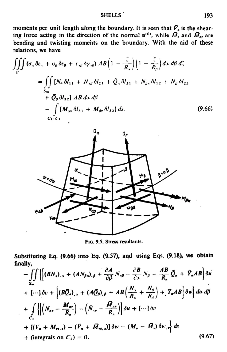
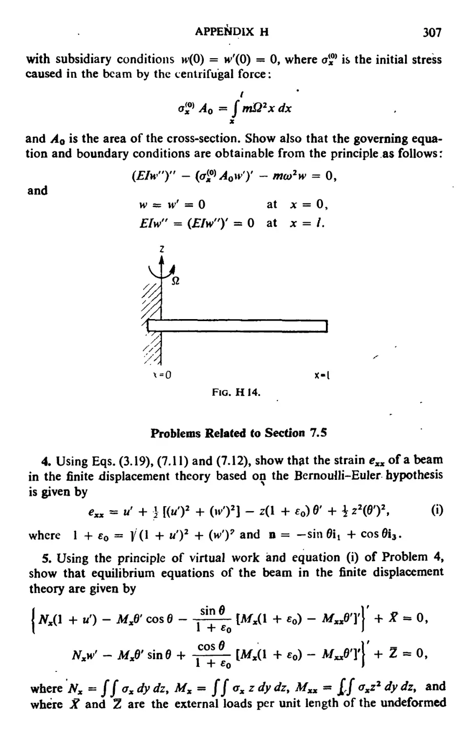
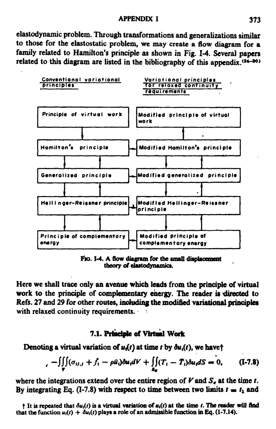
Текст
VARIATIONAL METHODS IN
ELASTICITY AND PLASTICITY
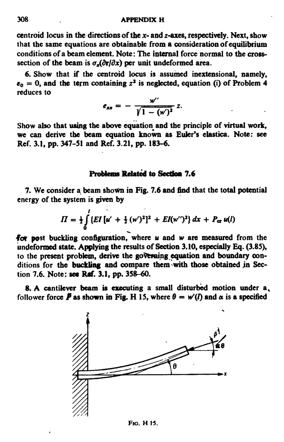
SECOND EDITION
K.YUICHIRO WASHIZU
Professor of Aeronautics and Astronautics, University of Tokyo
PERGAMON PRESS
Oxford • New York • Toronto
Paris • Sydney • Braunschweig
Pergamon Press Offices:
UK. Pergamon Press Ltd., Headington Hill Hall, Oxford, OX3
England
U.S.A. Pergamon Press Inc., Maxwell House, Fairview Park,
Elmsford, New York 10523, U.S.A.
C A N A D A Pergamon of Canada Ltd., 207 Queen's Quay West,
Toronto 1, Canada
AUSTRALIA Pergamon Press (Aust.) Pty. Ltd., 19a Boundary Street,
Rushcutters Bay, N.S.W. 2011, Australia
FRANCE Pergamon Press SARL, 24 rue des Ecoles,
75240 Paris, Cedex 05, France
WEST GERMANY Pergamon Press GmbH, D-3300 Braunschweig, Postfach
2923, Burgplatz 1, West Germany
Copyright © 1975
All Rights Reserved. No part of this publication may be
reproduced, stored in a retrieval system, or transmitted, in
any form or by any means: electronic, electrostatic, magnetic tape,
mechanical, photocopying, recording or otherwise, without the prior
permission in writing from the publishers.
First edition 1968
Second edition 1975
Reprinted 1975
Library of Congress Cataloging in Publication Data
Washizu, Kyuichiro, 1921- .
Variational methods in elasticity and plasticity.
(International series of monographs in aeronautics
and astronautics, Division I: solid and structural mechanics, v. 9)
Includes bibliographies.
1. Elasticity. 2. Plasticity. 3. Calculus of variations. I. Title.
QA931. W3>1974 620.P123 74-S861
ISBN 0-08-017653-4
Printed in Great Britain by A. Wheaton & Company, Exeter
FOREWORD
The variational principle and its application to many branches of mechanics
including elasticity and plasticity has had a long history of development.
However, the importance of this principle has been high-lighted in recent
years by developments in the use of finite element methods which have been
widely employed in structural analysis since the pioneering work by M. J.
Turner et al. appeared in Vol. 23, No. 9 issue of the' Journal of Aeronautical
Sciences in 1956. It has been shown repeatedly since that time that the
variational principle provides a powerful tool in the mathematical
formulation of the finite element approach. Conversely, the rapid development of the
finite element method has given much stimulus to the advancement of the
variational principle and new forms of the principle have been developed
during the past decade as outlined in Section 1 of Appendix I of tlurpresent
book.
The first edition of Professor Washizu's book, entitled Variational Methods in
Elasticity and Plasticity and published in 1968, was well received by engineers,
teachers and students working in solid and structural mechanics. Its
publication was timely, because it coincided with a period of rapid growth of
application of the finite element method. The principle features of the first edition was
that of providing a systematic way of deriving variational principles in
elasticity and plasticity, of transforming one variational principle to another
and of providing a systematic basis for the mathematical formulation of the
finite element method. The book was widely used and referenced frequently
m literature related to the finite element method.
Now, Professor Washizu has prepared a revised edition which adds a new
Appendix I. The new appendix introduces an outline of variational principles
which are used frequently as a basis for mathematical formulations in
elasticity and plasticity including those4new variational principles developed in
connection with the finite element method. As in the case of the first edition,
Appendix I is written in the clear, concise and elegant style for which
Professor Washizu is so widely known. The revised edition should form an
extremely valuable addition to the libraries and reference shelves of all
who are interested in solid and structural mechanics.
R. L. Bispunghoff
National Science^Foundation,
Washington D.C.
ACKNOWLEDGEMENTS
The author feels extremely honbred and wishes to express his deepest
gratitude to Dr. R. L. Bisplinghoff, Deputy Director of National Science
Foundation, for having given the Foreword to the revised edition of this book.
The author would like to express his deepest appreciation to Professor
T. H. H. Pain of the Massachusetts Institute of Technology and Professor
R. H. Gallagher of Cornell University for having given valuable comments
to the manuscript for the new appendix. Dr. Oscar Orringer of the
Massachusetts Institute of Technology coUaborated again with the author in
correcting the writing of the manuscript of the new appendix* Moreover, the
author should remember that he has been given numerous comments,
criticisms and encouragements from the reader since the publication of the
first edition of this book. The author would like to express his sincere
appreciation to all of these people, without whose encouragement and
collaboration, this revised edition couldn't be realized
K*Washizu
CONTENTS
FOREWORD
ACKNOWLEDGEMENTS
INTRODUCTION 1
CHAPTER 1. Small Displacement Thbory of Elasticity in Rbctanoular Car-
tesian Coordinates 8
1.1. Presentation of a Problem in Small Displacement Theory 8
1.2. Conditions of Compatibility 11
1.3. Stress Functions 12
1.4. Principle of Virtual Work 13
1.5. Approximate Method of Solution Based on the Principle of Virtual Work 15
1.6. Principle of Complementary Virtual Work 17
1.7. Approximate Method of Solution Based on the Principle of Complementary
Virtual Work . 19
1.8. Relations between Conditions of Compatibility and Stress Functions 22
1.9. Some Remarks 24
CHAPTER 2. Variational Principles in the Small Displacement Thbcmiy op
Elasticity 27
2.1. Principle of Minimum Potential Energy 27
2.2. Principle of Minimum Complementary Energy 29
2.3. Generalization of the Principle of Minimum Potential Energy 31
Z4. Derived Variational Principles 34
Z5. Rayleigh-Ritz Method—(1) 38
2.6. Variation of the Boundary Conditions and Castigliano's Theorem 40
2.7. Free Vibrations of an Elastic Body 43
2.8. Rayleigh-Ritz Method—(2) 46
2.9. Some Remarks 48
CHAPTER 3. Finite Displacement Theory op Elasticity in Rectangular
Cartesian Coordinates 52
3.1. Asalysis of Strain 52
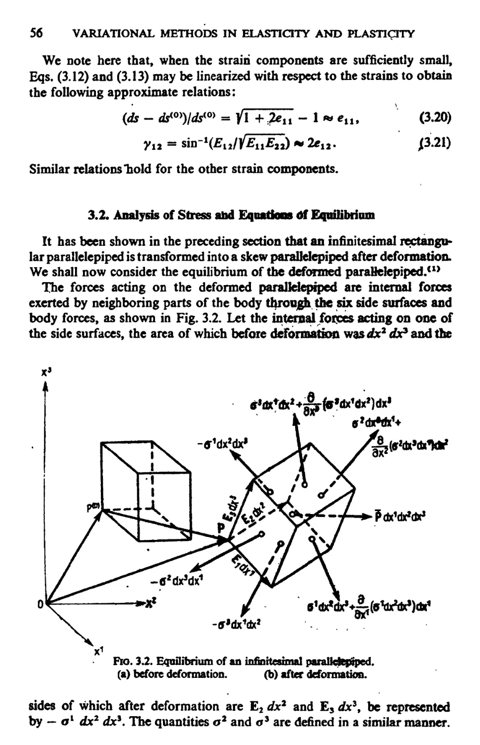
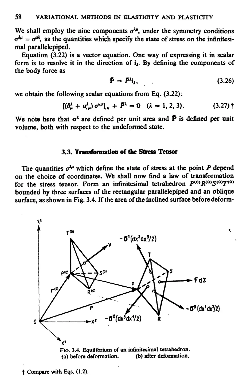
3.2. Analysis of Stress and Equations of Equilibrium 56
3.3. Transformation of the Stress Tensor 58
3.4. Stress-Strain Relations 59
3.5. Presentation of a Problem 60
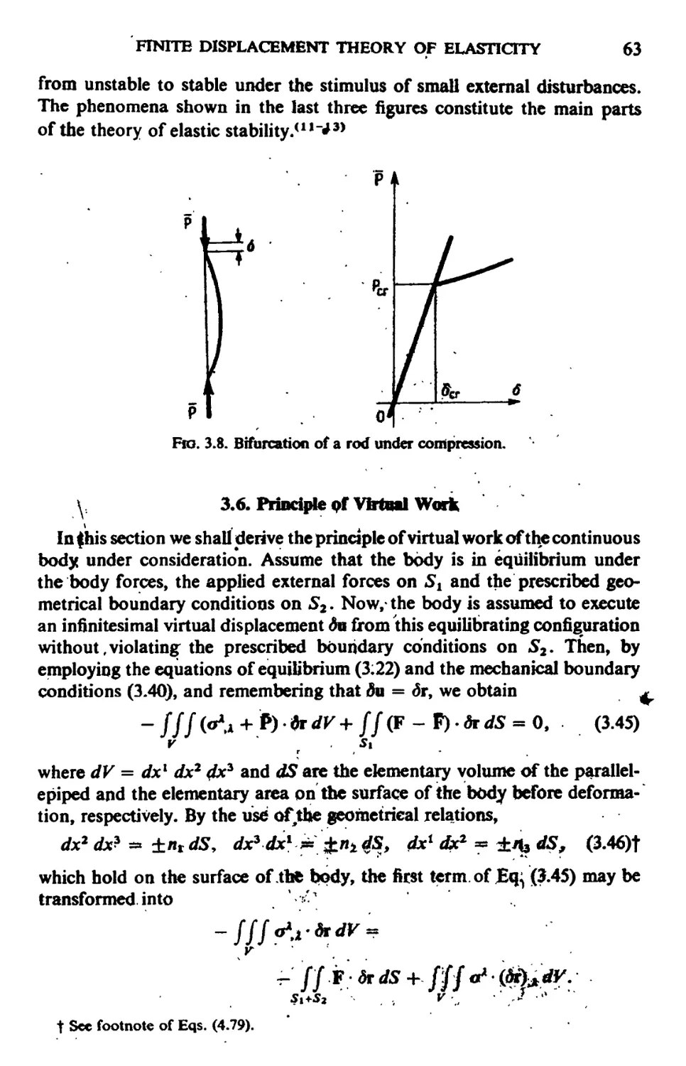
3.6. Principle of Virtual Work 63
3.7. Strain Energy Function 64
3.8. Principle of Stationary Potential Energy 67
3.9. Generalization of the Principle of Stationary Potential Energy 68
3.10. Energy Criterion for Stability 69
3.11. The Euler Method for Stability Problem 72
3.12. Some Remarks 74
IX
x CONTENTS
CHAPTER 4. Theory op Elasticity in Curvilinear Coordinates 76
4.1. Geometry before Deformation 76
4.2. Analysis of Strain and Conditions of Compatibility 80
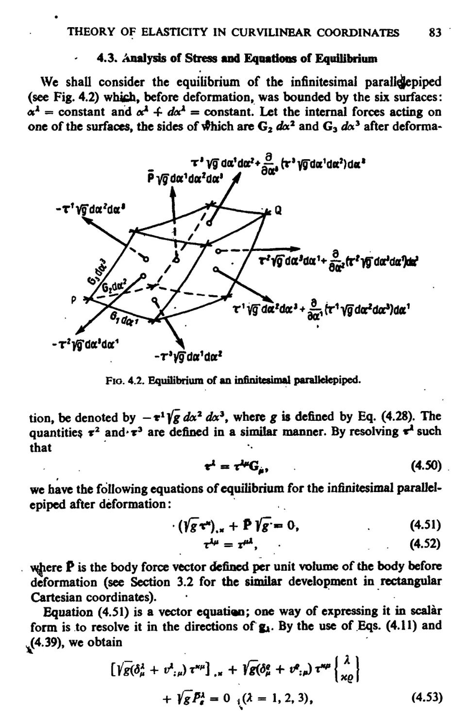
4.3. Analysis of Stress and Equations of Equilibrium 83
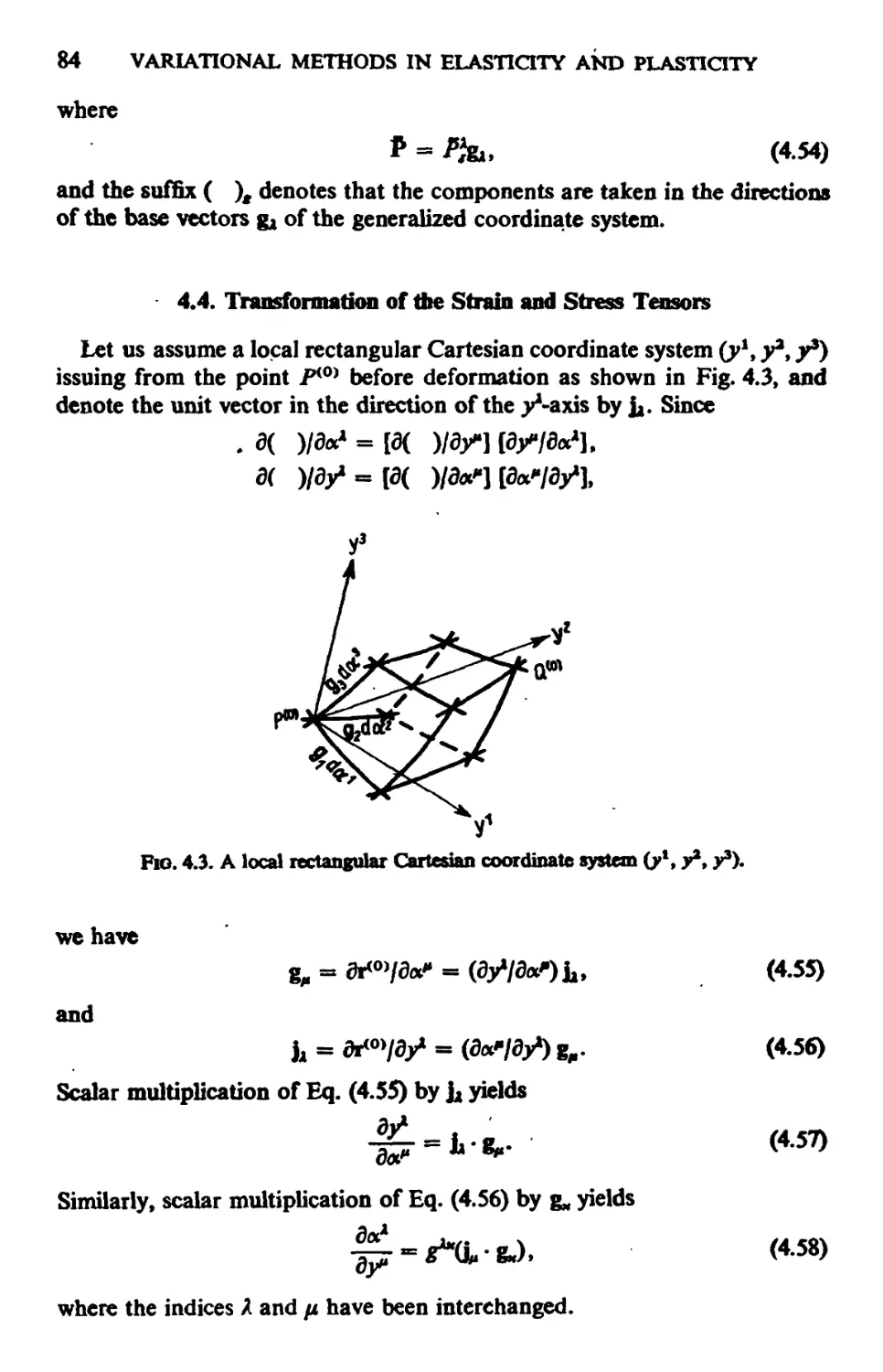
4.4. Transformation of the Strain and Stress Tensors 84
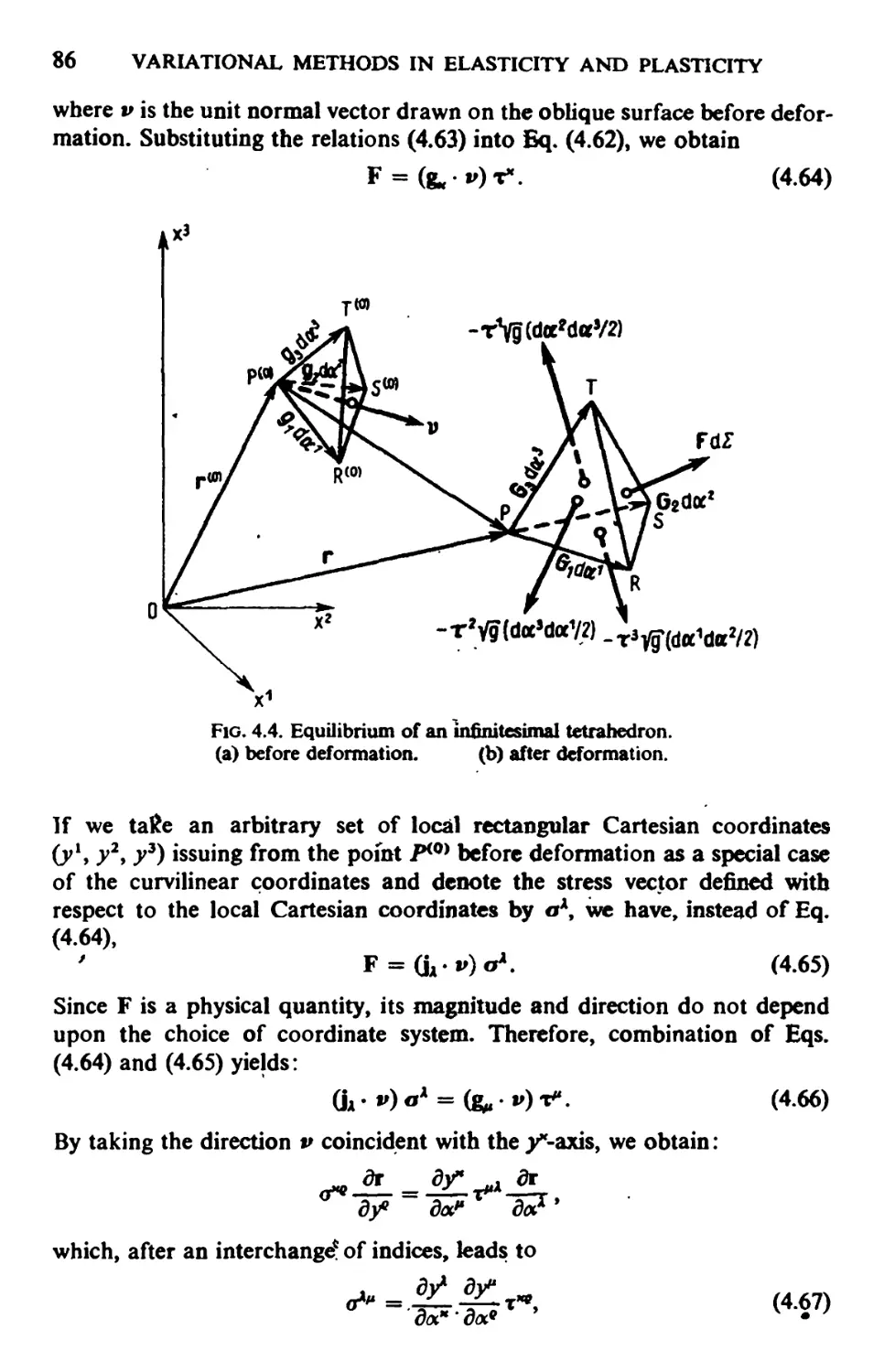
4.5. Stress-Strain Relations in Curvilinear Coordinates 87
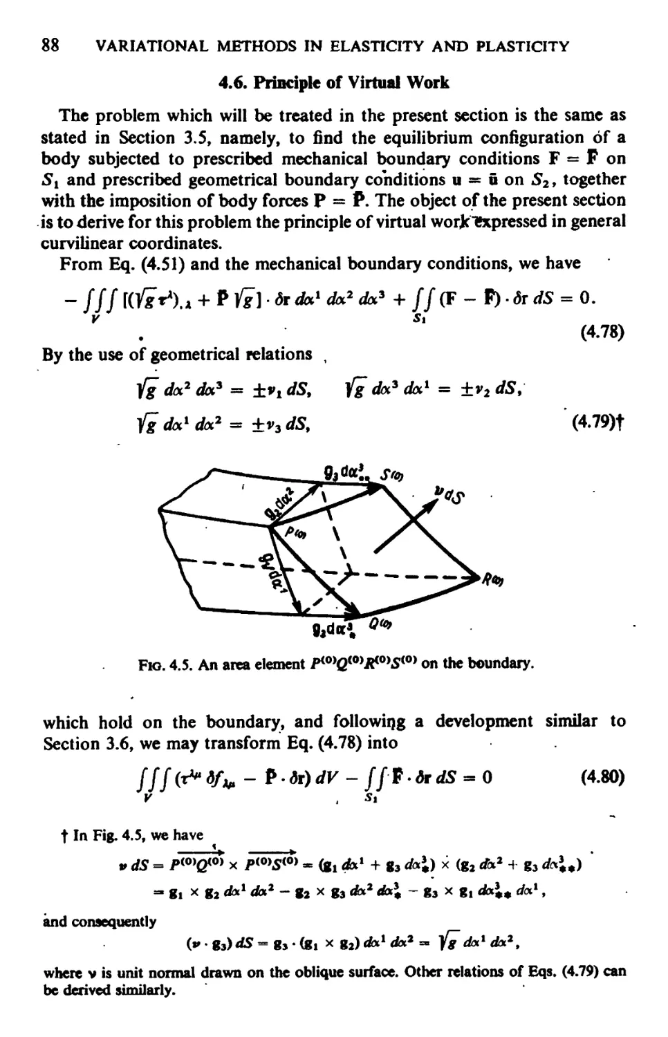
4.6. Principle of Virtual Work 88
4.7. Principle of Stationary Potential Energy and its Generalizations 89
4.8. Some Specializations to Small Displacement Theory in Orthogonal Curvi-
!inear Coordinates 90
CHAPTER 5. Extensions of the Principle of Virtual Work and Related
Variational Principles 93
3
5.1. Initial Stress Problems 7 93
5.2. Stability Problems of a Body with Initial Stresses 96
5.3. Initial Strain Problems
5.4. Thermal Stress Problems
5.5. Quasi-static Problems 101
5.6. Dynamical Problems 104
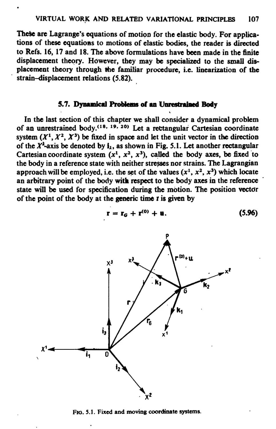
5.7. Dynamical Problems of an Unrestrained Body 107
CHAPTER 0. Torsion of Bars 113
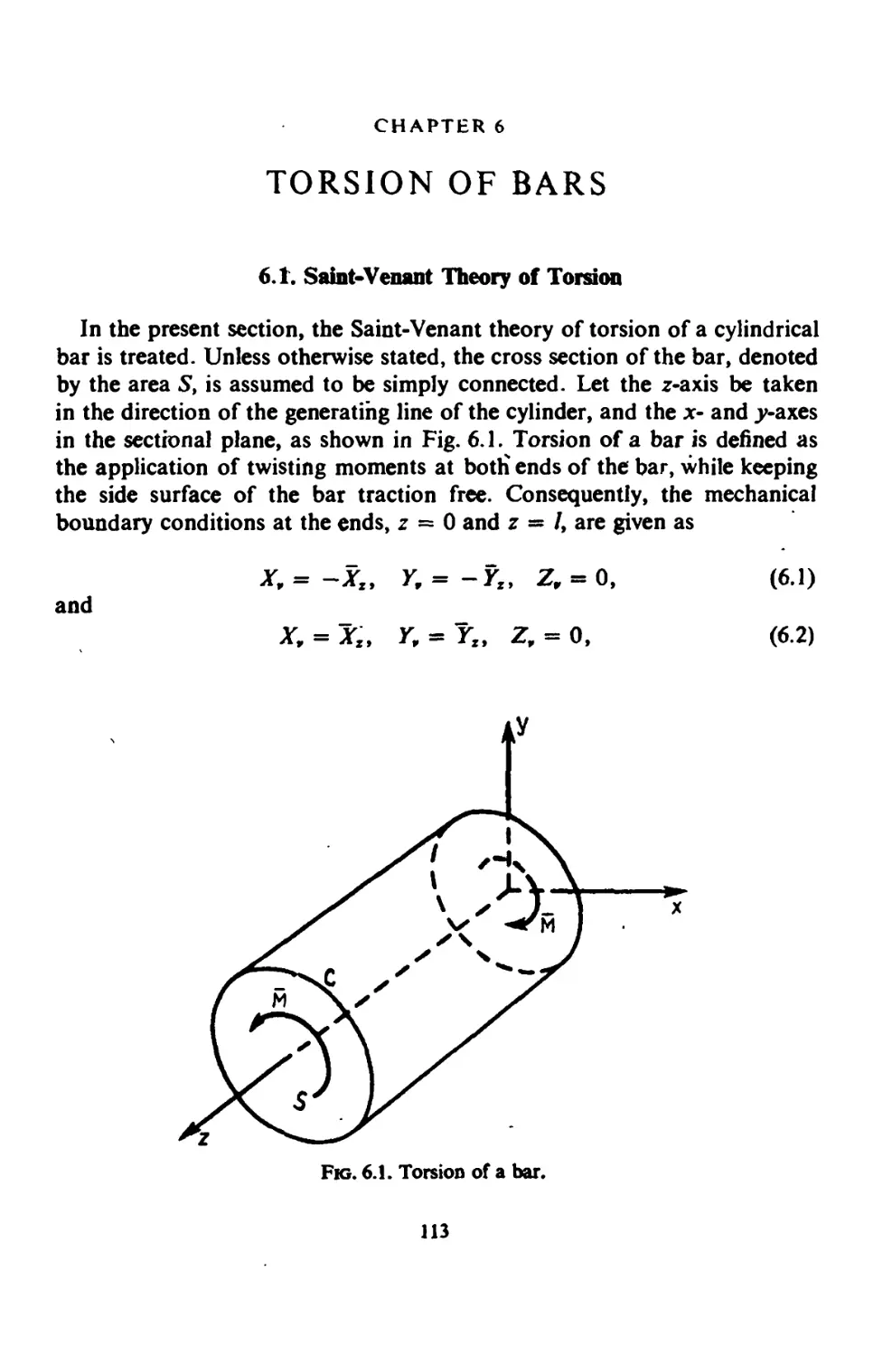
6.1. Saint-Vcnant Theory of Torsion 113
6.2. The Principle of Minimum Potential Energy and its Transformation 116
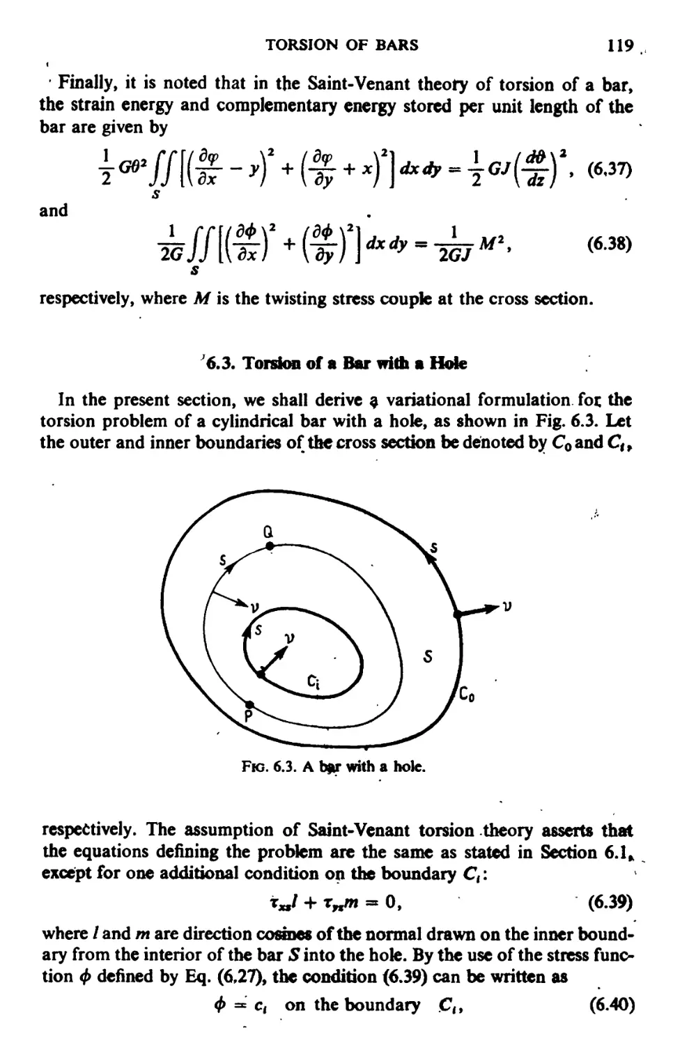
6.3. Torsion of a Bar with a Hole 119
6.4. Torsion of a Bar with Initial Stresses 121
6.5. Upper and Lower Bounds of Torsional Rigidity 125
CHAPTER 7. Beams 132
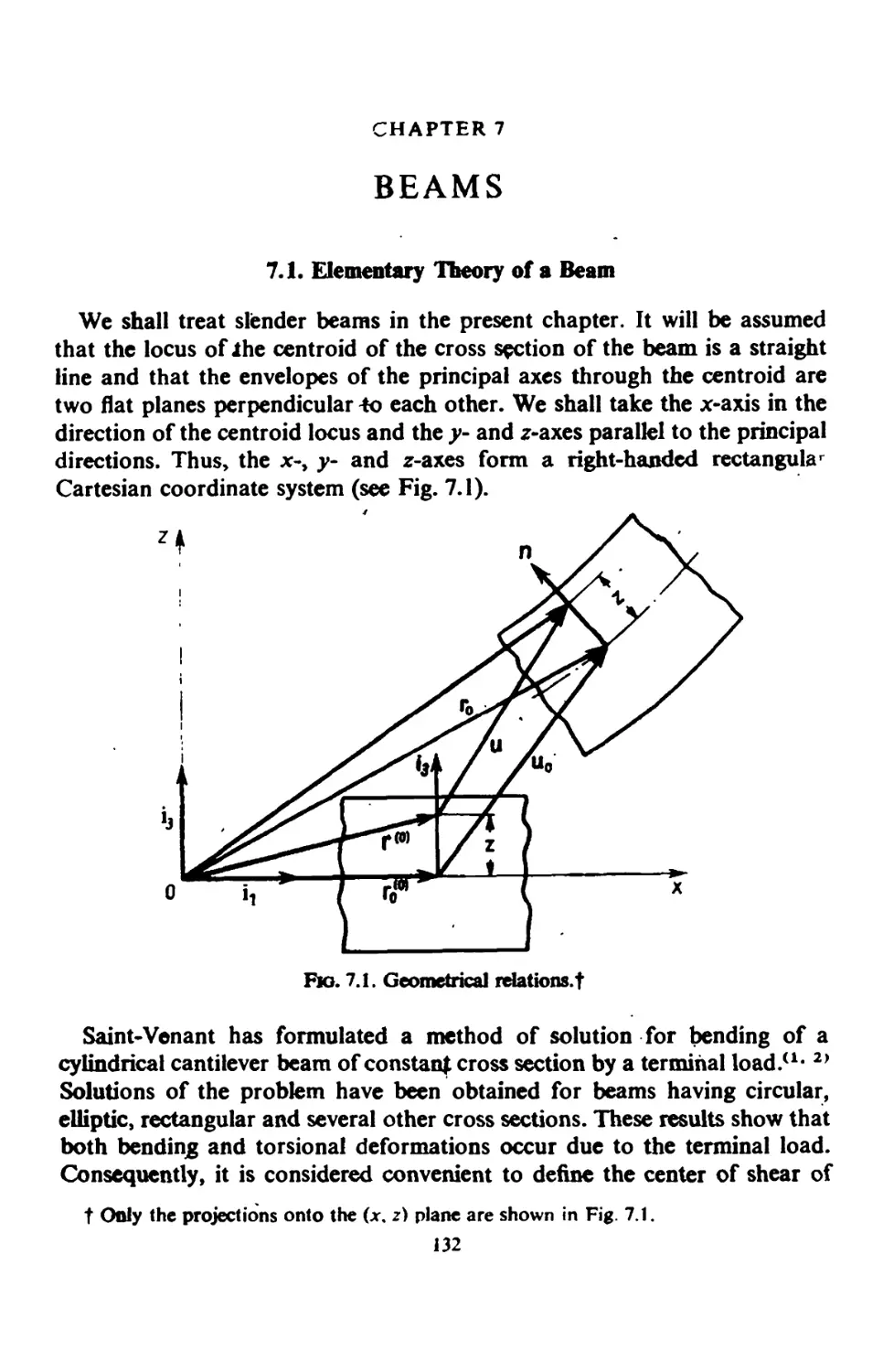
7.1. Elementary Theory of a Beam 132
7.2. Bending of a Beam 134
7.3. principle of Minimum Potential Energy and its Transformation 137
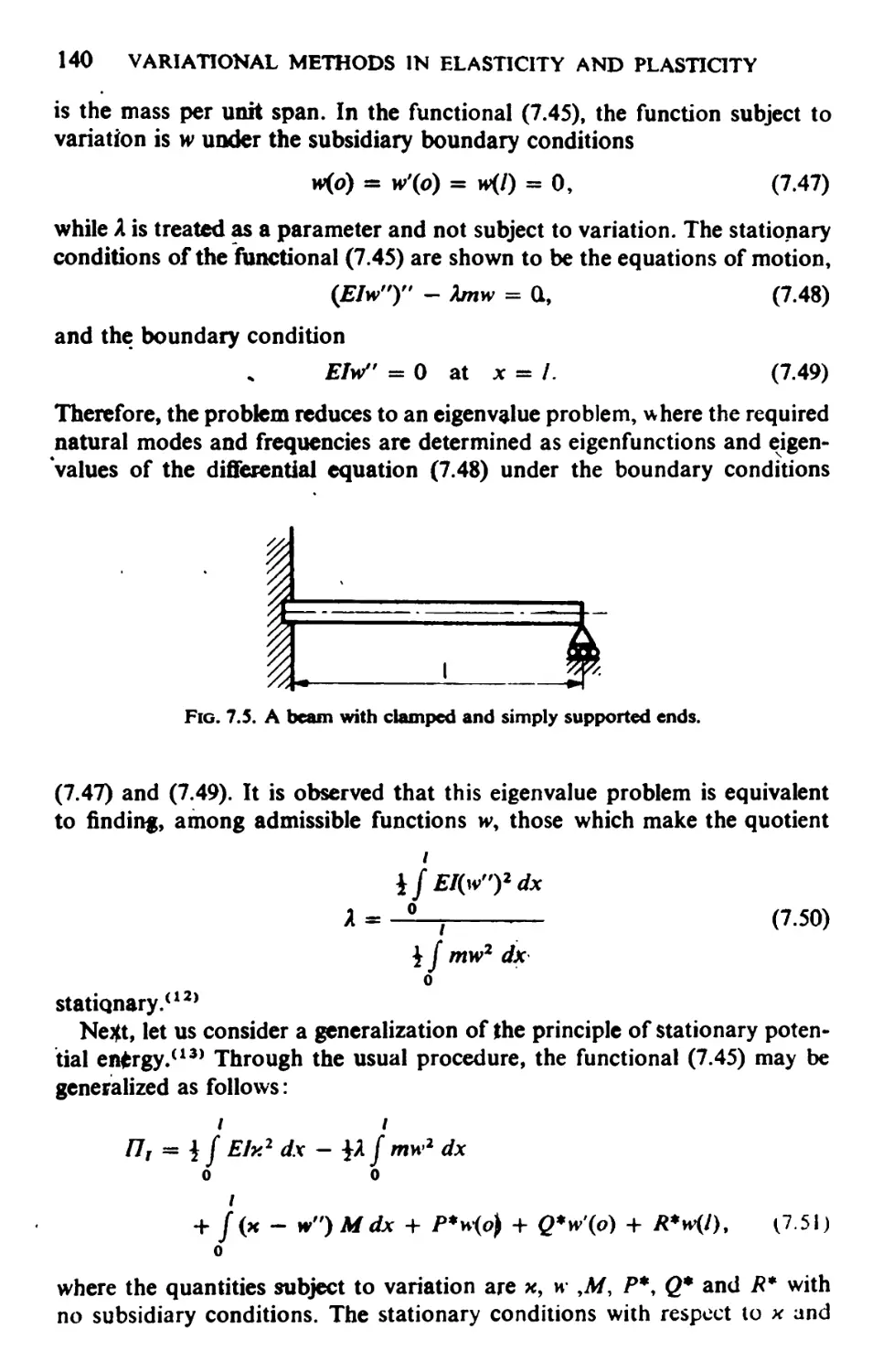
7.4. Free Lateral Vibration of a Beam 139
7.5. Large Deflection of a Beam 142
7.6. Buckling of a Beam 144
7.7. A Beam Theory Including the Effect of Transverse Shear Deformation 147
7.8. Some Remarks 149
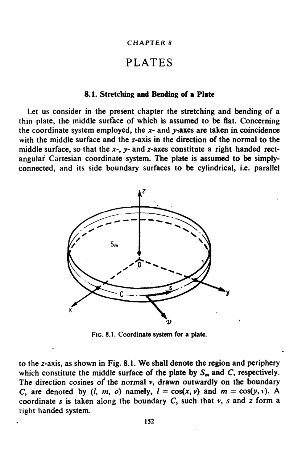
CHAPTER 8. Plates 152
8.1. Stretching and Bending of a Plate 152
8.2. A Problem of Stretching and Bending of a Hate 154
8.3. Principle of Minimum Potential Energy and its Transformation for the
Stretching of a Plate 160
8.4. Principle of Minimum Potential Energy and its Transformation for the
Bending of a Plate 161
8.5. Large Deflection of a Plate in Stretching and Bending 163
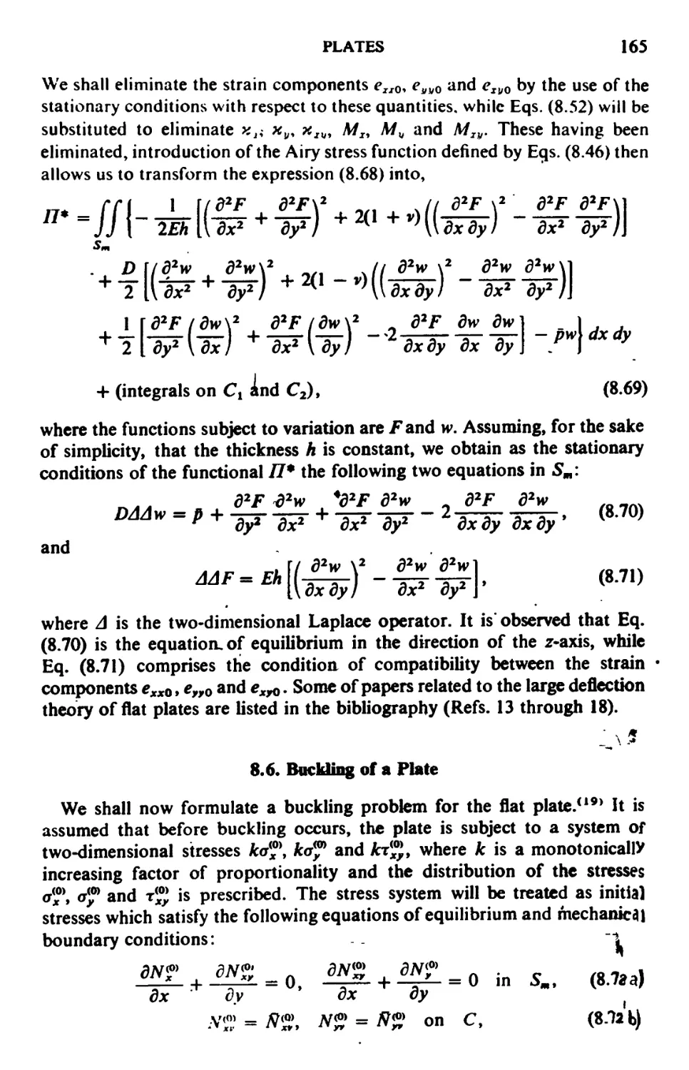
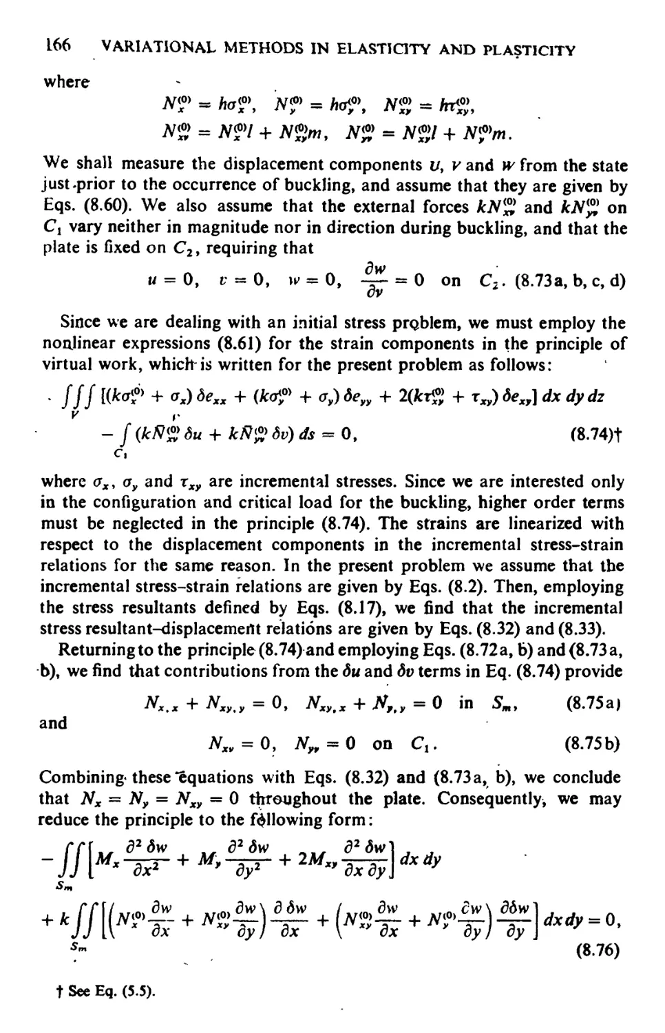
8.6. Ruckling of a Pk.te 165
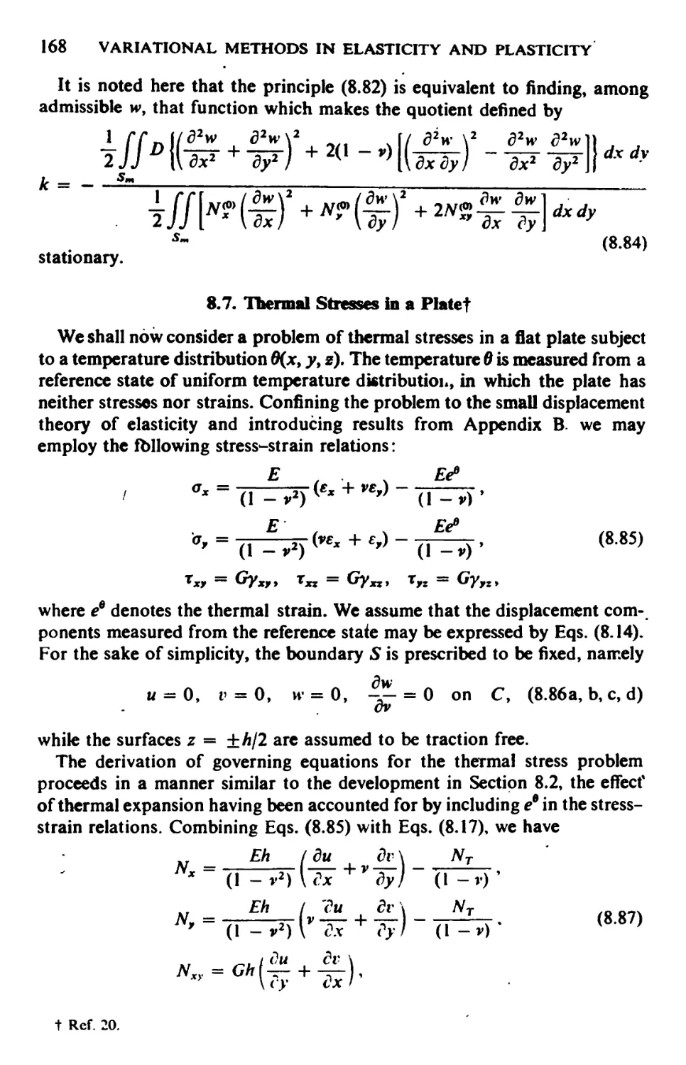
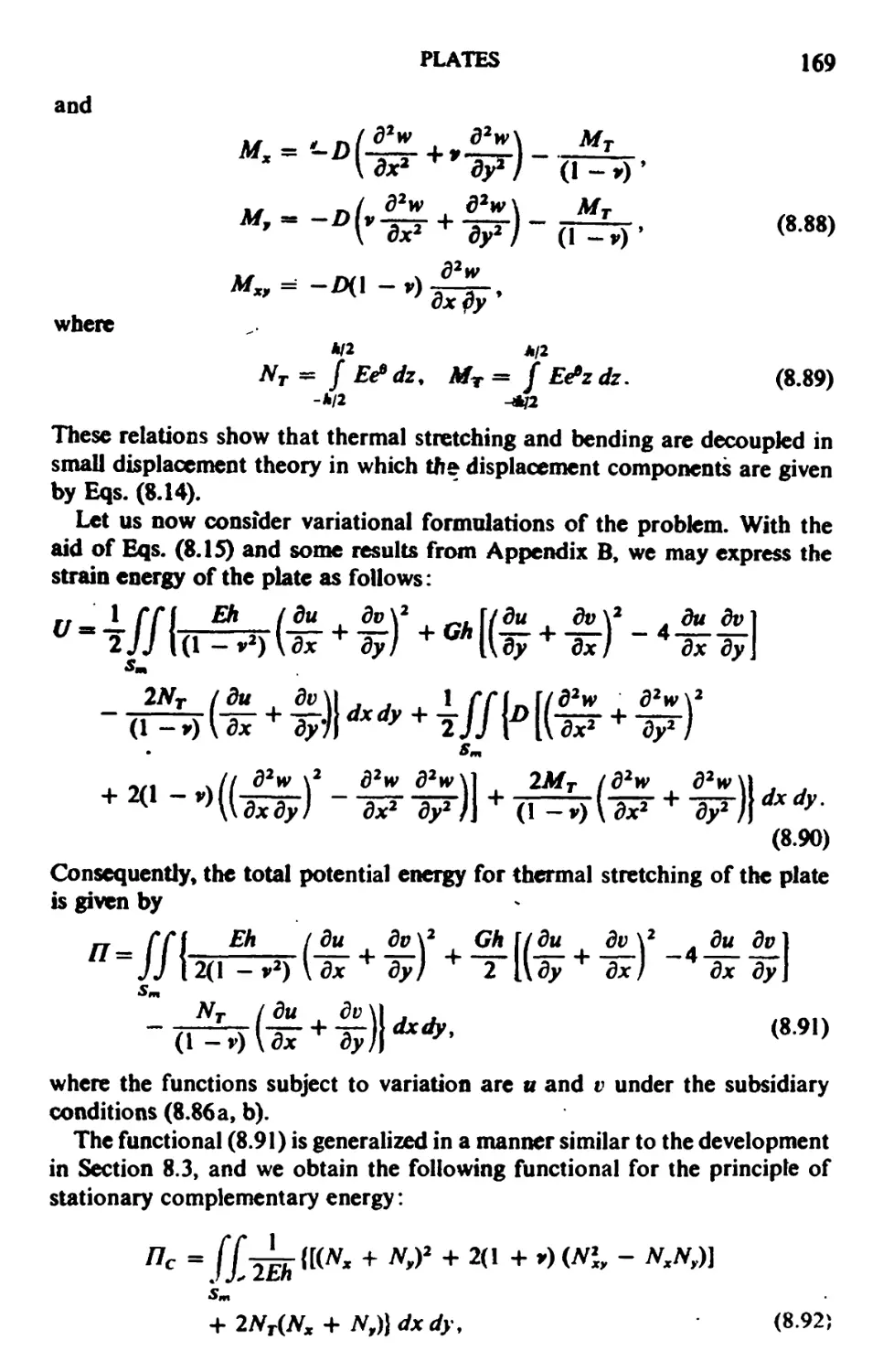
8.7. Thermal Stresses in a Plate 168
8.8. A Thin Plate Theory Including the Effect of Transverse Shear Deformation 170
8.9. Thin Shallow Shell 173
8.10. Some Remarks 178
CONTENTS xi
CHAPTER 9. Shells 182
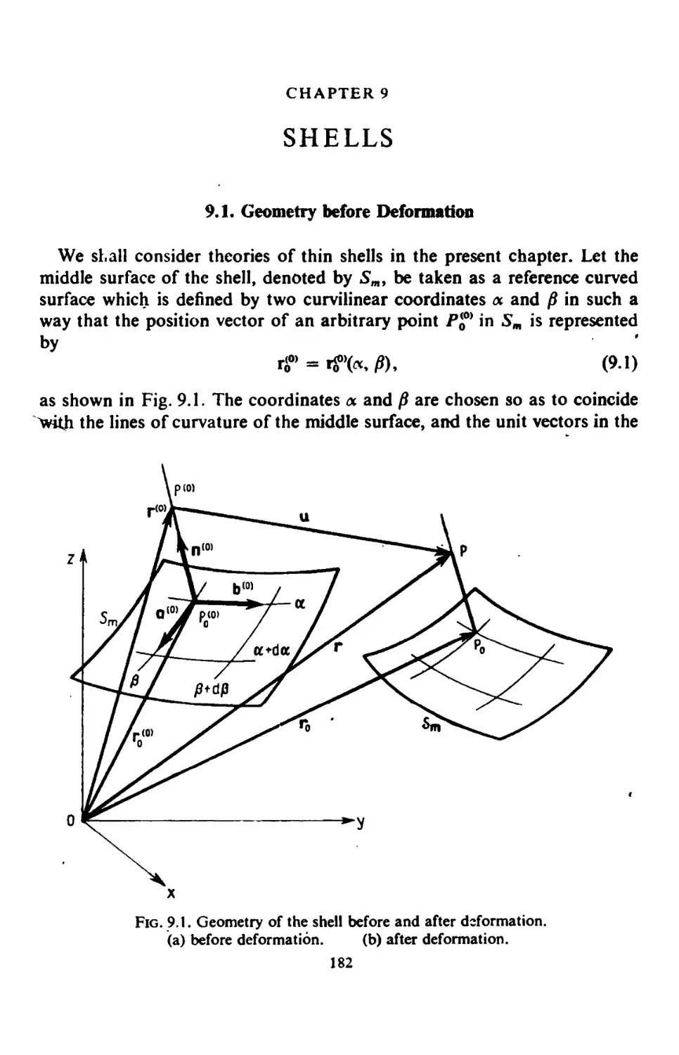
9.1. Geometry before Deformation 182
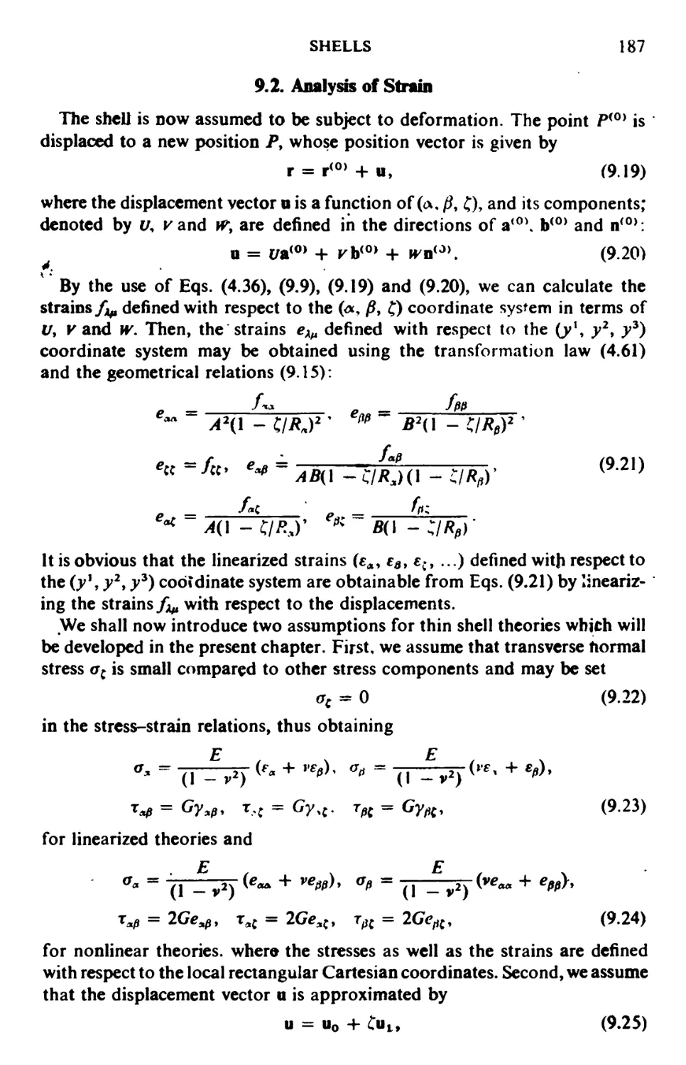
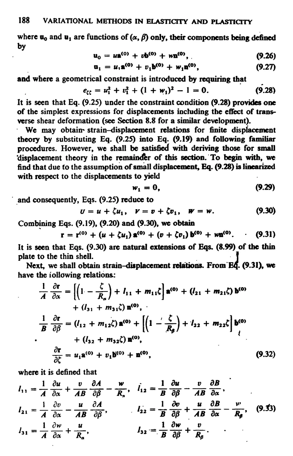
9.2. Analysis of Strain 187
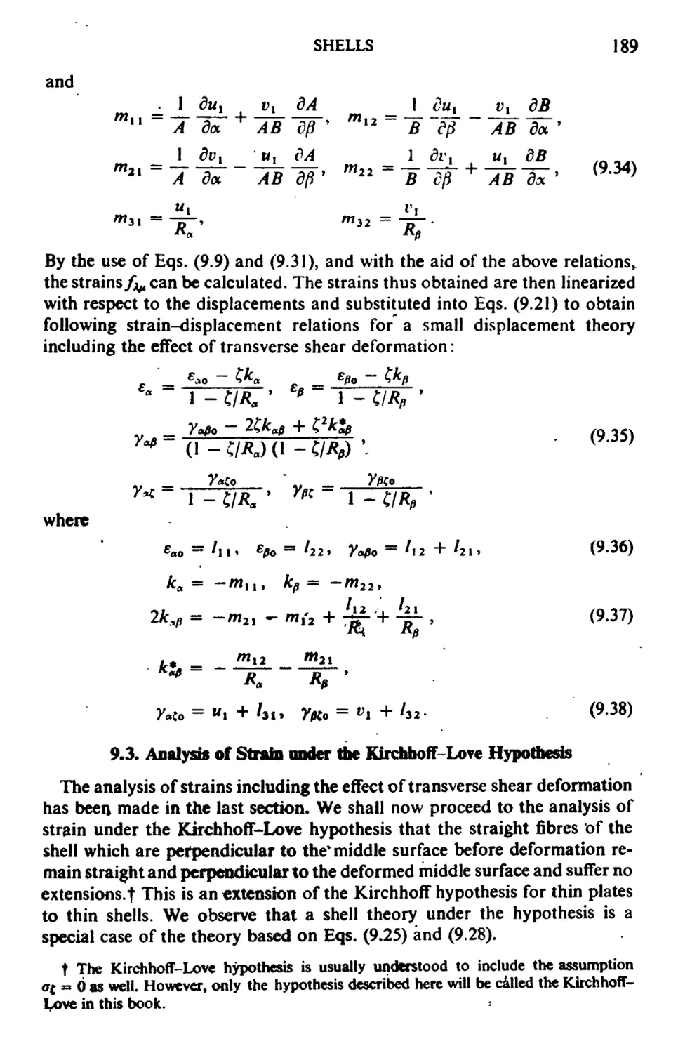
9.3. Analysis of Strain under the Kirchhoff-Love Hypothesis 189
9.4. A Linearized Thin Shell Theory under the Kirchhoff-Love Hypothesis 191
9.5. Simplified Formulations 195
9.6. A Simplified Linear Theory under the Kirchhoff-Love Hypothesis 197
9.7. A Nonlinear Thin Shell Theory under the Kirchhoff-Love Hypothesis 198
9.8. A Linearized Thin Shell Theory Including the Effect of Transverse Shear De-
formations 199
9.9. Some Remarks 201
CHAPTER 10. Structures 205
10.1. Finite Redundancy 205
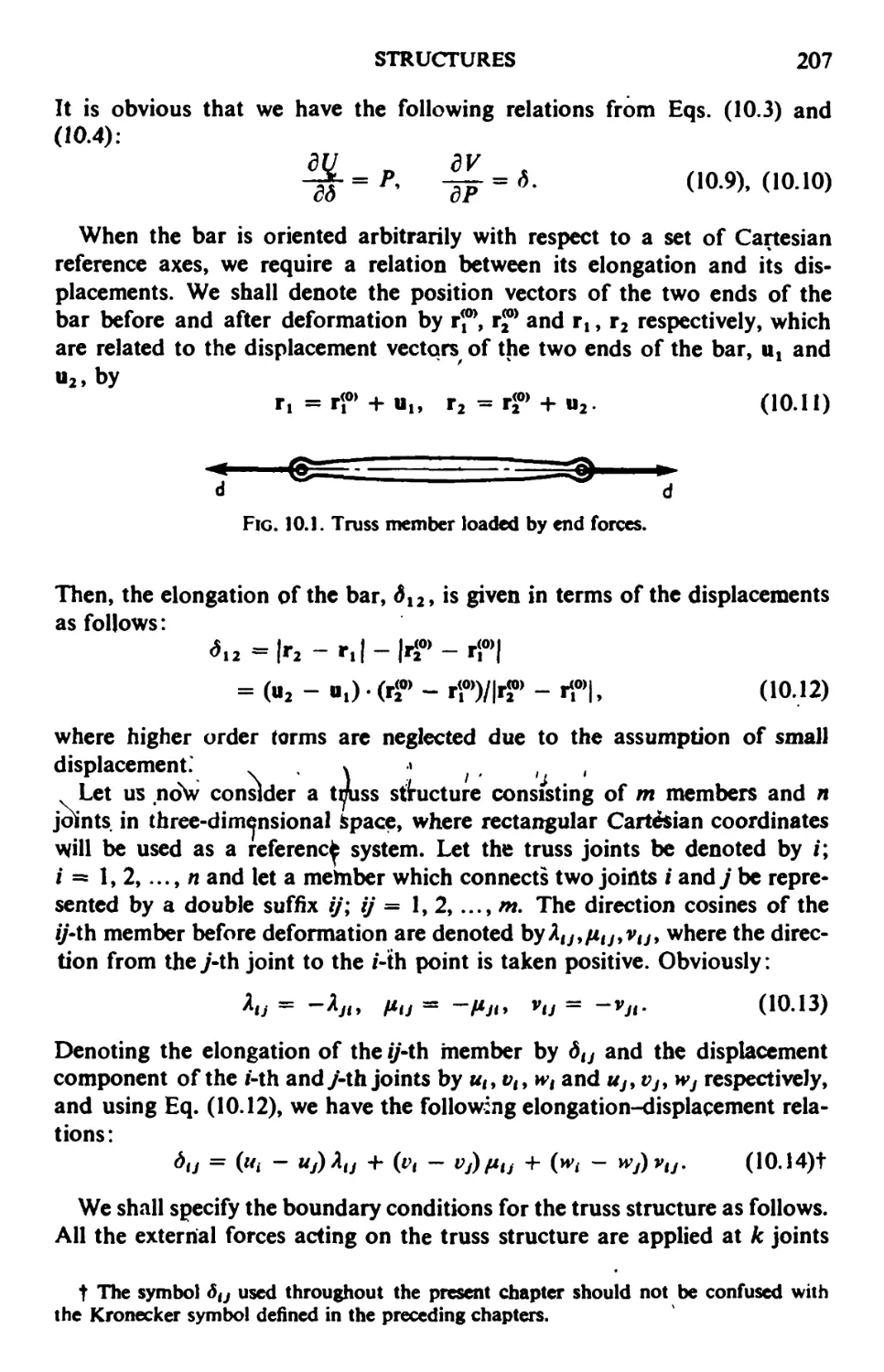
10.2. Deformation Characteristics of a Truss Member and Presentation of a Truss
Problem 206
10.3. Variational Formulations of the Truss Problem 209
10.4. The Force Method Applied to the Truss Problem 210
10.5. A Simple Example of a Truss Structure 213
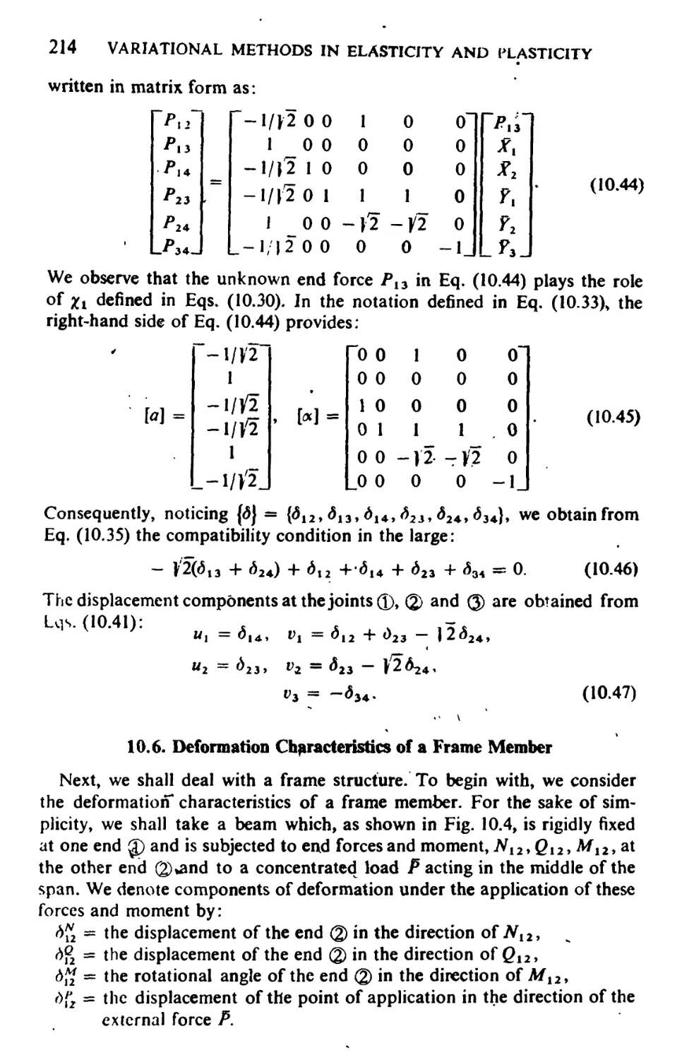
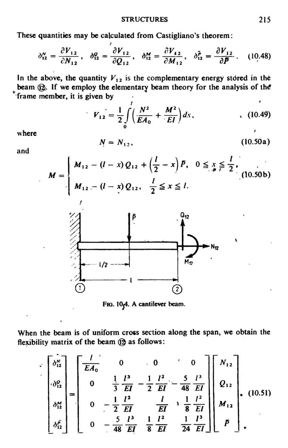
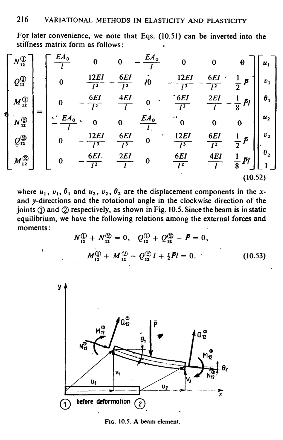
10.6. Deformation Characteristics of a Frame Member 214
10.7. The Force Method Applied to a Frame Problem 217
10.8. Notes on the Force Method Applied to Semi-monocoque Structures 221
10.9. Notes on the Stiffness Matrix Method Applied to Semi-monocoque
Structures 225
CHAPTER 11. The Deformation Theory of Plasticity 231
1 LI. The Deformation Theory of Plasticity 231
11.2. Strain-hardening Material 233
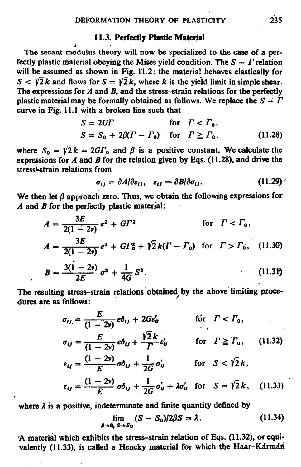
11.3. Perfectly Plastic Material 235
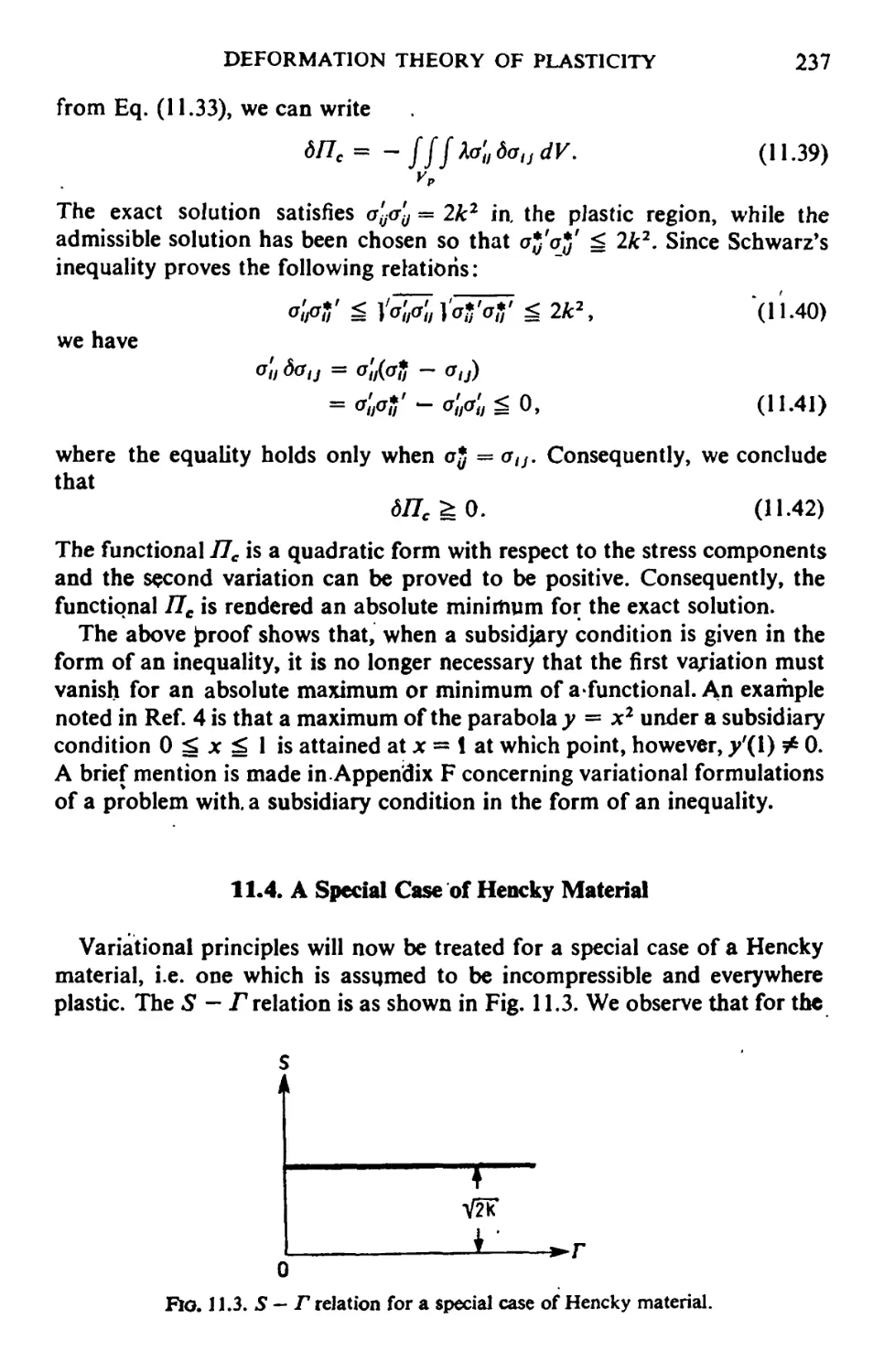
1 T.4. A Special Case of Hencky Material 237
CHAPTER 12. The Flow Theory of Plasticity 240
12.1. The Flow Theory of Plasticity 240
12.2. Strain-hardening Material 242
12.3. Perfectly Plastic Material 244
12.4. The Prandtl-Reuss Equation 245
12.5. The Saint-Venant-Levy-Mises Equations 247
12.6. Limit Analysis 250
12.7. Some Remarks 253
APPENDIX A. Extremum of a Function with a Subsidiary Condition 254
APPENDIX B. Stress-Strain Relations for a Thin Plate 256
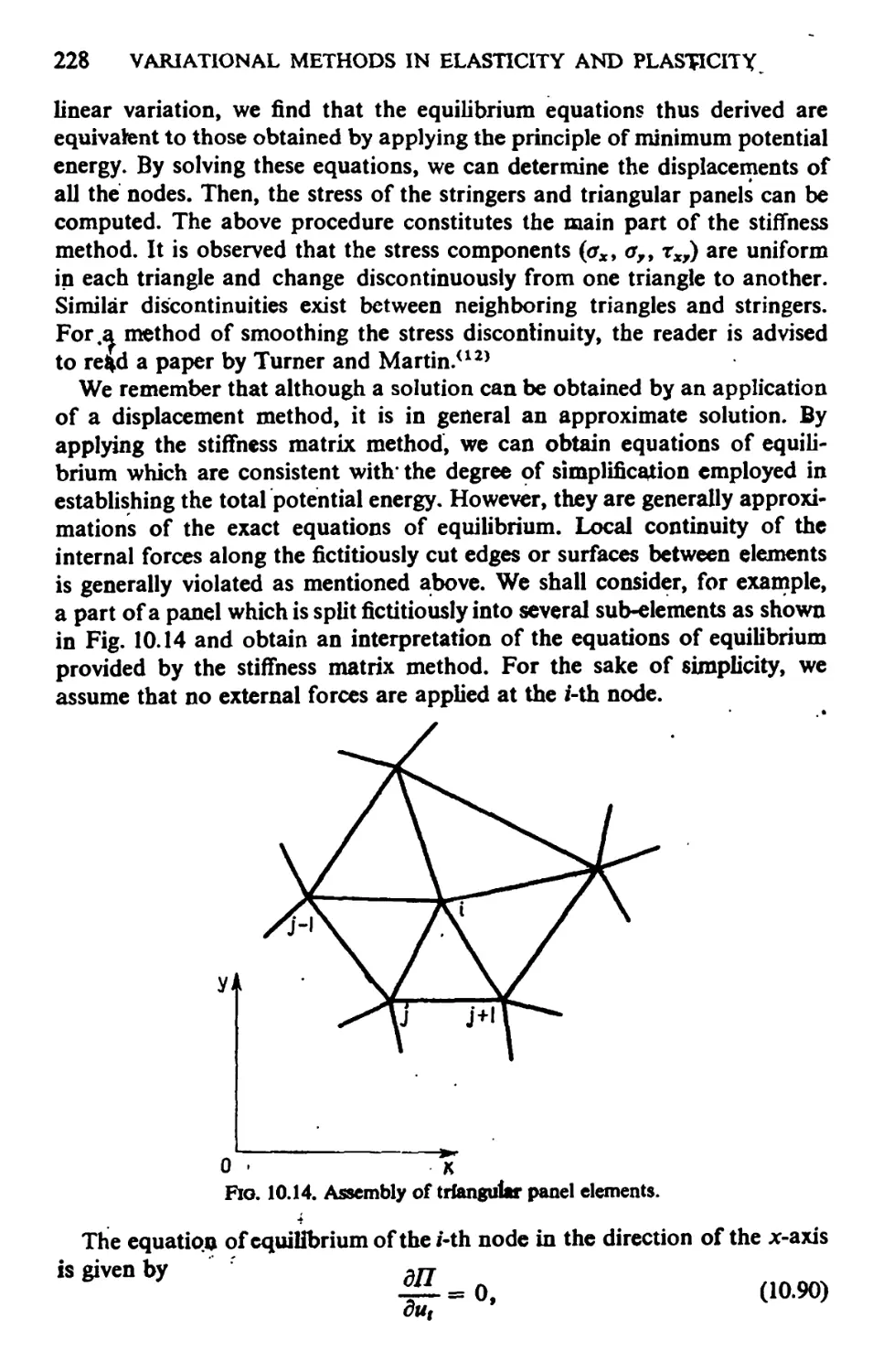
APPENDIX C. A Beam Theory Including the Effect of Transverse Shear
Deformation 258
APPENDIX D. A Theory of Plate Bendinp Including the Effect of
Transverse Shear Deformation 262
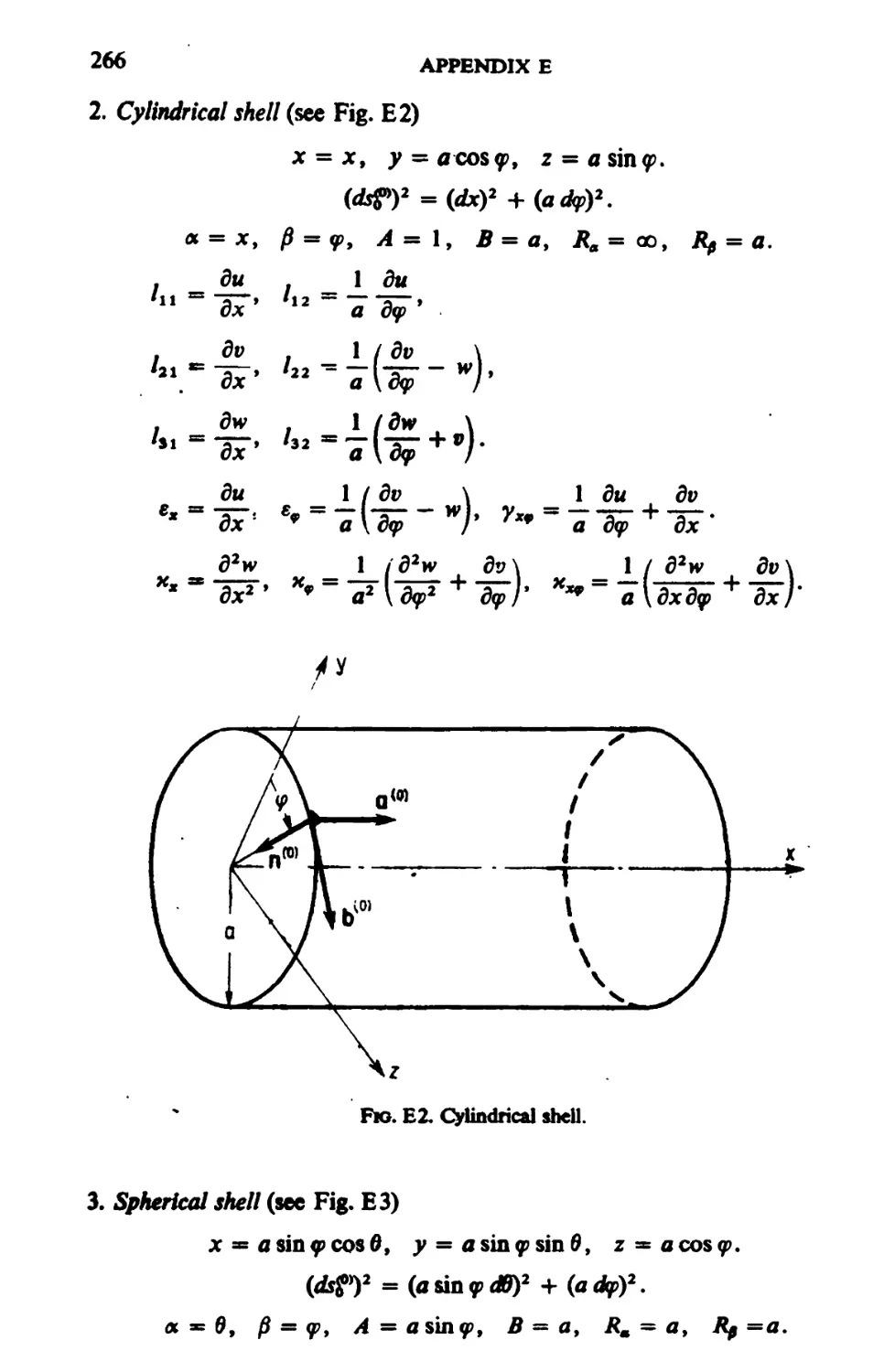
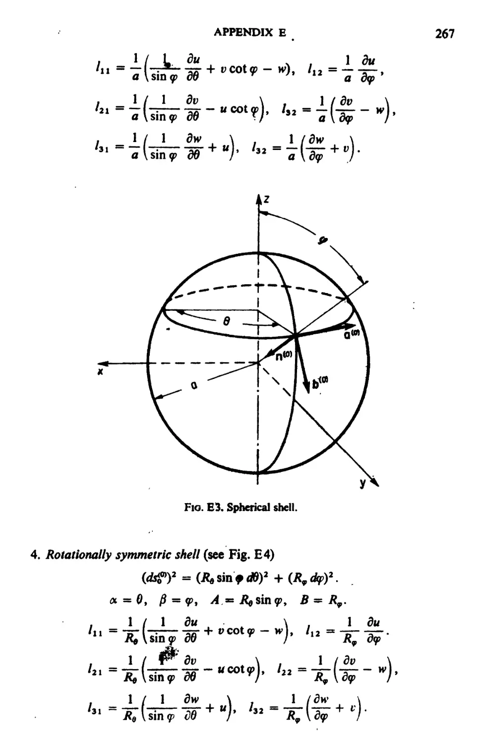
APPENDIX E. Specializations to Several Kinds of Shells 265
APPENDIX F. A Note on the Haar-KArman Principle 269
APPENDIX G. Variational Principles in the Thlory of Creep 270
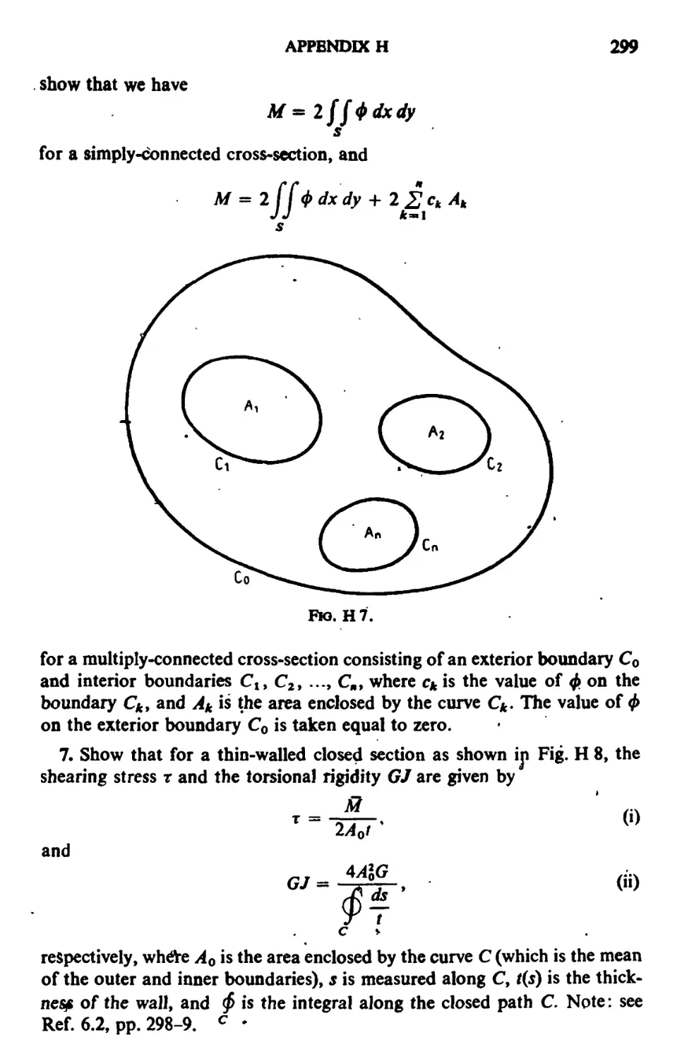
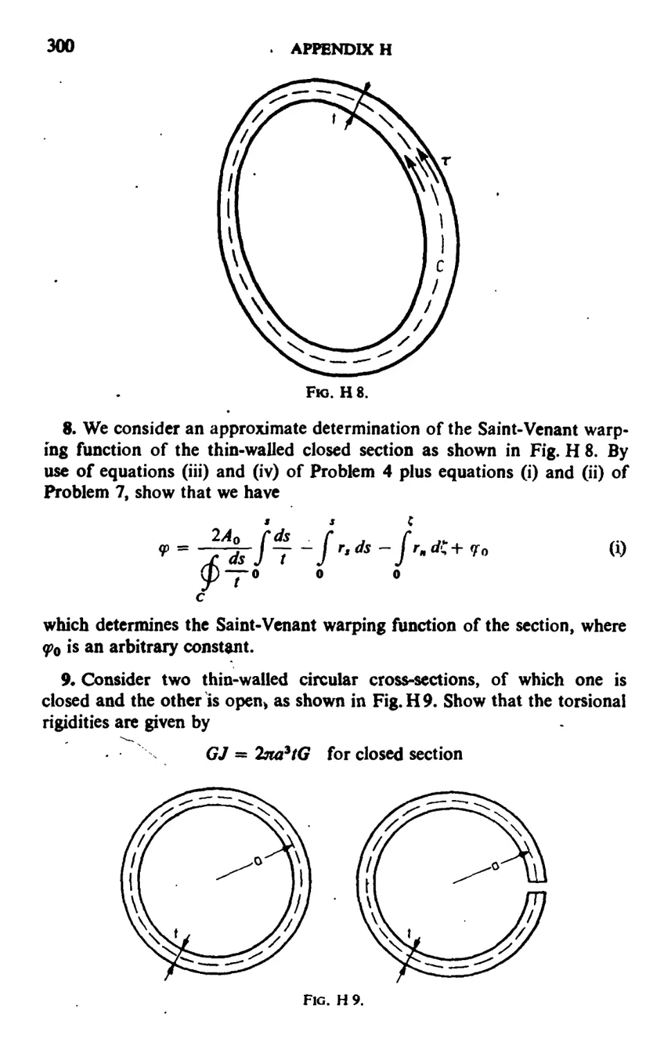
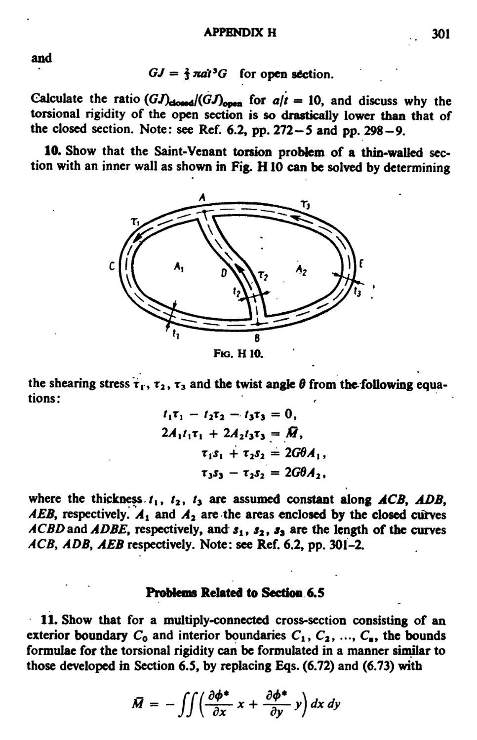
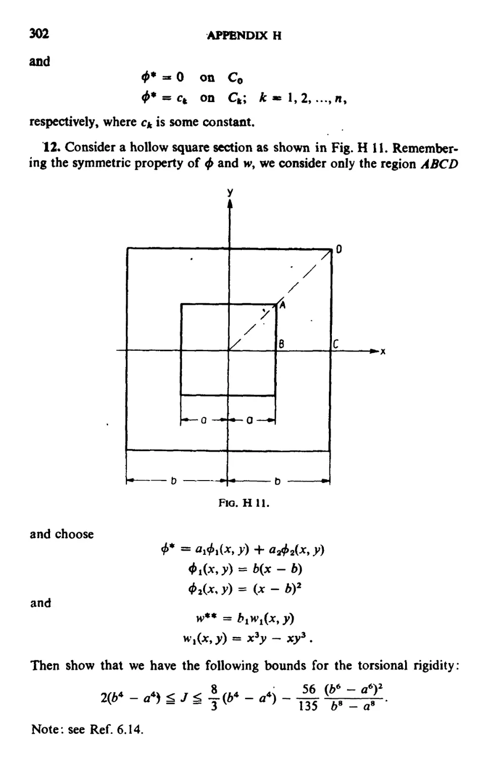
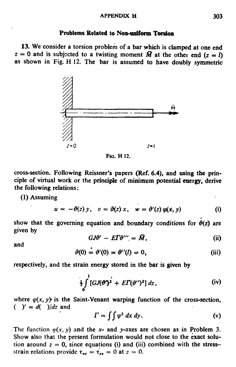
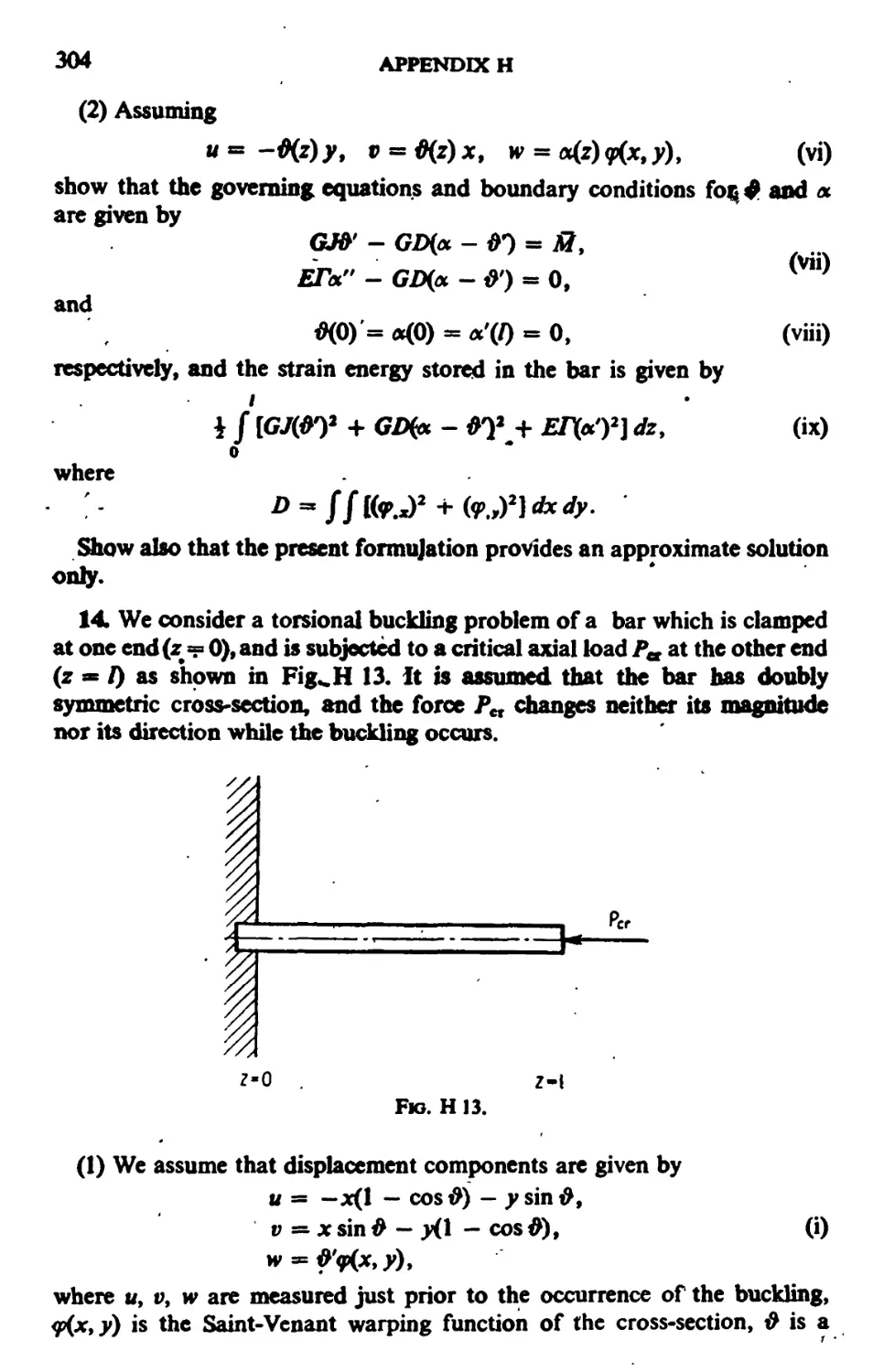
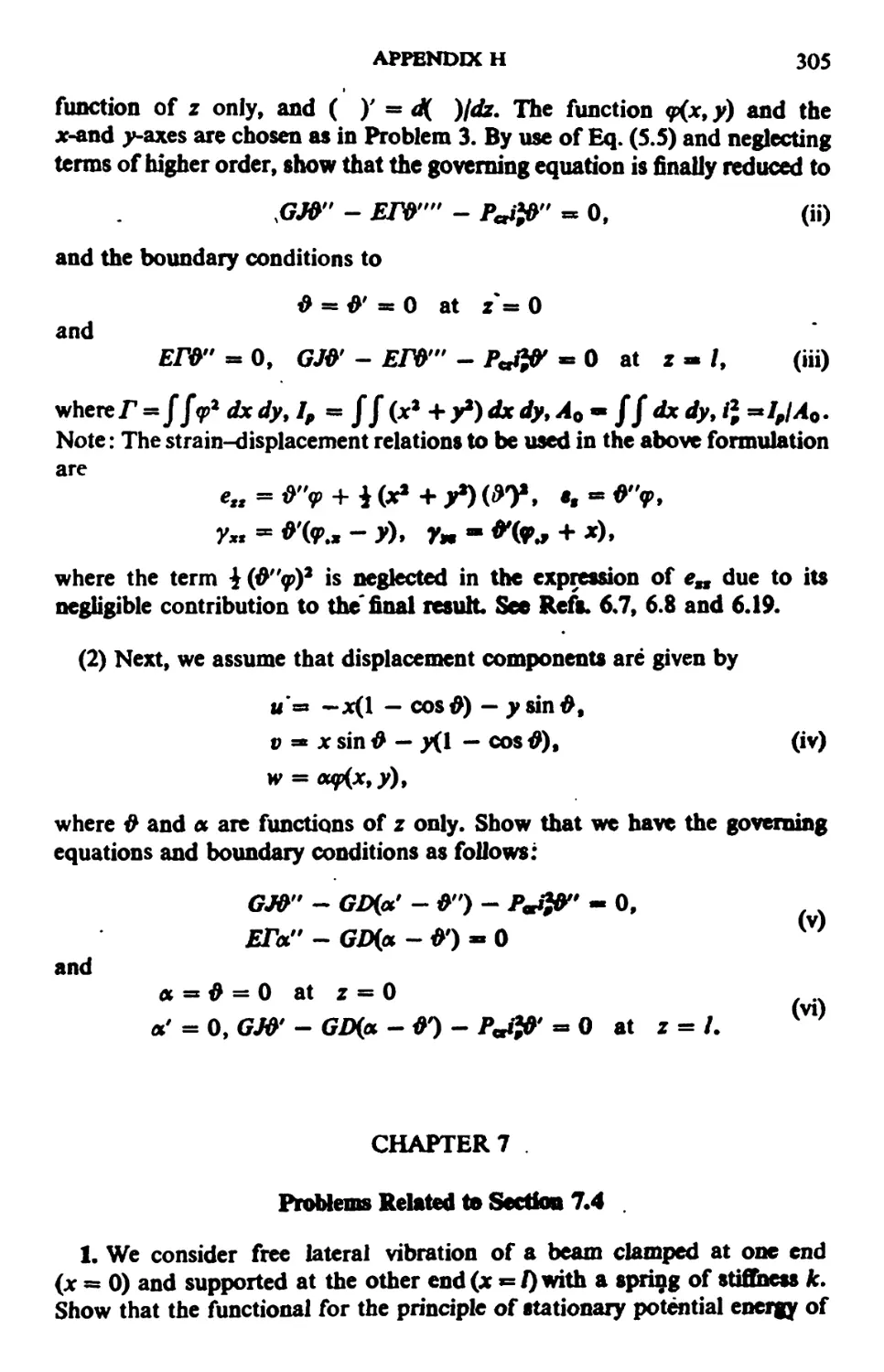
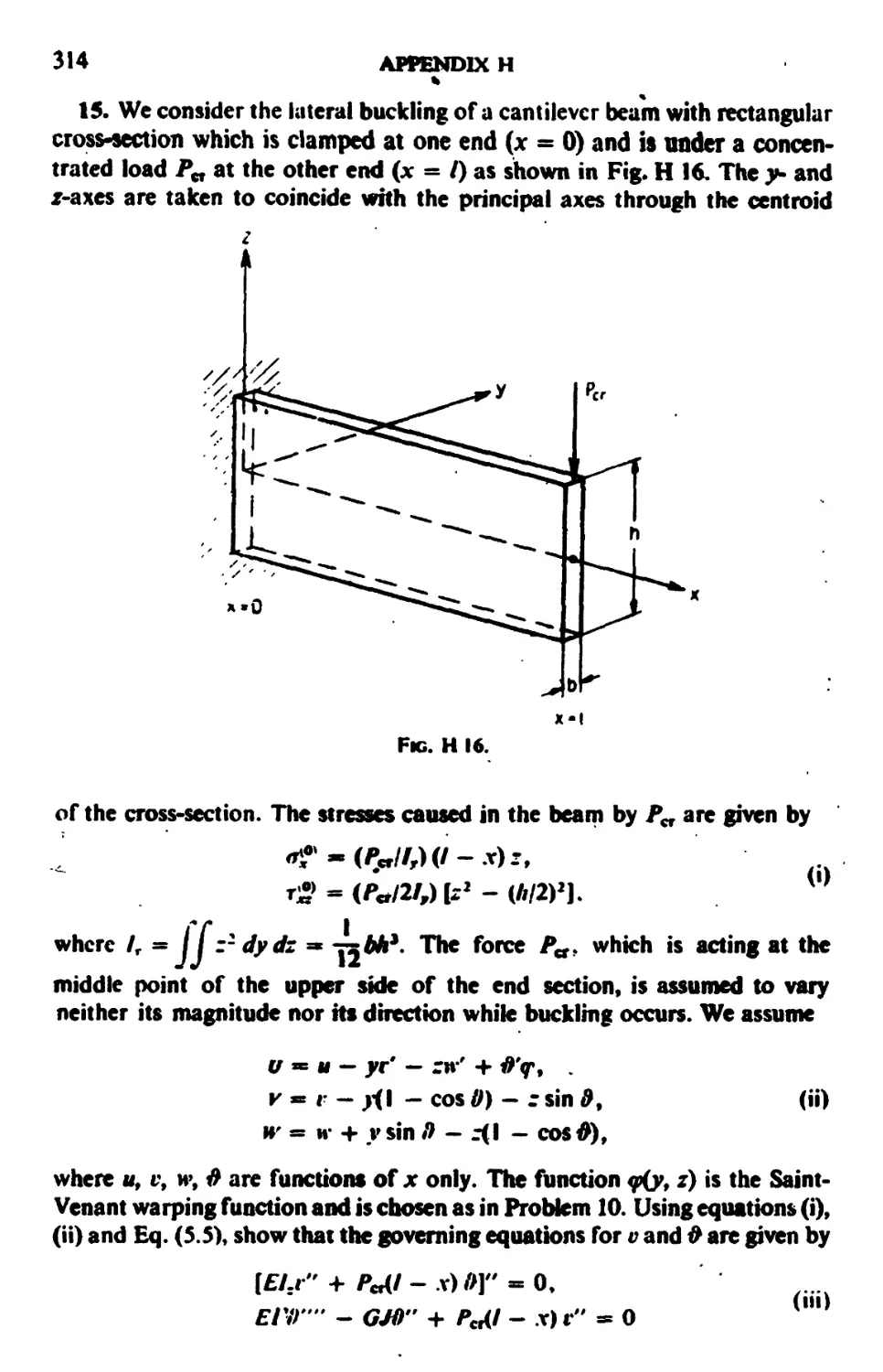
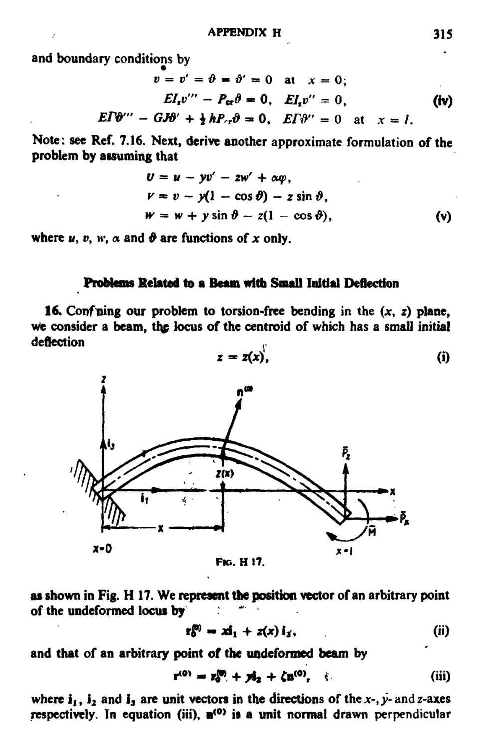
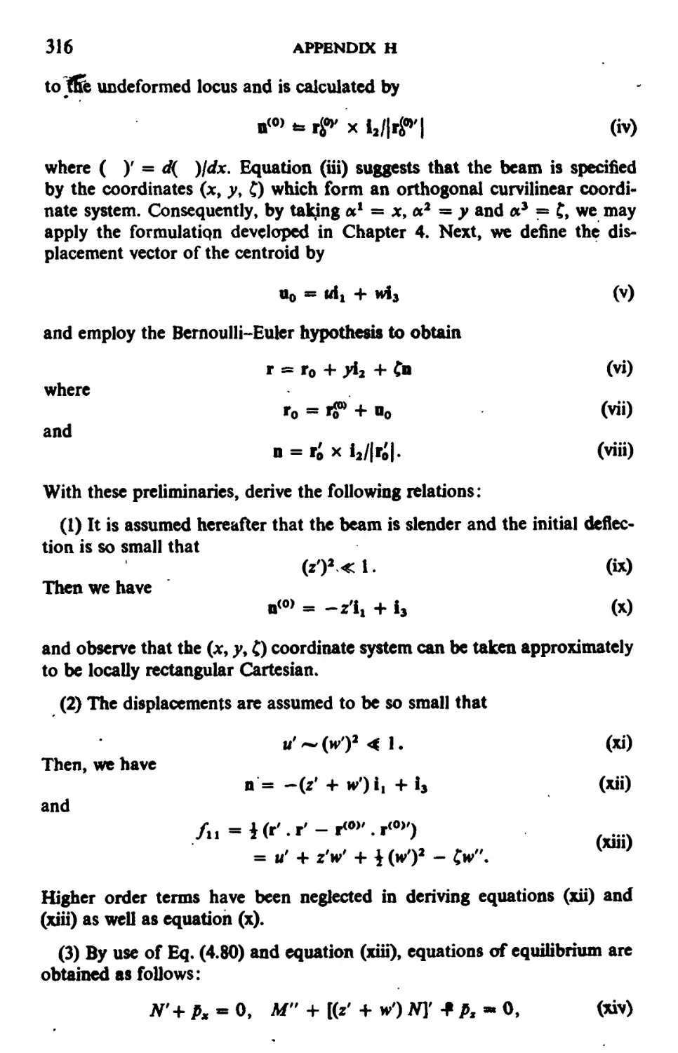
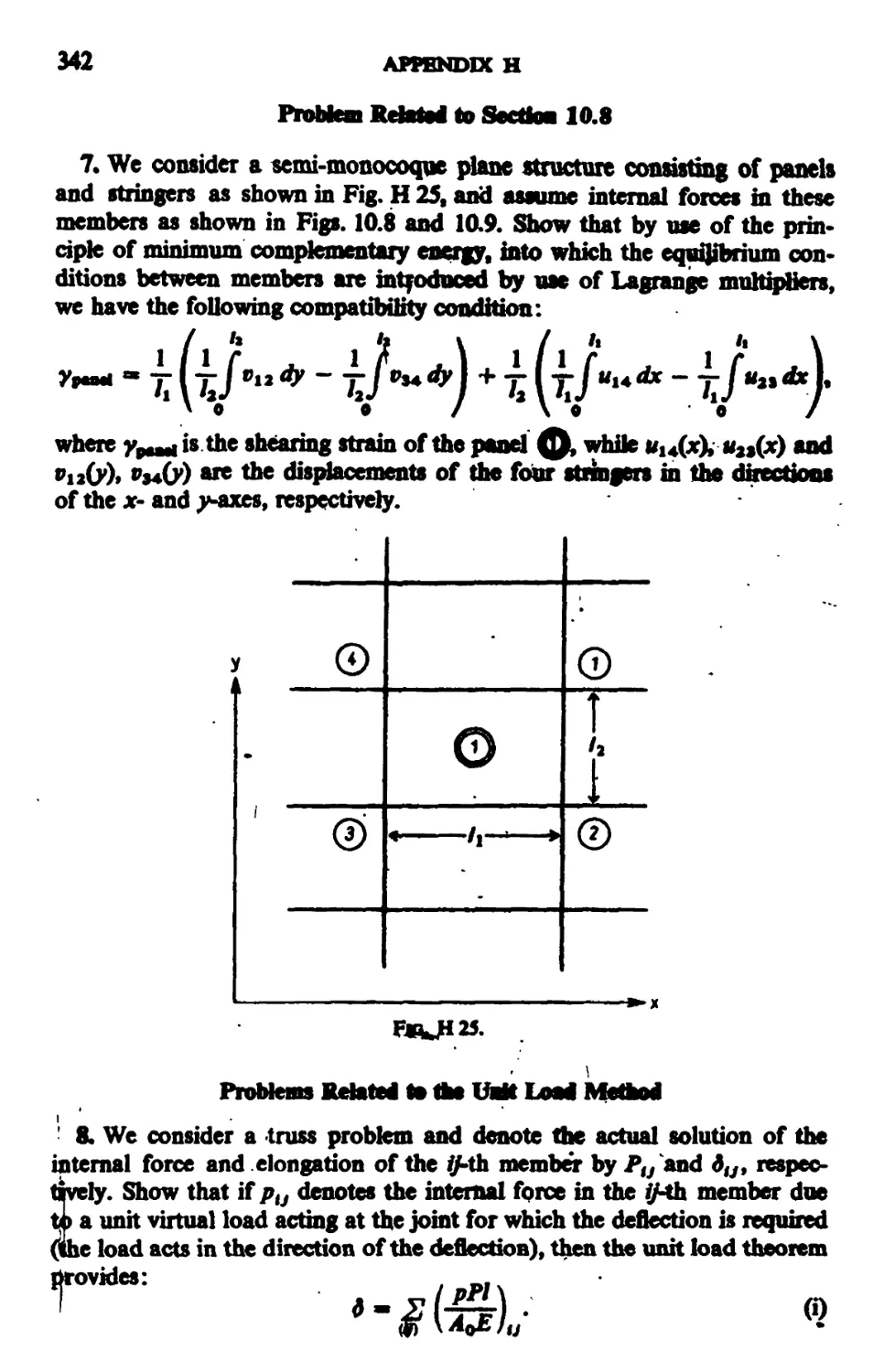
APPENDIX H. Problems 272
xii CONTENTS
APPENDIX I. Variational Principles as a Basis for the Finite Element
Method 345
1. Introduction 345
2. Conventional Variational Principles for the Small Displacement Theory of
Elastostatics 347
3. Derivation of Modified Variational Principles from the Principle of Minimum
Potential Energy 351
4. Derivation of Modified Variational Principles from the Principle of Minimum'
Complementary Energy 357
5. Conventional Variational Principles for the Bending of a Thin Plate 360
6. Derivation of Modified Variational Principles for the Bending of a Thin Plate 364
7. Variational Principles for the Small Displacement Theory of Elastodynamics 372
8. Finite Displacement Theory of Elastostatics 378
9. Two lncremcntaUTheories 384
10. Some Remarks on Discrete Analysis 397
APPENDIX J. Notes on the Principle of Virtual Work 405
INDEX
409
INTRODUCTION
The calculus of variations is a branch of mathematics, wherein the stationary
property of a function of functions, namely, a functional, is studied. Thus,
the object of the calculus of variations is not to find extrema of a function
of a finite number of variables, but to find, among the group of admissible
functions, the one which makes the given functional stationary.! A well-
established example is to find, among the admissible curves joining two
points in the prescribed space, that curve on which the distance between
the points is a minimum. The problem of finding a curve which encloses
a given area with minimum peripheral length is another typical example.
The calculus of variations has a wide field of application in mathematical
physics. This is due to the fact that a physical system often behaves in a
manner such that some functional depending on its behavior assumes a
stationary value. In other words, the equations governing the physical
phenomenon are often found to be stationary conditions of some variational
problem. Fermat's principle in optics may be mentioned as a typical example.
It states that a ray of light travels between two points along the path which
requires the least time. This leads immediately to the conclusion that a ray
of light travels in a straight line in any homogeneous medium.
Mechanics is one of the fields of mathematical physics, wherein the
variational technique has been extensively investigated. We shall take a
problem of a system of particles as an example and review the derivation
of its variational formulations. J
First, we shall consider the problem of a system of particles in static
equilibrium under external and internal forces. It is well known that the
basis of variational formulation is the principle of virtual work,ft which
may be stated as follows: Assume thai the mechanical system is in equilibrium
under applied forces and prescribed geometrical contraints. Then, the sum of
all the virtual work, denoted by 6' W, done by the external and internal forces
existing in the system in any arbitrary infinitesimal virtual displacements
satisfying the prescribed geometrical constraints is zero:
d'w = o. (i)tt
The principle may be stated alternatively in the following manner: IfffW
vanishes for any arbitrary infinitesimal virtual displacements satisfying the
• t For details of the calculus of variations, see Refs. 1 through 8 (see pp. 6-7).
t For details of the variational methods in mechanics, see Refs. 2, 9,10 and 11.
ft This principle is also called the principle of virtual displacements.
It 6'W\& not a variation of some state function W% but denotes merely the total virtual
work.
1
2 VARIATIONAL METHODS IN ELASTICITY AND PLASTICITY
prescribed geometrical constraints, the mechanical system is in equilibrium.
Thus, the principle of virtual work is equivalent to the equations of
equilibrium of the system. However, the former has a much wider
field of application to the formulation of mechanics problems than
the latter. When all the external and internal forces are derived from a
potential function U> which is a function of the coordinates of the system
of particles,! such that
b'W = -<5l/, (2)
the principle of virtual work leads to the establishment of the principle of
stationary potential energy: Among the set of all admissible configurations,
the state of equilibrium is characterized by the stationary property of the
potential energy U:
6U = 0. (3)
The above formulation may be extended to the dynamical problem of a
system of particles subject to time-dependent applied fprces and geometrical
constraints. By the use of d'Alembert's principle which states that the
system can be considered to be in equilibrium if inertial forces are taken into
account, the principle of virtual work of the dynamical problem can be
derived in a manner similar to the static problem case, except that terms
representing the virtual work done by the inertial forces are now included.
The principle thus obtained is integrated with respect to time t between two
limits t » tx and t = t2. Through integration by parts and by the use of the
convention that virtual displacements vanish at the limits, we finally obtain
the following principle of virtual work for the dynamical problem:
dfTdt+fd'Wdt = Q, (4)
a ft
where T is the kinetic energy of the system. Since Lagrange's equations of
motion of the system may be derived from the principle of virtual work thus
obtained, it is evident that the principle is extremely useful for obtaining
the equations of motion of a system of particles with geometrical
constraints.
When it is further assured that all the external and internal forces are
derived from a potential function U, which is defined in the same manner
as Eq. (2) and is a function of coordinates and the time,{ we obtain
Hamilton's principle, which states that among the set of all admissible configurations
of the system, the actual motion makes the quantity
f\r-v)dt (5)
t Forces of this category are called conservative forces.
% If U is time-independent, the forces are called conservative. In Ref. 2, the name
"monogenic** is given to forces derivable from a scalar quantity which is in the most
general case a function of coordinates and velocities of the particles and the time.
INTRODUCTION 3
stationary, provided the configuration of the system is prescribed at the limits
t = tx and t = t2. Hamilton's principle may be stated mathematically as
follows:
6JLdt = 0, (6)
where L = T - U is the Lagrangian function of the system. It is well known
that Hamilton's principle can be transformed by the use of Legendre's
transformation into a new and equivalent principle, and that Lagrange's
equations of motion are reduced to the so-called canonical equations.
Transformations of Hamilton's principle were extensively investigated and
an elegant theory known as canonical transformation was established.
The main object of this.book is to derive the principle of virtual work and
related variational principles in elasticity and plasticity in a systematic
way.f We shall formulate these principles in a manner similar to the
development in the problem of a system of particles. The outline is as followV. we
define a problem involving a solid body in static equilibrium under body
forces plus mechanical and geometrical boundary conditions prescribed
on the surface of the body. To begin with, we derive the principle of virtual
work. This principle is equivalent to the equations of equilibrium and the
mechanical boundary conditions of the solid body/and is-derived for small
displacement theory as well as finite displacement theory.} Within the realm
of small displacement theory we obtain another principle which will be
called the principle of complementary .virtual work.jf It is worthy of special
mention that the principles of virtual work and complementary virtual work
are invariant under coordinate transformations and that they hold
independently of the stress-strain relations of the material of the body. However,
the stress-strain relations should be taken into account for the formulations
of variational principles, and the theories of elasticity and plasticity should
be treated separately.
The variational method finds one of the most fruitful fields of application
in the small displacement theory of elasticity. When the existence of a strain
energy function is assured and the external forces are assumed to be kept
unchanged during displacement variation, the principle of virtual work
leads to the establishment of the principle of minimum potential energy. The
variational principle is generalised by the introduction of Lagrange
multipliers to yield a family of variational principles which includes the Hellinger-
t For variational principles in elasticity and plasticity, see Refs. 11 through 20. •
t In the small displacement theory, the displacements are assumed so small as to
allow linearizations of all governing equations of the solid body except the stress-strain
relations. Consequently, the equations of equilibrium, the strain-displacement relations
and the "boundary conditions are reduced to linearized forms in small displacement
theory.
ft This principle is also called the principle of virtual stress, the principle of virtual
force or the principle of virtual changes in the state of stress.
4 VARIATIONAL METHODS IN ELASTICITY AND PLASTICITY
4
Reissner principle, the principle of minimum complementary energy and
so forth.
On the other hand, the principle of complementary virtual work leads to
the establishment of the principle of minimum complementary energy when
the stress-strain relations assure the existence of a complementary energy
function and the geometrical boundary conditions are assumed to be kept
unchanged during stress variation. The principle of minimum
complementary energy is generalized by the introduction of Lagrange multipliers to yield
the Hellinger-Reissner principle, the principle of minimum potential energy
and so forth. It is seen that these two approaches to the formulation of the
variational principles are reciprocal and equivalent to each other as far as
the small displacement theory of elasticity is concerned.
In the finite displacement theory of elasticity, the principle of virtual .
work leads to the establishment of the principle of stationary potential
energy when the existence of a strain energy function of the body material
and potential functions of the external forces is assured. Once the principle
of stationary potential energy is thus established, it can be generalized
through the use of Lagrange multipliers.
The above technique is extended to dynamical elastic body problems by
taking inertial forces into account. Thus, we derive the principle of virtual
work for the dynamical problem with the introduction of the concept of
kinetic energy. The principle of virtual work is then transformed into a
variational principle under the assumption of the existence of a strain energy
function and potential functions of the external forces. The newly obtained
variational principle may be thought of as Hamilton's principle extended
to the dynamical elastic body problem, and it can be generalized through
the use of Lagrange multipliers.
The variational principle of an elasticity problem provides the governing
equations of the problem as stationary conditions and in that sense, is
equivalent to the governing equations. However, the variational formulation
has several advantages. First, the functional which is subject to variation
usually has a definite physical meaning and is invariant under coordinate
transformation. Consequently, once the variational principle has been
formulated in one coordinate system, governing equations expressed in
another coordinate system can be obtained by first writing the invariant
quantity in the new coordinate system and then applying variational
procedures. For example, once the variational principle has been formulated
in the rectangular Cartesian coordinate system, governing equations
expressed in cylindrical or polar coordinate systems can be obtained through
the above technique. It may be observed that this property makes the
variational method extremely powerful for the analysis of structures.
Second, the variational formulation is helpful in carrying out a common
mathematical procedure, namely, the transformation of a given problem
into an equivalent problem that can be solved more easily than the original.
INTRODUCTION 5
In a variational problem with subsidiary conditions, the transformation is
achieved by the Lagrange multiplier method, a very useful and systematic
tool. Thus, we may derive a family of variational principles which are
equivalent to each other.
Third, variational principles sometimes lead to formulae for upper or
lower bounds of the exact solution of the problem under consideration. As
will be shown in Chapter 6, upper and lower bound formulae for the
torsional rigidity of a bar are provided by simultaneous use of two variational
principles. Another example is an upper bound formula, derived from the
principle of stationary potential energy, for the lowest frequency of free
vibrations of an elastic body.
Fourth, when a problem of elasticity cannot be solved exactly, the
variational method often provides an approximate formulation for the problem
which yields a solution compatible with the assumed degree of
approximation. Here, the variational method provides not only approximate governing
equations, but also suggestions on approximate boundary conditions.
Since it is almost impossible to obtain the exact solution of an elasticity
problem except in a few special cases, we must be satisfied with approximate
solutions for practical purposes. Theories of beams, plates, shells and multi-
component structures are typical examples of such approximate formulations
and show the power of the principle of virtual work and related variational
methods. However, one should take care in relying upon the accuracy of
approximate solutions thus obtained. Consider, for example, an
application of the Rayleigh-Ritz method combined with the principle of stationary
potential energy. The method may provide a good approximate solution
for the displacements of a body if admissible functions are chosen properly.
However, the accuracy of stress distribution calculated from the
approximate displacements is not as reliable. This is obvious if we remember that,
in the governing equations obtained by the approximate method, the exact
equations of equilibrium and mechanical boundary conditions have been
replaced by their weighted means and that.the accuracy, of an approximate
solution decreases with differentiation. Thus, the equations of equilibrium
and mechanical boundary conditions are generally violated at least locally
in the approximate solution. In understanding approximate solutions thus
obtained, the principle of Saint-Venant is sometimes helpful. It states :<14)
44 If the forces acting on a small portion of the surface of an elastic body are
replaced by another statically equivalent system of forces acting on the same
portion of the surface, this redistribution of loading produces substantial
changes in the stresses locally; but has a negligible effect on the stresses at
distances which are large in comparison with the linear dimensions of the surface
pn which the forces are changed."
Due to the author's preference, approximate governing equations of
elasticity problems will be derived very frequently from the principle of
virtual work rather than from the variational principle, since the former
6 VARIATIONAL METHODS IN ELASTICITY AND PLASTICITY
holds independently of the stress-strain relations of the body and the
existence of potential functions. An approximate method of solution using
the principle of virtual work will be called the generalized Galerkin's method.!
As far as conservative problems in elasticity are concerned, results obtained
by the combined use of the principle of virtual work and the generalized
Galerkin's method are equivalent to those obtained by the combined use of
the principle of stationary potential energy and the Rayleigh-Ritz method.
It is quite natural in theories of plasticity to make the principle of virtual
work a basis for the establishment of variational principles. If the problem
is confined to the small displacement theory, the principle of
complementary virtual work may ajso be employed as another basis. Since stress-strain
relations in the theories of plasticity are more complicated than those in
the theory of elasticity, it may be expected that the establishment of a
variational principle in plasticity is more difficult. Several variational
principles which have been established for the theories of plasticity can
be shown to be formally derivable in a manner similar to those in the theory
of elasticity, although rigorous proofs should follow for showing the validity
of the variational principles.
The most successful application of variational formulations in the fl*w
theory of plasticity is the theory of limit analysis for a body consisting of
material which obeys the perfectly plastic Prandtl-Reuss equation. Limit
analysis concerns the determination of an eigenvalue called the collapse
load of the body. Two variational principles provide upper and lower bound
formulae for locating the collapse load. '
Since a great many papers have been written on variational treatment of
problems in elasticity and plasticity, the bibliography of this book is not
intended to be complete. The author is satisfied with citing only a limited
number of papers for the reader's reference. Literature such as Refs, 22 and
23 may be helpful for reviewing recent developments of the topic.
The variational method can, of course, be applied to problems other
than those mentioned herein..For example, it has been applied to problems
in fluid mechanics, conduction of heat and so forth. <*4~26> As a recent
application of engineering concern, we may add that problems of the
performance of flight vehicles have been extensively treated in the literature by
the optimization techr. que.<a7)
Bibliography
1. R. CouKANTand D. Hubert, Methods of Mathematical Physics, Vol. I, Interscience,
New York, 1953.
2. C. Lanczos, The Variational Principles of Mechanics, University of Toronto Press,
1949.
t This is also called the method of weighting functions. It is a special case of the
approximate method of solution called the method of weighted residuals/*1*
INTRODUCTION 7
3. O. fioLZA, Lectures on the Calculus of Variations, The University of Chicago Press,
1946.
4. G. A. Bliss, Lectures on the Calculus of Variations, The University of Chicago Press,
1946.
5. C Fox, An Introduction to the Calculus of Variations, Oxford University Press,
London, 1950.
6. R. Weinstock, Calculus of Variations with Application to Physics and Engineering,
McGraw-Hill, 1952.
7. P. M. Morse and H. Feshbach, Methods of Theoretical Physics, Vols. 1 and 2,
' McGraw-Hill, 1953.
8. S. G. Mikhlin, Variational Methods in Mathematical Physics, Pergamon Press, 1964.
9. H. Goldstein, Classical Mechanics, Addison-Wesley, 1953.
10. J. L. Synge and B. A. Griffth, Principles of Mechanics, McGraw-Hill, f959.
11. H. L. Langhaar, Energy Methods in Applied Mechanics, John Wiley, 1962.
12. C. B. Biezeno and R. Grammel, Technische Dynamik, Springer, Berlin, 1939.
13. R. V. Southwell, Introduction to the Theory of Elasticity, Clarendon Press, Oxford,
1941.
14. S. Timoshenko and J. N. Goodier, Theory of Elasticity, McGraw-Hill, 1951.
15. N. J. Hoff, The Analysis of Structures, John Wiley, 1956.
16. C. E. Pearson, Theoretical Elasticity, Harvard University Press, 1959.
17. J. H. Argyris and S. Kelsey, Energy Theorems and Structural Analysis, Butterworth,
1960.
18. V. V. Novozhilov, Theory of Elasticity, translated by J. K. Lusher, Pergamon Press,
1961.
19. J. H. Greenbero, On the Variational Principles of Plasticity, Brown University, ONR,
NR-041-032, March 1949.
20. R. Hill, Mathematical Theory of Plasticity, Oxford, 1950.
21. M. Becker, The Principles and Applications of Variational Methods, The
Massachusetts Institute of Technology Press, 1964.
22. Applied Mechanics Reviews, published monthly by the American Society of Mechanical
Engineers.
23. Structural Mechanics in U.S.S.R. 1917-1957, edited by I. M. Rabinovich. English
translation edited by G. Herrmann was published by Pergamon Press in 1960.
24. J. Serrin, Mathematical Principles of Classical Fluid Mechanics, Handbuch der
Physik, Band VII/I. Strdmungsmechanik I, pp. 125-265, Springer, 1959.
25. M. A. Biot, Lagrangian Thermodynamics of Heat Transfer in Systems including
Fluid Motion. Jdurnal of the Aeronautical Sciences, Vol. 25, No. 5, pp. 568-77, May
1962.
26. K. Washizu, Variational Principles in Continuum Mechanics, University erf
Washington, College of Engineering, Department of Aeronautical Engineering, Report 62-2,
June 1962.
27. G. Leitmann (Editor), Optimization Techniques with Applications to Aerospace
Systems, Academic Press, 1962.
CHAPTER 1
SMALL DISPLACEMENT THEORY OF
ELASTICITY IN RECTANGULAR
CARTESIAN COORDINATES
1.1* Presentation of a Problem in Small Displacement Theory
In the beginning of his classical work,(u Love states: "The Mathematical
Theory of Elasticity is occupied with an attempt to reduce to calculation
the state of strain, or relative displacement, within a solid body which is
subject to the action of an equilibrating system of forces, or is in a state of
slight internal relative motion, and with endeavours to obtain results which
shall be practically important in applications to architecture, engineering,
and all other useful arts in which the material of construction is solid/'
This seems to have been a guiding definition of the theory of elasticity.
In the first and second chapters of this book we shall deal with the small
displacement theory of elasticity and derive the principle of virtual work
and related variational principles for the problem of an elastic body in
static equilibrium under body forces and prescribed boundary conditions/1*2*
Rectangular Cartesian coordinates (x, y, z) will be employed for defining
the three-dimensional space containing the body. In the small displacement
theory of elasticity displacement components, u, v, w> of a point of the body
are assumed so small that we are justified in linearizing equations governing the
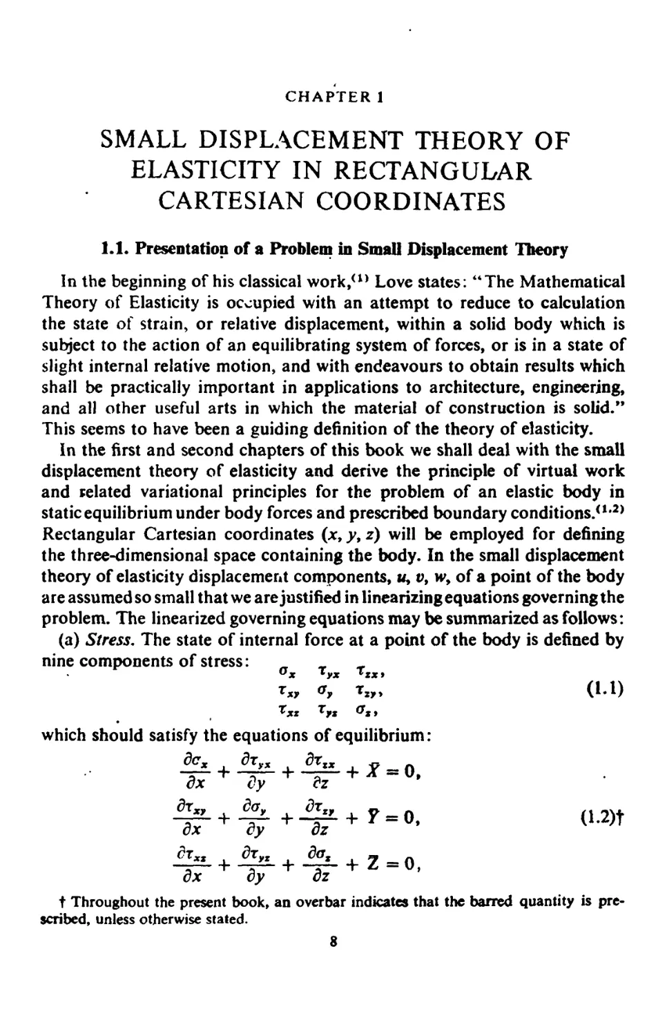
problem. The linearized governing equations may be summarized as follows:
(a) Stress. The state of internal force at a point of the body is defined by
nine components of stress:
°x ^yx ^zx»
*xy <*y Txy> 0-1)
^xz **tz &z*
which should satisfy the equations of equilibrium :
dcx drvx dxzx +- ^
dx vy dz
^2- + ^- +i£L+F = 0, (1.2)t
dx dy dz
fax* , d*yz , d<?z . f _n
dx vy dz
t Throughout the present book, an overbar indicates that the barred quantity is
prescribed, unless otherwise stated.
8
SMALL DISPLACEMENT THEORY OF ELASTICITY
and
fyz ^xy* ?xx
'XX 9
^xy Tyx*
(13)
where Zf T and Z are components of the body forces per unit volume. We
shall eliminate xsy9 xxs and rfX by the use of Eqs. (1.3), and specify the state
of stress at a point of the body with six components (aX9 of9 aX9 r,X9 rXX9 r^).
Then, Eqs. (1.2) become:
dax dr
17 + ~
dx
XX
dy
dz
dr
xy
dx
day dr.
~dy~ +^
dr
XX
dr
r*
dz
doz
+ * = 0,
+ F = 0,
+ 2 = 0.
(1.4)
dx dy dz
(b) Strain. The state of strain at a point of the body is defined by six
components of strain (eX9 ey9eX9 y,X9 yXX9 yXf).
(c) Strain-displacement relations. In small displacement theory the strain-
displacement relations are given as follows:
du _ dv dw
e, «
dx'
e,=
«,=
dw . dv
Ytz = -*- +
du
dz'
dw
dx~' Y"
dv du
+
(1.5)
dy ' dz* '" dz ' dxf '" dx ' dy'
(d) Stress-strain relations. In small displacement theory, the stress-strain
relations are given in linear, homogeneous form:
■—" •—1
Ox
°f
o%
fyx
rtx
^xy
»
^,
011 <*12 *13 014 015 016
021 022 023 024 025 fl26
031 032 033 034 035 036
041 042 043 044 045 046
051 052 053 054 055 *56
061 062 063 064 065 066
Vyx
V:x
Yxy
(1.6)
The coefficients of these equations are called elastic constants. Among them,
there exist relations of the fojrm:
0« = 0«r> (r,5 = 1,2, ..,6). (1.7)
Eqs. (1.6) may be inverted to yield:
e*
s,
Y,z
Yzx
Vxy
=
pn
*21
*31
b5i
b6l
*12
b22
l>32
*42
b$i
*62
b13
bz9
*3?
643
bi3
b63
61*
*24
*34
*44
654
*6*
*15
b25
>
O45
655
b6S
bl6
*26
*36
*46
b56
b*6
Ox
Oy
ot
Xyg
^ZX
^xy
(1-8)
where
frs
rsr*
(r,s = 1,2, .., 6).
(1.9)
Ox
o,
= 2<?
= 2(7
10 VARIATIONAL METHODS IN ELASTICITY AND PLASTICITY
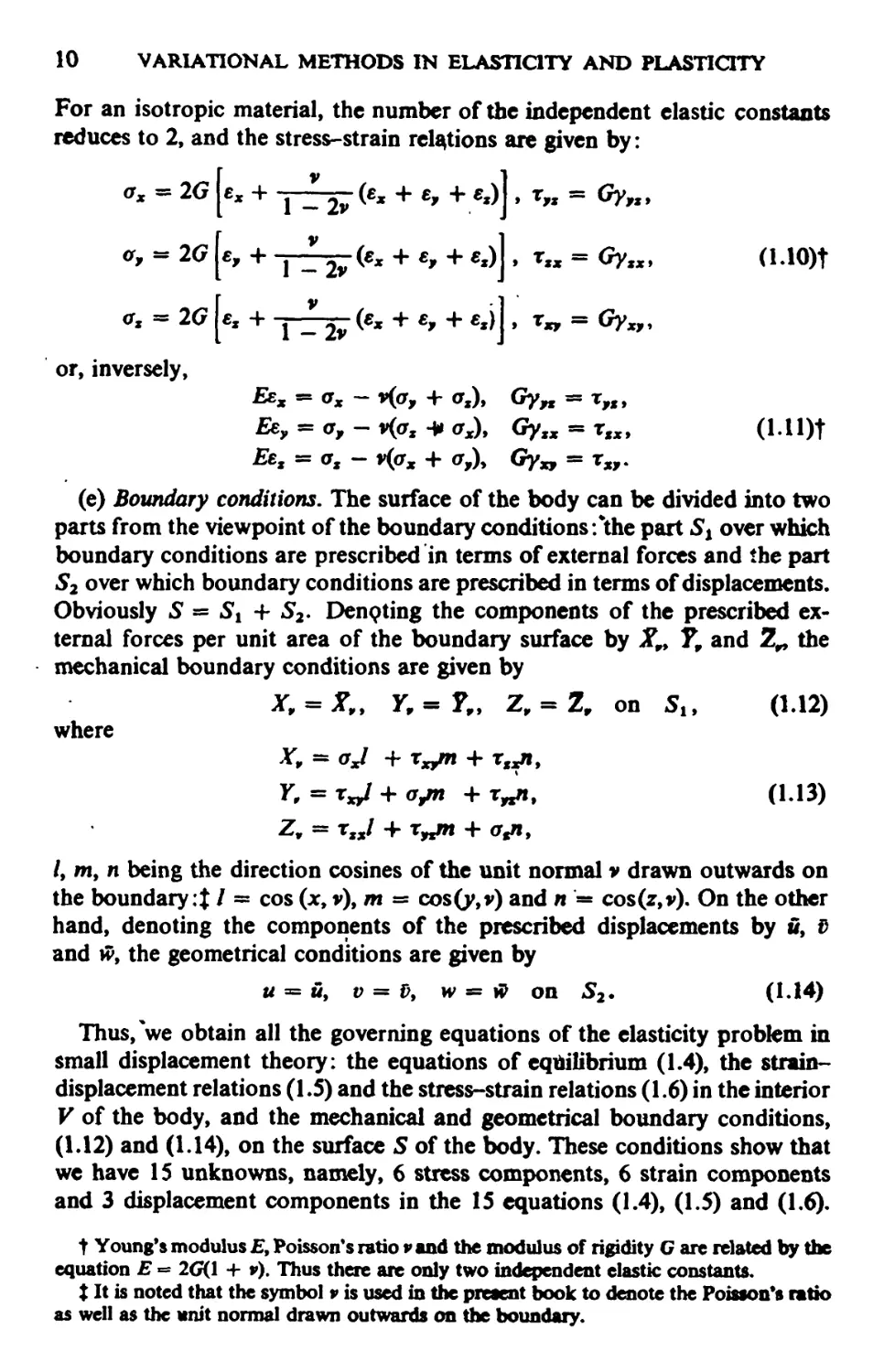
For an isotropic material, the number of the independent elastic constants
reduces to 2, and the stress-strain relations are given by:
*x + t _ 2v fa. + e, +*z)\ , rfs = Gy,s,
>>, + ! V_ 2v (** + *, + O]> *** = Gy*x> (!.10)t
or, = 2(7 £x + t ^2y (ex + «,+ «x) I, r^ = GyXfy
or, inversely,
ftis^- via, + <*z)> Gy„ = *,m>
Ee, = o,~ v(os -» ax)y Gytx = xtxy (l.U)t
£6, = as - y((rx + cr,), Gy„ = r„.
(e) Boundary conditions. The surface of the body can be divided into two
parts from the viewpoint of the boundary conditions /the part Sx over which
boundary conditions are prescribed in terms of external forces and the part
S2 over which boundary conditions are prescribed in terms of displacements.
Obviously S = Sx + S2. Denpting the components of the prescribed
external forces per unit area of the boundary surface by Xp> T9 and Z„ the
mechanical boundary conditions are given by
*, = JT„ y, = F„ ZP = ZP on Si, (1.12)
where
X¥ = oJ + rXJm + xsxny
Y, = Txyl + ojn + xrtn% (1.13)
Z, = rgxl + Xyjm + (Vi,
/, m, n being the direction cosines of the unit normal v drawn outwards on
the boundary:% I = cos (xy v), m = cos(y,v) and n = cos(z,v). On the other
hand, denoting the components of the prescribed displacements by «, tf
and iv, the geometrical conditions are given by
u = w, v = f>> w *s h> on 52. (1-W)
Thus, we obtain all the governing equations of the elasticity problem in
small displacement theory: the equations of equilibrium (1.4), the strain-
displacement relations (1.5) and the stress-strain relations (1.6) in the interior
V of the body, and the mechanical and geometrical boundary conditions,
(1.12) and (1.14), on the surface 5 of the body. These conditions show that
we have IS unknowns, namely, 6 stress components, 6 strain components
and 3 displacement components in the 15 equations (1.4), (1.5) and (1.6).
t Young's modulus £, Poisson's ratio v and the modulus of rigidity G are related by the
equation E = 2G(1 + t>). Thus there are only two independent elastic constants.
X It is noted that the symbol v is used in the present book to denote the Poisson's ratio
as well as the unit normal drawn outwards on the boundary.
SMALL DISPLACEMENT THEORY OF ELASTICITY 11
Our problem is then to solve these 15 equations under the boundary
conditions (1.12) and (1.14). Since all the governing equations have linear forms,
the law of superposition can be applied in solving the problem. Thus, we
obtain linear relationships between the prescribed quantities such as the
applied load on St and resulting quantities such as stress and displacement
caused in the body.
1.2. Conditions of Compatibility
We observe from Eqs. (1.5) that when a continuum deforms, the six
strain components (exy e,,exy yfMf y1Jr, yxf) cannot behave independently,
but must be derived from three functions uy v and w as shown. This
statement can be expressed in a different way as follows: Let the continuum
under consideration be separated into a large number of infinitesimal
rectangular parallelepiped elements before deformation. Assume that each
element is given six strain components (tXf ...,yx,) of arbitrary magnitude.
Then, trials to reassemble the elements again into a continuum are assumed
to be made. In general, such trials cannot be successful. Some relations should
exist between the magnitude of the strain components for a reassemblage
to be successful. Thus, a problem will arise which may be stated as follows:
What are the necessary and sufficient conditions for the elements to b*
reassembled into a continuous body?
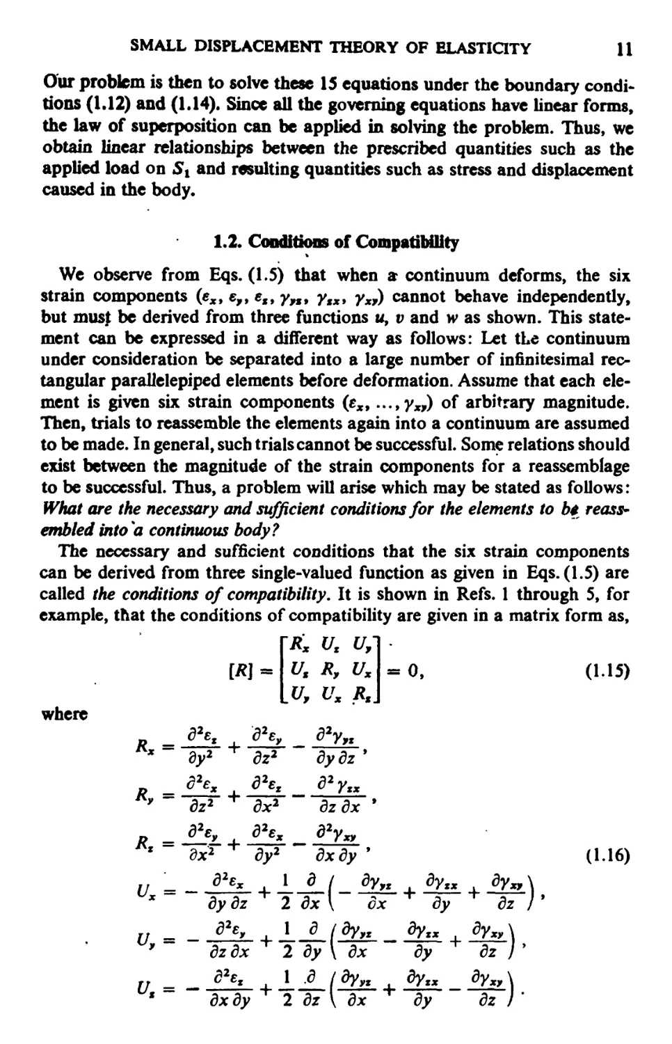
The necessary and sufficient conditions that the six strain components
can be derived from three single-valued function as given in Eqs. (1.5) are
called the conditions of compatibility. It is shown in Refs. 1 through 5, for
example, that the conditions of compatibility are given in a matrix form as,
[R] = UM R, Ux
U, Ux Rs]
- 0, (1.15)
where
dy2 "*" dz2 dydz '
d2ex d2ez d2y„
dz2 dx2 dz dx
d2e, t d2ex d2y„
Ry =
*, =
dx2 ' dy2 dxdy ' (1.16)
U d2ex i I d J dy,z | dytx ^ dy„ \
x dy dz 2 dx \ ox dy dz / '
n = dh> i 1 d (ty" ty" i dy"\
' dzdx "*" 2 dy \ dx dy dz J '
r, S2et , I d (dy,t dytx dy
dxdy "*" 2 dz\ dx "*" dy dz ) '
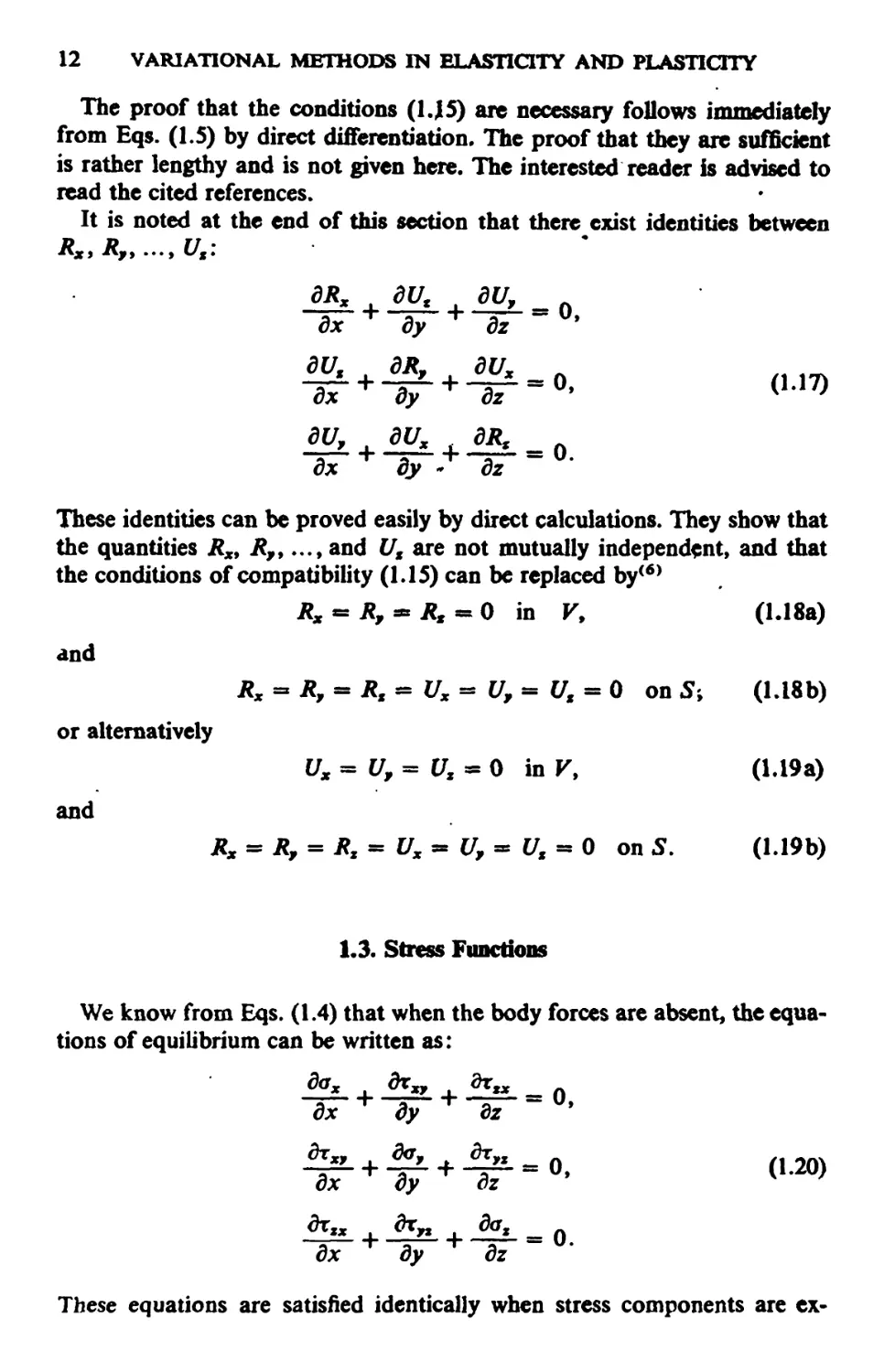
12 VARIATIONAL METHODS IN ELASTICITY AND PLASTICITY
The proof that the conditions (1.J5) are necessary follows immediately
from Eqs. (1.5) by direct differentiation. The proof that they are sufficient
is rather lengthy and is not given here. The interested reader is advised to
read the cited references.
It is noted at the end of this section that there exist identities between
/Vjt) «**/> •••» U% *
dR
X
+ «L+«S.. 0.
dx dy dz
dU% dR, dU,
dx dy dz
dU, dUx dRt
dx dy - dz
- 0, (1.17)
« 0.
These identities can be proved easily by direct calculations. They show that
the quantities Rxy Rfy..., and Ut are not mutually independent, and that
the conditions of compatibility (1.15) can be replaced by(6)
Rx mz Ry « Rt « 0 in V9 (1.18a)
and
Rx « R, = Rs « Ux « U, - U% = 0 on Sy (1.18b)
or alternatively
Ux= U,= UX = Q in V9 (1.19a)
and
Rx = *, = Rx « Z7X » tf, « £/, « 0 on 5. (1.19b)
1.3. Stress Functions
We know from Eqs. (1.4) that when the body forces are absent, the
equations of equilibrium can be written as:
d<*x dx*, dr^ _
dx dy dz
i^ + ^ + J^O, (1.20)
dx dy dz
dx2x dx„ dax = Q
dx dy dz
These equations are satisfied identically when stress components are ex-
SMALL DISPLACEMENT THEORY OF ELASTICITY 13
pressed in terms of either Maxwell's stress functions %\ > Xi and xs defined by
* dy2 dz2 ' " dydz '
dz2 + dx2 ' "~ ITdx'
(121)
5**i T _ _ &Z:
dx2 ■ dy2 ' " dxdy '
or Morera's stress functions Vi> Vj and y3 defined by
„ - g2yt L_£_/ ^i t aya , ay3\
* " dydz ' " ~ 2 dx\ dx + dy + dz j*
d2V*
a'~~d7dx~' T"
• ~ dxdy ' T" ~ 2 a* \ ax + a* az)'
It is interesting to note that, when these two kinds of stress functions are
combined such that
&%* , d2Xi 3yt
' U?~ 1P~ " ~dydz~' '"*'"*
^ ' (1.23)
*w
Jf«L . 1 * / 5v»i . ^Pa . av»3\
~"a7^ + 7ax"l~~ax IF "aH '
the expressions (1.16) and (1.23) have similar forms.
~ In a two-dimensional stress problem, where the equations of equilibrium
are
fo« , *»» _ 0 ^r*y , fry _ 0
ax a>> ' ax a>> *
(1.24)
the so-called Airy stress function defined by
d2F &F d2F n„
"*«ip-> ">~l£r> T"=-&^T (L25)
satisfies the equations of equilibrium identically*
1.4. Principle of Virtual Work
In this section we shall derive the principle of virtual work for the problem
defined in Section 1.1. We consider Ike fcrty in equilibrium under prescribed
body forces and boundaty eooditi**!, «ftd denote the stress components
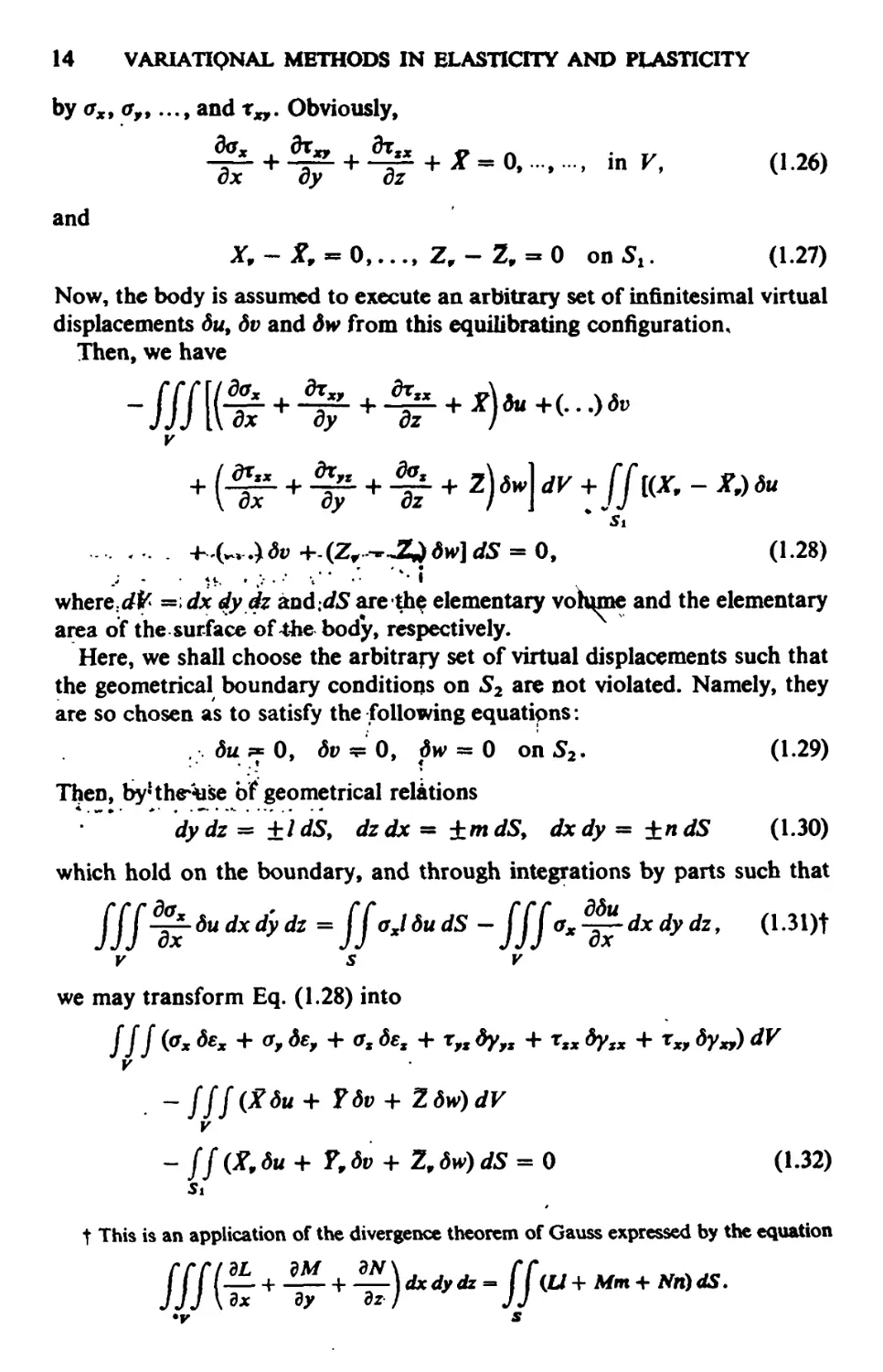
14 VARIATIQNAL METHODS IN ELASTICITY AND PLASTICITY
by axy ayy..., and x^. Obviously,
*** +^ + ^ + X= 0, -,..., in V, (1.26)
and
dx dy dz
X, - X, - 0,..., Zr - Z, = 0 on St. (1.27)
Now, the body is assumed to execute an arbitrary set of infinitesimal virtual
displacements du, dv and dw from this equilibrating configuration.
Then, we have
v
-- . •• . -h.(~.}dv +.(Z,-r~Zjdw]dS = 0, (1.28)
where, tffr =; */* rfy dz and:dS are the elementary vohune and the elementary
area of the surface of -the body, respectively.
Here, we shall choose the arbitrary set of virtual displacements such that
the geometrical boundary conditions on S2 are not violated. Namely, they
are so chosen as to satisfy the following equations:
. du ^ 0, dv m 0, pw = 0 on 52. (1.29)
Then, by*the**i$e of geometrical relations
dydz=±ldS, dzdx-±mdS, dxdy=±ndS (1.30)
which hold on the boundary, and through integrations by parts such that
///&*""** -ff'J»« -///*&***• (U1)t
V S V
we may transform Eq. (1.28) into
/// (** 6e* + a> *** + a*de* + r>**Yf* + T« *y» + r*> 8Yxf) dV
v
- fff(Xdu + Ydv + Zdw)dV
v
- ff&to + ?>dv + Z9dw)dS = 0 (1.32)
Si
t This is an application of the divergence theorem of Gauss expressed by the equation
•V S
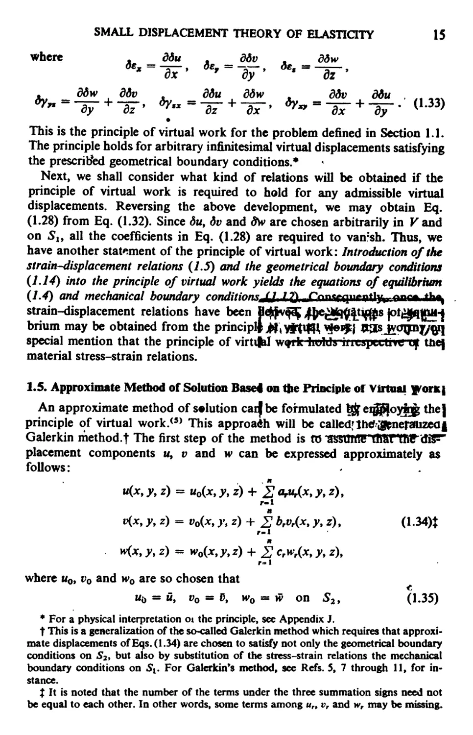
SMALL DISPLACEMENT THEORY OF ELASTICITY 15
where , ddu . ddv , ddw
. ddw ddv . ddu ddw t ddv ddu . ,. „x
This is the principle of virtual work for the problem defined in Section 1.1.
The principle holds for arbitrary infinitesimal virtual displacements satisfying
the prescribed geometrical boundary conditions.*
Next, we shall consider what kind of relations will be obtained if the
principle of virtual work is required to hold for any admissible virtual
displacements. Reversing the above development, we may obtain Eq.
(1.28) from Eq. (1.32). Since du9 dv and &w are chosen arbitrarily in Kand
on Si9 all the coefficients in Eq. (1.28) are required to van;sh. Thus, we
have another statement of the principle of virtual work: Introduction of the
strain-displacement relations (1.5) and the geometrical boundary conditions
(1.14) into the principle of virtual work yields the equations of equilibrium
(L4) and mechanical boundary ">*"*;*''*'>*JJ /ft, ,fyimrapifTf!fti f""^t t1^
strain-displacement relations have been Be$$v<p$ flFtMtffQ*$$s ^t^Mfi^l
brium may be obtained from the principlejft\yjftvR\ vfei£} S3s jvajpiyy^q
special mention that the principle of virtifel wyrk liuhls iiicsptUne qt the|
material stress-strain relations.
1.5. Approximate Method of Solution Basel on the Principle of Virtoal )f/or*|
An approximate method of solution caifbe formulated f^eq^oymg the]
principle of virtual work.<5) This approach will be called[Jhe?\gtne|-aiizeci|
Galerkin method.t The first step of the method is A3 assUMC1 tft&rthB diS^
placement components w, v and w can be expressed approximately as
follows :
u(x9 y9 z) = u0(x9 y,z) + £ OrUr(x, y9 z)9
ft
v(x9 y9 z) = v0(x9 y, z) + £ brvr(x9 y9 z)9 (1.34)t
r-l
n
w(x9 y9 z) = w0(x9 y,z) + £ crwr(x9 y9 z)9
where u^9 v0 and w0 are so chosen that
U{y as Q9 V0 = D9 W0 as W Oil S2, (1.35)
* For a physical interpretation 01 the principle, see Appendix J.
t This is a generalization of the so-called Galerkin method which requires that
approximate displacements of Eqs.(1.34) are chosen to satisfy not only the geometrical boundary
conditions on S2, but also by substitution of the stress-strain relations the mechanical
boundary conditions on Sx. For Galerkin's method, see Refs. 5, 7 through 11, for
instance.
% It is noted that the number of the terms under the three summation signs need not
be equal to each other. In other words, some terms among urp vr and wr may be missing.
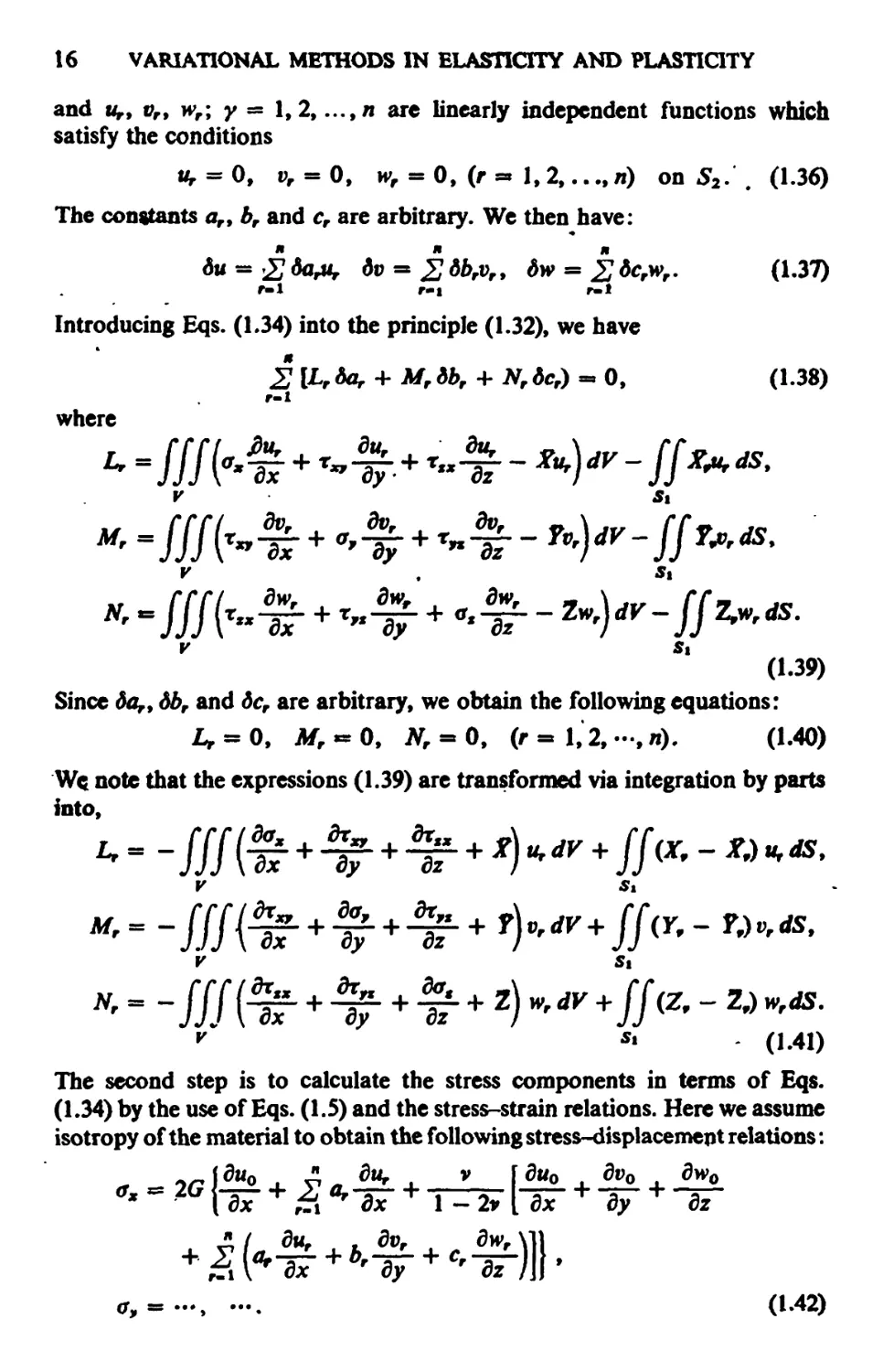
16 VARIATIONAL METHODS IN ELASTICITY AND PLASTICITY
and Ur, tv, wr; y = 1, 2, ...,ji are linearly independent functions which
satisfy the conditions
a, = 0, v, = 0, h>, = 0, (r » 1,2, ...,*) on S2.', (1.36)
The constants arf br and cr are arbitrary. We then have:
to^ZJdajt, 6v = 2forv„ 6w = jj tor,w,. (1.37)
f-1 r-i r-1
Introducing Eqs. (134) into the principle (1.32), we have
2 \Lr6or + Mf db, + JV,dcr) - 0, (1.38)
r-l
where
* -///(*-&+*$■+*■£- *K-?/***
P Si
(1.39)
Since fo,, <S6r and 6cr are arbitrary, we obtain the following equations:
Lr « 0, J/r « 0, AT, - 0, (r - 1,2, ••,*), (1.40)
Wc note that the expressions (1.39) are transformed via integration by parts
into,
v * (1.41)
The second step is to calculate the stress components in terms of Eqs.
(1.34) by the use of Eqs. (1.5) and the stress-strain relations. Here we assume
isotropy of the material to obtain the following stress-displacement relations:
r-i \
du, . dv, dw.
SMALL DISPLACEMENT THEORY OF ELASTICITY 17
Introducing Eq. (1.42) into Eq. (1.40), we have a set of 3n simultaneous
linear equations with respect to the 3/i unknowns ar, br and cr; r = 1, 2, ..., n.
By solving these equations, values of ar, br and cr are determined. By
substituting the constants thus determined into the expressions (1.34), an
approximate solution for the displacement components is obtained.
By a proper choice of the functions u0y v0, w0, ur, v„ \vr; r = 1, 2, ..., ny
and the number ny it is possible to obtain good approximate solutions for
the deformation of the body. However, the accuracy of the stresses
calculated by the use of Eqs. (1.42), employing the values of ar,br and cr thus
determined, is in general not as good. This is obvious if we remember that we
have replaced the equilibrium conditions (1.4) and the mechanical boundary
conditions (1.12) by the 3/i weighted expressions shown in Eqs. (1.41), and
that the accuracy of an approximate solution decreases with differentiation.
The equations of equilibrium as well as the mechanical boundary conditions
are generally violated, at least locally, in the approximate solution.
The accuracy of the approximate solution may be improved by increasing
the number of terms n. If Eqs. (1.34) represent the set of all admissible
*
functions when n tends to infinity, we may hope that the approximate
solution will approach close to the exact solution for a sufficiently large n9 and
tend to it when the number of terms increases without limit. However,
experience and intuition are required if one wishes to obtain an accurate
approximation while retaining only a small number of terms in Eq. (1.34).
Modifications of the above method are frequently employed. For example,
we might choose
u(x,y, z) = 2J/um(xyy)gm\z)y
■U I
v(x, y, z) =, '2 »m(x,y)gm(z), (1.43)
w{x, y, z) = '2 wm(x, y) &,(z),
/
m
where gm(z); m = 0, 1, 2,..., n are prescribed functions of r, while um> v
and wm are undetermined. Equations governing umy vm and wm are derived
from the principle of virtual work. We shall cite frequent examples of this
method in Chapters 7, 8 and 9.
1.6. Principle of Complementary Virtual Work
Within the realm of small displacement theory we can formulate another
principle which is complementary to the principle of virtual work in
defining the problem presented in Section 1.1. We consider the body in
equilibrium under the prescribed body forces and boundary conditions, and denote
the strain and displacement components by sxy ..., yxy and w, vy w, respect-
18 VARIATIONAL METHODS IN ELASTICITY AND PLASTICITY
ively. Obviously,
w — u as 0, ..., w — w a* 0 on S2. (1*45)
Now, the body is assumed to take an arbitrary set of infinitesimal virtual
variations of the stress components (6aXf Soff ..♦., frc*,) from this
equilibrating configuration. Then we have
///[(■
//
which, via integrations by parts, is tranibrmed into:?, < »^
V
+ (•••)« + (-) w dP-[f(u6X, + vdYv + wdZJdS
Sv
- ff(a dx, + f>dr, + wtzjds = o. (1.47)
Here, we shall choose the arbitrary set of virtual stresses such that the
equations of equilibrium and the mechanical boundary conditions are not violated.
Namely, they are so chosen as to satisfy the following equations.
oSox dtex? db*ix
dx dy dz
-0/
dfazx dbz„ dd<Tx -
dx dy dz 9
in the. interior of the bfcdy V and
dX9 « do J + dtxypt + fasji = 0,
6Y9 = foxj + bo/n + 6r^n = 0, (1.49)
dZ9 >■ <$rJjr/ + dr>xm + doji = 0,
on St. Then, Eq. (1.47) reduces to
- // (fid*, + i>dYp + #«Z,)rfS * 0. (1.50)
Si
SMALL DISPLACEMENT THEORY OF ELASTICITY 19
The formula (1.50) will be called the principle of complementary virtual
work. The principle holds for arbitrary infinitesimal virtual stress variations
satisfying the equations of equilibrium and prescribed mechanical boundary
conditions. It is seen that the principle of complementary virtual work has a
form which is complementary to the principle of virtual work given by
Eq. (1.32).
Next, we shall consider what conditions result if the principle of
complementary virtual work is required to hold for an arbitrary set of
admissible virtual stress variations. For such a formulation the Lagrange
multiplier method provides a systematic tool.f We shall treat Eqs. (1.48) and
(1.49) as constraints and employ the displacements u9 v and w as the
Lagrange multipliers associated with these conditions. Thus, reversing the
above development, we obtain Eq. (1.46) from Eq. (1.50). Since the
quantities 6aX9 da,, ...9drx, have been made independent of each other by
introduction of Lagrange multipliers, all the coefficients in Eq. (1.46) are required
to vanish. This leads to another statement of the principle of
complementary virtual work: Introduction of the equations of equilibrium (1.4) and the
mechanical boundary conditions (LI2) into the principle of complementary
virtual work yields the strain-displacement relations (7.5) and the geometrical
boundary conditions (1.14). Consequently, once the equations of
equilibrium have been derived in the small displacement theory, the strain-
displacement relations may be. obtained from the principle of
complementary virtual work. It is worthy of special mention that the principle of
complementary virtual work holds irrespective of the material stress-strain
relations.
1.7. Approximate Method of Solution Based on the Principle
of Complementary Virtual Work
*
An approximate method of solution can be formulated by employing
the principle of complementary virtual work. This approach is similar to
the one mentioned in Section 1.5 and may also be called the generalized
Galerkjn method. For the sake of simplicity, we shall consider a
two-dimensional elasticity problem of a simply connected body.} The side
boundary of the body is cylindrical with the generating line parallel to the
t For Lagrange multiplier method, see Chapter 4 of Ref. 12, and Chapters 2 and 5 of
Ref. 13.
X The two-dimensional elasticity problem defined here is a good approximation to the
so-called plane stress problem of a thin isotropic plate with traction-free Upper and lower
surfaces. In a plane stress problem we assume <r* ■» 0 and obtain Eet - —*(<** + <rr).C2>
On the other hand, this two-dimensional elasticity problem can be shown to be
mathematically equivalent to a plane strain problem of an isotropic body, by replacing E and t in
Eqs. (L51) with £*[ - £/(! - *2>] and •[ - */(l - *)1 respectively, and employing the
assumptions *, ■» 0 and aM «■ -Hpx + *»)/2>
20 VARIATIONAL METHODS IN ELASTICITY AND PLASTICITY
z-axis, and the deformation of the body is assumed independent of r. The
stress components <r2, r2X and t>2 are assumed to vanish. The remaining
stress components axy af and rxy are assumed to be functions of (x,y)
only, and related to the strain components as follows:
E*x - <*x - wy> Ee, = -vox + <Ty, Gyxy = rXft (1.51)
where
du dv du dv
Bx " dx '
ty ~" dy ' Yxy
du dv
~~ dy dx*
Under assumption of absence of body forces, the equations of equilibrium
then reduce to Eqs. (1.24), which suggests the use of the Airy stress function
defined by Eqs. (1.25).
The boundary conditions on the side surface must be prescribed
independently of z, and aip assumed to be given, for the sake of simplicity, in
terms of external forces only, namely
X, ~ S99 Y9 = n (1.53)
on the side boundary C, where
X9 = oxl + Txym9 Y9 = Tjjy/ + ojni.
(1.54)
In the above / and m are the direction cosines of the outward normal v to
the boundary C If the contour of the side boundary C is given parame-
trically in terms of the arc length s measured along C, such that
x = x(s), y = y(s)y (1.55)
we have
/ = dyjds, m = -dx/ds. (1.56)
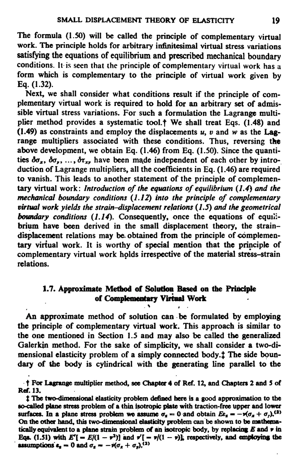
The arc length s is measured as shown in Fig. 1.1. By introducing the Airy
stress function and Eqs. (1.56) into Eqs. (1.54), we obtain X9 and Y9 in
A*
■^x
Fig. 1.1. A two-dimensional problem.
SMALL DISPLACEMENT THEORY OF ELASTICITY 21
terms of F:
* dy2 ds + dxdy ds * ds\dy)9
(1 57*
^t ^ d2F dy d2F dx _ J_(d£\
* dxdy ds dx2 ds " <& U*/'
We shall assurfe an expression for the stress function of the following form:
n
F(x9y) « F0(x9y) + 2 *rF£xyy), (1.58)
r-l
where Fo atyd jFr are chosen so that
4(f)-•• -t(£)-°- <--'-2 ■» <"■>
on the boundary C, and ar; r = 1,2,..., /i are arbitrary constants. The
equations (1.5$) suggest that both dFJdx and dF,/d>> are constant, along G Since
the addition to the stress fu act ion-/' of a function ax + by + c, where a, &
and c are arbitrary constants, is immaterial as far as the simply connected
body is concerned, we may take
Fr » 0, Mjl m 0; .^ p. 0 on C, (r - 1, 2,..., n) (L60)
without loss of generality.
Introduction of Eq. (1.59) intccEqs. (1.25) results in the following
expressions for the stress components:
PP d*F* ^ ' d2F,
aaF d2F0 ■ a*F,
0jc3y <Jx$y ,fi &*3y
A set of admissible virtual stress variation is then given by
• PflF JL 82F
Substituting Eq. (1.62) into the principle (1.50), and remembering that all
the surface boundary conditions are given in terms of forces only, we have
ZLrdOr^O, (1.63)
22 VARIATIONAL METHODS IN ELASTICITY AND PLASTICITY
where CCl d2F d2F d2F \
In Eq. (1.64), the length of the body in the direction of the z-axis is taken as
unity, and the integrations extend through the region of the body in the
(„v, y) plane. Since the variations of the constants, dar, are arbitrary, we
obtain the following equations:
Lr = 0, (r = 1,2, ...,/*). (1.65)
We note that by the use of Eqs. (1.60) and via integrations by parts, the
expression (1.64) is transformed into
S
By the use of Eqs. (1.51) and (1.61), Eqs. (1.65) can be reduced to n
simultaneous equations with respect to ar; r = 1, 2, ..., n. By solving these
equations, values of ar are determined. Substituting the value of ar thus
determined into Eqs. (1.61), we obtain an approximate solution for the stresses.
By judicious choice of F0> Fx, ..., Fn, approximate solutions of considerable
accuracy may be obtained. The factors which govern the accuracy of the
approximate solution are similar to those mentioned at the end of Section
1.5.
It is noted here that the strains calculated from the approximate stress
solution and the stress-strain relations do not satisfy, in general, the
conditions of compatibility, unless the number n is increased without limit.
For example, as the expression ^1.66) shows, Eqs. (1.65) are weighted means,
and consequently, approximations to the condition of compatibility for
the two-dimensional problem. Although we have taken a two-dimensional
problem as an example, the extension to three dimensions is straightforward.
1,8. Relations between Conditions of Compatibility and Stress Functions f
We have observed in Section 1.4 that the equations of equilibrium can
be obtained from the principle of virtual work (1.32). In view of the
development in Section'1.4, we might ask what kind of relations will be obtained
if the conditions of compatibility (1.15), instead oft/, rand w, are introduced
into the principle (1.32) by the use of Lagrange multipliers. The body forces
wilt be assumed ab^gnt throughout the present discussion.
We shall employ Eqs. (1.18a) as the field conditions of compatibility and
write the principle of virtual work (1.32) as follows:
/// \P***x + av8e* + — + Xxyfyxy
+ (surface terms) = 0, (1-67)
t Refs. 14 through 18.
SMALL DISPLACEMENT THEORY OF ELASTICITY 23
where Xi, Xi and X3 are the Lagrange multipliers. After some calculation,
including partial integrations, Eq. (1.67) is transformed into:
r„ + S%L\&vr.\dV
■" ' dxdy]*?"]
+ surface terms — 0. (1.68)
Therefore, since the quantities deX9 de,—, and iyxy are arbitrary, we have
dy2 + dz2 ' ' ~ dxdy9 U W)
thus proving that the Lagrange multipliers Xl9 X2 and X3 are Maxwells
stress functions. A similar procedure employing Eqs. (1.19a) as the field
conditions of compatibility leads to Morera's stress functions. The present
method of finding stress functions is applicable to any problem where the
principle of virtual work and conditions of compatibility have been
formulated.
On the other hand, we have observed in Section 1.6 that the strain-
displacement relations may be obtained from the principle of
complementary virtual work if the equations of equilibrium have been derived. Now, we
shall inquire what conditions result if stress functions are used in place of
the equations of equilibrium and Lagrange multipliers in conjunction with
the principle of complementary virtual work.
We shall employ as an example Maxwell's stress functions defined by
Eqs. (1.21). The principle (1.50) can now be written as follows:
d2dX3 , d26Xl\ , . d26X
///Kt^*4^)
+ "' Yx9 dxdy
dx dy dz
+ (surface terms) = 0. ' (1.70)
After some calculation, including partial integration, Eq. (1.70) is
transformed into
V
+(■§■+-^- - |^)<H ***+(surface terms> - °-
(1.71)
Since dXl, &Xi and dX3 are arbitrary, we have
Rx = R, = R, = 0, (1.72)
and conclude that Eq. (1.71) provides Eqs. (1.18a) as the field conditions
of compatibility. A similar procedure employing Morera's stress functions
leads to the conditions of compatibility given by Eqs. (1.19 a).
24 VARIATIONAL METHODS IN ELASTICITY AND PLASTICITY
The reader has already seen in Section 1.7 that the employment of Airy
stress function in the principle of complementary virtual work leads to the
condition of compatibility for the two-dimensional problem*
It is noted here that for a multiply connected body, such as a body with
several holes, formulation via the principle of complementary virtual work
combined with stress functions provides other geometrical conditions, the
so-called conditions of compatibility in the large.*19*20} A simple example of
these conditions will be illustrated in Section 6.3. In Chapter 10 we shall
show that the conditions of compatibility in the large play an essential
part in the theory of structures.
1.9. Some Remarks
We have observed in Sections 1.4 and 1.6 that the principles of virtual
work and complementary virtual work are complementary to each other
in defining the elasticity problem. .Here; we consider extensions of these
principles.
It has been assumed in deriving the principle of virtual work that the
virtual displacements are so chosen as to satisfy Eqs. (1.29). This restriction
may be removed to obtain an extension of the principle of virtual work as
follows:
fff(ox6ex + o,6e,+ ... + Txwiyxw)dy
v
- fff(Xdu + ?6v + Z6w)dV
v
-//(*,&# + ?pAv + Z9dw)dS
Si
- ff(X9tu + Y96v + Z9dw)dS «0. (1.73)
Si
On the other hand, we have assumed in deriving the principle of coqple-
mentary virtual work that the virtual variation of the stress components
are so chosen as to satisfy Eqs. (1.48) and (1.49). These restrictions may be
removed to obtain an extension of die principle of complementaiy virtual
work as follows:
(*,&?,+ e,Acr, + ... +yxp*ts,)dV
- fff {u6X + v6Y + w»Z)dV
v
- ff(u6X9 + vdY9 + w6Z9)dS
«*£/#'#& t **y* f **Z.)dS = 0. , 11.74)
w
SMALL DISPLACEMENT THEORY OF ELASTICITY 25
where 6X, 6Y and AZ are given by
ddax ddtx, dfazx mm,
dx .fly dz
fldr^ fldcr. fldr-, „„„
—r-2- + -~r- + —-H2- + «y = 0, (1.75)
ox fly dz
ft*7** fl^Tyr d&Ty , A- A
—5 + —5 + —r + OZs =5 U.
ox oy flz
In view of the above developments, we find that these principles are
special cases of the following divergence theorem:
///(% + V# + — + Wm,) dV
= ///(*" + fv+ 2w)dV
v
+ ff(Xju + Ypv + Zpw) dS
Si
+ ff(Xju + Yjo + Zpw) dS, (1.76)
s2
where (a*, oyy ...,1^) are an arbitrary set of stress components which
satisfy the equations of equilibrium (1.4), and (XP9 Y„ Zw) aje derived from
the stress components by the use of Eqs. (1.13), while (w, vy w) are an
arbitrary set of displacement components, and (eX9e„ ..., yXf) are derived from
these displacement components by the use Eqs. (1.5). The proof of the
theorem (1.76) is given in a manner similar to those mentioned in Sections 1.4
and 1.6. It should be noted here that the sets (ox,oy,..., t^) and (exy efy
">Yx*> *» *>♦ m) are independent of each other. Namely, no relations are
assumed to exist between these two sets. The divergence theorem has a wide
field of application in continuum mechanics. We find that this theorem con-
stitutes a basis for the unit displacement method and the unit load methodf
which play important roles in the analysis of structures/11}
We note that continuity of stresses as well as displacements is assumed for
the derivation of the divergence theorem. If some discontinuity exists in
stresses and/or displacements, Eq. (K76) should contain additional terms.
For example, consider that the stress components (<rx,..., rxy) are continuous,
while the displacement components (i#, p, w) arc discontinuous across an
interface Sil2) which divides the body Pinto two parts V(U and Vny
Then, a term
// [XJM + Yw[v) + ZJiW\) dS (1.77)
t This method is also called the dummy load method.001
26 VARIATIONAL METHODS IN ELASTICITY AND PLASTICITY
should be added to the righthand side of Eq. (1.76), where {X„ Y„ Z,)
are defined on the surface Sil2} with unit normal * drawn from KU) to Vi2),
and the square brackets denote the jumps of u, v and w across the surface:
M « U(i) — ui2}9 [v] » t;(1) — v{2}, [w] s= wi%) — w{2y A similar care should be
taken when the stress components show discontinuity.
Bflrfiognipfay
1. A. E. H. Love, A Treatise on the Mathematical Theory of Elasticity, Cambridge
University Press, 4th edition, 1927.
2. S. Timoshenko and J. N. Gooddbr, Theory of Elasticity, McGraw-Hill, 1951.
3. S. Moriguti, Fundamental Theory of Dislocation of Elastic Bodies (in Japanese),
Oyo Sugaku Rikigaku, Vol. 1, No- 2, pp. 87-90, 1947.
4. C. Pearson, Theoretical Elasticity, Harvard University Press, 1959.
5. V* V. Novozhilov, Theory of Elasticity, Translated by J. K. Lusher, Fergamon Press,
1961.
6. K. Washizu, A Note on the Conditions of Compatibility, Journal of Mathematics
and Physics, Vol. 36. No. 4, pp. 306-12, January 1958.
7. W. J. Duncan, Galerkiris Method in Mechanics and Differential Equations,
Aeronautical Research Committee, Report and Memoranda No. 1798, 1937.
8. C. Biezeno and R. Grammbl, Technische Dynamik, Springer-Vertag, 1939.
9. L. Collatz, Numerische Behandlung von Differentialgleichungen, Springer-Vertag,
1951.
10. N. J. Hoff, The Analysis of Structures, John Wiley, 1956.
11. J. H. Argyres and S. Kblsey, Energy Theorems and Structural Analysis, Butterworth,
1960.
12. R. Courant and D. Hilbbrt, Methods of Mathematical Physics, Vol 1, Interscaence,
New York, 1953.
13. C. Lanczos, The Variational Principles of Mechanics, University of Toronto Press,
1949.
14. R. V. Southwell, Castigliano's Principle of Minimum Strain Energy, Proceedings
of the Royal Society; Vol. 154, No. 881, pp. 4-21, March 1936.
15. R. V. Southwell, Castigliano's Principle of Minimum Strain Energy and Conditions
of Compatibility for Strains, S. Thnoshenko 60th Aniversary Volume, pp. 211-17,
1938.
16. W. S. Dorn and A. Schild, A Converse to the Virtual Work Theorem for Deform-
able Solids, Quarterly of Applied Mathematics, Vol. 14, No. 2, pp. 209-13, July 1956.
17. C. Truesdell, General Solution for the Stresses in a Curved Membrane, Proceedings
of the National Academy of Science, Washington, Vol. 43, No. 12, pp. 1070-2,
December 1957.
18. C. Truesdell, Invariant and Complete Stress Functions for General Continua,
Archives for Rational Mechanics and Analysis, Vol. 4, No. 1, pp. 1-29, November 1959.
19. S. Moriguti, On Castigliano's Theorem in Three-Dimensional Elastostatics (in
Japanese), Journal of the Society of Applied Mechanics of Japan, Vol. 1, No. 6, pp.
175-80, 1948.
20. Y. C. Fung, Foundations of Solid Mechanics, Prentice-Hall Inc., 1965.
21. W. Prager and P. G. Hodge Jr., Theory of Perfectly Plastic Solids, John Wiley &
Sons, 1951.
CHAPTER 2
VARIATIONAL PRINCIPLES IN THE
SMALL DISPLACEMENT THEORY
OF ELASTICITY
2.1. Principle of Minimum Potential Energy
We shall treat variational principles in the small displacement theory of
elasticity in the present chapter. In this section the principle of minimum
potential energy will be derived from the principle of virtual work established
in Section 1.4.
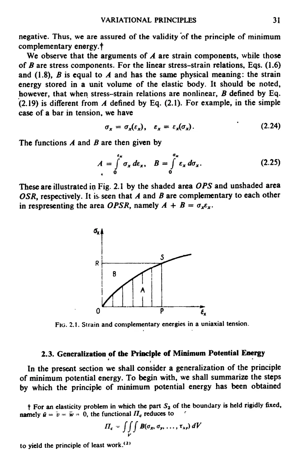
First, it is observed that we can derive a state function A(exy eyy..., yxy)
from the stress-strain relations (1.6), such that
6A = Gx&ex + (fydsy + -" + txydyxy, (2.1)
where
2A = (alx€x + a12e, + ••• + al6yxy)ex
-i- ...
+ (fiei^x + a62ey + ••• + a^y^y^. .• *{2.2br<
For the stress-strain relations of an isotropic material, namely Eqs. (lAf£
we have
Ev
A "* 2(1 + v) (1 - 2v) (** + Ey + Ez)2 + G^x + ^ + ®
G
+ y(tf* + yx2* + y*y). (2.3)
We shall refer to A as the strain energy function.! From physical
considerations which will be given in Chapter 3, we may assume the strain energy
function to be a positive definite function of the strain components. This
assumption involves some relations of inequality among the elastic
constants/1} For later convenience we introduce a notation A(u> v9 w) to indicate
that the strain energy function is expressed in terms of the displacement
components by introduction of the strain-displacement relations (1.5). For
t The quantity A is also cafled the strain energy per unit volume or the strain energy
density.
27
28 VARIATIONAL METHODS IN ELASTICITY *ND PLASTICITY
example, we have
r
Ag v Ev (du dv dw \2
' Aiu>v'w)=2(i+V)(i-2v){i); + i» + i)r)
+ 2
+ G
G
m+m+m:
I/dv , dw\2 , (dw , du\2 (du , dv \2] .„ _
for an isotropic material.
When the existence of the strain energy function is thus assured, the
principle of virtual work (1.32) can be transformed into:
dJffA(u9 v, w)dV - jjjiXdu + Ydv + Zdw) dV
V V
- ff(X,6u + ?9dv + Z9dw)dS = 0. t (2.5)
This expression is useful in application to elasticity problems in which
external fords are not derivable from potential functions.
Next, we shall assume that the body forces and surface forces are
derivable from potential function <P(u, v9 w) and ^(u, 0, w) such that
-<W> - Xdu + Ydv + Zdw$ ^ (2.6)
-&P = X, du + Y9 dv + Z9dw. (2.7)
Then, the principle (2,5) can be transformed into
<577 = 0t (2.8)
where
n m ffflA(uf v, w) + 0(u, v, w)\dV + ffYfa t>, w)dS, (2.9)
y Si
is the total potential energy. The principle (2.8) states that among all the
admissible displacements «, v and w which satisfy the prescribed geometrical
boundary conditions, the actual displacements make the total potential energy
stationary.
Hereafter, we shall confine our elasticity problem by assuming that the
body forces (Xf Y, Z), the surface forces (£, F„ ZP) and the surface
displacements («, 0, w) are prescribed, and kept unchanged in magnitudes and
directions during variation. Then, potential energy functions ate derived
for these forces as follows:
-& = Xu + Yv + Zw, . (2.10)
-!F « Xji + Yjo + Z,w, (2.11)
and we have a variational principle called the principle of minimum
potential energy: Among all the admissible displdcement functions, the actual
dV
VARIATIONAL PRINCIPLES 29
displacements make the total potential energy
n « jff A(u9 v9 w) dV - /// (Jfo +Yv + Zw) dV
V V
- //(*> + ?J> + Z9w) dS9 (2.12)
St
an absolute minimum.
For the proof of the principle of minimum potential energy, let the
displacement components Of the actual solution and a set of admissible,
arbitrarily chosen displacement components be denoted by u, v9 w and u*9 v*f
w*9 respectively, and put u* = u + du, v* = v + dv and w* = w + dw. We
then have
77(w*, v*9 h^) - 77(u, v9 w) + 6II + d2II9 (2.13)
where dH and d2IJ are the first and second variations of the total potential
energy. The first and second variations are respectively linear and quadratic
in du, dv9 dw and their derivatives, namely,
>n -SJfHt)+ •• +Mf+£) -**+-+"■»
V
-f[(X,9u + ... + Z,6w)dS, (2.14)
da77 - /// AQu, dv, 6w) dV, (2.15)
y
• <
where aX9..., and r„ are the stress components of the actual solution. Since
du =« dv « dw s» 0 on S2, and the stress components belong to the actual
solution, we find that the first variation, Eq. (2.14), vanishes:
Atr«*0. (2.1«)
Furthermore; since Ais& positive de£fiifc fattSioiv we must have
P?K- (2.17)
where the equality sign holds <^ wla^ ^ components which
are derived from du, dv and dw ale Mf^ Gpfttequentiy, we obtain
n*dmiMihi*&tI**mii> (2.18)
Since no restrictions have been made <*ll JfcfcJB&agttitudes of du, £t> and dw
in the above proof, we conclude that the t^^pot^tial energy is made an
absolute minimum for the actual Solution. :^K-a t
* -.
*•>* v
^
Principle of Minimum Omflunwtiry Energy
It will now be shown that another variational principle can be derived
from the principle of complementary virtual work* Eq. (1.50). We observe
that a state function £(<rx, o,9 .*,Txr) may be derived from the stress-strain
30 VARIATIONAL METHODS IN ELASTICITY AND PLASTICITY
relations (1.8), such that
SB ~ ex6ax + ey6oy + ••♦ + yxybrtxyy (2.19)
where
IB = (^ncr* + 612or„ + ••• + bl6rxy)ax
J» • • «
+ (^61^ .+ *62^ + -• + f>66Txy)Txy. (2.20)
For the stress-strain relations of an isotropic material, namely Eqs. (1.11),
we have
*
+ 2(1 + v) (tJx + tJx + r*, - oyrr - a,*, - <vrF)}. (2.21)
We shall refer to B as the complementary energy function.f It is obvious
that, the strain energy function A defined by Eq. (2.2) is equal to the
complementary energy function B defined by Eq. (2.20) and that, if the former
is positive definite, so is the latter. When the existence of the complementary
energy function is thus assured, the principle of complementary virtual work
can be transformed into:
6fJfB(axyoyy.„yTxy)dV-ff(udX9 + vdY, + wdZJdS = 0. (2.22)
v s*
Employing the assumption that the quantities u, v and w are kept unchanged
during variation, we can derive from Eq. (2,22) a variational principle
called the principle of minimum complementary energy: Among all the sets
of admissible stresses oxyayy ...yandrxy9 which satisfy the equations of
equilibrium and the prescribed mechanical boundary conditions on St, the set of
actual stress components makes the total complementary energy IIc defined
by
ne = fff B(ax, <r„ ...,r„)dV - ff (QXf + vYr + wZ9) dS, (2.23)
i V Sx
an absolute minimum.
_ For the proof, we denote the stress components of the actual solution
and a set of admissible, arbitrarily chosen stress components byax, oy, ...,rxy
ando£, o£,..., T*yy respectively and put o£ = ax + dox, a* = ay + doy,...,
z*y = rxy + drxy. Then, in a manner similar to the development in the
preceding section, we find that the first variation of the total complementary
energy vanishes for the actual solution and that, since J? is a positive definite
function, the second variation of the total complementary energy is non-
f The quantity B is also called the complementary energy per unit volume, com*
plementary energy density or the stress energy per unit volume.
VARIATIONAL PRINCIPLES 31
negative. Thus, we are assured of the validity of the principle of minimum
complementary energy.f
We observe that the arguments of A are strain components, while those
of B are stress components. For the linear stress-strain relations, Eqs. (1.6)
and (1.8), B is equal to A and has the same physical meaning: the strain
energy stored in a unit volume of the elastic body. It should be noted,
however, that when stress-strain relations are nonlinear, B defined by Eq.
(2.19) is different from A defined by Eq. (2.1). For example, in the simple
case of a bar in tension, we have
The functions A and B are then given by
A = f oxdex, B = f exdax. (2.25)
* o o
These are illustrated in Fig. 2.1 by the shaded area OPS and unshaded area
OSR, respectively. It is seen that A and B are complementary to each other
in respresenting the area OPSJR, namely A + B = oxex.
Fig. 2.1. Strain and complementary energies in a uniaxial tension.
2.3. Generalization of the Principle of Minimum Potential Energy
In the present section we shall consider a generalization of the principle
of minimum potential energy. To begin with, we shall summarize the steps
by which the principle of minimum potential energy has been obtained
t For an elasticity problem in which the part S2 of the boundary is held rigidly fixed,
namely u = v = w - 0, the functional IJC reduces to r
nc - jjf B(aX9 o„ ..., rxy) dV
v
to yield the principle of least work.<2)
32 VARIATIONAL METHODS IN ELASTICITY AND PLASTICITY
from the principle of virtual work. We have assumed that: (1) it is possible
to derive a positive definite state function A(ex, eyf..., y^) from the given
stress-strain relations; (2) the above strain components satisfy the conditions
of compatibility, that is, they can be derived from m, v and w as in the
relationships of Eqs. (l.S); (3) the displacement components u, v and w thus
defined satisfy the geometrical boundary conditions (1.14), and'(4) the body
forces and surface forces can be derived from potential functions 0 and W
as given by Eqs. (2.10) and (2.11). The principle of minimum potential
energy then asserts that, on the basis of the above assumptions, the actual
deformation can be obtained from the minimizing conditions of the
functional n defined by Eq. (2.12).
We shall now show that the subsidiary conditions stated m the
assumptions (2) and (3) above can be put into the framework of the variational
expressfon by introducing Lagrange multipliers^ and the principle of
minimum potential energy can be generalized."*5' By the introduction of
nine Lagrange multipliers ax$ a,t..., tx9 and pM9 p,f pz defined in V and
on &zt respectively, the generalized principle can be expressed as follows:
The actual solution can be given by the stationary conditions of a functional
TIi defined oift
/7, - fff[A(ex,e„ ....y„) - (Xu + ?v + Zw))dV
V
V
/ dw dv\ ( du dw\
♦ (r- : £ -£)..]«-//«. + r, + **«
Si
- jj[(« - u)px + (o - »)p, + (w - $)p,}dS. (2.26)
Si
The independent quantities subject to variation in the functional (2.26) are
eighteen in number, namely, exf e„ •..,)>*,; ut v, w; oX9 o,9 ...,tx,; px, p,
and pt with no subsidiary conditions. On taking variations with respect
f See Chapter 4, § 9 of Rcf. 3 for the Lagrange multiplier method and involutory
transformations. See also Appendix A.
tt It should be noted that ontie Lagrange multipliers have been employed, the phrase
4* minimizing conditions" used in the principle of minimum potential energy must be
replaced by "stationary conditions'*.
VARIATIONAL PRINCIPLES 33
to* these quantities, we have
(fox . #**» . St
+ ^+^ + X)dm (~)6»\dV
+ j([(X, - X,)du + ••• + (Z, - Z,)6w]dS
St
- \\[(u - u)5px + ••• + (w - w)bpt\dS
St
+ ffl(X,-px) 6u + - + (Z, - pt) Sw] dS, (2.27)
St
and the stationary conditions are shown to be
Ox = One* + al2e, + — + al6yx„ ... in V, (2.28)
du dv du
^* , ^J* , d*zx
+ JT-0,... in K, (2.30)
5jc dy 3z
X9 = ^r,..., Zr = Zr on 5i, (2.31)
u »fi h> =x # on 52» (2.32)
px = Jfr,..., />x = Zr on 5*2. (2.33)
. It is seen that Eqs. (2.28) and (2.33) determine physical meanings of the
Lagrange multipliers oxy oyy ,,.yxxyy px, pf and/?*, and that the
relationships for TIl to be stationary are the equations which define the elasticity
problem stated in Section 1.1. If Eqs. (2.29) and (2.32) are taken as subsidiary
conditions, IIx is reduced again to 77 defined by Eq. (2.12).
We may obtain another expression of the variational principle in which
the Lagrange multipliers pxy py and px have been eliminated. For this
purpose, we may require the coefficients of du9 dv and dw in the integral term on
S2 of the expression (2.27) to vanish. Thus, by the use of Eqs. (2.33) we may
34 VARIATIONAL METHODS IN ELASTICITY AND PLASTICITY
transform the functional (2.26) into
n" =Jjj[A(e"e" ■•'y")~ (*u + Tv + Zw)
du\ I dv du \
dV
-(£*--£)a' {?»- dx dy)
- ff(X¥ u + ?rv + Zrw) dS
s(
- ff[(u -Q)X, + (v- 9) Y, + (w - w) Z,] dS, (2.34)
st
or, through integrations by parts, into
#m = ~ JJJ Ke* + <V, + •• + rxfYXf - A(ex,e,j ...,y„)
v
+jj[(xw - x,)u + (n - n) *> + (z, - z,)»]ds
Si
+ /T(*," -I- Yju + Zvw) dS. (2.35)
The independent quantities subject to variation in the functional (2.34) or
(2.35) are 15 in number, namely, eX9 ef9 ...,yxy; u9 v9 w9 aX9 af9 ..., and r^
with no subsidiary conditions. On taking variations of these 15 quantities,
we find that the stationary conditions are given by Eqs. (2.28) through
(2.32).
2.4. Derived Variational Principles
It will be shown in the present section that the Hellinger-Reissner principle
and the principle of minimum complementary energy can be interpreted as
special cases of the generalized principle (2.26). Let the coefficients of 6eX9
dey, ..., 6yxy in the expression of 6TIS be required to vanish. This means that
eX9 ey9 ... and yxy are no longer independent, but must instead be determined
in a new formulation by the conditions (2.28), namely,
«x = ^lt** + ••• + f>l6rXf9
(2.36)
yxy - b6iax + ••• + bf6 rXf.
JJy the use of Eqs. (2.36), the strain components can be eliminated from the
functional (2.26) to yield another functional of the principle, TIR, as follows:
-//
VARIATIONAL PRINCIPLES 35
n Cff\ °u dv {to to\
n* =JJJ h ar + a>w + - + T"(&r + w)
v _ 1
- B(ax,ay, ...,rxy) - (Xu + Tv + Zw)\dV
- (((X,u + ?vv + 2,w) dS
s,
[(u - u) px + (r - f) p, + <u- - m>) px] dSy (2.37)f
where the quantity B is defined, as the above derivation shows, by
B = axex + <r,e, + ••• + Txyyxy - A, (2.38)
in which the strain components are eliminated by the introduction of the
stress-strain relationships (2.36). Since we have
6B = ax 6ex + ••• + rxy 6yxy + ex dax + ••• + yxv 6xxy — bA
- Zx&°x + ••• + y^y^, (2.39)
with the aid of Eq. (2.1), it is seen that the quantity B defined by Eq. (2.38)
is the complementary energy function defined by (2.19). The functional
(2.37) is equivalent to those in the Hellinger-Reissner principle.*6,7*
Because of the elimination of the strain components, the number of the
independent quantities subject to variation in the functional IJR is reduced
to 12: m, v, >v; axy ayy ..., rxy; pX9 pyy pz with no subsidiary conditions. On
taking variations of these quantities, we find that the stationary conditions
^ to •
= t>\\<*x + •'• + t>t6rxr>
dx
'. > (2.40)
dv cu
"dx + ~dy ~ 6l°x + '"' + b66Txy9
together with Eqs. (2.30) through (2.33).
The functional (2.37) may also be written via integrations by parts in the
following form:
-nt = ///[*..* *»> + (It + -£•+ %•+ *)"
- [f[(X9 - X,)u + (Yy -Y9)v + (Z,- Z9)w]dS
s\
-fflXJ + ^ + z^l dS> (241>
t This is a special case of the Legendre transformation ifl the calculus of vanation. The
unique inverse relations of Eqs. (2.28) should exist for the transformation to be justified.
36 VARIATIONAL METHODS IN ELASTICITY AND PLASTICITY
where Eqs. (2.33) have been used for the elimination of px, pf and pt. The
quantities subjected to variation in the functional (2.41) are u, v, w; ax,
afy ... and r^ with no subsidiary conditions.
We shall now impose further restrictions on the number of independent
functions in the generalized functional. All the coefficients of 6exy deyy...,
tyxyl <to, dv and dw in the expression of <5/7, are required to vanish: thus the
strains and displacements are eliminated by the use of Eqs. (2.28), (2.30),
(2.31) and (2.33) to transform the functional 77, into a functional Ttc defined
by
ttc - - /// B(pxy cr„ ..., rxf) dV + //(X9u + Yfi + Z9w) dS, (2.42)
V Si
where the quantities subject to variation are cx, ofy... and t^ under the
subsidiary conditions (2.30) and (2.31). Taking into account the positive
definiteness of the function B, we may state this new principle as follows:
Of all the admissible functions ox, c„ ... and tx9 which satisfy Eqs. (2.30)
and (2.31), the stress components of the actual solution make the functional
tlc an absolute maximum. We observe that the principle (2.42) is equivalent
to the principle of minimum complementary energy derived in Section 2.2.
In reversing the above development, we find that the functions u, vy w in the
functional (2.41) play the role of introducing the subsidiary conditions
(2.30) and (2.31) into the variational expression.
We have seen that, in the expression for 77, admissible functions are chosen
to satisfy the conditions of compatibility, Eqs. (1.5), and the geometrical
boundary conditions on S2, Eqs. (114), while in the expression of 77c,
admissible functions are chosen to satisfy the equations of equilibrium,
Eqs. (1.4), and the mechanical boundary conditions on Sx, Eqs. (1-12).
Consequently, 77 and 7?c are complementary to each other in defining the
elasticity problem. The transformation of 77into fle is known as Friedrichs' trans-,
formation ;(3,8) the actual solution characterized by the minimum property
of 77 is also given by the maximum property of fje.
Thus far, it has been shown that once the principle of minimum potential
energy has been established from the principle of virtual work, it can be
generalized by the introduction of Lagrange multipliers to yield a family of
variational principles which include the Heilinger-Reissner principle, the
principle of minimum complementary energy and so forth. The avenue of
this formulation is shown diagramatically in Table 2.1.
The principle of minimum .complementary energy was derived in Section
2.2 from the principle of complementary virtual work. It is easily verified
that the principle of minimum potential energy can be derived from the
principle of minimum complementary energy by reversing the development
in the present and preceding sections. The equivalence between these two
approaches is quite obvious as far as the small displacement theory of
elasticity is concerned. However, we shall emphasize the avenue of approach
Table 2.1. Variational Principles in thb Small Displacement Theory op Elasticity
Stress-Strain
Relations
Potentials of Body Forces
and Surface Forces
Strain Energy Function
Complementary Energy
Function
Strain-Displacement Relations
Geometrical Boundary
Conditions
■Oh
Principle of
Complementary
Virtual Work
*
Equations of Equilibrium
Mechanical Boundary Conditions
Principle of Virtual Work
Principle of Minimum
Potential Energy
Generalized Principle
Hellinger-Reissner Principle
Principle of Minimum
Complementary Energy
38 Variational methods in elasticity and plasticity
which leads from the principle of virtual work to the principle of minimum
potential energy and other related variational principles, because this
choice seems advantageous for a systematic treatment of problems in solid
mechanics.
It is noted here that these variational principles can be applied to an elastic
body consisting of several different materials, if the stress-strain relations
of each material assure the existence of a strain energy or complementary
energy function. For example, if the body consists of n different materials,
and the strain energy function of ;-th material is denoted by Aly the
principle of minimum potential energy may be formulated by replacing jjJA dV
n V
with 2J [f]AtdV.The continuity of displacement components on the inter-
face between the various materials must be satisfied if neither slipping nor
tearing is assumed. Similar statements can be made concerning the other
variational principles. It is also noted here that several other related
variational principles in elasticity have been proposed in Refs. 9,10 and 11.
2.5. Rayleigh-Ritz Method—(1)
It has been shown that the elasticity problem in small displacement theory
can be formulated by variational methods under the assumption that the
three functions A, 0 and *P exist. The exact differential equations and
boundary conditions defining the problem are then given by the stationary
property of the total potential energy and related functional. However, one
of the greatest advantages of the variational procedure is its usefulness in
obtaining approximate solutions. The so-called Rayleigh-Ritz method is
the best established technique for obtaining approximate solutions through
the use of the variational method,! We shall illustrate the Rayleigh-Ritz
method with two examples.
Let us first consider the principle of minimum potential energy applied
to the elasticity problem of Section 1.5. Let us assume a $et of admissible
displacement functions uy v and w as given by Eqs. (1.34), (1.35) and (1.36).
Introducing Eqs. (1.34) into Eq. (2.12) and carrying out the volume and
surface integrals, we can express IJ in terms of a,,, br and cr (r = 1,2,...,*).
The Rayleigh-Ritz method determines the values of these constants by
requiring dlJ = 0, which, in the present case, becomes:
bit . dll _ dtl . n / ! ^ x ,* A+\
— :=0, "g^-^O, -^r~°> (r-1,2,...,«). (2.43)
The* Eqs. (2.43) lead to a set of 3n simultaneous linear algebraic
equations in which the 3n unknowns are aw> br and i, (r = 1, 2,..., n). It is
observed that the 3/i equations thus obtained .are equivalent tQ those obtained
in Section 1.5.
t Refs. t% 3 and 12 through 17.
VARIATIONAL PRINCIPLES 39
Next, let us consider the principle of minimum complementary energy
applied to the twoniimensioifai problem of Section 1.7. Noting that the
stresses expressed by Eq. (1,61) constitute a set of admissible functions, w«
shall substitute them into
n*"II IE[i°*+ Cf)1 + 2(1 + v)(T^ " °^)]dxdy> (244)
which, after integration, can be written in terms of ar (r = 1, 2,..., n). The
Rayleigh-Ritz method asserts that the stationary property of the exact solu-.
tion can be satisfied approximately by requiring
^~0 (r=* 1,2,...,/!). (2.45)
The n simultaneous equations thus obtained determine values of a, (r = 1,
2,...,«), which, when substituted into Eqs. (1.61), provide approximate
solutions for the stress coqaponents. We also observe that the n equations
thus derived are equivalent to those obtained in Section 1.7.
Thus, we see that the Rayfeifcb-Rit* method leads to formulations
equivalent to those of the approxiijaate methods developed in Sections l.S and
1.7, as far as the elasticity problem of the small displacement theory is
concerned. However, each has its own Advantages and disadvantages in
applications to problems outside the elasticity problem. The approximate
methods are vrflid irrespective tot the stress-strain relations employed and
potentials of the external forces, but the proof that the approximate solutions
converge to the exact solution With increasing n is usually difficult. On the .
other handr the stress-strain relations, body forces and surface forces must
assure the existence of the state functions A, B9 0 and V for the formulation
of the variational expressions, $ the Rayleigh-Ritz method is to be used.
However, the convergence proof is less difficult, especially .when the
maximum or minimum property of th$ variational expressions has been
established.
When boundary value problems of elasticity can be solved only
approximately, it is desirable to obtain iipper and lower bounds of the exact
solution. However, this requirement is seldom answered, because bounds are
usually much more difficult to tifefedh than approximate solutions. Trefftz
proposed a method of deriving Upper and lower bound formulae for the
torsional rigidity of a bar by simultaneous use of the principles of minimum
potential and complementary enerfy (see Ref. 18 and Section 6.5). Since
his paper was published, many papers on this and related subjects have
appeared in the field of elasticity. Among them, the concept of function
space devised by W. Prager and J. L* Synge may be mentioned as a notable
contribution/1^
• In function space a. set of stress components (aXf ay t..., rxy), related to
a set of strain components (eX9t},...., y^) by Eqs. (1.6), is considered as a
40 VARIATIONAL METHODS IN ELASTICITY AND PLASTICITY
vector. Denoting two arbitrary vectors by N and N* and their components
of stress and strain by (ax, ..., rxy), («„..., yxy) and (or*,... ,t*,), (e*,..., y*,),
respectively, we define the scalar product of the two vectors in function
space by
(N, N*) « /// (oj* + <ve* + -. + t„>£) dV, (2.46)
the integral being taken throughout the body. Since the strain energy
function is a positive definite form, the following relations are obtained
immediately:
(N,N) £ 0, (2.47)
(N, N*) ^ (N, N)* (N*, N*)*. (2.48)
The function space thus defined enables us to grasp intuitively approximate
methods of solution and their convergence characteristics, and to estimate
the error of approximate solutions.(20) Due to the space available, the method
of deriving bound formulae in function space will not be shown here. The
interested reader is directed to Ref. 21 for details of the concept of function
space.
2.6. Variation of the Boundary Conditions and Castigliano's Theorem <,
Thus far, we have derived the principle of minimum potential energy
and its family under the assumption that the boundary conditions on St
and S2 are kept constant during variation. Now, we shall consider variation
of the boundary conditions. We assume that the problem defined in Sec*,
tioq 1.1 has been solved and that components of the stress and strain as well as
the functions A and B of the actual solution have been expressed in terms
of the prescribed body forces, surface forces on St and surface
displacements on S2. We denote the stress, strain and displacement components of
the actual solution by <xX9 <j,9 ...; eX9 ey9...; u9 v9 w, respectively in the
present section.
We shall consider first the variation of the geometrical boundary
conditions. The displacement components are given infinitesimal increments
du9 dv and dw on S2, while the body forces as well as the mechanical
boundary conditions of St remain unchanged. We assume that the incremental
displacements have yielded a new configuration and denote incremental
displacements caused in the body by du9 dv and dw. Th*n we have
dU = fjf(Xdu+ ?dv + Zdw)dV
v
+ ff(X,du+ Ywdv + Zpdw)dS
Si
+ ffXX, du +Y9dD + Z, dw) dS, (2.49)
S2
•VARIATIONAL PRINCIPLES 41
where
U-fffA dV, (2.50)
v
is the strain energy of the elastic body. We have derived Eq. (2.49) in a
manner similar to the developments of the divergence theorem, Eq. (1.76),
remembering that
dA = ax dex + a, dey + •• + rxy dyxyy (2.51)
and observing that the stress components ox, ... and the incremental stain
dexy... satisfy the equations of equilibrium and the conditions of
compatibility, respectively. We shall see in Chapter 3 that Eq. (2.49) holds for finite
displacement theory of elasticity as well.
The formula (2.49) is useful in determining the values of X„ Yp and Zp
on the boundary S2. As an example, we shall consider the truss structure
consisting of two equal members of uniform cross-section shown in Fig. 2.2.
Let the problem be defined such that the displacement 3 at the joint is pre-
Fig. 2.2. A truss structure.
scribed and the resulting force P is to be obtained. We denote the lengths of
members before and after deformation by /0 and /, respectively, and the
strain of the members by e. From geometrical considerations we have I2 = a1
+ (b + S)2 and 1% = a2 + b2, and we obtain
* « (/ - /0)//o = («)//*. (2.52)
where higher order terms are neglected. Consequently, we have
V = [(i) EA0l0e2] x 2 = EA0b2(8)2lll (2.53)
where A0 is the cross-sectional area of the member. Applying Eq. (2.49),, we
obtain
P = dU/dS = (2EA0b2IH)S. (2.54)
42 VARIATIONAL METHODS IN ELASTICITY AND PLASTICITY
Next, we shall consider the variation of the body forces and mechanical
boundary conditions. The body forces and the external forces on St are
given infinitesimal increments dXy dY, dZ ai\d d%„ d?„ dl„ respectively,
while the geometrical boundary conditions on S2 remain unchanged. We
assume that these incremental forces yield a new configuration, and denote
incremental stresses caused in the body by daxy dayy... and rfr„. Then,
we have
dV■« fff(udX+ vd? + w42)dV
v . « '
+ ff(udX9 + vd?, + wdZ9)dS
Si
.+ // (u dX9 + ,v dY9 + tf dZ9) dS, (2.55)
Si .
where
V^fffB dV (2.56)
is the complementary energy of the elastic body. We have derived Eq.
(2.55) in a manner similar to the development of the divergence theorem
remembering that
dB s= ex dax + e^ da, + ••• + Yxydtxy* (2.57)
and observing that the strain components ex,;.. and the incremental stresses
doxy... satisfy the conditions of Compatibility and the equations of
equilibrium, respectively.
The formula (2.55) is useful it) determining the values of uy v and w on the
boundary Sx. As an example, we consider; a body which is held rigiefw fixed
on the boundary S2, and is subject to n concentrated loads Fly P2, ...9fm
on the boundary St. For the sake of simplicity, these concentrated lodds
are assumed independent. In other words, any of these forces can be
assume* to be given increments Without interfering with those remaining.
Denoting the displacement compbrleni of the point of application of the
load Pi in the direction of the load by 4t> we haw from Eq. (2.55): '
i .fj
dV~.£JtdPt. (2.5d)
Since V is a function of the external forces, we have:
dV « i» (dV/dPt) dPt. (2.59)
Combining these two equations, we obtain:
!(!£-;d')<w,'=0- ■«*»
VARIATIONAL PRINCIPLES 43
Since the forces are assumed independent, we have
dV
dP<
= A, (i = 1,2, ...,/j). (2.61)
The formula (2.55) and its family are called Castigliano's theorem—a
powerful tool for analyzing problems in the small displacement theory of
elasticity (see Refs. 2 and 12 through 15, for instance).
2.7. Free Vibrations of an Elastic Body
The variational principles derived so far have been for the boundary
value problem of elasticity. In the last two sections of this chapter we shall
consider variational formulations of a problem of free vibrations of an
elastic body in small displacement theory. The problem is defined by
allowing the body to be mechanically free on S{ and geometrically fixed on 52.
Since the problem is confined to small displacement theory, all the equations
defining the problem are linear, and displacements and stresses in the body
behave sinusoidally with respect to time. Consequently if we denote the
amplitudes of stress, strain and displacement by ax, .. ,£x,... and u, v9 w,
respectively, we have for the equations of motion,
> »
&Tx dtty drzx 2
cx oy dz
^SL + J^L + *J5. + jlpr - 0, (2j62)
ox oy dz
ox dy dz
In Eqs. (2.62), X = to2 where a> is the natural circular frequency, and q is the
density of the material. The boundary conditions are given by
X9 = 0, Y, = 0/ Z,~ 0 on Sl9 (2.63)
and
u^O, v = 0, w = 0 on 52. (2.64)
From Eqs. (2.62) and (2.63), we have
~fff[(isr + "if + isr + Hdw + {')dv + ("b)H rfr
V
+ JT(*, <$« + Ywto + Z, 6w) dS = 0. (2.65)
St
Here we chose the arbitrary set of virtual displacements duy dv and dw such
that the geometrical boundary conditions are not violated, namely, 6u = dv
44 VARIATIONAL METHODS IN ELASTICITY AND PLASTICITY
= dw = 0 on S2. Then, we may transform Eq. (2.65) into
fff(axdex + ayde, + *•• + rxy 6yxy) dVt
v
- A JfJ {u du + v dv + wdwi) gdV = 0. (2.66)
This is the principle of virtual work for the free vibration problem.
If the relations between the amplitudes of stress and strain are given
by
ox = atiex + "iity + — + ol6yxyt ..., (2.67)
where
<*u — <*ji {Uj — 1, 2, ..., 6),
we are assured of the existence of the strain energy function defined by
Eq. (2.2). Moreover, the body forces Xqu9 Xqv and Aqw are derivable from a
potential function 0 defined by Eq. (2.6) such that
-0 = ±Aq(u2 + v2 + w2). (2.68)
Consequently, we obtain from Eq. (2.66) the principle of stationary potential
energy as follows: Among all the admissible displacement functions i#, v and w
which satisfy the prescribed geometrical boundary conditions, the actual
displacements make the total potential energy
n = /// A(u9 v9 w) dV - \XJfj (u2 + v2 + w2)odV9 (2.69)
V V
stationary. In the functional (2.69), the quantities subject to variation are
Uy v and w under the subsidiary conditions (2.64), while X is treated as a
parameter not subject to variation.
The principle of stationary potential energy can be generalized through
the use of Lagrange multipliers as follows:
nt =fff[A(eX9e,9...yyxy)-±Ae(u2 + v2 + w2)
v
~ ffo* + PyV + PzW) dS* (Z70)
Si
where the independent quantities subject to variation are eX9...; u9 ...;
<*x* -i Px> • • and pz. The stationary conditions are shown to be Eqs.
(2.67); Eqs. (2.62), (2.63) and
px = X„ ..., pz = Zp on S2; (2.71)
du dv du 0 .
dx ox vy
and Eqs. (2.64).
VARIATIONAL PRINCIPLES 45
Several variational principles can be derived from the generalized prin-
ciple.<22) Here, we shall derive a functional for the principle of stationary
complementary energy. It is shown that elimination of the strain components
by the use of Eqs. (2.67) and a simple calculation by the use of Eqs. (2.62),
(2.63) and (2.71) lead to a transformation of the functional (2.70) as follows:
nc = /// B(aX9 oy, ..., rxy) dV - iXffJ (u2 + v2 + h^) q dV, (2.73)
v x v
where the quantities subject to variation are w,...; ox,... and rxf under the
subsidiary conditions (2.62) and (2.63), and the stationary conditions are
shown to be equivalent to Eqs. (2.64) and (2.72). The functional (2.73) is
an expression for the principle of stationary complementary energy of the
free vibration problem. We note that another expression of the principle
of stationary complementary energy can be obtained by eliminating u, v
and w from the functional (2.73) by the use of Eqs. (2.62), thus expressing
the functional in terms of cr^, crr,... and t„ only.
It was shown in Refs. 23 and 24 that the principle of stationary
complementary energy might be extended to eigenvalue problems such as free
vibration and stability of elastic bodies. The principle was introduced and
proved in Ref. 25 by E. Reissner for a problem in which loa.ds, stresses and
displacements are simple harmonic functions of time. The functional (2.73)
is equivalent to that introduced by E. Reissner.
It is well established that the principle of stationary potential energy (2.69)
is equivalent to finding, among admissible functions w, v and w which satisfy
the prescribed geometrical boundary conditions, those which make the
quotient
X = UjT (2.74)
stationary, where
U = /// A(u, v9 w) dVy (2.75)
v
T = i /// (u2 +V2 + w*)g dV, (2.76)
v
nd the stationary values of A provide the Eigenvalues of the solution. For
the proof, we see that
« = ™L - ™i « ±(6U - X6T), (2.77)
where the variation is taken with respect to w, v and w. Consequently, the
condition that the quotient X is stationary is equivalent to the principle of
stationary potential energy. The expression (2.74) is the Rayleigh quotient
for the free vibration problem/16,26)
It is also well known that the principle of stationary potential energy
(2.69) is equivalent to a problem of finding, among admissible functions
m
46 VARIATIONAL METHODS IN ELASTICITY AND PLASTICITY
«, v and vv which satisfy the geometrical boundary conditions, those which
make U stationary under a subsidiary condition
T(u,v, w) - 1 =0. (2.78)
For the proof, we see that this problem is equivalent to obtaining the
stationary conditions of a functional defined by
U-X(T- 1), (2.79)
where A plays a role of a Lagrange multiplier and the variation is taken with
respect to w, v9 w and X under the subsidiary conditions (2.64).
2*8. Rayleigh-Ritz Method—(2)
We have seen the variational principles established for the free vibration
problem in the preceding section. When the variational expressions are thus
aw dable, the Rayleigh-Ritz method provides a powerful tool for obtaining
approximate values of eigenvalues. We shall consider a free vibration problem
of a beam as an example and follow the outline of the method.
We shall take a beam clamped at one end x = 0 and simply supported
at the other end x = / as shown in Fig. 7.5. The functional for the principle
of stationary potential energy for the present problem is given by
n = i / £/(w")2 dx-iXf mw2 dx9 (2.80) f
o. o
where EI, w and m are the bending rigidity, deflection and mass per unit
span of the beam, respectively, and ( )' = d( )fdx. In the functional
(2.80), the quantity subject to variation is w under the subsidiary conditions
w<0) = h</) = w'(0) = 0. (2.81)
We denote the exact eigenvalues by
Xt (i » 1,2,3,...), (2.82)
in ascending order of magnitude such that 0 < Xx < X2 < •■•.
We may transform the functional (2.80) to yield a functional for the
principle of stationary complementary energy:
**< " jf^Ef dx-^lj™2*** (2.83)t
0 0
where the quantities subject to variation are M and vv under the subsidiary
conditions
M" + Xmw = 0, (2.84)
t See Section 7.4 for the derivation of these fenctionals.
VARIATIONAL PRINCIPLES 47
and
Mil) = 0. (2.85)
We shall consider first the Rayleigh-Ritz method applied to the principle
of stationary potential energy. The well-known procedure proposed by the
method is followed by choosing a set of n linearly independent admissible
functions h>,(x), the so-called coordinate functions, which satisfy Eqs.
(2.81), and assuming w as a linear combination of these coordinate functions,
namely: x
w = gem, (2.86)
where cf(i = 1, 2, ..., n) are arbitrary constants. Substituting £q. (2.86) into
Eq. (2.80), and setting
x c?/7/?c, - 0 (i « 1, 2, ..., *), (2.87)
we obtain a set of n homogeneous equations. The requirement that the
determinant of the set must vanish for a nontrivial solution provides another
algebraic equation, called the characteristic equation of the set of the form:
det (mu - Xnu) = 0. (2.88)
If we denote the roots of the characteristic equation (2.88) by At
(i = 1,2, ...,n) in ascending order of magnitude, i.e. Ax <A2 ••• <Am9 we
have
A, ^/l, (i = 1,2, ...,/i). (2.89)f
Next, we shall consider the method applied to tne principle of stationary
compfementary energy. This is sometimes called the modified Rayleigh-Ritz
method,(13) and its outline is as follows: We choose w as given by Eq. (2.86),
where the coordinate functions w,(x) are so chosen as to satisfy Eqs. (2.81).
We substitute Eq. (2.86) into Eq. (2.84) and perform integrations with the
boundary condition Eq. (2.85) to obtain
OM)
M = c{x-t)- Ect [\fm(Z) *,($)#
dn, (2.90)
where c is an integration constant. Substituting Eqs. (2.86) and (2.90) into
the functional (2.83) and requiring that
dnjdc = 0, (2.91)
and
dncfdct = 0, i = 1, 2,..., n9 (2.92)
we obtain a characteristic equation which determines approximate eigenvalues.
For later convenience, these approximate eigenvalues are denoted by A*
(i = 1, 2,..., n) in ascending order of magnitude, i.e. /If < A\ < ••• < A*.
t For the proof, sec Refs. 3, 26 and 27.
48 VARIATIONAL METHODS IN ELASTICITY AND PLASTICITY
We see that the inclusion of the term c(x - /) in Eq. (2.90) and the
requirement of Eq. (2.91) are equivalent to obtaining the exact beam deflection due
to the inertial loading Im Hciwi. Thus, the method is equivalent to the
Grammers method in which the exact deflection due to the inertial loading
is obtained by the use of the Green's function or the so-called influence funo
tions.ca8'*9) It is stated in Ref. 28 that if the same assumed modes (2.86)
are employed, we have the following inequality relations:
Xt£A?<iAi9 /= 1,2, ...9n. ■' (2,93)
Thus, the Rayleigh-Ritz method provides an upper bound for each
eigenvalue. It is well established that the accuracy of approximate eigenvalues
thus obtained is good and sometimes excellent if the coordinate functions
are chosep properly. However, since an approximate method of solution
is applied to a problem whose exact solution cannot be obtained, we can
usually expect to have no information on the exact eigenvalues beforehand.
Therefore, formulae providing lower bounds are indispensable for locating
the exact eigenvalues. .•
There have been proposed several theorems for locating lower bounds of
eigenvalues. Among them, the Temple-Kato theorem and Weinstein's
method may be mentioned as typical. The Temple-Kato theorem provides a
lower bound for the eigenvalue A, when the value or a lower bound of the
eigenvalue AW4l is known.f This theorem often proves to be an effective tool
for eigenvalue location. On the other hand, Weinstein's method employs
as a basis one of Rayleigh's principles that, If the prescribed boundary
conditions are partly relaxed, all the eigenvalues decrease.} That is, if we denote
eigenvalues of a relaxed or intermediate problem by X$9 i — 1, 2,... in
ascending order of magnitude sq^bt that %x < X2 < -s then we havq
%t<>\$ ft** 1,2,...)- (2^4)
Therefore, if we obtain exact eigenvalues of the intermediate problem, they
provide lower bounds for the eigenvalues of the original problem.
The Rayleigh-Ritz method for the free vibration problem has been
illustrated. It is obvious that the method also finds a field of application in
other eigenvalue problems. The reader is .directed to Refs. 13,16 and 26 for
further details and numerical illustrations of the Rayleigh-Ritz method
applied to eigenvalue problems.
2.9. Some Remarks
We have derived some extensions of the principles of virtual work and
complementary virtual work in Section 1.9. It is obvious that the first terms
of Eqs. (1.73) and (1.74) may be replaced by 6U and 6 ^respectively, for
f Refe. 30 through 35.
X Refs. 36 through 38.
VARIATIONAL PRINCIPLES 49
elasticity problems, and several extensions of the principles (2.5) and (2.22)
may be obtained from these equations. For example, we have
dV - fff (u bX + v 6Y + w6Z) dV = 0, (2.95)
v
for an elasticity problem, where the boundary conditions are specified such
that
^=Fr=Z, = 0 on S„ (2.96)
4 *
u = t• = w = 0 on S2, (2.97)
and stress variations are so chosen as to satisfy Eqs. (1.75) and the boundary
conditions
6X9 = (5Kr = (5Z^O on S,. (2.98)
Next, a mention is made of the generalized Galerkin's method treated in
Section 1.5. The object of this mention is to note that the principle (2.5),
which may be used instead of the principle (1.32) for elasticity problems,
suggests a modification of the generalized Galerkin's method as follows:
Since
W * £ l&Ulto*) t><*r + tfUldb,)6br + {dUidc,) 6c,]9 (2.99)
r-l
we find that the principle (2.5) leads to an approximate method of solution
in which equations for the determination of the unknown constants ary bf
and ct (r = 1, 2,..., n) are given by
L, « 0, Mr = 0, Nf = 0, (r = 1, 2, ..., n) (2.100)
where
'*-%-fff»."-ff'**>
V St
dU
M:"^F~ Iff Tv'dv " // ?'Vr ds* (2\101)
V S,
V St
We shall see in Section 5.6 that this approximate method of solution is
* equivaleat to that employed in deriving Lagrange's equation of motion of
the dynamical problem. It is obvious that the principle (2.22) suggests a
similar modification of the generalized Galerkin's method treated in Sec^
tipn 1.7.
The approximate method of solution above mentioned can also be applied
to eigenvalue problems of an elastic body in which external forces are not
50 VARIATIONAL METHODS IN ELASTICITY AND PLASTICITY
derivable from potential functions. Such applications are usually based on
the principle of virtual work, Eq. (2.5), as illustrated in Refs. 39 and 40.
As an example of applications based on the principle of complementary
virtual work, we may refer to E. Reissner's work for flutter calculations/40
An examination of his paper reveals that his method may be considered as
an application of the principle (2.95) if aerodynamic and inertial forces are
taken as types, of body forces.
Bibliography
1. A. E. H. Love, A Treatise on the Mathematical Theory of Elasticity, Cambridge
University Press, 4th edition, 1927.
2. S. Timoshenko and J. N. Goodie*, Theory of Elasticity, McGraw-Hill, 1951.
3. R. C6urant and D. Hilbert, Methods of Mathematical Physics, Vol. 1, Interscicnce,
New York, 1953.
4. K. Washizu, On the Variational Principles of Elasticity and Plasticity, Aeroelastic
and Structures Research Laboratory, Massachusetts Institute of Technology,
Technical Report 25-18, March 1955.
5. H. C. Hu, On Some Variational Principles in the Theory of Elasticity and Plasticity,
Scintia Sinica, Vol. 4, No. 1, pp. 33-54, March 1955.
6. E. Hellinger, Der allgemeine Ansatz der Mechanic der Kontinua, Encyclopddie der
Mathematischen Wissenschaften, Vol. 4, Part 4, pp. 602-94, 1914.
7. E. Reissner, On a Variational Theorem in Elasticity, Journal of Mathematics and
Physics, Vol. 29, No. 2, pp. 90-95, July 1950.
8. K. Friedrichs, Ein Verfahren der Variationsrechnung das Minimum eines Integrals
als das Maximum eines andcren Ausdruckes darzustellen, Nachrichten der Academie
der Wissenschaften in Gottingen, pp. 13-20, 1929.
9. T. Iai, A Method of Solution of Elastic Problems by the Theorem of Maximum
Energy (in Japanese), Journal of the Society of Aeronautical Science of Nippon, Vol. 10,
No. 96, pp. 276-98, April 1943.
10. E. Reissner, On Variational Principles in Elasticity, Proceedings of Symposia in
Applied Mathematics, Vol. 8, pp. 1-6, MacGraw-Hill, 1958.
11. P. M. Naghdi, On a Variational Theorem in Elasticity and its Application to Shell
Theory, Journal of Applied Mechanics, Vol. 31, No. 4, pp. 647-53, December 1964.
12. C. Biezeno and R. Grammel, Technische Dynamik, Springer Verlag, 1939.
13. R. L. Bispunghofe, H. Ashley and R. L. Halfman, Aeroelasticity, Addison-Wesley,
1955L
14. N. J. Honv77u? Analysis of Structures, John Wiley, 1956.
15. J. H. ARGVRis and S. Kelsey, Energy Theorems and Structural Analysis, Butterworth,
1960.
16. G. Temple and W. G. Bickley, Rayleigh's Principle and its Applications to
Engineering, Oxford University Press, 1933.
17. S. G. Mikhlin, Variational Methods in Mathematical Physics, Pergamon Press, 1964.
18. E. Trefftz, Ein Gegenstuck zum Ritzschen Verfahren, Proceedings of the 2nd
International Congress for Applied Mechanics, Zurich, pp. 131 -7, 1926.
19. y/. Prager and J. L. Synge, Approximations in Elasticity Based on the Concept of
Function Space, Quarterly of Applied Mathematics, Vol. 5, No. 3, pp. 241-69, October
1947.
20. K. Washizu, Bounds for Solutions of Bouifdary Value Problems in Elasticity, Journal
of Mathematics and Physics, Vol. 32, No. 2-3, pp. 119-28, July-October 1953.
21. J. L. Synge, The Hyper circle in Mathematical Physics, Cambridge University Press,
" 1957.
VARIATIONAL PRINCIPLES 51
22. K. Washizu, Note on the Principle of Stationary Complementary Energy Applied
to Free Vibration of an Elastic Body, International Journal of Solids and Structures,
Vol. 2, No. 1, pp. 27-35, January 1966.
23. S. Timoshenko, Theory of Elastic Stability, McGraw-Hill, 1936.
24. H. M. Westergaard, On the Method of Complementary Energy and Its Application
to Structures Stressed Beyond the Proportional Limit, to Buckling and Vibrations, and
to Suspension Bridges, Proceedings of American Society of Civil Engineers, Vol. 67,
No. 2, pp. 199-227, February 1941.
25. E. Reissner, Note on the Method of Complementary Energy, Journal of Mathematics
and Physics, Vol. 27, pp. 159-60, 1948.
26. L. Collatz, Eigenwertaufgaben mit technischen Anwendungen, Akademische Verlags-
gesellschaft, Leipzig, 1949.
27. S. H. Gould, Variational Methods for Eigenvalue Problems, University of Toronto
Press, 1957.
28. R. Grammel, Ein neues Verfahren zur Losung technischer Eigenwertprobleme,
Ingenieur Archk\ Vol. 10, pp. 35-46, 1939.
29. A. I. van de Vooren and J. H. Greidanus, Complementary Energy Method in
Vibration Analysis, Reader's Forum, Journal of Aeronautical Sciences, Vol. 17, No. 7,
pp. 454-5, July 1950.
30. G. Temple, The Calculation of Characteristic Numbers and Characteristic Functions,
Proceedings of London Mathematical Society, Vol. 29, Series 2, No. 1690, pp. 257-80,
1929.
3^. W;Kohn, A Note on Weinstein's Variational Method, Physical Review, Vol.71,
No. 12, pp. 902-4, June 1947.
32. T. Kato, On the Upper and Lower Bounds of Eigenvalues, Journal of Physical Society
of Japan, Vol. 4, No. 4-6, pp. 334-9, July-December 1949.
33. G. Temple, The Accuracy of Rayleigh's Method of Calculating the Natural
Frequencies of Vibrating Systems, Proceedings of Royal Society, Vol. A211, No. 1105, pp.
204-24, February 1950.
34. R. V. Southwell, Some Extensions of Rayleigh's Principle, Quarterly Journal of
Mechanics and Applied Mathematics, Vol. 6, Part 3, pp. 257-72, October 1953.
35. K. Washizu, On the Bounds of Eigenvalues, Quarterly Journal of Mechanics and
Applied Mathematics, Vol. 8, Part 3, pp. 311-25, September 1955.
36. A, Weinstein, fitude des spectres des equations aux derivees partielles de la thdorie
des plaques dlastiques, Memorial des Sciences Mathematiques, Vol. 88, Paris, 1937.
37. N. Aronszajn and A. Weinstein, On the Unified Theory of Eigenvalues of Plates
and Membranes, American Journal of Mathematics, Vol. 64, No. 4, pp. 623-45,
December 1942.
38. J. B. Diaz, Upper and Lower Bounds for Eigenvalues, Proceedings of Symposia in
Applied Mathematics, Vol. 8, pp. 53-78, McGraw-Hill, 1958.
39. R. L. Bisplinghoff and H. Ashley, Principles of Aeroelasticity, John Wiley, 1962.
40. V. V. Bolotin, Nonconservative Problems of the Theory of Elastic Stability, Translated
by T. K. Lusher and edited by G. Herrmann, Pergamon Press, 1963.
41. E Reissner, Complementary Energy Procedure for Flutter Calculations, Reader's
Forum, Journal of Aeronautical Sciences, Vol. 16, No. 5, pp. 316-17, May 1949.
42. F. R. Gantmacher, The Theory of Matrices, Chelsea Publishing Company, 1959.
43. B. M. Fraeus de Veubeke, Upper and Lower Bounds in Matrix Structural Analysis,
in Matrix Methods of Structural Analysis, edited by B. M. F. de Veubeke and published
by Pergamon Press, 1964.
CHAPTER 3
FINITE DISPLACEMENT THEORY OF
ELASTICITY IN RECTANGULAR
CARTESIAN COORDINATES
*
3.1. Analysis of Strain
In the present chapter we shall treat finite displacement theory of
elasticity in rectangular Cartesian coordir ites.t The difference between spatial
variables and material variables cannot be overemphasized in the
formulation of finite displacement theory. Unless otherwise stated, we shall employ
the Lagrangian approach, in which the coordinates defining a point of the
body before deformation are employed for locating the point during the
subsequent deformation.]:
Let the rectangular Cartesian coordinates (xly x2> «x3) be fixed in space
and the position vectot of an arbitrary point P(0) of the body before
deformation be represented by
r<0> = r(0)(x\x\x3), (3.1)
as .shown in Fig. 3.1, where the superscript '*' means that the quantity is
referred to the state before deformation.ft £ct us henceforth employ a set
of tt^e values (x1, x2, x3), which the point P(0) occupies before deformation,
as parameters which specify the material point during deformation.
The base vectors in this coordinate system are given by
ia = ^- = ^ tf=l,23), (3.2)«
where and throughout the present chapter, the notation ( ).* denotes
differentiation with respect to x\ namely, ( \x = 5( )/dx*. They are unit
vectors in the directions of the coordinate axes and are mutually orthogonal:
ixK=K* 0-3>ttt
t Refs. 1 through 6.
X Or the other hand, coordinates associated with the deformed body are employed
in the Eulerian approach.
tt Superscript indices should not be mistaken for exponents.
XX A Greek index will be assigned in place of (I, 2, 3) in Chapters 3, 4 and 5.
ttt The notation a • b denotes the scalar product of two vectors a and b.
/
52
FINITE DISPLACEMENT THEORY OF ELASTICITY
53
where 6^ is the Kronecker symbol defined by
\
i2dx2
fcfc^* ^ «
£ >.
'<£\
;\
Js01
•Mr
^^s
Fig. 3.1. Geometry of an infinitesimal parallelepiped,
(a) before deformation. (b) after deformation.
(3.4)
We shall take a point (?<0> in the neighborhood of the point P(0> and denote
the coordinates of Qi0y by (jc1 + dxlf x2 + dx29 x* + dx*). Then the position
vector rfr(0) and the distance ds{0) between these two points can be expressed
as
<k™ = *$dx* = \xdx*9 (3.5)f
and
(<fc<0))2 « <*<0) • <*<0> = d^dxxdxttf (3.6)
t The summation convention will be employed in Chapters 3, 4 and 5. Therefore a
Greek letter index which appears twice in the same term indicates summation with re*
spect to (1, 2,3). For example:
x*ix = 2 A - *lfi + x2'1* + *3j3 •
4-1
3 3
°*%i = 22 °*%i - «lI«u + *I2«« + *13't3
4-1 ji«l
+ <T21<?21 + 0r22e22 + *23*23 + <**l**l + *3**32 + <733*33-
54 VARIATIONAL METHODS IN ELASTICITY AND PLASTICITY
respectively. For later convenience, an infinitesimal rectangular
parallelepiped enclosed by the following six surfaces:
Aa = constant, xx + dx* = constant (/ = 1, 2, 3)
will be fixed to the body. It has the line element />(0)(?(0> as one of the
principal diagonals and Ri0\ Si0\ and T{0) as the vertices adjacent to the
point P{0\
The body is now assumed to be deformed into a strained configuration.
The points P{0\ Qi0\ R(0\ 5(0) and 7(0) move to new positions denoted by
P, Q, R, S and 7, respectively, and the infinitesimal rectangular
parallelepiped is deformed into a parallelepiped which, in general, is no longer
rectangular. Let us denote the position vector of the point P by
t = t(x\x2,x*), J3.7)
and introduce the lattice vectors defined by
EA-^X = rA (A- 1,2,3). (3.8)
The sides of the parallelepiped issuing from the point P are then given
by E, dx\ E2 dx2 and E3 dxz. Consequently, the position vector dt and
the distance ds between P and Q can be expressed by
drt=T.Adx* = ExdxA. (3.9)
and
(ds)2 = dx • dt « EXfi dx* dx», (3.10)
respectively, where
£,„ = E,-E„ = £•„. (3.11)
Let us consider the geometrical meaning of £^. The lengths of the
infinitesimal line element jp(0)/?fC) before and after deformation are
(dsw)2 = (dx1)2 and (ds)2 «'Eix(dx1)2,
respectively. Therefore, the rate of elongation of Pi0)R{0) is .given by
(ds - </s(()))/c/s(0> «]£,!-!. (3.12)
The geometrical meanings of E12 and £33 follow similarly.
Next, consider two infinitesimal line elements P<°>>?(6> and Pi0>S{0\
which are orthogonal before deformation. After deformation, these two
elements move to new positions, PR and PS, the relative positions of
which are given by the vectors Ex dx1 and E2 dx2, respectively. If we
denote the acute angle between PR and PS by (^— yl2), we have
E, dxl-E2dx2 --= \Ei\\E2\dxldx2cos(^ - yI2),
FINITE DISPLACEMENT THEORY OF ELASTICITY 55
or
£12 = }lElxE12smyl2. (3.13)t
This gives the geometrical meaning of £12. The meanings of £23 and E3X
follow similarly.
Therefore, we conclude that after deformation an infinitesimal rectangular
parallelepiped is transformed into a skew parallelepiped, and the geometry
of the deformation can be specified by the set of values of the quantities
E^ (A,/i = 1, 2, 3). Consequently, we define strains of the parallelepiped
by
**. ^ K3* - <V) = ** (A, /i = 1, 2, 3), (3.14)
and employ the nine components?^, under the symmetry conditions e^ = e¥k9
as the quantities which specify the strain of the parallelepiped.
Let us express the position vector of the point P as
r « r<°> + u, (3.15)
where a is the displacement vector, whose components (ul9u29u2) are
defined by
a = A- (316)
From Eqs. (3.8) and (3.15), we have
EA = (^ + ^i,f (3.17)
where <JJ is the Kronecker symbol. By the use of Eqs. (3.14) and (3*17), the
strains can be calculated in terms of the displacement components as
follows:
If u9 v9 w are used instead of ux9 u29 u3, respectively, and x9 y9 z in place of
1, 2, 3, or x1, x29 x3, respectively, Eqs. (3.18) can be written as follows:
du 1 [/ du\2 ( dv\2 /dw\2
•XX
eyy —
e„ =
dx 2 [\ dx) \dx) \dx J
dv_
dy
dw . 1 17 du\2 . / dv\2 (dw\2
Iz
,_ dw dv du du dv dv dw dw _ ^
yx ~~ dy dz dy dz dy dz dy dz tf9
du dw du du dv dv dw dw
dz dx dz dx dz dx dz dx
dv du du du dv dv dw dw
17 + ^ + lxly+'dx'dy'dxlyr
t Compare with Eqs. (1.5).
56
VARIATIONAL METHODS IN ELASTICITY AND PLASTICITY
We note here that, when the strain components are sufficiently small,
Eqs. (3.12) and (3.13) may be linearized with respect to the strains to obtain
the following approximate relations:
(ds - <&<0))/<fc<0) = Vl +:2*n - 1 ~ elu
y12 « sin-1(Ei2l)/EtlE22) * 2e12.
Similar relations "hold for the other strain components.
(3.20)
p.21)
3.2. Analysis of Stress and Equations Of Equilibrium
It has been shown in the preceding section that an infinitesimal
rectangular parallelepiped is transformed into a skew parallelepiped after deformation.
We shall now consider the equilibrium of the deformed parallelepiped/11
The forces acting on the deformed parallelepiped are internal forces
exerted by neighboring parts of the body through the six side surfaces and
body forces, as shown in Fig. 3.2. Let the internal forces acting on one of
the side surfaces, the area of which before defonnatkm was dx2 dx* and the
Pdx'dxW
-ff»dx1dx2
♦£(»%Ak»)<tf
Flo. 3.2. Equilibrium of an infinitesimal parallelepiped,
(a) before deformation. (b) after
sides of which after deformation are E2 dx2 and E3 dxzt be represented
by — a1 dx2 dx%. The quantities a1 and o3 are defined in a similar manner.
FINITE DBPLACEMENT THEORY OF ELASTICITY 57
The internal forces acting on the six side surfaces are as follows:
-0%dx2dx\ a1dx2dx3 +-£-r(o1dx2dx*)dx1,
-o2 dx* dx\ a2 dx*dxx + -^ (a2 dx* dx1) dx29
- o3 dx1 dx2, a* dx1 dx2 + -2,- (a3 dxl dx2) dx*.
The body forces acting in the deformed parallelepiped will be represented
by P dx1 dx2 dx3. The force equations of equilibrium of the deformed
parallelepiped are then given by
o^ + P = 0. (122)
Let us define the components of ox by resolving it in the directions of the
lattice vectors:
o1 « <r*E„, (3.23)f
as shown in Fig. 3.3. Then, the moment equation of equilibrium of the
deformed parallelepiped are given by
(o* dx*dz*)x Etdxl +(o*dx*dxl) x E2dx2 + (o3dx1 dx*) x E^dx*
= (a1 x Ej)dxl dx2 dx3 » 0, (3.24)t
Fkfc 33. a1 - a1* Eju
Where higher order terms are neglected. By the use of Eq. (3.23), we
from Eq* (3.24) the following relations :
o^o*, (3.25)ft
t The quantity a*+ defined by Eq. (3,23) Is called pseudo-stress or generalised stress.
However, the familiar nomenclature i/reii wiD be used imtead in subsequent formulations,
% A notation mxb denotes a vector product of two vectors a and b.
tt It b noted tfet \ .
a* x Exmp*1£ X Zx-i**1 -<*%*)E$ * Mi + (°*2 - °23>M2 x ** + (*13 - ^)
x E* x E4> . .
and the three vectors Ei x E„ Rj x E3 and B^ x Ea are mutually independent.
58 VARIATIONAL METHODS IN ELASTICITY AND PLASTICITY
We shall employ the nine components a*1, under the symmetry conditions
<& — a*1*, as the quantities which specify the state of stress on the
infinitesimal parallelepiped.
Equation (3.22) is a vector equation. One way of expressing it in scalar
form is to resolve it in the direction of ij. By defining the components of
the body force as
P = P\9 . (3.26)
we obtain the following scalar equations from Eq. (3.22):
[(% + Ufr o^l* + P* - 0 (A - 1, 2, 3). (3.27) t
We note here that ox are defined per unit area and P is defined per unit
volume, both with respect to the undefprmed state.
3.3, Transformation of the Stress Tensor
The quantities o** which define the state of stress at the point P depend
on the choice of coordinates. Wfc shall now find a law of transformation
for the stress tensor. Form an infinitesimal tetrahedron pw/jw^oyw
bounded by three surfaces of the rectangular parallelepiped and an oblique
surface, as shown in Fig. 3.4. If the area of the inclined surface before deform-
Fig. 3.4. Equilibrium of an infinitesimal tetrahedron,
(a) before deformation. (b) after deformation.
f Compare with Eqs. (1.2).
FINITE DISPLACEMENT THEORY OF ELASTICITY 59
ation be denoted by dE and the internal force acting on the surface
RST after deformation be represented by F dEy the equilibrium equation
of the infinitesimal tetrahedron is'
¥dE = a\dx2 dx*l2) + o2(dx* dxl/2) + a\dxl dx2/2). (3.28)
From the geometry before deformation, we have
dx2 dx3 « 2(i! • v) dEy dx3 dxl = 2(i2 • v) dE,
dxl dx2 = 2(i3 • v) dEy (3.29)t
where v is the unit normal vector drawn outwards on the inclined surface
/?<0)5<0)r<0) before deformation. Substituting the relations (3.29) into Eq.
(3.28), we obtain
F = (ixv)o*. (3.30)
This gives the direction and magnitude of the internal force F acting on
the4 oblique surface. By resolving F in the direction of the base vectors as
F = F\y (3.31)
we obtain Eq. (3.30) in scalar form:
Fx = &*njfi + w.J), (3.32)
where nx = ix • v.
3.4. Stress-Strain Relations
In the present chapter we shall assume that the deformation under
consideration takes place either isothermally or adiabatically, and postulate
the existence of functions which define the stress in terms of the strain such
that(1)
** =***(eii,ei2. ••.,*«) ft A* = 1,2,3), (3.33)J
where the zero stress state corresponds to the zero strain state, namely,
(r^(0, 0, ..., 0) = 0. We also assume the existence of-Gnique inverse
functions which define the strain in terms of the stress:
^ = e^»,al2,...,a33) ft/* = 1,2,3). (3.34)+
When the strain components are assumed sufficiently small, we may
expand Eqs. (3.33) into power series with respect to e^ and neglect higher
t Sec footnote of Eqs. (4.63).
t Only six equations are physically independent in Eqs. (3.33). However, we may write
them and their inverse relations in nine equations of symmetrical form as given by Eqs.
(3.33) and (3.34), respectively.
60 VARIATIONAL METHODS IN ELASTICITY AND PLASTICITY
order terms to obtain the following linear stress-strain relations:
a** = a^Pe.fi. (3.35)t
It is obvious that, due to the symmetry property of the stress and strain
tensors, there exist the following relations among the coefficients:
Eqs. (3.35) may be inverted to yield:
e*n ■» ^^^ (3-36)f
where
blood — "fi&xA == Eludes
When the material is isotropic, the numerical values of <&** must be
independent of the coordinate system in which the stress and strain are
defined. This leads to the conclusion that d4"* is a fourth-order isotropic
tensor and is given by(*f 5)
a*# = & d*&* + G(#"d* + 6*d»*)f (3.37)
(1 + V) (1 — 2v)
and Eqs. (3.35) and (3.36) reduce to
** ~ (HW ^ + 2Ge»f (3;38)t
/■
and
% - ° ~ 2V) *** + ^-^, (3.39)f
respectively, where £ «= 2(1 + v) G. The quantities <r^ and e'^ are
deviator stresses and deviator strains defined by a**' -> o*" — trd** and
**, - **. - «8*» respectively, where <x - (1/3) o" = (1/3) (a11 + a22 + <r")
and * =* (1/3) e^ - (1/3) (eu + «aa + *3s).
3.5. Presentation of a Problem
<"
With the above preliminaries, we shall now defiite a boundary value
problem in the finite displacement theory of elasticity. Consider an elastic
body subjected to the following boundary conditions and body forces:
(1) Mechanical boundary conditions on Sx,
F m 99 (3.40)
where F is given by Eq. (3.30) with the understanding that the vector v is
now the unit normal drawn outwards on the boundary and F is the pre-
t Compare with Eqs. (1.6), (1.8), (1.10) and (1.11), respectively.
FINITE DISPLACEMENT THEORY OF ELASTICITY 61
scribed external force. Both F and f are defined per unit area of the unde-
formed state. Resolving P in the directions of the base vectors,
* « F%. (3.41)
we obtain from Eq. (3.40) the following scalar equations:
/* = /* (A« 1,2,3). (3.42)t
(2) Geometrical boundary conditions on S2,
ul = ux (A =1,2, 3). (3.43)t
(3) The body forces
Fx (A = 1,2,3). (3.44)
Our problem is then to find the Stresses and displacements existing in the
deformed body by employing the stress-strain relations (3.33).
By combining Eqs. (3.18) and (3.33), we can represent a** in terms of
u*. Introducing o*4 thus represented into Eqs. (3.27) and (3.42), we obtain
three simultaneous differential equations and the mechanical boundary
conditions in terms of u*. If these differential equations can be solved under
the boundary conditions on Sx and S2, we can obtain the required
equilibrium configuration. Once the displacement components u* have been
obtained, the state of stress induced in the body may be determined from
Eqs. (3.18) and (3.33).
Since the problem is nonlinear, the solution, if obtainable, generally
yields nonlinear relations between the applied external loads and the result-
ing deformations. Some typical examn es of nonlinear relations are
illustrated in Figs. 3.5, 3.6, 3.7 and 3.8, where the ordinate is the applied
external load and the abscissa denotes the resulting displacement of the point
Fio. 3.5. A load-deflection curve of a truss structure.
t Compare with Eqs. (1.12) and (1.14), respectively.
62
VARIATIONAL METHODS IN ELASTICITY AND PLASTICITY
of application in the direction of the external load.c7) In the example
illustrated in Fig. 3.5, the slope of the curve, dfjdd, increases with the increase
of the deflection. This shows that the body is stable under the external
load as long as it behaves elastically. On the other hand, in the example
illustrated in Fig. 3.6, the slope dJBfdp decreases with increasing deformation
Fig. 3.6. Flattening instability of a thin cylindrical tube under bending.
Fig. 3.7. Durchschlag or snap-through of a curved beam.
and the load M eventually reaches its maximum Afcr. This shows that the
body ceases to be stable at Mct9 beyond which the body fails elastically/8'9)
The phenomenon illustrated in Fig. 3.7, where the load-deflection curve
has the £-shape characteristic, is called Durchschlag or snap-through/l0)
If P is a dead load and increases from zero to />«,> the deflection jumps from
dcr to dt with kinetic energy illustrated by the shaded area of the figure. In
the case of unloading, another jump occurs.at P£.-If the load-deflection
relation is as shown in Fig. 3.8,jwhere a point of bifurcation exists at Pcr,
the system has two states of equilibrium at loads beyond the critical load.
The body prefers a stable configuration and changes its deflection suddenly
FINITE DISPLACEMENT THEORY OF ELASTICITY
63
from unstable to stable under the stimulus of small external disturbances.
The phenomena shown in the last three figures constitute the main parts
of the theory of elastic stability/1 *"**>
Pi o
r
Fio. 3.8. Bifurcation of a rod under compression.
V
3.6. Principle pf Virtual Work
In {his section we shall derive the principle of virtual work of the continuous
body under consideration. Assume that the body is in equilibrium under
the body forces, the applied external forces on Sx and the prescribed
geometrical boundary conditions on S2. Now,* the body is assumed to execute
an infinitesimal virtual displacement du from this equilibrating configuration
without, violating the prescribed boundary conditions on S2. Then, by
employing the equations of equilibrium (3:22) and the mechanical boundary
conditions (3.40), and remembering that du = <$r, we obtain *
-///C^ + 'P) -fr^+//(F-F)-*<tt = 0f (3.45)
V SX
X ,
where dV = dx1 dx2 <£c3 and dS ate the elementary volume of the
parallelepiped and the elementary area on the surface of the body before
deformation, respectively. By the use of,tbe geometrical relations,
dx2 dx? ~ ±ntdSy dx*dx1±£n%4S, dx1 dx1 ~ ±j^ dS, (3.46)f
which hold on the surface of the body, the first term of JEq^ (3.45) may be
transformed into ^'
-ffj+*•*&*
r-' ff F; to dS + /// a* • &*&.
S*+S, V - •' VJ •<*
t Sec footnote of Eqs. (4.79).
64 VARIATIONAL METHODS IN ELASTICITY AND PLASTICITY
Introducing the above into Eq. (3.45), and remembering that <5r = 0 on
S2, we obtain
/// ox • (eSr),, dV - /// f - <5r dV - // P <Jr dS - 0. (3.47)
The integrand o* • (eSr)^ dV of the first term in Eq. (3.47) may be
interpreted as the virtual work done, during the infinitesimal virtual
displacement, by the body forces and the internal forces acting on the deformed
infinitesimal parallelepiped, while the second and the third terms represent
the virtual work done by the body forces and the external forces on Sx,
respectively. Combination of Eqs. (3.23), (3.11), (3.25) and (3.14) yields
<r* • (dr\x = o% (Ar)u
Introducing the above into Eq. (3.47), we obtain
Jff^de^dV- JffP-drdV- fff-drdS = 0. (3.48)
V V Sx
This is the principle of virtual work for the elasticity problem in finite
displacement theory. By the use of Eqs. (3.16), (3.26) and (3.41), the principle
may be expressed alternatively as follows:
/// (** de* ~ pX&^)dv - //pX du* ds = °- (3-49>t
V SX
Reversing the above development, we obtain from the principle, the
equations of equilibrium (3.27) and mechanical boundary conditions (3.42) under
the assumptions of the strain-displacement relations (3.18), the symmetry
of stress components (3.25), and the prescribed geometrical boundary
conditions (3.43). We note that the principle holds regardless of the form of
the stress-strain relations of the body.
3.7* Strain Energy Function
Let us consider an element of the body which is a rectangular
parallelepiped and occupies a unit volume before deformation. When the element
is subjected to deformation along a loading path and is brought into a
strained state expressed by (eu, ii*,..., e33), we may calculate an integral,
(*X1 *33>
/ o*de*9 (3.50)
(Q,...,0)
t Compare with Eq. (1.32).
For consistency in tensor notation, it is better to write dxp Pxduf* or PxSux instead of
Px du* where dx^ is the Kroneckef symbol and dux ~ 6*? '^ However, we shall use the
simpler expressions for the sake of brevity, whenever the rectangular Cartesian coordinate
system is employed.
FINITE DISPLACEMENT THEORY OF ELASTICITY 65
along the loading path by the use of the stress-strain relations (3.33). The
value of the integral thus obtained generally depends on the loading path.
However, if the value does not depend on the loading path, but depends
only on the final strain, the quantity a* de^ is called a perfect differential
and the existence of a state function A(ellyel2, ...,e33) is assured such
that
dA =ox»deXtiy (3.51)
or equivalently,
dA
-fc-^o* (A,//= 1,2,3). (3.52)
The state function thus defined is the strain energy function in the finite
displacement theory of elasticity.
The present section is concerned with the conditions under which the
quantity o^de^ is a perfect differential. A detailed discussion of these
conditions may be found in any book on partial differential equations.
However, we may summarize them as follows:
If the stress-strain relations (3.33) satisfy the equations
«
■f£--TEr- &*.«./-1.2,3) (3.53)
oe^ oexf,
the quantity <& de^ proves to be a perfect differential.
Consequently, if the stress-strain relations (3.35) satisfy the equations
a**** = rf^, (3.54)
we have
A ~ tf^e^. (3.55)t
When the material is isotropic and the stress-strain relations given by Eq.
(3.38) may be employed, we have
IF
A = 2(1 _ 2y) e2 + (hW,. . (3.56)t
So far, conditions for the existence of the strain energy function have
been studied mathematically. We shall now show from physical
considerations that such a function really exists when an elastic body deforms either
isothermally or adiabatically in a reversible process/2'14*15)
We assume a unit volume of an elastic body again and call it an element.
The first law of thermodynamics is applied to the element by taking the
sum of energy supplied to the element during the strain's increase by de^ to
obtain,
dU0 - d'Q + o» de^, . (3.57)
f Compare with Eqs. (2.2) and (2.3), respectively.
66 VARIATIONAL METHODS IN ELASTICITY AND PLASTICITY
where dU0 and d'Q are the increments of the internal energy and heat energy
supplied to the element, respectively. The quantity dU0 is the differential
of the internal energy U09 which is a single-valued function of the
temperature and the instantaneous state of strain of the element. Physically
speaking, the internal energy U0 is a function of the mean position of the
molecules under the intermolecular forces and the kinetic energy of the
molecules about their mean positions.(16) However, Q is not a state function
and d'Q merely denotes an infinitesimal amount of heat energy supplied.
Therefore, the special notation d' is used here to avoid confusion. The
quantity a*4* dexfi is an infinitesimal amount of supplied mechanical energy. After
these two kinds of energy have been supplied to the element, there can never
be any distinction between portions of dU0 contributed by d'Q and o*" de^.
The second law of thermodynamics assures the existence of a state
function S9 called entropy, such that
d'Q cfc TdS, (3.58)
where T is the absolute temperature of the element. Combining Eqs. (3.S7)
and (3.58), we obtain,
dU0 = TdS + <& de^. (3.59)
Equation (3.57) shows that if the deformation takes place adiabatically in
a reversible process, we have
dU0 =0*"^. (3.60)
Consequently, the mechanical energy is stored in the element in the form
of internal energy and we obtain
A = U0 + constant. (3.61)
On the other hand, if the deformation takes place isothermally in a
reversible process, we have from Eq. (3.59)
dF0 -o*de^ (3.62)
where
F0 = (J0- TS (3.63)
is the Helmholtz free energy function. This shows that the mechanical
energy is stored in the form of Helmholtz free energy and we obtain
A ** F0 + constant. (3.64)
Therefore, it may be concluded that the quantity a*** de^ is a perfect
differential for these two special cases, and the existence of the strain energy
function is assured.
The differences between the assumptions of adiafcatic and isothermal
deformations appear, in mathematical formulations, only as differences
between adiabatic' and isothermal elastic constants. Generally speaking,
FINITE DISPLACEMENT THEORY OF ELASTICITY 67
the differences between these elastic constants have been proved by
experiments to be negligible. Consequently, the strain energy function is usually
assumed to exist in the theory of elasticity, although the deformation
process may be somewhere between adiabatic and isothermal.
We know from experimental evidence that when the strains are sufficiently
small, an element of the elastic body is stable. This requires that the strain
energy function must be a positive definite function of the strain
components for the small strain. Since we have also found that, when the strains
are small enough, the strain energy function can be expressed by Eq. (3.55),
we may conclude that the strain energy function (3.55) is a positive definite
function of the strains.
3.8. Principle of Stationary Potential Energy
We have investigated in the preceding section the condition under which
the strain energy function can exist. When the strain energy function is
assured to exist, the principle of virtual work (3.49) can be written as
follows:
6 fff A(u*) dV - /// Px 6ux dV - // Fx6ux dS - 0, (3.65)t
V V S\
where the strain energy function A(ux) is written in terms of u* by the use
of Eqs. (3.18). The principle (3.65) is very useful in application to elasticity
problems in which external forces are not derivable from potential functions.
Next, we shall assume further that the applied external forces are
conservative, namely, they are derivable from potential functions <P(i/*) and V^u*)
such that
d0=*-Px6ux, h'=-Fx6ux. (3.66)
If the applied external force? vary neither in magnitude nor in direction
during the virtual displacements, namely, if they are treated as dead loads,
we may have
0 = -/>V, K W =, -/V. (3.67)
Under the assumption of the existence of the strain energy function j4 and
two potential functions 0 and *¥, the principle of virtual work (3.49) yields
the principle of stationary potential energy as follows:
5/7 = 0, (3.68)
where
77 = /// [Atf) + *(«*)] dV + jj Vtf) dS (3.69#V
V St
«
t Compare with Eq. (2.5).
X Compare with Eq. (2.9).
68 VARIATIONAL METHODS IN ELASTICITY AND PLASTICITY
is called the total potential energy of the mechanical system under
consideration and is a functional containing u* which are the independent variables
subject to variation. The variables u* should be chosen so that they satisfy
the required continuity and differentiability criteria and the boundary
conditions on S2. The principle (3.68) can be stated as follows: Among all
admissible displacement functions uxf the actual ones are those which render
the total potential energy stationary. Retracing the development in the latter
half of Section 3.6, we can easily show that the conditions which make the
total potential energy stationary provide the equations of equilibrium and
the mechanical boundary conditions on St. However, in these equations
and conditions all the stress components are expressed in terms of
displacement components, and we obtain three simultaneous differential equations
of equilibrium in V and three boundary condition equations on St in terms
of ux. The formulation thus obtained can also be reached by direct elimination
of the stress components from the equations of equilibrium and the
mechanical boundary conditions by the use of the relations (3.18) and (3.33), as
observed at the end of Section 3.5.
3.9! Generalization of the Principle of Stationary Potential Energy
It is obvious that the principle of stationary potential energy established
in Section 3.8 can be generalized by the use of Lagrange multipliers. Through
familiar procedures, we obtain a generalized functional as follows:
V
+ ff ¥V) dS - // />V - *) dS, (3.70) t
t
where the independent quantities Wbject to variation are e^ n\ a*" and p1
with no subsidiary conditions. The functional for Reissner's principle07)
.can be derived from the functional (3.70) through elimination of e^ as
^follows:
V
- B(fj*\ + 0(u")] dV
+ JfYfadS - ///>V - *VS> (3.71)f
Si Sz
where the independent quantities subject to variation are w\ a*1 and p* with
no subsidiary conditions.
t Comparedtvith the functionate (2.26) and (2.37), respectively.
FINITE DISPLACEMENT THEORY OF ELASTICITY 69
The quantity £(<&) appearing in Eq. (3.71) is the complementary energy
function. A« the above development shows, it is defined by
B = **%. - A. (3.72)
The stress-strain relations (3.34) are introduced into Eq. (3.72) to express
B entirely in terms of the stress components. From Eqs. (3.51) and (3.72),
we have
dB^e^do*", (3.73)
or equivalently,
-^r = ^ (A,/i= 1,2,3). (3.74)
We note here that if Eqs. (3.34) satisfy the equations
do**
= -gjfr -<*. *.*./» = 1,2,3), (3.75)
the function B is assured to exist and may be determined from Eq. (3.73)
independently of the function A. Consequently, if Eqs. (3.36) satisfy the
equations
>
we have
B = {b^****. (3.77) f
When Eq. (3.39) is employed, we obtain
B = 3°2~2V) o* + jQ<y»'o*- (3.78)t
for the isotropic material.
Under the assumptions of small displacement theory, the principle of
minimum complementary energy can be expressed in terms of the stress
components only, as shown in Section 2.2. However, coupling of the
displacements with the stress components in finite displacement problems
complicates the derivation of the principle of stationary complementary energy
from IIR; the principle can nb longer be expressed purely in terms of stress
components.
•
3*10* Energy Criterion for Stability
We know that, as long as the applied external loads are sufficiently small,
we obtain linear relations between the loads and resulting deformations.
However, the deformation characteristics gradually deviate from the linear
relations with increasing loads. This tendency is usually pronounced in
t Compare with Eqs. (2.20) and (2.21), respectively.
70 VARIATIONAL METHODS IN ELASTICITY AND ELASTICITX'
slender or thin bodies, and a point is finally reached beyond which the
bodies cease to be stable for some loading conditions, as shown in the
examples illustrated in Figs. 3.6, 3.7 and 3.8. In the present section, we
shall consider the energy criterion for determining the stability and critical
load of equilibrium configurations of elastic bodies under conservative
external forces, f
We assume that the equilibrium configuration of the body has been
obtained for the problem defined in Section 3.S, and call it the original
configuration. Then, let the original configuration be given small virtual
displacements without violating the geometrical boundary conditions, thus
obtaining a new configuration. If the virtual work done by the external forces
does not exceed the increase of the stored strain energy, the body is
considered stable. If this condition is not met for some virtual displacements,
then the excess energy will appear a£ kinetic energy. This indicates an
instability of the original configuration for the virtual displacements.
The above considerations lead to the following mathematical
formulation. Let the displacement components of the original equilibrium
configuration and the new configuration be denoted by ux and ux + 6ux respectively.
Denoting the total potential energy of the original configuration and the
new configuration by I2(ux) arid 77(k* + du1) respectively, we have
n(ux + 6ux) = 77(u*) + M + d2n + 6*11 + - -, (3.79)
where &/7, <$2/7, <$3/7, ..., are the first, second, third,... variations of the
total potential energy. They are linear, quadratic,... with respect to dux
and their derivatives, and their coefficients contain the displacement
components of the original configuration as parameters.} Since the original
configuration is in equilibrium, we have
S$/7 » 0. (3.80)
With these preliminaries, we may now conclude that the stability of the
original configuration in its neighborhood can be determined by the sign
of the second variation d2II as follows:
(1) The configuration is stable ifd2II > 0 holds for all admissible virtual
displacements.^
t Refs. 1 and 18 through 22.
X When all the applied external forces are dead loads and their potential functions are
given by Eqs. (3.67), we have
dm - i Jff [{d^A/de^ de^ de^de^ + o* dtfx <$«£,] dVt
v
where a*** are the stress components of the original configuration and
2<5% = (dj + ift)^ + (<5j; + i£)Aft.
tt This statement, combined with the principle of minimum potential energy derived in
Section 2.1, assures that nd unstable configurations exist as far as problems of the small
displacement theory of elasticity are concerned.
FINITE DISPLACEMENT THEORY OF ELASTICITY 71
(2) 1%e configuration is unstable ifd2II < 0 holds for at least one
admissible set of virtual displacements.
Following Trefftz,<18) we shall consider the determination of the lowest
critical load beyond which the body ceases to be stable for the first time
during the loading process. We have seen that the original configuration
is stable as long as d2I7 > 0 holds for all admissible virtual displacements.
This criterion will now be expressed in a different manner. We introduce a
properly chosen functional N which is positive definite and quadratic with
respect to 6ux and their derivatives,! and seek, among admissible virtual
displacements which satisfy
di/* = 0 on S2> (3.81)
those which make the quotient
A = d2n/N (3.82)
<
a minimum. The criterion then states: if the minimum value of the quotient.
is found to be positive; the original configuration is stable.
We know that since
SX « S(d2n/N) = $(d2fr - XN)/N, (3.83)
where S indicates that the variation is taken with respect to 6u\ the stationary
condition of the quotient is given by
Md2n - IN) « 0. (3.84)
Equation (3.84) yields differential equations and mechanical boundary
conditions, which, together with the geometrical boundary conditions
(3.81), determine the stationary values of the quotient as eigenvalues.
Consequently, the stability criterion may be expressed as follows: if the
minimum of the eigenvalues is found to be positive\ the original configuration
is stable.
The above consideration leads to a conclusion for the determination of
the lowest critical load: the external load acting on the original configuration
is considered critical when the minimum of the eigenvalues reaches the value
zero; the variational equation
S(d2n) = 0 (3.85)
under the subsidiary conditions (3.81) then yields governing equations which
determine the lowest critical load. We note here that the governing equations
determine all the critical configurations which possess at least one eigenvalue
of the value zero in the eigenvalue problem derived from Eq. (3.84), and
the configuration corresponding to the lowest critical load is one of the
critical configurations. The lowest critical load thus determined is frequently
• t The functional N9 which is introduced here for the normalization of the virtual
displacements, has no effect on the final result, namely, Eq. (3.85).
72 VARIATIONAL METHODS IN ELASTICITY AND PLASTICITY
followed by unstable states upon further increase of the external load, but
the sign of the higher-order variation must be considered for a sufficiency
proof.
3.11. The Eider Method for Stability Problem
Another method of determining the critical load concerns the problem
of whether there exists at least one additional, distinct equilibrium
configuration in the very close neighborhood of the original configuration. If such
an adjacent equilibrium configuration exists, the body may change suddenly
from one equilibrium configuration to the other under the stimulus of small
external disturbances. We shall formulate the stability problem by this
approach, which is sometimes called the Euler method, for a body under
4 nonconservative external forces/21' 23)t
We assume the existence of a critical original configuration and develop
a linearized theory which determines the adjacent configuration. We denote
stresses, strains, displacements &nd external forces of the original and
adjacent equilibrium configuration by
and
0* + °?, % + «i> tS + u* Px + P*, FA + Fi,
respectively, where
ujf « 0 on S2 y (3.86)
because the geometrical boundary conditions are the same for both
configurations. We may derive from Eq. (3.49) the principle of virtual work of the
adjacent equilibrium configuration by replacing aAu> u\ ... by aAu + <rj\
u* + *£»..., respectively :
///(** + <#> *** + <&>*K - ///(/" + P\)6ul dV
v v
-//(/* + /»)<Si<i</S = 0, (3.87)
Si
where
2(<^+ e£) - (if* + **).„ + (W + uQ.k
+ {*' + <).AW + 0.t. <388>
and the variation is taken with respect to w*. The equation (3.87) is the
principle of virtual work for an incremental theory of elasticity
t It is emphasized in Ref. 23 that the stability problem of a nonconservative system
should be investigated not only by the Euler method which deals with the static instability,
but also by the dynamic method whrh deals with the dynamic instability of small
oscillations of the system about the original equilibrium configuration.
FINITE DISPLACEMENT THEORY OF ELASTICITY 73
Since we are interested in a linearized theory, we may assume that a*\
P* and F* are linear functions of k* and their derivatives. Remembering
that the original configuration is in equilibrium, we may reduce the principle
(3.87) into the following form:
/// «<H + <^«;.i*0 dv
V
- /// P\ du*m dV - // Fxm <S«J dS ~ 0, (3.89)
V Si
where
2*£ = (6"x + <*) <„ + (d; + u%) <* (3.90)
and higher order terms are neglected. The equation (3.89) yields differential /
equations in V and mechanical boundary conditions on St:
{arid* + «*.„) + <fulJ,H + Pi = 0, i[3.91)
<«*(# + «*,„) + o**nMui,, = F*'. (3.92)
Consequently, if the relations between the incremental stresses and strains
are given in a linearized form by
of = a*^$,, (3.93)
we have all the governing equations which determine the critical load and
the adjacept equilibrium configuration.
When Eqs. (3.93) satisfy the symmetry relations:
<fl*# « *■«*, (3.94)
the principle can be. written as follows:
6 (i /// [a»*eteb + o^jrtU dV}
- ffffiK dV - fffiduidS - 0, (3.95)
V Si '
where Eqs. (3.90) have been substituted to express e& in terms of «**
When the body is elastic and the external forces are conservative, we find
that the principle (3.89) reduces to the principle (3.85).
The above formulations show that the critical load depends upon the
relations between the incremental stresss and incremental strain measured
from the original configuration, rather than the previous stress-strain
relations. This suggests that the critical load problem can be treated more
generally as an instability of a body with initial stresses and deformations.
A stability problem of a body with initial stresses will be treated in Section
5.2 under an assumption that changes in the geometrical configuration of
the body remain negligible until the instability occurs.
74 VARIATIONAL METHODS IN ELASTICITY AND PLASTICITY
3.12* Some Remarks
Thus far, the principle of virtual work and related variational principles
have been written for the elasticity problem in finite displacement theory.
It is noted here that the approximate methods of solution such as the
generalized Galerkin's method mentioned in Section 1.4 and the Rayleigh-Ritz
method mentioned in Section 2.5 can similarly be applied to the elasticity
problem in the finite displacement theory. It is also noted that for a variation
of the geometrical boundary conditions on S2 by du*y we have
dU « fff Flh+dV + ffPdu*dS + ffftd&dS, (3.96)
V Sx S2
which is an extension of Eq. (2.49) to the elasticity problem in the finite
displacement theory.
We have derived in Section 1.2 the conditions of Compatibility for the
small displacement theory in rectangular Cartesian coordinates. The same
kind of conditions may be derived of the finite displacement theory for the
strains e^ to be derivable from scalar functions it. However, we shall not
show them in the present chapter, but shall be satisfied with formulating
the conditions for finite - displacement theory in general curvilinear
coordinates later in Section 4.2.
Mention is made here,of the principles of complementary virtual work
and minimum complementary energy. We have observed that these
principles play important rotes in the small displacement theory of elasticity.
However, extensions of these principles to the finite displacement theory of
elasticity are not found successful, since the displacements couple with the
stress components as mentioned in Section 3.9.
BibUography
1. R.Xappus, Zur Elastizit&tstheofie endlicber Vertchiebungen, ZeUschrtft fBr An*
gewandte Maihematik undMechanik, Vol. 19, pp. 271-85, October 1939 and pp. 344-61,
December 1939.
2. V. V. Novozhilov, Theory of Elasticity, Pergamon Press, 1961.
3. A. B. Green and W. Zbrka, Theoretical Elasticity, Oxford University Press, 1934.
4.1. S. Sojcolnikoff, Mathematical Theory of Elasticity, McGraw-Hill, 1956.
5. C. E. Pearson, Theoretical Elasticity, Harvard University Press, 1959.
6. C. TRuesdell, editor, Problems of Nob-linear Elasticity, Gordon and Breach, Science
jruoiisficrs, iyD3.
7. C Biezeno and R. Grammel, Tedmische Dynamik% Springer, 1939.
8. L. G. Brazier, The Flexure of Thin Cylindrical Shells and Other Thin Sections,
R. <£ AS. No. 1081, British Aeronautical Research Council, 1926.
9. L. G. Brazier, On the Flexure of Thin Cylindrical Shells and Other Thin Sections,
Proceedings of the Royal Society of London, Series A, Vol. 116, pp. 104-14, November
1927.
10. C. B. Biezeno, Das Durchschlafen eines schwach gekrummten Stabes. Zeitschrift
far Angewandte Mathematik und Mechanik, Vol. 18, No. i, pp. 21-30, February
1938.
FINITE DISPLACEMENT THEORY OF ELASTICITY 75
U.S. Timoshenko, Theory of Elastic Stability, McGraw-Hill, 1936.
12. H. L. Langhaar, General Theory of Buckling, Applied Mechanics Reviews, Vol. 11,
No. 11, pp. 585-8, November 1958.
13. M. Yoshiki et al., Handbook of Elastic Stability (in Japanese), edited by Column
Research Committee of Jaffen, Corona Publishing Co. Tokyo, revised edition 1960.
14. A. E. H. Love, A Treatise on the Mathematical Theory of Elasticity, Cambridge
University Press, 4th edition 1927.
15. Y. C. Fung, Foundations of Solid Mechanics, Prentice-Hall, 1965. ,
16. R. L. Bispunohoff, Some Structural and Aeroelastic Considerations of High Speed
Flight, Journal of the Aeronautical Sciences, Vol. 23, No. 4, pp. 289-327, April 1956.
17. E. Rbssner, Qn a Variational Theorem for Finite Elastic Deformations, Journal of
Mathematics and Physics, Vol. 32, No. 2-3, pp. 129-35, July-October, 1953.
18. E. Trefftz, Uber die Ableitung der Stabilit&ts-Kriterien des elastischen Gleichge-
wichtes aus der Elastizit&tstheorie endlicher Deformationen, Proceedings of the 3rd
International Congress for Applied Mechanics, pp. 44-50, Stockholm 1930.
19. K. Marguerre, Die Behandiung von Stabtlit&tsproblemen mit Hilfe der energctischen
Methoden, Zeitschrift fur Angewandte Mathematik und Mechanik, Vol. 18, No. 1,
pp. 57-73, February 1938.
20. K. Marguerre, Uber die .Anwendung der energetischen Methode auf Stabilities*
problcme, Jahrbuch der Deutschen Luftfahrtforschung, Flugwerk, pp. 433-43, 1938.
21. V. V. Novozhilov, Foundations of the Nonlinear Theory of Elasticityt Graylock Press,
1953.
22. H. L. Langhaar, Energy Methods in Applied Mechanics, John Wiley, 1962.,
23. V. V. Bolotjn, Nonconservative Problems of the Theory of Elastic Stability, translated
by T. IC Lusher, Pergamon Press, 1963.
CHAPTER 4
THEORY OF ELASTICITY IN
CURVILINEAR COORDINATES
•
4.1. Geometry before Deformation
We shall devote this chapter to the theory of elasticity expressed in general
curvilinear coordinates.! Let the space coordinates be defined by three
parameters (a1, «2, <x3) before deformation. We shall employ a set of values
of (a1, <x29 oc3) which locate an arbitrary point P<0) of the body before
deformation as parameters which specify the point during the deformation.
Therefore, the position vector of the point /*0> before deformation is given
by
r<°> = r<0V,a*,a3). (4.1)
The relations between the rectangular Cartesian coordinates (xl, x2f x*)
and the curvilinear coordinates (a1, <%2, <%?) are usually written
x* = *V> a2, a3) (A « 1, 2,3). (4.2)
A simple example of a curvilinear coordinates, system is cylindrical
coordinates, in which the relations (4.2) are
x1 = r cos 0, x2 = r sin 0, x* « zf (4.3)
where <%* = r, <%2 » 0, oc* = z. By introducing the unit vector ix associated
with the x* axis in the rectangular Cartesian coordinate system, we can write
Eq. (4.1) for the present example as follows:
r<0) = rcos0i, + rsin0i2 + zi3- (4.4)
We shall summarize geometrical relations which are useful in subsequent
formulations. For details of their derivations, the reader is advised to refer
to books on the tensor calculus and differential geometry4 First, we define
the covariant base vectors associated with the point /*0) by
9r<0)
as shown in Fig. 4.1, where and throughout the present chapter, the
notation ( ),* denotes differentiation with respect to <%\ namely, ( ),*
t Refs. 1 through 6.
t Refs. 7 through 11.
76 '
THEORY OF ELASTICITY IN CURVILINEAR COORDINATES 77
*H
Fig. 4.1. Geometry of an infinitesimal parallelepiped,
(a) before deformation, (b) after deformation.
= d( )/dax. By the use of the covariant base vectors, we define the covariant
metric tensor g^ by
the contravariant metric tensor g*4* by
***** - %> (4.7)
where <$£ is the Kronecker symbol, and the contravaoriant base vector g*
by
g* - **&,. (4.8)
From these relations, we obtain
fo - g»tr, (4.9)
g* ^ = ^. (4.10)
Next, we shall consider the derivative of the covariant base vector g„ with
respect to of. Since the derivative is again a vector, we may write
(4.H)
78 VARIATIONAL METHODS IN ELASTICITY AND PLASTICITY
where the notation {£} is related to the magnitude of the components of
g^, in the direction of g*. Since
8fl.* =S \*.t*i,9 = V»»/»#l == 8»«JJ>
we obtain
OKI-
Differentiating both sides of g^ • g, = gm with respect to a*, we have
Substituting (4.11) into the above, we obtain
fiX
Interchanging x with v in (a), we have
{£}*"+!«}*•-«-- (a)
{!,]*»+[!!,]*»''"" . w
Another interchange of x with /i in (a) leads to
liK + lil *--*-•*• (c)
Subtraction of (a) from the sum of (b) and (c) then yields
01
■r
By multiplying both sides of the above equation by g** and summing with
respect to *, we finally obtain
The quantity {£} is called the Christoffel three-index symbol of the second
kind. The Christoffel symbols are a measure of the curvature of the
curvilinear coordinate axes, and play an important role in tensor calculus. From
Eqs. (4.8) and (4.11), we obtain the derivative of the contra van ant base
vector g*- with respect to of as follows:
r
*.--{£}*• <»•'<>
Let us consider next a vector field in space and denote the vector by
of*1, <x29 a3). We define components of the vector n by resolving it in the
directions of gx at the point Pw as follows:
u « t>Ag„ (4.15)
THEORY OF ELASTICITY IN CURVILINEAR COORDINATES 79,
where v1 is called the contravariant component of the vector o.
Differentiating u with respect to <%", and using Eq. (4.11), we obtain
~ *>*;,&, (4.16)
where i/;r is called the covariant derivative oCr* and is given by
i^,-**., + {£}*. (4.17)
/
' Components of the vector 0 may be expressed alternatively by resolving it
in the directions of g1 at the point iH0>:
u = *ig\ (4.18)
where vx is called the covariant component of the vector a and is given from
Eqs. (4.9), (4.15) and (4.18) by
vi = g*jf. (4.19)
Differentiating u with respect to <*', we obtain
«> = (vjft.9 = Pa:*1, (4.20)
where ri;r is called the covariant derivative of vx and is given by
*>a.* * vKw - |£J vQ. (4.21)
It is defined in the theory of tensor calculus that the covariant derivative
of a tensor JT* •;; *# with respect to a* is
r #1
i-i ievi
"" -2/ * ft—M-iOU+i—*■ { „ M| * (4.22)
An application of this relation to ffectors has been shown in Eqs. (4.17) and
(4.21). As another application, We may show that the covariant derivatives
of the covariant and contravariant metric tensors g^ and g*" vanish:
S*J = 0, **, = 0. (4.23)
It is also added that the following fonpula holds for the covariant derivative
of a tensor product of two tensors Sjv;. and rj.v;:
W/i«««* f■ ••/;» "— *,n.«;»* f — > *-*/i ••■'* $•• :»• X^'^w
, Two more geometrical relations are noted here before proceeding to the
next section. If we take a point Q10* in the neighborhood of the point P(0>
and denote the coordinates of g(0) by (a1 + dix>, a2 + d*2, a3 + <fa3), the
80 VARIATIONAL METHODS IN ELASTICITY AND PLASTICITY
distance between P(0) and Qi0i can be expressed by
(<fc<°>)2 = *"» • <fr<0> - (& <fo*) • (^ «k")
^g^dctda*. (4.25)
Next, if we take an infinitesimal parallelepiped enclosed by six surfaces,
ccl = constant, <xx + dax = constant (A — 1,2, 3), its volume is given by
dV = ig dxl doc2 do?, (4.26)
where
V£ » gi • (g2 x g3) = g2 • (g3 x gt) - g3 • (gt x g2), (4.27)
and we have
g = iAuii »
£ll £l2 £ 13
#21 ?22 #23
$31 *32 £j3
(4.28)
With these geometrical preliminaries before deformation, we shall proceed
to the analysis of stress and strain.
4.2. Analydb of Strain and Conditio** of Compatibility
After deformation, the point /*0) moves to a new position P, the position
vector to which will be denoted by
i r^K*1,*2,*3). * (4.29)
We shall define the covariant base vector after deformation by
Ci-r.a (4.30)
and the covariant and contra variant metric tensors after deformation by
G* « Ga Ig, - G^ (4.31)
and
(POm " #' <432>
respectively, where £* is the Kronecker symbol. Differentiation of G, with
respect to of yields
in a manner similar to Eq. (4.11), where
THEORY OF ELASTICITY IN CURVILINEAR COORDINATES 81
The distance between the two points P and Q after deformation is given by
(ds)2 = dt • dt: - (Gx do*) ■ (G„ dot")
= G& da* d*". (4.35)
By using the relations (4.25) and (4.35Jf we may define the components of
the strain tensor in general curvilinear coordinates as follows:
/* - *(<?* - g^ = /M. (4.36)
Equation (4.36) is a natural extension to curvilinear coordinates of the
definition (3.14). The quantities/^ specify the state of strain of the
infinitesimal parallelepiped which was bounded by the six surfaces, a* = constant
and *x + docx = constant, before deformation.
Let us consider the strain-displacement relations. Defining the
displacement vector «(«*, <x2, a3) by
r«r<°> + u, (4.37)
and its components by
o « u*&, (4.38)f
we have
Gi-<« + **a>fc. (4.39)
Substituting Eq.' (4.39) into Eq. (436), we obtain expressions of the strain
in terms of the displacement components as follows:
/* = Kftbt^n + gn^il + &fz&tj- (4.40)
By the use of Eqs. (4.19), (4.23) and (4.24), the above relations may be written
alternatively as follows:
/* = HPa;, + iVsi + vHii<r:J- (4.41)
Next, we shall consider the conditions of compatibility in the curvilinear
coordinate system, namely, the necessary and sufficient conditions that
strain components /^ are derivable from a single-valued vector function
rfc1, a2, a3). It is known in the theory of tensor calculus that the conditions of
compatibility are given by
R^ = 0, (4-42)
where Af^ is the Riemann-Christoffel curvature tensor defined by
(4.43)
t Wc note here that the relation (4.38) is not the only way of defining the components
of a. For example, d may be resolved into the directions of h as expressed by the equation
(3.16), or in the directions of ga as expressed by the equation (4.18). Whatever the
definitions of the components may be, the definition of the strain (4.36) remains unchanged.
82 VARIATIONAL METHODS IN ELASTICITY AND PLASTICITY
The proof that the conditions (4.42) are necessary is easily given by using
the relations
»
dGu\ d3t d*r d / dG
doc'
(dGM\_ d'w _ SFt d (dG„\
\d«r) doc* dot doc- do? dor,da* la? {fa* J' K }
'together with* the relations (4.33). However, the proof that they are
sufficient is rather lengthy, and will not be given here. The reader interested in
. the proof is advised to refer to books on tensor calculus or advanced
elasticity. It is noted in this connection that the covariant curvature tensor
Rit*m defined by l
**,» = G*n- (4.45)
* is frequently used instead of J^Mm, and the conditions of compatibility
(4.42) can be written alternatively as
Rlt0m = O, (4.46)
where it may be shown that
*"" 2 \d.oc" doc' "*" dotioT dot1 doc' doc" doc")
+fiuni*nii/.n-ii-iui'.m. ^
MOO-UIO)-
The Greek letters in Eq. (4.42) are assigned in place of (1, 2, 3). Therefore,
it appears that relations totaling 34 = 81 in number are contained there.
However, there exist relations among the components of U^ such that
and it can be shown that the number of the independent conditions of
compatibility for three-dimensional space reduces to 6. Moreover, we can
prove the existence of Bianchi's identities
R?Xi*.m + •R?jb*:ji + R?Am*.r = 0 (4.48)
among the Riemann-Christoffel curvature tensors.
When the above-mentioned relations are linearized and applied to the
small displacement theory in rectangular Cartesian coordinates we find
that
Rx = ~"-Ra323» ^jr — "~^3131» &z = ""-^1212 >
Ux = — l?i231> U* = ~^2312» U* = ~^3123» (4.49)
and the conditions of compatibility (4.46) and Bianchi's identities (4.48)
are reduced to Eqs. (1.15) and (KIT), respectively.
THEORY OF ELASTICITY IN CURVILINEAR COORDINATES 83
4.3. Analysis of Stress and Equations of Equilibrium
We shall consider the equilibrium of the infinitesimal parallelepiped
(see Fig. 4.2) which, before deformation, was bounded by the six surfaces:
** = constant and «* -f- d»x = constant. Let the internal forces acting on
one of the surfaces, the sides of wliich are G2 da.2 and G3 dx3 after deforma-
tj yg- da'do** ^ (r» V^da'dit^d**
Py^a'da'da* J
-T^doe'da1
r'yyda'da1* -jfr'^doedB^uV
W
t1 vpa'da*+^ jr1 YjFdcAtaW
-T^da'da1
-T'yjdaW
Fio. 4.2. Equilibrium of an infinitesimal parallelepiped.
tion, be denoted by -vx]fgd*2 <A%3, where g is defined by Eq. (4.28). The
quantities t2 and*r3 are defined in a similar manner. By resolving ** such
that
r1 »t^G^ (4.50)
we have the following equations of equilibrium for the infinitesimal
parallelepiped after deformation:
- (VFt%, + P VF- O. (4-51)
t^ = t^, (4.52)
v^Jiere P is the body force vector defined per unit volume of the body before
deformation (see Section 3.2 for the similar development in rectangular
Cartesian coordinates).
Equation (4.51) is a vector equation; one way of expressing it in scalar
form is to resolve it in the directions of g*. By the use of Eqs. (4.11) and
J[4.39), we obtain
+ ^-0^=1,2,3), (4.53)
84 VARIATIONAL METHODS IN ELASTICITY AND PLASTICITY
where
* - P&i> (4.54)
and the suffix ( )t denotes that the components are taken in the directions
of the base vectors g* of the generalized coordinate system.
4.4. Transformation of the Strain and Stress Tensors
Let us assume a local rectangular Cartesian coordinate system O1, /> /)
issuing from the point i>(0) before deformation as shown in Fig. 4.3, and
denote the unit vector in the direction of the y*-axis by ja. Since
• 3( )id*x = [d( )/ayi [dy-M.
d( )/a/«[a( )/&**] [a«*i&i
y1
Fig. 4.3. A local rectangular Cartesian coordinate system (/, y2, y3).
we have
g„ « dr^/a*" - (d/ldof) j,, (4.55)
and
j, = a^°>/a/ = {8*16/) g„. (4.56)
Scalar multiplication of Eq. (4.55) by j* yields
-£-*•*• <457>
Similarly, scalar multiplication of Eq. (4.56) by g* yields
where the indices X and /* have been interchanged.
=
THEORY OF ELASTICITY IN CURVILINEAR COORDINATES 85
We may now formulate the transformation law for strain. Let the strain
tensor defined with respect to the local rectangular Cartesian coordinates
by denoted by e^f namely:
dt dt 0r<o) dr<0)
^^•I^IF'"^- • (459)
Then, we have from Eq. (4.36),
dt_ Jr__dr<0> fr™_
*"* dax'da" He?" da"
[ dt dt _ 5r^_ ^r«» 1 dy dy_
I dy ' dy dy ' dy J ~do? da"
dy dy >>
**"* da.1 da" '
Consequently, the transformation law between f^ and e^ may be written
or conversely
da" dofi - tA ,1X
*^F^' ( °
These relations show that/^ and e^ are covariant tensors of order two.
Next, we shall formulate the transformation law for stress. Let us isolate
an infinitesimal tetrahedron j*<»ii«»S«»j«» which is defined by the three
sides gt doc1, g2 doc2 and g3 da2 issuing from the point ?(0) before
deformation, and consider its equilibrium after deformation, as shown in Fig. 4.4.
Let the internal forces acting on the oblique surface of the tetrahedron be
denoted by F dZ, where dZ is the area of the oblique surface before
deformation* The condition of equilibrium of the internal forces acting on the
tetrahedron is '
F dZ « t1 fad*2 dot*jl) + x2 fad*2 da>ll) + T*fad*1 da212). (4.62>
From the geometry of the infinitesimal tetrahedron before deformation, we
have *
Y^da2 do? » 2(gt • v)dZ, igdai*dot1 « Vg2 v)dZf
Ygda^d*2 **!(&*v)dZ, (4.C3)t
i
t In Fig. 4.4, we have
2pdZ= #»sfax Jt5Jr<"0>- (L^-gKfe1) x (g**3 - ltd*1)
*=gi * Si dx1 dx2 + f * X^gj d»2 dot? + g3 xgiifa3*1.
Corabiningethis equation with Eqs. (4.27) dUd
Zt • (M* * gj) — 4 ''not summed
we obUin the relations (4.63).
86
VARIATIONAL METHODS IN ELASTICITY AND PLASTICITY
where v is the unit normal vector drawn on the oblique surface before
deformation. Substituting the relations (4.63) into Bq. (4.62), we obtain
F = (fc, -«>)t\ (4.64)
-T^gfoaW/a
Fdl
Yg(dcesdoc72) -T3y^d«ida2/2)
Fig. 4.4. Equilibrium of an infinitesimal tetrahedron,
(a) before deformation. (b) after deformation.
If we tatfe an arbitrary set of local rectangular Cartesian coordinates
(yl> y2> J3) issuing from the point /*0) before deformation as a special case
of the curvilinear coordinates and denote the stress vector defined with
respect to the local Cartesian coordinates by o\ we have, instead of Eq.
(4.64),
F = (jxv)ox. (4.65)
Since F is a physical quantity, its magnitude and direction do not depend
upon the choice of coordinate system. Therefore, combination of Eqs.
(4.64) and (4.6S) yields:
(Ia • ") <*1 = (2* • «0 r". (4.66)
By taking the direction v coincident with the y-axis, we obtain:
dr
&*
d/>
da." H?
which, after an interchange* of indices, leads to
(4.67)
THEORY OF ELASTICITY IN CURVILINEAR COORDINATES 87
or conversely
*= w w ^ (468)
These relations show that a** and t^ thus defined are contravariant tensors
of order two.
For later convenience, we note that the resolution of F in the directions
of the base vectors reads:
F = T""rK(^ + ^)fc, (4.69)
where vx is defined by
v^vxg\ (4.70)
4.5. Stress-Strain Relations jn Curvilinear Coordinates
Following the formulations in Section 3.4, we assume stress-strain
relations in the local rectangular Cartesian coordinate system to be given by
o* = <r*"0v), (4.71)
and, when the strain components are sufficiently small, by
a* ^ o^e^. (4.72)
When a problem of elasticity must be solved in curvilinear coordinates,
the stress-strain relations must be expressed as
t*=t*W, (4-73)
or, in linearized form as
t* = r*^%. (4.74)
Since the transformation laws for stress and strain have already been
developed (Eqs. (4.60), (4.61), (4.67) and (4.68)), it is rather easy to derive the
required relations. For example, Eqs. (4.72) can be written as,
da" da? dy d?Jrm%
or, after multiplication, summation and interchange* of indices as,
** - a*~ *£ *1 *£ *£/■ W75)
^ -«* dy dy» dy JrJ*» (4*7i)
which shows that
^*^*£2*L*°L ,*~. (4.76)
dy dy? d? dy K }
When the material is isotropic, Eq. (3.37) may be employed for the stress-
strain relations in the rectangular Cartesian coordinate system and Eq.
(4.76) takes the form
cW = (1 +vf(\-2v)**** + G(gV'' + gVg^' (4J?)
88 VARIATIONAL METHODS IN ELASTICITY AND PLASTICITY
4.6. Principle of Virtual Work
The problem which will be treated in the present section is the same as
stated in Section 3.5, namely, to find the equilibrium configuration of a
body subjected to prescribed mechanical boundary conditions F = F on
St and prescribed geometrical boundary conditions u « u on S2, together
with the imposition of body forces P = P. The object of the present section
is to derive for this problem the principle of virtual worjc"Expressed in general
curvilinear coordinates.
From Eq. (4.51) and the mechanical boundary conditions, we have
- ///'KVfAa + P iiY* d"1 <**2 <**3 +//(F- F)-ArdS = 0.
V St
(4.78)
By the use of geometrical relations ,
ig dx2 doc3 = ±*»1 dS, ig doc3 doc1 = ±v2 dS,
ig doc1 doc2 = ±v3 dS, (4.79)t
Fio. 4.5. An area element j*<»q«»j?«»s«» on the boundary.
which hold on the boundary, and following a development similar to
Section 3.6, we may transform Eq. (4.78) into
fffir^df^ - P.dt)dV - fff-frdS = 0 (4.80)
t In Fig. 4.5f we have
i* »
v dS = P«»e«» x p(0)5(0) « <gt <*** + g3 d<x\) x (g2 dcx2 + g3 dxlt)
» gi x g2 dx1 da2 - g2 x g3 dx1 d»\ - g3 x g, dx\+ doc1,
and consequently
(»g3)<£? = g3(gi x g2)dxld<x2 =» }fg docld&2,
where v is unit normal drawn on the oblique surface. Other relations of Eqs. (4.79) can
be derived similarly.
THEORY OF ELASTICITY IN CURVILINEAR COORDINATES 89
*
m where dV is given by Eq. (4.26). This is the principle of virtual work
expressed in a general curvilinear coordinate system. By the use of Eqs.
(4.18), (4.54) and
* = F&> (4.81)
..the principle can be expressed alternatively as follows:
/// (t**/* -P*8vddV- J J. /» 6vx dS = 0. (4.82)
V • Si
From Eqs. (4.60) and (4.68), wo have
T*Af» = <7*"&V (4.83)
Substituting Eq. (4.83) into Eq. (4.80), we obtain another expression for
the principle of virtual work:
jfj^de^-P-d^dV-fffdrdS^O. , (4.84)
V Si
It may appear that the principle (4.84) is identical with the principle (3.48).
However, the physical meaning is different, because the quantities a** and
**i appearing in Eq. (4.84) are defined with respect to a local rectangular
Cartesian coordinate system, while o** and e^ appearing in Eq. (3.48) are
defined with respect to the fixed Cartesian coordinates.
Thus far, the principle of virtual work has been written with respect to
the curvilinear coordinate system. The approximate method of solution,
mentioned in Section 1.5, and the technique of finding stress functions with
knowledge of the conditions of compatibility, mentioned in Section 1.8,
can be applied similarly to the present problem in curvilinear coordinates,
once the principle of virtual work has been established. As will be shown
in subsequent chapters, the principle plays a very important role in
formulations of elasticity problems where curvilinear coordinates can be favorably
employed..
m
4.7. Principle of Stationary Potential Energy and its Generalizations
We shall assume, as in Section 3.8, the existence of the functions Ay 0
and, if. These are state functions and do not depend on the choice of
coordinate system employed, i.e. the functional defined by Eq. (3.69) is invariant.
Consequently, once the principle of stationary potential energy has been
established in rectangular Cartesian coordinates, the principle in a general
curvilinear coordinate system can be expressed in terms of v* by the use of
the transformation law for strain (4.61), the strain-displacement relations
(4.40), and the transformation law for displacement components
«*-Ga-*^«>V (485)
where
U =: M*iA = tfgfX. <4.86)
90
VARIATIONAL METHODS IN ELASTICITY AND PLASTICITY
It is obvious that the principle can be expressed in terms of vx by the use of
Eq. (4.19).
The generalization of the principle of stationary potential energy is
rather straightforward. We shall be satisfied with writing one of its
generalizations which is given as follows:
Bi-Iff (*(/*) +*W-
V
- r*[f* - ifau, + iVa + vu;Xtf:J]} dV
+ // V(vx) dS - ffp\vx - 8J dS, (4.87)
Si S2
where vx is the prescribed displacement components defined by
u = v£ on S2. (4.88)
In the functional (4.87), the independent quantities subject to variation
are/^, vx> r*** and p\ while vx is 'dependent of v^ by
(4.89)
The stationary conditions are shown to be the governing equations of the
problem, together with
px = t**Jfo + vx.J, (4.90)
which determined the Lagrange multiplier p* on S2.
vx = g*%.
4.8. Some Specializations to Small Displacement Theory in Orthogonal
Curvilinear Coordinates
In the conclusion of this chapter, some of the resujts thus far obtained
will be applied to an orthogonal curvilinear coordinate system, where the
relation (4.25) reduces to v
(rf5<°>)2 « gli(d*1)2 + g22(d<x2)2 + g^(d<x>)2. - (4.91)
The summation convention will not be employed in the present section,
although Roman letters will be used in place of the numbers 1, 2 and 3.
First, we note that Eq. (4.28) reduces to
g^giigiigm (4.92)
and the Christoffel symbols given by Eq. (4.13) may be reduced to(,2)
1 dfa
i
• •
i
U
0
I
m •
[JJ
]'gu
doc' '
da.*
-l.'.l—J-
,jM _ Vg'J_
doc'
(4.93)
gu
= 0 , for /, j, k all different.
THEORY OF ELASTICITY IN CURVILINEAR COORDINATES 91
We shall confine our problem to the small displacement theory and derive
the equations of equilibrium from the principle of virtual work. Since the
magnitudes of the displacement components are assumed small, we may
obtain the following linear strain-displacement relations from Eqs, (4.40):
d* !%«„,
2f -2? — + yfiiL
2flt - 2gll ^ + £ —T
2fu
dvl dv> ,
g"-far + g»JJ- for
• / *
» * J
(4.94)
Next, we ,shall consider a set of local rectangular Cartesian coordinates
yl (i = 1, 2, 3) coincident with the direction of g, (i — 1, 2, 3) at the point
P(0), and denote the unit vector in the direction of gf by j,. We then have
g< - VgTih-
From Eqs. (4.57), (4.58) and (4.95), we obtain
dy' ,—. doc' I
(4.95)
(4.96)
where du is the Kronecker symbol. The components of the displacements
and body forces may be alternatively defined with respect to the local
Cartesian coordinates by
u = 2 u%9 (4.97)
3
i-i
(4.98)
Denoting the stresses and strains defined with respect to the local rectangular
Cartesian coordinates by a11,...,a33 and fu,...,e33, respectively, we
may use Eqs. (4.38), (4.61), (4.67) and (4.94) to obtain
u'^V^v', V (4.99)
' 1
eu =
l/gu gjj
■fu*
and
oiJ - V£^t",
(4.100)
(4.101)
«» -
1
2g
a
.^'^(ifcK^lfc.
92 VARIATIONAL METHODS IN ELASTICITY AND PLASTICITY
When Eqs. (4.97), (4.98) and (4.102) are substituted into the principle of
virtual work (4.84), we obtain the following equations of equilibrium:°3>
i
35? **" a**
+ F'^nhihi = 0,
(4.103)
the other two equations being obtained by cylic permutations of the indices.
It is obvious that Eqs. (4.103) are obtainable alternatively by specializing
Eqs. (4.53) to small displacement theory in the orthogonal curvilinear
coordinate system. :
Bibliography
1. A. E. GrebH and W. Zerna, Theoretical Elasticity, Oxford University Press, 1959.
2. V. V. Novozhilov, Theory of Elasticity, Pergamon Press, 1961.
3. Y. C Fung, Foundations of Solid Mechanics, Practice-Hall, 1965.
4 E. Koppe, Methoden der nichtlinearen Elastizitttsthcorie mit Anwendungen auf die
dCfcnne Pldtte endlicher Durchbiegung, Zeitschrtft ftir Angewandte Mathematik und
Mechanik, Vol. 36, No. 11/12, pp. 455-62, November/December 1956.
5. K. Kondo* Geometry of Elastic Deformation and incompatibility, and A Theory of
Stresses and Stress Densities, Memoirs of the Unifying Study of the Basic Problems in
Engineering Sciences by Means of Geometry, Vol. 1, pp. 361-73 and 374-91, Gakujutsu
Sunken Fukyu-kai, Tokyo, 1955.
6. Y. Yoshmura, Meta-theory of Mechanics of Cotitinm Subject to Deformation of
Arbitrary Magnitudes, Aeronautical Research Institute, University of Tokyo, Report
No. 343, *lay 1959.
7. L. Brand, Vector and Tensor Analysis* John Wiley* 1947.
8. S. L. Synch and A. Scrau>, Tensor Calculus, University of Toronto Press, 1949.
9. D. J. Stuudc, Lectures on Classical Differential Geometry, Addison-Wfcsley, 1950.
10.1. S. Sokolndcopf, Tensor Analysts, John Wiley, 1951.
11. H. D. Block, Introduction to Tensor /Owfyffr, Charies E. Merrill, 1962.
12. P. Mors and H. Feshbach, Methods of Theoretical Physics, Parts I and II, McGraw-
Hill, 1953.
13. C BmzENO and R. Grammel, Technische Dynamik, Springer Verlag, 1939.
14.*£» S. D. Mokley, Skew Plates and Structures, Pergamon Press, yH>3.
CHAPTER 5
EXTENSIONS OF THE PRINCIPLE
OF VIRTUAL WORK AND RELATED
VARIATIONAL PRINCIPLES
5.1. Initial Stress Problems
We have derived the principle of virtual work and related variational
principles of the boundary value problem in Chapter 3. We shall extend
these principles to other problems of elasticity in the present chapter.f
We shall formulate each problem in the finite displacement theory,
specializing to the small displacement theory whenever necessary. The rectangular
Cartesian coordinate system will be employed for describing the behavior
of the elastic body. However, due to the invariant character observed in
Chapter 4, expressions of the principles in the general curvilinear coordinate
system are obtainable through coordinate transformation.
The Lagrangian approach will be employed throughout the ^present
chapter. The set of values (x1, x29 x3) which locate an arbitrary point of
the body in a reference state will be used for specification during the
subsequent behavior. Determination of the reference state depends upon the
specific problem under consideration. Unless otherwise stated, the
displacement is measured from the reference state.
We shall first consider an initial stress problem/1* 2) By initial stress, we
mean those stresses which have existed in a body in the initial state, that is,
before the start of a deformation of interest. We choose the initial state
as the reference state of an initial stress problem.
Let a rectangular Cartesian coordinate system (jc\ x29 x3) be fixed in
space. Form an infinitesimal .rectangular parallelepiped enclosed by the six
surfaces: xx = constant and x* 4- dxx = constant (^=1,2, 3). Denoting
the initial internal forces per unit area acting on the surface x* = constant
by — cr(0)\ we define components of the initial stress as
t It is noted that some of the principles which 'will be derived in this chapter may have
fields of application outside of elasticity problems.
93
94 VARIATIONAL METHODS IN ELASTICITY AND PLASTICITY
where lM is the unit vector in the direction of the x"-axis. Initial body forces
and surface tractions are denoted by P(0) and F<0\ respectively, and their
components by
jko> = pio^ pio) =/rw^ (52)
For the sake of simplicity, we assume that these initial stresses and forces
form a self-equilibrating system, i.e.
</***., + P™x = 0 (5.3)
in the interior of the body and
on the surface of the body, where ( \M = d( )ldx*.
We define a boundary value problem of the body with initial stresses by
prescribing additional body forces P*, additional surface forces Fx on Sx and *
surface displacements u* on S2, where the displacements are measured from
the initial state.
Consider the equilibrium of the infinitesimal parallelepiped after
deformation in a manner similar to the development in Section 3.2, and denote the
internal forces acting on the surface with the sides E2 dx2 and E3 dx3 by
-(ai0)lft + alM) EM dx2 dx3. Those acting on the other surfaces are defined
in a similar manner. The quantities o*1 thus defined will be called incremental
stresses. Then, we find that the equations' of equilibrium and mechanical
boundary condition equations for the initial stress problem are derivable
from Eqs. (3.27) and (3.42) by replacing <&, P* and Fx with cr(0)^ + <r*
pioyx+^an(j pu»x+px^ respectively. Consequently following the development
in Section 3.6, we have the principle of virtual work for the initial stress
problem as fojlows:
[({r<oM„ + ^ de^ _ (jycoA + pi) 6ux] dv
- // (/*<»* + F1) du1 dS = 0, (5.5)
St
where
^ = K^ + ^ + ^^)> (5.6)
and dux is required to vanish on S2. When the initial stresses are in self-
equilibrium, we may employ Eqs. (5.3) and (5.4) to transform Eq. (5.5)
into:
/// [** *e* + cr<0>Va du?M - Px 6ux) dV
y
- ffFxduxdS = 0. (5.7)
Next, a formulation of the principle of stationary potential energy and
related variational principles will be considered. First, relations between
'/'
VIRTUAL WORK AND RELATED VARIATIONAL PRINCIPLES 95
the incremental stresses and strains are assumed to exist such that
°* = <**&<*; o<0"). (5.8)t
or conversely
** = e^o"; cr<0**), (5.9)t
where the initial stresses may be contained as parameters. Second Eqs.
(5.8) are iassumed to satisfy Eqs. (3.53). Then, the existence of the strain
energy function Aie^; oi0)A") defined by
dA » o* de^ (5.10)
is assured. Then Eq. (5.7) may be transformed into
dffj [A(ux; (r(0>A") + *<t<0)Va u^} dV
v
~ /// PX 6u* dV ~ fJ P 6uX dS = °> (5-U)
V Si
where A(ux; or10*4) is obtained from Aie^; a*0**1) by writing e^ in teniis of
» i/ by the use of Eqs. (5.6), and the variation is taken with respect to h1.
If the existence of the two potential functions defined by Eqs. (3.66) is
also assured, we have a functional for the principle of stationary potential
energy, which is then generalized by the use of Lagrange multipliers. Here,
we record only the expression for IIt:
n* = /// M<«*; o10*) + ^0>Vm, + W)
v
- «*[«* - K< + «fi + «r*«^l} dV
+ ffW(u*) dS - ffA"1- «*) dS, (5.12)
St Si
where the independent quantities subject* to variation are e^y ux9 o*" and p*
with no subsidiary conditions. The stationary conditions are shown to be
the governing equations of the initial stress problem, together with
/>* = J*****?, + <t" njft + u£), (5.13)
which determines the Lagrange multiplier p* on Sj. The expression (5.12)
suggests that the complementary energy function B^o**; a*0***)
corresponding to Aiej^; ai0}X4i) is given by
B^t&e^-A, (5.14)
where Eq. (5.9) is used to express strains in terms of stresses.
We shall derive in this connection a linearized formulation of the initial
stress problem, assuming that the displacements are of infinitesimal
magnitude, i.e. u* « 0(f)t and the initial stresses are of finite magnitude, i.e.
t We assume throughout the present chapter that stress-strain relations have unique
inverse relation, unless otherwise stated.
t The notation <Xe) stands for "order of e'\ where e denotes an infinitesimal magnitude.
96 VARIATIONAL METHODS IN ELASTICITY AND PLASTICITY
(7iO)xfi _ Q^ Thjs assumption ]eads to the reduction of the principle of
virtual work (5.7), and to the linearization of the strain-displacement
relations (5.6) and the stress-strain relations (5.8) as follows:
fjf [°Xfi &**,> + <r(0)Vi ^ - PXM] dV
v
- J{FxduxdS = Q, ' (5.15)
^ = i(qi + ifi), (5.16)
o* = c^e^. (5.17)
The principle (5.15) yields the equation of equilibrium
0*% + (a(0)*V,).« + /** = <>, (5.18)
and the mechanical boundary conditions
o**nH + oiWnjil =* F* on 52. (5.19)
By combining Eqs.(5.16), (5.17), (5.18), (5.19) and the geometrical boundary
conditions
ux = & on S2, (5.20)
we may obtain the governing equations for the desired linearization. Related
variational principles for the linearized problem can be derived in the usual
manner.
5.2. Stability Probfems of a Body with Initial Stresses
Consider a body with initial stresses koi0)Xti> under body forces kF{0)X in
V and surface tractions kFi0)X on 5, where k is a monotonically increasing
factor of proportionality. The quantities o{0)Xf*9 F{0)X and Fi0}X are assumed
to be prescribed. When k is sufficiently small, the equilibrating configuration
will be stable. However, with increase of k> a critical condition may be
reached, beyond which the body ceases to be stable. The present section
will be concerned with finding the critical initial stress distribution under
the assumption that, in spite of the increase of k9 changes in the geometrical
configuration of the body remain negligible until the instability occurs/2'3,4)
We shall confine our problem by assuming that the prescribed body forces
as well as the surface forces on S% vary neither their magnitudes nor their
directions, while the body is rigidly fixed on S2» during the period of
instability. It is observed that this instability problem may be considered as a
special case of the formulation developed in Section 3.11.
We shall employ as a criterion of instability the existence of an adjacent
equilibrium configuration introduced in Section 3.11. It is then obvious
that the linearized formulation in the preceding section yields the governing
equations of this instability problem. By replacing ai0)Xfi by ka{0)XfI and
VIRTUAL WORK AND RELATED VARIATIONAL PRINCIPLES 97
requiring that the incremental body forces P\ surface forces F} and
displacements ux vanish in Eqs. (5.15), (5.18), (5.19) and (5.20), we obtain
/// W" df^ + *<x(0>A" ifi <5w* ] dV = 0, (5.21)
n*% + (ko*°»»u>,)mX= 0, (5.22)
a**ny + kai0)xtAnxu^ = 0 on 5,, (5.23)
n? = 0 on S?. (5.24)
The equations (5.16), (5.17), (5.22), (5.23) and (5.24) describe completely
the instability problem under consideration. The solution of these equations
reduces to an eigenvalue problem, where the critical value of the parameter
k is determined as an eigenvalue and the adjacent equilibrium configuration
as the corresponding eigenfunction.
When the elastic constants in Eq. (5.17) satisfy the symmetry relation
a*'*"6 = a"**", the principle (5.21) is transformed into the principle of
stationary potential energy, of which the functional is given by
II = fff [A(ux; o(0>x") + i*oIOW|,w>.* J dV, (5.25)
v
where A(ux; a(0)X,i) is obtairred from
by writing e^ in terms of ux by the use of Eq. (5.16). In the functional
(5.25), the variation is taken with respect to ux under the subsidiary conditions
(5.24), while k is treated as a parameter not subject to variation.
Once the principle of stationary potential energy is thus derived, it can
be generalized through the use of Lagrange multipliers. Only the expression
of 77/ is shown below:
/// r fff Mfo„; >*■) + 4**°*^,
- o*[*v - \K + iifi)]} dV - ffpxuxdS, (5.27)
s2
where the quantities subject to variation area*1, eXfi9 uxand p* with no
subsidiary conditions. The stationary conditions are shown to be the governing
equations of the instability problem, together with
p* = kal0>xt,tiHu^ + o**nx, (5.28)
which determines the Lagrange multipliers p^ on S2.
Retracing the development in Section 2.^ it is observed that the principle
(5.25) is equivalent to finding, among admissible displacements ux, those
which make the quotient rrr M. av „#
/ // A(uA)dV
k = - fr. n. (5.29)
98 VARIATIONAL METHODS IN ELASTICITY AND PLASTICITY
stationary. When the smallest positive and largest negative values of k are
found to be K+ and K~, respectively, the body is stable as long as the value
ofk lies within the region bounded by the two extremities, i.e. K~ < k < K*.
The expression (5.29) is closely related to the Rayleigh quotient in
eigenvalue problems/5-6)
5.3. Initial Strain Problems
Assume that there exists a body in a reference state with neither stresses
nor strains. Let this body be cut into a number of infinitesimal rectangular
parallelepipeds and let each piece be given strains of arbitrary magnitude.
These strains are called initial strains and will be denoted by e$ in the
following formulation. Then, let the pieces be reassembled and brought
again into a continuous body.
A set of strains must be added to the initial strains to reproduce
continuous body, because of the incompatibility Of the arbitrary initial
strains. These incremental strains cause internal stresses, even if neither
external forces nor displacements are applied. We shall generalize the
present problem further by prescribing, together with the initial strains,
body forces P\ surface forces Fx on Sx, and surface displacements w* on
S2, where the displacements u* are measured from the reference state.
The set of incremental strains required to produce the/final configuration
is denoted by e^. In general, neither the initial strains oor the incremental
strains satisfy the conditions =of compatibility. But their/sums,
i
must satisfy the conditions of compatibility, namely, they should be
derivable from u\ measured from the reference state, such that
e» = K«4 + «."* + «*>",.). , (5.31)
Then, retracing the development in Section 3.6, we find that the principle
of virtual work for the initial strain problem is also given by Eq. (3.48)
through the use of the strain-displacement relations (S.31). ,
Next, we shall derive the principle of stationary potential energy and
related variational principles. First, we assume that stress-strain relations
are given by
o* = <&(e^; e%), (5.32)
or conversely
e» = ej&*x ,e%), (5.33)
where the initial strains appear as parameters and 0*%**$; e*$) = 0. Second,
Eqs. (5.32) are assu«led to satisfy Eqs/(3.53), thus assuring the existence of
a strain energy function Aie^; ej$) defined by
44=V"<fe*l. (5.34)
VIRTUAL WORK AND RELATED VARIATIONAL PRINCIPLES 99
Third, the existence of the two potential functions ^(w*) and Wiu*) is assumed.
We can now derive the principle of stationary potential energy for the
initial strain problem. The principle can be generalized by following familiar
procedures. For example /7, may be shown to be
v
- tf*K, - *<*, + ift + «,)]} dv
+ // SV) dS - ffpV - *) dS, (5 J5)
where the independent quantities subject to variation are a*", *%,, u* and ft
with no subsidiary conditions. The expression (S.3S) suggests that the
complementary energy function B{f&\ e$) corresponding to A(e^; e%>) is
B = a^e^ -A, (5.36)
where Eqs. (5.33) are used to<xpress e^ in terms of &*.
We may then conclude that the principle of virtual work and related
variational principles are derived in the same forms as those in Chapter 3,
except for the difference in the expressions for A and B. Similar statements
can be made for initial strain problems of the small displacement theory.
5*4. Thermal Stress Problems
Consider an elastic body in a reference state with neither stresses nor
strains and of uniform absolute temperature T0. Then, let a temperature
distribution T\xl, x2, x3) be given to the body, while body forces and
surface boundary conditions are applied as prescribed in Section 3.5. Our
problem is to find the stress distribution thus created in the body.f "
Since we know that the coupling between the elastic deformation and the
heat transfer is very weak and can usually be neglected, we shall assume that
the temperature distribution is prescribed and the stress-strain relations
are given as
** = o*fc*; fi), (5.37)
where
a*(0; 0)=*0 and 0«r-ro.
Once the above assumption is employed, the equations which govern the
thermal stress problem are found to be the same as those of the problem
in Chapter 3, .except that Eqs. (3.33) are now replaced by Eqs. (5.37), in
which the temperature 0 appears as a parameter. Thus, the principle of
virtual work for the thermal stress problem is also given by Eq. (3.48).
Retracing the development of Section 3.7 and keeping in mind that the
temperature distribution is prescribed, we find that the strain energy func-
t R«k* 7 through 14.
100 VARIATIONAL METHODS IN ELASTICITY AND PLASTICITY •
tion exists for each element of the elastic body in the thermoelastic problem
and is equal to the Helmholtz free energy given by Eq. (3.63). Consequently,
we need assume only the existence of the two state functions 0 and W for
the establishment of the principle of stationary potential energy, of which
the functional is shown to be
II = fjf [A(ux\ 6) + 0(ux)] dV + // ¥V) dS, (5.38)
y s\
where the quantities subject to variation are t/* under the geometrical
boundary conditions on S2> while the temperature 0 is treated as prescribed and
not subject to variation. Since the strain energy function appearing in the
functional (5.38) is equal to the free energy function, the principle of
stationary potential energy for the* thermoelastic problem is frequently called the
principle of stationary free energy.<9) Once the variational principle is thus
established, it can be generalized by the use of Lagrange multipliers in a
manner similar to the development in Section 3.9.
We may then conclude that the principle of virtual work and related
variational principles for the thermoelastic problem are expressed in the
same forms as those in Chapter 3, except for the difference in the expressions
for A and B. Similar statements can be made for thermoelastic problems
of the small displacement theory.
Mefition is made of the stress-strain relations and the expressions for
A and B. From the free energy function defined in Eq. (3.63), we may derive
the relation:
dF0 = dU0-TdS - SOT. (5.39)
Combining the above with Eq, (3.59), we obtain
mdF0 = a* de^ - SdTy (5.40)
which yields:
o*--fj2-. S*-45-. (5.41a, b)
oeXp or
This means that once the free energy function is given explicitly in terms
of e^ and T, the stress-strain relations (5.37) are derived functions.
We shall look for linear stress-strain relations for the thermoelastic
problem by assuming
F0 - a0 + *J%, + W^etf*. (5.42)
where a0, a$"and a*"* are functions of rand a*** = d**. Then, from Eqs.
(5.41a) and (5.42), we have
a* = ***%, + (fr. . (5.43)
If we denote the thermal strain by ej^, we have
<fr = -€f*4,9 (5.44)
because it is required that a**1 = 0 for e^ = e^r The inverse relations of
Eq. (5.43) may be obtained as
VIRTUAL WORK AND RELATED VARIATIONAL PRINCIPLES 101
Equations (5.45) show that for a linear relationship, the thermal strains may
be treated as initial strains. The expressions of the two functions defined by
dA = a1" de^, dB = eAfl do*" (5.46)
are derived from Eqs. (5.43) and (5.45):
A « tf^e^p - a^el^, (5.47)
B = iVX"*** + <&*• (5-48)
When the material is isotropic both elastically and thermally, we may
choose
e%> = <?K> (5-49)
and derive the following relations:
E . .„ , E_
<**" = 7i =TT e K + 2<?4 - 7! =-r e%„. (5.50)
e^ = " r"'' obx» + -^o*' + e"d>>\ (5.51)
(1
(1
2(1
3(1
- 2v)
- 2v)
E °
3E
- 2v)
- 2v)
.,- 3E
B = "'' "_."' a2 +-}- <r*" V"' + le'o, (5.53)
2£ 4G
where 6^ and d^ are the Kronecker symbols. If a linear relation is postulated
between the thermal strain ee and the temperature difference 0, we may
viite
e* « <x0, (5.54)
where <% is the coefficient of thermal expansion.
Thermal stress is closely associated with high speed flight and has been
one of the primary problems in the design of flight vehicles in recent years.
A great number of papers have been written on the subject, some of which
are listed in the bibliography for the reader's reference.
5.5. Quasi-static Problems
Consider a body in a reference state with neither stresses nor strains.
Let this body be subject to time-dependent body forces P\xl, x2, x3, /),
surface forces F\xl, x2, jc3, /) on St and surface displacements ux (x\ x2,
x3, /) on 52, where / and & are measured from the reference state. Our
problem is to find the deformation and stress distribution of the body
due to the motion.
In the present section, we shall consider a quasi-static formulation of the
dynamical problem presented above. By quasi-static, we mean that the
102 VARIATIONAL METHODS IN ELASTICITY AND PLASTICITY
time rate of change of the prescribed body forces, surface forces and
displacements is so gradual that inertial terms can be neglected in the equations
of motion. It is then obvious that the principle of virtual work and related
variational principles can be formulated in the same manner as in Chapter 3,
except that the time / now appears as a parameter. Consequently, we
shall be rather interested in the quasi-static problem expressed in terms of
rate as follows: given the distribution of stresses a** and displacements u*
in the body at the generic time, find the time rates of change of the stresses,
d**9 and displacements, ti* induced in the body, where a dot denotes
differentiation with respect to time.
Since the equations of equilibrium and boundary conditions are written
in terms of rate as
/*=/* on S,,
** - 0* on S*
where
/* = <r*nu(6* + «*„) + o^tf.,,
we have
- fff-^ m + o <n .. + **> ***dv
v y
+ f[(P-Fx)teldS = 0.
st
After some calculation, we may reduce £q. (5.59) to .
Jff [****+ + a^Aft, - PWdV
v
-ffPd&dS^O,
Si
where di^ denotes the variation of i± with respect to it only, namely,
*+ - 0i + «<•*)*•„ + («$ + «?,)«tt. . (5*1)
2*»* - 05 + <dto?> + (<5 + <Wa- (*62)
Equation (5.60) is the principle of virtual work for the quasi-static problem.
Next, we shall consider variational principles of the quasi-static problem.
First, we assume relations between the stress-rate and strain-rate to be
given by,
** - **■(<*; «*, **). (5.«)
or, conversely,
<V - *»,&*'• **, «*). (5-6*)
(5.55)
(5.56)
(5.57)
(5.58)
(5.59)
(5.60)
VIRTUAL WORK AND RELATED VARIATIONAL PRINCIPLES 103
where <f+ and e^ may be contained as parameters. Second, the relations
(5.63) are assumed to satisfy the equations
l^'l^9 (565)
which assure the existence of a state function A*^; o**9 e^ defined by
dA+^d^di^. (5.66)
third, two state functions 0*(il*) and W*(if) defined by
<W>* = -/*&**, dW* = -#*<te* (5.67)
are assumed to exist. Then, we may obtain the principle of stationary
potential energy for the quasi-static problem from Eq. (5.60). The principle thus
obtained can be generalized by the use of Lagrange multipliers; the
generalized expression 77, may be shown to be
v
+ // ^) dS - //^(* - 0*) dS, # (5.68)
where the independent quantities subject to variation are <**\ ^, i»* and ^
with no subsidiary conditions, while the quantities a*\ e^ and w* are treated
as parameters not subject to variation. The stationary conditions are shown
to be the governing equations of the quasi-static problem, together with
^«/*f (5.69)
which determine the Lagrange multipliers ft on S2, The functional (5.68)
is equivalent to that formulated by Sanders, McComb and Schkchte.<15)
The expression (5.68) suggests the functionB*(d**;o*\ ^corresponding
to A* to be
B*md¥i^-A*9 (5.70)
where i^ are expressed in terms of 6* by the use of Eqs. (5.64). *
When the <j\iasi-static problem is confined to the small displacement
theory, the governing equations corresponding to Eqs. (5.55), (5.56), (5.57)
and (5.61) are
*„., + 4 - 0 in V% (5.71)
dt/ij^Ft on St, (5.72)
i>, = 0, on S3, (5.73)
2*u m *t.j + *J.t in v> <5-74>
104 VARIATIONAL METHODS IN ELASTICITY AND PLASTICITY
respectively. Here, components of the stress, strain and displacement are
denoted respectively by otJ, etJ and ut, while the quantities JP,, Ft and ut
are respectively components of the prescribed body forces, surface forces
and displacements. From the above relations, we obtain the principle of
virtual work for the quasi-static problem of the small displacement theory
as,
/// iPu ^J - *i **i) dV - // Ft 6ut dS = 0, (5.75)
V Si
where Eqs. (5.74) have been substituted. Since Eqs. (5.7l) through (5.74)
hold without the dot notation, we have the principle in mixed forms as
/// (*u **u - Xt dud dV - // Ft 6utdS = 0, (5.76)
V Si
/// (a*J Si« ~ ** dU*) dV ~ If Fi dU* dS = °" (5-77>
v Si .
It is obvious that we may also obtain the principle of complementary virtual
work corresponding to Eq. (5.75) as
/// ttj teij dV - // 66unfa dS = 0. (5.78)
v s2
The expressions which correspond to Eqs. (5.76) and (5.77) may be derived
in a similar manner. When the relations between stress or stress-rate and
strain or strain-rate assure quantities such as au detJ to be perfect
differentials, the above principles may lead to variational formulations.
•
5.6. Dynamical Problems
We shall now consider the dynamical problem defined in Section 5.5
without requiring the motion of the body to be quasi-static. The equations
of motion for the dynamical problem are obtained from Eqs. (3.22) and
(3.25) by replacing P with P - Q(d2r/dt2):
a* = o*\ (5.80)
•
where q is the density of the body per unit volume in the reference state.
Consequently, Eq. (3.48) holds for the dynamical problem if the above
replacement is made. By integrating the equation thus replaced with respect
to time between / = tx and / = /2, and employing the, convention that
values of r at / = /j and / » t2 are prescribed such that dr(xl, x2, x3, /i)
= dr(xl, x2, X3, t2) = 0, we finally obtain the principle of virtual work for
the dynamical problem as follows:
f \ffJol*6e*tJV-6T-fffP-tedV-fft.todS
n [ v v Si
dt * 0, (5.81)
VIRTUAL WORK AND RELATED VARIATIONAL PRINCIPLES 105
where
*;,. = Kk. „ -H «'a + w>x„),
(5.82)
and T is the kinetic energy of the body defined by
1
r =
%ft"-5fff'W"y-
If the existence of the strain energy function defined by Eq.
assured, we find that the principle (5.81) becomes
/ \6T -SU + ///P • dr dV + / F . <5r dS
where U is the strain energy of the elastic body:
U = fff A(u*) dV.
(5.83)
(3.51) is
dt = 0,
(5.84)
(5.85)
The principle (5.84) is useful in application to dynamical problems of elastic
. bodies in which external forces are not derivable from potential functions.
If the existence of the two potentials 0 and iP defined by Eqs. (3.66) is
also assured, the above principle reduces to
6f\T-U-fff*dV-ffrdS
tl
dt = 0,
(5.86)
where the variation is taken with respect to ux. Equation (5.86) is Hamilton's
principle applied to the dynamical problem of the elastic body. It states
that among all admissible displacements which satisfy the prescribed
geometrical boundary conditions on S2 and the prescribed conditions at the limits
t = tt and t = t2, the actual solution makes the functional
f\T-U-fff*<lV-ffVdS]dt
'I I V Si
stationary.
It is an extension of the principle of stationary potential energy (3.68)
to the dynamical problem. Its generalization can be formulated in a manner
similar to the development in Section 3.9.
We shall employ Eq. (5.84) in subsequent formulations, m order to account
for forces not derivable from a potential function, and we shall consider
an approximate solution of the problem under the assumption that the
displaced components of the body can be expressed in terms of a discrete
number of generalized coordinates qr (r = 1, 2, ..., n) as follows:
ux = u\xl9x29x*'9'ql9q29 ..,?„, 0\ (5-87)
where the generalized coordinates are functions of time. The expressions
(5.87) are so chosen as to satisfy the prescribed geometrical boundary con-
106 VARIATIONAL METHODS IN ELASTICITY AND PLASTICITY
ditions on S2, irrespectively of the values of the generalized coordinates.
From Eqs. (5.87), we obtain
"^i^if' <588)
M-Z^bq,. (5.89)
Introducing Eqs. (S.87) and (S.88) into Eqs. (£.83) and (5.85), we can express
the Lagrangian function
L = T- U (5.90)
in terms of qr and qr. With these preliminaries, the first two terms on the
left hand sidfe of Eq. (5.84) are transformed into
A*-A
dqrdt
•
•£ dL A
-_?*L£
i, J £[~dt\dqJ
#1
>M ^lk*.
dL
dqr
(5.91)
J rM I at \ oqr / oqr J
where the convention dq£tx) = ifyX'a) = 0 (r = 1, 2,...,/i) is employed.f
Introducing Eq. (5.89) and remembering that dr = <5u, we find that the
remaining terms of Eq. (5.84) become
[[[pdTdV+[[ffodS=2]Qrdq„ (5.92)
V Si
where
du1 ... . rf« flu* " - - v „
///"•£-+//
Si
is called the generalized force. Introducing Eqs. (5.91) and (5.92) into pq.
(5.84), we have
i *i
Since the dqr are independent, the above equation leads to n simultaneous
equations:
4 (£)-■£■ -* <'='-2 »>• (5,5>
t This corresponds to our earlier assumption that
Hx\ x2, x3, tt) Mxx, x2, x3, t2) = 0.
VIRTUAL WORK AND RELATED VARIATIONAL PRINCIPLES 107
»
TheSe are Lagrange's equations of motion for the elastic body. For
applications of these equations to motions of elastic bodies, the reader is directed
to Refs. 16, 17 and 18. The above formulations have been made in the finite
displacement theory. However, they may be specialized to the small
displacement theory through the familiar procedure, i.e. linearization of the
strain-displacement relations (5.82).
5.7. Dynamical Problems of an Unrestrained Body
In the last section of this chapter we shall consider a dynamical problem
of an unrestrained body.08, 19t 20) Let a rectangular Cartesian coordinate
system (Xl9 X2, X3) be fixed in space and let the unit vector in the direction
of the A^-axis be denoted by iA, as shown in Fig. 5.1. Let another rectangular
Cartesian coordinate system (xl, x2, x3), called the body axes, be fixed to
the body in a reference state with neither stresses nor strains. The Lagrangian
approach will be employed, i.e. the set of the values (x1, x2, x3) which locate
an arbitrary point of the body with respect to the body axes in the reference
state will be used for specification during the motion. The position vector
of the point of the body at the generic time t is given by
r = rG + r<0> + B. (5.96)
Fio. 5.1. Fixed and moving coordinate systems.
108 VARIATIONAL METHODS IN ELASTICITY AND PLASTICITY
Here, r6 is the position vector from the origin of the space-fixed coordinates
to the origin of the body axes, r(0) is the position vector from the origin of
the body axes to a point of the body in the reference state and u is the
deformation vector. Components of the last two vectors are defined with respect
to the body axes as follows:
r«>) = x*kx> u = iA*, (5.97)
where kx is the unit vector in the direction of the x^-axis. Since
dkx
dt
= o> x kA,
(5.98)
where
o> = pk, + qk2 + rk3 (5.99)
is the angular velocity vector of the moving coordinate system, we have
dri0)
"" (5.100)
dt
Jn _ d*u
W~df
= o> x r
(0)
4- o> x u,
(5.101)
where d*( )jdt denotes a partial differentiation, the unit vectors k*
(A = 1, 2, 3) being held constant. For example, we have </*u/dt = u*kx.
We shall define the orientation of the body axes with respect to the space-
fixed coordinate system by the Eulerian angles <£, 6 and tpy as shown
in Fig. 5.2 to obtain the following geometrical and kinematical
relations^21* 22t 23)
kx
k2
cos 0 cos y\
— cos <p sintp +
sin 4> sin 0 cos y>,
sin 4> sin y> +
cos 0 sin y>,
cos 4> cos y> +
sin <f> sin 0 sin y>,
— sin <p cos tp +
cos 4> sin 0 cos y>> cos <f> sin 0 sin y>>
— sin 0
sin 4> cos 0
cos 0 cos 0
(5.102)
(5.103)
>* [1 0 -sin0 ]["<£
</ = 0 cos 4> sin 0 cos 0 0
r 0 - sin 0 cos <f> cos 0 I V
Combining Eqs. (5.96) and (5.100), we may express the kinetic energy of
the body as follows:
T=2
+
1 /dr,
dt
'///•
dV +
1
///<
to x r(0»)2 q dV
+
mi
■in
du\2 ... I dr
QdV +
dt
X CD
dxc
dt
du
dt -
o dV + to •
fffrm q dV
du
///(■"'"t)»-k- <5I04)
VIRTUAL WORK AND RELATED VARIATIONAL PRINCIPLES 109
The vector rG is a function of time only. Consequently, we have dr/dx*
«* d(r(0> + lO/dx* and we find that the strain-displacement relations are
given by
«* - K^J. + «ft + ifiO. (5-105)
Combination of Eqs. (5.%), (S.100) and (5.101) yields the following result
for the virtual displacement vector 6t:
* =* <Jrc + toAi + S'O x (r<0) + a), (5.106)
where
d'S = (# -dp sin 6) It; + (<Wcos4> + <fy sin ^ cos 0) k2
+ (-60 simp + (fycos4>cos0)k3. (5.107)
Fig. 5.2. The Etderiab angles, t
f The transformatioD from die space fixed afeeftpT1, Xz> *3)to the moving axes (x1, x2,
. x3) is defined by three successive angles of mlatloiL Writhe (A'1, ^JT3) axes are rotated
around the Jr*4Kis by ** «a§h IT *> obtain fy*, if1, A*) axes. Second, the (q1, i/2, *3)
axes are routed around the q*HBEis by the angfc 0 to obtain (x1, v2, *?3) axes. Finally, the
(**. *?*. n3)axesafetotaled atoimd thex^udsiy tbeangk0 to obtain (x1, x2, x3) axes.
The three angki #, 0 and y, called the Eukri^n angles, specify the orientation of the
. (x1, xa, x3) axes unjqudy. ;
110 VARIATIONAL METHODS IN ELASTICITY AND PLASTICITY
We shall define a dynamical problem of the unrestrained body by
prescribing, in addition to the body forces P(x\ x2, x3, /), the external forces
F(x!, x29 jc3, t) applied on the surface S of the body. We then find that the
principle of virtual work for the dynamical problem of the unrestrained
body is given by
J IJff^texvdV-dT-fffPdrdV-fff.drds
fi I K V S
dt = 0, (5.108)
which, when the strain energy function exists, becomes
f \6T - dll + /// P • dr dV + // P. 6t ds
n v s
dt = 0. (5.109)
Since dynamical problems are beyond the intended scope of this book,
we shall mention briefly only two special cases. The first example is the
motion of a rigid body, where the deformation vector a vanishes throughout
the body. We shall take the origin of the body coordinates in coincidence
with the center of gravity of the body. Equations (5.104), (5.106) and (5.109)
then reduce to
T - t (tt)7//«iV+t///<- * ■*>"e "• (5-'10>
V V
dt = 6vG +d'S x r(0), (5.111)
and
/ \ST + f(fP-jkdV + fff-drds
.***
dt = 0,
(5.112)
respectively. Since <5rc, 6<f>, 66 and dip are arbitrary, we obtain from the
principle (5.112) six equations of motion of the rigid body which are written
in vector forms as follows:
M
d2xG
fffi»+ff--
(5.113)
V.
and
</H
Tt * / \ j (r(o> x V)dv+j '(r(o> * v)ds'
V S
//■
(5.114)t
dr
t Since S fff $(u> x r<0>)2qdV~ Hx6p + H,Sq + Ht6r and dp - $<jt^sin0<fy
-y>66 cosfl,..., we have through integrations by parts 6 J [/// ¥■** * **0))a Q dV
-( ) h - / 6'0. N dt, where N = (Hx + qH, - rH,) kt + (H, + rHx - pHz) k,
+ {Ht'+ pM, - qHx) k3 = dH/dtSiA>
VICTUAL WORK AND RELATED VARIATIONAL PRINCIPLES 111
In the above equations, M and H are the total mass and the total angular
momentum around the centre of mass of the rigid body, respectively,
defined by the following relations:
M-fffedvt
H * //xk, + Hyk2 + Hzk3
Hx-
Hv
H*_
—
*jc **xy **xz
Jxy 'y Jyt
JXz Jyz 'z „
~p~
q
<* ^
(5.115)
(5.116)
(5.117)
V V V
Jn^-fffxyeW* Jvz=~fffyzQdV, J„=-fffxzgdV, (5.118)
V V V
where notations x, y, z are used in places of jc1, jc2, jc3.
The second example is a small disturbed motion of an elastic body. We
assume that the body is in rectilinear flight with a constant velocity before
it is subjected to small external disturbances. The steady flight state is taken
as a reference state, in which the origin of the body axes is located at the
center of gravity of the body. The jc*-axis is taken in coincidence with the
direction of the constant velocity. The Eulerian angles are measured from
a system of reference axes, the directions of which are coincident with those
of the body axes in rectilinear flight.
Now, the 1)0dy is assumed subject to small external disturbances.
Following Ref. .5.18, we may express the elastic deformation in terms of the normal
modes of the unrestrained elastic body as
oo
(5.119)
where <Pt is the i-th natural mode. Then, we obtain the equations of motion
of the unrestrained body from the principle of virtual work (5.109), where
the independent quantities are SrGy d<f>, 60f dtp and <$£* (i = 1, 2, ...). After
neglecting higher order terms, we may finally Teduce these equations to
linearized form. The reader is directed to Ref. 18 for further detail.
Thus far, we have derived the principle of virtual work and related
variational principles for several elasticity problems. In the five chapters which
follow, these principles will be applied to special problems such as torsion
of bars, beams, plates, shells and structures. In these applications, the
material is assumed isotropic and homogeneous, and problems are treated
in the small displacement theory, unless otherwise stated. Moreover, we
shall employ conventional notations in these problems. For example, u> v
and w will be used instead of i^ in Chapters 7, 8 and 9, while the symbols
u, v and w will be reserved Tor expressing displacement components of.the
112 VARIATIONAL METHODS IN ELASTICITY AND^LASTIOTY
t
centroid locus of the beam or of the middle surface of plates and shells.
As a second example, we note that axt a,9... and r^ will be employed even
in the finite displacement theory with an understanding that these symbols
now represent o* defined in Chapters 3 and 5.
Bibliography
« »
1. E. Trctftz, Zur Theorie dcr StabiliUU des elastischen Gleichgewichts, Zeitschrift fiir
Angewandte Mathematik und Mechanik, Vol. 13, No. 2, pp. 160*5, April 1933.
2. V. V. Novozmlov, Foundations of the Nonlinear Theory of Elasticity, Graylock, 1953.
3. W. Prager, The General Variational Principle of the Theory of Structural Stability,
Quarterly of Applied Mathematics, Vol. 4, No. 4, pp. 378-84, January 1947.
4. J. N. Goodier and H. J. Plass, Energy Theorems and Critical Load Approximations
in the General Theory of Elastic Stability, Quarterly of Applied Mathematics, Vol. IX,
No. 4, pp. 371-ft), 1952,
5. L. Collatz, Eigenwertaufgaben' ndt technischen Anwendungen, Akademische Ver-
lagsgesellschaft, Leipzig, 1949.
6. G. TfcMfrLB and W. G. Bickley, Raykigh's Principle and its Application to Engineering,
Oxford University Press, London, 1933.
7. S. Timoshbnko and J. N. Gooddkr, Theory of Elasticity, McGraw-Hill, 1951.
8. W. S. Hemp, Fundamental Principles and Methods of Thermal Elasticity, Aircraft
Engineering, Vol. 26, No. 302, pp. 126-7, April 1954.
9. W. S. Hemp, Fundamental Principles and Theorems of Thermoelasticity, Aeronautical
Quarterly, Vol. 7 Part 3, pp. 184-92, August 1956.
10. W. S. Hemp, Methods for the Theoretical Analysis of Aircraft Structures, AGARD
Lecture Course, April 1957.
11. B. E. Gatewood, Thermal Stresses, McGraw-Hill, 1957.
12. B. A. Boley and J. H. Weinbr, Theory of Thermal Stresses, John Wiley, 1960.
13. R. L. Bbpunghoff, Some Structural and Aerodastic Considerations of High Speed
Flight, Journal of the Aeronautical Sciences, Vol 23, No. 4, pp, 289-327, April 1956.
14. High Temperature Effects in Aircraft Structures, edited by N. J. Hoff, AGARDograph
28, Pergamon Press, 1958.
15. J. L. Sanders, Jr., H. G. McComb, Jr., and F. R. Schlechte, A Variational Theorem
for Creep with Applications to Plates and Columns, NACA TN 4003.
16. Y. C Fung, Introduction to the Theory of Aeroelasticity, John Wiley, 1955.
17. R. L. Bbpunghoff, H. Ashley and R. L. Halfman, Aeroelasticity, Addison-Wesley,
1955.
18. R. L. Bbpunghoff and H. Ashley, Principles of Aeroelasticity, John Wiley, 1962.
19. H. Goldstein, Classical Mechanics, Addison-Wesley, 1959.
20. J. L. Synge and B. A. Grottih, Principles of Mechanics, McGraw-Hill, 1959.
21. R. A. Frazer, W. J. Duncan and A. R. Collar, Elementary Matrices, Cambridge
University Press, 1938.
22. M. J. Abzug, Applications of Matrix Operators to the Kinematics of Airplane Mo*
tion, Journal of Aeronautical Sciences, Vol. 23, No. % pp. 679-84, July 1956.
23. B. Etkin, Dynamics of Flight, John Wiley, 1959.
24. B. L. Byrum and E. R. Grady, General Air-frame Dynamics of a Guided Missile,
Journal of Aeronautical Sciences, Vol. 22, No. 8, pp. 534-40, August 1955.
CHAPTER 6
TORSION OF BARS
6.1. Saint-Venant Theory of Torsion
In the present section, the Saint-Venant theory of torsion of a cylindrical
bar is treated. Unless otherwise stated, the cross section of the bar, denoted
by the area S, is assumed to be simply connected. Let the z-axis be taken
in the direction of the generating line of the cylinder, and the x- and >>-axes
in the sectional plane, as shown in Fig. 6.1. Torsion of a bar is defined as
the application of twisting moments at bottf ends of the bar, while keeping
the side surface of the bar traction free. Consequently, the mechanical
boundary conditions at the ends, z *= 0 and z — /, are given as
and
X9 — AZ9 ip — ltz> /sw —• U,
A9 = A?9 Ip = J*, ~v == ™9
(6.1)
(6.2)
*y
Fig. 6.1. Torsion of a bar.
113
114 VARIATIONAL METHODS IN ELASTICITY AND PLASTICITY
respectively, to produce the twisting couple
M = // ( Y2x - Xzy) dx dy. (6.3)
The displacement components u, v and w for a cylindrical bar in torsion
are assumed to ben-2)
u = - ft)\ v = dxy \\ =s u(x, j>, z), (6.4)
where # = #(z) is the twist angle of the cross section abound the r-axis,
and is a function of z. The relation (6.4) assures us that the only
non-vanishing strain components are €ZJ yxz and yyr, which are given by
dw dw di> dw d#
IF' y»=-K~lky* *»'!? + -& x- (65)t
€9 =
It is assumed in the Saint-Venant theory of torsion that the deformation of
the bar takes place independently of z. This means that h(x, >% z) and ddjdz
are independent of z. Therefore, we may write
u = —Oyz, v = 0xz, w = w(x, >), (6.6)
and
^ « 0, yxz = -^- - jtf, yys = — + xt>, (6.7)
where 0 = ddjdz is the rate of twist. Accordingly, the only non-vanishing
stress components are rxz and r>z, which are related to yxz and yyz by
rxz = GYxz> Tyi = Gyyz. (6.8)f
With the above preliminaries the principle of virtual work for the Saint-
Venant theory of torsion can be expressed as follows:
/7[T-$r"yd0)+ Ty*{w + xd6)\dxdy ~ Rd6 = °' {69)t
where the length of the cylinder is taken as unity, due to the uniformity of
the deformation in the direction of the z-axis. After some calculation the
principle (6.9) is transformed into:
s ' % c N \
+ (/Y(C* - rxz^ dx.dy - $1 68 = 0, (6.10)
where / and m are the direction cosines of the normal v drawn outward on
the boundary C. If the contour of the boundary C is given by x = x(s)
t Notations rxl and ;xz will be preferably employed instead of rxx and yzx in Chapters 6,
7 and 8.
+ Ste Eq. (1.32).
TORSION OF BARS
115
and y = y{s\ where s is measured along the contour as shown in Fig. 6.2,
we have
/ = dyjds, m = -dx/ds. (6.11)
Since dw and 66 are arbitrary, we have, from Eq. (6.10), the equation of
equilibrium and boundary conditions as follows:
and
xxtl + Tyznt = 0 on C,
A?= ff (*,** - t,^) dx dy.
(6.12)
(6.13)
(6-14)
Fig. 6.2. Directions of s and v.
One way of obtaining the solution is to eliminate rXZJ t^, yXI and y^ from
Eqs. (6.7), (6.8), (6.12) and (6.13). Using Eqs. (6.11), the elimin&tion finally
leads to
3V+4V=0 in s
dx
dy2
where
and
iV 1 *(jf2+V) on c
dv 2 ds ,
w = 6<p(x,y),
>. •
M
\
t
dip ^ jdq^ + m&P
(6.15)
(6.16)
(6.17)
(6.18)
dv - dx dy
Thus, the function 97, called the warping function of the cross section, is a
plane harmonic function which satisfies the boundary condition (6.16).
Once the solution has been obtained, we have from Eq. (6.14),
tt
- -//[■
dq> dq> ~ ~
-*r-x — -=z-y + x2 + y2
dy ox
dxdy,
(6.19)
116 VARIATIONAL METHODS IN ELASTICITY AND PLASTICITY
which means that the torsional rigidity of the cross section is given by GJ,
where
s
dxdy. (6.20)
Many studies of the Saint-Yenant torsion problem have been made.
The problem has been solved for various cross sectional forms such as the
circle, ellipse, square, rectangle and so forth. The interested reader is advised
to read* for example, Refs. 1, 2, and 3. l
%
6.2. The Principle of Minimum Potential Energy and its Transformation
It .'s observed that the functional (2.12), when combined with Eqs. (6.1),
(6 2), (6.6) and (6.7), provides the total potential energy for the Saint-Venant
t jrsion problem:
" - iff01(£ - *)'+(f+•*)') * * - •*■ **»
S
where the length of the cylinder is taken as unity, and the absolute minimum
property of the total potential energy for the actual solution can be proved.
Following a development similar to that in Chapter 2, y/t may generalize
the expression (6.21) as follows: _ • .
S
~ (Yft ~'~W " $x)x"\dx dy " m* (6'22)
where the independent functions and scalar quantity subject to variations
are y„, y,z, rxx, r,z, w and 0. Since the first variation of 77, is given by
6n, =jj{{Gy~ - r^dy^ + (Gy„ - rn)dy„
s
+ J(rJ +*««) ** * -. \& ~ ffbn* - rxty) dx <fy\ M, (6.23)
t This functional is also obtainable from the principle of virtual work (6.9) combined
with Eqs. /6.7) and (6.8).
TORSION OF BARS 117
it is easily shown that all the conditions which define the torsion problem
under consideration can be obtained from the requirement that 77, be
stationary.
Now, let us employ the following stationary conditions as subsidiary
conditions:
Gyxz = rxz, Gyyz = ry:, (6.24)
+ -—■ = 0 in S, (6.25)
dx dv
rxzl + r>zm = 0 on C, (6.26)
»
which mean elimination of yxt, yyz and w from 77|. Since Eq. (6.25) is
automatically satisfied through the introduction of a stress function 0(a, y)
defined by
T~ =17' T~aB --gj-' (6-27)
we shall use 4> in place of Eq. (6.25) in subsequent formulations. Then, by
using the relations (6.11), we may write Eq. (6.26) as
d<f> dy d<f> dx _ d<f> _
dy ds dx ds ds
or equivalently
<t> = c0y (6.28)
on the boundary C, where c0 is aj^ integration constant. Since the cross
section of the bar is assumed to betdmply connected, we may put
(j> = 0 on C, (6.29)
without loss of generality. Thus, elimination of yxz and y„ through Eqs.
(6.24) and introduction of the stress function <f> defined by Eq. (6.27)
transform 77i into 77n defined by
s
+ flit. w ds - 6 f(xl + ym)4>ds-0Ai. (6.30)
c c
Imposition of the condition (6.29) further simplifies Eq. (6.30) to
"»--//i^[(^),+(t )']-»♦}**-«• <»■>
s
which is the final result obtained from 77i through the elimination of yxs,
yyx and w by the use of the relations (6.24), (6.25) and (6.26)^
In 77,n derived above, the independent function and scalar subject to
variation are 4> and 0, respectively, where <f> satisfies the condition (629).
118 VARIATIONAL METHODS IN ELASTICITY AND PLASTICITY
Further reduction of Eq. (6.31) leads to the following stationary conditions:
^ + -^L + 2G0 = O in S, (6.32)
A? = 2jj <f>dxdyy (6.33)
s
where Eq. (6.29) is taken as the subsidiary condition. The equation (6.32)
thus obtained is the condition of compatibility for the torsion problem.
A direct proof will be given as follows: By the use of Eqs. (6.7), (6.8) and
(6.27), we have
, dw . dw _
dw = -r— dx + -r-dy
ox dy
- (Yxz + fy)dx + (yft - Bx)dy
By integrating the above relation along an arbitrary closed path within
the region S9 we have
where the bracket notation C^Z) indicates the increase of the value of the
enclosed function with respect to one complete circuit of the closed path.
The notation j> is the integral around the closed path, and the area integral
is defined wifh respect to the region enclosed by the closed path. Thus,
Eq. (6.32) assures that no dislocation is allowed for the displacement w.
Furthermore, if the condition (6.33) is taken as one more subsidiary con-
dition, ///// can be transformed into IIe written as follows:
where the independent function subject to variation is <p under the subsidiary
conditions (6.29) and (6.33). It ifr easily verified that among admissible
functions <p, the actual solution makes the functional Ue a maximum and
that the variational principle thus obtained is equivalent to the principle
of minimum complementary energy. If we trace backward from JIC to /7m,
it is easily seen that the scalar quantity 0 appearing in Eq. (6.31) plays the
role of a Lagrange multiplier via which the subsidiary condition (6.33) is
introduced into the framework of the variational expression., «'
TORSION OF BARS
119
Finally, it is noted that in the Saint-Venant theory of torsion of a bar,
the strain energy and complementary energy stored per unit length of the
bar are given by
dtp
5^
W/Kfc-^fcHV*-^*)'-*"
and
»//K£)'*Gm**-w"-
(6.38)
respectively, where AS is the twisting stress couple at the cross section.
)
6.3. Torsion of a Bar with a Hole
In the present section, we shall derive 9 variational formulation foe the
torsion problem of a cylindrical bar with a hole, as shown in Fig. 6.3. Let
the outer and inner boundaries of the cross section be denoted by C0 and Ct f
Fig. 6.3. A bftr with a hole.
respectively. The assumption of Saint-Venant torsion theory asserts that
the equations defining the problem are the same as stated in Section 6.1*
except for one additional condition on the boundary Ct:
tJ + r„m » 0, (6.39)
where / and m are direction cosines of the normal drawn on the inner
boundary from the interior of the bar S into the hole. By the use of the stress
function <f> defined by Eq. (6,27), the condition (6.39) can be written as
4> = ct on the boundary Ct, (6.40)
120 VARIATIONAL METHODS IN ELASTICITY AND PLASTICITY
where ct is an arbitrary integration constant. We have put the integration
constant c0 given in Eq. (6.28) equal to zero before. However, the same
disposition cannot be applied to the integration constant ct. A formula for
determining the value of ct will be given in the following.
With the above preliminaries, it is easily shown-that expression of the
total potential energy 77 is the same as (6.21), if the integration is taken over
the region between the two curves C0 and Ct. However, care should be taken
in generalizing the principle. The generalization 77, is the same as (6.22),
except for the region of integration. But in the avenue leading from 171 to
IIn P we should notice that we now have two boundaries. Thus, we have,
■"—7/{i[(*r+(*n-H**-»
s
+ j-^wds - 0 J(xl + ym)$ds
Co Co
Ci Ct
where the directions of s and v on the Ct are shown in Fig. 6.3. By use of the
relations (6.29) and (6.40), 77n can be reduced to
s
-cfif(xl + ym)ds. (6.42)
The quantities subject to independent variation in the above are 0, c{ and 6,
and the stationary conditions thereof are the same aS obtained in Section
6.2, except for one additional condition that
T^ ds + Gdf(xl + ym)ds = 0, (6.43)
Ct Ct
which is obtained by requiring the coefficient of dct in <5/7„, to vanish. Noting
that the direction s is defined clockwise on the boundary Cl9 we have
- f(xl + ym)ds=f(xdy-ydx)= -2Ai9 (6.44)
I Ci Ci
where A{ is the area enclosed by the curve Ct. Consequently, Eq. (6.43) is
^educed to(2, 3)
d4-ds^2GQA{. (6.45)
ov
ct
We have shown that, for a bar consisting of a simply connected region,
Eq. (6.32) gives the condition of compatibility. For a bar with a hole, Eq.
/
TORSION OF BARS 121
(6.45) gives an additional condition of compatibility, which is use4 to
determine the value of c<. For the proof, we shall again use the relation
(6.34), which, when integrated along an arbitrary path between two arbitrary
points P and Q, provides
q a q
d<f>
f-£ ds + of(y dx - %6^ (6.46)
p p
where the directions of s and v on the path PQ are shown in Fig. 6.3. Since
no dislocation is allowed for the displacement wy it is required that
<$)^ds + G6(p(xdy - y dx) =7) (6.47)
for any arbitrary closed path of integration within the region enclosed by
C0 and C,. If the closed path of integration is taken in coincidence with the
inner boundary C<, Eq. (6.47) may be shown to reduce to Eq. (6.45). Thus,
Eq. (6.45) is an additional condition of compatibility defined along the inner
boundary. By using the relations derived above, we can prove that Eq.
(6.47) holds for any arbitrary closed path on the cross section, provided
that the relations (6.32) and (6.45) are assumed to hold. Equation (6.45)
is called the condition of compatibility in the large for the torsiop of a bar
with a hole.
So far, only Saint-Venant torsion problems have been treated. Namely,
the strain of the bar is assumed to be independent of 2. It is obvious that for
the complete realization of Saint-Venant torsion, the mechanical boundary
conditions at the two ends, Eqs. (6.1) and (6.2), must be prescribed in a
manner such that they are exactly coincident with the stress distribution
given by the Saint-Venant solution. When a bar of finite length is subjected
to twisting moments applied on both ends in an arbitrary manner, stress
distribution induced in the bar may be different from that obtained from
the Saint-Venant torsion theory. However, it is assured from the Saint-
Venant principle mentioned in the Introduction of this book that the end
constraints disturb the stress distributions derived from Saint-Venant theory
only locally. The spread of the disturbed regions in the z-direction is of the
order of magnitude of the lateral dimensions of the bar, and the Saint-
Venant theory of torsion can apply quite well to regions away from the ends
of the bar. Approximate solutions have been obtained by other authors
through variational methods for end constraint problems in the torsion of
abar.<*-4)
6.4. Torsion of a Bar with Initial Stresses
Next, we shall consider the problem of torsion of a bar with initial stresses.
For the sake of simplicity, the initial stresses are assumed to consist of of
only, which is a function of (x9y) and independent of z. The governing equations
122 VARIATIONAL METHODS IN ELASTICITY AND PLASTICITY
for this torsion problem will be derived through the principle of virtual
work for the initial stress problem, Eq. (5.5).
Following Ref. 5, we assume the displacement components to be given by
u — —jc(1 — cos #) — y sin #,
v = x sin 0 - y(l - cos 0), (6.48)f
w = O0(x,y) + jqZ,
where #(z) is the twist angle and 0 = d&fdz is the rate of twist. The
deformation is assumed to take place independently of z. This assumption makes
6 and e0 constant and allows us to take the length of the cylinder as unity.
The quantities to be determined are <P(x, y) and the two constants 0 and,
e0. Frorii Eqs. (6.48), we obtain
= -1 + cost?, -r- = -sintf, -T- = -(* sin 0 + y cos 0) 0,
dx ' * d>> ' dz
-r— = sm #, -z- - -1 + cos #, -r- = (x cos 0 - >> sin 0) 0,
OX (7^ C7Z
dw d<P dw d0 a dw „ao.
1*=1*e> 1^1^ &-^ (649)
Consequently, Eqs. (3.19) provide:
«»
6yy
^ = e.4.y(x2+^)fl2+^, 2exy = ^^0>. (6.50)
These strain components are assumed to be related to incremental stresses,
denoted by ax9o,9... and t^, by Eqs. (3.38).
We shall be interested in formulating a linearized theory of the problem
of pure torsion and we shall follow the development in the latter half of
Section 5.1. Since the constant e0 proves to make no contribution to final
results of interest as far as the linearized theory is concerned, we allow *0
to vanish in the following formulation. To begin with, the principle of
virtual wo-k, Eq. (5.5), is written for the present problem. After neglecting
higher order terms, we find that the contribution from the volume integral
of the principle becomes:
// (T„ *y„ + r„dy* + < Ae„) dx dy, (6.51)
s
m
f Compare with Eqs. (6.4) and (6.17).
TORSION OF BARS 123
where
Y" = {^-y)e' Y»={j? + X)6> <6'52)
and
e*t = K*2 + y2) 02 • (6.53)
We define components of the external force F by
F - /*,!, + F& + Fzi3, (6.54)
and prescribe them as follows:
Fx m -X„ F, = -YIt Fz = -of' (6.55)
on the end at z = 0, and
Fx - 3F,cos0 - Yzsin6,
F, = Xt sin 6 + YtcosO, (6.56)
/•.-of
on the other end at z = 1. The side boundary is traction-free. Here, Xz
and Tx are the external forces applied at both ends to produce the twisting
moment /(? given by Eq. (6.3). Since the virtual displacements are obtained
from Eqs. (6.48) as
<Jtt = 0, dv = 0, dw = 0dO + 6d& (6.57)
on the end at z = 0, and
6u = — xdOsiriQ — ySOcosO,
6v = xdOcosd - yddsind, (6.58)
dw = 0dd + 0d<P
on the other; end at z — 1, the contribution from the surface integral of the
reduces to
-Side. . . (6.59)
By the use of the relations (6.51) and (6.59), we obtain the principle of
virtual work for the present problem. Through partial integration, the
principle becomes
-'//(& + £)»** + •/<
t»i/ + t„m) 60 ds
•xf > *W
c
30 \ (30
+{//Mir - *) ^if HH'
+ 6 ff(x2 + y2) of> dx dy - tt\ M = 0, (6.60)
124 VARIATIONAL METHODS IN ELASTICITY AND PLASTICITY
which yields following equations:
-^£1 + ^ = 0 in 5\ (6.61)
ex cy
*xzl + iyzm = 0 on C, (6.62)
M = ff (ry:x - rX2y) dx dy + 0 ff (a2 + y1) of dx dy. (6.63)
5 "S
To complete the formulation the stress-strain relations (3.38) are linearized,
and we obtain
rX2 = GyX2% Ty. = Gy>2. (6.64)
Substituting Eqs. (6.52) and (6.64) into Eqs. (6.61) and (6.62), we find
that the function 0 thus determined is equivalent to the warping function
<p defined in Section 6.1. Consequently, Eq. (6.63) may be written as
GJ + // (a-2 + y2) &x0) dx dy
0, (6.65)
M =
5
to yield the effective torsional rigidity,
GJtU = GJ + ff (a2 + y2) <xj°> dx dy, (6.66)
5
where J is defined by Eq. (6.20).
The last term in Eq. (6.66) shows the effect of the initial normal stress
of* on the torsional rigidity. The effect may be explained as follows: Since
the position vector of an arbitrary point of the bar after deformation is
r = (x + u) iy + (y + v) i2 + (z + w) i3, (6.67)
we have
-s— = - (x sin 0 + y cos 0) & ix
i'Z
+ (x cos ft - y sin ft) 0 j2 + (1 + s0) i3, (6.68)
with the aid of Eq. (6.49). Therefore, the stress af\drjdz) produces a twisting
moment
[(x cos ft - y sin ft) (x + w) + (x sin # + >> cos #) (y + i>)] of> 0
- (x2 + y2) of> 0 (6.69)
around the z-axis, as shown in Fig. 6.4.
It is seen that the resultant of the stress of\cTJcz) in the sectional plane
may not vanish, but yistead, may produce bending of the bar, unless the
axis of rotation is chosen properly. The effective torsional rigidity depends
on the location of the axis of rotation through the term (x2 + y2) involved
in the surface integral in Eq. (6.66). However, if the initial stress of* is
given such that
// <x<0) dx dy = ff of*x dx dy = // of>y dxdy = 0, (6.70)
TORSION OF BARS
125
the torsion does not produce bending and any location of the axis of rotation
may be used for the computation of the effective torsional rigidity/6*
We note that the governing equations for a torsion problem of a cylinder
with initial stresses o$\ o™9 o?>9 t$, t£2 and t*> can be derived in a manner
similar to the above development. When these initial stresses are functions
of (x, y) only and in self-equilibrium in the cylinder with the side boundary
surface traction-free, we obtain, in place of Eq. (6.61), the following
equation:
dx
XX
dx
+
dr
r*
dy
d2& d20 d2&
dx2
dy-
dxdy,
0 = 0, (6.71)
while Eqs. (6.52), (6.62), (6.63) and (6.64) remain unchanged.
y
*
(xcosi*-ysin#).
A
-0(xs»n-*+ycosn>)
*-x
Fig. 6.4. Components of dr/dz.
It is well known that the presence of axial tensile or compressive stress
can cause an increase or decrease in the torsional rigidity of a bar/7* 8)
In recent years, thermal stresses induced in structural members of high speed
flight vehicles due to aerodynamic heating have been one of the greatest
engineering concerns. Among the difficulties caused by the thermal stresses
is the loss of torsional rigidity of the lifting surfaces of flight vehicles/6* 9)
This loss is responsible for the reduction of safety margins for static and
dynamic aeroelastic phenomena in high speed flight.
6.5. Upper and Lower Bounds of Torsional Rigidityt
The topic of the last section of this chapter is to show that formulae
providing upper and lower bounds for torsional rigidity are derivable by
the simultaneous use of the principles of minimum potential and comple-
t Refs. 10 through 15.
126 VARIATIONAL METHODS IN ELASTICITY AND PLASTICITY
mentary energy. For the sake of simplicity, the bar is assumed to be simply
connected and the torsion problem is defined in the same manner as in
Section 6.1.
First, let us derive a lower bound* formula employing the principle \>f
minimum complementary-energy. Let ^ and 77c represent the stress function
and the total complementary energy corresponding to the exact solution,
and let <£* and 77* represent the corresponding quantities of an admissible
function which satisfies the subsidiary conditions:
&-2ff<t>*dxdy9. (6.72)
s
and tf* = 0 on C. (6.73)
Then, the principle of minimum complementary energy assures that:
ne<n*y (6.74)
where
and
*-w/jf[(£r*(*n**-w. ««*
5
"•±ffm+ffl\**-
Now, we shall assume <£* as a linear combination of 4>t(x, y) (i« 1,2,..., m)
such that m ■
+*-2*Mx,y) (6.77)
t-t
and consider the minimum value of 77*. The functions 4t(x> y) are chosen
to satisfy the required continuity and differentiability conditions in the
domain S and the boundary conditions <f>^xy y) = 0 on C, and a, are arbitrary
constants. The function <f>* thus expressed must satisfy the subsidiary
condition (6.72). Since the subsidiary condition can be introduced into the
variational expression through the use of a Lagrange multiplier A, the mini*
mum value is given by the extreme value of
*\2 /;*A*\2
mum+m-»*'}««+>» <->
5
where the quantities sutfjcct to variation are A and a, (i * 1,2,..., m).
After some calculation, we obtain the stationary conditions of the expression
(6.78) with respect to these quantities as follows:
,![//(£%+tt)**]*-- //♦•**•
(/= 1,2, ...,m), (6.79)
TORSION OF BARS 127
« •
and
s
By solving these equations, we may express at and X in terms of a.
Substitution of at and X thus obtained into Eq. (6.76) yields:
where
G/* - Mil. (0,82)
Combining Eqs. (6.74), (6.75) and (6,81), we obtain:
GJ* &GJ9 (6-83)
which shows that GJ* thus obtained provides a lower bound to the torsional
rigidity.
Second, we may derive an upper bound formula via the principle of
minimum potential energy. Let h>, 0 and 77 represent displacement, twist
angle per unit length and the total potential energy corresponding to the
exact solution, and let w**, 0** and 77** represent the corresponding
quantities of an admissible function. The principle of minimum potential energy
then assures that :
77^77**, (6.84)
where
"-W/[(^*HS+te)>*-"---w-w
S •
and
/ (6,86)
Now, let us assume w** as a linear combination of wfacf y)(i ** 1,2,..., n),
such that
w"-2?Mrf*,J>), " (6-87)
and consider the minimum value of 77**. The functions wfa, y) may be
chosen arbitrarily, except that they must satisfy the required differentiability
and continuity conditions in the domain S, and bt are arbitrary constants.
Substituting Eq. (6.87) into Eq. (6.86), and taking variations with respect
to bt and 0**, we obtain:
i[//(^T?^T?)**]*'--//^-'^K*-
0,-1,2,...,*) (6.88)
' y
128 VARIATIONAL METHODS IN ELASTICITY AND PLASTICITY
and
J[ "
s
M=G
2
IHW* ~ £')**!* + '"//^ + »**
(6.89)
By solving these equations, we may express the quantities bt and 0** in
terms of M. Substitution of bt and 0** thus obtained into Eq. (6.86) then
yields:
where
GJ** m Slfe**. (6.91)
* •
Combining Eqs. (6.84), (6.8S) and (6.90), we obtain the following formula
providing an upper bound to the torsional rigidity of the bar:
GJ £ GJ**. (6.92)
So far, no conditions have been prescribed for the admissible functions
wt, However, since the exact solution w should satisfy Laplace's equation,
it will be more convenient to choose wt so that they satisfy Laplace** equation
»
-^ + ^ = 0 (/« 1,2....,»). (6.93)
Then, the surface integrals on the left hand side of Eq. (6.88) can be replaced
by line integrals as follows:
s
where the line integrals are taken along the contour of the bar, and ? is in
the direction of the outward normal to the contour.
Thus, combining Eqs. (6.83) and (6.92), we finally obtain the upper and
lower bound formulae for the torsional rigidity of the bar:
GJ*£GJ&GJ**. (6.95)
The accuracy of the bounds obtained in this way can be improved by
increasing the number of admissible functions.
JSs an example of the procedure outlined above, bounds for the torsional
rigidity of the prismatic bar with a square cross section, as shown in Fig* 6.5,
will be calculated following Ref. 10. To begin with, we shall obtain a lower
bound by choosing
<l>i(x,y) = a\x2-a2)(y2-a')f
4>2(x, y) = (x2 + y2) (x2 - a2) (y2 - a2), (6.96)
TORSION OF BARS
129
thus assuming <f>* - a1<f>1 + a2^2- Then £qs. (6.79) and (6.80) may'be
written, after several integrations and cancellation of a common factor,
as:
26880 9216] To,] (GX\ [16800
9216 11264 L, "la4/ 6720
and
M = ^cfiiSa, + 2a2),
(6.97)
(6.98)
IV
T
Q
0
!
1.
*-X
Fio. 6.S. A square section.
which yield:
a, = (3885/ 6648) (G/l/a4),
a, = (1575/13296) ((W/a4),
# = (5600/ 2493) Ga*X.
Thus, we obtain for the lower bound:
(5600/2493) Go4 £ Of.
(6.99)
(6.100)
Next, we proceed to obtain an upper bound by choosing
wt = x*y - xy3, (6.101)
and expressing *>** in terms*of wt only, namely, m>** = fti^. It is easily
seen that wx is the imaginary jiart of (x + i?)4 where i * V-1, which ensures
that wx is a plane harmonic function. After further calculation, Eqs. (6.88)
and (6.89) can be written as foltows:
(96/35) a8 •*! = (16/15) a«0", $ (6.102)
& = G[-{\6j\S) rfbt +(8/3) a4©**], -1 (6.103)
which yield:
*i=(7/18)(0"/a*),
A? « (304/135) Ga4^*. (6.104)
130 VARIATIONkL METHODS IN ELASTICITY AND PLASTICITY
Thus, we obtain for the upper bound:
GJ £ (304/135) Go4, (6.105)
Combining Eqs. (6.100) and (6.105), we have the following upper and lower
bounds for the torsional rigidity:
(5600/2493) Co4 £ GJ £ (304/135) Go4, (6.106)
or
2.24628 Ga* £ GJ £ 2.25186G04. (6.107)
The exact value of the torsional rigidity is:
G/= 2.2496 Go4, (6.108)
as shown in Looks on the theory of elasticity. It is seen that the accuracy of
the bounds is excellent. It should be noted, however, that they do not
guarantee the same accuracy for displacements or stresses thus determined
approximately. More complex techniques are necessary for obtaining pointwise
bound formulae for'displacements or stresses at an arbitrary point of the
bafU6-l*>
Bibliography
•1. A. E. H.Lovb,- Mathematical Theory of Elasticity, Cambridge University Press,
4th edition, 1927.
2. S. Timoshenko and J. N. Goodier, Theory of Elasticity, McGraw-Hill, 1951.
3.1. S. SoKOfcNiKOFF, Mathematical Theory of Elasticity, McGraw-Hill, 1956.
4. E. Reissner, On Non-uniform Torsion of Cylindrical Rods, Journal of Mathematics
and Physics, Vol. 31, No. 2, pp. 214-21, July 1952. Note on Torsion with Variable
Twist, Journal of Applied Mechanics, VoL 23, No. 2, p. 315, June 1956. On Toraion
with Variable Twist, Osterreichisches Ingenieur-Archiv, Vol. 9, No. 2-3, pp. 218-24,
1955.
5. R. Kappus, Zur Elastizitatstheorie endlicher Verachiebungen, Zeitschrift fiir Ange-
wandte Mai he mat ik und Mechanic, Vol. 19, No. 5, pp. 344-61, December 939.
6. R. L> Bispunghoff et aL, Aerodynamic Heating of Aircraft Structures in High Speed
flight, Notes for a Special Summer Program, Department of Aeronautical Engmeer-
ing, Massachusetts Institute of Technology, June 25-July 6,1956.
7. H. Wagner, Verdrehung und Knickung von offenen Trofilen, 25th Anniversary
Publication, Technische Hochschule Danzig, 1904-29, pp. 329-44, Druck und Verlag
von A. W. Kafcmann GmbH, Danzig, 1929. Translated in NACA TM 807, October
1936.
8. F. Blotch and H. Blhch, Buckling Strength of Metal Structures, McGraw-Hill, 1952.
9. B. Bumansky and J. Mayers, Influence of Aerodynamic Heating on the Effective
Torsional Stiffness of Thin Wings, Journal of Aeronautical Sciences, Vol. 23, No. 12,
pp. 1081-93, December 1956.
10. E. Trefftz, Ein Gegenstuck zuro Ritzschen Verfahien, Proceedings of the 2nd
International Congress for Applied Mechanics, Zurich, pp. 131-7, 1926.
11. N. M. Basu, On an Application of the New Method* of Calculus of Variations to
Some Problems in the Theory of Elasticity, Philosophical Magazine, Vol. 10, No, 66,
pp. 886-904, November 1930.
UL L B. Diaz and A. Whnstqn, The Torsional Rigidity and Variational Methods,
American Journal of Mathematics, V6L 70, No. 1, pp. 107-16, January 1948,
TORSION OF BARS 131
13. A. WEINSTEIN, New Methods for the Estimation of Torsional Rigidity, Proceedings of
Symposia in Applied Mathematics* Vol. 3, pp. 141-61, McGraw-Hill, 1950.
14. Lin Hung-Sun, On Variational Methods in the Problem of Torsion for Multiply-
connected Cross Sections, Acta Sci-Sinica, Vol. 3, pp. 171-86, 1954.
15. S. G. Mikhlin, Variational Methods in Mathematical Physics, Pergamon Press, 1964.
16. H. J> Greenberg, The Determination of Upper and Lower Bounds for Solution of
the Dirichlet Problem, Jounufl of Mathematics and Physics, Vol. 27, No. 3, pp. 161-82,
October 1948.
17. J. L. Synge, The Dirichlet Problem: Bound at a Point for the Solution and its
Derivatives, Quarterly of Applied Mathematics, Vol. 8, No. 3, pp. 213-28, October 1950.
18. K. Washizu, Bounds fo? Solution of Boundary Value Problems in Elasticity, Journal
of Mathematics and Physics, Vol, 32, No. 2-3, pp. 117-28, July-October 1953.
19. S. Timoshenko, Theory of Bending, Torsion and Buckling of Thin-walled Members
of Open Cross Section, Journal of the Franklin Institute, Vol. 239, No. 3, pp. 201-19,
March 1945.
i
CHAPTER 7
BEAMS
7.1. Elementary Theory of a Beam
We shall treat slender beams in the present chapter. It will be assumed
that the locus of ihe centroid of the cross section of the beam is a straight
line and that the envelopes of the principal axes through the centroid are
two flat planes perpendicular io each other. We shall take the x-axis in the
direction of the centroid locus and the y- and z-axes parallel to the principal
directions. Thus, the *-, y- and z-axes form a right-handed rectangular
Cartesian coordinate system (see Fig. 7.1).
Bo. 7.1. Geometrical relations.t
Saint-Venant has formulated a method of solution for bending of a
cylindrical cantilever beam of constant cross section by a terminal load/1- 2>
Solutions of the problem have been obtained for beams having circular,
elliptic, rectangular and several other cross sections. These results show that
both bending and torsional deformations occur due to the terminal load.
Consequently, it is considered convenient to define the center of shear of
t Only the projections onto the (x, z) plane are shown in Fig. 7.1.
132
. BEAMS 133
the cross section as a point through which a shear force can be applied
without producing torsion, thus realizing torsion-free bending* It is known
from the above definition that once the shearing stress distribution over the
cross section due to the torsion-free bending has been obtained; the center
of shear is determined as the point of application of the resultant of the
0
shearing force.f When the cross section has an axis of symmetry, the center
of shear lies on that axis. When the beam has a doubly symmetric cross
section, the center of shear coincides with the centroid of the cross section.
Exact general solutions for bending of a beam with arbitrary cross section
along the span under arbitrary external loads have not been obtained.
The present chapter will treat, unless otherwise stated, the elementary
theory of a beam under the tacit assumptions that variation of the geometry
of the cross section along the x-axis is gradual and that torsion-free bending
has been realized in the (x, z>planc by proper application of external loads.
Since the longitudinal dimension of a slender beam is much larger than its
lateral dimensions, it is a common practice in the elementary theory to
employ the following two assumptions. First, we assume that the stress
components oyy aM and r,M may be neglected in comparison with the other -
stress components and may be set
a, = aM « xn « 0* (7.1)
Then Eqs. (1.10) and Eqs* (3.38) reduce to '£
and
*» « £*«> *x* = 2(?e„, r„ « 2Ge„, {7.3a, b, c)
respectively. Second, we employ the Bernoulfi-Euler hypothesis that the
cross sections which are perpendicular to the centroid locus before bending
remain plane and perpendicular to the deformed locus and suffer no strains
in their planes.
We shall show that expressions for the displacements are greatly simplified
by the introduction of^the hypothesis. We consider an arbitrary point of a
beam having the coordinates (x, y, z) Wore deformation^ 9od denote its
position vectors before and after deformation by r<0> attd r, respectively*
which are related to the displacement vector a by
r = i«» + ii, <7.4)f
where r<0) = tAx + yi2 + rf3, and llf i2, i3 are the unit vectors in the
directions of the jc-, y-y z-axes, respectively. Similarly, we denote position
4
t the analytical determination of the cento of shear depends upon the definition of
" torsion-free bending", and there exist several different definitions («oe Reft. 2 through 6).
A detailed and lucid discussion on the center of shear, center of twist, elastic axfe* etc.,
is given in Ref. 7. ,
\ The superscript <°> and subscript 0 used in Chapters 7,8 and 9 mean that the quantity
is referred to the state before deformation and to the centroid locus qr the midrfk surface,
respectively.
134 VARIATIONAL METHODS IN ELASTICITY AND PLASTICITY
vectors of a point (x, 0,0) of the centroid locus before and after deformation
by r£* and r0, respectively, which are related to the displacement vector
**** r0 = if + iio, ;(7.5)t
where r{J* = xit. We define components of u and o0 as follows:
u = uit + vi2 + *i3, (7.6)
Uo « tdx + h4*, (7.7)
where u and w are functions of x only. It is seen that the hypothesis allows
us to express r as
r -r0 + zn + yt2y (7.8)
where n is the unit normal to the deformed locus and is given by
In Eq. (7.9) and throughout the present chapter, the prime demotes
differentiation with respect to x> namely, ( )' — d( ){dx. Since
r0 = (x + u)i1 + wi3, (7.10)
we may express n in terms of u and w:
V(i + ii')2 + WY
From Eqs. (7.4), (7.5) and (7.8), we obtain
o - Po + z(n - i3). (7-12)
This is the expression for the displacements of a beam under the Bernoulli-
Eukr hypothesis. It is observed that the degree of freedom of the beam
deformation implied by Eq. (7.12) is two, namely u(x) and h<jc).
When a beam problem is confined to small displacement theory, Eq.
(7.12) may be linearized with respect to the displacement components to
yield
Cf = m — zw\ v = 0, w = w. (7.13)
Then, we find that in the elementary theory of bending, the only
non-vanishing strain component is
dx
<r„ = -^- = *' -zm/', (7.14)
which is related to ax by Eq. (7.2a).
7.2. Bending of a Beam
As a simple example of bending of a beam, let us consider a problem
shown in Fig. 7.2: a beam of spaa / is clamped at one end x = 0 and is
subjected to a distributed lateral load p(x) per unit span acting in the direc-
t Sec footnote to p. 133.
BEAMS
135
tion of the 2-axis. At x = /, it is subjected to end forces Px and Px in tier
directions of the jc- and 2-axes, respectively and to an external end moment
A?. We may write the principle of virtual work for the present problem as
follows:
j j j ax bex dxdydz — f p dw dx
v o
-Pxdu(l) - Pzdw(l) + M6w'{l) « 0,
(7.15)f
where Eq. (7.14) has been substituted, and 6u and dw should satisfy the
geometrical boundary conditions:
w(0) = 0, (7.16)
and
h<0) = h>'(0) = 0, (7.17)
Fig. 7.2. A cantilever beam.
respectively, integration of the first term in Eq. (7.15) with respect to y and
z leads to
j{N6uf - M6w")dx -,f pdwdx
where we define
o o
-Pxdu(l)- AMO + Mdw'(l) = 0,
\ •
\
M\\ \» \ * F ^ ffv^?dz>
i
\.
\
^/ = jjOxZdydz,
(7.18)
(7.19)
(7.20)
integrations being takeri over the cr^ss section S of the beam. The quantities
AT and M are axial force and bending mdment of the cross section as shown
in Fig. 7.3. \" \ \.
Now, we may proceed to derive approximate!equations of equilibrium
implied by Eq. (7.18). By the use of the conditions (7.16) and (7.17) and
f See Eq. (1.32).
136 VARIATIONAL METHODS IN ELASTICITY AND PLASTICITY
partial integrations, we have
- / [N' 6u + {M" + p) 6w) dx + (N- Px) 6u{[)
o
+ (M' - Pt) dw([) - (M - Si) dw'(l) = 0,
from which, we obtain
N' = 0, Ogxg/,
N = Px at x =i /,
and
M" + p = 0, 0 £ x £ /,
M' = Pz, M = ff at x = /.
pdx
M
1
Q
M+dM
Udx*J
Q+dQ
(7.21)
(7.22)f
(7.23)
(7.24)f
(7-25)
Ftc. 7.3. Positive directions of AT, Q and M.
In order to solve the problem, we must use the stress-strain relation (7.2 a),
which, when combined with Eqs. (7.14), (7.19) and (7.20), provide N and
M in terms of u and w as follows:
N= EA0u',
M= -EIw"t
where
A0=ffdydz, I = ffz2dydz
(7.26)
(7.27)
(7.28)
are the area and the moment of inertia of the cross section, respectively.
t As is well known, these equations can be obtained alternatively by writing the
equilibrium conditions with respect to forces and moments of the beam element shown in
Fig. 7.3 as
iv-'-0, C + p-0, M'-Q-O
and then eliminating ft where Q is the shearing force of the cross section.,
BEAMS 137
Using the relations above obtained, we have the governing differential
equations and the boundary conditions for the beam problem. Combining
Eqs. (7.16), (7.22), (7.23) and (7.26), we obtain a differential equation and
boundary conditions which determine the stretching of the beam.
Alternatively, combination of Eqs. (7.17), (7.24), (7.25) and (7.27) yields a
differential equation and boundary conditions which determine the bending of
the beam. Thus, in the small displacement theory of a beam where the
displacement components are assumed to be of the form (7.13), the stretching
and bending do not couple with each other and can be treated separately.
It is observed from the above relations that in the elementary theory of
bending of a beam, the stress ax and the strain energy U are given by
AQ 1
and
U = ifffEeidxdydz
v
i
= if [E40(u')2 + EW)2] dx, (7.30)
o ••
respectively.
Before leaving the present section, we note that if the distributed load
p(x) is discontinuous at some point along the span, care should be taken in
deriving Eq. (7.21). For example, if the beam is subjected to a concentrated
lokd P acting at x = f in the direction of the z-axis, Eq. (7.15) is appended
with a. term - P dw(g) and we have
f Mdw"dx = f Mdw"dx + fMdw"dx
0 0 £+0
»/ M"6wdx+ fM"dwdx + M6w'
0 t+0
+ [M(£ - 0) - M(S + 0)] 6w'{S)
~ [M\S - 0) - Af'(* + 0)]M£). (7.31)
Consequently, the principle of virtual work yields the connection conditions
at x =* £ as follows:
^ir-!!=o> "'K+*-°- (7-32)
7.3. Principle of Minimum Potential Energy and its Transformation
We shall consider in the present section variational principles of a beam
problem shown in Fig. 7:4: a beam is clamped at one end and is subjected
to a distributed lateral lgad p(x)9 while at the other end, it is supported and
- M'6w
138 VARIATIONAL METHODS IN ELASTICITY AND PLASTJCITY
is subjected to an end moment A?. Since no external forces are applied in
the ^-direction, we may take
u = -zw\ v = 0, w = w, (7.33)
(7.34)
(7.35)
M
The functional for the principle of minimum potential energy of this problem
is given, as suggested by the relations derived in the preceding section, by
/ /
n = if £/(w")2 dx - fpw dx + AtwV)* (7.36)
0 0
where w must satisfy the geometrical boundary conditions.
h<0) = w'(0) = ^I) = 0. (7.37)
Fio. 7.4. A beam with clamped fend supported ends.
Next, let us consider transformations of the principle of minimum
potential energy. By the introduction of an auxiliary function defined by
x « w" (7.38)
and with the use of Lagrange multipliers M(x), P*t Q* and /?*, the functional
(7.36) is generalized as follows:
/ /
II, = i/ EIx2 dx - fpw dx + Mw'{l)
0 0
+ j (x - w") Mdx + P*w(o) + Q*tf{o) + R*Mf), (7.39)
o
where the quantities subject to variation are x, w, M, P*, Q* and J?* with no
subsidiary condition?. After some calculation including partial integrations,
the first variation is shown to be
M, = f[(M + EIx) 6x - (M" +p)dw + (x - w") SAfidx
+ [P* - M'(p)] dw(o) + [Q* + M{o)\ dw'{p)
+ [R* + M'(l)]dw(l) - [M(l) - M]dw'(l)
+ w(o)6P* + w'(o)dQ* + w{i)dfi*.
(7.40)
BEAMS 139
Consequently, the stationary conditions are shown to be the governing
equations which define the problem, together with
7>* = M'(o), Q* * -M(o\ R* « -A/'(/) (7.41)
which determine the Lagrange multipliers P*f Q* and R*.
Familiar techniques lead to specializations of the generalized expression
(7.39). For example, by requiring that the coefficients of 6x, dw and dw' in
Eq. (7.40) vanish, thus eliminating x and w9 we obtain the functional for the
principle of minimum complementary energy as follows:
1 r M2
ITc = jjin-dx> {142)
o
where the function subject to variation is M(x) under the subsidiary
conditions
M" + p = 0, ' (7.43)
and
M(l) = M. (7.44)
We note that the principle of minimum complementary enejgy for the
beam problem is directly obtainable from the principle (2.23), assuming
that the stress component ax is given by Eq. (7.35) and all the other stress
components make negligible contributionsin establishing the complementary
energy function (see also Appendix C).
7.4. Free Lateral Vibration of a Beamf
Let us consider a free lateral vibration of a beam which is clamped at
x — 0 and pimply supported at x = /, as shown in Fig. 7.5. Following the
development in Section 2.7, we may express the total potential energy for
the free lateral vibration problem as
77 = i f EI(w")2 dx - ±A / mw2 dx, (7.45)J
0 0
where A = <o2 and
m(x) = fjgdydz (7.46)
t Refs. 8 through 11.
X In the derivation of the last term of Eq. (7.45) by the use of the functional (2.69) and
Eq. (7.33), the term ff qz2(w')2 dydz is neglected in comparison with the term JjQw2 dy dz
s s
due to the slendemess of the beam—at common practice in the elementary theory of the
lateral vibration of a beam.
140 VARIATIONAL METHODS IN ELASTICITY AND PLASTICITY
is the mass per unit span. In the functional (7.45), the function subject to
variation is w under the subsidiary boundary conditions
w(o) = W(o) = w(l) = 0, (7.47)
while X is treated as a parameter and not subject to variation. The stationary
conditions of the functional (7.45) are shown to be the equations of motion,
(EIw")" - Xmw = a, (7.48)
and the boundary condition
EIW = 0 at x « /. (7.49)
Therefore, the problem reduces to an eigenvalue problem, where the required
natural modes and frequencies are determined as eigenfunctions and
eigenvalues of the differential equation (7.48) under the boundary conditions
i
L
m
Fig. 7.3. A beam with clamped and simply supported ends.
(7.47) and (7.49). It is observed that this eigenvalue problem is equivalent
to finding, among admissible functions h\ those which make the quotient
i / £7(iv")2 dx
X = -?-j (7.50)
\ j mw2 dx
o
statiQnary.(12)
Ne#, let us consider a generalization of the principle of stationary
potential en*rgy.(13) Through the usual procedure, the functional (7.45) may be
generalized as follows:
77, « \JEIx2 dx - iXfmw2 dx
o o
+ J(* - w")Mdx + P**io) + Q*w(o) + /?*w{/), 17.51)
o
where the quantities subject to variation are *, w ,A/, />*, Q* and /?* with
no subsidiary conditions. The stationary conditions with respect to x and
BEAMS
141
w are shown to be
P* - ht'(o) = 0,
EIk + M = 0,
M" + Xmw = 0,
Q* + A/(o) = 0,
MO) = 0.
R* + A/'(0 - 0,
(7.52)
(7.53)
(7-54)
(7.55)
We eliminate x, P*f g* and R* by the use of Eqs. (7.52), (7.54) and (7.55),
and with the aid of Eq. (7.53), to transform the functional (7.51) into:
Uc ^Tj -Jfdx--2*]mw2dx>
(7.56)
where it is assumed that X # 0. In the functional (7.56), the quantities
subject to variation are M and w under the subsidiary conditions (7.53) and
(7.55). The expression (7.56) is a functional for the principle of stationary
complementary energy of the free vibration problem.
As mentioned in Section 2.8, the Rayleigh-Ritz method can be applied
for obtaining approximate eigenvalues of the free vibration problem, once
the variational expressions have been established. When the method is
applied to the principle of stationary potential energy (7.45), we may assume
where
W = CiWi + C2W2
wx = x2(x — /)> w2 = x*(x — /)
(7.57)
(7.58)
are coordinate functions which satisfy Eqs. (7.47). Substituting Eq. (7.57)
into the functional and requiring that
OCi
(7.59)
we obtain approximate eigenvalues.
Numerical results have been obtained for a beam with constant EI and
m, as shown in Table 7.1.
Tablb 7.1. Exact and Approximate Eigenvalues
*1
k2
1
Exact
eigenvalues
15.42
49.96
o>, = kt yEIjml*
Approximate eigenvalues
Rayleigh-Ritz method
applied to the functional (7.45)
15.45
75.33
Modified Rayleigh-Ritz
method applied to the func-\
tional (7.56) - <
15.42
'V
51.93 ;
142 VARIATIONAL METHODS IN ELASTICITY AND PLASTICITY
Next, we shall apply the modified Rayleigh-Ritz method to the principle
of stationary complementary energy (7.56). We choose was given by Eq.
(7.57). As the derivation of the functional (7.56) shows, it is not necessary v
for the coordinate functions wx(x) and w2(x) to satisfy Eqs. (7.47) for the
establishment of the principle. However, this imposition is desirable for
improving the accuracy of approximate eigenvalues and is essential for
obtaining the inequality relations (2.93). We substitute Eq. (7.57) into
Eq. (7.53) and perform integrations with the boundary condition (7.55)
to obtain
2 'f '
(1/A) M = c(x - I) - 2* e, f /m(|) wtf) <#
1-1
drj, (7.60)
where c is an integration constant. Substituting Eqs. (7.57) and (7.60) into
the principle (7.56) and requiring that
eUJdc = 0 (7.61)
and
dnjdct^Q, i-l,2, (7.62)
we obtain approximate eigenvalues. Numerical results have been obtained
for a beam with constant £7 and w, and are shown in Table 7.1. It is observed
that the inequality relations (2.93) hold between them. See Refs. 11, 12, 14
and 15 for other numerical examples of the Rayleigh-Ritz method and
modified Rayleigh-Ritz method applied to free vibration problems:
7.5. Large Deflection of a Beam
We shall consider large deflection of an elastic beam in this section and
take as an example the beam problem treated in Section 7.2. It is obvious
that since the displacements are given by Eq. (7.12) and the strains e%^ can
be calculated in terms of u and w by the use of Eqs. (3.19), a finite
displacement theory of the beam under the Bernoulli-Euler hypothesis may be
fortnulated by the principle of virtual work (3.49). However, we shall be
satisfied with confining the problem by assuming that although the deflection
of the beam is no* longer small in comparison with the height of the beam, it
is still small in comparison with the longitudinal dimension of the beam and
employ the following expressions for displacements and strain-displacement
relations:
V = u - zw\ v =5 0, w = w, (7.63)f
* * + ±(h02 - zW\ (7.64)f
XX
t These equations may be derived from Eqs. (7.12) and (3.19) by assuming that
ii' ~ (w')2 < 1, and terms containing z1 may be neglected in vtew of the hypothesis and
slenderness of the beam, where the notation ~ stands for "same order of magnitude**.
The first assumption states that the square of the slope and the strain of the centroid locus
are very small compared to unity.
BEAMS 143
Then, the principle of virtual work for the present problem may be written
as
/
Jjjax6exxdxdydz — jpdwdx
v o
- Pxbu{l) - Pzdw(l) + MdwV) = 0, (7.65) t
where Eq. (7.64) has been substituted. 3y introducing the stress resultants#
defined by Eqs. (7.19) and (7.20), we may transform the principle (7.65)
into
/
/ [N(duf + w' dw') - Mdw" -pdw]dx
0
- Px dud) - P2 6w(l) + Si dw'(l) = 0, (7.66)
where the independent variables are 6u and 6w under the subsidiary
conditions (7.16) and (7.17). After some calculation, we obtain from Eq. (7.66),
the governing differential equations
N' = 0, M" + (NwJ +p = 0 (7.67, 7.68)
and the mechanical boundary conditions at x = /:
N = PX9 M=M, Nw' + M' = Px. (7.69,7.70,7.71)
Comparing Eqs. (7.68), (7.70) and (7.71) with Eqs. (7.24) and (7.25), we
find that when the deflection of the beam becomes large, the axial.force
Nx has a contribution to the equations of equilibrium in the direction of the
z-axis due to the inclination of the centroid locus. From Eqs. (7.67) and.
(7.69), we have
N(x) = Px = constant. (7.72)
Combining Eqs. (7.3 a), (7.19), (7.20) and (7.64), we obtain the stress
resultant-displacement relations as follows:
N « EAQ[u' + K"02L (7.73)
M - -£/*"„ (7.74)
The equations (7.68), (7.72), (7.73) and (7.74), together with the boundary
conditions (7.16), (7.17), (7.70) and (7.71), constitute the governing equations
for the large deflection problem. It is observed that in the large deflection
theory of a beam, the stretching and bending couple with each other and
must be treated simultaneously.
We note that, in the large deflection theory of a beam, the stress ax is
given by Eq. (7.29) and the strain energy U by
U = ±fJjEexxdxdydz
v
i
= i/ {EAQ[u' + KO2]2 + EI(w")2) dx. (7.75)
t See Eq. (3.49).
144 VARIATIONAL METHODS IN ELASTICITY AND PLASTICITY
7.6. Buckling of a Beamf
Next, let us consider the buckling problem of a beam, as shown in
Fig. 7.6. The beam is fixed at one end, while at the other end it is simply
supported and under a compressive load P applied in the negative direction
of the x-axis. When thfe load reaches a critical value, denoted by Pw, the
column may buckle. We shall treat the column as a body with initial stress
a{y\ the magnitude of which is given from the equilibrium conditions as
#«»' = 0, 7V(0>(/) - -/>cr, (7.76)
where Ni0) = AQo%\ It is assumed that the force P„ changes neither its
magnitude nor its direction during the buckling. Following the derivation
in Section 5.1, we may write the principle of virtual work for the present
problem as
/// (of + **) &exx dxdydz + P€t du(l) - 0, (7.77)*
v
■ w
%
i
%
%
I
Per
Fio. 7.6. A beam under a critical axial load.
where ax is incremental stress and exx is given by Eq. (7.64). The subsidiary
boundary conditions of the displacements are
u{o) = 0 (7.78)
and
h<o) = W(o) = h</) « 0. (7.79)
Since we are interested in the determination of the critical load, we assume
,that of « 0(1) and aX9 u, w = 0(e) to neglect terms higher than 0(e2) in
the principle of virtual work (see Sections 5.1 amd 5.2 for a similar
development). Thus, by introducing stress resultants defined by Eqs. (7.19) and
(7.20), we have
/ (N^ <Ju' + N6u' + Ni0)w' d*' - Mdw") dx
+ ^c, MO-0. * - (7.80)
By the use of Eqs, (7.76) and (7.78), we find that the terms relating to du in
Eq. (7.80) reduce to
-fN'dudx + N(l) du(l). (7.81)
o
t Reft. 16 and 17.
X See Eq. (5.5).
BEAMS 145
Consequently, we have N'(x) = 0 and N(f) = 0, and we conclude that
N(x) = 0 throughout the beam. Thus, the principle (7.80) is simplified into
jf (M dw" + P^' 6w') dx = 0, (7.82)
o
or after some calculation, to
/
o ',?
i
o
4L
= 0. (7.83)
o
Consequently, taking accoijirt of Eqs. (7.79), we have from Eq. (7.83) the
equation of equilibrium
M" - Pcrw" = 0 (7.84)
and a boundary conditio**
A/(/) = 0. (7.85)
Combining Eqs. (7.3 a^'(7.20) and (7.64), we obtain the stress, resultant-
displacement relation a^ follows:
M= -EIW. (7.86)
The equations (7.84) aijd (7.86), together with the boundary conditions (7.79)
and (7.85), constitute the governing equations for the buckling problem.
When combined with Eq. (7.$6), the principle of virtual work (7.82) may
be transformed into the principle of stationary potential energy, of which
the functional is given by
// - i / £/(w")2 dx - i PQt f(w')2 dxy (7.87)
0 0
where the function subject to variation is w under the*subsidiary conditions
(7.^9). It is observed that the principle (7.87) is^equivalent to finding,
among admissible functions w, those which make the quotient
/
i / £/(u>")2 dx
Per « —, (7.88)
tf{w')2dx
stationary/12) °
Next, let us consider a generalization of the principle of stationary
potential energy/18) Through the usual procedure, the functional* (7.87) may be
generalized as
/ /
77, = ±/£/x* dx - ±Perf(w')2 dx
0 0
/
+,f(x _ w")Mdx + P*w(o) + Q*w'(o) + *M0, (7.89)
146 VARIATIONAL METHODS IN ELASTICITY AND PLASTICITY
where the quantities subject to variation are x, w, M, P*, Q* and R* with
no subsidiary conditions. The, stationary conditions with respect to x and
w are shown to be
EIx + M = 0, (7.90)
V - Pctw" = 0, (7.91)
/>*.+ Pttw'(o) - M'(o) = 0, Q* + M(o) = 0,
R* - Pt,H'il) + M'(l) = 0, (7.92)
M(l) = 0. (7.93)
We eliminate x, P*, Q* and R* by the use of Eqs. (7.90), (7.92) and (7.93),
and with the aid of Eq. (7.91), to transform the functional (7.89) into:
n* = t/"TT ^ ~ T p"j{w')2 dx' <794)
0 0
where it is assumed that PeT # 0. In the functional (7.94), the quantities
subject to variation are M and w under the subsidiary conditions (7.91)
and (7.93). The expression (7.94) is a functional for the principle of
stationary complementary energy for the buckling problem.
Table 7.2. Exact and Approximate Eigenvalues
P% - AU)(£///2)
km
*«>
Exact t
eigenvalues
20.19
59.69
Approximate eigenvalues
Rayleigh-Ritz method
applied to the
functional (7.87)
20.92
107.1
Modified Rayleigh-Ritz
method applied to the
functional (7.94)
20.30
67.70
Once the variational principles have thus been established, we can apply
the Rayleigh-Ritz method and the modified Rayleigh-Ritz method for
obtaining approximate eigenvalues. A numerical example is shown by
taking w as given by Eqs. (7.57) for a beam with constant EI. Numerical
results are listed in Table 7.2 and compared with the exact eigenvalues.
See Refs. 16 and 17 for other numerical examples of the Rayleigh-Ritz
method and modified Rayleigh-Ritz method applied to buckling problems.
We note that nonconservative problems of the stability of elastic beams have
been extensively treated in Ref. 19.
BEAMS 147
7.7. A Beam Theory Including the Effect of Transverse Shear Deformation
The elementary beam theory which has been considered in the preceeding
sections is based on the Bernoulli-Euler hypothesis, in which no transverse
shear deformation is allowed to occur. We shall consider in the present
section an approximate formulation for a dynamical beam problem taking
account of the effect of the transverse shear deformation. A dynamical problem
defined in a manner similar to the presentation in Section 7.2 will be taken
as an example, except that the external forces are now time-dependent. The
principle of virtual work is an avenue which leads to an approximate
formulation.
Since the displacement vector u is a function of (x, y, z), we*may expand
it into a Taylor series about z = 0:
u,W) = «(W) + (-*) 0z +^(^)^2> + .... (7.95)
Therefore^one of the simplest expressions for displacements to include the
effect of transverse shear deformation may be given by retaining the first two
terms only: , t- ^
0 = 00 + 211!, (7.96)
where components of U] are defined by
Uj = ux\x + wxiS9 (7.97)
and Wj and wx are functions of x only. The degree of freedom implied by
Eq, (7.96) is four, namely, u, >v, ut and wx. However, if we continue to use
the assumption (7.1), and employ Eqs. (7.3) as the stress-strain relations, we
may take ^ = ^ + (J + ^)2 _ { = Q (? 9g)
as an additional geometrical constraint to reduce the degree of freedom to
three. Equations (7.96) and (7.98) state that the cross sections perpendicular
to the undeformed locus remain plane and suffer no strains in their planes
although they are no longer perpendicular to the deformed locus.
We shall confine our problem to small displacement theory. Then, Eq.
(7.98) is linearized with respect to the displacements to yield
w, = 0. (7.99)
Consequently, the simplest expression for displacements to include the
transverse shear deformation is to assume that
U=u + zux; v = 0y w*=wy (7.100)
which provide the following nonvanishing strain components
ex = u* + zu[y yxz = W + w,. (7.101)t
t It is. seen that the Berntulli-Euler hypothesis imposes the constraint condition
Mi = — h>'.
148 VARIATIONAL METHODS IN ELASTICITY AND PLASTICITY
Then, the principle of Dfrtual work for the present dynamical problem is
written as
J
tx } V
I fjf(a*de* + rxzfyxz)dxdydz - djff±[u2 + w2]gdxdydz
f pdwdx - Pxdu(l) - Pzd*il) - Mdux
o
dt = 0, (7.102)f
whel%\Eqs. (7.100) and (7.101) have been substituted. Here, we introduce
new quantities defined by
Q = f{rxzdydz9
lm = fjgz2dydz,
(7.103)
(7.104)
in addition to the stress resultants defined by Eqs. (7.19) and (7.20). The
quantity defined by Eq. (7.103) is the shearing force of the cross section
as shown in Fig. 7.3, while the quantity defined by Eq. (7.104) is the mass
moment of inertia of the cross section. By the use of these quantities, the
first two terms of Eq. (7.102) may be written as follows:
/ \f[Ndu' + M6u[ + Q(6w' + 6ux))dx
- d f Umi* + w>) + ±/m«i?] dx
dt.
(7.105)
Consequently, after some calculation including integrations by parts, the
principle (7.102) is transformed into
/ / {(mii - N') du + (mw - Q' - p) dw
n to
+ (Ml
+ HN-
- M' + Q)dul)dx
Px) 6u + (Q- Pt) dw + (M
M) 6ux]x.t
- [Ndu + Qdw + M6ut]x,0
dt = 0,
(7.106)
from which we obtain the equations of motion
mii
mw
I mii i
=
=
=
AT
Q'
M'
9
+ P,
-Q>
(7.107) J
(7.108)*
(7.109)J
t See Eq. (5.81).
X Compare with Eqs. (7.22) and (7.24).
BEAMS 149
and the mechanical boundary conditions
N = PX9 Q = P„ M = A? at x = /, (7.110)
while it is suggested that the geometrical boundary conditions may be
specified approximately as
w = 0, h> = 0, k,=0 at x = 0. (7.111)
Combining Eqs. (7.2a, b), (7.19), (7.20), (7.101) and (7.103), we have the
following stress resultant-displacement relations:
N= EA0u' (7.112)
A/ = EIu[9 (7.113)
Q - GkA0(w' + ux), (7.114)
where k = 1. The factor k in Eq. (7.114) is appended to take account of the
nonuniformity of yxz over the cross section and the effect of yft. An approxk
mate method of determining the value of £ for a beam in static equilibrium
is shown in Appendix C, where the minimum complementary energy method
is employed. Another method may be to determine the value of k so that
some results obtained from the above approximate equations may be
coincident with those obtained from the exact theory of vibrations or wave
propagations (see Refs. 20 and 21). Substituting Eqs. (7.112), (7.113) and
(7.114) into Eqs. (7.107), (7.108) and (7.109), we obtain
mu = (EA0u')'9 (7.115)
mw = [GkA0(w' + ux)Y + p, (7.116)
IJi, = (EIu[y - GkA0(w' + Wl). (7.117)
These equations constitute the governing equations for the dynamical beam
problem including the effect of transverse shear deformations, the so-called
Timoshenko beam theory.0 0) From the above relations, it is observed that
the strain energy of the Tirtioshenko beam is given by
i
U = i/ [EA0(u')2 + EI(u[)2 + GkAQ(w' + Ul)2)dx. (7.118)
o
Effects of shear flexibility and rotary inertia play a very important role in
theories of beam vibration and dynamical behavior under impulsive loading
(see Refs. 21 through 25).
7.8* Some Remarks
The elementary theory of the beam, formulated in Section 7.1 is based on
the assumption (7.1) and the Bernoulli-Euler hypothesis. However, we
have ey = e% = 0 from Eqs. (7.13), and we find that the simultaneou^ise
of the assumption (7.1) and the hypothesis does not satisfy the stress- Sixain
150 VARIATIONAL METHODS IN ELASTICITY AND PLASTICITY
relations (1.10), and will nol lead to correct results. The same kind of
contradiction exists in the formulations of Sections 7.5 and 7.7. We have tried
to remove this difficulty approximately by setting ay — o2 = ry2 = 0 in the
three-dimensional stress-strain relatiorts and then eliminating e, and e'z.
For a complete removal of the inconsistency and an improvement of the
accuracy of the beam theory, we may assume
w= T wmn(x)yrz\ (7.119)
where the numbers of terms should be chosen properly. Equation* governing
wm„, vmn and wmn are obtainable by the use of the principle of virtual work. It
is noted here that a theory has been developed in Ref. 26 for expressions of
displacements and strain-displacement relations applied to rod problems.
A naturally curved and twisted slender beam presents a classical problem
in elasticity.*!) The principle of virtual work may provide an avenue to an
approximate formulation of the problem, where a curvilinear coordinate
system may be conveniently employed for describing the curved centroid
locus and the two curved surfaces constituted by the envelopes of the
principal axes through the centroid.(27»28> Variational formulations have been
proposed for the problem, and Ref. 29 is among recent contributions in
this field.
Bibliography
1. A. E. H. Love, Mathematical Theory of Elasticity, Cambridge University Press, 4th
edition, 1927.
2. S. Timoshenko and J. N. Goodier, Theory of Elasticity, McGraw-Hill, 1951.
3. E. Trefftz, (Jber den Schubmittelpunkt in einem durch einc Einzellast gebogenen
Balken. Zeitschrift fur Angewandte Mathematik und Mechanik, Vol. 15, No. 4, pp.
220-5, July 1935.
4. A. Weinstein, The Center of Shear and' the Center of Twist, Quarterly of Applied
Mathematics, Vol. 5, No. 1, pp. 97-9, 1947.
5. A. G. Stevenson, Flexure with Shear and Associated Torsion in Prisms of Uni-axial
and Asymmetric Cross Section, Philosophical Transaction of Royal Society, Vol. A237,
No. 2, pp. 161-229, 1938.
6. J. N. Goooier, A Theorem on the Shearing Stress in Beams with Applicatipas to
Multicellular Sections, Journal of the Aeronautical Sciences, Vol. 11, No. 3, pp. 272-80,
July 1944.
7. Y. C. Fung, An Introduction to the Theory of Aeroelasticity, John Wiley, 1955.
8. Lord Rayleigh, Theory of Sound, Macmillan, 1877.
9. J. P. Den Hartog, Mechanical Vibrations, McGraw-Hill, 1934.
10. S. Timoshenko, Vibration Problems in Engineering, D. van Nostrand, 1928.
11. R. L. Bispunghoff, H. Ashley and R. L. Halfman, Aeroelasticity, Addison-Wesley,
1955.
12. L. Collatz, Eigenwertaufgaben mit technischen Anwendungen, Academische Verldgs-
gesellschaft, 1949.
BEAMS 151
13. K. Washizu, Note on the Principle of Stationary Complementary Energy Applied
to Free Lateral Vibration of An Elastic Body, International Journal of Solids and
Structures, Vol. 2, No. 1, pp. 27-35, January 1966.
14. P. A. Libby and R. C. Sauer, Comparison of the Rayleigh-Ritz and Complementary
Energy Methods in Vibration Analysis, Reader's Forum, Journal of Aeronautical
Sciences, VoL 16, No. 11, pp. 700-2, November 1949.
15. S. H. Crandall, Engineering Analysis, McGraw-Hill, 1956.
16. S. Timoshenko, Theory of Elastic Stability, McGraw-Hill, 1936.
17. N. J. Hoff, The Analysis of Structures, John Wiley, 1956.
IB. K. Washizu, Note oik the Principle of Stationary Complementary Energy Applied
to Buckling of a Column, Transactions of Japan Society for Aeronautical and Space
Sciences, Vol. 7, No. 12, pp. 18-22, 1?65.
J 9. V. V. Bolotin, Nonconservative Problems of the Theory of Elastic Stability, Translated
by T. K. Lusher and edited by G. Herrmann, Pergamon Press, 1963.
20. R. D. MiNDLtN and G. A. Herrmann, A One-dimensional Theory of Compressional
Waves in an Elastic Rod, Proceedings of the 1st National Congress for Applied
Mechanics, Chicago, pp. 187-91, 1951.
21. Y. C. Fung, Foundations of Solid Mechanics, Prentice-Hall, 1965.
22. R. W. Trail-Nash and A. R. Collar, Effects of Shear Flexibility and Rotary Inertia
on the Bending Vibrations of Beams, Quarterly Journal of Mechanics and Applied
Mathematics, Vol. 6, No. 2, pp. 186-222, June 1953.
23. H. N. Abramson, H. J. Plass and E. A. Ripperge, Stress Wave Propagation in Rods
and Beams, Advances in Applied Mechanics, Vol.5, pp. 111-94, Academic Press,
1958.
24. R. W. Leonard and B. Budiansky, On Travelling Waves in Beams, NACA Report
1173, 1954.
25. R. W. Leonard, On Solutions for the Transient Response of Beams, NASA, Technical
Report R-21, 1959.
26. V. V. Novozhilov, Foundations of the Nonlinear Theory of Elasticity, Gray lock Press,
1953.
27. K. Washizu, Some Considerations on a Naturally Curved and Twisted Slender
Beam, Journal of Mathematics and Physics, Vol. 43, No. 2, pp. 111-16, June 1964.
28. K. Washizu, Some Considerations on the Center of Shear, Transactions of Japan
Society for Aeronautical and Space Sciences, Vol. 9, No. 15, pp. 77-83, 1966.
29. E. Reissner, Variational Considerations for Elastic Beams and Shells, Journal of the
Engineering Mechanics Division, Proceedings of the American Society of Civil
Engineers, Vol. 88, No. EMI, pp. 23-57* February 1962.
30. R. Kappus, Drillknicken zentrisch gedruckter Stabe mit ofTenem Profil im elastischen
Bereich, Luftfahrtforschung, Vol. 14, pp. 444-57, 1937.
31. J. N. Goodier, Torsion and Flexural Buckling of a Bar of Thin-walled Open Section
under Compression and Bending Loads, Journal of Applied Mechanics, VoL 9, No. 3,
pp. A-103-A-107, September 1942.
32. S. Timoshenko, Theory of Bending, Torsion and Buckling of Thin-walled Members
of Open Cross Section, Journal of the Franklin Institute, Vol. 239, No. 3, pp. 201-19,
March 1945; Vol.239, No. 4, pp. 249-68, April 1945; VoL 239, No. 5, pp. 343-61,
May J 945.
33. F. Bleich and H. Bleich, Buckling Strength of Metal Structures, McGraw-Hill, 1952.
34. K. Marguerre, Die Durchschlagskraft eines schwach geknimmten Balkens> Sitzungs-
berichte der Berliner Mathematischen Gesellschaft, pp. 22-40, 1938.
CHAPTER 8
PLATES
8.1. Stretching and Bending of a Plate
Let us consider in the present chapter the stretching and bending of a
thin plate, the middle surface of which is assumed to be flat. Concerning
the coordinate system employed, the jc- and j^axes are taken in coincidence
with the middle surface and the z-axis in the direction of the normal to the
middle surface, so that the x~, y- and z-axes constitute a right handed
rectangular Cartesian coordinate system. The plate is assumed to be simply-
connected, and its side boundary surfaces to be cylindrical, i.e. parallel
Fig. 8.1. Coordinate system for a plate.
to the z-axis, as shown in Fig. 8.1. We shall denote the region and periphery
which constitute the middle surface of the plate by Sm and C, respectively.
The direction cosines ot the normal vy drawn outwardly on the boundary
C, are denoted by (/, m, o) namely, / = cos(x, v) and m = cos(y, r). A
coordinate s is taken along the boundary C, such that r, s and z form a
right handed system.
152
°x = 71 7i\ (exx + veyy), ay = — -jr- (vexx + eyy),
PLATES 153
In formulating an approximate theory of/the thin plate in stretching and
bending, we shall employ the foHowing assumptions based on the thinness
of the plate. First, we assume that the transverse normal stress may be
neglected in comparison with the other stress components and may be set
oz = 0. (8.1)
Then, as shown in Appendix B, we have the following stress-strain relations
for linear theories of the thin plate:
E E
°x = (1 - v2) (£* + V£y)' °> = (i - v2) (ve* + c>)»
Txy = Gyxy9 rxz = Gyxz, rryz = Gyyz. (8.2)
For nonlinear theories, we may have
E E
(1 _ v*) I?** + Ve»'9 °» ~ (1 _ r2)
Txy = 2.\j€xy, ^xz "^ ^J(~xz» ^yz == £*J€yz* (o*«^)
Second, we shall employ the Kirchhoff hypothesis that the linear filaments
of the plate initially perpendicular to the middle surface remain straight
and perpendicular to the deformed middle surface and suffer no
extensions/1,2^
We shall derive expresions for the displacements under this hypothesis.
We consider an arbitrary point of a plate having the coordinates (x, y> z)
before deformation, and denote its position vectors before and after
deformation by r(0) and r, respectively, which are related to the displacement
vector u by
r = r(0) + u, (8.4)
where r(0) = xit + yi2 +• zi3, and il5 i2,13 are the unit vectors in the
directions of the jc-, y-9 z-axes, respectively- Similarly, we denote position vectors
of a point (x, y, 0) of the middle surface before and after deformation by
ro0) and r0, respectively, which are related to the displacement vector u0 by
r0 = C + u0, (8.5)
where rj0> = at, + y\2. We define components of u and u0 as follows:
u =s uix + vi2 + wl3f (8.6)
Ho = **h + vi2 + vvi3, (8.7)
where w, v and w are functions,of (x, y) only. It is seen that the hypothesis
allows us to express r as
r =5= r0 + rn, (8.8)
t The Kirchhoff hypothesis is usually understood to include the first assumption oz 0
as well as the second assumption. However, only the second assumption will be called ihe
Kirchhoff hypothesis in this book.
154 VARIATIONAL METHODS IN ELASTICITY AND PLASTICITY
where n is a unit normal to the deformed middle surface and is given by
dr0 dr
dr0 drt
x
dx dy
(89)
dx dy
Since
r0 = (x + u)it + (y + v)i2 + wi3, (8.10)
we may express n in terms of u9 v and w as follows:
j/z,2 + m2 + n2
dw dv dw dv dw
dx dx dy dy dx y
dw du dw du dw
dy dy dx dx dy
du dv du dv du dv
N= 1 +-r- + -t— +
where
dx dy dx dy dy dx
From Eqs. (8.4), (8.5) and (8.8), we obtain
u = u0 + z(n - i3). (8.13)
This is the expression for the displacements of a plate under the Kirch-
hoff hypothesis. It is observed that the degree x>f freedom of the plate
deformation implied by Eq. (8.13) is three, namely w(x, y)9 i{x, y) and w(x, y).
When a plate problem is confined to small displacement theory, Eq. (8.13)
may be linearized with respect to the displacements to obtain
dw dw /0 x
u = u - z-rr-9 v = v - z-r-, w=w. (8.14)
dx dy
Consequently, the strain components are given by
du d2w _ dv d2w
du dv d2w
?*> = l? + -te-2zWdi> (815)
^ = Yxz = yy* = o,
which are related to the stress components by Eqs. (8.2).
8.2. A Problem of Stretching and Bending of a Plate
We consider a problem of a plate stated as follows: Let the plate be
subject to a distributed lateral load p(x> y) per unit area of the middle
surface in the direction of the r-axis. The lateral load may consist of body
forces as well as external forces on the upper and lower surfaces of the plate.
On part of the side boundary, denoted by St, external forces are prescribed.
They are defined per unit area of the side boundary, and their components
PLATES 155
in the direction of the x-, y- und z-axes are denoted by FX9 Fy and F%9
respectively. On the remaining part of the side boundary, denoted by S2 ,
geometrical boundary conditions are prescribed.
The principle of virtual work for the present problem can be written as
follows:
/// fa* fox + ?y fey + *Xy fyxy) dx dy dz — fj p dw dx dy
- J J (Fx du + Fy dv + Fz dw) dsdz = Qy (8.16)f
Sx
wbtre Bqs. (8.14) and (8.15) have been substituted. Here, we define the
following stress resultants:
A/2 A/2 A/2
Nx= f oxdz, Ny= f oy dz9 Nxy « f rxy dz9
-A/2 -A/2 -A/2
A/2 A/2 A/2
Mx = j axzdz9 My = f OyZdz9 Mxy — j rxyzdz9 (8.17)
-A/2 -A/2 < -A/2
and A/2 A/2 A/2
f?xw= J Fxdz9 Nyw= j Fydz9 Px = f F,dz9
-A/2 -A/2 -A/2
A/2 A/2
Mxw = / Fxzdz9 Ji?„ = f Fyzdz9 (8.18)
-A/2 -A/2
and perform integrations with respect to z in Eq. (8.16), where h(x9y) is
the thickness of the plate. Then, through the use of an integration by parts,
SS\Mxdw^x + Mydw,yy + 2Mxydw,xy]dxdy
sm
« / [MxwdwtX + M„dw0f]ds - Jj[Qx<dw.x + Q,dw.,]dxdy9 (8.19)J
and the geometrical conditions
= /— m-zr-9 -^- = /w-^- + I-z-9 (8.20)
dx dv ds9 dy dv ds '
which hold on the boundary C, we may transform Eq. (8.16) into
- // [Wx.x + NxyJ6u + (NxytX + Ny.y)dv + (Qx.x + Q,.y + p)dw)dxdy
tsm
+ f[(Nxw - #„)<5« + (tf„ - #„)()t> + (F, - r,)dw
Ct
- (M, - Jl?r)(5w „ - (A/„ - Aljdw,,)ds
+ f [NX9du + N„dv + Vxdw - M9dw,9 - Af^dwjds = 0, (8.21)
t See Eq. (1.32).
t Notations( )fJC = a( )/a*,( )., = a( )/a^( )>f = a( )/a* and ( ).r = a( )/av
will be used for the sake of brevity whenever convenient.
156 VARIATIONAL METHODS IN ELASTICITY AND PLASTICITY
where Ct and C2 are parts ojf the boundary C which correspond to Sx and S2 y
respectively, and it is defined that
&-
dM, dM.
+
XV
. & =
dM.
Xf
+
dM,
(8.22)
(8.23)
dx " dy ' ~y dx ' dy '
N„ = Nxl + Nxym, Nyr = Nx/+ N/n,
M„ = MJ + -Mxyftl, My, = Mxyl + Myttt,
Mr = MJ + Mv/n = Mxl2 + IMJm + Mytn2, (8.24)
M„ « -Mxjn + Mrv/ = -{Mx - My) Im + Mxy(l2 - m2),
Vt = Qxl + Qym, (8.25)
M, = iff,,/ + Jff„m, M„ == -Ji?„m + Ji?^. (8.26)
The quantities defined by Eqs. (8.17) are stress resultants and moments per
unit length of the lines x and y of the middle surface as shown in Fig. 8.2.
Fig. 8.2. Stress resultants and moments.
The quantities Nxf Nf and Nxy are in-plane stress resultants, while Mx> M,
and Mxy are bending and twisting moments. The quantities Qx and Q9 defined
by Eqs. (8.22) are proved equal to shearing forces Qx and Qy per unit length
of the lines x and y of the middle surface by considering the equilibrium
conditions of the infinitesimal rectangular parallelepiped in the figure with
respect to momentsaroundtheaxesparalleltothe y- and x-axes,
respectively^ The quantities defined by Eqs. (8.18) and (8.26) are prescribed external
t See the footnote of Section 7.2 for a similar development.
PLATES
157
forces and moments per unit length along the boundary. It is seen that Vx
is the shearing force acting in the direction of the z-axis, while fitw and fftn
are bending and twisting moments as shown in Fig. 8.3.
Returning back to Eq. (8.21), we find that.some of the line integral terms
must be transformed through integrations by parts. For example, we have
f[(Vz - F2)6w - (M» - MJdw.Jds
= -(M„-M„)dw
+ / K^x + M„t9) - (F2 + Af„,,)]<5w<fc (8.27)
Ci Ci
where the notation ( )|Cl indicates that the difference in the values at the
ends of Cx is taken. The above equation shows that under the Kirchhoff
hypothesis, the action of the twisting moments Afn and A/„ distributed
Fig. 8.3. Resultant forces and couples on the boundary.
along the boundary is replaced by that of the shearing forces Vx and Vx,
respectively, while M9S and A?„ at the ends of Cx remain as concentrated
forces in the ±z-directions, respectively/1, 2) A similar transformation is
applied to the line integral on C2, and it is suggested that the geometrical
boundary conditions on S2 can be specified approximately as,
u = fi, v — t>, w = h>,
dw dw
dv dv
on C2. (8.28 a, b, c, d)
Consequently, we may put du = dv = dw = ddw/dv = OonC2.
In view of the above development, the principle of virtual wprk, (8.21),
is finally reduced to
- // Pk,■+ N„.,)du + (N^x + Ny,,)dv
+ (&.x + Q,., + P)6w]dxdy + j{(N„ - fi„)du + (N„ - ft„)6v
Ct
* HV, + Mrs.,) - (f\ + M„J]dw - (Mr - tt,)dw,,)ds = 0. (8.29)
158 VARIATIONAL METHODS IN ELASTICITY AND PLASTICITY
Since 6u, dv, dw and 6wf are arbitrary in Sm and on Ct, we obtain the
equations of equilibrium,
™*. + M"- = 0 8N» dN> - Q
dx dy ' dx dy \
d2Hx ~ d2Mx, d2M, n /D „rt L x
-lx^ + 2-8Tcf + -8y^+P = ^ (8-30a,b,c)
and the mechanical boundary conditions,
Nx, = ft„, N„=f}yv, Vt + -^=r: + ^-, Mr = Mr on C,.
(8.31a, b,c,d)
We now seek the stress resultant-displacement relations. Combining Eqs.
(8.2), (8.15) and (8.17), we find
"' ~ (i _ vi) [dx + V dy)' ■ ' ~ (1 - v2) Y dx + dy)
*- - «($+£)• (832)
and
JlC = -Z)(l-ir)^., (8.33)
where Z> = £A3/12(1 — v2) is the bending rigidity of the plate.
Combining Eqs. (8.28a, b), (8.30a, b), (8.31a, b) and (8.32), we obtain
two simultaneous differential equations and boundary conditions in terms
of u and v. By solving this boundary value problem, we can determine the
stretching of the plate. Alternatively, combination of Eqs. (8.28 c, d) (8.30c),
(&.31c, d) and (8.33) yields a differential equation and boundary conditions
in terms of w, which determine the beodingof the plate. When the plate
is of uniform bending rigidity, they take the form(l)
DAAw = p, (8.34)
*
dw dw
w ~ w, -t~ — -g— on C2, (8.36)
where J( ) = d2( )ldx2 + 32( )/3^2 is the two-dimensional Laplace operator.
The quantity q in Eq.(8.35) is the local radius of curvature of the periphery
-D
-D
d2w { d2w 1 dw
+ v
PLATES
159
Cx defined by 1/g = d&jds, where # is the angle between the tangent to the
periphery and the x-axis as shown in Fig. 8.4. Thus, in small displacement
theory of a plate, where the displacement components are assumed to be
of the form (8.14), the stretching and bending do not couple with each
other and can be treated separately.
The stress-strain relations (8.2) ensure the existence of the strain energy
function as shown in Appendix B. Consequently, with the aid of Eq. (8.15),
we have the expression for the strain energy of the plate as follows:
»-m
Eh
(1
(
du
) \dx
+
dy
)
+ Gh
[f
du_
dy
.+
dv \2 du dv
dx) dx dy
] j dx dy
+
t/M
d2w d2w
dx:
+
dy:
h*-4£#-
d2w d2w
~dxT~dyT
Vldxdy.
(8.37)
i •
l
M »*
Fig. 8.4. 0 and g.
It is observed that the two terms on the right-hand side of Eq. (8.37)
correspond to the strain energies due to stretching and bending, respectively.
Before leaving the present section, we note that, if the slope ffof the
contour or the quantity A/„ is discontinuous at some points on the boundary
Cx, care should be taken in deriving Eq. (8.27). For example, if Kt9S is
discontinuous at a point s = s*9 we should have
/(- V26w + M„dwtJds = M„dw
Ci
- [A/,5(5* + 0)- M»(s* - 0))dw(s*) - j{Vt + M9StS)dwds. (8.38)
Ci
Similar care should be taken in the transformation of the line integral on
C2. Howeier, in subsequent sections, we shall assume that such singular
points do not exist on the boundary.
160 VARIATIONAL METHODS IN ELASTICITY AND PLASTICITY
8.3. Principle of Minimum Potential Energy and its Transformation for
the Stretching of a Plate
The formulation in the preceding section suggests that the expression for
the total potential energy of the plate in stretching is given by
_ 1 ff\ Eh (du dv\2 ^Aidu dv \2 A du dv}\ ^ .
- ](ftxr" + Nyvv)ds,
(8.39)
Ci
where the independent quantities subject to variation are u and v under the
subsidiary conditions (8.28 a, b). By the introduction of three auxiliary
functions defined by
du dv du dv
CxO —
dx ' €y0 ~ dy' Yxy0 ~ *
+
cy
dx
(8.40)
the functional (8.39) is generalized into
ni = 11 -*T, T5T (e*o + «yo)2 + -T5- (tfU - 4^o«>o)
2(1 - v2)
- I CxO ~
dx
du
N* ~ (£>° ~ J$) N-
~ (Yxy0 ~lty~~£x} Nxy dX dy ~ j^** + ^"V^ dS
Ci
(8.41)
- - / [(« - «) NI¥ + (v - v) Nyt] ds.
c2
If we eliminate rxQ, eyQ, yxy0, u and v through the use of the stationary
conditions:
(ex0 + iFy0), Ny = — 3- (vex0 + ey0), Nxy = Ghyxy0,
(8.42)
N = -
' (1 - *2)
(1 -v2)
AT,., + Nx,.,y = 0, Nxy,x + Ny,y = 0 in Sm,
N„ - Rxv, Ny, — Nyy on C,,
the functional (8.41) reduces to
(8.43)
(8.44)
II.
= jff [4r (^ + K)2 + -tJt (*i " *M
Eh
Gh
dx dy
s„
- j {uNxv + cNyr) ds.
(8.45)
where the functions subject to variation are Nx,Ny and Nxy under the
subsidiary conditions (8.43) and (8.44). If the Airy stress function F(x, y) defined by
N. =
d2F
dy2 '
C2F
ex
.2
d2F
dx dy
(8.46)
PLATES 161
is employed, the functional (8.45) may be written as
-/(4(£)-4(§)]*-
where the independent function subject to variation is F under the subsidiary
boundary condition (8.44), namely,
The stationary conditions of the functional (8.47) are an equation in Sm
and boundary conditions on C2. The equations in Sm comprises the
condition of compatibility between the strain components ex0, ey0, and yXy0.
When the plate is of uniform thickness, the equation becomes
AAF = 0 in Sm, (8.49)
where A is the two-dimensional Laplace operator. It is obvious that the
boundary conditions on C2 are equivalent to Eqs. (8.28 a, b). It is noted here
that the functional (8.45) can be obtained directly from the functional
(2.23) by assuming that
N N N
<x, = ^. °> = Jf, ^-^-f. (8.50)
and all the other stress components vanish.
The problem of a plate in stretching has been extensively investigated,
and a great number of papers have, been written on the subject (see Refs. 3
through 6, for example). Variational principles combined with the Rayleigh-
Ritz method have been employed to obtain approximate solutions for the
analysis of plates in stretching (see Refs. 3, 7 and 8, for example).
8.4. Principle of Minimum Potential Energy and its Transformation for
the Bending of a Plate
As" is observed in Section 8.2, the total potential energy for the plate in
bending is given by
-//^**+n*.*i-(P.+.«*!),]*. (8.5.)
162 VARIATIONAL METHODS IN ELASTICITY AND PLASTICITY
where the independent function subject to variation is w under the
subsidiary condition (8.28c, d). By the introduction of three auxiliary functions
defined by -2 -, ~2
the functional (8.5,1) can be generalized as follows:
nt = jj j-^- [(xx + xy)2 + 2(1 - v) (*£, - xxxy)]
s,._
+ 2{y'»--d^)M»-pw}dxdy
<fc, (8.53)
where A/x; A/y, A/xy, P* and g* are Lagrange multipliers. Eliminating xx,
xy> xXf and w tjitough the use of following stationary conditions:
Mx = —D(xx + vxy)9 My = —D(vxx + xy)9
Mxy = -D(l -v)xxy, (8.54)
M^xx + 2Mxy.xy + My,yy +p = 0, (8.55)
Mw = Mv, Vz + M„,s = Px + A/rs,s on Ct (8.56)
and P* = A/„ g* = Kx + M„,, on C2, (8.57)
the generalized functional yields the following functional for the principle
of minimum complementary energy:
nc = y ff(jfi>) KM* + W + 2d + v) (Ml - MxMy)) dx dy
C2
•where the quantities subject to variation are Mxy My and Mxy under the
subsidiary conditions (8.55) and (8.56). The stationary conditions of the
functional (8.58) are shown to be the conditions of compatibility, which are
equivalent to Eqs. (8.52), and the geometrical boundary conditions (8.28c,d).
It is noted that the first term of the functional (8.58) can be obtained from
the first term of the functional (2.23) by assuming that ' #
" (*2/6) (A/2) ' y "* (h2/6) (A/2) • xy (h2/6) (A/2) ' X }
and all the other stress components vanish (see also Appendix D).
PLATES 163
The variational principles derived above can be applied to the solution
of problems of plates in bending. The principle of minimum potential
energy (8.51), combined with the Rayleigh-Ritz method, has been
successfully employed for obtaining approximate solutions for the. deflection of
plates in bending (see Refs. 2, 9 and 10, for example).
8.5. Large Deflection of a Plate in Stretching and Bending
We shall consider a large deflection theory of a plate proposed by T. v
Karmdn,f prescribing the plate problem in the same manner as in Section 8.2.
It is assumed that, although the deflection of the plate is no longer small in
comparison with the thickness of tfie plate, it is still small in comparison
with the lateral dimensions of the plate and the following expressions may
be employed for the displacements u, Kand w and for the strain-displacement
relations: qw gw
u - u - z-t— , K-y- z-=-, w = w (8.60)1
dx dy
du 1 /dw\2 d2w
2\dx)
€xx dx ' 2\dx) ~ dx2
dv 1 /dw\2 d2w
e
fj
dy
1 /dw\2 d2w «,..,
+ 2\W)-ZW <8-6l):
du dv dw dw _ d2w
2eXf = -^ +—r- + — ~ 2z
dy dx dx dy dxdy
higher order terms being neglected.
Since we are dealing with the large deflection theory, we must employ
Eq. (3.49) for establishing the principle of virtual work for the present
problem, and we have
fff&xtexx + <*,&e„ + Ix^be^dxdydz- ffpdwdxdy
V S
- ff [Fx6v + F,6v + Fzbw\dzds = 0, (8.62)
where Eqs. (8.60) and (8.61) have been substituted. After some calculation
and introduction of the quantities defined in Section 8.7, we find that Eq.
(8.62) reduces to an equation which may also be obtained from Eq. (8.29)
by making the following replacements:
Qx by Qx + NxwmX + NxyW.,,
Q, by Q, + N„wmM + N,w.,. "(8.63)
These replacements mean that when the deflection of the plate becomes
large, the in-plane stress resultants NXf Nr and Nxp have contributions to
t See Refs. 2, 11 and 12.
t These; equations may be derived from Eqs. (8.13) and (3.19) by assuming that
w%x * «.y ~v.x ~*\y ~iw.x)2 ~(w.y)2 « 1 and tenra containing z2 may be neglected.
The first assumption states that the quantities (h>,x)2, (w 7)2, the strain of the middle
surface as well as the rotation of the plate around the r-axis are very small compared to
unity.0 2)
164 VARIATIONAL METHODS IN ELASTICITY AND PLASTICITY
the equation of equilibrium in the direction of the z-axis due to the
inclination of the middle surface. Thus we obtain the equations of equilibrium
dNx dNx, A dN„ dN, .
(«
dx2 ' dxdy dy2 ' dx \ x dx " dy I
• d I dw dw\
+ ^{N--^ + N^) + pis0 (864)
and the mechanical boundary conditions on Cx,
Qxl + Q/n + NX9-jr- + JU-7ET + ~3T1 = ^ +
J/, = X?,. (8.65)
Combining Eqs. (8.3), (8.17) and (8.61), we obtain the in-plane stress
resultant-displacement relations as follows:
Eh * Eh
Nxy = 20*^0» (8-66)
where dw
lexy0 = — + — + — —. (*•$*)
5x
dw £i» dw dnr
dj> dx dx dj> '
while the bending moment-curvature relations are still given by Eqs. (8.33).
The equations thus obtained, together with the geometrical boundary
conditions (8.28 a, b, c, d), formulate the problem of the flat plate in large
deflection. It is observed that the stretching and bending couple with each
other in the large deflectiop theory and cannot be treated independently.
Next, let us consider variational formulations of the problem. Following
the development similar to that in small displacement theory, we can write
the principle of stationary potential energy, from which we obtain the
following generalized form, 77f:
Eh
57 [fe«o + e>yo)2 + 2(1 - v) (eiyo - e^o^o))
"■ ■//
2(1 - v2)
+ -j- [(*« + *„)2 + 2(1 - v) «, -x**,)) - pw
'»>' (£ + xdr)*) }n- - h° - (f +1 (|r)2)] n;
idu dv dw dw\) xr , [ d2w\
+ (terms on Cx and C2). (8.68)
PLATES 165
We shall eliminate the strain components ejx0, eyy0 and eJif0 by the use of the
stationary conditions with respect to these quantities, while Eqs. (8.52) will be
substituted to eliminate *,, xy% xlu, Mx, Mu and Miy. These having been
eliminated, introduction of the Airy stress function defined by Eqs. (8.46) then
allows us to transform the expression (8.68) into,
D\(d2w d2w\2 ^ x// d2w \2 d2w d2w\\
l \d2F (dw\2 d2F/dw\2 „ d2F dw dw] \ . .
+ (integrals on C, and C2), (8.69)
where the functions subject to variation are F and w. Assuming, for the sake
of simplicity, that the thickness h is constant, we obtain as the stationary
conditions of the functional 77* the following two equations in Sm:
nAA d2F J2w , *d2F d2w . d2F d2w .„ _A,
DAAW = P+ — — + — —-21^1^, (8.70)
and
d2w \2 d2w d2w
"--IGSar-SS
(8.71)
where A is the two-dimensional Laplace operator. It is' observed that Eq.
(8.70) is the equation, of equilibrium in the direction of the z-axis, while
Eq. (8.71) comprises the condition of compatibility between the strain
components exx0, eyy0 and exy0. Some of papers related to the large deflection
theory of flat plates are listed in the bibliography (Refs. 13 through 18).
8.6. Buckling of a Plate
We shall now formulate a buckling problem for the flat plate.U9> It is
assumed that before buckling occurs, the plate is subject to a system of
two-dimensional stresses ko®\ ko™ and At*", where k is a monotonicallV
increasing factor of proportionality and the distribution of the stresses
oJ\ o™ and tJJ is prescribed. The stress system will be treated as initial
stresses which satisfy the following equations of equilibrium and mechanical
boundary conditions:
--*
dx dv dx oy
\
;V2? = tf£>, tf$? = ffj? on C, (8.7a b)
L66 VARIATIONAL METHODS IN ELASTICITY AND PLASTICITY
where
NT « ho?, Nf> = h&?\ N% « Arg,
We shall measure the displacement components i/, v and >f from the state
just-prior to the occurrence of buckling, and assume that they are given by
Eqs. (8.60). We also assume that the external forces JUVj? and ifcJVj? on
Cx vary neither in magnitude nor in direction during buckling, and that the
plate is fixed on C2, requiring that
dw
ii = 0, v « 0, n> = 0, — = 0 on C2. (8.73a, b, c, d)
Since we are dealing with an initial stress problem, we must employ the
nonlinear expressions (8.61) for the strain components in the principle of
virtual work, whicfris written for the present problem as follows:
. /// [(*of> + ax) dexx + (*of + a,) deyy + 2(ktg + rxy) dexy) dx dy dz
- / (kN$ Su + kRy? Sv) ds = 0, (8.74)t
c,
where ax, ay and rxy are incremental stresses. Since we are interested only
in the configuration and critical load for the buckling, higher order terms
must be neglected in the principle (8.74). The strains are linearized with
respect to the displacement components in the incremental stress-strain
relations for the same reason. In the present problem we assume that the
incremental stress-strain relations are given by Eqs. (8.2). Then, employing
the stress resultants defined by Eqs. (8.17), we find that the incremental
stress resultant-displacemertt relations are given by Eqs. (8.32) and (8.33).
Returning to the principle (8.74) and employing Eqs. (8.72a, b) and (8.73 a,
b), we find that contributions from the 6u and 6v terms in Eq. (8.74) provide
*
Nx.x + N„., = 0, N„,x + N,., = 0 in Sm, (8.75a)
and
Nxv = 0, N„ = 0 on C,. (8.75b)
*
Combining these Equations with Eqs. (8.32) and (8.73a, b), we conclude
that Nx = Ny = Nxy — 0 throughout the plate. Consequently, we may
reduce the principle to the fallowing form:
-//[
w S2dw %, d2dw „„ d2<Wl
M, » , + AT. -r-T- + 2M
dxdy
' dx2 ' ' dy2 "dxdy
sm
t See Eq. (5.5).
dxdy = 0,
(8.76)
PLATES
167
which, through a familiar process, provides the equations of equilibrium
. in Sm,
d2M
d2M,
dx-
* + 2 "
dxdy
+
d2M,
dy2
)+i(
+"M"*!*+N-^+£(**£+*?£)! - «• <8-77>
ex \ ox '" dy} dy \ xy dx
and the mechanical boundary conditions on Ct,
Qxl + Q/n + k
dy
■)]
tf 2> ~ + ff S?
dw
XT
dx
dy
+
dM
ds
= 0, M, = 0. (8.78)
Equations (8.77) and (8.78), together with Eqs. (8.33) and (8.73c, d),
formulate the buckling problem under consideration. In the case of uniform
bending rigidity these equations may be written as follows:
DAAw = k V~ In?
dx + " dy
)
+—(n«»
+ dy \" dx
dw + NT dw
-D
d ,a ^ .t . d \ d /dw
+ k
dw
"~dx
(#«>:£+ #£>^_) = 0,
dy
dwJ
ly)
)] in Sm%
(8.79)
-D
d2w
dv2
+ v
(
d2w
ds2
+ — -5—11—0 on Cl5
and
w = 0,
dw
dv
Q dvfl
= 0 on Cr.
(8.80)
(8.81)
Consequently, the buckling configurations and critical loads can be
determined by solving the differential equation (8.79) under the boundary
conditions (8.80) and (8.81). '•
When the principle (8.76) is combined with Eqs. (8.33), we obtain the
principle of stationary potential energy for the buckling problem as follows:
<5/7 = 0, * (8.82)
where
77
•MM
d2w d2w\2 _„.. „ 17 d2w \2 d2w d2w
dx-
+
dy'1
)+*-'-«)-
+
W/[w(£),+«•(£)'♦«*
dx dy J dx2 dy2
dw dw
] J dx dy
dx dy
dxdy, (8.83)
and the independent function subject to variation is w under the subsidiary
conditions (8.73c, d). By employing the auxiliary functions defined by Eqs.
(8.52), we may generalize ther principle (8.82) in a manner similar to the
usual development, obtaining the principle of stationary complementary
energy. Due to the limited space available, the derivation will not be shown
here.
168 VARIATIONAL METHODS IN ELASTICITY AND PLASTICITY
It is noted here that the principle (8.82) is equivalent to finding, among
admissible w, that function which makes the quotient defined by
k = Sa-
dw\2 ..w»/5h'\2 ^ dw dw
m»?m+»H
+ 2N<»
dyl " dx dy
stationary.
dxdy
(8.84)
8.7. Thermal Stresses in a Platef
We shall now consider a problem of thermal stresses in a flat plate subject
to a temperature distribution 0(x, yy z). The temperature 0 is measured from a
reference state of uniform temperature distribution, in which the plate has
neither stresses nor strains. Confining the problem to the small displacement
theory of elasticity and introducing results from Appendix B we may
employ the following stress-strain relations:
E Ee*
Ox
O,
Txy
=
=i
(l
(i
—
E
GYx„
2\ I**
V*)
*' )
*xz =
+ ve,)
+ «,)
Gr«.
(I
(I
XyZ
-v)'
Ee>
= GjVr.
(8.85)
where e6 denotes the thermal strain. We assume that the displacement
components measured from the reference state may be expressed by Eqs. (8.14).
For the sake of simplicity, the boundary S is prescribed to be fixed, namely
u = 0, v = 0, w = 0, -a- = 0 on C, (8.86a, b, c, d)
ov
while the surfaces z = ±hj2 are assumed to be traction free.
The derivation of governing equations for the thermal stress problem
proceeds in a manner similar to the development in Section 8.2, the effect*
of thermal expansion having been accounted for by including eB in the stress-
strain relations. Combining Eqs. (8.85) with Eqs. (8.17), we have
_ Eh fdu dv_\ _ NT
x~ (1 -r2) \~te+V dy) (1-r)'
Ny = — j71v ~T~ + ~) - 71 7 • (8.87)
7 (1 - v2) \ ex cy 1 (1 — v)
Nxy = Gh
f du dv \
\ cy dx I'
t Ref. 20.
and
PLATES 169
\dx* * dy2) (1-*)'
"•--"K-^+wrw^r (888)
Mx, = -D{\ - *) ^
where
3*^'
A/2 A/2
JVr » / E<?dz. Mr= / £A&. (8.89)
-A/2 -4k/2
These relations show that thermal stretching and bending are decoupled in
small displacement theory in which the displacement components are given
by Eqs. (8.14).
Let us now consider variational formulations of the problem. With the
aid of Eqs. (8.15) and some results from Appendix B, we may express the
strain energy of the plate as follows:
sm
2NT ldu_ dv\\ „ A . 1 ff[^\(d2w . d2w
(1 - ») V dx dy1\ '
JfWfrwt
(8.90)
Consequently, the total potential energy for thermal stretching of the plate
is given by
rw_ ff\ Eh (du dv\2 Gh f / du dv \2 du dv
J J 12(1 -*2) \dx + dy) + 2 [\dy + dx) * dx dy
NT / du dv
)\dxdy9 (8.91)
(i - v) \ dx dy
where the functions subject to variation are u and v under the subsidiary
conditions (8.86 a, b).
The functional (8.91) is generalized in a manner similar to the development
in Section 8.3, and we obtain the following functional for the principle of
stationary complementary energy:
* ■//
2Eh
1 {[(#« + N,)1 + 2(1+1-) (N2xy - NxNy)]
+ 2NT(NX + N,))dxdy, (8-92)
170 VARIATIONAL METHODS IN ELASTICITY AND PLASTICITY
where the functions subject to variation are Nx, N, and Nx, under the
subsidiary conditions (8.43). Introduction of the Airy stress function defined
by Eqs. (8.46) reduces the functional further to
rr* CC • Ud2F d2F\2 o,. Al &F V &F d2F\
+ 2Ni{^- + w)\dxdy' (893)
where the only function subject to variation is F(x, y), upon which no
subsidiary conditions are imposed.
Thus, far, the variational formulations have been made for the thermal
.stretching. Formulations can also be made for the thermal bending in a
manner similar to Section 8.4, by employing the latter half of the Tight hand
side of Eq. (8.90). Extensions of the above formulations to thermal stress
problems of plates in Jarge deflection may be made in a manner similar to
the developments in Section 8.5. These variationarprinciples have been
used for obtaining approximate solutions in combination with the Jtayleigh-
Ritz method.12 J- 22> Thermal stresses in a plate are responsible for
phenomena such as thermal buckling or variation of stiffeness and vibration
frequencies of the plate.(23# a4)
8.8* A Thin Plate Theory Including the Effect of Transverse Shear Deformation
So far, theories of a thin plate have been established on the Kirchhoff
hypothesis. In this section, we shall consider a small displacement theory
of a thin plate including the effect of transverse shear deformation. In making
this extension, we are forced to abandon the hypothesis; ^alternative must
be chosen judiciously.
Since the displacement vector a is a function of (x, y, z), we may expand
it in power series of z:
■K*,,,z) = .(*,,,(» + (£)__o2+ -frfe)^ +■•••• (8.94)
Therefore, one of the simplest expressions for displacements to include the
effect of transverse shear deformation may be given by retaining the first'
two terms only: , /D A ~
J a = u0 + zuj, (8.95)
where components of ux are defined by
iii = ux\x + vtl2 + wti3> (8.96)
and ux, vt, wx are functions of (x> y) only. The degree of freedom implied
by Eq. (8.95) is six, namely, u9 vf wy ux, vx and wx. However, if we continue
ta use the assumption (8,1), and employ Eqs. (8.3) as the stress-strain
relations, we may take
2ezz - ii? + v\ + (1 + wx)2 -1=0 (8.97)
PLATES 171
as an additional geometrical constraint to reduce the degree of freedom to
five. Equations (8.95) and (8.97) state that the linear filaments perpendicular
to the undeformed middle surface remain straight and suffer no strains
although they ate no longer perpendicular, to the deformed middle surface.
Since we are interested in a small displacement theory,t Eq. (8.97) is
linearized with respect to the displacements to yield
w, « 0. (8.98)
Consequently, we observe that the most natural and simplest expression
to include the effect of transverse shear deformation is to assume that
v = u + zulf v^= v + zvl9 w = w. (8.99)
In a manner similar to the development in Section 8.2, it can be shown that
the functions u and v are related to the stretching of the plate, while the
functions ux, vx and w are related to the bending of the plate, and these
two problems can be treated separately. Therefore, we confine our
subsequent interest to bending only by assuming that
u - zul9 v ~ zvt, w = iv, (8.100)
and we obtain
dt*t dvt
xy
dw dw
It is seen from Eqs. (8.15) and (8.101) that the Kirchhoff hypothesis imposes
the constraint conditions, '
dw dw . iM.
„, = __,„,„__. (8.102)
We shall consider a dynamical problem defined in a manner similar to
the presentation in Section 8.2, except that the external forces and
geometrical boundary conditions are now time-dependent. The form of the
principle of virtual work for this dynamical problem is suggested by Eq.
(5.81) to be -
(<rx 6ex + a, dey + xx, dy^ + rxz 6yxx + ryx dyyx) dx dy dz
i w
- dfff \(u2 +• v2 + w2) q dx dy dz — J j p dw dx dy
V Sm
- // [Fx6u + F,dv + Fzdw] dsdz\dt = 0, (8.103)
s
t SSe Ref. 12 for a finite displacement theory in which Eq. (8.95) is employed as
an expression of displacements.
172 VARIATIONAL METHODS IN ELASTICITY AND PLASTICITY
where Eqs. (8.100) and (8.101) have been substituted. Here we shall introduce
new resultants defined as follows:
A/2 A/2
Q* = f rxx dzy Q,= f rfX dz, (8.104)
-h(2 -A/2
A/2 A/2
m = fgdz9 Im = fgz2dz. (8.105)
-A/2 -A/2
The quantities defined by Eqs. (8.104) are shearing forces per unit length
acting in the direction of the z-axis.f The quantities defined by Eqs. (8.105)
are the mass and mass moment of inertia per unit area of the middle surface.
With these preliminaries and some calculation including integrations by
parts, Eq. (8.103) is finally reduced to
/ (// [(/„«, - Mx,x - Mxy„ + Qx) 6ut
u \sm
+ {Imvl - M„.x - M,,, + Q,)dvt
+ {mw - Qx,x - Q,,r - p) 8w] dx dy
+ / W„ - fix,)dut + (M„ - M„) dVl + (QJ + Q/n- Pt)6w]ds
c,
+ / [M„ 6ut + My, dvt + (QJ + Qjn) 6w) ds\ dt = 0. (8.106)
Thus, the principle provides the equations of motion,
IJi=^jr+nt-- Q» (8108)
m* =rt+if+*• (8109)
and the mechanical boundary conditions on Cx,
*!„ = &„, A/„ = A?„, QJ + Q/n=Vz. (8.110)
while it suggests that the geometrical boundary conditions on C2 can be
specified approximately as m
ut = ul9 vt « &i, w « #. (8.111)
t Thus, the shearing forces Qx and Qf appear at independent quantities in the thin
plate theory including the effect of Uanmerse sheas deformation. Compare Eqs. (8.104),
(8.107) and f8.108) with Eqs. (8.22).
PLATES 173
The stress resultant-displacement relations are obtained from Eqs. (8.2),
(8.17), (8.101) and (8.104) as
MXy
a /r)k> \ /flu? \
Qx = Gkh{^ + Ul), Q,^Gkh^~+v1J, (8.113)
where k = 1. The factor £ in Eqs. (8.113) has been included to account for
the nonuniformity of the shearing strains over the cross section. In
Appendix D, a theory of a thin plate based on the principle of minimum
complementary energy is introduced following E/Reissner's papers! and the value
of k is found to be 5/6 for the isotropic plate. On the other hand, from the
result obtained in a vibrational problem of a thin plate, Mindlin(29) suggests
that k — 7t2j\29 which is. very close to 5/6 obtained from the formulation
based on the complementary energy principle. Introducing Eqs. <8A12) and
(8.113) into Eqs. (8.107) through (8.109), we obtain three simultaneous
differential equations in terms of ux, vt and w. Consequently, the dynamical
problem is reduced to solving these differential equations under the boundary
conditions (8.110) and (8.1 14).
It is seen from the above formulation that we have three mechanical
boundary conditions (8.110) on Ct and three geometrical boundary
conditions (8.111) on C2 in the thin plate theory including the effect of
transverse shear deformation. We have replaced through integrations by part£
the action of A?„ and M9f by that of V% and Vz respectively in the thin plate
theory under the Kirchhoff hypothesis: However, such replacements are
no longer necessary in the thin plate theory including the effect of transverse
shear deformation.
8.9. Una Shallow Shell
\
Tn the present section we shall consider a nonlinear theory of thin, shallow
shells proposed by K. Marguerre.(30> Let the rectangular Cartesian
coordinates fixed in space be (x, y9 z) and let the middle surface of the thin, shallow
shell be represented by
z = z(x,y) • (8.114)
as shown in Fig. 8.5. The position vector of an arbitrary point F? in the
undeformed middle surface is given by
if-Jrfi+j*2+*(x9jr)!,, (8.115)
t Refs. 25 through 28.
174 VARIATIONAL METHODS IN ELASTICITY AND PLASTICITY
where ix, i2 and i3 are unit vectors in the directions of the *-, y- and z-axes,
respectively. Then, the position vector of an arbitrary point P(0> outside the
middle surface before deformation may be given by
r<0) = !$» + £n<°>, (8.116)
where n<0) is a unit vector drawn perpendicular to the undeformed middle
surface and is calculated by
Fig. 8.5. A plate with small initial deflection.
and where £ is the distance from the middle surface to the point. Equation
(8.U6) suggests that an arbitrary point in the shell can be specified by the
coordinates (x, y9 f), which form a curvilinear coordinate system.
Consequently, by taking <xl = x, <%2 = y, <*3 = £ we may apply the formulations
developed in Chapter 4.
The shell is now assumed to be subject to deformation and the position
vectors of the two points P0 and P after deformation are represented by
ro = rg» + Uo (8-118)
and r = r<0) + if, (8.119)
PLATES
175
respectively, where u0 and u are displacement vectors, their components
being defined by
u0 « u\x + ti2 + HI3 (8.120)
and
u = uix + vi2 + wi3 (8.121)
respectively, where «, v and w are functions of x and y only.
. In subsequent formulations, we shall employ the Kirchhoff hypothesis,
under which the position vector r is related to r0 by
r » r0 + Cn, (8.122)
where n is the unit normal to the deformed middle surface and is given by
dtp v dto_ j\dr0 ^ dr0
dx dy
(8.123)
dx dy
Combining Eqs. (8.116), (8.118), (8.119) and (8.122), we obtain
a m u0 + f(n - n<°>). (8.124)
Then, the strain tensors /^ can be obtained in terms of the displacements
u, v and w by the use of Eqs. (4.36), (8.116) and (8.122).
It is assumed hereafter that the shell is shallow and thin to the extent
that
/ dz\* (dz\2 I dz dz
[dx] * \dy) ' \dx dy
< 1,
(8.125)
d2z
dx
2 »
d3z
dy
d2z
dxdy
< 1,
(8.126)
and terms containing £3 can be neglected. Then, we have
tn\ dz . dz»
(8.127)
and we observe that the (x, y, 0 coordinate system can be taken approximate-
ly to be locally rectangular Cartesian. In addition to the above assumption,
restrictions on the orders of magnitude of the displacements of the middle
surface are introduced. It is assumed that the initial deflection z(x, y) and
the displacement w(x, y) are of the same order of magnitude. Then, we have
the following approximate expressions :f
I dz dw\. (dz . dw
[lx' + ~dx~)lt '[ly
+ ^)iJ+i3,
fit = exxO ~~ &x* 111 ~ &wyO "~ Qxyi
(8.128)
(8.129)
(8.130)
t These equations may be derived by assuming that utX~ u§y ~» vtX ~- i\y ~ (w§x)2
(w,y)2 < 1 and terms containing £2 may be neglected/31}
176 VARIATIONAL METHODS IN ELASTICITY AND PLASTICITY
where
du dz dw
— ! (dw\2
dp dz 5»v I /dH>\2
e^-^ + ^;ip + i{-87): (8J31)
-* __ du dv dz dw dz dw dw dw
^~ly+W + lfrlty+Jylx+lxltyJ .
and
*~ ax2 ' *' " dy2 • xy ~~tety' l*'"^
higher order terms being neglected.
We may define the stress tensor t** with respect to the (jc, yy C) coordinates
in a manner similar to the definition in Chapter 4, and employ Eqs. (4.74)
and (4.77) as the stress-strain relations. However, since the shell is thin and
shallow, the-transverse normal stress oc may be neglected and the (x, yy £)
coordinate system can be considered approximately locally rectangular
Cartesian. Consequently, we may have
v.
Tl* = (| -,*) Vi» + y^a). t" - (| _ y2) (»/ii + /«).
• t" - 2<?/l2. (8.133)
A problem of a thin shallow shell is stated as follows. External forces
are prescribed per unit area of the (x, y) plane and their components in the
directions of the *-, y- and z-axes are denoted by Xy f and 2, respectively.
The side boundary generated by the envelope o( normals drawn
perpendicular to the middle surface divides into two parts, Sx and S2. External forces
per unit area are prescribed on Sly with components Fxy F, and Fx, and
geometrical boundary conditions are prescribed on S2 .
With the above preliminaries, we have the follbwing expression for the
principle of virtual work:
fffir11 Sftl + r»6f22 + 2r" dflt}dxdydC
-ff[X6u + ?dv + 2dw]dxdy
dsdC = 0. (8.134)t
-//['■(*■-<£)♦''(*-<&)♦'>'
St
t See Eqs. (4.80).
PLATES 177
V
Here we introduce stress resultants defined as follows:
♦
Nx = {t»K, N, = fr22dZ, NXf = fx12dC,
M;-fT"tdt, M, = fx22CdC, Mx, = fx12C<K, (8.135)
N„ = NJ+ Nxym, N„ = NJ + Njn, (8.136)
M, = MJ2 + IMxJm + M/n2,
Mrs = -(Mx - M,) Im + Af„(/2 - m2), (8.137)
Nx, = fFxdC N„ = fF,dt, ?, = /£#.
M„ = / F£ dC, fi?„ = fF£dt, (8.138)
ttr = Mj + M^m, fin = -fitSi + MJ, (8.139)
where integrations extend through the thickness of the shell. Following the
usual procedure, we find that the principle (8.134) provides the equations of
equilibrium,
™±+™2. + X = 0, -^a + i£ + y = o,
and the mechanical boundary conditions of Cx,
(8.141)
white it suggests that the geometrical boundary conditions on C2 are given
by
3w aw I ' MX
u = u, v = e, W s w, -g— = -=-•*. (8.142)
Combining Eqs. (8.130), (8.133) and (8.135), we obtain the following
relations between the stress resultants and strains :
Eh Eh
Nx, = 2Ghexf0, (8.143)
and
Mx « -D{xx + vx,)f M, = ~D(vxx + x,),
A/x, = -DO - v)*„. (8.144)
+
m
178 VARIATIONAL METHODS IN ELASTICITY AND PLASTICITY
These equations formulate the nonlinear theory of the thin, shallow shdl.
It is observed that the total potential energy for the present problem is
given by
77 = t//{(1 f*,i) [(*"° + ^)2 + 2(1 - v) (eU - exx0eyy0)}
Sm
+ D[(xx + x,)2 + 2(1 - y) (**„ - ^y)]J rfx rfy
- /T(JTw + fy + 2w)dxdy
-/[*** + ^ + (^ + -^) " - *^] *. (8-145)
Cx
where Eqs. (8.131) and (8.132) have been substituted. Generalizations and
transformations of the functional (8.145) can be formulated in the usual
manner.
So far, the nonlinear theory of the thin shallow shell has been derived.
It is noted in this connection that a linear theory can be obtained by
linearizing the strain-displacement expressions (8.130) as
du ' dz dw . d2w
dx dx dx dx2
dv dz dw d2w
dy dy dy dy4
/*<2 = — + — — - £ 37F > (8146>
du dv dz dw dz dw _ d2w
dy dx dx dy dy dx dx dy
and deriving equations in a manner similar to the development for the
nonlinear theory. Some related papers are listed in the bibliography.f
8.10. Some Remarks
The theories of thin plates developed in this chapter are based on the
assumption that the transverse normal stress may be neglected in the stress-
strain relations. Rigorously speaking, the transverse stress ax is induced in
the plate. However, a consideration such as given in Appendix D shows
that unless the surface forces are highly concentrated, the stress ot is in
general of smaller order of magnitude than ax and a,. Consequently, the
terms containing a2 are usually neglected in the stress-strain relations. On
the other hand, it is seen from Eqs. (8.15) that we have ez = 0 under the
Kirchhoff hypothesis. The three dimensional stress-strain relations, Eqs.
(1.10), show that a theory which includes ax = 0 as well as ez = 0 would
i
t See Refs. 3£ thfrough 36.
PLATES 179
fail to produce correct results. The same kind of contradiction exists in the
formulations of Sections 8.5 and 8.8. We have tried to avoid this difficulty
by putting az = 0 in the three-dimensional stress-strain relations and then
eliminating £*. To remove the inconsistency completely, it would be
necessary to employ
w{x, y, z) = h<x, y) + wt(x9 y)z + w2(x9 y)z29 (8.147)
instead of the last equatibn inEqs. (8.14) or (8.99). However, these
additional linear and quadratic terms are usually found small in comparison
with the leading term ^s far as the small displacement theory of thin plates
is concerned and may be omitted in a first approximate theory. The theories
of thin plates developed in this chapter have been based on the above
considerations, which are due mainly to Ref. 37. The accuracy of these plate
theories may be improved by assuming the displacement components as
v - 2 um(x, y) zT9 v - 2 *>m(*, y) zm, * = 2 wJLx, y) zT* (8.148)
m-0 m-0 m~0
thus adding terms of high powers with respect to z. We note here that a
theory of thin plates including the effect of transverse shear deformation
has been derived by Yu with the use of generalized Hamilton's principle in
which the variation is taken with respect to displacements, strains and
stresses.08*
Variational formulations can, of course, be made for free vibrational
problems of elastic plates, although no mention has been made of this
topic in this chapter/39, 40» 41> Ap application of the variational method
has been made to the problem of free vibration of non-isotropic, rectangular,
AT-cut quartz plates.(42) We also note that the self-excited or forced
vibration of plates due to aerodynamic forces has been one of the central
problems in the theory of aeroelasticity/43' 44)
Bibliography -
1. A. E. H. Love, Mathematical Theory of Elasticity* Cambridge University Press, 4th
edition, 1927.
2. S. Timoshenko and S. Woinowsky-Kreeger, Theory of Plates and Shells, McGraw-Hill,
1959.
3. S. Timoshenko and J. N. Goodier, Theory of Elasticity* McGraw-Hill, 1951.
4. I. S. Sokolnikoff, Mathematical Theory of Elasticity* McGraw-Hill, 1956.
5. N. L Muschelisvili, Practische Losung der fundamentalen Randwertaufgaben der
Elastizitats-Theorie in der Ebene fur einige Berandungsformen, Zeitschrift fur An-
gewandte Mat he mat ik und Mecha tik* Vol. 13, No. 4, pp. 264-82, August 1933.
6. S. Moriguti, Theory of Two-Dimensional Elasticity (in Japanese), Series on Modern
Applied Mathematics, Iwanami Book Publishing Co., 1957.
7. E. Reissner, Least Work Solutions of Shear Lag Problems, Journal of the Aeronautical
Sciences, Vol. 8, No. 7, pp. 284-91, May 1941.
8. E. Reissner, Analysis of Shear Lag in Box Beams by the Principle of {Minimum
Potential Energy, Quarterly of Applied Mathematics* Vol. 4, No. 3, pr). 268-78, October
1946.
180 VARIATIONAL METHODS IN ELASTICITY AND PLASTICITY
9. E. RaSNER and M. Stein, Torsion and Transverse Bending of Cantilever Plates,
NACA TN 2369, June 1951.
10. R. L. Bisplinghoff, H. Ashley and R. L. Halfman, Aeroelastidty, Addison-Wesley,
1955.
11. T.v. Karman, Festigkeitsprobleme im Maschinenbau, Encyklopddie derMathematischen
Wissenschaften, Vol. IV, pp. 314^85, 1910.
12. V. V. Novozhilov, Foundation of the Nonlinear Theory of Elasticity, Gray lock, 1953.
13. K. Marguerre, Die uber die Ausbeulgrenze belastete Platte, Zeitschrift fur Ange-
wandte Mathematik und Mechanik, Vol. 16, No. 6, pp. 353-5, December 1936.
14. K. Marguerre and E. Trefftz, Uber die Tragfahigkeit eines langsbelasteten Platten-
streifens nach Oberschreiten der Beultast, Zeitschrift fur Angewandtc Mathematik und
Mechanik, Vol. 17, No. 2, pp. 85-100, April 1937.
15. A. Fromm and K. Marguerre, Verhalten eines von Schub- und Druckkraften be-
anspruchten Plattenstreifens oberhalb der Beulgrenze, Luftfahrtforschung, Vol. 14,
No. 12, pp. 627-39, December 1937.
16. C T. Wang, Principle and Application of Complementary Energy Method for Thin
Homogeneous and Sandwich Plates and Shells with Finite Deflections. NACA TN
2620, 1952.
17. E. IjtEBSNER, Finite Twisting and Bending of Thin Rectangular Elastic Plates, Journal
of Applied Mechanics, Vol. 24, No. 3, pp. 391-6, September 1957.
18. R. L. Bispunghoff, The Finite Twisting and Bending of Heated Elastic Lifting
Surfaces, Mitteilung Nr. 4 aus dem Institut fur Flugzeugstatik und Leichtbau, E. T. H.,
Zurich, 1957.
19. S. Timoshenko, Theory of El&ic Stability, McGraw-Hill, 1936.
20. B. A. BolEV and J. H. Wei***. Theory of Thermal Stresses, John Wiley, 1960.
21. R. R. Heldenfels and W. M Roberts, Experimental and Theoretical Determination
of Thermal Stresses in a Flat Plate, NACA TN 2769, 1952.
22. M. L. Gossard, P. SmDFand W. M. Roberts, Thermal Buckling of Plates, NACA TN
2771, 1952.
23. R. L. Bispunghoff et ai.. Aerodynamic Heating of Aircraft Structures in High-speed
Flight, Notes for a Special Summer Program, Department of Aeronautical Engineer*
ing, Massachusetts Institute of Technology, June 25-July 6,1956.
24. N. J. Hoff, Editor, High Temperature Effects in Aircraft Structures, AGARDograph
28, Pergamon Press, 1958.
25. E. Rhssner, On the Theory of Bending of Elastic Plates, Journal of Mathematics and
Physics, Vol. 23, No. 4, pp. 184-91, November 1944.
26. E. Reissner, The Effect of Transverse-Shear Deformation on the Bending of Elastic
Plates, Journal of Applied Mechanics, Vol. 12, No. 2, pp. 6*-77, June 1945.
27. E. Reissner, Ou Bending of Elastic Plates, Quarterly of Applied Mathematics, Vol. 5,
No. 1, pp. 55-68, April 1947.
28. E. Reissner, On a Variational Theorem in Elasticity, Journal of Mathematics and
Physics, Vol. XXIX, No. 2, pp. 90-5, July 1950.
29. R. D. Mindlin, Thickness-Shear and Flexural Vibrations of Crystal Plates, Journal
of Applied Physics, Vol. 23, No. 3, pp. 316-23, March 1951.
30. K. Marguerre, Zur Theorie der gekrOmmfen Platte groBer FormSndcrung,
Proceedings of the 5th International Congress for Applied Mechanics, pp. 93-101, 1938.
31. E. Reissner, On Some Aspects of the Theory of Thin Elastic Shells, Journal of the
Boston Society for Civil Engineers. Vol. X1H, No. 2, pp. 100-33, April 1955.
32. E. Reissner, On Transverse Vibrations of Thin Shallow Elastic Shells, Quarterly of
Applied Mathematics, Vol. 13, No. 2, pp. 169-76, July 1955.
33. R. R. Heldenfels and L. F. Vosteen, Approximate Analysis of Effects of Large
Deflections and Initial Twist on Torsional Stiffness of a Cantilever Plate Subjected to
Thermal Stresses, NACA TN 4067, 1959.
PLATES 111
34. E. L. Reiss, H. J. Greenberg and H. B. Keller, Nonlinear Deflections of Shallow
Spherical Shells, Journal of the Aeronautical Sciences, Vol. 24, No. 7, pp. 533-43,
July 1957.
35. E. L. Reiss, Axially Symmetric Buckling of Shallow Spherical Shells under External
Pressure, Journal of Applied Mechanicsx Vol. 25, No. 4, pp. 556-60, December 1958.
' 36. H. B. Keller and E. L. Reiss, Spherical Cap Snapping, Journal of the Aero/Space
Sciences, Vol. 26, No. 10, pp. 643-52, October 1959.
37. F. B. Hildebrand, E. Reissner and G. B. Thomas, Notes on the Foundations of the
Theory of Small Displacements of Orthotropic Shells, NACA TN 1833, 1949.
38. Y. Y. Yu, Generalized Hamilton's Principle and Variational Equation of Motion
in Nonlinear Elasticity Theory, with Application to Plate Theory, Journal of the
Acoustical Society of America, Vol. 36, No. 1, pp. 111-19, January 1964.
39. R, Wetnstock, Calculus of Variations with Applications to Physics and Engineering,
McGraw-Hill, 1952.
40. M. V. Barton, Vibration of Rectangular and Skew Cantilever Plates, Journal of
Applied Mechanics, Vol. 18, No. 2, pp. 129-34, June 1951.
41. H. J. Plass Jr., J. H. Gaines, and C. D. Nevvsom, Application of Reissner's Variational
Principle to Cantilever Plate Deflection and Vibration Problems, Journal of Applied
Mechanics, Vol. 29, No. 1, pp. 127-35, March 1962.
42. I. Koga, Radio-Frequency Vibrations of Rectangular AT-Cut Quartz Plates, Journal
of Applied Physics, Vol. 34, No. 8, pp. 2357-65, August 1963.
43. R. L. Bisplinghoff and H. Ashley, Principles of Aeroelasticity, John Wiley, 1962.
44. V. V. Bolotin, Nonconservative Problems of the Theory of Elastic Stability, Translated
by T. K. Lusher and edited by G. Herrmann, Pergamon Press, 1963.
45. S. G. Mikhlin* Variational Methods in Mathematical Physics, Pergamon Press, 1964.
46. K. Washizu, Variational Methods Applied to Free Lateral Vibrations of a Plate with
Initial Stresses, Transactions of Japan Society for Aeronautical and Space Sciences,
Vol. 6, No. 9, pp. 36-42, 1963.
47. L. S. D. Morjley, Skew Plates and Structures, Pergamon Press, 1963.
CHAPTER 9
SHELLS
9.1* Geometry before Deformation
We shall consider theories of thin shells in the present chapter. Let the
middle surface of the shell, denoted by Smy be taken as a reference curved
surface which is defined by two curvilinear coordinates oc and /? in such a
way that the position vector of an arbitrary point P™ in Sm is represented
by
ip»if(«.0>. (9-1)
as shown in Fig. 9.1. The coordinates oc and /? are chosen so as to coincide
with the lines of curvature of the middle surface, and the unit vectors in the
x
Fig. 9.1. Geometry of the shell before and after deformation,
(a) before deformation. (b) after deformation.
182
SHELLS
183
directions of <x and P are denoted by a(0) and b<0), respectively:
a(o> = i_jC b<o>__L_^.
A da ' B ^f'
(9.2)
where
A- =
?rg» dtT
d<x da '
n2 &f aff»
Z7 =
(9.3)
dp dp '
The length of a line element between two neighboring points in Sm, the
coordinates of which are («, ft) and (a + </«, /? + <//?), is given by
(ds?Y = <frf • <ftf = A2(da)2 + B2(dp)2. (9.4)f
The unit vector perpendicular to Sm is denoted by n<0), which is chosen so
that a<0), b<0) and n<0) form a right-handed orthogonal system:
„(0) = a(o> x b(o> (95)
The radii of curvature in the directions of <x and p will be denoted by Ra
and RB, and are taken positive when the centers of curvature lie in the
positive direction of n<0>. The geometry of the middle surface gives rise to the
following matrix relatio.ns: %
1 dA
B dp
_d_
d<x
,<0)
b(0)
.(0)
0
dp
,<0)
1,(0)
,<0>
\_dA_
B dp
A
K
o
o
0
A~
0
0
_
a<°>
b(0)
r
n<°?
_ _
(9.6a)
1 dB
A d<x
1 dB
A Cot
0
0
0
B
0
a(0)
b<0)
„«»
(9.6 b)
Using the above relations and the following identities:
d2a<0> a2a<0) a2b<0) d2bm d2nm
fa dp ~~dp~dot' do. dp ~ dp do.* Jot dp "" dp dot'
we have,
d
IS
(JA--1.
\Rj) R<
d*'
d >/_A_\ _ J_ dA
dp
dp'
(9.7)
t Specializations to several kinds of shells are given in Appendix £.
t Refs. 1 apd 2. See also Problem 5 of Chapter 4 in Appendix H.
184 VARIATIONAL METHODS IN ELASTICITY AND PLASTICITY
and
JL/JL^\u- d (l dA\ AB a .on,
d*\A da}+ dp\B^P) + 'RJi^ • ( '
These relations are known as the conditions of. Codazzi and of Gauss,
respectively.
Next, we shall consider an arbitrary point P*0) outside the middle surface
of the shell. We represent its position vector by:
r<°> = #>(*, P) + Cn<0)(", ft, (9.9)
where £ is the distance of the point from the middle surface. The relation
(9.9) shows that an arbitrary point in the shell can be specified by the set
("> P> t)> which cao be employed as a set of orthogonal curvilinear
coordinates. Consequently, the formulations derived in Chapter 4 are applicable
and the notation a1 = *, a2 «= /?, *3 » f will be used whenever convenient.
From Eg. (9.9), we have the local base vectors as
<ki0)
g3=-^- = n«». (9.10)
The position vector connecting two neighboring points P10^*, p, £) and
&°>(* + d*9 ft + dp, C + dQ is
= xtl --~)si0)d* + b(\ - -|-)b(0)dp + n(0><£, (9.11)^
and its length, denoted by <&(0), is given by
3 ^
(dsi0))2 = <fr(0) *(0) - 2 g* d**d*», (9.1#
where
"■-;,('-x-): «••-*"('-if-
£33 » 1, *23 - gil - *12 » 0- (91,3)
The volume of an infinitesimal parallelepiped, enclosed by the six surfaces:
a = const, /? = const, £ = const, *■+ d<x=* const, P + dp = const, C -f^sK;
= const, is given by
dV=AB[\ ~^~)(l ~^~)d*dpdZ. t (9.14)
For later convenience, we shall locate a system of local rectangular Cartesian
coordinates (yl.y2, y*) at the point Pi0\ where the directions of the coordi-
SHELLS 185
nate axes are taken in coincidence with the unit vectors a(0), b(0) and n(0>
at the point P$\ respectively, as shown in Fig. 9.2. Then, from Eqs. (4.57)
and (9.10), we obtain the following geometrical relations:
#! = ^(l - Jr)<**, dy* = B(\ ~-fi-)dp> dy* = dCT (9.15)
Fig. 9.2. A shell element.
Let lis now consider the side surface of the shell. It is assumed that the
middle surface is simply connected and that the side surface, denoted by S,
is generated by the envelope of normals drawn perpendicular to the middle
surface S*. Let the intersection curve between Sm and S be denoted by C,
and let the unit vector drawn outwards on C and perpendicular to 5 be
denoted by i>, as shown in Fig. 9.3- Then, we have the area of an infinitesimal
rectangle on S as
186 VARIATIONAL METHODS IN ELASTICITY AND PLASTICITY
where / = a*0' • v and m == b(0) • v9 and s is measured along the curve C. We
have the following relations on the boundary C:
Ach=±mds9 Bd0=±lds, (9.17)
Fio. 9.3. Directions of vf s and nw.
as shown in Fig. 9.4. If the direction of increasing s is chosen in such a way
that the local vectors t>, s and n(0) form a right-hand system, as shown in
Fig. 9.3, we have
I d , d did d d /t% lox
.4 5a dv ds B dp dv ds
where s is the unit tangent vector in the direction of increasing s.
V
Fig. 9.4. Geometrical relations on the boundary C.
SHELLS 187
9.2. Analysis of Strain
The shell is now assumed to be subject to deformation. The point P(0) is
displaced to a new position P, whose position vector is given by
r = r<0) + u, (9.19)
where the displacement vector u is a function of (a, /?, £), and its components;
denoted by u, Kand W> are defined in the directions of a'°\ b<0> and n<0>:
o = tfa<0) + Kb<0> + wn<0\ (9.20)
' By the use of Eqs. (4.36), (9.9), (9.19) and (9.20), we can calculate the
strains f^ defined with respect to the (<%, /?, £) coordinate system in terms of
l/, V and w. Then, the strains e^ defined with respect to the (y\ y2> y3)
coordinate system may be obtained using the transformation law (4.61)
and the geometrical relations (9.15):
f«* „ fa
fi
««=/«. e* = AB{X -c//C)0 -:iRfty (92,)
P - ^c _ fa:
It is obvious that the linearized strains (eAy edy €c, ...) defined with respect to
the (y\y2, y3) coordinate system are obtainable from Eqs. (9.21) by
linearizing the strains/^, with respect to the displacements.
We shall now introduce two assumptions for thin shell theories which will
be developed in the present chapter. First, we assume that transverse fiormal
stress ac is small compared to other stress components and may be set
<xc « 0 (9.22)
in the stress-strain relations, thus obtaining
E E
°* = (l _ „2) (f* + V€fi>* °<> = JT^2) {V€* + *df
**fi = Gy^, t,c = Gy>c. rfiC = Gy„c, (9.23)
for linearized theories and
E E
a* * (i - y2) (*~ + vew)> afi = (l __vi) (ye«« + en>>
raP = 2Ge^9 r^ = 2Ge^y r„c = 2Ce,c, (9.24)
for nonlinear theories, where the stresses as well as the strains are defined
with respect to the local rectangular Cartesian coordinates. Second, we assume
that the displacement vector u is approximated by
u = u0 + Cut9 (9.25)
188 VARIATIONAL METHODS IN ELASTICITY AND PLASTICITY
where Oo and u, are functions of (<%, p) only, their components being defined
by
u0 = ua<0) + i*<°> + »n<°\ (9.26)
ut = n,a<0> + vjbF* + H>,n<°\ (9.27)
and where a geometrical constraint is introduced by requiring that
eCc = "? + tf + (1 + >?,)* -1=0. (9.28)
It is seen that Eq. (9.25) under the constraint condition (9.28) provides one
of the simplest expressions for displacements including the effect of
transverse shear deformation (see Section 8.8 for a similar development).
We may obtain- strain-displacement relations for finite displacement
theory by substituting Eq. (9.25) into Eq. (9.19) and following familiar
procedures. However, we shall be satisfied with deriving those for small
(displacement theory in the remaimfer of this section. To begin with, we
find that due fo the assumption of small displacement, Eq. (9.28) is linearized
with respect to the displacements to yield
wt = 0, (9.29)
and consequently, Eqs. (9.25) reduce to
u = u + £ut > v = v + Cvi, w = w. (9.30)
Combining Eqs. (9.19), (9.20) and (9.30), we obtain
r = r<°> + (ii + fti,) a<°> + (v + £vt) b<°> + m*<°\ - (9.31)
It is seen that Eqs. (9.30) are natural extensions of Eqs. (8.99) of the thin
plate to the thin shell. ?
Next, we shall obtain strain-displacement relations. From Eq. (9.31), we
have the i olio wing relations:
T^ = [(1-x) + ," + w"Cl*<°> + (/"+m"C)b<0>
+ (/3, +m31C)n<0>,
1 dr
B dp
dr
- (In + mu0*<0) + [(l J j~) + hi + wMC
+ ('32 + m32Q n<°\
= «,a(0> + o1«<0> + n<°>, (9.32)
where it is defined that
_ 1 du v dA w .' _ 1 du _ v dB
7,1 ~~A~fa+~AB~djT~~K* l2~~B~dJ ~AB~fa*
1 dv u dA . _ 1 dv u dB__w_ „ ^
lxx~H~^~~AB~W' l22~~B dp + AB doc R,' iy";
_ 1 dw u . _J__£^ p_
and
SHELLS 189
= _L d"i , _£i_ dA_ _ 1 dux vx dB
m|l~ A d<x + ~AB~dfT9 mi2~T~tf~~AB~fa:>
1 3i7i w, cM 1 (5r, w, d£ ._ _x
"•31 ~ "S-' W32 =
By the use of Eqs. (9.9) and (9.31), and with the aid of the above relations,,
the strains/^ can be calculated. The strains thus obtained are then linearized
with respect to the displacements and substituted into Eqs. (9.21) to obtain
following strain-displacement relations for a small displacement theory
including the effect of transverse shear deformation:
8* - 1 - UR. ' *> \ - tIR, '
y^ (l -C/JUO -W) '. l '
v y*co *v y^co
where
'«0
^'ll. ^0 = ^22, y^o = /!2+'2h (9.36)
£« = —'Win ^/J = -Mlly
2*„ - -m2l ^ mf2 + ^ + Al , (9.37)
, m12 *w21
y«co = «i + '31* y#0 = »i + '32- (9-38)
9.3. Analysis of Strain under the Kirchhoff Love Hypothesis
The analysis of strains including the effect of transverse shear deformation
has been made in the last section. We shall now proceed to the analysis of
strain under the Kirchhoff-Love hypothesis that the straight fibres of the
shell which are perpendicular to the" middle surface before deformation
remain straight and perpendicular to the deformed middle surface and suffer no
extensions.! This is an extension of the Kirchhoff hypothesis for thin plates
to thin shells. We observe that a shell theory under the hypothesis is a
special case of the theory based on Eqs. (9.25) and (9.28).
t The Kirchhoff-Love hypothesis is usually understood to include the assumption
at » 6 as well. However, only the hypothesis described here will be c&lled the Kirchhoff-
Love in this book.
190 VARIATIONAL METHODS IN ELASTICITY AND PLASTICITY
We consider an arbitrary point of the middle surface having the
coordinates (<%, /?, 0) before deformation, and denote its position vectors before and
afteri deformation by r^ and r0, respectively, which are related to the
displacement vector u0 introduced in Eq. (9.25) by
r0 = C + u0. (9.39)
Then, it is seen that the hypothesis allows us to express r as
r = r0 + £n, (9-40)
where a is a unit normal to the deformed middle surface and is given by
n =
dr0 dr0 /ldr0 dr0
d<x x dpl\d<x x dp
(9.41)
Since
r0 « tf> + u*i0> + t*<0) + wd<°>, (9.42)
we may express n in terms of u, v and w as follows:
La<°> + M b<°> + Afa<°> ,Q _
n = ,— , (9.43)
JL2 + M2 + N2 '
where
♦
L = — #31 + /21*32 ~" '22*31>
M - -l32 + hzUt - /ii/3J, (9.44)
N = 1 +/u +l2I +'/„/„ -/,2/21.
From Eqs. (9:9), (9.19), (9.39) and (9.40), we obtain
u = u0 + C(n - n0). (9.45)
We observe from Eqs. (9.25) and (9.45) that the hypothesis imposes the
following condition on nY:
o, = n - n<0) (9.46)
and reduces the freedom 3>f *hell deformation to w, v and w only.
When a shell problem is confined'to a small displacement theory, Eq.
(9.46> reduces to ~
" ux - -/,„ t>, = -/3a. (9.47)
Thus, the hypothesis allows us to express the displacement components as
v «= u - /31£, v = v - /32C, if = w, (9.48)
and the strain-displacement relations as
Yafi ~ (l-C//U(l-C/*„) * l
where
SHELLS 191
xa ~ -win, Xp = — w22»
2*«0 - -«2i - *»i2 + -^- + -^- , (9.50)
A» /?/}
m" ~ A doc "■" AB dp ' l2~ B dfi AB~do7>
. _ i 5/32 /31 dA _ i a/,2, /„ <w
~m2i-T~3S~"i^"^"' _m"-T"ir + "^"^r- (951)
We note here several formulae which will be useful in subsequent
formulations: . .
** = -«2i + -g- = -w.2 + -J2- - (9.52)
where the conditions of Codazzi are used for the proof of Eqs. (9.52).
9**4. A Linearized TUn SheD Theory osier the Kirchhoff-Lom Hypothecs
We shall begin this section by prescribing the following thin shell problem.
The body forces, together with the forces applied on the upper and lower
surfaces of the shell, are defined per unit area of the middle surface Smf and'
their components are defined by . %
Y =%f>c0) + F^ + Yj*i0K «* (9.55)
The external force F is applied on the part St of the side boundary S and
its components are defined by
F = />(0> + Ak<°> + /><°>. ; (9.56)
The displacement components are pftacribed on the remaining part Sz of
the side boundary S. * *
We shall derive a linearized thin shell theory for this problem under the
Kirchhoff-Love hypothesis. The principle of virtual work for this pcobfcfa
may b* written as:
v
- ff(fad*+?,&>+?m6w)ABd* dp
- //{Fa6u + F$6v+ F.6w)dS = 0, (9.57)t
s,
t S« Eq. (4.84).
192 VARIATIONAL METHODS IN ELASTICITY AND PLASTICITY
where Eqs. (9.48) and (9.49) as well as the geometrical relations (9.14) and
(9.16) have been substituted. Before proceeding to the reduction of Eqs.
(9.57), we shall introduce the following notation for the sjress resultants:
*■■/••(' -■£)*■ *'-/*('--£)*•
"„>=j\*(i - x)*-'"" ~/*«■(' ~ ■£)*• <9-58)
"•-/••('--&)«*• *»-/*(•-x){*-
MaP = jrae(\ --L^dZ, ^-/TA.(I"x)C*' (9*59)
,150, = -jpiAM,) + -£(BMJ +™-MPa--^-Ma, (9.60)
N„ = /Vn/ + V- N,. = NJ + Npm, (9.61)
»
M„ = MJ + A/^m, A/*, = A/a/,/ + Mfim9
Mr = MJ + A#^, A/,s = -ACro + MJ, (9.62)
^ = &/ + Qfn (9.63)
and
#„=//></£, fyr-fFpHdC, Pm=fFmHdl;9
M„= fFaHZd:9 A^, = //y/C#, (9.64)
M, =b A?a,/ + A/^w, A?,s = -$tajn + MJ.
Here //(C) is obtained from Eq. (9.16) as
"(0 = }[m(l - C/^)]2 + Wl - CW12. (9.65)
In Eqs. (9.58), (9.59), and (9.64), as well as throughout the present section,
the integrations with respect to £ extend from £ = — A/2 to £ = A/2, where A
denotes the thickness of the shell. The quantities defined by Eqs. (9.58) and
(9.59) are stress resultants and moments per unit length of the coordinate
curves <x and /? of the middle surface as shown in Fig. 9.5. The quantities
Na,Nfi, N4 and tfa»are in-plane stress resultants, while Ma>M^ M^ and M^
are bending, and twisting moments. The quantities Qa and Qfi defined by
Eqs. (9.60) are proved equal to shearing fqrces Qa and Qp defined per unit
length of, the curves <x and p of the middle surface by considering the
equilibrium conditions with respect to moments of the shell element in the figure.t
The quantities defined by Eqs. (9.64) are prescribed external forces and
t S& the footnote of Section 7.2 and Section 8.2 for similar developments.
SHELLS
193
moments per unit length along the boundary. It is seen that Pn is the
shearing force acting in the direction of the normal n<0>, while M„ and X/„ are
bending and twisting moments on the boundary. With the aid of these
relations, we have
v
sm
+ Q{,dl32]ABd%dti
- f[MayMit + MfivSli2]ds
(9.66)
CiTcj
Fie. 9.5. Stress resultants.
Substituting Eq. (9.66) into Eq. (9.57), and using Eqs. (9.18), we obtain
finally,
+ [-1*» + [(*&>.. + (A&).,, + AB(jf- + ^-) +?nAB^(hdfi
.♦/{[K-*)-(*--%)H<---'*
c,
+ [(*'. + */„.,) - (P„ + ^..)J^ - (A/, - A/„)oh.,} *
+ (integrals on C2) = 0. (9.67)
194 VARIATIONAL METHODS IN ELASTICITY AND PLASTICITY
Consequently, the equations of equilibrium are:
£<«u+^ maw+-£** - £*, - ^& + r^»=o,
■If (AN,) + -^(W^) + Hjv„ _ ^.jv„ _ ^.g, + T^tB - 0, (9.68)
£(*?.) + £nft) + ,<*(-£ + ^) + r^s = o.
The boundary conditions on Ct become:
/*« i\« /ty -fty
V"+^t~=V" + ^ir> *.-&.- ^ (9.69a, b, c, d)
Equation (9.69c) shows that under the Kirchhoff-Love hypothesis, the
actions of the twisting moments M„ and ^^distributed along the boundary
are replaced by that of the shearing forces V„ and Pi,, respectively. This
result is similar to the result we encountered in Section 8.2. Equation (9.67)
also suggests that in this approximate theory, the boundary conditions on
C2 are specified as follows:
u = u, v = v, w=w, —-«=—. (9.70)
"Next, we shall obtain relations between the .stress resultants and strains.
We may combine Eqs. (9.23), (9.49), (9.58) and (9.59) to yield the following
relations:
r^m, C4C- (971)
M
•f(l—£-
Since the exact evaluation of these integrals lead to very cumbersome stress
resultant-strain-relations, Lnr'e proposed to expand the integrands of the
integrals in Eqs. (9.71) in power series of £ and discard terms higher than £3
before integration, thus obtaining :0>
Eh r k1 I 1 1 \/«a0 \]
N = -
" (1 - v2)
N -' *
" ~ (1 - r2)
«.-«[r- + ^(i-i)(^-•**)].
0/ \ *\* /J f
.^-a[y.. + ^-^-)(^-.)]. («)
SHELLS
195
M„= -D
M„ =
D\xp + vxe
(9.73)
where D = £/r3/12(l - v2) is the bending rigidity of the shell. The strain
energy of the shell is calculable with the aid of Eqs. (9.49) and Eq. (3) of
Appendix B, and is expressed in the accuracy of Lur'e's approximation as
follows:
Sm
- Mjta - Mm - IM*^^ ABd&dfi,
where Eqs. (9.72), (9.73) and
(9.74)
C», = Gh
Cll Ci2l | Yafio
C21 ^22J L — 2*<*0J
1+12U* RaR0 + Rj j\'
(9.75)
c22 ~ w - »),
(9.76)
0
have been substituted to express the stress resultants in terms of the
displacements. We note that the accuracy of Eqs. (9.72) and (9.73) is found an
apparent one if we consider the assumptions and hypothesis on which the
present thin shell theory is based:0* 2> the terms containing h1} 12 in Eqs.
(9.72) and those containing e^, ty> or y^0 in Eqs. (9.73) are usually very
small and may be neglected in comparison with the preceding terms.
Consequently, these relations have been used very rarely in their original form for
practical purposes.
9.$. Simplified Formulations
Since the thin shell theory derived Sn Section 9.4 leads to rather cum*
bersome formulations of the shell problem, we shall be interested in deriving
simpler, formulations in the remainder of this chapter. We shall adopt a
simplifying assumption that the shell is so thin that terms of smaller
magnitude may be neglected in geometrical as well as strain-displacement
relations. The quantities h/Ra and hjRp may be considered negligible in com-
196 VARIATIONAL METHODS IN ELASTICITY AND PLASTICITY
parison with unity under this simplifying assumption. To begin with, we
admit that Eqs. (9.14) and (9.16) may reduce to
dV « ABdadfidt;, (9.77)
dS = dsd(;9 (9.78) .
respectively. The factor //(C) in Eqs. (9.64) may be taken equal to unity due
to the same reason.
Next, we shall proceed to the redaction of the strain-displacement
relations to simpler form and summarize results of some considerations as
follows:
(a) Linearized thin shell theory including the effect of transverse shear
deformation. We allow that Eqs. (9.35) reduce to
Y*c = Y*co> Yfic = reco* (9-79)
while the displacement components are still given by Eqs. (9.30).
(b) Linearized thin shell theory under the Kirchhoff-Love hypothesis. We
allow that Eqs. (9.49) reduce to
y*t = y«/>o - 2C*^, (9.80)
while the displacement components are still given by Eqs. (9.48).
We shall derive in this connection nonlinear strain-displacement relations
under the Kirchhoff-Love hypothesis plus the simplifying assumption. The
exact relations may be obtained by employing Eq. (9.45) as an expression
for the displacements and calculating the strain tensors in a manner similar
to the development in Section 9.2. However, we shall be satisfied with
obtaining approximate strain-displacement relations: we shall retain nonlinear
terms in the expressions of the strains of the middle surface, but we shall
retain only linear terms in the formulation of curvatures. Thus, we allow
that the nonlinear strain-displacement relations reduce to
£a* = e^Q — £*«> eft — epfio ~~ &fi*
e*t « e*?o - £**>, (9-81)
where
2^0 = 0 + 'n)2 + '?. + Hi - 1,
2em = lh + (1 + l22)2 + /?,'- 1, (9.82)
2eaP0 = (1 + /u)/12 + /21(1 + l22) + /31/32,
while the displacements are still given by Eqs. (9.48). It is obvious that the
linearization of the curvature terms in Eqs. (9.81) and the use of Eqs. (9.48)
restrict the field of application of a nonlinear theory founded on these
relations. However, this choice is considered useful in application to shell
SHELLS 197
problems such as buckling or vibrational problems of shells where small
displacement motions are executed about equilibrium configurations with
initial membrane stresses. See Ref. 3 for more detailed considerations on
finite displacement theories of thin shells.
9.6. A Simplified Linear Theory under the Kirchhoff-Love Hypothesis
We shall consider again the thin shell problem presented in Section 9.4
and derive for it a linear theory by the use of Eqs. (9.48), (9.77), (9.78) and
(9.80). The principle of virtual work is employed for the derivation of
governing equations. The principle suggests the adoption of the following definition
of the stress resultants:
Nm=faadC, #,-/*,«,
£* = /t^<£, S^^fr^d^ (9.83)f
Mm-faJC<K9 M, = fo£dCf
#*-/t*C#, M^^fr^Cdt, (9.84)f
"* = 5*~^f' N* = SP*~^- (9.85)f
After some calculation, we find that in this simplified linear theory of the
thin shell, the equations of equilibrium as well as the mechanical and
geometrical boundary conditions are derived, in the same-form as those in
Section 9.4. However, the stress resultant-strain relations and the expression
of the strain energy of the shell are now given in simpler form as follows:
., Eh . . ,. Eh . ,
S^ = S*. = Ghy^o. . (9.86)t
A/a = ~D[xa + tfep], Mp = -D[vxa + x„],
M^ = Mf, = -W\ - v)xtt(t. (9.87)J
N^ = S^ - MJR, = Ghly^o + (A2/6^) y.,„),
fy, = S^ -- MfJK - <?%«*<> + (A2/W x„]. (9.88)t
Sm
+ »{{** + *pY + 2(1 -v)(xlft- xax„)]| ABdocdp. (9.89)
t Compare these equations with Eqs. (9.S8) and (9.59).
t Compare these equations with Eqs. (9.72) and (9.73).
198. VARIATIONAL METHODS IN ELASTICITY AND PLASTICITY
We note here that the second terms in the right-hand sides of Eqs. (9.88)
are frequently neglected in comparison ufth tbe first terms to obtain the
following simpler relations:
AU = *,«'= G/r>w (9.90)+
The use of Eqs. (9.90) for practical purposes may be considered justified
if we remember the assumptions on which the present thin shell theory is
based. However, Eqs. (9.88) are employed for theoretical presentations
because this choice is consistent with the results derived from the principle
of virtual work or the principle of minimum potential energy.
9*7. A Nonlinear Thin Shell Theory under the Kircfchoff-Love ilypotfaesis
We shall consider the thin shell problem presented in Section 9.4 and
derive for it a nonlinear theory under the KirchhofF-Love hypothesis by
the use of Eqs. (9.81). The principle of virtual work for the present problem
may be written as
fff(oa6e„ + afide# + Ix^be^dV
v
- ff(?adu+ ?fidv+ Tndw)ABdadfi
- // (F« du + ffidv + Fm dw) dS = 0y (9.91)J
St
where Eqs. (9.48), (9.77), (9.78) and (9.80 have been substituted. With the
aid of the stress resultants defined by Eqs. (9.83), (9.84) and (9.85), we
have
fffiaade^ + aeden + lx^de^ABdadpdi; •
v
= // UK + NJIV + Vl^'ll + Wte + Vll + JVl2>#12
+ W* + NJ1X + Viz) #21 +'(ty + S*'ai + NfcJMn
+ (& + NJ31 + SJ„)WSX + (Qp + 5^/,k + Nfa) dli2) ABui? dp
- f[M„dl3l+Mfi,dl32]ds. (9.92)
Ci + Cj ,
t
Comparing Eq. (9.92) with Eq. (9.66), we find that the following
replacements yield the desired equations of equilibrium and mechanical boundary
conditions for the nonlinear theory :
NA by Nx + NJtl + Vi2> ^* by N* + Vu + NM>
N« by N^ + NJ2l + SJll9 N, by N, + V21 + tyn*
Q. by Qa + NJ3l + Sapl32, Q, by Qp + S0J3l + N0l32.
(9.93)
t Compare these equations with Eqs. (9.72) and (9.73).
t See Eq. (4.84).
SHELLS 199
Thu£, wc have for the equations of equilibrium in Sm,
■^{B[Na + NJtl + Vial) + ^Ml*#. + Vm + *M)
+ -^[Kfi + NJ21 + V«l --faW0 + V21 + V22]
AB ~
- -5- [& + NJ31 + VmI + ^aAB - 0,
AB
- -«- t& + S,J31 + NM + TfAB = 0,
AB AB
+ 7.AB «' 0 (9.94)
and for the mechanical boundary conditions on Ct,
&'+ ^31 + V32] / + (5/1 + V»l'+ ^32]/" + T « ^ +
*/, « #,. (9.95)
The geometrical boundary conditions are still given by Eqs. (9.70). The
stress resultant-strain relations and1 the expression for the strain energy of
the nonlinear theory are obtainedfi&m Eq*. (9.86), (9.87), (9.88) and (9.89)
by replacing ea0, e^ and y<*o with e«o > ^^0 and 2e^o, respectively.t
9.8. A Linearized Thin SbeB Theory iadnihc the Effect of Jtwmtnt
We shall consider again the problem prescribed in Section 9.4 and derive
for it a linearized thin shell theory including the effect of transverse shear
deformation in which all th<* prescribed forces and boundary conditions are
t As mentioned at the end of the last section, we may replace Sap and S^ in Eqs. (9.94)
and (9.95) by N«fi and Nfia, respectively, and employ the simpler relations Nap - jV#*
= S<xfi = Sp« « 2Ghea0O tor practical purposes.
200 VARIATIONAL METHODS IN ELASTICITY AND PLASTICITY
now assumed to be time-dependent. The principle of virtual work for the
present dynamical problem may be written as
/ I /// la* **• + afi dee + x°* ^"0 + T«c *Vat + rx &Yk\dv
-<5///ie(i/2 + v2 + w2)dV
v
- ff(?,du + T„dv + ?,6w)ABdxd(i
- jj [Fadv + F06v + F,6w] ds\ dt = 0. (9.96)f
st I
We shall adopt the simplifying assumption introduced in Section 9.5 and
employ Eqs. (9.30), (9 J7), (9.78) and (9.79) for the formulation. Here, we
introduce the following new definitions in addition to Eqs. (9.83), (9.84)
and (9.85): Qu-Ju«9 Q,-fr*K. (9.97)
m = ehAB, Im » -~eh*AB. (9.98)
The quantities defined by Eqs. (9.97) are shearing forces per unit length of
the coordinate curves of the middle surface as shown in Fig. 9.5. The
quantities defined by Eqs. (9.98) are related to the mass and mass moment of
inertia of the shell element shown in the same figure. With the aid of the stress
resultants thus defined, we have
V
= fflN.tlu + N+6l2X + <M'»i + ft>i
5m
+ Nfi*Mu + N0dl2i + Q06l3i + Qp6vt
+ Ma6mtl + Ma06m2t + Mfia6ml2 + M06m22] ABdadfl. (9.99)
Substituting Eq. (9.99) into Eqs. (9.96) and using Eqs. (9.30) for the
displacement components, we have the equations of motion,
£<ANJ + £(MNJ +™Nfia-t±N.-jjLQ0+r,AB = n«K
-^(BQ,) + ip{AQj> + AB[2± + -&) + ?.AB = mi (9.W0)
-^(AM,) + ±-(BMa0) + %M» - %M. - ABQ, = /„*,.
t See Eq. (5.81).
y-*> + Wka01' (9I05)
SHELLS 201
and the boundary conditions on C\,
N„ « #„, Nfiw - fifi99 QJ + Qpm= Vmy
M„ = Ji?„, J/,, = #*, (9.101)
while it is suggested that the boundary conditions on C2 are specified
approximately by:
u » fi, i; at »f w = #„ Wi = «i, ^ — Pj (9.102)
The stress resultant-strain relations and the expression of the strain energy
are obtained from-Eqs. (9.23), (9.79), (9.83), (9.84), (9.85) and (9.97), together
with the aid of Eq. (3) in Appendix Bf as follows:
^ = ^ = G/ty^0> (9.103)
**,# = Mp>= -D{y - *)*«,, . • (9.104)
[JL2 I f A2
Qa = GfcAy.co, Qf, = <?*Ay«o. (9106)
+ G*My*o + r»»)} ABthtdp, (9.107)
The factor fc in Eqs. (9.106) and (9.107) has been appended to take account
of the non-uniformity of the shearing strains y^ and yk over the cross
section. For isotropic shell, the factor k may assume the same value as mentioned
m Section 8.8.<4> • ,
It is seen from the above formulation that we have five mechanical
boundary ^nditions on Ct and the same.number of geometrical boundary
conditions on C2 and these are compatible with the assumed degree of freedom
of the displacement components, Le. tf, #, W9 ux and vt. We have replaced
the action of Mws and &rt by that of K. and Vm in the thin shell theories under
the Kirchhoff-Love hypothesis. However, such replacements are no longer
necessary in the thin shell theory including the effect of transverse shear
deformation. This is similar to the result we encountered in Section 8.8.
#
9.9. Some Remarks
Sincere Appearance of Love's approximate theory, many books have
been written on theories of thin shells (see Refs. 1 through 11, for example).
Many papers concerning shell problems have been published; an extensive
202 VARIATIONAL METHODS IN ELASTICITY AND PLASTICITY
bibliography is given in Ref, 12, while Ref. 13 presents a survey of progress
on .this topic. Theories of thin shells have been proposed by many authors
in the literature, and some discrepancies have been found among them.
A comparison of various theories was made in Refs. 4^9, 14, IS and 16.
The thin shell theories developed in this chapter are based on the
assumptions postulated in Section 9.2. As we remarked in Section 8.10, the
simultaneous use of the first and second assumptions mentioned in Section 9.2
may lead to an inconsistency in the stress-strain relations. For thp
improvement of the accuracy of thin shell theories, as well as for the complete
removal of the inconsistency, it is necessary to abandon the assumptions
and to assume the displacement components as
m-0 m-0 m-0
where the number of terms must be chosen properly.
Hildebrand, Reissner and Thomas have presented a theory of shells11**
in which u, v and w are approximated by quadratic functions with respect
to C, namely m = 2 in Eqs. (9.108). Naghdi has employed the approximation
u - i/o + C«i, v = o0 + tvl9 w m wo + £wt + Z2w2 (9.10$)
. and has developed a theory by the use of Reissner's variational
principle/18* l9} He applied his theory to problems of wave propagation in
cylindrical shells"0* and concluded that the form of the displacements in
Eqs. (9.30) needs no improvements, if a theory is sought in which only
transverse shear deformation and rotary inertia effects are retained/13) We
note here two papers which are related to the variational formulation of
thisshell theories."'1 ^2) •■ ?f.* i - <l/ ^
Variational Principles in shell theories pcoo^iitfdion with the Rayleigh-
Ritz method have provided powerful tools |br sofctpg shell problems
approximately (see Refs. 23 through 26, for example). A theory of thin cylindrical
shells was proposed by Donnel/27* and hat be«>extensively used for
analyzing problems of thin cylindrical shdte. The problems of buckling and
post-buckling behavior of shells haw been two of the central problems in
shell theory/38' £*} A snap-through theory was proposed by K&xmin and
Tsien (or the buckling of cylindrical and spherical shells/30- "> "> As other
problems of great engineering concern, we may mention thermal stresses
and thermal buckling of shells/33- *> and shell vibrations/16- 35> 36- 37)
* 9
Bibfography
1. V. V. NovozmLov, The Theory of Thin Shells, Tramialed by B, G. Lowe, P. Noord-,
hoff Ltd., Groningen, Netherlands 1959.
2. A. L. Goi/denvbizer, Theory of Ehslk That Shells. Translated by G. Hermann,
Pergamon Press, 1961.
3. V. V. Novozhilov, Foundations of the Nonlinear Theory of Elasticity; Graylock, f953.
SHELLS 203
4. P. M. Naghdi, Foundations of Elastic Shell Theory, Progress in Solid Mechanics,
edited by I. N. Sneddon and R. Hill, Vol. IV, Chapter 1, North-Holland, 1963.
5. A. E. H. Love, Mathematical Theory of Elasticity, Cambridge University Press, 4th
edition, 1927.
6. S. Timoshenko and S. Woinowsky-Krjeoer, Theory of Plates and Shells, McGraw-
Hill, 1959. •
7. W. FlOgge, Statik und Dynamik der Schalen, Springer Verlag, 1934.
8. A. E. Green and W. Zerna, Theoretical Elasticity, Oxford University Press, 1954.
9. W. S. Wlassow, Allgemeine Schalen-Theorie und Hire Anwendungen in der Technik9
Akademie-Verlag, 1958.
10. W. Flugge, Stresses in Shells, Springer Verlag, i960.
11. Kh. M. Mustari and K. Z. G alimov, Non-linear Theory of Thin Elastic Shells, Trans*
lated by J. Morgenstem, J. J. Schorr-Kon and PST Staff, Israel Program for
Scientific Translations Ltd., 1962.
12. W. A. Nash, Bibliography on Shells and Shell-like Structures, David Taylor Model
Basin Report 863,1954. Bibliography on Shells and Shell-like Structures (1954-1956).
Engineering and Industrial Experimental Station, University of Florida, 1957.
13. P. M. Naghdi, A Survey of Reoeat Progress in the Theory of Elastic Shells, Applied
Mechanics JUviews, Vol. 9, No. 9,'pp. 365-8, September 1956. <* '
14. W. T. KorreR, A Consistent First Approximation in the General Theory of TV
^Elastic Shells, Proceedings of the Symposium on the Theory of Thin Ekstk Shelf-,
I.U.T.A.M., Delft, pp. 12-33, North-Holland, Amsterdam, 1960.
15. D. S. Houghton and D. J. Johns, A Comparison of the Characteristic Equations in
the Theory of Circular Cylindrical Shells, The Aeronautical Quarterly, Vol. 12, Part 3,
pp. 228-36, August 1961.
16. R. L. Bispunchoff and H. Ashley, Principles of Aeroelastidty, John Wiley, 1962.
17. F. B. Hildebrand, E. Reksner and G. B. Thomas, Notes on the Foundation^ of the
Theory of Small Displacements of Orthotopic Shells, NACA TN 1833, 1949.
18. P. M. Naghdi, Qn the Theory of Thin Elastic Shells, Quarterly of Applied Malhema-
tics, Vol. .14, No. 4, pp. 369-80, January 1957, * .
19. P. M. Naghdi, The Effect of Transverse Shear Deformation on the Bending oUElastic
Shells of Revolution, Quarterly of Applied Mathematics, Vol. 15, No. 1, pp?41-52,
April 1957. m
20. P. M. Naghdi and P. M Cooper, Propagation of Elastic Waves in Cylindrical Shells,
including the Effects of Transverse Shear and Rotary Inertia, Journal of Acoustical;
Society of America, Vol. 28, No. 1, pp. 56-63, January 1956.
21. E. Trefftz, Ableitung der Schalenbiegungsgleichungen mit dem Gastiglianoachen
Prinzip, Zeitschrift fur Angewandte Mathematik und Mechanik, Vol. 15, No. 1/2,
pp. 101-8, February 1935.
22. E. Reissner, Variational Considerations for Elastic Beams and Shells, Journal of the
Engineering Mechanics Division, Proceedings of the American Society of Chil Engineers',
Vol. 88, No. EM 1, pp. 23-57, February 1962.
23. R. Schmidt and G. A- Wempner, The Nonlinear Conical Spring, Transactions of the
American Society for Mechanical Engineers, Series E, Vol. 26, No. 4, pp> 681-2,
December 1959.
24. N. C. Dahl, Toroidal-Shell Expansion Joints, Journal of Applied Mechanics, Vol. 20,
No. 4, pp. 497-503, December 1953.
25. C. E. Turner and H. Ford, Stress and Deflection Studies of Pipeline Expansion
Bellows, Proceedings of the Institute of Mechanical Engineers, Vol. 171, No. 15,
pp. 526-52, 1957.
26. P. G. Kafka and M. B. Dunn, Stiffness of Curved Circular Tubes with Internal
Pressure, Journal of Applied Mechanics, Vol. 23, No. 2, pp. 247-54, June 1956.
204 VARIATIONAL METHODS IN ELASTICITY AND PLASTICITY
27. L. H. Donnel, A New Theory for the Buckling of Thin Cylinders under Axial
Compression and Bending, Transactions of American Society for Mechanical Engineers,
Vol. 56, No. 11, pp. 795-806, November 1934,
28. S. Timoshenko, Theory of Elastic Stability, McGraw-Hill, 1936.
29. H. L. Lanohaar, General Theory of Buckling, Applied Mechanics Review, Vol. 11,
No. 11, pp. 585-8, November 1958.
30. T. von Karman and H. S. Tsien, The Buckling of Spherical Shells by External
Pressure, Journal of the Aeronautical Sciences, Vol. 7, No. 2, pp. 43-50, December 1939.
31. T. von Karman and H. S. Tsien, The Buckling of Thin Cylindrical Shells Under
Axial Compression, Journal of the Aeronautical Sciences, Vol. 8, No. 8, pp. 303-12,
June 1941.
32. H.S. Tsien, A Theory for the Buckling of Thin Shells, Journal of the Aeronautical
Sciences, Vol. 9, No. 10, pp. 373-83, August 1942.
33. N, J. Hoff, Buckling of Thin Cylindrical Shell under Hoop Stresses Varying in Axial
Direction, Journal of Applied Mechanics, Vol. 24, No. 3, pp. 405-12, September 1957.
34. D. J. Johns, D. S. I-Jouohton and J. P. H. Webber, Buckling due to Thermal Stress
of Cylindrical Shells subjected to Axial Temperature Distributions, College of
Aeronautics, Cranfield, CoA Report No. 147, 1961.
35. R. N. Arnold and G. B. Warburton, The Flexural Vibrations of Thin Cylinders,
Proceedings of the Institute of Mechanical Engineers, Vol. 167, No. 1, pp. 62-74, 1953.
36. J. B. Berry and E. Reissker, The Effect of an Internal Compressible Fluid Column on
the Breathing Vibrations of a Thin Pressurized Cylindrical Shell, Journal of the
Aeronautical Sciences, Vol. 25, No. 5, pp. 288-94, May 1958.
37. J. S. Mixson and R. W. Herr, An Investigation of the Vibration Characteristics oj
Pressurized Thin-walled Circular Cylinders Partly Filled with Liquid, NASA TR R-145,
1962.
CHAPTER 10
STRUCTURES
10.1. Finite Redundancy
Thus far, variational formulations have been developed for simply connect*
ed, continuous bodies, the torsion of a bar with a hole treated in Section 6.3
being the only exception. It will be shown in the present chapter that these
formulations are applicable, withr slight modifications, to structures: multiply
connected continuous bodies built up from basic members or components.
For the sake of simplicity, we shall restrict the investigation to the sqiall
displacement theory of structures.
We shall assume that a structure unddr consideration can be fictitiously
split into a number of simply connected members, the deformation
characteristics of which have been derived with the aid of methods of analysis for
simply connected bodies. JProbtems in vo tving^ the entire structure are then
reduced to the determination of internal foiaqp existing at the joints of these
members and at the points at which the structure is supported.
A structure is called redundant or statically indeterminate if the equations
of equilibrium are not sufficient for the determination of all the internal
forces: the degree of redundancy is then jthe difference between the number
of unknown internal forces and the mimbcf of independent equations of
equilibrium for the structure* According U> this terminology, structures
should be treated, in general, as multiply connected, continuous bodies
with infinite redundancy. The,analysis of tech structures would lead to
formidable calculations. However, experimental evidence and design
experience have shown that we are justified in simplifying our analysis of
structures by approximating the deformations of the members by finite
degree of freedom systems. In other,words, structures may be treated as
bodies with finite redundancy wider special circumstances.
Both trusses and frames are tx&mpks of structures in which such
simplifications are permitted. All the uieriiUfrs of a truss are assumed to be pin-
jointed arid capable of transmitting tensile or compressional axial loads
only, while frame members are assumed to be capable of transmitting axial,
bending and torsional forces and monjents. In order to make such
simplifications valid, each member must be slender and judiciously connected at the
joints, and external forces must be^toeftfy applied. Structures such as
205
206 VARIATIONAL METHODS IN ELASTICITY AND PLASTICITY
trusses or frames are sometimes called lumped parameter circuits by
analogy with their electric counterparts.
The principle of virtual work and related variational principles have been
found extremely effective in analyses of such simplified structures. An
approach using the principle of minimum potential energy is usually called
a displacement method,! while another using the principle of minimum
complementary energy is called a force method.! These two methods have
been guiding principles for analyses of structures. Due to the limited space
available, we shall concentrate mainly on the analysis of trusses and frames,
and put emphasis on the variational formulations. For practical details of
numerical examples and applications to other structures, we shall be
satisfied withlisting related books in the bibliography for the reader's reference
(Refs. 1 through 14).
10.2. Deformation Characteristics of a Trass Member and Presentation of a
Trass Problem
We shall consider a truss member under end forces P, as shown in Fig. 10.1,
and assume that the end force-elongation relation has been obtained:
P = Pifi* 00 1)
or conversely *.*(/). (10.2)
The elongation 6 may be considered to be the displacement of one end of
the member in the direction of the end force P while the other end is fixed.
The strain and complementary energies stored in the member are given by
6
U = fP(d)dd (10.3)
o
and - p
V = fd(P)dP. (10.4)
o
respectively. For an elastic member with uniform cross sectional area A0
and original length /, we have
P = ~^6, (10.5)
6 = XT p> (ia6)
FA
V = Z*L6\ (10.7)
v " TEu P' (,a8)
t They are also called the stiffness method and the flexibility method, respectively.
STRUCTURES 207
It is obvious that we have the following relations from Eqs. (10.3) and
(10.4):
dU dV
-gj--* TF = d- (10.9), (10.10)
When the bar is oriented arbitrarily with respect to a set of Cartesian
reference axes, we require a relation between its elongation and its
displacements. We shall denote the position vectors of the two ends of the
bar before and after deformation by ri0>, r^ and ri, r2 respectively, which
are related to the displacement vectors of the two ends of the bar, ut and
«2,by
r, =rT + «„ r2=r£0) + u2. (10.11)
d d
Fig. 10.1. Truss member loaded by end forces.
Then, the elongation of the bar, dl29 is given in terms of the displacements
as follows:
JuHra-r.l-liP-rH
= (u2 - o,) • (if - rP)/|if - rf»|, (10,12)
where higher order forms are neglected due to the assumption of small
displacement. \ \ *' / - ' '
Let us noW consider a tmiss structure consisting of m members and n
joints in three-dimensional Space, where rectangular Cartesian coordinates
will be used as a reference system. Let the truss joints be denoted by i;
i = 1, 2,..., n and let a member which connects two joints i and j be
represented by a double suffix if; if = 1, 2, ..., m. The direction cosines of the
y-th member before deformation are denoted byXij9fiij9vU9 where the
direction from the 7-th joint to the i-th point is taken positive. Obviously:
*u = ~Ajt> Pa - -Pjh vu - ~vjt' (10.13)
Denoting the elongation of the i/-th member by dtJ and the displacement
component of the i-th and y-th joints by ui9vl9 wi and uj9vj9 Wj respectively,
and using Eq. (10.12), we have the following elongation-displacement
relations:
&U = O'i - "j)*u + ("i - vj)f*ij + K - ^)vly. (10.14)t
We shall specify the boundary conditions for the truss structure as follows.
All the external forces acting on the truss structure are applied at k joints
t The symbol StJ used throughout the present chapter should not be confused with
the Kronecker symbol defined in the preceding chapters.
208 VARIATIONAL METHODS IN ELASTICITY AND PLASTICITY
of the total n:
(i = 1,2,...,*), .(10.15)t
as shown in Fig. 10.2, where
Xt - i^iA* Yt - 2?P^iif Z, - JJPtftj. (10.16)
' ' '
In Eqs. (10.16), Pu is the internal end force of the y-th member, and the
sununation with respect toy is taken over all the members which are directly
connected to the ?-th joint. For the sake of simplicity, we assume that the*
truss structure is rigidly fixed at the remaining (n — A:) joints:
W| = 0, i>i = 0, h>, = 0, (i » k + 1, ...,w). (10.17)J
Tn order to simplify the problem further, we assume that the geometrical
boundary conditions are sufficient to let the external forces be independent
of each other.
We assume that the internal force-elongation relations have been obtained
for each member as
Pu = Pttftj), (10.18)
or conversely
du - *«/*</>. (10.19)
t It is not necessary that all the three components of the external force or of the
displacement be prescribed at a joint. Only the complementary relations between 7<
and «i, 7f and vh 2t and w, are necessary. However, we have prescribed our problem as
above to simplify the subsequent formulations.
% An extension to a truss problem in which the geometrical boundary conditions are
given by Hi » tij, Pf « 7f, Wf = &t(i= k+ 1 n) is straightforward.
STRUCTURES 209
Combining Eqs. (10.14) and (10.18) with the boundary conditions (10.15)
and (10.17), we have the necessary and sufficient number of equations for
determining (2m + 3k) unknown quantities Pu, diJf ui9 vt and wt where
if = 1, 2, ..., m and i — 1, 2, ..., k.
10.3. Variational Formulations of the Truss Problem
We shall consider the principle of virtual work for the truss problem.
Denoting the virtual displacements of the i-th joint by dut9dvt and dwl9 and
using Eqs. (10.15), we have
2 [(Xt - Xt)dut + (Yx - rjdvi + (Z, - 2{)dwt] c= 0. (10.20)
4
Then recalling Eqs. (10.17), we can transform Eq. (10.20) into:
m k
Z Pu MtJ - Z (*i <*"i + ?i 6»t + Zi M) = 0, (10.21)
CM l-»
where Eq. (10.14) has been substituted. This is the principle of virtual work
for the truss problem.
The principle (10.21) suggests that the function for the principle of
minimum potential energy of the truss problem is given by *.
' n - 2 Ut/du) - 2 (Xi"t + ?<vt + Z,*,), (10.22)
<M 1-1 •
wheres *p
UiJ(diJ)^fPi/dij)ddlj9 (10.23)
and where Eq. (10.14) has been substituted. In the above, the quantities
subject to variation are u(> vt and wt under the subsidiary conditions (10.17).
The function (10.22) may be transformed through familiar procedure to
the generalized form: fr
Hi = 21 Utjdu) - 2 (^>i + ?i*i + ^wd
<M i-i
m
<M
- 2 (Xi"i + *>i + 2>,), (10-24)
where the quantities subject to variation are 6tj9 Pij9 ui9 vt and wi9
if = 1, 2,..., w and i *= 1, 2,..., n, under no subsidiary conditions.
The function for the principle of minimum complementary energy may
be derived,from Eq. (10.24) in the usual manner as follows:
m
,nc = s VtAPtjh 00.25)
210 VARIATIONAL METHODS IN ELASTICITY AND PLASTICITY
where P(/ ^
ViAPu) = / Wu) dPtj. (10.26)
o
The independent variables subject to variation in Eq. (10.25) are PtJ;
ij = 1, 2, ..., m under the subsidiary conditions (10.15).
Thus, we have derived the principle of minimum complementary energy
from the principle of minimum potential energy. However, it is obvious
that the principle of minimum complementary energy is derivable
alternatively by use of the principle of complementary virtual work
ZdtjdPtj-O, (10.27)
where 6tJand 6PtJare so chosen as to satisfy Eqs. (10.14) and (10.17), and
cXt = 0, 6Yi =0, dZ, = 0,
(/= 1,2, ...,fc) (10.28)
respectively. We note that if Eq. (10.27) holds for any combination of dPu
which satisfy Eqs. (10.28), the elongation du must be derived from ui9 vt
and w, as given by Eqs. (10.14) and (10.17)%
We shall now derive equations for the displacement components of the
joints where the external forces are applied. We assume that the truss
problem has been solved and the applied external forces at the j'-th joint ate
increased by the amounts dXi9 dYx and dZiy i » J? 2, :.\, fc, while the
geometrical boundary conditions are kept unchanged. Then, in a manner
similar to the development in Section 2.6, we have
2 *u dPtj « 2 ("i d*i + *>i d?t +. wt dZt). (10.29)
Equation (It).29) is equivalent to what is known as Castigliano's theorem
applied to the truss structure.
10.4. The Force Method Applied to the Trass Problem
We observe that Eqs. (10.15) consist of 3k equations and are generally
insufficient for the determination of the m unknowns Pu. In other words,
the truss structure is redundant, and the degree of redundancy is R — m — 3k
by definition. We shall obtain the remaining P equations from the principle
of minimum complementary energy (10.25). To begin with, we obtain the
general solution of Eqs. (10.15):
R k
(// = 1,2, ...,m). (10.30)
STRUCTURES
211
The first terms on the right-hand side of Eqs. (10.30) constitute the general
solution of the homogeneous equations,
j j j
(i= 1,2,...,*), (10.31)
thus defining a self-equilibrating system of the internal end forces. Eqs.
(10.30) can be written in matrix form as follows:
M-WW + WW, 00.32)
where the notations { } and [ ] denote column and rectangular matrices,
respectively, and
{p) =
Px
_*n-\.n_
[*] =
Ov
1'2.1
12. R
W =
AC
12. 1
*12.
L^n-1.». l
012. 1
W =
4»-i.»,«_
Pi2.k yi2. i
Xi
LX*J
Yl2.
.**»-l.n. 1 •••• ^n-l.«.k Pm-l.n. 1 • • • • P»-l.». k y»-l#n, 1
y»-l.».k^
(10.33)f
Introducing Eq. (10.30) into the principle of minimum complementary •
energy (10.25), and taking variations with respect to %py we obtain:
m
(10.34)
(10.35)
2*uP&ij = 0 (p= 1,2, ...,*)
or in matrix form
[*Y M = o,
where [ ]' denotes the transpose of the matrix [ ], and {6} = [dl2>..., ^n-i.*}-
It is obvious that relations equivalent to Eqs. (10.34) are obtainable from
the principle of complementary virtual work (10.27). Equations (10.34)
provide conditions which must exist between the elongations of the members
in order to ensure that none of the connections between the members of
the truss are broken after deformation. They are geometrical relations and
t A column matrix is denoted by either one of the following symbols:
|-*1» -*2» • • • » **n|»
*1
*2
L Xi.J
of which the former is frequently used for the sake of saving space.
212 VARIATIONAL METHODS IN ELASTICITY AND PLASTICITY
must hold irrespective of the internal end force-elongation relationships
employed. Namely, they are the compatibility conditions in the large for the
truss structure, and have the same geometrical meaning as Eq. (6.45), which
was derived for the torsion of a bar with a hole. By the use of Eqs. (10.30),
Eqs. (10.34) are reduced to simultaneous algebraic equations with respect
to Xp> P — 1» 2,..., R. By solving these equations, we obtain the values of
thex,, which, in turn, determine Pu and dtJ through Eqs. (10.30) and (10.19).
When all the members behave elastically, the relations between the
internal end forces and elongations are given in matrix form by:
' {<$} - [C] {/>}. (1036)
In the trass structure, [C] is a diagonal matrix as suggested by Eq. (10.6).
By the use of Eq. (10.32) and (10.36), we find that Eq. (10.35) provides
for the determination of %p, where
m = w ici w,
[//] = M'[C] [*J. *l
Substituting Eq. (10.3ft into Eq.^10.32), we obtain
{F\ - [W - [a] [G]-1 [H]} {Jf). (10.39)
By the use of Eqs. (10.36) and (10.39), we can determine the elongations of
all the members of the truss structure.
Next, we shall derive equations for the displacement components of the
joints where the external forces are applied. Introducing Eqs. (10.32) into
Eq. (10.29), and remembering that the external forces are assumed
independent of each other, we obtain:
Ui
where
m
•
5rm as
{«} = {«!,•
m
a-*
(/= 1,2, ...,*)
M - W {*},
•• » "fc, Vl y ... , V^t
W, i
Wl.
Iff
■
■
' ' • 9 ***fc J •
(10.40)
(10.41)
By the^use of Eqs. (10.36), (10.39) and (10.41), we obtain the displacement
components of the joints where the external forces are applied, and matrices
of structural influence coefficients can be derived. The above method
constitutes the main part of the force method.
A note is made here on the displacement method applied to the truss
problem. A well-known procedure is followed by substituting Eqs. (10.14),
(10.17) and (10.18) into Eqs. (10.15) and solving these 3k equations to
determine the unknown displacement components u,, vt and w,;
r"= I, 2, ...>&. Once the displacement components have been obtained, the
STRUCTURES
213
deformation and internal forces of the truss structure can be determined by
the use of Eq$. (10.14) and (10.18).
10.5. A Simple Example of a Truss Structure
As an application of the preceding formulations, we consider the plane
truss structure shown in Fig. 10.3. The truss consists of six members and
four joints, namely m = 6 and n = 4. The,external forces are applied at the
joints 0 and (2) in the directions of the a- and j-axes, while at the joint
t
0
*z
♦ X
Fie. 10.3. A truss structure.
the force is applied in tha ^-direction only. The equations of equilibrium
at these joints are:
/>i4 + U/V2)Pl3 = *,, P12 +(1/|2)P13 = P,,
*
P23 + (1/V2)P24 = X2, Piz + (1/>2)P24 = - Yi>
P34 + 0/V2)P,3« -F3. 00.42)
The geometrical boundary conditions are prescribed at the joints (3) and <£
as
w3 « 0, w4 = 0,
= 0.
(10.43)
Since we have five equations of equilibrium (10.42) for six unknown internal
end forces, the redundancy of the truss is 6—5 = 1, and Eqs. (10.42) can be
214 VARIATIONAL METHODS IN ELASTICITY AND PLASTICITY
written in matrix form as:
Pm
Pti
P>4
Pl3
P2*
•■34—
r
-1/J2 0 0
1 0 0
-\j)'2 I 0
-I/|l0 1
J 0 0
_ — 1 /1 2 0 0
I
0
0
1
0
0
0
0
1
-n
0
0"
0
0
0
0
-I_
p,*~
*2
F,
?2
_F3J
(10.44)
We observe that the unknown end force P13 in Eq. (10.44) plays the role
of xi defined in Eqs. (10.30). In the notation defined in Eq. (10.33), the
right-hand side of Eq. (10.44) provides:
W =
-1/V2
1
-1/V2
-1/V2
1
_-l/>'2_
t
0 0 1
0 0 0
1 0 0
0 I 1
0 0 -)2
_0 0 0
0
0
0
1
-V2
0
0
0
0
0
0
-1
(10.45)
Consequently, noticing {d\ — {<$12> <$i3, 614., «52j,^24» ^3*}* we obtain from
Eq. (10.35) the compatibility condition in the large:
- V2(<5»3 + <*24) + dl2 + <5I4 + d23 + <534 = 0.
(10.46)
The displacement components at the joints (J), (2) and (§> are obtained from
Lcjs. (10.41):
«l = ^14. »1 = <5|2 + <>23 - 12^24.
<
"2 = d23> *>2 = <*23 " V^^
l>3 « -<$34.
(10.47)
10.6. Deformation Characteristics of a Frame Member
Next, we shall deal with a frame structure. To begin with, we consider
the deformation* characteristics of a frame member. For the sake of
simplicity, we shall take a beam which, as shown in Fig. 10.4, is rigidly fixed
at one end ^) and is subjected to end forces and moment, Nl2,Qi 2 > A^i2> a*
the other end Q)%and to a concentrated load F acting in the middle of the
span. We denote components of deformation under the application of these
forces and moment by:
b"2 = the displacement of the end (2) in the direction of Nl2,
d?2 = the displacement of the end @ in the direction of Ql2,
d% = the rotational angle of the end (2) in the direction of A/12,
d(2 = the displacement of the point of application in the direction of the
external force P.
STRUCTURES
215
These quantities may be calculated from Castigliano's theorem:
ol2 —
dVl2
dNl2 '
dft =
12
dVi2
'12 —•
QVi2
dM12'
df, -
12
dP
(10.48)
in the above, the quantity V12 is the complementary energy stdred in the
beam @, If we employ the elementary beam theory for the analysis of the*
frame member, it is given by
where
and
M =
• 1 ft N2 M2\J
» (10.45>)
* = #,,,
(10.50a)
Mi2-(l-x)Ql2+{j~x)P, 0£x£j,
M12-(l-x)Ql2, ygx^/.
(10.50b)
'/A
■J
/
/
/
/
1/2
©
P
Q12
*
M
1?
©
Fig. 104. A cantilever beam.
¥
N«
When the beam is of uniform cross section along the span, we obtain the
flexibility matrix of the beam @ as follows:
tff
'%
AS
%
=
•
/ '
EA0
0
0
1 /3
0
1 /
0
5 /
0 -^r
0 -
T
1
2
5
EI
I2
EI
I3
2 EI
I
EI
1 I2
48 El
»1'2
8 EI
1 I3
48 EI 8 EI 24 EI
Nt
Qx
Mx
. (10.51)
216 VARIATIONAL METHODS IN ELASTICITY AND PLASTICITY
For later convenience, we note that Eqs. (10.51) can be inverted into the
stiffness matrix form as follows:
N®
12
<D
QZ
M
N
Q
®
12
12
12
EA0
I
0
0
' EA0 %
I
0
0
0
\2EI_
I3
6EI
0
\2EI
I3
6EI.
I2
0
6EI
~n~
4EI
~T
0
6EI
~
2EI
EA0
I
to
0 "
EA0
/.
0
0
0
0
0
12EI 6EI
I2
2 EI
i \
I3
*6EI
I2
0
12EI
I3
6EI
I2
I
0
6EI
I2
4EI
I
\"
0
«!
Vl
O,
«2
v2
o2
Li J
(10.52)
where ut9 vu 0X and u29 v2, 02 are the displacement components in the jc-
and ^-directions and the rotational angle in the clockwise direction of the
joints ® and @ respectively, as shown in Fig. 10.5. Since the beam is in static
equilibrium, we have the following relations among the external forces and
moments:
M®+ M($~Q®l + \Pl = Q.
(10.53)
©
before deformation
©
Fig. 10.5. A beam element.
STRUCTURES
217
When a curved beam is oriented arbitrarily with respect to a set of
Cartesian reference axes and is subject to combined actions of axial, shearing,
bending and torsional end forces and moments together with external loads
distributed along the span, the relations between the external forces and the
resulting deformation become complicated. The relations for a straight
beam have been obtained in the flexibility matrix and stiffness matrix forms
and are widely used in structural analysis.f
10.7. The Force Method Applied to a Frame Problem
With the above preliminaries, we shall now proceed to the analysis of
a frame structure. Rather than attempting to develop general formulations
for a three-dimensional frame structure, we shall consider only a simple
Fig. 10.6. A frame structure.
®
%
/.
©
®
*y
Go
N-.°«
©
®
/,
©
Fio. 10.7. Free body diagram of the frame structure.
A
t For the stiffness matrix, see Ref. 15.
218 VARIATIONAL METHODS IN ELASTICITY AND PLASTICITY
example of the plane frame illustrated in Fig. 10.6 and discover that
variational formulations prcfceed in a manner similar to that for thp truss
structure.
We shall be interested in the force method applied to the frame problem.
To begin with, let the frame structure be cut fictitiously into several members
and the internal end forces and moments be defined properly for the separate
members. For example, the structure may be cut into three members, @,
@ and @, as shown in Fig. 10.7, and the internal ei\d forces and moments:
#i2> Qiif Ml2; N23, Q23, A/23; JV14, g14, MlA may be defined on (Wend
of each of these three members, while the asterisked quantities JV&, 0£,
Mf2 are defined on the opposite end of member @. From equilibrium
conditions for member ©, we have the following relations among these
quantities:
Nf2 = Nl2, Qt* = Qi2-P, M\ = M12- 612/ + */*♦,00.54)
We define geometrical quantities of deformation for/these members as
follows* With respect to @, the end on which the asterisked quantities are
defined is assumed to be held fixed, and components of deformation denoted
by <5£, <5g, d*f and <5£ are defined as given in the preceding section. In a
similar manner, the quantities d£, 6% and djf are defined with respect to
@ in the directions of JV23, 623 a&d A*23> respectively, and the quantities
<5£, d?4 and <5*f with respect to <g£ in the directions of JV14, QlA and Mi4,
respectively. Then, denoting the complementary energies of the members
@, ® and © by Vl2 (Nl29 Ql29 Ml2, f), V2S (tf23, G23, ^23) and VlA
(^i4> (?i4> ^14)* respectively, we have
- *-sfe•••■•'*-ife- /,om)
• #
Let us now consider reassembling these three members into a frame
structure. To begin with, the equilibrium conditions at the joints 0 and @ should
be satisfied (see Fig. 10.7):
-tft4 + Qti ~ 0, Gi4 + ^1*2 - 0, -A/14 + Mfx = 0, (10.56)
-JV12 + 623 - 0, -G12 - #23 - 0, -^12 - ^23 = 0. (10.57)
Eliminating the asterisked quantities from Eqs. (10.56) by the use of Eqs.
(10.54), we obtain:
Nl2 + Gi4 - 0, G12 - #14 - P = 0,
Afi2 - Mi* ~ Q12I + l?l = 0- 0°-58)
Equations (10.57) and (10.58) comprise six equations of equilibrium for the
nine internal end forces and moments, thus showing that the redundancy
is 9 — 6 = 3.f These equilibrium equations can be written in matrix form as
t pue to the symmetry property of the problem, we may reduce the redundancy further.
How*p», this property will not be taken into account here, since our purpose is to show
the procedure of the force method.
follows:
-N12~
Qm
M12
N23
G23
A/23
N1A
Cl4
L^lJ
BI
«
STRUCTURES
1
0
0
0
1
0
0
-1
0
0
1
0
-1
0
0
1
0
-/
0
0
1
0
0
-1
0 -
0
1
0
0
0
0
0
0
-1
0
4/
219
■ v
0.2
Ml2
P
(10.59)
where Nl2, Qu and Ml2 are chosen as the independent end forces and
moments. Using the notation defined in Section 10.4, we may write
/
w
1 0 on
0 1 0
0 0 1
0-1 0
1 0 0
0 0 -I
0 J 0
-10 0
0 -/ l
, W-
- o~
0
0
0
0
0
-1
0
_ \L
(10.60>
We must introduce three conditions of compatibility in the large in order
to solve the present problem. They are given by the stationary conditions of
nc defined by
nc - V12 + V2i + Vtt, (10.61)
where the independent quantities subject to variation are N12,..., and Ml4,
under the subsidiary conditions (10.57) and (10.58). A careful consideration
shows that the conditions of compatibility in the large are given by
where
[a]' {6} = 0,
{6} = {($£, dS, <$£, <$£, %>, 6%, *£, <$S, <ft).
(10.62)
When written in explicit form, Eq. (10.62) becomes:
d£ + <>& - «?4 - 0, 6?2 - «5£ + d£ - 6>«l
o?2 - <$£ + <5u = 0.
= 0,
(10.63)
These are the conditions of compatibility in the large for the frame structure.
By combining Eqs. (10.55), (10.59) and (10.63), we have necessary and
sufficient equations for* the determination of the nin* unknown internal end
forces and moment^.
220 VARIATIONAL METHODS IN ELASTICITY AND PLASTICITY
Next, we shall determine the displacement dp of the point of application
in the direction of the external force P. We assyme that the frame problem
has been solved and the external force P is increased by an Amount dP. Then
we have
tvidfil2 + S?2dQX2 + - + 6?2 dP = bPdP (10.64)
in a manner similar to the development in Section 2.6. From Eq. (10.64) we
obtain c r ,, ,C1 c>
dp = [a]' {6} + 6f2 -
= -6?A + tful + &n- (10.65)
We note here that, if the subsidiary conditions (10.57) and (10.5$) arc
introduced into the framework of 77c via Lagrange multipliers, the expression
(10.61) is transformed into 77* defined as
n+ = vX2 + v23 + vlA + (Nl2 + g14) Ul
+ (Q12 - JV14 - P) vy + (MX2'~ Af14 ~ Ql2l + lPl)6l
- (*V« ~ G23) u2 - (Ql2 + N2J v2 - (M12 + N2>) 02y (10.66)
where the quantities subject to variation are Nx29 Qxl9 A/,2, Nx*9 014,
^7i4>^3> 023* A^2j> ux,vl90l9u29 ^2 and02 with no subsidiary conditions.
The physical meanings of w,, vx% 6X and w2, ^2> ^2 are the displacement
components in the x- and ^-directions and the rotational angle in the
clockwise direction of the joints® and ©respectively. The expression (10.66) may *
be consjdered as an extension of the Hellinger-Reissner principle to the
frame structure. When the mechanical quantities Nll9 Qil9 ... and Af23 are
eliminated from the expression (10.66) by the use of the stationary conditions
such that
+ w, - u2 « 0, ..., (10.67)
dVX2
dNx2
we have the function for the principle of minimum potential energy:
1 P2l3
n=ux2 + ulA + t/23-^
+ P
384 EI
y(t>i +v2) + j(02-el)
(10.68)
where Ul2(ulfvl90l9u29 v290l)9 UXA(ui9 vl96x) and U23(u29 v2, 02) are the
strain energies stored in these members, and the quantities subject to
variation are ul9 vt9 0l9 u29 v2 and 0X *rith no subsidiary conditions.f
We observe that the inversion of Eqs. (10.67) provides a stiffness matrix
in the same form as given by Eqs. (10.52). We observe also that by the use
of the notations defined before, Eqs. (10.67) can be written as
<% = "2-"i, i?2 = v2 + Otl-vl9 (5?2 = 02-0,,
*£ - v29 #, = -u29 6& « 029 (10.69)
and the compatibility conditions in the large (10.63) hold among them.
t See Problems 3 and 4 of Chapter 10 in Appendix H for the explicit expressions of
£/i2> ^14 and C/23.
STRUCTURES 221
A mention is made here of the stiffness matrix method applied to the
analysis of the frame structure.0 4) A formal procedure begins with deriving
the deformation characteristics <of all the frame members in stiffness matrix
forms. Then, a transformation of coordinates relating to member
coordinates and absolute coordinates is applied to express all the stiffness matrices
in absolute coordinates. Next, equations of equilibrium are derived for all
the joints with respect to forces and moments, and, by the use of the trans-
formed stiffness matrices, these equations are expressed in tefms of the
deformation quantities such as displacements and. rotational angles
belonging to the joints. It is seen that the equations of equilibrium thus derived
are equivalent to those obtained by applying the principle of minimum
potential energy. By solving these equations, we can determine all the
deformation quantities of the joints. Then, by the use of the stiffness
matrices, all the internal forces and moments at the joints, and consequently, the
deformation and stress of the frame structure can be determined.
As is easily seen, one must struggle with a large number of linear
simultaneous algebraic equations with the deformation quantities at the joints as
unknowns in the application of the the stiffness matrix method. The amazing
advance in the development of the high-speed digital computer has made
such computations a routine calculation/15)
10.8. Notes on the Force Method Applied to Semi-monocoque Structures
Semi-monocoque construction has wide applications in light structures
such as airplanes, ships and so forth. A semi-monocoque structure uoually
consists of panels and stringers, where the panels are used as transmitters
of in-plane forces, especially as shear members, and the stringers as
transmitters of axial forces. Variational principles have been formulated
extensively for analyses of these structures, reducing them to finite degree-of-
deformation or finite redundancy systems.
We shall have some considerations on the force method applied to the
analysis of a semi-monocoque structure,! and review briefly its variational
background. In the force method, a semi-monocoque structure is usually
split fictitiously into an assemblage of a number of elements consisting of
stringers and rectangular panels. For the sake of simplicity, we assume that
each stringer has uniform cross section and each panel uniform thickness.
One of the simplest assumptions on the stress distribution of these members
is as follows: A stringer is assumed to be subjected to end forces P and P*
together with uniformly distributed load q as shown in Fig. 10.8. From
static equilibrium, we have
p* =, p + ql. (10.70)
t For the force method applied to semi-monocoque structures, see the books of Refs. 1
through 13 and the papers of Refs. 16 through 24.
222 VARIATIONAL METHODS IN ELASTICITY AND PLASTICITY
The complementary energy of the stringer, Vi, is
V3=f1±r[P + V-x)q]*dX.
(10.71).
For a stringer with constant EA0, we obtain
Vs =
1
2EA,
1
P2l + Pql2 + j q2P
(10.72)
u
i
Fig. 10.8. A stringer undenuial forces and distributed shew.
Fie. 10.9. A shear panel.
A rectangular panel is assumed to be in a state of uniform shearing stress
under a shear flow q, uniformly distributed along the four edges as shown
in Fig. 10.9, where q = f /, t is the shearing stress and / is the thickness of
the panel. The complementary energy of the panel, Vp, is
a b
v^ffiG^dxdy-^2ab-
(10.73)
oo
STRUCTURES 223
By summing the complementary energies of all the meipbers, we obtain
the total complementary energy of the semi-monocoque structure. Then,
the force method reqi)ires that the total complementary energy assumes an
absolute minimum with respect tp the variation of the internal edge forces
under the subsidiary conditions that the internal edge forces are continous
between adjacent members and the equilibrium conditions at the joints or
nodes must be satisfied. The above procedure constitutes the main part of
thtf force method.
We have seen that in trusses and .frames, the deformation quantities such
as elongations and rotational angles are associated with internal end forces
and moments through tile complementary energy of the members as shown
by Eqs. (10.10) and (10.48), and that the principle of minimum
complementary energy provides the compatibility conditions in the large existing
among them. However, /or structural members under more complicated
internal loadings, the geometrical meanings of deformation quantities
associated with generalized internal forces through complementary energy
of the members become less clear, although the general process of
formulation remains the same. For example, let us consider a stringer shown in
Fig. 10.8, of which the complementary energy is given by ,Eq. (10.71).
Denoting the displacement in the direction of the x-axis by ti(jc), and
employing the relation
> P + (/ - jc) q - EA0(duldx)9 (10.74)
we obtain: ,
dV, f du
= f£dx = u(l)-u(0), 00.75)
dP
o
i i
dV, f du
dq
"■/■£"(/ ~x) *m I[tKx) ~ **)] *• (ia76)
thus realizing the physical meaning of these derivatives. It can be said that
although geometrical meanings of deformation quantities derived from the
complementary energy may become obscure,?a sequence of approximate
solutions obtained via the force method must converge to the actual solution
if the degree of redundancy is increased without limit.
It should be npted here, that, although a solution can be obtained by
applying one of the variational principles, it is in general an approximate
solution. For example, by applying a force method, we can obtain
compatibility conditions in the large which are consistent with the degrees of
simplification in establishing the total complementary etoergy. However, they are
generally approximations to the exact conditions of compatibility. Ldcal
continuity of displacement between members is generally violated in the
approximate solution. We consider, for example, the force method applied
to a plane semi-monocoque structure consisting of panels and stringers as
224 VARIATIONAL METHODS IN ELASTICITY AND PLASTICITY
shown in Fig. 10.10. We assume the distribution of internal edge forces of
these members as shown in Figs. 10.8 and 10.9, and determine the values
of these internal edge forces by the force method. Since a rectangular panel
subjected to a uniform shear flow q is deformed as shown in Fig. 10.11, in
which y is the shearing strain given by
y « q\Gty (10.77)
©
©
©
©
Fig. 10.10. A semi-monocoque plane structure consisting of rectangular panels and
stringers.
Flo. 10.11. Shear strain y.
it would be required that a geometrical relation
(10.78)
must hold for a joint formed by the four panels®, ®, (3) and 0 in Fig. 10.10
in order to ensure that the connections between these panels are not broken
after deform^ion. However, conditions of this kind are not satisfied in
general. Thus, if we were to calculate the displacement components of the
members independently, using the values of the internal forces obtained
STRUCTURES 225
f •
from the force method, we would find discontinuities of displacements on
the boundaries between the members. For an improvement of the accuracy
of the approximate solution, we must assume more complicated internal
edge forces instead of the uniformly distributed shear flow. It is obvious
that the principle of minimum complementary energy provides an effective
tool for achieving the improvement.
10.9. Notes on the Stiffness Matrix Method Applied to Semi-monocoque
Structures
Next, we shall have some considerations on the stiffness matrix method
applied to semi-monocoque structures following the pioneering work by
Turner, Clough, Martin and Topp,(25) and review briefly its variational
background.! In the stiffness matrix method, a semi-monocoque structure
Fx2
l*u:
Fig. 10.12. A stringer element.
is usually split fictitiously into an assemblage of a number of elements
consisting of stringers and triangular panels. For the sake of simplicity, we
assume that each stringer has uniform cross section and each panel uniform
thickness. One of the simplest assumptions on the deformation of these
members is as follows: A stringer is in a state of uniform' strain and its
strain en* gy, Usy is
U.-j^-iut-utf, (10.79)
where ux and u2 are the displacements of both ends in the axial direction,
a$ shown in Fig. 10.12. Defining the end forces by
dU, p dU9
dut9 X2 du2
Fxt=^L, F„--^. 00.80)
we obtain the stiffness matrix of the stringer:
C3-W-11KI-
t For the stiffness matrix method applied to semi-monocoque structures, see also the
books of Rcfs. 10 through 13.
226 VARIATIONAL METHODS IN ELASTICITY AND PLASTICITY
A triangular panel is assumed in a state of uniform strain:
du dv ,
_ du dv _.
Vxf ~ ly + W " °y
from which we obtain
u = ox + Ay + 8,
v =* by + (c - A)x + C,
(10.82)
(10.83)
A, B and C being constants of integration which define rigid body
translation and rotation of the triangle. Denoting the displacement components
Fig. 10.13. A triangular panel dement
of the three Vertices of the triangle by (ut, vx), (u2, vz) and (w*, v%)
respectively, we have the six constants a, b> c, A, B and C and consequently, the
stress components of the panel
<r» =
<x. =
**» =
(1 - v2) \ dx
du
/du dv
(1 - **) V
Gyx, = Gc$
"w+
dy
dv
■)-
(« + »*),
and the strain energy of the panel
tdxdy
t x%y 3,
(10.84)
(10.85)
STRUCTURES
227
m terms of ut, vt, u2, v2, u3 and ps, where / is the thickness of the plate.
It is seen that the stress components aX9 a, and r^f given by Eqs. (10.84)
satisfy the equations of equilibrium:
dcx dtt
xy
= 0,
dx
xy
dx •dy ~' dx
Defining the node forces at the vertices by
dy °'
(10.86)
F,x =
dU.
Fyt =
dU.
we obtain
i
where [K] is a symmetric matrix given by
Et
F„ =
dU,
dv3
(10.87)
-F*r
Fy%
F,x
F»
F»
If,J
-OT
"«*""
Vi
«3
_»3_
(10.88)
m
*2 *2?3
2(1 - **)
*2*32
*2 *
y* ». ^1*3*23
*? . , x2yi
vx3 A,x32
-r
■*23
^2^3
vx32
X3X23
x2 x2
_ *1*23
>3
-V
*23
y*
with xu = 3t, - x„ Aj = (1 - r)/2 and A2 « (1 + V)/2.
With these preliminaries, the analysis of a semi-monocoque structure by
the use of the stiffness matrix method proceeds as follows: First, a
transformation from the member axes to the absolute axes is applied to express
all the stiffness matrices in the absolute coordinates. Next, by the use of
these stiffness matrices, we obtain equilibrium conditions of all the nodes
in terms of the displacement components of the nodes. Since continuity
of the displacements along the fictitiously cut edges between the elements
has been satisfied by restricting the displacements between the nodes, to the
228 VARIATIONAL METHODS IN ELASTICITY AND PLASTICITY
linear variation, we find that the equilibrium equations thus derived are
equivalent to those obtained by applying the principle of minimum potential
energy. By solving these equations, we can determine the displacements of
all the nodes. Then, the stress of the stringers and triangular panels can be
computed. The above procedure constitutes the main part of the stiffness
method. It is observed that the stress components (<yX9 afy rxy) are uniform
in each triangle and change discontinuously from one triangle to another.
Similar discontinuities exist between neighboring triangles and stringers.
For a method of smoothing the stress discontinuity, the reader is advised
to refcd a paper by Turner and Martin/12>
We remember that although a solution can be obtained by an application
of a displacement method, it is in general an approximate solution. By
applying the stiffness matrix method, we can obtain equations of
equilibrium which are consistent with' the degree of simplification employed in
establishing the total potential energy. However, they are generally
approximations of the exact equations of equilibrium. Local continuity of the
internal forces along the fictitiously cut edges or surfaces between elements
is generally violated as mentioned above. We shall consider, for example,
a part of a panel which is split fictitiously into several sub-elements as shown
in Fig. 10.14 and obtain an interpretation of the equations of equilibrium
provided by the stiffness matrix method. For the sake of simplicity, we
assume that no external forces are applied at the i-th node.
H
o ■ x
Fio. 10.14. Assembly of triangular panel elements.
The equation of equilibrium of the i-th node in the direction of the x-axis
is given by m
4p = 0, (10.90)
ou,
STRUCTURES 229
where 77 is the total potential energy and u% is the displacement component
of the i-th node in the x-direction. It is obvious that a result equivalent to
Eq. (10.90) is obtainable from the principle of virtual work for the problem
, 2 ff (<**&* +<r,fe, + *xffyx,)tdxdy
+ ••• = 0, (10.91)
by requiring that the coefficient of dut must vanish, where the notation 2
A'
means that the summation is taken with respect to all the triangles, and
eX9 €, and y*, are derived from continuous functions u and v such that
du dv du dv r.rv^x
. e' = lF> ^'W y" = !»+l*' . (ia92)
Since ox, a, and xxy are so chosen as to satisfy Eqs. (10.86), the contribution
due to dut in the principle (10.91) reduces, via integrations by parts, to
J
2 f [**"-» + X™*ly] duu( ds = 0, (10.93)
J i
where X^iJJ'l) and XliJ'J+l) are the components of the internal stresses
distributed on the 17-th edge of the triangles (i9j9j — 1) and (i,j,j,+ 1) in the
direction of the x-axis respectively, and utJ is the displacement components
of the ij-th edge in the ^-direction. In Eq. (10.93), the summation with
respect toy is taken over all the edges which are directly connected to the i-th
node. Since uu is chosen t9 vary linearly along the y-th edge, we have
whe^e Itjis the length of the ij-th edge, and stJ is a coordinate measured from
the Mh to they-th node. Then, E4. (10.93) reduces to
J
2 f[X?JJ~l> + X?JJ*xy\ (l - j1-) / ds" « 0, (10.95)
i
which requires that the weighted mean of the unbalanced internal stresses
along the edges directly connected to the i-th node should vanish. Equation
(10.95) provides an interpretation of Eq. (10.90).
. Thus, the deformation and stress obtained by the stiffness matrix method is
approximate. For sgn improvement of the accuracy of the approximate
solution, we may have two approaches/2 5) First, the triangular stiffness matrix
may be used and the desired accuracy may be obtained by using a sufficient
number of sub-elements, or, second, a more genefral panel stiffness matrix
may be used with fewer sub-elements. It is obvious that the principle of
minimum potential energy provides an effective tool for the second approach.
230 VARIATIONAL METHODS IN ELASTICITY AND PLASTICITY
Bibliography
1. A. S. Niles and J. S. Newell, Airplane Structures, John Wiley, 1943.
2. D, J. Peery, Aircraft Structures, McGraw-Hill, 1949.
3. N. J. Hoff, The Analysis of Structures, John Wiley, 1956.
4. P. Kuhn, Stresses in Aircraft and Shell Structures, McGraw-Hill, 1956.
5. R. L. Bispunghoff, H. Ashley, and R. L. Halfman, Aeroelasticity, Addison-Wesley,
1955!
6. W. S. Hemp, Methods for the Theoretical Analysis of Aircraft 'Structures, AGARD
Lecture Course April, 1957.
7. J. H. Argyris, On the Analysis of Complex Elastic Structures, Applied Mechanics
Reviews, Vol. 11, No. 7, pp. 331-8, July 1958.
8. J. H. Argyris and S. Kelsey, Energy Theorems and Structural Analysis, Butterworth,
1960.
9. £. C. PeStel and F. A. Leckie, Matrix Methods in Elastomechanics, McGraw-Hill,
1963.
10. J. H. Argyris, Recent Advances in Matrix Methods of Structural Analysis, Pergamon
Press 1964.
11. R. H. Gallagher, A Correlation Study of Methods of Matrix Structural Analysis,
Pergamon Press 1964.
12. F. de Veubeke, Editor, Matrix Methods of Structural Analysis, Pergamon Press 1964.
13. O. C. Zienkiewicz and G. S. Houster, Editor, Stress Analysis, John WileysJ965.
14. H. C. Martin, Introduction to Matrix Methods of Structural Analysis, McGraw-Hill,
1966.
\5.IBM 7090(7094 FRAN Framed Structure Analysis Program, International Business
Machine Corporation, August 21, 1964.
16. H. Ebner and H. KOller, Ober die Einleitung von L&ngskraften in Versteiften
Zylinderschalen, Jahrbuch der Deutschen Luftfahrtforschung, pp. 464-73, 1937.
17. E. Ebner and H. K6ller, Zur Berechnung des Kraftverlaufs in Versteiften
Zylinderschalen, Luftfahrtforschung, Vol. 14, No. 12, pp. 607-26, December 1937.
18. E. Ebner and H. K6ller, Ober den Kraftverlauf in L&ngs-und-querversteiften
Scheiben, Luftfahrtforschung, Vol. 15, No, 11, pp. 527-42, October 1938.
19. S. Levy, Computations of Influence Coefficients for Aircraft Structures with
Discontinuities and Sweepback, Journal of the Aeronautical Sciences, Vol. 14, No. 10, pp.
547-60, October 1947.
20. A. L. Lang and R. L. Bisplinohoff, Some Results of Sweptback Wing Structural
Studies, Journal of the Aeronautical Sciences, Vol. 18, No. 11, pp. 705-17, November
1951.
21. B. Langefors, Structural Analysis of Swept-back Wings by Matrix-Transformations,
SAAB Aircraft Company, Linkoping, Sweden, SAAB TN 3, 1951.
22. B. Langefors, Analysis of Elastic Structures by Matrix Transformation with Special
Regard to Semi-monocoque Structures, Journal of the Aeronautical Sciences, Vol. 19,
No. 8, pp. 451-8, July 1952.
23. T. Rand, An Approximate Method for the Calculation of Stresses in Sweptback Wings,
Journal of the Aeronautical Sciences, Vol. 18, No. 1, pp. 61-3, January 1951.
24. L. B. Wehle and W. A. Lansing, A Method for Reducing the Analysis of Complex
Redundant Structures to a Routine Procedure, Journal of the Aeronautical Sciences*
Vol. 19, No. 10, pp. 677-84, October 1952.
25. M. J. Turner, R. W. Clough, H. C. Martin and L. J. Tofp, Stiffness and Deflection
Analysis of Complex Structures, Journal of the Aeronautical Sciences, Vol. 23, No. 9,
pp. 805-23, September 1956.
CHAPTER 11
THE DEFORMATION THEORY
OF PLASTICITY
11.1. The Deformation Theory of Plasticity
This chapter will discuss variational principles htfSed on the deformation
theory of plasticity, f The deformation theory is characterized among theories
of plasticity as the one in which relations between instantaneous states of
stress and strain are postulated in such a way, that when the strain is given*
the stress is uniquely determined or vice versa. However, this determination
may or may not be unique in both directions. For example, if the stress is
givenHh terms of the strain as
** = **(«*>, (11.1)
the inverse relations may or may not be unique in determining the strain
in terms of ther stress.
In deriving variational principles in this chapter, we shall assume that
the stress-strain relations do not change during the loading process. This
assumption restricts the deformation theory problems which we may
formulate to those in which the loading increases monotonically.
Consequently, the above assumption in effect renders the deformation theory of
plasticity undistinguishable from the nonlinear theory of elasticity discussed
in Chapter 3, except for materials which obey a yield condition.
Furthermore, we shall employ the assumption of small displacements and define
a problem of the deformation theory of plasticity as follows:J
(1) Equations of equilibrium
' 0tj.j = 0, (11.2)
where body forces am assumed absent for the sake of simplicity;
*
t It is well established that the deformation theory of plasticity is unsuitable for
describing completely the plastic behavior of a metal and should be replaced by* the flow theory
of plasticity, which follows in Chapter 12. However, this brief chapter is devoted to the
deformation theory of plasticity because of historical interest and its frequent use due to
mathematical simplicity.
X The summation convention is employed throughout Chapters 11 and 12. Thus, a
repeated Roman subscript means summation over the values (1, 2, 3).
231
232 VARIATIONAL METHODS IN ELASTICITY AND' PLASTICITY
(2) Strain-displacement relations
2e„ = uu + uJti; (11.3)
(3) Stress-strain relations
*u = *iX*m»), (11.4)
or conversely
*-» " *»(*m); (11-5)
(4) Boundary conditions
Oi/tj = Ft on Sl9 (11.6)
i/i = fi| on 52. (11.7)
Then, by taking the same steps we took in Chapter 1, we obtain the following
expressions for the principles of virtual work and complementary virtual
work:
ffj.*u *«/ ^ " // Ft *U dS = 0, (11.8)
and
/// tufaj/fK - // SfTtjnj u$dS = 0. (11.9)
V St
We repeat that these two principles hold independently of the stress-straib
relations.
If Eqs. (11.4) are analytic functions which assure the existence of the state
function A defined by
dA**audeUf (H10)t
the principle (11.8) leads to the principle of stationary potential energy:{
<5/7«0, (11.11)
where
n = fffA(u,)dV - ffftu,dS. ttl.12)
V Si
4
On the other hand, if Eqs. (11.5) are analytic functions which assure the
existence of the state function B defined by
<$fl = e„<J<ru, (H.13)t
the principle (11.9) leads to the principle of stationary complementary
energy: J
dlle=<0, (11.14)
t When the stress system under consideration is uniaxial* such as in a bar under tension,
the existence of the state functions A and B is assured for the deformation theory of
plasticity. This suggests that variational procedures will be extremejy powerful in analyzing
structures, if the stresses in the structures can be assumed uniaxial and the deformation
theory of plasticity can be applied/1,2* 3)/
t The appellations "potential energy" and "complementary energy" seem to be
misleading in the theory of plasticity. However, we shall employ them because their
mathematical definitions are the same as in the theory of elasticity.
DEFORMATION THEORY OF PLASTICITY 233
where
ne « /// Biau) dV - ff atjnjut dS. (11.15)
v sx
1
If it is assumed further that Eqs. (11.5) are unique inverse relations of
Eqs. (11.4), and vice versa, we can transform the principle of stationary
potential energy into the principle of stationary complementary energy,
and vice versa, in a manner similar to the development in Chapter 2.
Thus, the stationary property of the two functionals (11.12) and (11.15)
is assured under the assumptions mentioned above. However, the maximum
or minimum properties of these functionals cannot be guaranteed unless
the stress-strain relations are specified more in detail. Following Ref. 4,
we shall review some of the variational principles related to the deformation
theory of plasticity.
11.2. Strainrh&rdening Material
A type of deformation theory called the secant modulus theory in which
the stress-strain relations are given by
a{, = /4, (11.16)
will be discussed in this section. Here, a'u and e'y are the stress and strain
deviators defined as au = au — a<$uandfy = eu — edij9 where a = (1/3) aii9
e ss (1/3) eu and 6U is the Kronecker symbol. The quantity /i appearing in
Eq. (11.16) is assumed to be a positive quantity which depends in general
on the slate of strain. It follows immediately from Eq. (11.16) that
S = /*/\ (11.17)
i s = i£JW, r = V44, (n.18)
and consequently
SdS = o\tdo'ih rdT=e,i,de'ti. (11.19)
It is assumed that 5 is a single-valued continuous function of P, as shown in
Fig. 11.1, i.e.
S=S(r), (11.20)
and that the relations
5/r«^>0, dSldT>0 (11.21)
hold throughout the regions of JT aAd S under consideration. By combining
Eqs. (11.16) and (11.17), we have
«#-<^Q/TK. (1122)
and $=(rtS)IS)c'u. (11.23)
Only five of the relations in Eqs. (11.22) or (11.23) are independent
Therefore, a sixth relation, compressibility, will be added, i.e.
a *= 3Ke. (11.24)
234 VARIATIONAL METHODS IN ELASTICITY AND PLASTICITY
where K is the bulk modulus of the material. Under the assumption that the
plastic deformation causes no volume change, K can be expressed in terms
of Young's modulus £ and Poisson's ratio v as follows:
3K~
1 -»•
(11.25)
With the above preliminaries, we obtain the following expressions for A
and B under the secant modulus theory:
r
IE r
* JS(r)dr9 (11.26)
o
A =
• 2(1 - 2v)
e2 +
B =
3(1 - 2v) 2
Lo2 +
IE
fr(S)ds.
(11.27)
Fig. 11.1. S - r relation for a strain-hardening material.
By substituting Eqs. (11.26) and (11.27) into Eqs. (11.12) and (11.15)
respectively, we have the expressions of the functionals 77 and 77c of the
problem for a material obeying the secant modulus theory. We then have
two variational principles wKTch are called Kachanov's principles (4* 5t 6)
and stated as follows:
Kachanov principle L The exact solution of the problem renders the^
functional 77 a minimum with respect to admissible displacement
variations.!
Kachanov principle 2. The exact solution of the problem renders the
functional 77c a minimum with respect to admissible stress variation.}:
t Since 2d2 A - [3£/(l - 2v)\(f)e)2 -f (S/r*) [F^d^?- <W#&4)21+ (\/F2)(dSldF)
x (4 <5e!/)2, F2Ae'it 6t'u ^ (e'u Self)2 by Schwarz's inequality an&riS/dF > 0 from Eq. (11.21),
we have <52/7 "^ 0.
t Since 2d2B , [3(1 - 2v)lE](6a)2 + (r/53) [S2K<W/ - K Wl + 0/S2) (<#W
x (a',^,-)2, 52 6f?;; ($ajy > (aj, <5a;y)2 by Schwarz's inequality and dF/dS > 0 from Eq.
01.21), we have d2//, 2^0.
DEFORMATION THEORY OF PLASTICITY 235
11.3. Perfectly Plastic Material
A /
The secant modulus theory will now be specialized to the case of a
perfectly plastic material obeying the Mises yield condition. The S — jT relation
will be assumed as shown in Fig. 11.2: the material behaves elastically for
S < }[2k and flows for S = ]/2 k, where k is the yield limit in simple shear.
The expressions for A and 2?, and the stress-strain relations for the perfectly
plastic material may be formally obtained as follows. We replace the 5 — T
curve in Fig. 11.1 with a broken line such that
s = 2Gr for r<r0>
s = s0 + 2$(r - r0j for r^r09 (11.28)
where S0 = ]/2k = 2Gr0 and ft is a positive constant. We calculate the
expressions for A and B for the relation given by Eqs. (11.28), and drive the
stressWrain relations from
atJ = dA/dCij, etj =* dBldatJ. (11.29) '
We then let p approach zero. Thus, we obtain the following expressions for
A and B for the perfectly plastic material:
A-whze' + ar* for r<r"
a - g/ffr) ^ + or*. + Unr - r„) tor r>Ti, (11.30)
B= W-^ot+jgS*. (11.31)
The resulting stress-strain relations obtained by the above limiting
procedures are as follows:
E
atJ = _ 1 edtJ + 2Ge'9 for r < ro$
^ = xr#2^^+J7^^ for r-r°> (1L32)
^=ss° ~e2v)adtJ + la0" for 5<^*'
*"" ° £2V)"*"+^^ + ^ for S-V2A:, O1-33)
where X is a positive, indeterminate and finite quantity defined by
lim (S - S0)l2fiS » A. (11.34)
A material which exhibits the stress-strain relation of Eqs. (11.32), or
equivalent^ (11.33), is called a Hencky material for which the Haar-KirmiA
236 VARIATIONAL METHODS IN ELASTICITY AND PLASTICITY
principle holds.(7) This principle may be stated as follows:
* *
Among arbitrary sets of admissible stress components which satisfy the
equations of equilibrium, the mechanical boundary condition on St
and the condition o'yOy ^ 2k1, the exact solution renders
3(1 - 2v)
1
"•-///h-^+' -'-
2£
an absolute minimum.
AG
Qtfiil
dV - fjcjitju, dS
Si
Fig. 11.2. S — r relation for a perfectly plastic material.
(11.35)
Hie proof of the Haar-Kdrmdn principle given by Greenberg will be
followed here.(4) Let axh etJ and ti, represent the stresses, strains and
displacements of the exact solution and let the stress components of an
admissible solution be denoted by oj. In addition, the elastic and plastic
portions of the strain components will be separated by writing
etj^ei + tf. (11.36)
Then, observing that the body consists of a plastic region Vp and an elastic
region K«, we may write the first variation of IIc as
611 c = /// ^ datj dV - ff dotfijUt dS
V Si
- - f f f (*u - 4) **u & ~ f f **iJ"ft <®
V S2
= - ///(tori.* dV + fft°tj»J*i ^
V Si
+ // teiM«t - *i) dS - /// eZ datJ dV
s2 vp
- -fff***u*r-
(11.37)
Since we have
e> = Ait;;, X > 0
\\\M)
DEFORMATION THEORY OF PLASTICITY 237
from Eq. (11.33), we can write
611 c = - /// K do,j dV. (11.39)
p
The exact solution satisfies o'ijaii = 2k2 in, the plastic region, while the
admissible solution has been chosen so that o^'of}' ^ 2k2. Since Schwarz's
inequality proves the following relations:
o'iflti' ^ Wu 1'aS'ajJ' ^ 2k2, "(li .40)
we have
o'u 6otJ = aft/(afl - atJ)
= aljoj;' - aX^ 0, (11.41)
where the equality holds only when ajj = au. Consequently, we conclude
that
dI7c^0. (11.42)
The functional JJC is a quadratic form with respect to the stress components
and the second variation can be proved to be positive. Consequently, the
functional IJe is rendered an absolute minimum for the exact solution.
The above £roof shows that, when a subsidiary condition is given in the
form of an inequality, it is no longer necessary that the first variation must
vanish for an absolute maximum or minimum of a functional. An example
noted in Ref. 4 is that a maximum of the parabola y = x2 under a subsidiary
condition 0 g x £ 1 is attained at x « 1 at which point, however, /(l) # 0.
A brief mention is made in.Appen'dix F concerning variational formulations
of a problem with, a subsidiary condition in the form of an inequality.
11-4. A Special Case of Hencky Material
Variational principles will now be treated for a special case of a Hencky
material, i.e. one which is assumed to be incompressible and everywhere
plastic. The S - J* relation is as shown in Fig. 11.3. We observe that for the
S
■»
o
Fta. 11.3. S — r relation for a special case of Hencky material.
238 VARIATIONAL METHODS IN ELASTICITY AND PLASTICITY"
special case, the expressions (11.30) and (11.31) are reduced to
A - ilkr, 01-43)
5 = 0, (11.44)
and the corresponding stress-strain relations are
Vlk
»
The principle of minimum potential energy then holds as follows:
Among admissible solutions which satisfy the conditions of compatibility,
the geometrical boundary conditions on S2 and the incompressibility
condition, the actual solution! renders
n ^'fik jf f J7~^dv - ff FfitdS (ii.46)
V Si
an absolute minimum.
#
This principle is analogous to Markov's principle for the Saint-Venant-Levy-
Mises material in the flow theory of plasticity* On the other hand, the
principle of minimum complementary energy is expressed as follows:
Among admissible solutions which satisfy the equations of equilibrium,
the yield condition o'tfj'y = 2k2 and the mechanical boundary
conditions on St, the actual solution! renders
IIe = - f f OtjnjBi dS (11.47)
s2
an absolute minimum.
This principle is equivalent to Sadowsky's principle of maximum plastic
work which states that among admissible solutions, the actual solution
renders
s
an absolute maxjmum.(8) Sadowsky's principle is analogous to Hill's1
principle for the Saint-Venant-Levy-Mises material in the flow theory of
plasticity. Proofs of the above two principles are found in Ref. 4 (see also
Section 12.5 of this book).
Bibliography
1. N. J. Hoff, The Analysis of Structures, John Wiley, 1956.
2. J. H. Argyris and S. Kelsev, Energy Theorems and Structural Analysis, Butterworth,
I960.
3. H. Langhaar, Energy Methods in Applied Mechanics, John Wiley, 1962.
t Except for i possible indeterminate uniform hydrostatic stress.
DEFORMATION THEORY OF PLASTICITY
239
4. H. J. Greenberg, On the Variational Principles of Plasticity, Brown University, ONR,
NR-041-032, March 1949.
5. L. M. Kachanov, Variational Principles for Elastic-Plastic Solids, Prikladnaia
Mathematika i Mekhanika, Vol.6, pp. 187-96, 1942. (Translatiqn prepared at Brown
University for the Taylor Model Basin in 1946.)
6. A. A. Ilyushin, Some Problems in the Theory of Plastic Deformations, Prikladnaia
Afatematika i Mekhanika, Vol. 7, pp. 245-72, 1943. (Translation prepared at Brown
University for the Taylor Model Basin in 194$).
7. A. Haar and Th. v. Karman, Zur Theorie der Spannungszustande in Plastischen
und Sandartigen Medien, Nach. der Wiss. zu Gottingen, pp. 204-18, 1909.
8. M. A. Sadowsjcy, A Principle of Maximum Plastic Resistance, Journal of Applied
Mechanics, Vol. 10, No. 2, pp. 65-8, June 1943.
CHAPTER 12
THE FLOW THEORY OF PLASTICITY
<
12.1. The Florc theory of Plasticity
It is well established that unique relations do not exist in general* betwcc.
stress and strain components in the plastic region; the strain depends not
only on the final state of stress, but also on the loading history. Therefore,
the stress-strain relations which have been familiar to us in the theory of
elasticity must be replaced by relations between increments of stress and
strain in developing theories of plasticity. This avenue of the theory of
plasticity is called the incremental strain theory or flow theory of plasticity, f
The deformation theory of plasticity treated in the last chapter is only a
special case of the flow theory and has been found unsuitable for a/com-
plete description*of the plastic behavior of a metal.
We begin by observing that the flow theory of plasticity employs the
Eulerian descriptive technique. Namely, a set of values of the rectangular
Cartesian coordinates which an arbitrary point of a body under consideration
occupies at the generic time is employed for specifying the point during
subsequent incremental deformations. The stress components atJ at the
generic time are defined with respect to these coordinates in a manner
similar to the definition of initial stresses in Section 5.1.
. Following Prager, let us define a problem in the flow theory of plasticity.
At a given instant of time /, a body is assumed to 6e in a state of static
equilibrium, and the state of stress au and its loading history are assumed
to be known throughout the body. Now, external force increments dFly
i = 1, 2, 3 are prescribed on 5, and displacement increments dBt9 i = 1, 2, 3
are prescribed on S2* Our problem is then to determine increments of the
stress clou and displacement du{ induced in the body under the assumptions
that the increments are infinitesimal and all the governing equations may
be linearized. Thus, we have:{,)
(1) Equations of equilibrium
dotj%J = 0; (12.1)J
t Refs. 1 through 6.
X Here, dai} is the change of otj in 4 given element of the body (Lagrangian), and differs
from the change of otJ at a fixed point (Eulerian), denoted by d*ou% by the amount
dot, — d*ou^ <Uj.kd"k- Both the original and incremental stress,distributions satisfy
-the equations of equilibrium: aUJ - 0 and d+9y.j *= 0- Consequently, we have datJj
— au%k duktJ * 0, which leads to F<Js.'(12.1) under the assumption that increments of
plastic strain are constrained to be of order (l/£) x (the stress-increments), where E is
the Young's modulus of the material/f> ,
240
FLOW THEORY OF PLASTICITY 241
(2) Strain-displacement relations
2dEu = dultJ + dujti> (12.2)
(3) Linear relations between stress increments datJ
and strain increments deki; (123)
(4) Boundary conditions
dounJ = dFl on S,, (12.4)
dut = dui on S2. (12.5)
It is seen that the above problem is defined in a manner similar to an
city problem of the small displacement theory, except for the stress-strain
relations. Once the problem in flow theory has been thus formulated,
problems of finite plastic deformation can be analyzed by integrating the
resulting relations along the prescribed loading path.
It is apparent from the above relations that the principles of virtual work
and complementary virtual work may be written for the present problem as
/// dau ddeu dV - Jf ill7, ddut dS = 0. «* (12:6)
v s,
and
/// d&ifidou dV - jj JTiiddotjnj dS = 0J, (12.7)
v s2
respectively.
The above problem may be considered as quasi-static and staled in terms
of rate as follows. At a given instant of time, a body is assumed to be in a
state of quasi-static equilibrium. Now, the rates of application of the exter-
nal forces Fi9 i = 1, 2, 3 are prescribed on Sit while the surface velocity
&,, i = 1, 2, 3 are prescribed on S2. Our problem is then to fyad the stress
rates 6tJ and velocities vt induced in the body. Here, a dot sjjfcn dertotes a
derivative with respect to time, while t>, denotes a component off the velocity
with respect to the rectangular Cartesian coordinates.
The governing equations for the problem expressed in terror of rate are
obtained from Eqs. (12.1) through (12.5) by replacing dolJydtiJy duiKdFi
and dut with aij9 iij9 vi9 ~Ft and vi9 respectively. Two principles corresponding
to Eqs. (12.6) and (12.7) may then be written as
V St
and /
ffftu ddu dv ~ // *i dd*JnJ dS = 0. (12.9;
V Sz
242 VARIATIONAL METHODS IN ELASTICITY AND PLASTICITY
Since the state of stress qu at the given instant forms a self-equilibrating
system, we may add the following two principles: #
fffatjdeijdV- ffFtdv^S-0, (12.10)
and
fJJ&ijd*ijdV - jjv.fkr.jftjdS =; 0, (12.11)
V Si
where Ft = oijnj on 5,.
With these preliminaries, we shall review some of variational principles
related to the flow theory of plasticity.t
12.2. Straitt-feardcning Material
Following Ref. 1, we shall adopt:
as the incremental stress-strain relations for a strain-hardening material,
and call *
de:J = ^-^-dadIJ+^, (12.13)
def, = <x**h^-df9 (12.14)
catj
the elastic and plastic strain components, respectively. Here, da and do'u are
the increment of the average hydrostatic stress and the incremental stress
deviator: da = (1/3) dau and dofu = dau — du6u. The function A is a
positive definite function of au. The function/(cr^) is called the yield
condition and th$ surface
f=c (12.15)
the yield surface. The parameter c in the above specifies the final state of
strain-hardening, and its value may vary from point to point throughout the
body. Since df= {dfldatJ)daij9 we may specify the following loading
terminology concerning a set of4ncremental stresses doi}:
g if df>09
(12.16)
»
t Refs. 1 through 6.
loading if
neutral if
unloading if
df>09
df=0,
df<0.
•
FLOW THEORY OF PLASTICITY 24.^
The quantity a** in Eqs. (12.12) is defined via the above relations in the
following manner:
<%** «= 1 where f{ou) = c and df^ 0,
a** = 0 where f(atJ) < c, or where
f(0tj) = c and df<0. (12.17;
The parameter c may be given as a function of the total plastic work:
c = F(foude$ (12.18)
where F is a monotonically increasing positive function and the integral is
taken along the loading path- From Eqs. (12*14), (12.15) and (12.18), n\c
find that the three functions/, h and Fare related by hF^df/dOi^Oij = 1.
By multiplying both sides of Eq. (12.12) by dfldou, and taking summations
with respect to / and/, we obtain.
for <%** = 1. This suggests that df>Q corresponds to (df/do^detj > 0.
With thii preliminary, we may obtain from Eq. (12.12) the following inverse
relations expressing dai} in terms of dttj\
*»- <r^>*6"*2G<"'»~"'(_i_!'[g__gi\^ ('t20)
' 2Gh capq topq I
where de = (lj3)deu and dei} = deu — debtJ. The notation a* is defined
in the following manner:
\* ^ 1 uherfc f{<*\j) = c and (Sf/caki)dekl §; 0.
\* ~ 0 where f(otJ) < c or where
f(oiJ) = c and (cflC<rkl)drk, 0. (12.21)
Equations (12.12) or (12.20) are linear and homogeneous in terms of the
strain increments detJ and the stress increments dou. In that sense, they are
similar to the stress-strain relations in the linear theory of elasticity, except
that they are given in pairs, one set for loading and one set for unloading,
;«nd that the coefficients which correspond to the elastic constants are
dependent on the state of stress and loading history of the eleijient just before the
incremental deformation occurs.
Before proceeding with variational formulations of the problem, we hum
ascertain whether or not the incremental stress-strain relations, (12.12)
and (12.20), assure the existence of state functions sJ and ^? defined as:
hs4 « daiJddfiJ (12.22)
244 VARIATIONAL METHODS IN ELASTICITY AND PLASTICITY
and c^ , * , .
* da = deiJ6daij. (12.23)
Indeed, we find that they are given by / Pf \2
2G/i 3aM <5apa
« = JOjL*). (<fc)2 + *$#, + ^Vl(df)2. (12.25)
Consequently, two variational principles may be created for the work-
hardening material. The first principle states:
Among admissible solutions which satisfy the conditions of compatibility
and the geometrical boundary conditions, the exact solution renders
the functional
/7 = /// s*dV - jjdFt dut dS (12.26)
V Si
ail absolute minimum.
On the other hand, the Second principle states:
Among admissible solutions which satisfy the equations of equilibrium
and the mechanical boundary conditions, the exact solution renders
the functional
nc = fff adV- fjdatJnjdu{dS (12.27)
v s
an absolute minimum.
The proof of these principles is given in Ref. 1, together with reference to
the pioneers who contributed to the establishment of the principles.
t 12.3. Perfectly Plastic Material
By substituting h = l/fi into Eq. (12.12), where p is assumed to be a
positive constant, and letting p approach zero in such a way that
lim 4rs<ft><> (12-28>
where dX is a positive, indeterminate and finite quantity, we find the
following incremental stress-strain relations for a perfectly plastic material:
detJ = ^—^dadtJ + ^da'u + ***-%LdX. (12,29)
Here,
#** = 1 where f{aij) — c an(* 4f=0,
*** = 0 where f(<yu) < c or where
fiPu) = c and df< 0, (12.30)
FLOW THEORY OF PLASTICITY 245
and c is a material constant defining the yield conditions of the material
under consideration.
Simultaneous solution of Eqs. (12.29) yields the following inverse
relations :
2o(-^-(k„)
**>-inh»<*s'>+ 2C*»-«' {jl'jL\ & (l2-3,)
\daM daM)
Here,
a* = 1 where f(<fu) = c and (dfldoki)dekl ^ 0.
#* = 0 where f(ou) < c> or where
/(a„) = c and (df/doki)deki<0. (12.32)
The expressions for s/ and 3$ now become:
* = 2(1 - 2v) <*>" + °A1 *» " "* /a/" jf • (,i33>
9 " 3°2£2y> <*>* + ^ *& *&• (12J4)
for the perfectly plastic material.
By the use. of the expressions for sf and dt thus derived, we can obtain
two variational principles for the perfectly plastic material in a manner
similar to the development in the last section* except that admissible
solutions in the second principle are now subject to an additional subsidiary
condition in the form of an inequality,! namely, df<*0. The proof of these
principles is given in Ref. 1, together with reference to the pioneers who
contributed to the establishment of the principles.
12.4. The Prandtl-Reuss Equation
The Prandtl-Reuss equation is a special oase of the stress-strain relations
of Eqs. (12.12) and (12.29) and is based on the assumption that
/=<? (12.35)
where
t This is the same situation which we encountered in the Haar-Kirmin principle of
the deformation theory of plasticity. <*
X An overbar does not indicate that the barred quantity is prescribed in the notation 6.
246 VARIATIONAL METHODS IN ELASTICITY AND PLASTICITY
Introducing the notation di' = V(2/3) {defjdefi1'2, Eq. (12.18) is found to
be replaced by
a = H(fde1') (12.37)f
where H is a monotonically increasing positive function. Since the relation
hH' = 1 is obtained from Eqs. (12.12), (12,35) and (12.37), we may employ
the following equation in place of Eq. (12.12):
, (1 - 2v) - da'u 3afifda ,*~ ™v
*"= —£—**«+ is-+ a -liiT' (1138)
Hefe
<%** - 1 where & = c and do ^ 0,
<*** =5 0 where d < c or where
d = c and dd < 0. (12.3$)
The inverse form of Eq. (12.38) can be shown to be
■ da" = (T^g-**« + 2<7</£«" a ~TJW—^ a«- (12.40)
/
(5*0
Here
' ** = 1 where d ** c and o9udtiS £ 0,
a* = 0 where* 0 < c or where
0«c and *;,<&„ < 0. ' (12.41)
*
Equations (12.38) and (12.40) art 3aHed the Prandtl-Reuss equations for a
strain-hardening material. If both«S*W of Eqs. (12.38) and (12.40) are divided
by dt, we have the relations jn thfe jfcrra of rate:
0-*) v. V*« \ ** W /
eu =
w« + -W + ***Wr ' (,242)
J Ji
a, E ax * w -* 3G(g^fc<) ^,
• '-(Jo + V
where the definitions of a** and a* are obtained from Eqs. (12.39) and (12.41)
by replacing dd and detJ with 6 and «w, respectively.
The above relations may be extended to a perfectly plastic material for
which the yield condition is given by: '
cr^-ft2, -c (12.44)
where A: is a constant dependent on the material. By putting
Kin ** = dX > 0 (12.45)
t An overbar does not indicate that the barred quantity is prescribed in the notation
diF.
FLOW THEORY OF PLASTICITY 247
in Eq. (12.38), where dX is a positive, indeterminate and finite quantity, we
obtain
(1 — 2v) da'
d*tj = £ dadtJ + ^ + oc^o'vdX. (12.46)
Here,
a** = 1 where o'uo'u = 2k2 and a^da^ = 0,
a** = 0 where o^Oy < 2k2, or where
o't,°u * 2*2 and ct^ct;, < 0. (12.47)
The inverse forms of Eqs. (12.46) can be shown to be:
F C
*" = (i _ 2v) de diJ + 2G d€" "" "* "F (cT" *kl) "*' (12*48)
Here,
<x* = 1 where a^cxf, = 2A:2 and o^dt^ ^ 0,
a* = 0 where a,', cxf, < 2k2, or where
o'uo'ti = 2k2 and o'udeu<0. (12.49)
Equations (12.46) and (12.48) are called the Prandtl-Reuss equations for a
perfectly plastic material. The rate forms of these equations are given by
*" = ° £2^ dd» +lt + "***"*» (1250)
and
d'J = (1 f 2v) * diJ + 2G^ ~ ** TF (a«*fcl) "<" (12-51)
respectively, where /* = <tt/rf/ > 0. The definitions of a** and <x* in these
equations are obtained from Eqs. (12.47) and (12.49) by replacing do'y
and detJ with cty and £tJ, respectively.
Variational principles similar to those given in Sections 12.2 and 12.3
have been derived for materials which obey the Prandtl-Reuss equations/1}
12.5. The Smiirt-Venant-I^Ty-Mises Equations
If the elastic strain rates in Eqs. (12.S0) are assumed to be negligible
compared to the plastic strain rates, we have
&§J = fuj'u where o'lflq = 2k2 and a\fl\t = 0, (12.52a)
ilJ = 0 where a1^ < 2k2, or where
crX = 2k2 and o\pH < 0. (12.52b)
The inverse relations are
Vl k
o'u = -±LL-etJ (12.53)
248 VARIATIONAL METHODS IN ELASTICITY AND PLASTICITY
for Eq. (12.52a) only. Materials governed by the above relations are called
rigid-plastic materials. Equations (12.52a, b) are called the Saint-Venant-
Levy-Mises equations for rigid-plastic materials.
We shall consider, variational principles for a body composed of rigid-
plastic material under the assumption that the entire body is plastic. The
problem in this section will be defined in a slightly different manner from
the previous problems: ,
(1) Equations of equilibrium
°uj = 0; (12.54)
(2) Yield condition
a\fl'u = 2*2; (12.55)
(3) Stress-strain rate relations: Eq. (12.53);
(4) Rate of strain-velocity relation
2iu = vu + vj.il (12.56)
(5) Condition of incompressibility
iit = 0; (12.57)
(6) Boundary conditions
otJnj = Ft on Sl9 (12.58)
vt = vt on 52. (12.59)
There result two variational principles, the first of which may be stated
as follows:
Among admissible solutions which satisfy the conditions of compatibility
and incompressibility, as well as the geometrical boundary conditions
* on S2, the actual solutiont renders
n^fXkfff yi^j dV - ff Ftvt dS (12.60)
Y Si
an absolute minimum.
This is called Markov's principle.(7) The proof is as follows. Let the stress,
strain rate and velocity of the e^act solution be denoted by aiJ$ iu and vif
and the strain rate and velocity of an admissible solution by i* and vf.
Then, since
<#J £ V*to V5« 02.61)
by Schwarz's inequality, and
' <&t = otJk+ (12.62)
by the incompressibility qondition, we obtain from Eqs. (12.55), (12.61) and
(12.62) the following relation:
t Except for a possible indeterminate uniform hydrostatic pressure.
FLOW THEORY OF PLASTICITY 249
On the other hand, Eqs, (12.53) and (12.57) provide:
Oifrj^flkilJ^. (12.64)
Combining Eqs. (12.63) and (12.64), we obtain
]/2 k(}'i*Ijj - }^) £ a/if - iu). (12.65)
Integration of Eq. (12.65) through the entire body and integrations by parts
yield *
)f2kfffle*e*dV-ffFtvrdS2:
V St
ilk fff H^jdV- ///>,dS. (12.66)
s2
Since vf is an arbitrary admissible velocity,^ Eq. (12.65) proves Markov's
principle. The second principle may be stated as follows:
Among admissible solutions which satisfy the equations of equilibrium,
yield condition and the mechanical boundary conditions on S2, the
actual solutionfrenders
ITC « - jfotjfijVt dS (12.67)
St
an absolute minimum.
This is equivalent to Hill's principle of maximum plastic work which states
that among admissible solutions, the acttial solution renders
fffwAdS
Sx
• *
an absolute maximum/1, 8> The proof is as follows. Let the .stress, strain
rate and velocity of the actual solution be denoted by aijy tu and vly and the
stress of an admissible solution by aj. Then, from
a^ « 2k\ oft'of = 2k2 (12.68)
and ..
<W ^ V*X V«t - 2Jk2 (12.69)
we have
<tf'-««K£0i (12.70)
Substitution of Eqs. (1^53) and (12.57) into Eq. (12.70) yields:
(<*-*«/)<w£0. (12.71)
i
Integration of Eq. (12.71) throughout the body and integrations by parts
provide: '
//otjnfli dS £ // crj/i/', dS. (12^72)
' s2 Sz
Since <rj is an arbitrary admissible stress, Eq. (12.72) proves Hiu s principle.
t Except for a possible indeterminate uniform hydrostatic pressure
250 VARIATIONAL METHODS IN ELASTICITY AND PLASTICITY
A weak statement can be made on the above two principles that the
functionals (12.60) and (12.67) are rendered stationary with respect to
admissible velocity and stress variations, respectively. For example, we can
show
dII=Q (12.73)
for the exact solution with respect to admissible displacement variations.
The principle can then be generalized into :
n^iikjjflt^dv-jjFMds
v st
v
- f f otjnjv, - !><) dS (12-74)
S2
t
where au and a are' Lagrange multipliers which introduce the conditions
(12.56), (12.57) am} (12.59) into the variational expression. The stationary
condition of the functional (12.74) with respect to iu can be shown to be
(12.75)
and the expression of the functional (12.67) can be derived through the
elimination of ut and e0 in the usual manner. ,
12.6. Limit Analysis
One of the most successful applications of variational formulations in the
flow theory of plasticity is undoubtedly the theory of limit analysis/2*
Consider a continuum or structure, hereafter called a body, which consists
of a material obeying the perfectly plastic Prandtl-Reuss equations (12.50).
Surface tractions Ft; i = 1, 2, 3 are prescribed on St, and displacements
are prescribed on S2 such that u, = 0; / = 1, 2, 3. We assume that the
surface tractions are applied in proportional loading, that is, the external
traction is assumed to be given by xFt: i = 1, 2, 3 where * is a monotonically
increasing parameter. When the value of x is sufficiently" small, the body
behaves elastically. As x increases, a point in the body reaches the plastic
State; beyond this value of x the theory of elasticity is no longer applicable.
As x increases further, the plastic region of the body spreads gradually,
although larger parts of the body may still be in the elastic state. If the value
of x continues to increase, a state of impending plastic flpw will be reached
in such a way that an increase of plastic strain under constant surface tra^
tions becomes possible for the first time during the loading process. The
set of surface tractions which correspond to the impending plastic flow#is
FLOW THEORY OF PLASTICITY 251
called the collapse load of the body, and the ratio of the collapse load to the
design load is called the safety factor and is denoted by S. Thus, the safety
factor is the value of x at the collapse load. The problem in limit analysis
is to determine the safety factor of the body under the prescribed surface
tractions.
We observe that at the collapse load the elastic strain rates and stress
rates are identically zero and the body behaves as rigid-plastic.(2)
Consequently, the equations governing the state of impending plastic flow may
be given as follows:
(1) Equations of equilibrium
on., =* 0; (12.76)
(2) Yield condition
o'A £ 2k2; (12.77)
(3) Stress-strain rate relations
iu = fur'u where ofa = 2k2, (12.78a)
tu = 0 where oWu < 2k2; (12.78 b)
(4) Rate of strain-velocity relation
2iu - vi%J + vj9ii (12.79)
(5) Condition of incompressibility
*u = 0; (12.80)
(6) Boundary conditions
ounj = SFt on St, (12.81)
vt =0 on S2. (12.82)
These equations constitute an eigenvalue problem in which the value of 5
is determined as an eigenvalue.
The theory of limit analysis puts emphasis on the derivation of upper
and lower bound formulae for the safety factor. We shall restrict the problem
under consideration to continuous stress and velocity fields for the sake of
brevity! and introduce the following nomenclature. A set of stress
components <rj will be called statically admissible if it satisfies Eqs. (12.76), (12.77)
and
a$nj = mJFt on St9 (12.83)
• *
where ms is a number called a statically admissible multiplier. A set of
velocity components uf will be called kinematjcally admissible if it satisfies
Eqs. (12.80) and (12.82), and the condition
fFtvfdS>0. (12.84)
Si
t An extension to discontinuous velocity fields is found in Ref. 9.
252 VARIATIONAL METHODS IN ELASTICITY AMD PLASTICITY
A number defined by
mk
will be called a kinematically admissible multiplier, where 2eJ ,= v*j + vf%i.
We then obtain the following upper and lower bound formulae for the
safety factor:
ms^S^ mk. (12.86)
•
The proof is given as follows: First, we observe that Eq. (12.63) is still
'valid for the present problem. Integration of Eq. (12.63) through the entire
body and integrations by parts yield:
SfJFfifdS £ fekfjf yijfijjdV (12.87)
$l V
which, under the assumption (12.84), proves S ^ mk. Second, we observe
that Eq. (12.71) is still valid for the present problem. Integration of Eq.
(12.71) through the entire body and integrations by parts yield:
{m* - S) ff F(vt dS £ 0. (12.88)
Si
Since
ffFtv(dS^0
Si
for the exact solution, Eq. (12.88) proves ms ^ S.
Thus, the upper and lower bound formulae for the safety factor have
been obtained by the simultaneous use of the two variational principles.
In that sense, Eqs. (12.86) are analogous to the upper and lower bound
formulae for torsional rigidity, which were derived in Section 6.5 from the
principles of minimum potential and complementary energy, although the
determination of torsional rigidity is a boundary value problem and not an
eigenvalue problem. A variational consideration is given in Ref. 10 on the
bound formulae, Eq. (12.86).
The theory of limit analysis has been formulated for plane strain problems
' where detailed investigations have been made on the discontinuity of
velocity and stress fields (see Ref. 2). An excellent example of the plane strain
problem is shown in Ref. lira prismatic cylinder having a square section
and a circular hole at the center is under an uniform internal pressure, ancj
upper and lower bounds for the safety factor are obtained by assuming
discontinuous velocity as well as stress fields. Lynit theory has also proved
very powerful in the analysis of plates, shells and multi-component
structures (see Refs. 12 through 16).
fikfffitfMdv
V
/ />,* dS
(12.85)
FLOW THEORY OF PLASTICITY 253
12.7. Some Remarks
It has been assumed throughout Chapters 11 and 12 that the displacement
components are given in terms of three continuous functions. However,
deformation in the plastic region is known to consist of infinitesimal slips.(1)
This means that the representation of displacements by three continuous
functions is only an approximation, and suggests that the theory of plasticity
may be improved by taking the discontinuous character of the displacement
into account. One of the advances in this direction is known as the theory
of dislocation, an excellent description of which is given in Ref. 17. A brief
mention of variational principles in the theory of creep is made in
Appendix G.
Bibliography
1. R. Hill, Mathematical Theory of Plasticity, Oxford, 1950,
2. W. Praobr and P. G. Hodge, Jr., Theory of Perfectly Plastic Solids, John Wiley,
1951.
3. W. Prager, An Introduction to Plasticity, Addison-Wesley, 1959.
4. P. G. Hodge, Jr., The Mathematical Theory of Plasticity, in Elasticity and Plasticity
by J. N. Goodier aod P. G. Hodge, Jr., pp. 51-152, John Wiley, 1958.
5. D. C. Drucker, Variational Principles in the Mathematical Theory of Plasticity,
Proceedings of Symposia in Applied Mathematics, Vol. 8, pp. 7-22, McGraw-Hill,
1958.
6. W. T. Koiter, General Theorems for Elastic-Plastic Solids, Progress in Solid Mecha-
nics, Vol. 1, Chapter IV, .pp. 167-221, North-Holland, Amsterdam, Interscience-,
New York, 1960.
7. A. A. Markov, On Variational Principles in the Theory of Plasticity, Prikladnaia
Matematika i Mekhanika, Vol. 11, pp. 339-50, 1947. (Translation prepared at Brown
University.)
8. I^Hill, A Variational Principle of Maximum Plastic Work in Classical Plasticity,
Quarterly Journal of Mechanics and Applied Mathematics, Vol. 1, pp. 18-28, 1948.
9. D. C. Drucker, W. Prager and H. J. Greenbero. Extended Limit Design Theorems
for Continuous Media, Quarterly of Applied Mathematics, Vol. 9, No. 4, pp. 381-9,
1952.
10. T. Mura and S. L. Lee, Application of Variational Principles to Limit Analysis,
Quarterly of Applied Mathematics, Vol. XXI, No. 3, pp. 244-8. October 1963.
11. D. C. Drucker, H. J. Greenbero and W. Prager, The Safety Factor of an Elastic-
Plastic Body in Plane Strain, Journal of Applied Mechanics, Vol. 18, No. 4, pp. 371-8,
December 1951.
12. Van den Brobck, Theory of Limit Design, John Wiley, 1948.
13. B. G. Nral, The Plastic Methods of Structural Analysis, John Wiley, 1956.
14. L. S. BBB&U, Plastic Design of Steel Frames, John Wiley, 1958.
15. P. G. Hodob, Jr., Plastic ^Analysis of Structures, McGraw-Hill, 1959.
16. P. 6. HODGq, Jr., Limh Analysis of Rotationally Symmetric Plates and Shells, Prentice-
Hall, 1963.
17. B. A. BiLBy, Continuous Distributions of Dislocations, Progress in Solid Mechanics,
Vol. 1, Chapter VII, pp. 329-98, North-Holland, Amsterdam, Interscience, New York.
1960.
APPENDIX A
EXTREMUM OF A FUNCTION WITH
A SUBSIDIARY CONDITION
We shall consider a problem of finding the extremum of a function under
a subsidiary condition., For the sake of simplicity, we shall take a simple
example to illustrate the procedure.
Problem: Find the extremum of the function:
z =f(x,y) = x2 + y2 - 2x - Ay + 6, (1)
under the subsidiary condition: *
g(x,y) = 2x + y- 1 = 0. (2)
Geometrically speaking, the problem is one of finding the extremal value
of z on the curve of intersection of z *= Ax, y) and g(x, y) = 0. One of the
ways of solving the problem is to eliminate one of the variables, say yf from
Eq. (1) by the use of Eq. (2), thus obtaining
• z =f(x,y(x)) «/♦(*) - Sx2 + 2x + 3, (3)
and then finding the extremum of z by the condition
dx
By solving Eq. (4), we obtain
x - - I (5)
and find that M 7 Y,.
It is observed that this extremal value proves to be the absolute minimum of
fix).
The method of Lagrange multiplier asserts that the above problem is
equivalent to finding the stationary value of the function zt defined by
zI = x*+y2-2x-4y + 6 + X(2x + y - 1), (7)
' where the independent variables are x9 y and X and the stationary conditions
aregivenby 0z,/0* = 2* - 2 + 2A-= 0, (8)
dz\fdy = 2y - 4 + X = 0, (9)
dztfBX = 2x + y - 1 = 0. (10)
254
= lOx + 2 - 0, (4)
APPENDIX A 255
By solving these equations, we obtain
and find the stationary value of zt as follows:
*/.. = ¥ « *•**• (12)
If one of the independent variables, say x, is eliminated from zf through
the use of Eq. (8), the function is transformed into
• Zn^f+Xy-Xt-Ay + S, (13)
where there remain only two independent variables, namely X and y. The
stationary conditions are then given by:
dxnldy = 2y + X - 4 = 0, (14)
dzu\dX - y - 2X + 1 - 0, (15)
yielding immediately
J-J. A = |, (16)
and 'consequently
Going further, we shall eliminate x and y from z7 through the use of Eqs.
(8) and (9). Then, the function is transformed into
*///= -\X2 + 3X+ 1, (18)
where X is the only remaining independent variable. The stationary condition
is then given by
dzmfdX = -|A + 3 ±= 0, (19)
which gives
A-|,. '(20)
and consequently
*///., = t - *e.o * = -I y = l (21)
It is observed that $yIst is the absolute maximum of the function ziU with
respect to the single variable X. It is obvious that if Eq. (10) is employed as
a subsidiary condition, the function z, reduces to the original function, i
Thus, it has been shown that the stationary values are the same for all
the transformed formulations. The extremal value obtained as the minimum
in the function (3) is given as the maximum in the function (18). However
zJtt and z7/,e are no longer either maximum or minimum of the functions zt
and zllf respectively.
i
Bibliography
1. R. Courant and D. Hilbbrt, Methods**} Mathematical Physics, Vol. 1, Intcnckncc,
New York, 1953.
2. C. Lanczos, The Variational Principles of Mechanics, University of Toronto Press,
1949.
APPENDIX B
NDIX
STRESS-STRAIN RELATIONS
FOR A THIN PLATE
a* =
It is a common practice to assume that the transverse normal stress az may
be neglected in the stress-strain relation? when formulating a thin plate
problem approximately. This assumption reduces Eqs, (1.10) and (1.11) to
(1 J v2\ fa + w*)» Tv - °yy^
£
Gy = (1 - v*) ^x + *y)' Tzx = Gy"> M
a* = 0, Txy = Gyxy>
and
JEe, = ax — w,, Gy^ = Tyz,
£$, = -w, + <r„ Gylx = t1x, (2)
Eeg = —K^* + °y)y GYxy = ^y,
respectively. The expressions for the strain and complementary energy
functions for the above stress-strain relations can be shown to be
£ . _ G
2(1 - >*)
B = 2£ [fa + °t)2 + 2(1 + v) (tJ, + tJ, + x%, - tr,*,)]. (4)
When Eqs. (3.38) are employed as the stress-strain relations to take account
of nonlinear strain-displacement relations, we obtain relations
corresponding to Eqs, (1), (2) and (3) above by replacing,tx$ a,, sMf y„, y„ and y*, with
*xx> *„> en* **„, 2*MX and 2e„, respectively.
The assumption that the transverse normal stress may be neglected in the
stress-strain relations is frequently employed in thermal stress problems of
a thin plate and reduces Eqs. (5.50) and (5*31) to
E E&
fax + «w) - TfZri* Tyx = 2G€ytf
E#
{**xx + e„) - „> ^ , rxx « 2Gexx9 (5)
t = 2Ge
256
A = »» - .* (e* + *>¥ + "T biz + f,x +Y*,- 4e^,), (3)
<*x
/T
<ry
ff*
(1
"0
= 0,
-f2)
E
-»*)
APPENDIX B 257
and
exx = -g (<t» - vay) + e", e,, •= -^ rtt,
v . j. 1
respectively. The expressions for the strain and complementary energy
functions for the above stress-strain relations can be shown to be
£
A = 2(1 - v2) ^e" + e"** + 1G^" + & + £,- '«*„)
(exx + e„), (7)
0-»)
+ «■(*„ + a,). (8)
When linear strain-displacement relations are employed, we obtain relations
corresponding to Eqs. (5), (6) and (7) above by replacing exx, eyf% etl, 2e„,
2eIX and 2ex, with e,,«,, e,, y,ly yzx and yxy, respectively.
APPENDIX C
A BEAM THEORY INCLUDING
THE EFFECT OF
TRANSVERSE SHEAR DEFORMATION
We shall derive an approximate beam theory, including the effect of
transverse shear deformation, by employing the generalized principle of minimum
complementary energy (2.41). Consider a beam of uniform cross section
which is cramped at x = 0 and in static equilibrium under terminal loads at
the other end x = /. It is assumed that body forces and surface forces on the
side boundary are absent; thus a torsion free bending is realised in thp
(x, z) plane. The principle (2.41) is written fof the present problem as
follows:
-"- -/(/[*■•»' r-'+(If r t? +Tf )'*
\ cx cy cz I y ex ay cz } • J T
4- (terms on the boundary surfaces), (1)
where u,. v and w are displacement components and functions of (x, y, z).
We assume:
N(x) M(x) _
**>• = Q(x) 0xy(y, z), rxz = Q(x) 0xt(y, z), (3)
Oy - (J2 = Tyr = 0. (4)
It is seen that Eq. (2) is the same as Eq. (7.29). The two functions 0Xf and
0XZ in Eq. (3) are chosen to satisfy
2&xy S0XZ _ £
5^ "*■ dz / ~ v }
on the cross section, and
0xym + 0xzn = 0 (6)
on the side boundary, where m and n are the direction cosines of the normal
v drawn outwards on the side boundary, namely m = cos(y, y) and
n = cos(z, v). It is required that the functions 0xy and 0^ so chosen are
good approximations of the stress components rxy and rxz induced in the
258
APPENDIX C 259
beam. Substituting Eqs. (2), (3) and (4) into Eq. (1) and employing Eq. (2.21;
for the expression of B9 we have
Q2
2GkA0
o
+ N'u0 + (M' - Q) ut + Q\v0 + w0)] dx
+• (terms on the both ends), (7)
where it is defined that
1
(8)
kA{
and
u0A0 = jj udy dz, uxl = J J uz dy dz,
Vo = // vOxy dy dz9 *w0 « // wSxz dy dz< (9)
integrations being extended over the cross section of the beam. In the
functional (7), the quantities subject to variation are JV, M, Q, u09 ul9 v&2lt\<\
w0. We have the following stationary conditions:
N = EA0Uo, M = £/u,\ Q = GkA0[(v0 + w0)' + ux]9 (10)
7V' = o M* -e = o, e/==o. (ii)
Comparing Eqs. (10) with Eqs. (7.112), (7.113) and (7.114), we observe
that, if the quantities u9 ut and w are interpreted as
u = u09 ut =.ut9 w = v0 + Jf0« (12)
the two approaches provide equivalent formulations except for the value
of k as far as the present static problem is concerned. The values of 4he
transverse shear rigidity are shown below for three cross sections.
(1) Rectangular cross section. Let the breadth and height of the section be
b and A, respectively, as shown in Fig. C 1. We then have(1)
6^ = 0, ©„ = (l/2l)C(*/2)2-z2]f
A0 = bh, /=&Mr3, * = |. (13)
(2) Circular cross section. Let the radius of the section be a as shown in Fig. C 2.
We thien have(1)
_ (1 + 2v) 1 (3 + 2v) 17 2 _ 2 1 -2» 2\
*~ "" 4(1 + v) iyZy *** ~ 8(1 + v) J T Z 3 + 2v y r
• ^0 = ^2, / = ?-**. t = 0.851 for v±=0.3. (14)
4
(3) A single-celled, closed, thin-walled circular tube. In a thin-walled tube, the
shearing stress r on the cross section is assumed to be in the direction of the
260
APPENDIX C
periphery of the wall/2- 3> For a tube with the radius a and constant
thickness I shown in Fig. C 3, we have
t ~ (Qlnai) cos 0,
O^ =—(I/jwf)cos0sin0,
A0 - 2nat> k = ±.
0XZ = (\fnai) cos2 0,
(15)
^~l
Fig. CI. A rectangular section.
Fio. CL A circular section.
Fio. C3. A thin-walled, circular tube.
APPENDIX C 261
Bibliography
1. S. Timoshenko and J. N. Goodier, Theory of Elasticity, McGraw-Hill, 1951.
2. Y. G Fung, An Introduction to the Theory of Aeroelasticity, John Wiley, 1955.
3. D. J. Peery, Aircraft Structures, McGraw-Hill, 1949.
APPENDIX D
A THEORY OF PLATE BENDING
INCLUDING THE EFFECT OF
TRANSVERSE SHEAR DEFORMATION
We shall derive an approximate theory of plate bending including the
effect of transverse Shear deformation, employing the generalized principle
of minimum complementary energy (2.41). We prescribe that the thin plate
is in static equilibrium under mechanical boundary conditions
Fx, F„ Ft (1)
4
on Sx and geometrical boundary conditions
V, T, w (2)
on S2, while the external forces applied to the upper and lower surfaces are
gIVen y# *x* = 0, Ty, =s 0, at - p% on z = A/2,
xxs =s 0, ryz ~ 0, as = 0, on z = —A/2. (3)
The body forces are assumed absent. The principle (2.41) can be written
for the present problem as follows:
^-/fl>- *>+(£-*&♦£)"
F
- ff[(aJ + T**m) ^ + (W + «V*)* + (*»' + r^m)w]dzds
+ (integrals on St and z « ±A/2), (4)
where / *= cos(x, *) and m = cos(y, v). Following Refs. 1, 2, 3 and 4, we
may choose,
__ MX Z My Z _ Mxy Z
2
" ~ "^ I1 \hl2J y X" * (2A/3) I1 \hll) V
(2A/3)
•••T'tafe~y(w) +t]- (5)
262
AP&NDIX D 263
Substituting these equations into Eq. (4) and employing Eq. (2.21) for the
expression of B, we obtain
~n% "If It~W\{M' + Mf)1 + 20 + >) Wi - MxMf)
Sm
+ (integral on Ct), (6)
where k = 5/6 and it is defined that
(7a,b,c,d,«,f>
The quantities subject to variation in the functional (6) are MX9 M,, M^,
Qxt Q?> V\ > Vi ai*d *v The stationary conditions can be shown to be the
equations of equilibrium,
£ + # + *-0. <8.,b,c)
and the stress resultant-displacement relations,
C, = Gkh{^- + v,), Q, - Gkhi^- + v,), . (9d,e)
together with the geometrical boundary conditions,
' vt " Dt, Vi « P,, Wo = »V on C2. (10)
264 APPENDIX D
The above results suggest that the mechanical boundary conditions can be
specified approximately as follows:
MJ + Mxym - j FxZ dz, Mxyl + Mvm = J Fyz dz,
QJ + Qym= J Fzdz on C,. (11)
Unless the surface ioad p is highly concentrated, the last terms in Eqs.
(9a) and (9b) may be neglected in comparison to the preceding terms. Then,
comparing the above equations with those derived in Section 8.8, we
observe that, if the quantities ul9 tx and w are interpreted as
ui = Vi* vt - vlf w = w09 (12)
the two approaches provide equivalent formulations except for the value
of k as far as the present static problem is concerned.
Bibliography
1. E. Reissner, On the Theory of Bending of Elastic Plates, Journal of Mathematics and
Physics, Vol. 23, No. 4, pp. 184-91, November 1944.
2. £. Reissner, The Effect of Transverse-Shear Deformation on the Bending of Elastic
Plates, Journal of Applied Mechanics, Vol. 12, No. 2, pp. 6S*-77, June 1945.
3. E. Reissner, On Bending of Elastic Plates, Quarterly of Applied Mathematics, Vol. 5,
No. 1, pp. 55-68, April 1947.
4. E. Reissner, On a Variational Theorem in Elasticity, Journal of Mathematics and
Physics, Vol. XXIX, No. 2, pp. 90-5, July 1950.
APPENDIX E
SPECIALIZATIONS TO SEVERAL KINDS
OF SHELLS
Explicit expressions of the geometrical quantities defined in Chapter 9
are shown for several kinds of shells in the following:
1. Flat plate (see Fig. El)
(ds«y = (dx)* + (dy)2.
<x-x, 0 = J\ A-\y B—lt /f, = 00, Rfi**ao.
1,1 -~dx~' 'l2"dy~t
/ - 1L / -iL
CM'
114
73?"' *'
rw
~cy
ew =
e, =
cy
*, =
dy
_ 5« di>
d2W
dxdy '
2 >
*~ =
A*
Fig. £ 1. Flat plate.
265
266
APPENDIX E
2. Cylindrical shell (see Fig. E2)
<x
/,,
'21
/*>
«« -
X.
x = x, y = acosf, z = asin<p.
ids?)2 = (dx)2 + (ad<p)2.
= x, p = y, A=l, B = a, Ra=<x>, Rfl-a.
du
dx'
dv
dx'
dw
lx'
du_
dx'-
d2w
dx2
I du
li2-~a"dJ'
I
'V
I (dw \
-l(dv _ \
~ a\dw wr
1 / jto
dtp
1 iPw
d<p4
**
_ 1 du dv
~ a dq> dx
_ 1 / o'w dv\ _ 1 / d2w
0*
<fy>/
a \3x3flp dx
)•
yy
Pio. EZ Cylindrical shell.
3. Spherical shell (see Fig. E3)
x = asin<pcos6y j? = a sin 97 sin 0, z = acosy.
(dsfy = (asinqxtt)2 + (adfc>)2.
«*8, /? = y, /4=asin^, /* = a, Rm = a, Rp
=a.
APPENDIX E
/ l I I du x , 1 dtf
Ml = — ■ *'■ -5F + V COt OP — M>), ll2 = —,
a \sin<p dd T /» 12 a 5^ *
a\sin<p dd \}$ a\d<p /*
# I / I dw \
a \sm<p dO /
1 1 /aw
')■
F10. E3» Spherical shell.
4. Rotationally symmetric shell (sec Fig. E4)
(ds?>)2 = (Re sin f dd)2 + (R9 dtp)2.
oc = 0, /* = ?>, 4 = T^sin^, B = R9.
lu
-JU
1 du
A* \ sin 9? dd
t; cot 90 — km,
/12
1 a«
R, dip'
l21 =
/,
» JL/_L_
/?« \ sin 95
")» ^T^H-
268
Fig. E4. Rotationally symmetric shell.
is written as
APPENDIX F
A NOTE ON THE HAAR-KARMAN
PRINCIPLE
Equation (11.42) shows that the Haar-K4rm4n principle docs not possess
a stationary property in the conventional sense. However, if the subsidiary
condition in the form of inequality:
ofa - 2k2 £ 0 (1)
2k2 - oM, - z2 = 0, (2)
where z is a real variable, the functional (11.35) can be generalized as
follows :u* 2)
+ fff'.-'u.* + W2) (2k2 - otf, - z2)] dz
V
+ ff(otJnJ-Fi)uldS, (3)
Si
where ut and X are Lagrange multipliers which introduce the equations of
equilibrium, mechanical boundary conditions and the yield condition into
the variational expression. It is interesting to observe that the stationary
conditions of the functional (3) with respect to atJ and z provide:
' y0*u + uj.i) = E * <*6u + -2Ga'o + **», (4)
zA = 0. . (5)
The solutions of Eq. (5) are
z = 0, a = 0. (6a, 6b)
The first solution corresponds to the plastic state, while the second one
corresponds to the elastic state.
Bibliography
1. F. A. Valentine, The Problem of Lagrange with Differential Inequalities as Added
Side Conditions, in, Contributions to >he Calculus of Variations, 1933-1937,
University of Chicago Press, 1937.
2. A. Miele, The Calculus of Variations in Applied Aerodynamics and Flight Mechanics,
in. Optimization Techniques with Applications to Aerospace Systems, edited by G. Leit-
mann, Academic Press, 1962.
269
APPENDIX G
VARIATIONAL.PRINCIPLES IN THE
THEORY OF CREEP
Deformations of materials consist not only of elastic and plastic strains,
but also of a time-dependent portion, especially at elevated temperature.
This portion of the deformation proceeds with the lapse of time, even under
constant external loads, and is known as the phenomenon of creep.f Creep
deformations in structures cause changes in shape, changes in stress
distribution and such instabilities as creep buckling. Consequently, creep is
considered to be one of the decisive factors in the analysis of structures exposed
to high temperatures.
Several proposals have been made on the establishment of variational
principles in the theory of creep. Wang and Prager have formulated
variational principles for a boundary value problem defined (using the notation
of Chapter 12) as follows.<6) A body of work-hardening plastic material is
assumed to have been deformed, including creep behavior, and at the time /
occupies a region V bounded by a surface 5. It is also assumed that the
temperature 0, the stress au and the state of strain-hardening / are known
throughout V. We now prescribe an infinitesimal temperature change dd
throughout V9 infinitesimal changes dFt of the surface tractions on Sx and
infinitesimal changes dut of the surface displacements on S2. Given relations
between incremental components of elastic, plastic, thermal and creep straii),
denoted by de'Uy <fej, de* and deeUf respectively, and incremental components
of stress, temperature and time, the problem is then to find the stress
increments dau and displacement increments dut induced in the body. It is
understood that the sum of the thermal and creep strains, «fej + <fcj, can be
taken as initial strain increments, and the problem is thus reduced to a
boundary value problem of a body with initial strain increments in the flow
theory of plasticity.<7)
Sanders, McComb and Schlechte have formulated another variational
principle for a boundary value problem which may be defined (using the
notation in Section 5.5) as follows.(S> Consider that the stresses a* and the
displacements u* are known at the time /♦ Given the surface force rates f\
the surface displacement rates 0\ the body forces rates jP\ together with
f Refs. 1 through 5.
270
APPENDIX G 271
*
relations between stress rates and strain rates, find the stress rates <H* and
the displacement rates ti* induced in the body. It is understood that the creep
strain rates e%, can be taken as initial strain rates,w and the principles derived
in Section 5.5 may be employed for the establishment of variational
principles.
Bibliography
1. F. K. G. Odovbt, Recent Advances in Themes of Creep of Engineering Materials,
Applied Mechanics Reviews, pp. 517-19, December 1934.
2. N. J. Hoff, Approximate Analysis of Structures in the Presence of Moderately Large
Creep Deformations, Quarterly of Applied Mathematics Vol. 12, No. 1, pp. 49-55,
April 1954.
3. T. H. H. Pian, Stress Distribution and Deformation Due to Creep, Aerodynamic Heat-
ing of Aircraft Structures in High Speed Flight, Notes for a Special Summer Program,
Department of Aeronautical Engineering, Massachusetts Institute of Technology,
pp. 15-1 to 15-34, June 25-July 6, 1956.
4. W. Pragbr, Total Creep and Varying Loads, Journal of the Aeronautical Sciences,
Vol. 24, No. 2, pp. 153-5, February 1957.
5. N. J. Hoff, editor, High Temperature Effects in Aircraft Structures, AGARDograph
28, Ptrgamon Press, 1958.
6. A. J. Wano and W. Praoer, Thermal and Creep Effects in Work-Hardening Elastic-
Plastic Solids, Journal of the Aeronautical Sciences, Vol. 21, No. 5„pp. 343-4, May 1954.
7. K. Washizu, Variational Principles in Elasticity and Plasticity, Aerodastic and
Structures Research Laboratory, Massachusetts Institute of Technology, Technical Report
25-18, March 1955.
8. J. L. Sanders, Jr., H. G. McComb, Jr., and F. R. Schlbchtb, A Variational Theorem
for Creep with Application to Plates and Columns, NACA TN 4003, 1957.
9. T. H. H. Pun, On the Variational Theorem for Creep, Journal of the Aeronautical
Sciences, Vol. 24, No. 11, pp. 846-7, November 1957.
APPENDIX H
PROBLEMS
CHAPTER 1
Problems Related to Section 1.1 tad 1.2
1. Show that by use of Eqs. (1.5) and (1.10), we may express Eqs. (1.4)
and (1.12) in terms of displacements as follows:
and
„\{^du 2v \, (du dv\ Idu dw\ 1 -
Glte+it)1+(2^r+ r^'jm+b?+ w*\= f-(,,)
Glfe + if)' + fc + ar)« + (2 & + rru')"| = z-
respectively, where J( ) = ( ),xx + ( ),„ + ( ),„,e = w,x + i>„ + >f„,
( ),x = ^( )/5x, ( )„ = d( )fdyf and ( ),z = d( )jdz. Show also that
the elasticity problem is reduced to solving equations (i) under the boundary
conditions; equation (ii) and Eqs. (1.14).
2. Show that if the body forces are absent, the conditions of
compatibility, Eqs. (1.15), can be transformed, by the use of Eqs. (1.11) and (1.20),
into 4 ' 1 s20 „ , 1 d20 „
1 + v ox2 1 + v oy oz
J__^0_n 1 £2<9
1 + v dy2 ' xx + 1 +v dzdx
day + -r—— -t-t = 0, Arzx + -j-^— -^^ = 0, (i)
1 <n20 ^ ^ 1 5 29
Aaz + - 5-5- = 0, Jt™ + -: a a - 0,
z 1 + v dz2 y I + v dxdy
where J( ) = ( ),xx + ( ),yy + ( ),z2, and O - ax + ay + os. Show
also that if it is further assumed that the boundary conditions are given
272
APPENDIX H 273
entirely in terms of forces, the elasticity problem is reduced to solving
equations (i) and Eqs. (1.20) under the boundary conditions Xp - X„
Yp = T99 and Z, = Zp on 5.
3. We consider two sets of rectangular Cartesian coordinate systems
(x, y9 z) and (x, y9 z), and denote strain and stress components defined with
respect to these systems by eX9 ey9 .♦., yxy; aX9 ay9 ..., rxy and eX9 ey9 ..., yxy;
dX9 dy9 ..., rxyf respectively, where an overbar is used to distinguish
between the two coordinate systems. For the sake of brevity, we shall also
employ the following notations frequently:
x = X\, y = x2, z — x3, x == Xj, ..., z = x3;
£* = €U> £y = £22, ex ~ €33>
7 >Vx = C23 ~ €32> T^xx ^ €31 = €13> tyxy = €12 — €21>
€x ~ €11> •••> 2 y*y ~ €12 = €21>
<*x = ^11* ^y = ^22* °z = *33» *yx = <T23, Tiy — (X32,
T1JC = cr31, t*, — a13, xxy ~ cTxa, tryx = <r21,
^x = ^11> -••> ryx = ^21-
(1) Show that the following relations hold:
3 3
«<J = 2 E <*>S (*l> *m) COS (jC/, X,,) Emn9.
m«l 11=1 ...
33 _ 0)
°u - 2 2 cos (3c,, xm) cos (xJt x„) a^.
(2) Show that -the following quantities are invariant with respect to
transformations from one set of rectangular Cartesian coordinates to
another:
«/>, + etsx + e^y - i (yj, + yf, + yj„),
Sx£yE2 ■+■ £ KjfyzYzxYxy ^x)>x ~~ ^yYzx ~~ ^zYxy)»
** + *, + *x, (")
cyx, + c^cr, + a,*, - (zj, + rfx + r^y),
<W*x + 2TyxrzxTxy - (<XXT$X + <V^X + (XXT*,).
Show also that these quantities may be written as follows:
tt 222222 e'Jk *" «» «»««,
3 1 r/ 3 \2 3 1 0")
^222222 ***"*»*»**,*
274 APPENDIX H
respectively, where,
em _ q when any two of i, j9 k are equal,
= +1 when /, j9 k are an even permutaion of 1, 2, 3, (iv)
= -1 when i, j9 k are an odd permutation of 1 2, 3.
(3) Show that there exist only two independent elastic constants for an
isotropic elastic body.
Problems Related to the Conditions of Compatibility
4. Show that
Q
«Q) - u(P) + J{ bx dx + (yyxy - a^dy + (y y*x + »,) *}.
p
Q
v(Q) - v(P) + /{(yy*, + <»*)<& + tydy + (yyyt - a>x)<fe}, (i)
p
Q
w{Q) = w(P) + /{(y ** - a>,)<*x + (Iy>t + ©,) <fy + e,rfzj,
and
00
P
t(%-%)4
where mX9 m, and ox are components of rotation defined by •
dw dv du dw - dv du .....
* dy ' dz' " 3z dx * dx ay
APPENDIX H 275
while P and Q are two arbitrary points in the boo? and integrations are
taken along an arbitrary path bettveen two points P and Q.
Next, by using these relations, show that the conditions of compatibility
are given by Eqs. (US) for a simply-connected body.
5. Consider a doubly-connected body as shown in Fig. H 1, and reduce
it to a simply-connected body by means of a barrier surface & Take an
arbitrary closed circuit C which has initial and final points on Q and cannot
Fio. HI.
be contracted to a point without passing out of the body. Applying
equations (i) and (ii) of Problem 4 to the circuit C, show that even if strains of
the body are continuous and satisfy the conditions of compatibility, Eqs.
(1.15), we have
Uf - Ui = l% + p%z - pzy,
vf - v, = l2 +psx -ptz9
W/ - Wi s /3 + Ply ~ p2xy
where /,, /2, /3 andpl9/>2, p* are constant, and the suffixes / and i are
referred to the final and initial values, respectively. Note: see Ref. 1.1,
pp. 221-8, and Ref. 1.20, pp. 99-110. f
Problems Related to Sections 1.6 and 1.7
6. Show that the two-dimensional elasticity problem treated in Section 1.7
is reduced to solving the following equations:
t Ref. 1.1 denotes Ref. 1 in the bibliography of Chapter 1.
276 APPENDIX H
(1) Displacement method: solve the differential equations
- 1 + v be _ A 1 + v de . .
Au + 1 — = 0, Av + -t T»0 in S (i)
1 — v ox 1 — v oy
under the boundary conditions
(1
(1
E
^^M
r/*L
k2) 11 ax
I1-
v2) I 2
5t>\
+ '17>
v ( dv
-u+
a7i
2
/ +
v / dv
[dx
l du
Vlx-
+
+
du
dy
dv
dy
\m = X99
= Y„ on C,
where J( ) = d2( )/dx2 + d2{ )/dy2 and e = u„ + y„.
(2) Force method: solve the differential equation
AAF = 0 in S (iii)
under the boundary conditions
iffl-'- -MS)-'--<• <->
where AA( ) = d\ )jdxA + 2d\ )/dx2 dy2 + d\ ){dy*.
7. Show that the principle of complementary virtual work for the two-
dimensional problem treated in Section 1.7 may be given by
// fa* fox + Sy foy + 7xy ^xy) dx dy — f (u dXv + 1)dYJ ds = 0,
5 C
where ax, ay, tXff X9 and r, have been expressed in terms of F by use of
Eqs. (1.25) and (1.57), and u9 v are Lagrange multipliers. Show also that we
may derive from the above principle the following equations:
in S and '
€*,yy ' ^F»xx Yxy,xy "
u(s) = f [ex dx + (i yxy - a>z) dy) + ay + b,
S
v(s) — / [ft Yxy + ^m) dx + ey dy] — ax + c
o
on C, where
5
«>z = / [ft Yxy.x ~ «».*)<** + (*y.x ~ iy».jr)^]f
0
while a, 6, c are arbitrary constants and s is measured along the boundary C.
PPENDIX H 277
Problem Related to Section 1.9
8- We consider, as an example of Eq. (1.77), a two-dimensional problem
in which the stress field is continuous, while the displacement field has a
line of discontinuity as shown in Fig, H 2. To begin with, it is assumed
Fig. H 2.
that the line of discontinuity, denoted by C(12)l divides the two-dimensiopal
body R into two subregions Rit} and i?<2)- Two unit vectors, v(12> and t<12),
are defined on C(12) such that v(22) is the unit normal drawn from Rit)
to /?(2), and t02) is obtained by rotating va2) in a counter-clockwise
direction through 90°. The stress components (<yx> a,f r^) are assumed
continuous throughout the body R and to satisfy Eqs. (1.24) and (1.53)*
The tangential stress transmitted across the C(12) line from Ri2y to R^y is
denoted by 7(12) and taken positive when it is acting in the direction of t<12).
The displacement components (ti, v) are assumed continuous in each of
the subregions. The displacement components on Cu2) of the subregions
Ray and /*<2), taken in the directions of v(12> and t<f2)> are denoted by
^D» vhi) anc* #«!)> 0#o>> respectively, and continuity of the normal
components, i.e. t^,) — rK2), is assumed. Then show that we have the
divergence theorem as follows:
= f (Xvu + Y¥v)ds + f r(I2) [t?l(1) - rl(2>]rfjn2M
C C(|2)
where Eqs. (1.52) are assumed to hold in each of the subregions. Show also
that the above relation holds even if the line Cu2> does not extend between
two points on the boundary, but is a line segment contained in the region R.
Note: see Ref. 1.21, pp. 209-13.
278
APPENDIX H
CHAPTER 2
Problems Related to Sections 2.1 and 2.2
1. Prove KirchhofTs theorem that the solution of the elasticity problem
presented in Section 1.1 is unique.
2. Show that the stationary conditions of 77 defined by Eq. (2.9) are
coincident for an isotropic body with equations (i) and (ii) in Problem 1 of
Chapter 1.
3. Show that, for the two-dimensional problem treated in Section 1.7,
the functional for the principle of- minimum complementary energy is
given by
//,
-//I
1 \(d2F d2F
IE \\ dx
dy
\2 <>„ x (/ Q2F \2 d*F d2F}\ a j
and that the stationary condition is coincident with equation (iii) in
Problem 6 of Chapter 1.
Problems Related to Quadratic Functions
4. We consider a quadratic function with n variables xx, x2, ..>x,
/(*!, x29 ..., xn) = {x}' [A]{x]
where [A] is a symmetric matrix, and {x} is a column matrix:
[A} =
an ... a
i/i
an\ ... ann
w-
rx^
*n
and { }' denotes the transposed matrix of { }. Show that the function/
is positive definite if and only if
Di > 0, D2 > 0, ..., Dn > 0
(0
where D{J D2 Dn are the principal minors of the matrix A defined by
D{ = axl, D2 =
#11 #12
^21 o22
• • • y Un
*n
a
In
a
n\
a
nn
(ii)
Note: see Ref. 2.42, pp. 304-8. The relations (i) are useful, for example*
in deriving some relations of inequality among the elastic constants from
APPENDIX H 279
the assumption that the strain energy function is a positive definite function
of the strain components.
5. We consider a function with n variables xx, x2> ..., xn:
fix,, x29 .... xn) = i [x]9 [A] {x} - {by {x} (i)
where [.4] is a positive definite symmetric matrix, {x} is a column matrix,
and {b}' is a row matrix:
{b}f =? [fej, 62, •••» *«]•
Show that the stationary conditions of/are given by
Ml M = {b) (ii)
and that the minimum value of/is given by
/mio = - i {*«}' [A] {Xst} = - i {6}' {*„} (iii)
where {xJf} denotes the solution of equations (ii).
Problems Related to the Concept of Function Space
Here we cohsider the elasticity problem defined in Section 1.1, assuming,
however, that body forces are absent for the sake of simplicity.
6. Show that the' principles of minimum complementary energy and
minimum potential energy are given by
i (S\ S') - [S, S']2 £ i (S, S) - IS, S]2 (i)
and
i (S", S") - [S", S], £ \ (S, S) - [S, S], (ii)
in vectorial notations, respectively, where
S is the exact solution,
S' satisfies Eqs. (1.20) and (1.12),
S" satisfies Eqs. (1.5) and (1.14).
The brackets [ \x and [ ]2 denote surface integrals on Sx ans S2, respectively
such that
[S", S], - // (u"Xv + v"?v + w"Zv) clS,
Si
[s, s']2 = ff (ax' + or, + *z;) ds.
Si
The bracket is so defined that it contains the displacement components of
the .first vector and the stress components of the second one. Note: see
Ref. 2.20.
28C APPENDIX H
7. We consider a special case of the elasticity problem where the boundary
conditions are given by
Xy, ~ Xy, yv = Fv, Zv - 2y on S^ (i)
and
u = r = u> = 0 on S2. (ii)
Let us take
s' = % + 1/ aP i;f s" - i b. v; (iii)
and determine ap (p = 1, 2, ..., m) and ^ (g = 1, 2,.,., ii) so that they
make
\ (S', S') (iv)
and
±(S",S")-[S'\3]i, (v)
minimum, respectively, where
Si satisfies Eqs. (1.20) and equations (i),
Ip satisfies Eqs. (1.20) and homogeneous boundary conditions on 5,,
namely,
^'satisfies Eqs, (1.5) and equations (ii).
Then, show that we have the following inequalities:
(S'\ S") £ (S, S) g (S', S). (vi)
8. We consider another special case of the elasticity problem where the
boundary conditions are given by
Xy= Yv ==Z, = 0 on Sl9 (i)
and
u = w, v = 0, iv — # on S2» . (ii)
Let us take
m
s# = ^ *, K> s" -si? + jjb, r; - on)
and determine ap (p = 1, 2, ..., m) and 6€ (9 =* 1, 2, ...> n) so that they make
i (S', S') - (S, S']2 (iv)
and
\ (S", S") (v)
minimum, respectively, where
Ip satisfies Eqs. (1.20) and equations (i),
Sq satisfies Eqs. (l.S) and equations (ii),
lq satisfies Eqs. (l.S) and homogeneous boundary conditions on S2,
namely,
U as V as >V = 0.
APPENDIX H 281
Then, show that we have the following inequalities:
(S', S') £ (S, S) £ (S", S"). (vi)
Note: From equations (vi) of Problem 7 and equations (vi) of Problem 8,
bounds formulae for some scalar quantities are obtainable as exemplified
in Section 6.5. See also Ref. 2.43.
9. Obtain the following vectorial equations:
(S", S) - [S", S]x + [S'\ S]2, (i)
and
(S^O^^S'h + lS.S'],, (ii)
where S, S\ S" are defined in the same manner as in Problem 6. Discuss
relations between equation (i) and the unit displacement method, and alio
relations between equation (ii) and the upit load method. Note: See Ref. 2.14
for the unit displacement method and the unit load method.
10* We choose a vector 5*, having displacement components
w* = a%%x + a12y + a13zf
v* = a21x + a22y + a23z, (i)
w* = a31x + a32y + a33z,
%
where a^ (/, k — 1, 2, 3) are constants. Show that we have
(S,S*) - ///Kan + Oyttn + ••'• + TxMn + <*u)\W
v
= // [u*Xv + i>*n + »*Z,] dS (ii)
St+St
or /
(S, S*) = /// [a*tx + o*e, + ... M- r*yXf) dV
V
* // l"Xf + »1? + h>Z*] dS (Hi)
Si+St i
where S is the exact solution. Note: The above relations show that if the
boundary conditions are given either entirely in terms of forces or entirely
an terms of displacements, we can calculate the average value of stresses
or strains of the exact solution.
Problems Related ta Section 2.6
11. We consider an elastic body which is held fixed on S2. We apply
,two systems of body forces plus surface forces on Sx:
Jiy I$ Ct) ■***> «**> ^V> **■ * * $ £* t ^9* *9 > **9
282 APPENDIX H
to the elastic body independently, and denote displacement components
due to these forces by
w4 v9 u?; u*, i>*, h*,
respectively. Then show that Maxwell-Betti's theorem
/// (*w* + Yv* + Zw*) dV + (( (JFvu* + fvi>* + Zvh>*) dS
V Sx
= ///(**" + r*» + Z*w)dV + fftffu + ?*v + 2*w)dS
V Si N
holds between them.
12. Show that for a concentrated moment Jif on Sl9 Castigliano's theorem
provides:
where 0 is the rotational angle of the local surface (where Si is applied) in
the direction of A?.
13. Examine relations between the unit displacement method and
Eq. (2.49). Examine also relations between the .unit load method and
Castigliano's theorem.
Problem Related to Variational Principles of Elasticity
14. We-divide the ejastic body treated in Section 1.1 into two parts K(1)
and K(2) fictitiously, and denote their interface by Sil2>.
(1) Show that the functional for the principle of minimum potential
energy, Eq. (2.12), can be written with the use of Lagrange multipliers/?x,
py and pz as follows:
77 = /// MM<»>' »<»>» "<*>) " (*Mo> + ?v<» + Zw«& dV
+ fff [A(ui2)9 y(2)iw(2)) - (*ii<2) + ?vi2) 4- Zwm)]dV
- // tf>o> + Yvvil} + Zvw(1)) dS
i ^i /
+ // r/>«(«<l> - "(2)) + Py(»<l) - *><2)) + />x(W(i) " M>(2))] c/5 (i)
^(12)
wllere it is assumed without loss of generality that Sx belongs to KU). The
independent quantities subject to variation in the functional (i) are ii(l>,
<y<i>> wo>» M(2)» *><2>, h>(2), pX9 py9 pt under subsidiary conditions Eqs. (1.14).
Derive also the Stationary conditions of the functional (i).
APPENDIX H 2&3
(2) Show that, by the use of Lagrange multipliers qxy qf and qt, the
functional for the principle of minimum complementary energy, Eq. (2.23), can
be written as follows:
nc = J j J B(axil), aHl)f.^yTx^i^dV
s
+ J // B(ax<2)> <*H2)> •••> T**2>) ^
- ffiuXni) + vYH2) + wZvi2))dS
s2
+ // foc^O) + *,<2>) + ?,(n<l) + ^(2))
.+ ?r(^n + ZH2))]dS, (ii)
where it is assumed without loss of generality that S2 belongs to Vi2).
In defining XH1)y ... and ZH2) on the interface, the outward normals are
employed: the unit normal drawn from K(1) to V{2) is used in defining XHl),
YH1) and ZH1), while the unit normal drawn from V(2) to V{1) is used in
defining JkV<2>> YH2) and Z¥(2). The independent quantities subject-to
variation in the functional (ii) are a^D,..., t**,), axi2^$..., r ;(2), gx, q9
and &, under subsidiary conditions Eqs. (1.4) and (1.12). Derive also the
stationary conditions of the functional (ii).
Problems Related to VariatipiuU Formulation
15, We consider an eigenvalue problem of a function u(x) defined in
a < x <t b:
d
P(*)^\ +*<x)u-lu = 0 (i)
dx
with boundary conditions
uf(a) - <xu(a) « 0, u'(b) + fiu(b) = 0 (ii)
where A is a parameter related to the eigenvalues, and ol and ft are specified
constants. Show that we have a variational expression for the eigenvalue
problem as follows:
•^
»-4/K£)'*--«
dx
(HO
+ j*p(a)[u(a)Y + j ft>(6) l«(6)]2,
where the function subject to variation is u(x).
284
APPENDIX H
«
16. We consider a heat conduction problem, the field equation of which
is given by
fix., + Q,., + Q,a = q\x, y, z), (i)
where (Qx, Q„ Qz) is heat flux and q is the heat source. The relation between
heat flux and temperature gradient is assumed to be
fix
fi,
fi,
^11 C\2 ^13
C2l C12 ^23
^31 ^32 ^33.
0,x"
0>r
A,.
00
where & is the temperature, and the cv are constant and symmetric:
c,j = cJt;i,j^ 1,2,3. (iii)
The boundary conditions are assumed to* be
and
QJ + Q/n 4- Q,n «= -K (0, - 0) on St
0 as 0 on 5*2/
(iv)
(v)
where (/, m, n) are direction cosines of the normal drawn outwards from the
boundary, AT is a constant and dm and 0 are prescribed. Then show that we
have the following variational expression for this problem:
17 = * IK I*"0" + ^l + ^33 0
2
4- 2c2309f„ + 2r31M,x + 2cl2 09Jfi>r)dV
- fffqOdV - fj K$J - ±02)dS,
(vi)
where the-function subject to variation is 0(x9y9z) under tMe suBsidiary
condition (v).
CHAPTER 4
Problems Related to Section 4.1
• /
1. Vectors and tensors are systems of numbers or functions whose
components obey a certain transformatiop law when the coordinate variables in
the space undergo a transformation such that:
<%* = <%V\*aU3); A - 1,2,3. ^ (i)
An overbar is used to distinguish between two coordinate systems <%x
and s\ A system v* is called ql fcontravariant vector if its components 5* in
APPENDIX H 285
the new variables satisfy the relations:
do*
Similarly, we define a covariant vector vx by
[dot
a contravariant tensor of order two <f* by
da* dofi
dec*
a***-*' (i,)
a mixed tensor of order two a% by
and a covariant tensor of-order two 0^ by °
dot? da? - , .x
**-"EFW*" (V|)
In general, a system a*£:: is called a tensor when its components £**£''
in the new variables satisfy the relations:
. 35* da* dof , , ...
l**-« " a? a? aaP - *^:: (V1I)
(1) Show that the quantities 1/ defined by Eq. (4.15) and vx defined by
Eq. (4.18) are contravariant and covariant vectors, respectively.
(2) Show that the quantities g^ defined by pq. (4.6) and g*" defined by
Eq. (4.7) are covariant and contravariant tensors of order two, respectively.
(3) Show that the quantities defined by
/" - ~ (viii)
are a contravariant tensor of order three, where **" is defined by equa*
tions (iv) of Problem 3 of Chapter 1, and g is given by Eq. (4.28). Note:
see Ref. 4.1, pp. 10-12.
(4) A tensor of order two can be given by any one of the following three
forms: a*", o^ and aXM$ Show that any one of them can be changed into
another form by use of the principle of raising and lowering an index of a
component of the tensor such that
286
APPENDIX H
2. We employ the transformation represented by equation (i) of
Problem 1 again. By use of the relations:
fo =
g* — *-i z-x 8*>
gj.
d<xx*
d2r(0)
d^dJ" ~ da" \ dax
ar<0) _ da"
5a* da'
d {da*
g*)»
show that we have
a*- (A
a«*
1 _ d**" 5<x* 5"',,
M'
0)
3deA da* ' da* da* [pa)
where 1 J is the Chris toff el 3-index symbol of the second kind in the &x
coordinate system. By use of Eq. (i), show that tr\, defined by Eq. (4.17) as
well as vX;9 defined by Eq. (4.21) are tensors of order two. Show also that
TXJ *+ defined by Eq. (4.22) is a tensor.
3. Discuss geometrical relations between gx and g" defined by Eqs. (4.5)
and (4.8), respectively, and show that
gi x ii = VFg3, ga x g».~ VF K1. gs x g, = l^g2.
4. We consider a special case of curvilinear coordinate systems:
(<ft<°>)2 = gll {(US)2 + 2gl2 <h> da2 + g22 ((fa2)2 4- (<*%3)2, .
where git, gl2 and g22 are functions of a1 and <x2 only. Obtain the following
relations for the Christoffel symbols:
{ill =vT(gIlgui +^2gl2g21-1 -sl2gn.i)>
2) 1
ill yte21*11*1 + 2f "£*».» - g 2gii,i)>
i i
22
2
22
= J (g12 g22.2 + V*12.2 - gllgU.l)>
J = y (g22gi2.2 + *g2lgi2.2 - gl2gi2 i).
12|"{2l|"TCffl,*"-a+*l,*"-l)f
and alt the other
fiV
are zero.
APPENDIX H
287
Show also that if the variables (a1,*2) constitute an orthogonal
curvilinear system, namely, gl2 = 0, we have
l.'.K
I,2,) -
1 dA
da'
A dA
!2U-
1221 B
(i)" ;
12J = 1211 =
1 dB_
w
B_dB
A* da'
B ffa'
B2 dp'
1} | 1| Jl^a,*
12J (211 >4 a/9'
where a1 = a, a2 = /£, g,, = ^4* and g22 = B2.
5. We consider an orthogonal curvilinear coordinate systerti defined by
(<fr«»)2 = A2 (l - -£-)2 (</«)* + *2 (l - -|-)2 (</#* -h WO2-
where /4, A, /^, and'/tp are functions of («, 0) only. Choosing a1 = «,
a2 = /?, a3 = C, show that the Christoffel symbols at £ = P are obtained
as follows:
\_dA_
A da'
1 dA
l(.L- (
(l2)0= l2ll0= ^ 30
il3|°= l3lj0 = ~K'
. b2 a/5 '
2? £5
a*'
l22Jo A2
pi =-
nlo"
12i _ |2| ^air •
ll2|0~ l21)o~ B da'
IS}.-*2.!.-*
I22L ~ b a/3'
2
32
a. - (
ISL--
I22J0 V
R '
where
3
12,o
( X
ftv
31
21
inL Ullo {23J0 l32Jo 133J0 °
denotes the value
of{Ma.C = 0.
Problems Related to the
of Compatibility and Stress Functions
• 6. We consider a simply-connected body, assuming that strain
components f]^ are given as functions of (a1, a2f a3), and II Jl are expressed
288 APPENDIX H
in terms of/v by use of Eqs. (4.34) and (4.36). Show that Eqs. (4.42) are
necessary and sufficient conditions for the following equations to be
integrate :
That is, they are necessary and sufficient conditions for the existence of
single-valued vector functions r and Ga. Obtain relations between equations
(i) above and equations (i) and (ii) of Problem 4 of Chapter 1.
7. Show that the conditions of compatibility before deformation are given
by
R**^ - 0, (i)
where JP0*,*, is defined from Eqs. (4.43) by replacing 11 I]»• • • ^t*1
1 L..., and discuss the physical meaning of these conditions.
& We confine our problem to small displacement theory. Show that
Eqs. (4.40) and (4.53) reduce to
and
r\ + /? = 0, (ii)
respectively. Show also that equations (i) can be derived from equations (ii)
by use of the principle of complementary virtual work. Note:
\Xr\ ft do? '
9. We confine our problem to the small displacement theory. Show that
the Riemann-Christoffel curvature tensor is reduced to
»
or
where, by definition,
y*. - i (Ai.„ + /„. a - /ah. v)• <■»)
Show also that if
S*« » 6*~ J'tof^^ (iv)
\
APPENDIX H
289
the conditions of compatibility arc* given by
S*-0 (A,/i= 1,2,3), (v)
where «*■" is defined by equation (viii) of Problem 1. Notes: (1) y^v as
defined by equation (Hi) is not a tensor (see Ref. 4.1, pp. 61-2). (2)/V;rw
10. We confine our problem to the small displacement theory. Show that
the principle of virtual work may be written as follows:
- fSf?*^«*6U.mild**d0L*d**+ .. =0 (i)
where y^ are Lagrange multipliers. Show also that we obtain
T*-*^**,^ (ii)
from the principle, thus demonstrating that a symmetric covariant tensor y>^
plays the role of stress functions in the small displacement theory expressed
in curvilinear coordinates. Notes: (1) e**: m *= 0. (2) see Section 1.8 for similar
developments.
PreHf i Related to a Tuo-Ameastaal Skew Coordinate Systemf
11. We consider a two-dimensipnal skew coordinate system (£, q);
x = £ + i) cos <x, y * tj sin a
as shown in Fig. H 3, where <x is a constant. We confine subsequent
formulations to small displacement theory and choose <%x = £, <x2 = n
Fig. H 3.
*>*.i
t Rcf. 4.14.
290
APPENDIX H
(1) Derive the following relations:
^e^1* *„ = cosa, y.t = Q, yttl = sin<xy
fx=l, f,y = -cot<x, 17,, = 0, 17., = cosec<x,
*u"lf £22^1, S12 = £21 ~ cos<x, Vg = sin«,
gil = cosec2*, £22 = coses2*, £12 =* £21 = —cos <x cosec2 *,
A 1 = ^x» /22 = *x cos2 <* + «* sin2 a + yxy sin <x cos a,
2/12 = 2/ii = 2ex cos ot + y„ sin <x,
t1 l = ax + o, cot2 a — 2^ cot a, t22 = <xy cosec2 <x,
T12 _. T21 _ _ajcC0t(X + T^ COSeC <X.
(2) Denoting the displacement vector by
• « «*i + rg2,
where gt and g2 are the unit vectors along the £- and i}-axes, respectively,
show that
fn = (« + fcos*)^, f12 = (wcosa + !?),„
2/12 - (« + rcosaX, + (t*cos<x + »X|.
(3) Show that the condition of compatibility is given by
# A\.m +/22.CC -" 2/i2.en ~ 0-
(4) By use of the principle of virtual work, show that the equations of
equilibrium are given by
(5) By use of the principle of virtual work combined with the condition
of compatibility:
ffit*VA> ~ Wu.w+ ViiM ~ 2dfl2tin)) sin (xdSdtj + - = 0,
show that the stress components are expressed in terms of the stress
function F:
TU =F
m*
,22 _
M>
2 = T21 = — JF
• *l
(6) Show that if the stress-strain relations are given in the (x, >)
coordinate system as
1 v 0
xy
0-^)
9 1 0
0 01^
or inversely
-Yxy ~
E
1 -v
—V
■•» 0 "
1 0
0 2(1 + v)_
~ox '
Of
S*f-
APPENDIX H
291
then from Eqs. (4.76) we have stress-strain relations in the (£, rj) coordinate
system as follows:
11
22
12
£cosec4<x
(1 L v2)
or inversely
i
cos2 (x + v sin2 <x
cos a
cos2 (x + v sin2 a
— COS (X
1
— cos a
— COS (X
1 + cos2 (% — vsin2 ex
7n
22
2/>
12
J22
L2/12J
1
cos2 a — vsin2*
cos2 (x — vsin2<x
1
2cos<x
2cos<x
2(1 + cos2 a + vsin2<*)_
2 cos (x 2 cos (x
Problems Related to Orthogonal Curvilinear Coordinates
12. Derive the following relations:
rTn
22
12
*
y^2
1 dfeZ
j2,
5*2 V*n *|L
iL- J-iikLi
a«> ^ a«*_j\'
5*3 yjn 5«2
^ 1 avin.
*» -jet a«_
^2 . • 1 d Via a 5
1 d \!g22
die
ign d*1
j.>
a*2
g ika ,
a«3 ,2
ji -
1/833
1 d}/g33 ,
h
m yfu a»> " ij" a«2
where j,; i = I, 2, 3 are defined by Eq. (4.95). Write these relations for
cylindrical and polar coordinate systems.
13. Show that for the small displacement theory expressed in the
cylindrical coordinates r, 0 and z (x = r cos 0, y = r sin 0, 2 = z), we have
«' = r, «2 = 6, a.3 = z,
S11 = 1, £22 - r2, g33 = 1,
a*. 1 /due \
'" ar» 6<>-7l"aT + ,/T
du,
£l a* '
— Ha*, j. J. J!it
yr9T" dr + r 36
r
Yrz =
du. dur
1 du,
du
0
ar
dz ' Yze r dd + a? '
292
APPENDIX H
SO, 1 Sir* . d*n
dr + r 36 +
1
dz + 7 ((Tr ~ *•* + f- = °»
dr
rx
dr
1 fr^ a<rg rrx ~
r dO dz r
= 0,
= 0.
A
Fig. H 4.
14. Show that for the small displacement theory expressed in the polar
coordinates r, 0 and <p {x ^ r simp cos 0, >> = r sin <p sin 0, z =* r cos (jo),
we have
ac! = r, «2 = 0, *3 = y,
fit - *> #22 = (rsin^)2, £33 = r2,
e, «
£* =
** =
>v =
<?«,
dr
>
1
r sirup
1
r
du9
d<p
du9
M
■ +
+
-£ cos g> + ~
r r
1
cw« 1 du0 u$
r sin <p dd r dip r
yr,=
APPENDIX H
I dli, U, du,
r df r
293
dr
y* =
1
dt^ _ jfc + du±
rsitup d$ r dr
dct 1 dxH
dr r sin <p dd
• r dip
2ar-o9-o9 + r^ cot y + p _
r r
1 dr- + 3t^ 4- 2t„ cot y . p _
dr ^ r sirup dQ ^' r dip r *
for? + _J_^2t . j_iff. . (a9 ~ g») cot y + 3^ + p -
dr rs\nq> d6 r d<p r *
1 &r,
0,
0,
0.
Fio. H 5.
CHAPTER 5
Problems Related to Sections 5.1 and 5.2
1. Show that the principle (S.S) can be expressed in a curvilinear
coordinate system as follows:
* /// (T<°M" + ^W* ^<&fl <*** <*** + •" = °»
where t<0>Jm and *** are initial and incremental stresses referred to the
curvilinear coordinate system, respectively, and Eq. (4.40) or (4.41) has been
substituted.
294 APPENDIX H
2. Show that another expression for the functional of the principle of
stationary potential energy is derived from Eq. (5.5) as
77 = nil*0**'* + Mfi*.****) - /*0)V + 0(i^)] dV
v
St
for the initial stress problem, where A(ex,; a*0**") is given by Eq. (5.10),
and Eq. (5.6) has been substituted.
3. We have formulated stability problems in Sections 3.10, 3.11 and 5.2.
Discuss relations between these formulations.
Problems Related to Sections 5*3 and 5.4
4. Show that if Eqs. (5.32) and (5.33) are given by
<r" = cr^),
and
respectively, we may have
dA=o*deXfl
dB = (eg> + €,„) do*"
and consequently,
A=f<r*»dex,
for the initial strain problem treated in Section 5.3. Compare these relations
with Eqs. (5.43) through (5.53).
5. Show that if we confine the initial strain problem to the small
displacement theory, we can prove that the actual solution is given by the minimum
property of the total potential energy as well as total complementary
energy.
6. We consider a thermal stress problem of an isotropic clastic body in
the small displacement theory. Show that the functional of the principle
of minimum potential energy is given by
y
for a body with free boundary surface, where 0 = J5x0/(1 —,». Show
also that by the use of Green's theorem, the above equation is transformed
APPENDIX H
295
into
///[•
/do do do
\ dx by dz
\] tfx dy dz
- ff (Bht + Smv + Bnw) dS
which indicates that the problem is equivalent to that of an elastic body
under the body forces (-50/dx, -dQIdy, -dejdz) and hydraulic pressure
S distributed over the whole surface of the body.
Problem Belated to Section 5.7
7. We denote the direction cosines between two rectangular Cartesian
coordinate system (x\ x2, x3) and (X1, X*, Xs) by
X1
X2
x3.
.X1
/,
'a
J,
X2
m,
m2
m,
X*
nt
»2
"i
and define the direction cosine matrix [L] by
[L] « l2 mi nt
Show that if the (x1, x29 x3) system is rotated around
x*-axes by the angle of ^, 0 and y, respectively, the dim
of the new (xl9 jc*, jc3) system is pven by
fei<+)]E&]. katfUUJ, fesfrflix),
respectively, where
M*)l -
fe»(y)l
1 0 0
,0 cos0 sin^
0 —sin^ cos 4
cos ? sin y 0 ~
-siny cospO
0 0 1
ka(*)l
"costf 0 -sin6 1
0 1 0 ,
sin© 0 * cose J
Show also that Eq. (5.102) is obtained from the following matrix
multiplication:, v
fei(*)]fea(*>]fe»(v)]-
296 APPENDIX H
' & We have chosen the vector 6tG and three sclars 64>, 3d and fop as
independent quantities in order to derive Eqs. (S.113) and (5.114) from
Eq. (5.112), Show that the same equations may be obtained by resolving
the vector r either as >
or as
treating (xc , a^ , zc > 4« 0, y) or ({, q, £, $, 6, y) respectively as a system of
generalized coordinates.
CHAPTfik 6
ProMnH ReUtted to Sectlw &1
1. Show that if the equations
»
u = -Byz, v = Bxz, w*6iftx,y) (i)
are the solution of the Saint-Venant torsion problem, then a family of
displacements
u = -0z(y - y0), v - 0z(x - *©),
w = 6<p(x, y) - 0Ovr - x0y) - 9y0
(where x0, y0 and <p0 are arbitrary constants) are also the solution of the
torsion problem, and that as far as the Saint-Venant torsion problem is
concerned, the center of twist remains undetermined.
2L Show that
J = /, - D
and consequently
where J is defined by Eq. (6.20), lp is the polar moment of inertia, i.e.
h = JjV + y^dxdy, and D = // [(<p.,)2 + (*J*}dx<fy.
s s
3. We consider a doubly-symmetric cross-section. The jc- and .y-axes are
taken to coincide with the principal axes through the centroid of the cross-
section, and the z-axis is taken as the axis of rotation. An additive constant of
the Saint-Venant warping function is so determined that ff q>dxdy**0
s
(see equations (ii) of Problem 1). Then, show that the warping function thus
determined has the following property:
<f(x,y) = -<f(-wy) = -9<-\\ ->') = </l-.v, ->).
APPENDIX H 297
4. We consider an approximate determination of the Saint-Venant
warping function of a thin-walled open section as shown in Fig. H 6. The
middle line of the wall is denoted by C. A coordinate s is taken along C
and is measured from one end of the middle line. Two unit vectors t and n,
are taken to be tangential to and normal to the middle line,, respectively,
Fig. h 6.
so that the three unit vectors n, t and i3 constitute a right-handed system.
Denoting the position vector of an arbitrary point P on C by ij?, and that
of an arbitrary point Q on the normal drawn at P by r(0), we may write
r«>> = rg>) + £,f. (i)
#
where £ is measured from the middle line. The equation (i) suggests that a
set of parameters ($, £) may be taken as a curvilinear coordinate system
defining the section. Denoting the shearing stress in the direction of the
298 APPENDIX H
tangent on the middle line by rf, and the shearing stress in the direction of
the normal by r„ and using the relations
T
we have
«(£->)• *•-<*($♦«). <U)
8 8
(Hi)
0*0 0
along the middle line from $ = 0 to P, and
c c c
jxm dC = 60f(& Ix +•£*) + GBJr.O: ,(iv)
0 0 0
along the normal from P to Qy where
r, = rg».n, rH - -ri°>. t. (v), (vi)
The geometrical interpretation of rt and r. which belong to the point P is
shown in Fig. H 6. With these preliminaries, show that since r, and r, may
be taken approximately equal to zero in the thin-walled open section, we
have from equations (iii) and (iv) the value of q> at Q as follows:
<p = - fr9ds- frm<% + <pQ, (vii)
o o
where <p0 is an arbitrary constant. Equation (vii) determines the Saint-
Venant warping function of the section. Consider also the shearing stress
distribution of the thin-walled open section due to the Saint-Venant
torsion. Note: see Ref. 6.2, pp. 272^5, and Refs. 6.7, 6.8, 6.19.
Problem Related to Section 6.2
MP
5. Show that Eq. (6.32) can be derived from Eqs. (6.7), by eliminating w,
and then expressing y^ and yyt in terms of <f> by use of Eqs. (6*8) and
(6.27).
Problems Related to Section 6.3
6. By use of the relation:
show that we have
APPENDIX H
M=2f(<t>dxdy
299
for a simply-connected cross-section, and
M
= ljJ4>dxdy + 22ckAk
Fio. H 7.
for a multiply-connected cross-section consisting of an exterior boundary C0
and interior boundaries Ct, C2, ..., C„, where c* is the value of <f> on the
boundary Ckf and A^ is the area enclosed by the curve C*. The value of 4>
on the exterior boundary C0 is taken equal to zero.
7. Show that for a thin-walled closed section as shown in Fig. H 8, the
shearing stress r and the torsional rigidity GJ are given by
A?
T =
2Ant '
(0
and
<?/ =
w
(H)
respectively, wh#e j40 is the area enclosed by the curve C (which is the mean
of the outer and inner boundaries), 5 is measured along C, t(s) is the thick-
neap of the wall, and </> is the integral along the closed path C Note: see
Ref. 6.2, pp. 298-9. c •
300
APPENDIX H
Fro. H 8.
8. We consider an approximate determination of the Saint-Venant warp*
ing function of the thin-walled closed section as shown in Fig. H 8. By
use of equations (iii) and (iv) of Problem 4 plus equations (i) and (ii) of
Problem 7, show that we have
9 =
2A0 Cds
0
f-L-fr.&-frm*+U
(i)
which determines the Saint-Venant warping function of the section, where
<p0 is an arbitrary constant.
9* Consider two thin-walled circular cross-sections, of which one is
closed and the other is open* as shown in Fig. H 9. Show that the torsional
rigidities are given by
GJ = 2na*tG for closed section
Fig. H 9.
APPENDIX H .301
and
GJ « $ 7idt3G for open section.
Calculate the ratio (G^iotad/C&Oopwi for aft - 10, and discuss why the
torsional rigidity of the open section is so drastically lower than that of
the closed section. Note: see Ref. 6.2, pp. 272-5 and pp. 298-9.
10. Show that the Saint-Venant torsion problem of a thin-walled
section with an inner wall as shown in Fig. H10 can be solved by determining
Fig. H 10.
the shearing stress V,, x2, t3 and the twist angle 0 from the-following
equations :
'i*i - t2r2 — t3Ti = 0,
2^,/,t, + 2A2t3r3 = #»
T,5i + T2S2 = 2G0At,
t353 — x2s2 = 2GB A2%
■
where the thickness. tit t2, t* are assumed constant along ACBf ADBf
AEBy respectively. Ax and A2 are the areas enclosed by the closed curves
ACBD acid AD BE, respectively, and sly s2, j3 are the length of the curves
ACB9 ADB, AEB respectively. Note: see Ref. 6.2, pp. 301-2.
«
Problems Related to Section 6.5
11* Show that for a multiply-connected cross-section consisting of an
exterior boundary C0 and interior boundaries Cl9 C2y ..., CUf the bounds
formulae for the torsional rigidity can be formulated in a manner similar to
those developed in Section 6.5, by replacing Eqs. (6.72) and (6.73) with
302
APPENDIX H
and
0* - 0 on C0
0* s= ck on Ck; ft «* 1,2, ...,it,
respectively, where c* is some constant.
12. Consider a hollow square section as shown in Fig. H 11.
Remembering the symmetric property of <f> and w9 we consider only the region ABCD
y
A
and choose
and
71
</
0
/
y
/
6
Flo. Hll.
P
= <*i^i(*, >) + ajf>2(x, y)
4>i(x,y) = b(x-b)
<£*(*, y)=(x- b)2
w** = biW^x, y)
Hi(*,y) = *3.y - xy3.
Then show that we have the following bounds for the torsional rigidity
Note: see Ref. 6.14.
APPENDIX H
303
Problems Related to Non-uniform Torsion
13. We consider a torsion problem of a bar which is clamped at one end
z « 0 and is subjected to a twisting moment fH at the othei end (z = /)
as shown in Fig. H 12. The bar is assumed to have doubly symmetric
M
Z«(
Fio. H 12.
cross-section. Following Reissner's papers (Ref. 6.4), and using the
principle of virtual work or the principle of minimum potential energy, derive
the following relations:
(1) Assuming
u=-&(z)y, v = &(z)x9 w = P(z)tft9y)
(0
show that the governing equation and boundary conditions for 0(z) are
given by
GJV - ETW\ = A?, (ii)
and
0(0) = #'(()) = #"(/) «* 0, (Hi)
respectively, and the strain energy stored in the bar is given by
$ f [GJ(P)2 + EW')2] dz 9
(iv)
where <p(x9 y} is the Saint-Venant warping function of the cross-section,
( )' = d( )\dz and
r^ff<p2dxdy. (v)
The function tp(x, y) and the jc- and ^-axes are chosen as in Problem 3.
Show also that the present formulation would not close to the exact
solution around z = 0, since equations (i) and (Hi) combined with the stress-
strain relations provide xxz = ryx = 0 at z = 0.
304
APPENDIX H
(Vii)
(viii)
(2) Assuming
u m -tyz) y, v = 6(z)x, w = <x(z) <p(x, y), (vi)
show that the governing equations and boundary conditions 10$ 4 and *
are given by
GW - GD{* - 00 = M>
ET*" - GD(<x - &') - 0,
and
0(0) = *<o)« «xo - 0,
respectively, and the strain energy stored in the bar is given by
i / [GJ{V)2 + GD<* - #¥ + EIX*')2] dz,
0
where
Show also that the present formujation provides an approximate solution
only*
14 We consider a torsional buckling problem of a bar which is clamped
at one end (z == 0), and is subjected to a critical axial load Pa at the other end
(z =* I) as shown in Fig^H 13* It is assumed that the bar has doubly
symmetric cross-section, and the force Pct changes neither its magnitude
nor its direction while the buckling occurs.
Ox)
i
j
A
" t-
A
'Ct
Z'Q
Z-l
Fig. H 13.
(1) We assume that displacement components are given by
u = -x(l - cos#) - ysinO,
v=xsin&-y(\ -cos*), (0
where t/, v9 w are measured just prior to the occurrence of the buckling,
<p(x, y) is the Saint-Venant warping function of the cross-section, * is a
APPENDIX H 305
function of z only, and ( )' - d( )(dz. The function q>(x, y) and the
x-and j>-axes are chosen as in Problem 3. By use of Eq. (5.5) and neglecting
terms of higher order, show that the governing equation is finally reduced to
W - ET»"" - PeW « 0, (ii)
and the boundary conditions to
0 = 0' = o at z'- 0
and
EW - 0, GW - ETP" - PJ& « 0 at z - /, (iii)
wherer-//^ dxdy, /, « //(** + ,»)<& <fy,A0-ffdxdy,i\ =/,M0-
Note: The strain-displacement relations to be used in the above formulation
are
neglected
nei
nere inc icrm ?\y <p) 1S negieciecj in
sgligible contribution to the' final result
(2) Next, we assume that displacement components are given by
iT» ~x(l — cos 0) — y sin df
0 ~ jc sin 0 — >(! — cos 0), (iv)
where # and a are functions of z only. Show that we have the governing
equations and boundary conditions as follows:
GJ&" - GD(*' - 0") - PJgff" - 0f
ET<x" - GJX* - «0 - 0
and
* = * = 0 at z = 0
a' - 0, GW - (?/)(* - 00 - PJfP - 0 at z = /. (V1)
CHAPTER 7
Problems Related to Sectkm 7.4
1. We consider free lateral vibration of a beam clamped at one end
(x « 0) and supported at the other end (**=/) with a spring of stiffness k.
Show that the functional for the principle of stationary potential energy of
306 APPENDIX H
this problem is given by
/ » /
n = \ f EI(w")2 dx + $ k[w(l)]2 - i a)2 / mw2 dx
0 0
with subsidiary conditions w(0) = w%0) = 0, and derive the governing
equation and boundary conditions. Show also that the Rayleigh quotient
for this problem is given by
i / EI(w")2 dx + \ k Ml)]2
co2 =
k2 _ 0
/
\ f mw2 dx
2. We^pnsider lateral vibration of a beam with n constraint conditions:
t •
fmw4>i dx = 0 (i = 1, 2, 3, ..., /t), (i)
o •
where <f>i(x); i » 1, 2,..., n are prescribed functions. Show that the
functional for the principle of stationary potential energy of this problem is
given by
/ /
]J = i fEI (w")2 dx-\a>2 fmw2 dx
o o
n
+ 2 fttfmwttdx, (ii)
i«l 0
where /if; i = 1, 2, ..., /t are Lagrange multipliers, and dferive the stationary
conditions of the functional (ii). Show also that if a constraint is given by
w(a) = 0, 0 < a < /, (iii)
we have
n = ij£/(w")2 <fc - ±co2fmw2 dx + /iw(a)9 (iv)
0 * 0
where /u is a Lagrange multiplier, and derive the stationary conditions of
the functional (iv).
3. We consider free lateral vibration of a cantilever beam which j^otating
with constant angular velocity Q as shown in Fig. H 14. Show that thefttqic-
tional for the principle of stationary potential energy of this problem Jfc
given by
n = i/£/(>v")2 dx + if of A0(w')2 dx - $(o2fmw2 dx, .
APPENDIX H
307
with subsidiary conditions >v(0) = w'(0) — 0, where o{® is the initial stress
caused in the beam by the centrifugal force:
o*> A0= f mQ2x dx
X
and AQ is the area of the cross-section. Show also that the governing
equation and boundary conditions are obtainable from the principle as follows:
(£/*")" - (ax0^Aow,y - ma>2w = 0,
and
w = w' = 0 at x = 0,
EIW = (£/*")' = 0 at x = /.
i
]
x=0
x-l
Fig. H14.
Problems Related to Section 7.5
4. Using Eqs. (3.19), (7.11) and (7.12), show that the strain exx of a beam
in the finite displacement theory based on the Bernoulli-Euler hypothesis
is given by
exx = W + •} K«')2 + 0»')2] - *0 + *o) 0' + \ z2(6')2, (i)
where 1 + 60 - V'O + "')2 + (w')? and n = _sin 0ii + cos0»3-
5. Using the principle of virtual work and equation (i) of Problem 4,
show that equilibrium equations of the beam in the finite displacement
theory are given by
Nx(\ + u') - Mx& cos 0 -
Nxw' - Mx6' sin 6 +
sin 6
1 + c0
COS0
1 + c0
[A/,0 + c0) - A/,,0']'}' + X - 0,
[Mx(l + c0) - A/«0']j' + Z = 0,
where Nx = // ax dy dz, Mx = ff<rxz dy dz, Mxx « If axz2 dy dz, and
where X and 2 are the external loads per unit length of the undeformed
308 APPENDIX H
centroid locus in the directions of the x- and r-axes, respectively. Next, show
that the same equations are obtainable from a consideration of equilibrium
conditions of a beam element. Note: The internal force normal to the cross-
section of the beam is a^dw/dx) per unit undeformed area.
6. Show that if the centroid locus is assumed inextensional, namely,
e0 = 0, and the term containing z2 is neglected, equation (i) of Problem 4
reduces to
yi-(o2
Show also that using the above equation^ and the principle of virtual work,
we can derive the beam equation known as Euler's elastka. Note: see
Ref. 3.1, pp. 347-51 and Ref. 3.21, pp. 183-6.
Problems Related to Section 7.6
7. We consider a beam shown in Fig. 7.6 and find that the total potential
energy of the system is given by
/
77 = */{£/ [u' + i (w')2]2 + EI(w")2} dx + P* «</)
o
for post buckling configuration, where u and w are measured from the
undeformed state. Applying the results of Section 3.10, especially Eq. (3.85),
to the present problem, derive the gotaning equation and boundary
conditions for the budding and compare them with those obtained in
Section 7.6. Note: set Ref. 3J, pp. 358-60.
8. A cantilever beam is executing a small disturbed motion under a%
follower force P as shown in Fig. H 15, where 0 = W(t) and a is a specified
?
Fig. H 15.
APPENDIX H 3(#
constant. Show, by use of the principle of virtual work, that the equation of
motion and boundary conditions are
{EIw")n + Pw" + mw = 0,
and w«. o, w' = 0 at x = 0
EIW = 0, (EIw'J + P(\ - a) w' = 0 at x = /
respectively, where a dot denotes differentiation with respect to time.
Discuss also whether or not variational ^principles can be formulated for
this problem. Note: see Ref. 3.23.
9. Show that if the effect of transverse shear deformation is taken into
account, the functional (7.87) is to be replaced by
i i
77 » */ [EI(u[)2 + GkA0 (W + i/O2] dx-iP* /(>/)2 dx. (i)
o o
where ux and w are defined in Section 7.7. Show also that by use of
functional (i), we obtain the governing equations and boundary conditions of the
problem treated in Section 7.6 as follows:
[EIulY - GkA0(w' + ux) m 0,
[GkA0(w' + *,)]' - Per*" * 0 W
and
ux = 0, ,w = 0 at x • 0; • ^
£/»; = 0, w = 0 at x = /. ™'
Problems Related to Coupling of Bending and Torsion t
10. Following Trefftz (Refs. 7.3 and 7.4), show that the point (y„ zt)
defined by Iff 1 CC
yg = - jJJ zpdydz, zM » —jj ytpdydz (i)
coincides with the center of shear and center of twist of the cross-section
of a uniform bar, where the y- and z-axes are taken to coincide with the
principal axes through the centroid,/, = ff z2 dy dz and It » ff y2 dy dz.
The function <p(y, z) is the Saint*Venant warping function of the
cross-section with the x-axis as the axis of rotation and is chosen so that ffydydz « 0.
Show also that if <pj(y, z) is the Saint-Venant warping function with
the locus of the point (ys, zs) as the axis of rotation and is so chosen that
JJ<pJb>f z) dy dz = 0, we have
<pJb>> *) = <p(y>z) - w + y*z>
where Tt = //fto, z) dy dz and r = //^(y. *) dy dz. 3
f Beams are assumed to have uniform cross-section along the jNtids in ProMetpl Kk
through 15.
310 APPENDIX H
11. We can calculate the point (ys9 zs) of a thin-walled open section by
the combined use of equation (vii) of Problem 4 of Chapter 6 and
equation (i) of Problem 10 of Chapter 7 as follows:
y' = {f {/'>*) ztds>
*s
I
= -if (A*) '"*•
C
where the term — f rndt has been neglected due to its small contribution.
o
Show that the point (yt9 zs) thus obtained is in coincidence with the center
of shear derived from the shearing stress distribution due to torsion-free
bending. Note: see Ref. 7.32, p. 210 for the shearing stress distribution due
to torsion-free bending and the center of shear of a thin-walled open
section.
12. We can calculate the point (y„ zs) of the thin-walled closed section
shown in Fig. H 8 by the combined use of equation (i) of Problem 8 of
Chapter 6 and equation (i) of Problem 10 of Chapter 7 as follows:
T,f (/'.*)«*
2/1,
fl/?)"*
-{${{'■*)»*'
c
where the term — f rmd£ lias been neglected due to its small contribution.
o
Show that the point (yt> zt) thus obtained is in coincidence with the center
of shear derived from the shearing stress distribution due to torsion-free
bending. Note: see Ref 7.7, p. 474 for the shearing stress distribution of a
thin-walled closed section due to torsion-free bending.
13. We consider an approximate formulation of a bending-torsibn
problem of a cantilever beam which is fixed at one end (jc = 0), and at the other
end (x - l)is subjected to terminal loads:
X, = 0, Y, = Yx, Z, = Zx. (i)
APPENDIX M 311
We assume the displacement components to be given by
(/=«- vr- — rtr' + &q>
v = t - sd (ii)
w = ii- + yi>
where if, t\ w and # are functions of x only. The y- and z-axes arc taken in
coincidence with the principal axes through the centroid of the
cross-section. The function <p(}\ z) is the Saint-Venent warping function of the cross-
section and is chosen as mentioned in Problem 10. Show the following
relations:
(1) By using Eq. (1.32) and equations (ii), the principle of virtual work
can be written as
j[N<W + Msbc" - MT6w" + HW + MTW)dx
0 _ _ —
- P,lkil) - P. MO " MMK!) « 0 (iii)
where
N = ffa, dydz. *#_.-- ff°xydydz,
M9 = // oxz dydz, H - // o# dy dz, (iv)
MT = / / [rxv(<hy - z) + T,-Cy,- + v)]4>'<fc,
%
/\. = / / Yx dy dz, Pz= ff Zx dy d:,
A/ = //(Zvv- Y^Xfytk. (v)
Note: since the term / f[rxv yt, + T,sr/-,i]</i'rfr in equations (iv) above
is finally found to vanish, we have
(2) The governing equations arc obtained from equation (iii) as
N' - 0. A// » 0. A#" - 0.
,vz; -//* = o, (vi)
toccther with
ii « i = r' « n = m' = /; =» ?'/'« 0 at x = 0;
iV = 0, A/. = 0, .t/;=-#\, A/,=0,
A/; = p:, A/ = 0, *#r - H' = A/ at jt = /. (vii)
and
312 APPENDIX H
(3) By using Eqs. (7.2) and equations (ii) and (iv), the stress resultant-
displacement relations are given as follows:
N = EA0u',
Mz - EI.(v" - ztf").
A/v = - £/,(.!•" + yj>")> (viii)
H = E(1W - zj.v" + ys/yw"),
Mr - GJ*\
where /,, I., y„, zs and Pare defined in the same manner as in Problem 10.
(4) Consequently, the problem is reduced to solving the differential
equations:
EI.(v r- ztf)'" + py » 0,
EIy(w + y#)'" + P: - 0, (ix)
E(r» - zjy+ yjyiv)'" - GJ9' + A/ = 0,
under the boundary conditions:
v « v' - ir «. ir' = # * 0' = 0 at .v « 0;
£/r(r - zj»" = 0, £/,(«• + y,&)'' = 0, (x>
£(/^ - zv/sr + v,/„u•)" = 0 at x - /.
(5) Equations (ix) can be transformed into
-£/>'" + O/0' = A? + rfP, - v,?r,
where. %
i\ = r - rA ir* = ir + >',# (xii)
and l\ ts defined in Problem 10. Equations (xi) indicate the physical
meaning of the point (j\, z,): the choice of the locus of the point (yX7 zs) as the
reference axis decouples the governing equations into two groups and
allows us to treat bending and torsion of the beam separately. Note: see
Sections 35 through 38 of Ref. 7.33. See also Ret 7.28.
Next, derive another approximate formulation of the problem by
assuming that
u = u — yv' — z\v' + c«p
y = v - stf (xiii)
if = it* + jrf
where w. i\ \w (% and # are functions of-a* only.
APPENDIX H 313
14. Wc consider an approximate formulation of a torsional-flcxural
buckling problem of a beam which is clamped at one end (a = 0) and is
subjected to an axial force Pcr at the other end (x — /), as shown in Fig. H 13.
The symmetry of the cross-section is no longer assumed. The displacement
components measured from the state just prior to the occurrence of the
buckling are assumed to <be
u — u — yr' — zw' + it'*/.
v =* i — y\\ — cos if) — z sin it. (i)
w = it- + y sin H — r( I — cos #/),
where i/, r, w and 0 are functions of a* only. The >•- and r-axes are taken to
coincide with the principal axes through the centroid of the cross-section.
The function <p(y, z) is the Saint-Venant warping function of the cross-
section and is chosen as in Problem 10. By use of Eq. {5.5) and neglecting
terms of higher order, show that the governing equations of the buckling
problem are given by
[El, (r " - -v'/") + Pcrv\ = 0.
[El, in" + }\it") + P,r\v\ = 0, (ii)
Li I'it - zjzv + yjr\x)'" - HJil + Perrlt" = 0.
and boundary conditions bv
i- = »' = w = ii' = // = ,r = o at v = 0:
£7.(i " - zjl'") + Peri' - 0. £/..«" - r,»V ") = 0.
£/,(«■'" + JVr") + Per"' = 0. £7,.(i." + yjf) = 0.
£(/'// - zj.r + rs/,ii)" - 07/r + /»cf/-// = 0.
£(//> - :j.r + j\/,ir)" =0 at v « /. (iii)
where /' = J'JV </i </.-. ,4,, = // </>• </r. /„ = // (r2 + r-> dy dz,
i, s= /,//lo« «n<J J'.«, -r. ly lz arc defined in Problem 10. Note: see Rcfv
7.30 through 7.33.
Next, derive another approximate formulation of the problem by
assuming that
U = u — yr' — zir' + \<; .
i=i-i(| _ cos if) - z <in //. (iv)
<
w = ii 4- r sin // —; rfl - cos //).
where i/, r. ir, a and <? are functions of v only.
314
APPENDIX H
%
15. We consider the lateral buckling of a cantilever beam with rectangular
cross-section which is clamped at one end (x = 0) and is under a
concentrated load P^ at the other end (x = /) as shown in Fig. H 16. The y- and
/-axes are taken to coincide with the principal axes through the centroid
i
'/A
'//'/a
x»D
x-l
Fig. H 16.
or the cross-section. The stresses caused in the beam by P^ are given by
t2-<#W2/,)|tj-(A/2)j].
I
<i>
where lr = / / z1 dydx =» tsM*. The force PU9 which is acting at the
middle point of the upper side of the end section, is assumed to vary
neither its magnitude nor its direction while buckling occurs. We assume
Cf « ii - yc* - rn' + #yf .
k m v — j<(| — cos 0) — r sin 0,
h- = H + y sin #7 - r(l - cos#),
(«)
where u, r, m>, # are functions of x only. The function <p(yf z) is the Saint-
Venant warping function and is chosen as in Problem 10. Using equations (i),
(ii) and Eq. (5.5), show that the governing equations for v and # are given by
[ELi" + Pail - v) i>\" - 0,
£7Vr" - O/0" + Pct(l - r)r" * 0
(ui>
APPENDIX H 315
and boundary conditions by
v = v' = & » #' = 0 at x = 0;
£/fi>" -/>c,0 ~ 0, £Itv" = 09 (to)
EIW" - GM' + i AJVrd - 0, £Ttf " = 0 at jc = /.
Note: see Ret 7.16. Next, derive another approximate formulation of the
problem by assuming that
u =s u - ytf - iW + oup9
v = v - y(l - cos &) - z sin #,
*r = w + >> sin # - z(l - cos #), (v)
where w, t>, n\ a and 0 are functions of x only.
Problems Related to a Beam with Small Initial Deflection
«
16* Confning our problem to torsion-free bending in the (x, z) plane,
We consider a beam, tt\p locus of the centroid of which has a small initial
deflection K
z - z(xi (i)
Fie. H 17.
as shown in Fig. H 17. We represent the position vector of an arbitrary point
of the undeformed locus by : *
r^-jdt+rWij, (ii)
and that of an arbitrary point of the undeformed beam by
where it, l2 and i3 are unit vectors in the directions of thex-,j>-andz-axes
respectively. In equation (iii), mm is a unit normal drawn perpendicular
316 APPENDIX H
to ffib undeformed locus and is calculated by
rf°>t.ip xi2/|r£°>'| (iv)
where ( )' = </( )jdx. Equation (iii) suggests that the beam is specified
by the coordinates (x, yy C) which form an orthogonal curvilinear
coordinate system. Consequently, by taking a1 = xy <x2 = y and <*3 = f, we may
apply the formulatipn developed in Chapter 4. Next, we define the
displacement vector of the centroid by
Oo = tdi + Wl* (V)
and employ the Bernoulli-Eulcr hypothesis to obtain
r « r0 + yi2 + Cd (vi)
where
r0 = f^ + o0 (vii)
and
n = to x ia/|ri|. (viii)
With these preliminaries, derive the following relations:
(1) It is assumed hereafter that the beam is slender and the initial
deflection is so small that
(z')2 « 1. (ix)
Then we have
n<°> - -z\ + i3 (x)
and observe that the (*, y> £) coordinate system can be taken approximately
to be locally rectangular Cartesian.
(2) The displacements are assumed to be so small that
u'~(w)2 « 1. (xi)
Then, we have
n= -(z' + nOi,+i» (xii)
and
fn ^(r'.r' -rw>\r<0>')
_ U' + Z'W' + \ (V/)1 - Cw".
(xiii)
Higher order terms have been neglected in deriving equations (xii) and
(xiii) as well as equation (x).
(3) By use of Eq. (4.80) and equation (xiii), equations of equilibrium are
obtained as follows:
JV'+/>, = 0, M" + l(z' + w') N]' -f p, - 0, (xiv)
APPENDIX H
317
where it is defined that
N = ffTlldydC, M = ffrlltdydC (xv)
and where px and p, are distributed external loads per unit length of the
x-axis in the directions of the x- and z-axes, respectively.
(4) If mechanical boundary conditions are specified at x = /, we have
N=PX, Az' + w')N+Af' = P„
M - R at x = / (xvi)
where Px and Pt are concentrated external forces in the directions of the
x- and z-axes respectively.
(5) Since the (x, y, £) system is taken to be approximately a locally
rectangular Cartesian system, we may Utke
t" « Efxl (xvii)
and obtain stress resultant-displacement relations as follows:
M= -EIw".
(xviii)
Note: see Section 8.9 for a similar development applied to thm^shaUoW
shells.
17. We apply the results of Problem 16 to a snap-through proWetp as
shown in Fig. H 18. The total potential energy of the system is given by
77-
Fig. H18.
where z = z{x) is the small initial deflection of the beam, / is the span of
the beam, i2 = IIAQ, and P is the external force applied at x » 1/2 in the
negative direction of the z-axis.
318 APPENDIX H
(1) Derive the stationary conditions of the functional 77, where the
independent functions subject to variation are u and w under the boundary
conditions
h « >v = 0 at x = 0 and x « /.
(2) Derive an approximate solution by assuming that
- . nx • - . Ttx - . 2nx
z mf0 sin -p w « -/t sin — - /a *"* ~—
and noticing that
where ^ «/0/i, lt «/,/*, X2 «/a/if /I - (4//^/0) WJ. ^ - *W2-
Show also that we have the following critical load for the snap-through
problem:
Note: see Ref. 7.34. See also Refs. 3.19 and 3.20.
CHAPTER 8f
Problems Relate* to Sectie* 8.2 aai 8.4
1. We consider bending of a square plate with all edges built in and
subjected to uniform pressure p. Looking for an approximate solution, we
assume
w « c(l - **)* (1 - r?Y,
>
where c is an arbitrary constant, £ » x/(a/2), ij » yHfll?) and a is the side
length of the square. Using the principle of minimum potential energy and
applying the Rayleigh-Ritz method, show that we obtain
c - 0.001329 A*4/!)
and
Exact solution
(h>),.o, ,-o - 0.Q0mp**ID O.OOli!^!4//)
(3/,W. ,.o - -0.0425M* -0.0513JA2
(AT*)a-o. ,-o - OtiVtya2 0.023lpaz
t Unless otherwise stated, plates are aanmed to have constant thickness and density
to Problems 1 through 11.
APPENDIX H
319
where » » 0.3. The accuracy of the approximate solution is shown
Fig. H19 for reference by introducing a quantity defined by
in
" p U*4 +
d*w
d*w
dx*dy2 * dy*
■)-'•
Note: for details of the exact solution, see Ref. 8.2, pp. 197-202. See also
Ref. 8.45, pp. 413-19.
•- FIO. H 19. *
2. We consider bending of a cantilever solid wing of variable thickness
under the distributed pressure pQe, y). Assuming that
derive governing differential equations and boundary conditions for w(y)
and 6(y) by use of the functioiial (8.51) and explain the physical meanings
of these equations. Note: see Ref. 8.10, pp. 60-6.
320
APPENDIX H
Fig. H 20.
Problems Related to Sectfeaa 8.5 aai 8.6
3. Show that'Eq. (8.71) can be obtained directly hom Eqs. (8.67) through
the elimination of u and v by use of the identity
d2 Idv\ _
dx2 \dy) "~ dxdy \dy
92 (°a,+
dy1 \dx
)
d1 (d± dv_
dx
)•
and expressing exx0, e^ and eXf0 in terms of F by use of Eqs. (8.46) and
(8.66).
Fk>. H2K
4. We consider the problem of buckling of a uniformly compressed
circular plate as shown in Fig. H 21. The plate is simply supported ar r = a.
APPENDIX H 321
Confining our problem to rotationally symmetric buckling modes, show that
the principle of virtual work is finally reduced to
a
f [rMM' + MJrf + rN* w'dw'] dr = 0,
from which we obtain a differential equation
r*0" + r** + (ra<*2 - 1)0 = 0
and boundary conditions
lim (r$' + v4>) « 0, o*'(a) -I- v$(a) = 0
for the determination of the critical loads, where ( )' = d( )/dr,
a2 a iVcr/D and 0 = m>'. Note: see Problem 17 of this chapter for the strain-
displacement relations expressed in cylindrical coordinates,
5. We consider the problem of buckling of a circular plate with a
concentric circular hole which is subjected to internal and external pressures
Fto. H22»
plus shearing forces as shown in Fig. H 22. Show that the governing
equation for the buckling is given by
°
1 d I -. L 9w\ Id/-, dw\
322 APPENDIX H
where
In equation (i), of, of* and rfare the initial stresses caused by the internal
pressure p,, external pressure p, plus the shearing forces t, and t«, and are
given by
-w_ a2b2(p, - Pi) \ Pta2 - pjb2
- ~ b2 - a2 r2 + A2 - a2, '
_ _ aa*a(P> ~ Pi) I . />i<i2 - pjb2 ...
°F = 63_a2 >T + ^_a» > 0»)
The suffixes i and e denote that the quantities are referred to the internal
and external boundaries respectively.
Related to Section 8.7
6. A circular plate is subjected to a temperature distribution 0(r). The
surface of the disc is traction free. Derive from the principle of minimum
complementary energy the governing equations for ar and aB:
M*,)']' - *r + *#*' = 0, (w,)' = a$9
and the boundary conditions
Urn [rV; + (1 - v) r2ar] « 0, a^a) = 0,
where <x is the coefficient of thermal expansion, a is the radius of the plate
and ( )' = <K )/dK Show that if 6(r) is postulated as a polynomial of r,
i.e.
we have
*.l K + 2
*♦= -^TT|K*+ l)r*-o*].
7. Show that a thermal stress problem for a plate in large deflection can be
formulated from the equatiops developed in the small displacement theory
(see Section 8.7) by replacing eX9 e, and yXf with eMM9 e„ and 2eXf>
respectively, and that Eqs. (8.70) and (8.71) are generalized to include thermal
APPENDIX H 323
effects as follows:
DAAw + j—AMT - p + *.,,*.„ + F xxwt„ - 2F„w „.
AAF +ANT - EH**, - *„».„).
Problems Related to Lateral VDntlon of Plates
& Weinstein's method mentioned in Section 2.8 may be applied to free
lateral vibrations of a clamped plate. An intermediate problem can be defined
as follows: choose a sequence of linearly independent functions pt(xyy)y
Pi(*> /) - and p£xy y)9 all of which are taken to be plane harmonic func-
tions, and relax the geometrical boundary conditions of the original problem:
w a 0, dwjdf = 0 on C (i)
so that they are replaced by
w « 0, Jpi(dwldr) ds » 0f 1=1,2,..., n on C. (ii)
c
Show that the intermediate problem can be fornulated by the following
variational expression:
It - y d'J(h\xx + w „)2 dxdy^^ Qh<o*jjwl dx dy
- J?«« fpi 0W*O * + ft*' d*> (MO
c c
where oi; i « 1,2,..., n and g(*) are Lagrange multipliers. Show also that
the following relation is obtained as a natural boundary condition of the
functional (iii):
DJw = £atpt (iv)
Note: see Ref. 2.27.
9. Show that the functional for the principle of stationary potential energy
of a free lateral vibration problem for a flat plate with initial membrane
stresses N?9 N«* and N% is given by
f Sm + ATf (*.xy + N? (w.,Y + 2N» w.xw.r - (**>*»>) dx dy9
where the plate is assumed to be traction-free on the upper and lower
surfaces (z « ± A/2) and on the Ct part of the side boundary, while it is
324 APPENDIX H
geometrically fixed on the remaining part C2 of the side boundary. The
initial membrane stresses are so chosen that they satisfy
tff,+ tf£, = 0, NS>M + N&m-0 in Sm,
and
A?/ + N$m = 0, NSI + N?m = 0 on Cx.
10. We consider the free lateral vibration of a circular plate subject to an
initial stress system:
N*» - p(a2 - r*), *# - ft"2-'3r»)9 *3> - 0,
where /J is a constant, and a is the radius of the plate. The plate is assumed
traction-free. Confining our problem to rotationaUy symmetfic modes of
vibration where the rigid body mode is excluded, show that the functional
for the principle of stationary potential energy of this problem is given by
0
+ N™(w')2 - q/uo2w2 1 r dr,
where the quantity subject to variation is w(r)9 under a subsidiary condition
a
fwrdr**0.
o
Show also that the governing equation and boundary conditions are given
by
_/ d2 1 d\/d2w 1 dw\ 1 _ _._ ,„ , . a
and
D(rw" + vW) = 0,
D(rw" + vwj - D (vw" + —) - rN™ w' = 0/
at r = 0 and r = a, respectively.
11. We consider an approximate solution of Problem 10 by choosing
w = c{r2 - \ a2)
and applying the Rayleigh-Ritz method, where c is an arbitrary constant.
Show that we obtain the following approximate eigenfrequency of the lowest
mode:
(1) From the Rayleigh-Ritz method, we obtain
ghco2 = 96(1 + v) (Did*) + 8/3.
APPENDIX H 325
(2) From the modified Raykigh-Ritz method, we obtain
Note: (1) The values of * for the eigenfrequency of the lowest mode when the
initial stresses are absent are * « 8.8896 for * «* £ and x » 9.0760 for
v = |, where co = * fD/efci4.
(2) The value of the critical 0 which causes buckling of the lowest mode
is/J = —(3.135)2 (D/o4) for * = 0.3 (Ref. 8.46).
Problems Related to the Conditions of Compatibility aad Strtm Fractions
12. We assume the displacement components as given by Eqs. (8.99):
u = u + zul9 v « v + zvx, w = Wy ' (i)
where w, i\ u\ ux and vx are functions of (x, y) only. Show that we have
ex = wt, + zuUx, y» = w , + vl9
e, = »pF + zvltf9 yxs = w , + ul9
*i = 0, y,, = u9f + t;,, + 2(wltF + vUa). (ii) •
Show also that by use of the principle of virtual work
fff(*xfcx + <*,&€, + *xf*Vxf + *xifyxi + *fifyf*)dxdydz
— ffpdwdxdy + ... = 0 (iii)
and equation (ii), the equations of equilibrium for the problem presented
in Section 8.2 are given by
N** + N*,.t - 0, N„.x + AT,., = 0,
Mx.x + M*y., ~ Qx - 0, 3/,,., + M,,, - 0, - 0, (W)
Qx.x + Q,.,+P~0,
where NXfNf9...9MMW are defined by Eqs. (8.17), while Qx and g, are
defined by
A/2 A/2
Qx = f*xi<k, Q,= \*f<k. (V)
-A/2 -/A
Compare equations (iv) with Eqs. (8.22) and (8.30).
13. We consider the same problem as Problem 12, and write
&x = &xO , &*x > Yft ss YfxO >
«f"*jo-»f» y« = y«o, (0
326 APPENDIX H
in view of equations (ii) of Problem 12, where €x0, e,0f ..., and x^ are
functions of (jc, y) only. Then, Eqs. (1.16) are written as follows for the present
problem:
Rx = R, = Us = 0,
&z = «,o.« + e*o.w - Vxr*,x, - z(*,.xx + *x.„ - 2*x,.*,), (ii)
ux = *»., + K-ywo.« + y«o.F» - 2x„>x),
t/y = x,,,.^- i(ywo.xj> — yxro.yy ~ 2x*».»)-
Show that by use of Lagrange multipliers %3, y, and y>2 > the principle
of virtual work can be written as
// {Nx dex0 + N, de,0 + #,, dyw0 + C» ty«o + Q, fy,zo
— A/x dxx — M, 8h, — 2M„ dx^) dx dy
- fff {*3 6Rt + v, 6UX + y2 6U,} dxdydz + ••• = 0 (iii)
and that from the requirement that coefficients of &*o, <fe,0> • •• must vanish
in equation (iii), we obtain
*
**x = * ,ff* ™f = **,xx> <**** == **,xjr>
3/, = !Plt„ A/, - V2,xt M„ = -K^i., + ^2.,), (iv)
where
F(x9y) = fX*dz9 Yl(x,y)=fVldz, Y2(x9y) = fy>2dz. (v)
Next, by substituting equations (iv) into equations (iv) of Problem 12, show
that the functions F, Wx and W2 thus introduced play the role of stress
functions. Discuss also the role played by the function F* in equation (iii),
where F*(x, y) = J %*z dz.
Problems Related to Curvilinear Coordinates
14. We represent the middle surface of the plate by a nonorthogonal
curvilinear coordinate system (at1, at2) such that
(<fc<°>)2 = giJ dot doJ + {dz)\ (i)t
where gtJ; i,j = 1,2 are functions of (a1, a2) only. Using the formulations
developed in Sections 4.1, 4.2 and 8.1, show that we obtain a plate theory
based on KirchhofTs hypothesis as follows:
t It is noted here that a roman letter is used in place of (1,2) in Problems 14 and 18.
The summation convention is employed. Thus, a twice-appearing roman letter means
summation -with fespect to (1,2).
APPENDIX H
(1) The displacement vector is given by
u = uo + (n - i3) z.
By use of the relations
»o = v*%i + f2ga + wi3,
r0 = iff» + u0,
dr0 dr0 j
«
dr0
a&2
327
(«)
(iii)
(iv)
(v)
where gt = d^/da1, g2 = dt^/da2, and w1, t2, »v are functions of (a1, a2)
only, we obtain
.. , ,, u = (»»,+, /»*) g, + (t>2 + /2z) g2 + wi3, (vi)
/'- -ir'V/; «''=f 'i>2|r (vii)
and*" =g22lg,g22=glllg,gi2=g*t^-gi2lg, ( ),,«* )/<?*'.•
(2) The strain-displacement relations for the Kixmin theory are given by
fn = gnik:i + K*'. i)2 + W:i*»
/ai = ^2*^:2 + j(W.2)2 + g2*/*;2Z,
2/l2 = glkV>;2 + S2*"*;l + W.l^.2
+ (Su'*;2 +.g2»'*;i)^; (viii)
where t;*., = ^y + ..[ t/. The strain-displacement relations for the small
displacement theory are obtainable by neglecting the underlined terms in
equations (viii).
(3) A plate theory based, on the Kirch ho ff hypothesis is obtainable by
the use of these relations and the principle of virtual work, Eq. (4.80).
15. We represent the middle surface of the plate by a skew coordinate
system (£, rj) such that
(<fc(0))2 » (rf|)2 + '2 cos * # df\ + ((hj)2 + (rfz)2, (i)
where a is a constant. The displacement vector of the middle surface is
denoted by
Oo = «8i + vg2 + h*3, (ii)
where gx and g2 are unit vectors in the directions of the {- and 17-axes,
respectively, and if, v, w are functions of (£, ij) only. Using the results of
Problem 11 of Chapter 4 and Problem 14 of Chapter 8, and confining our
problem to the small displacement theory, show that we obtain the follow*
ing relations based on the Kirchhoff hypothesis:
328 APPENDIX H
(l)We have the displacement and strain-displacement relations as
follows:
o « [u - (coseca*w#l - cot a cosec a wt1) z] gt
+ iv - (-cot a cosec a w^ + cosec2 a wtV) z] g2
+ *<3, (iii)
fa « (w + ^cos«Xe - w h*,
/22 = (ticos* + tf),„ - w#wzf ^
2/12 = (w + ^ cos <x\v + (u cos a + 1;)^ - 2h># eiJ2, (iv)
(2) By use of Eq. (4.80), the equations of equilibrium are obtained as
follows:
*u.t + tfa\,-0, N%\% + N*\n - 0,
M ".* + 2A/'2.* + *".„ + /> - 0, (v)
where
.[AT11, AT", N12, IP1) - / [t11, t22, t12, t21] <fe,
and
[Ml\ M22, M12, M2t] m f [t11, t22, t12, t21] z dz.
(3) The equations which correspond to Eqs. (8.49) and (8.34) are
obtained in the (£, rj) coordinate system as follows:
4tn4n>f,-°» (vi)
and
DAiinfAiMw = p sin4 *, (vii)
respectively, where
-4cos"w +V
Note: see Ref. 8.47.
16. We represent the middle surface of the plate by an orthogonal
curvilinear coordinate system (a, fi) such that
(d^°02 « ^2(^)2 + B\dP)2 + (<fe)2, (i)
where A and A are functions of (a, fi) only. Using the results of Problem 14,
and denoting the unit Vectors in the <x~ and ^-coordinates by a(0) and b(0),
respectively, show that we have the following relations based on the Kirch-
hoff hypothesis:
APPENDIX H 329i
(1) We denote the displacement vector of the middle surface by
where u, v, w are functions of (a, fi) only, and obtain
— (" - T£*)»<0>+ (' " JWZ)V" + """• m
(2) The strain-displacement relations for Karman's theory are given by
1 du , v dA I ldw\2 ri a /l a»v\ 1 dA dwl
e~ = — — + —— +
1_/dw\2 _ N _£_M^v\
i4 to " ,41*30 ' 2A2 \ da) Z[A da\A d<x) ^ AB*~dp 30
" " B dp+ ABda + 2B2(dp) f [B lp\B dp) + A2Bda da J'
_J_il_ji.£d i a« t> dB 1 a* a*
a0~ A da AB dp + B dp . AB da AB da dp
n _a_ /j_ a* \ ^_ dA_ dw
2 [A da \B dp) A2B dp da
+ B dp \A da) AB2 da dp\' ™'
The strain-displacement relations for the small displacement theory are
obtainable by neglecting the underlined terms. Note: it is obvious that .these
relations coincide with those obtained from the equations of Problem 9 of
Chapter 9 by setting l/^„ = l/Rp = 0.
*
17. Show that the displacement and strabwiitpiaceroent relations
expressed in a cylindrical coordinate system:
* = rcos0f y~rsind, z ** z (i)
are given as follows for Karmdn's theory:
. = (,-£,).<».+ (■,-! £*)*» + •*,.
du 1 [dw\2 d2w
e" = IF + T(jf) ~z-dF2''
330 APPENDIX H
where m(0) and b(0) are unit vectors in the r- and 0-coordinates, respectively.
It is obvious that strain-displacement relations for the small displacement
theory are obtainable by neglecting the underlined terms.
1& We represent the middle surface of the plate by a nonorthogonal
curvilinear coordinate system (<%*, a2) such that that
(<fc«»)2 = gij d0ii d(XJ + (dzy (i)
and formulate a plate theory including the effect of transverse shear
deformation by assuming that
u = (vi + Vq z) gj + (t£ + »0 z) g2 + hi3, (ii)
where t?o» <£» w, 9q , pq are functions of (ft1, ft2) only, and gt, g2 are defined
as in Problem 14. Confining our problem to the small displacement theory,
show that strain-displacement relations are given by
Jw = £n «0;i + gu»<]);i z>
J22 ^ Sn "on + £2fP(J);2 z>
/33 = 0, (iii)
2/l3 = gu »(J)'+ M\i,
Show also that a plate theory including the effect of transverse shear
deformation is obtainable in the nonorthogonal curvilinear coordinate system
by use of these relations and the principle of virtual work, Eq. (4.80).
CHAPTER 9
Problem Related to Section 9.1
1. Show that Eqs. (9>7) and (9.8) may be derived from the conditions
AK -lint v
which have been introduced in Problem 7 of Chapter 4.
Problems Related to Sections 9.2, 9.3 mod 9.4
2. We assume the displacement components
u = u + tut, v « v + £t>i, if = h> (i)
APPENDIX H 331
as given by Eqs. (9.30). Confining our problem to the small displacement
theory, show the following relations:
(1) The strain-displacement relations are given by
/,, = A2(l -C//U(/.. +Cwu),
/22 = £2(1 -C/tf,)(/22 + £m22),
/33 = 0 , (U)
2/I2 = AB[(l - ZIRJ(In + £m12) + (1 - C/K,)(/2I + tm2l))
2/n = A(Ul + /31), 2fi3 = B(vt + /32).
(2) By use of equations (ii), we have
/// r*" Sfx, \~g doc1 doc2 doc3
= // [Na SI,, + N, 61^ + N„t d/21 + Nfia 61\ 2
+ M^Sntu + Mt6m22 + M^bmix + M,admi2
+ QA»x + Ui) + QAV* + '32)1 AB doc <#, (iii)
where N„, N0, N^ N&, MB, Mfi, M^, A/^, are defined by Eqs. (9.58)
and (9.59), while Qa and Qfi are defined by
fc-.M'-x)*- e>=f<><('-i)«- <iv>
(3) By use of equation (iii) and the principle of virtual work, we may
derive the equations of equilibrium for the problem presented in Section 9.4
in the following form:
liBK) + %(A*J + | ^ - %#, - %Q. + ?.AB = 0,
^) + ^(^) + ^^-^^-^+F,^ = 0,
<*W + jf (AQ,) + ^ (f; + ^) + F.^ - 0,
_a_ . .a
doc
(v)
^iAMf)+^.(BMafi) + *jL Mgm - °* Mm]r ABQ, = 0.
Compare these equations with Eqs. (9.60) and (9.68).
332 APPENDIX H
3. Show that equations (v) of Problem 2 are obtainable in a different
way from the following vectorial equations:
■^ [(NjP* + #<*tf°> + &*«») Bdp] doc
+ jg HW» + AT,b<°> + e,D<°>) A dot] dp
+ [F«a<°> + F,b<0> + J><°>] ABdocdp = 0, (i)
/3r<©>
and
dig*
dp x [iV,„a<0> + NJfi°> + g,«"»J 4 <fo
+ -^ li-M^™ + MJb«»)Bdp]doc
+ ^ l(-^<0> + *^b<°>) Adoc)dp = 0, 09
which are derived by considering the equilibrium conditions of the shell
element shown in Fig. 9.5 with respect to forces and moments. .
4. We represent the unit vectors in the directions of the oc- and
^-coordinates, and the unit vector normal to the middle surface after deformation,
by
«,b,n (0
respectively:
a_ra* *"J*> '"pnTki- (u)
Show that linearization of equations (tt) leads to
• 1 [ J -MiiulT**!
■J 1-/3I ^32 1 JI>0>J
(iii)
where terms higher than the second order with respect to the displacement
components (u, t\ w) have been neglected, assuming the displacements of
the shell to be small. Show also that differentiation of equations OiO with
respect to oc and p leads to
[
l2t dA Alzl
B dp x. '
1 dA d/12 Aln
B dp + dec Ra'
A din I32 dA
~ K ~ ~doc~ ~ ~B W*
\ dA dl2l
B dp doc*
/,a dA
B dp'
dhi . In dA
~~do7*~51$t
A dl3t 1
K doc
^32 . ^'l2
doc Ra
At*
R* J
»<0)
b<°>
,<0)
and
b
l2l dB
A doc '
1 dB dl12
A doc ' dp '
dl3l l32 dB
dp A doc'
APPENDIX H
1 dB dl21 Bl31
A doc + dp R, '
li2 dB Bl32
A doc R8 '
B dl32 *l3ldB
Re dp A docy
M%i . Bl2l
dp + R,
B dl32
*fi dp
Bl32
R»
333
(0)
a
b<0)
,(0>
Problems Related to the Conditions of Compatibility and Stress Functions
5. Using the results of Problem 9 of Chapter 4 and equations (ii) of
Problem 2, write the Riemann-Christoffel curvature tensor
-^2323 -^3131 -^1212
^1231 ^2312 ^3123
in terms of lil91^* hi> hi* "*n> m22, m12, m21, ux + /31 and vx + /32.
After having noticed that the Riemann-Christoffel curvature tensor thus
obtained can be expanded into power series with respect to £, obtain the
expressions of these tensor components at C — 0.
6. By use of Lagrange multipliers #3, y>iy y>2 and y3, the principle of
can be written as
6. By use of Lagrange mull
virtual work can be written as
fJ[Na6ltl + Npdl22 + .- + Qfid(vx + l32))ABdadp
- JJj [*3 <$*1212 + V>1 <5*1231 + V>2 <**2312 + ^3 ^3123] }/ld(X dfi ft
+ • « 0," (i)
where the expressions of the Riemann-Christoffel curvature tensor obtained
in Problem 5 have been substituted. We expand the Christoffel's symbols
and ifg in power series of C and introduce the following notations:
F = fx*dt, Vi-JndC, !F2=j>i#, ^3«J>3#. 00
Show that from the requirement that the coefficients of <$/ll9 dl22> ••■ must
vanish in equation (i)f we obtain Na, Nfif ... and Qp in terms of J% Vl9
W2 and !P3, thus discovering that the latter play the role of stress functions
in the small displacement theory of shells based on equation (i) of Problem 2.
Show also that the Stress functions thus obtained are equivalent to those
derived in pages 33-6 or Ref. 9.2.
334 APPENDIX H
Problems Related to Other Theories of Shells
7. An approximate nonlinear theory for a thin shell has been developed
in Section 5.2 of Ref. 9.16, which assumes
u-u- /jtC v = v - /j,C, w » w, (i)
where emMOf em$ e^0; xa, xp; and x^ are given by Eqs. (9.82); (9.50); and
2xa$ « -/ft21 - #ft12. (iii)
• ••.
rioyed. Derive the equa-
_ conditions and stress resultant-
the present approximate theory and oimpare
Section 9.7.
i displacement theory for a thin shell is obtained
by assuming that
1 dw „ \ dw * ~
Y*** Ya0o - T£*o$> 00
where «*>,<*>, y*o> *•♦ ** an<* *«* are given by Eqs. (9.36); and
1 a/1 M l dA dw
L1.1L
'•Ad* \A
- —JULIUS
*'~ B dp\B dp)
da) T AB% dp dp'
I dBdw
A2B da. da'
+
±d_(}_Sw\ 1_ fB dw (iii)
" ~ B d£\A da) AB2 da dp
Ll.iL lm\ _L_ ?A i^
+ A doc \B dp) *~ A2B dp da'
The assumptions Eqs. (9.77) aid (9.78) are also employed. By use of these
equations and the principle of virtual work, show that the equations of
equilibrium are given by
l«U. + [AN,.]., + |* #., - || AT, +' F^* = 0,
[AN,\., + [BN^U +d±Nfa-^K+ T,AB - 0, (iv)
[*&].. + [aQ,u + ^(t£ + ■£) + ^* » o,
APPENDIX H 335
mechanical boundary conditions by
and stress resultant-displacement relations by
Eh Eh
** = *0a = C^O, (VI)
M*, - ^#« - -0(1'- *) »W (vii)
for the present approximate theory, which is equivalent to the theory of
Mushtari-Vlassoy (see Ref. 9.1).
9. An approximate nonlinear theory for a thin shell is obtained by
assuming
1 dw „ • 1 dw „ /.v
<W - ««#o - £*«# (ii)
where e«0, e^, e^; xat xfi, x^ are given by
j^ a» « a* _ jv _i_ / dw\*
t"°mB9p ABfa R,+ 2B*\dfil
Ufi) '
9,0 ~ A d*~ AB~djt B dfr ABd* ABdocl^1 W
and equations (iii) of Problem 8, respectively. The assumptions Eqs. (9.77)
and (9.78) arc also employed. With the aid of the principle of virtual work,.
show that the equations of equilibrium and mechanical boundary
conditions for the present approximate theory are given by equations (W)
and (v) of Problem 8, if & and Q, are replaced by
1 dw 1 dw
& + "'aJ; + n"JW (iv)
and
Q' + N»Al£+N>TW (v>
336 APPENDIX H
respectively, and that stress resultant-displacement relations are obtainable
from equations (vi) and (vii) of Problem 8 by replacing <?<,„, efi0, y^0 with e^o,
em, 2*0*0, respectively. Note: see Ref. 9.29, p. 189.
10. We consider equilibrium conditions of the shell element shown in
Fig. 9.5 to obtain the following vectorial equations:
— [{Nji + A^b + Qjx)Bdp]d<x
+ ~ [(ty,a + Ntb + Q\^Ada\dp
and
% + [?y°> + f,bt0> + ?jtf°>) ABdtx dp =? 0, (0
j£d<x x [Na* + Njb + QABdp ♦ _
+ jI dp x [#,,8 + tf,b + Q,u] A d<x
+ ^ [(- A/„a + Mab) Bdp) da,
+ i K-A/,a + M,JB)Ad«)dp = 0 (ii)
where a, b and n are defined in Problem 4 (compare these equations
with equations (i) and (ii) of Problem 3). By use of equations (i) and (ii)
thus obtained, plus equations (iii) and (iv) of Problem 4, derive equations of
equilibrium in scalar forms for an approximate nonlinear theory of a thin
shell based on the Kirchhoff hypothesis and compare them with Eqs. (9,94).
Problems Related to Nonortbogaaal Curvilinear Coordinates t J
• 11. We represent the middle surface of the ..shell before defonqation by
a pair of parameters (a1, ct2) so that
.' , ip-iPfc1,**) •-• (i)
f See Reft. 10.2,10.4, 10.8 and 10.14. •
ijt is noted here that a Greek letter will be assigned in place of (1,2,3) tod a roman
letter in place of (1,2) in Problems 11 and 12. The summation convention will be employed.
Thus, a twice-appearing Greek or roman letter means summation with respect to (1, 2, 3)
or (1,2), respectively.
APPENDIX H 337
and define the two base vectors in the middle surface and the unit vector
normal to the middle surface by
gl = ^> gl = ^' g3' (ll)t
By use of these vectors, we define gAft and g*** by
gxv = g* • St = g^, gX9g¥fl « <*£• (iii)t
Next, we represent the position vector of an arbitrary point of- the shell
before deformation by
r(0) = rjo) + Cg3 f (iv)
and employ the set of the three parameters (ex1, <x2, £) as a system of
curvilinear coordinates, writing £ = <%3 whenever convenient. With these
preliminaries, show the following geometrical relations:
(1) Concerning the derivatives of the vectors gA, we have the well-known
formulae of Gauss and Weingarten in the theory of differential geometry:
fM*U+jf*,» (v)
% - -g'^g, (vi)
{ft L=Tgia {gajk+gakj ~ ftt-*)' (vii)
dV0)
Hw"md-*-H»- (viii)
It is obvious that in the orthogonal curvilinear coordinate system
introduced in Section 9.1, we have
#n — -£-> #22 = ]^-> #12 = #21 = 0- (1X)
(2) The distance between two neighboring points (*\ <x2, <&) and
(<xl + doc1, <x2 + dot2, <x3 + doc3) is given by
(<fc<0))2 - (g„ - 2#„£ + g"« #„#aiC2) </<*' <*%' + (#)*• W
•
t It is noted that g*, gAtt and &* defined here are different from those introduced in
Chapter 4. For the purpose of consistency, it may be better to write got, goXp and gty*
instead of ga, g^ and g***, respectively. However, we prefer simpler notations as far as
Problems 11 and J 2 are concerned.
where
338 APPENDIX H
(xi)
(3) We calculate Christoffel's symbol | I in the space defined by
equation (x), and denote its value at C - 0 by I 1 . We have
{fit Jo * ~28" ^gaJk + ***' ~ gJk^,
\ij}o~[ji\o=Hl"
33j0 " 13310 " 133I0 * Info" 131 J,* 123J. = 132|0 = °*
(4) Introducing a convention that /f„ = HtK = 0; x = 1, 2, 3, we can
write
*••-{&}.*• (xiii)
«
«*°\i-I*+c{£}o*. (xiv)
(5) We define components of a vector «(«', «2, a3) as follows:
■ = t^g4. (xv)
Then we have
". * - »SiIa (xvi)
where and throughout Problems 11 and 12 it is defined that
•■■•-£♦{£ I. *■• <™>
12* We assume the displacement vector u in the power series of C to be
such that
«-o
where <£ is a function of (*\ a2) only. By use of equation (i), an approximate
theory of a shell of moderate thickness can be formulated by use of the
principle of virtual work. For example, we may assume
U * (li + tfjj))*, + (flj + Cl>®)g2 + *og3 (")
and obtain
where
appendix H 339
9
fi% = o/«3, /33 « 0 (III)
2oA> = ^^o;l + Au^o;;*
+ Mlvl.*l+{*}.*'.
2o/« - *m »(I) + Ssa* o; i (iv)
and t><j> * 0. In deriving equations (iv), only linear forms are retained*
confining our problem to the small displacement theot y. By use of these
equations and the principle, of virtual work, we may derive the small
displacement theory of a thin shell which includes the effect of transverse
shear deformation and is expressed in the non-orthogonal curvilinear
CHAPTER 10
Problems Related to Section 10.2,10,3 and 10,4
1. Show that combination of Eqs. (10.36), (10.39) and (10.41) yields:
which provides the deflection influence coefficients, where
„ 2. We have considered in Section 10.2 a truss problem where tjie
geometrical boundary conditions are prescribed by Eqs. (10.17), and Obtained
the conditions of compatibility (10.34) and the relations (10.40). Show that
if the geometrical boundary conditions are prescribed such that
«i - *it *i«8it *i-Wit (/«*+lf ...•«)
tiie conditions of compatibility are given by
2 *is,** ~ 2 f2 (Mu + ¥«i + iW*«J - 0,
p = 1, 2,..., R
and CastigUano's theorem provides:
2 "tjt *ij -2 \si2 (*i/*ui) + h2 0*i/*ui)
+ *i 2 (*i/*ui)
j
« w,
2fiu**ij -2 Ui2 (Mud + *>>2 (mM
an i«*+il j j
+ *t2 Mud
j
«iv
340 APPENDIX H
2 Yut *u - 2 |«« 2 ttuYiji) + *'< 2 (Muyiji) + »i2 (ytjYlJI)
m i=*+i i j j j
= *>!,
Problems Related to Section 10.7
3. We consider the beam element shown in Fig. 10.5, and assume that the
force P is absent. Show that the strain energy stored in the beam is given by
Ul2 = ^(u2 - Wl)2 + -^ [<*2 + Oil - »i)2
+ i(v2 + v - *!> (e2 - »,) + j^2(e2 - a,)*]. (i)
4. We consider the frame structure shown in Fig. 10.6, and cut it
fictitiously into four members (m) , (f$), (§), and (§), where the section t5> is
chosen perpendicular to the centroid locus of the frame at the point of
application of the external force P. Show that the expression of 77 for the
principle of minimum potential energy for the present problem is given by
n = ul5 + u52 + c/14 + c/23 + PvS9 (0
where Uls{ul9vl9\dl9u59v59Os),U52{uS9 v5j05, u2% v2,02), C/,4(wi, vl90t)
and V2*(u2$ v2> ®2) are the strain energies stored in the beam elements,
respectively, and tfieir expressions are obtainable by the use of equation (i)
of Problem 3. The physical meanings of uit vl9 0X; u2y v2y 02; w5, v5f 05
are the, displacement components in the x- and j>-directions, and the
rotational angle in the clockwise direction of the joints Q), (2) and section ®>
respectively.
Show also that by the use of the stationary conditions of 77 with respect
to *99!;, and 0S: m m djj -
!^ = °> "57-°- -ST"0' (1,)
we may eliminate us, vs and 6S from 17 to obtain
1 P2/3
TI* = U12 + U14 + U23-
+ ?[y(»i +»2)+j(»2-»i)
384 EI
(iii>
and that the function 77* thus obtained coincides with Eq. (10.68).
5. We consider a frame structure subject to concentrated forces and
moments as shown in Fig. H 23. Show that we have
n* = v12 + k23 + k14 + (jv12 + q,4 + x,) u,
+ (Ar»2 - A/14 - QmI + \Pl + Mt)Ot
+ (-Ntt + (?23 + ^2>«2
+ (-£>2 - N23 + F2)r2
+ (-^12 ~ ^23 + ^2)^2 .
instead of Eqs. (10.66) for the present frame problem.
APPENDIX H
341
Fig. H 23.
6. We consider a plane frame structure as shown in Fig. H 24.
Remembering that, from elementary beam theory, the complementary energy
stored in the curved beam is given by'
/(
N2
M*
lAoE 2EI
y<k,
where s is measured along the oentroid of the curved beam, show that
the force method is applicable to the present problem in a manner similar
to the development of Section 10.6.
MK,
Fkj. H24.
342
APPENDIX H
Problem Related to Section 10.8
7. We consider a semi-monocoque plane structure consisting of panels
and stringers as shown in Fig. H 25, and assume internal forces in these
members as shown in Figs. 10.8 and 10.9. Show that by use of the
principle of minimum complementary energy, into which the equilibrium con*
ditions between members are intfodoced by use of Lagrange multipliers,
we have the following compatibility condition:
Yp**
J-+-Tf-+\*{\Tf
ulAdx
•I
/<
where y^^ is the shearing strain of the panel Q, while
v12(y), t?34(y) are the displacements of the four stringer
of the jt- and /-axes, respectively.
y
4
©
©
©
G
1
©
EIVJI23.
ProMens Related t* the Urit Load Method
• & We consider a truss problem and denote the actual solution of the
internal force and elongation of the ij-th member by P,/and diJ9 respec-
ly. Show that if ptJ denotes the internal force in the 1J4h member due
a unit virtual load acting at the joint for which the deflection is required
e load acts in the direction of the deflection), then the unit load theorem
g r>
AoEj,/
(0
APPENDIX H 343
Next, show that if we substitute the relation
*u - WIAoEh (ii)
into equation (i), and write
*«i7G>«)i„ (iii)
equation (iii) holds irrespectively of the load-elongation relations. Namely,
equation (ifi) is applicable to problems of plastic as weU as elastic truss
problems. Show also that Eqs. (10.47) are obtainable by an application of
the unit load method.
9, We consider a plane frame structure consisting of straight members,
and employ for the analysis of the structure the elementary beam theory
plus the assumption that the deformation due to dxial force is negligible
compared to that due to bending moment The actual solutions of the
curvature and bending moments of the ty4h member are denoted by *</*)
and Aff/x) respectively , where x is measured along the centroid locus. Show
that if itii/x) denotes the bending moment in the (jMh member due to a
unit virtual load acting at the point for which the deflection 6 is required
(the load acts in the direction of the deflection), then the unit load theorem
provides:
im£fnr*<
#
Show also that if m,/x) denotes the beading moment in the #-th member
due to unit virtual external moment acting at the point for which the
rotation 6 is required (the moment acts in the direction of the rotation), thai
the unit load theorem provides:
Next, «how that if we robctrtute the relation
Mu --(£&)„ OH)
into equations (i) and (ii), and write
0«-£fmx<fe (iv)
and
s 0- - 2 Jnrndx, (v)
(f)
/
respectively, equations (iv) and (v) hold irrespectively of the moment-
curvature relation. Namely, these equations are applicable to problems of
plastic as well as elastic frames. Show also that Eq. (10.65) is obtainable
by an application of the unit load method.
344 APPENDIX H
10. Show that the unit load method can be apptifed also to a
three-dimensional frame structure with naturally curved elements. The expression of the
complementary energy
ft t*2 .JtL + JlL.JL. & . <& \lh
J \2EA0 2EIX * 1EI, "*" 1GJ 2GM© * 2GMo/
may be helpful for the derivation of the unit load method formulae, where N
is the axial force, Mx and Aif are bending moments about the two principal
axes, T is the torsional moment, Qx and Q, are shearing forces, and s is
measured along the centroid. locus. Show also that by substitutions such as
those mentioned in Problems 8 and 9, we obtain \tnit load formulae which
are applicable to problems of plastic frame problems as well. Note: see
Rtfs. 10.1, 10.2, 10.3 and 10.9 for numerical examples and further
applications of the unit load method.
Problems Related to IaWal Strains
*
11. We consider a truss problem and assume that the />th member has an
excess of length of S?. Show that in applying the force method to
the problem, the complementary energy
/ P2l
is to be replaced by
12. We consider a plane frame problem and assume that the tf-th mem-
ber has initial strain eSKz), where the <x, z) coordinate system is taken in
a manner similar to Chapter 7. Show that in applying the force method to
the problem, the complementary energy
N* M2
+
is to be replaced by
N2
+
2AoE 2EI
£//* * *
*Lfj*»zdydz.
M2
APPENDIX I
Variational principles as a
basis for the finite
element method
Section 1. Introduction
Mathematical formulation of a problem for a continuous body is usually
made by the use of differential equations, as exemplified by the finite
displacement theory of elasticity introduced in Chapter 3, where mechanical or -
physical quantities of the continuous body, such as displacement, stress,
strain and so forth, are assumed to be continuous functions of the space,
coordinates xt; i = 1,2, 3 and the continuous body is treated a*an assembly
of fictitious elements of infinitesimal magnitude as shown in Fig. 3.1.
On the other hand, the continuous body is divided into a number of
fictitious elements of finite magnitude, ("finite elements"), and is treated as an
assembly of these elements in the formulation of the finite element method
(often abbreviated FEM). The continuous functions for the mechanical or
physical quantities are now replaced by approximate functions which are
smooth*In each element, but are continuous and piecewise smooth in the
whota body. These approximate functions are constructed by the use of
unknown parameters such as values of the quantities at the so-called nodal
points combined with the use of interpolation functions, in such a way that
distributions of the quantities in each element may be determined uniquely
once the values of the unknown parameters have been specified. Thus, we are
replacing the original differentia! equations by a number of algebraic
equations which govern the unknown parameters. Consequently, dur next
problem is how to obtaip the governing equations for the unknown
parameters.
It has bqm well established that the variational method provides a powerful
and systematic tool for derivation of the governing equations for these
unknowns. We remember that some mention has been made already in
Chapter 10 of interrelations between variational methods and FEM. There,
the generalized Galerkin method based on the principle of virtual work, and
the Rayleigh-Ritz method based on the principtes of minimum potential,
energy, of minimum complementary energy and :S6'forth are shown to be
applicable to the structural analysis of various assembly of finite elements
345
346 APPENDIX I
such as truss, frame and semi-monocoque structures. It is noted here that the
terminology finite element method may include those .techniques based on the
generalized Galerkin method as well as the Rayleigh-Ritz method.f
It is now widely recognized that Courant was one of the pioneering
mathematicians in the development of FEM. He presented an approximate solution
of the Saint-Venant torsion problem formulated by the use of the principle of
minimum complementary energy, assuming a linear distribution of the stress
function in each of the assemblage of triangular elements/1} On the other
hand, the paper by Turner, Clough, Martin and Topp(2> and the work by
Argyris and Kelsey(3) have been regarded as the most important and historical
contributions among pioneering works in FEM in the field of structure.
Since the appearance of these literatures, the variational method has been
used extensively in the mathematical formulation of FEM. Conversely,
the remarkable development of FEM has given great stimulus to the
advancement of the variational methods: new variational principles such as
variational principles with relaxed continuity requirements/4"** Herrmann's
principles for incompressible and nearty incompressible materials*9 •10)
and also for bending of plates(11 * xt) and so forth have been established during
the last ten years. The objective of this^ew appendix is to present a brief
survey of recent developments of variational principles which provide a
basis for the formulation of FEM in elasticity and plasticity. For practical
applications of these principles to the formulation of FEM, the reader is
directed to papers such as Refs. 5, 6 and 7.
As the contents of Refs. 2 and 3 show, the primary purpose of these
works was to develop a numerical method of analysing the rigidity and
stress of an elastic airplane. Since the appearance of these pioneering works,
numerous papers have been published concerning applications of FEM in a
broad field of engineering science.*13-16* FEM is now widely used not only for
numerical analysis of stresses and displacements of etasto-ptastic structures,
tut also for a variety of non-structural problems such as hydrodynamics, heat
transfer, seepage and so forth. Thus, the FEM technology, aided by amazing
advances of the digital computer, has been making a great contribution to
practical applications and will be much more developed and much more in
use in the future.
The bibliography of this short appendix is not. intended to be complete.
The author is satisfied with referring only to a very limited number of papers
which are directly and closely related to mathematical formulations
introduced in this new appendix. The reader is directed to Refs. 17 and 18, for
example, for a complete bibliography for FEM.
t For the sake of simplicity, the generalized Galerkin method will be called the Galerkin
method in this appendix.
APPENDIX I 347
Seetioo 2. CoaffUkmtl Variational Principles for the Small
Dhplactm«f Theory of BastosUtks
The first topic of this appendix will be a review of conventional variational
principles for the small displacement theory of cytostatics, the governing
equations of which may be given as follows, t
(1) Equations of equilibrium:
*<y.y+/* = <>. (1-2. l)J
(2) Strain-displacement relations:
«i/ - H«u + «*/>i)- (1-2.2)
(3) Stress-strain relations:
<*y ■» *«/*i**i» (1-23)
or convenely .
£u ~ bvkt?ki- (1-2.4)
(4) Mechanical boundary conditions:
t Tt = Tt ' onS„ (I-2.5)§||
where
Tt - *„»,. (1-2.6)11
(5) Geometrical boundary conditions:
ui = ul onSu. (1*2.7) ||
«
In the above, Eqs. (I-Z3) and (1-2.4) are equivalent to Eqs. (1.6) and (1.8),
respectively. For later convenience, Eqs. (1.6) and (1.8) are expressed in matrix
forms as follows:
M - MM (1-2-8)
{s} = [B]{o} (1-2.9)
where
{a}T =s [ot, <r„, <r„ r,,, r«, t^],
MT — fer, *v, *m, Y**> Y**> Ytvl
f The summation convention is empldyed in this appendix unkss otherwise stated. See
footnote on page 231 for the convention.
* I Notations /T; i » 1, 2, 3 are used instead of X> F, 2, respectively.
■ $ Notations T{ and f,; / =» 1,2,3 are used instead of XV9 YViZv and av, Fv, irrespectively.
t Notations nf; i » 1, 2, 3 are used instead of /, m, n, respectively.
II Notations 5a and 5„ are used instead of Si and S2, respectively.
348 APPENDIX I
/
and where [A] and [B] are positive definite symmetric matrices which obey the
relation
[B\-lA]-\ (1-2.10)
• • _
The strain energy function A and the complementary energy function B may
be written as either
*
^(O — \aiik ,eifek „ (1-2.11)
B(cmn) = \biiklaifok{, (1-2.12)
'or
A(emH) = MTiAfc}, a-2.13)f
B(amny = K<r}r[*K<r}. (I-2.14)f
For later convenience, a notation A(ut) is introduced here. It is obtainable by
substituting Eq. (1-2.2) into Eq. (1-2.11) and expressing the strain energy
function in terms of displacement components: '
A(ut) « fakimn(ukti + UuMjimj* + **.«)• (1-2.15)
With these preliminaries, the conventional variational principles mentioned in
Chapter 2 may be summarized as follows.
2.1. Principle of Virtual Work
The principle of virtual work may be written as
. jfjaifd^y - MfidUidY - JlTifoJS = 0, (1-2.16)t
V V Sa
where the subsidiary conditions are
&*i, - K*«w + *0A (1*2.17)
and
Arf«0 on S«. (1-2.18)
t Compare with Eqs. (2.2) and (2.20), respectively.
X Compare \yieh Eq. (J.32).
APPENDIX I 349
2.2. Principle of Minimum Potential Energy
The functional for the principle of minimum potential energy may be
written as
nP = SSJlA(ut) - fxux\dV - \\Txu4S (1-2.19)t
where the subsidiary conditions are
t/< * fi< on S*. (1-2.20)
23. Generalized Principle
The functional for the generalized principle may be written as
v
-J/f,MS- J/p^a, -uWS, a-2.21)t
*
with no subsidiary conditions, where ais and />< are Lagrange multipliers, of
which the physical meanings are given by Eqs. (2.28) and (2.33), respectively.
An alternate expression of the generalized principle may be written in the
following form:
Ha2 « IH{A(*») -'/Hi - <*u[*i, - i(i/<t, + uUi)])dV
V
-IJTtUtflS - jjnut - Qt)dS, (1-2.22)$
sa sM
with no subsidiary conditions; The generalized principle, expressed by
Eqs. (1*2.21) and (1-2.22), is sometime* called the Hu-Washizu principle.
1A. HettngnHBdaaer principle
»
The functional for the Hellinger-Reisaner principle may be written as
y
-ifajS. - jjnu, - uddS, (1-2.23)1,
•
t Compare with Eq. (2.12). The notation lir is now widely used for expressing the
functional for the principle of potential energy.
X Compare with Eq. (2.26). The notation ltQ will be used in this appendix to express the
N functional for the generalized principle.
f Compare with Eq. (2.34).
i Compare with Eq. (2.37). We note that p, in Eq. (2.37) have been replaced by 7, in
Eq. (f-2.23).
350 APPENDIX I
with no subsidiary conditions. Integrations by parts lead to the following
alternate expression for the principle:
-i7* - jjj[B(atf) + (*„, +/dui]dV
V
- H(Ti - T^dS - jJT&dS, (I-2.24)f
So Sm
where no subsidiary conditions are imposed.
2-5- Principle of Mfarimam Complementary Energy
The functional for the principle of minimum complementary energy may
be written as follows: 7
where the subsidiary conditions are
*«.*+/i-'0' in K (1-2.26)
and
Tt s= T, on Se. (1-2.27)
2.6. Principle of Complementary Virtual Work
This principle may be written as
MeiMtdV - JldTfiJS « 0, (I.2.28)§
where the subsidiary conditions are given by
(fads - 0 in ^, (1-2.29)
and
«rf«0 on S„. (1-2.30)
These variational principles are represented in the left-hand column.of
Fig. 1-1 in the form of a flow diagram*
t Compare with £q. (2.41).
X Compare with Eq. (2.23).
§ Compare with Eq. (150).
APPENDIX I
351
Conventional variational
principles
Modified variational
principles for relaxed
continuity requirements
Principle of virtual work
i
Modified principle of
virtual work
Principle of minimum
potential energy
Compatible model
m
MP
i
Modified principle of
potential energy
Hybrid displacement
model I, II
Generalized principle
EH
rm0
a
Modified generalized
principle
Hell inger-Reis sner
principle
Mixed model I
i—r^
rmR
□
Modified Hellinger-
Reissner principle
Mixed model II
Principle of minimum
complementary energy
Equilibrium model I
I
r/*C
nn
Modified principle of
complementary energy
Equilibrium model II
Hybrid stress model
Principle of complementary
virtual *work
I
Modified principle of
complementary virtual
work
Flo. 1-1. A flow diagram for the small displacement
theory of elastostatice.
\s
Section 3* Derivation of Modified Variational Principles
from the Principle tf Minimum Potential Energy
The purpose of the present section is to follow in Fig. 1-1 an avenue which
starts from the principle of minimum potential energy and leads to the
modified principle of potential energy, the modified generalized principle and
finally to the modified He{linger-Reissrier principle. We shall treat a solid
body problem, which is the same as defined in the preceding section, except
that the region^ is now subdivided fictitiously into a finite number of
elements: Vlt V2, Vz, ..., Vv. For later convenience, we denote two arbitrary
adjacent elements by Va and Vby and the interelement boundary between
Va and Vb by S& as shown in Fig. 1-2, where tetrahedral elements are used for
the purpose of illustration. Two symbols S& and S& will be used whenever
necessary to distinguish the interelement boundary Sab belonging to BV*
and dV* respectively.!
• t dVa denote the entire boundary of K«.
352 APPENDIX I
Fio. 1-2. V„ V% and S*.
3.1. Principle of Minfaan, Potential Energy
We shall denote displacements u% in each element by
**i * i * •••* i * i » •••••| »»^^ *> ^> j>
each of which will be called displacement functions. Then, the assembly of
these displacement functions may be taken as admissible functions for the
functional of the principle of minimum potential energy, if they satisfy
following requirements :
(i) They are continuous and single-valved in each element,
(ii) They are conforming on interelement boundaries:!
i/<*> «i/*> on $* (1-3.1)
(iii) Those belonging to an element containing Su satisfy Eq. (1-2.7).
Consequently, if the displacement functions are so chosen as to satisfy the
requirements (i), (ii) and (iii), the functional for the principle of minimum
potential energy is given by
n* - S/JJUOO - fi"iW - JJ^MS, (1-3.2)4:
where the notation 2 means summation over all the elements. The
independent quantities subject to variation in II, are u\l\ uf\ ..., iif\ v?\ ..-, uf(f)
(abridged as u\a) hereafter).
t See Reft. 14 and 19 for the definition of the terminology conforming.
% Compare with Eq. (1-2.19).
APPENDIX I 333
3.2. Modified Principles of Potential Energy
Next, we shall formulate a variational principle in which the subsidiary
conditions (1-3.1) are introduced into the framework of the variational
expression. By the use of Lagrange multipliers A, defined on Sab9 we obtain the
functional for a modified principle as follows :
nmP1 « nP - 2//,51 (i-3.3)
where ITP is given by Eq. (1-3.2), and
"«m = //A,(u<«> - ii?>)dS. (1-3.4)
Sab
In Eq. (1-3.3), the notation S in front of WaM means summation over all the
interelement boundaries. The independent quantities subject to variation in
I7mPl are u\a) and A, under the subsidiary conditions, Eq. (1-2.7). The principle
for the functional IJmPl will be called the first modified principle of potential
energy with relaxed continuity requirements because the requirement (ii) is
relaxed in /7mP1 and the displacement functions in each element may be chosen
independently without any oncern about the conformity requirement. After
some manipulation including integrations by parts, the first variation of ITmPX
on Sab is shown to be
6nmPX =
- «> - u^jdXthfS + ..., (1-3.5)
and we obtain the following stationary conditions on Sab:
1?Xu<r) - -7J»(«<») - K (1-3.6)
*<•> = u<*> (1-3.7)
where Tf\^f) and T^\t^y) are obtainable from
r<a> = o™n<*\ T™ « <**>*<», (1-3.8)
by substituting Eqs. (1-2.2) and (1-2.3) to express <r£> and <?<*> in terms of u\a}
and ii{5>, respectively. Needless to say, n\a) and n(ib) are the direction cosines
of the outward-drawn normals on S*, and ££, respectively, and we have
/!<"> = -*<», (1-3.9)
The stationary conditions (1-3.6) indicate the physical meaning of the
Lagrange multiplier: A, is equal to rja)(i/Ja)) on Sab. It is noted here that the
modified principle is no longer a minimum principle, but keeps its stationary property
*«b
354 APPENDIX I
only. The functional /7mP1 was originally proposed by Jones (20) and later
developed further by Yamamoto.(21)
The functional IJmP1 will be modified slightly. We introduce two functions
A<a> and A<5), which are defined on S*b and S*,, respectively, and obey the
following relation :
A<*> + A<» = 0. (1-3.10)
Then, by writing
A, = A<">, -A, « A<», (1-3.11)
the integrand of Eq. (1-3.4) can be expressed by
A<«>u<«> + A<»t*<»
under the subsidiary condition (1-3.10). Consequently, introducing a new
Lagrange multiplier fit defined on Sa&,.we may write Eq. (1-3.4) in an
equiVbfcont form denoted by Hab2 as follows:
Hm = IIWK* + WK* - /*&?* + WWS, (1-3.12)
Sab
or
H»% = SIKa)Ma) - PW + J J A<»(i/<» - pddS. (1-3.13)
sab Sla
By the use of Hab2 thus defined, Eq. (1-3.3) may be written in another form as
follows:
nmP2 - nP - S^a. (1-3.14)
This principle will be called r/te second modified principle of potential energy
with relaxed continuity requirements, where the independent quantities
subject to variation are u\a\ X\a) and /it under the subsidiary conditions
Eq. (1-2.7). Among these quantities, u\a) in Va, and A{a) on S*b may be chosen
independently of n{5) in Vb, and A{5) on S*a, respectively, while p% defined on
Sab must be common to S*b and S*a. After some manipulation including
partial integrations, the first variation of/7mp3 on Sab is shown to be
+JJ{[7,|a)(«Ja)) - A<°>]du<°> + [7™(k»>) - A<6>Jda<»
Sat.
- (A<°> + A»»)d/«,}d5 + ... (1-3.15)
and we obtain the following stationary conditions on Sab:
A(a> = r<«)(w(«)), A<» = T?\u<b)), (1-3.16)
«<•> - hl, „{» = ^ (1-3.17)
APPENDIX I 355
A<«> + A<»> = 0. (1-3.18)
The stationary conditions (1-3.16) and (1.3.17) indicate the physical meaning
of the Lagrange multipliers: Xf\ k\b> and pt are equal to T^\u1^) on 5"*,,,
T\bW) on S*, and uj on Sa(,9 respectively.
If we employ the stationary conditions (1-3.16) in order to eliminate A\a)
and X<*\ we may write H^ in another form as follows:
+ffT?\u?>W<>> - Mi)dS9 . (1-3.19)
and we obtain
nmF* = n,~ s/w (r-3.20)
This principle will be called the third modified principle of potential energy
with relaxed continuity requirements, where the independent quantities subject
to variation are u\a) and /*< under the subsidiary conditions Eq. (1-2.7).
Among these quantities subject to variation, u\a) in V(a) may be chosen
independently of i*Jb) in P», while /*< should be common tcf S*b and Sfh. The
functional IJmP2 and i7wF3 are equivalent to those derived originally by
Tong.(as> The modified principles with relaxed continuity requirements will
be called modified principles hereafter for the sake of brevity.
33, Modified CwmiHwd Principle
The modified principles of potential energy thus derived may be generalized
in a familiar manner. We shall start from the functional I7mP2 to obtain the
functional for a generalized principle as follows:
- SlT^S - ///»,(«« - WS, (I-3.2l)t
S„ S,
where the independent quantities subject to variation are e\f, off, u\a\ A<*)
and fit with no subsidiary conditions. It can be shown that stationary
conditions of JJu<n on 5a* provide,
<#a> - T?>, A<»> - 7?\ (1-3.22)
t Compare with Eq. (1-2.21).
356 APPENDIX I
together with Eqs. (1-3.17) and (1-3.18). Consequently, we may write the
functional for the generalized principle in another equivalent form as follows:
il«09«s///U(««)-/.««
' - ffTtutdS -!lTt(ut - UddS, (I,3.23)f
So 3n
where
Ha» =■ lIlT?*?* + W" - /i«(7™ + T?WS, d-3.24)
or
HM - Ifc'W* - ^)dS+ Ht?\u?> - fiddS. (1-3.25)
#
In Eq. (1-3.23), the independent quantities subject to variation are e\af\
o\*\ u\a) and /*< with no subsidiary conditions.
iA. Modified HdUngar-Rdmer Principle
Elimination of *v from the functional IImQ% by the use of the stationary
conditions (1-2.4) leads to the modified Hellinger-Reissner functional:
- £ JJ [7™w<"> + 7)b)u\b) - MT\a) + 7?>)]dS
- JlT/iJS - ff flui - *t)dS, (1-3.26)*
where the independent quantities subject to variation are a\J\ u\m} and /u<
with no subsidiary conditions. Through integrations by parts, we may obtain
another expression for the modified Hellinger-Reissner functional:
-77*. - Sj//[**„) + (aUJ + /JiijrfK
- SGo, - JJcr, - rjn.rfs - JJr,Ms; (1-3.27) §
So Sa
where
G* - J//ii(71a) + 7? W (1-3.28)
and the independent quantities subject to variations are o\°\ u\a) and^t, with
no subsidiary conditions.
t Compare with Eq. 0-2.22).
t Compare with Eq. (1-2.23).
§ Compare with Eq. (1-2.24).
APPENDIX I 357
Section 4. Derivation of Modified Variational Principles
from the Principle of Minimum Complementary Energy
The purpose of this section is to follow in Fig. 1-1 an avenue which starts
from the principle of minimum complementary energy, leading to the
modified principle of complementary energy and finally to the modified Hellinger-
Reissner principle. We shall treat the same problem as defined in the
beginning of Section 3, and proceed to a formulation of the principle of minimum
complementary energy for the assembly of the finite elements.
4-1- Principle of Minimum Complementary Energy
We shall denote stresses in each element by
ts * is * *" * is * is * * ■ * * is * * J ******
each of which will be called a function for stresses. The assembly of these
functions for stresses may be taken as admissible functions for the functional
of the principle of minimum complementary energy, if they satisfy following
requirements:
(i) They are continuous, single-valued and satisfy Eq. (I-2tl) in each
element.
(ii) They satisfy equilibrium conditions on inter-element boundaries:
IF> + I?>«0 on Si^ '(HO
where T\a) and T\b) are defined by Eqs. (1-3.8).
(iii) Those belonging to an element containing S, satisfy Eq. (1-2.5).
Consequently, if the functions for stresses are so chosen as to satisfy the
requirements (i), (ii) and (iii), the functional for the principle of minimum
complementary energy is given by
nc - XJiiBiovWV - iJTfijS, (I-4.2)t
where the independent quantities subject to variation are a\Q}\
Next, we shall formulate a variational principle in which the subsidiary
conditions (1-4.1) are introduced into the framework of the variational
expression. By the use of Lagrange multipliers [x{ defined on 5o6, we obtain the
functional for a modified principle as follows:
nmc - nc ~ zoo, (M.3)
t Compare with Eq. (i-2.25).
358 APPENDIX I
where J7C is given by Eq. (1-4.2) and where it is defined that
Ga» ~ iSt*AJ?> + T[»)dS (1-44)
and the independent quantities subjected to variation are o\*} and fit under the
subsidiary conditions, Eq. (1-2,1) and (1-2.5). The principle for the functional
Hmc W'H be called the modified principle of complementary energy with relaxed
continuity requirements, because the requirement (ii) is relaxed in fTmC and the
functions for stresses in each element may be chosen independently without any
concern about the equilibrium requirements on the interelement boundaries.
It is noted here that the modified principle is no longer a minimum principle,
but keeps its stationary property only. The functional fJmC was originally
formulated by Pian.(4- 5)
4.2. Modified Hdlinger-Rdssaer Principle
Next, we shall introduce the subsidiary conditions, (1*2.1) and (1*2.5), into
the framework of the variational expression 11 mC by the use of Lagrange
multipliers i/,. Then, we may have a functional which is the same as that of the
modified Hellinges-Reissner principle — fl *M given by Eq. (1-3.27). Needless
to say, it is a simple matter to transform —#** thus obtained into 17mH
defined by Eq. (1-3.26) through integration by parts.
Thus far, two avynues in the flow diagram of Fig. 1*1 have been traced.
Arrows in the diagram show conventional avenues leading from one principle
to another. The reader is advised to follow these arrows and familiarize
himself with these transformations.
. Several typical finite element models are also listed in the flow diagram,
together with the variational principles on which the models are based. A
detailed description of interrelations between these variational principles and
related finite element models are beyond the intended scope of this appendix.
Therefore only a brief mention will be made of finite element models based
on the principle of virtual work. For details of these interrelations, the
reader is directed to Refs. 5 through 8 and 23, for example.
As mentioned in the Introduction of this book, an approximate method of
solution based on the principle of virtual work is called the Galerkin method,
which may be considered as an application of the method of weighted
residuals. As far as the elastostatic problem in the small displacement theory
is concerned, this method provides a finite element formulation which is
equivalent to that obtained by the use of the compatible model. However,
the principle of virtual work or its equivalent provides a basis which is
broader than variational principles when applied to problems outside of the
small displacement elasticity problem. Similar observations may be made
concerning finite element formulations based off the principle of comple-
APPENDIX I 359
mentary virtual work, the modified principle of virtual work, and the modified
principle of complementary virtual work.
Problem I. Show that the modified principle of virtual work is given as
follows:
- SdJjA,«> - u™)dS- IJTiduidS « 0, (1-4.5)
where the subsidiary conditions are given by Eqs. (1-2.17) and (1-2.18).
Problem 2. Show that the modified principle of complementary virtual
work is given as follows:
^llhadaudy
- Sd///*^> + T}b V<? - jjdT^dS = 0, (1-4.6)
where the subsidiary conditions are given by Eqs. (1-2.29) and (1-2.30).
Problem 3. Read Refs. 5,6,7 and 22, and show that:
(a) Displacements /i«(=tfi) are assumed along all the interelement bound*
aries, and the stiffness matrix of each element is to be obtained by the use of
the principle of minimum potential energy in the hybrid displacement model
II based on i7mPa or i7mP3.
(b) Displacements /*<(=i/i) *re assumed along all the interelement
boundaries, and the stiffness matrix of each element is to be obtained by the use of the
principle of minimum complementary energy in the hybrid stress model based
on77mC.
Problem 4. Show that by the introduction of a new quantity e defined by
3€ = ^| T ^ T &mi
the strain energy function A given by Eq. (2.3) can be generalized as follows:
- TT^TX Oef + G(e» + *ay + 4)
(1 - 2v)
+ \Girl, + rl + y%)
- 2vGH[3e - (e, + ey + e,)\,
where H is a Lagrange multiplier, which is multiplied by 2vG for the sake of
convenience.
360 APPENDIX I
Next, show that A(e^ ey,..., y^; e, H) is transformed into
A(es, H)
« G{% + «» + e» + KyJ, + y*, + y£.)
+ 2v#(e, + ey + ea) - *(1 ~ 2v)H2]
through elimination of e by the use of the stationary condition of A(ez, ey,
••■tYxv',e>H) with respect to e, namely, •
3e « (1 - 2v)H.
Finally, indicate that A(ex, eyj ..., y^; H) is equivalent to the strain energy
function derived by Herrmann for nearly incompressible materials/9*10)
Section 5. Conventional Variational Principles
for the Bending of a Thin Plate
We shall devote the present and next sections to the derivation of
conventional and modified variational principles for the problem defined in
Section 8.1, namely, the bending of a thin plate based on the Kirchhoff
hypotheses, because problems of plate bending are frequently treated in
numerical examples of various finite element models. We shall first review
some fundamental relations of the problem. Unless otherwise stated, we shall
employ the same notation as used in Chapter 8.
We remember that in the bending theory of a thin plate, the stress-strain
relations are given by Eq. (8-2), and the strain tnergy function A and
complementary energy function B are given by ^
2(l-^)(Cx + C^^2
* = —. —Ae* + ev)2 + ?(Yl, + yl + V2*v-*e*ey)> d-S.l)t
and
B - ^[(ax + byf + 2(1 + *Xt,% + rj, + r*, -^oj&i (I-5.2)t
respectively. Wpnremembec also-^iflflTthe Kirchhofl^hypothesis imposes
geometrical constraints such that
V = -zwuI9 v = -zwtV9 w » h\ (I-5.3)J
and consequently,
e/= -zw.xx, «v = —WW Yxy — -2zw.xy, ez = yzz = Yv* = °> (I-5.4)§
/
t Refer to Eqs. (3) and (4) of Appendix B.
X Refer to Eqs. (8.14).
S Refer to Eq. (8.15).
APPENDIX I 361
where w(x, y) is the displacement of the middle surface in the defection of the
z-axis. Two relations are noted here, since they are frequently used in
subsequent formulations:
( ).x = /( ).*-*( )..,
( ).v~>"( ).v + /( ).., a-5.5)t
which hold on the boundary C and
s
jj[Mxn\xx 4- 2MxywtXy + MyWyytfxdy
= J [— ^*w + M¥w„ + M„wjds
ca+cH
+\\Wz.t* + 2M„M + My,yy]wdxdy, (I-5.6)J
Sm
where V29 My and M„ are defined by Eqs* (8.24) and (8.2S) by the use of
Mx> My and A/xv.
5.1. Principle of Minimum Potential Energy
The functional for the principle of minimum potential energy for the plate
bending problem is given as follows:
HF « H\A(w) - pw]dxdy
8m •
+ |t- P,w + XJ>,V +.M»w.Atb, (1-5.7)
Co
where
A{w) * | [(* „ + wM? + 2(1 - v)(w\Xy - w.„wM))9 (1-5.8)
and where the subsidiary conditions are
h> = w, w^ as fir; on C„. (1-5.9)
The functional (1-5.7) can be derived from Eq. (1-2.19) in a manner similar to
the development in Section 8.2, by first substituting Eqs. (1-5.1), (1-5.3) and
(1-5.4) into Eq. (1-2.19) and then performing integrations with respect to z,
noticing that
dS^dzds. (1-5.10)
A further partial integration was performed in Section 8.2 to obtain the
f Refer to Eq. (8.20).
X Refer to Eqs. (8.19), (8.20) and (8.21). Notations Co and CM are used instead of d and
Ca, respectively.
362 APPENDIX I
mechanical boundary conditions in a manner as given by Eq. (8.31).
However, it is preferable for later formulations to write the integration on C9 as it
is in Eq. (1-5.7).
5.2. Generalized Principle
The functional (1-5.7) may be transformed through familiar procedure to
obtain the functional for a generalized principle:
nQ1 = J J [A(xX9 xv, xxv) + (xx — h\xx)A/x
+ (*» — w.vv)My + 2(xzy — w.^Mxy -pwjdxdy
+ A- P> + A?,wv + &„w.9]ds
Co
+ (*..-*uiy*, 0-5.1 d
where
M*f xv, x„) - | [<* + *,)> + 2(1 - r)(x*y - xxxv)l, (1-5.12)
and where Pt9 Pa and P$ are Lagrange multipliers on Cu defined later by
Eqs. (1-5.17). The last term on the right-hand side of Eq. (1-5.11) is obtainable
from the last term on the right-hand side of Eq. (2.26) of Chapter 2, which is
written for the/present problem as follows :
A/2
-J f l(U - D)P* + (y ~ *&* + (* - ^)Pz\dzds, (1-5.13)
Cu -h!2
where p„ py and pz are Lagrange multipliers which introduce the geometrical
boundary conditions into the variational expression. By the use of Eq.
(1-5.3), (1-5.5) and (1-5.9), we may derive following geometrical relations on
the boundary Cu: .
u = -zw., - -z(/m>.,. - mwj,
V = -ZW., » -Z(»W., + '*.•),
W - w, a-514)
and
U « ~z(/flr, - m#.),
V » -z(w«r; + /#,),
ff=ff. (1-5.15)
Substitution of Eqs. (1-5! 14) and (1-5.15) into the integral (1-5.13) and
integrations with respect to z transform the integral into
j[-(w - #)P3 + (m\, - *r;)Pi + (w.. - #..)i»a]*, (1-5.16)
APPENDIX I *63
where
pi = ifpxzdz + mjpyZdz,
P2 ™ —mfpszdz + ifpyzdz,
P* = \p&> (1-5.17)
and we obtain the last term in Eq. (1-5.11). It is noted here that the Lagrange
multipliers P2 and P3 in Eq. (1-5.11) cannot be assumed independently,
because w and wt9 are not independent on C«.t
We may obtain another expression of the generalized variational principle
in which the Lagrange multipliers Pl9 P2 and P3 have been eliminated. For
this purpose, we may require the coefficients of dw and dw^ on Cu of dflax to
vanish. After some manipulations including integrations by parts and the
use of Eq. (1-5.6), we find that the first variation ofUai on Cu takes the
following form:
S[(Vm - Ps)^ - (A/v - Px)dw.¥ - (M„ - P2)dwt9]ds + ...
Cm
= -(M,f- P2)dw\bu + \{\{VZ + M„J - (P3 + P2t9)]6w
c.
- (A/v - Px)<$h>.,}A + ... . (1-5.18)
Consequently, the requirement that the coefficients of dw and dw;y on Cm
must vanish provides:
V* + ^v... - ^3 + P2.» M, - Px on C«, a-5.19)
and
M„=*P2 at the ends of C%. (1-5.20)
We find from Eqs. (1-5.19) and (1-5-20) that Pl9 Pa and P3 may be replaced by
A/v, A/vs and *%, respectively, in the*integral (1-5.16). Thus, we may transform
770i into
HQ2 « J J [ii(x« x„, x„,) + (x« — w*£M*
+ J[- K,(h>-h>) + M,(h>., - *Q + M*Awm9 - #.J]A, (1-5.21)
where the independent quantities subject to variation are x„ xv, xw h>, M* My
and Mly with subsidiary conditions that w = w at the ends of Cu.\
t See Section 8.2.
J The functional n<» with no subsidiary conditions is obtainable by eliminating J\, P*
and F3 by the use of the stationary conditions of n01 on C<? + C„. It is given by adding
—Z(w — w){M» - A9^)lck terms to the R.H.S. of Eq. (1*5.21), *Uri E means summations x
over all the O.
364 APPENDIX I
53. Hellinger-Reissaer Principle
We may eliminate xx, x„ and x,„ from the functional fl02 through the use of
the stationary conditions, Eq. (8.54), to obtain the functional for the Hellinger-
Reissner principle:
- 6(MX, MV9 Mn) - pwjdxdy
Co
»
+ Jf- V£w - tf) + A/V(w, - *r,) + */„(*. - *,)]&, (1-5.22)
where
*(A/X, M» M„) - ~ [(Mx + A/,)2 + 2(1 + #*£- AfxA/y)]. (1-5.23)
By the use of Eq. (1-5.6), the functional (1-5.22) may be transformed into
another expression of the functional for the Hellinger-Reissner principle:
-77J - If [MM* My, W«)
+ {Msas + 2M„M + My,yy + &»&&
+ JI ~(^ - P> + (A/, - #>., + (Mvt - Mys)wtS]ds
\ Co
+ J[- V& + MJK + itfva»tJdr. (1-5.24)
It is obvious that the functional for the principle of minimum complementary
energy may be derived from Eq. (1-5.24). We repeat here that special care must
be taken for formulating the mechanical boundary conditions for plate
bending problems under the Kirchhoff hypothesis.
Section 6. Derivation of Modified Variational Principles
for the Bending of a Thin Plate
We shall continue to treat the problem defined in the preceding section,
except that the region Sm is now divided into a number of finite elements:
Su S2, ..., SNy and the whole region is treated as an assembly of these
elements. For later convenience, we denote two arbitrary adjacent elements
APPENDIX I 365
by Sa and Sb, and the interelement boundary between Sa and Sb by Cat as
shown in Fig. 1-3. Two symbols C£ and C& will be used whenever necessary
to distinguish the interelement boundary C** belonging to dSa and dSb>
respectively. Arrows labelled with sa and sb in the same figure denote the
y*
Fto. 1-3. Sc, Sb and C«».
directions of measuring s along the boundaries of dSa and dSb, respectively.
Moreover, two arrows labelled with va and vb denote the outward normals
on C* and C*, respectively.
6.1. Principle of Minimum Potential Energy
We shall denote the deflection u(,y, y) in each element by
u,U> wCa) wia) w<*> • . (N>
WW y WW y . • • y TV y WW y . • »y f •
\
The assembly of these displacement functions may be taken as admissible
functions for the functional of the principle of minimum potential energy, if
they satisfy following requirements:
(i) They are continuous and single-valued in each element,
(ii) They are conforming on interelement boundaries:
(iii) Those belonging to an element containing Ctt satisfy Eq. (1-5.9).
Consequently, if the displacement functions are chosen to satisfy the
requirements (i), (ii) and (iii), the functional for the principle of minimum potential
energy is given by
366 APPENDIX I
11? = Zjjtf(h>) - pw]dxdy
+J[- ?** + ^,v + A/Vfwf]<fc, (I-6.2)t
where the notation X means summation over the entire elements. The
independent quantities subject to variation in fJP are w(a) under the subsidiary
conditions (ii) and (iii).
6.2, Modified Principles, of Potential Energy
Next, we shall formulate a variational principle in which the subsidiary
conditions (1*6.1) are introduced into the framework of the variational
expression. By the use of ti^x defined by Eq. (1-3.4) and remembering that
••
K<fl> ^ -ZW™
w («) = w<*\
t/f" = -ZW™
K<» = -ZW%\
tytb) = wmf
and
( ).,»/( ),.-*( )io>
where / and m are direction cosines of the normal va, we may transform
HabX into:
Habl - J[A3*<*> - Axm;<?> - Aa<>]*a
C«ft
+ /[- A,w<" - AlW<» - Aa<>]*>, (1-63)
where
Ax SB lJAxzdz + ntfx2zdz,
A2 — —mfXxzdz + !JX2zdz,
^a-jA^ (1-6.4)
are Lagrange multipliers derived from (Al9 Aa> A3). Consequently, we have the
following functional for the modified principle of potential energy:
77wF1 » nP - LiSU, (1-6.5)
*
t Compare with Eq. (1-5.7).
APPENDIX I 367
where 17 P and Habl are given by Eqs. (1-6.2) and (1-6.3), respectively. It is
noted here that the Lagrange multipliers A2 and A3 in Habl cannot be
assumed independently, because vv(a) and wjjj and also \\Ab) and w™ are not
independent on Cab.
Problem. Show that Habl may be transformed through integrations by
parts into the following form:
Han « /[(A3 + A2.f><"> - A1^)a)dxa
+J[-(A3 + A2.,><» - AtM-^JA, - A2(h><°> - *<»)(?, * (1-6.6)
*
where the notation |J means that values at the ends of Cab are taken. Note:
See Eq. (8.27).
63. Modified Generalized Principle
We note (omitting the algebra details) that the following functional for the
modified generalized principle may be derived from Eq. (1-6.5):
77mC = S//[il(x«, x„ xzy) + (xx — waz)Mz
Sa
+ (x» — w.nWu + 2(xiy — wM)M„ — pw\dxdy
-ZHabl + /[- P,w + M,w., + Mvtw,t\ds
+ /[- P3<w -*) + Pt (w.v - *Q + P2(w.t - w.t)]ds.
<M.7)t
6.4. Modified Hellinger-ileissner Principle
By the use of Eqs. (8.54), we may eliminate x», xv and x,, from Eq. (1-6.7)
to obtain a functional for the modified Hellinger-Reissner principle:
I7mR = £//{-3/IM'.„ - AfyW.yy
- 2Mzyw.ty - B(Mt, My, M„) - pw\ixdy
Co
+ /[-P3 (w - *) +pi(w.» - «Q
+ P2(w,-*.,)]*. (1-6.8)*
t Compare with Lq. (1-5.21).
J Compare with Eq. (5.22).
368 APPENDIX I
Problem I. Show that by the introduction of new functions:
Aia), A£>, A£a) defined on C£
A?>, A£\ A*> defined on C£
and
A*i» ^2 defined on Ca»,
the expression (1-6.3) may be written in an equivalent form denoted by
Hab2 as follows:
cj&
+ / [A?*""* - ^) - A<»« + fJ - A?^« - A*iX J**. d-6-9)
Problem 2. By replacing Habl in Eq. (1-6.8) with Hab2 of Eq. (1-6.9), show
that the stationary conditions of Eq. (1-6.8) on Cab with resjpject to wia) and wib)
allow us to set:
A<» « K*>, A?* ~ ^>, Af « Af<J>, (I-6.10)*
in the Eq. (1*6.9) and consequently, we may write Hab2 in an equivalent form
denoted by Habi as follows:
Cob
* (1-6.11)
6.5. Another Derivation of the Modified Hellinger-Retener
Principle
Thus far, we have formulated the modified Hellinger-Reissner principle
from the modified principle of potential energy. Now, we shall trace another
avenue and derive the modified Hellinger-Reissner principle from Eq.
(1-3.27), where the term Gab is given as follows:
G» - /W^T + 7?i)dS- d-6.12)
Remembering that the function fiu fi2 and /i3 in Eq. (1-6.12) correspond to
Uy V and w on SabJ respectively, and the (/, v and w are expressible as given
by Eq. (1-5.3), we may write Eq. (1-6.12) as follows:
Cab ~hl2
+ (Z<«> + Z?*)w}tkds. (P6.13)
* Eqs. (1-6.10) don't hold in general if one or both of the end points of C,> is on C, + C„ because the
determination of these Lagrange multipliers should be made by the use of the stationary conditions of the
functional n** or i7M«, in which //«m has been replaced by H.u.
APPENDIX I 369
After some manipulation, we obtain:
+ / IVP/h + M?>a ^ MStWuYb*. d-6.14)
where we set
*~Mu *\,s«/ia. (1-6.15)
In Eq. (1-6.14), fix and /i3 should be taken as Lagrange multipliers defined on
Co*. Thus, we obtain an expression of the modified Hellinger-Reissner
functional as follows:
-tf & « ill l*M» Mv> *«>
+ (MMat + 1M„ + M9M + p)w\ixdy - EG<»
+ /MK. - T> + (A#, - #>., + (M„ - #,>. J*
+ /I- M + M,W7, + If,.*. J4, (1-616)
c.
where G& is given by Eq. (1-6.14).
Performing partial integrations, we may transform the functional given in
Eq. (1-6.16) in another form:
— 8{Mxy My> Mjy) — pw]dxdy
- 2(J [>T(h><"> - ft) ~ AI?X< - Ma) - *W£ - M1..J1*.
+ J [FfX** - ft) - JK?>« + Ma) - ^}« - A.*)]*d
caa
Co
+ !l-V& - *) + **"* - (Tv) + ^.0*. - #..)!*. (1-6.17)*
6.6. A Spedal Case of the Modified Variational Principles
for the Beading of a Thin Plate
As the last topic of this section, we shall consider a special case of the
modified variational principles when the displacement functions are so
* The functional (1-6.16) and (1-6.17 are subject to subsidiary conditions for which
sufficient conditions may be given as follows: (i) *P> =» *P} = mi for all the nodal poiftts
on Cm and (ii) wU}=*w**}=»%*=$ for all the nodal points on C„.
370 APPENDIX I
chosen that they are continuous along the entire interelement boundaries:
*
*<•>«*<» on C«>. (1-6.18)
Then, Eq. (1-6.3) reduces to
H«n = -j AtO^ + w<*$ds. (1-6.19)
Cab
By the introduction of new functions A<a) and A<6) defined on C*b and C£,
respectively, together With a new Lagrange multiplier /ti, Eq. (1-6.19) may be
written in an equivalent form as follows:
Hm = -J [A?y«| + Ajy» - Ai(Aitt) - A<M)Jdf, (1-6.20)
Cob
or
#0*2 - -/A<*>(*<"a> - p)dsa - (A?X< + *)*• a-6.21)
By the use of Eq. (1-6.21), the functional for the modified principle of potential
energy, Eq. (1-6.5), can be written as follows:
nmP2 = nP - StfQb2, (1-6-22)
where the independent quantities subject to variation are wia\ A<0) and fi
under the subsidiary conditions, Eq. (1-5.9). Taking variations with respect to
these quantities, we find that the stationary conditions of TImP2 on C^
provide
A<«> - M?\w<*\ A<» « AfJbVb)), ' (1-6.23)
h^>«—^»|i, (1-6.24)
where Af<tt)(w(a)) ^d A/J5^***) are obtained by substituting the stress-
resultant and displacement relations, Eq. (8.33), into Af Ja) and M?\
respectively, to express them in terms of the displacements only. Eqs. (1-6.23) and
(1-6.24) indicate the physical meaning of the Lagrange multipliers A<*>, A<b>
and p> We also find that by the use of the stationary conditions, Eq. (1-6*23),
we may eliminate A(1°) and A'" to reduce the functional IJmM to
77mF3 = /7F - S//^, (1-6.25)
where
Hobs =■ -/JeX^OCt^g ~ #0*.
~ fM?\w^wff + p)dsb. a-6.26)
«
We may obtain the modified generalized principle and the modified
Hellinger-Reissner principle for this special case by substituting Eq. (1-6.20)
APPENDIX I 371
or Eq. (1-6.21) in place of Habl into Eq. (1-6.7) and (1-6.8), respectively. We
find that the stationary conditions on Cab of the functionals derived through
these substitutions provide
A<"> = M?\ A<» = M?\ (1-6.27)
Consequently, we find that we may replace Habl in Eqs. (1-6.7) and (1-6.8) by
//<** defined by the following equation:
- JM?\w«l + fi)dsbf (1-6.28)
to obtain alternate expressions of the modified generalized principle and the
modified Hellinger-Reissner principle for the special case specified by Eq.
(1-6.18).
We shall specialize our problem further by assuming that not only w, but
also Mv are continuous along the entire interelement boundaries:
Wia> = wlt^ Mia> _ M*) Qn CQb (1-6.29)
Then, Eq. (1-6.28) is reduced to
H** = -JM?W?dsa - J^><&>, (1-6.30)
<%» cu
and we have an expression of the functional for the modified HcHinger-
Reissner principle as follows:
— 8(MX, A£„ Mn) - pw\dxdy
c«» CU
+ Si- p*w + *>.» + #».». J*
c*
+ Si-VA» - *) + M£w., - fir;) + A/,/*., - #.j]&. 0*31)
Through integrations by parts, we may transform Eq. (1-6.31) into another:
form:
a.
Co
+ / [- VJLw - m>) - JY^ - Jf,.*..]*. (1-6.32)*
• Inc functionals (1-6.31) and (1-6.32) are subject to subsidiary conditions for which sufficient conditions
may be given as follows: w <•>» w <»« w for all the nodal points on C».
372 APPENDIX I
The functional (1-6.32) was originally formulated and applied to a finite
element analysis of the plate bending problem by Herrmann.01 -ia)
Section 7. Variational Principles for the Small
Displacement Theory of Etastodymmics
Our next topic will be variational principles for' the small displacement
of theory of elastodynamics, for which the governing equations may be given
as follows:
(1) Equations of motion:
(2) Strain-displacement relations:
«<i - Vfu + «>.d ■- (1-7.2)
(3) Stress-strain relations:
*u ** *ukt*kt (1-7.3)
or conversely
£u «■ *i>kt**i (1-7.4)
(4) Mechanical boundary conditions:
T^Ti on S. (1-7.5)
(5) Geometrical boundary conditions:
*,«n, on Su, (1-7.6)
where the quantities appearing in these equations, namely, aih eij9 ui9 /, $x
and u< are functions of time t as well as space coordinates *,; t» 1,2,3. For a
complete definition of the elastodynamic problem, the following initial
conditions should be added to the above equations:
ufa, xa, xs, 0) m Zjjfy9
*i(xu x29 x3,0) « am, (1-7.7)
where w,(0) and ii,(0) are prescribed functions of the space coordinates.
Hamilton's principle introduced in Section 5.6 is the best established and
most frequently used variational principle among those derived for the
APPENDIX I
373
elastodynamic problem. Through transformations and generalizations similar
to those for the elastostatic problem, we may create a flow diagram for a
family related to Hamilton's principle as shown in Fig. 1-4. Several papers
related to this diagram are listed in the bibliography of this appendix."*-80*
Convtntionol voriotionot
principles
Voriof ionol principles
tor retoxed continuity
rtquiremenr*
Principle of virtual work
Modifitd principle of virtuol
work
Homilton's principle
r
Generolized principle
I
I
Modifitd Hamilton's principlt
i
T
Modified generalized principlt
Mtll i nger~Reissner principlt
I
HModifitd Hellingtr-Reissner
principlt
Principlt of complementary
energy
Modified principle of
complementary energy
fw. M. A flow diagram for the small displacement
theory of elastodynamics.
Here we shall trace only an avenue which leads from the principle of virtual
work to the principle of complementary energy. The reader is directed to
Refs. 27 and 29 for other routes, including the modified variational principles
with relaxed continuity requirements.
7.1. Principle of Virtual Work
Denoting a virtual variation of !*<(*) at time t by dut(t), we havef
, ~Hh°iu +A- padWy + Ifa - Td&uJS - 0, (1-7.8)
where the integrations extend over the entire region of Pand Sc at the time t.
By integrating Eq. (1-7.8) with respect to time between two limits t — tx and
t It is repeated that <W) is a virtual variation of *,(/) at the time /. The reader will find
that the function ujj) + duffl plays a role of an admissible function in Eq. (1-7.14).
374 APPENDIX I
t = r2, and employing the convention that values of i/, at t = tx and f = ta
are prescribed such that
&/i(/i) « 0, <$!/,(/*) = 0, a-7.9)f
together with some manipulation including partial integrations with respect
to time as well as the space coordinates, we obtain the principle of virtual
work for the elpstodynamic problem as follows:
0
+ fJTtduJS}* m 0, (1-7.10)
where
T m tillptifrdV a-7.11)
V
is the kinetic energy of the elastic body, and where the subsidiary conditions
are given by «,
<ki, - Wuu + *%.A (1-7.12)
and
Ai,«0 on Sm9 (1-7.13)
together with Eqs. (1-7.9).
7.2* Haafltoii's Principle
If the body forces /* and external forces Tt on Sa are assumed to be
prescribed in such a way that they are not subjected to variation, we may derive
from Eq. (1-7.10), the principle of stationary potential energy, or Hamilton's
principle, as follows:
dj{T - n,)dt - 0, d-7.14)*
where rand 77P are given by Eqs. (1-7.11) and (1-2.19), respectively, while the
subsidiary conditions are given by Eqs. (1-7.6) and (1-7.9).
t This convention means that the initial conditions, namely Eqs. (1-7.7), are not taken
into serious consideration in the Hamilton's principle family, it may be said that the primary
concern for the family is derivation of the equations of motion and boundary conditions at
the time /; the initial conditions are of secondary concern.
X Refer to Eq. (5.86).
APPENDIX I 375
73. Generalized Principle
Next, we shall introduce new functions vt defined by
vt - 6, a 0, (1-7.15)
«
and write the kinetic energy Jin a generalized form as follows;
T0 - ///»pp,P, - />,(*, - *,)\dK (1-7.16)
where />< is Lagrange multiplier which introduces the subsidiary condition,
Eq. (1-7.15), into the framework of the expression of the kinetic energy. Then,
we obtain a generalized principle as follows:
t%
t>\ [To - n02)dt = 0, (1-7.17)
h
where Tc and //C2 are given by Eqs. (1-7.16) and (1-2.22), respectively, while
the subsidiary conditions are given by Eqs. (1-7.9).
7.4. Heffiager-Retaaer Principle
Elimination of ut and £0from Eq. (17.17) by the use of the stationary
conditions with respect v{ and eif; namely
pVi=Pi (1-7.18)
and Eq. (1-7.3), leads to the Hellinger-Reissner principle:
h
*/ { J7J (** ~ 5IV-)rfK " ^ } dt = °* a"719)
where 77H is given by Eq. (1-2.23), while the subsidiary conditions ^re given by
Eq. (1-7.9).
Through integrations by parts with respect to time as well as the space
coordinates, we obtain another expression for the Hellinger-Reissner
principle:
dj {- jjj (M + ^Pip) dV - n* } dt = 0, (1-7.20)
tt F
where 77* is given by Eq. (1-2.24), and the subsidiary conditions are given by
376 APPENDIX I
7.5. Principle of Stationary Complementary Energy
The principle of stationary complementary energy is obtainable by taking
ks subsidiary Conditions the stationary conditions with respect to the
displacements, namely:
**,./+/* = /*„ (1-7.22)
and
Tt^Tt on S„ (1-7.23)
and we obtain
i][-fffh>*<y*l !!«'•»"
«1
- f f Tfi4s)dt ~ 0, (1-7.24)
where Eqs. (1-7.21), (1-7.22) and (1-7.23) are taken as subsidiary conditions.
7.6. Another Expression of the Principle of Stationary
Complementary Energy
Next, we shall obtain an alternate expression for the principle of stationary
complementary energy. First, we introduce the following new notations:
i
o
0 0
vt »tf«9 i>i«Si- (I-7.25)t
Assuming px « 0 at / = 0, we may replace Eqs. (1-7*22) and (1-7.23) by the
following equations:
and
t% « f,. (1-7.27)
We may eliminate p% from Eq. (1-7.24) by the use of Eq. (1-7.26) and perform
partial integrations .with respect to time to obtain
«r
t These definitions for rih /,,/,, fi% vt and Prare used in Section 7.6 only.
APPENDIX I 377
+ SSlB(ru)dV + J/r^KCsiA - 0, (1-7.28)
F S% '
where the subsidiary conditions are Eq. (1-7.27) together with
<M'i) - 0, tJr,/'*) - 0. (1-7.29)
Eq. (1-7-28) is another expression of the principle of stationary
complementary energy which is expressed in terms of impulse and velocity instead of force
and displacement/97}
It is noted here that Hamilton's principle and the principle of virtual
work have been used frequently in mathematical formulations of the finite
element method applied to dynamic response problems. An elastic body under
consideration is divided into a number of finite elements and Hamilton's
principle is applied to obtain a .system of linear algebraic equations which may
be written in a matrix form as follows:
[MM + [CM* + m<l) - {Q}> fl-7.30)
where [M]t [C] and [K] are the inertia, damping and stiffness matrices,
respectively, while {q) is the column vector of nodal displacements, and {Q}is
the external load vector. Eq. (1-7.30) may be solved by either the mode
superposition method or a step-by-step integration procedure. The reader is
directed for Refs. 31 and 32, for example, for further details. It is also noted
here that the principle of stationary complementary energy has" been used
recently in application to the finite element method/26-*3'
7,7. Gurtin's Principle*33 •*>
We have seen that the initial conditions, Eq. (1-7.7), are not taken into
serious consideration in the variational family associated with the Hamilton's
principle and, in that sense, none of the family is complete in defining the
elastodynamic problem in the form of variational expressions. Gurtin
established variational principles which, in contrast to those belonging to the
Hamilton family, fully characterize the solution of the elastodynamic
problem. His formulation begins by first defining the convolution of two functions
#(*, t) and w(x, t) by
t
[»*<oYx, t) « J*(x, / - />(*, tyU\ (1-7.31)
o
and then observing that ou and u{ satisfy the equations of motion, if and
only if
378 APPENDIX I
g*°vj + / = m> (1-7.32)
where x denotes the space coordinates {xlt x2, xa), and
g(0 = /, (1-7.33)
A*, t) = [g+f&x, I) + rfjc, t)[t%x, o) + f?,(x, 0)]. (1-7.34)
By the use of these relations, Gurtin derived a family of variational principles
which have forms similar to those shown inJFig. 1-1, except for the presence of
g> the use of convolutions, and the appearance of the initial conditions and
the term p. For details, the reader is directed to Gurtin's original papers. It is
noted finally that variational formulations using convolution integrals have
been employed recently in the basic theoretical development of the finite
element method for time dependent problems.<86^8>
Section 8. Finite Displacement Theory of Ebstostatics
In Section 3.5 we defined a problem of the finite displacement theory of
cytostatics which is usually called a geometrically nonlinear problem,
because the solid body still behaves elastically, although the displacements are
finite and no longer small. We formulated the problem by the use of Kirchhoff
stress tensor ox* and Green strain tensor e^ in the first part of Chapter 3.t
In the subsequent sections of the chapter, we formulated for the problem the
principle of virtual work, the principle of stationary potential energy, the
generalized principle, and the Hellinger-Reissner principle, as represented by
Eqs. (3.49), (3.68), (3.70) and (3.71), respectively. These variational principles
can be modified into those for relaxed continuity requirements and we obtain
the flow diagram illustrating interrelations between these variational principles
as shown in Fig. 1-5.
8*1. Some Remarks on the Flow Diagnun
Three comments will be made here with regard to the flow diagram. The
first comment concerns the principle of complementary energy for the
nonlinear elastostatic problem. It can be shown that by the use of the equations
of equilibrium, Eq. (3.27), together with the mechanical boundary conditions,
Eq. (3.42), we may reduce the functional of Eq. (3.71) to
r
- HfitdS. (I-8.1)t§
t The stress tensor <r*< has been named pseudo-stress or generalized stress in the footnote
of page 57. It is also called the second Piola-Kiichkoff stress tensor in Ref. 39.
X In sections 8 and 9 of this appendix, we shall use subscript Roman letters instead of
superscript or subscript Greek letters employed in Chapter 3. Thus we write uu a\y> *u> F\>
...insteadof«1,<r4',*j0,F>*, . ^respectively.
§ The body forces and the external forces on Sa are assumed dead loads.
APPENDIX I
379
However, since the coupling of displacements with stress components
complicates the expression of IJC as well as the subsidiary conditions, Eqs.
(3.27) and (3.42), there seems to be little merit in deriving the expression for
IIC in the form as shown in Eq. (1*8.1). Consequently, the principle of
complementary energy is not listed in the flow diagram of Fig. 1-5. t
C9pv»pti9"gt vflriQtionol
princip)
pies
Voriotionol principles for
rsioxsd continuity ~"
rsquirsmsnts
Principls of virtual work
Principle of potsntiol
•nsrgy
Gsnsrolizsd princlpis
Modified principls of virtual
work
Modified potsntiol snsrgy
principls
Modlfisd gsnsrolizsd princlpis
HstllnQsr-Rsissnsr principls|
Modifisd Hsllinosr-Rsissnsr
principls
Ffco. 1-5. A flow diagram for the finite displacement Theories of
dastostatks and dastodynamks.
The second observation relates to the variational principles with relaxed
continuity requirements. It is easily observed that the functional for the
principle of stationary potential energy is given for a finite element formula*
tion as follows:
n* - 2/// MM + *MW + IftWB.
a-8.2)
while the functional for the modified principle of potential energy with relaxed
continuity requirements is given by
nmn - II, - Z/U (I-&.3)
where Ur is given by Eq. (1:8.2) and
t However, this statement does not reduce the value ofthepriiKriplcctf stationary
complementary energy which may be formulated for incremental theories of the geometrical
nonlinear problem.
380 APPENDIX I
"«m = IIW> - «?>)dS. (1-8.4)
*•>
In Eq. (1-8.4), the newly introduced functions A,; i = 1, 2, 3 are Lagrange
multipliers, while u\a) and u\b) are displacement components belonging to two
adjacent elements a and />, respectively.
The functional IJmPl may be transformed into another equivalent functional
HmP2 as follows:
#mP2 « /7f - S#a>2 (1-8.5)
where
or equivalently
Ha>2 « JJ^>«> - W|)rfS: + J/W," - ut)dS. (1-8.7)
The modified principle of potential energy may be generalized in the
usual manner to obtain the functional for the generalized principle:
- S//^ + //^(u^ - ///>,(*, - ut)dS. (1-8.8)
Elimination of ei} from //mci then leads to the functional for the modified
Hellinger-Reissner principle:
v*
+ JJV(*4)dS - JJ^a, - iiddS. ' (1-8.9)
Problem. Show that the stationary conditions on £<* of the functional
nmQ1 of Eq. (1-8.8) provide
Af> « /*•>, A<» - *», (1-8.10)
where
Show also that the stationary conditions on S& of the functipnal I7mP2 of
Eq. (1-8.5) provide:
APPENDIX I 381
A<"> _ J**>(«<«>), X?> = /*b)(u<b)), (1-8.13)
where /*a)(uja)) and /*b)(w<b)) can \x obtained from Eqs, (1-8.11) and (1-8.12)
by substituting Eqs. (3.33) and (3.18) to express /*•> and F)b) entirely in
terms of the displacement u\a> and uf\ respectively.
The third observation relates to the problem of the finite displacement
theory of elastodynamics defined in Section 5.6. It is apparent that we may
obt£n for the elastodynamic problem a flow diagram similar to that shown
in Fig. 1-5, if the inertia term is taken into account.
Thus far, several remarks have been made on the flow diagram of Fig. 1-5.
It is natural to conclude that we may formulate finite element models
corresponding to these variational principles in a manner similar to those for the
small displacement elastostatic problem. Among finite element models thus
formulated, the most frequently used is the compatible model based on the
principle of stationary potential energy. This model will be discussed briefly in
the next section.
8.2. A Formulation for the Compatible Model and the Modified
Incremental Stiffness Metbod(40)
A formulation for the compatible model begins by approximating u{ in
each element by
W = ISKl), (1-8.14)
with the aid of compatible shape functions, where {u}T ■=* [ul9 u2, u3] and {q}
is a column vector of nodal displacements. If the total strain energy U is
expressed in terms of qt:
U-IlllA(qtfV, (1-8.15)
we may obtain the following equations by the use of the principle of
stationary potential energy:
*
where {Q} is a column vector of the generalized forces. Since Eq. (1-8.16) are
nonlinear, several iterative solution methods have been proposed.
Here, we shall outline an iterative method called the modified incremental
stiffness method, assuming for the sake of simplicity that the elastic body is
fixed on Su. We divide the total strain energy in two parts such that
U=UV + UNL (1-8.17)
where UL is a linear term containing all the quadratic terms with respect to
displacements, while UNL is a nonlinear term containing all the remaining
382 APPENDIX I
higher-order products. The stiffness matrix [K] is then derived from
f~~) = [K){q). (1-8.18)
We now divide the loading path of the solid body problem into a number of
states:
Q<°\ Q(1\ Q(3\ ..., £}<*>, OP+l\ ..., Qif\
where Q(0) and Qa) are the initial and final states of the deformation,
respectively, while Q(N) is an arbitrary intermediate state. We shall derive an
incremental formulation for the determination of the ii(N +'} state assuming that this
state is incrementally close to the il{N) state and that the £1<W) state is known.
Denoting the generalized forces and displacements corresponding to the
Q<"> and Q("+1) states by {g(N)}, {?<">} and {£<"> + AQ}9 {?<"> + A?},
respectively, »and by the use of Eqs. (1-8.17) and (1-8.18), we may write Eq.
(1-8.16) for the Q(NH) state as follows: -
Ikwn)) + {A?» + {dUNL(9Z + Ay)) - i&N)) + &Q >• tf-8-19)
By the use of a Taylor series expansion
dqt dqt fdqKdq, *
in which the higher order terms are neglected, we may have
(«+m) ™
♦
We obtain {A^} by solving Eq. (1-8.20), and the displacements corresponding
to the &<N4-X) state are given by {qiN) + A^}.
It is a unique characteristic of the modified incremental stiffness method
that the term
{Q™} - CW"> - ^V"i?m)) d-8-21)
is retained on the right-hand side of Eq. (1-8.20) for an equilibrium check. It is
stated in Ref. 40 that the equilibrium check term plays the essential role of
preventing an approximate solution based on this incremental formulation
from drifting away from the exact solution.
A review has been given in Ref. 41 on various formulations for solving the
geometrically nonlinear problem numerically. These includes the incremental
APPENDIX I 383
stiffness procedure, self-correcting incremental procedure (modified
incremental stiffness method), Newton-RapHson method, perturbation method
and initial-value formulation. Distinguished features of each formulation are
discussed and recommendations are made as to which procedures are the best
suited. It is also stated in the reference that the treatment of the nonlinear
problem as an initial-value problem opens the door to a large number of
solution procedures. For details of these formulations and their applications
to FEM, the reader is directed to Refs. 40 through 44.
83. A Generalized Variational Principle by the Use of the
Piola Stress Tensor
The last topic of this section will be a derivation of another generalized
principle from the principle of stationary potential energy, Eq. (3.69). To
begin with, we find that the strain eu is a function of umn and may be written
as
*w = K*w + «yi + «k,aw), (1-8.22)
where by definition
a„ = uu (1-8.23)
*
By the use of Eq. (1-8.22), we may express the strain energy function A(elf)
in terms of <xkl and write
A[eis(*ki)] s A(ccif)
for the sake of brevity. Then, by the introduction of Lagrange multipliers
a^ and ph we may derive from Eq. (3.69) the following generalized functional:
Hoi - JIM**) + #(*,) -"**(«« " *l.$)W
V
*
+ JJ^u.ys - jjpfyii - adds, (1-8.24)
where the independent quantities subject to variation are <x„, uh of,, and pt
with no subsidiary conditions. Taking variations with respect to these
quantities, we obtain the following stationary conditions:
(1-8.25)
(1-8.26)
(1-8.27)
(1-8.28)
<*nni= Pi on $** (1-8.29)
8A
5IU
«w
0jini =
+Pi =
~ «l J a
■Fi on
Sf i,
0,
= o,
5<y,
384 APPENDIX I
Ui=sut on Su. (1-8.30)
These equations indicate the physical meaning of the Lagrange multipliers.
It is seen from Eqs. (1-8.25) and (1-8.26) that axj is the Piola stress tensor.f4
If the body forces Pt and the external force F; on S0 are treated as dead
loads, we may use Eqs. (1-8.26), (1-8.28) and (1-8.29) for the elimination of u{
to transform Eq. (1-8.24) into
ft0* « JJjMoci,) - d>i*t,)dV + SJa^^dS, (1-8.31)
where the independent quantities subject to variation are oc„ and 5U under the
subsidiary conditions of Eqs. (1-8.26) and (1-8.28). Thus, the merit of the use
of the Piola stress tensor is that the subsidiary conditions are expressed in
terms of du only in linear forms.
If it were possible to eliminate aiyfrom Eq. (1-8.31) by the use of Eq. (1-8.25),
wc might obtain a functional expressed entirely in terms of aKj and similar in
form to that of the principle of minimum complementary energy in the small
displacement theory of elasticity. However, this elimination is difficult in
general.(46) Consequently, it would seem advantageous, for practical
applications to FEM, not to struggle with the elimination to obtain the principle of
stationary complementary energy, but to be satisfied with the functional 7702,
taking a{j and au as independent quantities subject to variation under -the
subsidiary conditions Eqs. (1-8.26) and (1-8.28).
Section 9. Tim Iacremefltal Theories
In the present section, we shall formulate two incremental theories for a
nonlinear solid body problem with geometrical and material nonlinearity. The
deformation of the body is characterized by the features that not only its
displacements are finite, but also its strains are no longer small, and the
material behavior is elastic-plastic.
The formulation of the incremental theories begins by dividing the loading
path of the solid body problem into a number of equilibrium states
where Qi0) and Q(/) are the initial and final states of the deformation,
respectively, while ii(N) is an arbitrary intermediate state. It is assumed that all
t The Piola stran tensor is also called the Lagrange stress tensor,"" or the first Piola-
Kirchhoff stress tei*or.,3d) It is defined by a, * *«A, where «, and I, have the same meaning
as aA and I* introduced in Section 32. Unlike the Kirchhoff stress tensor aw, the Piola stress
tensor is generally unsymmetric.
X By combining o, » *„!, with o, * *dfa + «*>)!* riven by Eqs. (3.17) and (3.23). we
obtain ai9 «* aik(ofk -f <x/k). which is equivalent to Eq. (1-8.25).
APPENDIX I 385
the state variables such as stresses, strains and displacements, together with
the loading history, are known up to the Q(A0 state. Our problem is then to
formulate an incremental theory for determining all the state variables ip the
q<n +1 > state> un(jer ^ assumption that the ft(N +x} state is incrementally dose
to the Q.iN) state and all the governing equations may be linearized with
respect to the incremental quantities. The step characterizing the defoliation
process from the ii<N) state to the £l(N+1} state will be referred to *s the
(tf+l>thstep.
Let the positions of an arbitrary material point of the body in the 12(0>,
LVN) and 12<N + l) states be denoted by Pi0\ P{N} and /><" + 1>, respectively, and
the position vectors to these points by r(0), r(N) and r(N + 1>, respectively, as
Fto, 1-6. Q<°>, Q<"> and Q"*"
shown in Fig. 1*6, and let the rectangular Cartesian coordinates of the positions
/wo p<N> and p<N^i) be represented by xu X% and Yh respectively. Then, we
A have
er<»> = x,i1, (1-9.1)
r<"> - *,i, - r«» + a - (jc, + ut% (1-9.2),
r<*+l>= y,i, = r<°> + a + An
- (AT, + AttOI. * (x, + u, + AwOio (1-^-3)
where I,; /» 1,2,3 are the base vectors of the rectangular Cartesian
coordinates, while u and u + An, and u< and u< + At/,; i =» 1,2,3 are the displacement
vectors and their components of the point in the 12(N) and &N*X> states,
respectively.
386 APPENDIX I
9*1. Definitions of Strains
We shall denote the familiar Green strain tensors at the Q<w> and Q<w+1>
states by etf and eif + Ae,y, respectively. These are defined by
= ««./ + "y.i + «*.« "k./. (1-9.4)
and
2(eu + Ae„) = r<? ♦». r«f ♦» - r<?>. r»>
= (U, + Au,)., + (u, + Att,).i + («* + A«k).«(«<k + A«fc).,
(1-9.5)
respectively, where ( )., = <\ )/dxt. It is readily obtained from Eqs. (1-9.4)
and (1-9.5) that
— (*ki + Uk.,)&uk., + (6kl + Hfc>i)AukJ + Auki,Aufcy.
(1-9.6)
On the other hand, we may have another definition of the strain
increments for the (N + 1 )-th step, taking the 0<W) state as an initial state, and by the
use of the rectangular Cartesian coordinates (Xly X2, X3). Denoting the strain
increments by A*ew, we may have
dX% dXf dX\ dXf
_ d&tit dAu, dAuk dAuk
dXf dX% dXf dXf
The transformation laws between Aew and A*ew are as follows:
Ae« " IT IT A*<- <1"9'8)
dxt dXf
dx~ dXm
A*'u ~w,m **— (I"99)
If Ae,y and A*eti are linearized with respect to Auk, we obtain
2A«M = 0k/ + ukJ)buk.t + (6kt + «*.,)A«fcj (1-9.10)
dAtf< dAif/
APPENDIX I
387
We note here some of the geometrical relations which are useful in carrying
out later formulations. First, we define the Jacobians as follows:
/)<"> =
d^Xx, X2, X3)
2)<w + i> _
2(*i. x2, x9)
*KY» Y2, Y3)
d(xly x2y x3)
= l*u|,
\Xul
a-9.12)
and we obtain
Wi, Y2, Y3) _ d(Yu Y2, Y3) j djXlt X2, X9) = &»">
d(Xu X2, X9) d(xu x2, x3) I d(xu x2, x3)
/)<")
(1-9.13)
Second, the following relations are also worth noting:
Yij = &ti + ("t + A«4/
(1-9.14)-
and
dXi dXi dXi
dxl dx~2 Ox*
dX2 dX% dX2
HxT ix^ Txl
dX3 dX9 dX3
„ dxi dx2 dx3.
dxx dxx • dxx'
dXi dX2 &X$
dx2 &x2 &x2
dXi dX2 dX$
dx3 dxz dx3
ui
(1-9.15)
mdXi dX2 dX3i_
where [/] is a unit matrix. Third, if Au, is assumed sftwll, we may write
d(Xu X29 A3;
(1-9.16)
where A**f< - 2W6udl*XA.
. 9.2. Definitions of Stresses
First, we define the Kirchhoff st^p|s tensors by the use of the (xlt xa, x3)
coordinates, and denote those defined at the points PiN) and /><*♦ x> by ai} and
ait + Aa<y, respectively as shown in Fig. 1-7.t These stress tensors are defined
per unit area of the £1(0) state as introduced in Chapter 3.
Second, we define the Euler stress tensors(45> at the point PiN\ and denote
them by <x£; the Euler stresses are those acting on six surfaces:
Xi = const., X{ + dX{ = const.; 1 = 1, 2, 3
m
t The stress tensors alS and aif + Aa,, defined here are respectively tjtie same as aAu and
<jV + a^* defined in Section 3.11.
388
APPENDIX I
ft'
(01
ft
(Nl
(NH)
°i3tAois
<7,2*A«r(2
K, X2Y2
°ii ■»A<rn
Fig. 1-7. Definition of Kirchhoff stress tensors by the use of the
(Xi, xa, x») coordinate system.
«,<
ft
(Nl
ft'
(Ntl)
a, tAcr.
k(Ntl|L.—
»l^4
<T,f t A<tf
*2 X2 Y2
X, X, Y,
Fig. 1-8. Definition of Euler stress tensors.
of an infinitesimal rectangular parallelepiped containing the point P{N} as
shown in Fig. 1-8. It should be noted that the Euler stress tensors of, are defined
per unit area of the Q(N) state and they are taken in the directions of the
rectangular Cartesian coordinate axes, namely in the directions of i<; i = 1,2,3.
Following Ref. 45, we have the transformation law between ofy and <rM as
follows:
l ex{ dx,
** Dm dxk dxt
<7*i«
(1-9.17)
Third, we define the Euler stress tensors crf,+ Aof, at the point /><w + 1> and
APPENDIK I
389
obtain the transformation law between <rf; + A<xf; and aXi + A<t0 as follows:
1 ?i V h V
(1-9.18)
Fourth, we define another set of the Kirchhoff stress tensors at the point
p(N + i> by the use 0f the (X1% X2, X3) coordinates. We denote its components
(Ntl)
E A»
E Af
CT|2+A0-|2
*H ♦* «i,
■*• *2>X2 ^
X,,X, Y,
Fig. 1-9. Definition of the Kirchhoff stress tensors by the use of the
(Xu X2t X3) coordinate system.
*>
by of, + A*cr„, as shown in Fig. I-9.f The transformation law between
aEu + A*^, and aExj + A<xf, is written in the following form:
1 dYx dYi
a% + Act* «
#( Yu ^2> Y3) dXk dXi
(o*kl + A*<rfcl). (1-9.19)
d(Xi, Xit X3)
Combining Eqs. (1-9.18) and (1-9.19), and using the relation (1-9.13), we obtain
1 dX{ SX,
o% + A*<r„ -
(<rk, + A<rkl).
DiN> dxk dx,
Consequently, from Eqs. (1-9.17) and (1-9.20), we obtain
1 dXt dX,
* fr-9.20)
"N
A*<r,, =
/><"> 8xk dx,
AafcI.
(1-9.21)
t It is seen that a' and A*o„ defined here are respectively the same as ai0)Af and o**
defined in Section 5.1. It is also observed that A*c„ defined by Eq. (1-9.7) are the same as ex?
defined by Eq. (5.6). A*<r„ is sometimes called the TruesdeU stress increment tensor.'*7'
390
APPENDIX I
We note here the following relation which can be derived from Eq. (1-9.19)
neglecting the terms of higher order product of the incremental displacements
Aw* and the incremental stresses Aaf,:
A*aif = A<rf, - <Aft>p/ _ <rfpAwp<
-<**e>k - <rfk**eik + <rf,A**fck>
where it is defined that
(1-9.22)
" 2\dXt dXj
(1-9.23)
Eq. (1-9.16) together with the relation
dAu.
dX,
«■ A*C„ -r A(Oif
(1-9.24)
have been used in the derivation.
Finally, we define the Jaumann stress increment tensors. We denote the
Euler stresse&cting on the six surfaces of an infinitesimal rectangular
parallelepiped /><w + i>g<w-i>rt<N*i>s<»+i> by of,. + Aa'it as*hown in Fig. MO. The
direction cosines of the three sides of the parallelepiped relative to the
rectangular Cartesian coordinates (A',, Xa, X3) are specified in the following
tablet:
/>(N + 1>£(N + 1>
p(N + 1)^ + 1)
Xi X2
1 Acoia
—Acola 1
Ao>31 — Ao>23
xz
—Aco31
Acoaa
1
where ^cou have been defined by Eq. (1-9.23). The quantities Ao>,y represent
the rigid body rotation experienced by the infinitesimal rectangular
parallelepiped p<">g<">j?<*>sw at the (N + l)-th step. The stress increments A<rJ,
thus defined are called the Jaumann stress increment tensors.(47)
Next, we shall derive the relations among A<r[y, Aaf, and &*oif. We denote
the matrices of aEu + A<j{, and of, + Acr* at the point /><" + 1) by [aE + Ao7]
and [aE + Aa£] respectively.t The transformation law may be written in the
following form:
t ►
t The table indicates that the direction cosines of the vector p<N + l> q<n + *) rc|ative to
the (Xly X2, X<>) coordinate axes are (1, A<o12 — A^31). and sa-Sorth.
[a] ** J a2x o22 ^a3
3
APPENDIX I
391
where
[L] =
[o* + Ao'] = [L)[a* + A<7*][L]r,
I Acoia — A<o31~
— Aa>13 1 Aa>33*
Aco31 — Aa>23 1
which may be decomposed into the form
where
[L] = [/] + [Am],
[Ao>] =
0
— Aco12
Aco3i
Aa>12
0
— Acoa3
— A*>31
Aa>23
0
([-9.25)
(1-9.26)
(1-9.27)
(1-9.28)
V
<rf,+ A<
Qfu^n *e
*n* A<Ti2
(N»l) ^11 ♦A<»j|
X«.*2 \
Fig. I-10. Definition of the Jaumann stress increment tensors.
Neglecting terms of higher order product, we obtain from Eq. (1-9.25) the
following relation:
[A(^] « [Act*] + [os)[&€o]T + [Aco][cr*]f
or
(1-9.29)
(1-9.30)
AoJ, = Acrf, - ofpAcop, - <rfpAcop<.
By combining Eq. (1-9.22) with Eq. (1-9.30), we obtain
A*cr„ = AoJ, - a* A*elfc - a* A*e<fc + crflA*efcfc. (Ir9.31)
Eqs. (1-9.22), (1-9.30) and (I-?'.31) show the relations among Acrf,, Ao* and
A*aiy. ft is seen that A*at> reduces to Ao~{, if the strains A*fu may be assumed
small quantities.
392 APPENDIX I
9.3. Relations between Stress and Strain Increments
The next step in the incremental formulation is to assume relations between
the stress increments and the strain increments. One of the most natural
assumptions may be to postulate the relations between A*a0 and A*ekl in the
following form:
^*°n = C*kA*ekh (1-9.32)
or in a linearized form
W*u = Ct,kA***i* (I-9.33)f
In these equations, Cffkl may.include the effect of past history as mentioned
in the flow theory of plasticity introduced in Chapter 12. It is noted here that
since Cfm may be multi-valued in the flow theory of plasticity, some
technique is required to choose proper values of C*kl for an element under
consideration, if this incremental theory is applied to a finite element analysis.(48)
We can derive the relations between A<j0 and &ekl with the aid of Eqs. (1-9.9),
(1-9.21) and (1-9.32). The result may be written in the following form:
Aa„ = CiMbekU (1-9.34)
or in a linearized form
Aa„ = C„kAekl9 (1-9.35)
where
dx{ dxidxkdxx
dXp dXq dXr dXs
An alternate natural assumption may be to postulate the relations between
A<j{y and &*ekl in the following form:
*< « C\ikA*ekX. (1-9.37)
Eqs. (1-9.37) have been used frequently in the theoretical development and
analysis of elastic-plastic problems.
If Eqs. (1-9.37) are postulated, we can derive the relations between A*a,y
and ±*ekl by the use of Eqs. (1-9.31) and (1-9.37) and obtain C*kl as follows:
C*kt = C'im - < bt ,-<*„ + o%bkl, (1-9.38)
which are to be used for Eq. (1-9.33). We can now determine Cijkl with the aid of
Eqs. (1-9.36) and (1-9.38). The result is
t The linear relations between dau and deki derived for the fbw theory of plasticity in
Chapter 12 may be interpreted as the relations either between A**,, and A*ekt of Eq.
(1-9.33) or between Acr{, and &*ekl of Eq. (1-9.37).
Cijkl = D^C;qTt ^ —'^ ~- d-9.36)
APPENDIX I 393
C = n"" dXt dx' dXk dx'
im exvdxqdXtdXt
\C'PVt - *JA. - o*J„ + o*p9dr.), (L9.39)
m
which are to be used for Eq. (1-9.35). With these preliminaries, we shall now
proceed to formulating the incremental theories.
9.4. An Incremental Theory by the Lagrangian Approach
First, we shall formulate an incremental theory by the Lagrangian approach.
We begin by defining the stresses, strains, displacements, body forces, external
forces acting on Sa and the displacements prescribed on Su in the Q{N) and
fl<" + 1> states by
au> Git* t*u *u Fif #<,
and'
aif + Act,,, eu + Ae„, w, + Ai#„
N Pi + A/^, Ft + AFU u{ + Ail,,
respectively. Then, in a manner similar to the development of Section XII,
the principle of virtual work for the Q(N + l) state is expressed by
JJ/K't, + A*«,W«ii + Atv) - (Pi + UPtftotf**
V
- J/(Ff + A/,^Au<rfS<°> « 0, (1^.40)
where
An, = AiT, on Suy (1-9.411
and where exi + Aei} is given by Eq. (1-9.5). We repeat here thaifestnxly fonje*
and the surface forces on Sa are defined per unit volume and fftMttnttnrea in
the U(0) state, and that dV{0) - Jx.dx^dx^ and </5<0) are respectively elementary
volume and elementary surface area in the il(0) state. Neglecting the terms of
higher order product of the incremental displacements, wt obtain after some
manipulations
fff{bat,dAetj + (XiA£Ai/*.,AiO
v
- AJVAk, + [oi$dAeit - PfiAu^dV^
- IS (Af, + fJAAMP" - 0. (1-9.42)
So
If it is assured that the iliN) state is in equilibrium, then the terms
fff K<5A,l; - PMUiW™
\f F^AutdS^ (1-9.43)
v
394 APPENDIX I
will vanish in Eq. (1-9.42). However, the Q(AO state may not be in complete
equilibrium in this kind of incremental theory due to neglect of the higher
order terms and computational inaccuracies. Consequently, it is essential to
retain these terms in Eq. (1-9.42) for an equilibrium check, as mentioned in the
preceding section of this appendix. The principle of virtual work thus
established holds irrespective of the incremental stress-strain relations.
An application of Eq. (1-9.42) to a finite element formulation will be
discussed briefly at this point. To begin with, Aw, within each finite element is
approximated by
A«< - 2#<*A?k, (1-9.44)
where <f>ik(xly x2y x3) are the shape functions and &qk are incremental nodal
point displacements. We assume that these shape functions are chosen so
that the Aw, given by Eq. (1-9.44) are compatible with those of the adjacent
elements. Substituting Eqs. (1-9.10), (1-9.35) and (1-9.44) into Eq. (1-9.42),
we find that the terms representing the contribution from an arbitrary finite
element to the left-hand side of Eq. (1-9.42) can be expressed in the following
form:
* -
which may also be expressed in a matrix form as
where
{6*q)Tl([km) + [*(1)] + [*(2)])(A<7} - {A{3} - {Ac}],
*«" * JJJ<W«r.A» + «.A*
AS, = /// aA^K™ + Sj *FJkJS«»,
+ JJ Fk<f>ktdS«>\ (1-9.45)
+
and where Vn and S0n are respectively the region and the portion of S0
belonging to the element under consideration. The matrix [A:<0)] is the
incremental stiffness matrix. The matrices [k{1)] and [A:<2)] are called the initial
displacement stiffness matrix and the initial stress stiffness matrix,
respectively. (*9> The matrix {Ac} may be called the residual matrix. It is a common
APPENDIX I 395
practice to assemble the terms representing the contributions from all the
elements to obtain a system of linear incremental equilibrium equations for the
entire structure, which are subsequently solved to determine the state variables
in the Ll(N +!) state such as the stresses au + A<7,„ the increments of the nodal
point displacements Aw, and so forth.
Problem 1. Show that if applied to the geometrically nonlinear problem
for which the principle of stationary potential energy holds, the formulation
developed here is equivalent to that of the modified incremental stiffness
method treated in Section 8 of this Appendix.
Problem 2. Compare the present method with the Euler method for the
stability problem introduced in Section 3.11 of Chapter 3.
9.5. Another Incremental Theory by Combined Use of the
Eolerian and Lagrangian Approaches
We shall formulate a second incremental theory by combining the Eulerian
and Lagrangian approaches.(50) As mentioned in 9.2, we introduce the
(Xl9 X2, X3) coordinates in the il(N) state, and denote the Euler stress tenso/s
by fff,, body forces by Pt> and the surface forces on Sa by Ft in the i2<V) state.
It is noted here that <r* and Ft are defined per unit area and Ft are defined per
.unit volume of the iliN) state. On the other hand, we define the Kirchhoff
stress tensors af, + A*a<y, the body forces Pt + &Pt and the surface forces
Ft + AF, on Sa in the il{N +1} state, where it is understood that all these
quantities are defined per unit area and per unit volume of the il(N) state. Then, we
may write the principle of virtual work for the Q<A 41} state as follows:
JJJlK, + A*<rM)3A*ew - (P, + A/»,)AA«ttf K<w>
V
- //(/•, + &Fi)d&uidSiN> = 0, (l-9.46)t
whctC An, = Am, on *S¥, (1-9.47)
and where dV(gl) = dXldX2dX3 and dSiN) are respectively elementary volume
and elementary surface area of the iliN) state. Neglecting the terms of higher
order product of the incremental displacements, we obtain after some
manipulation .,' *'
- &PtdAUi + [<*A*eM - PMUi)}dV(Ni
- //(AF, + Ftf&UidS™* - 0. (1-9.48)
S„
t Eq. (1-9.46) is equivalent to Eq. (5.5) of Chapter 5.
396 APPENDIX I
By the use of Eq. (1-9.48), we can establish a finite element formulation in a
manner similar to the development in 9.4. By approximating Aw, in each
element by
Ai/t = I^*A</,, (1-9.49)
where <f>ik(Xly X2, X3) are compatible shape functions, and using Eqs.
(1-9.11) and (1-9.33), we find that the terms representing the contribution from
an arbitrary finite element to the left hand side of Eq. (f-9.48) can be expressed
in the following form:
i /
which may also be expressed in a matrix form as
{6bq}T[([k) + [*'e»l){Af> - ,'A0} - ,'A*}],
where
*</ )JJC«>* dXl dXq
*«, -JjJ^BXtdX,
Ag, = JJjA/^fcl</F<"> + HAFjkldS<»\
A*, = ffji-otAi.i + P*4>>iVr"y
+ 11 Fonts'"*, (1-9.50)
*«.
and where [km] is called the incremental geometric stifihess matrix.
By assembling the terms representing the contributions from all the elements
to obtain a system of linear equations for the entire structure and solvinp these
•equations, we can obtain the state variables in the Q(W+1) state. The stresses
erf, + A*<7„ thus obtained are now transformed by the use of Eq. (1-9.19) into
afj + Acxfy, which provide the initial stress for the (N + 2)th step. It should be
noted here that after each succeeding step, total displacements are computed by
adding all incremental contributions to update nodal point coordinates, and
the stiffness matrices [k] and [kiay] are recomputed for each step.
The above is an outline of the incremental theory developed in Ref. SO.
It is stated in the reference that if the strOctural response is highly nonlinear,
even the above procedure may lead to computed results which are in error.
APPENDIX I 397 *
It is also suggested that for this class of problems, Newton-Raphson iteration
procedures can be employed to reduce the error in the nodal point eqOilibrium
to any desired degree. The reader is directed to Refs. 48 through 51, for
further details of the incremental theories and other formulations, together
with their practical applications to geometrical and material nonlinear
problems.
Pro&lem 1. The two incremental theories formulated in Section 9 have
been made with reference to the rectangular Cartesian coordinate system.
Extend the above theories and develop them in the general curvilinear
coordinate system which have been introduced in Chapter 4.
Problem 2. Show that if the structural response is highly nonlinear, the
relations between stress and strain increments as given by Eq. (1-9.32), or
given in a more general form by
must be employed, and the principles of virtual work, Eq. (1-9.40) and Eq.
(1-9.46), must be used without neglecting the terms of higher order product.
Problem 3. Show that Eq. (1*9.46) is equivalent to Eq. (1-9.40). Note:
Relations such as Eqs. (F-9.9), and (1-9.20) and dV{N) = DiN)dVm are useful
for the proof.
Problem 4. Compare the incremental theory formulated in 9.5 with the
flow theory of plasticity introduced in Chapter 12.
Section 10. Some Remarks on Discrete Analysis
The term discrete analysis seems to cover a wide spectrum of numerical
analysis methods wherein a system having an infinite number of degrees of
freedom is approximated by a system having a finite number of degrees of
freedom. Thus, differential or integral equations established for a continuous
body problem are reduced to a finite number of algebraic equations in
discrete analysis, t As is well known, the method of weighted residuals
(abreviated MWR)<56 59) and the finite difference method (abreviated FDM)
are two major discrete analysis methods.}: As the last topic of this appendix,
we shall examine the MWR because it provides a broader and more flexible
basis to the formulation of FEM than the variational method. §
Following Ref. 58, we shall take, as an example, a two dimensional heat
conduction problem defined by the following differential equation:
f For discrete analysis applied to integral equations, see Refs. 52 through 55, for example.
t It is stated in Ref. 58 that FDM, which originally appeared to be a different process, has
recently been formulated on variational basis and can be identified in FEM terminology.
§ I wish to express my gratitude to Professor O. C. Zienkiewicz for his permission of my
frequent reference to Ref. 58 in the writing of Section 10.
398 APPENDIX I
together with prescribed boundary conditions:
3d
K-fn=4 on Ci, 0-10.2)
0 = 0 on C2, (1-10.3)
where 0, K and ,Q are the temperature, the heat conductivity and the heafr
source intensity respectively, while n is the normal drawn outwards on the
boundary, and q and B are prescribed functions of the space coordinates.
• _ •
10.1. A Variational
A variational principle will be derived here for this problem for later
reference. In a manner similar to the development for the Unear elasticity
problem, we begin by writing the following equation:
r
+ ((k^ - ij 86 ds = 0, (M0.4)
Ci
where 60 is a virtual variation of 0, a*nd Eq. (1-10.3) is taken as a subsidiary
condition. If it is assumed that 66 is a continuous, function in <S, integrations
by parts transform Eq. (1-10.4) into
//ws
dddse dOdde\ . i, ,
- jqdOds = 0. (1-10.5)
If it is further assumed that K, Q and q are not subjected to variation, we have
from Eq. (1-10.5) the following variational principle:
6n « 0, (1-10.6)
where
" ■ jji* m+m - *k
- fqdds. (1-10.7)
Ci
APPENDIX I 399
r
10.2. Method of Weighted Residuals
Returning to the topic of MWR, let us denote an approximate solution for
0 by 6 and express it as follows:
0 « i*<*.(*. y) + M*, yl (M0.8)
where<f>t(x, y);i = 1,2, ..., N are coordinate functions defined in the domain
5, and at; i = 1, 2, ..., Af are parameters to be determined. The function
<f>o(x> y) is included in Eq. (1-10.8) to take care of some inhomogeneous terms
appearing in Eqs. (1-10.1), (1-10.2) and (1-10.3). Introducing Eq. (1-10.8) into
Eqs. (1-10.1), (M0.2) and (1-10.3), we have the so-called residuals defined as
follows:
d / d0\ d / dd\
-«° ' Tx [Kte) + Ty \KJy) + t iD * (I-I09)
RCl = K^-q onSClf (1-10.10)
RC2 ,6-6 on C2. (M0.11)
Unless 0 is an exact solution by chance, these residuals never vanish. The
method of weighted residuals proposes to determine values of at in such a way
that the residuals are reduced to zero in the sense of weighted mean, namely,
jJRsWtdxdy + \RCx Wxds + JR^Wtds = 0,
/= 1,2, ...,#, (1-10.12)
where fP,; i = 1, 2, ..., N are the so-called weighting functions. They may be
any functions and have no continuity requirements. They may be
discontinuous functions including the delta function. There are several ways of
choosing the weighting functions. A different choice leads to a different formulation.
Some special cases of these choices will be shown in the following.
103. Point Collocation and Subdomain Collocation
If the weighting functions are chosen to be delta functions in such a way
that
W% = <5(jc - xif y - yd; i = 1,2,..., N, (M0.13)
where d is the delta function, and (jc„ yt) is the coordinates of a point in 5, or
on d, or on C2, we have a formulation called point collocation.
Next, we divide the region S, and the boundaries Cx and Cz into a number
of subdomains £lu Q2> ••• and choose the weighting functions in such a way
that
400 APPENDIX I
W, = 1 in the subdomain Qt,
Wt = 0 elsewhere,
to obtain a formulation called subdomain collocation.
104. Gakvtia Method
Now, we shall choose 6 of Eq. (1-10.8) in such a way that it satisfies
Eq. (1-10.3) and write Eq. (I-10.12) at follows:
HRsWidxfy + /*ci»Vfr - °>
a o%
i- 1,2,..., AT. (H0.14)f
If the continuity of the weighting functions is assumed, integrations by parts
transform Eq. (1-10.14) into
a
-\qW<ds « 0. (H0.15)i
The Oalerkin methftA proposes to employ either Eq.(I-10.14) or Eq. (1-10.15)
and to take
^< «*,(*, >);i«l, 2, ...,<V, (I-l<^6)
for the determination of the unknown parameters a{. In other words, the
weighting functions are taken in coincidence with the coordinate functions in
the Galerkin method.
10.5. Rayieigh-Ritz Method
Needless to say, the Rayleigh-Ritz method asserts that
|?-0;f-1,2, ...,*, a-10.17)
where
"-JMO'+ffl:]-*!-*
s
- jtfds, (1-10.18)
t Compare with Eq. (1-10.4).
X Compare with Eq. (M0.5).
APPENDIX I 401
and 0 is given by Eq. (M0.8), while Eq. (1-10.3) is taken as a subsidiary
condition. As expected, the equations obtained from Eq. (1-10.17) ar?
equivalent to those obtained by the use of the Galerkin method based on Eq. (I-10.15).
As mentioned before, the weighting functions have no continuity
requirements as far as Eq. (1-10.12) are concerned. However, the continuity on the
weighting functions is required in transforming Eq. (I-10.14) into Eq. (I-10.15).
It is stated in Ref.58 that integrations of Eq. (1-10.14) by parts into Eq.
(1-10.15) reduce the continuity requirements on the coordinate functions, but
increase those on the weighting functions.
Thus far, we have seen that MWR includes several methods such as
collocation methods, Galerkin method and variational method, providing a
broad basis for the discrete analysis technique and elucidating the features of
individual methods. MWR can be formulated for almost any problem in
engineering science and consequently has universality in applicationa to
practical problems. For further details, the reader is directed to Refs. 56
through 59, for example.
Bibliography
1. R. Coukant, Variational Methods for the Solution of Problems of Equilibrium and
Vibrations, Bulletin of the American Mathematical Society, Vol. 49, pp. 1-23, January
1943.
2. M. JL Turner, R. W. Clough, H. C. Martin and J. L. Topp, Stiffness and Deflection
Analysis of Complex Structures, Journal of Aeronautical Sciences, Vol. 23, No. 9, pp.
805-424, 1956.
3. J. H. Akgyris, Energy Theorems and Structural Analysis. Part I. General Theory,
Aircraft Engineering, Vol. 26, pp. 347-356, October 1954; pp. 383-387, 394 November
1954; and Vol. 27, pp. 42-58, February 1955; pp. 80-94, March 1955; pp. 125-134,
April 1955; pp. 145-158, May 1955. J. H. Argyris and S. Kelsey, Energy Theorem and .
Structural Analyst*. Part IL Applications to Thenpal Stress Analysis and to Upper and
Lower Limits of Saint-Venant Torsion Constant, Aircraft Engineering, Vol. 26, pp.
41CM22, December 1954 (reprinted as Ref. 2.15).
4. T. H. H. Pun, Derivation of Element Stiffness Matrices by Assumed Stress
Distribution, A'tAA Journal, Vol 2, No. 7, pp. 1333-1336, July 1964.
5. T. H. H. Pian and P. Tong, Basis of Finite Element Methods for Solid Continua,
International Journal for Numerical Methods in Engineerings Vol. 1, No. 1, pp. 3-28,
January-March 1969.
6. T. H. H. Pun, Formulation of Finite Element Methods for Solid Continua, in Recent
Advances in Matrix Methods of Structural Analysis and Design, edited by R. H.
Gallagher, Y. Yamada and J. T. Oden, The University of Alabama in Huntsville Press, pp.
49-8J 1971.
7. T. H.'fi. Pian, Finite Element Methods by Variational Principles with Relaxed
Continuity Requirements, in Variational Methods in Engineering, edited by C A. Brebbia
and H. Tottenham, Southampton University Press, pp. 3/1-3/24,1973.
8. T. H. H. Pian and P. Tong, Finite Element Methods in Continuum Mechanics, in
Advances in Applied Mechanics, edited by C. S. Yih, Academic Press, Vol. 12, pp. 1-58,
1972.
402 APPENDIX I
9. L. R. Herrmann and R. M. Toms, A Reformulation of the Elastic Field Equations, in
Terms of Displacements, Valid for All Admissible Value of Poisson's Ratio, Transactions
of the ASME,Journal of Applied Mechanics, Vol. 86, Ser. E, pp. 140-141,1964,
10. L. R. Herrmann, Elasticity Equations foi Incompressible and Nearly Incompressible
Materials by a Variational Theorem, A1AA Journal, Vol. 3, No. 10, pp. 1896-1900,
October 1965.
11. L. R. Herrmann, A Bending Analysis for Plates, Proceedings of the Conference on
Matrix Methods in Structural'Mechanics, AFFDL-TR-66-80, pp. 577-601, 1965.
12. L. R. Herrmann, Finite Element Bending Analysis for Plates, Journal of Engineering
Mechanics Division, Proceedings of the American Society of Civil Engineers, Vol. EM5,
pp. 13-26, October 1967.
13. O. C. Zienkiewicz, The Finite Element Method: From Intuition to Generality,
Applied Mechanics Reviews, Vol. 23, No. 3, pp. 249-256, March 1970.
14. O. C. Zienkiewicz and Y. K. Cheung, The Finite Element Method in Structural
and Continuum Mechanics, McGraw-HftH, 1967.
15. O. C. Zienkiewicz, The Finite Element Method in Engineering Science, McGraw-Hill,
1971.
16. J. H. Aroyris, The Impact of the Digital Computer on Engineering Sciences, Aero-
nautical Journal of the Royal Society, Vol. 74, pp. 13-41,1970 and Vol. 74, pp. 111-127,
1970.
17. J. R. Whiteman, A Bibliography for Finite Element Methods, Department of
Mathematics, Brunei University, TR/9, March 1972.
18. J. E. Akin, D. L. Fenton and W. C. T. Stoddart, The Finite Element Method, A
Bibliography of its Theory and Applications, Department of Engineering Mechanics, the
University of Tennesse, Knoxville, Report EM 72-1, February 1972.
19. G. Strang and G. Fix, An Analysis of the Finite Element Method, Prentice Hall, 1973.
20. R. E. Jones, A Generalization of the Discrete-Stiffness Metnod of Structural Analysis,
A1AA Journal, Vol. 2, No, 5, pp. 821-S26, May 1964.
21. Yi Yamamoto, A Formulation of Matrix Displacement Method, Department of
Aeronautics and Astronautics, Massachusetts Institute of Technology, 1966.
22. P. Tong, New Displacement Hybrid Finite Element Models for Solid Continua,
International Journal for Numerical Methods in Engineering, Vol. 2, No. 1, pp. 73-83,
January-March 1970.
23. K. Washizu, Outline of Variational Principles in Elasticity (in Japanese), in Series in
Computer-Oriented Structural Engineering, Vol. II-3-A, Baifukan Publishing Co.,
Tokyo, 1972.
24. R. A. Toupin, A Variational Principle for the Mesh-Type Analysis of Mechanical
Systems, Transactions of ASME, Journal of Applied Mechanics, Vol. 74, pp. 151-152,
1952,
25. K. Washizu, On the Variational Principles Applied to Dynamic Problems of Elastic
Bodies, Aeroelastic and Structures Research Laboratory, Massachusetts Institute of
Technology, March 1957.
26. R. L. Sakaguchi and B. Tabarrok, Calculation of Plate Frequencies from
Complementary Energy Formulation, International Journal for Numerical Methods in
Engineering, Vol. 2, No. 2, pp. 283-293, April-June 1970.
27. B. Tabarrok, Complementary Energy Method in Elastodynamics, in High Speed
Computing of Elastic Structures, edited by B. fraeijs de Veubeke, University of Liege,
Belgium, pp. 625-662, 1971.
28. M. Geradin, Computation Efficiency of Equilibrium Models in Eigenvalue Analysis, in
High Speed Computing of Elastic Structures, edited by B. fcraeijs de Veubeke, University
of Liege, Belgium, pp. 589-623, 1971.
29. K. Washizu, Some Considerations on Basic Theory for the Finite Element Method, in
Advances in Computational Methods in Structural Mechanics and Design, edited by
'R. W. Clough, Y. Yamamoto and J. T. Oden, The University of Alabama in Huntsville
Press, pp. 39-53, 1972.
30. B. Fraeijs de Veubeke, The Duality Principles of Elastodynamics Finite Element
Applications, in Lectures on Finite Element Methods in Continuum Mechanics, edited
APPENDIX I 403
by J. T. Odcn and E. R. de Arantes e Oliveira. The University of Alabama in Huntsville
Press, pp. 357-377, 1973.
31. R. W. Clough and K. J. Bathe, Finite Element Analysis of Dynamic Response, in
Advances in Computational Methods in Structural Mechanics and Design, edited by
R. W. Clough, Y. Yamamoto and J. T. Oden The University of Alabama in Huntsville
Press, pp. 153-179, 1972.
32. R, W. Clough, Basic Principles of Structural Dynamics, pp. 495-511; Vibration
Analysis of Finite Element Systems, pp. 513-523; Numerical Integration of the
Equations of Motion, pp. 525-533. in Lectures on Finite Element Methods in Continuum
Mechanics, edited by J. T. Oden and E. R. de Arantes e Oliveira. The University of
Alabama in Huntsville Press, 1973.
33. M. E. Gurtin, Variational Principles"for Linear EJastodynamics, Archiv for Rational
Mechanics and Analysis, Vol. 16, pp. 34-50, 1964.
34. M. E. Gurtin, Variational Principles for the Linear Theory of Viscoelasticity, Archivfor
Rational Mechanics and Analysis, Vol. 13, pp. 179-191, 1963.
35. E. L. Wilson and R. E. Nickel, Application of the Finite Element Method to Heat
Conduction Analysis, Nuclear Engineering and Design, Vol. 4, pp. 276-286, North-
Holland Publishing Co., Amsterdam 1966.
36. R. S. Dunham, R. E. Nickel and D. C Stricjcler, Integration Operators for Transient
Structural Response, Computers and Structures, Vol. 2, pp. 1-15, 1972.
37. J. Ghaboussi and E. L. Wilson, Variational Formulation of Dynamics of Fluid-
Saturated Porous Elastic Solids, Proceedings of the American Society of Civil Engineers,
Journal of the Engineering Mechanics Division, Vol. EM4, pp. 947-963, August 1972.
38. S. Atluri, An Assumed Stress Hybrid Finite Element Model for Linear Elastodynamic
Analysis, AIAA Journal, Vol. 11. No. 7, pp. 1028-1031, July 1973.
39. C. Truesdell and W. Noll, The Non-Linear Field Theories of Mechanics, in Hand-
buck derPhysik Band 111/3 edited by S. Fliigge, Springer Verlag, 1965.
40. J. A. Stricklin, W. E. Haisler and W. A. von Riesemann, Geometrically Nonlinear
Structural Analysis by Direct Stiffness Method, Journal of the Structural Division,
ASCE, vol. 97, No. ST9, pp. 2299-2314, Sept. 1971.
41. W. Haisler, J. A. Stricklin and F. J. Stebbins, Development and Evaluation of
Solution Procedures for Geometrically Nonlinear Structural Analysis, AIAA Journal,
Vol. 10, No. 3, pp. 264-272, March 1972.
42. J. T. Oden, Finite Elements of Nonlinear Continua, McGraw-Hill, 1972.
43. R. H. Gallagher, Finite Element Analysis of Geometrically Nonlinear Problems, in
Theory and Practice in Finite Element Structural Analysis, edited by Y. Yamada and
R. H. Gallagher. The University of Tokyo Press, pp. 109-124, 1973.
44. H. C. Martin and G. F. Carey, Introduction to Finite Element Analysis. Theory and
Application, McGraw-Hill Company, 1973.
45. Y. C Fung, Foundations of Solid Mechanics, Prentice-Hall, 1965.
46. W. T. Kotter, On the Principle of Stationary Complementary Energy in the Nonlinear
Thedry of Elasticity, Report No. 488, Laboratory of Engineering, Delft University of
Technology, the Netherland, January 1973, and also SI AM Journal on Applied
Mathematics, Vol. 25, No. 3, pp. 424-434/November 1973.
47. W. Prager Introduction to Mechanics of Continua, Ginn and Company, 1961.
48. Yamada, T. Kawai., N. Yoshimura and T. Sakurai, Analysis of the Elastic-
Plastic Problem by the Matrix Displacement Method. Proceedings of the Second
Conference on Matrix Methods in Structural Mechanics, Wright-Patterson Air Force
Base, Ohio, Oct. 15-17, 1968, AFFDL-68-150, Dec. 1969, pp. 1271-1299.
49. P.'V. Marcal, Large Strain, Large Displacement Analysis, pp. 535-543; Instability
Analysis Using the Incremental Stiffness Matrices, pp. 545-561. In Lectures on Finite
Element Methods in Continuum Mechanics, edited by J. T. Oden and E. R. de Arantes
e Oliveira, The University of Alabama in Huntsville Press, 1973.
50. L. D. Hofmeister, G. A. Greenbaum and D. A. Evensen, Large Strain, Elasto-Plastic
Finite Element Analysis, AIAA Journal, Vol. 9, No. 7, pp. 1248-1254, July 1971.
51. J. A. Stricklin, W. S. von Riesmann, J. R. Tillerson and W. E. Haisler, Static
Geometric and Material Nonlinear Analysis, in Advances in Computational Methods in
404 APPENDIX I
Structural Mechanics and Design, edited by R. W. Clough, Y. Yamamoto and J. T.
Oden, The University of Alabama in Huntsville Press, pp. 301-324, 1972.
52. R. L. Bispunchoff and H. Ashley, Principles of Aeroelasticity, John Wiley & Sons,
New York, 1962.
53. H. Ashley, S. Widnall and M. T. Landahl, New Directions in Lifting Surface
Theory, AIAA Journal, Vol. 3, No. 1, pp. 3-16, January 1965.
54. H. Ashley, Some Considerations Relative to the Predictions of Unsteady Airloads in
Lifting Configuration, Journal of Aircraft, Vol. 8, No. 10, pp. 747-756, OctoJ>er 1971.
55. J. L. Hess and A. M. O. Smith, Calculation of Potential Flow about Arbitrary Bodies, in
Progress in 'Aeronautical Sciences Vol. 8, edited by D. KUchemann, Pergamon Press,
1967, pp. 1-138.
56. S. H. Crandall, Engineering Analysis, McGraw-Hill, 1956.
57. B. A. Finlayson, The Method of Weighted Residuals and Variational Principles,
Academic Press, 1972.
58.0. C ZtoooEWicz, Note on the Finite Element Method and Its Applications, Industrial
Center of Technology, Japan, 1972.
59. O. C. Zbnkiewicz, Weighted Residual Processes in Finite Element with Particular
Reference to Some Transient and Coupled Problems, in Lectures on Finite Element
Methods in Continuum Mechanics, edited by J. T. Oden and E. R« de AranteaeOHveira,
The University of Alabama in Huntsville Press, pp. 415-458,1973.
\
APPENDIX J
NOTES ON THE PRINCIPLE OF
VIRTUAL WORK
We shall make two short notes here on the principle of virtual work
expressed by Eq. (1.32). The first note is concerned with Eq. (1.28). That is:
the term* such as
(£+£+%+4(-m-*
ay
(A* ~ <***)> (•••)> (•••)
appearing in Eq. (1.28) are taken from Eqs. (1.26) and (1.27), namely, the
equations of equilibrium in Fand the mechanical boundary conditions on St
of the solid body before the execution of the virtual displacements du, dv and dw.
In other words, (aS9 av,..., rxy) and (du, dv, dw) are independent of each other.
The second note is that Eq. (1.32) does not state the first law of
thermodynamics, but state merely a kind of divergence theorem which is a special
case of Eq. (1.76). A physical interpretation of Eq. (1.32) may be given as
follows: We consider an infinitesimal rectangular parallelepiped enclosed by
the following six surfaces:
x » const., x + dx** const;
y =* const., ,y + <fy" const.;
z « const., z + dz mm const.,
in the body V before the execution of the infinitesimal virtual displacements
6a » did + dej + 4t*k, (J-I)
and denote stresses acting on these six surfaces by
-to + rMy\ + r„k),
d
<M + Tjyj + txJl + — (aj + rjyj + rssk)dx;.... (j-2)
Then, the virtual work done, during the virtual displacements, by these
stresses and the body forces acting on this infinitesimal rectangular
parallelepiped is given by
405
406 APPENDIX J
—(oj + t„j + r„k) . fmdydz + \<xj + t„j + -r«k
+ ^(<r,i + r„j + tJiyjrJ . | da + — dx\ dydz
. + ...
+ (Jfow + Ydv + Zdw)dxdydz,
- ['■ •?+ '• «r + • + T» for + *r)J ,fa'•,*• (,J>
\yhere higher order terms are neglected and Eqs. (1.2) have been substituted.
Now, we divide the solid body fictitiously into a large number of
infinitesimal rectangular parallelepipeds and write relations such as givta by Eq.
(J-3) for all the parallelepipeds. If we sum up-these relations over all the
parallelepipeds, we find that the terms representing the contribution from the
virtual work done by the stresses acting on the interfaces between the adjacent
parallelepipeds are cancelled out. Consequently, by the use of the four
relations which hold on the boundary, namely, the relation
(X¥6u + Y¥dv + ZM)dS
= {os6u + rxy6v + rSJtdw)ldS + (rysdu + Oydv + rysdw)mdS
+ (r2Xdu + Tzy6v + o28w)ndS~ (J-4)
together with Eqs. (1.29), (1.30) and (1.12), we finally find that the sums of the
terms appearing in the left hand side of Eq. (J-3) is equal to the virtual work
done, during the virtual displacements, by the entire body forces and the
prescribed surface forces on Sx. Thus we obtain:
jff(p£ex + Oiflty + ... + Txyfryxy)dxdydz
v
« jjf(Xdu + tdv + Z6w)dxdydz
v
+ H(XM + Y*dv + Z¥ 6w)dS, ' (J-5)
where 6e„ dey$... and 6yxy are given in terms of du9 dv and dw as shown in Eq.
(1.33). Eq. (J-5) states: The virtual work done by the internal forces is equal to
the virtual work done by the external forces in arbitrary infinitesimal virtual
displacements satisfying the prescribed geometrical boundary conditions. This is
an interpretation of the principle of virtual work expressed by Eq. (1.32).
Problem 1. Show that the above interpretation is similar to that of the
divergence theorem of Gauss introduced in the footnote of page 14*
Problem 2. Show that the integrand aA. (<5r) tXdV in Eq. (3\47) may be
>
APPENDIX J 407
interpreted as the virtual work done, during the infinitesimal virtual
displacements, by the body forces and the surface forces acting on the deformed
infinitesimal parallelepiped.
Note:
-o1. drdx*dx* + (a1 + o^dx1). [6r + (dr)^dx^dxW
+ ... + P . drdxWdx3
ss ax . (fo)%xdx1dx1ldx* + (higher order terms).
INDEX
Base vector 52
contravariant 77
covariant 76, 80
Beam
bending of 134
bending-torsion of 310
buckling of 144, 304, 308, 313, 314
large deflection of 142
lateral vibration of 139, 305
Beam theory
elementary 133
finite displacement 307
including transverse shear deformation
147, 258, 309
naturally curved and twisted 150
small initial deflection 315
Bending rigidity 158, 195
Bernoulli-Euler hypothesis 133
Bia&chi's identity 82
Body axis 107
Boundary conditions
geometrical 10,61
mechanical 10,-60
Bounds
of boundary value problems 39
of eigenvalues 47, 48
of safety factor 252
of torsional rigidity 125, 302
Bulk modulus 234
Calculus of variations 1
Castigliano's theorem 43, 210, 282, 339
Center of shear 132, 309, 310
Christoffel three-index symbol of the
second kind 78,90,286
Codazzi, conditions of 184
Collapse load 251
Compatible models 351
Complementary energy 42
of beam 139
of frame 215,341,344
of panel 222
of plate 160,162
of stringer 222
of torsion bar 119
of truss 206
Complementary energy function 30, 31,
69,95,99, lOi
Conditions of compatibility 11, 22, 74,
81, 118, 274, 287, 290, 326, 333
in the large 24,121, 212. 219, 220, 223,
275, 339
Conforming 352, 365
Conventional variation principles 347,
351,360,373,379
Covariant derivative
of base vector 77, 78
of tensor 79
of vector 79
Creep 270
Curvilinear coordinates s 76
d'Alembert's principle 2
Deflection influence coefficient 339
Deformation theory of plasticity 231
Discrete analysis 397
Displacement method 206
Divergence theorem 14, 25, 277
Dummy load method 25
Durchschlag 62
Elastic stability 63
Energy criterion for stability 69
Entropy 66
Equations of equilibrium 8, 56, 83, 92
Equilibrium model 1, 11 351
Euler method 72
Euler stress tensor 387, 388
Eulerian angle 109, 295
Eulerian approach 52, 240
Finite element method 345
First variation 29, 70
Flattening instability 62
Flexibility matrix 215
Flow theory of plasticity 240
Follower force 308
Force method 206, 210,217, 221
Friedrichs' transformation 36
Functional 1
Function space 39, 279
409
INDEX
Galerkin method 15, 400
generalized 6, 15, 49, 74
Gauss, condition of 184
. Gauss and Weiggarten, formulae of 337
Generalized coordinates 105
Generalized force 106
Geometrical and material nonlinearity 384
Geometrical nonlinearity 377
Green's function 48
Green strain tensor 378, 386
Gurtin's principle 377
Haar-Karman principle 235, 269
Hamilton's principle 2, 105
He^inger-Reissner principle 35, 220
Helmholtz free energy function 66, 100
Hencky material 235
Herrmann's principles 360, 372
Hill's principle 249
Hu-Washizu principle 349
Hybrid displacement model 1, II 351
Hybrid stress model 351
Incremental theories
by Lagrangian approach 393
by Eulerian and Lagrangian approaches
395 .
Initial strain 98, 344
Initial stress 93
Internal energy 66
Jacobidn 387
Jaumann stress increment tensor 390
Kachanov principles 234
Karman's large deflection theory of plate
163
Kinematically admissible multiplier 252
Kinetic energy 2, 105,108
Kirchhoff hypothesis 153
Kirchhoff stress tensor 378, 387, 388, 389
Kiichhoff-Love hypothesis 189
Kronecker symbol 53
Lagrange multiplier 19, 32
Lagrange's equations bf motion 2, 106
Lagrangian approach 52, 93
Lagrangian function 3, 106
Lateral buckling 314
Lattice vector 54
Legendre's transformation 3, 35
Limit analysis 250
Loading 242
Marguerre's theory of thin shallow shell
173
Markov's principle 248
Maxwell-Betti's theorem 282
Method of weighted residuals 6, 397, 399
Metric tensor
contravariant 77, 80
covariant 77, 80
Mises yield condition 235
Mixed model I, II 351
Modified incremental stiffness method 381
Modified variational principles for relaxed
continuity requirements 351, 357,
364, 369, 373, 379
Modulus of rigidity 10
Neutral 242
Non-uniform torsion 303
Orthogonal curvilinear coordinates 90,
291
Panel 221
Perfectly plastic material 235, 244
Piola stress tensor 383
Plate
buckling of 165,320'
large deflection of 163
lateral vibration of 323
stretching and bending of 154
thermal stress of 168, 322
with small initial deflection see Thin
shallow shell
Plate theory
including transverse shear deformation
170, 262
problem related to
in cylindrical coordinates 329
in nonorthogonai curvilinear
coordinates 326, 330
in orthogonal curvilinear
coordinates 328
in skew coordinates 327
Point collocation 399
INDEX
411
Poisson's ratio 10
Positive definite function 27, 40, 67, 278
Potential function 2,28,67
Prandtl-Reuss equation 243 *
Principle of complementary virtual work
3, 17, 23, 24, 210, 232, 241, 276
Principle of least work 31
Principle of minimum complementary
energy 29
of beam 139
of frame 219
of plate 160, 162, 169
of torsion bar 118
of truss 209
Principle of minimum potential energy 27
of beam 138
of frame 220, 340
of plate 160, 161, 169,294
of torsion bar 116
of truss 209
Principle of minimum potential energy,
generalization of 31
of beam 138
of plate 160,162
of torsion bar 116
of truss 209
Principle of stationary complementary
energy 45
of beam 46,141,146
of deformation theory of plasticity 232
Principle of stationary free energy 100
Principle of stationary potential energy
2,44,67,89, 97, 100
of beam 139, 145. 306, 308, 317
of deformation theory of plasticity 232
of p\ate 167, 178
'Principle of stationary potential energy,
generalization of 44, 68, 90, 95,
97,99, 103
of beam 140, 145
of plate 164
Principle of virtual work 1,13, 22, 24, 44,
63, 88, 94, 97. 102, 104, 110, 289,
405
of beam 135, 143, 144, 148
of plasticity 232, 241
of plate 155, 163, 166, 171, 176, 326
of shell 191, 198,200,333
of torsion bar 114
of truss 209
Quadratic function 278
QOasi-static 10T
Ray!eigltfquotient 45, 97, 140, 145, 168
Rayleigh^Ritz method 38,46,74,141,146,
161, 163, 170, 202,400
modified 47, 142, 146
Rayleigh's principle 43
Redundancy 205
Reissner's principle 68
Residual matrix 394
Riemann-Christoffe! curvature tensor
81
Rigid-plastic material 248
Sadowsky's principle of maximum plastic
work 238
Safety factor 251
Scalar product of two vectors 52
in function space 40
Saint-Venant-Levy-Mises equation 247
Saint-Venant principle 5, 121
Saint-Venant theory of torsion 113
Secant modulus theory 233
Second variation 29, 70
Semi-monocoque structure 221
Shell, geometry of 182
cylindrical 266
rotationally symmetric 267
spherical 266
Shell theory
. In orthogonal curvilinear coordinates
linearized 191, 197
nonlinear 198
incluring transverse shear deformation
199
problem related to, in nonorthogonal
curvilinear coordinates 336
Small displacement theory 3
in orthogonal curvi I inear coordi nates 90
in rectangular Cartesian coordinates 8
problem related to
r, frTEJrtindrical coordinates 291 * -,
in polar coordinates 292 - *
in two-dimensional skew coordinates
289
Snap-through 62 202, 317
Statically admissible multiplier 251 *
Stiffness matrix 216, 225, 227
; incremental 394
' initial displacement 394
initial stress 394
a incremental geometric 396
s^iKr hc** ~>
Strain 9, 55, 81
Strain-displacement relations 9, 55, 81, 91
412
INDEX
of frame
of panel
of plate
of shell
Strain energy 41, 105
of beam 137, 143, 149
340
226
159, 169
195, 197, 201
of stringer 225
of torsion bar 119, 303, 304
of truss 206
Strain energy function 27, 31, 64, 95,
98, 101
Strain-hardening material 233, 242
Stress 8, 56, 83
Stress function
Airy 13, 160
in curvilinear coordinates 289
in two-dimensional skew coordinates
290
Maxwdl 13,23
Morera 13, 23
of plate theory 160, 326
of Saint-Venant torsion 117
of shell theory 333
Stress-strain relations 9, 59, 87, 100,
256,290
Stringer 221
Subdomain collocation 399
Summation convention 53
Thin shallow shell 173
Timoshenko beam theory 149
Torsional buckling 304
Torsional-flexural buckling 313
Torsional rigidity 116, 124, 299, 300,
302
Torsion-free bending 133
Total plastic work 243
•Transformation
of strain 85, 273
of stress 58, 86, 273
of tensor 285
of vector 285
Truesdell stress increment tensor 389
Two-dimensional skew coordinate system
289
Unit displacement method 25, 281, 282
Unit load method 25, 281, 282, 342
Unloading 242
Vector 284
Vector product of two vectors 57
Warping function 115, 297, 300
Weinstein's method 48,323
Temple-Kato theorem
Tensor 284
Thermal stress 99
of plate 168, 322
48
Yield condition 242
Yield surface 242
Young's modulus 10