/


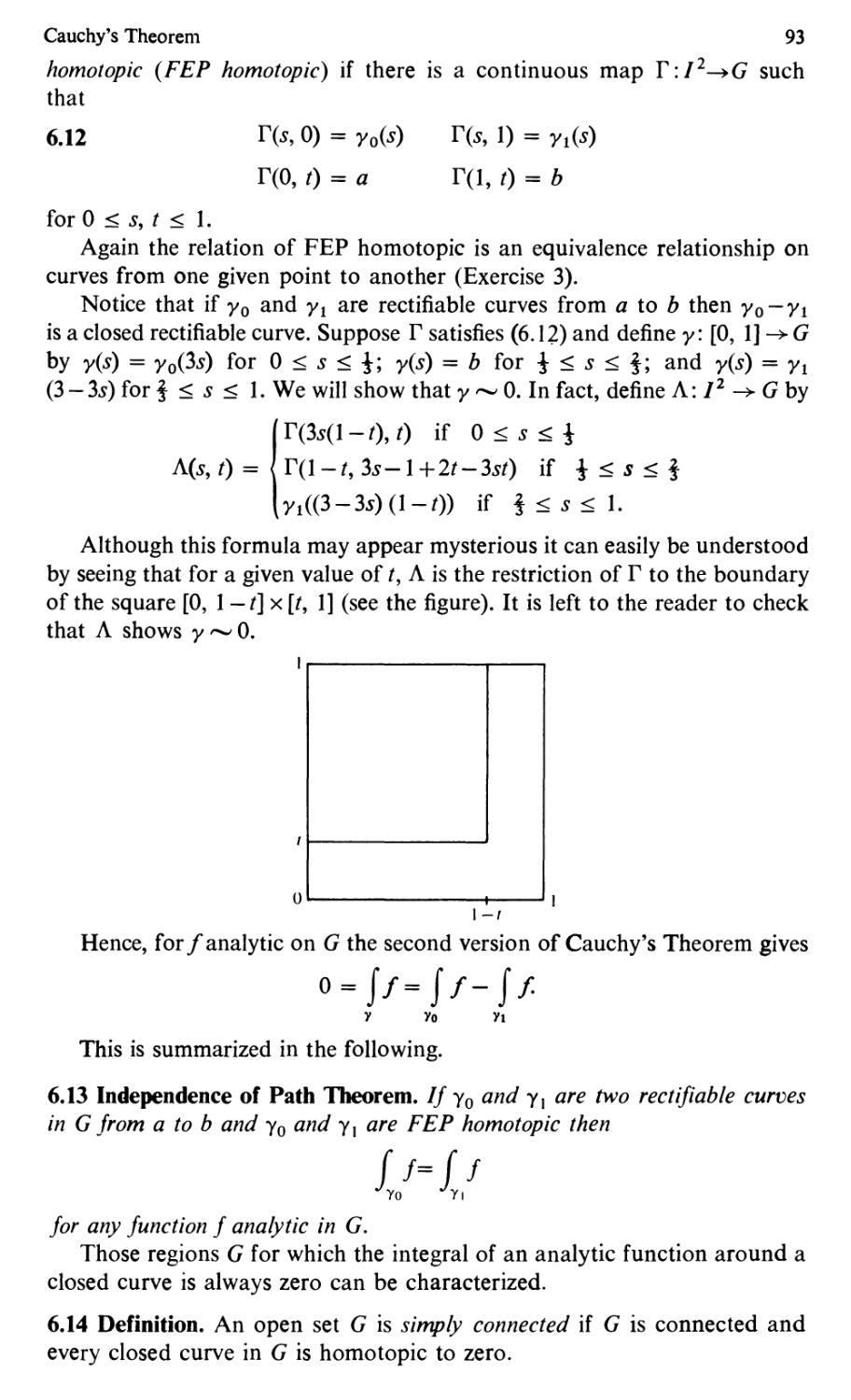


Текст
John B. Conway
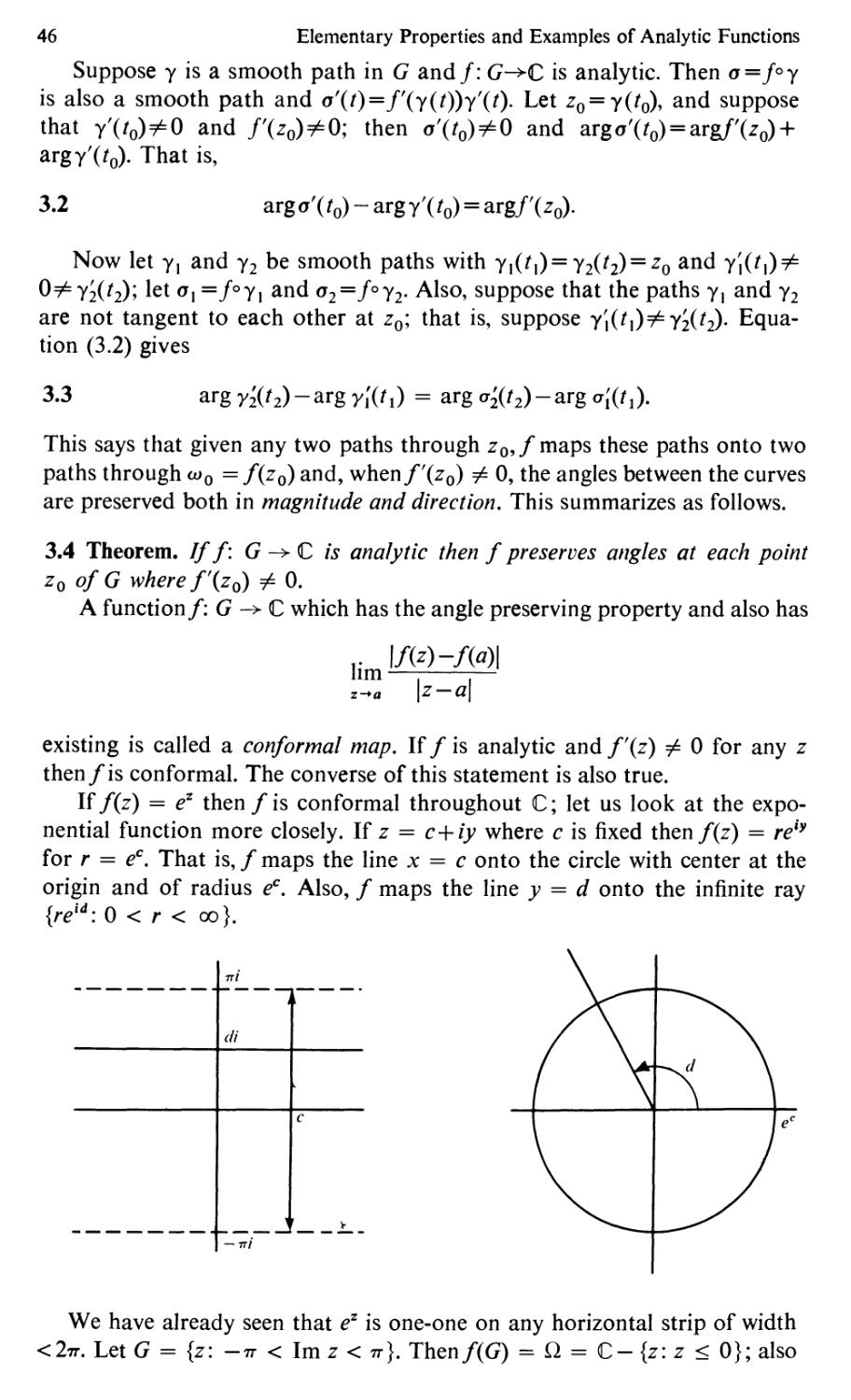
Functions of
One Complex
Variable
Second Edition
Springer-Verlag
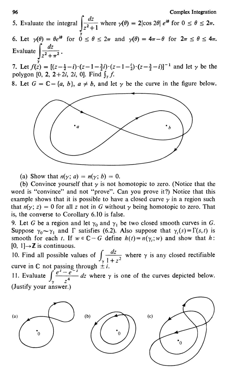
New York Heidelberg Berlin
ra uate exts in at ematics
Editorial Board
F. W. Gehring
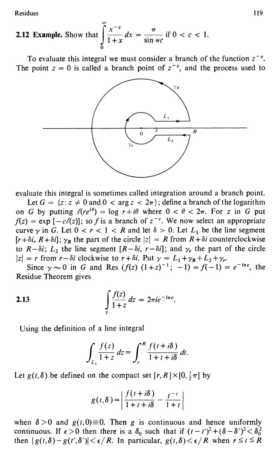
P. R. Halmos
Managing Editor
c. C. Moore
o n
.
.
.
. .
.
nn er- er a
New York Heidelberg Berlin
John B. Conway
Department of Mathematics
Indiana University
Bloomington, IN 47401
USA
Editorial Board
P. R. Halmos
F. W. Gehring
Departm.ent of Mathem.atics
University of Michigan
Ann Arbor, MI 48104
USA
C. C. Moore
Department of Mathem.atics
Indiana University
Bloomington, IN 47401
USA
Departm.ent of Mathem.atics
University of California
Berkeley, CA 94820
USA
AMS Subject Classification: 30--0 I
Library of Congress Cataloging in Publication Data
Conway, John B
Functions of one complex variable.
(Graduate texts in mathematics ; II)
Bibliography: p.
Includes index.
I. Functions of complex variables. I. Title.
II. Series.
QA331.C659 1978 515' .93 78-18836
All rights reserved.
No part of this book may be translated or reproduced in any
form without written permission from Springer-Verlag.
<0 1973 by Springer-Verlag, New York Inc.
<0 1978 by Springer-Verlag, New York Inc.
Printed in the United States of America.
9 8 7 6 5 432 I
ISBN 0-387-90328-3 Springer-Verlag New York
ISBN 3-540-90328-3 Springer-Verlag Berlin Heidelberg
To
Ann
PREFACE
This book is intended as a textbook for a first course in the theory of
functions of one complex variable for students who are mathematically
mature enough to understand and execute E - S arguments. The actual pre-
requisites for reading this book are quite minimal; not much more than a
stiff course in basic calculus and a few facts about partial derivatives. The
topics from advanced calculus that are used (e.g., Leibniz's rule for differ-
entiating under the integral sign) are proved in detail.
Complex Variables is a subject which has something for all mathematicians.
In addition to having applications to other parts of analysis, it can rightly
claim to be an ancestor of many areas of mathematics (e.g., homotopy theory,
manifolds). This view of Complex Analysis as "An Introduction to Mathe-
matics" has influenced the writing and selection of subject matter for this book.
The other guiding principle followed is that all definitions, theorems, etc.
should be clearly and precisely stated. Proofs are given with the student in
mind. Most are presented in detail and when this is not the case the reader is
told precisely what is missing and asked to fill in the gap as an exercise. The
exercises are varied in their degree of difficulty. Some are meant to fix the
ideas of the section in the reader's 11;1ind and some extend the theory or give
applications to other parts of mathematics. (Occasionally, terminology is used
in an exercise which is not defined e.g., group, integral domain.)
Chapters I through V and Sections VI.I and VI.2 are basic. It is possible
to cover this material in a single semester only if a number of proofs are
omitted. Except for the material at the beginning of Section VI.3 on convex
functions, the rest of the book is independent of VI.3 and VI.4.
Chapter VII initiates the student in the consideration of functions as
points in a metric space. The results of the first three sections of this chapter
are used repeatedly in the remainder of the book. Sections four and five need
no defense; moreover, the Weierstrass Factorization Theorem is necessary
for Chapter XI. Section six is an application of the factorization theorem.
The last two sections of Chapter VII are not needed in the rest of the book
although they are a part of classical mathematics which no one should
completely disregard.
The remaining chapters are independent topics and may be covered in any
order desired.
Runge's Theorem is the inspiration for much of the theory of Function
Algebras. The proof presented in section VIII. I is, however, the classical one
involving "pole pushing". Section two applies Runge's Theorem to obtain a
more general form of Cauchy's Theorem. The main results of sections three
and four should be read by everyone, even if the proofs are not.
Chapter IX studies analytic continuation and introduces the reader to
analytic manifolds and covering spaces. Sections one through three can
be considered as a unit and will give the reader a knowledge of analytic
. .
VII
. . .
Preface
VIII
continuation without necessitating his going through all of Chapter IX.
(
Chapter X studies harmonic functions including a solution of the Dirichlet
Problem and the introduction of Green's Function. If this can be called
applied mathematics it is part of applied mathematics that everyone should
know.
Although they are independent, the last two chapters could have been
combined into one entitled "Entire Functions". However, it is felt that
Hadamard's Factorization Theorem and the Great Theorem of Picard are
sufficiently different that each merits its own chapter. Also, neither result
depends upon the other.
With regard to Picard's Theorem it should be mentioned that another
proof is available. The proof presented here uses only elementary arguments
while the proof found in most other books uses the modular function.
There are other topics that could have been covered. Some consideration
was given to including chapters on some or all of the following: conformal
mapping, functions on the disk, elliptic functions, applications of Hilbert
space methods to complex functions. But the line had to be drawn somewhere
and these topics were the victims. For those readers who would like to explore
this material or to further investigate the topics covered in this book, the
bibliography contains a number of appropriate entries.
Most of the notation used is standard. The word "iff" is used in place of
the phrase "if and only if", and the symbol _ is used to indicate the end of a
proof. When a function (other than a path) is being discussed, Latin letters
are used for the domain and Greek letters are used for the range.
This book evolved from classes taught at Indiana University. I would like
to thank the Department of Mathematics for making its resources available
to me during its preparation. I would especially like to thank the students
in my classes; it was actually their reaction to my course in Complex Variables
that made me decide to take the plunge and write a book. Particular thanks
.
should go to Marsha Meredith for pointing out several mistakes in an early
draft, to Stephen Berman for gathering the material for several exercises on
algebra, and to Larry Curnutt for assisting me with the final corrections of the
manuscript. I must also thank Ceil Sheehan for typing the final draft of the
manuscript under unusual circumstances.
Finally, I must thank my wife to whom this book is dedicated. Her
encouragement was the most valuable assistance I received.
John B. Conway
PREFACE FOR
SECO
ED
ON
I have been very pleased with the success of my book. en it was
apparent that the second printing was nearly sold out, Springer-Verlag
asked me to prepare a list of corrections for a third printing. en I
mentioned that I had some ideas for more substantial revisions, they
reacted with characteristic enthusiasm.
There are four major differences between the present edition and its
predecessor. First, John Dixon's treatment of Cauchy's Theorem has been
included. This has the advantage of providing a quick proof of the theorem
in its full generality. Nevertheless, I have a strong attachment to the
homotopic version that appeared in the first edition and have proved this
form of Cauchy's Theorem as it was done there. This version is very
geometric and quite easy to apply. Moreover, the notion of homotopy is
needed for the later treatment of the monodromy theorem; hence, inclu-
sion of this version yields benefits far in excess of the time needed to
discuss it.
Second, the proof of Runge's Theorem is new. The present proof is due
to Sandy Grabiner and does not use "pole pushing". In a sense the "pole
pushing" is buried in the concept of uniform approximation and some
ideas from Banach algebras. Nevertheless, it should be emphasized that the
proof is entirely elementary in that it relies only on the material presented
in this text.
Next, an Appendix B has been added. This appendix contains some
bibliographical material and a guide for further reading.
Finally, several additional exercises have been added.
There are also minor changes that have been made. Several colleagues
in the mathematical community have helped me greatly by providing
constructive criticism and pointing out typographical errors. I wish to
thank publicly Earl Berkson, Louis Brickman, James Deddens, Gerard
Keough, G. K. Kristiansen, Andrew Lenard, John Mairhuber, Donald C.
Meyers, Jeffrey Nunemacher, Robert Olin, Donald Perlis, John Plaster,
Hans Sagan, Glenn Schober, David Stegenga, Richard Varga, James P.
Williams, and Max Zorn.
Finally, I wish to thank the staff at Springer-Verlag New York not only
for their treatment of my book, but also for the publication of so many
fine books on mathematics. In the present time of shri · ng graduate
enrollments and the consequent reluctance of so many publishers to print
advanced texts and monographs, Springer-Verlag is making a contribution
to our discipline by increasing its efforts to disseminate the recent develop-
ments in mathematics.
John B. Conway
.
IX
TABLE OF CONTENTS
Preface 7
I. The Complex Number System
§1. The real numbers ......... 1
§2. The field of complex numbers ....... 1
§3. The complex plane ........ 3
§4. Polar representation and roots of complex numbers ... 4
§5. Lines and half planes in the complex plane .... 6
§6. The extended plane and its spherical representation ... 8
II. Metric Spaces and the Topology of C
§1. Definition and examples of metric spaces . . . . . 11
§2. Connectedness . . . . . . . . . 14
§3. Sequences and completeness . . . . . . . 17
§4. Compactness 20
§5. Continuity 24
§6. Uniform convergence ........ 28
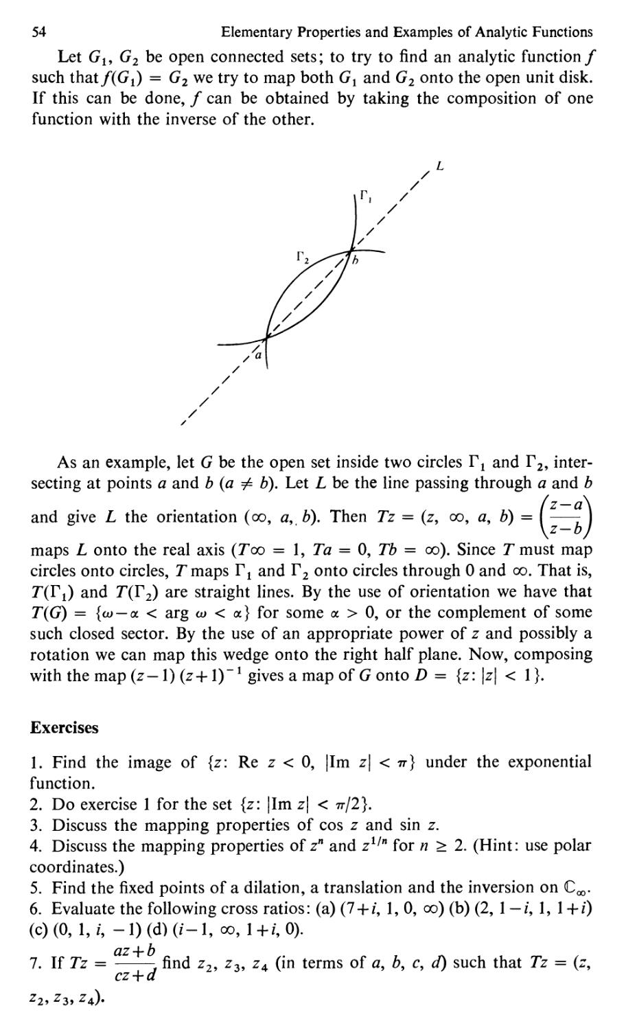
III. Elementary Properties and Examples of Analytic Functions
§1. Power series .......... 30
§2. Analytic functions ......... 33
§3. Analytic functions as mappings, Mobius transformations . . 44
IV. Complex Integration
§1. Riemann-Stieltjes integrals 58
§2. Power series representation of analytic functions . . . 68
§3. Zeros of an analytic function ....... 76
§4. The index of a closed curve 80
§5. Cauchy's Theorem and Integral Formula 83
§6. The homotopic version of Cauchy's Theorem and
simple connectivity 87
§7. Counting zeros; the Open Mapping Theorem .... 97
§8. Goursat's Theorem 100
V. Singularities
§1. Classification of singularities 103
§2. Residues 112
§3. The Argument Principle 123
XI
xii Table of Contents
VI. The Maximum Modulus Theorem
§1. The Maximum Principle 128
§2. Schwarz's Lemma 130
§3. Convex functions and Hadamard's Three Circles Theorem . 133
§4. Phragmen-Lindelof Theorem 138
VII. Compactness and Convergence in the
Space of Analytic Functions
§1. The space of continuous functions C(G,ft) . . . . 142
§2. Spaces of analytic functions . . . . . . . 151
§3. Spaces of meromorphic functions 155
§4. The Riemann Mapping Theorem 160
§5. Weierstrass Factorization Theorem 164
§6. Factorization of the sine function 174
§7. The gamma function 176
§8. The Riemann zeta function 187
VIII. Runge's Theorem
§1. Runge's Theorem 195
§2. Simple connectedness 202
§3. Mittag-Leffler's Theorem 204
IX. Analytic Continuation and Riemann Surfaces
§1. Schwarz Reflection Principle 210
§2. Analytic Continuation Along A Path 213
§3. Mondromy Theorem 217
§4. Topological Spaces and Neighborhood Systems . . . 221
§5. The Sheaf of Germs of Analytic Functions on an Open Set . 227
§6. Analytic Manifolds 233
§7. Covering spaces 245
X. Harmonic Functions
§1. Basic Properties of harmonic functions 252
§2. Harmonic functions on a disk 256
§3. Subharmonic and superharmonic functions .... 263
§4. The Dirichlet Problem 269
§5. Green's Functions 275
XI. Entire Functions 279
§1. Jensen's Formula 280
§2. The genus and order of an entire function .... 282
§3. Hadamard Factorization Theorem 287
Table of Contents xiii
XII. The Range of an Analytic Function
§1. Bloch's Theorem • . . . 292
§2. The Little Picard Theorem 296
§3. Schottky's Theorem 297
§4. The Great Picard Theorem 300
Appendix A: Calculus for Complex Valued Functions on . . . 303
an Interval
Appendix B: Suggestions for Further Study and
Bibliographical Notes 307
References 311
Index 313
List of Symbols 317
apter I
The Complex Number System
1. The real numbers
We denote the set of all real numbers by
. It is assumed that each
reader is acquainted with the real number system and all its properties. In
particular we assume a knowledge of the ordering of R, the definitions and
properties of the supremum and infimum (sup and inf), and the complete-
ness of IR (every set in IR which is bounded above has a supremum). It is
also assumed that every reader is familiar with sequential convergence in
IR and with infinite series. Finally, no one should undertake a study of
Complex Variables unless he has a thorough grounding in functions of one
real variable. Although it has been traditional to study functions of several
real variables before studying analytic function theory, this is not an
essential prerequisite for this book. There will not be any occasion when
the deep resul ts of this area are needed.
2. The field of complex numbers
We define C, the complex numbers, to be the set of all ordered pairs
(a, b) where a and b are real numbers and where addition and multiplication
are defined by:
(a, b)+(c, d) (a+c, b+d)
(a, b) (c, d) (ac bd, bc+ad)
It is easily checked that with these definitions C satisfies all the axioms for
a field. That is, C satisfies the associative, commutative and distributive
laws for addition and multiplication; (0,0) and (1,0) are identities for
addition and multiplication respectively, and there are additive and multi-
plicative inverses for each nonzerO element in C.
We will write a for the complex number (a, 0). This mapping a >- (a, 0)
defines a field isomorphism of
into C so we may consider
as a subset of
c. If we put i (0, 1) then (a, b) a+bi. From this point on we abandon
the ordered pair notation for complex numbers.
Note that i 2 1, so that the equation Z2 + 1 0 has a root in C. In
fact, for each z in C, Z2+ 1 (z+i) (z i). More generally, if z and ware
complex numbers we obtain
Z2+W 2 (z+iw) (z iw)
1
2 The Complex Number System
By letting z and w be real numbers a and b we can obtain (with both a and
b i= 0)
1 a ib
a+ib a 2 +b 2
a
a 2 + b 2
b
.
I
a 2 + b 2
so that we have a formula for the reciprocal of a complex number.
When we write z a + ib (a, b E rR) we call a and b the real and imaginary
parts of z and denote this by a Re z, b 1m z.
We conclude this section by introducing two operations on C which are
not field operations. If z x + iy(x, y E rR) then we define Izl (x 2 + y2)-!- to
be the absolute value of z and z x iy is the conjugate of z. Note that
2.1
Iz 2
-
zz
In particular, if z i= 0 then
I
-
Z
Z2
-
z
The following are basic properties of absolute values and conjugates
whose verifications are left to the reader.
2.2
Rez
!(z + z) and 1m z
I
2.3
2.4
2.5
2.6
(z+w)
z+w and zw
-
zw.
Izw
z/w
Iz
Iz I w ·
z/w.
z.
The reader should try to avoid expanding z and w into their real and
imaginary parts when he tries to prove these last three. Rather, use (2.1),
(2.2), and (2.3).
Exercises
I. Find the real and imaginary parts of each of the following:
I z a 3 + 5i
- · - ( a E lR ) . Z3. ·
Z ' z + a " 7i + I '
l+i 3 3;
2
1 i 3 6
2
· in.
, ,
1 +i n
- for 2 < n < 8.
2
2. Find the absolute value and conjugate of each of the following:
3 i i
. .
2+3i' i+3 '
2+i;
3; (2 + i) (4 + 3 i) ;
(1 +i)6; i 17 .
The complex plane 3
3. Show that z is a real number if and only if z z.
4. If z and ware complex numbers, prove the following equations:
z+w 2 z 2+2Re zw+ w 2.
Z w 2
Z 2 2Re z w + w 2.
z+w 2 + z W 2 2(/z 2+/ W 2).
5. Use induction to prove that for z
/w w 1 /... wn/;z zl+...+zn;w
6. Let R(z) be a rational function of z.
coeflicien ts in R( z) are real.
Z 1 +. · · + Zn; W
WI. · · W n e
Show that R(z)
WI W z · · · w n :
R(z) if all the
3. The complex plane
From the definition of complex numbers it is clear that each z in C can
be identified with the unique point (Re z, 1m z) in the plane 2. The addition
of complex numbers is exactly the addition law of the vector space 1R2.
If z and ware in C then draw the straight lines from z and w to 0 ( (0, 0)).
These form two sides of a parallelogram with 0, z and w as three vertices.
The fourth vertex turns out to be z + w.
Note also that z W is exactly the distance between z and w. With this
in mind the last equation of Exercise 4 in the preceding section states the
parallelogram law: The sum of the squares of the lengths of the sides of a
parallelogram equals the sum of the squares of the lengths of its diagonals.
A fundamental property of a distance function is that it satisfies the
triangle inequality (see the next chapter). In this case this inequality becomes
/Zl Z2 < Zl z31 + /Z3 z21
for complex numbers Zl, Z2, Z3. By using Zl Z2 (Zl Z3)+(Z3 Z2), it is
easy to see that we need only show
3.1
z+W < z + w (Z,WEC).
To show this first observe that for any z in C,
3.2 z < Re z < z
- z < 1m z < z
Hence, Re (zw) < zw z/ w. Thus,
z+w 2 z 2+2Re (zw) + w 2
< z 2+2 z w + w 2
(z + W/)2,
from which (3.1) follows. (This is called the triangle inequality because, if we
represent z and w in the plane, (3.1) says that the length of one side of the
triangle [0, z, z + w] is less than the sum of the lengths of the other two sides.
.
Or, the shortest distance between two points is a straight line.) On encounter-
4 The Complex Number System
ing an inequality one should always ask for necessary and sufficient conditions
that equality obtains. From looking at a triangle and considering the geo-
metrical significance of (3.1) we are led to consider the condition z tw
for some t E lR, t > o. (or w tz if w 0). It is clear that equality will
occur when the two points are colinear with the origin. In fact, if we look
at the proof of (3.1) we s ee that a necessary and sufficient condition fo r
z+ w z + w is that zw Re (zw). Equivalently, this is zw > 0 (i.e., zw
is a real number and is non negative). Multiplying, this by w/w we get
wI 2 (z/w) > 0 if w =F O. If
t z/w
1 \
w 2(Z/W)
w 2
then t > 0 and z tw.
By induction we also get
3.3
Zt+ Z 2+...+Zn < Zt +Z2 +...+zn
Also useful is the inequality
3.4
z w < Z W
Now that we have given a geometric interpretation of the absolute value
let us see what taking a complex conjugate does to a point in the plane.
This is also easy; in fact, z is the point obtained by reflecting Z across the
x-axis (i.e., the real axis).
Exercises
I. Prove (3.4) and give necessary and sufficient conditions for equality.
2. Show that equality occurs in (3.3) if and only if Zk/Z, > 0 for any integers
k and 1, I < k, 1 < n, for which z, =F o.
3. Let a E lR and c > 0 be fixed. Describe the set of points Z satisfying
Iz al Iz+al 2c
for every possible choice of a and c. Now let a be any complex number
and, using a rotation of the plane, describe the locus of points satisfying the
above equation.
4. Polar representation and roots of complex numbers
Consider the point z x + iy in the complex plane C. This point has
polar coordinates (r, 0): x r cos 0, y r sin O. Clearly r z and () is
the angle between the positive real axis and the line segment from 0 to z.
Notice that () plus any multiple of 27T can be substituted for () in the above
equations. The angle () is called the argument of z and is denoted by () arg z.
Because of the ambiguity of (), "arg" is not a function. We introduce the
notation
4.1
cis () cos 0 + i sin ().
Polar representation and roots of complex numbers
Let Zl '1 cis ° 1 , Zz - 'z cis Oz. Then Zl Z Z 'l'Z cis ° 1 cis 0z
[(cos 0 1 cos 0z sin 0 1 sin Oz)+i (sin 0 1 cos Oz+sin 0z cos {}1)].
formulas for the sine and cosine of the sum of two angles we get
5
'1'2
By the
4.2
Z 1 Z Z , l' z cis (0 1 + ( 2 )
Alternately, arg(zlzZ) argz 1 +argz z . (What function of a real variable
takes products into sums?) By induction we get for Zk 'k cis Ok' 1 < k < n.
4.3
Zl Z Z.. · ZII r 1 ,z. ..'n cis (01 +. · .+On)
In particular,
4.4
Zn r n cis (nO),
for every integer n ;> O. Moreover if Z =I- 0, z. [, - 1 cis (0)] 1; so that
(4.4) also holds for all integers n, positive, negative, and zero, if z =I- o. As a
special case of (4.4) we get de M oivre' s formula:
(cos 0+ i sin o)n cos nO + i sin nO.
We are now in a position to consider the following problem: For a given
complex number a =I- 0 and an integer n > 2, can you find a number z
satisfying zn a? How many such z can you find? In light of (4.4) the
solution is easy. Let a - a cis a; by (4.4), z la l/n cis (a/n) fills the bill.
However this is not the only solution because z'
n
4.5
satisfies (z,)n - a. In fact each of the numbers
. 1
lal 11n CIS - (a+27Tk), 0 < k < n 1,
n
in an nth root of a. By means of (4.4) we arrive at the following: for each
non zero number a in C there are n distinct nth roots of a; they are given by
formula (4.5).
Example
Calculate the nth roots of unity. Since 1 cis 0, (4.5) gives these roots as
2 4 2
1, cis , cis , . . . , cis (n 1).
n n n
In particular, the cube roots of unity are
1
- (1 + i 3),
2
1
- (1
2
-
i 3).
1,
Exercises
1. Find the sixth roots of unity.
6 The Complex Number System
2. Calculate the following:
(a) the square roots of i
(b) the cube roots of i
-
(c) the square roots of 3 + 3i
3. A primitive nth root of unity is a complex number a such that
1,a,a 2 ,...,a n - 1 are distinct nth roots of unity. Show that if a and bare
primitive nth and mth roots of unity, respectively, then ab is a kth root of
unity for some integer k. at is the smallest value of k? at can be said
if a and bare nonprimitive roots of unity?
4. Use the binomial equation
n
n n-k b k
k a ,
(a + b )n
k=O
where
n n!
k k!(n k)!'
and compare the real and imaginary parts of each side of de Moivre's
formula to obtain the formulas:
cos nO
cos n ()
n cosn- 2 sin2 0+ n cosn- 4 0 sin 4 ()
2 4
. . .
sin nO
27T
5. Let z . cis for an integer n > 2. Show that l+z+.. .+zn-l o.
n
6. Show that cp(t) cis t is a group homomorphism of the additive group
onto the multiplicative group T {z: z 1 }.
7. If z E C and Re(zn» 0 for every positive integer n, show that z is a
positive real number.
5. Lines and half planes in the complex plane
Let L denote a straight line in C. From elementary analytic geometry,
L is determined by a point in L and a direction vector. Thus if a is any point
in Land b is its direction vector then
L {z a+ tb: 00 < t < oo}.
Since b =1= 0 this gives, for z in L,
z a
1m
o.
b
In fact if z is such that
o - 1m
z a
b
then
z a
t
b
Lines and half planes in the complex plane
implies that z a + tb, 00 < t < 00. That is
7
z a
5.1
L
z: 1m
o .
b
What is. the locus of each of the sets
z: 1m
z a
b
> 0 ,
z: 1m
z a
b
< 0 ?
As a first step in answering this question, observe that since b is a direction
we may assume 'bl 1. For the moment, let us consider the case where
a 0, and put Ho {z: 1m (z/b) > O}, b cis 13. If z r cis {} then
z/b r cis (0 f3). Thus, z is in Ho if and only if sin (0 f3) > 0; that is, when
f3 < 0 < 'TT + f3. Hence Ho is the half plane lying to the left of the line L if
Ho
f3
we are "walking along L in the direction of b." If we put
z a
Ha
then it is easy to see that Ha a + Ho {a + w: W E Ho }; that is, Ha is the
translation of Ho by a. Hence, Ha is the half plane lying to the left of L.
Similarly,
Ka
z: 1m
z a
b
<0
is the half plane on the right of L.
Exercise
1. Let C be the circle {z: z c
r}, r > 0; let a c+r cis a and put
8
The Complex Number System
LfJ ' z: 1m
z a
o
b
where b cis f3. Find necessary and sufficient conditions in terms of f3 that
LfJ be tangent to C at a.
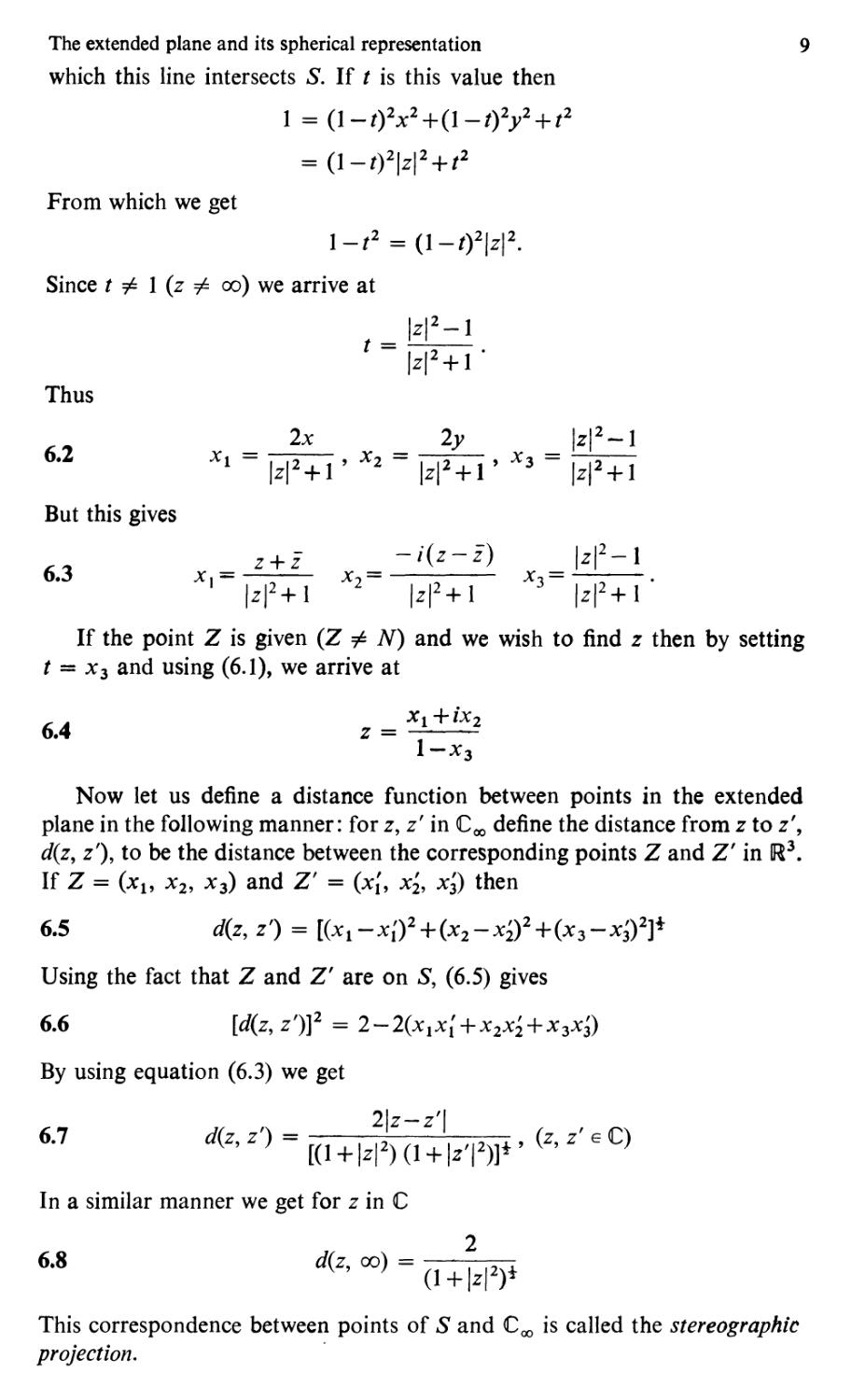
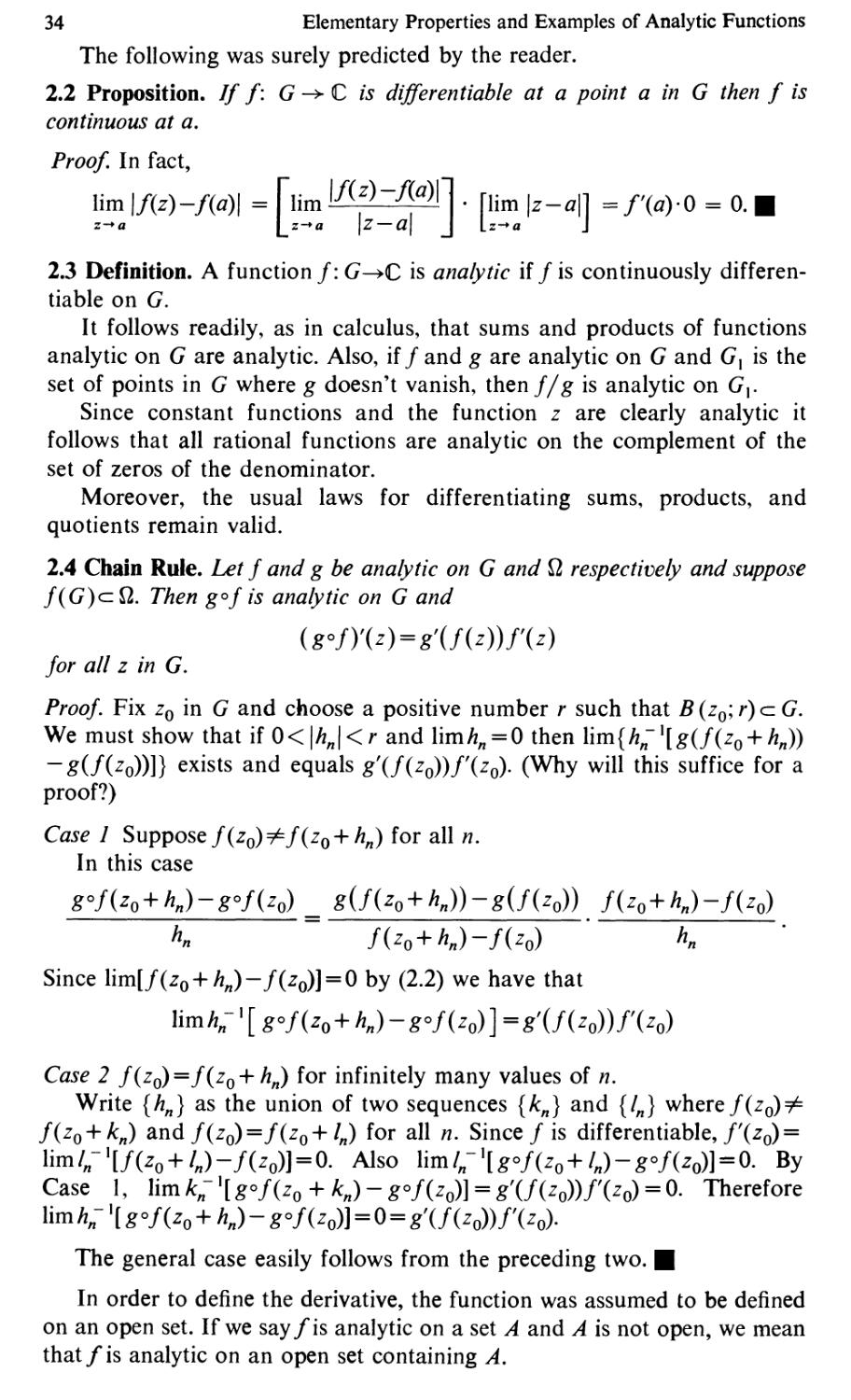
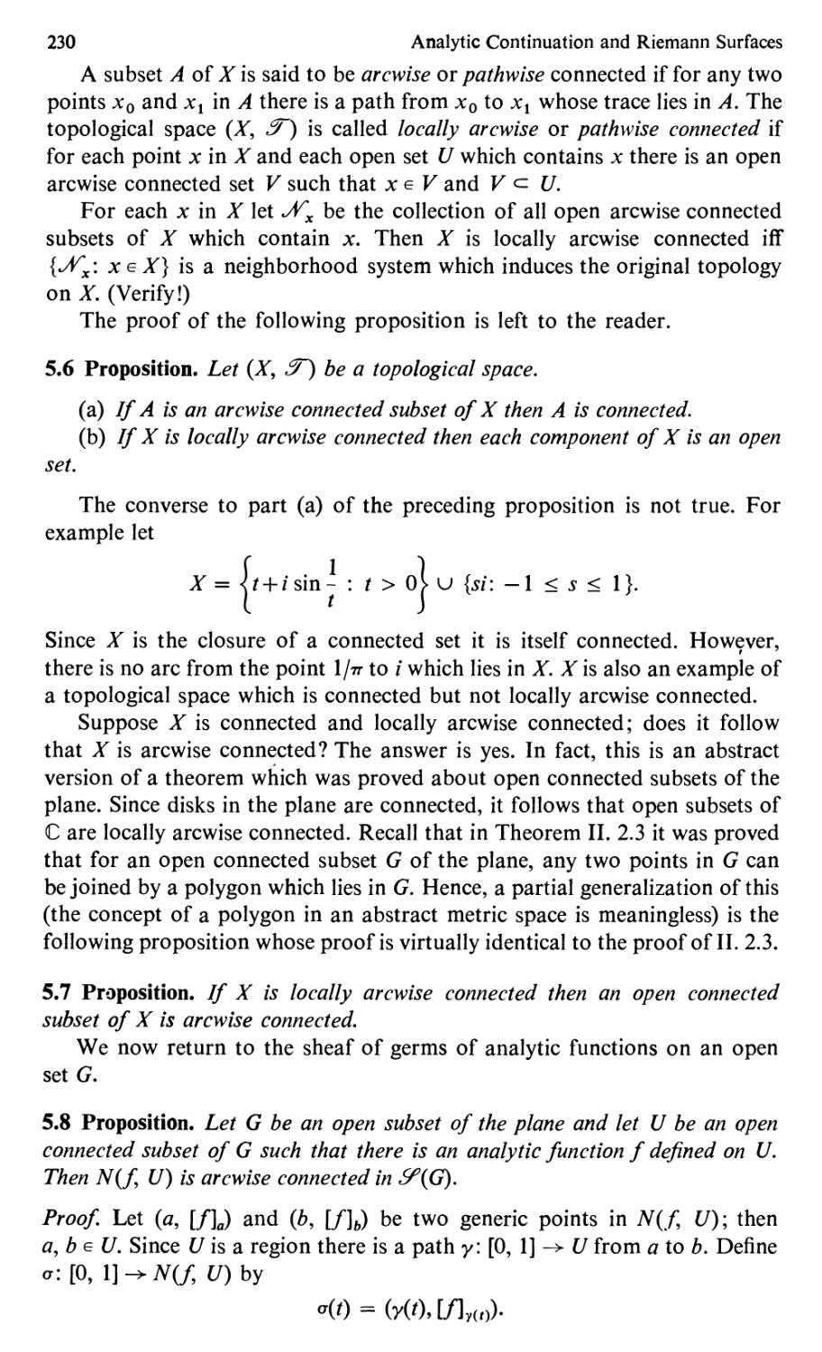
6. The extended plane and its spherical representation
Often in complex analysis we will be concerned with functions that be-
come infinite as the variable approaches a given point. To discuss this situa-
tion we introduce the extended plane which is C u {(X)} Coo. We also
wish to introduce a distance function on Coo in order to discuss continuity
properties of functions assuming the value infinity. To accomplish this
and to give a concrete picture of Coo we represent Coo as the unit sphere
in lR 3
,
s
{( ) rJl) 3 . 2 2 2
Xl' X 2 , X3 E · Xl +X2+ X 3
I }.
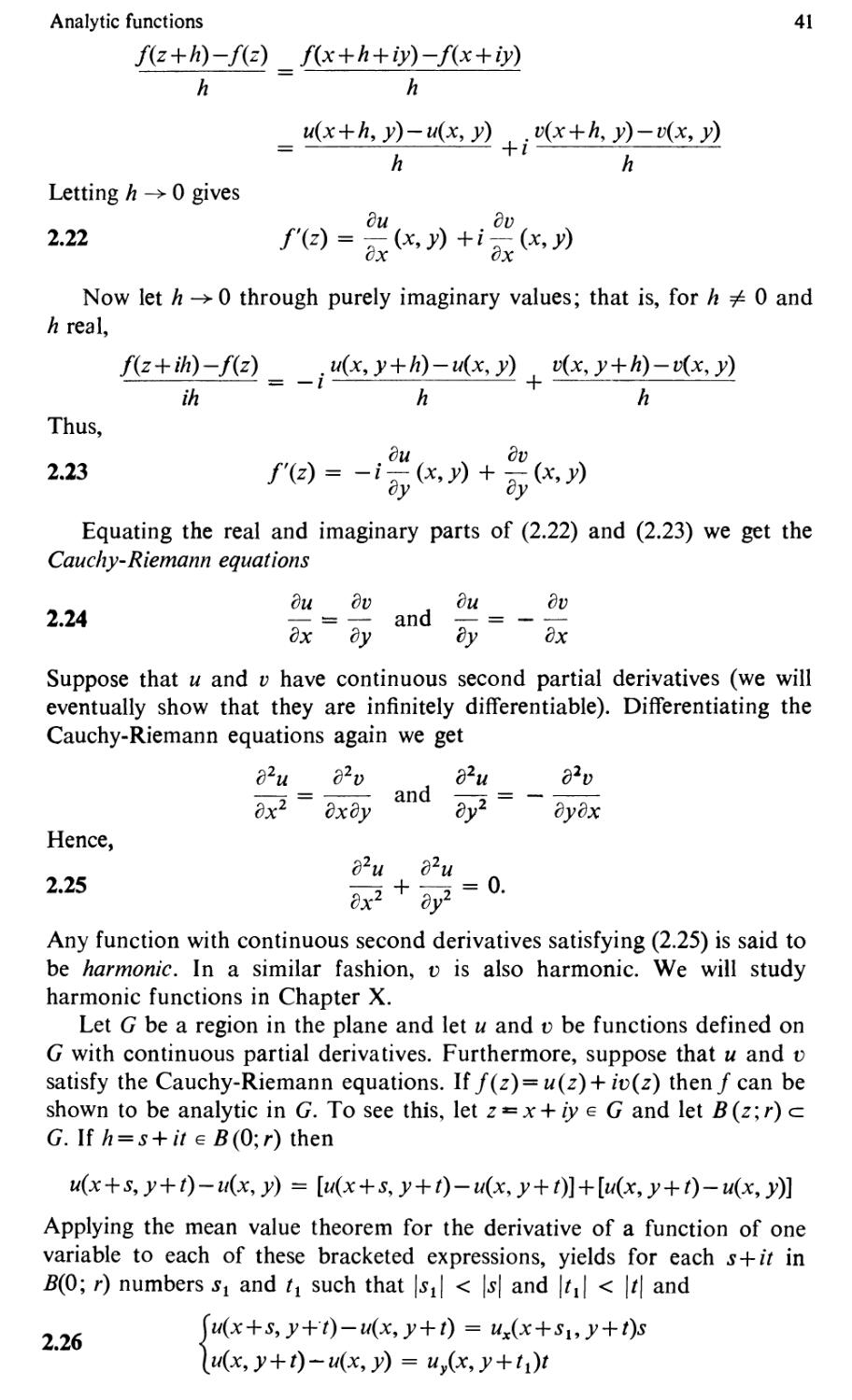
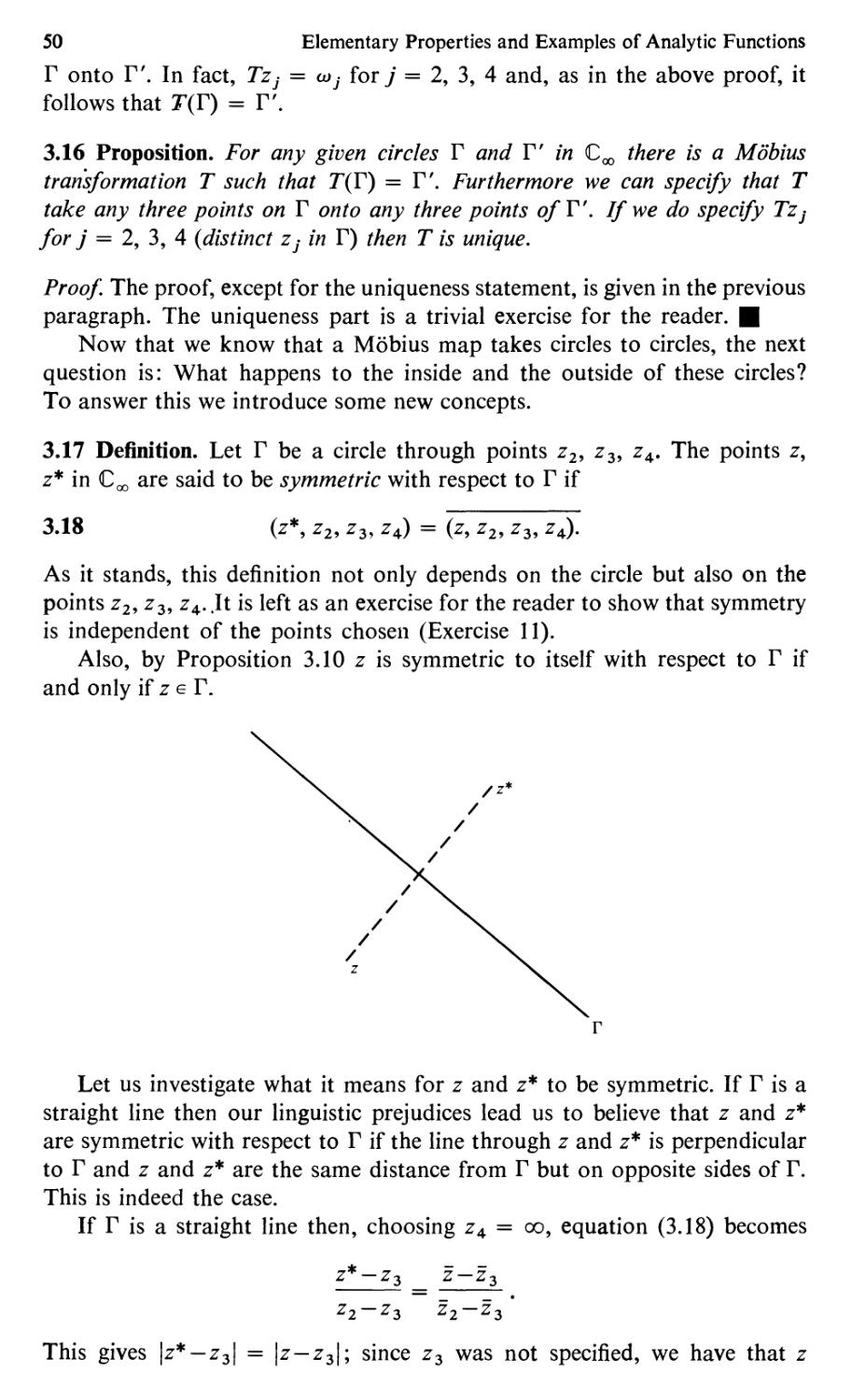
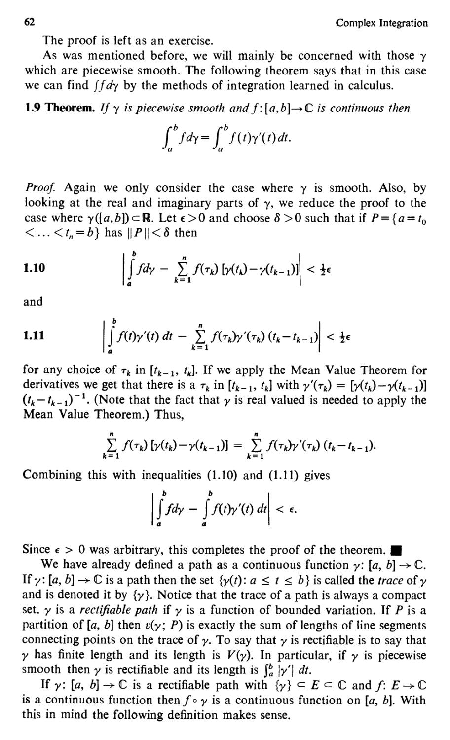
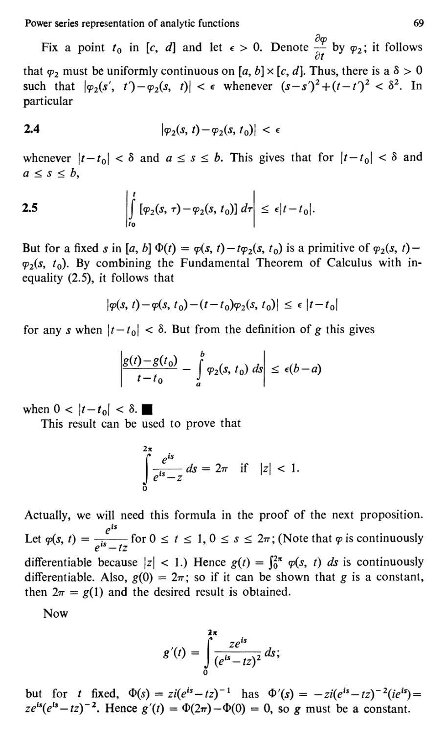
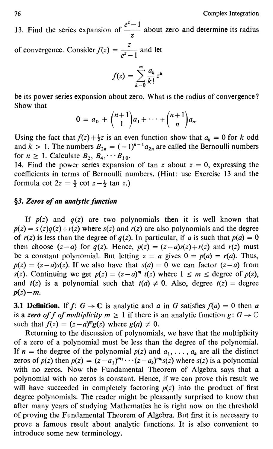
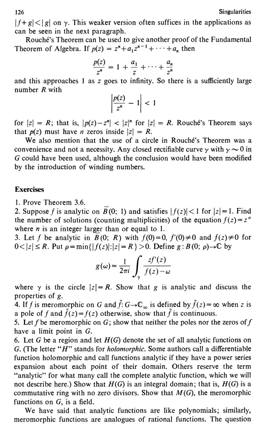
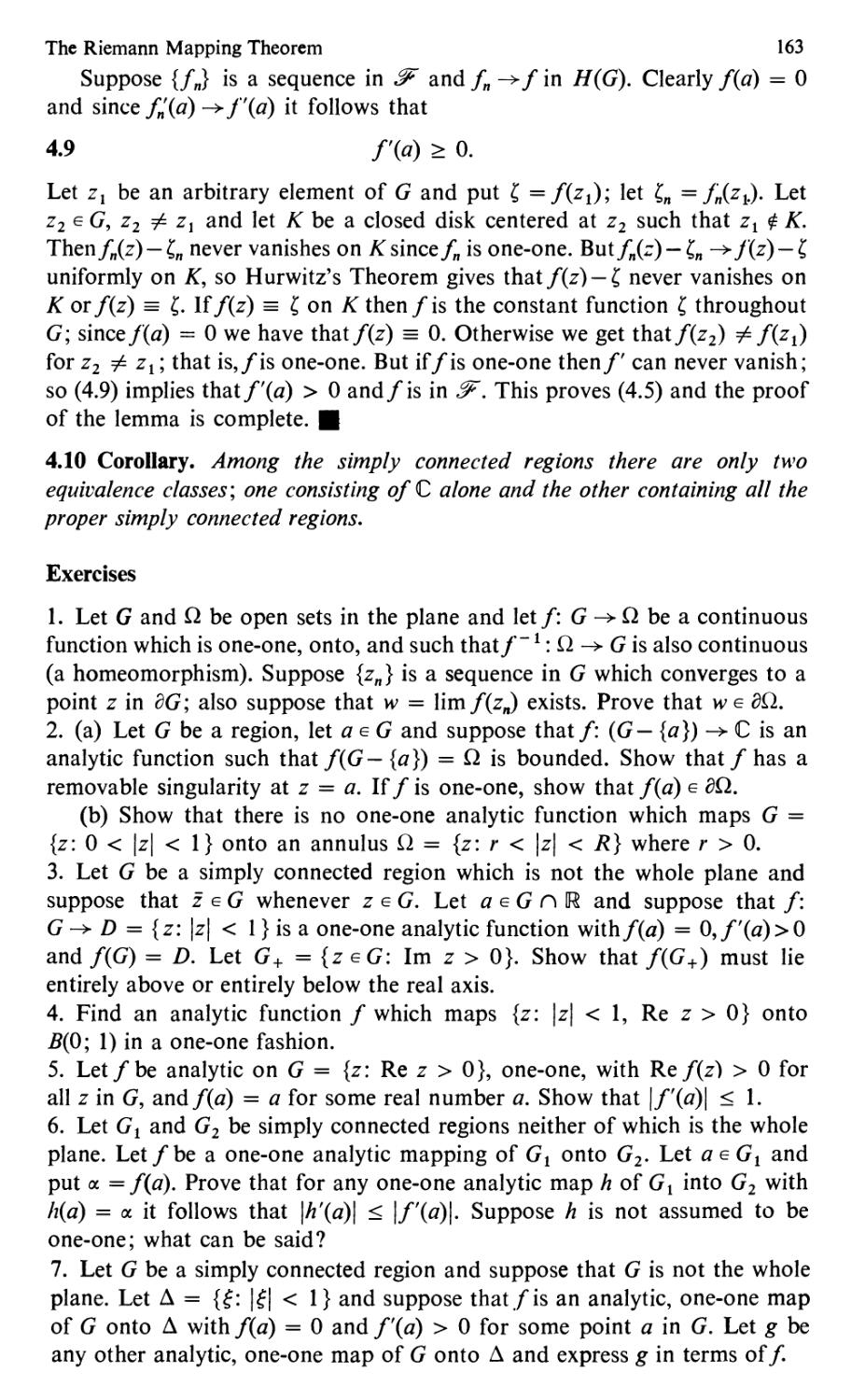
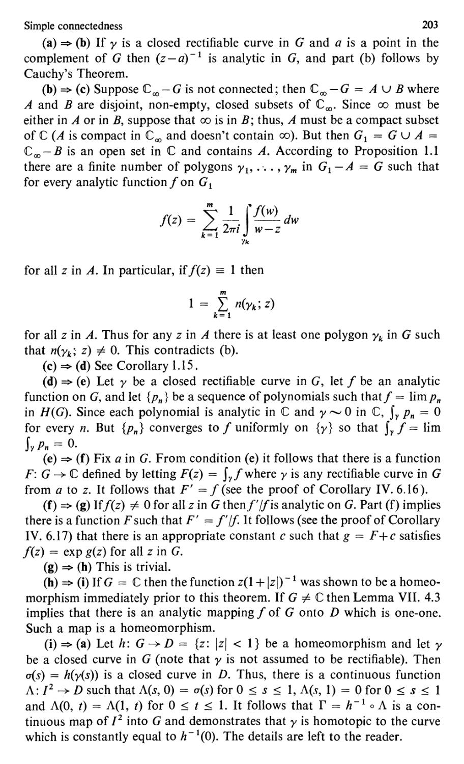
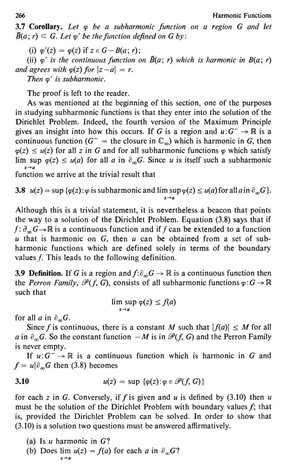
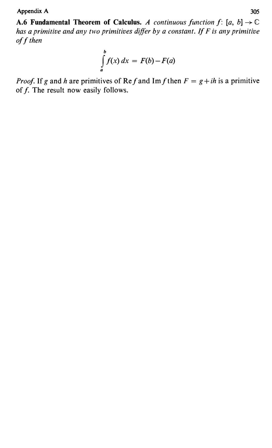
Let N (0, 0, I); that is, N is the north pole on S. Also, identify C with
{(Xl' X 2 , 0): Xl' X2 E IR} so that C cuts S along the equator. Now for each
point z in C consider the straght line in 3 through z and N. This intersects
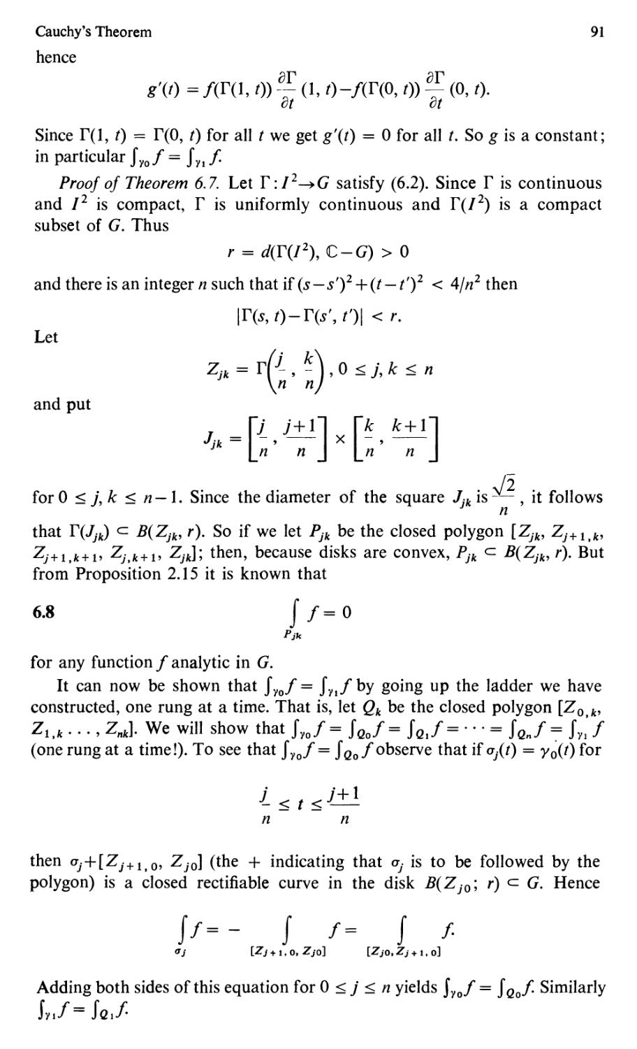
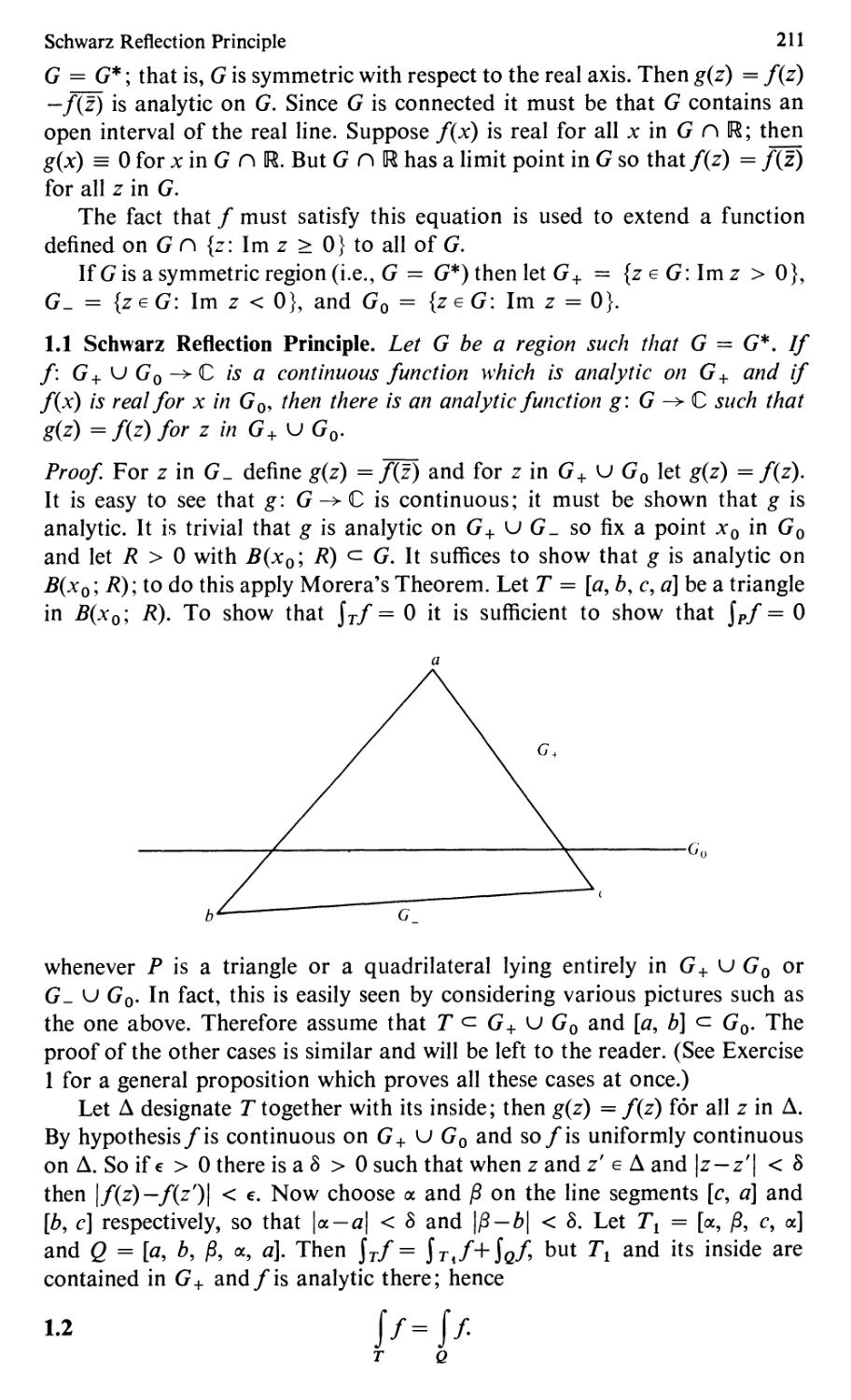
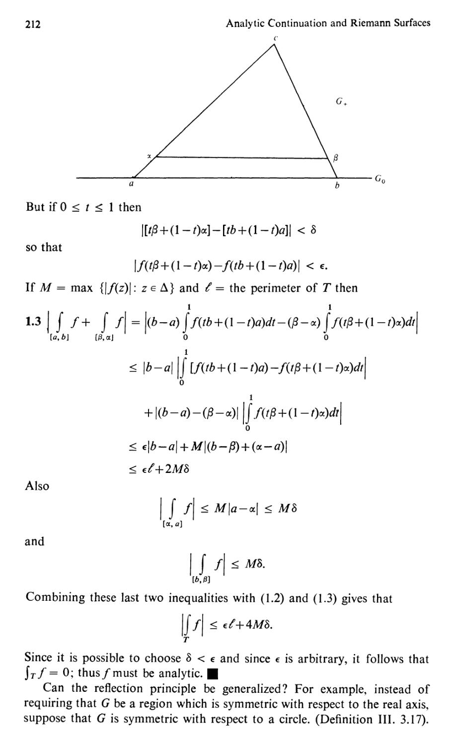
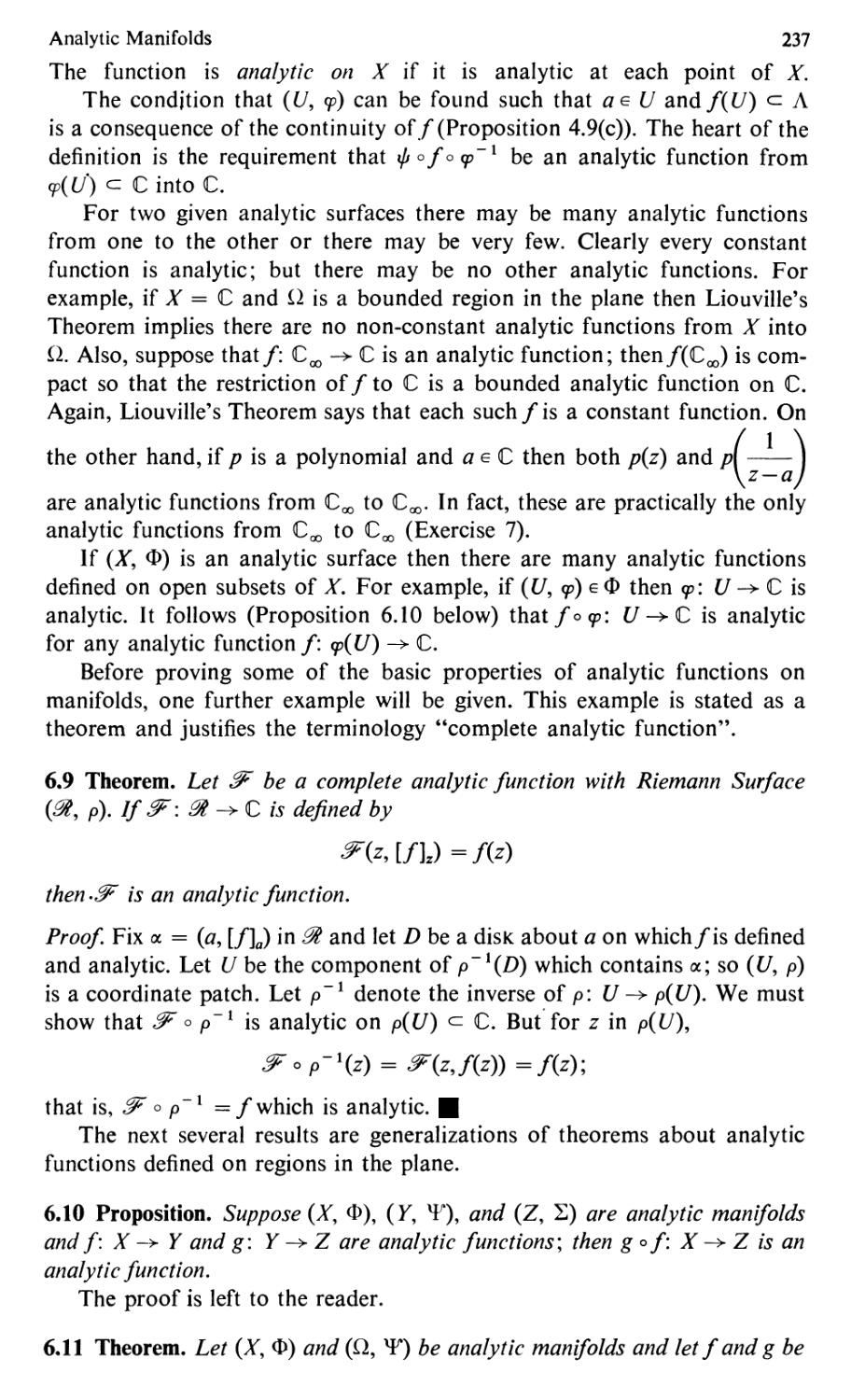
N
"
"
"-
"-
'"
z
J
I
z
\
\
-
- --
/
/
/
/'
""
"'
"
"
"
-
-
the sphere in exactly one point Z =1= N. If Iz > 1 then Z is in the northern
hemisphere and if z < I then Z is in the southern hemisphere; also, for
z 1, Z z. What happens to Z as z 001 Clearly Z approaches N;
hence, we identify N and the point 00 in Coo. Thus Coo is represented as
the sphere S.
Let us explore this representation. Put z X+ iy and let Z (Xl' X 2 , x 3 )
be the corresponding point on S. We will find equations expressing Xl' X2,
and X3 in terms of X and y. The line in (R3 through z and N is given by
{tN+(l t)z: 00 < t < oo}, or by
6.1
{((I t)x, (1 t)y, t): 00 < t < oo}.
Hence, we can find the coordinates of Z if we can find the value of t at
The extended plane and its spherical representation
which this line intersects S. If ( is this value then
1 (1 t)2x2+(1 t)2y2+t 2
(1 t) 2 Z 2 + (2
9
From which we get
1 t 2 (1 t)2 z 2.
Since t i= I (z "# (0) we arrive at
t
Z 2 1
z2+1 ·
Thus
6.2
Xl
2x
2y
Z 2 - 1
z2+1
But this gives
-
z+z
z 2+ I
. -
. I Z Z
Z 2 I
6.3
Z 2+ 1
X 3
x -
I
X 2
z 2+ I
.
If the point Z is given (2 =F N) and we wish to find z then by setting
t . X3 and using (6.1), we arrive at
X t + ix 2
- -
.
1 X3
Now let us define a distance function between points in the extended
plane in the foIlowing manner: for z, z' in Coo define the distance from z to z',
d(z, z'), to be the distance between the corresponding points Z and Z' in (R3.
If Z (Xt, X2, X3) and Z' (x;, X2, X3) then
6.4
z
6.5
d(z, z') [(Xt X{)2 +(X 2 X2)2 +(x 3 X3)2]t
Using the fact that Z and Z' are on S, (6.5) gives
6.6
[d(z, Z')]2 2 . 2(x 1 x{ +X 2 X2+ X 3 X 3)
By using equation (6.3) we get
6.7
, 2 z . z'/ ,
In a similar manner we get for z in C
6.8
d(z, (0)
2
.
(I + z 2)t
This correspondence between points of S and Coo is called the stereographic
projection.
10
Exercises
The Complex Number System
I. Give the details in the derivation of (6. 7) and (6.8).
2. For each of the following points in C, give the corresponding point of
s: 0, 1 + i, 3 + 2i.
3. Which subsets of S correspond to the real and imaginary axes in C.
4. Let A be a circle lying in S. Then there is a unique plane P in (R3 such
that P n S A. Recall from analytic geometry that
P {(Xt, X 2 , X 3 ): Xtf3t +X2f32+X3 3 I}
where ({3t, {32, 3) is a vector orthogonal to P and I is some real number.
It can be assumed that {3i+{3 +{3 I. Use this information to show that
if A contains the point N then its projection on C is a straight line. Otherwise,
A projects onto a circle in C.
5. Let Z and Z' be points on S corresponding to z and z' respectively. Let
W be the point on S corresponding to z + z'. Find the coordinates of W in
terms of the coordinates of Z and Z'.
etric Spaces and the Topology of C
1. Definition and examples of metric spaces
A metric space is a pair (X, d) where X is a set and d is a function from
Xx X into IR, called a distance function or metric, which satisfies the following
conditions for x, y, and z in X:
d(x, y) > 0
d(x, y) 0 if and only if x y
d(x, y) d(y, x) (symmetry)
d(x, z) < d(x, y)+d(y, z) (triangle inequality)
If x and r > 0 are fixed then define
B(x; r) {y E X: d(x, y) < r}
B(x; r) {y E X: d(x, y) < r}.
B(x; r) and B(x; r) are called the open and closed balls, respectively, with
center x and radius r.
Examples
1.1 Let X or C and define d(z, w) z w. This makes both (IR, d)
and (C, d) metric spaces. In fact, (C, d) will be the example of principal
interest to us. If the reader has never encountered the concept of a metric
space before this, he should continually keep (C, d) in mind during the study
of this chapter.
1.2 Let (X, d) be a metric space and let Y eX; then (Y, d) is also a metric
space.
1.3 Let X C and define d(x+iy, a+ib) x a + Iy b. Then (C, d) is
a metric space.
1.4 Let X C and define d(x+iy, a+ib) max {Ix a, Iy bl}.
1.5 Let X be any set and define d(x, y) 0 if x y and d(x, y) 1 if x =F y.
To show that the function d satisfies the triangle inequality one merely
considers all possibilities of equality among x, y, and z. Notice here that
B(x ; E) consists only of the point x if E < 1 and B(x ; E) X if E > 1. This
metric space does not appear in the study of analytic function theory.
1.6 Let X IR n and for x (Xl' . . . , x n ), Y (YI, . . . , Yn) in IR n define
n t
d(x; y)
(x j Yj)2
j= 1
11
12 Metric Spaces and the Topology of C
1.7 Let S be any set and denote by B(S) the set of an functions I: S > C
such that
11/1100 sup {/(s) : s E S} < 00.
That is, B(S) consists of all complex valued functions whose range is con-
tained inside some disk of finite radius. For.f and g in B(S) define d(j; g)
III gILX). We will show that d satisfies the triangle inequality. In fact if f,
g, and h are in B(S) and s is any point in S then f(s) g(s) f(s) h(s) +
h(s) g(s) < f(s) h(s) + Ih(s) g(s) < IIf h 1100 + IIh g 100. Thus, when the
supremum is taken over all s in S, I I g 1100 < I f h 1100 + 1/ h g 1/00' which is
the triangle inequality for d.
1.8 Definition. For a metric space (X, d) a set G c X is open if for each
x in G there is an E > 0 such that R(x; E) C G.
Thus, a set in C is open if it has no "edge." For example, G {z E C:
a < Re z < b} is open; but {z: Re z < O} u {O} is not because S(O; E) is not
contained in this set no matter how small we choose E.
We denote the empty set, the set consisting of no elements, by D.
1.9 Proposition. Let (X, d) he a metric space; then:
(a) The sets X and 0 are open; n
(b) If G 1 , . · . , G n are open sets in X then so is G k ;
k=l
(c) If {G j: j E J} is a collection 01 open sets in X, J any indexing set,
then G . U {G j : j E J} is also open.
n
Proof. The proof of (a) is a triviality . To prove (b) let x E G G k ; then
k=l
x E G k for k I, . . . , n. Thus, by the definition, for each k there is an Ek > 0
such that B(x; Ek) C G k . But if E min {El, E2, . . . , En} then for 1 < k < n
R(x; E) C B(x; Ek) C G k . Thus B(x; E) c G and G is open.
The proof of (c) is left as an exercise for the reader. II
There is another class of subsets of a metric space which are distinguished.
These are the sets which contain all their "edge"; alternately, the sets whose
complements have no "edge."
1.10 Definition. A set F c X is closed if its complement, X F, is open.
The following proposition is the complement of Proposition 1.9. The
proof, whose execution is left to the reader, is accomplished by applying
de Morgan's laws to the preceding proposition.
1.11 Proposition. Let (X, d) be a metric space. Then:
(a) The sets X and 0 are closed; n
(b) If F 1 , . . . , Fn are closed sets in X then so is Fk ;
k=l
(c) If {F j : j E J} is any collection of closed sets in X, J any indexing set,
then F n {F j : j E J} is also closed.
The most common error made upon learning of open and closed sets
is to interpret the definition of closed set to mean that if a set is not open it is
Definition and examples of metric spaces 13
closed. This, of course, is false as can be seen by looking at {z E C: Re z > O}
U {O}; it is neither open nor closed.
1.12 Definition. Let A be a subset of X. Then the interior of A, int A, is the
set {G: G is open and G c A}. The closure of A, A -, is the set {F: F
is closed and F ::) A}. Notice that int A may be empty and A - may be X.
If A -- {a+bi: a and bare r3;tional numbers} then simultaneously A - C
and int A D. By Propositions 1.9 and 1.11 we have that A - is closed and
int A is open. The boundary of A is denoted by oA and defined by oA A-
(X A)-.
1.13 Proposition. Let A and B be subsets of a metric space (X, d). Then:
(a) A is open if and only if A int A;
(b) A is closed if and only if A A - ;
(c) int A X (X A)-; A- - X int (X A); oA A- int A;
(d) (A U B)- A- u B-;
(e) Xo E int A if and only if there is an € > 0 such that B(xo; €) c A;
(f) Xo E A - if and only if for every £ > 0, B(xo; €) A =F D.
Proof. The proofs of (a)-(e) are left to the reader. To prove (f) assume
Xo E A - X int (X A); thus, Xo ft int (X A). By part (e), for every
€ > 0 B(xo; €) is not contained in X A. That is, there is a point y E B(xo; €)
which is not in X A. Hence, y E B(xo; €) f1 A. Now suppose Xo ft A-
X int (X A). Then Xo E int (X A) and, by (e), there is an € > 0 such
that B(xo; E) c X A. That is, B(x o ; E) f1 A 0 so that Xo does not
satisfy the condition. II
Finally, one last definition of a distinguished type of set.
1.14 Definition. A subset A of a metric space X is dense if A-X.
The set of rational numbers Q is dense in and {x+ iy: x, Y E Q} is
dense in C.
Exercises
1. Show that each of the examples of metric spaces given in (1.2)-( I .6) is,
indeed, a metric space. Example (1.6) is the only one likely to give any
difficulty. Also, describe B (x; r) for each of these examples.
2. Which of the following subsets of C are open and which are closed: (a)
{ z: z < I } ; (b) the real axis; (c) {z: z n I for some integer n > I } ; (d)
{z E C: z is real and 0 < z < I } ; (e) z E C : z is real and 0 < Z < I ?
3. If (X, d) is any metric space show that every open ball is, in fact, an open
set. Also, show that every closed ball is a closed set.
4. Give the details of the proof of (1.9c).
5. Prove Proposition 1.11.
6. Prove that a set G c X is open if and only if X G is closed.
7. Show that (Coo, d) where d is given by (I. 6.7) and (I. 6.8) is a metric space.
8. Let (X, d) be a metric space and Y c X. Suppose G c X is open; show
14 Metric Spaces and the TOpOlOgy of C
that G () Y is open in (Y, d). Conversely, show that if G 1 c Y is open in
(Y, d), there is an open set G c X such that GIG n Y.
9. Do Exercise 8 with "closed" in place of "open."
10. Prove Proposition 1.13.
II. Show that cisk:k > O is dense in T Z E C: z I. For which
values of 9 is {cis(k9): k > O} dense in T?
fil. Connectedness
Let us start this section by giving an example. Let X {z E C: z < I}
u {z: z 3 < I} and give X the metric it inherits from C. (HencefoFward,
whenever we consider subsets X of IR or C as metric spaces we will assume,
unless stated to the contrary, that X has the inherited metric d(z, w) z tV.)
Then the set A {z: z < I} is simultaneously open and closed. It is closed
because its complement in X, B X A {z: z 3 < I} is open; A is
open because if a E A then B(a; 1) c A. (Notice that it may not happen
that {z E C: z a < I} is contained in A for example, if a I. But the
definition of B(a; 1) is {z EX: z a < I} and this is contained in A.)
Similarly B is also both open and closed in X.
This is an example of a non-connected space.
2.1 Definition. A metric space (X, d) is connected if the only subsets of X
which are both open and closed are D and X. If A c X then A is a connected
subset of X if the metric space (A, d) is connected.
An equivalent formulation of connectedness is to say that X is not
connected if there are disjoint open sets A and B in X, neither of which is
empty, such that X A u B. In fact, if this condition holds then A X B
is also closed.
2.2 Proposition. A set X c is connected iff X is an interval.
Proof. Suppose X [a, b], a and b elements of IR. Let A c X be an open
subset of X such that a E A, and A =I- X. We will show that A cannot also be
closed and hence, X must be connected. Since A is open and a E A there is
an € > 0 such that [a, a+€) c A. Let
r sup {€: [a, a+€) c A}
Claim. [a, a + r) ,c A. In fact, if a < x < a + r then, putting h a + r x > 0,
the definition of supremum implies there is an € with r h < € < rand
[a, a+€) c A. But a < x a+(r h) < a+€ implies x E A and the claim is
established.
However, a+r f# A; for if, on the contrary, a+r E A then, by the openness
of A, there is a 8 > 0 with [a+r, a+r+8) c A. But this gives [a, a+r+S)
c A, contradicting the definition of r . Now if A were also closed then a + r E B
X A which is open. Hence we could find a 8 > 0 such that (a+r 8,
a+r] c B, contradicting the above claim.
The proof that other types of intervals are connected is similar and it wiIJ
be left as an exercise.
The proof of the converse is Exercise I. II
Connectedness 15
If wand z are in C then we denote the straight line segment from z to w
by
[z, w] {tw+(l t)z: 0 < t < I}
n
A polygon from a to b is a set P [Zk, Wk] where z 1 a, w n band
k=l
W k Zk+ 1 for I < k < n 1; or, P [a, Z 1 . . . Zn, b].
2.3 Theorem. An open set Gee is connected iff for any two points Q, b in
G there is a polygon from a to b lying entirely inside G.
Proof. Suppose that G satisfies this condition and let us assume that G is
not connected. We will obtain a contradiction. From the definition, G
A U B where A and B are both open and closed, A (1 B D, and neither
A nor B is empty. Let a E A and b E B; by hypothesis there is a polygon P
from a to' b such that peG. Now a moment's thought will show that one
of the segments making up P will have one point in A and another in B.
So we can assume that P [a, b]. Define,
S {SE[O, I]: sb+(I s)aEA}
T {t E [0, 1]: tb+(1 t)a E B}
Then S (1 T D, S u T [0, I], 0 E S and lET. However it can be shown
that both Sand T are open (Exercise 2), contradicting the connectedness of
[0, I]. Thus, G must be connected.
Now suppose that G is connected and fix a point a in G. To show how to
construct a polygon (lying in G!) from a to a point b in G would be difficult.
But we don't have to perform such a construction; we merely show that one
exists. For a fixed a in G define
A {b E G: there is a polygon peG from a to b}.
The plan is to show that A is simultaneously open and closed in G. Since
a E A and G is connected this will give that A G and the theorem will be
proved.
To show that A is open let b E A and let P - [a, Zl, . . . , Zn, b] be a
polygon from a to b with peG. Since G is open (this was not needed in the
first half), there is an € > 0 such that B(b; €) c G. But if z E B(b; €) then
[b, z] c B(b; E) c G. Hence the pqlygon Q P u [b, z] is inside G and goes
from a to z. This shows that B(b; E) c A, and so A is open.
To show that A is closed suppose there is a point z in G A and let € > 0
be such that B(z; E) c G. If there is a point b in A (l B(z; E) then, as above,
we can construct a polygon from Q to z. Thus we must have that B(z; E) t1 A
D, or B(z; €) c G A. That is, G A is open so that A is closed. II
2.4 Corollary. If Gee is open and connected and a and b are points in G
then there is a polygon P in G from a to b which is made up of line segments
parallel to either the real or imaginary axis.
Proof. There are two ways of proving this corollary. One could obtain a
16 Metric Spaces and the Topology of C
polygon in G from a to b and then modify each of its line segments so that a
new polygon is obtained with the desired properties. However, this proof
is more easily executed using compactness (see Exercise 5.7). Another proof
can be obtained by modifying the proof of Theorem 2.3. Define the set A as
in the proof of (2.3) but add the restriction that the polygon's segments are
all parallel to one of the axes. The remainder of the proof will be valid with
one exception. If Z E B(b; E) then [b, z] may not be parallel to an axis. But it
is easy to see that if z x+iy, b p+iq then the polygon [b, p+iy] U
[p+iy, z] c B(b; E) and has segments parallel to an axis. II
It will now be shown that any set S in a metric space can be expressed,
in a canonical way, as the union of connected pieces.
2.5 Definition. A subset D of a metric space X is a component of X if it is a
maximal connected subset of X. That is, D is connected and there is no
connected subset of X that properly contains D.
If the reader examines the example at the beginning of this section he
will notice that both A and B are components and, furthermore, these are
the only components of X. For another example let X {O, 1, t, t, . . .}.
Then clearly every component of X is a point and each point is a component.
1
Notice that while the components - are all open in X, the component {O}
n
is not.
2.6 Lemma. Let x 0 E X and let {D j : j E J} be a collection of connected subsets
of X such that x 0 E D j for each j in J. Then D {D j : j E J} is connected.
Proof Let A be a subset of the metric space (D, d) which is both open and
closed and suppose that A =F D. Then AnD j is open in (D j, d) for each j
and it is also closed (Exercises 1.8 and 1.9). Since D j is connected we get that
either A (1 D j D or AnD j D j. Since A =F D there is at least one k
such that A n Dk =F D; hence, A n Dk Dk. In particular x 0 E A so that
Xo E A n Dj for every j. Thus A n Dj Dj, or Dj c A, for each index j.
This gives that D A, so that D is connected. _
2.7 Theorem. Let (X, d) be a metric space. Then:
(a) Each Xo in X is contained in a component of X.
(b) Distinct components of X are disjoint.
Note that part (a) says that X is the union of its components.
Proof (a) Let !$ be the coIlection of connected subsets of X which contain
the given point Xo. Notice that {xo} E !$ so that!?) =F D. Also notice that
the hypotheses of the preceding lemma apply to the colIection fg. Hence
C {D: DE!?)} is connected and Xo E C. But C must be a component.
In fact, if D is connect.ed and C c D then x 0 E D so that DE!?); but then
D c C, so that C D. Thus C is maximal and part (a) is proved.
(b) Suppose C 1 and C 2 are components, C 1 =F C 2 , and suppose there is
a point Xo in C 1 () C 2 . Again the lemma says that C 1 U C 2 is connected.
Sequences and completeness 17
Since both C 1 and C z are components, this gives c 1 . C 1 U C z C z , a
contradiction. II
2.8 Proposition. (a) If A c X is connected and A c B c A -, then B is connected.
(b) If C is a component of X then C is closed.
The proof is left as an exercise.
2.9 Theorem. Let G be open in C; then the components of G are open and
there are only a countable number of them.
Proof. Let C be a component of G and let x 0 E C. Since G is open there is an
€ > 0 with B(xo; E) c G. By Lemma 2.6, B(xo; E) U C is connected and so
must be C. That is B(xo; €) c C and C is, therefore, open.
To see that the number of components is countable let S {a+ib:
a and b are rational and a+bi E G}. Then S is countable and each com..
ponent of G contains a point of S, so that the number of components is
countable. II
Exercises
I. The purpose of this exercise is to show that a connected subset of IR is an
interval.
(a) Show that a set A c R is an interval iff for any two points a and b
in A with a < b, the interval [a, b] c A.
(b) Use part (a) to show that if a set A c R is connected then it is an
interval.
2. Show that the sets Sand T in the proof of Theorem 2.3 are open.
3. Which of the following subsets X of C are connected; if X is not connected,
what are its components: (a) X {z: Izi < I} U {z: Iz 2 < I}. (b) X
I
[0, 1) U 1 +- : n > I . (c) X C (A u B) where A [0, (0) and B .'
n
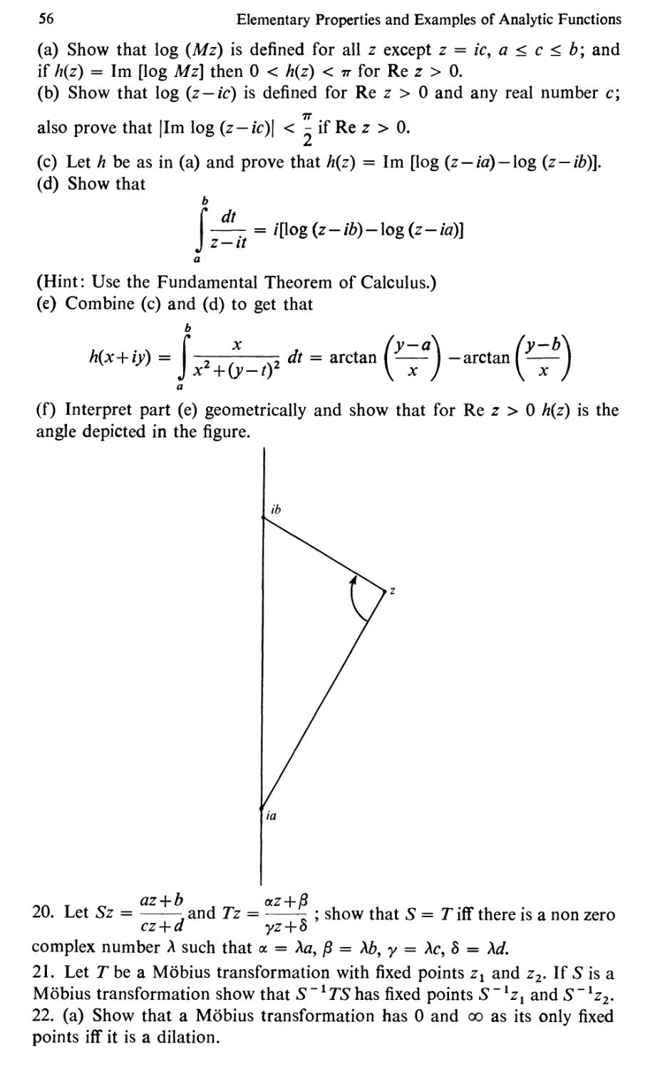
{z ' r cis f}: r 0, 0 :< f) < oo}?
4. Prove the following generalization of Lemma 2.6. If {D j: j E J} is a
collection of connected subsets of X and if for each j and k in J we have
D j n Dk -# 0 then D ..0 {D j: j E J} is connected.
5. Show that if F c X is closed and connected then for every pair of points
a, b in F and each E > 0 th' re are points Zo, Zt, . . . , Zn in F with Zo · a,
Zn band d(Zk _ I' Zk) < E for I < k < n. Is the hypothesis that F be closed
needed? if F is a set which sati fies this property then F is not necessarily
connected, even if F is closed. Give an example to illustrate this.
3. Sequences and completeness
One of the most useful concepts in a metric space is that of a convergent
sequence. Their central role in calculus is duplicated in the study of metric
spaces and complex analysis.
3.1 Definition. If {Xl' X2, . . :} is a sequence in a metric space (X, d) then
18 Metric Spaces and the Topology of C
{x n } converges to x in symbols x lim x n or x n x if for every E > 0
there is an integer N such that d(x, x n ) < E whenever n > N.
Alternately, x lim X n if 0 lim d(x, x n ).
If X C then z lim Zn means that for each E > 0 there is an N such
that Z Zn < E when n > N.
Many concepts in the theory of metric spaces can be phrased in terms
of sequences. The following is an example.
3.2 Proposition. A set F c X is closed iff for each sequence {xn} in F with
x Iim X n we have x E F.
Proof. Suppose F is closed and x Iim X n where each X n is in F. So for every
E > 0, there is a point X n in B(x; E); that is B(x; E) n F -# D, so that x E F-
F by Proposition 2.8.
Now suppose F is not closed; so there is a point Xo in F- which is not
in F. By Proposition 1.13(f), for every E > 0 we have B(xo; E) n F -# D.
1
In particular for every integer n there is a point X n in B .X 0; - n F. Thus,
n
> x o. Since x 0 ft F, this says the con-
n
dition fails. II
3.3 Definition. If A c X then a point x in X is a limit point of A if there
is a sequence {xn} of distinct points in A such that x lim Xw
The reason for the word "distinct" in this definition can be illustrated
by the following example. Let X C and let A [0, I] U {i}; each point
in [0, I] is a limit point of A but i is not. We do not wish to call a point such
as i a limit point; but if "distinct" were dropped from the definition we
could taken X n i for each i and have i lim Xn.
3.4 Proposition. (a) A set is closed iff it contains all its limit points.
(b) If A c X then A- A u {x: x is a limit point of A}.
The proof is left as an exercise.
From real analysis we know that a basic property of IR is that any sequence
whose terms get closer together as n gets large, must be convergent. Such
sequences are called Cauchy sequences. One of their attributes is that you
know the limit will exist even though you can't produce it.
3.5 Definition. A sequence {xn} is called a Cauchy sequence if for every
E > 0 there is an integer N such that d(xn, x m ) < E for all n, m > N.
If (X, d) has the property that each Cauchy sequence has a limit in X
then (X, d) is complete.
3.6 Proposition. C is complete.
Proof. If {xn+iYn} is a Cauchy sequence in C then {xn} and {Yn} are Cauchy
sequences in IR. Since [R is complete, X n > x and Yn > Y for points x, y in IR.
It follows that x + iy lim (xn + iYn), and so C is complete. II
Consider Coo with its metric d (I. 6.7 and I. 6.8). Let Zn, Z be points in C;
Sequences and completeness 19
it can be shown that d(zn, z) > 0 if and only if IZn zi > O. In spite of this,
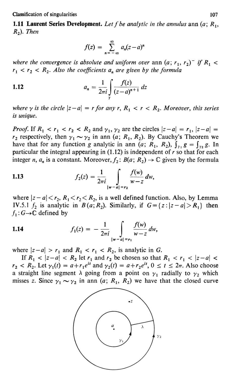
any sequence {zn} with Iim IZnl 00 is Cauchy in Coo, but, of course, is not
Cauchy in C.
If A c X we define the diameter of A by diam A sup {d(x, y): x and
yare in A}.
3.7 Cantor's Theorem. A metric space (X, d) is complete iff for any sequence
00
{Fn} of non-empty closed sets with F 1 => F 2 => . . . and diam Fn > 0, Fn
consists of a single point. n= J
Proof. Suppose (X, d) is complete and let {Fn} be a sequence of closed sets
having the properties: (i) F 1 => F 2 :::> . . . and (ii) lim diam Fn O. For each
n, let X n be an arbitrary point in Fn; if n, m > N then X n , X m are in FN so that,
by definition, d(xn, x m ) < diam FN. By the hypothesis N can be chosen
sufficiently large that diam FN < E; this shows that {xn} is a Cauchy sequence.
Since X is complete, Xo Iim X n exists. Also, X n is in FN for all n > N
00
since Fn c F N ; hence, Xo is in FN for every N and this gives Xo E Fn F.
n=l
So F contains at least one point; if, also, y is in F then both Xo and yare in
Fn for e ach n and this gives d(xo, y) < diam Fn )- O. Therefore d(xo, y) 0,
or Xo y.
Now let us show that X is complete if it satisfies the stated condition.
Let {xn} be a Cauchy sequence in X and put Fn {xn, X n + l' . . .} -; then
F 1 => F; => . .. . If E > 0, choose N such that d(xn, x m ) < E for each n,
m > N; this gives that diam {xn, X n + 1, . . .} < E for n > N and so diam
Fn < E for n > N (Exercise 3). Thus diam Fn > 0 and, by hypothesis, there
is a point Xo in X with {xo} F 1 r'1 F 2 r'1 . . . . In particular Xo is in Fn,
and so d(xo, x n ) < diam Fn > O. Therefore, Xo lim Xn. II
There is a standard exercise associated with this theorem. It is to find a
sequence of sets {Fn} in IR which satisfies two of the conditions:
(a) each Fn is closed,
(b) F 1 => F 2 => · · · ,
(c) diam Fn > 0;
but which has F F 1 () F 2 r'1 . . . either empty or consisting of more than
one point. Everyone should get examples satisfying the possible combina-
tions.
3.8 Proposition. Let (X, d) be a complete metric space and let Y eX. Then
(Y, d) is a complete metric space iff Y is closed in X.
Proof. It is left as an exercise to show that (Y,d) is complete whenever Y is
a closed subset. Now assume ( Y, d) to be complete; let Xo be a limit point
of Y. Then there is a sequence {Yn} of points in Y such that Xo limYn.
Hence {Yn} is a Cauchy sequence (Exercise 5) and must converge to a
point Yo in Y, since (Y, d) .is complete. I t follows that Yo Xo and so Y
contains all its limit points. Hence Y is closed by Proposition 3.4. II
20
Exercises
Metric Spaces and the Topology of C
1. Prove Proposition 3.4.
2. Furnish the details of the proof of Proposition 3.8.
3. Show that diam A = diam A -.
4. Let Zm Z be points in C and let d be the metric on Coo' Show that IZn - zi 0
if and only if d(zn' z) O. Also show that if IZnl 00 then {zn} is Cauchy
in Coo' (Must {zn} converge in Coo 1)
5. Show that every convergent sequence in (X, d) is a Cauchy sequence.
6. Give three examples of non complete metric spaces.
7. Put a metric d on such that Ix" - xl 0 if and only if d(xm x) 0,
but that {xn} is a Cauchy sequence in (IR, d) when Ixnl --). 00. (Hint: Take
inspiration from Coo.)
8. Suppose {X,.} is a Cauchy sequence and {x nk } is a subsequence that is
convergent Show that {x n } must be convergent.
4. Compactness
The concept of compactness is an extension of the benefits of finiteness to
infinite sets. Most properties of compact sets are analogues of properties
of finite sets which are quite trivial. For example, every sequence in a finite
set has a convergent subsequence. This is quite trivial since there must be at
least one point which is repeated an infinite number of times. However the
same statement remains true if "finite" is replaced by "compact."
4.1 Definition. A subset K of a metric space X is compact if for every collec-
tion of open sets in X with the property
4.2
Kc U {G:GE },
there is a finite number of sets G 1 , . . . , G n in cg such that K c G 1 U G 2 U
. . . u G n . A collection of sets cg satisfying (4.2) is called a cover of K; if
each member of @ is an open set it is called an open cover of K.
Clearly the empty set and all finite sets are compact. An example of a
non compact set is D =:= {z E C: Izi < I}. If G n = {z: Izi < 1 - } for n =
2, 3, . . . , then {G 2 , G 3 , . . .} is an open cover of D for which there is no
finite subcover.
4.3 Proposition. Let K be a compact subset of X; then:
(a) K is closed;
(b) If F is closed and F c K then F is compact.
Proof To prove part (a) we will show that K = K-. Let Xo E K-; by Pro-
position 1.13(f), B(xo; €) () K =I D for each € > o. Let G n = X-B(xo; )
00 00
and suppose that Xo ft K. Then each G n is open and K c U G n (because n
n=l n=l
Compactness 21
_ I
B x 0; - {x 0 }). Since K is compact there is an integer m such that
n
K c G n . But G 1 c G 2 C . . . so that K c G m
n=l
-
X B
1
m
xo;
m
. Bllt this
1
gives that B Xo; (') K 0, a contradiction. Thus K K-.
m
To prove part (b) let be an open cover of F. Then, since F is closed,
c:g u {X F} is an open cover of K. Let G 1, . . . , G n be sets in c:g such that
K c G 1 U . . . U G n U (X F). Clearly, F c G 1 U . . . u G n and so F is
compa ct. II
If . is a colJection of subsets of X we say that ' h as the finite inter-
section property (f.i.p.) if whenever {Fb F 2 , . . . , Fn} c , F 1 (') F 2 (') . . . (')
Fn =1= D. An example of such a collection is {D G 2 , D G 3 ,...} where
the sets G n are as in the example preceding Proposition 4.3.
4.4 Proposition. A set K c X is compact iff every collection of closed
subsets of K with the fi.p. has { F : F E !# } =1= D.
Proof Suppose K is compact and is a co ll ection of closed subsets of K
havi ng the f.i.p. Assume that {F: F E :#' } D and l et c:g {X F:
FE !# }. Then, {X F: FE :#' } X {F: FE :#' } X by the
assumption; in particular, is an open cover of K. Thus, there are F 1 , . . . ,
n
n
n
Fn E . such that K c (X F k ) X Fk. But this gives that Fk
k=l k=l n k=l
C X K, and since each Fk is a subset of K it must be that Fk D. This
contradicts the f.i. p. k = 1
The proof of the converse is left as an exercise. II
4.5 Corollary. Every compact metric space is complete.
Proof. This follows easily by applying the above proposition and Theorem
3.7. II
4.6. Corollary. If X is compact then every infinite set has a limit point in X.
Proof. Let S be an infinite subset of X and suppose S has no limit points.
Let {aI' a 2 ,...} be a sequence of distinct points in S; then Fn {an,
a n + l' . · .} also has no limit points. But if a set has no limit points it contains
all its limits points and must be closed! Thus, each Fn is closed and {Fn:
00
n > I} has the f.i.p. However, since the points a 1 , a 2 , . . . are distinct, Fn
0, contradicting the above proposition. II n = 1
4.7 Definition. A metric space (X, d) is sequentially compact if every sequence
in X has a convergent subsequence.
It will be shown that compact and sequentially compact metric spaces
are the same. To do this the following is needed.
4.8 Lebesgue's Covering Lemma. If (X, d) is sequentially compact and
22 Metric Spaces and the Topology of C
is an open cover of X then there is an € > 0 such that if x is In X, there is a
set G in with B(x; E) C G.
Proof The proof is by contradiction; suppose that is an open cover of X
and no such € > 0 can be found. In particular, for every integer n there is a
I
point X n in X such that B x n ; - is not contained in any set G in . Since X
n
is sequentially compact there is a point Xo in X and a subsequence {x nk }
such that x 0 lim x nk . Let G 0 E such that x 0 EGO and choose E > 0
such that B(xo; E) C Go. Now let N be such that d(xo, x nk ) < E/2 for all
nk > N. Let n k be any integer larger than both Nand 2/€, and let y E B(x nk ;
link). Then d(xo, y) < d(xo, xnk)+d(x nk , y) < E/2+ link < E. That is, B(x nk ;
link) c B(xo; E) C Go, contradicting the choice of x nk . II
There are two common misinterpretations of Lebesgue's Covering
Lemma; one implies that it says nothing and the other that it says too much.
Since is an open covering of X it follows that each x in X is contained in
some G in . Thus there is an E > 0 such that B(x; €) c G since G is open.
The lemma, however, gives one E > 0 such that for any x, B(x; E) is con-
tained in some member of . The other misinterpretation is to believe that
for the € > 0 obtained in the lemma, B(x; €) is contained in each G in
such that x E G.
4.9. Theorem. Let (X, d) be a metric space; then the following are equivalent
statements:
(a) X is compact;
(b) Every infinite set in X has a limit point;
(c) X is sequentially compact;
(d) X is complete and for every E > 0 there are a finite number of points
Xl' · · · , X n in X such that
n
X B(x k ; E).
k=l
(The property mentioned in (d) is called total boundedness.)
Proof. That (a) implies (b) is the statement of Corollary 4.6.
(b) implies (c): Let {x n } be a sequence in X and suppose, without loss of
generality, that the points Xl' X 2' . . . are all distinct. By (b), the set {x 1 ,
X2, · . .} has a limit point Xo. Thus there is a point x n1 E B(xo; I); similarly,
there is an integer n2 > nl with x n2 E B(xo; 1/2). Continuing we get integers
nl < n2 <. . . , with x nk E B(xo; Ilk). Thus, Xo lim x nk and X is sequen-
tially compact.
(c) implies (d): To see that X is complete let {x n } be a Cauchy
sequence, apply the definition of sequential compactness, and appeal to
Exercise 3.8.
Now let E > 0 and fix Xl E X. If X B(x l ; €) then we are done; other-
wise choose X2 EX B(x!; €). Again, if X B(Xl; E) U B(X2; €) we are done;
Compactness 23
if not, let x 3 E X [B(x 1 ; €) U B(X2; E)]. If this process never stops we find a
sequence {xn} such that
n
Xn+l E X B(x k ; E).
k=l
But this implies that for n i= m, d(xn, x m ) > E > O. Thus {xn} can have no
convergent subsequence, contradicting (c).
(d) implies (c): This part of the proof will use a variation of the "pigeon
hole principle." This principle states that if you have more objects than you
have receptacles then at least one receptacle must hold more than one
object. Moreover, if you have an infinite number of points contained in a
finite number of balls then one ball contains infinitely many points. So
part (d) says that for every E > 0 and any infinite set in X, there is a point
y E X such that B(y; E) contains infinitely many points of this set. Let {x n }
be a sequence of distinct points. There is a point y 1 in X and a subsequence
{x 1)} of {xn} such that {x 1)} c B(Y1; I). Also, there is a point Y2 in X
and a subsequence {X 2)} of {X l)} such that {X 2)} c B(Y2; -1-). Continuing,
for each integer k > 2 there is a point Yk in X and a subsequence {X k)} of
{X k-1)} such that {X k)} c B(Yk; Ilk). Let Fk {X k)} - ; then diam Fk < 21k
00
and F 1 :::> F 2 :::> . .. . By Theorem 3.6, Fk {xo}. We claim that X k) >
k=l
Xo (and {X k)} is a subsequence of {x n }). In fact, Xo E Fk so that d(xo, X k») <
diam Fk < 2jk, and Xo lim X k).
(c) implies (a): Let be an open cover of X. The preceding lemma gives
an € > 0 such that for every x E X there is a G in with B(x; €) c G. Now
(c) also implies (d); hence there are points Xl'...' x n in X such that
n
X B(x k ; E). Now for I < k < n there is a set G k E with B(x k ; €) c G k .
k= 1 n
Hence X G k ; that is, {G 1 ,..., G n } is a finite subcover of . _
k=l
4.10 Heine-Borel Theorem. A subset K oflR n (n > I) is compact iff K is closed
and bounded.
Proof. If K is compact then K is totally bounded by part (d) of the
preceding theorem. It follows that K must be closed (Proposition 4.3);
also, it is easy to show that a totally bounded set is also bounded.
Now suppose that K is closed and bounded. Hence there are real
numbers a),...,a n and b),...,b n such that KeF [a),b.]X ... X [an,b n ]. If
it can be shown that F is compact then, because K is closed, it follows that
K is compact (Proposition 4.3(b)). Since Rn is complete and F is closed it
follows that F is complete. Hence, again using part (d) of the preceding
theorem we need only show that F is totally bounded. This is easy
although somewhat "messy" to write down. Let t: > 0; we now will write F
as the union of n-dimensional rectangles each of diameter less than t:.
m
After doing this we will have F c
B (x k ; £) where each X k belongs to
. ..
24 Metric Spaces and the Topology of C
one of the aforementioned rectangles. The execution of the details of this
strategy is left to the reader (Exercise 3). II
Exercises
1. Finish the proof of Proposition 4.4.
2. Let P (Pt, . · . , Pn) and q (qt, · . . , qn) be points in IRn with Pk < qk
for each k. Let R [Pt, qt] x . . . x [Pn' qn] and show that
" t
diam R d(p, q) (qk Pk)2 .
k=l
3. Let F [at, ht] x . . . x [an, b n ] c IRn and let £ > 0; use Exercise 2 to
m
show that there are rectangles Rt, . . . , Rm such that F Rk and diam
k-l
R" < £ for each k. If Xk E Rk then it follows that Rk c: B(x k ; €).
4. Show that the union of a finite number of compact sets is compact.
5. Let X be the set of all bounded sequences of complex numbers. That is,
{x n } E X iff sup {x n : n > I} < 00. If x {xn} and Y {Yn}, define
d(x, y) sup {x n Yn: n > I}. Show that for each x in X and £ > 0, B(x; £)
is not totally bounded although it is complete. (Hint: you might have an
easier time of it if you first show that you can assume x .- (0, 0, . . .).)
6. Show that the closure of a totally bounded set is totally bounded.
5. Continuity
One of the most elementary properties of a function is continuity. The
presence of continuity guarantees a certain degree of regularity and smooth-
ness without which it is difficult to obtain any theory of functions on a metric
space. Since the main subject of this book is the theory of functions of a
complex variable which possess derivatives (and so are continuous), the study
of continuity is basic.
5.1 Definition. Let (X, d) and (0, p) be metric spaces and let f: X >- 0 be
a function. If a E X and W E Q, then Iimf(x) w if for every € > 0 there is a
x-+-a
8 > 0 such that p(f(x), w) < € whenever 0 < d(x, a) < S. The function f is
continuous at the point a if Iimf(x) f(a). Iff is continuous at each point of
x-+-a
X then f is a continuous function from X to O.
5.2 Proposition. Let f: (X, d) )- (0, p) be a function and a E X, (X f(a).
The following are equivalent statements:
(a) f is continuous at a;
(b) For every € > 0,f- 1 (B«(X; €» contains a ball with center at a;
(c) (X limf(xn) whenever a Jim Xn.
The proof will be left as an exercise for the reader.
That was the last proposition concerning continuity of a function at a
Continuity 25
point. From now on we will concern ourselves only with functions continuous
on all of X.
5.3 Proposition. Let f: (X, d) > (0, p) be a function. The following are
equivalent statements:
(a) f is continuous;
(b) If d is open in Q then f-l(d) is open in X;
(c) If f is closed in 0 then f-l(f) is closed in X.
Proof (a) implies (b): Let d be open in 12 and let x E f- led). If w f(x)
then w is in d; by definition, there is an € > 0 with B( w ; E) C d. Since f is
continuous, part (b) of the preceding proposition gives a 8 > 0 with B(x; 8)
c f-I(B(w; E)) C f-l(d). Hence, f-l(d) is open.
(b) implies (c): If f c 12 is closed then let d 12 f. By (b),f-l(d)
X f-1(f) is open, so thatf-l(r) is closed.
(c) implies (a): Suppose there is a point x in X at whichf is not continuous.
Then there is an € > 0 and a sequence {.I\n} such that p(f(xn), fCx)) > E
for every n while x lim Xn- Let r Q B(f(x); E); then r is closed and
each X n is inf-l(f). Since (by (c))f-l(r) is closed we have x Ef-l(r). But
this implies p(f(x), f(x)) > E > 0, a contradiction. II
The following type of result is probably well understood by the reader
and so the proof is left as an exercise.
5.4 Proposition. Let f and g be continuous functions from X into C and let
a, (3 E C. Then af+{3g and fg are both continuous. Also, fig is continuous
provided g(x) =1= 0 for every x in X.
5.5 Proposition. Let f: X > Y and g: Y > Z be continuous funct ions. Then g of
(where go f(x) g(f(x))) is a continuous function from X into Z.
Proof. If U is open in Z then g-l( U) is open in Y; hence, f-l(g-l( U»)
(g 0 f) - 1 (U) is open in X. II
5.6 Definition. A function f: (X, d) > (0, p) is uniformly continuous if for
every E > 0 there is a 8 > 0 (depending only on €) such that p(f(x),f(y)) < E
whenever d(x, y) < 8. We say that.fis a Lipschitzfunction if there is a constant
M > 0 such that p(f(x),f(y)) < Md(x, y) for all x and y in X.
I t is easy to see that every Lipschitz function is uniformly continuous.
In fact, if E is given, take 8 E/ M. It is even easier to see that every uniformly
continuous function is continuous. What are some examples of such func-
tions? If X Q IR then f(x) x 2 is continuous but not uniformly
continuous. If X 12 [0, I] then f(x) x 1 is uniformly continuous but
is not a Lipschitz function. The following provides a wealthy supply of
Lipschitz functions.
Let A c X and x EX; define the distance from x to the set A, d(x, A), by
d(x, A) inf {d(x, a): a E A}.
5.7 Proposition. Let A eX; then:
(a) d(x, A) d(x, A -);
26
Metric Spaces and the Topology of C
(b) d(x, A) 0 iff x E A - ;
(c) d(x, A) d(y, A) < d(x, y) for all x, y in X.
Proof (a) If A c B then it is clear from the definition that d(x, B) < d(x, A).
Hence, d(x, A -) < d(x, A). On the other hand, if € > 0 there is a point
y in A - such that d(x, A -) > d(x, y) €/2. Also, there is a point a in A with
d(y, a) < €/2. But d(x, y) d(x, a) < d(y, a) < E/2 by the triangle inequality.
In particular, d(x, y) > d(x, a) €/2. This gives, d(x, A -) > d(x, a) € >
d(x, A) E. Since € was arbitrary d(x, A -) > d(x, A), so that (a) is proved.
(b) If x E A- then 0 d(x, A-) d(x, A). Now for any x in X there is
a minimizing sequence {an} in A such that d(x, A) lim d(x, an). So if
d(x, A) 0, lim d(x, an) 0; that is, x lim an and so x E A -.
(c) For a in A d(x, a) < d(x, y) + d(y, a). Hence, d(x, A) inf {d(x, a):
a E A} < inf {d(x, y)+d(y, a): a E A} d(x, y)+d(y, A). This gives d(x, A)
d(y, A) < d(x, y). Similarly d(y, A) d(x, A) < d(x, y) so the desired in-
equality follows. II
Notice that part (c) of the proposition says that f: X > IR defined by
f(x) d(x, A) is a Lipschitz function. If we vary the set A we get a large
supply of these functions.
It is not true that the product of two uniformly continuous (Lipschitz)
functions is again uniformly continuous (Lipschitz). For example, f(x) x
is Lipschitz butf./is not even uniformly continuous. However if bothfand
g are bounded then the conclusion is valid (see Exercise 3).
Two of the most important properties of continuous functions are
contained in the following result.
5.8 Theorem. Let f: (X, d) > (11, p) be a continuous function.
(a) If X is compact then I(X) is a compact subset 01 Q.
(b) If X is connected then f(X) is a connected subset of Q.
Proof To prove (a) and (b) it may be supposed, without loss of generality,
that I{X) Q. (a) Let {w n } be a sequence in 12; then there is, for each
n > I, a point X n in X with W n I(x n ). Since X is compact there is a point
x in X and a subsequence {x nk } such that x Iim x nk . But if W I(x), then
the continuity of I gives that W lim w nk ; hence Q is compact by Theorem
4.9. (b) Suppose L c Q is both open and closed in Q and that L -# D.
Then, becausef(X) Q, D -# f- 1 ('£); also,f-l(L) is both open and closed
because I is continuous. By connectivity, f-l( ) X and this gives 12 L.
Thus, Q is connected. II
5.9 Corollary. If I: X > Q is continuous and K c X is either compact or
connected in X then f(K) is compact or connected, respectively, in Q.
5.10 Corollary. If f: X , R is continuous and X is connected then f(X) is an
interval.
This follows from the characterization of connected subsets of IR as
intervals.
Continuity 27
5.11 Intermediate Value Theorem. If f: [a, b] > is continuous and f(a) <
< f(b) then there is a point x, a < x < b, with f(x) .
5.12 Corollary. Iff: X > is continuous and K c X is compact then there are
points Xo and Yo in K withf(xo) sup {f(x): x E K} andf(yo) inf {f(x):
x E K}.
Proof. If a sup {[(x): x E K} then a is in f(K) because f(K) is closed and
bounded in . Similarly {3 inf {f(x): x E K} is in f(K). II
5.13 Corollary. If K c X is compact and f: X > C is continuous then there
are points x 0 and Yo in K with
If(x 0)
sup {[(x) : x E K} and f(yo)
inf {f(x) : x E K}.
Proof. This corollary follows from the preceding one because g(x) I/(x)
defines a continuous function from X into IR.
5.14 Corollary. If K is a compact subset of X and x is in X then there is a
point y in K with d(x, y) d(x, K).
Proof Define f: X > IR by fey) d(x, y). Then f is continuous and, by
Corollary 5.12, assumes a minimum value on K. That is, there is a point
y in K with fey) < fez) for every Z E K. This gives d(x, y) d(x, K). II
The next two theorems are extremely important and will be used re-
peatedly throughout this book with no specific reference to the theorem
numbers.
5.15. T rem. Suppose f: X >- Q is continuous and X is compact; then f is
uniformly continuous.
Proof. Let E > 0; we wish to find as> 0 such that d(x, y) < 8 implies
p(f(x), fey)) < E. Suppose there is no such 0; in particular, each olin
will fail to work. Then for every n > I there are points X n and Yn in X with
d(x n , Yn) < l/n but p(f(x n ), f(Yn)) > E. Since X is compact there is a sub-
sequence {x nk } and a point x E X with x lim x nk .
Claim. x lim Ynk. In fact, d(x, Ynk) < d(x, x nk ) + I/nk and this tends to zero
as k goes to 00.
But if w f(x), w lim f(x nk ) lim f(Ynk) so that
E < p(f(xnk),f(Ynk))
< p(f(x nk ), w) + p(w,f(Ynk))
and the right hand side of this inequality goes to zero. This is a contradiction
and completes the proof. II
5.16. Definition. If A and B are subsets of X then define the distance from
A to B, dCA, B), by
dCA, B) inf {dCa, b): a E A, b E B}.
Notice that if B is the single-point set {x} then dCA, {x}) d(x, A). If
28 Metric Spaces and the Topology of C
A {y} and B {x} then d( {x}, {y}) d(x, y). Also, if A t1 B i= D
then dCA, B) 0, but we can have dCA, B) 0 with A and B disjoint. The
most popular type of example is to take A {(x, 0): x E IR} C 2 and
B {(x, eX): x E }. Notice that A and B are both closed and disjoint and
still dCA, B) O.
5.17 Theorem. If A and B are disjoint sets in X with B closed and A compact
then dCA, B) > o.
Proof Define f: X > by f(x) d(x, B). Since A (") B 0 and B is closed,
I(a) > 0 for each a in A. But since A is compact there is a point a in A such
that 0 < f(a) . inf {/(x): x E A} dCA, B). II
Exercises
I. Prove Proposition 5.2.
2. Show that if f and g are uniformly continuous (Lipschitz) functions from
X into C then so is f+ g.
3. We say that f: X > C is bounded if there is a constant M > 0 with
I(x) < M for all x in X. Show that if I and g are bounded uniformly
continuous (Lipschitz) functions from X into C then so is Ig.
4. Is the composition of two uniformly continuous (Lipschitz) functions
again uniformly continuous (Lipschitz)?
5. Suppose I: X > Q is uniformly continuous; show that if {x n } is a Cauchy
sequence in X then {f(x n )} is a Cauchy sequence in .0. Is this still true if we
only assume that f is continuous? (Prove or give a counterexample.)
6. Recall the definition of a dense set (1.14). Suppose that 0 is a complete
metric space and thatf: (D, d) (0; p) is uniformly continuous, where D is
dense in (X, d). Use Exercise 5 to show that there is a uniformly continuous
function g: X > 0 with g(x) I(x) for every x in D.
7. Let G be an open subset of C and let P be a polygon in G from a to b.
Use Theorems 5.15 and 5.17 to show that there is a polygon Q c G from a
to b which is composed of line segments which are parallel to either the real
. .
or ImagInary axes.
8. Use Lebesgue's Covering Lemma (4.8) to give another proof of Theorem
5.15.
9. Prove the following converse to Exercise 2.5. Suppose (X, d) is a compact
metric space having the property that for every € > 0 and for any points a,
b in X, there are points Zo, Zt, . . . , Zn in X with Zo Q, Zn b, and d(zk-t,
Zk) < € for I < k < n. Then (X, d) is connected. (Hint: Use Theorem 5.17.)
10. Let I and g be continuous functions from (X, d) to (.0, p) and let D be
a dense subset of X. Prove that if I(x) g(x) for x in D then f g. Use
this to show that the function g obtained in Exercise 6 is unique.
6. Uniform convergence
Let X be a set and (0, p) a metric space and suppose h 11, 12' . . . are
functions from X into Q. The sequence {f,,} converges uniformly to f written
Uniform convergence 29
f u Iim fn if for every E > 0 there is an integer N (depending on E
alone) such that pc/ex), f,,(x)) < £ for all x in X, whenever n > N. Hence,
sup {p(/(x),f,,(x)): x E X} < £
whenever n > N.
The first problem is this: If X is not just a set but a metric space and each
j is continuous does it follow that lis continuous? The answer is yes.
6.1 Theorem. Suppose fn: (X, d) > (0, p) is continuous lor each n and that
f u }im In; then I is continuous.
Proof Fix x 0 in X and E > 0; we wish to find as> 0 such that p(/(x 0),
f(x)) < £ when d(xo, x) < S. Since I u lim In, there is a function In with
p(/(x), j (x)) < E/3 for all x in X. Since In is continuous there is as> 0
such that p(f,,(x 0), f,,(x)) < £/3 when d(x 0' x) < S. Therefore, if d(x 0' x) < 8,
p(f(xo), f(x)) < p(f(xo), f,,(xo)) + p(f,,(xo), f,,(x)) + p(fn(x), I(x)) < E. II
Let us consider the special case where 0 C. If Un: X > C, let f,,(x)
00
u 1 (x) +. . . + Un(x). We say f(x) un(x) iff/ex) Iim};,(x) for each x in X.
00 n l
The series un is uniformly convergent to I iff I u lim In.
1
6.2 Weierstrass M-Test. Let un: X > C be alunction such that Un (x) < M n
00
00
for every x in X and suppose the constants satisfy M n < 00. Then
n=l
.
Un IS
1
uniformly convergent.
Proof. Letf,,(x) u 1 (x)+. . .+un(x). Then for n > m,
n
00
Ifn(x) fm(x)/ /u m + 1 (x) +. · · + un(x)/ < M k for each x. Since M k
k=m+l 1
converges, {f,,(x)} is a Cauchy sequence in C. Thus there is a number g E C
with g - Iim fn(x). Define f(x) g; this gives a function /: X > C. Now
00
00
00
I(x) f,,(x)
Un(x) <
Un(x) <
M k ;
k=n+l
k=n+t
k=n+l
00
00
.
81 n ce
M k is convergent, for any E > 0 there is an integer N such that
k=n+l
f,,(x) < E for all x in X when
1
M k < E whenever n > N. This gives /I(x)
n > N. II
Exercise
I. Let {In} in a sequence of uniformly continuous functions from (X, d)
into (Q, p) and suppose that I u Iim J;. exists. Prove that I is uniformly
continuous. If each J;. is a Lipschitz function with constant M n and sup
M n < 00, show that f is a Lipschitz function. If sup M n 00, show that f
may fail to be Lipschitz.
Elementary Properties and Examples of
alytic Functions
1. Power series
In this section the definition and basic properties of a power series will
be given. The power series will then be used to give examples of analytic
functions. Before doing this it is necessary to give some elementary facts on
infinite series in C whose statements for infinite series in IR should be well
00
known to the reader. If an is in C for every n > 0 then the series an
m n=O
converges to z iff for every E > 0 there is an integer N such that an zi < E
n=O
whenever m > N. The series an converges absolutely if an converges.
an converges.
1.1 Proposition. If an converges absolutely then
Proof. Let E > 0 and put Zn ao +a 1 +. . . +a n . Since
an converges
00
there is an integer N such that an < E. Thus, if m > k > N,
n=N
m
m
00
Zm Zk an < an < an < E.
n=k+ 1 n=k+ 1 n=N
That is, {ZII} is a Cauchy sequence and so there is a Z in C with Z lim Zn.
Hence an z. II
Also recall the definitions of limit inferior and superior of a sequence in
IR. If {an} is a sequence in IR then define
lim inf an lim [inf {an, a n + l' · · .}]
n-+ 00
lim Sup an
Jim [sup {an, a n + 1, · · .}]
n-+ 00
An alternate notation for lim inf an and Iim sup an is lim an and lim an. If
b n inf {an, a n + l' . . .} then {b n } is an increasing sequence of real numbers
or { oo}. Hence, lim inf an always exists although it may be + 00. Similarly
lim sup an always exists although it may be + 00.
A number of properties of lim inf and lim sup are included in the exercises
of this section.
00
A power series about a is an infinite series of the form an(z a)n. One
n=O
of the easiest examples of a power series (and one of the most useful) is the
00
geometric series zn. For which values of Z does this series converge and
n=O
30
Power series
when does it diverge? It is easy to see that I Zn+ 1
so that
31
( 1 Z) (I + z +. . . + Zn),
1.2
1 + z +. . . + Zn
1
I
zn+l
.
z
If z < I then 0 Jim zn and so the geometric series is convergent with
C()
z"
1
I
.
z
o
If z > 1 then lim z n 00 and the series diverges. Not only is this result
an archetype for what happens to a general power series, but it can be used
to explore the convergence properties of power series.
00
1.3 Theorem. For a given po1-ver series an(z a)n define the number R,
n=O
o < R < 00, by
1
R
lim su p a l/n
n ,
then:
(a) if z a < R, the series converges absolutely:
(b) if Iz a/ > R, the terms of the series become unbounded and so the
series diverges;
(c) if 0 < r < R then the series converges uniformly on {z : z < r}.
Moreover, the number R is the only number having properties (a) and (b).
Proof We may suppose that a O. If z < R there is an r with z < r < R.
1 1
Thus, there is an integer N such that a n / l/n < - for all n > N because - >
r r
1 1
. But then ani < and so Qn z " <
R ".
Izi n
for all n > N. This says that
r
00
the tail end anz" is dominated by the series ,
n=N r r
the power series converges absolutely for each z < R.
Now suppose r < R and choose p such that r < p < R. As above, let
1 . r n
N be such that an < for all n > N. Then If z < r, anz n < and
pn
p
r
< 1. Hence the Weierstrass M-test gives that the power series converges
p
uniformly on {z: Iz
To prove (b), let
from the definition of Iim sup, this gives infinitely
I z n
- < an 1/". It follows that anz n >
r
become unbounded.1I
The number R is called- the radius of convergence of the power series.
< r}. This proves parts (a) and (c).
.11
z > R and choose r wIth z > r > R. Hence - < ;
r R
many integers n with
z
and, since
> I, these terms
r
r
32
1.4 Proposition. If
vergence R, then
Elementary Properties and Examples of Analytic Functions
an(z a)" is a given power series with radius of con-
R lim an/an + 1
if this limit exists.
Since z < r we get that
n=1
hence converges. Since r < (X was arbitrary this gives that ex < R.
On the other hand if z > r > ex, then a" < r a n + 1 for all n larger than
some integer N. As before, we get ant' > B aNr N for n > N. This
zn
gives anz" > B n which approaches 00 as n does. Hence,
r
Proof Again assume that a 0 and let ex lim an/an + 11, which we suppose
to exist. Suppose that z < r < ex and find an integer N such that r <
an/an + 1 for all n > N. Let B aN r N ; then aN+ 1 r N + 1 aN+ 1 rl' <
aN r N B; aN+2 r N + 2 aN+2 rr N + 1 < aN+ 1 r N + 1 < B; continuing we get
z " z n
anr" < B for all n > N.
r" r n
anz" is dominated by a convergent series and
anr" :< B for all n > N. But then anz n
GO
a"z" diverges
and so R < cx. Thus R ex. II
ex> II
n=O n.
has radius of convergence 00. Hence it converges at every complex number
and the convergence is uniform on each compact subset of C. Maintaining a
parallel with calculus, we designate this series by
1.4 we have that this series
co
zn
, '
n= 0 n.
e% exp z
the exponential series or function.
Recall the following proposition from the theory of infinite series (the
proof will not be given).
1.5 Proposition. Let an and b n be tu'o absolutely convergent series and put
II
C n akbn - k.
k=O
Then c n is absolutely convergent with sum
an b n ·
1.6 Proposition. Let an(z a)n and bn(z a)n be power series with radius
of convergence > r > o. Put
n
C n akbn-k;
k== 0
then both power series (an + b n ) (z a)" and cn(z a)n have radius of con-
vergence > r, and
Analytic functions
33
(an+bn)(z a)n
an(z a)n + bn(z a)n
an(z a)n bn(z a)n
Cn(Z a)n
for z a < r.
Proof. We only give an outline of the proof. If 0 < s < r then for Izi < s,
we get lan+bnl Izln < lanls n + Ibnls n < 00; Icnl Iz n < Janls n
b n sn < 00. From here the proof can easily be completed. II
Exercises
I. Prove Proposition 1.5.
2. Give the details of the proof of Proposition 1.6.
3. Prove that lim sup (an + b n ) < lim sup an + lim sup b n and lim inf (an + b n )
> lim inf an+lim inf b n for {an} and {b n } sequences of real numbers.
4. Show that lim inf an < lim sup an for any sequence in .
5. If {an} is a convergent sequence in and a Jim an' show that a lim
inf an lim sup an.
6. Find the radius of convergence for each of the following power series:
00 00 00 00
(a) ctz n , a E C; (b) a n2 z n , a E C; (c) knz n , k an integer :I 0; (d) zn!.
n=O n=O n=O n=O
7. Show that the radius of convergence of the power series
00
n
n=l
is 1, and discuss convergence for z I,
efficient of this series is not ( l)n/n.)
I, and i. (Hint: The nth co-
2. Analytic functions
In this section analytic functions are defined and some examples are
given. It is also shown that the Cauchy-Riemann equations hold for the real
and imaginary parts of an analytic function.
2.1 Definition. If G is an open set in C and I: G > C then I is differentiable
at a point a in G if
1m
" -+ 0 h
exists; the value of this limit is denoted by I'(a) and is called the derivative of
I at a. If f is differentiable at each point of G we say that I is differentiable
on G. Notice that if j' is differentiable on G then f'(a) defines a function
I': G > C. If/' is continuous then we say that lis continuously differentiable.
If I' is differentiable then f is twice differentiable; continuing, a differentiable
function such that each successive derivative is again differentiable is called
infinitely differentiable.
(Henceforward, all functions will be assumed to take their values in C
unless it is stated to the contrary.)
34 Elementary Properties and Examples of Analytic Functions
The following was surely predicted by the reader.
2.2 Proposition. If f: G >- C is differentiable at a point a in G then f is
continuous at a.
Proof In fact,
lim I/(z) f(a) I
f'(a). 0 O. II
z-+a
%-+a Iz a %-+a
2.3 Definition. A function f: G ) C is analytic if f is continuously differen-
tiable on G.
It follows readily, as in calculus, that sums and products of functions
analytic on G are analytic. Also, if f and g are analytic on G and G 1 is the
set of points in G where g doesn't vanish, then f g is analytic on G 1 .
Since constant functions and the function z are clearly analytic it
follows that all rational functions are analytic on the complement of the
set of zeros of the denomina tor.
Moreover, the usual laws for differentiating sums, products, and
quotients remain valid.
2.4 Chain Rule. Let f and g be analytic on G and g respectively and suppose
f(G)c . Then gof is analytic on G and
gof '(z) g' f(z f'(z)
for all z in G.
Proof. Fix Zo in G and choose a positive number r such that B (zo; r) c G.
We must show that if 0< h n <r and limh n 0 then lim{hn-1[g(f(zo+h n »
g(f(zo»] exists and equals g'(f(zo»f'(zo). ( y will this suffice for a
proof?)
Case J Supposef(zo)*f(zo+h n ) for all n.
In this case
gof(zo+ h n
h n
gof Zo
g f(zo+ h n g f Zo
f(zo+ h n f(zo
f(zo)] 0 by (2.2) we have that
gof zo+ h n gof Zo g' f(zo
.
f(zo+ h n
h n
f(zo
.
Since lim[f (zo + h n )
lim h n - 1
f' zo)
Case 2 f(zo) f(zo + h n ) for infinitely many values of n.
Write {hn as the union of two sequences {kn and {In where f(zo) *
f(zo + k n ) and f(zo) f(zo + In) for all n. Since f is differentiable, f'(zo)
liml n - 1 [f(zo+ln) f(zo)] O. Also liml n - 1 [gof(zo+ln) gof(zo)] O. By
Case 1, lim k n - 1 ( go f(zo + k n ) go f(zo)] g'(f(zo»)f'(zo) O. Therefore
limh n - 1 [ gof(zo + h n ) gof(zo)] 0 g'(f(zo»f'(zo).
The general case easily follows from the preceding two. II
In order to define the derivative, the function was assumed to be defined
on an open set. If we say f is analytic on a set A and A is not open, we mean
that f is analytic on an open set containing A.
Analytic functions
35
Perhaps the definition of analytic function has been anticlimatic to many
readers. After seeing books written on analytic functions and year-long
courses and seminars on the theory of analytic functions, one can excuse a
certain degree of disappointment in discovering that the definition has
already been encountered in calculus. Is this theory to be a simple generaliza-
tion of calculus? The answer is a resounding no. To show how vastly different
the two subjects are let us mention that we will show that a differentiable
function is analytic. This is truly a remarkable result and one for which there
is no analogue in the theory of functions of a real variable (e.g., consider
1
x 2 sin - . Another equally remarkable result is that every analytic function
x
is infinitely differentiable and, furthermore, has a power series expansion
about each point of its domain. How can such a humble hypothesis give
such far-reaching results? One can get come indication of what produces
this phenomenon if one considers the definition of derivative.
In the complex variable case there are an infinity of directions in which a
variable can approach a point a. In the real case, however, there are only two
avenues of approach. Continuity, for example, of a function defined on IR
can be discussed in terms of right and left continuity; this is far from the
case for functions of a complex variable. So the statement that a function of
a complex variable has a derivative is stronger than the same statement about
a function of a real variable. Even more, if we consider a function f defined
on Gee as a function of two real variables by putting g(x, y) f(x+ iy)
for (x, y) E G, then requiring that f be Frechet differentiable will not ensure
that f has a derivative in our sense.
In an exercise we ask the reader to show thatf(z) z 2 has a derivative
only at z 0; but, g(x, y) f(x+iy) X 2 +y2 is Frechet differentiable.
That differentiability implies analyticity is proved in Chapter IV; but
right now we prove that power series are analytic functions.
00
2.5 Proposition. Let j'(z)
Then:
(a) For each k > 1 the series
an(z a)n have radius of convergence R > O.
n=O
00
2.6
n( n 1)... (n k + 1 )a n ( z a )n - k
lI=k
has radius of convergence R;
(b) The function f is if?finitely differentiable on B(a; R) and, furthermore,
f(k)(Z) is given by the series (2.6) for all k > 1 and z a < R;
(c) For n 0,
2.7
an
1
f(n)(a).
n!
Proof. Again assume that a O.
(a) We first remark that if (a) is proved for k 1 then the cases k 2, . . .
will follow. In fact, the case k 2 can be obtained by applying part (a) for
k 1 to the series nan(z a)n-l. We have that R- 1 lim sup an tIn; we
36
wish to show that R- 1
. log n
rule that hm 0, so that lim n1/(n-l) . 1. The result will foJIow from
n 00 n I n 00
Exercise 2 if it can be shown that lim sup an I/(n - I) R - I.
Let (R') - 1 lim sup an I/(n -I); then R' is the radius of convergence of
00
an+lzn.Noticethatz a n + 1 z'l+ aO anzn;henceifjzj < R'
Elementary Properties and Examples of Analytic Functions
lim sup nanI1/(n-l). Now it follows from l'Hopital's
00
a zn - 1
II
a n + lZn < 00. This gives R' < R. If z < Rand
I n I
R' and completes the proof of part (a).
n 00
na"zn-l, sn(z) D"Zk, and Rn(z)
n=1 k==O k==n+l
akz k . Fix a point w in B(O; R) and fix r with w < r < R; we wish to show
thatf'(w) exists and is equal to g(w). To do this let S > 0 be arbitrary except
for the restriction that B(w; S) c B(O; r). (We will further restrict 8 later in
the proof.) Let z E B( w; S); then
1
then
o
anz n .< ao + z
z i= 0 then
a,.znr < 00 and
that R < R'. This gives that R
ex>
(b) For z < R put g(z)
2.8
}'(z) few)
g(w)
Sn(z) Sn(w)
s (w) + [s (w) g(w)]
z w
z w
,
Rn(z) Rn(w)
+
z w
Now
Rn(z) Rn(w)
I 00
Qk(Zk w")
Z W k=n+ 1
())
Zk w"
- ak
k=n+l Z W
z w
But
IZk w"J
-
Zk-I +Zk-2 W +. . . +ZW k - 2 + #-1 < kr"-I.
z w
Hence,
Rn(z) Rn(w) <
00
laklkrk - 1
z W k=n+ 1
00
Since r < R, ak kr k - I converges and so for any E > 0 there is an integer
k = 1
N I such that for n > N I
Rn(z) Rn(w) E
< -
Z w 3
(z E B(w; S».
Also, lim s (w)
s (w) g(w)
whenever n > N 2 . Let n
the maximum of the two integers N J and N 2 .
Analytic functions
Then we can choose S > 0 such that
37
Sn(Z) sn(w)
€
s (w) <-
3
z w
whenever 0 < Iz wi < S. Putting these inequalities together with equation
(2.8) we have that
fez) few)
g( w) < €
z w
for 0 < Iz w < S. That is, f'(w) g(w).
(c) By a straightforward evaluation we get f(O) f(O)(O) ao. Using
(2.6) (for a 0), we getf(k)(O) k!ak and this gives formula (2.7).11
00
2.9 Corollary. If the series an(z a)n has radius of convergence R > 0 then
00 n=O
I(z) an(z a)n is analytic in R(a; R).
n=O 00
Hence, exp z z n n! is analytic in C. Before further examining the
n=O
exponential function and defining cosz and sinz, the following result must
be proved.
2.10 Proposition. If G is open and connected and f:G )- C is differentiable
with I'(z) 0 for all z in G, then f is constant.
Proof. Fix Zo in G and let Wo f(zo). Put A {z E G:f{z) wo}; we will
show that A G by showing that A is both open and closed in G. Let z e G
and let {zn} c A be such that z lim Zn. Since f(zn) Wo for each n > 1
and / is continuous we get fez) Wo, or z E A. Thus, A is closed in G. Now
fix a in A, and let £ > 0 be such that B(a; €) c G. If z E B(a; E), set g(t)
f(tz+(l t)a), 0 < t < I. Then
2.11
get) g(s)
t s
get) g(s) (t s)z + (s t)a
.
(t s)z+(s t)a t s
.
Thus, if we let t ) 5 we g et (A.4(b), Appendix A)
1m f'(sz+(l s)a).(z a) o.
t-.s t s
That is, g'(s) 0 for 0 < s < 1, implying that g is a constant. Hence,
fez) gel) g(O) f(a) woo That is, R(a; E) c A and A is also open. II
Now differentiate f(z) e Z ; we do this by Proposition 2.5. This gives
that
00 00 00 1
/'(z) zn-l fez).
n= 1 n! n= 1 (n I)! n= 0 n!
Thus the complex exponential function has the same property as its real
counterpart. That is
2.12
d
e Z e Z
dz
38 Elementary Properties and Examples of Analytic Functions
Put g(z) eZe a - z for some fixed a in C; then g'(z) eZe G - Z + e Z ( eG-j O.
Hence g(z) w for all z in C and some constant w. In particular, using
eO 1 we get w g(O) ea. Then e eG-Z e a for all z. Thus e G + b eGe b
for all a and b in C. This also gives 1 eZe- z which implies that e Z =F 0
for any z and e- Z - IJe z . Returning to the power series expans ion of e Z ,
since all the coefficients of this series are real we have exp z - e xp z. In
particular, for 0 a real number we get e iB 2 eiBe- iB eO I. More
generally, e Z 2 eZe z e Z + z exp (2 Re z). Thus,
2.13
exp zl exp (Re z ).
We see, therefore, that e Z has the same properties that the real function eX
has. Again by analogy with the real power series we define the functions
cos z and sin z by the power series
cos z
I
Z2 Z4
Z2n
2n)!
.
SIn z
z
Z3 Z5
Z2n + 1
n+ I !
Each of the series has infinite radius of convergence and so cos z and sin z
are analytic in C. By using Proposition 2.5 we find that (cos z)' sin z
and (sin z)' cos z. By manipulating power series (which is justified since
these series converge absolutely)
I ·
( e lZ
2i
.
e - IZ)
2.14
COS Z
t( e iz + e - iz)
.
SIn z
This gives for z in C, cos 2 z+sin 2 Z 1 and
2.15
.
e lZ . cos z + i sin z.
In particular if we let z a real number () in (2.15) we get e iB cis ().
Hence, for z in C
2.16
z
z e iB
where f} argz. Since eX+iy eXe iY we have e Z exp(Rez) and arge Z
Imz.
A function f is periodic with period c if fez + c) j(z) for all z in C. If c
is a period of e Z then e Z e Z + c eZe c implies that e C 1. Since 1 e C
expRe(c), Re(c) O. Thus c if} for some f} in R. But 1 e C e i8 cosf}+
i sin f} gives that the periods of e Z are the multiples of 2'1TI. Thus, if we
divide the plane into infinitely many horizontal strips by the lines Imz
'1T(2k 1), k any integer, the exponential function behaves the same in
each of these strips. This property of periodicity is one which is not present
in the real exponential function. Notice that by examining complex func-
tions we have demonstrated a relationship (2:15) between the exponential
function and the trigonometric functions which was not expected from our
knowledge of the real case.
Analytic functions 39
Now let us define log z. We could adopt the same procedure as before
and let log z be the power series expansion of the real logarithm about some
".
point. But this only gives log z in some disk. The method of defining the
logarithm as the integral of t - 1 from 1 to X, x > 0, is a possibility, but
proves to be risky and unsatisfying in the complex case. Also, since e Z is not
a one-one map as in the real case, log z cannot be defined as the inverse of e Z .
We can, however, do something similar.
We want to define log w so that it satisfies w e Z when z log w.
Now since e Z # 0 for any z we cannot define log O. Therefore, suppose e Z w
and w -# 0; if z x+iy then wi eX and y arg W+21Tk, for some k.
Hence
2.17
{log Iw +i(arg W+21Tk): k is any integer}
is the solution set for if w. (Note that log w is the usual real logarithm.)
2.18 Definition. If G is an open connected set in C and f: G > C is a con-
tinuous function such that z exp f(z) for all z in G then f is a branch of
the logarithm.
Notice that 0 f# G.
, Suppose f is '3. given branch of the logarithm on the connected set G
and suppose k is an integer. Let g(z) fez) + 21Tki. Then exp g(z) exp f(z)
z, so g is also a branch of the logarithm. Conversely, if f and g are both
branches of log z then for each z in G, f(z) g(z) + 21Tki for some integer k,
where k depends on z. Does the same k work for each z in G? The answer is
yes. In fact, if h(z)
21Tl
C 7L, the integers. Since G is connected, h( G) must also be connected
(Theorem II. 5.8). Hence there is a k in 1. withf(z) + 21Tki g(z) for all z in
G. This gives
2.19 Proposition. If Gee is open and connected and f is a branch of log z
on G then the totality of branches of log z are the functions f(z) + 21Tki, k E 7L.
Now let us manufacture at least one branch of log z on some open
connected set. Let
G C {z: z < O};
that is, "slit" the plane along the negative real axis. Clearly G is connected
and each z in G can be uniquely represented by z z e i8 where 1T < (J < 1T.
For (J in this range, define f(re i8 ) log r+ i(). We leave the proof of con-
tinuity to the reader (Exercise 9). It follows thatfis a branch of the logarithm
on G.
Isfanalytic? To answer this we first prove a general fact.
2.20 Proposition. Let G and Q be open subsets of c. Suppose that f: G > C
and g: Q > C are continuous functions such that f(G) c Q and g(f(z) z
for all z in G. If g is differentiable and g'(z) -# 0, f is differentiable and
. I
40
Elementary Properties and Examples of Analytic Functions
If g is analytic, f is analytic
Proof. Fix a in G and let h E C such that h =F 0 and a+h E G. Hence a
g(f(a) and a+h g (f(a+h» impliesf(a ) =F f(a+h). Also
h
gU(a+h))
f( a + h)
g(f(a)
j'( a )
f(a+h) f(a)
.
h
.
Now the limit of the left hand side as h > 0 is, of course, 1; so the limit
of the right hand side exists. Since lim [f(a + h) I(a)] 0,
h-+ 0
g'(f(a».
h O f(a+h) j(a)
'Hence we get that
f(a)
1m
h O h
exists since g'(f(a) =1= 0, and I g'(f(a»)f'(a).
Thus, f'(z) [g'(f(Z»)]-l. If g is analytic then g' is continuous and this
gives that f is analytic. II
2.21 Corollary. A branch of the logarithmfunction is analytic and its derivative
is z - 1 . -
We designate the particular branch of the logarithm defined above
on C {z: z < O} to be the principal branch of the logarithm. If we write
log z as a function we will always take it to be the principal branch of the
logarithm unless otherwise stated.
Iff is a branch of the logarithm on an open connected set G and if b in C
is fixed then define g: G >- C by g(z) exp (bf(z»). If b is an integer, then
g(z) Zb. In this manner we define a branch of Zb, b in C, for an open con-
nected set on which there is a branch of log z. If we write g(z) Zb as a
function we will always understand that Zb exp (b log z) where log z is
the principal branch of the logarithm; Zb is analytic since log z is.
As is evident from the considerations just concluded, connectedness
plays an important role in analytic function theory. For example, Proposition
2.10 is false unless G is connected. This is analogous to the role played by
intervals in calculus. Because of this it is convenient to introduce the term
"region." A region is an open connected subset of the plane.
This section concludes with a discussion of the Cauchy-Riemann equa-
tions. Letf: G > C be analytic and let u(x, y) Re.f(x+iy), vex, y) 1m
f(x+ iy) for x+ iy in G. Let us evaluate the limit
f' ( z)
. f(z+h) "fez)
h--.O
in two different ways. First let h >- 0 through real values of h. For h i= 0
and h real we get
Analytic functions
j(z+h) fez)
h
41
f{x+h+iy) f(x+iy)
h
u(x+h, y) u(x, y) . v(x+h, y) vex, y)
h
Letting h 0 gives
au aD
(x, y) +i (x, y)
ox ox
Now let h > 0 through purely imaginary values; that is, for h # 0 and
h rea I,
2.22
I' (z )
.
. u(x, y + h) u(x, y) vex, y + h) v(x, y)
f(z+ih) fez)
ih
Thus,
ou ov
2.23 f'(z) i (x, y) + (x, y)
oy oy
Equating the real and imaginary parts of (2.22) and (2.23) we get the
Cauchy- Riemann equations
2.24
ou
ox
.
ov ou
and
oy oy
ov
ox
Suppose that u and v have continuous second partial derivatives (we will
eventually show that they are infinitely differentiable). Differentiating the
Cauchy-Riemann equations again we get
02U 02V a 2 u
2 - and 2
ox oxoy oy
02V
-
oyox
Hence,
2.26
a 2 U 02U
2.25 2 + 2 o.
OX oy
Any function with continuous second derivatives satisfying (2.25) is said to
be harmonic. In a similar fashion v is also harmonic. We will study
harmonic functions in Chapter X.
Let G be a region in the plane and let u and v be functions defined on
G with continuous partial derivatives. Furthermore, suppose that u and v
satisfy the Cauchy-Riemann equations. If fez) u(z) + iv{z) then f can be
shown to be analytic in G. To see this, let Z:i:: x + iy E G and let B (z; r) c
G. If h s + i 1 E B (0; ,) th en
u(x+ s, y + t) u(x, y) -- [u(x+ s, y + t) u(x, y + t)] + [u(x, y+ t) u(x, y)]
Applying the mean value theorem for the derivative of a function of one
variable to each of these bracketed expressions, yields for each s+ it in
B(O; r) numbers Sl and t 1 such that s11 < sand 11 < t and
u(x+s,y+"t) . u(x,y+t) U x (x+s 1 ,y+t)s
u(x, y + t) - u(x, y) uy(x, y + t t)t
42
Letting
Elementary Properties and Examples of Analytic Functions
cp(s, t}
(2.26) gives that
cp(s,t s
· · U x
s + It s + It
[u(x+s, y+t) u(x, y)] [ux(x, y)s+uy(x, y)t]
X+s1,y+ t) ux(x,y
s+ it
U y ( x,y )
But s < s + it, t < s + it, s t < s, t 1 < t, and the fact that U x and u y
are continuous gives that
2.27
11m
.
s+it...O S+lt
Hence
u(x+s, y+t) u(x, y) ux(x, y)s+uy(x, y)t+cp(s, t)
where cp satisfies (2.27). Similarly
v(x+s, y+ t) v(x, y) vx(x, y)s+ vy(x, y)t+tP(s, t)
where tP satisfies
2.28
o
s+ it.... 0 S + it
Using the fact that u and v satisfy the Cauchy-Riemann equations it is easy to
see that
j(z+s+it) fez)
s+it
U x z + IV x Z + .
S+lt
In light of (2.27) and (2.28), f is differentiable and f'(z) ux(z) + ivx(z).
Since U x and V x are continuous, I' is continuous and I is analytic. These
results are summarized as follows.
2.29. Theorem. Let u and v be real-valued functions defined on a region G
and suppose that u and v have continuous partial derivatives. Then f: G >- C
defined by I(z) u(z) + iv(z) is analytic iff u and v satisfy the Cauchy-Riemann
equations.
Example. Is u(x, y) log (x 2 + y2)! harmonic on G C {O} 1 The answer
is yes! This could be shown by differentiating u to see that it satisfies (2.25).
However, it can also be shown by observing that in a neighborhood of each
point of G, u is the real part of an analytic function defined in that neighbor-
hood. (Which function 1)
Another problem concerning harmonic functions which will be taken
up in more detail in Section VIII. 3, is the following. Suppose G is a region
in the plane and u: G >- is harmonic. Does there exist a harmonic function
v: G >- IR such that I u + iv is analytic in G? If such a function v exists it is
called a harmonic conjugate of u. If V t and V2 are two harmonic conjugates
of u then i(VI V2) (u+ iv t ) (u+ iv 2 ) is analytic on G and only takes on
AnaJytic functions
purely imaginary values. It follows that two harmonic
harmonic function differ by a constant (see Exercise 14).
Returning to the question of the existence of a harmonic conjugate, the
above example u(z) log z of a harmonic function on the region G C
{O} has no harmonic conjugate. Indeed, if it did then it would be possible to
define an analytic branch of the logarithm on G and this cannot be done.
(Exercise 21.) However, there are some regions for which every harmonic
function has a conjugate. In particular, it will now be shown that this is the
case when G is any disk or the whole plane.
43
conjugates of a
2.30 Theorem. Let G be either the whole plane C or some open disk. If
u: G > IR is a harmonic function then u has a harmonic conjugate.
Proof To carry out the proof of this theorem, Leibniz's rule for differentiating
under the integral sign is needed (this is stated and proved in Proposition IV.
2.1). Let G B(O; R), 0 < R < 00, and let u: G > IR be a harmonic function.
The proof will be accomplished by finding a harmonic function v such that
u and v satisfy the Cauchy-Riemann equations. So define
y
v( x, y)
ux(x, t)dt + cp(x)
o
and determine cp so that V x
with respect to x gives
u y . Differentiating both sides of this equation
y
vx(x, y)
uxx(x, t) dt+cp'(x)
o
y
Uyy(x, t) dt + cp'(x)
o
So it must be that cp'(x)
uy(X, y) + uy(x, 0) + cp'(x)
uy(x, 0). It is easily checked that u and
y
x
v( x, y)
ux(x, t)dt
uy(s, O)ds
o
o
do satisfy the Cauchy-Riemann equations. II
Where was the fact that G is a disk or C used? Why can't this method of
proof be doctored sufficiently that it holds for general regions G? Where
does the proof break down when G C {O} and u(z) log zl?
Exercises
I. Show that fez) Iz 2 x 2 + y2 has a derivative only at the origin.
2. Prove that if b n , an are real and positive and 0 < b lim b n , a lim
sup an then ab lim sup (anb n ). Does this remain true if the requirement of
positivity is dropped?
3. Show that Jim n 11n I.
44
4. Show that (cos z)'
5. Derive formulas (2.14).
6. Describe the following sets: {z: e Z i}, {z: e Z
{z: cos z O}, {z: sin z O}.
7. Prove formulas for cos (z+ w) and sin (z+ }it').
.
cos z
9. Suppose that Zn, Z E G - C {z: z < O} and Zn 'n ei8n , Z re iB where
'TI' < 0, On < 'TI'. Prove that if Zn > Z then On > ° and r n > r.
10_ Prove the following generalization of Proposition 2.20. Let G and g be
open in C and suppose f and h are functions defined on G, g: g > C and
suppose thatf(G)cg. Suppose that g and h are analytic, g'(w) *0 for any
w, thatf is continuous, h is one-one, and that they satisfy h(z) g(f(z» for
z in G. Show that f is analytic. Give a formula for f'(z).
11. Suppose that f: G > C is a branch of the logarithm and that n is an
integer. Prove that zn exp (nf(z») for all z in G.
12. Show that the real part of the function zt is always positive.
13. Let G C {z: z < O} and let n be a positive integer. Find all analytic
functions f: G > C such that z (j(z»n for all z E G.
14. Suppose f: G > C is analytic and that G is connected. Show that if
j(z) is real for all z in G then/is constant.
15. For r > 0 let A w: w
z
Elementary Properties and Examples of Analytic Functions
sin z and (sin z)' cos z.
1 }, { z: e Z
i},
8. Define tan z
set A. '
16. Find an open connected set Gee and two continuous functions f and
g defined on G such that/(z)2 g(z) 2 I Z2 for all z in G. Can you make
G maximal? Are f and g analytic?
17. Give the principal branch of I z.
18. Letj-: G > C and g: G > C be branches of ZO and Zb respectively. Show
thatfg is a branch of Z,,+b andf/g is a branch of za-b. Suppose that/(G) c G
and g(G) c G and prove that bothfo g and g 0 fare branches of zab.
19. Let G be a region and define G* {z: Z E G}. If f: G > C is analytic
prove thatf*: G* > C, defined by j*(z) fez), is also analytic.
20. Let Zt, Zz, . . . , Zn be complex numbers such that Re Zk > 0 and Re (Zl . . .
Z k) > 0 for 1 < k < n. S how that log (z, . . . z n) log z 1 + . . . + log z n'
where log z is the principal branch of the logarithm. If the restrictions on the
Zk are removed, does the formula remain valid?
21. Prove that there is no branch of the logarithm defined on G C {OJ.
(Hint: Suppose such a branch exists and compare this with the principal
branch. )
3. Analytic functions as mappings. Mohius transformations
Consider the function defined by fez) Z2. If z x+iy and lL+iv fez)
then J1. x 2 y2, V 2xy. Hence, the hyperbolas x 2 y2 c and 2xy d
are mapped by f into the straight lines IL c, v d: One interesting fact is
Analytic functions as mappings. Mobius transformations 45
that for c and d not zero, these hyperbolas intersect at right angles, just as
their images do. This is not an isolated phenomenon and this property will
be explored in general later in this section.
Now examine what happens to the lines x c and y d. First consider
x c (y arbitrary);1 maps this line into p, c 2 y2 and v 2cy. Eliminating
y we get that x c is mapped onto the parabola v 2 4c 2 (ft c 2 ). Similarly,
I takes the line y d onto the parabola v 2 4d 2 (ft + d 2 ). These parabolas
intersect at (c 2 d 2 , + 2 cd/). It is relevant to point out that as c >- 0 the
parabola v 2 4c 2 (p, c 2 ) gets closer and closer to the negative real axis.
This corresponds to the fact that the function zt maps G C {z: z < O}
onto {z: Re z > O}. Notice also that x c and x c (and y d, y d)
are mapped onto the same parabolas.
What happens to a circle centered at the origin? If z re i8 then I(z)
,2e 2i8 ; thus, the circle of radius r about the origin is mapped onto the circle
of radius ,2 in a two to one fashion.
Finally, what happens to the sector S(a, P) {z: rx < arg z < P}, for
rx < ? It is easily seen that the image of S(rx, P) is the sector S(2a, 2P). The
restriction of I to Sea, ) will be one-one exactly when P a < 1T.
The above discussion sheds some light on the nature of I(z) Z2 and,
likewise, it is useful to study the mapping properties' other analytic functions.
In the theory of analytic functions the following problem holds a paramount
position: given two open connected sets G and Q, is there an analytic function
f defined on G such that I(G) Q? Besides being intrinsically interesting,
the solution (or rather, the information about the existence of a solution)
of this problem is very useful.
,
3.1 Definition. Apalh in a region Gee is a continuous function y: [a,b] >
G for some interval [a,b] in R. If y'(t) exists for each t in [a,b] and
y': [a,b] >- C is continuous then y is a smooth path. Also y is piecewise
smooth if there is a parti tion of [a, b], a to < t 1 < ... < In b, such that y is
smooth on each subinterval [I}_I' I}], I < j < no
To say that a function y: [a,b] > C has a derivative y'(t) for each point t
in [a, b] means that
y t+h y(t)
h . 0
y' t)
exists for a < t < b and that the right and left sided limits exist for I a and
t b, respectively. This is, of course, equivalent to saying that Re y and
1m y have a derivative (see Appendix A).
Suppose y: [a,b] ) G is a smooth path and that for some to in (a, b),
y'(to)=FO. Then y has a tangent line at the point Zo y(t o ). This line goes
through the point Zo in the direction of (the vector) y'(t o ); or, the slope of
the line is tan(argy'(lo)). If YI and Y2 are two smooth paths with YI(t l )
Y2(1 2 ) Zo and yi(II)=FO, y;(t 2 )=FO, then define the angle between Ihe paths
YI and Y2 at Zo to be
'argy; 1 2 argyi( t I).
46
Elementary Properties and Examples of Analytic Functions
Suppose y is a smooth path in G and f: G >- C is analytic. Then 0 fo y
is also a smooth path and o'(t) f'(y(I»y'(t). Let Zo y(t o ), and suppose
that y'(to)=FO and f'(zo) =1= 0; then o'(lo)=FO and argo'(lo) arg['(zo)+
argy'(t o ). That is,
3.2
argo'( to) arg y'( to) argf'{zo).
Now let Y. and Y2 be smooth paths with y.(t.) Y2(t 2 ) Zo and y (t.)=1=
0=FY2(t 2 ); let o. foy. and O 2 fOY2. Also, suppose that the paths Y. and Y2
are not tangent to each other at zo; that is, suppose y (t .)=F Y2(t 2 ). Equa-
tion (3.2) gives
3.3
arg y (t 2) arg y;(t 1) arg al(t 2) arg a;(t 1).
This says that given any two paths through z 0' f maps these paths onto two
paths through Wo . f(zo) and, whenf'(zo) i= 0, the angles between the curves
are preserved both in magnitude and direction. This summarizes as follows.
3.4 Theorem. If f: G > C is analytic then f preserves angles at each point
Zo of G where f'(zo) i= O.
A functionf: G > C which has the angle preserving property and also has
1m
z"'a Z al
existing is called a conformal map. If f is analytic and f'(z) -# 0 for any z
then f is conformal. The converse of this statement is also true.
If fez) e Z then f is conformal throughout C; let us look at the expo-
nential function more closely. If z c+ iy where c is fixed then fez) rei,
for r e C . That is, f maps the line x c onto the circle with center at the
origin and of radius e C . Also, f maps the line y d onto the infinite ray
{re id : 0 < r < oo}.
-
.
.
1T1
{Ii
(I
C e C
- - -
.
-TT/
We have already seen that e Z is one-one on any horizontal strip of width
< 27T. Let G {z: 7T < 1m z < 7T}. Thenf(G) Q C {z: z < O}; also
Analytic functions as mappings. Mobius transformations 47
f maps the vertical segments {z c + iy, 'TT < Y < 17} onto the part of the
circle {ece iO : 17 < (J < 17}, and the horizontal line y d, 17 < d < 17,
goes onto the ray making an angle d with the positive real axis.
Notice that log z, the principal branch of the logarithm, does the opposite.
It maps 12 onto the strip G, circles onto vertical segments in G, rays onto
horizon tal lines in G.
The exploration of the mapping properties of cos z, sin z, and other
analytic functions will be done in the xercises. We now proceed to an
amazing class of mappings, the Mobius transformations.
az+b .
ez+
tional transformation. If a, b, c, and d also satisfy ad be =f:= 0 then S(z) is
called a M 6bius transformation.
3.5 Definition. A mapping of the form S(z)
cz+a
S(S -1(Z)) S - l(S(Z)) z; that is, S -1 is the inverse mapping of S. If
Sand T are both linear fractional transformations then it follows that SoT
is also. Hence, the set of Mobius maps forms a group under composition.
Unless otherwise stated, the only linear fractional transformations we will
consider are Mobius transformations.
( ) az + b. .
Let S z
ez+
If S is a Mobius transformation then S-l(Z)
dz b
satisfies
(Aa)z+ (Ab)
(Ae)z + (Ad) ·
S(z)
That is, the coefficients a, b, c, d are not unique (see Exercise 20).
We may also consider S as defined on Coo with S( (0) alc and S( dlc)
00. (Notice that we cannot have a 0 e or dOe since either
situation would contradict ad bc =f:= 0.) Since S has an inverse it maps Coo
onto Coo.
If S(z) z+a then S is called a translation; if S(z) az with a =f:= 0
then S is a dilation; if S(z) eiOz then it is a rotation; finally, if S(z) Ijz
it is the inversion.
3.6 Proposition. If S is a M 6bius transformation then S is the composition of
translations, dilations, and the inversion. (Of course, some of these may be
missing. )
Proof. First, suppose e O. Hence S(z) - (ajd)z+(bld) so if Sl(Z) (ajd)z,
S2(Z) z+(bjd), then S2 0 SI S and we are done.
Now let e =f:= 0 and put Sl(Z) z+dje, S2(Z)
ljz, S3(Z)
(bc ad)
2 z,
e
S4(Z) z+ajc. Then S u S4 0 S3 0 S2 0 St. II
What are the fixed points of S1 That is, what are the points z satisfying
S(z) z. If z satisfies this condition then
cz 2 +(d a)z b O.
48 Elementary Properties and Examples of Analytic Functions
Hence, a Mobius transformation can have at most two fixed points unless
S(z) z for all z.
Now let S be a Mobius transformation and let Q, b, c be distinct points
in Coo with (X Sea), fi S(b), y S(c). Suppose that T is another map
with this property. Then T- t 0 S has a, b, and c as fixed points and, there-
fore, T- t 0 S I the identity. That is, S - T. Hence, a Mobius map is
uniquely determined by its action on any three given points in Coo.
Let Z2, z 3' Z4 be points in Coo. Define S: Coo Coo by
Z2 Z3
Z2 Z4
S(z)
Z Z3
Z Z4
Z Z3
Z Z4
if z 2, Z 3' Z 4 E C;
S(Z)
if Z2
00.
,
S(Z)
00 ·
,
S(z)
Z Z4
Z Z3
Z2 Z3
if Z4
00.
In any case S(Z2) I, S(Z3) 0, S(Z4)
tion having this property.
3.7 Definition. If Zt E Coo then (Zt, Z2, Z3, Z4). (The cross ratio of Zt, Z2, Z3,
and Z4) is the image of z 1 under the unique Mobius transformation which
takes z 2 to I, z 3 to 0, and Z4 to 00.
For example: (Z2, Z2, Z3, Z4) 1 and (z, 1,0, (0).. z. Also, if M is any
Mobius map and w 2 , W 3 , W 4 are the points such that MW2 1, MWj 0,
MW4 00 then Mz (z, W2, W3, w 4 ).
00 and S is the only transforma-
3.8 Proposition. If Z2, Z3, Z4 are distinct points and T is any Mobius trans-
formation then
(z l' Z2, Z 3' Z4) (Tz l' Tz 2 , Tz 3' Tz 4 )
for any point z 1.
Proof. Let Sz (z, Z2, Z 3, Z4); then S is
then M(Tz 2 ) 1, M(Tz 3 ) 0, M(Tz 4 )
Tz 3 , Tz 4 ) for all z in Coo. In particular, if z
a Mobius map. If M ST- t
00; hence, ST-IZ . (z, Tz 2 ,
Tz 1 the desired result follows. II
3.9 Proposition. !fZ2, Z3, Z4 are distinct points in Coo and W2, W3, W4 are also
distinct points of Coo, then there is one and only one Mobius transformation S
such that SZ2 W2, SZ3 W3, SZ4 W4
Proof. Let Tz (z, Z2, Z3, Z4), Mz (z, W2, W3, w4) and put S M- 1 T.
Clearly S has the desired property. If R is another Mobius map with Rz j
W j for j 2, 3, 4 then R- 1 0 S has three fixed points (Z2, z 3, and Z4). Hence
R - t 0 S I, or S R. II
It is well known from high school geometry that three points in the plane
determine a circle. (Recall that a circle in Coo passing through 00 corresponds
to a straight line in C. Hence there is no need to inject in the previous state-
Analytic functions as mappings. Mobius transformations 49
ment the word "non-colinear.) A straight line in the plane will be called a
circle.) The next result explains when four points lie on a circle.
3.10 Proposition. Let Zl, Z2, Z3, Z4 be four distinct points in Coo. Then (Zl, Z2,
Z 3' Z4) is a real number iff all four points lie on a circle..
Proof. Let S: Coo > Coo be defined by Sz . (z, Z2, Z3, Z4); then S-l(lR) . the
set of z such that (z, Z2, Z3, Z4) is real. Hence, we will be finished if we can
show that the image of [Roo under a Mobius transformation is a circle.
Let Sz x E IR and w - S -lex) then x - SW implies that
cz + d '
S(w) - Sew). That is,
iiW+h
cw+d
aw+b
cw+d
Cross multiplying this gives
3.11 (ac dc) fw 2+(ad bc)w+(bl
If ai is real then ac . ac 0; putting 0:
multiplying (3.11) by i gives
3.12 0 1m (o:w) fi
da)w + (bd vd) . o.
, 2(ad be), · i(bd
hd) and
1m (ocw - . {3)
since {j is real. That is, w lies on the line determined by (3.12) for fixed (X and
{3. If ac is not real then (3.11) becomes
w 2+ yw + yw S 0
for some constants 'Y in C, 8 in IR. Hence,
3.13
w+y
A
where
( y 2 + S)t
ad be
> O.
- -
ae - ae
Since y and ,\ are independent of x and since (3.13) is the equation of a circle,
the proof is finished. II
3.14 Theorem. A Mobius transformation takes circles onto circles.
Proof. Let r be any circle in Coo and let S be any Mobius transformation.
Let z 2' Z 3, Z4 be three distinct points 011 r and put W j Sz j for j 2, 3, 4.
Then 0)2' W3, W4 determine a circle r'. We claim that S(r) f'. In fact,
for any Z in Coo
3.15
(Z, Z2, Z 3' Z4) (Sz, w2, W3, w 4 )
by Proposition 3.8. By the preceding proposition, if z is on r then both
sides of (3.15) are real. But this says that Sz E r'. II
Now let rand r' be two circles in Coo and let Z2, Z 3' Z4 E r; W2, w3, w4 E
r'. Put Rz (z, Z2, Z 3' Z4), 'Sz . . (z, w2, W3, w4). Then T S -1 0 R maps
50
r onto r'. In fact, Tz j
follows that T(r) r'.
Elementary Properties and Examples of Analytic Functions
W j for j 2, 3, 4 and, as in the above proof, it
3.16 Proposition. For any given circles rand r' in Coo there is a Mobius
transformation T such that T(r) r'. Furthermore we can specify that T
take any three points on r onto any three points of r'. If we do specify Tz j
for j 2, 3, 4 (distinct Z j in r) then T is unique.
Proof The proof, except for the uniqueness statement, is given in the previous
paragraph. The uniqueness part is a trivial exercise for the reader. II
Now that we know that a Mobius map takes circles to circles, the next
question is: What happens to the inside and the outside of these circles?
To answer this we introduce some new concepts.
3.17 Definition. Let r be a circle through points Z2, Z3, Z4. The points z,
z* in Coo are said to be symmetric with respect to r if
3.18
(Z*, Z2, Z3, Z4) (z, Z2, Z3, Z4).
As it stands, this definition not only depends on the circle but also on the
points Z2, Z 3, Z4..It is left as an exercise for the reader to show that symmetry
is independent of the points chosen (Exercise 11).
Also, by Proposition 3.10 Z is symmetric to itself with respect to r if
and only if Z E r.
/z*
/
/
/
/
/
/
/
/
/
z
r
Let us investigate what it means for Z and z* to be symmetric. If r is a
straight line then our linguistic prejudices lead us to believe that z and z*
are symmetric with respect to r if the line through z and z* is perpendicular
to rand z and z* are the same distance from r but on opposite sides of r.
This is indeed the case.
If r is a straight line then, choosing Z 4 00, equation (3.18) becomes
Z* Z3
- -
Z Z3
- -
Z2 Z3 Z2 Z3
.
This gives z* z 3
Z Z 3 ; since z 3 was not specified, we have that Z
Analytic functions as mappings. Mobius transformations
and z* are equidistant from each point on r. Also
51
z* Z3
1m
Z2 Z3
1m
- -
Z2 - z 3
- -
Z Z3
1m Z Z 3
Z2 Z3
Hence, we have (unless z E r) that z and z* lie in different half planes deter-
mined by r. It now follows that [z, z*] is perpendicular to r.
Now suppose that r {z: z a R} (0 < R < (0). Let Zz, Z3, Z4 be
points in r; using (3.18) and Proposition 3.8 for a number of Mobius trans-
formations gives
(z*, Z2, z 3' Z4) (z, Z2, z 3' Z4)
(z a,z2 a,z3 a,z4 a)
R 2 R Z R 2
- -
z a, , ,
Z2 a Z3 a Z4 a
R 2
_, Z2 a, Z3 a, Z4 a
-
z a
R 2
_ _ + a, Z 2, Z 3' Z 4
Z a
Hence, z* a + R 2 (z a) -lor (z* a) (z a) R 2 . From this it follows that
z* a R 2
Z a z a
so that z* lies on the ray {a+t(z a): 0 < t < oo} from a through z. Using
the fact that z a z* a R Z we can obtain z* from z (if z lies inside r)
as in the figure below. That is: Let L be the ray from a through z. Construct
a
z
z*
a line P perpendicular to L at z and at the point where P intersects r con-
struct the tangent to r. The point of intersection of this tangent with L is
the point z*. Thus, the points a and 00 are symmetric with respect to r.
3.19 Symmetry Principle. If a Mobius transformation T takes a circle r 1
onto the circle r 2 then any pair of points symmetric with respect to r 1 are
.
mapped by T onto a pair of points symmetric with respect to r 2.
52 Elementary Properties and Examples of Analytic Functions
Proof Let Z2, z 3, Z4 E r 1; it follows that jf z and z* are symmetric with
respect to r 1 then
(Tz*, Tz 2 , Tz 3 , Tz 4 ) (z*, Z2, Z3, Z4)
. T
(z, Z2, Z 3' Z4)
(Tz, Tz 2 , Tz 3' Tz 4 )
by Proposition 3.8. Hence Tz* and Tz are symmetric with respect to r 2. .
Now we will discuss orientation for circles in Coo; this will enable us to
distinguish between the "inside" and "outside" of a circle in Coo. Notice
that on Coo (the sphere) there is no obvious choice for the inside and outside
of a circle.
3.20 Definition. If r is a circle then an orientation for r is an ordered triple
of points (Zl, Z2, Z3) such that each Zj is in r.
Intuitively, these three points give a direction to r. That is we "go"
from z 1 to z 2 to z 3. If only two points were given, this would, of course, be
ambiguous.
az+b
Let r and let Zl, Z2, Z3 E ; also, put Tz (z, Zt, Z2, Z3) , .
ez+d
Since T(lRoo) oo it follows that a, b, c, d can be chosen to be real numbers
(see Exercise 8). Hence,
Tz
az+b
cz+d
az+b
cz+
I
cz+
Hence,
1m (z, Zl, Z2, Z3)
(ad be )
ez+
Thus, {z: 1m (z, Z1, Z2, Z3) < O} is either the upper or lower half plane
depending on whether (ad be) > 0 or (ad be) < O. (Note that ad be is
the "determinant" of T.)
Now let r be arbitrary, and suppose that Z1, Z2, Z3 are on r; for any
Mobius transformation S we have (by Proposition 3.8)
{z: 1m (z, Zl, Z2, Z3) > O} {z: 1m (Sz, SZ1, SZ2, SZ3) > O}
S-1 {z: 1m (z, SZt, SZ2, SZ3) > O}
In particular, if S is chosen so that S maps r onto 1R00, then {z: 1m (z, z 1,
Z2, z 3) > O} is equal to S -1 of either the upper or lower half plane.
If (z l' Z 2' z 3) is an orientation of r then we define the right side of r
(with respect to (z l' Z2, z 3)) to be
{z:lm(z,zt,Z2,z3) > O}.
Analytic functions as mappings. Mobius transformations
Similarly, we define the left side of r to be
{z: Im(z,zl,Z2,Z3) < O}.
The proof of the following theorem is left as an exercise.
3.21 Orientation Principle. Let r 1 and r 2 be two circles in Coo and let T be
a Mobius transformation slich that T(r 1) r 2. Let (z 1, Z2, Z 3) be an orienta-
tion for r 1. Then T takes the right side and the left side of r 1 onto the right
side and left side of r 2 with respect to the orientation (Tz l' Tz 2 , Tz 3).
Consider the orientation (1, 0, (0) of . By the definition of the cross
ratio, (z, I, 0, (0) z. Hence, the right side of with respect to (1, 0, (0)
is the upper half plane. This fits our intuition that the right side lies on our
right as we walk along from I to 0 to 00.
As an example consider the following problem: Find an analytic function
f: G >- C, where G {z: Re z > O}, such thatf(G) D {z: Iz < I}. We
solve this problem by finding a Mobius transformation which takes the
imaginary axis onto the unit circle and, by the Orientation Principle, takes
G onto D (that is, we must choose this map carefully in order that it does not
send G onto {z: z > I}).
If we give the imaginary axis the orientation ( i, 0, i) then {z: Re z > O}
is on the right of this axis. In fact,
53
(z, i, 0, i)
2z
.
Z l
2z z+i
.
z i z+i
2
. · (z 2 + iz)
z I 2
Hence, {z: 1m (z, i, 0, i) > O} {z: 1m (iz) > O} {z: Re z > O}.
Giving r the orientation ( i, 1, i) we have that D lies on the right of r.
Also,
(z,
1, i)
2i
i I
z+l
.
I,
.
.
Z 1
.
If
2z
and Rz
2i
i 1
z+l
Sz
.
Z 1
.
Z 1
then T R- 1 S maps G onto D (and the imaginary axis onto r). By algebraic
manipulations we have
Tz
Z 1
z+l
e Z 1
Combinin g this with previous results we have that g(z) maps
e Z + 1
the infinite strip {z: 11m zl < 1T/2} onto the open unit disk D. (It is worth
e Z 1 .
tanh (z/2).)
e Z +
54 Elementary Properties and Examples of Analytic Functions
Let G 1 , G 2 be open connected sets; to try to find an analytic function f
such thatf(G 1 ) G 2 we try to map both G 1 and G 2 onto the open unit disk.
If this can be done, f can be obtained by taking the composition of one
function with the inverse of the other.
L
/
/
rJ /
/
/
/
/
/
/
/
/
/
/
/
As an example, let G be the open set inside two circles r 1 and r 2, inter-
secting at points a and b (a i= b). Let L be the line passing through a and b
z a
and give L the orientation (00, a" b). Then Tz
(z, 00, a, b)
z b
maps L onto the real axis (Too 1, Ta 0, Tb 00). Since T must map
circles onto circles, T maps r 1 and r 2 onto circles through 0 and 00. That is,
T(r 1) and T(f 2) are straight lines. By the use of orientation we have that
T( G) {w Ct < arg w < Ct} for some Ct > 0, or the complement of some
such closed sector. By the use of an appropriate power of z and possibly a
rotation we can map this wedge onto the right half plane. Now, composing
with the map (z 1) (z+ 1)-1 gives a map of G onto D {z: Iz < I}.
Exercises
1. Find the image of {z: Re z < 0, 11m zl < 1T} under the exponential
function.
2. Do exercise 1 for the set {z: 1m z < 7T/2}.
3. Discuss the mapping properties of cos z and sin z.
4. Discuss the mapping properties of zn and z1/n for n > 2. (Hint: use polar
coordinates. )
5. Find the fixed points of a dilation, a translation and the inversion on Coo-
6. Evaluate the following cross ratios: (a) (7 +i, 1,0, 00) (b) (2, 1 i, 1, 1 +i)
(c) (0, I, i, I) (d) (i 1, 00, 1 +i, 0).
az+b .
7. If Tz (z,
cz+
Z2, Z 3, Z4).
Analytic functions as mappings. Mobius transformations
az+b
8. If Tz
cz+
real numbers.
9. If Tz
cz+
where r is the unit circle {z: z I}.
10. Let D {z: z < I} and find all Mobius transformations T such that
T(D) D.
II. Show that the definition of symmetry (3.17) does not depend on the
choice of points Z2, z 3' Z4. That is, show that if W 2, W3, W4 are al so in r then
equation (3.18) is satisfied iff (z*, W2, W3, w4) (z, W2, W3, w 4 ). (Hint: Use
Exercise 8.)
12. Prove Theorem 3.4.
13. Give a discussion of the mappingf{z) !(z+ I/z).
14. Suppose that one circle is contained inside another and that they are
tangent at the point a. Let G be the region between the two circles and
map G conformally onto the open unit disk. (Hint: first try (z a)-I.)
15. Can you map the open unit disk conformally onto z: 0 < z < 1 ?
16. Map G . C {z: 1 < z < I} onto the open unit disk oy an analytic
function f. Can f be one-one?
17. Let G be a region and suppose that f: G >- C is analytic such that f{G)
is a subset of a circle. Show that f is constant.
.
z la .
Z 1
{z: 1m z b}, L 2 {z: 1m z a} and L3 {z: Re z O}. Determine
which of the regions A, B, C, D, E, F in Figure I, are mapped by M onto the
regions U, V, W, X, Y, Z in Figure 2.
ss
!RCX) iff we can choose a, b, c, d to be
r
18. Let
00 < a < b < 00 and put M z
A
D
ib
u
w
"
t
y
1
v
B
E
o
x
z
.
lQ
}-
c
F
L- -
Figure 1
Figure 2
19. Let a, b, and M be as in' Exercise 18 and let log be the principal branch of
the logarithm.
56
Elementary Properties and Examples of Analytic Functions
(a) Show that log (Mz) is defined for all z except z ic, a < c < b; and
if h(z) 1m [log Mz] then 0 < h(z) < 1T for Re z > o.
(b) Show that log (z ic) is defined for Re z > 0 and any real number c;
'IT
(c) Let h be as in (a) and prove that h(z) 1m [log (z ia) log (z ib)].
(d) Show that
b
dt
z it
i[log (z ib) log (z ia)]
a
(Hint: Use the Fundamental Theorem of Calculus.)
(e) Combine (c) and (d) to get that
b
h(x+iy)
x dt
x 2 +(y t)2
y a
arctan
x
y b
arctan
x
a
(f) Interpret part (e) geometrically and show that for Re z > 0 h(z) is the
angle depicted in the figure.
ib
z
.
la
cz + yz +
complex number such that (X Aa, p Ab, y AC, 8 Ad.
21. Let T be a Mobius transformation with fixed points Zl and Z2. If S is a
Mobius transformation show that S-lTShas fixed points S-lZl and S-lZ2.
22. (a) Show that a Mobius transformation has 0 and 00 as its only fixed
points iff it is a dilation.
Analytic functions as mappings. Mobius transformations 57
(b) Show that a Mobius transformation has 00 as its only fixed point iff
it is a translation.
23. Show that a Mobius transformation T satisfies reO) 00 and T( (0) 0
iff Tz az - 1 for some a in C.
24. Let T be a Mobius transformation, T =1= the identity. Show that a
Mobius transformation S conlmutes with T if Sand T have the same fixed
points. (Hint : Use Exercises 21 and 22.)
25. Find all the abelian subgroups of the group of Mobius transformations.
26. (a) Let GL 2 (C) - all invertible 2 x 2 matrices with entries in C and
let JI be the group of Mobius transformations. Define cp: GL 2 (C) > JI by
a b az + b . .
c cz+
Find the kernel of cpo
(b) Let SL 2 (C) be the subgroup of GL 2 (C) consisting of all matrices of
determinant I. Show that the image of SL 2 (C) under cp is all of JI. What
part of the kernel of cp is in SL 2 (C)?
27. If t;g is a group and % is a subgroup then % is said to be a normal subgroup
of if S -1 TS E JV whenever T E JV and S E . is a simple group if the
only normal subgroups of are {I} (I -. the identity of' ) and itself.
Prove that the group vii of Mobius transformations is a simple group.
28. Discuss the mapping properties of (I z )i.
29. For complex numbers a and f3 with a 2 + f3 2 I
az fJ
-. and let U ua fJ: a 2 + f3 2 I .
{3z · ii
(a) Show that U is a group under composition.
(b) If SU 2 is the set of all unitary matrices with determinant 1, show that
SU 2 is a group under matrix multiplication and that for each A in SU 2
there are unique complex numbers a and f3 with a 2 + /3 2 I and
a {3
U a ,/1 Z
A
.
fJ
-
ex
a f3
(c) Show that _ U a ,/1 is an isomorphism of the group SU 2
onto u. 13 a
(d) If lEO, i, I, ,...} let HI all the polyno mi als of degree < 2/. For
that, TJ/) is an invertible linear transformation on HI and u T;f) is an
injective homomorphism of U into the group of invertible linear transfor-
mations of HI onto HI.
30. For z < I define j(z) by
1/2
j z) exp
1 og I I z
.
(a) Show that f maps D {z: z < I} conformally onto an annulus G.
(b) Find all Mobius transformations S (z) that map D onto D and such
that j(S (z» j(z) when z < l.
apter IV
Complex Integration
In this chapter re ults are derived which are fundamental in the study of
analytic functions. The theorems presented here constitute one of the pillars
of Mathematics and have far ranging applications.
1. Riemann-Stieltjes integrals
We will begin by defining the Riemann-Stieltjes integral in order to
define the integral of a function along a path in C. The discussion of this
integral is by no means complete, but is limited to those results essential to
a cogent exposition of line integrals.
1.1 Definition. A function 1': [a, b] C, for [a, b] c IR, is of bounded variation
if there is a constant M > 0 such that for any partition P {a to < t 1
< . . . < t m b} of [a, b]
m
v(y; P)
y(t k ) y(tk-t) < M.
k= 1
The total variation of 1', V(y), is defined by
V(y) sup {v(y; P): P a partition of [a, b]}.
Clearly V(y) < M < 00.
It is easily shown that I' is of bounded variation if and only if Re I'
and 1m I' are of bounded variation. If I' is real valued and is non-decreasing
then .1' is of bounded variation and V(y) y(b) yea). (Exercise 1) Other
examples will be given, but first let us give some easily deduced properties of
these functions.
1.2 Proposition. Let 1': [a, b] >- C be of bounded variation. Then:
(a) If P and Q are partitions of [a, b] and P C Q then v(y; P) < v(y; Q);
(b) If a: [a, b] r C is a/so o.f bounded variation and tX, /3 E C then tXy+f3a
is of bounded variation and V(tXy+/3a) < tX V(y)+ (3 yea).
The proof is left to the reader.
The next proposition gives a wealthy collection of functions of bounded
variation. In actuality this is the set of functions which is of principal concern
to us.
1.3 Pro ition. If y: [a,b] > C is piecewise smooth then y is of bounded
variation and
b
V(y) y'(t) dt
II
S8
Riemann-Stieltjes integrals S9
Proof. Assume that y is smooth (the complete proof is easily deduced from
this). Recall that when we say that y is smooth this means y' is continuous.
Let P a to < t I < ... < t m b. Then, from the definition,
m
v(y; P) .
y(t k ) y(t k - 1 )
k=l
m
tic
y'(t) dt
Ie=!
tic - 1
m tic
y'(t) dt
k= 1
tk-l
b
y'(t) dt
a
Hence V(y) y'(t) dt, so that y is of bounded variation.
Since y' is continuous it is uniformly continuous; so if E > 0 is given we
can choose 8 1 > 0 such that s tl < 8 1 implies that y'(s) y'(t)1 < E. Also,
we may choose 8 2 > 0 such that if P {a to < t 1 <.. .<t m b} and
IIPII . max {(t k t k - 1 ): 1 k m} < 8 2 then
b
m
y'(t) dt
y'( Tk) (t k t k - 1 ) < E
a
k=l
where Tk is any point in [t k - I , t k ]. Hence
"
m
Iy'(t) dt E +
I y , ( T k) ( 1 k t k - 1)
k=!
a
m
tJc
€+
1"( Tk) dt
k=l
tk-1
m
tk
m
tk
€+
[y'( Tk) y'(I)] dt +
y'(t) dt
k=l
tk-l
k=l
tk-l
If I PI < mine I' 2) then y'( T k ) y'(t) < £ for t in [t k - I , t k ] and
b
m
ly'(t)1 dt < E + E(b a) +
y(t k ) y(t k - I )
a
k=l
E[1 + (b a)] + v(y; P)
E[l + (b a)] + V(y).
60
Letting E >- 0 +, gives
Complex Integration
b
y'(t) dt < V(y),
a
which yields equality. II
1.4 Theorem. Let y: [a, b] >- C be of bounded variation and suppose that
f: [a, b] >- C is continuous. Then there is a complex number I such that for
every € > 0 there is a 8 > 0 such that when P {to < t 1 <.. .<t m } is a
partition of [a, b] with liP II max {(t k - t k - 1 ): 1 < k < m} < 8 then
m
I f(rk) [y(t k ) y(lk-l)] < E
k=l
for whatever choice of points Tic' t k - 1 < Tk < t k .
This number I is called the integral 01 f with respect to y over [a, b] and
is designated by
b b
I
fay
f(t) dy(t).
G a
Proof. Since 1 is continuous it is uniformly continuous; thus, we can find
(inductively) positive numbers 8 1 > 8 2 > 8 3 >. . . such that if S If < 8m'
1
s) I(t) < . For each m > 1 let m the collection of all partitions P
m
of [a, b] with liP II < 8m; so gJ 1 ::> 2 ::> .... Finally define Fm to be the
closure of the set:
PI
1.5 f( Tk)[y(t k ) y(tA:-l)]: p e f7J WI and t k - 1 < Tk < t k ·
k=l
The following are claimed to hold:
F 1 ::> F 2 ::> · . . and
m
1.6
If this is done then, by Cantor's Theorem (II. 3. 7), there is exactly one com-
plex number I such that I E Fm for every m > I. Let us show that this will
complete the proof. If € > 0 let m > (2/€) V(y); then € > (21m) V(y) >
diam Fm. Since I E Fm, Fm c B(l; E). Thus, if S 8m the theorem is proved.
....
Now to prove (1.6). The fact that F 1 ::> £2 ::>. . . follow s trivially from
m
m
stages, each of which is easy although the first is tedious.
If P to < ... < t n is a partition we will denote by S (P) a sum of the
form f( 'Tk)[ y( t k ) y( t k - 1)] where 'Tk is any point with t k -1 < 'Tk < t k .
Riemann-StieItjes integrals 61
Fix m > 1 and let P E .9'm; th e first ste p will be to show that if P c Q (and
m
the case where Q is obtained by adding one extra partition point to P. Let
1 < p < m and let t p _ 1 < t* < t p ; suppose that P u {t' Q. If t p _ 1 < (J < t*,
t* < 0' < t and
p'
S Q f (Jk Y t k Y t k - I + Joy t* Y t p - I
k=-l=p
+ f ( 0' Y t p
then, using the fact that f ( 'T)
Y t* ,
for 'T 0 < 8m'
m
S P S Q [f( 'Tk) f(a k )] [y(tk) y(t k - 1 )] + f( 'T p) [y(t p ) y(t p _ I )]
k p
f(a) [y(t*) y(t p _ I )] f(a') [y(t p ) y(t*)]
1
< y(t k ) y(t k - I ) + [f( 'T p) f(a)] [y(t*) y(l p - 1 )]
m kJ'p
+ [/{ 'T p ) f{a')] (y(lp) y(t*)]
1 1
< y(t k ) y(l k - 1 ) + y(t*) y(t p _ l )
m "J'P m
1
+ y(1 p) y(t*)
m
1
< V{y)
m
For the second and final stage let P and R be any two partitions in .9' m. Then
Q PuR is a partition and contains both P and R. U sing the first part
we get
SP SR < SP SQ +S Q SR
m
The next result follows from the definitions by a routine E 8 argument.
1.7 Proposition. Let f and g be continuous functions on [a, b] and let y and a
be functions of bounded variation on [a, b]. Then for any scalars IX and (3:
(a) (tXf+f3g) dy IX :fdy+{3 : gdy
(b) :fd(IXy+f3a) (X :fdy+P :fda.
The following is a very useful result in calculating these integrals.
1.8 Proposition. Let y: [a, b] C be of bounded variation and let f: [a, b] > C
be continuous. If a to < II <... < t n b then
y.
m
b
II
tJc
. fdy
fdy.
k=l
tic --1
II
62
Complex Integration
The proof is left as an exercise.
As was mentioned before, we will mainly be concerned with those y
which are piecewise smooth. The following theorem says that in this case
we can find ffdy by the methods of integration learned in calculus.
1.9 Theorem. If y is piecewise smooth and f: [a,b] ) C is continuous then
b b
fdy f t)y'( t dt.
a a
Proof Again we only consider the case where y is smooth. Also, by
looking at the real and imaginary parts of y, we reduce the proof to the
case where y([ a, b]) c R. Let f > 0 and choose 8 > 0 such that if P a to
< ... < t n b has" P /I < 8 then
b
II
1.10
fdy
f( Tk) [yet,,) y(t k - I )] < 1 f
"=1
II
and
b
II
1.11
f(t)y'(t) dt
f( Tk)Y'( Tk) (I k t k -1) < 1£
k=l
tJ
for any choice of Tk in [t k - 1 , t k ]. If we apply the Mean Value Theorem for
derivatives we get that there is a Tk in [t k - 1 , t k ] with "'1'( 'Tk) [y(t k ) y(t k - 1 )]
(t k t k - I ) -I. (Note that the fact that "'I is real valued is needed to apply the
Mean Value Theorem.) Thus,
n n
f( Tk) [y(t k ) y(t k - I )] f( Tk)Y'( Tk) (t k t k - 1 ).
k=1 k=l
Combining this with inequalities (1.10) and (1.11) gives
b b
fdy f(t)y'(t) dt < E.
II II
Since £ > 0 was arbitrary, this completes the proof of the theorem. II
We have already defined a path as a continuous function "'I: [a, b] >- c.
If "'I: [a, b] >- C is a path then the set {y(t): a < t < b} is called the trace of "'I
and is denoted it by {"'I}. Notice that the trace of a path is always a compact
set. "'I is a rectifiable path if "'I is a function of bounded variation. If P is a
partition of [a, b] then v(y; P) is exactly the sum of lengths of line segments
connecting points on the trace of "'I. To say that "'I is rectifiable is to say that
"'I has finite length and its length is V(y). In particular, if "'I is piecewise
smooth then "'I is rectifiable and its length is "'1'1 dt.
If "'I: [a, b] >- C is a rectifiable path with {"'I} c E c C and f: E >- C
is a continuous function then f 0 "'I is a continuous function on [a, b]. With
this in mind the following definition makes sense.
Riemann-Stieltjes integrals 63
1.12 Definition. If y: [a, b] )0 C is a rectifiable path and I is a function
defined and continuous on the trace of y then the (line) integral of f along y is
b
J(y(t» tiy(t).
a
This line integral is also denoted by "II "IJ(z) dz.
As an example let us take y: [0, 21T] ). C to be yet) e it and define
.f(z) 1.9 we have
z
1
v - dz x e - it(ie it ) dt 21Ti.
, z
Using the same definition of y and letting m be any integer > 0 gives
zmdz 1Te;mt( ie it)dt i '1T exp (i(m + l)t) dt i '1T cos (m+ I)t dt
Now let a,b C and put yet) tb+(l t)a for 0 < t < I. Then y'(t) b
a, and using the Fundamental Theorem of Calculus we get that for
I
n > 0, "I z"dz (b a) [tb+(l t)a]" dt (b"+ 1 a"+ 1).
n+l
There are more examples in the exercises, but now we will prove a certain
"invariance" result which, besides being useful in computations, forms the
basis for our definition of a curve.
If y: [a, b] )0 C is a rectifiable path and ep: [c, d] ). [a, b] is a continuous
non-decreasing function whose image is all of [a, b] (i.e., ep(e) a and
CP(d) b) then y 0 ep: [c, d] ). C is a path with the same trace as y. Moreover,
y 0 cp is rectifiable because if c So < s 1 <... < s" d then a ep(s 0) <
CP(Sl) < · · · < ep(s") b is a partition of [a, b]. Hence
II
y(ep(Sk» y(ep(Sk-l» < V(y)
k=l
so that V(y 0 ep) < V(y) < 00. So if f is continuous on {y} {y 0 ep} then
Yo tp J is well defined.
1.13 Proposition. If y: [a, b] > C is a rectifiable path anti ep: [e, d] >- [a, b J
is a continuous non-decreasing function "'ith ep(e) a, ep(d) . b; then for an)'
function f continuous on {I'}
f f
y yocp
Proof. Let E > 0 and choose 01 > 0 such that for {so < Sl <... < s"}, a
partition of [c, d] with (Sk Sk-l) < 8 1 , and Sk-l < Uk < Sk we have
n
1.14
f
fey 0 cp( Gk) [I' 0 ep(Sk) y 0 CP(Sk - I)] < tE
k=l
y 0 tp
Similarly choose 8 2 > 0 such that if {t 0 < t 1 <... < t n } is a partition of
[a, b] with (t k t k - I ) < 8 2 and t k - I < Tk < t k , then
64
Complex Integration
II
1.15
f
f(y( Tk)) [y(t k ) y(t k - 1 ) < 1-£.
k=!
y
But cp is uniformly continuous on [e, d]; hence there is a 8 > 0, which can be
chosen with 8 < 8 1 , such that <p(s) <p(s') < 8 2 whenever s s' < S. So if
{so < Sl <... < sn} is a partition of [e, d] with (Sk Sk-1) < S < 8 1 and
t k <P(Sk)' then {to < t 1 < ... < t n } is a partition of [a, b] with (t k t k - 1 )
< 8 2 . If Sk-l < Uk < Sk and Tk q;(u k ) then both (1.14) and (1.15) hold.
Moreover, the right hand parts of these two differences are equal! It follows
that
f f < £
y yolp
Since £ > 0 was arbitrary, equality is proved. II
We wish to define an equivalence relation on the collection of rectifiable
paths so that each member of an equivalence class has the same trace and
so that the line integral of a function continuous on this trace is the same for
each path in the class. It would seem that we should define u and y to be
equivalent if a y 0 <p for some function <p as above. However, this is not
an equivalence relation!
1.16 Definition. Let a: [e, d] C and y: [a, b] >- C be rectifiable paths.
The path a is equivalent to y if there is a function <p: [c, d] >- [a, b] which is
continuous, strictly increasing, and with <p(c) a, cp(d) b; such that
a y 0 cpo We call the function <p a change of parameter.
A curve is an equivalence class of paths. The trace of a curve is the trace
of anyone of its members. Iffis continuous on the trace of the curve then the
integral off over the curve is the integral off over any member of the curve.
A curve is smooth (piecewise smooth) if and only if some one of its
representatives is smooth (piecewise smooth).
Henceforward, we will not make this distinction between a curve and its
representative. In fact, expressions such as "let y be the unit circle tra-
versed once in the counter-clockwise direction" will be used to indicate a
curve. The reader is asked to trust that a result for curves which is, in fact,
a result only about paths will not be stated.
Let y: [a, b] >- C be a rectifiable path and for a < t < b, let y (t) be
V(y; [a, t]). That is,
n
Iy (t) sup
y(t k ) y(t k - 1 ): {to,..., t n } is a partition of [a, t] ·
k=l
Clearly Iy (t) is increasing and so y : [a, b] >- C is of bounded variation. If
f is continuous on {y} define
b
fdz
f(y(t)) d y (t).
1
a
If y is a rectifiable curve then denote by y the curve defined by ( y) (t)
Riemann-Stieltjes integrals 65
y( t) for b < t < Q. Another notation for this is y - 1. Also if C E C
let y+c denote the curve defined by (y+c) (t) y(t)+c. The following
proposition gives many basic properties of the line integral.
1.17 Proposition. Let y be a rectifiable curve and suppose that f is a function
continuous on {y}. Then:
(a) yf' - yf;
(b) yf < y f dz < V(y) sup [f(z) :ZE {y}];
(c) If c E C then yf(z) dz y+cf(z c) dz.
The proof is left as an exercise.
The next result is the analogue of the Fundamental Theorem of Calculus
for line integrals.
1.18 Theorem. Let G be open in C and let y be a rectifiable path ill G with
initial and end points 0( and f3 respectively. Iff: G )- C is a continuous function
with a primitive F: G > C, then
f F(fi) F{rIw)
y
(Recall that F is a primitive off when F' f)
The following useful fact will be needed in the proof of this theorem.
1.19 Lemma. If G is an open set in C, y: [a, b] > G is a rectifiable path, and
f: G ) C is continuous then for every £ > 0 there is a polygonal path r in G
suchthatf(a) y(a),f(b) ,y(b),and fyf frf<£.
Proof. Case I. Suppose G is an open disk. Since y} is a compact set,
d dist({y},aG»o. It follows that if G B(c;r) then y cB(c;p) where
p rid. The r e ason for passing to this smaller disk is thatf is uniformly
continuous in B(c;p)cG. Hence without loss of generality it can be
assumed that f is uniformly continuous on G. Choose > 0 such that
fez) f(w) < £ whenever z w < . If y: [a,b] )- C then y is uniformly
continuous so there is a partition to < t 1 < ... < t n of [a, b] such that
1.19a
y(s) yet) <
if t k - I < s, t < t k ; and such that for t k - I < Tk < t k we have
n
1.20
f f y T k ) y(t k y(t k - I <£.
Y k = I
Define f: [a,b] ) C by
I
f(t)
t k
t k -I
t k t)y(t k - I +(t tk-I)y t k )
if t k - I < t < t k . So on [tk-I,t k ], f(t) traces out the straight line segment
from y(t k - I ) to y(t k ); that is, f is a polygonal path in G. From (1.19a)
66
1.21
Complex Integration
f(t) y(T k )<8 fortk_l < t < t k .
Since J r f J/:f(f(t»)f'(t)dt it follows that
n y t k
f
r k = I t k
y (t k - 1
t k -I
dt.
r" I
Using (1.20) we obtain
n
f f < £+ f Y(Tk) y(t k y(t k - I f
y r k=1 r
n
< t:+
Y t k Y t k - 1 t k t k - I f f t f Y Tk dt.
r" _ I
k=1
Applying (1.21) to the integrand gives
n
f f < £+£ y(t k y(t k - I ) < £ 1+ V(y).
y r k=1
The proof of Case I now follows.
Case II. G is arbitrary. Since y} is compact there is a number r with
0< r < dist( y , aG). Choose 8 > 0 such that yes) y(t) < r when s t <
8. If P {to < t 1< ... < t n } is a partition of [a, b] with "PI/ < 8 then
y(t) y(t k - I ) <r for t k - I < t < t k . That is if Yk :[tk-1,t k ] > G is defined by
Yk(t) y(t) then Yk}cB(y(tk-1);r) for I < k < no By Case I there is a
polygonal path fk:[tk-I,t k ] B(y(tk_I);r) such that fk(t k - 1 ) y(t k - 1 ),
fk(t k ) y(t k ), and Jy f Jr <f n. If f(t) fk(t) on [tk-1,t k ] then f has
the required properties. II
Proof of Theorem 1.18. Case I. y: [a,b] ) C is piecewise smooth. Then Jyf
J:f(y(t)y'(t)dt J:F'(y(t»y'(t)dt J:(Foy)'(t)dt F(y(b»
F(y(a» F( f3) F(a) by the Fundamental Theorem of Calculus.
Case I I The General Case. If £ > 0 then Lemma 1.19 implies there is a
polygonal path f from a to f3 such that J yf J r f < E. But f is piecewise
smooth, so by Case I Jrf F(f3) F(a). Hence Jyf [F({J) F(a)] <f;
since £ > 0 is arbitrary, the desired equality follows. II
The use of Lemma 1.19 in the proof of Theorem 1.18 to pass from the
piecewise smooth case to the rectifiable case is typical of many proofs of
results on line integrals. We shall see applications of Lemma 1.19 in the
future.
A curve y: [a, b] C is said to be closed if yea) y(b).
1.22 Corollary. Let G, y, and f satisfy the same hypothesis as in Theorem
1.18. If y' is a closed curve then
f 0
y
Riemann-Stieltjes inte rals
67
The Fundamental Theorem of Calculus says that each continuous
function has a primitive. This is far from being true for functions of a
complex variable. For example let fez) Zl2 x 2 + y2. If F is a primitive
of f then F is analytic. So if F U+iV then X 2 +y2 F'(x+iy). Now,
using the Cauchy-Riemann equations,
oU
o
oV
oy
oU
X 2 +y2 and
oy
oV
o
o.
8U
But 0 implies that U(x, y) u(x) for some differentjable function u.
ay
au
But this gives x 2 + y2 u'(x), a clear contradiction. Another way to
ax
see that z 2 does not have a primitive is to apply Theorem 1.18 (see Exercise
8).
Exercises
1. Let y: [a, b] , IR be non decreasing. Show that y is of bounded variation
and V(y) y(b) yea).
2. Prove Proposition 1.2.
3. Prove Proposition 1.7.
4. Prove Proposition 1.8 (Use induction).
5. Let yet) exp (( 1 + i)t -1) for 0 < t < 1 and y(O) o. Show that y is
a rectifiable path and find V(y). Give a rough sketch of the trace of y.
6. Show that if y; [a, b] >- C is a Lipschitz function then y is of bounded
variation.
7. Show that y: [0, I] >- C, defined by yet)
t
y(O) 0, is a path but is not rectifiable. Sketch this path.
8. Let y and a be the two polygons [1, i] and [1, 1 + i, i]. Express y and a as
paths and calculate y f and a f where f(z) Iz 2.
9. Define y: [0, 21T] >- C by yet) exp (int) where n is some integer (positive,
1
negative, or zero). Show that - dz 2'1Tin.
yZ
10. Define yet) e it for 0 < t < 2'1T and find y zn dz for every integer n.
11. Let y be the closed polygon [1 i, 1 + i, 1 + i, I i, 1 i]. Find
1
- dz.
yZ
that lim I(r) .
r -:;. ex)
13. Find y z-t dz where: (a) y is the upper half of the unit circle from
+ 1 to 1 : (b) y is the lower half of the unit circle from + I to I.
.
e lZ
dz where y: [0, 1T]
Y Z
o.
> C is defined by yet)
re it . Show
12. Let I(r)
68 Complex Integration
14. Prove that if cp: [a, b] > [e, d] is continuous and cp(a) c; cp(b) d
then cp is one-one iff cp is strictly increasing.
15. Show that the relation in Definition 1.16 is an equivalence relation.
16. Show that if y and u are equivalent rectifiable paths then V(y) yea).
17. Show that if y: [a, b] >- C is a path then there is an equivalent path
a: [0, I] > c.
18. Prove Proposition 1.17.
19. In the proof of Case I of Lemma 1.19, where was the assumption that y
lies in a disk used?
20. Let y(t) 1 + e it for 0 < t < 211 and find y (Z2 I) -1 dz.
21. Lety(t) .. 2e it for 71' < t < 1Tandfind y(Z2 1)-1 dz..
22. Show that if F 1 anq F 2 are primitives for I: G > C and G is connected
then there is a constant c such that F 1 (z) c+ F 2 (z) for each z in G.
23. Let y be a closed rectifiable curve in G and a f/ G. Show that for n > 2
y (z a - n dz 0..
24. Prove the following integration by parts formula. Let f and g be analytic
in G and let y be a rectifiable curve from a to b in G. Then 'Ijg' f(b)g(b)
f(a)g(a) yl'g.
2. Power series representation of analytic functions
In this section we will see that a function f, analytic in an open set G,
has a power series expansion about each point of G. In particular, an analytic
function is infinitely differentiable.
We begin by proving Leibniz's rule from Advanced Calculus.
2.1 Proposition. Let cp: [a, b] x [c, d] C be a continuous function and define
g: [c, d] > C by
2.2
b
get) .. cp(s, t) ds.
a
.. . ocp . . . .
[a, b] x [c, d] then g is continuously differentiable and
2.3
g'(t)
b
ocp
a
Proof. The proof that g is continuous is left as an exercise. Notice that if we
prove that g is differentiable with g' given by formula (2.3) then it will follow
f h fi h ' · · · Ocp · · H
rom t erst part t at g IS contInuous SInce IS contInuous. ence, we
01
need only verify formula (2.3).
Power series representation of analytic functions 69
of{)
Fix a point to in [c, d] and let E > O. Denote by f!J2; it follows
ot
that f!J2 must be uniformly continuous on [a, b] x [c, d]. Thus, there is a 8 > 0
such that f!J2(S', t') f!J2(S, t) < E whenever (s S')2 + (t t')2 < 8 2 . In
particular
2.4
f!J2(S, t) f!J2(S, to) < E
whenever t to < 8 and a < s < b. This gives that for It to < 8 and
a < s < b,
t
2.5
[f!J2(S, T) f!J2(S, to)] dT < E t to.
to
But for a fixed s in [a, b] <I>(t) . f!J(s, t) tG;2(S, to) is a primitive of f!J2(S, t)
f{)2(S, to). By combining the Fundamental Theorem of Calculus with in-
equality (2.5), it follows that
cp(s, t) g;(s, t 0) (t t 0)CP2(S, t 0) < E t t 0
for any s when t to < 8. But from the definition of g this gives
get) g(t o )
t . to
b
g;2(S, to) ds < E(b a)
a
when 0 < t t 0 < 8. II
This result can be used to prove that
211:
.
e lS
. ds 277 if z < I.
rs
e z
o
Actually we will need this formula in the proof of the next proposition.
.
e" s
Let cp(s, t) . for 0 < t < 1, 0 < s < 217; (Note that f!J is continuously
e IS t z
differentiable because z < 1.) Hence get) 1t cp(s, t) ds is continuously
differentiable. Also, g(O) 21T; so if it can be shown that g is a constant,
then 277 g(l) and the desired result is obtained.
Now
2
g'(t)
.
ze lS
e tz
o
but for t fixed, <I>(s) zi(e is tZ)-l has <I>'(s) zi(e is tz)-2(ie is )
zeis(e fs . tZ)-2. Hence g'(t) <I>(21T) <1>(0) - 0, so g must be a constant.
70 Complex Intestration
The next result, although very important, is transitory. We will see a
much more general result than this Cauchy's Integral Formula; a formula
which is one of the essential facts of the theory.
2.6 Proposition. Let f: G > C be analytic and suppose B(a; r) c G(r > 0).
If y(t) a+re it , 0 < t < 217, then
f(z)
1
21Ti w z
y
for z a < r.
Proof. By considering G 1 f(a+
r
rz) we see that, without loss of generality, it may be assumed that a 0
and r 1. That is we may assume that 8(0; 1) c G.
Fix z, z < 1; it must be shown that
1
211i w z
"
fez)
2K
1 f(eiS)e iS .
. ds,
211 e lS z
o
that is, we want to show that
o
2K
f(eis)e is
· ds 21Tf(z)
el& z
o
2IE
f(eiS)e is
-
f( z) ds
.
e lS z
o
We will apply Leibniz's rule by letting
cp(s, t)
j(z+ t(e is z»e is
fez),
.
e lS z
t) + t e is < I ,
K cp(s, t) ds;
for 0 < t < 1 and 0 < s < 217. Since z+t(eis z) " z(l
cp is well defined and is continuously differentiable. Let get)
so g has a continuous derivative.
The proposition will be proved if it can be shown that gel) 0; this is
done by showing that g(O) 0 and that g is constant. To see that g(O) 0
Power series representation of analytic functions
compute:
71
2n
g{O) cp(s, 0) ds
o
211:
.
f(z)e lS
fez) ds
.
e 'S z
o
211:
fez)
.
e lS
· ds 27Tf{z)
e 'S z
o
0,
since we showed that
211: eis
is ds
o e z
27T prior to the statement of this pro-
position.
To show that g is constant compute g'. By Leibniz's rule, g'{t)
CP2(S, t) ds where
2a
o
CP2(S, t) eiJ'(z + t(e iS z)).
However, for 0 < t < I we have that <I>(s) it- 1 f{z+t(e iS z)) is a
primitive of CP2(S, t). So g'(t) <I> (27T) «1>(0) 0 for 0 < t < 1. Since g' is
continuous we have g' 0 and g must be a constant. II
How is this result used to get the power series expansion? The answer is
that we use a geometric series. Let z a < r and suppose that w is on the
circle w a - r. Then
.
I 00
(w . a)
n==O
z a II
I
1
1
w z
w a I
w a
z a
w a
since z a < r w a. Now, multiplying both sides by [f(w)/27Ti] and
integrating around the circle 1': war, the left hand side yieldsf(z) by the
preceding proposition. The right hand side becomes what? To find the
answer we must know that we can distribute the integral through the infinite
sum.
2.7 Lemma. Let I' be a rectifiable curve in C and suppose that F" and Fare
continuous functions on {y}. If F u lim F" on {I'} then
F lim F".
., y
72 Complex Integration
Proof. Let € > 0; then there is an integer N such that Fn(w) F(w) < EJV(y)
for all w on {y} and n > N. But this gives, by Proposition 1.17(b),
(F Fn)
F En
y y
y
< F(w) Fn(w) dw
y
< €
whenever n > N. II
00
2.8 Theorem. Let f be analytic in B(a; R); then fez) an(z a)n for
n=O
1
z a < R where an f<II>(a) and this series has radius of convergence > R.
n!
Proof. Let 0 < r < R so that B(a; r) c B(a; R). Ify(t) a+reit,O < t < 217,
then by Proposition 2.6,
fez)
1
27Ti
for
z a < r.
w z
1
But, since Iz al < rand w is on the circle {y},
f( w) z a n M z a n
<
W ajn+ 1 r r
z a
where M max {f(w); war}. Since < I, the Weierstrass
r
M-test gives that few) (z a)nJ(w a)n+ 1 converges uniformly for w on
{y}. By Lemma 2.7 and the discussion preceding it
00
1
27Ti
(z a)n
2.9
fez)
(w a)n+ 1
n=O
y
If we set
an
I f( w)
27Ti
y
then an is independent of z, and so (2.9) is a power series which converges
for z a < r.
1
It follows (Proposition 111.2.5) that an f(n>(a), so that the value of an
n!
is independent of y; that is, it is independent of r. So
00
2.10
fez) an(z a)n
n= 0
for rz al < r. Since r was chosen arbitrarily, r < R, we have that (2.10)
Power series representation of analytic functions 73
holds for z a < R; giving that the radius of convergence of (2.10) must
be at least R. II
2.11 Corollary. If I: G C is analytic and a E G then fez)
z a < R where R d(a, 8G).
ro
an(z a)n lor
o
Proof. Since R dCa, 8G), B(a; R) c G so that f is analytic on B(a; R).
The result now follows from the theorem. II
2.12 Corollary. If f: G r C is analytic then f is irljinitely differentiable.
2.13 Corollary. Iff: G C is analytic and B(a; r) c G then
n! few)
f(n)(Gi) .. .
2'TT1
y
where y{t) a+re it , 0 < t < 21T.
2.14 Cauchy's Estimate. Let f be analytic in B(a; R) and suppose If(z) I < M
for all z in B(a; R). Then
Proof Since Corollary 2.13 applies with r < R, Proposition 1.17 implies
that
n' AI n!M
f<n>(a) <. · 21Tr
21T ,.,. + 1 r"
Since r < R is arbitrary, the result follows by letting r > R . II
We will conclude this section by proving a proposition which is a special
case of a more general result which will be presented later in this chapter.
2.15 Proposition. Let f be analytic in the disk B(a; R) and suppose that y is a
closed rectifiable curve in B(a; R). Then
f O.
'1
Proof. This is proved by showing that I has a primitive (Corollary 1.22).
Now, by Theorem 2.8, f(z) - an(z a)n for z a < R. Let
00
CIJ
F(z)
a)n + 1
(z a)
an
(z a)n .
n+l
n=O
n+l
o
Since Iim (n + I)l/n
of convergence as
F'(z) f(z) for z
1, it follows that this power series has the same radius
an(z a)n. Hence, F is defined on B(a; R). Moreover,
a < R. II
Exercises
1. Show that the function defined by (2.2) is continuous.
2. Prove the following analogue of Leibniz's rule (this exercise will be
74 Complex Integration
frequently used in the later sections.) Let G be an open set and let y be a
rectifiable curve in G. Suppose that cp: {y} x G >- C is a continuous function
and define g: G > C by
g(z) cp(w, z) d}v
y
OZ
then g is analytic and
oq;
(w, z) dJv.
OZ
g'(z)
y
3. Suppose that y is a rectifiable curve in C and q; is defined and continuous
on {y}. Use Exercise 2 to show that
g(z)
w z
y
is analytic on C
{y} and
g(n)(z)
n!
q;(w)
}'
4. (a) Prove Abel's Theorem: Let an (z a)n have radius of convergence 1
and suppose that an converges to A. Prove that
lim
r-+ 1 -
an'" A.
(Hint: Find a summation formula which is the analogue of integration by
parts.)
(b) Use Abel's Theorem to prove that log 2 1 1+1 ...
5. Give the power series expansion of log z about z i and find its radius of
convergence.
-
6. Give the power series expansion of z about z 1 and find its radius of
convergence.
7. Use the results of this section to evaluate the following integrals:
(a)
.
e" z
2 dz,
z
yet)
e it ,
o < t < 217;
1
(b)
dz
,
yet) a + re it ,
o < t < 217;
z a
1
.
SIn z d
(c) 3 Z,
Z
yet)
e it
,
o < t < 217;
y
(d)
Z,
zn
y(t)
1 + -le it ,
o < t < 2'TT and n > o.
.,
Power series representation of analytic functions 75
8. Use a Mobuis transformation to show that Proposition 2.15 holds if the
disk B(a; R) is replaced by a half plane.
9. Use Corollary 2.13 to evaluate the following integrals:
(a)
z -z
zn
e it , 0 < t < 27T;
y
(b)
dz h .... d ( )
were n IS a posItive Integer an y t
(z !)11
e it , 0 < t < 27T;
y
(c)
dz
where yet)
Z2+ I
2e it , 0 < t < 27T. (Hint: expand (Z2 + 1) -1 by
y
means of partial fractions);
(d)
.
sIn z
dz where y(t)
z
e it 0 < t < 27T.
, ,
1
(e)
Zl l m
(z I m
1 +-te it , 0 < t < 27T.
1
10. Evaluate
Z2+ 1
2 dz where yet)
z(z + 4)
re it , 0 < t < 27T, for all possible
y
values of r, 0 < r < 2 and 2 < r < 00.
11. Find the domain of analyticity of
fez)
I
I +iz
.
I iz '
also, show that tan fez) z (i.e., f is a branch of arctan z). Show that
00
Z2k + 1
( 1 )k for I z I < 1
2k+l
f(z)
k=O
(Hint: see Exercise III. 3.19.)
12. Show that
00
sec z
for some constants E 2 , E4'. · .. These numbers are called Euler's constants.
What is the radius of convergence of this series? Use the fact that 1 cos z
see z to show that
E 2n
2 n 2 n
l)n
o.
Evaluate E 2 , E 4 , E 6 , E8. (£10 50521 and E 12 2702765).
76 Complex Integration
e Z I
13. Find the series expansion of about zero and determine its radius
z
and let
e Z I
z
of convergence. Consider fez)
00
a k k
Z
k =0 k!
be its power series expansion about zero. What is the radius of convergence?
Show that
fez)
o
n+l n+1
a o + a +... +
1 1 n
an-
Using the fact thatf(z)+-!z is an even function show that ak - 0 for k odd
and k > I. The numbers B 2n ( l)n-l a2n are called the Bernoulli numbers
for n > I. Calculate B 2 , B4'. · · B 10 .
14. Find the power series expansion of tan z about z 0, expressing the
coefficients in terms of Bernoulli numbers. (Hint: use Exercise 13 and the
formula cot 2z t cot z t tan z.)
3. Zeros of an analytic function
If p(z) and q(z) are two polynomials then it is well known that
p(z) s (z)q(z) + r(z) where s(z) and r(z) are also polynomials and the degree
of r(z) is less than the degree of q(z). In particular, if a is such that pea) 0
then choose (z - a) for q(z). Hence, p(z) (z a)s(z)+r(z) and r(z) must
be a constant polynomial. But letting z a gives 0 :. pea) rea). Thus,
p(z) (z a)s(z). If we also have that sea) 0 we can factor (z a) from
s(z). Continuing we get p(z) (z a)m t(z) where 1 < m < degree of p(z),
and t(z) is a polynomial such that tea) ¥= O. Also, degree t(z) degree
p(z) m.
3.1 Definition. If f: G >- C is analytic and a in G satisfies I(a) - 0 then a
is a zero of f of multiplicity m > I if there is an analytic function g: G >- C
such that fez) (z a)mg(z) where g(a) =F O.
Returning to the discussion of polynomials, we have that the multiplicity
of a zero of a polynomial must be less than the degree of the polynomial.
If n the degree of the polynomial p(z) and aI' . . . , ak are all the distinct
zeros of p(z) then p(z) (z a 1 )m l · · · (z ak)mkS(Z) where s(z) is a polynomial
with no zeros. Now the Fundamental Theorem of Algebra says that a
polynomial with no zeros is constant. Hence, if we can prove this result we
will have succeeded in completely factoring p(z) into the product of first
degree polynomials. The reader might be pleasantly surprised to know hat
after many years of studying Mathematics he is right now on the threshold
of proving the Fundamental Theorem of Algebra. But first it is necessary to
prove a famous result about analytic functions. It is also convenient to
introduce some new terminology.
Zeros of an analytic function 77
3.2 Definition. An entire function is a function which is defined and analytic
in the whole complex plane C. (The term "integral function" is also used.)
The following result follows from Theorem 2.8 and the fact that C
contains B(O; .R) for arbitrarily large R.
3.3 Proposition. If f is an entire function then f has a power series expansion
00
fez)
a z"
n
n=O
with infinite radius of convergence.
In light of the preceding proposition, entire functions can be considered
as polynomials of "infinite degree". So the question arises: can the theory of
polynomials be generalized to entire functions? For example, can an entire
function be factored? The answer to this is difficult and is postponed to
Section VII. 5. Another property of polynomials is that no non constant
polynomial is bounded. Indeed, if p(z) zn +an_tz n - 1 + · · · +ao then
lim p(z) lim zn [I + an_tz- t + · · · + aoz- n ] 00. The fact that this also
z-+ 00 z-+ 00
holds for entire functions is an extremely useful result.
.
3.4 Liouville's Theorem. If f is a bounded entire function then f is constant.
Proof. Suppose f(z) < M for all z in C. We will show that f'(z) 0 for
all z in C. To do this use Cauchy's Estimate (Corollary 2.14). Since f is
analytic in any disk B(z; R) we have that If'(z) < MfR. Since R was arbi-
trary, it follows that f'(z) 0 for each z in C. II
The reader should not be deceived into thinking that this theorem is
insignificant because it has such a short proof. We have expended a great
deal of effort building up machinery and increasing our knowledge of analytic
functions. We have plowed, planted, and fertilized; we shouldn't be surprised
if, occasionally, something is available for easy picking.
Liouville's Theorem will be better appreciated in the following applica-
tion. ·
3.5 Fundamental Theorem of Algebra. If p(z) is a non constant polynomial
then there is a complex number a with pea) O.
Proof. Suppose p(z) i= 0 for all z and letf(z) [p(Z)]-l; thenfis an entire
function. If p is not constant then, as was shown above, lim p(z) 00 ;
Z-+OO
so limf(z) O. In particular, there is a number R > 0 such that fez) < 1
z-+oo
if z > R. Butfis continuous on B(O; R) so there is a constant M such that
fez) < M for z < R. Hencefis bounded and, therefore, must be constant
by Liouville's theorem. It follows that p must be constant, contradicting our
assumption. II
3.6 Corollary. If p(z) is a polynomial and at, . . . , am are its zeros with aj
having mul iplicity k j then p(z) c(z a 1 )k 1 · · · (z am)k m for some constant c
and kt + · · · +k m is the degree of p.
Returning to the analogy between entire functions and polynomials, the
78 Complex Integration
reader should be warned that this cannot be taken too far. For example, if p
is a polynomial and a E C then there is a number z with p(z) a. In fact,
this follows from the Fundamental Theorem of Algebra by considering the
polynomial p(z) a. However the exponential function fails to have this
property since it does not assume the value zero. (Nevertheless, we are able
to show that this is the worst that can happen. That is, a function analytic
in C omits at most one value. This is known as Picard's Little Theorem and
will be proved later.) Moreover, no one should begin to make an analogy
between analytic functions in an open set G and a polynomial p defined on
C; rather, you should only think of the polynomials as defined on G.
For example, let
I+z
cos , z < I.
I z
NotIce that maps D {z: z < I onto G {z: Re z > O}. The zeros
I z
fez)
n1T + 2
However, as n 00 the zeros approach 1 which is not in the domain of
analyticity D. This is the story for the most general case.
3. 7 orem. Let G be a connected open set and let f: G >- C be an analytic
function. Then. the following are equivalent statements:
(a) f 0;
(b) there is a point a in G such that f(n)(a) 0 for each n > 0;
(c) {z E G:f(z) O} has a limit point in G.
Proof Clearly (a) implies both (b) and (c). (c) implies (b): Let a E G and a
limit point of Z {z E G: I(z) O}, and let R > 0 be such that B(a; R) c
G. Since a is a limit point of Z and I is continuous it follows that I(a) O.
Suppose there is an integer n > I such that I(a) f'ea) · · · I(n-l)(a)
o and f(n)(a) i= O. Expanding I in power series about a gives that
00
fez) ak(z a)k
k=n
for z a < R. If
00
g(z) ak(z a)k-n
k=n
then g is analytic in B(a; R), fez) (z a)ng(z), and g(a) an i= O. Since
g is analytic (and therefore continuous) in B(a; R) we can find an r, 0 < r <
R, such that g(z) i= 0 for Iz a < r. But since a is a limit point of Z there
is a point b with I(b) 0 and 0 < b a < r. This gives 0 (b a)ng(b)
and so g(b) 0, a contradiction. Hence no such integer n can be found;
this proves part (b).
(b) implies (a): Let A {z E G: f(n)(z) 0 for all n > O}. From the
hypothesis of (b) we have that A i= D. We will show that A is both open
Zeros of an analytic function 79
and closed in G; by the connectedness of G it will follow that A must be G
and so I O. To see that A is closed let z E A - and let Zk be a sequence in
A such that Z lim ak. Since each I(n) is continuous it follows that
1(1I)(Z) lim 1(1I)(Zk) o. So Z E A and A is closed.
To see that A is open, let a E A and let R > 0 be such that B(a; R) c G.
1
Then fez) an(z a)n for Iz a.< R where an I(n)(a) 0 for each
n!
n > O. Hence fez) 0 for all z in B(a; R) and, consequently, B(a; R) c A.
Thus A is open and this completes the proof of the theorem. II
.
3.8 Corollary. If f and g are analytic on a region G then f g iff {z E G:
fez) g(z)} has a limit point in G.
This follows by applying the preceding theorem to the analytic function
f g.
g(z)
3.9 Corollary. If f is analytic on an open connected set G and f is not identi-
cally zero then for each a in G with f(a) 0 there. is an integer n > 1 and an
analytic function g: G > C such that g(a) i= 0 and fez) (z a)lI g (z) for all
z in G. That is, each zero off has finite multiplicity.
Proof Let n be the largest integer ( > I) such that f(n-l)(a) 0 and define
1
n.
in G {a}; to see that g is analytic in G it need only be shown to be analytic
in a neighborhood of a. This is accomplished by using the method of the
proof that (c) implies (b) in the theorem. II
.
3.10 Corollary. If'f: G C is analytic and not constant, a E G, and f"(a) 0
then there is an R > 0 such that B(a; R) c G andf(z) i= Of or 0 < Iz . al < R.
Proof By the above theorem the zeros of f are isolated. II
(z a) -j(z) for z # a and g(a)
There is one instance where the analogy between polynomials and analytic
functions works in reverse. That is, there is a property of analytic functions
which is not so transparent for polynomials.
3.11 Maximum Modulus Theorem. If G is a region and f: G > C ;s an analytic
function such that tht!re is a point a in G with I(a) > fez) for all z in G, then
f is constant.
Proof. Let B(a; r) c G, yet) a+re it for 0 < t < 21T; according to Pro-
position 2.6
f(a)
1
27Ti w a
.,
2ft
1
211
o
f(a+re it ) dt
80
Hence
Complex Integration
21t
I I( a)
l
f(a + re it ) dt < I(a)
<
21T
o
since If(a+re it ) < I(a) for all t. This gives that
21t
o [ I(a) I/(a + re it ) ] dt;
o
but since the integrand is non-negative it follows that f(a) f(a + re it )
for all t. Moreover, since r was arbitrary, we have that j maps any disk
B(a; R) c G into the circle Izi lex where a. f(a). But this implies that I
is constant on B(a; R) (Exercise III. 3.17). In particular fez) a. for Iz al
< R. According to Corollary 3.8, I a.. II
According to the Maximum Modulus Theorem, a non-constant analytic
function on a region cannot assume its maximum modulus; this fact is far
from obvious even in the case of polynomials. The consequences of this
theorem are far reaching; some of these, along with a closer examination of
the Maximum Modulus Theorem, are presented in Chapter VI. (Actually,
the reader at this point can proceed to Sections VI. I and VI. 2.)
..
Exercises
I. Let I be an entire function and suppose there is a constant M, an R > 0,
and an integer n > 1 such that I(z) < M z n for z > R. Show that 1 is a
polynomial of degree < n.
2. Give an example to show that G must be assumed to be connected in
Theorem 3.7.
3. Find all entire functions 1 such that I(x) eX for x in IR.
4. Prove that e Z + a eZe a by applying Corollary 3.8.
5. Prove that cos (a+b) cos a cos b sin a sin b by applying Corollary 3.8.
6. Let G be a region and suppose that I: G ? C is analytic and a E G such
that I(a) < I(z) for all z in G. Show that either I(a) 0 or 1 is constant.
7. Give an elementary proof of the Maximum Modulus Theorem for
polynomials.
8. Let G be a region and let I and g be analytic functions on G such that
I(z)g(z) 0 for all a in G. Show that either I 0 or g O.
9. Let U: C ? IR be a harmonic function such that U(z) > 0 for all z in C;
prove that U is constant.
-
10. Show that if f and g are analytic functions on a region G such that.fg is
analytic then either f is constant or g O.
4. The index of a closed curoe
The following result shows that this is not peculiar to the path y.
Cauchy's Theorem 81
4.1 Pro ition. If y : [0, I] ) C is a closed rectifiable curve and a f y then
1 dz
2wi z a
y
is an integer.
Proof. This is only proved under the hypothesis that y is smooth. In this
case define g : [0, I] ) C by
g t
t '(
Y s a
o
Jy(z a)-Idz. We also have that
y' t)
-
Y t a
Hence, g(O) J 0 and g( I)
g'( t
for 0 < t < I.
But this gives
= e - gy, g' e - g y a
( -)
J e - g y/ y' yay . a
o
So e-g(y a) is the constant function e-g(O)(y(O) a) y(O) a
e- g (1)(y(l) a). Since y(O) y(l) we have that e- g (1) I or that g(l) 2'1rik
for some integer k. II
4.2 Definition. If y is a closed rectifiable curve in C then for a f Y
I -I
Wi y
is called the index of y with respect to the point a. It is also sometimes
called the winding number of y around a.
Recall that if y : [0, I] ) C is a curve, y or y - 1 is the curve defined by
( y)(t) y(l t) (this is actually a reparametrization of the original
definition). Also if y and 0 are curves defined on [0, I] with y(l) 0(0)
then y+o is the curve (y+o)(t) y(2t) if O < t < 1 and (y+o)(t) 0(1
2t) if t < t < 1. The proof of the following proposition is left to the reader.
n y;a
4.3 Proposition. If y and 0 are closed rectifiable curves having the same
initial points then
(a) n( y; a) n( y; a) for every a f y ;
(b) n ( y + 0; a) n ( y ; a) + n ( (J; a) for every a {y} U { 0 } .
y is n(y;a) called the winding number of y about a? As was said
before ify(t) a+e 2 '1Tint for 0 < t < 1 then n(y;a) I n. In fact if (b a)< 1
then n( y; b) n and if b a > 1 then n( y; b) o. This can be shown
directly or one can invoke Theorem 4.4 below. So at least in this case
n(y; b) measures the number of times y wraps around b with the minus
sign indicating that the curve goes in the clockwise direction.
82 Complex Integration
The following discussion is intuitive and mathematically imprecise.
Actually, with a little more sophistication this discussion can be corrected
and gives insight into the Argument Principle (Y.3).
If y is smooth then
I y' t )
(z a) - I dz dt.
y 0 Y t) a
log[y(t) a] : . Since y(l) y(O), this would always give zero. The diffi-
culty lies in the fact that yet) a is complex valued and unless yet) a lies
in a region on which a branch of the logarithm can be defined, the above
inspiration turns out to be only so much hot air. In fact if y wraps around
the poin t a then we cannot define loge y ( t) a) since there is no analytic
branch of the logarithm defined on C {a}.
Nevertheless there is a correct interpretation of the preceding discus-
sion. If we'think of logz log z + i argz as defined then
z a) - I dz log y (I) a log y (0) a
y
log y( 1
a
log y(O
a + i arg y I
a
arg y 0
a
.
Since the difficulty in defining logz is in choosing the correct value of
argz, we can think of the real part of the last expression as equal to zero.
Since y(l) y(O) it must be that even with the ambiguity in defining argz,
arg[ y(l) a] arg[ y(O) a] must equal an integral multiple of 2'1T, and
furthermore this integer counts the number of times y wraps around a.
Let y be a closed rectifiable curve and consider the open set G C
y}. Since y} is compact {z: z > R} c: G for some sufficiently large R.
This says that G has one, and only one, unbounded component.
4.4 Theorem. Let y be a closed rectifiable curve in C. Then n ( y; a) is
cOllstant for a belonging to a component of G C y}. Also, n(y;a) o for
a belonginK to the unbounded component of G.
Proof. Define f: G ) C by f (a) n ( y; a). I t will be shown that f is continu-
ous. If this is done then it follows that f(D) is connected for each
component D of G. But since f( G) is contained in the set of integers it
follows that f(D) reduces to a single point. That is, f is constant on D.
To show that f is continuous recall that the components of G are open
(Theorem II. 2.9). F ix a in G a nd let r dCa , y} ). If a - b < < r then
2'1T y
f a) f(b
z · b - I dz
1
27T
(a b)
dz
(z a z b)
y
a b
<
2'lT
dz
z a z b
y
Cauchy's Theorell1
But for a b < tr and z on {y} we have that z
28
'lTr
then, by choosing 8 to be smaller than i rand ('lTr 2 £) 28 V ( y), we see that f
must be continuous. (Also, see Exercise 2.3.)
Now let U be the unbounded component of G. As was mentioned
before the theorem there is an R > 0 such that U::> z: z > R . If f > 0
choose a with a >R and z a > (2'17')-IV(y) uniformly for z on y;
then n(y;a) <E. That is, n(y;a) ) 0 as a ) 00. Since n(l';a) is constant on
U, it must be zero. II
83
a > r > i rand
So if £ > 0 is given
Exercises
1. Prove Proposition 4.3.
2. Give an example of a closed rectifiable curve y in C such that for any
integer k there is a point a f {y} with n(y;a) k.
3. Let p(z) be a polynomial of degree n and let R >0 be sufficiently large
so that p never vanishes in {z: z > R }. If y( t) Re II, 0 < t < 2'17', show that
p' (z)
y p z
4. Fix W re lf } *0 and let y be a rectifiable path in C {O} from I to w.
Show that there is an integer k such that J yZ - 1 dz logr + iO + 2'17'ik.
5. Cauchy's Theorem and Integral Formula
We have already proved Cauchy's Theorem for functions analytic In a
disk: if G is an open disk then f y1 0 for any analytic functionf on G and
any closed rectifiable curve y in G (Proposition 2.15). For which regions G
does this result remain valid? There are regions for which the result is
false. For example, if G C, {O} and fez) z -I then y( t) e it for 0 < t <
2'lT gives that f yf 2'17'i. The difficulty with C O} is the presence of a hole
(namely {O}). In the next section it will be shown that f yf 0 for every
analytic function 1 and every closed rectifiable curve y in regions G that
have no "holes."
In the present section we adopt a different approach. Fix a region G
and an analytic functionf on G. Is there a condition on a closed rectifiable
curve y such that fyf O? The answer is furnished by the index of y with
respect to points outside G. Before presenting this result we need the
following lemma. (This 'has already been seen in Exercise 2.3.)
5.1 Lemma. Let y be a rectifiable curve and suppose <p is a function defined
and continuous on {y}. For each m > I let Fm(z) fy<p(w)(w z)-mdw for
z f {y}. Then each Fm is analytic on C {y} and F:n{z) mF m + I{Z).
Proof. We first claim that each Fm is continuous. In fact, this follows in the
same way that we showed that the index was continuous (see the proof of
Theorem 4.4). One need only observe that, since f y} is compact, cp is
" - ." - .
84
bounded there; and use the factorization.
Complex Integration
m
m
I
w a)m
1
1
1
z)m - k
I
w a)k - I
1
w z
w z
w a
k=1 W
1
z)m w a
+
5.2
z a)
(w
I
) m-I (
W Z W
..,.. . . .
a)2
I
w z) w
a)m
+
The details are left to the reader.
Now fix a in G C y} and let z E G, z =1= a. It follows from (5.2) that
Fm z) Fm a cp w)(w a)-I cp w) w a- m
5.3 dw + · · · + dw
z a y (w z)m y W z
Since a f y}, cp(w)(w a)-k is continuous on {y} for each k. By the first
part of this proof (the part left to the reader), each integral on the right
hand side of (5.3) defines a continuous function of z,z in G. Hence letting
z ) a, (5.3) gives that the limit exists and
F' a
m
y
cp(w)
dw+...+
) m+ 1
W a
ep w
dw
(w a)m+1
y
mFm+I(a .11
5.4 Cauchy's Integral Formula (First Version). Let G be an open subset of
the plane and f: G ) C an analytic function. If y is a closed rectifiable curve
in G such that n( y; w) 0 for all w in C G, then for a in G y}
n y;a f a z
2'TTi z a ·
y
Proof. Define ep:GxG ) C by ep(z,w) [f(z) f(w)] (z w) if z=l=w and
ep(z,z) f'(z). It follows that ep is continuous; and for each w in G,
z ) CP(z, w) is analytic (Exercise I). Let H w E C: n( y; w) O}. Since
n(y; w) is a continuous integer-valued function of w, H is open. Moreover
HuG C by the hypothesis.
Define g: C ) C by g(z) f yepez, }iJ)dw if z E G and g(z) f y(w
z)- Ij(w)dw if z E H. If z E G n H then
f w) f z)
dw
w z
cp( z , w ) dw
y
y
f(w)
dw f z) n ( y ; z ) 2 'TTi
yw z
f(w)
dw.
yw z
Hence g is a well-defined function.
Cauchy's Theorem
85
By Lemma 5.1 g is analytic on C; that is, g is an entire function. But
Theorem 4.4 implies that H contains a neighborhood of 00 in Coo. Since f
is bounded on "I} and lim (w z) - I 0 uniformly for w in "I },
z . 00
5.5
lim g ( z) . lim
z oo z . 00
w z
y
In particular (5.5) implies t here is an R >0 such that g(z) < 1 for
z > R. Since g is bounded on B (0; R) it follows that g is a bounded entire
functi on . Hence g is constant by Liouville's Theorem. But then (5.5) says
that g O. That is, if a E G 'Y} then
f z) f a)
o dz
z a
Y
f z
dz
z a
f(a)
dz
.
Y
z a
Y
This proves the theorem. II
Often there is a need for a more general version of Cauchy's Integral
Formula that involves more than one curve. For example in dealing with
an annulus one needs a formula involving two curves.
5.6 Cauchy's Integral Formula (Second Version). Let G be an open subset of
the plane and f: G ) C an analytic function. If "II'...' "1m are closed rectifiable
curves in G such that n(YI;w)+... +n(Ym;w) o for all w in C G, then
for a in G "I }
m
m
I
2 wi
f(z
dz.
z a
YA
f a) n(Yk;a)
k=1
k=1
Proof. The proof follows the lines of Theorem 5.4. Define g(z, w) as it was
done there and let H {w:n(YI;w)+... +n(Ym;w) O. Now g(z) is
defined as in the proof of (5.4) except that the sum of the integrals over
"I I' · · · , "1m is used. The remaining details of the proof are left to the reader.
II
Though an easy corollary of the preceding theorem, the next result is
very important in the development of the theory of analytic functions.
5.7 Cauchy's Theorem (First Version). Let G be an open subset of the plane
and f: G ) C an analytic function. If "II'...' "1m are closed rectifiable curves in
G such that n(YI; w)+ · · · + n(Ym; w) 0 for all w in C G then
m
f O.
k = I Y"
Proof. Substitute f(z)(z a) for f in Theorem 5.6.11
Let G {z: RI < z < R 2 } and define curves "II and 'Y2 in G by YI(t)
rle it , Y2(t) r 2 e- it for 0 < t < 2'T1', where R I <r l <r 2 <R 2 . If w < R I ,
86
n(YI;w) I
+ n(Y2; w)
Complex Integration
n( Y2; w); if w > R 2 then n( YI; w) n( Y2; w) o. So n( YI; w)
o for all w in C G.
5.8 Theorem. Let G be an open subset of the plane and f: G ) C an analytic
function. If Y I' · · · , Y m are closed rectifiable curves in G such that n (y I ; w)
+ · · · + n ( Y m; w) 0 for all w in C -- G then for a in G { y} and k > I
k!
I
2 wi
f z
dz.
a)k + I
m
f< k ) a) n ( Y ) ; a )
j=l
m
)=1
y/
z
Proof. This follows immediately by differentiating both sides of the for-
mula in Theorem 5.6 and applying Lemma 5. I. II
5.9 Corollary. Let G be an open set and f: G > C an analytic function. If Y is
a closed rectifiable curve in G such that n(y; w) 0 for all w in C G then
for a in G Y }
f( k ) a) n ( Y ; a
k!
27Ti
f z
dz.
a)k + I
(z
y
Cauchy's Theorem and Integral Formula is the basic result of
complex analysis. With a result that is so fundamental to an entire theory
it is usual in mathematics to seek the outer limits of the theorem's validity.
Are there other functions that satisfy Iyf 0 for all closed curves y? The
answer is no as the following converse to Cauchy's Theorem shows.
A closed path T is said to be triangular if it is polygonal and has three
sides.
5.10 Morera's Theorem. Let G be a region and let f: G ) C be a continuous
function such that f Tf 0 for every triangular path T in G; then f is analytic
in G.
Proof. First observe that f will be shown to be analytic if it can be proved
that f is analytic on each open disk contained in G. Hence, without loss of
generality, we may assume G to be an open disk; suppose G B(a; R).
Use the hypothesis to prove that f has a primitive. For z in G define
F(z) I[a.z]f. Fix Zo in G; then for any point z in G the hypothesis gives
that F(z) f[a.zo]f + f[zooz]f. Hence
F z) F(zo
I
f.
[ Z 0' Z ]
Z Zo
Z Zo
This gives
F(z) F(z 0)
I(zo)
1
(z z 0)
[%o,z]
1 f(z 0)
Z - Zo
I
(z z 0)
[f(w) f(zo)] dw.
[ z 0, z ]
Cauchy's Theorem
But by taking absolute values
87
F z) F(zo
I Zo < I z I Zo ·
z Zo
which shows that
lim
z ) zo
F z F Zo
Z Zo
I Zo · II
Exercises
1. Suppose I: G ) C is analytic and define cp: G X G ) C by cp(z, w) [j'(z)
j(w)](z w)-) if z =1= wand cp(z,z) I'(z). Prove that cp is continuous and
for each fixed w, z ) cp(z, w) is analytic.
2. Give the details of the proof of Theorem 5.6.
3. Let B B( + 1; i), G B(O; 3) (B+ U B_). Let Y)'Y2'Y3 be curves
whose traces are z I 1, z + 1 I, and z 2, respectively. Give 'Yl' 'Y2'
and 'Y3 orientations such that n( 'Yl; w) + n( 'Y2; w) + n( 'Y3; w) 0 for all w in
C G.
4. Show that the Integral Formula follows from Cauchy's Theorem.
5. Let'Y be a closed rectifiable curve in C and a fl 'Y}. Show that for n > 2
f y ( z a ) - n dz o.
6. Let I be analytic on D B (0; 1) and suppose I (z) < 1 for z < I. Show
j'(O) < I.
7 . Le t 'Y ( t)
tegers n.
8. Let G be a region and suppose j" : G ) C is analytic for each n > I.
Suppose that In converges uniformly to a function I: G ) C Show that I
is analytic.
9. Show that if I: C ) C is a continuous function such that I is analytic off
[ I, I] then I is an entire function.
10. Use Cauchy's Integral Formula to prove the Cayley-Hamilton Theo-
rem: If A is an n X n matrix over C and I(z) det(z A) is the characteris-
tic polynomial of A then I(A) O. (This exercise was taken from a paper
byC'. A. McCarthy, Amer. Math. Monthly, 82 (1975),390 391).
6 The homotopic version of Cauchy's Theorem
simple connectivity
This section presents a condition on a closed curve y such that f yl 0
for an analytic function. This condition is less general but more geometric
than the winding number condition of Theorem 5.7. This condition is also
used to introduce the concept of a simply connected region; in a simply
connected region Cauchy's Theorem is valid for every analytic function
and every closed rectifiable curve. Let us illustrate this condition by
88
Complex Integration
considering a closed rectifiable curve in a disk, a region where Cauchy's
Theorem is always valid (Proposition 2.15).
Let G = B (a; R) and let y: [0, I] G be a closed rectifiable curve. If
o < 1 < I and 0 < S < I, and we put z = la + (1- I)y(s); then z lies on the
straight line segment from a to y(s). Hence, z must lie in G. Let Yt(s) = la
+(1- I)y(s) for 0 < s < I and 0 < 1 < 1. So, Yo= Y and Y. is the curve
constantly equal to a; the curves Yt are somewhere in between. We were
able to draw y down to a because there were no holes. If a point inside y
were missing from G (imagine a stick protruding up from the disk with its
base inside y), then as y shrinks it would get caught on the hole and could
not go to the constant curve.
6.1 Definition. Let Yo, Y. : [0, I] G be two closed rectifiable curves in a
region G; then Yo is homolopic to Y. in G if there is a continuous function
f: [0, I] X [0, I] G such that
{ f( s, 0) = y o( s) and f( s, I) = Y. ( s ) (0 < S < I)
6.2
f(O,/)=f(I,/) (0 < 1 < 1)
So if we define Yt :[0, I] G by Yt(s)=f(s,/) then each Y t is a closed
curve and they form a continuous family of curves which start at Yo and go
to Y.. Notice however that there is no requirement that each Y t be
rectifiable. In practice when Yo and Y. are rectifiable (or smooth) each of
the Y t will also be rectifiable (or smooth).
If Yo is homotopic to Y. in G write Yo Y.. Actually a notation such as
yo y.(G) should be used because of the role of G. If the range of f is not
required to be in G then, as we shall see shortly, all curves would be
homotopic. However, unless there is the possibility of confusion, we will
only write Yo Y..
It is easy to show that " " is an equivalence relation. Clearly any
curve is homotopic to itself. If Yo Y. and f: [0, I]X[O, I] G satisfies (6.2)
then define A(s, I) = f(s, 1- I) to see that Y. Yo. Finally, if Yo Y. and
Y. Y2 with f satisfying (6.2) and A: [0, I]X[O, I] G satisfying A(s,O) =
1'2
A
1
2
r
0
Cauchy's Theorenl
89
'YI(S), A(s, 1)= 'Y2(S), and A(O,t)=A(I,t) for all sand t; define <1>[0, I]X
[0, I] G by
{ f(S,2t)
<I>(s, t) =
A(s,2t-l)
if 0 < t < i
if i < t < 1
Then <I> is continuous and shows that YO-'-'Y2.
6.3 Definition. A set G is convex if given any two points a and b in G the
line segment joining a and b, [a, b], lies entirely in G. The set G is star
shaped if there is a point a in G such that for each z in G, the line segment
[a,z] lies entirely in G. Clearly each convex set is star shaped but the
converse is just as clearly false.
We will say that G is a- star shaped if [a,z] c G whenever z E G. If G is
a- star shaped and z and ware points in G then [z, a, w] is a polygon in G
connecting z and w. Hence, each star shaped set is connected.
6.4 Proposition. Let G be an open set which is a- star shaped. If Yo is the
curve which is constantly equal to a then every closed rectifiable curve in G is
homotopic to 'Yo.
Proof. Let 'YI be a closed rectifiable curve in G and put f(s, t) = tYt(s) +
(1- t)a. Because Gis a- star shaped, f(s,t) E G for 0 < s,l < 1. It is easy to
see that f satisfies (6.2). II
The situation in which a curve is homotopic to a constant curve is one
that we will often encounter. Hence it is convenient to introduce some new
terminology.
6.5 Definition. If 'Y is a closed rectifiable curve in G then Y is homotopic to
zero ('Y -.-0) if Y is homotopic to a constant curve.
6.6 Cauchy's Theorem (Second Version). If f: G C is an analytic function
and 'Y is a closed rectifiable curve in G such that Y -.-0, then
!1=0.
y
This version of Cauchy's Theorem would follow immediately from the
first version if it could be shown that n(y; w)=O for all w in C- G
whenever 'Y-'-O. This can be done. A plausible argument proceeds as
follows.
Let 'YI = Y and let 'Yo be a constant curve such that Yt-'-YO. Let f satisfy
(6.2) and define h(t)=n(Yt;w), where Yt(s)=f(s,t) for O < s, 1 < I and w is
fixed in C - G. Now show that h is continuous on [0, I]. Since h is integer
valued and h(O)=O it must be that h(t) O. In particular, n(y; w)=O for all
w in C - G.
The only point of difficulty with this argument is that for 0 < t < 1 it
may be that Yt is not rectifiable.
As was stated after Definition 6.1, in practice each of the curves Yt will
not only be rectifiable but also smooth. So there is justification in making
90 Complex Integration
this assumption and providing the details to transform the preceding
paragraph into a legitimate proof (Exercise 9). Indeed, in a course de-
signed for physicists and engineers this is probably preferable. But this is
not desirable for the training of mathematicians.
The statement of a theorem is not as important as its proof. Proofs are
important in mathematics for several reasons, not the least of which is that
a proof deepens our insight into the meaning of the theorems and gives a
natural delineation of the extent of the theorem's validity. Most important
for the education of a mathematician, it is essential to examine other
proofs because they reveal methods.
A good method is worth a thousand theorems. Not only is this
statement valid as a value judgement, but also in a literal sense. An
important method can be reused in other situations to obtain further
results.
With this in mind a comrlete proof of Theorem 6.6 will be presented.
In fact, we will prove a somewhat more general fact since the proof of this
new result necessitates only a little more effort than the proof that
n( Y; w) = 0 for w in C' - G whenever y---O. In fact, the proof of the next
result more clearly reveals the usefulness of the method.
6.7 Cauchy's lbeorem (Third Version). If Yo and YI are two closed rectifiable
curves in G and YO---YI then
f f= f f
Yo YI
for every function f analytic on G.
Before proceeding let us consider a special case. Suppose r satisfies (6.2)
and also suppose r has continuous second partial derivatives. Hence
02r
oso/
02r
-
%s
throughout the square 1 2 = [0, 1] x [0, 1]. Define
1
f or
g(t) = I(r(s, t)) - (s, t) ds;
OS
o
then g(O) = fro j and g(l) = fri f By Leibniz's rule g has a continuous
derivative,
1
f[ or or 02 r ]
g'(t) = j'(r(s, t)) - -- + j(r(s, t)) - ds
os ot 8tos
o
But
[ (lor) or ] = (f' 0 r) or or + for 02r ;
os ot os ot 8s8t
Cauchy's Theorem
hence
91
8r 8r
g'(t) = l(r(I, t)) -- (1, t) - l(r(O, t)) - (0, t).
8t 8t
Since r(I, t) = r(O, t) for all t we get g'(t) = 0 for all t. So g is a constant;
in particular S Yo I = S Y 1 !
Proof of Theorem 6.7. Let r: ]2 G satisfy (6.2). Since f is continuous
and ]2 is compact, f is uniformly continuous and f(]2) is a compact
subset of G. Thus
r = d(r(/2), C-G) > 0
and there is an integer n such that if(s-s')2+(t-t')2 < 4/n 2 then
1 r(s, t) - r(s', t')1 < r.
Let
Zjk = r0, ), 0 < j, k < n
and put
J'k = [ l, j+I J x [ , k+I J
} n n n n
for 0 < j, k < n -1. Since the diameter of the square k is .../2 , it follows
n
that r(.ljk) c B(Zjk' r). So if we let P jk be the closed polygon [Zjk, Zj+ l,k'
Zj+l,k+l' Zj,k+l' Zjk]; then, because disks are convex, P jk c B(Zjk' r). But
from Proposition 2.15 it is known that
6.8
ff=O
Pjk
for any function I analytic in G.
It can now be shown that fyol = f y1 1 by going up the ladder we have
constructed, one rung at a time. That is, let Qk be the closed polygon [Z 0, k,
Zl,k · · · , Znk]. We will show that Syo! = SQo! = SQl! =.. . = SQn! = SYl!
(one rung at a time I). To see that f Yo! = f Qo lobserve that if uj(t) = y (t) for
. . 1
.L < t < J+
n n
then u j +[Zj+l,O, Zjo] (the + indicating that u j is to be followed by the
polygon) is a closed rectifiable curve in the disk B( Z jO; r) c G. Hence
f f= - f f=
Uj [Zj+ I. 0, ZjO]
f f.
[ZjO,Zj+l.0]
Adding both sides of this equation for 0 < j < n yields J yol = S Qo! Similarly
JYlf= SQl!
92 Complex Integration
To see that f Q f= f Q f use equation (6.8); this gives
k k+]
n-l
6.9 0 =.L I f
J = ° P jk
ZJ+l,k+l
ZJ,k+l
Zj+2,k+\
i
ZJk
However, notice that the integral fpjk f includes the integral over [Zj+I,k'
Zj+t,k+I], which is the negative of the integral over [Zj+t,k+I, Zj+I,k]'
which is part of the integral JPj+ l,k f. Also,
ZO,k = r(o, ) = r(l, ) = Zl,k
so that [ZO,k+ l' ZO,k] = - [ZIk' Zt ,k+ 1]. Hence, taking these cancellations
into consideration, equation (6.9) becomes
o = I f- I f
Qk Qk+l
This completes the proof of the theorem. II
The second version of Cauchy's Theorem immediately follows by
letting 'Y] be a constant path in (6.7).
6.10 Corollary. If 'Y is a closed rectifiable curve in G such that y-.-O then
n('Y; w)=O for all w in C - G.
The converse of the above corollary is not valid. That is, there is a
closed rectifiable curve 'Y in a region G such that n( 'Y; w) = 0 for all w in
C - G but 'Y is not homotopit to a constant curve (Exercise 8).
If G is an open set and 'Yo and 'Y] are closed rectifiable curves in G then
n( 'Yo; a) = n( 'Y]; a) for each a in C - G provided 'Yo-'-'Y]( G). Let 'Yo(t) = e 2 '1Tit
and 'Y](t) = e -2'1Tit for 0 < t <. 1. Then n( 'Yo; 0) = I and n( 'Y]; 0) = - I so that
'Yo and 'Y] are not homotopic in C - {O}.
6.11 Definition. If 'Yo, 'Y] : [0, l] G are two rectifiable curves in G such that
'Yo(O)='Y](O)=a and 'Yo(I)='Y](I)=b then 'Yo and 'Y] are fixed-end-point
Cauchy's Theoren1 93
homotopic (FEP homotopic) if there is a continuous map r: I2 G such
that
6.12
r(s, 0) = Yo(s)
r(O, t) = a
r(s, I) = Yl (s)
f(l, t) = b
for 0 < s, t < 1.
Again the relation of FEP homotopic is an equivalence relationship on
curves from one given point to another (Exercise 3).
Notice that if Yo and Yt are rectifiable curves from a to b then Yo -Yl
is a closed rectifiable curve. Suppose r satisfies (6.1 ) and define Y: [0, 1] G
by y(s) = Yo(3s) for 0 < s < -!; y(s) = b for -! < s < t; and y(s) = Yt
(3-3s) for t < s < 1. We will show that Y 1'.1 O. In fact, define A: 1 2 G by
r(3s( 1 - t), t) if 0 < s < -!
A(s, t) = r(I-t, 3s-I +2t-3st) if -! < s < !
Yt«3-3s) (I-t)) if t < s < 1.
Although this formula may appear mysterious it can easily be understood
by seeing that for a given value of t, A is the restriction of r to the boundary
of the square [0, 1- t] x [t, 1] (see the figure). It is left to the reader to check
that A shows Y "-' o.
o
.
,
1-(
Hence, for f analytic on G the second version of Cauchy's Theorem gives
O=fl=fl-fl
"I "10 "It
This is summarized in the following.
6.13 Independence of Path 1beorem. If Yo and "II are two rectifiable curves
in G from a to b and Yo and "II are FEP homotopic then
f f= f f
'Yo 'YI
for any function f analytic in G.
Those regions G for which the integral of an analytic function around a
closed curve is always zero can be characterized.
6.14 Definition. An open set G is simply connected if G is connected and
every closed curve in G is homotopic to zero.
94 Complex Integration
6.15 Cauchy's Theorem (Fourth Version). If G is simply connected then
Iyf = 0 for every closed rectifiable curve and every analytic function f.
Let us now take a few moments to digest the concept of simple connected-
ness. Clearly every star shaped region is simply connected. Also, examine the
complement of the spiral r = e. That is, let G = C - {Oe i9 : 0 < e < oo};
then G is simply connected. In fact, it is easily seen that G is open and
connected. If one argues in an intuitive way it is not difficult to become
convinced that every curve in G is homotopic to zero. A rigorous proof will
be postponed until we have proved the following: A region G is simply
connected iff Coo - G, its complement in the extended plane, is connected in Coo.
This will not be proved until Chapter VIII. If this criterion is applied to the
region G above then G is simply connected since Coo - G consists of the
spiral r = e and the point at infinity.
Notice that for G = C - {O}, C - G = {O} is connected but Coo - G =
{O, oo} is not. Also, the domain of the principal branch of the logarithm is
simply connected.
It was shown earlier in this chapter (Corollary 1.22) that if an analytic
function 1 has a primitive in a region G then the integral of 1 around every
closed rectifiable curve in G is zero. The next result should not be too sur-
prising in light of this.
6.16 Corollary. If G is simply connected and f: G C is analytic in G then f
has a primitive in G.
Proof. Fix a point a in G and let 1'1' 1'2 be any two rectifiable curves in G
from a to a point z in G. (Since G is open and connected there is always a
path from a to any other point of G.) Th n, by Theorem 6.15,0 = JYI-Y2
f = JYI!- JY2f (where 1'1 -1'2 is the curve which goes from a to z along 1'1
and then back to a along - 1'2). Hence we can get a well defined function
F: G C by setting F(z) = Jyfwhere I' is any rectifiable curve from a to z.
We claim that F is a primitive off
If Zo E G and r > 0 is such that B(zo; r) c G, then let I' be a path from
a to zoo For z in B(zo; r) let I'z = I'+[zo, z]; that is, Yz is the path I' followed
by the straight line segment from z 0 to z. Hence
F(z)-F(zo) = 1 i J.
z - z 0 (z - z 0) [ Z 0, Z ]
Now proceed as in the proof of Morera's Theorem to show that
F'(zo) = f(zo). II
Perhaps a somewhat less expected consequence of simple connectedness
is the fact that a branch of log I(z) where 1 is analytic and never vanishes,
can be defined on a simply connected region. Nevertheless this is a direct
consequence of the preceding corollary.
6.17 Corollary. Let G be simply connected and let f: G C be an analytic
function such that f(z) =1= 0 for any z in G. Then there is an analytic function
Cauchy's Theorem 95
g: G C such that f(z)=expg(z). If Zo E G and e WO = f(zo), we may choose g
such that g(zo) = W 0 0
Proof Since f never vanishes, L is analytic on G; so, by the preceding
f
corollary, it must have a primitive g t. If h(z) = exp g t (z) then h is analytic
and never vanishes. So, [ is analytic and its derivative is
h
h(z)f'(z) - h'(z)f(z)
h(z)Z
But h' = g h so that hf' - fh' = O. Hence f/h is a constant c for all z in G.
That isf(z) = c exp gt(z) = exp [gt(z)+c'] for some c'. By letting g(z) =
gt(z)+C'+27Tik for an appropriate k, g(zo) = Wo and the theorem is
proved. II
Let us emphasize that the hypothesis of simple connectedness is a topo-
logical one and this was used to obtain some basic results of analysis. Not
only are these last three theorems (6.15, 6.16, and 6.17) consequences of
simple connectivity, but they are equivalent to it. It will be shown in
Chapter VIII that if a region G has the conclusion of each of these
theorems satisfied for every function analytic on G, then G must be simply
connected.
We close this section with a definition.
6.18 Definition. If G is an open set then y is homologous to zero,. in symbols
y O, if n(y; w)=O for all w in C- G.
Using this notation, Corollary 6.10 says that y---O implies y O. This
result appears in Algebraic Topology when it is shown that the first
homology group of a space is isomorphic to the abelianization of the
fundamental group. In fact, those familiar with homology theory will
recognize in the proof of Theorem 6.7 the elements of simplicial approxi-
mation.
Exercises
1. Let G be a region and let at, az: [0, 1] G be the constant curves
at(t) = a, az(t) = b. Show that if y is closed rectifiable curve in G and y "-' at
then y "-' az. (Hint: connect a and b by a curve.)
2. Show that if we remove the requirement "r(O, t) = r(l, t) for all t"
from Definition 6.1 then the curve yo(t) = e Z1tit , 0 < t < 1, is homotopic to
the constant curve Yt (t) = 1 in the region G = C - {O}.
3. L et = all rectifiable curves in G joining a to b and show that Definition
6.11 gives an equivalence relation on .
4. Let G = C - {O} and show that every closed curve in G is homotopic
to a closed curve whose trace is contained in {z: Izl = I}.
96 Complex Integration
f
5. Evaluate the integral 2 where y(O) = 2/cos 20/ e ' for 0 < 0 < 217.
z +1
"'I
6. Let y(O) = Oe iB for 0 < 0 < 21T and y(O) = 417 - 0 for 217 < 0 < 417.
f dz
Evaluate 2 2 ·
Z +1T
"'I
7. Letf(z) = [(z-t-i).(z-l- i).(z-l- ).(z- -i)]-l and let y be the
polygon [0, 2, 2 + 2i, 2i, 0]. Find J y f.
8. Let G = C- {a, b}, a =/; b, and let y be the curve in the figure below.
(a) Show that n(y; a) = n(y; b) = o.
(b) Convince yourself that y is not homotopic to zero. (Notice that the
word is "convince" and not "prove". Can you prove it 1) Notice that this
example shows that it is possible to have a closed curve y in a region such
that n(y; z) = 0 for all z not in G without y being homotopic to zero. That
is, the converse to Corollary 6.10 is false.
9. Let G be a region and let Yo and YI be two closed smooth curves in G.
Suppose YO'--YI and r satisfies (6.2). Also suppose that y,(s) = res, t) is
smooth for each t. If WEC-G define h(t)=n(y,;w) and show that h:
[0, l] Z is continuous.
10. Find all possible values of f dz where y is any closed rectifiable
y I + Z2
curve in C not passing through + i.
J ez-e- z
II. Evaluate dz where y is one of the curves depicted below.
y Z4
(Justify your answer.)
(a)
(b)
Counting zeros; the Open Mapping Theorem
97
7. Counting zeros; the Open Mapping Theorem
In this section some applications of Cauchy's Integral Theorem are
given. It is shown how to count the number of zeros inside a curve; also,
using some information on the existence of roots of an analytic equation,
it will be proved that a non-constant analytic function on a region maps
open sets onto open sets.
In section 3 it was shown that if an analytic functionfhad a zero at z = a
we could writef(z) = (z-a)mg(z) where g is analytic and g(a) =I O. Suppose
G is a region and let f be analytic in G with zeros at ai' . . . , am. (Where some
of the ak may be repeated according to the multiplicity of the zero.) So we
can writef(z) = (z-a 1 ) (Z-a2) . . . (z-am)g(z) where g is analytic on G and
g(z) =I 0 for any z in G. Applying the formula for differentiating a product
gives
7.1
f'(z)
fez)
1
+ 1
z-a 2
+...+
1
+ g'(z)
g(z)
Z- a l
z-a m
for z =I at, . . . , am' Now that this is done, the proof of the following
theorem is straightforward.
7.2 Theorem. Let G be a region and let f be an analytic function on G with
zeros at, . . . , am (repeated according to multiplicity). Ify is a closed rectifiable
curve in G which does not pass through any point ak and if y 0 then
f f'(Z) dz = f n(y; Ok)
27Ti f(z) k= 1
"'I
Proof If g(z) =I 0 for any z in G then g'(z)Jg(z) is analytic in G; since y 0,
Cauchy's Theorem gives f g'(Z) dz = O. So, using (7.1) and the definition of
g(z)
"'I
the index, the proof of the theorem is finished. II
7.3 Corollary. Let f, G, and y be as in the preceding theorem except that
a I' . . . , am are the points in G that satisfy the equation f (z) = a; then
1 f f ' (z) m
---: dz = L n(y; ak)
27T1 f(z) - ex k= 1
"'I
A . 11 . I I I f (2z+ 1) d h . .
s an I ustratIon, et us ca cu ate 2 z were y IS the cIrcle
z +z+ 1
y
Izl = 2. Since the denominator of the integrand factors into (z - wI) (z - W2 ),
where WI and W2 are the non-real cubic roots of 1, Theorem 7.2 gives
f 2z+ 1 d 4 .
z = 71'1.
Z2 + z + 1
"'I
98
Complex Integration
As another illustration, let y : [0, I ] G be a closed rectifiable curve in
C, y O. Suppose that f is analytic in G. Then fo y = 0 is a closed rectifiable
curve in C (Exercise I). Suppose that a is some complex number with
a rI {o} = f( {y}), and let us calculate n( 0; a). We get
1 f dw
n(u; ex) = -. -
211'1 W - ex
is
= f !'(z) dz
211'i fez) - ex
'V
m
= L n(y; ak)
k=l
where a k are the points in G withf(ak)=a. (To show the second equality
above takes a little effort, although for y smooth it is easy. The details are
left to the reader.)
Note. It may be that there are infinitely many points in G that satisfy the
equation fez) = a. However, from what we have proved, this sequence
must converge to the boundary of G. It follows that n(y;z)*O for at most
a finite number of solutions of fez) = a. (See Exercise 2.)
Now if [3 in C - {o} belongs to the same component of C- {o} as does
a, then n( 0; a) = n( 0; /3); or,
L n(y; Zk(ex)) = L n(y; Z j({3))
k j
where zk(a) and Zj([3) are the points in G that satisfy f(z)=a andf(z) = [3
respectively. If we had chosen y so that n(y;zk(a))= I for each k, we
would have thatf(G) contains the component of C-f({y}) that contains
a. We would also have some information about the number of solutions of
fez) = [3. This procedure is used to prove the following result which, in
addition to being of interest in itself, will yield the Open Mapping
Theorem as a consequence.
7.4 Theorem. Suppose f is analytic in B(a; R) and let ex = I(a). If I(z) - ex has
a zero of order m at z = a then there is an € > 0 and S > 0 such that for
I -exl < S, the equationf(z) = has exactly m simple roots in B(a; E).
A simple root of fez) == is a zero of fez) - of multiplicity 1. Notice that
this theorem says thatf(B(a; E)) :::> B(ex; S). Also, the condition thatf(z)-ex
have a zero of finite multiplicity guarantees that I is not constant.
Counting zeros; the Open Mapping Theorem
99
Proof of Theorem. Since the zeros of an analytic function are isolated we
can choose E > 0 such that E < tR, fez) = ex has no solutions with 0 <
Iz-al < 2E, and f'(z) =1= 0 if 0 < Iz-al < 2E. (If m > 2 then f'(a) = 0.)
Let yet) = a+E exp (21Tit), 0 < t < 1, and put a =foy. Now ex {a}; so
there is as> 0 such that B( ex; S) n {a} = D. Thus, B( ex; S) is contained in
the same component of C-{a}; that is, lex-'I < S implies n(a; ex) = n(a;
p
,) = I n(y; Zk(')). But since n(y; z) must be either zero or one, we have that
k = 1
there are exactly m solutions to the equation fez) = , inside B(a; E). Since
f'(z) =1= 0 for 0 < Iz-al < E, each of these roots (for' =1= ex) must be simple
(Exercise 3). II
7.5 Open Mapping Theorem. Let G be a region and suppose that f is a non
constant analytic function on G. Then for any open set U in G, f( U) is open.
Proof If U eGis open, then we will have shown that f( U) is open if we
can show that for each a in U there is as> 0 such that B( ex; S) C f( U),
where ex = f(a). But only part of the strength of the preceding theorem is
needed to find an E > 0 and as> 0 such that B(a; E) C U andf(B(a; E)) ::::>
B(ex; S). II
If X and !2 are metric spaces and f: X Q has the property that f( U)
is open in !2 whenever U is open in X, then f is called an open Inap. Iff is a
one-one and onto map then we can define the inverse map f-l: Q X
by f-l(w) = x where f(x) = w. It follows that f- 1 is continuous exactly
when f is open; in fact, for U c X, (f-l) -1( U) = f( U).
7.6 Corollary. Suppose f: G ---* C is one-one, analytic and f(G) = Q. Then
f-}: Q---*C is analytic and (f-l)'(w) = [f'(Z)]-1 where w =f(z).
Proof By the Open Mapping Theorem, f-l is continuous and Q is open.
Since z = f-l(f(z)) for each z E Q, the result follows from Proposition III.
2.20. II
Exercises
1. Show that if f: G C is analytic and y is a rectifiable curve in G then fo y
is also a rectifiable curve. (First assume G is a disk.)
2. Let G be open and suppose that y is a closed rectifiable curve in G such
that y o. Set r=d({y},aG) and H={z EC:n(y;z)=O}. (a) Show that
{z : d (z, aG) < i r} C H. (b) Use part (a) to show that if f: G C is analytic
then f(z) = a has at most a finite number of solutions z such that
n(y;z)*O.
3. Let f be analytic in B(a; R) and suppose that f(a) = o. Show that a is a
zero of multiplicity m ifff(m-1)(a) = . . . = f(a) = 0 andf(m)(a) =1= O.
100 Complex Integration
4. Suppose that f: G C is analytic and one-one; show that f'(z) =1= 0 for
any z in G.
5. Let X and Q be metric spaces and suppose that f: X Q is one-one and
onto. Show that f is an open map iff f is a closed map. (A function f is a
closed map if it takes closed sets onto closed sets.)
6. Let P: C IR be defined by P(z) = Re z; show that P is an open map
but is not a closed map. (Hint: Consider the set F = {z: 1m z = (Re z) - 1
and Re z :F O}.)
7. Use Theorem 7.2 to give another proof of the Fundamental Theorem of
Algebra.
fiB. Goursat's Theorem
Most modern books define an analytic function as one which is differen-
tiable on an open set (not assuming the continuity of the derivative). In this
section it is shown that this definition is the same as ours.
Goursat's Theorem. Let G be an open set and let f: G C be a differentiable
function; thenfis analytic on G.
Proof. We need only show thatf' is continuous on each open disk contained
in G; so, we may assume that G is itself an open disk. It will be shown that
f is analytic by an application of Morera's Theorem (5. 7). That is, we must
show that IT f = 0 for each triangular path Tin G.
Let T = [0, b, c, 0] and let be the closed set formed by T and its inside.
Notice that T = () . Now using the midpoints of the sides of form four
triangles 1' Ll 2 , 3' 4 inside and, by giving the boundaries appropriate
('
b
a
directions, we have that each Tj = () j is a triangle path and
4
8.1 I I = ,L f I
T J = 1 Ti
Among these four paths there is one, call it T(l), such that IIT(1)!1 > IITifl
for j = 1, 2, 3, 4. Note that the length of each Tj (perimeter of j)-denoted
by t(Tj)-is tt(T). Also diam Tj = 1- diam T; finally, using (8.1)
II II < 41 I II.
T T(1)
Goursat's Theorem
101
Now perform the same process on T(I), getting a triangle T(2) with the
analogous properties. By induction we get a sequence {T(II)} of closed tri-
angular paths such that if (II) is the inside of T(II) along with T(II) then;
8.2
(I) :::> (2) :::> . . . ;
8.3
I I II < 41 I II;
T(n) T(n+l)
8.4
t{T(1I + I» = !t'{T(II»;
8.5
diam (II+ 1) = ! diam (II).
These equations imply:
8.6
II II < 4" I I II;
T T(n)
8.7
t{T(II» = (!)"t where t = t{T);
8.8
diam (II) = {t)"d where d = diam .
Since each (n) is closed, (8.2) and (8.8) allow us to apply Cantor's
00
Theorem (II. 3.6), and get that n (n) consists of a single point z o.
n=l
Let E > 0; since f has a derivative at Zo we can find a 0 > 0 such that
B{zo; 0) c G and
I(z)-/(zo) - I'(zo)
Z-Zo
< E
whenever 0 < Iz-zol < o. Alternately,
8.9
I!{z)-f{zo)-f'{zo) {z-zo)1 < E Iz-zol
whenever Iz-zol < o. Choose n such that diam (n) = (-t)nd < o. Since
Z 0 E (n) this gives (ia) .c B{z 0; 0). Now Cauchy's Theorem implies that
o = !T(n) dz = ST(n) Z dz. Hence
I I II = I I [/(z)-/(zo)-f'(zo) (Z-Zo)] dzl
T(n) T(n)
< € I Iz-zolldzl
T(n)
< E [diam (n)] [t(T(n»]
= Ed 1(1)"
102
But using (8.6) this gives
II II < 4 n £dt(!)" = £dt.
T
Since E was arbitrary and d and t are fixed, IT f = o. II
Complex Integration
Chapter V
Singularities
In this chapter functions which are analytic in a punctured disk (an open
disk with the center removed) are examined. From information about the
behavior of the function near the center of the disk, a number of interesting
and useful results will be derived. In particular, we will use these results to
evaluate certain definite integrals over the real line which cannot be evaluated
by the methods of calculus.
1. Classification of singularities
This section begins by studying the best behaved singularity-the
removable kind.
1.1 Definition. A function f has an isolated singularity at z = a if there is an
R >0 such that f is defined and analytic in B(a;R)-{a} but not in
B (a; R). The point a is called a removable singularity if there is an analytic
function g:B{a;R) C such that g{z)=f{z) for O<lz-al<R.
. sin z 1 1 . . . .
The functIons - , - , and exp - all have Isolated slngularItIes at z = O.
z z z
SIn z .. ..
However, only - has a removable sIngularIty (see ExerCIse 1). It IS left to
z
the reader to see that the other two functions do not have removable
singularities.
How can we determine when a singularity is removable? Since the function
has an analytic extension to B(a; R), Jyl = 0 for any closed curve in the
punctured disk; but this may be difficult to apply. Also it must happen that
lim I{z) exists. This is easier to verify, but a much weaker criterion is
z a
available.
1.2 Theorem. II I has an isolated singularity at a then the point z = a is a
removable singularity iff
lim (z-a)/(z) = 0
z-+a
Proof Suppose I is analytic in {z: 0 < Iz-al < R}, and define g(z) =
(z-a)/(z) for z =I a and g{a) = o. Suppose lim (z-a)/{z) = 0; then g is
z a
clearly a continuous function. If we can show that g is analytic then it follows
that a is a removable singularity. In fact, if g is analytic we have g{z) =
(z-a)h{z) for some analytic function defined on B{a; R) because g(a) = 0
(IV. 3.9). But then h{z) and I(z) must agree for 0 < Iz - al < R, so that a is,
by definition, a removable- singularity.
103
104 Singularities
To show that g is analytic we apply Morera's Theorem. Let T be a
triangle in R(a; R) and let be the inside of T together with T. If a rt then
T"-IO in {z: 0 < Iz-al < R} and so, JTg = 0 by Cauchy's Theorem. If a
is a vertex of T then we have T = [a, b, c, a]. Let x E [a, b] and Y E [c, a] and
c
a
x
b
form the triangle T 1 = [a, x, y, a]. If P is the polygon [x, b, c, y, x] then
JT g = JTI g+ Jp g = JTI g since P "-lOin the punctured disk. Since g is
continuous and g(a) = 0, for any € > 0 x and y can be chosen such that
Ig(z) I < €ft for any z on Tt, where t is the length of T. Hence lIT gl =
IJT I gl < €; since € was arbitrary we have JT g = o.
If a E and T = [x, y, z, x] then consider the triangles T 1 = [x, y, a, x],
T 2 = [y, z, a, y], T3 = [z, x, a, z]. From the preceding paragraph JTi g = 0
x
y
for j = 1,2,3 and so, JTg = JTIg+ JTzg+ J T 3g = o. Since this exhausts all
possibilities, g must be analytic by Morera's Theorem. Since the converse is
obvious, the proof of the theorem is complete. II
The preceding theorem points out another stark difference between
functions of a real variable and functions of a complex variable. The function
f(x) = lxi, x E IR, is not differentiable because it has a "corner" at x = o.
Such a situation does not occur in the complex case. For a function to have
an honest singularity (Le., a non-removable one) the function must behave
badly in the vicinity of the point. That is, either If(z) I becomes infinite as z
nears the point (and does so at least as quickly as (z-a)-l), or If(z)1 doesn't
have any limit as z a.
Classification of singularities 105
1.3 Definition. If z = a is an isolated singularity of f then a is a pole of f
if lim If(z) I = 00. That is, for any M > 0 there is a number E > 0 such that
z a
If(z) I > M whenever 0 < Iz - al < E. If an isolated singularity is neither a
pole nor a removable singularity it is called an essential singularity.
It is easy to see that (z-a)-m has a pole at z = a for m > 1. Also, it is
not difficult to see that although z = 0 is an isolated singularity of exp (z - 1),
it is neither a pole nor a removable singularity; hence it is an essential singu-
lari ty .
Suppose that.fhas a pole at z = a; it follows that [f(Z)]-1 has a removable
singularity at z = a. Hence, h(z) = [f(Z)]-1 for z =1= a and h(a) = 0 is
analytic in B(a; R) for some R > O. However, since h(a) = 0 it follows by
Corollary IV. 3.9 that h(z) = (z - a)mhl (z) for some analytic function hI with
hi (a) =1= 0 and some integer m > 1. But this gives that (z-a)mf(z) = [h 1 (z)]-1
has a removable singularity at z = a. This is summarized as follows.
1.4 Proposition. If G is a region with a in G and if f is analytic on G - {a}
with a pole at z = a then there is a positive integer m and an analytic function
g: G -> C such that
1.5
fez) = g(z) .
(z-a)m
1.6 Definition. If f has a pole at z = a and m is the smallest positive integer
such thatf(z) (z-a)m has a removable singularity at z = a thenfhas a pole
of order m at z = a.
Notice that if m is the order of the pole at z = a and g is chosen to
satisfy (1.5) then g(a) =1= o. (Why?)
Let/have a pole of order m at z = a and putf(z) = g(z) (z-a)-m. Since
g is analytic in a disk B( a; R) it has a power series expansion about a. Let
00
g(z) = Am+Am-l(z-a)+... +Al(z-a)m-l+(z-a)m L ak(z-a)k.
k= 0
Hence
1.7
Am Al
f( z) = + . . . + + g 1 (z)
(z-a)m (z-a)
where g 1 is analytic in B(a; R) and Am =1= o.
1.8 Definition. If / has a pole of order m at z = a and f satisfies (1.7) then
Am(z - a) -m + . . . + Al (z - a) -1 is called the singular part of f at z = a.
As an example consider a rational function r(z) = p(z)jq(z), where
p(z) and q(z) are polynomials without common factors. That is, they have
no common zeros; and consequently the poles of r(z) are exactly the zeros of
q(z). The order of each pole of r(z) is the order of the zero of q(z). Suppose
q(a) = 0 and let S(z) be the singular part of r(z) at a. Then r(z) - S(z) =
r 1 (z) and r 1 (z) is a rational function whose poles are also poles of r(z). More-
106 Singularities
over, it is not difficult to see that the singular part of r I (z) at any of its poles
is also the singular part of r(z) at that pole. Using induction we arrive at the
1
following: if a l ,' · ., an are the poles of r(z) and Sj(z) is the singular part of
r(z) at z = a j then
1.9
n
r(z) = L Sj(z) + P(z)
j=l
where P(z) is a rational function without poles. But, by the Fundamental
Theorem of Algebra, a rational function without poles is a polynomial! So
P(z) is a polynomial and (1.9) is nothing else but the expansion of a rational
function by partial fractions.
Is this expansion by partial fractions (1.9) peculiar only to rational
functions? Certainly it is if we require P(z) in (1.9) to be a polynomial. But
if we allow P(z) to be any analytic function in a region G, then (1.9) is valid
for any function r(z) analytic in G except for a finite number of poles.
Suppose we have a function f analytic in G except for infinitely many poles
(e.g.,f(z) = (cos Z)-l); can we get an analogue of (1.9) where we replace the
finite sum by an infinite sum? The answer to this is yes and is contained in
Mittag-Leffler's Theorem which will be proved in Chapter VIL.
There is an analogue of the singular part which is valid for essential
singularities. Actually we will do more than this as we will investigate
functions which are analytic in an annulus. But first, a few definitions.
1.10 Definition. If {zn: n = 0, + 1, + 2, . . .} is a doubly infinite sequence of
00 00 00
complex numbers, L Zn is absolutely convergent if both L Zn and L Z-n
n= - 00 n=O n=l
00 00 00
are absolutely convergent. In this case L Zn = L z - n + L Zn. If Un is a
· n = - 00 n = 1 n =0
00
fun.ction on a set S for n = 0, + 1, . . . and L un(s) is absolutely convergent
-00 00 00
for each s E S, then the convergence is uniform over S if both L Un and L
n=O n=l
U- n converge uniformly on S.
The reason we are limiting ourselves to absolute convergence is that this
is the type of convergence we will be most concerned with. One can define
00 m
convergence of L Zn, but the definition is not that the partial sums L Zn
-00 n=-m
converge. In fact, the series L ! satisfies this criterion but it is clearly not a
n;eO n 00
series we wish to have convergent. On the other hand, if L Zn is absolutely
-00
m
convergent with sum z then it readily follows that z = lim L Zn'
n= -m
If 0 < RI < R 2 < 00 and a is any complex number, define ann (a; R 1 ,
Rz) = {z: RI < Iz-al < R 2 }. Notice that ann (a; 0, Rz) is a punctured
disk.
Classification of singularities 107
1.11 Laurent Series Development. Let f' be analytic in the annulus ann (a; R 1 ,
R 2 ). Then
00
fez) = L an(z-a)n
n= - 00
where the convergence is absolute and uniform over ann (a; r 1 , r 2 )- if R 1 <
r 1 < r2 < Rz. Also the coefficients an are given by the formula
1.12
a = f fez) dz
n 27Ti (z _ a)n+ 1
'I
where Y is the circle Iz-al = r for any r, R 1 < r < R 2 . Moreover, this series
is unique.
Proof If R 1 < r1 < r2 < Rz and Yl, Yz are the circles Iz-al = '1' Iz-al =
r2 respectively, then Yl I"o,J Y2 in ann (a; R 1 , Rz). By Cauchy's Theorem we
have that for any function g analytic in ann (a; R 1 , Rz), Jy. g = JY2 g. In
particular the integral appearing in (1.12) is independent of r so that for each
integer n, an is a constant. Moreover, fz: B(a; Rz) --* C given by the formula
1.13
fi z ) = f
27Tl
Iw-al =r2
few) dw,
w-z
where Iz - al < '2' RI <'2 < R 2 , is a well defined function. Also, by Lemma
IV.5.1 12 is analytic in B (a; R 2 ). Similarly, if G = {z : Iz - at> R I } then
11 : G C defined by
1.14
fl(z) =
- f few) dw,
27Ti w-z
Iw-al =r.
where Iz-al > r 1 and R 1 < r 1 < Rz, is analytic in G.
If R 1 < Iz-al < Rz let r 1 and r 2 be chosen so that R 1 < r 1 < Iz-al <
r2 < Rz. Let Yl(t) = a+r 1 e it and yz(t) = a+rze it , 0 < t < 27T. Also choose
a straight line segment A going from a point on Yl radially to yz which
misses z. Since Yl I"o,J Y2 in ann (a; R 1 , Rz) we have that the closed curve
'Y2
108
Singularities
')I = ')12 - A - ')II + A is homotopic to zero. Also n(Y2, z) = 1 and n(Yl, z) = 0
gives, by Cauchy's Integral Formula, that
fez) = f f(W) dw
27T1 w-z
"I
= f f(W) dw - f l(W) dw
27Ti w-z 27Ti w-z
"12 "11
= f2(Z)+fl(Z).
The plan now is to expand /1 and 12 in power series (/1 having negative
powers of (z - a»; then adding them together will give the Laurent series
development of I(z). Since 12 is analytic in the disk B(a; Rz) it has a power
series expansion about a. Using Lemma IV. 5.1 to calculate lin>(a),
1.15
00
12(z) = L an(z-a)n
n=O
where the coefficients an are given by (1.12).
Now define g(z) for
o < Izi < by g(z) = fl ( a + ) ;
R 1 Z
so Z = 0 is an isolated singularity. We claim that z = 0 is a removable
singularity. In fact, if r > Rl then let p(z) = d(z, C) where C is the circle
{w: fw-af = r}; also put M = max {/I(w)/: WE C}. TheJ! for fz-af > r
Mr
Ifl(Z)/ < p(z) ·
But lim p(z) = 00; so that
z-+oo
Jim g(z) = l im/l ( a + ! ) = o.
%-+0 %-+0 Z
Hence, if we define g(O) = 0 then g is analytic in B(O; 1/ R 1 ). Let
1.16
00
g(z) = L Bn zn
n=l
be its power series expansion about O. It is easy to show that this gives
1.17
00
11(z) = L a_n(z-a)-n
n=l
where a_ n is defined by (1.12) (the details are to be furnished by the reader
00
in Exercise 3). Also, by the convergence properties of (1.15) and (1.17), L
-00
an(z - a)n converges absolutely and uniformly on properly smaller annuli.
The uniqueness of this expansion can be demonstrated by showing that
00
if j(z) = an(z - a)n converges absolutely and uniformly on proper
n=-oo
annuli then the coefficients an must be given by the formula (1.12). .
Classification of singularities
109
We now use the Laurent Expansion to classify isolated singularities.
GU
1.18 Corollary. Let z = a be an isolated singularity 01 f and let I(z) = L
a n (Z-a)" be its 4zurent Expansion in ann (a; 0, R). Then: -00
(a) z = a is a removable singularity iff an = 0 for n < - 1 ;
(b) :3 = a is a pole of order m iff a_ m i= 0 and an = 0 for n < -(m+ I);
(c) z = a is an essential singularity iff an -# 0 for infinitely many negative
integers n.
Proof. (a) If an = 0 for n < -I then let g(z) be defined in B(a; R) by
00
g(z) = L an(z - a)n; thus, g must be analytic and agrees with 1 in the punc-
n-O
tured disk. The converse is equally as easy.
(b) Suppose an = 0 for n < -(m+ I); then (z-a)mf(z) has a Laurent
Expansion which has no negative powers of (z-a). By part (a), (z-a)mf(z)
has a removable singularity at z - a. Thus f has a pole of order m at z = a.
The converse follows by retracing the steps in the preceding argument.
(c) Since f has an essential singularity at z = a when it has neither a
removable singularity nor a pole, part (c) follows from parts (a) and (b).11
One can also classify isolated singularities by examining the equations
1.19 lim !z-a!S If(z)! = 0
%....a
1.20
lim !z-aI S !f(z) I = 00
%....a
where s is some real number. This is outlined in Exercises 7, 8, and 9; the
reader is strongly encouraged to work through these exercises.
The following gives the best information which can be proved at this time
concerning essential singularities. We know that f has an essential singularity
at z = a when lim !f(z) I fails to exist ("existing" includes the possibility that
z-+a
the limit is infinity). This means that as z approaches a the values of fez)
must wander through C. The next theorem says that not only do they wander,
but, as z approaches a,f(z) comes arbitrarily close to every complex number.
Actually, there is a result due to Picard that says that fez) assumes each
complex value with at most one exception. However, this is not proved until
Chapter XII.
1.21 Casorati-Weierstrass Theorem. If 1 has an essential singularity at z = a
then for every S > 0, {f [ann (a; 0, S)]} - = C.
Proof. Suppose that 1 is analytic in ann (a; 0, R); it must be shown that if
c and E > 0 are given then for each S > 0 we can find a z with Iz-al < S
and If(z) - cl < E. Assume this to be false; that is, assume there is a c in C
and E > 0 such that If(z)-cl > E for all z in G = ann (a; 0, S). Thus Iim
Z
Iz-al-1Ij(z)-cl=oo, which implies that (z-a)-l(j(z)-c) has a pole
at z=a. If m is the order of this pole then lim Iz-alm+1Ij(z)-cl=O.
Z
Hence Iz - alm+1Ij(z)1 < Iz - alm+1Ij(z) - cl + Iz - alm+1lcl gives that
110 Singularities
limlz-a/m+1/j(z)/=O since m > l. But) according to Theorem 1.2, this
z-+a
gives that j(z)(z - a)m has a removable singularity at z = a. This con-
tradicts the hypothesis and completes the proof of the theorem. II
Exercises
1. Each of the following functions I has an isolated singularity at z = o.
Determine its nature; if it is a removable singularity define 1(0) so that I is
analytic at z = 0; if it is a pole find the singular part; if it is an essential
singularity determine I( {z: 0 < JzI < 8}) for arbitrarily small values of 8.
(a) I(z) = SIn z ;
z
(b) I(z) = cos z ;
z
(c) fez) = cos z-I ;
z
(d)/(z) = exp(z-l);
(e) fez) = log ( + I) ;
z
Z2+ 1
(g) fez) = z(z-I) ;
(i) fez) = z sin! ;
z
(f) fez) = cos 1-1) ;
Z
(h) I(z) = (1- e Z ) -1 ;
1
(j) I(z) = zn sin - .
z
2. Give the partial fraction expansion of r(z) = (Z2+Z Z-1)2 ·
3. Give the details of the derivation of (1.17) from (1.16).
4. Letf(z) = ( ; ( ) ; give the Laurent Expansion of fez) in each of
z z-I z-2
the following annuli: (a) ann (0; 0, I); (b) ann (0; 1,2); (c) ann (0; 2, (0).
5. Show that I(z) = tan z is analytic in C except for simple poles at
Tr
Z = 2 + nTr, for each integer n. Determine the singular part of I at each of
these poles.
6. If I: G C is analytic except for poles show that the poles of I cannot
have a limit point in G.
7. Let I have an isolated singularity at z = a and suppose I O. Show that
if either (1.19) or (1.20) holds for some s in IR then there is an integer m such
that(I.19)holdsifs> mand(I.20)holdsifs < m.
8. Let}; a, and m be as in Exercise 7. Show: (a) m = 0 iff z = a is a remov-
able singularity and I(a) i= 0 ; (b) m < 0 iff z = a is a removable singularity
and/has a zero at z = a of order -m; (c) m > 0 iff z = a is a pole of/of
order m.
9. A function I has an essential singularity at z = a iff neither (1.19) nor
(1.20) holds for any real number s.
Classification of singularities
111
10. Suppose thatfhas an essential singularity at z = a. Prove the following
strengthened version of the Casorati-Weierstrass Theorem. If C E C and
E > 0 are given then for each S > 0 there is a number DC, le-exl < E, such
that f(z) = ex has infinitely many solutions in B(a; S).
11. Give the Laurent series development of j(z) = exp (D. Can you
generalize this result?
12. (a) Let " E C and show that
exp{tA(Z + D} = ao + an(zn + :n )
for 0 < Izi < 00, where for n > 0
1t
an = f t!' cos t cos nt dt
o
(b) Similarly, show
exp{tA(Z - D} = b o + bn(zn + ( )n )
for 0 < Izi < 00, where
1t
I f .
bPI =:;; cos (nt-" SIn t) dt.
o
13. Let R > 0 and G = {z: Izi > R}; a functionf: G C has a removable
singularity, a pole, or an essential singularity at infinity if f(Z-l) has, respec-
tively, a removable singularity, a pole, or an essential singularity at z = o.
If f has a pole at 00 then the order of the pole is the order of the pole of
f( z - 1) at z = o.
(a) Prove that an entire function has a removable singularity at infinity
iff it is a constant.
(b) Prove that an entire function has a pole at infinity of order m iff it is a
. ,
polynomIal of degree m.
(c) Characterize those rational functions which have a removable singularity
at infinity.
(d) Characterize those rational functions which have a pole of order m at
infinity.
14. Let G = {z: 0 < Izi < I} and let .f': G C be analytic. Suppose that
y is a closed rectifiable curve in G such that n(y; a) = 0 for all a in C - G.
What is J "if? Why?
15. Let f be analytic in G = {z: 0 < Iz-aj < r} except that there is a
sequence of poles {an} in G with an a. Show that for any w in C there is
a sequence {Z,.} in G with a = lim z,. and w = lim f(zn).
112 Singularities
16. Determine the regions In which the functions f(z)=(sin!)-I and
Z
g( z) = I (t - z) - I dt are analytic. Do they have any isolated singularities?
Do they have any singularities that are not isolated?
17. Letfbe analytic in the region G=ann(a;O,R). Show that if f Llf(x+
iy )1 2 dx dy < 00 then f has a removable singularity at Z = a. Suppose that
p>O and fLlf(x+ iy)IPdxdy< 00; what can be said about the nature of
the singularity at z = a?
2. Residues
The inspiration behind this section is the desire for an answer to the
following question: If f has an isolated singularity at z = a what are the
possible values for f yf when y is a closed curve homologous to zero and
not passing through a? If the singularity is removable then clearly the
integral will be zero. If z = a is a pole or an essential singularity the answer
is not always zero but can be found with little difficulty. In fact, for some
curves y, the answer is given by equation (1.12) with n=-1.
2.1 Definition. Let f have an isolated singularity at z = a and let
<X)
fez) = L a,,(z-a)"
"=-00
be its Laurent Expansion about z = a. Then the residue of f at z = a is the
coefficient a _ 1. Denote this by Res (f; a) = a _ 1. The following is a generaliza-
tion of formula (1.12) for n = -I.
2.2 Residue Theorem. Let f be analytic in the region G except for the isolated
singularities a1, a2, . . . , a". If y is a closed rectifiable curve in G which does not
pass through any of the points ak and if y 0 in G then
2 f f = f n(y; ak) Res (f; a k ).
7Tl k=l
y
Proof. Let mk = n( y; ak) for I < k < m, and choose positive numbers
'I'''. ,r m such that no two disks B (a k ; 'k) intersect, none of them intersects
{y}, and each disk is contained in G. (This can be done by induction and
by using the fact that y does not pass through any of the singularities.) Let
Yk(t)= a k + 'kexp( -2'lT im k t ) for 0 < t < 1. Then for I < j m
m
n(y;t;)+ n(Yk;aj)=O.
k=l
Since y O(G) and B(ak;rk)cG,
m
n(y;a)+ n(Yk;a)=O
k=l
Residues 113
for all a not in G - {a I'... ,am}. Since f is analytic In G - {a I'''. ,am}
Theorem IV.5.7 gives
2.3
m
0= f f+ L f f
y k = I y"
00
If f(z)= L bn(z-ak)n is the Laurent expansion about z=a k then this
- 00
00
series converges uniformly on B (ak;r k ). Hence f f= L bnf (z-akt.
y" - 00 y"
But f (z-akt=O if wt=- -I since (z-akt has a primitive. Also f (z-
n n
ak)-I = 2'lTin( Yk; ak)Res(f; ak). Hence (2.3) implies the desired result. II
Remark. The condition in the Residue Theorem that f have only a finite
number of isolated singularities was made to simplify the statement of the
theorem and not because the theorem is invalid when f has infinitely many
isolated singularities. In fact, if f has infinitely many singularities they can
only accumulate on aGo (Why?) If r = d( {y}, aG) then the fact that y O
gives that n(y;a)=O whenever d(a; aG)< tr. (See Exercise IV.7.2.)
The Residue Theorem is a two edged sword; if you can calculate the
residues of a function you can calculate certain line integrals and vice versa.
Most often, however, it is used as a means to calculate line integrals. To use
it in this way we will need a method of computing the residue of a function at
a pole.
Suppose 1 has a pole of order m > 1 at z = a. Then g{z) = (z - a)m/{z)
has a removable singularity at z = a and g{a) =1= O. Let g{z) = ho + hI (z - a) +
. . . be the power series expansion of g about z = a. It follows that for z near
but not equal to a,
ho h m - l k
j(z) = + . . · + ( ) + L- bm+k(z-a) ·
{z-a)m z-a k=O
This equation gives the Laurent Expansion of 1 in a punctured disk about
z = a. But then Res (I; a) = b m - l ; in particular, if z = a is a simple pole
Res (I; a) = g{a) = lim (z-a)j{z). This is summarized as follows.
z-.a
2.4 Proposition. $uppose 1 has a pole 01 order m at z = a and put g(z) =
(z-a)m/{z); then
1
Res (I; a) = g(m-l){a).
(m -I)!
The remainder of this section will be devoted to calculating certain integrals
by means of the Residue Theorem
2.5 Example. Show
00
f X2 7T
1+x 4 dx = .J2
-00
114 z Singularities
z
If fez) = 1 4 then f has as its poles the fourth roots of - 1. These are
+z
exactly the numbers ei8 where
3 5 7
(J = - - - and-
4' 4' 4' 4.
Let
an = exp({ +(n-l) J)
for n = 1, 2, 3, 4; then it is easily seen that each an is a simple pole of f
Consequently,
Res (I; at) = lim (z-at)/{z) = aI{a t -a z )-t{a t -a3)-t{a t -a4)-1
z-+ 01
1 - i ( i )
= 4/2 = t exp - 4 ·
Similarly
Res (f; a 2 ) = i = t exp ( - :71i ) .
Now let R > 1 and let y be the closed path which is the boundary of
the upper half of the disk of radius R with center zero, traversed in the
counter-clockwise direction. The Residue Theorem gives
-R -I
o
) R
2 i f f = Res (f; at) + Res (f; a 2 )
"I
-i
- 2 2
But, applying the definition of line integral,
R n
1 f 1 f X2 1 f R3e3it
- - - dx - dt
2 i 1-2 i 1+x 4 +2 1+R 4 e 4it ·
y -R 0
This gives
2.6
R n
f Xz f e3it
dx = -= - iR 3 . dt.
l+x4 2 1+R 4 e 4Jt
-R 0
Residues 115
For 0 < t < 'l1', I + R 4e 4il lies on the circle centered at I of radius R 4; hence
II + R 4e 4il I > R 4 - I. Therefore
iR 3 J 71 e3/ 4. dt < 'TTR 3 ;
I + R e II R 4 - I
o
2
and since x 4 > 0 for all x in , it follows from (2.6) that
l+x
00 R
f X2 f X2
1 4 dx = lim 1 4 dx
+x R oo +x
- 00 -R
Tr
== 2
2.7 Example. Show
00
f sin x dx = .
x 2
o
e iz
The function j(z) = - has a simple pole at z = O. If 0 < r < R let Y be the
z
closed curve that is depicted in the adjoining figure. It follows from Cauchy's
-R
-r
r
R
Theorem that 0 = J y f. Breaking y into its pieces,
2.8
R -r
f e iX f eiZ f eix f e iZ
0= x dx + zdz+ x dx + -;dz
, "I R - R "I,
where YR and Yr are the semicircles from R to - Rand - r to r respectively.
But
R R
f sin x 1 f eiX-e-iX
-=- dx
x 2i x
r ,
R -,
1 f eix 1 f eix
=- -dx+- -dx
2i x 2i x
r -R
116
Also
Singularities
7t
f e Z dz = i f exp (i R ei9) dO
'YR 0
7t
< f lexp (i R ei 1 dO
o
,.
= f exp (-R sin 0) dO
o
By the methods of calculus we see that, for S > 0 sufficiently small, the
largest possible value of exp (- R sin 0), with S < 0 < TT - S, is exp (- R
sin S). (Note that S does not depend on R if R is larger than 1.) This gives that
1t - B
f e z dz < 28 + f exp ( - R sin 0) dO
'YR B
< 2S+1T exp (-R sin S).
If E > 0 is given then, choosing S < t E, there is an Ro such that exp (- R
E
sin S) < - for all R > Ro. Hence
3TT
lim f e iZ dz = O.
R-+ 00 Z
'YR
e iz - 1
Since has a removable singularity at z = 0, there is a constant
z
e iz - 1
M > 0 such that < M for Izl < 1. Hence,
z
that is,
f e iZ - 1
z dz < TTrM;
"I,.
f e iZ -1
o = lim dz.
r-+ 0 Z
"I,.
But f dz = -wi for each r so that
"/,. f eiz
-TTi = Iim - dz
r-+ 0 Z
"I,.
So, if we let r 0 and R 00 in (2.8)
00
f sin x dx =
x 2
Residues 117
Notice that this example did not use the Residue Theorem. In fact, it could
have been presented after Cauchy's Theorem. It was saved until now because
the methods used to evaluate this integral are the same as the methods used
in applying the Residue Theorem.
2.9 Example. Show that for a > I,
11:
f dO 'IT
a + cos 0 = .J a 2 - 1 ·
o
"0 1
If z = e l then z = - and so
z
( I ) z2+2az+1
a+cos 0 = a+!-(z+z) = o+!- z + - = .
z 2z
Hence
11: 211:
f dO - ! f dO
a+cos 0 a+cos 0
o 0
= -; f z2+::Z+1
"I
where y is the circle Izi = 1. But z2+2az+l = (z-ex) (z-f3) where ex =
-a+(a 2 -1)1-, f3 = -a-(a 2 -1)1-. Since a > 1 it follows that lexl < 1 and
1,81 > 1. By the Residue Theorem
f dz 'IT;
Z2 + 2a z + 1 = .J a 2 - 1 ;
"I
by combining this with the above equation we arrive at
11:
f dO 'IT
a + cos (J = .J a 2 - 1 ·
o
2.10 Example. Show that
00
f log x dx = O.
l+x 2
o
To solve this problem we do not use the principal branch of the logarithm.
Instead define log z for z belonging to the region
{ 'IT 3 'IT }
G = Z E C: z # 0 and -"2 < arg z < 2 ;
118 Singularities
if z = Izi e ilJ ¥- 0 with - < () < 317 , let t(z) = log Izi + i(). Let 0 < r < R
2 2
and let y be the same curve as in Example 2.7. Notice that t(x) = log x for
x > 0, and t(x) = log Ixl +7Ti for x < O. Hence,
R 11:
f fez) d - f log x d · f [IOg R+iO] iO J[j
Z - 2 X + IR 2 2 ° 0 e uu
1 + Z2 1 + x 1 + ReI
"/ , 0
2.11
-, 0
f log Ixl +7Ti d · f [IOg r+ iO] °OJ[j
+ x+ Ir ° e l uu
1 + x 2 1 + ,2 e 2 10
-R 11:
N ow the only pole of f(z) (1 + Z2) - 1 inside y is at z = i; furthermore, this
is a simple pole. By Proposition 2.4 the residue of t(z) (I + Z2) -1 is i
7T
(log Iii +p,i] = 4. So,
f t(z) 7T 2 i
dz=-
1 + Z2 2
"J
Also,
R -, R R
f lOgX d f IOgIXI+7Ti d 2f lOgX d O f dx
x + x = X+7TI
1 + x 2 1 + x 2 1 + X2 1 + x 2
, -R , ,
Letting r 0+ and R 00, and usjng the fact that
00
f dx 7T
1 + x 2 = "2
o
(Exercise 2(f)), it follows from (2.11) that
00 11:
f log x.. f [log, + iO] iO
2 dx =! 11m Ir 2 2iO e dO
1 +x '....0+ 1 +r e
o 0
11:
f [IOg R+iO] '0
- 1- lim iR 1 R 2 2iO e l dO.
R....oo + e
o
We now show that both of these limits are zero. If p > 0 then
11: 11: 11:
f [IOg p+iO] iOdO < p Ilog pi f dO + p f OdO
p 1 +p 2 e iO e - II-p2J II-p 2 1
o 0 0
7Tp Ilog pi p1T 2
= II-p 2 1 + 211-p21 ;
letting p 0 + or p 00, the limit of this expression is zero.
Residues
119
(f)
2.12 Example. Show that f x-C dx == .7T if 0 < c < 1.
1 +x SIn 7TC
o
To evaluate this integral we must consider a branch of the function z - c.
The point z == 0 is called a branch point of z-c, and the process used to
R
evaluate this integral is sometimes called integration around a branch point.
Let G = {z: z =1= 0 and 0 < arg z < 27T}; define a branch of the logarithm
on G by putting ((reW) == log r + i8 where 0 < 8 < 27T. For z in G put
fez) == exp [ - cf(z)]; so f is a branch of z - c. We now select an appropriate
curve Y in G. Let 0 < r < 1 < R and let S > O. Let L 1 be the line segment
[r + Si,. R + Si]; YR the part of the circle Izl == R from R + Si counterclockwise
to R-8i; L 2 the line segment [R-8i, r-8i]; and Yr the part of the circle
Izi == r from r - Si clockwise to r + Si. Put Y == L 1 + YR + L 2 + Yr.
Since Y"""'" 0 in G and Res (f(z) (1 + z) -1; -1) == I( -1) == e- inc, the
Residue Theorem gives
2.13
f I( z) d 2 . - in c
1 + z z == 'TTle ·
y
Using the definition of a line integral
f j(z) f R j(/+i8)
dz = . dl.
I + z I + 1 + 18
LI r
Let g(/,8) be defined on the compact set [r,R]X[O, 4-17] by
j(/+i8) I- C
g (/,8 ) = I + 1 + i8 - I + 1
when 8 >0 and g(/,O) o. Then g is continuous and hence uniformly
continuous. If l > 0 then there is a 8 0 such that if (I - 1')2 + (8 - 8 ')2 < 8J
then Ig(/,8)-g(t',8')I<l/R. In particular, g(/,8)<l/R when r < I < R
120
and 8 < 8 0 . Thus
Singularities
f R g ( t, 8 ) dt < E
r
for 8 < 8 0 . This implies that
j R t-C . f j(z)
-dt= hm dz.
r 1 + t o o+ L) I + z
Similarly, using the fact that l(i)=I(z)+2'lTi
0 j R t-C . f j(z)
- e- 2mc - dt= hm dz.
1 + t o o+ I + z
r L 2
Now the value of the integral in (2.13) does not depend on 8. There-
fore, letting 8 O + and using (2.14) and (2.15) gives
2.14
2.15
2.16
2'lTie- i 'TTC - (1- e- 2 'TTiC) j R dt= lim [ f j(z) + f j(z) ] .
1 + t o o+ 1 + z I + z
r Y, YR
N ow if p > 0 and p =t= 1 and if y p is the part of the circle Izi = p from
vp 2-8 2 +i8 to Vp 2-8 2 -i8 then
f j(z) p-c
I + z dz < II _ pi 2", p.
Y p
Since this estimate is ind pendent of 8, (2.16) implies
j R -c -c R -c
. - i'TTC - 2'TTic t < r
2'TTle - ( I - e ) r I + t dt - II _ rl 2'TTr + II _ R I 2", R.
But as r O+ and R oo the right-hand side of this last inequality
converges to zero. Hence
00
. . f t-C
27Ti e- urc = ( l-e- 2 urc ) - dt.
l+t '
o
or,
co
f t-C 27Ti e- inc
- dt = .
l+t l_e- 27t1c
o
217;
e nic _ e -nic
'1T
SIn 7TC
Residues
Exercises
121
1. Calculate the following integrals:
00
f x2dx
(a) x 4 +x 2 +1
o
00
(b) f cos :2- 1 dx
o
n
f cos 2BdB
(c) 2 (J 2 where a 2 < 1
1 - a cos + a
o
n
f dB
(d) ( B) 2 where a > 1.
a+cos
o
2. Verify the following equations:
00
f dx 'IT
(a) (x 2 +a 2 )2 = 4a 3 ' a > 0;
o
00
(b) f (lOg X)3 dx = 0
l+x 2
o
00
(c ) f cos ax dx = 1T(a+ 1) e- a if a > 0;
(1 +X2)2 4
o
nl2
f dO 'IT
(d) a+sin 2 (J = 2 [a(a + 1)]t'
o
if a > 0;
00
f log x
(e) (1 +X2)2 dx =
o
4'
00
(f) f 1 :X2 = ;
o
'IT
00
f eQX
(g) dx =
l+e x
'IT
sIn a'lT
if 0 < a < 1;
-00
2n n
(h) f log sin 2 2(Jd(J = 4 f log sin (Jd(J = - 41T log 2.
o 0
3. Find all possible values of f y expz -} dz where y is any closed curve not
passing through z = o.
4. Suppose thatfhas a simple pole at z = a and let g be analytic in an open
set containing a. Show that Res (fg; a) = g(a) Res (f; a).
5. Use Exercise 4 to show that if G is a region and f is analytic in G except
for simple poles at at, . . . , an; and if g is analytic in G then
1 f n
_ 2 . fg = L n(y; ak) g(a k ) Res (f; ak)
'lTl k=l
'Y
122 Singularities
for any closed rectifiable curve y not passing through aI' . . . , a" such that
y 0 in G.
6. Let y be the rectangular path [n+t+ni, -n-t+ni, -n-t-ni, n+t-ni,
n + t + ni] and evaluate the integral J y7T(Z + a) - 2 cot 7Tzdz for a i= an integer.
Show that lim J y 7T(Z + a) - 2 cot 7Tzdz = 0 and, by using the first part, deduce
that n 00
7T 2 00 1
sin 2 7Ta = L (a+n)2
,,= - 00
(Hint: Use the fact that for z=x+ry, Icoszl 2 =cOS 2 x+sinh 2 y and
Isinzl 2 =sin 2 x+sinh 2 y to show that IcOt1Tzl < 2 for z on y if n is
sufficiently large.)
7. Use Exercise 6 to deduce that
7T 2 00 1
8 - (2n+l)2
8. Let y be the polygonal path defined in Exercise 6 and evaluate J y 1T(Z2 - a 2 ) - 1
cot 7Tzdz for a =I- an integer, Show that lim J y 7T(Z2 - a 2 ) -1 cot '1Tzdz = 0, and
consequently n oo
1 00 2a
7T cot 7Ta = - + L 2 2
a a -n
n=1
for a =/:. an integer.
9. Use methods similar to those of Exercises 6 and 8 to show that
1T 1 L oo 2( -1)"a
=-+
sin 1Ta a n = 1 a 2 - n 2
for a =/:. an integer.
10. Let y be the circle Izi = 1 and let m and n be non-negative integers.
Show that
f (Z2:1: l)mdz =
2'1Ti zm+n+ 1
y
( :1: I)P(n + 2p)!
, ( ) , ' if m = 2p + n,
p. n+p . p > 0
o otherwise
11. In Exercise 1.12, consider an and b n as functions of the parameter A and
use Exercise 10 to compute power series expansions for an(A) and bn(A).
(bn{A) is called a Bessel function.)
12. Let f be analytic in the plane except for isolated singularities at aI' a 2 ,
. . . , am. Show that
Res (f; (0) =
m
L Res (f; ak).
k=1
The Argument Principle
123
(Res(f; (0) is defined as the residue of - z - 2j(z -I) at z = O. Equivalently,
Res(f; (0) = - 2 1 . If when yet) = Re it , 0 < t < 2w, for sufficiently large R.)
WI
What can you say if f has infinitely many isolated singularities?
13. Letfbe an entire function and let a, b E C such that lal < Rand Ibl < R.
Ify(t) = Reit,O < t < 27T,evaluateS y [(z-a)(z-b)]-lj(z)dz. Use this result
to give another proof of Liouville's Theorem.
3 The Argument Principle
3.1
Suppose that f is analytic and has a zero of order m at z = a. So fez) =
(z-a)mg(z) where g(a) #= O. Hence
f'(z) m g'(z)
-=-+-
fez) z-a g(z)
and g' /g is analytic near z = a since g(a) #= O. Now suppose that f has a
pole of order m at z = a; that is, fez) = (z-a)-mg(z) where g is analytic
and g(a) #= o. This gives
3.2
f'(z) -m g'(z)
-=-+-
fez) z-a g(z)
and again g' / g is analytic near z = a.
Also, to avoid the phrase "analytic except for poles" which may have
already been used too frequently, we make the following standard definition.
3.3 Definition. If G is open and f is a function defined and analytic in G except
for poles, then f is a meromorphic function on G.
Suppose that f is a meromorphic function on G and define f: G Coo
by setting fez) = 00 whenever z is a pole of f It easily follows that f is
continuous from G into Coo (Exercise 4). This fact allows us to think of
meromorphic functions as analytic functions with singularities for which
we can remove the discontinuity of f, although we cannot remove the non-
differentiability of f
3.4 Argument Principle. Let f be meromorphic in G with poles PI' P2, · · · ,Pm
and zeros ZI, ZZ' . . . , Zn counted according to multiplicity. If y is a closed
rectifiable curve in G with y 0 and not passing through PI' · · · , Pm ;
Z l' · · · , Zn; then
3.5
1 f f'(Z) n m
_ 2 . "' ( ) dz = L n(y; Zk) - L n(y; p j).
7Tl J'z k=I j=l
'Y
Proof By a repeated application of (3.1) and (3.2)
f'(z) 1 1 g'(z)
f(z ) = 6 z-a k - Z-Pj + g(z)
124 Singularities
where g is analytic and never vanishes in G. Since this gives that g'lg is
analytic, Cauchy's Theorem gives the result. II
Why is f this called the "Argument Principle"? The answer to this is not
completely obvious, but it is suggested by the fact that if we could define
log/{z) then it would be a primitive for I'I/. Thus Theorem 3.4 would give
that as z goes around 1', log/{z) would change by 27TiK where K is the integer
on the right hand side of (3.5). Since 27TiK is purely imaginary this would
give that 1m log I{z) = arg I{z) changes by 27TK.
Of course we can't define log fez) (indeed, if we could then J}I I' /f = 0
since I' /f has a primitive). However, we can put the discussion in the above
paragraph on a solid logical basis. Since no zero or pole of I lies on I' there
is a disk B{a; r), for each a in {y}, such that a branch of logf{z) can be defined
on B{a; r) (simply select r sufficiently small that I{z) i= 0 or 00 in B{a; r».
The balls form an open cover of {I' }; and so, by Lebesgue's Covering Lemma,
there is a positive number € > 0 such that for each a in {I'} we can define a
branch of log I{z) on B{a; E). Using the uniform continuity of I' (suppose
that I' is defined on [0, 1]), there is a partition 0 = to < t 1 <... < t k = 1
such that yet) E B{y{t j-l); €) for t j-l < t < t j and 1 < j < k. Let t j be a
branch of log I defined on B(y{t j-l); €) for 1 < j < k. Also, since the j-th
and (j+ 1)-st sphere both contain yet j) we can choose t 1 , . . . , t k so that
t 1 (y{ t 1» = t 2 (y{ t 1»; t 2 (y( t 2» = t 3 (I' t 2»; . · · ; t k - 1 (y{ t k - 1» = tk{y{ t k - 1».
If I' j is the path I' restricted to [t j - l' t j] then, since tj = l'lf,
f l'
f = t'Jy(t j)] - t'Jy(t j-I)]
'Yj
for 1 < j < k. Summing both sides of this equation the right hand side
"telescopes" and we arrive at
f l'
f = t k {a)-t 1 {a)
)I
where a = y{O) = y{I). That is, tk(a) - t 1 (a) = 27TiK. Because 27TiK is purely
imaginary we get 1m tk(a) - 1m t 1 (a) = 27T K. This makes precise our con-
tention that as z traces out 1', arg fez) changes by 27TK.
The proof of the following generalization is left to the reader (Exercise 1).
3.6 Theorem. Let I be meromorphic in the region G with zeros z l' Z 2' . . . , Zn
and poles PI' . . . , Pm counted according to multiplicity. If g is analytic in G
and I' is a closed rectifiable curve in G with I' 0 and not passing through
any Zi or Pj then
1 f I' n m
217; g f = i 1 g(zi)n(y; Zi) - jJ;1 g(pj)n(y; Pj)'
'Y
We already know that a one-one analytic function I has an analytic
inverse (IV. 7.6). It is a remarkable fact that Theorem 3.6 can be used to give
The Argument Principle 125
a formula for calculating this inverse. Suppose R > 0 and that / is analytic
and one-one on B(a; R); let Q = f[B(a; R)]. If Iz-al < R and = fez) E Q
thenf(w)-g has one, and only one, zero in B(a; R). If we choose g(w) = w,
Theorem 3.6 gives
z = f wf'(w) dw
27Ti f(w)-g
}'
where y is the circle Iw-al = R. But z = fe-leg); this gives the following
3.7 Proposition. Let / be analytic on an open set containing B(a; R) and
suppose that / is one-one on B(a; R). If Q = f[B(a; R)] and y is the circle
Iz-al = R thenf-l(w) is defined/or each w in Q by the formula
f-l(w) = f zf'{z) dz.
27Ti fez) - w
"I
This section closes with Rouch6's Theorem.
3.8 _Rouche's lbeorem. Suppose f and g are meromorphic in a neighborhood
of B(a; R) with no zeros or poles on the circle y={z: Iz-al=R}. If Zf,Zg
(Pj' Pg) are the number of zeros (poles) of f and g inside y counted according
to their multiplicities and if
If(z) + g( z)1 < If( z)1 + I g(z)1
on y, then
Zf- Pf= Zg - Pg.
Proof. From the hypothesis
f(z) f(z)
g(z) + I < g(z) + I
on y. If A = f(z)/ g(z) and if A is a positive real number then this inequality
becomes A + I < A + I, a contradiction. Hence the meromorphic function
f / g maps y onto Q = C - [0, (0). If I is a branch of the logarithm on Q then
I(f(z)/g(z» is a well-defined primitive for (f/g),(f/g)-I in a neighbor-
hood of y. Thus
0= 2 i f U/g)'U/g)-J
y
= 2 i f[ j - ]
y
=(Zj-Pf)-{Zg-P g ). II
This statement of Rouche's Theorem was discovered by Irving Glicks-
berg (A mer. Math. Monthly, 83 (1976), 186-187). In the more classical
statements of the theorem, f and g are assumed to satisfy the inequality
126 Singularities
I j + gl < I gl on y. This weaker version often suffices in the applications as
can be seen in the next paragraph.
Rouche's Theorem can be used to give another proof of the Fundamental
Theorem of Algebra. If p(z) = zn+a1zn-l + . . . +a n then
p(z) at an
-=1+-+"'+-
zn z zn
and this approaches 1 as z goes to infinity. So there is a sufficiently large
number R with
p(z) _ 1 < 1
zn
for I I = R; that is, Ip(z) - znl < Izln for Izl = R. Rouche's Theorem says
that p(z) must have n zeros inside Izi = R.
We also mention that the use of a circle in Rouche's Theorem was a
convenience and not a necessity. Any closed rectifiable curve y with y 0 in
G could have been used, although the conclusion would have been modified
by the introduction of winding numbers.
Exercises
I. Prove Theorem 3.6.
2. Suppose j is analytic on B (0; I) and satisfies 1 j (z)1 < I for 1 z I = I. Find
the number of solutions (counting multiplicities) of the equation j(z) = zn
where n is an integer lar ge r than or equal to 1.
3. Let j be analytic in B(O; R) with j(O) =0, j'(O)=I=O and j(z) =1=0 for
0< Izl < R. Put p=min{lj(z)I:lzl = R} >0. Define g: B(O; p) C by
g(w)= I zj'(z)
27Ti j(z)-w
y
where y is the circle Izi = R. Show that g is analytic and discuss the
properties of g.
4. If j is meromorphic on G andj: G Coo is defined by j(z) = 00 when z is
a pole of j and j(z) = j(z) otherwise, show that j is continuous.
5. Letfbe meromorphic on G; show that neither the poles nor the zeros off
have a limit point in G.
6. Let G be a region and let H (G) denote the set of all analytic functions on
G. (The letter "H" stands for holomorphic. Some authors call a differentiable
function holomorphic and call functions analytic if they have a power series
expansion about each point of their domain. Others reserve the term
"analytic" for what many call the complete analytic function, which we will
not describe here.) Show that B(G) is an integral domain; that is, B(G) is a
commutative ring with no zero divisors. Show that M(G), the meromorphic
functions on G, is a field.
We have said that analytic functions are like polynomials; similarly,
meromorphic functions are analogues of rational functions. The question
The Argument Principle 127
arises, is every meromorphic function on G the quotient of two analytic
functions on G? Alternately, is M(G) the quotient field of H(G)? The answer
is yes but some additional theory will be required before this answer can be
proved.
7. State and prove a more general version of Rouch6's Theorem for curves
other than circles in G.
8. Is a non-constant meromorphic function on a region G an open mapping
of G into C? Is it an open mapping of G into Coo ?
9. Let " > 1 and show that the equation ,,- z - e - Z = 0 has exactly one
solution in the half plane {z: Re z > O}. Show that this solution must be
real. What happens to the solution as A 1 ?
10. Let f be analytic in a neighborhood of D = B (0; I). If If(z)1 < I for
Izi = I, show that there is a unique z with Izl < 1 and f(z) = z. If If(z)1 < 1
for Izi = 1, what can you say?
Chapter VI
The Maximum Modulus Theorem
This chapter continues the study of a property of analytic functions first
seen in Theorem IV. 3.11. In the first section this theorem is presented again
with a second proof, and other versions of it are also given. The remainder
of the chapter is devoted to various extensions and applications of this
maximum principle.
1. The Maximum Principle
Let 0 be any subset of C and suppose a. is in the interior of O. We can,
therefore, choose .a positive number p such that B( ex; p) c Q; it readily
follows that there is a point in 0 with I I > lexl. To state this another way,
if a. is a point in 0 with la./ > I I for each in the set 0 then ex belongs to 80.
1.1 Maximum Modulus Theorem-First Version. 111 is analytic in a region G
and a is a point in G with I/(a) I > I/(z) I for all z in G then I must be a constant
function.
Proof. Let 0 = f(G) and put a. = I(a). From the hypothesis we have that
1a.1 > I I for each in 0; as in the discussion preceding the theorem a. is in
ao () O. In particular, the set 0 cannot be open (because then 0 f1 80 = D).
Hence the Open Mapping Theorem (IV. 7.5) says thatlmust be constant. II
1.2 Maximum Modulus Theorem-Second Version. Let G be a bounded open
set in C and suppose f is a continuous function on G- which is analytic in G.
Then
max {'f(z)': Z E G-} = max {If(z)': z E 8G}.
Proof. Since G is bounded there is a point a E G- such that If(a)/ > I/(z)/
for all z in G-. If I is a constant function the conclusion is trivial; iff is not
constant then the result follows from Theorem 1.1. II
Note that in Theorem 1.2 we did not assume that G is connected as in
Theorem 1.1. Do you understand how Theorem 1.1 puts the finishing touches
on the proof of 1.21 Or, could the assumption of connectedness in Theorem
1.1 be dropped 1
Let G = {z = x+iy: -!1T < y < t7T} and putf(z) = exp [exp z]. Then
I is continuous on G- and analytic on G. If z E 8G then z = x :t !7Ti so
'f(z) I = lexp ( + ie X )/ = 1. However, as x goes to infinity through the real
numbers, f(x) 00. This does not contradict the Maximum Modulus
Theorem because G is not bounded.
In light of the above example it is impossible to drop the assumption of
the boundedness of G in Theorem 1.2; however, it can be replaced. The
128
The Maximum Principle 129
substitute is a growth condition on If(z) I as z approaches infinity. In fact,
it is also possible to omit the condition that f be defined and continuous on
G-. To do this, the following definitions are needed.
1.3 Definition. Iff: G IR and a E G- or a = 00, then the limit superior of
fez) as z approaches a, denoted by lim sup fez), is defined by
z-+a
lim sup fez) = lim sup {f(z): z E G n B(a; r)}
z-+a r-+O+
(If a = 00, B(a; r) is the ball in the metric of Coo.) Similarly, the limit.if?ferior
of fez) as z approaches a, denoted by lim inf fez), is defined by
z-+a
lim inff(z) = lim inf (f(z): z E G n B(a; r)}.
z-+a r-+O+
It is easy to see that lim fez) exists and equals ex iff ex = lim sup fez) =
z-+-a
z-+-a
lim inf fez).
z-+-a
If G c C then let 000G denote the boundary of G in Coo and call it the
extended boundary of G. Clearly 000G = oG if G is bounded and 000G =
oG U {oo} if G is unbounded.
After these preliminaries the final version of the Maximum Modulus
Theorem can be stated.
1.4 Maximum Modulus Theorem-Third Version. Let G be a region in
C and f an analytic function on G. Suppose there is a constant M such that
lim sup If(z) I < M for all a in 0ooG. Then I/(z) I < M lor all z in G.
z-+-a
Proof Let S > 0 be arbitrary and put H = {z E G: If(z) I > M + S}. The
theorem will be demonstrated if H is proved to be empty.
Since If I is continuous, H is open. Since lim sup I/(z) I < M for each
z-+a
a in 0ooG, there is a ball B(a; r) such that If(z) I < M + S for all z in G n B(a;
r). Hence H- c G. Since this condition also holds if G is unbounded and
a = 00, H must be bounded. Thus, H - is compact. So the second version of
the Maximum Modulus Theorem applies. But for z in oH, I/(z) I = M +8
since H - c {z: If(z) I > M + 8}; therefore, H = D or I is a constant. But
the hypothesis implies that H = D if I is a constant. II
Notice that in the example G = {z: 11m zl < !1T}, I(z) = exp (e Z ), I
satisfies the condition lim sup I/(z) I < 1 for all a in oG but not for a = 00.
z-+a
Exercises
1. Prove the following Minimum Principle. If f is a non-constant analytic
function on a bounded open set G and is continuous on G-, then either f
has a zero in G or If I assumes its minimum value on oG. (See Exercise IV.
3.6.)
2. Let G be a bounded region and suppose I is continuous on G- and
130 The Maximum Modulus Theorem
analytic on GI Show that if there is a constant c > 0 such that /I(z) I = c
for all z on the boundary of G then either f is a constant function or I has a
zero in G.
3. (a) Letfbe entire and non-constant. For any positive real number c show
that the closure of {z: rf(z)/ < c} is the set {z: If(z) I < c}.
(b) Let p be a polynomial and show that each component of {z: 'p(z)/ < c}
contains a zero of p. (Hint: Use Exercise 2.)
(c) If p is a polynomial and c > 0 show that {z: Ip(z)1 = c} is the union
of a finite number of closed paths. Discuss the behavior of these paths as
c 00.
4. Let 0 < r < R and put A = {z: r < Izl < R}. Show that there is a
positive number € > 0 such that for each polynomial p,
sup {Ip(z) - z - 1/ : z E A} > €
This says that z-t is not the uniform limit of polynomials on A.
5. Let I be analytic on B(O; R) with /I(z) I < M for Izl < Rand 1/(0)1 =
a > O. Show that the number of zeros of/in B(O; tR) is less than or equal to
1 log ( M ) . Hint: If z t, . . . , Zn are the zeros of f in B(O; t R), consider
log 2 a
the function
g(z) = fez) [8 (1 - ) J-1,
and note that g(O) = f(O). ( Notation: fI ak = a 1 a2 · · · an. )
k=l
6. Suppose that bothfand g are analytic on B(O; R) with If(z)1 = Ig(z)1 for
Izi = R. Show that if neither f nor g vanishes in B(O; R) then there is a
constant A, IAI = 1, such thatf = Ag.
7. Let I be analytic in the disk B(O; R) and for 0 < r < R define A(r) =
max {Re f(z): Izi = r}. Show that unless I is a constant, A(r) is a strictly
increasing function of r.
8. Suppose G is a region, f: G C is analytic, and M is a constant such that
whenever z is on 000G and {zn} is a sequence in G with z = lim Zn we have
lim sup If(zn)/ < M. Show that /I(z) I < M, for each z in G.
2. Schwarz's Lemma
2.1 Schwarz's Lemma. Let D = {z: Iz/ < I} alLl. lppose I is analytic on D
with
(a) If(z) I < 1 for z in D,
(b) 1(0) = o.
Then 11'(0)/ < 1 and I/(z)/ < Izlfor all z in the disk D. Moreover ifff'(O)1 = 1
or if /f(z) I = Izl for some z =I 0 then there is a constant c, lei = 1, such that
f(w) = cw for all w in D.
Schwarz's Lemma
131
Proof. Define g: D C by g(z)= j(z) for Zo-FO and g(O) = 1'(0); then g is
z
analytic in D. Using the Maximum Modulus Theorem, I g(z)1 S r- l for
Izi < rand 0 < r < 1. Letting r approach I gives 1 g(z)1 < I for all z in D.
That is, If(z)1 < Izi and If'(O)1 = I g(O)1 < 1. If If(z)1 = Izi for some z in D,
1=F0, or If'(O)1 = I then I gl assumes its maximum value inside D. Thus,
again applying the Maximum Modulus Theorem, g(z) - e for some con-
stant c with lei = 1. This yields f(z)= cz and completes the proof of the
theorem. II
We will apply Schwarz's Lemma to characterize the conformal maps of
the open unit disk onto itself. First we introduce a class of such maps. If
lal < 1 define the Mobius transformation:
z-a
<Pa(z) = 1 -
-az
Notice that CPa is analytic for Izi < lal- 1 so that it is analytic in an open disk
containing the closure of D = {z: Izi < I}. Also, it is an easy matter to
check that
<P a( cP - a( z)) = z = cP - a( cP a( z)).
for Izi < 1. Hence CPa maps D onto itself in a one-one fashion.
Let (J be a real number; then
e i8 - a
Icpa(e i8 )1 =
1 - ae i8
e i8 - a
-
e i8 - a
= 1
This says that CPa(8D) = aD.
These facts, and other pertinent information which can be easily checked,
are summarized as follows.
2.2 Proposition. If lal < 1 then <Pa is a one-one map of D = {z: Izl < I}
onto itself; the inverse of CPa is CP-a. Furthermore, CPa maps 8D onto 8D, cpa(a)
= 0, cp (O) = l-laI 2 , and cp (a) = (1-laI 2 ) -1.
Let us see how these functions CPa can be used in applying Schwarz's
Lemma. Suppose I is analytic on D with I/(z) I < 1. Also, suppose lal < 1
andf(a) = (so I I < 1 unlessfis constant). Among all functionsfhaving
these propertie'S what is the maximum possible value of II'(a) 1 ? To solve
this problem let g = cPrz 0 I 0 CP-a. Then g maps D into D and also satisfies
g(O) = cprz(/(a)) = cPrz(rx) = O. Thus we can apply Schwarz's Lemma to obtain
that Ig'(O)1 < 1. Now obtain an explicit formula for g'(O). Applying the chain
rule
132
The Maximum Modulus Theorenl
g'(O) = (CPa 0 f)'(cp (O)) cP- a(O)
= (CPa 0 f)' (a) (1-laI 2 )
= cp (a.)f'(a) (1-laI 2 )
= l-lal 2 f'(a).
1-1a.12
Thus,
2.3
If'(a) I < 1-11%1 2 ·
1-la1 2
Moreover equality will occur exactly when Ig'(O)1 = 1, or, by virtue of
Schwarz's Lemma, when there is a constant c with Icl = I and
2.4
f ( z ) = <p - a ( c<p a ( Z ) )
for Izi < 1.
We are now ready to state and prove one of the main consequences of
Schwarz's Lemma. Note that if Icl = 1 and lal < 1 then f = Cf{Ja defines a
one-one analytic map of the open unit disk D onto itself. The next result
says that the converse is also true.
2.5 Theorem. Let f: D D be a one-one analytic map of D onto itself and
suppose f(a) = O. Then there is a complex number c K-'ith Icl = 1 such that
f = ccpa.
Proof Since f is one-one and onto there is an analytic function g: D D
such that g( fez») = z for Izi < 1. Applying inequality (2.3) to both f and g
gives If'(a)1 < (1-laI 2 )-1 and Ig'(O)1 < 1-la1 2 (since g(O) = a). But since
I = g'(O)f'{a), If'(a)1 = (1-laI 2 )-1. Applying formula (2.4) we have that
f = ccpa for some c, Icl = 1. II
Exercises
1. Suppose If(z)1 < 1 for Izi < 1 and f is analytic. By considering the
function g: D D defined by
f(z)-a
g(z) = 1- dj(z)
where a = f(O), prove that
If(O)I-lzl < I f(z) I < /f(O)1 + [z[
1 -If(O)llzl 1 + If(O)llzl
for Izi < 1.
2. Does there exist an analytic function/: D D withf(!) = t and f'(!) =
i?
Convex functions and Hadamard's Three Circles Theorem
133
3. Suppose f: D C satisfies Re fez) > 0 for all z in D and suppose that
.f is analytic.
(a) Show that Re fez) > 0 for all z in D.
(b) By using an appropriate Mobius transformation, apply Schwarz's
Len1ma to prove that if f(O) = 1 then
IJ(z) I < 1 + Izl
l-lzl
for Izi < 1. What can be said if f(O) =1= I?
(c) Show thatfalso satisfies
I J(z) I > l-izi .
1+lzl
(Hint: Use part (a)).
4. Prove Carat he odory's Inequality whose statement is as follows: Let f be
analytic on B(O; R) and let M(r)=max{lf(z)I:lzl=r}, A(r)=
max{Ref(z): Izi = r}; then for 0 < r < R, if A (r) > 0,
M(r) < R+r [A(R) + If(O)\]
R-r
(Hint: First consider the case where f(O) = 0 and examine the function
g(z) = f(Rz) [2A(R)+f(Rz)]-1 for Izl < 1.)
5. Letf be analytic in D = {z: Izi < I} and suppose that If(z) I < M for
all z in D. (a) If f(Zk) = 0 for 1 < k < n show that
PI
I J(z) I < M n l Z-:k I
k = 1 11 - Z k Z I
for Izi < 1. (b) If f(Zk) = 0 for 1 < k < n, each Zk :1= 0, and f(O) = Me i %
(Zt Z 2 · · · zPl)' find a formula for f
6. Suppose f is analytic in some region containing .B(O; 1) and If(z) I = 1
where Izl = 1. Find a formula for f. (Hint: First consider the case where f
has no zeros in B(O; 1).)
7. Suppose f is analytic in a region containing .B(O; 1) and If(z) I = 1 when
Izl = 1. Suppose that f has a simple zero at z = -!-(1 + i) and a double zero
at z=i. Canf(O)=i?
8. Is there an analytic functionj' on B(O; 1) such that If(z) I < 1 for Izl < 1,
f(O) = t, andf'(O) = 1? If so, find such an! Is it unique?
i3. Convex functions and Hadamard's Three Circles Theorem
In this section we will study convex functions and logarithmically convex
functions and show that such functions appear in connection with the study
of analytic functions.
134 The Maximum Modulus Theorem
3.1 Definition. If [a, b] is an interval in the real line, a function f: [a, b] IR
is convex if for any two points Xl and X2 in [a, b]
f{tx 2 + (I - t)x 1) < if{x 2) + (I - t)f{x 1)
whenever 0 < t < 1. A subset Ace is convex if whenever z and lV are in
A, tz + (1 - t)w is in A for 0 < t < 1; that is, A is convex when for any two
points in A the line segment joining the two points is also in A. (See IV. 4.3
and IV. 4.4.)
What is the relation between convex functions and convex sets? The
answer is that a function is convex if and only if the portion of the plane
lying above the graph of the function is a convex set.
3.2 Proposition. A function f: [a, b] IR is convex iff the set
A = {{x,y): a < x < b andf(x) < y}
is convex.
Proof Supposef: [a, b] IR is a convex function and let (Xl' Yt) and (x 2 , Y2)
be points in A. If 0 < t < 1 then, by the definition of convex function,
f{tx 2 +(I-t)x 1 ) < if{x 2 )+{I-t)f{x 1 ) < tY2 +(I-t)Yl. Thus t(x 2 , Y2)+
(I-t) (Xt, Yt) = (tx 2 +(I-t)x 1 , tY2+(I-t)Yl) is in A; so A is convex.
Suppose A is a convex set and let Xt, x 2 be two points in [a, b]. Then
(tx 2 +(I-t)x 1 , if{x 2 )+{1-t)f{x t )) is in A if 0 < t < 1 by virtue of its
convexity. But the definition of A gives thatf{tx 2 +(1-t)x 1 ) < t!{x 2 )+
(I- t)f(x 1); that is, f is convex. II
The proof of the next proposition is left to the reader.
3.3 Proposition. (a) A function f: [a, b] IR is convex iff lor any points
n
Xl' · · · , x n in [a, b] and real numbers t 1 , . . . , t n > 0 with L t k = 1,
k=l
JCt1 tkXk) < kt1 td(Xk)'
(b) A set Ace is convex iff for any points z 1, . . . , zn in A and real
n n
numbers tt, . . · , t n > 0 with L t k = 1, L tkz k belongs to A.
k=l k=l
What are the virtues of convex functions and sets? We have already seen
the convex sets used in connection with complex integration. Also, the fact
that disks are convex sets has played a definite role, although this may not
have been apparent since this fact is taken for granted. The use of convex
functions may not be so familiar to the reader; however it should be. In the
first course of calculus the fact (proved below) that I is convex when I" is
non-negative is used to obtain a local minimum at a point to whenever
f'(t o ) = O. Moreover, convex functions (and concave functions) are used to
obtain inequalities. Iff: [a, b] IR is convex then it follows from Proposition
3.2 that f(x) < max {/{a), f(b)} for all X in [a, b]. We now give a necessary
condition for the convexity of a function.
Convex functions and Hadamard's Three Circles Theorem 135
3.4 Proposition. A differentiablefunctionf on [a, b] is convex ifff' is increasing.
Proof First assume that f is convex; to show that f' is increasing let
a < x < y < b and suppose that 0 < t < 1. Since 0 < (I-t)x+ty-x =
t(y - x), the definition of convexity gives that
f«l-t)x+ty)-f(x) f(y)-f(x)
< .
t(y-x) - y-x
Letting t ---* 0 gives that
3.5
f'(x) < f(y)-/(x) .
y-x
Similarly, using the fact that 0 > (1- t)x+ ty- y = (1- t) (x- y) and letting
t ---* I gives that
3.6
f'(y) > f(y) - f(x) .
y-x
So, combining (3.5) and (3.6), we have that f' is increasing.
Now supposing thatf' is increasing and that x < u < y, apply the Mean
Value Theorem for differentiation to find rand s- with x < r < u < s < y
such that
i"(r) = feu) - f(x )
u-x
and
f'(s) = f(y) - f(u) .
y-u
Since f'(r) < f'(s) this gives that
feu) - f(x) f(y) - feu)
<
u-x y-u
whenever x < u < y. In particular by letting u = (1- t)x+ ty where
o < t < I,
f(u)-f(x) < f(y)-f(u) .
- ,
t(y-x) (I-t) (y-x)
and hence
(1- t) [feu) - f(x)) < t[f(y) - feu)].
This shows that f must be convex. II
In actuality we will mostly be concerned with functions which are not
only convex, but which are logarithmically convex; that is, logf(x) is convex.
Of course this assumes that f'(x) > 0 for each x. It is easy to see that a
logarithmically convex function is convex, but not conversely.
3.7 Theorem. Let a < b and let G be the vertical strip {x+iy: a < x < b}.
136 The Maximum Modulus Theorem
Suppose f: G- C is continuous and f is analytic in G. If we define M:
[a, b] IR by
M(x) = sup {/f(x+iy)/: -00 < y < oo},
and /f(z)! < B for all z in G, then log M(x) is a convex function.
Before proving this theorem, note that to say that log M(x) is convex
means (Exercise 3) that for a < x < u < y < b,
(y-x) log M(u) < (y-u) log M(x)+(u-x) log M(y)
Taking the exponential of both sides gives
3.8 M(u)(Y-x) < M(x)(Y-u) M(y)(u-X)
whenever a < x < u < y < b. Also, since log M(x) is convex we have that
log M(x) is bounded by max {log M(a), log M(b)}. That is, for a < x < b
M(x) < max {M(a), M(b)}.
This gives the following.
3.9 Corollary. Iff and G are as in Theorem 3.7 and f is not constant then
'f(z)! < sup {!f(w)!: w E 8G}
for all z in G.
To prove Theorem 3.7 the following lemma is used.
3.10 Lemma. Let f and G be as in Theorem 3.7 and further suppose that
If(z)! < 1 for z on 8G. Then If(z)! < 1 for all z in G.
Proof. For each € > 0 let g£(z) = [1+€(z-a)]-l for each z in G-. Then for
z = x+iy in G-
Ig£(z) I < IRe [1 + €(z - a)]1- 1
= [1 +€(x-a)]-l
< 1.
3.11
So for z in 8G If(z)g£(z)! < 1. Also, sincefis bounded by B in G,
If(z)g£(z) I < B!I+€(z-a)I- 1
< B[€ 11m Zj]-l
So if R = {x+iy: a < x < b, !yl < B/€}, inequality (3.11) gives !f(z)g(z)!
< 1 for z in 8R. It follows from the Maximum Modulus Theorem that
If(z)g({z)! < 1 for z in R. But if !Im z/ > B/€ then (3.11) gives that If{z)g({z)!
< 1. Thus for all z in G.
If(z) I < 11 +€(z-a)!.
Letting € approach zero the desired result follows. II
Proof of Theorem 3.7. First observe that to prove the theorem we need only
establish
M(U)(b-a) < M(a)(b-u) M{b)(u-a)
Convex functions and Hadamard's Three Circles Theorem 137
for a < u < b (see (3.8)). To do this recall that for a constant A > 0,
A Z = exp (z log A) is an entire function of z with no zeros. So g(z) defined by
g(z) = M (a)(b- z)j(b - a) M(b )(z - a)j(b- a)
is entire, never vanishes, and (because /A z / = ARe Z) for z = x + iy
3.12 /g(z)/ = M(a)<b-X)j(b-a) M(b)<x-a)j(b-a).
(It is assumed here that M(a) and M(b) i= O. However, if either M(a) or
M(b) is zero then f = 0.) Since the expression on the right hand side of
(3.12) is continuous for x in [a, b] and never vanishes, /g/-l must be bounded
in G-. Also, Ig(a+iy)/ = M(a) and /g(b + iy)/ = M(b) so that /f(z)jg(z)/ < 1
for z in 8G; and fig satisfies the hypothesis of Lemma 3.10. Thus
/f(z) 1 < /g(z)l, z E G.
Using (3.12) this gives for a < u < b
M(u) < M(a)(b-u)!(b-a) M(b)(u-a)!(b-a)
which is the desired conclusion. II
Hadamard's Three Circles Theorem is an analogue of the preceding
theorem for an annulus. Consider ann (0; R 1 , Rz) = A where 0 < R 1 < Rz
< 00. If G is the strip {x + iy: log R 1 < X < log Rz} then the exponential
function maps G onto A and 8G onto 8A. Using this fact one can prove the
following from Theorem 3.7 (the details are left to the reader).
3.13 Hadamard's Three Circles Theorem. Let 0 < R 1 < Rz < 00 and suppose
f is analytic on ann (0; R 1 , Rz). If R 1 < r < Rz, define M(r) = max
{/f(re i8 )/: 0 < (J < 21T}. Then for R 1 < r 1 < r < rz < Rz,
1 M( ) logrz-Iogr 1 M( ) logr-Iogrl I M( )
og r < og r 1 + og rz ·
log rz -log r 1 log rz -log r 1
Another way of expressing Hadamard's Theorem is to say that log M(r)
is a convex function of log r.
Exercises
1. Let f: [a, b] ---* and suppose that f(x) > 0 for all x and that f has a
continuous second derivative. Show that f is logarithmically convex iff
f"(x)f(x) - [f'(x)]z > 0 for all x.
2. Show that iff: (a, b) ---* IR is convex thenfis continuous. Does this remain
true if f is defined on the closed interval [a, b]?
3. Show that a function .f: [a, b] ---* is convex iff any of the following
equivalent conditions is satisfied:
( f(U) U 1 )
(a) a < x < U < Y < b gives det f(x) x 1 > 0;
fey) y 1
138 The Maximum Modulus Theorem
(b) a < x < u < y < b gives f(u)-f(x) < f(y)-f(x) ;
u-x y-x
(c) a < x < u < y < b give J(u)-f(x) < f(y)-f(u) .
u-x y-u
Interpret these conditions geometrically.
4. Supply the details in the proof of Hadamard's Three Circle Theorem.
5. Give necessary and sufficient conditions on the function f such that
equality occurs in the conclusion of Hadamard's Three Circle Theorem.
6. Prove Hardy's Theorem : Iff is analytic on B(O; R) and not constant then
2ft
I(r) = I If(rei8)ldO
21T
o
is strictly increasing and log I(r) is a convex function of log r. Hint: If
o < r 1 < r < r 2 find a continuous function cp: [0, 21T] C such that
cp(O)f(re i8 ) = /j'(re i8 )/ and consider the function F(z) = J 1t f(ze i8 )r:p«())d().
(Note that r is fixed, so cp may depend on r.)
7. Letfbe analytic in ann (0; Rb R 2 ) and define
21t
1 2 (r) = f /f(rei8)/2dO.
21T
o
Show that log 1 2 (r) is a convex function of log r, R 1 < r < R 2 .
4. The Phragmen-Lindelof Theorem
This section presents some results of E. Phragmen and E. Lindelof (pub-
lished jn 1908) which extend the Maximum Principle by easing the require-
mept of boundedness on the boundary.
The Phragmen-Lindelof Theorem bears a relation to the Maximum
Modulus Theorem which is analogous to the relationship of the following
result to Liouville's theorem. If f is entire and If(z) I < 1 + Izl t then f is a
constant function. (Prove it!) So it is not necessary to assume that an entire
function is bounded in order to prove that it is constant; it is sufficient to
assume that its growth as z 00 is restricted by 1 + Izl t . The Ph ragmen-
Lindelof Theorem places a growth restriction on an analytic function
f: G C as z nears a point on the extended boundary. Nevertheless, the
conclusion, like that of the Maximum Modulus Theorem, is thatfis bounded.
4.1 Phragmen-Lindelof Theorem. Let G be a simply connected region and let
f be an analytic function on G. Suppose there is an analytic function r:p: G ---?- C
which never vanishes and is bounded on G. If M is a constant and 000G = A u B
such that:
(a) for every a in A, lim sup If(z)1 < A-f;
z---+a
Phragmin-Lindelof Theorem 139
(b) for every b in B, and 1'} > 0, lim sup 'f(z) I lCP(z)l71 < M;
z b
t/zen If(z)1 < Mfor all z in G.
Proof. Let Icp(z) I < I( for all z in G. Also because G is simply connected there
is an analytic branch of log cp(z) on G (Corollary IV. 4.16). Hence g(z) = exp
(7J log cp(z)) is an analytic branch of cp(Z)71 for 'T} > 0; and Ig(z)J = lCP(z) 117.
Define F: G -+ C by F(z) = j(z)g(Z)I(-71; then F is analytic on G and
IF(z) I < If(z)/ since 'cp(z) I < I( for all z in G. But then, by conditions (a)
and (b) on 8 00 G, F satisfies the hypothesis of Theorem 1.4. Thus
IF(z) I < max (M, 1(-71M) for all z in G. This gives
/f(z)/ < Icp(z)I-T] max (M, I( -71M)
for all z in G and for all 7J > o. Letting 7J 0+ gives that 'f(z) , < M for
all z in G. II
4.2 Corollary. Let a > -! and put
G = {z: largzl < } .
Suppose that f is analytic on G and there is a constant M such that lim sup
z-+w
If(z) I < M for all w in 8G. If there are positive constants P and b < a such that
4.3
If(z) 1 < P exp (Izl b )
for all z with Izi sufficiently large, then If(z) I < M for all z in G.
Proof. Let b < c < a and put cp(z) = exp (_ZC) for z in G. If z = re i8 ,
101 < 1T/2a, then Re ZC = r C cos cO. So for z in G
'cp(z) 1 = exp ( - r C cos cO)
when z = re i8 . Since c < a, cos cO > P > 0 for all z in G. This gives that cp is
bounded on G. Also, if 7J > 0 and z = re i8 is sufficiently large,
If(z)l/cp(z)l71 < P exp (r b -7Jr c cos cO)
< P exp (r b - 7Jr C p )
But r b -7Jr c p = r C (r b - c -7Jp). Since b < c, r b - c 0+ as r 00 so that
r b -7Jr c p - 00 as r 00. Thus
lim sup If(z)llcp(z)/71 = 0
Hence, f and cp satisfy the hypothesis of the Phragmen-Lindelof Theorem
so that If(z)/ < M for each z in G. II
Note that the size of the angle of the sector G is the only relevant fact
in this corollary; its position is inconsequential. So if G is any sector of angle
1T/a the conclusion remains valid.
140 The Maximum Modulus Theorem
4.4 Corollary. Let a > !,
G = {z: largzl < ;: },
and suppose that for every w in 8G, lim sup If(z) I < M. Moreover, assume that
z-+w
for every S > 0 there is a constant P (which may depend on S) such that
4.5
'f(z) I < P exp (SlzIQ)
for z in G and !zl sufficiently large. Then !f(z)! < M for all z in G.
Proof. Define F: G C by F(z) = f(z) exp (-€zQ) where € > 0 is arbitrary.
If x > 0 and S is chosen with 0 < S < € then there is a constant P with
!F(x)! < Pexp[(S-€)x Q ].
But then !F(x)1 0 as x 00 in IR; so M 1 = sup {IF(x)!: 0 < x < oo}
< 00. Define M 1 = max {M 1 , M} and
H+ = {ZEG:O < argz < TT/2a},
H_ = {ZEG:O > argz > -7T/2a};
then lim sup 'f(z)! < M 2 for all z in 8H+ and 8H_. Using hypothesis (4.5),
z-+w
Corollary 4.2 gives 'F(z)! < M 2 for all z in H + and H _ hence, !F(z)1 < M 2
for all z in G.
We claim that M 1 = M. In fact, if M 1 = M 1 > M then IF/ assumes its
maximum value in G at some point x, 0 < x < 00 (because I F(x) I 0 as
x 00 and lim sup If(x) I = lim sup I F(x) I < M < M 1 ). This would give
x o x o
that F is a constant by the Maximum Principle and so M = MI. Thus,
M 1 = M and !F(z)! < M for all z in G; that is,
'f(z) I < M exp (€ Re zQ)
for all z in G; since M is independent of €, we can let € 0 and get !f(z)1 < M
for all z in G. II
Let G = {z: z =I 0 and !arg z! < 7T/2a} and let fez) = exp (zQ) for z E G.
Then 'f(z)! = exp (lzlQ cas aO) where 0 = arg z. So for z in 8G If(z)! = 1;
but f(z) is clearly unbounded in G. In fact, on any ray in G we have that
!f(z)! 00. This shows that the growth condition (4.8) is very delicate and
can't be improved.
Exercises
1. In the statement of the Phragmen-Linde16f Theorem, the requirement
that G be simply connected is not necessary. Extend Theorem 4.1 to
regions G with the property that for each z in a 00 G there is a sphere V in
Coo centered at z such that V () G is simpJy connected. Give some
examples of regions that are not simply connected but have this property
and some which don't.
The Ph ragmen- Lindelof Theorem 14]
2. In Theorem 4.1 suppose there are bounded analytic functions CfJ), CfJ2' .. .,
CfJn on G that never vanish and a 00 G = A u B) u ... U Bn such that condition
(a) is satisfied and condition (b) is also satisfied for each CfJk and Bk' Prove
that If{z)1 < M for all z in G.
3. Let G = {z: 11m zl < l1T} and suppose f: G ---* C is analytic and lim sup
%-4W
If(z) 1 <: M for w in eG. Also, suppose A < 00 and a < 1 can be found such
that
If{z) 1 < exp [A exp (a IRe zl)]
for all z in G. Show that If(z) 1 < M for all z in G. Examine exp (exp z) to
see that this is the best possible growth condition. Can we take a = 1 above?
4. Let f: G ---* C be analytic and suppose M is a constant such that lim sup
If(zn)! < M for each sequence {zn} in G which converges to a point in 8ooG.
Show that If(z)1 < M. (See Exercise 1.8).
5. Let f: G ---* C be analytic and suppose that G is bounded. Fix z 0 in 8G
and suppose that lim sup If(z) I < M for w in 8G, w =1= zoo Show that if
%-4W
lim Iz - z oil If{z) 1 = 0 for every E > 0 then /f{z) 1 < M for every z in 8G.
% -4% 0
(Hint: If a i G, consider cp{z) = (z - z 0) (z - a) -1.)
6. Let G = {z: Re z > o} and let f: G ---* C be an analytic function with
lim sup /f(z) 1 < M for w in 8G, and also suppose that for every S > 0,
%-+w
lim sup {exp { - Elr If(reilJ)l: /81 < l 1T } = O.
r-+ 0
Show that If(z) 1 < M for all z in G.
7. Let G = {z: Re z > O} and letf: G---*C be analytic such thatf{l) = 0
and such that lim sup If(z) 1 < M for }v in eG. Also, suppose that for every
%--+W
S, 0 < S < 1, there is a constant P such that
If(z) 1 < P exp (l z I 1 -O).
Prove that
[ 2 2 J 1
Ij(z) I < M (I-x) +y 2.
(1 +X)2 + y2
( Hint: Consider j(z) ( + ;) .)
Chapter VII
Compactness and Convergence in the
Space of Analytic Functions
In this chapter a metric is put on the set of all analytic functions on a
fixed region G, and compactness and convergence in this metric space is
discussed. Among the applications obtained is a proof of the Riemann
Mapping Theorem.
Actually some more general results are obtained which enable us to also
study spaces of meromorphic functions.
1. The space of continuous functions C(G,n)
In this chapter (0, d) will always denote a complete metric space.
Although much of what is said does not need the completeness of 0, those
results which hold the most interest are not true if (0, d) is not assumed to
be complete.
1.1 Definition. If G is an open set in C and (0, d) is a complete metric space
then designate by C(G, 0) the set of all continuous functions from G to O.
The set C(G, 0) is never empty since it always contains the constant
functions. However, it is possible that C(G, 0) contains only the constant
functions. For example, suppose that G is connected and 0 = N = {I,
2, . . .}. If lis in C(G, Q) thenf(G) must be connected in 0 and, hence, must
reduce to a point.
However, our principal concern will be when 0 is either C or Coo. For
these two choices of 0, C(G, Q) has many non constant elements. In fact,
each analytic function on G is in C(G, C) and each meromorphic function
on G is in C(G, Coo) (see Exercise V. 3.4).
To put a metric on C(G, 0) we must first prove a fact about open subsets
of C. The third part of the next proposition will not be used until Chapter
VIII.
1.2 Proposition. If G is open in C then there is a sequence {Kn} of compact
00
subsets of G such that G = UK,.. Moreover, the sets Kn can be chosen to
n=l
satisfy the following conditions:
(a) Kn C int K n + 1 ;
(b) KeG and K compact implies K C Kn for some n;
(c) Every component of Coo - Kn contains a component of Coo - G.
142
The space of continuous functions C( G ,n)
Proof. For each positive integer n let
Kn = {z: Izi < n} n {z: d(z, C-G) > } ;
since Kn is clearly bounded and it is the intersection of two closed subsets
of C, Kn is compact. Also, the set
143
{z: Izi < n+I} n { z: d(z, C-G) > }
n+I
is open, contains Kn, and is contained in Kn + 1. This gives that (a) is satisfied.
00 00
Since it easily follows that G = U Kn we also get that G = U int Kn; so if
n=l n=l
K is a compact subset of G the sets {int Kn} form an open cover of K. This
gi ves part (b).
To see part (c) note that the unbounded component of Coo -Kn ( Coo -G)
must contain 00 and must therefore contain the component of Coo - G
which contains 00. Also the unbounded component contains {z: Izi > n}.
So if D is a bounded component of C - Kn it contains a point z with
d(z, C - G) < . But by definition this gives a point w in C - G with
n
1 ( 1 ) ..
Iw-zl < . But then z E B w; C Coo -K n ; sInce dIsks are connected and
z is in the component D of Coo -Kn> B( w; ) c D. If D 1 is the component
of Coo - G that contains w it follows that Dt cD. II
If G = U Kn where each Kn is compact and Kn c int Kn+ l' define
n=l
1.3
Pn(f, g) = sup {d(j(z), g(z)): z E Kn}
for all functions j and g in C(G, Q). Also define
p(f, g) = f (t)n Pn(f, g)
n= 1 1 + Pn(f, g)
1.4
since t(I + t) - 1 < 1 for all t > 0, the series in (1.4) is dominated by L (!)n and
must converge. It will be shown that P is a metric for C(G, Q). To do this the
following lemma, whose proof is left as an exercise, is needed.
1.5 Lemma. If (S, d) is a metric space then
( ) des, t)
fL s, t =
1 +d(s, t)
is also a metric on S. A set is open in (S, d) iff it is open in (S, fL); a sequence
is a Cauchy sequence in (S, d) iff it is a Cauchy sequence in (S, fL).
1.6 Proposition. (C(G, Q), p) is a metric space.
144 Compactness and Convergence
Proof. It is clear that p(f, g) = p(g,f). Also, since each Pn satisfies the triangle
inequality, the preceding lemma can be used to show that p satisfies the
00
triangle inequality. Finally, the fact that G = U Kn gives that f = g whenever
p(/, g) = O. II n = 1
The next lemma concerns subsets of C(G, Q) x C(G, Q) and is very useful
because it gives insight into the behavior of the metric p. Those who know
the appropriate definitions will recognize that this lemma says that two
uniformities are equivalent.
1.7 Lemma. Let the metric p be defined as in (1.4). If £ > 0 is given then there
is a 8 > 0 and a compact set KeG such that for f and g in C( G, (1),
1.8
sup {d(f(z), g(z»: z E K} < S p(/, g) < £.
Conversely, if S > 0 and a compact set K are given, there is an £ > 0 such
that for f and g in C(G, Q),
1.9 p(/, g) < £ sup {d(f(z), g(z»: z E K} < S.
00
Proof. If £ > 0 is fixed let p be a positive integer such that L (t)n < t£
n=p+l
and put K = Kr Choose 8 > 0 such that 0 < t < S gives < -!€. Suppose
l+t
f and g are functions in C(G, 12) that satisfy sup {d(f(z), g(z»: z E K} < S.
Since K,. c Kp = K for 1 < n < p, p,.(f, g) < S for 1 < n < p. This gives
p,.(f, g) <!E
1 + p,.(f, g)
for 1 < n < p. Therefore
p
p(/, g) < L (t)n(t£) +
,.=1
00
L (t)n
,.=p+l
< £
That is, (1.8) is satisfied. 00 00
Now suppose K and S are given. Since G = U K,. = U int Kn and K is
n=l n=l
compact there is an integer p > 1 such that K c K p ; this gives
pp(f, g) > sup {d(f(z), g(z»: z E K}
Let £ > 0 be chosen so that 0 < s < 2 P £ implies < S; then < 2 P £
1-s l+t
implies t < S. So if p(/, g) < € then pp( ;') < 2 P € and this gives pi/' g)
1 + Pp , g)
< S. But this is exactly the statement contained in (1.9). II
1.10 Proposition. (a) A set (!J c (C(G, Q), p) is open ifffor eachfin (!J there
is a compact set K and as> 0 such that
(!) :::> {g: d(f(z), g(z» < s, z E K}
The space of continuous functions C(G,Q) 145
(b) A sequence {In} in (C(G, Q), p) converges to f iff {h} converges to f
uniformly on all compact subsets of G.
Proof If (!) is open and f E (!) then for some E > 0, (!) :::> {g: p(f, g) < E}.
But now the first part of the preceding lemma says that there is a 8 > 0
and a compact set K with the desired properties. Conversely, if (!) has the
stated property and f E (!) then the second part of the lemma gives an E > 0
such that (!) :::> {g: p(f, g) < E}; this means that (!) is open.
The proof of part (b) will be left to the reader. II
1.11 Corollary. The collection 01 open sets is independent of the choice of the
00
sets {Kn}. That is, ifG = U K where each K is compact and K c int K +l
n=l
and if J-L is the metric defined by the sets {K } then a set is open in (C(G, Q), J-L)
iff it is open in (C(G, Q), p).
Proof This is a direct consequence of part (a) of the preceding proposition
since the characterization of open sets does not depend on the choice of the
sets {Kn}. II
Henceforward, whenever we consider C(G, Q) as a metric space it will
be assumed that the metric p is given by formula (1.4) for some sequence
co
{Kn} of compact sets such that Kn c int Kn+l and G = U Kn' Actually, the
n=l
requirement that Kn c int Kn+ 1 can be dropped and the above results will
remain valid. However, to show this requires some extra effort (e.g., the
Baire Category Theorem) which, though interesting, would be a detour.
Nothing done so far has used the assumption that Q is complete. How-
ever, if Q is not complete then C( G, Q) is not complete. In fact, if {w n } is
a non-convergent Cauchy sequence in Q and In(z) = W n for all z in G, then
{In} is a non-convergent Cauchy sequence in C(G, Q). However, we are
assuming that Q is complete and this gives the following.
1.12 Proposition. C(G, Q) is a complete metric space.
Proof Again utilize Lemma 1.7. Suppose{fn} is a Cauchy sequence in C(G, Q).
Then for each compact set KeG the restrictions of the functions f" to K
gives a Cauchy sequence in C(K, Q). That is, for every 8 > 0 there is an
integer N such that
1.13
sup {d(ln(z),fm(z)): z E K} < 8
for n, m > N. In particular {In(z)} is a Cauchy sequence in Q; so there is a
point fez) in Q such that fez) = lim f,,(z). This gives a function f: G Q;
it must be shown that f is continuous and p(ln, f) O.
Let K be compact and fix 8 > 0; choose N so that (1.13) holds for n,
m > N. If z is arbitrary in K but fixed then there is an integer m > N so that
d(f(z), fm(z)) < S. But then
d(f(z),f,,(z)) < 28
146 Compactness and Convergence
for all n > N. Since N does not depend on z this gives
sup {d(/{z),I,lz)): z E K} 0
as n 00. That is, {j;,} converges to f uniformly on every compact set in G.
In particular, the convergence is uniform on all closed balls contained in G.
This gives (Theorem II. 6.1) that I is continuous at each point of G. Also,
Proposition 1.1 0 (b) gives that p(ln, I) o. II
The next definition is derived from the classical origins of this subject.
Actually it could have been omitted without interfering with the development
of the chapter. However, even though there is virtue in maintaining a low
ratio of definitions to theorems, the classical term is widely used and should
be known by the reader.
1.14 Definition. A set ff c C{G, 2) is normal if each sequence in ff has a
subsequence which converges to a function f in C(G, (2).
This of course looks like the definition of sequentially compact subsets,
but the limit of the subsequence is not req ired to be in the set . The next
proof is left to the reader.
1.15 Proposition. A set ff c C{G, Q) is normal iff its closure is compact.
1.16 Proposition. A set ff c C{G, 2) is normal iff lor every compact set
KeG and S > 0 there are functions ft, . . . ,In in Y such that lor I in ff
there is at least one k, 1 < k < n, with
sup {d(/{z),h{z)): z E K} < S.
Proof Suppose is normal and let K and S > 0 be given. By Lemma 1.7
there is an E > 0 such that (1.9) holds. But since g;- is compact, g; is
totally bounded (actually there are a few details to fill in here). So there
are 11' . . . ,In in g; such that
n
g; C U {I: p(f,h) < E}
k==l
But from the choice of E this gives
n
ff C U {I: d(/{z),h{z)) < S, z E K};
k==l
that is, g; satisfies the condition of the proposition.
For the converse, suppose has the stated property. Since it readily
follows that /F- also satisfies this condition, assume that g; is closed. But
since C{G, Q) is complete ff must be complete. And, again using Lemma 1.7,
it readily follows that g; is totally bounded. From Theorem II. 4.9 g; is
compact and therefore normal. II
This section concludes by presenting the Arzela-Ascoli Theorem. Al-
though its proof is not overly complicated it is a deep result which has
proved extremely useful in many areas of analysis. Before stating the theorem
a few results of a more general nature are needed.
The space of continuous functions C( G ,Q)
147
00
Let (X n , d n ) be a metric space for each n > 1 and let X = Il X n be their
n=l
cartesian product. That is, X = {g = {xn}: X n E X n for each n > I}. For
g = {xn} and T} = {Yn} in X define
1.17 d(g, 7]) = f: ctt dn(xn, Yn) .
n= 1 1 + dn{xn, Yn)
1.18 Proposition. CO; X n , d), where d is defined by (1.17), is a metric space.
00
If gk = {x }:= 1 is in X = Il X n then gk g = {xn} iff x X n for each n.
n=l
Also, if each (X n , d n ) is compact then X is compact.
Proof The proof that d is a metric is left to the reader. Suppose d{gk, g) 0;
sInce
dn< , k Xn ) < 2 n dW, g)
1 + dn{xn, x n )
we have that
1 . dn{x , x n ) - 0
1m k -.
k-+ 00 1 + dn{xn, x n )
This gives that x X n for each n > 1. The proof of the converse is left to
the reader.
Now suppose that each (X n , d n ) is compact. To show that (X, d) is com-
pact it suffices to show that every sequence in X has a convergent subsequence;
this is accomplished by the Cantor diagonalization process. Let gk = { } E X
for each k > 1 and consider the sequence of the first entries of the gk; that
is, consider {xf} k= 1 C Xl. Since XI is compact there is a point x 1 in XI
and a subsequence of {xf} which converges to it. We are now faced with a
problem in notation. If this subsequence of {xf }k= 1 is denoted by {xfj} j 1
there is little confusion at this stage. However, the next step in the proof is to
consider the corresponding subsequence of second entries {x j} j 1 and take
a subsequence of this. Furthermore, it is necessary to continue this process
for all the entries. It is easy to see that this is opening up a notational
Pandora's Box. However, there is an alternative. Denote the convergent
subsequence of {xf} by {xf: k E 1}, where 1 is an infinite subset of the
positive integers . Consider the sequence of second entries of {gk: k E I}.
Then there is a point X 2 in X 2 and an infinite subset 2 c 1 such that
lim {x : kEN 2} = X2. {Notice that we still have lim {xf: k E 2} = XI.)
Continuing this process gives a decreasing sequence of infinite subsets of
N, N 1 :::> N 2 . . . ; and points X n in X n such that
1.19 lim {X :kE n} = X n
Let k j be the jth integer in j and consider {gk j }; we claim that gkj g =
{xn} as k 00. To show this it suffices to show that
1.20
x = lim j
n n
kJ-+ 00
148 Compactness and Convergence
for each n > 1. But since c: N n for j > n, {x j: j > n} is a subsequence
of {x:: k E N n }. So (1.20) follows from (1.19). II
The foIIowing definition plays a central role in the Arzela-Ascoli Theorem.
1.21 Definition. A set !F c C(G, Q) is equicontinuous at a point Zo in G iff
for every € > 0 there is a B > 0 such that for Iz-zol < S,
d(f(z),f(zo» < €
for every fin F. :F is equicontinuous over a set E c G if for every € > 0 there
is a B > 0 such that for z and z' in E and Iz-z'l < S,
d(f(z), f(z'» < €
for all f in !F.
Notice that if :F consists of a single functionfthen the statement that :F
is equicontinuous at z 0 is only the statement that f is continuous at z o. The
important thing about equicontinuity is that the same S will work for all
the functions in :F. Also, for = {f} to be equicontinuous over E is to
require that f is uniformly continuous on E. For a larger family to be
equicontinuous there must be uniform uniform continuity.
Because of this analogy with continuity and uniform continuity the
following proposition should not come as a surprise.
1.22 Proposition. Suppose c C(G, Q) is equicontinuous at each point ofG;
then !F is equicontinuous over each compact subset of G.
Proof. Let KeG be compact and fix € > O. Then for each w in K there is
a Ow > 0 such that
d(f(w'),f(w» < -!-€
for allfin whenever /w-w'/ < Bw. Now {B(w; Bw): WE K} forms an open
cover of K; by Lebesgue's Covering Lemma (II. 4.8) there is a 8 > 0 such
that for each z in K, B(z; 8) is contained in one of the sets of this cover.
So if z and z' are in K and Iz-z'/ < S there is a w in K with z' E B(z; S) c
B(w; Sw). That is, /z-w/ < Swand Iz-z'l < Sw. This gives d(f(z),f(w» < t€
and d(f(z'), few» < 1€; so that d(f(z), fez'» < € and:F is equicontinuous
over K. II
1.23 Arzela-Ascoli Theorem. A set :F c C(G, Q) is normal iff the following
two conditions are satisfied:
(a) for each z in G, {fez): fE:F} has compact closure in Q;
(b) is equicontinuous at each point of G.
Proof. First assume that ff:" is normal. Notice that for each z in G the map
of C(G, !2) n defined by f fez) is continuous; since S;- is compact its
image is compact in n and (a) follows. To show (b) fix a point Zo in G and
let E > O. If R > 0 is chosen so that K = B(z 0; R) c G then K is compact
The space of continuous functions C(G,Q) 149
and Proposition 1.16 implies there are functions j , . . . , In in such that
for each f in there is at least one h with
1.24
€
sup {d(f(z),h(Z)): Z E K} < - .
3
But since eachh is continuous there is a S, 0 < S < R, such that Iz-zol < S
implies that
€
d(h(z),h(zo)) < -
3
for 1 < k < n. Therefore, if Iz-zol < S, fE!F, and k is chosen so that
(1.24) holds, then
d(f(z),f(zo)) < d(f(z),h(z)) +d(h(z),h(zo)) +d(h(zo),f(zo))
< €
That is, !F is equicontinuous at Z o.
Now suppose ff satisfies conditions (a) and (b); it must be shown that ff
is normal. Let {zn} be the sequence of all points in G with rational real and
imaginary parts (so for Z in G and S > 0 there is a Zn with Iz-zlIl < S). For
each n > 1 let
x,. = {f(zn):fE } - c Q;
from part (a), (X n , d) is a compact metric space. Thus, by Proposition 1.18,
00
X = TI XII is a compact metric space. For fin ff define J in X by
n=1
1 = {f(Zl),f(Z2)' · · .}.
Let {h} be a sequence in ff; so {It} is a sequence in the compact metric
space X. Thus there is a g in X and a subsequence of {lk} which converges
to g. For the sake of convenient notation, assume that g = lim lk. Again
from Proposition 1.18,
1.25
lim h(zn) = {w n }
k-+ 00
where g = {w n }.
It will be shown that {h} converges to a functionfin C(G, Q). By (1.25)
this function f will have to satisfy f(zn) = W n . The importance of (1.25) is
that it imposes control over the behavior of {h} on a dense subset of G. We
will use the fact that {h} is equicontinuous to spread this control to the rest
of G.
To find the functionfand show that {h} converges to fit suffices to show
that {he} is a Cauchy sequence. So let K be compact set in G and let € > 0;
by Lemma 1.7 it suffices to find an integer J such that for k, j > J,
1.26 sup {d(he(z),fj(z)): Z E K} < €.
Since K is compact R = d(K, 8G) > O. Let Kl = {z: d(z, K) < -!-R}; then
K 1 is compact and K c int Kl c Kl C G. Since is equicontinuous at each
150 Compactness and Convergence
point of G it is equicontinuous on KI by Proposition 1.22. So choose 0,
o < 0 < tR, such that
1.27
E
d(f(z),f(z'» < -
3
for all fin :F whenever z and z' are in KI with Iz-z'l < o. Now let D be
the collection of points in {zn} which are also points in K I ; that is
D = {zn: Zn E KI }
If Z E K then there is a Zn with Iz-znl < 0; but 0 < -!R gives that d(zn, K)
< tR, or that z,. E KI. Hence {B(w; 0): wED} is an open cover of K. Let
WI' . . . , W,. E D such that
,.
K c U B(Wi; 0).
i= I
Since lim.li(wi) exists for 1 < i < n (by (1.25» there is an integer J such that
R-+oo
for j, k > J
1.28
E
d(h(Wi),Jj(Wi» < -
3
for i = 1, . . . , n.
Let Z be an arbitrary point in K and let Wi be such that IWi-zl < o. If
k and j are larger than J then (1.27) and (1.28) give
d(i'k(z),Jj(z» < d(i'k(Z),i'k(Wi» + d(fk(Wi),Jj(Wi» + d(Jj(wi),Jj(z»
< E.
Since z was arbitrary this establishes (1.26). II
Exercises
1. Prove Lemma 1.5 (Hint: Study the function f(t) = for 1 > -1.)
1+1
2. Find the sets K,. obtained in Proposition 1.2 for each of the following
choices of G: (a) G is an open disk; (b) G is an open annulus; (c) G is the
plane with n pairwise disjoint closed disks removed; (d) G is an infinite strip;
(e) G = C-Z.
3. Supply the omitted details in the proof 0 f Proposition 1.18.
4. Let F be a subset of a metric space (X, d) such that F- is compact. Show
that F is totally bounded.
5. Suppose {j;,} is a sequence in C(G, Q) which converges to f and {Z,.} is a
sequence in G which converges to a point z in G. Show lim j;,(zn) = fez).
6. (Dini's Theorem) Consider C(G, IR) and suppose that {J;.} is a sequence
in C(G, IR) which is monotonically increasing (i.e., j;,(z) < /,,+ I(Z) for all
z in G) and limfn(z) = j'(z) for all z in G wheref E C(G, IR). Show that};. -+ f.
7. Let {j;,} c C(G, 0) and suppose that {j;,} is equicontinuous. Iff E C(G, 0)
andf(z) = lim.t;.(z) for each z then show that/" f.
Spaces of analytic functions
151
co
8. (a) Let f be analytic on B(O; R) and let f(z) = L anz n for Izl < R. If
n n=O
f,.(z) = L akz\ show that};. fin C(G; C).
k-O
(b) Let G = ann (0; 0, R) and letfbe analytic on G with Laurent series
00 n
development f(z) = L anz n . Put f,.(z) = L ak zk and show that f" f in
C(G; C). n=-oo k=-oo
2. Spaces of analytic functions
Let G be an open subset of the complex plane. If H (G) is the
collection of analytic functions on G, we can consider H (G) as a subset of
C (G, C). We use H (G) to denote the analytic functions on G rather than
A (G) because it is a universal practice to let A (G) denote the collection of
continuous functions f:G- C that are analytic in G. Thus A(G)+
H (G). The letter H is used in reference to "analytic" because the word
holomorphic is commonly used for analytic. Another term used in place of
analytic is regular.
The first question to ask about H (G) is: Is H (G) closed in C (G, C)?
The next result answers this question positively and also says that the
functionf f' is continuous from H(G) into H(G).
2.1 Theorem. If{f,.} is a sequence in H(G) andfbelongs to C(G, C) such that
f,. -+ f then f is analytic and f k) f(k) for each integer k > 1.
Proof. We will show that f is analytic by applying Morera's Theorem (IV.
5.10). So let T be a triangle contained inside a disk D c G. Since T is
compact, {fn} converges to f uniformly over T. Hence f Tf = lim f Tfn = 0
since each fn is analytic. Thus f must be analytic in every disk D c G; but
this gives that f is analytic in G.
To show that f k) -+ f(k), let D = B(a; r) c: G; then there is a number
R > r such that B(a; R) c: G. If i' is the circle Iz-al = R then Cauchy's
Integral Formula gives
f k){z)-J<k){Z) = !! f /,.(W)-f(W) dw.
27Ti (W-Z)k+ 1
"I
for z in D. Using Cauchy's Estimate,
2.2 If k){Z) - f(k){Z) I < k !M"k 1 for Iz - al < r,
(R-r)
where M n = sup {1};.(w)-f(w)l: Iw-al = R}. But since/,. f, lim M n = O.
Hence, it follows from (2.2) thatf k) f(k) uniformly on B(a; r). Now if K
is an arbitrary compact subset of G and 0 < r < d(K, oG) then there are
n
aI' . . . , an in K such that K c: U B(a j ; r). Since f k) f(k) uniformly on
j=l
each B(a j ; r), the convergence is uniform on K. II
We will always assume that the metric on H(G) is the metric which it
152 Compactness and Convergence
inherits as a subset of C(G, C). The next result foHows because C(G, C) is
complete.
2.3 Corollary. H(G) is a complete metric space.
00
2.4 Corollary. If In: G C is analytic and L In(z) converges uniformly on
n=l
compact sets to I(z) then
00
l(k)(Z) = L I k)(z).
n=l
It should be pointed out that the above theorem has no analogue in the
theory of functions of a real variable. For example it is easy to convince
oneself by drawing pictures that the absolute value function can be obtained
as the uniform limit of a sequence of differentiable functions. Also, it can
be shown (using a Theorem of Weierstrass) that a continuous nowhere
differentiable function on [0, 1] is the limit of a sequence of polynomials.
Surely this is the most emphatic contradiction of the corresponding theorem
for Real Variables. A contradiction in another direction is furnished by the
1
following. LetJ;.(x) = - x n for 0 < x < 1. Then 0 = u-lim/;'; however the
n
sequence of derivatives {/ } does not converge uniformly on [0, 1].
To further illustrate how special analytic functions are, let us examine a
result of A. Hurwitz. As a consequence it follows that if J;. .r and each In
never vanishes then either I = 0 or I never vanishes.
2.5 Hurwitz's Theorem. Let G be a region and suppose the sequence {};.} in
B(G) converges to f If I 0, R(a; R) c G, and I(z) =t= 0 for Iz-al = R
then there is an integer N such that for n > N, I and In have the same number
of zeros in B(a; R).
Proof Since I(z) =I 0 for Iz-al = R,
S = inf {If(z) I : Iz-al = R} > O.
ButL i uniformly on {z: Iz - al = R} so there is an integer N such that if
n > N and Iz-a/=R then
I
li(z) - L (z)1 < 2 8< li(z)1 < li(z)1 + lin (z)l.
Hence Rouche's Theorem (V.3.8) implies that i and in have the same
number of zeros in B (a; R). .
2.6 Corollary. If {J;.} c B(G) converges to I in B(G) and each f,. never
vanishes on G then either f = 0 or f never vanishes.
In order to discuss normal families in B(G) the following terminology is
needed.
Spaces of analytic functions 153
2.7 Definition. A set c B(G) is locally bounded if for each point a in G
there are constants M and r > 0 such that for all f in ff,
Ij'(z) I < M, for Iz-al < r.
Alternately, ff is locally bounded if there is an r > 0 such that
sup {If(z)l: Iz-al < r,fE ff} < 00.
That is, ff is locally bounded if about each point a in G there is a disk on
which ff is uniformly bounded. This immediately extends to the requirement
that ff be uniformly bounded on compact sets in G.
2.8 Lemma. A set ff in B(G) is locally bounded iff for each compact set
KeG there is a constant M such that
If(z) I < M
for all f in !F and z in K.
The proof is left to the reader.
2.9 Montel's Theorem. A family ff in B(G) is normal (ff ff is locally bounded.
Proof Suppose !F is normal but fails to be locally bounded; then there is a
compact set KeG such that sup {If(z)l: z E K, f E ff} = 00. That is, there
is a sequence {fn} in !F such that sup {1J;.(z)l: z E K} > n. Since :F is normal
there is a function f in B(G) and a subsequence {h k } such that h k -+ f But
this gives that sup {/hk(z) - f(z) I : z E K} 0 as k 00. If If(z) I < M for
z in K,
nk < sup {1J;.ktz)-f(z)l: z E K}+M;
since the right hand side converges to M, this is a contradiction.
Now suppose ff is locally bounded; the Ascoli-Arzela Theorem (1.23)
will be used to show that ff is normal. Since condition (a) of Theorem 1.23
is clearly satisfied, we must show that ff in equicontinuous at each point
of G. Fix a point a in G and E > 0; from the hypothesis there is an r > 0
and M > 0 such that R(a; r) c G and If(z) I < M for all z in R(a; r) and
for all f in ff. Let Iz - al < ir and f E ff; then using Cauchy's Formula
with yet) = a + re it , 0 < t < 21T,
If(a)-f(z)1 < 1- f few) (a-z) dw
21T (w-a) (w-z)
y
4M
< -Ia-zl
r
Letting S < min {-t r , 4 €} it follows that la-zl < S gives If(a)-f(z)j
< E for allf in ff. II
154
Compactness and Convergence
2.10 Corollary. A set ff c B(G) IS compact iff it is closed and locally
bounded.
Exercises
1. Let f, 11' 12, · . . be elements of B(G) and show that In -+1 iff for each
closed rectifiable curve y in G, /,,(z) -+ I(z) uniformly for z in {y}.
2. Let G be a region, let a E , and suppose that I: [a, 00] x G -+ C is a
continuous function. Define the integral F(z) = S: I(t, z)dt to be uniformly
convergent on compact subsets of G if lim S I(t, z)dt exists uniformly for z
b oo
in any compact subset of G. Suppose that this integral does converge uni-
formly on compact subsets of G and that for each t in (a, (0), I(t, .) is
analytic on G. Prove that F is analytic and
00
F(k)(z) = f (ll(f, z) dt
OZk
a
3. The proof of Montel's Theorem can be broken up into the following
sequence of definitions and propositions: (a) Definition. A set !F c C( G, C)
is locally Lipschitz if for each a in G there are constants M and r > 0 such
that I/(z)-/(a)1 < Mlz-al for alliin ff and Iz-al < r. (b) If c C(G,
C) is locally Lipschitz then ff is equicontinuous at each point of G. (c) If
ff c B (G) is locally bounded then l is locally Lipschitz.
4. Prove Vitali's Theorem: If G is a region and {fn} c B (G) is locally
bounded and f E B (G) that has the property that A = {z E G: Iimfn(z) =
f(z)} has a limit point in G then (n (.
5. Show that for a set c B(G) the following are equivalent conditions:
(a) is normal;
(b) For every E > 0 there is a number c > 0 such that {c/: IE ff} c
B(O; E) (here B(O; €) is the ball in B(G) with center at 0 and radius E).
6. Show that if !F c B(G) is normal then ff' = {/':/E ff} is also normal.
Is the converse true? Can you add sonlething to the hypothesis that ff' is
normal to insure that is normal?
7. Suppose ff is normal in B( G) and Q is open in C such that I( G) c Q for
every lin/F. Show that if g is analytic on Q and is bounded on bounded sets
then {g 0 I: IE!F} is normal.
8. Let D = {z: Izi < I} and show that c H(D) is normal iff there is a
sequence {M n } of positive constants such that lim sup M n < 1 and if
00
I(z) = L anz n is in then lanl < M n for all n.
o
9. Let D=B(O; I) and for O<r< I let Yr(9=e 27Tlt , 0 < t < 1. Show that a
sequence {In} in B(D) converges tofiff J"lf(z)-fn(z)lldzl O as n oo
Yr
for each r, 0< r< 1.
10. Let {j;.} c B(G) be a sequence of one-one functions which converge
to f. Show that either j' is one-one or I is a constant function.
Spaces of meromorphic functions
155
11. Suppose that {In} is a sequence in H(G), I is a .non-constant function,
and In --+.f in H( G). Let a E G and ex = I(a); show that there is a sequence
{an} in G such that: (i) a = lim an; (ii) f,.(a n ) = ex for sufficiently large n.
12. Show that lim tan nz = - i uniformly for z in any compact subset of
G = {z: 1m z > O}.
13. (a) Show that if fis analytic on an open set containing the disk B(a; R)
then
21t R
1!(aW < 1T 2 f f 1!(a+re i9 W rdrdO.
o 0
(b) Let G be a region and let M be a fixed positive constant. Let be
the family of all functions fin H (G) such that f f If(z)1 2 dxdy < M. Show
tha t ff is normal. G
3. Spaces of meromorphic functions
If G is a region and f is a meromorphic function on G, and if fez) = 00
whenever z is a pole of G thenf: G --+ Coo is a continuous function (Exercise
v. 3.4). If M(G) is the set of all meromorphic functions on G then consider
M(G) as a subset of C(G, Coo) and endow it with the metric of C(G, Coo).
In this section this metric space will be discussed as H(G) was discussed in
the previous section.
Recall from Chapter I that the metric d is defined on Coo as follows:
for ZI and Z2 in C
d(z z) - 21 z 1 -z21 ·
l' 2 - [(I+lzI12) (1 + IZ212)]t '
and for z in C
2
d ( z (0 ) =
, (1 + Izl2)t -
Notice that for non zero complex numbers Zt and Z2,
3.1
d(zt, Z2) = d ( !, ! ) ;
Zl Z2
and for z =F 0
d(Z,O)=dG, (0)-
Also recall that if {zn} IS a sequence in C and Z E C that satisfies
d(z,zn) O then Iz - znl O.
Some facts about the relationship between the metric spaces C and Coo
are summarized in the next proposition. In order to avoid confusion B(a; r)
will be used to designate a ball in C and Boo(a; r) to designate a ball in Coo-
3.2
156 Compactness and Convergence
3.3 Proposition. (a) If a is in C and r > 0 then there is a number p > 0 such
that Boo(a; p) c B(a; r).
(b) Conversely, if p > 0 is given and a E C then there is a number r > 0
such that B(a; r) c Boo(a; p).
( c) If p > 0 is given then there is a compact set K c C such that Coo - K
c Boo( 00; p).
(d) Conversely, if a compact set K c C is given, there is a number p > 0
such that Boo( 00; p) c Coo - K.
The proof is left to the reader.
The first observation is that M(G) is not complete. In fact if In(z) = n
then {};,} is a Cauchy sequence in M (G). But {};,} converges to the function
which is identically 00 in C(G, Coo) and this is not meromorphic.
However this is the worst that can happen.
3.4 Theorem. Let {};,} be a sequence in M(G) and suppose};, lin C(G, Coo).
Then either.f is meromorphic or f = 00. If each In is analytic then either I is
analytic or f = 00.
Proof Suppose there is a point a in G with I(a) i= 00 and put M = I/(a) I.
Using part (a) of Proposition 3.3 we can find a number p > 0 such that
Boo(/(a); p) c B{/{a); M). But since};, -+ j' there is an integer no such that
d(};,(a),f(a)) < 1P for all n > no. Also {!:fl,f2' . . .} is compact in C(G, Coo)
so that it is equicontinuous. That is, there is an r > 0 such that /z - a/ < r
implies d(j,,(z), In(a») < -!p. That gives that d(j,,(z), .l(a» < p for /z-a/ < r
and for n > no. But by the choice of p, /};,(z) 1 < I};,(z) -/(a) 1 + I/(a) 1 < 2M
for all z in B(a; r) and n > no. But then (from the formula for the metric d)
2
(1 + 4M 2 ) If,.(z) - f(z) I < d(f,.(z),f(z»
for z in B(a; r) and n > no. Since d(};,(z), I(z» 0 uniformly for z in
B(a; r), this gives that Ij,,(z)-f(z)/ O uniformly for z in B(a; r). Since the
tail end of the sequence {J;.} is bounded on B(a; r),};, has no poles and must
be analytic near z = a for n > no. It follows thatfis analytic in a disk about a.
Now suppose there is a point a in G withf(a) = 00. For a function g in
C(G, Coo) define! by ( ! ) (z) = ) if g(z) #- 0 or 00; ( ) ) (z) = 0 if g(z) =
g g g g
00; and G) (z) = 00 if g(z) = O. It follows that E C(G, Coo), Also, since
f,. -?- f in C( G, Coo) it follows from formulas (3. I) and (3.2) that ; -?- j in
C(G, Coo), Now each function! is meromorphic on G; so the preceding
f"
paragraph gives a number r > 0 and an integer no such that} and 1_ are
/ j"
1 1
analytic on B(a; r) for n > no and - - uniformly on B(a; r). From
In /
Spaces of meremorphic functions 157
Hurwitz's Theorem (2.5) either j = 0 or j has isolated zeros in B(a; r}. So
iff;/:. 00 then j;/:. 0 andfmust be meromorphic in B(a; r}. Combining this
with the first part of the proof we have that f is meromorphic in G iff is not
identically infinite.
If each fn is analytic then l has no zeros in B(a; r}. It follows from
f,.
. 1 1 .
Corollary 2.6 to Hurwitz's Theorem that eIther j = 0 or f never vamshes.
1
But since f(a} = 00 we have that j has at least one zero; thus f = 00 In
B(a; r). Combining this with the first part of the proof we see that f = 00 or f
is analytic. II
3.5 Corollary. M(G) u {oo} is a complete metric space.
3.6 Corollary. H( G) u {oo} is closed in C(G, Coo).
To discuss normality in M(G) one must introduce the quantity
2/f'(z)1
1 + If(z) I 2 '
for each meromorphic function f. However if z is a pole off then the above
expression is meaningless since f'(z) has no meaning. To rectify this take the
limit of the above expression as z approaches the pole. To show that the
limit exists let a be a pole of.f of order m > 1; then
f(z)=g(z)+ Am +...+ Al
(z-a)m (z-a)
for z in.some disk about a and g analytic in that disk. For z =I a
f'(z) = g'(z) - [ mAm + I + . . . + A I 2 J
(z-a)m (z-a)
Thus
2/f'(z)1
1 + If(z)1 2
mAm AI ,
2 + 1 + · · · + ( )2 - g (z)
(z-a)m z-a
Am At 2
1 + ( ) m + . · · + ( ) + g( z)
z-a z-a
2Iz-al m + 1 ImAm+ .. .+At(z-a)m-l_g'(z) (z_a)m+l l
Iz-aI 2m +IA m +... +A 1 (z-a)m-l+ g (Z) (z_a)mI2
158
So if m > 2
Compactness and Convergence
lim 2/f'(z)/ = 0
z-+a 1 + If(z) I 2
If m = I then
lim 2 1 f'(z)'2 = - .
z-+a I + If(z)/ /A 11
3.7 Definition. If f is a meromorphic function on the region G then define
/-L(f): G IR by
2/f'(z)1
p,(f) (z) = I + If(zW
whenever z is not a pole of f, and
(f) ( ) I . 21f'(z)1
/-L a = 1m 2
z-+a I + If(z)/
if a is a pole of f.
It follows that /-L(f) E C(G, C).
The reason for introducing /-L(f) is as follows: If f: G Coo is mero-
morphic then for z close to z' we have that d(f(z), fez'» is approximated by
/-L(f) (z) /z-z'l. So if a bound can be obtained for /-L(f) thenfis a Lipschitz
function. Iff belongs to a family of functions and /-L(f) is uniformly bounded
for f in this family, then the family is a uniformly Lipschitz set of functions.
This is made precise in the following proof.
3.8 Theorem. A family c M(G) is normal in C(G, Coo) ifJ'/-L( ) = {/-L(/):
f E } is locally bounded.
Note. If f,.(z) = nz for n > I then p,(f,.) (z) = I + IZI2 · Thus .'F = {f,,} is
normal in C(G, C(XJ and /-L( ) is locally bounded. However, is not
normal in M(G) since the sequence {J;.} converges to the constantly infinite
function which does not belong to M(G).
Proof of Theorem 3.8. We will assume that /-L(!F) is locally bounded and
prove that !F is normal by applying the Arzela-Ascoli Theorem. Since Coo
is compact it suffices to show that is equicontinuous at each point of G.
So let K be an arbitrary closed disk contained in G and let M be a constant
with /-L(/) (z) < M for all z in K and all f in . Let z and z' be arbitrary
points in K.
Suppose neither z nor z' are poles of a fixed function f in !F and let
> 0 be an arbitrary number. Choose points Wo = Z, WI' . . . , W n = z' in
K which satisfy the following conditions:
3.9 w in [w k _ l' lV t ] implies W is not a pole of f;
Spaces of meromorphic functions
159
Ii
3.10 L Iwk-Wk-11 < 2/z-z'/;
k=l
3.11 1 + If(Wk)/2 _ 1 < ex
[(1 + /J'(W k ) I 2) (1 + If(Wk-l)1 2 )]+ '
3.12 f(Wk) - J'(W k - 1 ) - f'(W k - 1 ) < ex, 1 < k < n.
Wk - W k - 1
1 < k < n;
To see that such points can be found select a polygonal path P in K satisfying
(3.9) and (3.10). Cover P by small disks in which conditions similar to (3.11)
and (3.12) hold, choose a finite subcover, and then pick points wo, . . . , W n
on P such that each segment [Wk _ 1, Wk] lies in one of these disks. Then
{W o , . . . , w n } will satisfy all of these conditions. If f3k = [(1 + If(W k - 1 )/2)
(1 + If(Wk)1 2 )]t then
n
d(f(z),f(z'») < 2: d(f(Wk-1),f(W k »
k=l
n 2
= 2: -If(Wk)-f(Wk-1)1
k = 1 f3k
n
< 2: 2 f(wk)-f(W k - 1 ) - f'(W k - 1 ) Iwk-Wk-11
k = 1 f3k Wk - W k - 1
n 2
+ 2: -1f'(Wk-l)llwk-Wk-d
Ie = 1 f3k
Using the fact that 2/f'(w k )/ < M(1 + /f(w k ) I 2) and the conditions on
w o , . . . , W n this becomes
n n ( 2 )
d(f(z),f(z'» < 2<x 2: l l w k- W k-ll+ M 2: 1+lf(w k - 1 )! IWk-Wk-ll
k = 1 f3k k = 1 f3k
n
< (4<x+2<xM) IZ-Z'I + 2: MIWk-Wk-11
k=l
< (4a+2aM +2M)lz-Z'1
Since ex > 0 was arbitrary this gives that if z and z' are not poles of.t then
3.13
d(f(z),f(z')) < 2Mlz-z'l.
Now suppose z' is a pole of f but z is not. If W is in K and is not a pole
then it follows from (3.13) that
d(f(z), (0) < d(f(z),f(w))+d(f(w), (0)
< 2Mlz-wl+d(f(w), (0).
160 Compactness and Convereence
Since it is possible to let w approach z' without wever being a pole of f
(poles are iso]ated !), this gives that f( HJ) fez') == 00 and Iz - wi Iz - z' /.
Thus (3.13) holds if at most one of z and z' is a pole. But a similar procedure
gives that (3.13) holds for all z and z' in K. So if K = B(a; r) and € > 0 are
given then for Q < min {r, €/2M} we have that Iz-al < Q implies d(f(z),
j(a)) < €, and Q is independent off in ff. This gives that ff is equicontinuous
at each point a in G.
The proof of the converse is left to the reader. II
Exercises
1. Prove Proposition 3.3.
2. Show that if ff c M(G) is a normal family in C(G, Coo) then J-L(ff) is
locally bounded.
4. The Riemann Mapping Theorem
We wish to define an equivalence relation between regions in C. After
doing this it will be shown that all proper simply connected regions in C
are equivalent to the open disk D = {z: Izi < I}, and hence are equivalent
to one another.
4.1 Definition. A region G l is conformally equivalent to G 2 if there is analytic
function f: G l C such that f is one-one and f(G l ) = G 2 . Clearly, this is
an equivalence relation.
It is immediate that C is not equivalent to any bounded region by
Liouville's Theorem. Also it is easy to show from the definitions that if G l
is simply connected and G l is equivalent to G 2 then G 2 must be simply
connected. If f is the principal branch of the square root then f is one-one
and shows that C - {z: z < O} is equivalent to the right half plane.
4.2 Riemann Mapping Theorem. Let G be a simply connected reginn which is
not the whole plane and let a E G. Then there is a unique analytic function
j: G C having the properties:
(a) f(a) = 0 andf'(a) > 0;
(b) f is one-one;
( c) j( G) = {z: I z I < I}.
The proof that the function f is unique is rather easy. In fact, if g also
has the properties ofjand D = {z: Izl < l}thenfog-l:D Disanalytic,
one-one, and onto. Also f 0 g-l(O) = j"(a) = 0 so Theorem VI. 2.5 implies
there is a consta'1t c with /c/ = 1 and j 0 g-l(Z) = cz for all z. But then
f(z) = cg(z) gives that 0 < f'(a) = cg'(a); since g'(a) > 0 it follows that
c = 1, or j = g.
To motivat'e the proof of the existence off, consider the family of all
analytic functions j having properties (a) and (b) and satisfying /j(z)/ < 1
for z in G. The idea is to choose a member of :F having property (c). Suppose
The Riemann Mapping Theorem
161
00
{Kn} is a sequence of compact subsets of G such that U Kn = G and a E K,.
n=l
for each n. Then {f(Kn)} is a sequence of compact subsets of D = {z: Izi
< I}. Also, as n becomes larger f(Kn) becomes larger and larger and tries to
fill out the disk D. By choosing a function f in ff with the largest possible
derivative at a, we choose the function which "starts out the fastest" at z = a.
It thus has the best possible chance of finishing first; that is, of having
00
Uf(K n ) = D.
n=l
Before carrying out this proof, it is necessary for future developments
to point out that the only property of a simply connected region which will
be used is the fact that every non-vanishing analytic function has an analytic
square root. (Actually it will be proved in Theorem VIII. 2.2 that this property
is equivalent to simple connectedness.) So the Riemann Mapping Theorem
will be completely proved by proving the following.
4.3 Lemma. Let G be a region which is not the whole plane and such that
every non-vanishing analytic function on G has an analytic square root. If a E G
then there is an analytic function f on G such that:
(a) I(a) = 0 andf'(a) > 0;
(b) I is one-one;
(c) f(G) = D = {z: Izl < I}.
Proof Define ff by letting
:F = {fE H(G):/is one-one,f(a) = O,.f'(a) > O,f(G) c D}
Since f(G) c D, sup {If(z)l: z E G} < 1 for I in ff; by Montel's Theorem
ff is normal if it is non-empty. So the first fact to be proved is
4.4
:F =1= D.
It will be shown that
4.5
- = u {O}.
Once these facts are known the proof can be completed. Indeed, suppose (4.4)
and (4.5) hold and consider the function.f f'(a) of B(G) C. This is a
continuous function (Theorem 2.1) and, since /F- is compact, there is an
fin :F- with f'(a) > g'(a) for all g in . Because :F =1= D, (4.5) implies
that IE !F. It remains to show that I(G) = D. Suppose WED such that
W /(G). Then the function
f(z)-w
l-wf(z)
is analytic in G and never vanishes. By hypothesis there is an analytic function
h: G C such that
4.6
[h(Z)]2 = fez) - W .
l-wl(z)
162 Compactness and Convergence
Since the Mobius transformation n = - maps D onto D, I1(G) c D.
l-w
Define g: G C by
g(z) = 111 '(a) I h(z'C!!(a)
h'(a) I-h(a)h(z)
Then g(G) c D, g(a) =-= 0, and g is one-one (why?). Also
'(a) = Ih'(a)1 . h'(a) [l-lh(aWJ
g h'(a) [1-lh(a)1 2 ]2
Ih'(a)1
l-lh(a)1 2
But Ih(a)1 2 = I-wi = Iwl and differentiating (4.6) gives (sincef(a) = 0) that
2h(a)h'(a) = f'(a) (1-/w/ 2 ).
Therefore
g'(a) = I'(a) (l-lw/ 2 ) . 1
2 /w/ l-/w/
= f'(a) ( 1 + /w l )
2J/wl
> f'(a)
This gives that g is in ff and contradicts the choice of f. Thus it must be
thatf(G) = D.
Now to establish (4.4) and (4.5). Since G i= C, let b E C - G and let g
be a function analytic on G such that [g(Z)]2 = z-b. If ZI and Z2 are points
in G and g(z 1) = + g(z 2) then it follows that z 1 = Z 2. In particular, g is
one-one. By the Open Mapping Theorem there is a number r > 0 such that
4.7
g(G) B(g(a); r)
So if there is a point z in G such that g(z) E B( - g(a); r) then r > /g(z) + g(a) I
= I-g(z)-g(a)/. According to (4.7) there is a w in G with g(w) = -g(z);
but the remarks preceding (4.7) show that w = z which gives g(z) = O. But
then z-b = [g(Z)]2 = 0 implies b is in G, a contradiction. Hence
4.8
g(G) n {,: I'+g(a)/ < r} = D.
Let _ U be the disk {,: I' + g(a)/ < r} = B( - g(a); r). There is a Mobius
transformation T such that T(Coo-U-) = D. Let gl = Tog; then gl is
analytic and gl(G) c D. If ex = gl(a) then let g2(Z) = f/Jrz ogl(Z); so we still
have that g2(G) c D and g2 is analytic, but we also have that g2(a) = o.
Now it is a simple matter to find a complex number c, lei = I, such that
g3(Z) = eg 2 (z) has positive derivative at z = a and is, therefore, in :F.
This establishes (4.4).
The Riemann Mapping Theorem 163
Suppose {In} is a sequence in and j;, I in B(G). Clearly I(a) = 0
and since I:(a) }"(a) it follows that
4.9
f'(a) > O.
Let z 1 be an arbitrary element of G and put , = fez 1); let 'n = j (z 1.)' Let
z 2 E G, z 2 =I z 1 and let K be a closed disk centered at z 2 such that z 1 K.
Thenj;.(z) - 'n never vanishes on K since/" is one-one. ButJ;,(=) - 'n }'(z) -,
uniformly on K, so Hurwitz's Theorem gives that fez) -, never vanishes on
K or fez) = ,. If I(z) = , on K then f is the constant function' throughout
G; sincej'(a) = 0 we have thatf(z) = O. Otherwise we get thatf(z2) =I f(ZI)
for z 2 =I z 1 ; that is, I is one-one. But iff is one-one then f' can never vanish;
so (4.9) implies thatf'(a) > 0 andfis in ff. This proves (4.5) and the proof
of the lemma is complete. II
4.10 Corollary. Among the simply connected regions there are only tM'O
equivalence classes; one consisting 01 C alone and the other containing all the
proper simply connected regions.
Exercises
1. Let G and 0 be open sets in the plane and let I: G 0 be a continuous
function which is one-one, onto, and such thatj'-l : 0 G is also continuous
(a homeomorphism). Suppose {zn} is a sequence in G which converges to a
point z in 8G; also suppose that w = lim f(zn) exists. Prove that w E 00.
2. (a) Let G be a region, let a E G and suppose that I: (G- {a}) C is an
analytic function such that f(G - {a}) = 0 is bounded. Show that f has a
removable singularity at z = a. If f is one-one, show that f(a) E 00.
(b) Show that there is no one-one analytic function which maps G =
{z: 0 < Izi < I} onto an annulus 0 = {z: r < Izl < R} where r > o.
3. Let G be a simply connected region which is not the whole plane and
suppose that Z E G whenever z E G. Let a E G (1 IR and suppose that f:
G D = {z: Izi < I} is a one-one analytic function withf(a) = O,f'(a) >0
and f(G) = D. Let G+ = {z E G: 1m z > O}. Show that f(G+) must lie
entirely above or entirely below the real axis.
4. Find an analytic function j' which maps {z: Izi < 1, Re z > O} onto
B(O; 1) in a one-one fashion.
5. Let I be analytic on G = {z: Re z > O}, one-one, with Re fez) > 0 for
all z in G, andf(a) = a for some real number a. Show that If' (a) I < 1.
6. Let G 1 and G 2 be simply connected regions neither of which is the whole
plane. Let I be a one-one analytic mapping of G 1 onto G 2 . Let a E G 1 and
put ex = f(a). Prove that for anyone-one analytic map h of G 1 into G 2 with
h(a) = ex it follows that Ih'(a)1 < If'(a)l. Suppose h is not assumed to be
one-one; what can be said?
7. Let G be a simply connected region and suppose that G is not the whole
plane. Let = {g: I gl < I} and suppose that ,r is an analytic, one-one map
of G onto with f(a) = 0 and f'(a) > 0 for some point a in G. Let g be
any other analytic, one-one map of G onto and express g in terms off.
164 Compactness and Convergence
8. Let '1' '2' R 1 , Rz, be positive numbers such that Rt/ r ! = R2/r Z ; show
that ann (0; r 1 , R 1 ) and ann (0; r 2 , R 2 ) are conformally equivalent. (The
converse of this is presented in Exercise X. 4.)
9. Show that there is an analytic function f defined on g = ann(O; 0, 1) such
that f' never vanishes and f( G) = B (0; 1).
5. The Weierstrass Factorization Theorem
The notion of convergence in H(G) can be used to solve the following
problem. Given a sequence {ak} in G which has no limit point in G and a
sequence of integers {mk}, is there a function f which is analytic on G and
such that the only zeros off are at the points a b with the multiplicity of the
zero at ak equal to m k ? The answer to the question is yes and the result is due
to Weierstrass.
If there were only a finite number of points, a 1 ,. . . , an then .f(z) =
(z - an)m 1 . . . (z - an)m n would be the desired function. What happens if there
are infinitely many points in this sequence? To answer this we must discuss
the convergence of infinite products of numbers and functions.
Clearly one should define an infinite product of numbers Zn (denoted
co
by n zn) as the limit of the finite products. Observe, however, that if one of
n=l
the numbers Zn is zero, then the limit is zero, regardless of the behavior of
the remaining terms of the sequence. This does not present a difficulty, but
it shows that when zeros appear, the existence of an infinite product is
tri vial.
n
5.1 Definition. If {zn} is a sequence of complex numbers and if Z = lim rI Zk
k = 1
exists, then Z is the infinite product of the numbers Zn and it is denoted by
00
Z = n Zn°
n=l
00
Suppose that no one of the numbers Zn is zero, and that Z = n Zn exists
n=l
n
and is also not zero. Let Pn = n Zk for n > 1; then no Pn is zero and
k= 1
= Zn0 Since Z =/:. 0 and Pn -+ Z we have that lim Zn = 10 So that except
Pn-l
for the cases where zero appears, a necessary condition for the convergence
of an infinite product is that the n-th term must go to 10 On the other hand,
note that for Zn = a for all nand lal < 1, nZn = 0 although lim Zn = a =/:. o.
Because of the fact that the exponential of a sum is the product of the
exponentials of the individual terms, it is possible to discuss the convergence
of an infinite product (when zero is not involved) by discussing the con-
vergence of the series L log Zn, where log is the principal branch of the
logarithm. However, before this can be made meaningful the Zn must be
Weierstrass Factorization Theorem 165
restricted so that log Zn is meaningful. If the product is to be non-zero, then
Zn 1. So it is no restriction to suppose that Re Zn > 0 for all n. Now
n
suppose that the series L log Zn converges. If Sn = L log Zk and Sn s then
n 00 k=l
exp Sn exp s. But exp sn = IT Zk so that IT zn iS4Convergent to Z = fI =I O.
k=l n=l 00
5.2 Proposition. Let Re zn > 0 for all n > 1. Then IT zn converges to a non
n=l
00
zero number iff the series L log Zn converges.
n=l
Proo.f. Let Pn = (Zl' . . zn)' Z = re i6 , -Tr < (J < Tr, and t(Pn) = log IPnl + i(Jn
where (J-Tr < (In < (J+Tr. If Sn = log Zl + . · · +log Zn then exp (sn) = Pn so
that Sn = t(Pn) + 27Tik n for some integer k n . Now suppose that Pn z. Then
sn sn-l = log zn O; also t(Pn)-t(Pn-l) O, Hence, (kn-kn-l) O as
n 00. Since each k n is an integer this gives that there is an no and a k such
that k m = k n = k for m, n > no. So Sn t(z) + 27Tik; that is, the series
L log Zn converges. Since the converse was proved above, this completes the
proof. II
Consider the power series expansion of log (1-t- z) about Z = 0:
00
zn Z2
log (l+z) = (_I)n-l_ = Z - - +...,
n= 1 n 2
which has radius of convergence 1. If Izi < 1 then
I _ log (1 +z) = l!z-tz 2 +. . .1
Z
< t( I Z I + I Z 1 2 +. · .)
Izi
= t I-izi ·
If we further require Izi < -1 then
1 _ log (1 + z) < -t.
Z
This gives that for Izi < -1
5.3
tizi < Ilog (1 +z)1 < Izi.
This will be used to prove the following result.
5.4 Proposition. Let Re zn > -1; then the series L log (1 +zn) converges
absolutely iff the series L zn converges absolutely.
Proof. If L IZnl converges then Zn 0; so eventually IZnl < t. By (5.3)
L Ilog (1 +zn)1 is dominated by a convergent series, and it must converge
also. If, conversely, L Ilog (1 + zn)1 converges, then it follows that IZnl < -1
for sufficiently large n (why?). Again (5.3) allows us to conclude that L IZnl
converges. II
166 Compactness and Convergence
We wish to define the absolute convergence of an infinite product. The
first temptation should be avoided. That is, we do not want to say that
n IZnl converges. Why? If n IZnl converges it does not follow that n z,.
converges. In fact, let z,. = -1 for all n; then IZnl = 1 for all n so that
n
n IZnl converges to 1. However n Zk is + 1 depending on whether 11 is even
k=l
or odd, so that n z,. does not converge. Thus, if absolute convergence is to
imply convergence, we must seek a different definition.
On the basis of Proposition 5.2 the following definition is justified.
5.5 Definition. If Re z,. > 0 for all n then the infinite product n Zn is said to
converge absolutely if the series L log Zn converges absolutely.
According to Proposition 5.2 and the fact that absolute convergence of
a series implies convergence, we have that absolute convergence of a product
implies the convergence of the product. Similarly, if a product converges
absolutely then any rearrangement of the terms of the product results in a
product which is still absolutely convergent. If we combine Propositions 5.2
and 5.4 with the definition, the following fundamental criterion for con-
vergence of a infinite product is obtained.
5.6 Corollary. 11 Re zn > 0 then the product n Zn converges absolutely iff
the series L (zn -1) converges absolutely.
Although the preceding corollary gives a necessary and sufficient con-
dition for the absolute convergence of an infinite product phrased in terms
with which we are familiar, it does not give a method for evaluating infinite
products in terms of the corresponding infinite series. To evaluate a particular
product one must often resort to trickery.
We now apply these results to the convergence of products of functions.
A fundamental question to be answered is the following. Suppose {};.} is a
sequence of functions on a set X and f,,(x) f(x) uniformly for x in X;
when will exp (fn(x) exp (f(x» uniformly for x in X? Below is a partial
answer which is sufficient to meet our needs.
5.7 Lemma. Let X be a set and let.f, 11' f2, . . . be functions from X into C
such that j (x) f(x) uniformly for x in X. If there is a constant a such that
Re f(x) < a for all x in X then exp f,,(x) exp f(x) uniformly for x in X.
Proof. If € > 0 is given then choose 0 > 0 such that le z - 11 < € e - a whenever
Izi < o. Now choose no such that If,,(x) - f(x) I < 0 for all x in X whenever
n > 110. Thus
€ e- a > lexp [f,,(x) - I(x)] -11
= exp };.(x) _ 1
expf(x)
It follows that for any x in X and for n > no,
lexp};.(x)-expf(x)1 < €e- a lexp j'(x) I < €.II
5.8 Lemma. Let (X, d) be a compact metric space and let {gn} be a sequence
Weierstrass Factorization Theorem 167
of continuous functions from X into C such that L g,,(x) converges absolutely
and uniformly. for x in X. Then the product
ex>
f(x) = n (1 + g,,(x))
,,=1
converges absolutely and uniformly for x in X. Also there is an integer no such
that f(x) = 0 iff g,,(x) = -1 for some n, 1 < n < no.
Proof Since L gn(x) converges uniformly for x in X there is an integer no
such that Ig,,(x) I < -! for all x in X and n > .1'10. This implies that Re [1 + g,,(x)]
> 0 and also, according to inequality (5.3), Ilog (1 + g,,(x)) I < 19,,(x) I for
all n > no and x in X. Thus
ex>
h(x) = L log (1 + g,,(x))
" = no + 1
converges uniformly for x in X. Since h is continuous and X is compact it
follows that h must be bounded; in particular, there is a constant a such that
Re h(x) < a for all x in X. Thus, Lemma 5.7 applies and gives that
ex>
exp h(x) = n (1 + g,,(x))
" ="0 + 1
converges uniformly for x in X.
Finally,
f(:x) = [1 + g 1 (x)], . . [1 + g"o(X)] exp h(x)
and exp h(x) =F 0 for any x in X. So if.f(x) = 0 it must be that g,,(x) = -1
for some n with 1 < n < no. II
We now leave thi,s general situation to discuss analytic functions.
5.9 Theorem. Let G be a region in C and let {f,,} be a sequence in H(G) such
that no .f" is identically zero. IfL [J;.(z) -1] converges absolutely and uniformly
00
on compact subsets ofG then rIf,,(z) converges in H(G) to an analyticfunction
n=1
f(z). If a is a zero of f then a is a zero of only a finite number of the functions
in, and the multiplicity oj'the zero off at a is the sum 01 the multiplicities of the
zeros of the functions f" at a.
Proof. Since L [f,,(z) -1] converges uniformly and absolutely on compact
subsets of G, it follows from the preceding theorem that j'(z) = nf,,(z)
converges uniformly and absolutely on compact subsets of G. That is, the
infinite product converges in H( G).
Suppose f(a) = 0 and let r > 0 be chosen such that B(a; r) c: G. By
hypothesis, L [J;.(z) -1] converges uniformly on B(a; r). According to Lemma
5.8 there is an integer n such that f(z) = /1 (z) . . . f,.(z )g(z) where g does not
vanish in B(a; r). The proof of the remainder of the theorem now follows.1I
Let us now return to a discussion of the original problem. If {an} is a
sequence in a region G with no limit point in G (but possibly some point
may be repeated in the sequence a finite number of times), consider the
168 Compactness and Convergence
functions (z - an). According to Theorem 5.9 if we can find functions gn(z)
which are analytic on G, have no zeros in G, and are such that
I(z - an)gn(z) - 11 converges uniformly on compact subsets of G; thenf(z) =
IT(z - an)gn(z) is analytic and has its zeros only at the points z = an. The saf-
est way to guarantee that gn(z) never vanishes is to express it as gn(z)=exp
hn(z) for some analytic function hn(z). In fact, if G is simply connected it
follows that gn(z) must be of this form. The functions we are looking for
were introduced by Weierstrass.
5.10 Definition. An elementary factor is one of the following functions Ep(z)
for p = 0, 1, . . . :
Eo(z) = l-z,
( Z2 ZP )
Ep(z) = (l-z) exp z + 2 + . . . + p , p > 1.
The function Ep(z/a) has a simple zero at z = a and no other zero. Also
if b is a point in C - G then Ep ( a - b ) has a simple zero at z = a and is
z-b
analytic in G. These functions will be used to manufacture analytic functions
with prescribed zeros of prescribed multiplicity, but first an inequality must
be proved which will enable us to apply Theorem 5.9 and obtain a con-
vergent infinite product.
5.11 Lemma. If Izl < 1 and p > 0 then 11 - Ep(z) I < IzIP+ I.
Proof. We may restrict our attentiol) to the case where p > 1. For a fixed
p let
00
Ep(z) = 1 + L akz k
k=1
be its power series expansion about z = O. By differentiating the power
series as well as the original expression for Ep(z) we obtain
00
E;(z) = L kakz k - I
k=l
= - zP exp (z + . . . + )
Comparing the two expressions gives two pieces of information about the
coefficients ak. First, a 1 = a 2 = . . . = a p = 0; second, since the coefficients
of the expansion of exp (z + · · · + ) are all positive, ak < 0 for k > p + 1.
Thus, lakl = -ak for k > p+ 1; this gives
00
o = E p (l) = 1 + L ak'
k=p+l
or
00
L lakl =
k =p + 1
00
L a k = 1.
k =p + 1
Weierstrass Factorization Theorem
169
Hence, for Izi < 1,
IE p (z)-ll = I L akzkl
k =p + 1
00
= I ziP + 1 I L akz k - P - 11
k=p+l
00
< IzIP+ 1 L lakl
k=p+l
= IzIP+ 1
which is the desired inequality. II
Before solving the general problem of finding a function with prescribed
zeros, the problem for the case where G = C will be solved. This is done for
several reasons. In a later chapter on entire functions the specific information
obtained when G is the whole plane is needed. Moreover, the proof of the
general case, although similar to the proof for C, tends to obscure the rather
simple idea behind the proof.
5.12 Theorem. Let {an} be a sequence in C such that lim Ian I = 00 and a,. .=1= 0
for all n > 1. (This is not a sequence of distinct points; but, by hypothesis, no
point is repeated an infinite number of times.) If {Pn} is any sequence oj'integers
such that
5.13
i ( -[;- ) pn + 1 < 00
n= 1 I nl
for all r > 0 then
00
fez) = n EPn (zlo,.)
n=1
converges in B(C). The function j' is an entire function with zeros only at the
points an. lj' Zo occurs in the sequence {an} exactly m times then f has a zero
at z = Zo of multiplicity m. Furthermore, if p,. = n-1 then (5.13) 'will be
satisfied.
Proof. Suppose there are integers Pn such that (5.13) is satisfied. Then,
according to Lemma 5.11,
Z Pn + 1 ( r ) pn + 1
11 - Epn(zfan)j < an < lanl
whenever Izi < rand r < lanl. For a fixed r > 0 there is an integer N such
that lanl > r for all n > N (because lim lanl = (0). Thus for each r > 0 the
series L 11- Epn(zla,.) I is dominated by the convergent series (5.13) on the
disk B(O; r). This gives that L [1- Epn(zla,.)] converges absolutely in B(C).
00
By Theorem 5.9, the infinite product n Epn(zla n ) converges in B(C).
n=l
To show that {Pn} can be found so that (5.13) holds for all r is a trivial
170 Compactness and Convergence
matter. For any r there is an integer N such that lanl > 2r for all n > N.
This gives that C:nl ) < t for all n > N; so if Pn = n -1 for all n, the tail
end of the series (5.13) is dominated by L (i)n. Thus, (5.13) converges. II
There is, of course, a great latitude in picking the integers Pn' If Pn were
bigger than n-1 we would have the same conclusion. However, there is an
advantage in choosing the Pn as smaIl as possible. After all, the smaIIer the
integer Pn the more elen1entary the elementary factor Epn(zja n ). As is evident
in considering the series (5.13), the size of the integers Pn depends on the rate
at which {Ian I } converges to infinity. This will be explored later in Chapter
XI.
5.14lbe Weierstrass Factorization lbeorem. Let f be an entire function and
let {an} be the non-zero zeros of f repeated according to multiplicity; suppose
f has a zero at z=O of order m O (a zero of order m=O at z=O means
f(O) =1= 0). Then there is an entire function g and a sequence of integers {Pn}
such that
I(z) = zmef/(z) D Epn ( :J ·
Proof According to the preceding theorem integers {Pn} can be chosen such
that
h(z) = zm D Epn ( )
has the same zeros as f with the same multiplicities. It follows that f(z)jh(z)
has removable singularities at z = 0, at, a2,". . Thus f/h is an entire
function and, furthermore, has no zeros. Since C is simply connected there
is an entire function g such that
f(z) = e!1(z)
h(z)
The result now follows. II
5.15 Theorem. Let G be a region and let {a j } be a sequence of distinct points
in g with no limit point in G; and let {m j} be a sequence of integers. Then there
is an analytic function f defined on G vhose only zeros are at the points a j;
furthern10re, a j is a zero off of multiplicity m j'
Proof We begin by showing that it suffices to prove this theorem for the
special case where there is a number R > 0 such that
5.16
{z: Izi > R} c G and lajl < R for alIj > 1.
It must be shown that with this hypothesis there is a function f in B(G)
with the a /s as its only zeros and m j = the multiplicity of the zero at z = a j;
Weierstrass Factorization Theorem
and with the further property that
171
5.17
lim /(z) = 1.
% -+ co
In fact, if such an / can always be found for a set satisfying (5.16), let G 1 be
an arbitrary open set in C with {Ct j} a sequence of distinct points in G 1 with
no limit point, and let {m j} be a sequence of integers. Now if B(a; r) is a
disk in G 1 such that Ct j B(a; r) for all j > 1, consider the Mobius trans-
formation Tz = (z-a)-l. Put G = T(G 1 ); it is easy to see that G satisfies
condition (5.16) where a j = TfXj = (Ctj-a)-l. If there is a function / in
H(G) with a zero at each a j of multiplicity m j, with no other zeros, and such
that/satisfies (5.17); then g(z) = /(Tz) is analytic in G 1 - {a} with a remov-
able singularity at z = a. Furthermore, g has the prescribed zero at each Ct j
of multiplicity m j.
So, assume that G satisfies (5.16). Define a second sequence {ZII} consisting
of the points in {a j}, but such that each a j is repeated according to its multi-
plicity m j. Now, for each n > 1 there is a point W II in C - G such that
I W II - znl = d(zll' C - 0).
Notice that the hypothesis (5.16) excludes the possibility that G = C unless
the sequence {a j} were finite. In fact, if {a j} were finite the theorem could
be easily proved so it suffices to assume that {a j} is infinite. Since la jl < R
for allj and {a j} has no limit point in G it follows that C - G is non-empty as
well as compact. Also,
lim IZII- will = o.
Consider the functions
( ZII- WII ) .
Ell ,
Z-W II
each has a simple zero at Z = Zll. It must be shown that the infinite product
of these functions converges in H(G).
To do this let K be a compact subset of G so that d(C - G, K) > O. For
any point Z in K
zn-Wn
< I Z II - W n I [d( W II , K)] - 1
z-W n
< IZIl-wnl [d(C-G, K)]-l
It follows that for any 0, 0 < 0 < 1, there is an integer N such that
Zn-Wn < 0
Z-W n
for all z in K and n > N. But then Lemma 5.11 gives that
( z - W )
En n n _ 1 < 0" + 1
Z- W II
5.18
172 Compactness and Convergence
for all z in K and n > N. But this gives that the series
[ En ( :n n ) - 1 ]
converges uniformly and absolutely on K. According to Theorem 5.9
j(z) = Ii En ( Zn W n )
n= 1 Z W n
converges in B(G), so that f is an analytic function on G. Also, Theorem 5.9
implies that the points {a j} are the only zeros off and m j is the order of the
zero at z = aj (because OJ occurs m j times in the sequence {zn}). To show
that limf(z) = 1, let € > 0 be an arbitrary number and let R 1 > R (R 1 will
z -+- t;1;)
be further specified shortly). If lzJ > R 1 then, because IZnl < Rand W n E C-
G c B(O; R),
/ zn-Wn 2R
I < ·
Z-W n - R 1 -R
So, if we choose R 1 > R so that 2R < o(R 1 -R) for some 0, 0 < 0 < 1,
(5.18) holds for Izl > R 1 and for all n > 1. In particular, Re En( :J > 0
for all nand lzl > R 1 ; so that
5.19
Ij(z)-ll = exp ( log En ( ; :: )) - 1
is a meaningful equation. On the other hand (5.3) and (5.18) give that
i log En ( Zn.=-W n ) < i log En ( Zn Wn )
n= 1 Z W n n= 1 Z W n
00 ( )
3 Zn-Wn
< -E -1
- 6 2 n Z-I 'n
00 3
< _ 8n + 1
- 2
n=1
3 8 2
---
21-0
for /z/ > R 1 . If we further restrict 8 so that le w -1 I < € whenever
3 ( 82 )
/w/<2 1- 8'
Weierstrass Factorization Theorem 173
then equation (5.19) gives that If(z) -11 < € whenever Izi > RI. That is,
limf(z) = 1. II
z -'; 00
One of the more interesting results that follows from the above theorem
says (in algebraic terms) that M(G) is the quotient field of the integral
domain H(G). Avoiding this language the result is as follows.
5.20 Corollary. Iff is a meromorphic function on an open set G then there are
analytic functions g and h on G such that f = g/h.
Proof. Let {a j} be the poles of f and let m j be the order of the pole at a j.
According to the preceding theorem there is an analytic function h with a
zero of multiplicity m j at each z = a j and with no other zeros. Thus hf has
removable singularities at each point a j. It follows that g = hf is analytic in
G.II
Exercises
1. Show that n (1 +zn) converges absolutely iff n (1 + IZnD converges.
log (1 +z)
2. Prove that lim = 1.
z z
3. Let f and g be analytic functions on a region G and show that there are
analytic functions .fl, gl, and h on G such that f(z) = h(z)fl(Z) and g(z) =
h(Z)gl(Z) for all z in G; andfl and gl have no common zeros.
4. (a) Let 0 < lal < 1 and Izl < r < 1; show that
a+lal z I+r
<-
(I-az)a - I-r
(b) Let {an} be a sequence of complex numbers with 0 < lanl < 1 and
L (I-lanD < 00. Show that the infinite product
B(z) = fr lanl ( a,, z )
n= 1 an I-a"z
converges in H(B(O; 1)) and that IB(z)\ < 1. What are the zeros of B?
(B(z) is called a Blaschke Product.)
(c) Find a sequence {an} in B(O; 1) such that L (I-lanD < 00 and every
number e iO is a limit point of {an}.
00
5. Discuss the convergence of the infinite product TI lp for p > O.
n=l n
6. Discuss the convergence of the infinite products n [1 + ] and n 1 + .
00 ( 1 ) 1
7. Show that TI 1 - 2 = -.
n =2 n 2
8. For which values of z do the products n (I-zn) and n (1 +z2n) converge?
Is there an open set G such that the product converges uniformly on each
compact subset of G? If so, give the largest such open set.
174 Compactness and Convergence
9. Use Theorem 5.15 to show there is an analytic function f on D = {z: Izl
< I} which is not analytic on any open set G which properly contains D.
10. Suppose G is an open set and {J;.} is a sequence in B(G) such that
fez) = nJ;.(z) converges in H(G). (a) Show that
k l k(Z) JJ/ (Z)J
converges in B(G) and equals ['(z). (b) Assume that f is not the identically
zero function and let K be a compact subset of G such that f(z) =1= 0 for all
z in K. Show that
f'(z) = f (z)
fez) 61 f,,(z)
and the convergence is uniform over K.
11. A subset J of B(G), G a region, is an ideal iff: (i) f and g in J implies
af+bg is in J for all complex numbers a and b; (ii)fin J andg any function in
B(G) impliesfg is in f. J is called a proper ideal if J =1= (0) and J =1= H(G);
J is a maximal ideal if J is a proper ideal and whenever J is an ideal with
J c J then either J = J or J = H(G); J is a prime ideal if whenever
/ and g e B(G) and .fg E J then either f E f or g E f. Iff e H(G) let fZ(f)
be the set of zeros of/counted according to their multiplicity. So «z-a)3)
= {a, a, a}. If!7 c B(G) then fZ(ff) = n {!Y(f):fe!7}, where the zeros
are again counted according to their multiplicity. So if [/ = {(z-a)3 (z-b),
(z-a)2} then ([/) = {a, a}.
(a) Iff and g e B(G) then f divides g (in symbols, fig) if there is an h in
H(G) such that g = fh. Show that fig iff fZ(f) c (g).
(b) If !/ c H(G) and [/ # 0 then [is a greatest common divisl?' of
ff if: (i) fig for each g in B(G) and (ii) whenever hlg for each g in B(G),
hi/. In symbols, f = g.e.d.ff. Prove that f = g.e.d.ff. iff fl'( f) = fl'(f/)
and show that each non-empty subset of B(G) has a g.e.d.
(c) If A c G let J(A) = {fE H(G): fl'(f) :::> A}. Show that J(A) is a
closed ideal in B(G) and J(A) = (0) iff A has a limit point in G.
(d) Let a E G and J = J( {a}). Show that J is a maximal ideal.
(e) Show that every maximal ideal in H(G) is a prime ideal.
(f) Give an example of an ideal which is not a prime ideal.
12. Find an entire function f such that fen + in) = 0 for every integer n
(positive, negative or zero). Give the most elementary example possible (i.e.,
choose the Pn to be as small as possible).
13. Find an entire functionf such thatf(m + in) = 0 for all possible integers
n1, n. Find the most elementary solution possible.
6. Factorization of the sine function
In this section an application of the Weierstrass Factorization Theorem
to sin TTZ is given. If an infinite sum or product is followed by a prime
Factorization of the sine function 175
(apostrophe) (i.e., :L' or [l'), then the sum or product is to be taken over all
the indicated indices fl except n = O. For example,
co 00 co
:L' an = L a_ n + Lan.
n=-oo n=1 n=1
The zeros of sin 1TZ = i (e in - e - in) are precisely the integers; moreover,
each zero is simple. Since
n% Gr < 00
for all r > 0, one can (5.13) choose Pn = 1 for all n In the Weierstrass
Factorization Theorem. Thus
sin 1TZ = [exp g(z)] z Jj (1 - ) e zfn ;
or, because the terms of the infinite product can be rearranged,
sin 1TZ = [exp g(z)] z D (1 - :: )
6.1
for some entire function g(z). Ifj(z) = sin 1TZ then, according to Theorem 2.1,
j'(z)
1T cot 1TZ = --
j(z)
co
' ( ) 1 L 2z
=gz+-+ 22
z z -n
n=1
and the convergence is uniform over compact subsets of the plane that
contain no integers (actually, a small additional argument is necessary to
justify this-see Exercise 5.10). But according to Exercise V. 2.8,
1 co 2z
1T cot 1TZ = - + 2 2
Z Z -n
n=1
for z not an integer. So it must be that g is a constant, say g(z) = a for all z.
It follows from (6.1) that for 0 < Izi < 1
sin 1TZ = e a fI ( 1 _ z: ) .
1TZ 1T n = 1 n
6.2
Letting z approach zero gives that e a = 1T. This gives the following:
sin 1TZ = 1TZ fI ( 1 - :: )
n=1
and the convergence is uniform over compact subsets of C.
176
Exercises
Compactness and Convergence
00 [ 4 2 ]
1. Show that cos 1TZ = Il 1 - Z 2 .
n = 1 (2n - 1)
2. Find a factorization for sinh Z and cosh z.
( 1TZ ) ( 1TZ ) Il ( 1 + ( - 1 )n z )
3. Show that cos 4 - sin 4 = n 1 2n - 1 ·
. 1T Il oo (2n)2
4. Prove WallIs's formula: - = ) 2 ·
2 n = 1 (2n - 1 ( n + 1)
7. The gamma/unction
Let G be an open set in the plane and let {/,.} be a sequence of analytic
functions on G. If {j;.} converges in H(G) to f and f is not identically zero,
then it easily follows that {f,,} converges to f in M (G). Since d(z 1, z 2) =
d ( , ) , where d is the spherical metric on Coo (see (3.1)), it follows that
Zl Z2
{ } converges to in M(G). It is an easy exercise to show that { } con-
/,. f h
verges uniformly to ! on any compact set K on which no f,. vanishes. (What
f
does Hurwitz's Theorem have to say about this situation). Since, according
to Theorem 5.12, the infinite product
il ( 1 + ) e- z / n
converges in B(C) to an entire function which only has simple zeros at
z = - 1, - 2, . . . , the above discussion yields that
7.1
il (1 + ) - 1 e z / n
converges on compact subsets of C - { - 1, - 2, . . .} to a function with
simple poles at z = - 1, - 2, . . . .
7.3
7.2 Definition. The gamma function, r(z), is the meromorphic function on C
with simple poles at z = 0, - 1, . . . defined by
fez) = e yz fr ( 1 + ) -lez/n,
.:.. n= 1 n
where y is a constant chosen so that r(I) = 1.
The gamma function 177
The first thing that must be done is to show that the constant y exists;
this is an easy matter. Substituting z = 1 in (7.1) yields a finite number
00 ( 1 ) -1
C = D 1 + ;; e 1 !n
which is clearly positive. Let y = log c; it follows that with this choice of y,
equation (7.3) for z = 1 gives r(l) = 1. This constant y is called Euler's
constant and it satisfies
7.4
00 ( 1 ) -1
e Y = IT 1 + ;; e 1 !n
Since both sides of (7.4) involve only real positive numbers and the real
logarithm is continuous, we may apply the logarithm function to both sides
of (7.4) and obtain
y = log [(I + rlel!kJ
= [ ! - log (k+ l)+log k J
k=l k
- ! [ -IOg(k+l)+IOgkJ
- lim [( 1 + + . . . + ! ) - log (n+ I) J ·
n-+oo 2 n
Adding and subtracting log n to each term of this sequence and using the
fact that lim log ( n: 1 ) = 0 yields
7.5 y = lim [( 1 + ! + · . . + ! ) - log n J .
n-+oo 2 n
This last formula can be used to approximate y. Equation (7.5) is also
used to derive another expression for fez). From the definition of fez) it
follows that
fez) = e- Yz lim ri ( 1 + ) -leZ/k
z n-+ 00 k = 1 k
e-)'Z. TI n kez/k
= - 11m -
z n-+oo k=l z+k
_ lim e-yzn! exp ( Z ( 1 +1-+ . . . + ! ))
n-+ooz(z+l)...(z+n) 11
178
However
Compactness and Convergence
e - 1% exp [ ( 1 + 1- + · · · + } ] = n% exp [z( - y + 1 + t + .. · + l- log n ) l
So that the following is obtained
7.6 Gauss's Formula. For z =1= 0, -1, . . .
. n ! n Z
f(z) = hm
n....oo z(z+ 1). . . (z+n)
The formula of Gauss yields a simple derivation of the functional equation
satisfied by the gamma function.
7.7 Functional Equation. For z =1= 0, -1,...
f(z+ 1) = zf(z)
To obtain this important equation substitute z + 1 for z in (7.6); this
gl ves
ll' n Z + 1
f(z+ 1) = lim .
n....oo (z+ 1) . . . (z+n+ 1)
= z Jim [ n ! n Z ] [ n ]
n....oo z(z+I)...(z+n) z+n+l
= zf(z)
. . ( n )
SInce hm 1 = 1.
z+n+
Now consider f(z+ 2); we have r(z +2) = f«z+ 1) + 1) = (z+ 1) r(z+ 1)
by the functional equation. A second application of (7.7) gives r(z + 2) =
z(z + l)r(z). In fact, by reiterating this procedure
7.8
f(z+n) = z(z+I)... (z+n-l)r(z)
for n a non negative integer and z =I 0, - 1, . . . . In particular setting z = 1
gives that
7.9
f(n+ 1) = n!
That is, the r function is analytic in the right half plane and agrees with the
factorial function at the integers. We may therefore consider the gamma
function as an extension of the factorial to the complex plane; alternately,
if z =I - 1, - 2, . . . then letting z! = r(z + 1) is a justifiable definition of z!.
As has been pointed out, f has simple poles at z = 0, - 1, . . . ; we wish
to find the residue of r at each of its poles. To do this recaJI from Proposition
V. 2.4 that
Res (f; -n) = lim (z+n)r(z)
z....-n
The gamma function
for each non-negative integer n. But from (7.8)
(z+n)r(z) = r(z+n+ 1) .
z( z + 1) . . . (z + n - 1)
So letting z approach - n gives that
179
7.10
( _ I)n
Res(r; -n) = , n > o.
n!
7.11
According to Exercise 5.10 we can calculate r' jr by
r'(z) 1 z
r(z) = -y - + 6 n(n+z)
for z =I 0, -1,... and convergence is uniform on every compact subset
of C - {O, -I,...}. It follows from Theorem 2.1 that to calculate the
derivative of r' /r we may differentiate the series (7.11) term by term. Thus
when z is not a negative integer
7.12
( r ' (z » ) , 1 00 1
r(z) = Z2 + 6 (n+z)2 ·
At this time the reader may well be asking when this process will stop.
Will we calculate the second derivative of r'/r? The answer to this question
is no. The answer to the implied question of why anyone would want to
derive formulas (7.11) and (7.12) is that they allow us to characterize the
gamma function in a particularly beautiful way.
Notice that the definition of r(z) gives that rex) > 0 if x > O. Thus,
log rex) is weB defined for x > 0 and, according to formula (7.12), the
second derivative of log rex) is always positive. According to Proposition
VI. 3.4 this implies that the gamma function is logarithmically convex on
(0, (0); that is, log rex) is convex there. It turns out that this property
together with the functional equation and the fact that r(l) = 1 completely
characterize the gamma function.
7.13 Bohr-Mollerup Theorem. Let f be a function defined on (0, (0) such that
f(x) > 0 for all x > o. Suppose that f has the follo}ving properties:
(a) log f(x) is a convex function;
(b)f(x+l) = xf(x) for all x;
(c) f(l) = 1.
Then j'(x) = rex) for all x.
Proof. Begin by noting that since f has properties (b) and (c), the function
also satisfies
7.14
f(x+n) = x(x+ I) . . . (x+n-I)f(x).
for every non - negative integer n. So if f(x) = rex) for 0 < x < 1, this
180 Compactness and Convergence
equation will give that f and r are everywhere identical. Let 0 < x I and
let n be an integer larger than 2. From Exercise VI. 3.3
logf(n -1) - logf(n) Iogf(x+n) -logf(n) logf(n + I) -logf(n)
< <
(n-l)-n - (x+n)-n - (n+ I)-n
Since (7.14) holds we have thatj'(m) = (m-I)! for every integer m I.
Thus the above inequalities become
logf(x+n)-log (n-I)!
-log(n-2)!+Iog(n-l)! < < logn!-log(n-I)!;
x
or
xlog(n-I) < logf(x+n)-log(n-I)! < xlogn.
Adding log (n -I)! to each side of this inequality and applying the
exponential (exp is a monotone increasing function and therefore preserves
inequalities) gives
(n-I)X(n-l)! < f(x+n) < nX(n-I)!
Applying (7.14) to calculate f(x+n) yields
(n _I)X (n -I)! n X (n -I)!
< f(x) <
x(x+ 1) . . . (x+n-l) - - x(x+ 1) . . . (x+n-l)
n X n! [ x+n J
= x(x+ 1) . . . (x+n) --;;- ·
Since the term in the middle of this sandwich, f(x), does not involve the
integer n and since the inequality holds for all integers n > 2, we may vary
the integers on the left and right hand side independently of one another
and preserve the inequality. In particular, n + 1 may be substituted for n on
the left while allowing the right hand side to remain unchanged. This gives
nXn! nXn! [ x+n J
< f(x) < -
x(x+ 1) . . . (x+n) x(x+ 1) . . . (x+n) n
for alln > 2 and x in [0, 1). Now take the limit as n 00. Since lim ( x:n )
= 1, Gauss's formula implies that rex) = f(x) for 0 < x < 1. The result
now follows by applying (7.14) and the Functional Equation. II
7.15 Theorem. If Re z > 0 then
00
fez) = J e-tt Z - t dt
o
The integrand in 7.15 behaves badly at t ::2:: 0 and t = 00, so that the
meaning of the above equation must be explicitly stated. Rather than give
a formal definition of the convergence of an improper integral, the properties
of this particular integral are derived in Lemma 7.16 below (see also Exercise
2.2).
The gamma function
7.16 Lemma. Let S = {z: a < Re z < A} where 0 < a < A < 00.
(a) For every E > 0 there is as> 0 such thatfor all z in S
181
fJ
f e - t t Z - 1 dt < E
«
whenever 0 < < f3 < S.
(b) For every E > 0 there is a number K such that for all z in S
/l
f e - t t Z - 1 dt < E
«
whenever fJ > > K.
Proof. To prove (a) note that if 0 < t < 1 and z is in S then (Re z-I) log
t < (a-I) log t; since e- t < 1,
Ie - t t Z - 11 < t Re Z - 1 < t a - 1 .
So if 0 < < f3 < 1 then
/l /l
f e - t t Z - 1 dt < f t a - 1 dt
« «
= ! (pa_ a)
a
for all z in S. If E > 0 then we can choose S, 0 < S < 1, such that a- 1 (f3a _ a)
< E for I - f31 < S. This proves part (a).
To prove part (b) note that for z in Sand t > 1, It Z - 1 1 < t A -1. Since
t A - 1 exp (-1;-t) is continuous on [1, (0) and converges to zero as t 00,
there is a constant c such that t A - 1 exp ( - 1;-t) < c for all t > 1. This gives
that
le- t t Z - 1 1 < c e- tt
for all z in Sand t > 1. If f3 > > 1 then
/l /l
f e- t t z - 1 dt < c f e- tt
« «
= 2c(e- t « - e- tP ).
Again, for any E > 0 there is a number K > 1 such that 12c(e- t «-e- tP )1 < E
whenever , f3 > K, giving part (b). II
The results of the preceding lemma embody exactly the concept of a
uniformly convergent integral. In fact, if we consider the integrals
1
f e- t t z - 1 dt
«
182
Compactness and Convergence
for 0 < (X < 1, then part (a) of Lemma 7.16 says that these integrals satisfy
a Cauchy criterion as (X --* O. That is, the difference between any two will be
arbitrarily small if (X and f3 are taken sufficiently close to zero. A similar
interpretation is available for the integrals
at
I e-tt z - 1 dt
t
for (X > 1. The next proposition formalizes this discussion.
7.17 Proposition. JIG = {z: Re z > O} and
n
fn(z) = I e-tt z - 1 dt
I/n
lor n > 1 and z in G, then each f" is analytic on G and the sequence is COIl-
vergent in B(G).
Proof. Think of/n(z) as the integral of <pet, z) = e- t t z - 1 along the straight line
segment [ , nJ and apply Exercise IV. 2.2 to concI ude that j" is analytic.
Now if K is a compact subset of G there are positive real numbers a and A
such that K c: {z: a < Re z < A}. .Since
tin m
fm(z)-j,,(Z) = I e- t t z - 1 dt + I e- t t z - 1 dt
11m n
for m > n, Lemma 7.16 and Lemma 1.7 imply that {J;.} is a Cauchy sequence
in B(G). But B(G) is complete (Corollary 2.3) so that {j;.} must converge.1I
If I is the limit of the functions {J;.} from the above proposition then
define the integral to be this function. That is,
7.18
ex>
f(z) = I e- t t z - 1 dt, Re z > o.
o
To show that this function/(z) is indeed the gamma function for Re z > 0
we only have to show that j(x) = rex) for x > 1. Since [1, (0) has limit
points in the right half plane and both I and r are analytic then it follows
thatfmust be r (Corollary IV. 3.8). Now observe that successive performing
of integration by parts on (1- t/n)nt X - l yields
n
f( t ) n n! n X
1 - - t X - 1 dt =
n x( x + 1) . . . (x + n)
o
which converges to rex) as n --* 00 by Gauss's formula. If we can show that
the integral in this equation converges to So e- t t x - l dt = I(x) as n --* 00 then
The gamma function 183
Theorem 7.15 is proved. This is indeed the case and it follows from the
following lemma.
7.19 Lemma. (a) {( 1 + y} converges to e Z in H(C).
(b) If t > 0 then (1 - y < e - t for all n > t.
Proof. (a) Let K be a compact subset of the plane. Then Izi < 11 for all z in
K and n sufficiently large. It suffices to show that
lim nlog ( 1 + ) = Z
n-+ 00 n
uniformly for z in K by Lemma 5.7. Recall that
00 1-t,k
log (1 + 11') = 2: (- l)k - 1 k
k=l
for 11VI < 1. Let n > jzl for all z in K; if z is any point in K then
1l10 g ( 1 + ) = z _ _! Z2 + ! Z3 _
11 2 n 3 n 2 · .. ·
So
7.20 n log ( 1 + ) - z = { - G) + GY - · · .J ;
taking absolute values gives that
n log (I + ) - z
00 1 k-l
< Izi 2: -
k =2 k n
00 z k
< Izi 2:
k=l
Izl 2 1
-
n 1 -Iz/nl
R 2
<
-n-R
where R > Izi for all z in K. If n ---* 00 then this difference goes to zero
uniformly for z in K.
(b) Now let t > 0 and substitute - t for z in (7.20) where t < n. This gives
( ) 00 1 ( ) k - 1
n log 1 - + t = - t 2: - < 0
n k=l k n
184
Thus
Compactness and Convergence
nlog(l - ) < -t;
and since exp is a monotone function part (b) is proved. II
Proof of Theorem 7.15. Fix x > 1 and let E > O. According to Lemma 7.16 (b)
we can choose K > 0 such that
7.21
r
f e-tt x - I dt <
K
whenever r > K. Let n be any integer larger than K and let/" be the function
defined in Proposition 7.17. Then
n l/n
fJx) - f (1 - ;,)" t x - I dt = - f (1 - )" t x - I dt +
o 0
n
f[e- t - (I + )] 1"-1 dt
tIn
Now by Lemma 7.19 (b) and Lemma 7.16 (a)
7.22
1 1
f (I - y t x - I dt < f e-tt x - I dt <
o 0
for sufficiently large n. Also, if n is sufficiently large, part (a) of the preceding
lemma gives
(I - y
-t
-e
E
<-
- 4MK
for t in [0, K] where M = So t x - l dt. Thus
7.23
K
f[ e- t - (I - )] t x - I dt
l/n
E
<-
-4
Using Lemma 7.19 (b) and (7.21)
11 n
f[e- t - (I - )] 1"-1 dt < 2 f e-tt x - I dt <
K K
for n > K. If we combine this inequality with (7.22) and (7.23), we get
11
.fn(x) - f ( 1
o
t ) n
x-I
- t dt < E
The gamma function
for n sufficiently large. That is
185
11
o = lim (X) - f(l - )"tX-1 dt]
o
[ n' n X ]
= lim f,(x) - ·
11 x( x + 1) . . . (x + n)
= f(x) - r(x).
This completes the proof of Theorem 7.15. II
As an application of Theorem 7.15 and the fact that r(!) = .J; (Exercise
3) notice that
ex>
.j 1T = f e-tr t dt.
o
Performing a change of variables by putting t = S2 gives
ex>
J; = f e- 52 s- 1 (18) ds
o
ex>
= 2 fe- 52 ds
o
That is,
f oo - 52 d .J 'TT
e s=-
2
o
This integral is often used in probability theory.
Exercises
1. Show that 0 < y < 1. (An approximation to y is .57722. It is unknown
whether y is rational or irrational.)
2. Show that r(z) r(I-z) = 'IT CSC 'TTZ for z not an integer. Deduce from this
that r(t) = .J;.
3. Show: .J '1T r(2z) = 2 2 %-1 r(z) r(z+!). (Hint: Consider the function r(z)
r(z+!) r(2z)-1.)
4. Show that log r{z) is defined for z in C -( - 00, 0] and that
log r(z) = -log z-yz - t [ log ( 1 + -= ) - -= ] .
11= 1 n n
5. Let f be analytic on the right half plane Re z > 0 and satisfy: f(I) = 1,
. f(z+n)
f(z+l) = zf(z}, and 11m Zf() = I for all z. Show thatf= r.
11-+ CX) n n
186
6. Show that
Compactness and Convergence
00
r(z) = f (-It + f e-ttZ-l dt
n=O n!(z+n)
1
for z #= 0, -1, -2,... (not for Re z > 0 alone).
7. Show that
00 00
I sin (t 2 ) dt = I cos (t 2 ) dt = h/ t 7T .
o 0
8. Let u > 0 and v > 0 and express r(u) rev) as a double integral over the
first quadrant of the plane. By changing to polar coordinates show that
1[/2
r(u) r(v) = 2r(u+v) f (cos O)2U-l (sin O)2 V - 1 dO.
o
lhe function
B(u, v) = r(u) r(v)
f(u+v)
is called the beta fUllction. By changes of variables show that
1
B(u, v) = f. t u - I (1- t)V-I dt
o
co
f t" - 1
= dt
(1 + t)"+v
o
Can this be generalized to the case when u and v are complex numbers with
positive real part?
9. Let (Xn be the volume of the ball of radius one in IRn (n > 1). Prove by
induction and iterated integrals that
1
IXn = 21X n -1 I (1- t 2 )<n-l}/2 dt
o
10. Show that
TT'n /2
(X =
n (n/2)r(n/2)
where (Xn is defined in problem 9. Show that if n = 2k, k > 1, then (Xn = 7T k /k!
11. The Gaussian psi function is defined by
'Y(z) = r'(z)
fez)
(a) Show that 'F is meromorphic in C with simple poles at z = 0, -1, . . .
and Res ('F; -n) = -1 for n > o.
The Riemann zeta function 187
(b) Show that 'Y(I) = -y.
1
(c) Show that 'Y(z+I)-'Y(z) = -.
z
(d) Show that 'Y(z)-'Y(I-z) = -'IT cot 'lTZ.
(e) State and prove a characterization of 'Y analogous to the Bohr-
Mollerup Theorem.
8. The Riemann zeta function
Let z be a complex number and n a positive integer. Then In%1 = lexp
(z log 11)1 = exp (Re z log n). Thus
n n
L Ik-zi = L exp(-Rezlogk)
k=l k=l
11
= L k - Re %
k=l
So if Re z > 1 + E then
n n
L Ik-zi < L k-(l +£);
k=l k=l
that is, the series
00
L n- z
n=l
converges uniformly and absolutely on {z: Re z > 1 + E}. In particular, this
series converges in H( {z: Re z > I}) to an analytic function '(z).
8.1 Definition. The Riemann zeta function is defined for Re z > 1 by the
equation
00
'(z) = L
n=l
-z
n .
The zeta function, as well as the gamma function, has been the subject
of an enormous amount of mathematical research since their introduction.
The analysis of the zeta function has had a profound effect on number
theory and this has, in turn, inspired more work on ,. In fact, one of the
most famous unsolved problems in Mathematics is the location of the zeros
of the zeta function.
We wish to demonstrate a relationship between the zeta function and
the gamma function. To do this we appeal to Theorem 7.15 and write
00
r(z) = f e- t t z - 1 dt
o
188 Compactness and Convergence
for Re z > o. Performing a change of variable in this integral by Jetting
t = nu gives
00
r(z) = n Z f e-n'tz-t dt;
o
that is
00
n-Zr(z) = f e-n'tz-t dt.
o
If Re z > I and we sum this equation over all positive n, then
8.2
00
'(z)r(z) = L n-Zr(z)
n=l
00
00
= L f e-n'tz-t dt.
n= 1 0
We wish to show that this infinite sum can be taken inside the integral sign.
But first, an analogue of Lemma 7.16.
8.3 Lemma. (a) Let S = {z: Re z > a} where a > 1. If € > 0 then there is
a number S, 0 < S < 1, such that jar all z in S
fJ
f (e' - 1) - t t Z - t dt < €
«
whenever S > fJ > (X.
(b) Let S = {z: Re z < A} where - 00 < A < 00. If € > 0 then there is
a number K > 1 such that for all z in S
fJ
f (e' - 1) - t t Z - t dt < €
«
whenever fJ > (X > K.
Proof (a) Since e t -1 > t for all t > 0 we have that for 0 < t < 1 and z in S
I (e t - 1) - 1 t Z - 11 < t a - 2.
Since a > 1 the integral SA t a - 2 dt is finite so that S can be found to satisfy (a).
(b) If t > 1 and z is any point in S then, as in the proof of Lemma 7 .16 (b),
there is a constant c such that
l(e t -l)-lt Z - 1 1 < (e t _l)-l t A-l < cett (e t _l)-l.
Since e tt (e t _l)-1 is integrable on [1, (0) the required number K can be
found. II
The Riemann zeta function 189
8.4 Corollary. (a) If S = {z: a < Re z < A} where 1 < a < A < 00 then
the integral
00
I (e t -1) -1 t%-l dJ
o
converges uniformly on S.
(b) If S = {z: Re z < A} where -00 < A < 00 then the integral
00
I (e t - 1) - 1 t% - 1 dt
1
converges uniformly on S.
8.5 Proposition. For Re z > 1
00
(z)f(z) = I (e t -1) -I t %-1 dt
o
Proof According to the above corollary this integral is an analytic function
in the region {z: Re z > I}. Thus, it suffices to show that {(z)r(z) equals this
integral for z == x > 1.
From Lemma 8.3 there are numbers (X and f3, 0 < (X < fJ < 00, such that:
cz
f (e t - 1) - 1 t X - 1 dt < ,
o
00
f (e t -1) - 1 t X - 1 dt < .
fJ
Since
n 00
L e - kt < L e - kt = (e t - 1) - 1
k=l k=l
for all n > 1,
cz
? f e- nt t x - 1 dt < ,
o
00
? f e- nt t x - 1 dt < ·
fJ
Using equation (8.2) yields
00
nx)r(x) - I (e t _l)-l t x-l dt
o
fJ
- I (e t -1) - 1 t X - 1 dt
cz
00 fJ
< € + nf: 1 I e- nt t x - 1 dt
IX
8.6
190 Compactness and Convergence
But L e- nt converges to (e t _l)-1 uniformly on [ex, ,8], so that the right hand
side is exactly E. II
We wish to use Proposition 8.5 to extend the domain of definition of , to
{z: Re z > -I} (and eventually to all C). To do this, consider the Laurent
expansion of (e Z - 1) - 1 ; this is
111 00
= - z - _ 2 + anz n
e Z -l L
n=1
for some constants at, a2'.... Thus [(e t -l)-I_ t -t] remains bounded in a
neighborhood of t = O. But this implies that the integral
1
f ( 1 - ! ) tZ - 1 dt
e t - 1 t
o
converges uniformly on compact subsets of the right half plane {z: Re z > O}
and therefore represents an analytic function there. Hence
1 00
8.7 '(z)r(z) = f( t 1 1 - ! ) tz-l dt+(z-I)-l + f t:-l dt,
e- t e-l
o 1
and (using Corollary 8.4(b)) each of these summands, except (z-I)-t, is
analytic in the right half plane. Thus one may define '(z) for Re z > 0 by
setting it equal to [r(z)] -1 times the right hand side of (8.7). In this manner
, is meromorphic in the right half plane with a simple pole at z = 1 (L n - 1
diverges) whose residue is 1.
Now suppose 0 < Re z < 1; then
00
(Z-1)-1 = - f t z - 2 dt.
1
Applying this to equation (8.7) gives
8.8
00
{(z)f(z) = f Ct 1 - n t z - 1 dt,O < Re z < 1.
o
Again considering the Laurent expansion of (e Z _l)-1 (8.6) we see that
[(e t -1) -1 - t- 1 +1-] < ct for some constant c and all t in the unit interval
[0, 1]. Thus the integral
1
f( 1 I 1 ) 1
- - + - t Z - dt
e t - 1 t 2
o
is uniformly convergent on compact subsets of {z: Re z > -I}. Also, since
. ( I 1 )
hm t t - - = 1
t-+oo e -1 t
The Riemann zeta function
there is a constant c' such that
Ct 1 - D < ' , t > 1.
This gives that the integral
191
00
f ( 1 - ! ) tZ - 1 dt
e t - 1 t
1
converges uniformly on compact subsets of {z: Re z < I}. Using these last
two integrals with equation (8.8) gives
8.9
1 00
f ( 1 1 1 ) Z 1 1 f ( 1 I ) 1
'(z)r(z) = - - + - t - dt - - + - - t Z - dt
e t - 1 t 2 2z e t - 1 t
o 1
for 0 < Re z < 1. But since both integrals converge in the strip - 1 < Re z
< 1 (8.9) can be used to define '(z) in {z: -1 < Re z < I}. What happens
at z = 01 Since the term (2z) -1 appears on the right hand side of (8.9) will
, have a pole at z = 01 The answer is no. To define '(z) we must divide (8.9)
by r(z). When this happens the term in question becomes [2zr(z)]-1 =
[2r(z + 1)] - 1 which is analytic at z = O. Thus, if , is so defined in the strip
{z: -1 < Re z < I} it is analytic there. If this is combined with (8.7),
'(z) is defined for Re z > -1 with a simple pole at z = 1.
Now if - 1 < Re z < 0 then
00
f t%-1 dt =
1
1
z
inserting this in (8.9) gives
00
8.10 t(z)r(z) = f Ct 1 - + D t%-1 dt, -1 < Rez < O.
o
But
1 1 1 ( e t + 1 ) i
e t _ 1 + 2 = 2 e t _ 1 = 2 cot (-lit).
A straightforward computation with Exercise V. 2.8 gives
2 00 1
cot (-lit) = -:- - 4it "'"' 2 2 2
It 6 t +4n 'IT
for t i= O. Thus
( 1 1 1 ) 1 1
e t - 1 - t + 2 t = 2 6 t 2 + 4n 2 1f2
192
Applying this to (8.10) gives
Compactness and Convergence
8.11
00
(z)r(z) = 2 f ( t2+ n21T2 ) t Z dt
o
00
co f t%
- 2 dt
- t 2 + 4n 2 1T2
o
co
co f %
= 2 L (21TnY-l / dt
n= 1 t + 1
o
co
f t%
= 2(21T)% -1 '(1- z) 2 dt,
t +1
o
for -1 < Re z < O. (It is left to the reader to justify the interchanging of
the sum and the integral.) Now for x a real number with -1 < x < 0, the
change of variable s = t 2 gives (by Example V. 2.12)
8.12
00 00
f tX 1 f S!(X-l)
dt = - ds
t 2 + 1 2 s+ 1
o 0
1
= i 1T cosec [t1T(I- x)]
1
= 2 1T sec (-!1TX).
But Exercise 7.3 gives
1 r(l-x) r(l-x)
r(x) = 1T sin 1TX = 1T [2 sin (1-1TX) cos (-!-1TX)]
Combining this with (8.11) and (8.12) yields the following.
8.13 Riemann's Functional Equation.
'(z) = 2(21T)%-1 r(l- z)'(I- z) sin (-!1TZ)
for - 1 < Re z < o.
Actually this was shown for x real and in ( - 1, 0); but since both sides
of (8.13) are analytic in the strip - 1 < Re z < 0, (8.13) follows. The same
type of reasoning gives that (8.13) holds for - 1 < Re z < 1 (what happens
at z' = 01). But we wish to do more than this. We notice that the right hand
side of (8.13) is analytic in the left hand plane Re z < O. Thus, use (8.13) to
extend the definition of '(z) to Re z < o. We summarize what was done as
follows.
The Riemann zeta function 193
8.14 Theorem. The zeta function can be defined to be meromorphic in the
plane with only a simple pole at z = 1 and Res (,; 1) = 1. For z i= 1 'satisfies
Riemann's functional equation.
Since r(l-z) has a pole at z = 1, 2, . . . and since' is analytic at z =
2, 3, . . . we k,now, from Riemann's functional equation, that
8.15
'(1- z) sin (pz) = 0
for z = 2, 3, . . . . Furthermore, since the pole of r(l- z) at z = 2, 3, . . .
is simple, each of the zeros of (8.15) must be simple. Since sin (t'7Tz) = 0
whenever z is an even integer, '(1- z) = 0 for z = 3, 5, . . . . That is (z) =
o for z = - 2, - 4, - 6, . . . . Similar reasoning gives that , has no other
zeros outside the closed strip {z: 0 < Re z < I}.
8.16 Definition. The points z = - 2, - 4, . . . are called the trivial zeros of ,
and the strip {z: 0 < Re z < I} is called the critical strip.
We now are in a position to state one of the most celebrated open questions
in all of Mathematics. Is the following true?
The Riemann Hypothesis. If z is a zero of the zeta function in the critical
strip then Re z = -1.
It is known that there are no zeros of , on the line Re z = 1 (and hence
none on Re z = 0 by the functional equation) and there are an infinite
number of zeros on the line Re z = t. But no one has been able to show that
, has any zeros off the line Re z = t and no one has been able to show that
all zeros must lie on the line.
A positive resolution of the Riemann Hypothesis will have numerous
beneficial effects on number theory. Perhaps the best way to realize the
connection between the zeta function and number theory is to prove the
following theorem.
8.17 Euler's Theorem. IfRe z > 1 then
(z) = Ii ( 1_1 _. )
n=l Pn
8.18
where {Pn} is the sequence of prime numbers.
Proof. First use the geometric series to find
1 00
1- -. = L p;m.
Pn m= 0
for all n > 1. Now if n > 1 and we take the product of the terms (1 - Pk %)-1
for 1 < k < n, then by the distributive law of multiplication and by (8.18),
8.19
n ( 1 ) 00
TI 1- -. = L n/'
k=l Pk j=l
when the integers n l' n2, . . . are all the integers which can be factored as a
194 Compactness and Convergence
product of powers of the prime numbers PI' . . . , Pn alone. (The reason that
no number n j - Z has a coefficient in this expansion other than 1 is that the
factorization of nj into the product of primes is unique.) By letting n 00
the result is achieved. II
Exercises
1. Let (z) = z(z-I)1T -tz'(z)r(!z) and show that is an entire function
which satisfies the functional equation (z) = (I-z).
2. Use Theorem 8.17 to prove that L P n - 1 = 00. Notice that this implies
that there are an infinite number of primes.
L oo den) .
3. Prove that 2(Z) = - for Re z > 1, where den) IS the number of
n Z
n=l
divisors of n.
00
4. Prove that (z) (z-l) = '" a(n) , for Re z > 1, where a(n) is the sum of
L n Z
n=l
the divisors of n.
00
5. Prove that '(z-l) - - L cp(n) C or Re Z > 1 h ( ) . h b f
11 , were cp n IS t e num er a
'(z) n=l n Z
integers less than n and which are relatively prime to n.
1 W .
6. Prove that (z) = ;S 7 for Re z > 1, where fL(n) IS defined as follows.
Let n = p}tp 2 . . . p m be the factorization of n into a product of primes
PI' · · · , Pm and suppose that these primes are distinct. Let (1) = 1; if
k 1 = · · · = k m = 1 then let (n) = (-I)m; otherwise let (n) = o.
"(z) L oo A(n)
7. Prove that -y- ) = - - for Re z > 1, where A(n) = log P if n =
(z n Z
n=l
pm for some prime p and m > 1; and A(n) = 0 otherwise.
8. (a) Let '7(z) = "(z)/'(z) for Re z > 1 and show that lim (z-zo)1](z) is
z zo
always an integer for Re z 0 > 1. Characterize the point z 0 (in its relation to ,)
in terms of the sign of this integer.
(b) Show that for € > 0
00
Re'7 (1 +€+it) = L A(n)n-(1 +€) cas (t log n)
n=1
where A(n) is defined in Exercise 7.
(c) Show that for all € > 0,
3Re'7 (1 +€)+4Re '7 (1 +€+it)+Re '7 (1 +€+2it) < o.
(d) Show that '(z) =I 0 if Re z = 1 (or 0).
Chapter VIII
Runge's Theorem
In this chapter we will prove Runge's Theorem and investigate simple
connectedness. Also proved is a Theorem of Mittag-Leffler on the ex-
istence of meromorphic functions with prescribed poles and singular parts.
1. Runge's Theorem
In Chapter IV we saw that an analytic function in an open disk is given
by a power series. Furthermore, on proper subdisks the power series con-
verges uniformly to the function. As a corollary to this result, an analytic
function on a disk D is the limit in H(D) of a sequence of polynomials. We
ask the question: Can this be generalized to arbitrary regions G? The answer
is no. As one might expect the counter-example is furnished by G = {z:
o < Izi < 2}. If {Pn(z)} is a sequence of polynomials which converges to an
analytic function f on G, and y is the circle Izl = 1 then Jyf = lim JyPn == O.
But Z-l is in H(G) and JyZ-l =I O.
The fact that functions analytic on a disk are limits of polynomials is due
to the fact that disks are simply connected. If G is a punctured disk then the
Laurent series development shows that each analytic function on G is the
uniform limit of rational functions whose poles lie outside G (in fact at the
center of G). That is, each f in H(G) is the limit of a sequence of rational
functions which also belong to H(G). This is what can be generalized to
arbitrary regions, and it is part of the content of Runge's Theorem.
We begin by proving a version of the Cauchy Integral Formula. Unlike
the former version, however, the next proposition says that there exists
curves such that the formula holds; not that the formula holds for every
curve.
1.1 Proposition. Let K be a compact subset of the region G; then there are
straight line segments Y I' . . . , Yn in G - K such that for every function f in
H(G),
j(z) = f f(W) dw
k= 1 27Tl w-z
}'k
for all z in K. The line segments form a finite number of closed polygons.
Proof. Observe that by enlarging K a little we may assume that K =
(intK)-. Let O<8<id(K,C-G) and place a "grid" of horizontal and
vertical lines in the plane such that consecutive lines are less than a
distance 8 apart. Let R I' .. . , Rm be the resulting rectangles that intersect K
195
196 Runge's Theorem
(there are only a finite number of them because K is compact). Also let JR j
be the boundary of R.i, I < j < m, considered as a polygon with the
coun ter-clockwise direction.
If Z E Rj, 1 < j < m, then d(z, K) < J2S so that Rj c G by the choice
of S. Also, many of the sides of the rectangles R 1, . . . , Rm will intersect.
Suppose R j and R i have a common side and let U j and Ui be the line segments
in oR j , and oR i respectively, such that R i n Rj = {Uj} = {ui}. From the
direction given oR j and oR i , U j and U i are directed in the opposite sense. So
if cp is any continuous function on {Uj},
J <P + J <P = o.
a.
&
aj
Let Yt'..., Yn be those directed line segments that constitute a side of
exactly one of the Rj' I < j < m. Thus
1.2
ktl J <P = itl J <P
'Yk ()Rj
m
for every continuous function q; on U BRj.
j.:;:l
We claim that each Yk is in G - K. In fact, if one of the Yk intersects K, it
is easy to see that there are two rectangles in the grid with Yk as a side and
so both meet K. That is, Yk is the common side of two of the rectangles
R 1 , . . · , Rm and this contradicts the choice of Yk.
If z belongs to K and is not on the boundary of any R j then
1 ( f(W) )
cp(Jv) = -
27Tl w-z
m
is continuous on U oR j for f in B(G). It follows from (1.2) that
j=l
1.3 f f(w) dw = * f f(W) dw.
? 27Ti w-z 27Ti w-z
)=1 k-1
()
But z belongs to the interior of exactly one R j. If z R j,
f f( w) dw = o.
27Ti w-z '
()Rj
and if z is in R j, this integral equals f(z) by Cauchy's Formula. Thus (1.3)
becomes
1.4
f(z) = i f f(W) dw
k=127Tl w-z
'Yk
m
whenever z E K - U oR j . But both sides of (1.4) are continuous functions
j=l
on K (because each Yk misses K) and they agree on a dense subset of K.
Thus, (1.4) holds for all z in K. The remainder of the proof follows. II
Runge's Theorem 197
This next lemma provides the first step in obtaining approximation by
rational functions.
1.5 Lemma. Let y be a rectifiable curve and let K be a compact set such that
K () {y} == D. If f is a continuous function on {y} and E > 0 then there is a
rational function R(z) having all its poles on {y} and such that
f f(W)
-dw-R(z)
w-z
y
< E
for all z in K.
Proof Since K and {y} are disjoint there is a number r with 0 < r < d(K,
{y}). If y is defined on [0, 1] then for 0 < s, t < 1 and z in K
(t)) _ fi (S)) < : f(y(t))y(s)-f(y(s))y(t)-zff(y(t))-f(y(s))]
y -z y s -z r
1 1
< 2 f(y(t») y(s)-y(t) + 2 y(t) f(y(s»
r r
Izi
- j(y(t» + 2 f(y(s» - f(y(t»
r
There is a constant c > 0 such that Izi < c for all z in K, ly(t)1 < c and
If(y(t» I < c for all t in [0, 1]. This gives that for all sand t in [0, 1] and z in K,
f(y(t)) _ f(y(s)) < ly(s)-y(t)1 + 2c If(y(s))-f(y(t))1
y(t)-z y(s)-z r 2 ,2
Since both y and f 0 yare uniformly continuous on [0, I}, there is a partition
{O = to < t 1 < . . . < t,. = I} such that
f(y(t» _ f(y(t j» <
y( t) - z y( t j) - z V (y)
for t j-l < t < t j, 1 < j < n, and z in K. Define R(z) to be the rational
function
1.6
n
R(z) = L f(y(t j - 1 » [y(t j )-y(t j - 1 )] [y(t j _ 1 )-Z]-1
j=1
The poles of R(z) are y(O), yet 1)' . . . , y(t n - 1 ). Using (1.6) yields that
f f(W)
---:- dtv-R(z)
w-z
y
Ij
= * f[ f(y(t» - f(y(ti-t)) ] dy(t)
£i y(t)-z y(t j - 1 )-z
Ij-l
Ij
< V;y) f dlyl(t)
tj-l
=E
for all z in K. II
198
Runge's Theorem
Before stating Runge's Theorem let us agree to say that a polynomial is
a rational function with a pole at 00. I t is easy to see that a rational
function whose only pole is at 00 is a polynomial.
1.7 Runge's Theorem. Let K be a compact subset of C and let E be a subset
of Coo - K that meets each component of Coo - K. If f is analytic in an open
set containing K and £ > 0 then there is a rational function R (z) whose only
poles lie in E and such that
If(z)-R(z)I<€
for all z in K.
The proof that will be given here was obtained by S. Grabiner (A mer.
Math. Monthly, 83 (1976),807-808). For this proof we place the result in a
different setting. On the space C (K, C) we define a distance function p by
p(f,g)=sup{lf(z)-g(z)/:z E K}
for f and g in C (K, C). It is easy to see that p(1n,J) O iff f = u -limfn on
K. Hence C(K,C) is a complete metric space.
So Runge's Theorem says that if f is analytic on a neighborhood of K
and £ > 0 then there is a rational function R (z) with poles in E such that
p(f, R) < €. By taking £ = 1/ n it is seen that we want to find a sequence of
rational functions {Rn(z)} with poles in E such that P(f,Rn) O; that is,
such that f = u -lim Rn on K.
Let B (E) = all functions f in C (K, C) such that there is a sequence
{ Rn} of rational functions with poles in E such that f = u -lim Rn on K.
Runge's Theorem states that if f is analytic in a neighborhood of K then
fl K, the restriction of f to K, is in B ( E).
1.8 Lemma. B(E) is a closed subalgebra of C(K, C) that contains every
rational function with a pole in E.
To say that B (E) is an algebra is to say that if f and g are in B (E) and
a E C then af, f + g, and fg are in B (E). The proof of Lemma 1.8 is left to
the reader.
1.9 Lemma. Let V and U be open subsets of C with V c U and av n U = D.
If H is a component of U and H n V =1= D then H c V.
Proof. Let a E H n V and let G be the component of V such that a E G.
Then HuG is connected (11.2.6) and contained in U. Since H is a
component of U, G c fl. But aG c av and so the hypothesis of the lemma
says that aG n H = D. This implies that
H - G = H n [( C - G -) u aGJ
=Hn(C-G-)
so that H - G is open in H. But G is open implies that H - G = H (1 (c-
G) is closed in H. Since H is connected and G=I=D, H-G=D. That is,
H = G c V. .
Runge's Theorem
1.10 Lemma. If a E C - K then (z - a)-l E B (E).
Proof. Case 1. 00 E.
Let U =C - K and let V = {a E C: (z - a)-I E B (E)}; so E eVe U.
1.11 IfaE Vandlb-al<d(a,K)thenb r {2V.
199
The condition on b gives the existence of a number r, 0 < r < I, such that
Ib-al<rlz-al for all z in K. But
(Z-b)-I=(z-a)-I [ I- b-a ] -1.
z-a
1.12
Hence Ib - allz - al- 1< r < 1 for all z in K gives that
1.13
[ 1- b - a ] -I = ( b - a ) n
z-a z-a
n=O
converges uniformly on K by the Weierstrass M-test.
( b - a ) k
If Qn(z)= k O z-a then (z-a)-IQn(z) E B(E) since a E V and
B (E) is an algebra. Since B (E) is closed (1.12) and the uniform conver-
gence of (1.13) imply that (z - b) -I E B (E). That is, b E V.
Note that (1.11) implies that V is open.
If b E av then let {an} be a sequence in V with b = lima n . Since b V it
follows from (1.11) that Ib - ani > d(a n , K). Letting n oo gives (by 11.5.7)
that O=d(b,K), or b E K. Thus av () U=D.
If H is a component of U=C-K then HnE=I=D, so Hn V=I=D. By
Lemma 1.9, H c V. But H was arbitrary so U c V, or V = U.
Case 2. 00 E E.
Let d= the metric on Coo. Choose a o in the unbounded component of
C-K such that d(ao,oo) < td(oo,K) and la o l>2max{lzl:ZEK}. Let
Eo= (E - {oo}) U {a o }; so Eo meets each component of Coo - K. If a E C-
K then Case I gives that (z - a)-I E B (Eo). If we can show that (z - ao)-I
E B(E) then it follows that B(Eo)cB(E) and so (z-a)-I E B(E) for
each a in C - K.
Now Iz/ aol < t for all z in K so
11 00
= - - (z/ao)n
a o ( 1 - z / ao) a o n = 0
1
z-a o
converges uniformly on K. So Qn(z)= -ao-IL =o(z/ao)k is a polynomial
and (z-ao)-I=u-limQn on K. Since Qn has its only pole at 00, Qn E
B(E). Thus (z-ao)-I E B(E)..
The Proof of Runge's Theorem. If f is analytic on an open set G and K c: G
then for each £ > 0 Proposition 1.1 and Lemma 1.5 imply the existence of a
rational function R (z) with poles in C - K such that If(z) - R (z)1 < £ for
200 Runge's Theorem
all z in K. But Lemma 1.10 and the fact that B (E) is an algebra gives that
R E B (E). .
1.14 Corollary. Let G be an open subset of the plane and let E be a subset of
Coo - G such that E meets every component of C 00 - G. Let R (G, E) be the
set of rational functions with poles in E and consider R ( G, E) as a subspace
of H(G). If f E H(G) then there is a sequence {Rn} in R{G,E) such that
f=limRn. That is, R{G,E) is dense in H{G).
Proof. Let K be a compact subset of G and £ >0; it must be shown that
there is an R in R{G,E) such that If{z)-R(z)I<€ for all z in K.
According to Proposition VIII.1.2 there is a compact set K) such that
K c K) c G and each component of Coo - K) contains a component of
Coo - G. Hence, E meets each component of Coo - K). The corollary now
follows from Runge's Theorem. .
The next corollary follows by letting E = { oo} and using the fact that a
rational function whose only pole is at 00 is a polynomial.
1.15 Corollary. If G is an open subset of C such that Coo - G is connected
then for each analytic function f on G then is a sequence of polynomials {Pn}
such that f = limpn in H (G).
Corollary 1.14 can be strengthened a little by requiring only that E-
meets each component of Coo - G. The reader is asked to do this (Exercise
I).
The condition that E - meet every component of Coo - G cannot be
relaxed. This can be seen by considering the punctured plane C - {O} = G.
So Coo - G = {O, oo}. Suppose that for this case we could weaken Runge's
Theorem by assuming that E consisted of 00 alone. Then for each integer
n > 1 we could find a polynomial Pn(z) such that
1 1
- - Pn{z) <-
Z n
1.16
for! < Izi < n. Then II-zPn(z)1 < fl < 1 for! < Izi < n. But if Izi = n
n n n
then
1 1 1 2
lPzlz) I = - IZPn(Z) I < - IZPn(z) -11 + - < - ·
n n n n
By the Maximum Modulus Theorem, IPn(z)/ < for Izi < n. In particular,
n
Pn(z) 0 uniformly on Izi < 1. This clearly contradicts (1.16) and shows
that E must be the set {O, oo}.
Of course, the point in the above paragraph could have been made by
appealing to what was said about this same example at the beginning of
this section. However, this further exposition gives an introduction to a
concept whose connection with Runge's Theorem is quite intimate.
1.21 Definition. Let K be a compact subset of the plane; the polynomially
Runge's Theorem 201
convex hull of K, denoted by K, is defined to be the set of all points w such
that for every polynomial p
Ip(w)1 < max {lp(z)l: z E K}.
That is, if the right hand side of this inequality is denoted by lip ilK' then
K = {w: Ip(w)1 < lip ilK for all polynomials p}.
If K is an annulus then K IS the disk obtained by filling in the interior hole.
In fact, if K is any compact set the Maximum Modulus Theorem gives that
K is obtained by filling in any "holes" that may exist in K.
Exercises
1. Prove Corollary 1.14 if it is only assumed that E - meets each compo-
nent of Coo - G.
2. Let G be the open unit disk B(O; 1) and let K = {z: ! < Izi < i}. Show
that there is a function f analytic on some open subset G 1 containing K
which cannot be approximated on K by functions in B(G).
Remarks. The next two problems are concerned with the following question.
Given a compact set K contained in an open set G 1 c G, can functions in
H(G 1 ) be approximated on K by functions in B(G)? Exercise 2 says that
for an arbitrary choice of K, G, and G 1 this is not true. Exercise 4 below
gives criteria for a fixed K and G such that this can be done for any G 1.
Exercise 3 is a lemma which is useful in proving Exercise 4.
3. Let K be a compact subset of the open set G and suppose that any bounded
componentDofG-KhasD- (") 8G =I D. TheneverycomponentofCoo-K
contains a component of Coo - G.
4. Let K be a compact subset of the open set G; then the following are
equivalent:
(a) If f is analytic in a neighborhood of K and € > 0 then there is a g
in B(G) with If(z)-g(z)1 < € for all z in K;
(b) If D is a bounded component of G-K then D- n 8G =I D;
(c) If z is any point in G-K then there is a functionfin B(G) with
If(z) I > sup {If(w)l: win K}.
5. Can you interpret part (c) of Exercise 4 in terms of K?
6. Let K be a compact subset of the region G and define KG = {z E G:
If(z) I < IIfllK for all fin B(G)}.
(a) Show that if Coo - G is connected then KG = K.
(b) Show that d(K, C-G) = d(KG' C-G).
(c) Show that KG c the convex hull of K = the intersection of all convex
subsets of C which contain K.
202
Runge's Theorem
(d) If KG C G 1 C G and G 1 is open then for every gin B(G 1 ) and € > 0
there is a function fin B(G) such that /f(z)-g(z)/ < € for all z in KG. (Hint:
see Exercise 4.)
(e) KG = the union of K and all bounded components of G-K whose
closure does not intersect aG.
2. Simple connectedness
Recall that an open connected set G is simply connected if and only if
every closed rectifiable curve in G is homotopic to zero. The purpose of this
section is to prove some equivalent formulations of simple connectedness.
2.1 Definition. Let X and Q be metric spaces; a homeomorphism between
X and !J is a continuous map f: X Q which is one-one, onto, and such
that f- 1 : Q X is also continuous.
Notice that if f: X Q is one-one, onto, and continuous then I is a
homeomorphism if and only if I is open (or, equivalently, f is closed).
If there is a homeomorphism between X and Q then the metric spaces
X and Q are homeomorphic.
We claim that C and D = {z: Izi < I} are homeomorphic. In fact
fez) = z(l + Iz/) -1 maps C onto D in a one-one fashion and its inverse,
1- 1 (w) = w( 1 -I w j) - 1, is clearly contin uous. Also, if I is a one-one analytic
function on an open set G and Q = I( G) then G and 2 are honleomorphic.
Finally, all annuli are homeomorphic to the punctured plane.
2.2 Theorem. Let G be an open connected subset of C. Then the following are
equivalent:
(a) G is simply connected;
(b) n(y; a) = 0 for every closed rectifiable curve y in G and every point
a in C-G;
(c) Coo - G is connected;
(d) For any f in B (G) there is a sequence of polynomials that converges
tofin B(G);
(e) For anyf in H(G) and any closed rectifiable curve y in G, Jyl = 0;
(f) Every functionf in B(G) has a primitive;
(g) For any fin B(G) such thatl(z) =1= Ofor all z in G there is afunction g
in B(G) such thatf(z) = exp g(z);
(h) For any I in B(G) such that fez) =1= 0 for all z in G there is a function
gin B(G) such thatf(z) = [g(z)] 2 ;
(i) G is homeomorphic to the unit disk;
(j) If u: G R is harmonic then there is a harmonic function v: G R
such that f = u + iv is analytic on G.
Proof The plan is to show that (a) => (b) => . . . => (i) => (a) and (h) => (j)
=> (g). Many of these implications have already been done.
Simple connectedness 203
(a) => (b) If Y is a closed rectifiable curve in G and a is a point in the
complement of G then (z-a)-1 is analytic in G, and part (b) follows by
Cauchy's Theorem.
(b) => (c) Suppose Coo - G is not connected; then Coo - G = A u B where
A and B are disjoint, non-empty, closed subsets of Coo. Since 00 must be
either in A or in B, suppose that 00 is in B; thus, A must be a compact subset
of C (A is compact in Coo and doesn't contain (0). But then G 1 = G u A =
Coo - B is an open set in C and contains A. According to Proposition 1.1
there are a finite number of polygons Yl, .'.., Ym in G 1 -A = G such that
for every analytic function 1 on G 1
f(z) = i J f(w) dw
k= 1 27T1 W-Z
Yk
for all z in A. In particular, if I(z) = 1 then
m
1 = L n(Yk; z)
k=1
for all z in A. Thus for any z in A there is at least one polygon Yk in G such
that n(Yk; z) =I O. This contradicts (b).
(c) => (d) See Corollary 1.15 .
(d) => (e) Let Y be a closed rectifiable curve in G, let f be an analytic
function on G, and let {Pn} be a sequence of polynomials such thatf = lim Pn
in H (G). Since each polynomial is analytic in C and Y t'-J 0 in C, J y Pn = 0
for every n. But {Pn} converges to f uniformly on {y} so that I y 1 = lim
Iy Pn = o.
(e) => (f) Fix a in G. From condition (e) it follows that there is a function
F: G ---* C defined by letting F(z) = I y 1 where y is any rectifiable curve in G
from a to z. It follows that F' = 1 (see the proof of Corollary IV. 6.16).
(f) => (g) If/(z) =I 0 for all z in G then/' Ijis analytic on G. Part (f) implies
there is a function F such that F ' = j' If It follows (see the proof of Corollary
IV. 6.17) that there is an appropriate constant c such that g = F + c satisfies
I(z) = exp g(z) for all z in G.
(g) => (h) This is trivial.
(h) => (i) If G = C then the function z(1 + Izl) -1 was shown to be a homeo-
morphism immediately prior to this theorem. If G =I C then Lemma VII. 4.3
implies that there is an analytic mapping f of G onto D which is one-one.
Such a map is a homeomorphism.
(i) => (a) Let h: G D = {z: Izi < I} be a homeomorphism and let Y
be a closed curve in G (note that Y is not assumed to be rectifiable). Then
a(s) = h(y(s)) is a closed curve in D. Thus, there is a continuous function
A: [2 ---* D such that A(s, 0) = a(s) for 0 < s < I, A(s, I) = 0 for 0 < s < 1
and A(O, t) = A(I, t) for 0 < t < 1. It follows that r = h- 1 0 A is a con-
tinuous map of [2 into G and demonstrates that y is homotopic to the curve
which is constantly equal to h- 1 (0). The details are left to the reader.
204 Runge's Theorem
(h) => (j) Suppose that G =I C; then the Riemann Mapping Theorem
implies there is an analytic function h on G such that h is one-one and h( G)
= D. Ifu: G R is harmonic then U 1 = U 0 h- 1 is a harmonic function on D.
By Theorem III. 2.30 there is a harmonic function VI: D R such that
11 = Ul + iV I is analytic on D. Let I = 11 0 h. Then I is analytic on G and
u is the real part off Thus v = 1m f = VI 0 h is the sought after harmonic
conjugate. Since Theorem III. 2.30 also applies to C, (j) follows from (h).
(j) => (g) Suppose I: G C is analytic and never vanishes, and Jet u =
Ref, v = Imf If U: G-+R is defined by U(x, y) = log II(x+iy)/ = log
[u(x, y)2 + iv(x, y)2]t then a computation shows that U is harmonic. Let V
be a harmonic function on G such that g = U + iV is analytic on G and
let h(z) = exp g(z). Then h is analytic, never vanishes, and Ji h (z) = 1 for all
(z)
z in G. That is,f/h is an analytic function whose range is not open. It foHows
that there is a constant c such that/(z) = c h(z) = c exp g(z) = exp [g(z) +
c 1 ]. T)1us, g(z) + C 1 is a branch of logf(z).
This completes the proof of the theorem. II
This theorem constitutes an aesthetic peak in Mathematics. Notice that it
says that a topological condition (simple connectedness) is equivalent to
analytical conditions (e.g., the existence of harmonic conjugates and Cauchy's
Theorem) as well as an algebraic condition (the existence of a square root)
and other topological conditions. This certainly was not expected when
simple connectedness was first defined. Nevertheless, the value of the theorem
is somewhat limited to the fact that simple connectedness implies these nine
properties. Although it is satisfying to have the converse of these implica-
tions, it is only the fact that the connectedness of Coo - G implies that G is
simply connected which finds wide application. No one ever verifies one of
the other properties in order to prove that G is simply connected.
For an example consider the set G = C - {z = re ir : 0 < r < oo}; that
is, G is the complement of the infinite spiral r = (J, 0 < () < 00. Then
Coo - G is the spiral together with the point at infinity. Since this is connected,
G is simply connected.
Exercise
I. The set G= {rei': - 00 < t<O and 1+ e' < r< I +2e'} is ca d a
cornucopia. Show that G is simply connected. Let K = G -; is int K con-
nected?
3 Mittag-Leffler's Theorem
Consider the following problem: Let G be an open subset of C and let
{ak} be a sequence of distinct points in G such that {a k } has no limit point
in G. For each integer k > 1 consider the rational function
3.1
mk A
'k
Sk(Z) = L... ( _J )i '
j = 1 Z a k
Mittag-Leffler's Theorem 205
where mk is some positive integer and A lk, . . . , Amkk are arbitrary complex
coefficients. Is there a meromorphic function f on G whose poles are exactly
the points {ak} and such that the singular part of fat z = ak is Sk(Z)? The
answer is yes and this is the content of Mittag-Leffler's Theorem.
3.2 Mittag-Leffler's Theorem. Let G be an open set, {a k } a sequence of
distinct points in G without a limit point in G, and let {Sk(Z)} be the sequence
of rational functions given by equation (3.1). Then there is a meromorphic
function I on G whose polc.s are exactly the points {ak} and such that the
singular part 01 I at ak is Sk(Z).
Proof Although the details of this proof are somewhat cumbersome, the
idea is simple. We use Runge's Theorem to find rational functions {Rk(z)}
with poles in Ceo - G such that Lt Sk(Z) - Rk(Z)} is a Cauchy sequence in
M (G). The resulting limit is the sought after meromorphic function. (Actually
we must do a little more than this.)
Use Proposition VII. 1.2 to find compact subsets of G such that
00
G = U Kn, Kn c int K,.+I'
,.=1
and each component of Coo - K,. contains a component of Coo - G. Since
each Kn is compact and {Ok} has no limit point in G, there are only a finite
number of points a k in each K,.. Define the sets of integers I,. as follows:
1 1 = {k: a k E K 1 },
I,. = {k:a k E K,.-K"_l}
for n > 2. Define functions f. by
f",(z) = L Sk(Z)
kern
for n > 1. Then.lr is rational and its poles are the points {a k : k E In} C Kn-
Kn _ I. (If In is empty let in = 0.) Since in has no poles in Kn _ I (for n > 2) it is
analytic in a neighborhood of Kn _ I. According to Runge's Theorem there
is a rational function Rn(z) with its poles in Coo - G and that satisfies
1J;.(z)-R,.(Z)1 < (t),.
for all Z in K,.-l. We claim that
3.3
00
I(z) = fl(z) + L [/,.(z)-R,.(z)]
,.=2
is the desired meromorphic function. It must be shown that f is a mero-
206 Runge's Theorem
morphic function and that it has the desired properties. Start by showing
that the series in (3.3) converges uniformly on every compact subset of
G - {a k : k > I}. This will give that f is analytic on G - {a k : k < I} and it
will only remain to show that each a k is a pole with singular part Sk(Z). So
let K be a compact subset of G - {ak: k > I}; then K is a compact subset of
G and, therefore, there is an integer N such that K c KN. If n > N then
Iln(z) - Rn(z) I < (,)n for all z in K. That is, the series (3.3) is dominated on K
by a convergent series of numbers; by the Weierstrass M-test (II. 6.2) the
series (3.3) converges uniformly on K. Thus f is analytic on G - {a k : k > I}.
Now consider a fixed integer k > 1; there is a number R > 0 such that
laj-akl > R for j =1= k. Thusf(z) = Sk(Z)+g(z) for 0 < Iz-akl < R, where
g is analytic in B(ak; R). Hence, z = ak is a pole off and Sk(Z) is its singular
part. This completes the proof of the theorem. II
Just as there is merit in choosing the integers Pn in Weierstrass's Theorem
(VII. 5.2) as small as possible, there is merit in choosing the rational functions
Rn(z) in (3.3) to be as simple as possible. As an example let us calculate the
simplest meromorphic function in the plane with a pole at every integer n.
00
The simplest singular part is (z - n) - 1 but L (z - n) - 1 does not converge in
-co
M(C). However (z-n)-l+(z+n)-l = 2Z(Z2_ n 2)-1 and
1 00 2z
- + ""'
z L z2_n 2
n= 1
does converge in M (C). The singular part of this function at z = n is (z - n) - 1.
In fact, from Exercise V. 2.8 we have that this function is 'IT cot 'lTZ.
Exercises
1. Let G be a region and let {an} and {b m } be two sequences of distinct points
in G such that an =1= b m for all n, m. Let Sn(z) be a singular part at an and let
Pm be a positive integer. Show that there is a meromorphic function.f on G
whose only poles and zeros are {an} and {b m } respectively, the singular part
at z = an is Sn(z), and z = b m is a zero of multiplicity Pm.
2. Let {an} be a sequence of points in the plane such that lanl 00, and let
{b ll } be an arbitrary sequence of complex numbers.
(a) Show that if integers {k ll } can be chosen such that
3.4
i ( ) kn bn
11=1 all all
converges absolutely for all r > 0 then
3.5
i ( ) kn bll
11= 1 an z-a ll
converges in M(C) to a function f with poles at each point z = (In.
3.6
Mittag-Leffler's Theorem 207
(b) Show that if lim sup Ibnl < 00 then (3.4) converges absolutely if
k n = n for all n.
(c) Show that if there is an integer k such that the series
00 b
L Ok: 1
n= 1 n
converges absolutely, then (3.4) converges absolutely if k n = k for all n.
(d) Suppose there is an r > 0 such that Ian-ami > r for all n =1= m. Show
that I lanl- 3 < 00. In particular, if the sequence {b n } is bounded then the
series (3.6) with k = 2 converges absolutely. (This is somewhat involved and
the reader may prefer to prove part (f) directly since this is the only applica-
tion. )
(e) Show that if the series (3.5) converges in M(C) to a meromorphic
function f then
j(z) = [ n + bn { l + ( ) +... + ( z ) kn-l }]
n = 1 Z an an an an
(f) Let wand w' be two complex numbers such that 1m (w'/w) =1= o.
U sing the previous parts of this exercise show that the series
1 ( 1 1 Z )
'(z) = - + I' - + - + - ,
z z - w W w 2
where the sum is over all w = 2nw + 2n' w for n, n' = 0, + 1, + 2, . . . but
not w = 0, is convergent in M(C) to a meromorphic function' with simple
poles at the points 2nw + 2n' w'. This function is called the Weierstrass zeta
function.
(g) Let gJ(z) = - "(z); gJ is called the Weierstrass pe function. Show that
gJ(z) = 1 2 + I' ( 1 )2 - )
Z z-w w
where the sum is over the same w as in part (f). Also show that
gJ(z) = gJ(z+2nw+2n'w')
for all integers nand n'. That is, gJ is doubly periodic with periods 2w and 2w'.
3. This exercise shows how to deduce Weierstrass's Theorem for the plane
(Theorem VII. 5.12) from Mittag- Leffler's Theorem.
(a) Deduce from Exercises 2(a) and 2(b) that for any sequence {an} in C
with lim an = 00 and an =1= 0 there is a sequence of integers {k n } such that
[ 1 1 1 ( z ) 1 ( Z ) k n - 1 ]
h(z) = + - + - - +... + - -
n= 1 z-a n an an an an an
is a meromorphic function on C with simple poles at aI' a2, . .. .
The remainder of the proof consists of showing that there is a functionf
such that h = I'lf This function f will then have the appropriate zeros.
208 Runge's Theorem
(b) Let z be an arbitrary but fixed point in C - {at, a2' . . .}. Show that if
)It and )12 are any rectifiable curves in C - {at, a 2 , . . .} from 0 to z and h is
the function obtained in part (a), then there is an integer m such that
J h - J h = 27Tim.
11 12
(c) Again let h be the meromorphic function from part (a). Prove that
for z =I at, a2, . . . and )I any rectifiable curve in C- {at, a2, . . .},
j(z) = exp ([ h)
defines an analytic function on C - {at, a2' . . .} with f'/f = h. (That is, the
value of fez) is independent of the curve )I and the resulting function I is
analytic.
(d) Suppose that z E {at, a2, . . .}; show that z is a removable singularity
of the function I defined in part (c). Furthermore, show that j(z) = 0 and
that the multiplicity of this zero equals the number of times that z appears
in the sequence {at, a2' . . .}.
(e) Show that
3.7
00 ( z ) [ z 1 ( z ) 1 ( Z ) k" J
j(z) = T1 1 - - exp - + - - 2+ ... + - -
n = t an an 2 an k n an
Remark. We could have skipped parts (b), (c), and (d) and gone directly
from (a) to (e). However this would have meant that we must show that (3.7)
converges in B(C) and it could hardly be classified as a new proof. The steps
outlined in parts (a) through (d) give a proof of Weierstrass's Theorem
without introducing infinite products.
4. This exercise assumes a knowledge of the terminology and results of
Exercise VII. 5.11.
(a) Define two functionsfandg in B(G) to be relatively prime (in symbols,
(f, g) = 1) if the only common divisors of land g are non-vanishing functions
in R(G). Show that (f, g) = 1 iff (/) n (g) = D.
(b) If (f, g) = 1, show that there are functions It, gt in B(G) such that
1ft + gg 1 = 1. (Hint: Show that there is a meromorphic function cP on G
such that II = cpg E B(G) and gl(I-Ift).)
(c) Let It, . . . ,In E B(G) and g = g.c.d {It,. . . ,In}. Show that there
are functions CPt, . . . ,CPn in B(G) such that g = cptft + · · · + CPn/". (Hint:
Use (b) and induction.)
(d) If {JczJ is a collection of ideals in B(G), show that J = n Jcz is
cz
also an ideal. If !7 c B(G) then let J = n {J: J is an ideal of B(G) and
!7 c /}. Prove that J is the smallest ideal in B(G) that contains !7
and J = {!PI/t + . . . +!Pn/": !Pk E B(G), h E !7 for 1 < k < n}. J is called
the ideal generated by !7 and is denoted by J = (Y). If !7 is finite then
(Y) is called a finitely generated ideal. If !7 = {I} for a single function
I then (f) is called a principal ideal.
Mittag-Leffler's Theorem 209
(e) Show that every finitely generated ideal in H (G) is a principal ideal.
(f) An ideal J is called afixed ideal if (f) 1= 0; otherwise it is called
a free ideal. Prove that if J = (9') then .2"(5) = .2"(//) and that a principal
ideal is fixed.
(g) Letj;.(z) = sin (2- n z) for all n > 0 and let f = ({ft,f2,.. .}). Show
that J is a fixed ideal in H(C) which is not a principal ideal.
(h) Let J be a fixed ideal and prove that there is an f in H(G) with
fl'(f) = (J) and f c (f). Also show that f = (I) if f is finitely gener-
ated.
(i) Let .A be a maximal ideal that is fixed. Show that there is a point
a in G such that .A = «z - a».
(j) Let {an} be a sequence of distinct points in G with no limit point in G.
Let J = {feH(G):f(a n ) = 0 for all but a finite number of the an}. Show
that J is a proper free ideal in H(G).
(k) If J is a free ideal show that for any finite subset // of J, .2"(//)
=1= D. Use this to show that f can contain no polynomials.
(I) Let J be a free ideal; then J is a maximal ideal iff whenever g e H(G)
and .;?l'(g) n fl'(f) =1= 0 for all 1 in J then g E J.
5. Let G be a region and let {an} be a sequence of distinct points in G with
no limit point in G. For each integer n > 1 choose integers k n > 0 and
constants A k), 0 < k < k,., Show that there is an analytic function f on G
such that f(k)(a n ) = k !A k). (Hint: Let g be an analytic function on G with a
zero at an of multiplicity k n . Let h be a meromorphic function on G with
poles at each an of order k n and with singular part Sn(z). Choose the S,. so
that! = gh has the desired property.)
6. Find a meromorphic function with poles of order 2 at 1, 2, 3, . . .
such that the residue at each pole is 0 and lim (z-Jn)2/(z) = 1 for all n.
z.... V n
Chapter I X
Analytic Continuation and Riemann Surfaces
Consider the following problem. Letfbe an analytic function on a region
G; when can f be extended to an analytic function 11 on an open set G 1
which properly contains G? If G 1 is obtained by adjoining to G a disjoint
open set so that G becomes a component of G l' I can be extended to G 1 by
defining it in any way we wish on G 1 - G so long as the result is analytic.
So to eliminate such trivial cases it is required that G 1 also be a region.
Actually, this process has already been encountered. Recall that in the
discussion of the Riemann zeta function (Section VII. 8) '(z) was initially
defined for Re z > 1. Using various identities, principal among which was
Riemann's functional equation, , was extended so that it was defined and
analytic in C - {I} with a simple pole at z = 1. That is, , was analytically
continued from a smaller region to a larger one.
Another example was in the discussion that followed the proof of the
Argument Principle (V.3.4). There a meromorphic function f and a closed
rectifiable curve y not passing through any zero or pole of I was given.
If z = a is the initial point of y (and the final point), we put a disk D 1 about
a on which it was possible to define a branch t 1 of log f. Continuing, we
covered y by a finite number of disks D 1 , D 2 , . . . , Dn, where consecutive
disks intersect and such that there is a branch t j of logf on D j. Furthermore,
the functions t j were chosen so that tj(z) = t j - 1 (z) for z in Dj-1 () Dj,
2 < j < n. The process analytically continues t 1 to D 1 U D 2 , then D 1 u D 2
U D 3 , and so on. However, an unfortunate thing (for this continuation)
happened when the last disk Dn was reached. According to the Argument
Principle it is distinctly possible that tn(z) =I t 1 (z) for z in Dn () D 1 . In fact,
tll(z) - t 1 (z) = 27TiK for some (possibly zero) integer K.
This last example is a particularly fruitful one. This process of continuing
a function along a path will be examined and a criterion will be derived
which ensures that continuation around a closed curve results in the same
function that begins the continuation. Also, the fact that continuation around
a closed path can lead to a different function than the one started with, will
introduce us to the concept of a Riemann Surface.
This chapter begins with the Schwarz Reflection Principle which is more
like the process used to continue the zeta function than the process of
continuing along an arc.
1. Schwarz Reflection Principle
If G is a region and G* = {z: Z E G} and iff is an analytic function on G,
thenf*: G* C defined by I*(z) = j'(z) is also analytic. Now suppose that
210
Schwarz Reflection Principle 211
G = G*; that is, G is symmetric with respect to the real axis. Then g{z) = I{z)
- fez) is analytic on G. Since G is connected it must be that G contains an
open interval of the real line. Suppose f{x) is real for all x in G n IR; then
g{x) = 0 for x in G n IR. But G n IR has a limit point in G so thatf{z) = fez)
for all z in G.
The fact that 1 must satisfy this equation is used to extend a function
defined on G n {z: 1m z > O} to all of G.
If G is a symmetric region (i.e., G = G*) then let G + = {z E G: 1m z > O},
G_ = {z E G: 1m z < O}, and Go = {z E G: 1m z = O}.
1.1 Schwarz Reflection Principle. Let G be a region such that G = G*. If
f: G + U G 0 C is a continuous function 'hich is analytic on G + and if
f(x) is real for x in Go, then there is an analytic function g: G C sllch that
g{z) = fez) for z in G + U Go.
Proof For z in G _ define g{z) = fez) and for z in G + U Go let g{z) = I{z).
It is easy to see that g: G C is continuous; it must be shown that g is
analytic. It is trivial that g is analytic on G + U G _ so fix a point x 0 in Go
and let R > 0 with B{xo; R) c G. It suffices to show that g is analytic on
B{xo; R); to do this apply Morera's Theorem. Let T = [a, b, c, a] be a triangle
in B{x o ; R). To show that IT! = 0 it is sufficient to show that Ipf = 0
a
Go
b
whenever P is a triangle or a quadrilateral lying entirely in G + U Go or
G _ u Go. In fact, this is easily seen by considering various pictures such as
the one above. Therefore assume that T c G+ u Go and [a, b] c Go. The
proof of the other cases is similar and will be left to the reader. (See Exercise
1 for a general proposition which proves all these cases at once.)
Let designate T together with its inside; then g{z) = fez) for all z in .
By hypothesis 1 is continuous on G + U Go and so f is uniformly continuous
on . So if E > 0 there is as> 0 such that when z and z' E and Iz-z'l < S
then I/{z) - f(z')1 < E. Now choose ex and f3 on the line segments [c, a] and
[b, c] respectively, so that lex-al < Sand l,a-bl < S. Let T 1 = [ex, f3, c, ex]
and Q = [a, b, f3, ex, a]. Then ITI = I Ttf+ IQh but T 1 and its inside are
contained in G + and 1 is analytic there; hence
1.2
f f= f f
T Q
212
Analytic Continuation and Riemann Surfaces
('
a
b
Go
But if 0 < t < 1 then
/[1,8 + (1 - t)et] - [tb + (1- t)a]l < S
so that
If(t,8 + (1- t)cx) - f(tb + (1- t)a)/ < E.
If M = max {/f(z)/: zEd} and t = the perimeter of T then
1 1
1.3j f I + f II = I(b -a) f l(tb + (1- t)a)dt - ([3 -IX) f f(t[3 + (1- t)lX)dtl
[a, b J [13, J 0 0
1
< /b-allf [f(tb+(I-t)a)-/(t[3+(1-t)o:) dt l
o
1
+ I(b -a) - ([3 -1X)III.r(t[3 +(1- t)o:)dtl
o
< Elb-al +M/(b-f3)+(et-a)1
< Et+2MS
Also
I I II < Mla-IXI < MS
[ , a]
and
I I II < MS.
[b,13]
Combining these last two inequalities with (1.2) and (1.3) gives that
II II < d+4MS.
T
Since it is possible to choose 8 < E and since E is arbitrary, it follows that
J T j' = 0; thus f must be analytic. II
Can the reflection principle be generalized? For example, instead of
requiring that G be a region which is symmetric with respect to the real axis,
suppose that G is symmetric with respect to a circle. (Definition III. 3.17).
Analytic Continuation Along a Path 213
Can the reflection principle be formulated and proved in this setting? The
answer is provided in the exercises below.
Exercises
1. Let y be a simple closed rectifiable curve with the property that there is a
point a such that for alI z on y the line segment [a, z] intersects {y} only at z;
i.e. [a, z] n {y} = {z}. Define a point w to be inside y if [a, w] n {y} = D
and let G be the colIection of all points that are inside y.
(a) Show that G is a region and G- = G u {y}.
(b) Let I: G- C be a continuous function such that lis analytic on G.
Show that J}' I = o.
(c) Show that n(y; z) = + 1 if z is inside y and n(y; z) = 0 if z rt G-.
Remarks. It is not necessary to assume that y has such a point a as above;
each part of this exercise remains true if y is only assumed to be a simple
closed rectifiable curve. Of course, we must define what is meant by the
inside of y. This is difficult to obtain. The fact that a simple closed curve
divides the plane into two pieces (an inside and an outside) is the content of
the Jordan Curve Theorem. This is a very deep result of topology.
2. Let G be a region in the plane that does not contain zero and let G* be
the set of all points z such that there is a point w in G where z and ware
symmetric with respect to the circle I I = 1. (See III. 3.17.)
(a) Show that G* = {z: (l/z) E G}.
(b) If f: G C is analytic, define f*: G* C by I*(z) = I(l/z). Show
that f* is analytic.
(c) Suppose that G = G* and f is an analytic function defined on G
such that fez) is real for z in G with Izi = 1. Show that I = 1*.
(d) Formulate and prove a version of the Schwarz Reflection Principle
where the circle I gl = 1 replaces IR. Do the same thing for an arbitrary circle.
3. Let G, G +, G _, Go be as in the statement of the Schwarz Reflection
Principle and let I: G + U Go Coo be a continuous function such that f is
meromorphic on G +. Also suppose that for x in Go I(x) E IR. Show that there
is a meromorphic function g: G Coo such that g(z) = fez) for z in G + U Go.
Is it possible to allow f to assume the value 00 on Go?
2. Analytic Continuation Along a Path
Let us begin this section by recalling the definition of a function. We use
the somewhat imprecise statement that a function is a triple (f, G, 0) where
G and 0 are sets and I is a "rule" which assigns to each element of G a unique
element of O. Thus, for two functions to be the same not only must the rule
be the same but the domains and the ranges must coincide. If we enlarge the
range 0 to a set 0 1 then (f, G, 0 1 ) is a different function. However, this
point should not be emphasized here; we do wish to emphasize that a change
in the domain results in a new function. Indeed, the purpose of analytic
continuation is to enlarge the domain. Thus, let G = {z: Re z > -I} and
214 Analytic Continuation and Riemann Surfaces
fez) = log (1 + z) for z in G, where log is the principal branch of the logarithm.
Let D = B(O; 1) and let
00 n
g(z) = L (_1)"-1 :
n=t
for z in D. Then (f, G, C) =I (g, D, C) even thoughf(z) = g(z) for all z in D.
Nevertheless, it is desirable to recognize the relationship betweenf and g.
This leads, therefore, to the concept of a germ of analytic functions.
2.1 Definition. A function element is a pair (f, G) where G is a region and
fis an analytic function on G. For a given function element (f, G) define the
germ of f at a to be the collection of all function elements (g, D) such that
a E D and fez) = g(z) for all z in a neighborhood of a. Denote the germ
by [f]a.
Notice that [f]a is a collection of function elements and it is not a function
element itself. Also (g, D) E [[]a if and only if (f, G) E [g]a. (Verify!). It should
also be emphasized that it makes no sense to talk of the equality of two
germs [f]a and [g]b unless the points a and b are the same. For example, if
(f, G) is a function element then it makes no sense to say that [f]a = [f]b
for two distinct points a and b in G.
2.2 Definition. Let y: [0, 1] C be a path and suppose that for each t in
[0, 1] there is a function element eft, Dt) such that:
(a) yet) E Dt;
(b) for each t in [0, 1] there is as> 0 such that Is- tl < S implies
yes) E Dt and
2.3 [h]y(s) = Lft]y(s).
Then (ft, Dt) is the analytic continuation of (fo, Do) along the path y; or,
(fl' Dt) is obtained from (fa, Do) by analytic continuation along y.
Before proceeding, examine part (b) of this definition. Since y is a
continuous function and yet) is in the open set Dt, it follows that there is a
o > 0 such that yes) E Dt for Is- tl < o. The important content of part (b)
is that (2.3) is satisfied whenever Is - tl < o. That is,
h(z) = j,(z), zEDs n Dt
whenever Is-tl < o.
Whether for a given curve and a given function element there is an
analytic continuation along the curve can be a difficult question. Since no
degree of generality can be achieved which justifies the effort, no existence
theorems for analytic continuations will be proved. Each individual case
will be considered by itself. Instead uniqueness theorems for continuations
are proved. One such theorem is the Monodromy Theorem of the next
section. This theorem gives a criterion by which one can tell when a con-
tinuation along two different curves connecting the same points results in the
same function element.
Analytic Continuation Along a Path 215
The next proposition fixes a curve and shows that two different con-
tinuations along this curve of the same function element result in the same
function element. Alternately, this result can be considered as an affirmative
answer to the following question: Is it possible to define the concept of
"the continuation of a germ along a curve?"
2.4 Proposition. Let y: [0, 1] ---* C be a path from a to b and let {(/" Dt):
o < t < I} and {(gt, Bt): 0 < t < I} be analytic continuations along y such
that [/o]a = [g O]a. Then [/db = [g l]b.
Proof This proposition will be proved by showing that the set
T = {t E [0, 1]: [/'l)'(t) = [gt]y(t)}
is both open and closed in [0, 1]; since T is non-empty (0 E T) it will follow
that T = [0, 1] so that, in particular, 1 E T.
The easiest part of the proof is to show that T is open. So fix t in T and
assume t =I 0 or 1. (If t = 1 the proof is complete; if t = 0 then the argu-
ment about to be given will also show that [a,a + 8) c T for some 0 > 0.)
By the definition of analytic continuation there is a 0 > 0 such that for
Is-tl < 0, yes) EDt n Bt and
2.5 { Lf:] yes) = [/,] yes).
[gs]y(S) = [gt]}.(s).
But since t E T, J:(z) = gt(z) for all z in Dt n Bt. Hence [/,]y(S) = [gt]y(s) for
all yes) in Dt n Bt. So it follows from (2.5) that [j ]y(S) = [gs]y(S) whenever
Is- tl < o. That is, (t - 0, t+ 0) c T and so T is open.
To show that T is closed let t be a limit point of T, and again choose
o > 0 so that yes) E Dt n Bt and (2.5) is satisfied whenever Is - tl < o. Since
t is a limit point of T there is a point s in T with Is - tl < 0; so G = Dt n Bt
n Ds n Bs contains yes) and, therefore, is a non-empty open set. Thus,
liz) = gs(z) for all z in G by the definition of T. But, according to (2.5),
j (z) = j,(z) and gs(z) = gt(z) for all z in G. So /,(z) = gtCz) for all z in G
and, because G has a limit point in Dt n Bt, this gives that [/,]y(t) = [gt]y(t).
That is, t E T and so T is closed. II
2.6 Definition. If y: [0, 1] ---* C is a path from a to band {(/" Dt): 0 < t < I}
is an analytic continuation along y then the germ [/l]b is the analytic con-
tinuation of [/o]a along y.
The preceding proposition implies that Definition 2.6 is unambiguous.
As stated this definition seems to depend on the choice of the continuation
{(/" Dt)}. However, Proposition 2.4 says that if {(gt, Bt)} is another con-
tinuation along y with [/o]a = [g O]a then [fl]b = [g db. So in fact the definition
does not depend on the choice of continuation.
2.7 Definition. If (f, G) is a function element then the complete analytic
function obtainedfrom (f, G) is the collection of all germs [g]b for which
there is a point a in G and a path y from a to b such that [g]b is the analytic
continuation of [f]a along y.
216 Analytic Continuation and Riemann Surfaces
A collection of germs is called a complete analytic function if there is a
function element (f, G) such that ff is the complete analytic function ob-
tained from (f, G).
Notice that the point a in the definition is immaterial; any point in G
can be chosen since G is an open connected subset of C (see II. 2.3). Also,
if ff is the complete analytic function associated with (f, G) then [f]z E ff
for all z in G.
Although there is no ambiguity in the definition of a complete analytic
function there is an incompleteness about it. Is it a function? We should
refrain from calling an object a function unless it is indeed a function. To
make ff a function one must manufacture a domain (the range will be C)
and show that ff gives a "rule". This is easy. In a sense we let be its own
domain; more precisely, let
/Jf = {(z, [f]z): [f]z E ff}.
Define : /Jf -? C by g;(z, [f]z) = I(z). In this way ff becomes an "honest"
function. Nevertheless there is still a lingering dissatisfaction. To have a
satisfying solution a structure will be imposed on /Jf which will make it
possible to discuss the concept of analyticity for functions defined on /Jf.
In this setting, the function defined above becomes analytic; moreover, it
reflects the behavior of each function element belonging to a germ that is in
ff. The introduction of this structure is postponed until Section 5.
Exercises
1. The collection {Do, D 1 , . . . , Dn} of open disks is called a chain of disks
if D j - 1 n Dj #- D for 1 < j < n. If {(Ij, D j ): 0 < j < n} is a collection of
function elements such that {Do, D 1 , . . . , Dn} is a chain of disks andfj-l(z)
= fj(z) for z in D j - 1 n Dj, 1 < j < n; then {(ij, D j ): 0 < j < n} is called
an analytic continuation along a chain 01 disks. We say that (In, Dn) is obtained
by an analytic continuation of (fo, Do) along a chain of disks.
(a) Let {(/j, D j): 0 < j < n} be an analytic continuation along a chain
of disks and let a and b be the centers of the disks Do and Dn respectively.
Show that there is a path y from a to b and an analytic continuation {(gt, Bt)}
n
along y such that {y} cUD j, [loJa = [g O]a, and [};.]b = [g l]b.
j=O
(b) Conversely, let {eft, Dt): 0 < t < I} be an analytic continuation
along a path y: [0, 1] -? C and let a = y(O), b = y(I). Show that there is an
analytic continuation along a chain of disks {(gj, B j ): 0 < j < n} such that
n
{y} C U Bj, [Io]a = [gO]a, and Lfl]b = [gn]b.
j=O
2. Let Do = B(I; 1) and let /0 be the restriction of the principal branch of
.Jz to Do. Let yet) = exp (21Tit) and aCt) = exp (41Tit) for 0 < t < 1.
(a) Find an analytic continuation {(ft, Dt): 0 < t < I} of (/0, Do) along
y and show that [/1]1 = [-/0]1.
Monodromy Theorem 217
(b) Find an analytic continuation {(gt, Be): 0 < t < I} of (fo, Do) along
a and show that [gt]t = [go]t-
3. Letfbe an entire function, Do = B(O; 1), and let y be a path from 0 to b.
Show that if {(ft, Dt): 0 < t < I} is a continuation of (f, Do) along y then
fl (z) = f(z) for all z in Dt. (This exercise is rather easy; it is actually an
exercise in the use of the terminology.)
4. Let y: [0, 1] C be a path and let {(ft, Dt): 0 < t < I} be an analytic
continuation along y. Show that {(I:, Dr): 0 < t < I} is also a continuation
along y.
5. Suppose y: [0, 1] C is a closed path with y(O) = y(l) = a and let
{(ft, Dt): 0 < t < I} be an analytic continuation along y such that [fl]a =
[/ ]a andl o =I O. What can be said about (/0, Do)?
6. Let Do = B(I; 1) and let 10 be the restriction to Do of the principal
branch of the logarithm. For an integer n let yet) = exp (27Tint), 0 < t < 1.
Find a continuation {(It, Dt): 0 < t < I} along y of (/0, Do) and show that
[/dt = [/0 + 27Tin]t.
7. Let y: [0, 1] C be a path and let {eft, Dt): 0 < t < I} be an analytic
continuation along y. Suppose G is a region such that !r(D t ) c G for all t,
and suppose there is an analytic function h: G C such that h(/o(z)) = z
for all z in Do. Show that h(/,(z)) = z for all z in Dt and for an t.
Hint: Show that T = {t: h(/,(z)) = z for all z in Dr} is both open and
closed in [0, 1].
8. Let y: [0, 1] C be a path with y(O) = 1 and yet) =I 0 for any t. Suppose
that {eft, Dr): 0 < t < I} is an analytic continuation of fo(z) = log z. Show
that each fr is a branch of the logarithm.
3. Monodromy Theorem
Let a and b be two complex numbers and suppose y and a are two
paths from a to b. Suppose {(fr, D,)} and {( g" H,)} are analytic continua-
tions along y and a respectively, and also suppose that [io]a = [gO]a' Does it
follow that [idb = [g db? If y and a are the same path then Proposition 2.4
gives an affirmative answer. However, if y and a are distinct then the
answer can be no. In fact, Exercises 2.2 and 2.6 furnish examples that
illustrate the possibility that [fdb =1= [g db' Since both of these examples
involve curves that wind around the origin, the reader might believe that a
sufficient condition for [fdb and [gdb to be equal can be couched in the
language of homotopy. However, since all curves in the plane are homo-
topic the result would have to be phrased in terms of homotopy in a
proper subregion of C. For the examples in Exercises 2.2 and 2.6, this
sought after criterion must involve the homotopy of the curves in the
punctured plane. This is indeed the case. The origin is discarded in the
above examples because there is no germ [h]o centered at zero that belongs
to the complete analytic function obtained from (f o , Do).
If (f, D) is a function element and a E D thenfhas a power series expan-
218 Analytic Continuation and Riemann Surfaces
sion at Z = a. The first step in proving the Monodromy Theorem is to
investigate the behavior of the radius of convergence for an analytic continua-
tion along a curve.
3.1 Lemma. Let y: [0, 1] C be a path and let {eft, Dt): 0 < t < I} be an
analytic continuation along y. For 0 < t < 1 let R(t) be the radius of con-
vergence of the power series expansion of ft about z = yet). Then either R(t)
= 00 or R: [0, 1] (0, 00) is continuous.
Proof. If R(t) = 00 for some value of t then it is possible to extend It to an
entire function. It follows that h(z) = It(z) for all z in Ds so that R(s) = 00
for each s in [0, 1]; that is R(s) = 00. So suppose that R(t) < 00 for all t.
Fix t in [0, 1] and let T = y{t); let
00
It(z) = L Tn{Z-T)n
n= 0
be the power series expansion of It about T. Now let 8 1 > 0 be such that
ls-tl < 8 1 implies that yes) EDt () B(T; R(t)) and [h]y(s) = [ft]y(s). Fix s
with Is- tl < ° 1 and let a = yes). Now It can be extended to an analytic.
function on B(T; R(t)). Sinceh agrees with It on a neighborhood of a, Is can
be extended so that it is also analytic on B( T; R{t)) U Ds. If Is has power
series expansion
00
h(z) = L an(z-a)n
n= 0
about z = a, then the radius of convergence R{s) must be at least as big as
the distance from a to the circle IZ-TI = R(t): that is, R(s) > dCa, {z: IZ-TI
= R(t)}) > R(t)-IT-al. But this gives that R{t)-R(s) < ly(t)-y(s)l. A
similar argument gives that R(s) - R(t) < Iy(t) - y(s) I ; hence
IR(s) - R(t)1 < Iy(t) - y(s) I
for Is-tl < 8 1 . Since y: [0, 1] C is continuous it follows that R must be
continuous at t. II
3.2 Lemma. Let y: [0, 1] C be a path from a to b and let {eft, Dt): 0 < t
< I} be an analytic continuation along y. There is a number € > 0 such that
if a: [0, 1] C is any path from a to b with Iy(t) - a(t)1 < € for all t, and if
{(gt, Bt): 0 < t < I} is any continuation along a }vith [g O]a = [foJa; then
[g db = L/;]b.
Proof For 0 < t < 1 let R(t) be the radius of convergence of the power
series expansion of J, about z = yet). It is left to the reader to show that if
R(t) = 00 then any value of € will suffice. So suppose R{t) < 00 for all t.
Since, by the preceding lemma, R is a continuous function and since R{t) > 0
for all t, R has a positive minimum value. Let
3.3
o < € < t min {R{t): 0 < t < I}
and suppose that a and {(gt, Bt)} are as in the statement of this lemma.
Monodromy Theorem 219
Furthermore, suppose that Dt is a disk of radius R(t) about yet). The truth of
the conclusion will not be affected by this assumption (Why?), and the
exposition will be greatly simplified by it.
Since la(t)-y(t)1 < € < R(t), aCt) E Bt () Dr for all t. Thus, it makes
sense to ask whether g,(z) = fr(z) for all z in Bt () Dt. Indeed, to complete
the proof we must show that this is precisely the case for t = 1. Define the
set T = {t E [0, 1]: !,(z) = g,(z) for z in Bt () Dt}; and show that 1 E T.
This is done by showing that T is a non-empty open and closed subset of
[0, 1].
From the hypothesis of the lemma, 0 E T so that T =1= D. To show T is
open fix t in T and choose 0 > 0 such that
Iy(s) - y(t)1 < €, [h]y(s) = [!,]y(S),
3.4 la(s) - a(t)1 < €, [gs]u(S) = [gt]u(S), and
a(s) E Bt
whenever Is-tl < o. We will now show that Bs () Bt () Ds () Dt =1= D for
Is- tl < 0; in fact, we will show that a(s) is in this intersection. If Is- tl < 0
then
la(s)-y(s)1 < € < R(s)
so that a(s) E Ds. Also
la(s)-y(t)1 < la(s)-y(s)1 + ly(s)-y(t)1 < 2€ < R(t)
by (3.3); so a(s) E D,. Since we already have that a(s) E Bs () Bt by (3.4),
a(s) E Bs () Bt () Ds () Dt = G.
Since t E T it follows thatfr(z) = gt(z) for all z in G. Also, from (3.4) h(z) =
fr(z) and gs(z) = gt(z) for all z in G. Thus h(z) = gs(z) for z in G; but since
G has a limit point in Bs () Ds it must be that SET. That is, (t-8, t+8) c T
and T is open. The proof that T is closed is similar and will be left to the
reader. II
3.5 Definition. Let (f, D) be a function element and let G be a region which
contains D; then (f, D) admits unrestricted analytic continuation in G if for
any path y in G with initial point in D there is an analytic continuation of
(f, D) along y.
If D = {z: Iz - 11 < I} and f is the principal branch of z or log z then
(f, D) admits unrestricted continuation in the punctured plane but not in
the whole plane (see Exercise 2.7).
It has been stated before that an existence theorem for analytic con-
tinuations will not be proved. In particular, if (f, D) is a function element
and G is a region containing D, no criterion will be given which implies that
(f, D) admits unrestricted continuation in G. The Monodromy Theorem
assumes that G has this property and states a uniqueness criterion.
3.6 Monodromy Theorem. Let (f, D) be a function element and let G be a
region containing D such that (f, D) admits unrestricted continuation in G.
220 Analytic Continuation and Riemann Surfaces
Let a E D, bEG and let 1'0 and 1'1 be paths in G from a to b; let {(f" Dt):
o < t < I} and {(gt, Dt): 0 < t < I} be analytic continuations of (f, D) along
1'0 and 1'1 respectively. If 1'0 and 1'1 are FEP homotopic in G then
[fdb = [g l]b.
Proof. Since 1'0 and 1'1 are fixed-end-point homotopic in G there is a con-
tinuous function r: [0, 1] x [0, 1] G such that
r(t, 0) = I'o(t)
reo, u) = a
r(t, 1) = I'I(t)
r(l, u) = b
for all t and u in [0, 1]. Fix u, 0 < u < 1 and consider the path I'u, defined
by I'u(t) = r(t, u), from a to b. By hypothesis there is an analytic continuation
{(ht,u, Dt,u): 0 < t < I}
of (f, D) along I'u. It follows from Proposition 2.4 that [gdb = [hI, db and
[fl]b = [hI, O]b. So it suffices to show that
[h 1 ,0]b = [hI, db.
To do this introduce the set
u = {u E [0, 1]: [h 1 ,u]b = [hI, O]b},
and show that U is a non-empty open and closed subset of [0, 1]. Since
o E U, U =I D. To show that U is both open and closed we will establish the
following.
3.7 Claim. For u in [0,1] there is as> 0 such that if lu-vl < S then [h 1 ,u]b =
[hI, v]b. For a fixed u in [0, 1] apply Lemma 3.2 to find an E > 0 such that if
a is any path from a to b with /yu(t) - a(t)1 < E for all t, and if {(kt, Et)} is
any continuation of (f, D) along a, then
3.8
[hI, u]b = [k db.
Now r is a uniformly continuous function, so there is as> 0 such that
if lu-v/ < S then /yu(t) - I'v(t)/ = /r(t, u)- r(t, v)/ < E for all t. Claim 3.7
now follows by applying (3.8).
Suppose u E U and let 0 > 0 be the number given by Claim 3.7. By the
definition of U, (u-S, u+S) c U; so U is open. If u E U- and S is again
chosen as in (3.7) then there is a u in U such that lu-vl < o. But by (3.7)
[h1,u]b = [h 1 ,v]b; and since VE U [h1,v]b = [ht,o]b. Therefore [ht,u]b =
[h 1, O]b so that u E U; that is, U is closed. II
The following corollary is the most important consequence of the
Monodromy Theorem.
3.9 Corollary. Let (f, D) be a function element which admits unrestricted
continuation in the simply connected region G. Then there is an analytic
function F: G C such that F(z) = fez) for all z in D.
Proof Fix a in D and let z be any point in G. If y is a path in G from a to z
Topological Spaces and Neighborhood Systems 221
and {eft, Dt): 0 < t < I} is an analytic continuation of (f, D) along y then
let F(z, y) = It (z). Since G is simply connected F(z, y) = F(z, a) for any
two paths y and a in G from a to z. Thus, F(z) = F(z, y) gives a well defined
function F: G C. To show that F is analytic let z E G and let y and
{eft, Dt)} be as above. A simple argument gives that F(HJ) == It(w) for w in a
neighborhood of z (Verify!); so F must be analytic. II
Exercises
1. Prove that the set T defined in the proof of Lemma 3.2 is closed.
2. Let (f, D) be a function element and let a ED. If y: [0, 1] -* C is a path
with y(O) = a and y(I) = band {(h, Dt): 0 < t < I} is an analytic con-
tinuation of (f, D) along y, let R(t) be the radius of convergence of the power
series expansion of It at z = yet).
(a) Show that R(t) is independent of the choice of continuation. That is,
if a second continuation {(gp Bt)} along y is given with [g O]a == [/]a and r(t)
is the radius of convergence of the power series expansion of gt about
z = yet) then r(t) = R(t) for all t.
(b) Suppose that D = B( 1; 1), I is the restriction of the principal branch
of the logarithm to D, and yet) = 1 +a t for 0 < t < 1 and a > o. Find
R(t).
(c) Let (f, D) be as in part (b), let 0 < a < 1 and let yet) = (I-a t)
exp (27Tit) for 0 < t < 1. Find R(t).
(d) For each of the functions R(t) obtained in parts (b) and (c), find
min {R(t): 0 < t < I} as a function of a and examine the behavior of this
function as a 00 or a O.
3. Let r: [0, 1] x [0, 1] -)- G be a continuous function such that reo, u) == a,
rei, u) = b for all u. Let yu(t) = r(t, u) and suppose that {(h,u, Dt,u):
o < t < I} is an analytic continuation along Yu such that [/o,u]a = [/o,v]a for
all u and v in [0, 1]. Let R(t, u) be the radius of convergence of the power
series expansion of h,u about z == r(t, u). Show that either R(f, u) = 00 or
R: [0, 1] x [0, 1] -* (0, (0) is a continuous function.
4. Use Exercise 3 to give a second proof of the Monodromy Theorem.
4. Topological Spaces and Neighborhood Systems
The notion of a topological space arises by abstracting one of the most
important concepts in the theory of metric spaces-that of an open set.
Recall that in Chapter II we were given a metric or distance function on a
set X and this metric was used to define what is meant by an open set. In a
topological space we are given a collection of subsets of a set X which are
called open sets, but there is no metric available. After axiomatizing the
properties of open sets, it will be our purpose to recreate as much of the
theory of metric spaces as is possible.
4.1 Definition. A topological space is a pair (X, !T) where X is a set and !T
is a collection of subsets of X having the following properties:
222
(a) D E :T and X E :T;
Analytic Continuation and Riemann Surfaces
n
(b) if U I , . . . , Un are in :T then n U j E :T;
j=l
(c) if {Ui: i E I} is any collection of sets in :T then U Vi is in :T.
iEl
The collection of sets :T is called a topology on X, and each member of :T
is called an open set.
Notice that properties (a), (b), and (c) of this definition are the
properties of open subsets of a metric space that were proved in Proposi-
tion II. 1.9. So if (X, d) is a metric space and y- is the collection of all open
subsets of X then (X,.9"") is a topological space.
When it is said that a topological space is an abstraction of a metric
space, the reader should not get the impression that he is merely playing a
game by discarding the metric. That is, no one should believe that there is a
distance function in the background, but the reader is now required to prove
theorems without resorting to it. This is quite false. There are topological
spaces (X, .9"") such that for no metric d on X is :T the collection of open
sets obtained via d. We will see such an example shortly, but it is first neces-
sary to further explore this concept of a topology.
The statement "Let X be a topological space" is, of course, meaningless;
a topological space consists of a topology :T as well as a set X. However,
this phase will be used when there is no possibility of confusion.
4.2 Definition. A subset F of a topological space X is closed if X - F is
open. A point a in X is a limit point of a set A if for every open set U that
contains a there is a point x in A () U such that x =1= a.
Many of the proofs of propositions in this section follow along the same
lines as corresponding propositions in Chapter II. When this is the case the
proof will be left to the reader. Such is the case with the following two
propositions.
4.3 Proposition. Let (X, :T) be a topological space. Then:
(a) D and X are closed sets;
(b) if F I , . . . , Fn are closed sets then F 1 U . . . U Fn is closed;
(c) if {F i : i E I} is a collection of closed sets then n F i is a closed set.
iET
4.4 Proposition. A subset of a topological space is closed iff it contains all its
limit points.
Now for an example of a topological space that is not a metric space.
Let X = [0, I] = { t : 0 < t < I} and let:T consist of all sets U such that:
(i) if 0 E V then X - U is either empty or a sequence of points in X;
(ii) if 0 rt U then U can be any set.
It is left to the reader to prove that (X, .9"") is a topological space. Some
of the examples of open sets in this topology are: the set of all irrational
numbers in X; the set of all irrational numbers together with zero. To see
Topological Spaces and Neighborhood Systems 223
that no metric can give the collection of open sets Y', suppose that there is
such a metric and obtain a contradiction. Suppose that d is a metric on X
such that U E:T iff for each x in U there is an E > 0 such that R(x; E) =
{y: d(x, y) < E} C U. Now let A = (0,1); if U E Y' and 0 E Uthen there is a
point a in UnA, a =I 0 (in fact there is an infinity of such points). Hence,
o is a limit point of A. It follows that there is a sequence {t n } in A such that
d(t n , 0) O. But if U = {x E X: x =I t n for any ll} = X - {tt, t 2 , . . .} then
o E U and U is open. So it must follow that t n E U for n sufficiently large;
this is an obvious contradiction. Hence, no metric can be found.
This example illustrates a technique that, although available for metric
spaces, is of little use for general topological spaces: the convergence of
sequences. It is possible to define "convergent sequence" in a topological
space (Do it !), but this concept is not as intimately connected with the
structure of a topological space as it is with a metric space. For example, it
was shown above that a point can be a limit point of a set A but there is no
sequence in A that converges to it.
If a topological space (X, ff) is such that a metric d on X can be found
with the property that a set is in ff iff it is open in (X, d), then (X, ff) is
said to be metrisable. There are many non-metrisable spaces. In addition to
inventing non-metrisable topologies as was done above, it is possible to
define processes for obtaining new topological spaces from old ones which
will put metrisable spaces together to obtain non-metrisable ones. For
example, the arbitrary cartesian product of topological spaces can be defined;
in this case the product space is not metrisable unless there are only a count-
able number of coordinates and each coordinate space is itself metrisable.
(See VII. 1.18.)
Another example may be obtained as follows. Consider the unit interval
1 = [0, 1]. Stick one copy of 1 onto another and we have a topological space
which still "looks like" I. For example, [1, 2] is a copy of I and if we stick
it onto 1 we obtain [0, 2]. In fact, if we "stick" a finite number of closed
intervals together another closed interval is obtained. What happens if a
countable number of closed intervals are stuck together? The answer is that
we obtain the infinite interval [0, (0). (If the intervals are stuck together on
both sides then IR is obtained.) What happens if we put together an uncount-
able number of copies of I? The resulting space is called the long line. Locally
(i.e., near each point) it looks like the real line. However, the long line is not
metrisable. As a general rule of thumb, it may be said that if a process is used
to obtain new spaces from old ones, a non-metrisable space will result if
the process is used an uncountable number of times.
For another example of a space that is non-metrisable let X be a set
consisting of three points-say X = {a, b, c}. Let Y' = {D, X, {a}, {b},
{a, b} }; it is easy to check that :T is a topology for X. To see that (X, Y')
is not metrisable notice that the only open set containing c is the set X itself.
There do not exist disjoint open sets U and V such that a E U and c E V.
On the other hand if there was a metric d on X such that Y' is the collection
of open sets relative to this metric then it would be possible to find such
224 Analytic Continuation and Riemann Surfaces
open sets (e.g., let U = B(a; €) and V = B(c; €) where € < dCa, c)). In other
words, (X, ff) fails to be metrisable because ff does not have enough open
sets to separate points. (Does the first example of a non-metrisable space also
fail because of this deficiency?) The next definition hypothesizes enough open
sets to eliminate this difficulty.
4.5 Definition. A topological space (X, :T) is said to be a Hausdorff space
if for any two distinct points a and b in X there are disjoint open sets U and
V such that a E U and b E V.
Every metric space is a Hausdorff space. As we have already seen there
are examples of topological spaces which are not Hausdorff spaces. Many
authors include in the definition of a topological space the property of a
Hausdorff space. This policy is easily defended since most of the examples of
topological spaces which one encounters are, indeed, Hausdorff spaces.
However there are also some fairly good arguments against this combining
of concepts. The first argument is that mathematical pedagogy dictates
that ideas should be separated so that they may be more fully understood.
The second, and perhaps more substantial reason for not assuming all spaces
to be Hausdorff, is that more examples of non-Hausdorff spaces are arising
in a natural context. Even though there will be no non-Hausdorff space
which will appear in this book, this separation of the two concepts will be
maintained for a while longer.
The next step in this development is the definition, in the setting of
topological spaces, of certain concepts encountered in the theory of metric
spaces and the stating of analogous propositions.
4.6 Definition. A topological space (X, !T) is connected if the only non-
empty subset of X which is both open and closed is the set X itself.
4.7 Proposition. Let (X, ff) be a topological space; then X = U {C i: i E I }
where each C i is a component of X (a maximal connected subset of X). Further-
more, distinct components of X are disjoint and each component is closed.
4.8 Definition. Let (X, !T) and (0, 9') be topological spaces. A function
f: X 0 is continuous if .f-l( ) E :T whenever E 9'.
4.9 Proposition. Let (X, ff) and (0, 9') be topological spaces and let.r: X 0
be a function. Then the following are equivalent:
(a) f is continuous;
(b) if A is a closed subset of 0 then f-I(A) is a closed subset of X;
(c) if a E X and iff(a) E E 9' then there is a set U in !T such that a E U
andf(U) c .
4.10 Proposition. Let (X, ff) and (0, 9') be topological spaces and suppose
that X is connected. If f: X 0 is a continuous function such that f(X) = 0,
then 0 is connected.
4.11 Definition. A set K c X is compact if for every sub-collection (!) of !T
Topological Spaces and Neighborhood Systems 225
such that K c U {U: U E (9} there are a finite number of sets U I , . . . , Un
n
in (9 such that K c U Uk'
k=l
4.12 Proposition. Let (X, g") and (0, Y) be topological spaces and suppose
K is a compact subset of X. If j': X ---* 0 is a continuous function then f(K) is
compact in O.
If (X, d) is a metric space and Y c X then (Y, d) is also a metric space.
Is there a way of making a subset of a topological space into a topological
space? We could, of course, declare every subset of Y to be open and. this
would make Y into a topological space. But what is desired is a topology on
Y which has some relationship to the topology on X; a natural topology on a
subset of a topological space.
If (X, :T) is a topological space and Y c X then define
g"y = {Un Y: UEg"}.
It is easy to check that g" y is a topology on Y.
4.13 Definition. If Y is a subset of a topological space (X, Y) then g" y is
called the relative topology on Y. A subset W of Y is relatively open in Y
if W E y; W is relatively closed in Y if Y - W E g" y.
Whenever we speak of a subset of a topological space as a topological
space it will be assumed that it has the relative topology unless the contrary
is explicitly stated.
4.14 Proposition. Let (X, :T) be a topological space and let Y be a subset of x.
(a) If X is compact and Y is a closed subset of X then (Y, Y y) is compact.
(b) Y is a compact subset of X iff(Y, g"y) is a compact topological space.
(c) If(X,!T) is a Hausdorffspace then (Y, !T y ) is a Hausdorffspace.
(d) [f(X, ) is a Hausdorff space and (Y, g" y) is compact then Y is a closed
subset of x.
Proof The proofs of (a), (b), and (c) are left as exercises. To prove part (d)
it suffices to show that for each point a in X - Y there is an open set U such
that a E U and Un Y = D. So fix a point a in X - Y; for each point y in Y
there are open sets U y and V y in X such that a E U y , Y E V Y ' and U y n V y =
D (because (X, g") is a Hausdorff space). Then {V y n Y: y E Y} is a collec-
tion of sets in g" y which covers Y. So there are points y I' . . . , y n in Y such
n n n
that Y c U (V Yi n Y) c U V Yi = V. Since a E U Yi for each i, a E U = n
;=/ ;=/ n ;=1
U yi ; also U E . It is easily verified that U n V = U (U n V yi ) = 0 so
that Un Y = 0.11 i= I
The proof of this proposition yields a stronger result.
4.15 Corollary. Let (X, :T) be a Hausdorff space and let Y be a compact
subset of X; then for each point a in X - Y there are open sets U and V in X
such that a E U, Y c V. and U n V = D.
If we return to the consideration of metric spaces we can discover a new
226 Analytic Continuation and Riemann Surfaces
way to define a topology. The sequence of steps by which open sets are
obtained in a metric space are as follows: the metric is given, then open balls
are defined, then open sets are defined as those sets which contain a baIl
about each of their points. What we wish to mimic now is the introduction
of balls; this is done by defining a neighborhood system on a set.
4.16 Definition. Let X be a set and suppose that for each point x in X there
is a collection AI.x of subsets of X having the following properties:
(a) for each U in JV x , x E U;
(b) if U and V EAI.x, there is a W in AI.x such that W c U n V;
(c) if U E AI.x and V E JV y then for each z in V n V there is a W in
such that W c U n V.
Then the collection {AI.x: x E X} is called a neighborhood system on X.
If (X, d) is a metric space and if x E X then AI.x = {B(x; E): E > O} gives
a collection {AI.x: x E X} which is a neighborhood system. In fact, this was
the prototype of the above definitions.
Notice that condition (c) relates the neighborhood systems of different
points. If only conditions (a) and (b) were satisfied, it would not follow that
these neighborhoods would be open sets in the topology to be defined. For
example, if X is a metric space and AI.x is the collection of closed balls about
x then {AI.x: x E X} satisfies conditions (a) and (b) but not (c). Moreover, it
is easy to verify that by letting x = y = z condition (b) can be deduced from
(c) (Verify!).
The next proposition relates neighborhood systems and topological
spaces.
4.17 Proposition. (a) If (X, Y) is a topological space and .Alx = {U E Y:
x E U} then {AI.x: x E X} is a neighborhood system on X.
(b) If {AI.x: x E X} is a neighborhood system on a set X then let Y = {U:
x in U implies there is a V in AI.x such that V c U}. Then Y is a topology on
X and AI.x c Y for each x.
( c) If (X, Y) is a topological space and {AI.x: x E X} is defined as in part
(a), then the topology obtained as in part (b) is again ff.
(d) If {.Al x : x E X} is a given neighborhood system and Y is the topology
defined in part (b), then the neighborhood system obtained from ff contains
{JV x : x E X}. That is, if V is one 0.( the neighborhoods of x obtained from .r
then there is a U in AI.x such that U c v.
Proof The proof of parts (a), (c), and (d) are left to the reader. To prove part
(b), first observe that both X and D are in Y{D E .r since the conditions
n
are vacuously satisfied). Let VI' . . . , Un E Y and put U = n U j . If x E U
j=l
then for each} there is a V j in AI.x such that V j c U j . It follows by induction
n
on part (b) of Definition 4.16 that there is a V in JlI x such that V c n V j .
i = 1
Thus V c U and U must belong to Y. Since the union of a collection of
The Sheaf of Germs of Analytic Functions on an Open Set 227
sets in .r is clearly in .r, .r is a topology. FinaIIy, fix x in and let U E .Alx.
If y E U it follows from part (c) of Definition 4.16 that there is a V in .Aly
such that V c U. Thus U E .r. II
4.18 Definition. If {'#x: x E X} is a neighborhood system on X and .r is the
topology defined in part (b) of Proposition 4.17, then.r is called the topology
induced by the neighborhood system.
4.19 Corollary. If {.h/'x: x E X} is a neighborhood system on X and .r is the
induced topology then (X, .r) is a Hausdorff space iff for any two distinct
points x and y in X there is a set U in .Alx and a set V in JV y such that
U n V = D.
Exercises
1. Prove the propositions which were stated in this section without proof.
2. Let (X, .r) and (12, ) be topological spaces and let Y c X. Show that
if f: X f2 is a continuous function then the restriction of f to Y is a con-
tinuous function of (Y, .r y) into (0, ).
3. Let X and 0 be sets and let {JV x : x E X} and {.A w: W EO} be neigh-
borhood systems and let .r and be the induced topologies on X and 0
respectively.
(a) Show that a function I: X 0 is continuous iff when x E X and
W = I(x), for each in .Aw there is a U in A: such that f( U) c .
(b) Let X = 12 = C and let = .A z = {B(z; E): E > O} for each z in C.
Interpret part (a) of this exercise for this particular situation.
4. Adopt the notation of Exercise 3. Show that a functionf: X 0 is open
iff for each x in X and U in A: there is a set in JIt w (where w = I(x)) such
that c I( U).
5. Adopt the notation of Exercise 3. Let Y c X and define O/ty = {Y n U:
U E JV y } for each y in Y. Show that {0/1 y: y E Y} is a neighborhood system
for Y and the topology it induces on Y is .r y.
6. Adopt the notation of Exercise 3. For each point (x, w) in X x 0 let
o/1(x,W) = {Ux : UEA:, EJtw}
(a) Show that {Ol'(x,w): (x, w) E Xx O} is a neighborhood system on
Xx 0 and let f?JJ be the induced topology on Xx O.
(b) If U E.r and E , call the set Ux an open rectangle. Prove that
a set is in f?JJ iff it is the union of open rectangles.
(c) Define PI: XxO X and P2: XxO O by Pl(X, w) = x and
P2(X, w) = w. Show that PI and P2 are open continuous maps. Furthermore
if (Z, ) is a topological space show that a function f: (Z, ) (X x 0, f?JJ)
is continuous iff PI 0 I: Z X and P2 o.f: Z 0 are continuous.
5. The Sheaf of Germs of Analytic Functions on an Open Set
This section introduces a topological space which plays a vital role in
complex analysis. In addition to the topological structure, an analytical
228 Analytic Continuation and Riemann Surfaces
structure is also imposed on this space (in the next section). This will furnish
the setting in which to study the complete analytic function as an analytic
function.
If (f, D) is a function element, recall that the germ of (f, D) at a point
z == a in D is the colIection of alI function elements (g, B) such that a E B
and g(z) == fez) for alI z in B n D. This germ is denoted by [f]a.
5.1 Definition. For an open set G in C let
!/(G) == {(z, [f]z): z E G,fis analytic at z}.
Define a map p: !/(G) C by p(z, [f]z) == z. Then the pair (!/(G), p) is
called the sheaf of germs of analytic functions on G. The map p is called the
projection map; and for each z in G, p -1(Z) == P -1( {z}) is called the stalk or
fiber over z. The set G is calIed the base space of the sheaf.
Notice that for a point (z, [ft ) to be in !/(G), it is not necessary thatfbe
defined on all of G; it is only required that 1 be analytic in a neighborhood
of z.
How do we picture this sheaf? (There are, of course, too many dimensions
to form an accurate geometrical picture.) One way is to follow the agri-
cultural terminology used in the definition. On top of each stalk there is a
collection of germs; the stalks are tied together into a sheaf. A better feeling for
!/(G) can be obtained by examining the notation for points in !/(G). When we
consider a point (z, [f]z) in !/( G), think of a function element (f, D) in the germ
[f1:: instead of the germ itself. For every point win D there is a point (w, [f]w)
in !/(G). Thus about (z, [f]z) there is a sheet or surface {(w; [f]w): wED}.
In fact, !/( G) is entirely made up of such sheets and they overlap in various
ways. Alternately, we can think of !/(G) as the union of graphs; each point
(z, [f]z) in !/(G) corresponding to the point (z,/(z)) on the graph of (f, D).
(The graph of (f, D) is a subset of C 2 or [R4.) Two function elements are
equivalent at a point z if their graphs coincide near z.
A topology will be defined on !/(G) by defining a neighborhood system.
For an open set D contained in G and a function I: D C analytic on D
define
5.2
N(f, D) == {(z, [f]z): zED}.
That is, N(f, D) is defined for each function element (f, D). If we think of
!/( G) as a colIection of sheets lying above G which are indexed by the germs,
then N(f, D) is the part of that sheet indexed by j' and which lies above D.
5.3 Theorem. For each point (a, [f]a) in !/(G) let
a,[/]a) = {N(g, B): a E Band [g]a == [f]a}.
then { a ,[/Ja): (a, [f]a) E !/( G)} is a neighborhood system on !/( G) and the
induced topology is Hausdorff. Furthermore. the induced topology makes the
map p: !/( G) G continuous.
Proof Fix (a, [f]a) in !/(G); since it is clear that condition (a) of Definition
The Sheaf of Germs of Analytic Functions on an Open Set 229
4.16 holds, it remains to verify that condition (c) holds. (Condition (b) is a
consequence of (c).) Let N(gl, B 1 ) and N(g2, B 2 ) eJf(a,[!]a) and let
5.4 (b, [h]b) E N(gl' B 1 ) n N(g2, B 2 ).
It is necessary to find a function element (k, W) such that N(k, W) EJf(b,[h]b)
and N(k, W) c N(gl' B 1 ) n N(g2, B 2 ). It follows from (5.4) that b E B 1 n B 2
and [h]b = [gl]b = [g2]b. If b EWe Bl n B 2 and h is defined on W then
N(h, W) c N(gb B 1 ) n N(g2, B 2 ).
To show that the induced topology is Hausdorff, use Corollary 4.19. So
let (a, [f]a) and (b, [g]b) be distinct points of !/(G). We must find a neighbor-
hood N(f, A) of (a, [f]a) and a neighborhood N(g, B) of (b, [g]b) such that
N(f, A) n N(g, B) = O. How can it happen that (a, [f]a) :F (b, [g]b)? There
are two possibilities. Either a :F b or a = band [f]a :F [g]a. If a :F b then
let A and B be disjoint disks about a and b respectively; it follows immediately
that N(f, A) n N(g, B) = D. If a = b but Lna =1= [g]a, we must work a little
harder (but not much). Since [/]a :F [g]a there is a disk D = B(a; r) such that
bothfand g are defined on D andf(z) =1= g(z) for 0 < Iz-al < r. (It may
happen that f(a) = g(a) but this is inconsequential.)
Claim. N(f, D) n N(g, D) = D.
In fact, if (z, [h]z) E N(J, D) n N(g, D) then zED, Lh]z = [/]z' and [h]z =
[g]z. It follows thatfand g agree on a neighborhood of z, and this is a contra-
diction. Hence the induced topology is Hausdorff.
Let U be an open subset of G; begin the proof that p: !/(G) G is
continuous by calculating p -1( U). Since p(z, [/]z) = z,
P -1( U) == {(z, [f]z): z E U}.
So if (z, [f]z) E P -1( U) and D is a disk about z on whichl is defined and such
that D c U, N(f, D) c P -1( U). It follows that p must be continuous
(Exercise 4.3). _
. Consider what was done when we showed that the induced topology was
Hausdorff. If a =1= b then (a, [f]a) and (b, [g]b) were on different stalks
p -l(a) and p -l(b); so these distinct stalks were separated. In fact, if a E A,
bE B and A n B = D then p-l(A) n p-l(B) = D. If a = b then (a, If]a)
and (a, [g]a) lie on the same stalk p - l(a). Since [/]a =1= [g]a we were able to
divide the stalk. That is, one germ was "higher up" on the stalk than the
other.
In the remainder of this section some of the properties of !/(G) as a
topological space are investigated. In particular, it will be of interest to
characterize the components of !/(G). However, we must first digress to
study some additional topological concepts.
5.5 Definition. Let (X, ) be a topological space. If Xo and Xl E X then an
arc (or path) in X from Xo to Xl is a continuous function y: [0, 1] X such
that y(O) = Xo and y(l) = Xl. The point Xo is called the initial point of y and
X 1 is called the .final point or terminal point. The trace of y is the set {y} =
{y(t): 0 < t < I}.
230 Analytic Continuation and Riemann Surfaces
A subset A of X is said to be arcwise or pathwise connected if for any two
points x 0 and Xl in A there is a path from x 0 to Xl whose trace lies in A. The
topological space (X, ff) is called locally arcwise or path wise connected if
for each point x in X and each open set U which contains x there is an open
arcwise connected set V such that x E V and V c u.
For each x in X let JV x be the collection of all open arcwise connected
subsets of X which contain x. Then X is locally arcwise connected iff
{JV x : x E X} is a neighborhood system which induces the original topology
on X. (Verify!)
The proof of the following proposition is left to the reader.
5.6 Proposition. Let (X, ff) be a topological space.
(a) If A is an arcwise connected subset of X then A is connected.
(b) If X is locally arcwise connected then each component of X is an open
set.
The converse to part (a) of the preceding proposition is not true. For
example let
x = {t + i sin : t > o} u {si: - 1 < s < I} .
Since X is the closure of a connected set it is itself connected. However,
,
there is no arc from the point 1/7T to i which lies in X. X is also an example of
a topological space which is connected but not locally arcwise connected.
Suppose X is connected and locally arcwise connected; does it follow
that X is arcwise conn cted? The answer is yes. In fact, this is an abstract
version of a theorem which was proved about open connected subsets of the
plane. Since disks in the plane are connected, it follows that open subsets of
C are locally arcwise connected. Recall that in Theorem II. 2.3 it was proved
that for an open connected subset G of the plane, any two points in G can
be joined by a polygon which lies in G. Hence, a partial generalization of this
(the concept of a polygon in an abstract metric space is meaningless) is the
following proposition whose proof is virtually identical to the proof of II. 2.3.
5.7 Pr position. If X is locally arcwise connected then an open connected
subset of X is arcwise connected.
We now return to the sheaf of germs of analytic functions on an open
set G.
5.8 Proposition. Let G be an open subset of the plane and let U be an open
connected subset of G such that there is an analytic function f defined on U.
Then N(f, U) is arcwise connected in (G).
Proof. Let (a, [f]a) and (b, [f]b) be two generic points in Ntf, U); then
a, b E U. Since U is a region there is a path y: [0, 1] ---* U from a to b. Define
a: [0, 1] N(f, U) by
aCt) = (y(t), [f]y(t»).
The Sheaf of Germs of Analytic Functions on an Open Set 231
Clearly a(O) = (a, [f]a) and aCt) = (b, [f]b); if it can be shown that a is
continuous then a is the desired arc.
Fix t in [0, 1] and let N(g, V) be a neighborhood of aCt). Then yet) E V
and [f]y(t) = [g]y(t). So there is a number r > 0 such that B(y(t); r) c U n V
and fez) = g(z) for Iz-y(t)1 < r. Also, since y is continuous there is a
8 > 0 such that /y(s)-y(t)1 < r whenever Is-tl < S. Combining these last
two facts gives that
(t- S, t+ S) c a-1(N(g, V)).
It follows from Exercise 4.3 that a is continuous. II
5.9 Corollary. !/(G) is locally arcwise connected and the components of !/(G)
are open arcwise connected sets.
Proof The first part of this corollary is a direct consequence of the preceding
proposition. The second half follows from Proposition 5.6(b) and Pro-
position 5.7. II
In light of this last corollary, it is possible to gain insight into the nature
of the components of //(G) by studying the curves in !/(G).
5.10 Theorem. There is a path in !/(G) from (a, [f]a) to (b, [g]b) iff there is a
path y in G from a to b such that [g]b is the analytic continuation of[f]a along y.
Proof: Suppose that a: [0, 1] -+ , (G) is a path with a(O) = (a, [f]a)' a(l) =
(b, [g]b). Then y = p 0 a is a path in G from a to b. Since aCt) E !/(G) for
each t, there is a germ Lh]y(t) such that
aCt) = (y(t), [h] yet»).
We claim that {[h]y(t): 0 < t < I} is the required continuation of [i']a
along y. Since [f]a = [/o]a and [g]b = [/l]b, it is only necessary to show that
{[h]y(t)} is a continuation. For each t let Dt be a disk about z = y(t) such
that Dt c G andh is defined on Dt. Fix tin [0, 1]; since Nth, Dt) is a neigh-
borhood of aCt) and a is continuous, there is as> 0 such that
(t-8, t+8) c a-1(N(h, Dt)).
That is, if Is- tl < 8 then (y(s), [h]y(s») = a(s) E N(h, Dt). But, by definition,
this gives that y(s) E Dt and [h]y(s) = [j ]i'(s); and this is precisely the con-
dition needed to insure that {(h, Dt): 0 < t < I} is a continuation along y
(Definition 2.2).
Now suppose that y is a curve in G from a to band {[ft]y(t): 0 < t < I}
is a continuation along y such that [/o]a = [f]a and [fdb = [g]b. Define a:
[0, 1] -). !/(G) by aCt) = (y(t), Lh]y(t»); it is claimed that a is a path from
(a, [f]a) to (b, [g]b). Since the initial and final points of a are the correct ones
it is only necessary to show that a is continuous. Because the details of this
argument consist in retracing the steps of the first half of this proof, their
execution is left to the reader. II
5.11 Theorem. Let rc c !/(G) and let (a, [f]a) E rc; then is a component of
// (G) iff'
232
Analytic Continuation and Riemann Surfaces
= {(b, [g]b): [g]b is the continuation of[f]a along some curve in G}.
Proof Suppose is a component of (G); by Corollary 5.9 is an open
arcwise connected subset of (G). So by the preceding theorem, for each
point (b, [g]b) in , [g]b is the continuation of [/]a along some curve in G.
Conversely, if [g]b is the continuation of [j']a along some curve in G then
(b, [g]b) belongs to the component of (G) which contains (a, [/]a); that
is, (b, [g]b) E .
Now suppose that consists of all points (b, [g]b) such that [g]b is a
continuation of [f]a. Then is arcwise connected and hence is connected.
If 1 is the component of (G) containing then by the first half of this
proof it follows that = t. II
Notice that the point (a, [f]a) in the statement of the preceding theorem
has a transitory role; any point in the component will do.
Fix a function element (f, D) and recall that the complete analytic
function ff associated with (f, D) is the collection of all germs [g]z which
are analytic continuations of [f]a for any a in D (see Definition 2.7). Let
5.12
G = {z: there is a germ [g]z in ff} ;
it follows that G is open. In fact, if z E G then there is a germ [g]z in ff and a
disk B about z on which g is defined. Clearly BeG so that G is open.
It follows from Theorem 5.11 that
5.13
Bl = {(z, [g]z): [g]z Eff}
is a component of (C) and that p(Bl) = G. (It is also true that PA c (G).)
5.14 Definition. Let ff be a complete analytic function. If PA is the set
defined in (5.13) and p is the projection map of the sheaf (C) then the
pair (PA, p) is called the Riemann Surface of :F. The open set G defined in
(5.12) is called the base space of ff.
5.15 Theorem. Let g; be a complete analytic function with base space G and
let (PA, p) be its Riemann Surface. Then p: PA -+ G is an open continuous map.
Also, if(a, [f]a) is a point in PA then there is a neighborhood Nef, D) of (a, [f]a)
such that p maps N(f, D) homeomorphically onto an open disk in the plane.
Proof Consider PA as a component of (C). Since p: (C) -+ C is con-
tinuous it follows that p: PA -+ G is continuous. To show that p is open it is
sufficient to show that p(N(j U)) is open for each (f, U) (Exercise 4.4). But
p(N(f, U») = U which is open.
If (a, [f]a) E PA let D be an open disk such that (f, D) E [f]a. Then p:
N(f, D) -+ D is an open, continuous, onto map. To show that p is a homeo-
morphism it only remains to show that p is one-one on N(f, D). But if
(b, [f]b) and (c, [f]c) are distinct points of N(f, D) then b =1= c which gives
that p is one-one. II
Remarks. In its standard usage the Riemann surface of a complete analytic
function consists not only of what is here called a Riemann Surface but also
Analytic Manifolds 233
some extra points-the branch points. These branch points correspond to
singularities and permit a deeper analysis of the complete analytic function.
Exercises
1. Define F: 9'(C) -+ C by F{z, [f]z) == fez) and show that F is continuous.
2. Let :# be the complete analytic function obtained from the principal
branch of the logarithm and let G == C - {O}. If D is an open subset of G
andf: D -+ C is a branch of the logarithm show that [f]a E :# for all a in D.
Conversely, if (f, D) is a function element such that [f]a E g- for some a in
D, show thatf: D -+ C is a branch of the logarithm. (Hint: Use Exercise 2.8.)
3. Let G == C - {O}, let ff be the complete analytic function obtained from
the principal branch of the logarithm, and let {(ji, p) be the Riemann surface
of g- {so that G is the base of (ji). Show that (ji is homeomorphic to the graph
r == {(z, e Z ): z E G} considered as a subset of C x C. {Use the map h: (ji r
defined by h(z, [f]z) == (f{z), z) and use Exercise 2.) State and prove an
analogous result for branches of zl/n.
4. Consider the sheaf 9'{C), let B == {z: Iz -1/ < I}, let I' be the principal
branch of the logarithm defined on B, and let 1'1 (z) == f(z) + 27Ti for all z in B.
(a) Let D == {z: Izi < I} and show that (1, [t]t) and (1, [tl]t) belong to the
same component of p -leD). (b) Find two disjoint open subsets of 9'{C)
each of which contains one of the points (1, [t]t) and (1, [tl]t).
6. Analytic Manifolds
In this section a structure will be defined on a topological space which,
when it exists, enables us to define an analytic function on the space. Before
making the necessary definitions it is instructive to consider a previously
encountered example of such a structure. The extended plane Coo can be
endowed with an analytic structure in a neighborhood of each of its points.
If a E Coo and a =/:. 00 then a finite neighborhood V of a is an open subset of
the plane. If 9': V -+ C is the identity map, 9'{z) == z, then 9' gives a "co-
ordinatization" of the neighborhood V. (Do not become confused over the
preceding triviality. The introduction of the identity function cP seems an
unnecessary nuisance. After all, V is an open subset of C so we know what it
means to have a function analytic on V. Why bring up 9'? The answer is that
for the general definition it is necessary to consider pairs such as (V, 9');
trivialities appear here because this is a trivial example.) If a == 00 then let
V oo == {z: Izl> I}u {<X)} and define CPoo: Voo-+C by 9'oo{z) ==Z-l for
z =/:. 00, 9'00( (0) == O. So CPoo is a homeomorphism of V 00 onto the open disk
B{O; I). Hence to each point a in Coo a pair (Va, CPa) is attached such that Va
is a neighborhood of a and 9'a is a homeomorphism of U a onto an open sub-
set of the plane. What happens if two of the sets U a and U b intersect? Suppose
for example that a=/:. 00 and U a " V oo =/:. D. Let Goo == B(O; I) == 9'oo{U oo )
and let G a == fPa( Va) (= Va). Then cP l{Z) == Z-l for all z in Goo; thus
9'a 0 9' l{Z) == Z-l for all z in CPoo(V oo " Va). Since 00 f/ Va' 0 f/ CPoo(U oo " Va)
234 Analytic Continuation and Riemann Surfaces
so that 9'a 0 9' 1 is analytic on its domain. Similarly, if both a and bare
finite then 9'a 0 9'b- 1 is analytic on its domain. This is the crucial property.
6.1 Definition. Let X be a topological space; a coordinate patch on X is a
pair (U, 9') where U is an open subset of X and 9' is a homeomorphism of U
onto an open subset of the plane. If a E U then the coordinate patch (U, 9')
is said to contain a.
6.2 Definition. An analytic manifold is a pair (X, <P) where X is a Hausdorff
connected topological space and <P is a collection of coordinate patches on
X such that: (i) each point of X is contained in at least one member of <P,
and (ii) if (Va' CPa), (Vb' CPb) E <P with Va n Vb =1= D then CPa 0 CPb- 1 is an analytic
function of CPb{ Va n Vb) onto CPa { Va n Vb). The set <P of coordinate patches
is called an analytic structure on X.
An analytic manifold is also called an analytic surface.
Note immediately that 9'a 0 9'b- 1 is one-one since both 9'a and 9'b are.
Henceforward, for the sake of brevity, care will not be taken in mentioning
the appropriate domain of a function such as 9'a 0 9'b- 1.
Next, it must be emphasized that the definition of an analytic manifold
is tied to its analytic structure. It is possible to give the open disk two in-
compatible analytic structures (one of them the natural one). This is also the
case with the torus which can be made into an analytic manifold in an un-
countable number of incompatible ways. (Exercise 4.) But this investigation
must be postponed until we have the notion of an isomorphism between
analytic surfaces.
With the collection of coordinate patches introduced prior to Definition
6.1, Coo becomes an analytic manifold. However, a closed disk is not a mani:.
fold since the points on the boundary cannot be surrounded by a coordinate
patch. Similarly, the union of two intersecting planes in IR 3 is not an analytic
manifold.
A number of examples of analytic surfaces will be available after sub-
stantiating the following observations which are gathered into a proposition.
6.3 Proposition. (a) Suppose (X, <P) is an analytic surface and V is an open
connected subset of X. If
<P v = { ( V f1 V, cP ) : ( V, cP ) E <P }
then (V, <Pv) is an analytic surface. (b) If (X, <P) is an analytic surface and Q
is a topological space such that there is a homeomorphism h of X onto Q, then
with
'I' = { (h ( V), cpo h - I) : ( V, cp) E <P },
(Q, '1') is an analytic surface.
Analytic Manifolds
235
Proof. (a) This is a triviality.
(b) It is clear that Q is connected, that 'I' is a collection of coordinate
patches for Q, and that each point of Q is contained in at least one member
of '1'. So let (U,cp) and (V,JL) E <I> such that h( U)n h( V)#=D. But then
Un V:;i=D sinc h(U)nh(V)=h(Un V). So, (cpoh-l)o(JLoh- I )=
(cpo h - I)o(h o JL - I) = cpo JL - 1 which is analytic by the condition on <1>. Thus
(Q, '1') is an analytic manifold. .
In virtue of part (a) of the preceding proposition the following assump-
tion is made on all analytic structures <I> that will be discussed:
If ( U, cp) E <I> and V is an open subset of U then (V, cp) E <1>.
Of course, when an analytic structure is defined one does not bother to
give all the coordinate patches, but only those that generate <I> in the above
manner.
Proposition 6.3 also implies that any space that is homeomorphic to a
region in the plane is an analytic surface. Hence a piece of paper with a
crease in it is an analytic surface. Is this a shock to you? If the reader has
ever seen an introduction to differentiable manifolds, he may be surprised
a t this.
If X is a subset of R 3 then X is a differentiable 2-manifold if each point
in X is contained in a coordinate patch (U, cp) such that cp -I : cp( U) U c
1R3 has coordinate functions with continuous partial derivatives. That is, let
G=cp(U) and cp-I(S,t)=( (s,t), YJ(s,t), (s,t)) for all (s,t) in G. It is
required that , YJ, and be functions from G into R with continuous
partial derivatives. A folded piece of paper is not a differentiable 2-mani-
fold. In fact, if (U, cp) is a patch that contains a point on the crease then
cp - I has at least one non-differentiable coordinate function. Since analytic-
ity is a stronger notion than differentiability this seems confusing, but the
explanation is simple. If h is a homeomorphism of X onto the region G in
the plane then an analytic structure is imposed on X via h. In fact, by
considering X with this structure we are only considering G under a
different guise. In the definition of a differentiable 2-manifold there is no
differentiable structure "imposed" on X; the structure is restricted by
conditions that it inherits as a subset of (R 3 (where there is already a
diff eren tiable structure).
In a similar fashion the surface of a cube in (R3 is an analytic surface
since it is homeomorphic to Coo.
Suppose now that G is a region and f: G C is an analytic function
such thatf'(z)#=O for any z in G. We wish to give the graph
r = { (z ,f ( z )) : z E G }
an analytic structure. If p: r -+ G is defined by p(z, I(z)) == z then p is a
homeomorphism of r onto G; conseq uently r inherits the analytic structure
of G as in 6.3( c). But this does not use the analyticity of f, let alone the fact
236
Analytic Continuation and Riemann Surfaces
that f' does.n't vanish. This is surely an uninteresting structure. So, to
rephrase the problem: put an analytic structure on r that is "connected"
to the analytic properties of f
Fix ex = (a,f(a» in r. Since.f'(a) =F 0 there is a disk Da about a such that
Da c G and f is one-one on Da. Let
6.4
U a == {(z,f(z»: z E Da}
and define CPa: Ua. C by
6.5
for each (z, fez)) in Ua.
f{Ja(z,f(z» = f(z)
6.6 Proposition. Let G be a region in the plane and let f be an analytic
function on G with non-vanishing derivative. If r is the graph off and
<I> = {( Ua' CPa): ex E r, U a and f{Ja as in (6.4) and (6.5)}
then (r, <1» is an analytic manifold.
Proof. Since r is homeomorphic to G it must be connected. Fix ex == (a,f(a»
in r; it is left to the reader to show that f{Ja. is a homeomorphism of'V a onto
f(Da). Suppose. that f3 == (b, f(b» E r with Va. n V p =F D and compute
f{Ja 0 f{Jf-l. Sincef: Db C is one-one there is an analytic function g: 2 Db,
where Q = f(D b ), such that f(g(w» == w for all w in !t Since f{Jp( Vp) = 12
it follows that f{JfJ- I( w) == (g( w), w); thus f{Ja. 0 f{J{3- I( w) = f{Ja.(g( w), w) == w for
each w in f{Jp( Va. n Up). In particular f{Ja. 0 f{J{3- I is analytic. II
Henceforward, whenever the graph of an analytic function with non-
vanishing derivative is considered as an analytic manifold, it will be assumed
that it has the analytic structure given in the preceding proposition.
6.7 Theorem. If (91, p) is the Riemann surface of a complete analytic function
and <I> = {( U, p): U is open in 9l, p is one-one on V}, then (3/, <1» is an analytic
manifold.
Proof. It follows from Theorem 5.15 that each point of :3£ is contained in an
open set on which p is one-one and that p is a homeomorphism there.
Furthermore, if (U, p) and (V, p) E <I> and V n V =F D then p 0 (pi V) - 1 is
the identity map. (The notation pI V is used to denote the restriction of p to
U.) Since 9l is connected it is an analytic surface. II
6.8 Definition. Let (X, <1» and (n, 'Y) be analytic manifolds and let f: X 2
be a continuous function; let a E X and ex == f(a). The function f is analytic at
a if for any patch (A, lj;) in 'Y which contains ex there is a patch (U, cp) in <I>
which contains a such that:
(i) f(V) c A;
(ii) lj; 0 f 0 f{J - 1 is analytic on f{J( U) c C.
Analytic Manifolds 237
The function is analytic on X if it is analytic at each point of X.
The condition that (U, 9') can be found such that a E U and f( U) c A
is a consequence of the continuity of.( (Proposition 4.9(c)). The heart of the
definition is the requirement that if; 0 f 0 9' - 1 be an analytic function from
9'( u) c C into C.
For two given analytic surfaces there may be many analytic functions
from one to the other or there may be very few. Clearly every constant
function is analytic; but there may be no other analytic functions. For
example, if X = C and 2 is a bounded region in the plane then Liouville's
Theorem implies there are no non-constant analytic functions from X into
ft Also, suppose that f: Coo ---* C is an analytic function; then f( Coo) is com-
pact so that the restriction of f to C is a bounded analytic function on C.
Again, Liouville's Theorem says that each such f is a constant function. On
the other hand, if p is a polynomial and a E C then both p(z) and P ( )
z-a
are analytic functions from Coo to Coo. In fact, these are practically the only
analytic functions from Coo to Coo (Exercise 7).
If (X, <1» is an analytic surface then there are many analytic functions
defined on open subsets of X. For example, if (U, cp) E <I> then cp: U ---* C is
analytic. It follows (Proposition 6.10 below) that f 0 cp: U C is analytic
for any analytic function f: 9'( U) ---* C.
Before proving some of the basic properties of analytic functions on
manifolds, one further example will be given. This example is stated as a
theorem and justifies the terminology "complete analytic function".
6.9 Theorem. Let !F be a complete analytic function with Riemann Surface
(81, p). If !F: 8l ---* C is defined by
!F(z, [f]%) = fez)
then.g; is an analytic function.
Proof Fix ex = (a, [/]0) in and let D be a disk about a on whichfis defined
and analytic. Let U be the component of p - 1 (D) which contains ex; so (U, p)
is a coordinate patch. Let p -1 denote the inverse of p: U ---* p( U). We must
show that ff 0 p - 1 is analytic on p( U) c C. But' for z in p( U),
ff 0 P -1(Z) = ff(z,f(z)) = f(z);
t hat is, !F 0 p - 1 = f which is analytic. II
The next several results are generalizations of theorems about analytic
functions defined on regions in the plane.
6.10 Proposition. Suppose (X, <1», (Y, '¥), and (Z, ) are analytic manifolds
and f: X - Y and g: Y Z are analytic functions; then g 0 f: X Z is an
analytic function.
The proof is left to the reader.
6.11 Theorem. Let (X, <1» and (Q, '¥) be analytic manifolds and let f and g be
238 Analytic Continuation and Riemann Surfaces
analytic functions from X into O. If {x E X:f(x) = g(x)} has a limit point in X
thenf = g.
Proof. Define the subset A of X by
A = {x: f and g agree on a neighborhood of x}.
This set A will be shown to be non-empty and the reader will be required to
prove that A is both open and closed in X. By hypothesis there is a point
a in X such that for every neighborhood U of a there is a point x in U with
x =I a and f(x) = g(x). It is easy to conclude that f(a) = g(a) = . If
(A, .p) E 'Y and E A then there is a patch (U, q;) in <I> such thatf(U) and g(U)
are contained in A with both .p 0 f 0 q; - 1 and .p 0 g 0 q; - 1 analytic in a disk D
about Zo = q;( ). But the hypothesis gives that Zo is a limit point of {z E D:
.p 0 f 0 q; -1(Z) = .p 0 g 0 q; -1(Z)} = F. In fact, if f(x) = g(x) then q;(f(x» E F.
Thus .p ofo q;-I(Z) = .p 0 go q;-I(Z) for all Z in D; or f(x) = g(x) for all x
in Un q;-I(D). Hence a E A and A =I D. II
6.12 Maximum Modulus Theorem. Let (X, <1» be an analytic manifold and
let f: X C be an analytic function. If there is a point a E X and a neighborhood
U of a such that If(a) I > If(x)/ for all x in U then f is a constant function.
The proof is left to the reader.
The Maximum Modulus Theorem allows us to generalize Liouville's
Theorem in the following way.
6.13 Liouyille's Theorem. If (X, <1» is a compact analytic manifold then there
is no non-constant analytic function from X into C.
6.14 Open Mapping Theorem. Let (X, <1» and (0, 'Y) be analytic manifolds
and let f: X 0 be a non-constant analytic function. If U is an open subset of
X then f( U) is open in o.
Proof Let U be an open subset of X and let Ef(U). If a E: U such that
= f(a) and (A, ) E'Y which contains , then let (V, q;) E <1> such thatf(V)
c A and 0 f 0 q; -1 is analytic. Let W = U n V; then W is open and so
q;( W) is an open subset of the plane. Since I is not a constant function it
follows from Theorem 6.11 that 0 f 0 q; - 1 is not constant. Hence, the Open
Mapping Theorem for functions of a complex variable implies that (/(W»
= 0 f 0 cp -1(q;( W» is open in C. But then f( W) = if; -1( (f( W» is open
and E f( W) C f( U). So I( U) must be open. II
6.15 Definition. If (X, <1» and (0, 'Y) are analytic manifolds, an isomorphism
of X onto 0 is an analytic function f: X --* 0 which is one-one and onto. If
an isomorphism exists then (X, <1» is said to be isomorphic to (0, 'Y).
If I: X --* 0 is an isomorphism then I is an open mapping by (6.14). It
follows that f-l: 0 X is a homeomorphism. Is 1-1 also analytic? The
answer is yes and the reader is asked to prove the next proposition.
6.16 Proposition. If f: X --* 0 is an isomorphism then f-l: 0 --* X is also an
isomorphism.
Analytic Manifolds 239
Recall that the Riemann Mapping Theorem states that if G is a simply
connected region in the plane and G =1= C, then G is isomorphic to the open
unit disk if both are considered as analytic surfaces. Also recall that Proposi-
tion 6.3(c) states that if (X, <1» is an analytic manifold and h: X Q is a
homeomorphism of X onto the topological space Q, then h induces an
analytic structure on Q; denote this structure by <1> 0 h - 1. Suppose Q already
has an analytic structure 'Y. It is easy to see that <1> 0 h -1 = 'Y iff h is analytic;
that is, iff h is an isomorphism from (X, <1» onto (0, 'Y). .
As an example let X = C and Q = {z: Izl < I}, and define h: X Q by
z
h( z) = I I ·
1+ z
Then h is a homeomorphism of C onto Q, but it is clearly not analytic.
So using h and the analytic structure on C, a structure can be induced on Q
which is completely unrelated to its natural structure. For example, with this
induced structure Q will have no bounded non-constant analytic functions.
Consider the following situation: let G be a region in the plane and let
f: G C be an analytic function with non-vanishing derivative. Let (g, D)
be a function element such that g(D) c G and f(g(z)) = z for all z in D.
(That is, g is a "local" inverse of f) If :F is the complete analytic function
obtained from (g, D) and ( , p) is its Riemann surface, let us examine
whether and the graph of f are isomorphic analytic manifolds. (The
analytic structure for the graph of f was introduced in Proposition 6.6.)
The answer to this question is yes provided that the domain of f is not
restricted. To illustrate what can go wrong let G = {z: Izi < I} and let f be
the exponential function e Z . There :F consists of all germs of branches of the
logarithm (Exercise 5.3); so is rather large and complicated. However,
{(z, e Z ): z E G} is a simple copy of the disk G. The difficulty arises because
the domain of e Z has been artificially restricted. If instead G is the whole
complex plane then :F and the graph of G are indeed isomorphic analytic
surfaces (see Exercise 5.3).
6.17 Definition. Let f: G C be an analytic function with non-vanishing
derivative. If a E G and ex = f(a), let (g, D) be a function element such that
ex ED and f(g(z)) = z for all z in D. If :F is the complete analytic function
obtained from (g, D) then :F is called the complete analytic function of local
inverses for f
There are two questions that arise in connection with this definition.
First, does the definition of the complete analytic function of local inverses
for f depend on the choice of the function element? Could we have started
with another local inverse and still have obtained the same complete analytic
function? Second, does :F contain the germ of every local inverse off? The
answer to each of these questions is given in the following proposition; it
is "yes".
6.18 Proposition. Let f be an analytic function with non-vanishing derivative
on a region G. Let a and bEG, ex = f(a), f3 = f(b); and let o and 1 be disks
240
Analytic Continuation and Riemann Surfaces
about ct and f3 respectively such that there are analytic junctions go: o C
and gJ: J C H'ith go(ct) = a, gJ(f3) = b, f(go(')) = , for all , in o'
ft J ( ,») = 'for all , in 1. Inen there is a path a ill f( G) (rom ct to f3 such
that (g b 1) is the continuation of (g 0' o) along a.
Proo.f. Since G is connected there is a path y in G from a to b. For 0 < t < 1
let Dt be a disk about yet) such that Dt c G and on which f is one-one. Let
a = f 0 y and let t be a disk about aCt) such that , c feD,). Finally, let
gt: t C be an analytic function such that
f{gt(')) = 'for' in t
gt{a{t)) = yet)
Claim. {(gt, t)} is an analytic continuation along a. To show this fix t and
let S be chosen so that yes) Ef-l{ t) n Dt whenever Is-tl < o. Now fix s
y
a
-- -....... D
/' ....... f
/ "
/ \
/ ,...--......... \
I/''' \
r / y( t )" I
/\ \ I
I \ /" ....\B "
I \ ( I 1
\ ' 2c:J' ..-'/'/ I
\ -- /
//Ds
" ./
.........--....,.,
..........--.......
/' ,,---
/ / "-
/ / a( I ) \ ,
/ I \ t
/ I (
\ .... - I ( B )/
/ \ a( S) .} /
/ ,-" /
/ -_/
/
/
I
,
\
,
"-
"
........
........
\
\
,
I
I
I
I
I
I
// f(Dt)
./
".
with Is- tl < 0 and let B be a disk about yes) such that B c f-l{ t) n Ds
n Dt. So f{B) is an open set containing a{s) = f(y{s)) and .f{B) c f{Dt).
By definition gs(f{z)) = z for z in B; thus f(gs(')) = , for all , in f{B). But
f{B) c t which gives that f(gt{')) = , for all , in f{B). But for' in f{B)
both gs{') and gt(') are in f-l{ t) n Ds n Dt and f is one-one here. Hence
gs{') = gt(') for all , inf{B); alternately, [gs]u(S) = [gt]u(S) whenever Is -t/ < o.
This substantiates the claim. II
Recall that if (81, p) is the Riemann surface of a complete analytic func-
tion ff, the symbol ff is also used to denote the analytic function :
81 C defined by ff{z, [f]z) = fez) (Theorem 6.9).
6.19 Proposition. Let f be an analytic function on a region G which has a non-
vanishing derivative, let ff be the complete analytic function of local inverses
Analytic Manifolds 241
off, and let (fJi, p) be the Riemann surface of g;. If g;( ) = G and p( ) =
f(G) then
T(Z, [g]z) = (g(z), z)
defines an isomorphism between the analytic manifold and graph (f).
Before proving this proposition we must show that under the same
hypothesis each member of g; is a local inverse off This provides a partial
converse to Proposition 6.18.
6.20 Lemma. Let f, G, g; and ( , p) be as in the preceding proposition.
If [g]a E then there ;s a disk D about a on which g is defined and such that
f(g(z)) = z for all z in D.
Proof Fix [g]a in :F (so (a, [g]a) E P4); then, by hypothesis, g(a) = (a, [g]a) E
G. If b = f(g(a)) then there is a disk B about b and an analytic function
h: B ---* C such that h(b) = g(a) and f(h(z)) = z for all z in B. From Propo-
sition 6.18, [h]b E . Also a = pea, [g]a) E p(P4) = f(G). According to Theorem
5.11 there is a path y in f( G) from a to b such that [h]b is the continuation
along y of [g]a. Let {(gt, Dt)} be a continua ion along y such that [g O]a = [g]a
and [gt]b = [h]b. Define a subset T of [0, 1] by
T = {t:f(gt(z)) = Z for all Z in Dt}.
We want to show that T = [0, 1]. In fact, once this is proved it follows that
o E T so that (g, D) must be a local inverse of f.
Since T contains 1 it is non-empty; it must be shown that T is both open
and closed in [0, 1]. For any number t in [0, 1] let 0 > 0 such that [gs]y(S) =
[gt]y(S) whenever Is- tl < o. If t E T then f(gs(z)) = f(g,(z)) = z for all z
in Ds n Dt and Is - tl < o. It follows that (t - 0, t + 0) c T and so T is open.
If t E T- then there is an s in T such that Is - tl < o. For z in Ds n Dt we
have that f(g,(z)) = f(gs(z)) = t so that t E T. That is, T is closed. II
Proof of Proposition 6.19. It follows from the preceding lemma that (g(a), a) E
graph (f) if (a, [g]a) E P4. Thus, T does indeed map P4 into graph (f).
Suppose (ex, f(ex)) E graph (f) and a = f(ex). If (g, D) is a function element
such that a E D, g(a) = ex, and f(g(z)) = z for all z in D, then [g]a E :F and
T(a, [g]a) = (ex, f«(X)). That is T( ) = graph (f). To show that T is one-one
let (a, [g]a) and (b, [h]b) E P4 such that T(a, [g]a) = T(b, [h]b); that is, (g(a), a) =
(h(b), b). Thus, a = band g(a) = h(b) = ex. Moreover, Lemma 6.20 implies
that
6.21
f(g(z)) = f(h(z))
for z in a neighborhood of a. But .('( ex) =1= 0, so that f is one-one in a neigh-
borhood of , = ex. It follows from (6.21) that [g]a = [h](l and therefore, T is
one-one.
I t remains to show that T is analytic. This is actually an easy argument
once the question to be answered is made explicit. So fix (a, [g]a) in and
put ex = g(a). Let be a disk about ex on which f is one-one and let D be a
disk about a on which g is defined and such that D c f( ). Let U = {("
242
Analytic Continuation and Riemann Surfaces
'-,
I '---_
/ "
./ "
/ \
/ \
// \
I . (a, [g]a) I
f I
, I
\ I
\ /
, /
" /'
'--.... ".,.-""
---
T
------
/ " U
/ '\
/ \
I ,
, . (iX, f(a)) I
\ /
\ //
" ./
......... ,/
"""- - -
p
1(')): 'E } and define cp: U C by cp(', .r(,)) =f('); so (U, cp) is a co-
ordinate patch on graph (f) (Proposition 6.6). Also N(f, D) = {(z, [g]z):
zED} gives that (N(g, D), p) is a coordinate patch on !1i (Theorem 6.7)
containing (a, [g]a)' and satisfying T(N(g, D)) c U. Hence to complete the
proof it must be shown that cp 0 TOp -1 is an analytic function on D. This is
trivial. In fact, if zED then
cp 0 TOp -1(z) = cp 0 T(Z, [g]z)
= cp(g(Z), Z)
- .
- ,
that is, cp 0 TOp - 1 is the identity function on D. II
If G is the punctured plane and I(z) = z" for some n or if G = C and
f(z) = e Z then the hypothesis of Proposition 6.19 is satisfied. Let us examine
this a little more closely for the case where fez) = Z2, Z E G = C - {O}. So
is isomorphic to the graph of Z2; let r = {(z, Z2): z -1= O}. Now T: r
is defined by T(a, [g]a) = (g(a), a). Recall that ff: /3£ C is defined by
ff(a, [g]a) = g(a). For this case ff acts like the square root function. In other
words, we have found a natural domain of definition of zt. The corresponding
function on r would project (z, Z2) to its first coordinate.
Even though we have shown that (a very abstract object) is equivalent
to a less abstract object (the graph r), this is still somewhat dissatisfying.
After all, the graph is a subset of C 2 which is beyond our geometric intuition.
Analytic Manifolds
243
Plane )
Plane 2
*
*
Therefore, we would like to have a more geometric picture of the Riemann
surface. Consider two copies of the plane that have been slit along the
negative real axis. So imagine the planes as having two negative real axes
and label them * and 1"../ as shown in the figure. The space X we will describe
will be the union of the two planes but where the two *-axes are identified
and the two I"../-axes are identified. So if a curve in Plane 1 approaches the
*-axis and hits it at - x then it exits in Plane 2 at - x on the *-axis. For the
point -Ion the *-axis a typical neighborhood would consist of a half
disk about - 1 above the *-axis in Plane 1 and half a disk about - 1 below
the *-axis in Plane 2. This is a representation of the Riemann surface of local
inverses for Z2 (the Riemann surface of -J i for short). To see this define a
map k: X -+ !Jl as follows. If z is in Plane 1, z not on the negative real axis,
let h(z) = (z, [g]z) where g is the principal branch of the square root. If z
is in Plane 2 but not on the negative real axis let h(z) = (z, [g]z) where - g
is the principal branch of the square root. It remains to define h(z) for z on
the *-axis and the I"../-axis. This we leave to the reader along with the proof
that the resulting function h is an isomorphism (the space X has a natural
analytic structure).
In the case fez) = zn we can carry out the same construction, but here n
copies of the plane are required. If fez) = e Z the same ideas are again em-
ployed but now it is necessary to use an infinite number of planes indexed by
all the integers. In the case of the surface for ZI/", a curve which passes
through the negative real axis of one plane exits through the negative real
axis of the next one. I f it is in the n-th plane, then it exits through the negative
axis of the first plane. For the surface of log z, a curve can continue hopping
from one plane to the next and will never return to the plane where it started
unless it "retraces its steps".
Exercises
1. Show that an analytic manifold is locally compact. That is, prove that if
a E X and U is an open neighborhood of a then there is an open neighborhood
V of a such that V - C U and V - is compact.
244 Analytic Continuation and Riemann Surfaces
2. Which of the following are analytic manifolds? What is its analytic
structure if it is a manifold? (a) A cone in 3. (b) {(Xl' X2, X 3 ) E 3: xi+x
+ X = 1 or xi + X > 1 and x 3 = o}
3. The following is a generalization of Proposition 6.3(b). Let (X, <1» be an
analytic manifold, let Q be a topological space, and suppose there is a con-
tinuous function h of X onto Q that is locally one-one (that is, if x E X
there is an open set U such that X E U and h is one-one on U). If (U, cp) E <I>
and h is one-one on U let = h( U) and let if;: -+ C be defined by if; ( w) =
cp 0 (hi U) -1( w). Let 'Y be the collection of all such pairs ( , if;). Prove that
(0, 'Y) is an analytic manifold and h is an analytic function from X to O.
4. Let T = {z: Izi = I} x {z: Izi = I}; then T is a torus. (This torus is
homeomorphic to the usual hollow doughnut in 3.) If wand w' are complex
numbers such that 1m (wlw') =F 0 then wand w', considered as elements of
the vector space C over , are linearly independent. So each z in C can be
uniquely represented as z = tw + t' w'; t, t ' in . Define h: C -+ T by h(tw +
tw') = (e 21tit , e 21tit '). Show that h induces an analytic structure on T. (Use
Exercise 3.) (b) If w, w' and " " are two pairs of complex numbers such that
1m (wlw') =1= 0 and 1m ('I") =F 0, define a(s'+s"') = (e 21tis , e 21tis ') and
'T(tw+t'w') = (e 21tit , e 21tit '). Let G = {tw+t'w': 0 < t < 1,0< t' < I} and
o = {s'+s"': 0 < s < 1,0< s' < I}; show that both a and 'T are one-one
on G and 0 respectively. (Both G and 0 are the interiors of parallelograms.)
If <l>T and <I>(}" are the analytic structures induced on T by 'T and a respectively,
and if the identity map of (T, <l>T) into (T, <I>(}") is analytic then show that the
function f: G -+ 0 defined by I = a-I 0 'T is analytic. (To say that the
identity map of (T, <l>T) into (T, <I> (}") is analytic is to say that <l>T and <I> (}" are
equivalent structures.) (c) Let w = 1, w' = i, , = 1, " = ex where 1m ex =1= 0;
define a, 'T, G, 0 and I as in part (b). Show that <l>T and <I>(}" are equivalent
analytic structures if and only if ex = i. (Hint: Use the Cauchy-Riemann
equations.) (d) Can you generalize part (c)? Conjecture a generalization?
5. (a) Let f be a meromorphic function defined on C and suppose f has two
independent periods wand w'. That is,/(z) = I(z+nw+n'w') for all z in C
and all integers nand n', and 1m (w/w') =F O. Using the notation of Exercise
4(a) show that there is an analytic function F: T -+ Coo such that f = F 0 h.
(For an example of a meromorphic function with two independent periods
see Exercise VIII. 4.2(g).)
(b) Prove that there is no non-constant entire function with two indepen-
dent periods.
6. Show that an analytic surface is arcwise connected.
7. Suppose that I: COO -)- Coo is an analytic function.
(a) Show that either I = 00 or I- I ( 00) is a finite set.
(b) If I 00, let a l' . . . , an be the points in C where I takes on the
value 00. Show that there are polynomials Po, Pl, . . . , Pn such that
j(z) = Po(z) + Pk C aJ
for z in C.
Covering Spaces 245
(c) If f is one-one, show that either fez) = az + b (some a, b in C) or
fez) = - + b (some a, b, c in C).
=-c
8. Furnish the details of the discussion of the surface for Jz at the end of
this section.
9. Let G = {z: - < Re z < } and definej: G -+ iC by j(z) = sin z. Give
a discussion for f similar to the discussion of .Jz at the end of this section.
7. Covering spaces
In this section the concept of a covering space will be introduced and
some of its elementary properties will be deduced. One byproduct of this
study is the fact that two closed curves in the punctured plane are homotopic
iff they have the same winding number about the origin.
Intuitively, a topological space X is a covering space for the topological
space 1 if X can be wrapped around n in such a way that it can be easily
unwrapped. What is meant by "wrapping" one space around another?
This seems to indicate that we want a function from X onto n. To say that
it must be easily unwrapped must mean that we can find an inverse for the
function.
7.1 Definition. If n is a topological space then a covering space of n is a pair
(X, p) where X is a connected topological space and p is a continuous function
of X onto n such that: for each w in n there is a neighborhood of w such
that each conlponent of p - 1 ( ) is open, and p maps each of these components
homeomorphically onto . Such an open set is called fundamental and
is properly covered.
Both (C, exp) and (C - {O}, zn) are covering spaces of the punctured
plane; also, each open disk in the punctured plane is fundamental. If r =
{z: Izi = I} and p: ---* r is defined by pet) = exp (2TTit), then ( , p) is a
covering space of r. Every proper arc in r is fundamental.
The following is a list of properties of covering spaces. Their proof is
left to the reader.
7.2 Proposition. Let (X, p) be a covering space of n.
(a) p is an open mapping of X onto n.
(b) If x E X then there is an open neighborhood U of x on which p is a
homeomorphism.
(c) Every fundamental open set is connected.
(d) If n is locally arcwise connected then so is X.
In light of part (b) of the preceding proposition it is natural to ask if
every locally one-one function p of X onto n makes (X, p) a covering space of
£2. The answer is no. For example, let X = {z E C: z =I 0,0 < arg z < 5TT/4},
p(z) = Z2, and let f2 = p(X) = C - {O}; then p is locally one-one. Let r =
{g: Ig-il < r} for any r, 0 < r < 1. It is easy to see that p-l( r) consists
246 Analytic Continuation and Riemann Surfaces
of two components. One of these (the one in the first quadrant) is mapped
homeomorphically onto r' while the other is not. In fact, g = i is not in the
image of this second component.
One of the most important properties of covering spaces is the fact that
a curve in Q can be lifted to a curve in X.
7.3 Definition. Let (X, p) be a covering space of Q and let y be a path in Q.
A path y in X is called a lifting of y if p 0 Y = y.
A useful way of understanding what a lifting is is to consider the following
diagrams. If I = [0, 1] and the path y is given then we have the following
mapping diagram:
x
p
I
) f1
i'
To say that y can be lifted is to say that the diagram can be completed in
such a way that it is a commutative diagram:
x
p
J
!.l
y
that is, one can go from one place in the diagram to another without being
concerned about which path is taken.
It is an important property of covering spaces that every path may be
lifted when the base space is locally arcwise connected. Actually a stronger
result which will be of use later can be pro ed.
7.4 Theorem. Let (X, p) be a covering space of the space Q. If F: [0, 1] x [0, 1]
Q is a continuousfunction with F(O, 0) = Wo and ifx o is any point in X with
p(x o ) = wo, then there is a unique continuous function P: [0, 1] x [0, 1] X
such that P(O, 0) = Xo and p 0 F = F.
Before giving the proof of this theorem let us state an important corollary.
7.5 Corollary. Let (X, p) be a covering space of the space Q. If y is a path in Q
with initial point Wo and p(xo) = w o , then there is a unique lifting y of y with
initial point xo.
Covering Spaces 247
Proof. Define F: [0, 1] x [0, 1] Q by F(s, t) = y(s); so F is continuous and
F(O, 0) = W00 According to Theorem 7.4 there is a unique function 1":
[0, 1] x [0, 1] X such that 1"(0, 0) = Xo and pol" = F. Let yes) = F(s, 0);
then y has initial point Xo and is a lifting of y. To prove the uniqueness of y,
suppose u is also a path in X with initial point Xo and which lifts y. Define
K: [0, 1] x [0, 1] X by K(s, t) = u(s). Then K: (0, 0) = Xo and p 0 K(s, t) =
p 0 u(s) = yes) = F(s, t). By the uniqueness part of Theorem 7.4, I" = K.
Thus yes) = pes, 0) = K(s, 0) = u(s). II
Proof of Theorem 7.4. Let {O = So < Sl < ... < Sn = I} and {O = to < t l
< . . . < t n = I} be partitions off [0, 1] such that for 0 < i, j < n -1,
F([Si' Si+ I] x [t i' t j+ d)
is ontained in a fundamental open set ij in Q. (Verify that this can be done.)
Now Wo = F(O, 0) E oo. Let U 00 be the component p -I( OO) which
contains Xo. Since pi U 00 is a homeomorphism of U 00 onto oo, it is possible
to define F: [0, s 1] x [0, t I] X by
- 1
F(s, t) = (pi U 00) - 0 F(s, t).
Now extend F to [0, S2] x [0, t l ] as follows. 1"( {Sl} X [0, t l ]) is connected
(Why?) and, since F( {Sl} X [0, td) C I 0, it is contained in p -I( I 0). Let
U IO be the component of p-I( IO) which contains F({SI}X[O, td). Then
pi U I 0 is a homeomorphism; define
F(s, t) = (pi U I 0) -I 0 F(s, t)
for (s, t) in [Sl' S2] x [0, t l ]. This gives a continuous function F on [0, S2] x
[0, t d. (The domain can be written as the union of two closed sets, on each
of these sets F is continuous, and F agrees on their intersection; hence, F is
continuous on their union.) Continuing this process leads to a continuous
function P: [0, 1] x [0, 1] X such that poP = F and P(O, 0) = Xo. Since
at each stage of this construction the definition of F is unique (because p is
a homeomorphism on each Uij), it follows that F is unique. II
The next result is called the Monodromy Theorem. To distinguish this
from the theorem of the same name which was obtained in 3, the present;.
version is referred to as the "abstract" theorem. Later it will be shown how
the original theorem can be deduced from this abstract one.
7.6 Abstract Monodromy Theorem. Let (X, p) be a covering space of Q and
let y and a be two paths in Q with the same initial and final points. Let y and
a be paths in X with the same initial points such that y and u are liftings of y
and a respectively. If y "-I a (FEP) in Q then y and u have the same final
points and y "-I u (FEP) in X.
Note. Although we have not defined the concept of FEP homotopy between
two curves in an arbitrary topological space, the definition is similar to that
given for curves in a region of the plane (Definition IV. 6.11 1 ).
Proof. Let Wo and W1 be the initial and final points, respectively, of y and a.
248 Analytic Continuation and Riemann Surfaces
Let x 0 E P -l( W 0) such that y(O) = a(O) = x o. By hypothesis there is a
continuous function F: [0, 1] x [0, 1] -> Q such that F(O, t) = wo, F(I, t) =
WI' F(s, 0) = /(S), and F(s, 1) = a(s) for all sand t in [0, 1]. According to
Theorem 7.4 there is a unique continuous function P: [0, 1] x [0, 1] X
such that P(O, 0) = Xo and poP = F. Now F({O}x[O, 1]) = {wo} and
poP= F implies that P({O}x[O, I]) C p-l(wO). But each component of
p -1(wO) consists of a single point (Exercise 4) and P( {O} x [0, I]) is connected.
Therefore P(O, t) = Xo for all t. Similarly, there is a point Xl such that
P(I, t) = Xl for all t and p(x l ) = WI.
By the uniqueness of y and the fact that s pes, 0) is a path with initial
point Xo which lifts y, it must be that yes) = pes, 0). Similarly, a(s) = pes, 1).
Therefore y(I) = a(I) = Xl = F(I, t) for all t, and P demonstrates that
y a(FEP) in X. II
In order to show that the Monodromy Theorem can be deduced from
the preceding version, it is necessary to first prove a lemma. This preliminary
result is actually the Monodromy Theorem for a disk and the reader is
asked to supply an elementary proof.
7.7 Lemma. Let (g, A) be a function element and let B be a disk such that
A C Band (g, A) admits unrestricted analytic continuation in B. If' y is a closed
curve in B with y(O) = y(l) = a in A and {(gt, At,)} is an analytic continuation
of(g, A) along y then [gO]a = [gda.
The next theorem will facilitate the deduction of the Monodromy Theorem
from the Abstract Monodromy Theorem. Additionally, it has so'me interest
by itself.
7.8 Theorem. Let (f, D) be a function element which admits unrestricted
continuation in the region G, and let be the component of the sheaf(!7(G), p)
that contains (zo, [f]zo),(or some Zo in D. Then ( , p) is a covering space ofG.
Proof. Let B be any disk such that BeG and let 0/1 be the component of
p - I(B) which is contained in . The proof will be completed by showing
that p maps 0/1 homeomorphically onto B.
Fix (a, [g]a) in 0/1; then
7.9 Claim. (z, [h]z) E 0/1 iff z E Band [h]z is the continuation of [g]a along
some curve in B.
In fact, if (z, [h]z) is such a point then there is a curve y in p -1(B) (c g;(B»
from (a, [g]a) to (z, [h]z) (Theorem 5.10). Thus (z, [h]z) must belong to the
same componen of p -1(B) as does (a, [g]a); that is, (z, [h]z) E 0/1. For the
converse, let (z, [h]z) E 0/1; since 0/1 is pathwise connected (Proposition 5.7)
there is a path in 0/1 from (a, [g]a) to (z, [h]z). But this implies that [h]z is the
continuation of [g]a along a path in p(O/I) c B (Theorem 5.10). So claim 7.9
has been shown.
Since (f, D) admits unrestricted continuation in G and [g]a is a con-
tinuation of [f]zo (z 0 in D), it is a trivial matter to see that [g]a admits un-
restricted continuation in B. In view of (7.9) this gives that p(O/I) = B.
It only remains to prove that plO/l is one-one. This amounts to showing
Covering Spaces 249
that if (b, [h]b) and (b, [k]b) E Cl/I then [h]b = [k]b. But since Cl/I is arcwise
connected, this is exactly the conclusion of Lemma 7.7. II
Let us retain the notation of the preceding theorem. Fix a in D and let
y and a be paths in G from a to a point z = b. Suppose that {(/" Dt)} and
{(gt, Bt)} are continuations of (f, D) along y and a respectively; so [[O]a =
[gO]a = [f]a. Now yet) = (y(t), [/,]y(t») and aCt) = (a(t), [gt]a(t») are paths in
(see the proof of Theorem 5.10) with the same initial point (a, [f]a). More-
over p 0 y = y and p 0 a = a; so y and a are the unique liftings of y and a to
. According to the Abstract Monodromy Theorem, if y I"o.J a(FEP) in G
then y and a have the same final point. That is, (b, [[db) = y(I) = a(I) =
(b, [gdb) so that [[db = [gt]b. This is precisely the conclusion of Theorem 3.6.
For another application of the Abstract Monodromy Theorem we wish
to prove that closed curves in the punctured plane are homotopic iff they
have the same winding number about the origin. To do this let r = {z:
Izi = I}; as we observed at the beginning of this section, if pet) = exp (271'lt)
then (IR, p) is a covering space of r. If y is any rectifiable curve in C - {O}
it is easy to see that y is homotopic (in C - {O}) to the curve a defined by
aCt) = y(t)l/y(t)/ (Exercise IV. 6.4). So assume that /y(t)/ = 1 for all t.
Similarly, we can assume that y(O) = 1.
Let y be the unique curve in IR such that y(O) = 0 and yet) = exp (271'ly(t)).
Since y is rectifiable it is easy to see that y is also rectifiable. Also
1 f dZ
n(y; 0) = ---: -
271'l Z
'Y
1
1 f dy(t)
-- -
271'1 yet)
o
1
= f d exp (271'iy(t))
21Ti yet)
o
1
= f dy(t);
o
so
7.10
n(y, 0) = y(I)
since y(O) = O.
So if a is also a closed rectifiable curve with la(t)1 = 1, a(O) = 0 = a(I)
and n(y; 0) = n(a,O) = n then a(I) = y(I) = n, where a is the unique lifting
of a to IR such that a(O) = O. Let F: [0, 1] x [0, 1] r be defined by
F(s, t) = exp {21Ti[I- t)a(s) + ty(s)]}
then F(O, t) = 1 = F(I, t) (Why?) and F demonstrates that i' I"o.J u.
250 Analytic Continuation and Riemann Surfaces
Notice that the rectifiability of y and a was only used to define the winding
number of y and a about the origin. It is possible to extend the definition of
winding number to non-rectifiable curves.
7.11 Definition. If y is any closed curve in C - {O} with y(O) = y(l) = 1,
let Yl (t) = y(t)l/y(t)/ and let y be the unique curve in such that y(O) = 0
and Yl (t) = exp (27Tiy(t)); the winding number o.f y about the origin is
n(y; 0) = y(I).
In view of (7.10) this definition agrees with the former definition for
rectifiable curves.
7.12 Theorem. Let y and a be two closed curves in C - {O} such that a(O) =
y(O) = 1; then y a in C - {O} iff n(y; 0) = n( a; 0).
Proof: It was shown above that if n(y; 0) = n(a; 0) then y a. Conversely,
if y a then the Abstract Monodromy Theorem implies that the liftings y
and 0- such that y(O) = 0-(0) = 0 have the same end point. That is, n(y; 0) =
n(a; 0). II
Exercises
1. Suppose that (X, p) is a covering space of 0 and (0, 7T) is a covering space
of Y; prove that (X, 7T 0 p) is also a covering space of Y.
2. Let (X, p) and (Y, a) be covering spaces of 0 and A respectively. Define
px a: Xx Y ---* Ox A by (px a) (x, y) = (p(x), a(y)) and show that (Xx Y,
p X a) is a covering space of 0 x A.
3. Let (0, if1) be an analytic manifold and let (X, p) be a covering space of Q.
Show that there is an analytic structure <1> on X such that p is an analytic
function from (X, <1» to (Q, if1).
4. Let (X, p) be a covering space of 0 and let W E O. Show that each com-
ponent of p -l(w) consists of a single point and p -l(w) has no limit points in
X.
5. Let 0 be a pathwise connected space and let (X, p) be a covering space of
O. If WI and W2 are points in 0, show that p -l(Wl) and p -1(W2) have the same
cardinality. (Hint: Let y be a path in 0 from WI to W2; if Xl E p -l(Wl) and
y is the lifting of y with initial point Xl = y(O), let l(x 1 ) = y(I). Show that
I is a one-one map of p -l(Wl) onto p -1(W2)')
6. In this exercise all spaces are regions in the plane.
(a) Let (G,/) be a covering of 0 and suppose thatlis analytic; show that
if 0 is simply connected then I is one-one. (Hint: If I(Zl) = l(z2) let y be a
path in G from z 1 to z 2 and consider a certain analytic continuation along
1 0 y; apply the Monodromy Theorem.)
(b) Suppose that (G 1 , 11) and (G 2 ,/2) are coverings of the region 0 such
that both 11 and 12 are analytic. Show that if G 1 is simply connected then
there is an analytic function I: G 1 ---* G 2 such that (G 1 , I) is a covering of
G 2 and 11 = 12 0 f. That is the diagram is commutative.
Covering Spaces
251
j
G 1
G 2
Q
(c) Let (G1,fl)' (G 2 ,f2) and 0 be as in part (b) and, in addition, assume
that both G 1 and G 2 are simply connected. Show that there is a one-one
analytic function mapping G t onto G 2 -
7. Let G and 2 be regions in the plane and suppose that f: G 0 is an
analytic function such that (G,f) is a covering space of O. Show that for every
region 0 1 contained in 2 which is simply connected there is an analytic
function g: 0 1 G such thatf(gt(w)) = W for all W in 0 1 -
8. What is a simply connected covering space of the figure eight?
9. Give two nonhomeomorphic covering spaces of the figure eight that are
not simply connected.
10. Prove that the closed curve in Exercise IV.6.8 is not homotopic to zero
in the doubly punctured plane.
Chapter X
Harmonic Functions
In this chapter harmonic functions will be studied and the Dirichlet
Pro blem will be solved. The Dirichlet Problem consists in determining all
regions G such that for any continuous function f: 8G IR there is a con-
tinuous function u: G- IR such that u(z) = f(z) for z in 8G and u is
harmonic in G. Alternately, we are asked to determine all regions G such
that Laplace's Equation is solvable with arbitrary boundary values.
1. Basic properties of harmonic functions
We begin by recalling the following definition and giving some examples
of harmonic functions.
1.1 Definition. If G is an open subset of C then a function u: G IR is
harmonic if u has continuous second partial derivatives and
8 2 u 8 2 u
-+-=0
OX2 8y2 .
This equation is called LAPLACE'S EQUATION.
We also review the following facts about harmonic functions.
(1) (Theorem 111.2.29) A function! on a region G is analytic iff Re! = u
and 1m f = v are harmonic functions which satisfy the Cauchy-Riemann
equations.
(2) (Theorem VIII.2.2(j)) A region G is simply connected iff for each
harmonic function u on G there is a harmonic function v on G such that
! = u+iv is analytic on G.
1.2 Definition. Iff: G C is an analytic function then u = Re! and v = 1m!
are called harmon,ic conjugates.
With this terminology, Theorem VIII.2.2(j) becomes the statement that
every harmonic function on a simply connected region has a harmonic
conjugate. If u is a harmonic function on G and D is a disk that is
contained in G then there is a harmonic function v on D such that u + iv is
analytic on D. In other words, each harmonic function has a harmonic
conjugate locally. Finally note that if VI and V2 are both harmonic
conjugates of u then i( VI - V2) = (u + iv l ) - (u + iv 2 ) is an analytic function
whose range is contained in the imaginary axis; hence VI = V 2 + c, for some
constant c.
1.3 Proposition. If u: G C is harmonic then u is infinitely differentiable.
Proof. Fix Zo = xo+iyo in G and let S be chosen such that B(zo;S) c G.
252
Basic properties of harmonic functions 253
Then u has a harmonic conjugate v on B(zo ;8). That is, f = u+ iv is analytic
and hence infinitely differentiable on B(z 0 ;8). It now follows that u is
infinitely differentiable. II
The preceding proposition gives a property that harmonic functions share
with analytic functions. The next result is the analogue of the Cauchy
I ntegral Formula.
1.4 Mean Value Theorem. Let u: G -7 be a harmonic function and let B(a; r)
be a closed disk contained in G. If y is the circle Iz-al = r then
21t
u(a) = f u(a+rei8) dB
21T
o
Proof Let D be a disk such that B(a; r) c D c G and let f be an analytic
function on D such that u = Re j: I t is easy to deduce from Cauchy's Integral
Formula that
21t
I(a) = f f(a+rei8) d8.
21T
o
By taking the real part of each side of this eq uation we complete the proof. _
I n order to study this property of harmonic functions we isolate it.
1.5 Definition. A continuous function u: G -7 has the Mean Value Property
(MVP) if whenever B(a; r) c G
21t
u(a) = f u(a+rei8) dB.
21T
o
In the following section it will be shown that any continuous function
defined on a region that has the MVP must be a harmonic function. One
of the main tools used in showing this is the following analogue of the
Maximum Modulus Theorem for harmonic functions.
1.6 Maximum Principle (First Version). Let G be a region and suppose that
u is a continuous real valued function 0/1 G tfith the MVP. If there is a point
a in G such that u(a) > u(z) for all z in G then u is a constant function.
Proof Let the set A be defined by
A = {z E G: u( z) = u( a) }.
Since u is continuous the set A is closed in G. If z 0 E A let r be chosen such
that B(zo;r) c G. Suppose there is a point bin B(zo;r) such that u(b) =1= u(a);
then, u(b) < u(a). By continuity, u(z) < u(a) = u(zo) for all z in a neighbor-
hood of b. In particular, if p = Iz 0 - bl and b = z 0 + pe if3 , 0 < f3 < 21T then
254 Harmonic Functions
there is a proper interval I of [0, 27T] such that f3 E I and u(z 0 + peW) < u(z 0)
for all e in I. Hence, by the MVP
21t
u(zo) = f u(zo+pei8)de < u(zo),
27T
o
a contradiction. So B(zo ;r) c A and A is also open. By the connectedness
of G, A = G. II
1.7 Maximum Principle (Second Version). Let G be a region and let u and
v be two continuous real valued functions on G that have the MVP. If for
each point a in the extended boundary a 00 G,
lim sup u (z) < lim inf v (z)
z---+a =---+a
then either u(z) < v(z) for all z in G or u = v.
Proof. Fix a in (}ooG and for each S > 0 let G = G (') B(a;S). Then according
to the hypothesis,
o > lim [sup{u(z): z E G }-inf{v(z): z E G }]
8-+ 0
= lim [ s up {u( z) : z E G } + sup { - v( z ) : z E G }]
8-+ 0
> lim sup {u(z) - v(z): z E G }.
8-+ 0
So lim sup [u(z) - v(z)] < 0 for each a in 0ooG. So it is sufficient to prove the
z-+a
theorem under the assumption that v(z) = 0 for all z in G. That is, assume
1.8
lim sup u(z) < 0
z-+a
for all a in aooG and show that either u(z)<O for all z in G or u o. By
virtue of the first version of the Maximum Principle, it suffices to show
that u(z) < 0 for all z in G.
Suppose that u satisfies (1.8) and there is a point b in G with u(b»O.
Let £>0 be chosen so that u(b»£ and let B={z E G:u(z» £}. If
a E a oo G then (1.8) implies there is a = (a) such that u(z) < £ for all z in
G (') B (a; ). Using the Lebesgue Covering Lemma, a can be found that
is independent of a. That is, there is a > 0 such that if z E G and
d(z, a oo G) < then u(z) < £. Thus,
B c {z E G: d( z, {} 00 G) > S}.
This gives that B is bounded in the plane; since B is clearly closed, it is
compact. So if B i= D, there is a point Zo in B such that u(zo) > u(z) for all z
in B. Since u(z) < € for z in G - B, this gives that u assumes a maximum
value at a point in G. So u must be constant. But this constant must be
u(z 0) which is positive and this contradicts (1.8). II
Basic properties of harmonic functions 255
The follo\ving corollary is a useful special case of the Maximum Principle.
1.9 Corollary. Let G be a bounded region and suppose that w: G - is a
continuous function that satisfies the MVP on G. If w( z) = 0 for all z in JG
then w(z) = 0 for all z in G.
Proof. First take w = u and v = 0 in Theorem 1.7. So w(z) < 0 for all z or
w(z) = O. Now take w = v and u = 0 in (1.7); so either w(z) > 0 for all z or
w(z) = O. Since both of these hold, w = O. II
Even though Theorem 1.7 is called the Maximum Principle, it is also a
Minimum Principle. For the sake of completeness, a Minimum Principle
corresponding to Theorem 1.6 is stated below. It can be proved either by
appealing to (1.7) or by considering the function -u and appealing to (1.6).
1.10 Minimum Principle. Let G be a region and suppose that u is a continuous
real valued function on G with the MVP. If there is a point a in G such that
u(a) < u(z) for all z in G then u is a constant function.
Exercises
ou ou
1. Show that if u is harmonic then so are U x = ox and u y - oy"
2. If u is harmonic, show that f = U x - iu y is analytic.
n
3. Let p(x, y) = L ak,xky' for all x, y in IR.
k.l = 0
Show that p is harmonic iff:
(a) k(k-l)ak.l-2+1(/-I)ak-2.l = 0 for 2 < k, I < n;
(b) an - 1. l = an. l = 0 for 2 < I < n;
(c) ak.n-l = ak.n = 0 for 2 < k < n.
4. Prove that a harmonic function is an open map. (Hint: Use the fact that
the connected subsets of are intervals.)
5. Iffis analytic on G andf(z) =1= 0 for any z show that u = log/fl is harmonic
on G.
6. Let u be harmonic in G and suppose B(a;R) c G. Show that
u(a) = 1T 2 f f u(x, y) dx dy.
B(a ;R)
7. For Izi < 1 let
u(z) = 1m [ G+ ;Yl
Show that u is harmonic and lim u(re i8 ) = 0 for all O. Does this violate
r....l -
Theorem 1.7? Why?
8. Let u:G be a function with continuous second partial derivatives
and define U(r, e) = u(r cos e, r sin e).
(a) Show that
256
Harmonic Functions
r 2 [ a 2 u + a 2 u J = ,2 a 2 u + , au + a 2 u
ox 2 oy2 or 2 or of)2
a ( 0 U ) 02 U
= r or r or + 0()2 ·
So if 0 rt G then u is harmonic iff
r ( r au ) + a 2 u = O.
or or 00 2
(b) Let u have the property that it depends only on /z/ and not arg z. That
is, u(z) = .cp(lz/). Show that u is harmonic iff u(z) = a log /zl + b for some
constants a and b.
9. Let u:G ---* be harmonic and let A = {z E G: ux(z) = uy(z) = O}; that
is, A is the set of zeros of the gradient of u. Can A have a limit point in G?
10. State and prove a Schwarz Reflection Principle for harmonic functions.
I I. Deduce the Maximum Principle for analytic functions from Theorem
1.6.
2. Harmonic functions on a disk
Before studying harmonic functions in the large it is necessary to study
them locally. That is, we must study these functions on disks. The plan is to
study, harmonic functions on the open unit disk {z:/z/ < I} and then inter-
pret the results for arbitrary disks. Of basic importance is the Poisson kernel.
2.1 Definition. The function
co
Pr(O) = L rlnlein8,
II=-CO
for 0 < r < 1 and - 00 < () < 00, is called the Poisson kernel.
Let z == re i8 , 0 < r < 1; then
1 + re i8
1 i8 = (1 +z)(1 +Z+Z2 + · · .)
-re
co
= 1+2 Lz n
11=1
co
= 1 + 2 L r" e in8
n=1
Hence,
( 1 +rei8 ) 00
Re 1 i8 = 1 +2 L r" cos nO
- re II = 1
00
= 1 + L r"(e in8 + e- in8)
11=1
= P.(O)
Harmonic functions on a disk
1 +re '8 1 +re'8-re-18-r2
Also i8 - i8 2 so that
1 - re 11 - re I
l-r 2 ( I +rei8 )
2.2 P (0) = 2 = Re .
, I-2rcos8+r I-re r8
2.3 Proposition. The Poisson kernel satisfies the following:
257
n
(a) L f Pr(8) d8 = 1;
-n
(b) P,(O) > 0 for all 0, P,( - 0) = P,(O), and P, is periodic in 8 with period
217';
(c) P,(O) < P,(8) if 0 < 8 < 181 < 17;
(d) for each 8 > 0, lim P,(8) = 0 uniformly in 8 for 17' > 1 8 1 > 8.
,"'1-
Proof. (a) For a fixed value of r, 0 < r < 1, the series (2.1) converges
uniformly in O. So
n n
f Pr(U) d8 = ,1 11 1 f ein8 dO = 1
217' 11= - ex> 217'
-n -n
(b) From equation (2.2), P,(O) = (l_r 2 )II_re i8 1-2 > 0 since r < 1.
The rest of (b) is an equally trivial consequence of (2.2).
(c) Let 0 < 8 < {} < 17 and define f: [8, 0] R by f(t) = P,(t). Using
(2.2), a routine calculation shows that f'(t) < 0 so that f(8) > f(O).
(d) We must show that
lim [sup {P,({}): 8 < 181 < 17'}] = 0
,.-+ 1 -
But according to part (c), P,(O) < P,(8) if S < 101 < 17'; so it suffices to show
that lim P,(S) = O. But, again, this is a trivial consequence of equation (2.2).11
,-+1-
Before going to the applications of the Poisson kernel, the reader should
take time to consider the significance of Proposition 2.3. Think of P,(O) not
as a function of rand 8 but as a family of functions of 8, indexed by r. As r
approaches 1 these functions converge to zero uniformly on any closed
subinterval of [-17, 17] which does not contain 8 = 0 (part d). Nevertheless,
part (a) is still valid. So as r approaches 1, the graph of P, becomes closer to
the 8 axis for 0 away from zero but rises sharply near zero so that 2.3(a) is
maintained.
The next theorem states that the Dirichlet Problem can be solved for the
unit disk.
2.4 Theorem. Let D = {z:lzl < I} and suppose thatf:8D IR is a continuous
[unction. Then there is a continuous function u:D - IR such that
(a) u(z) = f(z) for z in 8D;
(b) u is harmonic in D.
258
Moreover u is unique and is defined by the formula
Harmonic Functions
2.5
1t
'0 1 f '
u(re' ) = - P,«()- t)f(e,t) dt
21T
-7t
for 0 < r < 1, 0 < e < 27T.
Proof Define u: jj ---* by letting u(re iO ) be as in (2.5) if 0 < r < 1 and
letting u(eiO) = l(e iO ). Clearly u satisfies part (a); it remains to show that u
is continuous on D- and harmonic in D.
(i) u is harmonic in D. If 0 < r < 1 then
1t
, 1 f [ 1 +rei(O-t) ] ,
u(re'O) = - Re '_ f(e,t) dt
27T 1 - re'( 0 t)
-1[
1t
{ I f it [ 1 +rei(O-t> ] }
= Re 27T f(e) l-re i (O-t) dt .
-1[
7t
{ I f , [ eit+re iO ] }
= Re _ 2 I(e't) 't '0 dt ·
7T e' - re'
-1[
So define g:D ---* C by
7t
1 f , [ e it + Z ]
g(z) = - f(e,t) 't dt.
27T e' -z
-7t
Since u = Re g we need only show that g is analytic. But this is an easy
conseq uence of Exercise IV.2.2.
(ii) u is continuous on D -. Since u is harmonic on D it only remains to
show that u is continuous at each point of the boundary of D. To accomplish
this we make the following
2.6 Claim. Given ex in [ -7T, 1T] and € > 0 there is a p, 0 < p < 1, and an arc
A of oD about ei such that for p < r < 1 and eiO in A,
lu(re iO ) - f(ei )1 < €
Once claim 2.6 is proved the continuity of u at ei is immediate since I is a
continuous function.
To avoid certain notational difficulties, the claim will only be proved for
ex = O. (The general case can be obtained from this one by an argument
which involves a rotation of the variables.) Since f is continuous at z = 1
there is as> 0 such that
2.7
I f(e iO ) - f(I)1
1
< -€
3
Harmonic functions on a disk 259
if 18J < S. Let M = max {If(eiO)I: 101 < 7T}; from Proposition 2.3 (d) there
is a number p, 0 < p < 1, such that
2.8
E
P,(O) < 3M
for p < r < 1 and 181 > is. Let A be the arc {e iO : 101 < is}. Then if e i8 E A
and p < r < 1,
1t
1 f "
u(re l )-f(l) = - P,(0-t)f(e 1t ) dt-f(l)
27T
-1t
1 f " 1 f "
= 27T P,(8-t)(f(e 1t )-f(I)]dt+ 27T P,(8-t)[f(e 1t )-f(I)]dt.
It I <8 It I 8
If It I > 8 and 1 8 1 < is then It- 01 > 1 S ; so from (2.7) and (2.8) it follows that
lu(re i9 )-f(I)1 < ! €+2M ( ) = E.
3 3M
This proves Claim 2.6.
Finally, to show that u is unique, suppose that v is a continuous function
on D- which is harmonic on D and v(e iO ) = f(ei8) for all 0. Then u-v is
harmonic in D and (u-v) (z) = 0 for all z in oD. It follows from Corollary
1.9 that u-v = 0.11
2.9 orollary. If u : D - IR is a continuous function that is harmonic in D
then
1t
"0 1 f "
u(re l ) = - P,(0-t)u(e 1t ) dt
27T
-1t
for 0 < r < 1 and all () . Moreover, u is the real part of the analytic function
1t
1 O f eit + z "
fez) = _ 2 °t u(e 1t ) dt.
7T e l - Z
-n
Proof The first part of the corollary is a direct consequence of the theorem.
The second part follows from the fact that f is an analytic function (Exercise
IV.2.2) and formula (2.2). II
2.10 Corollary. Let a E C, p > 0, and suppose h is a continuous real valued
function on {z: Iz-al = p}; then there is a unique continuous function
w:B(a; p) such that w is harmonic on B(a; p) and w(z) = h(z) for Iz-al
= p.
Proof: Consider f(e iO ) = h(a+ pe i8 ); thenfis continuous on oD. If u: D-
is a continuous function such that u is harmonic in D and u(e i8 ) = f(e iO ) then
260 Harmonic Functions
it is an easy matter to show that w(z) = u( z p a) is the desired function on
R(a; p).11
It is now possible to give the promised converse to the Mean Value
Theorem.
2.11 Theorem. If u: G IR is a continuous function which has the MVP then
u is harmonic.
Proof. Let a E G and choose p such that R(a; p) c G; it is sufficient to show
that u is harmonic on B( a; p). But according to Corollary 2.10 there is a
continuous function w: B(a; p) which is harmonic in B(a; p) and
w(a + pe iO ) = u(a + peiO) for all (). Since u - w satisfies the MVP and
(u-w)(z) = 0 for /z-al = p, it follows from Corollary 1.9 that u = w in
B(a; p); in particular, u must be harmonic. II
To prove the above theorem we used Corollary 2.10, which concerns
functions harmonic in an arbitrary disk. It is desirable to derive a formula
for the Poisson kernel of an arbitrary disk; to do this one need only make a
change of variables in the formula (2.2).
If R > 0 then substituting r/ R for r in the middle of (2.2) gives
R 2 _ r 2
R 2 -2rR cos ()+r 2
2.12
for 0 < r < R and all (). So if u is continuous on R(a; R) and harmonic in
B(a; R) then
2.13
1t
1 f [ R2 - r 2 ]
u(a+rei = 2 (8 ) 2 u(a+Reit)dt
21T R -2rR cos -t +r
-1t
Now (2.12) can also be written
R 2 _ r 2
/Re it - re iO I2
and R - r < /Re it - re iO / < R + r. Therefore
R-r R 2 _r 2 R+r
-< <-
R+r - R 2 -2rR cos ((}-t)+r 2 - R-r.
If u > 0 then equation (2.13) yields the following.
2.14 Harnack's Inequality. If u: B(a; R) IR is continuous, harmonic in
B(a; R), and u > 0 then for 0 < r < R and all ()
R-r . R+r
-- u(a) < u(a+re lO ) < - u(a)
R+r R-r
Before proceeding, the reader is advised to review the relevant definitions
and properties of the metric space C(G, ) (Section VILI).
Harmonic functions on a disk 261
2.15 Definition. If G is an open subset of C then Har( G) is the space of
harmonic functions on G. Since Har( G) c C (G, IR) it is given the metric that
it inherits from C (G, IR).
2.16 Harnack's Theorem. Let G be a region. (a) The metric space Har(G) is
complete. (b) If {un} is a sequence in Har(G) such that U 1 < U2 < . . . then
either un(z) 00 uniformly 011 compact subsets of G or {un} converges in
Har(G) to a harmonic function.
Proof (a) To show that Har( G) is complete, it is sufficient to show that it is
a closed subspace of C(G, IR). So let {un} be a sequence in Har(G) such that
Un u in C(G, IR). Then (Lemma IV.2.7) it follows that u has the MVP and
so, by Theorem 2.11, u must be harmonic.
(b) We may assume that U 1 > 0 (if not, consider {u n -u 1 }). Let u(z)
= sup {un(z): n > I} for each Z in G. So for each Z in G one of two possi-
bilities occurs: u(z) = 00 or u(z) E IR and un(z) u(z).
Define
A = {ZEG:U(Z) = oo}
B= {ZEG:U(Z) < oo};
then G = A u B and A n B = D. We will show that both A and B are open.
If a E G, let R be chosen such that B(a; R) c G. By Harnack's inequality
R-Iz-al R+ Iz-al
I I un(a) < un(z) < I I un(a)
R+z-a R-z-a
2.17
for all Z in B(a; R) and all n > 1. If a E A then un(a) 00 so that the left half
of (2.17) gives that un(z) 00 for all Z in B(a; R). That is, B(a; R) c A and
so A is open. In a similar fashion, if a E B then the right half of (2.17) gives
that u(z) < 00 for Iz-al < R. That is B is open.
Since G is connected, either A = G or B = G. Suppose A = G; that is
u = oo.AgainifB(a;R) c GandO < p < RthenM= (R-p)(R+p)-l> 0
and (2.17) gives that M un(a) < un(z) for Iz-al < p. Hence un(z) 00
uniformly for z in B(a, p). In other words, we have shown that for each a in
G there is a p > 0 such that un(z) 00 uniformly for Iz-al < p. From this
it is easy to deduce that un(z) 00 uniformly for z in any compact set.
Now suppose B = G, or that u(z) < 00 for all z in G. If p < R then, as
above, there is a constant N, which depends only on a and p such that
M Un (a) < un(z) < N un(a) for Iz-al < p and all n. So if m < n
o < un(z) - um(z) < N un(a) - M um(a)
< C[ulI(a) - um(a)]
for some constant C. Thus, {un(z)} is a uniformly Cauchy sequence on
R(a; p). It follows that {un} is a Cauchy sequence in Har(G) and so, by part
(a), must converge to a harmonic function. Since un(z) u(z), U is this
harmonic function. II
It is possible to give .alternate proofs of Harnack's Theorem. One involves
262 Harmonic Functions
applying Dini's Theorem (Exercise VII. 1.6). Another involves using the
Monotone Convergence Theorem from measure theory to obtain that u has
the MVP. However, both these approaches necessitate proving that the
function u is continuous. This is rather easy to accomplish by appealing to
(2.17) and the fact that un(z) -=).- u(z) for all z; these facts imply that
R-Iz-al R+ Iz-al
I I u( a) < u( z) < I I u( a)
R+z-a R-z-a
Hence
-2Iz-al 2l z -al
I I u(a) < u(z)-u(a) < I I u(a);
R+z-a R-z-a
or
2 Iz-al
lu(z) - u(a)/ < I I u(a)
R- z-a
So as z -=).- a, it is clear that u(z) -=).- u(a).
Exercises
1. Let D = {z: Izl < I} and suppose thatf: D- -=).- C is a continuous function
such that both Refand Imfare harmonic. Show that
11:
00 1 f 0
f(re l ) = 21T f( e1t)p r ( () - t) dt
-1t
for all re iO in D. Using Definition 2.1 show that f is analytic on D iff
1t
f f( eit)eint dt = 0
-1t
for all n > 1.
2. In the statement of Theorem 2.4 suppose that f is piecewise continuous
on oD. Is the conclusion of the theorem still valid? If not, what parts of the
conclusion remain true?
3. Let D = {z: Izi < I}, T = oD = {z: Izi = I}
(a) Show that if g: D- -=).- C is a continuous function and gr: T -=).- C is
defined by gr(z) = g(rz) then gr(z) g(z) uniformly for z in T as r 1-.
(b) If f:T -=).- C is a continuous function define !:D- -=).- C by!(z) = f(z)
for z in T and
1t
J( re i9) = f f( eit)Pr( () - t) dt
21T
(So Rej and Imj are harmonic in D). Define i: T C by i(z)= j(rz).
Show that for each r < I t ere is a sequence {Pn(z,i)} of polynomials in z
and z such thatpn(z,i) J;.(z) uniformly for z in T. (Hint: Use Definition
2.1.)
Subharmonic and superharmonic functions 263
(c) Weierstrass approximation theorem for T. If f: T C is a continuous
function then there is a sequence {Pn(z,Z)} of polynomials in z and z such
that Pn(z,z) f(z) uniformly for z in T.
(d) Suppose g:[O, 1] C is a continuous function such that g(O)=g(I).
Use part (c) to show that there is a sequence {Pn} of polynomials such that
Pn(t) g(t) uniformly for t in [0, I].
(e) Weierstrass approximation theorem for [0,1]. If g: [0, l] C is a
continuous function then there is a sequence {Pn} of polynomials such
that Pn(t) g(t) uniformly for t in [0, I]. (Hint: Apply part (d) to the
function g( t) + (I - t) g( 1) + tg(O).)
(f) Show that if the function g in part (e) is real valued then the
polynomials can be chosen with real coefficients.
4. Let G be a simply connected region and let r be its closure in C ;
000G = r-G. Suppose there is a homeomorphism cp of r onto D-(D
- {z: Izi < I}) such that cp is analytic on G.
(a) Show that cp(G) = D and cp(oooG) = aD.
(b) Show that if I: 000G IR is a continuous function then there is a
continuous function u: r IR such that u(z) = I(z) for z in 000G and u is
harmonic in G.
(c) Suppose that the function 1 in part (b) is not assumed to be con-
tinuous at 00. Show that there is a continuous function u: G- IR such that
u(z) = fez) for z in oG and u is harmonic in G (see Exercise 2).
5. Let G be an open set, a E G, and Go = G- {a}. Suppose that u is a har-
monic function on Go such that lim u(z) exists and is equal to A. Show that
z a
if U: G (R is defined by U(z) = u(z) for z i= a and U(a) = A then U is
harmonic on G.
6. Let f: {z :Re z = O} (R be a bounded continuous function and define
u: {z:Re z>O} IR hy
00
. 1 f )(I(it)
U(X+IY) = - 2 ( )2 dt.
7T )( + y- t
-00
Show that u is a bounded harmonic function on the right half plane such that
for c in lR,f(ic) = lim u(z).
z ic
7. Let D = {z : Izl < I} and suppose f: aD 8! is continuous except for a
jump discontinuity at z = 1. Define u: D R by (2.5). Show that u is
harmonic. Let v be a harmonic conjugate of u. What can you say about
the behavior of vCr) as r l-? What about v(re iO ) as r l- and (} O?
3. Suhharmonic and superharmonic functions
In order to solve the Dirichlet Problem generalizations of harmonic
functions are introduced. According to Theorem 2.11, a function is harmonic
exactly when it has the MVP. With this in mind, the choice of terminology in
the next definition becomes appropriate.
264 Harmonic Functions
3.1 Definition. Let G be a region and let cp: G IR be a continuous function.
cp is a subharmonic function if whenever B{a; r) c G,
2K
cp(a) < L f tp(a+re i9 ) dO.
o
cp is a superharmonic function if whenever B(a; r) c G,
21£
cp(a) > L f tp(a+re i9 ) dO.
o
The first comment that should be made is that cp is superharmonic iff - cp
is subharmonic. Because of this, only the results on subharmonic functions
will be given and it will be left to the reader to state the analogous result for
superharmonic functions. Nevertheless, we will often quote results on
superharmonic functions as though they had been stated in detail.
In the definition of a subharmonic function cp it is possible to assume
only that cp is upper semi-continuous. However this would make it necessary
to use the Lebesgue Integral in the definition instead of the Riemann Integral.
So it is assumed that cp is continuous when cp is subharmonic even though
there are certain technical advantages that accrue if only upper semi-
continuity is assumed.
Clearly every harmonic function is subharmonic as well as superharmonic.
In fact, according to Theorem 2.11, u is harmonic iff u is both subharmonic
and superharmonic. If CPt and CP2 are subharmonic then so is a t CPl +a2CP2
if at, a2 > o.
It is interesting to see which of the results on harmonic functions also
hold for subharmonic functions. One of the most important of these is the
Maximum Principle.
3.2 Maximum Principle (Third Version). Let G be a region and let cp: G IR
be a subharmonic function. If there is a point a in G with cp(a) > cp(z) for all z
in G then cp is a constant function.
The proof is the same as the proof of the first version of the Maximum
Principle. (Notice that only the Minimum Principle holds for superharmonic
functions.)
The second version of the Maximum Principle can also be extended, but
here both subharmonic and superharmonic functions must be used.
3.3 Maximum Principle (Fourth Version). Let G be a region and let cp and .p
be real valued functions defined on G such that cp is subharmonic and .p is
superharmonic. If for each point a in 000G
lim sup cp{z) < Iim inf .p(z),
Z-+Q
z-+a
then either cp(z) < .p{z)for all z in G or cp = .p and cp is harmonic.
Subharmonic and superharmonic functions 265
Again, the proof is identical to that of Theorem 1.7 and will not be
repeated here.
Notice that we have not excluded the possibility that a subharmonic
function may assume a minimum value. Indeed, this does happen. For
example, fP(x, y) = x 2 + y2 is a subharmonic function and it assumes a
minimum at the origin. This failure of the Minimum Principle is due to the
fact that if u has the MVP then so does -u; however, if fP is subharmonic
then - fP is never subharmonic unless it is harmonic.
When we say that a function satisfies the Maximum Principle, we refer
to the third version. That is, we suppose that it does not assume a maximum
value in G unless it is constant.
3.4 Theorem. Let G be a region and fP: G IR a continuous function. Then rp is
subharmonic iff for every region G 1 contained in G and every harmonic function
u I on G I' fP - U 1 satisfies the Maximum Principle on G I.
Proof Suppose that fP is subharmonic and G 1 and U t are as in the statement
of the theorem. Then fP - U t is clearly subharmonic and must satisfy the
Maximum Principle.
Now suppose fP is continuous and has the stated property; let B(a, r) c G.
According to Theorem 2.4 there is a continuous function u: B(a, r) IR
which is harmonic in B(a; r) and u(z) = rp(z) for Iz-al = r. By hypothesis,
rp-u satisfies the Maximum Principle. But (cp-u)(z) = 0 for Iz-al = r. So
ft> < u and
1t
9'(a) < u(a) = L f u(a+re i9 ) dO
-7t
1t
= L f <p(a+rei dO.
-1t
Therefore rp is subharmonic. II
3.5 Corollary. Let G be a region and cp : G IR a continuous function; then cp
is subharmonic iff for every bounded region G t such that G t - c G and for
every continuous function u}: G}- IR that is harmonic in G} and satisfies
<p(z) < u}(z) for z on JG},cp(z) $ u}(z) for z in G}O
3.6 Corollary. Let G be a region and rpi and rp2 subharmonic functions on
G; if fP(z) = Max {CP1 (z), rp2(Z)} for each z in G then rp is a subharmonic
function.
Proof Let G t be a region such that G 1 c G and let Ut be a continuous
function on G 1 which is harmonic on G t with rp(z) < u 1 (z) for all z in oG t .
Then both fPt(z) and rp2(Z) < u 1 (z) on oG I . From Corollary 3.5 we get that
ft>t(z) and CP2(Z) < ut(z) for all z in G t . So fP(z) < uI(z) for z in G I , and,
again by Corollary 3.5, fP is subharmonic. II
266 Harmonic Functions
3.7 Corollary. Let cp be a subharmonic function on a region G and let
R(a; r) c G. Let cp' be the function defined on G by:-
(i) cp'(z) == cp(z) if z E G - B(a; r);
(ii) cp' is the continuous function on B(a; r) which is harmonic in B(a; r)
and agrees with cp(z) for Iz-al == r.
Then cp' is subharmonic.
The proof is left to the reader.
As was mentioned at the beginning of this section, one of the purposes
in studying subharmonic functions is that they enter into the solution of the
Dirichlet Problem. Indeed, the fourth version of the Maximum Principle
gives an insight into how this occurs. If G is a region and u: G - ---* IR is a
continuous function (G- == the closure in Coo) which is harmonic in G, then
cp(z) < u(z) for all z in G and for all subharmonic functions cp which satisfy
lim sup cp(z) < u(a) for all a in 0ooG. Since u is itself such a subharmonic
z-+a
function we arrive at the trivial result that
3.8 u(z) == sup {cp(z):cp is subharmonic and lim supcp(z) < u(a) for allain 0ooG}.
z-+a
Although this is a trivial statement, it is nevertheless a beacon that points
the way to a solution of the Dirichlet Problem. Equation (3.8) says that if
f: aooG 1R is a continuous function and if f can be extended to a function
u that is harmonic on G, then u can be obtained from a set of sub-
harmonic functions which are defined solely in terms of the boundary
values f. This leads to the following definition.
3.9 Definition. If G is a region andf:oooG ---* IR is a continuous function then
the Perron Family, f!JJ(j G), consists of all subharmonic functions cp: G ---* IR
such that
lim sup cp(z) < f(a)
z-+a
for all a in 0ooG.
Since f is continuous, there is a constant M such that If(a) I < M for all
a in 0ooG. So the constant function - M is in f!JJ(f, G) and the Perron Family
is never empty.
If u: G- ---* IR is a continuous function which is harmonic in G and
f == uloooG then (3.8) becomes
3.10
u(z) == sup {cp(z): cp E f!JJ(f, G)}
for each z in G. Conversely, if f is given and u is defined by (3.10) then u
must be the solution of the Dirichlet Problem with boundary values f; that
is, provided the Dirichlet Problem can be solved. In order to show that
(3.10) is a solution two questions must be answered affirmatively.
(a) Is u harmonic in G?
(b) Does lim u(z) == f(a) for each a in 0ooG?
z-+a
Subharmonic and superharmonic functions 267
The first question can always be answered "Yes" and this is shown in
the next theorem. The second question sometimes has a negative answer and
an example will be given which demonstrates this. However, it is possible to
impose geometrical restrictions on G which guarantee that the answer to
(b) is always yes for any continuous function f This will be done in the next
section.
3.11 Theorem. Let G be a region andf:oooG IR a continuous function; then
u(z) = sup {<p(z): <p E f!JJ(f, G)} defines a harmonic function u on G.
Proof Let I/(a) I < M for all a E 0ooG. The proof begins by noting that
3.12 cp(z) < M for all z in G, cP in f!JJ(f, G)
This follows because, by definition, lim sup cp(z) < M whenever cP E f!JJ(f, G);
z-a
so (3.12) is a direct consequence of the Maximum Principle.
Fix a in G and let B(a; r) c G. Then u(a) = sup {cp(a): cp E f!JJ(f, G)};
so there is a sequence {<Pn} in f!JJ(f, G) such that u(a) = lim CPn(a). Let
<I>n = max {CPI' . . . , CPn}; by Corollary 3.6 <I>n is subharmonic. Let <I> be the
8ubharmonic function on G such that <1> (z) = <1>n(z) for z in G - B(a; r) and
<1> is harmonic on B(a; r) (Corollary 3.7). It is feft to the reader to verify the
following statements:
3.13 <1> <1> + I
3.14 CPn < <1>n < <1>
3.15 <1> E f!JJ( f, G).
Because of (3.15), <1> (a) < u(a); from (3.14) and the choice of {<Pn}, this gives
that
3.16
u(a) = lim <1> (a).
Moreover, statement (3.12) gives that <1> < M for all n; so using (3.13),
Harnack's Theorem implies that there is a harmonic function U on B(a; r)
such that U(z) = lim <1> (z) uniformly for z in any proper subdisk of B(a; r). It
follows from (3.15) and (3.16) that U < u and U(a) = u(a), respectively.
Now let Zo E B(a; r) and let { n} be a sequence in f!JJ(f, G) such that
u(z 0) = lim n(z 0).
Let Xn = max {CPn' n}' X n = max {x l' . . ., Xn}, and let X be the sub-
harmonic function \vhich agrees with X n off B(a; r) and is harmonic in
B(a; r). As above, this leads to a harmonic function U 0 on B(a; r) such that
U o < u and Uo(zo) = u(zo). But <1>n < X n so that <1> < X . Hence
U < U 0 < u and U(a) = U o(a) = u(a). Therefore U - U 0 is a negative
harmonic function on B(a; r) and (U- Uo)(a) = O. By the Maximum
Principle, U = U o ; so U(zo) = u(zo). Since Zo was arbitrary, u = U in
B(a; r). That is, u is harmonic on every disk contained in G. II
3.17 Definition. Let G be a region and let f: 000G IR be a continuous
268 Harmonic Functions
function. The harmonic function u obtained in the preceding theorem is
called the Perron Function associated with f.
The next step in solving the Dirichlet Problem is to prove that for each
point a in 000G lim u(z) exists and equalsj(a). As was mentioned earlier, this
z-'a
does not always hold. The following example illustrates this phenomenon.
Let G = {z:O < /z/ < I}, T = {z:/zl = I}; so oG = Tu {O}. Define
f: oG IR by fez) = 0 if z E T andf(O) = 1. For 0 < E < 1 let uf(z) = (log
/zl) (log E)-t; then u€ is harmonic in G, u€(z) > 0 for z in G, u€(z) = 0 for
z in T, and u€(z) = 1 if Iz/ = E. Suppose that v E f!JJ(f, G); since If I < 1,
I v(z) I < 1 for all z in G. If R€ = {z: E < Izi < I} then lim sup v(z) < u€(a)
z-'a
for all a in oR€; by the Maximun1 Principle, v(z) < u€(z) for all z in Re Since
E was arbitrary this gives that for each z in G, v(z) < lim uiz) = O. Hence
f-'O
the Perron function associated with f is the identically zero function, and
the Dirichlet Problem cannot be solved for the punctured disk. (Another
proof of this is available by using Exercise 2.5 and the Maximum Principle.)
Exercises
1. Which of the following functions are subharmonic? superharmonic?
harmonic? neither subharmonic nor superharmonic? (a) cp(x, y) = x 2 + y2;
(b) cp(x, y) = x 2 _y2; (c) cp(x, y) = x 2 +y; (d) cp(x, y) = x 2 _y; (e) cp(x, y)
= X+y2; (f) cp(x, y) = x-y2.
2. Let Subhar(G) and Superhar(G) denote, respectively, the sets of sub-
harmonic and superharmonic functions on G.
(a) Show that Subhar(G) and Superhar(G) are closed subsets of C(G; ).
(b) Does a version of Harnack's Theorem hold for subharmonic and
superharmonic functions?
3. If G is a region and if f: 000G IR is a continuous function let uf be the
Perron Function associated with! This defines a map T:C(oooG; 1R) Har(G)
by T(f) = U f. Prove:
(a) T is linear (i.e., T(atft +a2f2) = a t T(ft)+a 2 T(fl)).
(b) T is positive (i.e., iff(a) > 0 for all a in 000G then T(f)(z) > 0 for all
z in G).
(c) T is continuous. Moreover, if {J;,} is a sequence in C(oooG; IR) such
that J;, .f uniformly then T(f,,) T(f) uniformly on G.
(d) If the Dirichlet Problem can be solved for G then T is one-one. Is the
converse true?
4. In the hypothesis of Theorem 3.11, suppose only that f is a bounded
function on 0ooG; prove that the conclusion remains valid. (This is useful if
G is an unbounded region and g is a bounded continuous function on oG.
If we define f: 000G IR by fez) = g(z) for z in oG and f( (0) = 0 then the
conclusion of Theorem 3.11 remains valid. Of course there is no reason to
expect that the harmonic function will have predictable behavior near 00-
we could have assigned any value to f( (0). However, the behavior near points
of 8G can be studied with hope of success.)
The Dirichlet Problem 269
5. Let G be a region and f: () 00 G ---* IR a continuous function. Define U(I, G)
to be the family of all superharmonic functions .p on G such that lim inf
Z-+Q
y;(z) > I(a). If v: G IR is defined by v(z) = inf {y;(z):.p E U(f, G)}, prove
that v is harmonic on G. If u is the Perron Function associated with f, show
that u(z) < v(z). Prove that lim u(z) = I(a) for all a in 000G iff u(z) = v(z)
z-+a
for all z. Can you give a condition in terms of u and v which is necessary and
sufficient that lim u(z) = f(a) for an individual point a in 0ooG?
z-+a
6. Show that the requirement that G I is bounded in Corollary 3.5 is
necessary.
7. If f: G Q is analytic and cp: Q R is subharmonic, show that cpof is
subharmonic if f is one-one. What happens if f'(z)=FO for all z in G?
4. The Dirichlet Problem
4.1 Definition. A region G is called a Dirichlet Region if the Dirichlet Problem
can be solved for G. That is, G is a Dirichlet Region if for each continuous
functionf: 000G IR there is a continuous function u: G- IR such that u is
harmonic in G and u(z) = .f(z) for all z in 0ooG.
We have already seen that a disk is a Dirichlet Region, but the
punctured disk is not. In this section, we will see conditions that are
sufficient for a region to be a Dirichlet Region. The first step in this
direction is to suppose that there are functions which can be used to
restrict the behavior of the Perron Functions near the boundary.
For a set G and a point a in 0ooG, let G(a; r) = G () B(a; r) for all r > O.
4.2 Definition. Let G be a region and let a E 0ooG. A barrier for G at a is a
family {ifl,: r > O} of functions such that:
(a) r is defined and supernarmonic on G (a; r) with 0 < \¥r(z) < 1;
(b) lim ap,(z) = 0;
z-+a
(c) lim y;,(z) = 1 for win G () {w:lw-al = r}.
z-+w
The following observation is useful: if"', is defined by letting "'r = -Pr on
G(a; r) and tfr,(z) = 1 for z in G-B(a; r), then "'r is superharmonic. (Verify!)
So the functions tfr "approach" the function which is one everywhere but
z = a, where it is zero. The second-observation which must be made is that
if G is a Dirichlet Region then there is a barrier for G at each point of 0ooG.
In fact, if a E 000G (a =1= (0) and fez) = Iz-a(l + (z-a()-l for z =1= 00
with I( (0) = 1, then f is continuous on 0ooG; so there is a continuous
function u: G- IR such that u is harmonic on G and u(z) = fez) for z in
(}ooG. In particular, u(a) = 0 and a is the only zero of u in G- (Why?)
Let C r = inf {u(z): Iz-al = r, z E G} = min {u(z): Iz-al = r, z E G-} > O.
Define tPr:G(a; r) --* by tPr(z) = min {u(z), c r }. It is left to the reader to
C r
check that {ap,} is a barrier.
270
The next result provides a converse to the above facts.
4.3 Theorem. Let G be a region and let a E 000 G such that there is a barrier for
(j at a. If I: 000G IR is continuous and u is the Perron Function associated
with f then
Harmonic Functions
lim u(z) = I(a)
z-+a
Proof Let {if1r: r > O} be a barrier for G at a and for convenience assume
a =1= 00; also assume that f(a) = 0 (otherwise consider the function f -.((a)).
Let E > 0 and choose 8 > 0 such that If(w) I < E whenever w E 000G and
Iw-al < 28; let if; = if;{). Let (fr:G 1R be defined by (fr(z) = if;(z) for z in
G(a; S) and (fr(z) = 1 for z in G - B(a; S). Then (fr is superharmonic. If
If(w) I < M for all w in 0ooG, then -M(fr-E is subharmonic.
4.4 Claim. - M(fr - E is in &(f, G).
If WE 0ooG-B(a; S) then lim sup [-M(fr(Z)-E] = -M -E < few). Because
z-+w
(fr(z) > 0, it follows that lim sup [-M(fr(Z)-E] < -E for all w in 0ooG. In
z-+w
particular, if w E 000G n B(a; 8) then lim sup [-M(fr(Z)-E] < -E < few) by
z-+w
the choice of s. This substantiates Claim 4.4. Hence
4.5 -M(fr(Z)-E < u(z)
for all Z in G.
A similar analysis yields
lim inf [M (z) + E] > lim sup cp(z)
z-+w
z-+w
for all cp in [!}J(f, G) and w in 0ooG. By the fourth version of the Maximum
Principle, cp(z) < M (z) + E for cp in f!JJ(f, G) and z in G. Hence
u(z) < M (Z)+E;
or, combining thIS with (4.5),
4.6 -M (Z)-E < u(z) < M (Z)+E
for all Z in G. But lim tfr(z) = lim if1(z) = 0; since E was arbitrary, (4.6) gives
that z-+a z-+a
lim u(z) = 0 = I(a).
z-+a
This completes the proof. II
Notice that the purpose of the barrier was to construct the function tfr
which "squeezed" u down to zero.
4.7 Corollary. A region G is a Dirichlet Region iff there is a barrier for G at
each point oloooG.
The above corollary is not the solution to the problem of characterizing
Dirichlet Regions. True, it gives a necessary and sufficient condition that a
region be a Dirichlet Region and this condition is formally weaker than the
definition. However, there are aesthetic and practical difficulties with Corol-
lary 4.7.. One difficulty is that the condition in (4.7) is not easily verified.
The Dirichlet Problem 271
Another difficulty is that it is essentially the same type of condition as the
definition; both hypothesize the existence of functions with prescribed
boundary behavior.
What is desired? Both tradition and aesthetics dictate that we strive for
a topological-geometric condition on G which is necessary and sufficient
that G be a Dirichlet Region. Such conditions are usually easy to verify for
a given region, and the equivalence of a geometric property and an analytic
one is the type of beauty after which most mathematicians strive. At the
present time no such equivalence is known and we must be content with
sufficient conditions.
4.8 Lemma. Let G be a region in C and let S be a closed connected subset of
Coo such that 00 E Sand S n 000G = {a}. If Go is the component of Coo - S
which contains G then Go is a simply connected region in the plane.
Proof Let Go, G 1 , . . . be the components of Coo - S with G c Go; note that
each G n is a region in C. If z E 000G n then G n U {z} is connected (Exercise
11.2.1). Since G n is a component it follows that 000G n c S. By Lemma
00
11.2.6 G n U S ( = G; U S) is connected and, consequently, so is U (G n U S)
n=l
= Coo - Go. In virtue of Theorem VIII 3.2(c), Go is simply connected. II
4.9 Theorem. Let G be a region in C and suppose that a E 000G such that the
component of Coo - G which contains a does not reduce to a point. Then G has a
barrier at a.
Proof Let S be the component of Coo - G such that a E S. By considering an
appropriate Mobius transformation if necessary, we may assume that a = 0
and 00 E S. Let Go be the component of Coo - S which contains G. The
preceding lemma gives that Go is simply connected; since 0 $ Go there is a
branch t of log z defined on Go. In particular t is defined on G. For r > 0,
let tr(z) = t(z/r) = t(z)-log r for z in G(O; r). So - tr(G(O; r)) is a subset
of the right half plane. Now let C r = G n {z: Izi = r}; then C r is the union
of at most a countable number of pairwise disjoint open arcs Yk in {z: Izi = r}.
But - tr(Yk) = (icxk' i{3k) = {it: CXk < t < f3k} for k > 1. Hence
00
- t r ( C r ) = U (icxk' if3k)
k=l
and these intervals are pairwise disjoint. Furthermore, the length of Yk is
r({3k - (Xk); so
4.10
00
L ({3k - cxk) < 27T.
k=l
Now if log is the principal branch of the logarithm then
( z - iCX k )
hk(z) = 1m log "fl
Z-l k
272 Harmonic Functions
is harmonic in the right half piane and 0 < hk(z) < 1T for Re z > 0 (see
Exercise 111.3.19). Moreover
4.11
fJk
hk(x+iy) = f 2 (X )2 dt
x + y-t
tlk
if x > O. From (4.11) it follows that
00
n f x
L hk(x+iy) < 2 2 dt = 'IT.
k=l X +(y-t)
-00
00
Since each h k > 0, Harnack's Theorem gives that h = L h k is harmonic in
the right half plane. Hence k = 1
1
-Pr(z) = - h (- tr(z»
'IT
is harmonic in G(O; r). It will be shown that {tPr} is a barrier at a.
Fix r > 0; then lim Re [- tr(z)] = + 00. So it suffices to show that
z-+O
h(z) O as Re z +00. Using (4.11) and (4.10) it follows that for x> 0,
00
h(x+iy) = hk(x+iy)
k=l
00 fJk
- f l/x dt
- 61 1 +(y-t/X)2
CXk
1 00
< - ((3k-a.k)
X k=l
2'IT
<-
- .
x
So, indeed, lim h(x+ iy) = 0 uniformly in y; this gives that lim tPr(z) = o.
x-+ + 00 z-+O
To prove that lim -Pr(z) = 1 for w in G with Iwl = r, it is sufficient to
prove that %-+w
4.12
lim h(z) = 1T if <Xk < C < f1k for some k
% -+ ic
So fix k > 1 and fix c in (<Xk, fJk). The following will be proved.
4.13 Claim. There are numbers oc and fJ such that oc < <Xk < fJk < fJ and if
u(z) = 1m log ( z- a. ) ,
z - lOCk
v(z) = 1m log G=:;k )
The Dirichlet Problem 273
then x > 0 and <Xk < Y < Pk implies 0 < h(x+iy)-hk(x+iy) < u(x+iy)
+v(x+iy).
Once 4.13 is established, Equation 4.12 is proved as follows. From Exercise
111.3.19,
( y - f3k ) ( y - (3 )
v(x+iy) = arctan x -arctan x ·
so if x+iy ie, e < f3k < P, then v(x+iy) o.
Similarly u(x + iy) 0 as x + iy ie, with <X < <Xk < c.
Hence, Claim 4.13 yields
4.14
lim [h(z)-hk(z)] = O.
But
hix+ iy) = arctan e (Xk ) -arctan e: Pk ).
so lim hk(z) = 1T; this combined with (4.14) implies Equation (4.12).
z ic
It remains to substantiate Claim 4.13; we argue geometrically. Recall
(Exercise 111.3.19) that hj(z) is the angle in the figure. Consider all the
intervals (i<x j, ip j) lying above (i<Xk' iPk) and translate them downward along
the imaginatwy axis, keeping them above (i<Xk' iPk) until their endpoints
coincide and such that one of the endpoints coincides with iflk. Since
I(fJ J - <X j) < 21T there is a number P < (Pk + 21T) such that each of the trans-
lated intervals lies in (iPk' ifJ). Now if z = x + iy, x > 0 and <Xk < Y < f3k,
i{1j
z
ia.j
274 Harmonic Functions
then the angle h j(z) increases as the interval (i j, if3 j) is translated downward.
Hence <Xk < 1m Z < f3k implies
4.15
Ih j(z) < v(z),
j
where v is as in the statement of the claim and the sum is over all j such that
ex j > f3k. By performing a similar upward translation of the intervals (iex. j'
if3 j) with f3 j < ex.k, there is a number ex. < (ex.k - 27T) such that the translates
lie in the interval (iex., iexk). So if u is as in the claim and ex.k < 1m Z < f3k'
4.16
Ihj(z) < u(z)
j
where the sum is over all j with f3 j < ex.k. By combining (4.15) and (4.16) the
claim is established. II
4.17 Corollary. Let G be a region such that no component of Coo - G reduces
to a point,. then G is a Dirichlet Region.
4.18 Corollary. A simply connected region is a Dirichlet Region.
Proof. If G =1= C the result is clear since Coo - G has only one component.
If G = C then the result is trivial. II
Theorem 4.9 has no converse as the following example illustrates. Let
1 > r 1 > r 2 > . . . with 'n --* 0; for each n let Yn be a proper closed arc of
00
the circle Izi = r n with length V(Yn). Put G = B(O; l)-[U{Ym} U {OJ] and
00 n=l
suppose that lim V(Yn)/r n = 27T. So Coo - G = {OJ u U {Yn} U {z: Izi > I}.
n=l
According to Theorem 4.9 there is a barrier at each point of 000G = oG with
the possible exception of zero. We will show that there is also a barrier at zero.
m
If rn-l > r > r n and if m > n, let Bm = B(O; r)-U {Yj}. Let h m be the
j=n
continuous function on B;;' which is harmonic on Bm with hm(z) = 1 for
m
Izi = rand hm(z) = 0 for z in U {y j}. Then {h m } is a decreasing sequence of
j=n
positive harmonic functions on G(O; r); by Harnack's Theorem {h m } con-
verges to a harmonic function on G(O; r) which is also positive (Why?)
Since lim h(z) = 1 for Iwl = r, we need only show that lim h(z) = O. Let k m
z w z o
be the harmonic function on B(O; r m) which is 0 on {Ym} and 1 on {z: Izi
= r m} - {Ym} (this does not have continuous boundary values, only piecewise
continuous boundary values which are sufficient-see Exercise 2.2). Then
o < h < k m on B(O; r m) and
21t
km(O) = J km(r me iO ) d8
27T
o
= ( 27T- V(Ym) )
27T r m
Green's Function 275
Since V(y",) --* 21T, k",(O) --* 0; it follows that h(z) --* 0 as z --* O. Thus, G has
r m
a barrier at zero.
Exercises
1. Let G = B(O; 1) and find a barrier for G at each point of the boundary.
2. Let G = C-(oo, 0] and construct a barrier for each point of 0ooG.
3. Let G be a region and a a. point in 000 G such that there is a harmonic
function u: G ---* IR with lim u(z) = 0 and lim inf u(z) > 0 for all w in 0ooG,
z a z w
W "# a. Show that there is a barrier for G at a.
4. This exercise asks for an easier proof of a special case of Theorem 4.9.
Let G be a bounded region and let a E 8G such that there is a point b with
[a, b] n G - = {a}. Show that G has a barrier at a. (Hint: Consider the
transformation (z - a)(z - b) -1 .)
5. Green's Function
In this section Green's Function is introduced and its existence is dis-
cussed. Green's Function plays a vital role in differential equations and other
fields of analysis. I
5.1 Definition. Let G be a region in the plane and let a E G" A Green's
Function of G with singularity at a is a function ga: G ---* IR with the
properties:
(a) ga is harmonic in G - {a};
(bl G(z) = ga(z)+log Iz-al is harmonic in a disk about a;
(c) lirn ga(z) = 0 for each w in 0ooG.
z w
For a given region G and a point a in G, ga need not exist. However, if it
exists, it is unique. In fact if ha has the same properties, then, from (b),
ha- ga is harmonic in G. But (c) implies that lim [ha(z) - ga(z)] = 0 for every
j w
w in 800G; so ha = ga by virtue of the Maximum Principle.
A second observation is that a Green's Function is positive. In fact, ga is
harmonic in G - {a} and lim g(z) = + 00 since ga(z) + log Iz - al is harmonic
z a
at z = a. By the Maximum Principle, ga(z) > 0 for all z in G - {a}.
Given this observation it is easy to see that C has no Green's Function
with a singularity at zero (or a singularity at any point, for that matter). In
fact, suppose go is the Green's Function with singularity at zero and put
g = -go; so g(z) < 0 for all z. We will show g must be a constant function,
which is a contradiction. To do this, it is sufficient to show that if 0 "# z 1
"# Z2 "# 0 then g(Z2) < g(ZI). If € > 0 then there is as> 0 such that
276 Harmonic Functions
I g( z) - g( Z 1) I < E if I z 1 - z I < 8; so g( z) < g( z 1) + E if I z - z 11 < 8. Let
r > IZ1 -z21 > 8; then
g(ZI) + E I z-zl
hr(z) = ( 8 ) log I r
log -
r
is harmonic in C - {ZI}. It is left to the reader to check that g(z) < hr(z)
forzontheboundaryoftheannulusA = {z:8 < Iz-zll < r}.BytheMaxi-
mum Principle, g(z) < hr(z) for z in A; in particular, h r (z2) > g(Z2). Letting
r 00 we get
g(Z2) < lim h r (z2) = g(ZI)+E;
r- 00
since € was arbitrary, g(z 2) < g(z 1) and g must be a constant function.
When do Green's Functions exist?
5.2 Theorem. If G is a bounded Dirichlet Region then for each a in G there is
a Green's Function on G with singularity at a.
Proof Define f: 8G IR by fez) = log .Iz-al, and let u:G- -+ IR be the
unique continuous function which is harmonic on G and such that u(z) = fez)
for z in 8G. Then ga(z) = u(z)-log Iz-al is easily seen to be the Green's
Function. II
This section will close with one last result which says that Green's
Functions are conformal invariants.
5.3 Theorem. Let G and Q be regions such that there is a one-one analytic
function I of G onto n; let a E G and (X = f(a). If ga and Ya are the Green's
Functions for G and Q with singularities a and (X respectively, then
ga(z) = Y;x(f(z)).
Proof Let cp: G IR be defined by cp = Ya 0 f To show that cp = ga it is
sufficient to show that cp has the properties of the Green's Function with
singularity at z = a. Clearly cp is harmonic in G - {a}. If w E 8 00 G then
lim cp(z) = 0 will follow if it can be shown that lim cp(zn) = 0 for any sequence
z-w
{zn} in G with Zn -* w. But {f(zn)} is a sequence in Q and so there is a sub-
sequence {znk} such that f(znk) -+ w in Q - (closure in Co:J. SO y (j(Znk)) -+ o.
Since this happens for any convergent subsequence of {f(zn)} it follows that
lim cp(zn) = lim Ya(f(zn)) = O. Hence lim cp(z) = 0 for every w in 800G.
z-w
Finally, taking the power series expansion of f about z = a,
I( z) = a + Al (z - a) + A 2 (z - a) 2 +. . .;
or
f(z)-a = (z-a)[A I +A 2 (z-a)+.. .].
Hence
5.4
loglf(z)-al = loglz-al +h(z),
Green's Function 277
where h(z) = log IA 1 + A 2 (z - a) +. . .1 is harmonic near z = a since Al =1= o.
Suppose that Y(l(w) = (w)-logIW-ctl where is a harmonic function
on Q. Using (5.4)
cp(z) = (f(z)) -loglf(z) - ctl
= [ ({(z)) -h(z)] -loglz-al.
Since 0 1- h is harmonic near z = a, cp(z) + log Iz - al is harmonic near
z = a. _
Exercises
1. (a) Let G be a simply connected region, let a E G, and let I: G -* D = {z:
Izi < I} be a one-one analytic function such that I(G) = D and I(a) = o.
Show that the Green's Function on G with singularity at a is ga(z) = -log
If(z)l.
(b) Find the Green's Functions for each of the following regions:
(i) G = C-(oo, 0]; (ii) G = {z:Re z > O}; (iii) G = {z:O < 1m z < 21T}.
2. Let ga be the Green's Function on a region G with singularity at z = a.
Prove that if if; is a positive superharmonic function on G - {a} with lim inf
z-+Q
[if1(z)+log Iz-a\] > - 00, then ga(z) < -/1(z) for z =1= a.
3. This exercise gives a proof of the Riemann Mapping Theorem where it is
assumed that if G is a simply connected region, G =1= C, then: (i) Coo - G is
connected, (ii) every harmonic function on G has a harmonic conjugate,
(iii) if a $ G then a branch of log(z - a) can be defined.
(a) Let G be a bounded simply connected region and let a E G; prove that
there is a Green's Function ga on G with singularity at a. Let u(z) = ga(z)
+ log/z - al and let v be the harmonic conjugate of u. If cp = u + iv let
fez) = eiC«z-a)e-CP(z) for a real number ct. (Solis analytic in G.) Prove that
If(z) 1 = exp ( - ga(z)) and that lim If(z) 1 = 1 for each W in 8G (Compare this
z-+w
with Exercise 1). Prove that for 0 < r < 1, C r = {z: If(z)/ = r} consists of
a finite number of simple closed curves in G (see Exercise VI.l.3). Let G r
be a component of {z:/f(z)1 < r} and apply Rouche's Theorem to get that
I(z) = 0 and/(z)-w o = 0, Iwo/ < r, have the same number of solutions in
Gr. Prove thatfis one-one on Gr. From here conclude thatf(G) = D = {z:
Izl < I} and f'(a) > 0, for a suitable choice of et.
(b) Let G be a simply connected region with G =1= C, but assume that G
is unbounded and 0, 00 E 800G. Let t be a branch of log z on G, a E G, and
et = tea). Show that t is one-one on G and fez) =1= et + 21Ti for any z in G.
Prove that cp(z) = [t(Z)-ct-21Ti]-1 is a conformal map of G onto a bounded
simply connected region in the plane. (Show that t omits all values in a
neighborhood of et + 21Ti.)
(c) Combine parts (a) and (b) to prove the Riemann Mapping Theorem.
4. (a) Let G be a region such that 8G = y is a simple continuously differen-
278 Harmonic Functions
tiable closed curve. If f:oG ---* is continuous and g(z, a) = ga(z) is the
Green's Function on G with singularity at a, show that
5.5
f og
h(a) = fez) - (z, a) ds
on
}'
is a formula for the solution of the Dirichlet Problem with boundary valuesf;
where og is the derivative of g in the direction of the outward normal to y and
on
ds indicates that the integral is with respect to arc length. (Note: these con-
cepts are not discussed in this book but the formula is sufficiently interesting
so as to merit presentation.) (Hint: Apply Green's formula
ff[ULlV-V ll]dXdY = f[ u :: -v :: ] ds
o o
with Q = G- {z: Iz-al < S}, S < dCa, {y}), u = h, v = ga(z) = g(z, a).)
(b) Show that if G = {z: Izi < I} then (5.5) reduces to equation (2.5).
Chapter XI
Entire Functions
To begin this chapter, let us recall the Weierstrass Factorization Theorem
for entire functions (VII. 5.14). Let f be an entire function with a zero of
nlultiplicity m > 0 at z = 0; let {an} the zeros off, an =I 0, arranged so that
a zero of multiplicity k is repeated in this sequence k times. Also assume
that la 1/ < la 2 1 < . . . . If {Pn} is a sequence of integers such that
0.1
( r ) pn + 1
L- <00
n=l lanl
for every r > 0 then
0.2
00
P(z) = IT Epn(z/a n )
n=l
converges uniformly on compact subsets of the plane, where
0.3
( Z2 zP )
Ep(z) = (l-z) exp z + 2 + · · · + P
for p > 1 and
Eo(z) = l-z
Consequently
0.4
j(z) = zm eg(z) P(z)
where g is an entire function. An interesting line of investigation begins if we
ask the questions: What properties off can be deduced if g and P are assumed
to have certain "nice" properties? Can restrictions be imposed on j which
will imply that g and P have particular properties? The plan that will be
adopted in answering these questions is to assume that g and P have certain
characteristics, deduce the implied properties of f, and then try to prove the
converse of this implication.
How to begin? Clearly the first restriction on g in this program is to
suppose that it is a polynomial. It is equally clear that such an assumption
must impose a growth condition on eg(z). A convenient assumption on P is
that all the integers Pn are equal. From equation (0.1), we see that this is to
assume that there is an integer P > 1 such that
00
L lanl- P < 00;
n=l
that is, it is an assumption on the growth rate of the zeros of f In the first
279
280 Entire Functions
section of this chapter Jensen's Formula is deduced. Jensen's Formula says
that there is a relation between the growth rate 'of the zeros of I and the
growth of M(r) = sup {1/(re i8 )1: 0 < () < 21T} as r increases. In succeeding
sections we study the growth of the zeros of land the growth of M(r). Finally,
the chapter culminates in the beautiful factorization theorem of Hadamard
which shows an intimate relation between the growth rate of M(r) and these
assumptions on g and P.
1. Jensen's Formula
If I is analytic in an open set containing B(O; r) and I doesn't vanish in
B(O; r) then log III is harmonic there. Hence it has the Mean Value Property
(X. 1.4); that is
1.1
27t
log 1/(0)1 = 2 flOg /1(reil)l dO,
o
Suppose I has exactly one zero a = reif% on the circle /z/ = r. If g(z) = I(z)
(z-a)-l then (1.1) can be applied to g to obtain
27t
log Ig(O) I = f [log I/(reiB)J-log /re iB - reif%/] dO
21T
o
Since log /g(O)/ = log /I(O)/-log r, it will follow that (1.1) remains valid
where f has a single zero on /z/ = r, if it can be shown that
21t
1 f 00 0
21T log /re l - relf%1 dO = log r;
o
alternately, if it can be shown that
21t
f log II -e ill / dO = O.
o
But this follows from the fact that
27t
flog (sin 2 20) dO = - 47r log 2
o
(Exercise V. 2.2(h)). So (1.1) remains valid iff has a single zero on /z/ = r;
by induction, (1.1) is valid as long asfhas no zeros in B(O; r).
The next step is to examine what happens if f has zeros inside B(O; r).
In this case, log If(z)/ is no longer harmonic so that the MVP is not present.
1.2 Jensen's Formula. Let I be an analytic function on a region containing
Jensen's Formula 281
B(O; r) and suppose that a l' . . . , an are the zeros of f in B(O; r) repeated
according to multiplicity. if f(O) =I 0 then
21t
log If(O)/ = - log C;k/ ) + L flOg If(re i9 )j dO.
o
Proof If Ibl < 1 then the map (z-b) (l-bz)-1 takes the disk B(O; 1) onto
itself and maps the boundary onto itself. Hence
,2(Z - ak)
,2 - Qk Z
maps B(O; r) onto itself and takes the boundary to the boundary. Therefore
" 2 -
T1 r -ak z
F(z) =f(z) k=l r(z-ok)
is analytic in an open set containing .8(0; r), has no zeros in B(O; r), and
1 F(z) 1 = If(z) I for Izl = r. So (1.1) applies to F to give
21t
log 1 F(O) 1 = L flOg If(re i9 ) I dO.
o
However
F(O) = f(O) D ( - ;J
so that Jensen's Formula results. II
If the same methods are used but the MVP is replaced by Corollary X. 2.9,
log I/(z) 1 can be found for Z =I ak, 1 < k < n.
1.3 Poisson-Jensen Formula. Let I be analytic in a region which contains
B(O; r) and let a l' . . . , an be the zeros 01 j' in B(O; r) repeated according to
multiplicity. If Izl < rand f(z) =I 0 then
2: " r2 - Qk Z j 1 f 21t ( ,ei8 + Z ) .
log If(z)1 = - log ( ) + - Re i9 log If(re' 1 dO,
k= 1 r Z-ak 27T ,e -Z
o
Exercises
1. In the hypothesis of Jensen's Formula, do not suppose that 1(0) =I o.
Show that if f has a zero at Z = 0 of multiplicity m then
211:
I(m)(o) " ( , ) 1 f .
log I + m log r = - 2: log ' - I + - log If(re r8 )1 dO.
m. k=l ak 27T
o
282 Entire Functions
2. Let / be an entire function, M(r) = sup {1/(re i8 )I: 0 < () ::; 21T}, n(r) =
the number of zeros of/in B(O; r) counted according to multiplicity. Suppose
that 1(0) = 1 and show that n(r) log 2 < log M (2r).
3. In Jensen's Formula do not suppose that/is analytic in a region containing
B(O; r) but only that / is meromorphic with no pole at z = O. Evaluate
21t
f log If(re i8 )1 dB.
21T
o
4. (a) Using the notation of Exercise 2, prove that
r
f n ( )
n( t) r
(dt = 6 log lakl
o
where ai' · · . , an are the zeros of / in B(O; r).
(b) Let / be meromorphic without a pole at z = 0 and let n(r) be the
number of zeros of / in B(O; r) minus the number of poles (each counted
according to multiplicity). Evaluate
r
f n t) dt.
o
5. Let D = B(O; 1) and suppose that/: D C is an analytic function which
is bounded.
(a) If {an} are the non-zero zeros of / in D counted according to multi-
plicity, prove that L(I-lanD < 00. (Hint: Use Proposition VII. 5.4).
(b) If / has a zero at z = 0 of multiplicity m > 0, prove that fez) =
zm B(z) exp ( - g(z)) where B is a Blaschke Product (Exercise VII. 5.4) and g
is an analytic function on D with Re g (z) > -log M (M = sup {If(z)l:
Izi < I}).
2. The genus and order of an entire function
2.1 Definition. Let / be an entire function with zeros {a I' a 2 , . . .}, repeated
according to multiplicity and arranged such that 'all < la 2 1 < . . . . Then
/ is of finite rank if there is an integer p such that
2.2
00
L lanl-(P+ 1) < 00.
n=1
If p is the smallest integer such that this occurs, then / is said 10 be 0.( rank p;
a function with only a finite number of zeros has rank O. A function is of
infinite rank if it is not of finite rank.
The genus and order of an entire function 283
From equation (0.1) it is seen that iff has finite rankp then the canonical
product P in (0.4) can be taken to be
2.3
00
P(z) = n Ep(z/a n ).
n=l
Notice that iff is of finite rank and p is any integer larger than the rank
of J, then (2.2) remains valid. So there is a second canonical product (2.3),
and this shows that the factorization (0.4) off is not uniq ue. However, if the
product P is defined by (2.3) where p is the rank of fthen the factorization
(0.4) is unique except that g may be replaced by g + 21Tmi for any integer m.
2.4 Definition. Letfbe an entire function ofrankp with zeros {at, a2,.. .}.
Then the product defined in (2.3) is said to be in standard form for f. If f is
understood then it will be said to be in standard form.
2.5 Definition. An entire function f has .finite genus if f has finite rank and if
f(z) = zm e'(z) P(z),
where P is in standard form, and g is a polynomial. If p is the rank of f
and q is the degree of the polynomial g, then JL = max (p, q) is called the
genus of f.
Notice that the genus of f is a well defined integer because once P is in
standard form, then g is uniquely determined up to adding a multiple of 27Ti.
In particular, the degree of g is determined.
2.6 Theorem. Let f be an entire function of genus JL. For each positive number
(X there is a number ro such that for Izl > ro
If(z) I < exp (tXlzIJl+ 1)
Proof. Since f is an entire function of genus JL
00
j(z) = zm eg(z) n EJl(z/a n ),
n=1
where g is a polynomial of degree < JL. Notice that if Izi < t then
2.7 log IEJl(z) I = Re {log (l-z)+z+. . . +zll/JL}
{ I + 1 1 +2 }
= Re - fL + 1 zP - fL + 2 zP -.. ·
< I z lll+ 1 { + J:L +.. . }
JL+l JL+2
< Izlll+ t(1 +1+(1)2 +. . .)
= 2 IzIJl+ 1
Also
so that
IE Il (z)/ < (1 + Iz/) exp (Izl +. . . + Izlll/ JL ),
log IEJl(z) I < log (1 + Iz/) + Izi +. . . + Izlll / JL.
284
Hence,
Entire Functions
r log /EJl(z)/ - 0
z IzjJl+ 1 -
So if A > 0 then there is a number R > 0 such that
2.8 log IEJl(z) I < AlzIJl+ 1, /z/ > R.
But on {z: ! < Izi < R} the function \Zl-(Jl+l) log I EJl(z) \ is continuous
except at z = + 1, where it tends to - 00. Hence there is a constant B > 0
such that
2.9 log I EJl(z) I < B/zIJl+ 1, -! < Izi < R.
Combining (2.7), (2.8), and (2.9) gives that
2.10 log IEJl(z) I < M IzIJl+ 1
for all z in C, where M = max {2, A, B}.
Since ]anl-(Jl+ 1) < 00, an integer N can be chosen so that
00
L !a n l- V .<+l) < "
n=N+ 1 4i\f
But, using (2.10),
Z Jl+ 1 ex
2.11 L log I EJl(z/a n ) I < M L - < 4. IzIJl+ 1.
n=N+ 1 n=N+ 1 an
Now notice that in the derivation of (2.8), A could be chosen as small as
desired by taking R sufficiently large. So choose , 1 > 0 such that
ex
log IEJl(z) I < 4N IzIJl+ 1, for Izi > '1.
If'2 = max {la 1 1 '1' la21 '1' · · · , laNI 'I} then
N
L log IE,..(zja n ) I < Izill + 1 for Izi > '2"
n=1
Combining this with (2.11) gives that
2.12
00
log IP(z)1 = L log I E,..(zfa n ) I < i Izll"+ 1
n=1
for Izi > '2. Since g is a polynomial of degree < J.L,
I . m log Izi + Ig(z)1 _
1m I / Jl+1 - o.
z-+ 00 Z
So there is an'3 > 0 such that m log Izl + Ig(z)1 < t ex IzIJl+ 1. Together with
(2.12) this yields
log If(z) I < ex IzIJl+ 1
The genus and order of an entire function 285
for jzl > ro = max {r 2 , r 3 }. By taking the exponential of both sides, the
desired inequality is obtained. II
,
The preceding theorem says that by restricting the rate of growth of the
zeros of the entire function fez) = zm exp g(z)P(z) and by requiring that g
be a pofynomial, then the growth of M(r) = max {If(reio)l: 0 < 0 < 21T} is
dominated by exp (exlzIJL+ 1) for some J.L and any ex > o.
We wish to prove the converse to this result.
2.13 Definition. An entire function f is of finite order if there is a positive
constant a and an ro > 0 such that If(z) I < exp (Izla) for Izi > roo If fis not
of finite order then f is of infinite order.
If f is of finite order then the number A = inf {a: If(z)j < exp (Izla) for
Izi sufficiently large} is called the order of f
Notice that if If(z) I < exp (Izla) for Izi > ra > 1 and b > a then If(z) I <
exp (izi b). The next proposition is an immediate consequence of this obser-
vation.
2.14 Proposition. Let j' be an entire function of finite order A. If € > 0 then
If(z) I < exp (lzl).+t:) for all z with Izi sufficiently large; and a z can be found,
with Izj as large as desired, such that If(z) I > exp (lzl).-t:).
Although the definition of order seems a priori weaker than the con-
clusion of Theorem 2.6, they are, in fact, equivalent. The reader is asked to
show this for himself in Exercise 3.
So it is desirable to know if every function of finite order has finite genus
(a converse of Theorem 2.6). That this is in fact the case is a result of
Hadamard's Factorization Theorem, proved in the next section.
The proof of the next proposition is left to the reader.
2.15 Proposition. Let f be an entire function of order A and let M(r) = max
{If(z)l: Izi = r}; then
. log log M(r)
A = hm sup I
r-+oo ogr
Consider the function fez) = exp (e Z ); then If(z) I = exp (Re e Z ) = exp
(e'" cos 0) if z = re iO . Hence M(r) = exp (e'") and
log log M(r) r
-
log r log r '
thus, f is of infinite order. On the other hand if g(z) = exp (zn), n > 1, then
jg(z)j = exp (Re zn) = exp (r n cos mO). Hence M(r) = exp (r") and so
log log M(r)
log r
= n;
thus g is of order n. For further examples see Exercise 7.
Using this terminology, Theorem 2.6 can be rephrased as follows
2.16 Corollary. Iff is an entire function of finite genus J.L then f is of finite order
A < J.L + 1.
286
Exercises
Entire Functions
1. Let I(z) = Lc"z" be an entire function of finite genus J-L; prove that
lim c lI (n!)I/(Jl+l) = o.
11-+ 00
(Hint: Use Cauchy's Estimate.)
2. Let 11 and 12 be entire functions of finite orders "1 and "2 respectively.
Show that I = 11 + 12 has finite order " and " < max ("1' "2). Show that
" = max ("1' "2) if "1 =1= "2 and give an example which shows that" < max
("1' "2) with I =1= o.
3. Suppose I is an entire function and A, B, Ct are positive constants such
that there is a ro with I/(z) I < exp (Alzla+B) for Izi > rOe Show thatlis of
finite order < a.
4. Prove that if I is an entire function of order " then I' also has order ".
5. Let I(z) = LCIIZ" be an entire function and define the number Ct by
1 . . f -Ioglcnl
Ct = 1m In
11-+ 00 n log n
(a) Show that if I has finite order then Ct > O. (Hint: If the order of I is "
and f3 > " show that Icnl < r- II exp (r P ) for sufficiently large r, and find the
maximum value of this expression.)
(b) Suppose that 0 < Ct < 00 and show that for any € > 0, € < Ct, there
is an integer p such that Ic n I 1 / 11 < n-(rz-E) for n > p. Conclude that for
Izi = r > 1 there is a constant A such that
If(z) I < Ar P + n ( n:-' )"
(c) Let p be as in part (b) and let N be the largest integer < (2r)I/(rz-E).
Take r sufficiently large so that N > p and show that
m =?; l ( n:-' )" < 1 and n l C:-. )" < B exp «2r)1/(a-'>Iog r)
where B is a constant which does not depend on r.
(d) Use parts (b) and (c) to show that if 0 < ex < 00 then I has finite
order " and " < ex - 1 .
(e) Prove that I is of finite order iff Ct > 0, and if I has order" then
" = ex-I.
7. Find the order of each of the following functions: (a) sin z; (b) cos z;
00
(c) cosh z; (d) L n-anzn where a > O. (Hint: For part (d) use Exercise 6.)
n=1
8. Let 11 and 12 be entire functions of finite order "1' "2; show that I = 11/2
has finite order" < max ("b "2).
9. Let {an} be a sequence of non-zero complex numbers. Let p = inf {a:
L lanl- a < oo}; the number p is called the exponent of convergence of {an}.
Hadamard Factorization Theorem 287
(a) Iff is an entire function of rank p then the exponent of convergence
p of the non-zero zeros of f satisfies: p < p < p + 1.
(b) If p' = the exponent of convergence of {an} then for every E > 0,
L lanl-(P+£) < 00 and L lanl-(p-£) = 00.
. (c) Letfbe an entire function of order A and let {aI' a2, . . .} be the non-
zero zeros of f counted according to multiplicity. If p is the exponent of
convergence of {an} prove that p < A. (Hint: See the proof of (3.5) in the
next section.)
00
(d) Let P(z) = n Ep(z/a:t) be a canonical product of rank p, and let p
n=l
be the exponent of convergence of {an}. Prove that the order of P is p.
(Hint: If A is the order of P, p < A; assume that la 1 1 < la 2 1 < . . . and fix z,
Izi > 1. Choose N such that lanl < 2 Izi if n < Nand lanl > 2 Izi if n > N
+ 1. Treating the cases p < p+ 1 and p = p+ 1 separately, use (2.7) to show
that for some € > O.
n= 1 log Ep ( ) < A /zIP+£.
Prove that for Izi > !, log I Ep(z) I < B IzlP where B is a constant independent
of z. Use this to prove that
log Ep ( ) < C IzIP+<
for some constant C independent of z.)
10. Find the order of the following entire functions:
00
(a) f(z) = n (l-a n z), 0 < lal < 1
n=l
(b) j(z) = D (I - :J
(c) f(z) = [r(z)] -1.
3. Hadamard Factorization Theorem
In this section the converse of Corollary 2.16 is proved; that is each
function of finite order has finite genus. Since a function of finite genus can
be factored in a particularly pleasing way this gives a factorization theorem.
3.1 Lemma. Let f be a non-constant entire function of order A with f(O) = 1,
and let {aI' a2, . . .} be the zeros of f counted according to multiplicity and
arranged so that la 1 1 < la21 < . . . . If an integer p > A -1 then
d P [ f'(z) J 00 1
dz P j(z) = -pI (a n -z)p+l
for z =/:. aI' a 2, . . . .
288 Entire Functions
Proof Let n = n(r) = the number of zeros of fin B(O; r); according to the
Poisson-Jensen formula
21t
n r 2 -Ok Z 1 f ( rei() +z ) .
log If(z) I = - log ( ) + - Re i8 log If(re' 1 dO
k r Z-ak 21T re -z
o
for Izl < r. Using Exercise 1 and Leibniz's rule for differentiating under an
integral sign this gives
f'(z) * ( ) -1 * _ ( 2 - ) -1
fez) = 6 Z-ak + 6 ak r -akz
21t
+ f 2rei8(rei8 - z) - 2 log If(re i8 ) I dO
21T
o
for Izl < rand z =I ai' . . . , an. Differentiating p times yields:
3.2
d P [ f'(Z) ] _ _ , ( _ ) -p-l + , -p+l ( 2_ - ) -p-l
d p fi( ) - p. L ak z p. L a k r ak z
z z k= 1 k= 1
21t
+(p+ I)! L f 2re i8 (re i8 _Z)-p-2 log If(rei 1 dO.
o
Now as r 00, n(r) -)- 00 so that the result will follow if it can be shown that
the last two summands in (3.2) tend to zero as r -> 00.
To see that the second sum converges to zero let r > 2Iz!; then !akl < r
gives Ir 2 -o k zl > !r 2 so that (IOkl Ir 2 -o k zl- 1 )p+l < (2/r)p+l. Hence the
second summand is dominated by n(r) (2/r)P+ 1. But it is an easy consequence
of Jensen's Formula (see Exercise 1.2) that log 2 n(r) < log M(r). Since f is
of order A, for any E > 0 and r sufficiently large
log 2 n(r) r-(P+ 1) < log [M(r)] r-(P+ 1)
< r O .+£) -(p+ 1)
But p+ 1 > A so that E may be chosen with (A+E)-(P+ 1) < O. Hence
n(r) (2/r)P+ 1 ---* 0 as r ---* 00; that is, the second summand in (3.2) converges
to zero.
To show that the integral in (3.2) converges to zero notice that
21t
I re i8 (re i8 - z)-P- 2 dO = 0
o
since this integral is a multiple of the integral of (w - z) - P - 2 around the
circle ! wi = r and this function has a primitive. So the value of the Integral
in (3.2) remains unchanged if we substitute log Ifl-Iog M(r) for log If I.
Hadamard Factorization Theorem 289
So for 21z1 < r, the absolute value of the integral in (3.2) is dominated by
27t
3.3 (p + I)! 2 p +3 r -(P+ 1) f [log M(r) -log /1(re ilJ )/] dB.
21T
o
But according to Jensen's Formula,
21t
L flOg If(re i8 )j dB > 0
o
since 1(0) = 1. Also log M (r) < r A + £ for sufficiently large r so that (3.3) is
dominated by
(p + I)! 2 P + 3 ,. . + £ - (p + 1 )
As before, € can be chosen so that r A + £ - (p + 1) --* 0 as r --* 00. II
Note that the preceding lemma implicitly assumes that I has infinitely
many zeros. However, if I has only a finite number of zeros then the sum in
Lemma 3.1 becomes a finite sum and the lemma remains valid.
3.4 Hadamard's Factorization Theorem. II I is an entire function 01 finite
order ,\ then I has finite genus J-t < '\.
Proof Let p be the largest integer less than or equal to '\; so p < " < p + 1.
The first step in the proof is to show that f has finite rank and that the rank
is not larger than p. So let {aI' a2, . . .} be the zeros of I counted according
to multiplicity and arranged such that la 1 1 < la21 < . . . . It must be shown
that
3.5
00
L /anl-(P+ 1) < 00.
n==l
Th.ere is no loss in generality in assuming that 1(0) = 1. Indeed, if I has
a zero at the origin of multiplicity m and M(r) = max {If(z)l: /z/ = r} then
for any € > 0 and Izl = r
log /I(z)z-ml < log [M(r)r- m )
< r).+£-m log r
< r).+ 2£
if r is sufficiently large. So I(z)z-m is an entire function of order ,\ with no
zero at the origin. Since multiplication by a scalar does not affect the order,
the assumption that 1(0) = 1 is justified.
Let n(r) = the number of zeros of fin B(O; r). It follows (Exercise 1.2)
that [log 2] n(r) < log M(r). Since I has order '\, log M(r) < r A + t £ for any
€ > 0 so that lim n(r)r-(A+£) = O. Hence n(r) < r A +£ for sufficiently large r.
r-+ 00
Since la 1 1 < la 2 / < . . ., k < n(lakl) < /ak/ A +£ for all k larger than some
integer ko. Hence,
/akl-(P+ 1) < k-(P+ l/A+£)
290 Entire Functions
for k > ko. So if E is chosen with A+E < p+l (recall that A < p+l) then
L lakl-(P+ 1) is dominated by a convergent series; (3.5) now follows.
Let f(z) = P(z) exp (g(z)) where P is a canonical product in standard
form. Hence for z =/:. ak
j'(Z) = g'(z) + P'(z)
f(z) P(z)
Using Lemma 3.1 gives that
CY) d P [ P1(Z) ]
-p! (a n -z)-(p+l) = g(p+l)(Z) + - -
6i dz P P(z)
However it is easy to show that
d P [ P1(Z) ] _ -p! (a n -z)-(P+l)
dz P P ( z ) -
n=1
for z =/:. aI, a2, . . . . Hence g(P+ 1) = 0 and g must be a polynomial of degree
< po So the genus off < p < A.II
As an application of Hadamard's Theorem a special case of Picard's
Theorem can be proved. This theorem is proved in full generality in the next
chapter.
3.6 Theorem. Let f be an entire function of finite order, then f assumes each
complex number with one possible exception.
Proof. Suppose there are complex numbers (X and p, (X =/:. p, such thatf(z) =/:. (X
andf(z) =/:. P for all z in C. So f - (X is an entire function that never vanishes;
hence there is an entire function g such that fez) - (X = exp g(z). Since f has
finite order, so doesf-(X; by Hadamard's Theorem g must be a polynomial.
But exp g(z) never assumes the value p - (X and this means that g(z) never
assumes the value log (P - (X), a contradiction to the Fundamental Theorem
of Algebra. II
One might ask how many times f assumes a given value (X. If g is a
polynomial of degree n > 1, then every (X is assumed exactly n times. How-
ever f = e g assumes each value (with the exception of zero) an infinite number
times. Since the order of e g is n (see Exercise 2.5) the next result lends some
confusion to this problem; the confusion will be alleviated in the next chapter.
3.7 Theorem. Let f be an entire function of finite order A where A is not an
integer; then f has infinitely many zeros.
Proof. Suppose fhas only a finite number of zeros {aI' a2, . . . , an} counted
according to multiplicity. Then f(z) = e g (Z)(z-a 1 ) . . . (z-a n ) for an entire
function g. By Hadamard's Theorem, g is a polynomial of degree < A. But
it is easy to see thatf and e g have the same order. Since the order of e g is the
degree of g, A must be an integer. This completes the proof. II
Hadamard Factorization Theorem 29 I
3.8 Corollary. Iff is an entire function of order A and A is not an integer then 1
assumes each complex value an infinite number 01 times.
Proof If cx E I(C), apply the preceding theorem to 1 - cx. II
Exercises
1. Let 1 be analytic in a region G and suppose that 1 is not identically zero.
Let Go = G- {z: j(z) = O} and define h: Go IR by h(z) = log If(z)l.
oh oh f'
Show that - - i - = f on Go.
ox oy
2. Refer to Exercise 2.8 and show that if Al =1= A 2 then A = max (AI' A 2 ).
3. (a) Let f and g be entire functions of finite order A and suppose that
f(a n ) = g(a n ) for a sequence {an} such that L lanl-().+ 1) = 00. Show that
f= g.
(b) Use Exercise 2.9 to show that iff, g and {an} are as in part (a) with
L lanl-(). £) = 00 for some € > 0 then f = g.
(c) Find all entire functions f of finite order such that f(log n) = n.
(d) Give an example of an entire function with zeros {log 2, log 3, . . .}
Chapter XII
The Range of an Analytic Function
In this chapter the range of an analytic function is investigated. A generic
problem of this type is the following: Let be a family of analytic functions
on a region G which satisfy some property P. What can be said about f( G)
for eachfin ff? Are the setsf(G) uniformly big in some sense? Does there
exist a ball B(a; r) such thatf(G) ::) B(a; r) for eachfin ff? Needless to say,
the answers to such questions depend on the property P that is used to
define :F.
In fact there are a few theorems of this type that have already been
encountered. For example, the Casorati-Weierstrass Theorem says that if
G = {z: 0 < Iz - al < r} and is the set of analytic functions on G with
an essential singularity at z = a, then for each S, 0 < S < r, and each fin
ff f( ann (a; 0; S)) is dense in C (V. 1.21). Recall (Exercise V. 1.13) that iff is
entire and f(l/z) has a pole at z = 0, then f is a polynomial. So iff is not a
polynomial thenf(l/z) has an essential singularity at z = O. So as a corollary
to the Casorati- Weierstrass Theorem, f(C) is dense in C for each entire
function (if f is a polynomial then f(C) = C).
This chapter will culminate in the Great Picard Theorem that sub-
stantially improves the Casorati- Weierstrass Theorem. Indeed, it states that
if f has an essential singularity at z = a then f(ann (a; 0; S)) is equal to the
entire plane with possibly one point deleted. Moreover, f assumes each of
the values in this punctured disk an infinite number of times. (See Exercise
V. 1.10.) As above, this yields that f(C) is also the whole plane, with one
possible point deleted, whenever f is an entire function. This is known as the
Little Picard Theorem. However, this latter result will be obtained inde-
pendently.
Before these theorems of Picard are proved, it is necessary to obtain
further results about the range of an analytic function-which results are of
interest in themselves.
1. Bloch's Theorem
To fit the result referred to in the title of this section into the general
questions posed in the introduction, let D = B(O; 1) and let be the family
of all functions f analytic on a region containing D - such that f(O) = 0
and f'(O) = 1. How "big" can j'(D) be? Put another way: because f'(O) =
1 =1= 0, f is not constant and so feD) is open. That is, feD) must contain a
disk of positive radius. As a consequence of Bloch's Theorem, there is a
positive constant B such thatf(G) contains a disk of radius B for eachfin .
292
Bloch'8 Theorem 293
1.1 Lemma. Let f be analytic in D = {z: Izi < I} and suppose that f(O) = 0,
1'(0) = 1, and/l(z)1 < M for all z in D. Then M > 1 andf(D) B(O; 116M).
Proof Let 0 < r < 1 and fez) = z + a 2 z 2 +. . . ; according to Cauchy's
Estimate lanl < Mlr n for n > 1. So 1 = la 1 1 < M. If Izl = (4M)-1 then
00
If(z) 1 > Izi - L I anz n I
n=2
00
> (4M)-1 - L M(4M)-n
n=2
= (4M)-1_(16M-4)-1
> (6M)-1
since M > 1.
Suppose Iwl < (6M)-1; it will be shown that g(z) = I(z) - w has a zero.
In fact, for Izl = (4M)-1, If(z)-g(z)1 = Iwl < (6M)-1 < If(z)l. So, by
Rouche's Theorem, I and g have the same number of zeros in B(O; 114M).
Sincef(O) = 0, g(zo) = 0 for some zo; hencef(D) B(O; 116M). II
1.2 Lemma. Suppose g is analytic on B(O; R), g(O) = 0, Ig'(O)1 = J-L > 0, and
Ig(z) I < M for all z, then
g(B(O; R» ::J B ( 0; ;2 )
Proof Let fez) = [Rg' (0)] - 1 g(Rz) for Izi < 1; then f is analytic on D =
{z: Izi < 1 },f(O) = O,f'(O) = 1, and If(z) 1 < MIJ-LR for all z in D. According
to the preceding lemma, feD) B(O; J-LRI6M). If this is translated in terms
of the original function g, the lemma is proved. II
1.3 Lemma. Let f be an analytic function on the disk B(a; r) such that
If'(z) - f'(a) 1 < If'(a)1 for all z in B(a; r), z -# a; then f is one-one.
Proof Suppose Zl and Z2 are points in B(a; r) and Zl -=1= Z2. If y is the line
segment [z l' z 2] then an application of the triangle inequality yields
If(Zl)-f(Z2)1 = IIf'(z)dzl
"I
> IIf'(a) dzl-II [f'(z)-f'(a)] dzl
Y "I
> If'(a)ll z l -Z21 - Ilf'(z)-f'(a)lldzl.
"I
Using the hypothesis, this gives If(zl)-f(z2)1 > 0 so thatf(zl) 1=1(z2) and
f is one-one. II
1.4 Bloch's Theorem. Let I be an analytic function on a region containing the
closureofthediskD = {z: Izi < l}andsatisfyingf(O) = 0,.1"(0) = 1. Then
there is a disk SeD on which I is one-one and such that f(S) contains a disk
of radius 1/72.
294 The Range of an Analytic Function
Proof Let K(r) = max {If'(z)l: Izi = r} and let h(r) = (1- r)K(r). It is
easy to see that h: [0, 1] is continuous, h(O) = 1, h(l) = O. Let ro =
sup {r: h(r) = I}; then h(r o ) = 1, ro < 1, and h(r) < 1 if r > ro (Why?).
Let a be chosen with lal = ro and If' (a) 1 = K(ro); then
1.5 If' (a) 1 = (l- r o)-I.
Now if Iz-al < t (1-'0) = Po, Izl < 1- (1 +'0); since '0 < 1- (1 +r o ), the
definition of , 0 gives
1.6 11'(z)1 < K(t(l +'0))
= h(!(1 +ro)) [1-t(1 +'0)]-1
< [1 - t( 1 + r 0)] - 1
= II Po
for Iz-al < Po. Combining (1.5) and (1.6) gives
If'(z) - f'(a) I < /f'(z)1 + If'(a) 1
< 3/2po.
According to Schwarz's Lemma, this implies that
1f'(z)-f'(a)1 < 3lz al
2po
for z in B(a; Po). Hence if z E S = B(a; j-po),
1
If'(z) - f'(a) 1 < - = 1/'(a)1
2po
By Lemma 1.4,/is one-one on S.
It remains to show that f(8) contains a disk of radius 1/72. For this
define g: B(O; !Po) C by g(z) = f(z+a)-f(a) then g(O) = 0, /g'(O)/ =
1/'(a)1 = (2po)-1. If zEB(O; !Po) then the line segment y = [a, z+a] lies
in S c B(a; Po). So by (1.6)
Ig(z) I = If f'(w) dwl
'Y
1
< -izi
Po
< t.
Applying Lemma 1.2 gives that
g(B(O; !Po) ::> B(O; a)
where
OpoY( r
u= 60)
1
72
Bloch's Theorem
If this is translated into a statement about f, it yields that
295
f(S} ::J B (f(a); 7 ) · .
1.7 Corollary. Let f be an analytic function on a region containing B(O; R);
1
then f(B(O; R)) contains a disk of radius - Rlf' (0)1.
. 72
Proof Apply Bloch's theorem to the function g(z) = [f(Rz) - f(O)]/Rf' (0)
(the result is trivial if f'(O) = 0, so it may be assumed that f'(O) =I 0). II
1.8 Definition. Let ff be the set of all functions f analytic on a region con-
taining the closure of the disk D = {z: Izi < I} and satisfying f(O) = 0,
f'(O) = 1. For each f in ff let (l(f) be the supremum of all numbers r such
that there is a disk S in D on whichfis one-one and such thatf(S) contains
a disk of radius r. (so f3(f) > 7 ) · Bloch's constant is the number B defined
by
B = inf {{l(f): f E ff}.
1
According to Bloch's Theorem, B > 72 . If one considers the function
fez) = z then clearly B < 1. However, better estimates than these are
known. In fact, it is known that .43 < B < .47. Although the exact value
of B remains unknown, it has been conjectured that
rG)r C )
B=
(l +J3}t r G)
A related constant is defined as follows.
1.9 Definition. Let ff be as in Definition 1.8. For eachfin ff define A(f) =
sup {r: feD) contains a disk of radius r}. Landau's constant L is defined by
L = inf {A(f):f E ff}.
Clearly L > B and it is easy to see that L < 1. Again the exact value of
L is unknown but it can be proved that .50 < L < .56. In particular, L > B.
1.10 Proposition. If f is analytic on a region containing the closure of the disk
D = {a: Izi < I} and f(O) = 0, f'(O) = 1; then feD) contains a disk of radius
L.
Proof The proof will be accomplished by showing that feD) contains a disk
of radius A = A(f}. For each n there is a point IXn inf(D} such that B( IXn; A- )
c feD). Now (Xn Ef(D) C f(D-) and this last set is compact. So there is a
296 The Range of an Analytic Function
point (X inf(D-) and a subsequence {a: nk } such that a: nk --* a:. It is easy to see
that we may assume that a: = lim a: n . If /w-a:/ < A, choose no such that
Iw-a:1 < A-l/ n o. There is an integer n 1 > no such that
1
/a:n-a:/ < A - - - /w-a/
no
for n > n 1 . Hence
Iw - etnl < Iw - etl + let - etnl
1
< A--
no
1
<A--
n
ifn > n 1 . That is wEB(et n ; A-l/n) cf(D). Since w was arbitrary it follows
that B(a:; A) c feD). II
1.11 Corollary. Let f be analytic on a region that contains B(O; R); then
f(B(O;R)) contains a disk of radius Rlf'(O)IL.
Exercises
1. Examine the proof of Bloch's Theorem to prove that L > 1/24.
2. Suppose that in the statement of Bloch's Theorem it is only assumed that
f is analytic on D. What conclusion can be drawn? (Hint: Consider the
functionsh(z) = s-lf(sz), 0 < s < 1.) Do the same for Proposition 1.10.
2. The Little Picard Theorem
The principal result of this section generalizes Theorem XI. 3.6. However,
before proceeding, a lemma is necessary.
2.1 Lemma. Let G be a simply connected region and suppose that f is an
analytic function on G that does not assume the values 0 or 1. Then there is
an analytic function g on G such that
fez) = -exp (in cosh [2g(z)])
for z in G.
Proof Since f never vanishes there is a branch t of log j'(z) defined on G;
that is e t = f Let F(z) = (2ni) -1 t(z); if F(a) = n for some integer n then
f(a) = exp (2nin) = 1, which cannot happen. Hence F does not assume any
integer values. Since F cannot assume the values 0 and 1, it is possible to
define
H(z) = F(z) - F(z)-I.
Now H(z) =I 0 for any z so that it is possible to define a branch of g of
10gH on G. Hence cosh(2g)+1 = -!(e 29 +e- 29 )+1 = -!(e 9 +e- 9 )2 =
Schottky's Theorem 297
1
!(H+l/H)2 = 2F = t. But this givesf= e t = exp [7Ti+7Ti cosh (2g)] =
7Tl
- exp [7Ti cosh (2g)]. II
Suppose I and g are as in the lemma, n is a positive integer, and m is any
integer. If there is a point a in G with g(a) = + log (In+Jn--l)+-!- im7T,
then 2 cosh[2g(a)] = e 2g (a) + e- 2g(a) = e im1C (Jn + In _ 1)-1:. 2 + e- im1t(Jn +
In-I)-1:.2 = (-I)m[(Jn+Jn-=-I)2+(Jn-Jn-=I)2] = (-I)m[2(2n-l)]; or
cosh [2g(a)] = (-I)m(2n-l). Thereforef(a) = -exp [( -1)m(2n-l)7Ti] and,
since (2n-l) must be odd,f(a) = 1. Hence g cannot assume any of the values
{:tlog (J +J n-l )+!im7T: n > 1, m = 0, + 1,.. .}.
These points form the vertices of a grid of rectangles in the plane. The height
of an arbitrary rectangle is
l!im7T-!i(m+ 1)7T1 = 1 7T < J3.
The width is log (In+l+Jn)-log (In+J n-l ) > O. Now <p(x) = log
(J x + 1 + Jx) - log (J x + J x -=- 1) is a decreasing function so that the width
of any rectangle < <p(I) = log (1 +J2) < log e = 1. So the diagonal of the
rectangle < 2. This gives the following.
2.2 Lemma. Let G, f, and g be as in Lemma 2.1. Then g(G) contains no disk
0.( radius 1.
2.3 Little Picard Theorem. If f is an entire function that omits two values
then f is a constant.
Proof If I(z) =I a and fez) =I b for all z then (I-a) (b-a)-l omits the
values 0 and 1. So assume thatf(z) =I 0 andf(z) =I 1 for all z. According to
Lemma 2.2, this gives an entire function g such that g(C) contains no disk
of radius 1. Moreover, if I is not a constant function then g is not constant
so there is a point Zo with g'(zo) =I O. By considering g(z+zo) if necessary,
it may be supposed that g'(O) =I O. But according to Corollary 1.11,
g(B(O; R)) contains a disk of radius LRlg '(0)1. If R is chosen sufficiently large
this gives that g(C) does contain a disk of radius I-a contradiction. So f
must be constant. II
Exercises
1. Show that iff is a meromorphic function on C such thatCoo-f(C) has
at least three points then f is a constant. (Hint: What if 00 ft f(C)?)
2. For each integer n > 1 determine all meromorphic functions f and g on
C such thatfn+gn= I.
3. Schottky's Theorem
Let f be a function defined on a simply connected region containing the
disk B(O; 1) and suppose that f never assumes the values 0 and 1. Let us
examine the proof of Lemma 2.1. If t is any branch of log f let
298
The Range of an Analytic Function
1
F=-t.
27Ti '
H = JF- F-l,
g = a branch of log H.
There are two places in this scheme wnt;re we are allowed a certain amount
of latitude; namely, in picking the functions t and g which are branches of
log I and log H, respectively. For the proof of Schottky's Theorem below
specify these branches by requiring
3.1 0 < 1m t(O) < 27T,
3.2 0 < 1m g(O) < 27T.
3.3 Schottky's Theorem. For each a and J:J, U < a < 00 and 0 < {3 < I, there is
a constant C (a, {3) such th at if f is an analytic function on some simply
connected region containing B (0; I) that omits the values 0 and I, and such
that If(O)1 < a; then If(z)1 < C (a,{3) for Izi < {3.
Proof It is only necessary to prove this theorem for 2 < (X < 00. The proof
is accomplished by looking at two cases.
Case 1. Suppose 1- < 1/(0)1 < (X. Recalling the functions F, H, and g in
Lemma 2.1 (and rediscussed at the beginning of this section), (3.1) gives
1
IF(O)I = 27T Iiogi f(O) 1 + i 1m t(O) I
1
< - log (X + 1 ;
27T
1
Let Co«(X) = -log (X+ 1. Also
27T
3.4 IJ F(O) + JF(O)-I/ < I J F(O) I + IJF(O)-I/
= exp (-!- log I/(O)/) + exp (-tlog IF(O) -1 /)
= I O)lt + IF(O)-ll t
< Co«(XY!- + [Co«(X) + l]t
Let C t «(X) = Co«(X)t + [Co((X) + 1]1-. Now if IH(O)I > 1 then (3.2) and (3.4) give
Ig(O)1 = Iiogi H(O) 1+ i 1m g(O) I
< log IH(0)1+27T
< log C t «(X)+27T.
If IH(O)I < 1 then in a similar fashion..
Ig(O) I < -log IH(O)I + 27T
= log CH O)I ) + 27T
= log IJ F(O) + J F(O)-11 + 27T
< log C t «(X)+27T.
Schottky's Theorem
299
Let C 2 (Ct) = log C 1 (Ct) + 21T.
If lal < 1 then Corollary 1.11 implies that g(B(a; 1-1 a\) contains a disk
of radius
3.5 L(I-la\) Ig'(a)l.
On the other hand, Lemma 2.2 says that geBCO; 1» contains no disk of
radius 1. Hence, the expression (3.5) must be less than 1; that is,
3.6 Ig'(a)1 < [L(I-la\)]-1 for lal < 1.
If laJ < 1, let y be the line segment [0, a]; then
Ig(a) I < Ig(O)1 + Ig(a)- g(O) I
< Cioc)+lf g'(z) dzl
'Y
< C 2 (ex) + lal max {lg'(z)l: z E [0, a]}
Using (3.6) this gives
lal
Ig(a) 1 < C 2 (oc) + £(I-lal)
If C 3(Ct, ) = C 2 (Ct) + [L(I- )] -1 then this gives
Ig(z) I < C 3(Ct, )
if Izi < . Consequently if Izi < ,
I/(z) I = lexp [1Ti cosh 2g(z)]1
< exp [1Tlcosh 2g(z)1]
< exp [1Te 21 g(z)l]
< exp [1Te 2C3 «(%,P)];
define C 4 (ex, ) = exp {1T exp [2C 3(ex, )]}.
Case 2. Suppose 0 < 1/(0)1 < t. In this case (I-f) satisfies the conditions
of Case 1 so that 1 1 - I(z) I < C 4 (2, (3) if Izi < f3. Hence I/(z) I < 1 + C 4 (2, (3).
If we define
C(Ct, (3) = max {C 4 (ex, ), 1 + C 4 (2, )},
the theorem is proved. II
3.7 Corollary. Let I be analytic on a simply connected region containing
B(O; R) and suppose that I omits the values 0 and 1. If C( ex, ) is the constant
obtained in Schottky's Theorem and 1/(0)1 < Ct then I/(z) I < C(Ct, ) for
Izi < R.
Proof. Consider the function/(Rz), Izi < 1. II
What Schottky's Theorem (and the Corollary that follows it) says is that
a certain family of functions is uniformly bounded on proper subdisks of
B(O; 1). By Montel's Theorem, it follows that this family is normal. It is
this observation which will be of use in proving the Great Picard Theorem
in the next section.
300
4. The Great Picard Theorem
The Range of an Analytic Function
The main tool used in the proof of Picard's Theorem is the following
result.
4.1 Montel-Caratheodory 1beorem. If ff is the family of all analytic
functions on a region G that do not assume the values 0 and 1, then ff is
normal in C (G, Coo)
Proof Fix a point Zo in G and define the families c:g and £ by
c:g == {j' E ff: I/(zo)1 < I},
Ye == {/E : I/(zo)1 > I};
so ff == c:g u £. It will be shown that c:g is normal in B(G) and that £ is
normal in C(G, Coo) (that 00 is a limit of a sequence in Ye is easily seen by
considering constant functions). To show that c:g is normal in B(G), Montel's
Theorem is invoked; that is, it is sufficient to show that c:g is locally bounded.
If a is any point in G let y be a curve in G from Zo to a; let Do, Dt, . . . , Dn
be disks in G with centers Z 0' Z t, . . . , Zn == a on {y} and such that Zk - t
and Zk are in D k - 1 () Dk for 1 < k < n. Also assume that D k - c G for
o < k < n. We now apply Schottky"s Theorem to Do. It follows that there
is a constant Co such that I/(z) 1 < Co for = in Do and f in c:g. (If Do ==
B(zo; r) and R > r is such that .8(zo; R) c G then, according to Corollary
3.7, If(z) 1 < C(I, (j) for Z in Do and/in whenever (j is chosen with r < (3R).
In particular I/(zl)1 < Co so that Schottky's I-heorem gives that c:g is
uniformly bounded by a constant CIon D 1 . Continuing, we have that c:g is
uniformly bounded on Dn. Since a was arbitrary, this gives that c:g is locally
bounded. By Montel's Theorem, c:g is normal in B(G).
Now consider £ == {I E : I/{zo)1 > I}. If f E £ then III is analytic
on G because I never vanishes. Also Ilf never vanishes and never assumes
the value 1; moreover 1(111) {zo)1 < 1. Hence :II == {llf: IE £} c qj and
:it is normal in H{ G). So if {In} is a sequence in £ there is a subsequence
{h k } and an analytic function h on G such that {l/h k } converges in B(G)
to h. According to Coronary VII. 2.6 (Corollary to Hurwitz's Theorem),
either h = 0 or h never vanishes. If h = 0 it is easy to see that hk{z) 00
uniformly on compact subsets of G. If h never vanishes then Ilh is analytic
and it follows that fnk(z) I/h(z) uniformly on compact subsets of G. II
4.2 Great Picard Theorem. Suppose an analytic function f has an essential
singularity at z == a. Then in each neighborhood of a I assumes each complex
number, with one possible exception, an infinite number of times.
Proof For the sake of simplicity suppose that I has an essential singularity
at z == O. Suppose that there is an R such that there are two numbers not in
{f(z): 0 < Izi < R}; we will obtain a contradiction. Again, we may suppose
that fez) -=I 0 and fez) -=I 1 for 0 < Izi < R. Let G == B(O; R)- {O} and
define in: G C by fn(z) == I(zln). So each fn is analytic and no In assumes
the value U or 1. According to the preceding theorem, {In} is a normal
family in C(G, Coo).
The Great Picard Theorem 301
Let {Ink} be a subsequence of {In} such that fn k -> q; uniformly on {z:
Izi = iR}, where q; is either analytic on G or q; = 00. If q; is analytic, let
M = max {1q;(z)l: Izi = !R}; then If(z/nk)/ = /h.k(z) I < /hk(Z) -q;(z)1 +
Icp(z) I < 2M for nk sufficiently large and Izi = iR. Thus /f(z) I < 2M for
Izi = R/2nk and for sufficiently large nk. According to the Maximum Modulus
Principle, f is uniformly bounded on concentric annuli about zero. This
gives that f is bounded by 2M on a deleted neighborhood of zero and, so,
z = 0 must be a removable singularity. Therefore q; cannot be analytic and
must be identically infinite.
It is left to the reader to show that if q; = 00 then f must have a pole at
zero.
So at most one complex number is never assumed. If there is a complex
number w which is assumed only a finite number of times then by taking a
sufficiently small disk, we again arrive at a punctured disk in which f fails to
assume two values. II
An alternate phrasing of this theorem is the following.
4.3 Corollary. If f has an isolated singularity at z = a and if there are two
complex numbers that are not assumed infinitely often by f then z = a is either
a pole or a removable singularity.
In the preceding chapter it was shown that an entire function of order
A, where A is not an integer, assumes each value infinitely often (Corollary
XI.3.8). Functions of the form e g , for g a polynomial, assume each value
infinitely often, although there is one excepted value-namely, zero. The
Great Picard Theorem yields a general result along these lines (although
an exceptional value is possible), so that the following result is not
comparable with Corollary XI.3.8).
4.4 Corollary. If f is an entire function that is not a polynomial then f
assumes every complex number, with one exception, an infinite number of
times.
Proof. Consider the function g(z) = f(l / z). Since f is not a polynomial, g
has an essential singularity at z = 0 (Exercise V.I.I3). The result now
follows from the Great Picard Theorem. .
Notice that Corollary 4.4 is an improvement of the Little Picard Theorem.
Exercises
1. Let f be analytic in G = B (0; R) - {O} and discuss all possible values of
the in tegral
f f'(z) dz
21Ti f(z)-a
y
where y is the circle Izi = r < R and a is any complex number. If it is
assumed that this integral takes on certain values for certain numbers a,
does this imply anything about the nature of the singularity at z = 01
2. Show that if f is a one-one entire function then fez) = az + b for some
constants a and b, a=t=O.
Appendix A
Calculus for Complex Valued Functions
on an Interval
In this Appendix we would like to indicate a few results for functions
defined on an interval, but whose values are in C rather than [R. If f: [a, b]
--* C is a given function then one can easily study its calculus type properties
by considering the real valued functions Re f and 1m f. For example, the
fact that for a complex number z == x+ iy
max (lxi, Iy\) < Izl == J x 2 + y2 < 2 max (lxi, Iy\),
easily allows us to show thatfis continuous iff Refand Imfare continuous.
However we sometimes wish to have a property defined and explored directly
in terms of f without resorting to the real and imaginary parts of f. This is
the case with the derivative of f.
A.I Definition. A function f: [a, b] C is differentiable at a point x in (a, b)
if the limit
. f(x+h)-f(x)
!lm
h-+O h
exists and is finite. The value of this limit is denoted by f'ex). For the points
x == a or b we modify this definition by taking right or left sided limits. If f
is differentiable at each point of [a, b] then we say that f is a differentiable
function and we obtain a new function f': [a, b] C which is called the
derivative of f.
The next Proposition has a trivial proof which we leave to the reader.
A.2 Proposition. A function f: [a, b] --* C is differentiable iff Re f and 1m fare
differentiable. Also, f'ex) == (Re f)/(X) + i(lm f)/(X) for all x in [a, b].
Of course it makes no sense to talk of the derivative of a complex valued
function being positive; accordingly, the geometrical significance of the
derivative of a real valued function has no analogue for complex valued
funC'tions. However the reader is invited to play a game by assuming that
Re j' and 1m f have positive or negative derivatives, and then interpret these
conditions for f.
One fact remains true for derivatives and this is the consequence of a
vanishing derivative.
A.3 Proposition. If a function f: [a, b] --* C is differentiable and j"(X) == 0 for
all x then f is a constant.
303
304
Appendix A
Proof. If f'(x) = 0 for all x then (Re f)' (x) = (1m f)' (x) = 0 for all x. It
follows that Re f and 1m f are constant and, hence, so is f.
One important theorem about the derivative of a real valued function
which is not true for complex valued functions is the Mean Value Theorem.
In fact, if f(x) = x 2 + ix 3 it is easy to show that
f(b)-f(a) = .f'(c) (b-a)
for some point c in [a,b] only when a=b.
One of the principal applications of the Mean Value Theorem for
derivatives is the proof of the Chain Rule. In ligi:" of the discussion in the
preceding paragraph one might well doubt the validity of the Chain Rule
for complex valued functions. The Chain Rule tells us how to calculate the
derivative of the composition of two differentiable functions; this leads to
two different situations. First suppose that f: [a,b] C is differentiable
and let g: [c,d] [a,b] also be differentiable. Then f(g(t))=Ref(g(t))+
i Imf( get)); from here the Chain Rule follows by applying the Chain Rule
from Calculus. In the second case the result still holds. Let G be an open
subset of C such thatf([a,b])cG and suppose h:G C is analytic. We
wish to show that hof is differentiable and calculate (hof)'. Since the proof
of this Chain Rule follows the line of argument used to prove the Chain
Rule for the composition of two analytic functions (Proposition 111.2.4) we
will not repeat it here. We summarize this discussion in the following.
A.4 Proposition. Let f: [a, b] C be a differentiable function.
(a) If g: [c, d] [a, b] is differentiable then fog is differentiable and
(f 0 g)'(t) = f'(g(t))g'(t).
(b) If G is an open subset of C containing f([a, b]) and h: G C is an
analytic function then h 0 f is differentiable and (h 0 f)' (x) = h'(f(x))f'(x).
To discuss integral calculus for complex valued functions we adopt a
somewhat different approach. We define the integral in terms of the real and
imaginary parts of the function.
A.5 Definition. Iff: [a, b] C is a continuous function, we define the integral
of f over [a, b] by
b b b
I f(x)dx = I Ref(x)dx+i I Imf(x)dx.
a a a
If the reader wishes to see a direct development of the integral he need
only work through Section IV. 2 of the text with yet) = t for all t. However,
this hardly seems worthwhile.
Besides the additivity of the integral the only result which interests us is
the Fundamental Theorem of Calculus.
Recall that if F: [a, b] C is a function and f = F' then F is caIIed a
primitive off.
Appendix A 305
A.6 Fundamental Theorem of Calculus. A continuous function f: [a, b] C
has a primitive and any t}VO primitives differ by a constant. If F is any primitive
of f then
b
f f(x) dx = F(b)-F(a)
a
Proof If g and h are primitives of Refand Imfthen F = g+ ih is a primitive
of f The result now easily follows.
Appendix B
Suggestions for Further Study
and Bibliographical Notes
GENERAL
The theory of analytic functions of one complex variable is a vast one.
The books by Ahlfors [1], Caratheodory [9], Fuchs [17], Heins [24], Hille
[26], Rudin [41], Saks and Zygmund [42], Sansone and Gerretsen [43], and
Veech [46] treat some topics not covered in this book. In addition they
contain material which further develops some of the topics discussed here.
We have not touched upon the theory of functions of several complex
variables. The book by Narasimhan [37] contains an elementary introduc-
tion to functions of several complex variables. Also Cartan [10] contains an
introduction to the subject. The book by Whittaker and Watson [47]
contains some very classical analysis and several bibliographical com-
ments. Finally the two volume work by Polya and Szego [39] should be
looked at by every student. These books contain problems on analysis with
the solutions in the back.
CHAPTER III
I. A more thorough treatment of power series and infinite series in
general can be seen in the book by Knopp [28].
2. There are several ways to define an analytic function. Some books
(for example, Ahlfors [1]) define a function to be analytic if it has a
derivative at every point in an open subset of the plane. Other books (for
example, Cartan [10] ) define a function to be analytic in an open subset of
the plane if at every point of this open set the function has a power series
expansion. This latter approach has one advantage in that it is the
standard way of defining a function to be analytic in several variables.
In many ways the study of analytic function theory can be considered
as the study of the logarithm function. This will become more evident in
the remainder of the book.
3. More information concerning Mobius transformations can be ob-
tained from the book by Caratheodory [9].
CHAPTER IV
3. See the paper by Burdick and Lesley [8] for more on uniqueness
theorems.
307
308
Appendix B
4 and 5. Cauchy's Theorem first appeared in the treatise [11]. How-
ever Cauchy's original statement was far diffe"rent from the one that
appears in this book. Cauchy proved his theorem under the assumption
that the function f is differentiable and that the derivative is continuous on
and inside a simple closed smooth curve. Goursat [20, 21] removed the
assumption thatf' is continuous but retained the assumption that the curve
over which the integral is to be taken is a simple closed smooth curve.
Pringsheim [40] introduced the method of proof that is used by many
today. He first proved the theorem for triangles (the method used to prove
Goursat's Theorem in 8) and then approximated the contours by poly-
gons. The role of the winding number in Cauchy's theorem and the
extension to a system of curves such that the sum of the winding numbers
with respect to every point outside of the region of analyticity is zero,
seems to have first been observed by Artin [4]. The proof of Theorem
IV. 5.4 is due to Dixon [13].
CHAPTER V
For more examples of the use of residues to calculate integrals see the
books by Lindelof [31] and Mitrinovic [35]. An interesting paper is the one
by Boas and Friedman [7].
3. The reference for Glicksberg's statement of Rouche's Theorem is
[ 18].
CHAPTER VI
The original paper of Phragmen and Lindelof [38] is still worth reading.
CHAPTER VII
1. Much of the material in this section can be done in a more general
setting. See for example the books by Kelley [27] and Dungundi [15].
2. Montel's book [36] on normal families is well worth reading. In this
treatise he explores several applications of the theory of normal families to
problems in complex analysis.
4. There is a wealth of material on conformed mappings. Caratheodory
[9] has some additional information. Also the books by Bergman [5],
Goluzin [19], and Sansone and Gerretsen, vol. II [43] have extensive
treatments. It is also possible to use Hilbert space techniques to construct
conformal maps. See Bergman [5] and the second volume of Hille [26].
7. For more information on the gamma function look at the book of
Artin [3]. Also the paper [30] contains more information about the gamma
function. An interesting survey article is one by Davis [12].
8. The book by Edwards [16] gives a complete exposition of the
Reimann zeta hypothesis from an historical point of view. This book
Appendix B 309
examines Riemann's original paper point by point and fully explicates his
results. There is a result of Beurling (see the book by Donoghue [14]) that
gives an equivalent formulation of the Riemann zeta hypothesis in terms of
functional analysis.
CHAPTER VIII
The reference to Grabiner's treatment of Runge's Theorem is [22].
There are several other proofs of Runge's Theorem. One proof is by "pole
pushing"; this was used in the earlier edition of this book and also appears
in [42]. A proof using functional analysis appears in Rudin's book [41].
CHAPTER IX
3. An interesting paper on the monodromy theorem is [45].
6. The book by Springer [44] gives a readable introduction to the
theory of Riemann surfaces. A more advanced treatment is [2].
7. An excellent treatment of covering spaces can be found in Massey
[33].
CHAPTER X
Further results on harmonic functions can be found in Helms [25]. This
area of harmonic functions has been extended to functions of more than
two variables. In addition the Dirichlet problem can be formulated and
solved in this more general setting.
CHAPTER XI
The theory of entire functions is one of the largest branches of analytic
function theory. The book by Boas [6] is a standard reference.
CHAPTER XII
The book by Hayman [23] contains many generalizations of the theo-
rems presented in this chapter. Also the paper by MacGregor [32] contains
many applications and additional results. This paper also contains an
interesting bibliography.
There are essentially two ways of proving Picard's Theorem. The
elementary approach used in this chapter is based on the treatment found
in Landau's book [29]. The other treatment uses the modular function and
can be found in [1] or [461
References
[I] L. V. AHLFORS, Complex Analysis, McGraw-Hill Book Co. (1966).
[2J L. V. AHLFORS and L. SARlO, Riemann Surfaces, Princeton University Press (1960).
[3] E. ARTIN, The Gamma Function, Holt, Reinhart, and Winston (1964).
[4] E. ARTIN, Collected Papers, Addison-Wesley Publishing Co. (1965).
[5J S. BERGMAN, The Kernel Function and Conformal Mapping, American Mathematical
Society (1970).
[6] R. P. BOAS, Entire Functions, Academic Press (1954).
[7] R. P. BOAS and E. FRIEDMAN, A simplification of certain contour integrals, Amer. Math.
Monthly, 84 (1977), 467-468.
[8] D. BURDICK AND F. D. LESLEY, Some uniqueness theorems for analytic functions, Amer.
Math. Monthly, 82 (1975), 152-155.
[9] C. CARATHEODORY, Theory of Functions (2 vols.), Chelsea Publishing Co. (1964).
[IOJ H. CARTAN, Elementary Theory of Analytic Functions of One or Several Complex Vari-
ables, Addison-Wesley Publishing Co. (1963).
[II] A. CAUCHY, Memoire sur les Integrales Definies entre des Limites Imaginaires, Bure Freres
( 1825).
[12] PHILIP J. DAVIS, Leonhard Euler's Integral: A historical profile of the gamma function,
Amer. Math. Monthly 66 (1959), 849-869.
[13] JOHN D. DIXON, A brief proof of Cauchy's integral theorem, Proc. Amer. Math. Soc., 29
(1971), 625-626.
[14J W. F. DoNOGHUE, Distributions and Fourier Transforms, Academic Press (1969).
[15] J. DUGUNDI, Topology, Allyn and Bacon (1966).
[16] H. M. EDWARDS, Riemann's Zeta Function, Academic Press (1974).
[17] W. H. J. FUCHS, Topics in the Theory of Functions of One Complex Variable, D. Van
Nostrand Co. (1967).
[18] I. GLICKSBERG, A remark on Rouche's theorem, Amer. Math. Monthly, 83 (1976), 186.
[19] G. M. GOLUZIN, Geometric Theory of Functions of a Complex Variable, American
Mathematical Society (1969).
[20] E. GOURSAT, Demonstration du Theoreme de Cauchy, Acta Math., 4 (1884), 197-200.
[21J E. GOURSAT, Sur la Definition General des Fonctions Analytiques d'apres Cauchy, Trans.
Amer. Math. Soc., I (1900), 14-16.
[22] S. GRABINER, A short proof of Runge's theorem, Amer. Math. Monthly, 83 (1976),
807-808.
[23] W. K. HAYMAN, Meromorphic Functions, Oxford at the Clarendon Press (1964).
[24] M. HEINS, Selected Topics in the Classical Theory of Functions of a Complex Variable,
Holt, Reinhart, and Winston (1962).
[25] L. L. HELMS, Introduction to Potential Theory, Wiley-Interscience (1969).
[26] E. HILLE, Analytic Function Theory (2 vols.), Ginn and Co. (1959).
[27] J. L. KELLEY, General Topology, Springer-Verlag (1975).
[28] K. KNopp, Infinite sequences and series, Dover Publications (1956).
[29] E. LANDAU, Darstellung und Begrundung einiger neuerer Ergebnisse der Funktionentheorie,
Springer-Verlag (1929).
[30] R. LEIPNIK AND R. OBERG, Subvex functions and Bohr's uniqueness theorem, Amer. Math.
Monthly, 74 (1967) 1093-1094.
[31] E. LINDELOF, Le Calcul des Residues et ses Applications a la theorie des Fonctions, Chelsea
Publishing Co. (1947).
[32] T. H. MACGREGOR, Geometric Problems in Complex Analysis, Amer. Math. Monthly 79
(1972), 447-468.
[33] W. MASSEY, Algebraic Topology: An Introduction, Springer-Verlag (1977).
[34] CHARLES A. MCCARTHY, The Cayley-Hamilton Theorem, Amer. Math. Monthly 82
(1974), 3 391.
[35] D. S. MITRINOVIC, Calculus of Residues, P. Noordhoff (1966).
[36] P. MONTEL, Let;ons sur les series de polynomes, Gauthier-Villars (1910).
[37] R. NARASIMHAN, Several Complex Variables, The University of Chicago Press (1971).
[38] E. PHRAGMEN AND E. LINDELOF, Sur une extension d'un principe classique de fanalyse et
sur quelques proprietes des fonctions monogeues dans Ie voisinage d'un point singulier,
Acta Math. 31 (1908), 381-406.
311
312
References
[39] G. POLYA AND G. SZEoO, Problems and Theorems in Analysis (2 vols.), Spnnger-Verlag
(vol. 1, 1972; vol. 2, 1976).
[40] A. PIuNGSHEIM, Uber den Goursat'schen Beweis des Cauchy'schen Integralsatzes, Trans.
Amer. Math. Soc., 2 (1901), 413-421.
[41] W. RUDIN, Real and Complex Analysis, McGraw-Hill Book Co. (1966).
[42] S. SAKS AND A. ZYGMUND, Analytic Functions, Monografie Matematyczne (1952).
[43] G. SANSONE and J. GERRETSEN, Lectures on the Theory of Functions of a Complex Variable
(2 vols.), P. Noordhoff (vol. 1, 1960; vol. 2, 1969).
[44] G. SPRINGER, Introduction to Riemann Surfaces, Addison-Wesley Publishing Co. (1957).
[45] DAVID STYER and C. D. MINDA, The use of the monodromy theorem, Amer. Math.
Monthly, 81 (1974), 639-642.
[46] W. A. VEECH, A Second Course in Complex Analysis, W. A. Benjamin, Inc. (1967).
[47] E. WHITIAKER and G. N. WATSON, A Course of Modern Analysis, Cambridge University
Press (1962).
INDEX
Abel's Theorem 74
absolute value 2
absolutely convergent product 166
absolutely convergent series 30 , 106
analytic continuation along a path 214
— along a chain of disks 216
— of a germ 215
analytic function 34 , 236
analytic manifold 234
analytic structure 234
analytic surface 234
angle between two paths 45
arc 229
arcwise connected 230
argument 4
argument principle 123
Arzela—Ascoli Theorem 148
barrier 269
base space 228 , 232
Bernoulli numbers 76
Bessel function 122
beta function 186
Blaschke product 173
Bloch's constant 295
Bloch's Theorem 293
Bohr—Mollerup Theorem 179
boundary 13
bounded function 12
branch of the logarithm 39 , 40
Cantor's Theorem 19
Caratheodory's inequality 133
Casorati—Weierstrass Theorem 109 ,
111
Cauchy's estimate 73
Cauchy's Integral Formula 84
Cauchy—Riemann equations 41
Cauchy sequence 18
Cauchy's Theorem
— first version 85
— second version 89
— third version 90
— fourth version 94
Cayley - Hamilton Theorem 87
Chain of disks 216
chain rule 34
Change of parameter 64
closed ball 11
closed curve 66
closed map 99
closed set 12 , 222
closure 13
compact 20 , 224
complete analytic function 215 , 216
— of local inverses 239
complete metric space 18
component 16
conf ormal mapping 46
conformally equivalent 160
conjugate 2
connected 14 , 224
continuous function 24 , 224
convergent sequence 18
convergent series 30 , 106
convex function 134
convex set 89 , 134
coordinate patch 234
cover 20
covering space 245
critical strip 193
cross ratio 48
curve 64
DeMoivre's Formula 5
dense 13
diameter of a set 19
differentiable function 33
dilation 47 , 56
Dini's Theorem 150
Dirichlet problem 252 , 269
Dirichlet region 269
distance between a point and a set 25
distance between two sets 27
distance function 11
elementary factor 168
empty set 12
314
entire function 77
equicontinuous 148
equivalence of paths 64
essential singularity 105 , 111
Euler's constant 75 , 177 , 185
Euler's Theorem 193
exponent of convergence 286
exponential function 32
exponential series 32
extended boundary 129
extended plane 8
FEP homotopic 93
f . i . p . 21
fiber 228
final point 229
finite genus 283
finite intersection property 21
finite order 285
finite rank 282
finitely generated ideal 208
fixed ideal 209
free ideal 209
function element 214
function of bounded variation 58
functional equation of the gamma
function 178
of the zero function 192
fundamental set 245
Fundamental Theorem of Algebra 77 ,
100
gamma function 176
Gaussian psi function 186
Gauss's Formula 178
genus 283
geometric series 30
germ 214
Goursat's Theorem 100
Great Picard Theorem 300
greatest common divisor 174
Green's function 275
Hadamard's Factorization Theorem
289
Hadamard's Three Circles Theorem
137
Hardy's Theorem 138
harmonic conjugate 42 , 252
harmonic function 41 , 252
Harnack's Inequality 260
Harnack's Theorem 261 , 268
Hausdorff space 224
Heine—Borel Theorem 23
holomorphic function 126 , 151
homeomorphism 163 , 202
homologous to zero 95
homomorphism 6
homotopic closed curves 88
homotopic to zero 89
Hurwitz's Theorem 152
ideal 174
ideal generated by Sf 208
imaginary part 2
Independence of Path Theorem 93
index 81
infinite order 285
infinite product 164
infinite rank 282
initial point 229
integration around a branch point 119
interior 13
Intermediate Value Theorem 27
inversion 47
isolated singularity 103
isomorphism 238
Jensen's Formula 280
Jordan Curve Theorem 213
Landau's Constant 295
Laplace's Equation 252
Laurent Series Development 107
Lebesgue's Covering Lemma 21
left side of a circle 53
Leibniz's Rule 68 , 73
lifting 246
limit inferior of a function 129
— of a sequence 30
limit point 18 , 222
limit superior of a function 129
— of a sequence 30
line integral 63
linear fractional transformation 47
Liouville's Theorem 77 , 123 , 238
Lipschitz function 25
Little Picard Theorem 297
Index
315
locally bounded 153
locally arcwise connected 230
locally Lipschitz 154
logarithmically convex function 135
MVP 253 , 260
maximal ideal 174
Maximum Modulus Theorem ,
— first version 79 , 128 , 238
— second version 128
— third version 129
Maximum Principle for harmonic
functions
— first version 253
— second version 254
— third version 264
— fourth version 264
mean value property 253 , 260
Mean Value Theorem 253
meromorphic function 123
metric space 11
metrisable space 223
Minimum Principle 129 , 255
Mittag—Leffler's Theorem 205
Mobius transformation 47
Monodromy Theorem 219 , 221 , 247
Montel—Carathedory Theorem 300
Montel's Theorem 153
Morera's theorem 86
multiplicity of a zero 76
neighborhood system 226
normal set of functions 146
normal subgroup 57
open ball 11
open cover 20
open map 99
Open Mapping Theorem 99 , 238
open set , 12 , 222
order 285
orientation 52
Orientation Principle 53
parallelogram law 3
partial fractions 106
path 45 , 229
pathwise connected 230
periodic function 38
Perron family 266
Perron function 268
Phragmen—Lindelof Theorem 138
Picard's Great Theorem 300
Picard's Little Theorem 297
Poisson—Jensen Formula 281
Poisson Kernel 256
pole 105 , 111
polygon 15
polynomial^ convex hull 200
power series 30
prime ideal 174
primitive 65 , 94
principal branch of the loagrithm 40
principal ideal 208
projection map 228
proper ideal 174
properly covered 245
punctured disk 103
radius of convergence 31
rank 282
real part 2
rectifiable path 62
region 40
regular function 151
relative topology 225
relatively prime 208
removable singularity 103 , 111
residue 112
Residue Theorem 112
Riemann's Functional Equation 192
Riemann Hypothesis 193
Riemann Mapping Theorem 160 , 277
Riemann Surface 232
Riemann Zeta Function 187
right side of a circle 53
roots of unity 5
rotation 47
Rouche's Theorem 125
Runge's Theorem 198
Schottky's Theorem 298
Schwarz Reflection Principle 211 , 256
Schwarz's Lemma 130
sequentially compact 21
sheaf of germs 228
simple group 57
316
simple root 98
simply connected 93 , 202
singular part 105
singularity at infinity 111
stalk 228
standard form 283
star shaped set 89
stereographic projection 9
subharmonic function 264
superharmonic function 264
symmetric points 50
Symmetry Principle 52
terminal point 229
topological space 221
topology induced by a neighborhood
system 227
total boundedness 22
total variation 58
trace of a path 62 , 229
translation 47
Index
triangle inequality 3 , 11
triangular path 86
trivial zeros 193
uniform convergence 28 , 29
uniformly continuous 25
uniformly convergent integral 154
unrestricted analytic continuation 219
Vitali's Theorem 154
Wallis's Formula 176
Weierstrass Approximation Theorem
263
Weierstrass Factorization Theorem
170 , 207
Weierstrass M - test 29
Weierstrass Pe Function 207
Weierstrass Zeta Function 207
winding number 81 , 250
LIST OF SYMBOLS
C , R 1
I , \z\ 2
argz 4
cis# 4
Coo 8
D 12
B(S) 12
A' 13
inM 13
dA 13
Q 13
[z , w] 15
Mm fix) = w 24
x—*a
d(x , A) 25
</(i4 , tf) 27
/ - K - lim/B 29
liminfa , , 30
limsupa , , 30
(7L2(C) 57
SL2(C) 57
SU2 57
Kr ; ^) 58
W) 58
JJ/* 60
Jv/ 63
$vf\dz\ 64
*(y ; <0 81
ro ~ vi 88
y~0 89
y^O 95
Rcs(/ ; a) 112
liminf/(z) 129
z—>a
Urn sup /(z) 129
z - ^a
C(G , Q) 142
ftf , g) 143
#(G) 151
M(G) 155
/*(/) 158
?(A 2(S) 174
. /M) 174
2' , II' 175
£ 201
p(z) 207
G* 210 , 213
(/ , G) 214
[f]a 214
^V 225
iV(/ , />) 228
^(at[f]a) 228
(£/ , *) 234
(Z , $) 234
Har(G) 261
^ (AG) 266
317
Graduate Texts in Mathematics
Soft and hard cover editions are available for each volume up to vol. 14, hard cover
only from Vol. 15
1 TAKE UTI/ZARING. Introduction to Axiomatic Set Theory.
vii, 250 pages. 1971.
2 OXTOBY. Measure and Category. viii, 95 pages. 1971. (Hard cover edition only.)
3 SCHAEFFER. Topological Vector Spaces. xi, 294 pages. 1971.
4 HILTON/STAMM BACH. A Course in Homological Algebra.
ix, 338 pages. 1971. (Hard cover edition only)
5 MACLANE. Categories for the Working Mathematician.
ix, 262 pages. 1972.
6 HUGHES/PIPER. Projective Planes. xii, 291 pages. 1973.
7 SERRE. A course in Arithmetic. x, 115 pages. 1973. (Hard cover edition only.)
8 TAKEUTI/ZARING. Axiomatic Set Theory. viii, 238 pages. 1973.
9 HUMPHREYS. Introduction to Lie Algebras and Representation Theory. 2nd
printing, revised. xiv, 171 pages. 1978. (Hard cover edition only.)
10 COHEN. A Course in Simple Homotopy Theory. xii, 114 pages. 1973.
11 CONWAY. Functions of One Complex Variable. 2nd ed. approx. 330 pages. 1978.
(Hard cover edition only.)
12 BEALS. Advanced Mathematical Analysis. xi, 230 pages. 1973.
13 ANDERSON/FuLLER. Rings and Categories of Modules.
ix, 339 pages. 1974.
14 GOLUBITSKY/GUILLEMIN. Stable Mappings and Their Singularities.
x, 211 pages. 1974.
15 BERBERIAN. Lectures in Functional Analysis and Operator Theory.
x, 356 pages. 1974.
16 WINTER. The Structure of Fields. xiii, 205 pages. 1974.
17 ROSENBLATT. Random Processes. 2nd ed. x, 228 pages. 1974.
18 HALMos. Measure Theory. xi, 304 pages. 1974.
19 HALMos. A Hilbert Space Problem Book. xvii, 365 pages. 1974.
20 HUSEMOLLER. Fibre Bundles. 2nd ed. xvi, 344 pages. 1975.
21 HUMPHREYS. Linear Algebraic Groups. xiv. 272 pages. 1975.
22 BARNES/MACK. An Algebraic Introduction to Mathematical Logic.
x, 137 pages. 1975.
23 GREUB. Linear Algebra. 4th ed. xvii, 451 pages. 1975.
24 HOLMES. Geometric Functional Analysis and Its Applications.
x, 246 pages. 1975.
25 HEWITT/STROMBERG. Real and Abstract Analysis. 4th printing. viii, 476
pages. 1978.
26 MANES. Algebraic Theories. x, 356 pages. 1976.
27 KELLEY. General Topology. xiv, 298 pages. 1975.
28 ZARISKI/SAMUEL. Commutative Algebra I. xi, 329 pages. 1975.
29 ZARISKI/SAMUEL. Commutative Algebra II. x, 414 pages. 1976.
30 JACOBSON. Lectures in Abstract Alegbra I: Basic Concepts.
xii, 205 pages. 1976.
31 JACOBSON. Lectures in Abstract Algebra II: Linear Algebra.
xii, 280 pages. 1975.
32 JACOBSON. Lectures in Abstract Algebra III: Theory of Fields and
Galois Theory. ix, 324 pages. 1976.
33 HIRSCH. Differential Topology. x, 222 pages. 1976.
34 SPITZER. Principles of Random Walk. 2nd ed. xiii, 408 pages. 1976.
35 WERMER. Banach Algebras and Several Complex Variables. 2nd ed.
xiv, 162 pages. 1976.
36 KELLEY/NAMIOKA. Linear Topological Spaces. xv, 256 pages. 1976.
37 MONK. Mathematical Logic. x, 531 pages. 1976.
38 GRAUERT /FRITZSCHE. Several Complex Variables. viii, 207 pages. 1976
39 ARVESON. An Invitation to C*-Algebras. x, 106 pages. 1976.
40 KEMENy/SNELL/KNAPP. Denumerable Markov Chains. 2nd ed.
xii, 484 pages. 1976.
41 ApOSTOL. Modular Functions and Dirichlet Series in Number Theory.
x, 198 pages. 1976.
42 SERRE. Linear Representations of Finite Groups. 176 pages. 1977.
43 GILLMAN/JERISON. Rings of Continuous Functions. xiii, 300 pages. 1976.
44 KENDIG. Elementary Algebraic Geometry. viii, 309 pages. 1977.
45 LOEVE. Probability Theory. 4th ed. Vol. 1. xvii, 425 pages. 1977.
46 LOEVE. Probability Theory. 4th ed. Vol. 2. xvi, 413 pages. 1978.
47 MOISE. Geometric Topology in Dimensions 2 and 3. x, 262 pages. 1977.
48 SACHS/WU. General Relativity for Mathematicians. xii, 291 pages. 1977.
49 GRUENBERG/WEIR. Linear Geometry. 2nd ed. x, 198 pages. 1977.
50 EDWARDS. Fermat's Last Theorem. xv, 410 pages. 1977.
51 KLINGENBERG. A Course in Differential Geometry. xii, 192 pages. 1978.
52 HAR TSHORNE. Algebraic Geometry. xvi, 496 pages. 1977.
53 MANIN. A Course in Mathematical Logic. xiii, 286 pages. 1977.
54 ORA VER/W ATKINS. Combinatorics with Emphasis on the Theory of
Graphs. xv, 368 pages. 1977.
55 BROWN/PEARCY. Introduction to Operator Theory. Vol. 1: Elements
of Functional Analysis. xiv, 474 pages. 1977.
56 MASSEY. Algebraic Topology: An Introduction. xxi, 261 pages. 1977.
57 CROWELL/Fox. Introduction to Knot Theory. x, 182 pages. 1977.
58 KOBLITZ. p-adic Numbers, p-adic Analysis, and Zeta-Functions.
x, 122 pages. 1977.
59 LANG. Cyclotomic Fields. xi, 250 pages. 1978.
60 ARNOLD. Mathematical Methods in Classical Mechanics.
approx. 480 pages. 1978.
61 WHITEHEAD. Elements of Homotopy Theory. approx. 500 pages. 1978.
John B. Conway is Professor of Mathematics at the University of
Tennessee, Knoxville. He received his Ph.D. in mathematics from
Louisiana State University in 1965.
Professor Conway has published several papers in functional
analysis including some which have applied the theory of complex variables.
He has also published A Course in Functional Analysis this same
series and the second volume of the present work entitled Functions
of One Complex Variable II.
springeronline.com