VLADIMIR I.ARNOLD
Collected Works
VOLUME II
Hydrodynamics, Bifurcation Theory,
.nd Algebraic Geometry
1965-1972
Springer

VLADIMIR I. ARNOLD
Collected Works
Springer

Vladimir I. Arnold, drawing, 1968.
Photo by Dmitry Arnold

VLADIMIR I. ARNOLD
Collected Works

VLADIMIR I. ARNOLD
Collected Works
volume π
Hydrodynamics, Bifurcation Theory,
and Algebraic Geometry 1965-1972

VLADIMIR I. ARNOLD
Collected Works
VOLUME II
Hydrodynamics, Bifurcation Theory,
and Algebraic Geometry 1965-1972
Edited by
Alexander B. Givental
Boris A. Khesin
Alexander N. Varchenko
Victor A. Vassiliev
Oleg Ya. Viro
Springer

Vladimir I. Arnold
June 12, 1937-June 3,2010
Editors
Alexander B. Givental
Department of Mathematics
University of California
Berkeley, CA, USA
Boris A. Khesin
Department of Mathematics
University of Toronto
Toronto, ON, Canada
Alexander N. Varchenko
Department of Mathematics
University of North Carolina
Chapel Hill, NC, USA
ISBN 978-3-642-31030-0 ISBN 978-3-642-31031-7 (ebook)
DOI 10.1007/978-3-642-31031-7
Library of Congress Control Number: 2013937321
© Springer-Verlag Berlin Heidelberg 2014
This work is subject to copyright. All rights are reserved, whether the whole or part of the material
is concerned, specifically the rights of translation, reprinting, reuse of illustrations, recitation,
broadcasting, reproduction on microfilm or in any other way, and storage in data banks.
Duplication of this publication or parts thereof is permitted only under the provisions of the
German Copyright Law of September 9, 1965, in its current version, and permission for use must
always be obtained from Springer. Violations are liable to prosecution under the German
Copyright Law.
The use of general descriptive names, registered names, trademarks, etc. in this publication does
not imply, even in the absence of a specific statement, that such names are exempt from the
relevant protective laws and regulations and therefore free for general use.
Cover design: WMXDesign GmbH, Heidelberg
Printed on acid-free paper
Victor A. Vassiliev
Steklov Mathematical Institute
Russian Academy of Sciences
Moscow, Russia
Oleg Ya. Viro
Institute for Mathematical Sciences
Stony Brook University
Stony Brook, NY, USA
Springer is part of Springer Science+Business Media (www.springer.com)

Preface
This volume of the Collected Works appears in print after Vladimir Arnold's untimely
death in June 2010. His passing was a terrible loss for mathematics and science in general.
We hope that this project of Collected Works, which is needed now more than ever, will
contribute to establishing the tremendous legacy of V.I. Arnold, a remarkable
mathematician and human being. Some memories of V.I. Arnold can be found in the recent March and
April 2012 issues of the Notices of the AMS.
Our Editorial team has also suffered an unprecedented blow since Volume I was
published in 2009. Jerry Marsden passed away in September 2010, and Vladimir Zakalyukin
passed away in December 2011. We dedicate this volume to their memory.
This Volume II of the Collected Works includes papers written by V.I. Arnold mostly
during the period from 1965 to 1972. This was an amazingly productive period, starting
with a year Arnold spent in Paris. During this period he made fundamental contributions to
the fields of hydrodynamics, algebraic geometry, singularity and bifurcation theories, and
dynamical systems. We have also added later papers by Arnold on related topics so as to
make this volume more complete and comprehensive.
Several papers were translated from Russian specifically for this volume. Unfortunately
it was not possible to replace certain previously existing translations, completed in the era
of the Iron Curtain, when it could not be expected that translators understood the subject.
As an alarming example, we refer the reader to the paper "Local problems of analysis", and
to the editors' comment therein. As a counter-example, see the paper "On the arrangements
of ovals...", which has been translated once again.
For the same reason some of the titles in the reprinted translations were incorrect. Since
it was not possible to correct them in the reprinted articles, we have given their correct
versions in the Contents along with the versions used in the reprinted contributions.
November 2012 Alexander Givental
Boris Khesin
Alexander Varchenko
Victor Vassiliev
Oleg Viro
VII

Acknowledgements
The Editors thank the Gottingen State and University Library for providing the original
articles for this edition, as well as D. Auroux, A. Chenciner, G. Gould and R. Montgomery
for the translation and editing of several papers in this volume. They also thank the Springer
office in Heidelberg, and in particular Ruth Allewelt and Martin Peters, for their extensive
help and tireless support with this project.
VIII

Contents
1 A variational principle for three-dimensional steady flows of an ideal fluid
Published as "Variational Principle for three-dimensional steady-state flows of an ideal fluid" in
J. Appl. Math, Meek 29:5, 1002-1008, 1965. Translation ofPrikl. Mat. Mekh, 29:5, 846-851, 1965 1
2 On the Riemann curvature of diffeomorphism groups
Translation ofC.R. Acad. Sc. Paris 260, 5668-5671, 1965. Translated by Denis Auroux 9
3 Sur la topologie des ecoulements stationnaires des fluides parfaits (French)
С R. Acad. Sc. Paris 261, 17-20, 1965 15
4 Conditions for non-linear stability of stationary plane curvilinear flows
of an ideal fluid
Sov. Math, Dokl. 162, No. 5, 773-777, 1965. Translation ofDokl. Akad. NaukSSSR, 162:5,
975-978, 1965 19
5 On the topology of three-dimensional steady flows of an ideal fluid
J. Appl. Math, Meek 30:1, 223-226 1966 Translation ofPrikl. Mat. Mekh, 30:1, 183-185, 1966 25
6 On an a priori estimate in the theory of hydrodynamical stability
Am. Math. Soc. Transl. (2) 79, 267-269, 1969. Translation oflzv. Vyssk Uchebn. Zaved. Mat. 5:54,
3-5, 1966 29
7 On the differential geometry of infinite-dimensional Lie groups and its
applications to the hydrodynamics of perfect fluids
Translation ofAnnales de L'Institut Fourier, Vol. 16, No. 1, 319-361, 1966. Translated by
A lain Chenciner 33
8 On a variational principle for the steady flows of perfect fluids and its
applications to problems of non-linear stability
Translation of Journal de Mecanique, Vol. 5, No. 1, 29-43, 1966. Translated by Alain Chenciner 71
9 On a characteristic class arising in quantization conditions
Published as "Characteristic class entering in quantization conditions " in Fund. Anal. Appl. 1,
1-13, 1967. Translation of Funkts. Anal. Prilozk 1:1, 1-14, 1967 85
10 A note on the Weierstrass preparation theorem
Published as "A note on Weierstrass' auxiliary theorem" in Fund. Anal. Appl. 1, 173-179, 1967.
Translation of Funkts. Anal. Prilozk 1:3, 1-8, 1967 99
11 The stability problem and ergodic properties for classical dynamical systems
Am. Math. Soc. Transl. (2) 70, 5-11, 1969. Translation ofProc. Internat. Congr. Math,, Moscow
1966,387-392. 1968 107
DC

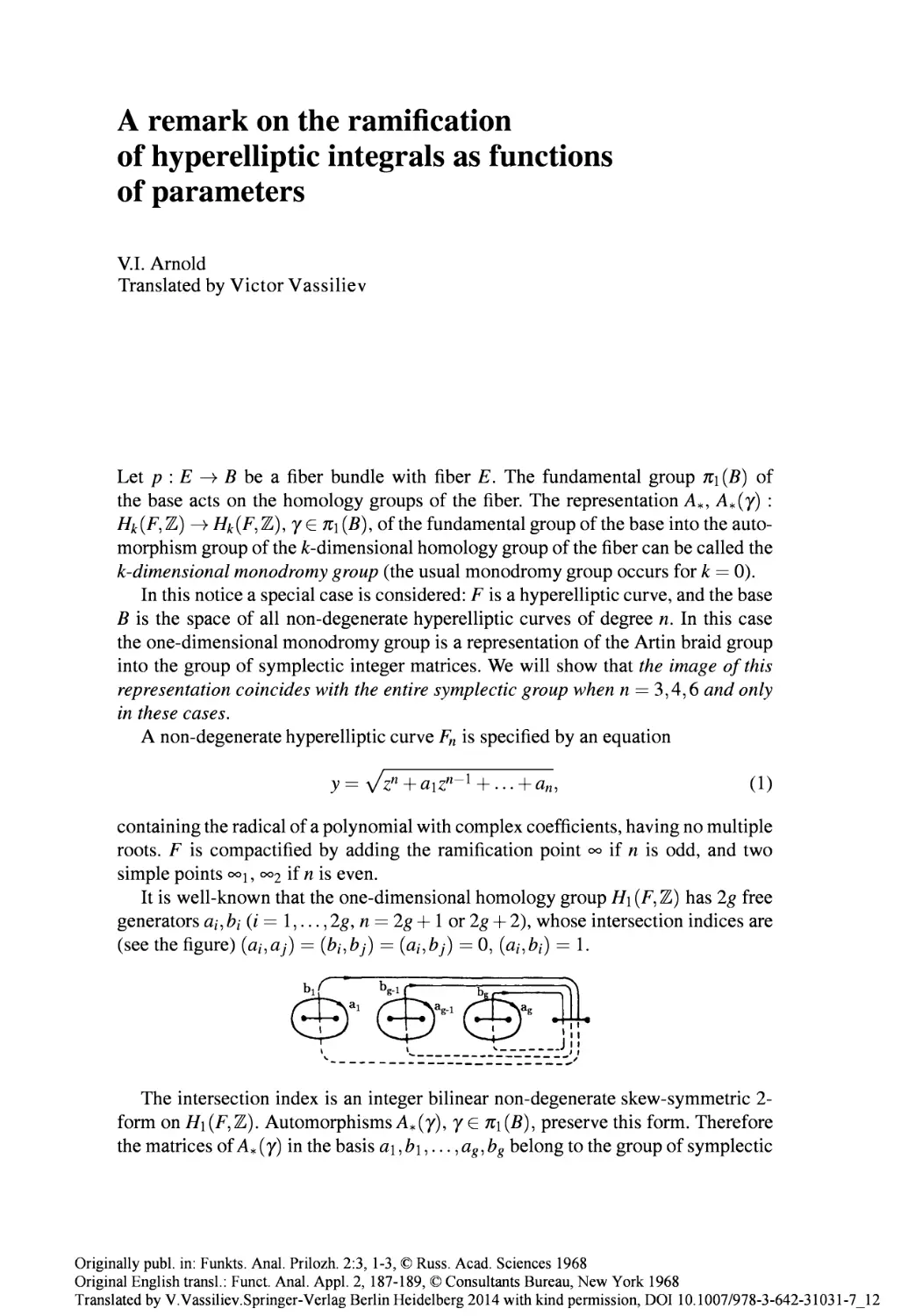
12 A remark on the ramification of hyperelliptic integrals as functions
of parameters
Published as "Remark on the branching of hyperelliptic integrals as functions of the parameters" in
Funct. Anal. Appl. 2, 187-189, 1968. Translation ofFunkts. Anal. Prilozh. 2:3, 1-3, 1968. Translated
by Victor Vassiliev 115
13 Singularities of smooth mappings
Russ. Math, Surv. 23, 1-43, 1968. Translation of Usp. Mat. Nauk 23:1, 3-44, 1968 119
14 Remarks on singularities of finite codimension in complex dynamical systems
Fund. Anal. Appl. 3, 1-5, 1969. Translation ofFunkts. Anal. Prilozh. 3:1, 1-6, 1969. Translated by
Victor Vassiliev 163
15 Braids of algebraic functions and the cohomology of swallowtails
Translation of Usp. Mat. Nauk 23:4, 247-248, 1968. Translated by Gerald Gould 171
16 Hamiltonian nature of the Euler equations in the dynamics of a rigid body
and of an ideal fluid
Translation of Usp. Mat. Nauk 24:3, 225-226, 1969. Translated by Gerald Gould 175
17 On the one-dimensional cohomology of the Lie algebra of divergence-free
vector fields and rotation numbers of dynamical systems
Published as "One-dimensional cohomologies of the Lie algebras of nondivergent vector fields and
rotation numbers of dynamic systems" in Funct. Anal. Appl. 3, 319-321, 1969. Translation of
Funkts. Anal. Prilozh. 3:4, 77- 78, 1969. Translated by Victor Vassiliev 179
18 The cohomology ring of the colored braid group
Math. Notes 5, 138-140, 1969. Translation of Mat. Zametki 5:2, 227-231, 1969. Translated by
Victor Vassiliev 183
19 On cohomology classes of algebraic functions invariant under
Tschirnhausen transformations
Funct. Anal. Appl. 4, 74-75, 1970. Translation of Funkts. Anal. Prilozh, 4:1, 84-85, 1970. Translated
by Victor Vassiliev 187
20 Trivial problems
Translation ofProc. 5th Int. Conf. on Nonlinear Oscillations, Kiev 1969. Vol. 1, 630-631, Ukrain.
Acad. Sciences, Kiev 1970. Translated by Gerald Gould 191
21 Local problems of analysis
Moscow Univ. Math, Bull. 25 (1970), 77-80, 1970. Translation ofVestn. Mosk Univ. Ser. I,
Mat. Mekh. 25:2, 52-56, 1970 193
22 Algebraic unsolvability of the problem of stability and the problem
of topological classification of singular points of analytic systems
of differential equations (Russian)
Usp. Mat. Nauk25:2, 265-266, 1970 197
23 On some topological invariants of algebraic functions
Transact. Math, Moscow Soc. 21, 30-52, 1970. Translation ofTr. Mosk. Mat. Obsc, 27-46, 1970 199
X

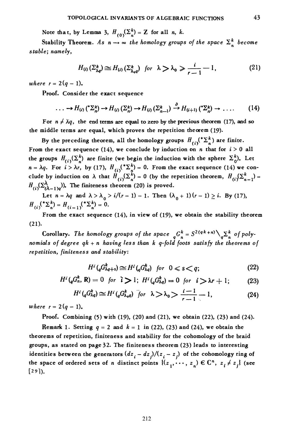
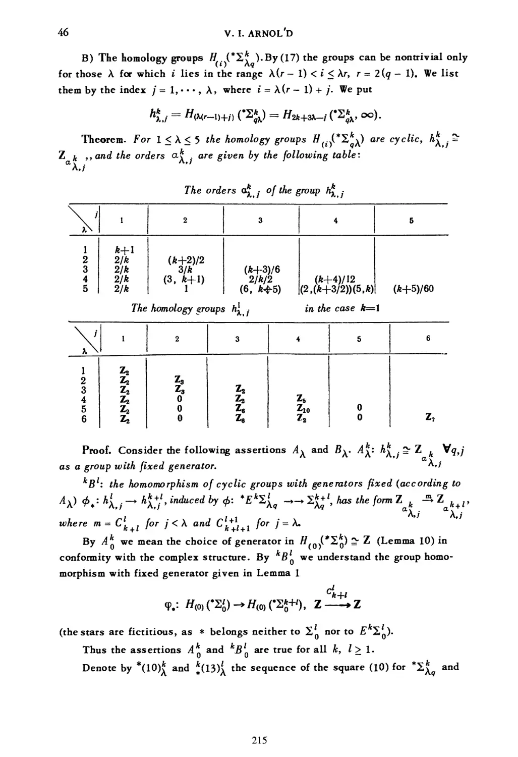
24 Topological invariants of algebraic functions II
Fund. Anal. Appl. 4, 91-98, 1970. Translation of Funkts. Anal. Prilozh, 4:2, 1-9, 1970 223
25 Algebraic unsolvability of the problem of Lyapunov stability and
the problem of topological classification of singular points of an analytic
system of differential equations
Fund. Anal. Appl. 4, 173-180, 1970. Translation of Funkts. Anal. Prilozh, 4:3, 1-9, 1970 231
26 On the arrangement of ovals of real plane algebraic curves, involutions
of four-dimensional smooth manifolds, and the arithmetic
of integral quadratic forms
Published as "Distribution of ovals of the real plane of algebraic curves, of involutions of four-
dimensional smooth manifolds, and the arithmetic of integer-valued quadratic forms" in Fund.
Anal. Appl. 5, 169-176, 1971. Translation of Funkts. Anal. Prilozh. 5:3, 1-9, 1971. Translated by
OlegViro 239
27 The topology of real algebraic curves (works of LG. Petrovsky and their
development)
Translation of Usp. Mat. Nauk 28:5, 260-262, 1973. Translated by Oleg Viro 251
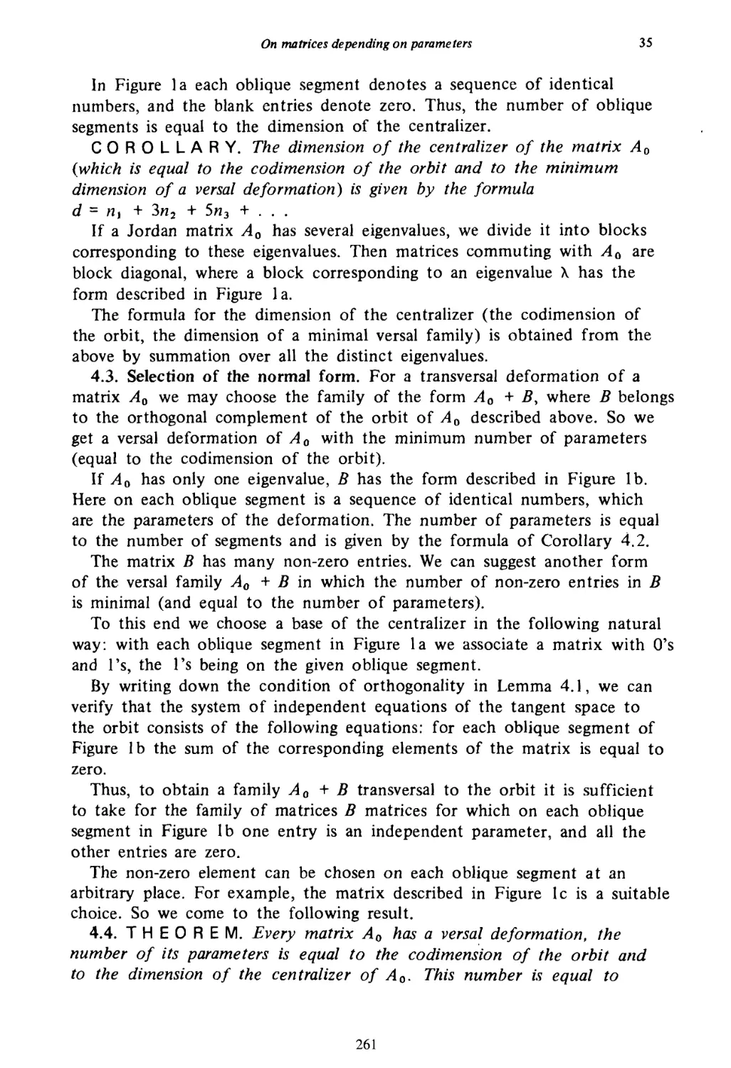
28 On matrices depending on parameters
Russ. Math, Surv. 22, 29-43, 1971. Translation of Usp. Mat. Nauk 26:2, 101-114, 1971 255
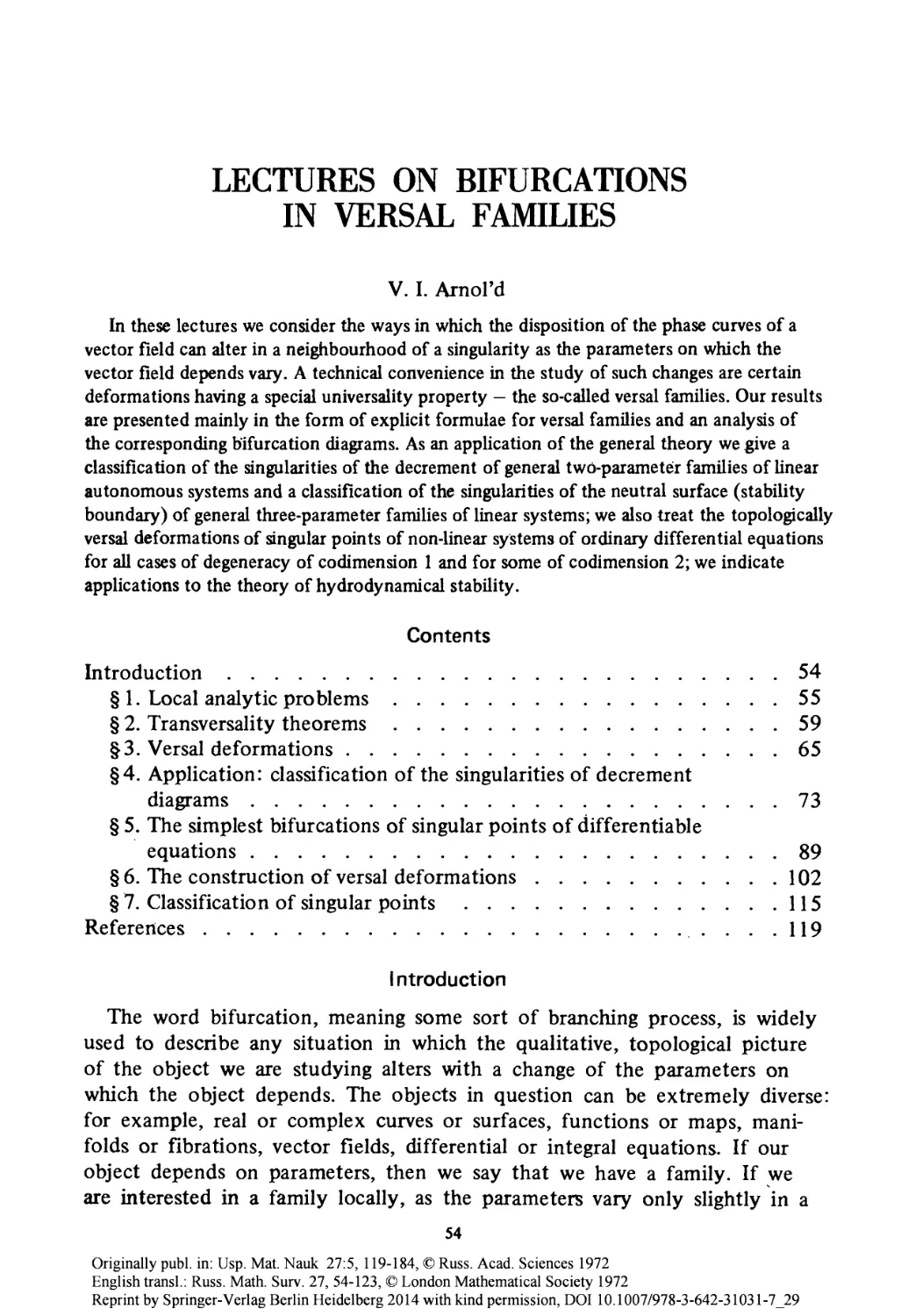
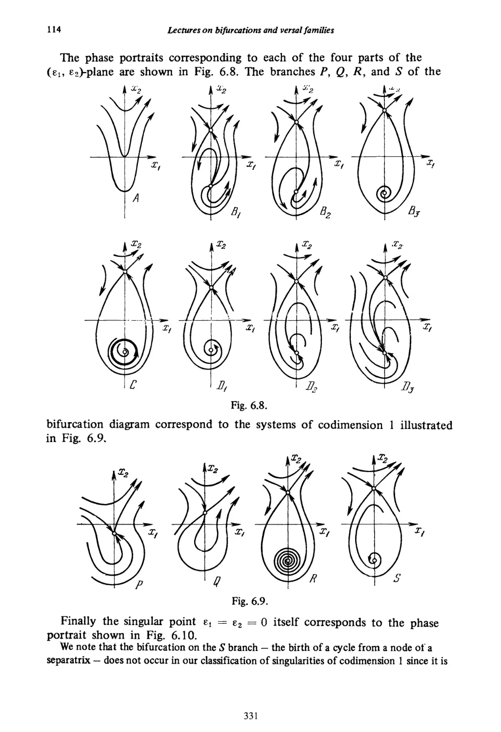
29 Lectures on bifurcations in versal families
Russ. Math, Surv. 27, 54-123, 1972. Translation of Usp. Mat. Nauk 27:5, 119-184, 1972 271
30 Versal families and bifurcations of differential equations (Russian)
Izd. Inst. Akad. Nauk Ukrain. SSR, Kiev, 42-49, 1972 341
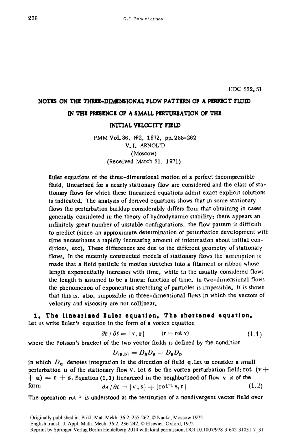
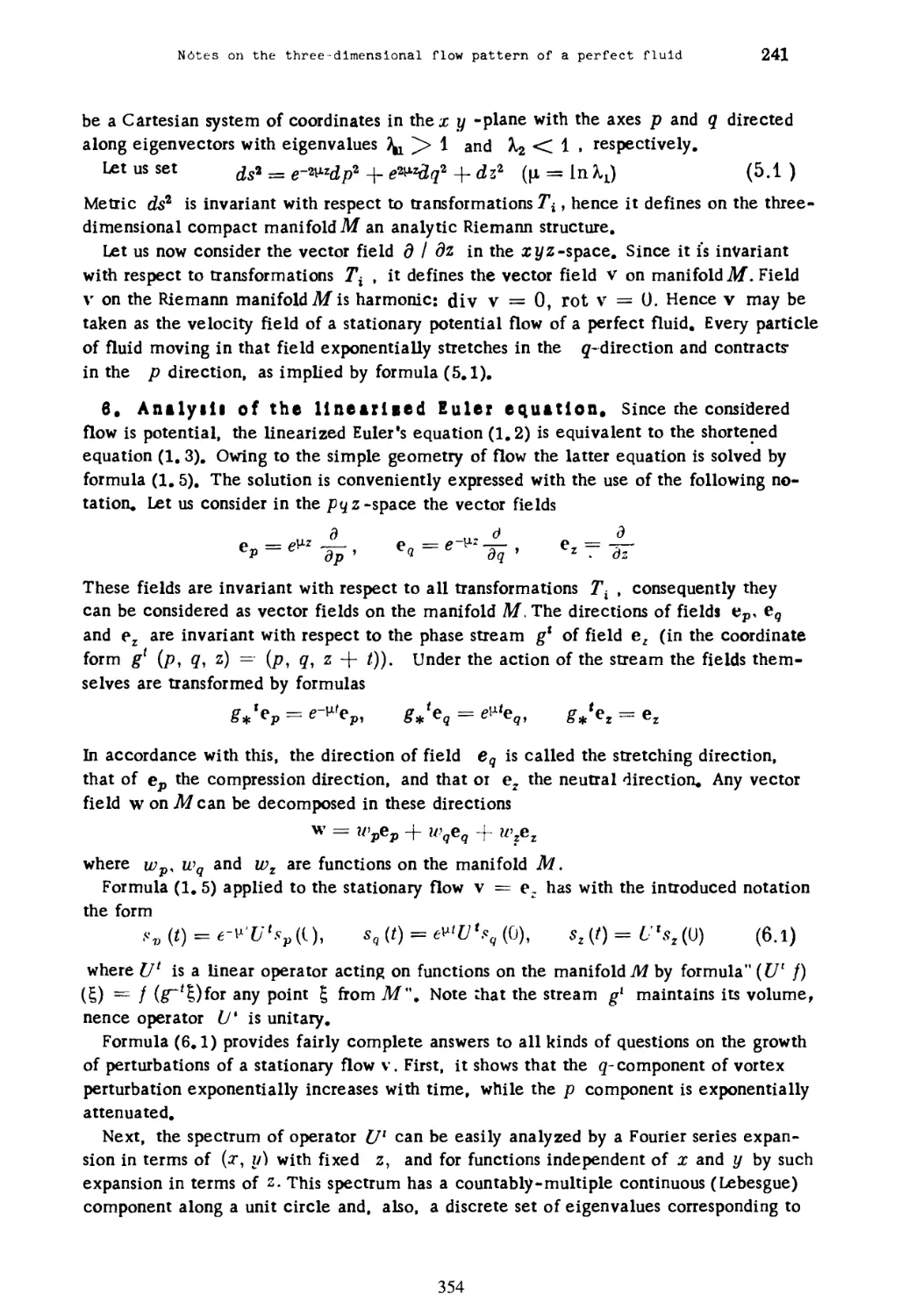
31 Remarks on the behaviour of a flow of a three-dimensional ideal fluid
in the presence of a small perturbation of the initial vector field
Published as "Notes on the three-dimensional flow pattern of a perfect fluid in the presence of a small
perturbation of the initial velocity field" in J. Appl. Math, Mech, 36:2, 236-242, 1972. Translation
ofPrikl. Mat. Mekh, 36:2, 255-262, 1972 349
32 The asymptotic Hopf invariant and its applications
Selecta Math, Sov. 5:4, 327-345, 1986. Translation ofProc. All-Union School in Diff. Eq. with
Infinite Number of Variables and in Dyn. Syst. with Infinite Number of Degrees of Freedom,
Dilhan 1973, 229-256, 1974 357
33 A magnetic field in a moving conducting fluid (with Ya.B. Zeldovich,
A.A.Ruzmaikin, and D.D. Sokolov)
Translation of Usp. Mat. Nauk 36:5, 220-221, 1981. Translated by Gerald Gould 377
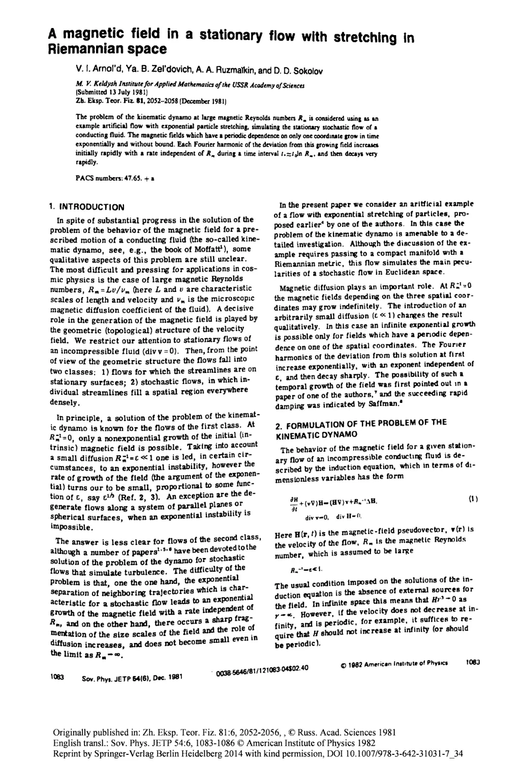
34 A magnetic field in a stationary flow with stretching in a Riemannian
manifold (with Ya.B. Zeldovich, A.A.Ruzmaikin, and D.D. Sokolov)
Published as "A magnetic field in a stationary flow with stretching in Riemannian space" in
Sov. Phys. JETP 54:6, 1083-1086, 1982. Translation ofZh, Ebp. Teor. Fiz. 81:6, 2052-2056, 1981.... 379
XI

35 Stationary magnetic field in a periodic flow (with Ya.B. Zeldovich,
A.A.Ruzmaikin, and D.D. Sokolov)
Published as "Steady-state magnetic field in a periodic flow" inSov. Phys. Dot 27:10, 814-816,
1982. Translation of Dokl.Akad. NaukSSSR, 266:6, 1357-1361, 1982 383
36 Some remarks on the antidynamo theorem
Moscow Univ. Math. Bull. 37, 57-66, 1982. Translation ofVestn. Most Univ. Ser. I, Mat. Mekh. 6,
50-57, 1982 387
37 Evolution of a magnetic field under the action of transfer and diffusion
Translation ofUsp. Mat. Nauk38:2, 226-227, 1983. Translated by Gerald Gould 397
38 The growth of a magnetic field in a three-dimensional steady incompressible
flow (with E.LKorkina)
Moscow Univ. Math. Bull, Ser. I, Math. Mech. 3, 50-54, 1983. Translation ofVestn. Mosk Univ.
Mat. 38:3,43-46, 1983 399
39 On evolution of a magnetic field under the action of drift and diffusion
(Russian)
Some Problems in Modern Analysis, 8-21, MGU, Moscow 1984 405
40 Exponential scattering of trajectories and its hydrodynamical applications
Translation ofN.E. Kochin and the Development of Mechanics, 185-193, Nauka, Moscow 1984.
Translated by Gerald Gould 419
41 Kolmogorov's hydrodynamic attractors
Proc. Royal Soc. London A 434:1890, 19-22, 1991 429
42 Topological methods in hydrodynamics (with B.A. Khesin)
Annu. Rev. FluidMech, 24, 145-166, 1992 433
43 Translator's preface to J. Milnor's book "Morse Theory"
MIR, Moscow 1965. Translated by Gerald Gould 455
44 Henri Poincare: Selected Works in Three Volumes. Vol. I New Methods
of Celestial Mechanics - Preface. From the editorial board. Comments
Nauka, Moscow 1971, 747-752. Translated by Gerald Gould 457
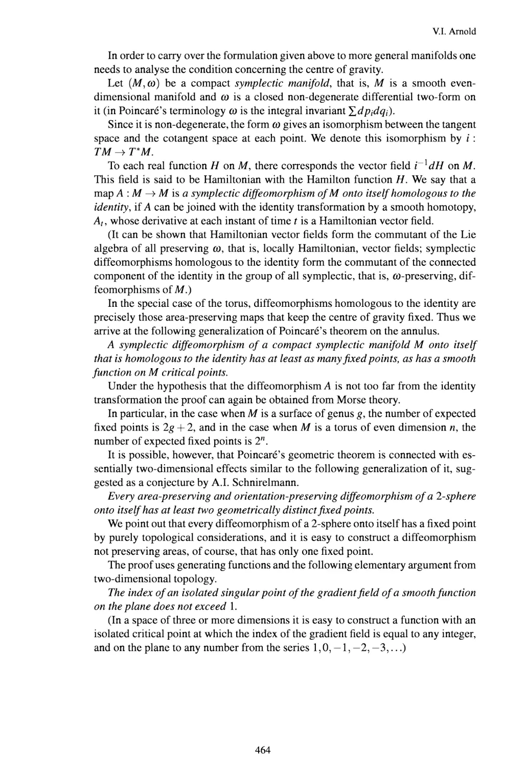
45 Comments on the paper "On a geometric theorem" by Henri Poincare
H. Poincare: Selected Works in Three Volumes. Vol. II. Klassiki Nauki, Nauka, Moscow 1972,
987-989. Translated by Gerald Gould 463
Acknowledgements 465
XII

Books or book prefaces by V. Arnold written in 1965-1972, but not included in the "Collected
Works"
1. (with A. Avez): "Problemes ergodiques de la mecanique classique" (in French), Monographies
Internationales de Mathematiques Modemes, No. 9, Gauthier-Villars, Paris, 1967, ii+243pp.; English
translation: "Ergodic problems of classical mechanics", W. A. Benjamin, Inc., New York-Amsterdam,
1968, ix+286pp.
2. "Obyknovennye differentsialnye uravneniya" (in Russian) Nauka, Moscow, 1971, 239pp.; English
translation: "Ordinary differential equations", The M.I.T. Press, Cambridge, 1973, ix+280pp.; Other
translations/editions of this book are French (1984), Russian (2nd edition, unrevised, 1975), Russian
(3rd edition, revised and extended, 1984), Polish (1975, 1983), Portuguese (1985), German (1980),
etc.
3. Editor's preface to a collection of papers "Singularities of differentiable mappings", Mir, Moscow,
1968.
4. Translator's preface to F. Pham's book "Introduction to the topological study of Landau's
singularities", Mir, Moscow, 1970.
5. Translator's preface to J. Milnor's "Singular points of complex hypersurfaces", Mir, Moscow,
1971.
XIII

VARIATIONAL PRINCIPLE FOR THREE-DIMENSIONAL
STEADY-STATE PLOWS OP AN IDEAL PLUID
(VARIATSICNHTX PRINTSIP DLIA TREKHMERNYKH
STATSICNARMYKH TEOHENII IDEAL1 N01 ZRXX3K0STI)
PMM Vol.29, №5, 1965; PP. 8^6-851
V.I. ARNOL'D
(Moscow)
(Received June 14, 1965)
It is proved that a steady-state flow has an extremal kinetic energy in
comparison with "equivorticity" flows. This result is applied to investigate
the stability of steady-state flows: if the extremum is a minimum or a
maximum, then the flow is stable, i.e. a small change in the initial velocity
field causes only a small change in the velocity field for all time. To
determine the nature of the extremum (maximum, minimum, etc.) a second
variation is explicitly calculated. For the case of plane flows, sufficient
conditions of the stability with respect to small finite perturbations are
found. These conditions are close to the necessary ones.
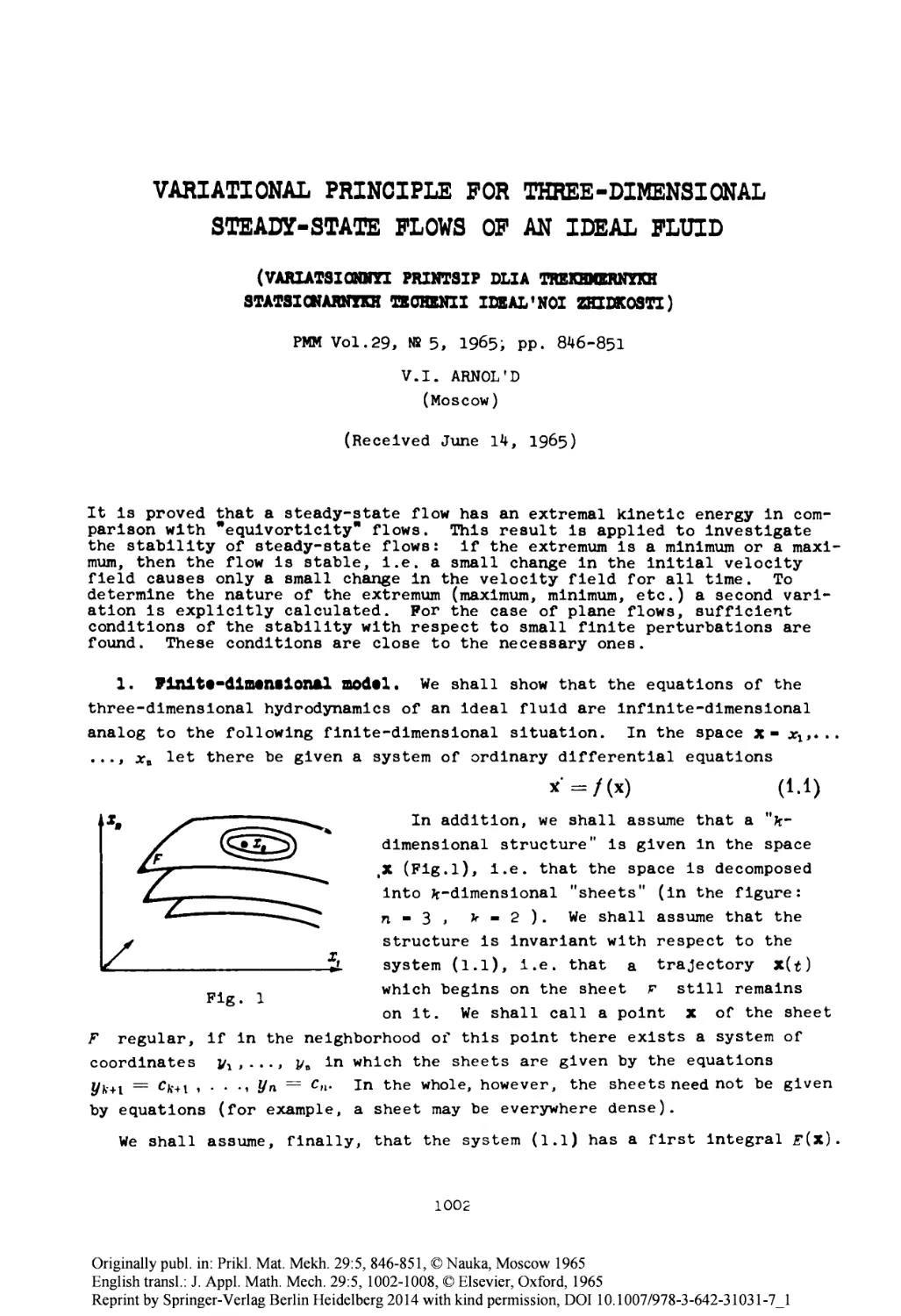
1. FlXlltt-dimtniional modtl. We shall show that the equations of the
three-dimensional hydrodynamics of an ideal fluid are infinite-dimensional
analog to the following finite-dimensional situation. In the space х- дгг,...
..., χζ let there be given a system of ordinary differential equations
*" = /(*) (i.i)
кХй s* __ __ "-^, *n addition, we shall assume that a "fc-
dimensional structure" is given in the space
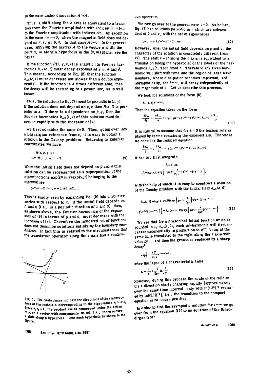
gX (Fig.l), i.e. that the space is decomposed
into ^-dimensional "sheets" (in the figure:
n ш 3 t у ш 2 ). We shall assume that the
ι у structure is invariant with respect to the
l^_ Jl system (l.l), i.e. that a trajectory x(t)
„. „ which begins on the sheet f still remains
Fig. 1
on it. We shall call a point χ of the sheet
F regular, if in the neighborhood of this point there exists a system of
coordinates y^ ,..., yb in which the sheets are given by the equations
i/fr+ι = ck+\ 1 · ♦ ·ι Уп — cn- In the whole, however, the sheets need not be given
by equations (for example, a sheet may be everywhere dense).
We shall assume, finally, that the system (l.l) has a first integral r(x).
1002
Originally publ. in: Prikl. Mat. Mekh. 29:5, 846-851, © Nauka, Moscow 1965
English transl.: J. Appl. Math. Mech. 29:5, 1002-1008, © Elsevier, Oxford, 1965
Reprint by Springer-Verlag Berlin Heidelberg 2014 with kind permission, DOI 10.1007/978-3-642-31031-7_1

Three1-dimensional steady-state Г1о\:з of an Ideal fluid 1003
We shall consider a local conditional extremum of the function Ε on the
sheet F . We shall assume that it occurs at a regular point x^ and that
the quadratic form d2E is nonsingular on the sheet F . The following
three theorems are easily proved (cf.[l]).
Theorem 1.1. The point Xq is the equilibrium position of the
system (1.1) / (x0) = 0
Theorem 1.2. If the extremum is a maximum or a minimum, then the
equilibrium position j^ is stable with respect to small finite perturbations.
Theorem 1.3· The spectrum of the problem of small oscillations
corresponding to (l.l) Л£ = λξ (Α = dt I dx in X0) is symmetric with
respect to the real and imaginary axes of λ .
The hydrodynamic analog of these theorems will be formulated below. They
are, in fact, corollaries of the general theorems on Li geodesic groups
provided partially with an invariant metric (cf.[2]). However, an independent
proof is given here which makes use neither of Li groups·, nor even of the
existence and uniqueness theorems which correspond to the partial
differential equations. Prom a mathematical point of view, these theorems will be
"a priori" equalities and estimates.
2. Notation. Let Ό be a domain, bounded by the fixed surface Γ , in
a three-dimensional Euclidean space; let ν be the velocity' field of an
ideal fluid (incompressible, with density equal to 1 , inviscid, exterior to
a nonpotential mass force field) which fills the volume j) ; and let ρ be
the pressure.
The Euler equation
-gl +(v-V)v= — gradp, divv = 0, ν·η = 0 on Γ (2.1)
has as a corollary the Bernoulli equation
~ = vxr — gra<U, r = rotv, λ = ρ + 1/ιν1 (2.2)
Hence, in view of the identity
rot (Α χ B) = {AB} + A diν Β — В div A (2.3)
there follows
dr/df = {vr} (2.4)
Неге {АВ] is the Poisson bracket of the vector fields
{АВ}{= J] VAi I dXj) Bt — {дВ{/ dx5) Ai
If Я is a smooth mapping of χ -» g{x) , then we shall denote by g* the
corresponding mapping of the vectors
(*·*)< = 53 (e**/ia!i>*i
3. Bquivortioity fitldi, In order» to formulate the law of coservation
of vorticity in a form suitable for later use, we shall consider two vector
fields ν and v' in D
2

1004
V.I. Amol'd
divv = 0, divv'^0, (v.n) = 0, v'.n = 0 on Γ
Definition 3.1. The fields ν and v' are eauivorticity
fields if there exists a smooth, volume preserving, mapping g of the domain
Ό into itself such that (*) r» r»
Φνώ=4) v'dx (3.1)
for every closed contour γ in the domain J) .
The law of conservation of vorticity now takes the following form. Let
v(*,£)_he the velocity field of the ideal fluid of (2.1).
Theorem 3.1. The fields v(x,0) and v(x,t) are fields of equi-
vorticity. In fact, let x(t) be the trajectory of a fluid particle. The
mapping g is then that which transforms x(o) into x{t) .
We shall now consider the Euler equation (2.1) as the system (l.l) in an
infinite-dimensional space of the vector fields v(x) (where div V * 0 and
V · η « 0 on Γ ). We shall show that this system has the characteristics
of the system (l.l). In the space of the fields v(x) the following
structure is specified: two fields belong to the same sheet if they are equi-
vorticity fields. According to Theorem 3·1^ this structure is invariant.
Steady-state flows are "equilibrium position" of the system. Finally, the
Euler equation (2.1) has a first integral of the energy
2E = [[{\*dx
t
In order to transfer the results of Section 1 to the hydrodynamic
equations (2*1) it is necessary to calculate the first and second variations of
the function Ε on the sheet F -
4. Variational prinoiplt (**). The following fundamental Theorem is the
analog of Theorem 1.1.
Theorem 4.1. The steady-state flow v(x) has an extremal energy
in comparison with all close equivorticity flows v'(x) .
3y closeness here is meant closeness "with respect to the sheet", i.e.
♦) The mapping g transforms the vorticity of V into vorticity of v'
#*rot ν = rot v' (3.2)
Actually, if ς , η is an infinitesimal parallelogram, then, since
det g*m ι ,
ξΧη-rot ν = (g*l)x(H*r\).(g*rot v)
and corresponding to (3·ΐ)
(ξχη-rot ν) = (ff*l)xte*Ti)-iOt v'
If the domain D is not simply connected, then condition (3-1) is stronger
. than (3.2).
**) Another variational principle relating to unsteady flows has been
determined and applied in the Investigation of stability у FJflrtoft [3].
3

Three-dimensional steady-state flows of an ideal flu.ld 1005
v'(x) is considered to be close to v(x) if the corresponding mapping Q in
(3.1) is close to the identity mapping. To determine the closeness of 0
to the identity mapping we shall introduce the "coordinates" / into the
space 0 in the following way.
Let f(x) be a vector field in D such that
divf = 0, bn--=0 on Г
Definition 4.1. Lt f( = exp ft be a mapping of D into
itself, determined by the solutions x(t) of the ordinary differential
equations X = f (x) according to Formula g (x (0)) = X (t).
The field v' will be considered to be close to V if the "coordinates"
/ of the transformation д in (3.1) are small. In this case, the velocity
perturbation fiv = v' — v. is also small. The relation between δ.ν and f
is given by the following Formula (4.2).
Lemma 4.1. If for every closed contour γ in D
& vdx = <bv'dx, divv = 0, divv' = 0 (4.1)
then
v'-Y = <(fxr) + l/2t* f χ {fr} + О (i3) + grad α (4.2)
where α is a single-valued function and r « rot ν .
Proof of the Lemma . According to the Stokes formula
φ vdx = — -Lgr<fc= <f> fxrdx (4.3)
d
dt
"a e- /γ
Since the Jacobian of 0_t* is equal to unity, we then have
<£ ixrdx=^gt*t(g-tx)xgt*T(g-tx)dx (4.4)
g-C у
But, according to the definition of gt we have gt*t (g-t x) = f (x).
Therefore, (4.3) and (4.4) give d
± § vdx = §txr(t)dx (4.5)
g-a t
fined by Formula
r(x,t) = gt*t(g.tx) (4.6)
find
= {fr}, r{t) = T + {b}t + 0{t*) (4.7)
But, according to condition (4.1),
A § Ydx = $%-dx, ν'μ« = ν (4.8)
g-t-Г Ύ
Integrating (4.5) and (4.6) with respect to t , we find from (4.6)
t
<£ (V' _ V) dx = <J> jj f x [r + {f, r} t + О (t2)] dt dx
g-O t
The field r(t) here is defined by Formula
Differentiating (4.£), we find
dr I
dt \t =o
4

1006
V.I. Arnolkd
Therefore,
which is equivalent to (4.2).
Proof of the basic Theorem . If v'isa equi-
vorticity flow close to the steady-state flow ν , then according to (4.2)
the first variation is
δν = f χ г + grad oc
Therefore,
6E = SS y6ydx = й y'V xr + gr*da)dx = СГС [f-(r χ v) + v-grada] dx
For a steady-state flow, according to (2.2),
rxv = —grad λ
fl£ = $$(v'grada—f-gradX);dx=0
This result is obtained by integrating by parts, talcing into account
Equalities divv = 0, divf = 0; (ν·η)|Γ=0, (/,n)|r=0
The Theorem is proved.
5· Formula for the laoond variation. According to Lemma 4.1
v' = ν + δν + δ2ν + #(/3)
where
δν = f χ г + grad аъ δ2ν = у· [f χ {fr}] + grad aa
Correspondingly,
2δ2£ = Щ Γ(δν)2Α+2(ν.δ2ν)] da; = ift Γ(δν)2 + vf χ {fr} + 2v-grad<%,] dx
Integrating the last term by parts, we obtain the following form for the
second variation of the energy Ε όη the "sheet" F of the fields having
equivorticity with V , in terms of the variables f introduced in Section
4 : 26*E = ^(&v)2+vxi{t.r)dx (5.1)
This expression is quadratic with respect to f , since δν , linearly
expressed in terms of f , is
δν = f x г + grad α!
where αϊ is determined from div δν — 0 and (δν·η)|Γ=0 and, therefore,
is linearly dependent on f . We also observe that according to Formula
(2.3) {fr} = βΓ.
The following theorem is the analog of Theorem 1.2.
Theorem 5.1. If the quadratic form (5.l) is of fixed sign, then
the flow V is stable with respect to small finite perturbations. By a
small perturbation here is meant one of which δν and f , i.e. δν and br
or form \b2E\ , are small.
The form (5.1) represents the first integral to the linear problem of
small oscillations close to a steady-state flow ν . In accordance with
Theorem 1.3, the spectrum of this problem is symmetric with respect to both
axes. Hence —
5

Three-dimensional steady-state flows of an ideal fluid 1007
Theorem 5.2. If some perturbation of the steady-state flow ν
is damped, then some other perturbation is amplified and the flow ν is
unstable.
The author was not able to find a flow V for which the quadratic form
6aJT was of fixed sign for three-dimensional perturbations. However, in
specifically symmetric cases Theorem 5.1 gives simple stability criteria.
6. Suppltmantary inttgral·. Generalizing Theorem 1.2, we shall assume
that the Euler equation (1.2) has a first integral Μ such that for a
steady-state flow V crr
6M = \\\ A-tydz (A x rot ν = grad a) (6.1)
The assumption (6.1) is satisfied in the following three examples.
Example 6.1. For the energy integral Mxm Е we have
A = ν = [vxrot v] = grad λ
according to (2.2).
Example 6.2. If the domain Ώ and the flow V are invariant
with respect to displacements along the χ-axis, the integral
Μ2 = \ \ \ v · exdx dy dz
is then preserved.
For it A = ex and A x rot ν = grad (v-ex).
Example 6.3. If the domain D and the flow ν are invariant
with respect to rotations about the г-axis, then
Λ/3= \\\ (vxR. e2) dx dy dz
is preserved, where R is the radius vector of the point x, у, г . In this
A = Rxezl Ax rotv = grad (ν χ R-e2)
Theorem 6.1. The value of the integral Μ over the velocity
field of a steady-state flow ν is an extremal in comparison with the values
over close equivorticity fields , provided that Μ satisfies condition (6.1).
The proof is identical to the proof of Theorem 1.2. The corresponding
formulas of the second variation have the form
26W2= [\\(exxi){fr}dxdydz (6.2)
2δ2Λ/3= \\\(Rxezx\){ir}dxdydz (6.3)
Fixed sign behavior of some linear combination
λι62Μ1 4- λ2δ2Μ2 -f λ3δ2Λ/3
is sufficient for the stability of ν .
We shall illustrate the application of Theorem 5.1, Formulas (5.1),(6.2)
and (6.3) in an example of plane flows.

1008
V.I. ArnoX'd
7. Pltn· perturbation· Of plan· flow». Let the flow ν have a stream
function if(x,y) such that
ν = Ψν, — ♦*, 0; r = 0, 0, —Δψ (7.1)
Substituting (7.1) Into (5.1), we obtain after a brief calculation,taking
Into consideration that {fr} = fir, the formula given in [1]
2VE = g [{byf + T^JL (4r)·] dx dy (7.2)
Prom (7.2) and Theorem 5.1 there follows
Corollary 7-1 (cf.[l]). In anjr domain plane flows with a
concave velocity profile (Vtj? / VA\Jj^>0) are stable with respect to finite
plane perturbations.
We shall refer to* specifically symmetric flows. The case of plane-parallel
flows (the Rayleigh theorem) is considered in detail in [1]. We shall
consider the flow in the annulus between concentric circles. After a brief
calculation, Formula (6.3) is reduced in the plane case to the form
2*»Л/, = ^*(вг)« (7.3)
Prom (7.3) and Theorem 5.1 there follows
Corollary 7-2. A plane circular flow in a circular annulus is
stable with respect to small finite plane perturbations if the vorticity
/aries monotonously with the radius.
Actually, if the sign of V/?2 / VAlb is preserved, then the form
fi2tf - δ2£ + λδ2Μ3
is positive definite for suitable λ .
Finally, we note that the investigation of parallel flows with a single
inflection point carried out in [l], owing to Formula (7-3), remains in
effect for the case of circular flows.
BIBLIOGRAPHY
1. Arnol'd, V.I., Ob usloviiakh nelineinoi ustoichivosti ploskikh statsio-
narnykh krivolineinykh techenii ideal'noi zhidkosti (On nonlinear
stability conditions of plane steady-state curvilinear flows of an
ideal fluid . Dokl.Akad.Nauk SSSR, Vol.162, №5, 1965.
2. Moreau, G.G.. Mechanique des Fluides - une methode de "Cinematique Fonc-
tionnelle et hydrodinamique. C.r.hebd.Seanc.Acad.Sci., Paris, Vol.
249, N9 21, P.2156, 1959.
3. Fjprtoft, R., Application of Integral theorems in deriving criteria of
stability for laminar flows and for the baroclinic circular vortex.
Geofys.Publ., Oslo, Vol.17, №6, p.52, i960.
Translated by R.D.C.
7

On the Riemann curvature
of diffeomorphism groups
Note by Mr. Vladimir Arnold, presented by Mr. Jean Leray
Translated by Denis Auroux
Abstract One calculates explicitly the sectional curvatures of certain infinite-
dimensional Lie groups equipped with left-invariant metrics whose geodesies
correspond to flows of an ideal fluid. The sectional curvature turns out to be negative in
certain two-dimensional directions.
/. Below I present an explicit expression (9) for the Riemann curvature of a Lie
group equipped with a left-invariant metric. More generally, I will also call Riemann
curvature the same expression for an infinite-dimensional group. In particular, I
calculate the curvature of the group of area-preserving diffeomorphisms of the torus
T2, see (14). In that example, certain sectional curvatures (13) turn out to be
negative. It has been known since Hadamard [1] that the sign of curvature influences the
behavior of geodesies: negatively curved manifolds have unstable geodesies.
The interest in geodesies on the manifold underlying a Lie group is naturally
justified by the following examples:
(a) For SO(3) they represent rotations of a rigid body in the three-dimensional
Euclidean space E3.
(b)For the group SDiff <& of volume-preserving diffeomorphisms of a Riemannian
domain ^, they represent flows of an ideal fluid filling Of [3, 4, 5].
(c)The group of positive dilations and translations of W1 gives rise to the geodesic
flow on the space of constant negative curvature, while nilpotent groups give rise
to "nilflows" [6].
2. Notations Given a Riemannian space M, denote by TMX the tangent space
at jc G M, and by ( , ) the scalar product defined by the metric. Given χ e Μ and
Translation of C.R. Acad. Sci. Paris 260 (1965), 5668-5671
Originally publ. in: C.R. Acad. Sc. Paris 260, 5668-5671, © French Acad. Sciences, Paris 1965
Translated by D. Auroux, Springer-Verlag Berlin Heidelberg 2014 with kind permission, DOI 10.1007/978-3-642-31031-7_2

V. Arnold
ξ <G TMX, denote by γ{χ,ξ,ί) = γ(ζ,ί) = y(t) = 7 the geodesic through jc = y(0)
with tangent vector ξ = 7(0), parametrized by time t.
The parallel transport along 7 of a vector 77 <G TMX yields a vector Ργη which can
be defined by the following construction. Set
1 d
γ(χ,ξ + τη,ήεΤΜγ(ή. (Ι)
τ=0
Then Ργ(ήη — Πγ(ήη = 0(t2) as t —> 0. The covariant derivative V^r/ of 77 along
ξ is, by definition:
v>=|
|r=0
^4(^,0)=^
Π^η(7(ξ,0)· (2)
|r=0
Let ξ and η be two orthonormal vectors in TMX. The sectional curvature /?ξη of
Μ at лг in the 2-plane defined by ξ and η is, by definition [7],
Цц = "(ν^ν^,η) + (νηνξξ,η) + (^[ξ,η]ξ,η), (3)
where [ξ, 77] is the Lie bracket of the vector fields ξ and 77, whose restrictions at jc
are respectively ξ (χ) and 77 (χ).
Let G be a real Lie group, and 21 = TG^ its Lie algebra equipped with the Lie
bracket [, ]. The group exponential map1 exp : 21 —» G makes it possible to interpret
the Lie algebra as a chart of G in a neighborhood of the identity element e.
For a <G 21,1 will denote exp α = a. Denote by
Lg : TGh -> rGgh, Z^ : mh -> Γ21ίΛ
the maps of tangent spaces induced by left translations.
It is easy to see that the map
La : 21 = Γ210 -> Γ2ία = 21
from 21 to itself is given by the formula
Ζ^ξ=ξ + -[α,ξ] + 0(α2), whereat e 21, |a| < 1. (4)
Let (a, fc) be any scalar product on the algebra 21. A left-invariant metric on G is
defined in terms of ( , ) by the scalar product
(cLyb)g = (L„-ia,L„-ib), where a,b <G ^Gg.
From now on, all metric notions such as geodesies, curvature, etc., will be taken
with respect to this metric.
In general different from the geodesic exponential map.
10

On the Riemann curvature of diffeomorphism groups
The curvature of G will be expressed (9) in terms of the operation В defined as
follows:
Let а, с <G 21, then the formula
([a,b],c) = (B(c,a),b), for all b in 21, (5)
defines a bilinear map В : 21 x 21 —» 21.
Example 1. Let (a,fc) = (Aa,fc), where ( , ) is a bi-invariant scalar product, and A is
a symmetric operator. Then B(c,a) = A~l [Ac,a].
Another example is given in section 4.
3. The results Let γ(γ0, y,t) be a geodesic on G. Consider2 the velocity vector
jeTGy transported at e:
One has
Lemma 1. The vector ξ (t) satisfies Euler's equation [2]:
ξ=Β(ξ,ξ). (6)
For the proof, it suffices to consider the case of y0 = e.
Then one writes the Euler-Lagrange equations for the Lagrangian L= ^(ζ,ζ)
and uses (4).
Expressed differently, one has
Lemma 2. The image ο/γ(β,ξ,ί) in 21 is
γ(ξ,ή = ξί + Β(ξ,ξ)^ + 0(ί% f->0. (7)
Let ξ (g) and η (g) be two left-invariant tangent vector fields on G. Then V^ ^ ?] (g)
is also left-invariant. I denote by V^ η its value atg = e. Let us compute this value.
Lemma 3. The covariant derivative is given by
2νξη = [ξ,η}-Β(ξ,η)-Β(η,ξ). (8)
It follows from (1) and (7) that
Π7(ξ,0^ = η + δί + 0(ί2), f->0,
where
2δ = Β(ξ,η)+Β(η,ξ).
2 In dynamics of a rigid body, ξ (ή is called the vector of angular velocity in the body. In
hydrodynamics, it is the velocity field at time t.
11

V. Arnold
Using (2) and (4), one obtains (8).
Next, using (8) and (3) one derives
Theorem 1. The sectional curvature ofGate is
Ιίξη = (δ,δ) + 2(α,β)-3(α,α)-4(Βξ,Βη), (9)
where
2α = [ξ,η], 2β=Β(ξ,η)-Β(η,ξ),
2δ=Β(ξ,η)+Β(η,ξ), 2Βξ=Β(ξ,ξ), 2Βη=Β(η,η)
and the operation B is defined by (5).
4. Applications to diffeomorphism groups Let G = SDiff Of be the group
of diffeomorphisms of a Riemannian domain Of which preserve the volume element.
The algebra 21 consists of vector fields ν in Of such that div ν = 0, and satisfying
ν · Я = 0 on the boundary dS> of S>. Let us define 3 a metric on 21 by
(m,v) = / u-vdx,
where dx is the volume element of $.
In order to calculate the curvature (9), let us write down an explicit expression
for the operator B. The expression for В is particularly simple if Of is a domain in
the Euclidean space E3.
Denote by и · ν the dot product, and by и Л ν the vector cross-product.
Theorem 2. Let u, ν G 21, then
B(u,v) = (сигШ) Λν + gradoc, (10)
where a is the function determined by the conditions: div В = 0inS>,Bn = 0on
If @4s a domain in the {x,y)-plane, one can identify the algebra 21 of vector fields ν
with the algebra of stream functions ψ(χ,γ):
vi = 3-, v2 = --5- (И)
dy ox
with [1//1,1//2] the Jacobian of the functions ψ\ and 1//2.
Using these notations, according to (10) the field Β(ψ\, Ψ2) G 2ί is given by
Β{ψ\,ψι) = -^i//igradi//2 + gradoc, (12)
3 It follows from the principles of mechanics that geodesies on G describe the flow of an ideal
fluid in @.
12

On the Riemann curvature of diffeomorphism groups
where
Λ-— —
дх2 dy2
Example 2. Let Of = T2 be any torus equipped with a flat metric. Consider at the
identity of G = S Diff <& the two-dimensional plane spanned by the two stream
functions
ψι =cos(£i -x), y/2 = cos(£2·*), (13)
where k\ and %2 are the "wave vectors".
Using (9), (11) and (12), one obtains
Theorem 3. The sectional curvature of the group S Diff T2 at e in the direction of
the plane (13) is
/?=_^±Msin2(psin2(p/5 (14)
where S is the area of the torus, φ is the angle between k\ and &2> and φ' is the angle
between k\ + ^2 and k\ — &2·
In particular, ifT2 = {x mod 2π, у mod 2π}, then the curvature of SDiffT2 in
the two-dimensional direction defined by the vector fields и with components smy
and 0 and ν with components 0 and sin* is R = — 1/8π2.
References
[1] I. Hadamard, J. Math, pures et appl., 5e serie, 4, 1898, p. 27-73.
[2] L. Euler, Theoria motus corporum solidorum seu rigidorum, 1765.
[3] J.-J. MOREAU, Comptes rendus, 249, 1959, p. 2156.
[4] V. Judovic, С R. Acad. U. R. S. S„ 136, 1961, p. 564.
[5] V. Arnold, Journal de Mecanique (in press).
[6] L. Auslander, L. Green and F. Hahn, Ann. Math. Studies, 53, 1963.
[7] J. MiLNOR, Ann. Math. Studies, 51, 1963.
13

G. R. Acad. Sc. Paris, t. 261 (5 juillet 1965). Groupe 1.
17
TOPOLOGIE. — Sur la topologie des ecoulements stationnaires des fluides
parfaits. Note (*) de M. Vladimir Arnold, presentee par M. Jean Leray.
On considere les ecoulements stationnaires d'un fluide parfait, incompressible
et non visqueux, dans un domaine borne D. On suppose que le vecteur vitesse n'est
pas partout colineaire au vecteur rotation. On demontre alors que le domaine D est
divise, par certaines surfaces et courbes, en un nombre fini de « cellules » ouvertes,
fibrees en tores ou en cylindres engendres par des lignes de courant. Les lignes de
courant sont fermees sur les cylindres, fermees ou denses sur les tores.
1. Soit Μ une variete riemannienne analytique reelle, orientee, compacte,
connexe, a trois dimensions, de premier nombre de Betti nul :
(0 b, (M) ^dimll^M, R) =o.
Soient a et b deux champs de vecteurs tangents a M, analytiques, et
de divergence nulle :
(2) diva = o, divo = o.
Theoreme 1. — Si les champs de vecteurs a et b, a divergence nulle,
commutent :
(3) [a,b\ = o,
et ne sont pas partout colineaires :
(4) «Λδ^ο,
alors, presque toutes les trajectoires du champ a sont fermees ou partout denses
sur des tores T2 analytiques plonges dans M. Les autres trajectoires forment
un vrai sous-ensemble analytique compact de M.
Precisons les notations utilisees. La trajectoire du champ a issue de #€M
est, par definition, la courbe : Trt(#, t) = T„(i) = T(i), i€R, definie par
(5) *1
(5) dt
:а(д?), Ύη(χ, o)~χ.
A chaque vecteur tangent a on peut associer un operateur differentiel Qr/,
une 1-forme ωια} et une 2-forme ω* :
(β) *.*=&
φ(Τβ(ί)); ω^£=<α, ς>; ω#* (;, η) =<α, ; Λ Ή >,
ού φ est une fonction derivable arbitraire sur Μ, ξ un vecteur tangent
arbitraire, (ξ, η) un bivecteur tangent arbitraire. La metrique riemannienne
de Μ definit un produit scalaire <(ξ, η)> sur Tespace tangent a M, et,
avec l'orientation de M, un produit vectoriel ξ Д η sur Tespace tangent.
Originally published in: С R. Acad. Sc. Paris 261, 17-20, © French Acad. Sciences, Paris, 1965
Reprint by Springer-Verlag Berlin Heidelberg 2014 with kind permission, DOI 10.1007/978-3-642-31031 -7_3

18
С. Н. Acad. Sc. Paris, t. 261 (5 juillet 1965). Groupe 1.
Avec les notations (6), on peut definir les notions de crochet
de Poisson [ , ], gradient, rotationnel, divergence :
( Θ[Λ.6]=Θ„0Α—ΘΑ0Λ, <grad<p-, Α>=θ6φ,
oil τ est Γ element de volume de M.
Nous utiliserons l'identite classique :
(8) τοί(η Λ b) = \b, a\ 4- a.aivb — b.diva.
2. Demonstration du theoreme 1. — Les deux champs commutant a et b
determinent Taction du groupe RJ sur M. Etudions les orbites F de ce
groupe. Nous allons montrer qu'elles sont compactes, et par consequent
toriques. D'apres (2), (3), (8), rota/\b = o. II existe done une fonction α
analytique, univalente [d'apres (1)], non constante [d'apres (4)], telle que :
(9) a Λ ft = grade.
Ainsi, chaque orbite F est contenue dans une surface de niveau de la
fonction a. Puisque Μ est compacte, α analytique, α n'a qu'un nombre
fini de valeurs critiques. D'apres (4) les « surfaces » de niveau critiques
forment un vrai sous-ensemble analytique de M. Soit С une composante
connexe d'une surface de niveau non critique de a. Alors, sur C, grada ^o;
par suite, d'apres (9), les champs de vecteurs a et b sont lineairement
independents sur С II en resulte que С = F, qui est done une orbite non
degeneree du groupe R2. Comme surface de niveau, C = F est compacte;
e'est done un tore.
Les trajectoires du champ a sont les orbites de RcR2. Cela acheve la
demonstration car on sait que ces orbites sont fermees ou partout denses
sur le tore.
3. Extension aux varietes a bord. — Le theoreme 1 est encore vrai si Μ
est une variete a bord <?M analytique, et si le champ a est tangent а <Ш.
Preuve. — Soit a() une valeur critique telle qu'il existe un point χ dans Μ
oil grada = oeta(a;) = a0, ou telle qu'il existe un point χ sur <Ш ou grada
est orthogonal а <Ш et α(#) = α0. On sait qu'il n'existe qu'un nombre
fini de valeurs critiques a0. Les surfaces de niveau non critiques sont
maintenant des sous-varietes (eventuellement a bord) de M. Si С est une
composante connexe de surface de niveau non critique, de bord ^C,
alors <?C est forme d'un nombre fini de trajectoires fermees sur dM.
Soit xGdC,
(10) Тя(дг, t + u) =T„(.r, t)
la composante de ОС contenant x. Sur CU^C, les vecteurs a et b sont
16

С. К. Acad. Sc. Paris, t. 261 (5 juillet 1965). Groupe 1.
19
partout lineairement independants. Chaque point ζ de С est done de la
forme : z= Tfa+sfj(x, i).
D'apres (3), (io) :
(II.) Т„(Г., il) =T{t+u)a+<b{xy l)=Tta+sb(Ta(x, tl) , l) ='z.
La trajectoire issue de ζ est done fermee, ce qui demontre le theoreme.
La formule (11) montre aussi que С est un cylindre :} (£, s) (t mod щ s € [o, S) j.
4. Applications aux fluides, parfaits. — Soit D un domaine riemannien,
compact, connexe, a trois dimensions, de bord dD. Par exemple, une
partie bornee de l'espace euclidien E3.
Theoreme 2. — Soit ν le champ de vitesse d'un ecoulement stationnaire
d?un fluide parfait dans D(e, D, c>D sont analytiques reels). Si ν nest pas
partout colineaire au vecteur rotation, alors presque toutes les lignes de
courant sont fermees ou partout denses sur des tores analytiques reels plonges
dans D; les autres lignes de courant forment un vrai sous-ensemble ana-
lytique compact de D.
Remarque. — II est probable que les ecoulements tels que rott> = X*>,
λ = Cte ('), ont des lignes de courant a la topologie compliquee. De telles
complications interviennent en mecanique celeste [voir (*), fig. 6]. La
topologie des lignes de courant des ecoulements stationnaires des fluides
visqueux peut etre semblable a celle de ('), fig. 6.
Demonstration du theoreme 2. — Le champ de vitesse d'un fluide parfait
de E' verifie l'equation d'Euler-Newton :
(I2) 7Π~~*™άρ> divr = o,
Dans E% (12) equivaut a :
dv
(l3) ^7 —г Л rote —grade,
, dv
Oil —r —
dt
divr==: 0,
dv dv
= 5ϊ + 3ϊΓ· ^Pression·
011 α = ρ ч >
que j'appelle equation de Bernoulli. L'equation de Bernoulli (i3) est
encore valide pour les ecoulements dans un espace de Riemann Ό [voir (2)] :
par definition, les ecoulements d'un fluide parfait dans D sont les geo-
desiques du groupe S DiffD des diffeomorphismes de D conservant Pelement
de volume.
Pour les ecoulements stationnaires (i3) se reduit a
(ι4) ν Λ iOti' = grada, divnzzo.
En utilisant (8), on voit que :
(i5) [V, rot^] = o.
17

20 G. R. Acad. Sc. Paris, t. 261 (5 juiUet 1965). Groupe 1.
Le theoreme 2 se ramene done au theoreme 1 applique a ^ et rot ^.
Remarquons que la restriction topologique (i) n'est pas necessaire pour
le theoreme 2, elle est remplacee par'(i4).
(*) Seance du 28 juin ig65.
(J) V. Arnold, Russian mathematical surveys, 18, n° 6, 196З, p. 91-192.
(2) V. Arnold, Comptes rendus, 260, 1966, p. 5668.
(') Par exemple, sur D = ΤJ = { x, y, z, mod 2 π j :
x = Λ sin ζ -+- С cosy. у = В ътх -+- A coss, ζ = С sin у -ь В qosx.
(Institut H. Poincare, 11, rue Pierre-Curie, Paris, 5e
et Universite .В-2З4, Moscou.)
18

Doklady 196$
Tom 162, No. 5
CONDITIONS FOR NONLINEAR STABILITY OF STATIONARY
PLANE CURVILINEAR FLOWS OF AN IDEAL FLUID
v. i. arnol'd
1. The present article demonstrates some hydrodynamical corollaries of three simple theorems
in the theory of ordinary differential equations. In particular, we shall derive sufficient conditions
for the stability of stationary, plane, curvilinear flows of an inviscid incompressible fluid with
respect to finite perturbations.
The stability condition for infinitely small perturbations of plane-paralled flows was derived by
Rayleigh: it suffices that the velocity profile have no points of inflection [1 — 3]. It turns out that
Rayleigh's condition is sufficient also for stability with respect to finite perturbations. But, in
addition to that, our results prove the stability of certain flows which have one inflection point.
The term perturbation refers here to a small change of the initial velocity field, consistent with
the condition of incompressibility. All functions occurring in our discussion, including the
perturbations, are assumed to be differentiable as many times as necessary. For the sake of simplicity we
shall consider only perturbations which do not change the value of velocity circulation along each
boundary.
By stability we mean "Ljapunov stability". In other words, we shall prove that if the
perturbation 8ψ is small at the initial time, then the velocity field of the perturbed motion is near to the
unperturbed motion at all times ("nearness" is understood here in the sense of metric (11)).
2. Conditional extrema and states of equilibrium. The basis of Theorems 1 and 2 is the well-
known argument which proves the stability of Eulerian rotation of a solid body around its large or
small axis of inertia (cf. [4]). Let the system of differential equations
*=/(*) (x = Si, ·. .,Xn) (D
have single-valued first integrals E(x); F.(x), · · · , Fk(x) (l < к < η). Consider the level set
Fi(x)=d (i = 1 Ac). (2)
Let %0 be the point of conditional extremum of the function Ε under conditions (2), i.e. with
the appropriate Lagrange multipliers we have at the point x~
dH = dE + XidFi + ... + XhdFu = 0. (3)
Theorem 1. The point Xq is a position of equilibrium of system (1) if one of the following two
conditions holds:
1) x~ is a point of conditional maximum or minimum (possibly only local)t
In the case of plane-parallel flows it can easily be shown that stability with respect to such perturbations
leads to stability with respect to all perturbations. In fact, a perturbation which changes the value of
circulation can be regarded as a perturbation which does not change the circulation of some neighboring stationary
flow. In an analogous manner, the restriction on total flow in Example 2 of §6 is immaterial.
773
Originally publ. in: Dokl. Akad. Nauk SSSR, 162:5, 975-978, © Russ. Acad. Sciences 1965
English transl: Sov. Math. Dokl. 162, No. 5, 773-777, © American Math. Soc, Providence, RI, 1965
Reprint by Springer-Verlag Berlin Heidelberg 2014 with kind permission, DOI 10.1007/978-3-642-31031-7_4

2) the extremum is nondegenerate, i.e. the quadratic form
d?H = d?E + Xi&Fi + ... + lk(PFh (4)
is nondegenerate in the subspace dF^ = 0, · · · , dF^ = 0.
By Theorem 1, the following variational principle holds: a stationary flow has extremal energy
with respect to flows with equimeasurable vorticity.
Theorem 2. If both conditions of Theorem 1 are satisfied, then the position of equilibrium x =
Xq is stable.
The following simple theorem is a generalization of the theorem of Poincare-Ljapunov on the
eigenvalues of Hamiltonian systems [5, 6].
Theorem 3. If the linear real system χ = Ax has as a first integral a non-degenerate quadratic
from (Bx, x), then the set of the eigenvalues λ of the operator A is symmetric (taking account of
multiplicity) with respect to the real and imaginary axes. The number of points λ which lie strictly
in the left half-plane Re λ < 0 does not exceed the smallest of the indices of inertia ν+, v_ of the
quadratic form (Bx, x).
3. Equations of motion and their first integrals. Let ψ(χ, у; t) be the stream function, let
f j = дф/ду, Vj = -дф/дх be the components of the velocity v, and let curl ν = -Δφ be the vorticity.
The region D, filled with an ideal fluid, will be assumed to be an annulus bounded by two smooth
stationary curves Γ\, Г2 (Figure 3)· The velocity at the boundary is assumed to be parallel to the
boundary. Thus at each moment of time t the stream function ψ assumes at each boundary Г, 2 а
constant value φ. = 0, Φ2 = φ(ή·
Taking the curl of both sides of the ν = -grad p, we obtain
d^/dt = — [νΔψ, νψ], where [ξ, η] = ξιη2 — ί^ηι. (5)
Equation ($) defines a dynamical system (1) in the space of functions ф(х, у).
Equation ($) represents the conservation of vorticity of a fluid particle, dtbtyldt - 0. In view of
the incompressibility of the fluid, this leads to the ,,equimeasuгability,, of vorticity: the measure of
the set of points in D at which Δφ < α, does not change in time. Therefore, for every function
φ(£) the functional
F = \\<V(by)dzdy (6)
in the space of ф(х, у) is a first integral of system (5). Another integral is obtained from the law of
conservation of the energy E, where
2E = ^(Vq>)2dxdy. (7)
The states of equilibrium of system ($) are the stationary flows ф(х, у). For such flows,
according to ($), VA^r and V^ are collinear, i.e.
ψ = Ψ(Δψ), <8>
As the region D is doubly-connected, the vorticity equation (5) does not uniquely define a solution
ψ(χ, у; t) from the initial condition φ(χ, γ) and boundary conditions φ\η = 0, ψ\ гг = Φ(0· Equation (5)
must be supplemented by the law of conservation of circulation <X>vds, which follows from the fact that the
Γ,
pressure ρ is single-valued. The value of the flow rate φ(ί) does not enter the boundary conditions, and must
be calculated from the solution.
774
20

if ¥Δψ £ 0, i.e. if the vorticity does not have points of extremum inside D.
4. Calculation of the first and second variation. Consider the class of functions ψ(χ, у) which
are constant on each of the boundary curves Г\, Г2 and satisfy the conditions
$-£*-*!. $£*-'.· (9)
r. r,
The corresponding flows have fixed values of the velocity circulation C, 2 on eacn component
of the boundary. We shall seek a conditional extremum of Ε at fixed F according to Lagrange's
formula
δ# = δ ^ 7« (νψ)2 + λΦ (Δψ) dx dy = 0.
Integrating by parts, we obtain, for и = ψ - λΦ' (Δψ)
6Η = -^bubqdxdy + § ^d^ds + §λΦ'-^ds.
D Γ Γ
When и = 0, and taking account of (9), we see that the right-hand side vanishes. This proves
У У
1
(Ю)
^///Jj/////////////////////////,
*-x
ν//////////////////////////////
Figure 1
W77Z
2__
шт///м/м////мш
Figure 2
Theorem I. The stationary flow (8) is a point of conditional extremum of Ε for fixed F and
a point of absolute extremum of the functional Η = Ε + \F defined by formulas (6), (7), where
λΦ(ξ) = ξψ(η)Λι.
Calculating the quadratic form 8 H, we obtain the basic formula
2VH = J J (νδψ)2 + -^ (Δδψ)2 dx dy.
(11)
$. Stability conditions.
Theorem II. The stationary flow defined by the stream function ψ(χ, у) is stable if form (11)
is of fixed sign for δψ \ r, = 0, δψ | r2 = Cq-
In fact, the first integral Η = Ε + \F has ψ as its point of local maximum or minimum (in the
class of smooth ψ(χ, у) with fixed boundary conditions (9))· This proves the stability of ψ with
respect to smooth perturbations which preserve the value of circulation at the boundary.
If, without attempting a rigorous justification, we apply Theorem 3 to system (5) linearized
about the stationary flow (8), we obtain
Theorem III. The set of eigenvalues λ of the stability problem associated with a plane flow of
an ideal fluid is symmetrical with respect to each of the axes: the real and the imaginary*
*In the case of parallel flows this condition means that the velocity profile has no points of inflection.
77$
21

Remark. In the case of a plane-parallel flow, this result can be proved by a straightforward
analysis of the Огг-Sommerfeld equation for ν - 0 (the fact that the equation is real corresponds to
symmetry with respect to the imaginary axis of A, and the invariance of the equation with respect to
interchange of α and -a corresponds to symmetry with respect to λ = 0). It appears to the author
that the spectrum is symmetric under conditions considerably more general than (8), e.g. in the case
of three-dimensional flows of an inviscid fluid.
6. Examples. First we shall apply the results of §5 to flows parallel to the χ axis in the strip
Wl<y<y2> *mod*|.* We then have
ψ = ψ(ι/), νψ = l>, Δψ = υ', νΔψ = υ". (12)
Example 1. Flows without points of inflection (ν" έ 0).
Choose an inertial system of coordinates, in which the sign of ν is everywhere equal to the sign
of x". In that case form (11) is positive definite. Thus all flows which have no points of inflection
are stable.
Example 2. Flows with one point of inflection (v" (θ) = 0).
Assume that the velocity profile is symmetric with respect to the
point of inflection. Choose an inertial system of coordinates, in which
the velocity of the point of inflection is zero, so that v(~y) = ~v(y).
Form (11) is positive definite if ν and v" are of the same sign. Thus
flows which have a velocity profile of the form represented in Figure 1
are stable. For example, the flow with ν = a + by + cy* is stable for
be > 0. As has been shown by Tollmien [7]f this flow is unstable for
Figure 3
6 = 0, У, + Υj
When ν and v" are of opposite sign, a sufficient condition for stability is that form (11) be
negative definite. Consider those perturbations which also preserve, apart from circulation, the total
flow rate of the unperturbed flow:** δψ\ρ = 0. With this boundary condition we have
^(V64>)««teiy<-
я»
(13)
Inequality (13) leads to the stability of flows with
|»-»(0)Κ (y«-
•Ytf
it»
For example, the flow with velocity ν = a+ b sin у is stable when Υj- Υ,< π (Figure 2). As
has been shown by Tollmien [7], this flow is unstable for Υ' - Υ' > ττ, Υ2 + Υ. = π.
Example 3· Flow in a curvilinear annulus of general form.
Theorem II leads to the stability of flows with a concave velocity profile (V^/VA^r > 0, Figure 3)·
When the velocity profile is convex (V^/VA^ < 0), then Theorem 3 and inequalities of type
(13) lead to the finiteness of the set of unstable eigenvalues (Re λ > 0) of the corresponding linear
problem.
We consider the flow X to be periodic in χ and the points (x + X, y) as being identical with (xt y). The
results are independent of X.
It is clear from the law of conservation of momentum that in the case of such perturbation of the initial
conditions the flow rate will remain equal to the flow rate of the unperturbed flow of all t.
ΊΊβ
22

The author expresses his sincere gratitude to A. L. Krylov and V. I. Judovic', for discussions
which have led him to the present subject.
Moscow State University Received 18/NOV/64
BIBLIOGRAPHY
[l] Lin Chia-chiao, The theory of hydro dynamic stability, Cambridge University Press, Cambridge,
1955; Russian transl., Moscow, 1958. MR 17, 1022.
[2] H. Schlichting, Entstehung der Turbulenz, Handbuch der Physik, Bd. 8/1, Stromungsmechanik I,
Springer, Berlin, 1959, pp. 351-450; Russian transl., IL, Moscow, 1962. MR 21 #6836d;
MR 26 #3319-
[З] Rayleigh, Scientific papers, Vol. 1, Cambridge University Press, Cambridge, 1880, p. 474.
[4] L. D. Landau and E. M. Livsic, Mechanics, Theoretical physics, Vol. I, Fizmatgiz, Moscow,
1958, Fig. 51; English transl., Pergamon Press, London and Addison-Wesley, Reading, Mass.,
1960. MR 21 #985; MR 22 #11531.
[5] H. Poincare, Les methodes nouvelles de la mecanique celeste, Vol. 1, Paris, 1892, p. 193.
[6] A. M. Ljapunov, General problem of stability of motion, Kharkov, 1892, §51·
[7] W. Tollmien, Nachr. Akad. Wiss. Gottingen Math.-Phys. Kl. 50 (1935), 79.
[8] M. Rosenblatt and A. Simon, Phys. Fluids 7 (1964), no. 4, 557.
[9] R. Fjjatorf, Geofys. Publ. Norske Vid.-Akad. Oslo 17 (1950), no. 6. MR 14, 815-
Translated by:
A. Solan
*Note added in proof. The author is grateful to L. A. Diktf, who has brought to his attention two important
papers [8,9] which contain many results identical to the results of the present work.
777
23

ON THE TOPOLOGY OF THREE-DIMENSIONAL STEADY FLOWS
OF AN IDEAL FLUID
(O TOPOLOGII TREKHMERNYKH STATSIONARNYKH TECHENII
IDEAL'NOI ZHIDKOSTI)
PMM Vol. 30, No. 1, 1966, pp. 183*185
V.I. ARNOL'D
(Moscow)
(Received August 16, 1965)
We shall consider the rotational steady flows of an incompressible inviscid fluid in a
bounded region D. It will be assumed that the vectors of velocity and vorticity are not
everywhere colinear. It will be shown that the region of flow D is divided by the critical
'Bernoulli surfaces' into a finite number of cells, in each of which the streamlines are
either closed, or else, everywhere they closely encircle toroidal surfaces.
1. The equations of motion. The Euler-Newton equation
dv ι dv dv dv \
-w = -gmdp. div* = o [-&-= ~дГ +-fa-η (l.i)
is equivalent to the 'Bernoulli equation'
--ft- = [v, curl v] — grad a, div ν = 0 (a = ρ + ΎΙ2ν2) (1.2)
For steady flow the Bernoulli equation takes the form
[v, curl v] = grad a, div ν — 0 (1.3)
Let us make use of the well known identity of vector analysis
curl [a, b] = {it a} + a div b — b div a (1.4)
Here (б, a\ is Poisson's bracket
From the formulas (1.3) and (1.4) it follows that the velocity field of a steady flow
commutates with its vorticity:
\v, curluNo (1.5)
We shall assume that the region of flow D is connected, finite and bounded by an
223
Originally publ. in: Prikl. Mat. Mekh. 30:1, 183-185, ©Nauka, Moscow 1966
English transl.: J. Appl. Math. Mech. 30:1, 223-226, © Elsevier, Oxford, 1966
Reprint by Springer-Verlag Berlin Heidelberg 2014 with kind permission, DOI 10.1007/978-3-642-31031 -7_5

224
V.I. ArnoVd
analytical surface Γ; the boundary conditions are (yy γΑ* = Q (tangency).
2. Theorem. Let υ be an analytic, steady velocity field, not everywhere colinear with
its vorticity
[v, curl v] 5^0 (2.1)
Then, almost all the streamlines are either closed or everywhere dense on two-
dimensional toruses: all streamlines of other type fill a finite number of analytic sub-
manifolds of D.
Note. To remove the condition (2.1) is probably impossible, since flows with
curl ν = \ν (λ = const) can evidently have streamlines with very complex topology, typical
for the problems of celestial mechanics (see [l], fig. 6). Such intricate streamlines,
however, can also exist in steady flows of a viscous fluid, closely resembling the flows of an
ideal fluid. We notice, moreover, that formulas (1.1) to (1.5) and the theorem together with
its proof are easily applicable to the case of flow of an ideal fluid in three-dimensional
Niemann space (see [2]).
3. Proof. Let us consider the level surfaces of the function α (see (1.3)). The
connected components of these surfaces will be called Bernoulli surfaces. The streamlines
and lines of vorticity, according to (1.3), are orthogonal to grad α and therefore lie on the
Bernoulli surfaces. We shall show that the majority of Bernoulli surfaces are toruses or
rings.
a b
FIG. la, b
We shall call the value a0 poor if there exists a point χ in the region D where
grad <X = 0 and α (χ) = α0, or, if there exists a point χ on the boundary Γ, at which grad a
is orthogonal to Γ and a (x) - a0. From the analycity of a and Γ it follows that poor
values of α are finite in number. The points χ at which the function α takes poor values
form a finite number of analytic sub-manifolds of D of dimensionality not higher than 2
(since the function α is not constant, see (2.1)). These sub-manifolds can be called poor,
whilst all the remaining Bernoulli surfaces are good.
26

On the topology of three-dimensional steady flows of an ideal fluid 225
The poor sub-manifolds divide the region D into cells, each of which is stratified by
good Bernoulli surfaces. A good Bernoulli surface, not intersecting with the boundary of
the region Γ, is a closed smooth two-dimensional surface, since grad <X^ 0 on it. It turns
out that this surface is a torus (see the case (1) and fig. la).
A good Bernoulli surface intersecting with the boundary of the region Γ intersects with
it transversely (since on the boundary grad α is not orthogonal to Γ). Therefore such a
surface is smooth, with a boundary consisting of a finite number of smooth closed curves
lying on Γ. It turns out that this surface is a ring (see case (2) and fig. 16).
Case (1). LetΛ/be on unbounded Bernoulli surface. Let us construct on Μ a system of
angular co-ordinates a9 β (mod 277) so that the streamlines would have the equation
da I d$ = λ = Const. This proves that Μ is a torus. But on the torus the lines
do. Ι ίίβ = λ are closed if λ is a rational number, and everywhere dense if
λ is irrational. Therefore the theorem in case (1) is fully proved if the co-ordinate α, β
сап be constructed.
Let us consider a system of ordinary differential equations in У (Τ, ΐ, θ)
*M- = scuAv(y)-\-tv, y{0,x, o) = x, <s = (s, t)
dx
Here the parameter χ is a point on the Bernoulli surface Д/, whilst σ is a point on the
s, t-plane. Since the vectors ν and curl ν touch Mt the point у lies on the same Bernoulli
surface as x. When χ is fixed, the formula
Ρχ(θ)= У (1, X, О) (31)
determines the mapping of the σ plane onto the Bernoulli surface M. From (1.5) the relation
of commutativity follows
PPxiO) (<0 = Px (* + *') = Ppx(a>) (О) (3.2)
Since the vectors ν and curl υ are linearly independent on Mt the mapping (3.2) has a
good overlap (i.e. the local value of о can be taken as a co-ordinate on Л/)· In fact,
however, there are many points σ overlapping x. These points form, according to (3.2), a
•lattice' (if ρχ (θ) = ρχ (θ') = Xy then also px (σ + σ') = χ). From the
commutativity of the Bernoulli surface Μ it follows, that this lattice has two generators σχ
and σ2 (two points of the plane such that any σ overlapping the point χ has the form
ntOl -f~ ηθ2 with integral m and n). Let us make on the plane σ a linear substitution of
the variables s and t by α and /3, so that the co-ordinates of the points ax and σ2 would be
(277, 0) and (0, 277). It is easy to see that α, β (mod 277) are the required angular со·
ordinates on the Bernoulli surface M. Hence the theorem is proved for the case (1).
Case (2). Let Μ be a Bernoulli surface with a boundary. The boundary of Μ consists
of several closed streamlines lying on the boundary surface Γ (since the vector ν is
tangent to both Μ and Γ). Let χ be a point on the boundary of Af. Then, in the notation
of (3.1), the closed streamline passing through χ is
The above hypothesis was verified by M. Hennon by numerical experiment on the machine
of the astrophysics institute in Paris.
27

226
V.I. Arnol'd
Ρχ (Ο, ί)=Α(0,ί + Γ) (oo < /< + 00) (3 3)
Let us put Ζ = px (s, t) . Then, from the relations (3.2) and (3.3) it follows that
Pz (0, T) = px (S, t + T) = pPx(0,T) (5, ί) = Αχ (ί, 0 = 2 (3.4)
i.e. the streamline passing through ζ is closed. But every point of Μ has the form
Ζ = px (sy t) (in view of the linear independence of υ and curl υ and the connectedness
of \fl. Therefore the formula (3.4) proves that all streamlines on Μ are closed. At the same
time this formula introduces on M, the co-ordinates of the ring
t (mod T), s, 0<s<5 0Γ ΚΚ0
Thus the proof of the theorem is completed.
BIBLIOGRAPHY
1. Arnol'd V.I. Malye znamenateli i problemy ustoichivosti dvizheniia ν klassicheskoi i
nebesnoi mekhanike (Small denominators and problems of stability of motion in classical
and celestial mechanics'). Uspekhi matem. naukv Vol. 18, No. 6, pp 91-192, 1963.
2. Arnol'd V.I. Sur la topologie des e'coulements stationaires des fluides parfaits. (Comptes
Rendus Acad. Sci. Paris, Vol. 261, No. 1, 1965.
Translated by A.N.A.
28

ON AN APRIORI ESTIMATE IN THE THEORY OF
HYDRODYNAMICAL STABILITY
UDC 517.917
V. I. ARNOL'D
This note contains a proof of the stability theorem stated in [i].
Let D be a domain on the (x, y)-plane bounded by the curves Г . А
solution u(x, y; t) of the "vortex equation'* d&u/dt = [Vu, VAa], where
[u, v] = и t>2 — u2v , with boundary conditions
«|r, = M0» «is0, "5τφΐΞ"Λβ()·
Г
is called the stream function of the flow of an ideal fluid in D.
Let ф{х, у) be the stream function of a stationary flow: \Уф, VA^] = 0.
The vectors V^ and VA^ are therefore collinear. We further assume that
φ = Ψ(Δφ); for this it is sufficient that VA^ 4 0. But φ = Ψ(Δ^) in certain
other cases also (see Example 2 in [1]). Let и ~ φ + ф(х, у; t) be the
stream function of another flow, where φ r (дф/дп) ds = 0 for t = 0; then by
the law of conservation of circulations (b ~ (дф/дп) ds ~ 0 for all t. We
assume, finally, that in D
С < -5*- < С, where 0 < С < С < CO. (1)
νΔΨ
Theorem 1. ГАе perturbation ф(х, у; ί) αί any moment of time is
estimated in terms of the initial perturbation фп = ф(х, у; О) by
J J (V?)2 + С (Δφ)« ^ЛГАГу < J J (V?0)2 + С (Δφ0)' dxrfy. (2)
D D
Proof. We set Φ = ^4!(η)άη. Then Φ" = V^/VA^r, and thus for
min АгД < f < max АгД we have
с<Ф"(0<С (3)
We extend the definition of Ф(£) to cover the whole ξ axis subject to this
inequality, and in what follows Φ denotes the function extended in this way.
We form the functional
tf2 (φ) = ff Ш- + [Φ (Δψ + Δφ) - Φ (Δψ) - Φ' (Δψ) Δφ] dxdy. (4)
D The boundary conditions do not require the values of с Д*) but merely that
с ι be independent of χ and y.
267
Originally publ. in: Izv. Vyssh. Uchebn. Zaved. Mat. 5:54, 3-5, © Kazan State-Univ. 1966
English transl.: Am. Math. Soc. Transl. (2) 79, 267-269, © American Math. Society, Providence, RI, 1969
Reprint by Springer-Verlag Berlin Heidelberg 2014 with kind permission, DOI 10.1007/978-3-642-31031-7_6

268 V. I. ARNOL'D
Lemma. The functional H2 is preserved:
H2 (? (X, У, /)) = H2 (φ (X, у, 0)). (5)
Proof. We consider the functional
H{u) = j]*| (V")2 + Φ (Δα) dxdy.
о
This functional is preserved by the laws of energy and vortex conservation:
H(u(x, y; t)) = H(u(x, y; 0)). Therefore Η(φ) = Η (ψ + φ)-Η(ψ) is also a
preserved functional:
Щ?(х.У1^) = Щ?(х,у>0))· (6)
We put Η (φ) in the form of a sum Η (φ) = Η (φ) + Η2(φ), where
Я] ίφ)=Яνφνψ+Φ'(Δψ) Δ? rfxrf-v>
Η2 (φ) = JJ 1 (V?)2 + [Φ (Δψ + Δφ) - Φ (Δψ) - Φ' (Δψ) Δφ] dxdy.
D
The first term is zero (this is Theorem 1 of [l]). For, on integrating by
parts, we have
Ηχ (φ) = Γ Γ (- ψΔφ + Φ'Δφ) dxdy + j) ψ -|jj- ds.
D Γ
But Φ'=Ψ, the гД|г are constant and фг(дф/дп) ds = 0. Hence Ηχ(φ) = 0.
Therefore Η (φ) = ΗΛφ) and, in accordance with (6), #2 is preserved. This
proves the lemma.
Returning to the proof of the theorem, we note that it follcrws from (3)
that for any h
Hence
с -^-<-Ф(5 + А)-Ф(5)-Ф'(5)А<С —
HA?«))>tt^ + c^dxdy,
(7)
ff2(H0))<^^+C^dxdy. (8)
D
On comparing (5), (7) and (8) we obtain (2), which we needed to prove.
Estimate (2) implies the stability of stationary flows with Чф/^кф > 0.
Now let a stationary flow be such that с < - 4ψ/4Δφ < С, 0 < с <
С <оо.
30

HYDRODYNAMICAL STABILITY 269
Theorem 2. The perturbation ф(х, у; t) is estimated in terms of
ф(х, у; 0) by
Г Г с (Δφ)« - (V?)2 dxdy < J j* С (Δφ0)2 - (νφ0)ΐ rfxrfy., (9)
D D
Proof. Let ф(£) = $*Ψ(η) άη be extended again over the whole ξ axis
with с < -Ф"< С. Then in place of (7) and (8) we obtain
-HA?m<]$C^-^dxdy,
(Ю)
D
which, together with (5), gives (9). The theorem is proved.
If //Dc(A0)2 - (Уф)2dxdy is positive definite, for a certain Θ > 0 we
shall have
Π с (Δφ)2 - (νφ)2 dxdy > be f J (Δφ)2 rfjo/y.
D D
Therefore it follows from (9) that
j'J (Δφ)« dxdy < -^ JJ (*?o)2 Лс<(У.
which expreses the stability of the stationary flow φ.
Remark. The statement of Theorem II in [l] contains an error. It asserts
that a sufficient condition for stability is that
(ν?)* + -ττ(Δ?),*«0' (11)
should be of fixed sign with respect to φ (where 0|r. = c. and
уг(дф/дп) ds = 0). Stability is in fact proved when (11) is positive definite
(Theorem 1 above) and when
Я
JJ (V?)2 + ( max Jgj.) (ΔΤ)« itafy
is negative definite (Theorem 2 above). In specific examples (§6 of t1])
Theorem II was used in this form. If, however, (11) is negative definite we
have stability in the linear approximation.
BIBLIOGRAPHY
[l] V. I. Arnol'd, On conditions for non-linear stability of plane stationary
curvilinear flows of an ideal fluid, Dokl. Akad. Nauk SSSR 162 (1965),
975-978 = Soviet Math. Dokl. 6 (1965), 773-777. MR 31 #4288.
Translated by T. Garrett
31

On the differential geometry of infinite-
dimensional Lie groups and its applications
to the hydrodynamics of perfect fluids*
V. Arnold
Translated by Alain Chenciner
In the year 1765, L. Euler [8] published the equations of rigid body motion which
bear his name. It does not seem useless to mark the 200th anniversary of Euler's
equations by a modern exposition of the question.
The eulerian motions of a rigid body are the geodesies on the group of
rotations of three dimensional euclidean space endowed with a left invariant metric.
Basically, Euler's theory makes use of nothing but this circumstance; hence Euler's
equations still hold for an arbitrary group. For the other groups, one obtains the
"Euler equations" of rigid body motion in the и-dimensional space, the equations of the
hydrodynamics of ideal fluids, etc.
Euler's theorem on the stability of the rotations around the longest and shortest
axes of the inertia ellipsoid also has analogues in the case of an arbitrary group. In
the case of hydrodynamics, this analogy is an extension of Rayleigh's theorem on
the stability of flows whose velocity profile is inflexion free (see §10).
As another application of Euler's theory, we prove in §8, the explicit formula of
the riemannian curvature of a group endowed with a left invariant metric. In §11,
this formula is used in the study of the curvature of the group of diffeomorphisms,
whose geodesies are ideal fluid flows.
In what follows, I tried, following the call of Bourbaki [6], to always substitute
blind computations for Euler's lucid ideas.
1 Modern notations
Let G be a Lie group, Я its Lie algebra. A curve g(t) is a mapping g : Ш —» G. The
velocity vector g = dg/dt belongs to the tangent space to G at the point g\ we shall
denote this tangent space TGg. Obviously, TGe = H.
Annales de l'lnstitut Fourier, tome 16 n°\ (1966), p. 319-361
1 Most of the results have been announced in [1, 2, 3, 4].
Originally publ. in: Annales de L'lnstitut Fourier, Vol. 16, No. 1, 319-361, © Institut Fourier, Grenoble 1966
Translated by A. Chenciner. Springer- Verlag Berlin Heidelberg 2014 with kind permission, DOI 10.1007/978-3-642-31031-77

V. Arnold
Let g <G G. The left and right translations Lg and Rg are mappings from the group
G into G, defined by
Lgh = gh, Rgh = hg, (heG). (1)
The mappings induced on the tangent spaces will be denoted
Lg : TGh —» TGgh, Rg : TG^ —» TGhg. (2)
We shall denote Adg the mapping from the algebra Я to itself
Ad^=Rg-iLg^ (ξ£ίι)> (3)
We shall denote ex p. : Я —» G the natural map from the algebra into the group;
exp(/0=*(0> (^K,/gH,^G) (4)
is a one parameter group whose velocity vector is dg/dt\t=o = /. We shall denote,
for ξ e Я, η e Я
the algebra commutation operation, which is bilinear and defined by
exp[^,?]]=exp^exp?]exp(-^)exp(-?]) + 0(^2) + 0(?]2).
From the definition of the commutator and from (3) it follows that:
Αά,Μ/ήξ=ξ+ί[/,ξ] + 0(ί2), (ί-Ю). (5)
The commutator is antisymmetric and satisfies the Jacobi identity:
[ξ+ίη,ζ] = [ξ,η}+ί[η,ζ}, [ξ, η] = -[η,ξ]; (ξ,η,ζβίΧ),
[[ξ,η},ζ} + [[η,ζ},ξ} + [[ζ,ξ],η} = 0 (6)
The operator Adg is an algebra automorphism; for g variable, the operators Adg form
an antirepresentation of the group:
A^ [ξ, η] = [Adg ξ, Adg η]; Adgh =AdhAdg. (7)
The dual of the tangent space TGg will be called the cotangent space and denoted
T*Gg. An element ξ <G Γ*Gg is a linear form on TGg; its value on 77, will be denoted
(£,i])eR, £еГС„ i]^G,.
The conjugate operators of Lg,Rg will be denoted
L* : T*Ggu -» r*G^, Я* : r*G/^ -» T*G/I.
34

On the differential geometry of infinite dimensional Lie groups
These operators are defined by
φ;ξ,η) = (ξ,ϊιιη), (R£,rt = G,Rrf).
Finally, the operator Ad* : H* ->· 11* is defined by
(Αά;ξ,η) = (ξ,Αάίη). (8)
Let £ : Я* —> Я* be a symmetric operator:
(£ξ,η) = (£η,ξ). ξ,η Gil.
Let us define the symmetric operator £g : TGg —» T*Gg by left translation:
£g|=L;_,£Lg-i|.
The operator £ will be supposed to be positive definite, which means that the
scalar product of ξ, η e TGg
(ξ,η), = (£^,η) = (£,η,ξ) = (η,ξ), (9)
is a positive definite form. The product (,)g defines on G a left invariant riemannian
metric.
The product (, )g in the algebra will be denoted (,). Let us introduce the operation
В : Я -> Я defined by
([л, fe], с) = (Я(с, а), Ζ?) for all Z? е Я.
(10)
Of course, B(c,a) depends bilinearly on с and a and, for fixed c, (B(c,a),b) is
antisymmetric in α and £:
(Д(с,л),*) + (Д(с,*),л)=0 (11)
35

V. Arnold
u
-с-1
11* ««-
Ada
TG„
I'
T*G0
Ad*
-+ U
u«
2 Classical notations
In rigid body mechanics, the objects defined above have the following names:
G = SO(3)
8
[ξ,4]
coc=Lg-igeii
ω, =Rg-\g=Adg(Oc
M = Z8g
H*
Ms=RlM = AdUMc
the configuration space;
rigid body configuration;
rigid body motion;
rotational velocity;
space of rotation vectors;
vector product in M?;
rotation vector w.r.t. the body;
rotation vector w.r.t. space;
inertia operator;
angular momentum;
space of angular momenta;
angular momentum w.r.t. the body;
angular momentum w.r.t. space;
1
1
(g,g)g = ~{°>c,o>c) = -(Мс,шс) = -(M,#)
the kinetic energy.
36

On the differential geometry of infinite dimensional Lie groups
The principle of least action asserts that the motions of a rigid body around a
fixed point are (in the absence of exterior forces) the geodesies2 of the group G
endowed with a left invariant metric (9). To each geodesic g(t) correspond 4 curves
<oc{t)eii, cos(t)eil, Mc(t)eii\ Ms(t)eii\
(12)
3 Euler's theorems
For the curves (12) and G = SO(3), Euler proved the following two theorems
Theorem 1. The curves (12) satisfy the Euler equation
dMc
dt
[Mc,(Oc
Theorem 2. The angular momentum with respect to space is invariant:
dMs
dt
0.
With the notations of §1, one can write formula (13) in the form
—- =B(coc,coc)
dt
a>c =Lg-n
(13)
(14)
(15)
We shall prove formulae (14) and (15) for the case of an arbitrary Lie group.
2 A curve g{t) in the riemannian space is a geodesic, if it is an extremal of the "action" integral
kite,*)*
37

V. Arnold
The tangent vectors to G are represented by straight arrows; the cotangent vectors
are represented by series of parallel hatchings which represent the level planes
of a corresponding 1-form on the tangent space.
4 Proof of Euler's first theorem
The left translate of a geodesic of a left invariant metric is also a geodesic. Hence,
the derivative d(Oc/dt depends only on (oc and not on g\
In order to find the form of this universal function F{(oc), it is sufficient to
consider the geodesic g(t) with g(0) = e, £(0) = a>c.
In order to study this geodesic, let us write the Euler-Lagrange equation in a
special coordinate system around the point e <G G.
In particular, the mapping exp : Я —» G allows us to consider the neighborhood of 0
in Я as a chart of the neighborhood of e in G. The tangent space to Я at a, Tiia, is
naturally identified with Я.
38

On the differential geometry of infinite dimensional Lie groups
Lemma 1. Let us consider the operator La, induced by the left translation Lexpa:
La:ii=Tiio^ma=ii. (16)
For this operator
1αξ=ξ+1-[α,ξ] + 0(α2)
|я|->0.
(17)
Proof of lemma 1. It is known that all computations on Lie groups and Lie
algebras may be done as if on a matrix group. For example, for any a,b eil
(exp a) (exp fc) = exp [ a + b + - [a,b] + 0(a2) + 0(b2)
(<z,fe->0).
Setting b = ξί, t -> 0, \a\ -> 0 in (18) one finds
(18)
(exp a) (exp ξ ί) = exp
ξ+1-[α,ξ}+0(α'))ί + 0(ί2)
, (t -»· 0)
which is equivalent to (17). Lemma 1 is proved.
Proof of formula (15). Now, let q be cartesian coordinates in the algebra 11,
endowed with a metric (,). In a neighborhood of e e G, on can use q as local
coordinates. Let g(t) be a curve in G. According to lemma 1, the coordinates q e Я of the
velocity vector g are related to the vector3 ω = L ig by the formula
(0 = q-^[q,q}+O(q2) |$|-> 0.
Hence, the Lagrange function L(q,q) is given by the formula
2£=<ω)ω) = (9)ί)-<9,[9)ί]> + 0(92)> (|?|->0)
(19)
(20)
Using (10), (19) in order to compute the partial derivatives of L, one finds the
impulse ρ = dL/dq:
p = q-\[qA]-\B{q,q) + o{q2)
= 0)-^B((O,q) + O(q2).
According to (19), (20), (21), the Euler-Lagrange equation
dL
(21)
' Here and in the following computation, the index с is omitted in order to simplify the formulae.
39

V. Arnold
that is
ρ = l-B(q, q) + 0(q) = ± Д (ω, ω) + Oq) (22)
becomes
ώ - ^(ω, ω) = ±Д(<о, ω) + 0(q). (23)
When g = О, (23) becomes (15). Theorem 1 is proved.
Remark. It follows also from (21), (22) that for a geodesic q(t) with g(0) = 0,
one has
ί(0)=5(4(0),4(0))=5(ω,ω). (24)
5 Proof of Euler's second theorem
Euler's second theorem is a special case of "Noether's theorem". But, for what
follows, it is useful to compute independently dMs/dt. Here, in accordance with §2,
the vector Ms <G H* is
Ms(t)=Adg-i{t)£coc(t).
Lemma 2. Let g{t) be a curve in the group G and ζ be an element of the algebra il
In the algebra, let us consider the curve defined by
Α(ή=Αά8-4ήζ (25)
Then
jtA(t) = \A(tW)] (26)
where
Proof of lemma 2. According to (27) one has
g(t + dt) = g(t)exp{$ (t)dt + 0(dt2)).
Hence, substituting (25) in (3) and neglecting 0(dt2), one finds
A(t + dt) =Ag-\(t+dt}£ =Rexp&dt)Lexp(^dt)RgLg-^ =
= Κχρ(ξώ)Κχρ(-ξώ)Α(ί) =Ααεχρ(-ξώ)Μί)·
According to (5), this last expression is
Αάβχρ(-ξώ)Μί) = Α(ί) + [Α, ξ] A + 0(dt2)
which proves lemma 2.
40

On the differential geometry of infinite dimensional Lie groups
Lemma 3. If in lemma 2, g{t) = е&, then
Α(ή = ζ + ί[ζ,/} + ^[[ζ,/},/} + - (28)
Proof of lemma 3. The vector (27), ξ (t) = / does not depend on t for g(t) = е&.
Hence (26) gives
dA r. „Ί d2A
^ = [A,/],^ = [[A,/],/],
But as A(0) = ζ, (28) is proved.
Remark. If A(t) =Αά^ήζ, then
where
|л(г) = [А(г),т?(г)], (29)
(30)
η(0 =
-V
dg
1—·
dt
:, in accordance with lemma 2 (29) holds with
V(t)=Lg—g-1(t), et
d
dt8
-'(0 = -
~*r
■V
dg
ι —
Proof of formula (14). By definition,
МД0=А^_1(0£шс(0еЯ*. (31)
Let us consider ζ eii. According to (8), (31), (9),
(M„C) = (£ω0Α^_ιζ) = (abMg-ιζ)-
Now, theorem 1 and lemma 2 give
^|^ = <β(ω„ fljb),A) + {ok, [Α, ω,])
with A = Adg-\ ζ. Hence, by definition of the operation В (10),
ά(Μ5,ζ)/Λ = 0
for all ζ, which proves Euler's second theorem.
41

6 Stationary motions
V. Arnold
Now, let us consider more carefully the system of Euler's equations
(32)
dco
which determine the evolution of the vector ω in the algebra Я. Let ν be a stationary
point of system (32):
5(v,v)=0. (33)
Then, the geodesic g(t), originating from the point e with initial velocity g(0)
v, is a subroup: g(t) = expvt. Because according to (15), (33), for all t:
dg ~ dexpjvt)
Definition 1. The geodesic g(t) is called a "stationary motion", if it is a one
parameter subgroup.
We just proved that the stationary motions are the only motions for which the
"rotation vector with respect to the body" ω = L~lg is constant: ώ = 0.
For the classical rigid body (G = SO(3)) the stationary motions are the rotations
around the great, the middle, or the small axis of the "inertia ellipsoid". In the
general case, the stationary motions possess an interestsing property of extremality. In
order to describe this property, we start with some remarks.
Lemma 4. The system (32) admits the energy first integral
Ε = ^(ω,ω). (34)
Proof According to (32), (10)
E = (ω,ώ) = (ω,β(ω,ω)) = ([ω, ω], ω) =0, C.Q.F.D.
Definition 2. Under the name "foliation", I shall include every decomposition into
equivalence classes of an arbitrary equivalence relation. I shall say that a foliation
of the algebra Я is invariant, if with a point ω(0), the whole trajectory co(t) of the
system (32) belongs to one and the same leaf.
Example. According to lemma 4, the decomposition of Я into level surfaces of Ε
is an invariant foliation. The leaves are the spheres (ω, ω) = 2E > 0 and the point
ω = 0.
Euler's second theorem provides another example of an invariant foliation.
Definition 3. The vectors ω e Я and ω' e Я are "isorotating",
ω ~ ω'
42

On the differential geometry of infinite dimensional Lie groups
if there exists g £ G such that
Α</*£ω = £ω'.4 (35)
Lemma 5. The relation ~ defines an invariant foliation in il.
Proof. Obviously, ω ~ ω. Equation (7) implies the relations (ω ~ ω') => (ω' ~
ω) and (ω ~ ω' ~ ω") => (ω ~ ω"). Hence ~ is an equivalence relation. The
invariance of the leaves results from (14), (31), (35). Lemma 5 is proved.
In what follows, the words leaf, foliation, will indicate the foliation of the algebra
Я into leaves of isorotating ω. Obviously, these leaves are the linear images of orbits
of the adjoint action Αάω of the group in the algebra. 5
Examples. For G = SO(3) (rigid body) the leaves are concentric ellipsoids and
the point
((M5(a>),M5(a>)))=C
where ((,)) is the bi-invariant product in H*. For G = SO(n), the leaves are the "flag
manifolds". For the group of homotheties and translations of a line, the leaves are
two half-planes and all the points of the line which separates them.
Theorem 3. The stationary points ν of the system (32) are the conditional extrema
ω of the energy Ε on the leaves made of the co's isorotating with v.
For the proof of theorem 3, we shall use some computations.
Lemma 6. Let ω <G H, / <G H, and
co(t)=£-lAd*ft£co (36)
Then .
^ =*(«>,/), (37)
t2
ω(ή = ω + ίΒ(ω,/) + -B(B(<o,f),f) + ■■■ (38)
Proof. For any ζ eld, using (36), (9), (8), (9), one finds :
(ω(ή,ζ) = (£-lAd*eft£a),0 = (Ad*eft2(0,C) =
= (£ω,Αά€ρζ) = (ω,Αά€ρζ).
For every ζ e il, according to (39), (29) and (10), one has for t = 0
(39)
<^,C> = <ω,^> = {<o,[f,A}) = (Β(ω,/),ζ), (40)
4 In rigid body dynamics, the isorotating ω correspond to the same angular momentum. In
hydrodynamics, they are the "isorotational" velocity fields (see[l]).
5 transl. note: Nowadays these 'isorotating leaves' are usually viewed in the dual Lie algebra where
they form the famous co-adjoint orbits
43

V. Arnold
where A(t) = Ade/t ζ. As ζ is arbitrary, formula (40) proves (37) for t = 0. Formula
(36) implies the identity
ω(*ι +ί2,ω(0)) = ω(*ι,ω(ί2,ω(0))).
Hence, formula (37) is proved for all t. Hence the derivatives
^=β(β(ω,/),/);...;^=β(...(β(ω,/),..., /);...
which is equivalent to (38). Lemma 6 is proved.
Proof of theorem 3. Let ξ be a vector tangent to a leaf at the point v. As the leaves
are orbits of a differentiable action of the group G (see (35)), there exists /(ξ) <G Я
such that
ν + ξί = co(t) + 0(t2) f->0
where the function a>(t) is defined by (36) with ω(0) = v.
According to (37) one has
ξ=^(ν,/)- (41)
In accordance with (34), (41), (11), the total differential of the energy on the leaf
is
dE = (ν,ξ) = (v,5(v,/)> = -(5(v, v),/>. (42)
Formula (42) shows that d£ = 0 for all ξ if and only if B(v, v) = 0. C.q.f.d.,
according to (33).
7 Stability of stationary motions
Consider a system of ordinary differential equations
x = f(x). xeRn. (43)
Definition 4. A point jco ( with /(*o) = 0) is stable if
Ve > 0,35 > 0 : (|jc(0) -jc0| < δ) => (\x(t) -x0\ < ε Vi > 0).
Suppose now that a foliation invariant with respect to the system (43) is defined
in the space W1. The point jco is a regular point, if there exists, on a neighborhood of
jco, a system of differentiable local coordinates у (у(хо) = 0) such that the connected
components of the intersections of the leaves with the neighborhood are parallel
planes of a fixed dimension к for the coordinates y.
Let Ε be a first integral of system (43). Suppose that
1) jco is a conditional extremum point of Ε on the leaf;
2) jco is a regular point and that
3) the second derivative of Ε on the leaf at xq is a non degenerate quadratic form.
44

On the differential geometry of infinite dimensional Lie groups
One proves easily a lemma well known since Lagrange:
Lemma 7. A point xo satisfying conditions I), 2), 3) is a stationary point of system
(43). If moreover, the second derivative of Ε on the leaf is a positive-definite (or
negative-definite) quadratic form, the stationary point xo is stable.
Indeed, in coordinates y,
1 .
E(У) = 2 (^У) + °(У ) ou (Ε&>z) = & E2z),
Ё = (Е2у,у) + 0(у2)у. (y->0).
If у φ 0 for у = 0, then for у small enough (E2y,y) φ 0 and Ε is not a first integral.
Hence у = 0 and jco is a stationary point. The claim of stability is obvious (Lagrange,
Dirichlet, etc.).
Let us apply lemma 7 to system (32).
Let ν be a stationary point of Euler's system (32). Suppose that ν is a regular
point, i.e. that ν belongs to a leaf of maximal dimension. Consider the quadratic
form
' 2d2E = (Д(у,/),Д(у,/)> + <[/, v],5(v,/)>. I (44)
Theorem 4. If the quadratic form (44) is positive-definite or negative-definite, the
stationary point ν is stable.
Here the form d2E is considered as a quadratic form on the vector space tangent
to the leaf
ξ=Β(ν,/), feii.
Proof of theorem 4. According to lemma 7, it is enough to prove that the
second derivative of the energy on the leaf has the form (44). Formula (38) defines an
algebra mapping on the leaf, which transforms
f^ω = v + ξl + ξ2 + 0(f),
ξι=*(ν,/), 2&=ВДу,/)).
Substituting ω in (34) and taking (42), (33) into account, one finds
2^2Ε = (ξι,ξι)+2{)
which is equivalent to (44).
It follows from the definition of d2E that the form (44) does not depend on /, but
rather only on ξ\ = B(y,f). In fact, one can check this by a small computation:
Lemma 8. The bilinear form C(x,y) = ([x, v]yB(vyy)) is symmetric:
C(x,y)=C(y,x). (45)
45

V. Arnold
Proof. According to (11), (10), (6), (10), (33)
([x,v],B(v,y)) = (B(v,[v,x]),y) = ([[v,x],y],v)
= {[v,[x,y]},v) + {[x,[y,v}},v) =
= (B(v,v),[x,y}) + (B(v,x),\y,v}) =
= (\y,v],B(v,x)}. C.Q.F.D.
Let now β(ν,/ι) = B(v,f2). Let us show that the corresponding values of d2E
coincide. We set χ = /ι - /2, у = /ι. Then B(v,x) = 0. According to (44), (45)
2(d2E(f1) -d2E(f2)) = ([x,v},B(v,y)) =
= (\y,v},B(v,x)}=0.
Hence the quadratic form (44) depends only on ξ = B(v,f). Theorem 4 now follows
immediately from lemma 7.
Remark. Consider the "variational equations" of Euler's equations (32) in the
neighborhood of v:
ξ=Β(ν,ξ)+Β(ξ,ν). (46)
As the leaves and the energy are invariant, the form (44) must be a first
integral of system (46). Actually, one can check the conservation of d2E by a direct
computation.
Indeed, according to (44), (45), (41)
^ά2Ε = (ξ,ξ) + ([/,ν],ξ)·
Substituting ξ from (46), one gets by using successively (11), (45), (41), (10),
(45), (11):
U2E =
dt
(ξ,β(ν,ξ)) + (ξ,β(ξ,ν)) + ([/,ν],β(ν,ξ)) + ([/,ν],β(ξ,ν)) =
(ξ,Β(ξ,ν)> + ([ξ,ν],ξ)> + ([ν,^,ν]],ξ)> =
= ([v,Lf,v]],5(v,/)) = -(Lf,v],5(v,Lf,v])>=0, C.Q.F.D.
8 The riemannian curvature of Lie groups
As an example of application of Euler's theorems, I shall compute the connexion
(55) and the riemannian curvature (53) of a Lie group, endowed with a left invariant
metric (compare to [3]).
Let Μ be a riemannian manifold, χ eM and ξ e TMX a tangent vector to Μ at jc.
We shall denote
γ(χ,ξ,ή = γ(ξ,ή = γ(ή = γ
46

On the differential geometry of infinite dimensional Lie groups
the geodesic6 on M, originating from jc = y(0) with initial velocity ξ = y(0).
One determines the parallel transport along у
πγ(ή '■ ™γ(0) -> ™y(t)
with the help of the following construction.
Let
Ργ(ξ^ = 7^|τ=07(*>ξ + ??V) G ™7(ty (47)
Then
πγ(ήη=Ργ(ήη + 0(ή (f->0).
The covariant derivative V ξΤ) of a tangent vector-field ?] along the direction of
the tangent vector ξ <G ΓΜΧ is, by definition, the vector-field
v«4 = ΙΜ^η(7(ξ'0) = έΜ^η(7(ξ'0) G ΓΛ#χ· (48)
Let ξ, ?] be two orthogonal unit vectors in TMX. One calls7 the riemannian
sectional curvature of Μ along ξ, ?] the real number
^η = (-νξν^,η} + (νην^,η}-(ν{ξ;η}ξ,η), (49)
where (,) is the scalar product determining the metric, and ξ, η denote two vector-
fields. Finally, the vector-field {ζ,η} denotes the Poisson bracket 8 of the two
vector-fields ξ, η.
With regard to Poisson bracket, we shall use the following known things. To each
vector-field ζ on M, corresponds a one-parameter group of diffeomorphisms of Μ
dz
εχρξί :χπφ,ί) eM; z(x,0) =х, — = ζ.
The Poisson bracket of the vector-fields ξ, η tangent to Μ is defined as the
commutator in the Lie algebra9: the vector-field {ζ,η} depends bilinearly on ξ,η and
satisfies the equation:
εχρξίεχρη5εχρ(-ξήεχρ(-η5) = εχρ{ξ,η}5ί + 0(s2) + 0(t2). (50)
In a system of local coordinates χ on Μ the Poisson bracket is given by the
formula:
6 That is the extremal of the "least action principle" δ J j2dt = 0.
7 See for example [13].
8 transl. note: Nowadays called the Lie bracket
9 And differs by the sign from [13].
47

V. Arnold
Indeed, computing the left hand side of (50), one finds
exp<^ :χ^χ + ξί + 0(ί2),
εχρξίεχρης : jc »-> jc + ξί + ?]5 + -^-rfst + 0(s2) + 0(t2),
ox
exp^iexp?]5'exp(-^)exp(-?]5') :
χ ^ χ + ί у-?] - у!-ξ 1 rf + 0(sz) + 0(r),
which proves formula (51).
Let now Μ be a Lie group G, Я its Lie algebra, ξ and η two ng/ii-invariant vector-
fields. Then the vector-field {ζ,η} also is right-invariant. A right-invariant vector-
field is well-defined by its value at the neutral element, ξβ <G Я. The Poisson bracket
of the right-invariant vector-fields coincide at the point e with the commutator of
the Lie algebra:
{ξ,η}€ = [ξ€,η€}.
Indeed, let βχρ(ξί) be a one-parameter group of diffeomorphisms of the group
G, corresponding to the right-invariant vector-field ξ. Then, for jc <G G
βχρ(ξί) : jc ι-» {βχρξβί)χ
where exp£,et is the one-parameter subgroup of the group G. Hence
exp^iexp?]5'exp(—£i)exp(—r)s) :^и εχρξ6ίεχρη65εχρ(—ξ6ί)εχρ(—η65)χ.
C.Q.F.D.
Finally, let ξ and η be two /e/if-invariant vector-fields on G. The value at e of the
Poisson bracket of left-invariant vector-fields differs by the sign of the commutator
in the Lie algebra :
{ξ,η}β = -[ξβ,ηβ]. (52)
Indeed, a left-invariant vector-field on G is a right-invariant vector-field on the
group G' with the operation g\*g2 = g2g\- But the commutator of the Lie algebra
Я' of the group Gf differs by the sign from the commutator in the algebra Я.
Now, let as above G be a Lie group, endowed with a left-invariant metric, Я its
Lie algebra, (,) the scalar product in the algebra, which determines the metric, [,]
the Lie bracket in the algebra, and В the operation defined in § 1.
Theorem 5. The sectional curvature of the group G at the point e for the plane
defined by the two orthogonal and unitary vectors ξ, η £ Я, is given by the formula
Οξη = (δ,δ)+2(α,β)-3(α,α)-4(Βξ,Βη)
(53)
48

On the differential geometry of infinite dimensional Lie groups
where
2δ = Β(ξ,η) + Β(η,ξ), 2β=Β(ξ,η)-Β(η,ξ),
2a = [ξ, Τ]], 2Βξ=Β(ξ,ξ), 2Βη=Β(η,η).
(54)
Remark. For a bi-invariant metric, one has Β(ξ,η) = [ξ,η], hence Βξ = Βη =
δ = 0, β = 2α. Thus, (53) becomes the known formula
In order to prove theorem 5, we shall at first express the covariant derivative in
terms of В operations.
Lemma 9. Let ξ,η be two left-invariant vector-fields on the group G. Then at the
point e, the left-invariant vector-field V^r/ is given by the formula
νξη = -([ξ,η}-Β(ξ,η)-Β(η,ξ)).
(55)
Proof of lemma 9. One first computes the parallel transport (47) in algebra
coordinates (§4). According to (24), the geodesies of the group have the following
expression in the algebra
γ(0,ξ,ή=ίξ + -Β(ξ,ξ) + Ο^) ί->0.
It follows from (56) that the vector
1 d
has coordinates
* ατ\τ=0
ΡΎ(ξ,,)η=η + τ(Β(ξ,η)+Β(η,ξ)) + 0(ί2).
By definition (48), for a left-invariant vector-field η
(56)
(57)
7ξη = Jt\ ViW1*^·
ш l*=o
(58)
Substituting in (58) the expressions (17) for Ζ,^ξ^η and (57) for Ργ, one finds
successively
^ = |и^<м(чф.ч] + 0('2))
£ η + ί([ξ,η}-Β(ξ,η)-Β(η,ξ)) + 0(ί2) C.Q.F.D.
at |ί=0 ζ
49

V. Arnold
Remark. Parallel transport πγ on a riemannian manifold preserves the scalar
product (a,b). But the left-invariant product of left-invariant vector-fields (a,b) is
constant. Hence Ve is an antisymmetric operator :
(V,fl,ft) + (V,M)=0. (59)
One checks easily that the expression (55) satisfies the antisymmetry relation
(59).
Proof of theorem 5. Let ξ, η be two left-invariant vector-fields. Then the vector-
fields [ξ, η], V^ η and νη ξ also are left-invariant. According to (54) and (55), their
values at point e are
-<ν{ξ,ί,}ξ,7]> = (ν[ξ,Ι,]ξ,7]> = 1([[ξ)η])ξ],7])-1(Β([ξ)η])ξ))η>
1-{Β(ξ,[ξ,η}),η).
(60)
νξη = α-δ, νηξ = -(α + δ),
νξξ = -2Βξ, νηη = -2Βη
Substituting (60) in (49) and using (59), one finds
(-νξνηξ,η) = (νξη,νηξ) = -(α-δ,α + δ), (61)
<νηνξξ,η) = (-νξξ,νηη) = -4(Βξ,Βη). (62)
It follows from (55) that
(63)
2
Taking into account (10), (11), (54), one finds
{[[ξ,η],ξ},η) = {-Β(η,ξ),[ξ,η})Λ
(Β([ξ,η],ξ),η) = ([ξ,η],[ξ,η}), \ (64)
(Β(ξ,[ξ,η]),η) = (-Β(ξ,η),[ξ,η})-)
Substituting (64) in (63), one finds in accordance with (54)
-(ν{ξ|Τ?}ξ,ΐ]> = -2(α,α>+2(α,ρ>. (65)
Finally, substituting (61), (62), (65) in (49), one finds
€ξιη = -(α-δ,α + δ)-4(Βξ,Βη)-2(α,α)+2(α,β),
which is equivalent to (53). Theorem 5 is proved.
50

On the differential geometry of infinite dimensional Lie groups
9 The case of a diffeomorphism group
Let D be a bounded domain in a Riemann space. We shall denote SDiff D the group
of volume preserving diffeomorphisms of the domain D. Even though SDiff D is not
a Lie group, it is interesting to see the assertions which the formulas of the previous
paragraphs become transformed into, in this case. Such a "heuristic" study leads to
propositions which can be rigorously checked afterwards (see [2]). In accordance
with the heuristic character of this and the following paragraph, we leave aside
differentiability problems and other similar details.
The algebra Я corresponding to the group SDiff D is made of the vector-fields ν
tangent to D such that
divv = 0, and (v,n)=0 on dD. (66)
One defines the scalar product in the algebra Я by the formula
(vuV2)=J(vi'Vi)dx, (67)
D
where (·) is the scalar product which determines the metric in Д and dx is the
riamannian volume element on D.
In order to write the formulas of the previous paragraphs for the group SDiff Д
we shall use some notions from vector analysis. According to (50), the Lie
commutator [vi, V2] of two vector-fields coincide with their Poisson bracket {vi, V2}.
Let (ok be a differential form of degree к on Д ξ* a k-vector ξ* = ξ\ Λ · · · Λ
ξΐς. The value of the form (ok on the poly vector ξ* will be denoted by (Ok\£,k. The
convolution operation
/(ξ*) : ω1 -> ω'"*
is defined by the formula
ϊ(ξ')ωι\ηι-' = ωι\ξ*Λη1-' (68)
for any (/ — к)-vector r)l~k.
The riemannian structure associates with each tangent vector с г 1-form ω],
namely
ωΙ\ξ=ί{ξ)ωΙ = {€,ξ) (69)
for all tangent vectors ξ.
Theorem 6. Let a and с be vector fields in Я The vector-field B(c,a) G Я is given
by the formula (see (10)):
ωΐ = i(a)d(ol + da (70)
where a is the univalent function on D defined by (70) and В е Я (see (66)).
51

V. Arnold
Proof of theorem 6. - According to H. Weyl's orthogonal decomposition
theorem, each vector-field ξ on D admits a unique decomposition into the sum of two
orthogonal vector-fields
ξ = ξι + ξ2 where ξι e Я, ξ2 = gradcc,
a being a univalent function on M. Applying the decomposition theorem to the
vector-field which corresponds to the form ί(α)άω^ one finds a unique
decomposition into ω^ and -da. So that formula (70) determines a unique field В <G Я.
Formula (10) determines the scalar products (#,£) for all b <G Я :
(5(c,fl),ft) = ([fl,ft],c> (10)
Hence, there cannot exist more than on vector B(c,a) satisfying (10). Therefore, in
order to prove theorem 6 it remains to prove that the function B, determined by (70),
satisfies the identity (10) for all b <G Я.
One shall make use of the known identities (71), (76) in vector analysis
d{<ok Λ ω1) = dcokcol + (- 1)*ω* Λ άωι (71)
сокЛсо1 = (-1)к1со1Лсок, (72)
ϊ(α)(ω^ι) = (ϊ(α)ω^Αωι-^(-1)^Α(ϊ(α)ωι), (73)
i(aAb)co = i(b)i(a)co for all vectors a,fc (74)
Let τ be the riemannian volume on D (an и-form, η = dim/)).
Then, for all tangent vector-fields a,b, one has
(fl,ft)T = ffliA(/(ft)T), (75)
(76)
d(i(a Л Ь)т) = i({a,Ь})т + i(a)di(b)r - i(b)di(a)r.
It follows from (67), (50) and (75) that for all vector-fields a,b,c
<M],c) = J({a,b},c)T = j'ωΐΜ{{αΜ)τ· (77)
Z) Z)
For two fields a, £ <G Я, on finds according to (66)
<//(я)т = τ diva = 0, di{b)x = τ di\b = 0. (78)
According to (78), it follows from (76) that for a,b <G Я,
rf/(flAi?)T = i({a,i})T. (79)
52

On the differential geometry of infinite dimensional Lie groups
It follows from (79), (71) and Stokes formula that
J со} Ai(aAb)r = J d<ol M(a/\b)x- Ι ωι£ Ai(aAb)r. (80)
D D dD
According to (66), for the fields a,b <G Я, the integral along dD is equal to 0.
Indeed, let ξη~ι = ξ\ Α · · · Λ ξη-\ be a poly vector tangent to dD. According to (68),
ωε1Λί(αΛ*)τ|ξ=Χ±(ω,1|δ)(ψΛ*Λξ/)
i
where
£/ = £lA---£_iA£+iA---A^.
But τ\α A b Α ξ{ = 0, because the n-vector a A b Α ξ{ is tangent to the manifold dD
of dimension η — 1. Hence, for a, £ e Я
[ (О^А1(аАЬ)т = 0. (81)
It follows from (72), (74), that
da>l M(a/\Ь)т = (i(aAb)T)Ad(Oc = (ίψ)ί(α)τ) Ad(Olc. (82)
Let us notice that, being of degree η + 1, the form (ί(α)τ) Αάω] is equal to zero.
Hence it follows from (73) that
(i(b)i(d)T)/\d<ol = (-\)η{ί(α)τ) A{i(b)d(Dlc). (83)
The form τ A i{b)dw>] is also of degree η + 1, hence equal to zero. Therefore (73)
gives
(i(d)T)/\(i(b)d<ol) = (-\)n+\TAi(a)i(b)d(Dlc) = (-\)n{i(b)i(a)d(Dlc)T. (84)
Comparing the formulas (77), (80), (81), (82), (83), (84), one finds
([a,b],c) = f {i{b)i{a)d<ol)x. (85)
D
It follows from (70) and (69), that
i(b)i(a)da)l =i(b)(ωιΒ -da) = (fe,£-grada). (86)
According to the orthogonal decomposition theorem, the field b e Я is orthogonal
to gradoc. Hence it follows from (85) and (86) :
([a,b],c)=i(b,B-g^da)T=(B(c,a),b) C.Q.F.D.
53

V. Arnold
The tridimensional case. If η = 3, the formula (70) takes the form
B(c,a) =rotcAa + gradoc
(87)
where Λ is the vector product associated to the metric10 of D. The proof of formula
(87) is immediate.
The bidimensional case. Let D be a riemannian manifold of dimension 2,
possibly with boundary dD. The vector-fields ν <G Я admit "stream functions" ψ. Indeed,
let ν <G Я, / the operator of right angle rotation "to the right". Then, for each contour
which is homologous to zero, γ = do,
Q= diwdx = Φ vdn = Φ Ivdx
σ до до
hence the 1-form (Iv)dx is closed.
So
ν =/grady/ = roty/
(88)
where ι// is the, possibly multivalued, "stream function", it follows from (71), that
the stream function V{vi,v2} °f me commutator {vi, V2} of the two fields Vi, V2 G Я
w the jacobian of the stream functions of these fields :
Ψ{νι,ν2}=1(ψνι,Ψν2) = νιΛν2.
(89)
Theorem 6 now becomes the following assertion: let i//c, у/д be the stream
functions of the fields с, а <G Я. Then the vector-field Z?(c, a) is given by the formula
Β = -Λ ψ€ grad ψα + grad ос,
(90)
where Л = div grad=-rotrot
One deduces formula (90) from (87). Now с = rot\yc,a = rotι//^,rote Λα =
rotroty/c · grady/я. In the special case of euclidean space x,y the formulas (88),
(89), (90) become
d\j/ _ d\j/ _ d\j/Vl d\j/y2 d\j/Vl d\j/y2
ду ' y дх' ^Vi'v2j дх ду ду дх
дх2 ду2
10 Applications to hydrodynamics
Let, as in §9, SDiffD be the group of those diffeomorphisms of a bounded
riemannian domain D which preserve the volume element.
1 Changing the orientation of D changes simultaneously the signs of rot and Λ.
54

On the differential geometry of infinite dimensional Lie groups
It follows from the principles of Mechanics that the geodesies of the right
invariant metric corresponding to (67) are the ideal fluid flows in D.
Indeed, let us consider an ideal fluid (incompressible, inviscid, homogeneous),
which fills the domain D. The transformation
g(t):D^D
which displaces each particle of the fluid from its position at time 0 to its position
at time t preserves the volume element. Hence, g(t) <G SDiffD. According to the
least action principle, the curve g(t) is a geodesic of the group SDiffD, because it
extremizes the integral fTdt, where Τ is the kinetic energy:
Ό
where ν is the velocity field11. Now
g(t + dt) = (exp(vdt))g(t).
Hence the velocity field is the right translation of the vector g in the algebra H:
Hence, g(t) is the geodesic of a right invariant metric, corresponding to the form
(67).
The formulas of the preceding paragraphs correspond to left invariant metrics. In
order to obtain the corresponding formulas in the right invariant case, it is enough,
by (52), to change the signs in front of all the commutators and the В operations;
this does not change the quadratic forms (44), (45), (53).
In accordance with (32) and (52), the velocity field of the ideal fluid satisfies the
equation
^ = -β(ν,ν). (92)
Comparing to (87), one finds the equation of motion "in the form of Bernouilli"
for the ideal fluid in a riemannian domain D of dimension 1:
dv
— = vArotv + gradoc, div ν = 0, (ν,η) =0ondD. (93)
at
In the case of a steady flow, (93) and (76) imply
vArotv =-gradoc, {v,rotv} = 0. (94)
From the mathematician's point of view, one can consider this principle as a definition of the
ideal fluids. See[ 14, 11].
55

V. Arnold
Thus, the velocity field of a steady flow commutes with its curl. One immediately
deduces from this a topological classification of analytic steady flows of ideal fluids
in three-dimensional domains [4].
In particular, the domain D turns out to be divided by an analytic subspace into
a finite number of open "cells", fibered by tori or cylinders generated by the stream
lines12. The stream lines are closed on the cylinders, closed or dense on the tori (fig.
2,3).
More precisely, the following theorem holds true
Theorem 7. (see [4]). Let us suppose that
1) The three-dimensional domain D is connected and compact.
2) The steady flow velocity field v, the domain D and the boundary dD are real
analytic.
3) the velocity and the curl are not eveywhere collinear:
V Λ rot V φ 0.
Then almost every stream line is either closed or everywhere dense on analytic tori
analytically embedded in D: all the other stream lines make up a true compact
analytic subset in D.
Remark. The analyticity condition is probably not very important. The non
collinearity condition is probably important.
The trajectories of the velocity field v.
56

On the differential geometry of infinite dimensional Lie groups
Because the flows with rot ν = Α ν13 allow probably for stream lines with a
topology as complicated as the one of orbits in celestial mechanics (see [5], fig. 6). In the
same way, the stream lines of stationary flows of viscous fluids may possess a
complicated topology.
Proof of theorem! According to (94), the stream lines, as the curl lines, are
orthogonal to grad a/ Hence they belong to the level surfaces a = constant. Let us
study the topology of these surfaces.
We shal call Oq a critical value if there exists a point jc in Д where grad a(x) = 0
and oc(jc) = «b, or if there exists a point jc in dD, where grad a(x) is orthogonal to
dD and cc(x) = Oq. From the analyticity of a and dD, it follows that there is only a
finite number of critical values. As the function a is not constant (non collinearity),
the points jc such that oc(jc) is critical make up a finite number of analytic surfaces
and curves in D
These surfaces divide D U dD into "cells", in each of which grad α φ 0 and grad a
is not orthogonal to dD. We shall show that in each cell, the stream lines are closed
or everywhere dense on tori.
Let us consider a connected component С of a non-critical level surface oc(jc) =
a\, the value a\ being non-critical. This component C, either
1) does not intersect dD, then С is a closed analytic surface in Д or
2) intersects dD, CddD = dC is made of a finite number of closed analytical curves
(the intersection is transversal because grad a is not orthogonal to dD).
If С is a surface without boundary, the group R2 acts on С globally and without
fixed point. Indeed, let (s,t) G M2,jc g C. Consider the solution y(so',s,f,T) of the
system
dy
— =sr + tv, y(x0;s,t;0) =*0, (r = rotv).
Example: D = T3, vx = Asinz + Ccosy, vy = fisinx + Ccosz, vz = Csiny + Bcosx.
57

V. Arnold
As the vector-fields r and ν commute (94), the mapping
jc : С χ R2 -> С
given by jc^o;^) =y(xo',s,t;l), defines the action of R2 on С
But a\ is non-critical, hence vAr/0 everywhere on C, so that R2 acts without
fixed point. Hence С is a torus, and the stream line x(xo;0,t) is the orbit of a one
parameter subgroup; this proves theorem7 when dC = 0.
Suppose now that дС ф 0. Then dC is composed of a finite number of closed
stream lines in 3D. Let jc(jco;0, τ) be one of these components of dC:
χ(χο;0,τ + Τ) =jc(jc0;0,t) for all τ.
Due connectedness of С and the condition of non-collinearity, each point of С
can be written in the form
χι =x(xo'9s,t).
Hence the commutativity of R2 implies
χ(χι·90,Τ) =χι
that is, the stream line through x\ is closed. One sees also that С has the topology of
the cylinder Sl χ I1. Theorem 7 is proved.
In hydrodynamics, the variational equation (46) in the neighborhood of the
steady flow (94) corresponds to the Rayleigh equation (Orr-Sommerfeld equation
for a non viscous fluid). The quadratic form (44) is a first integral of this linear
equation. In accordance with theorem 4, it is sufficient for the stability of the steady
flow that the quadratic form (44) be definite (positive or negative).
It seems that, for three-dimensional flows, the form (44) is never definite. It is
only for two-dimensional flows that theorem 4 implies effective stability criteria.
Let, for example, D be a planar annulus (fig. 4).
The steady flow in D is stable if its stream function satisfies the concavity
condition of its velocity profile.
Vii/
ΈΊΓ > °· (95)
58

On the differential geometry of infinite dimensional Lie groups
ILLL
Indeed
Theorem 8. The quadratic form (44) is
2δ2Ε
II^1
Ψλψ
(Sr) dxdy
(96)
where Sr = rot v.
Remark. In (95) and (96) the ratio of the vectors Vy/ and УАц/ is a scalar,
because for the steady flow these vectors are collinear (see (94) and (91)).
The condition (95) implies: the form (96) is definite positive. Hence, according
to theorem 4, the steady flow (95) is stable. One will find a rigourous proof of
stability in [2].
Proof of theorem 8. According to formulae (41), (44), (67), the quadratic form
(44) is
(97)
2δ2Ε= J(5v2 + 5v{f,v}dxdy, where δ ν =B(v,f) = гЛ/+ grada,
D
r= -Λψ.
Integrating by parts, one finds according to (76) and (71)
[[ Sv{f,v}dxdy= Jίδν rot (/ Λ v)dxdy= fΙ\δή(/ Av)dxdy, (98)
D D D
with obvious notations.
59

V. Arnold
Formula (88) implies
/Av = /A/Vy/=-(/,Vy/). (99)
On the other hand, it follows from (97), (51) and (91), that
8r = {rJ} = -Δψχίι ~AWhx ~AWyf2 -Δψίι.
= -A¥(flx+f2y)-A¥xfl-A¥yf2 = -(/,V4vO·
Comparing formulae (99) and (100), one finds
(100)
/Av = ^*r. (101)
Formula (96) results directly from (97), (98) and (101). Theorem 8 is proved.
Remark. The steady flow may be stable even in case formula (96) is neither
positive definite, nor negative definite.
Indeed, the circular flow in a circular annulus
(ψ=ψ(χ2+γ2))
is stable, if ^- does not change sign. For the proofs see [1]; one uses theorem 4
and the first integral of angular momentum.
In the same way, the planar-parallel flow
v = v(y),0; Y\<y<Yi\ xmodX
is stable, if vyy φ 0, that is if the velocity profile has no inflexion points (non linear
analogue of Rayleigh's theorem, see [12, 9]). Moreover, a flow with a single
inflexion point is stable in the case of figure 5 (v/vyy > 0), while in the case of figure 6
(y/\uyy < 0), it is stable in a sufficiently narrow band. For example, if
v(y) = sinyji +Y2 = 0, X = 2π,
the flow is stable for 11^ — У\ | > π. For the proofs, see [1] and [2]; one uses theorem
4 and the first integral of linear momentum.
The methods of [1, 2] also apply to the other two-dimensional motions. For
example, in [7] , L.A. Dikii has studied spherical flows.
60

On the differential geometry of infinite dimensional Lie groups
У
/ / A
7-ΓΤΊ
///////////////
* χ
/////////////////
У
A
JJJL
///////У///////
9-
Ψ X
*//\//////////////
The problem: does there exist a stable flow among the three-dimensional steady
flows of an ideal fluid ? remains open.
61

V. Arnold
11 The riemannian curvature of diffeomorphisms groups
The expression (53) for the curvature of the Lie group endowed with a left invariant
metric14, is still meaningful in the case of the infinite dimensional group SDiffD
of diffeomorphisms of a riemannian domain D. I call this same expression the
"riemannian curvature" of the group SDiffD.
As an example, in this paragraph we shall compute the curvature of SDiffT2,
the diffeomorphisms of a torus T2, endowed with a locally euclidean metric. The
computations show that, in "good enough" sections, the curvature is finite. One finds
many sections in which the curvature is negative (theorem 9). But one knows since
Hadamard [10], that negative curvature implies the instability of geodesies. As the
geodesies of the group SDiffD are ideal fluid flows, this shows the instability15 of
some flows.
On the other hand, one finds sections in which the curvature is positive. I do not
know if there exists conjugate points on the group SDiffT2.
Let us first prove some auxiliary formulae. As we saw in §9, the algebra Я of
the group SDiffT2 may be considered as the algebra of stream functions ψ(χ,γ).
From now on we shall restrict ourselves to the subalgebra ilo of univalent stream
functions16.
Let Clio be the complex extension of the algebra ilo. The extension of the
operations [,],(,), B(,), V,R, defined in the former paragraphs, is immediate; one has
[Αζ,ΑΥ] =λλ'[ζ,ζ!}\ (λζΜ)=λλ\ζ,ζ!),
Β(λζ,λ'ζ')=λλ'Β(ζ,ζ), (102)
VAzAY = AA'V;
<Я(А;, ΑΥ)Α'Υ', Α"Υ") = k№kM(R(z,WJ"h (ЮЗ)
for all z e Cife and all A e C.
Obviously, the operations extended in this way satisfy the algebraic identities
(6), (10), (11), (45), (53), (59). The Riemann tensor appearing in (103) is defined
in the real case by
R(X,Y)Z= -VxVyZ + VyVxZ + V[xy]Z. (104)
14 Of course, in the case of a right invariant metric, the curvature of a corresponding section is the
same.
15 here, the word instability has a meaning which differs from the one in par. 10: the question is
about the proximity of the curves g(t) in the group and not the the one of their images v(f) in the
algebra.
16 This subalgebra is an ideal. The associated invariant subgroup (group of motions preserving
the "center of mass") is a totally geodesic submanifold of SDiffT2, as results from the law of
conservation of linear momentum. Hence, the curvature of the corresponding sections in the group
SDiffT2 and in the subgroup are the same.
62

On the differential geometry of infinite dimensional Lie groups
It is related to the the curvature (49) in the section defined by the two orthonormal
vectors ξ, η, by the formula
<:ξτ, = (*(ξ,ΐ])ξ,ΐ]), (105)
and it satisfies the symetry and Bianchi identities:
(R(X,Y)Z,W) = -(R(XJ)W,Z) = (R(Z,W)XJ) (106)
(R(X,Y)Z,W) + (R(X,Z)W,Y) + (R(X,W)Y,Z) = 0. (107)
The relations (106) and (107) remain valid in CHq.
Now, set
*k = e"
a univalent function on the torus T2 = Μ2/Γ, R2 = {jc}, к г vector in the euclidean
plane R2. Obviously, the admissible vectors к form a lattice and the functions ек,кф
0, form a basis in the space CHq. One shall compute the operations (102), (103) on
the basis vectors.
Let S be the area of the torus T2, and Rkj,m,n — {R{ek->ei)em->en).
Lemma 10. The following formulae hold true:
(ek,ei)=0 for к + ΙφΟ; (ek,e_k) = k2S\
[ek,et] = (kAl)ek+r,
B(ek,ei) = bkiiek+h bkJ = (k/\l)
Vekei = di,k+iek+i, duy
for k+l+m+n=0
(νΛ«)(«· ν)
(108)
(109)
(ПО)
(111)
(112)
(ИЗ)
ifk + l + m + пфО, thenRk^m,n = 0.
Proof of lemma 10. Formula (108) is an immediate consequence of definition
(67), and formula (109) is a consequence of formulae(51) and (52).
Then, it follows from formulae (10) and (109) that
,l,m,n
one has
(uAv)2
au,v — ~\ ; г
|κ + ν|
'
(B(ek,ei),em) = (lAm)(et+m,ek).
(114)
63

V. Arnold
According to (108), formula (114) shows that B{e^ei) is orthogonal to em for
k + l + m^0. Hence В(еь, ej) = b^e^i. One finds the expression (110) for b^ by
using (114) and (108) with m = -k-L
According to (109), (110), it follows from (55) that
But obviously
м-£^-<а+,>
(k + l)2'
Formulae (115) and (116) imply (111).
Then, substituting (111) into (104) , one finds according to (103)
l+mdm.l+mCk+l+m ·>
(115)
(116)
(117)
(118)
(119)
Comparing formulae (104), (117), (118), (119) and (108), one finds Rkj^n = 0
for к + / + m + η φ 0, and for к + / + m + η = 0, one finds
Rk,l,m,n = (dk+m,ndm,k+m ~ di+m,ndmj+m + (kAl)dm,n)n S, (120)
(one has used the fact that, according to (111), ащл> is symetric in и and in v)).
Now, let к + / + m + η = 0. According to (111), one has
"■k+m,n
~dm,l+m
~dm,k+m
~Щ+т,п
1Л(к + т).
= \k + m,n)\
mAl
(l + m,m)\
2(£ + ra,ra);
(/ + m)2
m/\k
(k + m)
(l + k)/\m, ч
2 {™,П)-
kA(l + m)
n^
-(/ + m,n);
(121)
It follows from (121) and (120) that:
S~lRk,i,m,n = A(l Ak)(m Ak) + (A - B)(l Am)(m Ak) + B(k A I)(I Am), (122)
64

On the differential geometry of infinite dimensional Lie groups
where
one
shall
use
A = ^—
(k + m)2
(/ + га,га)(/ + га,и)
= (/ + m)2
the identiy
(a,b)(a,c
a2
) (аЛЬ)(аЛ
"+ a~2
-(/и, η);
-(/и, η);.
^ = (>,*:
where a, b, с are three arbitrary vectors in the euclidean plane.
(Formula (124) is best known in the form
cos a cos β + since sin J3 = cos(oc — j3)).
It follows from (123), (124) and к + / + m + η = 0, that
(кЛт)(1Лп) (1Лт)(кЛп)
(k + m)2 ' (/ + m)2
(123)
(124)
A= v „_/v 2 У, Д= v /f Л_ч9 У. (125)
Formula (122) is equivalent to
S~lRk,i,m,n = А(тЛк)(1 Л(к + т)) + B(l Лт)(кЛ(1 + m)). (126)
Taking into account that £ + / + га + и = 0, (126) reduces to
S~lRk,l,m,n = A(m Лк)(п Л1) + B(l Лт)(п Лк). (127)
Comparing (127) and (125), one finds
! (£Лщ)2(/Лк)2 (/Лт)2(/:Лп)2
5 **■'""'- (* + m)2 (/ + m)2 * (128)
Formula (128) is equivalent to (112), (113), because к + m = — (l + n) and/ +
m = — (k + ri). This proves lemma 10.
Theorem 9. /n вас/г section which contains the vector ξ <G H, corresponding to the
stream function coskx, the curvature of the group SDiffT2 is non-negative.
Theorem 9 is an immediate consequence of formula (129) below.
Lemma 11. Let
2ξ = ek + e_b η = Σχιβι
be two real vectors in H, that is such thatx^j = xj. Then, with the notations of (113),
{Ιί(ξ,η)ξ,η) = --J^altlxt+xt^kl2
4 ι
(129)
65

V. Arnold
We note a corollary of formula (129):
Corollary 1. In the section defined by the stream functions ζ = cosfcc, η = cos Ix,
the curvature of the group SDiffT2 is
C,
r + /z .
ξ,η
4S
sin a sin β
(130)
where S is the area of the torus, a the angle between к and /, β the angle between
к + / and к —I.
For example, for T2 = {x,y mod 2π} the curvature in the section determined by
the vector-fields (sin;y,0) and (0,sin;c) is
-ξ,η
%π2'
Formula (130) implies (131); here к2 = I2 = 1, S = Απ2, α = β = §.
Proof of formula (130). As the vectors ξ, η are orthogonal in Я
According to (108),
(ξ,ξ) = ^, {η,η) = \ΐ2Ξ.
Setting in (129), χι = x_/ = \, one finds
(131)
(132)
(133)
(ϋ(ξ,η)ξ,η) = ~'-*
(al,l) + аЬ-2к + 4-l) + 4,-l-2k·
In accordance with formula (113), a2kl_lk = a\_, anda\_l_2k = a\,.
Hence (134) becomes
(Λ(ξ,η)ξ,η> = -|(4/ + 4_ζ).
It follows from (113) that
1 1
(134)
(135)
aU+al-i = (kAl) I — ~ — j > h+=k + l,h-=k-l. (136)
One shall use the obvious identities
h\+h2_=2(k2 + l2), h+Ah- = -2(kAl). (137)
66

On the differential geometry of infinite dimensional Lie groups
It follows from (136) and (137) that
°w-,=('A'^r)2(t2+'2)· <138>
Comparing formulae (138), (135), (133), (132) and taking into account that
(kAl)2=k2l2sin2a, (h+Ah-)2 =η\η2_ sin2 β,
one gets (130). The corollary is proved.
Proof of lemma 11. According to (103),
4 ι (139)
+Rk,l,-k,-lXlX-l +R-k,l,k,-lXlX-l)·
Using (112), one finds for the coefficients of the quadratic form (139) the values
Rk,l,k,-2k-l = R-k,l,k,-l = ~ak,lS^ Rk,l,-k,-l = R-k,l,-k,2k-l = ~%-1^·
Hence, the form (139) becomes
(^(ξ,η)ξ,η) = -^[fli)/(¥-2i-/+¥-/)+^-/(¥a-/+¥-/)]· (140)
4 /
But it follows from formula (113) that
4,-i = 4j-2k- (141)
Using (141), one shows easily that
Σα*,-/(*/*2*-/ +*/*-/) = Σ^Α^+ΜΧ-Ι +xl+2kX-l-2k)· (142)
It follows from (140), (142) and the reality relation x-j = jc/, that
(Λ(ξ > *7 )ξ > *7 ) = - 7 ΣаЬ (Xl*l+2k + -ВД + Л/+2Й + ^/+2Й+2^),
4 /
which is equivalent to (129). Lemma 11 is proved.
Remark. There also exist sections in which the curvature of the group SDiffT2 is
positive. Indeed, let us consider a section, defined by two stream lines
ξ =cos(3px-y)+cos(3px + 2y),
η = cos(px + y) + cos(px — 2y),
67

on the torus T2 = {x,y mod 2π}. The sectional curvature is
(ΙΙ(ξ,η)ξ,η) 9
V. Arnold
(144)
Proof of formula (144). Let /:, /, m, η be integer planar vectors, k + m = l + n, and
ξ = x^cos/:x + xmcosmx,
?]=)>/ cos Ix + ;yw cos их.
(145)
<Λ(ξ, η)ξ, 77) =—(aux2kxf + ак,пхгкугп + amJxzmyf
Then, according to (103), (106), (107), one finds
+ a^nx^yl + <xxkxmytyn),
where, in accordance with formula (112),
akJ = -2(я^ + <£_,); aKn = -2(a2kn + a2k_n);
(146)
amJ = -2(a2ml + a2m_j);
a,
tn,n
^\am,n ' am,-n)>
(147)
The vectors (143) have the form (145) with xk = xm = yj = yn = 1, and
k=— 3/?, 1; ra = 3/?,2;l
l = p,U n = -p,2.\
(148)
It follows from expressions (148) that for ρ —> °o, all the products к Л I... are of
order p, with the sums and differences \k± l\..., except
\k + m\ = \l + n\ =3.
Hence, according to (113), all the a^... in (147) are of order p, except
Thus, one obtains for (146) the asymptotic expression:
27 p2, aljn = 3p2.
(Λ(ξ,η)ξ,η)~^~^^-, (p->~).
(149)
Accordingto (108), (ξ, ξ) = \(k2 + m2)S\ (η,η) = \(l2+ n2) S. Hence it follows
from (148) that
<ξ,ξ)~9ρ25, (η,7]) ~p2S (p->~).
(150)

On the differential geometry of infinite dimensional Lie groups
Given the area S = 4π2 of the torus, formulae(149) and (150) give (144). Q.E.D.
A more precise computation shows that ϋξη > 0 already for ρ = 2, that is in the
section
ξ = cos(6jc — y) + cos(6jc + 2y), η = cos(2jc + y) + cos(2jc — 2y).
References
[1] V. Arnold, Journal de Mecanique (to appear)
[2] V. Arnold, Doklady, 163 n°2 (1965)
[3] V. Arnold, C.R.A.S., 260 (1965), p. 5668
[4] V. Arnold, C.R.A.S., 261 (1965), p. 17
[5] V. Arnold, Russian mathematicla surveys, 18 n°6 (1963), 91-192
[6] N. Bourbaki, Γ Architecture de la Mathematique, in N. Bourbaki, Istoria
Matematiki, Moscow, Fizmatgiz, (1963).
[7] L.AL Dikii, Sur la theorie non-lineaire de la stabilite hydrodynamique, Prik-
ladnaia Mathematiqua i Mecaniqua, 29 n°5 (1965), 852-855
[8] L. Euler, Theoria motus corporum solidorum sei rigidorum, (1765)
[9] R. Fjortioft, Geofysiske Publikasjoner, Oslo, 17 n°6 (1950)
[10] J. Hadamard, J. Math? Pures et Appl. 5e serie, 4 (1898), 27-73
[11] V. Judovic, Doklady, 1366 (1961), p. 564
[12] C.C. Lin, The theory of hydrodynamic stability, Oxford (1953)
[13] J. Milnor, Morse theory, Ann. Math. Studies, 51 (1963)
[14] J.J. Moreau, C.R.A.S., 249 (1959), p. 2156
Manuscript received on October 13 1965
V. Arnold,
Faculty of Mechanics and Mathematics,
Moscow University, Moscow V-234 (S.S.S.R.)
69

On a variational principle for the steady flows
of perfect fluids and its applications to problems
of non-linear stability
V. Arnold1
Translated by Alain Chenciner
Summary One shows that a steady fluid flow has an extremal energy value among
"isovorticed flows". If the extremum is maximum or minimum, the steady flow is
stable with respect to a finite perturbation. In order to clarify the nature of the
extremum, an explicit expression for the second variation of energy is given. This way
one obtains sufficient conditions of flow stability. These conditions are close to be
necessary ones, at least for planar flows.
1 A finite-dimensional model
We shall show that the system of hydrodynamical equations of an ideal fluid may be
considered as an infinite-dimensional generalization of finite-dimensional systems
of differential equations of a certain kind. Indeed, let
* = /(*), x={xw~,Xn) (1)
be a system of ordinary differential equations. We assume that the following
hypotheses are satisfied:
(#1) the space of jc's is endowed with an "invariant foliated structure", i.e., the
space is stratified by leaves F of dimension к (in Figure 1: η = 3, к = 2) in such a way
that an integral curve x(t) of (1) originating from a point in leaf F, remains forever
in this leaf. We shall say that a point jc in F is a "regular point", if in a neighbourhood
of χ there exists a coordinate system y\, · · · ,yn such that the equations of leaves are
Ук+l = C*+l,··· ,yn = Cn-
(H2) the system (1) admits a first integral E(x).
Translation of Journal de Mecanique, Vol. 5 n°\ (March 1966), p. 29^3.
1 Professor of Moscow University. The author thanks Professor P. Germain who helped him write
this text in French.
Originally publ. in: Journal de Mecanique, Vol. 5, No. 1, 29-43, © Gauthier-Villars, Paris 1966
Translated by A. Chenciner. Springer-Verlag Berlin Heidelberg 2014 with kind permission, DOI 10.1007/978-3-642-31031-7_8

V. Arnold
Now, let us consider a regular point jco at which the function Ε assumes an
extremal value on the leaf F and let us suppose that at jco the quadratic form d2E on F
is non-degenerate. Then, one proves easily the following three theorems.
Μ
Fig.l
Theorem 1. The point xo is stationary: f(xo) = 0.
Theorem 2. If the extremum is a maximum or a minimum, the point xq is stable with
respect to finite perturbations.
Theorem 3. The spectrum {λ} for the problem of "small motions" Αξ = λξ
associated to (1), where A = |^|jc0> is symmetric with respect to both the real and
imaginary axes of the λ plane.
Therefore, if there exists a damped (Re(X) < 0) motion of the linearized system,
then there also necessarily exists a motion of this system whose amplitude increases
without bound.
Theorem 3 is a corollary of the following proposition:
Let χ = Ax be a system of linear differential equations which admits a non-
degenerate quadratic first integral (Βχ,χ). Then the spectrum satisfies the symmetry
conditions expressed in Theorem 3. The proof is immediate:
det(A-A£) = det(BABl -λΕ) = (-l)ndzt(A'+ λΕ) = (-lfdet(A + A£)
because ΒΑ +Α'Β = 0, where A' is the transpose of the matrix A.
Of course, the roots of det(A — λΕ) = 0 are either real or form an imaginary
conjugate pair, while the above identity shows that if λ\ is a root, so is —λ\. This
proves the proposition.
The hydrodynamical analogues of Theorems 1, 2, 3, are Theorems 5, 6, 7
which are proved below. These theorems are particular cases of general theorems
72

On a variational principle for steady flows of ideal fluids
on geodesies of Lie groups endowed with one-sided invariant metrics ([1, 2]). But
here it is not necessary to use the theory of Lie groups or theory of partial
differential equations. Hence, from the mathematical point of view, the results given below
are a priori equalities and inequalities.
2 Notations
Let Of be a domain in the standard space and with a fixed boundary Γ. Let ν be
the velocity field of an ideal fluid flow (incompressible, nonviscous, with density
1). The exterior forces are neglected. Let ρ be the pressure. The field ν must
satisfy the following equations (the Euler equation, the continuity equation, boundary
conditions):
dv
— + v· Vv= — grad/?, divv = 0, (ν,η) = 0οηΓ. (2)
at
As a consequence, one can write the Bernoulli equation
dv llvll2
— = vAr-grad/г, h = pA —, r = curlv. (3)
at 2
Let us denote by {A,B} the Poisson bracket
{АВх.-дЛв._дЛА.
{A,Bi,~dxjJ dxjJ-
Thanks to the identity
curlA Λ Β = {Α,Β} + AdivB - BdivA
the equation of motion may be put in the form
§Ην·'>· (4)
Let G be a differentiable mapping jc \-> G(x), and denote by G* the associated
linear mapping on the vectors ξ:
By hypothesis, the linear mapping G* is non-singular.
By definition, we say that a field ν defined on ^ is a kinematically admissible
field, if div ν = 0 in Of and (v, n) = 0 on the boundary Γ of Of.
73

3 Isovorticed flows
V. Arnold
Let ν and v' be two kinematically admissible fields defined on Of. We shall introduce
the following definition.
Definition 1. The kinematically admissible fields ν and v' are called isovorticed if
there exists a differentiable mapping G from <& to Q), which preserves the volume
and satisfies
φ vdx = Φ vdx (5)
7 Gy
for every curve у drawn in <%}.
First let us show that the mapping G preserves the vorticity, that is one has
G*curlv = curlv/. (6)
Indeed, G is volume preserving, hence one can write the following identity for
the mixed products:
(G*^,G*77,G*curlv) = (ξ, 77, curl v)
for any vectors ξ,η. On the other hand, according to (5) and the Stokes theorem
one has:
(G*£,G*77,G*curlv') = (ξ, 77, curl v),
which proves (6). We note that in the case when Of is multi-connected, condition
(5) is stronger than condition (6).
Now, the theorem of conservation of vorticity assumes the following form.
Theorem 4. Let v(x,t) be a fluid velocity field at time t (this field, by hypothesis,
satisfies equations (2)), then the fields v(jc,0) andv(x,t) are isovorticed.
Let us consider system of equations (2) as a system generalizing (1) to the
(infinite-dimensional) functional space of kinematically admissible vector fields
v(jc). The latter space is endowed with a foliated structure: two vector-fields belong
to the same leaf is they are isovorticed. This foliated structure is invariant (Theorem
4). Steady flows are the stationary points of system (2). Finally, this system admits
the energy integral 2E = J v2dx.
Hence the conditions of § 1 are all satisfied.
4 The variational principle2
Theorem 5. The energy of a steady flow ν is extremal with respect to all sufficiently
close kinematically admissible isovorticed flows v'.
2 Another variational principle, valid in the non-steady case, is given by Fjorthoft [3] who also
applies it to stability problems, see also [4].
74

On a variational principle for steady flows of ideal fluids
Here, "sufficiently close" means "sufficiently close in the leaf. In other words,
two flows ν and v' are close if the mapping G [see (5)] is close to the identity. It is
easy to construct mappings close to the identity in the following way. Let f(x) be a
kinematically admissible field on Of (div/ = 0 in ^, (/, л) = 0 on Γ). Let
Gt = exp(/f) : *(0) »-> Gtx(0) = x(t)
be the mapping from <& to Q) defined by solutions x{t) of the system of differential
equations χ = f(x). Such a mapping preserves volumes. The mapping gt is close to
the identity if / is small. Hence one can use / as "coordinates" of v' in (5) on the
leaf F. If / is small, so is v' — v. The precise expression of the difference v' — ν is
given by the following lemma:
Lemma If for every closed curve у drawn in 3> and for every t
G-tj
then
Φ vdx = Φ v'dx, (div ν = div v' = 0)
(7)
t2
v/-v = i/Ar+-/A{/Ar} + grada + 0(i3) (8)
where a is a univalent function in @ and r = curl v.
Proof of the lemma. According to the Stokes formula and to the formula of La-
grangian derivative for the flux of a conservative field,
d
dt
Φ vdx = —— rds = Φ / Λ rdx.
G-tJ G-ty
The Jacobian of G-t is equal to 1, therefore
(9)
I fArdx= £Gtf(G-tx) AGtr(G-tx)dx.
(10)
jt J vdx = JfAr(t)dx, (11)
G-t γ 7
But G*f(G-tx) = /(*). From (9) and (10) one derives
d_
t
G-t γ 7
where r(t) is the vector field
r(x,t) = G*tr(G-tx). (12)
By differentiating (12) one obtains
Tt> =U»' (13)
75

V. Arnold
and hence
r{t) = r + t{f,r} + 0{t2).
But, according to (7),
— / vdx = / -^—dx
dt J J dt
G-a 7
and moreover v'|i=o = v, hence, integrating (11), (13) between moments 0 and t one
gets
t
i(v'-v)dx= I (fA(r + t{f,r} + 0(t2))dtdx,
γ γ о
which leads to the formula (8).
Proof of theorem 1. Let V be a flow isovorticed with and sufficiently close to the
steady flow v. According to (5) and (8), δ ν = / Л г + grad a. Therefore
δΕ= ίί fvSvdv= JJfv(fAr + grada)dv
= (f-rAv + v-gmda)dv.
For a steady flow, according to (3),
rAv = grad/г.
Hence
δΕ = (ν· grad a - f · gmdh)dv
= f f f div (av - hf)dv = ί ί (av-hf)ds = 0.
я г
This result is obtained by taking into account the equalities
divv = div/ = 0 and (v,n) = (/,л) = 0 on Г.
5 The second variation
The second variation of energy on the leaf of fields isovorticed with ν can be written
in the following form (14), making use of the "coordinates" / introduced in the last
76

On a variational principle for steady flows of ideal fluids
section:
0
Proof. According to (8)
δ2Ε = JJj((5v)2 + \(vAf) ■ {f,r})dv. (14)
δν = / Л г + grad a\,
? 1
5zv=-/A{/,r} + grada2-
Then
2δ2Ε = JJJl({8v)2 + v82v)dv = jJJ(2{8vf+v (fA{f,r}))dv
(in the above, the integral with grad «2 is equal to 0). Formula (14) is proved.
Note that (14) is a quadratic form in / because δν is a linear homogeneous
function in /. Indeed, δν = / Л г + grad ос, where the function a is determined3 by
div δν = 0, (δν, л) = 0 on Г, and hence, a depends linearly on /.
The hydrodynamical analogues of Theorems 2, 3 are:
Theorem 6. The steady flow ν is stable with respect to a finite (but sufficiently small)
perturbation provided that the quadratic form (14) is positive definite or negative
definite.
Theorem 7. If some perturbation goes to 0, then another one increases and hence
the steady flow is unstable.
This statement is made more precise and proved in the appendix.
We did not find flows for which the quadratic form (14) is sign definite for all
three-dimensional perturbations. But in some particular cases with symmetries
Theorem 6 gives effective criteria (see §7).
6 Symmetric flows
To generalize Theorem 5, let us suppose that the Euler equation admits a first
integral Μ such that for a steady flow ν one has:
δΜ = ASvdxdydz, where А Л curl ν = grad a. (15)
Condition (15) is satisfied in the following examples:
3 The function α is a solution of the Poisson equation defined by a Neumann boundary condition.
This solution exists and it is defined up to an additive constant due to the divergence theorem.
77

V. Arnold
Example 1. For the energy integral M\=E one takes
A = ν and A A curl ν = grad h
according to the Bernoulli equation (3).
Example 2. Let a domain Of and a steady flow ν be invariant under translations
parallel to the jc axis. Then one can take
Μ = M2 = v' exdxdydz.
One also has
A = e x and a = ν · ex.
Example 3. Let a domain S> and a steady flow ν be invariant under rotations
around the ζ axis. Then one can take
M = M3= J J jiy Л Д) · ezdxdydz.
One has
A = RAez and a = vARez,
where R is the vector (x,y,z).
Theorem 8. The value of Μ for a steady flow ν is extremal among the values
corresponding to neighbouring fields v' isovorticed with v.
The proof repeats the one of Theorem 5. The corresponding second variation
formulae are:
252M2 = JJJexAf-{f,r}dv, (16)
252M3=JJJ(RAez)Af.{f,r}dv. (17)
Let us add that in (14), (16), (17)
{/, r} = Sr = curl δν
[see (4) and (8)].
Arguing as in Theorem 6, one obtains
Theorem 9. A sufficient condition for stability of the field ν is that a certain linear
combination
δ2Η = λγδ2Μι + λ2δ2Μ2 + Α3δ2Μ3
is positive definite or negative definite.
78

On a variational principle for steady flows of ideal fluids
7 Applications to steady flows (see also [3,4])
Now suppose that the (unperturbed and perturbed) flows are planar. A planar flow
admits a stream function ψ(χ,γ):
v=(v^,-y*,0); curlv = (0,0,-4v0. (18)
For a stationary flow, one derives from (4):
Vy/AVz\y/ = 0. (19)
Hence, the vectors Vy/ and VAyf are collinear. Substituting (18) in (14), (16),
(17), and using (19), one obtains
Theorem 10. In the planar case, the second variations (14), (16), (17) are
2δ2Ε = J J (ΐ(δν)2 + ^(5r)A dxdy, (20)
252M2 = JJ^-(5r)2dxdy, (21)
νΔψχ
■V(x2+y2)
^-JJ-Ш1^2^
ΐνλψ
9)
(22)
where Sr = curl δν.
Here are some examples of application of theorems 9 and 10.
Example 1. A stationary now in an arbitrary domain (Figure 2).
Let us suppose that the velocity profile is concave ί -γ^ > 0 J, i.e., the form (20)
is positive. Theorems 9, 10 give
Theorem 11. All stationary flows with a concave velocity profile are stable.
Recall the precise notion of non-linear stability used here.
For any ε > 0 there exists δ > 0 such that, if one changes the velocity held ν at
instant t = 0 by a sufficiently small perturbation (i.e. |v;(0) — v| < δ), the difference
between the two solutions of the Euler equation remains small for all t < +°o (i.e.
|v;(f)-v| < ε). Here
| |δν| |2 = / / (δν2 + δr2)dxdy, δr = curl δν.
Example 2. Flows parallels to the χ axis: ψ = ψ(γ).
In this case, one can use the integral Mi.
If the velocity profile has no inflection point (VA ψ φ 0) (Figure 3), one can
choose Я such that Щ^- > 0, and hence δ2£ + λδ2Μ2 > 0, see (21).
Therefore, Theorems 9, 10 give
79

V. Arnold
Fig. 2
5
1
Fig.3
Theorem 12. The parallel flow is stable if the velocity profile has no inflection point.
The stability under infinitesimally small perturbations of flows satisfying these
conditions constitute the well known theorem of Rayleigh [5,6].
Example 3. Flows with an inflection point (see also [7].)
Suppose now that the velocity profile v(y) possesses an inflection point yo.
Choose λ = —v(yo). Then:
δ2Ε + λδ2Μλ
II
Sv2 +
v(y) ~ v(?o)
v"G0
(Srfdxdy > 0
if the velocity profile has the shape sketched in Figure 4. Hence, one obtains from
Theorems 9, 10, the following
Corollary 1 The flow whose velocity is given by
v(y) = аУ + ^У3> ab>0
is stable.
If the velocity profile has the shape depicted in Figure 5, then
v(y) ~ v(?o)
v"G0
<0.
Therefore
δ2Ε + λδ2Μ\ < 0 for a sufficiently narrow strip <2f.
80

On a variational principle for steady flows of ideal fluids
-*4
4
Уо
Fig. 4
-*
Fig. 5
For example, one gets from Theorems 9, 10,
Corollary 2 The flow whose velocity field is given by v(y) = siny in the strip Y\ <
у <Уг is stable ifY\ —Υ2<π.
On the other hand, Tollmien [8] has shown that the same flow is unstable in the
band Y\ <y< Y2, if Y2-Y\> π and Y\+Y2 = π.
Example 4. Circular Hows: ψ = ц/(х2+у2) (Figure 6).
In this case one can use the integral M3.
Fig. 6

V. Arnold
V (\ι/-\- — R^ ^
If VA ψ φ 0 one can choose A such that νΔ2ψ > 0, hence
S2£ + AS2M3>0,
see (22). Therefore, theorems 9, 10 give:
Theorem 13. The circular flow is stable if its rotation is monotone (i.e. if У Λ ψ φ 0).
One can also study inflection points (Example 3) for circular flows.
APPENDIX.
On the symmetry property of the spectrum
Let < x,y > be a real non-degenerate symmetric bilinear form, and let A be a real
linear operator satisfying
< Ax,y > + < x,Ay >= 0. (1)
The proof of the symmetry of the operator A spectrum given in §1 uses
determinants. Hence, in the infinite-dimensional case (where the spectrum may be
continuous), the proof must be modified.
Extend the form < x,y > and the operator A to the complex space X by setting
(A(x + iy)=Ax + iAy,
1 < x + iy,u + iv> = < x,u > + <y,v > +i(<y,u > — < x,v >).
So, for any x,y in X and any complex numbers Я,μ,
A(Ajc) = AAjc; < Xx^y >=λμ < x,y >, (3)
< x,y >= <y,x> =< y,x > . (4)
Definition A complex number ν belongs to the spectrum of the operator A, if the
resolvent of A has a singularity at v. More precisely, ν is in the spectrum of A if for
some x,y the function of one complex variable λ
ВД =< Rkx,y >= ((A - XE)~lx,y)
is not holomorphic at the point λ = v.
Theorem 7 The spectrum of the operator A is symmetric with respect to both the
real and imaginary axes.
Proof. It follows from (4) and from the reality of A that
<Rxx,y>=<Rxx,y>. (5)
82

On a variational principle for steady flows of ideal fluids
The formula (5) shows that if ν is a singularity of < R^x,y >, then ν is a
singularity of < R^x,y >; hence the spectrum is symmetric with respect to the real
axis.
Below one shall prove the formula
<Rxx,y>= - <R_x%x> (6)
using (1). It follows from formula (6) that if ν is a a singularity of < R^x,y >, then
-v is a singularity of < R^y,x >. Hence the spectrum is symmetric with respect to
the origin. Together with the symmetry with respect to the real axis proved earlier,
this completes the proof of the theorem.
Proof of formula (6). Let X* be the dual space of X; the elements у of X* are the
linear forms (x,y) on X such that:
(λχ,μγ) =λβ(χ,γ) forxeX,yeX\ (7)
The dual operator A* :X*-^X*ofA:X-)>Xis defined by
(Ax,y) = (x,A*y) forjcinX, yinX*. (8)
For example, for the operator proportional to the identity
(A£)* = λΕ. (9)
The form < x,y > defines an operator В : X —»X* such that, according to (4),
< x,y >= (x,By) = (y,Bx) = <y,x> =< y,x > . (10)
It follows from formulae (1) and (2), that for any x,y in X
<Ax,y> + <jc,A)>>=0. (11)
Formulae(lO) and (11) imply
(Ax,By) + (x,BAy) = 0. (12)
It follows from (12) and (8) that for any x,y in X
(x,A*By).(x,BAy)=0,
and hence
А*Я + ЯА = 0. (13)
Using formulae 13) and (9), one finds
Β(Α-λΕ)-ιΒ~ι = (Β(Α-λΕ)Β~ι)~1
= ((BA)B~l -λΕ)~1 = -(A*+A£)"1 = -(Α + λΕ)~ι\
83

V. Arnold
In other words,
Β(Α-λΕ)~ι = -(Α + λΕ)~ι*Β. (14)
Using consquentially formulae(lO), (14), (8) and again (10), one finds:
{(A-XE)-lx,y) = (y,B(A-XE)-lx) = -(y,(A + lE)-l*Bx)
= ((A + lE)-ly,Bx) = -((Α + λΕ)~ιγ,χ).
This formula is equaivalent to (6).
References
[1] VI. Arnold, C.R.A.S., 261 (1965), p. 17
[2] JJ. Moreau, C.R.A.S., 249 (1959), p. 2156
[3] R.G. Fjortjoft, Geofysiste Publikasjoner, Oslo, vol. 17, n°6 (1950)
[4] V.Arnold, D.A.N. (1965)
[5] C.C. Lin, The theory of hydrodynamical stability, Cambridge (1955)
[6] H. Schlichting, Boundary layer theory, London (1955)
[7] M. Rosenblath & A. Simon, The physics of uuids, vol. 7, 7V°4, p. 557-558
(1964)
[8] C. Tollmien, Ein allgemeines Kriterium der Instability laminarer
Geschwindigkeitsverteilungen, Nachr. Ges. Wiss. Gottingen; Math, phys.,
Klasse, Bd. 5o, S. 79-114 (1935)
84

CHARACTERISTIC CLASS ENTERING IN QUANTIZATION CONDITIONS
V. I. Arnol'd
Recently V. P. Maslov gave a mathematically rigorous treatment of multidimensional asymptotic
methods of "quasiclassical" type in the large, i.e., for any number of conjugate points [1, 2]. It turned
out that there appeared in the asymptotic formulas certain integers, reflecting homological properties of
curves on surfaces of the phase space and closely related to the Morse indexes of the corresponding
variational problems. In particular, Maslov defined a one-dimensional class of integer-valued coho-
mologies whose values on the basis cycles enter into the so-called "quantization conditions."
In this note we give new formulas for the calculation of this class of cohomologies. This class is
characteristic in the category of real vector bundles, whose complexification is trivial and trivialized,
and also in certain wider categories.
§ 1. NOTATION
1.1. Phase Space
Phase space will be 2n-dimensional real arithmetic space
R™ = {*}, x = qt p; q = qv ... , qn; ρ = pv ... , pn.
InR21 we shall consider the following three structures:
1. The Euclidean structure, given by the scalar quadratic
(x, x) - p* 4- q\
2. The complex structure, given by the operator
/. Ц2Л _, gM, / (/λ φ = (__ g> pyf 2t=p + iq> C" - {Z}.
3. The simplectic structure, given by the skew-scalar product
[*, ?!-(/*. y) = —\y. x\. (1)
The automorphism groups of R21 preserving these structures are called the orthogonal group 0(2n),
the complex linear group GL(n, C), and the simplectic group Sjp(n), respectively. From (1) there follows
LEMMA 1.1. An automorphism preserving two of these structures preserves the third also, so that
О (2л) П GL (я, C) = GL (n, C) f] Sp (n) = Sp {n) f) 0 (2/i) - U (я).
The automorphisms preserving two (and thus all three) structures form the unitary group U(n). The
determinant det of a unitary automorphism is a complex number with modulus 1. Thus there arises a
mapping of U(n) onto the circle
SU(n) — U(rt)^Sl, (2)
which is obviously a fibering (the fiber is the group SU(n) of unitary automorphisms with determinant 1).
1.2. The Lagrangian Grass mani an Λ(η)
We consider an η-dimensional plane RnC R2a. It is called Lagrangian if the skew-scalar product
of any two vectors of Rn equals zero. For example, the planes ρ = 0 and q = 0 are Lagrangian.*
The name comes from the "Lagrange brackets" in classical mechanics.
Moscow State university. Translated from Funktsional'nyi Analiz i Ego Prilozheniya, Vol. 1, No. 1,
pp. 1-14, January-March, 1967. Original article submitted September 28, 1966.
1
Originally publ. in: Funkts. Anal. Prilozh. 1:1, 1-14, © Russ. Acad. Sciences 1967
English transl.: Funct. Anal. Appl. 1, 1-13, © Consultants Bureau, New York 1967
Reprint by Springer-Verlag Berlin Heidelberg 2014 with kind permission, DOI 10.1007/978-3-642-31031-7_9

The manifold of all (nonoriented) Lagrangian subspaces of Rm is called the Lagrangian Grassmanian
Λ(η).
From the complex point of view Lagrangian planes can be called real-similar, since there holds
LEMMA 1.2. The unitary group U(n) actsonA(n) transitively with stationary subgroup O(n).
Proof. Let λ be a Lagrangian plane. By (1) this means that the plane Ιλ is orthogonal to λ. Let
λ'€Λ(η) and £, £? be orthogonal frames in λ, λ'. Then the automorphism of Rm carrying £ into £? and
Ц intoI£* is unitary.
From this lemma it follows that Λ(η) is a manifold, Λ(η) =U(n)/0(n): thus there is a fibering
0(/n->U(rt) — Л (л). (3)
1.3 The Mapping Pet2: Λ(η) -> S1
The determinant of an orthogonal automorphism АбО(п) С U(n) equals ±1. Therefore the square of
the determinant of a unitary automorphism carrying the plane ρ = 0 into the Lagrangian plane λ depends
only on λ. In this way a mapping is constructed
Det2: Л (л) — Sl.
Denote by SA(n) the set of Lagrangian planes A6A(n) with Det2 λ =1. On this set the group SU(n)
of unitary unimodular automorphisms acts transitively, and the stationary subgroup of any point is
isomorphic to the rotation group SO (n). Therefore SA(n) = SU (n)/SO(n) is a manifold.
Thus we obtain a diagram (obviously commutative) of six fiberings:
50(л) —0(n)Ss<>,
1 I i
I i 1 2»
Det*
SA(/i)-*A(n)--· S1,
where z2 is the mapping of the circle (z = ei<P — e2*<P = z2).
1.4. The Cohomology Class o?6H1(A(n), Z)
LEMMA 1.4.1. The fundamental group A(n) is free cyclic,
^(A(/i))-Z,
and its generator goes into the generator of S1 under the mapping induced by Det2.
The proof is obtained from the exact homotopy sequences of the left column and lower row of the
diagram of section 1.3.
COROLLARY 1.4.2. The one-dimensional homology and cohomology groups of A(n) are free cyclic:
^(A(a). Ζ)^//»(Λ(/ι), Z)^^(A(n))^Z.
For the generator a? of the cohomology group H^Afn), Z) we take the number of rotations of Det2,
i.e., the cocycle whose value on a closed curve γ: S1 — A(n) is equal to the degree of the composition
(Here S1 is the circle e1^, oriented on the side of increasing φ.)
Example 1.4.3. Let λ be a Lagrangian plane: λ6Λ(η). Consider the automorphisms е^^Еби(п).
The Lagrangian planes e*<P*(0 < ^ < ?r) form a closed curve γ: S1 — A(n), since eiirE =-E.
The value of the class a on the curve γ equals n.
Indeed, det(e^E) =ein<P, therefore Det2ei(PA = e2ln<?Det2X.
2
86

1.5. Lagrangian Manifolds
Let Μ be an η-dimensional submanifold of the phase space R2n. The manifold Μ is called Lagrangian
if its tangent plane at each point is Lagrangian. For example, in the case η = 1 every curve Μ on the
phase plane R2 is Lagrangian.
Let Μ be a Lagrangian manifold. We consider the tangential mapping
τ: Μ-+Α(η),
carrying each point x€M into the subspace тх6Л(п) parallel to the tangent plane to Μ at x.
The cohomology class α6Η4Λ(η), Ζ) introduced above induces on Μ a one-dimensional cohomology
class
** = x'a£Hl(M, Ζ).
The value of οι* on an oriented closed curve γ: S1 — Μ is defined as the number of rotations of the
square of the determinant of the tangent plane, i.e., as the degree of the composition
The aim of this note is the proof of the following assertion.
THEOREM 1.5. The cohomology class ο^ξΗ^Μ, Ζ) coincides with the "index of closed curves on the
Lagrangian manifold M" introduced by Maslov in [1].
§2. PROOF OF THEOREM 1.5
The Maslov index is defined by him as the index of intersection of a certain two-sided
(n-1)-dimensional cycle on Mn — the singular cycle.
2.1. The Singular Cycle
Let Μ be an η-dimensional Lagrangian manifold. Consider the projection /: Μ —Rn of the manifold
Μ onto the plane ρ = 0; /(ρ, q) = q. The set Σ of points of Μ where the rank of the differential of / is less
than η is called the singularity of the mapping/. Regarding the singularity Σ, Maslov formulates the
following assertions 1-5 (proofs are given below in § 3 and 4).
THEOREM 2.1. By an arbitrarily small unitary rotation the manifold Μ can be brought into "general
position" relative to the projection/, so that the following assertions are valid:
ASSERTION 1. The singularity Σ consists of an open (n-1)-dimensional manifold Σ1, where d/ has
rank η—1, and the boundary (Σ—Σ1) dimension strictly less than n —2, so that Σ determines an (n—1)-
dimensional (unoriented) cycle in M.
ASSERTION 2. This cycle is two-sided in M.
The choice of a positive side of Σ can be carried out in the following way.
ASSERTION 3. In a neighborhood of the point Χ6Σ1 the Lagrangian manifold Μ is given by η equations
of the form
Як = <7*(p*. Як ). Pk (Pk, Як)* (4)
where k = 1, 2 k—1, к + 1,. . ., η for some k, 1 ^k ^n.
Э qi.
Obviously, in a neighborhood of such a point χ the singularity Σ1 is given by an equation —£- = 0.
Эрк
ASSERTION 4. On passing through Σ1 the quantity dq^/др^ changes sign.
It turns out that for the positive side of Σ1 we can take the one for which Э qt/9 pt > 0.
ASSERTION 5. Such a definition of the positive side is correct, i.e., does not depend on which of the
coordinate systems p., q£(k = 1,. . ., n) we use.
3
87

Fig. 1
2.2. The Maslov Index, indeH^M, Z)
Suppose there is given on the Lagrangian manifold Μ in "general
position" in the sense of Theorem 2.1. a curve γ, transversal to the
cycle Σ, with the initial and end points of у nonsingular:
dr = *! — x0> *ι*€ Σ» *ο?2.
Maslov calls the index ind у of the curve у its index of
intersection with Σ, i.e., the number v+ of points of passage from the negative
side to the positive side minus the number v_ of points of passage from
the positive side to the negative:
indT = v+ — v_.
Example. Let η = 1 and let Μ be a curve in the pq-plane (Fig. 1). For Μ in general position, Σ
consists of separate points a, b, c, . . . . The indexes of the curves yj Oyj = Xj-x,,) are equal to 0, 1, 0,
1, 2. respectively.
THEOREM 2,2. The index of a closed oriented curve у on the Lagrangian manifold in general
position Μ depends only on the homology class of γ and is the value of a one-dimensional class of integer-
valued cohomologies of Μ on the cycle γ: ind€H1 (M,Z).
2.3. Index of Curves on the Grassmanian Λ(η)
Proofs of the formulated theorems (1.5, 2.1, 2.2) are based on the following construction.
In the manifold of Lagrangian planes of Λ(η) we single out the sets Ak(n) of planes having a k-dimen-
sional intersection with a fixed plane σ6Λ(η) (namely, the plane q = 0). It turns out that the closure A*(n)
determines a cycle (nonoriented) of codimension 1 (see 3.2.2).
In section 3.5 we prove
THE FUNDAMENTAL LEMMA. AJ(n) is two-sidedly imbedded in Λ(η) , i.e., there exists a
continuous vector field transversal to A*(n) and tangent to Λ(η).
Such a vector field is constructed by means of the orbits of action of S1 = {еЩ on A(n). In § 3 we
prove
LEMMA 3.5.1. Every circle
θ-*ί«·λ, 0<0<π, λ6Λ(/ι), (4)
is transversal to A*(n).
For the positive side of AJ(n) we choose the one toward which the velocity vectors of the curves (4)
are directed.
The two-sidedness of A*(n) allows us to define
Ind€//l(A(n), Z)
as the index of intersection of oriented closed curves on Λ(η) with AJ(n) (Definition 3.6.1).
The index Ind is connected with the Maslov index ind and the cohomology class a of section 1.4.
Namely, it turns out that the choice of a positive side of A*(n) by means of the curves (4) agrees with the
definition of the positive side of Σ1 from section 1.2. In § 4 we prove
LEMMA 4.3.1. The index Ind generates the Maslov index ind under the tangential mapping r:
Mn —■ A(n); ind = r* Ind, i.e., for every curve y: S1 —Μ we have ind у = bid ту.
Proof of Theorem 1.5. Calculation of the index of the curves (4) (see Example 3.6.2) gives Ind γ
= η=α?(γ) (Example 1.4.3). But HJ(A(n), Z) =Z (Corollary 1.4.2). So, Ind = a. By Lemma 4.3.1 ind =
τ* Ind and by Definition 1.5. a* = r* a. Thus ind = a*, which was to be proved.

3. PROOF OF THE FUNDAMENTAL LEMMA
In this section we prove the two-sidedness of the singular cycle ЛЧп) and define the index Ind6H1
(Λ(η), Ζ).
3.1. Generating Functions
Let Μ be a manifold in phase space which is given in a simply connected neighborhood of the point
Q = % Ρ =Po by an equation of the form ρ =p(q).
LEMMA 3.1.1. The manifold Μ is Lagrangian if and only if there is a "generating function" s(q)
such that
ds
(5)
dq
<?
Proof. Let s(q) = \ p(q)dq. Independence of this integral of path is equivalent to the differential
d(pdq) = dp Л dq being 0 on M. But the value of dp A dq on the bivector ξ Λ η is exactly equal to the skew-
scalar product [ξ, Г7], so that equality of dpAdq to zero on Μ is equivalent to Μ being Lagrangian. The
function s(q) satisfies (5), proving the lemma.
Remark 3.1.2. The function s(qj is determined up to a constant summand. In the particular case
where Μ is a subspace, this summand can be chosed so that s(q) is a quadratic form. From this there
follows
COROLLARY 3.1.3. The set of Lagrangian subspaces of the form ρ =p(q) (i.e., transversal to the
plane q = 0) make up in the manifold Λ(η) an open cell A°(n), diffeomorphic to the linear space D of all real
symmetric matrices of order n. The diffeomorphism is given by the mapping
φ: D -* Λ0 (n), φ (S) = Xs (Sf D, λ5 6 Л° {п))щ
where λ s denotes the plane ρ = Sq.
The proof is obtained from (5) by setting s(q) ^ (Sq, q).
The space of symmetric matrices D is Rn(n+i)/2. Thus we have proved
COROLLARY 3.1.4. The manifold A(n) has dimension
dim.\(/i) -«(я-j- l)/2.
3.2. The Singular Cycle A*(n)
Notation 3.2.0. Let σ be the Lagrangian plane q = 0. We denote by Ak(n) the set of all Lagrangian
planes λ€Λ(η) whose intersection with the plane σ is k-dimensional
LEMMA 3.2.1. The set Ak(n) is an open manifold of codimension k(k + l)/2 in the Lagrangian Grass-
manian Λ(η).
Proof. We compare with each plane А6Лк(п) its intersection with the plane σ. There arises a
mapping of Лк(п) on the Grassman manifold Gn ^ of all k-dimensional subspaces of the η-dimensional space
σ. It is easily verified that this mapping determines a fibering
Л"(л —Α)-+Λ*(η)-+0,.*.
By Corollary 3.1.4 dim A°(n~k) = (n-k)(n- k+ l)m since dim G^ ^ = k(n-k), we find
а\тА*(п)-~(п-к){\-к±±-гЬ(п-Ь)=П(П;г-и -fe(fc|1) =d\mAin)-kik£" ,
which was to be proved.
COROLLARY 3.2.2. Λ^η) determines an (unoriented) cycle of codimension 1 in Λ(η).
Proof. The manifold Λ(η) can be considered algebraic. The closure Λ*(η) = U Λ (η) is an algebraic
k>i
89

submanifoid of codimension l(k(k + l)/2 > 1 for к > 1). Therefore Λ*(η) determines a fnonoriented) chain.
The singularity of the algebraic manifold Λ*(η) is the algebraic submanifoid Λ2(η) = U л (η) of codimension
k>2
3 in Λ(η), since k(k +1)/2 > 3 for к > 2. Thus the homological boundary of the chain Λ (η) equals 0, which
was to be proved.
3.3. Coordinates on Л(д)
We consider a Lagrangian plane λ€Λ(η). Let λ€Λ (η), i.e., let the intersection λΠσ be k-dimen-
sional. We introduce coordinates on Λ(η) in a neighborhood of λ.
Notation 3.3.0. Let К be a subset of the set 1,2 n. Denote by σκ the Lagrangian coordinate
plane
σ* = {ρ, q: pk = 0, qt = 0 V*6/C, V/6/C}.
LEMMA 3.3.1. The plane АбЛ^п) is transversal to one of the c£ coordinate planes σκ, where К
has к elements.
Proof. The intersection λ Π σ= λ0 is k-dimensional. Consequently, the plane λ0 in σ is transversal
to one of the C{[ (n-k)-dimensional coordinate planes r = σκΠ σ, i.e., for some К we have λ0 Π σκΠσ=0.
We shall show that the plane στζίβ transversal to λ: σ^Π λ =0.
By the condition, λ0 + τ =σ. From the Lagrangian property of λ and σκ it follows that [λ, λ0] = 0
(since X0C λ) and [o^, r] =0 (since тС σ χ). Thus, [λΠσκ, λο + τ) = 0, i.e., [λ Π σ^,σ] =0. But the
largest number of pairwise skew-orthogonal independent vectors in Яш equals n. Therefore the n-dimen-
sional plane σ is itself a maximal skew-orthogonal plane, thus (λΠ σ^) С σ. So, (λ Πσ^)£(λ(ΊσΠσ^ =
(λο Π τ) = 0, which was to be proved.
From the lemma just proved it follows that every plane λ€Λ(η) is transversal to one of the 2n
coordinate planes σχ* This allows us to set up an atlas of Λ(η) of 2n charts.
One of the maps was constructed in section 3.1.1: the region Λ°(η) is diffeomorphic to the space of
symmetric matrices D =Rn(n+1)/2, where the diffeomorphism φ: D—■ λ°(η) is defined as
<F(S) = Xs = {/>, q:p = Sq) VS6D.
Notation 3.3.2. We denote by IKthe operator of multiplication by i of the variables ζχ =Px+iqH.
x€K:
Ik' R2n-+Rin,
and for η =Ικξ
<7x (П) - + P, (l\ P* (П) = - Як (ξ), V x 6 /С,
Я^ (П) = qv (ξ), /\ (η) = /\ (l)> Vν 6 λ'·
The operator Ij^ is unitary, therefore it carries Lagrangian planes into Lagrangian planes. In particular,
*Κσ =σΚ· Thus Ik carries the set Л°(п) of planes transversal to σ into the set of planes Ι|ςΛ°(η)
transversal to σ κ- Thus the formula
<P*(S) ^Ικλ3£\(η), S£D (6)
gives a diffeomorphism φ^: D — IKA°(n), where Ij^V°(n) is the set of all Lagrangian planes transversal to
By Lemma 3.3.1 the 2n regions Ij^A°(n) cover Л(п) entirely, so that formula (6) gives an atlas of
Л(п) of 2n charts.
LEMMA 3.3.3. The set Лк(п) is covered by C^ charts φχΌ{Κ consisting of к elements) and in the
coordinates S = φΖ*\ is given by k(k + l)/2 linear equations δμν = 0 (\ftx6K,Vy6K).
Proof. Let dim λ Π σ = к. By Lemma 3.3.1 λ Π σκ= 0 for some Κ of k elements. Therefore the
plane Ικλ = Ι^λ is transversal to σ and has an equation ρ = Sq. The intersection (Ικλ)Π σκ=ΙΚ<λ Π σ)
has dimension k. But on σ^ we have qj = 0 (V/^K), pm = 0 (Vm6K). Therefore on a k-dimensional
subspace q/ = 0 (/^K) of the plane ρ = 0, к of the functions ρμ (ρ = Sq, μ 6 К) must vanish identically. This
is equivalent to the equations SL,, =^0, as was to be proved.
90

3.4. Unitary Paramateri zation
By means of the coordinates S introduced above it is possible to express the unitary
transformations carrying the "purely imaginary" plane ρ = 0 into the plane Ag€A°(n).
It is obvious that we have
LEMMA 3.4.1. Let S, U be square η χ η matrices with complex elements. Then
and for S, U, related by formulas (7),
S is self-adjoint if and only if U is unitary,
S is symmetric if and only if U is symmetric.
Thus, formulas (7) set up a diffeomorphism between the space D of real symmetric matrices S and
the manifold of unitary symmetric nonsingular matrices U. (The unitary matrix U is nonsingular if -1
is not a proper value; for a real symmetric S we always have det(E+ iS) * 0).
It is always possible to take the square root of a nonsingular unitary matrix, defining it by continuity,
beginning from νϋΤ = Ε.
LEMMA 3.4.2. Let Ag€A°(n) be a plane ρ = Sq. Then the matrix
r Ve + sa
gives a unitary transformation carrying the plane ρ = 0 into the plane Ag.
Proof. Since S is symmetric and real, \^E + S2 is real, and vTJ carries the plane ρ = 0 into the same
image as E-iS. The latter transformation carries the point
(0, <7)fR2", i.e. , iq£iRnaCn
into the point
iq + Sq (I C", i.e., (Sq, <7) С *s С R2",
which was to be proved.
COROLLARY 3.4.3. The mapping Det2: Λ(η) —-S1 of section 1.3 is given by the formula
DetUs = det|^|-.
£ -f iS
COROLLARY 3,4.4. The symmetric nonsingular unitary matrix U for which yf\j carries the plane
ρ = 0 into the plane λ is uniquely determined by this plane λ€Λ.°(η).
In fact, by 3.4.1 U is uniquely determined by S, and by 3.4.2 S is uniquely determined by λ.
3.5 Two-Sidedness of the Singular Cycle
Let λ be a Lagrangian plane. Then each of the planes β10λ is Lagrangian.
LEMMA 3.5.1. If X6A1(n), then the curve y: S1 — \(n),eie^ei0\ is transversal to the cycle Λ*(η)
at the point θ = 0.
Thus, the velocity vectors ν(λ) = — (ei6X) form a transversal structure to Λ*(η), from which
άθ I 9=0
there follows the
FUNDAMENTAL LEMMA. The singular cycle AJ(n) is two-sidedly imbedded in Λ(η).
We will carry out the proof of Lemma 3.5.1 in three stages.
A. First let λ€Λ°(η), λ = Ag, where S6D is a real symmetric matrix. We shall compute the
coordinates of the velocity vector of the curve e^X in this coordinate system.
LEMMA 3.5.2. For any matrix S6D
d
cp-^'Us-— (E4-S2).
dQ !e=o
91

Proof of Lemma 3.5.2. According to section 3.4 the plane λ is in a unique correspondence with a
nonsingular unitary symmetric matrix U so that
and Vu carries the plane ρ = 0 into λ.
Let U(0) =e2i0U. The matrix U(0) is unitary, symmetric, and for small J0J nonsingular, so that
VU(0) = e*eJ\J. Therefore VU(0) carries the plane p = 0 into eie\, so that
λ«ι/(·» = e*KS(U), or 4>-le»kS(U) = S(U(B)). (8)
The vector -гт L _ Q φ~ι β10λ lies in the tangent space to the linear space of symmetric matrices D;
this tangent space is naturally identified with D itself. With this identification, by the formula of 3.4.1,
which together with the formulas (8) proves Lemma 3.5.2.
B. Now let λ€Λ*(η)· By Lemma 3.3.3 the point λξΛ^η) belongs to one of the η charts φχΡ* where
К consists of one element κ. 1 - κ -η· In other words, in the notation of 3.3.2
λ = IK Steles 6 A Is 6 Λ0 (n).
It is easy to calculate the velocity vector of the curve y: S1 — Λ(η), eie — eieA for Θ = 0 in the
coordinate system φ~ιλ = S.
LEMMA 3.5.3. For any matrix SeD, λ =I^S'
Indeed, by Definition 3.3.2, φ„ = Ιγ^φ, and 1^ commutes with e1^ . Therefore
φ*l eiB λ = φ"1 7*1 et9 IK Is = φ"1 e" Ks,
and Lemma 3.5.3 follows from Lemma 3.5.2.
C. The singular cycle A*(n) in the coordinates S = φγ£λ has an equation S = 0 (Lemma 3.3.3).
The velocity vector ν =-τ^- <p~*ei0X by Lemma 3.5.3 is a negative definite matrix, "^v ^ I· Thus,
όΘ Ι Θ = 0
ν and A^n) are transversal, which proves Lemma 3.5.1.
Remark 3.5.4. At the same time we have shown that the vector ν is directed to the side of A^n)
where SHX > 0.
3.6. The Index Ind of Curves on A(n)
Let у be an oriented curve in A(n), transversal to A*(n), and let ν(λ) be the velocity field of
Lemma 3.5.1.
DEFINITION 3.6.1. By Ind γ we shall denote the index of intersection of the curve γ with the cycle
A^n), equipped with the field ν(λ).
In other words, Ind у ~ v + — у _, where v+ is the number of points of intersection of у with A (n)
in which the vectors у and ν lie on the same^side of A^n), and v_ is the number of those on which they
lie on opposite sides.
The index of the closed curve y, like every index of intersection, is determined by the homology
class of у and can be considered as a one-dimensional cohomology class
Indc-Z/MAMZ).
EXAMPLE 3.6.2. The index of the closed curve γ: Si — A(n), formed by eie\, 0 < Θ s тг, is n:
Ind γ = п.
92

Proof. We have that dim Λ2(η) = dim л\п) is 2 (Lemma 3.2.1). Therefore for almost all λ the
curve ei0 λ does not intersect Λ2(η). Such a curve is transversal to AJ(n) at every point of intersection
(Lemma 3.5.1). In this case Ind γ is simply the number of these points of intersection (Definition3.6.1).
Let λ6Λ°(η). By Lemma 3.4.4 we have λ =Ag/u)» where U is a unitary symmetric nonsingular
matrix. We may consider the plane λ to be such that all proper vales of the matrix U
are distinct.
But
by formula (8) of 3.5.2, and
"*, Kft<n. |«*1<π,
(>V^,e A°(«))^(det(£ + e>»U) = 0)
by Lemma 3.4.2. In other words, in the points of intersection of γ with Λ*(η)
8= i(modJi).
There are precisely η such Θ on the interval 0 < 0 < ?r. Thus, Ind γ = n, as was to be proved,
§ 4. PROOFS OF THE THEOREMS ON GENERAL POSITION
Here we prove Theorems 2.1 and 2.2 of § 2.
4.1. Transversality
Notation 4.1.1. Let A be a smooth manifold, and let a 6 A. By TAa we denote the tangent space to
A at the point a. If/: А—В is a smooth mapping, then by /* : TAa — TB^ ,а) we denote the differential of
/ at a.
Let/: A — B, h: С —В be two smooth mappings. The mappings/, h are called transversal at the
point b6B if
f.TAa + h.TCc = TBb
for every pair of points a£A, с£С, for which/ (a) =h(c) =b. The mappings/ and h are transversal if they
are transversal at every point b£B.
In the particular case where/ or h is an imbedding, we may speak of the transversality of a
mapping to a submanifold or of the transversality of two submanifolds.
The concept of transversality extends also to the. case where A is the union of several manifolds,
A = U Afc [for example, A*(n) = U Лк(п) in § 3] — in this case the restriction of / to each Ak must be
transversal to h.
It is easy to prove (see, for example, [3]) the lemma of M. Morse and A. Sard
LEMMA 4.1.2. Let/: A — В be a smooth mapping. Then the measure of the set of points b€B not
transversal to / equals 0 (the point bCB is a zero-dimensional submanifold of B).
From Lemma 4.1.2 there follows (see, for example, (4])
LEMMA 4.1.3. Let В be a homogeneous space on which a Lie group G acts transitively (V g 6G, g:
B—>B is a diffeomorphism). Let CCB be a smooth submanifold of В and let /: A — В be a smooth
mapping. Then the measure of the set of points g6G for which the mapping
fa A-+B, Ш =£/(«)
is not transversal to С is zero.
For completeness we carry out the proof of Lemma 4.1.3.
Remark 4.1.4. Since the union of a countable number of sets of measure zero has measure zero, it
93

is sufficient to prove Lemma 4.1.3 for a neighborhood Aq of a point a0 6 A, a neighborhood C0 of a point
c0 6 С and a neighborhood of the identity e in the group G.
From the transitivity of the action of G there follows easily
ASSERTION 4.1.5. There exists a diffeomorphism of the product of spheres
и : Dx χ D, — G,
D. = {x G RV/. I * \< 1}. vt = dim β — dim C, \, - dim G - v„
such that u(0, 0) = e, and the mapping
3: Dx X D., :< C0 -* Β Χ D2,
given by the formula
3 (x, //, c) = (u (x, y) c, y), Vr 6 Οι. У 6 Аг» с 6 C0,
is a diffeomorphism of D, x D2 χ C0 onto some neighborhood Ε of the point (c0, 0) in В х D2.
Now define the projection of EC Β χ D2 on Dj x D2
Ф: E^ Dtx D2 by the formula Φ (3(дг, у, с)) = (χ, у).
Further, define the mapping
/: A x D2— Β χ D2 by the formula f(a, y) = (/ (a), y).
We apply Lemma 4.1.2 to the composite mapping
θ = Φο): Α0 χ Dt -> Dx X Dt.
ASSERTION 4.1.6. Let x.yeDj χ D2 be a point transversal to the mapping Θ. Then the mapping
/g: A0-B, g = (u{x.y))-\
is transversal to the imbedding C0CB.
Proof of Assertion 4.1.6. Consider Φ-1(χ, y)(x6D!, y6D2). Obviously, Ф^х, у) =(Сху,у), where
Cxy =u(x, y)C0CB. The kernel of the differential Ф* : T(B x D2)D y — T(Dj χ D^^ is exactly the tangent
space to (CX)V, У):
кегФ« = Т(Сху, y)by.
Therefore the transversality of the mapping Θ = Φ ·/ to the point x,y implies
/,7<A, χ D2)av + T(Cxy, y)f(ahy = T(B χ Dt)by
for all a e A0, for which / (a) = b6Cxy. Thus, the mapping /: A0 — В is transversal to the imbedding
CX)yCB. Applying the diffeomorphism g = (u(x, y))-16G, we see that g/ : A0 —B is transversal to gCx>v =
C0, as required.
Proof of Lemma 4.1.3. We apply Lemma 4.1.2 to Θ. The set of points x, y€Dj χ D2 not transversal
to Θ has measure zero. The corresponding set of points g = (u(x, y))-1 6G has measure zero in G. For the
remaining g close to e the mapping /g is transversal to C0 by 4.1.6. This proves Lemma 4.1.3 according
to remark 4.1.4.
4.2. Proof of Theorem 2.1.
We apply Lemma 4.1.3 to the case where A is a Lagrangian manifold Mn, В is the Lagrangian Gras-
smanian Λ(η), / is the tangential mapping r: Mn— Л(п), С is the submanifold Лк(п)СЛ(п), and G is the
unitary group U(n).
From Lemma 4.1.3 it follows that for almost all u€U(n) the manifold uMn is such that its tangential
mapping г is transversal to every Лк(п) С Л(п), к = 1,2, .... Let us show that such a manifold uMn is
in "general position" in the sense of Theorem 2.1.
Assertion 1 of Theorem 2.1 follows from the implicit functions theorem and Lemmas 3.2.1 and 3.2.2.
Assertion 2 follows from the fundamental lemma of section 3.5. Assertion 3 is deduced from Lemma 3.3.1.
Assertion 4 is obtained from Lemma 3.3.3 for к = 1. Finally, Assertion 5 follows from Lemma 3.5.1 and
remark 3.5.4. Theorem 2.1 is thus proved.
10
94

4.3. Proof of Theorem 2.2
Let Mn be a Lagrangian manifold in general position, and let y: S1 -*M be an oriented closed curve,
transversal to the singular cycle Σ.
LEMMA 4.3.1. Let το γ: S1 —> Λ(η) be the tangential mapping of Mn onto the curve γ. Then
indr = lndtoy.
In fact, Σ = τ-1 Λ1 (η) (definitionsof sections 2.1 and 3.2). Further, the positive (in the sense *of
section 2.1) side of Σ1 is carried under the mapping τ into the positive (in the sense of Definition 3.6.1)
side of A*(n) —this follows from remark 3.5,4. Thus, each point of intersection of γ with Σ1 gives to ind
the same contribution as the corresponding point of intersection of τ ο γ with ЛЧп) to Ind, which proves
Lemma 4.3.1.
At the same time we have proved Theorem 2.2. also, since Ind τ о «у does not change under
replacement of γ by a homologous curve γ' [this follows from the fact that dim A2(n) = dim A*(n) — 2).
§ 5. A QUASICLASSICAL ASYMPTOTIC EXPRESSION
Here we give without proof the asymptotic formulas of Maslov, in which the index plays a role, for
the simplest example.
5.1. Asymptotic Expression as h — 0 of the Solution of the SchrodingerEquation
at Δ
with the initial condition
Н=„ = Ф(<7)£ ,wherecp(<j) is a finite function. (Щ
To the Schrodinger equation there corresponds the classical dynamical system given in the 2n-dimen-
sional phase space R2n by the Hamilton equations
dp dq 2
The solutions of the Hamilton equation define a one-parameter group of canonical* diffeomorphisms of
the phase space-the phase flow g*: R2*1 — R2n.
To the initial condition (10) there corresponds a function <p(q) on a surface Mn, given in the phase
space R by the equations
Μ-{*</: P(?) = ^}·
The surface Μ is projected uniquely onto the q-plane. It is Lagrangian by Lemma 3.1.1. The phase
flow gt carries Μ into another Lagrangian surface gt Μ = Mt·- The surface M^ is no longer necessarily
projected uniquely onto the q-piane. There arises a mapping Q(q) = q(gt(p(q), q)) (Fig. 2).
Let xj = (pj, q;) be points of Μ such that g4c. = (Pj, Q) £Mt· Assume that the Jacobian —-^·
Maslov proved the following asymptotic formula for the solution of equation (9) with the condition
(10).
THEOREM 5.1. Ash—0
* 0.
q= Qj
*A diffeomorphism g: R2n -*R2n is called canonical, if for every closed curve γ: S1 -*R2n we have
^ pdq = £ pdq. The differential g* has then at each point a simplectic matrix: under a canonical trans-
formation the 2-form dp Λ dq goes into itself. Therefore a Lagrangian manifold under a canonical
diffeomorphism goes into a Lagrangian.
11
95

q| ^_^ ♦ftO = 2i(i.)|f|,'v"i"M,'' + 0№
where Sj(Q, t) Is the action along the trajectory g^Xj:
Si(Q, t) = f %) + J L d8. L = -ί- - Ufo); <ρ(β), </(Θ)) = g*x„
0
and μ* is the Morse index of the trajectory g0Xj, i.e., the number of
points q(g^Xj), 0 < θ < t, focal to M.
„. r 5.2. Connection between the Maslov and Morse Indexes
Fig. 2
In Theorem 5.1 there appeared the Morse index μ . The Morse
index is a special case of the Maslov index; there holds
THEOREM 5.2. Consider in the (2n + 2)-dimensional phase space R2n + 2 ={p, q} , ρ = p0, p; q=q0,
q: (P. q) 6R2n, the (n + 1)-dimensional manifold ftl: (p, q)€Mt» q0 = t, p0 =-H(p, q). Then the manifold t/i
is Lagrangian, and the Morse index of the trajectory gx, 0 < θ < t, is the Maslov index of the curve
(Θ, -H, g Θχ) on the manifold Μ.
The proof follows easily from the definitions of the indexes μ and ind: since[—£1 ξ , Λ > 0, a
\ Эр2 /
simple focal point gives a contribution of + 1 to ind.
COROLLARY. For any curve γ on Μ
ind g< γ — ind γ = μ (ge r) - μ {g9 Г),
where g0y+, ZQy (0 <0 < t) are trajectories with endpoints y, dy = γ+ -γ".
For, the quadrilateral γ, g0y+, (gV)-1» (g0?-1)-1 on Μ is, obviously, homologous to zero; therefore
its Maslov index equals zero (Theorem 2.2), which in view of Theorem 5.2 proves the desired relationship.
5.3. Quantization Conditions
In Theorem 5.1 there appear indexes of curves which are not closed. The indexes of closed curves
enter into asymptotic formulas for stationary problems.
Let Μ be an invariant Lagrangian manifold of the phase flow g*, lying on the hypersurface Η = Ε
(such invariant manifolds exist not only for integrable systems: see [5]).
Maslov proved
THEOREM 5.3. The equation
has a series of proper numbers λ N — « with asymptotic expressions λ ν = μΝ + 0(μ "^ if for every
ГбЯ^М, Ζ)
—~d}PdQ= inc* T (mod4).
(И)
In this case the characteristic functions #N are also related to the manifold Μ (in a sense defined
precisely in [1] and under assumptions of the type of a simple spectrum).
In the particular case η = 1 the index of the circle equals 2, and formula (11) becomes the classical
"quantization condition"
LITERATURE CITED
1. V. P. Maslov, Theory of Perturbations and Asymptotic Methods (inRussian], izd. MGU (1965).
2. V. P. Maslov, The WKB Method in the Multidimensional Case, Supplement to Heading's Book "An
Introduction to Phase-Integral Methods " [in Russian], Biblioteka sb. "Matematika," Mir (1965).
12
96

3. L. S. Pontryagin, Smooth manifolds and their applications in homotopy theory, Trudy V. A. Steklov
Matem. inst. AN SSSR, Vol. 45 (1955).
4. R. Abrakham, Supplement to Lang's Book "Differentiable Manifolds" [in Russian], Biblioteka sb.
"Matematika," Mir (1966).
5. V. Arnold and A. Avez, Problemes ergodiques de la mecanique classique, G.-V. (1966).
97
13

A NOTE ON WEIERSTRASS' AUXILIARY THEOREM
V. I. Arnol'd
Let there be given an analytic mapping, у =/(x),/(0) = 0, in the neighborhood of zero in the n-
dimensional complex space c£ to another complex space, Cy. Then each function <p(y), analytic in the
neighborhood of the point у = 0, can be considered as a function of χ, φ(/(χ)). In general, these functions
do not exhaust the ring of all functions of χ which are analytic in the neighborhood of χ =0.
The auxiliary theorem of Weierstrass asserts that, if the mapping/ at 0 has finite multiplicity
(i.e., there are only a finite number of proimages of points close to 0), then the ring of analytic functions
o"f χ forms a module with a finite number of generators on the ring of functions φ(/(ιή) (see below,
Theorem 1).
Thus, if we denote the generators of this module by ei(x), then each function, <p(x), permits a
"Weierstrass expansion"
r
<p(*) = 2 Ф'(уЖ*)·
1=1
where у =/(x) and the <pi(y) are analytic functions in the neighborhood of у = 0. More than that, this is a
free module, i.e., the generators ei(x) can be so chosen that the expansion is unique.
There thus appears a linear operator which puts into correspondence with each function <p(x) its
collection of coefficients (<Pi(y)). For this operator, we shall obtain, in this note, a "bound without loss of
domain," showing that its analytic properties are no worse than those of the operator of (r-l)-fold
differentiation.
Such a bound is useful, for example, in studying the deformations of mappings: it is easy to derive
from it the analytical stability of each infinitesimally stable shoot.*
§ 1. Notation
Let C§ = {x} be an η-dimensional complex space, χ = x^ . . ., xn, U d C8,
/:1/->CJ, y=f(x),
a mapping which is analytic in neighborhood U of the point χ = 0. Let /(0) = 0 and let 0 be an isolated
point, the preimage/'^O).
By the multiplicity, r, of mapping/ at 0, we mean
r = \im max r(y,U),
where r(y, U) is the number of points in the preimage, /-1(у) in the neighborhood U of point χ = 0. It is
known that the limit, r, exists and is finite, whereby, for sufficiently small U, almost every point у
sufficiently close to 0 has, in U, exactly r pre images (see [ID.
By the local ring, Q, or mapping/ at 0, we mean
♦An analogous theorem of stability in the infinitely differentiable case was announced recently by Dzh.
Mezer (but not yet published).
Moscow State University. Translated from Funktsional'nyi Analiz i Ego Prilozheniya, Vol. 1, No. 3,
pp. 1-8, July-September, 1967. Original article submitted January 25, 1967.
173
Originally publ. in: Funkts. Anal. Prilozh. 1:3, 1-8, © Russ. Acad. Sciences 1967
English transl.: Funct. Anal. Appl. 1, 173-179, © Consultants Bureau, New York 1967
Reprint by Springer-Verlag Berlin Heidelberg 2014 with kind permission, DOI 10.1007/978-3-642-31031-7_10

where Ηχ (Ну) are ringe of shoots of analytic functions of χ (of y) at 0, $Ry is a maximal ideal of Ну, and
/* is the mapping induced by/: /*(<p(y)) (x) = </</"(х)). One of the modern formulations of the so-called
auxiliary theorem of Weierstrass is as follows:
THEOREM 1. As a C-linear space, ring Q has dimensionality r. If ej 6 Ηχ (i = 1, . . ., r) are
some representatives of the generators of Q as a C-linear space, then each shoot, φ(χ) 6 Ηχ, is
represented, in a single-valued manner, in the form
фМ=2><Й4М. (1)
where φ^ € Ну, and у =/(x) (i.e., ?i(y) means if* φ{) (χ)).
The existence of Expansion (1) was proven in [2], its uniqueness in [3]* (see also, [4]).
Expansion (1) defines the linear "Weierstrass operator"
ν?:Ηχ-+(Η„Υ, Ψψ=(ψι φ,). (2)
Example. Let η = 1, /(χ) = χ2, et = 1, e2 = x, then
Ψ[ψ(χ)](χ*) = (Ф(Г)+2Ф(-Г) , 9W-*i-*\ .
The aim of the present note is to study the analytic properties of the Weierstrass operator.
S 2. Bounds Without Loss of Domain
We fix mapping/ and generators ei. Let V be a sufficiently small neighborhood of point у = 0 in
Cy, let U Q /_1( V) be a connected component of the null pre image of V in c£, and let <50 > 0 be a
sufficiently small positive number. Then, Theorems 2 and 3 following are valid.
THEOREM 2. If <p(x) is an analytic function in the neighborhood of region U, then the
vector-function W<p is analytic in the closure of V, and
ll(^)Wlk<cJil^±i (3)
for any 5, 0 < δ < δ0, where the constant Ct > 0 does not depend on φ, д, U or V, but depends only on the
original mapping,/, and the generators, ei.
Here, ||f(z)||o = sup| ψ(ζ)|, Ιψ., ..., ifol = max 1**1, and U + δ is a ^neighborhood of U in the metric
{x[ =max |xk|.
Note. It is impossible to decrease the exponent r = 1 in (3); for example, in the case η = l,/(x) =
xr; et = 1 er = x1""1; <?Kx) = xM.
The proof of Theorem 2 is based on the construction of a certain representation of the ring of
analytic functions of χ in the ring of analytic matrices of y.
We denote by Q» the r-dimensional space spanned by the e\ (x):
Q' = {a), a = 2 otA(jt), α/бС, flap = 2 ΚΙ*·
We make correspond to each function φ(χ), analytic in a neighborhood of region U, the endomorphism Ф(у):
Q» — Q», analytically depending on у and acting as multiplication by φ(χ):
♦See [3], p. 299.
174
100

THEOREM 3. The endomorphism Ф(у): Q» — Q», which satisfies Condition (4) and is continuous for
у € V, exists, is unique, is analytic in у in the closure of V, and admits the bound
„©WIKc'lii^ti- (5)
for any ό, 0 < 6 < 60, where the constant C2 > 0 does not depend on Φ, δ, U or V, but depends only on/ and
the ei.
We note that Theorem 2 is a consequence of Theorem 3. Indeed, according to Theorem 1, in some
neighborhood of the point χ = 0 (it can be considered that this neighborhood contains U + Oq) , there exists
the expansion 1= ^\^t(f(x))et(x) . Consider the vector, depending on у 6 V, ly = V β, {у) et (χ) 6 Q' . If
'=1 1=1
ф(У) h= 2 tfr(i/R(*)€<?',then, by virtue of (1) and (4), (W<p) (у) = (фх (у), . . ., фг(у)) and, from the bound
/=1
in (5) the bound of (3) follows. Thus, for the proof of Theorem 2, it suffices to construct the endomorphism
Ф(у) satisfying Theorem 3, which we shall do in the following sections.
§ 3. The Basis Endomorphisms Xj(y)
Turning now to the construction of the representation of function <ftx) by the endomorphisms Ф(у) in
the entire domain V =/(U): the existence of Ф(у) in some neighborhood of point у = 0 for each fixed
analytic function <p(y) follows directly from Theorem 1. In particular, for each of the coordinate functions
xi (l < i < n), we define the endomorphism Xi(y): Qr — Q* of its action on basis Qf:
where the coefficients
xlkl(y)
are the same as in the rn expansions of the form of (1):
*A=2X/«(0e/(*), y = f(x), l<*<r, 1<ί</ι.
Then, Xi(/"(x)) acts inQ* as multiplication by xi, i.e.,
{Xi (f (*)) a) (x) = x<* (x), v<* 6 Q'· (6)
In a sufficiently small neighborhood, V0, of the point у = 0, all the endomorphisms X[(y) are analytic
and bounded:
l|Xi(y)lk<c» ι <*'<*. (7)
§ 4. Eigenvalues
We now find the eigenvalues of the endomorphisms Xi(y). We denote by U0 the connected component
of zero in the preimage/-1(V0). If region V0 is sufficiently small, then almost every point у € V0 has
exactly r preimages in U0. We shall call such points у points of general position.
Let i*f . . ., 4r e /-i(y) Π U0 be preimages of point of general position у € V0.
LEMMA 1. If endomorphism Ф(у): Q'— φ1 satisfies Relationship (4), then each of its r eigenvalues
equals the value of φ at one of the points ξ\ and the corresponding eigenvector is that function, 6^i(x),
whose value at point £* equals 1 and, at all other points £k, equals zero:
«ξί «*) = **·). (8)
Ф(^/ = Ф(£Н<·, *<*<'- (9)
+ , = ί 1 if к = i,
ik (0ifk*i.
175
101

Proof. Relationship (9) follows Immediately from (4) and (8). If, now, у is a point of general
position, then the r vectors δ|ί(1 < i < r) form a basis in Q\ which also proves the Lemma.
COROLLARY 1. For each point y€ V0, the endomorphisms Xj(y) (1 < i < n) commute in pairs, and the
eigenvalues of Xi(y) equal the values of the coordinates xi at the points/_1(y).
Indeed, in accordance with Relationship (6), Condition (4) is met (where Φ = Xi, φ = x{). For a point
у of general position, the assertion follows from (9). But then, by the continuity of Xi(y), it is proven for
ally e,V0.
COROLLARY 2. Endomorphisms Ф^у) and Ф2(у), continuously dependingony and satisfying Condition (4),
coincide.
Indeed, they coincide, according to (9), on the everywhere dense set of points у of general position.
Thus, the uniqueness of Ф(у) is proven. In order to construct Ф(у), we consider function ψ and the
endomorphisms Xi.
§ 5. Construction of Ф(у)
Let V be an arbitrarily small neighborhood of the point у = 0, so small that its connected component
in the preimage of V enters into U0 in a 60-neigjiborhood. Let φ(χ) be an analytic function in U + δ, where
0 < δ < δ0. We fix point y0 6 V. Starting out from the basis endomorphisms Xi(y), we provide ourselves
with the endomorphism Ф(у): Qf-* Qf in the neighborhood of point y0 by the Cauchy integral
Ф{Л"УШ) J— ■ (ίο)
*=ι
The contour of integration, у(Уо), depends both on y0 and on δ; it will be described in §6. We so choose it
that Ф(у) will act on Q' as multiplication by Ф: Relationship (9) will hold for each point of general position
У 6 V.
For the endomorphism of (10), Relationship (9) is proven in §8, while the bound of (5) is obtained in §7.
§ 6. Choice of the Contour of Integration γ
We begin with certain notation related to the Cauchy integral.
We call the cross, Kt, of a point 4 € Cn, the union of all the coordinate planes passing through £'
κι = ί*:Π<*-ω-ο|.
We call a polycylinder in Cn a direct product of circles,
ω = {*:[*-4|<**. k=l' ···.*}·
We call the hull of a polycylinder the direct product of neighborhoods r=(*·I ** — *ί| = #*. Λ =1, · · ·» «},
oriented in the usual fashion.
Let g(x) be an analytic function in polycylinder ω. If the cross of point £ does not intersect hull γ of
polycylinder щ, we then define the Cauchy integral
1 \»f *<*)ΛτιΛ ■·■ Λ*. (11)
"•-ЙЛ
π <**-**>
With this, if ξ lies within ω, then G(Q = g(£), while if £ is outside ω, then G(£) = 0.
LEMMA 2. Let I1, . . ., £r be pointe in Cn (not necessarily different), and let τ > 0. There then
exist ρ < r pairwise non-intersecting polycylinders ω3(1 < j < p) such that:
1) each point ξ lies in one and only one of the polycylinders ω J;
176
102

2) the hull of each of the polycylinders cJ is at a distance of not less than τ from each of the r
crosses K£*;
3) the radius of none of the polycylinders ωΐ exceeds гт.
The proof of Lemma 2 is given in §9.
Turning now to the construction of the contour of integration in Cauchy Integral (10), we apply
Lemma 2 to the r (not necessarily different) preimages ξ J 6 /~l(y0) Π U of point y0 ,6 V, setting τ = ό/Sr.
Then, all the polycylinders cJ lie in U + 6.
We form the contour of integration, y(y0), in (10) from the hulls of the polycylinders cJ(l ^ j ^ p).
§ 7. Bound on the Cauchy Integral
The bound on Integral (10) is based on the following Lemma, proven in §10.
LEMMA 3. Let Ak: C-+C (k =1 n) be commuting endomorphisms of Cr. If [fAkfl ^ a and all
eigenvalues of all Ak are not less than ε in modulus, then
Плг1
< С4е-(я+'-1), where C4 (a, ryn) = r (гап)г~1
(the norm is Hermitian).
Let у 6 V be a point of V sufficiently close to y0. We denote its preimages (not necessarily
different) by £J 6 /~l(y) Π U(l<j<r). Letx = (xj Xn) 6 γ. We set Ak =хкЕ~Хк(У). It follows from
(7) that [|AkJ < 2C3. According to §4, the endomorphisms Ak commute, and their eigenvalues are χΐς-
xk(^) (l^jsr). According to the choice of γ, and by virtue of assertion 2) of Lemma 2, [xk~xk(£J)[— r
so that, for a point у sufficiently close to y0, we have
| ^* — ^* (!') j > ε = г/2 = 6/4r.
Applying Lemma 3 to the Ak, we obtain
t[(xkE-Xk(y))-1
<Cfi~
where C5 = C4(2C8, r, n) (бг/14"'"1. It follows from this that Integral (10) exists, is analytic with respect
to y, and satisfies the bound
ΙΙΦΜΙΚ^-^ΜΙφΜΪ^. (12)
where C6 = C5r because, according to assertion 3) of Lemma 2, the measure of γ does not exceed г(2тгб)п.
§ 8. Proof of Theorem 3
Let у be a point of general position, sufficiently close to y0. We shall prove Relationship (9), We
apply Ф(у) of (10) to vector δ of (8). Since, according to § 4, Xk(y)^£j = ^ίδξί. then, using Cauchy Formula
(11), we find that
'-1 - n<*.-u>
*=i
where yx is the hull of polycylinder ω', and Xj is the characteristic function of αΛ
In accordance with the choice of contour γ, and by virtue of assertion 1) of Lemma 2, each point £J
lies in exactly one of the polycylinders ω*. Therefore, 2 */(£') — I» *&<* Relationship (9) is proven.
1=1
It was shown in §5 that (4) follows from Relationship (9). Since the bound of (12) has the form of (5),
Theorem 3 is proven.
177
103

S 9. Proof of Lemma 2
Initially, let η = 1. We call a mapping, Ω, of a finite set, {£ tyt of points of C1 into the set of circles
in C1 a τ -admissible system of circles if 1) the point £* lies in a r-neighborhood of circle Ω(ξ*); 2) the
radius of Ω(£*) does not exceed ντ, where ν is the number of points ξί for which Ω(ξ*) = Ω(ξ^).
For example, the mapping Ω,,, making correspond to each point £*, 1 < i < r the closure of its τ
neighborhood, is a r -admissible system of r circles.
If the circles of а т -admissible system are pairwise non-intersecting, the Lemma is then proven.
If, now, two circles, ω1 and ω2, of system Ω intersect, then the number of circles can be decreased,
replacing ω1 and ω2 by the circumscribed circle ω, i.e., setting
Ω' (?) =
ω, if Ω (?) = ω1 or ω2,
Q (Й, if 0<Sf)+ ω1, nor ω2.
It is easily verified that the system Ω1 thus obtained will be τ -admissible system consisting of the least
number of circles, the circles do not intersect and, for η = 1, Lemma 2 is proven.
Now, let η > 1. For given i (1 < i < n), we consider the ith coordinate of our r points ξ}, . . . £f C1.
Since the Lemma is proven for η = 1, there exists a τ -admissible system of p(i) circles Ωί(£|) (1 ^ j ^ r),
pairwise non-intersecting. We cover each point £J 6 Cn by the polycylinder corresponding to the circle
covering its projection:
ω (ξ1) = {*:*, €0|(ЙМ=1, ....η}.
These polycylinders satisfy all the requirements of Lemma 2 (requirement 2) is satisfied because
for any i, each of the p(i) neighborhoods dfy(£J) is at a distance no less than τ from each of the r points
{j 6 C1). Lemma 2 is proven.
§ 10. Bounds on the Product of Commuting Matrices
LEMMA4. Let Τ be an upper-triangular r x r matrix all of whose diagonal elements are not less
than ε in modulus, and none of whose elements exceeds na" in modulus. Then, the inverse matrix, T"1,
has the majorant
e\ ее* er-i /
(13)
where A is a nilpotent upper-triangular matrix all of whose r(r-l)/2 elements equal "a."
Proof. We expand Τ into a diagonal and,a superdiagonal part: Τ = Λ + Δ = Λ(Ε + Λ"1 Δ). Then,
7^* = Λ~ι—Α~ιΔΑ"ι+(Λ-ιΔ)ΡΑ"ι±...±(Α-ιΔ)Γ",Λ-1. (14)
But, by hypothesis, A"1 ·< —, Δ·<Α and (13) follows from (14).
Proof of Lemma 3. Since the Ak commute, their matrices have the triangular forms Tk in one and
the same Hermitian orthonormal basis. With this, each element of matrix Tk is no larger than na," and
the diagonal elements are no smaller than ε.
By Lemma 4, the matrices T^1 have a common majorant, given in (13). Since Ar = 0,
Й**<М£ + 7+ ■■·■ +£)"<7(£ + тЧ-?+ - +^)·
But, obviously ||A || < ra, ε < a, so that
|п^И(,+^+-+(^П<^
q.e.d.
178
104

LITERATURE CITED
1. Μ. Erve, Functions of Many Complex Variables [in Russian], Moscow, "Mir" (1965).
2. Seminaire H. Cartan, Paris, No. 18 (1960/1961).
3. G. Grauert, Complex Spaces [in Russian], Moscow, "Mir" (1965).
4. V. P. Palamodov, "On the multiplicity of holomorphic mappings,n Funkts, Analiz, _!, No. 3, 54-65 (1967)
105
179

THE STABILITY PROBLEM AND ERGODIC PROPERTCES
FOR CLASSICAL DYNAMICAL SYSTEMS
V. I. ARNOL D
A classical dynamical system consists of a smooth manifold Μ and a
one-parameter group g* (t G R or Z) of diffeomorphisms gli Af —> Af.
The differential equations of classical mechanics (for example, the
three body problem) provide us with many examples of systems (M, gc).
However, these systems belong to the narrower class of Hamiltonian systems
Ш, gl, ω1): the manifold Μ = M2n has an even number of dimensions, and
on it there is defined a canonical structure, i.e. a fixed 1-form ω1 (defined
up to the total differential of a one-valued function) with nondegenerate
derivative in suitable local coordinates p, a on Af; the
diffeomorphisms gl are canonical; for an arbitrary closed curve у
у gly
Intermediate between the general and Hamiltonian systems are the
"systems with invariant measure" (A/, gl9 r): on Μ there is a fixed
nondegenerate differential form τ of maximal dimensionality and gl preserves this form.
The theory of dynamical systems deals with the problem of studying
the behavior of a typical orbit of a typical system (Af, g*), (Af, g*9 r) or
(Af, G£, ω1). The theory is completely different for the three types of systems*
For general systems one of the typical possibilities consists of asymptotically
stable motions, attracting the neighboring motions* But for systems with invariant
measure asymptotically stable motions are impossible. Less well known
are the special subsidiary properties of Hamiltonian systems: they show
themselves, for example, in the conservative resistance of the evolution of
the system.
At the present time there is no even remotely satisfactory general
theory for any of the three cases· Only certain special systems have been
carefully studied. Let us attempt to investigate the situation by
transforming special systems into general ones by means of small perturbations·
1. Theory of perturbations. Let Af = Tk χ Rl be the direct product of
the λ-dimesnional torus Τ with the euclidean space R , let φ = φ · ^^фк
mod 2π be angular coordinates on Γ , and / = /···/. Cartesian
coordinates on RK As an "unperturbed system" let us take the system defined by
Originally publ. in: Proc. Internat. Congr. Math., Moscow 1966, 387-392.·© MIR, Moscow 1968
English transl.: Am. Math. Soc. Transl. (2) 70, 5-11, © American Math. Society, Providence, RI, 1969
Reprint by Springer-Verlag Berlin Heidelberg 2014 with kind permission, DOI 10.1007/978-3-642-31031-7_11

6
ν. ι. arnol'd
die differential equations
—^ = ω(/), —~=0 (ω = ω,, · <<* ω.). (1)
it it ι*
It is obvious that every torus / = const is invariant. If the frequencies on it
are incommensurable: η ω. + · ч+ «ΑωΛ ^ 0 for integral n.f n* + · *< + n^ = 0;
then the orbit φ(ί) is everywhere dense on the torus and the motion is said
to be quasiperiodic, with к frequencies. If the frequencies are dependent,
then the closure of the orbit is a torus of less than к dimensions (resonance).
For the investigation of the "perturbed system"
4k-uV) + tfU,4>), -? =«F</,*) (2)
at at
the classical (i«e. nonrigorous) theory of perturbations prescribes that we
set up the mean value F(I) = (2n)~k фг* F(l, <f>)i<f> and the "evolutionary
equation"
1 = tFU). (3)
It is assumed that for e < 1 the difference between the solutions l(t) and
J(t) of the systems (2) and (3) with identical initial conditions remains
small, at least for a long period of time 0 < t < l/e.
Problem 1. How are I(t) and J{t) related to each other, 0 < t < l/e?
Except for certain special cases when the system (3) has an
asymptotically stable motion, very little is known:
Theorem 1. For к = 1, ω ^ 0 we have \I(t) - J(t)\ < Ce [i]. For к = 2,
«Λω/ω^/Λ ί 0 we have \I(t) - J(t)\ < Су/Г log \/€ [2].
The case к > 2 has been very little studied. We know only that for
systems with an invariant measure did φ the quantity e \I{t) - J(t)\ is small
for small e under the great majority of initial conditions (cf. [3], [4]).
Now let the system (2) be Hamiitonian: к = /, ω' = ϋφ·
2. Perturbations of Hamiitonian systems. The Hamiitonian system (2)
is of the form
£ » "ψ n-Hjj) + afl,4>\ (4)
it dl it дф ° l
Thus the averaging process produces zero:
F(/)-(2*)-*<£~<ty = 0.
Ткдф
Consequently the evolutionary system is a null system, and to the first
approximation there is no evolution. Moreover, we have the following theorem.
108

CLASSICAL DYNAMICAL SYSTEMS
Theorem 2. (cf. [5]). Let Η , Η be analytic for I 6 G, |Im<£| < ρ and
on G
d« 22?
= det
<?2tf0|
<?/2 1
1*0.
Then the greater part of G χ Tk is filled outy for sufficiently small e9 with
invariant k-dimensional toruses of the system (4).
Theorem 2 can be generalized to certain cases where d2H /dl2 = 0,
which are important in celestial mechanics. For example, it was in this way
that the quasiperiodic motions were discovered in the many-body problem [б].
The assumption of analyticity can also be weakened; it is enough to assume
the existence of several hundred derivatives (cf. [7])·
The set of invariant torus es in Theorem 2 has an everywhere dense open
complement.
Problem 2. How do the orbits from this complementary set behave? In
particular, is it true that for them there is no evolution in the 5th
approximation; i.e. |/(i) - /(0)| < 1, 0 < t < {l/c)s?
A recent article on "formal stability" [8] apparently leaves this
important question open. In the older astronomical literature it was regarded as
solved in the affirmative sense. I do not know of any mathematically rigorous
proof, except for the case of two degrees of freedom, when we may decide
about stability in accordance with the presence of invariant toruses.
3. Invariant toruses and stability. In the case к =2 the invariant toruses
of Theorem 2 partition the three-dimensional set of energy level Η - const
in system (4). Moreover, if the ratio of the frequencies changes along Η =
const, that is, if
det
d2HQ/dI2
dHQ/dI
dHQ/dl
f<0,
then there are many such toruses on each energy level. These toruses
enclose each orbit in a narrow layer bounded by them, so that the motion is
stable for all initial conditions in the sense that
|/W - /(0)| < C(e), - oo < t < + oo; C(e) — 0 for e — 0.
For к > 3 the toruses Tk do not partition the ilk - l)-dimensional
level Η = const.
Conjecture. The "general case" for a Hamikonian system (4) with
к > 3 is represented by the situation that for an arbitrary pair of neighbor-
109

8
V. I. ARNOL'D
hoods of toruses / = /', / = /", in one component of the level set Η (J) = HQU")
there exists, for sufficiently small e, an orbit intersecting both neighborhoods.
That such orbits, joining neighborhoods of distant toruses, are in general
possible, is shown by an example [9] of a system which satisfies all the
conditions of die theorem on invariant toruses and is therefore stable for the
great majority of initial conditions but is not stable for "resonance0 initial
conditions. The mechanism of "transitional sequences" which occurs in
this example is probably of very general application.
For the construction of a nonstable orbit [9] use is made of a family of
invariant toruses with simple resonance (of dimension к - 1). The first
general theorems on existence of such toruses were obtained very recently by
V. K. Mel'nikov, J· Moser and A. M. Leon to vie. In order to take the
final step in the proof of the above conjecture, it is necessary to examine
the transition from simple to double resonance (resonance of order 3 and
higher is unimportant in topological arguments). As the model problem here
we may take the construction of the transitional sequence uniting two
periodic orbits and the position of equilibrium in the system on Τ2 χ R2.
Η = + и(фг ф2).
We may make use of the following elementary theorem proved by E.
Gaidukov.
Theorem. Through each point of a Riemannian T2 there passes a
geodesic which is asymptotic to a closed geodesic homotopic to a given one.
4. The geometric theorem of Poincare. Another chapter that is far
from solved in the theory of multidimensional Hamiltonian systems is the
theory of periodic orbits. For example, the following generalizations of
Poincare's "last theorem" appear very probable.
A. Let A: q —* q -f f(q) be a diffeomorphism of the torus T2 =
\qv q , modd2n\ preserving the measure dq dq and the center of gravity
(ffftydq.dq = θ). Then A has at least four fixed points, if account is
taken of multiplicity, and at least three geometrically distinct fixed points.
B. Let Ω= TkxBk, Tk = [qmod2n\, Bk = {p€Rk, |p| < l} be a
toroidal ring with Canonical structure ω1 = pdq, and let Α: Ω —> Ω be a
canonical diffeomorphism homotopic to the identity and such that every sphere
q x dBk is linked with its image on the covering edge Tk χ <9δ*. Then A
has at least 2 fixed points, if account is taken of multiplicity, among
which к + 1 are geometrically distinct*
110

CLASSICAL DYNAMICAL SYSTEMS 9
The proofs, which are based on the Morse-Ljusternik-Snirel'man theory,
can be carried out only under additional restrictions (see [10])·
5. Ergodic properties.
Problem. To determine the ergodic properties of motions in the region
complementary to invariant toruses of system (4)* In particular, is the entropy
of this system positive?
Up to now "typicality" has been proved for only two types of behavior
of dynamical systems with invariant measure: the quasiperiodic ones
discussed above, and the unstable ones dealt with in a report by Anosov at
this Congress. But a number of models of intermediate type are well known,
the oricyclic flows [12], systems with quasidiscrete spectrum [13],
overlaying of segments [14], etc. For the study of these "systems with slow
intermingling" a special technical apparatus has been constructed, of
rational approximations, 2n-entropy [13], etc. But it remains unknown how
such systems behave under perturbations, and whether or not they split into
components with discrete spectrum and into other components with positive
entropy.
It would be very interesting to investigate, for example, perturbations
of oricyclic flows which in the algebraic case separate systems with the
discrete spectrum from systems with exponential distribution. This will
enable us to follow the transition from systems with invariant toruses to a
X-system.
To the same general range of ideas belongs the question of the
continuity of the integral of a classical dynamical function as a function of the
system; here all that has been proved is the boundedness of the entropy of
a diffeomorphism of a compact manifold [16].
Particularly interesting is the study of the ergodic properties of
systems (4) when e is no longer small. In this case, it would be useful to
make a numerical experiment, but such experiments show that the measure
of the invariant toruses decreases rapidly [17] with increasing f.
BIBLIOGRAPHY
[l] M. Kruskal, Adiabatic invariants.
[2] V. Araol'd, Conditions for the applicability, and estimate of the errory
of an averaging method for systems which pass through states of re son·
ance in the course of their evolution, Dokl. Akad. Nauk SSSR161 (1965),
9-12 = Soviet Math. Dokl. 6 (1965), 331-334. MR 31 #3661·
111

10
V. I. ARNOL D
[3] D. Anosov, Averaging in systems of ordinary differential equations
with rapidly oscillating solutions, Izv» Akad. Nauk SSSR Ser. Mat. 24
(I960), 721-742· (Russian) MR 23 #A3888.
[4] T. Kasuga, On the adiabatic theorem for the Hamiltonian system of
differential equations in the classical mechanics. Ill, Proc. Japan Acad.
37 (1961), 377-382· MR 27 #4404c
[5l A. N. Kolmogorov, On conservation of conditionally periodic motions for
a small change in Hamilton*s function, Dokl» Akad» Nauk SSSR 98 (1954),
527-530* (Russian) MR 16, 924.
[6] V. Arnol'd, a. The classical theory of perturbations and the problem
of stability of planetary systems, Dokl. Akad· Nauk SSSR 145 (1962),
487-490 - Soviet Math Dokl. 3 (1962), 1008-1012. MR 25 #5781.
b. Proof of a theorem of A. N. Kolmogorov on the
preservation of conditionally periodic motions under a small perturbation of the
Hamiltonian, Uspehi Mat. Nauk 18 (1963), 00. 5 (113), 13—40. (Russian)
MR 29 #328.
[7] J. Moser, On invariant curves of area-preserving mappings of an annulus,
Nachr. Akad. Wiss. Gottingen Math. Phys. Kl. II1962, 1-20.
MR 26 #5255.
[8] J. Glimm, Comm. Pure Appl. Math» 17 (1964), no. 4.
[9] V. Arnol'd, Instability of dynamical systems with several degrees of
freedom, Dokl. Akad. Nauk SSSR 156 (1964), 9-12 = Soviet Math. Dokl.
5 (1964), 581-585. MR 29 #329.
[до] ,...,. ,,y Sur une propriete topologique des applications glob ale me η t
canoniques de la mecanique classique, C. R. Acad. Sci. Paris 261
(1965), 3719-3722. MR 33 #1861.
til] L. W. Green, The Pythagorean group and ergodic flows, Bull. Amer.
Math. Soc. 72 (1966), 44-49- MR 32 #1652.
[12] L. Auslander, F. Malm and L. Green, Flows on homogeneous spaces,
Ann. of Math. Studies, no. 53, Princeton Univ. Press, Princeton, N.J.,
1963. MR 29 #4841.
[13] L. M. Abramov, Metric automorphisms with quasi-discrete spectrum,
Izv. Akad. Nauk SSSR Ser» Mat. 26 (1962), 513-530; English transl.,
Amer. Math. Soc. Transl. (2) 39 (1964), 37-56. MR 26 #606.
[14] A. Katok and A. Stenik, Report at this Congress.
[15] A. Kusbirenko, Report at this Congress.
112

CLASSICAL DYNAMICAL SYSTEMS 11
[χ6] y An estimate from above for the entropy of a classical dynamical
system, Dokl. Akad. Nauk SSSR 161 (1965), 37-38 « Soviet Math. Dokl.
6 (1965), 360-362. MR 31 #1668.
[17] M. Henon and C. Heiles, The applicability of the third integral of
motion: Some numerical experiments9 Astronom. J. 69 (1964), 73—79.
MR 28 #1969.
Translated by:
S. H. Gould
113

A remark on the ramification
of hyperelliptic integrals as functions
of parameters
VI. Arnold
Translated by Victor Vassiliev
Let ρ : Ε —» В be a fiber bundle with fiber E. The fundamental group K\(B) of
the base acts on the homology groups of the fiber. The representation A*, A*(y) :
Щ(Е, Ζ) —> Щ(Е, Ζ), у G ΤΓι (Β), of the fundamental group of the base into the
automorphism group of the ^-dimensional homology group of the fiber can be called the
k-dimensional monodromy group (the usual monodromy group occurs for k = 0).
In this notice a special case is considered: F is a hyperelliptic curve, and the base
В is the space of all non-degenerate hyperelliptic curves of degree n. In this case
the one-dimensional monodromy group is a representation of the Artin braid group
into the group of symplectic integer matrices. We will show that the image of this
representation coincides with the entire symplectic group when η = 3,4,6 and only
in these cases.
A non-degenerate hyperelliptic curve Fn is specified by an equation
y= Vzn + aizn-l + ... + an, (1)
containing the radical of a polynomial with complex coefficients, having no multiple
roots. F is compactified by adding the ramification point °° if η is odd, and two
simple points °ob ©o2 if η is even.
It is well-known that the one-dimensional homology group H\ (F, Z) has 2g free
generators a/, bi(i= 1,..., 2g, η = 2g + 1 or 2g + 2), whose intersection indices are
(see the figure) (a,·,ay) = {b^bj) = {a^bj) = 0, (a,-,b,·) = 1.
k \ ^ J J j
The intersection index is an integer bilinear non-degenerate skew-symmetric 2-
form on H\(F,Z). Automorphisms А* (у), у е πι (β), preserve this form. Therefore
the matrices of A* (y) in the basis a\,bi,...,ag,bg belong to the group of symplectic
Originally publ. in: Funkts. Anal. Prilozh. 2:3, 1-3, © Russ. Acad. Sciences 1968
Original English transl.: Funct. Anal. Appl. 2, 187-189, © Consultants Bureau, New York 1968
Translated by V.Vassiliev.Springer-Verlag Berlin Heidelberg 2014 with kind permission, DOI 10.1007/978-3-642-31031-7_12

V.I. Arnold
(i.e. preserving the formx\ /\y\ +... + xg Ayg) integer matrices or order 2g, A* (7) <G
Spfe,Z).
The space of curves (1) is naturally identified with the space Gn of complex
degree η polynomials with leading coefficient 1, having no multiple roots. Therefore
the fundamental group of our fiber bundle is the Artin braid group on η strings, Β (ή)
(see [1]). So, we obtain a representation of the braid group in the symplectic group:
A*:*(n)->Sp(s,Z), η = 2g + lor 2g + 2. (2)
Theorem 1. A) For η = 3,4,6, and В) for only these values of η we have
A*B(n)=Sp(g,Z).
Let S be the Riemann sphere of the variable ζ in (1). Let us fix a hyperelliptic
curve F\ let zi,... ,Z2g+2 £ S be its ramification points. Let S' be the sphere with
holes obtained by removing sufficiently small discs from S centered at these
ramification points. The ramified covering φ : F —» S induces the two-fold covering
φ': F' —» S' of the surface with holes F' С F to the sphere with holes S' С S.
Any homology class from H\ (F, Z) is represented by a curve 7 lying entirely in
F'\ its projection φ'у lies in S". The homology class of the latter curve in H\ (S',Z)
depends on the representative 7. However, the following statement holds.
Lemma 1. The map φ' induces a homomorphism
Proof Consider the commutative diagram of exact sequences of pairs (F, F') and
(S,Sf) with coefficients in Z2:
-> H2(F/F') -Λ Hi(F') -S Hi(F) —> Hi(F/F') = 0
-> Я2(5/50 Л Я!(Sf) —> Я!(5) =0.
(We have used the fact that F/F1 ~ S/S' is the wedge of 2g + 2 two-dimensional
spheres, and the endomorphism in the left-hand column is induced by a map of
degree 2 on any sphere of the wedge.) Let 7 G H\(F). H\(F/Ff) = 0, therefore
7 = /*J3, j3 <G H\ (Ff). We need to prove that φΐβ does not depend on the choice of
β from β"1/. Let it G ken*. Then k = dl9le H2(F/F'). Therefore ср'^к = φ'+dl =
д(01)=0.
The map Φ takes the action A* of the braid group on H\ (F, Z) into the action A[
of the braid group on H\ (S", Z2):
ffi(F.Z) ^ ^(F.Z)
Φ 4- Φ 4- уеВ(п).
я1(5',22)АД)я1(5',й2),
116

A remark on the ramification of hyperelliptic integrals as functions of parameters
Indeed, S' is a deformation retract of the space S" obtained from the sphere S by
removing 2g + 2 ramification points (for odd η one of them is the point °o, and for
even η none of them is °°). Consider the fiber bundle with fiber S", whose base is the
space of all spheres with removed 2g-\-2 points, obtained from the given sphere S
(with the above-mentioned distinction in the cases when η is even or odd). The base
of this fiber bundle is naturally identified with the space Gn of complex polynomials
without multiple roots with leading coefficient 1 (the removed points are the roots
of the polynomial and °° if η is odd). The fundamental group of the base is the
braid group Β (ή) and acts on the homology of the fiber S", and hence acts on the
homology of its deformation retract Sf.
Lemma 2. If η = 2g + 1, then the set H\(S'^2) can be realized as that of all 2n
subsets of the η-element set {e\,..., en}, and the action A[ of the braid group B(n)
corresponds to permutations of elements e\,...,en.
Ifn = 2g + 2, then H\{S' ^2) can be realized as the set of all 2n~l partitions of
the η-elements set {e\,...,en} into two parts, and the action A* of the braid group
B(n) is reduced to permutations of elements e\,..., en.
Proof of Lemma 2. The group H\ (Sf, Z2) is generated by 2g + 2 circles, forming
the boundary of S"; the sum of all of them is homologous to 0. If η = 2g + 1, then
the circles e\,..., en centered at finite removed points form the basis of H\ (S", Z2).
Standard generators of the braid group B(n) permute ei and ei+\.
\fn = 2g + 2 then the circles e\,...,en satisfy the relation e\ +... + en ~ 0. Hence
the homology class Σ^ι (£/ £ ^2) is defined by the splitting of the set {e\,...,en}
into two parts: {ei: ε,· = 0} and {β{: ε,· = 1}. Standard generators of the braid group
Β (ή) permute Ei and £,+i.
Proof of the Theorem, statement B. Let a^bi G H\(F,Z) be the standard
generators (see the picture). If g > 1 (i.e. n^3,4) then the symplectic group Sp(g,Z)
contains a transformation Τ moving ag-\ to bg-\. Let us show that if η φ 6 then
Τ does not belong to the monodromy group: Τ φ Α* (7). The reason consists in the
fact that the path ag-\ goes round two ramification points, and the path bg-\ goes
round four of them.
Let η be odd. By Lemma 2, Oag-\ and Obg-\ G H\ (S1, Ζ2) are realized as subsets
consisting of two and four elements respectively. No permutation Α[(γ) can move
two elements into four.
Let η be even. Then Фая-\ and Obg-\ are realized by partitions of the form
η = 2 + (η — 2) and η = 4 + (η — 4). If η φ 6 then the parts of both partitions have
different numbers of elements. Therefore they cannot be transformed one into the
other by permutations A*(7). So, for any η A*(y)ag-\ φ bg-\.
Proof of the Theorem, statement A. Let g = 1, i.e. η = 3 or 4. Applying Picard-
Lefschetz formulas to vanishing cycles a and b, we check that transformations
{a, b}^ {a + b,b} and {a, b} \-> {a, a + b} belong to the monodromy group A*B{n).
But these two transformations generate the entire modular group Sp( 1, Z). Hence in
the cases η = 3,4 we haveA*Z?(7i) = Sp(l,Z).
117

V.I. Arnold
Now suppose that g = 2, η = 61. Let us apply Picard-Lefschetz formulas to six
vanishing cycles a\, «2, я ι + #2, ^b ^2, ^l — ^2- Denote by e,j the 4 χ 4 matrix, whose
single non-zero element is 1 in the /th row and yth column. Automorphisms A* (7)
are expressed in the basis a\,a2,b\,b2 G H\(F,Z) by (4 χ 4) matrices. The four
vanishing cycles indicated above correspond to matrices Ajc = Ε -\- V*, where
V\ = —e\2\ V2 — — £3,4? V3 = Vi + V2 — e\4 — ^з;2?
V4 = «2,i; V5 = 64,3; V6 = V4-\-Vs-e2,3-e4ii.
Therefore, the matrices A*Z?(6) also include
A7 =AiA2A3"1 =£ + e2j3+ «4,1; ^8 =A4A5A6l = £ + £1,4 + ^3,2-
But the four matrices A2, Α5, A7, Ag form the standard collection of generators of the
group Sp(2,Z) (related with simple roots of the Lie algebra).
References
[1] V.I.Arnold, Braids of algebraic functions and the cohomology of swallowtails,
Uspekhi Mat. Nauk (Russian Math. Surveys), 23:4 (1968), 253-254
[2] С Jordan, Traite des Substitutions, Paris, 1870
Moscow State University Original paper submitted April 2, 1968
1 As I.R. Shafarevich has indicated to the author, similar calculations for the case η = 6 are
contained in the С Jordan's book [2].
118

SINGULARITIES OF SMOOTH MAPPINGS
V .1. ARNOL'D
The paper is based on a course of lectures on the local theory of
singularities delivered in 1966 at a Summer School in Katsiveli and at the
Moscow State University.
Contents
Chapter 1. The structure of singularities 1
§1. Examples 1
§2. The classes Σ1 7
§3. The quadratic differential 12
§4. The local ring of a singularity and the Weierstrass
preparation theorem 17
Appendix. A proof of the Weierstrass preparation theorem 20
Chapter 2. Deformations of singularities 24
§5. " Infinite-dimensional Lie groups " acting on " infinite-
dimensional manifolds" 24
§6. The stability theorem 28
§7. Proof of convergence 34
§8. In the neighbourhood of an isolated critical point every
analytic function is equivalent to a polynomial 38
References 42
Chapter I
THE STRUCTURE OF SINGULARITIES
§1. Examples
The theory of singularities of smooth2 mappings is concerned with
local properties of differentiable mappings of differentiable manifolds,
ι The author is grateful to B. Malgrange, Yu.I. Manin, B. Morin, V.P. Palamodov
and R. Thorn for fruitful discussions and to S.M. Vishik, A.6. Kushnirenko and
A.M. Leontovich for their assistance in preparing these lectures for the
printer.
2 Here and in the sequel "smooth" and "differentiable" mean "infinitely
differentiable " . The tangent space at a point χ in a manifold Μ is denoted by
Originally publ. in: Usp. Mat. Nauk23:l, 3-44, © Russ. Acad. Sciences 1968
English transl.: Russ. Math. Surv. 23, 1-43, © London Mathematical Society, 1968
Reprint by Springer-Verlag Berlin Heidelberg 2014 with kind permission, DOI 10.1007/978-3-642-31031-7_13

V.I. Arnol'd
f: Mm—>7Vn,
invariant under diffeomorphisms
h: M-+M, k: N-+N.
EXAMPLE 1. Consider the mapping /: R1 -> R1 given by the formula
У = f(x) = x2 (fig. 1). In the neighbourhood of every χ Φ О, / is a diffeo-
morphism.
Fig. 1.
Pig. 2.
This is not the case in the neighbourhood of χ - 0; / has a singularity,
the differential of / degenerates at 0. This singularity is stable: every
mapping / near / whose derivatives are near to those of / has a similar
singularity.
EXAMPLE 2. The mapping у = χ3 (fig. 2) also has a singularity, but
it is unstable: for small deformations the singularity can vanish (f±) or
split into two (/2).
We give now a general
DEFINITION 1. A differentiable mapping /: Μ - N is said to be
stable if for any differentiable mapping f: Μ -> N sufficiently close1 to /
there are diffeomorphisms h: Μ -> Μ, k: N -> N close to the identity
"converting" / to /, that is, such that the diagram
m-Un
Μ
4
commutes. If there are homeomorphisms h and k that are near to 1д/ and lpf
and make the diagram commute, then the mapping is said to be topologically
stable.
1 The topology on the space of differentiable mappings is that defined by these
neighbourhoods of zero in the space of differentiable functions of local
coordinates:
U (ку ε)= «j φ (χ): max
Ι |α|-<Λ
■■φ.
дха
<ε
120

Singularities of smooth mappings
3
Slightly more complicated is the definition of stability at a point.
DEFINITION 2. A smooth mapping f'.U-tN11 defined on a neighbourhood U
of a point xQ in A/"1 is said to be stable at xQ if for every mapping /: ί/-> ΛΡ1
sufficiently near to / there exist neighbourhoods V С U С Мт of x0 and W С tf" of
yo = /(*o)» aud diffeomorphic embeddings h: V -> U, k: W -> Nn close to the identity
and such that the diagram
/
Mm ji/DV —> W CZ Nn
hi \k
Mm ZD U —> Nn
commutes. If, in addition, the h and k can be taken as homeomorphisms, we get the
definition of topological stability at xq\ if /, /, h and k can be taken as real
(complex) analytic functions, we get the definition of real (complex) analytic
stability at xo·
EXAMPLE 3. The implicit function theorem asserts that a mapping
whose rank at xq is maximal is stable at xo.
EXAMPLE 4. "Morse's Lemma" (see [l], p. 14) states that a
mapping R" -> R1 given by a non-degenerate quadratic form
f(x) = x\+ · · . + x\ — ai+i— . . . — Xn,
is stable at 0.
The ideal to which the theory of singularities strives is achieved in
the special case of mappings R" -> R1 (Morse theory). The results of this
theory that interest us can be stated as follows:
THEOREM 1. 1) The stable mappings f: Mm -♦ R1 of a compact manifold
Μ to the line form an everywhere dense set in the space of all smooth
mappings.
2) A mapping f is stable if and only if the following two conditions
are satisfied:
M1# / is stable at every point (that is, every critical point of the
function f is поп-degenerate).
M2. All critical values of f are distinct.
3) The mapping f: M"1 -♦ R1 is stable at x0 if and only if coordinates
*i· *2* ···» xm. У can be introduced in neighbourhoods of x0 in Μ and
yQ = f(x0) in R1 in such a way that f can be written in one of the m + 2
forms:
MI. y = Z\,
Μ IIft. y = x\+... +4-4ri-··· — *m (A = 0, 1, . ... m).
The following important case - the theory of two-dimensional manifolds -
has received exhaustive study (Whitney И).
THEOREM 2. The mapping f: M2 - № is stable at the point x0 if and
only if it is equivalent in some neighbourhood of xq to one of three
mappings (fig. 3):
WI. y1 = xlt у2 = *2 (regular point),
WII. yi = xlt y2 = x\ (fold),
Will, y! = xlt y2 = xix2 - 3 x\ (cusp) of a neighbourhood of 0 in the
121

4
V.I. Arnol'd
(*i. xo)-plane into a neighbourhood of 0 in the (ylt у2)-plane.
The stable mappings f: M2 -> R2 of a compact surface into the plane
form an everywhere dense set in the space of all
smooth mappings.
The smooth mapping f: M2 -> R2 is stable if
and only if the following two conditions are
satisfied:
WI. The mapping is stable at every point in
M2.
WII. The images of folds intersect only pair-
wise and at non-zero angles, whereas images of
folds and cusps do not intersect.
EXAMPLE 5. The Whitney mapping W. III.
is stable (see fig. 4). Let us examine the
structure more closely. Each line x1 = С goes into
the line y1 = C. But if С < 0, the image is
monotone, while if C> 0 it is like /2 in Example 2.
The differential /, has the matrix
1 0
X2 Xi X2
The rank of /♦ is 2 everywhere except on the parabolic fold x± = x\.
On the fold /* has a kernel parallel to the *2-axis. The image of the fold
2
is the semi-cubic parabola y1 = x2t y2 = ^x^. Every point inside the angle
has three pre-images,
Fig. 3.
Fig. 4.
each point outside it has one. Note that the fold in the *-plane has no
singularity, whereas its image in the y-plane has a singularity at 0. This
is explained by the fact that the restriction of / to the parabola x1 = x2
has rank 0 at 0 (the kernel of /♦ is tangent to the parabola at 0).
EXAMPLE 6. Consider the mapping ζ -> ζ2 of the complex plane onto
itself. The singularity at 0 is clearly not one of the types I, II, III.
By Whitney' s theorem, the mapping is unstable and small deformations can
make it into a stable mapping having no singularities apart from folds and
cusps. It turns out that it is enough to consider the nearby mappings
ζ -> ζ2 + 2ετ
122

Singularities of smooth mappings
5
The branch-point splits into three cusps, the circumference into a
fold (Pig. 5). The image of the fold is a hyjpocycloid with three angles;
Fig. 5.
the points of the inside have four pre-images, those outside have two. The
images of circles of large radius make two turns around the origin.
These examples might give rise to the hope that in higher dimensions
every singularity is almost stable, and that stable singularities are
easily classifiable. Indeed such a classification exists in dimensions less
than six (Whitney [2б]). However, the position is completely different in
higher dimensions.
THEOREM 3 (Thorn [з]). For л > 9 there exist mappings Rn -> Яп
unstable at 0 but such that every sufficiently close mapping is unstable.
Thus, for η > 9 the stable mappings do not form a dense set in the
space of all mappings Mn -> Ν \ there exist continuous invariants of smooth
mappings / with respect to diffeomorphisms h and k. We give the proof of
this theorem in §3.
Naturally the topological classification is coarser.
THEOREM 4 (Thorn [4]). There exists a topological classification
of germs of smooth mappings f: R"1 -* Rn if a set of infinite codimension in
the space of all germs is neglected.1
More accurately this means the following. Denote by 5 the space of all
germs of smooth mappings /: Rw -> Rn at 0. Then
where Γ is a countable set, each Sy has finite codimension in £ and
The proof has not yet been published.
123

6
V.I. Arnol'd
consists of topologically equivalent1 germs; and S^ has infinite со-
«
dimension.
We give here the definitions of some of the terms arising. The germ of the
mapping /: Mm -> Nn at xq is the equivalence class of mappings of neighbourhoods of
xQ, φ: U -> Nn, x0 e U CM"1, where we say that two mappings (ft: U± -> iV", φ2: ί/2 -> ΛΡ1
are equivalent if they coincide on some neighbourhood of xq contained in ϋΎ f] U2.
The codimension of a submanifold А* С ВР is n-fe; that is, "the number of equations
giving A locally". This definition carries over to the infinite-dimensional
manifold 5 of germs when one uses the finite-dimensional approximations of 5 by the
spaces of jets.
Two mappings (ft: ί/ι -> ΛΡ1, φ2: U2 -* Nn are said to have tangency of order k at
a point in i/x f] U2 if |<Pi(x) -ФгЫ! = o(\x\ ) in some (and therefore in all)
local coordinates. The jet of order k of the germ of a mapping /: M"1 -> Nn at χ
in Mm is the set of germs of mappings at χ having tangency of order k with / at x.
We denote this jet by ;'*(/)· Clearly, ;£(/) = f{x)t j\(f) is defined by the
differential fx: 1MX -> TNf(x) of / at x.
Let xi xm and ylt ... , yn be choices of local coordinates in Μ and N,
respectively. Then the jet ;*(/) is defined by a segment of the Taylor series
for /,
/S</>~/io+-g-
, 1 / c?2/ ι \ 1 / a*/ I \
Let Jx(A/m, /V71) stand for the space of jets of order k of germs /: Mm -> Nn at
x. The preceding formula introduces into this space the structure of a finite-
dimensional manifold of dimension
dim/«(Mm, №) = n + mn — —Ц )-n^-... + I In.
There is a natural mapping
-Jh
associating with each germ at χ its jet jx(f).
A set S1 C«S is of finite codimension Z, if for some k,
^ = (πΛ)-ΐ7',
k
where J' is a submanifold of codimension I in Jx. In other words, the set S' of
germs has finite codimension I if it is given by I conditions on the Taylor
coefficients of fixed order. Further, S* has infinite codimension if it lies in the
intersection of a sequence of sets of increasing codimensions.
The set of all Jets of order k of germs of mappings /: AP -+ N*1 at different
points forms a fibre bundle Jk(Mmt N") with base J°(M, Ν) = Μ χ N. It can be
regarded as a vector bundle with the same base, and then we call it the bundle of
k-jets of mappings of Μ into N. Finally, proceeding to the limit, as k -* oc, in the
sequence of projections J* +1 -♦ J* -> ... -♦ J°, we get the bundle of Jets J°° = J(M, N).
The notation J™ (M, N) = JX(M, N) and 7~ (/) = /*(/) пае a similar meaning.
Two germs flt fa'. AP -♦ ЛР1 at χ in Mm are topologically equivalent if there is
a germ of a homeomorphlsm h: Mn -* M"1 fixing χ and a germ of a homeomorphism
k: tf" -♦ N" "taking ДЫ to /2(*)M, that is, such that the diagram
Mm
4
Mm
/1
it
Nn
TV"
commutes.
124

Singularities of smooth mappings
7
§2. The classes
Let /: Mn -> Nn be a smooth mapping and i an integer > 0.
DEFINITION 1. A point χ of Mm lies in the set Σ*(/) С М if the
kernel of the differential /»: ΤΛ/™
Щ(х)
has singularity Σ1 at χ or a singularity of class Σ\
EXAMPLE 1. For the Whitney singularity (fig. 6)
has dimension i. We say that /
we have
/«=
tfl
J<) t£< -^q
i/2
■ χιχ,-τ.κ
dim Ker /:
-K
if
if
#1 — X2·
Thus, Σ0 is the whole plane excluding the parabola xx = x\, Σ1 is the
parabola, the kernel is parallel to the z2-axis; and for i > 2, Σ1 is
empty.
We remark that the parabola Σ1 is a smooth manifold which includes the
cusp point 0. This point is distinguished by the
fact that the kernel of /0 is tangent to Σ1 at it.
In other words, / restricted to Σ1, has rank 1 at
all points other than 0. Thus, 0 lies in Σ1(/|Σ1(/)),
and all other points on the parabola lie in
l^flUf)). We write 2ia(/|lil(/)) as lilis(f).
With this notation the Whitney cusp 0 lies in
Σ"</> с Σ1 (Л-
For any set I = ilt i2 in of integers the
set Σ*(/) is defined by induction as follows.
DEFINITION 2. Let Σ7(/) = Σ11 l*(/) CM.
Μ a smooth manifold. Then
Fig. 6.
,U. г2,
",i*ii*+i(/) = Si*+i(/|S/(/))
is the set of all points where the kernel of the differential of the
restriction of / to Σ*(/) has dimension i^ +1.
REMARK. By the definition, the manifolds
M:
ill»2 —. уП*2*3
are embedded in one another. Thus, the kernels of the restrictions of /
to these embedded submanifolds are also embedded in one another. So the
sequence of numbers i\, i2, ... comprising I must be non-decreasing,
m > it > i2 > i3 > ... > 0. If one of these inequalities is violated, then
Σ^ is empty.
The set Σ^(/) is not necessarily a manifold, therefore the definition
given above (due to Thorn) does not give a definition of Σ^(/) for all /.
Boardman [δ] has proposed a definition of Σ*(/) in terms of the space
of jets. For any set J= ilt ... i* of integers he defines a subset Σ7 of
the space of fc-jets Jk(Mn, Nn), not depending on any mapping / (see below,
p. 11). He has proved:
125

8
V.I. Arnol'd
THEOREM 1. For any I = ilt .... i^ the set if is a (not necessarily
closed) submanifold of codimension ^i(mt n) in J^(Mmt Nn). (The formula for
Vj is given below, p.9).
The significance of Σ^ is that a "good" mapping / has singularity
lf(f) at χ in the sense of the preceding definition if and only if the jet
of / at χ lies in Σ1.
DEFJNITION 3. Let /: Mm -> Nn be a smooth mapping. The induced
mapping /: Mm -+ Jk(Mn, Nn) associates with each point χ of Af1 the jet of
/ at x:
T(x)=fUf)·
A mapping is called "good" if its induced mapping / is transversal1 on
Σ1.
Boardman has proved _
THEOREM 2. 1) If f is good, then if {f) = /_1(ΣΙ); that is, Σ7(/)
is a manifold of codimension Vj(m, n) in Mm, and χ e Σ (f) if and only if
the jet of f at χ lies in if.
2) Every smooth mapping can be approximated, together with an arbitrary
number of its derivatives, as closely as desired by a good mapping»
Assertion 2) follows from 1) and Thorn' s transversality lemma. For
k = 1 these results were established by Thorn [з] and for fe = 2 by
Levine [з].
Let us consider the case k = 1 in more detail. A 1-jet of a smooth
mapping taking x0 in Mm to yo in Nn is given in local coordinates
*i xm in Mm and y1 yn in iV" by the matrix of the differential
OXj
xo
The m χ η matrices form an mn-dimensional linear space L. Consider the
set Lr of matrices of rank r. The numbers k = m - r and I = η - r can be
called the coranks.
LEMMA 1. The matrices of rank r form a smooth (non-closed) sub-
manifold Lr in the space L of all m χ η matrices, and the codimension of
Lr is the product of the coranks:
dim Lr = mn — kl = ran — (m — r) (n — r).
PROOF. Since GL(nt R) xGL(mt R) acts transitively on Lr, it is
sufficient to consider the neighbourhood of the following matrix in Lr:
Let А, В, С be smooth manifolds, /'· A -> В and g: С -+ В smooth mappings. Then
/ and g are said to be transversal if for every pair a € A, c € С of points for
which f(a) = g(c) = b we have f.(TAa) + ft(TCc) = TBb. If g is an embedding,
then we speak of the transversallty of / on the manifold С Here /"ЧО is a
submanifold of A and its codimension in A is the codimension of С in В (implicit
function theorem).
Thorn's "Transversality Lemma" asserts that the eet of mappings f\ A -> β
trantvertal to a given mapping g'* С -» В is everywhere denee in the space of all
different!able mappings. Further» the set of mappings f eixch that f it
transversal on an arbitrary submanifold of the space of jets is everywhere dense
(and clearly open).
126

Singularities of smooth mappings
9
I
I11.
1 l
0
о 1
о |l
η
For a nearby matrix A to lie in Lr it is necessary and sufficient that the
kl bordering minors are 0. The resulting equations have the form
and are therefore independent for a = 0, as required.
EXAMPLE 2. The manifold of square matrices of corank 1 has co-
dimension 1; the manifold of square matrices of corank 2 has codimension 4,
and in general, the codimension is k2 for corank k.
COROLLARY 1. Suppose that the mapping f: Mm -* Rn is " good" in
the sense that the induced mapping χ -► (matrix of the differential at x)
is transversal on the manifold Lr of matrices of rank r. Then the set
TLl(f), i = m - r, defined at the beginning of this section, is a submani-
fold of Mm of codimension (m - r)(n - r) = i(n - m + i).
EXAMPLE 3. Let us consider mappings of manifolds of the same
dimension (m = n). The codimension of Σ*(/), where the rank of a "good"
mapping splits into k units, is k2.
On the other hand, a mapping " of general type " is good, because every
mapping can be approximated by a good one (Thorn's Lemma [з]).
It follows from this, for example, that the set Σ2 of singularities
has codimension 4 and so cannot arise for mappings of the plane to the
plane (see Example 5 in §1.)· But it can even be non-removable for
mappings Rn -♦ Rn when η is greater than 3.
EXAMPLE 4. The two good mappings /+ given by the formulae
*/i = *i,
У9 = A ± X\ + *1*3 + *2*4>
Ук = Х*Хц
both have a non-removable point Σ20 at zero.
In the next section it will be shown that the germs of /+ at 0 are not
equivalent. This means that the classification of singularities into the
classes is not complete.
Boardman's formula for the codimension ο/Σ*, I- ilt i2 in is
V/(tfi, n) = (m — η + ί^μ^ ί2, ..., in) — (Ч~ ^)μ (*2> *з, . . ., *η)— ·· ·
...— (*η-ι — Ά) μ
(«nowhere \L(ilt i*, ..., in) is the number of sequences jlt jz jn of
integers satisfying the conditions:
a) ji > Jq > ... > >„,
127

10
V.J. Arnol'd
b) ir > jr > 0 for all r (1 < r < n) when j\ > 0.
EXAMPLE 5. For η = 1 we have I = i, μ(ί) = i, so that
vj(m, n) = (m - η + i)£, that is, formula (*) for the product of coranks.
EXAMPLE 6. For /=1, 1, . .., 1 we have μ(1, 1 1) = k,
к
V/(m, n) = (m - η + l)k.
In particular, the Whitney singularity of class Σ11 has codimension 2
when m = n, and is therefore non-removable for mappings of the plane to
the plane at discrete points, for mappings R3 -> R3 on curves, and so on.
B. Morin [б] has considered good mappings of class Σ for all
то, n. It turns out that they are always stable if m > Vj = (m - η + l)fe,
and completely characterized by their own class. For instance, the
following assertions are equivalent for the mapping /: Rn -+ Kn:
1,1 1.0
η
a) χ ε Σ
b) The germ of / at χ is equivalent to that of the " generalized
Whitney mapping "
J/n-i — xn-u
У η = X&n + *2*n + · · · + Sn-i^n"1 + Xn* ·
EXAMPLE 7. For I = i, j we have μ(ί, ;) = i(l + j)
from which we get the formula found earlier by Levine,
ν i j (m, η) = (m — η + i) i + ^ [ (m — η + i) (2 ί — / + 1) — i + j ].
In particular, for m = n,
Hence it follows that α singuZarity o/ class Σ1'·7 /irst appears as
nonremovable for m = η if
<./■
*!.,/ = *
1.0
1
1.1
2
2,0
4
2,1
7
2, 2
10
3, 0
9
3,1
16
3,2
22
3,3
27
4,0
16
4,1
29
4,2
40
4,3
49
4,4
56
EXAMPLE 8. For m ■ η < 16 the following classes are realized as
points (for good mappings):
j(j - 1)
128

Singularities of smooth mappings
11
η - vj
/
η
in
A
2
7
2, 1
9
3
10
2, 2
2] T2
13
2, i3
15
2,2,1
16
3, 1
4
2, 14
where ln denotes 1, 1, . . ., 1.
BOARDMAN'S DEFINITION OP Σ1. We first give the definition in
non-invariant terms, using local coordinates x± xm in Mm and
У1 Уп in ЛР.
DEFINITION 4. Let В be an ideal in the ring A of germs of
infinitely differentiable functions φ(*ι, ...( xn). The ideal Δ&(β) of A
consisting of partial
dXi
generated by В and the Jacobians det
I "-*j 1
derivatives of functions in Д is called a Jacobian extension of Bt
REMARK. The Jacobian extension is invariant, that is, it does not
This is because
6/φ
от'
Λφ дх
~ή7 дх' '
EXAMPLE
Χι.
Χι,
*2>
X2,
3·
x3.
*4"
*4·
depend on the coordinate system x±
and the determinant is multilinear.
LEMMA 2. Afe +1(β) с Afe(£) for k = 1, 2
This follows on expanding determinants by rows.
DEFINITION 5. A Jacobian extension Δ^(β) is called critical if
bk(B) i A, bk-i(B) = A.
In other words, for a critical extension the order of the adjoint
minors is the least order for which the extension does not coincide with
the whole ring.
9. Take m = 4, and let В be the ideal generated by
Then the critical Jacobian extension Δ3(β) is generated by
For this ideal Δ3(β) the critical extension is the fifth:
Δ5Δ3(£) = Δ3(Β).
EXAMPLE 10. Take m = 1 and let В be the ideal generated by *3. We
have the sequence of critical extensions: Δ^β) = Ax1, ^±^(В) = Ax,
AaAAiB) = Ax.
For convenience we use a different numbering for extensions in what
follows.
Notation: Δ* = ΔΛ_*+1. Thus, in Example 9 the critical extensions are
Δ2 and Δ°Δ2; in Example 10 they are Δ1, Δ^1 and Δ°Δ1Δ1.
Let J be a set of integers i± > i2 > ... > i*.
DEFINITION 6. Suppose that the germ of the mapping /: tt -> Nn
is given in coordinates x, у by the formulae yt = fi(x), /(0) = 0. We say
that f has a singularity of class Σ* at 0 i/. the successive critical
Jacobian extensions of the ideal generated by the functions
fi(x), i- 1, ..., n, are the Δ^Δ1*"1 ... Δ*1.
EXAMPLE 11. The mapping у = χ3 has a singularity of class Σ110
at 0; у = xk +1 has a singularity of class Σ1*' . The mapping y± = x1x^t
У 2 = xl - ** and tne maPPin« of Example 4 have singularity of class Σ2'0.
129

12
V.I. Arnol'd
REMARK. It is clear that the definition given above imposes a
restriction only on the coefficients of the Taylor expansion of orders up to
k inclusive. It is easy to check that, in fact, the conditions do not
depend on the coordinate system and are imposed only on the fe-jet Jo(/). The
set of all fc-jets satisfying these conditions also defines the intersection
of Σ1 cJk(M, N) with the fibre bundle Jk(Mt N) - Μ χ Ν.
§3. The quadratic differential
The rank of the first differential gives rise to the singularity
classes 5/. An investigation of the quadratic part of the mapping yields
a finer classification: with each singularity we associate, in an invariant
manner, its family of quadratic forms. The second differential is defined
uniquely only on the kernel of the first differential, and only to within
the image of the first. Therefore we define the quadratic differential of
the mapping /: M"1 -♦ Nn at χ in Mm to be a quadratic1 mapping
fx: Ker (/*)-> Coker (/*),
where Kerfx С TMX is the kernel of the first differential fx. TMX -* TNf(x),
and Coker fx = TNf(x)/fxTUx is its cokernel.
Firstly we define fxx by means of local coordinates
X: TM?-»Mn\ Y\ TN^X)-+Nny
where
X(0) = *. У (0) «/(*), 4-
b.ex<w«b wLjm-*·
at
In these coordinates / takes the form
φ: TMx->TN1(x)l where ф = У"1в/вХ.
DEFINITION 1. The value of fxx at 5 in Ker fx is
fxx (I) = lim i^L / f TMX 6 Coker /,.
LEMMA 1. The quadratic differential fxx is independent of the
choice of local coordinates X, Y.
The proof is clear from Taylor's formula (Fig. 7),
ф<ч> = -£
If η € Ker fxt η- 0(t)t С = 0(t*)t then
ι A mapping a: A -♦ В of linear space is said to be quadratic if there is
symmetric bilinear mapping a': A + A + В such that α = α'ο Δ, where Δ is the
diagonal mapping Δ: A ·* A + Α, Δ(χ) = (χ, χ).
130

Singularities of smooth mappings
13
and so on. At the same time we have proved that, for a local system of
coordinates in which η1§ ..., η^ are the coordinates of ЛбКег fx and
Φι Φι the coordinates in Coker fx, the quadratic differential is
given by the formula
(/«(#42
2 ^ dlj alk
i. ft
ЛЯА-
EXAMPLE 1. For the mapping in Example 4 of §2, the quadratic
differential is given by fxx: x3, %A -> x* + **, ζ3*4.
REMARK. The cubic differential cannot be defined in a similar way. To give
a definition of invariant differentials of higher orders we have to iterate a
construction of Porteous, which associates with each mapping g\ F1 -> F2 of vector
bundles over Μ an invariantly defined " inner derivative " at χ in M,
(dg): TMX* Horn (Ker g\χ, Coker g|x).
In particular, with the
differential fx we associate the mapping
Ш _> fTN of the tangent bundle of
Μ to the inverse image of the
tangent bundle of N. The derivative
(dg) defines a bilinear mapping
TMX X Ker g \x ->- Coker g \x,
(ς, η)-* №0(6) Л.
which reduces to the quadratic
differential when ξ = η:
dg(r\< η)-/*2/«(η).
t2
™m
sr777///f?
—^ζζζζζΆ.
tZ
Imf.jp
7^//7i
Y/Z/u
t2
Pig. 7.
The quadratic differential fxx is associated with a bundle L of
quadratic forms, in an invariant fashion. Denote by F the linear space of
all real quadratic forms on Ker fX9 and by
С the dual space of Coker fx. To every
form
a: Coker/ж—>R1, a£C"
there corresponds a quadratic form
»- а о fxx ε F.
a DEFINITION 2. The linear mapping
of the cokernel of fx into the space of
quadratic forms on the kernel of fx defined
by L(a) = а о fXXt L: С - F. is called the
bundle of quadratic forms corresponding to
Pig. 8. fxx.
EXAMPLE 2. Suppose that Ker fx
and Coker fx both have dimension 2. The
space F of quadratic forms in two variables is 3-dimensional, and L is a
mapping of the two-dimensional plane C1 into the 3-dimensional space F.
This space F has an additional structure defined by classifying forms
according to their indices of inertia. Let *i, *2 be coordinates in Ker fx.
We take coordinates in F so that the point with coordinates a, b, с means
axl + 2bxix2 + czl.
131

14
V.I. Arnol'd
Forms of rank 1 (parabolic) form the cone b2 = ac (Fig. 8). The vertex
is the null form. The insides of the two halves of the cone contain
elliptic forms of type + + and , and the outside contains hyperbolic
forms of type + -.
The bundle L is represented by the subspace L(Cf) of Ft and this sub-
space can be situated in one of seven ways:
1. A plane lying entirely outside the cone (all forms hyperbolic).
Example: M*2 - *2) + a2x1x2-
2. A plane intersecting the cone (two parabolic forms in the bundle).
Example: o^*2 + a2*2.
3. A plane tangent to the cone (one parabolic form).
Example: α±χ* + α2*ι*2.
4. A line inside the cone. Example: <t^(x\ + *2) + <Χ2·0.
5. A line outside the cone. Example: d^x^x2 + fl2-0.
6. A line tangent to the cone.. Example: OL±x* + <X2-0.
7. The point 0 (oti-0 + α2·0).
Thus, the disposition of the subspace L(C') С F is an invariant of the
singularity.
DEFINITION 3. Let F(Rk) stand for the space of all quadratic
forms in k indeterminates, and let
H(cy £) = Hom(Rc, F(Rk))
be the linear space of all bundles of с quadratic forms in k variables.
The group GL(c, R) xGL(k, R) acts on #(c, k) in a natural way,
according to the formula
gc X gkL (lc) lk = L (g^lc) glxlk,
L£RC, bkGR*. gc£GL{c, R), ghtGL(k,Tl).
EXAMPLE 3. H(2, 2) is 6-dimensional and splits into 7 orbits under
the action of GL(2, R) χ GL(2t R), as listed in Example 2.
We recall now that with every germ of a mapping /: Μ -> /V there is
associated a quadratic differential, and with the latter there is
associated a bundle of quadratic forms
Lf£Hom(C',F(K)), С = Сокег fx, K = Kerfx.
If we choose the identifications
С ж Rc, с = dim Сокег /л, К « R\ к == dim Ker fx1
then Lf corresponds to an element of H(c, k). A change in these
identifications of linear spaces gives rise to an operation of GL(c, R) χ GL(k, R)
on tf(c, k), as described above. So we have proved:
LEMMA 2. The construction described associates with each germ of a
mapping f: Μ -> N at χ an orbit of the action of GL(c, R) xGL(kt R) on
the space H(c, k), where с = dim Coker fx, k = dim Ker fx\ and the
correspondence is invariant under diffeomorphisms of Μ and N.
COROLLARY 1. Consider the two mappings /+: R4-» R4 given by the
132

Singularities of smooth mappings
15
Their germs at 0 are not equivalent, that is, there do not exist germs of
diffeomorphisms h, k with h(Q) = 0, k(0) = 0 for which the diagram
Rn^Rn
-A
i
0
"г
4
^*-
1.1 Ik
V V
is commutative.
PROOF. In this case с = k = 2, and we have the conditions of
Example 2. The bundles L+ are given by the formulae
and define a plane in the (a, b, c) space. In the case of /_ this plane lies
outside the cone, hence /_ corresponds to the first of the orbits in
Example 2. For /+ the plane
intersects the cone, so that /+
corresponds to the second orbit in that
Example. These orbits are different,
hence the germs of /+ and /_ are not
equivalent, as we wanted to show.
REMARK 1. It is easily
checked that /+ and /_ have an
unstable singularity of type Σ20 at 0.
Therefore the classification by the
Σ* is incomplete.
REMARK 2. It is easy to check that /+ and /_ are distinct in the
topological as well as the differentiable sense. To understand their
structure better we may regard them as mappings of
the plane
Z3 x\ ± x\ + XiX2 + Х-Хь
xk х*Хь,
depending on parameters xlt *2. For x1=x2=0
we get either the complex mapping ζ -> z2
(for /_) or a "corner" (for /+) equivalent
to the mapping
О
Fig. 9.
Fig. 10.
v2
(see fig. 9).
Even from this it is clear that /+ and /. are topological^ inequivalent;
the image of /_ covers R4, whereas that of /+ does not. For small xlt x2
we get nearby mappings (i) in the case of /_ as in Example 6 of §1, (ii) in
the case of /+ as described in Fig. 10.
133

16
V.I. Arnol'd
REMARK 3. Later (§6) we shall prove that the germs of /+ and f_
are analytically stable; it can be shown that every mapping MA -♦ /V4 may be
approximated by a mapping whose germ at each point is equivalent to one of
the 7 stable germs given by the formulae:
= 1 4
= 1, . . ., o, 1/4 = x4,
= 1, . . ., 3, z/4 = х&ь + xv
= 1, . . ., 3, yk = хлхь + x2x\ + x\,
= 1, . . . , Ο, ϊ/4 = ^^4 -|- #2^1 1" ^3^4 "T ^4i
— 1,2, Уз = X"2 + Xx ~\- ХлХз + ^2^4» У\ — ^3^4»
= 1,2, г/3 = X3 — #4 + ^1^3 "Г #2^4» i/4 — ^3-r4-
We note another consequence of the lemma:
THEOREM 1 (Thorn [3]). The set of stable mappings Mn -> Nn is not
everywhere dense in the space of all smooth mappings for η > 3.
The proof is based on the following remark.
LEMMA 3. The codimension of every orbit of GL(n, R) xGL(n, R) in
the space H(n, n) of bundles of η quadratic forms in η variables is
positive for η > 3.
PROOF. We have, clearly,
dim//(n, n) = —v2r ,
dim GL (л, R) X GL (nt R) = 2n2.
There is a one-dimensional subgroup (the scalars) leaving all points of
Я fixed. Therefore the codimension of each orbit is not less than
*2(*2+1)--(2гс2--1)>1 for n>3.
This proves the lemma.
Consider now a mapping /: Mn -> Nn having a transversal singularity at
0 of type Σ". By the formula for the product of codimensions, Σα(/) has co-
dimension n2 and every nearby mapping has a singularity of type Σα at some
nearby point.
Next we examine the quadratic differential fxx at 0 and the orbit in
tf(n, n) corresponding to it. Since this orbit has codimension > 1, there is
a mapping / in an arbitrary neighbourhood of / whose quadratic differential
at a point of Σα(/) corresponds to another orbit (such an / can be
constructed easily, by changing / only on a jet of order 2). Consequently, the
germ of every mapping /: Λ/"2 -> Nn is unstable at the point 0 of Σα(/), and
this proves the theorem.
REMARK 4. Let us consider the "plane" of pairs of natural
numbers (m, n). Then (m, n) lies in the "region of stability" if every
mapping Rm -+ Rn can be approximated by a stable mapping.
Thus all points (m, 1) lie in the region of stability (Morse, Theorem 1
of §1) as do the point (2, 2) (Whitney, Example 5) and all points (m, n)
with η > 2/Ti (Whitney's embedding theorem). On the other hand, as we have
Σ0:
Σ10:
Σ110:
21110.
211110.
/ V20.
/- - Σ:0:
Vi
У1
yi
yt
Vi
У1
Уг
= Χ'ι,
= Zi,
— %ii
= Xi,
= Xu
^^ %i ?
= Xh
134

Singularities of smooth mappings
17
list ability
/7-7
seen, (9, 9) lies in the region of
instability. Mather announced in the
autumn of 1965 that the boundary of
the region of stability is as shown
in Pig. 11.
REMARK 5. We can restate the
theorem mentioned above as the
assertion that the differentiable
singularities of mappings Mn2 -+ Nn2
for large η have "moduli " (that is,
invariants changing continuously with
the mapping). For example, it can be
seen from our proof that there is at
least one modulus for η > 3.
Thorn has shown that for sufficiently
large η the number of moduli is infinite, that is, the space of non
equivalent differentiable singularities is infinite-dimensional.
Pig. 11.
§Ц. The local ring of a singularity and the Weierstrass
preparation theorem
The local ring of a singularity is a very powerful invariant. This
ring is "a ring of functions on infinitesimal pre-images of a point" and
is defined as follows.
Let / be the germ at 0 of a smooth map
/:1Г->1Г, y = f(x), x£R"\ y£Rn, /(0) = 0.
DEFINITION 1. The local ring Q of the germ of / at 0 is the ring
Q=%(x)if*[m(y)]E(x),
where
Ё(х) is the ring of germs of smooth functions φ(χ) at 0,
Ш (y) is the ring of germs of smooth functions φ(γ) at 0,
ШШ (у) с: % (y) is the maximal ideal of % (*/), consisting of germs φ(γ)
vanishing at 0, φ(0) = 0,
/* [Ш¥{у)\ a %(x) is the image of the maximal ideal in the ring of
functions of x, that is, the set of germs of the -form φ (/ (x)), ф£ 5Ш£(*/),
/* [9Л£(г/)] ¥(х) is the ideal generated by this last set in Ш(х).
EXAMPLE 1. Consider the mapping R1 -> R1 given by у = χ2. In this
case
Ш(у)=-у¥(у), П№(у)] = х*ё(х*), f*№S(y)]$(z) = x*g(x).
Thus, Q is the two-dimensional local ring
Q = Щ (х)/х2П (χ) = R [x]/x2R [x]
of linear functions a0 + a^x (with multiplication according to the rule
x2 = 0).
135

18
V.I. Arnol'd
MOTIVATION. The ring Q can be regarded as the ring of functions on
infinitesimal pre-images of у = 0 (in our example, the ring of functions on two
coincident points). To give these words an exact meaning we consider the family of
mappings
/e: Ri^Ri, y = x2-E2.
depending on ε. Рог ε φ 0 the pre-images of у = 0 consist of two points χ = + ε.
Instead of the local ring we consider the analogous ring
QB = F{x)/f*[WmF(*)<
where F(%), F(y) are the rings of infinitely differentiable functions of χ and y.
PROPOSITION 1. The ring Qe is a ring of functions on the pre-images of
the point у = 0, that is, on Ε and -6.
This follows easily from the fact that the ring ft [Ш (y)] F (x) is the ring of
all smooth functions of χ that vanish at the points χ = ± ε. It follows from
Proposition 1 that every element of Qz can be regarded as a linear function
aQ+ a1x. As we have seen, the local ring of Example 1 also consists of linear
functions of x.
PROPOSITION 2. As Ε -> 0, the multiplication in Qz tends to that in the
local ring Q.
This follows from the fact that both pre-images χ = + ε tend to 0 as ε -> 0.
Thus, the local ring Q is the limit of the rings Q€ of functions on the inverse
image of /g1(0), where the pre-images merge as ε -► 0. In particular, it is clear
from this that it is no accident that the dimension of Q is the number of pre-
images in the more general situation.
EXAMPLE 2. Consider the mapping R1 - R1, у = xn. Here
Ш (y) = y% (y)> f* 1Ш (y)) = χη% (χ11), Г1Ж (у)] Ш (χ) = χη% (*).
Therefore Q is the η-dimensional ring
Q = % (x)lxn% (x) = R [x]/xnR [x]
of polynomials ao + a±x + ... + α^-ι*""1, with multiplication determined
by xn = 0. (This is called the ring of truncated polynomials). The
dimension η is the multiplicity of the pre-image of 0.
EXAMPLE 3. This ring has a generalized Whitney singularity:
/: R^-^R»1, yt=Xi (i = l, 2, .... n-2),
У η == XiXn-i ~l· Xzxn— 1 T" · · · "T" Xn-2Xn— 1 "Γ Xn— 1 ·
EXAMPLE 4. The two mappings /±: R4 - R4 of class Σ20 (Example 4
of §2),
X\ X\i
Xi Xi%
Хз ^i^4"f" XfX3 ~b XzXfa
Xt XzX^
have поп-isomorphic 4-dimensional rings
Q = R[x3, Ха]1{хз> х^ х\±х^^[х^ Zth
The equivalence classes of the monomials 1, z3l xAt x\% for instance, can
be taken as four linear generators for Q. The multiplication in Q then
takes the form xQxA = 0, x\ = + χ\> x\ =0, x\ = 0.
136

Singularities of smooth mappings
19
REMARK. If the germs of Д and f2 at 0 are differentiably equivalent, then
the rings Qi = %i/Ii and Q<l — %oJIi are equivalent in the sense that there is a
commutative diagram
It It It
0-^/2_-»$2-><?2->0.
Up to equivalence the ring Q represents the strongest invariant of a
singularity.
Mather has announced the following results:
1. A stable singularity is uniquely determined by its ring', that is, if the
germs /1 and /2 are stable and the rings Qi and Q2 are equivalent, then f± and /2
are differentiably equivalent'
/1
M-^ N
4 l*
/2
where h and k are germs of diffeomorphisms.
2. If the germ f: Km -> R", η > m, lies in Σ20 at 0, then the local ring Q is
equivalent to one of the following'
Ia,b R[[*. !/]]/{*i/, *a + !/bh b>a>2,
Ha.b R[[*, у]]/{ху, ха—Уъ}, b>a>2 even,;,
Hle.b RII*. y]]l{*a, УЬ, *У), n>m,
IVe R[[x, г/]]/{*2+г/2, *a}, fl>3,
Va R [[*, i/]]/{xa, jA iy}, a > 3, η >/n.
The codimensions of the corresponding singularities can also be computed:
codim Ia, b = codim Па.ь = (° + b —1) (m —n + l) + l,
codimIIla>b = (a + b — 2)(n — m + 2) + 2,
codimIVe = (2a + l)(ri—/я+1) + 1,
codim Va = (2fl + 2)(n — m + 2) + 2.
EXAMPLES 5. A stable singularity of the mapping /: R"-> R", y= f(x),
with local ring of type Ια& (ΙΙβ&), η = a + 6, is given by the formulae
у4=хг (i = l, ...,α-1), ^ί=Λί (i> = 1> ···. b—1), ya = xax^
Уъ = х1*а + *2*1+. ■ · +*а-1*а-1 + *а+ *i*b+ *2χί>2 + · · · +хЪ-1х'ъ~1 ± ^
for a suitable choice of coordinates
* = *!, ..., xe.lf xe, xj, ..., x^j, x^; y = ytl ..., уд.!, yat yl ..., yj_lf ^.
The stability of this singularity will be proved later, in §6.
The fundamental technical tool for working with singularities of smooth
mappings is the Weierstrass "preparation theorem" and its generalizations.
As before, let /: R"1 -> Rn, у = f(x), /(0) = 0, be the germ of a smooth
mapping.
THEOREM 1. Suppose that the local ring Q is finite-dimensional as
a real linear space, and let е±(х), ..., er(x) in %{x) be representatives
of generators of Q. Then every germ φ(χ) in % (x) has a representation of
the form
137

20
У.I. Arnol'd
φ (χ) = φ! (ι/) β4 (χ) + . . . + φΓ (у) ег (χ), у = / (ζ), φΛ ζ g (ζ/),
that is, £(#) is a finite-dimensional %(у) -module.
This is the form in which Malgrange [ϊ], [δ] proved the theorem. This
proof, which is very complicated, was recently simplified by Mather [9].
An analytic version of the theorem (see [ΐθ]) preceded Malgrange's paper.
Let /: С -> С , у = f(x), /(0) = 0, be the germ of an analytic mapping
at 0, SS (x) the ring of germs of functions of χ analytic at 0, 36 (y)
the same thing for y.
THEOREM 2. If the local ring
(?=яе(х)/{Г№$е(у)])<$ю(х)
is finite-dimensional over С and e1(x)t .... er(x) denote representatives
of generators of Q in $6 (x), then every germ φ(χ) in St {x) has a
representation of the form
Ψ (x) = <Pi (У) *ι W+..-τ фг (У) ет (х), y = f (χ), φΑ ζ SB (у),
that is, Ш (x) is a finite-dimensional $£ (y)-module.
This theorem will be useful in the sequel; we give a proof below.
APPENDIX
A PROOF OF THE PREPARATION THEOREM
I. First of all we make some preliminary remarks. Let Q be an r-
dimensional local ring of mappings у « /(*), /(0) = 0.
LEMMA 1. The r-th power of every element of the maximal ideal of
Q is 0: ШГ = 0.
PROOF. Take a in Ш ; for λ? Ο, (α-λβ)"1 exists. We interpret
multiplication by α as an operator A: Q -+ Q, and show that all eigenvalues
of A are zero. Let £ be an eigenvector, at = λ£, λ ψ 0. Then (α - λβ)£ = 0.
Multiplying by (α - λβ)"1 we get £=0, contrary to assumption. Therefore
λ = 0, hence AT = 0, so that ar = 0 and the lemma is proved.
COROLLARY 1. Consider the germs χχ xm of local coordinates
in С at 0. Then there exist m decompositions
η
χ\= Σ !/A;iW, λ»(χ)ζ&β(χ). (1)
PROOF. The class of xi in Q lies in the maximal ideal. By the lemma,
the class of x\ is zero, as required.
To (1) we add the obvious decompositions
r η
xk = Σ Wi (x) + Σ iAik (ж), λ,-k tffl(x)i aki ζ C, (2)
i=l i=l
where xk denotes the monomial χ\ΐχ\* ... Xnn and all ki < r. There are
only finitely many such monomials.
138

Singularities of smooth mappings 21
2. Formal preparation theorem. Every germ y£3£{x) is given by a
power series
Φ(*)= Σ Фк*к, xk = x^ ... ^m. (3)
Our immediate aim is to construct power series for the Ф{(у) such that,
formally1
Φ (*) = Φι (У) ei(x)+ ... + сГг (у) ег (χ), where у = f (x). (4)
With each power series (3) we associate the polynomial
Ρ[φ]= Σ Фк*к. (S)
1= 1 , . . . , 771
We divide the remainder of the series by *{. To this end we use the
notation
τ«[<ρ]= У Фк^ 0' = 1' ••■.^)ι (°)
h.>r x
and divide φ by χ[, the remainder by *£, and so on:
i—1
а<1(р] = тг [φ— Σ ^ЛФ]] ι <7i = *i (i = l, ..., w). (7)
Then
Φ = Ρ[φ]-ί-Σ^[φ]^. (8)
ι=1
Every monomial φ^χ for which k± &ΐ-ι < r, k{> r, gives a con-
tribution Фк —to o^ [φ]; if all k{ < r, then Фк*к occurs in ρ[φ].
xi
We transform ρ [φ] and x\ by means of (1) and (2). We get
η
φ = Ρΐφ]+ Σ ί/Λ[φ], (9)
where
р[ф]= Σ piM^i рг [φ] = Σ фкак< (10*
i=l ht<r
1=1 m
Here /(χ) can be understood as a formal power series and the et(x) as formal
power series in χ representing the generators of the ring
$ = Φ (*)//* [Ш>(у)] Ф (*),
where Ф(х)(Ф(у)) is the ring of formal power series in χ (in y). The formal
Weierstrass theorem will then be proved; if a formal mapping f has a finitely
generated ring Q and c{(x) are representatives of the generators, then (4)
is valid for any φ б ф(х).
139

22
V.I. Arnol'd
and
m
*ЛЧ>1= Σ Ф^к (ж) + S σ« [φ] λ^ (ж) (7 = 1, ...,η). (11)
/=i m
Iterating (9) we arrive
η η
φ = ρ [φ] + Σ ϊ^ [φ] + Σ yhVhshsh [φ]
and generally for each I,
η η
φ = ρ [φ] + Σ ynPsh [ф] + Σ yhVhPshsh [φ] + · · ·
ji=l л. ia=l
η
• · · + Σ Уh · · · J/;,P*j, . . . six [φ] +
л. . · ·, л=1
η
+ . Σ Ул ■ · ■ ΛΊ»ί+Λ'ζ+1^ · · · sn [Φΐ· (12)
Collecting the coefficients of et we get finally the required expression (4)
r
in the form φ= Σ Ф*(!/)ем where the power series
i=l
oo П
φ*0/)=Σ Σ ψϋι...i,»ii... »i. (13)
1=0 h, . . ., j£=i l
has coefficients
ΦύΊ...;ζ = Ρ^, ··· *ή[φΙ· (14)
This proves the formal theorem.
3. Investigation of convergence. If φ is the germ of an analytic
function, then by Cauchy' s inequality there exist С > 0, N > 0 such that
|фк|<СЛГ|к|, \к\ = кх+...+кт. (15)
This is expressed by the symbol φ -< (С, Ν). The inequality (15) is
satisfied by some C = C(N) if N > 1/R, where R is the radius of convergence. The
expressions (1) and (2) are fixed and finite in number.
Suppose that
\aki\<A4 A>0. (16)
Further we may assume that
λ* < (l, 4) , kji (x) < (l, -i) (17)
(this can be achieved by a suitable choice of the scales of χ and y). Prom
Prom (15), (16), (7) we find that
φ < (C, N)=*at [φ] «< (CN\ N), (18)
while from (15), (16), (5), (10),
ф<(С\ло^Ыф]|<Л-лслг, (19)
where A± = Ax(r, m) > 0. Furthermore it is easy to prove:
140

Singularities of smooth mappings 23
LEMMA 2. Suppose that φ-< (1. θ), ψ-< (С, iV), 0<θ<1<7ν. TTien
фф<(Л2С, TV), uAere А2 = А2(в, m)>0. (20)
PROOF OF LEMMA. If
φ- Σ Ф^к, Ы<е,к|, ψ= Σ %*■<, |^к|<слг|к|,
then
k^O
where
|(ф*)к| = 1 Σ Фн^-нк Σ е|КЫк-хк
< Σ e«c^,k|(Z + i)m<civ,k| Σ е'(г + 1)т<слг|к|л2(е, т),
0^/^[k| 0^i<£|k|
where this time
Λ= Σ θ'(Ζ + ιγ<οο,
as we wanted to show.
Next, we find from (11), (17), (18), (20) that
I (sj [<p])k I < rmCNr + mA2CNrN]kK
that is,
φ ^ (Cf TV) =» s; [φ] -< (Л3СЛГ, N), where Л3 (г, те) = mA2 (у /Ί*) + rm. (21)
Repeating (21) we get
sjf ... sh [φ] -< (С (Λ3ΛΓΓ)', Ν). (22)
It follows from (14), (22) and (19) that
\<fih...h\<A1.A.N'(A3Nr)lC. (23)
Rewrite (13) in the form
Φι (У) = Σ ΦιλίΛ. ί/λ = ί/}1 ■ ■ · ift1. Ι λ Ι = Ζ· (24)
λ
Every monomial y* can be written in the form y;i ... yy in not more
than n* ways. It is then clear from (13) and (23) that, for any i=l r,
| φ4λ | < ηιΑ,ΑΝτ (AsNr)1 С < DM,
where £>= А^Л^С, Л/= nAJ^Ir. Thus the series (24) represents the germ of
an analytic function q^ (у) ζ$β (у), as required.
141

24
V.I. Amol'd
Chapter 2
DEFORMATIONS OF SINGULARITIES
§5. 'Infinite-dimensional Lie groups" acting on
"infinite-dimensional manifolds11
We want to discuss the infinite-dimensional analogue of the following
situation. Let G be a Lie group, Μ a smooth manifold, and let G χ Μ -> Μ
be a given operation of G on Λ/. The point /τι* 0f Μ is called stable if every
point m of Μ sufficiently near it is the image of /tu under some element of
G, that is, if the orbit Gm+ of m* contains a neighbourhood of m+ in Λ/.
Further, /τι, is said to be infinitesimally stable if every point m of Μ
sufficiently near m+ is the image of m, under an infinitely small displacement
in G. In other words, the mapping L of the tangent space of G at the
identity into the tangent space of Μ at m* given by
L:TGe-*TMm„ L = ^-
(1>
must be a mapping onto. We could also say that mm is infinitesimally stable
if the operator L has a (one-sided) inverse
L:TMmt-+TGe, LL = E. (2)
It follows quickly from the implicit function theorem that
THEOREM 1 (on stability). Every infinitesimally stable point is
stable.
Here I have in mind a proof not depending on the implicit function
theorem that lends itself better to a generalization to the infinite-
dimensional case.
Suppose that coordinate systems have been introduced in a neighbourhood of the
identity of G and in a neighbourhood of л, in M. Then we can Identity the points g
in G and m in Μ in our neighbourhoods with elements of the linear spaces TGe and
TMm%. The action of G on Μ is then given by the formulae
gm = m + Lg+R(gt m), (3)
where I = L(m*) is the differential of the action given by (1) and A is a remainder
term of second order of smallness:
| Л (g, m) |< Ct | g | ([ tf | + | m |). (4)
In these terms stability of m* means the solubility of the equation g/n = 0 in
g for sufficiently small /л.
We solve this equation by successive approximations
g8=— Lm^it me==gems_1 = /i(ge, тш-х) (t=l,2, ...), m0 = m. (5)
The solution is given by the infinite product
g=\img6 ... g2gi. (6)
•-►oo
The convergence of the approximations follows for sufficiently small no from the
estimates
lg.KCalm.-il. |mI+1|<C3|iiiep (C2 = \\L\U С3^С,С2 (i + Ca». (7)
142

Singularities of smooth mappings
25
which come from (4) and (5). It is clear from (7) that the sequence \ms\ decreases
faster than any geometric progression for sufficiently small \m0\, so that the
product (6) converges to a solution of the equation gm = 0.
The advantage of applying these arguments (over applying the implicit
function theorem) to the solution of m + Lg + R(g, m) = 0 lies in the fact
that we use the value of the inverse operator L only at the single point m*
(whereas the value of L is needed in a neighbourhood of m+ for the implicit
function theorem). Of course, in the finite-dimensional case the difference
is inessential; on the other hand, in infinite-dimensional cases it turns
out to be impossible, or very difficult, to evaluate i in a neighbourhood
of /τι*.
The stability theorem admits of a generalization to the infinite-
dimensional case when the g and m in (3) are elements of function spaces.
A similar generalization has essentially been used in the paper [ll] of
H. Cartan, and particularly in Kolmogorov [l2]. An abstract formulation of
the conditions of this generalization would be too cumbersome1 because
algebraic and topological notions turn up which have not yet been given
names. For this reason I have restricted myself to an indication of the
character of the restrictions imposed, and to a detailed discussion of an
example in §6 and §7.
The most essential condition is that the operator L must have finite
order. Suppose, for example, that we are considering spaces of analytic
functions. Here L will be of finite order V if it takes functions m
analytic in a neighbourhood of a domain U to functions analytic in a domain
V such that for any δ > 0,
\lm\v<C\ т|и+вб-\ (8)
where U + δ denotes the δ-neighbourhood2 of U.
It turns out that if the operator L in (3) has finite order (and
satisfies certain other conditions whose formulation would take up too
much space, but which are always satisfied in natural questions of
analysis) then the successive approximations converge for sufficiently
small m = m0 to a solution of the equation gm = 0.
We mention now some analytic questions whose solutions arise as special
cases of the infinite-dimensional stability theorem not stated above.
EXAMPLE 1. The stability of the germ of an analytic mapping from
one complex space to another.
Let
</ = /(*), /(0) = 0, x£X, y£Y% (9)
1 And would certainly not lie on the Procrustean bed of the theory of infinite-
dimensional manifolds with Banach charts.
2 For instance, the operator has order v, as can be seen from Cauchy's formula
dzv
143

26
V.I. Arnol'd
be an analytic mapping of a domain in an η-dimensional complex affine space
X into another such space Y. The germ of / at 0 can be regarded as a point
in the "infinite-dimensional manifold" Μ of germs of mappings. An
"infinite-dimensional local Lie group G" acts on M, namely the direct
product of local Lie groups of analytic mappings of domains of X into X,
and of domains of Υ into У. The elements h χ k of G operate on Μ as change
of coordinates in image and in pre-image:
The question of the stability of (9) is that of the stability of / in
Μ under the action of the " group M G.
In connection with the general stability theorem it is sufficient to
have infinitesimal stability and the estimate (2) for the inverse operator.
In this case it turns out that it is enough for infinitesimal stability to
know that the following η linear equations in 2n germs at 0 of the analytic
η χ η matrices #{(*). ^i(y) have a solution:
XiE = -?LHi(x) + Ki(f(x)) ( Ε the η χ η unit matrix. (10)
Here the inverse operator L has finite order and we obtain
COROLLARY 1. If the η equations (10) are soluble, then f is
stable at 0.
A similar proof is given in §§6 and 7. Mather proved an analogous
theorem in [l3] for infinitely differentiable functions.
EXAMPLE 2. Every analytic function is equivalent to a polynomial
in the neighbourhood of an isolated critical point.
Let
/: C»->C*, /(0) = 0, d/|0 = 0,
be the germ of an analytic function having 0 as an isolated critical point.
The group of germs at 0 of bi-analytic diffeomorphisms g: Ca -♦ c", g(0)= 0,
operates on the space of functions /: C" -+ C1 as a group of change of
variables:
gf = fog-
Let Μ be the "manifold" consisting of functions / having a fixed jet of
order k at 0:
Consider the subgroup of the group of germs of diffeomorphisms leaving
fixed a fc-jet of / at 0:
/5(*/) = /'8(/).
This subgroup G contains, for example, all germs that coincide with
the identity up to order k: g(x) - χ = o(|x|*). The "infinite-dimensional
Lie group GM acts on the "infinite-dimensional manifold U" .
Suppose now that 0 is an isolated critical point. Then, for sufficiently
large k, the pojjit / in Μ is infinitesimally stable. Furthermore, the
inverse operator L turns out to have finite order, and we get from the general
theorem:
144

Singularities of smooth mappings
27
COROLLARY 2. If 0 is an isolated critical point of a complex
analytic function f, then an analytic system of coordinates can be chosen
in a neighbourhood of 0 such that f is a polynomial in those coordinates.
See §8 for the proof (and the dissertation [14] of Tougeron for
another proof).
EXAMPLE 3. A normal form for the germ of an analytic mapping of Cn into
itself at a fixed point.
Let
m: ζ -► μζ-\- ..., μ — dm \z^q, (Π)
be the germ of an analytic mapping of complex η-dimensional space Cn into itself.
Clearly m leaves 0 fixed. We ask whether it is possible to "change coordinates"
g: ζ -»> w~ z+ ... (12)
in the neighbourhood of 0 in such a way that m is brought to linear normal form
g о mo g~^: iv -y μιν.
This is a question of the stability of the point m of the " infinite-dimensional
manifold" Μ of germs of type (11); the "infinite-dimensional group" G of germs
of the form (12) acts on Μ as a group of change of variables:
gm = gomo g-i.
Straightforward calculation shows that the point μ is infinitesimally stable and
the inverse operator L has finite order if the eigenvalues /χ; of the endomorphism
μ satisfy the condition
η η
I ^ _ II P?* I > C 1 k TV for a11 inteSers fy > 0, I*| = 2 kj > 2. (13)
Prom the general theorem we get:
COROLLARY 3. If the eigenvalues of μ satisfy (13), then (11) reduces to
linear normal form under a Ы-analytic change of coordinates.
This result is contained in C.L. Siegel's book [15] and is very non-trivial
even for η = 1. The same method can be used to give his results on normal linear
form for systems of analytic ordinary differential equations in the neighbourhood
of a fixed point, or of periodic motion (see [l6j); and also some of the results
of [17] on normal forms for analytic differential equations on the torus.
EXAMPLE 4. Decomposition of analytic matrix functions.
Let D = D± ρ D2 be the intersection of two sufficiently good bounded domains
in the complex z-plane. We consider the "infinite-dimensional manifold" Μ of non-
degenerate matrix functions analytic in Dt n: D -> GL(nt C). The
"infinite-dimensional Lie groups " of analytic non-degenerate matrix functions in D1 and in D2
act on Μ by left and right multiplication:
(gi X £2) 'л = gimgl\ gO Dt —± GL (n, C), g2: D2 —> GL (я, С).
It turns out that the unit matrix η = Ε is infinitesimally stable with respect
to such an operation; from the general theorem we get
COROLLARY 4. For any two closed domains F± C. Dl9 F2C.D2, every matrix
function m{i) sufficiently near a constant in D can be represented on the
intersection F± 0 F2 in the form of a product m(z) = gi(*)g2 (2) of matrices analytic
in both domains: g^ F1 -» GL(n, C), gz-F2-> GL(n,"C).
This result is due to H. Cartan [ц].
145

28
V.I. Arnol'd
§6. The stability theorem
We consider an analytic mapping / of a neighbourhood of 0 in an n-
dimensional complex affine space X into another such space Y:
jy = / (яг), x = xu...,xn\ y = yt,...,yn, f = fu---*fn, /(0) = 0. (1)
We recall that / is said to be (analytically) stable at 0 if every
nearby mapping /0 is equivalent to it. To be precise, if for every
neighbourhood U of 0 in A' and every mapping /0: U -> Υ sufficiently near /
there exist neighbourhoods t/\ W of 0, 0£U' cz U cX, 0g W cz / (£/) c= У
and analytic diffeomorphic embeddings h: U* -> U, k: W -> Υ near to the
identity and carrying /o to / so that in £/',
Α"1ο/Οολ = /Ι ft| |* (2)
Here nearness is to be understood relative to the topology given by these
neighbourhoods of zero
U (ε, г) = {φ: max I φ (χ) \ < ε}
in the space of analytic functions.
The main result of this chapter is the following.
THEOREM 1 (on stability1). The mapping (1) is stable at 0 if in
some neighbourhood of χ = 0 there exist η decompositions
xtE^f'Ht + Kt (i = l л), (3)
Ъf
where Ε is the η χ η unit matrix; f'(x) = — is the Jacobian matrix of
Ъх
/"· Hi(x), Ki(y) are nx η matrices analytic in neighbourhoods of χ = 0
(of у = 0); and у = f(x).
EXAMPLE 1. The mapping у = χ2 of the line is stable at 0, because
for any φ(χ) there exists a decomposition of the form
φ (χ) = 2xh(x) + к (х2).
On the other hand, the mapping у = χ3 is unstable at 0, because there is no
decomposition χ = 3x2h(x) + k(x3) of the type (3).
EXAMPLE 2. Consider the Whitney cusp Σ110:
i/i=*l*2— J^l» !/2 = *2. Λ =2, (4)
where to get decompositions (3) we may take
Hi =
0 1
1 Xi
-*i =
0 ft
1 0
, #2 = 0, #2 = у2Я.
ι The infinite-dimensional analogue of this theorem has been proved recently by
Mather [13].
146

Singularities of smooth mappings
29
COROLLARY 1. The mapping (4) is stable at 0 (Whitney's
Theorem M).
EXAMPLE 3. Consider the more general singularity of class Σ1γι,°·
С" -> Cn:
^ = ^-^3 + 4*^ } (δ)
t/2 = x2, ..., yn = xn.
To obtain decompositions (3) in this case it is sufficient to take H{ = 0,
Ht = 0, Ki = yiE for ί>1.
#,
0 1
1 Xi 2x3
1 x± ox^
1 Xi (n—l)xn
1 Xl
-K,=
0 y2
1 0 2j/3
1 0 3j/4
1 0 (n-i)yn
1 0
ϊ, + ij 0 0 1
0 Ϊ3+10
— хя 0 0 0
0 0 10
, κ3 =
— У1
0
J/3
0
0 0
0 ±1
0 0
— J/3 —J/2
-1
0
0
0
COROLLARY 2. The mapping (5) is stable at 0 (theorem of
B. Morin [б] and Jo Ging-tzung [ΐδ]).
EXAMPLE 4. Consider a non-parabolic mapping of class Σ20, C4 -♦ C4:
2/i = *l» 2/2 = 2*2, */3 = *3*4> ί/4 = 7(*3±*ϊ)+*1*3 + *2*4. (6)
For the matrices in (3) we can take
tft = 0, Ki = ytF (i = l,2)f
Яа =
and similar expressions for tf4, K4.
COROLLARY 3. 77ie singularity (6) is stabZe at 0 (see Whitney [2б]).
REMARK l. If / and the decompositions (3) are real, then / is real
analytically stable. In particular, this applies to the mappings (4), (5),
(6) of the preceding examples.
REMARK 2. In fact, we prove a stronger assertion than that of the
stability theorem. For example, every mapping /0 having tangency of
sufficiently high order with / at 0 is already sufficiently near to / for the
existence of a commutative diagram (2). Thus, in particular, such a mapping
is equivalent to a polynomial, namely to a segment of its Taylor series.
The proof of the stability theorem is given below. Condition (3) is
nothing more than the condition of infinitesimal stability of / at 0
(see §5).
INFINITESIMAL STABILITY. We recall that a mapping / is said
to be infinitesimally stable if every mapping /0 " infinitely near " to /
is the image of / under " infinitely small " diffeomorphisms h, k. To write
147

30
V.J. Arnol'd
down the corresponding formulae, we consider three arbitrary mappings
/0: x —>f(x) + <p(x), h: x-> x + h (x), k: y—>y + k(y).
Here φ(χ), h(x), k(y) are sets of germs of η analytic functions, which we
shall (illegally) call "vector fields".
LEMMA 1. The mapping k о / о h is given by the formula
kof0oh: x—>f(x) + q>(x), где q>(x) = Σ0 + Σί + Σ2 + Σ3,
20 = ФМ + /'МЬМ + к(/(1)),
Σ1 = f (χ + h (χ)) -f{x)- /' И h (χ), \ (7)
Σ2 = φί;τ + η(;Γ)) — φ(χ), |
Σз = k(/(^ + h(x)) + (p(^ + h(^)))-k(/(^)). J
The proof is by an obvious substitution.
If we take φ, h, к to have values of the first order of smallness then,
as is clear from (7), Σ0 is also of the first order of smallness, and
^, Σ2, Σ3 of the second order. Thus for the infinitesimal stability of /
the equation Σο = 0 must have a solution in h, k.
DEFINITION 1. A mapping f is said to be infinitesimally stable
at 0 if for every vector field φ(ζ) analytic at 0 there exist analytic
vector fields h(x) and k(y) at 0 such that φ is expressed by the formula
-<t(x) = f'(x)h(x) + k(f(x)) (8)
in some neighbourhood of χ - 0.
We denote by К a sufficiently small neighbourhood of 0 in Υ and by U
the component of 0 in the pre-image f~*V. Let X be an operator from the
space of functions of χ analytic in U into the space of functions analytic
in χ (or in y) in the closure of U (or of V).
DEFINITION 2. The operator X has degree ρ and order V if for
any function φ,
II 2Ч> ||i/ (or V)<C(|M|L4e)»6-v (9)
for arbitrary δ, 0 < δ < δο.
Here || ||D = sup, and U + δ is the δ-neighbourhood of U.
Now we state a theorem concerning the solubility of equation (8).
THEOREM 2 (on infinitesimal stability). If there exist η
decompositions (3), then f is infinitesimally stable. Furthermore, there
exist linear operators Η and К of degree 1 and of finite order V with
vector values and vector arguments,
H[(pHl = h(i), K[V(x)] = k(y)f
satisfying (8)t
-φ.-=/Ή[φ]+Λ:[φ].
Here the order V does not exceed r - 1, where r is the multiplicity of f
at 0.
148

Singularities of smooth mappings
31
The proof of this theorem is given on pages 31 -33. Using the theorem on
infinitesimal stability it is easy to prove the theorem of stability by the
successive approximations that are described in abstract form in §5. In our
case these approximations come to the following.
PROOF OF THEOREM 1 (on stability). Suppose that у = fQ( χ),
fQ(x) = /(+) + Φ(ζ), is a mapping near у = f(x). We want to establish the
equivalence of / and fQ and introduce the following notation for the
remainder term in (7) for Σ0 = 0:
Д[(р, hik] = S1 + E2 + E3, (10)
where the expressions for Σι, Σ2, Σ3 are indicated in (7). We set
R[(p] = /?[(p, Я[ф]Д[ф]], (11)
where Η and К are the operators in the statement of the theorem on
infinitesimal stability.
Starting with <p0, we define inductively vector fields
φ* = R [<Ps-ib hfi = Η [(ps-J, ks = К [φ,-il, (12)
and mappings
hs: х->х + Ъ8(х), ks: y^>y + ks(y), fs: x-+f(x) + φ8(χ), (13)
and further mappings
hs = Д10/г2о . . . ohSi k9 = kao .. . о£1ф (14)
Finally we consider mappings whose convergence will be proved in §7:
h = limhs, k = limk\ (15)
β-юо S-yoo
Note that by Lemma 1
A. °/.-i ■*. = /., (16)
(because Σο = 0 by definition of Η and K). And so, by (14), (16),
ksof0ohs = fs. (17)
Since lim fs = /, we get from (15), (17) that
Ao/0oA = /, (18)
which proves the stability theorem.
PROOF OF THE THEOREM ON I NF Ι Ν Ι Τ ES I M A L S Τ Α Β I L Ι Τ Υ.
We shall prove that the existence of η decompositions as in (3) is
equivalent to infinitesimal stability.
LEMMA 1. The mapping у = f(x) is infinitesimally stable at 0 if and
only if for every function <p(x) analytic at 0 there exist η χ η matrices
Η(χ) and K(y) analytic at 0 such that
У (x) Ε ■= f'H + К (f (χ)), Ε the unit η χ η matrix. (1)
PROOF. Suppose that the decompositions (1) exist, and that
η
ф(я)= Σ φ* (я)ег-
149

32
V.I. Arnol'd
is the coordinate representation of the field φ. Then
η η
-<p = /'h + k, where п=-У]Ь*, k= - Σ Ъ. (2)
where h{ and k{ are the i-th columns of the matrices #, K, respectively,
that arise in <P{£. Conversely, suppose that a decomposition (8) exists.
Then
— (р(.г)е£=:/'Ь* + 1^ (i-1, ..., л).
Therefore the matrices Η, Κ with the columns -h{, -ki satisfy (1), as we
wanted to show.
In particular, if / is infinitesimally stable at 0, then there exist η
decompositions (3). The converse is also true: having η such decompositions,
one can construct an expression (1) for any function φ(χ) and so, by
Lemma 1, all the decompositions (8).
LEMMA 2. If the functions Φι and Φ2 have decompositions like (1),
<flE = f'Hi + K1, щЕ = ГНг + Къ
then their product also has such a decomposition:
cpiq>2# =/'#12 + Ki2,
where
H& = Ψι#2 + Η^Κ2, Ki2 = KtK2.
The proof of Lemma 2 is straightforward. According to the lemma we
derive from (3) that there is a decomposition (1) for any polynomial φ(ζ).
On passage to the limit it then follows that we can construct a
decomposition (1) for any analytic function <p(z); however, insofar as we need
estimates for Я and К in terms of φ, it is convenient to derive (1) by
other means, namely by using the Weierstrass preparation theorem.
LEMMA 3. If decompositions (3) exist, then f has finite multiplicity
at 0.
LEMMA 4. If f is an analytic function of finite multiplicity r at
0, then every function φ(χ) analytic at 0 can be written as a sum of r terms9
r
φ (χ) = Σ Ψ* (у) ek (*), у - f (*), (3)
where e1(x)t ..., er(x) are monomials in xlt .... xn not depending on φ,
and Щ(у) Уг(у) are functions of у analytic at 0. Further, there
exist (linear) operators Wfc of degree 1 and finite order r - 1 for which
^k=Wk[(f] (A=lf ...,r). (4)
The proof of Lemma 3 is given below. Lemma 4 represents an analytic
150

Singularities of smooth mappings 33
refinement of the Weierstrass preparation theorem and was proved1 in [l9].
Theorem 2 of §6 on infinitesimal stability follows easily from
Lemmas 1-4. By Lemma 3, the multiplicity г is finite. By Lemma 4 there
exist monomials e^ and operators W&. Using Lemma 2 and starting from the
decompositions (3), we decompose the monomials efe like this:
ekE = r№h{*) + Xh{y) (*=!· ■■■,'·). (5)
Next we define operators SB and Ж1 acting on functions φ(χ) and taking
values that are η χ η matrices analytic in χ (or y), by the following
relations:
r r
сЙ?[ф]= Σ Wfc Ιψ] 3Bh, Ж [φ] = Σ WA [cp] Жк.
Л=1 h=i
Then in view of (3) -(5),
<f(x)E = rSei<p](x) + <X[vUy). (6)
Relation (6) reduces to (1) with ffl [φ] = #, Щу]=К. By Lemma 1 the
mapping / is infinitesimally stable at 0.
Furthermore, Ш and Ж are linear operators of order V, because the Wfe
are. The operators Η: φ -> h, Κ: φ -► к are linear of order V, because h and
к are obtained from g?# [φ], and Ж [φ] by using (2). This proves the
theorem on infinitesimal stability.
PROOF OP LEMMA 3. Suppose that / has infinite multiplicity at 0, that
is, for each r every neighbourhood contains r different points with the same value
fix). Then 0 is not an isolated point of /_1(0), and /_1(0) contains a curve γ
passing through 0 (see for instance Herve [21], Chapter IV, Theorem 11). Clearly,
det |/|=0 around this curve. Take a sequence of points £{ -> 0 on γ, and consider
the η + 1 linear subspaces
f'\l(rxl)=TlczTY0 (ξ-ξ,·. gf+i ξΐ+д)-
Since det \ί\ξ = 0, we must have dim Τξ < η. Now let φ(χ) be a "vector field".
If the η + 1 planes <p(f) + Τξ, ξ = ξι, ..., ξ± + η in the η-dimensional space 7У0
do not intersect in a single point, then the field ф(х) cannot be represented in
the form
-q> = /'h + k(/(*))
for any ξ{ ξ{+ η contained in a neighbourhood of 0.
But for fixed i and almost all ф, the n+ 1 planes ψ(ξ) + Τξ, ξ = ξι ξ{ + ^
do not intersect in a single point in the space of vector polynomials of
sufficiently high degree. Thus, for almost all vector polynomials φ, the same must be
true for all i. So for almost all φ a decomposition -φ = / h + к is impossible
in every region containing ξ{ Si+n f°r any i, that is, in any neighbourhood
of 0. On the other hand, it follows from Lemmas 1 and 2 that φ admits a
decomposition -φ = /'h + k. This contradiction proves Lemma 3.
We remark that this lemma is the only difficult part of our proof of the
stability theorem, and the only place where analyticity is used in an essential
way. If an estimate similar to Lemma 4 could be found in the infinitely
differential case, then the successive approximations in §5 combined with the Nash-
Moser smoothing [20] would lead immediately to an infinite-dimensional
stability theorem (and such a theorem has been proved by Mather, using a
completely different method).
151

34
V.I. Arnol'd
§7. Proof of convergence
Notation. To ease the discussion we introduce some abbreviated
notation. Let V be a sufficiently small closed neighbourhood of у = 0,
V С Уо- Then we denote the component of 0 in /-1(V) by U. If φ is a func-
function1 of у analytic in V, then we write
|ф|г = тах|ф(*/)|.
If φ is a function of χ analytic in t/, then
|q>|v = max|q>(a;)|.
For δ > 0, the symbol V - δ denotes the set of points having a δ-neighbour-
hood lying entirely within V. In what follows the following obvious fact
will often be used:
LEMMA 1. If C*
of
rix
, then f-x(V - δ) С U -Сб.
PROOF. For any x0 in f'1(V - δ), f(x0) € V - δ. Let us consider the
segment f(x0 + Qh), 0 < θ< 1, |fc| < Сб. We have
|/(*ο + ΘΑ)-/(*0)|
Of
dx
[ ft I < δ, so that xo + 9ft £ i/, as required.
Let L be an operator taking functions φ analytic in one domain to
functions Ι [φ] analytic in another, and let ρ > 0, V ^ 0, V0 > 0. We write
£[φ]<φΓ(ν|ν0)
and say that i is an operator of degree ρ if, for some δο > 0, we have
|£[φ]|ν-δ<
1я>|£
whenever | φ |ν < δν<\ 0<δ<δ0, 0^cF0.
A similar definition holds for operators £[ψι, .... <pjj of several
arguments. The relation
L [ψι, · · ., Φα] < Φ (Φι, . · ·, <Ρα) (ν Ι ν01, .. ., ν0Λ)
means that
μ(Τ)ν-6|<Φ(Ιφ)Ιν,·ν··'ΙφΑΐν), whenever |φ,|ν<64
Ο
ϊ = ι, ..., κ ο<δ<δο.
Examples. EXAMPLE 1. Put L = ^—. Then L [φ] -< φ (α + 11 0).
This is because by Cauchy' s formula and Lemma 1,
daq>
dx°
V-δ (Co)a 6a+i V II dx \\V)
EXAMPLE 2. Put L[φ] «/(*+ Φ) -/(*). TTien £ [φ]-< φ(1 | 2).
For if xtf-*(V-6), |φ|<δ2, δ<δ0<
4ΜΓ'. then
dx \\v
ι With values in a normed space of numbers, vectors or .matrices.
152

Singularities of smooth mappings
35
iL(piv-6<||"£||vicpi<i(pi6~1·
Similarly, if L[q>] = f(x + φ) - f(x) - f(x)V, then L [φ] -< φ2 (Ι | 2).
EXAMPLE 3. I/L[<P, Λ] = φ(* + Ji) - Φ(*). then L [cp, А]«рй (11 0,2).
The proof is similar.
EXAMPLE 4. If L[q)]< Φ1 (λ| λ0), Μ[φ}<φ?η(μ|μ0), then
(L + M)[cp] <φΓ0ν|νο), vhere r = min(/t rn), v-max (λ, μ) + 1, v0 = max(X0, μ„),
L[y]M [φ] ■< φΓ (ν | ν0), where r = l + m, ν = λ+μ, v0 = max (λ0, μ0),
M[L[cp]]<cpr(v|v0), where r = lm, ν = ^λ + μ+1, v0 = max (λο+l, у ) .
The proof is obvious.
Estimates for the operators Σ, RH, K, R. We turn now to an estimate of
the operators Σι, Σ2, Σ3 in formula (7) of §6. We find that
2tlh]-<h»(l|2)f
Σ2[φ, h] < φΐι (11 0, 2),
Е31ф,Ь>к]^к(ф + Ь)(2|3, 3,0).
The estimates of ^ and Σ2 are contained in Examples 2 and 3 above. To
deal with Σ3 we use the representation 13 = 5,3[к, Δ[η,φ]], where
S3 [к, Δ] = к (/ (χ) + Δ (χ)) - к (/ (χ)) < кЛ (1J 0, 2),
^b,<p] = f(x + h)-f(x) + <f(x + h)<b + <f(l\2,0).
Finally, for R = Σι + Σ2 + Σ3 we get
7?[φ, h, к] < h2 + hcp + k((p + h)(3|3, 3, 0).
Now let Η and Κ be the operators in the theorem on infinitesimal
stability. These operators have order not more than r - 1, where r is the
multiplicity of the mapping at 0. By Lemma 1 we can write in our new
notation
Η[φ]<φ(Γ|0), Κ[φ]<φ(Γ|0). (1)
Combining these estimates with those for Д[<р, h, k] we get
R[<pM<f2(2r + l|r + 4). (2)
for the operator R[cp] = Я [φ, Η [φ], Κ [φ]]. This shows that the remainder
term has degree higher than one, and this ensures the rapid convergence of
the successive approximations.
A convergence lemma. For the proof of convergence we use some obvious
assumptions.
LEMMA 2. Suppose that we are given a sequence δλ > δ2 > .. . > 0 of numbers»
a sequence UQ Z3 Ui ZD ... ZD 0 of domains and a sequence
h8: U8 -* Us_iy h6 (x) = x + bs (x),
of analytic mappings for which the following conditions hold:
153

36
V.I. AmoVd
a) tfeс«/,_!-«„ нм<сав,
oo
OK
в)
v <<5«. 2 όβ<°°·
s=i
Then the sequence of mappings hs: Us->UQj /i^^o/^o ,., o/?s on the intersection
krcc= Π Us converges to a differentiable mapping h: ί/Όο -> Uq, χ -* x-{~h(x).
β~>οο
PROOF. If χ 6 ϊ/β+1, then by A) the segment χ + Qhs + 1(*), 0 < θ< 1, lies
in t/s. Therefore
| h*+ix — h*z | - I /is (* -i- hi+1 (*)) - /г5 (χ) |
rf/i-5 II
\\Us'
<
dx
lh*+l Ilc78+i·
But, by B),
dx I
<n||^IL<n(^|^IU<n(^x^
i=i
i=l
i=l
Thus, \h8+1x — h*x\u < CiCom, so that the sequence /ι5 is uniformly convergent in
^oc. Further, —5 = — fil- so that
ax ax ax
dh*+* ctts
dx dx
<
j d/is
| dx
11
dhs+i 1
dx 1
<^Α+ι·
Therefore the product converges uniformly in ί/oc. and this concludes the proof of
the lemma.
1
LEMMA 3. Let As be linear operators such that \\ As \\ ^ 6S ^-^-, /, ^s —С < oo.
s==i
s
77ien lim Π (£-Μ;) = Π exists and || Π |j <>C, || Π"* ||<<?2C.
PROOF.
Ι|Π||< Π (i + 6,)<ecf ||Π-ΐ||< Д <!-ов)-1<Д (1 + 20S)<*2C.
S=i 8=1 S=l
LEMMA 4. Set k' [k, φ, h] = к (/ (x + h (x)) + φ (χ + h (χ))), k"[cp] =
-к'[Κ [φ], φ, Η [φ]]. Then
кЧфМФ^ + Иг + З). (З)
The proof of (3) is similar to the argument above; first we introduce the
estimate
k'[k, φ, Ь]-<к(0|0,2, 2),
and then use the estimates (1).
Convergence of the sequences of mappings h8, ks. Set
^o = h: \y\ ^ Poi. and assume that |φοΙκο^ ^ο· We have to show that for
sufficiently small M0t the sequences hs = ^ο.,.ο/ι^, fes = feso. ttok1 defined
by the relations
hs: x-+x + hs(x), ks: y-*y + ks (г/),
hs = Η [φ^], ks - К [φ,-jh φ5 = R [φ,-j],
(s = 1, 2, ...) converge in some neighbourhood of 0.
154

Singularities of smooth mappings
37
We use the estimates (1), (2), (3) already established:
Η Ιψ] -< φ (г I 0), Κ [φ] < φ (r J 0), R [φ] < φ2 (2r + 11 г + 4),
k"[<p|<<P(r + l|r + 3)>
and the following immediate consequence of (1):
^Η[φ]<φ(Γ + 2|0), -£ Κ [φ] -< φ (г + 2 | 0). (4)
Let δ0 be the constant in (1) - (4), С the constant of Lemma 1, and let δ±
be a sufficiently small positive number:
0<fi1<min(0.1; 0,lp; б0; 0.5C).
We show that, for the convergence of the sequences hs, ks, it is sufficient
that
|φ0|ν„<Μ0 = δ[, Г = 4г + 2. (5)
Define a sequence 6i > δ2 > ... > 0 of numbers and a sequence
V0 =э Vt td . . . zd 0, U0 zd ί/j zd ... ZD 0, of domains by the rules
ii
δ.+ι = δΛ Vt = V^-6„ U. = f-We (s=l,2, ...). (6)
ОС
By the choice of 6lf we have Σ 6S < 0. 2p. Therefore Voc= П VS contains
S = 1 S > 1
a neighbourhood of 0. We use the notation |·\s = |. \y .
LEMMA 5. The functions in Us and in Vs listed above are well-
defined, analytic, and satisfy the following inequalities:
I q>s U < Afe = 6jli (5 = 1, 2, ...). (7)
max (|hs|s, | k" [φΑ·]
PROOF. For s = 0 we have (7) = (5). Suppose that | Φβ -11 * -1 < 6**-
Then Ιφ,-ιΙ,-ι < δ* +ι' because -Г> г + 4. So we apply the operator R
and by (2), (6) we see that |ф,|ж - \κ[φ8-Δ |« « δ*Γδ;(2Γ + ° = bf = 6j + li
which proves (7) for all s = 1, 2 The inequalities (8) follow from
(7) by means of (1), (3), (4), (6). This proves the lemma.
CONVERGENCE OF hs. It follows, in particular, from (8) that
the mapping hs: χ -+ χ + hs(x) is defined on l/s. The image h8Ua lies in Us-i\
for |hs|s < δ? < Cbs by (8), and so Us С U3 + x - C6S by Lemma 1.
Thus, the mappings hSt s = 1, 2, ... satisfy all the requirements of
Lemma 2 (inequalities A) and B) follow easily from (8)). By Lemma 2, the
sequence of mappings hs « /ΐιο,,,οΛ, converges in ί/^ to an analytic mapping
h: i/oe -♦ i/0. By Lemma 3, h has a non-degenerate differential; therefore h
defines a diffeomorphism in some neighbourhood of χ = 0.
CONVERGENCE OF ks. Consider next the mappings
fc*: У + У + ^s(y)· It follows from the estimate for k" in (8) that k3 is
defined and analytic in /8.х о h8(Us)t where f9.x: χ -♦ /(χ) + <ps«i(*) in i/s.
And in i/, we have from (16) of §6 that fs=kso /,.χ ο Λ,. We show that
dx
— к И
dy Ks J
<δ°
(8)
155

38
V.I. Arnol'd
the mapping k8 = ks о .. . о k± is defined and analytic in fQ о hs(Us). For
s = 1 this has already been done. Suppose that k8'1 is defined and
analytic in fo oh8"1(U8.1)§ and that /s_! = fcs_1 о /0 о h8'1 in LFe.le Then
we get fs = fejOtH^o/ooM'1) о hs in t/e, since hs: Us - i/^; and it
follows that ks = kgok8'1 is defined and analytic in /0o/is(i/rs), and also
that fs = k8 ofooh8.
Furthermore, using the estimate (8) for ||k"||, we see that k8 converges
uniformly in V* = /0oli(^) to the mapping k: V - V^.
The fact that к is differentiable and non-degenerate follows from
Lemma 3 and the estimate (8) for
A k
Consequently, к defines a diffeo-
morphism from some neighbourhood of fooh(O) to a neighbourhood of у = 0.
It is easy to derive1 the limit relation /= kof0oh from (7), (8) and the
fact that fs = k* o/oo/i*.
Finally, the estimate (8) shows that for sufficiently small M0 the
mappings h and k are arbitrarily near to the identity. This proves the
stability theorem.
REMARK. Every mapping f0 having tangency of sufficiently high
order m with f at 0 is equivalent to f at 0.
For suppose that f0(x) = f(x) + φ0(*), |φο(*)| <^ Ci|x|" + 1. Since /
has finite multiplicity r, we get
*ге(30Шу)<да«, \x\r<c2\f(x)\.
ffl + 1
(see the Appendix to §4). Therefore |φο(*)Ικ0< СэР г . If 2-±-i>T«4r+2
and ρ Is sufficiently small, then (5) is satisfied for δ1 = O.lp. So, If2
m > 4r2 + 2r, then /o is equivalent to / in a sufficiently small
neighbourhood of χ = 0. At the same time we have proved:
COROLLARY 1. The mapping f is equivalent to a polynomial at 0,
namely to its Taylor polynomial of degree m.
§8. In the neighbourhood of an Isolated critical point
every analytic function le equivalent to a polynomial
The germs of functions /: Cn -> C, g: С" -» С at 0 are equivalent If
there exists a bi-analytic diffeomorphism h of neighbourhoods U, V of 0 in
C" such that h(0) « 0 and the diagram
ι Take χ in С/^. Then h(x) and hs(x) can be connected by a curve in h*(U9) whose
length ie small, as а -+& . Further, /o has derivative In hs(U3) bounded by a
constant independent of j. Thus, /o°/i(x) and fo°hs(x) can also be Joined by a
short curve in fo°h*(U9). The derivative of ks is also bounded in fo°h9(U8)
independently of s\ thus, for large s the points fcs<> /0 oh3(χ) and ks°f0oh(x) are
near each other. Finally, k9°f0<>h(x) is near to A°/o°/i(*) for large s. Thus,
kof0oh = lim к* о /0 о h9 = lim fa = /.
•-►oc •-►ос
2 Actually this is more than we need for our argument.
156

Singularities of smooth mappings
39
ί/Лс
V
is commutative.
It is easy to see that every analytic function of a single variable is
equivalent to a polynomial in the neighbourhood of any critical point.
N. Levison [22] has proved the analogous result for functions of two
variables. Whitney [23] has given examples of analytic functions of three
variables that are not equivalent to a polynomial in the neighbourhood of
a critical point. An example of such a function is
f(x, yy z) = xy(x — y)(x — yz)(x — yez).
The proof of the non-equivalence is based on the following remark. A surface
transversal to the 2-axis at the point ю intersects the level set / = 0 in five
curves passing through the point χ = у = 0, ζ = ζο· Consider the cross-ratios
formed by the tangents at zq\ they are independent of the choice of surface. The
cross-ratio α corresponding to the first four factors of / define 20. Therefore
the cross-ratio β corresponding to the last four factors is a function /3(a). if /
were equivalent to a polynomial at 0, then /3(a) would be algebraic, whereas ez is
transcendental.
Note that the critical point χ = у = 2 = 0 in Whitney' s example is not
isolated.
THEOREM 1. The germ of an analytic function at an isolated critical
point is equivalent to the germ of its Taylor polynomial of sufficiently
high degree.
PROOF1. Let f(x) = /(*i, ..., xn) be the given function and suppose
that χ = 0 is an isolated critical point. Let h(x) - (hx(x)t .... hn(x)) be
the germ of a "vector field" analytic at zero and φ(χ) the germ of a
function analytic at zero.
LEMMA 1. The following identity holds:
ί(χ + ϊι(χ)) + ψ(χ + ίι(χ))^ί(χ) + Σο + Σ{ + Σ2,
where
Σ0 = Π*)Μ*) + φ(.τ),
Zx = f(z + h(x))-f(z)-r(z)h{z)%
Σ2 = φ (z + h (x)) — у (x).
Corresponding to the general theme of §5 we must investigate the
" infinitesimal " equation Σο - 0.
LEMMA 2. Suppose that φ(χ) has sufficiently high order N at zero.
Then there exists a field h(x) such that
<f(z) + f'(z)h(z) = 0.
The construction of h is performed as follows. We consider the mapping
1 Another proof can be found in Tougeron' s dissertation [н].
157

40
V.I. Arnol'd
/': x-^[~—, ..., -t^-| · The critical points of / are the inverse images
of zero under /'. Since χ - 0 is an isolated critical point, the analytic
function /' has finite multiplicity at zero (the "theorem on zeros").
Consequently the local ring of /' at zero has finite dimension r. It
follows that there exist η decompositions
4 = /'(*) hi <*) (£ = 1, ..., л),
where the hi(x) are the germs of vector fields analytic at zero (see the
Appendix to §4). We assume that hi(x) is analytic in the unit disc with
respect to the first coordinate (if not, change the scale).
If N is sufficiently large (N > nr), then the germ of the function
φ(χ), which is analytic at zero and of order N, can be written as
η
<f(x)= Σ χ1 (φ* (·*))> where the cpf = σ; [φ] (i = i, . . ., n)
i = i
are obtained by the successive division of φ(χ) by x\ (see the Appendix to
§4). We introduce the operator
н=-S h^. (i)
The field h = Η [φ] satisfies the conditions of the lemma, so that the proof
of Lemma 2 is complete.
Suppose now that /0(*) = f(x) + Φο(*) is a mapping close to /. We
define by recursion functions cps and fields hs starting with <p0(*) and
continuing with
q>a = R[<P.-ib h. = !!№,-!] (5=1,2, ...),
К[ф] = Л[ф,Н[ф]], Л[ф,Ь] = 21 + Е2.
We define further mappings:
hs: χ -» χ + hs (x), fs: я —» / (x) + cps (x), he = hx о ... о hs.
By Lemma 1, /s_i о hs = fs, so that /0o/is = /s. Thus, our theorem follows
from the following proposition.
LEMMA 3. If (Po has sufficiently high order at 0, then h= lim hs
s -* cc
is a diffeomorphism in a sufficiently small neighbourhood of χ = 0, and
/о о h = /.
For the convergence proof we introduce the following notation. Let φ
be a function analytic in |x| <: ρ < 1 and having order not less than a at
0. Set
|ф|а.р=тах-1^1.
Further, let L be an operator taking analytic functions to analytic
functions, and suppose that a, b, V, V0 > 0. The notation
158

Singularities of smooth mappings
41
|£[φ]|α<Φ(|φ|*)(ν|ν0)
means that there exists a constant δ0 > 0 such that
|£[ф11а,Р-а<Ф(|^,|ь-р) , if 0<6<(δ0, -§-) and |<p|b|/) < б"0. The meaning
of the symbol -< for operators of several arguments is defined in a
similar way.
EXAMPLE 1. The following estimate holds:
dtp
dx
α_,^|φ|α (2|0).
For by using Cauchy's formula for дг^О, ά = δ _ί> 0<δ<-ί-, we find
άψ
< |φ|α(|«1 + «0η ^ -* μ ΐα-1 as required.
In the same way one proves
Ι Σ4 [h] |a -< | h fa (111), | Σ2 [φ, h] | a+b-i -< Ι φ la I h |ь (2 I 0, 2). (2)
LEMMA 4. The operator Η satisfies
\flM\y-r<\<f\N{n+i\0), N>nr. (3)
PROOF. As is clear from (1), it is enough to establish that
Ι σι Ιφ] |л.-г -< Ι φ U(n + 11 0).
This is done by a simple calculation of the Taylor coefficients. If
|φ(χ)| < M\x\N for |x| <: p, then <p(x) = 2q>k*k, where k= (k± kn),
and |<pk| <: ΜςΡ'* (k = k± + ... + knt k > N).
By definition of а{[ср], the coefficients cp^k of the Taylor expansion
σι [ф] = Σ Фг, к^к (i = l, ..., η)
к
are obtained from <pk by displacing the index r positions. Thus,
| (pi, k | < Afp*-fc-r [k>N—r).
Suppose now that 0 < δ < 0. 5p, so that θ = 1 - б/г > 0.5. Then
I rr r^l I - Μ V I x \k-y+r / Ajfar-N Vflk/ m" / M2V
|σι[φ]|4ν-ΓΐΡ-β^^2ϋ |f Ι <Μβτ~Ν 2j 9к<(1_9)л< 6n '
к к
as required.
Comparing (2) and (3) we get for N > nrt η > 2,
|К[ф]к-<|ф|2дг(2п + 4|п + 3). (4)
PROOF OF LEMMA 3. We prove convergence for
|cp0(z)|<C|a;|m, m>4rc + 7 + AT, N = nr% n>2.
Let δ0 be the constant in (3) and (4). Define sequences 6SI ps (s=l,2,...)
of numbers by the rules δ5+1=δ^6, ps = ps-1 - 6SI δ± = 0. lp0.
159

42
V.I. Arnol'd
If po is sufficiently small, then 6S < 0.5ps-lf 6S < δ0, ps > 0. 5p0
and
I Фо к Po < 6J\ Г = 4л + 6.
Here we use the notation |-|s = Ι* \ν, ρ ·
LEMMA 5. The following estimates hold:
|<Ρ,|,<δΓ+ι (5-1,2, ...)· (5)
For s = 0, (5) is clearly true. If |<Ps-ile-i< δΓ. then by (4),
k5|s=|R[cps-i]|5<6fr6s-(2n'f4)=62r^6j;1,
as required.
It follows from (3) and (5) that
|Μ*)Ι<βϊ. |^Μ*)|<β;. (6)
for |*| < ps. The convergence of the sequence hs is a consequence of (6)
by Lemma 2 of §7 (p. ). This proves Lemma 3 and with it the theorem.
REMARK 1. We have shown that the germ of a function is equivalent
to its Taylor polynomial of degree m = nr + 4n + 6 at zero. It is easy to
see that in fact m = 2r will do.
REMARK 2. A.M. Samoilenko has carried the proof over to the case
of infinitely differentiable functions, using the Nash-Moser smoothing
[20]. Of course, instead of assuming that the critical points are isolated
we have to assume that the local ring of mappings χ -> zr- is finite-
dimensional. x
References
[l] J. Mllnor, Morse Theory, Princeton 1963.
Translation: Teoriya Morsa, Izdat. "Mir", Moscow 1965.
[2] H. Whitney, On singularities of mappings of Euclidean spaces. I. Mappings of
the plane into the plane, Ann. of Math. 62 (1955), 374-410.
Гз] R. Thorn and H. Levlne, Singularities of differentiable mappings I, Bonn 1959.
[4] R. Thorn, Local topological properties of differentiable mappings, Bombay
Colloquium on Differentiable Analysis, Oxford University Press 1964.
[5] J.M. Boardman, Singularities of differentiable maps, University of Warwick
(1965). 1-105.
[б] В. Morln, Formes canonlquee des singular it e's d'une application differentiable,
Compt. Rendus Acad. Sci. Paris 260 (1965), 5662-5665, 6503-6506.
[7] B. Maigrange, Le theoreme de preparation en geometrie differentiable,
Semlnalre H. Cartan (1962/63), Nos. 11, 12, 13, 22.
[β] Β. Malgrange, Ideals of differentiable functions, Oxford University Press,
1966.
[9] J. Mather, On the preparation theorem of Malgrange, Princeton 1966.
[lOJ С Houzel, Geometrie analytique locale I, Seminalre H. Cartan (1960/1961),
No. 18.
[ll] H. Cartan, Sur les matrices holomorphes de η variables complexes, J. Math.
Puree. Appl. 19 (1940), 1-26.
[12] A.N. Kolmogorov, On the preservation of conditionally periodic motions, Dokl.
Akad. Nauk SSSR 98 (1954), 527-530. MR 16, 294.
160

[18]
Γι αϊ
Singularities of smooth mappings 43
£l3] J. Mather, Structural stability of mappings, Princeton 1966.
[l4j J.C. Tougeron, Ide'aux des functions differentiables, Universite de Rennes,
1967.
[ΐδ] C.L. Siegel, Vorlesungen uber Himmelsmechanik, Springer-Verlag, Berlin 1965.
Translation: Lektsii po necebnoi mekhanik, Izdat.-Lit, Moscow 1959.
[ΐβ] C.L. Siegel. Uber die Normal form analytischer Differentialgleichungen in der
Nahe einer Gleichgeirichtslbsung, Nachr. Akad. Wiss. Gbttingen, Math.-Phys. Kl.
1952, 21-30. MR 15, 222.
[17] V.I. АгпоГ d, Small denominators. I. Mappings of a circle onto itself, Izv.
Akad. Nauk Ser. Mat. 25 (1961), 21-86. MR 25, # 4113.
Jo Ging-tzung, Singularities Sro, Sci. Sinica \4 (1965), 816-830.
[l9j V.I. АгпоГ d, A remark on the Weierstrass preparation theorem, Punktsional.
Anal i prilozhen. I (1967), 1-8.
[20] J. Moser, A new technique for the construction of solutions of non-linear
differential equations, Proc. Acad. Nat. Sci. U.S.A., 47 (1961), 1824-1831.
[21] M. Herve', Functions of several complex variables, Oxford University Press
1963.
Translation: Funktsii mnogikh kompleksnykh perernennykh, Izdat. "Mir",
Moscow 1965.
[22] N. Levinson, A polynomial canonical form for certain analytic functions of
two variables at a critical point, Bull. Amer. Math. Soc. 66 (1960), 366.
[23] H. Whitney, Local properties of analytic varieties; in the book: Differential
and combinatorial topology, Princeton 1965.
[24] H. Whitney, The general type of singularity of a set of 2n-l smooth functions
of η variables, Duke. Math. J. 10 (1943), 161-172.
[25] H. Whitney, The self-intersections of a smooth η-manifold in 2n-space, and
(2n-l)-space, Ann. of Math. Ser. 2, 45 (1944), 220-293.
[2б] Н. Whitney, On singularities of mappings of euclidean spaces, Symposium
Internaclonal de Topologia Algebralca, Mexico 1958.
[27] R. Thorn, Les singularites des applications differentiables, Ann. Inst.
Fourier 6 (1956), 43-87.
[28] R. Thorn, Remarques sur les problemes comportant des inequations
diffe'rentielles globales, Bull. Soc. Math, /ranee 87 (1959), 455-461.
[29] R. Thorn, L' equivalence d' une fonction differentiable et d'un polynome,
Topology 3 (1965), 297-307.
[30] A. Haefliger, Sur les self-intersections des applications differentiables,
Bull. Soc. Math. France 87 (1959), 351-359.
[31] A. Haefliger, Quelques remarques sur les applications differentiables d'une
surface dans le plan, Ann. Inst. Fourier 10 (1960), 47-60.
[32] A. Haefliger, Points multiples d'une application et produit cyclique reduit,
Amer. J. Math. 83 (1961), 57-70.
[33] A.W. Tucker, Branched and folded coverings, Bull. Amer. Math. Soc. 12 (1936),
859-862.
[34] Z. Wolfsohn, On differentiable maps of Euclidean η-space into Euclidean m-
space, Bull. Amer. Math. Soc. 61 (1955), 171.
[35] N. Levinson, Transformation of an analytic function of several variables to
a canonical form, Duke. Math. J. 28 (1961), 345-353.
£зв] H.I. Levine, The singularities S*. Illinois. K. Math. 8 (1964), 152-168.
37] H.I. Levine, Elimination of cusps, Topology 3 (1965), 263.
.38] H.I. Levine, Mappings of manifolds into the plane, Amer. J. Math. 88 (1966),
357-365.
[39] L.S. Pontryagin, Vector fields on manifolds, Mat. Sb. 24 (66) (1949), 155-162.
= Amer. Math Soc. Translations, no. 13 (1949).
Received by the Editors September 4, 1967.
Translated by J. Wiegold.
G
161

Remarks on singularities of finite codimension
in complex dynamical systems
V.I. Arnold
Translated by Victor Vassiliev
It is natural to study singular points of dynamical systems from the viewpoint of the
singularity theory of maps (see [1], [2]).
Singularities "in general position" are explored by Poincare [3] and Siegel [4].
They have shown that in a neighborhood of a generic singular (i.e. fixed) point an
analytic dynamical system becomes linear in appropriate coordinate system.
At first glance, more complicated singular points should not occur in the
nature, because any system can be approximated by one, all whose singular points are
generic. This is, however, not completely true, if (as it often happens) we are
interested not in an individual system, but in a family of systems depending, say, on к
parameters. In such a family, non-generic singular points can occur in such a way
that they cannot be removed by small deformations of the family: namely, the points
of those classes whose codimensions in the functional space of all systems do not
exceed k.
Therefore we arrive at the problem of studying singular points of codimension к.
Despite many investigations of different exotic singular points, the simplest case of
к = 1 is still poorly explored.
We shall consider the topological and differentiable structure of complex
solutions in a neighborhood of a singular point of a dynamical system depending on
parameters. The change of parameters can change the topological type of the
singular point; we are interested in the transformation experienced when the parameters
are passing through critical or "resonance" values corresponding to singular points
of complex codimension k=l, i.e. to resonances of multiplicity 1. It turns out that
under transversal crossing of such a critical value an invariant manifold of
codimension к = 1 splits off from the separatrices of the singular point.1
Moscow State University. Translated from Funkts. Anal. Prilozh. 3:1, 3-44.
Original paper submitted September 18, 1968
1 A similar phenomenon occurs not only in the complex case, but also in real analytic and even
finitely differentiable ones. However sometimes the surgery of the topology in the complex domain
does not affect the topological arrangement of real solutions (examples: node and saddlepoint).
Originally publ. in: Funkts. Anal. Prilozh. 3:1, 1-6, © Russ. Acad. Sciences 1969
Original English transl.: Funct. Anal. Appl. 3, 1-5, © Consultants Bureau, New York 1969
Translated by V. Vassiliev. Springer-Verlag Berlin Heidelberg 2014 with kind permission, DOI 10.1007/978-3-642-31031-7_14

V.I. Arnold
For the study of this phenomenon, a mapping of our dynamical system onto a
one-dimensional one is useful. Such a mapping can be called a one-dimensional
cocycle (since the embeddings of a one-dimensional system into ours one are called
cycles). With any resonance we relate (at least in the class of formal series) some
one-dimensional cocycle; singular points of the one-dimensional system correspond
to (codimension 1) invariant manifolds of the initial one.
A different method of investigation of a complex neighborhood of a singular
point consists in the study of the intersection of solutions with a small sphere
centered at the singular point. In this case a real foliation on the sphere is related in an
invariant way with the complex system.
1. Resonances
Let Ai,..., λη be the eigenvalues of the linear part
z=Az, zeC\ (1)
of a system of ordinary differential equations
z = a(z), a(z)=Az + ..., (2)
where a(z) is a vector field, analytic in a neighborhood of ζ = 0.
A resonance is the relation
A; = (m,A), (3)
where m is a vector with integer non-negative components ra7·, |m| = Y^mj > 2, A =
Ai,..., A^, (·, ·) is the scalar product.
Relation (3) can be rewritten in symmetric form:
(μ,λ)=0, where μ = (ra7-<5;7). (4)
In the space C" = {A} of collections of eigenvalues the resonance equation (4)
specifies the resonance plane Γμ.
The entire space of collections of eigenvalues splits into two parts.
The Poincare domain & is the set of vectors A such that the convex hull of
Ai,..., λη does not contain 0.
The Siegel domain У is its complement, У = С" \ £?.
The Poincare domain is open, and the Siegel domain is closed. It is easy to check
that in the Poincare domain the resonance planes are placed discretely (i.e. any point
of Poincare domain has a neighborhood, intersecting only a finite number of
resonance planes), and in Siegel domain everywhere dense. Suppose that all η
eigenvalues Ai,..., λη are distinct.
Poincare theorem. If A <G 2?\ υΓμ then the system (2) can be reduced to linear
form (I) by a biholomorphic change of coordinates in a neighborhood of0.
164

Remarks on singularities of finite codimension in complex dynamical systems
Siegel theorem. For almost all {over the Lebesque measure) Я the system (2) can
be reduced to the linear form (1) by a holomorphic change of coordinates in a
neighborhood ofO.
A point Я is called k-fold resonance point if among relations (4) satisfied by it
there are к but no к + 1 linearly independent ones. The codimension of the set of
points of к-ϊολά resonance is equal to к. 1-fold resonance points are those points Я
of a resonance plane Γμ which do not belong to the intersection of Γμ with other
resonance planes.
We are interested in the mode of the change of the behavior of solutions of a
non-linear system (2) when Я passes through a one-fold resonance (4). Here the
following analogy with the system of differential equations on a torus is useful. Let
z\,..., zn be a coordinate system in which the linear part A of system (2) is diagonal.
The substitution ζ = el(p reduces (2) to the form
cpj = ω7 + ^ameim(p, where ω7 = —/A/.
On the torus, a linear integer relation (μ, со) = 0 between the frequencies ω7
defines an invariant manifold of codimension 1, which is close to (μ, φ) = с. Therefore
it is natural to seek an invariant manifold of the system (2), which is close to ζμ = с.
2. Invariant manifold Με
Consider an analytic family of dynamical systems
z = a(z,£), a(z,0) = a(z) =Αζ + ..., (2ε)
depending analytically on the complex parameter ε. Suppose that all eigenvalues
λ\,...,λη of the linear part A are not equal to 0, distinct, and form a vector Я of
one-fold resonance (3).
Conjecture. For almost all families (2ε), in a neighborhood of ζ = 0 there is a
manifold Με of codimension 1, invariant under (2ε), which for ε = 0 becomes a
separatrix manifold of the system (2o). More precisely, there is a change of variables
w = w(z.e), bianalytic in a neighborhood of 0 and depending analytically on ε,
such that in the new coordinates the invariant manifold Με is defined by equation
F(£,w)=0,
where F is a function, analytic in a neighborhood of ε = 0,w = 0, whose Taylor
series at 0 begins as
F = c0ew/ + ciwm + ..., (5)
where cq,ci are constants, wm = w^1... w™n.
165

V.I. Arnold
Therefore the invariant manifold M£ is defined in the first approximation by an
equation of the form w^ = c£.
Example. If λ\ = /ω,λ2 = —ζω, then the approximate equation of the invariant
manifold has the form w\W2 = ce. If the initial system is a real one, written in a
complex self-conjugate basis of eigenvectors, then W2 = w\. So, on distance ε from
the resonance (in the parameter space) there is a limit cycle, whose radius |w| is
proportional to y/ε. This situation is well studied (see [5]-[8], [10]).
Remark. The parameter ε is introduced solely for the convenience of writing down
the formula (5).
3. Calculations
Since all A,- are not equal to 0, by the implicit function theorem we can choose
coordinates ζ'(ζ,ε), depending analytically on ε, in such a way that the fixed point
of system (2£) for all ε will be the point i! = 0.
Since all A,- are distinct, we can turn the matrix of the linear part to diagonal form
by a new change of coordinates ζ"(ζ,ε). After that we can, following Poincare,
eliminate in (2£) arbitrarily many "non-resonant terms", so that our system in new
coordinates w(z", ε) will have the form
*j = ™№№) +^(£)wM + ...), 7 = 1,...,". (6)
Suppose that the terms of degrees bigger than |μ| + 1, denoted by dots, are equal to
0. Consider the function φ = w^. By (6) we have
φ = φ[6·ο(ε) + 6·ι(ε)φ], (7)
where co(e) = (μ,λ(ε)), c\(e) = (μ,£). The manifoldΜε, defined by the equation
M£ = {w : c0(e) + cx(ε)φ(\ν) = 0},
is invariant with respect to (6). Notice that co(0) = 0 (since (μ,λ(0)) = 0 by (4)).
Therefore co(e) = ο^ε + ...; it remains to set c\ = co(0) and multiply the equation
of Με by Wj, in order to reduce it to the form (5).
The terms (...), removed above, can indeed be eliminated by an analytic choice
of coordinates, if the vector A belongs to the Poincare domain. So, in the Poincare
case the above arguments can be turned into a proof. This was done by N.N. Brush-
linskaya.
In the Siegel case, generally speaking, one cannot remove the terms (...) in (6);
we can only push them to arbitrarily high degrees, replacing λ + ΰ\νμ by a
polynomial in degrees of w^. However, one can hope that these perturbations of high
degrees will not destroy the invariant manifold Mq.
166

Remarks on singularities of finite codimension in complex dynamical systems
4. Cocycles
A dynamical system (M,gf) is a one-parametric group g* of diffeomorphisms of the
manifold M.
A cycle or invariant manifold of the system (M,gf) is a dynamical system (TV, hi)
together with an embedding /: TV —> M, for which /# = gf/. The dimension of N is
called the dimension of the cycle.
A cocycle ox factor of the system (M,gf) is a dynamical system (K,f) together
with a map φ of the manifold Μ onto manifold K, such that <pgf = f φ. The
dimension of К is called the dimension of the cocycle.
In these terms we can say that the map φ : w \-> \νμ defines the one-dimensional
cocycle (7), and the invariant manifold Με is a cycle of codimension 1,
corresponding to the fixed point of the cocycle (7) (more precisely, one should speak on the
"germ of a meromorphic cocycle".
Thus, in the Poincare domain traversing a one-fold resonance we obtain the
bifurcation of the fixed point φ = 0 of the one-dimensional cocycle (7).
In the Siegel domain an one-dimensional cocycle, similar to (7),
φ = φ(Ζ?0 + ^ιΦ + ^2φ2 + ···) (8)
also exists, but only in the class of formal power series. It follows from [9] that the
corresponding series can be divergent for a majority of А <G У.
5. Intersection with the sphere
Complex trajectories of the system (2) form a two-dimensional (in the real sense)
foliation with singularity at 0 in a neighborhood of ζ = 0. To understand the structure
of this singularity, let us intersect the foliation by a sphere of small radius centered
at the origin.
Suppose that the linear part of the system (2) is diagonal in coordinates z\,... ,zw,
i.e. ij = XjZj + ...,j= 1,...,л.
Theorem. If the collection λ of eigenvalues belongs to the Poincare domain, then
any sphere \z\\2 + ... + \zn\2 = r2 of sufficiently small radius intersects the
foliation (2) transversally
Proof Consider first a linear system. We have
dr2 = Y^izjdzj + Zjdzj) =Adt+Adt, A = YJ\zj\2Xj.
The transversality condition of a fiber with the sphere means that the 1-form dr2
should not vanish on the tangent plane to the fiber. But the form Adt -\-Adt vanishes
only if A = 0. The condition A = 0 is not satisfied in Poincare case (and only in
Poincare case) for any ζ ф 0. Thus in the linear case theorem is proved: the fibers
intersect the sphere with a non-zero angle cc(z).
167

V.I. Arnold
Let Oq be the minimal value of angles cc(z) on the sphere |z| = r. The value Oq
does not depend on r (since cc(cz) = cc(z)). So, oc(z) > Oq > 0 for all ζ ^ 0.
Consider now a non-linear system. The angle between directions of the
nonlinear system and its linear part is small together with |z|. Therefore in a sufficiently
small neighborhood of ζ = 0 it is smaller than аь, and trajectories of the non-linear
system (2) intersect the sphere transversally. Theorem is proved.
Corollary 1. Intersections of trajectories of system (2) with a sphere of sufficiently
small radius |z| = rform a one-dimensional foliation without singular points on this
sphereS2"-1.
Corollary 2. The foliations obtained on all spheres of sufficiently small radii |z| = r
are diffeomorphic to one another Moreover, the differentiable type of the foliation
does not change at any deformation of the secant sphere, if it remains smooth and
transversal to the fibers.
Thus, the two-dimensional foliation (2) is homeomorphic to the cone over the
one-dimensional foliation on the sphere in a neighborhood of the singular point
z = 0.
Remark 1. The resulting one-dimensional foliation on the sphere S2n~l decomposes
the sphere into trajectories of a real dynamical system without fixed points. This
follows from the orientability of both the sphere and the foliation (2).
Remark 2. In the non-resonant case, accordingly to the Poincare theorem, the
system (2) is linear in appropriate coordinate system in a sufficiently small
neighborhood of the point ζ = 0. Therefore the differential type of the foliation on S2n~l in
the non-resonant case is the same as that for the linear part of system (2).
We conclude that the differentiable type of the foliation on S2n~l remains the
same as for the linear part of the system not only in a neighborhood of the origin,
where the Poincare series do converge, but also far beyond its boundary. Indeed,
close to the resonance the domain of convergence of Poincare series shrinks to 0,
while the size of the domain of transversality in the above theorem remains bounded
from below. Therefore we can watch the passage of the resonance by the change of
the one-dimensional foliation, obtained in the intersection with the sphere of a fixed
radius, |z| = tq.
6. Example
Let us describe the change of the topological type of the foliation in S3 at the passage
through the resonance λ\ = Ίλι in the system
i\ = λιζι + · · ·, ii = λ2Ζ2 + · · · (9)
168

Remarks on singularities of finite codimension in complex dynamical systems
We are in the Poincare domain if the ratio of eigenvalues Я = λ\ jXi is not a
negative number. Consider first the foliation in S3 corresponding to the linear part of
system (9).
The separatrices z\ = 0 and zi = 0 intersect the sphere along great circles, which
are cycles of a system on S3. Their linking number is equal to 1.
If Я is not a real number (the case of a "focus") then all other trajectories unwind
from one cycle and wind onto the other. The recurrence functions, corresponding to
our two cycles, are complex analytic (for an appropriate choice of of the complex
structure in the two-dimensional slice). Indeed, these recurrence functions are dif-
ferentiably equivalent to complex recurrence functions of separatrices (both in the
linear and non-linear cases). Therefore the eigenvalues of our (real two-dimensional)
functions are equal to β±2πιλ and β±2πιλ .
The foliations on S3, corresponding to all foci, are homeomorphic to one
another, but not all of them are diffeomorphic: the number Я2 + Я-2 is an invariant of
diffeomorphisms.
If Я is real positive ("node"), then we also are in the Poincare domain. In this
case the space of S3 between two linked cycles is fibered into two-dimensional tori,
filled in by windings with winding number equal to Я (for all tori).
Consider now the non-linear system (9).
In the case of a focus a resonance is impossible, therefore the foliation in S3,
corresponding to the non-linear system, is diffeomorphic to the above-described
foliation of the linear system. The same is true for a non-resonant node, i.e. for all
Я > 0, except for the case when Я or 1 /Я is an integer number.
Consider, for instance, the resonance Я = 2. In this case (if the coefficient c\
in (5) is not equal to 0) the system (9) has only one separatrice, and system on S3
only one cycle. Replace Я = 2 by a close non-real value. The obtained system in S3
should be close to a resonant system with one cycle. On the other hand, it should
be diffeomorphic to the above-considered system corresponding to the linear focus,
and therefore should have two cycles with linking number 1.
One can show that one of these cycles, C\, is close to the unique cycle of the
resonant system. The other cycle, C2, lies in a thin torus with the axial loop C\ and
closes after two rotations along C\ and one rotation along the meridian (so that the
linking number of C2 and C\ is equal to 1).
So, the transformation of the system in S3 at the passage through the resonance
Я = 2 consists in the bifurcation of a two-fold periodic trajectory from a periodic
trajectory with eigenvalues — 1, — 1.
The author is thankful to N.N. Brushlinskaya, A.D.Bruno and A.G. Koush-
nirenko for useful discussion, and also to the referee for valuable remarks.
169

V.I. Arnold
References
[1] Singularities of differentiable mappings. Collection of translations to
Russian2. Moscow, Mir PubL, 1968, 268 ρ
[2] Arnold V.I. Singularities of differentiable mappings. Russian Math. Surveys,
1968, 23(1), 3^4
[3] Poincare H. These, 1879. In: Oeuvres de Henri Poincare. Vol. 1. Paris, 1928,
132+382 ρ
[4] Siegel C.L., Ueber die Normalform analytischer Differentialgleichungen in
der Nahe einer Gleichgewichtslosung; Nachr. Acad. Wiss. Goettingen, Math.
Phys. ΚΙ,ΙΙΑ, 21-30 (1952)
[5] Landau L.D., Lifshitz E.M. Mechanics of Continuous Media: Fluid Mechanics
and Theory of Elasticity, Moscow, OGIZ, GITTL, 1944
[6] Naimark Ju.L, On some cases of dependence of periodic motions on
parameters, Dokl. Akad. Nauk SSSR 129(4), 1959, 736-739
[7] Brushlinskaya N.N., Qualitative integration of a system of η differential
equations in a region containing a singular point and a limit cycle, Dokl. Akad.
Nauk SSSR, 1961, 139(1), 9-12
[8] Sacker R.J. On Invariant Surfaces and Bifurcation of Periodic Solutions of
Ordinary Differential Equations. New York University, 1964
[9] Bruno A.D. On divergence of transformations of differential equations to
normal forms. Dokl. Akad. Nauk SSSR, 1967, 174(5), 1003-1006
[10] Hopf E., Abzweigung einer periodishen Losung von einer stationaren Losung.
Berich. Sachs. Acad. Wiss., Leipzig, Math.-Phys. KL, 1942, 94(19), 3-22
' Containing articles by J.Mather, R.Thom. B. Malgrange, B. Morin, and others
170

Braids of algebraic functions
and the cohomology of swallowtails
V.I. Arnold
Translated by Gerald Gould
There is an interesting connection between the theory of algebraic functions and
Artin's braid theory: the space Gn of nth-degree polynomials not having multiple
roots is the space Κ{π, 1) for the group Β (ή) of braids on η strands:
nl(Gn)=B(n), m(Gn)=0 for />l. (1)
This connection can be used in both directions: both for the study of braid groups
and for the study of algebraic functions. Here are some examples.
A) Along with the monodromy group, which describes the rearrangements of the
leaves of a function when going round its ramification locus, there is a finer invariant
of an algebraic function, namely, the braid group of the function. This group takes
into account not only the rearrangement of the function values after going round the
ramification locus, but also how they go round each other in the plane of function
values. The monodromy group is a representation of the fundamental group of the
complement of the ramification manifold in the permutation group. The braid group
of an algebraic function is a representation of the same fundamental group in the
Artin braid group.
B) The space Gn can be regarded as the space of hyperelliptic curves of degree n.
On the one hand, one can derive from this remark the representation of the braid
group in the group of symplectic integer-valued matrices (namely, matrices of
automorphisms of the homology of a curve induced by contours in the coefficient space).
It can be shown that this representation is a representation on the entire symplectic
group in the cases η = 3,4,6 and only in those cases.
On the other hand, we obtain information on the branching of hyperelliptic
integrals as functions of the paramters: relations between the Picard-Lefschetz matrices
follow from the relations between the generators of the braid group.
C) The space Gn can be regarded as the set of regular values of the map Σ1η.
Thus, the relation (1) and the theorems stated below provide us with information on
the topology of the simplest singularities of complex analytic maps.
Translation of Uspekhi Mat. Nauk 23, No. 4 (1968), 247-248
Originally publ. in: Usp. Mat. Nauk 23:4, 247-248, © Russ. Acad. Sciences 1968
Translated by G. Gould. Springer-Verlag Berlin Heidelberg 2014 with kind permission, DOI 10.1007/978-3-642-31031-7_15

V.I. Arnold
D) The space Gn can be regarded as the complement of the ramification manifold
of the universal η-valued entire algebraic function z(a):
zn + al?-l + --- + an = 0 (2)
(root of a general nth-degree equation as a function of its coefficients).
It is clear from this remark what the significance of the cohomology of Gn
is. Indeed, an n-valued entire algebraic function (respectively, algebroid, pseudo-
algebraic function) z(x) is induced by a polynomial (respectively, analytic,
continuous) map a(x) of the space of arguments χ into the space of arguments a of the
universal function (2). Under this map the cohomology classes of Gn induce special
cohomology classes in the complement of the ramification manifold of the function
z(x). On the other hand, it follows from (1) that the cohomology of Gn coincides
with the cohomology of the braid group on η strands (the action of Ζ is trivial):
Н\Сп,Ъ)=Н\Вп,Ъ).
Ε) Cohomology of the braid group. The complex and algebraic structure of Gn
turn out to be very useful for the study of the cohomology of braid groups.
First of all we point out that Gn is an и-dimensional Stein manifold (because
Gn is given in the space Cn of all nth-degree polynomials of the form (2) by
the polynomial condition Λ (a) ^ 0, where Λ is the discriminant). Consequently,
Hi(Gn) = Hl(B{n)) = 0 for / > n. Further results are obtained in a more detailed
study of the geometry of stratified manifolds Л (а) =0 (these manifolds can be
called multidimensional swallowtails, since the case η = 4 corresponds to the
surface "queue d'aronde").
Table of braid cohomology groups Hl(B(ri),Z), η < 12
i
η
2, 3
4, 5
6, 7
8, 9
10, 11
0
Ζ
Ζ
ζ
ζ
ζ
1
ζ
ζ
ζ
ζ
ζ
2
0
0
0
0
0
3
0
^2
^2
4
0
0
^2
^2
5
0
0
0
ζ6
6
0
0
0
ζ3
Ι ^б?з Ι
7
0
0
0
^2
Ζ2?1
8
0
0
0
0
^2
9
0
0
0
0
^5
FINITENESS THEOREM. The cohomology groups are finite apart from H° and
Я1. Here Н\В{п)) = Ofor i > n.
REPETITION THEOREM. All the braid cohomology groups of odd number of
strands are the same as for the preceding even number of strands:
H\B(2n+\))^H\B(2n)).
Ill

Braids of algebraic functions and the cohomology of swallowtails
STABILIZATION THEOREM. As η increases, the ith cohomology group of the
braid group of η strands stabilizes: Hl{B{n)) = Hl{B(2i — 2)) for η > 2l — 2.
Thus, the first stable cohomology groups (they are singled out in the above table)
are Z, Z, 0, Z2, Ζ2, ^6,....
Similar theorems hold for the cohomology groups of spaces of polynomials
having at most k roots of multiplicity q}
References
[1] V. I. Arnol'd, Cohomology ring of coloured braids, Mat. Zametki 4 (1968),
no. 6.
[2] V. I. Arnol'd, A remark on the ramification of hyper elliptic integrals as
functions of the parameters, Functional. Anal, i Prilozhen. 2 (1968), no. 3.
Submitted on April 11, 1968
1 A more detailed exposition of this report will be published in "Trudy Moskov. Mat. Obshch.'
21(1969).
173

Hamiltonian nature of the Euler equations
in the dynamics of a rigid body and
of an ideal fluid
V.I. Arnold
Translated by Gerald Gould
The following simple arguments in the theory of Lie groups (given below) imply
new conservation laws in the hydrodynamics of an ideal fluid.
1 Euler equation
Let G be a Lie group, 21 its Lie algebra, 2Γ its dual space, and [, ] the Lie
commutator in 21. Each element a <G 21 acts on 2Γ as a linear operator Ad*. We denote Ad* ξ
by {α,ξ } (where a <G 21, while ξ and {α, ξ } belong to 2Γ). Then, by definition,
(ft,{fl,ft}) = ([*,*],£).
Let Я be a function on 21*. The cotangent space to 2i* at each point is naturally
identified with 21. The equation
Μ = {ω,Μ}, whereMe2T, ω(Μ) = dH\M e 21. (1)
is called the Euler equation for a rigid body with group G and energy Η (see [1]).
In the case of an ordinary rigid body G = SO(3), and Μ and ω are the angular
momentum and the angular velocity respectively. In the case of an ideal fluid G =
SOiff D is the group of diffeomorphisms of the Riemannian domain D that preserve
the volume element. In this case ω is the velocity field and Μ is the circulation.
Translation of Uspekhi Mat. Nauk 24, No. 3, (1969), 225-226.
Originally publ. in: Usp. Mat. Nauk 24:3, 225-226, © Russ. Acad. Sciences 1969
Translated by G. Gould. Springer-Verlag Berlin Heidelberg 2014 with kind permission, DOI 10.1007/978-3-642-31031-7_16

V.I. Arnold
2 Hamilton equation
The orbits of the group G action in 2Γ are invariant manifolds of equation (1) (law
of conservation of momentum). On each of these orbits there is a natural symplectic
structure (see [2]). Namely, let ξ and η be vectors tangent to the orbit V at the point
Μ <G 21*. Then in the algebra there are / and g in 21 for which
ξ = {/,Μ}, n = {g,M}.
We set
Ω(ξ,η) = ([/,8],Μ).
The value of Ω (ξ, η) does not depend on the choice of the representatives / and g.
The differential 2-form Ω on the orbit V is non-degenerate and closed and therefore
defines the structure of a symplectic manifold on V.
On the symplectic manifold (V,Q) any function F defines a Hamiltonian vector
field Xf in accordance with the formula "Ω(ξ,Χρ) = (dF,%) for each vector ξ
tangent to V". The equation χ = Xp, χ e V is called the Hamilton equation with
Hamilton function F. The following result is straightforward.1
Theorem. The Euler equation (1) on each orbit V is Hamiltonian with Hamilton
function H.
Proof. Each vector ξ tangent to V at the point Μ has the form
ξ = {ί,Μ}-
In particular, the Euler field (1) has the form X = {dH,M}. It follows from the
definition of Ω and { , } that
β(ξ,Χ) = (\f,dH]№) = (dH,{f,M}) = (ιΙΗ,ξ),
as required.
3 Integral invariants and first integrals
Applying general theorems of Hamiltonian dynamics to equation (1) we get the
following result.
Corollary 1. On each orbit V Euler's equation (1) has an invariant 2-form Ω and
also an exterior power of Ω.
Let Μ be an equilibrium point of equation (1) on V. Applying standard methods
[3] we get the next result.
This fact was also noted by A. M. Vershik.
176

Hamiltonian nature of the Euler equations in the dynamics
Corollary 2. An elliptic non-degenerate equilibrium of Euler's equation (1) on an
orbit У is a density point of conditionally-periodic trajectories. In a neighbourhood
of such a point Μ equation (1) has η formal first integrals on V (where 2n = dim V).
If the equilibrium Μ is not isolated on V, so that there exists a vector ξ at Μ tangent
to V and to the manifold of equilibria of equation (1), then we have the following
corollary.
Corollary 3. Linearized Euler's equation (1) in a neighbourhood of Μ on У has a
linear first integral.
Namely, such an integral is
Φ(η)=β(ξ,η).
4 Hydrodynamical case
Applying the above to the equations of an ideal fluid one obtains the conservation
for quantities of an unusual nature, Ω and /. The quantity Ω is a functional of three
infinitesimally close isovorticed fields. The corresponding integral
/= ((ω
Jl·
is taken over a two-dimensional chain in a functional space. The form Ω is preserved
in the linearized problem, and the integral / is preserved exactly.
Example. Consider flows of an ideal fluid in a bounded simply connected domain
D of the Euclidean (x,y)-plane. The Lie algebra 21 of the group G = SDiffD can be
identified with the algebra of stream functions that vanish on the boundary; here the
Lie commutator becomes the Jacobian of the stream functions
д(х,у)
The dual space 21* can be identified with curl functions r. The operation { , } then
reduces to the Jacobian of the stream function and the curl function.
Consider some initial velocity field ν <G 21 and two infinitesimally close fields
vi = ν + δνι and V2 = ν + δν2 in 21. These fields are isovorticed with ν if their
curls can be represented in the form r + δ?ν, where δ г; = J (δ φι, r), δ φι <G 21. Under
the fluid motion with initial conditions v, vi and V2 the velocity fields will remain
isovorticed all the time, so that for all t we shall have δ г; = J (δ φι, r) (with the fields
δ φι dependent on t). The following quantity will be preserved (in the linearized
problem):
Ω{δνι,δν2) = jj rJ{5$u5fa)dxdy.
The author thanks V. I. Yudovich for useful discussions.
177

V.I. Arnold
References
[1] V. I. Arnol'd, Surla geometrie differentielle des groupes de Lie de dimension
infinie et ses applications a Vhydrodynamique des fluides parfaits, Annales
Inst. Fourier 16, No. 1, 319-361 (1966).
[2] A. A. Kirillov, Characters of unitary representations of Lie grouops,
Functional. Anal, i Prilozhen. 2 No. 1, 40-55 (1968).
[3] V. I. Arnol'd, Small denominators and problems of stability of motion in
classical and celestial mechanics, Uspekhi Mat. Nauk 18, No. 6, 91-196 (1963).
Submitted on February 17, 1969
178

On the one-dimensional cohomology
of the Lie algebra of divergence-free vector fields
and rotation numbers of dynamical systems
V.I. Arnold
Translated by Victor Vassiliev
1. Definitions
Let 21 be a Lie algebra. The commutant [21,21] is the set of finite sums of
commutators of elements of 21. The one-dimensional cohomology group Я1(21,М) is the
linear space dual to 21/ [21,21].
Let G be the group of diffeomorphisms, preserving the volume element τ of an
infinitely differentiable compact connected и-dimensional manifold M. The
corresponding Lie algebra 21 consists of divergence-free C°°-vector fields on (Μ, τ).
A divergence-free vector field X on (Μ, τ) is also called a dynamical system
(Χ,Μ, τ). The rotation class [1], [2] of a dynamical system X is the one-dimensional
homology class λ(Χ) <G H\ (M,M) defined in the following way.
The natural isomorphism between dynamical systems on (Μ, τ) and closed (n —
1)-forms on Μ allows us to associate a cohomology class h <G #w_1 (M, Ж) with any
dynamical system X. The Poincare isomorphism D : Hnl —> H\ takes h into the
rotation number A(X). The map A : 21 —> H\ is a homomorphism of Lie algebras
(where Я1 is a trivial algebra).
Theorem 1. The commutant ofOi is the Lie algebra of all dynamical systems with
zero rotation number: [21,21] = kerA, Я1(21Д) = Hl(M,R).
2. Proof
Consider the corresponding local problem. Denote by Vх the unit closed cube in
W1 = {jc = (jci, ... ,*„)}. Let us call a function (or a form, or a vector field, ...)
Moscow State University. Translated from "Ob odnomernyh kogomologijah algebry Li bezdiver-
gentnyh vektornyh polej i о chislah vrashhenija dinamicheskih sistem," Funktsional'nyi Analiz i
ego Prilozheniya, 1969, Vol. 3, No. 4, pp. 77-78. Original article submitted May 15, 1969.
Originally publ. in: Funkts. Anal. Prilozh. 3:4, 77-78, © Russ. Acad. Sciences 1969
Original English transl.: Funct. Anal. Appl. 3, 319-321. © Consultants Bureau, New York 1969
Translated by V. Vassiliev. Springer-Verlag Berlin Heidelberg 2014 with kind permission, DOI 10.1007/978-3-642-31031-7_17

V.I. Arnold
finite, if it vanishes in a neighborhood of the boundary of the cube. Denote by 2lo
the Lie algebra of finite divergence-free C°°-vector fields in P.
Lemma l.Ifn^2 then the Lie algebra 2lo coincides with its commutant
Let η > 2. The Theorem follows from the Lemma, since by a partition of unity
any divergence-free field X in Μ can be represented as a finite sum of divergence-
free fields with small supports.
The proof of the Lemma is based on an explicit representation of any vector field
as a sum of Poisson brackets {Ρ/,β/}, where the fields Pi are fixed. The fields Q[
are then determined by linear equations, which can be solved. Here we can take for
Pi even non-finite divergence-free vector fields, because any divergence-free field
in Ρ can be made finite by changing it in an arbitrarily small neighborhood of the
boundary, where anyway Qi = 0.
Let X <G 2lo. The field X is associated with a closed (n — l)-form. This form can
be represented as dQ, where the (n — 2)-form Ω is finite (by the Poincare lemma
and the homology of the sphere). The form Ω can be split into basic ones: Ω =
я 12^*3 Л ... Л dxn + — The coefficients a^ are finite. If the integral of αγι is equal
to 0, then the field corresponding to the summand with an can de represented as
a sum of Poisson brackets of basic fields (Pi = ei) with fields Q[ <G 2lo, since this
problem can be reduced1 to the representation of a finite function, whose integral is
equal to 0, in the form of the divergence of a finite field, which can be done with the
help of Poincare lemma. So, the commutant of 2lo contains oilfields X, such that
the integrals of all their coefficients a^ are equal to zero.
The condition η > 3 is exploited in the following way in the fight with integrals
Of dij.
Consider vector fields Υ = хт,е2 — хге^, Ζ = v\e^ — v^e\9 where ν,· = dv/dxi, ν
a finite function. The fields Υ and Ζ are divergence-free, and Ζ is finite. Poisson
bracket {F,Z} is the vector field corresponding to the (n — 2)-form Ω, all whose
coefficient are equal to zero, except for an = .X3V3, «23 = *3Vi, and a^ = JC2V3. All
integrals of aij vanish except for / α^τ = — / ντ.
Hence, the commutant ofOi^ contains the fields X with any prescribed values of
integrals of aij. Lemma is proved.
By the way, we see that the second commutant of 21 (or 2lo) coincides with the
first one. In a similar way one can verify that the commutant of the Lie algebra of
all vector fields on a manifold coincides with this algebra (cf. [3]).
3. Symplectic case
In the case η = 2 Lemma 1 is not valid. However, it is better to consider this case
within a different series of algebras.
here half-page of calculations is omitted
180

On the one-dimensional cohomology of the Lie algebra
Let (Μ2η,ω2) be a symplectic manifold, i.e. ω2 is a closed non-degenerate 2-
form on M2n. The corresponding Lie algebra 21 is called the algebra of hamiltonian
vector fields.
Theorem 22. The commutant of 21 is the Lie algebra of hamiltonian fields with
single-valuedHamiltonians: 21/[21,21] = Hl(M,R)\ Я1(21Д) = #i(M,R).
Lemma 2. The commutant of algebra 2lo of finite hamiltonian fields (in the cube I2n
of the space Ш2п, ω2 = dp\ /\dq\ +.. .+dpnAdqn) is the Lie algebra of hamiltonian
fields defined by finite Hamilton functions with zero mean value.
Lemma 3. Any function on a connected manifold Μ with volume element τ, whose
mean value is equal to zero, can be represented as a sum of functions, also with zero
mean values, with arbitrarily small supports.
Lemma 3 follows immediately from the connectedness of the nerve of any cover
of Μ (see also [4]). Theorem 2 follows from Lemmas 2 and 3 and Darboux theorem
[5] in the same way how theorem 1 follows from Lemma 1.
Simultaneously we notice that the commutant of the Lie algebra of Hamilton
functions on (Μ, ω) coincides with the Lie algebra of functions on Μ with zero
mean value.
4. Two-dimensional case
On a two-dimensional manifold the sets of hamiltonian and divergence-free fields
coincide. Therefore Theorem 1 for η = 2 follows from Theorem 2. Notice that in
the two-dimensional case Theorems 1 and 2 look as follows3.
Theorem 3. Any 2-form a on a connected compact two-dimensional manifold M,
whose integral is equal to 0, is induced from the standard form ω = dp\ /\dq\ +... +
dpn A dqn in some Euclidean space Ш2п by a map f : Μ —> Ш2п, so that a = /* ω.
For instance, any function on the two-dimensional sphere with zero mean value
can be represented as a sum of three Jacobians of maps of the sphere to the plane.
5. Remark
Any hamiltonian field is divergence-free, and therefore has a rotation class. The
problem arises: (A) does any hamiltonian field with zero rotation class have a
single-valued Hamiltonian? Equivalent questions: (B) does any homology class in
2 This theorem was also proved by Palais and Calabi
3 This formulation is inspired by a V.A. Rokhlin's talk concerning the works by Nash on embed-
dings of Riemannian metrics
181

V.I. Arnold
H\ (M, Ж) contain a hamiltonian field? (C) Is the operator of multiplication by ωη1
an isomorphism Hl -)► H2nl (M2n, R) ? The answer is affirmative, if (M2n, ω2)
admits a Kaehler structure.
References
[1] Swartzman S., Ann. Math., 1957, 66(2), 270-289
[2] Gelfand I.M., Piatetsky-Shapiro I.I. On a theorem by Poincare. Dokl. Ac. Sci.
USSR, 1959,127(3), 490^93 (in Russian)
[3] Gelfand I.M., Fuchs D.B. Cohomology of the Lie algebra of vector fields on a
circle. Functional Analysis and Its Applications, 2(4), 342-343
[4] Moser J.K. On the volume elements on a manifold. Trans. Amer. Math. Soc,
1965,120(2), 286-294
[5] Darboux G. Sur le probleme de Pfaff. Bull. Sci. Math. Astron., 1882, 6, 14-30,
49-68
182

The cohomology ring of the colored braids group
V.I. Arnold
Translated by Victor Vassiliev
The cohomology ring of the space of ordered subsets of η different points of the
plane is calculated.
The group I(n) of colored Artin braids is defined as the fundamental group of the
space Mn of ordered collections of η pairwise distinct points of the plane1 It is easy
to show that Mn is the Κ{π, 1) space for the group I(n):
πι(Μη)=Ι(η), щ(Мп)=0 fori>l.
Therefore the cohomology ring of the group I(n) coincides with that of the space
Mn (one assumes the trivial action on Z):
Я*(/(л))~Я*(Мл,2).
In this article that cohomology ring is described. We use the realization of Mn as
the complex affine space C" = {z = (z\,... ,zn)} with "removed diagonals":
Denote by A{n) the exterior graded ring generated by Q) one-dimensional elements
ω£,/ = w/,b I <k^ I <n which satisfy the (") relations
(OuCOlm + GH,mG>m,k + <^т,к<ЙсЛ = °· С1)
Moscow State University. Translated from Mat. Zametki 5:2, 227-231,
Original article submitted April 29, 1968.
1 The name is motivated by another definition: I(n) is the kernel of the natural homomorphism
B{n) —> S(ri) of the braid group of η strings to the symmetric group of permutations of endpoints
of these strings. In other words, I(n) consists of braids whose strings are individualized (each
colored its own color) and end where they begin.
Originally publ. in: Mat. Zametki 5:2, 227-231, © Russ. Acad. Sciences 1969
Original English transl.: Math. Notes 5, 138-140, © Consultants Bureau, New York 1969
Translated by V. Vassiliev. Springer-Verlag Berlin Heidelberg 2014 with kind permission, DOI 10.1007/978-3-642-31031-7_18

V.I. Arnold
Theorem 1. The cohomology ring of the colored braid group is isomorphic to A{n).
The isomorphism Я* (M„, Ζ) ~ A{n) is defined by formulas
1 dik ~ dzi
ω*,/ = — · (2)
2πι Zk - zi
In other words, the one-dimensional generators 0)^,/ correspond to rotations around
diagonals Zk = Z\.
Corollary 1. The cohomology groups of the colored braid group are torsion-free.
Corollary 2. The Poincare polynomial of the manifold Mn is equal to
ρ(0 = (ΐ + 0(ΐ + 2ί)···(ΐ + (Λ-ΐ)0·
In other words, the cohomology groups of the manifold Mn (or group I{n)) are
the same as of the direct product of the circle, the wedge of two circles, ..., wedge
of n— 1 circles.
Corollary 3. An additive basis of the ring A(n) consists of all products of the form
GHcuh <%,/2 ' ' ' Mkpjp > where ks<ls, h<l2<" <lp. (3)
Corollary 4. The subring of the ring of exterior differential forms generated by C^
forms (2) is isomorphic to A(n).
Corollary 5. An exterior polynomial on differential forms (2) is cohomologous to 0
in Mn if and only if it is equal to 0.
Corollary 6. The symmetrization of any exterior polynomial of degree > 2 in
differential forms (2) is equal to 0.
Example. There is a non-evident identity
X u>ij2 Λ 0)2,3 Λ 0)3,4 Λ 0)4,5 = О,
120
where the sum is taken over all 120 permutations of indices 1,..., 5.
It is easy to prove
Lemma 1. There is a fiber bundle Mn —> Mn_\\ its fiber is the plane without n—\
points. The action of the fundamental group of the base Mn_\ in the cohomology of
the fiber is trivial. The fiber bundle ρ has a cross-section.
Indeed, set p{z\,... ,zn) = (zi, · · · ,zn-i)· Then the fiber F„_i is equal to {z G
С : ζ τ^ ζ\, · · · ,Ζη-ΐ}· The fiber F„_i is homotopy equivalent to the wedge of η — 1
circles. The one-dimensional (co)homology group of the fiber is isomorphic to Ζ +
•... · +Z (n — 1 times). The fundamental group of the base is the group I{n — 1) of
colored braids with η — 1 strings. Its action in the fiber is the usual action of the
braid group in the plane with removed points. But the braids of I(n — 1) are colored,
184

The cohomology ring of the colored braids group
therefore they do not permute the removed points. Therefore I{n — 1) acts trivially
in the (co)homology of the fiber. The cross-section can be defined by the formula
zn = : Ь2 max \zi-Zj\ + l.
П-\ l<i,j<n-l
The simple proof of Theorem 1 given below is due to D.B. Fuchs.
Consider the cohomology spectral sequence of the fiber bundle Mn —> Mn_\. The
group tti(Mw_i) acts trivially in the cohomology of the fiber Fn-\, therefore the
term E\ = H*(Mn-\,H*(Fn-i)) is the same as if the fiber bundle were a direct
product. The only possible differential di is equal to 0. (This fact follows easily
from the existence of the cross-section.) Therefore Ε-χ = £<*,. So, the (co)homology
groups of Mn are the same as if it were a direct product of M„_i and Fn-\. Setting
consecutively η = 2,3,... (M\ = C) we obtain that the (co)homology groups of Mn
are the same as those of the direct product of the circle, lemniscate, ..., wedge of
η — 1 circles. Corollaries 1 and 2 are proved.
Let us construct an additive basis of Я* {Mn, Z). Our spectral sequence implies
that such a basis can be obtained from the image of an additive basis of Я* (M„_i, Z)
under the map p* by adding to this image the products of elements from this image
with η — 1 one-dimensional cohomology classes which are mapped into generators
of Я1 (Fn-\, Z) by the homomorphism /* (where /: Fn_\ <—> Mn). Notice that for such
one-dimensional classes one can take the cohomology classes of differential forms
^ι,η-,^λ,η', ····> (On-i,n from (2). Setting consecutively η = 2,3,... we obtain that the
products (3) form an additive basis of #*(M„,Z).
The differential forms (2) satisfy relations (1) as can be verified by substitution.
The cohomology classes of these differential forms (2) a fortiori satisfy these
relations. We can therefore construct a ring homomorphism φ : A{n) —> H*(Mn,Z) by
sending the generators ω^ι G A{n) to differential forms in accordance with formula
(2). Above we have proved that φ is surjective. Let us prove that it has no kernel. It
is easy to prove
Lemma 2. The ring A{n) is additively generated by products (3).
Indeed, the skew commutativity implies that A {n) is generated by products (Okifo '
... · (Ok ι , where ks < ls,ls < ls+\. The relation (1) allows us to remove products
having equal indices /. For instance,
(Oki,l(Ok2,l = ω*ι,*2ω*2,ί ~ ω*ΐ,*2ω*1,ί·
In all summands the indices of the first factor are less than /. Therefore all products
of (Okj can be expressed as sums of products where ks < ls, ls < ls+\. (See (3).) The
lemma is proved.
This implies that the kernel of the ring homomorphism φ : A(n) —> H* is trivial.
Indeed, the products (3), generating A(n) additively, go into independent elements
of Я* (above we have proved that they form an additive basis in Я*). Therefore the
kernel of φ is trivial, and φ is a ring isomorphism. Theorem 1 is proved.
185

V.I. Arnold
Simultaneously Corollary 3 is proved, since we already know that products (3)
form an additive basis in the ring Я*. Corollaries 4 and 5 follow from the fact that, on
one hand, cohomology classes of forms, generated by (2), form the ring #*(M„,Z)
isomorphic to A(n), and on the other hand, the differential forms (2) themselves
satisfy the relations (1).
Corollary 6 follows from Corollary 5 and the finiteness of cohomology groups
Hl(B(ri)), i > 1 (B{n) is the braid group with η strings).
Remark. Let Μ be a manifold obtained from C" by removing an arbitrary finite
collection of hyperplanes:
М = {геСл:а*(г)^0,*=1,...,#}.
Probably the ring Я* (Μ, Z) has no torsion and is generated by one-dimensional
classes ω^ = ^ -^ and an exterior polynomial in the ω^ is cohomologous to 0 in
Я* only if that polynomial is equal to zero.
The author is thankful V.P. Palamodov and D.B. Fuchs for useful discussions.
References
[1] V.I.Arnold, On braids of algebraic functions and cohomology of swallowtails.
Russian Math. Surveys 23(4), 1968, 247-248
186

On cohomology classes of algebraic functions
invariant under Tschirnhausen
transformations
V.I. Arnold
Translated by Victor Vassiliev
There is an analogy between algebraic functions and vector bundles, where the
role of the Grassmann manifold is played by the space Κ(π, 1) of the braid group.
Among the cohomology classes of the ramification variety of an algebraic
function, one can distinguish the classes induced from the cohomology classes of the
braid group. Some of these classes (including the one-dimensional mod 2 classes
and the three-dimensional classes) are invariant under Tschirnhausen
transformation. This implies, in particular, that the function w(a,b,c) given by the equation
w4 + aw2 + bw + с = 0 cannot be represented as the Tschirnhausen transformation
with polynomial coefficients of any algebraic function z(u,v) of two variables w, ν
that are polynomials in a, £, c.
1. Cohomology classes of an algebraic function
An algebraic (entire и-valued) function z(x) of к variables jc is induced by a
polynomial map ρ : C^ —> Cn of the space of its arguments to the space C" = {a} of
arguments of the universal function ζ (a) given by the equation
zn + alzn-l + ..- + an = 0.
The ramification variety of the universal function ζ (a) is the variety in C"
specified by the equation Λ (a) = 0, where Λ is the discriminant. The ramification variety
Σ(ρ) of the function z(x) induced by the map ρ is the variety ρ~ι(Σ). Their
complements will be denoted G = Cn \Σ and G(p) = £}(\Σ(ρ). The function z(x) is
properly η-valued if G(p) is not empty. The restrictions of ρ to Σ(ρ) and G(p) will
be denoted simply by p. The map ρ also induces a map of cohomology groups,
Moscow State University Translated from Funkts. Anal. Prilozh. 4:1, 84-85.
Original article submitted September 29, 1969.
Originally publ. in: Funkts. Anal. Prilozh. 4:1, 84-85, © Russ. Acad. Sciences 1970
Original English transl.: Funct. Anal. Appl. 4, 74-75, © Consultants Bureau, New York 1970
Translated by V. Vassiliev. Springer-Verlag Berlin Heidelberg 2014 with kind permission, DOI 10.1007/978-3-642-31031-7_19

V.I. Arnold
ρ* : H\G,T) -> H[(G(p),T). Let a e H\G). The cohomology class a(p) of a
properly n- valued algebraic function induced by the map ρ is defined as the class
Р*аеН\С{Р)).
Some information on cohomology classes of the universal function Hl(G) is
given in [1]. In particular, for η > 4 we have H° = Hl = Z, H2 = О, Я3 = Z2.
Denote by a\ = ο\(2πϊ)~ιά\ηΑ the generator of Я1, and by 0C3 the generator of Я3.
The classes a\ and 0C3 have the following geometrical sense. Let X be an algebraic
sub variety in CN. Denote by ρ Η the homology groups with closed supports, and by
/ : Hl{CN \X) —> pH2N-i-\ P0 the Alexander isomorphism. Let Ek be the algebraic
subvariety in C" consisting of all polynomials a having at least к double roots, i.e.
having the form a = a\an_2k- Then Ia\ = cl Σ1, /0C3 = cl Σ2.
2. Tschirnhausen transformation
Let C" be the space of polynomials of the form zn + a\zn~l Η Yan with roots
ζι,···,ζη· Let C^ be the space of polynomials b of the form b\zn~l Η l· bn. The
Tschirnhausen map Τ sends the pair (a,b) to the polynomial с of the form W1 +
с\м^~1 Η Ycn whose roots are w,· = b(zi). It is easy to check that Τ : С" х С£ —>
Cl is a polynomial map.
Let ρ : C^ —> C" be a polynomial map, defining an algebraic function z(x). Let
g : C^ —> Cl be another polynomial map. The Tschirnhausen transformation of the
function z(x) with coefficients q sends z(x) to the algebraic function w(x) defined by
the map r : C^ —> Cn, where
r(x) = T{p(x),q(x)).
The Tschirnhausen transformation can only enlarge the ramification variety.
Therefore there is the natural embedding of complements, /: G{r) —> G(p),
inducing a cohomology map /* : Hk{G(p)) —> Hk{G(r)). We will assume that the function
w(x) is properly n-valued.
3. Theorem
The cohomology classes a\ mod 2 and 0C3 are invariant under the Tschirnhausen
transformation:
ai(r) = i* ax (p) + 2J3, oc3 (r) = i* «3 (p) ·
Here Ι β is the fundamental cycle of some hypersurface in Ck.
188

On cohomology classes of algebraic functions
4. Calculations
Let / : CM —> CN be a polynomial map, X С C^ an algebraic submanifold, Υ =
f~lX. The Alexander isomorphism transforms the cohomology map /* : Hl(CN \
Х)^Я/(СМ\У) to the homology map/1 = If*I~l: FH2N-i-i(X) -^FHm-i-i(Y)·
If some quasitransversality condition is satisfied, then f can be interpreted as the
taking of pre-images accounting for multiplicities.
In particular, take for (/,X) the Tschirnhausen transformation Τ : C2n —> C" and
the variety Σ1 с Cnc. Denote by Ч*к С C2n = Cna χ Cnb the set of pairs (a,b) such
that the polynomial b takes equal values Ь(ц) = b(z/) at /: non-intersecting pairs of
roots of the polynomial a. Let Σ\ = X^ χ C^ С С2" be the set of pairs (a,b) such
that the polynomial a has at least к double roots. Denote by [v] the fundamental
homology class of the closure of v. Counting the multiplicities of components of
T~l(Ek) shows that
Tl[Ek] = [Xf] +2[Xf-1 Π Ψ1} +4[Xf-2n Ψ2} + · · · + 2*pF*].
The theorem of §3 follows from this formula with k=\ and 2. The invariance of
a\ mod 2 can be obtained also by taking the logarithm of the identity A (T(a, b)) =
Λ (a)Q2(a,b) (where β is a polynomial) relating the discriminants of the function
and its Tschirnhausen transformation.
5. Corollary
If a properly η-valued algebraic function of an arbitrary number of variables χ
can be obtained by a Tschirnhausen transformation with polynomial coefficients
b = q{x) from an algebraic function z(u,v) in two variables u,v that depend
polynomial^ on x, then the cohomology class 0C3 for this function is equal to 0.
Indeed, Я3 (C2 \ Σ) = 0 for any algebraic curve Σ с С2.
The class 0C3 for the function w(a,b,c), where w4 + aw2 + bw + с = 0, is non-
trivial. Thus, this function cannot be obtained in the above-described way from
algebraic functions in two variables.
6. Remarks
1. The polynomiality of maps /?, q, r is not essential for our considerations, therefore
the result can be easily generalized to non-algebraic functions (e.g. to algebroid
germs).
2. D.B. Fuchs has indicated that the comparison of cohomology of braid groups
and symmetric groups allows one to extend the theorem of §3 to some other
cohomology classes.
189

V.I. Arnold
Note added in proof. In a similar way, one can prove that the function in k = η — 1
variables, specified by the equation
f + aif~2 + · · · + ak = 0, η = 2r, r > 2,
cannot be represented as a superposition of algebraic functions in a lower number
of variables, that has exactly η values. In particular the formula for the solution in
radicals of equations of degree 4 defines a 72-valued function.
References
[1] V.I.Arnold, On braids of algebraic functions and cohomology of swallowtails.
Russian Math. Surveys 23(4), 1968, 247-248
190

Trivial problems
V.I. Arnold
Translated by Gerald Gould
Define a problem to be a decomposition of a functional space into subsets. For
instance, in the problem of stability of an equilibrium for systems of ordinary
differential equations one deals with the decomposition of the space of vector fields with
zero at О into two classes: the class of fields for which the point О is stable, and the
class of fields for which the point О is unstable.
The problem is called trivial if the decomposition of the &-jets corresponding to
this problem is finite and semi-algebraic for each k. In this case the question to which
class a given function belongs can be answered with the help of a finite number of
arithmetical manipulations with Taylor coefficients, except for the "special case" of
infinite codimension.
For instance, the problem of whether the point О is a point of strict local
minimum of an infinitely differentiable function is trivial.
In this talk the following hypotheses are discussed:
1. The problem of the asymptotic (or Lyapunov) stability of equilibrium is trivial.
2. The problem of the topological classification of equilibria for the system of real
differential equations is trivial. It should be noted that the similar problem
considered in the complex domain is not trivial.
Translation of V.I. Arnold - Trivial Problems. Proceedings 5th International Conference on
Nonlinear Oscillations (Kiev 1969), Vol. 1. Mathematics Institute of the Ukrainian Academy of Sciences,
Kiev. pp. 630-631 (1970)
Originally publ. in: Proc. 5th Int. Conf. on Nonlinear Oscillations, Kiev 1969. Vol. 1, 630-631, © Ukrain. Acad. Sciences, Kiev 1970
Translated by G. Gould. Springer-Verlag Berlin Heidelberg 2014 with kind permission, DOI 10.1007/978-3-642-31031-7_20

LOCAL PROBLEMS OF ANALYSIS
V.I. Arnol 'd
Vestm'k Moskovskogo Universiteta. Matematika, Vol. 25, No. 2, pp. 52-56, 1970
UDC 517
The aim of this paper is to indicate a number of natural problems which arise in
investigating the local behavior of various analytic objects. Let us begin with some
examples .
Examples of analytic objects:
1. A real function / which is analytic in a neighborhood of the point О of the space
R .
2. The system of differential equations
x = v(x), (1)
specified by a vector field which is analytic in the neighborhood of point 0.
3. An analytic mapping F of a neighborhood of the point 0 into a neighborhood of 0.
Examples of local problems:
1. Does the function / have a local minimum at point 0?
2. Is the equilibrium position 0 of system (1) (or a stationary point 0 of mapping
F) stable (either Lyapunov-stable or asymptotically stable)?
3. Are the following two systems topologically equivalent in a neighborhood of the
equilibrium position 0: (1) and
x = u(x)? (2)
This includes, for example, the problem of distinguishing center and focus.
The list of examples could easily be continued; any student of analysis can find many
such problems.
A problem will be understood to be a further breakdown of the space of shoots* of
functions which are analytic in 0 into a certain number of classes. Thus in Example 1 we
are dealing with a partition into two classes: the class of shoots of functions which have
a minimum in 0 and of functions which do not have a minimum.
Certain problems may be solved by a finite number of arithmetic operations on
coefficients of the Taylor expansion. An example is provided by the problem of the minimum of
functions of one variable. These problems are encountered so frequently and have so many
common features that they deserve a special name. We will call them trivial problems.
Their formal definition consists in the following. Let S be a space of analytic
objects of interest to us (a space of analytic shoots of some mappings at point 0). We
consider the corresponding spaces of streams** J and natural projections of the
infinite-dimensional space S onto the finite-dimensional spaces of the streams
pk'-S-*Jk, S-* ... ->·/*-* ... -^Jl-*J().
The problem is the partition of S into nonintersecting subsets S=US„ where i€/ and
I is some set of indices. A problem is called trivial if for each к there exists a
partition of the space of streams into nonintersecting semialgebraic*** subsets
such that <e#
*A shoot of a mapping at point 0 is an equivalent class of the mapping of the
neighborhoods of 0; two mappings are equivalent if they coincide in some (generally speaking
smaller) neighborhood 0. A shoot of an analytic function in 0 may be identified with its
Taylor series in 0.
**A stream of a mapping at points 0 is an equivalent class of the mapping of the
neighborhoods of 0; two mapping are equivalent if they are tangential of order k, i.e.,
If(jc) _ £(jc)|-0(|jc|»). The set J\ of all k-streams in 0 may be identified with the space of
segments Taylor series of length к ([1]).
***A semialgebraic set in the neighborhood of each of its points if a finite union of
sets each of which is specified by a finite number of polynomial equations (?^ ■ 0) and
inequalities (Q± ϊ 0) (see, e.g., [1]).
77
Originally publ. in: Vestn. Mosk. Univ. Ser. I, Mat. Mekh. 25:2, 52-56, © Izdat. Moscow Univ. 1970
English transl.: Moscow Univ. Math. Bull. 25 (1970), 77-80 © Allerton Press, Inc., New York, 1970
Reprint by Springer- Verlag Berlin Heidelberg 2014 with kind permission, DOI 10.1007/978-3-642-31031-721

1) Pi"V«CS,;
2) lim(dim/A — dim Λ) = oo.
k-*m
In other words, for each к we can determine, by arithmetic operations on the Taylor
coefficients up to order k, either to which of the classes S. a given shoot s belongs (and
then all shoots which have a tangent to it of order k), or whether we should include
derivatives of order greater than k, i.e., that s£ p7lJk.
Condition 2 means that the set of shoots for which it is impossible to determine by
any finite number of derivatives whether they belong to S. (ПрГ'Л)· is of codimension °° in
S; this "neutral" case is thus completely exclusive.
Example. In the problem of the minimum of the function f (x) = avx-\-агхг + ... we have J. =
Jk=Jk'+Jhl+Jh2, where the set J. is specified by the condition oi = ... = afc=0 and the set J,, by
the condition that the first nonzero coefficient appear with an even power of χ not greater
than к and positive; the set J,- contains all the remaining cases.
Thus our problem is trivial.
Unlike this simple example, the enumeration of all possible cases is virtually
impossible in many trivial problems. Fortunately, the basic issue, i.e., whether or not a
given problem is really trivial, may sometimes be solved without writing out all the special
cases explicitly.
Example. The Sturm-Tarskii-Seidenberg theorems [2] (the image of a semialgebraic set
is semialgebraic under a polynomial mapping) imply that the problem of the local minimum
of a function of η variables is trivial.
Moreover, algebraic equations and inequalities for Taylor coefficients which ensure
a minimum become rapidly intractable as к and η increase.
In exactly the same way it may be proved, without writing out the conditions for a
center explicitly, that the center-focus problem is trivial.
Let us consider some other problems from this point of view.
Problem 1. Is the problem of the Lyapunov ability of the equilibrium position of
system (1) trivial? Is the problem of asymptotic stability trivial?
Roughly speaking, we are asking whether the boundary between regions of (asymptotic)
stability and instability (for fixed derivatives on the right side up to order к in 0) is
specified by algebraic equations and inequalities or whether this boundary has a more
complex structure.
Problem 2. Is the problem of the existence of an analytic Lyapunov function for (1)
trivial?
In view of what was stated above regarding the minimum problem, it would be sufficient
to investigate the following problem: is it possible to represent as the derivative of
some analytic function in the direction of a given vector field ν at least one analytic
function, which is positively defined in the neighborhood of 0,
Problem 3. Is the problem of the topological classification of the equilibrium
positions of system (1) in η-dimensional space trivial?
It is a consequence of Bendixon's result [3] that this problem is trivial for η = 2.
That the problem of topological classification is trivial means that it is possible
to partition the space S of shoots of analytic vector fields in 0 into a denumerable
number of pairwise nonintersecting parts,
S'\JSit i = 1,2,
parts,
nts S,=pTlJki,
such that 1) one of the parts, S', is of codimension °°; 2) each of the remaining
S., is specified by algebraic conditions on a finite number of Taylor coefficien _t rtt .wf
where J. . is a semialgebraic subset of the space of k-streams J. ; к = k(i); 3) any two sys
terns (1), (2) belonging to one set S. are topologically equivalent in the neighborhood of
0, i.e., there exists a homeomorphism of the neighborhood of 0 which carries the phase
curves of system (1) into the phase curves of system (2).
We should note that we are thus dealing with topological classification to within a
set S1 of codimension «. It is natural to expect that S» will include, e.g., linear
systems with more than one pair of purely imaginary eigenvalues; the topological type of this
78
194

system may be varied by restructuring only the Taylor coefficients of arbitrarily high
order.
Example of a nontrivial problem. The problem of topological classification of the
phase curves of system (1) in the neighborhood of the equilibrium position 0 in complex
space Cn, n^2, is nontrivial.
This is a consequence of the following facts.
1. An analytic system of type (1), η = 2, is analytically equivalent to its linear
part:
*l ^ Vl. Z2 = λ2*2 (3)
for almost all (in the sense of the Lebesgue measure) negative values of the number λ= -^~
(Siegel's theorem [ ^ ]) . λ*
2. The topological types of the linear system (3) varies continuously with a change
in λ. This is a consequence of the fact that rotations of the neighborhood through various
angles are not topologically conjugate [5].
3. The set of systems (1) with fixed linear parts (3) is of finite codimension in the
space of all systems.
Classification of special cases. In formulating the problem of topological
classification we neglected special cases of codimension °°. This is due to the following
considerations .
Nongeneral cases, i.e., those that belong to a subset of nonzero codimension in the
space of all possible cases, disappear under small deformations. For example, at the
critical point of a function of "general form" the second differential must not degenerate,
while the eigenvalues of the linear part of "general" system (1) must be arithmetically
independent, and so forth. Indeed, if such is not the case for our system, it may always
be approximated by another one for which all the singular points will be nonsingular (of
сodimansion 0).
The need for considering cases which belong to a subset of nonzero codimension arises
in studying families of systems which depend on parameters. For example, in a
one-parameter system we may encounter a singularity of codimension 1 which cannot be eliminated by
small deformations of the family; in a k-parametric system we may encounter one of
codimension k. Here a small deformation of a k-parametric family may be used in such a way
that the singularities of codimension I will appear only "transversely" on submanifolds of
dimension к - I in the space of the parameters (transversality theorem of Thorn [1]). In
particular, cases whose codimension is greater than к may be avoided entirely. This
implies that the appearance of cases which belong to a set of infinite codimension may
always be avoided by a small deformation of a family with an arbitrary finite number of
parameters . *
On the basis of what has been said we may conclude that we should always pay attention
to the codimensions in classifying special cases. It is, of course, first necessary to
study the most important (and usually the simplest) general case (codimension 0).
In studying cases of high codimension we should bear in mind that the greater the co-
dimension of the case, the less frequently it is encountered (and, as a rule, the more
difficult it is to study). Therefore investigation of special cases of codimension 2 is
meaningless as long as cases of codimension 1 remain undealt with, etc.
Although the principles we have enumerated here are obvious and have been known for a
long time,** students of analysis rarely pay attention to them. In the forest of
explicitly and implicitly written conditions it is difficult to see what the codimension of the
case in question is, or even whether or not it is finite. For example, in the theory of
singular points of differential equations (1), cases of codimensions 1 have been quite
unsatisfactorily investigated, and this of course largely invalidates a considerable number
of investigations of more complex singular points.
We encounter a similar situation in other problems of analysis. For example, in the
oblique-derivative problem we deal with a vector field which is specified on the edg3 of a
manifold and is tangent to that manifold. Here the local behavior of the field in the
neighborhood of an edge point is important. At a "general" point the field is transversal
to the edge; at certain points of the edge, however, the field may be tangential. In the
"general case" these points form an edge manifold of codimension 1. At certain points of
this submanifold the field may be tangential to it, etc. It may be shown that the general
case in this problem will be as follows: in the neighborhood of each edge point there ex-
ists a coordinate system χ,,.,.,χ in which the vector field has the components (1,0,...,0)
*In addition, the case of codimension « may appear as a result of a particular
symmetry of the problem due to conservation laws, etc. Examples are Hamiltonian systems, invert-
ible systems, etc.
**For example, Andronov and his school in Gor'kii systematically studied the "degree
of refinements" (codimension) of the special cases.
79
195

and the edge is given by the equation
xf + *a*?"2 + *,*f"3 + ... +x* = 0, 1 <k<n.
All the more complex cases are of higher codimension; they may be avoided by an
arbitrarily small deformation of the field.
There has been a series of investigations of such complex special cases of large co-
dimension in the oblique-derivative problem; the general case (codimension 0), however,
has been fully accounted for only in the two-dimensional problem.
Note added in proof. Recently the author has shown that the problem of Lyapunov
stability of a neighborhood of the equilibrium position in three-dimensional space is nontriv-
ial. Hence no algebraic algorithm exists either for determining Lyapunov stability or for
determining the topological types of a singular point, even if we neglect special cases of
infinite codimension.
REFERENCES
1. Collection: Singularities of Differential Mappings [Russian translation], Mir,
Moscow, 1968.
2. E. A. Gorin, "Asymptotic properties of polynomials and algebraic functions of
several variables," UMN, 16, no. 1, (97), 91-117, 1961.
3. I. Bendixon, "Curves defined by differential equations," UMN, no. 9, 191-253,
19^1.
Ц. K. L. Siegel, "Normal form of analytic differential equations in the neighborhood
of an equilibrium position," collection: Matematika [Russian translation], 5:2, 1-19, 1961
5. V. I. Arnol'd, "Singular points of finite codimension in complex dynamic systems,"
Funkts. analiz i ego prilozheniya, 3, no. 1, 1-6, 1969.
Editor's remark on translation. In this paper, Russian terms translated as "shoot" and "stream"
were supposed to be translated as "germ" and "jet" respectively. Furthermore, the first two
sentences on the second page of this paper should read:
"In other words, for each к we can determine, by arithmetic operations on the Taylor coefficients
up to order k, either to which of the classes Si a given germ s (and then every germ tangent to it
to order k) belongs, or whether we should include derivatives of order greater than k, i.e., that
Condition 2 means that the set ΠΓ=ι Ρ к ^ί °^ germs> f°r which it is impossible to determine
whether they belong to Si by any number of derivatives, is of codimension <*> in S; this
'undetermined' case is thus completely exceptional."
80
196

1970 г. март—апрель т. XXV, вып. 2 (152)
УСПЕХИ МАТЕМАТИЧЕСКИХ НАУК
СООБЩЕНИЯ МОСКОВСКОГО МАТЕМАТИЧЕСКОГО ОБЩЕСТВА
АЛГЕБРАИЧЕСКАЯ НЕРАЗРЕШИМОСТЬ ПРОБЛЕМЫ УСТОЙЧИВОСТИ
И ПРОБЛЕМЫ ТОПОЛОГИЧЕСКОЙ КЛАССИФИКАЦИИ ОСОБЫХ ТОЧЕК
АНАЛИТИЧЕСКИХ СИСТЕМ ДИФФЕРЕНЦИАЛЬНЫХ УРАВНЕНИЙ
В. И. Арнольд
Решение обеих проблем хорошо известно в случае общего положения, когда среди
собственных чисел линейной части нет чисто мнимых. В этом случае топологический тип
особой точки определяется количествами собственных чисел в левой и в правой
полуплоскости. Поэтому существуют алгебраические критерии, позволяющие определить
топологический тип особой точки общего положения конечным числом арифметических действий
над коэффициентами Тейлора правой части дифференциального уравнения.
Подобные критерии для определения топологического типа и, в частности, для
распознавания устойчивости по Ляпунову известны и в некоторых случаях не общего
положения.
Оказывается, критерии такого вида не могут существовать в достаточно сложны
особых случаяХу даже если мы согласимся пренебрегать особыми случаями бесконечной
коразмерности (или даже коразмерности 103).
Рассмотрим пространство г-струй векторных полей в точке 0 пространства Rn.
Особая точка векторного поля с заданной г-струей (т. е. с заданным разложением Тейлора
до членов степени г, если фиксировать систему координат) может быть: (I) устойчивой
(по Ляпунову) независимо от продолжения ряда Тейлора; (II) неустойчивой независимо
от продолжения; (III) устойчивой или неустойчивой, в зависимости от продолжения.
В соответствии с этим мы называем струю устойчивой (I), неустойчивой (II) или
нейтральной (III).
Теорема 1. Разбиение пространства струй на части I, II, III не является полу-
алгебраическим *), если размерность фазового пространства η больше 2, а порядок струй г
больше 4.
Это и означает, что алгебраический критерий устойчивости по Ляпунову (а значит,
и критерий для определения топологического типа) в особых случаях достаточно большой
коразмерности не существует.
Я не пытался точно определить наименьшую коразмерность, где это явление
наступает впервые. При η ]> 3, г ;> 5 можно указать такую плоскость коразмерности 102 в
пространстве струй, что в этой плоскости часть границы между струями классов I и II является
трансцендентной аналитической гиперповерхностью.
*) Полуалгебраическим множеством называется конечное объединение разностей
алгебраических, т. е. множество, определенное при помощи конечного числа
полиномиальных уравнений и неравенств.
Originally publ. in: Usp. Mat. Nauk 25:2, 265-266 (Russian), © Russ. Acad. Sciences 1970
Reprint by Springer-Verlag Berlin Heidelberg 2014 with kind permission, DOI 10.1007/978-3-642-31031-7_22

266
В МОСКОВСКОМ МАТЕМАТИЧЕСКОМ ОБЩЕСТВЕ
Пример. Рассмотрим четырехпараметрическое семейство систем в R3
Xi=zX2X^JrXi\F-\- -G), Ί
'х2= -xix$ + x2(F + G)-nxpi \ (1)
где
F = axi + b{x\ + xl)x\+c{x\ + x:i)\
G^=x*-4(xl+xl-xl)*
и где а, Ьу с, μ — параметры. Рассмотрим точку Μ пространства параметров:
а = —1, Ъ = 2, с = —1, μ = 0.
Теорема 2. Граница, разделяющая устойчивые и неустойчивые системы (1)
4 четырехмерном пространстве параметров (а, 6, с, μ), имеет трансцендентную
аналитическую компоненту, проходящую через М.
Утверждение останется верным, если добавить к правым частям уравнений (1)
любые добавки выше 5-й степени. Поэтому теорема 1 следует из теоремы 2.
Доказательство теоремы 2 основано на рассмотрении соответствующего системе (1)
слоения на проективной плоскости. Это слоение описывается в аффинной карте
дифференциальными уравнениями вида
х'-=Р(х,у), у'= <?(*, у), (2)
где Ρ и Q — многочлены. Уравнения (1) подобраны так, что смена устойчивости при
изменении параметров в системе (1) происходит в момент рождения пары предельных
циклов системы (2): одного устойчивого и одного неустойчивого.
Условие рождения циклов не может быть алгебраическим. Ибо иначе существовал бы
эффективный способ находить число предельных циклов для систем (2).
Можно и непосредственно доказать, что условие рождения пары предельных циклов
{вдали от особых точек) — трансцендентное. Например, для системы (2),
соответствующей (1), полезно рассмотреть поведение аналитического продолжения границы
устойчивости вблизи точки
а = Ъ = с = 0
при фиксированном μ φ 0. Уравнение касательного конуса в этой точке выражается
через эллиптические интегралы, и легко проверить, что конус трансцендентен.
Приведенные примеры заставляют предположить, что «патологии», обнаруженные
в последние годы в теории дифференциальных уравнений на многомерных многообразиях
{и заключающиеся в том, что задача топологической классификации, видимо, не допускает
разумного решения, даже если ограничиться случаями «общего положения»), могут
проявиться также и в локальных задачах при исследовании окрестности особой точки, если
только размерность фазового пространства и коразмерность рассматриваемого случая
достаточно велики.
В частности, можно ожидать, что граница устойчивости, утратив полуалгебраич-
ность и ничем более не сдерживаемая, будет представлять патологии уже на теоретико-
множественном уровне. Например, множество устойчивых струй в конечномерном
алгебраическом подмногообразии пространства струй фиксированного порядка может,
вероятно, иметь бесконечное число компонент связности или быть всюду плотным вместе со своим
дополнением. Точно так же можно ожидать, что в задаче о топологической классификации
особых точек встретится (при изучении случаев достаточно большой, но конечной
коразмерности) бесконечное число различных топологических типов, образующих столь же
«скверное разбиение пространства струй, как топологические типы векторных полей
на многообразии в аналогичной глобальной задаче.
Поступило в Правление общества 25 ноября 1969 г.
198

Trudy Moskov. Mat. Obsc. Trans. Moscow Math. Soc.
Tom 21 (1970) Vol. 21 (1970)
ON SOME TOPOLOGICAL INVARIANTS OF ALGEBRAIC FUNCTIONS0
UDC 513.83
V. /. ARNOL'D
CONTENTS
§0. Notation 33
§1. Squares and cubes 36
§2. Punctures 39
§3· Finiteness, repetition, and stability theorems 41
§4. Computations for small values of η 44
Bibliography 50
There are some interesting connections between the theory of algebraic
functions and Artin's theory of braids. For instance, the space G of polynomials of
degree η not having multiple roots is the space Κ(π7 l) for the group B(n) of
braids with η strings:2^
*! (G„) = В (п), щ (G„) = 0 for i > 1. (1)
It is possible to make use of this relation in both directions, both for the
study of the braid group and for the study of algebraic functions. Here are a few
examples.
A) The braid group of an algebraic function. Apart from the monodromy group,
which describes the permutation of the sheets of a function as we go round the
branching manifold, there exists a more delicate invariant of the algebraic
function (but not of the corresponding covering): the braid group of the function. This
1) The results in this article were announced in [26]. The author thanks S. P. Novikov,
V. P. Palamodov and D. B. Fuks for some useful discussions about the results obtained.
2) The group Β (η) of braids with η strings has η — 1 generators cr " " · , cr and
relations σ.σ = σ.σ. {\i - /| > 1) and σ{σ. σ. = σ. J^.o: (ί = 1, 2, · · ·, η - 2). It can
be defined as the fundamental group of the space of unordered sets of η distinct points in
a plane. A path representing an element of this fundamental group yields an л-valued
mapping of the segment 0 < * < 1 into the (x, y)-plane. The graph of this mapping in three-
dimensional (x, y9 f>space has the form of a braid with η strings. For the theory of
braids see [5]—[ 25]. Copyright ©1971, American Mathematical Society
30
Originally publ. in: Tr. Mosk. Mat. Obsc, 27-46, © Izdat. Moscow Univ. 1970
English transl.: Transact. Math. Moscow Soc. 21, 30-52, © American Math. Society, Providence, RI, 1970
Reprint by Springer- Verlag Berlin Heidelberg 2014 with kind permission, DOI 10.1007/978-3-642-31031-723

TOPOLOGICAL INVARIANTS OF ALGEBRAIC FUNCTIONS 31
group takes into account not only the permutation of the values of the function
after the circuit, but also how they circulate around one another in the plane of
values of the function. For example, the monodromy groups of the functions yfz
and are identical, while the braid groups differ. The monodromy group is a
representation of the fundamental group of the complement of the branching
manifold in the symmetric group. The braid group of an algebraic function is a
representation of the same fundamental group in Artin's braid group. Certain noteworthy
subgroups of the braid group are connected with the behavior of the function in the
neighborhood of the branching manifold and on the manifold itself.
B) The space G of polynomials without multiple roots. Some other
applications of the connection mentioned above are based on the following three
interpretations of G .
η
1) G can be thought of as the space of hyp ere Hip tic curves of degree n.
From this remark one can extract, on the one hand, a representation of the
braid group in the group of symplectic integral matrices (namely, the matrices of
automorphisms of the homologies of the curves, induced by circuits in the
coefficient plane). It can be shown that this yields a representation on the whole of the
symplectic group in the cases η = 3, 4, 6, and only in these cases.
On the other hand, we obtain information about the branching of hyperelliptic
integrals as functions of the parameters: the relations between the generators of
the braid group give rise to relations between the Picard-Lefschetz matrices (see
[27] and [28]).
2) G can be regarded as the set of regular values of the mapping ΣΐΛ (see
t1], [2])· Thus the relation (1) and other results of the present article yield facts
about the topology of the simplest singularities of complex analytic mappings.
3) G can be considered as the complement to the branching manifold of a
universal η-valued entire algebraic function ζ (α , · · ·, α ):
ζη + αχζ*-1 + ... + αη = 0 (2)
(a root of an equation of degree η is regarded as a function of the coefficients).
The manifold G is the base of the л-sheeted covering corresponding to this
function.
One can see from this remark what significance the cohomology classes of
Hl(G ) have. In fact, an л-valued entire algebraic (respectively, algebroid or
quasi-algebraic) function ζ (χ) gives rise to a polynomial (respectively, analytic
or continuous) mapping a(x) of the space of arguments {*} into the space of
arguments \a\ of the universal function (2). Under this mapping, the cohomology
classes of Hl(G ) induces special cohomology classes in the complement to the
branching manifold of ζ (χ).
200

32 V.I. ARNOL'D
On the other hand, it follows from (1) that the cohomology groups of G
coincide with those of the braid group with η strings (with trivial action on Ζ ):
я'(В(п)) = я'(Оя,г).
С) The cohomology of the braid group. The complex and algebraic structures
of G have proved very useful in investigating the cohomology of braid groups.
First of all we remark that G is an л-dimensional Stein manifold (since G
η η
is given in the space Cn of all polynomials of degree η of the form (2) with the
condition that Δ (α) 4 0, where Δ (a) is the discriminant of a). Hence, for i > η
H'(B(n)) = Hi(Gn)=0. (3)
We show (see §4) that for η < 12 the cohomology groups of the braid group
with η strings are given by the following table (the empty spaces in the table all
stand for 0):
Cohomology table of the braid groups Н1(В(п))=Н*(0(п)), л<12
V i
л4^
2,3
4,5
6,7
8,9
10,11
0
ζ
ζ
ζ
ζ
ζ
1
ζ
ζ
ζ
ζ
ζ
2
0
0
0
0
3
Ш
ζ2
ζ2
ζ2
4
Ш
ζ2
ζ2
5
ζ3
ΐΖβϊ
ζβ
6
ζ3
foil
7
ζ2
Ζ2?ι
8
ζ2
9
ζ5
We shall in addition prove (see §3) the following three theorems:
Finiteness Theorem. With the exception of H° = Hl = Z, гАе cohomology
groups of the braid groups are all finite. Further,
H£(B(n))=0 for t>/i.
Repetition Theorem. All the cohomology groups of a braid group with an odd
number of strings are the same as those of the braid group with the preceding even
number of strings:
H*(B(2n+ 1)) = H'(B(2n)).
Stability Theorem. As η increases, the ith cohomology group of the braid
group with η strings becomes stable.'.
Η*(Β(ή)) = Η'(Β(2ί — 2)) for n>2i — 2.
201

TOPOLOGICAL INVARIANTS OF ALGEBRAIC FUNCTIONS 33
Thus the first stable cohomology groups (in the boxes in the above table) are
i
&(B)
0
Ζ
I
Ζ
2
0
3
Z2
4
Z2
5
z8
6
^β?3
The proofs of all these results are based on the relation (1) and on a study of
the manifold G . Beginning with Artin, many authors have given proofs of the first
part of the relation (1) (in other terms, of course). **
The second part of (1) is almost obvious (for a detailed proof see [4], where
of course the assertion is stated in different terms).
Thus to study the cohomology of braid groups it is sufficient to study the
cohomology of the manifold G . To this end we consider the natural stratification
of the algebraic manifold of polynomials with multiple roots by a Young diagram.
In fact, we obtain more information about this stratification than indicated above.
To state these results (see §§3 and 4) we need first to introduce some notation.
§0. Notation
A) The transition to homology. We adopt the unusual notation Η . for the
integral homology groups relative to a point, counted "downwards", so that Η .
is the highest group, Η has codimension 1 and so on:
H{i)(X) = HN-i(X,x;Z), (4)
where X is an /V-dimensional complex with base point x. By a polynomial we
mean a complex polynomial of the type (2) in the single variable ζ with leading
coefficient 1.
Let S2n be the one-point compactification of the space Cn of all polynomials
of degree n. We are interested in the open subset G >—> S consisting of
1) We mention that yet another proof can be derived from Zariski's theorems on the
fundamental group of the complement to an algebraic manifold. We further remark that,
conversely, the theory of braids throws some light on the nature of Zariski's arguments. It
seems a reasonable conjecture that the fundamental group of the complement to an affine
manifold Μ does not have elements of finite order. The conjecture would be proved if it
were known that every element of this fundamental group could be represented by a non-
trivial braid of some algebraic function with branching manifold M.
Another proof of the trivality of the higher homotopy groups of Gn can be derived from
the contraction of a component of ln in the group of homeomorphisms of the plane with
points removed. (It is necessary to consider the action of the group of homeomorphisms
of С .)
η
202

34 ν. ι. arnol'd
polynomials without multiple roots. *' The complement Σ = is the one-
point compactification of the space of polynomials having at least one multiple
root. Σ and S2n have base point «>. The dimension of Σ is equal to 2n — 2. By
the duality theorems of Lefschetz and Alexander we have
W(G„) = #,„_, (S*·, Σ) = Я(/_1) (Σ), i > 0. (5;
Therefore the formulation of the above-stated results on the cohomology of G
follows from the corresponding theorems on the homology groups // (Σ). To prove
them it will be useful to consider certain algebraic sub manifolds of Σ.
B) The manifolds Σ . Our constructions will be dependent on an integer
q > 0. This number is fixed and will usually be omitted from the notation. The
case q = 2 is especially important. This case alone will be used for the
calculation of the cohomology of the braid groups. If desired, it may be assumed
henceforth that q = 2.
Denote by °Σ the set of polynomials of degree kq + η having at least к
q-iold roots (the other η roots being arbitrary). Obviously, °ΣΛ is a closed
irreducible algebraic (n + A:)-dimensional affine submanifold of the space of all
polynomials of degree kq + n:
;ς* = {ίήρη\ >-» c*«+", dime ;ς* = π + к
We mention the natural homeomorphisms
q 0 ^ » q η
Witt's Theorem and the fundamental theorem of algebra establish the homeo-
morphism between Cn and the symmetric nth power of C1: each polynomial
corresponds to the set of its roots. This homeomorphism is compatible with one-point
compactification: at least one root tends to oo precisely when at least one
coefficient tends to oo.
By Σ = ΣΛ we denote the one-point compactification of the manifold °ΣΛ
' q η η Γ Γ q n
with the distinguished point <χ>· In this notation, the manifold Σ of subsection A
takes the form Σ = Σ1 ^==Σ1 ^ (at least one double root). We mention the
л-2 2 л- 2 ч
natural embedding Σ «--< Σ +1 (η > q) as an algebraic submanifold of complex
codimension q — 1 completed by the point <χ>.
C) The mappings φ. The multiplication of polynomials is defined by a
system of natural mappings of tensor products of the spaces Σ, which we describe directly.
l)The symbol >-* denotes an embedding, while -*-► is an onto mapping (of sets,
manifolds, groups, and so on); the symbol I-* stands for the action of a mapping on an element
(for example z2: C1 -►-► Cl, * |—> — 1).
203

TOPOLOGICAL INVARIANTS OF ALGEBRAIC FUNCTIONS 35
Let (X, x) and (У, y) be spaces with base point. The tensor product X # У
is defined to be the space with base point
X# Υ =Χ χ Υ/(Χ χ y) V(V χ χ)
(the direct product with contraction of the pairs involving χ or y). The operation
# is associative. If X is the A:-dimensional sphere, then X # У is called the
k-fold suspension of У. In our notation (4), suspension does not alter homology:
Hw(Sk#Y)^HU)(Y). (6)
Multiplication of polynomials is defined by the continuous "onto" mapping
φ : (С" + oo) # (Ся + oo) -~ (Cm+n + oo), (pm, p„) I-* p^pn.
Passing to the manifolds Σ, we obtain mappings (also onto)
,<C: Κ # Σ*-~ΣΗ£, (Pmpj, ρ„ίφ 1- ртРя (рЛ)«.
As a rule, we omit the indices from the mappings φ, so that these mappings are
natural; that is, they yield commutative diagrams when combined with the
inclusions mentioned in B). The letter φ is also used to denote other analogous
natural mappings, for instance
Y **m +r η +* s m+n+s'
We note that φ(<χ>) = φ"1 (oo) = 00, this being the base point of all our spaces.
D) The degrees of the mappings φ. We remark that Σ is a complex
algebraic irreducible affine manifold, compactified at the point 00. Therefore
//,.4(Σ ) = Ζ. The complex structure provides ΣΛ with an orientation (at the
(0) η Γ ' η
nonsingular points) and likewise fixes a generator of Η . φ induces a mapping
of Η given by the integer to which the generator passes. This integer is called
the degree of φ. Insofar as the mapping φ is consistent with the complex
structure at the nonsingular points, the degree of φ is simply equal to the number of
preimages of some (and thus of any) regular point.
Lemma 1. The mapping
1 m η m+n
has degree Cn C* .
σ m+n l+k
Proof. A general point of Σ*+ is a polynomial having m + η + к + I
distinct roots, m + η of these being simple and к + I 9-fold. The number of
preimages of such a point is equal to the number of ways of choosing η simple roots
from m + n and к q-iold roots from к +1, that is, Cn C* ., as required.
204

36
ν. ι. arnol'd
We indicate the degree of φ by a number above the arrow:
Σ1 # Σ* C"+"C*+f 2/+* .
We mention two special cases: the case m = 0 and the case 1=0. In these
cases Σ is a sphere, and tensor multiplication by Σ is a multiple suspension.
We introduce two notations for the 2m-fold suspension of Σ :
Ε Σ* = Σ° it Σ* Em Σ* = Σ? # Σ*.
In these notations there exist mappings φ:
cn ck
Пт *n >-> *т+п> β "л ~ ^л *
In particular, for к = 0
£2(т+л) = £™Σ°->"-» Σ™.
Thus each of the manifolds Σ171 is obtained from a sphere under a certain
mapping of degree 1. The investigation of the homology of Σ™ will be based
upon a study of the singularities of this mapping.
§1. Squares and cubes
Our calculation of the homology of Σ will be in essence the calculation of
the spectral sequence of the filtration given by the embeddings
^л *^ л—q ^^ л—2?
To find the differentials we use geometrical information in the form of
commutative diagrams of two types: squares and cubes.
A) The square and the sequence of a square. Consider the manifolds Σ ,
n> q. We have the commutative diagram
Ekl
1 ,
η п—q
U+i
I 1
л л—q
S «-< A
1 1
ι ι
Σ *-<Β
where the horizontal arrows stand for the natural embeddings and the vertical for
the mappings φ; the numbers beside the arrows denote the degrees. We call (7)
the square for Σ .
We mention that 1) in the upper left-hand corner there is a sphere £ΛΣ° =
$2(п+к). 2) in each column there stand complexes of the same dimension: 3) the
205

TOPOLOGICAL INVARIANTS OF ALGEBRAIC FUNCTIONS 37
right-hand column is embedded in the left with complex codimension q — 1.
Lemma 2. The mapping φ establishes a homeomorphism of complements
Ekl°\Ekll ^Σ*\Σ*+1.
η n — q η n—q
Proof. If a polynomial has the form ρ pq. but not the form ρ pq, , then
the factor pq is uniquely determined.
Remark. In a surprising way the difference Σ \Σ + turns out to be homeo-
morphic to a domain of Euclidean space, although the algebraic manifold Σ has
complicated singularities outside Σ +1.
Corollary. For η < q, Σ is home ото rphic to a sphere
e2*~SW>, n<q.
For Σ +1 is empty for η < q.
Lemma 3· If in the diagram of complexes with base point
S<-<A dimS = dim Σ = Ν
(8)
A / 4
Σ<-<β dim,4 = dimB = W — г
S = SN is a sphere, the horizontal arrows are embeddings of closed subcomplexes,
and the vertical arrows are continuous mappings onto, establishing the
homeomorphism S\A *\. Σ\β, then // (Σ) = Ζ and for i > 1 — r there is an exact sequence
... -* #(/_1} (B) t Hu+r-.» (Σ) Λ H(l) (A) *>HU) (B)-+.... (9)
Proof. We form a commutative diagram from the exact sequences of the pairs
(S, A) and (2, β):
... - Я(,+г_1) (S) -* Я((+г_1) (S/A) -* HU) (A) -» Hll+r) (S) -* ...
... -* #(,·+,_!, (2) -*#(,·+,_,, (Σ/θ) _» Я(г) (θ) -» Hu+r) (Σ) -* ....
Insofar as // (S) = 0, the mapping /7 .(S/Л) —* И(ЛА) is an
isomorphism. By the hypothesis of the lemma, /7 (S/A) —► Я . (Σ/β) is
also an isomorphism. This establishes an isomorphism // (Σ/β) =" Η ΛΑ)
which transforms the sequence of the pair (Σ, B) into the sequence (9). For i =
1 - r we discover from the same diagram that 7/ (Σ) = Ζ. This proves the lemma.
We remark that, by Lemma 2, the square (7) satisfies the conditions of
Lemma 3 (with N = 2{n + k) and r = 2(<7 - 1)). We call the sequence (9),
constructed from the square (7), the sequence of the square for Σ . Since suspension
206

38
ν. ι. arnol'd
does not alter homology (see (6)), this sequence has the form (i > 1 — r, r= 2(q — 1))
' Hu-i) (2«-i) -* Hu+r-i) (2«) -* #ω (2i-</) S #ω (2«ii)
(10)
B) The cube and the diagram of sequences of the cube. The sequence (10)
links the homology of Σ with the homologies of Σ and of Σ **. In both
spaces the lower index is less than n. To compute Η /Λ(Σ ) by induction on η
it will be useful to know φ*. Information about φ* is derived from the following
commutative cube. Consider the mapping φ: £ Σ -*-* Σ + . It can be included
in the mapping of the suspended square for Σ onto the square for Σ + ; we have
a commutative diagram
(Π)
Here the horizontal arrows are embed dings, while the vertical and oblique arrows
are the mappings φ; the numbers beside the arrows are the degrees. The diagram
(11) is called the cube for the mapping φ: £ Σ -»-* Σ + . This mapping
corresponds to the left-hand lower edge.
Lemma 4. Let (S, Α; Σ, B) and (S , A ; Σ , Β') be two commutative squares
satisfying the conditions of Lemma 3· Then the commutative cube mapping the
second square onto the first induces a commutative diagram of exact sequences of
squares (for i > 1 - r, r = 2(q - l)):
• //„_!, (В') -» Ни+Г+) (2') -> HU) (A') -» HM (B')
1 i i i
>HU.1)(B) -* //(„.,-«(Σ) -+Ни)(А)-Нш(Щ -
(12)
This follows from the natural exact sequences of pairs and the compatibility
of the identifications Д(|+г_1}(27Я') 3- Η(i)W) and H(i+r_ „(Σ/β) > #(i)U),
constructed in the proof of Lemma 3·
We call (12) the diagram of sequences of the cube. Note that the cube (11)
satisfies the hypothesis of Lemma 4, the suspension Ε of the square for Σ
representing the square involving the primed symbols. Since suspension does not
alter homology (see (6)), the diagram of sequences of the cube (11) has the form
207

TOPOLOGICAL INVARIANTS OF ALGEBRAIC FUNCTIONS 39
Κΐ,-Η 4^+/ ic£+/ !<*£+, (13)
... ^Нм(1&!+1)-+ни+гЛ}(1!**)-*ни)(2'_,) *±i±u^,,(s*±/+1)-»..·.
The vertical arrows are induced by the oblique edges of the cube; that is, by
the mappings φ. We remark that the mapping φ: EkEl%1 -+-+E + *Σ* simply
induces multiplication by C, . in the cohomology of Σ _ in all dimensions. In
the remaining cases, the number beside the arrow in the diagram (13) indicates
the degree; that is, the action of φ+ on Η .
Diagram (13) allows us to obtain, recursively with respect to л, information
about the group Я .(Σ ) and the mappings φ*, using (8) for the initial conditions.
This information is sufficient to yield the table on page 32 and the Finiteness
Theorem (page 32). Additional facts about //(Σ) are obtained by comparing Σ
with Σ _ ., and this we carry out below.
§2. Punctures
The set Σ is not a manifold in the topological sense. We now consider the
structure of neighborhoods of certain special points of Σ , and also the spaces
obtained from Σ when punctured at isolated points.
A) Neighborhoods of the point 0. First consider the "most singular" point
0 6 Σ , the polynomial all of whose N = qk + η roots are equal to zero. The
collection of all polynomials all of whose roots have modulus less than e forms
a neighborhood Vie) of 0.
Lemma 5- The neighborhood Vie) is homeomorphic to the finite part, °Σ =
Σ \oo, of Σ . The point 0 is a deformation retract of V(e) and of °Σ .
Proof. In accordance with B) of §0 the set V(e) (or °Σ ) can be regarded
as the collection of unordered sets of N points of С *. The corresponding
collection of ordered sets forms the polycylinder D = \z € С : |z| < e\ (\z\ = max|z.|)
(or the whole of С ). The homeomorphism ζ I—> zie-jzl)"1, D-*-*C gives
rise to a homeomorphism V(e) -+-* °ΣΛ. The retraction ζ |—» tz, ζ Ε D, 0 < t < 1,
(or ζ €, CN) gives rise to the retraction of V(e) (or °Σ ) to 0. This is because
they are permuted under the action of the symmetric group.
We note that the homeomorphism and the retraction just constructed are
natural in the sense that they do not affect the multiplicities of roots, and, in
particular, the associated manifold Σ* is preserved. This property of naturality
is also possessed by the homeomorphisms and the retractions constructed in the
proofs of the following two lemmas.
Lemma 6. The complement Σ \F(e) is a deformation retract of the
complement of a point ΣΛ\θ.
Proof. In the notation of the proof of Lemma 5 the retraction is given by the formulas
208

40 V. I. ARNOL'D
ζ\^εί\ζ\-1ζ (0<|ζ|<εΟ, ζΐ-»ζ(εί <|г|<оо), 0<ί<1.
Β) Neigborhoods of the point *. Now consider the "next most singular"
point, * β ΣΛ, the polynomial that has one root equal to 1 and the remaining kq +
η — 1 roots all equal to 0.
Lemma 7. In Σ , the point * has a neighborhood U homeomorphic to the
direct product C1 χ °ΣΛ_.; furthermore, ΣΛ\ί/ is a deformation retract of ΣΛ\*.
Proof. Consider the collection U(e) of all polynomials having one root that
differs from 1 by less than e and the remaining kq + η — 1 roots less in modulus
then е- If € < lA, then U = U(e) is naturally represented in the form of the direct
product of the circle \z - l| < e and the neighborhood V (e) of the point
0 €Σ*_Γ Lemma 5 guarantees the homeomorphism i/ *\- С χ °Σ
Let ζ = {ζ9ζ9···7ζΝ .) € С . We give a deformation retract of \z: 0 <
|z| < e} onto \z: \z \ = e} by the formulas in the proof of Lemma 6. We compare the
point ζ and the polynomial with the roots I + ζQ, ζ , z2, · · ·, ζN . The
retraction we have constructed yields a retraction of u\* into the boundary dU = U\i/
and thus a retraction of Σ \* onto ΣΛ\ί/.
C) The space *ΣΛ. We denote by *ΣΛ гАе space ΣΛ\* obtained by
Λ η ' η l η J
puncturing Σ αί iAe "лея£ most singular97 point *. When η = 0 it coincides with ΣΑ.
The homology groups of Σ and *Σ are connected by the following exact
sequence.
Lemma 8. There exists an exact sequence (i > 0)
...-+HU)(·Σ*)-»ЯН)(Σ*)-+ HU)(Σ*_ι) -^ #(ί+ι>(*Σ*)-».... (14)
Proof. Consider the exact sequence of the pair
-> tf(i) (Σ*\1/) - #«> (Σ») - #ω (Σ*, Σ*\£/)-» Я(1.+г) (Σ*\ί/) -»....
By Lemma 7 the embedding Σ \U >—* *Σ induces an isomorphism of
homology groups. The same lemma yields a homeomorphism (Σ /(Σ \U)) *\. (U/dU) *\.
£ Σ . By (6) we obtain (14). We note that this sequence is natural in the same
sense as the homeomorphisms and retractions of Lemmas 5 — 7, by means of which
it was constructed.
D) The space *Emlk. We denote by *Emlk the set (Ет1Ь)\* obtained by
puncturing Em2k at the single point * = (zqm, zqk+n~l(z - 1)). This notation is
somewhat ambiguous, as the symbol * is being used for points of different spaces.
However, this ambiguity is harmless, because the choice of the point * is
compatible with the natural embeddings and with the mappings φ. We also write * =
(zm, z\ zk*+n-l(z - 1)) € EmEl lk.
209

TOPOLOGICAL INVARIANTS OF ALGEBRAIC FUNCTIONS 41
Lemma 9- Under the mappings φ:
£m2*->-»2!m+* £m£/2*-w£m+/2* EmEl Σ* -*-*Em ΣΗ"* Π 5)
n η η η η η \ '
the image and the complete inverse image of the point * is once again the point *:
φ( *) = φ-ΐ( * )= *.
Proof. Since ζ = 1 is a simple root of the polynomial *, the factors zmq and
ζ q will necessarily be distinguished in Em and Ε .
Corollary. ГДе mappings φ indicated in (15) yield mappings of spaces with
base points *. If stars are placed on all six spaces in (15), then we obtain
mappings that are natural with respect to the embeddings Σ <— Σ + ι, etc. We
denote these mappings, as before, by φ.
We mention a standard property of suspensions: embeddings of the form
£m2 >--* *Em% give rise to isomorphisms of homology groups.
HU) (*£<" Σ*) ^ Ηω (£<"*Σ*) ^ HU) (*Σ*),
Яа)(*£<"£'2*)^Яа)(*2*). (16)
Corollary. The diagrams of the square (7) and the cube (11), as well as
Lemma 2, remain valid if stars are placed at all the vertices.
The resulting diagrams will be called the diagram of the square for *Σ and
the diagram of the cube for the mapping *E Σ -*-* *Σ , respectively.
Lemma 10. The space *Σ is homeomorphic to the Euclidean space К2<л + А>
for 0 < η < q, and to the sphere S2k for η = 0.
This is because, for 0 < η < q, *Σ is obtained from the sphere (8) by
throwing away the single point *, and for η = 0 it coincides with this sphere.
Lemma 11. For the space *Σ , η > q, we have the exact sequence of the
square (*10) of the form (10) and the diagram of sequences of the cube (,*13) of
the form (13) for i > 1 - г, г = 2(q - l). These are obtained from (10) and (13)
by placing stars on all the spaces.
This is proved as in §1, with (15) taken into account. We note that instead
of the sphere 5 = Ε Σ° in the upper left-hand corners of the squares, there
stands the Euclidean space *ΕΛΣ°, and therefore Η,. 1Λ(Σ/β) = Η ΧΑ) even
for i = 1 - г.
§3· Finiteness, repetition and stability theorems
Keeping in view the sequence (14), we begin our study of the homology of
Σ with an examination of the homology groups of the spaces *Σ ·
210

42 V. I. ARNOL D
A) The homology of *lk. We will prove the following statement.
Theorem. All the homology groups // (*Σ ), η > 0, are finite. They can
differ from zero only for η - Xq and only for X values of i, namely for X(r — l) <
i<Xr, r= 2(q- 1):
#(ί) (*Σ*) = 0 for Πφλς andfor tl=Xq, *>λΓ or ί<λ(Γ— 1), λ>0.
(17)
The values of the finite groups Η (*E\ ), X(r - l) < i < Ar, are calculated
for λ < 5 in §4.
Proof. Let η = Xq + s, 0 < s < q. We proceed by induction on λ, using
Lemma 11. Consider the following three assertions:
^:Я(0(*2^+5)=0 v*. К if зфО;
Βχ : #<o C^t) is a finite group \fi, k\
Cx : #(i)( *S*fl) = 0 v*. V» > λ/·, V*< λ (г- 1).
From the exact sequence (*10) of the square for *Σ it is clear that
Α%=$Αχ+\, Ζίλ=^βλ_μ, Са,=^Ся+1.
The assertion A follows from Lemma 10. We prove assertions В and С .
According to the exact sequence (*10) of the square for *Σ ·
#(0(·Σ$) = 0 for хфгу H{r)(^) = Zk+u (18)
where r= 2{q- 1). In fact, by Lemma 10, Л = *Ек2lQ = S2(* + 1) and Β = *Σ* + χ =
g2(A + i) fn the square in question, and by Lemma 1 the degree of φ: A ->-* В is
equal to к + 1. Thus the statements В and С are proved. Hence assertion
A \ is true for all λ > 0, and Β χ and C\ are true for all λ > 0, as required.
B) The homology of Σ . Combining the sequence (14) with the theorem just
proved, we obtain the following results.
Repetition Theorem. The homology groups of the space Σ , where η is not
a multiple of q, are isomorphic to the homology groups of the preceding space
л- 1
//«(^^^(Σ*,) for 0<s<q. (19)
Finiteness Theorem. The homology groups of the space Σ\ are finite,
except for the first one, and equal to 0 except for the first Xr + 1 groups (r =
2(9-1)):
tf<0 (2*,, R) = 0 for i > 0; H(i) (2y = 0 /or i > λτ. (20)
211

TOPOLOGICAL INVARIANTS OF ALGEBRAIC FUNCTIONS 43
Note that, by Lemma 3, //(0)(Σ*) = Ζ for all η, к.
Stability Theorem. As η —> <χ> the homology groups of the space Σ become
stable; namely,
Hm (Σ*,) s HU) (Σ*οί) /or λ > λ0 > -Lj - 1, (21)
where r = 2(^ - l).
Proof. Consider the exact sequence
... -* #w (*Σ*) -* Я„ (Σ*) - Я„ (Σ*_,) Д Я(|+1) («Σ») -».... (14)
For η 4 &q, the end terms are equal to zero by the previous theorem (17), and so
the middle terms are equal, which proves the repetition theorem (19)·
By the preceding theorem, all the homology groups // . (*Σ ) are finite.
From the exact sequence (14), we conclude by induction on η that for i > 0 all
the groups Н(.Х2, ) are finite (we begin the induction with the sphere ΣΑ Let
η = Xq. For i > \r, by (17), Η (*ΣΛ) = 0. From the exact sequence (14) we
conclude by induction on λ that // . (Σ*) = 0 (by the repetition theorem, #/ΛΣ ,) =
H(.SX\ )). The finiteness theorem (20) is proved.
Let η = \q and λ > AQ > i/(r - 1) - 1. Then (AQ + 1) (r - l) > L By (17),
*(ΐ/*Σ!!>-*«-ι>(*Σί>-0·
From the exact sequence (14), in view of (19), we obtain the stability theorem
(21).
Corollary. The homology groups of the space Gk = S2^qk+n^\ ΣΛ of
polynomials of degree qk + η having less than к q-fold foots satisfy the theorems of
repetition, finiteness and stability:
tf(/4)stf(^) for 0<s<<7; (22)
H* (,G*, R) = 0 for I > 1; Η' {ffo = 0 for i > kr + 1; (23)
ff'(^)sfl'(/t) ?°r λ>λ0> i^i- l, (24)
where r = 2(q - 1).
Proof. Combining (5) with (19), (20) and (21), we obtain (22), (23) and (24).
Remark 1. Setting q = 2 and к = 1 in (22), (23) and (24), we obtain the
theorems of repetition, finiteness and stability for the cohomology of the braid
groups, as stated on page 32. The finiteness theorem (23) leads to interesting
identities between the generators (dz . — dz )/(z . - ζ.) of the cohomology ring of
the space of ordered sets of η distinct points \(z , · · · , ζ ) € Cn, z. 4 ζ λ (see
[291).
212

44
ν. ι. arnol'd
Remark 2. There exists a natural embedding of the braid group with η — 1
strings into the braid group with η strings. It is compatible with the natural
embedding /: G ,>—*6 which extends to the embedding/: С"""1 >->C,l(and
even to j: 52(л""1)>-^ S2n). This embedding is constructed in the following way.
Let рбС1"1 be a polynomial of degree η — 1 with roots ζ , · · ·, ζ (with
any multiplicities). Then jp € Cn is the polynomial whose roots are
zl9z29 ... ,z„_i and z„ = z0 +max |*,— z0| + l, z0 = h±n^±In=Lt
l<i<n П — 1
It is easily seen that j preserves multiplicities of all roots, and therefore
preserves the associated G, Σ , etc.
From the constructions of §2 it is not difficult to discern that /*: H\Gk)~*
HKG*^) is dual to the mapping Η (Σ*) -> H(i)(2knl) in (14). Therefore the
stability and repetition isomorphisms (22) and (24) are induced by the embeddings /.
Remark 3· There also exist natural operations of "addition" of braids B(x) χ
Β (η) —► B(m + η) and of ''multiplication'J B(m) χ Β (η) —* B(mn), connected with
the mappings G χ G —► G and G χ G —* G .It would be interesting to
rr ° m η m +n ""** τη η mn °
study their effect on cohomology.
§4. Computations for small values of η
In the computation of the groups // (Σ ) we come across certain special
exact sequences; it is convenient to write these out beforehand.
A) Arithmetical lemmas. We denote by Z, the cyclic group of order k, and
by Ζ the free cyclic group, each group having a fixed generator. We denote by
m
the homomorphism carrying the generator of Z, into the mth power of the
generator of Ζ^ (not excepting the cases when A: or Ζ is equal to 1 or ©o). Of course,
mk must be divisible by /, and m defined modulo Z. Consider the exact sequence
Ker >->Zk^>Zl->-> Coker.
Lemma 12. In the kernel and in the cokernel the generator can be chosen in
such a way that the above sequence takes the form
и m 1
Ζκ >-» ΖΛ -» Ζ, ->-> Ζλ, (25)
where к = мк, I = и\, т = μλ and μ is relatively prime to u. This choice of
generators is unique and natural in the sense that the commutative diagram
213

TOPOLOGICAL INVARIANTS OF ALGEBRAIC FUNCTIONS
45
Pi m' \,9
Ζ»»~·Ζ/.
can be extended to the diagram
и m 1
Ζκ >—> Z^ ——* Z/ ►-» Z^
U pi I ^ I ^
Ζκ' >—» Zfc' »Ζ/' »-* Ζλ'
where и*ν = мр απ</ m'p = mqr.
Proof. For the generator of the kernel we take the least power of the
generator of Zk that lies in the kernel, and for the generator of the cokernel we take
the image of the generator of Ζ..
We require several special cases of the sequence (25)· We denote by
(a, b) the greatest common divisor of the integers a and b. We introduce the
notation
φ=-±- a/b/c = a/(b/c).
ία, Ь)
By means of the identity C? = (b/a) C?~ }, one can readily check
Lemma 13- We have the following exact sequences:
Z>2/b >-* Z2 » Zb -*-* Zft/2,
1 Cb 1
Z3/6 >—» Z3 > Zb/2 -*-* Zft/6,
4
1 C6 1
Z2/&/2 >-» Z2 » Zft/6 -*-* Zft/12,
1 c& 1
Z5/6 >—» Z6 ——* Ζί,/12 -*-* Z^/60,
1 b 1
Z(p,t)>-> Zp—» Zpjb ->-* 0, where ρ is simple.
(26),
(27),
(28),
(29),
(30)P>,
We remark that the group Ker(on the left) has the following values:
/0^4 ί 0 b even /0_ч (Оба multiple of 3 /OQ4 (0 6a multiple of 4
(26) к (>k <28)U
«IL1
0 6a multiple of 5 ,,^ν ί Zp b л multiple of ρ
214

46
V. I. ARNOL D
B) The homology groups /7 (*Σ£ ).By(17) the groups can be nontrivial only
for those λ for which i lies in the range A(r - 1) < i < Лг, r = 2 (α - 1). We list
them by the index / = 1, · · ·, λ, where i = X(r - l) + j. We put
hli = H(Hr-n+i) (*2*λ) = Я^+зя-Н·^, оо).
Theorem. For 1<λ<5 the homology groups Η Λ*Σ д) are cyclic, h\ . ^
Ζ д. „and the orders a,!* . are given by the following table:
λ,/
The orders a^j of the group Λ* ·
1
2
3
4
5
1
k+l
2/k
2/k
2/k
2/k
2
(*+2)/2
3/k
(3, k+l)
3
(*+3)/6
2/Λ/2
(6, *^5)
4
(Л+4)/12
(2,(*+3/2))(5,*)
5
(*+5)/60
The homology groups h^ ·
in the case Л=1
V
λ\
1
2
з
4
5
6 '
1
Ζ*
ζ*
гг
Ζϋ
ζ2
Ζ*
2
ζ3
Ζ3
0
0
0
3
ζ*
ζ*
ζβ
ζ.
4
zs
Ζιο
*2
5
0
0
6
z7
Proof. Consider the following assertions A\ and Βχ. Αχ: hχ .^ Ъ к Va,y
as a group with fixed generator. *,j
В : the homomorphism of cyclic groups with generators fixed (according to
Αχ) φ^: hlXj -+ Л£+', induced by φ: *Ε*21χς ->-> 2^l7 has the form Ζ k -^ Ζ fc+/,
ι » , λ, 7 λ,/
where m-C\ . for i < λ алс? С, , , for j'= λ.
k + l J J k+l + ι J J
By Л* we mean the choice of generator in // X*2Q) ~ Ζ (Lemma 10) in
conformity with the complex structure. By kBln we understand the group
homomorphism with fixed generator given in Lemma 1
cl
φ.: #(Ο)(·Σ£)-*#(Ο)(·Σ*+0, Ζ—*Ζ
(the stars are fictitious, as * belongs neither to Σ0 nor to Ε Σ0).
Thus the assertions A and В are true for all A:, / > 1.
Denote by *(10)£ and *(13)д the sequence of the square (Ю) for *Σχ and
215

TOPOLOGICAL INVARIANTS OF ALGEBRAIC FUNCTIONS
47
the diagram of sequences of the cube (13) for *E Σ\ -*-* *Σ\+ . The vertical
endomorphism of Η(i)(*ll(X_l)g) in +(13)£
is known to us: it is simply
multiplication by C, ,. Furthermore, the assertions A\_ contain a description of the
groups // . on the right-hand square of *(13)\, and the B\_. contain a
description of the homomorphisms appearing in this square. Having such information for
all iy we obtain assertions A\ and B\ from the diagram *(l3)\ by means of
Lemmas 12 and 13·
Setting λ= 1, 2, 3, 4, 5 in turn, we see that
•(10)jt + 4_i + Μ+\ + kBLi +Xx = <^Al (31)
*<13)i + A{ + A?1 + *fi£!, + Υκ = *βί -»*£, (32)
where A\ and Υ χ stand for arithmetical information from Lemmas 13 and 12
respectively. More precisely,
*i={0>-»Z >Ζ->-*Ζ*_μ},
X2 = (26)*+2, X3 = (27)л+3 + (30)2,*+i,
*4 = (28)л+4 + (30)3,*+i + (30)2,*+ь
Хь = (29)л+5 + (30)2.^ι + (33)Λ+ι,
where
Z(2,6) >—» Z2
^2/6/2 '
&2,(M-2/2)·
(33)»
The assertion Ak is obtained in weakened form, because Lemma 12 does not fix
the generator of AJ~ . for λ = 5, / = 3 and 4. The assertions β , generally
speaking, lose their meaning. Nevertheless from *S* we obtain
/
φ*
1
Z2->0
2
0->0
3
Ze—0
4
z10—>z5
5
0->Z7
21 * now yields the last line of the table of the homology groups h\ ., and the
theorem is proved. _
Remark. The groups hk . = Η k \ .(*Σ^ , °°) found above do not depend
on q.
C) The homology groups Η ΛΣχ ). Combining the results of the preceding
computations with the exact sequence (14) we can compute many of the homology
groups Η(.£Σχ ), particularly for large values of q. For λ< r = 2(q - 1) the
sequence Η . {Σχ ), i = 0, 1,· · · , consists of segments of the form //_ (*Σ* ),
μ < λ, separated by zeros. For example, for q = 3 the homology groups Η Λ Σ])
216

48
ν. ι. arnol'd
are given by the table
i
Ни)
0
ζ
'
0
2
0
3
0
4
ζ,
5
0
6
0
7
Z2
8
z3
^9
0
The first ten groups (i < 9) are stable, in accordance with (21).
In the case q = 2, which is of particular interest to us, we have the
Theorem. The homology groups Η,.XXk), η < 10, are cyclic. Η ^ Z,
"m=* ^' ол<^ *^е orders of the others are given by the following table:
The orders β* c of the groups #(/) (Σ*)
\
2,3
4,5 ,
6,7 j
8,9
2
Λ+1
k+l
k+l 1
3
2/*
2/k
2/k |
4
(*+2)/2
((k+2)/2)(2/k)
((k+2)/2)(2/k)
5
3/*
6/fo;
6
(*+3)/6
(3,*+l)((*+3)/12)a
7
№)(2/k/2)
8
(*+4)/12
//ere μ, ν = 1 if к £ 4s + I. But if к = 4s + 1, гАел α, ν = 1 or 2, α + ν = 3·
The homology groups #(/)(Σ^)
N. i
η \
ο,ι
2,3
4,5
6,7
8,9
0
Ζ
ζ
ζ
ζ
ζ
1
0
0
0
0
2
ζ2
ζ*
ζ2
ζ2 Ι
3
ζ2
ζ2
ζ2 Ι
4
ζ3
ζβ
ζβ Ι
5
ζ3
Ζβ?3 Ι
6
ζ2
Ζ2?ι
7
ζ2
8
ζ*
The stable groups #/(ς£,)
ί
"«·>(Σ~)
0
ζ
ζ
1
0
0
2
Zfe-Ll
ζ2
3
Z2/fe
ζ2
4
Ζ(*-|-2)/2^Ζ2/*
ζβ
5
Ζβ/Λϋ
Ζβ for 3
Remark. Passing to cohomology by means of formula (5), we obtain the co-
homology table of the complements 2G - S2* +Λ*\2Σ , in particular, for
к = 1 we have the cohomology tables of the braid groups given on pages32 and 33-
Proof of the theorem. Consider the following assertions:
217

TOPOLOGICAL INVARIANTS OF ALGEBRAIC FUNCTIONS
Αχ: #(;)(Σ2^) ^ Ζ и as a group with fixed generator.
49
kDi.
'2λ.
β^: The homomorphism <j>j Η(.y&2)) -* ff(i)C£*j[') Aas the form Ζ t -I
Ζ Jt + /, where m. is given by the table
"2K i
2λ,ί
i
mi
0
I
2
C*+/+l
3
4
^k+l+2
5
6
Cfc+/+3
By Л 0 we understand the choice of generator of Я (Σ*) in conformity with
the complex structure, and by kBl we understand the homomorphism φ :
Ζ ±—> Ζ (Lemma 1) of groups with fixed generator.
The assertions Л * and *B^ are thus true for all к and I.
The proofs of Л χ and β^, λ = 1, 2, 3, are obtained from (31) and (32) by deleting
the stars and replacing Χχ and YAby X\ and Υ χ, where Л^ = Χχ + 21^, Y{ =
У^+ δ^_χ, ?IQ= Л0 and δ0 = BQ. The assertion Л for odd A: is obtained in
weakened form, because Lemma 12 does not fix the generator for λ = 3, i = 4.
Thus for i = 4, kB1^ is not determined if A: or Ζ is odd. Nevertheless, from 55
the kernel of the mapping φ^: // (Σ*) —» Η ΧΣ* + ι) is obtained up to a direct
factor Ζ :
Zs/* + Z„>-* Ze -+ Z(^+3)/2 + Ζ(2,Λ),
where и = 1 for λ ^ 4s + 1, and for A: = 4s + 1 either и = 1 or и = 2.
2l4 now yields the values of β^ . indicated in the table, and the theorem is proved.
Remark. All the groups // . (Σ2^) found above turn out to be equal to the
direct sums 2^=оЯ(.)(*2*м).
Added in translation. Recently H*(B(n)7 ЪЛ has been completely
calculated by D. B. Fuks [3 4]. He found that the natural mapping
ff*(O0i), Z2)—ff*(BU), Z2)
is an epimorphism; that is7 that all the Ζ со homo logy classes of braid groups
are generated by the Stiefel-Whitney classes.
This gives a new proof to our theorem on the Tschirnhausen transformations
of algebraic functions [30]. One can deduce from [34] a theorem on the
impossibility of reducing the number of variables of an algebraic function by the
superposition of entire algebraic functions (see [3 3]).
Received 10 MAY 68
218

50
ν. ι. arnol'd
BIBLIOGRAPHY
[ 1 ] B. Morin, Formes canoniques des singularites d'une application differentiable,
C. R. Acad. Sci. Paris 260 (1965), 5662-5665, 6503-6506. MR 32 #8354.
[2 ] V. I. Arnol'd, Singularities of smooth mappings, Uspehi Mat. Nauk 23 (1968),
no. 1 (139), 3-44 = Russian Math. Surveys 23 (1968), no. 1, 1-43-
[ 3 1 O. Zariski, Algebraic surfaces, Ergebnisse der Mathematik, Bande 3, 5,
Springer-Verlag. Berlin, 1935-
[4 ] E. Fadell and L. Neuwirth, Configuration spaces, Math. Scand. 10 (1962),
111-118. MR 25 #4537.
[51 R. H. Fox and L. Neuwirth, The braid groups, Math. Scand. 10 (1962), 119-
126. MR 27 #742.
[6 1 E. Artin, Theorie der Zopfe, Abh. Math. Sem. Univ. Hamburg 4 (1925), 47-72.
[7 ] F. Klein, Vorlesungen iiber hohere Geometrie, 3rd ed., Springer, Berlin,
1926; Russian transl., ONTI, Moscow, 1929-
[ 8 ] W. Burau, Uber Zopfinvarianten,. Abh. Math. Sem. Univ. Hamburg 9 (1932),
117-124.
[9 ] , Uber Zopfgruppen und gleichsinnig verdrillte Verkettungen, Abh.
Math. Sem. Univ. Hamburg 11 (1935), 179-186.
[lO] A. A. Markov, Uber die freie Aquivalenz der geschlossenen Zopfe, Mat. Sb.
1 (43) (1936), 73-78; Trudy Mat. Inst. Steklov. 16 (1945), (Russian)
MR 8, 131.
[Ill E. Artin, Theory of braids, Ann. of Math. (2) 48 (1947), 101-126. MR 8, 367.
[l2l , Braids and permutations, Ann. of Math. (2) 48 (1947), 101-126. MR 9, 6.
[13] F.Bohnenblust, The algebraical braid group, Ann. of Math. (2) 48 (1947), 127-
136. MR 8, 367.
[141 W. L. Chow, On the algebraical braid group, Ann. of Math. (2) 49 (1948),
654-658. MR 10, 98.
[15] E. Artin, The theory of braids, Amer. Sci. 38 (1950), 112-119- MR 11, 377.
[l6] J. E. Reeve, A summary of results in the topological classification of plane
algebroid singularities, Rend. Sem. Math. Torino 14 (1954/55), 159—187.
MR 20 #3146.
[17] B. J. Gassner, On braid groups, Abh. Math. Sem. Univ. Hamburg 25 (1961),
10-22. MR 24 #A174.
[18] S. Lipschutz, On a finite matrix representation of the braid group, Arch.
Math. 12 (1961), 7-12. MR 23 #A2469-
[19] E. Fadell and J. Van Buskirk, On the braid groups of E2 and S2, Bull. Amer.
Math. Soc. 67 (1961), 211-213- MR 23 #A2877.
219

TOPOLOGICAL INVARIANTS OF ALGEBRAIC FUNCTIONS
51
[20l J. A. H. Shepperd, Braids which can plaited with their threads tied together
at each end, Proc. Roy. Soc. Ser. A 265 (196l/62), 229-224. MR 24 A#2959.
[21] G. Burde, Zur Theorie der Zopfe, Math. Ann. 151 (1963), 101-107.
MR 27 #1942.
[22l S. Lipschutz, Note on a paper by Shepperd on the braid group, Proc. Amer.
Math. Soc. 14 (1963), 225-227. MR 26 #4350.
[23l G. Burde, Uber Normalisatoren der Zopfgruppe, Abh. Math. Sem. Univ.
Hamburg 27 (1964), 97-115. MR 30 #1188.
[24] J. Van Buskirk, Braid groups of compact 2-manifolds with elements of
finite order, Trans. Amer. Math. Soc. 122 (1966), 81-97. MR 32 #6440.
[25] W. Magnus, A. Karrass and D. Solitar, Combinatorial group theory, Inter-
science, New York, 1966. MR 34 #7617.
[26]* V. I. Arnol d, Braids of algeb raic functions and the cohomologies of swallow
tails, Uspehi Mat. Nauk 23 (1968), no. 4 (142), 247-248. (Russian)
MR 38 #156.
[27]* , A remark on the branching of hyperelliptic integrals as functions of
the parameters, Funkcional. Anal, i Prilo^en. 2 (1968), no. 3, 1—3 =
Functional Anal. Appl. 2 (1968), 187-189-
[28]* A. N. Varfcenko, On the bounding of multiple integrals dependent on the
parameters, Funkcional. Anal, i Prilo^zen. 3 (1969), no. 4, 79—80 =
Functional Anal. Appl. 3 (1969), 322-324.
[29]* V. I. Arnol d, The cohomology ring of the group of dyed braids, Mat. Zametki
5 (1969), 227-231. (Russian) MR 39 #3529-
[ЗО]* , On cohomology classes of algebraic functions preserved under
Tschirnhausen transformations, Funkcional. Anal, i Priloizen. 4 (1970), no. 1
no. 1, 84-85 = Functional Anal. Appl. 4 (1970) (to appear)
[3l]* E. A. Gorin and V. Ja. Lin, The braid group and algebraic equations with
continuous coefficients, Uspehi Mat. Nauk 24 (1969), no. 2 (146), 225-226.
(Russian) MR 39 #3479-
[32]* , Algebraic equations with continuous coefficients and some problems
of the algebraic theory of braids, Mat. Sb. 78 (120) (1969), 579-610 = Math.
USSR Sb. 7 (1969), 569-596.
* The articles marked with an asterisk appeared while the present article was being
printed.
220

52 V. I. ARNOL D
[33]** V. I. Arnol'd, Topological invariants of algebraic functions. II, Funkcional.
Anal, i PriloSen. 4 (1970), no. 2, 1-9 = Functional Anal. Appl. 4 (1970) (to
appear).
[34]** D. B. Fuks, Mod 2 cohomology of braid groups, Funkcional. Anal, i
Prilofcen. 4 (1970), no. 2, 62-73 = Functional Anal. Appl. 4 (1970) (to
appear).
[35]** J. Birman, Mapping class groups and their relationship to braid groups,
Comm. Pure Appl. Math. 22 (1969), 213-242. MR 39 #4840.
[36]** W. Magnus and A. Peluso, On a theorem of V. /. ArnoVd, Comm. Pure Appl.
Math. 22 (1969), 683-692.
Translated by:
D. L. Johnson
**Editor*s note. References [33 ] -[36] were added by the author for the English
translation.
221

TOPOLOGICAL INVARIANTS OF ALGEBRAIC
FUNCTIONS. II*
V. I. Arnol'd
In an earlier paper of the same name [2] the connection between algebraic functions and braids was
used in order to calculate the cohomologies of braid groups. In this work the cohomologies of braid groups
are used to confirm the non-representabiltty of algebraic functions of a certain number of variables as
superpositions of algebraic functions of a smaller number of variables.
The reason for this non-representability is topological: a representation of a function as a
superposition prevents the classes of cohomologies of the complement to the branch manifold of the function from
being induced by the class of cohomologies of the braid groups.
§1. DEFINITION OF THE SUPERPOSITION OF MANY-VALUED FUNCTIONS
The standard designations of many-valued functions are at present ambiguous. For example, how
many values are attained by the function /z~+ Vz: two, three, or more? We will make use of the following
formalisms:t
A. Symmetric Power. Let X be a topological space. The space of unordered collections of η not
necessarily distinct points of X is called the n-th symmetric power of X and denoted by Symnx. Thus the
symmetric power SymnX is a topological space obtained from the Cartesian n-th power X11 factorized by
νγΐ
means of the real symmetric group S(n) of coordinate permutations: Symn X =—r.
П!
Example. Let С be the complex plane. Then SymnC = Cn by the theorem of Vieta and the
"fundamental theorem of algebra."
B. Many-valued Mappings. A mapping/:X — SymnY is called an η-valued mapping of X into Υ and
written in the form/:X -^ Y. For the point χ 6 X the corresponding point yi 6 Υ (i = 1, . . ., n) Is called
the value of the mapping / at the point x.
Example. The n-th order equation
z^+c^-i -- ... +a„ = 0 (1)
defines an η-valued mapping ζ : Cn jp С, whose value at the point a with coordinates a u . . „an is the set
of η roots of Eq. (1). The mapping ζ is called a universal (entire, η-valued) algebraic function. (In
standard notation ζ = ζ (я).)
C. Superpositions. Let/:X -» Υ and g : Υ -» Ζ be multiple-valued mappings. The superposition
g °/ of the mappings g and/ is a mapping g °/ : X — Z, whose value at the point χ e X consists of every
one of the mn values of g at the η image points in Υ of the point χ under the mapping/. The operation °
is associative, whence we will write/ ° (g ° h) in the form/ ° g ° h.
♦The author is grateful to B. B. Venkov, D. K. Faddeev, and D. B. Fuks for their helpful discussions. The
author is, on the other hand, particularly grateful to D. B. Fuks for making available his recent paper [5].
tWe will define the superposition of algebraic functions as their composite product.
Moscow State University, Moscow. Translated from Funktsional'nyi Analiz i Ego Prilozheniya, Vol.
4, No. 2,pp. 1-9, April-June, 1970. Original article submitted December 14, 1969.
G1970 Consultants Bureau, a division of Plenum Publishing Corporation, 227 West 17th Street, New York,
N. Y. 10011. All rights reserved. This article cannot be reproduced for any purpose whatsoever without
permission of the publisher. A copy of this article is available from the publisher for $15.00.
91
Originally publ. in: Funkts. Anal. Prilozh. 4:2, 1-9, © Russ. Acad. Sciences 1970
English transl.: Funct. Anal. Appl. 4, 91-98, © Consultants Bureau, New York 1970
Reprint by Springer-Verlag Berlin Heidelberg 2014 with kind permission, DOI 10.1007/978-3-642-31031-724

Example, Let ρ : C^ —► Cn be a polynomial (single-valued) mapping and let ζ : Cn — С be the
universal function of (1). Then the n-vahied mapping/ = ζ « ρ : Ck ^ C1 is said to be an algebraic (entire, n-
v/ued) function on C^ with coefficients p. We note that an algebraic function/ uniquely defines the
polynomial mapping p. (In other words we have/(x) = z(p(x).)
D. An Entire Superposition. Together with the superposition (°) we will examine the concept of an
entire superposition (♦). An entire superposition g */ is an mn-valued mapping of X into the Cartesian
product Υ x Z. The value of the mapping g*/:Xj- Υ x Zata point χ 6 X is the pair (y, ζ), where у is
one of the values of/ at the point x, while ζ is one of the values of g at the point y. The operation * is non-
associative, and we will follow the convention that h * g */ denotes h *(g */).
Example. Let/: Ck ^ C1 be an algebraic function, q: Ck+* — C1- a polynomial, and 1: Ck — Ck
the identity operator. Then the η-valued algebraic function F=qo(f *1): Ck jp C1 is called a Tschirn-
hausen transformation of the function/ with coefficients q. (In functional notation F(x) =q(/"(x), x).)
E. The Representation of a Rinctlon by a Superposition. Let <P\: C1 ^ C1 (i = 1, . . ., N) be algebraic
function of I variables. Let pp Ск*1-1 —-С* (i = 1, . . ., Ν) be polynomial mappings. For the functions
<Pi and pi we construct the composite function/. Let us define algebraic functions Φ[ = <P{ ° pi : Ck+i~l ^r
C1. We now define the sequence
/ri=Oi*l:C*-C*+\F2=Ot*F1:C*-^r-C*+a F„ = Фл, ,Fv_l : c*_—^c*+»
(where 1 : Ck — Ck is the identity mapping). The function/: eft а» С is represented in the form of a super-
position of algebraic functions of I variables, <P[, if/ =Ф^ ° Fn-i» i.e.,
f=Q>N ° Φν-ι * ■ · · * Φι * 1. (2)
(Actually writing this term is awkward; yet for N = 2 we have/(x) = ^{Рг^ОД*))· xlb) We note that/
is an m = nt . . . n^-valued function.
Example. The formula for the solution of the cubic equation z3 + 3xjZ + 2x2 = 0
/-Φ3 + Φ2Ι φ3 = γ— хг — ф1Р Фа= νΦι — χ2, Φ! - У χ\ -\- χ\
defining an 18-valued algebraic function of two variables xlf x2 is representable in the form of a superposi-
3 _ 3
tion of algebraic functions of one variable φι - V~, φ2 = Υ , φ3 = γ~. The original three-valued function
does not coincide with this 18-valued function, and is only one of its "indecomposable components."
F. Remark. The polynomial mapping pi: с "**~1 — C* in the definition of representability of a
function as a superposition can be taken as a linear function (and indeed as a projection onto a coordinate sub-
space). The class of representable functions for this is not changed if we take 7-2. In fact every
polynomial can be represented in the form of a superposition of single-valued algebraic functions of the two
variables ζ = χ + у, ζ = ху.
Every function/ representable in the form of a superposition of algebraic functions (2) is algebraic.
The proof is obvious. We note that the coefficients of an algebraic function/ are polynomials in x.
The coefficients of the latter are expressed as polynomials using the coefficients of the polynomials pi and
those of all polynomials of I variables, constituting the coefficients of the algebraic functions <P\.
§2. THEOREM ON NON - REPRES ENT ABI LIT Υ
The following theorem is proved in part 4 with the aid of techniques of part 3.
A. THEOREM. An algebraic function of к variables βχ, . . .. βη
2« -f о1гп~* -τ α2ζη-* -- . .. - ак = 0 (k =-- η — 1) (3)
cannot be represented as a superposition of algebraic functions of less than к variables, if η = 2Г, г - 2.
92
224

In particular the roots of a polynomial of even order
ζ4 -τ α^2 -ι- а2г — c3 - О,
considered as functions of the coefficients, cannot be represented as the superposition of algebraic
functions of two variables.
The following lemma reduces the problem to a particular case already considered in [3].
LEMMA 1. If the function (3) can be represented as a superposition (2), then all of the algebraic
functions φ ι, . . ., <?n. except one, are single-valued.
B. Indecomposable Coverings. The proof of Lemma 1 is based on the following remark.
Let pj: Υ — X and p2: Ζ — Υ be (unbranched) coverings. Then p3 =Pj °p2: Ζ — X is also a covering.
We will say that the covering p3 is indecomposable if for any of its composite representations p3 = pj ° p2
of two coverings, one of the factors is trivial (reciprocally s ingle -valued). It is easily proved that
LEMMA 2. If the monodromy group of an η-sheeted covering is the symmetric group S(n), then it is
indecomposable.
Proof of Lemma 2. The monodromy group Mj of the covering pj is a factor group of the monodromy
group S(n) of p3. Let η - 5. Then Щ = 1, for either S(n) or Z2> since S(n) has as normal divisors only S(n),
1 and the group A(n) of even permutations. In the first case pt is reciprocally single-valued, while in the
second case p2 is. In the third case p7*(x) consists of two points yv y2. The group A(n), operating on η
points of the set p^ix), does not affect n/2 points of p^iyj). But the group A(n) operates on η points of
Ρ3~!(χ) transitively. Therefore the third case is impossible.
In the case η = 2 or 3 the proof is obvious, since the numbers 2 and 3 are prime. If η = 4, then the
coverings pt and p2 may be two-sheeted, but then the monodromy group is smaller than S(4). Lemma 2 is
thus proved.
C. Coverings by Means of Given Functions. Let/: Ck ^ C1 be an algebraic function all m of whose
values at some point χ 6 Ck are distinct. Then the set G of all such points χ is open and is the complement
to some algebraic hypersurface Σ in Ck; this set is called the branch manifold. To such an algebraic
function/ we can assign a non-branching m-sheeted covering ρ: Ε — G. Namely, p_1(x) = if (χ), x) 6 Ck+1
consists of m points of the graph of / in Ck x C1.
Example. To the algebraic function (3) corresponds an η-sheeted covering ρ: Ε — G. It is easily
seen that its monodromy group is the symmetric group S(n). By Lemma 2 the covering ρ is indecomposable.
D. Coverings by Means of Given Superpositions. Let us now assume that our algebraic function
/: Ck j^- С can be represented in the form of a superposition (2). Then the corresponding covering ρ: Ε — G
can be resolved into the composition of N coverings
£=£.v^£v_1-^=i- ... £G, ρ=ρχ*ρ>* ... *px. (4)
Formally we can define E[ as the subset of Ck+i consisting of the values у of the mapping Fi: C^- -*
Ck+i at the points χ of the set G; for this pfi j(y) = φί+ι(ν). We note that pi is an ni-sheeted covering,
since all of the щ points *i+i(y) are distinct. In the opposite case not every m = ni . . . πν value of the
function/ at the point χ iG would be distinct.
E. Proof of Lemma 1. Let the covering ρ of formula (4) corresponding to the superposition (2) be
indecomposable. Then we conclude from D that in (2) every number щ must equal 1, except one value,
which must be equal to n.
Consequently, in the representation of such a function by a superposition (2) only one of the functions
φ\ is not single-valued. By С the covering corresponding to the function (3) is indecomposable. Lemma 1
is proved.
A single-valued algebraic function is a polynomial. Therefore the resolution (2) in which we
find only one η-valued algebraic function <P{: c' „· C1, while the remaining functions <Pj are single-valued,
can be written in the form/ = Q ο ((φ ° ρ) * 1), i.e.,
/(*) =Q (φ (Ρ (*)),*), (5)
where Q: Ck+1 — C1 and P: Ck — Cl are polynomial mappings.
93
225

For the proof of the theorem of paragraph A it is sufficient to prove that a function of к variables (3)
cannot be represented in the form (5) for any choice of an η-valued algebraic function φ of less variables.
The impossibility of such a representation for the roots of a polynomial of even order (3) considered
as a function of the coefficients au a^a^ is proved in [3] on the basis of information about the cohomology
class of the braid group, found in [1J and [21. A generalization of the results of [3], set forth below, is
based on the following considerations of cohomologies of braid groups, due to D. B. Riks [5].
§3. THE COHOMOLOGIES OF THE COMPLEMENT TO A BRANCH MANIFOLD
The complement to a branch manifold of an algebraic function can be used as a basis for some of the
stratifications (with distinct group structures) related to this function. Accordingly we may extract from
among the classes of cohomologies of the complement that class of cohomologies induced by the mappings
in the classification space.
A. The Braid Group. We will denote by SymnX the symmetric part of n-th order of X, formed by
the choice of η pairwise distinct points of X. If X is a manifold then SymnX has the natural structure of the
manifold of the same class.
Example. Sym^C can be identified with the complement to the branch manifold of the universal k-
valued algebraic function (1) (see part 1, section A).
The fundamental group of the space Symjfc is called the braid group of η threads and denoted by B(n).
It is easily seen that SymnC is the space K(B(n), 1), i.e., that щ (SymfC) = 0 for i > 1.
Let/; Ck =r C1 be an algebraic η-valued function, having at least one point at which it attains η equal
values. We denote by G/ the complement to the branch manifold of the function/. The space G/ admits a
natural mapping into the complement of the branch manifold of the universal function (1). Namely, such a
mapping is equivalent to a contraction to G/ of the polynomial mapping p: Ck — Cn, assigned to the function
/ (see part 1, section C).
The image of the fundamental group under the induced mapping
p.: nl(G,)-+nl{Syn£q = B{n)
is called the braid group of the function/.
B. Cohomologies of an Algebraic Function. Every class of cohomologies a of the braid group (i.e.,
the space Sym^C) induces a class of cohomologies a\f] = p*a among the cohomologies of the complement
to the branch manifold of the function/ under the mapping of the cohomologies p*: H*(SymnC) — H*(G/).
The induced class will be called the class of cohomologies a\f] of the algebraic function/.
Example. Let/ be the algebraic function of (3) (for η not necessarily of the form 2r). Then the
mappings p*and p* are isomorphisms.
This follows from the fact that ρ imbeds G/ into the complement to the branch manifold of the
universal function (1) in its capacity as a factor in the direct product resolution SymnC л С х G/.
Such a resolution depends on the replacement of the problem of choosing η roots z{ of Eq. (1) having
the "center of gravity" z0 ~-at/n by that of choosing "relative coordinates" yi = zi~z0.
In view of what has been said the function (3) and the complement to its branch manifold in homotopic
problems can be replaced by the universal function (1) and the manifold Symnc.
C. A Covering. The classification space of η-sheeted coverings (of fibers with the structure of the
group S(n)) can be constructed in the following manner. Let us examine the manifold SymnCN of unordered
choices of η pairwise distinct points in the multi-dimensional space CN. This manifold serves as a basis
for the smooth fibers with the symmetric structure of the group S(n). The fiber space is obtained from the
Cartesian power (CN)n by discarding the "diagonal* and by means of a transformation is factored into a
rearrangement of its co-factors.
It is easily seen that the homotopy groups of the fiber space of dimension less than 2N-1 are trivial
(see i.e., [4]). Consider the natural imbedding SymnCN — SymfC^-4"1. There exists a limiting principal
stratification Ε — Sym^C00, which is universal for the S(n)-stratifications: any η-sheeted covering is
induced by means of the mapping of the basis into SymnC°° = K(S(n), 1) = BS(n); chis mapping is unique up to
a homotopy.
94
226

Example. A covering over SymnC! corresponding to the universal algebraic functions (1) is yielded
by a natural imbedding i: Sym^C1 — SymnC°°. This mapping induces a homomorphism of the fundamental
groups i*: B(n) — S(n) and of the cohomologies i*: H*(S(n)) — H*(B(n)) (i.e., i: H*(SymnC°°) — H*(SymnO).
D. The Classes of Cohomologies of Coverings. Every class of cohomologies a of the symmetric
group (i.e., of the space SymJ^00) induces a class of cohomologies φ*α in the base В of any n-sheeted
covering: a mapping of the cohomologies Ψ: H^SymJe00) — H*(B) is induced by means of the
classification mapping ψ: Β — SymnC°°. We will refer to this class as the class of cohomologies o?[p] of the inves-
tigated covering p.
Example. Let/be an algebraic η-valued function, assuming η equal values at least for one point (see
paragraph A). For such a function we can assign an η-sheeted covering. The classification mapping Ψ:
Gf — Symjfc00 can be resolved as the composition of a polynomial mapping p: G/ -►SymfC1 and an
imbedding i: Sym^C1 — SymfC^. Therefore φ * can be omitted by means of the cohomologies of the braid group:
Ρ*/ \i* Py/ \Л
rte,)-*·· —/fist/at , n/s,)-£*~s(n) ·
Thus the class of cohomologies of the covering corresponding to the algebraic function is that cohomology
class of an algebraic function (see paragraph Β), which is induced in the cohomologies of the braid group by
means of the cohomologies of the symmetric group for the mapping i *.
In exactly the same way the monodromy group of the algebraic function φ ^(G/) is the image of the
braid group of the function under the natural homomorphism i* of the braid group B(n) onto the symmetric
group S(n).
E. A Covering and a Vector Stratification. There exists a natural imbedding of the symmetric group
into the orthogonal S(n) — O(n) in the form of a permutation of the coordinate axes. This imbedding enables
us to construct a vector stratification of any η-sheeted covering. It induces as well a mapping of the
classification spacest j : BS(n) — BO(n) and hence, a mapping of the cohomologies j*: H* (BO(n))—H*(BS(n)). Any
class of cohomologies a of the Grassmann manifold BO(n) induces the class j*a in the cohomologies of the
symmetric group.
Let an η-sheeted covering be given by means of a mapping ψ of its base into BS(n). Then the class of
cohomologies of the covering <P*}*a is the characteristic class at of vectors of the O(n) stratification
corresponding to the given covering.
Example. Let/ be an algebraic η-valued function which for at least one point assumes η distinct
values. Then among the classes of cohomologies of the complement to its branch manifold we may
distinguish the subring of cohomology classes of the function in which the subring of the classes of
cohomologies for the corresponding function is a covering and in which the subring of the cohomology classes for the
corresponding covering is a stratification:
Η' (G,) Z> p*H- (B (n)) ZD р'ГН* (BS (n)) ГЭ pV/7T {ВО (л)).
The following two remarks will not be used by us hereafter.
F. Remark 1. The chain of groups and mappings B(n) — S(n) — O(n) can be extended to the left and
to the right:
H(n)-+B(n)-+S(n)-+ 0(n)-*U(n).
By means of the reverse mapping from the braid group we obtain the infinite-dimensional group H(n) of
homeomorphisms of the plane j leaving η given points fixed. The operation of the entire group of such
homeomorphisms of the plane Η on the space of collections of η points SymnC defines the principal stratifi-
t This mapping Sym^C1 — BO(n) can be realized with the aid of the following "Vandermonde spiral." Let
ζ € С Let us set t{z) = et + ze2 + . . . -*- ζη_1βη, where e^ is a basis of the space Cn. For a choice (zlf
. . ., zn) 6SymnC we compare the plane Rn with the space R2n = Cn spanned by £(zt), . . ., ξ(ζ^. We
obtain in this way the "Vandermonde mapping" w: Sym^C1 — Gn,2n-
j Stationary in a neighborhood of «>.
95
227

cation Η — Symjk? with the structure of the group H(n). It is known that the group Η (with respect to a
weaker measure) is homotopically trivial. Hence the indicated stratification is a classification under a
stratification by means of the structure group H(n)i which (in a weaker measure) is homotopically
equivalent to the braid group B(n). Thus, the complement to the branch manifold of the universal algebraic
function (1) is classified by the space under the group of homeomorphisms of the plane leaving η points fixed,
and stationary in a neighborhood of infinity: SymnC = BH(n). In general we can associate with every
algebraic function, a stratification by means of the structure group H(n). A polynomial mapping p: Gf — SymnC
(see paragraph A) is simply a classification mapping.yielding this stratification.
On the other hand the group O(n) can be imbedded in U(n). However, the image of H*(BU(n)) in
H*(BB(n)) is trivial; this stems from the triviality of the tangential stratification to SymnC. The latter is
seen from the representation of SymJH^ as the complement to the discriminant of the manifold of the
algebraic function (1). See [5].
G. Remark 2. To any two coverings ξ^ with a general base В we can assign two new coverings by
means of the sum ξ{ Θ ί2 anc*tne product £t ® i2- These coverings originate from the natural imbeddings
of the symmetric groups S(nt) xS(n2) —-S^ + n2) and S(nt) x S(n2) —S(njn2), since the sum of an nt-sheeted
covering has nt + n2 sheets, and the product, ntn2. We raise the natural problem of how to find the class of
cohomologies of a sum and product.
Let us denote by H** the ring of cohomologies with coefficients in the field factored by the ideal
spanned by the factor elements (of the form a. = otla2, dim a{> 0). Let a 6 H** (S(°°)) be the standard class
of cohomologies of the symmetric group. Then in H**(B) we have
«ISi Θ У = «liil + «1Ы. «1Ь ® U = νίδιΐ + *1«1Ы.
The composition operation arises for the superposition of coverings; this operation is related to the wreath
product of the structure groups.
Let pt: Et — Blf p2: E2 — B2 be coverings such that the base of the second coincides with the space
of the first. Then we may define a third covering pj ° p2 : E2 — Bj. It is of interest to explain the
connection between the classes of cohomologies of all three coverings. In the simplest .case the result is given
by the following formula. Let a 6 H^Si*), Z2) be a unique nontrivial element of these groups. Then
αϊ [ft ° /7,1 = n.^ [pt] -j- ptl at [p2l
where n2 is the number of sheets of p2 and the mapping pj ι: H*(Ej) -* H*(Bj) has a dual preimage Pi1 :
H+iBj) -H*(Ej).
§4. PROOF OF THE NON-R Ε PRES ENT A BILIT Υ
We now present a proof of the theorem of paragraph A, section 2, based on the fact that functions of a
small number of variables do not have multivariate cohomologies.
A. LEMMA. Let/: C^ — C1 be an algebraic function of к variables. Then every class of
cohomologies of the function/ of dimension greater than k, is equal to 0.
Proof. We will examine the complement G/ to the branch manifold of the function/ in Ck. This
complement is a k-dimensional Stein manifold; it is given in C^ by the equation Δ * 0, where Δ is the
discriminant. Since for any k-dimensional Stein manifold H*(G/) = 0 for i > k, the theorem is proved.
Example. Let/: C^jp C1 be an η-valued algebraic function. Then every class of cohomologies of the
function/ whose dimension is greater than or equal to η is null.
In fact, this is so for η-valued fiinctions ofn-1 variables (3), according to the lemma. In agreement
with paragraph В of section 3 the truth of the assertion follows for the universal function of n-values (1) and
therefore for any η-valued functions.
B. Invariance of the Classes of Cohomologies of the Covering under a Tschirnhausen Transformation.
Let ψ: С1 —С and/: Ck j* С be η-valued algebraic functions, connected by relation (5), such that/ as-
sumes η distinct values for at least one point. Then the complement G/ to the branch manifold of the
function/ is nonempty and the mapping Ρ transforms G/ into the complement G<p to the branch manifold of the
function φ.
96
228

The function ψ assigns an η-sheeted covering of G<p. The mapping Ρ : G/ — G<p over G/ induces an
η-sheeted covering on G/. Formula (5) proves that this covering is equivalent (as a covering) to that which
furnishes the algebraic function/. Thus we have proved the
LEMMA. The cohomologies of the covering of an algebraic function/ are induced by the cohomolo-
gies of the covering of the function ψ under the mapping Ρ : G( — G<p:
H'(BS(n))
H'(Gf) Г H'(GV).
Example. Let Ρ be the identity mapping. Then the mapping from ψ to/ is a Tschirnhausen
transformation. Thus under Tschirnhausen transformations the classes of cohomologies of an algebraic
function which are cohomology classes of the corresponding covering remain invariant. The invariance under
Tschirnhausen mappings was proved in [3] for one-and three-dimensional classes al9 a3. The deduction of
the general formulation was done by D. B. Fuks using arguments of the work [3].
C. Stiefel-Whitney Classes. In the group of k-dimensional cohomologies the Grassmann manifold
Hk(BO(n), Z2) is a Stiefel-Whitney class w^. This class is a major barrier to the construction of n~~k + 1
intersecting O(n)-stratifications.
Let ξ be an O(n) stratification, and S(n) a stratification or an η-sheeted algebraic function. We will
denote by wfc[£] the image of wfc in the group of k-dimensional cohomologies for the base of the covering or
stratification (corresponding to the complement to the branch manifold of the algebraic function).
In particular the universal S(n)-stratification and universal algebraic function (1) have the Stiefel-
Whitney classes
wk(:Hk(S(n),Z2y, wkeHk(B(n),Z.2).
Example. For η = 2r the class wn_t € Hn_I (B(n), Z2) is non-null. This follows from the calculations
of D. B. Fuks [5].
For r = 1, 2 we obtain the classes v/t e HJ(B(2), Z2) and w3 6 H3(B(4), Z2), which in [3] are denoted by
<*1» <*з·
Every class wkf^J of an algebraic function ξ is invariant under a Tschirnhausen transformation.
This follows from the lemma of section В.*
D. Completion of the Proof of the Theorem. Assume that the function of (3) having η = 2r values and
of к = η—1 variables is represented in the form (5) with the aid of an algebraic function φ of less variables.
By the lemma of section A, the k-dimensional Stiefel-Whitney class w^[<^] 6 Hk (G<p, Z2) of the function φ
is empty. By the lemma of part В the k-dimensional Stiefel-Whitney class w\t\f] 6 Hk (G/, Z2) of the
function/ is also empty.
On the other hand, in accordance with section С the k-dimensional Stiefel-Whitney class of the
universal function (1) is not 0. By section В of §3, it also differs from 0 for the homotopically equivalent
function (1) to the function/ given by formula (3). This contradiction completes the proof of the theorem.
E. Remark. The non-triviality of the k-th Stiefel-Whitney class of the function does not exclude the
possibility of representing this function in the form of one of the branches of the superposition of algebraic
functions of less than к variables.
For example, it is known that for any η the universal algebraic function (3) can be represented in the
form of one of the branches of the superposition of algebraic functions of a smaller number of variables
(A. Wiman [6]). In particular the equation of fourth order z4 + «jz2 +a2z +a3 = 0 is solvable by means of
radicals.
The proof of the theorem requires only that we obtain the superfluous root.
*From the results of D. B. Fuks [5] we also see that every class of cohomologies of an algebraic function
with coefficients Z2 remains invariant under a Tschirnhausen transformation.
97
229

We also note that algebraic investigations of the functions are not really essential for our arguments.
For example the algebraic functions <P{ in (2) can be replaced by germs of algebraic functions and the
polynomials ρj by germs of holomorphic transformations.
LITERATURE CITED
1. V. I. Arnol'd, "Braids of algebraic functions and cohomologies of swallowtails," Usp. Matem. Nauk.,
23, No. 4,247-248 (1968).
2. V. I. Arnol'd, "On some topological invariants of algebraic functions," Trud. Mosk. Matem. Obshch.,
21, 28-43 (1970).
3. V. I. Arnol'd, "On classes of cohomologies of an algebraic function, invariant under Tschimhausen
transformations/ Funktsional'.Analiz. i Ego Prilozhen., 4, No. 1, 84-85 (1970).
4. E. Fadell and L. Neuwirth, "Configuration spaces/ Math. Scand., 1£, No. 1, 119-126 (1962).
5. D. B. B\iks, "Cohomologies of a braid group with respect to modulo two," Funktsional' Analiz. i Ego
Prilozhen., 4, No. 2, 62-73 (1970).
6. A. Wiman, Uber die Anwendung der Tschimhausen Transformation auf die Reduktion algebraischer
Gleichungen," Nova Acta, Uppsala, 1J0, 3-8 (1927).
98
230

ALGEBRAIC U NSOLV ABILI Τ Υ OF THE PROBLEM
OF LYAPUNOV STABILITY AND THE PROBLEM
OF TOPOLOGICAL CLASSIFICATION OF SINGULAR
POINTS OF AN ANALYTIC SYSTEM OF DIFFERENTIAL
EQUATIONS
V. I. Arnol'd
Further on, it is proved that the problem of stability, and therefore the problem of topological
classification as well, is not a trivial problem in the sense of [1]: i.e., it does not permit an algebraic
solution, even if cases of codimensionality infinity (and even codimensionality 103) are neglected.
The solution of both problems for singular points having a general position is well known: the
topological type of the singular point is determined by the quantities of eigennumbers of the linear part of the
equation in the left and right half-planes. These quantities can be found by means of a finite number of
arithmetic operations on the coefficients of the linear part of the equation. Thus, algebraic criteria exist
for membership of a singular point having a general position in some topological type. (In particular, an
algebraic stability criterion exists.)
In considering singular points which do not have a general position a large number of different cases
develops. It is natural to classify them according to the codimensionality of the corresponding submanifold*
in the funct. Μ space of all vector fields (see [1, 2, 3)). For example, the case of one zero eigennumber
and the с ·»■ f ne pair of purely imaginary eigennumbers are cases of codimensionality one.
Numerous investigations have been carried out on singular cases having a small codimensionality.t
In these cases, as in the case of a general condition (i.e., the case of codimensionality zero), it is possible
to give the algebraic stability criteria (corresponding to the topological classification). In other words, in
the cases considered the stability of the singular point (correspondingly, its membership in some
topological type) is recognized by a finite number of arithmetic operations on Taylor coefficients of finite order.
The example given in the present paper shows that criteria of this kind cannot exist when singular
cases of sufficiently large (but finite) codimensionality are considered.
In order to explain the cause of this phenomenon we shall consider a space of streams (of fixed order)
of vector fields at a singular point. Having chosen the coordinates in the neighborhood of the singular point,
we can identify the space of streams with the space of segments (of fixed length) of the Taylor series in the
right sides of the differential equation. Thus, the space of streams considered is finite-dimensioned.
The singular point of a vector field having a stipulated stream of fixed order can be:
I. stable (in the Lyapunov sense) for any continuation of the Taylor series;
♦For the sake of brevity we shall call it the "codimensionality of the case."
Regrettably, it is difficult to understand the codimensionality up to which exhaustive stability criteria
exist at present. The same applies to the problem of topological classification.
Moscow State University. Translated from Funktsional'nyi Analiz i Ego Prilozheniya, Vol. 4, No. 3,
pp. 1-9, July-September, 1970. Original article submitted December 18, 1969.
С 1971 Consultants Bureau, a division of Plenum Publishing Corporation, 227 West 17th Street, New York,
N. Y. 10011. All rights reserved. This article cannot be reproduced for any purpose whatsoever without
permission of the publisher. A copy of this article is available from the publisher for $15.00.
173
Originally publ. in: Funkts. Anal. Prilozh. 4:3, 1-9, © Russ. Acad. Sciences 1970
English transl.: Funct. Anal. Appl. 4, 173-180, © Consultants Bureau, New York 1971
Reprint by Springer-Verlag Berlin Heidelberg 2014 with kind permission, DOI 10.1007/978-3-642-31031-7_25

П. unstable, regardless of the continuation;
III. stable or unstable, depending on the continuation.
In accordance with this we call a stream stable (I), unstable (II),
or neutral (III).
Thus, the space of streams of fixed order can be partitioned
into three parts: I +11 + Ш. It turns out that the subdivision of
the space of streams is not semialgebraic* if the dimensionality
of the phase space is larger than two and the order of the stream
is larger than four.
From this it is clear that the algebraic criterion of Lyapunov
stability (and therefore the criterion for recognizing the
topological type also) cannot exist in singular cases having a sufficiently
large codimensionality.
The author has not attempted to provide a precise
definition of least codimensionality where this phenomenon occurs for
the first time. From the example given below it follows that no algebraic stability criterion exists
beginning with codimensionality 102.
SI. Stability of Singular Points in Space and Limit Cycles on a Plane
Let us begin by investigating the stability of the singular point zero of a system in the
three-dimensional Euclidian space R3
*ί = α,-(*!,*„*,), i -1,2,3, (1)
whose right sides are homogeneous polynomials of degree k.
1.1. Lowering the Order. As is well known, the system (1) allows the order to be lowered. This
means the following. A natural mapping p: R3\0 -* RP2 of the complement to the point 0 on the projective
plane exists: the point in space is associated with a straight line connecting it with 0. As a consequence
of the homogeneity of the system (1) it follows that in representing ρ the partition of R^O into trajectories
of the system (1) is mapped on a certain (completely defined) partition of the projective plane into curves.
We shall call it a factor-partition.
The association between the geometric properties of the original system (1) and the curves of the
factor-partition of the projective plane is the following: the singular points on RP2 correspond to the directions
of entry into R3, the cycles in RP2 correspond to invariant cones in R3, etc.
In affine coordinates on the projective plane (x : у : 1 = xt : x2 : X3) the factor-partition is the
partitioning into phase curves of the system of differential equations
x' = P(x,y), y' = Q(x,y), <2)
where, as is easily calculated,
Ρ=Αχ — χΑ» Q = A%-yAt. (3)
Here Aj - ajix, y, 1) are inhomogeneous polynomials of x, у of degree no higher than k.
In order to define radial motion of a point in R3 we consider the rate of change of the square of the
distance from 0. This rate (r2) is a homogeneous polynomial of degree к + 1. We shall assume that к is odd
(in our example к = 5). Then the character of radial motion (attraction or repulsion) is determined by the
sign of the function (r2),/rk+1, which is defined on the projective plane. In affine coordinates, as is easily
calculated,
ft-fi
(r2)7r*+l-(l+p2) 2R(x,y), (4)
*A set is called semialgebraic if it can be stipulated by a finite number of polynomial equations and
inequalities .
174
Fig. 1
232

(x)\ / ,. where
*(*. У) = (Ρ2)' Ь 2Л3( 14 ρ2), ρ2 - ** -f ί/2, (5)
and where, in accordance with (2), (Ρ2)' = 2Px + 2Qy. The function R is an in-
homogeneous polynomial of x, у of degree no higher than к + 1. The sign of the
radial component (4) in a finite portion of the x, у plane is determined by the
sign of the function R, and on an infinitely distant straight line it is determined
by the sign of the homogeneous part of R having the degree к + 1.
Equations (2), (3) and (4), (5) reduce the investigation of the system (1) to
the problem of differential equations with a polynomial right side on a plane-
Note that this reduction can be partially reversed.
Fig. 2
Namely, assume Ρ and Q are arbitrary polynomials of the variables x, у having a degree no higher
than k, and assume A3 is any polynomial of degree no higher than k-1. Then Eqs. (3) determine
polynomials Alf A2 of degree no higher than k. From the polynomials At, A2, and A3 it is possible to formulate
homogeneous polynomials at and the system (1). For the formulated system (1) the factor-partition has the
form (2), (3), and the radial motion has the form (4), (5) with chosen P, Q, A3.
Our example of the system (1) will be formulated precisely by this method: we shall choose the
polynomials P, Q, A3 so that the system (1) has the required properties.
1.2. The Change of Stability During the Generation of a Cycle. When the coefficients of the
polynomials Ρ and Q change, the topological properties of the factor-partition (2) can change. In particular,
the creation of a pair of limit cycles "out of thin air" (i.e., far from the singular points and the separa-
trixes; Fig. 1) can occur.
More precisely, we can denote a pair of polynomials (P0> Q0) and a closed trajectory Cq which
corresponds to the system (2) in such a way that the following proposition is satisfied.
PROPOSITION A. In the space of pairs of polynomials (P, Q) of degree no higher than к there exists
a vicinity U of the point (P0, Qq) and an analytical hypersurface Σ separating U into two parts (U = U2 + Σ +
Uq) which are such that
1) systems (2) belonging to the domain U2 have two limit cycles in the vicinity of the curve C0: a
stable cycle and an unstable cycle;
2) systems which do not have cycles near C0 lie in the domain U0;
3) systems having one twofold (semistable) cycle near C0 lie on the surface Γ (these include the pair
P0> Q0 itself).
We shall call the surface £ the generation surface.
Let us recall that the sequence function is defined as the mapping φ of the segment Δ which is
transversal relative to the cycle C0 on itself (or on its continuation), which is achieved by the trajectories of the
system (2). The shape of the graphs of the sequence functions of systems from U2, £, and U0 is clear from
Fig. 2.
Let us consider a ring-shaped vicinity K0 of the cycle C0, which is bounded by two smooth curves.
This vicinity can be chosen in such a way that the following proposition will be satisfied.
PROPOSITION B. The trajectories of the system (2) corresponding to (P, Q) 6 U, enter K0 through
one of its boundaries, while they exit from K0 through its other boundary. Under these conditions if there
are no cycles ((P, Q) 6U0), then all the trajectories cross K0 without being delayed. However, if there are
cycles ((P, Q) 6 U2), then the entering trajectories are wound on a stable cycle, while the exiting
trajectories are unwound from an unstable cycle (see Fig. 1).
Note that if the transversality condition В is satisfied for the polynomials Ρ = P0, Q = Q0 and the ring
K0, then it remains valid if we replace P0, Qo by some sufficiently close polynomials P, Q and the ringK0
by some sufficiently enclose ring K.
Let us now consider the radial component of the motion (1) [more precisely, the function (4)] on the
projective plane. The polynomials Ρ = P0, Q =Q0, andA8 = A30 can be chosen in such a way that the
following proposition is satisfied.
175
233

Fig. 3
PROPOSITION С. There exists a ring K0 such that the function (r2)'/rk+1
is positive inside Kq and negative throughout the entire remaining part of the
projective plane; under these conditions its gradient on the boundary of K0
does not vanish anywhere.
Note that then the function (4), as calculated for the values of (P, Q) (and
the previous A3 = A30) which are sufficiently close to (P0, Q0), will have the
same properties in a certain ring-shaped region К = K(P, Q) which is close to
K0.
Let us now assume that the vicinity U of the pair of polynomials (P0, Qq)
is chosen to be so small that all three propositions A, B, and С are satisfied
for the pairs of polynomials (P, Q) 6 U and domains К = K(P, Q). It is easy to
prove the following lemma (see 1.3).
LEMMA 1. The system (1) is stable as long as any trajectory of the factor-system (2) traverses
the ring К without being delayed (i.e., for (P, Q) 6 Uq) , and is unstable if the ring К contains two limit
cycles (i.e., P,Q 6U2).
From this it is evident that under the conditions indicated a change in stability occurs at precisely
the instant at which the cycle is generated. In other words, the boundary of the stability domain in the
space of the coefficients of the polynomials ai defining the system (1) contains a piece whose equation has
the form
(P. Q)e2- (6)
On the other hand, in §3the following lemma is proved.
LEMMA 2. The generation surface Σ in the domain U of the space of the polynomial pairs (P, Q) is
not algebraic but transcendental.
From Lemmas 1 and 2 it is evident that the partitioning of the space of the system (1) into stable and
unstable domains cannot be semialgebraic if propositions A, B, and С cannot be satisfied. The possibility
of satisfying conditions A, B, and С is verified in §2.
1.3. Independence of Stability from Completion of the Process of Writing the Leading Terms. Let us
prove Lemma 1 in a somewhat intensified form: For the same conditions the zero equilibrium condition of
any system close to (1),
it = a, + о <r*)f i--i,2,3. (7)
is stable (unstable).
Proof. Assume that there are no cycles. Let us use Kt to designate the vicinity of the ring К on
whose boundary the field (2) is still transverse with respect to the boundary, while the Junction (4) is
already negative.
Let us consider the conical region p^Kj corresponding to the ring Kj in R3 (Fig. 3). Let us designate
it by Ti- Any trajectory of the system (1) which enters Tj through one of the conical surfaces bounding it
exits from Tt through the other surface (since the trajectories of the factor-system (2) pass through Kt).
In a sufficiently small vicinity of the origin the same thing also applies to the system (7). Outside of Tj the
trajectories of the system (1) approach 0. Since the function (4) is away from zero on the projective plane
outside of Kj, the same thing applies to the system (7) in a sufficiently small vicinity of the origin.
Thus, for t — + *> any trajectory of the system (1) and any trajectory of the system (7) having initial
conditions sufficiently close to 0 always exit from Tt and tend to 0. Therefore, the singular point 0 of the
system (1) (or, (7)) is asymptotically stable.
Let us assume that cycles exist. Let us use K2 to designate the vicinity of the stable cycle on whose
boundary the field (2) is directed into the interior of K2, while the function (4) is positive.
Let us consider the conical region p-1K2, corresponding to the ring K2 in R3 (Fig. 4). Let us designate
it by T2. Inside T2 the field (1) is directed away from the center everywhere. Therefore, in a sufficiently
small vicinity of 0 the field (7) is similarly directed away from the center.
176
234

Fig. 4
On the conical surfaces which bound T2 the field (1) is directed into the
interior of T2. Therefore, in a sufficiently small vicinity of the point 0 the
same thing is also valid for the system (7).
Therefore, the singular point 0 of the system (1) (or (7)) is unstable (in
the Lyapunov sense).
The lemma has been proved. It remains for us to 1) designate the
polynomials P0> Q0, A30, the cycle C0, and the ring K0 which satisfy propositions
xf+x* A, B, and С of 1.2; 2) prove Lemma 2.
§2. Example
Propositions A, B, and С are in the nature of inequalities: if they are
satisfied for a certain system (1), then they are also satisfied for all close
systems of the same kind.
Let us indicate the domain in which all three conditions are satisfied in the space of triplets of
homogeneous polynomials ai of degree к = 5 of three variables xj.
2.1. A Degenerate System. Our example is formulated by means of a small perturbation of the fol-
lowing simplest system. Let us give the polynomials P, Q, A3 in Eqs. (2), (3) of §1 the following values:
^oa = У, Qm - -x, 4» = 1-4 (f -l)2, где ρ» -= χ2 - f. Щ
The system (2) then has the circles ρ = const as trajectories. The function A30 is negative
everywhere except in the ring K0o» where 0.5 ^ ρ2 ^ 1.5. The radial motion is determined according to (5) by the
quantity R = 2A30 (1 + p2). The homogeneous portion of R (sixth degree) is negative-definite, while the sign
of R coincides with the sign of A3. Thus, condition С (see 1.2) is satisfied for the ring K0o and the values of
P, Q, A3 indicated in (8).
Therefore, condition С remains satisfied if P00> Q00 are replaced by any sufficiently close polynomials
of no higher than the fifth degrees and the ringK00 is replaced by an appropriate close ring.
2.2. Dissipative Perturbations. Let us replace P00> Q00 by the close polynomials
Po = y + *xf, Qo=-*\-*yf, (9)
where/ = a + βρ2 + yp4. By choosing a, β, γ, we can achieve satisfaction of conditions A and В of 1.2.
Actually, according to (2) and (9) the function u =p2 satisfies the equation
и =2mf{u), (10)
from which it is easy to find (or to investigate) the sequence function. Let us assume, for example, that
/(u) =-(u-l)2. Then the circle C0 = {x, у : u = l} is a semistable cycle of the system (2). It is easy to
verify the fact that conditions A and В are satisfied. Moreover, it is possible to choose the ringK0 from
2.1 as the ring vicinity of the cycle C0 which is incorporated in these conditions.
Therefore, for a sufficiently small call three conditions A, B, and С are satisfied for (A30, P0, Qo) in
a certain ring K0 which is close to Κ0ο·
Let us specify such a small e. Then the conditions A, B, and С remain satisfied if P0, Q0 are
replaced by any polynomials of degree no higher than the fifth which are sufficiently close to the chosen ones,
and Ко is replaced by the appropriate close ring.
2.3. A Hamilton Perturbation. In order to prove the transcendental nature of the generation surface
it is sufficient to verify the fact that its intersection with some algebraic submanifold of the space of
polynomial pairs (P, Q) is transcendental. It is convenient to take a four-dimensional plane obtained from a
three-dimensional plane of systems of the form (9) by means of a one-parameter "Hamiltonian perturbation"
(11) as such a submanifold. The intersection of the generation surface with its four-dimensional plane R4
will be called a generation surface as before, and will be designated by Σ. κ is easy to check the fact that
in the vicinity of the point (9), where/ = -(u-1)2, the surface £ is an analytical manifold (both in R4 and in
the entire space of polynomial pairs).
Let us assume that
P-tf, '.ex/, Q = ~Hy + Etft (11)
177
235

where the "Hamilton function" Η is a polynomial of degree no higher than the sixth which differs only
slightly from (χ2 + ^)/2 for small values of the parameter μ:
The choice of Hj does not have any special significance; it is convenient to take Ht = x4. For
sufficiently small |μ | the conditions A, B, and С will be satisfied for the system (2) having the right side (11)
for the zj chosen in 2.2.
2.4. Explicit Equations for the Four-Parameter Family. In accordance with Eqs. (11), (9), (8), and
(3), let us consider the family of systems (2) which depend on four parameters a, b, c, μ:
x = у + χ(α -f bf {- cp*), у' = — χ —4μχ» + у (a -f- V + с?1), <12)
and the corresponding four-parameter family of the system (1):
f xt =X7x\ f ^(F-hG),
\xt - - xxx\ + x2(F + G) - ΑμχΙχΙ (13)
{ x3 = xfi,
where F=ax| +b(x| + x^)x| +c(x\ + xf)2,G = x|~4(xf +χ|-χ|)2.
In accordance with 2.2 and 2.3, all conditions A, B, and С of Lemma 1 (and therefore its conclusion)
are satisfied for a sufficiently small ε in the vicinity of the point M: a = —ε, b = 2ε, с = —ε, μ = 0 in the
four-dimensional parameter space. On the other hand, § 3 proves the following lemma.
LEMMA 3. The analytical branch of the generation surface Σ passing through the point Μ of the
parameter space is transcendental.
Applying Lemmas 1 and 3 in the vicinity of the point M, we arrive at the following conclusions.
2.5. Results. THEOREM 1. The boundaries separating Lyapunov-stable and Lyapunov-unstable
systems (13) in the four-dimensional parameter space (a, b, c, μ) are not a semialgebraic set.
FUrther, let us consider the space of r-streams of vector fields at the point 0 of three-dimensional
space R3. Assume r -5. Then in the space of r-streams there is a submanifold N formed by streams for
which the Taylor series begin with terms of degree no higher than the fifth. This submanifold N has co-
dimensionality 102 in the space of all r-streams.
THEOREM 2. The boundary separating Lyapunov-stable and Lyapunov-unstable streams from N is
not a semialgebraic subset.
Theorem 2 derives from Theorem 1, since the boundary indicated is an analytical hypersurface in the
space N in the vicinity of one of its points, while the four-dimensional plane of the systems (13) intersects
this hypersurface transversally.
§3 . Proof of Nonalgebraicity
Here Lemma 3, which was formulated in 2.4, is proved.
3.1. The Reduction Plan. The generation surface in four-dimensional parameter space R4 has an
analytical branch Σ passing througji the point Μ (the point Μ corresponds to the system (9) with/ = -(u-l)2
and with small ε).
In order to prove the transcendental nature of Σ, it is sufficient to prove the transcendental nature of
£j which is the analytical continuation of this branch (the continuation £t may also not belong to the
generation surface). In order to establish the transcendental nature of the continuation £j it is sufficient to prove
that its intersection Σ2 with some algebraic manifold (for example, with the plane R3) is transcendental.
In order to prove the transcendental nature of the intersection £2 it is sufficient to consider the cone
% which is tangent to Σ2 at some point of R3 and to establish the fact that it is transcendental in R3.
The latter check reduces to checking whether the curve 24 corresponding to the cone £3 in the
projective plane RP2 is transcendental.
178
236

It turns out that this entire construction can be carried out in such a way that explicit equations (17)
are written out in terms of Abelian integrals (16) for the curve 24. From these equations it is evident that
the mapping of £4 on an affine map is closer to the graph of a logarithm than an algebraic curve can allow.
It is this which proves the transcendental nature of the generation surface Σ.
3.2. Reduction to Abelian Integrals. The Rs plane is stipulated by the equation μ = — */$ i.e., we
choose the Hamiltonian Η = (2xa + 2y2-x4)/4. The point a =b = с = 0 of this plane R3 corresponds to the
Hamilton equation (12). We shall study the cone 23 which is tangent to the intersection 22°fthe analytical
continuation Σί of the generation surface with the R8 plane at the point a =b = с = 0.
The Hamilton equation has the first integral H. Therefore, the sequence function φ of the system (2)
having the right side (11) is an identical transformation for ε = 0. Let us consider the behavior of the
sequence function φ for small ε. We take Δ as the coordinate on the transversal segment h = H(x, y). We
use Ψ to designate the increment of the sequence function in such a way that <p(h) =h + Ψ(η). Easy
calculation shows that if
дс' = //у + еЛ, y'^—Hx + tBt <14)
then for ε — 0 we have
ψ(Λ) = ε [ —Ady\BdxO{&y (15)
We use I to designate the integral in the right side of (15). I is a linear function of the integrand form.
In particular, we shall move along the straight line a = εα, b = ε0, с = εγ in our three-dimensional
plane; substituting the values of A and В from (12) into (15), we find
/ = α/0(Λ)+βΜΛ) W.W.
where
ln = J (x2 f iff (ydx — x dy). (16)
We recall now that the cycles correspond to the zeros of the function Φ. The line Η = h will be the
limit of the cycles of Eqs. (12) (where a = ear, . . .) for ε — 0, provided that al0(h) + /Sljfli) + yl2(h) = 0, and
in the limit of twofold cycles if, in addition, the derivative with respect to h is equal to zero:
«Λ0Ο + Vx (Λ) f yJz(h) = 0, where Jm(h) =±lm (Λ).
ah
From this it is evident that the vector product of the vectors I and J (with the components Im, Jm)
for each h is a direction vector a (with the components α, β, γ) tangent to the generation surface:
a(A) = U.Jl. (17)
It is this which is the parametric equation of the direction cone £3 or the homogeneous equation of
the curve 24. It is easy to check the fact that the vector a(h) is tangent precisely to that component 2t of
the generation surface which is obtained for the analytical continuation of the portion 2. of the generation
surface of interest to us which lies near the point M, provided only that 0 < h < 1/4.
3.3. Calculations. It is necessary to show that the curve on the projective plane, which is para-
metrically stipulated by Eqs. (17) by means of the elliptical integrals (16) over the cycle 2x2 +2u2-x* =4h,
is transcendental. In our calculations we can replace the free integrals Im by their more convenient linear
combinations. Moreover, the multiplication of the vectors I and J by numbers does not affect the curve £4.
As the linear combinations replacing Im it is convenient to take
4^2 %Ϋ2 12/2
Then we introduce the substitutions
4h=\-u\ Λ = 1η—i-, Af = Af-i.
Vb 4
237

It is not difficult to check the fact that the asymptotic relationships (for u —- + 0) for the integrals
written above and their derivatives with respect to the parameter 2h are given by the following equations:
U = x— -(Me— y)u2 + [u3\, U' =Ле —у-Ыи].
where the vectors x, e, у are linearly independent
V 3 105 10395 У ' J V 3 35 j
Here |u | designates any small quantity of the form 0<u^logHu) for some x> 0.
From this we find the asymptotic relationships for the components of the vector product [TJ, U'] =
Xfx.e] +Y(y,xI +Z[e,y]:
X = A + [u\. Y = \ + \u\t Z = £- + \tf\.
Therefore, in the affine coordinates £ = 8 ZY"1, η =ΧΥ_1, the parametric equation of the curve £4
has the form: ξ =u2 + [u3], η =Λ + [u].
For ^ -Owe find that η = -1/4 In ξ + О (1). This means the curve £4 is not algebraic, and this is
what it was required to prove.
The author thanks V. M. Alekseev who indicated the errors in calculating the asymptotic relationships
for the integrals Im, and Yu.S.Hfyashenkowho showed that these calculations can be replaced by reference
to the Riemann-Rojas theorem.
LITERATURE CITED
1. V. I. Arnol'd, "On local problems in analysis," Vestnik Mos. Gos. Univ. (1970).
2. V. I. Arnol'd, "Comments on the singularities of finite codimensionality in complex dynamic systems,"
Funktsional'.Analiz i Ego Prilozhen.,3, No. 1, 1-6 (1969).
3. V. I. Arnol'd, "Singularities of smooth mappings," Uspekhi Matem. Nauk, 23, No. 1, 3-44 (1968).
4. V. I. Arnol'd, "Algebraic unsolvability of the problem of Lyapunov stability and the problem of
topological classification of singular points of an analytic system of differential equations," Uspekhi Matem.
Nauk, 25, No. 2, 265-266 (1970).
180
238

On the Arrangement of Ovals of Real Plane
Algebraic Curves, Involutions
of Four-Dimensional Smooth Manifolds,
and the Arithmetic of Integral Quadratic Forms
V.I. Arnol'd
There is an interesting connection between the arrangement of branches of a real
algebraic curve on the projective plane, on the one hand, and the topology of certain
complex algebraic surfaces, on the other. In the present paper this connection is
used for extracting, from simple considerations of four-dimensional topology and
the arithmetic of integral quadratic forms, information about the arrangement of
ovals of a real plane algebraic curve.
§1. Formulation of the Result
Consider a nonsingular real algebraic curve of degree η on the real projective plane
MP2. Such a curve is a compact smooth one-dimensional manifold without
boundary. Its connected components are diffeomorphic to the circle. They are called ovals.
A. Harnack [1] proved that the number of ovals does not exceed g + 1, where
g = {n — 1) (n — 2)/2 is the genus of the curve. Curves with g+1 ovals do exist, and
are called M-curves.
The question of possible arrangements of ovals was considered by many authors
(in particular, D. Hilbert [2], K. Rohn [3], I.G. Petrovsky [4], and D.A. Gudkov [5]),
but has been answered only for curves of degree 6 and less (see a survey in [5]).
For formulation of the result, we need the division of ovals into positive and
negative introduced by I.G. Petrovsky. Assume that the curve has even degree: η =
2k (we retain this notation throughout the paper). Then the ovals lie two-sidedly in
MP2, and each of them bounds an interior domain (diffeomorphic to a disk) and an
exterior (diffeomorphic to a Mobius strip). We shall call an oval positive (or even) if
it lies inside (in the interior domain) of an even number of other ovals, and negative
(or odd) if it lies inside of an odd number of other ovals. For example, the usual
circle x2 + v2 = 1 is an even oval.
Moscow State University. Translated from Funktsional'nyi Analiz i Ego Prilozheniya, Vol. 5, No. 3,
pp. 1-9, July-September, 1971. Original article submitted March 22, 1971.
Originally publ. in: Funkts. Anal. Prilozh. 5:3, 1-9, © Russ. Acad. Sciences 1971
Original English transl.: Funct. Anal. Appl. 5, 169-176, © Consultants Bureau, New York 1971
Translated by O.Viro. Springer-Verlag Berlin Heidelberg 2014 with kind permission, DOI 10.1007/978-3-642-31031-7_26

V.I. Arnol'd
Theorem 1. Let ρ be the number of positive and m the number of negative ovals of
an M-curve of degree 2k. Then, the following congruence holds:
p — m = k2moa4. (1)
Note that congruence (1) does not exhaust all the restrictions on the arrangement
of the ovals. For example, I.G. Petrovsky [4] proved the inequality
\2(p-m)-l\<3k2-3k+l (2)
for any curve of degree 2k (with not necessarily maximal number of ovals), and
D.A. Gudkov [5] proved, for M-curves of degree 6, a congruence of the form of (1)
but modulo 8. For other restrictions, see §9, Remarks 4, 5, and 6.
The proof of congruence (1) given below is based on a consideration of the action
of involutions of a certain four-dimensional manifold Υ on the two-dimensional
homology of it.
§2. Construction of Four-Dimensional Manifold Υ
The manifold У is a two-fold covering of the complex projective plane, ramified
along the set of complex points of the curve under consideration.
Let f(x,y) = 0 be the affine equation of the curve. Here jc and у are real
variables and / is a non-homogeneous polynomial of degree 2k with real coefficients.
The corresponding homogeneous equation has the form F(xo,x\,X2) = 0, where
f(x,y)=F(l,x,y).
Here F is a homogeneous polynomial of degree 2k with real coefficients. Since
the degree of F is even, the sign of F is the same at all the points (*o>*b*2)
corresponding to the same point (jco · *i · xi) of the projective plane MP2 which does
not lie on the curve. We can choose F so that, at the points corresponding to the
non-orientable component of the complement to the curve in MP2, the values of F
will be negative. Fix such a polynomial F.
Now consider the equation
z2 =F(xq,xi,x2) , (3)
where xo, *i and x2 are complex variables that do not vanish all simultaneously. This
equation defines a compact complex algebraic surface Υ embedded in the three-
dimensional complex space Ε of a one-dimensional vector bundle over the complex
projective plane
P':E^(CF2 = {(x0:xi:x2)})
240

On the Arrangement of Ovals of Real Plane Algebraic Curves
whose sections are homogeneous functions of degree k of the variables *o> *ь and
X2. From the real point of view, У is a four-dimensional compact smooth orientable
connected manifold without boundary.
In the affine coordinate system in Ε corresponding to the affine coordinate system
(jc, v) in CP2, the surface Υ is defined by the equation z2 = f(x,y)·
The restriction Ρ of the mapping P' to Υ gives a two-fold ramified covering of
the complex projective plane. The ramification locus is the intersection of Υ with
the zero section of P'. Denote this ramification locus by A. It is clear from Eq. (3)
that PA is precisely the set of complex points of our algebraic curve F = 0. Thus,
A is a smooth orientable connected compact submanifold without boundary of the
four-dimensional manifold Y. The real dimension of A (and its codimension in Y)
equals 2.
§3. Involution τ and Form Φτ
Multiplication of ζ by —1 determines a smooth involution τ of Y. The set of fixed
points of τ is just our complex curve A.
On all our complex manifolds we choose the natural orientations (defined by the
form Rezi Λ Inui... Re^ Λ Imzs), so that the intersection numbers of any complex
manifolds are non-negative. Observe that the involution τ preserves the orientation
ofy.
Denote by #2 00 = #2(^5^) mod Tors the two-dimensional integer homology
group of Υ factorized by the torsion. The intersection number (,) of two-dimensional
cycles defines on #200 a bilinear integral nonsingular form (the Poincare duality).
The involution τ : Υ —> Υ induces an isomorphism τ* : #2 (У) —> #2 00- Define on
#2(F) the bilinear form Φτ by the formula
Фт(а,Ь) = (r*fl,ft), a,beH2(Y). (4)
Lemma 1. Form Φτ is symmetric and nonsingular (ά&ίΦτ = ±1).
Proof. Since involution τ preserves the orientation of У, we have: (τ*α,&) =
τ*(τ*α,£) = (α,τ*&) = (τ*£,α). Nonsingularity of Φτ follows from the Poincare
duality.
§4. Arithmetic Lemma
Let Φ : ΊΙ χ ΊΙ —> Ζ be an integral symmetric nonsingular (ad Φ = ±1) bilinear
form. The following lemma is well known (see [6, 7, 8]).
Lemma 2. There exists an element w G ΊΙ such that, for all χ^ΊΙ
Φ (χ, χ) = <2>(w,;c)mod2 . (5)
241

V.I. Arnol'd
The element w is defined uniquely modulo 21/. The congruence class Φ(νν, w) mod 8
does not depend on the choice ofw, and coincides, modulo 8, with the signature of
the form.
In what follows we use only that Eq. (5) implies
Ф(м/,м/) = <2>(w,w)mod8 for w' = w + 2x. (6)
Proof of (6). We have
0(wf,wf) = 0(w,w) + 4Φ(\ν,χ) + 4Φ(ι,ι) ,
where, according to Eq. (5), the numbers Φ(νν,χ) and Φ(χ,χ) have the same parity.
Element w (defined modulo 2) will be called the fundamental class of form Φ.
§5. Calculation of the Fundamental Class of Φτ
Let τ: Y4s —> Y4s be an orientation-preserving involution of an oriented compact
smooth ^-dimensional manifold without boundary with the 2,y-dimensional
oriented manifold of fixed points A25. Define a form Φτ on H2s(Y4s) by formula Eq. (4).
Lemma 3. The homology class [A2s] represented by the cycle A2s is a fundamental
class of Φτ.
Proof. To each intersection point Q of the cycles a and τα, which does not lie on
A2\ there corresponds another intersection point xQ. At an intersection point of a
and A2\ one can achieve pairwise transversality ofA2\ a, and τα by a small move
of a. Therefore, the intersection numbers of a with τα and with A25 coincide modulo
2.
Now, let А С Υ be the manifolds from §3.
Lemma 4. The self-intersection number of A in Υ equals the half of square of the
degree of algebraic curve PA:
Φτ([Α],[Α]) = (Α,Α)=2/:2.
Proof. Consider the projection PA of A in CP2. Let A! and A" be curves,
homologous to PA, in CP2 intersecting each other transversally, and not on PA. Then, the
intersection number of A' and A" in CP2 equals the square of the degree of curve
PA, i.e., 4k2. Consequently, the intersection number of the cycles P~lAf and P~lA"
in Υ equals Sk2. But in Υ we have PlA' - 2A - PlA", therefore (A,A) = 2k2.
242

On the Arrangement of Ovals of Real Plane Algebraic Curves
§6. The Real Part Π of Υ
Now let us study the set of real points of У, i.e., points at which the coordinates ζ
and xo : x\ : хг take real values.
Consider, on the real projective plane MP2, the set С of points at which F > 0.
Set С is a smooth two-dimensional submanifold in MP2 whose boundary is formed
by the ovals we study. Generally speaking, manifold С is not connected; due to the
assumption about the sign of F made in §2, it is orientable. Observe that the Euler
characteristic of С equals the difference p — m between the numbers of positive and
of negative ovals.
Lemma 5. The set Π of real points of Υ is a smooth compact two-dimensional
orientable manifold without boundary, smoothly embedded in Y. Manifold Π is diffeo-
morphic to the sum of two copies of С attached to each other by the identity map of
the boundary.
The proof follows from Eq. (3) and triviality of the fibration Ρ over C; the latter
is guaranteed by the choice of sign of F.
Lemma 6. The self-intersection number of a real orientable compact smooth
analytic manifold Μ of dimension 2s in its complexification equals ( — l)s%, where χ is
the Euler characteristic ofM.
Proof Let us construct on Μ a tangent vector field with simple singular points,
and multiply this vector field by i. The sign ( — l)s corresponds to the difference
between the two orientations of C2s\ one can take all real base vectors and then all
the corresponding imaginary vectors, or one can choose the orientation as prescribed
in§3.
Lemma 7. The Euler characteristic of Π is expressed in terms of the numbers of
positive and negative ovals by the formula
X = 2(p-m).
For the proof, notice that ρ — m is the Euler characteristic of C, and then use
Lemma 5.
By combining Lemmas 6 and 7, we obtain the following result.
Lemma 8. The self-intersection number of Π in Υ equals (Π,Π) = 2(m — p).
§7. A Homology between the Cycles A and Π
Lemma 9. The homology classes represented by surfaces A and Π in Υ coincide
modulo 2; more precisely,
[А] = [Л]еЯ2(У)®£2.
243

V.I. Arnol'd
Proof. Denote by °° the complex line "at infinity" defined by the equation jco = 0
in CP2 with coordinates jco · *i · *2 from formula Eq. (3). We shall assume that this
line intersects the curve PA trans ver sally inn = 2k points. We can consider the line
ooasa cycle (with coefficients in Ζ or in Z2).
Denote by [°o] the homology class of cycle °° in Я2(СР2). Each cycle с in
H2(CP2) is homologous to (c,oo)[oo]. For example, PA ~ 2fc[°o].
Further, denote by °°y the cycle P~loo in У, and by [°°y] its homology class in
H2(Y). Lemma 9 follows from the following two relations.
[А]=*[~у]еЯ2(У), (7)
[n]=k[ooY]eH2(Y,Z2). (8)
To prove the relation (8), notice that the integer cycle PA — 2k°° is the boundary
of some integer three-dimensional chain K$ in CP . Set Щ = P~lK^. Then, дЩ =
2A — 2к°°у, i.e., [A] — fc[«>y] is an element of order 2 in Η2(Υ,Έ), which proves
Eq. (8) (recall that H2(Y) is the homology group factorized by torsion).
To prove the relation (8), note that the ovals divide M-curve PA into two parts,
the complex conjugation taking one part into the other (this is established in the
proof of Harnack's Theorem). Let В be one of these parts. В is a connected compact
oriented two-dimensional manifold with boundary. The boundary of В consists of
the ovals of the curve F = 0 on MP2.
Consider the surface В + С, where С is the submanifold in MP2 bounded by
the ovals of the curve F = 0 (manifold С was defined in §6). The nonsmooth
surface В + С is a combinatorial, not necessarily orientable, connected compact two-
dimensional submanifold without boundary in CP2. Therefore, В + С is a cycle in
CP2 with coefficients in Z2.
Let us show that the intersection number of cycles B + C and °° in CP equals к
modulo 2.
Indeed, if the ovals do not intersect the line at infinity, then exactly half of the 2k
intersection points of PA and °° belong to В (the complex conjugation interchanges
the interiors of В and PA — B). If the ovals do intersect the line at infinity, then, by
putting this line in general position with respect to В + С, one can make it intersect
only with B, transversally, and at exactly к points.
For the proof, let us choose the affine coordinates (x, y) so that the line 00 would
have the equation χ = 0, and its point at infinity would lie outside C. The line χ=ίε,
where ε > 0 is sufficiently small, is homologous to the line jc = 0, does not intersect
C, and trans ver sally intersects В in precisely к points. Indeed, orient by a tangent
vector field ξ each oval. Then, upon movement in the (x, y) plane in the direction
of ξ along an oval, we cross the line χ = 0 from left to right as many times as from
right to left. Intersections of one type correspond to points of intersection of PA with
line jc = ίε lying in В and, the other, in PA — В (this follows from the fact that ίξ is a
normal vector field to the oval in B). The numbers of nonreal intersection points of
PA with (x = ίε) that lie in В and PA —В are equal if ε is sufficiently small (because
this is the case when ε = 0).
244

On the Arrangement of Ovals of Real Plane Algebraic Curves
Thus, our assertion italicized above is proven. It implies that [B + C] = k[°°] <G
#2(CP2,Z2). Therefore, the cycle В + С — &°o is homologous to 0 as a Z2 chain:
there exists a three-dimensional Z2 chain L3 in CP2 such that
dL3 =B + C-koo.
Setting L3 = P~lL3 we find
dLf3 =2(p-lB)+II-kooY, i.e., [n]=k[ooY] еЯ2(Ц2) ·
Lemma 9 is proven.
§8. Proof of Theorem 1
Apply Lemma 2 to the form Φτ and homology classes w = [A] <G Я2(У), w' = [П] <G
According to Lemma 1, the form is symmetric and nonsingular; according to
Lemma 3, the class w is fundamental. By Lemma 9, the class wf differs from w by
an even element. Thus, Lemma 2 is applicable, and we find from Eq. (6) that
Фт([Л],[Л]) = Фт([П,П])тоа8.
Notice that t*w = w, t*W = — W (change of the sign of ζ changes the
orientation of Я). Thus, Φτ([Α],[Α}) = (Α, Α), Φτ([Π,Π]) = -(Π,Π). Therefore, (Α,Α) +
(Π, Π) = 0mod8. Substituting the values of the self-intersection indices (A,A) =
2k2 from Lemma 4 and (Π, Π) = 2(ra — p) from Lemma 8, we find
2£2 + 2(m-/?) = 0mod8,
q.e.d.
§9. Remarks
1. Assertion (1) (modulo 8 rather than 4) was formulated by D.A. Gudkov as a
conjecture supported by a large number of examples. Although the proof of congruence
(1) does not use the results of D.A. Gudkov, the present paper could not have been
produced if D.A. Gudkov had not communicated his conjecture to the author.
2. Manifold Υ was studied by V.A. Rokhlin in a recent work [9] using of the
Hirzebruch-Atiyah-Singer signature formulas ([10], §6). By combining Rokhlin's
computations with ours and with the Lefschetz-Dold-Atiyah-Bott formulas given
by Hirzebruch in [11], one can obtain an additional information on manifold Υ and
its involutions.
245

V.I. Arnol'd
Notice that the real differential type of manifold Υ with involution τ depends
only on the degree of curve A, for this the curve A need not to be real. However, the
complex conjugation involution σ\ Υ —> Υ depends on the arrangement of the real
ovals of A.
Involutions a and τ commute, so that the group Η = Ζ2 + 1>г of the four elements
1, σ, τ, στ acts on Υ. Denote by Φ^ (where he H) the form Φ^(χ, v) = (h*x,y) on
#2(7). Denote by Π' the submanifold consisting of those points of Υ for which the
point xo : x\ : хг is real, while ζ is purely imaginary. Then, for any real curve F = 0
(not necessarily with maximal number of ovals), the relations shown in Table 1 hold:
Table 1
h
Fixed point set of h;
Fundamental class of Oh
Trace of /ι*.
Signature of Φ/j
1
Υ
(Hi)H
2 + 2g
2-2k2
σ
Π
k[°°Y]
2(p — m) — 2
2{m-p)
τ
A
k[°°Y]
~2g
2k2
στ
Π'
(*+l)[~r]
2{m-p)
2{p — m) — 2
None of these results was used in the proof of congruence (1) presented above,
but without the computations of V.A. Rokhlin this proof would hardly have been
found. To be more specific, the formulation of Lemma 9 has been guessed from
a comparison of Table 1 with the D. A. Gudkov conjecture.
3. The connection between the arrangement of ovals and the involutions of four-
dimensional manifold Υ that we have discovered can also be used in the opposite
direction, for obtaining information on the involutions of manifold Υ on the basis
of information about the real curve. For example, from relationships (1) and (2) we
find that
2 + Ήσ* ξ2£2πκ^8 (forMcurves); |l+Tra*| <3£2-3£+l.
From Table 1 it follows also that the forms Φσ and Φτ have the same parity as
the number k, while the forms Φ\ and Φστ have the parity ofk+ 1. Indeed, for even
k, the signature of form Φι, and for odd к the signature of Φτ, is not divisible by
8. Consequently, for all к there exists a cycle whose intersection number with °°γ is
odd. By combining this information with the form of the fundamental classes, we
obtain our assertion.
From Table 1, congruence (1), and inequality (2), it is clear that forms Φι and
Φστ cannot be definite, while forms Φσ and Φτ are definite only for к = 1 and
к = 2. Theorems on the structure of a quadratic form ([8], Chapter 5), therefore
permit a complete reconstruction of the canonical forms for Φι, Φσ, Φτ, Φστ for
all k. For example, when к = 2 (i.e., for curves of degree 4), in the notation of [8]
the form — Φσ = Φτ is Д corresponding to the Lie algebra E%.
246

On the Arrangement of Ovals of Real Plane Algebraic Curves
4. It is interesting that consideration of the involution a gives a simple proof of
the I.G. Petrovsky inequality (2). To this end, consider the linear space Ε = #2(F, Ж)
with inner product given by the intersection pairing. Involution σ* acts in £,
preserving the inner product, so that Ε splits into a direct sum of two orthogonal eigenspaces
E\ and Ε-ι, corresponding to eigenvalues 1 and —1 of the operator σ*.
Observe that the inner product is non-degenerate. Therefore, each of the spaces
E\ and Ε-γ can be presented in the form of the direct sum of orthogonal subspaces
on which the inner square is positive (negative) definite:
Ex = E++E{ , £_i = £+ +ΕΖλ ·
Let us introduce now the following notation: aimE^ = a, dimE^ = b, dimE+l =
c, dim£~1 = d. In this notation,
Τνσ* = a + b — c — d, Trl* = a + b + c + d,
Sgn0(j = a-b-c + d, Sgn<2>i =a-b + c-d.
Substitute into the left hand sides of these equations the values of traces and
signatures from Table 1. Adding and subtracting the equations thus obtained, we
find
a = (k - 1)(k - 2)/2, с = a + 1, b + d = Ък2 - Ък + 1, b - d = 2(p - m) - 1.
Since b and d are non-negative, \b — d\ <b + d, that proves the inequality (2).
5. Our constructions give rise also to new restrictions on the arrangement of ovals.
In order to formulate these restrictions, we partition all ovals into three classes
according to the sign of the Euler characteristic of the component of the curve's
complement for which the oval is the exterior boundary. Denote the numbers of positive
ovals bounding from outside domains with positive, zero, and negative Euler
characteristic by /?+, /?o, and p- respectively, and the numbers of negative ovals by m+,
mo, andm_, so that
p = P++ Po + p- , m = m+ + mo + m_ .
For example, /?+ is the number of positive ovals containing no other ovals inside
themselves.
Theorem 2. For any curve of degree 2k,
(k-l)(k-2) (k-l)(k-2)
P-<- Jj -, m-<- ^ -, Р+<Ъ, m+<d,
where the numbers b and d are defined in Remark 4.
Proof. Consider the connected component Д of surface П, projected to the region
of MP2 bounded externally by the given oval ji. Out of ρ surfaces Д, /?_ have
negative Euler characteristics.
247

V.I. Arnol'd
The homology classes [Д] <G #2 00 represented by these p- surfaces (of
whatever orientation) are pairwise Φι-orthogonal, and the quadratic form Φι on the p-
classes [Д] takes positive values. Besides, σ*[Π;] = [Д].
It follows from this that the p- classes [Д] are linearly independent, and that
on the subspace L spanned by them, the form Φι is positive definite, while σ* = 1.
Therefore,
ρ = dimL < dim£+ = (к~1)(к~2) ;
which proves our first inequality.
The other three inequalities are proven similarly (in considering ra_ it is
necessary to take into account the nonorientable component of the complement).
6. Linear independence of all Д would imply the following stronger inequalities
(*-l)(*-2) (*-!)(*-2)
P-+Po< 2 ' m-+mo< 2 '
p+ + Po < b , m+ + mo < d ,
and, for M-curves of degree 2k, the following lower bound on the number of empty
ovals: /?+ + m+ > к2.
According to D.A. Gudkov, in all the known examples of M-curves, /?+ + m+ >
k2 + (k — 1) (k — 2)/2. Furthermore, for any odd к there exists an M-curve of degree
2k with/?+ = к2, po = m+ = {к— \){к — 2)/2.
7. Note also that the quotient space X = Υ/τσ from the naturally arising
commutative diagram of the two-fold ramified coverings
Υ -> X
□)2
-»
54
is a closed connected simply-connected oriented four-dimensional smooth manifold
for which
1 о
SgnX = -(SgnУ + SgnΦτσ) =p-m-kz = a-d,
and for all known M-curves
a<d, c<b, a — d = 0 (mod 8) .
From validity of these relations for all M-curves it would follow both the validity
of the Gudkov conjecture modulo 8 and the inequality
\p-m-l\<k2-l ,
which is a strengthening of the Petrovsky inequality for M-curves.
248

On the Arrangement of Ovals of Real Plane Algebraic Curves
8. For the first proof of Lemma 9 the author is indebted to A.N. Varchenko, to
whom the author communicated this lemma in the form of a conjecture. In spite of
some flaws in A.N. Varchenko's proof, it convinced the author in the validity of the
lemma, and without this the present work could not be done. The proof of Lemma 9
presented above uses some ideas from A.N. Varchenko's arguments. Thus, the proof
of congruence (1) is the result of joint efforts of the author and A.N. Varchenko.
Unfortunately, A.N. Varchenko did not agree to consider himself a co-author of this
work.
The author is grateful to A.N. Varchenko, D.A. Gudkov, VA. Rokhlin, and
D.B. Fuchs for numerous discussions and support.
References
[1] A. Harnack, „Uber Vieltheiligkeit der ebenen algebraischen Curven", Math.
Ann., 10, 189-199(1876).
[2] D. Hubert, „Uber die reellen Zuge algebraischer Kurven", Math. Ann., 38,
115-138(1891).
[3] K. Rohn, „Die Maximalzahl und Anordnung der Ovale bei der ebenen Kurve
6. Ordnung und bei der Flache 4. Ordnung", Math. Ann., 73, 177-229 (1913).
[4] I. Petrovsky, "On the topology of real plane algebraic curves", Ann. Math., 39,
No. 1, 187-209(1938).
[5] D.A. Gudkov, "Topology of sixth-order curves and fourth-order surfaces",
Uchenye Zapiski Gor'k. Un-ta, 87, 3-153 (1969) (Russian). English
translation: Nine Papers on Hilbert's 16th Problem D. A. Gudkov and G. A. Utkin,
American Math. Soc. Translations- Series 2, Volume 112 (1978); 172 pp.
[6] F. Hirzebruch and K.H. Mayer, „O-Mannigfaltigkeiten, exotische Spharen und
Singularitaten", Lecture Notes Math., 57, 89-91, J. Springer (1968).
[7] J. Milnor, "On simply-connected 4-manifold", in: Symposium Internacional
de Topologia Algebraica, 122-128, Mexico (1958).
[8] J.-P. Serre, "Cours d'arithmetique", Presses Universitaires de France, Paris
(1970).
[9] VA. Rokhlin, "Two-dimensional submanifolds of four-dimensional
manifolds", Funktsional. Analy. i Ego Prilozhen., 5, No. 1,48-60 (1971) (Russian).
English translation: Funct. Analysis and Its Appl., 1971, 5:1, 39-48.
[10] M.F. Atiyah and I.M. Singer, "Indices of elliptic operators. Ill", Usp. Matern.
Nauk., 24, No. 1, 127-128 (1969) (Russian). English original: The Annals of
Mathematics, Second Series, Vol. 87, Issue 3 (1968) 546-604.
[11] F. Hirzebruch, "Elliptic differential operators on manifolds", Usp. Matem.
Nauk, 23, No. 1, 191-209 (1968) (Russian). German original: Elliptische
Differentialoperatoren auf Mannigfaltigkeiten, Veroff. Arbritsgemein. Forsch.
Land. Nordrhein - Westfalen. Natur-und Ing. Giesellschaftswiss., 157 (1965),
33-60.
249

Topology of real algebraic curves
(works of I.G. Petrovsky and their
development)*
V.I. Arnol'd
Translated by Oleg Viro
1. Classical results (Apollonius, Descartes, Newton, Harnack). The sixteenth
Hilbert problem.
2. Theorems by I.G. Petrovsky on upper bounds for the Euler characteristic of
a sublevel set of a polynomial with a fixed degree and for the Euler characteristic
of a level surface of a polynomial. The Euler-Jacobi-Kronecker formula (Lefschetz-
Atiyah-Bott)
^ p(*k' -0, xeCm, deg/ = n, degp<m(n-2)
^det\d2f/dx2\Xk
(the summation runs over all (n — l)2 critical points of the polynomial /).
Applications by I.G. Petrovsky of this formula to proving of lower bound for the
sum of the number of critical points of even indices with positive critical values and
the number of critical points of odd indices with negative critical values.
3. Estimates for the Betti numbers of real algebraic varieties: the works by
I.G. Petrovsky, O.A. Oleinik, J. Milnor, R. Thorn.
4. Theorem by D.A. Gudkov on arrangements of ovals of sextic curves. D.A. Gud-
kov's conjecture about congruence modulo 8, its proof (V.I. Arnold, A.N. Varchenko,
VA. Rokhlin) and generalizations (VA. Rokhlin, VM. Kharlamov, D.A. Gudkov,
A.D. Krakhnov).
5. The recent achievements in the topology of real algebraic surfaces (G.A. Utkin,
VM. Kharlamov). New proofs of I.G.Petorvsky's inequalities for curves and their
generalizations for varieties. (VI. Arnold, VM. Khalamov).
6. The conjecture about algorithmic insolvability of the topological classification
problem for real algebraic varieties that are non-singular complete intersections of
hyper surf aces of fixed degrees defined by equations with rational coefficients.
A talk at the meeting of Moscow Mathematical Society on March 7, 1973.
Originally published in: Usp. Mat. Nauk 28:5, 260-262 (Russian), © Russ. Acad, of Sciences 1973
Translated by O.Viro. Springer-Verlag Berlin Heidelberg 2014 with kind permission, DOI 10.1007/978-3-642-31031-7_27

V.I. Arnol'd
General A.A. Markov's results and the approximation J. Nash's theorem seem
to imply only impossibility of such an algorithm depending algorithmically on the
dgrees of the equations.
7. Estimations for the number of connected components of an algebraic hyper-
surface and the vibration theory.
The nodal curve of the rath Eigenfunction divides a membrane into at most ra
parts (Courant - Hilbert, vol. I, Ch. 6, §6). Courant claimed that the zero curve of
any linear combination of the first ra Eigenfunctions (of the Laplace operator on a
compact Riemann manifold) has the same property, i.e., divides the manifold into at
most ra parts.
Eigen oscllations of the sphere with the standard metric are described by
spherical functions, i.e., polynomials. Therefore the Courant statement cited above implies
the following estimate
dimRH0(RPN-Vn,R) <C%+n_2 + l (1)
for the number of connected components of the complement to an algebraic hyper-
surface of degree η in the TV-dimensional projective space.
For planar curves (N = 2), the estimation (1) is exact (it turns into equality on a
configuration of η lines in general position) and can be proven independently of the
Courant statement. For smooth surfaces of degree 4 in RP3 the estimation is also
exact and proved (by V.M. Kharlamov).
In general case, the Courant statement is false (a counter-example can be
constructed by a small perturbation of the standard metric on the sphere). Nonetheless
the estimation (1) seems to be plausable: for proving it one has to verify the Courant
statement only for oscilations of the sphere (or the projective space) with the
standard metric.1
References
[1] I. Petrovsky, "On the topology of real plane algebraic curves", Ann. of Math.
39, No. 1, 187-209(1938).
[2] I.G. Petrovsky, O.A. Oleinik, "On topology of real algebraic surfaces", Izvestia
Acad Sci. 13, 389^02 (1949).
[3] D.A. Gudkov, "Topology of sixth-order curves and fourth-order surfaces",
Uchenye Zapiski Gor'k. Un-ta, 87, 3-153 (1969) (Russian). English
translation: Nine Papers on Hilbert's 16th Problem D. A. Gudkov and G. A. Utkin,
American Mathematical Society Translations - Series 2, Volume 112 (1978);
172 pp.
Translator's remark: the inequality (1) does not hold true for smooth surfaces of any even degree
> 6 in RP3. Counter-examples to (1) were constructed in the paper of O. Viro, "Construction of
multicomponent real algebraic surfaces", Soviet Math. Dokl. 20, No. 5, 991-995 (1979).
252

Topology of Real Algebraic Curves
[4] V.I. Arnold, "On the arrangement of ovals of real plane algebraic curves,
involutions of four-dimensional smooth manifolds, and the arithmetic of integral
quadratic forms", Funktsional. Analiz i Ego Prilozhen., 5, No. 3, 1-9, (1971),
see also this volume, pp 239-249.
[5] VA. Rokhlin, "Proof of the Gudkov conjecture", Funktsional Analiz i Ego
Prilozhen., 6, No. 2, 62-64 (1972).
[6] VA. Rokhlin, "Congruences modulo 16 in Hilbert's sixteenth problem",
Funktsional. Analiz i Ego Prilozhen. 7, No. 2, 58-64 (1973) (Russian).
[7] V.M. Kharlamov, "The maximal number of components of a 4th degree surface
in MP3," Funktsional. Analiz i Ego Prilozhen. 6, No. 4, 101 (1972).
[8] V.M. Kharlamov, "New congruences for the Euler characteristic of real
algebraic varieties", Funktsional. Analiz. i Ego Prilozhen. 7 (1973), 74-78
[9] D. A. Gudkov and A.D. Krakhnov, "On the periodicity of the Euler
characteristic of real algebraic M-l-manifolds", Funktsional Analiz i ego Prilozhen. 7,
15-19(1973).
[10] O.A. Oleinik, "Bounds for Betti numbers of real algebraic hyper surf aces",
Mat. Sb., 28, (1951), 635-640.
[11] R. Thorn, "Sur l'homologie des varietes algebriques reeles", Diff. and comb,
top., A symposium in honor of M. Morse, Prinston Univ. Press, 1965, pp. 255-
265
[12] J. Milnor, "On the Betti numbers of real varieties", Proc. Amer. Math. Soc. 15,
No.2,275-280(1964).
253

To Ivan Georgievich Petrovskii
on his 70th birthday.
ON MATRICES DEPENDING
ON PARAMETERS
V. L Arnold
Given a family of matrices smoothly depending on parameters of endomorphisms of a
complex linear space, it is shown that there is a normal form to which the family can be
reduced by the choice of a base smoothly depending on the parameters. The formulae
obtained are applied to the investigation of bifurcation diagrams of families of matrices.
Contents
Introduction
§1. Versal and universal deformations
§ 2. Versality and transversality
§3. An example
§4. The construction of transversal deformations
§5. Remarks
References
Introduction
The reduction of a matrix to its Jordan normal form is an unstable
operation. For both the normal form itself and the reducing mapping
depend discontinuously on the elements of the original matrix. Therefore,
if the elements of a matrix are known only approximately, then it is
unwise to reduce it to its Jordan form.
Furthermore, when investigating a family of matrices smoothly
depending on parameters, then although each individual matrix can be reduced to
a Jordan normal form, it is unwise to do so, since in such an operation
the smoothness (and also the continuity) relative to the parameters is lost.
Thus, the problem arises of finding the simplest possible normal form
to which not only one specific matrix, but an arbitrary family of matrices
close to it can be reduced by means of a mapping smoothly depending on
the elements of the matrices.
In the present note this problem is solved for a family of matrices
depending holomorphically on parameters. In other words, we investigate
29
Originally publ. in: Usp. Mat. Nauk 26:2, 101-114, © Russ. Acad. Sciences 1971
English transl.: Russ. Math. Surv. 22, 29-43, © London Mathematical Society, 1971
Reprint by Springer- Verlag Berlin Heidelberg 2014 with kind permission, DOI 10.1007/978-3-642-31031-728
29
30
31
33
34
37
42

30
V. I. Arnold
the problem of a normal form of matrices over the ring of germs of holo-
morphic functions of several complex variables.
Obviously, it is enough to consider a deformation of a Jordan matrix,
that is, a family containing a matrix that reduces to the Jordan normal
form when its parameters have the value zero. Theorem 4.4 gives a form
to which all close matrices holomorphically depending on parameters can
be reduced by a change of base.
This normal form differs from the original Jordan form in that some
entries instead of being zero are holomorphic functions of parameters that
vanish when the value of the parameters is zero. This is the simplest form
in the sense that the number of such entries is as small as possible.
The reduction to this normal form is stable: if the matrix is known only
approximately, then both the elements of the normal form and the reducing
mapping can be found approximately.
The construction of the normal form is based on a well known theorem
on commuting matrices and on standard arguments of the theory of
singularities of differentiable mappings [2]. The result obtained has obvious
applications in the theory of the bifurcations of non-linear differential and
integral equations (see [3]-[7]).
The author is grateful to N. N. Brushlinskaya, D. A. Kazhdan and
S. G. Krein for useful discussions.
§1. Versal and universal deformations
1.1. Deformations. We consider square complex matrices of order n. Let
A0 be such a matrix. A deformation of A0 is a matrix A(\) of the same
order as A0 with entries that are power series of an arbitrary number к of
complex variables λ,., convergent in a neighbourhood of λ = 0, with
A(0) = A0. A deformation is also called a family, the variables Xi parameters,
and the parameter space A = {λ} a base of the family.
Two deformations ^4(λ) and B(\) of the matrix A0 are called equivalent
if there exists a deformation C(\) of the identity matrix with the same
base such that A(\) = C(\)B(\)C-1 (λ).
Let ^ be a germ of a mapping С -> Ck holomorphic at 0, that is, a set
of к power series in / complex variables convergent in a neighbourhood of
0. We assume that φ(0) = 0. The mapping φ of the parameter space {μ} into
the base of the deformation A(\) defines a new deformation of A0
according to the formula
(φ*Λ)(μ)=-Λ(φ(μ)), μ(ζΟ.
The deformation φ*Α is said to be induced by A under the mapping φ.
1.2. Versal deformations. A deformation Α (λ) of A0 is called versal1 if
1 The term "versal" is obtained from the word universal by discarding the prefix "uni" indicating
uniqueness.
256

On matrices depending on parameters
31
every other deformation Β(μ) of A0 is equivalent to a deformation induced
by Α (λ) under a suitable change of parameters:
Β (μ) = С (μ) Α (φ (μ)) С"1 (μ), С (0) = Я, φ (0) = 0.
A versal deformation Α (λ) is called universal if the change of parameters of
φ is determined uniquely by Β(μ).
EXAMPLE. Of the three deformations
At λ2\ /λ< 1+λ3\ /1+λ! 0\
U λ4/' Vo λ2 /· ν ο λ2)
the first is versal but not universal, the second is not versal, and the third
is not only versal but also universal.
§2. Versality and transversality
2.1» Transversality. Let N с Μ be a smooth submanifold of a manifold M.
We consider a smooth mapping А: Л -> Λί of another manifold Λ into Λ/,
and let λ be a point in Λ such that Α (λ) G N.
The mapping Л is called transversal to N at λ if the tangent space to Μ
at Л (λ) is the sum
TMAM = AtTAk + TNAW.
2.2. Orbits. We consider the set Μ = Cn2 of all π Χ η matrices and the
Lie group G = GL(n, C) of all non-singular η Χ η matrices. The group G
acts on Μ according to the formula
(1) Adgm = gmg-1 (m ζΜ, g£ G).
Consider the orbit of an arbitrary fixed matrix A0 G Μ under the action
of G. This smooth submanifold of Μ is denoted by N. Thus, the orbit N of
AQ consists of all the matrices similar to A0.
2.3. The versality condition. A deformation Α(λ) of a matrix A0 may be
regarded as a mapping A: A -► Μ of the base of the family into the space
Μ of matrices. The following lemma is obvious and well known.
LEMMA. A deformation A{\) is versal if and only if the mapping A is
transversal to the orbit of A0 at λ = 0.
We shall prove that the versal deformation A is transversal. Let Β(μ) be
any deformation of A0. Then by the versality of A
Β(μ)=€(μ)Α(ψ(μ))^(μ),
hence
Consequently, for every tangent to the base of В at the origin of a vector
ζ we have Β*ξ = Α*φ*ξ + [C*£, A0]. Hence, any vector in the space TMA
257

32
К /. Arnold
is the sum of a vector in the image of A* and a vector tangent to the
orbit. Thus, A is transversal to the orbk.
We precede the proof of the versality of a transversal deformation by
the following construction.
2.4. Orbit and centralizer. We consider the mapping a: G -* M, given by
(1) for a fixed m = A0. The mapping α carries the group G into the orbit
of ΑΌ. The stationary subgroup Η of A0 is mapped to A0\ it consists of
all the elements of G that commute with A0.
The mapping a induces a mapping of the tangent space at the unit
element of the group into the tangent plane to the orbit
a*: TGe -> TMM, a*C = [C\ Л0].
The kernel Ker a* of a* is the tangent plane to the stationary subgroup
H. The subalgebra Ker a* of the Lie algebra TGe consists of all the matrices
that commute with A0 and is called the centralizer of A0.
Note that the dimension of the matrix group G is the same as that of
the matrix manifold Μ (namely n2). Consequently, the codimension of the
orbit of A0 is equal to the dimension of its centralizer.
2.5. Decomposition into a direct product. By means of the unit element
of G we introduce a submanifold V, transversal to the centralizer and of
complementary dimension (equal to the dimension of the orbit). Let
A: A -+ M, A(0) = A0, be an arbitrary deformation of A0 transversal to
the orbit of A0, where the dimension of the base A is equal to the co-
dimension of the orbit (that is, has the minimum value for transversal
deformations).
Let j8: V X A -> Μ be the mapping given by the formula β(υ, λ) = ΑάυΛ(λ).
Note that the dimension of the direct product Κ Χ Λ is the same as
that of Μ (namely n2). From the transversality of A to the orbit and the
transversality of V to the centralizer it follows that the derivation 0*1 (e 0)
is non-singular. By the inverse functions theorem the mapping β determines
a holomorphic diffeomorphism between a sufficiently small neighbourhood
of (e, 0) in Κ Χ Λ and a sufficiently small neighbourhood of A0 in M.
Replacing V and Λ by smaller manifolds, we may assume that a
neighbourhood of A0 in Μ splits into the direct product V X A.
2.6. Transversality => versality. Let A be a transversal deformation. If the
dimension of the base is greater than the minimum (that is, the codimension
of the orbit), we replace the base by a submanifold whose dimension is
equal to the codimension of the orbit and such that the restriction of A to
this subspace is still transversal to the orbit. Let us prove that the resulting
family is versal. If we obtain more, so much the better.
Let Β(μ) be an arbitrary deformation of A0. For sufficiently small μ the
matrix Β(μ) has a unique representation in the form Β(μ) = β(ν, λ), ν e V,
λ Ξ Λ (see 2.5). Hence, Β can be written in the form
Β(μ) = ί(μ)^(φ(μ))^(μ),
258

On matrices depending on parameters
33
where φ(μ) = ΐΐ2β~1Β(μ), С(д) = πίβ~1Β(μ), and where π! and π2 are the
projections of Κ Χ Λ onto V and onto Λ. Thus, A is versal, and the
lemma of 2.3 is proved.
Note that in spite of the uniqueness of this decomposition, the
deformation A need not be universal. The fact is that uniqueness holds only for a
fixed submanifold V and the latter can be chosen in different ways.
§3. An example
3.1. A Sylvester family. Consider an п-parameter family of η Χ η matrices
/0 1 ν
A(a)^.
0 1
0 1
\Ctl CCo ... UnJ
We call this a Sylvester family.1
3.2. Versality of a Sylvester family. By a direct computation of the
commutators it is easy to verify that a Sylvester family is transversal to the
orbit of each of its matrices. Lemma 2.3 therefore has the following
consequence.
COROLLARY. A Sylvester family determines an η-parameter versal
deformation of each of its matrices.
If a matrix A0 can be reduced to a Sylvester normal form, then also
matrices close to A0 can be reduced to a Sylvester form without losing
their smooth dependence on the parameters.
3.3. Universality of Sylvester deformations. Note that the elements a. of
a Sylvester matrix are (to within the sign) the coefficients of its
characteristic polynomial. Hence, the elements of the Sylvester normal form of a
given matrix are uniquely determined.
COROLLARY. A Sylvester family defines a universal deformation
of each of its matrices.
Thus, the problem of a normal form of a deformation of a matrix A0 is
solved for the case when A0 can be reduced to Sylvester form, that is,
when only one Jordan block corresponds to each eigenvalue.
3.4. Universal deformation of a Jordan block. In particular, we consider
the case when A0 is a Jordan block with the eigenvalue λ. From Lemma
2.3 and Corollary 3.3 we obtain:
COROLLARY. A versal (and even a universal) deformation of a
Jordan block is an η-parameter deformation
D (αϊ, . . ., an) =%E + Л (a),
where A(a) is a Sylvester matrix.
This can also be regarded as the family of all ordinary linear differential equations of order η with
constant coefficients.
259

34
К /. Arnold
If a matrix A0 is a Jordan block, then matrices close to A0 can be
reduced to the form just given, and the reducing mapping and the
parameters cl{ of the Sylvester matrix depend holomorphically on the
elements of the original matrix.
3.5. Codimensions of orbits. From Corollary 3.3 we also derive:
COROLLARY. For any Sylvester matrix, irrespective of the
multiplicity of the eigenvalues, the codimension of the orbit {which is equal to
the dimension of the centralizer and also to the number of parameters of
a universal deformation) is one and the same, namely the order η of the
matrix.
§4. The construction of universal deformations
4.1. The orthogonal complement. We introduce in the space of matrices
Μ = Cn2 a Hermitian scalar production (A, B) = Tr(A8*), where B* is the
adjoint of B. The corresponding scalar square is simply the sum of the
squares of the moduli of the matrix elements.
LEMMA. The vector В е TMA is perpendicular to the orbit of the
matrix A0 if and only if [2?*, A0] =0.
PROOF. The tangent vectors to the orbit of A0 are the matrices that
can be represented in the form [C, A0]. Since В is orthogonal to the orbit,
for any matrix С we have ([C, A0], B) = 0. In other words, for any С we
have 0 = Tr([C, A0]B*) = Tv(CAQB* - A0CB*) = Тг([Л0, В*]С) = ([4β, Β*], С*).
Since С is arbitrary, this condition is equivalent to [B*, A0] =0.
Thus, the lemma is proved: the orthogonal complement to the orbit of
A0 is the adjoint of its centralizer.
4.2. Centralizers of Jordan matrices. It is not difficult to compute the
centralizers of matrices reduced to Jordan normal forms. We assume at first
that the matrix A0 has only one eigenvalue λ and a sequence of upper
Jordan blocks of dimensions nx > n7 > . . .
LEMMA.1 The matrices that commute with A0 are precisely those
described in Figure 1 below.
«N
V
N
^
\
N:
^
^
tk
K_
У\1
У\
\Ί\Ι
■ 1 "
Гц
a) A matrix in
the centralizer
b) A vector
orthogonal to the orbit
Fig. 1.
c) A normal form
The proof is in [8], 199-207.
260

On matrices depending on parameters
35
In Figure la each oblique segment denotes a sequence of identical
numbers, and the blank entries denote zero. Thus, the number of oblique
segments is equal to the dimension of the centralizer.
COROLLARY. The dimension of the centralizer of the matrix A0
(which is equal to the codimension of the orbit and to the minimum
dimension of a versal deformation) is given by the formula
d = η χ + Зп2 + 5π3 + . . .
If a Jordan matrix A0 has several eigenvalues, we divide it into blocks
corresponding to these eigenvalues. Then matrices commuting with AQ are
block diagonal, where a block corresponding to an eigenvalue λ has the
form described in Figure la.
The formula for the dimension of the centralizer (the codimension of
the orbit, the dimension of a minimal versal family) is obtained from the
above by summation over all the distinct eigenvalues.
4.3. Selection of the normal form. For a transversal deformation of a
matrix A0 we may choose the family of the form A0 + B, where В belongs
to the orthogonal complement of the orbit of A0 described above. So we
get a versal deformation of A0 with the minimum number of parameters
(equal to the codimension of the orbit).
If A0 has only one eigenvalue, В has the form described in Figure lb.
Here on each oblique segment is a sequence of identical numbers, which
are the parameters of the deformation. The number of parameters is equal
to the number of segments and is given by the formula of Corollary 4.2.
The matrix В has many non-zero entries. We can suggest another form
of the versal family A0 + В in which the number of non-zero entries in В
is minimal (and equal to the number of parameters).
To this end we choose a base of the centralizer in the following natural
way: with each oblique segment in Figure la we associate a matrix with O's
and l's, the l's being on the given oblique segment.
By writing down the condition of orthogonality in Lemma 4.1, we can
verify that the system of independent equations of the tangent space to
the orbit consists of the following equations: for each oblique segment of
Figure lb the sum of the corresponding elements of the matrix is equal to
zero.
Thus, to obtain a family A0 + В transversal to the orbit it is sufficient
to take for the family of matrices В matrices for which on each oblique
segment in Figure lb one entry is an independent parameter, and all the
other entries are zero.
The non-zero element can be chosen on each oblique segment at an
arbitrary place. For example, the matrix described in Figure lc is a suitable
choice. So we come to the following result.
4.4. THEOREM. Every matrix A0 has a versal deformation, the
number of its parameters is equal to the codimension of the orbit and
to the dimension of the centralizer of A0. This number is equal to
261

36
V. I. Arnold
d = Σ (nx + 3n2 + 5n3 + ...), where nx > n2 > . . . are the orders of
Jordan blocks corresponding to the eigenvalue λ and the summation is over
all the distinct eigenvalues, A versal deformation with fewer parameters does
not exist.
If A0 is in the Jordan normal form, then for a versal deformation with
the minimum number of parameters we may take a d-parameter "normal
form" A0 + B, where the blocL· of the block-diagonal matrix В have the
form described in Figure 1 с. Лге order of a block is equal to the
multiplicity of the corresponding eigenvalue. The entries indicated in Figure lc
are independent parameters and the other entries are equal to zero.
In other words any complex matrix close to the given matrix can be
reduced to the above d-parameter normal form A0 + В (where A0 is the
Jordan normal form of the given matrix), so that the reducing mapping
and the parameters of the normal form depend holomorphically on the
elements of the original matrix.
Aliter: each matrix over the ring of germs of functions holomorphic at
zero can be reduced to the above d-parameter normal form A0 + B, where
A0 is the Jordan form of the value of the germ at zero and В is a matrix
whose only non-zero entries are those indicated in Figure lc.
4.5. Examples. If all the eigenvalues of A0 are distinct, then d = η and
our normal form is diagonal.
If A0 is the null matrix, then d = n2 and our versal deformation is
simply the family of all matrices.
If Aq consist of one Jordan block, then d = η and our normal form is
the Sylvester form.
We denote a matrix in Jordan normal form by the product of the
determinants of its blocks. For example, α3 α2 denotes a matrix having two
Jordan blocks (of order 3 and 2) with the same eigenvalue a, and the
matrix α2αβ2 has blocks of order 2 and 1 with the eigenvalue a and a
block of order 2 with the eigenvalue β.
By Theorem 4.4 minimal versal deformations of the matrices a3a2 and
α3αβ2 can be chosen in the following form
a
0
λ,
Κη
ι
a
о
о
о
1
α·+ λ3
О
О
о
о
λ5
1
α + λ.
The dimensions of the families are
0
0
К
a
Ac
α
λ,
λ4
о
о
1
α 4 λ2
О
О
о
о
λ3
α + λ5
О
О
о
о
о
β
λβ
о
о
о
1
β+λ,
d = /ii + 3n2 = 3-f 3-2---9,
respectively, equal to
ώ = η1(α) + 3η2(α) + Λ1(β) = 2 + 3·1 + 2 = 7.
Thus, any family of matrices close to a matrix of order 5 with a unique
eigenvalue a and Jordan blocks of orders 3 and 2 can be reduced, without
262

On matrices depending on parameters
37
loss of smoothness, to the above nine-parameter normal form. If the
matrices of the family depend holomorphically on the parameters then the
coefficients λ!, λ2, . . . , λ9 of the normal form also depend holomorphically
on the parameters.
Similarly, any family of matrices close to α2α02 can be reduced smoothly
to the above seven-parameter normal form.
§5. Remarks
5.1. Generalizations. 1. Similar propositions can also be proved for the
real case and for differentiable dependence on parameters, but the formulae
are tedious.
2. In all the definitions instead of families of matrices we could have
talked of fibre sections of fibre endomorphisms of the given vector fibering.
This would have made the statements longer, without changing the proofs.
3. Similar (but simpler) results can be obtained for families of rectangular
matrices (mappings from one space into another). Here a minimal versal
family has the form
Er
Xki. . .λ
where r is the rank of A0, ET is the identity matrix of order r, and λι7 are
independent parameters.
4. In Lemma 2.2 neither the fact that the manifold Μ consists of matrices,
nor that С is a group of matrices are essential: important only is the fact
that the Lie group G acts on M.
5.2. Applications. By combining the formulae we have obtained with the
transversality theorem [2], we can derive many results on families of
matrices "of general form".
For example, from the versality of the family in 5.1.3 we obtain the
following corollary.
COROLLARY. In the space of families of linear mappings A : Cm -> С
an open everywhere dense set forms a family of the following kind. The
rank of A is everywhere equal to min (m, «), except on the "bifurcation
diagram", which is formed by a finite number of smooth manifolds Σ' in
the parameter space. On Σ' the rank is reduced to i units; the codimension
of Σ'* is equal to (m - r) (n - r). In the neighbourhood of each point the
stratification { Σ1} of the parameter space is diffeomorphic to the direct
product of a domain in C* and the stratification of a neighbourhood of
zero in one of the verbal families of 5.1.3.
EXAMPLE. Let m = η and let the rank of A0 be η - L Then the
bifurcational diagram of a family of general form in the neighbourhood of
263

38
V. /. Arnold
A0 is a smooth hypersurface Σ1. If the rank of AQ is η - 2, then the
bifurcation diagram consists of a smooth submanifold Σ2 of codimension 4
and a hypersurface Σ1 which tends to Σ2 so that in every plane normal to
Σ2 , Σ1 has close to Σ2 the form of a quadric cone.
The normal forms of § 3 and § 4 lead to sintilar results, but to state
them we have first to get rid of the continuous parameters - the eigenvalues.
5.3. Orbits of a bundle. We call a bundle the set of all matrices whose
Jordan normal forms differ only by their eigenvalues, but for which the sets
of distinct eigenvalues and the orders of the Jordan blocks are the same. For
example, all the diagonal matrices with simple eigenvalues define one bundle.
Each bundle is a semi-algebraic smooth submanifold of the space of
matrices, it is a fibre space whose fibres are the orbits. The base of this
fibering is the configuration space consisting of sets of coloured eigenvalues
(two eigenvalues have the same colour if the corresponding Jordan blocks
have the same order).
The splitting into bundles is a finite semi-algebraic stratification of the
space Cn2, and we can make use of the transversality theorem.
С О R О L L A R Y. In the space of families of η Χ η matrices an open
everywhere dense set forms a family transversal to all the bundles of the
orbits.
5.4. Families in general position. Families of matrices that are transversal
to all the bundles are said to be in general position. Corresponding to the
decomposition of the space of matrices into bundles, the parameter space
of the family decomposes into submanifolds. In a family щ general position
almost all the matrices have simple eigenvalues. The exceptional parameter
values to which there correspond matrices with multiple eigenvalues define
a subset of the parameter space. We call this a bifurcation diagram.
The bifurcation diagram of a family in general position is a finite union
of smooth manifolds; to each bundle of orbits there corresponds a manifold
in the parameter space — a manifold of matrices with fixed orders of the
Jordan blocks. The codimension of such a manifold in the parameter space
of a family in general position is equal to the
codimension of the corresponding bundle in
the space of all matrices.
The singularities of the bifurcation diagram
of a family in general position are the same
as those in bifurcation diagrams of versal
deformations.
EXAMPLE. We assume that a family
Fig. 2. Bifurcation diagram of in general position contains a Jordan block of
a family in general position order n. Then the bifurcation diagram (in
containing a Jordan block of some neighbourhood of the corresponding
order 3. value of the parameter) has the form of a
264

On matrices depending on parameters
39
direct product of a swallow tail1 of the required dimension and a
Euclidean space. For example, Figure 2 represents the bifurcation diagram
of a family in general position containing a Jordan block of order 3.
5.5. Codimensions of bundles. It is easy to prove:
LEMMA. The codimension of a bundle can be expressed by the dimensions
of Jordan blocks пх(Х) > n2(\) > . . . according to the formula
c = 2 2 (no + 2n3 + 3ii4+ ■■■) + Σ(*ι + *2+ ...-1).
λ λ
For с = d - ι>, where d is the codimension of the orbit, and ν is the
number of distinct eigenvalues λ. By Theorem 4.4
<* = Σ(*ι + *2+ •..) + 2S(^2 + 2^ + 3m44-...)1 v=2l,
λ λ λ
from which the formula follows.
Note that in the formula for the codimension of a bundle simple
eigenvalues make no contribution. In addition, the codimension of a bundle does
not depend on the order η of the matrix, but depends only on the sizes of
the Jordan blocks corresponding to multiple eigenvalues. Therefore Lemma
5.5 permits us to enumerate quickly singularities of small codimensions in
bifurcation diagrams of families in general position irrespective of the order of
the matrices.
5.6. Enumeration of singularities of small codimension. The only bundle
of codimension l in the space of all matrices is that of matrices having a
single eigenvalue of multiplicity two. We denote tMs bundle by a2, without
indicating the simple eigenvalues, which can be arbitrary. For the sake of
brevity we say "the codimension of a case" (instead of "the codimension
of a bundle in the space of all matrices"). In the case a2 the bifurcation
diagram is a smooth hypersurface.
There are two cases of codimension 2: that of a pair of Jordan blocks
each of order 2 with distinct eigenvalues (α2β2) and that of one Jordan
block of order 3 (a3). The corresponding bifurcation diagrams in the plane
are a pair of intersecting straight lines and a semi-cubical parabola.
By Corollary 5.3 a two-parameter family in general position has a
bifurcation diagram with singularities only of these two forms.
Thus, the versal families of §4 allow us to investigate the singularities of
bifurcation diagrams of families in general position with a large number of
A swallow tail of dimension к — 1 is a hypersurface in С given by an equation Δ(α) = 0, where Δ
is the discriminant of the polynomial zk*x + avzh~l + ... + a - 0. A one-dimensional swallow
tail is a semi-cubical parabola; a two-dimensional one is shown on the left of Figure 3.
265

40
К /. Arnold
parameters.1 With increasing codimension с the number of distinct bundles
N grows in the following form:
с
N
1
1
2
2
3
4
4
7
5
11
6
19
7
30
8
51
9
73
All cases of codimension с < 5 are enumerated in the following list:
•
det
ι ·
a2
2
α», α2β2
3
a4, act, α3β2, α2β2Υ2
4
a5, a2a, α4β2, ααβ2, α3β2γ2, αψ, αψγ2δ*.
For example, the column с = 3 indicates that ^Ле bifurcation diagrams of
three-parameter families in general position have no singularities except those
in Fig. 3.
Fig. 3. Singularities of bifurcation diagrams of
three-parameter families in general position.
Note that the bifurcation diagram of a family in general position with
several distinct multiple eigenvalues is locally diffeomorphic to a direct
product of diagrams of families corresponding to cases with one multiple
eigenvalue.
We call bundles whose matrices have only one multiple eigenvalue
elementary. All the other bundles are essentially transversal intersections of
elementary ones. In particular, the codimension of a complex singularity is
equal to the sum of the codimensions of the elementary components.
Note that a versal ^/-parameter deformation of the matrix А 0 is transversal to the orbit and consequently
to the bundle containing A 0. The codimension с of this bundle is less than d. Therefore, to construct
bifurcation diagrams we can consider deformations with fewer parameters transversal to the bundle but
not to the orbit.
Such a deformation is, for example, the c-parameter subfamily of the versal family of Theorem 4.4,
which is obtained if one of the diagonal parameters of В is equated to zero (Fig. lb) for each eigenvalue
λ. Another c-parameter deformation, transversal to the bundle, is obtained if in the normal form of
Theorem 4.4 we restrict ourselves to matrices В in which all the blocks corresponding to distinct
eigenvalues have trace zero.
To prove this consider vectors tangent to the bundle but orthogonal to the orbit. Our assertions
follow from the fact that if the matrix AQ has only one eigenvalue, then such vectors and only they are
scalar matrices.
266

On matrices depending on parameters
41
The orders of the Jordan blocks of all the elementary bundles of co-
dimension с < 16 are given in the following table:
с
{щ]
1
2
2
3
3
4
1, 1
...
7
8
5, 1
2, 2
8
9
6, 1
3, 2
1, 1, 1
...
...
11
12
9, 1
6, 2
4, 1, 1
3, 3
12
13
10, 1
7, 2
5, 1, 1
4, 3
2,2,1
...
15
10
13, 1
Ю, 2
8, 1, 1
7, 3
5, 2, 1
4, 4
1, 1, 1,1
The number ac of elementary bundles of codimension с can be computed
by Euler's method [9] with the help of the generating function
2 acxc+i= [J (l-*W)-i.
Here we must take a_{ - a0 = I. The first few coefficients are
с
1
4
1
Μ
2
1
3
2
/t
2
5
2
6
2
7
3
8
4
9
4
10
4
11
-I
5
12
6
13
6
14
6
15
8
ADDED IN PROOF. With each matrix we can associate an
interesting family of algebraic manifolds. Namely, we assign to each matrix the set
of coefficients of its characteristic polynomial. The space of all matrices
then becomes the complete space of families of algebraic manifolds (the
fibre of a family is the set of all matrices with a fixed characteristic
polynomial).
In exactly the same way the base of a deformation of an arbitrary
matrix decomposes into subsets corresponding to matrices with common
267

42
К /. Arnold
characteristic polynomials. Our versal deformations are algebraic (linear),
therefore their bases are complete spaces of algebraic families of algebraic
manifolds.
The explicit formulae of versal deformations make it possible to indicate
explicitly the equations defining these families. Computations show that
even for the simplest matrices we get highly unusual families of algebraic
manifolds. Let us show, for example, how to obtain in this way one of
Briescorn's results [12] on rational double points.
The dimension of the manifold of a family constructed for a given
matrix is expressed in terms of the orders of the Jordan blocks according
to the formula
D _ d- η = 2 2/г2 (λ) +4/г3 (λ) + 6л4 (λ) 4- . ..
(in the notation of 4.2).
Hence, the family so constructed is that of algebraic surfaces (D = 2) if
and only if to each eigenvalue there corresponds one Jordan block except
for a single eigenvalue to which there correspond two Jordan blocks one
of which is of order 1.
By computing the characteristic polynomial of matrices corresponding to
a versal family we can write down explicitly the equations of the resulting
family of surfaces. After insignificant transformations these can be put into
the form
xy-\-zhi * f a^zh'{ -f . . . -fak=-0,
where al9 . . . , ah are the parameters of the family. But this is the standard
versal deformation of a surface with a rational double point of type Ak,
which was obtained in detail by M. Artin, Briescorn and Tyurina [13]. Thus,
families of algebraic surfaces arising from versal deformations of matrices,
and only these, are versal deformations of surfaces with rationed double
points of type Ak.
References
[1] G. Frobenius, Ueber die vertauschbaren Matrizen, S.-B. Preuss. Akad. Wiss. Phys. Math.
Kl. (1896), 7-16.
[2] Singularities of differentiable mappings. A collection of translations, Izdat. "Mir",
Moscow 1968.
[3] V. I. Arnold, Remarks on singularities of finite codimension in complex dynamical
systems, Funktsional Anal, i Prilozhen. 3 (1969), 1—6.
= Functional Anal. Appl. 3 (1969), 1-5.
[4] R. J. Sacker, On invariant surfaces and bifurcation of periodic solutions of ordinary
differential equations, New York University, 1964.
[5] N. N. Brushlinskaya, A versal family of vector fields of a Poincare domain, Funktsional
Anal, i Prilozhen. 4 (1970), 6-13.
= Functional Anal. Appl. 4 (1970).
268

On matrices depending on parameters
43
[6] S. G. Krein and V. P. Trofimov, On holomorphic operator functions of several complex
variables, Funktsional Anal, i Prilozhen 3 (1969), 85-86.
= Functional. Anal. Appl. 3 (1969), 330-331.
[7] F. V. Atkinson, Multiparameter spectral theory, Bull. Amer. Math. Soc. 74 (1968),
1-27.
[8] F. R. Gantmakher, Teoriya matrits, second ed. Izdat. Nauka, Moscow 1967.
Translation: The theory of matrices, Chelsea, New York 1969.
[9] L. Euler, De partitione numerorum, Novi Comment. Acad. Sc. Petrop. 3 (1950/1),
125-135.
[10]1 W. Wasow, On holomorphically similar matrices, J. Math. Anal. AppL 4 (1962),
202-206.
[II]1 S. Khabbaz and G. Stengle, An application of ^-theory to global analysis of matrix-
valued function, Math. Ann. 179(1969), 115-122.
[12]l E. Briescorn, Nice Mathematical Congress, 1970.
[13]1 G. N. Tyurina, The resolution of singularities of plane deformations of rational double
points, Funktsional. Anal, i Prilozhen. 4 (1970), 77-83.
= Functional Anal. Appl. 4 (1970).
Translated by H. Freedman.
1 Added in proof.
269

LECTURES ON BIFURCATIONS
IN VERSAL FAMILIES
V. I. Arnol'd
In these lectures we consider the ways in which the disposition of the phase curves of a
vector field can alter in a neighbourhood of a singularity as the parameters on which the
vector field depends vary. A technical convenience in the study of such changes are certain
deformations having a special universality property — the so-called versal families. Our results
are presented mainly in the form of explicit formulae for versal families and an analysis of
the corresponding bifurcation diagrams. As an application of the general theory we give a
classification of the singularities of the decrement of general two-parameter families of linear
autonomous systems and a classification of the singularities of the neutral surface (stability
boundary) of general three-parameter families of linear systems; we also treat the topologically
versal deformations of singular points of non-linear systems of ordinary differential equations
for all cases of degeneracy of codimension 1 and for some of codimension 2; we indicate
applications to the theory of hydrodynamical stability.
Contents
Introduction 54
§ 1. Local analytic problems 55
§ 2. Transversality theorems 59
§3. Versal deformations 65
§4. Application: classification of the singularities of decrement
diagrams 73
§ 5. The simplest bifurcations of singular points of differentiable
equations 89
§ 6. The construction of versal deformations 102
§7. Classification of singular points 115
References 119
Introduction
The word bifurcation, meaning some sort of branching process, is widely
used to describe any situation in which the qualitative, topological picture
of the object we are studying alters with a change of the parameters on
which the object depends. The objects in question can be extremely diverse:
for example, real or complex curves or surfaces, functions or maps,
manifolds or fibrations, vector fields, differential or integral equations. If our
object depends on parameters, then we say that we have a family. If we
are interested in a family locally, as the parameters vary only slightly in a
54
Originally publ. in: Usp. Mat. Nauk 27:5, 119-184, © Russ. Acad. Sciences 1972
English transl.: Russ. Math. Surv. 27, 54-123, © London Mathematical Society 1972
Reprint by Springer-Verlag Berlin Heidelberg 2014 with kind permission, DOI 10.1007/978-3-642-31031-7_29

V. I. Arnold
55
neighbourhood of fixed values, then we speak of a deformation of the
object corresponding to these values of the parameters.
It turns out in many cases that the study of all possible deformations
leads to that of a single one, from which all others can be obtained. Such
a deformation, in some sense the largest one, should give all the essentially
distinct bifurcations of the given object; it is called a versal deformation.
The study of bifurcations and versal families of various objects of analysis
is one of the applications of the theory of singularities of smooth maps. In
the present lectures we consider mainly the bifurcation of phase portraits1
of dynamical systems in a neighbourhood of a position of equilibrium.
This article is based on lectures given in the autumn of 1970 to the
Leningrad Mathematical Society, in the winter of 1971 to the Voronezh
mathematical winter school, and in more detail in June 1971 to the
Katsiveli summer school. The author is grateful to V. M. Alekseev, who
took notes of the lectures at Katsiveli, and also to R. I. Bogdanov,
N. N. Brushlinskaya, A. D. Bryuno, A. N. Varchenko, S. M. Vishik,
N. K. Gavrilov, D. M. Galin, V. M. Zakalyukin, Yu. S. Il'yashenko,
D. A. Kazhdan, S. G. Krein, A. G. Kushnirenko, V. P. Palamodov,
A. S. Pyartly, A. N. Shoshitaishvili and V. I. Yudovich for useful
discussions. I take the opportunity to mention that the study of versal
families of vector fields first arose under the influence of the late Galina
Tyurina's work on versal deformations of the singularities of algebraic
varieties.
§1. Local analytic problems
In many problems of analysis it becomes necessary to consider various
"singular cases". The study of singularities in diverse problems has a
number of common features. One of these is that as the theory becomes
deeper, it breaks up into separate branches, devoted to a more and more
detailed study of more and more particular cases.
The investigation of the particular cases recalls the computation of the
logarithms of individual numbers to more and more significant figures: the
general, principal features of the object in question can remain hidden in
such д study.
The theory of the singularities of smooth maps (see the articles of
Whitney [1], Thorn and Levine in the collection [2], or the survey
article [3]) gives one general method of setting out these general
properties. In the present lectures we show to what results this approach
can lead in the study of specific analytical problems. The majority of the
problems considered here are connected with the theory of ordinary
The term "phase portrait" is used to describe the disposition of the phase curves of a dynamical system
or differential equation. (TransL)
272

56
Lectures on bifurcations and versal families
differential equations, but it is easy to find many problems in other
branches of analysis that are amenable to the same study. We begin with
the simplest examples.
1.1. A function near a critical point. Consider a smooth (infinitely
differentiable) function у = /(χ), χ e Rn. A point x0 is said to be non-
critical for / if the derivative of / at x0 is non-zero. The behaviour of a
function near a non-critical point is determined by the implicit function
theorem: it follows from this theorem that we can choose a coordinate
system x' = (x\, . . ., x'n) in a neighbourhood of a non-critical point such
that / = x\.
How does a function behave near a critical point? Suppose that df\x = 0,
that is, that x0 is a critical point. If the Hessian det
Э2/
\jdxjbxj
of / does not
vanish at Хб, then x0 is said to be a non-degenerate critical point (Fig. 1.1).
Morse's Lemma [4] asserts that near a non-
degenerate critical point there is a coordinate
system in which
/ = С + x\ +
+ *k **+i
X2
This normal form permits a detailed analysis
of the behaviour of the function in a
neighbourhood of a non-degenerate critical point.
If we wish to study more complicated Fig. 1.1.
degenerate cases, then we fairly soon get
bogged down in a vast classification of particular cases (a fortunate
exception is the case of a function of one variable, when the complete
classification is easy; see also [90]).
The principal questions arising here are:
1) Is the (differential) topological type of a function in the
neighbourhood of a critical point determined by a finite truncation of its Taylor
series?
If 1) can be answered positively, then the next question is:
2) Is there a finite algorithm to determine the topological type in terms
of a truncation of the Taylor series?
It has been shown that the analytical type of an analytic function in the neighbourhood of
a complex-isolated critical point is determined by a finite truncation of its Taylor series; in
the smooth (and even in the finitely differentiable) cases, analogous results have been obtained
under the assumption that the critical point has finite multiplicity. (A critical point of a
function is said to have finite multiplicity if it is isolated in some complex neighbourhood for
some finite truncation of the Taylor series.) For critical points of finite multiplicity, the
answer to the second question is also positive. For critical points of infinite multiplicity (in
the analytic case these are just non-isolated critical points) even the first question has a
negative answer. For more details, see the articles of Tougeron [5], Arnol'd [3], Mather [6],
273

V. J. Arnold
57
Artin [8], Samoilenko [7], Palomodov [9], Kuiper [10], Kuo [11], [12], Boshnak [13],
Takens [14], Varchenko [81], [89].
1.2. Singularities of vector fields. Consider a smooth vector field given by
the differential equation
χ = u(x), χ Ε Rn,
in a neighbourhood of a point x0 Ξ Rn.
The point x0 is said to be non-singular if the vector υ(χ0) is non-zero.
The structure of a vector field near a non-singular point is completely
determined by the linearization theorem of the theory of ordinary
differential equations [15].
It follows from this theorem that in a neighbourhood of a non-singular
point there is a coordinate system у = (yl9 ...,7л) such that the field
vectors are all equal and parallel: у = ev (where ex is the field with the
components (1, 0, . . ., 0)).
What does a vector field look like near a singular point? For simplicity
we may translate the singularity to the origin, so that υ(0) = 0. Let us
expand ν as a Taylor series in a neighbourhood of
the origin: υ = Ax + . . ., where A: Rn -> Rn is a
linear operator. The singular point χ = 0 is said to
be simple if the following non-degeneracy condition
, дк holds: Re λ| # 0· (f = 1, . . ., n) for all eigenvalues
λ| of the operator A. Thus, for a simple singular
point a certain number к of eigenvalues of A lie in
the right half-plane, and the remaining η — к in the
left half-plane of the complex variable λ.
Fig. 1.2. TTie Hartman-Grobman theorem ([ 16] -[ 19])
asserts that there exists a homeomorphism of a
neighbourhood of a simple singular point onto a neighbourhood of the
origin taking the phase curves of the given equation into those of the
following equation, which is especially easy to study:
• (Eh 0 \
y=[0 __E )y (У E Rn, E\ is the identity map R* -> R').
This normal form (the "multi-dimensional saddle") permits a detailed
study of the behaviour of the phase curves in a neighbourhood of a
singular point (Fig. 1.2).
If we wish to study more complicated singularities, then we run into a
mass of cases which it is difficult to survey. A substantial part of the
following lectures is devoted to various approaches to the classification of
these cases, to the principal questions arising out of this classification, and
to sketches of the few general results that are known in the subject.
1.3. The problem with an oblique derivative. Let D be a domain with a
УК
лг
274

58
Lectures on bifurcations and versal families
smooth boundary Γ (Fig. 1.3). In the "problem with an oblique derivative"
a vector field υ is given on the boundary, tangent to D\ it is required to
determine a function harmonic in D from its directional derivative with
respect to v.
In this problem the singularities turn out to be
those points of the boundary for which the field is
tangent to Γ. In studying this problem one is
tempted to look at more and more particular cases.
For instance, the set of singular points itself may
have complicated singularities, the contact may be
of a high order and so on. The principal problem
arising in this situation is that of knowing what Fig. 1.3.
singularities are to be regarded as being in,
"general position".
It can be shown ([20], [21]) that those vector fields which can be written in the form
д . д ^ _l д » д
in a suitable coordinate neighbourhood of any point of the boundary (where Г has the
equation xx = 0, and к is some integer with 1 < к < η = dimD) are everywhere dense in the
space of all vector fields on Γ tangent to D.
Despite the abundance of investigations of complicated singularities in the problem with
an oblique derivative (see the articles of Malyutov [22], Egorov, and Kondratev [23], and
Maz'ya [24]), the case of general position has so far only been analyzed in the two-
dimensional problem.
1.4. Normal forms of matrices. Consider a linear operator
A: Rm -+ Rm.
Which operators are "in general position", and which are exceptional?
Here we run into a problem belonging to algebra rather than to analysis:
instead of the function spaces of the previous examples we now have the
finite-dimensional space of all linear operators from Rm to Rn, which is,
of course, isomorphic to Rmn.
The linear operators Rm -► Rn of greatest possible rank r = min(m, n)
form an everywhere dense subset of Rmn. Such operators will be said to be
non-singular; by the theorem on the rank of a matrix, a non-singular
matrix is given in a suitable basis by the rxr identity matrix, completed by
a rectangle of zeros.
All singular operators form a proper algebraic subvariety of Rmn. The
subsequent study of special cases includes an investigation of the
singularities of this variety.
The group GL(Rm) X GL(Rn) acts on Rmn by interchanging the variable in image and
inverse image: (g, h)A = hAg~l (where g G GL(Rm) and h G GL(Rn)). The whole space Rmn
\mt*
275

V. /. ArnoVd
59
is broken up into the orbits of this action: two operators Л and В belong
to the same orbit if В = hAg~l for some h and g. Thus, each orbit consists
of all operators of fixed rank p. The operators of rank ρ form a smooth
subvariety of Rmn, whose codimension is easy to work out: it is just the
product of the coranks (m - p)(n- p).
The decomposition of R'nn into orbits consisting of all operators of
fixed rank ρ is a stratification - a partition into finitely many subvarieties
given by algebraic equations and inequalities. Another example of a
stratification is the partition of R3 into the six pieces shown in Fig. 1.4: the
three pieces of the complement of the cone, the two halves of the cone,
and the vertex. This is a stratification of the space of quadratic forms on
the plane corresponding to the classification of quadratic forms by their
inertia indices. Every algebraic variety (and every difference of algebraic
varieties) can be stratified - see the articles of Whitney [25], Thorn [26],
Mather [27] and Lojasievich [28].
An analogous situation arises in the study of Jordan forms of matrices
of endomorphisms (maps of a linear space into itself)· The classification of
matrices to within similarity leads to a partition of our space into
manifolds; however, even here the number of parts is not finite, but continuous:
the eigenvalues are similarity invariants.
Thus, already in this algebraic problem we encounter a difficulty that
causes trouble in analytic problems; to deal with it we have to introduce a
number of general concepts, to which we now proceed.
§2. Transversal ity theorems
In formalizing the concept of "general position" it is convenient to use
the terminology of spaces of jets; reference to certain standard "transversality
theorems" can then often be used to prove the possibility of moving into
general position. The present section contains the formulation of these
theorems; proofs are in [2], [29].
2.1. Jets and germs. Consider (Fig. 2.1)
a smooth map of smooth manifolds
/: Μ"
ΛΓ
(for example, Μ and N could be domains
in Euclidean space). Two such, maps are
said to be k-equivalent at a point x0 £ Μ
if there is contact of order k:
PN(fi(x), fi(x)) = o(pM(x, x0)k).
Here ρ denotes some Riemannian metric
(for instance, Euclidean distance); it is easy
to see that the ^-equivalence of two maps
does not depend on the metrics pN and pM.
276

60
Lectures on bifurcations and versal families
Two maps are O-equivalent if and only if they take the same value at
x0. It is easy to check that contact of order к is an equivalence relation
(that is, U ~ /a * Λ ~ /ι, /ι ~ U ~ /з =* /ι ~ h and fx ~ fx).
DEFINITION (Ehresman). The k-jet of a smooth map / at a point x0 is
the ^equivalence class of maps from Μ to N to which / belongs. It is denoted by
/*t CO = { /1: /1 is ^-equivalent to / at x0) .
Note that if we choose coordinates on Μ and TV in a neighbourhood of
x0 and f(x0), respectively, then we can identify a &-jet with the set of
derivatives of / at x0 of order up to and including k\ under this
identification of jets
A(/)=/(*o), /u/) = (/(*o),^|J' /5*ю=(/(*о),-2·
Fixing such an identification we can speak of the Лг-jet of a map at x0
being "the same thing as" the k-th truncation of the Taylor series of the
map.
Apart from ^-equivalence of maps there is another important notion of
equivalence which leads to the concept of germs rather than jets. Two
maps fx and f2 given in neighbourhoods Ux and U2 of x0 are said to be
equivalent if there is a third neighbourhood U3 of x0 on which two maps
agree: fi\u% = /2 1 lts -
The equivalence class of / under this equivalence relation is called the
germ of /at x0.
It is clear that we can define the 0-jet, l-jet, and so on, at x0 for a
germ just as for a map.
2.2. Spaces of jets. The set of all fc-jets of germs of smooth maps from Μ
to N at all points of Μ is called the space of k-jets and is denoted by
Jk(M, N) = the space of fc-jets from Μ to N.
This set has a natural structure of a smooth manifold. For, a point of
the set is a Λ-jet 7 of a germ of a mapping / at some point x0 e M. We
choose coordinate charts in a neighbourhood of x0 and f(x0) in Μ and N,
respectively; then the coefficients of the Taylor polynomial of degree к of
/ at x0 form coordinates for 7 in /*. Note that, conversely, we can easily
construct a germ of a map with any assigned choice of Taylor coefficients:
it suffices to take the Taylor polynomial itself.
It is easy to calculate the dimension of Jk (Μ, Ν)· For example,
/°(Λί, Λ0 = Μ Χ Ν, dim/°(Af, ΛΟ = dimAf + dimW,
dim J1 (Л/, Л0 = dim Μ + dim.TV + dim Μ dim N.
There is a natural map Jk^l{My N) -► /*(Λί, Λ0 (а {к + l)-jet determines
a Λ-jet, since contact of some order implies contact of a lower order). This
d*f
)·
etc.
277

V. I. ArnoVd
61
smooth map is a fibration, and we obtain a chain of fibrations
...->/* -> Ζ*"1 -> . .. -> J1 -> J° = Μ Χ N.
Each fibre of the fibration /* -► /*-1 is diffeomorphic to a linear space,
but does not have a natural linear structure.
2.3. The group of jets of local diffeomorphisms. Consider the space of
jets Jh(M, Λί). Inside this space there lies the submanifold of fc-jets of
diffeomorphisms. This submanifold is not a group, because two jets can
only be composed if the image of the first is the inverse image of the
second.
We fix some point x0 £ Μ and consider all germs of diffeomorphisms
leaving x0 in place. Their fc-jets form a group, which we call the group of
k-jets of local diffeomorphisms of Λί at x0 and denote /* (Λί). In particular,
the group of 1-jets of local diffeomorphisms is isomorphic to the linear
group
/i(R") = GL(R").
For к > 1 we obtain a more complicated Lie group. Since a fc-jet
determines a (fc— 1 )-jet, we have a chain of maps
... - /ίο(Λί) - /;-lW - ... - /io(Af) = GL(R").
It is easy to see that these maps are homomorphisms, and that the kernels
of /* (Λί) -► /J"1 (Λί) are commutative groups.
For if Дх) = x + <cc*(modjc*+1) and*(jc) = x + Ьхк(тоах*+1), then
(f° g)(x) = x + axk + bxh (modx*+1).
2.4. Jets of vector fields. A vector field on a manifold Λί is a section of
the tangent bundle ρ: ΤΜ ·+ Λί, that is, a map υ: Λί -► ΓΛί such that the
diagram
Λί V—+TM
identity N.
Λί
is commutative.
The definitions' of germs, jets, and jet spaces of vector fields are just
repetitions of the preceding definitions.
The group of diffeomorphisms of Λί acts on the set of all vector fields
on Λί.
The group of fc-jets of local diffeomorphisms of Λί at x0 acts on the
space of (k— l)-jets of vector fields on Λί at x0\ this action is linear.
For example, let у - axx + a2x2 + . -. be a 2-jet of a local diffeomorphism. The image of
278

62
Lectures on bifurcations and versal families
the 1-jet of the vector field υ(χ) = υ0 + υ χ + ... is given by the formula
w(x) = w0 + u^jc + ..., where w0 =fliUo, wi =αιυια~ι +2α2α~ιυ0.
This formula is obtained on writing the equation χ = υ(χ) in terms of the coordinates^.
2.5. Transversality. DEFINITION. Two linear subspaces Lx and L2 of a
linear space L are said to be transversal if
For example, two planes of R3 meeting at a non-zero angle are transversal
(Fig. 2.2).
Now suppose that А, В, С are three smooth manifolds, and that two
smooth maps are given (Fig. 2.3).
/ g
В -+ A <- C.
The maps /: В -> A and g: С -> A are said to be transversal at
(b9 с) е В X С if either f(b) Φ g(c) or if f(b) = g(c) = a e A and the
images of the tangent planes to В and С at b and с under the action of /
Fig. 2.2. Fig. 2.3.
and g respectively, are transversal in the tangent space to A at a:
f*TbB + gmTeC = TaA.
The two maps f: В -> A and g: С ·+ A are said to be transversal if they
are transversal at any point (b, c) € В X С.
For example, two lines in R3 are transversal only if they do not
intersect.
Suppose that we are given a smooth map f: В -> A and a smooth sub-
manifold С с A. Then / is said to be transversal to the submanifold С if
it is transversal to the embedding i: С -> A.
Note that a map of a line into a plane can fail to be transversal to a given line in the plane
even when the image is normal to the given line (the image of the tangent space and the
tangent space to the image are not one and the same thing).
If С с A is a stratified submanifold of A, being given as a finite union
279

V. I. ArnoVd
63
of smooth disjoint submanifolds (the strata), then a map /: В -► A is said
to be transversal to the stratification of С if it is transversal to each
stratum.
2.6. The weak transversality theorem. This theorem asserts that a map
which is not transversal to a fixed submanifold can
be made transversal by an arbitrarily small shift
(Fig. 2.4).
THEOREM. Let f: В -+ A be a smooth map of
a compact manifold В to a manifold A containing
a compact submanifold С с A. Then the maps f Fig. 2.4.
that are transversal to С form an open everywhere
dense subset of the function space of all maps f: В -+ A (with the
Cr-topology, s < r < «>, where s > max (dim В — dim A + dim C, 0)).
For a proof see, for example, Thorn and Levine [2].
REMARK.An analogous theorem holds when В and С are not compact. If С is non-
compact, then the words "open subset" must be replaced by "intersection of a countable
family of open sets" (an example: Л is a torus and С an everywhere dense helix on the
torus). For the maps transversal to С to be everywhere dense it suffices that С is a regular
submanifold (that is, each point of С should have a neighbourhood U in A such that the pair
(i/, U Π С) is diffeomorphic to (Rn, R*)).
If В is non-compact, then it is convenient to give the space of maps the "fine topology".
In this topology a neighbourhood of a map/: В -+A is defined as follows: we fix an open set
G in the jet space J*(B, A) for any k. The set of C°°-maps/: В -*А whose fc-jets at any point
belong to G is open in the fine topology; these open sets form a basis for the open sets of the
fine topology in the space of infinitely differentiable maps/: В -+A.
Thus, to say that two maps are close together in the fine topology means that these two
maps (and any number of their derivatives) approach each other arbitrarily quickly "at
infinity"; in particular, the graph of a map sufficiently close to /lies in a neighbourhood of
the graph of/that narrows down arbitrarily quickly "at infinity".
The transversality theorem has an obvious extension to the case of a
stratified submanifold С whose strata are all regular submanifolds.
EXAMPLE. Let A be the space of linear operators M: Rm -► Rn, and
let С be the stratified variety of operators of less than maximal rank (see
§ 1.4). A map /: В -► A is a family of operators depending smoothly on
the parameters (that is, on a point of B). The transversality theorem has
the following consequence.
COROLLARY. In the space of smooth families f: Β -+Ά of m Χ η
matrices, those families that are transversal to the stratified variety С form
an everywhere dense set. In particular, the values of the parameters
corresponding to matrices of rank r form in general (that is, for families
belonging to an everywhere dense intersection of open sets in the space of all
families) a smooth submanifold of the parameter space В of codimension
(m — r)(n — r).
For example, in a 5-dimensional family of 2 X 3 matrices in general
\7~\
—
!*~H
280

64
Lectures on bifurcations and versal families
position, the rank is 1 on a 3-dimensional smooth submanifold of the
parameter space and never vanishes; if for a given family this is not so,
then it can be moved to general position by an arbitrarily small
deformation.
2.7. Thorn's transversality theorem. Thorn's transversality theorem is a
generalization of the weak transversality theorem in which the part of the
submanifold С is played by a submanifold of a jet space.
With every smooth map f: Μ -+ N there is associated its "Λ-jet
extension"
/: M-+Jk(M,N)J(x)=ikx(f)
(sending a point χ ε Μ to the fc-jet of / at x).
THEOREM. Let С be any regular submanifold of the jet space Jk(M,N).
Then the set of maps f: Μ -» N whose к-jet extensions are transversal to С
is an everywhere dense intersection of open sets in the space of smooth
maps.
For a proof see, for example, Thorn and Levine [2] or Vishik [29].
We remark that the weak transversality theorem is obtained by putting к = 0 in the
statement of the theorem. The strong theorem cannot be deduced directly from the weak one
for the following reason.
We could apply the weak theorem to the map/: Μ-+β and obtain a transversal map
near to /. However, the deformed map need not be the fc-jet extension of any map from Μ
toN.
Thorn's transversality theorem asserts that one can choose the transversalized deformation
of a fc-jet extension from a narrower class of deformations: it is sufficient to restrict ourselves
to deformations of our map in the space of jets that are induced by genuine deformations of
the map M-+N. Thus, the integrability conditions (which distinguish deformations of/
induced by deformations of/) are not an obstruction to obtaining transversality.
The proof of Thorn's theorem reduces to a construction of the required deformations by
means of explicit polynomial formulae with sufficiently many parameters. The possibility of
choosing parameter values so as to achieve transversality is guaranteed by Sard's lemma (the
measure of the set of critical values of a smooth map is zero).
Thorn's transversality theorem extends
in an obvious way to the case of a
stratified variety C, whose strata are all regulai
submanifolds of a jet space.
Generalizations to the case of symplectic, or
contact, or volume preserving maps can
be found in [29].
EXAMPLE. Consider the space of
smooth functions /: Μ -> R on a
smooth compact manifold M.
Let С be the set of 1-jets with
vanishing linear term (df \X(> = 0).
Fig. 2.5.
281

V. I. Arnold
65
Then С is a smooth regular submanifold of the jet space J1 (Л/, R) (whose
codimension is equal to the dimension of M).
It is easy to see that transversality of a map f: Μ -+ J1 (Λ/, R) at a
point x0 of С just means non-degeneracy of the second differential
d2f\x . Therefore the transversality theorem has the following consequence.
COROLLARY. In the space of smooth functions f: Μ ·+ R, those
functions whose critical points are all non-degenerate form an everywhere
dense intersection of open sets.
If a function / has a degenerate critical point, then by an arbitrarily
small shift of the function it can be ensured that the complicated
singularity is dispersed into several non-degenerate ones.
Fig. 2.5. shows how the critical point at the origin of the function/= x3 — 3xy2 can be
broken up into two non-degenerate critical points by the deformation/ =x3 — Зху2 — гх.
(The shaded area is the set of points where the function takes negative values.)
§3. Versal deformations
From the preceding it is clear that a most important characteristic of
"degenerate" or "singular" cases is the codimension of the corresponding
submanifold of the space of jets. The transversality theorem allows us to
move a given function into general position by an arbitrarily small shift.
In particular, if the codimension of the submanifold in question in the
space of jets (which for brevity we call the codimension of the singularity)
is greater than the dimension of the manifold from which we are mapping,
then we can arrange, by an arbitrarily small shift, that the singularity does
not occur at all: it is split up into a number of simpler ones.
For example, in the study of singularities of a vector field on an
я-dimensional manifold the subvariety of the space of jets of vector fields
corresponding to degenerate singular points has codimension η + 1. This
number is greater than the dimension of manifold Μ that is being mapped.
Therefore by a small deformation of any vector field we can achieve that
all the singular points become non-degenerate.
From what we have said one might come to the conclusion that one never
has to consider singularities whose codimensions exceed the dimension of the
manifold: one can get rid of them by an arbitrarily small shift.
However, very often we are interested not in just a single object (say, a
vector field), but in a whole family of them, depending on a number of
parameters. In a fc-dimensional family we can come across singularities of
codimension к that we cannot get rid of by a small shift (Fig. 3.1) (the
corresponding codimension in the space of jet exceeds the dimension of the
manifold that is being mapped by k).
For example, in a one-parameter family of vector fields on Mn we can
meet (and not be able to avoid by any small shift of the family) the simplest
degenerate singularities (belonging to a subvariety of the space of jet of
282

66
Lectures on bifurcations and versal families
codimension η + 1).
Thus, the discussion of all possible /c-parameter families make it
necessary for us to consider singularities of all
finite codimensions к in the corresponding function
space. Clearly, the simpler and more important
cases of degeneracy correspond here to small
codimensions k.
For example, the sets only of codimension 1 can
divide up the function space. Therefore an
investigation of the singularities of codimension 1 allows
us to go continuously from any "general" point of
Fig. 3.1. the function space to any other, and to describe
the "bifurcations'* that occur as we cross the
singularities of codimension 1.
The greater the codimension of a singularity, the harder it is to study it, and
(as a rule), the less use there is in such a study.
The study of singularities of large codimension к is reasonable only if we are
interested in ^-parameter families. But then the natural object of study is not
the individual singularity itself (say a vector field with a complicated
singular point), but a sufficiently large family so that the singularity of the
type in question does not vanish away under a small deformation of the
family.
Such a "sufficiently large" family is called a versal family. The present
section is devoted to the definition of this notion and its application to a
problem on the canonical form of matrices.
Sometimes we also have to study singularities of infinite codimension: for instance,
Hamiltonian dynamical systems or.systems with one particular group of symmetries or another
have infinite codimension in the space of all dynamical systems. In such cases one can often
reduce the function space such that the case under discussion has only finite codimension.
However, it is not always easy to achieve this. Thus, boundary-value problems for partial
differential equations can be regarded from the point of view of transversality of the
intersection of the manifold of solutions with the manifold of functions satisfying the boundary
conditions. The analysis of this situation requires the ability to distinguish between various
infinite codimensions: the condition for a function of one variable constructed from a given
object to vanish identically defines in the function space a submanifold of smaller (infinite)
codimension than the vanishing of a function of two variables.
The problem with a directional derivative (see § 1.3) seems to be one of the simplest
models where such a computation of infinite codimensions is needed, corresponding to
kernels and cokernels consisting of functions on manifolds of different dimensions.
The local structure of these manifolds (on which boundary conditions have to be given
or, conversely, one kind of discontinuity or another in the solutions is to be allowed) can
be understood, for fields in general position, from the local models indicated in § 1.3.
3.1. Versal families. The reader familiar with final objects in categories
will recognize in the definition of (uni)versal deformations the final object
283

V. I. ArnoVd
67
of the category of deformations. Unfortunately the formal definition is a
long one. We begin with an informal description (according to taste, the
reader can skip this and proceed to §3.2, where the formal definition is
given; this may also be omitted if the reader wishes to reach the final
result of this section immediately: the normal form theorem of § 3.3).
Let A(\) be a family of any kind of objects, and λ the parameter of
the family. Let B(jx) be another such family. We assume that some class of
such families has been fixed (in what follows A and В will be matrices,
vector fields, or smooth maps).
We can often speak of maps of one family into another, Β(μ) -► Α (λ).
By this we mean that to each value of the parameter μ of the family Β(μ)
there corresponds a definite value λ = φ(μ) of the parameter of the family
A(\) and that some class of such maps has been fixed.
A versal family is one into which one can map every other family of the
given class (by means of a map of the given class).
A universal family is a versal family A(\) such that in mapping a family
Β(μ) into it, the "change of parameters" λ = φ(μ) is uniquely determined
by the family Β(μ).
The term "versal" is formed from the word "universal" by dropping the prefix "uni",
which denotes the uniqueness of the map φ. It is also useful to remark that "versal" is the
intersection of the two words "universal" and "transversal". For more on the topic of versal
families of algebraic and analytic varieties with singularities see the articles of Douadi [30],
Grauert and Kerner [31], Tyurina [32], Grauert [33], and Pham [34].
The formal definition of a versal family is given below in a simple
special case: the discussion will be on families of matrices of maps of a
linear space into itself.
3.2. Example: deformations of matrices of endomorphisms. We denote
by
End(Cn) = Cn2
the set of и X л complex matrices.
The relation of similarity partitions C"2 into semi-algebraic varieties: two matrices lie in
one subvariety if they have the same eigenvalues and the same
size Jordan blocks. On account of the eigenvalues this is a
partition into a continuum of parts. As a rough model one can
imagine the partition of 3-space into the strata of the varieties
x2 =y2 -z2 + с (Fig. 3.2).
Every individual matrix A 0 G C"2 can be put into the Jordan
normal form (by a similarity transformation). However, this
process is unstable: under a small alteration of the elements of
the matrix both the Jordan form and the similarity
transformation leading to it change discontinuously, in general. The versal
deformation of a matrix A 0 is a "normal form" into which not
Fig. 3.2. only Α ο, but also any family of nearby matrices can be put.
284

68
Lectures on bifurcations and versal families
Of course, this new normal form must itself contain parameters; its advantage is that both
the elements of the new normal form and the similarity transformation leading to it can be
chosen depending smoothly on the elements of the original matrix (varying in a
neighbourhood of Ao). In Fig. 3.2 a versal deformation of the matrix A 0 is illustrated in the form of a
line segment transversal to the cone at A0.
We define a family of matrices to be a holomorphic map A: Λ -> Cn2
where Λ is a neighbourhood of 0, the origin of coordinates in some
parameter space C1. The germ of the family A at 0 is called a deformation
of the matrix A(0) = A0.
A deformation A' of A0 is said to be equivalent to A if there is a
deformation С of the identity such that
A\\) = С(\)А(\)(С(\)Г1.
Let φ: Μ ·+ Λ be a holomorphic map (Л/ С Cm, Л С С1). The family
induced from A by φ is
(φ*Α)(μ) = Α(φ(μ)\ μ Ε Μ.
The induced deformation φ*A of the matrix A0 is defined in the same way
with reference to a deformation A of A0 and a germ of a map
(C"1, 0)- (C, 0).
A deformation Л of a matrix A0 is said to be versa/ if any deformation
A' of Л0 is equivalent to a deformation induced from A; a deformation Л
is said to be universal if the map φ inducing A' is uniquely determined by
A\
A trivial example of a versal deformation is the family C"2 of all
matrices, which defines a n2 -parameter versal deformation of any of its
matrices. We would like to have a versal deformation with fewer parameters.
For example, if all the eigenvalues alf ..., an of A0 are distinct, then
there is an «-parameter versal deformation of A0. This is defined by the
family of operators having diagonal form with elements a,- + Xf in the same
basis as for A0; it is also universal.
3.3. Explicit form of versal deformations of matrices. Denote by a, the
eigenvalues of A0 and let Κι(α{) > пг{а{) > ... be the size of the Jordan
blocks belonging to the a(, in decreasing order.
THEOREM. The smallest number of parameters of a versal deformation
of a matrix A0 is 2 [^(a,·) + Зи2(<*,·) + 5п3(а() + . . . ].
г
For a proof see [35]. There still remains some element of arbitrariness
in the choice of one versal family or another.
In particular, the three normal forms described in the following theorem
are versal deformations of a matrix reduced to upper triangular form.
THEOREM. Let A be a family of linear operators from Cn into itself
depending holomorphically on parameters λ e Cz, and suppose that for
some value \0 of the parameters the operator A(\0) has eigenvalues a, and
285

V. I. ArnoVd
69
Jordan blocks of order пх(ай) > п2{ад > . . .
Then there exists a basis of Cn depending holomorphically on the
parameters λ as they vary in some neighbourhood of λ0, and such that in
this basis the matrix of the operator A{\) has the diagonal block form
A0 + B(\),
where A0 is the Jordan upper triangular matrix of A(\0) and B(\) is a
diagonal block matrix whose blocks correspond to the eigenvalues of A0.
The block
к
к
\
^
*J
Ы^1
^
iJ
Fig. 3.3.
Bi corresponding to the eigenvalue a, has only zero entries apart from the
places indicated in Fig. 3.3, where the entries are holomorphic functions of
the parameters λ.
Three normal forms are illustrated in Fig. 3.3. In the first two the number of non-zero
entries in /?, is η ^α,·) + Ъп ι (α,·) + ...; in the third all the elements on any one of the
indicated diagonals are equal. A versal deformation of A0 is obtained if the indicated
elements of the Bi are regarded as independent parameters; in any of the three cases there are
Σ [ΐι(α,·) + 3n2(pti) + ... ] of them. The first two normal forms have the advantage that the
i
matrix has the fewest possible non-zero entries. The advantage of the third form is that the
versal deformation is orthogonal to the corresponding orbit (in the sense of the element-
wise scalar product of matrices). Thus, the "regularization" of the unstable problem of
reducing matrices to the Jordan normal form leads to normal forms of the third type. A
proof of this theorem is in [35].
3.4. Examples. We denote an upper triangular Jordan matrix by the
product of the determinants of its blocks. For instance, a2 denotes a
2X2 Jordan block, and eta a 2 X 2 block that is a scalar multiple of the
unit matrix.
The first normal form of the theorem of §3.3 leads to the following
versal deformations with the minimal number of parameters.
A) A versal (and universal) 2-parameter deformation of the 2X2 Jordan
block a2 :
<1) С I)+(", l) ■
286

70
Lectures on bifurcations and versal families
B) A versal (but not universal) 4-parameter of the scalar 2X2 matrix
aa: /a 0\ ίλι λ2\
\0 a) + Us λ4/ "
C) A versal and universal 3-parameter deformation of the 3X3 Jordan
block a3:
α 1 0\ / 0 0 0 \
0 α 11+ 0 0 0.
00α' \Λ λ2 λ3/
D) A versal 5-parameter deformation of the matrix a2a:
/a 1 0\ /0 0 0\
(θ α 0 j + lXj λ2 λ3 Ι .
\0 θα/ \λ4 0 λ J
For example, every holomorphic family of matrices having a2 as a
Jordan block when the parameters are zero can be put into the normal
form (1) for small values of the parameters, where \x and λ2 are
holomorphic in the parameters.
In the investigation of many problems relating to the behaviour of
operators depending on parameters, our construction of normal forms
allows us to restrict our attention to special families: versal deformations
with the minimal number of parameters. One such problem is the question
of the structure of bifurcation diagrams.
3.5. Bifurcation diagrams. A bifurcation diagram of a family of matrices
is a partition of the parameter space Λ according to the Jordan types of
the matrices. The family is a map A\ Л -> С"2 of the parameter space into
the space of matrices, so that in studying the bifurcation diagram we have
to investigate the partition of the space of all matrices into matrices with
Jordan forms of various types. In this partition we will put together all the
matrices with the same size Jordan blocks that differ only in their
eigenvalues. The partition so obtained is a finite stratification of the space C"2
of all matrices.
Each stratum of this stratification is determined by a list of all the sizes
^ι(α,) > η2(<*ί) > ... of the Jordan blocks corresponding to the ν distinct
eigenvalues (1 < i < v). The codimension с of such a stratum in C"2 is
less than the codimension d of the corresponding orbit by the number of
distinct eigenvalues, that is, by v:
V
c = d-v=2 [«,(/) + 3«2(i)+...-l].
We remark that simple eigenvalues contribute nothing to this sum. Applying
the weak transversality theorem we arrive at the following result:
THEOREM. In the space of all families of η Χ η matrices the families
transversal to the stratification according to the Jordan type form an
everywhere dense set.
287

V. I. Arnold
71
This theorem together with the formulae for versal families of § 3.3
allows us to describe the bifurcation diagrams of families in general
position. In particular, for families with only a few parameters we arrive
at the following results.
A. ONE-PARAMETER FAMILIES. From с = 1 we deduce that the
matrix has only one two-fold eigenvalue corresponding to a 2 X 2 Jordan
block. This stratum will be denoted by a2.
COROLLARY. In a one-parameter family of matrices of general form
the only matrices that can turn up are those with only simple eigenvalues,
and for particular isolated values of the parameters, matrices of type a2
(with one 2X2 Jordan block). If a family has matrices of a more
complicated Jordan structure, then this can be avoided by an arbitrarily small
shift of the family.
к
-o—
*2 ^ ^JXX*
cc
Fig. 3.4.
Thus, the bifurcation diagram of a general one-parameter family has the
form indicated in Fig. 3.4.
B. TWO-PARAMETER FAMILIES. There are precisely two different
Jordan types with с = 2: α3 (a single 3X3 Jordan block) and α2β2 (two
2X2 blocks with distinct eigenvalues).
COROLLARY. The bifurcation diagram of a general
two-parameter family of matrices has the form of a
plane curve whose only singularities are cusps and
nodes (Fig. 3.5). The cusps correspond to matrices of
type a3 with a 3 X 3 Jordan block, and the nodes to
matrices of type α2β2 with two 2X2 Jordan blocks
with distinct eigenvalues. Other points on the curve
correspond to matrices having a single 2X2 Jordan
blocks, and points off the curve to matrices with distinct eigenvalues.
If the family has matrices of a more complicated type, or if the
bifurcation diagram has worse singularities, then they can be avoided by an
arbitrarily small shift in the family.
C. THREE-PARAMETER FAMILIES. There are four strata with с = 3:
α2β2у2 (three 2X2 blocks), αα (two 1 X 1 blocks with the same
eigenvalue), α2β3 (a 2 X 2 and a 3 X 3 block), and a4 (a 4 X 4 block).
Consequently, the bifurcation diagrams of general three-parameter
families have at worst singularities of the forms shown in Fig. 3.6.
*Ψ
Fig. 3.5.
cccc
^r
a*
Fig. 3.6.
l/
0c2y2
ν^ζβ2Λ
288

72
Lectures on bifurcations and versal families
The singularity corresponding to a4 is called the swallow's tail: this surface is given by the
equation А(д, b, c) = 0, where Δ is the discriminant of the polynomial z4 + az2 + bz + c.
Strictly speaking, all that has been said above refers to the complex case, so that the surfaces
illustrated in Fig. 3.6 should be regarded as complex surfaces.
Versal deformations of real matrices are constructed by Galin in [36]. The construction
goes as follows. Suppose first that the real operator on R2n whose versal deformation we
look for has just one pair of complex conjugate eigenvalues χ ± iyiy Φ 0), with Jordan
blocks of order η ι > n2 > ..., so that η ι + n2 + ... = л. Then for some real basis of R2n
the matrix of the operator has the same form as the matrix of the realification of the
complex Jordan operator A 0: Cn -* Cn with a unique eigenvalue χ + iy and Jordan blocks
of order Wi >n2 >..., that is,
/ X —yE\
where X is an upper triangular real Jordan matrix with the eigenvalue χ and blocks of order
η! > n2 ^ ♦ ♦ ♦, and Ε is the nX η unit matrix.
It turns out that one can take the realification of a minimal complex versal deformation
of the complex matrix A0asa minimal versal deformation of a real matrix A 0.
For example, a real 4X4 matrix with two 2X2 Jordan blocks corresponding to
eigenvalues χ ± iy has a 4-parameter versal deformation obtained by realifying the complex versal
deformation
(θ J+U λ2)'
that is, the following deformation with parameters Ρ\,ρ2,τλ,τ2:
— у 0\ /0 0 0 (Г
(χ 1
0 χ
у о
0 у
0
X
0
— у
1
XJ
\
Г !
Pl Р2
0 0
\Ч τ2
— τι
0
Pi
— τ2 1
0
P2/
z = x-\-iy,
λΛ = ρΛ-ΗτΑ.
Every real matrix is similar over the real field to a matrix of block diagonal form in
which every real eigenvalue has a corresponding real Jordan matrix, and every complex
conjugate pair has a corresponding block of the form (2).
A versal real deformation (with the minimal number of parameters) of such a matrix is
obtained on replacing each block by its minimal versal deformation. The minimal number of
parameters of a real versal deformation is thus given by the formula
<Ι=2[/ι1(λ) + 3η2(λ)+5/ι8(λ)+...]ι
λ
where the summation extends over all ν eigenvalues, real and complex.
Explicit formulae for versal deformations and tables of bifurcation diagrams are given in
[36] for d-p<3.
For applications to mechanics one should also produce tables of versal deformations of
symplectic and Hamiltonian (inflnitesimally symplectic) matrices (deformations are to
preserve the symplecticity).
One use of the bifurcation diagrams we have obtained is the following. Suppose that in
the study of some phenomenon or other a bifurcation diagram of a different type from those
listed here turns up. Then it is likely that one of the following two is happening: either in our
idealization of the phenomenon we have omitted something essential, which can qualitatively
alter the structure of the diagram, or else there is some special reason for additional
multiplicity of the spectrum or for non-transversality to the Jordan stratification (for example,
symmetry, or Hamiltonian character of the problem).
289

V. I. Arnold
73
§4. Application: the classification of
singularities of decrement diagrams
As one of the applications of versal deformations of matrices we consider
here the solution of the following problem. Suppose that we are given a
family of linear homogeneous autonomous ordinary differential equations.
As is well known, the asymptotic behaviour of solutions is determined by
the eigenvalue with the greatest real part of the operator specifying- the
equation. How does this real part depend on the parameters?
In engineering the real part (with a minus sign) is known as the
decrement. Thus, our problem consists in the investigation of the behaviour
of the decrement as the parameters vary.
A convenient way of describing the behaviour of the decrement as the
parameters vary is to indicate in the parameter space (plane, 3-space, . . . )
the level curves (surfaces, . . . ) of the decrement. The family of curves of
level decrement, drawn in the parameter plane, is called the decrement
diagram.
The appearance of the decrement diagram varies a lot from family to
family; in some cases it can have very complicated singularities. It turns out,
however, that for families in general position the decrement diagram can
only have certain very simple singularities: all the more complicated
singularities break up under a small shift of the family.
In the present section we describe all the singularities of the decrement
diagrams of 2-parameter families in general position.
The classification of singularities of decrement diagrams in general
position serves much the same purpose in the study of the dependence of
the system on parameters as the classification of general position
singularities in the study of phase portraits.1
The appearance on a decrement diagram of singularities not in general
position should cause concern: it can be explained by special symmetry
properties of the family, or they can show up the inadequacy of the
idealization ("uncorrectness"), in which the neglect of small effects in the
equations (for instance "parasite connections" in electronics) can change
the picture qualitatively.
The classification of the singularities of 2-parameter decrement diagrams
in general position includes, in particular, a study of the singularities of the
stability boundary of 3-parameter families of linear equations in general
position (null decrement surfaces).
The results we obtain can also be applied to non-linear systems having
stationary points that depend smoothly on the parameters: the decrement
of the linearization of the non-linear system at such a point has, as a
function of the parameters, only the simplest singularities (in the case of a
family in general position).
1 See transits footnote on p. 55.
290

74
Lectures on bifurcations and versal families
However, in applying the results to non-linear systems we have to exclude
the part of the stability boundary corresponding to the eigenvalue zero,
since the smooth dependence of the stationary point on the parameters, is
lost here. Thus, a description of the singularities of the stability boundary
for non-linear systems in general position (and of the decrement diagram in
the neighbourhood of points of this boundary) demands a further study.
We return to this problem in §§5 and 6.
In the study of iterations of maps, and also of equations with periodic coefficients or
motions in a neighbourhood of a periodic trajectory, the greatest modulus of the eigenvalues
plays the role of the decrement. If this modulus is non-zero, then its singularities (as function
of the parameters in a family in general position) are just the same as those of the decrement
in a family in general position. For this reason henceforth we only consider the decrement.
In the study of the moduli of eigenvalues in non-linear problems of the types just referred
to, the results of the present section are applicable outside the stability boundary and at
those points of the stability boundary for which 1 is not an eigenvalue.
4.1. Decrement diagrams. Consider a family A of linear differential
operators in a Euclidean space Rn, depending smoothly on a point λ of the
parameter space Λ,
A(\): Rn -> Rn.
DEFINITION. The increment1 of the family A is defined as being that
function / of the parameter whose value at λ is the greatest real part of
eigenvalues of the operator A(\):
/(λ)= lim 1ΐη||^(λ)ί||.
The function / is continuous, but not necessarily differentiable. Our task is
to study the singularities of / for two-parameter families in general position.
Thus, we may assume that the parameter space Λ is either R2 or some
plane domain.
The family of level curves of / on the plane Λ is called the decrement
diagram. A bar perpendicular to the level lines ("Bergstrich" in topography)
indicates the direction of the slope, that is, the direction in which /
decreases. In other words, the direction bar is on the side of increasing
stability.
EXAMPLE. Consider the differential equation
Y=xz +yz,
depending on the parameters χ and y. The matrix of the corresponding system has the form
Engineers refer to the absolute value I/1 as the decrement if/< 0, and as the increment if/> 0.
291

V. I. ArnoVd
75
The decrement diagram is sketched in Fig. 4.1. The parabola Ax +y2 = 0 divides the
(*> дО-plane into two parts in each of which the increment is a continuous function. To the
left of the parabola the eigenvalues are complex and f = y/2. To the right the eigenvalues are
real, and
-^Ml
1*
r
Fig. 4.1. Fig. 4.2.
/= [y + V(4x +y2)] /2. The level lines of the increment are rays tangent to the parabola.
All the points on the parabola are singularities of the decrement diagram. They correspond
to matrices Л having a 2 X 2 Jordan block. As we cross the parabola from left to right, the
increment changes from linear to square root behaviour (Fig. 4.2).
It is clear that the singularity indicated here cannot be avoided by a small shift of the
family. There are other unavoidable singularities, and our aim is to list them completely.
4.2. Strata of codimension one and two in the space of matrices. If the
maximal real part of an eigenvalue of A(\0) belongs to a single real
eigenvalue, or to a single complex conjugate pair,1 then the increment is a
smooth function in a neighbourhood of the parameter value λ0 in question.
Smoothness can only be lost when an eigenvalue with the maximal real
part is not unique. Matrices for which the maximal real part belongs to
several eigenvalues at once form a closed semi-algebraic subvariety F in the
space Rn* of all η Χ η matrices. F has codimension 1, and its complement
consists of two open components.
Dx. The stratum (a). The maximal real part belongs to precisely one
real eigenvalue.
D2. The stratum (α ± /со). The maximal real part belongs to precisely
one complex conjugate pair.
It is easy to stratify F. The strata of maximal dimension (codimension 1)
can be listed as follows:
Ft. The stratum (a2). The maximal real part belongs to precisely two
coincident eigenvalues; these are real, and correspond to a 2 X 2 Jordan block.
F2. The stratum (α, α ± ίω). The maximal real part belongs to precisely
three eigenvalues, one real, and one complex conjugate pair.
Here and in what follows the numbers of a complex conjugate pair are assumed to be non-real.
■\r
292

76
Lectures on bifurcations and versal families
F3. The stratum (a ± ico2). The maximal real part belongs to
two distinct complex conjugate pairs.
It is clear that the strata Fx, F2 and F3 are smooth regular non-closed
non-intersecting subvarieties of codimension 1 in the space Rn* of all matrices.
The remainder F\ (Fx и F2 и F3) off (the variety of matrices with non-
unique eigenvalues of maximal real part) is a closed semi-algebraic sub-
variety of codimension 2 in the space Rn* of all matrices. The strata of
maximal dimension in F \ {Fx и F2 и F3) have codimension 2 in Rn*,
and it is easy to list them:
Gx. The stratum (a3). The maximal real part belongs to precisely three
coincident real eigenvalues corresponding to a 3 X 3 Jordan block.
G2. The stratum ((a ± ico)2). The maximal real part belongs to precisely two
coincident complex conjugate pairs of eigenvalues corresponding to a 2 X 2
Jordan block.
G3. The stratum (α2, α ± ico). The maximal real part belongs to precisely
four eigenvalues, two of which are real and coincident and correspond to a
2X2 Jordan block; the other two are complex conjugate.
G4. The stratum (α, α ± ιωχ, α ± ico2). The maximal real part belongs to
precisely five eigenvalues: one real, and two distinct complex conjugate pairs.
G5. The stratum (α ± ιωχ, a ± /co2, a ± *co3). The maximal real part
belongs to precisely three distinct complex conjugate pairs.
The strata Gx — Gs are regular non-closed, non-intersecting submanifolds1
of codimension 2 in the space Rn* of all matrices. The remainder
F\u F,.\u Gi is a closed semi-algebraic subvariety of R"2 of codimension
3.
The following is a corollary of the weak transversality theorem of § 2.6:
COROLLARY. In 2-parameter families of matrices in general position
there are no matrices having sets of eigenvalues with maximal real part
other than the types (Dh Fh Gt) listed above; these collections occur only
transversally.
Thus, in a family in general position collections of eigenvalues of
codimension 1 (Ft) occur in the parameter plane along smooth curves
having singularities only at those points of the parameter plane where
collections of codimension 2 (Gt) occur. The latter can only happen at
isolated points of the parameter plane.
The segments Fx and F2, together with the singular points corresponding
to the Gh form curves that divide the parameter plane into parts of the
two types Dx and D2. It is not hard to see that the segments F3 all lie
inside the part D2.
All the manifolds D,·, Fj, G,- are connected for sufficiently large n. Exceptions are: D2 and F, for
η = 2, F,, G, and G, for η = 4, and Gf for η = 6 all have two components.
293

V. I. AmoVd
77
Furthermore,
the points Gx (a3 ) lie at the join of Fx (a2 ) and F2 (α, α ± ίω ),
G2 ((a ± ίω )2 ) adjoin F3 (α ± ίω t, α ± ίω 2 ),
G3 (a2, α ± ίω) lie at the join of F\ (a2 ), F2 (a, a ± /со) and
F3 (α ± ίω Xj 2 )>
G4 (a, a ± /со lf 2 ) at the join of F2 (α, α ± ίω ) and F3 (α ± ίω Xy 2 ),
G5(a ± /colf 2, з) adjoin F3(a ± ίω12)
Fig. 4.3 shows a (hypothetical) example of a configuration which these
curves could form on the parameter
plane of a family hi general position.
4.3. The structure of the
decrement diagrams near points of a
strata of codimension 0 or 1. On the
complement to the set F of
singularities / is a smooth function of the
parameters. However, the decrement
diagram can have singularities at some
points of this complement: these are
the critical points of/.
From Thorn's transversality theorem
and Morse's lemma we deduce that outside F the increment of a family in
general position has only simple critical points, that is, the three types of
points shown in Fig. 4.4 (six types if we distinguish between the case of
Fig. 4.3.
Jf
Df
Fig. 4.4.
real eigenvalues (Dt) and complex eigenvalues (D2)):
Df. Minimum. Near the point under discussion we can choose smooth
coordinates χ and у in the parameter plane so that the increment takes
the form
/ = const + x2 + y2.
D\. Saddle point. In suitable coordinates, / = const + x2 — y2.
D\. Maximum. / = const — x2 — y2.
Now let us .investigate the behaviour of / near non-singular points of Fy
that is, near the interior points of the curves F% in the parameter plane.
Here we must distinguish two cases: the point of Fx can be non-critical for
the increment, regarded as a smooth function along this curve, but it can
also be critical.
From Thorn's transversality theorem it follows that in families in general
294

78
Lectures on bifurcations and versal families
position critical points of the restriction of the increment to the curves Ft
can only be non-degenerate maxima or minima.
Combining this information with the explicit formulae of §3 for versal
families of matrices, we easily arrive at the following normal form of the
increment near points of the strata of codimension 1.
THEOREM In a neighbourhood of a non-critical point of the restriction
of the increment f of a family in general position to a curve Ff we can
choose smooth coordinates χ and у in the parameter plane such that f
takes one of the following three forms:
The case F\ (a Jordan block; Fig. 4.5):
о
/ = const + у +
0,
0.
if χ >
if χ <
The cases F% and F* {simple fishbone; Fig. 4.6):
/ = const + χ + \y \.
The curves F? and F? divide up the domains of real and of complex eigenvalues Dx and
D2. The level increment lines approach the FY curve tangentially from the side of real roots,
and transversally from the side of complex roots. They approach the curves F2 and F3
α±ίω А у
Fig. 4.5. Fig. 4.6.
transversally from either side. In all cases the level curves have an angle of less than 180° at
the break line on the side of decreasing/.
Fig. 4.7.
In a neighbourhood of a critical point of the restriction of the increment
in a family in general position, we can choose coordinates χ and у such
that the increment takes one of the following twelve forms:
The cases F\ and F*, к = 1, . . ., 4 (a conditional extremum along a
fish-bone; Fig. 4.7)
/ = const + ex2 + <p(y) + | у
= (-i)A
295

V. I. Arnold
79
where φ(γ) = ay + ... is a smooth function, a > Ο, α Φ 1.
The four values of к are obtained as combinations of the two signs of ε and the two
possibilities for a:
к
a
1, 2
(0, 1)
3, 4
(1, +cw)!
Odd values of к correspond to a conditional maximum and even ones to a minimum. To
obtain an explicit idea of the form of the decrement diagram it suffices to consider the case
φ(γ) = ay: in this case the level curves of/consist of pieces of two parabolas, shifted along
the^-axis.
f/-
У
Fig. 4.8.
The cases F\, к = 1. ,.., 4 (a conditional extremum with Jordan block
f = const + εχ2 + φ {у) +
a2; Fig. 4.8):
ί >/y, if У> 0,
0, if у < 0.
Here ε = ±1, φ(γ) = ay + ... is a smooth function, α Φ 0.
The four values of к are obtained as combinations of the signs ε and a:
к
sign ε, sign j
1
j
2
- +
3
+-
4
++
Odd к correspond to a conditional maximum, and even ones to a minimum. To obtain an
explicit idea of the form of the decrement diagram, it suffices to consider the cases <p(y) = ±y.
Our theorem asserts that the increment of a 2-parameter family in
general position has no singularities at internal points of the curves F other
than the 15 listed types Ff (15 = 12 + 3): if some particular family has
other singularities, then these can be avoided by an arbitrarily small shift
in the family. The singularities Ff, however, are obviously unavoidable.
4.4. The structure of decrement diagrams near strata of codimension 2.
In the study of singularities of the strata of codimension 2 in 2-parameter
families in general position we can restrict our attention to the "least
degenerate" cases, since any further degeneracy increases the codimension,
and the singularity becomes avoidable.
296

80
Lectures on bifurcations and versal families
Combining the transversality theorem and the explicit formulae of §3
for versal deformations of families of matrices we arrive at the following
normal forms of the increment near points of strata of codimension 2.
THEOREM. In a neighbourhood of any point of a stratum of
codimension 2 (G, in the notation of §4.2) we can choose smooth
coordinates χ and у in the parameter plane of a family in general position
such that the increment f takes on one of the following 18 forms:
Fig. 4.9.
The cases Gf (a 3 X 3 Jordan block; Fig. 4.9):
/= φ(χ, У) + λ(χ, у),
where λ is the greatest real part of the roots of the cubic equation
λ3 = λχ +y, and φ is a smooth function for which (θ</>/θχ)(0, 0) = α Φ 0.
The form of the decrement diagram is determined by the sign of a.
The signs + and — in G? correspond to a > 0 and a < 0, respectively. To obtain an explicit
idea of the form of the decrement diagram it suffices to consider the cases φ = ±x. Two
curves approach tangentially the point χ = у = 0: the ray F2(y = 0, χ < 0) and one half of
the semi-cubical parabola F\(4x3 = 21 у2, у < 0). These two curves divide the domain of
complex conjugate roots D2 (the convex one) from the domain Dx of real eigenvalues. On
moving along this boundary between Dx and D2 the increment / varies monotonically in the
case a > 0, but has a minimum at the point Gj" in the case a < 0. From the side of DY the
level increment curves touch the semi-cubical parabola Fx.
Fig. 4.10.
297

V. I. ArnoVd
81
The cases G% (a complex pair of 2 X 2 Jordan blocks; Fig. 4.10):
/= φ(χ, У) + IReV(* + V) I.
Here Re denotes the real part, φ is a smooth function for which
(3</>/3jc)(0, 0) = α Φ 0. The form of the decrement diagram is determined
by the sign of a.
The signs + and — in G^ correspond to a > 0 and a < 0, respectively. To get an explicit
idea of the form of the decrement diagram it suffices to consider the cases φ = ±x. The ray
Ръ(у = 0, jc < 0) approaches χ = у = 0 (and stops there). In the case a < 0 the function / has
a minimum at Gl(x =y = 0). In the case a > 0 the point G%(x -y = 0) is topologically non-
singular for/. The level line of/passing through this point has a singularity of the semi-
cubical type.
Fig. 4.11.
The cases G* (k = 1, . . ., 6) (a coincident complex pair and Jordan
block; Fig. 4.11):
- , ^ ^ (V*, *(*, y)ifx> 0,
/ = const + j> + max {
I 0, φ{χ9 y)ifx < 0.
#ere φ(χ, у) = ax + by + ... is a smooth function, α Φ 0, b Φ 0, аис?
fc * -1.
The six values of к are obtained as combinations of the two possible signs of a and the three
intervals in which b can lie:
298

82
Lectures on bifurcations and versal families
к
sgna,
interval
of b
1
j+, (0, +oo)
2
-, (0, +°°)
3
-, (-1,0)
4
+, (-1.0)
5
-,(-oo, -1)
6
+ .(-co,-l)
To obtain an explicit idea of the form of the decrement diagram, it suffices to take φ to be
linear. Three smooth rays Fx, F2, and F3 approach the point, Ft and F2 meet head-on with
first order tangency; F3 approaches transversally from the side of D2 corresponding to
complex roots. In the case G| (that is, when a < 0, b < — 1) the increment has a minimum at
χ = у = 0; in all other cases Gs(k Φ 5) is a topologically non-singular point of/.
Fig. 4.12.
The cases G£, к = 1, 2, 3 (ufowWe fish-bone; Fig. 4.12)
/ = const + χ + max ( I>> I, </>(*, y)),
where φ(χ, у) = αχ + by + ... is a smooth function, a < 0, b > 0,
β + 1 ^ +i.
The three values of к for G5 correspond to the three intervals in which a can lie:
*
condition on a
1
6 —1<α
2
—6 — 1 < a< 6 — 1
3
a<—6— 1
To obtain an explicit idea of the form of the decrement diagram it suffices to take φ to
be linear.
In each of the three cases (fc = 1, 2, 3) three smooth branches of F3 approach G*
transversally. In the last case the point is a minimum of the increment, and in the other two
it is a topologically non-singular point. On approaching G* along three of the curve segments
the increment increases, and along the others it decreases.
299

V. I. ArnoVd
83
Fig. 4.13.
The cases Gj, к = ±1, ±2, 3 (a double fish-bone together with a real
root; Fig. 4.13). The increment is given by the same formula as in the
cases G*, but we have to distinguish more variants according to which of
the sectors correspond to the real root.
Negative k corresponds to the cases in which the decrement increases on approaching G*
along the line F3 (along which the complex pairs coincide). The other two rays are branches
ofF2.
4.5. Discussion. An analysis of the normal forms listed above leads to a
number of conclusions of a general character on the structure of the
decrement diagram both locally and globally. First of all we note that the
theorems of §4.3 and §4.4 have the following consequence:
COROLLARY. The increment f: A -► R of a 2-parameter family in
general position is topologically equivalent to a smooth function having
only simple critical points.
For the minima are just the points of type Df9 Ffy G7,2, Gf, G\iS.
Points D] and Ff are topologically equivalent to saddle points. In a
neighbourhood of the maxima (Df points) the increment is a smooth
function. Points of all other types are topologically non-singular for the
increment.
This corollary obviously implies Morse's inequalities for the number of singular points of
the various types. In particular, if some closed level increment curve bounds a simply-
connected domain, then the total number of points of type D?*2, F?, G^ 2, G3 and G\t 5
inside this domain exceeds by 1 the number of points D\andFf. I do not know whether the
assertion of the corollary holds good for /-parameter families with / > 2.1
From the fact that the segments Fx and F2 together form closed curves,
and from the above description of the singularities at the ends of the
Note that in the case / > 2 the singularities of the increment are the same as the singularities of the
greatest real part of a root of an algebraic equation whose coefficients are functions in general position
of / parameters. For / > 3, this is no longer true: the increment can have more complicated singularities.
300

84
Lectures on bifurcations and versal families
segments F3 we deduce the following result.
COROLLARY. // the parameter space A is a closed 2-dimensional
manifold, then the number of points of type Gx and G3 have the same
parity, and the total number of points G2, G3, G4 and Gs is even.
If the parameter space Λ is a compact domain with a boundary that intersects the Ft
transversally and does not pass through points G,·, then the result has to be altered as follows:
the total number of points G\ and G3 has the same parity as the total number of
intersections of the boundary with curves FY and F2, and the total number of points G2, G3, G4
and G5 has the same parity as the number of intersections of the boundary with F3.
The study of the increment we have made allows us, in particular, to
investigate the singularities of the stability boundary (that is, the curve of
zero increment) in the parameter plane of a two-parameter system in
general position. The following is a corollary to the theorems of §4.3 and
§4.4.
COROLLARY. The stability boundary of a general two-parameter family of
matrices consists of smooth arcs intersecting transversally at their ends.
Note that the breaks in the stability boundary, according to the classification of §4.3 and
§4.4, can only be of the types F? (2 X 2 Jordan block) or F2 or F3 ("simple fish-bone").
Each arc of the boundary can therefore be extended beyond its end-points without loss of
smoothness.
Here the total number of break points of type F? and F2 is even on each closed
component of the stability boundary.
Note also that the preceding analysis of the singularities of the increment
of two-parameter families suffices for the study of the stability boundary
of three-parameter families.
For by the transversality theorem the singularities of the strata of
codimension 3, as well as the critical points of the restrictions of the
increment to the strata of codimension 0, 1 or 2 can be moved away from
the stability boundary by small shifts of the family. Thus, the stability
boundary of a general family consists of smooth surfaces, and its
singularities lie along the curves of intersection with the surfaces of type Fi9 and at
the points of intersection with the strata G, (the latter appear as curves in
general three-parameter families).
Moving along such a curve G, we can consider our three-parameter
family as a one-parameter family of two-parameter families (the two
parameters are the coordinates in a plane transversal to Gi9 and the one a
coordinate t along G,·). In considering the normal forms of §4.3 and §4.4
we must now assume that all the constants and the derivatives of φ depend
smoothly on t. Furthermore, in the case of general position we may take
for the parameter ζ these functions φ(χ, у, t) themselves. So we come to
the following conclusions:
COROLLARY. The stability boundary of a general three-parameter family
of matrices has the same singularities as the increment graphs of general
301

V. I. Arnold
85
two-parameter families.1 These singularities can be listed to within diffeo-
morphism as follows:
iz Unstable
F G\
Unstable
F
/ / Stable
Fig. 4.14.
Stable
Fig. 4.15.
Two faces meeting along a ridge (Ft\ Fig. 4.14): ζ + \y I = 0.
Three faces meeting at a corner (G34s; Fig. 4.15): ζ + max (χ, \y\) = 0.
Cuspidal point on a ridge (G2; Fig. 4.17): ζ + I ReVC* + 0>) I = 0.
(This surface in R3 is diffeomorphic to that given by the equations
XY2 = Z2, where Υ > 0.)
Node on a ridge (Gj; Fig. 4.16): ζ + λ(χ, у) = 0, where λ is the
greatest real part of the roots of the equation λ3 = x\ + y. (This surface
in R3 is diffeomorphic to that given by X2Y2 = Z2, X > 0, Υ > 0.)
Unstable
Unstable
Fig. 4.16.
Fig. 4.17.
The acute angles of the stability boundary always point into the domain
of instability.
From what we have said we can also deduce some global properties of
the stability boundary. For example, if this boundary is closed, then the
total number of vertices of all the types (G{) is even and so is the number
of vertices of type Gx and G3 together.
4.6. The construction of normal forms. The proofs of the theorems of
§4.3 and §4.4 demand an exhausting analysis of many special cases; here
we only touch on the basic methods on which the study is based.
Let fx: X -► R and f2: X -► R be smooth functions on an «-dimensional
manifold X. We construct the new function /: X -+ R
In just the same way the stability boundary of an (n + l)-parameter family has the same singularities as
the increment graphs of л-parameter families.
302

86
Lectures on bifurcations and versal families
fix) = max fitx).
i= 1, 2
The function / is not necessarily everywhere differentiable. The question
arises: what singularities can it have? The following lemma answers this for
a function / in general position.
LEMMA. For almost all1 (fl9 f2) we can choose smooth coordinates in
a neighbourhood of any point x0 e X such that / takes one of the
following forms:
a) / = const + xx {non-singular point),
b) / = const + x\ + . . . + xl - xl+1 - ... - x\ (a Morse point),
c) / = const + xx + \x21 (simple ridge),
d)f = const + x] + . . . + xl - xl+l - ... - х2п-г + \xn I + φ(χη),
where φ(χη) = axn + ... is a smooth function, a > 0, α Φ 1 (a
conditional extremum).
PROOF. If/i(x0) ^/2(^0), then the maximum in a neighbourhood of x0 is just one of
the functions, and is smooth. According to Morse theory we may assume that/f has one of
the forms a) or b) in a neighbourhood of x0.
If fi(xo) =/2(^0), then we may assume by the (weak) transversality theorem that
4Л(*о) ^zdf2(xo)- Hence/j and/2 coincide (in a neighbourhood of x0) along a smooth
hypersurface Y. We must now distinguish two cases:
c) the differentials offx andf2 are linearly independent. This condition means precisely
that x0 is a non-critical point of the restriction of the/} to the manifold Y, where they
coincide. In this case we can set 2xx =/Ί +/2 — 2Дх0), 2x2 =/1 — f2, and obtain
/= const +jcj + Ijc2I.
d) the differentials offx andf2 are linearly dependent. This condition means that x0 is a
critical point of the restriction of the f to Y.
We can deduce from the transversality theorem that for functions f in general position all
the critical points x0 are non-degenerate. Now consider the one-parameter family of
manifolds Yt given in a neighbourhood of x0 by the equations /\ — f2 -2t.
The function 2g=fi +f2 restricted to Yt has a non-degenerate critical point on Yt
depending smoothly on t (as t varies in a small neighbourhood of zero). An easy
generalization of Morse's lemma to the case of a one-parameter family of functions allows us to choose
a system of coordinates on Yt in a neighbourhood of the critical point such that g takes the
canonical form
and that the coordinates vary smoothly with t (for small I Г I).
The constant с in this equation depends on t\ setting c(t) = c(0) + φ(ί) and choosing
xn = ±t we obtain a coordinate system on X in which/has the form indicated in the
statement of the lemma.
Almost all the assertions of the theorem of §4.3 are obtained by
applying the lemma we have just proved.
That is, for all except a countable union of nowhere dense closed set in the function space of pairs
(ft. ft).
303

V. I. Arnold
87
The normal form for the case F? indicated in the list in a
neighbourhood of a 2 X 2 Jordan block is obtained from the versal family
0
^'•ад=(о i) + (°, °J
on making the change of variables χ = \x + \\IA, у = λ2.
The normal form for the cases Ff can be obtained as follows. Since the
deformation A is versal, there is a map of the parameter plane onto the
x, y-plane, where χ and у are the coordinates just indicated. In the case
Ff (see [3]) this map has a fold that cuts the line of Jordan blocks
(x = 0) transversally; we may assume that this intersection takes place at
the origin. Let у = φ(χ) be the equation of the fold. Then we can take as
coordinates on the parameter plane of the considered family in question
the functions
Υ = χ, X = V[ ь(У - φ(χ))} (where ε = 1 or -1).
In these coordinates the eigenvalues are given by the formula
a+jiVx = tt + eI2 + φ(Υ) ±yjYy
which leads us to the normal form F*.
The study of points of type Gi9 when 3X3 Jordan blocks appear, is
based on the consideration of the versal family with parameters φ, χ, у.
/φ 1 0\ /0 0 0\
0 φ 11+ 0
\0 0 φ/ \у
We denote by λ(χ, у) the greatest real part of the roots of the cubic
equation λ3 = χλ + у. We must study the function / = λ + φ, where φ is
a smooth function in general position in a neighbourhood of the origin.
It is easy to check that the level curves of the function λ consist of
segments tangent to the semi-cubical parabola 4x3 = 21y2 (Fig. 4.18). It is
convenient to carry out the investigation of the function λ + φ on the
plane of roots of the equation.
In the smaller of the two domains bounded by the semi-cubical parabola
the roots are real; we denote them by
a > β > — a — β. Then λ(χ, у) = α, and χ and
у vanish at the origin О of the (a, 0)-plane
faster than to the first order. Hence the level
lines of the function λ + φ on the (a, 0>plane
behave like the straight lines a = const
(Fig. 4.19).
In the larger region we denote the roots by
2α, -α ± ίω(ω > 0). When a > 0 we find λ = 2α,
and when α < 0 we have λ = -α. The form of the Fig. 4.18.
304

88
Lectures on bifurcations and versal families
level curves of λ + φ on the (a, cj)-plane is determined by the behaviour
of that part of φ on the line α = 0 that is quadratic in ω. By Vieta's
formula χ = За2 — ω2, and у = 2α(α2 + ω2). Hence the behaviour of φ
on the ray α = 0 is determined by the sign of Θ^/Эх at zero. Depending
on this sign we obtain on the (a, cj)-plane one of the two pictures of
Fig. 4.20, which gives us the set-up of Fig. 4.9 on the (x, >>)-plane.
Fig. 4.19.
Fig. 4.20.
The study of the points of type G2 (two complex conjugate 2X2
Jordan blocks) is based on the consideration of the (real four-parameter)
versal family with complex parameters ρ and q
la 1\ / 0 0\
\0 a)^\p-qV4 q!
Setting q = χ + iy, ρ = p(x, y) we arrive at the problem of studying
the real function / = φ(χ, у) + I Re\/(* + iy) I, where φ = Re(a +p(x, y))
is a function in general position.
It is again convenient to carry out the investigation on the plane of the
roots. Let χ + iy = (u + iv)2, и > 0. Then I ReV(* + iy) I = u. The
behaviour of/ on the half-plane {u, v: и > 0} depends on the behaviour
of the part of φ that is quadratic in υ on the line и = 0. This quadratic
part in υ is defined by the part that is linear in χ and y: if
φ = const + ax + by +
then φ = const + a(u2
) + 2buv +
Fig. 4.21.
305

V. I. ArnoVd
89
Depending on the sign of a we obtain one of the two set-ups of Fig. 4.21
on the half-plane { u, v: и > θ}. Returning to the (x, j>)-plane, we obtain
Fig. 4.10.
The cases G3 — Gs are simpler and their study demands only patience.
The form of the decrement diagram of general two-parameter families
becomes perhaps more lucid if we remark that the level decrement lines
have the form of sections of the stability boundary of general three-
parameter families (Figs. 4.14—4.17) by planes in general position.
§5. The simplest bifurcations of
singularities of differential equations
In this section the general ideas of §§1—3 are applied to non-linear
autonomous systems of differential equations. We shall be concerned with
the neighbourhood of a singularity at which the vector field defining the
system vanishes. In local coordinates with the origin at the singular point
the system can be written in the form χ = Ax + . . ., χ e Rn, where
A: Rn -► Rn is a linear operator.
In this situation the case of general position is that in which all the
eigenvalues of A have non-zero real parts. If we denote by л_ and n+ the
number of eigenvalues in the left and right half-planes, respectively (so that
л_ + n+ = и), then the integer «-is the only topological invariant and it
determines the system in a neighbourhood of zero to within a
homeomorphism.
Thus, for the topological classification in the case of general position we
obtain altogether η + 1 classes of singularities in Rn.
The smooth classification is quite another matter. First of all, the
eigenvalues \k(A) are diffeomorphism invariants, so that there is at any rate a
continuum of classes. Apart from this, a more detailed analysis shows that
so-called "resonances" or effects connected with "small denominators"
make the differentiable classification very complicated and cause
"pathological" phenomena.
We shall return to the smooth classification in §6, restricting ourselves
here to a topological investigation, but we consider apart from the cases of
general position also the cases of small codimension (1 or 2). In
accordance with the general point of view of §§ 1—2 we shall study not
individual equations with degenerate singularities, but /c-dimensional
families of differential equations in which for certain "bifurcational" values
of the parameters degeneracy of codimension к occurs.
Since we are only interested in the topological classification we have to
modify the notion of a versal deformation and to introduce that of a
topologically versal family. A differentiable determination of versal families
of vector fields was first given by Brushlinskaya in [58].
5.1. Topologically versal deformations. We recall that a topological
306

90
Lectures on bifurcations and versal families
orbital equivalence of the systems
χ = υ(χ), χ e X; у = w(y), у e Υ
is a homeomorphism h: X -> Υ that takes the phase curves (orbits) of the
first system into those of the second, with preservation of the direction of
time.
Agreement of the speed of motion is not required, so that h does not necessarily take
solutions of the first system into solutions of the second.
Two systems are said to be topologically orbitally equivalent if there is
a topological orbital equivalence between them.
Consider a family of differential equations depending smoothly on
parameters ε:
(1) x = v(x, ε).
Topological orbital equivalence determines a partition of the parameter
space into classes. We call this partition the bifurcation diagram of the
family.
A family of differential equations depending smoothly on parameters ε
(2) у = w(y, ε ),
is said to be (topologically) equivalent to the family (1) if there exists a
homeomorphism h( ε), depending continuously on ε , that takes the
(oriented) phase curves of the system (1ε) into those of (2ε).
In other words, a topological equivalence of families is a topologically
orbital equivalence of systems, depending continuously on the parameter.
A family of differential equations depending smoothly on parameters μ
(3) x = u(x, μ),
is said to be induced from (1) if it is obtained from (1) by a continuous
change of parameters, that is, if there exists a continuous map ε = φ(ρ)
such that
u(x, μ) = υ(χ, φ(μ)).
The germ of the family (1) at ε = 0 is called a deformation of the
equation χ = u(x, 0). The deformation (1) is said to be a topologically
versal deformation of the equation χ - u(x, 0) if every other deformation
of the same equation is equivalent to one induced from (1).
5.2. Topologically versal deformations of germs. We shall be concerned
with the local problem, that is, the study of germs of vector fields at a
point and the study of the behaviour of the phase curves in a
neighbourhood of the point, as the parameter passes through a bifurcational value.
For this purpose we have to localize the preceding notions, replacing
vector fields by their germs everywhere.
307

V. I. Arnold
91
However, in this localization procedure we must take a little care lest we throw out the
baby with the bathwater.
In the classical theory of singularities of differential equations for each value of the
parameter a neighbourhood of the singular point is constructed in which the phase portrait
is studied. As the parameter approaches a bifurcational value, this neighbourhood contracts
to 0, and at the bifurcational value goes up with a jump. As a result, we may not be able to
sense the change-over (say the approach of a neighbouring singular point) that occurs at the
bifurcational value (Fig. 5.1).
This reasoning explains why it is impossible in the
localization simply to replace the family u(jc, ε) by the
germ of a family of germs of vector fields, and why we have
to introduce the following definitions.
By a local family (ν, x0, ε0) we mean the
germ of the map υ (see (1)) at the point (χ0,εο)
of the direct product of the phase space
with the parameter space. Thus, each
representative of this germ is given in a whole neighbourhood of (x0, ε0) in the
product space (and not just in a neighbourhood of x0 in the phase space).
By an equivalence of the local families (1) (u, x0, ε0) and (2) (w, >Ό,ε0)
we mean a germ (at (x0, ε0)) of a continuous map у = h(x, ε ) for the
representatives of which Λ(·, ε) for each ε is a homeomorphism, taking
the phase curves of (1) (within the domain of definition of h) into those
of (2), and for which h(x0, ε0) = y0-
We note that the germs of the homeomorphisms Λ(·, ε) do not
necessarily take x0 into y0 for ε φ ε0.
A local family (3) (u, x0, μ0) is induced from (1) by means of the germ
at до of the continuous map ε = φ(μ), where φ(μ0) = εο·
A local family (u, x0, ε0) is said to be a topologically versal deformation
of the germ of the field υ0 = u(·, ε0) at x0 if every other local family
containing this germ is equivalent to a family induced from the given one.
We should emphasize that the existence of a topologically versal
deformation of a given family is not in the least obvious; it is easy to give
examples of fields that do not have such a deformation with finitely many
parameters (for example, the zero field).
5.3. Simplest examples. EXAMPLE 1. Let x0 be a non-singular point of
a field v0 (that is, uo(*o) ^ 0). Then we can take the trivial 0-parameter
deformation as a versal deformation. In a neighbourhood of a non-singular
point all vector fields have the same structure (even in the smooth sense).
EXAMPLE 2. Let x0 be a non-degenerate singular point of a field v0
(that is, υ0(*ο) = 0, but none of the eigenvalues of the matrix (bv0/dx)(x0)
is purely imaginary). Then we can still take the trivial 0-parameter family
as a versal deformation (whereas one might require infinitely many
parameters to construct "differentially versal" deformations). Thus, for
308

92
Lectures on bifurcations and versal families
non-singular and non-degenerate singular points the bifurcation diagrams are
trivial: the topological type of the field does not change on deformation,
and the topologically versal deformation consists just of the one original
field.
Things turn out otherwise when x0 is a degenerate singular point of υ0.
In this case the minimal dimension that a topologically versal family can
have is the minimal number of parameters of families in which singularities
of the given topological type occur so that they cannot be avoided by
small shifts.
We then have a bifurcation diagram in the parameter space of the family
(Fig. 5.2): to every class of points into which the bifurcation diagram
decomposes the parameter space, there corresponds a
certain phase portrait. In the large, the collections of
phase portraits obtained for various parameter values,
form something Uke a fibration: as long as we stay in
one class of points of the bifurcation diagram we have
a genuine fibration, but to each contiguity of one class
onto another there corresponds a certain degeneration Fig. 5.2.
of the phase portrait.
The construction of versal deformations reduces the study of all possible deformations
of a given field to that of a single — versal — one. In particular, to investigate the
degeneration of the phase portrait as we approach strata of smaller dimension on the
bifurcation diagram, we construct a plane transversal to this part (Fig. 5.2). The family
induced on the transversal plane by its inclusion mapping into the parameter space is a
versal deformation of its singular point, or at any rate, it can be investigated by means
of versal deformations with no more parameters than the dimension of the transversal.
The program sketched above for studying versal deformations has so far
only been completely worked out for cases of codimension 1, and in part
for cases of codimension 2. Already in certain cases of codimension 3
finite-dimensional/topologically versal deformations apparently do not exist,
(this was pointed out to me by N. K. Gavrilov).
5.4. A remark on codimensions. In defining the codimensions of
degenerate singularities of vector fields there are two possible ways of
starting the count, so that a more detailed discussion is in order.
Let /* be the manifold of fc-jets of vector fields on a manifold Μ of
dimension n. Amongst these jets there are the jets of vector fields with
singularities; all such jets form in /* a submanifold of codimension n.
However, we wish to regard this case to be of codimension zero, because
it is the case of general position: the vector field determines a map of Μ
into /*, and the transversal intersections of Μ with the submanifold .of
singular jets cannot be avoided by small shifts.
Consequently we define the "codimension of a case" as the codimension
of the corresponding submanifold of Jk minus n. Thus, to say that a
309

V. I. ArnoVd
93
singularity of a vector field has codimension с is to say that the fc-jet of
the vector field at the point in question
belongs to some submanifold of co-
dimension с + η in the space of jets Jk.
*~~ In what follows, by the codimension of
a singularity we always understand the co-
dimension of the submanifold of the space
Fig. 5.3. of jets minus n. According to the transver-
sality theorem, singularities of codimension
с occur unavoidably in families with not fewer than с parameters. We
begin with cases of codimension 1, that is, with the unavoidable singularities
of one-parameter families.
The transversality theorem guarantees that the only degenerate
singularities that can occur in one-parameter families in general position are of the
following two types (Fig. 5.3):
1) the linear part of the field at the singular point has one eigenvalue
zero;
2) the linear part of the vector field at the singular point has one pair
of purely imaginary eigenvalues.
We present topologically versal deformations for the germs of these two
types. After this it turns out that in a general one-parameter family
all the singular points are non-degenerate points for all values of the
parameter except for a discrete set of bifurcational parameter values in a
neighbourhood of which the situation can be studied by means of versal
families.
5.5. The case of one eigenvalue zero. To begin
with we consider the one-parameter family of
vector fields on the line
(4) J = ± j2 + e, a: 6 R, e 6 R.
This family gives the topologically versal deforma- *^J
tion of the germ of the vector field υ at the
simplest degenerate singular point (v(x) = ±x2 ), Fig. 5.4.
which was undoubtedly well known to Poincare
(and possibly earlier). As the parameter passes through the critical value
8-0 (Fig. 5.4), what happens depends on the sign: either two singular
points, one stable and one unstable, annihilate one another, or a pair of
singular points is born and they immediately move apart (asymptotically
to VIе 0-
It turns out [37] that a topologically versal deformation of a general
singularity in Rn, in the case of one zero root of the characteristic equation,
can be obtained from (4) by a simple building-on process, which we will
310

94
Lectures on bifurcations and versal families
refer to as "suspension":
(5)
x=±x2 + e, x£R, εζΚ,
я_ and л+ being the number of roots in the left and right half-planes, so
that η = η- + n+ + 1.
For example, for η = 2 the system (5) describes the fusion of a saddle
point and a sink (Fig. 5.5). At ε = 0 we obtain a so-called saddle-sink.
J\\\J
Mm
o^ »-
X
e<0
A'j
•^ o-^—
Μ λ
Fig. 5.5.
ky
Μ
У
χ
ε>0
From the transversality theorem we deduce:
THEOREM. In the space of one-parameter families of vector fields those
families for which the following propositions hold form an open1
everywhere dense set:
1. For all parameter values except a discrete set of bifurcational values,
all the singular points are non-degenerate.
2. // ε0 is a bifurcational parameter value, then a single degenerate
singular point corresponds to it; for this parameter value the linear part of
the field at this point has either one eigenvalue zero or a conjugate pair of
purely imaginary eigenvalues.
3. In the first case the germ of the family at (e0, %o) is topologically
equivalent to the germ of the form (5) at the origin, and in the second
case to the germ (7) below.
We consider the set of all pairs (ε, χ) in the product of the parameter
space {ε} and the phase space, where χ is a singular point of the field
corresponding to the parameter value ε .
By the transversality theorem this set, swept out by the singular points
of the field as the parameter varies, is a smooth curve for a family in
general position. This curve might have the form shown in Fig. 5.6: as the
parameter passes through bifurcational values, singular points can swallow
each other up or be born in pairs.
Under the assumption that the base of the family is compact; in the non-compact case it is the
intersection of a sequence of open sets.
311

V. I. Arnold
95
The points at which the curve projects badly onto the ε -axis are just
the degenerate singularities, and their projections are the bifurcational
values of the parameter. For we can
determine χ (ε) by means of the implicit
function theorem from the equation
υ(χ, ε) = 0, provided that a certain
determinant is non-zero, and this
determinant is just \du/dx I, that is, the
product of the eigenvalues of the linear
Fig. 5.6. part of υ at the singular point.
We note that the curve of singularities
in the (ε, x)-space is non-singular even at birfurcational values (this is
clear, for example, from (5)): the whole singularity comes from the
projection.
From what has been said above it follows that if in some problem a more complicated
curve of singularities turns up, for example, the one illustrated in Fig. 5.7 on the left, then
this indicates the fact that the family in question is not in general position. This may be
connected with some special symmetry of the situation, or it may point to an inadequate
€-
η
or
Fig. 5.7.
idealization in which we have neglected some small effect that is nevertheless capable of
changing qualitatively the behaviour of the singular points as the parameter varies.
Fig. 5.8.
Fig. 5.9.
An example of such a configuration of singular points, which is not possible in a family
in general position, is shown in Fig. 5.8, which is taken from the book "The theory of
oscillations" by Andronov, Witt and Khaikin.
Under a small shift of the family the singularities of the curve of singular points illustrated
in Fig. 5.7 on the left disintegrate, for example, as shown in Fig. 5.7 on the right; Fig. 5.8
must take on the form of Fig. 5.9 A or B.
312

96
Lectures on bifurcations and versal families
If we wish to find out which of the cases actually holds in a real system whose idealization
leads to a non-general singularity, then we must compute some of the terms discarded in the
idealization; formula (5) then suggests which ones.
5.6. The case of a pair of purely imaginary eigenvalues. Let us start with
an example due to Poincare and Andronov of a one-parameter family of
vector fields on the plane. We write it in complex form
(6) ζ = ζ(ίω + ε + czz),
where ζ = χ + iy is a complex coordinate on the plane R2 regarded as the
complex z-plane.
In (6) ω and с are real non-zero constants, which we could take to be
±1 if so desired; ε is a real parameter.
For all ε the point ζ = 0 is an equilibrium point of the spiral type.
This spiral is stable if ε < 0 and unstable for ε > 0. For ε = 0 the
linear approximation gives the centre; the character of the singular point
for ε = 0 is determined by the sign of с: с < 0 corresponds to stability,
с > 0 to instability.
If we carry out the analysis of the singular points locally in z, we observe that at ε = 0
the singular point loses its stability, but we miss an important phenomenon connected with
this loss in stability — the birth of a limit cycle (see Fig. 5.12). To avoid this mistake we
have to consider a neighbourhood of zero in the (ζ, ε )-space, and not just in the z-plane for a
fixed ε.
The investigation of a neighbourhood of zero in the (ζ, ε )-space can
conveniently be carried out as follows. Consider the function φ(ζ) = zz.
From (6) we find the equation for φ:
φ = φ(2ε + 2αρ), φ ^ 0.
The resulting family of equations on the ray φ > 0 is easy to study. Apart
from the singularity at φ = 0, which is present for each ε , we also have
(if ε and с have opposite signs)
the singular point φ = — г/с. For
с > 0 the vector field φ has one
ε>0
c>0
φ
e<0
c<0
c>0
Fig. 5.10.
Fig. 5.11.
of the forms indicated in Fig. 5.10, depending on the sign of ε.
To the point φ = 0 there corresponds the origin of the ζ = χ + (y-plane,
and to φ = — el с a limit cycle (which is real only if ε and с have opposite signs).
313

V. I. ArnoVd
97
To understand the situation better we trace ±lz I against ε . Then the
behaviour of the cycle, as the parameter varies, is depicted by one of
the two diagrams of Fig. 5.11, depending on the sign of c. Thus, the radius
of the cycle is proportional to y/\ ε I.
Let us first consider the case с < 0. As ε passes through zero, the spiral
at the origin loses its stability. When ε = 0, there is still a stable spiral at
the origin, but it is only weakly stable: the phase curves no longer approach
the origin exponentially.
For ε > 0 the phase curves leave the origin to a distance proportional
to V^ and wind themselves around a stable limit cycle. Thus, the loss in
stability as ε passes through zero is
accompanied in the case с < 0 by the
birth of a stable limit cycle whose
radius grows like V ε .
In other words, the stationary situation
becomes unstable and is replaced by a stable
periodic regime whose amplitude is proportional
£■*# ε-Ο ε>0 to the square root of the distance of the
parameter from the critical values. Physicists
Fig. 5.12. refer to this situation as weak perturbation of
auto-oscillations.
In the case с > 0 (Fig. 5.13) we have an unstable limit cycle for ε < 0.
As ε tends to zero, this cycle settles at the equilibrium position, which for
ε < 0 is a stable spiral. At ε = 0 the spiral becomes unstable (weakly
rather than exponentially unstable). For positive ε the spiral is unstable
even in the linear approximation.
This case is known as strong perturbation for the following reason.
Let us imagine that a system is near a position of stable equilibrium and that this
equilibrium position becomes unstable as the parameter changes. In the case с > 0, as ε
tends to zero from the negative side (and even somewhat earlier), the disturbances, which are
e^O
ε=0
€>0
Fig. 5.13.
always present, throw the system out of the neighbourhood of the equilibrium position, and
it immediately jumps over to some other regime (for example, to some distant equilibrium
position, or limit cycle, or to some more complicated attracting set). Thus, under a continuous
change of the parameter the regime of motion changes by a jump, strongly.
314

98
Lectures on bifurcations and versal families
In the case с < 0 the amplitude of the growing auto-oscillation depends at least
continuously (though not smoothly) on the parameter (singularity of the square root type);
in this sense the regime of motion changes weakly.
In studying the equation (6) we have made essential use of the "versal"
point of view: if instead of a neighbourhood of the origin in the (ζ, ε>
space we had considered a neighbourhood in the z-space for fixed ε , then
we should have missed the limit cycles. This agrees with the principle that
we must study degeneracies of codimension fc in a ^-dimensional family:
our case (6) of codimension 1 is contained in a one-parameter family,
which is in fact a topologically versal deformation for a general plane field
with a pair of purely imaginary eigenvalues.
In a space of an arbitrary number η of dimensions, a topologically versal
deformation of a degenerate singular point of general type with a pair of purely
imaginary eigenvalues is obtained by a simple process of building on to (6):
(7)
After what has been said above the study of the topologically normal form (7) does not
present any difficulties. We note that there are no singularities on the curve of singular points
of the degeneracy in question. We note further that the map h that takes a family in general
position in a neighbourhood a degeneracy of the type in question into the form (7) is not
only a homeomorphism, but also a combinatorial (P.L.) equivalence, and even has many of the
attributes of smooth maps. In particular, a large part of the invariant manifolds obtained on
multiplying the equilibrium position and the cycle of the system (6) by the saddle point
(u = 0, ν = 0) is smooth not only for the normal form (7), but also for the non-smooth map
of the original system that takes it into the form (7).
The degenerate case considered here has been investigated by many authors (in particular,
E. Hopf [38], Neimark [39], Brushlinskaya [40]); however, the final theorem on the
topological versality of the family (7) (and with it the theorem of §5.5) has only been
proved recently in the article of Shoshitaishvili (see [37]).
5.7. Applications to the theory of hydrodynamical stability. The
phenonema analyzed above often occur in diverse concrete situations:
mechanical, physical, chemical and biological, economics systems lose their
stability at every step. Here we consider as an example one special problem
of this kind - the question of the loss of stability of a stationary current
of an incompressible viscous fluid.
Let О be a domain filled with a fluid, and υ the velocity field of the
fluid. The motion is described by the Navier—Stokes equations
(8) lf + ^V' ν) = νΔν — gradp + /, divy = 0,
where the coefficient ν denotes the viscosity, / is a field of non-potential
mass forces; the pressure ρ is determined by the condition of incompressibility.
315

V. I. ArnoVd
99
On the boundary of D we impose, say, the adhesion condition (v \bD = 0).
We assume that the initial velocity field determines the whole subsequent
motion, so that the equations (8) determine a dynamical system in the
infinite-dimensional space of source-free vector fields vanishing on the
boundary of D.
In fact, this has only been proved for the two-dimensional case. A wide literature is
devoted to the existence, uniqueness, and properties of solutions of the equations (8),
however, the basic problems remain open. See the articles of Gyunter [41], Ladyzhenskaya
[42], [44], Ebin and Marsden [43].
Consider, for example, the Poiseuille flow (with parabolic velocity profile;
Fig. 5.14) in a plane channel or a cylindrical tube. The Poiseuille flow is a
stationary point of our dynamical system in the function space for any
value of the viscosity v. This position of equilibrium is stable for
sufficiently large viscosity; however, it loses its stability as the viscosity
drops. We can investigate what happens in this process using the theorems
of §5.5 and 5.6.
Of course, we must take special precautions owing to the
fact that the problem is infinite-dimensional. This is not
very dangerous because viscosity quickly dampens the
higher harmonics, so that for any non-zero value ν of the
viscosity the system, in fact, reduces to a finite-dimensional
one. There is another difficulty in that we cannot be certain
that our system is in general position: this has to be checked
by computations. It seems natural that the system (8)
should be in general position in a domain "of general type"
and for general mass forces/, however, the Poiseuille flow
is very special, for example, in that it has a large symmetry group.
We restrict ourselves to perturbations whose velocity field repeats itself
periodically along the stream, with wave length /. To normalize the velocity
of the basic current we change the external forces proportionally to the
viscosity so that the outflow Q of the fluid is constant (f = const·Qv\ In
that case we obtain a two-parameter system with the parameters / and v.
One usually takes as parameters the reciprocals a = 2-n/l (the wave number),
and R = const · Q/i> (the Reynolds number). Thus, a decrease in the
viscosity, which produces instability, corresponds to an increase in the
Reynolds number.
Numerical computations (which in practice cannot be performed without
a computer) show that as the Reynolds number grows past a certain critical
value R0 = Ro(«), a pair of complex eigenvalues crosses the imaginary axis
from the stable half-plane to the unstable one (see, for example, the books
of Lin' [45] and of Betchov and Kriminale [46]). Hence we run here into
that situation of loss of stability (§5.6) in which a Hmit cycle is born or
dies.
Fig. 5.14.
316

100
Lectures on bifurcations and versal families
The sign of the coefficient с in (6), which determines whether the
perturbation is weak or strong, has been
computed by Andreichikov and
Yudovich [47]. To describe the result it
is convenient to draw the stability
boundary in the (a, R>plane. It turns
out that it has the "tongue" shape
shown in Fig. 5.15; the extreme left-
hand tip of the tongue is especially
important: its R-coordinate corresponds
to the first loss of stability, and its a-
coordinate determines the most dangerous wavelength for instability.
It turns out '(see [47]) that for the whole left-hand and upper part of
the tongue-shaped stability boundary the coefficient с is positive, so that
strong perturbation takes place. Consequently, even before the Reynolds
number passes through the critical value R0, some oscillatory regime1 arises
somewhere in the phase space, away from the stationary point (that is,
from the Poiseuille flow), and any small perturbation, as the Reynolds
number approaches R0, throws the system into it. This new regime can be
a stable stationary point (in hydrodynamical terms — a stationary current
other than the Poiseuille flow), or a limit cycle (a periodic current), but it
can also have a more complicated structure; for example, it can turn out
to be a conditionally periodic motion on a torus. Furthermore, the regime
arising from a strong perturbation can be a У-system, that is, an attracting
set having very irregular, unstable trajectories on it. The spectrum of the
corresponding dynamical system can turn out to be discontinuous even
despite the fact that the number of degrees of freedom is finite (that is,
the attracting set is finite-dimensional). Experimentalists would call such a
regime of currents turbulent.
We remark, however, that the determination of the regime into which
our concrete system actually goes, as stability of the Poiseuille flow is lost,
lies, according to the specialists, on the boundary of what is possible with
present-day computers.
In this situation the qualitative predictions that can be made without
any calculations, merely on the basis of the above account of the general
theory of bifurcations probably must not be neglected.
In the problem considered there are two parameters, α and R. Hence,
apart from singularities of codimension 1, those of codimension 2 may also
turn up. Let us turn our attention to one of these, namely that connected
with the change of sign of c. The computations of Andreichikov and
Yudovich [47] show that for a sufficiently large Reynolds number R strong
Another possibility in systems of arbitrary form is going off to infinity; in our case apparently this
does not happen, because at infinity the phase velocity is directed back to the origin in view of the
damping action of viscosity.
317

V. I. Arnold
101
perturbation on the lower side of the loss of stability tongue of Fig. 5.15
gives way to weak perturbation. To understand what happens at this
instant we need to construct a two-parameter versal family for such a
double degeneracy. This family is easy to construct (how, we shall discuss
in the next section): it has the form
ζ = z(m + ει + e2zz + c2z2z2), ζ = χ + iy ζ R2,
(the remaining coordinates in the phase space correspond to stable
eigenvalues, and I do not write them down). The meaning of the parameters εΑ
and ε2 is clear from Fig. 5.15; the character of the change-over at
8l = 82 = о is determined by the sign of c2.
If we set φ - zz as above, we obtain for φ the equation
φ = 2cp(8i + ε2φ + c2q>2), φ > 0.
Depending on the signs of ε and с we have the following possibilities:
1. Let c2 < 0, ε2 < 0. Then as ει passes from negative to positive
values, the system is weakly perturbed into a stable periodic regime of
oscillations (Fig. 5.16).
2. Let c2 < 0, ε2 > 0. Then as ει passes from negative to positive
values (Fig. 5.17), the system strongly goes into a stable periodic regime of
auto-oscillations, which comes into being even before the loss of stability
by the position of equilibrium (together with an unstable oscillatory regime
that settles at the position of equilibrium at the moment of loss of stability).
±\z\
C2< 0,
Fig. 5.16.
Fig. 5.17.
We were able to study the indicated stable limit cycle near the point at which strong
perturbation gives way to weak since here it is near to the equilibrium position. However, an
analytic continuation of this cycle can exist (far away from the equilibrium position) also
for other values of the parameters (a, R); as we can see, we can look for it as an analytic
continuation of the unstable cycle which falls into the equilibrium position when strong loss
of stability occurs. This stable cycle is one of the candidates for the role of the regime
established as stability is lost.
3. c2 > 0, ε2 < 0 (Fig. 5.18). There is weak loss of stability, but the
limit cycle that appears soon dies off, fusing with an unstable limit cycle
which arrives from afar; after this the system is strongly perturbed into a
318

102
Lectures on bifurcations and versal families
new regime.
4. c2 > 0, ε2 > 0 (Fig. 5.19). Ordinary strong perturbation.
* ЭД
-O
3^
V
τ 1
\
\ f
) с
1
i
>—^y
'
Fig. 5.18.
c2> 07 €2>0
Fig. 5.19.
Thus, whatever the sign of c2, for a suitable sign of ε2 our analysis allows us to establish
a phenomenon that is qualitatively new by comparison with those of §5.6: for c2 < 0 we
find a clearly established regime after strong perturbation; and for c2 > 0 we find a
shortlived weak perturbation of the regime. To find out which of the two cases (c2 < 0 or c2 > 0)
actually occurs, we have to carry out vast calculations.
We remark in conclusion that in the theory of hydrodynamical stability various
singularities of stability boundaries and decrement diagrams occur (see, for example, [46]), so that
here we can find applications of the results of §4. To apply the general theory of bifurcations
to the theory of hydrodynamical stability it would be important to study the case of general
position in problems with various symmetry groups, because in many hydrodynamical
problems the domain D of flow has one group of symmetries or another (for example, the
group of translations of the channel in the Poiseuille flow problem; representations of this
group take part in investigations in the form of the parameter a).
The behaviour of a fluid after the loss of stability of a stationary flow is discussed in
many articles (see, for example, the textbook of Landau and Lifshits [48] and the recent
articles of Ruelle and Takens [49], [50]). Here one usually assumes a weak regime of auto-
oscillations, and the loss of stability is studied by means of a limit cycle. Landau proposed
that conditionally periodic regimes with greater and greater frequencies would then arise;
this can undoubtedly be explained by the fact that other dynamical systems were not known
to him. Recently Ruelle and Takens [49] have constructed examples of the loss of stability
of a cycle in which a more complicated regime arises; however, their example has an exotic
character, because it corresponds to a metrically very thin (though open) part of the
parameter space.
It should be mentioned that the results of the papers quoted can only be applied if the
loss in stability originates in a weak regime, whereas the regime of stability loss of the
Poiseuille flow turns out to be strong, at least in the plane case.
§6. The construction of versal deformations
Here we describe the arguments by means of which the versal families investigated in §5
were found.
There are two steps in the construction of versal deformations. Firstly, the algebraic
investigation of normal forms of individual objects (for example, the reduction to the Jordan
normal form in the problem of deformations of matrices) and secondly, the execution of a
319

V. I. ArnoVd
103
(trans)versal deformation, the choice of which is dictated largely by aesthetic considerations.
As applied to ordinary differential equations, the first part — the construction of normal
forms of vector fields — leads essentially to Poincare's dissertation [51], although Poincare
used a different terminology. Poincare's theory was developed by Dulac [52] and Birkhoff
[53], and was perfected by many authors.
It is interesting to note that specialists in singularities of linear differential equations with
variable coefficients do not seem to be familiar with the theory of Poincare's normal forms.
The equation
can be written in the form of a non-linear autonomous system with a singular point at zero:
y = A(x)y, x = xn.
The application of Poincare's method to this system immediately gives a considerable part of
the formal (and sometimes also the analytical) results on singular points; see, for example,
the book of Wasow [54], who apparently did not know of the works of Poincare, Dulac,
and Birkhoff.
Poincare's theory as expounded below has a number of variants: instead
of equilibrium positions of autonomous systems one can consider fixed
points of maps, or also equilibrium positions and periodic solutions of
equations with constant or with periodic coefficients. There are also
analogous theories for the Hamiltonian case, but we do not concern
ourselves with all the variants here. For more details see the books of Birkhoff
[53] and Siegel [55].
6.1. Formal normal forms. All possible vector fields (on a fixed manifold)
form the infinite-dimensional Lie algebra 91 of the infinite-dimensional
group of diffeomorphisms A. The question of normal forms is that of the
orbits of the adjoint action of the group on the algebra:
(Adgv)(x) = g*v(g-lx), υ e Я , g e A.
In the study of the orbits of this action it is helpful to go over to the
infinitesimal case. For convenience we suppose in the subsequent account
that the field ν has a singular point at 0, so that in a fixed coordinate
system near the origin
v(x) = Ax + . . .
As for the diffeomorphism g, we assume that it leaves the point χ = 0
fixed and has at this point the identity Ε as its linear part, so that the
Taylor expansion of g in the coordinate system in question has the form
g = Ε + ft2 + ft3 +...=£ + ft.
We restrict ourselves for the time being to the formal point of view and
do not yet worry about the convergence of series: in actual fact we are
only interested in the algebraic problem connected with the behaviour of
320

104
Lectures on bifurcations and versal families
jets of finite order.
A short calculation leads to the usual formula
(1) AdE+h v = v + adhv + 0(h*),
where adhu = [h, υ] is the commutator in the Lie algebra of vector fields,
that is, the Poisson bracket.
In coordinates the components of the Poisson bracket of two vector
fields a and b is expressed in terms of the components of the fields by
the formula
(2) „,*_(*»_».) -J**»,-·*..,.
Note that if a and b are homogeneous vector polynomials of degree к and
/, then [a, b] is a homogeneous vector polynomial of degree к + I — 1.
Hence if у is a linear vector field and h is homogeneous, then [h, υ] is
a homogeneous vector polynomial of the same degree as h.
Now let us study the orbit of the linear field u(x) = Ax, that is, let us
see how we can write it in other coordinate systems. We must therefore
investigate the conditions for the following equation in h to be soluble:
Ad£+hy = υ + w,
where υ is a linear field, and w is a non-linear "perturbation". By the
implicit function theorem we must linearize this equation with respect to
h\ according to (1) we obtain the equation
adj, υ = w,
which we can also write in the form
Lvh = w,
where Lv is the operator of commutation with the linear field.
The investigation of the linear operator Lv acting from the space of
vector fields with zero linear part into itself is made easier by the fact
indicated above: it leaves invariant the space of homogeneous vector
polynomials of any degree. Suppose for simplicity that the operator A
giving our linear vector field υ(χ) = Ax is diagonal. Let λ,- (i = 1, . . ., η)
be its eigenvalues, and e,- its eigenvectors.
Computing commutators by (2) we obtain the following conclusion,
again discovered by Poincare:
LEMMA. // the operator A of the field v(x) = Ax is diagonal, then the
operator Lv of commutation with υ is also diagonal. The eigenvectors of
Lv are the vector monomials x'e,- (where xl = x/» . . . xlnn, xt being the
coordinates in a basis of eigenvectors of A). The eigenvalues of Lv are
linear functions in the eigenvalues of A, namely
-Lvx% = [λ,- - (/, λ)]χ4, Ι /1 = Λ +...+/„> 2.
321

V. I. Arnold
105
If A is not diagonal, then Lv also has Jordan blocks, but the eigenvalues are all given by
exactly the same formula.
It is clear from the lemma that if all the numbers α = [λ,- — (/, λ)] are
non-zero (that is, if none of the eigenvalues λ,- is such a linear combination
of the eigenvalues including itself with non-negative integral coefficients
whose sum exceeds 1), then Lv is invertible.
Suppose that the condition "all the α are non-zero" is fulfilled. Then we
say that there is no resonance between the λ,·, or that the field υ is
resonance-free. The formal result of Poincare consists in the following
theorem.
THEOREM. The orbit of a resonance-free linear field v(x) = Ax in each
space of jets under the action of the group of diffeomorphisms with the
identity as the linear part at zero consists of all jets of fields with the
linear part Ax at zero.
In other words, by a polynomial change of variables any equation whose
linear part at zero is resonance-free can be linearized to within terms of
arbitrarily high degree. From the proof it is also clear that one can
construct a "formal change of variables" which completely linearizes the
formal series u(x) = Ax + ... at zero.
A proof of Poincare's theorem is obtained from the lemma by induction on the degree of
the jet. To linearize the 2-jet у χ + υ2, where υχ (χ) = Αχ, we set h2 =L~1v2- To linearize the
(k + l)-jet υχ + v2 + ... + Ufe+i we linearize first the fc-jet, that is, we choose a system of
coordinates in which the (k + l)-jet has the form vx + wfe+1. After this we set /ife+1 = Z,"1 wfe+1;
then the diffeomorphism (E + /ife+1) takes у χ into υλ + Wk+i, and the inverse diffeomorphism
linearizes υλ + w^+i'.
In the resonance case when some of the eigenvalues of Lv are zero, an
analogous procedure can be applied. This does not, however, allow us to
get rid of all the non-linear terms of the expansion of υ in a Taylor series,
but only the non-resonant ones, that is, those for which the eigenvalues a
are non-zero. As a result, instead of a linear formal normal form we can
use a formal mapping to bring our system of equations to the form
(3) ii = ^-2^ (i = l, ..., /г),
к
where к ranges over the integral vectors satisfying the relation (λ, к) = 0
(resonance), and such that if we insert x,- into the sum, then we obtain the
series
λΑ + Σδί*1 (ί>0, Σί.·>2).
Thus, the coefficientsclk in (3) can only be non-zero if кг >—\,kj>0(for i =£/), Ък8 > 1.
The proof that we can bring our equation to the form (3) is just like that of the formal
linearization in the resonance-free case. The only difference is that the operator Lv is not
322

106
Lectures on bifurcations and versal families
diagonal in this case, but upper triangular. However, the diagonal elements have the same
form α = λ, — (/, λ) as in the resonance-free case. Hence the application of L^1 allows us to
annihilate all the non-resonant terms of degree 2, 3, and so on.
6.2. Poincare and Siegel domains. The step from the formal
consideration on the level of jets to the study of the actual reduction of our
equation to normal form by means of a smooth change of the variables is
not a harmless operation, as Poincare observed (and before him Euler).
Even in the analytical case the resulting series can diverge (for example,
because in inverting Lv we have to divide by "small denominators" a). To
formulate convergency results we need some auxiliary constructions. We
consider the space of matrices, for simplicity even diagonal matrices, with
diagonal entries λ,·. This is a complex «-dimensional space
Cn = {λ = (λχ, . . ., λη)}. The set of all possible vectors λ,- satisfying a
fixed resonance relation (λ, к) = 0 forms a hyperplane in Cn; we denote
it by Гк and call it a resonance hyperplane.
Changing the vector к with integer components we obtain a countable
set of resonance hyperplanes corresponding to the countable number of
possible values of к in (3). Let us consider now how the whole set of
resonance hyperplanes is situated in the space Cn of eigenvalues.
LEMMA. If η > 2, then the space Cn = { λ } is divided by a many-
sided cone into two open parts: in one of these the resonance hyperplanes
are everywhere dense (this part is called the Siegel domain), and in the
other it is discrete so that a sufficiently small neighbourhood of any point
meets only finitely many resonance hyperplanes (this part is called the
Poincare domain).
The point λ belongs to the Poincare or the Siegel domain according as
to whether the convex hull of the points \l9 . . ., λη on the complex
plane contains the point 0.
In the case η = 2 the closure of the resonance hyperplanes has real dimension 3, that is,
codimension 1 in C2. In this case the only singular points that do not fall into the Poincare
domain are those for which the ratio of the eigenvalues is a real negative number. Saddle
points and centres belong to this type.
POINCARE'S THEOREM. If the vector λ of eigenvalues of the linear
part of an analytic system of differential equations χ = Ax + ... is
resonance-free at zero and belongs to the Poincare domain, then the
system is analytically equivalent to its linear part.
SI EG EL'S THEOREM. For almost all (in the sense of Lebesgue measure)
choices λ of eigenvalues the system is equivalent to its linear part. There
exists an everywhere dense subset of the Siegel domain consisting of
resonance-free choices of λ for which there is a system with eigenvalues λ
that is analytically not equivalent to its linear part.
Poincare's theorem can be generalized to the case of resonance; if λ
belongs to the Poincare domain, then there can only be finitely many
323

V. I. ArnoVd
107
resonances in the system. A proof of the convergence of the series reducing
the system to normal form was given in this case by Dulac [52]. Bryuno
[56] has recently concerned himself with sharpening Siegel's theorem.
Proofs of Poincare's and Siegel's theorems can be found, for example, in
the books of Nemytskii and Stepanov [57] or Siegel [55]).
In accordance with the general statements of §§ 1 and 2, for the study
of resonances, as for that of every kind of degeneracy, a reasonable
formulation of the problem must contain at least as many parameters as the
codimension of the degeneracy.
Thus, suppose that the vector fields defining our differential equations
depend on parameters. If we try to apply the above construction at once
to the whole family of equations, then we have to divide by the quantities
a = λ/ — (λ, /). Each of the α = af>1 is a function of the parameters of
the family; on dividing by the a poles appear. In the Siegel domain the
zeros of the various o^ t form an everywhere dense set, so that there is no
hope that a finite-dimensional (smooth or analytic) versal family exists here.
The situation with topologically versal families turns out to be more
pleasant: the point is that the first few terms of the formal series give the
necessary normal form, and the remaining terms do not affect the
topology of the phase curves of the equations of the family. The
topological normal forms introduced in § 5 were obtained in precisely this
way; we now explain in more detail how they were found.
6.3. Example: a pair of roots crossing the imaginary axis. When the pair
λι,2 = ±ico(Fig. 6.1) crosses the imaginary axis, resonances always appear:
λ;· = λ, + wXi + m\2 for all /, m. If there are no other resonances (which
we will suppose), then it is natural to look for a one-dimensional
(trans)versal family, since crossing the imaginary axis is a phenomenon of
codimension 1. Thus, we are concerned with the reduction of the family
χ = v(x, ε), χ 6 Rn, ε 6 R\
to the topologically normal form, and we may assume that the equilibrium
position is fixed as ε varies (this can always be arranged by a translation
of the origin depending smoothly on ε ). Suppose then that the linear part
of υ in the equilibrium position does not have multiple
eigenvalues (otherwise the system would be even more degenerate).
Then our differential equations take the form
xj = xfc(e) + . . .,
where the λ/ (ε) are smooth functions. For ε = 0 the
resonance relation (λ(0), к) = 0 holds. To construct a versal
Fig. 6.1. family it is natural to assume transversality to the resonance,
that is, to suppose that
(λ(0),*) = 0, £(λ(β),*)
ε=0
324

108
Lectures on bifurcations and versal families
The resonance vector к in our case has the form к = (1, 1, 0, . . ., 0),
since XiCO) + λ2(0) = ίω - ίω = 0, and there are no other relations. To
annihilate the terms of degree 2 we have to invert Lv on polynomials of degree 2,
that is, to divide by a = λ, — (/, λ), Ι / I = 2. For our resonance k, with
I / I = 2, we obtain α Φ 0, so that all the terms of degree 2 can be
annihilated by a smooth (for example, polynomial) change of variables,
depending smoothly on ε .
We can continue in the same way until we run into a resonance term,
which we do not annihilate not only for ε = 0 (which is impossible), but
also for ε Φ 0 (when it can be annihilated at the cost of a pole in the
change of variables, that is, in the final analysis by a restriction of the
neighbourhood of .the singular point in the лг-space).
Thus, a polynomial change of variables depending smoothly (or
analytically if we are in the analytical case) on ε allows us to reduce the
whole family at once to the form
(4) xj = Xj[K(b) + cj(*)ZiX2 + dj(E)xlxl +...,/= 1, . . ., n,
where the dots denote terms of higher degree.
In this way we can always bring the family to its normal form (in which
the terms that remain are resonant at ε = 0), to within terms of
arbitrarily high degree.
If we start from a point of the Poincare domain, then this procedure
gives an analytic method of reducing the whole family to the polynomial
normal form. Brushlinskaya [58] has proved the following result:
THEOREM. A germ of an analytic (smooth) vector field of Poincare
type has a finite-dimensional analytic (smooth) versal family consisting of
polynomial vector fields. A local family of analytic (smooth) vector fields
with a singular point О of Poincare type is analytically (smoothly)
equivalent in a neighbourhood of О to a family formed from sufficiently
long segments of the Taylor series at O.
In the Siegel domain, in the presence of resonances, it may not be
possible to reduce a family, or even an individual equation to the resonance
normal form by an analytic map (for examples, see Euler [59], Siegel [60],
Bryuno [56]).
The divergence of the series reducing our system to a normal form does
not, however, contradict the topological equivalence of a family with its
normal form. Thus, for example, we can check that the family (4) obtained
above,
xj = xjlhj(e) + с^г)ххх2\ + 0(\ χ |5),
after returning to the real space where the family v(x, ε) was given, is
topologically equivalent to the family
(5) xj = xjllj(z) + cj(b)xix2],
325

V. L Arnol'd
109
(provided that -£-(^ + X2)| φ0, cx(0) + c2(0) Φ 0). The latter family
is obviously topologically equivalent to the versal deformation considered
in § 5.6 (6); the derivation of this normal form is now complete.
6.4. A discussion of the divergence of the transformations to normal
forms. We have seen above that in the Siegel domain difficulties connected
with small denominators arise in the reduction to normal form. Ho.wever,
the topological picture can be quite simple, for example, an ordinary saddle
has the same topological structure whether the ratio of the eigenvalues is
rational or irrational. The same phenomenon also occurs in the Poincare
domain: resonances need not have any effect on the phase portrait.
A natural question is why resonances, which do not appear topologically,
can hinder us in the analytic (or even finitely smooth) reduction to normal
form. Here it is useful to bear in mind the behaviour of resonances in the
theory of perturbations of conditionally periodic motions, for example, in
problems of mechanics (see [61]). Consider the differential equation on an
«-dimensional torus Tn
(6) θ = ω + ε . . ., (mod 2тг) G Tn ω 6 Rn, ε < 1.
The resonance (со, к) = 0 corresponds (at least in the absence of
perturbations, that is, when ε = 0) to a change in the topological properties of
the system: the phase curves are everywhere dense not in the «-dimensional
torus, as in the resonance-free case, but in an (n — 1 )-dimensional subtorus.
For example, for η = 2 resonances usually give rise to coarse periodic
regimes (stable and unstable limit cycles on the torus). Clearly the existence
of such cycles prevents us from reducing the equations to the normal form
(7) 0 = со,
which is the usual one for the resonance-free case.
These arguments lie at the base of Poincare's proof of the non-existence
of first integrals of the three-body problem (see [62], [63]).
One assumes that the influence of resonances on the local problem,
which we have discussed above, is of a similar nature, but connected with
the change of the topology of the fibration generated by the phase curves
in a complex rather than a real domain (see [64]). Such a change, even if
it makes absolutely no difference to the real part of phase space
necessarily prevents the analytic reduction and can hinder the Cr-smooth
reduction.
We note that the system (3) can be brought to the form (6) by the
substitution χ = eie (real со correspond to purely imaginary λ). The usual
methods of searching for limit cycles for the system (6) lead to the
consideration of a first integral φ = eiie'ky of the non-perturbed system (7);
in the notation of the system (3) this is nothing other than the quantity
φ = zk, which was used in § 5. The equation of the first approximation for
326

no
Lectures on bifurcations and versal families
the invariant manifold corresponding to resonance is obtained from
relations analogous to (4):
φ = <pl(fc, λ) + (ft, с)ц> + . . .1.
We find
(*, λ(ε))
(8) Ф«- (А, с (е)) *
For η = 2 these arguments can be reinforced by a rigorous proof of the
existence of a complex limit cycle which near a resonance has the
asymptotic form (8) (such a proof was given by Pyartli; see [65]).
At the instant of resonance, when (k, λ) = 0, a cycle (a complex not
simply-connected phase curve) approaches the complex separatrix of the
singular point. A non-contractible path lying on this cycle vanishes under
resonance, by fusing with the equilibrium position. A special case is the
birth (or death) of a cycle from an equilibrium position under loss of
stability (see §5). In this case к = (1, 1, 0, . . ., 0), and all the phenomena
can be observed in the real domain (see Fig, 5.12). In other cases (even
with the same resonance, for example, in the case of a saddle) the
topology of the real phase curve need not alter under resonance.
The differences in the topology between the complex phase curves of an
equation (or a family) and those of its normal form is one obstruction to
the analytic reduction to normal form. Furthermore, if this difference is
determined (as it usually is) by a jet of finite order, then it is an
obstruction not only to the analytic reduction to normal form but also to
the finitely-smooth reduction. For example, the divergence of the reducing
series in the case when the ratio of the eigenvalues can be well
approximated by rational numbers can be explained by the existence in
any neighbourhood of a stationary point of complex, limit cycles coming
from nearby resonances of high orders: the system in normal form does
not have such cycles, so that the transformation to normal form must
necessarily diverge. See Pyartli's article [65].
The investigation of the questions touched upon here is far from complete. The existing
divergency proofs (Siegel [60] and Bryuno [56]) are based on an estimate of the growth of
coefficients and do not explain the essence of the matter (in the same sense that such an
estimate of the coefficients of the series for arctan ζ does not explain the divergence of this
series for I ζ I > 1, although it proves the divergence). We should also mention that the
completeness of the study of divergence in [56] is illusory, because it is not at all proved that
for the normal forms in question divergence is the rule and convergence the exception. In
fact, in [56] only very special examples are given of divergence for chosen normal forms.
The divergence of the reduction to these normal forms for a system "in general position" (in
a class of systems with a fixed normal form) is plausible, but is not proved.
6.5. The reduction theorem. Apart from the construction of the formal
theory of Poincare's normal forms another general theorem was used in
327

V. I. Arnold
111
the derivation of the versal families of § 5, which allows us not to worry
about the eigenvalues with non-zero real part. This theorem consists in the
following.
Suppose that we are given a family of equations
(9) χ = v(x, ε), χ 6 Rn, ε 6 R'
We assume that for ε = 0 the system has an equilibrium position at the
origin and that the operator A = — (0, 0) of the linear part of the field
has к eigenvalues on the imaginary axis (zero and conjugate pairs being
counted). Let и_ and n+ be the number of eigenvalues with negative or
positive real part, so that к + и_ + n+ = п.
Shoshitaishvili has proved the following reduction theorem [37]:
THEOREM. The local family (9) is topological^ equivalent to a suspension
of some smooth local family with a k-dimensional phase space.
In other words, the local family (9) is topologically equivalent to a
family of the form
( Р = ш(р>г)9 />6R\ ε6#,
(10) \ *q=-q, </6Rn-,
[ r=r, r6Rn+.
The proof is based on the construction of a ^-dimensional invariant submanifold in
each system (9) such that the situation in any (л_ + w+)-dimensional transversal direction is
"hyperbolic". We then construct, as usual in hyperbolic situations, invariant fibrations under
which the whole phase space projects onto the ^-dimensional submanifold. There are five
such fibrations in the present case, rather than two as in the ordinary hyperbolic theory (see
the book of Anosov [66] or Smale's survey [67]): stretching, contraction^ neutral, neutral-
stretching or neutral-contracting. These fibrations were also constructed, independently of
Shoshitaishvili, by Tikhonova [68], and by Hirsch, Pugh and Shub [69].
The reduction theorem gives useful results not only in the theory of bifurcations for
which it Was devised, but also in the study of individual equations. Indeed, it follows from
this theorem that the topological type of a singular point in Rn is determined by the integers
л_, w+ and by the behaviour of the phase curves on some invariant submanifold whose
dimension к is equal to the number of eigenvalues on the imaginary axis. Thus, the study of
the topological type of a singular point in Rn reduces to the analogous problem in a space of,
as a rule, much smaller dimension k. For a special case of the problem of topological
classification, the stability problem (either in the sense of Lyapunov or asymptotic), this reduction
was introduced earlier by Pliss [70].
We also note that actually Shoshitaishvili has proved a little more than what was stated
above. In particular, it follows from his results that if the system (10) is in "general position"
in some sense, then the reduced system
(H) Ρ = w(Py ε), ρ ζ R*
328

112
Lectures on bifurcations and versa! families
is in general position. In particular, in many cases one can deduce from the topological
versality of the family (11) that of the suspended system (10). This is just how the versal
deformations (5), (7) in §5 were obtained.
6.6. Cases of codimension 2. Degenerate singular points of codimension 1
were analysed in §5: they correspond to a single eigenvalue zero or to a
pair of purely imaginary ones, and we have given and studied topologically
versal deformations for them.
The cases of codimension 2 have so far not been fully analysed. There
are five such cases:
1. A single zero root with additional degeneracy. An example is the
following:
χ = ±x 3 + Ζιχ + ε2, ifR
(Fig. 6.2). It is easy to check that the above deformation is (topologically)
versal; in the higher-dimensional case a versal deformation can be obtained
by suspension of a saddle (see [37]).
The bifurcation diagram (for the case + x3) is illustrated on the left of
Fig. 6.2. The semi-cubical parabola divides the (εΐ5 e2)-plane into two parts.
In the smaller part the system has three equilibrium positions near χ = 0,
and in the greater part one only. The change-over in the phase portrait as
the parameters move around the point Ei = ε2 = 0 in the small circle of
Fig. 6.2. Fig. 6.3.
Fig. 6.2 is shown in Fig. 6.3. The product of this circle with the (one-
dimensional) phase space is an annulus on which the equilibrium positions
form a smooth curve; the behaviour of the vector field is clear from
Fig. 6.3.
2. An imaginary pair with additional degeneracy. An example is the
following:
(12) ζ = ζΐϊω + &i + e2zz± zWL ζ = χ + iy g R2.
We have already met this deformation in §5.7." The bifurcation diagram
consists of the line ε4 «= 0 and half of a parabola touching it at zero; it is
shown in Fig. 6,4 for the case when we have +z2z2 in (12).
329

V. I. Arnol'd
113
Fig. 6.4. Fig. 6.5. Fig. 6.6.
The change-over in the phase diagram as we move in a small circle around
0, is shown in Fig. 6.5. The annulus in the figure is the product of the
circle on the parameter plane with the line on which ± I z I is plotted. The
circle in this figure corresponds to the equilibrium position
* = 0,
and each limit cycle is represented by the two points of intersection of the
radius with the curve
ει + ε2 Ι ζ |2 + | ζ |* = 0.
The bifurcation diagram and the family over the circle for the case when
we have —z2~z2 in (12) is shown in Fig. 6.6.
3. Two imaginary pairs.
4. An imaginary pair and a zero root.
The study of these cases (see, for example, Sacker's article [71]) has not yet been carried
to that state of completion in which it would be possible to describe the versal families;
furthermore, it is unclear whether in the case of two imaginary
pairs there is a two-parameter (or at least a finite-dimensional)
topologically versal family (even under the assumption of
normal incommensurability of the ratios of the frequencies as
they cross simultaneously from one half-plane to the other).
(13)
Fig. 6.7.
Finally, there remains one last case of co-
dimension 2:
5. Two zero roots. An example is the family of
equations on the plane
i ·
I #2 = ει + *&ι + я\ ± х&г
with parameters z^ and ε2 . The bifurcation diagram divides the(eb ε2)-
plane into the four parts denoted А, В, С, and D in Fig. 6.7, which
corresponds to the choice + хгх2 in (13) (the case with — ΧχΧ2 is just the same
if we reverse the direction of time, and we do not consider it).
330

114
Lectures on bifurcations and versal families
The phase portraits corresponding to each of the four parts of the
(ει, e2>plane are shown in Fig. 6.8. The branches P, Q, R, and S of the
Fig. 6.8.
bifurcation diagram correspond to the systems of codimension 1 illustrated
in Fig. 6.9.
^2 j
Fig. 6.9.
Finally the singular point z^ = ε2 = 0 itself corresponds to the phase
portrait shown in Fig. 6.10.
We note that the bifurcation on the S branch — the birth of a cycle from a node of a
separatrix — does not occur in our classification of singularities of codimension 1 since it is
331

V. I. Arnold
115
a global rather than a local phenomenon (near the singular point). So we see that as the
number of parameters of a family grows, in the local study of the bifurcations of singular
points global bifurcations of smaller codimensions begin to play a role. It then follows that
with a sufficient number of parameters we run into a local problem with the same difficulties
that arise in the global problem on vector fields on a manifold from the fact (discovered by
Smale [72]) that the structurally stable systems are non-dense.
Bogdanov, from whose article we have borrowed the example we have
analysed, constructed the family (13) as a topologically versal deformation
for a system in general position in the class of plane systems with two
eigenvalues zero. The proof of versality is far from simple;
the principal difficulty consists in the study of the limit
cycles: it has to be shown that there are not more than
one both for the system (13) and for any member of a
two-parameter family in general position in which for
some value of the parameters a singular point with two
eigenvalues zero appears.
The system (13) has been studied by many authors,
especially Rychkov ([73]—[75]), but a proof of its
versality (that is, the possibility of putting every two- Fig. 6.10.
parameter family in general position with a singular
point with two eigenvalues zero locally into the form (13) by a homeo-
morphism depending continuously on the parameters) has only recently
been obtained by Bogdanov.
§7. The classification of singular points
In this section we abandon our "universal" point of view and consider
not families, but individual systems of differential equations in a
neighbourhood of a singular point of the vector field, and we allow degeneracies of
arbitrarily large codimension. The study of such complicated singularities
has a very limited value from the point of view of §§ 1—6, since
complicated degeneracies have large codimension and occur rarely.
However, the knowledge of general, principal features of arbitrary
singularities is of interest even in those complicated cases that lie outside
the bounds of present computing techniques.
In particular, it can be useful to know what sort of pathologies can occur
in cases of large codimension if only not to waste our efforts on
nonessential things. Among such non-essential objects upon which much effort
has been wasted are, for example, algebraic criteria for stability (in the
sense of Lyapunov or asymptotic), and also algebraic criteria in the problem
of the spiral centre (when there are eigenvalues zero).
To show what our principal objects of discussion are we first consider a
very simple problem that can be easily studied in complete detail.
7.1. Singular points of functions on the line. Let /(χ), χ G R, be a
332

116
Lectures on bifurcations and versal families
smooth real function in a neighbourhood of χ = 0. If χ = 0 is not a
critical point, then the function is smoothly equivalent in this
neighbourhood to a linear function (y = χ + с). What happens at a critical point is
also well known: if /'(0) = 0, then the behaviour of / is determined by the
sign of/"(0), and so on.
Consider now for definiteness the problem of finding conditions for / to
have a minimum at 0. The answer can be presented in the following way:
the space ./* of fc-jets of functions at 0 splits up into three parts,
J* = Ι υ II и III;
where I consists of the jets that guarantee a minimum,
II consists of the jets guaranteeing the absence of a minimum, and
HI consists of the jets from which we cannot decide whether there is
a minimum or not.
Jets of types I and II are said to be sufficient, and those of type III to
be indeterminate.
The sets I, II, and III in our problem satisfy the following two
conditions.
1) SEMI-ALGEBRAICITY. Each of the sets I, II, and HI is a semi-
algebraic submanifold of the space of jets ./*.
A semi-algebraic set of RN is defined as a finite union of subsets each of which is given by
a finite system of polynomial equations and inequalities (/*,· = 0, Qj > 0, Rk ^0). If the
inequalities are not needed, then the set is said to be algebraic. The following theorem is a
useful property of semi-algebraic sets (for a proof, see [76], [77]).
THE TARSKII-seidenberg principle. The image ofa semi-algebraic set under a
polynomial map is semi-algebraic.
A formally weaker, but equivalent statement is the following proposition:
The projection of a semi-algebraic set onto a subspace is semi-algebraic.
We remark that even the projection of an algebraic set need not be algebraic (for example,
the projection of a sphere onto a plane).
2. ALMOST FINITE DETERMINACY. As к -> °° the codimension of the
set HI с J* of indeterminate jets tends to infinity.
In other words, the indeterminate jets of β are determined by a number
of conditions that increases with к. As a result it turns out that the set of
functions for which the question whether 0 is a local minimum is not
decidable by any number of terms of the Taylor series is very slim: it has
infinite codimension in the function space.
7.2. Other examples. The analogous problem for functions of several
variables does not have such a simple algorithm: if the second differential
is degenerate, we have to appeal to the following ones, and we arrive at a
problem of the same type as that of classifying algebraic curves, surfaces,
and so on. All the same, the decomposition /= Ι υ II и III of the space
of fc-jets of functions on R" has the properties of semi-algebraicity and
333

V. I. ArnoVd
117
almost finite determinacy, although there is no hope of writing out
explicitly the equations and inequalities on the Taylor coefficients when η
and к are large. The existence of these equations and inequalities can be
deduced from the Tarskii—Seidenberg theorem, whose proof also contains
an algorithm to compute these equations and inequalities (generalizing the
theory of Sturm).
The next example is the problem of the topological classification. of
germs of smooth mappings. In 1964 Thorn announced a theorem on semi-
algebraicity and almost finite determinacy in this problem, but he did not
give a complete proof (see {79]). The recent articles of Mather ([80], [27])
and Varchenko ([81], [82]) allow us to hope that Thorn's theorem will
soon at last be proved. Varchenko has proved an analytic variant of Thorn's
theorem by the same method by which he previously proved Zariski's
conjecture on the topological equivalence of algebraic varieties (see [88],
[89]).
Following [20], we call problems in which the two properties of semi-
algebraicity and almost finite determinacy are satisfied trivial. Another
example of a trivial problem is that of computing the index of a singular
point of a vector field. The triviality of this problem was proved by
Zakalyukin in [83], where an algorithm is indicated which either computes
the index by a finite number of arithmetical and logical operations, or goes
on working indefinitely. The latter only happens in cases of infinite co-
dimension (for example, in the analytic situation only if the singularity is
non-isolated).
7.3. Singular points of vector fields. We return to the problem of the
topological classification of singular points of vector fields. At first sight
the situation appears to be as simple as that of a function. Non-degenerate
singular points are classified by the number of eigenvalues in the left half-
plane. The space of 1-jets splits into finitely many parts corresponding to
the number of roots in the left half-plane. Each of these parts is a semi-
algebraic set in the space of jets; the polynomial inequalities defining it can
even be written out explicitly (the Routh—Hurwitz conditions).
The indeterminate 1-jets form a semi-algebraic submanifold of
codimension 1 dividing up the domains corresponding to different numbers
of eigenvalues in the left half-plane. In the preceding sections we have
discussed a number of examples of investigations into what happens in
these degenerate cases as we go over to 2-jets, and so on. Thus, the
impression is formed that here too we can go as far as we like, and that only
the complexity of the computations and the number of variants prevents us
from giving an algebraic classification of cases of arbitrarily large
codimension. It turns out, however, that things just don't happen this way,
and that we are, in fact, up against a non-trivial problem (see [84]).
Furthermore, the condition of semi-algebraicity of the decomposition of the
jet space ceases to hold even in such a simple problem as that of
334

118
Lectures on bifurcations and versal families
distinguishing a centre and a spiral (true, only for eigenvalues zero: the
triviality of this problem for non-zero eigenvalues was already established
by Poincare).
The conjecture as to the transcendency of the conditions determining the
character of a degenerate spiral was put forward by Bryuno and proved by
Il'yashenko in [85]. In particular, it follows from this result that no
algebraic algorithm can determine the problem of stability of an equilibrium
position (in the sense of Lyapunov or asymptotic), and hence also that of
the topological classification of singular points (of sufficiently large
codimension).
There still remains some hope for the existence of a non-algebraic
algorithm, that is, one for which the condition of almost finite determinacy
still holds: the set of germs whose topological type (or whose stability) is
not determined by any finite segment of the Taylor series may possibly
have infinite codimension. The question whether this is so is very difficult;
it must be made more precise by indicating the exact meaning of the word
codimension: the sets in the space of fc-jets whose codimensions have to be
determined are non-algebraic, and set-theoretical difficulties are possible.
Thorn has conjectured in [87] that the answer to this question is in the
negative.
7.4. Structure of the sets of indeterminacy. The question of the almost
finite determinacy refers to the behaviour of the sets of indeterminate jets
in the space β of fc-jets as к tends to infinity. Questions on the structure
of the sets of indeterminacy for a fixed к lend themselves better to
investigation. Let us fix an indeterminate (Jk — l)-jet of a vector field at 0
and consider the set / of all possible fc-jets with the given (k — l)-jet. For
the sake of definiteness we consider the problem of asymptotic stability.
Then the space / splits up into two (possibly empty) parts: I (the stable
fc-jets) and II (the unstable fc-jets), and the remainder HI consists of the
indeterminate jets (in the problem of the topological classification there
are more parts). A reasonable form of the problem of a stability criterion
consists in asking what properties the parts I, II, and the boundary between
them have. For example, the transcendence of the boundary points to the
non-existence of an algebraic stability criterion. One could ask how
complicated the structure of this boundary can be. For example, can it (or
either of the open parts I or II) have infinitely many connected
components? And could points of part I mix in with points of part II like
rational and irrational numbers?
Examples of this kind are not known, but one might fear that this is just the sort of thing
that happens in singular cases of sufficiently large codimension in a many-dimensional space.
There is a close connection between the local problem on the behaviour of phase curves
near a singular point in R" and the global problem on differential equations given by a
polynomial system in the projective space RP"-1 of dimension one less. In [84] this connection
is used to deduce the transcendence of the stability boundary in the space of jets for a local
335

V. I. Arnold
119
problem in R3 from the transcendence of the surface of births of limit cycles in the space of
coefficients of polynomial systems on the projective plane. But in the many-dimensional
global situation much more complicated phenomena are possible than limit cycles, for
example, systems on the torus with intermingled commensurable and incommensurable
winding numbers, or the open domains in a function space discovered by Smale [72], which are
free from structurally stable systems. All these phenomena can be realized in polynomial
systems in a projective space, and each of them can make its contribution to the entanglement
of the stability boundary in /.
References
[1 ] H. Whitney, On singularities of mappings of Euclidean spaces, I, Mappings of the plane
into the plane, Ann. of Math. (2) 62 (1955), 374-410.
[2] R. Thorn and H. Levine, Singularities of differentiable mappings, Bonn. Math. Schr. 6,
Bonn 1959.
= Singularities of differentiable maps, Mir, Moscow 1968,164—182.
[3] V. I. Arnol'd, Singularities of smooth mappings, Uspekhi Mat. Nauk 23:1 (1968), 3-44.
= Russian Math. Surveys 23:1 (1968), 1-43.
[4] J. Milnor, Morse theory, Ann*, of Math. Studies 51, Univ. Press, Princeton, N.J., 1963.
Translation: Teoriya Morsa, Mir, Moscow 1965.
[5] J. С Tougeron, Ideaux de fonctions differentiables, These, Universite de Rennes 1967.
[6] J. N. Mather, Stability of C°°-mappings, III, Finitely determined map-germs, Inst.
Hautes Etudes Sci. Publ. Math. no. 35 (1968), 279-308.
= Matematika 14 (1970), 145-175.
[7] A. M. Samoilenko, On the equivalence of a smooth function to its Taylor polynomial
in a neighbourhood of a critical point of finite type, Functsional Anal, i Prilozhen. 2:4
(1968), 63-69.
= Functional Anal. Appl. 2 (1968), 318-323.
[8] M. Artin, On the solutions of analytic equations, Inventiones Math. 5 (1968), 277—291.
[9] V. P. Palomodov, Remarks on differentiable maps of finite multiplicity, Functsional
Anal, i Prilozhen. 6:2 (1972), 52-61.
[10] N. H. Kuiper, ^-equivalence of functions near isolated critical points, Sympos.
infinite-dimensional topology, Baton Rouge 1967, University Press, Princeton, N.J.,
1968.
[11] Т. С Kuo, A complete determination of C°-sufficiency in /r(2, 1), Invent. Math. 8
(1969), 226-235.
[12] Т. С Kuo, On C°-sufficiency of jets of potential functions, Topology 8 (1969),
167-171.
[13] J. Bochnak, Jets suffisants et germes de determination finie, Preprint, Inst. Hautes
Etudes Sci.
[14] F. Takens, A note on sufficiency of jets, Invent. Math. 13 (1971), 225-231.
[15] V. I. Arnol'd, Obyknovennye differentsial'nye uravneniya (Ordinary differential
equations), Nauka, Moscow 1971.
[16] D. M. Grobman, Homeomorphism of systems of differential equations, Dokl. Akad.
Nauk SSSR 128 (1959), 880-881.
[17] D. M. Grobman, Topological classification of a neighbourhood of a singular point in
w-dimensional space, Mat. Sb. 56 (1962), 77-94.
336

120 Lectures on bifurcations and versal families
Ph. Hartman, A lemma in the theory of structural stability of differential equations,
Proc. Amer. Math. Soc. 11 (1960), 610-620.
Ph. Hartman, On the local linearization of differential equations, Proc. Amer. Math.
Soc. 14(1963), 568-573.
V. I. Arnol'd, On local problems of analysis, Vestnik Moscov Gos. Univ. Ser. Mat.
Mekh. 1970, no. 2, 52-55.
S. M. Vishik, On the oblique derivative problem, Vestnik Moscov. Gos. Univ. Ser. Mat.
Mekh. 1972, no. 1,21-28.
Yu. V. Egorov and V. A. Kondrafev, On the oblique derivative problem, Mat. Sb. 78
(1969), 148-176.
= Math. USSR Sb. 7:1 (1969), 139-169.
Μ. Β. Malyutov, On the problem with oblique derivative in three-dimensional space,
Dokl. Akad. Nauk SSSR 172 (1962), 283-286.
= Soviet Math. Dokl. 8 (1967), 87-90.
V. G. Maz'ya, A degenerating problem with an oblique derivative, Uspekhi Mat.
Nauk 25:2 (1970), 275-276.
H. Whitney, Tangents to analytical varieties, Ann. of Math. (2) 81 (1964), 496-549.
R. Thorn, Ensembles et morphismes stratifies, Bull. Amer. Math. Soc. 75 (1969),
240-284.
J. Mather, Stratifications and mappings, preprint, Harvard, 1971, 1—68.
= Uspekhi Mat. Nauk 27:5 (1972), 85-118.
S. Lojasiewicz, Triangulation of semi-analytic sets, Ann. Scuola Norm. Sup. Pisa (3) 18
(1964), 449-474.
S. M. Vishik, Some transversality theorems, Mat. Sbornik 85 (1971), 140-156.
A. Douady, Varietes et espaces mixtes, Families d'espaces complexes et fondement de
la geometrie analytique, Seminaire H. Cartan 1960/1961.
H. Grauert and H. Kerner, Deformationen von Singularita'ten komplexer Raume, Math.
Ann. 153 (1964), 236-260.
G. N. Tyurina, Local semi-universal plane deformations of isolated singularities of
complex spaces, Izv. Akad. Nauk SSSR Ser. Mat. 33 (1969), 1026-1058.
= Math. USSR Izv. 3 : 5 (1969), 967-999.
H. Grauert, Uber die Deformationen isolierter Singularitaten analytischer Mengen,
Invent. Math. 15 (1972), 171-198.
F. Pham, Remarque sur 1'equisingularite universelle, Preprint 1970.
V. I. ArnoPd, On matrices depending on parameters, Uspekhi Mat. Nauk 26:2 (1971),
101-114.
= Russian Math. Surveys 26:2 (1971), 29-43.
D. M. Galin, On real matrices depending on parameters, Uspekhi Mat. Nauk 27:1
(1972), 241-242.
A. N. Shoshitaishvili, On the bifurcation of topological type of a vector field near
a singular point, Funktsional. Anal, i Prilozhen. 6:2 (1972), 97-98.
= Functional Anal. Appl.
E. Hopf, Abzweigung einer periodischer Losung von einer stationaren Losung, Sachs.
Akad. Wiss. Leipzig Sber. Math. Phys. Kl. 94 (1942) no: 19,15-25.
Yu. I. Neimark, On some cases of dependence of periodic motions on parameters,
Dokl. Akad. Nauk SSSR 129 (1959), 736-739.
337

V. I. Arnold
121
[40] N. N. Brushlinskaya, Qualitative integration of one system of differential equations,
Dokl. Akad. Nauk SSSR 139 (1961), 9-12.
= Soviet Math. Dokl. 2 (1961),
[41] N. M. Gyunter, On a basic problem of hydrodynamics, Izv. Fiz.-Mat. Inst. Steklov 2
(1927), 1-168.
[42] O. A. Ladyzhenskay a, Matematicheskie voprocy dinamiki vyazkikh nezhimaemykh
zhidkostei (Mathematical problems of the dynamics of viscous incompressible fluids),
Nauka, Moscow 1970.
[43] D. G. Ebin and J. E. Marsden, Groups of diffeomorphisms and the motion of an
incompressible fluid, Ann. of Math. (2) 92 (1970), 102-163.
[44] O. A. Ladyzhenskaya, On the solubility in the small of non-stationary problems for
incompressible ideal and viscous fluids and for vanishing viscosity, Zap. Nauchn.
Sem. LOMI 21 (1971), 65-78.
[45] Ts. Ts. Lin', Teoriya gydrodynamicheskoi ustoichivosti (The theory of hydrodynamical
stability), Izdat. Inost. lit., Moscow 1971.
[46] R. Betchov and V. Kriminale, Voprosigydrodynamicheskoi ustoichivosti (Questions of
hydrodynamical stability), Mir, Moscow 1971.
[47] I. P. Andreichikov and V. I. Yudovich, On auto-oscillatory regimes branching out from
the Poiseuille flow in a plane channel, Dokl. Akad. Nauk SSSR 202 (1972), 791-794.
= Soviet Math. Dokl. 13 (1972),
[48] L. D. Landau and E. M. Lifshits, Mekhanika sploshnoi sredy, second ed. Gostekhizdat.
Moscow 1953 (§27, The onset of turbulence).
Translation: Mechanics of a continuous medium, Pergamon Press, Oxford 1958.
[49] D. Ruelle and F. Takens, On the nature of turbulence, Comm. Math. Phys. 20 (1971),
167-192.
[50] D. Ruelle and F. Takens, Note concerning our paper "On the nature of turbulence",
Comm. Math. Phys. 21 (1972).
[51] H. Poincare, Sur les proprietes des fonctions definies par les equations aux
differentielles partielles, These, 1879, Oeuvres completes, vol. I. Gauthier—Villars,
Paris 1928.
[52] H. Dulac, Solutions d'un systeme d'equations differentielles dans le voisinage des
valeurs singulieres, Bull. Soc. Math. France 40 (1912), 324-383.
[53] G. D. Birkhoff, Dynamical systems, second ed. Amer. Math. Soc. New York 1948.
Translation: Dinamicheskie sistemy, Gostekhizdat, Moscow—Leningrad 1941.
[54] W. R. Wasow, Asymptotic expansions for ordinary differential equations, John Wiley
& Sons, Inc. New York, J 966.
Translation: Asimptoticheskie razlozheniya reshenii obiknovennykh differentsial'nykh
uravnenii, Mir, Moscow, 1968.
[55] С L. Siegel, Vorlesungen uber Himmelsmechanik, Springer-Verlag, Berlin-Heidelberg—
Gottingen 1956.
Translation: Lektsii no nebesnoi mekhanike, Izdat. Inost. lit. Moscow 1959.
[56] A. D. Bryuno, The analytic form of differential equations, Trudy Moskov. Mat.
Obshch. 25 (1971), 119-262.
= Trans. Moscow Math. Soc.
[57] V. V. Nemytskii and V. V. Stepanov, Kachestvennaya teoriya obiknovennykh
differentsial'nykh uravnenii (The qualitative theory of ordinary differential equations),
Gostekhizdat. Moscow—Leningrad 1947.
338

122
Lectures on bifurcations and versa! families
[58] N. N. Brushiinskaya, A finiteness theorem for families of vector fields in a
neighbourhood of a singular point of Poincare type, Funktsional. Anal, i Prilozhen. 5:3 (1971).
10-15.
[59] L. Euler, De seriebus divergentibus, Opera omnia, Ser. 1 14:247, 585—617 (see p. 601).
[60] С L. Siegel, On the integrals of canonical systems, Ann. of Math. (2) 42 (1941),
806-822.
= Matematika 5 (1961), 103-117.
[61] V. I. Arnol'd and A. Avez, Problemes ergodiques de la mecanique classique,
Gauthier-Villars, Paris, 1967.
[62] H. Poincare, Les methodes nouvelles de la mechanique celeste, Ch. V., Oeuvres
completes, vol. I., Gauthier—Villars, Paris 1928.
[63] С L. Siegel, Uber die existenz einer Normalform analytischer Hamiltonischer
Differentialgleichungen in der Nahe einer Gleichgewichtslosung, Math. Ann. 128
(1954), 144-170.
= Matematika 5(1961), 129-155.
[64] V. I. Arnol'd, Remarks concerning singularities of finite codimension in complex
dynamical systems, Funktsional. Anal, i Prilozhen. 3:1 (1969), 1—6.
= Functional. Anal. Appl. 3 (1969), 1-3.
[65] A. S. Pyartli, The birth of complex invariant manifolds near a singular point of a
vector field which depends on parameters, Funktsional. Anal, i Prilozhen. 6:4 (1969),
1-6.
= Functional Anal. Appl.
[66] D. V. Anosov, Geodesic flows on closed Riemannian manifolds of negative curvature,
Trudy Mat. Inst. Steklov 90 (1967).
= Proc. Math. Inst. Steklov. 90 (1967).
[67] S. Smale, Differentiable dynamical systems, Bull. Amer. Mat. Soc. 73 (1967),
747-817.
= Uspekhi Mat. Nauk 25:1 (1970), 113-185.
[68] E. A. Tikhonova, Analogy and homeomorphism of a perturbed and an unperturbed
system with a block triangular matrix, Differentsial'nye Uravneniya 6 (1970),
1221-1229.
[69] M. W. Hirsch, С. С. Pugh, and M. Shub, Invariant manifolds, Bull. Amer. Math. Soc. 76
(1970), 1015-1019.
[70] V. A. Pliss, A reduction principle in the theory of stability of motion, Izv. Akad. Nauk
SSSR Ser. Mat. 28 (1964), 1297-1324.
[71] R. J. Sacker, On invariant surfaces and bifurcation of periodic solutions of ordinary
differential equations, New York University, New York 1964.
[72] S. Smale, Structurally stable systems are not dense, Amer. J. Math. 88 (1966), 491-496.
= Matematika 11 (1967), 107-112.
[73] N. N. Bautin, Povedenie dinamicheskikh sistem vblizi granits oblasti ustoichivosti (The
behaviour of dynamical systems near the boundary of the domain of stability),
Gostekhizdat, Moscow 1949.
[74] A. Andronov, E. Leontovich, I. Gordon, and A. Maier, Teoriya bifurcatsii
dinamicheskikh sistem na ploskosti (The theory of bifurcation of plane dynamical
systems), Nauka, Moscow 1967.
339

V. I. Arnold
123
G. S. Rychkov, A complete investigation of the number of limit cycles of the equation
(Ью* + У) dy = 2 atJxiy> dx. Differentsial'nye Uravneniya 6 (1970), 2193-2199.
A. Seidenberg, A new decision method for elementary algebra, Ann. of Math. (2) 60
(1954), 356-374.
E. A. Gorin, On asymptotic properties of polynomials and algebraic functions of
several variables, Uspekhi Mat. Nauk 16:1 (1961), 91-118.
= Russian Maths. Surveys 16:1 (1961), 93-119.
R. Thorn, Local properties of differentiable mappings, Differential Analysis, Bombay
1964, 191-202.
= "Singularities of differentiable maps", Mir, Moscow 1968, 164—182.
R. Thorn, The bifurcation subset of a space of maps, Manifolds, Amsterdam 1970,
Springer Lecture Notes 197 (1971), 176-193.
= Uspekhi Mat Nauk 27:5 (1972), 51-57.
J. Mather, Notes on topological stability,Preprint,Harvard 1970.
A. N. Varchenko, Theorems on the topological equisingularity of families of algebraic
varieties and families of polynomial mappings, Izv. Akad. Nauk SSSR Ser. Mat. 36
(1972).
A. N. Varchenko, A theorem on the equisingularity of families of algebraic varieties,
Uspekhi Mat. Nauk 26:1 (1971), 217-218.
V. M. Zakalyukin, The algebraic computability of the index of a singular point of a
vector field, Funktsional. Anal, i Prilozhen. 6:1 (1972), 77-78.
V. I. Arnol'd, The algebraic insolubility of the problem of Lyapunov stability and the
problem of the topological classification of singular points of an analytic system of
differential equations, Funktsional Anal, i Prilozhen 4:3 (1970), 1—9.
= Functional Anal. Appl.
Yu, S. iryashenko, The algebraic insolubility and the almost algebraic solubility of the
spiral centre problem, Funktsional. Anal, i Prilozhen. 6:3 (1972), 30—37.
N. N. Brushlinskaya, A versal family of vector fields in the Poincare domain,
Funktsional. Anal, i Prilozhen. 4:1 (1970), 6-13.
R. Thorn, Problem 5 concerning manifolds, Manifolds, Amsterdam 1970, Springer
Lecture Notes 197 (1971), 229.
O. Zariski, Some open questions in the theory of singularities, Bull. Amer. Math. Soc.
77 (1971), 481-491.
= Uspekhi Mat. Nauk 27:5 (1972), 59-68.
A. N. Varchenko, On germs of analytic maps whose topological type is determined by
a finite jet, Funktsional. Anal, i Prilozhen. 6:3 (1972), 63-64.
V. I. Arnol'd, Some forms of functions near degenerate critical points, the Weyl groups
Ak, Dk and Ek, and Lagrangian singularities, Funktsional. Anal, i Prilozhen. 6:4 (1972).
Translated by M. Reid.
340

ВЕРСАЛЬНЫЕ СЕМЕЙСТВА И БИФУРКАЦИИ
ДИФФЕРЕНЦИАЛЬНЫХ УРАВНЕНИЙ
В.И.АРНОЛЬД
Речь идет о приложениях идей и методов теории
особенностей гладких отображений к анализу
бифуркаций в локальных задачах теории обыкновенных
дифференциальных уравнений. Преимущество общей точки
зрения теории особенностей состоит, главным
образом, в том* что она указывает правильную
постановку вопросов; к их решению сделаны лишь первые
шаги, о которых и~рассказывалось в лекциях.
С простейшими понятиями теории особенностей
(особенности общего положения и особенности
конечной коразмерности, версальные деформации и
бифуркационные диаграммы) можно познакомиться при
рассмотрении совсем простых примеров·
Рассмотрим в качестве такого примера
функциональное пространство гладких функций на окружности*
Будем считать две функции эквивалентными, если они
устроены одинаково, то есть переходят одна в
другую при подходящих гладко обратимых заменах
координат в прообразе и образе» Можно сказать то жа
иными словами: прямое произведение групп диффео -
морфизмов окружности ж прямой действует на
функциональном пространстве функций на окружности, и
эквивалентны друг другу те функция, которые
принадлежат одной орбите этого действия,
II II ШИ Ш ■ I I II !■ Ι ι II и Ь ш
«/Более подробно лекции изложены в журнале
"Уопехн математических наук" (т.27, вып.5 (1972)).
42
Originally published in: Izd. Inst. Akad. Nauk Ukrain. SSR, Kiev, 42-49 (Russian), © Naukova Dumka, Kiev 1972
Reprint by Springer-Verlag Berlin Heidelberg 2014 with kind permission, DOI 10.1007/978-3-642-31031-7_30

Как устроены орбиты (т.е. класо
эквивалентных функций) и как они подходят друг к зругу в
функциональном пространстве? Этот вопрос является
основным в теории бифуркаций (вместо
пространства функций могло бы стоять пространство векторных
полей или иных объектов анализа). Ниже вводятся
термины, позволяющие точно сформулировать
поставленный вопрос, и с помощью которых на него можно
ответить.
Прежде всего, выделим орбиты * общего
положения"'. Они состоят из функций, все критические
точки которых невырождены (второй дифференциал не
нуль), а все критические значения (значения в
критических точках) различны. Эти орбиты открыты и
образуют все вместе открытое всюду плотное
множество в функциональном пространстве — множество
функций общего Положения. Такие функции обладают
важным свойством структурной устойчивости: при
малой неформалии функция общего положения остается
эквивалентной себе.
Остальные орбиты составлены из вырожденных
функций и на первый взгляд представляют гораздо
меньший интерес. Действительно, при сколь угодно
малой деформации вырожденные особенности могут
распадаться на простейшие, невырожденные.
Простейшие вырожденные орбиты имеют
очевидное значение границ, разделяющих разные орбиты об*
щего положения. Типов таких простейших орбит 2: в
них входят функции с двумя равными критическими
значениями и функции с одной кубической
критической точкой (второй дифференциал нуль, третий не
нуль). Орбиты этих двух типов имеют в
функциональном пространстве коразмерность один.
Имеет ли смысл рассматривать орбиты большей
коразмерности?
Ответ отрицателен, если нас интересует
отдельная, случайно выбранная функция, мало вероятно, что
такая функция будет иметь сложные вырожденные
43
342

критические точки. Однако,представим себе, что мы
исследуем целое семейство функций, зависящих от
некоторого количества параметров. Каждую
отдельную функцию семейства можно малым шевелением
превратить в функцию общего положения· Однако,
сделать функциями общего положения все функции
семейства сразу удается не всегда.
Действительно, рассмотрим, например, однопара—
метрическое семейство функций. Можем представлять
©го себе как кривую в функциональном пространстве,
и :>та кривая может трансверсально (под ненулевым
углом) пересекать орбиту коразмерности 1,
разделяющую орбиты общего положения (это произойдет,
например, если при изменении параметра функция дефорт-
мируется так, что один локальный максимум
обгоняет другой, или так, что локальный максимум и
локальный минимум умирают слившись).
В таком случае ясно, что всякая близкая
кривая в функциональном пространстве также
пересекает указанную орбиту коразмерности один , и притом
в близкой точке. Следовательно, всякое семейство,
близкое к данному, имеет функцию вырожденного
типа при некотором значении параметра, близком к
тому значению, при котором имело вырожденную точку
исходное семейство.
Точно также в к -параметрических
семействах могут встречаться при отдельных значениях
параметров неустранимые малым шевелением семейст-
ва-вырожденные случаи, принадлежащие орбитам
коразмерности не выше А ,
Итак, вырождения всех конечных
коразмерностей имеет смысл рассматривать, но лишь в том
случае, когда нас интересует не индивидуальная функция
а семейство; при рассмотрении семейств основной
объект изучения не особенности отдельных членов
семейства (они могут быть очень простыми, напри-
мерг невырожденными), а бифуркации, то есть
перестройки, происходящие при изменении параметра.
44
343

Удобным техническим средством для изучения
этих перестроек являются версальиые семейства,
определенные ниже.
Проведем через точку орбиты конечной кораз -
мерности конечномерное многообразие, трансверсаль—
ное к этой орбите, минимально возможной
размерности (равной коразмерности орбиты). Иными словами,
включим данную функцию в конечнопараметрическое
семейство функций так, чтобы выполнялось указан -
ное выше условие трансверсальности. (Например, в
случае орбиты функций с двумя равными максимума-*
ми условие трансверсальности заключается в том,
что производные максимумов по параметру различны)
Теперь легко сообразить, что всякое другое
семейство, содержащее данную функцию при одном из
значений параметров, эквивалентно семейству,
полученному из данного заменой параметра. А именно,
всякое семейство G (^j**) {ju - параметр),
эквивалентно семейству, индуцированному из построенное
го семейства £*(&,Л),при гладкой замене параметра
Л - X (ju) , так что
G (*.ju) -Y(F(X(*ju), Λ (ju)Xju),
где Х(зс) и WyJ - гладко зависящие от JU
диффеоморфизмы.
Всякое семейство, обладающее указанным выше
свойством универсальности, называется версальной
деформацией деформируемой функции FOtrt>)^(p(x,o)*
Если версальная деформация построена^ то раз~
личные вопросы о всевозможных деформациях данной
функции достаточно решать для одной единственной
деформации — версальной*
Рассмотрим, например, функцию а: » Легко
сосчитать, что двупараметрическая версальная
деформация задается локально формулой
яс + аз: + Лс.
45
344

Рассмотрим плоскость параметров <эу 6 .
Разбиение функционального пространства на орбиты
высекает на этой плоскости разбиение на 4 области,
разделяемые полукубической параболой и идущим внутри
ее острия лучом. В частях внутри параболического
крючка лежат значения параметров, при которых
функция имеет три критические точки , снаружи
-одно; на луче совпадают критические значения, на
параболе лежат функции с кубическими критическими
точками, в вершине (острие) параболы - функция зс*',
принадлежащая орбите коразмерности 2.
Указанное разбиение называется бифуркационной
диаграммой. Бифуркационные диаграммы можно
строить для любых семейств, а не только для версальных
Бифуркационные диаграммы версальных деформаций
имеют особое значение, так как они являются локаль
ными моделями бифуркационных диаграмм любых се -
мейств общего положения. Более того,
бифуркационная диаграмма любой Деформации получается из
нереальной при гладком отображении в последнюю·
Аналогичному исследованию можно подвергнуть
другие аналитические объекты, где встречаются
вырождения. Рассмотрим, например, задачу о поведении
фазовых кривых системы обыкновенных
дифференциальных уравнений в окрестности особой Точки. Случаи
общего положения здесь разобраны Пуанкаре и Зиге-
лем; дополнительная неприятность ( по сравнению с
задачей о функциях) состоит здесь в том, что
открытых орбит нет§ так как собственные числа линейной
части поля в особой точке - инварианты
диффеоморфизмов.
Если собственные числа лежат в одной
полуплоскости (случай Пуанкаре), то конечномерное версаль*
вое семейство существует· А именно, как доказано
Н«Н«БрушлияскоЙ9 гладкое векторное поле, зависящее
гладко от параметров,с особой точкой типа
Пуанкаре, гладкой и гладко зависящей от параметров заме·"
ной переменных приводится к полиномиальному виду -
эти полиномы с неопределенными коэффициентами и
46
345

образуют версальную деформацию (хотя и не с
минимальным числом параметров).
Вне области Пуанкаре более разумным
представляется поьлтие топологически нереального семейства
( в определениях диффеоморфизмы заменены
гомеоморфизмами). В настоящее время полностью
изучены топологически версальные деформации
вырождений коразмерности одил (их две, во-первых, слияние
и смерть или рождение пары неподвижных точек, во-
вторых> рождение или смерть предельного цикла в
положении равновесия). А.Н.Шошитайшвили, которо -
му принадлежат эти результаты, получает их на
основе принципа сведения, согласно которому
собственные числа с ненулевой вещественной частью не
влияют на бифуркации, так что задача сводится к
аналогичной в пространстве такого числа измерений,
сколько есть собственных чисел с нулевой вещественной
частью.
Случаи коразмерности 2 изучены не полностью*
Здесь нужно отметить недавний результат
Р.И.Богданова, построившего и исследовавшего топологически
версальные деформации особых точек с двумя
нулевыми корнями на плоскости. Наиболее трудным
кажется случай двух пар чисто мнимых собственных
чисел; можно также думать, что в общем случае
коразмерности три ( а возможно н в некоторых случаях
коразмерности два) топологически вереального
конечномерного семейства вообще не существует.
Другие результаты, обсуждавшиеся в лекциях:
нормальные формы матриц, зависящих от параметров
(Д.М.Галин [θ] ) алгебраическая вычислимость ин-
декса особой точки векторного поля (В.М.Закалюкин
fl4J ) и, алгебраическая неразрешимость проблемы
устойчивости и проблемы центр-фокус{ А.Д«Брюно [И]
Ю.С.Ильяшенко [16] ), особенности декремента как
функций от параметров, жесткое и мягкое
возбуждение автоколебаний в жидкости [8,17] и т.д«
47
346

Литература
1. Особенности дифференцируемых отображений,
Сборник переводов, М., Мир, 1968.
2. В.И.Арнольд, Особенности гладких отображений,
УМН, 2ZL· № 1 , 1968 , 3-44.
3. В.И.Арнольд, О локальных задачах анализа,
Вестник МГУ, сер. математика , № 2, 1970, 52-55.
4. С.М.Вишик, Векторные поля в окрестности края
многообразия, Вестник МГУ, сер.математика, № 1,
1972, 21-28.
5# В.И.Арнольд, О матрицах, зависящих от
параметров, УМН, 22*. № 2, 1971, 101-114.
6. Д.М.Галин, О вещественных матрицах, зависящих
от параметров, УМН, 27f № 1, 1972, 241-242.
7* А.Н.Шошитайшвили, О бифуркациях топологического
типа особых точек векторных полей, Функц.анализ и
его приложения. 6. JSte 2, 1972, 97-98.
8. И.П.Андрейчиков, В.И.Юдович, Об
автоколебательных режимах, ответвляющихся от течения Пуаэейля
в плоском канале, ДАН, 202. № 4, 1972, 791-794.
9. Н.Н.Брушлинская, Версальное семейство
векторных полей области Пуанкаре, Фуикц. анализ и его
приложения. 4Г № 1, 1970, 8-13.
10. Н.Н.Брушлинская, Теорема конечности для
семейств векторных полей области Пуанкаре, Фут>кц. анализ
и его приложения. 5 . № 3, 1971, 10-15.
11» А.Д.Брюно, Аналитическая форма
дифференциальных уравнений, Труды ММО, J25 , 1971, 119-282.
12· В.И.Арнольд, Замечания об особенностях
конечной коразмерности в комплексных динамических
системах, Функ.анализ и его приложения, _3_> № 1,
1969, 1^8.
48
347

13. А.С.Пяртли, Рождение комплексных инвариантных
многообразий вблизи особой точки векторного поля,
зависящего от параметра, Функц. анализ и его
приложения, 6, №> 4, 1872, 95-96.
14. В.М,Закалюкин, Алгебраическая вычислимость
индекса особой точки векторного поля, Функц.анализ
и его приложения, 8, № 1, 1972, 77-78.
15. В.И.Арнольд, Алгебраическая неразрешимость
проблемы устойчивости по Ляпунову, Функц.анализ и
его приложения, 4, № 3, 1970, 1-9.
1Θ. Ю.С.Ильяшенко, Алгебраическая неразрешимость
и почти алгебраическая разрешимость проблемы
центр-фокус, Функц.анализ и его приложения,
6, № 3, 1972, 30-37.
17· D.Ruell, F.Takeus, On the nature of
turbulence, ComnuMath.Phys., 20 /1971/Д67-192.
49
348

236
Q.I.Pshenictmov
UDC 532.51
NOTES ON THE THREE-DIMENSIONAL FLOW PATTERN OF A PERFECT FLUID
IN THE PRESENCE OF A SMALL PERTURBATION OF THE
INITIAL VELOCITY FIELD
PMMVoU36, №2, 1972, pp.255-262
V.I. ARNOL'D
(Moscow)
(Received March 31, 1971)
Euler equations of the three-dimensional motion of a perfect incompressible
fluid, linearized for a nearly stationary flow are considered and the class of
stationary flows for which these linearized equations admit exact explicit solutions
is indicated. The analysis of derived equations shows that in some stationary
flows the perturbation buildup considerably differs from that obtaining in cases
generally considered in the theory of hydrodynamic stability: there appears an
infinitely great number of unstable configurations, the flow pattern is difficult
to predict (since an approximate determination of perturbation development with
time necessitates a rapidly increasing amount of information about initial
conditions, etc). These differences are due to the different geometry of stationary
flows. In the recently constructed models of stationary flows the assumption is
made that a fluid particle in motion stretches into a filament or ribbon whose
length exponentially increases with time, while in the usually considered flows
the length is assumed to be a linear function of time. In two-dimensional flows
the phenomenon of exponential stretching of particles is impossible. It is shown
that this is, also, impossible in three-dimensional flows in which the vectors of
velocity and viscosity are not collinear.
1· The linearised Euler equation· The shortened equation.
Let us write Euler's equation in the form of a vortex equation
dTldt={v,r\ (r = rotv) (1.1)
where the Poisson's bracket of the two vector fields is defined by the condition
^{a,b> = DbDb — DaDb
in which Dq denotes integration in the direction of field q.Let us consider a small
perturbation ц of the stationary flow v. Let s be the vortex perturbation field: rot (v +
-H u) = г + s. Equation (1.1) linearized in the neighborhood of flow ν is of the
to™ dsldt = {v,s} + (rot-^rj (1.2)
The operation rot1 is understood as the restitution of a nondivergent vector field over
Originally published in: Prikl. Mat. Mekh. 36:2, 255-262, © Nauka, Moscow 1972
English transl.: J. Appl. Math. Mech. 36:2, 236-242, © Elsevier, Oxford, 1972
Reprint by Springer-Verlag Berlin Heidelberg 2014 with kind permission, DOI 10.1007/978-3-642-31031-7_31

Notes on the three-dimensional flow pattern of a perfect fluid 237
its vortex field. In the multiply-connected case it is necessary to consider instead of
the vortex field the totality of velocity field circulations over all possible closed contours
(not necessarily homologous to zero), i.e., the vortex field together with velocity field
circulations over basic univariate cycles. If the flow region has a rim, the velocity field
is to be assumed tangent to it.
Let us examine the bahavior of solutions of this equation which is linear with respect
to s . Note that the first term in the right-hand side of (1.2) is a more powerful linear
operator over s than the second. Hence the second term may be considered as a
perturbation of the first. In this way we obtain the shortened equation
ds/dt= (v,s) (1.3)
If the stationary flow is potential (r = 0), the second term in Eq. (1.2) vanishes, and
in that case the shortened equation (1.3) is the same as the linearized Euler equation
(1.2). In accordance with the theory of perturbations [1] it is reasonable to assume that
the shortened equation defines the continuous part of the spectrum of Eq. (1.2).
The shortened equation (1.3) implies that vector s is carried by the stationary flow.
If the geometry of the stationary flow ν is known, this equation can be solved explicitly.
Let {g*} be a one-parameter group of diffeomorphisms induced by the stationary flow,
hence gl (x) is the solution of the system of ordinary differential equations
-£rgt(x) = y(g4*))' g°{*) = x (1.4)
Solution for s of the shortened equation (1.3) can now be expressed in terms of its initial
conditions by formula
s^il^g^lO.f'H) (1.5)
where g% is the derivative of the image of gf.
2, The action- angle verleblei. The geometry of stationary flows of
perfect fluid was examined in [2]. It is shown there that, when the fields ν and τ are
not identically colli near in any region, the space filled with fluid becomes divided into
cells in each of which the stream- and vorti city-lines lie on torus surfaces (·).
Curvilinear coordinates, similar to the action- angle variables in conventional mechanics. We
denote these coordinates by φ and z. The coordinates φ = (φΧί φ2) mod 2π are
angular coordinates along the tori and ζ is the "action variable" numbering the latter.
The coordinates φχ, q>2 and ζ can be chosen so that a volume element is defined by
ώφ1αφ2ώζ and the fields ν and r by
v=yi(z)4+i;2(z)4' r=ri(z)4+r2(z) 4;
Equations (1.4) are integrable in the system of coordinates φ, ζ · For the components
of field s in coordinates φ, ζ
from (1. 5) we obtain the expressions
*) Cells of a different kind in which all streamlines are closed are also possible in the
case of flow in a manifold with a rim; this case is not considered here.
350

238
V.I.Arnol'd
*ι,2 (<; Ψ, 2) = slt2 (0; φ0, ζ) + iyi>293 (0; φ0> ζ), s3 (ί; ρ, ζ) = s3 (0; φ0, ζ)
(φ0 = φ-ν*) (2.1)
where the prime denotes a derivative with respect to z.
Formulas (2.1) imply that solutions of the shortened equation (1.3) (for ν' φ 0)
usually increase linearly with time. Hence the conventional (exponential) instability
of linearized Euler equation can only be due to the second term in formula (1.2). In
accordance with the theory of perturbations it is reasonable to expect the appearance
of a finite number of unstable discrete eigenvalues (there is no rigorous proof of this).
An interesting exception is the instability of the Couette flow between two cylinders
(this was brought to the author's attention by V. I. Iudovich).
In a Couette flow the velocity component of the basic flow along the cylinder axis is
zero, hence invariant with respect to Bernoulli's constant. This results in the degeneration
of a whole segment of the continuous spectrum into a single point. The longitudinal
velocity component vm in formula (3.1) is for certain values of the wave vector m
independent of z.
The assumption of finiteness of the number of unstable configurations relates to a non-
degenerate continuous spectrum, when the longitudinal velocity component varies with
Bernoulli's constant, i. e., v ' φ 0 in (3.1). For such nondegeneracy to exist it is, for
example, sufficient for the curvature of the plane curve i\ — ι\ (ζ), υ2 — v2 (z) to be
nonzero and for the curve to be regular.
The question of retention of the detected above slow instability when passing from
the shortened equation (1. 3) to the complete equation (1.2) is discussed in Sect. 4 below.
The other possibility of exponential instability is related to the collinearity of ν and r,
when the action - angle variables cannot be introduced and the stationary flow geometry
differs from the described above (cf. [3]). This form of instability is examined in Sect. 5.
3, Spectrum of the shortened equation. For a more detailed analysis
of solutions of Eq. (1. 3) we expand s into a Fourier series in terms of φ,using the foil
owing notation. Let m,which we shall call the wave vector, be a pair of integers mx
and /n2. We denote m1if1 ~г ^гфг by (mt φ) the number J/ mx2 + m2z by m and
the pair nx = — m2 and n2 = mx by η ·
For each wave vector we determine the "longitudinal", "transverse", and "normal"
vector fields
ni\ <-> ftii 0 гщ д . nil Ь О
л __ _ _ _]__ ρ = -- —I G = *
m m d^i ' tn ϋφ> ' n rn dcpi ' m όφ2 ' z dz
(For m = 0 we assume, e.g., em = δ/Οφχ and еп = д]ду2).
The Fourier expansion of field s can now be written as
S = Σ Ишвт + ^твп + Cmez) **<«.*>
III
where Am, Bm and Cm are functions of ^.
It can be readily verified that the divergence of fields em, en and e2 is zero (this
is the result of the form dyx d^dz) of the volume element). Hence
div s = 2 (imAm + DCm) e4™,*) (/> = ^)
Consequently the nondivergent fields are determined by the condition " imAm -f-
351

Nw'U'B ..n the three-dimensional flow pattern of a perfect fluid 239
+ DCm = 0 for all mH.
In accordance with this condition the set of functions Bm and Cm (for m — 0 we
have C0 — const but A0 is to be added) can be taken as the "coordinates" in the space
of convergent fields. In such system of coordinates Eq. (1.3) is decomposed into a series
of triangular systems , n ~ , ,n
where ν = v,„em -f- vnen is the velocity field of the stationary flow (for m — 0 we
add the equation A0 = r0' C0)\ the prime and the dot denote differentiation with
respect to ζ and t. respectively.
Formula (3.1) again implies the nonexponential instability of Eqs. (1.3). Furthermore,
it contains the definition of the spectrum of Eq. (1. 3): to each wave vector m corresponds
a segment of the continuous spectrum along the imaginary axis. The related "frequencies"
mvm are equal to all kinds of frequencies (m, v) of the stationary flow at various tori
corresponding to various values of the ζ -coordinate. The multiplicity of each segment
is not less than two (the B- and C-components have the same frequencies).
4. The theorem of Squire for shear flows. The coordinates introduced
above are suitable for analyzing the shortened equation (1.3), however, since in
curvilinear coordinates the operator rot-1 is of a complicated form, analysis of the complete
equation (1.2) is generally difficult. A particular case in which the analysis can be
reduced to a one-dimensional problem is that of flow with straight streamlines. All plane
rectilinear flows, as well as the more general ones in which the fluid flows in parallel
planes at constant velocity which varies in magnitude and direction when passing from
one plane to another, belong to this class. Study of the latter may be considered as an
approximate analysis of general flow in the torus geometry, in which the torus curvature
is neglected, while shear (variation of the direction of streamlines from one torus to
another) is taken into consideration.
Let φΐ7 φ2 and ζ be Cartesian coordinates and dl2 --· dcfY" ~ dcp22 + dz2. In tnis
case it is expedient to consider periodic flows of not necessarily 2π periodicity (e. g,
we can assume the periods of ц\ and (f2 to be 2яХг and 2πΧ2 · respectively). The
only alteration to be introduced in formulas in Sect. 3 is that now the wave vector m
does not run through a grid of whole points but through grid {(rn1 ! λ\, m2 ! A'2)}.
On these assumptions the expansion of the vortex field r -in terms of unit vectors вин
en and c- is of the form r = — л,/ em + vm en. The matrices of operator rot in
coordinates Bm* t\n and the operator of Poisson's bracket containing r are,respectively,,
/ 0 — Ε -ι nC-D1 \ ι imvn ^m" \
im\E (I У "{ 0 imvn' I
where Ε is an identical transformation. Hence in our coordinates the linearized Euler's
equation (1.2) is decomposed into a set of systems of equations corresponding to various
m. After calculation we obtain for m =£= 0 the triangular system
Bm =\imvm ι I=l(/?-m-*us)-1] Д™
Cm - imvmCm -, y„' (E - m-W*)-iBm (7*.l)
and for m = 0 we have the system A„ - B0 — C0 = O.The first equation becomes
352

240
V.I .Αΐ'π. 1 \i
separated and, if the #-component does not have exponential instability, the latter is
also absent in the C- component (this is implied by the nonhomogeneous linear equation
obtaining for Cm ).
Note that the equation for Bm contains only the longitudinal velocity component
vm. Hence this equation is the same as that derived in the analysis of two-dimensional
flow of a perfect fluid, whose velocity profile is the component ν ш (ζ) of the velocity
vector of a three-dimensional flow in the direction of the wave vector m.
Thus a rectilinear three-dimensional flow is exponentially unstable when, and only
when, at least one of the two-dimensional flows of a perfect fluid, obtained by the
substitution for the velocity vector ν of its longitudinal component i:m> is exponentially
unstable. The problem of exponential instability of the considered class of
three-dimensional flows of perfect fluid is thus reduced to a similar problem for a series of
two-dimensional flows corresponding to various values of the wave vector.
In the particular case of flow free from shear (constant direction of ν ) all velocity
profiles are proportional to each other and the obtained result conforms to the theorem
of Squire for a perfect fluid [4].
The Jordan form of system (4.1) tends to indicate that in three-dimensional flows,
unlike in two-dimensional ones, the linear increase of vortex perturbations with time is
the rule, even in the absence of exponential instability.
6. Stationary flows with exponential stretching of particle*.
The flow region is a three-dimensional compact manifold Μ constructed in the following
manner. (·)
Let us, first, consider a conventional three-dimensional space in coordinates x, y, ζ
and determine the following three diffeomorphisms of that space:
Тг (x, */, z) = (x + 1, y, z), T2 (x, y, z) = (x, у + 1, ζ)
T9 (χ, у, ζ) = (2χ + у, χ + у, ζ + 1)
Each of these transforms into itself the lattice of points with complete coordinates χ, ι/,
z. Let us identify all points of the χ у ζ -space which can be obtained from each other
by successive application of Ti and T{~1 (in any order). As the result a compact
analytic manifold Mis created which may be visualized as the product of multiplication of
a two-dimensional torus {(x, y) mod 1} by segment 0 ^ ζ ^ 1 whose end tori are
identified by formula (x, г/, 0) ξ= (2χ + у, х + У, 1)· We introduce on the drived
manifold a Riemann metric. For this we construct in the x у ζ -space a Riemann metric
invariant with respect to all T{.
Let us examine the linear transformation of the χ у -plane
Transformation A has eigenvalues λ1(2 = (3 -fc r 5) / 2 . Note that λχ > 1 > λ2 ">
Χ), λχλ2 — 1 д and the eigendirections are orthogonal to each other. Let (p, q)
·) This kind of manifold became important in the contemporary qualitative tneory of
ordinary differential equations after the work of Smile, whose attention was drawn to
this example by Thorn.
353

Notes on the three-dimensional flow pattern of a perfect fluid 241
be a Cartesian system of coordinates in the χ у -plane with the axes ρ and q directed
along eigenvectors with eigenvalues \^^> ί and λ2 < 1 . respectively.
Let us set ds* = β-βμ*ίρ* + ^щ* + dz2 (μ = Inλλ) (5.1 )
Metric ds2 is invariant with respect to transformations Τ χ, hence it defines on the three-
dimensional compact manifold Μ an analytic Riemann structure.
Let us now consider the vector field д I dz in the я yz-space. Since it is invariant
with respect to transformations Ti , it defines the vector field ν on manifold M. Field
ν on the Riemann manifold Μ is harmonic: div ν = 0, rot ν = 0. Hence ν may be
taken as the velocity field of a stationary potential flow of a perfect fluid. Every particle
of fluid moving in that field exponentially stretches in the (/--direction and contracts*
in the ρ direction, as implied by formula (5.1).
8. Antlyiii of the lincirifecd Euler equation. Since the considered
flow is potential, the linearized Euler's equation (1.2) is equivalent to the shortened
equation (1. 3). Owing to the simple geometry of flow the latter equation is solved by
formula (1. 5). The solution is conveniently expressed with the use of the following
notation. Let us consider in the pq ζ -space the vector fields
д „. d д
These fields are invariant with respect to all transformations Ti , consequently they
can be considered as vector fields on the manifold Μ. The directions of fields ep, eq
and ez are invariant with respect to the phase stream g* of field ez (in the coordinate
form gl (p, q, z) = (p, q, ζ + /)). Under the action of the stream the fields
themselves are transformed by formulas
8* ?p ==z e **pi £* ^q = e eg> 8* ^z ~ ®z
In accordance with this, the direction of field eq is called the stretching direction,
that of ep the compression direction, and that oi e2 the neutral direction. Any vector
field w on Μ can be decomposed in these directions
w = wpep _j_ Wqeq + M,?ez
where wp< wq and wz are functions on the manifold Λ/.
Formula (1. 5) applied to the stationary flow ν = ez has with the introduced notation
the form
sv (t) = 6-^%(l), sQ (t) = e^U\ (0), sz (t) = U\({)) (6.1)
where £/' is a linear operator acting on functions on the manifold Μ by formula" (Ul /)
(£) = / (#"'£)for any point ξ from M". Note that the stream gi maintains its volume,
nence operator L·1 is unitary.
Formula (6.1) provides fairly complete answers to all kinds of questions on the growth
of perturbations of a stationary flow v. First, it shows that the q-component of vortex
perturbation exponentially increases with time, while the ρ component is exponentially
attenuated.
Next, the spectrum of operator Ul can be easily analyzed by a Fourier series
expansion in terms of (a% υ) with fixed z, and for functions independent of χ and у by such
expansion in terms of z. This spectrum has a countably-multiple continuous (Lebesgue)
component along a unit circle and, also, a discrete set of eigenvalues corresponding to
354

242
V.3.Arnol' I
eigenfunctions (pm = e2nimz (m are integers). This implies that Euler's equation (1.2)
linearized for a close to stationary flow ν = e2 has a countable set of unstable
eigenvalues μ — 2nim related to the countable set of increasing perturbations of vortex
s = <fm (z)ea (m = ± 1, ± 2,...).
The difficulty of predicting solutions of the linearized Eulei equation (1.2) for flows
with exponential stretching of particles is also indicated by formulas (6.1): to find an
approximate solution in terms of t it is necessary to know with considerable exactitude
a number of high order harmonics in the initial perturbation s (U) which rapidly increase
with t . Comparison of formulas (6.1) and (2.1) shows that the exponential increase
of particle stretching considerably increases the difficulty of predicting the growth of
perturbations, as compared with conventional flows with linear stretching of particles
considered in Sect. 2-4.
Phenomena similar to those brought to light in this example are to be expected also
in other flows with exponentially stretched particles, and such flows are possible in
regions of conventional three-dimensional space. Experimental confirmation of this can
be found in [5, 6]. Computer calculations cited in [5] tend to show that the stationary
flow of a perfect fluid specified by formulas [2]
vx = A sin ζ T Cdsj, vtl = Bsinx + A cosz, vz = С sin у + Bco<z
has the property of exponentially stretched particles.
The author thanks L.D. Faddeev and V. I. Iudovich for valuable discussions.
BIBLIOGRAPHY
1. Faddeev L.D., On the theory of stability of plane-parallel stationary flows of
perfect fluid. Boundary Value Problems of Mathematical Physics, Vol. 5, Zap.
Nauchn. Seminarov LOMI, Vol.21,'pp. 164-172, "NaukaM, Moscow, 1971.
2. Arnold V., Sur la geometric differentielle des groupes de Lie de dimension in-
finie et ses applications a l'hydrodynamique des fluides parfaits. Annales de
l'Institut Fourier, Vol.16, №1, p. 347, 1966.
3. Grad H. , Mathematical problems arising in plasma physics. Actes du congres
international des mathematiciens. Vol.3, pp. 105-113, Gautier-Villars, Paris,
1971.
4. Squire Η . Β . , On the stability of the three-dimensional disturbances of viscous
flow between parallel walls. Proc. Roy. Soc., A, Vol.142, 1933.
5. Henon M., Sur la topologie des lignes de courant dfns un cas particulier. Comptes
Rendues de TAcad. des Sc., Vol.262, Paris, 1966.
6. Froeschle C,, A numerical study of the stochasticity of dynamical systems
with two degrees of freedom. Astronom. and Astrophys., Vol. 9, 1970.
Translated by J. J. D.
355

Sel Math Sov
vol. 5, No. 4, 1986
The Asymptotic Hopf Invariant and
Its Applications*
V. I. Arnold
The classical Hopf invariant distinguishes among the homotopy classes of
continuous mappings from the three-sphere to the two-sphere and is equal
to the linking number of the two curves that are the preimages of any two
regular points of the two-sphere.
The asymptotic Hopf invariant is an invariant of a divergence-free vector
field on a three-dimensional manifold with given volume element. It is
invariant under the group of volume-preserving diffeomorphisms, and
describes the "helicity" of the field, i.e., the mean asymptotic rotation of
the phase curves around each other. The asymptotic Hopf invariant
coincides with the classical Hopf invariant for the unitary vector field that
is tangent to the Hopf bundle. In the general case the asymptotic Hopf
invariant can have any real value (whereas the classical Hopf invariant is
always an integer).
The asymptotic Hopf invariant can also be considered as a quadratic
form on the Lie algebra of the volume-preserving diffeomorphisms of the
three-dimensional manifold that is invariant under the adjoint action of the
group on the algebra.
In this paper we present the definition and simplest properties of the
asymptotic Hopf invariant, as well as some of its applications to an unusual
variational problem that arises in magnetohydrodynamics which was called
to the author's attention by Ya. B. Zel'dovich. In connection with this
problem there arise a whole series of unsolved mathematical problems,
some of which appear to be difficult. The main object of this paper is to
discuss these unsolved problems; all the theorems in the paper are obvious.
Attention was first called to the problems considered here by Voltjer [7]
in connection with magnetohydrodynamics. Applications to ordinary
hydrodynamics were given by Moffatt [4], [5] and Kraichnam [3].
* Originally published in Materaly Vsesoyuznoi Shkoly po Differentsialnym Uravneniyam
s Beskonechnym Chislom Nezavisimyh i po Dinamicheskim Sistemam с Beskonechnym
Chislom Stepenei Svobodny, Dilizhane, May-June 1973, Akademiya ArmSSR, Erevan, 1974,
pp. 229-256. Translated by R. P. Boas.
Originally publ. in: Proc. Ail-Union School in Diff. Eq. with Infinite Number of Variables and in Dyn. Syst.
with Infinite Number of Degrees of Freedom, Dilhan 1973, 229-256, © Acad. Sc. Arm. SSR 1974
English transl.: Selecta Math. Sov. 5:4, 327-345, © Birkhauser Boston, Inc. 1986
Reprint by Springer-Verlag Berlin Heidelberg 2014 with kind permission, DOI 10.1007/978-3-642-31031-7_32

328 V. I. Arnold
1. The problem of the minimum magnetic energy of a
frozen-in field
Let Μ be a three-dimensional closed Riemannian manifold, and ξ a
divergence-free vector field on M. The energy of the field is the integral
J м
We are to find the minimum energy for fields obtained from a given field under
the action of volume-preserving diffeomorphisms of the manifold M.
Here the action of a volume-preserving diffeomorphism g: Μ -» Μ
associates with a divergence-free field ξ on Μ another divergence-free field g * ξ
such that the flux of the field ξ across any surface σ is equal to the flux of
g * ξ across ga. In other words, the field is frozen into a covering of Μ by
an incompressible fluid: the vector field can be thought of as drawn on the
elements of the fluid and expanding as these elements expand.
The two-dimensional analog can be formulated as follows:
To find a function that minimizes the Dirichlet integral
E=\{VuyVu)=\ Γ {VuyVu)dv
J Μ
among all functions и on the closed two-dimensional Riemannian manifold
Μ obtained from a given function u0 by the action of an area-preserving
diffeomorphism on itself:
u(x) = u0(g~lx).
It is clear that similar problems arise for manifolds with boundary, for
example, for functions u(x, y) in an ordinary Euclidean disk. The
mathematical aspects of investigations of these problems have been highly
unsatisfactory.
1.1. The Euler equation
Theorem. The extremals of the problem stated above are divergence-free
fields that commute with their curl.
Proof. Let η be any divergence-free field. The variation of a field ξ under
the infinitesimal diffeomorphism defined by η is given by the Poisson bracket
££ = {*?> ξ) (in terms of the coordinates, (η, ξ) = (ξ4)η - (η4)ξ).
Consequently δΕ = <£ δξ) = (ξ, {η, ξ}). But, by a formula from vector
analysis, curl[7j, ξ] = {η, ξ} - η div ξ- ξ div η on any three-dimensional
Riemannian manifold. Since our fields ξ and η are divergence-free, 0 = δΕ =
(£curl[7j, ξ]) = (curl £ [>,£!> = (17, [f, curl ξ]). Since η is divergence-free,
358

Asymptotic Hopf Invariant 329
the vector product [£ curl ξ] is orthogonal to all divergence-free fields.
Consequently it is a gradient:
[£curlf] = grada,
whence, taking the curl of both sides, we obtain
«■curl f}-0,
as was to be proved.
Remark 1. In the two-dimensional case we obtain the equation
[Vw,VAm] = 0,
which says that the gradient of the extremal function is collinear with that
of its Laplacian.
Remark 2. A similar calculation leads to the following expression for the
second variation:
82E = ({Vy 0, {η, £}> + <{η, 0, [curl f, i|]>
(where ξ is an extremal whose first and second variations are given by the
formula
e2
fU) = f+eUf} + yUR 0}+···, *->0,
in terms of a divergence-free vector field η).
1.2. Study of the extremal fields
Let ξ be a divergence-free field on a three-dimensional closed orientable
Riemannian manifold Μ for which [£ curl ξ] = grad a. All such fields are
extremals for our problem. It turns out that the field lines of ξ have a very
special topology.
Theorem. Every noncritical level set of the function a is diffeomorphic to a
torus (or union of tori). In a neighborhood of such a torus we can define
coordinates (ply φ2 (mod 2ττ), ζ, such that φ is the angular coordinate on the
torus, ζ indexes the torus, and the field ξ (as well as the field curl ξ) has
components
ξ = ωι(ζ)—+ω2(ζ) — ; curlf = a>i(z)—-+ω'2(ζ)—-.
д<рх θφ2 σψι θφ2
Here the coordinate z can be chosen so that the volume element has the form
άψι л άφ2 л dz.
Remark. The coordinates (P\y(p2yz are analogs of the action-angle
variables of classioal mechanics. The theorem means, in particular, that both
the field lines of ξ and of curl ξ lie on the tori a = const. These lines are
either closed (if the relative frequency ω is rational) or dense on the torus.
359

330 V. I. Arnold
For the proof see [1]. It follows from the theorem that, for example, in
the analytic case, when a ^ const the manifold Μ is divided by the critical
level sets of a into a finite number of cells, diffeomorphic to the product
of the torus by intervals in each of which the fields ξ and curl ξ are tangent
to the torus and generate periodic or conditionally periodic windings of
the torus. Consequently, we obtain an explicit description of the topology
of the field ξ (or curl ξ).
It remains to consider the case when grad a = 0. In this case [ξ, curl ξ] =
0, i.e., the fields ξ and curl ξ are collinear at each point. Such fields are
called force-free fields in magnetohydrodynamics.
If a force-free field ξ is never zero, then curl ξ = c£ where с: Λί -» R is
a smooth function. But div curl ξ = 0; consequently, (grad c, ξ) = 0, i.e., the
function с is a first integral of the field ξ (and also of curl ξ). Hence it
follows that the connected components of the nonsingular level surfaces of
с are tori, and the field lines of ξ are windings on these tori (in the
corresponding coordinates φ,, φ2> ζ, the constants along the field lines of
ξ will be the frequency ratios, φ\/φ2 = κ(ζ)). Therefore even in the case of
a force-free field the field lines lie on two-dimensional tori, provided that
the field does not have zeros and с is not constant.
A force-free field with curl ξ = λξ, where λ is a constant, can have a
much more complicated topology. An example of such a field on the
three-dimensional torus {*, yy z, mod 2тг} is given by the components
ξχ = A sin ζ + С cos у, ξγ = В sin χ + A cos ζ, ξζ = С sin у + В cos z.
The topology of these field lines was investigated experimentally by Henon
[2], using the computer at the Astrophysical Institute at Paris. As a result
he discovered a set of tori filled out by field lines ("magnetic surfaces")
together with whole domains of three-dimensional space whose field lines,
as far as one can tell from the experimental data, are ergodic, or everywhere
dense.
1.3. Discussion
Returning to our extremal problem, we see that a field of minimum energy
in a given class of frozen-in fields must either have a very special topology
(the field lines fill out tori), or be force-free fields of a special kind. But the
topological properties of the field lines are invariant under diffeomorphisms,
and therefore if the original field is a general one, then every field obtained
from it by a diffeomorphism has the same property. Consequently, a field
of minimum energy either does not exist (in the class of smooth fields to
which the preceding analysis applies) or is a force-free field of special type.
But force-free fields with curl ξ — λξ are scarce; they are eigenvectors of
the field of the operator curl on the space of divergence-free fields. Hence
360

Asymptotic Hopf Invariant 331
we must assume that our variational problem apparently does not always
admit a smooth solution.
In this connection we consider the following example. Let Μ be a sphere
in three-dimensional Euclidean space, and let the field lines of ξ be
horizontal circles with centers on the vertical axis. According to Zel'dovich, the
energy of such a field can be made arbitrarily small by means of a suitable
diffeomorphism which preserves volumes and is fixed in a neighborhood
of the boundary. In fact, let us divide the whole sphere into a number of
slender solid tori (doughnuts) formed from the circles of the field, and a
remainder of small volume. Then let us deform (preserving its volume) each
solid torus (violating the axial symmetry of the field) so that it becomes fat
and small, with the hole decreasing almost to zero. Then the field energy
in the solid tori is decreased (since the field lines are shortened). It can be
seen that the whole construction can be carried out in such a way that the
field energy in the remaining small volume is not increased by too much,
as a result the total energy remains arbitrarily small.
It would be of interest to carry out this construction precisely.
In connection with this example, there arises the question of whether it
is possible to reduce the energy of an arbitrary field to an arbitrarily small
value by an appropriate volume-preserving diffeomorphism. We shall see
below that this is not the case. An obstacle to the complete annihilation of
the energy can be constructed by considering two linked doughnuts of field
lines. In this case the shortening of the field lines in one doughnut, shrinking
its hole, induces a lengthening of the field lines in the other, so that there
is an obstacle to the decrease of the energy. The asymptotic Hopf invariant,
which measures the linking of the field lines (not necessarily closed) lets
us give a qualitative expression for this situation in the form of a lower
bound for the energy.
1.4. Magnetohydrodynamic discussion
In magnetohydrodynamics the role of ξ is played by the magnetic field H,
frozen into a fluid of finite viscosity, but of infinite conductivity, which fills
M. With an appropriate choice of units, the velocity field ν and the magnetic
field Η satisfy the system of equations
dv
— +(Vi>, i>) = -gradp-i>Ai> + [jH], div v=0y
dt
— = {v, H}, div Η = 0, curl Η =j.
dt
The magnetic field Η and the velocity field ν are prescribed at the initial
time. In the course of time, the kinetic energy is dissipated because of the
viscosity, and the motion ceases "in the end," since each particle approaches
361

332 V. I. Arnold
some terminal position. The magnetic field, being frozen in, then attains
some terminal value. The energy of this terminal field must be a minimum;
otherwise the magnetic energy would have been converted into kinetic
energy and, on account of the Lorenz force, the fluid would move until it
dissipated the excess of magnetic energy above the minimum.
This sort of description of the behavior of solutions of the system
presented above is usually given by physicists. Unfortunately, the preceding
analysis of the topology of the extremal fields holds out little hope that this
description is correct for any general initial conditions: in fact, the initial
magnetic field can be taken without having magnetic surfaces, and then the
limiting field, if there is one, must be a force-free field of special type; but
such fields are too scarce, and one would hardly find a field with the
prescribed lines of force among them.
It appears that for a correct description of the actual process it is necessary
to take account of the magnetic viscosity, which violates the assumption
that the field is frozen in, and was not taken into account in our system of
equations.
The question of the extent to which one can use the extremal field to
study the behavior of Η over an extended period of time during which the
ordinary viscosity succeeds in extinguishing the motion of the fluid, but the
magnetic viscosity does not extinguish H, is an interesting unsolved problem.
Zel'dovich proposed the problem of the minimum magnetic field in
connection with the question of the evolution of the magnetic field of a
star. In this case Μ is a sphere in three-dimensional Euclidean space, and
the field is propagated over the whole space with the boundary conditions
curl Η = 0 outside M, div Η = 0 outside M,
(H,n) is continuous on ЭМ,
and the condition of decrease at infinity. Consequently, the volume-
preserving diffeomorphism of Μ acts on the field Η throughout the whole
space. It is necessary to minimize the total energy of the field Η (i.e., the
integral over all space). The minimizing field must provide a minimum of
the magnetic energy inside Μ with respect to fields obtained from the given
diffeomorphism and stationary near the boundary.
We will not discuss the question of how close this simple model is to
reality. In what follows we restrict ourselves to a more simple system, in
which Μ is a manifold without boundary.
2. Definition of the invariant
We begin with a dogmatic presentation: we consider an ad hoc definition
of the invariant, and establish its simplest properties. The interesting
meaning of the invariant (and an explanation of how the invariant was found)
will be discussed in the following sections.
362

Asymptotic Hopf Invariant 333
Let Μ be a three-dimensional manifold that is closed (compact, without
boundary), oriented, and connected, and let ν be the volume element (i.e.,
a 3-form defining the correct orientation) on M. It will be convenient to
assume that the total volume of Μ is 1. Notice that we are given a volume
element on M, but we are not given any particular Riemannian metric.
2.1. Notation
Every vector field ξ on Μ generates a differential 2-form ωξ according to
the formula
<ύξ(V, ζ) = ν(ξ, V, ζ) for all η, f,
and the correspondence ξ*-*ωξ is an isomorphism of the linear spaces of
fields and 2-forms. The derivative of the form ωξ, as for every 3-form, can
be written in the form
ά<ύξ = φν,
where φ: Μ -> R is a smooth function. The function φ is called the divergence
of the field ξ:
φ = div ξ.
The velocity field of a flow that preserves the volume element on Μ is
divergence-free; and, conversely, every flow with divergence 0 on Μ is the
velocity field of an incompressible flow (i.e., of a flow that preserves the
volume element ν on M).
A divergence-free vector field ξ on Μ is said to be homologous to zero
if the 2-form ωξ corresponding to it is the total differential of a 1-form a
on Μ :
ωξ = da.
The 1-form a will be called a form-potential. A field is homologous to
zero if and only if its flux across every closed surface is zero.
Remark. If a Riemannian metric is given on Μ then the 1-form a can be
identified with the vector field a for which
<*(v)= (a> *?) f°r every η.
In this case ξ = curl a, and the vector field a is called the vector potential
of ξ. However, it is essential to observe that the forms ω and a (in contrast
to the field a) do not depend on the Riemannian metric, but only on the
choice of the volume element v.
2.2. Definition
The (mean)Hopf invariant of a field ξ that is homologous to zero on the
three-dimensional manifold Μ with volume element ν is the integral of the
363

334 V. I. Arnold
product of the form ωξ and its form-potential, i.e., the number
J(f)=| d*da9 where ωξ = άα.
Let us show that this definition is consistent, i.e., that the value of I does
not depend on the particular choice of the form-potential a, but only on the
field ξ.
In fact, if β = a + у is another form-potential, then dy = 0, and therefore
αΛάα-βλάβ=\ у л da = d(y*a)
J Μ J Μ J Μ
= у л а = 0.
JdM
Remark. If a Riemannian metric with volume element ν is given on M, then
/(f) = I (£,а)Л> = <£сигГ!£>,
where a is any vector potential of ξ. Therefore / is the scalar product of the
field with its vector potential. It is essential to observe, however, that the
Riemannian metric does not enter into the definition of /.
2.3. Invariance
Corollary. Every volume-preserving diffeomorphism g: Μ -» Μ carries every
field ξ that is homologous to zero into a field with the same Hopf invariant.
In particular, on a Riemannian manifold the scalar product of a divergence-
free field and its vector potential is preserved when the field is acted on by a
volume-preserving diffeomorphism.
Consequently the invariance of / under diffeomorphisms that preserve
the volume element follows from the fact that / can be defined by using no
structures other than the smooth structure of Μ and the volume element v.
Remark. The question of whether / is preserved under homeomorphisms
that preserve the volume element (transforming the phase flow of ξ into
the phase flow of another field ξ') is an interesting unsolved problem, as
is the closely related problem of whether one can define the invariant I directly
for one-parameter groups of homeomorphisms that preserve the volume element.
Remark. In the case when Μ is a manifold with boundary, the number /
is preserved under all volume-preserving diffeomorphisms that are stationary
in a neighborhood of the boundary. If, however, ξ is tangent to the boundary,
then / is preserved under all volume-preserving diffeomorphisms provided
that Μ is simply connected. The question of whether one can define an
364

Asymptotic Hopf Invariant 335
invariant analogous to / for general divergence-free fields on a manifold
with boundary (including a surface term in /) is an interesting unsolved
problem.
2.4. Examples
If we take ξ to be a magnetic field, we arrive at the conclusion that the
Hopf invariant of a magnetic field frozen into an incompressible fluid that fills
a closed manifold does not change during any flow of the fluid.
If we interpret the field ξ as the vorticity field of a perfect fluid, we
obtain the result that in the flow of a perfect fluid on a closed three-dimensional
manifold, the scalar product of the velocity field and the vorticity field does
not change with time.
If we consider the field ξ as an element of the Lie algebra of the group
S Diff Μ of volume-preserving diffeomorphisms of the three-dimensional
manifold M, we obtain the result that on the Lie algebra of the group S diff Μ
there is a symmetric bilinear form that is invariant with respect to the
corresponding action of the group on the algebra. If we give a Riemannian metric
on Μ then
/(£*?) = <£ curl"1 i|>.
where curl"1 η is the vector potential of the field η. In particular, for every
divergence-free field η we have
({f,r?},curl-,f> = 0,
which is, of course, easily verified by direct calculation.
For a two-dimensional manifold Μ we obtain a skew-symmetric form
instead of a symmetric form.
3. Asymptotics of the coefficient of linking
with a curve
Let Μ be a closed connected oriented and simply connected three-
dimensional manifold with volume element vy let γ be a smoothly embedded
closed orientable curve in M, and let ξ be a divergence-free vector field on
M. We define an asymptotic coefficient of the linking of the field lines of
ξ that issue from the point χ with the curve y. Let {g1: Μ -» Μ} be the
phase flow of the field ξ. Select a 2-chain σ (of smooth simplexes) for which
θσ= γ.
3.1. Asymptotic linking coefficient
For every pair of points xj of Μ we introduce a "short curve" Δ(χ, у)
that joins these points and has the following properties:
(1) If χ and у do not belong to γ, then Δ does not intersect γ.
365

336 V. I. Arnold
(2) The number of intersections of Δ(χ, у) with у is bounded by a
constant independent of χ and y.
It is easy to construct such a system of "short curves;" the dependence
of Δ on χ and у can be made measurable (and even piecewise smooth).
We fix a system of curves Δ and consider the segment of the orbit g'x
of χ corresponding to 0< t < T. We join the last point gTx = у with the first
by Δ(>>, χ); then we have a closed curve Гг(х). We assume that this curve
does not intersect y.
Let NT{x) denote the linking coefficient of Гт{х) with у (i.e., the index
of the intersection of Гт(х) with σ).
Theorem. For almost all χ in Μ the limit
\im^-NT{x) = \{x)
T-+OC J
exists (where Τ runs through the values for which Γτ(χ) does not intersect
y). This limit belongs to Lx(My v) and, as an element of Lly is independent
of the system of curves Δ.
The limit λ(χ) is called the asymptotic linking number of the orbit g*x with
the curve y.
To prove the theorem it is convenient to give a different definition of the
asymptotic linking number, and then prove that it is equivalent to the
definition given above.
3.2. Second definition of the asymptotic linking number
On the manifold Μ - у we can construct a closed differential 1-form a with
the following properties:
(1) The linking number with у of every closed curve δ in Μ - у is equal
to the integral of a over δ.
(2) There is a diffeomorphic embedding u: SlxD2^>M of the direct
product of a circumference and a disk into Μ such that the
circumference S1 xO maps to у and the form a induces, on the complement
of this circumference, the standard form и * a = (1/2π) arc tan(>>/x)
(where x, у are the coordinates in D2).
We select a form a with these properties, and consider the limit
Theorem. The limit exists for almost all χ and is independent of the choice
of the I-form a satisfying hypotheses (1) and (2).
366

Asymptotic Hopf Invariant 337
Proof. Consider the function
.. , d\
/(*) = <*(£(*)), where f(*) = ^
1=0
This function belongs to the space Lx(M,v) by condition (2) on a. By
Birkhoffs ergodic theorem, the time average of/ exists almost everywhere.
This establishes the first part of the theorem, since λ(χ) is the time average
of/
To prove the second part, we observe that a is defined on Μ - у up to
a differential of a single-valued function. If φ is a smooth function on
Μ - γ, then
J d(f>\dtgX) ώ = φ^χ)~φ(χ)'
Now we observe that if g'x does not approach у asymptotically as t -» oo,
we can choose a sequence Г*-»оо such that the distance of the points gTx
from у remains bounded below. But φ is bounded above by a constant
C(e) outside an e-neighborhood of γ. Consequently, for all points χ that
are not asymptotic to у there is a sequence 7^-»+oo along which (p(gT,x)
is bounded above. Therefore the limit k(x) is the same for any two 1-forms
a for all points χ except those asymptotic to у (and those points for which
one of the limits does not exist). But the points asymptotic to у form a set
of measure 0 (since the field ξ is divergence-free), and we have established
that λ is independent of a for almost all x.
3.3. Equivalence of the definitions
The theorem of Section 3.1 is a consequence of the following theorem.
Theorem. For almost all x, the limit \(x) exists and is equal to k(x).
Proof. By property (1) of the form a, it is enough to prove that for almost
all*
lim-^ ί α(ξ)ώ = 0.
But since the number of intersections of Δ and σ is bounded (see property
(2) of the curves Δ), it follows that the integrals of a along Δ are uniformly
bounded; consequently, the limit (over a sequence of values of Τ for which
Δ does not intersect y) is zero; this establishes the theorem.
Remark. We have simultaneously proved that \(x) is independent of the
family of short curves Δ.
367

338 V. I. Arnold
Remark. It is obvious from the theorem that the asymptotic linking number
is invariant under volume-preserving diffeomorphisms, in the sense that if
a diffeomorphism h carries the system (M, i>, % £ χ) to (Μ', v\ y\ ξ\ χ')
then
λξγ(χ) = λξ^{χ').
The question of whether the asymptotic linking number is invariant under
volume-preserving homeomorphisms is an unsolved problem, as is the related
question of the possibility of defining an asymptotic linking number with a
topological curve у for a one-parameter group of volume-preserving
homeomorphisms.
3.4. The mean linking number with a curve
Let {g'} be the phase flow of a divergence-free field ξ on a simply connected
three-dimensional manifold Μ with volume element v. Let у = да be an
oriented smooth curve in M, and let σ be a piecewise smooth 2-chain. The
mean linking number of {g1} with у is the average of the asymptotic linking
number with respect to M:
A= k(x)v.
J Μ
Theorem. The mean linking number λ is equal to the flux of the field ξ through
the surface σ.
Proof. The number λ(χ) is the time average of f(x) = α(ξ(χ)).
Consequently, the space averages of / and λ are the same, i.e.,
λ= α(ξ)ν= алшг
J м J м
Now the theorem follows from the homology of the 2-chain σ and the
1-form a as de Rham flows in Μ - у (strictly speaking, we should consider
not Μ - γ, but the complement in Μ of an €-neighborhood of γ, and then
let e^O).
Remark. One can obtain similar results for the case when у is not smoothly
embedded, but is a piecewise smooth curve. In addition, one can assume
that Μ is л-dimensional and that the chain у is (n -2)-dimensional.
4. Asymptotic linking number of a pair of trajectories
Let Μ be a three-dimensional closed simply connected manifold with
volume element v, let ξ be a divergence-free field on M, and let {g1} be its
phase flow.
368

Asymptotic Hopf Invariant 339
4.1. Definition of the asymptotic linking number of a
pair of trajectories
We consider a pair xx, x2 of points of M. We are going to associate with
this pair of points a number that characterizes the "asymptotic linking" of
the trajectories of {g1} that issue from them. For this purpose we first join
any two points of Μ by a "short path" connecting the points (the conditions
imposed on a short path were described above and are satisfied for "almost
any" choice of the short path).
We select two large numbers T, and T2, and close the segment g*kxk
(0<ik<Tfc) of the trajectories issuing from xx and x2 by short paths
&(gTkxk, Xk) (k = 1,2) so that we obtain two closed curves Гк = ГТк(хк). We
assume that these curves do not intersect (which is true for almost all pairs
x,, x2 for almost all T,, T2). Then the linking number NTxtT2(xx, x2) of Г,
and Г2 is defined as follows.
Definition. The asymptotic linking number of the pair of trajectories
gxx > gx2 is defined as the limit
\(xyy)= lim ^—
тит2-*со TXT2
(T, and T2 are to vary so that Г, and Г2 do not intersect).
We are going to prove that this limit exists almost everywhere and is
independent of the system of short paths (as an element of LX(M xM)).
4.2. Digression on Gauss's formula
It will be useful to have the formula given by Gauss for the linking number
of two closed curves in three-dimensional Euclidean space. There is also a
similar formula for a simply connected manifold: see de Rham's book
Varietes differentiables.
In order to state Gauss's formula, we introduce the following notation.
Let xx: S}-»R3 and x2: S2-»R3 be smooth mappings of a circumference
in three-dimensional Euclidean space, with disjoint images. Let tx (mod Tx)
and t2 (mod T2) be coordinates on the first and second circumference; then
we denote by дс, = х,(^) the velocity vector of the flow on the first, and by
x2 = x(t2) that on the second.
We assume that the circumferences are oriented by the choice of the
parameters tx and f2, and we fix an orientation for R3. Then we can define
vector products and triple scalar products in R3.
Gauss's Theorem. The linking number of the closed curves xx(Sl) andx2(S2)
369

340 V. I. Arnold
is equal to
h! 4. l f [ l(X4X2>Xl-X2)_.t .,
Nl,2 = +— i η ΛΐΛ2·
4ttJ0 Jo pc,-x2-
Proof. Consider the mapping
f'T2^S2
of the torus on the sphere, making a pair of points on our circumferences
correspond to the vector of unit length directed from x2{h) to xx{t^)'.
f=F/\\F\l where F(ilf t2) = xl(tl)-x2(t2).
We orient the sphere by the inner normal and the torus by the coordinates
ίλ, t2. The degree of the mapping is equal to the linking number N, 2. In fact,
this is true for widely separated small circumferences: both the linking
number and the degree of the mapping / are 0. Furthermore, it is easy to
verify that under a deformation of a curve by any passage of one curve
through another both the linking number and the degree of the mapping
change by 1, in the same direction. Now the equation N12 = deg/ is
established, in view of the connectedness of the set of smooth mappings
5UR3.
Let us show that the degree of the mapping f is given by the integral formula
of Gauss. In fact, by the definition of the degree,
τ
where ω2 is the area element on the unit sphere. By the definition of/, the
value of the form f* ω2 on the pair of vectors ξχ, f2> tangent to the torus,
is equal, at f, to its triple scalar product with the vector -f=~f(t) (we
oriented the sphere by the inner normal),
op,(/*f,,/*f2) = (/*fi,/*f2,-/).
Differentiating/ we obtain/* ξ = F * ?/||?|| + c(f)/ and therefore
op2(/*fi,/*f2) = (/7*fi,/7*f2,-F)/||F||3.
Since F = xx-x2y we obtain, for an element of the spherical image of the
torus, the expression
/*ω2 = +(χ1,χ2,χ,-χ2)||χ1-χ2||"3Λ1ΛΛ2,
as was to be shown.
43. A second definition of the asymptotic
linking number
Let {g1} be a phase flow, defined by a divergence-free field ξ in a three-
dimensional compact Euclidean domain Μ The field is assumed to be
370

Asymptotic Hopf Invariant 341
tangent to Μ on the boundary of M. We set
λ(χ,,χ2):
lim ——- — —-——— . . „, dtx dt2.
η— Γ,Γ24π Jo Jo ||*ι(Ί)-*2('2)||3
ΤΙ
T2-*oo
We shall show that:
(1) the limit λ(χ,, x2) exists almost everywhere on Μ χ Λί;
(2) the number k(xx, x2) coincides, for almost all χ,, x2 > with the number
λ(χ, у) defined above.
To prove the first statement it is enough to verify that λ is the "time
average" of a summable function on the manifold Μ χ Μ, on which the
commutative group {g'x} x {g'2} acts.
The integrand
Φ(Χι,Χ2) = (ξι,ξ2,Χι-Χ2)/\\Χι-Χ2\\3 (&=;f~|, 0 *'"**)
has a singularity on the diagonal of Μ χ Μ of order no higher than r~2
(where r is the distance to the diagonal): since the codimension of the
diagonal is 3, the function Φ belongs to the space Lx(Mx M), as was to
be proved.
To compare λ with λ we represent the linking coefficient of the curves
ΓΤιχ, and ГТзх2 by Gauss's integral with 0< f,< T, + l, 0< f2< T2 + l, and
using the value of the parameter tk from Tk to Tk+} for parametrizing the
"short path" that joins gTkxk to xk.
Definition. A system of short paths joining the points xjeMisa system
of paths, depending in a measurable way on χ and yy such that the integrals
of Gauss type for every pair of nonintersecting paths of the system, and
also for any nonintersecting pairs (paths of the system, segments of phase
curves g'x, 0</<т<1), are bounded independently of the paths by a
constant с
It is easy to verify that systems of short paths exist (it is useful to keep
in mind that an integral of Gauss type for a pair of straight-line segments
remains bounded when the segments approach each other).
Now the difference
rr2i rr2i гт2 гт,
Jo Jo Jo Jo
of integrals of Gauss type can be estimated by the sum of at most [ T,] 4- [ T2] +
3 terms, none of which exceeds с Consequently,
а^')-^"-г5=.^(Г"Г"-ГГ)
371

342 V. I. Arnold
(where Tx and T2 tend to infinity on any sequence for which the curves
ΓΤιχ, and TT2x2 do not intersect).
4.4. Average linking number
Theorem. The mean value of the asymptotic linking number of a pair of
trajectories,
II λ (x,, x2) dvx dv2 I I dvx dv2y
M*M M*M
is equal to the asymptotic Hopf invariant of the phase velocity field,
Ι(ξ) = (curl"1 ξ9ξ).
Proof. Consider the Biot-Savart integral
4π J^
where [ , ] denotes the vector product. Then curl η = ξ and therefore
(77, f) = (curl f, f> = +— jj JT3 Λ(χ,) ifo(x2),
MxM
as was to be proved.
Remark. There is a similar result for any compact simply connected
three-dimensional Riemannian manifold M, but the Gauss integral has to
be replaced by the integral of de Rham's "double form;" this form cannot
be written as explicitly, but has similar properties.
Remark. The question of whether the asymptotic and mean linking numbers
are invariant for a pair of trajectories under homeomorphisms that preserve
the volume element remains open, as does the closely related question of
whether one can define asymptotic and mean linking numbers for trajectories
of one-parameter groups of volume-preserving homeomorphisms.
5. Applications to the variational problem
From the existence of the Hopf invariant there follow some lower bounds
for the energy of any field obtained from a given field by a volume-preserving
diffeomorphism. In particular, on any three-dimensional Riemannian
manifold one can find a field that is minimal in its class. In particular, certain
special force-free fields have this property.
372

Asymptotic Hopf Invariant 343
5.1. Minimal force-free fields
Let Μ be a three-dimensional closed Riemannian manifold. We consider
the operator curl on divergence-free fields that are homologous to zero (i.e.,
have a single-valued divergence-free potential). By Weyl's lemma on
orthogonal projctions, we can define a single-valued inverse of the operator
curl on our space, so that there is an inverse (integral) operator curl-1 from
the space of divergence-free fields that are homologous to zero, onto itself.
This operator is symmetric, and its spectrum accumulates at zero on both
sides.
Theorem. The eigenfield of curl"* corresponding to the eigenvalue ν of largest
modulus has minimum energy in the class of divergence-free fields obtained
from the eigenfield under the action of volume-preserving diffeomorphisms.
Proof. Let i>_ and v+ be the smallest and largest eigenvalues of the operator
curl"1. Then for every field ξ that is homologous to zero we have
i^£f)<<curr4f>^+<f,f>, v-<0<v+.
Consequently, we have the following bound for the energy in terms of the
Hopf invariant:
(ξ,ξ)>(οντ\-ιξ9ξ)/ν,
where ν denotes the value v+ or V- of larger modulus.
The inequality becomes an equality for the eigenfield with the eigenvalue
v. The right-hand side of the inequality is invariant under volume-preserving
diffeomorphisms (see Section 2). Consequently, under the action of such a
diffeomorphism on the eigenfield with eigenvalue v, the field energy can
only increase. This completes the proof of the theorem.
5.2. Examples
Let us take Μ to be the three-sphere with the usual Riemannian metric.
The eigenfield of the operator curl-1 can be calculated explicitly. The
eigenfields with largest and smallest eigenvalues are the Hopf field and its
symmetric field (corresponding to Hopf invariant -1). The moduli of these
eigenvalues are equal.
Corollary. The Hopf field on the three-sphere has minimum energy among
all fields obtained from it by the action of a volume-preserving diffeomorphism.
(The field lines of the Hopf field are circles, and the linking coefficient of
any two of them is 1.)
373

344 V. I. Arnold
As another example, we consider the three-dimensional torus with the
usual Riemannian metric. The eigenfields of the operator curl"1 with largest
and smallest eigenvalues can be written explicitly in terms of sines and
cosines. We obtain the following corollary:
Corollary. Each of the fields
ξχ = A sin ζ 4- С cos у, ξγ = В sin χ 4- A cos ζ, ξζ = С sin y + В cos ζ
on the three-dimensional torus has minimum energy among all fields obtained
from it under volume-preserving diffeomorphisms.
Consequently, a minimal force-free field can have a complicated topology
for its field lines, as is the case for generic nonintegrable systems (some
field lines cover two-dimensional tori densely, others do not lie on any
two-dimensional surfaces: see the experiment of Henon mentioned in
Section 1.2).
In conclusion, we remark that we can extract from the asymptotic linking
number λ(χ, у) more invariants than the mean linking number λ; for
example, the measure m(\0) of the set {x, ye Μ χ Μ: λ(χ, >0<λο}, or the
value of the Hopf invariant for various regions that are invariant under the
flow of a given field ξ. By using such invariants one can sometimes give
lower bounds for the energy of a field obtained from a given field by the
action of diffeomorphisms, more precisely than those found by using only
the Hopf invariant.
Acknowledgment
The author thanks the participants in Zel'dovich and Novikov's seminar
for their information about the existence of papers [3]-[5] and [7] and for
valuable discussions.
Note added June 6, 1985. A survey of modern generalizations of the
asymptotic Hopf invariant is given in [6]. In the simplest generalization
one begins with two closed 2-forms a, b on S4 such that as2 = а л b = b2 = 0
and considers I(a, b) = ρ \a л d~xa *d~lb + q\ b /\d~xa л d~lb. Such forms
define two foliations of S4 into surfaces intersecting along lines and the
functional / probably has an asymptotic ergodic description similar to that
given here for the Hopf invariant.
References
[1] V. I. Arnold, Sur la geometrie differentielle des groupes de Lie de dimension infinie et ses
applications a Vhydrodynamique des fluides parfaitsy Ann. Inst. Fourier (Grenoble) 16
(1966), fasc. 1,319-361.
374

Asymptotic Hopf Invariant 345
[2] M. Henon, Sur la topologie des lignes de courant dans un cas particulier, C. R. Acad. Sci.
Paris 262 (1966), 312-314.
[3] Η. K. Moffatt, The degree of knottedness of tangled vortex lines, J. Fluid Mech. 35 (1969),
117-129.
[4] Η. Κ. Moffatt, Report on the NATO Advanced Study Institute on magnetohydrodynamic
phenomena in rotating fluids, J. Fluid Mech. 57 (1973), 625-649.
[5] Η. Κ. Moffatt, Magnetostatic equilibria and analogous Euler flows of arbitrarily complex
topology, J. Fluid Mech. 159 (1985), 359-378.
[6] S. P. Novikov, Analytical generalized Hopf invariant. Multivalued functionals (in Russian),
Uspehi Mat. Nauk. 39:5 (1984), 97-106.
[7] L. Voltjer, A theorem on force-free magnetic fields, Proc. Nat. Acad. Sci. U.S.A. 44 (1958),
489-491; On hydromagnetic equilibrium, ibid., 833-841.
375

A magnetic field in a moving conducting fluid
V.I. Arnold, Ya.B. Zel'dovich, A.A. Ruzmaikin and D.D. Sokolov
Translated by Gerald Gould
The problem of the evolution of a magnetic field in a moving conducting medium is
of current importance in connection with an explanation of the nature of the Earth's
magnetic field, the mechanism of cyclic solar activity and the magnetism of other
astrophysical objects. In recent years there have been discovered magnetic fields in
several planets of the solar system and intensive cycles of activity of a broad class
of stars.
In the absence of foreign sources the magnetic field H(r,t) in a medium moving
with velocity v(r,f) is subject to the induction equation
-ΤΓ- = rot[v, h] - R~lrotTOtH, divH = 0,
ot
where the magnetic Reynolds number Rm in cosmic conditions is usually very
large. It is important to answer the question whether exponential growth of the
field (Η ~ expy?) is possible for a given velocity (kinematic dynamo problem).
A definite answer to this problem can be given when the flow is stationary and two-
dimensional: the increment of exponential growth γ —> 0 as Rm —> °° or is negative.
The dynamo is impossible when the fluid moves in stationary plane or spherical
surfaces (Zel'dovich, 1956).
A sufficient condition for the streamlines of an Eulerian stationary flow to lie
on surfaces ψ(τ) = const, that is, to satisfy (v(r),V)y/ = 0, is the non-vanishing
of the quantity [v,rotv] (the condition of an Euler stationary flow means that
rot[v,rotv] ξ0).
A stationary flow is not two-dimensional if the individual streamlines everywhere
densely fill spatial domains (stochastic flow). It is natural to expect that in such flows
the magnetic field will increase with its velocity that is independent of Rm. A most
important property of a stochastic flow is the exponential scattering of close
particles. An example of such an Eulerian stationary flow on the compact Riemannian
Talk at the Petrovsky seminar on differential equations and mathematical problems of physics,
March 25, 1981; Translation of Uspekhi Mat. Nauk 36, No. 5, (1981), 220-221.
Originally published in: Usp. Mat. Nauk 36:5, 220-221, © Russ. Acad. Sciences 1981
Translated by G. Gould. Springer-Verlag Berlin Heidelberg 2014 with kind permission, DOI 10.1007/978-3-642-31031-7_33

V.I. Arnold
manifold (x,y,z) ~ (x+l,y,z) ~ (x,y+l,z) ~ (2x + y,x + y,z + 1) was constructed
by V.I. Arnol'd in 1972. The velocity field of such a flow is constant and directed
along one of the coordinate axes (z). Special magnetic fields that are periodic in
ζ and perpendicular to the ζ axis increase exponentially and unboundedly in time.
Each Fourier harmonic of the deviation from this increasing field starts to increase
sharply with the increase rate, which does not depend on Rm during the time ~ \nRm,
and then sharply decays. The authors assume that there is an analogous increase of
the field Η for ν = (Asinz + Ccosy,Bsmx + Acosz,Csmy + Bcosx). In this case
[v,rotv] = 0, and computer simulations of E.I. Korkina detect exponential scattering
of particles in certain domains (for example, for A = В = С).
378

A magnetic field in a stationary flow with stretching in
Riemannian space
V. I. Arnol'd, Ya. B. ZePdovich, A. A. Ruzmalkin, and D. D. Sokolov
M. V. Keldysh Institute for Applied Mathematics of the USSR Academy of Sciences
(Submitted 13 July 1981)
Zh. Eksp. Teor. Fiz. 81, 2052-20S8 (December 1981)
The problem of the kinematic dynamo at large magnetic Reynolds numbers R„ is considered using as ал
example artificial flow with exponential particle stretching, simulating the stationary stochastic flow of a
conducting fluid. The magnetic fields which have 8 periodic dependence on only one coordinate grow in time
exponentially and without bound. Each Fourier harmonic of the deviation from this growing field increases
initially rapidly with a rate independent of A„ during a time interval /.sr/oln Яя, and then decays very
rapidly.
PACS numbers. 47.65. + a
1. INTRODUCTION
In spite of substantial progress in the solution of the
problem of the behavior of the magnetic field for a
prescribed motion of a conducting fluid (the so-called
kinematic dynamo, see, e.g., the book of Moffatt1), some
qualitative aspects of this problem are still unclear.
The most difficult and pressing for applications in
cosmic physics is the case of large magnetic Reynolds
numbers, Rm=Lv/vm (here L and ν are characteristic
scales of length and velocity and vm is the microscopic
magnetic diffusion coefficient of the fluid). A decisive
role in the generation of the magnetic field is played by
the geometric (topological) structure of the velocity
field. We restrict our attention to stationary flows of
an incompressible fluid (div ν = 0). Then, from the point
of view of the geometric structure the flows fall into
two classes: 1) flows for which the streamlines are on
stationary surfaces; 2) stochastic flows, in which
individual streamlines fill a spatial region everywhere
densely.
In principle, a solution of the problem of the
kinematic dynamo is known for the flows of the first class. At
Я;х=0, only a nonexponential growth of the initial
(intrinsic) magnetic field is possible. Taking into account
a small diffusion Л;l = e«l one is led, in certain
circumstances, to an exponential instability, however the
rate of growth of the field (the argument of the
exponential) turns our to be small, proportional to some
function of c, say tl/3 (Ref. 2, 3). An exception are the
degenerate flows along a system of parallel planes or
spherical surfaces, when an exponential instability is
impossible.
The answer is less clear for flows of the second class,
although a number of papers1"· have been devoted to the
solution of the problem of the dynamo for stochastic
flows that simulate turbulence. The difficulty of Uie
problem is that, one the one hand, the exponential
separation of neighboring trajectories which is
characteristic for a stochastic flow leads to an exponenlai
growth of the magnetic field with a rate independent
*.,, and on the other hand, there occurs *№*?*'
mentation of the size scales of the field and the role oi
diffusion increases, and does not become small even
the limit as/**-00.
In the present paper we consider ал artificial example
of a flow with exponential stretching of particles,
proposed earlier4 by one of the authors. In this case the
problem of the kinematic dynamo is amenable to a
detailed investigation. Although the discussion of the
example requires passing to a compact manifold with a
Riemannian metric, this flow simulates the main pecu-
larities of a stochastic flow in Euclidean space.
Magnetic diffusion plays an important role. At K;' = 0
the magnetic fields depending on the three spatial
coordinates may grow indefinitely. The introduction of an
arbitrarily small diffusion (c« 1) changes the result
qualitatively. In this case an infinite exponential growth
is possible only for fields which have a periodic
dependence on one of the spatial coordinates. The Fourier
harmonics of the deviation from this solution at first
increase exponentially, with an exponent independent of
ε, and then decay sharply. The possibility of euch a
temporal growth of the field was first pointed out in a
paper of one of the authors,7 and the succeeding rapid
damping was indicated by Saffman.1
2. FORMULATION OF THE PROBLEM OF THE
KINEMATIC DYNAMO
The behavior of the magnetic field for a given
stationary flow of an incompressible conducting fluid is
described by the induction equation, which in terms of di-
mensionless variables has the form
? + (vV)H-(HV)v+fl..-'Ml.
t
divv-0, divH-0.
0)
Here H(r 0 is the magnetic-field pseudovector, v(r) Is
the velocity of the flow, Rm is the magnetic Reynolds
number, which is assumed to be large
The usual condition Imposed on the solutions of the
induction equation is the absence of external sources for
Ше f°eld Ш infinite space this means that Я>>-0 as
r-1 However, If the velocity does not decrease at in-
#•«1* and is periodic, for example, it suffices to re-
Ju"* that Η should not increase at infinity (or should
be periodic).
1C*3 Sov. Phyi. JETP 64(6), Dec. 1981
оозвбвДб/^/^овз-о^до
© 1ΘΘ2 American Inititute of Phyiici 1083
Originally published in: Zh. Eksp. Teor. Fiz. 81:6, 2052-2056,, © Russ. Acad. Sciences 1981
English transl.: Sov. Phys. JETP 54:6, 1083-1086 ©American Institute of Physics 1982
Reprint by Springer-Verlag Berlin Heidelberg 2014 with kind permission, DOI 10.1007/978-3-642-31031-7_34

Time does not enter explicitly into Eq. (1). Therefore
one can set in (1)
where, injgeneral, у is complex since the differential
operator Ρ is not self-adjoint.
3. STATIONARY FLOW WITH EXPONENTIAL
PARTICLE STRETCHING
The problem (1) can be solved to the end for the case
of an artifical example proposed by one of the authors,4
which is a model of the fundamental property of a
stochastic flow, namely the exponential stretching of the fluid
particles. The domain of the flow is a
three-dimensional compact manifold, which In Cartesian coordinates
can be constructed as the product of the two-dimensional
torus {(x,y)mod l} with the segment 0<z<l, for which
the end-tori are identified according to the law
0Γ,„,0)-(2χ+¥,χ+ν. 1).
On this manifold one can introduce a Riemannian metric
as the metric in Λ5 which is invariant under the
transformations
(x,y,z)-(x+l,y,z),
(x, y, z)-(x, y+1, z),
(x,y,z)-(2x+y, x+y, z+1).
(2)
The last transformation is implemented by the
area-preserving matrix
/2 i\
■(;;)■
which has the eigenvalues
λ(.,-(3±Υ5)/2, λ,λ,-1,
λ,*2.11>1, λ,*0.34<1.
(3)
Changing from the coordinates*, у, г to the coordinates
t>, Я, *, where p has the direction of the eigenvector
with λ,< 1, and ς is along the eigenvector with the
eigenvalue λι >l, then the metric given by the line
element
dt^e^dp'+e^dq'+dz1, μ-1η λ,*0.75
(4)
is invariant with respect to the transformations (2) and
therefore determines an analytic Riemannian structure
on the compact three-dimensional manifold.
On this Riemannian manifold we consider a flow with
the stationary velocity field
τ-(0, 0, v),
(5)
where i/=const, so that dtvv=0 and curlv^O. When
moving in this velocity field, each fluid particle is
exponentially stretched in the tf-direction and
exponentially contracted along the />-axis (cf. Ref. 4).
In the space with the metric (4) and coordinates p, q, ζ
the differential operations have the form
dp oq dz
1084 Sov. Phys. JETP 64(6), Dec. 1981
„Our-(_--_-).
dp oq
Δ ' dp' dq* dz'
The Laplacian ΔΗ is identified with - curl curlH.
Projecting Eq. (1) with the velocity field (5) onto the
directions e'^Vp, e**Va, V, we obtain
^+^=-μ^[(Λ-μ.,«,-2μ,·^.].
dt dz \ * dz)
(6)
The equation for the z-component of the field
separated, therefore asymptotically, for f-00 the component
Ht decays. Indeed, let us multiply the last equation by
Нй and integrate over the volume contained between the
planes <z=0 and z=l. Recognizing that the integrals
iH\dpdq on these planes coincide, we obtain
^- JlfAfpdfdz—2e J {4H)ldpdqdz.
The negative character of the right-hand side of this
equation proves the assertion. On the basis of this
result we can for simplicity assume in the sequel that the
component Нж of the field vanishes.
The equations for the ρ and q components differ only
by the substitution μ- - μ, it is therefore sufficient to
consider only the ^-component, which we denote by Я,
Etfwith μ>0:
дН дН
РаГ+уИ"111;Я+е(л"ц,)Я·
(7)
Let us formulate the boundary conditions. This is
simplest in the original coordinate system х,У,2- The
symmetry (2) means that the function Я is periodic in
*,У:
Я(х, у, ж, t) - £ Нщм{г, t) expl2ni(**+;ny) J
-£**(*.0exp[i(op+p?)l,
where ntm are integers and α, β are related to 2im,
2m by a linear transformation corresponding to the
transition from the coordinates x, у to p, q U rotation
of the cartesian axes x, у by an angle arctan(2 -Л)
«"72°]. The symmetry with respect to a shift along the
г axis:
#(*. V, *. t)=H{2x+y, *+1Λ z+1, t)
allows us to impose restrictions on the Fourier
amplitudes. Substituting the last relation Into Eq. (8), we
obtain
Я.(г+1)=-Ял..(г),
where n=(n,m), and A' is the transpose of the matrix A;
_, 1084
Arnol'drf*·
380

in the case under discussion A'-A.
Thus, a shift along the ζ axis is equivalent to a
transition from the Fourier amplitudes with indices (w,m)=n
to the Fourier amplitudes with indices An. An exception
is the case "='« = 0, when the magnetic field does not
depend on x, y, or p, q. In that case Л0=0. In the general
case, applying the matrix Λ to the vector η shifts the
point и, m along a hyperbola in the (", m) plane, see the
figure.
If the function H{x, y,ztt) is analytic its Fourier
harmonics ha3{z, t) must decay exponentially in a and β.
This means, according to Eq. (2) that the function
hau(ztt) must decrease not slower than a double
exponential. If the function is k times differentiable, then
the decay will be according to a power law, as is well
known.
Thus, the solutions to Eq. (7) must be periodic in {x, y).
If the solution does not depend on />, q then H(z, t) is
periodic in г. If there is a dependence on p, q, then the
Fourier harmonics hau{z, t) of this solution must
decrease rapidly with the increase of \z\.
We first consider the case ε=0. Then, going over into
a Lagrangian reference frame, it is easy to obtain a
solution to the Cauchy problem. Returning to Eulerian
coordinates we have
Hit, p, q, z)
^'7/(0,,. q, s-.-f). (9)
When the initial field does not depend on p and q this
solution can be represented as a superposition of the
eigenfunctions exp(2nimz)exp(ym0 belonging to the
eigenvalues
ϊ--μ«·-2.π</ιιι·, m-0, ±1, ±2
This is easily seen by expanding Eq. (9) into a Fourier
series with respect to г. If the initial field depends on
Ρ and q (i.e., is a periodic function of χ and y), then,
as shown above, the Fourier harmonics of the
expansion of (9) in terms of p and q, must decrease with the
increase of |г|. Therefore the indicated set of functions
does not describe solutions satisfying the boundary
conditions. In fact this is related to the circumstances that
the translation operator along the ζ axis has a continu-
FIG.l. The dashed axes indicate the directions of the ei*envec"
^a of the matrix A corresponding to the eigenvalues λ, > :
Sln<* M,» 1, the product nm Is conserved under the action
«Λ on a vector with components lntm). I.*.. Λβ"*°"*'
• «hlft along a hyperbola. One such hyperbola Is shown in tne
«Sure.
1085 Sov. Phyi. JETP 54(8), Dec. 1981
ous spectrum.
We now go over to the general case с * 0. As before.
Eq. (7) has solutions periodic in ζ which are
independent of ρ and q, with the set of eigenvalues
■μι— e(4.Tms-V)- 2
(10)
However, when the initial field depends on ρ and </, the
character of the solution is completely different from
(9). The shift ζ - vt along the ζ axis is equivalent to a
translation (along the hyperbola) of the labels of the
harmonics hai{z, t) for fixed г. Therefore any given
harmonic will shift with time into the region of large wave
numbers, where dissipation becomes important, and
asymptotically, for /·*, will decay independently of
the magnitude of c. Let us describe this process.
We look for solutions of the form (8)
Then the equation takes on the form
_-—τι· -!-(εμ'-μι—caV" тгуе -')*,»-'——
*: ": (in
It is natural to assume that for с - 0 the leading role is
played by terms containing the exponentials. Therefore
we consider the reduced equation
dt i:
It has two first integrals
/ι-1-ЬЧ,
Л-Ам(*,«)«р[-й*+у^-(о,е,"-а,в·'··) J,
with the help of which it is easy to construct a solution
of the Cauchy problem with the Initial field hab{z,Q).
..(!-«--')
Art<i.i>-*-<*-'*0>"p{^|-ib,f
_?ν-(1-^·'))}*'».,(ι-^0)ίιρ{μα(-^:^—"}. (12)
We see that for a prescribed initial function which is
bounded in z, hai(z,Q)t each amnemonic will first
increase exponentially in proportion to e , being at the
same time translated to the right along the ζ axis with
velocity r, and then the growth is replaced by a sharp
decayl)
after the lapse of a characteristic time
= l , l
t. * — + ;Γ~ι°"ΊΓ
(13)
However, during this process the scale of the field ш
L ζ direction starts changing rapidly (approximately
Tver the same time Interval, only with In(c^) rtplac-
e4byln<cl*irl|. i.e. the transition to the compact
equation is no longer justified.
in order to find the asymptotic solution for <--■ wt«go
over fn>m the equation (11) to an equation of the Schrd-
dinger type:
Arnol'dif*/. 1085
381

Δ*+(*-ί/)*-0;
i/dW^+pV-'-ZlaiUVhjtf, z-i+^-ln |y|.
The potential U has a minumum at the point 2=0:
tf«.-2|ctfP
and increases exponentially rapidly on both sides of the
minumum. One can roughly estimate that the lowest
"energy" level is of the order of Umtn. This leads to
υ· ρ"
γ * - — + μν-μ'ι-ϋ.,.-* - —.
It can be shown that for ζ -· the corresponding eigen-
functlon has the form
*..(*.О «ежр[ (-~ + μι/)ΐ+£ΐ-2ΐαΜ*Λϊ].
We thus come to the conclusion that asymptotically, for
/- ·, only the solution which is independent of ρ and q
survives.
We want to stress the fundamentally
three-dimensional character of the problem. The expansion occurs in
the P,q plane, and the velocity of the flow is along the
г axis. It was the shift along the ζ axis which was
responsible for the increasing factor έμν', which does not
depend on p and q, in the field. On the other hand, the
same shift along the ζ axis gives rise to the continuous
spectrum, leading to the sharp decay of the harmonics
in the expansion with respect to ρ and q.
^Roughly speaking we have k^t = kueuwt, h^ =Λ—(0)β"*,
which leads to the exponential in the argument of the
exponential.
*K. H. Moffatt, Generation of Magnetic Fields in a Conducting
Medium (Russian Transl.), Mir, 1980.
2Ya. B. Zel'dovich and A. A. Rumaikin, Zh. Eksp. Teor. Fix.
78, 980 (1980) (Sov. Fhys. JETP 51, 493 (1980)1.
3A. A. Ruzmaikin and D. D. Sokoloff, Geophys. Astrophye.
Fluid Dyn. 16, 73 (1980).
4V. I. Arnol'd, Prikl. Matem. Mekh. 36, 255 (1972).
5A. F. Kazantsev, Zh. Eksp. Teor. Fiz. 53, 1806 (1967)
ISov. Phys. JETP 26, 1031 (1968)1.
eS. I. Vainshtein, Zh. Eksp. Teor. Fiz. 79, 2175 (1980) ISov.
Phys. JETP 52, 1099 (1980)).
TYa. B. Zel'dovich, Zh. Eksp. Teor. Fiz. 31, 154 (1956)
[Sov. Phys. JETP 4, 460 (1957)1.
§P. G. Saffman, J. Fluid Mech. 16, 545 (1963).
Translated by Meinhard E. Mayer
wee
Sov. Phyv JETP 54(6), Dec. 1981
ArnoTdrf·'·
ΙΟββ
382

ary conditions, for example u(t, 0) = e2Po [t, u(t, 0), p(t(
0) с j, where the function μ0 Is regular in ε and periodic
In t; 2) for general systems of the gas-dynamic type that
are reducible to Rlemann invariants.
4). V. Rudenko ma S. I. Soluyin, Theoretical Foundation of Nonlinear
Acouitla (lo Ruulanl, Ntuka, Мясо* (1975).
fN. N. Bogolyubov and Yu. A. Mltropol'tkii, Ajymptotlc Methods In the
Theory of Nonlinear Oscillations fin Russian), Nauka, Moscow (1974).
'A. L. Shtaras, Dokl. Akad. Nauk SSSR 237. 525-528 (1977).
*V. V. Kaner, O. V. Rudenko, and R. V. Khokhlov, Akust. Zh. 23, 756-
765 U977) [Sov. Fhys. Acoust. 23, 432 (1977)1.
hfu. K. Engel'brekht and U. K. Nlgul, Nonlinear Deformation Waves tin
Russian], Nauka, Moscow (1981).
6L. A. Ostrovskii, Nonlinear Acoustics, Preprint No. 32, Scientific-Research
Institute of Radio physics, Gorkil (1973).
TB. L. Rozhdestvenskll and N. N. Yanenko, Systems of Ouasilinear Equatloni
[in Russian], Nauka, Moscow (1978).
Translated by David G. Miller
Steady-state magnetic field in a periodic flow
V. I. Arnol'd. Academician Ya. Θ. Zet'dovich, A. A. Ruzmaikin, and D. D. Sokolov
M. V. Lomonosou State University, Moscow; M. V. Ktldysh Institute of Applied Mathematics, Academy of Sciences of the
USSR. Moscow
(Submitted June 9, 1982)
Dokl. Akad. Nauk SSSR 266, 1357-1361 (October 1982)
PACS numbers: 03.4O.Gc
1. Of particular Interest In the consideration of a
magnetic field Ln a specified flow of a conducting fluid is
the problem of the enhancement or maintenance of the
initial magnetic Held (kinematic dynamo). Steady-state
fields (the maintenance case) usually arise with an
increase in the magnetic Reynolds number, when the
exponential attenuation changes to an exponential growth,
which is finally limited by the nonlinearUy arising
because of the effect of the field on the motion. We shall
Indicate another type of steady-state magnetic field, which
exists for any magnetic Reynolds number. The simplest
example of such a field (s a nonzero averaged field in
infinite space. The attenuation mechanism related to
dissipation leads to a finite system, as a rule, to an
attenuation time r proportional to the square L2 of the
characteristic size. As L—· ··, τ —«α also. One can say that the
attenuation disappears in the limit L — «. However, one
can construct an analog of this situation with finite
dimensions. This Is the subject of this article. Maintenance of
steady-state unattenuated fields is possible in multiply
connected (or periodic) velocity fields. Although steady-
state fields of this topological type have been obtained in
a number of examples (see, for example, Ret 1), the
fundamental difference between them and steady-state
fields of the first type has not been discussed. We shall
discuss the problem of the existence and number of such
solutions. The interesting problem of the spatial
structure of the steady-state field remains beyond the scope
of this article. As the example of the convective flows
investigated in Ref, 2 shows, the field distribution depends
significantly on whether the flow is two- or
three-dimensional.
2, Problem of the steady-state solution.
Let us consider the steady-state flow v(r) of a fluid having
constant conductivity. The evolution of the initially
specified magnetic field H^ r) is described by the induction
equation, which in dimensionless variables has the form
url ν XH + R^AH, divH«0,
(1)
where R^ is the magnetic Reynolds number, which is
determined by the characteristic scale and velocity of the
flow and the conductivity.
In the dynamo problem Eq. (1) is supplemented by
boundary conditions corresponding to the absence of
external emf» s. When the velocity decreases at infinity, it
is natural to distinguish the intrinsic field depending on
the processes in the region where the fluid is moving.
We shall Ignore those fields which increase at infinity or
tend to a constant and limit ourselves to fields satisfying
the condition Η = Odrj-3), |r| — «. In a periodic velocity
field it is natural to require the same periodicity of the
magnetic field, instead of the decrease at infinity.
For the formulated boundary conditions Eq. (1)
conserves the Integral /H(t, r^r. In periodic flow the
integration is carried out over a periodicity cell, and In
aperiodic flow the integration is carried out over all space.
If Η = Odrl-3"^), ε > ο at Infinity, then the integral
converges to zero. For ε * о the integral converges in the
sense of the principal value and, within a factor of 8* /3,1
equals the magnetic dipole moment of the field
configuration under consideration.
To prove the conservation of the integral, we
integrate Eq. (1) over the volume. The Integrals on the right-
hand side reduce, according to the Stokes theorem, to
surface integrals:
- /HdV = idS Χ (ν Χ Η - R^curl H).
(2)
814 Sov Phv,.OoW.27(10i.Octob*riee2 0038-5689/82/1008
In infinite space the Integrals over an Infinitely remote
surface vanish by virtue of the decrease of the magnetic
field. The periodic problem is equivalent to consideration
of the vectors ν and Η on a compact manifold (which on
extension gives the periodic pattern). For example, the
fields in Cartesian coordinates x, y, ζ with periods lu I»
/3 are equivalent to the fields on a torus obtained from
Euclidean space after the Identifications (x, y, z) = (x +
n*i» У «■ ml2t г ♦ p/j)f Where n, m, ρ are Integers. In this
14-03*02.20
Э1983 American Institute of Phytic·
Originally published as Dokl. Akad. Nauk SSSR, 266:6, 1357-1361, © Russ. Acad. Sciences 1982
English transl.: Sov. Phys. Dok. 27:10, 814-816 © American Institute of Physics 1982
Reprint by Springer-Verlag Berlin Heidelberg 2014 with kind permission, DOI 10.1007/978-3-642-31031-7_35

case the integrals on the rLght-hand side of (2) vanish
simply because of the absence of a boundary. For an
individual periodicity cell one can speak of compensation of
the contribution of the Identified boundaries.
The result can be interpreted in the following manner.
Let us specify an initial field with a nonzero integral
/H0d3r. Then is the discrete spectrum of problem (1) is
complete, it necessarily has a zero eigenvalue and
corresponding eigenfunction, which appears with a nonzero
coefficient in the expansion of the initial field. In the
aperiodic case the zero point also belongs to the spectrum (in
view of the conservation of the magnetic moment), but, as
the examples of Ret. 1 showed, steady-state solutions in
the aperiodic case are usually obtained only for fixed
magnetic Reynolds numbers.
In the periodic case the zero point belongs to the
discrete spectrum. This was first noted in the numerical
experiments of E. I. Korkina. This eigenvalue is
degenerate, i.e., it corresponds to several eigenfunctions. For
example, there is a triple degeneracy in the case of the
three-dimensional torus. This is related to the fact that
the initial field distribution with nonzero magnetic
moment can be specified in three different ways by directing
the magnetic moment along the x, y, or ζ axes. In general
the degree of degeneracy is no less than the number of
topological^ different closed curves on the manifold (the
Betti number). In the aperiodic case the zero point, which
in this case may have no corresponding elgenfunctions, is
also no less than triply degenerate, in correspondence
with the three linearly independent directions of the
magnetic moment.
Let us emphasize the necessity of a constant
component of the initial field. Formally such a field is periodic
with any period. Without a constant component the
integral /HcPr vanishes in the periodic problem (1).
It Is important to obtain an answer to the question of
whether the solutions for which /H^r * 0 Initially
converge to the steady-state solution described above. The
positive answer to this question is obvious for sufficiently
small Reynolds numbers, when the increasing modes are
not excited In the system. Of course, in the general case
the answer to the question is negative, since examples of
exponentially increasing solutions are known for
sufficiently large magnetic Reynolds numbers.
These results are formulated mathematically in the
following manner. Let us consider the evolution of a k-
dimensional differential form on a compact Riemannian
m-dimensional manifold without a boundary under the
effect of transfer by the flux of the vector field (not neces-
(p
sarily solenoidal») and diffusion. Then: 1) the
dimensionality r of the space of steady-state solutions is no
less than the k-dimensional Betti number of the manifold:
r > bk; 2) for high viscosity r = bk and the evolution
always leads to a steady state; 3) in the two-dimensional
case m = 2, к = 1 the emergence to a steady-state regime
occurs for any viscosity (the exclusion theorem); 4) in
the three-dimensional case m = 3, к = 2 examples exist
with r > b2, and there also exist flows in which the
magnetic field with a unique vector potential increases
exponentially.
At first glance, the result for the two-dimensional
case contradicts the exclusion theorem forbidding a
dynamo (even steady-state) for two-dimensional flows.3
Actually, magnetic fields with boundary conditions
corresponding to the aperiodic case were considered In this
theorem. Let us generalize this theorem to the periodic
case.
3. Exclusion theorem for the
two-dimensional case. The problem of the behavior of a
vector field lying on a surface, as is well known, leads
to the problem of the transport of a scalar quantity, say,
the temperature in the flow. We shall consider the truly
two-dimensional problem (two-dimensional velocity field
and two-dimensional vector field, independent of the third
coordinate).
For a scalar quantity the transport equation
— + (W)f= χΔΓ
(3)
for any (even three-dimensional) velocity v(r) and Initial
temperature leads with the assumption of Incompreesibility
(diw = 0) to the dissipation theorem
-if(r-r)'d,r*-/7Vr»-2x/(Vr),J,r.
A dt
(4)
FIG. 1
815 Sov. Phy·. Dokl. 27110). October 1982
For an initial smooth T0(r) and small thermal dlffuelvlty
the temperature gradients increase at first; In particular,
the Integral /(УГ) Vr starts to Increase. However, this
integral necessarily changes in time to a decrease and
the integral on the right-hand side of (4) vanishes.
The dissipation theorem can be generalized to the
case of variable χ: χΔΤ -dlvtf W) and even to the
nonlinear case x(T), as well as to the case of an arbitrary
function of T:
dt
Hence it follows that VT - 0 everywhere asymptotically
f«t-- Le the scalar field becomes uniform T(t, r) «
I,, to tbe'pertodlc velocity field the solution Τ » const
W formally ttaTelgenfunctlon of Eq. (3) with .Rvalue
γ = 0.
The two-dimensional magnetic field Is tbe curl of a
vector potential having a single nonrero component A,
normal^ the surface of the motion. With respect to
^formation, of the coordinates on to. surface A be-
taZ №· · <"*lar. to » ,ocaUy EuclldeM' wo4Umen-
eional space,
Θ15
AmoI'dtt·!.
384

И*'
Rm /(V/t,)V2r = -fi.i^Ox + byVy^r.
(Ό
by
and the magnitude of the field is determined by the
modulus of the two-dimensional gradient:
i"'-v/«^ = /(£)V£)'
But, in contrast to a scalar, the vector potential on a
compact, multiply connected surface is not necessarily unique.
For example, on the torus x, y(mod 1), where there are
two families of lines not con tractable to a point, the
potential does not necessarily return to the initial value
after one circuit of these lines, and one can obtain
constant Increments a and b. In the periodic problem
corresponding to the torus the potential can be represented In
the form
x+by + Al{x.y.t).
(5)
where At le a periodic function of χ and y. The magnetic
field of this potential contains the constant component of
(Ηχ, Ну) = (b, -α), which is conserved in time by virtue
of the conservation of /HdV. Therefore, a and b do not
depend on t.
The potential A satisfies an equation resulting from
(1):
-♦(«rVM- Λ^ΔΛ.
(6)
Multiplying by A and integrating over the periodicity cell,
we obtain
(compare with (4)]. The second integral over the boundary
of the cell vanishes only for a unique potential.
Therefore, attenuation occurs only in this case.
The steady state for the magnetic field must be
established asymptotically as t —« in the general case.
For specified constants a and b and d/dt = 0 we obtain
from (6) the steady-state average value of the magnetic
field deviating from the constant field (the deviation le
described by the periodic potential A}):
Hence, it is seen that a characteristic scale of the order
of ~R~^2 isformed. We notice that A, = о does not satis-
m . ,
fy Eq. (6) with nonzero a , b, and v.
The origin of a no nun i que vector potential can be
interpreted physically by imagining a thin layer of a
conductor (a liquid metal, e.g., mercury or sodium) between
the walls of two nested tori (Fig. 1). An annular conductor
with current Ij is inserted within the torus, and a straight
conductor with current I2 penetrates the entire torus. The
constants a and b are proportional to Ij and I2i
respectively. Of course, the magnetic field is not two-dimensional
In this case. There Is a field component normal to the
surface of the torus, and this component is transported
by the motion without stretching but is coupled to other
components through the diffusion term. However, the
presence of this component does not change the conclusion
about the nonuniqueness of the potential.
The motion of the fluid does not affect the currents
It and I2, but generates a small-scale field. The energy
of this small-scale magnetic field and the energy lost to
the enhanced dissipation are derived from the forces
causing the motion of the fluid. If the fluid is at rest,
then Aj vanishes [cf. Eq. (I)); i.e., there are no currents
in the conducting layer and, correspondingly, no energy
dissipation.
We note in conclusion that a definite average value
of a scalar with zero average gradient arises in a
periodic field. In contrast to this, the two-dimensional
magnetic situation with a nonunique vector potential is
equivalent to the scalar problem with a specified average
gradient, i.e., to the problem in which, with periodic
conditions on the velocity, the solution does not satisfy the
periodicity condition. Such a thermal problem can be
realized in infinite space with periodicity cells in v, but
with infinite temperature at spatial infinity. But this
situation cannot be realized on the torus, where all the
uniquely defined variables are strictly periodic. In the
problem under consideration the dissipation alters the
flow entering from the outside.
lH. K. Moffat. Magnetic Field Generation in Electrically Conducting Fluids.
Cambridge Univ. Press (1978).
*E. M. Drobyihevikii and V. S. Yuferev, J. Fluid Mech. 65. 33 U974).
*Ya. B. Zel'dovlch. Zh. Etop. Teor. Flz. 31, 154 (1956) [Sov. Ptiyu JETP
4.460 α 957)].
Translated by David G. Miller
81 β SovPhyfOoW. 27110). October 1982
Arnol'd at «I.
816
385

SOME REMARKS ON THE ANTIDYMAHO THEOREM
V. I. Arnol'd
Vestnik Moskovskogo Universiteta. Matematika,
Vol. 37, No. 6, pp. 50-57, 1982
UDC 538.4
1. DESCRIPTION OF THE RESULTS
1. The antidynamic theorem is the assertion that a magnetic field is
attenuated under the action of magnetic viscosity (despite its elongation by the motion
of the medium, into which the field would be frozen if there were no viscosity).
Cowling [1] and Zel'dovich [2] proved antidynamic theorems for a two-dimensional
incompressible medium filling a simply connected region. From the general
theorems proved below, there follow, in particular, generalizations of the antidynamic
theorem for the nonsimply-connected case, when instead of attenuation of the field
we observe the establishment of a stationary (constant with respect to time) field.
The assumption that the medium is incompressible turns out to be superfluous (in
the compressible case we need merely consider not the vector field but the vector
density). The assumption that the evolving field is solenoidal is also
superfluous: we shall see that the evolution automatically leads in the end to a
solenoidal density, even if the initial condition was arbitrary. The assumption of two-
dimensionality is extremely important, but some results can be proved even for
motion in a field of arbitrary dimensionality m, for example, m = 3·
2. Thus, we consider the evolution of k-forms on a compact n-dimensional
Riemannian manifold without boundary, which is acted upon by translation and
diffusion (k = 0 corresponds to functions, к = m to densities, к = m - 1 to vector
densities, etc.). For such an evolution the closed form remains closed. It is
found that for any к the number of linear independent stationary (remaining
unchanged during the evolution closed k-forms is not less than the k-dimensional
Betti number on the manifold (the number b, of independent k-dimensional cycles).
In the case к = 0 or к = m, i.e., in the case of the evolution of .functions and
densities, we can assert the following: the number of linearly independent
stationary solutions is exactly equal to the Betti number, i.e., is equal to a number
of connectivity components of the manifold, and evolution with any initial
condition leads in adjoint to a stationary distribution of the scalar in question.
e 1962 by Altorton Prtss, Inc.
57
Originally published in: Vestn. Mosk. Univ. Ser. I, Mat. Mekh. 6, 50-57, © Izd. Moscow State Univ. 1982
English transl.: Moscow Univ. Math. Bull. 37, 57-66, © Allerton Press, Inc., New York, 1982
Reprint by Springer-Verlag Berlin Heidelberg 2014 with kind permission, DOI 10.1007/978-3-642-31031-736

In the case к = 1 for closed 1-forms (and hence for the total differentials
of multi-valued functions) the number of linearly independent stationary solutions
is equal to the Betti number^b-,, and evolution with any closed, i.e., vortex-free)
initial condition leads to a stationary solution with the same periods (integrals
over closed curves); this stationary solution is uniquely defined by the periods.
For the case к = m - 1 (for vector densities) we establish that -the evolution as
time goes on makes the density devergence-free (even if the medium is
compressible), but in this case we cannot assert that the evolution leads to a
time-stationary vector density; only in the two-dimensional case (m = 2), as mentioned
earlier, does the emergence to the stationary divergence-free density as for any
initial condition.
3. In the case which is of greatest physical importance, namely, a magnetic
field in three-dimensional space (k = 2, m = 3), we give examples showing that:
1) the number of linearly independent stationary solutions may exceed the Betti
number b', 2) the evolution of a divergence-free field of general position may,
as time goes on, lead not to a stationary field but to a field which grows
exponentially (if the viscosity is sufficiently low). Our growing field is cohomolo-
gous to zero (it has a single-valued vector potential).
The increments of the growing field as the viscosity decreases will tend not
to zero but to a positive limit ("half dynamo"). It seems to us that this effect
is due not to the topology of the manifold in which the flow takes place but
simply to the exponential elongation of the particles of liquid, and that it can take
place for flows in limited regions of Euclidean three-dimensional space, but this
has not been proved.
When the viscosity is sufficiently high, then for any к and m the dimension
of the space of stationary solutions is equal to the Betti number b, , and as time
goes on, a stationary regime is established (unique in the class of cohomologies
of initial closed form). It is probable that for any values of viscosity in each
class of cohomologies there is a stationary solution, but this has not been
proved.
2. EQUATIONS OF MOTION
We consider the equation of transfer and diffusion of k-forms
όω/όί=Ιοω+0Δω (1)
on a compact m-dimensional manifold M. Here ω is a differential k-form on Μ
evolving under the action of the mostness of field, given by the vector field
ν on M, and the diffusion with coefficients D > 0. The Lie differentiation
operator L is defined by the condition that the form is frozen into the medium: the
58
388

value of the form evolving under the action of Eq. (1), with D = 0, on the vectors
drawn on the particles of the medium and of their images as the particles move
(given by the velocity field v) does not change with time, although the particles
move to a new place.
The linear operator L is expressed in terms of the operator i (substitution
of the field into the form as the first argument) and the external-derivative
operator d by the "homotopy formula" Lv=*iv<> d+ d°iv. The Laplace operator Δ on the k-
forms is defined by the formula A=d6+6d, where δ is the operator conjugage to d
in the sense of the Riemannlan metric on M.
Example 1. Suppose that Μ is a three-dimensional Euclidean space (with the
normal metric ds2=dx3+dy2+dz2). We can specify a 2-form v = Pdy/\dz+Qdzf\dx+Rdxf\dy by
the vector field Ω with components P, Q, R, i.e., ω = /βτ, where x=dxf\dyf\dz is an
element of volume. Equation (1) for 2-forms, as we can readily convince ourselves,
takes on the form of the following equation on the vector field Ω:
ao/d*=rot[i>xn]+udivn+Z>(graddivO—rot rot Ω). (2)
In particular, if the field Ω is solenoidal for f—0 (divfl«-0), then it remains sole-
noidal for all t and will evolve according to the law
dQ/dt=rot[vxQ] — D rot rot Ω. (3)
If, in addition, the medium is incompressible (div ν = 0), then Eq. (3) takes the
form
Ω = {Ω, ι»}—D rot rot Ω (4)
(where {,} are the Poisson brackets) and for D = 0 the field Ω is frozen into
liquid. Thus, Eq. (1) is a direct generalization of Eqs. (4), (3), and (2).
Example 2. For к = 0, i.e., for functions, Eq. (1) takes the form of the
heat-conducting equation with translation:
df/dt=<v, gradf>+Dtif (5)
[which is also convenient in the Riemannian case if we take Δ as div grad and
define the vector operations by the condition <ξ, grad/>=d/|fc for any vector ξ (the
scalar product is Riemannian) ; xdiVi4 = diAT, where τ is the Riemannian element of the
volume].
Example 3. For к = m, i.e., for ω = gi (where τ is an element of volume),
Eq. (1) takes the form of an equation on the scalar density g, namely,
(6)
dgfdt = div (gv)+DAg.
59
389

3. FORMULATION OF THE RESULTS
Definition. A closed k-form ω is called stationary if it satisfies the
equation
Zm><u+DA<u = 0. (7)
Theorem 1. The number of linearly independent stationary k-forms is not
less than the k-dimensional Betti number of the manifold M.
Examples in which the first number is strictly larger than the second are
given below.
Theorem 2. If the diffusion coefficient D is sufficiently large, then the
numbers proved in Theorem 1 are equal, and: 1) in each cohomology class of closed
k-forms there is a stationary form; 2) there is exactly one such form; 3) the
evolution of Eq. (1) with any closed initial conditions leads in the limit to a
stationary form belonging to the same cohomology class, i.e., with the same in-
t^pr*als with respect to k-dimensional cycles; 4) the evolution of Eq. (1) with
any initial conditions leads in the limit to a closed form; 5) all solutions of
Eq. (7) are closed.
Remark 1. Examples show that Assertions 2 and 3 are no longer true if the
viscosity is sufficiently low (except in the cases к = 0, к = 1, and к = m,
considered below). In the example proposed in [3], к = 2, m = 3· Equation (4) has
an increasing solution Ω =*ev'e<i, where γ = у - Dy (in the notation of [3])· If
D = μ~ , then this solution is stationary. It is cohomological to zero (e
= — μ_,Γοί£ρ). The manifold of the example considered here has b~ = 1· For any D,
Ej. (4) has the stationary harmonic solution Ω = ν (in the notation of [3])· For
D = L/y the dimension of the space of stationary solutions is not less than 2 >
- b2 = 1.
As another example with the same properties, we can consider the geodesic
flow on a manifold of constant negative curvature (as e and e we have the velo-
•\by field of the oricyclic flows, and as ν we have the field of geodesic flow).
Theorem 3. We consider the heat-conduction equation with transfer for
scalar·., (4) on a connection compact Hiemannian manifold. For any positive value of
the diffusion coefficient: 1) every stationary solution of Eq. (5) is constant;
) the solution of Eq. (5) with any initial condition tends to a constant as t ■+
Theorem 4. We consider the heat-conduction equation with transfer for
scalar densities (6) on a connected compact Riemannian manifold. For any positive
value of the diffusion coefficient D: 1) the dimension of the space of stationary
60
390

solutions of Eq. (6) is equal to 1; 2) there exists a stationary solution (and
the solution is unique) with any value of the integral over the entire manifold;
3) the solution with any initial conditions tends as t -»· °° to a stationary
solution with the same integral; 4) in particular, the solution with initial
conditions g = div Ω tends to zero as t -»· °°, irrespective of the field Ω.
Theorem 5. We consider Eq. (1) for closed 1-forms on a compact Riemannian
manifold. For any positive value of the diffusion coefficient:
1) the dimension of the space of stationary solutions is equal to the one-
dimensional Betti number of the manifold;
2) there exists a stationary solution (and the solution in unique) with any
values of the integrals over (independent) one-dimensional cycles;
3) the solution with any initial conditions tends as t -»· °° to a stationary
solution with the same integrals.
Theorem 6. We consider Eq. (1) for an m - 1-form on a compact m-dimensional
Riemannian manifold, i.e., for vector densities.* Then as t -»· °°, the divergence
of the evolving density tends to zero for any value of the diffusion coefficient
D > 0. In particular, every stationary solution of Eq. (1) for m - 1-forms is
closed.
Example 4. The solution of Eq. (2) with any initial conditions which is
periodic in all three coordinates (for a field ν of the same periodicity) becomes
solenoidal as t + », i.e., div Ω -»· 0.
In particular, every stationary solution of Eq. (2) is solenoidal.
Theorem 7. We consider Eq. (1) for 1-forms on a compact two-dimensional
manifold. For every positive diffusion coefficient every solution tends as t ^
-+ °° to a stationary closed 1-form.
Example 5. We consider the system of equations
/>= (Px+Qv)u+(Pv-Qu)v+DbP,
Q=(Px+Qv)v-{Pv-Qu)x+DbQ
in the unknown functions Ρ and Q with periods (X, Y) with respect to the variables
(x» У)» where u, ν are known functions with the same periods. By Theorem 7, the
solution with any initial conditions tends as t -»· <» to a stationary solution
which is divergence-free (P,-fQvsO). For any constant a and b, there exists a sta-
*For an m - 1-form ω with vector density Ω we have ω = ΙΩτ (τ is the
Riemannian element of the volume); the law of evolution of the vector density Ω is
Ω«.{Ω, u)+Qdivu+DAQ.
61
391

tionary solution (and the solution is unique)-of the form
where ψ is a function of period X in χ and Υ in y.
In particular, we consider the equation
n--rot[a>xn]+0Aa (8)
with respect to a solenoidal field Ω which is periodic in χ and у and is
independent of z, with components (P, Q, 0), for a field w which is independent of ζ
and periodic with respect to χ and у and has components (u, v, 0).
Theorem 8. For every D > 0, Eq. (8) has: 1) a stationary solution with any
predetermined periods a and b, and there is only one such solution; 2) a solution
with any solenoidal initial conditions (periodic and independent of z) tends as
t + и to a stationary solution with the same "flows" a and b as the initial
condition.
4. PROOFS
Proof of Theorem 1 (according to E. I. Korkina). We consider on the closed
k-forms the operator A = L + DA. We denote by Ker A the set of solutions of
the homogeneous equation Αω = 0 and by Im A the image of A - the subspace of the
space Η of closed k-forms. The factor space H/Im A is called the cokernel (CokerA).
The difference between the dimensions dim Ker Α-dim Coker A is called the
index of the operator. In the finite-dimensional case the index of the operator
acting from a space into itself is always equal to zero. In the
infinite-dimensional case this is not always so, but it is true for the Laplace operator, and
since our operators differs from DA only in its higher-order terms (L is of
first order), it follows that indi4 = indA (see, e.g., [A,5]). This means that dim
Ker A = dim Coker A, But ImAalmd ( since Λω = <ί(Λ>ω4-Ζ)6ω) if άω = 0). Consequently,
dim ΗI AH > dim ///{dw*"1} -6*
(de Rama's theorem).
Proof of Theorem 2. A. In the evolution of Eq. (1) the cohomology class of
the closed form does not change, since Αω = ά{ϊνω+θ6ω) is an exact form. B. On the
orthogonal complement of the harmonic forms in closed forms, i.e., on the exact
forms ω, the following equations hold:
(ω, ω)<α(δω, δω), (ω, ί.0ω)<β(δω, δω),
where α and Q are positive constants independent of ω. С. From A and В it follows
that in the space of exact forms the evolution of Eq. (1) leads to a degeneracy
if D is sufficiently large:
62
392

(ω, ω) =2(ω, ί.0ω) — 2Ζ)<ω, άδω) <2(β —0) (όω, βω) < — 2γ(ω, ω),
if Ζ)>04-<*Υ· D. From A and Β it follows that in an affine space of closed forms
lying in one (any) cohomology class, the evolution of Eq. (1) defines the flow of
compressed transformations (in the Hilbert metric) and consequently has a fixed
point. V/e have thus proved assertions l)-3)· E. Both L and Δ commute with d,
and therefore άω satisfies an equation (1) of the same kind as ω. But the form
duj is exact, and therefore, in accordance with C, it tends exponentially to zero
as t -» <». Consequently, the distance from uj(t) to the space of closed forms tends
exponentially to zero as t ■+ <». Moreover, the same tendency to zero is found in
metrics which take account of the derivative (if the diffusion coefficient D is
sufficiently large; this is proved, as in C, by using inequalities of the type
<Δω, ΔΔνωχ£><Δω, A2<o>for the exact forms).
We now denote the orthogonal decomposition of the initial form ω into exact,
harmonic, and co-exact (lying in the image of the operator 6) terms by ω = ρ +
+ h + q. Equation (1) takes the form of the system
p = AiP+Azh + A3q, h = Akqt q = Abq
(since for q(0) = 0 the form remains closed, i.e., q(t) ξ 0, and a closed form
retains its cohomology class, i.e., h = 0 for q = 0).
Now, since q(t) ■+ 0 (in metrics with derivative) exponentially, h(t) tends
to a finite limit (also in metrics with derivative). But in accordance with C,
the transformation exp(A,t) is compressed, and therefore p(t) also tends to a
finite limit. Consequently, u>(t) converges to a finite limit p(oo)-fA(oo) which is
a closed form. This proves assertions Ц) and 5).
Proof of Theorem 3 (according to Yu. S. Il'yashenko and Ε. Μ. Landis). If
the stationary solution were at any point larger than its minimum, it would
immediately increase everywhere (since the heat is propagated instantaneously) and
would not be stationary (the so-called strengthened maximum principle).
Consequently, it must be everywhere equal to its minimum, i.e., it must be constant.
The same reasoning shows that a time-periodic solution of Eq. (5) must also
be a constant. Consequently, the operator A=Lv-\-D& on functions has no pure
imaginary eigenvalues and has a single eigenvector with eigenvalue zero. It is also
impossible to have any Jordan cells with eigenvalue zero (by the maximum
principle); this means that zero is an eigenvalue of multiplicity one, and all other
eigenvalues lie strictly in the left-plane.
Since A is the sum of an elliptic operator DA and an operator L of lower
order, from the information we have obtained about the spectrum we can derive by
standard arguments the convergence of all solutions and constants (even in metrics
63
393

with derivatives).
Proof of Theorem 4. The operator В on the right side of Eq. (6), which
carries g into div{gv+Dbg)t is conjugate to the operator y4 = L.B+£>A on function: A = B*.
The eigenvalues of the operators В and B* coincide, and therefore the dimensions of
the spaces of stationary solutions of Eqs. (6) and (5) are identical; they are
equal to 1, by Theorem 3. Assertions 2) and 3) of Theorem 4 follow from the
information on the spectrum of the operator A which we obtained in proving Theorem
3. Assertion 4) follows from 3), since /((ΗνΩ)τ=0.
Proof of Theorem 5. It should be noted that the operator Lv+D& commutes
with d. From this it follows that the solution with initial condition ω„ = d/*Q
evolves under the implicit Eq. (1) in the same way as the derivative df of the
solution f of Eq. (5) with initial condition /Q. From Theorem 3 it follows that
/ ■+ const (with derivatives). This means that df ■+ 0, i.e., the exact 1-form
degenerates as time goes on. Thus, the sole stationary solution which is an exact
form is zero. But by Theorem 1, the dimension of the space of solutions of a
rtationary equation is not less than b, , i.e., the codimension of the subspace
<<f exact 1-forms in the space of closed forms. Since the space of stationary
solutions intersects the subspace of exact forms only at zero, its dimension is
exactly equal to the Betti number b-, , and its projection onto the space of adjacency
classes of closed forms for exact forms is an isomorphism. This proves assertions
1) and 2). Assertion 3) follows from the fact that the exact 1-forms are
degenerate .
Proof of Theorem 6. Since the operators d and Lv+Db are commutative, the
m-form άω = gi evolves according to the law (6). By Theorem 4, item 4, g tends to
r.ero as t -»· » (the condition dm = gi means that g is the divergence of the vector
field which specifies the form ω).
Proof of Theorem 7. For m = 2, the 1-form ω is an m - 1-form. By Theorem
6, as t + °°, it becomes closed (άω -»· 0). Here the tendency to zero is exponential
(even in metrics with derivatives). Using the same reasoning as in the proof of
Theorem 2, item E, and using Theorem 5 to investigate the behavior of the exact
Гогтз, we arrive at the conclusion that the limit of ω as t -»· <» exists and is
closed.
Proof of Theorem 8. This is a special case of Theorem 7: it must be applied
to the 1-form (u = Pdy—Qdx.
5. THE DISCRETE CASE
Suppose that g:M -»· Μ is a diffeomorphism of a compact Riemannian manifold,
gi=g4-i is its action on the forms (by forward translation), ht is the evolution
64
394

during time t under the' action of the diffusion equation:
Л<«=ехр(/Д), ft = htg, .
We consider the action of g, on the cohomologies, G\ : H*-*~H* (//♦ = H*(M,R).
Theorem 9: 1. The cohomology class of the closed form /^ω is obtained from
the class of the closed form ω by the action of G,. 2. If t is sufficiently
large and G is the identity transformation, then
a) for any closed form ω the limit Ηχη/Λο exists;
b) this limit is a unique closed form, cohomologic to ω and fixed under the
action of ft;
c) if the form ω is exact, then ^"ω-^Ο as n-*-oo;
d) for any form ω (not necessarily a closed form), as η -»· °°, the sequence of
forms j' ω is convergent and the limit is a closed form.
Theorem 10. Let Μ be a two-dimensional manifold; then assertions a)-d) of
Theorem 9 are true for any t > 0 (and not only for large values of t).
These discrete analogs of Theorems 2 and 7 (and the analog of the other
theorems) are proved in the same way as the theorems themselves.
The same method can be used to prove, for example, that if Μ = Τ and Gi = (J. 'V
then /<"ω increases not more rapidly than the first power of n.
Remark 2. The case 0i = (?}) is used in [3,6] for constructing a kinematic
dynamo on a three-dimensional compact Riemannian manifold. The flow on a three-
dimensional torus [3]
u= (A siny+Bcosz, Bsinz + Ccosx, С sin x + A cos y),
which creates an exponential elongation of the particles, is a natural candidate
for the kinematic amplification of a magnetic field, i.e., for the existence of
a growth increment of the closed 2-form ω in the evolution of (1) such that the
increment remains positive as D -»· 0.
E. I. Korkina, in an attempt to discover numerically the growth of the field,
encounters a stably zero increment (for large values of D). This observation led
successively to Theorems 2 and 1 and then the remaining results of this paper.
ForD =1/12, A = В = С = 1, Ε. I. Korkina used the Galerkin method to discover
the positive increment: λ = 0,0079±6,2/ (the two roots crossed the imaginary axis and
entered the unstable half-plane).
The author is grateful for valuable comments to M. I. Vishin, Ya. B. Zel'-
dovich, Yu. S. Il'yashenko, E. I. Korkina, Ε. Μ. Landis, A. G. Khovachkii, and
M. A. Shubin.
65
395

REFERENCES
1. Т. G. Cowling, "The magnetic field of sunspots," Mon. Notic. Roy. Astron.
Soc, vol. 94, pp. 39-^8, 193^.
2. Ya. B. ZelMovich, "A magnetic field in connection with the
two-dimensional motion of a conductive turbulent liquid," ZhETF, vol. 31, pp. 15^-156, 1956.
3. V. I. Arnol'd, "Remarks on the behavior of flows of a three-dimensional
ideal liquid for a small perturbation of the initial field of velocities," Prikl.
Matem. i Mekhan., vol. 36, no. 2, pp. 255-262, 1972.
4. R. Pale, Seminar on the Atieh-Singer Index Theorem [Russian translation],
Moscow, 1979.
5. Pham Ngoc Thao, "Natural differential operators on compact manifolds,"
Differents. Uravnen., vol. 5, no. 1, pp. 186-198, 1969.
6. V. I. Arnol'd, Ya. B. Zel'dovich, A. A. Ruzmaikin, and D. D. Sokolov,
"A magnetic field in a stationary flow with elongation in Riemannian space,"
ZhETF, vol. 81, no. 6, pp. 2052-2058, 1981.
19 May 1982
66
396

Evolution of a magnetic field under the action
of transfer and diffusion
V.I. Arnold
Translated by Gerald Gould
The equation of a (divergence-free) magnetic field Η in the flow of an
incompressible conducting fluid with velocity field ν and coefficient of diffusion μ has the form
Я = {у,Я} + дАЯ,
where Δ = —rotrot and {·, ·} is the Poisson bracket. The fields Η and ν are assumed
to be 27T-periodic in (x,y,z). The flow
ν = (cos у + shu, cosz + sinx, cosjc + siny)
exponentially stretches the fluid particles (the increment is of order 0.15, cf. [1]).
The calculation of the eigenvalue of the operator A = μ-1 {ν, ·} + Δ with the largest
real part was carried out by Korkin [2] for μ-1 < 18 (about 20,000 harmonics were
taken into account in the Galerkin approximation). The growth of Я was discovered
for 9 < μ-1 < 17, with the largest increment for μ-1 « 12 being of order 0.01.
The increasing mode turned out to have no harmonics el(k'x"> for which k2 =
3,4,7,12,15,16,23,28,31,39,47,48,55,60,63,64,71,···· The absence of k2 =
4α(8Ζ? + 7) is explained by the absence of representation by the sum of three squares.
The remaining k2 in the list are of type Aa and 3 · 4a. The absence of all of them would
be explained by the symmetry of the problem if the following conjecture could be
proved.
Conjecture. The square and the triple square of an odd prime admit a non-trivial
representation as the sum of three squares.
The group of symmetries of the operator A is isomorphic to the group of rotations
of the cube. In the decomposition of the eigenspaces of the operator A into
irreducible ones, for k2 = 2 there is no trivial one-dimensional representation, while for
Talk at the Petrovsky seminar on differential equations and mathematical problems of physics,
October 13, 1982
Originally published in: Usp. Mat. Nauk 38:2, 226-227, © Russ. Acad. Sciences 1983
Translated by G. Gould. Springer-Verlag Berlin Heidelberg 2014 with kind permission, DOI 10.1007/978-3-642-31031-7_37

V.I. Arnold
к2 = 3 both one-dimensional representations are absent. Therefore [3] the
increasing mode is transformed according to a non-trivial one-dimensional representation
and its Fourier series starts with
H\ = (cosy — sinz,cosz — sinx,cosx — sinv).
As μ increases the eigenvalues of the operator A move into the left half-plane, for
μ « 1 they collide near A = —1.35, and as μ —> +°° they diverge to — 1 and —2.
The latter results were also obtained by perturbation theory (taking account of
symmetry, for k2 < 5, only 5 harmonics survive out of 112). The specific nature
of the field ν enables one to find in finite form the initial part of any finite length
of the Puiseux series of the eigenvalues. The corresponding diagram technique is
applicable to any equation of "Mathieu type", for example, to the Hill equation, in
which the constant coefficient has been modulated by a trigonometric polynomial.
The width of the forbidden zone in this case decreases with decreasing the depth of
the modulation as a certain power of the depth; this power increases directly
proportionally to the number of zones of the modulation and inversely proportionally
to the degree of the polynomial
For the general equation ώ = Lr(o + μΑω of the evolution of a closed &-form ω
on a compact Riemannian manifold (under the action of transfer by the flow of the
divergence-free field v) it is known that the dimension of the space of stationary
solutions is not less than the kth Betti number of the manifold. It is not known whether
there is a stationary solution in each cohomology class. For large viscosity μ this
is true, and even an initially non-closed form evolves to a stationary closed form as
t ->oo [4].
References
[1] M. Henon, Sur la topologie des lignes de courant dans un cas particulier, C. R.
Acad. Sci. Paris (1966), 262.
[2] V. I. Arnol'd, E. I. Korkina, Growth of a magnetic field in three-dimensional
steady flow of an incompressible fluid, Vestn. Moskov. Gos. Univ., Ser. Mat.
Mekh., No. 3,43^6(1983).
[3] V. I. Arnol'd, Evolution of a magnetic field under the action of transfer and
diffusion, Collection of articles in memory of V. M. Alekseev, Moskov. Gos.
Univ., Moscow (1983).
[4] V. I. Arnol'd, Some remarks on the antidynamo theorem, Vestn. Moskov. Gos.
Univ., Ser. Mat. Mekh., No. 6 (1982).
398

THE GROWTH OF A MAGNETIC FIELD IN A THREE-DIMENSIONAL
STEADY INCOMPRESSIBLE FLOW
V. I. Arnol'd and E. I. Korkina
Vestnik Moskovskogo Universiteta. Matematika,
Vol. 38, No. 3, pp. 43-46, 1983
UDC 538.4
We describe a numerical experiment for determining the growth of a
magnetic field in a three-dimensional flow with exponential particle
dilatation for Reynolds numbers of the order 60. In a certain range of
Reynolds numbers, an exponential growth of the field is revealed, which
changes to decay as the Reynolds numbers increase. The computations
are carried out by the Galerkin method, taking into account
approximately 20,000 harmonics.
The aim of this paper is the numerical investigation of the behavior of the
solutions of an equation that describes the evolution of a magnetic field in a
steady incompressible flow:
dH/dt={v, 1Ι)+ΜΗ. (1)
Here ν is a given field of divergence zero (the field of current speeds), Η is
a magnetic field, evolutionary in the course of time t, {к, //}«W//-i/Vi) is the Pois-
son bracket, A=--rotrot is the Laplace operator, and ε > 0 is magnetic viscosity.
We assume that ν and Η are defined in the whole of three-dimensional space and
have period 2π in each of the three coordinates (x, y, z).
For the investigation we shall choose the special field of speeds
ν ^ (cos у ·+ sin z) д/дх + (cos г + sin x) д/ду + (cos χ -f sin у) д/дг.
For this field it has been established experimentally [1] that the particles of
the liquid expand exponentially, and so exponential growth of the field Η is
observed when ε = 0.
The index of the exponent (lim In\H{t)\/t) is defined as the largest characters-
tic Lyapunov index of the field ν (roughly speaking, ν has Lyapunov index λ at a
given point if the particle emanating from this point increases with time
according to the function e ). The largest characteristic Lyapunov indices that we
have observed have order of magnitude 0.15 (for example, for the initial point
© 1983 by Altorton Ртам, Inc.
50
Originally published in: Vestn. Mosk. Univ. Mat. 38:3, 43-46, © Izd. Moscow State Univ. 1983
English transl.: Moscow Univ. Math. Bull, Ser. I, Math. Mech. 3, 50-54, © Allerton Press, Inc., New York, 1983
Reprint by Springer-Verlag Berlin Heidelberg 2014 with kind permission, DOI 10.1007/978-3-642-31031-7_38

ν=0,1·2π, y=Q,42n, ζ = 0,51 ·2π). On the other hand, the field ν is very convenient for
investigating the equation by means of Galerkin approximations, since it has
small harmonics.
1. RESULTS OF THE COMPUTATIONS
We have computed the eigenvalue of the linear operator A on the right hand
side of (1) that has the largest real part. For a large magnetic viscosity ε
this real part turns out to be exactly zero and does not depend on ε.
As the magnetic viscosity decreases to some critical value ε-, the pair of
conjugate complex numbers goes from the left-plane to the right. If the viscos-
tiy decreases till further, the real parts of these eigenvalues increase until
the viscosity attains a second critical value ε2, after which they begin to
decrease; for a third critical value of the viscosity ε-, they vanish again, and
then become negative.
We have thus observed the growth of the magnetic field ("kinematic dynamo")
in the interval between the values ε1 and ε-, of the magnetic viscosity. We have
not been able to carry out the computations for values of the viscosity
significantly less than ε-,, and we do not know whether all the eigenvalues lie in the
left half-plane as ε -► 0 or go over to the right.
The variation of the real part of the eigenvalue λ as ε decreases is shown
in Fig. 1. The critical values of the viscosity are:
ei«0,112, e2*0,083, e3«0,057.
In. the table we give the positions of the pair of eigenvalues that goes into
the right half-plane, for certain values of ε.
lOOOe
1000 Re λ
1000|ImX|
435
—433
548
250
-151
602
143
—22,6
625
111
0.44
607
100
5.3
625
90.9
7.6
623
83.4
7,9
618
71.5
6.1
604
55.6
-0.67
580
For large values of ε it is convenient to regard the Poisson bracket in (1)
as a perturbation, and so in this case we have computed the eigenvalues of the
operator
//~Δ#+η{ι>, //}, η-1/e (2)
(these numbers differ from those considered above by a factor η).
If η = 0, the eigenvalues of. the operator (2) are equal to 0 (with multipli-
51
400

city 3), -1 (with multiplicity 12), -2 (with multiplicity 24), and so on. The
triple eigenvalue 0 is preserved for all values of η (the stationary solutions of
(1) correspond to it). Three linearly independent stationary solutions correspond
to the three components of the vector of the mean value of H. The mean value of
Η is preserved under the evolution (1). For sufficiently large viscosity
(sufficiently small η) as t -> « the field Η tends to a stationary field with the same
mean value as the original field. The eigenvalue -1 of the operator (2) is also
preserved for all η (it corresponds to the eigenvector Η = v).
We have investigated the behavior as η decreases, that is, as the viscosity
increases, of the pair of conjugate complex eigenvalues of (2), which goes through
the imaginary axis at the critical value η, = 1/e-^. It turns out that as η
decreases to a critical value nQ, for which the real part of the eigenvalues of the
pair becomes -1, these eigenvalues have the largest real part among all the
eigenvalues of (2) in the space of solenoidal fields with mean value zero. As η further
decreases, the eigenvalues of the pair approach one another. They merge and go
over to the real axis for the next critical value n#, after which as η -+ 0 one of
the eigenvalues tends to -1 and the other to -2.
The behavior of the real parts of the eigenvalues λ as η varies is shown in
Fig. 2. The critical values are:
ηι«8,93, η0«2,29, η.«0,96.
The corresponding eigenvalues are:
λι«5,6, λο« —1 + 1,25/, λ. « — 1,35.
The eigenvectors corresponding to these eigenvalues go into themselves under
a cyclic permutation of the coordinates (x, y, z). The first harmonics of these
vectors do not depend on the parameter (ε or η) and have the form
Hx = (cos г — sin у) д/дх -\- (cos χ — sin z) д/ду -I- (cos у — shi jc) d/dz.
The distribution of the amplitudes of the Fourier coefficients of an
eigenvector according to the numbers of the harmonics reveals distinctive regularities.
We denote by E(k2) the sum of the squares of the moduli of the Fourier coefficients
:f the harmonics ««*"."?) with wave vectors, the square of whose lengths is equal to
к . For certain values of к the computed value of I-(k-)turns out to be zero.
These values are
l·- = 3, 4, 7, 12, 15, 16, 23, 28, 31, 39, 47, 48, 55, 60, 63, 64, 71,...
Among them are, firstly, all numbers of the form 4a(8b4-7) that are not squares of
lengths of wave vectors), and secondly, all numbers of the form 4a and 3·4α
(explained by the special symmetry of the eigenvector [3])· The symmetry reduces
52
401

Re Λ
*· Ъу^Ъ \ V*
Fig. 1 Fig. 2
the Reynolds magnetic number by 3 (to itiij/3 --. 2π/3* η/3).
2. THE TECHNIQUE OF COMPUTATION
To attain the necessary accuracy in the computation of the eigenvalues for
our values of the viscosity (up to ε s 1/20) we need to find the eigenvalues of a
matrix of order =20,000, so we explain how we have computed them.
We have approximated the operator (2) by a Galerkin approximation, that is,
we have considered trigonometric sums Η with wave vectors к for which |£2|</?2.
We have replaced the Poisson bracket {ν, Η) by the projection on this space, that
is, we have rejected harmonics with large |k |. We have computed the eigenvalue
of the resulting operator A in a space of finite dimension Nf/V^2· —— · /?3J that
has largest real part, by the iterations
H(n+l) = (E +tA)H(n),
2
where we have chosen t to be sufficiently small (usually half of 1/R ).
We have computed the approximate value of the eigenvalue with largest real
part from the projections of the last three vectors'//'"», (£+ 7V4)#<»>, (E+TA)Wn> on the
plane of the harmonics with small wave vectors. The value of Τ is chosen large
enough to distinguish the eigenvalue from unity, but small enough to nullify the
influence of the negative eigenvalues of the Laplacian that are large in absolute
value (in practice, we have chosen Τ ~ 0.1).
The iterations cease for values of n so large that the approximate eigenvalue
ceases to change in the third decimal place.
By this method of computation we have managed to avoid storing the elements
of the matrix A in the memory. It is very important that an eigenvalue is
computed from the behavior of the projections onto the low-dimensional space of the
smallest harmonics; we have not succeeded in carrying out the computations without
this improvement in the iteration method.
53
402

We have chosen the parameter R (the radius of cut-off of the Galerkin
approximation) as follows. Firstly, we have controlled the stability of our
approximation to the eigenvalue in relation to the increase in R, and secondly the
smallness of the amplitudes of the high harmonics. We have stopped at those vaK
_5
ues of R such that no more than 10 of the total energy of the eigenvector is
concentrated in the harmonics with |Ла|=/?а. It turns out that it is sufficient
to choose R of order 3 γχ\ .
The largest value of η attained was equal to 18, and sufficient accuracy is
given by choosing R = 13, that is, the harmonics are calculated up to |£3f= 169.
The computations were carried out by E. I. Korkina on a VAX computer with
the high speed of 300,000 operations per second. For η = 18 the computation of
the eigenvalue took about 200 kilobytes of operating memory and 50 hours of
machine time.
The authors are grateful to A. G. Khovanskii, who took an active part in
discussing the paper.
REFERENCES
1. M. Henon, "Sur la topologie des lignes de courant dans un cas particu-
lier," C.R. Acad. Sci. Paris, vol. 262, pp. 312-31^, 1966.
2. V. I. Arnol'd, "Some remarks on the anitdynamo theorem," Vestn. Mosk.
Univ. Mat., Mekh. [Moscow University Mathematics Bulletin], no. 6, pp. 50-57, 1982
3. V. I. Arnol'd, "On the evolution of a magnetic field under the action
of translation and diffusion," in: Collection in Memory of V. M. Alekseev, Moscow,
1982.
26 November 1982
54
403

ОБ ЭВОЛЮЦИИ МАГНИТНОГО ПОЛЯ ПОД ДЕЙСТВИЕМ ПЕРЕНОСА
И ДИФФУЗИИ
В♦И.Арнольд
§ I. Проблема стационарного кинематического динамо
Уравнение эволюции магнитного поля Η дивергенции О
под действием переноса потоком с полем скоростей ΐ/
дивергенции 0 и диффузии с коэффициентом диффузии μ имеет вид
где А*-*оГго1 - лапласиан, ( f j - скобка Пуассона·
Мы рассматриваем это уравнение с периодическими граничными
условиями ( Η не меняется при сдвигах на кратные 2ίΓ
вдоль любой из трех координатных осей)· Поле скоростей V-
фиксированное поле такой же периодичности, а именно:
V =(eos и + sin ζ) Ъ/Ъ χ + (2)
+ (со$ Ζ +$цг хуЪ/Ъу + (cos л +8ту)Ъ/дъ .
Нас будет интересовать зависимость инкремента Υ =Re\
наиболее быстро растущей моды Н=е Н0(х,Ц,%) от
магнитного числа Рвйнольдса у и · Поле V называется
динамо (при данном числе Рейнольдса), если существует растущая
мода (1>θ) ♦ Динамо называется сильным, если инкремент
остается ограниченным снизу положительной постоянной при
уменьшении магнитной вязкости, т.е. если
Ит γ>ο при μ-*ο .
Существует ли сильное динамо - неизвестно* Двумерное
течение не может быть сильным динамо, так как в таком течении
нет экспоненциального растяжения частиц·
Специальное течение (2) было выбрано для исследования
по следующим соображениям· При fJ-Ο уравнение (I)
означает вмороженное» поля Η в жидкость* Если фазовый потов
поля If экспоненциально растягивает частица жидкости
(т.е. если наибольший характеристический показатель 1япу-
Originally published in: Some Problems in Modern Analysis, 8-21 (Russian), © Izd. MGU, Moscow 1984
Reprint by Springer-Verlag Berlin Heidelberg 2014 with kind permission, DOI 10.1007/978-3-642-31031-7_39

нова положителен на множестве положительной меры), то
вмороженное поле Η экспоненциально растет (растягивается
потоком)· Поле (2) является одним из простейших полей,
обладающих экспоненциальным растяжением частиц (насколько
можно судить по данным численных экспериментов, ср· [IJ ).
Растяжение частиц течением "общего положения" происходит
предположительно примерно так же, как в этом течении·
Поскольку течение растягивает частицы неравномерно, растущее
поле Η со временем становится изрезанным· Вязкость
быстро гасит высшие гармоники· Будет ли работать динамо
(будет ли Υ>0 ) зависит от того, какой процесс идет быстрее:
рост вмороженного поля или вязкое затухание·
§ 2· Результаты численного эксперимента
Зависимость инкремента ft от магнитного числа Рей-
ыольдса η (Д исследовалась численно при помощи галеркин-
ских приближений Е.И.Коркиной. Искалось собственное число
оператора Ая , Α Η =&{^н} + А Н с наибольшей
вещественной частью. Собственный вектор Η
раскладывался в ряд Фурье и высшие гармоники отбрасывались.
Вычисления были доведены до числа Рейнольдса R = 19 , что
потребовало учета гармоник е >г' с К * 169 : таким образом,
порядок матрицы, собственное число которой искалось, был
около 20 000· Вычисления контролировались несколькими
способами: изменением порядка учитываемых гармоник,
сохранением бездивергентности эволюционирующего поля и
выполнением условий симметрии, о которых подробно сказано ниже·
Оказалось, что необходимо учитывать гармоники с К ^ 9 Я .
Вычисления были начаты с малых чисел Рейнольдса, чтобы
использовать найденный собственный вектор в качестве
первого приближения при вычислениях с большими числами
Рейнольдса· Однако оказалось, что при малых числах Рейнольдса £
собственное число Д оператора А^ не зависит от
числа Рейнольдса: оно в точности равно нулю·
Причина этого явления состоит в том, что при больной
вязкости решение уравнения (I) выходит при ί-*·«*> на
стационарный режим, определяемый классом когомологий
начального иолл Η (т.е. вектором средних значений по ля). Выход
на стационарный режим подробно обсуждается в [2] (в более
общей ситуации эволюции К - форм на п - мерном
многообразии}. Чтобы избавиться от этого эффекта мы ограничились
406

рассмотрением полей со средним нуль. Однако и в этом
случае вычисления дали не зависящее от числа Рейнольдса
собственное число λβ-4 оператора А^ , пока число
Рейнольдса £ остается меньшим критического значения £^£р3 -
Причина здесь состоит в том, что £ιζ v7=0 $ а в
силу ч^) A'tf = -V» поэтому само наше поле χ? является
собственным вектором оператора А0 с собственным числом
λ—i .
При увеличении числа Рейнольдса обнаруживается
комплексная пара собственных чисел с ^>-ί , которая
двинется вправо и пересекает границу динамо $=0 при Й * 5,0 .
Наибольшее значение Jf на этой ветви достигается вблизи
йя ^^%}5 к равно 0,096. Затем инкремент уменьшается
и при £ ~У?^5" он снова становится отрицательным.
Таким образом, поле V является динамо при Йг*#<£.
Вопрос о том, является ли это поле динамо при £-*<*> ,
остается открытым. Д.Галловей обнаружил динамо при 3o<r<ico.
Распределение энергии найденного собственного вектора
Η по гармоникам обнаружило странную аномалию: при
некоторых "пустых" значениях К величина ^ \Н ) точно
равна нулю, а при некоторых "удивительных" значениях - с
точностью вычислений. Пустыми оказались значения Κζ~?
1э ZbyZi,$1,*4 » а удивительными - значения К = 3,//,42^6,
™96Ч9.* · Пустые значения объясняются просто: это все
числа вида Ц (il + 7) . Как известно» эги и только эти числа
не допускают представлений суммой трех квадратов.
Удивительные значения имеют вид Η и 3'Ϋα . Их
появление объяснено ниже соображениями симметрии (они
связаны с разложением представлений группы вращений куба в
пространствах тригонометрических векторных многочленов на
неприводимые). Эти соображения позволяют ускорить
вычисления в десятки и даже сотни раз. Например, собственный зек-
тор галеркинского приближения с учетом кЫ& мы
выписываем явно (без учета симметрии потребовалось бы
рассмотреть матрицу порядка 112). Мы даже точно находим первую
гармонику истинного собственного вектора изучаемой моды при
любых числах Рейнольдса;
+ (cos х-зйгуЗ^/Э*.
40
407

Однако тот факт, что именно эта мода растет быстрее всех
(имеет наибольший инкремент) получен только из численного
эксперимента и только при R*19 .
§ 3· Симметрии поля скоростей
Из формулы (2) видно, что поле скоростей Ό*
переходит в себя при циклической перестановке координат. Легко
доказывается
Теорема. Группа симметрии поля if , сохраняющих Δ ,
содержит 24 элемента и изоморфна группе вращений куба.
Действительно, легко проверить, что поле ОТ
переходит в себя при преобразовании Q : (3Cyy,1t) ь-**(сс +&/ζ 9
7ί,-*/ζ Р ^δ-jj/) . Преобразование Ω имеет порядок 4
(т.е. О? szioC ). Вместе с циклической перестановкой
Ъ:(Х>УЛ) *—* (У>*>х) оно П0Р°хДает группу £ из 24
элементов, изоморфную группе вращений куба. Отметим еще
сохраняющее д и меняющее знак V преобразование k :
Группа вращений куба имеет 5 неприводимых
представлений:
Тривиальное одномерное (I);
нетривиальное одномерное (-1) (перестановка двух вписанных
тетраэдров);
двумерное (2) (перестановка трех осей координат),
трехмерное (3) (действие жа куб);
подкрученное трехмерное (-3) (тензорное произведение (-1)
и (3)).
Эта группа (г действует на пространстве векторных
полей дивергенции 0 на торе·
Действие G коммутирует с действиями операторов
Λ, |^'} , а эначит и А^ ♦ Поэтому
1) £ действует на собственных подпространствах
оператора Δ .
2) Оператор А^ распадается в жрамую сумму пяти
операторов, действующих в пространствах, где представление
группы 6 кратно каждому из пяти неприводимых.
3) Собственный вектор "почти наверное" принадлежит
одному из 5 указанных пространств - ведь совпадение
собственных чисел двух из 5 операторов прямой суммы "невероятно".
4) Операторы А * AR изоморфны (и следователь-
11
408

но, мх собственные чнода одинаков», так что гаранте рнзтн-
ческое уравнение четно относительно £ ).
Свойство <0 следует из того, что к переводит Αβ
§ 4. Разложение представлений на неприводимые
Рассмотрим представление группы Q вращений куба
в собственном подпространстве оператора Лапласа,
действующего на бе8дивергентиые полн на торе со средним значение*
нуль· Собственное подпространство состоит из тригоаометрм-
ческжх многочленов с векторными коэффициентами,
ортогональными волновым векторам
*ViW, W-o,
с фиксированной суммой квадратов компонент волнового век-
гора К4 **■*£* *Кз = К >0 (собственное число оператора
Лапласа есть - К& ). Размерности этих пространств
кдвое превосходят числа целых точек на соответствующих
сферах, например,
dW-tt, ά(ι)-Ζ4; ά(ζ)=ί6, d(4)=1&,
d(S) ~4%y ci (G)= M, d(y) -0, d(44) = 06 ,
Приведенные ь § 3 формулы действия образующих ^ и ^ч
на торе позволяют найти характеры представления группы £
в каждом собственном пространстве оператор? Лапласа·
Зная характеры, мы раскладываем представление на
неприводимые.
Результаты (довольно длинных) вычислений таковы·
Все целые точки на сфере Σ. К· -К** разобьем на
орбиты группы перестановок координат и изменений их знаков.,
Для каждого из 7 типов орбит, указанных в первой графе
следующей таблицы, в следующих графах указаны размерность jf f
соответствующего собственного подпространства оператора
Лапласа (т.е. удвоенно число точек орбиты), затем остальные
характеры, затем кратности вхождения неприводимых
представлений и наконец, три первые значения К , при которых
12.
409

встречается такая орбита:
(I) (-D (2) (3)(-ЗЬ к
ρ о
ρ о
Й8 О
Е4 О
96 О
|48 О
16-2
-4 О
4 О
О О
О -4
О О
О О
О О
О
I
2
О
4
2
О
I
2
2
4
2
О
2
4
2
8
4
2 2
1 I
6 6
4 2
12 12
6 6
2 2
4 16 36
1 9 25
5 10 13
2 8 18
14 21 26
27 36
(£г + 1,0>о)\
(α,α,ο)
Μ с)
(й,а,С,)|48 0 0 00 I 2 2 4 66|6
(α,α,α)|ΐ6-2 рОО ΙΟ Ο 2 2 2' 3 12 27
Например, представленмя в собственных пространствах
оператора Лапласа с малым собственными числами разлагаются так:
К*Ч :(1)®(-Ί)®ζ(ζ)®(3)®(-3) .
Κί=Ζ·.2(4)®Ζ(ζ)®4(3)€>2.(-3) ,
К^=Ъ : Ζ(ζ)®Ζ(3)®Ζ(-3),
K^f:Z(3)®Z(-3) ,
Κ^5:Ζ(4)®Ζ(4)&4(ζ)Φ6(3)®6(-3).
Из приведениях таблиц вытекает
Теореиа,Раздо—юе представления в пространстве поле!
о данный К^ на нварподимые имеет вид
где коэффициенты выражаются ч*рде число # целых точю
ка сфере так:
к*
*λ*£λ*3λ*
(«t*i/
Α β
А//« 0
ОбУ« ι
С?
0
0
2>
0
0
£
0
0
1Ъ
410

Lixz \(H-B)ia о 2 ο η
t
Ζ Κ \(N-li)/W 0 0 2 0
3/г* [ (V-i)/« οοο2
Замечание· А.Б.Гивентадь указал мне, что эту теорему
можно получить короче при помощи двойственности Φpoбeниycav
примененной к паре ( G , стационарная подгруппа волнового
вектора ). Для нас существенны только приведенные выше
таблицы разложений, поэтому *н не останавливаемся на этом
подробнее*
§ 5. Симметрия растущей моды
Сопоставим "удивительные значения" К из § 2,
соображение 3 13 § 3 и таблицу разложений из § 4· Очевидна
Теорема. Амплитуды гармоник искомой моды с данным К
будут нулевыми в тех случаях, когда представление, по
которому мода преобразуется, не входит в разложение
пространства полей с данным К на неприводимыес
Таким образом,"удивительные значения" являются
своеобразными отпечатками пальцев, по которым можно найти если
не саму моду, то во всяком случае ее симметрию·
Из таблиц § 4 видно, что при Кг*3,*,«*'*>*'* **>···
в разложение не входит нетривиальное одномерное
представление (и только оно)· Следовательно, мода принадлежит
пространству, преобразующемуся по этому представлению· Это
пространство полей, удовлетворяющих условиям foHsH , 9*Η*-Μ·
Оно распадается в прямую сумму своих пересечений с
собственными пространствами.оператора Далласа· Размерности этих
пересечений, согласно таблицам § 4, таковы
*\
dim
I 2 3 4 5 6 8 9 10 II 12 13 14 16
1200222322 0 2 4 0
4.4
411

'Три "удивительных1' значениях к*^4Л и 3-ζ.<Λ размерность
пересечения равна 0· Пра всег сстагиышх значениях к **
размерность положительна. Это вытекает из следующих
утверждений теории чисел:
1· Квадрат каадого нечетного простого числа допускам
нетривиальное представление суммой трех квадратов♦
'"'■. Утроенный квадрат каадого простого чмслс; доцус^и·
представление суммой трех не равных веек шесте юяадратоз.
Ьти утверждения доказаны уже Гауссом (автор
благодарен Ж.-П.Серру 8а эту информацию).
§ 6· Алгебра четных и нечетных долей
Чтобы найти поля, преобразующиеся по представление
(-1)» удобно поступить так. Назовем поле Η четным* ясли
$3Н = Н = 9ЧН , и нечетным, если ^H*H»-^W
Суммы четных и нечетных полей - инвариантные относительно
О и Q поля. Оки образуют алгебру Ли.
Паше исходное поле V = (coS Ц +31п%)Ъ/д£ +
(циклические перестановки) четно. Нетрудно проверить, что поде
Н4 =(со$ Ч "Sin %.) Ъ/Ъх + (циклические
перестановки)
нечетно. Кратная скобка Пуассона четных и нечетных полей
будет четной или нечетной в зависимости от того, четно или
нечетно число участвующее в ней нечетных полей·*' Таким
образом, все поля {tf H,} · ftf '{V, W4}j t ... нечетны.
Если поле четно (нечетно), то его проекция на каждое
собственное подпространство оператора Лапласа также четна
(нечетна). Мы будем обозначать проекцию поля Η на
подпространство с собственным числом -К (т.е. сумму
гармоник поля Η с волновым вектором с квадратом длины К*)
знаком (HJL* . Например, (щ -1/ . Комбинируя скобки
Пуассона и проекции можно получить иэ 1/ и ^ много
нечетных полей (может быть, все?)· Возникающая алгебра довольно
запутана. Начальный отрезок ее таков:
g) Иными словами, алгебра Ли сумм четных и нечетных полей
3L - градуирована.
412

Теорема, имеют место соотношения
где явные выражения базисных полей таковы:
Hs =(c£SZy -iX$2*-T;CZxcy-zc2xSZ-
Здесь С и 3 означают CO<J и Jtfi , а ... -
циклическую нерестановщу·
§ 7· Дредставдение колчана, порожденное
коммутированием с #
Назовем векторное поде на торе полиномиальным, если
его компоненты - тригонометрические многочлены· Назовем
полиномиальное поде однородным, если оно явдяется
собственным для^оператора Лапласа,^!·е. если для всех.его гармоник
^ gH>S г J величина ~KZ имеет одинаковое значение·
Это общее значение Κζ мы назовем степень» однородного
поля·
Пространства четных и нечетных полиномиальных нолей
являются прямыми суммами своих однородных составляющих.
Оператор {ΐξ·} скобки Пуассона с полем (2) перемешивает
однородные составляющие непроизвольным образом·
Назовем гармонией в ^*& и е1* >*' соседними,
если целочисленные вектора К и К' отличаются лишь на
I в одной из трех компонент (у каждой гармоники, таким
образом, 6 соседей)«Образуем теперь граф, вершинами которого
являются степени нечетных однородных полей. Две вершин К*
и К * соединим ребром, если они являются степенями
входящих в нечетные воля соседних гармоник·
16
413

Тогда скобка Пуассона нашего поля V с однородным
полем степени К* имеет составляющими только поля
соседних с К в построенном графе степеней (ибо само поле
однородно степени I).
Начальный отрезок графа имеет, согласно таблицам § 4,
вид -17·
Теорема» Каждая четная вершина соединена только с
нечетными, а нечетная только с четными· При этом никаких
других отрезков, кроме указанных, к вершинам 1,2,5,6,8,10
не подходит· В некоторых случаях полезнее граф с большим
числом вершин, соответствующих не степеням Κζ , а
орбитам действия группы перестановок координат волнового
вектора и смен их знаков .
Ограничение /}· оператора {ΐξ·} коммутирования
с полем V на пространство ^ однородных нечетных
полей степени ί представляется в виде конечной суммы
однородных слагаемых
где ^ пробегает всех соседей / в построенном
графе·
Если заменить каждое ребро нашего графа парой
противоположно направленных стрелок, то получится (бесконечный)
колчан· Выше построено яредсхавление этого колчана:
вершине t сопоставлено конечномерное линейное пространство
£ $ стрелке i -* j - линейный оператор А· >
Теорема· Размерности первых трех пространств ^ , 3±
2 - 1864
1?
414

и $s равны It2,2 соответственно, базисы в них образуют
приведенные в § б пом Н£ , Ht н W^ , Hs * Hj- ·
Матрицы операторов Д · в этих баансах следующие:
(\>n),('J-(o,v*),(*vHt Д
Это - другая формулировка теоремы § 6.
§ 8· Гадеркинская дятимодовая система
Отбрасывая в ряду Фурье Н = (Н)<+(«)г+·^)^. < -
члены вина 5 степени, ш яадучаем галеркинсхую систему мэ
5 линейных уравнений для компонент нечетного собственного
вектора
операторе ЯА * р (.'ЧЧ J *^ -· ♦ W Ρ - проекция
на ^ θ У2 Φ 9^. . Заметим при этом, что соотношения
ма уровне У4 м ^ получаются в точности такие же*как
для полной (не галеркннской) системы, т.к. вершины I и 2
в графе соединены линь с вершиной 5.
Теорема» Явный вид галерскинской системы пяти
нечетных мод таков:
Двкамхмооыо фквдглв § 7.
Рюах аду адехежу ш без труда каходим хараюерисм-
чоджое урамвшв
+(fX+*i)fL4-Q,
IS
415

SX +&i
График этой функция изображен на рмсуике
Если вязкость достаточно велика, то мы можем
пренебречь высокими гармониками· Поэтому при малых значениях
числа Рейнольдса R можно использовать полученный график
для суждения о поведении инкремента быстрее всего растущей
(точнее, медленнее всего затухаюцей) нечетной моды·
Сравнение с численным счетом при больных числах Рейнольдса
показывает хороиее согласие ивучаеыого нятимодового гадер-
хииомого приближения с точным реиением при RZ^ID ,
При нулевом числе Рейнольдса Я -О спектр
веществен (А— ±,-*,-*> ~* ,~S">
Теорема* В галеркияской пятнмодовой системе о ростом
R. два собственных числа ( Xж- L % X » -Z )
начинают двигаться навстречу друг другу. При критическом числе
R -0 , 9&&Ч два вещественных собственных числа
сталкивается (у значения λ0 «■ -1,356 ) и сходят в
комплексную область· (Точка А на рис» I·) После этого
вещественная часть jf родившейся пары комплексных собственных
чисел растет с эозраотаняем числа Рейнольдса (линия АВ на
рис I). Около Rt*&f03Z (точка В) величина f
достигает значения -ΐ/ι нечетная мода обгоняет четиу» моду <&
(для которой Г =-1 ЯР* всех числах Рейнольдса). Начи-
13
416

ная с этого момента изучаемая мода становится ведущей
(имеет наименьшее затухание). При дальнейшем росте числа Рей-
нодьдеа Υ продолжает расти (асимптотически как
RVi+VS/Z ^ О, 9 fc ), переходя через 0 при Й-%32.
Хотя ясно, что при таких больиих числах Рейнольдса
отбрасывание гармоник выше 5 степени недопустимо, поведение
^(Я) при R<5 удовлетворительно описывается пяти-
модовым приближением; это приближение выявляет
происхождение растущей комплексной моды из столкнувшейся пары
вещественных затухающих мод степеней I и 2 (в точной системе
§ 9. Диаграммная техника
В действительности,наши вычисления дают больше, чем
галеркииские приближения: мы получаем также точные
выражения для коэффициентов рядов Тейлора (или Пюизе) разложений
собственных чисел полной (не галеркинской) системы (I) по
степеням Я=*/£ · Ответ дается в терминах построенного
выше представления колчана: члены степени η в ряду
Тейлора корня, родившегося из -KZ , отвечают петлям длины η
с началом в вершине К* ·
Для простоты мы начнем с однократного корня А0--± ·
Теорема. ГЗ ] Первый ненулевой коэффициент при Ft"" в
разложении собственного числа λ - еС0+<с±|^<-<с2 R.V.. , <LQ--±
«шератора Δ+ (L {у-, · } ; дается суммой
А- А- > А <
об = V ι^Λ ' ' ' ι<>1*· ι*>ιι (з)
" К\)...К-\)Ял) '
раешростракеяирл на все нетля 10"~*\*~~* « . .—*1пч~~*10
длины η , начинающиеся и кончающиеся в вершине 1о .
В нашем случае Le = i ; операторы А^· введены в § 7.
Доказательство формулы (3) несложно и ш покажем лишь, каж
ев пользоваться.
1) Is формулы (3) следует, что ©^ ш вообще все
нечетные Ы.а равны нулю, поскольку длина любой петли ι
нашем колчане четна·.
2) Единственная нетля длины 2 с началом I есть
to
All

1 ~^2 —**l , Согласно формулам § 7β А*1^и~®
Следовательно, об,,* О *
3) Единственная петдя длины 4 с началом I есть
ем
ί-*£ —*5 —*-2 —* 1 · Перемножая матрицы, получа-
(v/*)(f.!)(U)(-*) t
ОС« —
{ ·* -1 ""*
Таким образом, для полной бесконечномерной системы
λ =-4 -К/V +0(fc\) как и для галеркинского приближения
§ 8.
4·) Мы заключаем также, что на oin влияет только
ограниченная часть колчана, и можем оценить какая.
В общем случае, когда корень oi0 кратный, формула
(3) определяет не число, а линейный оператор оС ; $. —*
— з[в . п 1°
При°расчете возмущения кратного собственного числа
можно заменить бесконечномерное пространство полей
конечномерным пространством 3^ и весь оператор - матрицей
оС0Е -hRoc^ +£*Ц, + .!\ .
Например, в вершине 2 начинаются ровно две петли
длины 2, И ->1-*£ и £ —·+$-+£ . Им соответствуют ела-
с погрешностью 0(fcv нужно знать еще <*^ . Для галер-
кинской системы о^=0, Лв-4+Л^"% + у*/з)+0(ИМ) в
согласии с формулами § 8·
Литература
1# Нетеса И» Sur la tepologl· d· llgaee de oourant dans xm
oae particulier* - C#R. Acad· Sol, Parle, 1966, т. 262,
Ρ· 312-314.
2. Арнольд В.И. Неокодько замечаний об антидинамо теореме.-
- Вестник МГУ, сер. матем., мех., 1982, I 6.
3. Арнольд ВА Замечания о теории возмущений дня задач
тжпа Матье· - ЗШ, I983t т. 38, * 4, о. 189-208.
4# Арнольд В.И., Kojkkki S«H» Воет магнитного ноля в трёх-
мерном стационарном потоке неожнмаемой жидкости. -
164 - Веетник МГУ, сер* матем», мех, 1983, Л 3 , с* 43-46.
418

Exponential scattering of trajectories
and its hydrodynamical applications
V.I. Arnold
Translated by Gerald Gould
At the beginning of the 1960s in the theory of dynamical systems with finitely many
degrees of freedom some remarkable events occurred: the stability of exponential
divergence of trajectories in phase space or on a subset of it attracting neighbouring
trajectories was discovered. The fundamental importance of these discoveries for the
description of turbulence-type phenomena both in finite-dimensional and infinite-
dimensional systems was understood fairly soon. However, this idea became widely
accepted only in the seventies after Ruelle and Takens invented the term "attractor",
which rapidly became fashionable, and took the whole area out of the restraining
framework of rigorous theorems (of Anosov, Sinai, Smale, and others) into the vast
terrain of numerical and physical experiments.
In this lecture, I will talk on three interrelated directions of rigorous
mathematical investigation, resulting from the interaction of ideas in the modern theory of
finite-dimensional dynamical systems and hydrodynamics: upper estimates of the
dimension of attractors, applications of the geometry of infinite-dimensional Lie
groups in the hydrodynamics of an ideal fluid, and certain questions relating to the
problem of the stationary kinematic dynamo in magneto-hydrodynamics.
1. The dimension of strange attractors
Ten years ago A.N. Chetaev became interested in the following problem of pursuit.
Suppose that in и-dimensional phase space W1 an га-dimensional submanifold Μ
(the target) is given, and at each point of phase space it is known toward which
target point to aim. In mathematical language this means that we are given a map
/ : W1 —> Mm. The differential equation of pursuit has the form
* = /(*)-*,
Translation of N.E. Kochin and the Development of Mechanics, Nauka, Moscow (1984), 185-193,
254.
Originally published in: N.E. Kochin and the Development of Mechanics, © Nauka, Moscow 1984
Translated by G. Gould. Springer-Verlag Berlin Heidelberg 2014 with kind permission, DOI 10.1007/978-3-642-31031-7_40

V.I. Arnold
that is, we move directly towards the target (though evasive, since as our state
changes our target alters).
Such a system, generally speaking, establishes some limiting regime (attractor),
situated near the target manifold Mm, but, generally speaking distinct from Mm.
Chetaev posed the question of the dimension of the limiting set of states of the
process arising under arbitrary initial conditions, that is, the set
* = П№
t>0
where g* is the transformation of the phase flow and В is a sufficiently large ball in
the phase space (it is easy to see that X does not depend on the choice of this ball,
provided that it contains M). The set X is called the global attractor of the system.
An analysis of the dimension of the global attractor led A.N. Chetaev and
Yu.S. Il'yashenko to the general theory of "^-compressing" systems, which is an
interpolation between the theory of contracting maps (k = 1) and systems of
negative divergence (k = n). While refereeing their work I noticed that the new theory
can also be useful for the investigation of infinite-dimensional systems, for example,
the Navier-Stokes system. At present this idea has been realized (Yu.S. Il'yashenko)
for a two-dimensional Navier-Stokes system; here for the dimension of the global
attractor an upper estimate by a quantity of the order Re4 was obtained. (Strictly
speaking, in [1] Yu.S. Il'yashenko considers: a) only Galerkin approximations and
b) only periodic boundary conditions. The estimate of the dimension does not
depend on the order of the approximation. Probably in the near future restrictions a), b)
will be removed1 but it is as yet unknown whether one can give a similar estimate
in the 3-dimensional case.)
Here I merely want to explain the essence of the matter, namely, the concept of a
k-contraction and its connection with the dimension of an attractor.
A map g : V —> V of an и-dimensional Euclidean space (or a Riemannian
manifold) into itself is said to be &-contractible if it uniformly decreases ^-dimensional
volumes of ^-dimensional submanifolds.
To check whether a map is a ^-contraction it suffices to consider the axes of an
infinitesimal ellipsoid into which an infinitesimal ball centered at a point jc is taken
by the derivative of g at the point jc. If r is the radius of the ball and a\ > ... > an
are the semiaxes of the ellipsoid obtained from it then the k-contractibility condition
has the form a\... an/ ΐ* < λ < 1 (the coefficient A is the same for all points jc).
Theorem. Suppose that a subset Μ ofV is invariant with respect to the map g, that
is, gM = M. Then Μ has k-dimensional measure zero.
This is easy to understand because
mes^M = mes^(^M) < Ames^M, A < 1.
The restriction a) was removed by Yu.S. Il'yashenko himself and b) by M.I. Vishik and by
A.B. Babin, who also obtained estimates of the order exp(CRe4) on a two-dimensional manifold
with boundary.
420

Exponential scattering of trajectories and its hydrodynamical applications
(Here mes£ is ^-dimensional Hausdorff measure; it is defined for any set M, is equal
to zero for manifolds of dimension less than k, is equal to infinity for manifolds
of dimension greater than k, and is equal to the ordinary ^-dimensional volume for
^-dimensional manifolds.)
Suppose now that we are given a differential equation x = v(x), for example, the
equation of pursuit or the Navier-Stokes system. In such a case the &-contractibility
condition for the phase flow is easily verified by calculating the derivatives of v. For
example, the и-contractibility condition (n = dim{jc}) simply has the simple form
maxdiv ν < 0. In the general case one has to consider the quadratic form (ν*ξ, ξ) (its
matrix elements are (dvt/dxj + dvj/dxi)/2). Let λ\ > ... > λη be the eigenvalues
of this matrix. The &-contractibility condition has the form max(Ai Η h A*) < 0.
In the case of the equation of pursuit such a condition (with к, of order of the
dimension of the target, being independent of the dimension of the phase space) is
satisfied due to the term — χ on the right-hand side. In the case of the Navier-Stokes
equation the viscosity summand plays a similar role: the dissipation on the high
harmonics is so strong that our quadratic form can have only finitely many positive
eigenvalues and the sum of the negative ones rapidly diverges to — °°.
The Hausdorff measure of attractors of the equations of hydrodynamics was also
considered up to the work of Il'yashenko in a number of papers by Mallet-Paret,
Foias and Ruelle. However, in these works the existence of a global attractor was
not established, and only conditional upper estimates were obtained for the
dimension of any attractor occurring in some function space or other. Il'yashenko's work
guarantees also the convergence to the attractor of estimated dimension starting from
any initial condition, but, unfortunately, it is this technically most difficult part of
the work that depends the most on the two-dimensionality of the problem.
2. Curvature of the group of diffeomorphisms and poor
predictability of a fluid motion
Although the passage of the fluid motion after loss of stability of a laminar flow to
the established regime with exponential divergence of the trajectories in phase space
appeared obvious already at the beginning of the 60s, a rigorous mathematical proof
of these ideas is still missing. Here I shall discuss one of the first attempts along
these lines.
It has been known (since the time of Hadamard) that the motion along geodesies
on manifolds of negative curvature has the property of exponential instability. On the
other hand, the motion of an ideal (incompressible inviscid) fluid can be regarded
as the motion along a geodesic on an (infinite-dimensional) manifold, namely, on
the group of diffeomorphisms of the flow domain that preserve the volume element.
The kinetic energy defines on this infinite-dimensional Lie group a right-invariant
Riemannian metric (strictly speaking, it is only a "weak metric" in view of the fact
that the manifold is infinite-dimensional).
421

V.I. Arnold
There arises the following question: what is the curvature for two-dimensional
sections of this infinite-dimensional Riemannian manifold? The negativeness of the
curvature is an indication of the flow instability and the curvature value affects the
growth rate of the perturbations. It turned out that the curvature of the diffeomor-
phism group of a two-dimensional torus has both signs, but in the majority of the
two-dimensional directions it is negative [2]. For example, the degree of instability
of a "trade-wind flow" with the stream function sin ν on a two-dimensional torus is
such that the perturbations increase at least 20-fold for the period of one orbit of the
quickest particles around the torus. This makes it impossible to give a long-range
forecast of the motion of the fluid (if one regards the Earth as the torus and the
atmosphere as an incompressible fluid, then the prediction error of the motion of the
atmosphere over two months increases by a factor 105 as compared with the error
in one's knowledge of the initial conditions.
In recent years A.M. Lukatskii has continued the study of the curvature of the
diffeomorphism group in a number of papers. In particular, he has extended it to the
cases of three-dimensional and и-dimensional flows [3], as well as to the case of
flows on a two-dimensional sphere [4]. The results obtained are qualitatively (and
even quantitatively) close to the results for a two-dimensional torus. I would like to
note an entirely new advance in this area, which is also due to Lukatskii: the
introduction and investigation of the Ricci curvature of infinite-dimensional manifolds.
By the Ricci curvature of an и-dimensional manifold in a fixed direction we mean
the sum of its curvatures in the directions of two-dimensional planes drawn through
the line of the chosen direction and through η — 1 lines orthogonal to the chosen line
and to each other.
For an infinite-dimensional manifold this sum is in general equal to infinity. But
if one divides the Ricci curvature of an и-dimensional manifold by η — 1, then one
obtains the mean value of the curvature over all two-dimensional planes containing
the chosen line. This (normalized) Ricci curvature for many infinite-dimensional
manifolds is already finite (for example, for a sphere of radius 1 it is equal to 1).
Theorem (A.M. Lukatskii). The Ricci curvature of the group of diffeomorphisms of
an η-dimensional torus that preserve the volume element is negative for any η > 2
in the direction of any non-constant field.2
Thus, although the curvature in some two-dimensional directions is positive, in
the mean the curvature is negative; consequently, exponential divergence between
the fluid flows with close initial conditions is more likely than power-type
divergence or oscillation of one flow around another, which corresponds to positive
curvature.
The study of the curvature of a group of diffeomorphisms was undertaken as
an attempt to obtain a rigorous lower estimate of the dimension of an attractor
for Navier-Stokes equations with low viscosity. Although rigorous theorems along
these lines have not been proved so far, it seems to me that the exponential
instability of the motion of an ideal fluid, which is indicated by negative curvature, is
The curvature in a direction of a constant field is zero: Rice ν = —const · \\y/—Δν|
422

Exponential scattering of trajectories and its hydrodynamical applications
a basic mechanism involving an increase in the dimension of the attractor, an
increase in the number of exponentially increasing independent perturbations and an
increase in entropy (the sum of the exponents of the increasing perturbations) as the
Reynolds number increases.
The geometry of infinte-dimensional Lie groups also manifests itself in other
problems of hydrodynamics: for example, the fact that the justification of three-
dimensional hydrodynamics lags a long way behind that of two-dimensional
hydrodynamics is explained by the difference of the orbit geometry of the corresponding
coadjoint representations.
Although much still remains to be done here, I recall a recent result of Shnirel-
mann.
Theorem ([5]). The group of volume-pre serving diffeomorphisms of a compact
three-dimensional manifold has finite diameter, while for a two-dimensional
manifold the diamater is infinite.
In other words, any transformation of all the particles of a three-dimensional
incompressible fluid to these new positions can be undertaken by a continuous path
of bounded length (in the energy metric), whereas in the two-dimensional case the
length of the required path can be arbitrarily large. This is related to the twist
possible in the two-dimensional case: the path in the group of diffeomorphisms twisting
the fluid particles in such a way that it completes many revolutions in one direction
in the two-dimensional case and cannot be replaced by a short path bringing about
the same final transformation of the particle positions.
3. The problem of the stationary kinematic dynamo
We consider the stationary flow3 of an incompressible fluid given by a vector field
ν in three-dimensional space; divv = 0.
We also consider a "magnetic" divergence-free vector field Η "frozen" in the
fluid (that is, transported by fluid particles in accordance with the rule
H(g,x,t)=g[xH(x,0),
where {g*} is the phase flow of the field ν and g{x is its derivative at the point x).
Suppose that the field Η is further subjected to a weak diffusion; in other words,
we consider the equation of magneto-hydrodynamics, which is linear with respect
to the unknown magnetic field Я,
дН/dt = {ν, Η} + μΑΗ, divH = 0,
with fixed stationary velocity field ν of zero divergence and with small magnetic
viscosity μ; here {v,H} = rot[v χ Η] is the Poisson bracket of the field ν and H.
3 The velocity field does not depend on time.
423

V.I. Arnold
The problem of the stationary kinematic dynamo (see, for example, [6]) is as
follows. Suppose that fields ν and Η have compact support (equal to 0 outside a
finite region) or satisfy periodic boundary conditions. Can Η exponentially grow
with time (with exponent not tending to zero as μ —> 0)?
It was known for a long time that if the flow ν is two-dimensional, then such a
dynamo is impossible (this was established by Zel'dovich in 1956). The essence of
the matter is that in a two-dimensional stationary flow of an incompressible fluid in a
bounded region there does not occur exponential stretching of particles (the distance
between originally close particles increases for most initial conditions only as the
first power of the time). Therefore a magnetic field frozen in a two-dimensional fluid
flow expands only linearly (rather than exponentially) with time.
In the three-dimensional case stationary flows of an incompressible fluid with
exponential stretching of the majority of the particles in a bounded region are
possible. One of the simplest examples of this kind was suggested by the author in 1965:
the divergence-free velocity field is given by the components
(Asinz + Ccosv,Z?sin;c + Acosz,Csin;y + Z?cosjc) (1)
(for this field rot ν is proportional to v).
Although the exponential stretching of the majority of particles in such a field
has so far not been rigorously proved, numerical experiments, carried out at the
author's request by M. Henon [8] in 1966 and E.I. Korkina in 1981 clearly indicate
exponential divergence of close trajectories, including the case A = В = С.
In the diagram there are shown returns of the trajectory of the field (1) on the
torus (x,y,z) mod 2π in the plane jc = 0. All the points belong to one and the same
trajectory. Clearly this trajectory does not visit some regions of the plane, while it
fills others densely. Successive intersection points of the trajectory with the plane
jc = 0 appear in weakly intercorrelated places due to the exponential scattering of
the trajectories.
424

Exponential scattering of trajectories and its hydrodynamical applications
Thus, the exponential growth of a magnetic field with zero magnetic viscosity
for this flow is experimentally established with sufficient certainty. The question
whether this conclusion still holds for a small but finite magnetic viscosity is highly
non-trivial, since the most rapidly increasing field for zero viscosity looks very
discontinuous (it is concentrated on the ergodic component of the dynamical system
defined by the field v, while this system is non-integrable and has complicated (in
the set-theoretic sense) ergodic components similar to the zones of instability of the
three-body problem and of other non-integrable problems of classical mechanics).
The fact that the most rapidly increasing field has numerous folds leads to its
rapid decay due to the magnetic viscosity; therefore it is not clear how this
struggle between the exponential growth (due to the stretching of the particles) and the
dampening (due to the viscosity) will turn out.
I think that this question could be solved (if the exponential growth of Η for our
field ν does not decay as μ —> 0) by considering Galerkin approximations on a fairly
powerful computer. Carrying out such computations would be very desirable, since
the geometric question formulated above apparently does not yield to the rigorous
methods of contemporary mathematics.
It is, however, possible to solve it by a certain idealization of the problem: it
suffices to consider the motion of a fluid in a suitable three-dimensional compact
Riemannian manifold, rather than in three-dimensional Euclidean space, in order
to construct an example of exponential growth of the magnetic field with exponent
bounded away from zero as the magnetic viscosity tends to zero. An example of
such a compact manifold and flow was described by the author in 1972, see [9]; it
was applied to the problem of the magnetic dynamo in a recent joint work [10] by
the author, Zel'dovch, Ruzmaikin and Sokolov.
The manifold Μ is constructed from three-dimensional space by the following
identifications:
(x,y,z) ~ (x+ l,y,z) ~ (x,y + l,z) ~ (2x + y,x + y,z + 1). (2)
The Riemannian metric on this manifold is defined by the formula
ds2 = e2azdp2 + e~2azdq2 + dz2, (3)
where ρ and q are the Cartesian coordinates in the (jc,v) plane with axes directed
along the eigenvectors of the linear transformation A (x,y) = (2x + y,x + y) and a is
the logarithm of the eigenvalue of this transformation.
The velocity field ν is given in (x,y,z) coordinates by the components (0,0,1).
If one takes the magnetic field Η to be directed along the contracting eigenvector
of the transformation A and constant in magnitude, then AH = 0 and hence such a
field independently of the magnetic viscosity value is transformed as a frozen one.
The frozen field directed this way exponentially increases because the phase flow
of the field ν exponentially stretches the length of the eigenvector of the contracting
direction for A.
425

V.I. Arnold
It is interesting to note that the fields Η of other directions behave in the following
manner for a finite viscosity μ: during time of order log μ they increase up to a value
of order l/μ and then rapidly decay.
All these results have the character of an exactly soluble model example (in a
sense it is a question of the well-known Hubble flow, which is brought about by
means of mathematical tricks on a compact manifold). Another exactly soluble
example of this sort (not checked in detail as far as I know) is obtained from the
geodesic flow on a surface of constant negative curvature (the exact solubility is
guaranteed by the fact that the velocity field of a horocyclic flow is harmonic in the
natural Riemannian metric of the phase space).4
By the way, the last example refutes the point of view that the conditions
£ = rotA, (Я,А)=0, A^O (4)
imply that the flow В is two-dimensional. If for A one takes a negative horocyclic
field, then the field В = rotA will be positive horocyclic and consequently the lines
of the field В fill a three-dimensional manifold everywhere densely.
In fact, conditions (4) merely ensure that the lines of the field В lie on two-
dimensional surfaces (orthogonal to trajectories of field A): this is Frobenius's
theorem. But these surfaces can be non-closed and densely fill a three-dimensional
region.
However, I do not know whether such a phenomenon is possible in a region of
the three-dimensional Euclidean space.
One of the approaches to the seemingly analytically unapproachable problem of
the growth of Я in the field (1) can consist in considering small perturbations of the
velocity field ν or the metric (3) on the manifold (2) and investigating the stability
of the exponential growth of Η with respect to the perturbations of ν and ds2.
The point is that an exact solution in the example (2), (3) is guaranteed by a
common eigenvector of the operators of shift of the frozen field and diffusion (that
is, the operator adv of the Poisson bracket with ν and the Laplace operator Δ).
Under generic perturbations of the field ν and the metric ds2, the common eigenvector
disappears and the problem becomes more similar to the problem for the field (1),
while remaining, nevertheless, close to exactly soluble, and consequenly not so
unapproachable.
To conclude this survey I should like to recall a number of geometric problems
connected with so-called hellicity (that is, the Hopf invariant or the average linking
number of the field trajectories). These problems were discussed in detail in [11]
and, as far as I know, they remain unsolved.5
4 Editors' note: This example was thoroughly studied in Section V.4 of the book "Topological
methods in hydrodynamics" by V. Arnold and B. Khesin (1998), Springer.
5 Editors' note: Some of these problems were solved in the papers by J.-M. Gambaudo and Ё. Ghys
(1997), S. Muller and P. Spaeth (2011), and others.
426

Exponential scattering of trajectories and its hydrodynamical applications
References
[1] Yu. S. Il'yashenko, Weakly contractible systems and attractors of Galerkin
approximations of the Navier-Stokes equation, Uspekhi Mat. Nauk 36, No. 3,
243-244(1981).
[2] V. I. Arnol'd, Sur la courbure de Riemann des groupes des diffeomorphismes,
С R. Acad. Sci. Paris 260, 5668-5671 (1965).
[3] A. M. Lukatskii, On the curvature of measure-preserving diffeomorphisms of
an η-dimensional torus, Uspekhi Mat. Nauk 36, No. 2, 187-188 (1981).
[4] A. M. Lukatskii, On the curvature of measure-preserving diffeomorphisms of
a two-dimensional sphere, Funktsional. Anal, i Prilozhen. 13, No. 3, 23-27
(1979).
[5] A. I. Shnirel'mann, Geometry of the group of diffeomorphisms and the motion
of an ideal incompressible fluid, Uspekhi Mat. Nauk 35, No. 5, 216 (1980).
[6] Η. Κ. Moffatt, Magnetic field generation in electrically conducting fluids,
Cambridge University Press, 1978.
[7] Ya. B. Zel'dovich, The magnetic field for the two-dimensional motion of a
conducting turbulent liquid, JETP 31, 154-155 (1956).
[8] M. Henon, Sur la topologie des lignes de courant dans un cas particulier, С
R. Acad. Sci. Paris (1966).
[9] V. I. Arnol'd, Notes on the three-dimensional flow pattern of an ideal fluid
under a small perturbation of the initial velocity field, Prikl. Mat. Mekh., 36,
N0.2,255-262(1972).
[10] V. I. Arnol'd, Ya. V. Zel'dovich, A. A. Ruzmaikin and D. D. Sokolov The
magnetic field in a stationary flow with stretchings in a Riemannian space,
JETP 11, No. 6, 2052-2058 (1981).
[11] V. I. Arnol'd, The asymptotic Hopf invariant and its applications, In the book:
Materials of the All-Onion School on differential equations with infinitely
many independent variables and on dynamical systems with infinitely many
degrees of freedom, Dilijan, Erevan, 1973; English translation: Selecta Math.
Soviet. 5, 327-345 (1986).
427

Kolmogorov's hydrpdynamic attractors
By V. I. Arnol'd
Steklov Mathematical Institute, Vavilova 42, GSP-1, Moscow 117966, U.S.S.R.
This paper discusses briefly the content and the lasting influence of Kolmogorov's
1958 seminar on dynamical systems and hydrodynamic instability.
A. N. Kolmogorov considered his work on turbulence to be non-mathematical. He
wanted to explain observed phenomena from first principles, i.e. from the
Navier-Stokes equations. This dream was one of the sources of his interest in the
theory of dynamical systems, in which he perceived a set of tools for the description
of turbulent chaos.
In the fall of 1958, the programme of a new series of Kolmogorov seminars.
'Theory of dynamical systems and hydrodynamical instability', appeared on the
announcement board of the MechMat (Mechanics and Mathematics) Faculty of
Moscow Lomonosov University (Arnol'd & Mechalkin 1960). The text of the
programme was:
1. Boundary problems for hyperbolic equations, whose solutions depend
everywhere discontinuously on a parameter (see for instance the article of S. L. Sobolev,
Doklady 109, 1956, 707).
2. Problems of classical mechanics, whose eigenfunctions depend everywhere
discontinuously on a parameter (see the survey of this topic in A. N. Kolmogorov's
talk at the Amsterdam Congress. 1954).
3. Monogenous functions of Borel, and quasianalytical functions of Gontchar (in
the hope of using these functions as tools for the study of problems (1) and (2)).
4. The appearance of high-frequency oscillations in systems with a small
parameter multiplying the highest derivative term (for ordinary differential
equations - see the works of Volosov and Lykova).
5. In the mathematical theory of partial differential equations containing a small
parameter multiplying the term with the highest derivative; until now only such
phenomena as boundary layers or interior layers (their limiting position for
vanishing viscosity being surfaces of discontinuity of the limit solutions or of their
derivatives) have been studied.
6. Stability problems for laminar flows. Asymptotically vanishing stability (at
least for the same model equations). [The shrinking of the attracting domain of some
stationary solutions to a point as the Reynolds number tends to infinity - V.A.]
7. The possibilities of application of the techniques of the metric theory of
dynamical systems to real physical and mechanical problems. The problem of
stability of different spectral types. The structurally stable system and the
structurally stable properties (almost nothing is known in this domain for systems
with more than one degree of freedom).
8. The discussion (at least at the level of models) of the conjecture, that in the
presence of the phenomena described at the end of (5) the dynamical system becomes
Proc. R. Soc. Lorid. A (1991) 434, 19-22
Printed in Great Britain 19
Originally published in: Proc. Royal Soc. London A 434:1890, 19-22, © The Royal Society, London 1991
Reprint by Springer-Verlag Berlin Heidelberg 2014 with kind permission, DOI 10.1007/978-3-642-31031-741

20
V. I. Arnold
in the limit a stochastic process (the conjecture of the practical impossibility of
longtime weather prediction).
At that time Kolmogorov had in mind at least two scenarios for the transition
from the laminar to turbulent flows. The first scenario was an extension of the
Landau idea of bifurcations, transforming a steady flow into a period one, a periodic
flow into a quasi-periodic one with two basic frequencies, described by a two-
dimensional torus-attractor in the phase space, transforming a two-dimensional
torus into a three-dimensional torus, and so on.
Kolmogorov posed the question as to whether an infinite sequence of such
bifurcations can occur within a finite range of Reynolds numbers. He suggested that
a system with a discrete spectrum generated by an infinite number of basic
frequencies describing motion on an infinite-dimensional torus would seem very
similar, for an experimentalist, to a mixing system whose spectrum is continuous.
It is known that such an infinite sequence of bifurcations is impossible in two-
dimensional flows. Today most experts believe that it is also impossible in the three-
dimensional case (but, as far as I know, this still has not been proved rigorously).
Kolmogorov related the poor predictability of flows with the influence of the
higher-order harmonics on the basic, lower-order modes. Suppose, he would say, that
the velocity field be changed in every cubic kilometre without changing its average
in this cube. We have to study what the time interval is beyond which this change
will crucially affect the weather. It is clear that dynamic weather prediction is
impossible for longer periods (and will remain impossible in spite of all the future
progress in computer techniques).
This reasoning, which Kolmogorov related to infinite-dimensional tori, is in fact
independent of their conjectural existence: an attracting invariant torus of
sufficiently high finite dimension, covered by quasi-periodic orbits, would lead to the
same conclusions.
As far as I know, Kolmogorov's ideas on the experimentalist's difficulties in
distinguishing between quasi-periodic systems with many basic frequencies and
genuinely chaotic systems have not yet been formalized.
Suppose that some modes (of small amplitude) are neglected in an approximate
description of a system whose attract or is filled by quasi-periodic orbits. Since some
of the phases of the initial conditions are neglected in the approximation, the
observed projection of the quasi-periodic motion on a torus of smaller dimension will
seem to be sensitively dependent on the initial conditions, to have positive Ljapunov
exponents and positive Kolmogorov-Sinai entropy. The quasi-periodicity becomes
evident only much later, when we observe the orbit during a time period which grows
exponentially with the number of neglected modes. The distinction between quasi-
periodic attractors with many basic frequencies and really chaotic attractors with
positive Ljapunov exponents is still a difficult experimental problem.
The alternative scenarios with finite-dimensional attractors carrying complicated
dynamics under generic small perturbations was mentioned by Kolmogorov in his
1954 talk at the Amsterdam Congress of Mathematicians. He discussed there the
motion along the geodesies on negatively curved manifolds and raised the question
as to whether their ergodic properties should persist under generic hamiltonian
perturbations (which, he believed, should be the case).
S. Smale's conjecture of the stability of this kind of 'chaotic' dynamics under
arbitrary smooth perturbation appeared several years after the Kolmogorov 1958-59
Proc.R. Soc.Lond. A (1991)
430

Kolmogorov's hydrodynamic attractors
21
seminar. The works of Sinai and Anosov on the structural stability and ergodic
properties of these exponentially unstable motions appeared even later. Thus
Kolmogorov's scenario was based on the complexity of the dynamics along the
attractor rather than on its stability.
In a sense he was right. The attractors observed in real hydrodynamics are rather
far from the structural stability paradigm, which makes the Sinai-Anosov theory so
nice and which gives it its definitive character (making it at the same time so useless
for application to the study of most of the attractors occurring in physics).
To isolate the main difficulty, Kolmogorov suggested the following model hydro-
dynamic problem: to study the flow of an incompressible viscous fluid along a torus
(the periodic boundary conditions replacing the walls) under the action of a
distributed exterior force field (replacing the exterior pressure or the boundary
motion).
The viscosity and the exterior force are supposed to be small and proportional to
the same small parameter - the scale of the resulting attractor has to be fixed while
the Reynolds number grows to infinity.
The flow in this 'Kolmogorov model·' is usually supposed to be two-dimensional
and the exterior force field has usually the form of the first harmonic. If the Reynolds
number is small, the steady laminar flow emerges: its velocity profile has a sinusoidal
form. This flow loses its stability as the Reynolds number grows. The Kolmogorov
1958 programme was to study rigorously the bifurcations of the attractors in this
system and their dependence on the growing Reynolds number. This programme was
partially fulfilled in the work of Mechalkin & Sinai (1961). As far as I know, the
bifurcations in such systems have not been completely understood even now, even in
the two-dimensional case and even numerically, using the Galerkin approximation
for moderate Reynolds number (but see Nicolaenko & She 1990).
It should be stressed that the Lorentz model, in which the chaotic motion along
the attractor has been observed, is related to another mechanism of generation of
oscillations.
The Kolmogorov system, written as a system of ordinary differential equations
(using, say, the Galerkin approximation) takes the form
xi — Σι &jic xj xjc "i Xi ι~/ι·
The first nonlinear term corresponds to the inertial term, in the Euler equation.
The linear term takes into account the viscosity, while the constant term describes
the amplitude of the corresponding harmonics of the exterior force field. In the
Kolmogorov model both the dissipation b and the force/are proportional to the same
small parameter (to the viscosity).
The inertial term satisfies the incompressibility conditions Hialik = 0 and the
energy conservation condition
^ ajk Xi Xj xk = V-
The viscous linear term dissipates the energy, if the exterior force is absent:
\x2 = const., if b =f = 0.
Taking into account the exterior force, we find that the energy is dissipated if the
amplitudes are high (outside some ellipsoid in the phase space). Inside this ellipsoid
the energy is injected by the exterior force field.
Proc. R. Soc. Lond. A (1991)
431

22
V.I.Arnol'd
In the Lorentz model (Lorentz 1963) the constant term is absent, and the linear
term is responsible both for energy dissipation and injection. The boundary
separating the dissipation region from the injection region is a quadratic cone
surface. This larger injection region enhances the instability of the trajectories along
the attractor. Hence the Lorentz type systems are more sensitive to initial conditions
than the Kolmogorov type systems, whose attractors have more relation to the
Navier-Stokes equation attractors than those of the Lorentz model.
In any case, Kolmogorov's problem of the proof of the instability of the
trajectories along the attractors of his system, formulated by him in the fifties,
remains unsolved even now. In modern terms one of his problems reads:
Does the minimum of the Hausdorff dimensions of the attractors grow with
Reynolds number for the Navier-Stokes system on a compact two-dimensional
manifold (for, say, the Kolmogorov model) ?
References
Arnol'd, V. I. & Mechalkin. L. D. 1960 The Kolmogorov seminar on analysis (1958-1959). Usp.
mat. Nauk. 15, 247-250. (In Russian.)
Lorentz, E. 1963 Deterministic nonperiodic flow. J. atmos. Sci. 20, 130-141.
Mechalkin. L. D. & Sinai, Ya. G. 1961 The study of the stability of a stationary solution of one
system of equations of the plane motion of the incompressible viscous fluid. Appl. Math. Mech.
6, 1140-1143.
Nicolaenko, B. & She, Z.-S. 1990 Coherent structures, homoclinic cycles and vorticity explosions
in Navier-Stokes flows. In Topological fluid mechanics (ed. Η. Κ. Moffatt & A. Tsinober), pp.
265-277. Cambridge University Press.
Proc. R. Soc. Lond. A (1991)
432

Annu. Rev. Fluid Mech. 1992. 24:145-66
Copyright © 1992 by Annual Reviews Inc. All rights reserved
TOPOLOGICAL METHODS IN
HYDRODYNAMICS
V. I. Arnold
Steklov Mathematical Institute, 42 Vavilova St., 117966 Moscow GSP-1,
USSR
B. A. Khesin
Department of Mathematics, University of California, Berkeley, CA 94720
KEY WORDS: incompressible fluid, diffeomorphism group, invariants of motion,
linking number
INTRODUCTION
A group theoretical approach to hydrodynamics considers hydrodynamics
to be the differential geometry of diffeomorphism groups. The principle
of least action implies that the motion of a fluid is described by the
geodesies on the group in the right-invariant Riemannian metric given by
the kinetic energy. Investigation of the geometry and structure of such
groups turns out to be useful for describing the global behavior of fluids
for large time intervals.
We begin with a survey of conservation laws for incompressible and
barotropic fluid flows and superconductivity. These laws are determined
by the infinitesimal structure of the corresponding diffeomorphism groups
(i.e. the structure of their Lie algebras and coalgebras). For example,
the equations of an inviscid incompressible fluid are Hamiltonian on the
coadjoint orbits of the group of volume-preserving diffeomorphisms
(Arnold 1966, 1969a, 1989). It is well known that for a two-dimensional
flow there is an infinite number of enstrophy-type integrals [j/(curl v) d2x],
and in a three-dimensional case there is the total helicity integral
[ j (curl v, v) d3x]. It turns out that these ideal hydrodynamics equations (as
well as barotropic fluid and superconductivity equations) have an infinite
145
0066-^189/92/0115-O145S02.00
Originally published in: Annu. Rev. Fluid Mech. 24, 145-166, © Annual Reviews Inc., Palo Alto, California, USA 1992
Reprint by Springer-Verlag Berlin Heidelberg 2014 with kind permission, DOI 10.1007/978-3-642-31031-742

146 ARNOLD & KHESIN
number of invariants for flows on an arbitrary even-dimensional manifold
("generalized enstrophies"). In an odd-dimensional case, they have at least
one first integral ("generalized helicity") [we follow the paper of Serre
(1984) and Khesin & Chekanov (1989)].
The second Section is devoted to the ergodic interpretation of hydro-
dynamical invariants. For three-dimensional manifolds, the helicity
invariant coincides with the average linking number of the trajectories of
corresponding curl vector fields (Arnold 1974). We present a survey of
recent works extending this theme: new energy estimates for nontrivial
linked fields (Freedman 1988; Freedman & He 1991a,b), ergodic
interpretation of multidimensional hydrodynamic invariants as the average multi-
linking number of certain surfaces, and interpretation of Novikov
invariants (Khesin 1991) and of Godbillon-Vey-type characteristic classes
(Tabachnikov 1990).
Further results concern the geometry and curvatures of the different
diffeomorphism groups themselves. Shnirelman's theorem (1985) states
that the group of volume-preserving diffeomorphisms of a three- (or
higher-) dimensional ball has a finite diameter if it is considered to be a
Riemannian manifold. Contrary to this case, it was recently shown that
the symplectomorphism group of any even-dimensional manifold has an
infinite diameter (Eliashberg & Ratiu 1991b). In the conclusion, we discuss
some results on the curvatures of diffeomorphism groups. The negativeness
of these curvatures is responsible for hydrodynamical instability and for
unreliable forecasts (Arnold 1966, 1989).
1. INVARIANTS OF MOTION FOR FLUID FLOWS
1.1 Hydrodynamics on Riemannian Manifolds
Let Μη denote a compact Riemannian manifold (without boundary) and
μ a volume form [which, in general, has no relation to the volume form
induced by the metric (.,.)]. The equation of the incompressible fluid on
Mis:
v= -(v,V)v + V/7 (1)
where ν and ρ are a time-dependent vector field and a function on M,
respectively, the flow of ν preserves the form μ (i.e. Ι^,μ = 0 or divv = 0),
and (v,V)v denotes the covariant derivative Vvv for the Riemannian
connection.
Theorem 1 Equation (1) has
(i) the integral
АЪА

TOPOLOGICAL METHODS 147
/(v) = \ и л {du)m (2a)
JM
in the case of an arbitrary odd-dimensional manifold Μ (η = 2m + l);
(ii) an infinite series of integrals
//(v) =
Γ ,((duT\
ιΛτ>
(2b)
w the case of an arbitrary even-dimensional manifold Μ (n = 2m), where
и is the 1-form induced from ν by the "lifting of indices" defined by the
metric и (ξ) = (4, ξ) V ξ е ΤΧΜ, andfis an arbitrary function of one variable.
The statement above was settled for the standard R" by explicit
coordinate calculations by Tartar and Serre (Serre 1984). In our summary,
we follow the works by Khesin & Chekanov (1989) and Ovsienko et al
(1989) in which the general theorem was proved. This generalization differs
considerably from that proposed by Dezin (1983) in which the
odd-dimensional integral is obtained. Symmetries of the two- and three-dimensional
equations were investigated by Olver (1982).
Proof This theorem is based primarily on the investigation of the
structure of the Lie algebra # of divergence-free vector fields and its dual
space.
There exists a natural isomorphism between the dual space #* and the
quotient space of differential 1-forms over Μ modulo differentials of
functions: Qj/ί/Ωο (Marsden & Weinstein 1983). The corresponding pairing
is <[w],v> = ]Μιι(\)μ where ve# and the form weQj is an arbitrary
representative o{[u]eQJdQ0.
Let G = SDiff (M) be the group of all volume-preserving diffeo-
morphisms. Then the definition of the change of variables in the integral
and the invariance of μ imply the coincidence of the coadjoint G-action
with the G-action on the space of 1-forms.
The crucial point of the proof is the following
Proposition The integrals I(u) and If(u) given by (2a,b) are well-
defined functionals on <&* (i.e. they don't depend on the choice of the
representative и in the class fuj) and are invariants of the coadjoint action.
Proof Since the coadjoint action is push-forward, the statement follows
from the change of variables formula and the coordinate-free definition of
the corresponding integrals.
Let (.,.) be a Riemannian metric on Μ (whose volume form differs, in
general, from the given volume μ). It defines a nondegenerate scalar pro-
435

148 ARNOLD & KHESIN
duct on #: (v,w)^ = J (ν, γ/)μ and, hence, an invertible operator A:<& -+
&*9 called the inertia operator [see Arnold (1989)].
This operator takes Equation (1) on ^ into the following equation on
<§*\ [ύ\ = — Lv[w], where [u] = A\ and the operator Lv is the Lie derivative
determined by the vector field ν on M. [Indeed, for a particular
representative и of this class [w], this equation has a more recognizable form:
й = —LvU + dij/, cf (1).] So, in fact, the equation for an ideal fluid is the
equation on #*; moreover, this is Hamiltonian under the canonical Lie-
Poisson linear structure on the coalgebra ^* [the Hamiltonian function is
the kinetic energy #(v) = <Λν,ν>, see Arnold (1966, 1989)]. This implies
that trajectories of the Euler equation are tangent to the orbits of the
coadjoint G-action on #*, hence, If([u]) and I([u]) are its integrals [for
details see Khesin & Chekanov (1989)].
Example: In the standard metric of R3 the integral (2a) coincides with
/(v) = J (v, curl ν)μ, and for R2 the integral (2b) coincides with
/f(v) = J/(curlv)/j = |/(ΔΑν)μ, where hv is the "stream function" of the
vector field v, i.e. the Hamiltonian for v, relative to the symplectic form μ
[see Arnold (1966)].
Remark 1 The invariant (2b) of the plane-parallel 2rw-dimensional
flow induced by any (2m— l)-dimensional flow is trivial, since (du)m = 0.
Therefore, the reduction of dimension gives no integrals different from
(2a).
Remark 2 The integrals /([w]) and /f([w]) do not form a complete set
of continuous invariants of coadjoint orbits. By analogy with two- and
three-dimensional cases (Arnold 1974), it is possible to construct
parametrized families of orbits with equal values of these functionals. A precise
description of the coadjoint orbits for the diffeomorphism groups still
remains an unsolved and intriguing problem. In particular, it is unknown
whether there exists a dense orbit in each level set of the integral /(v) for
п = Ъ.
Remark 3 The manifold Μ may be multi-connected. In the nonsimply-
connected case, the cohomological class of [w] is also an invariant [compare
Arnold (1969b)]. Other examples of (discrete) invariants of the Euler
equation are the number of points on Μ where du is degenerate and the
order of its degeneracy (here [u] = Av).
Remark 4 The manifold Μ may be noncompact or may have a
boundary (we may consider Μ = R"). In general, we should consider vector fields
tangent to the boundary.
The rest of this section is devoted to the case of fluid motion on
odd-dimensional manifolds. In this case, Theorem 1 provides the existence
of one invariant. The geometrical approach to its proof allows us to obtain
the following statements.
436

TOPOLOGICAL METHODS 149
Corollary 1 On an odd-dimensional manifold (n = 2m + l)t define the
curl vector field ξ by ιξμ = (du)m, where ιξ* denotes the inner product of the
vector field ξ with a differential form. Then ξ is "frozen in the fluid."
Proof The class [w] [and, therefore, (аи)™] is Lie transported by the
flow; the volume μ is invariant and, hence, the vector field ξ is also Lie
transported geometrically, i.e., is "frozen in the fluid."
Corollary 2 [for η = 3 see Arnold (1974)]. The incompressible fluid
equations on an odd-dimensional manifold have a set of integrals
Ic(v) = Jcw л (du)m, where the integral is taken over any ergodic component
с of the momentary curl vector field.
The proof follows immediately from the Stokes formula and from the
observation that the restriction of {du)m to the boundary of any ergodic
component vanishes.
Remark 5 All the integrals in question are invariants of the coadjoint
representation of the corresponding Lie groups (the so-called Casimir
elements), i.e. they do not depend on the particular choice of the Hamil-
tonian. This opens the way to the investigation of the nonlinear stability
problems by Routh or by the energy-momentum method (Arnold 1967,
Holm et al 1985, Marsden et al 1989). We also think that information
about the orbits can be of help in the study of the Cauchy problem of
multi-dimensional hydrodynamics.
Note that the existence of an infinite series of integrals for the flow of
an even-dimensional fluid has nothing to do with the complete integrability
of the corresponding hydrodynamic equations. The invariants considered
only define the coadjoint orbits (generally speaking, infinite-dimensional)
on which the evolution takes place. For the equations on this orbit, there
is a unique energy integral, while the integrability requires an infinite
number of integrals.
Nevertheless, in the recent paper by Murometz & Razboynich (1990),
it is shown that the hydrodynamics equations on a plane admit finite-
dimensional truncations of arbitrarily large size that turn out to be Hamil-
tonian integrable systems. It would be very interesting to find nontrivial
integrable subsystems for multidimensional hydrodynamics.
1.2 Generalized Superconductivity and Barotropic
Fluid Equations
It turns out that multidimensional generalizations of superconductivity
and barotropic fluid equations have conservation laws analogous to the
hydrodynamic invariants. In both cases, the equations have an infinite
series of integrals if the dimension η of the manifold is even, and at least
one integral if this dimension is odd [see Holm & Kuperschmidt (1983)
437

150 ARNOLD & KHESIN
and Holm et al (1985) for η = 3 and Khesin & Chekanov (1989) for the
general cases]. The reasons for these similarities are different.
(a) The relation of superconductivity to the equations of
incompressible fluid is due to the fact that, at a high density, an electronic gas is
similar to a fluid. Indeed, the repelling of the particles having equal charges
in the electronic clusters makes the gas incompressible.
The equation of (nonrelativistic) superconductivity in R3 is
ν = _(v, V)v-v χ B + V/>, (3)
where ν denotes a divergence-free field of the electronic gas velocity, В is
a constant external divergence-free magnetic field, and the symbol χ is
the vector product for the standard metric (Feynman 1972).
We define the analog of this equation on an arbitrary manifold. Let Mn
be a manifold with volume μ and Riemannian metric g. We suppose that
ν is a divergence-free vector field with respect to μ, and В is a "strictly
divergence-free" (n — 2)-vector field with respect to the volume yjg, i.e. the
substitution of В in yfg is exact: i^y/g = da (for example, if H2(M) = 0,
the condition diBy/g = 0 is sufficient). We define "the vector product" of
the field ν and (n — 2)-vector field В in the standard way: ν χ Β = *(v л В),
where * is the Hodge isomorphism of k- and (n — /c)-vector fields induced
by the metric g. We call (3) the generalized superconductivity equation.
Theorem 2 The multidimensional superconductivity Equation (3) has
the integrals I(v) and I{(v) given by (2a,b) with the replacement of и by
μ-fa, where a is a 1-form satisfying the relation da = i^\/9· The 1-form и
is obtained by the "index lifting'" action of the metric g on the vector field
v.
In fact, the Euler form of these equations differs from the standard
hydrodynamics equation by a Coriolis force-type term. As in the ideal
hydrodynamics case, the superconductivity equation is Hamiltonian on
#*, but the corresponding Hamiltonian function differs from the quadratic
form by the shift of the origin of #*.
(b) The configuration space of the barotropic fluid on a manifold is a
semi-direct product of the diffeomorphism group and the space of all
functions on the manifold considered; see Marsden et al (1984) for a
derivation via reduction for the Lagrangian representation. The similarity
of the barotropic fluid to the ideal one can be explained by its "incom-
pressibility" in the coordinates connected with the density.
More precisely, a barotropic fluid (the pressure of which depends only
on the density) on a manifold Μ with metric # is described by the following
system of equations for the velocity ν and density p:
438

TOPOLOGICAL METHODS 151
v= -(v,V)v+V/>(p)
p + div(pv) = 0. (4)
We use the w-form θ = ρμβΩ(Μ)9 where ρ is the fluid density function
and μ is the standard volume form induced by the metric, i.e. μ = yfg.
Theorem 3 The barotropic fluid Equations (4) admit the integrals I(v)
and Ι((v) given by (2a,b) with the replacement ofn-form μ by θ = ρμ.
A heuristic proof of the theorem is based on the fact that the density ρ
is transported by the flow, and the fluid is incompressible with respect to
the new volume θ (depending on time and on the initial conditions). Thus,
we can apply Theorem 1, the assumptions of which require no connection
between the metric and the volume form.
1.3 Topology of Steady Flows
The investigation of steady flows is one of the most advanced areas in
hydrodynamics. For the three-dimensional case the complete description
of analytic steady ideal flows is given by the following theorem.
Theorem 4 (Arnold 1966) Assume that the region D is bounded by a
compact analytic surface and that the field of velocities is analytic and not
everywhere collinear with its curl Then the region of the flow can be
partitioned by an analytic submanifold into a finite number of cells, in each
of which the flow is constructed in a standard way. Namely, the cells are of
two types: those fibered into tori invariant under the flow and those fibered
into surfaces diffeomorphic to the annulus R χ S\ invariant under the flow.
On each of these tori the flow lines are either all closed or all dense, and on
each annulus all flow lines are closed.
In this theorem, it is important that the velocity and vorticity vector
fields are not collinear. Computer experiments conducted by Henon (1966)
show a more complicated behavior for the flow lines for a velocity field
satisfying curl ν = Αν (Beltrami flow) than described in the theorem for the
general case. The results of Henon's calculations suggest that some flow
lines densely fill a three-dimensional region [see further research in Dombre
etal(1986)].
Another approach to the investigation of steady flows (or rather, another
side of the same approach) is connected with the description of the flows
as extremals of the energy functional §y2dnx. For vector fields "frozen in
the fluid" (for example, magnetic fields), the corresponding variational
problem goes as follows: minimize the energy (J y2dnx) of a divergence-
free vector field ν by the action of volume-preserving diflfeomorphisms on
v. The energy of such a frozen field is closely related to the topology of its
439

152 ARNOLD & KHESIN
flow lines (see Section 2), and the extremal field is stationary (Arnold
1974).
For the two-dimensional case, the problem is to minimize the Dirichlet
integral, J(VA)2rf2x, among all functions h "equal-valued" with the given
function ft0 (i.e. among all functions obtained from the given one by area-
preserving diffeomorphisms). If the initial function on a disk has only one
critical point, then the extremum in the problem is accessible on the
symmetrized function, the value of which depends only on the distance to
the center of the disk (Mostow 1968). This is the only case of a satisfactory
description of an extremum. It should be mentioned that this extremal
vector field not only has the energy minimum among all diffeomorphic
fields, but also has the energy maximum among all isovortical fields
(Kop'ev & Leont'ev 1988). The last result implies the acoustic instability
of such rotations if any weak dissipation of energy exists.
So far the extremals are unknown if the topological type of the initial
function is more complicated. Perhaps they should have some singularities
(Moffatt 1986). Further investigations of this and related variational
problems are contained in the recent papers by Laurence & Stredulinsky (1990)
and Laurence & Avallaneda (1991).
In conclusion, we recall two results concerning the Dirichlet problem in
2-dimensional domains. For ideal and barotropic steady flows there is only
one solution for the boundary problem in a rectangle in the analytic
category, while there is an infinite number of solutions in the C°°-category
(Troshkin 1988). As far as we know, analogous results for higher
dimensions have not been proved yet.
2. ERGODIC INTERPRETATION OF
HYDRODYNAMIC INVARIANTS
The "frozenness" of a vorticity vector field into an ideal fluid and the
helicity conservation law are crucial points of three-dimensional
hydrodynamics. A description of the relation between these two concepts and
the ergodic interpretation of total helicity as the average linking number
of trajectories of a curl field (Arnold 1974) stimulated interest and recent
progress in this subject.
2.1 Main Definitions for the Three-Dimensional Case
Let Μ3 be a simply-connected manifold with volume μ, and ξ and η two
divergence-free vector fields on M; let g\ and g*4 denote their phase flows.
Given two points x,ye M, we define the "asymptotic linking number" of
the trajectories of g\ and g\ starting at χ and y, respectively. For this
purpose, we first connect any two points on Μ by a "short" path Δ (the
440

TOPOLOGICAL METHODS 153
conditions imposed on the short paths will be described below and are
satisfied by almost any choice of the "short" paths Δ).
We select two large numbers, Τ and S, and close the segment g\x
(0 < t < T) and g'4y (0 < t < S) of the trajectories issuing from χ and у
by short paths A(g]x, х) and A(gly,y), so that we obtain two closed curves
Г = Гт(дг) and Γ' = rs(y). We assume that these curves are non-
intersecting (this is true for almost all pairs of χ and y, and for almost all
Γ and S). Then, the linking number NTtS(x,y) of Γ and Γ' is well-defined.
Definition 1: The asymptotic linking number of the pair of trajectories
g\x and g\y is defined as the limit
л(*,у)= hm —=——
(T and S are to be varied so that Г does not meet Г'). It turns out that
this limit exists almost everywhere and is independent of the system of
short paths Δ [as an element of L,(M χ Μ)].
Definition 2: The average linking number λ of two divergence-free vector
fields ξ and η is
-Я
λ(χΐ9χάμχμ2.
Theorem 5 (Arnold 1974) The average linking number λ of two
divergence-free vector fields ξ and η on a simply connected three-dimensional
manifold Μ with volume μ coincides with J M ι^μ л d~l (ι4μ).
The condition of the vanishing of the divergence for the vector field η
on Μ is equivalent to the condition άί4μ = 0 or ι,μ = dv by simple
connectivity of M. Note that the integral J ιζμ л ν evidently does not depend
on the choice of ν eill(M) for a fixed dv.
Remark If ξ = ι/, the integral JM ίζμ л d~ \ίςμ) coincides with the hel-
icity invariant for vector field v, the curl of which is equal to ξ = curl v.
Indeed, by definition, iCUri^ = du, where и is a 1-form induced from
ν by "index lifting" defined by the metric (see Section 1.1); therefore,
\Μιξμ a d~\w) = \du л и.
2.2 Linking Numbers in Magnetohydrodynamics
In magnetohydrodynamics, we assume that the magnetic field В is "frozen"
in the ideal fluid of infinite conductivity, filling a manifold M. The fluid
flow preserves the volume μ on Μ induced by the metric g. The velocity
field ν and the frozen magnetic field В (divv = divB = 0) satisfy the so-
called ideal magnetohydrodynamic equations:
441

154 ARNOLD & KHESIN
v = -(ν, V)v+curlB χ B+Vp
6 = [v,B]. (5)
(The second equation is the definition of the "frozenness" of the field B,
[.,.] denotes the Jacobi-Lie bracket of two vector fields.)
Notice that the frozenness of the field В immediately implies the
conservation law for the average linking number of the trajectories of this
field. (This means that the integral |/Βμ л d~ χ(ι*μ) is the invariant of the
motion by the above theorem.)
It turns out that there is also another invariant for these equations:
Theorem 6 (Vishik & Dolzanskii 1978) The value of\ (ν, Β)μ is pre-
served by the solutions of the magnetohydrodynamic Equations (5).
Corollary 3 (Khesin & Chekanov 1989) The magnetohydrodynamic
invariant J (ν,Β)μ on a simply connected three-dimensional manifold
coincides with the average linking number of vector fields curl ν and B.
Proof Indeed, applying our theorem to vector fields ξ = Β and η =
curl ν (and using the relation [w] = A\, du — icuri^), we obtain
J* ιΒμ л dr Vcuriv/*) = \ ίΒμ л d~ \du) = j* ιΒμ л и = j* w(B)/i. QED
Note that, in spite of the dependence of ν = A~ l[u] on the choice of
metric, the field curl ν is defined unambiguously by icur\^ = d[u].
The ergodic interpretation of J (ν, Β)μ as an average linking number of
curl ν and В is somehow unexpected since curl ν (in contrast to B) is not
"frozen" [see Equations (5)]. The evolution changes the field [w] (and,
hence, d[u] as well) by some additive summand, which depends on B, but
it turns out that the average linking number of the kernel field curl ν and
the vector field В is preserved.
Notice that the Lie algebra # associated with these equations is the
semidirect product of the Lie algebra ^ of all divergence-free vector fields
on Μ (with volume μ) and of its dual space #*: # = ^X^*, see Holm &
Kuperschmidt (1983) and Marsden et al (1984).
Moffatt (1990a) reviews the applications of flow invariants for obtaining
solutions of nontrivial topological structure for two- and
three-dimensional magnetohydrodynamic equations.
2.3 Estimates of Energy and Helicity of Vector Fields
Natural magnetohydrodynamical systems (for example, stars) are usually
nonconservative and dissipate magnetic energy E(B) = J (Β, Β)μ. This
diffusion corresponds to an additional dissipative term νΔν in the first
equation of (5). Nevertheless, the field В remains frozen in the fluid (due
to the second equation) as long as the fluid's evolution follows this system.
442

TOPOLOGICAL METHODS 155
The question is whether the topology of the divergence-free vector field В
determines a lower boundary for its energy E.
A quadratic form of helicity /(B) = J (curl"l Β,Β)μ turns out to be a
very useful tool in the solution of this problem. Unlike the magnetic energy,
this form is invariant under the group of volume-preserving diffeo-
morphisms due to its coordinate-free definition as /(B) = j d~ Χί*μ) л ιΒμ.
It turns out that complicated topology of flow lines (and so nontrivial
helicity) is an obstacle to the full dissipation of the energy. The precise
result is as follows. Consider the curl operator on divergence-free vector
fields homological to zero. This operator is invertible and the
corresponding inverse operator curl"l has a spectrum accumulating at zero
on both sides.
Theorem 7 (Arnold 1974) An eigenvector field of the operator curl'1
corresponding to the eigenvalue of largest modulus λ has minimum energy
in the class of divergence-free fields obtained from the eigenfield under the
action of volume-preserving diffeomorphisms.
For example, the standard Hopf vector field on 53[vH(x,,x2»^3»^4) =
(—x29X\9 — *4,*з) on S3 = {(хих2,Хз,Х4)еИ4,^х? = 1}] corresponds
to the maximal eigenvalue (=1) on S3 with the standard metric and
has the minimal energy among the diffeomorphic fields [notice that
/Ы * i].
The existence of the vector field with minimal energy on the given orbit
implies, of course, that the energy must be separated from zero on this
orbit. If all trajectories of a vector field are closed and unlinked (for
example, the rotation field of a 3-dimensional ball around a
one-dimensional axis), this field can be deformed to make its energy arbitrarily small.
This fact supposed by Zeldovich (see Arnold 1974) was recently proved
by Freedman.
To the contrary, now let a divergence-free vector field ν on a manifold
Μ have a trajectory (or a set of trajectories) realizing an essential link L
and, moreover, let this field ν be "modeled on L" (i.e. there is a tubular
neighborhood oficM that carries a foliation by circles that are integral
curves of ν near the link L). Freedman (1988) proved that in such a case
there is a positive lower bound of the energy E(g*y) over the orbit, with
geSOiff(M). In fact he proved that there exist no diffeomorphisms that
simultaneously transform all long linked trajectories together into
trajectories that are short enough.
Moffatt (1990b) suggested using these lower boundaries of the energy
as invariants of knots or links (or, more precisely, invariants of tubular
neighborhoods of knots or links). Namely, for any knot, consider a satellite
flux-tube of volume V carrying an "unlinked" vector field of flux Q (across
443

156 ARNOLD & KHESIN
any meridian section of the tube), and look at the associated energy of this
vector field. This energy can be decreased by a diffeomorphism action,
preserving both V and g, to a topological accessible minimum. On
dimensional grounds this minimal energy £(v) = mQ2V~1/3, where m = m(Q, V)
is a positive real number depending on the knot topology. If for a given
knot, different minima of energy states are accessible, then the sequence
{m0tmu..., mr} of possible values could be reasonably described as the
energy spectrum of the knot. The lowest number m0 provides a possible
natural measure of knot complexity.
Another point of view on this knot spectrum is the following. Introduce
an "energy" function on the space of embeddings of a given knot, tending
to infinity when the embedding becomes singular. The number of critical
points can be estimated then by Morse theory and by Vassiliev's calculation
of the Betti numbers of the space of embeddings (Vassiliev 1990). Perhaps
the equilibrium states for the Moffat spectrum correspond to the critical
points for a particularly chosen "energy," and a new energy function may
define a new invariant.
In recent papers, Freedman & He (1991a,b) introduced an
"asymptotic crossing number" of a vector field on a three-dimensional manifold
and obtained new energy estimates by means of the topology of the vector
field in these terms. For two closed curves in R3 the crossing number is
equal to the integral of the modulus of the Gauss integrand for their linking
number.
An asymptotic version of this crossing number c(v) allows the authors
to give the following energy estimate for an arbitrary divergence-free vector
field ν in R3:
*W-\n) vol(suppv)1/3
where supp ν denotes the support of v. For particular cases of linked and
knotted tori, combinatorial versions of this formula have been proved.
2.4 Ergodic Meaning of Multidimensional Invariants
We recall that the averaged asymptotic linking number of two divergence-
free vector fields ξ and η on a simply-connected manifold Μ3 turns out to
be equal to the Hopf invariant /(a, β) = J^a л d~ ιβ of the corresponding
closed two-forms a and β (ιζμ = α, ι,μ = β, where μ is a volume form
on Μ3, see Section 2.2). For manifolds of higher dimensions, there are
analogous integral invariants of Novikov (1984); we discuss here their
ergodic interpretation (Khesin 1991).
It happens that, unlike the three-dimensional case where the asymptotic
444

TOPOLOGICAL METHODS 157
linking number is defined for almost every pair of trajectories of vector
fields, for the multidimensional case there is no satisfactory definition of
the system of short paths; hence, it is necessary to consider asymptotic
linkage of any trajectory with the whole foliation of codimension 2. The
interpretation presented here is a kind of dictionary for the translation
of the facts about differential forms into the description of their kernel
intersections.
More precisely, the closed 2-form α of rank <2 determines a (non-
regular) foliation of codimension 2 on the manifold Μn. If Μ is equipped
with the volume form μ, then this foliation as the field of (n — 2)-vectors
s/ (the kernel of a) is given by the relation ί^μ = α. This field is completely
integrable by the Frobenius criterion, as the kernal field of a closed 2-
form.
Definition 3: The average linkage of a curve Γ and the foliation s/ is
the flow of α through the arbitrary film д~ 'Г bounded by Γ:
k(T,s/) = <x= rf-'a.
id- Τ Jr
Notice that for a foliation with compact nonsingular fibers, the number
к is in fact the averaged linking number of the curve Г with every fiber.
Similar to the 3-dimensional case, we can now define an asymptotic linking
k(x, v, s/) of the trajectory of vector field ν passing through the point xeM
and the foliation si. This is the time-average of the linking number of the
long segment (for time T) of the trajectory gjx, starting in χ e Μ and
closed by some short path:
k(x,y,si) = lim -k(glxysi).
T-*ao J
Then, the average linking number of the vector field ν and the foliation s/
over Μ equipped with the volume form μ is K(\, si) = JMk(x, v, si)μ.
Now, we are able to give an ergodic interpretation of Hopf-type integral
invariants /(a,...,ω) = JM d~ 'a л β л · · · л ω for a set of w-h 1 closed
2-forms a,..., ω on an odd-dimensional manifold Μ ^+1 with a volume
form μ. Notice that /(a,..., ω) is symmetric under the permutation of
a,..., ω and doesn't depend on the choice of the 1-form d~ xu..
Theorem 8 Let the rank of one of the forms (for example^ cc) be at
most 2. Then I(oLy 0,..., ω) = ] ^ rf~ ^ л · · · л ω coincides with the average
linking number of the vector field curl(fi9. ..9ω) and the foliation si:
/(a,..., ω) = K[curl(fiy..., ω), s/J, where the fields curl(fi> ...9ω) and
s/ are defined by icuri^ ω)μ = β л · · · л ω αηάι^μ = a.
445

158 ARNOLD & KHESIN
Certainly, for the definition of the flow of a, and so in this theorem,
rank α is not important: In the general case, we would consider the linkage
with an л-2 vector field instead of an n — 2 dimensional foliation. If,
conversely, all these forms have rank < 2 (of course, this is seldom the
case), then one can interpret the number /(a,..., ω) as the multilinkage of
the corresponding foliations.
Namely, by analogy with the usual linking number of two surfaces P*
and Ql in M" with k+l = n— l,Pr\Q = 0 (i.e. the linking number is the
bilinear form on the space of nonintersecting submanifolds of appropriate
dimensions), we define the multilinking number as a multilinear form on
the space of r- tuples of submanifolds (Pu...,Pr) such that
r
£ codimP, = л-М
i= I
and
By definition this form is equal to the number of the intersection points
(with the corresponding signs) of a film bounded by one of these surfaces
Pi with all the other submanifolds. If these submanifolds are equipped
with transversal orientations then all films bounded by them and their
intersections are also oriented, and so the signs of the intersection points
are well-defined. For example, it is possible to link three circles on a plane
or two spheres and one circle in 3-space.
We recall that every closed 2-form of rank < Ъ determines a foliation of
codimension 2, and if the leaves would be compact, one could consider
the multilinkage of these leaves for (m + 1) 2-forms in Μ2m+1
Гж+1
£ (codimension of leaves) = 2m+ 2 — dim Μ +1
So, in these terms, the theorem above reads as "The Hopf-type invariant
is equal to the average asymptotic multilinking number of leaves
determined by the given 2-forms."
Remark In fact, this interpretation may be thought of as a sort of
dictionary: instead of "closed 2-forms," we say their "kernel fields" (for
forms of a rank ^2, the kernel fields form foliations of codimension 2),
so the operations d~~1 and л correspond to the transfer from the surfaces
to the films bounded by them and to their intersections, respectively.
Finally, the integration §M is the summation of the intersection points with
the corresponding signs. This translation has precise meaning for singular
446

TOPOLOGICAL METHODS 159
2-forms concentrated on separate (n — 2}-surfaces. In the general case, it
is necessary to average this amount.
So far, we have discussed invariants on odd-dimensional manifolds.
Novikov (1984) suggested a set of invariants on Μ of arbitrary dimension,
and here, for illustration, we consider the case of Μ4.
Let α and β be closed 2-forms (on Μ) satisfying the following conditions:
ала = ал/? = /?л/? = 0. These conditions ensure that the forms α and
β determine certain foliations of dimension 2 on M4 (гка, rkj? < 2), that
the intersections of their leaves form a 1-dimensional foliation (а л β = 0),
and moreover, the distribution which is the sum of the kernels of α and β
defines a 3-dimensional foliation. Then the integrals
/(α,α,β)= d~locA а л ά~χβ
and
j(xjj)= d~locA β Αά~χβ
JM
don't depend on the choice of d~ la and d~ ιβ.
To describe the ergodic meaning of these integrals, let's extend the
concept of multilinking: We drop the codimension condition if it is
compensated by new intersection conditions. For example, two circles Sl and
a sphere S2 can't be linked in R3 (one can untie any configuration of
them not passing through triple points). However, if these two circles are
meridians of the same ball (and so their intersection consists of two points,
i.e. S°\ the linkage may be nontrivial. In the definition of invariants /,
the (а л β = 0)-type conditions provide the nongeneric intersections of
corresponding leaves.
Theorem 9 The invariant J(ol^ol^) [J(α,β,β)J coincides with the
average linking number of the foliation s/ of 2-form α (foliation St of β)
with the vector field curl d(d~ loc л d~ ιβ).
Roughly speaking, these two amounts are the average linking numbers
of the 1-dimensional foliation of the intersections s/ and #, with each of
the foliations s/ and Я (determined by α and β).
Remark In concluding this section, we discuss the relation of the
asymptotic generalized Hopf invariant to quantum anomalies, following
Novikov (1984). Let's consider the space S£ of smooth mappings/: S4 -*
Mn homotopic to zero. It turns out that the invariants described above
determine multivalued functions F(f) on the space JSf (or closed 1-forms
dF on JS?), depending on a finite number of derivatives off:
447

160 ARNOLD & KHESIN
Here θ is a closed (q+ l)-form on Μ (examples: α л d~ xol for q + 1 = 3
or d~ loc л α л d~ χβ for q +1 = 4), / is extended to a mapping Dq+1 ->
Мя, and F depends just onf\dD*+\=s«. Moreover, there is the integer lattice
inside the space of {Θ} consisting of "homotopy invariant elements." The
meaning of this lattice is exactly equivalent to the role of the usual integer-
valued Hopf invariant of mapping S3 -> S2 among all asymptotic linking
invariants for arbitrary divergence-free vector fields on S3. It is natural to
call the last phenomenon a quantization condition (Novikov 1984).
2.5 Interpretation of Godbillon-Vey-type Characteristic
Classes
Let 3F be a cooriented foliation of codimension 1 on the manifold M, and
у be a 1-form determining this foliation. Then dy = у л η for a certain 1-
form η. The form η л dr\ turns out to be closed, its cohomology class does
not depend on the choice of у and η, and it is called the Godbillon-Vey
class of the foliation 3F.
Following Tabachnikov (1990), we describe the corresponding
asymptotic Hopf invariant of η л dr\ on a 3-dimensional manifold M. Fix a
vector field ν such that y(v) = 1 and let g* be the flow of v. If μ is the volume
form on Μ3, we define the vector field
d ( d \
ξ = сит\-(д1у л y)\t=0 (or ιξμ = -(g'y л y)|,_0 1.
This field ξ is tangent to ^ and determines the axis and the angular
velocity of tangent spaces of У with respect to the flow g\ Let the vector
field ζ be the velocity of ξ along g*\
W = jp(9'y л У)1/-о.
Theorem 10 (Tabachnikov 1990) The asymptotic Hopf invariant of the
field ζ is equal to the Godbillon-Vey class of 3F.
The Godbillon-Vey class on manifolds of higher dimensions is an
element of H\M), hence it is determined by its values on 3-cycles. Any
such value coincides with the asymptotic Hopf invariant of the
corresponding field ζ, constructed for the induced foliation on this 3-cycle.
It would be interesting to consider whether similar techniques can be
applied to generalize the Casson invariant and the Fiber homology of
448

TOPOLOGICAL METHODS 161
homological 3-spheres to aspherical 4fc— 1 manifolds with an additional
structure (say, to contact manifolds).
3. DIFFERENTIAL GEOMETRY OF
DIFFEOMORPHISM GROUPS
ЗЛ Finiteness of the Diameter for the Group of
Volume-Preserving Diffeomorphisms
The group of volume-preserving diffeomorphisms SDiff(M) of a manifold
Μ (with a volume form μ) is the configuration space of an ideal
incompressible fluid on M. If the manifold Μ is Riemannian, it is natural to
equip this diffeomorphism group with a right-invariant Riemannian
metric. Namely, the tangent space TeSDiff(Af) to the group SDiff(M) at
the identity element e is the space of all divergence-free vector fields on M.
The scalar product of two such vector fields v, w on Μ [ν, w e TeSDiff(A/)] is
defined as
(v,w)TeSDiff(A/)= [v(x), Ψτ(χ)]Μμ-
JM
Now, extending this metric from TeSDiff(A/) to the whole tangent bundle
TSDiff(M) by right translation, make the group SDiff(M) a weak infinite-
dimensional Riemannian manifold. It is hence natural to investigate its
intrinsic differential-geometric properties.
We can compute the length of any curve on SDiff(M) and define the
distance between any two diffeomorphisms, i.e. any two different points
of the group. Namely, the distance between the diffeomorphisms φ0 and
φι will be the minimal length of all paths connecting these two points: i.e.
dist(0o,0!) = inf/(7),
(y)
where у is a curve on SDiff(M) connecting ф0 and фи and l(y) is the length
of γ in the introduced metric.
We'll say that the group SDiff(M) has infinite diameter if there is a
sequence of diffeomorphisms φ,, ,φη» such that sup„dist(e,φη) =
+ oo and that SDiff(A/) has finite diameter if there is a constant К such
that for any φ e SDiff(Af), dist(e, φ) <> K. This constant К depends only
on Μ and on the metric on Af. In other words, for the last case, one
can connect each two points on SDiff by a short path. The theorem of
Shnirelman (1985) states that the diameter of the group SDiff(Af) is finite
if Μ is a 3-dimensional cube. More precisely:
Theorem 11 (Shnirelman 1985) Let Αφ(χ) = \χ-φ(χ)\ be the Euclid-
449

162 ARNOLD & KHESIN
ean distance between two points xeM and φ (χ) eM [фе SDiff(M)] for
3-dimensional contractible МаЯъ% Then dist(e^) < с\\Аф\\12{М) where
c>0,ol> 0 are constants depending only on M.
Though Shnirelman formulated his theorem only for a 3-dimensional
cube, his proof can be modified for the case of the group of volume-
preserving diffeomorphisms of any compact simply-connected Rieman-
nian manifold of dimension greater than 2. However, the diameter can
become infinite if the fundamental group is not trivial (Eliashberg & Ratiu
1991b).
Shnirelman also proved that there are configurations for a 3-dimensional
fluid [i.e. diffeomorphisms ф^фхеSDiff(M3)] such that it is impossible to
connect them by a shortest path (the infimum of the distance between ф0
and φχ isn't accessible). This means that the corresponding boundary-
value problem for the hydrodynamical Euler equation has no classical
solutions.
3.2 Infinite Diameter of the Symplectomorphism Group
It turns out that the situation is completely different for the group of
symplectic diffeomorphisms Symp(Af) (which plays a similar role in
plasma physics as SDiff(M) plays for fluid dynamics). Eliashberg & Ratiu
(1991a,b) proved that the diameter of this group for any compact exact
sympletic manifold Μ (necessary with boundary: дМ ф 0) is infinite.
Unlike for the volume-preserving case, the infinite diameter of the group
of symplectomorphisms has a local nature and does not depend on the
topology of the underlying manifold. The distinction between the cases
comes from the fact that the fundamental group of the group of linear
symplectic transformations is infinite, while in the volume-preserving case
it is finite in dimension > 2.
In fact, Eliashberg & Ratiu (1991b) proved that the diameter is infinite
in the metric on Symp(Af) generated by the V (rather than the L2) norm
on its Lie algebra. This implies the result of all LP norms, p>\. The same
holds for the biinvariant metric recently introduced by Hofer (1989). The
main tool of the proof is the use of the Calabi invariant, which measures
the difference between the 1-forms defining the symplectic structure on Μ
before and after the application of symplectomorphisms.
The proof is greatly simplified for the case of the group of exact
symplectomorphisms fixed at the boundary of the manifold. In this case, the
three main steps of the proof are: (a) an inequality between the length of
a path and the value of the Calabi invariant of the final
symplectomorphism, (6) the independence of the Calabi invariant from the choice
of the path, and finally, (c) the existence of symplectomorphisms with
450

TOPOLOGICAL METHODS 163
arbitrarily large values of the Calabi invariant [see Eliashberg & Ratiu
(1991a)].
As an example of an arbitrarily long path on the symplectomorphism
group, one may consider a flow (within any ball) generated by an isotropic
nonquadratic Hamiltonian for a long period of time. Notice, that although
this path will be long in the class of "symplectic" curves, there is a short
path connecting its initial and final points within the class of volume-
preserving diffeomorphisms by Shnirelman's theorem—if the dimension
of the manifold is more than 2 (see Section 3.1).
3.3 Curvatures of Diffeomorphism Groups
It is known that negative curvature of a Riemannian manifold implies
exponential instability of the geodesies on it. In the work of Arnold (1966),
explicit formulas were obtained for the connection and curvature of the
right-invariant metric on the subgroup S0Diff(r2) с SDiff(r2) consisting
of divergence-free diffeomorphisms that leave the center of mass of the
torus fixed. Negativeness of these curvatures (under the assumption that
the motion of the atmosphere looks like the flow of an ideal 2-dimensional
fluid on a torus) implies that a small error ε at the initial moment in the
state of the weather will give an error of prediction after η months of order
«1025"·ε. For example in order to predict the weather two months in
advance, we must have initial data with five more digits of accuracy
than the prediction accuracy. Practically, this means that calculating the
weather for such a period is impossible.
Analogous results on the curvatures of the group of volume-preserving
diffeomorphisms on S2, Г\ were obtained by Lukatskii (1979, 1981). It
turned out that these curvatures for SDiffX.!?2) have the same order, and
therefore the same conclusion holds as to the impossibility of long-term
forecasts.
Later, the computations of curvatures were extended to the cases of
arbitrary 2-dimensional compact manifolds (the answer is given in a form
that includes the commutator of vector fields and the Laplace operator on
the manifold), and of an arbitrary manifold with flat metric (Lukatskii
1988, and in preparation).
Let's recall now that the group of volume-preserving diffeomorphisms
is a subgroup of the wider object: the group of all diffeomorphisms of
the manifold. Just like its subgroup this large group is also equipped
with a weak Riemannian metric: <0*?,ψ*ν> = |*[#({»ν)]*ωμ(χ), where
ξ, η g Vect(Af), ρ(ξ, η) is the scalar product of { and η with respect to the
metric g on M, and φ e Diff(Af). Already this metric is not right-invariant
on Diff(Af). Bao & Ratiu (1990) have studied the total geodesic (or
asymptotic) directions on the Riemannian submanifold SDiff(Af)c
451

164 ARNOLD & KHESIN
Diff(Af), i.e. such directions in the tangent space TcSDiff(Af) (or such
divergence-free vector fields on M) for which the second fundamental
form of SDiff(M) relative to DifF(Af) vanishes. For an arbitrary manifold
Mn they have obtained the explicit description of such directions ф*уе
T^SDiff(Af) in the form of a certain first-order nonlinear partial
differential equation on v. For the 2-dimensional case this equation can be
rewritten as an equation for the stream function. For easier formulation, let
dM = 0 and H\M) = 0.
Theorem 12 (Bao & Ratiu 1990) For 2-dimensional Μ the divergence-
free vector field φ*ν€Τφ3Όιβ*(Μ) is a totally geodesic direction on
SDiff(M) iff the stream function h of the field ν satisfies the degenerate
Monge-Ampere equation 2*det(Hess h) = K*g· \\dh\\2 (hereg = detig^)
in some coordinates {xj, (Hess h)y = diJh/dXjdXj, and К is the Gaussian
curvature function on M).
Their paper also contains examples of manifolds for which the Monge-
Ampere equation has or has no solutions. Bao et al (1991) characterized
all manifolds Μ for which SDiff(Af) has harmonic asymptotic vectors in
Diff(Af).
Apparently the same Monge-Ampere equation describes the totally
geodesic directions on Symp(M) с Diff(Af) for any symplectic manifold
Μ (where h is the Hamiltonian function of the Hamiltonian field v).
Acknowledgments
We are deeply grateful to V. Ginzburg, S. Tabachnikov, T. Ratiu, and A.
Weinstein for their interest in our work, numerous valuable remarks, and
fruitful discussions.
Literature Cited
Arnold, V. I. 1966. Sur la geometrie differ-
entielle des groupes de Lie de dimension
infinie et ses applications a l'hydro-
dynamique des fluides parfaits. Ann. Inst.
Fourier \6: 316-61
Arnold, V. I. 1967. An a priori estimate in
the theory of hydrodynamic stability. Izv.
Vyssh. Vckebn. Zaved. Mat. 54(5): 3-5.
Transl. 1969 in AMS Transl. 19: 267-69
Arnold, V. I. 1969a. The hamiltonian
character of the Euter equation for the
dynamics of a rigid body and an ideal
fluid. Usp. Mat. Nauk 24(3): 225-26 (In
Russian)
Arnold, V. I. 1969b. One-dimensional
cohomologies of Lie algebras of
divergence free vector fields and rotation
numbers of dynamical systems. Fund. Anal.
Appl. 3(4): 319-21
Arnold, V. I. 1974. The asymptotic Hopf
invariant and its applications. Proceedings
of Conference on Differen. Equations, 1973,
Erevan; English translation 1986: Set
Math. Sov. 5(4): 327-45
Arnold, V. I. 1989. Mathematical Methods
of Classical Mechanics. Berlin: Springer-
Verlag. 511 pp. 2nded.
Bao, D., Lafontaitte, J., Ratiu, T. 1991. On
the extrinsic geometry of the
volume-preserving diffeomorphism group of a bound-
aryless manifold. Рас. J. Math. In press
Bao, D., Ratiu, T. 1990. On the geometrical
origin and the solutions of a degenerate
Monge-Ampere equation. Proc. Symp.
452

Pure Math. "Differential Geometry."
Summer School, UCLA. In press
Dezin, A. A. 1983. Invariant forms and some
structure properties of the Euler equations
of hydrodynamics. Zeit. Anal. Anwend. 2:
401-9 (In Russian)
Dombre, Т., Frisch, V., Greene, J. M.,
Henon, M., Mehr, Α., Soward, A. M.
1986. Chaotic streamlines in the ABC
flows. J. Fluid Mech. 167: 353-91
Eliashberg, Y., Ratiu, T. 1991a. On the
diameter of the symplectomorphism
group of the ball. Seminaire Sud-Rho-
danieu a Berkeley\ MSRI Springer Series.
New York: Springer-Verlag
Eliashberg, Y., Ratiu, 1991b. The diameter
of the symplectomorphism group is
infinite. Invent. Math. 103: 327-40
Feynman, R. P. 1972. Statistical Mechanics.
New York: Benjamin
Freedman, Μ. Η. 1988. A note on topology
and magnetic energy in incompressible
perfectly conducting fluids. /. Fluid Mech.
194: 549-51
Freedman, M. H., He, Z.-X. 1991a.
Divergence-free fields: energy and asymptotic
crossing number. Ann. Math. 134: 189-
229
Freedman, Μ. Η., He, Z.-X. 1991b. Links
of tori and the energy of incompressible
flows. Topology 30(2): 283-87
Henon, M. 1966. Sur la topologie des lignes
de couzant dans un cas particulier. C. R.
Acad. Sci. Paris 262: 312-14
Hofer, H. 1989. On the topological
properties of symplectic maps. Preprint
Holm, D. D., Kupershmidt, B. A. 1983. Pois-
son structures of super-conductors. Phys.
Lett. A 93: 177-81
Holm, D. D., Marsden, J. E., Ratiu, Т.,
Weinstein, A. 1985. Nonlinear stability of
fluids and plasma equilibra. Phys. Rep.
123(1): 1-116
Khesin, B. A. 1991. Ergodic interpretation
of integral hydrodynamic invariants.
Preprint PAM-522, Univ. Calif. Geometry and
Physics. In press
Khesin, Β. Α., Chekanov, Yu. V. 1989.
Invariants of the Euler equations for ideal
or barotropic hydrodynamics and
superconductivity in D dimensions. Physica D
40: 119-31
Kop'ev, V. F., Leont'ev, E. A. 1988.
Acoustic instability of plane vortex flows with
circled flow lines. Acousticheskii J. 34(3):
475-80 (In Russian)
Laurence, P., Avallaneda, M. 1991. On
Voltjer's variational principle for force
free fields. /. Math. Phys. 32(5): 1240-
53
Laurence, P., Stredulinsky, E. 1990.
Convergence of a sequence of free boundary
problems associated with the grad vari-
TOPOLOGICAL METHODS 165
ational problem in plasma physics. Comm.
Pure AppL Math. 43: 547-73
Lukatskii, A. M. 1979. Curvature of groups
of diffeomorphisms preserving the
measure of the 2-sphere. Fund. Anal. Appl.
13(3): 174-78
Lukatskii, A. M. 1981. On the curvature of
the group of measure-preserving
diffeomorphisms of an ^-dimensional torus.
Russ. Math. Surv. 36(2): 179-80
Lukatskii, A. M. 1988. Structure of the
curvature tensor of the group of measure-
preserving diffeomorphisms of a compact
2-dimensional manifold. Siber. Math. J.
29(6): 947-51
Marsden, J. E., Simo, J. C, Levis, D., Pos-
bergh, T. A. 1989. Block diagonalization
and the energy-momentum method. Con-
temp. Math. 97: 297-313
Marsden, J., Ratiu, Т., Weinstein, A. 1984.
Semidirect product and reduction in
mechanics. Trans. Am. Math. Soc. 281:
147-77
Marsden, J., Weinstein, A. 1983. Coadjoint
orbits, vortices and Clebsh variables for
incompressible fluids. Physica D 7: 305-
23
Moffatt, Η. Κ. 1986. On the existence of
localized rotational disturbances which
propagate without change of structure in
an inviscid fluid. J. Fluid Mech. 173: 289-
302
Moffatt, Η. Κ. 1990a. Structure and stability
of solutions of the Euler equations: a
lagrangian approach. Philos. Trans. R.
Soc. London Ser. A 333: 321-42
Moffatt, Η. Κ. 1990b. The energy spectrum
of knots and links. Nature 347(6291). 367-
69
Mostow, G. D. 1968. Quasi-conformal
mappings in л-space and the rigidity of
hyperbolic space forms. Publ. Math. IHES 34:
53-104
Murometz, Y., Razboynick, S. 1990. Inte-
grability of models of two-dimensional
turbulance. In Integrable and Super-
integrable Systems, ed. B. A.
Kupershmidt, pp. 34-45. London: World
Scientific
Novikov, S. P. 1984. The analytic
generalized Hopf invariant: multivalued func-
tionals. Russ. Math. Surv. 39(5): 113-24
Olver, P. J. 1982. A nonlinear Hamiltonian
structure for the Euler equations. /. Math.
Anal. AppL 89: 233-50
Ovsienko, V. Yu., Khesin, Β. Α., Chekanov,
Yu. V. 1989. Integrals of the Euler
equations of multidimensional hydrodynamics
and superconductivity. Zap. LOMI 172:
105-13 (English translation in /. Sov.
Math. In press)
Serre, D. 1984. Invariants et degenerescence
symplectique de l'equation d'Euler des
453

166 ARNOLD & KHESIN
fluides parfaits incompressibles. С R.
Acad. Sci. (Paris), Ser. A 298: 349-52
Tabachnikov, S. L. 1990. Two remarks on
asymptotic Hopf invariants. Fund. Anal.
Appl. 24(1): 74-75
Shnirelman, A. I. 1985. On the geometry
of the group of diffeomorphisms and the
dynamics of an ideal incompressible fluid.
Mat. Sb. 128TT):English translation Math.
USSR Sb. 56(1): 79405
Troshkin, O. V. 1988. On topological
analysis of structure of hydrodynamical flows.
Russ. Math. Surv. 43(4): 153-90
Vassiliev, V. 1990. Cohomology of knot
space. Adv. Sov. Math. Vol. 1: Theory of
Singularities and Its Applications, ed. V. I.
Arnold. Providence: Am. Math. Soc.
Vishik, S. V., Dolzanskii, F. V. 1978.
Analogs of the Euler-Lagrange equations and
magnetohydrodynamics equations
connected with Lie groups. Sov. Math. Dokl.
19: 149-53
454

Translator's preface to J. Milnor's book
"Morse Theory"
V.I. Arnold
Translated by Gerald Gould
Milnor's book is a textbook on Morse theory. Starting with the simplest example
and finishing with Bott's Periodicity theorem, the exposition remains geometrically
intuitive but rigorous. It is modern but also elegant; it is extensive1 but also self-
contained: the necessary facts from differential geometry, calculus of variations,
and so on, are derived in the book itself in a form required by the author.
Morse theory, that is, the study of critical points of functions and functionals "in
the large", plays a significant role in modern topological research. "Morse surgeries"
are constantly required as a flexible and adequate tool in work with differentiable
manifolds; this tool is considerably more convenient and powerful than the
combinatorial approach. The techniques developed here have already given a whole series
of fundamental results. For example, the "Theorem on the exactness of inequalities"
proved by Smale implies the Poincare conjecture2 in dimensions greater than 5, as
well as the equivalence of the notions of /г-homology and diffeomorphism, which
is essential for the classification of differential structures on the sphere (Milnor and
Kervaire).3
The theory of critical points of functionals obtained an interesting application in
the works of Bott. At the time when Poincare, Birkhoff, Morse, Shnirel'mann and
Lusternik were applying topological methods to problems of variational calculus in
1 We point out that Milnor's book does not claim to be a complete account of all the questions
of the calculus of variations in the large. In particular, the classical problems on the geometrically
distinct critical points and on non-self-intersecting closed geodesies are completely untouched.
2 A manifold homotopy equivalent to an «-sphere Sn is combinatorially equivalent (and therefore
homeomorphic) to the sphere.
3 Let | θ (и) | be the number of differentiable manifolds homeomorphic to Sn and not diffeomorphic
to each other. Then
η
\θ(η)\
1
1
2
1
3
1
4
?
5
1
6
1
7
28
8
2
9
8
10
6
11
992
12
1
13
3
14
2
See Μ. Kervaire and J. Milnor, On differential structures on spheres, Ann. Math. 77, No. 3, 504-
537 (1963).
Originally published in: Translation of J. Milnor: Morse Theory, 5-7, © MIR, Moscow 1965
Translated by G. Gould. Springer-Verlag Berlin Heidelberg 2014 with kind permission, DOI 10.1007/978-3-642-31031-7 _43

V.I. Arnold
the large, Bott applied the methods of variational calculus in the large to
topological problems. By considering minimal geodesies on classical Lie groups he found
the "stable homotopy groups" of the latter. For example, let 0(N) be the group of
orthogonal matrices of order TV, and πη (Μ) the nth homotopy group of the manifold
Μ (that is, the group of homotopy classes of maps of the и-sphere into M). Then for
iV»nwe have and πη+%®(Ν) = πηΟ(Ν) and
η
0
1
2|3|4|5|6|7
8
9
πηΟ(Ν)\Ζ2\Ζ2\0\Ζ\0\0\0\Ζ\Ζ2\Ζ2
10
0
Here Ζ is the group of integers and Z2 is the group of residues modulo 2 consisting
of the elements 0, 1.
Bott's periodicity theorem (πη+%0 = πηΟ) became the cornerstone of "K-theory",
which presently has been intensively developed. As a result, there has been solved
such a classical problem as the determination of the maximal number k(n) of
linearly independent vector fields on a sphere Sn of any dimension (by Adams).4
Another example is the calculation of the index of elliptic differential equations in the
multidimensional case (Atiyah and Singer).
It is assumed that the reader of the book has only basic knowledge in topology,
some acquaintance with manifolds, homology, homotopy and fibre bundles.5 The
meaning of certain terms less known to the Russian reader is explained in the
appendix written by D.V. Anosov.
One can hope that Milnor's book, which is not overburdened with algebraic
formalism, can help Soviet readers to enter the realm of ideas and methods of modern
differential topology.
4 For η even k(n) = 0, while the first few values of k(n) for odd values of η are given in the table
below:
η
к{п)
1
1
3
3
5
1
7
7
9
1
11
3
13
1
15
7
17
1
19
3
31
9
5 The required minimum is amply covered by the books of Seifert and Threlfall [11], Steenrod [34]
andHuSy-Tsan[43].
456

Henri Poincare: Selected Works in Three
Volumes: Vol. I. New Methods
of Celestial Mechanics
V.I. Arnold
Translated by Gerald Gould
This book contains the first two volumes of "New methods of celestial mechanics".
The third volume is included in the second book of the present edition. This
major work of the remarkable French mathematician and physicist is published in the
Russian language for the first time.
In "New methods of celestial mechanics", H. Poincare developed the theory of
integral invariants, constructed the theory of asymptotical expansions, investigated
periodic orbits, and brought a significant contribution to the solution of a number
of other problems of applied mathematics, mechanics, and astronomy. This work,
which has become a classic, has had a great influence on the development of the
exact sciences, and even nowadays has not lost any of its value.
From the editorial board
Henri Poincare (1854-1912) entered the scientific world as a mathematician and
in the course of just over thirty years of his creative activity managed to enrich
almost all areas of mathematics by results of the highest significance. At the same
time, while remaining a mathematician and applying mathematics, he, in a series of
courses and memoirs, encompassed the whole of the theoretical and mathematical
physics of his time; with his own work, opened a new epoch in the history of
celestial mechanics; took part in the creation of the theory of relativity and quantum
theory, which were emerging at that time; embarked on general questions of science,
and was its brilliant popularizer. He can rightly be called not only an extraordinary
mathematician, but also a first-class engineer, physicist, and astronomer.
A substantial portion of Henri Poincare's heritage remains a living component of
modern science, and the tremendous volume of this heritage makes the task of
selecting his work for the present edition quite challenging. Yet two decisions seemed
Originally published in: H. Poincare: Selected Works in Three Volumes. Vol. I, New Methods of Celestial Mechanics, Preface,
From the Editorial Board, Comments, 747-752, © Nauka, Moscow 1971
Translated by G. Gould. Springer-Verlag Berlin Heidelberg 2014 with kind permission, DOI 10.1007/978-3-642-31031-7_44

V.I. Arnold
to be indisputable: to minimise the repetition in our collection of Poincare's work
existing in Russian translation, and to include the three volumes of his celebrated
"New methods of celestial mechanics", which is strikingly abundant with results
and ideas. They take up the first volume and part of the second volume of our
edition. The rest of the second volume consists of the classical works of Henri Poincare
on topology and other memoirs adjacent to "New methods of celestial mechanics".
The third volume consists of mathematical works, in particular, works on function
theory, as well as works on physics and some articles on general problems of
science.
The first and second volumes of "New methods of celestial mechanics" have been
translated: the first by A.A. Bryandinskaya and I.V. Ioslovich under the editorship
of V.I. Arnold, and the second by Yu. A. Danilov under the editorship of V.M. Alek-
seev. The overall editing of "New methods" was carried out by V.I. Arnold.
It has to be pointed out that in the preparation of this volume for printing a
considerable amount of work of a technical nature was carried out and numerous mistakes
in the formulae of the French original version were corrected.
Comments
Almost all the material of the first volume of "Methodes Nouvelles" has become
classical. The first chapter contains a compact account of the main theorems of
analytical dynamics accompanied by examples of applications to the choice of suitable
coordinates in various problems of celestial mechanics. Poincare introduces and
systematically uses the canonical action-angle variables (Delaunay variables), first in
the restricted and later in the unrestricted three-body problem. He then introduces
new canonical variables (Poincare variables), which are convenient for the study of
near-circular orbits.
The second chapter contains analytical preparatory material for further
investigations. Here the method of Cauchy majorants is set forth in detail. Next, the
implicit function theorem, algebroid singular points and Puiseux series are considered.
Finally the conservation of parity of the number of real singular points under the
deformation of a function is proved.
The third chapter is devoted to periodic solutions. Here the behaviour of
periodic solutions under perturbations (bifurcation theory), and the "Poincare method"
of finding periodic solutions by a power-series expansion in a small parameter are
investigated. The results are applied to the three-body problem, for which Poincare
found many interesting periodic solutions. Next, Poincare finds periodic solutions
for a general canonical system of differential equations that are close to integrable;
the ideas of this section served as the basis of Birkhoff's theorems on the existence
of infinitely many periodic solutions in a neighbourhood of a given periodic
solution.
The fourth chapter, characteristic exponents, is in two parts. In the first part, the
general thoery of linear equations with periodic coefficients is set forth; here the
458

New Methods of Celestial Mechanics
presence of first integrals and integral invariants is taken into account. In the
second part, characteristic exponents of periodic solutions of the three-body problem
are studied, and their expansions in a (generally fractional) power series of a small
parameter are found.
The fifth chapter is devoted to the proof of non-integrability of the three-body
problem. Here the non-existence of an analytic (and dependent analytically on the
parameters) first integral that is independent of the classical ones and is single-
valued in the action-angle variables is proved. The essence of Poincare's idea is
that the complicated behaviour of the solutions of a perturbed system (in particular,
the birth of numerous non-degenerate periodic solutions) is incompatible with inte-
grability: the presence of each additional first integral imposes on the behaviour of
the solutions rather stringent restrictions. The opportunities afforded by this idea are
far from exhausted, even today.
In the sixth chapter the analytical properties of the perturbation function are
studied, that is, the interaction energy and the asymptotics of its high-order Fourier
coefficients. From a mathematical point of view, this is a question of the investigation
of the singular points of the integral of an analytic function of several variables,
regarded as a function of parameters ("pinch points"). This investigation is then
carried out in detail for the special case of a perturbation function of the three-body
problem. The result is applied to the verification of the non-degeneracy of the three-
body problem, required in the previous chapter for the proof of the non-existence of
first integrals to go through. However, the value of these investigations by Poincare
goes far beyond the framework of celestial mechanics, since similar problems on
asymptotics and integrals depending on a parameter are encountered in the most
diverse areas.
The seventh chapter, asymptotical solutions, is devoted to invariant manifolds in
connection with periodic solutions, stable and unstable "moustaches". The theory
outlined by Poincare was later developed by Hadamard and Perron. The chapter
ends with the construction of the asymptotical expansions for invariant manifolds of
near-integrable Hamiltonian systems.
2. (p. 16). The problem of the attraction of two fixed centres is worked out in
detail in the book Celestial mechanics by Charlier (C. L. Charlier, Die Mechanik des
Himmels, 1902-1907 (2nd edition 1927), Leipzig: Veit (2 volumes)). Inaccuracies
in Charlier's qualitative investigations were later corrected in the works of Talquist
(Acta Soc. Sci. Fennicae 1, Nos. 3, 5 (1927) and Badalyan (Astron. J. II, No. 4
(1934); Comment. Phys.-Math. Soc. Sci. Fennicae, 8, No. 2 (1935).
In recent years further attention has been given to the problem of two fixed
centres. The potential of two centres well approximates the potential of a slightly
elongated ellipsoid. If one places the centres at imaginary points, then one obtains a good
approximation of the potential of a flattened ellipsoid. Therefore the solution of the
problem about two fixed centres can be used as an approximation in the investigation
of the motion of the satellites of oblate planets.
In this connection see, for example, the paper by Aksenov, Grebennikov and
Demin in Astron. Zh. 40, No. 2 (1963) and also W.T. Kyner, Qualitative properties
of orbits about an oblate planet, Commun. Pure Appl. Math. 17. No. 2, 227-236
459

V.I. Arnold
(1964); С. С. Conley, A disc mapping associated with satellite problems, ibid., 237-
243.
12. (p. 75). Taken literally, the expressed statement is refuted by the example
F0=xi + V2x2, Fi=F2 = ...=0.
Poincare's assertion that in any neighbourhood of any point there is a closed
trajectory can naturally be referred to systems "in general position". In such a form it
is plausible, but is as yet unproven. Important results in this direction have recently
been obtained by Pugh, The Hamiltonian closing lemma, at the International
Mathematical Congress in Moscow 1966. Pugh showed that by means of a small (with
first derivatives) change of the Hamiltonian vector field it can be arranged that a
trajectory passing through a given point becomes closed. It is unknown whether this
is achieved by a smoother deformation, and especially an analytic one, as Poincare
required.
17. (p. 111) In these words of Poincare, the embryo of what is now called "Morse
Theory" can be seen.
In fact, he is talking about the number of critical points of a smooth function on
a torus.
Poincare's argument was probably as follows.
In the memoirs "On curves defined by differential equations" (C. R. Acad. Sci.
Paris XCVII, 287-289 (1884)) Poincare essentially proved that for any smooth
function on a manifold the number
χ=Μ0-Μι+Μ2
where Mo is the number of minima, M\ is the number of saddle points with one
negative square, M2 with two, ..., is the same and coincides with the "Euler-Poincare
characteristic" of this manifold, χ = bo — b\ Η , where b\ is the /th Betti number.
In particular, the Euler characteristic of the torus is zero, therefore
M0-Mi+M2 = 0.
But since the number Mo of minima and the number M2 of maxima is at least 1, it
follows that Mi is at least 2. Hence Poincare arrives at the conclusion that the total
number of critical points of a function on a torus is at least 4. For a three-dimensional
torus the Euler-Poincare characteristic is equal to 0, therefore
M0-Mi+M2-M3 =0.
Although Mo and M3 are at least 1, Poincare was not able to derive from this any
information about the existence of other critical points, hence the concluding part of
his sentence on p. 111.
In fact, any smooth function on a manifold not homeomorphic to a sphere has
critical points other than maxima and minima (J. Milnor, Sommes de varietes dif-
ferentiables des spheres, Bull. Soc. Math, de France, 87, 439^47 (1959)).
The relation between the number of critical points of a function on a manifold
and the topology of the manifold was investigated in detail by M. Morse (see, for
460

New Methods of Celestial Mechanics
example, Milnor's book Morse Theory, Princeton Univ. Press, Princeton NJ 1963).
It follows from Morse's inequalities that the total number of critical points is at least
the sum of the Betti numbers.
M0 + Mi + M2 + · · · > b0 + b ι + b2 + · · · ·
For an и-dimensional torus the sum of the Betti numbers is equal to 2n. Therefore
a function on a two-dimensional torus has at least four critical points, on a three-
dimensional torus at least eight, and so on.
In accordance with this, under a perturbation of a three-dimensional torus filled
with periodic trajectories there are at least four periodic solutions, of a four-
dimensional torus at least eight and so on (cf. V. I. Arnold, С R. Acad. Sci. Paris
261,3719-3722(1965)).
Note that above by critical points we always meant to have in view
non-degenerate ones, that is, those critical points at which the second differential of the function
is non-degenerate; if, in fact, there are also degenerate critical points, then they need
to be taken into account with their multiplicities.
The number of geometrically distinct critical points on a manifold can also
be estimated via topological invariants of the manifold, such as the Lyusternik-
Schnirelmann category (see, for example, Lyusternik and Schnirelmann Topological
methods in variational problems, Moskov. Gos. Univ., 1930).
The category of a two-dimenional torus is 3, and on an и-dimenional torus η + 1.
Hence it follows that a function on a two-dimenional torus has at least three
geometrically distinct critical points, and on an и-dimenional torus at least η + 1.
These estimates are attained: there exist functions having exactly η + 1 critical
points.
In accordance with this, under a perturbation of an и-dimensional torus filled with
periodic trajectories there arise at least η geometrically distinct periodic solutions.
21. (p. 205). The non-existence of a single-valued analytic integral in the three-
body problem has so far not been proved with full rigour. In fact, Poincare
considers only integrals that are analytic not only with respect to the Delaunay variables,
but also with respect to the parameter μ or ^/μ. The first accurate proof of the
non-integrability of a Hamiltonian system of sufficiently generic form is due to С
L. Siegel (Mathematische Annalen, 128 (1954), 144-170); see also J. Moser, On
the integrability of area preserving Cremona mapping near an elliptic fixed point,
Buletin de la Sociedad Matematica Mexicana (1961) and the literature cited therein.
It interesting to note that non-analytic integrals are possible in the problems
considered above; their existence in problems with two degrees of freedom follows
from a theorem of A. N. Kolmogorov (see A. N. Kolmogorov, Dokl. Akad. Nauk
SSSR 48, No. 4, 527-530 (1954) and V. I. Arnol'd, Uspekhi Mat. Nauk 18, Nos. 5,
6 (1963)). By contrast, in the case when the number of degrees of freedom is greater
than two, for systems of general form, most likely even continuous integrals are not
possible, (see V. I. Arnol'd, Dokl. Akad. Nauk SSSR 156, No. 1, 9-12 (1964)).
461

Comments on the paper "On a geometric
theorem" by Henri Poincare
V.I. Arnold
Translated by Gerald Gould
Associated with Poincare's "geometric theorem", there are a number of proven and
unproven propositions on fixed points of symplectic (or, as called by Poincare,
canonical) diffeomorphisms of symplectic manifolds more general than a circular
annulus (or, even more generally, on intersections of so-called Lagrangian submani-
folds of a symplectic manifold).
In the simplest of these generalizations the annulus is replaced by a torus.
Consider a torus Τ with angular coordinates (0i, $2) m°d 2π and the element of area
άφ\άφ2. The map A: T2 —> Γ2, which is homotopic to the identity transformation,
is given by the formula
A(0l,02) = {ψΐ,ψλ) = (01 +/ΐ(Φΐ,ψ2),(ψ2+/2(Φΐ,ψ2)),
where f\ and /2 are periodic functions with period 2π. We say that A is an area-
preserving (or symplectic) diffeomorphism of the torus if the Jacobian of ψ with
respect to φ is everywhere equal to 1. We say that A keeps the centre of gravity of
the torus fixed if the mean values of the functions f\ and /2 are zero.
Poincare's theorem then follows from the following proposition:
Every area-preserving diffeomorphism of the torus has at least four fixed points
{counted with multiplicities); at least three of them are geometrically distinct.
(In order to derive Poincare's theorem on the annulus from this, it is necessary to
slightly extend the annulus along its boundaries and glue it to a second such annulus
so as to obtain a torus.)
Unfortunately, the proof runs into the same difficulties as those encountered by
Poincare. Under certain additional restrictions a proof can be obtained from Morse
theory (which must be applied to the generating function of the map A). For
example, it suffices that the eigenvalues of the Jacoby matrix Jjf do not become equal to
— 1 at any point.
Originally published in: H. Poincare: Selected Works in Three Volumes. Vol. II. Klassiki Nauki, 987-989, © Nauka, Moscow 1972
Translated by G. Gould. Springer-Verlag Berlin Heidelberg 2014 with kind permission, DOI 10.1007/978-3-642-31031-7_45

V.I. Arnold
In order to carry over the formulation given above to more general manifolds one
needs to analyse the condition concerning the centre of gravity.
Let (Μ, ω) be a compact symplectic manifold, that is, Μ is a smooth even-
dimensional manifold and ω is a closed non-degenerate differential two-form on
it (in Poincare's terminology ω is the integral invariant Y^dpidqi).
Since it is non-degenerate, the form ω gives an isomorphism between the tangent
space and the cotangent space at each point. We denote this isomorphism by / :
TM -> T*M.
To each real function Η on M, there corresponds the vector field i~ldH on M.
This field is said to be Hamiltonian with the Hamilton function H. We say that a
map A : Μ —> Μ is a symplectic diffeomorphism of Μ onto itself homologous to the
identity, if A can be joined with the identity transformation by a smooth homotopy,
At9 whose derivative at each instant of time t is a Hamiltonian vector field.
(It can be shown that Hamiltonian vector fields form the commutant of the Lie
algebra of all preserving ω, that is, locally Hamiltonian, vector fields; symplectic
diffeomorphisms homologous to the identity form the commutant of the connected
component of the identity in the group of all symplectic, that is, ω-preserving,
diffeomorphisms of M.)
In the special case of the torus, diffeomorphisms homologous to the identity are
precisely those area-preserving maps that keep the centre of gravity fixed. Thus we
arrive at the following generalization of Poincare's theorem on the annulus.
A symplectic diffeomorphism of a compact symplectic manifold Μ onto itself
that is homologous to the identity has at least as many fixed points, as has a smooth
function on Μ critical points.
Under the hypothesis that the diffeomorphism A is not too far from the identity
transformation the proof can again be obtained from Morse theory.
In particular, in the case when Μ is a surface of genus g, the number of expected
fixed points is 2g + 2, and in the case when Μ is a torus of even dimension n, the
number of expected fixed points is 2n.
It is possible, however, that Poincare's geometric theorem is connected with
essentially two-dimensional effects similar to the following generalization of it,
suggested as a conjecture by A.I. Schnirelmann.
Every area-preserving and orientation-preserving diffeomorphism of a 2-sphere
onto itself has at least two geometrically distinct fixed points.
We point out that every diffeomorphism of a 2-sphere onto itself has a fixed point
by purely topological considerations, and it is easy to construct a diffeomorphism
not preserving areas, of course, that has only one fixed point.
The proof uses generating functions and the following elementary argument from
two-dimensional topology.
The index of an isolated singular point of the gradient field of a smooth function
on the plane does not exceed 1.
(In a space of three or more dimensions it is easy to construct a function with an
isolated critical point at which the index of the gradient field is equal to any integer,
and on the plane to any number from the series 1,0, —1,-2,—3,...)
464

Acknowledgements
Springer-Verlag thanks the publishers of V.I. Arnold's papers for having granted
permission to reprint them in these Collected Works.
The numbers given behind the original sources correspond to the numbers given in the
Table of Contents.
We have made every effort to identify the copyright owners for all articles included in
this book in order to obtain reprint permission. Some of our requests have however
remained unanswered. The following list includes all sources, and owners where known.
Reprinted from Am. Math. Soc. Transl. (2) 6, 11
Reprinted from Annu. Rev. Fluid Mech. 42
Reprinted from С R. Acad. Sc. Paris 3
Reprinted from Funct. Anal. Appl 9, 10, 24, 25
Reprinted from Izd. Inst. Akad. Nauk Ukrain. SSR, Kiev 30
Reprinted from J. Appl. Math. Mech. 1, 5, 31
Reprinted from Moscow Univ. Math. Bull. 21, 36, 38
Reprinted from Proc. Royal Soc. London 41
Reprinted from Russ. Math. Surv. 13, 28, 29
Reprinted from Selecta Math. Sov. 32
Reprinted from Some Problems in Modern Analysis, MGU Moscow 39
Reprinted from Sov. Math. Dokl. 4
Reprinted from Sov. Phys. JETP 34
Reprinted from Sov. Phys. Dok. 35
Reprinted from Transact. Math. Moscow Soc. 23
Reprinted from Usp. Mat. Nauk 22, 27
A.B. Givental et al. (Eds.), Vladimir I. Arnold- Collected Works,
DOI 10.1007/978-3-642-31031-7, © Springer-Verlag Berlin Heidelberg 2014