Klaus Deimling
Nonlinear
Functional Analysis
With 35 Figures
Springer-Verlag
Berlin Heidelberg New York Tokyo

Klaus Deimling
Nonlinear
Functional Analysis
Wiih 35 Figures
Springer-Verlag
Berlin Heidelberg New York Tokyo

Klaus Deimling
Gesamthociiischule Paderborn
Postfach 1621
D-4790 Paderborn
Federal Republic of Germany
AMS Subject Classification (1980):
47Hxx, 58-01, 58C30. 58Cxx
ISBN 3-540-13928-1
Springer-Verlag Berlin Heidelberg New York Tokyo
ISBN 0-387-13928-1
Springer-Veriag New York Heidelberg Berlin Tokyo
Library of Congress Cataloging in Publication Data
Deimling. Klaus. 1943 Nonlinear functional analysis
Bibliography p includes index
1 Nonlinear functional analvsis I Title
QA320 D4 19K5 515 7 K4-26KX0
ISBN 0-387-13928-1 <U S )
I*his work is subject to copyright All rights arc reserved, whether the whole or part of
the material is concerned, specificallv those of translation, reprinting, re-use of
illustrations, broadcasting, reproduction by photocopying machine or similar means.
and storage in data banks Under $ 54 ol the German Copyright Law where copies arc
made for other than private use. a fee is payable to "Verwertungsgcsellschaft Wort,"
Munich.
<t by Springer-Verlag Berlin Heidelberg 1985
Printed in German)
Typesetting Daten- und Liehisai7-Service. Wurzburg
Pnnting and binding: Graphtschcr Betrieb. Konrad Tnltsch. Wurzburg
2141 3140-543210

German intellect is an excellent thing, but when a
German product is presented it must be analized.
Most probable it is a combination of intellect (I)
and tobacco-smoke (T) In many cases metaphysics
(M) occurs and 1 hold that /„ T„Mt never occurs
without A*^? > 2a
Augustus de Morgan
Preface
Dear Reader,
The title tells you that this book deals with 'nonlinear functional analysis'.
Roughly speaking. (linear) functional analysis is that mathematical discipline
which is concerned with infinite-dimensional topological vector spaces, a fruitful
combination of linear and topological structure, and the study of mappings
between such spaces which respect these structures, i.e. linear maps that are
somehow linked with the topologies of the spaces - continuous linear maps in the
simplest case. Originally functional analysis could be understood as a unifying
abstract treatment of important aspects of linear mathematical models for
problems in science, but the latter receded more and more into the background during
the intensive theoretical investigations. It was clear from the start that most of the
linear models are in fact only first approximations to models involving nonlinear
maps. But given that some classes of linear topological spaces had already been
basically understood, it was of course more natural to study linear maps, and this
was further justified by the fact that not a few natural phenomena can be explained
by linearization of nonlinear models. Thus, except for a fruitful period in the
1930s, the abstract treatment of the latter remained in the shade of the linear
theory until a real boom started in the 1960s. Since then the existing methods,
which had existed for thirty years or more, have been considerably extended,
mainly motivated by new types of problems appearing also in nonclassical fields
of application such as biology, chemistry or economics, and many new concepts
and methods have been developed. Today some of these theories are well
established and have almost reached their boundaries while others are still the subject
of much activity. The purpose of the book is therefore to present a survey of the
main elementary ideas, concepts and methods which constituted nonlinear
functional analysis so far.
To explain what we understand by elementary", let us first remark that we
have tried to present things in such a way that a graduate student can understand
not only what is formally going on but also the spirit of the whole subject and its
relations to adjacent parts of mathematics: so it is clear that one has to invest some
more labour and time than for a conventional introduction to one of the special

V!
Preface
topics. However, only a modest preliminary knowledge is needed. In the first
chapter, where we introduce an important topological concept, the so-called
topological degree for continuous maps from subsets of R" into R". you need not
know anything about functional analysis. Starting with Chapter 1 where infinite
dimensions first appear, one should be familiar with the essential step of
considering a sequence or a function of some son as a point in the corresponding vector
space of all such sequences or functions, whenever this abstraction is worthwhile.
One should also work out the things which are proved in $ 7 and accept certain
basic principles of linear functional analysis quoted there for easier references,
until they are applied in later chapters. In other words, even the 'completely linear'
sections which we have included for your convenience serve only as a vehicle for
progress in nonlinearity.
Another point that makes the text introductory is the use of an essentially
uniform mathematical language and way of thinking, one which is no doubt
familiar from elementary lectures in analysis that did not worry much about its
connections with algebra and topology. Of course we shall use some elementary
topological concepts, which may be new, but in fact only a few remarks here and
there pertain lo algebraic or differential topological concepts and methods. This
will become clear as early as the first chapter (where an introduction, on the same
level, of the basic concepts of algebraic topology needed for degree theory and
some other ideas, would have taken at least as much space) but also in later
chapters, say in § 27, where we deal with certain manifolds yet hardly use the
language of the professionals in the field. This explains why we have described the
topological concepts used as 'elementary', although we could have similarly
described those ideas and concepts from algebraic or differential topology which
have been used so far in nonlinear functional analysis, if we had chosen to begin
with a different introductory chapter. We will come back to this remark in the
epilogue.
Finally, let us mention a few things about 'examples' and 'applications'. As in
the linear case, nonlinear functional analysis starts with the inspection of various
types of equations or questions arising in nonlinear models for problems in, for
example, natural science. Observing a phenomenon shown by such diverse
problems, we may be led to introduce a certain class of nonlinear maps on a certain
class of subsets of a certain class of Banach spaces. This class will then be studied
by, say, analytical, topological or geometric means, first with regard to the
phenomenon, but then also for purely theoretical reasons and for interest. Without
saying more, it is clear that a book on this subject must contain examples of
models, examples illustrating concepts and methods, and examples illustrating
how the abstract results can be applied to the questions arising in a 'concrete'
model or in other abstract contexts. In almost all cases we have deliberately
chosen the simplest significant class of concrete equations or problems to which
an abstract result applies.
Having explained for which reasons the book was written and what is needed
to understand it, let us explain how it is organized. There are thirty sections
arranged in ten groups called chapters. Every chapter has an introduction which
explains what you will find there and how it is related to earlier chapters. It is
necessary but of course not sufficient to read these introductions. Every section

Preface
VII
ends with final remarks and exercises. Some of these remarks will become clearer
when you see them in the context of final remarks to later sections. The exercises
range from almost obvious to by no means obvious Only the major concepts are
recorded in definitions, others can be rediscovered by means of the index.
References arc indicated hv namc<> followed by numbers in square brackets which you
find in the bibliography The latter contains most of the relevant books, lecture
notes and survey articles up to date, but the selection of other research papers is
more personal. The numbering of theorems etc. is evident for example Theorem
15 X means Theorem X in $ 15
Now knowing that writing a book is a waste of time unless somebody is going
to publish it and that the long road from the first handwritten version to the final
form of the manuscript could not be managed without considerable help from
others. I have great pleasure in thanking the publishers for fruitful collaboration:
Mr. Alan Whittle for his hard work in replacing a lot of Germanisms by
(sometimes too) proper English: Mrs. Walburga Kropp for typing the manuscript even
with enthusiasm and never grumbling at a lot of changes: my wife Brigilte for
preparing the index and designing the bifurcation ghost (Fig. 29.1): Dipl. Math.
Dieter Paschke for drawing the figures and reading proofs: colleagues who send
me re- and preprints. I am especially grateful to Drs. Sonke Hansen, Harald
Monch and Jan PriiB for a lot of discussions and helpful suggestions which
considerably improved the content of the book
Paderborn. autumn 19S4
Klaus Deimling

Contents
Chapter 1. Topological Degree in Finite Dimensions 1
§ 1. Uniqueness of the Degree 5
1.1 Notation 5
1.2 From C(3) to C tQ) 6
13 From Singular to Regular Values 7
1.4 From O'-Maps to Linear Maps 9
1.5 Linear Algebra May Help 10
Exercises 12
§2. Construction of the Degree 12
2.1 The Regular Case 12
2.2 From Regular to Singular Values 13
2.3 From C2(Q) to C(Q) 15
Exercises 16
§3. Further Properties of the Degree 16
3.1 Consequences of (d 1) (d 3) 16
3.2 Brouwer's Fixed Point Theorem 17
3.3 Surjective Maps 19
3.4 The Hedgehog Theorem 19
Exercises ...... 20
§ 4. Borsuk's Theorem 21
4.1 Borsuk's Theorem 21
4.2 Some Applications of Borsuk's Theorem 22
Exercises 23
§ 5. The Product Formula 24
5.1 Preliminaries 24
5.2 The Product Formula 24
5.3 Jordan's Separation Theorem 26
Exercises 27

X Contents
§6. Concluding Remarks - 27
6.1 Degree on Unbounded Sets . . , 27
6.2 Degree in Finite-Dimensional Topological Vector.Spaces . . , 28
6.3 A Relation Between the Degrees for Spaces of Different
Dimension 29
6.4 Hopfs Theorem and Generalizations of Borsuk's Theorem . . 29
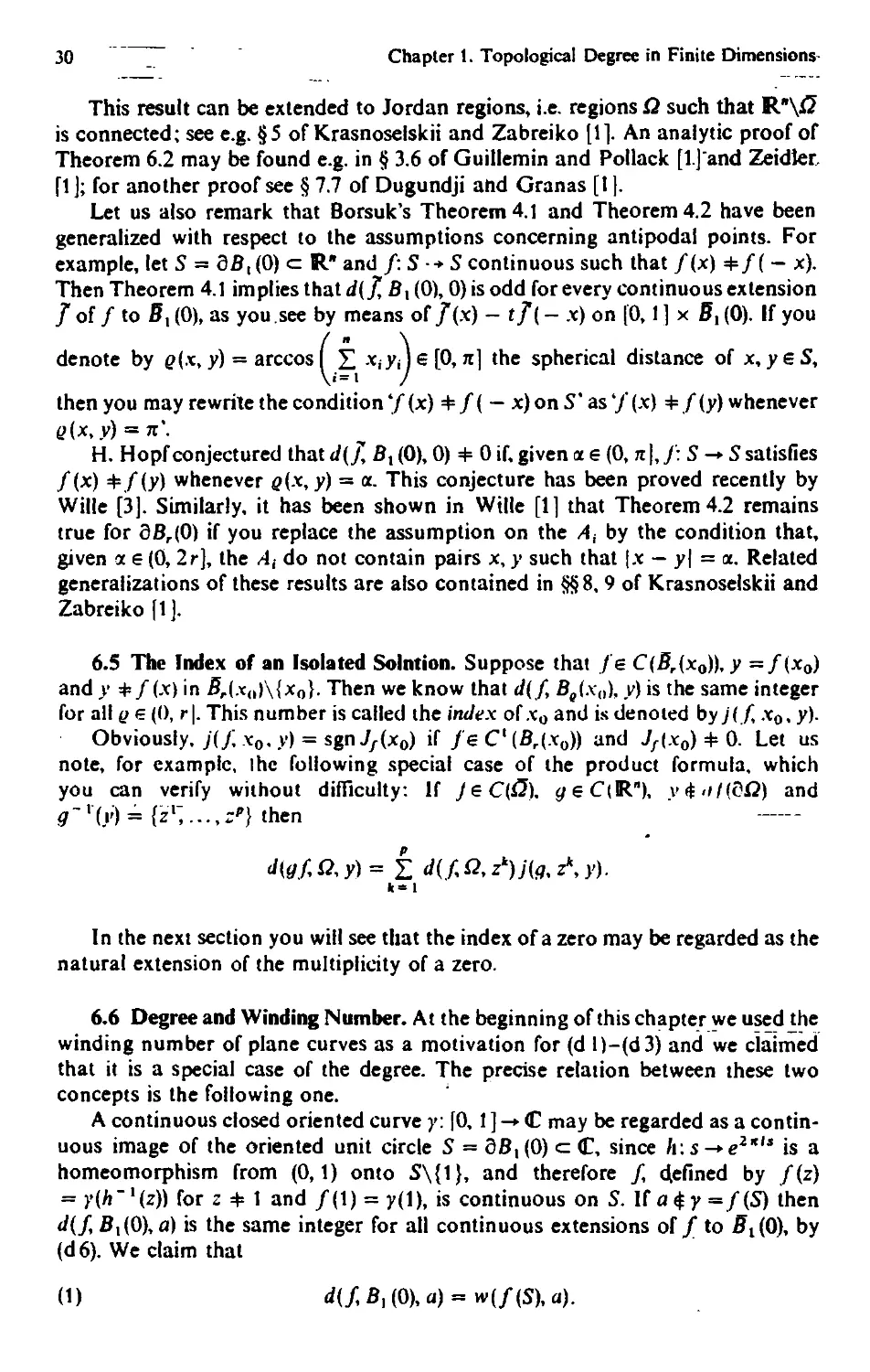
6.5 The Index of an Isolated Solution 30
6.6 Degree and Winding Number 30
6.7 Index of Gradient Maps 32
6.8 Final Remarks 33
Exercises - 33
Chapter 2. Topological Degree in Infinite Dimensions 35
§ 7. Basic Facts About Banach Spaces 38
7.1 Banach's Fixed Point Theorem 39
7.2 Compactness 40
7.3 Measures of Noncompactness 40
7.4 Compact Subsets of CX(D) 42
7.5 Compact Subsets of Banach Spaces with a Base 43
7.6 Continuous Extensions of Continuous Maps 44
7.7 Differentiability 45
7.8 Remarks 49
Exercises 52
§ 8. Compact Maps 55
8.1 Definitions , . 55
8.2 Properties of Compact Maps 55
8.3 The Leray-Schauder Degree 56
8.4 Further Properties of the Leray-Schauder Degree 58
8.5 Schauder's Fixed Point Theorem 60
8.6 Compact Linear Operators 61
8.7 Remarks 66
Exercises 67
§ 9. Set Contractions 68
9.1 Definitions and Examples . . 69
9.2 Properties of y-Lipschitz Maps 70
9.3 A Generalization of Schauder's Theorem 71
9.4 The Degree for y-Condensing Maps 71
9.5 Further Properties of the Degree 74
9.6 Examples 75
9.7 Linear Set Contractions 77
9.8 Basic Facts from Spectral Theory 79
9.9 Representations of Linear ^-Contractions 83
9.10 Remarks 84
Exercises 85

Contents XI
§ 10. Concluding Remarks 87
10.1 Degree of Maps on Unbounded Sets 87
10.2 Locally Convex Spaces -.-.,. 87
10.3 Degree Theory in Locally Convex Spaces 89
10.4 Degree for DifTercntiable Maps 90
10.5 Related Concepts 92
Exercises 92
Chapter 3. Monotone and Accretive Operators 95
§11. Monotone Operators on Hilbert Spaces 97
11.1 Monotone Operators on Real Hilbert Spaces 97
11.2 Maximal and Hypermaximal Monotone Operators 102
11.3 The Sum of Hypermaximal Operators 104
11.4 Monotone Operators on Complex Hilbert Spaces 108
11.5 Remarks 109
Exercises 109
§ 12. Monotone Operators on Banach Spaces 111
12.1 Special Banach Spaces 111
12.2 Duality Maps 114
12.3 Monotone Operators 117
12.4 Maximal and Hypermaximal Monotone Operators 119
Exercises 122
§ 13. Accretive Operators 123
13.1 Semi-Inner Products 123
13.2 Accretive Operators 124
13.3 Maximal Accretive and Hyperaccretive Maps . 126
13.4 Hyperaccretive Maps and Differential Equations 127
13.5 A Degree for Condensing Perturbations of Accretive Maps 130
Exercises 132
§ 14. Concluding Remarks 133
14.1 Monotonicity 133
14.2 Ordinary Differential Equations in Banach Spaces 136
14.3 Semigroups and Evolution Equations 137
Exercises 144
Chapter 4. Implicit Functions and Problems at Resonance 146
§ 15. Implicit Functions 147
15.1 Classical Inverse and Implicit Function Theorems 147
15.2 Global Homcomorphisms 152
15.3 An Open Mapping Theorem 154
15.4 Newton's Method 157
15.5 Scales of Banach Spaces 159
15.6 A 'Hard' Implicit Function Theorem 162
15.7 Remarks 168
Exercises 170

XII Contents
§T6 Problems afResonance 172
16.1 Applications of Degree Theory 172
16.2 The Lyapunov-Schmidt Method . .< 176
16.3 Examples 177
16.4 Remarks 183
Exercises 184
Chapter 5. Fixed Point Theory 186
§17. Metric Fixed Point jfheory 187
17.1 Some DescendJpts of Banach 187
17.2 When is FaIs&ict Contraction? 191
17.3 Fixed Points of Nonexpansive Maps 193
17.4 The Browder-Caristi Theorem and Normal Solvability ... 198
Exercises 200
5 18. Fixed Point Theorems Involving Compactness 203
18.1 Fixed Points in Open Sets 204
18.2 Fixed Points in Closed Convex Sets 205
18.3 Weakly Inward Maps 207
18.4 Fixed Points of Weakly Inward Maps 210
18.5 The Set of All Fixed Points 212
18.6 Remarks 213
Exercises 215
Chapter 6. Solutions in Cones 217
§ 19. Cones and Increasing Maps 218
19.1 Cones and Partial Orderings 218
19.2 Positive Linear Functionals 221
19.3 Fixed Points of Increasing Maps 224
19.4 Differentiability with Respect to a Cone * . . . . 225
19.5 Positive Linear Operators 226
19.6 Order Topologies 229
19.7 Fixed Points of Increasing Maps Once More 231
19.8 Remarks 233
Exercises 235
§ 20. Solutions in Cones 238
20.1. The Fixed Point Index 238
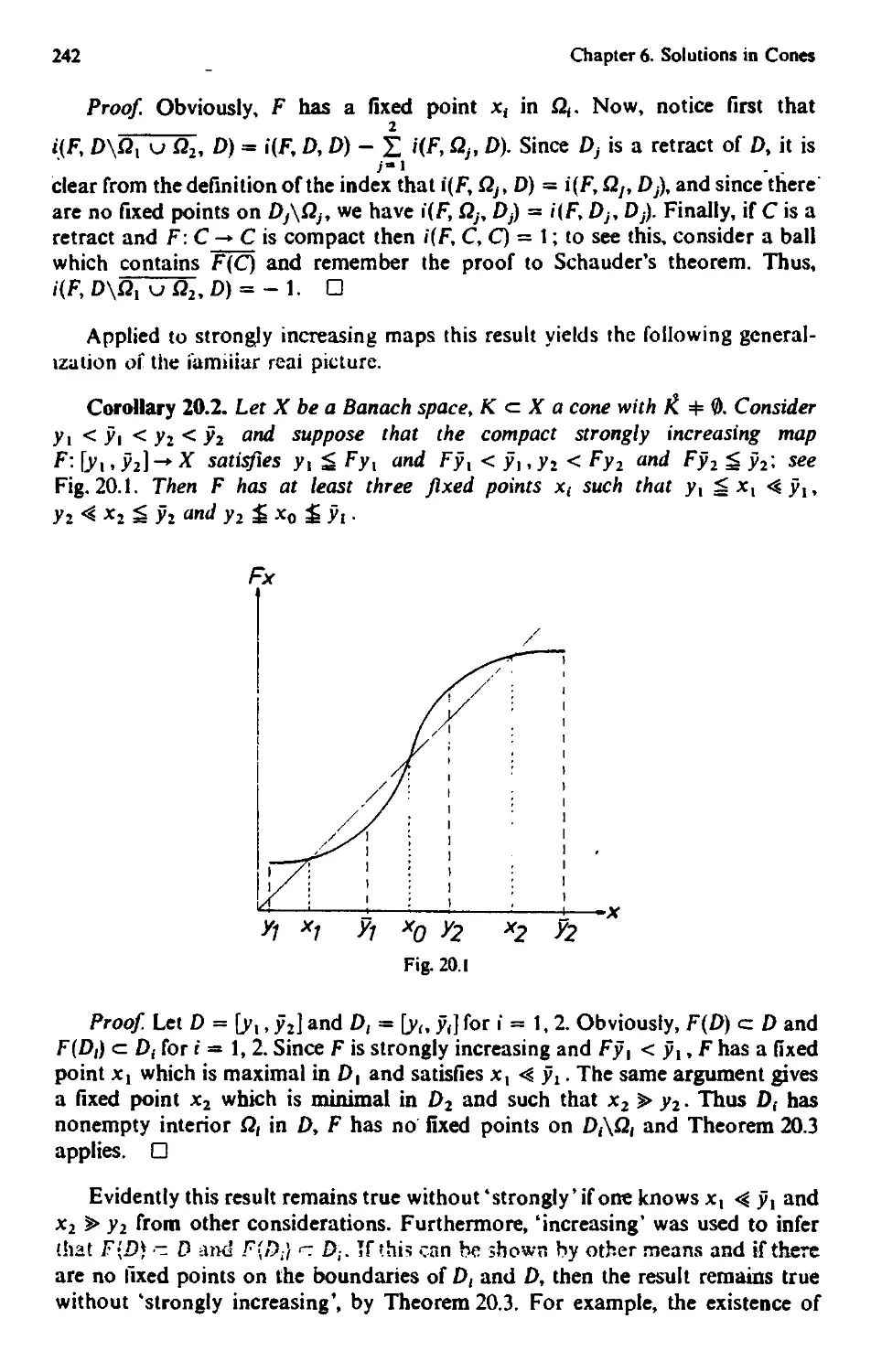
20.2 Fixed Points in Conical Shells 239
20.3 Existence of Several Fixed Points 241
20.4 Weakly Inward Maps 245
20.5 Remarks 252
Exercises 253
Chapter 7. Approximate Solutions 256
§21. Approximation Solvability 257
21.1 Projection Schemes 257
21.2 /!-Proper Mappings 259

Contents XIII
21.3 Approximation Solvability 261
21.4 Linear A-Proper Maps and Approximation of Isolated
Solutions . . . .- . ........ ,„ , x :_.-.-.-. -.-._.-.-. , 262
21.5 Remarks . . 264
Exercises 266
§ 22. /1-Proper Maps and Galerkin for Differential Equations 267
22.1 Topological Degrees 267
22.2 Fixed Point Theorems 269
22.3 Galerkin for Differential Equations .....;' 271
Exercises " 276
Chapter 8. Multis 278
§ 23. Monotone and Accretive Multis 280
23.1 Definitions 280
23.2 Convex Functionals 281
23.3 Properties of Monotone Multis 285
23.4 Subdifferentials 288
23.5 Dense Single-Valuedness of Monotone Multis 291
23.6 Accretive Multis 292
23.7 Remarks 296
Exercises 296
§ 24. Multis and Compactness 299
24.1 Semicontinuity of Multis 299
24.2 Examples 301
24.3 Continuous Selections 303
24.4 Approximate Selections -—^-.- . 305
24.5 Measurable Selections 305
24.6 Degree for y-Contracting Multis 309
24.7 Fixed Points of Multis 310
24.8 Remarks 314
Exercises 315
Chapter 9. Extremal Problems 319
§ 25. Convex Analysis : . . . 321
25.1 Minima of Convex Functionals 321
25.2 Conjugate Functionals 323
25.3 Second Conjugates 327
25.4 Remarks .. 329
Exercises 330
§ 26. Extrema Under Constraints 332
26.1 Local Minima of Differentiable Maps 332
26.2 Minima Under Equality Constraints 333
26.3 Examples 336

XIV Contents
26.4 More General Constraints . 341
26.5 Remarks 345
Exercises .- . .. ; . - . ' 347
§"27. Critical Points of Functionals 349
27.1 The Minimax Characterization of Eigenvalues 349
27.2 A Variational Method 350
27.3 Category and Genus 353
27.4 Banach Manifolds 358
27.5 Finsler Manifolds 362
27.6 Semigroups Generated by Pseudo-Gradient Fields 364
27.7 Some Consequences of Condition (C) 368
27.8 Remarks 371
Exercises 375
Chapter 10. Bifurcation 378
§ 28. Local Bifurcation 380
28.1 Necessary Conditions 380
28.2 The Odd Multiplicity Case 381
28.3 The Simple Eigenvalue Case 383
28.4 Examples 386
28.5 Bifurcation at Infinity 387
28.6 Banach Algebras May Help 390
28.7 Remarks 394
Exercises 396
§ 29. Global Bifurcation 398
29.1 Global Continua of Solutions 398
29.2 Global Continua in Cones . . 402
29.3 Secondary Bifurcation 406
29.4 Remarks 408
Exercises 409
§ 30. Further Topics in Bifurcation Theory 411
30.1 Variational Methods 412
30.2 Stability 415
30.3 Hopf Bifurcation and Last Remarks 419
Epilogue 426
Bibliography 428
Symbols 445
Index 447

Everything should be made as simple as possible.
M not shnife. "" " " • Alben Ejnstejn
When a mathematician has no more ideas,
he pursues axiomatics. Fq[{x Klein
I hope, good luck lies in odd numbers ...
They say, there is divinity in odd numbers,
cither in nativity, chance, or death?
William Shakespeare
Chapter 1. Topological Degree in Finite Dimensions
In this basic chapter we shall study some basic problems concerning equations of
the form / (x) = y, where / is a continuous map from a subset Q a R" into R" and
y is a given point in R". First of all we want to know whether such an equation
has at least one solution x e Q. If this is the case for some equation, we are then
interested in the question of whether this solution is unique or not. We then also
want to decide how the solutions are distributed in Q. Once we have some answers
for a particular equation, we need also to study whether these answers remain the
same or change drastically if wc change J and y in some way. It is most probable
that you have already been confronted, more or less explicitly, by ail these
questions at this stage in your mathematical development.
Let us review, for example, the problem of finding the zeros of a polynomial.
First we learn that a real polynomial need not have a real zero. Then we are taught
that a real polynomial of odd degree, say /?2m+ , (r) = rm+ { + /?2m(0» has a real
zero, and you will recall the simple proof which exploits the fact that /?2m(0 is
'negligible* relative to t2m*l for large f, and therefore p2m+1 (r) > 0 for t ^ r and
Pim+1 (0 < 0 for f ^ — r with r sufficiently large, which in turn implies thatp2m+1
has a zero in (— r, r), by Bolzano's intermediate value theorem. Next we learn that
every polynomial of degree m ^ I has at least one zero in the complex plane <C.
Then we introduce the multiplicity of a zero z0. If this is /c, then z0 is counted k
times, and by means of this concept the more precise statement is arrived at that
every polynomial of degree m ^ 1 has exactly m zeros in C. At this stage the
problem of finding the zeros of a polynomial over C is solved for the pure
algebraist and he will turn to the same question for more general functions over
more general structures. The 'practical' man, if he is fair, will appreciate that the
'pure* fellows have proved a nice theorem, but it does not satisfy his needs.
Suppose that he is led to investigate the behaviour as t -+ oo of solutions of a linear
system x' = A x of ordinary differential equations, where A is an n x n matrix.
Then the information that the characteristic polynomial of A has exactly n zeros
inC, the eigenvalues of A. is not enough for him since he has to know whether they
are in the left or right half plane or on the imaginary axis. In another situation he
may have obtained his polynomial by interpolation of certain experimental data

2
Chapter 1. Topological Degree in Finite Dimensions
which usually contamsdme Hopefully small errors. Then he may need to know
that the zeros of polynomials close to p are close to the zeros of p,
NowT we want to construct a tool, the topological degree of/ with, respect to
Q and y, which is very useful in the investigation of the problems mentioned at the
beginning. To motivate the process, let us recall the winding number of plane
curves and its connection with theorems on zeros of analytic functions. If you
missed this topic in an elementary course in complex analysis, you may either
consult Ahlfors |11, Dieudonne [11, Krasnoselskii et al. [11, or believe in what we
are going to mention in the sequel, since we shall indicate in § 6.6 how the winding
number is related to the -degree in the case of R2.
Let r e C be an oriented closed curve with the continuously difTerentiable (Cl
for short) representation z(t){t e [0,1), z(0) = z(\)) and let aeCXT. Then, the
integer
2tti*rz-a 2k i x2(t) + y2(t)
for z(t) = x(t) + iy(t) + a
is called the winding number (or index) of T with respect to a e <C\T, since it tells
us how many times T winds around a, roughly speaking. If r is only continuous
then we can approximate r as closely as we wish by C1-curves, and it is easy to
see that all these approximations have the same winding number provided that
they are sufficiently close to T. More precisely, if zx (t) and z2(t) are
C1-representations of the closed curves T, and I\ with the same orientation as T and are such
that
max {\zj(t) - z(t)\: re [0,1]} < minfla - z(t)\: t e [0. 1]} for ; = 1,2
then w(rj, a) = vv(T2, a). Therefore, we can define w{H a) to be w(r{, a) for any
such T,. Then we have defined
w: {(f, a): r closed continuous, a e C\r} -*> TL'
and it is not hard to see that this function w has the following properties:
(a) w is continuous in (r, a), i.e. constant in some neighbourhood of (r, a).
(b) w{r,') is constant on every connected component of <C\r - in particular, equal
to zero on the unbounded component.
(c) If the curves /J> and Tt are homotopic in C\{a}, then w(/J,, a) = w(rt, a). More
explicitly, let z0(t) and zrft) be representations of r0 and fj such that"thefe~exists
a continuous h: [0,1 ] x [0, 1 ] -> <C\{a} satisfying /t(0, t) = z0(t) and h(\, t) = zx (t)
in [0,1] and /i(s, 0) = h(s, 1) for every s e [0,1]; then w(rs, a) is the same integer for
all 5 e [0,1 ], where /] is the closed curve represented by /i(s, •)•
(d) If r~ denotes the.curve T with its orientation reversed, then w(r~,a)
= -w(r,a).
Property (c) is the most important one, since it allows us for example to
calculate the winding number of a complicated curve by means of the winding
number of a possibly simpler homotopic curve. Furthermore, (a) and (b) are
simple consequences of (c).

Chapter 1. Topological Degree in Finite Dimensions
3
Now, let G c C be a simply connected region, f: G -* C be analytic and r c G
be a closed C1-curve such that f(z) 4= 0 on T. Then the 'argument principle' tells
us that
(is w( f (run = * . j Jr ^ 1. - f /,'(2) d2 = L w(r, Zk) ak,
where the zk are the zeros of / in the regions enclosed by T and the <xk are the
corresponding multiplicities. If we assume in addition that T has positive
orientation and no intersection points, then we know from Jordan's curve theorem,
which will be proved in this chapter, that there is exactly one region G0 c G
enclosed by T, and w(T, j0) = 1 for every z0eG0. Thus, (2) becomes
w(/(n,o) = 2>kt
k
i.e. the total number of zeros of / in G0 is obtained by calculating the winding
number of the image curve f(T) with respect to 0. In general, w(ry zk) can also be
negative and then we can only conclude that / has at least |w(/(r), 0)| zeros in
the regions enclosed by T.
In the more general case of continuous maps from subsets of R" into R" we
shall imitate these ideas. We consider open bounded subsets QcR" instead of the
regions enclosed by T, continuous maps /: Q -► R" and points y e Rn which do not
belong to the image J'(dQ) of the boundary of Q. With each such 'admissible'
triple (/, Q, y) we associate an integer d{ f\ Q, y) such that the properties of the
function d allow us to give significant answers to the questions raised at the
beginning. Of course, as in daily life, we cannot achieve everything, but the
following minimal requirements and their useful consequences turn out to be a good
compromise.
The first condition is simply a normalization. If/= id, the identity map of R"
defined by id(.x) - x, then fix) = yeQ has the unique solution x = v, and
therefore we require
(dt) dM.Qyy)=\ foryeQ.
The second condition is a natural formulation of the desire that d should yield
information on the location of solutions. Suppose that Qt and Q2 are disjoint open
subsets of Q and suppose that f(x) = y has finitely many solutions in Q{ u Q2 but
no solution in 5\(&i u Q2). Then the number of solutions in Q is the sum of the
numbers of solutions in Qx and QZl and this suggests that d should be additive in
its argument Q, that is
(d 2) d(f Qy y) = d(f Qx, v) + d(f Q2, y) whenever Qx and Q2 are disjoint
open subsets of Q such that y$f(Q\(Qx u Q2)).
The third and last condition reflects the desire that for complicated / the
number d(f Q, y) can be calculated by d(g, Q, y) with simpler g, at least if / can

4
Chapter 1. Topological Degree in Finite Dimensions
be continuously deformed"into g such that at no stage of the deformation we get
solutions on the boundary. This leads to
(d3) :d(h(t, -),Q, y(t)) is independent of t e J = [0,1 ] whenever h: J x S -+ Rn
and y: J -* R" are continuous and y{t) $ h(u dQ) for all t e J.
There are essentially two different approaches to the construction of such a
function d. The older one uses only concepts from algebraic topology, which is
quite natural, since (d l)-(d 3) involve only topological concepts such as open sets
and continuous maps and a 'little bit' theory of groups like Z; see, for example,
AlexandrolT and Hopf [1 J, Cronin |2], Doid [2], Dugundji and Granas [1 ].
We shall present the more recent second approach which is simpler for ltrue'
analysts, not worrying much about topology and algebra, since it uses only some
basic analytical tools such as the approximation theorem of K.. WeierstraB, the
implicit function theorem and the so-called lemma of Sard (see § 2). Presentations
still using topological arguments can be found in books on differential topology,
for example, in Guillemin and Pollack [1 ], Hirsch [11 and Milnor [2|, while purely
analytical versions have been given by Nagumo [1 ] and Heinz [I) in the 1950s. An
interesting mixture of the two methods has been given in Peitgen and Siegberg [1 ]
- an outgrowth of recent efforts in finding numerical approximations to degrees
and fixed points, based on the observation that the essential steps of the old
method can be put into the form of algorithms.
In principle, it is an inessential question how we introduce degree theory, since
there is only one Z-valued function d satisfying (d l)-(d3), as you will see in § 1,
and since it are the properties of d which count, as you will see throughout this
chapter. Starting with the uniqueness of d, by exploiting (dl)-(d3) until we end
up with the simplest case f(x) = Ax with det/1 4= 0, has the advantage that the
basic formula, which a purely analytical definition has to start with, does not fall
from heaven - it is enough that the natural numbers do (according to
L. Kronecker) - and that we are already motivated to introduce some
prerequisites which we need anyway later on. However, you will keep in mind that
choosing the analytical approach we lose topological insight to a considerable extent,
while going through the mill of the elements of combinatorial topology you will
hardly become aware of the fact that the same goal can be arrived at so simply by
an analytical procedure. Thus, the essential question is why we introduce degree
theory, but this has already been answered by the general remarks given in the
foreword and the more special ones in this introduction which we are going to
close by a few historical remarks.
The winding number is a very old concept. Its essentials can already be found
in papers of C F. GauB and A. L. Cauchy at the beginning of the 19th century.
Later on L. Kronecker, J. Hadamard, H. Poincare and others extended formula
(1) by consideration of integrals of differentiable maps over {xeR": |x| = 1}.
Finally, L. E. J. Brouwer established the degree for continuous maps in 1912. It is
now tradition to speak of the Brouwer degree. The way towards an analytical
definition was paved by A. Sard's investigation of the measure of the critical
values of differentiable maps in 1942. You will find much more in the interesting
papers of Siegberg (1 ], [2].

§1. Uniqueness of the Degree
5
§ 1. Uniqueness of the Degree
In this section"w«r shall show that there is only one function
d: {(/, Q, y): Q a R" open and bounded, /: Ci -*■ R" continuous,
yeRn\f(dG)}-*Z
satisfying
(dl) d(id,i*>y) = 1 for y eQ
(d 2) d{f:>3, y) = d( /, 42,, y) f </(/, &2, y) whenever Q{, £2 are disjoint open
subsets of Q such that y $f{friQx u £2)).
(d 3) (i(/i(t, •), Q, y(t)) is independent of t € J = [0,1 ] whenever /i: J x £ -+ R" is
continuous, y: J -*■ R" is continuous and y{r) $ *»(*, d£) for all f e J.
This will be done by reduction to more agreeable conditions, the final one being
the case where / is linear, i.e. f{x) = /1.x with det A 4= 0. During the simplifying
process we introduce basic tools which are also needed for the construction of the
function d in § 2, and you will see already here that the homotopy invariance (d 3)
of d is a very powerful property.
Let us start with some notation for the whole chapter.
l.l Notation. We let R" = {x=<x, .xrt):.x,eR for i = l,...,n} with
/ n \l/2
Jjc | = f 2 xf\ . For subsets A c R" we use the usual symbote A, dA to
denote the closure and the boundary of A, respectively. If also 5cR" then
B\A = {x 6 B: x $ A}, which may be the empty set 0. The open and the closed ball
of centre x0 and radius r > 0 will be denoted by
Br(x0) = {x e R": |x - .T01 < r) = x0 + 0,(0) and Br(x0) = KM-
Unless otherwise stated, Q is always an open bounded subset of R".
For maps/: A c R"-> R" we let ./(/1)={/(.x):x6^} and /_t(y)
= {x 6 /4 :/(x) = y}. The identity of R" is denoted by id, i.e. id(x) = x for all
x e R". Linear maps will be identified with their matrix A = (ay) and we write
det A for the determinant of A. We shall also use L. Kroneckefs symbol Sij9
defined by Si} = 1 for i =j and <5r, = 0 for i 4=y, so that id = (J,v). If B c R" is
compact, i.e. closed and bounded, then C{B) is the space of continuous /: B -► Rn,
and we let |/|0 = max |/(x)| for fe C(B). We shall write fe C(B; Rm) to erapha-
B
size /(B) c Rm, if necessary.
You will recall that /: Q -+ R" is said to be differentiate at x0 if there is a
matrix /'(x0) such that
f(x0 + /i) =/(x0) -f /'(x0) /i -4- (uUi) for heQ- x0 = {x - x0:xeQ]
where the remainder (o(h) satisfies \a)(h)\ 5* g |/i| for |/?| ^ <5 = c>(£, x0). In this case
f'ixohj = djfi(x0) = d/i(x0)/dxj, the partial derivative of the ith component /
with respect to Xj.

6 Chapter 1. Topological Dcgrccjn Finite Dimensions
At several points in this book it will be more convenient to iise~£. Landau's
symbol instead of the e — 3 formulation of the condition for the remainder, Le. we
shall say that *oj(h) = o(\h\) as h - 0' iff \a>{h)\/\h\.-+ 0 as [h\ -+0, Thus
differentiability of / at x0 means f(x0 + h) -f(x0) -f'(x0) h = o(\h\) as h -►0. The
formal advantage consists in the freedom to write things like <xo(\h\) = o(\h\) if a
is constant, or co,(/i) 4- a)2(h) = o{\h\) if co^h) = o(\h\) for t = 1,2, etc. We
denote by
Ck{Q) the set of /: Q -» R" which are fc-times continuously differentiable in
£, while Ck(Q) = C*(G) n C(S) and C°°(0) = fl £*(£)• If A*o) exists the&
Jyt-.xo) = det/'(.x0) is the Jacobian of/ at x0, and x0 is called a critical point ofjf
if Jf(x{)) = 0. Since these points play an important role we also introduce
Sf(Q) = {xeQ:Jj (x0) = 0} and write Sf for brevity whenever Q is clear from the
context. Furthermore, a point y e R" will be called a regular value of f: Q -> R" if
/ ~l(y) ^ Sf{Q) = 0, and a singular value otherwise.
In general R-valued maps will be denoted by Greek letters while we shall use
Latin letters for vector-valued functions.
1.2 From C(H) to C°°(J2). The first step in the reduction is to show that d is
already uniquely determined by its values on C™-functions. To this end let us
mention the following two facts.
Proposition 1.1. Let A c Rn be compact and f: A -* R" continuous. Then f can
be extended continuously to Rn, i.e. there exists a continuous J\ R" -* R" such that
T(x)=f(x)forxeA. '
Proof. Since A is compact, there exists a dense and at most denumerable
subset {a\a2y...} of A. Let g(.x, A) be the distance of the point x to A, i.e.
q(x, A) = inf{|x — a\:ae A), and
(Pi(x) = max {2 - '——-^,0} forx$A.
£>(.X, A)
Then
f(x) for xe A
/(*> = ■' ' ' ■
(I 2"' MX)) ' £ 2-' fl(x) /(«') for x <M
defines a continuous extension of /. If you find this difficult, it does not matter,
since we shall give a detailed proof of a much more general extension theorem
later on. □
Proposition 1.2. (a) Let A c R" be compact, fe C(A) and e>0. Then there
exists a function g e C^R") such that \f(x) - g(x)\<>e on A.
(b) Given fe Cl (Q\ e > 0 and 3 > 0 such that Qd = {xeQ: g(x, dQ) ^ 3} * 0,
there exists g e Cx(Rrt) such that \f- g\0 + max |/'(x) - g'(x)\ ^ e.
Proof Let / be a continuous extension of / to Rn and let
/.(*> = 11(0 <P*(t ~ x) dZ for x € R" and a > 0,

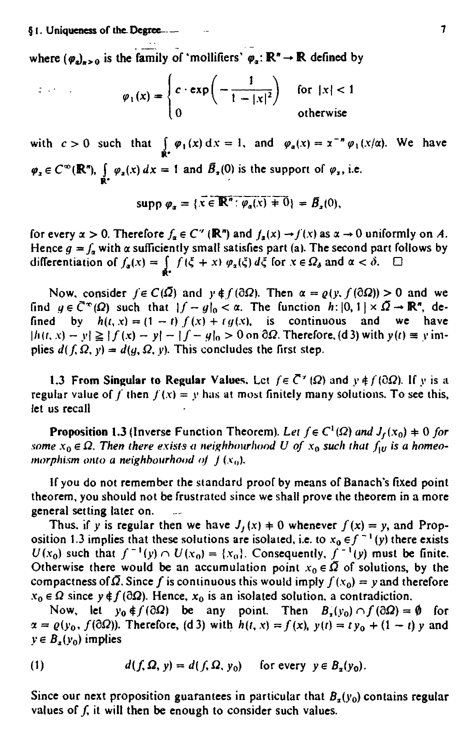
§ 1. Uniqueness of the. Degree
7
where (^Jar>0 is the family of 'mollifiers' <pa: R" -* R defined by
^ = {c-exp(-r=W) for|x|<1
(0 otherwise
with c>0 such that Jp,(x)dx = l, and (px{x) = x~n <p{{x/<x). We have
<px e C"°(RHl $ <p2(-x) dx s 1 and JJ,(0) is the support of <pjy i.e.
R-
supp q>a = {x iTFT^xT+O} = S,(0),
for every a > 0. Therefore fa 6 C (Rn) and /a(x) -»/(x) as a -+ 0 uniformly on A.
Hence g =/a with a sufficiently small satisfies part (a). The second part follows by
differentiation of fjx) = j" f{$ + x) tpa(q) d£ for xeQA and <x < 6. Q
R"
Now, consider /g C(£) and y<j?/(0G). Then a = e(>»,/(dfi)) > 0 and we
find (/ e C^(G) such that \f - g\0 < a. The function h: |0,1 ] x £ — Rw,
defined by /i(r, x) = (1 — t) f(x) + /r/(x), is continuous and we have
|/i(f, x) - y\ ^ |/(x) - y| - |/- g\0 > Oon 6#.Therefore,{d3) with y(t) = y
implies d(/, 42, y) = </(#, £, y). This concludes the first step.
1.3 From Singular to Regular Values. Let /<= C* {Q) and y<$f{dQ). If y is a
regular value of/ then fix) = y has at most finitely many solutions. To see this,
let us recall
Proposition 1.3 (Inverse Function Theorem). Let /e C1 (Q) and Jf(x0) # 0 for
some x0 G Q. Then there exists <t neighbourhood U of x0 such that f\V is a homeo-
morphism onto a neighbourhood of J (x„).
If you do not remember the standard proof by means of Banach's fixed point
theorem, you should not be frustrated since we shall prove the theorem in a more
general setting later on.
Thus, if y is regular then we have Jj(x) 4= 0 whenever f(x) = y, and
Proposition 1.3 implies that these solutions are isolated, i.e. to x0 ef ~l (y) there exists
U(x0) such that f'Uy) n U(x0) = {x„}. Consequently, f~l[y) must be finite.
Otherwise there would be an accumulation point x0e(2 of solutions, by the
compactness of 8. Since / is continuous this would imply /(x0) = y and therefore
x0 eQ since y $f{dQ). Hence, x0 is an isolated solution, a contradiction.
Now, let y0$f(dQ) be any point. Then £a(y0) r\f(dQ) = 0 for
* = <?(j'o, f@Q)Y Therefore, (d 3) with h(ty x) =/(x), y{t) = ty0 + (1 - t) y and
ye #a(y0) implies
(1) d(fQy y) = d(fQy y0) for every y e BJy0).
Since our next proposition guarantees in particular that £a(y0) contains regular
values of /, it will then be enough to consider such values.

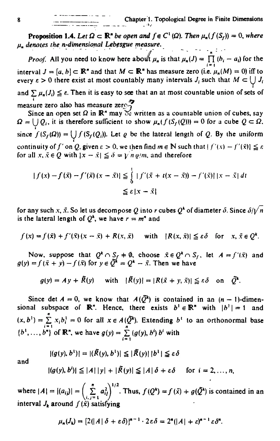
8 Chapter 1. Topological Degree in Finite Dimensions
Proposition 1.4. Let QczWbe open andfeC1 (Q). Then fi„(f(Sf)) = 0, where
lin denotes the n-dimensional Lebesgue measure.
Proof. All you need to know here abowt pi„ is that n„(J) = n (^i — ad f°r tne
i- 1
interval J = [a, h] c R" and that M c= R" has measure zero (i.e. nn{M) = 0) iff to
every r > 0 there exist at most countably many intervals Jt such that M cz\J Jf
and 2 MnWi) = e- Then it is easy to see that an at most countable union of sets of
measure zero also has measure zenvi
Since an open set Q in R" may oe written as a countable union of cubes, say
Q = (J Qf, it is therefore sufficient to show /*,(/(S/(0)) = 0 for a cube Q e £,
since f{Sf{Q)) = IJ/(£/(&))• Let g be the lateral length of Q. By the uniform
continuity of/' on Q. given /; > 0. we then find m e N such that | /"(.\) — /'(.x)| ^ £
for all x, x e () with |x — x| 5^ r>" = y no/nu and therefore
| Ax) -/(x) -/'(ic)(.x - x)| ^ j |/'(x + r(x - x)) -/"(.x)| I* - *l ^<
£e|.x-.x|
for any such x, x. So let us decompose Q into r cubes Q* of diameter S. Since <ty]/K
is the lateral length of Q\ we have r = mn and
/(x)=/(x)-f-/'(x)(x~x) + /?(x,x) with |fl(x,x)| ^ eS for x,.xeQ*.
Now, suppose that Qk r\ S, 4= 0, choose xe&nSf* let /i =/'(x) and
#(y) =/(-x + y) —/(.x) for y e 2 = Q* — x. Then we have
#(y) =/iy + J?(y) with |J?(y)| = |JR(x + y, x)| S £<$ on Qk.
Since det/I =0, we know that Affi) is contained in an (n — l)-dimen-
sional subspace of R". Hence, there exists fr!eRB with l/?1!^^ and
(x, b1) = X *ib} = 0 for all xe A(Qk). Extending bl to an orthonormal base
{bl, ...,/>"} of R", we have g[y) = £ (0W. ^) &' w»th
i= 1
and
t(g(3/),fei)|g|^||y| + |«(>:)|^M|<5 + £<5 for . = 2 »,
where \A\ = |(aiy)| - f I flyY'*. Thus, f(Qk) =f{x) + g(Q") is contained in an
interval/* around f(x) satisfying
MM = [2(|/I | 6 + eS)rl-1** = 2"(MI + <=r'^".

§1. Uniqueness of the Degree 9
Since f is bounded on the large cube Q, we have |/'(x)| ^ c for some c, in
r
particular \A\ g c. Therefore, f(Sf(Q)) c. (J Jk with
'-' ' ' ■"'"/"
I /<* W ^ r • 2nic + /;)" ' erf" = 2"(c + £)fl"'i/ngYe.
* = i
i.e. /(S/(0) has measure zero, since r. > 0 is arbitrary. □
Let us remark that Proposition 1.4 is a special case of Sard's lemma: l%$2 a R"
is open, feCx{Q) and Q* a Q measurable, then f{Q*) is measuwtale and
H„{f{Q*)) < [\J/(x)\ dx: see e.g. Schwartz f2| for a complete proof.
1.4 From C"-Maps to Linear Maps. At the present level we only need to
consider /e C* {Q) and y * /'(OG u S,).
Suppose first that / l (y) - 0. From (d 2) with Q{ ~ Q and Q2 = 0 we obtain
d(j\ 0, y) = 0, and therefore di f\ Q, y) = </(/, £,, y) whenever^ is an open subset
of Q such that y $f{Q\Qx). Hence / ' (y) = 0 implies d(j\ Q, y) = d()\ 0, y) = 0.
In case / "l (y) = {x\ ..., x"}, we choose disjoint neighbourhoods U{ of x' and
obtain d{j\Q, y) = I d[£ U^ y) from (d2). To compute d(£ Uh y), let A = /'(x')
and notice that 4=i
/(x) = y + A (x - x1') + o(\ v - x'|) as |x - x'| - 0.
Since det<4#0 we know that A'1 exists, and therefore |z| = |/4 _1,4z|
£ | /I"111A z |, i.e. | .4 z | ^ c | z | on R" for some c > 0. By means of this estimate we
see that y(t) = ty and /?(f, x) = tf{x) + (1 — t) A(x - x') satisfy
|/iU, x) - y(r)| = \A(x - x«) + r • <>{\x - x'|)| ^ c\x - x'\ - o(\x - x'|) > 0
for all t e [0,1] provided that |x - x'| S S with <* > 0 sufficiently small. Hence
d{f, Bs(x% y) = d(A- A x\ Bs(x\ 0) by (d 3). Since /(x) * y in R\55(x'), we also
have d(j\ l/{, y) = d(j\ Bs[x% y) by (d 2), and therefore
d( f\ L^ y) = d(A - Ax\ Bt(x\0).
Since x' is the only solution of Ax — Ax1 = 0, (d2) implies
d(A - A x', ^(x1), 0) = d(A - /tx\ JBr(0), 0)
for J3r(0) 3 B,(x'), and A(x - fx') * 0 on [0J 1 x 6£r(0) yields
c/(/,(y,,y) = J(/'(xf),Br(0),0),
by (d 3). Finally, r > 0 may now be arbitrary, by (d 2). Thus, we have arrived at a
very simple situation and you will see that

JO
Chapter 1. Topological Degree in Finite Dimensions
l^TJnear Algebra May Help. The only thing that remains to be shown is that
d{A, £r(0), 0) is uniquely determined if A is a linear map with det A * 0. It turns
,out that d(A, Qs 0) = sgn det A, the sign of det A. The proof of this result requires
some basic facts from jfnear algebra which you will certainly have seen unless you
slept through those lessons which prepared, for example, Jordan's canonical form
of a matrix. If you did, it is sufficient to accept that our next proposition is true
since we shall prove a more general result in a later chapter.
Proposition \.5. Let Abe a real n x n matrix with det A 4= 0, let X l,..., Xm be
the negative ei&nvalues of A and a,,...,am their multiplicities as zeros of
det (A — X id)^A>vided that A has such eigenvalues at all. Then R" is the direct sum
of two sub spaces N and M, R" = N © M, such that
(a) N and M are invariant under A,
(b) A\N has only the eigenvalues X{,...,Xm and A\M has no negative eigenvalues.
m
(c) dim N = y ak.
k= 1
Let det (A - X id) = (- t)" U U - V U U~ Mjfj- Then
det A = (- 1 )a ft I4r II tf* with a = £ ak = dim N,
hence sgn det A = (— t )*.
Now, if A has no negative eigenvalues then det{tA + (1 — t) id) 4= 0 in [0, 1],
and therefore d(A% Br(0), 0) = </(id, £r(0), 0) * 1 = sgn det A by (d 3) and (d 1). So,
let us consider the case N 4= {0} and let us write Q for Br(0).
Step /. Suppose that a = dim N is even. Since R" = N © M, every x e Rn has
a unique representation x = P{x -f P2x with P{xeN and /|.x"e jCfT Thus we
have defined linear projections Px:Kn^N and P2 = id - P,: R"-* M. Then
/I = /4 P, 4- /4 P2 is a direct decomposition of A since A (N) a N and A(M) cMby
Proposition 1.5(a). Now, since A Pv has only negative eigenvalues and A P2 has no
negative eigenvalues by Proposition 1.5(b), it is easy to see that A is homotopic
to - Pi 4- P2. We claim that
(2) h{t,x) = tAx + (\ -t)(-Plx + P2x)*0 on [0, l]xd£.
To see this, notice first that /i(0, x) = 0 implies P1 x = P2x, hence P{ x = P2x
6 N n Af = {0} and therefore x = 0. Next, h(t, x) = 0 with f 4= 0 means
AP{x = XPyxeN and ^P2x =-AP2x€iV/ with A = t_1(1 - r) > 0
which is possible only for Px x = P2 x = 0, by the remark on the eigenvalues of A P{
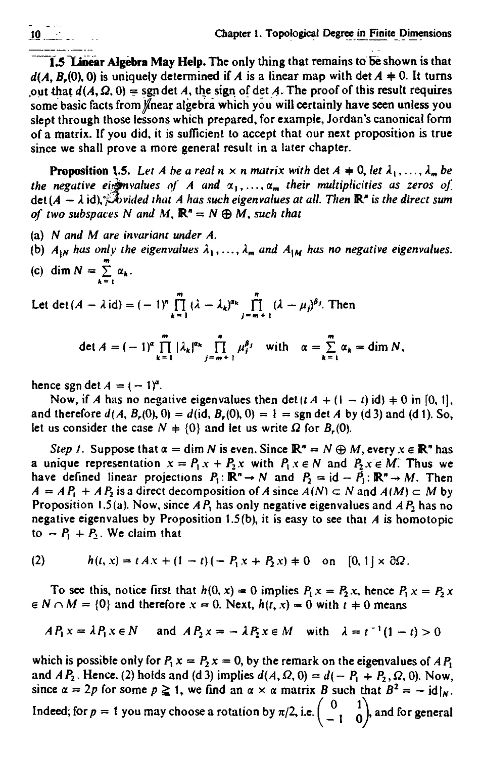
and A P2. Hence. (2) holds and (d 3) implies d(A9 £, 0) = d( - Pt + P2, £,0). Now,
since a = 2p for some p ^ 1, we find an a x a matrix B such that B2 = - id|w.
Indeed; for p - 1 you may choose a rotation by 7r/2, i.e. ( n), and for general

§ 1. Uniqueness of the Degree It
p you may arrange p such blocks along the main diagonal, i.e.
b2j-i.2j = ) = rM).Ur\ Jor;>-l,.....p. and V = P, -- - :
for all other ;, k. Since B has only complex eigenvalues we find homotopies
from - ?! + P2 to BPX + P2 and from BPX + P2 to id = P, + P2, namely
rBPX - (1 - r) P, + P2 and f BP, + (1 - /) P, + P2, as you may easily check.
Hence
<i(/4,ft0) = d(- P, 4- P2,G,0) = J(id,X2,0) = ^= (- l)2' = sgndet A.
-J
Step 2. Let us finally assume that a = dim N = 2p 4- 1 for some p ^ 0.
Then we may decompose N = Nx © JV2, with dim Nt = 1 and dim N2 - 2p,
which yields projections Qx: N -» N, and <52 = id|w — Qi: N -+ N2. Then
Pi = 6i Pi + Qz Pi a°d as *n the first step we find homotopies, indicated by -♦,
such that
4--P, +P2- -^Pl +Bg2P, +P2--&A + &P, + *2-
Hence </K £, 0) = </( - Qx 4- <?2, ft 0) with Qx = Q, P, and Q2 = Q2PX + P2.
Notice that Qx and Q2 = id — Qx are the projections from the decomposition
R" = Nx © (N2 © M). Since x = 0 is the only zero of - Qx 4- Q2 we may also
replace Q = J5r(0) by any open bounded set containing x - 0, without changing
</, for example by Br(0) n Nx 4- £r(0) with £r(0) = Br(0) n (N2 © M); recall that
Qx +Q2 = {.x +)':x€fl,,y6fl2|.
Now, you will see immediately that we are essentially in a one-dimensional
situation. Indeed, given Q c Nx open and bounded and g.8-*Nx continuous
with 0*0(30), let <7(0,ftO) = </(0"Qi 4- (?2.&4- #r(0),0).
Then you will convince yourself that (d 1) — (d3) imply
(dl) £T(id|Ari,ft0) = 1 forOel?.
(d 2) 3{g, Qy 0) = J(#, Qx, 0) 4- <?(#, £22, 0) whenever ^t, Q2 are disjoint open
subsets of Q c N, and 0 $ 0(£\(&, vj £2)).
(<f3) c/(J?(f, •), 1?, 0) is constant on J = [0, 11 whenever /i: J x £ -+ ty is
continuous and 0 £ /i(J x d£).
In this notation we have to compute
I[- i^U>ftOH d(- Q{ + g2,# + Br(0),0),
where Q cz N is any open bounded set with 0 e Q. Since we guess (?(— id|Wl, Q, 0)
= — 1 = (— l)2p+! = sgn det A and since (d 1) is the only concrete thing we have
at hand, it is natural to look for a function g and sets Q^QX kjQ2 such that
H(g, Q, 0) = 0, g\Qt is homotopic to - id|0t and g\Q2 is homotopic id|ft2, since then
S( - id \Nx, Qx, 0) = - <7(id |„,, Q2,0) = - 1, by (<T2) and (d 3). This is roughly the
idea of the
Last step. Since dimNx =l,we have Nx = {Xe: X eR} for some eeR" with
\e\ = 1. Consider
^ = {Ae:Ae(~2,2)}, £, = {A^: Ae(- 2,0)}, Q2 = {A^:Ag(0,2)}

12 . Chapter. ^Topological Degree in Finite Dimensions
and f(Xe) = {\X\ - 1) e. Since f(0) =-~e * 0 and h(t. Xe) = r(|A| - 2) e + e * 0
on [0, 1 ] x dQ, we have
6 = H(e,Qy 0) = <?(/,£,0) = 3(f,Qx, 0) + 2(f%Q2% 0)
by (d2), (d3) and (d2) again. Now, /Io,(a£?) = - (X + 1)* has the only zero
— e eQx <= Q, whence
3(f,Qx, 0) = J(- idU, - e,£,0) = <?(- idU,.£,0),
since also - Xe - te + 0 on [0, 1 ] x 3£>. By the same argument we obtain
J{fM2,Q) = J(idliy^ftO). and therefore^- id|*,,fl.0) = - I, as we wanted to
show. Thus we have proved
Theorem I.I. Let
M = {(/ Q:y): Q c R" open bounded, fe C{Q) and y e R"\/(6G)}.
Then there exists at most one function d: M -* Z with the properties (d 1) — (d 3).
Furthermore, these properties imply that d{A,Q, 0) = sgn det .4 for linear maps A
with det A =*= 0 and OeQ.
Having seen that homotopies and linear algebra are useful, you will certainly
enjoy the following
Exercises
1 Let A be a real n x n matrix and eA - Y —r. Then dett^ > 0. Hint: Consider e'A.
n.40 m!
2. Let A be a real n x n matrix with det A > 0. Then there exists a continuous map H from [0,1 ]
into the space of all n x n matrices such that H(Q) = id, H{\) = ,4 and det H{t) > 0 in [0, I].
Hint: The proof is hidden in vj 1.5.
§ 2. Construction of the Degree
At the end of § 1 we reached the simplest situation. Now, progress by stages to the
general case.
2.1 The Regular Case. It will be convenient to start with
Definition 2.1. Let CcR" be open and bounded, feCx(Q) and
y e Rn\f(dQ u Sf). Then we define
d{ff Q, y) = £ sgn Jf (x) (agreement: £ =f 0).
In the sequel, the main difficulty will be to get rid of the assumption y $f(Sf).
We already know that this exceptional set has measure zero, and since such sets
are immaterial when we integrate, let us replace £ sgn Jf(x) by a suitable integral.

§2. Construction "of the Degree 13
Proposition 2.1. Let Q, f and y be as in Definition 2.1 and let {<pX>o be the
mollifiers from the proof to Proposition 1.2. Then there exists e0 = e0(y.f) such
that d(fJQ,y) = [<pA£(xl-y)Jf(x)dx for 0<e£r.Q. >
" ' "* 7" "' """ " " ~
Proof. The case J ' (y) = 0 is trivial since <pt{f(x) -y)s0 for
e < a = £(y,/(#)). If / liy) = ix1 x^l, then we find disjoint balls BQ(xl)
such that /Ib^um is a homeomorphism onto a neighbourhood V{ of y and such that
sgn Jr(x) = sgnjy(x') in Bq{x% Let Br(.v) c (\ K and (/, = BQ(xl) r>f-l(Br(y)).
Then |/(x) - y\ ^ ft on.3 (J (.', for some ft > 0, and therefore /; < ft implies
{ 9.(fM-y)Jf(x)dx = £ sgni^x') f 9ti f ix) - y) \Jf(x)\ dx.
h i-i r,
Since^(x) = Jr -y(x) and /(£/,-) - y = 5r(0), the well-known substitution formula
for integrals yields
f 9Afix)-y)\Jf-Ax)\dx= J 4Mx)i/x = 1 for e<min{flr}. D
2.2 From Regular to Singular Values. Consider / e C2(£) and y0 $/(d£). Let
a = Q{y0,f(dQ)) and suppose that y\ y2e #a(y0) are two regular values of /.
Finally, let S = a — max {|y' — y0|: / = 1,2}. By Proposition 2.1 we find r. < 6
such that
</(/,£, y') = J pc(/ (x) - y«) ./^x) </.x for i = 1, 2.
We shall show that these integrals are equal and then we may define d(f Q, y0)
as d(fyQ, yl) since wc know that regular values y1 exist in £,(y0). To prove that
the difference of the integrals is zero, notice first that
<pc(x - y2) - <pr(x - y{) = div vv(x)
for vv(.v) = (yl - y2) J <p,(x - y1 + t(yl - y2))dt,
o
n
since divw(x) = ]T dw.-UVdx,- be definition. Furthermore suppw cz Br(y0) for
i= i _
r = a — (<$ — e) < a, since supp pe = B, (0). This implies in particular that
f(dQ) n suppw = 0. We shall show in a minute that this property enables us to
find a map oeC1 (Rn) such that suppv cz Q and
0) f«M/(*)-y2)- ^(/(x)-yI)U/(x) = divr(x) in Q.
Then we are done, since integration over a cube Q = [— a, a]n such that Q cz Q
yields
d(f%Q,y2) - </(/,£, yl) = f 6iwv{x)dx = J divy(x) dx
= I J ... f | Srrf.x,)rfx1...rf.xJ_,rfxl+l...rfx.-0.
i= 1 -a a \ - a UXj /

14 Chapter 1. Topological Degree in Finite Dimensions
To find v we need an old formula which is" well-known for people familiar with
differential forms. Since others may not have seen it, let us prove
- Proposition 2.2. Let i?cR" be open, feC2(Q) and dtj(x) the cofactor of
dfj(x)/dXi in Jf(x)y i.e. d^x) is (— 1)'+; times the determinant which you obtain from
Jf(x) cancelling the jth row and the ith column. Then
I -^ = 0 fory = l,...,n.
i=l OX/
Proof Fix jy let dk - d/'dxk and let fXk denote the column (dk fy...ydkj)-ly
oW}+, dkfH). Then
du(x) = (- \y+Jdet(fx%,..., f^^J,,, fXi fjy
where the hat indicates cancellation. Since a determinant is linear in each column,
you may easily check that
a^l,(x) = (-ir^£det(Al,...,/JCi,...,/JCk_t,a(./Xk, rXh„ fj.
fc= 1
Let cki = detO£ fXk, /t1,..., fXi,..., /Xlc,..., fXn). Then cki = cik since fe C2(Q).
and since the sign of det changes whenever we permute two adjacent columns, we
obtain
(- D'^a^yW = Z (- 0*"1 cki + S (- l)*-2ck|. = £ (- I)*" l afc,cu
k < I * > j * = 1
with 0*11 = 1 for k < /', or,,- = 0 and aki = — <7iik for all i, /c. Therefore
i = 1 i. k = 1 Jt, i = 1
- i (-ir,+,ff*ic*.
i.e. the sum is zero. D
Now, let us define vt(x) = £ Wj(f(x)) di}(x) on Q and t?((x) = 0 on R"\0, for
/ = 1 n. Then supp vv c B,(y0) c Ba(y0) implies supp v cz 42, and we have
a,M*)= £ <iw^i(/(x))al./,(x) + i wj(/(x))a,.^(x).
j.k=l j=l
Since X ^M^Al.^^^M with Kronecker's Sjky Proposition 2.2 yields
i= J
divi;(x) = £ dkWj(f(x))SjkJf(x) = divw(f(x))Jf(x)y
k.j= I
i.e. the formula (1). Thus we have justified

§ 2. Construction of the Degree
—ts
Definition 2.2. Let Q a R" be open and bounded, fe C2(Q) and y $fi$Q\
Then we define d(f Q, y) = d{f Q, yl), where yl is any regular value off such that
\yl —y\ < e(y,./(d£))and J(^ i?,_y,)-is giveaby Definition 1.1.
2.3 From C2(Q) to C(f2). In this final step we shall show that the degree of
Definition 2.2 is the same for all C2(£?)-functions sufficiently near to a given
continuous map. To this end we use a special case of the implicit function theorem
which is appropriate for the present purpose. A more general result will be proved
in a later chapter. ^
Proposition 23. Let'^h: R x Q -+ R" be continuously differentiate,
h(to,xo) = 0 and ^<i0.-)^xo) 4= 0 for some (r0, x0)e R x Q. Then there exist
an interval (f0 — r, r0 + r), a hall B6lx0) c Q and a continuous function
x: (f0 — r, f0 + r) -* Ba(x0) swr/i f/itff x(f0) = x0 and x(t) is the only solution in
Bi(xo)qfh(Ux)~0.
Now, let us prove
Proposition 2.4. Let fe C2(Q) and y $f(dQ). Then, for g e €2{Q) there exists
aJ = S(f y,g)>0 such that d(f+ tg% Q, y) = d(f Q, y) for \t\ < 6.
Proof 1. In case / ~ '(y) = 0 it is obvious that f(x) -f tg(x) * y in £ for |r|
sufficiently small, and therefore both degrees are zero.
2. Let f'l(y) = {.x1 .xm} and Jf{xk) #= 0 for i = l,...,m, /; =/-f ^ and
/i(r,x)=y;(x)-y. We have /i(0,.x'") = 0 and Jfc,0. .,(*') = Jfix*)* 0. By
Proposition 2.3 we therefore find an interval i — r,r), disjoint balls BQ(x') and
continuous functions z^f—^r) -+ Bff(x|-)such that/, ~{(y) r\ K= {zl(t)y ...,zm(t)}
m
for K= (J B^x1). We choose ^ also so small that sgn Jf(x) = sgn-T^x') on 5e(x').
Since-|/(x) — y| >/? in S\V for some // > 0, we even have
frl{y) = {zl(t),-...zm(t)} for \t\<60 = min{rj\g\;1}.
Finally, since J/,(x) is continuous in (r, x), we find S^S0 such that
I-7/,W - JjrWI < min{l/rW|: zeF} for |/| < <>' and xe V. Hence, sgnJ/t(z'(r))
= sgn JfizHt)) = sgn/^x'), that is, d{ft,Q,y) = d{f%Q,y) for |r| < <5, by
Definition 2.1.
3. For the last case, suppose that y is not regular. Then we choose a
regular ~y0 e Ba/3(y), where a = q(\\ f (6&)), and we find a S0 > 0 such that
d(ft>Qiy0) = d(fQyyQ) = difQ,y) for |r| < <S0, by the second step. Let
S = min{<50, ±\g\o la}. Then |>'0 ~.AW| > a/3 for xedQ and \t\ < <5, and
therefore \y0-y\<Q(y0* ft{dQ)). Thus, d(ftnQ%y0) = dift,Q,y) by
Definition 2.2. D
By means of this result it is now easy to see that the degree is constant on all
C2-maps sufficiently close to a continuous map. Indeed, let fe C(G\ y$f(dQ)
and a = g{yy f(dQ)\ Consider two functions g, g e C2(Q) such that \g —/|0 < a
and \g -/|o < a, let h(t, x) = g(x) + t(g(x) - ^(x)) and <p(t) = d(h(t. •),&, y) for
t e[0,1]. Since h(u •) = h(t0l •) 4- (t - t0)(g - #), Proposition 2.4 tells us that ^(r)

16
-Chapter -t*Topological Degree in Finite Dimensions
is constant in a neighbourhood of t0. Thus, <p is continuous on [0,1 ] and since this
interval is a connected set, p([0,1 ]) is connected too, Le. <p is constant in [0,1 ]; in
particular, d(g,Q, y) = d(g,Q, y). Hence, we have our final- - .
Definition 2.3. Let feC(S) and ye R"\/(6G). Then we define d(f,Qyy)
:= d(g,Q, y), where g e C2(Q) \s any map such that \g -/|0 < Q(y*f(dQ)) and
d{g,Q, y) is given by Definition 2.2.
Now, you will have no difficulty in proving that <& satisfies (dl)-(d3), by
reduction to the regular case. After so much theory you v^pll find some light relief
in the following %$
Exercises
\. (a* Let Q <=. R be an open interval with OsQ and let /(x)-ax* with a + 0 Then
il( /, G, 0) = 0 if k is even and </( /, Q% 0) =* sgn a if it is odd.
k - \
(b) Let if(x) =/ (.v) + £ *,•*' for x € R, with J from (a). Then </(</, ( - r, /•), 0) =</(/;( - r, r), 0)
i = <►
for sufficiently large r
(c) Let [a% /?]cR, /: (<i,/>] — R continuous and such that f[d\ fib) * 0. Then
</( f\ [a, />), 0) - * (sgn / M"" s8n /"(tf0- "wr: Consider </(*) - a.v + // such that via) -J Ui) and
</(/>) -j(b) and show that <y is homotopic to /.
2. Let n = 1 and show that d is surjective, i.e. for m e Z there exists an admissible (/, Qy 0) such
that </(/,&.()) = m.
^7Let /: R2-- R2 be defined by /x(x,y) = x3 - 3x>'2 and y2(x, v) = - y3 + 3x2y, and let
a = (1, 0). Then </{ /, fl, (0), a) = 3
4 Lcttf = 5,(0) -j:eC ^R2:|z|< 1}. y = 0 and
[|z| for r =0, zeG
/i(/,z) = jz|exp</>/*) for 0< t g t, 2 = |rkl> and 0 ^ <p ^ Int
[\z\ for 0 < f < 1, z « |zj e'* and 2m< q> % In
You will easily verify that /i(r, •) and /?(•, 2) are continuous on £ and [0. I], respectively.
Furthermore, hit, z) * 0 on [0. Ij < dQ and <i(/i(f, •), #, 0) = t. Finally, /i(0, •) is homotopic to J iz)
s (1,0), consider, for example, </(s, z> = s(|z|, 0) -K (1 — a) (1.0). Therefore </(/i<0, •),£, 0) = 0, a
contradiction with (d3)'?
§ 3. Further Properties of the .Degree
This is an appropriate point to show that the degree is useful. Let us start with
3.1 Consequences of (d l)-(d3). The basic properties (d 1)—(d3) immediately
yield some simple consequences which weare going to list as (d4)-(d7) in the
following
Theorem 3.1. Let M = {(j]Q,y): QaRn open bounded, feC(Q) and
y #/(d£)} and d: M -*Z the topological degree defined by Definition 2.3. Then d
has the following properties.

§.3*. Further Properties of the Degree
47
(dl) d(id,£,y) = l for yeQ.
(d2) d(fQ,y) = d(fQx, y) + d(fQ2,y) whenever Qx and Q2 are disjoint open
subsets ofQ such that y 4/(£\(&, u Q2)l - - - -
(d3) d{h{t, *),Q,y(t)) is independent of t whenever h: fO, 11 x G-+ R" and
v: [0,1 ] -* R" are continuous and v(t)$ /i(f, dQ) for every t e [0,1 ].
(d4) i(/, G, y) * 0 im/?fe / "' (y) 4= 0.
(d5) <*(-,£, y) aw* d{f%Q,-) are constant on {g e C(Q):\g -f\0 < r) and
Br(y) c R", respectively, where r = q{\\ f(£Q)). Moreover, d(fyQ, •) is con-
stant on every connected component of R"\/(df2).
(d6) dig, Q, y) = d(f Q, y) whenever g\MI = f)?ii
(d7) d(f Q,y) = d{fQx, y) for every open subset Qx of Q such that y ^f^SSfl^).
Proof At the beginning of § 1.4 we saw that (d 2) implies (d 7) and d(f Q,y) = 0
if / " * (y) = 0* and so (d4) follows. Next, (d 6) follows from (d 3) with y(t) s y and
Ai{/, •) = ^/*H- (1 — 0 g- The first two parts of (d 5) are obvious by Definition 2.3 or
by (d3), as you prefer. For the last part, recall first that a (connected) component
is a connected set which is maximal (with respect to inclusion) in the connected
sets. Since Rw\/(0i2) is open, its components are open, and for open sets in R"
connectedness is the same as arcwise connectedness. Therefore, if C is a
component of R"\f(dQ) and y\ y2 are points in C, we find a continuous curve
y: [0, 1]-* C with y(0) = y1 and y(l) = y2; hence the last part follows from (d3)
again. D
3.2 Brouwer's Fixed Point Theorem. You have no doubt met situations where
one wants to solve equations of type / (x) = x, and you know that such points x
are called fixed points of the map f. Before we state a fairly general result on
existence of fixed points of a continuous map f:DcR"-»D. let us recall that D
is said to be convex if A x + (1 — a.) y e D whenever x, y e D and A e |0,1 ], that the
intersection of convex sets is also convex and that the convex hull of D.conv D for
short, is defined as the intersection of all convex sets which contain D. From these
definitions it is clear that D is convex iff D = conv Dy and it is easy to see that
convD = | £ A.x'ix'eDiA.elO, IJand £ A, = l;neNi.
Theorem 3.2 (Brouwer). Let D c R" he a nonempty compact convex set and
f:D-+D continuous. Then f has a fixed point. The same is true if D is only
homeomorphic to a compact convex set.
Proof Suppose first that D - J3r(0). We may assume that f(x) 4= x on
dD since otherwise we are done. Let h{t, x) = x — tf(x). This defines a
continuous h: [0,11 x D -► R" such that 0 $ /?(|0. 11 x dD), since by assumption
\h(t,x)\^\x\-t\f(x)\^(\ -t)r>0 in |0,1) x dD and f(x) * x for |x| = r.
Therefore d{id -f D, 0) = <f(id, £r(0), 0) = 1, and this proves the existence of an
x e Br(Q) such that x -/(x) = 0, by (d4).
Next, let D be a general compact and convex set. By Proposition 1.1 we
have a continuous extension /: R" -> R" of /, and if you look at the defining
formula in the proof of this result you see that /(R") c conv/(D) c D since

18 Chapter 1. Topological Degree in Finite Dimensions
X2">,(x) Z 2~' Vi M f (flf)is defined for m = m(x) sufficiently large, and
belongs to conv f{D). Now, we choose a ball EjQ) 3D, and we find a fixed point.
x of / in 5,(0), by the first step. But f(x) e D and therefore x «/(x) =/(x). '
Finally, assume that D = h(D0) with D0 compact convex and h a homeo-
morphism. Then h~l fh: D0-+D0 has a fixed point x by the second step and
therefore f(h(x)) = /i(x)eD. D
Let us illustrate this important theorem by some examples.
%
Example 3.1 (Perron-Frobenius). Let A = (atj) be an %-% n matrix such that
ai} ^ 0 for ail ij. Then there exist X ^ 0 and x =# 0 such that xt ^ 0 for every i and
Ax = Ax. In other words, /I has a nonnegative eigenvector corresponding to a
nonnegative eigenvalue.
To prove this result, let
D = jx 6 R"
xt ^ 0 for all i and £ x, = 1
If A x = 0 for some x 6 D, then we are done, with X = 0. If A x =4= 0 in D, then
£ (/I x)i ^ a in D for some a > 0. Therefore, f:x~* A x/ £ (/I x){ is continuous in
i = \ i = t
Z), and /(D) c: D since a{j ^ 0 for all ij. By Theorem 3.2 we have a fixed point of
n
f, i.e. an x0 € D such that Ax0 = Ax0 with A = X M*o)/- You will find more
results of this type e.g. in Varga [1 ] and Schafer [3].
Example 3.2. Consider the system of ordinary differential equations
M'=/(r, m), where "=77 and /:RxR"->R" is co-periodic in ty i.e.
f(t + w,x) =/(r, x) for all (f, x)eRxRw. Then it is natural to look for
a>-periodic solutions. Suppose, for simplicity, that / is continuous and that there
is a ball Br{0) such that the initial value problems
(1) u'=/(r,ti),.-u(0) = x6gr(0)
have a unique solution u{t\ x) on [0, 00). If you do not remember conditions on /
which guarantee this property of (1), you will meet them in a later chapter as easy
exercises to Banach's fixed poinr theorem. "
Now, let Ptx — u(t; x) and suppose also that /satisfies the boundary condition
(f{t, x), x) = £ f(ty x) x{ < 0 for 16 [0, to] and |x| = r.
»=i _
Then, we have Pt: Br(0) -► Br(0) for every t e R+, since
jt \u(t)\2 - 2(u'(4 u(t)) = 2(/(r, u(f)), u(t)) < 0
if the solution u of (1) takes a value in 9^(0) at time r. Furthermore, Pt is
continuous, as follows easily from our assumption that (1) has only one solution. Thus

§3. Further Properties of the Degree
19
/J, hasaTfixed point xw€~6r(0), i.e. u'=/(r, u) has a solution such "thaT
u(0; jc J = xw = u((o; xj. Now, you may easily check that v: |0, oo) -► R"f defined
by v(t) = u(t — k<o\ xj on \k(o, (k + 1) cw|, is an w-periodic solution of (1). The
map Pa is usually called the Poincare operator oft/ = /(f, u), and it is now evident
that u(-; x) is an ^-periodic solution iff x is a fixed point of P(tt. The problem of
existence of periodic solutions to differential equations will be considered in later
chapters too.
' Example 33. It is impossible to retract the whole unit ball continuously onto
its boundary such that the boundary remains pointwise fixed, i.e. there is no
continuous /: ff, (0) — 6B1 (0) such that fix) = x for all x e aBx (0).
Otherwise g = — / would have a fixed point x0, by Theorem 3.2, but this
implies |x0| = 1 and therefore x0 = - f(x{)) = - x0, which is nonsense. This
result is in fact equivalent to Brouwers theorem for the ball. To see this,
suppose that /: Bx (0) -» Bx (0) is continuous and has no fixed point. Let g(x)
be the point where the line segment from /(x) to x hits d£,(0), i-e.
y(x) =/(x) -l- r(x)(x — fix)), where t{x) is the positive root of
t2 |x - f(x)\2 + 2/( / (x). x - fix)) + |/(x)|2 = 1 .
Since f(x) is continuous, g would be such a retraction which does not exist by
assumption.
3.3 Surjective Maps. In this section we shall show that a certain growth
condition on fe C(Rn) implies /(]Rn) = R". Let us consider first j0(x) — Ax with
a positive definite matrix A. Since det A 4= 0, fn is surjective. We also have
(/0(x), x) ^ c |x|2 for some c > 0 and every x e R", and therefore
(/o(x), x)/|x| -♦ao as |x| -> oo-. This condition is sufficient for surjectivity in the
nonlinear case too, since we can prove
Theorem 3.3. Let fe C(R") be such that (f(x\ x)j\x\ - oo as \x\ -► oo. Then
f(Rn) = R\
Proof Given y 6 R", let h(u x) = f x + (1 - t) f(x) - y. At |x| = rwe have
[hiU x), x) ^ r\tr + (1 - t) (/(x), x)/|x| - |y|] > 0
for t e [0,1] and r > \y\ sufficiently large. Therefore, d(f Br(0)y y) = 1 foi such an
r, i.e. f(x) = y has a solution. D
Another way to prove /(R") = R" is to look for conditions on / implying that
/(R") is both open and closed and to use the connectedness of R". This will be
done later.
3.4 The Hedgehog Theorem. Up to now we have applied the homotopy invar-
iance of the degree as it stands. However, it is also useful to use the converse
namely: if two maps / and g have different degree then a certain h that connects
/ and g cannot be a homotopy. Along these lines we shall prove

2<r ——
Chapter 1. Topological Degree in Finite Dimensions
Theorem 3.4. Let Q c R" be open bounded with OeQand let f: dQ -»R"\{0}
be continuous. Suppose also that the space dimension n is odd. Then there exist
jc*e dQ and k =£ 0 such that /(*) j Ax. .-,--._ .
Proof. Without loss of generality we may assume /e C(S\ by Proposition
1.1. Since n is odd, we have d( - id,tf,6) = - 1. If <i(/,£,0) * - 1, then
h(t,x) = (\ -r)/(x)-rx must have a zero (r0,x0)6(OJ)x3fl. Therefore,
f{x0) = 'oU - ^o)"l-<o- If* however, </(/,£.()) = - 1 then we apply the same
argument to /?(r, x) = (1 -~|n /(x) 4- tx. G
Since the dimension sijdd in this theorem, it does not apply in C. In fact, the
rotation by j of the unit sphere in C = R2, i.e. f(xt, x2) = ( - x2* x{), is a simple
counterexample. In case Q = Bx (0) the theorem tells us that there is at least one
normal such that / changes at most its orientation. In other words: there is no
continuous nonvanishing tangent vector field on 5 = 55,(0), i.e. an /: S-»R"
such that f(x) 4= 0 and (/(x), x) = 0 on S. In particular, if n = 3 this means, that
*a hedgehog cannot be combed without leaving tufts or whorls'. However,
f{x) = (x2, — x, x,m, — x->m_,) is a nonvanishing tangent vector field on
S cz R2m.
Having reached this level you should have no difficulty with the following
Exercises
1 Let £cR" be open bounded, feC\Q)s geC{Q) and \g(x)\ < \J (x)\ on oQ. Then
d(J + #, Q, 0) = d{f,Q. 0). For analytic functions this result is known as Rouche's theorem. Hint:
Use(d3).
2. The system^x + y + sinfx + >•) = 0, .x - 2 v -I- cosLx + >•) = 0 has a solution in Br{0) c 1R2,
where r > \jy'S.
3. Let Q = 0,(0) c R", /"e C(0) and 0$/(£). Then there exist x, vecfi and k > 0./< < 0 such
that /(x) = ax and f(\) = /i>\ i.e. /" has a positive and negative eigenvalue, each with an
eigenvector in d(2.
4. Let Q = Bl (0) c: R2m r l and /: 0*2 — c*2 continuous. Then there exists an x e dQ such that
either x =y (.x) or x = — fix).
5. Let ,4 be a real n x ?i matrix with det .4*0 and fe C(R") such that |x - Af(x)\ % a |.x| + £
on R" for some a e [0. 1) and Ji ^ 0. Then /(R") = R".
6. Consider, as in F.xample 3.2, the ODE u = /"(r, u) in R" with co-periodic / such that the I VPs
*T/ — f(t, u), m(0) as x have a unique solution uit: x) on [0. x). Let us call xeR" to-irreversible if
u(f;x) * x in (0,w]. Suppose that Q <=. R" is open bounded. 0$/'(0,312) and every xedQ is
w-irreversible. Then (/(id - P„,Q.0) - U(-J'(Q. '),*2.0). Example 3.2 is a special case of this
result, which is from Krasnoselskii [3]. Hint: Consider the homotopv, defined by
ix - u(ojt; .x)) • [ + t) for t 4= 0
h(t. x)= { ^ tea )
-f(0.x) for r = 0.
7. Let>t be a symmetric n x n matrix and let s, > s2 > ... > s„ be given real numbers. Some
applications require the determination of a diagonal matrix V - diag(rt,..., uj such that A + V
has the eigenvalues .*,... .sn (inverse eigenvalue problem).
Let 0j = £ K*l and sj — Sj+1 > 2 max {gjy g}+x) for; = I,..., n — I. Then such a Vexists,
satisfying in addition |r; ~ ^.| g g} forj « 1 n.

§4. Borsuk's Theorem 21
Similarly, given a positive definite A and s, > ... > sm > 0, find a positive diagonal
matrix V such that VA has the eigenvalues s{,...,sm. This problem has a solution if
sii"~ sj+1 > ^ max lHj*9j+i} s\ f°T J = I*-- -n ~~ ^ "mr: Without loss of generality, au - 0 in
the first problem and atl — 1 in the. second one; let 0 — diag(u,,,,...ra„J and .consider
DV(D~l'2/tD~,'2)D1'2 in the second case to see this' Consider /
C - {ve R": s, + /: ^ r, £ r2 a . . ^ r„ ^ s„ - f.\ for some « > 0
and Hit, r) -(/.,(/) 1,(D)6R", where A,U) ^ ... £ *„(/) are the eigenvalues of f/t -I- K and
K(/ -f HA - /)) in the first and second problem, respectively. Notice that s = (s,,..., s„) e <? and
tf{0, •) = id. The verification of s 4 tfjf, dO for r 6(0, 1] requires some knowledge about the
Gerschgorin discs {X: \X — v}\ ^ #,;. These results are from lladeicr [2] 'A^re you will find the
proofs. Applications are indicated in. for example, Madder [I). <^J
§ 4. Borsuk's Theorem
Whenever we want to show by means of degree theory that f(x) = y has a
solution in Q, we have to verify d{ f\ Q, y) 4= 0. The following result of Borsuk [2]
helps a lot.
4.1 Borsuk\s Theorem. Recall that Q is said to be symmetric with respect to the
origin if Q = — Q, and a map/* on Q is said to be odd if/( — x) = —f(x) on Q.
Theorem 4.1. Let Q c R" he open hounded symmetric with QeQ. Let fe C(Q)
be odd and 0 $f(dQ). Then d{fQ% 0) is odd.
Proof. 1. We may assume that fe Cl{Q) and Jf(Q) 4= 0. To see this,
approximate fe C(@) by gx e Cs {Q\ consider the odd part g2(x) = \(gx(x) — gx( — x))
and choose a 3 which is not an eigenvalue of g'2(0). Then /= g2 — S id is in
Cx (Q\ odd with Jf(0) 4= 0, and close to /if J and \gx — f\0 are chosen sufficiently
small. Hence d(f Q. 0) = </(/&, 0).
2. Let fe Cl {Q) and Jf{0) 4= 0. To prove the theorem, it suffices to show that
there is an odd geCx (Q) sufficiently close to / such that 0 $ g(Sg), since then
d(f Q, 0) = d{g. G, 0) = sgn J9(0) + I sgn Jg(x)y
Q*xeg '(0)
where the sum is even since g(x) = 0 iff g( — x) = 0 and Jg(*) is even.
3. Such a map£ will be defined by induction as follows. Consider
Qk = {xeQ: .x, 4= 0 for some i ^ k] and an odd <peCl (R) such that <p'(0) = 0
and ^(r) = 0 iff f = 0.
Consider J(x) = f(x)/q>(xx) on the open bounded Qx = {xeQ:xx 4=0}.
By Proposition 1.4, we find yl $?(Sr{Qx)) with |y11 as small as necessary in the
sequel. Hence, 0 is a regular value for gx(x) =f{x) — <p{xx)yl on Qi% since
g\(x) = (p(xx)J'(x) for xeQx such that gx(x) = 0. Now, suppose that we have
already an odd gke€x {Q) close to / on Q such that 0 & gk(Sgk(Qk))y for some k < n.
Then we define gk + x (x) = gk(x) - ip(xk ¥,) / + l with |/f! | small and such that 0
is a regular value for gk+ x on (xefi:xH, 4= 0}.

22
Chaptet 1. Topological Degree in Finite Dimensions
Evidently,</H,6 Cl{Q) is odd and close to / onQ. If x €Qk +, and xk +, =0
then xeQk,gk+{ (x) = #k (x) and #; +1 (x) = #; (x), hence Jg t, (x) * 0, and
therefore 0 $ gk+x tS9k +, (A+i))- Thus, # -= yn 4s odd, close to /..on 5. and such that
0$</(Sg(£\{0})), since Qn = i2\{0}. By the indu/tion step you see that we also
have g' (0) = g\ (0) = f'(0); hence 0 $ g(Sg(Q)). D
This proof is from Gromes [1). The following generalization is an immediate
consequence of Theorem 4.1 and the homotopy invariance.
Corollary 4.1. Let Q c R" be open bouMed symmetric and OeQ.Let fe C(Q)
be such that 0 */(60) am/ /(- x) * Xf$fon dQ for alU^l. Then d(fQ< 0) is
Pnw/: /i(r, x) = /(x) - tf{ - x) for r e [0,1 ] defines a homotopy in Rn\{0}
between / and the odd </, defined by g(x) = /(x) — /'{ — x). D
4.2 Some Applications of Borsuk's Theorem. The first result is known as the
Borsuk-Ulam theorem and reads as follows:
Corollary 4.2. Let Q e R" be as in Theorem 4.1, /: dQ -♦ Rm continuous and
m < n. T/i^rt /(x) =/( — x) /or some x e dQ.
Proof. Suppose, on the contrary, that g(x) =/(x) —f{ — x) 4= 0 on dQ and
let g be any continuous extension to Ci of these boundary values. Then
</(0,0, v) = d{g,Q, 0) % 0 for all y in some ball £r(0), by Theorem 4.1 and (d5).
Thus, (d4) implies that the R"-ball Br(0) is contained in g{Q) a Rm, which is
nonsense. D
In the literature-you will find the metereological interpretation that at two
opposite ends of the earth we have the same weather, i.e. temperature and pressure
(n = 3 and m — 2). Our second result tells us something about coverings of the
boundary dQ. Sometimes it is called the Luster nik-Schnirelmann-Borsuk theorem,
and it will play a role in later chapters.
Theorem 4.2. Let Q aJR." be open bounded and symmetric with respect to
0 e £>, and let {Ax Ap) be a covering of dQ by closed sets Atc:dQ such that
At n{-Ai) = 0 for i= 1 p. Then, p ^ * + 1.
Proof. Suppose that p g n; let ft(x) =1 on Ax and /(x) = - 1 on - /I, for
j = 1, ...,/>- 1 and fix) = 1 on 8 for / = />,..., n. Extend the / with / < p - 1
continuously to Q and let us show that / satisfies /( - x) 4= A/(x) on dQ for every
X ^ 0. Then d(f Q, 0) 4= 0 by Corollary 4.1, i.e. /(x) = 0 for some x 6 £; a
contradiction to /„(x) == 1 in ii.
Now, xeAp implies - x $ Ap and therefore ~xe^ for some i <; p — 1, i.e.
p-i
xe-zl,. Hence d£ c: (J {^ u (- /!,)}'. Let xe3I2. Then xe/1, implies
/(x) = 1 and /,( - x) = - 1, and x e - Ai implies /}(x) = - 1 and f}( - x) « 1.
Hence, /(— x) doesn't point into the same direction as /(x) in both cases. D

§4. Borsuks Theorem
23
Thus you have seen, in particular, that you need at least n + 1 closed subsets
At containing no antipodal points if you want to cover dB,(0) c R" by such sets.
In this special case n + 1 of them are also enough rconsidef, for^xarnple, thfeearcs
of length I n in case n = 2.
Finally let us apply Theorem 4.1 to the problem of finding conditions sufficient
for a continuous map / to be open, i.e. to map open subsets of its domain onto
open sets, a property which does not follow from continuity alone as you will
convince yourself by simple examples. The result is the domain-invariance theorem
for maps / which are locally one-to-one, i.e. such that to every x in the dom;%i
off there exists a neighbourhood Uix) such that f\Uw is one-to-one. <2
Theorem 4.3. Let Q c R" he open and /: Q -♦ R" continuous and locally one-to-
one. Then f is an open map.
Proof. It is sufficient to show that to x0 eQ there exists a ball Br(x0) such
that f(Br(x0)) contains a ball with centre j (x0). Passing to Q — x0 and
f{x) —f{x + x0) —/(x0) for x e Q — x0, if necessary, we see that we may assume
x0 = 0 and /'(()) = 0. Let us choose r > 0 such that f\g {0) is one-to-one and
consider
*(,-x)~'(rbx)~K~rbx) forf€iai1, -x6^(0)-
Evidently, h is continuous in (r, x), /i(0. •) =/ and to(t,x) = /(| x) — /(— \ x)
is odd. if h(u x) = 0 for some (/, x) e |0. 1 | x dBr(0l then x/{\ +r) = - xf/(l + 0
since / is one-to-one. i.e. x = 0, a contradiction. Therefore,
d{ /: Br(0), y) = </(/i(t, •), Br(0)f0) 4= 0
for every y in some ball BS(Q) and this implies Bs{0) <=/(JBr(0)). D
Theorem 4.3 may be used, for example, to prove surjectivity results for
continuous maps /': R" -► R". Suppose, for example, that / is locally one-to-one and
|/(x)| - qo as |x| - oo. Then we have /(Rn) = R". Indeed,/(R") is open by
Theorem 4.3, but also closed since fixn) -► v implies that (xn) is bounded, hence
xn^>*o without loss of generality, and therefore v -f(x0). Thus, /(Rn) = R"
since R" is connected.
Now, you would no doubt like.to do something by yourself. Here are some
Exercises
1. Let P-<£"-*<£ be a homogenous polynomial of degree m, i.e. P(z) = J] a^-z1 with
l«|-m
z* = z\x... z^", olj nonnegative integers and |a| = £ *;• Such a polynomial is said to be elliptic
if P(x) * 0 in Rn\{0}. Show that m is even if P is elliptic and n > 2. Hint: Suppose m is odd; apply
Theorem 4.1 to
/(Xp.x^fRePf.XpX^O 0UmP(xl,x2f0,...,0))
and consider
/(.x,. v2) = (ReP(.x,, *,,£,(),. .,0),ImP(.x„.x2,0 0))

24 Chapter I. Topological Degree in Finite Dimensions
for a sufficiently small <!; =# 0, Such polynomials play an important role in the study of differential
0*' 0*"
operators £ K *— ... =r— via Fourier transform. Notice that m may be odd if n « 2; consider,
for example, P{zx,z,) = z, + iz2, which corresponds to the Cauchy-Riemann operator.
2. If/: \x 6 R"' l.x| = r\ ~* Rm with m < n is continuous and odd then / has a zero.
3. 'The sandwich problem': Given n measurable bounded sets Ax , An in R", there exists a
hyperplane which cuts their volumes into equal halves (n = 3: Ay - bread, 4,= ham,
,4,= cheese, the hyperplane = a long knife). Hint' For x edB^O) c R"*\ let
Hx = {>• 6 R"+ l: (\\ x) = .x„r!) and /// = (>• e!R"M: (y. .x) > x„+ ,) Then /: 3B, (0) - R"
defined by fi{x) «//J.4; n Hc") is continuous.
4. Let /: R"-> R" be continuously differentiate, Jr(x) 4s 0 in R" and |y (.x)| -* oo as |x| -»• oo.
Then /(R") = R". In a later chapter, you will prove that J is in fact a homeomorphism.
§ 5. The Product Formula
In this section we present a useful formula that relates the degree of a composed
map gf to those of g and /. By means of this formula it is easy to prove Jordan's
curve theorem, as you will see.
5.1 Preliminaries. Let Q a JR." be open bounded and fs C(Q). By (d5) we
know that d(j\Q* y) is the same integer for every y in a connected component K
of Kn\f(dQ). It will therefore be convenient to denote this integer by d(fQ, K).
Since f{dQ) is compact, we have one unbounded component K^ of Rn\/(d£) if
n > 1, and two such components if n = 1, in which case Kx will denote the union
of these two. In the sequel, Kti will play no role since it contains points y $f(8)
and therefore d{fQ, K J = 0.
5.2 The Product Formula. We shall write gf for the composition of g and /,
i.e. (gf) (x) = g(f(x)). Then we have
Theorem 5.1. Let Q <= R" be open and bounded, fe C(£>\ g e C(R") and X, the
bounded connected components of Rn\f(dQ). Suppose that y $(gf){dQ). Then
(1) d{gfQyy) = £ d(fQ, Kt)d{g9 *„>•),
where only finitely many terms are different from zero.
Proof 1. Let /(fi)cBf(0). Since M = Br(0) n g~l(y) is compact and
M cr R"\f(dQ) = \J K;, there are finitely many /, say i ±= 1,...,/?, such that
(J Ki and K,M = Kwn jBr+,(0) cover M. Then </(/,ft^+1) = 0, and
<% K,, y) = 0 for y ^ /? + 2 since K, <=£r(0) and #_' (>») n Kj = 0 for these y.
Therefore, the summation in (1) is finite.

§5. The Product Formula
25
2. Formula (1) is easy to check in the regular case. Therefore let us start with
feCl(Q\ geCl(Rn) and ytgf(S„f). We have (gf)'(x) = g'(f(x)) f'(x) and
therefore -._:.-
d{gj\ Q. y) = I sgn J0l (x) = £ sgn J0(f{x)) sgn Js (x)
tela/1 ' (v>
= Z sgn ^W sgn /f M = Z sSn Jg(*)
.re/ '«2» zee ' (y»
= 60 ' <V> Ze/<f?>
= I *gnJM(z)dif%Q.z).
9(z) = v
X sgnJr(x)
..re/ Mr) J
In the last sum we may replace Kz e f(QY by *z e Br(0)\/(c)£V since </(/, £, z) = 0
for r $f(Q\ and since the K, are disjoint, we obtain
diqfmQ%y) =1 I sgn JfUMtf &z) = Z «/(/0, K,)
i= 1 reK< i*l
r z sgny.w]
reK,
Lze# l(v) J
= £j(/;<2, k,)</(^ K<,y>.
By definition of the degree, it is clear that (1) is also true if v e gf(Sgf).
3. Now, let us consider the general case fe C{8) and gs C(R"). Since the
components may change when we pass to Cl-approximations, we shall write
down all details. It will be convenient to rearrange the right-hand side of (1) as
follows. Let
SL = {:6BP+l(0)\/(afl):(/(/ft:) = m} and Nm = {i eN: d(ftQ9 KJ = m}.
Since Sm = (J /C,, we have by {d3)
IrfaflfK,)%^y) = Im
Z <%K„y)
= Im-^,Sm,y).
Thus, we have to show
(2) J(!//,C,)1 = Im-%S.,v).
m
Since esm c/(e#), we find </0 eC'dR") such that
(3) <%<>/ #, y) = <%/ a y) and </(</0, 5m, y) = d(g% Sm, y) for all m,
and we may assume that M0 = 5r+, (0) n <y0" ! (y) is not empty; otherwise (2) is
trivially 0 = 0 by (3). Since M0 is compact and y $ g0f{oQ), we have
q(M0. f(dQ)) = inf {|.x - z\\ x e M0, z ef(dQ)} > 0.

26 Chapter 1. Topological Degree in Finite Dimensions
Now, we choose /0 e Cl (Q) such that
- -\f--fo\o=m**\f(x)-fo(x)\<Q(M0,f@Q)) and faQ) <= Br+1(0)
and define
Sm={:e *,+ i(O)\/o(6GM(/o.0,2) - m\.
Then we have the essential equality Sm n M0 = Sm r\ M0% since z G M0 implies
Q(z.fidQ)) ^ o(M0,f(dQ)) > \f-fo\o and therefore d{f0,Q,z) = <i(/,fl, r) by
<d5)«
Evidently Smn M0 = $mn M0 implies that both sets are contained in Sm n Sm
and therefore
(4) d(g0y SM, .v) = <%<,, Sm n Sm. y) » d(0o, &, y).
by (d7). Thus, the second step, 13) and (4) yield
d(9ofo*Q y) = S m • J(^o. 5». v) = Iw <% Sw. y),
m m
and by the first part of (3) it remains to be shown that d{g0 f0 ,Q,y) = d{g0 f Q, y).
But this follows from (d3) with /i(r, •) = g0(f+ t[f0 -/)), since y e /i([0,1 ] x dQ)
would imply J (x) + f (./o(x) -/(x)) e A/0 for some (r, x) e |0, 11 x c)£, but
|z - / (x) - t[f0(x) -fix))\ ^ g{M0,f{dG)) - I/-./0I0 > 0
for all z e M0. C
5.3 Jordan's Separation Theorem. You will remember the famous 'obvious
but hard to prove' curve theorem of C. Jordan, which says that a simple closed
curve C in the plane divides" the plane into two regions Gx and G2 such that
C -dG{ = 0G2 and G2 = R2\Si. Since such a curve is hom'eomorphic to the
unit circle d£, (0), and since B, (0) and R2\£, (0) are the components of
R2\dfl,(0)t the curve theorem may also be formulated as follows: if C cz R2 is
homeomorphic to dB{ (0) then R2\C has precisely two components. This version
can be extended to R", i.e. we have
Theorem 5.2. Let Qx c R" and Q2 c R" be compact sets which are
homeomorphic to each other. Then Rn\Ql and Rn\£22 have the same number of connected
components.
Proof. Let h:Qx -+Q2 be a homeomorphism onto Q2\Ti a continuous
extension of h to R"; h~l a continuous extension to R" of h~l:Q2-*Ql; Kj the
bounded components of lR.n\Qv and L, those of R"\p2 • Notice that SK, c £, and
dLi c Q2. Now, let us fix j and let Gq denote the components of R"\/i(9K,). Since
U u = R"\p2 c R-\fc(a^) = U <v
' 9
we see that to every i there exists a q such that Lf c Gq\ remember that
components are maximal connected sets. In particular, L^c G^- Consider any ysKj.

§6. Concluding Remarks 27
Then (d6) and Theorem 5.1 imply that
1 = d{ir' Tu Kh v) = X d(k KJmG,) d(ir\ G,, y).
" ' ■■/•••-■••-■■
If AL = {i:L,cGA then </(/? \ Gq, v) = I d[h '\ L,, v) by (d2) and
rf(/i, K;, Gq) = d(k Kj, Lt) for every ieNH% by the definition of </(•, •, K) for a
component K. Therefore
(5) 1 = I £ <*& *j, J-i> «/(fT\ Lt.y) = I d(K. K,, Ld d(}T\ L„ K,), .
since y 6 K} c R"\/i~! {Q2) a R"\/i"! (OLJ. We may repeat the same argument
with fixed L, instead of Kj to obtain
(6) 1=1 d(H, Kj. L^ d[iT\Li, Kj) for every i.
If there are only m components L,, then (5) and summation over i in (6) yields
m = £ !=II «/<», XV Lt)diir\ L^ Kj) = £ 1.
i = i i i«i j
i.e. there are only m components K} too, and conversely. Therefore W\QX and
Rrt\£2 either have the same finite number of components or they both have
countably many. Q
You will find some simple consequences in the following
Exercises
T." Let /€C{R") be such that / maps <)£,(()) onto itself, for some r > 0. Then d{fm, Br(0),0)
= [</(/, Br(0), op.
2. If 12 c R" is open bounded and f e C(Q) is one-to-one, then d(j,Q, y) e {1, — 1} for every
v 6 /"(£). Hint: f is a homeomorphism onto / (£>); let y0 = fix0), Kj the component of R"\ / (d£)
that contains y0 and /"' an extension of f l; notice that d(f ' \ Kit x0) =# 0 implies
/(£)n Ki=:0for i*j.
§ 6. Concluding Remarks
This last section on finite-dimensional degree theory is a mixture of various
extensions of earlier results and of clarifying final remarks.
6.1 Degree on Unbounded Sets. So far we have always assumed that the open
sets£ c R" in the second argument of d are bounded, so that / ~l (y) is a compact
subset of Q whenever fe C(£2) and v $f(dQ). Now, suppose that Q c R" is open
but possibly unbounded. Then J l (y) will still be compact if/ does not grow too
fast. More precisely, let us assume that /eC(£), sup |x — f(x)\ < oo and
a

28
Chapter 1. Topological Degree in Finite Dimensions
y if (dQ). Then / "l (y) is compact and d(f, Q r\QQ> y) is the same integer for all
open bounded G0 3/~! (y), by (d7). Therefore, we have the following extension
of Definition 2.3.
Definition 6.1. For Q e R" open, let C(Q) be the set of all /e C(Q) such mat
sup |x -/(x)| < 72. Let Jl? = {(f9Q,y):Q <= R" open, fe€(G) and y$f(dQ)}.
Q
Then we define J: M -* Z by <7(/, £, y) = <*(/, £ n £0, y), where £0 is any open
bounded set that contains / "l (y).
\
Obviously, I has ail properties of d and coincides with d ofy triplets
(/,£, y)e M with bounded 42. For example, the homotopy invarian^J[d 3) says
that J(h(t. •), G,y(t)) is constant on 10,1 ] if h: [0, t] x Q-+R" and y: |0, 11 — R"
are continuous, sup {|x — h(t, x)|: (r, .x) e [0,1 ] x &} < oo and y(0 $ fi(r, 0£) on
[0, 11. This extension of d is needed if one wants to extend degree theory to maps
between spaces where all open sets 4s 0 are unbounded - e.g. proper locally
convex spaces, as you will see in a later chapter.
6.2 Degree in Finite-Dimensional Topological Vector Spaces. We always used
the natural base {e\ ..., e"} of R", where e) = 6^. It is immediately seen that we
obtain the same degree function if we consider a different base, say {el,..., e"},
since there is a matrix A with det A 4s 0 such that x = /tx, i3 = AQ and
y(x) = A J (A " l x) for x e Q are the representations of x, Q and / with respect to
the new base, and
^(.x) = dot A • Jf(A ~ l x) det A ' l = J}(^ " ' x)
in the differentiate case.
Now, let X be an n-dimensional real topological vector space, i.e. a real vector
space X of dim X = n with a topology r such that addition and multiplication by
scalars are continuous. In the references given in § 10.2 you will find that X
is homeomorphic to R"; indeed, choose a base {x1,...,xn} for X and show
n n
that h: £ a,(x)x'-> Z ^Me1 is a homeomorphism. Now, let Q c X be open
bounded, F:Q -+X continuous and y $ F(d£>. Then d(j\ h(Q\ h{y)) is defined for
/= /iF/T !^and if we choose another base {x!,..., xrt} and the corresponding h,
then h = A T\ with det A 4= 0, and therefore we get the same integer as before. Thus,
it is natural to introduce
Definition 6.2. Let AT be a real n-dimensional topological vector space and
M = {(F,£, y): Q c X open bounded, F.Ci -> X continuous and y € X\F{dQ)}.
Then we define d: M - Z by <*(F, fl, y) = d{hFh~\ h{Q), h(y)\ where h: X -> R"
is the linear homeomorphism defined by n(x') = e\ with {x\..., xn} a base for X
and {el,..., en} the natural base of R\
Finally, suppose that we have two real n-dimensional topological vector
spaces X and Y, Q c X open bounded, F:8>-*.Y continuous and y 6 Y\F(dQ).
We consider bases {x!,..., x"} for X and {yl,...,/} for K and the corresponding
homeomorphisms X-^R'i-K Then d(f, h(Q\ 5(y)) is defined for f = h Fh ' l.

§6. Concluding Remarks
29
Therefore we may define d(F, Q, y) as d{h F h \h (Q\ Ji(y)). However, if we change
the bases, then h = Ah, H = Bh* and B xfA is the new / Therefore
d(B' lfA, h(Q\ h*(y)) = sgn (det A • det B) d(J\ h(Ql K(y)),
i.e. our last definition depends on the choice of the bases. In this situation the
widely used terminology is as follows. Say that two bases for X have the same
orientation if A, defined by A x* = x' for / = 1 n, has det .4 > 0. Evidently, this
gives you an equivalence relation with exactly two equivalence classes. Call X
'oriented' if you have chosen which class is admissible for you, so that you ignore
the other one. Then the degree of continuous maps between oriented spaces X and
Y of the same dimension is defined, since you only have det A > 0 and det B > 0
above.
6.3 A Relation Between the Degrees for Spaces of Different Dimension.
Suppose that Q c: R" is open bounded, that /: Ci -* Rm with m < n is continuous and
that yeR.m\f(dQ). Let g = id — /. Then y[x) = y for some xeQ implies
.x =/(x) + ye Rm, i.e. all solutions of y{x) = y are already in Q r\ Rm and
therefore it is to be expected that </(id - f,Q, y) can be computed by means of the
m-dimensional degree of (id —/)krrrR=. This is in fact easy to prove, i.e. we have
Theorem 6.1. Let Xn he a real topological vector space of dim Xn — ny Xm a
suhspace with dim Xm = m < ny Q c: X„ open hounded, /': Q -► Xm continuous and
y e Xm y(dQ), where y = id - /. Then </(</, G, y) = d(y\d ,\m.Qn Xm.y).
Proof. By §6.2 we may assume that Xn = Rn and Xm = Rm={xe R": xm + {
= ... = x„ = 0}, and since the reduction to the regular case presents no
difficulties, let us assume that fe C1 (Q) and y $ y(Sg). Suppose that g(x) = y for some
x e Q c\ Rm, let ym = glorrtr^ h tne & x k identity matrix and (0) the (n — m) x m
zero matrix. Then we have J9m(x) = det(/m - idjfix))) and
^w.detr^-rA^A-JM^l.
L (0) : /fl-m J
Developing with respect to the last n - m rows, we obtain Jg(x) = J8m(x) and
therefore d(gm,finRwj) = d(y,Q. y). D
We shall need this observation as early as the next chapter.
6.4 HopPs Theorem and Generalizations of Borsuk's Theorem. You have seen
that homotopic maps have the same degree. H. Hopf has shown that the converse
is also true for spheres, that is
Theorem 6.2. Let Q = Br(Q) <z Rn with n ^ 2. Suppose that fe C(Q) and
g e C(i3) are such that d(f Q, 0) = d(y, Qy 0). Then there is a continuous
h: [0, 11 x Q - R" such that 0 $ /i(f0, 11 x 60) and h(0y •) = /, h(\, •) = g.

30
Chapter 1. Topological Degree in Finite Dimensions
This result can be extended to Jordan regions, i.e. regions Q such that R"\(7
is connected; see e.g. §5 of Krasnoselskii and Zabreiko [11. An analytic proof of
Theorem 6.2 may be found e.g. in § 3.6 of Guillemin and Pollack [l.J'and Zeidtet
[1 ]; for another proof see § 7.7 of Dugundji and Granas [I ].
Let us also remark that Borsuk's Theorem 4.1 and Theorem 4.2 have been
generalized with respect to the assumptions concerning antipodal points. For
example, let S = dBx(0) <= JR." and f:S +Scontinuous such that f(x) 4=/( - x).
Then Theorem 4.1 implies that d(f,Bx (0), 0) is odd for every continuous extension
/ of / to Bx (0), as you.see by means of f(x) - tf( - x) on [0,1]xS, (0). If you
denote by g(x, y) = arccos I £ x.yJefO, tt] the spherical distance of x, yeS,
then you may rewrite the condition 'f(x) 4=/( - x) on S' as 4/(x) ±f{y) whenever
Q{x,y) = n\
H. Hopf conjectured that d{f, Bx (0), 0) =♦= 0 if, given a e (0, n]J':S^S satisfies
f(x) 4=/(y) whenever g(x, y) = a. This conjecture has been proved recently by
Wille [3]. Similarly, it has been shown in Wille [1] that Theorem 4.2 remains
true for dBr(Q) if you replace the assumption on the At by the condition that,
given a 6 (0, 2r], the Ax do not contain pairs x, y such that |x — y\ = a. Related
generalizations of these results are also contained in §§ 8,9 of Krasnoselskii and
Zabreiko [1].
6.5 The Index of an Isolated Solution. Suppose that fe C(Sr(x0)), y =/(x0)
and y +/(x) in 5r(xo)\{x0}. Then we know that d(f, BQ(x{)), y) is the same integer
for all q e (0, r\. This number is called the index of x0 and is denoted by j(f\ x0, y).
Obviously, j(]\x0,y) = sgnJf(x0) if fe C} (Br{x0)) and Jf{x0) 4= 0. Let us
note, for example, the following special case of the product formula, which
you can verify without difficulty: If jeC{&)< geC(Rn), y$<i({dQ) and
9~ r(v) = [zr,..., zp} then
d(gfQ,y)= t d(fQ,zk)j(g,z\y).
In the next section you will see that the index of a zero may be regarded as the
natural extension of the multiplicity of a zero.
6.6 Degree and Winding Number. At the beginning of this chapter we used the
winding number of plane curves as a motivation for (d D-(d3) and we claimed
that it is a special case of the degree. The precise relation between these two
concepts is the following one.
A continuous closed oriented curve y: [0, 1 ] -* C may be regarded as a
continuous image of the oriented unit circle S = 3BJ0) c C, since h:s-*eZKis is a
homeomorphism from (0,1) onto S\{1}, and therefore /, defined by f(z)
= y{h~l{z)) for z =t= 1 and /(I) = y(l), is continuous on S. If a$y=f{S) then
d(f B^O), a) is the same integer for all continuous extensions of / to SJ0), by
(d6). We claim that
(1)
</(/,Bi (OX a) «i¥(/(S),fl).

§6. Concluding Remarks
31
By the definitions of d and w it is sufficient to prove (1) in case /e Cl (£i(0))
and a $f{Sf). Let / "l {a) = {z, zp}. Then we have to show
(2)
\ ~ dz P
27TI /(.v» z - d k=i
Let S > 0 be so small that the Uk = Bb(zk) are disjoint, sgn Jr(z) = sgn Jf(zk) on
C7k c: B, (0) and /l^ is a homeomorphism. Let Sk = dUk. Then /(Sk) is a closed
Jordan curve such that the point a lies in its interior region, f{Sk) has the same
orientation as Sk if Jf(zk) > 0 and the opposite orientation \Uf(zJ< 0. To see this,
let Sk: <p{t) - zk = (S cost, 6 sint) for r e [0, In] and let y/{t) =f((p(t)\ Then
(^W-^x^JO-flV^lJ^zJ + ^IHtfW-zJxC^W-Zfc)' as <5-0,
where
w x v = f 0,0, det Uy "2 IJ g R3 for u, y
eR2
Now, let G = 5, (0)\ (J C/k. Then \f(z) - a\ ^ a in G for some a > 0 and since
/ is uniformly continuous on G, we can divide G into rectangles R such that
Fig. 6.1
sup \f(z) -f(z)\ is less than a on each /*; see Fig. 6.1, where we have also
indicated the orientation. Since the image /(/J) of the boundary rR — b(R n G) does
not wind around u, we have vv( f{fR\ a) = 0 and summation over all R yields
i
dz
+ i .(
t/z
/is) z — a k=i /<.*„> z — a
0, that is J
</z
/(S)
-i .1
dz
*=i /(sk) z — a
but /(Sj) winds exactly once around a and since the orientation of f(Sk) is
determined by sgn Jf(zk\ we have f
f(Sk)
dz
= 2ni sgn Jf(zk), and therefore (2). D

32 Chapter U Topological Degree in Finite Dimensions
Now, the relation between index and multiplicity of a zero of an analytic
function becomes evident. Suppose that / is analytic in Br (z0) <= C, f(z0) = 0 and
/(-*)-=# 0 in Br-(7o)\{5oK andietj? be the multiplicity of z0. Then we have for q < r
and <p(zf= z0 + qz, by the product formula,
j(J\ r0,0) = </(/ 0, (z0), 0) = d(ftp. Bx(0), 0) = w{f<p[S\ 0)
= w(/(aa(f(z0)),o) = /7.
#.7 Index of Gradient Maps. Suppose that fp: R"-+ R is continuously differ-
e^JJable. Recall that /= grad tp% i.e. f{ = dt rp for i = 1,..., w, is said to be a
gradient map and <p is said to be a potential of /, and you may have seen that such
maps play a prominent role in various disciplines, e.g. physics.
Now, suppose that grad ip{x) 4= 0 for all sufficiently large x e R". Then
ind rp — </(grad <p, Br(0). 0) is the same integer for all sufficiently large r > 0 and is
called the index of <p.
In the simplest case, (p(x) = (x, b) = £ *<&,• with b 4= 0, we have grad p = /)
and therefore ind ip = 0. In the quadratic case, p(x) = j(/t.x, .x) with A symmetric
and det A 4= 0, we have grad (p{x) = /lx and therefore ind (p — sgn det A. As a less
obvious result, let us prove
Theorem 6.3. Let <p: R" -* R1 />e continuously differentiate, grad p(x) 4= 0 for
\x\^q and (p(x) -* oo as \x\ -*■ oo. Then ind (p = 1.
Pro*/. We may assume ^cC^R"), if necessary replacing <p by <pt(x)
= j ^(£)£*(£ — *Mf with mollifiers ££ as in the proof to Proposition 1.2 and
£ > 0 small. Hence / = grad <p e C1 (R") and the initial value problems
(3) M'=-/(M), u(0) = xeR"
have unique local solutions u(r) = «(f;x). Now, y/(f) = <p(u{t)) satisfies
V'(0 = — \f(u(t))\2 ^ 0, hence ^(w(r)) ^ p(x) on the interval where u(-;x)
exists. Therefore u remains bounded since (p{y)-*oo as |y| —► oo. Consequently,
u' = — /*(«) remains bounded, and therefore u can be extended to a unique
solution u(-;x) of (3) on [0, oo).
Without loss of generality we also have (p(x) ^ 0 since addition of a constant
does not change /. Now let M, =max p(x), choose r > q so large that
(p{x) ^ Mx + 1 for |x| ^ r and let M2 =max g>(x). You have already seen that
(4) *(«(*;*))* p(x)-)|/(u(s;x))|2(is for f £0.
Thus, the solutions starting at x e d£r(0) satisfy ^(u(r; x)) ^ ^(x)'g M2 in [0, oo).
In fact, we get much more. Since r > q and /(>») 4= 0 in |y| ^ g, let a = min {|/(.y)|:
|y| ^ q and p(y) ^ Af2}« Then (4) and |x| = r imply
0 ^ <p(u(t;x)) g tp{x) - cc2t g M2 - a2t as long as |w(t;x)| ^ g.

§6. Concluding Remadcs
33
Thus, \u(t0;x)\ <j q for some t0 = t0(x) < <o = a"2M2, hence ^(«(r0;x)) g M,
and therefore p(u(t;x)) gM, for all t ^ r0- This means that the Poincare />,
satisfies Pw(aBf(0)) c Br(Q), since.
p(Pwx) g M, g M, + 1 § p(x) for |x| = r.
Now, we are done since ind <p = d{j\ Br(0), 0) = d(\d - ?„, £r(0), 0) by
Exercise 3.6 and d(id - P„y Br(0), 0) = 1 by (d3) with h(u x) = x - f Pwx. D
Results of this type have been applied to obtain existence of periodic solutions,
bounded solutions, etc. of ordinary Slfferential equations; see e.g. Amann |8|,
Krasnoselskii [3], Mawhin |1]. Rela^d ideas will play an essential role in §27.
6.8 Final Remarks. This chapter is an improved version of Chap. 2 in Deim-
ling [8]. In § 1 we profited by Amann and Weiss ft ]. You have become familiar with
one of the basic concepts in the study of nonlinear equations and you have seen
that the topological degree may be useful to solve nontrivial existence problems,
especially in situations where one doesn't expect that the problem has a unique
solution. Uniqueness will be studied later on by other means. You will have
noticed that in nearly every case we exploited the fact that bounded subsets of R"
are relatively compact. This is not the case in most of the interesting infinite
dimensional spaces and therefore large portions of the following chapters centre
around the problem of finding powerful substitutes motivated by Concrete'
problems. Before you leave finite dimensions you should perhaps convince yourself
that you are ready to enter infinite dimensions. The final exercises may help you
to clarify this point.
Exercises
1. Let£ c R" be open bounded and fe Oil) Suppose there exists an x0 e Q such that /"satisfies
"the following boundary condition *If fix) - v0 = /.|x - .*„) for some x e dG then k £ 1/
Then j has a fixed point. This is the most general fixed point theorem for continuous / on
open sets. Two special cases are:
(i) OeQ and \x -f(x)\2 £ |/(x)|2 - |x|2 on oQ or equivalent^ (for the Euclidean norm) OeQ
and (/"(*), x) £ |x|2 on 912;
(ii) QeQy k& aU for le{0, I) and j (0&) c Q.
21 Let [a, h] c R" such that a, < b, for f - 1,. .. n\ f: [a, b] -* R" continuous,
fi{xt *,-_,,a|tXj+I xm) ^ 0 and /",(x,... , x,„ , ,&,, x, + , xj £ 0 for i = 1 n.
Then / has a zero. Hint: Find a suitable x0 in Exercise 1.
3. Utfic R" open bounded, fe C(0), f[Q) <=. Q and f{x) = x on dQ. Then f{G) = Q.
4. Let flcR" open bounded and 0 6 Q, fe CiQ) and (/(x), x) £ 0 on dQ. Then / has a zero.
5. Let Q c R" open bounded, 0 e Q and fi star-shaped with respect to 0, i.e. y e Q implies t y e 8
for f e [0,1]. Suppose also that dQ is simple, i.e. y e dQ implies i y e Q for t e [0,1). Then fe C(fi)
and f(dQ) c5 imply that / has a fixed point. It is still an open problem whether this result
remains true if dQ is not simple.
6. Let fl„cR" and QH c R" be open bounded, /: Qm-+ Rm and g:&H-+R" continuous,
;- e R"V(dflJ and z e Rm\g(dQj. Then
dUg),Qm x Q„Ay\z)) = dif,Qm.y)dig%Qmtz).

34
Chapter 1. Topological Degree in Finite Dimensions
7. Let p: R^-* R1 be continuously diflerentiable, grad <p(x) * 0 for all |x| £ <?. Then (i) ind <p is
odd if <p is even, (ii) ind <p - (— \f if <p(x) -► - oo as Ix| -* oo. Hint: Product formula for A with
A x =* - x. (iii) ind p * 1 if <p is homogenous of degree a > 0, i.e. p(f x) » r* p(x) for f > 0, and
<p(x) > Q forjc * 0. .-..-■ - - - . - - - , - - - j .
J) Consider u' -/(f, u), where /e C1 (R x W) and / is co-periodic in t. Suppose that (grad q>{x\
f{t,x)) | 0 for all t e[0,«>] and |x| ^ q, where ^:R"-*R is continuously differentiable and
<p{x) -» — oo as |x| -+ oo. Then u' =/(f, u) has an co-periodic solution.
9. Let Q c C be open bounded, fe C(Q) and / analytic in Q, a */*(dfl). Then d(fyQ% a) ^ 0. If
Q is connected and f(z) ^M in ft, then d(fyQ, a) is the number of solutions of f{z) = a. Hint:
Remember the Cauchy-Riemann differential equations for the real and the imaginary part of /.
The following problem arises iq« Hmodel for generation of sound near an infinite compliant
wall; see Mohring and Rahman [l]^or zeQ = {z eC: Imz ^ 0}, let
f(z) = iaj2(z)g{zA)Qc + [u>2(z) - c2 \k\2]l'\ w(z) = z - kxu^ k « (A^fcJeR2,
where g is analytic in £ and such that
iim \g(z. k)z~2\< oo, lm</(z,*)*0 for r * 0 and x Im</(x,fc) > 0 on R\{0},
1*1 - *
c is the constant speed of sound and i<0, q are constants. The square root has to be chosen such
that its imaginary part is negative in Q. Does / have a zero in £? You might be able to show
that there is a zero if u^k^QyiO.k) > ((1 - MQ)2k\ + fcfj1'2 with M0 = u0/c. Winr: A tedious
calculation shows that the choice of the square root implies x Re[a>2(x) — c2 |/c|2]1'2 SOonR.
Consider this fact as given. Notice that sup \\f{z) — z\: z <=£} < oo Choose q as the homotopy
parameter. If q is large, notice that / can have zeros for small aj(z) only, and consider
ui'-IAIfogOio*!.*)!"1.
11. Let Q (=. R" be open bounded. For n - 1 we have
{(/(/,fl.y):/6C(fi),y*/(afl)}*2
IRQ has infinitely many components. However, d(\Q, •) may be surjective even if Q is connected
but n > 2.

Pure mathematics is the magician's real w#hd.
Novalis
Fantasy, energy, self-confidence
and self-criticism are the characteristic endowments
of the mathematician. _ ,
Sophus Lie
Even the easy things are of some account.
Stjv*islaw Jerzy Lee
Chapter 2.
Topological Degree in Infinite Dimensions
Mathematical models for a large number of problems in science lead to equations
Fx = y in infinite-dimensional spaces rather than to the finite systems of
equations considered in the first chapter. In particular, all kinds of differential
equations, integral equations, integro-differential equations etc. can be formulated this
way on usually infinite-dimensional spaces of functions.
Consider, for example, a walking stick of length / = 1 with a force K acting on
the handle. Writing the deviation u from the equilibrium as a function of the arc
length s, as sketched in Fig. 2.1, the equilibrium of the forces acting on the stick
yields the differential equation
(1) u"(s) + Kq(s) u(s) [\ - (*'(s))l}!/l.=,a on- J = [0,1],
where the continuous q{-) describes the elasticity of the stick. Furthermore, we
have the boundary condition
(2) ii<0) = ii(1> »0.
This boundary-value problem may be considered as
Fu = 0 on X = {rrG~e^7i<(0r= a(t) = 0},
where Fu is defined by the left-hand side of (1) and X is infinite-dimensional since
it contains the infinitely many linearly independent functions sin(n^r) forneN.
K—l

36
Chapter 2. Topological Degree in Infinite Dimensions
The length of the 'vector' u e X can be measured by \u\ = max |iT(*)|f which is a
j
norm on X since \u\ = 0 implies u(t) = <xt + /? and therefore m = 0 by the
boundary condition u(0) = u(\) = 0. Note that, due to the square root in (1), Fu is not
defined for all ue X, but it is certainly defined for u satisfying \u\ ^ 1, since this
implies max |i*'(f)| ^ 1. Furthermore, if u is not smoother than C2, then we can
j
only expect to have Fue Y= C(J).
Clearly, there are many ways to put a given problem into the abstract form
Fx - y. Let us consider (1), (2) once more. Let u e C2{J) satisfy (1) and (2), define
vis) — — u"(s) and
fa(1 - f) for 0 < s < t < 1
kls t) — < ~ _ —
' (/(l - s) for 0 g f g 5 g T
Then an elementary calculation shows that y satisfies the integral equation
1'2
= 0 on ./,
where ks = ofc/S.s. On the other hand, if yeY satisfies (3), then u(s)
= f k(.•», f) y(t) dt satisfies (1) and (2). Hence, (3) is an equivalent formulation of (1),
(2) in the sense just described, and (3) can be considered as Fy = (/ — F0) >' = 0,
where/ is the identity of V(i.e. I y = v for all ye Y), and the function F0 vis defined
by the rest of the left-hand side in (3) if the norm \y\Q = max \y(t)\ is sufficiently
j
small. In this formulation of (1), (2) we therefore have a map F from a subset of Y
into the same space Y and solving (1), (2) means finding zeros of F or fixed points
ofF„.
Concerning such equations Fx = ywe are again interested in answers to the
questions raised in the first chapter, and since the toplogical degree was very useful
there, let us try to define a concept of similar importance in this more general
situation. In the main we shall restrict ourselves to maps F from a subset Q of a
Banach space (a complete normed vector space) X into X. This covers the
majority of applications, possibly after appropriate reformulations of the given
problems, as in the example just considered.
Now, the essential difference between finite- and infinite-dimensional Banach
spaces X lies in the sad fact that bounded sets need not be relatively compact
if dim X = oo; that is, a bounded sequence (xn) c X need not have a
convergent subsequence if dim X = oo. Consider, for example, X = C(J) with
|x|0 = max |.x(r)|, J = [0,1 ] and xH(t) = tn for n ^ 1. Convergence with respect to
j
| • |0 means uniform convergence on 7. Hence (x„) has no convergent subsequence,
despite the fact that |x„|0 = 1 for all n € N.
As a first consequence of this observation, it is impossible to define a
topological degree for the large class of all continuous maps. To see this, remember that
we used only (d l)-(d 3) to prove Brouwer's fixed point theorem, and consider the
(3)
y(s)-KQ(s)^k(s,t)y(t)dt\\ - Uk,(s, t) y{t)dt\ 1

Chapter 2. Topological Degree in Infinite Dimensions
37
following counter-example showing that this result fails if we replace R" by a
Banach space X with dim X = oo.
- Let X"-- (ck, the Banach space of real sequences x = (x„) tending to zero, with
norm |x| = max |x„|. Let F: X -*• ,Y be defined by
n
(Fx), = (1 4- |x|)/2 and (Fx)rt + , = xm for n ^ 1.
This F is continuous, since \Fx - Fy\ = |x - v|, and it mapsff^O)
= {xe j$: |x| g 1} into itself But F has no fixed point since x = Fx. implies
x* = lO- l*D/2 for a,! n = j a,uJ therefore x = (xj * UV
So let us be less ambitious and recall the old truth 'He who seeks for methods
without having a definite problem in mind seeks for the most part in vain1
(D. Hilbert). Certainly, the existence of a solution u 4= 0 to (1), (2) is a definite
problem and you have seen that it is of type Fx = {/ — F0) x = 0 on X = C{J). If
you know a little bit more (the Ascoli-Arzela theorem), you see that F0 maps a
sufficiently small ball of centre x = 0 into a relatively compact set. This indicates
a reasonable compromise to begin with: Since the open bounded sets Q are not
relatively compact we could at least require that the continuous F0 map the sets
Q into relatively compact sets. It turns out that a large variety of models lead
to such special equations x — F0 x = 0, motivation enough for J. Leray and
J. Schauder to show in 1934 that there is a complete analogue of the finite-
dimensional degree theory for this class of'compact perturbations of the identity *
F — I — F0, as they are traditionally called. This is essentially the content of § 8,
based on the observation that such a 'compact map' F0 can be uniformly
approximated by maps having their range in finite-dimensional subspaces, so that we can
apply the Brouwer degree for these approximations due to the fact that
F = I — F0 is 'proper*, i.e. F l iM) is relatively compact whenever M is. This
process is comparable to the one given in the first chapter where we got the degree
for continuous maps via approximation by diflerentiable maps.
Now, in most of the purely analytical subfields of analysis, perturbations
which do not destroy a certain property of the unperturbed problem usually have
to be small in some norm. Compared to this, the compact perturbations F0 just
considered may be very large. But measuring smallness by a more adequate
concept, you will see that such maps F0 are really harmless. Such a concept, a
so-called measure of noncompactness, was introduced by K. Kuratowski in 1930
for purely topological purposes, a circumstance which explains perhaps why it
remained in the dark for almost three decades. By definition such a measure of
noncompactness is a map y from the family of bounded subsets of X into R+ such
that, in particular, y(B) = 0 iff B is relatively compact and, in the case of Kura-
towskfs measure,
(4) y(F0B) ^ky(B) for all bounded B <= Q
if F0 is Lipschitz of constant k on Q. i.e. |F0x — F0y\ ^ k \x — y\ for all x, y eQ.
This suggests that we speak of a strict y-contraction if F0 satisfies (4) with k < 1.
For such perturbations of the identity R, NuBbaum gave, in about 1970, an

38
Chapter 2. Topological Degree in Infinite Dimensions
extension of the Leray-Schauder degree, by reduction to the compact case, as you
will see in § 9. Of course, 'definite' problems showing the need for this extension
Aviilalso be given there and injsubsequent chapters. As a by-product, these
considerations shed sor/e additional light on such a classical field as the theory of
bounded linear operators between Banach spaces, which may be interesting even
for those experts who are 'totally linear*.
If you are a newcomer to infinite dimensions these introductory remarks are
certainly more than enough, and you may even feel that you have found another
proof to A. i. Whitehead's theorem 'It is a safe rule to apply that, when a
mathematical or, Jfailosophical author writes with a misty profundity, he is talking
nonsense', bo let us note that this stuff is preceded by § 7 which, as you have seen
in the table of contents, serves to condense the last of the tobacco-smoke
concerning 'the actual or the potential infinite' (terminology of the 19th century) which
might still block your vision.
§ 7. Basic Facts About Banach Spaces
In the sequel (X% | • |) will always be a Banach space, i.e. a vector space over K,
where K = R or C, with a norm | • |: X -* R which induces the topology whose
open sets are such that to every x0eQ there is a ball Br(x0) = {xe X:
\x — x0\ < r} cz Q, and which is such that [X, | • |) is complete, i.e. such that every
Cauchy sequence is convergent.
Sometimes it helps to consider another norm || • || on X. Then it is useful to
remember that || - || is said to be equivalent to | • | if both norms yield the same
topology, i.e. if every || • ||-ball contains a | • |-ball and vice versa. As an easy
exercise, you may verify that this is the case iff cx \\x || ^ |x| ^ c2 ||x|| onX for
some positive constants c,, c2.
Concerning subsets o(X and mappings from subsets of X into another Banach
space Y over the same IK, we shall use essentially the same notation as in the first
chapter. For convenience we shall write Fx instead of F(x), the image of x e X
under the map F. Instead of a map F we shall also speak of an operator F,
especially when F is linear, and every K-valued map will be called a functional.
L(A\ Y) is the vector space of all bounded linear operators T:X ->Y with
norm |T\ = sup{|7x|:|x| = 1}. This is a Banach space if Y is Banach. We shall
write L(X) for L(X, X) and X* for L(X, K), the Banach space of all continuous
linear functionals x*: X~>K The value of x*eX* at xeX will always be
denoted by x*{x) or by (x, x*). The simplest element of L(X) is /, the identity on
X, i.e. Ix — x on X.
Having introduced some notation, we will not gather together everything we
shall need about Banach spaces for the whole book. In the main, the following
sections contain only that material which is relevant for the present chapter. Other
facts from linear functional analysis will be given in those chapters where they are
really needed, except for some basic principles which are essential nowadays for
the sound education of every mathematician. For ease of reference, these will be
mentioned in the final remarks to this section.

§ 7. Basic Facts About Banach Spaces
39
Proofs may be found in, for example, the basic texts of Day [1], Dunford and
Schwartz [1 ], Hille and Phillips fl 1, Kothe [1 ], Schafer f 1 ], Schechter [1 ], Taylor
[1 |and Yosida (1 [. For topological facts we recommend the books_of Dugundji [1 ]
and Kelley [1 ]. ' " ' /
7.1 Banach's Fixed Point Theorem. Let us start with the following basic
Theorem 7.1. Let X he a Banach space, D <z X closed and F: D -* D a strict
contraction, i.e. \Fx — Fy\ £ k\x — y\ for somes, k e (0, 1) and all x, ye D. Then
F has a unique fixed point x+. Furthermonhthe successive approximations
xn+Y = Fxn = F"x0, starting at anv x0 e D, cfkjerge to x# and satisfy \xn — xj
£(\ -k)-lkn\Fx0-xQ\.
Proof. Although the proof may be found in many existing books, we make no
apology for repeating it. Let q„ = \xn +, — xj. Then
Qm = \Fxm-Fxn.l\ZkQM-l£...£k"Q0
and therefore
Ix^.-xJ^x^of^ll-^-'^o-O as n-oo,
i = n i ~ 0
i.e. (x„) is Cauchy, hence convergent to some x+ e D. Since F is continuous,
xn+l = Fxn yields x+ = Fx„, and when we let p -* oc in the estimate above we get
the bound for |x„ — x J. Finally, if x0 is a fixed point of F, then x0 = Fnx0 -*■ x#,
that is, x0 = x^,. □
Since we shall return to this useful theorem in a later chapter, let us just
consider an example which is also a good exercise in equivalent norms.
Example 7.1. Let J^l\D^h[<=: ILand /: J x R"-► R" continuous. Suppose
also that / satisfies thevLipschitz condition* \ / (f, x) — f(t, y)\ g k |x — y\ for some
k > 0 and all (r,x), (r, y)e J x Rrt. Then the initial value problem x'=/(r, x),
x(0) = x0 e R" has a unique solution on J.
To see this, notice first that the existence of a solution on J is equivalent to the
existence of an x e X = C(J) satisfying the integral equation
(1) X(f) = x0 + \f(s,x(s))ds on J.
For x g X let (Fx) (t) be the right-hand side of (1). Then F maps X into X and we
have the estimate |Fx - Fy\0 <* ka |x - y|0, so that a direct 'application of
Banach's theorem is possible for ka < 1 only. However, when you consider the
equivalent norm |x|c = max (|x(r)| e *') with q > 0 then you obtain
|(Fx) (t) - (Fy) (r)| ^ k j \x(s) - v(s)| e-***'ds £ k \x - y\Q j e°°ds
£-|x-y|f«"

40 - - - Q,ap|er 2^ Topological Degree in Infinite Dimensions
and therefore \Fx - Fy\Q £ kjq \x - y\Q. Thus, you may choose q > k and apply
Banach directly.
Now, let us recall a concept which makes a bj| difference between finite and
infinite dimensional spaces, namely
7.2 Compactness. A subset M of X is said to be compact if every open covering
of M can be reduced to a finite open covering of M, i.e. if M c: (J Qk and Qx c X
Ae.t
is open for every X in the index set A then ,^ere exist already finitely many, say
QX} Qkwn, such that M a \J QXi. While this could be called 'the finite union
property', its equivalent counterpart, 'the finite intersection property' is
sometimes just as useful: M is compact iff f] Qx =£ 0 whenever {Qx)xe.\ *s a family of
XeA
closed subsets of M such that the intersection of every finite subfamily is
nonempty.
However, in most cases it will be convenient to use a third equivalent: M is
compact iff every sequence (xn) <=. M has a convergent subsequence with limit
in M.
A compact set M is separable, i.e. there exists an at most countable dense
subset M0 of M: recall that M, c M2 is said to be dense in M2 if Mi ^ M2.
A subset M of X is called relatively compact if M is compact, and precompact
(or totally bounded) if to every e > 0 there exist finitely many balls Bc(.x,) c ,Y
such that M <= (J B£(x,-). Since we are in a complete space you will have no
i
difficulty in checking that relative compactness is equivalent to precompactness.
Now, let us prove
Proposition lAr Let (Xy | • |) be a normed linear space with dim X = oo. Then
there exists a sequence (xn) a dB} (0) such that \xn — xm\ ^ 1 for m 4= n.
Proof. Choose x, e X such that |x,| = 1 and let Xx = span {.x,}
= |ix, : X e IK J. Since dim X > 1 there exists y e X\X{ and to y a vector z e .V,
such that <?(y, Xx) = |y - z| > 0. Let x2 = \y - z\~' (y - z).Then |.x21 = 1 and
1*2 - *iI = \y - -rl \y - (2 + ly - z| xt)l ^ i
since z + |y — z|x, e XT. Now, we repeat the same argument with
X2 = span {.x, , x2} instead of A^, 'and so on\ which is possible since
dimJV = oo. D
Proposition 7.1 implies that dBx (0) is compact iff dim X < oo, and also the sad
fact that every relatively compact subset of X with dim X = oo does not have
interior points. Since so many sets are not relatively compact it will be very helpful
to have
7.3 Measures of Noncompactness. Let & be the family of all bounded subsets
of the Banach space X; recall that B c X is said to be bounded if B is contained
in some ball. If B e if is not relatively compact (= precompact) then there exists

§7. Basic Facts About Banach Spaces _ 41
an e > 0 such that B cannot be covered by a finite number of fi-balls, and it is then
also impossible to cover B by finitely many sets of diameter < e; recall that
diam B = sup{|.x — y\: x e By y e B] is called the- diameter-o( B. Therefore -it .is
natural to introduce
Definition 7.1. Let ,Y be a Banach space and & its bounded sets. Then
a: #-lR + , defined by
a(B) = inf {d > 0: B admits a finite cover by sets of diameter ^ d}t
is called the (Kuratowski-)meusure oj noncompactness. the a-MNC for short, a^J
P:£-+R+ defined by
P(B) = inf {r > 0: B can be covered by finitely many balls of radius r}
is called the ball measure of noncampactness.
In the whole chapter, the letters a and ft will only be used in this context.
Definition 7.1 is not only natural but also useful since a and ft have interesting
properties, some of which are listed in
Proposition 7.2. Let X be a Banach space with dim X = oo, 3$ the family of all
bounded sets of X. and y: % -» Rf be either % or ft. Then
(a) y{B) — 0 iff B is compact.
(b) 7 is a seminorm, i.e. y(jLB) = U| y{B) and */(£, + B2) ^ y(B,) + y(B2).
(c) Bx c B2 implies y(Bx) ^ y{B2); y{Bl u B2) = max {y(£,), y(B2)}.
(d) >• (conv B) = y(B)
(e) y is continuous with respect to the Hausdorff distance qh. defined by
QIt(B{, B2) = max < sup q{x. B2)% sup q{x, £,)>; in particular y(B) = y(B).
Proof. You will have no difficulty in checking (a)-(c) and (e) by means of
Definition 7.1. Concerning (d), we only have to show that y(conv B) ^ y(B)y since
Be conv B. Let p > y(B) and B c (J M, with diamM.^/z if y = a and
M.^fxjify^.
Since diam (conv M{) ^ // and B^.x,) is convex, we may assume that the M{ are
convex. Since
conv B cz conv
c conv
|M, uconvf Q mA\
\Mx v conv M2 u conv ( (jMj c...,
it is sufficient to show that y(conv(C, u C2)) ^ max {yfC^), y(C2)} for convex Cv
and C2. Now, we have conv(Cj u C2) <= M [ACt + (1 - A) C2], and since

42 —-
Chapter 2. Topological Degree in Infinite Dimensions
Cx — C2 is bounded, there exists an r > 0 such that |x| g r for all x € Cj — C2.
p
Finally, given e> 0, we find A,,..., Xp such that [0,1 ] c (J Be/r(At) and therefore
conv(C, u C2) <= U \X,Cx + (1 - i.) C2 + 5,(0)1.
»= 1
Hence, (c) and (b) and the obvious estimate y(Bf(0)) <; 2e imply
y(conv(Cl u C2)) ^ max {yiCJ, y(C2)} + 2 c, for every e > 0. D
To become more familiar with these measures, let us say a little more.
Evidently, P(B) <* a(B) <* 2 /?(B) for all BeJ, and in the exercises you will find B such
that the strict inequalities hold. For oc(B) the covering sets M, may be taken as
subsets of B since diam (M, n B) ^ diam M, and B = (J (M, n B)/However, for
i
P(B) it is essential to emphasize the set in which the centres of the covering balls
must lie. Suppose, for example, that B is contained in some subset Q and that for
some reason or other it is desirable to choose the centres from Q only. Then the
corresponding ft will be denoted by ftQ and in general 0(B) ^ Pq(B\ where the
strict inequality is possible.
Now, let us compute the measures of a ball Br{x0) = x0 + rBjfO). Evidently,
>'(Br(x0)) = ry{B] (0)) and y(Bl (0)) = y(S) for 5 = dB, (0). Furthermore, a(S) ^ 2
n
and ft(S) <* 1. Suppose that a(S) < 2. Then S = (J Af, with closed sets Mf and
i= t
diam M, < 2. Let Xn be an n-dimensional subspace of X. Then S r\ X„
n
= (J JVf, n Xn is the boundary of the unit ball in Xn and therefore one of the sets
M( n ;¥„ contains a pair of antipodal points, x and — x, by Theorem-4.2. Hence,
diamM, ^ diam(M, n XJ = 2 for this i, a contradiction. Thus a(S) = 2 and
1 = a(S)/2 ^ ft{S) ^ 1, i.e. in infinite dimensions we have a(Br(x0)) = 2r and
fi(Br(x0)) = r.
Let us consider yet another example. Sometimes it is useful to retract a set B
into a ball, i.e. it is useful to apply the retraction P:X ^ Bx (0), defined by Px = x
for |x| ^ 1 and Px = x/|x| for |x| > 1, to B. Then we have y(PB) ^ y(B) since
PBcconv(Bu {0}).
For special spaces which are met quite often in applications it helps a lot to
have a simple criterion for compactness of subsets. Let us devote the next sections
to this subject.
7.4 Compact Subsets of Cx (D). Let X be a Banach space, D c JR" compact
and 7= CY(Z)), the space of all continuous u:D^X with norm |w|0
= max {|u((^)|: £ e D}. Recall that B c Y is said to be equicontinuous on D if to
every e > 0 there exists a <S = <5(c) such that sup {\u{£) - h(i/)|: u e B} g e
whenever |(^ — //| ^ <5. Now, let B c 7 be a bounded equicontinuous set and consider
the slices B(£) = {u(<J): w 6 B}. We claim that a(B) = sup a(B(<J)).
D

§ 7. Basic Facts About Banach Spaces 43
~~ p
Indeed, let // > a(B). Then B a (J Mt with diam Af f <;//. Hence, B(f) a
p «=i
. Q.Mi(0 and. diamMt((J)^diamM,, that is, a(B(£))S/* and therefore
i=l
sup a(B(s)) ^ <x(B). To obtain the opposite, notice that given e > 0 we find
/> /»
{' ?eD such that B(£) c Q (B(<T) 4- B£(0)) for every £ € D, since B is
equity i
continuous and D is compact. Furthermore, to /i > supa(B(c;)) we find
p m D
Mi Mm such that diam M, ^ p. and (J B(<J'') c \J Mr Now, B is the union
of the finitely many sets {u e B. u(<|;!) e M>t w{<;p) e M,r}, each of which has
diameter g p + 2^, and therefore oc(B) < // + 2«.Thus,a(B) ^ sup a(B(£)). Let us
write down this result and a simple consequence as D
Proposition 7.3. Let X be a Banach space, D c: JR." compact and B c CX(D).
Then
(a) ol(B) = sup a(B(c;)) i/ B w bounded and equicontinuous.
D
(b) B /s relatively compact iff B is equicontinuous and B{£) is relatively compact for
every 4 e D.
Proof. Since (a) has been shown, let us prove (b). Evidently, sufficiency follows
from (a). But a(B) = 0 implies a(B(<;)) = 0 since the map u -+ u(<J) is continuous.
p
Furthermore, given f. > 0 we can find Mj,..., m such that B <= (J B£(u,), and
»= i
{ut,...,iip} is equicontinuous. Therefore there exists <>* = <)"(«)> 0 such that
|d; — n\ ^ <> implies sup {\u(0 — m(j/)|* i/eB) §3/?. Hence, both properties of B
are also necessary. G
7.5 Compact Subsets of Banach Spaces with a Base. Recall that a sequence
(ej c: X is said to be a te for X if every x e X has a unique convergent expansion
x = 2 xi e. wi1*1 *i e K. If we define the coefficient functional e* e X* by means
of ef (e^) = Kronecker's 6ij% then x,~ef(.x). It is also useful to introduce
the projections Pn: X -* Xn = span {ex en) and the remainders Rn: X
-+ span {en+, }% defined by P„x = £ ef(x) e{ and Rnx = £ eT(x) *V Then
i%n ii n + 1
x = PNx + /?B.x,Pnx^ x and Rnx -► 0 as n -* oo, for every .x e X. Furthermore, we
have sup \P„\ < x by the uniform boundedness principle; see Remark 4 in § 7.8.
Let us note that every Banach space with a base is separable, and * almost air
separable Banach spaces met in * applications' have a base. That is to say that all
examples of separable Banach spaces without a base, constructed since P. Enflo's
first one in 1973, are very exotic in the eyes of almost everyone who is not
specialized to the theory of special Banach spaces. Compared to these
counterexamples the following examples are trivial.
Example 7.2. The sequence (e,) of sequences ei9 defined by eu = 3ijy is a
base for the space (c)0 of all sequences tending to zero, and for the spaces

44 Chapter 2. Topological Degree in Infinite Dimensions
/p = <xe<CN: |x|p = ( £ IXil") < ook where/><=[!, oo). The ef are equal to ex,
considered as elements of X* =^/* and X* = P respectively, where \jp + \/q = 1.
Example 7.3. The sequence (e,), defined by t?0(f) = —=, e2*-i(0 =-7=
j )/27r yn
• sin(nt) and e-,„(r) = -^ cos(nr) for n ^ 1, is a base for
yn
Lp(Q,2n) = {ySU^-^C Lebesgue-measurableand |x|p = ( f \x{t)\pdt) < oo>,
in case 1 < p < oo. Here, we have again ef — eiy considered as an element of X*.
You will find these and many other examples e.g. in the books of LindenstrauB
and Tzafriri 111 and Marti 111.
Now, let us prove
Proposition 7.4. Let X be a Banach space with a base. Then B a X is relatively
compact iff B is bounded and sup {\R„x\: x e B} -* 0 as n -* oo.
Proof. If B is compact then B is bounded and to e > 0 there exist x1,..., xm
m
such that B c (J Be(x!). Therefore
supl^xl ^ csupl^l + sup{|/?„xi|:/ = l,...,m} ^ 2e
B 'n
for all sufficiently large n. On the other hand, if B is bounded and sup \Rnx\ -* 0
B
as n — oo, then x(B) ^ <x{PnB + RnB) < <x(RnB) - 0 as n -+ oo. D
Having said enough about compactness, let us consider next
7.6 Continuous Extensions of Continuous Maps. Recall that we have proved a
simple result of this type, namely Proposition 1.1. This can be generalized
considerably to Dugundjfs extension theorem (see Chap. IX.6 in Dugundji [1 ]), a special
case of which reads as follows.
Theorem 7.2. Let X and Y be normed linear spaces, A c: X closed and F: A -► Y
continuous. Then F has a continuous extension F: X -> Y such that F(X)
c conv(F(A)).
Proof. The idea of proof is simple. At first we construct a suitable locally finite
open covering (Ux)XeA of X\A, which means that X\A = \J Ux, Ux is open and to
every x € X\A there exists a neighbourhood V(x) which meets only finitely many
of the Ux. Then we define
fO if x$Ux _, v <px{x)
Q{x,dUx) if x<=Ux TAV £ ^(x)'
neA

§7. Basic Facts About Banach Spaces
45
Notice that £ </>„(*) > 0 in X\A and that \j/x is continuous in X\A, since £ <pM(x)
contains only a fixed finite number of nonvanishing terms in V(x). Furthermore,
0 g &x(x) ^ 1 anc* 21 #*(*) = ^ Then we choose suitable/joints ax e A and we let
- (Fx for x € /4
(2) Fx = <
XLtiMFtx for x<M
Obviously, F is an extension of F with ff/V) c co^jF(A), F is continuous in X\/t
and at interior points of A if there are any, and
\Fx- Fx0\ ^Z<Mx)|FtfA - Fx0| for x $/! and x0eA.
Now, let x0 edA a A. Given e > 0 we then find S > 0 such that |Fz — Fx0| < e
in A n Bs(x0). Hence, to prove the continuity of P at x0, we should have that
\j/k{x) 4= 0 (that is x e Ux) with |.x — x0| sufficiently small implies that the
corresponding ax must be in Bs(x0\ since then \Fx — Fx0| ^ r X <Aa(x) = F~
A
To find appropriate Ux and aA, let Bx be a ball with centre xeX\/l such
that diam Bx ^ #(£,, /I), for example Bx = Br|x) with r = g(x, /i)/6. Then X\A
= [) Br This open covering of A\/t admits a locally finite refinement (Ux)XeA,
xeX\A
i.e. a locally finite open covering of X\A such that every Ux is contained in some
Bx; see a topology textbook under the heading 'paracompactness'.
Now Ux c Br implies q(U> , .4) ^ q{Bz, A) > 0, and therefore we can choose
aA e .4 such that £(dA, Ux) < 2q{Vx> A) for every A e ,4. Then |x — x0| < Si'4 and
•Aa(x) =# 0, i.e. x e Ux c B. for some z e X\/4, imply
|x - ax\ ^ g(ax, Ux) + diam Ux S 2^([/A, A) + diam 0. ^ 3<?(l/A, A) ^ 3 |x - x0|,
and consequently |aA — x0| ^ 4 |x - x0| < <5. D
Let us note a simple consequence of this theorem. Recall that a subset D of X
is said to be a retract of X if there exists a continuous map/?: X -> D such that
/? x~= x for every x e D. In other words, D is a retract of X if 71^ has a continuous
extension to X. By Theorem 7.2 every closed convex set of a normed linear space
is a retract. Such results are useful e.g. in fixed point theory, as you will see later.
It will also be convenient for you to recall some concepts of
7.7 Differentiability. The idea of differentiability in vector spaces other than
R" is the same as in R\ namely to locally approximate a nonlinear map by a linear
map within a certain accuracy.
Let X and Y be two Banach spaces over the same IK and let Q c X be open.
A mapF:G-> Y is said to be (FTQchet-)differentiable at x0eQ if there is an
F'(x0) e L(X, Y) such that
F(x0 + h) = F(x0) + F'(x0) h + °>(xo* h) and o>(x0, h) = o(\h\) as h -> 0;

46
Chapter 2. Topological Degree in Infinite Dimensions
remember Landau's symbol from §1.1. In this case F'(x0y is the (Frechet-)
derivative of F at x0. If F is differentiable at each xeQ and F':Q-*L(Xy Y) is
continuous, then F is said to be continuously differentiable,in Qy F_e Cl(Q)Jor
short. In the special case X = IK, we identify L(K, Y) with V, i.e. F'(x0) is a vector
from Y if the derivative exists, and for /: [a, b] a R -► V we define differentiability
at the endpoints as in the case Y = R.
Suppose, for example, that Y is a sequence space, say
y«r« JyeC^lyL-sugl^Koo
Then the differentiability at t0 of /: (a, /?) -► F implies that all components
/: (a,/>)-+€ are differentiable at f0, in fact equidifferentiable at r0, i.e. the
remainders ojt{t0y h) are o(\h\) as /i -► 0 uniformly with respect to i e N.
Higher derivatives are defined in the usual way by induction, i.e. if F is /?-times
difFerentiable in a neighbourhood of x0 and the pth derivative F{p)( •) is
differentiable at x0 then F is said to be (p + l)-times differentiable at x0. The only point
not explained by this definition is the space to which F(p>(x0) belongs. Since
F'(x)eL(,Y, Y\ we have F"(x0) e L(X, L(X, Y)). This space can be identified
with the space L2(X\ Y) of bounded bilinear maps ,4: X x X -► Y, i.e. maps A
such that A{x, •) and A( •,x) are linear for all xe X and
M| = sup{M(x,x)|:|x| S 1,|*|^ 1} <oc.
Indeed, given Te L(Xy L{X, V)), define A(x, x) = (7x) x. Then A is bilinear and
M(x,x)| Z\Tx\LlXtY)\x\ g |T|L(XtL(X.y))|x| |x|,
hence \A\ ^ | T | and even | A \ = | T |, as you may easily check. Furthermore, given
A e L2{X; Y\ you see that (Tx)x = /J(x, x) on X x X defines an element
TeL^Y, L(,Y, 7)) with |T| = M|.
In the same way you see by induction that F(p)(x0) can be identified with an
p
element of LP(X\ Y)s the Banach space of bounded ^-linear forms A: J~[ X -► Y,
which will be discussed further in Exercise 9. i== l
Partial derivatives are defined as derivatives of the corresponding partial maps.
For example, suppose that F\Q c X x Y-+Z is given. Then F has a partial
derivative Fx(x0, >>0) e L(X, Z) if the partial map F( •, y0) is differentiable at x0
with derivative Fr(x0,y0).
In the special case of functionals q>:Q a X -► IK we have ^'(x0) 6 JY* if the
derivative exists. As in the case X — R", it will also be useful to consider weaker
differentiability concepts. First of all, the derivative of <p in direction h e X at x0 is
defined as lim r"l(^(x0 + th) - ^(x0))ifit exists. Next, (p will be called Gateaux-
differentiable, G-differentiable for short, ajt„x0 if there exists an x* e X* such that
lim t~l((p(x0 + th) - p(x0)) = x*(h) for all he X, in which case x* will be
denoted by grad (p(x0), the gradient or G-derivative of (p at x0. If grad ^(x0) exists,

§7. Basic Facts About Banach Spaces
47
then we even have
t3) urn »(*« + '*>-»{*>> , (fc ^ v(Xo)) for all h e x,
since
lim rl{<p(xQ + f/i) - q>(x0)) = - Km \t\~l(<p(x0 - \t\h) - <p(x0))
= -X*(-/l) = X*(/l).
In the special case X « R" you recover the familiar definition of grad </>(x0),
since the left-hand side of (3) becomes (pXj(x0) for h = eiy the ith basis vector, and
therefore grad<p — (</>,,,..., <pXn). Already in R2 you see that the existence of
grad</>(x0) is a much weaker condition on <p than the existence of <p'(x0). For
example, <p(x,, x2) = |x, x2|,/2 has grad <p(0) = 0 but <p'(0) does not exist.
However, it is not difficult to prove
Proposition 7.5. Let X he a Banac h space, Q c X open and cp: Q -* K smc/i f/iat
grad<p(x) exists in a neighbourhood of x0 e ft and is continuous at x0. Then
grad(/>(x0) = <p'(x0).
Proof. Consider heX and \jt{t) = rp(x0 + th). For |/i| sufficiently small,
say \h\£S> this function \jt is differentiable on J = [0,1 ] with ^'(t)
= (/i, grad<p(x0 + th)). Furthermore \pJ is bounded on J since grad </>(•) is
bounded in a neighbourhood of xn, a consequence of its continuity at x0. Hence
i
\p' is Lebesgue-integrable and »/f(l) — »//(0) = f \j/'(t)dt. Consequently,
\<p(x0 + h) - <p(x0) - (/^ grad r/>(x0))| =
f (/j, grad <p(x0 + th)- grad <p(x0)) </r
i
^ |/i| f |grad<p(x0 + th) - grad(/>(x0)| dr,
and therefore q>(x0 + fi) = </>(x0) -f (/i, grad </>(x0)) 4- o(\h\) as h -► 0 since grad <p
is continuous at x0. D
This result offers a practical way to determine the derivative <p'(x0), since
G-derivatives are usually easier to calculate, as you will see in examples. Let us
also remark that a map F:Q c X -► X* is called a potential operator with
potential q> if Fx = grad <p(x) on (2, for some <p\ Q -> K such that grad <p exists on Q. In
this context we shall usually assume <p e C1 (Q) so that you may also write F = <p'.
The following examples will improve your feeling for differentiability if necessary.
Example 7.4. Consider the integral operator
(Fx) (t) = J *(r, s) f(s, x(5)) </s for r e fa, 6] = J
a
on the space X = C(J\ where /c: JxJ^R,/ and 5//Qx: J x R -► R are contin-

48 Chapter 2. Topological DegreelitTnfinilc Dimensions
uous. You should have no difficulty in checking that F: X -*X is continuously
diflerentiable with F'(x) given by
(F'(x) h) (t) = f k(u s) 4~ (5, x(s)) h(s) ds for h e X.
a OX
Example 7.5. Consider the functional <p\ C{J) -* 1R defined by
b x(x)
<p(x) = ] f f{T.s)dsdr,
a 0
b 1
where /: J x IR -> R is continuous. Since <p(x) = J f/(t,^x(t))x(t)^ Jt, you
see immediately that <p is continuously differentiable and <p'{x){h) = j"/(r, x(r))
•/i(r) Jr. If you are fairly familiar with Lp(J)-spaces, suppose in addition that
(4) \f(t.s)\ £c{\ + |5|p/<?) on J x R, with c>0,/?>l and p~l +q~l = 1.
The the Nemytskii operator F, defined by (Fx)(f) =/(f, x(f))» maps LP(J)
into Lf(J) = (Zf(/))*, a simple consequence of Holder's inequality $x{t)y(t)dt
^ \X\P \y\q f°r x e *W) and y e £*(A Furthermore, F is continuous; notice that
|x„ — x\p~* 0 implies the existence of an almost everywhere convergent
subsequence, i.e. xnu{t) -► x{t) on J\N with /^ (/V) = 0.
Since a function in W{J) is almost everywhere finite, you see that for x, h e 13(J)
and k > 0
b xix\ +khiz\ b A/i(t)
tp(x + A/i) - p(x) = J J /(r, s) dsdx^l [ /(t, x(t) + g) </<?c/r
a .t(tj a 0
= /. J h(z) \ /(r, x(r) 4- sXh(z)) ds dx%
a 6
hence
| <p(x + A/i) - p(x) - A(A, Fx)| ^ A J |/i(r)| J |/(r, x(t) + s>l/i(r))
-/■(r,x(r))|ds<*T.
Now, as an easy consequence of (4) and Holder's inequality and Lebesgue's
theorem on dominated convergence, you can check that the integral on the right-
hand side tends to zero as a-+0+. Therefore, Fx = grad (p(x\ and even
Fx = (p'(x) by Proposition 7.4.
Example 7.6. Let X be a real Hilbert space, i.e. a real Banach space where
the norm is defined by an inner product (•, •) as |x| = (x, x)1/2. Let A e L(X).
Then <p(x) = (Ax. x) is differentiable and grad <p = A + /4*, where A* is the
adjoint of A defined by (AxJy) — (xJA*y) for all xjel This follows from
<p{x + h) - <p(x) -(lx + 4*x, fr) = (Ah, h) = o(|li|) as h - 0. For 4 = / we ob-

§ 7. Basic Facts About Banach' Spaces
49
tain grad|x|2 = 2x and you will have no difficulty in verifying that
grad |x| = x/|x| for x * 0.
Example 7.7. A norm is difierentiable in every direction at every point. To
see this, notice first that <p(y) = |x + y\ is convex in y, i.e. q>(Xy + (1 - X) z)
^ A (p{y) -f (1 - X) (p(z) for X e [0, 11. Therefore, 0 < s < r implies
|x +s/i|-M =
X4-5
5,.+(.-?).,
-|x|s|(|x + «A|-|x|),
i.e. r -> r~l(|x 4- th\ - |x|) is monotone increasing in f > 0. This function is also
bounded from below by - \h\. Hence, lim r'Mlx + f/i| - |x|) exists. You will
see in a later chapter that such derivatives of the norm have some properties of
an inner product which make it possible to simulate Hilbert space methods to
some extent in any Banach space.
7.8 Remarks. 1. Since we have mentioned differentiability, we should also
mention integration of functions x: J -*■ X, Here, we shall usually be content with
the Riemann integral defined as the limit of the Riemann sums ifjt exists, as in case
X = R. In particular, every continuous x( •) is integrable. Whenever we need
more about these topics in later chapters we shall go into details there, but if you
feel that you have not learned enough for your present satisfaction, you may
consult Chap. Ill of Hille and Phillips |1 |on integration and Nashed [11, Vainberg
[1] where you will find rather more than you need about differentiation.
2. Perhaps you know already a fair amount about linear functional analysis.
If so you may be astonished that we do not formulate everything in so much
generality as is found in many books on this subject. We have not worried too
much about incomplete normed spaces, metric spaces, more general topological
spaces, etc., nor shall we do so. In most cases you can check by yourself whether
completeness or linear structure or metrization, etc., plays a role when we
introduce a concept or mention a result. Sometimes we shall give such extensions in the
remarks at the end of a section or a chapter.
For example, once you have seen the version of Banach's fixed point theorem
given in § 7.1 and once you know what is understood to be a complete metric
space, then it is trivial to extend this version to the 'more general' one, where 'Q
be a closed subset of a Banach space' is replaced by 4(i2, d) be a complete metric
space* since you only have to change |x — y| into d(x, y). In fact,'if you know a
little bit more theory - namely that every complete metric space (Q, d) is isometri-
cally isomorphic to a closed subset of a Banach space, see Exercise 10 - then you
see that § 7.1 already contains the general case and the only advantage of the
metric version lies in the practical choice of the metric.
As another example, suppose you know already that a metric space is para-
compact. Then you see that the space X of Theorem 7.2 can be any metric space,
and if you know already what is called a locally convex space then it is also clear
that Y may be any such space in Theorem 7.2.

50
Chapter!. Topological Degree in Infinite Dimensions
3. Rather than progressing to more general spaces we may even retreat to more
special Banach spaces if there is hope of obtaining better results there. Some of
these spaces, characterized by certain geometric properties of the norm-balls or
existence dt bases/ will be considered in those chapters where they are relevant.
For the moment we need only mention that it is sometimes useful to check
whether the Banach space under consideration is a Banach algebra, i.e. a Banach
space with a second relation (x, y) -> xy between its elements, usually called
multiplication, which is associative, distributive and continuous, i.e. |xy| :g |x| \y\ on
X x X without loss of generality, and such that Xpxy = (kx) (piy) for all A, p e K.
We.^all only consider Banach algebras X with unit, i.e. with an e e X such that
\e\ = 1 and xe = ex = x for all x e X. This is no loss of generality since one can
always embed a Banach algebra without unit into one with unit, by adding an
'ideal* element e and extending addition and multiplication appropriately. Simple
examples are
(a) R" with |x| = max|x,| and xy = (x,}'h...,xjj6R", where e — (1,..., 1)
eR";
(b) C(J) with | • |0 and (xy) (t) = x{t) y(t) on J, where e{t) = 1 on J;
(c) L(X) whith IT| = sup |7x| and (TS)x = T(Sx), where e = /.
The advantage of Banach algebras consists in the fact that some elements
x have an inverse x"' e X. We always let X~x = {x e X: there exists x~l e X
such that xx ' = x "l x — e}y the set of invertible elements. X~! is nonempty
and open, since eeX~l and (e — x)~x = X x" for 1*1 < U hence x0 + x
= x0(e + x0"1x)eX"1 if x0 e X "l and |x| < |xq 11~!. For example,
(RT1 = {x6R":x,-4=0 for all /}, C(J)~l = {xe C(J): x(t) 4= 0 on J}, and
L(X)~l = {Te L(X): T is one-to-one and onto X}, by the open mapping theorem
in the next remark.
4. Among the basic principles mentioned in the introduction to this paragraph
are, first of all, R. Baire's category theorem and some of its consequences which
we list here for reference.
Proposition 7.6 (Baire). Every complete metric space (Af, d) is of second
category, i.e. M = \J Mn implies int (MJ 4= 0 for some n, where int {A) = A denotes the
interior of A.
Proposition 7.7 (Uniform boundedness principle). Let (M, d) be a complete
metric space and {(Px)XeA be a family of continuous junctionals (px: M -> R such
that sup (Px(x) < oo for every xeM. Then there is a closed ball Br(x0)
x
= {x e M: d(x, x0) ^ r} such that sup {sup <px(x): x e 5r(x0)} < oo. In particular,
x
if X and Y are Banach spaces and {Tk)XeA a L(X, Y) is such that sup | Txx\ < oo for
every xe X, then sup|Tx\ < oo. x
x
Before we state further consequences of Proposition 7.6 let us first introduce
some more notation which will be used throughout the book. Let X, Y be Banach

§7. Basic Facts About Banach Spaces
51
spaces over the same K and T. X -* Y be linear. Then R{T) = {Tx:xeX},
N(T) = {xeX:Tx = 0} and graph (T) = {(x, Tx): xeX) a X x Y. If
Te L(X, Y) then T*: Y* - X*,.defined by (Tx, y*) = (x, T*.y*lon X * Y*, is in
L( Y*, X*) and is called the adjoint of T. /
For a subspace Jf0cXwe let *£ = {x*€ X *: x*|.Yo = 0} and for a subspace
McTwe let XM = {x € X: x*(x) = 0 for all x*e M} = f] N(x*).
x*eM
Proposition 7.8. Let X, Y be Banach spaces. Then we have
(a) Open mapping theorem: If Te L(X, Yigiaps onto Y, then T is open, i.e. T(Q) is
open whenever Q is. In particular, TJ^e L( Y, X) iff Te L(X, -Y) is one-to-one
and onto Y.
(b) Closed graph theorem: If the linear operator T: X -+ Y has closed graph then
Te L(X\ Y).
(c) Closed range theorem: If Te L(X, Y) then
R(T) is closed oR(T*) is closed oR(T) = LN(T*)<>R(T*) = N(T)\
At several places we shall use another criterion for closed range, namely
Proposition 7.9. Let X, Y be Banach spaces and TeL(X, Y). Then R{T) is
closed iff cg(x, N(T)) ^ 1Tx| on X for some c> 0.
Proof Since T is continuous, we have N(T) closed. Hence X = X/N(T)
= {x = x 4- N(T): x e^| is a Banach space under the norm |x| = inf {|x + z\:
z e N{T)} = $(x, N(T)), as you may easily check. Furthermore t: X -> R(T\
defined by Tx = Tx, is well defined, one-to-one and onto. Now, suppose that
R(T) is closed. Then R(T) is a Banach space, hence T~leL(R(T\ X) by the
open mapping theorem, and therefore |7x|^c|x| with c = \t~x\~l% i.e.
|7x| ^ cQ{xy N(T)) on X. If, on the other hand, this estimate holds then Tx„-+ y
implies c |x„ — ~x^\~SJTxn — Txm\ -* 0, hence x,, -»• x0 for some x0, and therefore
Tx0 = 7x0 = y\ i.e. R{T) is closed. LI
5. It will also be useful to recall a few things about direct sums and projections.
We are only interested in topological direct sums, i.e. X = Xx ® X2 with closed
subspaces Xx, X2: "Associated with direct sums we have the projections
P: X - R(P) = Xt and / - P: X - X2 = NIP). If .V is a Banach space then P is
continuous iff R(P) and N(P) are closed. Indeed, if P is continuous then N{P) is
closed and Px„^xjmpj]es Pay = P2x„-» Py, hence y = Py e R(P). If, on the
other hand, R(P) and N{P) are closed, then you check easily that graph(P) is
closed, hence P is continuous by the closed graph theorem. Thus, X = Xx © X2
is topological iff the associated P is continuous. Consequently, we are only
interested in continuous projections.
Now, given a subspace X0 of X, you have seen that there exists a continuous
projection P: X -+ X0 = R{P) only if X0 is closed. In general closedness is not
sufficient, but in Hilbert space it is, since one has the orthogonal projection
P: X -*X0 defined by |Px — x| = min {|x - x0|: x0 e X0}. In a general Banach
space X we are sure to have a continuous projection if either dim X0 < oo or
codim X0 = dim X/X0 < oo, a consequence of

52
Chapter 2. Topological Degree in Infinite Dimensions
Proposition 7.10. Let X, Y be Banach spaces and Te L(AT, Y). Then R(T) is
closed if' codim R{T) < oo.
Proof. We have Y = K(T)® Y, with dim 7, < oo," hence Y, closed. Thus
Xx7t is a Banach space under the norm |(x,yx)\ = |x| 4- |yt| and
S(x, yj = 7x 4- v, on «Y x Y, defines a continuous linear S from X x Y, onto Y
Hence \Tx + yt'i ^ <^((x, y,), iV(5)) ^ <:(#(*, N(T)) + |y,l) by Proposition 7.9,
since /V(S) = iV(T) x {0}. In particular, |7x| ^ cq(x, N(T)) on X. D
6. Let us finally write down the last basic principle which is concerned v|jth
linear extensions of linear functional, usually called the Hahn-Banach theo-fm.
To this end, let us note that p: X -» R is called sublinear if (p(Xx) = X (p{x) for
X ^ 0 and <p\x + y) g <p(x) + ^(y), and (p is called a seminorm if, in addition,
0>(/x) = \X\ g>{x) for all X e K.
Proposition 7.11 (Hahn-Banach theorem). Lef JV be a Banach space over IK, X0
a subspace of X, xfi: X0 -♦ IK linear and such that |xj$(x)| ^ <p(x) on X0 for some
seminorm q>. Then there is a linear extension x*: X -+ IK sur/i f/irtt |x*(x)| fs #?(x)
on X. In case IK = R the same is true if <p is only sublinear. In particular, an xj e X£
/?as an extension x* e ,Y* a/ r/ie same wjrm.
In several chapters we shall apply some consequences of this result, especially
some geometric ones called separation theorems for convex sets and attributed to
S. Mazur. Let us first recall some definitions. For x* e X*\{0} and r e R, the set
H — {xeX: Rex*(x) = r) will be called a real hyperplane; of course we omit 'real'
in case IK = R. The sets {x e X: Rex*(x) ^ r} and [xeX: Rex*(x) ^ r} will be
called the sides of H and we shall say that H separates A, B a X if A is contained
in one side of H and B is contained in the other one. Finally, H will be called a
supporting hyperplane for A c X if A is contained in one side and A n H 4= 0.
Proposition 7.12 (Mazur's theorem). L*r X be a Banach space and CcX
convex with £ 4= 0. Then we have
(a) Let M = x0 + A"o w^» *o e X and X0 a subspace of X. If M n C = 0 r/ien
f/iere is d rea/ hyperplane H such that M a H and H n C = 0. In particular, to
every x0 e C\<? r/ierre? is a supporting hyperplane for C containing x0.
(b) // Ci 4= 0 is another convex set such that C\ n C = 0 r/iew r/iere is a real
hyperplane which separates C and Ct.
As a simple consequence of this result.you see,, for example, that a compact
convex C{ can be separated from a disjoint closed convex C2, since their distance
r is positive and C = {x € X: g(x, d) < r} is open convex with C r\C2=$.
Now I hope you will enjoy the following exercises which contain further
information.
Exercises
1. Let X be a Banach space, and R: X -♦ Br(xQ) c X be defined by
Rx = x for |x - x0j ^ r and Rx = x0 + r — for |x - * | > r.
I* - x0l

§ 7. Basic Facts About Banach Spaces 53
Then \Rx -Ry\£2 \x -~y\ for ail t, y e X. If X is Hilbert then \Rx - Ry\ % \x - y\ and De
Figueiredo and Karlovitz (11 have shown that the Lipschitz constant t is characteristic for
Hilbert spaces of dim X ^ 3.
2. Let .V be a Banach space, /: [0, a] x X -» X continuous and locally Lipschitz. i.e. for (r0, x0)
there exist positive constants <5, r, L such that
|/tf, x) -/(/, .v)| g L|x - y\ for / 6 [i0 - <5, r0 + (5] n [0. <j] and x, >' 6 5r(x0).
Then the IVP x' ~/(f, x), *(0) = -<0 nas a unique local solution, i e. there exist t 6(0, a] and a
uniquely determined C!-function x. [Q,j] -* X satisfying the differential equation on [0. r] and
y(0) = xQ. Hint: Restrict / to (0, S] y Br{ v„) and extend this one by means of R from Exercise
1 and use Example 1 for X instead of R"
3. Consider the subsets B2 cz B3 c S, c C ((0,1]), defined by
B, = {x:x(0)«0,xO)= 1.0 < xit)£ t in [0, 1]},
B2 = (x6Bt:0^x(f)S 1/2 in (0. 1/2) and 1/2 < x(t) £ I in [1/2, 1]}
B3 « (x6/5,:0^x(/)g 2/3 in [0. 1/2] and 1/3 % xit) £ 1 in [1/2,1]}.
Then (1{B,) = 1/2 for i * 1, 2, 3 and a(B,) = 1, <x{B2) = 1/2, x(B3) = 2/3. This example is taken
from Furi and Martelli [1J.
4. Let .V be a Banach space, (B.) a decreasing sequence of nonempty closed subsets such that
<*{B) ~* 0 as i -► oo. Then p| B{ is nonempty and compact. Hint: Choose x, e Bi and notice that
i
cl{ (x,. / ^ 1}) = «({X|: / ^ p}) for every /? ^ 1. This result will play an important role later on and
is due to Kuratowski [1].
5. Let AT be a Banach space, J = [0, 1 ] a R and (xj a sequence of functions x„: J -* X which is
bounded in Clx{J), i.e. |x„|0 + \x'H\n ^ c for some <• and all n, and equidifferentiable at every t e J,
see §7.7. Let !j/{t) = z({xnU): n ^ 1}). Then D~if/(t)£ *([x'm(t):n ^ 1}) in (0,«J, where D~^(t)
= limsup<</r(r) — ^(f — /i))//i. This result fails if we omit 'equidiflcrentiable'. For example, let
*=(i%and r (n y*{t) \-|»-
*»(0 = sin{ en for n ^ 1 and t 6 J.
where (e„) is the natural base, see Example 7 2, and <peCl(J) is such that r/>(r) ^ 0 in 7 and
M = {f: <p[t) = 1 and <p'(f) > 0} 4= 0. Then
D-ilf(t) = <p'(t)>% <p'{t) = z{{x'n{t):nZ 1}) for all reM;
this example is taken from Deimling (11).
■ 6. Let * and Y be Banach spaces, Qc^be open and F* Q -♦ Y continuous Then F can be
^"approximated, uniformly on Q. by maps that are locally Lipschitz. Hint • Given a > 0, consider
Kc(xl = {>• e Q:\Fy- Fx\ < n/2) for x 6 «; let [Vx)keA be a locally finite refinement of {Vt(x))x9Q
and let q>x and ^ as in the proof to Theorem 7.2. Choose ax e VA and let Ftx - £ tyx{x) Fax.
Then Fe is locally Lipschitz and sup|F£x- Fx| ^ e. This result is taken from Lasota and
Yorke(l]. °
7. Let A' be a Banach space. Then
b
(a) J x'{t) dt = x{h) - x{a) if x: [a. b] -».Y is continuously differentiate. Hint: Here and in other
a
situations it is a useful trick to consider x*(x(r)) for every x*e X* and to use elementary
calculus.

54
Chapter^'Topological Degree in Infinite Dimensions
(b) If F:Q<zX — Y, where Y is also-a Banach space, is continuously differentiable and
{x + t(y - x): t e[0,1]} c G, then Fy - Fx = j F'(x + f(y - x))(y - x)<if.
o
8.- Let X; V-be Banach spaces, Q <=. X open and F: Q -+ Y /Mimes differentiable at x0, for some
p ^ 2. Then Fip,{x0) is a symmetric />-linear form, i.e.
/™Uo)0*i V -^"W (*.up -A,,*)
for every permutation a of |1, ...,p}, as vou see by induction when you have proved the case
P-2.
9. Let A € LJX; Y) be a symmetric n-linear form. Define the n-th order monomial /4(x") as
A{xt xj with x, = x2 = .. = x„ = x and let us write /1(ii\ r"~k) if Ac of the n arguments are
equal to it and the other n - k are equal to v. Then
(a) A((u + v)") = £ (l)A(iik>v"-k)
k=0 fJ (( " Y\
(b) A(xl,.. , vj = —X^t, ... an A\ ( X <7i*f J ) where <r{ 6 {1, — 1} for every / g n and the
summation is taken over all (tr,, ...,<rj€ {1, — 1}"
(c) |M ((• D j| = sup {| A (xn) |: I x | ^ 1} defines a norm on the space of monomials of order n and
one has the estimate \A\ ^ —t \\A({ • )")\\. Hint: (c) follows easily from (b). To prove (b). let
B(x) = .4 (x"), notice that "'
I>i • "MjL**) " I*2-".W*i + _£ ff,x,J - b(- xt + £ atxji
= | ... I^f Z^xiJ(x1, ..xjc/i, . .c/f„,
and show that &nt{x) = -j A for all x:
10. Let (M, d) be a metric space. Then M can be embedded isometrically as a closed subset
of a normed linear space. This result is due to R. Arens and J. Eells. and a simple proof
due to Michael [3] runs as follows: Consider Ml = M u {x0} with x0$M; extend d
to Ml x Mt (fix xx e M, let d(x, x0) = d(x0, x) - 1 + d(x, xk) on M and rf(x0, x0) = 0)
and let E be the Banach space of all <p: Mx -* R such that <p{x0) = 0 and <p is Lipschitz,
with norm l|<p|| = sup{|^(x) - </>(y)\/d(x, y): x * y\. Define /?:M,-ȣ* by [<p, h(x))
= <p(x) and let X =span{/j(.x):xeM}. Hint: Given x, yeM, consider p(;:) = d(z, y)
— «/(y. x0) to see \h(x) — h(y)\^ d(x,y); show that /i(M) is linearly independent: for
|.x, xl+,} <=. M consider <p(z) = dist(z, {x0>..., x„}) to see that h(x„+,) is independent of
(M*,) HxH)l
11. Let M be a metric space and M - [j Vx an open cover. A partition of unity with respect to
this cover is a family of continuous functions (px: M — R such that 0 £ ^(x) ^ I, ^(x) — 0 on
M\I^, to every x„ 6 M there exists a neighbourhood V- V(x0) such that <pk\v = 0 expect for
finitely many A. and £ <M*) — I on M.
Now you can show that a partition of unity exists such that the (px are also locally Lipschitz.
Hint: Let {U9)9*a be a locally finite refinement of {Vx)i6A and {^Ja€/4 a partition of unity with
respect to {Vx)1ttA, as in the proof to Theorem 7;2. Note that this one is locally Lipschitz. Now
choose /: A -*■ A such that Ua c Vfw and define <px = £ ^,-

§8. Compact Maps
55
§8. Compact Maps
Weshaltconsider continuous mapsFbetweenBanachspaces,such that bounded
sets are mapped into relatively compact sets. Given this property it is possible to
define a degree for / — F which has all properties of the Brouwer degree
considered in the first chapter and was first established by Leray and Schauder [1] in
1934. Subsequently these maps have been studied extensively, since they appear
in many applications. Let us start with some
•9
8.1 Definitions.<^nsider two Banach spaces X and K a subset Q of X and a
map F:Q-+Y Then F is said to be compact if it is continuous and such that F(Q)
is relatively compact. JT(f2, Y) will denote the class of all compact maps and we
shall write Jf(Q) instead of .# (£>, A). F is said to be completely continuous if it is
continuous and maps bounded subsets of Q into relatively compact sets. F is said
to be finite-dimensional if F{Q) is contained in a finite-dimensional subspace of Y.
The class of all finite-dimensional compact maps will be denoted by ^(Q Y) and
we shall write -F[Q) instead of .^(& X).
Instead of * maps' we shall also speak of'operators'. You will have noticed that
these definitions include more hypotheses than in the linear case: If F: X -► Y is
linear and maps bounded sets into relatively compact sets then it is automatically
continuous, and if it is linear and finite-dimensional then it is automatically
compact. Consider, however.
Example 8.1. Let dim ,Y = r. By Proposition 7.1 there exisjs (xn) <z dB{(0)
such that |x„ — xm| j> 1 for n + m. Let
^x^I**1 -2l.x-.xJ) if xeB]!2(xk)
(0 otherwise.
The functional cp is continuous but unbounded on B2(0), hence Fx = <p{x)xx is
continuous and one-dimensional but not in .&r(B2{0)).
Finally, let Q cz X be closed and bounded. Then F:Q -+ Y is said to be proper
if F~l(K) is compact whenever K is compact. Let us note that a continuous
proper map is closed, i.e. F(A) is closed whenever A c Q is closed. In fact, if
(xn) c A and Fxn -♦ y then (.v„) c: F l ({Fx„: /? ^ 1} u {y}) and therefore (x„) has
a cluster point .x0 e A, and y = F x0 e F(A).
Next, we introduce some useful
8.2 Properties of Compact Maps. Together with the degree for finite
dimensional spaces the following proposition will be essential to obtain a degree for
compact perturbations of the identity.
Proposition 8.1. Let X and Y be Banach spaces, and B a X closed bounded.
Then
(a) ^(B, Y) is dense in Jt {B, Y) with respect to the sup norm, i.e. for F e Jf (B, Y)
and e > 0 there exists an Ft e &{B, Y) such that sup |Fx - Ftx\ <; e.
(b) If Fe JT(B) then I - F is proper. B

56 Chapter 2. Topological Degree in Infinite Dimensions
Proof. To prove (a), let FeJf{B,Y)9 e > 0 and yt,...,yp such that
p p
F(B) c (J Bt{yi). Let ?\(y) = max {0, e - |y - yf|} and ^(y) = p((y)/ £ <Pj(y) for
y € F(B), ancf define F£(x) = £ ^(Fx)y( for x€B. Then Fc is continuous,
i= 1
Fe{B) c: span {yt,..., yp}, /^(B) is relatively compact and sup \Ftx — Fx\ ^ e.
To prove (b), let A =(I — F)~UK) and K compact. Then
<x{A) <i x[F(A)) -f a(K) = 0 and A is closed, and therefore compact. D
For^ifferentiable compact maps we have
Proposition 8.2. Let X, Y be Banach spaces, Q a X be open, F eJf(Q, Y) and
F differentiable at x0 e Q. Then F'(x0) is completely continuous.
Proof. Since F'(x0)e L{Xy Y\ it is sufficient to prove that F'(xo)(B,(0)) is
relatively compact. Recall that F{x0 + h) = Fx0 + F'(x0) h + w{x0; h) with
|w(.x0; h)\ ^ £r5 for \h\ g <> = <$(«, x0). Therefore,
d'F'(x0) B, (0) = F'(x0) Ba(0) c - FxQ + F(B,(x0)) + <5BC(0),
and this implies <)' • *(F'(x0) B, (0)) ^ 2fi<>, i.e. a(F'(x0) Bt (0)) = 0 since e > 0 has
been arbitrary. G
In the exercises you will find an example showing that the converse is not true.
Although it is a trivial consequence of Theorem 7.2, let us write down
Proposition 8.3. Let X, Y be Banach spaces, A a X closed bounded and
FeJf\A%Y). Then F has an extension F e X{X, Y) such that F{X) c conv F(A).
Proof By Theorem 7.2 we find a continuous extension F with F(X)
c conv F{A)% and we have z(F{X)) ^ a(conv F(A)) = a(F(A)) = 0. D
8.3 The Leray-Schauder Degree. Let A' be a real Banach space, Q a X open
bounded, F 6 JT(Q) and y $ (/ - F) (512). On these admissible triplets (/ - F, Q, y)
we want to define a Z-valued function D that satisfies the three basic conditions
corresponding to (d 1 )-{d 3) of the Brouwer degree, namely
(Dl) £>(/,£, y)= 1 forye£;
(D2) D(/ - F,£,y) = />(/ - F9Qlty) + D(/ - F,G2,y) whenever jQ, and #2
are disjoint open subsets of Q such that y${I — F) (S\(£, u Q2));
(D3) £>(/ - /f(f, -),£,y(r)) is independent of re [0,1] whenever tf:[0, l]x£
-► .Y is compact, v: [0,1] -► X is continuous and v(t) $ (J — ff (£, •)) (5jQ) on
[0,1].
If you remember the reduction in § 1 you will agree that we should try the same
thing here, with the finite-dimensional approximations of Proposition 8.1(a) in
place of the differentiable ones. The first step is obvious: Since G = / — F is proper
and y $ G(d£), we have q = q(\\ G{dQ)) > 0, and if we choose F, e &{Q) such that
sup{|F,x - Fx\:xeQ) < q, then H(t, x) = Fx + *(Ftx - Fx) satisfies (D3)
with y(f) = y, and therefore D(I - F,Q-y) = D(/ - F{ ,£,y).

§8. Compact Maps
57
Next, since F, (Q) is contained in a finite-dimensional subspace, we may choose
a subspace Xx with dim Xx < oo such that y e X, and F, (£) c X,.
Then x — F, x = y{or somex eftimplies that x.is already in Q n A^and this
suggests that D(I — F,, ft y) should already be de^rmined by the Brouwer degree
of (/ — FJIffTrx; w*th respect to Q n Xx and v. Notice, in particular, that
Q n Xx = 0 implies 0 « D(/ - F,, ft y) = D(/ - F, ft y), by (D 2).
To make this precise, notice first that there exists a continuous projection
Px from X onto Xx. Then X = XX®X2* where X2 = P2(,Y), P2 = / - P,, and
X2 is closed since P2 is continuous. Let Qx = 0 n Xx 4= 0 and /\: ,Y, -► .V!
be any continuous extension of F, |$ ?Then we obtain D{1 — F,, ft y)
= D(/ - Fi P, ,ft y), by means of (D3) applied to H{u x) = tFx x + (1 - r) f, ^ x
and y(t) = y. But all solutions in £ of x — Fx Px x - y belong to ft and therefore
(D2) tells us that we may replace Q by any bounded open set which contains Qx,
for example by Qx + £,(0), where B,(0) is the unit ball of X2. Hence, we have
D(I - F.Q,y) = D(I - F,,ft >•) = £>(/ - ^ Pt ,ft + B,(0),y)
= D(/ ~FXPX,QX + £l(0),y).
Now, you will guess how we have to proceed. Given any open bounded set
ft c X{, /ei5l -> X, continuous and y e .V, >. /(dft), we define
i/0(/»«,.v) = />(/-(/ -/)P,,ft + B,(0Ky) = D(/P, + P2,ft + 5,(0), y).
Then (Dl)-(D 3) imply that J() satisfies (d 1)—(d 3), and therefore J0 is the Brouwer
degree for Xx. In particular, choosing j'= (/ — Ft)Iqttt;< we obtain
Z>(/ - F,, ft y) = </0((/ - F^lff^, 0 n X,, y).
Thus, there is at most one function D. But the construction of D is now a simple
exercise in using Theorem 6.1. In fact, if F2 and X2 satisfy the same conditions as
F, and A\, we let X0 be the span of Xx and X2, and Q0 - Q n X0. Then
Theorem 6.1 implies
did - /v)k,<Vy) « <*((/ - F,)|tf,.fl„ y) for i = 1, 2,
and since x - /i(f, x) =£ y on [0, 11 x Oft, for h{t, x) = f F, x + (1 - t) F2x,
(d3) implies d{(l—Fx)\ao,Q0i y) = d{{I - F2)\an,Q0.y). Therefore, we define
D{I — F, ft y) by */((/ - F, )|Ci, ft, y) for any pair Fx, A^ of the type mentioned
above. Let us write down this result as
Theorem 8.1. Let X be a real Banach space and
M = {(/ - F, ft y): Q cz X open hounded, F e JT[G) and y${I - F) (6£)}.
Then there exists exactly one function D: M -+Z, f/ie Leray-Schauder degree,
satisfying (D 1)~(D3). 77w> /m^er £>(/ - F, ft y) is giv«i by d'({I - Fx)\0x, ft, y),
w/ien? p! is any map in &(&) such that sup \Fxx - Fx\ < o(y,(I - F)(6ft),

58 Chapter2. Topological Degree in Infinite Dimensions
Qx =Q n Xlt and Xx is any subspaceof X such that dimXx < oo, y 6Xx and
F, (Q) c Xx , and d is the Brouwer degree of Xx.
Although it is rather clear that we. obtain-'nearly everything '.of -the first _
chapter in the present situation too, we do not hesitate t/write down these
consequences.
8.4 Further Properties of the Leray-Schauder Degree. First of all there is no
problem to extend Theorem 3.1, i.e. we have
Theorem 8.2. Besides (D1)-(D3), the Leray-Schaudc^degree has the following
properties *0
(D4) D(I - F,a y) 4= 0 implies (/ - F)~l(y) =t= 0;
(D5) D(I - G,a)) = D(/ - F, £, y) for Ge3T(G)n Br(F) and D(I - F, £, •) is
constant on Br(y\ where r = g(y, (I — F) (dQ)). Even more: D{I — F, ft •) is
constant on every connected component of X\(I — F) (dQ);
(D6) D(l - G,Q,y) = D(I - F,Qyy) whenever G\aa = F|?fl;
(D7) D[I - F,a v) = D{I - F,QXiy) for every open subset Qx of Q such that
y${I-F)(G\Qx).
Theorem 8.3. Let Q c: X be open bounded and symmetric with respect toOeQ,
F e X{Q\ G = / - F. 0 $ G(d0) and G(- x) #= AGx on 0£ /or a// A ^ 1. Then
D(l — F,£, 0) is odd. In particular, this is true if F\tu is odd.
Proof Let Hit, x) = y-^— Fx - y-^— F( - x). Then H e JT([0, 11 x 0, *) and
x # H(f,.x) on |0, 1] x d£, since G(-x) 4= AGx for a ^ 1. Thus £>(/ - F,#,0)
= D(/-Fo,G,0). where F0x = ±(Fx - F(- x)) is odd. Choose Fxe&{8)
with sup|F, \-F()x| <o(0,(J-F0)(e&)) and let F2 = ^(Ftx - Ft(-x)).
Then Fle&((2) is odd and sup |F2x — F0x| ^ sup |Fj.x — F0x|. Therefore
D(/-Fo,£,0) = </((/-FJ^G^O) and tnis integer is -odd by
Theorem 4.1. □
You will find two simple consequences in the exercises, but let us state here the
'domain-in variance theorem', which may be proved like Theorem 4.3.
Theorem 8.4. Let Q c X be openy F:Q -*■ X completely continuous and I — F
locally one-to-one. Then I — F is open.
Again, this theorem may be applied to obtain surjectivity results, but such
problems will be discussed in a later chapter. Let us show instead that we have a
product formula.
Theorem 8.5. Let Q c X be open bounded, F0e,Xr(i5) and F = / - F0,
G0: X -► X completely continuous and G = / — G0, y $ GF(dQ) and (Kx)AeA the
connected components of X\F(dQ). Then
D(GFyQy y) = I D(F,Qy Kx) D(G, K„ y),
X«A
where only finitely many terms are nonzero and D(F, Q, K^ is £>(F, Q, z) for any
zeKx.

§8. Compact Maps
59
Proof. If X is not separable we may have more than countably many
components. Nevertheless, the sum is finite since G~x{y) n Br{0) with Br{0) ■=> F(ii) is
compact; cf. the first step in the proof to Theorem 5.1. We-may follow the.third
step of the proof until (4) in § 5 where we choose F, e&(&) 'near* F0 and
Gx€^(Br+l{0)) 4near' Gf) and wc replace fn by F = / - Fx and g0 by
(J = / — G,. Thus, we have
ID(F,aKJD(G1K,;y) = Im.D(G,Sm,y) = ImD((J,5„,y),
X mm
and D(GF, Q, y) = D(CF. Q, y): see (3) in § 5. Now, we choose a subspace Xx such
that dim Xj < oo, y e Xx, F, (5) c Xt and G, (Sr+ i (0)) c X,. Then Theorem 8.1,
Theorem 5.1 and Theorem 8.1 again imply
Zrn'D(GJm,y) = Zm'd(G\^JmnXx,y)^d(CF\^^rQnXlyy)
m m
= D{GF.Q,y).
Hence, like in the proof to Theorem 5.1, it remains to show that D((jP,Q,y)
= D(6F,Qyy). Consider //(>, x) = F0x + f(F,x - F0x) + Gx(Fx + t(/x - Fx))
for _ (r, x) € [0, t) x 3. We have H e JT(|0.1 ] x £, X) and x - H(ty x)
= G(Fx + t(Fx — Fx)), and therefore the choice of G and F> described by 'near'
above, implies that x — //(f, x) 4= y on [0,11 x dQ. Thus, (D3) gives the desired
result. D
Again, the following version of Jordan's separation theorem is an easy
consequence.
-Theorem 8.6. Let A and B be closed bounded subsets of the reatBanach space
X such that there exists a homeomorphism G — I — F from A onto J3, with
F e Jf(A). Then X\A and X \B have the same number of components.
This theorem may be proved along the lines of the proof to Theorem 5.2, by
means of Proposition 8.3 and the fact that G~l = / — F, with Fx eJf(B); see
Exercise t. Finally, let us prove the result corresponding to Theorem 6.1, the
reduction property.
Theorem 8.7. Let X0 be a closed subspace of X\ Q <=TX~ operCW6undedy
F:n~+X0 compact, G = / - F, veX0 and y$ G(dQ). Then D(G, Q, y)
-DWv^Tr^QnX^y).
Proof We have q = e(y, G{dQ)) > 0 and we find Fx€^(Hy X0) such that
suplFjX — Fx| <q. Let X, be a subspace of X such that dimX^ < oo,
Fl(G)cXlJyeXly and let Q0 =QnX0 and Qx = Q0 r\ Xx. Since dQ0 c6£,
we also have sup {|Ft x - Fx|: xeQ0} < o(y\ G(dQ0)). Hence, X0 n Xx is a
candidate for Xx in Theorem 8.1 in both cases, and therefore
D(G,Q,y) = d[(l - F.>lfl,,0i,:y) = D(G|,jo,G0,y). D

60
Chapter 2. Topological Degree in Infinite Dimensions
This theorem is useful, in particular, to compute the degree of a linear
perturbation of the identity, as you will see later on. Now, no doubt you are anticipating
thefixed point theorem corresponding to Brouwer's theorem. Here it is.
8.5 Schauder's Fixed Point Theorem. Theorem 3.2 was extended to compact
maps by Schauder (11 in 1930 and this extension has been used in a lot of research
papers right up to the present day.
Theorem 8.8. Let X he a real Banach space, C <=. X nonempty closed bounded
and convex, F: C -> C compact. Then F has a fixed point.
This can be proved like Theorem 3.2; recall that C is a retract, consider FR on
a sufficiently large ball, where R.X-+C is a retraction, and apply (D3) with
H(t, x) = t FRx instead of (d 3). Of course, if you already have a compact convex
C which is invariant under F, then you only have to verify that F is continuous.
On the other hand it is also sufficient that C is only homeomorphic to a closed
bounded convex set.
Given a 'concrete' problem in which you want to apply Schauder's theorem
or a degree argument, you first look for a suitable Banach space X* the choice of
which is at hand in many cases since you want to have a solution of a certain type,
e.g. a continuous function or a sequence from /r, etc. Then you formulate the
problem as x - F x = 0 such that F is completely continuous, hopefully.
Hereafter you want to apply a certain homotopy Hit, x) to reduce / — F to a simpler
map / - F0. In many cases it is the most difficult part to find a suitable open
bounded Q such that Hit, x) 4= x on the boundary, or to find a closed bounded
convex C which is invariant under F. This is the question of finding a priori bounds
for the possible solutions, i.e., in the simplest case, to find an r > 0, such that
{x: x - XFx = 0 for some X € |0, 11) c 5,(0). Let us illustrate this remark by
Example 8.2. Let X be a real Banach space, J = [0, a] cz R, j\ J x X -► X
completely continuous and |/(r, .x)| ^ c(l -4- |.x|) on J x X, for some c ^ 0. Then
the initial value problem
(1) *'=/(',*), x(0) = .xo
has at least one solution on J. Here again, it is useful to notice that (1) is equivalent
to the existence of a continuous function x:J-*X such that
(2) x(r) »x0 + j/(s, x(s))ds on 7,
and the natural space for (2) is Y= CX(J). By means of Proposition 7.3 you will
see that F: Y-+ V, defined by the right-hand side of (2), is completely continuous;
notice that
/(s, x(s)) ds: xeBVczt conv {/(s, x(s)): s € [0, t], x e £}
since f g(s) ds is the limit of Riemann sums t • X#(5i) (5* — 5»- \)/t- Now, suppose

§8. Compact Maps
61
that x is a solution of (2) with X F instead of F, for some X e [0,1 ]. Then
Mt)\ £\x0\ + c\{\_ +.\x{s)i\ds £c.t-+*}|.x(s)|ds = (p(t)
/ °
with Cj = |.x0| + c • a. We have (p'(t) = c \x(t)\ g c (p(t\ i.e. ((p(t)e~a)' ^ 0, and
therefore <p(t)e~et ^ ^(0) = cx for all re J. Hence, we have the a priori
estimate |x|0 ^ c^'" = c2. Let us choose r>c2. Then D(I - F, Br(0), 0)
= D(/, Br(0), 0) — 1, i.e. (2) has a continuous solution. In Exercise 11 you will find
a continuous / s^ch that (1) has no solution.
For a long iime after the appearance of the papers of Schauder and Leray,
Theorem 8.8 was much more popular than degree theory. No doubt you noticed
that Theorem 8.8 may be proved without degree theory, since it can be reduced
to Brouwer's theorem by means of Proposition 8.1(a), and Brouwer's theorem
may be proved indirectly by means of the map*/ from Example 3.3. Therefore it
has been the practice to try to prove results, obtained by simple homotopy tricks,
directly by means of Schauder's theorem.
Let us mention a result of Schiifer |2| concerning the simple homotopy
H{tJx) = tFx.
Corollary 8.1. Let F: X -+ X he completely continuous. Then the following
alternative holds: Either x —*F.x = 0 has a solution for every refO, 1] or
S — {x: x = tFx for some t e (0, t)} is unbounded.
Proof. Suppose that x — r0 Fx = 0 has no solution for some f0 € (0, 1 ] and let
F0 = r0 F. Then, to any r > 0 there exist < with | x | = r and fi e (0, 1) such that
x = fi F0.x. Indeed, if R denotes the radial retraction of X onto Br(0) (see
Exercise 7.1 with .x0 = 0), then R F* has a fixed point x e Sr(0), by Theorem 8.8.
Since x±t0Fx on X, we have |F0.x|>r and therefore x—fiFx with
0 < // = rt0 |F0.x|"x < 1 and |.x| = r. Thus, S is unbounded. D
8.6 Compact Linear Operators. Up to now we have considered arbitrary
nonlinear compact operators. In many applications, however, one has nonlinear-
ities of type F = L+ /?, where L is linear and R is nonlinear but small in some
sense. For example, you might think of a Taylor expansion of F around x0, where
L is F'(x0). In such cases one hopes that nice properties of L carry over to F, to
some extent, and therefore it is useful to know basic facts about linear operators
even if one is only interested in nonlinear problems. Now, among the linear maps
of a Banach space X into itself, the compact operators are quite simple, since
many ideas from linear algebra can be extended to this class, which will be
denoted by CL(A'). In the terminology of this chapter we should call L 6 CL(X)
'completely continuous' but 'compact' is shorter and more usual today.
The main purpose of this section is to prove a formula corresponding to
d(A^QyO) = sgn det/4 from Chapter 1. To this end we shall draw some
conclusions from what you have seen about compact maps so far, and we shall exploit
the basic spectral theorem for such operators, a proof of which will be sketched
since it has already been announced in § 1.

62 Chapter 2.Topological_Degree in Infinite Dimensions
Proposition 8.4. Let X be a real Banach space, L0 e CL(X) and L= / — L0.
Then we have
(a) LftM = / —' M0 with M0 e CL(X). Suppose also that L and M are one-to-one.
Then D(LM,Q,Q) = D(L, £, 0) D(My £, 0) for every open hounded Q a X
such that QeQ.
m
(b) Let X = © X{ he the topological direct sum of suhspaces Xx,..., Xm such that
L0(Xj) <=. Xj. Let L be one-to-one. Then
D(L, B, (0), 0) = fl D(L\X„ B, (0) n X„ 0).
1=1
Proof, (a) follows immediately from the product formula.
(b) It will be enough to consider the case m = 2. So let us choose projections
Pi'. X -* X{ and consider Mx = LPX + P2 and Af2 = Pi + LP2\ compare with
Section 1.4, where we had Ax and A2. We have L= Mx M2, (/ — M){Xt) c X,,
I - M{ = L0P{e CL(X) and I - M2 = LQP2e CL(X). Furthermore, Af, is one-
to-one. Thus, Theorem 8.7 and (a) imply that
£>(L,G,0) = D{MX M2,tf, 0) = n D(M„ft 0) = II Z>(M,|ffrnr>0 n Xi9 0)
i= 1 i=l
2
^UD(L\XrQnXiy0) for £ = 5,(0). □
«= i
The spectral theorem is based, in particular, on the following
Proposition 8.5. Let X be a Banach space, L^e QL{X) and L= I — L0. Then
(a) N(L) = {xeX: Lx = 0} is finite-dimensional and R(L) = {Lx: x e X} is
closed.
(b) Suppose that V and W are closed suhspaces of X such that Kc W, V4= W and
L(W) a V. Then there exists awe W\V such that \w\ = 1 and q(L0w, L0(V))
k 1/2.
Proof, (a) L~l (0) n B l (0), the unit ball of the kernel of L, is compact by
Proposition 8.1 (b) and therefore dim JV(L) < oo by Proposition 7.1. To prove
that R{L) is closed, we have to show \Lx\ ^ c |x| for some c > 0. Suppose, on the
contrary, that \Lx„\ < - and \x„\ = 1 for all n ^ 1. Since dim N(L) < oo we find
zn 6 N(L) such that 1 = |.xj = \xH- zj, and \L(xm - zn)\ = \Lxn\ -> 0 as n - oo,
hence without loss of generality x„ — za -* z e N(L) since L|5i(0) is proper, and
therefore 1 = |xj -► \z| = 0, a contradiction.
(b) Let w0 e W\V and S = q(w0, V). Choose veV such that | w0 - t?| £ 2<S
and let w - (w0 - v)/\w0 - v\. Then w e W\K |w| = 1 and
L0x — L0w = n~l[(tjx — rjLx + y + nLw) — w0] with 77 = |w0 — u|.

§8. Compact Maps
63
But n(x — Lx) + v + tjLwe K for x e K since L(W) c K Therefore,
q(UwkL0(V)) ^jyr'.^wo, K) > 1/2. . D
' /
Now, we are in position to prove the following spectral theorem which you will
find in the basic texts on functional analysis mentioned in § 7.
Theorem 8.9. Let X he a Banach space over K = R or K = <C, L0 € CL(X),
Lx = L0 — Xf for AeK, and let A |>e f/ie set of all eigenvalues of L0. Then
(si) A c: {fteK: |/i| ^ |L0|}, /* w^f mosr countable and only p = 0 may be a
cluster point of A.
(s2) LA is a homeomorphism onto X for every k$A kj {0}.
(s3) To every k e A\{0} there exists a smallest natural number k = k(k) such that
we have, with R(k) = R(L\) and N(k) = JV(L\),
(a) X = R(k) © /V(x), dim N(k) < x am/ R(k) is closed.
(b) R(A) and N{k) are invariant under L0 and LA)RU) is a homeomorphism
onto R{k).
(c) N(jj) <=. R(k) whenever A, // 6 /i\{0} an J A =*= /*.
Proo/ Let us start with (s3). Since Lx = - A(/ - A~l L0) and A"1 L0 e CL(#),
we may assume A = 1 for simplicity, and we shall let L= / — L0, iyf = N(I?) and
/?, = K(L'). Let us remark that Lm = / - £ (m)( - l)""1 L'0 and therefore
Lm = / - L0 with L0 6 CL(AT). •"=l V ' /
To find the smallest /c, notice first that /Vj c /V2 c: ... and Rx r> #2 => Now,
we cannot have N{ £ Ni+l for all /. since this would imply, by Proposition 8.5, that
there is a sequence of xt e N{+ ,\N,- such that |.x,| = 1 and |L0xr- — L0x7| ^ 1/2 for
7 < i, which is impossible since L0 e CL(X). The same observation applies to the
R{ since they are closed, by Proposition 8.5 again. Hence, there exist a smallest k
such that Nk = /Vt+pforaIl/? ^ 1 and a smallest /such that Rt = Rt + p for all/? ^ 1.
We have Kk n /Vk — {0}, since y — Hx and Lky = 0 imply L2kx = 0 and
therefore I}x = 0. Suppose that I > k\ then /V, = N* and Rt £ Rk; hence, we find
y 6 #i_ {\Rt c &fc and we have LyeRt = LRly i.e. L(y — z) = 0 for some :e/?,
and therefore y - z e N{ n Rk c Nk n Rk = {0}, a contradiction. Hence, / ^ &.
But we cannot have / < k since this would imply Rk = R, and N, £ Nk, i.e. L*x = 0
and 0 4= Zix = L*y for some x, y e .V and therefore 0 = Lkx = Lk~l + lx = L2k~ly,
i.e. yeN2ik_T= At»a contradiction. Hence, / = /c. Now, L*x e L*#k, i.e. I}x = Lky
for some y e Kk, and therefore X = Nk® Rk. Thus, we have part (a) of (s3).
Since [}L0 = L0I}, you see that i?k and Nk are invariant under L0, and since
^jk n Nk =■ {0} we have 1= L^,, one-to-one. Hence /V(Lm) = {0} for every m e N,
and therefore, by the reasoning above, we get TL(Rk) = Rk. This proves part (b) of
(s3). Now, (s2) and the first part of (s 1) are obvious. For the second part of (si)
it is sufficient to prove that every k0 e A\{0} is an isolated eigenvalue.
To see this let LA = Lx{Ru0) and notice that |Iiox| ^ c \x\ for some c > 0, by
part (b) of (s3). Therefore |LAx| ^ (c - \k - A0|) |x|, i.e. LA is one to one for
\k — k0\ < c. But you also see that kQ is the only eigenvalue of L0 on N(k0). In fact
Lkx = 0, for some x € N(A0), implies LXox = (k - A0) x and therefore 0 = LkXox

64
Chapter 2. Topological Degree in Infinite Dimensions
= (X-X0)kx for k « k(X0), i.e. x = 0 if X * a0. Since X -"JR^jeiV(A0), we
therefore have A r\ {X: \X — X0\ < c} = {a0}.
Finally, to prove (c) of(s3), notice that xeN(p) has arepresentation_x * ^+-:.
with y 6 R(X) and z e N(a), and therefore 0 = I* x = L* y + Lpuz for/? = fc(/i). But
R(X) and N(a) are invariant under L£ and L£UU> *s one to one as we have just seen.
Therefore, Lptty = L^ z = 0 and L* z = 0 implies z = 0. Hence, x = y € /*(a1 D
Since this is a basic result for compact linear maps, some further remarks are
perhaps in order. First of all you no doubt noticed that we did not mention the
existence of eigenvalues. If X is real there may not be any; consider a rotatio^?in
R2. Contrary to the finite-dimensional case, the point X = 0 is always an &*2ep-
tional one, i.e. 0 is in the spectrum of L0 (see § 9 if you are unfamiliar with this
term). In fact, L0 eCL{X) cannot be a homeomorphism since otherwise
/ = Lol L0 and therefore the unit ball of X would be compact. But X = 0 need not
be an eigenvalue, and if it is one it need not be an isolated one; consider e.g.
X = (c)0, L0x = £ t xfe, and L0x = £ - -^i, respectively. The second part of
i £ 1 ' il> 2 l
(b) in (s3) is trivial in finite dimensions but not in case dim X = oo. As in linear
algebra, dimNU) is called the algebraic multiplicity of the eigenvalue X while
dim N{LX) ^ dim N{X) is called the geometric multiplicity of A. You may remember
that, in case X = R", dim N(X) and dim N(LX) are the multiplicities of a as a zero
of the characteristic polynomial and the minimal polynomial of L, respectively.
Now, let us prove the analogue of d{A, Q, 0) = sgn det A = ( — l)dim N from § 1,
as given in Leray and Schauder [1 ].
Theorem 8.10. Let X be a real Banach space, L e CL(X\ X 4= 0 and X~l not an
eigenvalue of L. Let Q cz X be open bounded and OeQ. Then D(l — XL,Q, 0)
= ( — t)mU), where m(X) is the sum of the algebraic multiplicities of the eigenvalues
p satisfying pX > 1, and m(X) = 0 if L has no eigenvalues p. of this kind.
Proof M = / — /L= — X(L — X~lI) is a homeomorphism onto X. Hence it
is sufficient to consider Q = Bx (0). By (s 1) there are at most finitely many p e A
p
such that pX > 1, i.e. sgn/j = sgn a and \p\ >'\X\ \ say py,...,pp. Let V= 0
p i=i
N(Pi) and W= f] /?(/*,), and let us show that X = V® W. First of all
;»i p
Vr\ W = {0}, since xeVnW implies x = £ xy with xi e N(jij) and x € R(/ij) for
p j=i p
j — 1,. ..,/>; since £ x, e fl^), by (c) of (s3), we have xt = x r- J^XjeRip^
;'=2 i»2
n N(px) ~ {0}, and similarly we obtain x2 = ... = xp = 0.
Now, any x e X may be written as x = Xj + y} with Xj e N(pJ) and y} e R(jXj),
and by (c) of (s 3) again, we have
p
x-T. xj = x~xk-Z Xj = yk - £ XjeRlMk) for k = 1,...,/?,
P
and therefore x - £ x7 e W Hence, X = K© W Next, Proposition 8.4(b) tells
us that D(M.Q,0) = D(M|K,£n K0) D(M\WfQ n *K0).

§8. Compact Maps 65
But D(M\WtQ nW,Q) = 1 since L\w has no eigenvalues with fiX > 1 and
therefore x — tXLx defines an admissible homotopy from / — XL to /. By the
p
^ame proposition we have D{M\V,Q n K 0) = n d(M\Sim)%Q n N (//,), 0). Since
pi} is the only eigenvalue of L\N{ftj), h{ty x) = (2f - 1) x - tXLx defines an
admissible homotopy from M\Nlltj) to - /!*,„,, and therefore
rflMl^fl n iV(//,),0) = (- l)d-»<«,\
Thus, we have D(M,£, 0) = (- l)mU> with m(A) = V dim JV (//,), and if there are
i- 1
no such m at all, then X = If and D(M, a 0) = 1 = ( - 1)°. D
Let us illustrate this theorem by
Example 8.3. Consider the boundary value problem
(3) x" + //x=0 in J = |0,1],
(4) x(0) = x(l) = 0
and notice that (3), (4) is equivalent to the problem of finding xeC(J) such that
(5) x(t) - ix f k(r, s) x(s) ds = 0 in J,
where
. . , fs(l - 0 for 0 < s < t < 1
k(t,s) = < - ~ -
(r(l - s) for 0 ^ r g s ^ 1
is 'Green's function' for (3), (4). x
Therefore, let X = C(J) and (Lx) (t) = f /c(f, s) x{s) ds. Since fc is continuous,
we have LgCL(X), the short version of (5) is x — //Lx = 0, and nontrivial
solutions exist iff//" * is an eigenvalue of L. Now, for // <; 0 the general solution
of (3) is _ _
/v ._ ' ,(/e"1-"' if//<0
if// = 0
and then (4) implies c = d = 0. However, for // > 0 we have
x(t) = c sin (\/Jt t) + d cos (j/// t)
and (4) implies d = 0 and c sin (]///) = 0, and this is possible for c 4= 0 iff// = n2 n2
for some n e N. Thus, the eigenvalues of L are given by X„ = (n27r2)"l for n ^ 1
and N{L — X„I) is the one-dimensional subspace of X spanned by x,,^)
= sin(«7U). Let us show that k(Xn) = 1 for all n. Let (L - AB/)2x = 0, i.e.
x" + X~l x = cn47t4 sin(n^f) for some c and x(0) = x(l) = 0. Hence,
c ! l
- nAnA = c;i4tt4 f sin2(/t;rr)</f = J(x" + A~lx) sin(n7rf)c/f = 0

66
Chapter 2. Topological Degree hr-Infinite- Dimensions
by partial integration, and therefore c = 0, i.e. (Z- — XnI)x —Q. Thus, Theorem
8.10 implies that
f 1 far — oo < X < n1
Z)(/-AL,Bl(0),0) = {(_ir te^lK^V*: - \
8.7 Remarks. 1. You no doubt noticed that very little in the preceding sections
depended on completeness. In particular you can write down the definition and
the properties of the degree for compact perturbations of the identity in every
normed linear space, be it real or complex. |
2. Contrary to the finite-dimensional case, the unit sphere $S =
{x g X: |x| = I} of an infinite dimensional normed linear space is a retracVof the
unit ball Bt = Bx (0) and therefore of .V.
To see this, consider a dense subspace X0 c Xy e.g. the kernel of an unbounded
linear functional on X. Then S0 = S n X0 is dense in S, and /|s has a continuous
extension F: Bx -*Su conv S0 c S <u (Bx n X0) £ Bx, as you will see by means
of (1) in the proof of Theorem 7.2, choosing the ax e S0 there. Now, choose any
x0 e B,/3\F(B|) and r = I, and define R0: 5,\{x0} - S by
R*x =
r(x-x0) + |.x--x0|x0
\r{x - x0) + |x -x0|x0|
x
if 0 < |x - x0| < r
if |x-x0| ^r.
Then R0F: Bx -+ 5 is continuous and #0Fx = x for all x e S. This result is due to
Dugundji and the idea of the short proof given here is taken from Steinlein [3|.
Notice that the continuous map G: Bx (0) -* EY (0), defined by Gx = R0F( - x),
has no fixed point.
3. Let us indicate by means of a simple example-at this-stage how properties
of linear maps L may be extended to nonlinear maps F = L + N, under
appropriate conditions on N. You will find more in later chapters.
Let X be a Banach space and F: X -* X completely continuous. Suppose also
that F is asymptotically linear, i.e. there exists an LeL{X) such that
|Fx - Lx|/|x| -+0as|x|-» oo; in other words: Fx = Lx -f Nxand |Nx|/|x|->0
as |x| -* oo. Then it is fairly obvious that L e CL(X). In fact, if (x„) is a sequence
in the unit sphere, then
oi{{Lxn:n^ 1}) ^ a({A"1 N(XxH)7n~^ \JT^0 "as"X-* ao.
Suppose in addition that X = 1 is not an eigenvalue of L. Then we know, by
Theorem 8.9, that / — L is a homeomorphism onto X. Let us show that / — F is
at least onto.
For fixed y e X, F — y is asymptotically linear with the asymptote L.
Therefore, it is sufficient to prove 0 e R(I — F). We have
4-f)
x-Lx + t(Lx-Fx)\Z c-i—-!)|x| forfe[0,1j and x * 0,

§8. Compact Maps _
67
where c - |(/ - L)-_lX S This implies D{I - F, Br(0), 0) = D(I - L, flr(0), 0) * 0
for r sufficiently large, and therefore x — Fx = 0 for some x € A\
Following our usual practice, we also have some compact
Exercises
1. Let X be a Banach space, flc.V closed and bounded, F0 e .#'(B) and F = I ~ FQ one to one.
Then F~l: F(B) - B may be written as F » = / - F, with F, € .* (F(B)).
2. Let X =(c)0 and F: X - X given by F( £ x^) = £ x?*,; sec Example 7.2. Then F is
continuously difTerentiable with F'(x) e CL(X) for every x e X, but F is not completely
continuous. This example is taken from Bonic [1].
3. Let F06JT(5f(0)K F = \ - F0 and let there exist an LeCL(X) such that \F0x - Lx\
< \x - Lx| on dflr(0). Then D(F, Br(0), 0) is odd.
4. There is no F = I - F0: fft (0) — aj^ (0) such that F0 is compact and Fx = x on dB{ (0).
IFxl
5. Let A" be a Banach space. F: X -* X is said to be quasibounded if |F|fr = lim sup -r\ < °°-
|JT|-W l-Vl
Evidently, L 6 L(X) is quasibounded with \L\h = |L|, and in case F is asymptotically linear with
asymptote L then F is quasibounded and \F\h £ |L|. Now, suppose that F is completely
continuous and |F|„ < 1. Then / — F is onto X.
6. Let X be Banach space, F - I - F0 with F0: X ~* X completely continuous and such that
|Fx — Fy| ^ <p{\x — y|), where (p: R f -* R f is such that (p{r) -* 0 implies r -* 0. Then F is a
homeomorphism onto X.
7. Let J = [0, a] c R, X = C(7) and /.: X - X be defined by [Lx) (t) =* } fc(f, s) x(s) Js. where
/c 6 C(J x J). Then L e CI AX) and /, has no eigenvalues ± 0. If -I- is continuous and /c(f, f) 4= 0
in J, then A = 0 is not an eigenvalue of /..
8. Let J = [0,7f], X = C(J) and F: X - X be defined by
2 *
(Fx) (0 = - f [a sin / sin.s + /> sin2/ sin 2s] [x(s) -f x3(s)] Js.
7T o
Compute F'(x), the eigenvalues of F'(0) and their algebraic multiplicity.
9. Let X be a Banach space and CcX. Suppose that to each x 6 X there exists a unique Fx € C
such that |x — Pxf = q{x, C). Then C is said to be a Chebyshev set and the mapP: X -* C is
called the metric projection onto C. For example, every closed convex subset of a Hilbert space
is Chebyshev, as you will see in §9. On the other hand it is an 'old* open problem whether every
Chebyshev subset of a Hilbert space is convex. The answer is affirmative if dim H < oo.
Now, let C c H be Chebyshev. For x $ C and A £ 0, let z{Xy x) = Px + A(x - Fx). Then
Piz{^ x)) = Fx for A e (0.1). Indeed, |x - z(A, x)| + |z(A, x) - Px| = |x - Px| and therefore
|z(A, x) -y\£ \ziL x) - Px\ for all y € C.
C is called a sun iff P(zfA, x)) = Px for all x and all X £ 0. It can be shown that every sun
of a Hilbert space is convex. Therefore, one way to attack the open problem is to prove that a
Chebyshev set C must be a sun. This has been shown by P. L. Vlasov if C satisfies the strong extra
condition of being boundedly compact* i.e. C n Br(0) is relatively compact for every r > 0. You
should prove this result by means of the following hints:
(a) Suppose P{z(XQy x0)) * Px0 for some x0$C, XQ > 0. Let A, = sup {A: P(z(A,x0))
- Px0}. Then 1 g A, g A0. Now P~*(Px0) = f| {z e X: |z - Px0| £ |r - c\) is closed and
ceC
therefore Py = Px0 for y = z(Aj,x0). Furthermore z(A,y) = z^jI^Xq). Hence, A2 = 1 is the
largest X > 0 such that P(z(A, y)) = Py.
(b) Choose r > 0 such that S*(y) n C = 0 and let Fz^y-^ r/\y - Pz\ (y - Pz) for
zs£r(y). Notice that P(Br[y)) is relatively compact since C is boundedly compact; apply

68 Chapter £ Topological Degree in Infinite Dimensions
Schauder's theorem to obtain z0 = Fz0 fbr"some~z0e£r(y). Then y * z{X^l, z0) with
;.3 « r/|y - Pzn| 4- 1 > 1 implies Py - Pz0, and therefore Py » Pz0 = PUU3, y)), a
contradiction, since A3 > X2 » I.
You will find more about'suns'.in the survey of Vlasov^1]; for example* and of course in -
books on astronomy p
10. The 'characteristic' initial value problem
( flu / du\
r-r-=/'U*u, — for (.x,y)ei = [0^)x[0,lilcR2
(6) dxOy V 9V
I u(x, 0) = tp(x) in [0, a] and u(0, y) = ^(y) in *0, ft)
■ -?
has a 'classical' solution it e Cl(J) such that «_„ = € C(J) it the following conditions are
fulfilled *x*y
(i) ?eC"([0.<i)), ^eC!([0.ftj)and <p(0) - y(0);
(ii) /:ixR2-*R is continuous, J/(x, y,u, 0)| £ Af (1 + |m|) and
| /(x, y, u, v) -/(x, y, ii, o)| ^ L\v - r|
Him: (6) is equivalent to the system of integral equations
(7) ii(x, y) - p(x) + r(y) ~ 9(0) + J J /(£ *, «(£ 7), »tf. *)) Kdrj,
y
18) p(.x, V) * y'ix) + J /(x, 7, w(x, 7), i>(x, rj)) drj.
o
i.e. a solution (u, p) e C(J) x C{J) of (7), (8) is a solution of (6), and vice versa. For fixed u e C(J),
solve (8) by means of Banach's theorem; let v « Tm be the solution; find a priori estimates by
means of GronwalVs Lemma: If Q(t) ^ #(f) 4- M Jq{s) ds with £, 9 continuous and M ^ 0 then
tf(') ^ </(0 + Af ] gis) eMu 's)ds, which you will prove by yourself or find in Lakshmikantham
O
and Leela [1] and Walter [1]. Then Schauder's theorem gives you a fixed point of the map defined
by the right hand side of (7) with v = Tu. In both references you will .And more on problems of
this type.
11. Let X = (c)0; (*,.) the natural base of X, x0 =* £ r1ei and /(x) = 21 jx,!1'2^. Then
x' = /(x), x(0) — x0 has no solution. In §2.6 of Deimling [9] you will find such an example of
A. N. Godunov for an arbitrary Banach space X.
12. Let X be a Banach space, Q c: R x X open bounded, F0:£-> X compact and F(t, x)
= x - F0U,x). Let Q{t) = {xeX:(f,x)6fl} and y e X. Let J e R be an interval such that
y * f(f,x) for ail re J and xe(30)(f). Then D(F(/,-),0((),y) is constant on J (Leray and
Schauder [1]).
§ 9. Set Contractions
You have seen that it is quite easy to extend finite-dimensional degree theory to
a corresponding theory for compact perturbations of the identity. In this section
we shall extend the Leray-Schauder degree to a larger class of perturbations,
defined in terms of measures of noncompactness, since there are several interesting
types of functional equations that cannot be treated by means of compact opera-

§9._Set Contractions -:;' 69
tors but need the framework of this larger class. The starting point is a 'pure* one,
namely Darbo's [1 ] extension of Schaudcr\s theorem, which states that a
continuous F: E^O) -* 5, (0) has a fixed point if <x(FB) ^ kcc(B) for some k<\ and all
Bcf,(0).
9.1 Definitions and Examples. In the sequel, X will always be a Banach space
and y: 3 -♦ R+ will be a or /J, Kuratewskfs or the ball measure of noncompact-
ness.
Let Q c: X and F'.Q — X continuous. F will be called y-Lipschitz if
y{FB) ^ ky(B) for some k ^ 0 and all bounded BcQ.If/c<lwe shall speak of
a strict y-contraction and write /c-y-contraction if k is important. F is said to be
y-condensing i(y(FB) < y(B) whenever B c Q is bounded and y(B) > 0; in other
words, y{FB) ^ y(£) implies y(B) = 0. The class SC,(G) will consist of all strict
-/-contractions F: Q -* X and CY(Q) of all y-condensing maps.
Of course, these definitions contain the condition that F is bounded, i.e. F
maps bounded subsets of Q into bounded sets. Obviously SCy(Q) c CY(Q) and
F 6 Cy(G) is y-Lipschitz with k = 1. We shall also maintain the earlier definitions
that F is Lipschitz if |Fx — Fy| :g /c |.x — y| for some k > 0 and all x, y e fl, and
a srricr contraction if /c < 1; if k = 1 is the smallest Lipschitz constant, F will be
called nonexpansive.
Now, let us consider some simple examples.
Example 9.1. If F: Q -> X is Lipschitz with constant /c, then F is a-Lipschitz
with the same constant /c, as follows immediately from the definition of a. If
G.Q-+ X is a-Lipschitz with K then F + G is a-Lipschitz with constant /c + E.
Suppose, for example, that wc have to find a solution u e C(J)o(
u(t) = </>(*, u(t)) + J i//(f, s, w(s)) ds for r e J = [0, a],
0
where <p and ^ are continuous. Then the integral part defines a completely
continuous G: C{J) -♦ C(J), but this is not the case for F defined by (Fu) (t) = <p(f, w(r))
unless q> is independent of u. If, however,
(1) |<p(f, u) - <p(r, y)| ^ k \u - u| for re J and u, ueR,
then F is a-Lipschitz with /c, and the same is true for F + G.
Example 9.2. Some models for 'concrete' problems in vehicular traffic,
biology, queuing theory, etc. lead to integrodiflerential equations involving terms such
as q>(t, u(t)) J^(f,5, u(s))ds which again do not define completely continuous
j
operators, except for trivial special cases. But if <p and iff are continuous, cp satisfies
(1) and u is restricted to some ball Br(0), then this operator is a-Lipschitz with
constant
E = /cs
sup
\il/{-,s<u(s))ds
q:« 6 0,(0)1.

70
Chapter 2. Topological Degree in Infinite Dimensions
Example 9.3. NuBbaum [2] has given the following example of a map F:
B{ (0) -* Ex (0) <= X with dimX = oo which is a-condensing but not a strict
a-contraction. Let <p: [0, lj^tp^l] be continuous^ strictly decreasing,. p(0) -f 1
and Fx = <p(\x\)x. f
Since FB cz conv(B u {0}) we have <x{FB) ^ <x(B) for every BczBx (0). On the
other hand, dBr<pir)(0) c FBr(Q) for r e [0, 1J and therefore
a(FSr(0)) ^ a(6B^(r)(0)) = 2r <p{r) = a(Sr(0)) p(r).
Since <p(r) -* 1 as r -+0, F cannot be a strict a-<%ntraction. Now, suppose that
a(B) = d > 0, let 0 < r < d/2, B, = 5 n Br(0)1*3d B2 = B\£r(0). Then ol(FBx)
g2r <a(B)and
a(FB2) g a({j[x: 0 ^ A ^ p(r) and x € B2})
^ a(conv [q>(r) B \j {0}]) g p(r) a(B) < a(£).
Hence, ol(FB) = max {afFBj), <x(FB2)} < a(£).
In the exercises you will find further examples. Recall also another one which
we had mentioned in §7.3, the ball-retraction R: X -» Bx(0), defined by Rx = x
for |x|gl and Rx = x/|x| for |x| ^ 1, satisfies |/*x - Ry\ ^ 2 |x - v| but
y(RB)gyiB).
9.2 Properties of y-Lipschitz Maps. Several results valid for compact maps
can be extended immediately to y-Lipschitz maps, as you will guess on account of
the proofs given in § 8. For example, we have
Proposition 9.1. (a) Let B cz X be closed bounded and F e Cy(B). Then I — F is
proper and I — F maps closed subsets of B onto closed sets.
(b) Let Q cz X open, FTCF^ X be~y-Lipschitz with constant k and differentiate
at x0. Then F'(x0) is y-Lipschitz with the same k.
Proof, (a) If A = (/ — F)~l(K) with K compact, then A is closed since F is
continuous and K is closed. Furthermore y(A) z% y(F A) + y(K) = y(F A), and
therefore y(A) = 0. The second part follows easily from the first one.
(b) We have F(x0 + h) = Fx0 4- F'(x0) h + o>(x0, h) with |a>(x0, h)\ z% e \h\
for |/r| ^ S = S(e). If B cz X is bounded, then B cz Br(Q) for some r > 0, and
therefore XBcz £,(0) for X = S/r. Hence,
y(F'(x0)(XB)) i% y(F(x0 + IB)) + led z% ky(XB) + 2e(>\
This implies y{F'(x0) B) z% ky(B) + 2er -► fcy(£) as s -► 0. D
While the existence of a compact extension to a compact map on a closed
subset of X is a simple consequence of Dugundjfs extension theorem, such a
general result is not available for y-Lipschitz maps. If F: 5r(x0) -> X is y-Lipschitz
with Jc, there exists an extension to all of X which is y-Lipschitz with the same fc,
namely F ° K, where K is the retraction from Exercise 7.1. If X is a Hilbert space
the same is true for every closed convex set. This result follows from

§9. Set Contractions
H32oi
Proposition 9.2, Let X be a Hilbert space and C c X closed convex. Then the
metric projection P: X -+C is nonexpansive, in particular ct-Lipschitz with constant
* = 1. --...,-..-
Proof. The existence of P may be proved as follows. Consider (x„) a C such
that |x - x„\ -+ q(x, C); let u = \ (x„ - x) and v = ±(xm — x) and apply the
parallelogram equation \u + v\2 + \u - v\2 = 2(|i<|2 + |u|2) to see that (x„) is Cauchy,
since C is convex; its limit is Px. Now, let X be real; in the complex case you only
have to write Re(•, •) instead of (•,•)• At first, (x - Px, Px — y) ^ 0 for all yeC.
This is obvious if you draw a picture, and may be proved as follows. For t > 0 and
y = Px + r(y — Px), we have
0 £ |x - Px|2 - |x - y|2 = 2f(x - Px, y - Px) - t2 \y - Px|2.
We divide by f, let t -► 0 and interchange y and Px to obtain the result. In
particular, we have (x — Px, Px — Py) ^ 0 for all x, yeX. Changing the roles
of x and y and adding the new inequality to the old one we obtain
\Px - Py|2 ^ (x - y, Px - Pyl and therefore |Px - Py| ^ |x - y\. D
9.3 A Generalization of Schauder's Theorem. This time we prove the basic
fixed point theorem first, since its proof gives a clear idea of the procedure leading
from the Leray-Schauder degree to a degree for y-condensing maps.
Theorem 9.1. Let C c X be nonempty closed bounded convex, and F:C -> Cbe
y-condensing. Then F has a fixed point.
Proof. I. Without loss of generality we may assume that 0 e C. Suppose that
the theorem is true for strict y-contrachons. Then knF: C -» C has a fixed point x„,
where we choose k„ < 1 such thai kn -+ 1 as n -> x. Thus, x„ — Fxn = (/:„— 1)
Fxn -» 0, and therefore v — F\: - 0 for some x e C. since (/ — FT(CJ is closed.
2. Now, let F be a strict -/-contraction with constant k < 1. Define the
decreasing sequence (C„) by C() - C and Cn = conv (FC„_ ,) for n^l. We have
Y(Cm) ^ ky(Cn. ,) ^ ... £ kn y(Cn) - 0 as n -> x. Hence, C = f) C„ is compact,
by Exercise 7.4. Furthermore, C is convex and F maps C into itself. Therefore,
Schauder's theorem shows that F has a fixed point in C cr C. D
Notice that all fixed points of F are in C. The historical forerunners of
Theorem 9.1 were Darbo's theorem and a fixed point theorem-o^Krasnoselskii
[1 J, who had F = Fx + F2 with F, compact, F2 a strict contraction and the stronger
condition F^C) + F2{C) c C. The improvement (Fi + F2)(C) cC of this last
condition was one of the first striking advantages of measures of noncompactness,
since it is hard to see how it can be achieved otherwise.
9.4 The Degree for y-Condensing Maps. Following the pattern that has
proved successful in finite dimensions and for compact perturbations of the
identity, let us consider open bounded sets Q c A\ F e C7{Si) and y$(I — F) (dQ), and
let us look for a function D from these admissible triplets (/ — F,Q, y) to Z that
satisfies

72
Chapter 2, Topological Degree in Infinite Dimensions
(D1) Z>(/,fty) = 1 foryeG
(D2) Z>(/ - F,ft y) = D(/ - F, ft, y) + D(/ - F, ft,y) wheneverft andft are
, disjoint open subsets of Q such that y $ (I - F) (*3\(ft vj ft));
(D 3) £>(/ - tfU, •), ft y(t)) is independent of f e J = [0,1 ] whenever HeC(J x ft
and y(H(J x B)) < y(B) for all B c jff with y(B) > 0, y: [0, 1 ] - X is
continuous and y(r) #= x - tf(f, x) for all xedQ and t e [0,1 ].
Now, first of all, we observe that D is already determined by its values on the
admissible triplets such that F is a strict y-contraction, since (D3), with
H{u x) = (1 - t{\ - k)) Fx and for fc < 1 and 1 - k.sufficiently small, implies
D{I - F,ft y) = Oil - /cF,ft y). Therefore, let F be a strict /-contraction with
constant k < 1.
Next, (/ - F)~ l iy) = 0 implies D(I - F,ft y) = 0. by (D2). Let us then as-
sume (/ - F)~ l iy) * 0- Consider
(2) C0 = conv(F(ft+ y) and C„ = conv(F(£> n CM_t) + y) for w £ 1.
As in the proof to Theorem 9.1, (CJ is a decreasing sequence of closed convex sets
such that y[C„) -> 0. Hence, C^ = f] C„ is compact convex. By the definition of
the C„ it is also obvious that (/ - F)~ *(y) <= C^ nQ and F(£ n CJ + y c C^.
Now, let Cx + 0 and K: X -► C(JO be a retraction. Then R~l(Q) r\Q is open
and (/ - F)_ ' (y) <= K_! (ft n G. Hence, (D 2) implies D(/ - F, ft y)
= D(/-F,R"lBnfl,y), We claim that this integer is equal to
D[I - FR.R~[(ft n ft y). Consider tf (f, x) = Fx + r(F K x - Fx) on [0, 1J
x R~l(Q) n Q. Evidently, H is continuous and, by the definition of the sets C„,
x — H{t, x) = y implies
x = (1 - t) (Fx + y) + f (FRx + y) € conv(F(£ n C„) + y) for every « ^ 0.
Hence, x e Cx , fix = x and x - H(t, x) = x - Fx = y. But (/ - F)"l(y)
c £ ~ ' (ft n £ and therefore x f e(K ~ l (ft n ft. Since Rei (X), we also have
y(/f (J x B)) ^ y(conw(FB vj FKJ3)) ^ >'(FJ3) ^ /cy(5).
Therefore, we may apply (D 3) to obtain what we have claimed to be true. Now,
we observe that D is defined, in particular, on the admissible triplets such that
FeX{£i). But on this subset there is only one Z-valued function satisfying
(D1)-(D3), the Leray-Schauder degree DLS.
Thus, we have arrived at
(3) Z)(/~F,fty) = DLS(/-FR,/?-1(ftnfty) if (/ - F)"1 (y) 4= 0,
and D(I - F,ft 0) = 0 if (J - F)"l (y) = 0. Finally, it is fakly obvious that the
right-hand side of (3) does not change'if we replace R by R, the retraction of X
onto any closed convex set C such that C*, c: C, F(£ n C) + y c: C and F(£ n C)
is relatively compact. Such a C will be said to be admissible. Indeed, let
ft = R~ !(ft n ft ft = £" '(ft n G and ft « ft n ft. Then (D2) for the

§9. Set Contractions
73
Leray-Schauder degree implies
D(I-FRyQuy)=pU -FRyQ„y)
and/W - FR,Q2,y) = D(I - F/?,£3,y).
To see that the right-hand sides coincide, consider Hit,-) = t FR + (1 — t) FR
which is continuous on [0, 1 j x £3. Furthermore,
//(J x fi^c conv(F(£ n Cr) u F(£ n C))
is relatively compact and x — Hit, x) = y implies xeC*, as above, i.e.
Rx = Kx = x and therefore x g (/ - F) ' (y) c J23. Hence, (D3) for the Leray-
Schauder degree implies what we wanted to show. Now, it is clear that we start
the construction of D with the necessary condition (3), and we end up with
Theorem 9.2. Let X he a Banach space and
M = {(/ - F, Q, y): Q c X open bounded, F e CV{Q) and y $ (I - F) @Q)}.
Then we have
(a) There exists one and only one map D: M -*TL satisfying (D1 )-(D3), the 'degree
for y-condensing maps'.
(b) Let F e SCy(8). Then D(I - F,Q, y) = DLS(I - FR,R~*(£2) n Q, y) if there
exists a closed convex C cz X such that CtcC, F(Q m C) 4- y c: C and
F{8 r\ C) is relatively compact. Here, C^ = f] C„ is defined by (2) and R is
any. retraction onto C. In particular, if C„ =# 0, f/ie/i C = C,, is admissible. If
no such C exists, then D{I — F, £, y) = 0.
(c) // F is only condensing then D[I - F,Q, y) = £)(/ - kF, Q, y), wfiere k € [0,1)
an(i (1 - k) • sup {|Fx|: x e8] < o(y, (I - F)(dQ)).
(d) D has rfo? properties (D4)-(D7) from Theorem 8.2, vWf/i JT(5) replaced by
cT(fi).
Proo/ As usual, (D4)-(D 7) follow from (D1 )-(D 3) since, in particular, H(r, x)
= f Fx + (1 - t) Gx with t e J = fO, 1J and F, G e Cy(Q) is admissible for (D3).
Furthermore, (D1) is obvious, and you will have no difficulty in checking (D2) by
means of (D 2) for the Leray-Schauder degree.
For(D3), it is sufficient to consider a y-contraction H with constant k < 1 and
y:J-+X continuous such that y{t) 4= x - H(ty x) on J x dQ. Let
C0 = conv(//(J x Q) + y(J% Cn = cohv|//(J xfin Cn_x)) + y(J)\ for n ^ 1
and C,o(H) = f] C„. Then CX(H) is compact and convex and x = H(f, x) -I- y(0
implies x e C^(//). Hence, Cv (H) = 0 implies D{I - H(r, •), Q> y(t)) = 0 on J. Let
Coo(^) * 0 and R a retraction onto CT,(//). Notice that CW(H) is an admissible

74
Chapter 2. Topological Degree in Infinite Dimensions
C for every H(t, •), and therefore ~- ~
D(I-H(t^),Q.y(t)) = D(I-H(t,R-\R-l(Q)nQ,y(t)) in J
by definition. But y(H(J x R(R~l(Q) r\Q))) = 0. Hence, (D3) for the Leray-
Schauder degree tells us that D(/ - H(t, -),G, y(0) is constant in J. □
9.5 Further Properties of the Degree. First of ail, the following result may
easily be reduced to the corresponding result for compact perturbations of the
identity.
Theorem 9.3. (a) Let X0 be a closed subspace of X. Q c X open bounded,
F: Q -+ X{) a y-condensing map, yeX0^ Then
D(I - F,Q,y) = D{(I - F)b^,fl n X0,y).
(b) Let X - Xx ® X2 with X{ closed, Q =QX + Q2 such that Q{ cz AT, is open,
F € C7(fi) and F(fi,) c ,Y„ y = yx + y2 $ {I - F) (Bfl) a/u/ v,- € X,-\(/ - F) (6ft).
Tfc«i D(/ - F,ft y) = £((/ - F)\arQx, *) ' D{(I - F)\Qi,Q2, y2).
Proof. You should be able to prove (a) without hints. With reference to (b), let
F{ = F\at and C^iFd the corresponding Cx; then you obtain CX(F) = C^(FX)
+ C^(F2) by induction with respect to n, the index of the corresponding C„. Let
RiiXi-^C^iFi) be retractions and i?: X -+ AT, projections. Then fl = /?iP,
-f fl2 P2 is a retraction of JV onto C^(F). Thus, the result for strict -/-contractions
follows from its special case for compact maps, and the condensing case is
obtained by approximation with strict contractions. □ y
The extension of Borsuk's Theorem 8.3 is also simple. We have
Theorem 9.4. Let Q cz X be open bounded and symmetric with respect to
QeQ,Fe C7(G\ 0 $ (/ - F) (dQ)_and (J - F) (- x) * X(I - F) (x) on dQ for all
X ^ 1. Then D{1 — F, Q, 0) is odd. /n particular, this is true if F\?n is odd and
x # Fx on dQ.
Proof The application of (D 3) with H(t, x) = t-~- Fx - ^— F( - x) yields
D(I - F, Q, 0) - D(/ - G, £, 0), where- G = \(Fx - F( - x)) is odd. Now, it is
sufficient to consider the case G e 5Cy(^3). Then C^fG) is symmetric as you will
see from the C„. If R0: X -> C^fG) is a retraction then Px = | (R0x - R0( — x))
is also a retraction onto C^iG). Furthermore R~l{Q)r\Q is symmetric and
Oe R~* (Q) n Q. Therefore, Theorem 8:3 gives the desired result. D
Now, let us prove the following 'domain-invariance theorem',
Theorem 9.5. Let Q a X open, F.Q-+X locally a strict y-contraction and
I — F locally one-to-one. Then I — F is an open map.
Proof As in earlier proofs, such as Theorem 4.3, we may assume that OeQ,
F(0) = 0, F e SCy(Br(Q))and (/ — F)|5(0)is one-to-one, and it is sufficient to prove
that BQ(0) c (/ - F) (Br(0)) for some <? ><0. This will follow from Borsuk's
theorem if we can show that H(t, x) = F ( y—- x J - F( - t—- x J on J x 5r(0) is

§9. Set Contractions
75
admissible for (D3), and here the only difficulty is to show y(H(J x B)) £ ky(B)
for B c ffr(0), where k < 1 is the contraction constant of F|fl(0,.
Let B <=B,(Q\S > 0 apd / = (J^(r,) with Ufa) = (*, - 5. t{ + <S) n 7. Then
we have y(/f(J x B)) = max ?(//(./,,(/,) x B)) and
y{H(Mtt) xB))^ky (I ~- x.te J5(rt), x e B
But the first { ...} is contained in (1 -f /,) l B + Br,,(0), while the second one is in
tt{\ -f f,)"1 B + flr(>(0). Thus, }'(H(J x B)) g *y(B) + 4fcr<5 for every S > 0. D
By the same proof you may extend this result to continuous F:Q -+ X such
that / — F is locally one-to-one and to every \0 e Q there exists fff(x0) <= Q
such that fim y(f (£,)) < y(B) for all B c £r(0) with y(B) > 0, where
Bc = {B + Bc(0)) n B,(x0). This is the statement of Theorem 2 in NuBbaum [4].
Finally, let us mention the product formula.
Theorem 9.6. Let Q,Q0 c X he open bounded, F: Q -» X and G\(5Q~* X such
that (I - F) (8) c Q0 and F, G andG(l - F) 4- F tire y-condensing. let y * [(/ - G)
(oi20) u (/ - G) (/ - F) (60)| <W (Kji(i, fof rfre components of Q0\(I - F) (dQ).
Then
DHI - G)(/ - no, v) = Z D(7 - G, /CA,y) D(I - F,G, #CJ,
where the sum contains only finitely many nonvanishing terms and D\T — J\'JG, KA)
is defined by D(I — F,Q,z) for any z e Kx.
This theorem may be proved along the lines of the proofs to the earlier special
cases, e.g. Theorem 8.5, where we had Q0 = X for simplicity, but this time it
requires tricky constructions of suitable homotopies. Since the argument is
lengthy let us refer to the original - Theorem 1 and Remark 2 in Monch and von
Harten ft]. A corresponding version of Jordan's separation theorem is not
available since we do not know enough about extensions of y-condensing maps. It is
not-even clear whether (/ — F)~l is again of the form / — G with G a strict
y-contraction if F is such a strict contraction and I — F is a homeomorphism; see
Exercise 4 for a special case.
9.6 Examples. Let us illustrate some of the results by means of two examples
from the theory of differential equations.
Example 9.4. Let X be a real Hilbert space with dim X = oo, fe X(Br(0)) and
(f{x), x) < 0 on dBr(0). Let e > 0 and ft =/- e/, and let us look for co-periodic
solutions of u' =f(u) for some o> > 0. First of all, we observe that there even
exists a constant solution, i.e. fe has a zero in B,(0). In fact, / +f = (1 - e) I +/
is a strict y-contraction with constant 1 — e and / - t{I +/c) has no zeros on

76
Chapter 2. Topological Degree in Infinite Dimensions
fO, 1 ] x dBr(0) since (f(x), x) < 0 implies that (1 - r(l - e)) \x\2 * t(f(x\ x), and
therefore D{ -/„ Br(0), 0) =* 1.
Next, suppose that / is also locally Lipschitz. Then we may prove the existence
of an ^-periodic solution also by means of the Poincare operator ij, of u' =/£(u);
see Example 3.2. In fact, P„: 3,(0) - Br(0)exists, and it satisfies y(P0>B) ^ e~ttoy(B)
for B c 5r(0). To see this let u{t: x) be the solution of u =/,(u), w(0) = x. Then
v(t:x) = u(t:x)ect satisfies v'=five~")e" and i?(0) = x. Let Bcgr(0) and
(pit) = y(y(r; B)). Then p<0) = y(B) and
<pU) ^ p(r - h) + /i}1(/(i)(s;x)r")('":.x6B and se|*-M|]) = <p(r - h).
Hence, <p(t) g */(B) and therefore yiuit; B)) Se~uy(B). If we let c = 0 then /J, is
only y-Lipschitz with constant A: = 1 and it turns out that u =/(n) need not have
an co-periodic solution for any oj > 0; you will find an example in the exercises.
Example 9.5. Consider the initial value problem for the 'functional differential
equation of neutral type'
(4) x(t) = f(xtmt), x'lmril x(0) = x0,
where m e (0, 1) and /: R2 —> R is continuously differentiate. If there exists a
solution, then necessarily x'(0) = /*(xo,x'(0)). Therefore let us assume that there
exists an xt such that x, =/(x0. x,). Suppose also that m |d/(x0, xx)(Qy\ < 1, and
let us show that (4) has a local solution under these conditions. Notice first, that
every solution x e C1 (J) is already in C2(J) and x2 = x"(0) is uniquely determined
by x2 = m ———^ x, + m dJ~^~ x2. Here, we let J = [0, 6|, where b > 0
will be chosen sufficiently small later on. Now, let pit) = x0 + x,f + ^x2r2,
.V = C2(J) with norm |x| = max [|x(0)|, |x'(0)| + |x"|0} and X0 = {yeX:y(Q)
= /(0) = y"(0) = 0}. Then y e X0 is a solution of
t
(5) y(t) = x0 - p{t) + jfipims) + yims), p'(ms) + y'(ms)) ds = (Fy) (t)
iff x = /? 4- y is a solution of (4). Evidently, F: X0^ X0 is continuous and
F(Br(0)) c: Br(0) if 6 is sufficiently small. Let us prove that F is a strict
a contraction for such small b, where a2 and a0 are Kuratowski's measure of
noncompactness for X and for C{J) respectively.
By the definition of | • | it is clear that a2(B) = a0(B") for B a X0 and
B": = {y": v e B}. Now, (FB)H is contained in the sum of the sets
Mt = Ize C(J):z(r) = m' g——- *'("") with xe/» + BV,
f ,.,,*,* o/(x(mr),x'(mr)) )
M2 = jz e C(J): z(£) = m ' y"(mt) with x e /> + BJ,
M3 = <z e C(J): z(f) = - x2 + m JK v ; x2 with x e p + B>.

§9. Set Contractions 77
By the compactness criterion for C(J) we have ol0(M\)^ <x0(Af3) » 0 and it is
clear that
But m • sup {...} = k < 1 if we choose b sufficiently small, and therefore
<x2(FB) = <x0{{FB)") ^ ka0(B") = k*2(B).
Henc ?we may apply Theorem 9.1 to see that F has a fixed point, i.e. (4) has a local
solution. You will find more about (4) in NuBbaum |51, and for the use of measures
of noncompactness in the general theory of functional differential equations see
Hale [11.
9.7 Linear Set Contractions. For the reasons indicated in §8.6, let us also state
some facts about bounded linear operators concerning their behaviour with
respect to measures of noncompactness. First of all, it is obvious that Te L(X) is
y-Lipschitz with constant | T |. However it may happen that the y-Lipschitz
constant is much smaller then \T\. Let us give an example showing the different
behaviour with respect to a and // too.
Example 9.6. Let J = |0, 11, X = C(J) and
(Tx)(f) =
\x(2t) + | x:<0) for O^t ^ 1/2
\ x(2t - t) + i.x(l) for 1/2 S t£ 1.
Then TeL(,Y)and |T| = 1 since |Tx| g |x| and |7\0| = 1 forxo(0 = 1. We claim
that T is a strict a-contraction with constant k = 1/2.
LetB c A\diamB gr + /;and g = sup {|x(0)|, |.x(l)|: x e B}. Consider inter-
/> p
vals Jf of length £ such that |-£,£;| = U ^.Thenfl = \J Cjk with Cjk = {x e B:
x(0)e J,andx(l)e Jk} anddiam(7CM) g r/2 + e, and therefore a(TB) g r/2 + e.
This clearly implies a{TB)^\t(B) for all bounded 5cX. Hence, T is
/?-Lipschitz with k = 1. But k = 1 is the best constant for the ^-estimate as you will
verify by consideration of a suitable sequence in
5 = {x6X:x(0) = 0..x|l) = 1 and0^x(r)^l in J}
which is such that fi(B) = fi(TB) = 1/2.
Now, it is natural to introduce
y(T) = inf{/c > 0: T is y-Lipschitz with k}.
Evidently y: L(X) -► R + is a seminorm and y(T) = 0 iff Te CL(X).
If you are already familiar with the classical theorem of Schauder which says
that Te L(X) is compact iff its adjoint T* e L(X*) is compact, then you will
appreciate

78 ~"
Chapter 2- Topdlogicat'Dcgrec in Infinite Dimensions
Theorem 9.7. Let Te L(X) and T* its adjointrThen
(a) // T is P-condensing, then T is already a strict ft-contraction.
(h) a{T*) ^ IHJ) and <x(T) ^ 0(T*).
#art (a) is easy since k = piTS^O)) < 0(8^0)) = 1 implies that T is a
^-/^-contraction. The proof of the second part is not much shorter than in the
compact case, and therefore we refer to NuBbaum [1 ].
A strict y-contraction T need not be compact, but 5 = / — T belongs to a class
of linear operators which is almost as popular as the compact ones, namely the
Fredholm operators. If you have not met this class before, recall first what we had
in case Te C L(X). By Proposition 8.5, dim N(S) < oo and R(S) is closed.
Furthermore, codimfl(S) = dim (X/R (S)) < oo since, in" the terminology of Theorem
8.9, Ar = R(l)0N(l) and R(\) c R{S) and therefore X = R(S)® M = R(\)
®(Z® M) implies dim M ^ dim(Z© M) = dimN(l) < oo. Now, you are
prepared for
Definition 9.1. S € L(X) is said to be a Fredholm operator if /i(S)
= dim N(S) < oo and v{S) = codim R(S) < oo (and (R(S) is closed). The class of
all Fredholm operators is denoted by <P{X).tfS e <P(X), then ind(S) = n(S) - v(S)
is called the index of S. If only fi(S) < oo and R(S) is closed, then S is said to be
a semi-Fredholm operator, S e <P+ (X) for short.
Let us remark that 'R(S) closed' follows from v(S) < oo, since X is a Banach
space. Moreover, the usual notation for (py v) is (a, /?), but these letters have
already been reserved for the measures of noncompactness. Let us collect several
useful properties of Fredholm operators which are proved in many books, e.g. in
Goldberg [11, Kato fl ], Schechter [1 ].
Lemma 9.1. (a) Let Te CL(X) and S = I - T. Then Se<P(X) and indS = 0.
(b) // S,, S2 e (P(X), then 5X S2 e <P(X) and ind 5, S2 = ind Sx + ind 52.
(c) <P+(X) is open in L(X\ i.e. to S e<P+(XTth~ere exists an r > 0 such that
Br(S) c <P+{X). Moreover; r > 0 may be chosen such that irid(S) = indS for all
SeBr(S).
By (c), ind: $+(X)-*Zu {— oo} is continuous and therefore constant on
connected components of <P+ (X). In particular, 5! -f XS2 e <P+ {X) for all A e [0, 1 ]
implies ind St = ind (St + S2). Obviously, every homeomorphism S from X onto
X is in <P{X) and such that ind 5 = 0. Now, let us prove the following
characterization of <P+ {X). given by Yood [1 J.
Proposition 9.3. S e <P+ {X) iff the restriction of S to closed bounded sets is
proper.
Proof. Suppose that S, restricted to closed bounded sets, is proper. Then
{xeN(S): \x\ ^ 1} is compact and therefore /i(S) < oo. Furthermore,
X = M ® N{S) for some closed M. Then R{S) = S(M) and S\M is one-to-one.
This implies |5.x| ^ c\x\ for some c > 0 and all x e M, and from this inequality
it is clear that S(M) is closed. Hence S e 4>+ (X). Now, let S e #+ (X), B c X closed
bounded and (xn) <= B such that Sx„ -*y for some ye X. As before,
X = M®N{S)and thereforexn = yn + z„andSxn = Sy„-+ y.SinceS^l:R(S) -> M

§9. Set Contractions-
t 79
is continuous, we have y„ -*y0 for somey0. Moreover, (zj is a bounded sequence
in a finite-dimensional subspace and therefore (xB) is compact. D
As an immediate consequence" of Proposition 9. 3* we have -
Theorem 9.8. Let Se0(X). Te L(X) and y(TB) < y(SB) for all bounded
Bc;Y such that y(S B) > 0. Then S + Te 0(X) and ind(S 4- T) = ind S. In
particular, I - Te0(X) and ind(/ - T) = 0 if Te Cy(X) r\ L(X).
Proof. Let (S 4- T) B, = B2 witfLB! closed bounded and B2aX compact.
Then SB, <z B2 - TBX and thei^re y(SB,) £ y(TB,). Hence, the condition
'y(TB) <y(SB) if y{SB)>0% implies that SB, is relatively compact. Now,
Proposition 9.3 and Se<P(X) imply that Bx is relatively compact and another
application of Proposition 9.3 yields S 4- Te <P+ (X). Since t T satisfies the same
hypotheses as T if t e |0,11, we have ind (S 4 T) = ind S e TL and therefore
S + Te0(X). U
Several better known perturbation results for Fredholm operators are special
cases. The simplest one is *Se&(X) and TeCL{X) imply S + Te<P(X) and
ind(S 4- T) = indS\ You will find another one in the exercises.
9.8 Basic Facts from Spectral Theory. In §8.6 we saw that kl — T with
Te CL(X) has a bounded inverse if k + 0 is not an eigenvalue of T Such a simple
classification of the 'exceptional values' k is not possible for essentially larger
classes of linear operators, and therefore it is perhaps useful to recall some basic
concepts of the 'spectral theory' for bounded linear operators. Here, it is more
convenient to consider complex spaces X. It is therefore advisable, given a real
Banach space X, to consider its complexification X^, the complex Banach space
of all pairs (x^with-Jc^yLe A\ where (x,, y,) + (x2, y2) = (x, 4- x2, y, + y2),
(k{ 4- ik2) (x, y) = (a, x — A2y, kxy 4- k2x)
and
l(^y)l = sup {|x cos (/> 4- y sin <p\: (p e [0, 2n\).
Then X is isometrically isomorphic to the real subspace X = {(x, 0): x e X] of X€.
If Te L(X\ then its complexification 7^ e L(XC) is defined by 7i(x, y) = (7x, Ty)
and it has the same norm as T, i.e. 17^1 = |T|. Note also that you will find
everything which is not proved and for which no explicit referenced given in, for
example, Dunford and Schwartz fl], Goldberg [1], Kato [1], Schechter [1].
Now let X be a complex Banach algebra with unit e; see §7. Then
cr(x) = {k e C: ke — x $ X'l} is called the spectrum of x, q(x) = C\cr(x) is the
resolvent set of x and r(x) = sup {|A|: k.e a(x)} is the spectral radius of X. Two
basic facts which we shall need several times are first that a(x) 4= 0 for all x and
second that the spectral radius is given by Gelfand's formula r(x) = iim Ix"!17".
n — oo
From now on we are mainly concerned with the special algebra L(X\ where
X is a complex Banach space. In this case k e a(T) iff kl - T has no inverse
in L(X). Concerning the Fredholm property it is also useful to introduce

80
Chapter 2. Topological Degree in Infinite Dimensions
<j0(T) = {X eC: XI — T is not Fredholm}, the Fredholm spectrum, its radius
r0(T) = sup {\X\\ X € a<p{T)} and the corresponding concepts for #+ instead of (P.
Let us note.that a(T) •=> a9(T\ => o^¥ (T) and all three are compact. For example,
c<t>(T) = <7*+ (7) = {6} if Ye CL(X) and dim X'f oo, as we haveseenln § 8.6. In
this special case every eigenvalue X 4= 0 is an isolated point of the spectrum, the
eigenspaces N(X1 — T) are finite-dimensional, and therefore there exist
continuous projections from X onto these subspaces. As a useful generalization of these
ideas one has introduced the concept spectral set r c <t(T) of 7; i.e. subsets of a(T)
which are open and closed with respect toithe topology of <j(T) induced by <C. In
particular, every isolated point X e o(T) g^s the spectral set r = {X}. With every
r there is associated a projection Px and IWubspace Xx = Pt(X) such that one has,
n
among other things, T(XX) c Xx and a(T\Xt) = r. If a(T) = (J xk and the rk are
disjoint then £/?„ = / and X = © Xtfc. Let us also recall how the Px are defined.
Given any /, holomorphic in a neighbourhood PV of <r(T\ you find a
neighbourhood U cz W such that its boundary /"consists of finitely many simple closed
paths and then you consider the Dunford map f~-*f{T) = ^—: f f(X) (XI — T)~l
dXeLiX) which turns out to be a homomorphism from the algebra of these
holomorphic functions to the algebra L(X). Now, if r is a spectral set for T then
r and a(T)\r have disjoint neighbourhoods, you define ft(X) = 1 in the
neighbourhood of t and fT(X) = 0 in the neighbourhood of <t(t)\t, and then Pt =/r(T).
Finally, let us mention another part of a{T), the essential spectrum. Here, it
depends on taste and routine which points X e a(T) you prefer to consider as
'harmless', and once this question is settled, then the other points of a{T) are said
to be essential. Thus, it will be no surprise to find varying definitions of the
essential spectrum in the literature. For example, Schechter [t | considers that part
of a(T) as essential which cannot be removed by compact perturbations of T, i.e.
<7,(T) = f] a(T+ K). By considering the complements in C you will prove in
KeCHX)
Exercise 11 that
(6) as(D = {A6(j(T):Ae^(r) or indiXI - T) 4= 0}.
Another definition may be found, for example, in Browder 111 who considers
ae(T) = {X e <r{T): R(XI - T) is not closed}
u {X 6 <t(T): A is a cluster point of a(T)}
v{Xe (j(T): (J N((XI - T)") is infinite dimensional}.
Recall that in the compact case we had [j N{(XI - T)") = N(X) for every eigen-
value X * 0. The remaining discussion will be simplified considerably by the
following useful result, parts of which you will be able to prove in the exercises
with the help of some hints.

§9. Set Contractions
81
Proposition 9.4, Let X be a complex Banach space and Te L(X). Then we have
(a) dim X = oo implies G<t,(T) ± 0.
(b) Let X0 be isolated in a(T). Then (J N({X0I — Tf} has finite dimension if
n2 i
dim,YUo, < oo or, in particular, X0 e Q^iT) = C\(T0{T).
(c) pi (XI — 7) = dimN(A/ — 7) /s constant for all sufficiently small X =i= 0 if
Te <P(X).
(d) // H is a component of £<j>(7), then p(Xl — T) is constant on H except for
isolated points.
(e) X0 € Qe(T) = <C\ae(T) iff there is a component H of Q0(T) such that H n Q(T^
* 0 and X0 e H. ^
Proof (a) is a simple consequence of (6) and a(T) 4= 0, as you will see in
Exercise 12 which contains (b) too. Part (c) is Exercise 13. Part (d) is an easy
consequence of (c). Indeed, consider X0,XS e H and choose a curve Tc //joining
XQ and Xr. Since H <z q^(T\ to every / e 7 there is a discBa{X) such that p. is
constant on B5(X)\{X] and, since 7 is compact, Tcan be covered by finitely many
discs Bi.(Xi) of this kind. Hence.;/ is constant on 7 possibly except for the A,. This
clearly implies (d). So let us prove
(e) If X0 4 ae{T\ then X0I - 7e <P+ (X) and X0 is not a cluster point of cr(7).
Hence, ind(A0/ - T) = ind(Xl - T) = 0 for 0 < \X - a0I < <* with S > 0
sufficiently small, since XI — T is a homeomorphism onto ,Y for these X. Thus
*o e £s(71 and the component containing A0 intersects q{T).
To prove the converse, we may assume a0€<t(7). Clearly* X0eH c (?*(T)
implies that R(X0I - T) is closed. Next, ind(/0/ - T) = 0 since // n q(T) * 0
and the index is constant on H. Since }.i[X / - T) = 0 on /^n g(7), part (d) tells
us that X0 is isolated, and therefore dim
words, X0 e Qe(T). □
It is one of the pleasant facts about these spectra that all of them have the same
radius, i.e. we have
Proposition 9.5. Let Te LiX). Then r*(T) = rs(T) = re{T) = r«> J7).
Proof We have Qe(T) c qs(T) c q0(T) c q#, (T), where the first inclusion follows
from (6) and Proposition 9.4(e). Let H be the unbounded component of q*(T) and
notice that H is also the unbounded component of q0> (7). By Proposition 9.4(e),
H a ge(T) and, since <C\// is compact, we find X0$H such that \X0\
= max{|A|:>i$//}. Since A0e67Z we have A0$(?*,(T),"and therefore |A0|
^ r<>, (7). But <r«>, (7) c C\// implies r*, (7) g |A0|,and therefore \X0\ = r«>,(7),
i.e. all radii are equal. D
It is interesting that this common radius may be obtained by Gelfand's
formula with 17"| replaced by y(7n), where y(T) is the seminorm defined in front of
Theorem 9.7, i.e. we have
Theorem 9.9. Let TeL(X). Then
r+AT) = r#(T) = rs(T) = re(T) = lim (y(T")]l/".
(J N((X0l - 7)") < oo by (b), in other

82
Chapter 2. Topological Degree in Infinite Dimensions
Proof. 1. Let 5 = inf {[y(TH)j1"*: n ^ 1}. As in the proofs of Gelfand's formula
for r(T) one can show that actually S = lim (y{T"))l,\ since the essential
properties y(Tx) ^ 0 and y(Tt T2) £ y (7t) y(r/are satisfied for all 7,; ,72 e L(X). ---
2. If |A| > <5 then y{Tn) < \X\m for some n and therefore (J~l 7)" is a strict
y-contraction. Hence, Exercise 9 implies XI - Te<P{X) and ind(;./ - 7) = 0.
Thus, rs(7)^J. Now, let \TU = M{\T+K\: KeCL(X)}. Since y(7)
= y(T+ K) ^ |7 + K\ for all compact K, we have y(T) <i |7|, and therefore
S <> <5, = lim |T"||/n. Hence, we have only to show that rs(T) = rJT) < <*t is
impossible. W
3. Let r„(T)<r<d\. If X eQ = <x(7) n {X:\X\ £ r}, then^l ^ re(7)
= r<*(7), that is A is isolated, and X is an eigenvalue since X e QS(T) n rx(7). Since
£ is compact, Q has only finitely many elements, say Q = {Xx,..., An}, and £ is a
spectral set. Therefore <7<7|Xn) = Q, and since the Fredholm spectrum of T\Xn is
empty, we conclude from Proposition 9.4(a) that dimXQ< oo. Let Px = PQ and
p2 = Ptf(rnn.Then 7 = TP, 4- 7P2, 7Pt is finite-dimensional and a(TP2) c gr(0).
Thus, we have r(TP2) = lim \(TP2)m]llm£ r by Gelfand's formula, but on the
n -» ao
other hand (7 P,)" = 7"+ K for some K eCL(X\le. \(TP2)H\ ^ 17" |1% and there-
fore r(7P2) ^ ^ > r, a contradiction. D
This result is taken from NuBbaum [1 ]. It is now easy to extend Theorem 8.10
to strict y-contractions, i.e. we have
Theorem 9.10. Let X be a real Banach space* Te L(X) a strict y-contraction and
1 $ <r(7c). Then D(l - ZQ. 0) = ( - \)miT\ where Q is any neighbourhood of zero
and ,
m(T)= Z dim Au, f recall £ = 0
Proof We only sketch the essential steps, since the proof is much the same as
that given for Theorem 8.10. First of all, rs(7) = re(T) = r*(7) < 1 and therefore
{Xe<E: \X\ ^ 1J n a(T) has only finitely many elements, these numbers X are
isolated eigenvalues, and therefore the Xk = PAyc are finite-dimensional by
Proposition 9.4. Hence, m(7) < oo, t = o(T\_c\ (l*_oo) is a spectral set and r yields
a decomposition Xc = Xx © X2, where 7(X,) c= Xiy a(T\Xx) n (1, oo) = 0,
a(T\xJ - x and dim X2 = m(7). Now you may proceed as in the proof of
Theorem 8.10. □
Let us close this section by
b
Example 9.7. While Fredholm integral equations u(t) = g(t) + J /c(f, s) u(s) ds
a
partly motivated the study of linear compact maps, the same type of equations,
with the finite interval of integration replaced by an unbounded one, was one of
the earliest examples giving rise to Fredholm operators of arbitrary index. Let us
consider, for example, the Wiener-Hopf equation
(7)
Xx(t) - 1 k(t - s)x(s) ds = y(t) in t ^ 0,

§9. Set Contractions,
83
where k e Llc(R) and yeX = Li:(R+). If we write (Tx) (t) for the integral then
Te L(X) and \T\ g \k\x * J |*(r)| Jr. Thus, (7) is (A/ - T) x « y. Now, a linear
R
equation on a function space where one has a Fourier transform calls for an
application of this transform, in particular, since the image of a convolution is the
product of the images of the factors. So let V = L1 (R) and x(t) = y(t) = 0 for
t < 0. Then (7) becomes
kx(t) - ] kit- x) x{x) dx = b(t) in R
- en
where b(t) = y(r) for f £ 0 and b(r) = - J k(t - r) x(t) dr for t < 0.
0 oo
Let us apply the Fourier transform Y-* Y given by x(s) = J x{t)eistdt for
- 00
s 6 R. Then Ax(s) - £(s) x(s) = 5(s) on R and, in case A - E(s) 4= 0 on R = R
u {— oo, oo}, we have x(s) = b(s)/{X — k{s)). Thus, the problem is reduced to the
question of whether the right-hand side may be written as the Fourier transform
of a function x e Y with x(t) = 0 for t < 0. We cannot enter into details here, you
will find them in the references given below, but let us mention the results.
It turns out that XI-Te<P{X) iff A - H(s) 4= 0 in R, and *r(A)
= ind(/l/ - T) » - w(rA, 0) for rA = {A - E(s): -oo^s^oo}; notice that E is
continuous and such that E(s) -* 0 as |s| -► oo, and therefore Tx is closed. If k(A) ^ 0
then ^(/./ — T) = /c(A) and v(A/ — T) = 0, and in case k(a) < 0 we have
/i(A/-T) = 0 and v(A/ - T) = - *(A). Hence, a*(T) = E(R) and r0(T) =
max{|E(s)|:seR}, ff(T) = iE(lR)u {A: w(rA, 0) 4= 0} = <x,(T) and therefore
cr^T) = a(T)too. It can also be shown that_Ae E(R) implies A/ — T$ $+(J0,and
therefore <j*,(T) = <x*(T). In case A $ £(R) and k:(A) 4= 0, Theorem 9.8 tells us
that k~x T cannot be y-condensing.
For the special example k(t) ~ e ~c|1' with c > 0 we have lc(s) — 2c/(s2 + c2)
and therefore <x<,(T)~= [0, 2/c] and r^T) = 2/c = Ifcd . Furthermore, HG, 0) = 0
for A$ [0, 2/c] since /^ does not wind around the origin. Hence <r(T) = a0(T)
= [0, 2/c]. Details about equation (7) may be found, for example in Corduneanu
[1 ]; M. G. Krein [1 ], Gohberg and Feldman [1 J, ProBdorf [1 ] have similar results
for systems and in the last reference you also find results for cases where k — lc(s)
has zeros of finite order.
9.9 Representations of Linear y-Contractions. We know that T= T{ -f T2 is a
strict y-contraction if \TX| < land T2 e C L{X). In this section we shall show that
the converse is also true, at least when we pass from the original norm to an
equivalent one which has to do with the spectral radius of T. Therefore let us start
with
Proposition 9.6. Let Te L(X) and r(T) its spectral radius. Then, given e > 0,
there exists an equivalent norm | • |e such that r{T) ^ |T|e ^ r(T) + e. In case
(X, | • |) is Hilbert, I • \e may be chosen such that (X, | • U is Hilbert.
Proof. Choose n such that | Tn\llm <; r(T) + e and define He by
1*1. = (r[T) + ay"1 l*| + (r{T) + e)"'2 \Tx\ + ... + IT""1*!

84 _1_ . Chapter 2. Topological Degree in Infinite Dimensions
and | T |e = sup {| Tx \t: |* |f = 1}. Then it is easy to verify the first assertion. In case
| • | comes from an inner product (•,•), define (•,•). by
+ ...+(Tn~lx, Tn~ly). D
Let us remark that in Hilbert spaces \T\ = r(T) if T is selfadjoint. But in
general one needs |. positive e; consider e.g. the Volterra operator (Tx)(t)
= f /c(f, s) x(s) ds Qtt(J) which has r(T) = 0. We shall also need
Proposition 9.7. Let Te L(X) and e > 0. Then there exist TXyT2e L(X) such
that T« Tx 4- T2 with Tx finite-dimensional and r0(T) £ r{T2) £ r*(T) + £.
Proof. Let us choose r e (r+(T\ r<t>(T) + e) and proceed as in the third step of
the proof to Theorem 9.9. We have r(TP2) ^ r < r+(T) + « and r«(T) ^ r(TP2)
since (2 c q#(T). Moreover Tx = TPx is finite-dimensional. O
Now, a combination of both results yields
Theorem 9.11. Let Te L{X) be y-condensing. Then T= 7\ + T2 with 7] € L(X)
such that Tx is finite-dimensional and r0(T) ^r(T2) ^ ||T2|| < 1, where || ■ || is
equivalent to | • |.
Proo/ By Theorem 9.8 we have U - Te<D(X) for \X\ ^ 1 since A"1 T is
y-condensing. Hence, /^(T) < 1. By Proposition 9.7 we have T= Ti -I- T2 with Tt
finite-dimensional and r(T2) < 1, and finally Proposition 9.6 yields an equivalent
norm || • || such that r(T2) g || T2 || < 1. D
Let us remark that this result is also true for real Banach spaces AT: Since the
set Q in the proof to Proposition 9.7 is finite it is sufficient to prove that Px — =—:
f WAc — ?c) l ^A maps X into X. where t = {A0} c Q and T is a circle of radius
r around A0. Then Px and P2 map X into AT and we have the real decomposition
T= Tx 4- T2. Now A — re10 gives
* = f- I Kr'e - e-i97i)-' + (r/e + e-"rerl]«W,
In o
and a simple calculation shows that Pz(x, 0) = ^— J [... ] (.x, 0) d0 = (u, 0) e X. for
some ueX. u
9.10 Remarks. 1. It is possible to extend the degree to triplets (/ — F,Qy y\
where Q is open bounded as before, F is only y-Lipschitz with constant k = 1, and
y $ (I — F) (dQ). Notice that (I — F) (9f2) need not be closed in this more general
case. (D1)-(D3) are obtained via appxoximation by knF with /c„e(0,1) and
kn -*1 as n -► oo, as earlier.

§9. Set Contractions
85
2. Another generalization is the degree defined in Sadovskii [1] for limit
compact perturbations of /. Here,4limit compact' means that the restriction of F to
its limit range is compact,- where the limit range is a closed convex subset
constructed by a process like (2), but now the index set consists of/rdinal numbers.
However, this class is so large that the convex combination of two limit compact
maps may not be an admissible homotopy. You will find details, for example, in
the surveys of Sadovskii [t ] and Danes [1 ].
3. It is also possible to start a degree theory by means of Theorem 9.10. In § 10
we shall say more about this approach. L
4. Sometimes it is useful to consider not only <x or ft bv^lnore general functions
y: & -+ R+ that have at least some properties of a and ft. For example, in the linear
sections it is enough to require that y satisfies (a), (b) and the first part of (c) in
Proposition 7.2, and y(B) = y(B), except for Theorem 9.9 and the results based on
this one since there we also need y(T) ^ c \ T | for some c > 0. Sometimes it is also
useful to admit that y has values in a more general partially ordered set; see § 1.2
of Sadovskii [1] for a very general definition of 'measures of noncompactness\
More remarks will be given in § 10 but for the moment it will be of greater value
to do some work yourself.
Exercises
1. Let F:Q c X -♦ X satisfy \Fx — Fy\ ^ <p(\x — y|), where <p: Rf -• R + is upper semicontin-
uous, that is !im sup {<p(r): r ^ 0 and 0 < \r — r0\ < 3} £ p(r0) for all r0 e R*. Suppose also that
(p(r) < r for r > 0. Then F is oc-condensing. Such maps have been considered, for example, in
Nashed and Wong [1J.
2. Let V: X x X — X continuous, Q <= X and F:Q — X such that Fx =» V{x% x) for x eQ. F is
called a strict semicontraction if there exists a k < 1 such that V( •, x) is Lipschitz with constant
k for every xe X and V(y, •) is completely continuous for every v e X. Show that F is a strict
/^-contraction with the same k. You will find related results in, for example, § 13 of Browder [8j.
3. Let Q c X be open bounded, H: [0, t] x Ci — X continuous in r, uniformly with respect to
xe(5, and H(t, •) a strict y-contraction with the same k<\ for all te [0,1]. Then
y $ (/ - H) ([0, i] x dQ) implies that D{! - H(t% •),Q% y) is constant on [0, 1].
4. Let Q <=. X be bounded. F. Q -*■ X a strict a-contraction with constant k such that / — F is a
homeomorphism onto (/ - F) (Q). Then / — (/ — F)~l is ot-Lipschitz with constant k(\ — k)~l.
5. Let Q c ,Y open bounded, FeSCjQ) with constant k < 1/2 and I - F one-to-one. Then
D(I - F, G, y) = ± 1 for every y e (/ - F) (Q).
6. Let X = l\ r > 0 and /: .V - .V be defined by
fH(x) = <x„xH + fl,(|x| - r)2 for n*l.
where a, -> 0 and <x„ < 0, (#,) 6 /2 and (/?„*"l) $ /2 Then / is completely continuous, (/(jc), jc) < 0
on dfl,(0), but u' =f(u) has no oj-periodic solution, for every w > 0. Hint: If u were an w-periodic
solution, then
0 = J u;(0 df - *mcm + ft J (|u(s)| - r)2ds
o o
and
Z <•;« Z (W>)</4 <oo.
This implies u{t) s r, a contradiction. This example is taken from Deimling [10].

86 _ . Chapter^ Topological Degree in Infinite Dimensions
7. Let F e CY(X) be quasibounded with |F|> < 1. Then / - F is onto X.
8. Let £ c X open bounded, F e SCY(6) continuously differentiable in Q. y $ (/ - F) (dQ) and
(/ - F)~l(y) = {x, xj. Suppose also that /-F'ix{) is *>ntq X for i = l,...,m. Then
D(/ - F,«, y) = £ 0(/ - F'(x,), Bt (0), 0). /
9. Let Te UX) and T" y-condensing for some n £ 1. Then / - Te<P(X) and ind(/ - T) = 0.
Hint: Consider (/ - T) Bl = B2 with Bx closed bounded and B2 compact; notice that / = T"
+ Z T«"(/ - T).
10. Lebov and Schechter [1] have proved Proposition 9.5 by gleans of the following seminorm
|| • I! on L{X): ^J
\\T\\ = inf {k > 0: there exists a subs pace M with codtm ;Vf < qo and |7x| ^ k \x\ on M}.
Show that a(T) ^ \\T\\ g 20(T). Hint: The subspaces M are closed and there are continuous
m
projections P: X -» M. For the second inequality choose y\,..., ym such that Tfl, (0) c \J Br{Vi)
i= 1
and r £ /?(T) + e. Choose vf, ...,}£e X* such that \yf\ = t and .vf(y,.) - |y,|, and consider
M = {xeX. r*yf (x) = 0 for / = t,...,m}.
n.rrt(T)= f) a(T + K) = {A ea(T): X e o+{T)qtind (A/ - T) =1= 0}. Hint: X e U y(T+ K)
JCeC'LiXl K
implies ind {XI - T) = 0,by the results in §9.7. If ind (A/ — T) = 0 then without loss of generality
A = 0. by translation. Consider then a base {x^ ...,x„} for N(T), {xf,.. , x*} e X* such that
x*(x;) = 3^, X = RlT)@span{yl3...,ym} and Kx = £ xf(x)yf. To see that K(T) n K(K)
i= 1
= {0}, consider yf e R(T)L such that yf(yj) =* <$y. Then 0 e e(T" + K).
12. Let X be a complex Banach space with dim A" = oo and Te L(.Y). Then
(a) a0(T) * 0. r
(b) If ;.0 is isolated in o(T) and dimXUo|< oo then dim (J ,V((A0/ - TV)
|_** i
//into: (a) a* (D = 0 means ind (A / — T) = 0 in <C, hence XI — T+ Kx is a homeomorphism onto
.V for some KX&CL(X\ by Exercise 11. We get a contradiction as follows. Consider
M = L(X)/CUX) with \t\ = in({\T+ K\: K e CL(X)}. This is a Banach algebra with unit
e = /. Since (XI — T+ Kx)ri e JbfX)-we-ha ve-Ar/— Te M~l on C, which is impossible since
a(T) * 0.
(b) Let t, = {A0} and r2 = ^TA^. Then
N((X0! - m = N((A0/ - TT\Xu)toNi(X0I - T)*\Xu).
13. Let A" be a complex Banach space and Te<P{X). Then dimjV(A/ — T) is constant in
0 < \X\ < <5 for small 8 > 0. ffi/rt: N{Xl - T) c M = f| K<Tk) for A * 0 and M is closed.
Consider T, = TjM. Since dim N(T) < oo we have AT(T) n R(Tk) = N(T)n R(Tka) for some fc0
and fc ^ /c0. Hence Ti maps onto M and ind (A/ — T,) = ind Tx for small A. Notice too that
N(XI- T) = iV(A/-TL)_fqrA + 0._
14. Let Te L(X) be y-Lipschitz with constant k and kl -Te<t>+ {X). Then T= ^ + T2 with Tt
finite-dimensional and {|T2\\ S k for some equivalent norm || * II•
15. The operator T from Example 9.6 does not admit a splitting T- T{ -f T2 with Tx
finite-dimensional and |T2|<1. A contradiction to Theorem 9.11? Hint: Compute \T\{
-inf{|r+K|:KeCL(J0}.
16. Let Te 0(X)andO 6(7(7). Then R(T*+") = R(Tk) and N(Tk+p) = N(Tk) for some k £ 1 and
allp ^ 1 iffO is an isolated eigenvalue and ind T= 0. Hint: If k exists then X' = N{Tk)®R(T\
cf, the proof to Theorem 8.9, hence ind 7* = 0, ind T= 0 and 0 is isolated since T: R(Tk)-+ R(Tk)
is a homeomorphism. If 0 is isolated and ind T= 0 then the hint to Exercise 13 yields 0 e <MT,),
and therefore dim I |J N(T') j < oo. Since ind T" = 0 for all n, the rest follows as in the proof to
Theorem 8.9. V*1 /

§ 10. Concluding Remarks —8T
§ 10. Concluding Remarks
Let us also close this second degree chapter with various extensions of earlier
results and other related remarks. First of all, let us consider
10.1 Degree of Maps on Unbounded Sets. Let X be a Banach space, Q a X
open and F:& -+ X locally compact, i.e. such that for every xsQ there exists
a neighbourhood U = U(x) with F\v compact. Let y e X\(I — F) (dQ) and
(/ - F)~l (j>)'be compact. Then we may define D(I - F, £, y) as DLS(I - F, K y\
where VczQ is any bounded neighbourhood of (/ — F)_,(y) such that F\p is
compact; remember § 6.1, where we had fe €{£2) for simplicity, in order to be sure
that f~l(y) was compact. In the preceding paragraphs you gained sufficient
experience in verifying (Dt)-(D3) and their consequences to be able to do so
fairly painlessly. Instead of * locally compact* one may also consider locally
/-condensing maps. One may even define a degree for maps of this type from
5cX into another Banach space Y by replacing the identity by an appropriate
homeomorphism from CI into Y Wc did not consider this more general case, since
you should be able to reduce it to the case of self-maps of .V whenever you meet
such a situation. As an 'early' paper on this section let us mention Browder and
Nufibaum [1], where you will also find more on semicontractions and related
maps; remember Exercise 9.2.
10.2 Locally Convex Spaces. If you already feel at home in such spaces, you
will have noticed that most parts of this chapter are also valid there, since you
have only to replace the norm by the family of seminorms generating the topology
and to consider convex neighbourhoods instead of balls. If not, you will perhaps
iippreciate the following review of some basic facts about such spaces.For proofs
see e.g. Dunford and Schwartz [11, Kothe fl], Schafer [1].
1. Let (X, t) be a topological vector space, i.e. a vector space X with a topology
r such that addition A: (x, v) -* x 4- y and scalar multiplication 5: (A, x) -► Ax are
continuous. The field K of scalars is either R or <C. We also assume that x is
separated, i.e. such that different points have disjoint neighbourhoods. By the
continuity of the two basic operations A and 5, it is then sufficient to operate with
a basic system ?/(0) of neighbourhoods of zero having the following properties
(i)- U e '#(0) and A 4= 0 => k U e ?/(()) (continuity of S).
(ii) For U e#(0) there exists Ve ?/(0) such that K+ Kc U (continuity of A).
(hi) f| U = {0} (r is separated).
(iv) Every U e$f(0) is open, absorbant and balanced,
where U is called absorbant if to each a* e X there exists A > 0 such that x e k Uy
and balanced if XV a U for all A with |A| <; 1.
The basic neighbourhood system of any x0gX is then given by #(x0)
= x0 4- ^T(O). An Q c X is said to be bounded if to every U e <?/(0) there exists
Ay > 0 such that Q c Xv I/, and compact if it has the 'open covering property';
remember §7.2. A set is closed if its complement is open. An n-dimensional

88
Chapter 2. Topological Degree in Infinite Dimensions
subspace of {X, r), with the induced topology, is homeomorphic to K", so in
particular it is closed.
2. The topological vector space (X, r) is said to be locally convex if there exists
a neighbourhood base ?/(0) satisfying in addition
(v) Every U e '#(0) is convex.
For U € #(0), the functional pv: X -► R, defined by pv(x) = inf {X > 0: x e X I/},
is called the Minkowski functional of U. It is a continuous seminorm and
U = (xeX:pu(x)<\) and dU = {x e X:pv(x) = 1}.
Normed linear spaces are locally convex since #(0) = {rB,(0):r > 0} satisfies
(i)-(v); in this case pv{x) = \x\/r for U = rBx (0). On the other hand, Kolmogo-
rov's theorem tells us that, given a locally convex space (X, r), there exists a norm
X -* R generating r iff some Q e r is bounded. Hence, we shall never assume that
open sets are bounded, since the normed case has been considered in the preceding
paragraphs.
A locally convex space is called a Frechet space if its topology can be generated
by a translation-invariant metric, i.e. a metric </: ,Y x X-»>R+ such that
d(x + z, y + z) = d(x, y) for all x, y, z e .Y, and (X, d) is complete. In this case
#(0) = (Be(0): a > 0} satisfies (i)-(v), where Be(0) = {x e X: d(x, 0) < e}.
Example 10.1. Let X = C(R+), p„(x) = max {|x(f)|: t g [0, n]} and
<l(x< y) = I 2 — for x, y e X.
«gi 1 4-/>n(x-y)
Then (X, d) is Frechet and convergence with respect to d is precisely uniform
convergence on every compact subinterval of R+.
Example 10.2. Let (X. | • |) be a normed linear space and X* its dual. Consider
the seminorms pG(x) = max {|x*(x)|: x* 6 G}, where G is any finite subset of X*,
let
#(0) = {{x€X:pG(x) <e}:e>0and G <= X* finite},
and call Q cz X open if to each xeQ there exists U e <%(0) such that x_+ {/ c Q.
This topology on X is called the weak topology a = <r(AT, AT*). Then (X, a) is
locally convex, but neither normable nor metrizable if dim X — oo, the only case
we are interested in. Similarly, you may consider <j(X*t X\ the 'weak star
topology' on X*, w*-topology for short, generated by the seminorms pF(x*)
= max{|x*(x)|: x e F} with F a X finite.
Notice that we even have a countable neighbourhood base ^(0)
= (Be(0): 0 < e e Q} in Example 10.1, but not in Example 10.2. Therefore, it is not
always sufficient to check continuity, compactness etc. by means of sequences in
case r = <x(X, X*) or ct(X*, X). One has to use filters or nets (= 'directed
families').

§ to. Concluding Remarks
89
3. Let us recall that (xx)XeA c X is a net if the index set A is directed, i.e.
partially ordered and such that any two elements have a common majorant. For
example, {xv)Ve^m% where ^(0) is partially ordered by "Ux £ U2 iff U2 c Ux' so
that Ux r\ U2 is a majorant for C/t and (/2.
The net (xx)X€A is said to be convergent to x0, or lim xx = x0 for short, if to
every U e #/(x0) there exists Xv such that xx e U for all A ^ kv. Corresponding to
subsequences one considers subnets. A net (yjm€a is a subnet of (xx)XeA if there
is a map q>\ Q -* /I such that y,f> = *<„„,„ on Q and for a € A there exists caA e Q such
that a> ^ (ox implies <p(o>) ^ A. Finally, x is called a duster point of the net (xx)XeA
if, given U € #(x) and A € /I, there exists /* ^ A such that x„ € (7.
In terms of these definitions it is not difficult to see that M c X is compact iff
every net (xx)X€A a M has a cluster point in M, and x is a cluster point of (xx)XeA
iff there is a subnet convergent to x; see e.g. JCelley [11 or Dugundji [1]. In the
exercises we shall mention a few more things about a (AT, X*) and a{X*, X) which
will be needed in subsequent chapters. Now, it is easy to introduce
10.3 Degree Theory in Locally Convex Spaces. Let us start with the analogue
of Proposition 8.1.
Proposition 10.1. Let X be locally convex, Q <=. X and F:Q -+ X compact, i*e.
continuous and such that F{Q) is compact. Then we have
(a) For U e 4/(0) there exists a finite-dimensional Fv such that Fvx — Fxe U onQ,
(b) / — F maps closed subsets of Q onto closed sets.
Proof (a) Since F(Q) is compact, we find yu...tymeX such that F(Q)
<= 0 (y,-+ </). Let
*(x) = max {0, 1 - Pu(Fx - y(-)}, A<(x) = ( £ 9j(x)\ ' ^(x)
m
and Fvx = £ *.(-x) yi on &• Then pv(Fx — Fvx) < 1, i.e. Fx - F^x e U on 12.
i~ 1
(b) Let lim(xA - Fxx) = y for some net (xx)XsA cr J20 with G0 c & closed.
Then (Fxx)X€A has a cluster point v0, and therefore x0 = y 4- y0 is a cluster point
of (*Ja6/i- Since Q0 is closed, we have x0 sQ0 and (/ - F)x0 = y, since F is
continuous. D
Now, let Q c X be open, F:G-*X compact and y e X\{I - F) (d£). Then,
by (b) of Proposition 10.1, there exists U ej%(0) such that (y + U)
n{I — F) (dQ) = 0, and by (a) we find a finite-dimensional Fx such that
Fx x - Fx e 1/ on 42. As in § 8 we may then consider a subspace Xx cz X with
dimX,<oo such that yeXx and F,(fi)cA'1. Since [/-(/- FX)\(GX) is
bounded, </((/ - Fx)\Qi,Qx , y) is defined by Definition 6.1, and it turns out to
be independent of Fx and Xx with these properties. Therefore we may define
D{I — F, 12, y) to be this integer.

90
Chapter 2. Topological Degree in Infinite Dimensions
It is easy to see that this degree satisfies (D1)-(D3) and the consequences
(D4)-(D7), with the appropriate change of notation. For example (D 5) becomes:
-'Let V s#(0) be such that (y + U) n (/ - F)@Q) = 0. Then D(I - G, G, y)
-D(l — F,Q, y) for all compact G satisfying suppv(Gx - Fx) < 1, and
D(I - F, Q, •) is constant on connected components of X\(I — F) (dQ)\
Furthermore. Borsuk's theorem, the domain-invariance theorem and the
product formula hold too. If necessary, you will find details in Nagumo [2],
For an extension to condensing perturbations of the identity we refer to § 3 of
Sadovskii [1 ]. Let us only note that 'condensing* is defined with respect to
'measures of noncompactness' having their range in a partially ordered set of functions
from a set P to R + , since we do not have one norm but many seminorms.
For example, let # be the family of all bounded subsets of X,
P = {pv: U e °I/(Q)) and <t> the space of all functions <p: P -+ R+, with the usual
partial ordering "<px ^ <p2 iff <P\(p) ^ 9i(p) for all peP\ Then 'Kuratowskfs
measure' a: M -♦ <t> is defined by
a(B) (p) - in({d > 0: B is the finite union of subsets Bt such that
sup {p(x — y): x, y e BJ ^ d for all /}.
Finally, let us consider the extension of Schauder's fixed point theorem to the
present situation, namely the fixed point theorem of Tychonov |lj.
Theorem 10.1. Let X be locally convex, C c X closed convex, F:C -* C
continuous and F(C) compact. Then F has a fixed point.
Proof. Given U e #(0), we find yit..^yme F[Q c C such that F(Cj c Q
i= 1
(y, + (J). Consider Fv from the proof to Proposition 10.1. Then FV:CX -* Cx is
compact, where C{ — C n-span.^-, rym}- By Brouwer's fixed point theorem,
applied to conv FV{CX\ we find an xv e C{ such that xv = Fvxv. Since U e #(0)
has been arbitrary, this implies that F has a fixed point. Otherwise there would
exist Ve '#(0) such that x — Fx $ V on C, a contradiction to xv — Fxv — xv
-FyXyGV. D
Of course. Theorem 10.1 remains true if C is only homeomorphic to a closed
convex set. The reduction to a degree argument, as in the proof of Schauder's
theorem, has not been possible since an extension theorem like Proposition 8.3 is
not available if the domain of definition is a subset of a general locally convex
space. However, it is available if the domain is metrizable, as we mentioned in § 7.
In the exercises you will find some examples. If you feel that locally convex spaces
are not general enough then we cannot help you, but you will find attempts at a
degree theory in larger classes of topological vector spaces e.g. in Klee [1 ] and
Kaballo [1 J, arid you can judge for yourself how much is gained from a theory in
which the essential properties from Proposition 10.1 cannot be established but
have to be assumed.
10.4 Degree for Differentiable Maps. Quite often it happens that concrete
models lead to equations x = Fx -f y where F is differentiable or even analytic.

§.10. Concluding Remarks
91
For this reason attempts have been made to define a degree for such maps directly,
following the approach for the finite-dimensional case in § 2 hoping at the same
time that the-class of diflerentiable-maps in which a degree may be defined is larger
than the class of conde/sing perturbations of the identity which are differentiable
to the same order. This program has been realized for a certain class of Fredholm
operators, where G: Q -+ X is called Fredholm if G e C1 (Q) and G'(x) is Fredholm
for every x e Q. Let us sketch this procedure in the following special case.
Let X be a Banach space, Q cz X open bounded, Fs Cl(Q) r\ C(S\
Q = / — F and t*J G{dQ). Suppose that G is proper and that F'(x) is a strict
y-contraction fcr-jpvery x e Q. As in § 2, one starts with regular values of y. In the
present situation y is regular for G if G' (x) is surjecti ve for every x e G ~l (y). Under
these conditions, G~ l (y) is compact and G'(.x) e <P(X) with ind G'(x) = 0 on Q.
Furthermore, G'(x) is a homeomorphism onto X for every xeG~l(y\ since
v(G'(x)) = 0 by assumption. This implies that G~l(y) is finite, and it is clear that
we define
D(GJly)= S (-iy<F'<*»
with m(F'(xj) from Theorem 9.10. To get rid of the extra condition that y be
regular, we need an extension of Sard's Lemma, namely the following result of
Smale [1] which you may also find in, for example, Quinn and Sard [1].
Lemma 10.1. Let Q a X be open. G e Cr(Q) and G\B proper, for every closed
bounded subset B of Q. Let G'(x) e 0 ♦. (X) and r > max {0, ind G'(x)} on Q. Then
the set of all regular values of G is dense in X.
Furthermore, it is possible to show that D{G, Q, y) is the same integer for all
regular y in the same connected component of X\G{dQ\ provided that G is also
in CZ(Q). Thus, it is clear that one defines D(G,Q, v) = lim D(G,Q, yn) in case y
n— no
is not regular, where (yn) is any sequence of regular values tending to y. Then
(D 1)-(D2) are satisfied, and (D 3) holds too for H belonging to the same class on
[0,1 ] x S.
Finally, our first assumption 'G = I — F and F'(x) a strict y-contraction' can
be weakened to 4GeCl(#), G'(x)e<P(X) with ind G'(x) = 0 and XI - G'(x)
e <t>(X) for all X e (— oo, 0]\ since the last condition is sufficient for the formula
D{G'{x\ £, 0) = (- \ r with m = X dim XlM;
see the proof to Theorem 9.10. You will find more about nonlinear Fredholm
operators e.g. in the interesting survey of Borisovich et ai. [1 ], § 14 of Browder
[8], Elworthy and Tromba [1), Geba [1 ], §4 of Eisenack and Fenske [1], and
those who are even able to understand the language of the ancient Romans
will enjoy Fenske's 'Extensio gradus ad quasdam applicationes Fredholmii'
[1] from 1976. Further remarks on Fredholm maps will also appear in later
chapters.
For extensions of Theorem 6.3 (on the index of gradient maps) to Hilbert space
you may consult Amann [71.

92
Chapter 2. Topological. Degree in Infinite Dimensions
10.5 Related Concepts. 1. Some results proved by degree theory for compact
perturbations of the identity have also been established in the language of'essen-
tiaK and 'inessential' vector fields, e.g. mOranasJl ]; see also Chap. II in-Bugundji
and Granas 111. Given two metric spaces X and Y, M c X closed and a
component U of X\M, a continuous F:M -+ Y is said to be inessential with respect to U
if F has a continuous extension F: M u U -♦ Y. Otherwise F is essential with
respect to U. For example, in the class of compact perturbations of the identity
Borsuk's theorem then reads as follows. Let M = 9Br(0) c X and F: M -► Y
= X\{0] be odd. Then F is essential with respect to Br(0) since, aswou know,
every extension to 5r(0) has a zero. r ?
You know too that degree theory can only be applied indirectly iTt maps into
a proper subspace of X, since then DLS(F, Qy 0) = 0 whenever it is defined, so that
some deformation to a G with nonvanishing degree cannot be a homotopy;
remember for example the proof of the hedgehog Theorem 3.4. In principle, the
concept of 'essential maps' does not have this defect, but it is hard to decide
whether a map with lower dimensional range is essential.
2. In the attempt to build up a spectral theory for some classes of nonlinear
operators which preserves to a reasonable extent the spectral properties of the
corresponding linear maps, Furi et al. [1J introduced the following concepts.
Let X, y be Banach spaces. Then a continuous F: X -* Y is called a strong
surjection if Fx = Gx is solvable for every compact G, and stably solvable if
Fx = Gx is solvable for every quasibounded completely continuous G with
| G|ft = lim sup |Gx|/|x| = 0; remember Exercise 8.5. Finally, F is said to be regu-
lar if F is stably solvable and
d(F) = lim sup |Fx|/|x| > 0 and e(F) = inf {a(FB)/a(B): a(B) > 0} > 0.
1*1 - »
Clearly, a stably solvable F is a strong surjectiotr. If d(F) > 0, the converse is also
true, as you may easily check. Among other things discussed in this paper, there
are also the following relations between regular and essential maps of the
preceding remark. Let X0 be a subspace of finite <odimension and F = I — F0 with
F0 compact. Then F: 55,(0) -*> Xo\{0} is essential with respect to B^O) iff
F:X -+X0% defined by
Fx = |x| F(x/|x|) for x* 0 and F(0) = 0,
is regular; see Exercise 6. On the other hand, suppose that d(F) = d(I - F0) > 0
and let r be such that Fx # 0 for |x| ^ r. Then F is regular iff F\dBt{0) is essential
for some s^r. Further issues arise in the following
Exercises
1. Let us recall some facts about reflexive spaces, <r(A\ X*) and a(X\ X). Remember that a
Banach space is said to be reflexive if the canonical embedding J: X —■ X**, defined by (x*, Jx)
= x*(x) on X*, maps onto X**. Now, we have
(a) X is reflexive iff every bounded sequence has a weakly convergent subsequence (Eberlein-
Smulyan theorem). We shall write x.-" x0 if (xj is weakly convergent to x0, i.e. x*(xn — x0)
--0forallx*eX*.

§10. Concluding-Remarks
93
(b) Let X* be separable and Af c X bounded. Then (M, a{X. X*)) is metrizable. Consider, for
example,
rf(x-y.0)-d(x, v)« I 2 ' -'vv—-—- with {xf:i€N} dense in X*.' "
(c) Let McFbe closed bounded. Then [M. <r(X*% X)\ is metrizable iff X is separable.
(d) M <z X* is w*-compact iff M is bounded and w*-closed (Alaoglus theorem).
2. Let X be reflexive, M <z X bounded and \„ e Xtw, i e. x0 is in the <x(X, X*)-closure of M. Then
there exists (xj e Af such that x„ -^ x0. Hint' Given m, n e N and (zj,.. , :*) e B„ = f] #i(0)»
the unit ball of (XT = (XT, we have '"l
M n
jxeX:zf(x - x0) < i for / = I ni * 0.
Hence, (J {(xf xJ)e(XT |x?(x - x0)| < t/m for i»\ n} is a (t((X*)+, X")-open
covering of Bm. Since B„ is «rl(JfT, X")-compact by Alaoglu's theorem, there is a finite set
Mmm c M such that Bn a M { ..}. Then X0 = span < (J Af„„,> is a closed separable subspace
of X. Now, x0 is already in the <r(X0, X£)-closure of M n X0.
Indeed, given z\ z* e X* and r. > 0, extend the zf to z? e X* with the same norm and
choose m e N such that \zf\ < cm for all i ^ n. Then
Af n X0 n \x e X0' |z*(x - x0)| < e for i £ n)
=> Mm- n (* e X: |z*(x - x0)| < \zf\jm for i\% n) * 0.
Finally, X0 is reflexive as a closed subspace of the reflexive X. and therefore XJ is separable since
(X£)* = X0 is- Hence, by Exercise Kb), there exists (x„) c M n X0 such that a(X0,XJ)
— limx, = x0. This implies (t{X, X*) - limx„ = x0> i.e. x„-^ x0.
3. The initial value problem for the countable system
(1) xj = /l(/,xI,x2, .), x,(0) = xo, for i£ 1, reJ = (0,a]
has a solution, i.e. a sequence (x{( •)) e (C1 (J))N satisfying (1), provided that every ft depends only
on m, of the xjy f,: J x R"" -♦ R is continuous and | £•(*, x)| ^ Af, on 7 x R"". Hmr: Consider the
corresponding system of integral equations on (C(J))N with
</(x, y) = £ 2
r$« i+l*,->\lo
In § 7 of Deimling [9] you will find more about countable systems.
4. Let X be reflexive, C c X closed bounded convex and F: C -* C weakly sequentially
continuous, i.e. x„-»x implies Fxn~* Fx. Then F has a fixed point. Hint: For a convex set 'closed* is the
same as 'weakly closed*. Show that F is weakly continuous: If limx^ = x0 but lim Fxx =# Fx0
then there exists VeWiO) and to X there is fi ^ A such that Fxm$ Fx0 + V\ notice that
Q - (/i 6 A: Fx„^ Fx0 + T/} is directed, hence lim xM = x0, and Exercise 2 yields a
contradiction. "*a
5. Let X = (c)0 and F: X -► X be defined by F( X ^.^ ) = I *?*,. Then / + F is proper, F is
V*1 / ^»
not completely continuous, but F'(x)eCL{X) for all x. Compute D{I + F% Br(0\ y) for
|y| 4= r(l + r2), according to § 10.4.
6. Let F - / — F0: dfll (0) -* Xo\{0) be a compact perturbation of the identity and X0 a subspace
of finite codimension. Then F is essential iff £x = |x| F(x/|x|) and £(0) = 0 define a regular map;

94
Chapter^JTopological Degree in Infinite Dimensions
cf. Remark 2 in § 10.5. Hint: For 'if: given H ** / - H0: 5^0) - X0 and HjdB|(0) = F, consider
Gx « Fx - Hx for |x[£ 1 and Gx = 0 for |x| £ 1; for 'only if: notice that d(F) > 0 and that
it is sufficient to solve Fx = Gx for G with bounded support, i.e. Gx = 0 for all large |.x|; consider
Hx = Fx -r''G(r.x) with large r.
7. Let X be a Banach space over K, and F: X -* X continuous. Define the spectrum of F as
a(F) — {Xe K: XI — Fis not regular} and let «j^(F) ={AeK:A/ — Fis not stably solvable}; see
§10.5. Then
(a) a(F) is the usual spectrum if Fe L(X).
(b) Let dim X * oo and MF) « inf {fc: a(Ffl) g fcot(B) for all bounded B <= X}. Then 6(F) £ d(F)
if F maps onto X.
(c) If />(F) < d(F) then a = 0 is an interior point of <r6(F).
Hint: For (b): without loss of generality d{F) > 0. Consider a e(0, </(F)). Then |Fx( £ a |x| - b
and F.x 6 B„(0) implies x e B.J0) with r„ = (n + b)a~l. Hence fr(F) > a. For (c): b{Xl - F)
< (/(A / — F) for | A | < r. and a sufficiently small. Hence XI — F is not onto for these X (Furi et al.

Narrowness of outlook becomes
broader and broader.
Nobody is so stupid that he would
not feign stupidity here and there.
He who has the widest horizon,
usually has the worst prospect.
Stanislaw Jerzy Lee
Chapter 3. Monotone and Accretive Operators
So far we have mainly been concerned with existence of solutions to Fx = y in
some Banach space X% using compactness arguments. Now we also study
uniqueness, using monotonicity arguments.
You no doubt remember that monotonicity plays an important role in the
theory of real-valued functions. Let us only recall that a continuous strictly
monotone fJcR-»R is a homeomorphism onto <p(J). Whereas the use of
compactness became problematic when we left finite dimensions, the trouble in
extending monotonicity starts even in two dimensions. We have the following
alternative. Either we start with an appropriate relation 4 ^' and require again
that x ^ y implies Fx <; Fy, or we use the fact that a real-valued q> is monotone
iff(<p(x) — q>(y)) (x — y) ^ 0 for all x, y e J and extend this condition to R" or any
Hilbertspace^replacing the product by the inner product. Both ways of extension
can be motivated by sufficiently many examples. The first concept will be
discussed in a later chapter, while in the present one we are going to draw some
interesting conclusions from the strong condition that F: D <=. X -+ X satisfies
(1) (Fx - Fy\ x - y) ^ 0 for all x, yeD,
where X is a Hilbert space with inner product (•, •). It is usual to call such an F
monotone, while F is said to be dissipative if — F is monotone, following a
terminology_used in mechanics where dissipative forces are forces which do not
increase the energy.
We are sure that you have seen monotone maps, at least in Rn. For example,
in the linear case fix) = Ax, condition (1) just means (Ax,x) ^ 0 on R", i.e.
monotonicity is the same as positive semidefiniteness of the matrix A. Next,
fe Cl(R"; R") is monotone hT/'tx) is positive semidefinite, as you see by means of
(f{x + th) -/(.x), th) = t2 J (f'(x + sth) K h) ds
when you divide by t1 and let t -► 0. In particular, if / is a gradient map with
potential <p e C2(R"; R), then / is monotone iff the Hessean <p" = (d2 </>/<)x.-dx,) is

96
-i'Chapter 3^Monotonc and Accretive Operators
positive semidefinite, in which case q> is necessarily convex, since we have
cp(y + Mx - y))—- ?(y).-*.A(?.(x) -? <p(y))
= xtf - 1) j lsq>miyis%t))(x-y,x-y)dtds g 6,
where A € [0,11 and >>(s, r) = y + (i - t + Ar) s(x - y).
Without going into details concerning the results presented in this chapter, let
us give some remarks on their presentation. Contrary to fisting texts on this
subject, we start with the simplest case, namely monotone isjps on Hilbert spaces,
as indicated above. This way you will clearly recognize the very few places where
one has to introduce monotone set-valued maps to get some more satisfactory
results. Thus, the totally overemphasized multivalued stuff will be discussed much
later in § 23. Next, significant examples show that we are not flexible enough when
we restrict ourselves to Hilbert spaces.
One way to extend the theory to more general Banach spaces consists in the
study of maps F: D <z X -* X* which are said to be monotone if
[x - v\ Fx - Fy) ^ 0 for all x, y € D;
remember that we write (x, x*) for x*(x) and that X* is identified with X in case
X is Hilbert. For this generalization it is essential to find a useful substitute
&\ X — „Y* for the identity (a so-called duality map) and to know some properties
of special classes of Banach spaces, in most cases characterized by geometric
properties of the norm-balls. Then the extension of the Hilbert space results is
more or less routine, as you will see in § 12.
The second way consists in defining something like an inner product for every
Banach space. Here it is natural to introduce the semi-inner products (-,*)±,
defined by
(x,>').=|v1flim r'fly+ rx|-|yl)
and
(x,y). =Mtiim rl(\y\-\y-tx\)y
since both limits exist for every norm (remember Example 7.7) and since they
coincide with (x, y) if X is HilberU-Then anF:DcX-»A" satisfying
(Fx - Fy, x - y)+ .^ 0 for all x, y e D
is said to be accretive, while F is dissipative if — F is accretive. A satisfactory
extension of the Hilbert space results to accretive operators is possible if X and
X* are uniformly convex, as you will see in § 13. Nevertheless, accretivity may also
be useful in other spaces and in the more realistic situation where only some part
of the equation under consideration defines an accretive operator while the other
terms define operators of different classes. Some examples of this type will appear
in later sections too. Whenever it makes sense, we emphasize the strong inter-

§11. Monotone Operators on Hilbert Space
^n
relation between the concepts mentioned so far and the initial-value problems for
abstract differential equations such as x' = Fx, with a dissipative F in the simplest
case, especially in § 14, where you will find a short outline of basie results^about
such 'evolution equations*, as they are called when F is only defined on a relatively
'meagre' set Although this outline does not advance very far it may help you to
find the red line in some of the main texts on this special field, texts which you will
of course measure by their examples before you proceed further in this direction.
§11. Monotone Operators on Hilbert Spaces
Let us start with
11.1 Monotone Operators on Real Hilbert Spaces. In this section X will always
be a real Hilbert space with inner product (•, *).
Definition 11.1. F: D c X -* X is said to be monotone if (Fx — Fy, x — y) ^ 0
for all x, y e />; strictly monotone if (Fx — Fy\ x — y) > 0 for x4=y; strongly
monotone if (Fx — Fy, x — y) ^ c \x — y\2 for some c > 0 and all x, y e D, and F
is dissipative if — F is monotone.
Evidently, F + cl is strongly monotone if F is monotone and c > 0. If F0 is a
strict contraction then F = / — F0 is strongly monotone and if F0 is only nonex-
pansive, then F is only monotone, e.g. if F0 is the metric projection onto a closed
convex subset of X. A simple linear example that is strictly but not strongly
monotone is X = /2, F: (xj -► (a„xJ w*th a„ > 0 and a„ -+ 0 as n -* oo. For better
reference, let us write down the following i
Example 11.1. Let J = fO, <o] c R, f: J x R"-> R" measurable in teJ and
continuous in x e R": /(♦, 0) e <Y = L2(J) and (f{t, x) -/(r, y)) • (x - y) £ 0 for
t e J and x, y e R", where the dot indicates the inner product of R" while (u, v)
= J u{t) • v(t) dt for w, v e A". Let
DF={ueX:/K«(.))€l) and (Fu)(t) =/(*,u(0).
Then F: DF-+ X is monotone.
The first remarkable fact about monotone operators is their local bound-
edness at interior points of their domain; this is trivial for X = R1 only.
Theorem 11.1. If F: D ^ X is monotone, then F is locally bounded on 6.
Proof Given x^e 6 we have to show that |Fx| £ c on Br(x0) c: D for some
c> 0 and r > 0. Considering D = D - x0 and Fx = F(x + x0) for x e D if
necessary, we may assume x0 = 0. Let M = Be{0) c D and zeAf. Then
(Fx,x — z) 7>(Fz,x — z) ^ - n for some neN and all x€ M. Therefore, let Mn
= {z e M: (Fx, x-z)^-«onM} and notice that M = (J M„ and Af„ = A?,.
By Proposition 7.6 we find r > 0 and z0 such that z0 4- ffr(0) <= Mm for some m.

98
Chapter 3. Monotone and Accretive Operators
Hence, (Fx,x - z0 - y) ^ - m for all x € M and y e 5r(0). Since™-~JQ~eM9 for
some/? eN, this implies (Fx, 2x - y) ^ - (m + />)on M x 5,(0). Now, xe5r/4(0)
and z e 5r/2(0) imply y = 2x - z e £r(0), and therefore (Fx, z)-^ - (m + p) for all
these x and z. Thus,
|Fx| = 2r-Isup{(Fx,z):|z|^r/2}^2(m-f/7)r-1 on £r/4(0). D
Notice that F may be unbounded at dD. Consider, for example, X = R" with
* £ 2, D = 5, (0), {*': leNJc 3D and /: D - R" defined by f(x) = x for x 4= xi
and /(x') = (i + 1) x\ The next interesting point has to do with relatively weak
continuity assumptions on F. Recalling that -* and —* denote convergence and
weak convergence respectively, let us introduce
Definition 11.2. F: D-*> X is called hemicontinuous if F(x + tny)—±Fx as
f„ -* 0+, and demicontinuous if x„ -► x implies FxB—* Fx.
Now, recall that there are simple examples of functions of two variables like
p(x, y) = xy2(x2 -I- y4)"1 which are not continuous but continuous on every
ray, hence hemicontinuous. Such functions cannot be monotone as you will
see by the following consequence of Theorem 11.1 which is remarkable even for
1 < dim X < oo, in which case weak convergence is equivalent to strong
convergence.
Corollary 11.1. // F: D -*> X is monotone and hemicontinuous then F is
demicontinuous on D.
Proof. Let x0 e D and x„ -► x0. By Theorem 11.1, we may assume that (FxJ is
bounded, and since X is reflexive, we may then assume FxH —*y for some yeX.
Therefore,
0 ^ (Fx„ — Fz, x„ — z)->{y — Fz, x0 — z) as n -+ oo, for every z e BQ(x0) c D.
Now, the standard trick for monotone operators is to consider z — x0 + tv with
v e X arbitrary and t > 0 sufficiently small, to divide by t > Q and to let t -► 0.
Since F is hemicontinuous, the result is {y — Fx0, - u) ;> 0 for every ve X, and
the choice v = y — Fx0 gives y = Fx0. □
As a first application let us prove an existence theorem-for the-initial value
problem
(1) x'=Fx, x(0) = xo in X,
where F is assumed to be dissipative, or more generally,
(2) (Fx — Fy, x — y) ^ k \x — y|2 for some k e R and all x, y € D.
Notice that (2) is essentially weaker than the classical Lipschitz condition
|Fx — Fy| <i k \x — y|, but it only guarantees solutions to the right.

§11. Monotone Operators on Hilbert Space 99
Lemma 11.1. Let D = Er(x0) c X% F: D -+X demicontinuous such that (2)
holds and \Fx\ ^ c on D. Then (1) has a unique solution on [0, r/c]f where a solution
is understood to be continuous and weakly differentiate. If F is demicontinuous on
X and\2) is satisfied on D = X, then there is a unique solution on R+.
Proof. 1. Consider the 'Peano approximations'
|x0 Tor t S 0,
x0 4- f Flxjs--\\ds for t ^ 0.
Then \xn(t) - x0| S ct ^ r on J = [0, r/cj, |x„(r) - x„(s)\ <; c |f - s| for all r, s e J
and *;(r) = FhcJf - MJ. Fix *, m and let <p(t) = |x„(r) - xm(r)|. Then <p(0) = 0
<p(t) D~ <p{t) = (x'n(t) - x'Jt), xn(t) - xw(r))
s(f,.(,-l)-„.(,-i).,(,-l) .„(,.!))
Sl[,W + c(! + i)]%2,.(iti).
where D" p(f) = Hm /i" VW - <p(t - h)). Since (a + fl2^ 2(a2 4- £2), this
implies ~*
(4) D~ cp2(t)^4\k\(p2{t) + <xnm with anm->0 as n,m-*oo.
Now, (4) implies that <p2 is not larger than the solution of the corresponding initial
value problem q' = 4 \k\ q + anm, #(0) = 0. Since this argument will be used
several times in the sequel, let us prove it. Given e > 0, let qt be the solution of
Qt = 4 |/c| & + a„m 4- s, ge(0) = e. Then p2(0) < ^(0) and if there would be a first
r0 > 0 such that q>2(tQ) = e£(r0)> then
D V('o) = jjm h-l(<P2(to) - <P2(t0 - h)) £ AHm h'l{gM{t0)- Qt(t0 - *))
= 4 |*| <?£(f0) + <xnm + e = 4 |*| p2(r0) -f anm 4- e > D~ tp2(t0)y
2l contradiction. Hence, tp2{t) ^ Qt(t) in J, and letting e -► 0 we obtain q>2(t) g o(t).
Thus, ^2(r) ^ c{(xnm with ct = (4 |/c|)"'1exp(4 |fc| r/c) for * =1= 0 and cx = r/c for
/c = 0. Hence (xj is Cauchy, and therefore x„(r) -► x(r) uniformly on /, for some
continuous x:J -> D. Now, (3) implies x(t) = x0 4- f Fx(s) ds and this shows that
x is weakly differentiable and x'(t) = Fx(t) on J.
2. Uy is another solution of (1), then <p(t) = \x(t) - y(t)\ satisfies <p(0) = 0 and
(p(t)D~ <p(t) «£ k q>2(i), and therefore q>{t) = 0, i.e. we have uniqueness.

100
Chapter 3. Monotone and Accretive Operators
3. Finally, let D = X and suppose that the solution exists only on [0,5) with
S < (so. Let us prove that xd = lim x(t) exists. This is then a contradiction, since
t *■♦ j
wemay.solve.the JV-P y' - Fy,y(5) = x3 to-the right of.<5 and therefore z, defined
by z(t) - x{t) for t < S, z{5) = x, and/(f) = y'(t) for f ><5, is the unique solution
of (1) on an interval larger than [0, 5). Let (p(t) = |x(f 4- h) - x(t)\ for £ < 5 - Ji.
Then p(0) = |x(/i) - x0| and <p(t) D~ <p(t) ^ k<p2(t) in (0,<S-/i). Hence ^(r)
^e*>(0), that is,
|x(r + fr)-x(Ol^e*'W«--x(0)l,
and by this estimate it is obvious that lim x (t) exists. □
By means of this lemma it is now easy to prove the following basic theorem.
Theorem 11.2. Let F: X -* X be monotone, hemicontinuous and such that
\Fx\ -> oo as \x\ -+ oo. Then F is onto X. In particular, a continuous strongly
monotone F: X -> X is a homeomorphism onto X.
Proof. 1. It is sufficient to show 0 e F{X) since, for fixed yeX,F — y has the
same properties as F. Let us consider first the case where F is strongly monotone
with constant X > 0. Since hemicontinuity on X implies demicontinuity, by
Corollary 11.1, the initial-value problem u = — Fu, u(Q) = x has a unique
solution u(-,x) on R*, by Lemma 11.1 with k = — X < 0. Hence, given co > 0, the
Poincare operator Pto: X -► X is defined, and \Plltx — JJ,y| g e"A<° |x — y\ since
«p(r) = \u(ty x) - u(t, y)\ satisfies <p(0) = |x - y\ and <p(t) D~ cp{t) ^ - X <p2{t). By
Banach's fixed point theorem, P^ has a unique fixed point x0, and therefore
u = u(\x0) is an co-periodic solution of u' = — Fu. Then \u(t) — u(0)| = \Ptou(t)
-Fwu(0)| ^e-Xto\u(t) -u(0)| implies u(r) == u(0) = x0. Hence u'(f) = 0, i.e.
Fx0 » G. 1
2. If F is not strongly monotone, then we consider F + - /, which is. Hence,
1
we have Fx„ = x„ for some x„, by the first step. Then (Fx„ — F(0), xn) ^ 0
1 n
implies -\xm\ 5^ |F(0)| and |Fxn| ^ |F(0)| implies that (xn) is bounded, since
|Fx|-+oo as |x|-*oo by assumption. Therefore Fx„->0 and without loss of
generality x„-^x0. Now we can apply the 'standard trick* to obtain Fx0 = 0.
3. Finally, if F is strongly monotone with X > 0, then F"1 is Lipschitz with
constant 1 /A, since
X\F-lx-F-ly\2S(x-y,F-lx-F-ly)^\x-y\\F-lx-F-ly\. D
In Exercise 1 you will prove that the condition '|Fx| -♦ oo as |x| -* oo1 is
necessary for surjectivity of monotone maps on R". Notice that it is weaker
than the usual coercivity condition on F, where F is said to be coercive if
(Fx, x)/|x| -► oo as |x| -+ oo. You may also expect, and prove in Exercise 3, that the
same technique yields open mapping theorems if F is defined only on an open
subset of X. Let us consider an example.

§ 11. Monotone Operators on Hilbert Space 101
Example 11.2. We claim that the integral equation
(5) x(t) + lk(t - s) /(s, x{s)) ds = g(t) for t e R+
has a solution x e X = L2(R + ) if the following conditions are satisfied:
(i) k e V (R) and (K x, x) ^ 0 for all x 6 X, where (Kx) (t) = ?fc(r - s) x(s) ds;
(ii) /:R+ x R —R is as in Example 11.1 and |/(f,x)| ^ a(*) + £(*) |x| with
a€Xand£eL°°(R+);
(iii) /(*, x) x ^ yx2 - <5(r) |x| with y > 0 and 3 e X\
(iv)geX.
Let us write (5) as x + KF(x + g) = 0. By (i), we have K e L(JT) and the
oo
adjoint K* is given by (K*x) (t) = f k{s - f) x(s) (is. By (ii), F maps X into itself
and is continuous. Since it is not clear that KF is monotone, let us try to find a
solution x = K*y. Then x+KF(x + ^) = 0 becomes K*y + KF(K*y + #) = 0
with the monotone K* 4- KF(K* + g). Thus, we find y„ e A' such that
K*ym + KFiK*ym + g) + ±ym~0.
Let x„ = K*yn. Then (x„, yj ^ 0 and (x„, y„) + (F(xn + <j), x„) « -1 |yj2. Hence
(F(x„ + #), x„ + </) ^ | F(x„ + g)\ \g\, and this implies the boundedness of (x„) since
(Fx, x)/|x| -♦ oo as |x|-♦ oc by (iii), and |Fx|/|x| is bounded by (ii). Now,
H^itl2^ — (F(x„ + #), x„) implies that -|>U2 is bounded too, and therefore
- yn -+ 0, i.e. x„ + K F(x„ + g) -+ 0 as n -► oo.-Without loss of generality we may
assume *„—*x0 and F(x„ + g)--*z0. Consequently, KF(x„ + g)-± Kz0 and
x0 + Kz0 = 0. So it remains to show that z0 = F(x0 + g).
By the monotonicity of F we have
0 ^ (Vz - F(x„ + 0),* - 0 + KF(x„ + 9) + Jy„)
= (Vz - F(x„ + </),z - ^ + i y\ + (Fz, KF(x„ + </))
-(F(x„ + </),KF(x„+ <?)),
where the first term tends to (Fz - z0,z - g) and the second one to (Fz, Kz0)
= — (Fz* x0). Since K is linear and monotone you will have no difficulty in
showing that zn-*z0 implies (Kz0,z0)^ Jim (Kznyz„). Therefore (Kz0,z0)
«-* oo
<; (Fz - z0, r - g) - (Fz, x0), and Kz0 = - x0 gives (Fz - z0, z - (x0 + #)) ^ 0
for all z € X. Thus the standard trick yields z0 = F(x0 + g) and x = x0 + g is a
solution of (5). □

102
Chapter 3. Monotone and Accretive Operators
So far we have assumed that the domain of F has nonempty interior. To
circumvent this restriction, let us continue with
11.2 Maximal and Hypermaximal Monotone Operators. Ir^this section X will
again be a real Hilbert space. You have seen that it is sometimes useful to know
that if (fx - y0, .x - x0) ^ 0 for all x e D, then x0eD and Fx0 = y0, or that
F + kI is onto for small k > 0. These two properties are essential to get rid of the
assumption 6 #= 0, and therefore we introduce
it-
Definition 11.3. Let F: D -► X be monotone. Then S is said to be maximal
monotone if (Fx — y0, x — x0) ^ 0 on D implies x0 6 D'%4d Fx0 = y0, and hyper-
maximal monotone if F + k I is onto # for some A > 0.
These terms may be justified as follows. If (Fx — y0, x — x0) ^ 0 on D but
x0 $ 0, then F\ Du(x0)->Jf with fx = Fx for x e D and fx0 = y0 is monotone
on D u {x0} and therefore a nontrivial monotone extension of F. If x0 e D but
y0 =# Fx0, the multivalued map F:D-+2X with fx = {Fx} for x 4= x0 and
Fx0 = {Fx0, yd is monotone provided we agree to say that G: D -* 2* is
monotone if (Gx — Gy\ x — y) ^ 0 for all x, y e £>, or more explicitly: (u — y, x — y)
^> 0 for all x, y e £>, u e Gx and u e Gy; such multivalued 'maps' will be
considered in a later 'multivalued' chapter. Hence, maximal monotone means that F has
no nontrivial monotone extension.
With regard to the rather extravagant term 'hypermaximal', let us note
first that we may replace 'for some X > 0* by 'for all k > 0' without changing
the concept. Indeed, let F„ = F + /il and suppose that Fx is onto. Then
F^~l:X->D is Lipschitz with constant \jk and FMx = y is equivalent to
x = FA~l (y + (k - y) x), where the right-hand side is Lipschitz with constant
11 — njk\. Hence, for p. e (0, 2k) we can apply Banach's fixed point theorem to see
that y e F^(X). Now we can repeatihe argument with \i near to IX instead of k to
see that Fe is onto for q s (0,4 A), and so on.
Furthermore, 'hypermaximal' suggests that such an F is maximal. This is in
fact the content of the simple
Proposition 11.1. // F: D -* X is hypermaximal, then F is maximal monotone.
Proof. Let (Fx - y0, x — x0) ^ 0 on D. Since F + / is onto, we find x, e D
such that Fx{ + x{ = x0 + y0. Therefore — |xt — x0|2 ^ 0, i.e. x0 = xxe D and
Fx0 = y0. D
It is a remarkable fact that the converse is also true. The method of proof is
to construct x0 € X such that (Fx + xo,x-xo)^0on/). Then the maximality
implies x0eD and Fx0 = - x0, i.e. 0 e R(I + F) and therefore F + / is onto.
Details will be given for the more general Banach spaces in § 12. By Proposition
11.1 and the second part of Theorem M«2*it is now obvious that we have the
following generalization of Theorem 1L2.
Theorem 11.3. // F:D-+X is hypermaximal monotone and such that
\Fx\ -* oo as |x| -* oo, then F is onto.
Let us consider some examples.

§U ^Monotone Operators on Hilbert Space
.19.3
Example 113, Consider J = |0. a>| c R, X = L2(A
D = (xeCl (J): x" e X, x(0) = x{w) and x'(0) = x'(co)}
and L: D-+X defined by Lx = — x". Then L is hypermaximal. In fact,
(Lx,x) s J |x'(f)|2dr ^ 0 and L-h XI is surjective for X > 0 since the periodic
problem x" — Ax = — y e X, x(0) = x(w) and x'(0) = x'(a>) has the unique
solute
tion x(0 = — f G(f, s) y(s) ds, where Green's function G is given by
_ f(?M- l)MM'-s) + p(<o)p(s-0] for sgr
2]/lG(r,s) = {
I (pM - 1) ! \<p(o>) <p(t - s) + «o(s - r)l for t <; s,
^(e) = exp(]/A^),
as you may check by elementary calculation.
Example 11.4. The map F from Example 11.1 is hypermaximal. To see this, let
us solve jf(r, x{t)) + x(t) = y(t), where ye X = L2(J) is given. For fixed te J,
/(f, •) is continuous, monotone and such that (/(r, x) + x) • x -♦ 00 as |x| -* 00.
Hence Theorem 11.2, or Theorem 3.3, implies that there exists x0(r) satisfying
f(U x0(t)) + x0{t) = y(t\ and it is clear that there is only one x0(t). Suppose that
the function x0 is measurable. Then |x0U)l ^ \y{r) —/(r, 0)| implies x0 e X and
therefore /(•, x0(-)) = y - x0 e X, i.e. x0 e DF. To prove the measurability of x0
we may use
Proposition 11.2. // f: J x R" -♦ Rn is measurable in t and continuous in x then,
given_e_>0y there is a closed set Jecz J such that J\JS has measure ^ s-andf is~
continuous on Jt x R".
For measurable functions g: J -* Rn this is Lusin's theorem, see, for example,
Hewitt and Stromberg [ 11, and from this theorem it is not hard to obtain the more
general result; see, for example, Deimling [3] or Vainberg [1], Thus, we may
assume that / and y are continuous on Jt x R" and Je, respectively. Since Jt is
compact, y and /(•, 0) are bounded there, and therefore |x0(r)| ^ r on J, for some
r > 0. It is then enough to consider fonJc x Br(0), where it is uniformly
continuous. Now, (tn) € Jt and tn -♦ t0 implies
*o(0 +/('o, x0(O) " yUn) "" (^('"' x°(t^ ~^(r°' Xo(r")W - ^ ^ n ~* °° •
Hence, x0(t„) -♦ x0(f0) smce /+ "f »s strongly monotone, i.e. x0 is continuous on
Je. Letting e -► 0, this shows that x0 is measurable on J. For « = 1 you will find
a more general result in Browder [7|.
In applications of monotone operators one often has a sum of two
hypermaximal operators and one wants to know whether the sum is hypermaximal too,
in order to apply an existence theorem such as Theorem 11.3. For example, if we
are looking for (^-periodic solutions of x" = /(f, x) with / cw-periodic in t and

j04 Chapter 3. Monotone and Accretive Operators
monotone in x, then we have Lx + Fx « 0 with L and F from the examples
above. So let us devote a special section to this question.
11.3 The Sum of Hypermaximal Operators. Let .Y be again a real Hilbert
space, F: DF-+ X and G:DG-> X hypermaximal monotone and DF n DG 4= 0. In
Exercise 6 you will find a linear example showing that F + G need not be
hypermaximal. To obtain positive results, the idea is to approximate one of the
operators by a better one, e.g. F by F(I + XF)~l for small X > 0 since (/ + XF)~l:
X -+ DF is nonexpansive and since you would expect that (/ + XF)\p l -*• /|D as
X -► 0. Let us start with
Definition 11.4. If F.D-+X is hypermaximal monotone, then we let
Rk = (/ + XF)'X for A > 0andFA = FKA = ^'(Z - itA). The FA are called yosWa
approximations for F.
Some useful properties of Rx and FA are contained in
Proposition 113. Let F\D -* X be hypermaximal monotone. Then
(a) Rx: X -+ D is nonexpansive and FA is monotone and Lipschitz with constant \/X;
(b) Rxx ->x as X-> 0+Jbr every x e conv D;
(c) |FAx| ^ \Fx\ and Fxx-*Fx as X -+ 0+, for every x e D.
Proof, (a) is an easy exercise.
(c) First, 0 ^ (Fx - FKAx, x - Rxx) = X(Fx - FAx, FAx) implies |FAx|
g |Fx|. Hence Fxx^y for some yeX and |x — KAx| = X \Fxx\ -*0 as X-+0+.
Since F is monotone, this implies (Fz — y, 2 — x) j> 0 on D and therefore y = Fx.
In Exercise 7 you will actually prove that FAx -► Fx.
(b) We know already that Rxx -> x for x e Z). Since Rx is nonexpansive, this
implies the boundedness of Rxx as X -*• 0, for every fixed x 6 X. Hence, given
x e conv Z), we may assume x — Rxx -*y as A -+ 0 + . Then for ze£),
|x - Rxx\2 = (x - RAx,x - z) + (x - Rxxyz - Rxx)
= (x - Rxx, x - z) - X(Fkx - Fz, Rxx - z) - a(Fz, flAx - z)
implies lim |x — Rxx\2 ^ (y, x — z). Evidently, this estimate is also true for all
z e convD, in particular for z = x. Hence RAx -► x as A -► 0+. D
Let us note, by the way, that (b) implies D = conv D since Rxx e D for all
X > 0, i.e. the closure of the domain of a hypermaximal F is always convex. It is
also clear that |FAx|-+oo as X->0 if x$D; otherwise we would have
|x — Rxx\ = a|Fax| -* 0 and therefore x e 25. Of course FA is also hypermaximal,
by Theorem 11.2. Now, let us prove
Proposition 11.4. Let F: Dp-* X and-GaDG -> X be hypermaximal monotone
and DF n DG 4= 0. Then we have
(a) Fx-\- G is hypermaximal monotone;
(b) IfyeX and xA is the unique solution of Fxxx + {G + I) xx = y (w/iic/i exists by
(a)), then (xA) is always bounded^ and y is in the range R(F 4- G + I) iff \Fxxx\
remains bounded as X -+ 0*.

§11. Monotone Operators on Htlbert Space 105
Proof. Without loss of generality we may assume 0 e £>F n DG and F(0)
= G(0) a 0. Then FA(0) = 0 for all A > 0.
- (a) For xeDa the equation Fxx + {G + nl)x = y is equivalent to
(G + fil)~l/y — FAx) = x. The left-hand side is Lipschitz with constant (//A)-1.
Hence, FA + G + // / is onto for /i > X l and therefore for all // > 0.
(b) If y = Fx0 + Gx0 + x0 for some x0 then, since F and G are monotone,
0 g |xA - x0|2 ^ (Fx0 - FAxA, xx ~ x0) = (Fx0 - FAxA, XFxxx + £AxA - x0)
<^(Fx0- FAxA,FAxA),
and therefore |FAxA| ^ |Fx0|. Since Fx{0) = G(0) = 0 implies |xA|2 <; (y, xA), we
see that xx remains bounded as A -+ 0*. If |FAxA| g c for all small A > 0 then
xx -* *o f°r some x0 € <Y, since
|xA - xM\2 g - (FRxxA - FK„xM, xA - x„)
= - (FKAxA - FKMx„, KAxA - /?Mx,)
- (FAxA - FMxM, AFAxA - /*F„xM)
g 2c2(A+ //)-0 as A —0 and //-+0.
Then we also have Fxxx—*v and Gxx-^y — x0 — v. This implies
(y — x0 — v — Gzy x0 - z) ^ 0 on D(t: hence x0 e DG and Gx0 = y — x0 — u.
Finally, Rxxx =s xA — AFAxA -»> x0 and therefore (v — Fz, x0 — z) g 0 on DF. Thus,
x0 € Z>F and Fx0 = u and Fx0 -h Gx0 + x0 = y. D
So, if we want to show that F -+■ G is hypermaximal, we have to find conditions
ensuring that for every ye X the corresponding (FAxA) is bounded. In §13, the
more general treatment of accretive operators, you will find another test for the
hypermaximality of sums by means of differential equations. Let us consider some
situations where Proposition 11.4(b) applies.
Theorem 11.4. Let F\DF-+X and G: DG~* X be hypermaximal monotone and
DF r\ DG 4= 0. Then F + G: DF n DG -* X is hypermaximal monotone if one of the
following conditions is satisfied.
(a) DFn&G±Q.
(b) (Gx, FAx) ^ 0 on DG for all small A > 0.
Proof (a) Let 0 e DF n DG, F(0) = G(0) = 0 and remember that |Gz| ^ M on
Be(0)c:6G for some M > 0 and q > 0, by Theorem 11.1. If xeDG then
|Gx| = q~ l sup {(Gx, z): \z\ g #} and
(Gx, z) = (Gx - Gzy z - x) + (Gx - Gz, x) 4- (Gzy z) g (Gx, x) + M |x| 4- Me,
hence o \Gx\ £ (Gx, x) + M |x| + Mq for all x e DG. Now, y = FAxA + GxA
+ xAimplies |xA| ^ |y|and(GxA,xA) ^ |y| |xA|.Therefore,e|GxA| g |y|2 + M \y\
+ Mq = c and |FAxA| ^ 2 |y| -f c/q.

106
Chapter 3, Monotone and Accretive Operators
(b) If y = Fxxx + Gxx + xXf then (Gxx,FxXj) £ 0 implies \Fxxx\2 £
\y ~ xx\ |FAxA|, and therefore (Fxxx) is bounded since (xx) is. D
Part (a) ancTTheorem 11.2 imply, in particular, that F + G is hypermaximal if
F: D -» X is hypermaximal and G: X -* X is montone and hemicontinuous. If, in
addition, either F or G is coercive (see the remark preceding Example 11.2), then
F -h G is onto, by Theorem 11.3. Let us consider
Example 11.5. We claim that the system
x(t) + j k(u s) f{s, x(s)) ds = g(t) for t e J = [0, co]
has a unique solution x e X = L2{J) if the following conditions are satisfied:
(i) k:J x J -> R"2 is such that the corresponding linear integral operator K
maps ,Y into X, and (Kx, x) ^ c |x|2 for some c > 0 and all x e X.
(ii) /: J x R" -+ R" is as in Example 11.1.
(iii) ^6X = L2(J).
First of all K: X -* X implies immediately that K is continuous; see e.g. Kras-
noselskii [11 or Krasnoselskii et al. [2]. Then (Xx, x) ^ c \x\2 implies that K is a
homeomorphism onto X, by Theorem 11.2. Hence L — K~l is a homeo-
morphism, in particular | Lx\ ^ cx \x\ for some c, > 0. Thus, L is monotone since
(JLx, x) ^ c |Lx|2 ^ c c2 \x\2. Now, x + KFx ~ g is equivalent to Lx -h Fx
= Lg. Since L:X-*.Y and F:DF->X are hypermaximal, L + F is
hypermaximal by Theorem 11.4(a). Since L is coercive, L + F is onto and Lx 4- Fx
= L<y has a unique solution.
If you compare Example 11.2 with Example 11.5, you will recognize the
general policy for Hammerstein equations:.the better K, the worse F may be, and vice
versa. Finally, let us illustrate by means of Theorem 11.4(b). that it is sometimes
possible and essential to have detailed knowledge about relations between the
ranges R{F), R(G) and R(F 4- G).
Theorem 11.5. Let F:DF-*X and G:DG->X be hypermaximal monotone,
DFnDG*$ and (Gx, Fxx) ^Oon DGfor small X > 0. Then
int [R(F + G)] = int [R(F) + R{G)] and R(F + G) = R(F) + R(G).
Proof. Evidently, it is enough to show that
fl(F) + K(G)cR(F + G) and int [R(F) + R(G)] c R(F + G).
1. Given y € AT and e > 0, we know that there is a unique xt e DF r\ DG such
that y = Fxe + Gxc 4- ex£ and xt - lim+ xt%x, where y = FAxe tJt 4- GxcA + fix«tjl.
By the proof to Theorem 11.4(b) we have \Fxxt%x\ ^ \y - exCtA|. Since for fixed
z0eDF n DG
e I*c.a - z0\ ^ |y - Fxz0 - Gz0 - ez0| ^ |y - Gz0 - ez0| + |Fz0|,

§11^ Monotone Operators on Hilbcrt Space f07
we see that («xft J is bounded, and therefore (FxxttX) is bounded too. Hence
FAxe>A—*Fxe implies |Fxe| g c for some c > 0 and all small e > 0, and (GxJ is
bounded too.
2. To prove R(F) + R(G) fc R{F + G\ let y = Fu + Gv and xK as in the first
step. Then
e |xe|2 = - (Fu - Fxc + G* - G xr, - xt) g |Fu - FxJ |u| + |Gt? - Gxe| |v|
by the monotonicity of F and G, and therefore ext -► 0 and (F + G) x£ -* y, i.e.
ye£(F + G). %
3. int(R(F) + K(G)<2 K(F + G) follows similarly: Let 5,(y) c /?(F) + R(G)
and y -I- /i = Fu* + Gvh for |/i| ^ q. Then
(fc xe) < \Fxt - Fuh\ \uh\ + |Gx, - Gi>„| |t>J ^ ck for e > 0.
This means, by the uniform boundedness principle, that xc remains bounded as
e ->0 + . Hence, xc ->x0 and Fxr + GxR ->>\ and since F 4- G is maximal, this
implies x0 eDFn DG and (F + G) x0 = v\ i.e. v € RiF + G). D
Let us close this section with
Example 11.6. We want to find ^-periodic solutions of x" =/(x) — g(t), where
g: R -* R is continuous and o>periodic and /e Cl (R) is monotone increasing. If
<o to to
x is an co-periodic solution then 0 = f x"{t) dt = f f(x(t))dt — J #(t) Jf, and
a ^ x(f) S P implies /(a) ^ w ' J / (x(r)) «/r ^/(//). Hence a>" l J flfW <*' e/(R) is
a necessary condition. Let us prove that
o) l|<7(/Ureint(/(R))
is sufficient. As in Example 11.3 and Example 11.4 we let X = L2(J\
Lx = - x" on DL = {xe C (J): x e X, x(0) = x(a>), x'(0) = x'(cy)},
(Fx)(r)=/(x(0) on Of = {xeX:f(x(-))eX}.
ZPJlA >5 we let /A = (1 + /./(-))" * be the inverse function of 1 + Xf(-) which is
again C*(R) with a positive derivative fx. Then FA is given by (Fxx)(t)
=f(fx(x(*)))> and for x € DL we have
(Lx,F,x) = - jfx"(r)/(/,(x(0)) </f = |(x'(f))lf'(fx(x{t)))fHx(t))dt^O.
o> at
Next, it is clear that R(L) = {y e X: J y(s) ds = 0}, since f y(s) ds = 0 implies that
y = Lx for ° *
x(r) = x(0) - ~ | sy(s) ds - f (t - s) y(s) ds.

108
Chapter 3. Monotone and Accretive Operators
Since also /(R) c R(F)f it is now easy to see that a0 = aT1 f g(s) dse int {f(R))
implies that g e int(R(L) + R{F)). Indeed, a + a0 e/{R) for-|a| ^ r and. |/i --#1
CO /—/^ \1/2"
Sr\/(o imply that Iw-1 J /i(f)<*r - <x0l ^ co'1 ]/(ol f |/i(*) - g(t)\2dt\ gr,
hence a>" * J /i(r) rfr =/(e) for some q and /? = (/i -/(<?)) + /fe) 6 R{L) + K(F).
Therefore, Theorem 11.5 implies </ e int \R(L + F)], in particular x" = /(x) — g(f)
for some xe DL. Since x € C(J) and / and </ are continuous, we have x e C2(J) and
we can extend x to an to-periodic solution. D
11.4 Monotone Operators on Complex Hilbert Spaces. You should convince
yourself that if X is a complex Hilbert space, then everything in the preceding
sections remains valid if we write Re(% •) instead of (•, •) everywhere, and
this means in particular that F\D -* X is said to be monotone if
Re(Fx - F\\ x - y) ^ 0 for all x, y e D.
Instead of strongly monotone in this sense, we could also consider the weaker
condition \(Fx — Fy, x - y)\ ;> c \x — y\2 for some c > 0 and x, y e £>, which is
also weaker in the real case. For such maps we want to prove a surjectivity result
similar to Theorem 11.2, indicating a useful different method of proof that consists
in proving the result for finite dimensional spaces first, to consider the family of
all finite-dimensional subspaces partially ordered by inclusion, and to show that
a certain net of solutions from such subspaces converges to a solution of the
original problem. Evidently this is related to the procedure in the sections on
compact maps.
Theorem 11.6. Let X be a Hilbert space, F:X-+X continuous on every
finite-dimensional subspace and such that \{Fx — Fy\ x — y)\ ^ c |x — y \2 for some
c > 0 and all x, y e X. Then F is onto X.
Proof It is again enough to show 0 e F(X).
1. Let U a X be a subspace with dim U < co, and Pv the orthogonal
projection of X onto U. Since FJf =/J,, we have \{PvFx — PyFy.x — y)\
^ c \x — y|2 for x, y e U. Hence, Pv F\v is continuous and one to one, and
therefore open by Theorem 4.3. But PVF(U) is also closed. Consequently, PVF\V is onto
U and we have a unique xy € U such that PvFxv - 0.
2. Let A be the family of all such I/, partially ordered by inclusion, and
My = {*v- V c Ve A}. Then {M%: U e A} has the finite intersection property,
since to U and V we find We A such that U u Kc W and therefore
Mv n My => Mw 4= 0. Furthermore, Pv Fx^ = 0 implies
\x<i\£c~l \PuF(0)\ ^c-!|F(0)| = r since |JJ,|«1.
Hence, A?£ c Er(Q) for all U and the weak compactness of B;(0) implies that even
n Ms * o.
UeA _
3. Let x0 e P| My, fix Ve A such that x0eV and Fx0 e K By Exercise 10.2 we
UeA
then find (x„) c Mv such that x„-*x0. Notice that xn e VH => Vy PnFxn = 0 for

§11. Monotone Operators on Hilbert Space. _
109
Pm = PVn and Pwx = x if x eKc W Then it is clear that
|(Fx0, x„ - x0)| = |(PnFxn - P„Fx0, xn - x0)| £ c |x„ - x0|2,
i.e. xH -♦ x0. For the same reason
0 = (PnFx„y xn - xK) = (FxH - FxK, x„ - xv) + (Fx^, xB),
hence 0 = (PK F*k, *o) = \(Fxv, *o)l ^ c |x0 - xK|2, i.e. x0 = xv. Thus, Fx0 6 V
implies |Fx0|2 = (FKFxv, Fx0) = 0. D
11.5 Remarks. In this section we have examined the basic ideas for monotone
operators in Hilbert spaces. Even if you have a monotone problem where another
Banach space seems to be more natural, e.g. Ck{J) if the given functions in integral
or differential equations are sufficiently smooth, it is sometimes useful to consider
the problem first in an appropriate Hilbert space, e.g. the "Sobolev space'
Wk'2(J) = [x € Ck l(J): xik) 6 L2(J)} with |x|J 2 = I f \x{i)(t)\2 dt, and to con-
i = 0 J
elude from the equation that the solutions are actually better. This is a typical
approach today, especially for partial differential equations. Example 11.6 may
also be regarded in this light.
However, there are many monotone examples in which a Hilbert space
approach is impossible or inadequate, whereas a similar approach in more general
Banach spaces may work, as you will see in the subsequent sections. There are
even more examples in which only some operators appearing in the equations are
monotone while others are not. In the simplest case this means, for example, that
you have Fx = y where F can be split into F, + F2 with F, monotone and F2
compact. Thus, there is a need for perturbation results combining the monotone
class with other classes of operators. This has been done to some extent under
Greek-English headings such as semi- or pseudomonotone operators. We shall
indicate such results in the exercises and, in the more general Banach space setting,
at the end of this chapter. Some references will be given in § 14. You should now
be adequately trained in monotone operators to enjoy the following exercises.
Exercises
1. Let /: R" -♦ R" be monotone and onto R". Then |/(x)| -* oo as |x| -» oo. This shows that we
have the right growth condition in Theorem 11.2 and Theorem 11.3
2. Let F: X -»X be hemicontinuous and monotone. Then
(i) y € X and (Fx - y, x) £ 0 for all x with |x| £ r implies y 6 F(X).
(ii) If |F(0)| < r £ liminf |Fx|, then £r(0) c F(X). Hint: Show that Fx0 * 0 for some x0 and
consider Fx„ — Fx0 + - xn = y for |y| < r.
3. Let D c X be open, F:D -> X hemicontinuous and (Fx - Fyy x - y) ^ a(|x - y\) \x - y\ for
x, y € D, where a 6 C(R + ), a(0) = 0, <x(q) > 0 for q > 0 and lim cl(q) > 0. Then F(D) is open.
This is a special case of Theorem 3 in Deimling [7]. »~ *
4. Let F: D — X be hypermaxima! and F~ ': F(D) -> 2* locally bounded, i.e. to y 6 F(D) there
exist r > 0 and M > 0 such that Fx € Br(y) implies |x| £ M. Then F is onto X. The converse

110
Chapter 3. Monotone and Accretive Operators
is also true as you will see in the chapter on multivalued maps. Hint: Without loss of generality
0 e D and F(0) = 0; given y e Xy solve Fx =* ty for small |r| and show that {t: ty e F(D)} is open
and closed.
5. Let L: D -> X be linear and monotone, D a subspace. Then L is maximal monotone iff 5 = X
and L is maximal in the family of all linear monotone K: DK -*■ X, DK a subspace. Hint: For
'necessary' notice that D is dense in X iff (x, z) * 0 for all x 6 D implies r « 0. For 'sufficient'
consider K{x + Xx0) =» Lx + Ay on span {x0, />} if (Lx - y, x - x0) £ 0 on D and x0 $ D.
6. A simple example of two linear hypermaximal operators with DF n DG =*= 0, the sum of which
is not hypermaximal: X = L2(R), DF = {x 6 C(R): Mm x(0 « 0 and x' e X} and Fx = x\
DG = {x€C(R): lim x(f) - 0 and x'€X) and Gx = - x'. Hint: Fx + Xx = yeX means
xU):**-" j e*Jy(s)ds.
- eo
7. Let F: D -* X be hypermaximal and FA the Yosida approximation. Then
(«) (Fj„«F^wforallyl,/<>0,
(ii) Fax-*Fx as A — 0\
Hmr: Proposition 11.3 and | Fx x j -► | Fx |.
8. Let F: DF -» X and G:DG-+ X be hypermaximal with DF <= DG and such that for every ye X
there exist r > 0, a 6 [0. 1) and ft ^ 0 such that | Gx| £ ex | Fx| + ft on DF n Br(y). Then F + G is
hypermaximal. For linear Fand G the global condition |Gx| ^ a |Fx| + //on Df plays a role e.g.
for self-adjointness of the sum; see e.g. Kato {!]. Hint: Without loss of generality Oe DF and
F(0) = G(0) = 0. Given ye^, solve Fx + Gx + x = ty for small t ^ 0 and show that
{t e [0, 1}: ty e R{F + G + /)} is open and closed in [0, 1]; use Exercise 7(ii) for this.
9. Let X = I2 and F X -> ,Y be given by (Fx)„ = \xn\"~l xn. Then F is hypermaximal, bounded
on Bt (0), but unbounded on Br{0) for r > 1.
10. Let (p: X -*R be Gateaux-differentiablc. Then q> is convex iff grad (p is hemicontinuous
and monotone. Hint: For 'necessary* notice that y/(t) = ^(x + f(y - x)) is convex; this implies
^' increasing: consider y/is + y/t) — ^(5) = ^(s + q(s + /1 — s» — y/(s) and \f/(t — gh) — y/{t)
= y/(f + #(f — /i — 0) ~ V(0 for (i < I and 5 < f to see this. For 'sufficient' notice that if/'(t) is
increasing, in particular ip'(t) — if/'(0) ^ 0. _
11. F- X -> X is said to be semimonotone if Fx - G(x, x), with G: X x X -* X satisfying the
following hypotheses
(i) G(x, •) is hemicontinuous monotone; G(% y) is hemicontinuous bounded;
(ii) if xH - x and iGU„t x„) - G(x„, y), xn - x) '-+ 0, then G{.x„, y) -* G(.x, y) for all y;
(iii) If xw -* x and G(x„, y) -» 2 then (G(xw, y), xj — (z, x).
Check that F = F{ + F2 is semimonotone if Fl: X -* X is completely continuous and
F2: X -* X is hemicontinuous strongly monotone.
12. F: D -* X is called pseudomonotone if x,,-* xeD and lim (Fx„, x„ - x) ^ 0 imply (Fx, x — y)
£ lim {FxHt x; - y) for all y e .V. Show that "~ "
(i) every semimonotone F is pseudomonotone;
(ii) every hemicontinuous monotone F: X -+ X is pseudomonotone;
(iii) the sum of two pseudomonotone operators from X into .V is also pseudomonotone.
Hint: Use Exercise H (ii) for (i) and notice that (G(x„, x)) is bounded by Exercise 11 (i). To
prove (iii), show that lim {FtxHf x„ - x) > 0 is impossible if lim IFj x„ 4- F2x„,x„ - x) ^ 0.
13. Let F: X -» X be dissipative and demicontinuous. Suppose also that F + /u / is quasibounded,
for some n > 0; see Exercise 8.5. Then F is onto and F maps bounded sets into bounded sets.
14. Let F: X -* X be demicontinuous and monotone. If r ^ inf {|Fx|: |x| > 0} for some r > Oand
q > 0 then Br(0) c F(flfl(0)). This is one of the results in Lange [1].

§ 12. Monotone Operators on Banach Spaces . -
111
§12. Monotone Operators on Banach Spaces
Lj^ us now indicate how the concepts and results for monotone maps on Hilbert
spaces can be extended to the more general situation F: X -> X* with X a real
Banach space. Knowledge about such operators gives more flexibility, for
example, in the study of weak solutions of differential equations, but also in some
standard problems. For example, if one looks for solutions of the Hammerstein
integral equation
x(t) = J fc(r, s) f(s, x(s)) ds = (KFx) (t),
j
it may be useful to consider F: X = LP(J) - X* = U(J) and K: X* - X*m = X
for some p > 1 and q such that p "' + q ~l = 1, depending on the properties of k
and /
Reviewing § 11, one could hardly expect everything to remain valid in general
Banach spaces. Therefore, let us recall first some basic facts about
12.1 Special Banach Spaces. Banach spaces having most of the nice properties
of a Hilbert space are the uniformly convex spaces, since the unit ball of such a
space is sufficiently rotund.
Definition 12.1. A Banach space X is uniformly convex if to every e e (0, 2] there
|x + vl
exists 5(e) > 0 such that | x\ = \y\ - 1 and |x — y\ ^ e imply
^ 1 - S(e).
For example, every Hilbert space is uniformly convex, as you will see from the
parallelogram equation \x - >|2 4- |x + y\2 = 2(|x|2 + \y\2). The spaces lp and
LF(Q) with Q c Rm measurable are uniformly convex for/7 e(t, x). You will find
this, together with everything not proved or for which no specific reference is given
in this section, in the books of Day [1), Diestel [1] and Kothe [1], for example.
There are many other classes of Banach spaces, defined by certain Hilbert space
properties and larger than the class of uniformly convex spaces. For the standard
function or sequence spaces used most frequently fn applications, you may say
that they are either uniformly convex or not in any of the larger classes defined
below. But even if you are or consider yourself an 'applied' mathematician, you
must admit the existence of interesting problems in which it is for example not
initially essential that X = Lf{Q) is uniformly convex, but that X has one or more
of the properties that define the larger classes.
For example, to find the metric projection onto a closed convex subset of X
it is sufficient, and more useful to begin with, to know that X is reflexive and
strictly convex, two properties that follow from uniform convexity as you will see
below. Furthermore, it is sometimes enough and possible to find an equivalent
norm which has some of the better properties. So let us introduce another
Definition 12.2. A Banach space X is said to be locally uniformly convex if to
£6(0,2] and xg6B,(0) there exists S = S(xte)>0 such that \y\ = 1 and
\y — x| ^ £ implies \y + x| g 2(1 - S). X is said to be strictly convex if dBt{0)

_ 112 _ Chapter 3. Monotone and Accretive Operators
does not contain line segments, i.e. |jc| = \y\ = 1 and x * y implies
|Ax + (l -X)y\<\ for all Xe(0,1).
Some useful consequences and reasons for this definition are contained in
Proposition 12.1. Let X he a Banach space. Then we have
(a) // X is uniformly convex, then X is reflexive and locally uniformly convex.
(b) // X is locally uniformly convex, then X is strictly convex and xn~*x together
with |x„| -> »|c| implies xn -+ x.
(c) X is strictly <jonvex iff\*\ satisfies the strict triangle inequality, i.e. \x + y\ = |x|
+ \y\ implies y = 0 or x = oy with q ^ 0.
(d) X is strictly convex iff every x* e X*\{0) attains its norm in at most one
point of dBx (0), and X* is strictly convex iff every x e X\{0}, considered as
an element of X**, attains its norm \x\ = sup{x*(x): |x*| = 1} for exactly
one x*; take Rex* if X is complex.
(e) X is reflexive iff every x* e X* attains its norm on dBl(0); take Rex* if X is
complex.
Proof. For the first part of (a) we refer to the literature; the second one is
obvious. The second part of (b) is trivial for x = 0; if x =# 0 then yn = xj\xn\
-^y = x/|x| and the uniform convexity at y, together with
2 = 2 |y| = 2sup{x*(y):|x*| = 1} ^ Hrn \y + yj,
n — oo
implies y„ -*• y, hence x„ -> x. For the first part of (b), recall that
X"l (|x -I- Xy\ — |x|) is increasing in X > 0. Hence X ^ 1/2 implies |x + X(y — x)|
^ 1 —2X5(x, e), while for X ^ 1/2 we have
|x4-A(y-x)| = |y + (1 _A)(x-y)|£l -2(1 -X)S(y,e) if \x-y\^e.
Hence, strict convexity follows.
(c) You will see immediately that the strict triangle inequality is sufficient. To
prove that it is necessary, let 0 4= x 4= y 4= 0 and |x + y\ = |x| + |y|. If |x| = \y\
then x = y is obvious. So we may assume \y\ < \x\ without loss of generality.
Then, for A = |y|/|x|:
1 >:
\x\
Vl.vl \x\)
^\x+y\-X\x\ \x\ + \y\-A\x\
1*1
and therefore x = |x| |yrJy.
(d) Let |x*| = 1, |x| = |y| = 1 and x 4= y. If x*(x) = x*(y) = 1, then
|Ax + (l -A)y|^x*(Ax + (l — A)y) = 1,
i.e. X is not strictly convex. If on the Other hand |x -+■ X(y — x)| = 1 for some
X € (0,1), we find x* with |x*| = 1 and 1 = |x + X{y - x)| = (1 - X) x*(x) +
Ax*(y), and therefore x*(x) = x*(y)= 1 too. The proof of the second part

§ 12. Monotone Operators on Banach Spaces
113
is similar; here we are sure that x attains its norm since dBt (0) c X* is <r(X*f X)-
compact.
(e) Necessity is trivial since if x*(xj -* |.x*| with |xn|-= 1 then-we may assume
x„-^x for some x and then x*(x) = |x*|, hence |x| = 1. TJfie converse is a deep
result of R.C. James; see the books mentioned above. □
Let us say a few words more about the relations between these classes. You
have seen that uniform implies strict convexity. In finite dimensions the converse
is also true since 3B, (0) is compact. Every finite-dimensional space is reflexive but
it need not be uniformly convex;consider, for exampir^V = R"with|x| = £ |x,|.
To give an example of a locally uniformly convex space which is not uniformly
convex, let (pn) c (1, oo), | • |Pn the usual norm of lPn and
X = |(xj: xm 6 /'" and \(xn)\ = ( £ l*Ji,Y'2 < 4-
This Banach space is locally uniform for every choice of (pn) c (1, oo), but uniform
iff 0>„) c [a, /?] for some 1 < a g ft < oo; see, for example. Day [1 ], p. 146. Next, it
is clear that a non-reflexive space cannot be provided with an equivalent norm
such that it becomes reflexive. However, it happens quite often that there is an
equivalent strictly convex or even locally uniformly convex norm. This is obvious
if (X. | • |) sits continuously in a larger strictly convex space (7, | • |,), for instance /!
in I2 or C{J) in L2{J). Then we may simply choose || x\\ = |x| -f a |x|, with any
fixed a > 0, since |x| ^ ||x|| g (1 -f at) |x| for some c > 0 and all x e X and
Proposition 12.1 (c) implies that || • || is strictly convex.
For separable Banach spaces it is even possible to find an equivalent | • \t which
is locally uniformly convex and such that X* with the dual norm |x*|i
= sup {x*(x): |x|i = 1} is strictly convex; see Day [1 ], p. 160. Thus, it is in
particular clear that there are many locally uniformly convex spaces which are not
reflexive. For reflexive spaces, S. L. Trojanski has shown that it is even possible to
change to an equivalent norm such that X and X* with the corresponding dual
norm are locally uniformly convex.
So, whenever constants do not play a role in the sequel, we can and will assume
that a reflexive X and its dual are locally uniformly or strictly convex. Finally, let
us mention some duality results related to differentiability of the norm. The classic
is V. L. Smulyan's theorem, which says that X is uniformly convex iff the dual
norm is uniformly differentiableotrQB^O) cr AT*, i.e. o(\h*\) in the definition of
differentiability is independent of x*ed#i(0). Since we shall sometimes assume
that X* is strictly convex or uniformly convex, let us prove
Proposition 12.2. Let X be a Banach space. Then
(a) X* is uniformly convex iff | • | is uniformly differentiable on QBj (0) c: X.
(b) | • | is Gdteaux-differentiable on X\{0} iff X* is strictly convex.
Proof 1. Recall that X is reflexive iff X* is. Then Proposition 12.1 (a) and
Smulyan's result imply that the norm of X = (X*)* is uniformly differentiate on
dBx(0).

114 _ Chapter 3. Monotone and Accretive Operators
2. Let x 6 *\{0}. Weknow that
- <t>-(y) = Mm-f\(\jc\-.\x-ty\l and £+(y)_= lira r l(|x + ty\ - |x|)
r - o * > -- . • * r— (r*
exist. Since |x + ty\ — |jc| ^ |x| — \x — £y|, we also have<£_(y) g <£+ (y). Now, if
x*e A* is such that |x*| = 1 and x*(x) = |x|, then0 _(y) ^ x*(y) ^<M.y) for all
y e A. Furthermore, you will have no difficulty in verifying that
Af*M - {**! X*:4>-(y) g x*(y) g* + (y) on X}
(1) = {xrfLA*:|x*| = t andx*(x) = |x|};
remember that f-1(l* + ty\ — |x|) is increasing and r^flxl — |x — ty\) is
decreasing in r > 0. Hence, the G-differentiability of | • |, that is <t> _ = (j> +, for every
x e A\{0}, implies that M*(x) has only one element, and therefore X* is strictly
convex by Proposition 12.1 (d).
3. If X* is strictly convex, then M*(x) = {x*}. Let us show, by means of the
usual Hahn-Banach trick, that this implies <f>- = x* = </>+ . For fixed y0 we define
x? on Ry0 by xf (Xy0) = A<£+(y0). Since<£+(Ay0) = X<t> + (y0) for A ^ 0 and
^+(y0) = ~ m<My0) = m*-(- yo) ^ UI<M- y0) = <KUy0) for A < 0,
we have x*(Ay0) ^</>+ (Ay0) for all X. The functional <j>+ is also subadditive, i.e.
0+(^i + ^2) ^0 + (>'i) + 0 + O>2), since
<M)>i + y2) ^ (tliyx\\x + r/2y, + r/2y2| - |x|] - f [|2x 4- tyx + ry2| - 2|x|l
^r_1[fx+ ry,|- |x|] + s"1^+ ^2! - 1*1] for 5^r.
Hence, by the Hahn-Banach theorem, there exists a linear extension xj of xf such
that xj(y) ^ <£+ (y) on A". But this implies |xj(y)| ^ |y| and therefore xj e A"*.
Furthermore, xj(- y) ^ -</>+(y) =<p_(- y) on A, and therefore xj = x*.
Applying the same argument once more with <j>_ instead of 0+, we see that </>_(y0)
= **0\>) = <t> + (yo) for all y0 e Ar, i.e. | • | is G-differentiable on A\{0}. D
The second and third step of this proof will also be useful for convex functions
other than norms, and you should therefore memorize it. Having seen some
candidates that may replace the Hilbert spaces in § 11, it is clear that we also need
suitable substitutes for the identity if we want to obtain similar results for
operators from A into A*. This need is met by
12.2 Duality Maps. Identifying A* with A' if A is Hilbert, we have
x = ]xf grad |x| for x + 0, hence |x| M*(x) = {x} for M*(x) from (1), and
therefore x -♦ |x| M*(x) can be identified with /. In a general Banach space A, grad | • |
may not exist, but the 'map'x -+ |x| M*(x) is still very useful. So let us introduce

§12. Monotone Operators on Banach Spaces
115
Definition 12.3. Let X be a real Banach space. Then &\ X -► 2**, defined by
9x = {x* e X*: \x*\ = |.x( and x*(x) - |;c|-2} -
is called the duality map of X.
Some properties of JF are contained in
Proposition 12.3. (a) jFx /s convex and <r(X*t X)-closed; ^(Xx) = X&x for all
(b) & is a map iff X* is strictly convex; in particular, &' = / if Zjis Hilbert.
(c) X* is uniformly convex iff &\X -* X* is uniformly continuous on bounded sets.
(d) The semi-inner products (% >)±: X x X -*IL, defined in the introduction to this
chapter, have the representations
(x, y)+ = max {y*(x): y* e &y) and (x, y)_ = min {y*(x): y* € J*y}.
Proo/ (a) .^x convex and .'F(Xx) = A^x follow immediately from the
definition. If x* is in the a(X*, yY)-closure of &x then there is a net (xJ)A6/t c J*x such
that xj(y)-*x*(y) for all yeX; in particular |x|2 = xj(x)-►x*(x), hence
x*(x) = |x|2 and |x*| ^ |x|. For every y e 5BJ0) we also have
x*(y)^|(y,x*-xj)|4-|x|-|x|,
and therefore |x*| g |x|. Hence, x*e^x.
(b) The first part follows from Proposition 12.1 and the second one is obvious.
(c) Since & is homogenous, its uniform continuity on bounded sets follows
from Proposition 12.2(a) if X* is uniformly convex. Since we did not prove Smu-
lyan's result, let us also show directly that i.Lis_impossibleto have |x„| = |y„| = 1,
|x» — vj -*• 0 and \&xn — &yn\ ^ *o for all n, since then
2(1 - S[e0)) £ \3?xn + 9yn\ £ (xn, ^xn + ^yj = 2 + (x„ - y„, J^yJ - 2.
If, on the other hand, 3F is a map, then X* is strictly convex, hence | • | G-
differentiable and 3Fx = |x| grad |x|, and therefore the uniform continuity of &
on bounded sets implies that | • | is uniformly differentiable on d£, (0), so that we
may apply Smulyan's theorem again, to obtain that X* is uniformly convex.
(d) From (1) and the definition of (xr^tiTwe have fx,"y)_ ^ y*(x) <; (x, y)+ for
all y*€^y, and by (a) and Alaoglu's theorem we know that &y is.<r(X*, X)-
compact. Since <f>: #*-*R, defined by <f>(x*) = x*(x) for fixed x, is a(X*, X)-
continuous, 4> attains its sup and inf on SFy. But we cannot have
max {y*(x): y* e Fy) < (x, y)+,
as you will realize if you have memorized the third step in the proof to
Proposition 12.2, and similarly (x, y)_ = min (y*(x): y* e &y). D
Let us see what light Proposition 12.3 throws on some of our old friends.

116 Chapter 3. Monotone and Accretive Operators
Example 12.1. Let X = lp for some /?€(l,oo). Then X* = lq with
q~l + p~x = 1 is uniformly convex. Hence
J" '- " ^x^-|xrgradM=/?"4 |x|2-'grad M".
Now /
r'Klx,- + thi\"-\xi\n^p I Ix.r-Msgnx,)/!,- as f-0.
Hence ^(0) = 0 and
(2) (&x), = |x|2 "f\Xi\p~l sgn^ =* |x|2-*|x,|p~2** for i^\ and x * 0.
For X 5= Lptf2), with /> e (1, oo) and Q cRm measurable, we have similarly
(3) (^x)(o = ixia-'w«)r"2x(«.
Example 12.2. Let Q c Rm be compact and X = CR(£) with the max norm.
Then to every x*g X* there exists a uniquely determined signed Baire measure /i
such that x*(x) = j" x(C) dpi for all x e X, and |x*| = \fi\ (Q\ the total variation of
fi on Q: see e.g. Dunford and Schwartz [1]. The converse is also clear. Given
xel\(0}, let us first compute </> + (>')• Consider A„-*0+ and £neQ such that
|x(C„) 4- Xny(£n)\ = |x ■+■ kny\. Then |x(C„)| -* |x| and without loss of generality
£, — Co efl". Hence |.x(f0)| = |x| and
l.xr'xKoJ^Co)* Hm Kll\x(C0) + l*yKo)\-\xiCo)\)£4>+ly)
n — t>
g fi'l(\x(U + /iy(C„)l - |x(C0)l) for K < /i.
Therefore,
<M>0 ^ /r '(ixKo) + /^y(Co)l - Ix(Co)l)- |xrlx(C0)rtCo)-
Furthermore, if Ce# is any point such that |x(OI = |x|, then we have
*(0 y(0 |x|~l ^<£ + (y), by the same argument. Finally, if we do the same for 0_
and if we let Qx = {CeQ: \x(Q\ = ]x|}, then we see that
(4) <^_(y)|x| = min{x(Oy(O:C6^x}^niax{x(Oy(C):C6r2x}=0 + (y)|x|.
Identifying x* with its measure /*, we can now prove that
(5) J^x = {{ieX*:\}i\(Q) = |x|, supp/i c <QX and ^sgnx ^0},
where supp //, the support of //, is the smallest of the closed subsets A of Q such
that J y(Q dp = 0 for all y e X with suppy c Q\A, and /* sgn x §: 0 means that
the measure jusgnx is positive, i.e. f y(f)sgnx{Qdpi ;> 0 for.all yeX such that
y{Q £ 0 on G. h
SinceQx is compact, supp// 4: Qx would imply the existence of y s X such that
supp y cz £\£x and (y, /^) 4= 0 which is, however, impossible for fi e &x, by (4) and
|x|0_(y) ^(y,//)^ |x|<K(y)for all ye* and/ze^x. Moreover, y(Q ;> OinD

§ 12. Monotone Operators on Banach Spaces
117
and fi € &x imply
0 i% f-(xy) |x|__= min {x2(0 yifr te 0,1
z% (xy, /i) = J x(0 v(0 <ty = |x| (y, \i sgi/x).
Hence
.fxcM = {/i6 3f*:|/i|(G) = |x|, supple Gxand /xsgnx ^0}.
If, on the other hand, \i e M, then we have a Hahn decomposition Q = P kj {Q\P),
i.e. /*(/!) ^ 0 for A cz P and jz(/l) ^ 0 for /I c fi\P, aisjlhe corresponding Jordan
decomposition of \i, i.e.
^ = ^ - ;i- with /*+(/l) = ^M n P), ji '(A) = /*(/* n (0\P)),
M + (0) + /i (fl) = l/<l(G);
see e.g. Dunford and Schwartz [1 ] or Hewitt and Stromberg [1 ]. Since \i sgn x is
a positive measure, we then have
(x, n) = |x| j sgn x(C) dn = |x| Q 1 d,i+ - j - 1 dii'\ = |x| |j!| (0),
i.e. (x, /i) = |x|2 and therefore \i e &x. D
You are now adequately prepared to consider
12.3 Monolone Operators. Unless otherwise stated, X will always be a real
Banach space. Recall that F: D cz X -> X* is said to be monotone if
(x ~ y, Fx — Fy) ^ 0 on D x D, and strictly monotone if equality implies x = y.
From the proof to Theorem 11.1 it is clear that a monotone F is locally bounded
on 6. Let us write x* — * x* for w*-convergence, i.e. xj(x) -* x*(x) for all x € X. Of
course we maintain the definitions of khemicontinuous' and 'demicontinuous',
with the w*-topology on X*, and then it is clear that a hemicontinuous monotone
F is demicontinuous on 6. One would also expect that the basic surjectivity
Theorem 11.2 remains valid for reflexive spaces. To see this let us start with
Theorem 12.1. Let X be a real reflexive Banach space, F: X -* X*
hemicontinuous, monotone and coercive, i.e. (x, Fx)/|x| -► oo as \x\ -+ oo. Then F is onto X*.
Proof. The finite-dimensional case reduces to X = R", and then we know
F(X) = X*. Now, we may follow the proof to Theorem 11.6. For U cz X with
dim U < oo, replace the orthogonal projection by the embedding Pv = l\v and
consider Fv = PJFPV; notice that Py*{x*) = x*\v. Then to x0 e f] My, xeX
C/e/t
and Ve A such that x e K we find (x„) cz Afv such that x„—*x0. Since FVnxn = 0
and FVn is monotone, this implies (x — x0, Fx) ^ 0. Since xeX was arbitrary, the
standard trick gives Fx0 = 0. Notice that the coerciveness is needed for the
uniform boundedness of the Mv. □

118 Chapter 3. Monotone and Accretive "Operators"
— If, in addition, F is strictly monotone then F~l: X* -► X is hemicontinuous,
strictly monotone and bounded, i.e. F~l maps bounded sets into bounded sets. In
particular, if L: X -+ X* is linear and (x, Lx)^c |x|2 on X for somec > 0 then
L is a homeomorphism onto X*. Next, let us show that the duality map has nice
properties if it is really a map.
Theorem 12.2. Let X* be strictly convex. Then the duality map&: X -* X*
is monotone, coercive and demiccntinuous. Furthermore, &x = \x\ grad|x|
= grad(^ |x|2), and & is strictly monotone iff X is also strictly convex.
Proof. &x = |x| grad|x| and the coerciveness of & are already clear. The
estimate
(6) (x - y, Fx - &y) = |x|2 + \y\l - (x, &y) - (y, &x) £ (|x| - |y|)2
shows that #" is monotone. The hemicontinuity of .F follows easily from
&x = |x| grad |x|. Indeed,
(z,&(x + t„y)) ^ |x + tny\ f-'fl* + tn(y + z)\ - |x 4- tny\)
= \x + r„y| [t; '(|x + tn(y + z)| - |x|) - r"' (|x + r„y| - |x|)j -> (z, ^x)
and similarly Urn (z, .^(x + f„y)) ^ (z, ^x), hence .^(x + ^yj-^^x as *„ -* 0+.
n~* co
Finally, suppose that x 4= y and (x — y, &x — ^"y) = 0. Then (6) implies |x| = \y\
= \,<?x\ = \:?y\, hence |x|2 - |x| (y/|y|,^x) = (x/\x\,J?y) - |y|2. If * were
strictly convex then the right-hand side would be negative while the left one was
positive, a contradiction. Thus, & is strictly monotone if X is strictly convex, and
the converse is obvious from the proof of Proposition 12.1 (d). □
Now, it is easy to see that Theorem 12.1 remains true if coerciveness is replaced
by k\Fx\ -¥ oo as |x| -> oo\ i.e. we have
Corollary 12.1. // X is a real reflexive Banach space, F: X -* X* a
hemicontinuous monotone map such that \Fx\ -♦ oo as |x| -* oo, then F is onto.
Indeed, you may change the norm of X such that X and X* are strictly convex;
then there exists x„ such that Fxn + - .¥xn = 0, and you can follow the proof to
Theorem 11.2. However, the duality map is also an example showing that
Theorem 12.1 is not true for nonreflexive spaces, since we have the following
immediate consequence of Definition 12.3 and Proposition 12.1 (e).
Theorem 12.3. The duality map&\ X -+ 2X* is onto X* iff X is reflexive.
For example, we know from the results mentioned in § 12.4 that there is an
equivalent norm on ll which is locally uniformly convex and such that the dual
norm on /°° is strictly convex; the corresponding & is monotone coercive and
demicontinuous, but not onto, i.e. Theorem 12.1 fails for /*- Let us close this
section with a review of Example 11.2.

§12. Monotone Operators on Banach Spaces
119
Example 12.4. Consider the Hammerstein equation
(7) x(ty + | k(t - s) f(s< x(s)) ds=0 for t e R+,
where k e V (R) n L^ (R), /: R+ x R -► R is measurable in r g R\ continuous^
and monotone increasing in x e R. Let us look for solutions xeX = Lf(R+), for
some p e (1, oo). For instance, if / grows like x3, then Fx =/(•, *(•)) e LP/3(R+)
for x € X and if we want F to map IP into (I/)* = 13 then 4 = />(/?- 1)~l = p/3
implies that p = 4 is the right choice for p. Hence, let us assume in addition that
p ^ 2 and
(a) (Kx,x) £ 0 for all xeT = Z5(R+);
(b) |/(f,x)| ^ <x(t) + fi(t)\x\'-1 with aer and ^€LT(R+);
(c) /(r, x) x ^ >• |x|" - S(t) \xr with y > 0, e e (0, p) and J 6 Lr(R+) with
r =p{p -e)~l.
Then (7) has a solution in LP(R+).
First of all, (b) and (c) imply that F: X -► X* is continuous and (x, Fx)/\x\ -+ 00
as |x| -♦ 00, as you may check by means of Holder's inequality. Furthermore,
K:X*-+X since
J k(t - 5) x(s) ds\ g J |/c(r - s)\l"(\kit - s)\lf* |x(s)|) (is
g Q |*(r - s)| rfsY" Q |*(r - s)| |x(s)|«<teY",
J*(*-s)x(s)</s SI*Il-,w(.[|fe(r-s)||.x(s)rd5j ,
hence
where the integral on the right-hand side is in Lnn(R+) n L!(R+) and therefore in
LP/<,(R + ) since p/q = p - 1 ^ 1. Thus, K: X* -> X is continuous by (a). Now, you
may proceed as in Example 11.2: consider (K* + KFK*) y = 0 for y e X*\ since
K* + KFK*: X* -* ,V** = ,Y is continuous and monotone, you find yn such that
(/C* + /CFK*)yn = -- J^y,,, where & is the duality map for L*(R+), and so on.
12.4 Maximal and Hypermaximal Monotone Operators. In the natural way a
monotone F: D cz X -► X* is said to be maximal monotone if (x — x0, Fx — xj)
^ 0 on D implies x0 e D and Fx0 = xj. With regard to hypermaximality, we shall
assume for simplicity that X* is strictly convex, so that 3F is a map and a
monotone F: Z> c X -* X* is said to be hypermaximal monotone if F + A^ is onto
for every A > 0. Then it is clear that ^ is maximal monotone, since 3F is monotone
and demicontinuous on X. If X is not reflexive then & + A J*" is not onto.
Therefore a maximal monotone map need not be hypermaximal, but the converse is
always true; to see this, choose xxe D such that Fx, 4- &xY = xj + ^x0 if
(x — x0, Fx — xj) ^ 0 on O. By this simple observation you may expect that there
is a satisfactory and easy extension of the Hilbert space results to reflexive spaces,

120 ChapterTTMonbtone and Accretive Operators
but for nonreflexive spaces little is known; some work done in-such spaces will be
mentioned at the end of the chapter.
For reflexive spaces, let us note first that Theorem 11.3 remains valid. It is also
possible to prove that maximal is the same as hypermaxirhal monotony in such
spaces. This will be one of the consequences of the following 'last' basic result for
monotone operators, and we shall at this stage include pseudomonotone
perturbations, since it does not complicate the proof. Here * pseudomonotone' is
understood as in Exercise 11.12, i.e.
xH-*x and lim (x„ - x, Fx„) ^ 0 imply jL
#1 — 00 jr
(x - v\ Fx) ^ Hm (xm - y, Fxn) for all y e X.
fl -* 00
Theorem 12.4. Let X be a real reflexive Banach space, F: D c X -♦ X*
maximal monotone, G: X ~+ X* pseudomonotone, bounded, coercive and demiconti-
nuous. Then there exists an x0 e X such that (x — xQ, Fx + Gx0) ^ 0 on D.
Proof. Without loss of generality we may assume 0 e D.
1. Let us consider first the case dim X < oo, with F only monotone and,
without loss of generality, X = R". Then we may also assume that D is bounded,
since if the theorem is true in this case, we find x„ such that (x — x„, Fx + Gxn) ^ 0
on D n Bn{0). Since G is coercive and continuous, we may then assume x„ -+ x0
and Gxn -► Gx0 to obtain (x - x0, Fx + Gx0) ^ 0 on D.
2. So let D cz K and /CcR" compact convex. If the theorem is wrong, then
K = (J >xe/C:(z-x,Fz + Gx)<0}
m
and the covering sets are open in K. Therefore K = \J K{ with
K, = {x e K:{2t - x, Fz{ + Gx) < 0}.
Let {</>,,..., cj>m} be a partition of unity with supp<^ c Kt and J ^(x) = 1 on K.
Then f(x) = £ <t>jM Zj defines a continuous /: K -* K which has a fixed point
x0 e K, by Brouwefs theorem. But for x e K:
(fix) - x, £ fax) Fzt + Gx) = ( £ (t>i(x) (Zj - x), £ fax) (Fz{ + Gx))
- £ *iW*iW {*} - x. ^ + Gx).
If i = j and 0,.(.x) * 0, then x € Kt and (zt - x, Fz, + Gx) < 0. If, however, i #= j
and <t>i{x)<l>j(x) * 0, then xe^n JC,- and
(z, - x, Fzj + Gx) + (Zj - x, Fzt + Gx) = (zt - x, Fz, H- Gx)
+ (z, - x, Fz, -h Gx) - (z, - z,-, Fzf - Fz,) < 0.
Hence, (/(x) - x, £ <^(x) Fz* + Gx j < 0 on K, a contradiction at x = x0.

§12. Monotone Operators on Banach Spaces
*2F
3. To prove the infinite dimensional version it is clear that we consider again,
the family A of all U c X with diml/<oo, Pv = I\Vj FV = P£FPV and
Gv = P£GPV, and we find xveU such that (x - xu%Fx + Gx^) g: 0 ori-
Dy = D n I/. Since G is coercive and bounded, we have \xv\ ^ r and \Gxv\ <s r
for some r > 0 and all 1/ e /l. Since 5P(0) c AT an(j J3r(0) e X* are weakly and
w*-compact, respectively, we find (x0, xj{) e f) Mv, where
M(; = {(.x^GxK):(/c VeA}.
If we fix Ke 4, then we find (xrt, Gxn) <= Mv such that x„ —* x0 and Gxn -^ xj. Then
(x - x,,, Fx + GxH) ^ 0 on Dv implies
hm(xB,Gxn)^(x-x0,Fx) + (x,xJ) on Dv.
Now, the right-hand side is defined on D and must be g (x0, xj) for some x{e D;
otherwise (x — x0, Fx + x*) > 0 on D, hence x0 e D since F is maximal, a
contradiction. Thus, if we fix any x e D and choose Ve A such that {x, Xj} c: V then
fim (x„ - x0, Gx„) = lim (x„, Gxn) - (x0, x?) ^ 0
n -• oo n--» or
for the corresponding sequence (x„), and therefore
(x0 - y, Gx„) ^ lim (x„ - >\ GxJ for all yeX,
since G is pseudomonotone. We also have (x — x„, Fx) J* (x„ — x, Gx„) since
x € Dv, hence
(x - x0, Fx + Gx0) ^ (x - xn, Fx) ~ lim (x„ - x, GxJ £ 0 on D. D
Let us mention only two consequences of this result. You will find more in the
exercises.
Theorem 12.5. Let X be a real reflexive Banach space and F: D c: X -* X*.
Then we have
(a) F is hypermaximal monotone iff F is maximal monotone.
(b) // ,Y, X* are strictly convex and F is maximal monotone then there is a unique
solution Rxxe D of 3F(y - x) + X Fy = 0, for every xeX and X > 0.
Proof (a) Recall that we may change norms such that X and X* are strictly
convex. Therefore, Theorem 12.4 with G = A.F — x* for X > 0 and x* e X* shows
that a maximal monotone F is hypermaximal, while the converse is already
clear. In (b), existence comes from Theorem 12.4 with XF instead of F and Gy
= 2F(y — x), while uniqueness follows from the strict monotonicity of !F\ notice
that we have to assume that X, X* are strictly convex, since the Rx may depend
on the choice of the norm. □

122
Chapter 3. Monotone and Accretive Operators
You will guess why we have mentioned part (b): Rx:X"^*Dlwd the Yosida
approximations Fx = FRX = A"l &(I - Rx): X -* X have again nice properties
that yield, for example, criteria for the maximality of sums of maximal monotone
operators. The main difference is simply that Rx and Fx need not be Lipschitz
continuous, but you will see in the exercises that Theorem 12.4 is a good enough
substitute for this. For example, if F and G are maximal, then F + Gx is maximal
on DF by Exercise 5 and Theorem 12.4, and so on.
At the end of the chapter we shall say a little bit more about monotone
operators, but first you should do some work yourself. $
Exercises
1. Compute .J7 for X = (c)0.
2. Find a strictly convex norm || • |jw on /", equivalent to Ix)^ — sup |x,|, and compute the norm
i
|| • II i on I1 such that || • (|^ is the corresponding dual norm. Hint: Given {6J c I2 with St > 0 for
ail i, /*' sits continuously in the Hilbert space {(x„): £ S2xf < oo}.
3. If X is uniformly convex, then for every r > 0 there exists a function a)r: IR* -»R* such
that (or{0) - 0, u)r{Q) > 0 for_(>>0, a>r is continuous at q — 0 and (x-y, x* —y*)
£ i»r(\x - y|) |.v - >»| for v, y e £r(0) and x* e .fx% ym e ^*y. Him: Consider
o>(r) = inf {|x - y\'l(x - y, &x - ^y): x, y 6 5r(0), |x - y| £ e}.
4. The duality map for /p, 1 < p < x. is weakly continuous, i.e. x„-»x implies &xn-*&x.
However, the duality map for LP(J), with J = [0, 1], I < p < x and /? =t= 2, is not weakly
continuous. Hint: x" - x in /p iff sup |x"| < x and x" -* x; for ail i e N. For the second part: Consider
i * i i
x0e IS (J) such that jx0(t)dt = 0, J'ix0(/)|p_2x0(M dt 4= Oand ] |x0(f)|pJf = I; extend x0 to R*
0 0 0
by x(t) = xf)(t - n) for t e[n, n + 1], and let x„(f) = x(nf); then |.xwJ = 1, x„— 0 (for this it is
a 1
sufficient to show j xn(t) dt -► 0 for every a e J), but JU^xJlfjLjif ^a_# 0...
o o
5. Let A' be reflexive, F. D <z X -> X* maximal monotone, Rx. X -* D defined by Theorem 12.5
and Fl = FRX = A",i5'(/ - Rx). Then
(a) /?Ax -♦ x on conv D as X -* 0 *.
(b) FA is bounded and maximal monotone, in particular demicontinuous.
(c) Fxx -♦ Fx on D, | FA x| — x for x $ £.
tf/nr Recall that we may change the norms of X, X* equivalently such that both are locally
uniformly convex.
6. Let X be reflexive, F: DF-+X* and G: Dc~-> A"* maximal monotone^ DF n DG * 0, and
xA e 0G the unique solution of FAxA + Gxx + &xx — y*, where y* 6 X* is fixed. Then (xA) is
bounded, and y* e R{F + G + .:F) ifT (FAxA) remains bounded as A -*0+. Check also that the
criteria for maximality of F + G, Theorem 11.4(a) and Exercise 11.8, remain valid here.
7. The result in Exercise 11.4 remains valid for reflexive spaces.
8. Let X be reflexive, F: D -> X* maximal monotone, G:D-*X* bounded pseudomonotone and
such that (x - x0, Gx)j\x\ -* oo as |x| -♦ oo, for some x0 6 D. Then F + G is onto X*. Hint:
(x-x0, Fx-fGx)^ -fc|x| for some fceRuaod-all XeD't {F + GV1 is bounded; let
oj(q) =r sup (|Gx| + 1: |xj ^ e}; then G + Aa>(jx|) &x is pseudomonotone bounded and
coercive, for all X > 0. Consider now xA such that FxA + Gxx + AcodXiJ) J^x^ = 0 [xx exists by
Theorem 12.4), to see 0 e R{F + G).

§ t3. Accretive Operators.
123
9. Let X be reflexive, F: %{0) c X -* X* demicontinuous, F odd on dBr(0) and of 'type(S)\ i.e.
x.-- x and lim (xm - x, F.x„) - 0 imply x. -+ x. Then F has a zero. For example, if F: X -* AT*
is demicontinuous pscudomonotone and r. > 0, then F -f /:.^" is of type (S). ///m: Do you
remember Borsuk's theorem for finite-dimensional spaces?
10. Lei X be reflexive, F: X -* X* demicontinuous pseudomonotone and such that \Fx\
+ (x, Fx)/|xj -* oo as |x| -» oo. Then F is onto X*. Hint: To prove Oe F(X), consider H(ft x)
= (t — t) Fx + r ;Fx which is * 0 on 0Sr(0) for r sufficiently large. Without loss of generality
r = 1: consider Hiu rx) if necessary. Show that G: #, (0) - ,Y\ defined by Gx = H(0, 2x) for
|x| < \ and Gx * tf (2 |x| - 1. x/|x|) for J £ |x| £ 1, is of type (S) and apply Exercise 9.
§13. Accretive Operators
In this section we extend the monotonicity concept from Hilbert to more general
Banach spaces by means of
13.1 Semi-Inner Products. Let X be a real Banach space and J5": X -► 2X* its
duality map. Let us recall that we have defined the semi-inner products (\ -)±:
,YxJ-*Rby
(1) (x.yU=\y\ lim rl(\y+ tx\-\y\)
I — o +
and (x,y).=|>'l \imt~l{\y\-\y-tx\)9
or equivalently '"*°f
(2) (x, y)+ = max {y*(x): y* e .^y} and (.x, y)- = min {y*(x): y* 6 ^y}.
Let us reconsider the examples in § 12.2.
Example 13.1 (a) Let X = lp for p e (1, oo). Then
(x,y) + = (x,y)_ = |y|2-' I x, |y,-r' sgny,- = |y|2"' I x,y, tyj^2.
For X = LP{Q) with ^ 6 (1, oo) and Q c Rn measurable, we have the
corresponding integral version (x,y) + = (x,y). = |y|2 " J x(£)y(<;) |y(£)r~~2^.
(b) Let X = Z1 and suppy = {i: )\ * 0} for y 6 X. Then
(x^U-MlW- I (|x,-| - x.sgny,)] and
L ic suppy J
(x, y)_ = - (x, y)+ +2 |y| £ x, sgn >v
r 6 suppy
In particular (x, y)+ = (x, y)_ iff y = 0 or suppx c suppy.
(c) Let Q c Rm be compact,' X = CR(tf) and Gy = {<J eQ: |y(f)| = |y|} for
y € A\ Then
(x,y)+= max {x(f) )>(£): £eGv} and (x,y)_ = min{xK)j>(fl:{efl,}.

124 — Chapter 3. Monotone and Accretive Operators
Similarly, we have
(jc,y)+ =-max{(;c(3,y(£))+:4eG,} and. .(*,*)_ = min{(jc(&y«:j)_:$efi,}
/ "■ " " "'
for X = CY{Q\ Y any Banach space.
Some essential properties of (•, -)± are contained in
Proposition 13.1. Let X be a real Banach space. Then we have
(a) (x, 2)_ + (y, zU £ (x + y* z)± £ (x, zk + (y, z)+ and |(x, y)± \Z\x\ \y\,
(x + ay, y)± — (x, y)± + a |y|2 forr>Jl a e JR um/ (ax, /?y)± = a/?(x, y)± /or
(b) (•,-)+ = (•, •)_ iff X* is strictly convex;
(c) (•,•)+ is upper semicontinuous, (•»•)_ is lower semicontinuous and (',y)± is
continuous, for every y e X;
(d) if X* is locally uniformly convex, then (•,•)+ =(.,.)_ is continuous, and if X*
is uniformly convex then (*,*)± is uniformly continuous on hounded subsets
of X x X\
(e) if x: (a, b) -*■ X is dijferentiable, then fp(t) — \x(t)\ satisfies
<p(t) D~ f(t) = (x'(f), x(*))- and <p(t) D+ <p(t) = (x'(0, x(t)K,
where
D~ (p{t) = Hm h~l((p(t) - <p(t - h)) and D+ <p(t) = ilm h~\q>{t + h) - (p{t)).
Proof Each part should be an easy exercise for you, provided that you gave
sufficient attention to § 12.2. For example, let us prove that (♦,-)+ can only jump
upwards: If x„ -»■ x and y„ -* y, then by definition
,v „ x . , .. \y* + txH\-\yn\ \ym + txn\ - \yn\
(*„» >'«)+ = IJ'J hrn g \ym\
Ay + tx\-\y\
y
and therefore hnL(xm9.ym)+ ^ |y| t" !(|y + tx| - |y|) — (x,y) + as £ — 0 + . D
n -* of)
13.2 Accretive Operators. Let Xbea real Banach space. Then it is already
clear from the introduction that F.DczX^X is said to be accretive if
(Fx — Fy, x — y)+ i> 0 for all x,j/gD, strictly accretive if (Fx — Fy, x — y)+ > 0
for x 4= y and strongly accretive if (Fx — Fy, x — y)+ ^ c |x — y\2 for some c > 0
and all xtyeD. Finally, F is said to be dissipative if — F is accretive, i.e. if
(Fx -Fyyx- y)r ^ 0.
These definitions do not fall from heaven, but are natural generalizations of
Hilbert space monotonicity. In fact, you can check easily that F is monotone iff
|(x — y) + t(Fx — Fy)| ^ |x - y\ for all t ^ 0 and x, yeD, and if you use this

§13. Accretive Operators _ 125
norm condition as a definition of "accretive* in any Banach space, then you get
what we have defined, namely
(Fx - Fy, x - v)+ = |x-y| lim f "l(|x - y + t(Fx~- Fy)\|- \x -y\) ^ 0.
I -0 *
To prove a basic surjectivity result like Theorem 11.2, let us start again with
Lemma 13.1. Let X he a real Banach space, D = Br{x0) c Xt F.D-+ X such
that \Fx\ ^ c on D and {Fx — F\\x — y)_ ^ k \x — y\2 for some keK and all
x, y 6 ZX Then the initial-value problem ^
(3) x' = Fx, x(0) = x0
has a unique solution on [0, r/c] if one of the following conditions is satisfied:
(a) F is demicontinuous and X* is uniformly convex;
(b) F is continuous.
Proof. Prove the first part like Lemma 11.1, taking into account
Proposition 13.1 (e) and the fact that (♦, •) t is uniformly continuous. Under
condition (b) you should remember Exercise 7.6, which says that F can be
approximated uniformly by locally Lipschitz maps F„. Then (3) with Fn instead of F
has a unique solution xn on J = 10, rjc\, and x'H = Fxn 4- yn(t) with \yn(t)\
^ sup \Fx — Fax\ -► 0 as n -+ oo. Now estimate as in the first part to see that (xn)
D
is Cauchy in CX{J\ Then x = lim xn is the unique solution on [0, r/c]. Q
n — t-
Unfortunately, there is no complete analogue of Theorem 11.2, as you see by
means of
Example 13.2. Let X = C(J) with J = [0,1 ] and F: X -> X be defined by
(Fx)U)=/(x(r)), where
( * - 1 for .s ^ 1
f(s) =0 for 0 < 5 < 1.
[ 5 for s ^ 0
Here, Fx = y has no solution for every y that changes sign in J.
However, you will check easily that Lemma 13.1 implies
Theorem 13.1. Let X he a real Banach space and F: X -♦ X strongly accretive.
Then F is a mapping onto X if F is continuous or X* is uniformly convex and F is
demicontinuous.
Let us look at
Example 13.3. Consider the Volterra integral equation of the first kind
(4) j/e(f,s,x(s))<i.s = y(f) in J = [0,o],
o

126
Chapter 3. Monotone and Accretive Operators
where yeCx (J) and y(0) = 0, k and kt = dk/dt e C(J2 x R). Differentiation of (4)
with x € C(J) gives
(5) /c(r, u x\t)) + j *,ff. s, x(s)) ks = /(f), K, x +/K2x = / for short.
Suppose that [k(u f, x) - fc(f, f, y)) (x- y)^X\x- y\2 inJxR2 for some X > 0,
and |*,(f, * *)l ^ M(\ + |.x|) on J2 x R. Then (4) has a solution x e X = C(J).
Indeed, K2: X -* X is completely continuous, Kx: X -+ Xis continuous and
satisfies I
(K,x - K, y, x - y)+ = max {[*(*, r, x(t)) -*J, r, y(r))| (xf t) - y(t)): teJx.y]
^X\x-y\2.
Hence Kx is a homeomorphism onto A", Kxx + K2x = / is equivalent to
x = Kr!(/ — JC2x) and the right-hand side defines a completely continuous
map. Hence, we only have to find an a priori bound for solutions. Now,
Kx x + K2x — / implies
X \x(t)\ ^ |y'| + \k{ •, •, 0)| + Mt + j M \x(s)\ cis in i,
0
and therefore |x(r)| ^ eca in J, for some c > 0.
13.3 Maximal Accretive and Hyperaccretive Maps. Let F: D cz X -► X be
accretive. Then F is said to be maximal accretive if (Fx — >\ x — x0)+ ^ 0 in D
implies x0 € 0 and y = Fx0, and hyperaccretive if F + a/ is onto X for some
A>0.
Again, it is clear that F is hyperaccretive iff F + XI is onto for all X > 0, and
a hyperaccretive F is maximal accretive, but the converse need not be true even
if X and X* are unifoYrhTy "convex; see Calvert [1], for example. Thus, hyper-
accretivity is the important concept here. We may also consider Rx = (/ + XF)~'
and Fx = FRX = X~l(I — Rx) which have some of the properties listed in
Proposition 11.3. However in § 11.3 we assumed that ^= /. Many ideas may be
extended directly provided that & is linear, but unfortunately this is not generally
the case for dim X ^ 2. Indeed, for this case #" is linear iff X is Hilbert, as you will
conclude from the fact that the parallelogram equation is the defining
characteristic of Hilbert spaces. Nevertheless, satisfactory extensions are relatively easy and
possible under the strong-assumption that X or X* is uniformly convex. Let us
prove
Proposition 13.2. Let X be a real Banach space and F:D -* X hyperaccretive.
Then we have
(a) Rx: X -* D is nonexpansive and Fx = FRX:X -* X is accretive and Lipschitz
with constant 2/X.
(b) Rxx -+ x on D as X-+ 0+, |FAx| g |Fx| on D and \Fxx\ is decreasing in X.
(c) If X* is uniformly convex then Fxx-±Fx and \Fxx\ -» |Fxf as X -*■ 0*. Hence
Fxx -> Fx on D if X is uniformly convex too.
(d) // X is uniformly convex* then Rxx -* x on conv D, hence D is convex.

§13. Accretive Operators
127
Proof, {a) and the first part of (b) are obvious. Evidently, \Fxx\
= X~l \Rx(x 4 XFx) - Rxx\ g |Fx|. An easy calculation gives \XFxx — //F^x|
^ \X -fi\ \Fxx\t hence |FAx| <; |FMx| for X^>/u. This- proves-(h). . . -. - -
Part (c) is also obvious since & is uniformly continuous on bounded
sets. To prove (d), let x, = tx 4- (1 - t) y for re(0,1) and x,yeD. Then
l*A*r - *l ^ l*i - *| + A \Fx\ and |KAxf - y\ ^ |x, - y| 4- X \Fy\. We may
assume Rimxt^v if Aw-0 + . Then |i> - x| ^ |xf - x| = (1 - t) \x - y\% \v - y\
^ \xt - y\ = t \x - y| and \v - y| ^ |x - y| - |y - x| ^ r |x - y|. Hence,
|t> - x| = |x, — x| and \v - y\ = |xr - y\. If v is on the line through x and y
then these two equations imply u=xf. If, however, y 4* x, for all seR,
then |i(t> - y) 4 (1 - f) (xf - y)\ < t \x - y[ and \t(v - x) 4 (1 - t) (x, - x)\
< (1 — t) |x — y\ since A" is strictly convex. But then
\y - x| = |r(o - x) 4(1-/) (x, - x) - t(v - y) - (1 - t) (xt - y)| < |x - y\,
a contradiction. Hence Rxxt -*x, as A -»0*. Furthermore
|xf-x|£ Hm |KAx,-x|g hm |KAx, - x| g |x, - x|
implies |KAx, — x| -»|x, — x|. Hence KAx, -► xf since X is locally uniformly
convex. Thus Rxz-*z for zeconvD, and since Rx is nonexpansive, this implies
Rxx -+ x for all x € conv D. G
Although FA 4 G is again hyperaccrctive on DF n DG if F and G are, it is in
general not clear whether something like Proposition 11.4(b) is possible or useful,
due to the nonlinearity of.?. You will find some simple exceptions in § 14 and the
exercises. Therefore, let us discuss another characterization of hyperaccretivity
which exploits the connection between existence of solutions to the initial-value
problems o' = — Fv, v{0) = x e D and surjectivity of F 4 XL, already.indicated
under continuity assumptions in Lemma 13.1 and Theorem 13.1.
13.4 Hyperaccretive Maps and Differential Equations. The basic result on the
existence of solutions to the initial-value problem is
Theorem 13.2. Let X be a real Banach space with X* uniformly convex,
F: D -* X hyperaccretive and x0 e D. Then the initial-value problem
(6) x' - - Fx, x(0) = x0
has a unique solution o«R + , where a solution is understood to be continuous and
weakly differentiable. Furthermore, \x'{t)\ is decreasing.
Proof. 1. Since Fx: X -*> D is Lipschitz with constant 2/X on X, the initial-value
problem x' = - FAx, x(0) = x0 has a unique C'-solution xx on R+, and since Fx
is accretive, we have for h > 0 and (pit) = |xA(r 4 h) — xx(t)\,
(p(t)D~ fit) = - iFxxx(t + fc) - FAxA(f), xx(t + h) - xx{t)U SO for t > 0.
Hence, f is decreasing, and therefore t ^ s implies |xi(r)| g |xA(s)|. In particular,
|FAxA(f)| = |xi(r)| ^ |x'A(0)| = |FAx0| ^ |Fx0| for t £ 0.

128 Chapter 3. Monotone and Accretive Operators
2. Now it is easy to prove that (xx) is Cauchy as a-+0+. Let (pit)
= |xA(0 - x„(t)\. Then p(0) = 0 and, since F is accretive,
: <p(t)D~ <p(t) g (Fxxx(t) - F,xJt\P{Rxxx(t) - RMx,it)) - *(xk{t) - x„(f)))
g2|Fx0||.F(KAxA-^x/l)«-Jsr(x,-x;<)| in t > 0.
Since |/*AxA - xj ^ A |Fx0| and & is uniformly continuous on bounded sets, the
right-hand side tends to zero as a,//-*0* uniformly on R + . Hence, x(t)
= lim xx(t) exists, and the convergence is uniform on compact intervals; in
particular, x is continuous.
3. To see that x is the solution of (6), notice first that x(0) = lim xA(0) = x0.
Next |KAxA(r)-xu)|gAIFx0| + \xx(t) - x(r)| -0 and Fxxx{t)-*y as A-0 + ,
for some y e X and fixed t > 0, imply (y - Fz, x(f) - r)± ^ 0 on D, hence x(r) e D
and FAxA(f) —>Fx(t) since F is maximal. The same argument shows that Fx is
t
weakly continuous. Since xx(t) = x0 — $ Fxxx(s)ds and (Fxxx) is bounded, we
i o
therefore obtain x(M = x0 — J Fx(s) ds, i.e. x is a solution of (6). Uniqueness is
obvious. D °
Under the hypotheses of Theorem 13.2 we may consider again the operators
U(t): D^D with U{t) x = u(r, x) and u( •, x) the solution of u' = - Fu, w(0) = x.
Evidently,
(7) 1/(0) = /, V(i).x-.xast-*CT,
Hit) is nonexpansive and U(t + 5) = U(t) U{s)%
where the last property is due to the unique solvability. In general such a family
of maps from a subset C of X into itself is called a semigroup (of nonexpansive
maps) on C. It is clear that it can be extended to C preserving all properties. In the
present case, we recover F by means of — Fx = a{X, X*) - lim t ~~l (U(t) x — x)
t -»o +
for x 6 D. In general, given a semigroup on C, the operator A: DA a C -+ X
defined by
xeC: lim t~l(U(t)x — x) exists> and Ax = lim t~l(U(t)x — x)
is called the infinitesimal generator of the semigroup. There is an extensive
literature on characterizations of infinitesimal generators with examples from the
theory of partial differential equations, integro-differential equations, countable
systems of ordinary differential equations and so on. In § 14 we shall indicate some
basic results of this special monotone or accretive field, but at the moment we only
want to prove a simple converse to Theorem 13.2, formulated in this language,
namely
Theorem 13.3. Let X be a real Banach space and F: D -*• X accretive. Suppose
that, for every yeX, — (F -f /) -f y is the infinitesimal generator of a semigroup
{Uy(t): t }z 0} of continuous maps Uy(t): D -+ D such that Uy(t) x is weakly differ en-
tiable in t ^ 0, for every x e D. Then F is hyperaccretive.
(8) D,
-

§13. Accretive Operators
129
Proof. Let y e X be fixed and let us write U(t) for U,(t). Notice first, that for
xeDwe have
(U(t) xY= \m\ /T liUfr+ h) *--{/(/) x) = lim iT'd/tfO U(t) x - (7(0 x)
= -F(/(i)x- l'(f).v + y.
Next you may check easily that we still have <p(t) D~ <p(t) ^ (z'(t), z(t)). in t > 0
if z is weakly differentiabie and <p(t) = |z(/)|. For p(r) * \U(t)x - C/(f)x| this
becomes^
p(r) D* ^(r) ^ ( - Fl/(/) x + FU[t) x% U(t) x - U(t) x)_ - p2(t) g - <p2(t)
in r > 0
and (p(Q) = |.x - y|, hence \U(t) x - U(£) x|_= <p(t) g |x - y| e~r in r ^ 0, for all
x, x € D. Clearly, U(t) can be extended to D satisfying the same estimate there.
Hence, for fixed t > 0, U(t) has a unique fixed point x0 € D. Then U(t) U{s) x0
= U(s) U(t) x0 = U{s) x0 implies U(s) x0 = x0 for all s §: 0, and therefore
lim t~l{U{t)x0 — x0) = 0, i.e. x0 is in the domain of — (F + /) + y and
— Fx0 — x0 + y = 0. Hence, F + / is surjective. D
•*•
To sum up, the basic idea underlying the proof of hyperaccretivity is the same
as in the continuous case, namely to solve the initial-value problems and to show
that there is a constant solution. Let us illustrate this procedure by a simple
Corollary 13.1. Let X be a real Banach space with X* uniformly convex,
F\D->X hyperaccretive and G: X -+ X demi continuous accretive. Then F + G is
hyper accretive.
Proof 1. By Lemma 13.1 (a) it is evident that u' = - Fxu — Gu — u, u(0) = x
has a unique solution xAonR+, and modifications of the proof to Theorem 13.2
which you should now consider trivial show that the same is true for
u' = - Fu - Gu - u, u(G) = x e D.
2. By the second half of the proof to Theorem 13.3 we know that there is
an x0 6 5 such that U(t) x0 = x0 for all / ^ 0 and | U(t) x — x0| -* 0 as t -* oo
for x e D. Let u(t) = U{t) x. Then \Fu{t) + Gu(t) + u(t)\ ^ |Fx"+ Gx + x| and
w(0-*xo. Hence Fu(t) + Gu(t) + u{t)-*y for some y, and therefore Fu(t)
-^y — Gx0 —x0. Since F is maximal this implies x0 € D and Fx0 + Gx0
+ *o = ^- Thus, U(t) x0 s x0 is a solution of u = — Fu — Gu — u, hence y = 0,
i.e.0eR(F + G + /). □
If you try to prove this result by the method of §11.3, then you get
Fx*x + Gxx + xx = 0 with bounded (xj, but to obtain the boundedness of (FAxA)
you need some more assumptions. Thus the advantage of the differential
equations approach lies in the fact that the boundedness of (Fxxx(t)) for a fixed initial
value is trivial. As another application, let us prove the following generalization
of Theorem 11.2.

130
Chapter 3. Monotone and Accretive Operators
Theorem 13.4. Let X aruTX* be uniformly convex, F:DF-+X hyperaccretive
and such that \Fx\ -► oo as \x\ -* oo. Then R(F) = X.
- Proof. As earlier, it is sufficient to show 0 e R{F). Since X* is uniformly convex,
Theorem 13.2 yields the nonexpansive semigroup {U{t): t ^ 0} on DF defined by
the weakly differenliable solutions of u' = - Fu, u(Q) = x e DF. Let us denote its
nonexpansive extension to DP by {V(t):t^0} again and notice that DF is
convex by Proposition 13.2(d), since Y is also uniformly convex. In the later
Theorem 17.8 you will see that a nonexpansive semigroup on a closed convex
subset C of a uniformly convex X has a fixed- point, i.e. U(t) x0 = x0 on R+ for
some x0 € C, provided that {U(t) xx\ t ^ 6} is bounded for some .x, e C. This
extra condition is trivial in the present situation, since Theorem 13.2 tells us that
\F(U(t) x,)| % |Fx, | on R+ for x, e DF and since we have assumed \Fx\ -» oo as
|x| -► oo. Finally, {U(t) x — x, &(x — x0)) ^ 0 since l/(f) is nonexpansive and
U(t) x0 = x0, hence (Fx, .^"(x - x0)) ^ 0 on Z)F since r"! (U{t) x - x)—> — Fx on
0F as r -► 0+, and therefore x0 e DF and Fx0 = 0 since F is maximal. D
So far we only considered purely monotone or accretive operators, except for
Exercises 11.11 and 11.12 on semimonotone and pseudomonotone operators. It
will therefore be useful at this stage to discuss a little further combinations of
operators from this chapter and the earlier ones.
13.5 A Degree for Condensing Perturbations of Accretive Maps. Let X be a
real Banach space, Del open bounded, Fx: Q -+ X continuous bounded and
accretive and F2:6 -+ X a-condensing as in Chapter 2. Then we have the
topological degree D{I — F2, Q, y) for y $ (/ — F2) (<3£), and in this section we want to
define a degree for I — F2 + Fx or, since it is almost as simple as in this special case,
for F having an intertwined representation Fx = G(x, x) with suitable G, which
we are going to introduce by
Definition 13.1. Let X be a real Banach space and Q c X op.cn bounded. Then
F:(S-*X is said to be semicondensing if there exist a continuous bounded
G: Q x Q -* X and a continuous strictly increasing or. R+ -* R+ with oj(0) = 0
such that Fx = G(x, x) in Q and
(a) {G( •, y): y e Q} is equicontinuous;
(b) to/lci2 with <x{A) > 0 there exist e e [0, a>(a(/4))) and a finite subdivision
m
A = \J /!,. such that
(9) a>(|y - y\) \y-y\£ (G(x, y) - G(x, y), y - y)+ + £ |y - y| for all y,yeQ.
whenever x, x are in the same Ax.
If you remember the definition of a(;4) and 'condensing' you will see that
/ — F2 + F{, with Fj accretive continuous and bounded and F2. condensing, is
semicondensing. Notice also that condition (b) is unchanged if we write (•,•)-
instead of (-,•) + , as you will see from the monotinicity of the right-hand sides in
(1), by substituting z = y - kG(xy y) and z = y - A G(x, y) for y, y in (9), dividing
by A > 0 and letting A -> 0. . .., (: .

§13. Accretive Operators
131
~ Since you already know a good deal about condensing and accretive maps, it
is trivial to check that a semicondensing F: 8 -* X is proper, in particular F(A) is
closed whenever A <= Ci island AF, + ftF2 is semicondensing whenever Ft, F2 are
and A, ft e R + are suc$ that A + )i > 0. In particular, the class of all
semicondensing mapsF:fi -♦ X is invariant under addition of accretive bounded continuous
maps or compact maps.
Now, how would you try to define a degree D(F,Q, 0) for semicondensing
F:G~* X with 0 $ F(6G)? An obvious approach is to start with the simple special
case G(x, y) » (| + Ft) y - F2x. Since (/ + F,) is one to one, (/ + Fx) y - F2x = 0
means y = (/ 4^i)"l F2 x = Tjc with T condensing, since (/ + F,)^1 is nonexpan-
sive and F2 is Condensing. Moreover, (/ + F,) x — F2x = 0 iff (J — T) x « 0.
Notice also that £0 — {x e £: (J + F,) y — F2 x = 0 for some y e Q) is open. This is
trivial ifQ0 — 0* and f°r A> * ® it follows from the continuity of F2 and the fact
that / + F{ is an open map; see Exercise 11.3, which is true for accretive maps in
every Banach space, by the same proof that you have given there. Thus, it is clear
that if there is a degree at all, it must be D{I - T, Q0,0). In the general
semicondensing case we shall do the same, and since we have to prove that the degree of
F is independent of the representation G, let us write down and indicate the
proof of
Proposition 13.3. Let X be a real Banach space, Q c X open bounded,
F,: & -+ X and F2: Q -> X semicondensing with representation Gx and G2
respectively. Then we have
(a) // W(u x, y) = tG, (x, y) + (1 - /) G2(x, y) for t e J = [0,1 ] and
M= {(i, x)eJ xQ: W{u x, y) = 0 for some y eQ},
then M is open in J x Q and there is a unique map T: M -*Q such that
W(t, x, T(t, x)) = 0 on M. Furthermore, T is continuous and ol(T{M n(J x A)))
< <x{A) for A czQ with <x(A) > 0.
(b) In particular, Mt = {x e Q\ G,( x, y) = 0 for some yeQ} is open and there is a
unique condensing map Tt: Mt -*■ Q such that G,(x, 7]x) = 0 on M{ for i — \,2. If
f F, x + (1 - t) F2x * 0 on J x dQ, then D(I - 7,, Mx, 0) = D(I - T2,M2, 0).
Proo/. (a) Since W satisfies (9) with a>(f, •) = tojl -f- (1 - t)co2 and e(r) = tex
+ (1 - r) s2 it is clear that (W(f, x, y) - W(f, x, y), y - y)± £ ty(r, |y - y\) \y - y|;
to see this, choose A = Br(x) and notice that 0 g e(r) < w(r, 2r) -*0 as r -> 0.
Since {W(-, -,y):y e£} is also equicontinuous, you will have no difficulty in
showing that M is open in J x Q; remember what we have said for the special case
G(x, y) = y -^ Fx y — F2 x. It is also clear that there is a unique T, and T is
continuous.
To prove that T is condensing, given A with <x(A) > 0, cover J by finitely many
neighbourhoods N(tj) such that | VV'(.s, x, y) -W(t}, x, y)\ ^ jM^, a(^)) - e(tj))
on N(r;) x £ x Q. Then (9) for W and (f, x), (£, x)e Af n (N(t,) x /*<) yield
aity, |T(f, x) - T(t, x)|) ^ fco^, a(/l)) + f e^-);
hence w(r;, diam T(M n (N(^) x ,4,)) < co(tj, a(/4)). Now, the strict monotonicity
of (o(tjt •) and M n (J x A) c |J M n (N(^) x >!,.) show that a(T(M n (J x ^)))
< a{A). ^

132
Chapter 3. Monotone and Accretive Operators
(b) If tFtx + (l -f)F2x*0 on J x.6fl,.then M « {(r,x)e M: T{t,x) = x}
* {(r, x) e J x £: W(t, x x) = 0} is closed. Furthermore, the fact that
A = {x e C2: (r, x) € A? for some (ei)cT(Mn(Jx4) shows that <x(A) ~ 0 and
therefore M c J x A is compact. Hence we may apply the homotopy irivariance
of the degree for condensing perturbations of the identity to obtain
D{I - T{, M,, 0) = Z>(/ - T2, M2,0). D
Thus, we have justified
Definition 13.2. Let X be a real Banach space, Q c X open bounded,
F.8-+X semicondensing with representation G and y0 e X\F(dQ). Then we
define the degree DSC(F,Q, y0) = D(I - T,Q0f y0), where £0 = {xeQ: G(x,y)
= y0 for some y e Q), T: Q0 -> X is defined by G(x, Tx) s y0 and D(/ — 7; Q0, y0)
is the degree given by Theorem 9.2.
Now you should have no difficulty in verifying the following basic properties
ofDK.
Theorem 13.5. Let X be a real Banach space and M = {(F, Q, y): Q c X open
bounded, F: & -* X semicondensing and y $ F(dQ)}. Then the degree Dx: M -*Xis
an extension of the degree D for condensing perturbations of the identity and
satisfies
(a) (Dl), (D2), (D4) from Theorem 9.2.
(b) Dsc(H(t. •), jQ, y) is independent of t e J = [0, \\if H: J x Q -+ X is continuous,
H(t, x) 4= y on J x dQy H(ty*) is semicondensing and {H(% x): x e dQ} is equi-
continuous:
(c) if F is strongly accretive and F~l (y) 4= 0, then DSC{F, Qy y) = 1;
(d) if Q is symmetric and F is odd on dQ, then DSC(F, Q% 0) is odd.
Let us close this section by the simple
.. _ i
Example 13.4. Consider again the integral equation J k(ty s, x(s)) ds = y(t) for
o
t e J = [0, a], and assume again that y e C1 (J) and y(0) = 0, k and kt e C(J2 x R).
Suppose this time that k(u U 0) = 0 in J, (k(t, f, x) - k(u U y)) (x - y) ^ c |x - y\2
for x, ye\-r,r\only,and |/c,(f, 5, x)| ^ M(l + |x|) on J2 x R. If x e # = C(J) is
a solution of Kxx + X(K2x — y') = 0 for some Xe [0,1], with KXi K2 as in
(5), then |x(f)| £ (|/| + Mr)exp(JVfr/c). Hence, xeBr(0)cX if |y'| and the
interval J are sufficiently small, and therefore DSC(KX + JC2 — y', £P(0), 0)
= DSC(K,, Br(0), 0) = 1, i.e. the integral equation has a solutions eC(J)for such
y and J.
Since further remarks and references concerning this section will be given in
the next one, we will now proceed to some exercises on accretive operators.
Exercises *
1. Compute (•,-)± for X = J", C0(R) =(xe C(R): lim x(t) = 0} and* C<*V) with one of the
usual norms. i - ± «
2. Let X be a real Banach space. Then x e X is said to be orthogonal to y 6 * if \x + ay| £ |x|
for all a e R. Show that x is orthogonal to y iff (y .x)_ ^ 0 ^ (y, x)+. This orthogonality relation
is symmetric iff X is Hilbert.

§14. Concluding Remarks
133
3. Let C c X be convex. Then |x0| = min |x| » e(0, Q for some xa€ C iff (x - x0, &xQ)+ £ 0
onC. c
4. Let X* be uniformly convex, F:DF-*X and G:DC-»X hyperaccretive, DFczDG and
|Gx| £ Je\Fx\ + ?(|x}) for all xeDF, with fc < 1 and <p continuous. Then F + G is hyper-
accretive. The same is true if DF n DG 4* 0 and (Fx, G4x)± £ 0 on DF for all A > 0. See Sohr [1]
for a better result and applications.
5 Improve the first part of Exercise 4 to: If DF <z DCt and to each y e X there exist Br(y), kx ^ 0
and k e [0,1) such that \Gx\£ k\Fx\ + kx on Br{y) n DF, then F + G is hyperaccretive. Notice
that Corollary 13.1 is a special case of this result.
6. Let F: DF -♦ X be hyperaccretive and such that |Fxj -♦> oo as |x| -♦ oo. Then
(a) R{F) is dense in X.
(b) R(F) = X \(F also satisfies (Fx - Fy, x - y) + £ ?(|x - y|) |.x - y| for all x, y 6 DF, where
y: R* -*R* is increasing and p(0) = 0.
7. Try to formulate, and of course to prove, a domain invariance theorem for semicondensing
maps.
§ 14. Concluding Remarks
Let us close this monotone chapter by some additional observations, remarks and
references. For most references the reader needs single-valued spectacles, since
shortly after the beginning of the theory it became a fashion to formulate most
things for multivalued monotone maps. We prefered to present the main ideas in
the usual language of maps. In the later chapter on multivalued maps you will see
that there are very few extra ideas developed due to the multivaluedness, and the
extensions of the present results are obvious modifications of the proofs given
here, if they are possible at all.
14.1 Monotonicity. 1. You will have noticed that monotonicity may also be
viewed as a geometrical condition on the map since (x, y) ^ 0 means that the angle
between x and y is from |0, n/2\. A concept related to this observation are the
angle-bounded monotone maps, where a linear L: D c X -* X* is said to be
angle-bounded if |(y, Lx) - (x, Ly)\ ^ 2a(x, Lx)1/2(y, Ly)i/2 for some a ^ 0.
Evidently a = 0 means that L is symmetric. To see what this definition has to do with
angles consider a Hilbert space, its complexification Xe = {x + iy:x,ye X],
with inner product
(2,, z2) - (xx, x2) + (y,, y2) + i[(x2, yx) - {x1, y2)}
for ij = Xj + iyje A>, and Lc: X€ —> X€ defined by Lcz = Lx + iLy. If L is
angle-bounded, then
(L€z, z) =s (Lx, x) 4- (Ly, y) + i((Lxy y) - (Ly, x)) = r (cos q> + i sin q>)
obviously implies |tg^|^a, i.e. the 'numerical range' {(Lcz,z):zeD and
\z\ = 1} is contained in {ze<C: |argz| ^ a}.

Chapter 3. Monotone and Accretive Operators
— It can be shown that a monotone L is angle-bounded iff
(1) {z-yJLx-Lz)£c{x-y,Lx-Ly) for c == (1 + a2)/4
and all x, y,zeD.
Inequality (1) for some c > 0 may be used as a definition for angle-boundedness
of nonlinear operators as well; notice that for z = y you get monotonicity.
A good survey for angle-bounded operators and their role in the theory of
Hammerstein equations is contained in Chap. IV of Pascali and Sburlan [1],
where, you may also find many references for such equations. You may also
consult Chapters V and VI of Vainberg [11 and, of course, the still interesting
original of Hammerstein [1 ].
2. The basic papers on local boundedness of monotone operators have been
Kato's |2|. See also Kato et al. [1], where it has been shown that a maximal
accretive F is locally bounded on DF if <Y* is uniformly convex. The same is true
if X is uniformly convex; see PriiB [3].
3. The problem of maximality of sums F 4- G of maximal monotone operators
and relations between the ranges R{F), R{G) and R(F + G) has attracted many
people; see for example, the survey of Brezis and Nirenberg [1J and Attouch [1 ].
The related results for accretive maps, given in § 13.4 and Exercises 4-6 in § 13 are
essentially from § 10 in Browder |8]; see also Barbu's Theorem 4 in § 14.3
following. PruB [3] has shown that the sum of hyperaccretive operators F and G is also
hyperaccretive if DF n Da + 0 and Xt X* are uniformly convex, a generalization
of Theorem 11.4(a), based on a characterization of uniformly convex spaces by
means of properties of &.
4. You will find more on the pseudomonotones, mentioned in Exercise 11.12,
e.g. in Brezis [1 ] and § 7 of Browder [8]. Various related classes are mentioned in
Chapterlll of Pascali and Sburlan [1]. In Hess [1] you will find more"on odd
monotones like those in the Exercises 12.9 and 12.10.
5. The finite-dimensional version of Theorem 12.4 is a special case of the early
results in Debrunner and Flor [1 ], and the method of proving infinite-dimensional
theorems by the corresponding ones for all U c X with dim U < oo has been
cultivated by F. E. Browder. More recently this approach has been used in
Mawhin and Willem fl] to prove existence of periodic solutions to x" =/(*, x, x')
in a Hilbert space.
6. In §12 and §13 of Browder [8] you will find a lot about maps- having
intertwined representations of various types. For example, he calls F: S -+ X
semiaccretive if the representation G: Q x Q -► X is bounded continuous, G(x, •)
is accretive and the map x -► G(x, •) from Q into the space of bounded continuous
maps on Q, with the sup norm, is compact. Evidently such an F is semicondensing.
Another forerunner of the maps - F, with F semicondensing, are Cellina's [2]
a-dissipative maps, i.e. f:JxD<zRxX-+X such that to s > 0 there exists a
finite covering {(2£: i= 1,..., m} of J x D such that (/(£, x) — ffc x), x - x)_ ^ e
whenever (r, x) and (r, x) belong to the same Qi9 introduced for existence theorems
for x' =/(*, x), x(0) = x0 in a Banach space. The semicondensing degree is taken
from Schoneberg [1 ].
rK—

§14. Concluding Remarks
135
7. In §12 we restricted ourselves to reflexive X, in which case & is onto.
However, there are also some interesting results for nonreflexive X, For example,
instead of the nonsurjective &s Gossez [1] considered &t\ X -+ 2X*, defined by
&cx = {x*6A'*:x*(x)^|.x| + sup(.x*(y)-|y|)-fi} for e>0.
x
This definition will become transparent in that subsection of § 23 which deals with
conjugates of convex functional. Although ^ is not monotone, you will check
easily that &x c: &tx on .V, &t(X) = X*y &t maps bounded sets into bounded sets
and .¥t is coercive in the sense that x*(x)/|x| -> oo as x* € &tx and |x| -+ oo. By
these properties, &t and RtX = (&c + kF)~x are still useful substitutes for & and
RXt at least for monotone F of 'dense type\ i.e. F having a maximal monotone
extension F: X**-+2X* such that graph (F) is dense in graph (F); see Gossez [1],
As a by-product, the study of possible extensions of monotone F: X -»X* to
monotone F: X** -* X* also yielded counterexamples in X = ll showing that the
range of a demicontinuous coercive monotone F: X -+ X* need not be dense in
X* and, contrary to the reflexive case which you will find in § 23, the range of a
maximal F: X -+ 2V* need not have convex closure; see Gossez [2], [4].
Nonreflexive X appear naturally when you want to treat integral or
differential equations the nonlinearities of which may grow more rapidly than every
polynomial, for example like eu< e"2, etc. Remember that we motivated the use of
monotone F: X -► X* by means of such equations whose nonlinear parts have at
most polynomial growth, so that the reflexive Lp-spaces are appropriate. In these
more general situations one has successfully used generalizations of the Lp-spaces,
the so called Orlicz spaces treated extensively in Chapter II of Krasnoselskii and
Ruticki [1J, the standard reference on this topic, in which you will also find the
following facts, mentioned here without proof.
Whereas LF(Q) was defined by means-ofthe convex (p(t) = 1*1* via the
condition J (p(u{x)) dx < oo, it was the idea of Orlicz [1 ] to replace this special function
Q
by any convex function <P: R -+ R which is continuous, even, positive for t > 0
and such that t"l <P{t) -♦ 0 as t -► 0 and t ~ l <P(t) -» oo as t -* oo.
Given a compact Q c R" you then consider the set of all Lebesgue-measurable
u: Q -* R such that J <P{uix)) dx < oo, take the equivalence classes with respect to
equality almost everywhere and define L<p{Q) as the linear hull of these classes to
get a linear space. This becomes a Banack space under the norm
|u|» = infix > 0: J ^f^jdx £ ll,
which is, of course, the Minkowski functional of the convex set
<u: J <P(u(x))dx ^ 1> and was introduced by W. Luxemburg; see, for example,
Luxemburg and Zaanen 11). Originally, W. Orlicz proceeded differently. Since the
bounded u are obviously in L*((2), let E^(Q) be the closure in L0(Q) of the
subspace of bounded functions. As you will see in § 23 the conjugate *P of 0,

136 _'_ Chapter 3. Monotone and Accretive Operators,
defined by *F(s) = sup {st - 0(f): t e R) has the same properties as 0, so thatyou
also have L^(Q) and E^(Q). Evidently, st g <P(t) + V(s), and from this it is not
hard to see that you get a substitute for the Holder-inequality, namely
J u(x) v(x)dx ^ 2 \u\0\v\* for u e L*(G), u 6 MG).
n
As in the Lr case this implies in particular that you can identify (£0(£))* with
Lv(Q); notice that %(s) =:Js|« for 0O(O = |t|p with p"l + </~l = t and that one
can prove £<p(G) = L<,(GVibfT 0(2 r) <; fc0(f) for some k> 0 and all large f, a
condition evidently satisf^S for 0O. Thus we may introduce the original norm of
Orlicz
\\u\\v = sup< Ju(.x) v(x)dx:ve £* and \v\0 g 1> for ue L^iQ),
which is equivalent to the previously defined one. since \u\v 5j ||u||r g 2 |u|v.
Since, as you will easily check, the conjugate of the conjugate ¥ of <P coincides
with 0 (see also § 23), it turns out that \\u||* = |m|<* and
J u(x) v(x) dx S il"II* \v\y for " e L^Q) and u e Lv(i2).
n
Finally, L^Q) is reflexive iff 0 and its conjugate <P satisfy the estimate mentioned
above for the equality E0(Q) = L^(Q). Thus, when you want to study integral
equations, for example, u(x) = f /c(x, y) /(j/, u(y)) rfv on Q with / growing more
rapidly than polynomials, then the appropriate Orlicz spaces are nonreflexive.
While Chapter IV of Ftrasnoselskii and Ruticki [1 ] is a good reference for such
integral equations, you will find more recent results on boundary value problems
for'strongly nonlinear' elliptic equations in Gossez [3], [5]. A prototype is -
where Q cz Rn is open bounded, <p is continuous, strictly increasing, odd, and
<p(t) -♦ oo as t -* oo is the only growth condition. Contrary to the classical
understanding of the use of Orlicz spaces sketched above, these papers show too that
such spaces are also useful if <p increases very slowly, e.g. like a logarithm, in which
case bounds on / need not imply a priori bounds for the solutions, so that the
corresponding monotone F defined by the weak formulation of the problem is not
coercive and more sophisticated estimates based on the local boundedness of F
have to be used. Last but not least you may like to refer to Chapters III and VI
of Fucik and Kufner [1 ] for more about monotone operators. There you will find
a small amount on the matters we have just mentioned and much more about the
standard use of monotone operators in the theory of differential equations.
14.2 Ordinary Differential Equations in Banach Spaces. Results such as
Lemma 13.1 are also proved in the books of Deimling [9], Lakshmikantham

§ 14. Concluding Remarks
137
and Leela [2] and Martin (11. An interesting open problem is to prove existence
of C1-solutions of x' = /(f, x) + git, x), x(0) = x0 in a Banach space X, where
/, g: [0, a] x Br(x0) -► X are continuous and bounded; and- - -
(2) [f(u x) -/U y), x - jp) . S *i I* - >'l2* rtofc *)) ^ k2y(B) for B c Sr(x0),
for some fc,, k2 e R. If/ + </ is uniformly continuous then a solution exists, see e.g.
Deimling [11] and Li (11. In the simpler case /= 0 the above condition and the
continuity of g are sufficient, as has been shown by Monch ancivon Harten [2|.
The perturbation result is useful in finding periodic solution if / and g are
periodic. As you saw in Exercise 9.6, /= 0 and k2 = 0 is not sufficient for this
purpose. Therefore, the idea is to improve the Poincare operator by means of a
dissipative term. For example, if (2) holds with y = a, then
0iiP(aB) <> koiiB) with k = exp[(fc, + k2)u>\
and if /c, is so negative that k < 1 then the fixed point theorems for a-contractions
yield periodic solutions; see the later Example 24.12. Boundary value problems
for x" = /(f, x, x') have been studied recently under conditions of type (2) on / and
gy as you will see in Section 18.
14.3 Semigroups and Evolution Equations. In a Banach space X, consider
differential equations whose right-hand side is discontinuous in x and defined on
relatively 'thin' subsets of X only. Such equations are often called 'evolution
equations'; they call for different techniques of a type which we started to indicate
in § 13.4. There is a well-elaborated theory for linear equations of this type which
you will find, for example, in Davies |1], Hille and Phillips [1 ], S. G. Krein [1],
Pazy [1 ]. Before starting the nonlinear theory it will be very helpful to review
quickly the relatively simple linear theorems, techniques of proof and
applications, and you will soon recognize that the nonlinear theory attempts to conserve
as much as possible of the linear ideas. This has created a jungle of nonlinear
results. Since this is not a book on differential equations we can only indicate the
basic ideas and theorems and, following the references in this section, you may
study the details when you are through the remainder of the present book if you
are interested. Thus we restrict ourselves to first-order autonomous equations
u' = — Fu and we shall discuss relations between F, solutions of the initial-value
problem, semigroups and their infinitesimar generators.
1. First of all, if F: D -► X is such that u' = — Fuy u(0) = x e D has a unique
weakly differentiable 'solution* u{tyx) then it is clear that F is accretive if
U(t) x = u(t; x) defines a nonexpansive semigroup (/(•) on D. More generally, if
U(-) is a nonexpansive semigroup onC a X then it is as obvious that its
generator A, defined by (8) in § 13, is dissipative. Notice that DA may be empty; see the
subsequent Remark 5. Hence, we shall concentrate on accretive operators.
Next, let us see which type of'solutions' we may expect for accretive F. In the
special situation of Theorem 13.2 we had weakly differentiable ones with \u'(t)\
decreasing. Evidently, this implies that u: R+ -► X is Lipschitz. If, on the other
hand, x e D, the domain of the generator of the semigroup {U{t): t ^ 0}, then

138
Chapter 3. Monotone and AccretiveOperators
l/(«)x is also Lipschitz on R+, as you will show in Exercise 2. Now, the Lfpschitz
property implies absolute continuity on bounded intervals.
- Recall that u: J -» X is.said to.be absolutely continuous {a.c. for short) if, given
e > 0, we find 6 = 6(e) > 0/uch that £ Mr,) - u\st)\ ^ e whenever the finitely
many intervals (s{, t{) c J do not overlap and £(*, — st) ^ S.
In case dim X < oo it is well known that u is a.c. ifT u is differentiate almost
everywhere (a.e. for short) and u'e Ll{J); this is what we used already in several
examples of this chapter. Komura f 1 ] has shown that the same characterization
holds in every reflexiv% X; in Exercise 8 you will prove this result for Lipschitz
maps. $
In a nonreflexive >>pace X an a.c. function need not be differentiable at any
point; consider e.g. ,Y = (c)0, J = [0,1 ] and u: J -► X, defined by un(t) = - sin(nr)
for all n e N, which is Lipschitz but nowhere differentiable. Thus, in nonreflexive.
spaces you are very lucky if you can find what we want to call a (global) solution
of u' = — Fu, w(0) = x, namely: u: R+ -► X a.c. on compact intervals and u(0) = x,
u differentiable a.e., u(t) e D a.e. and u' = — Fu a.e. on R+.
Since we consider accretive F it is clear again that the initial-value problem has
at most one solution.
2. Now, you should remember your first course in real analysis where you have
tbY" ... .,__,__ ,-*,
proved that e bt - Urn 1 -\ 1 , i.e. the solution e bt x of u = — bu, u(0) = x
n -» oo y ft J
in R can be approximated by I 1 4- — J x. If you now take the step of writing
F instead of b, then you are approaching the first basic result on generation of
semigroups, proved by Crandall and Liggett [1 ], namely
Theorem 14.1. Let X be a Banach space, F: D c X -* X accretive and such that
7?(T+IF) o D for all small X > 0. Then F generates a nonexpansive semigroupby
means of the * exponential formula* U(t) x — lim R"(nx = ( / + - F J x for xeD,
n — oo \ n J
where the convergence is uniform on compact subintervals of R\ and U(*)x is
locally Lipschitz. If, moreover, R(I + AF) zd B for all small k > 0, then the
exponential formula holds on D.
The proof that (R"/nx) is Cauchy requires very careful estimates, essentially
mpredifficult than in the linear case. Of course, a hyperaccretive F satisfies the
range condition /?(/ + AF) d D. The next essential result shows that U(t) x is the
solution of the initial-value problem if there is a solution at all.
Theorem 14.2. Let X and F be as in Theorem 14.1. Suppose also that F is closed,
i.e. graph(F) is closed, and let {U{t): t^ 0} be the semigroup from Theorem 14.1.
Then u is a solution of u' = — Fu, u(0) = x e D iff u{t) = U{t)x and U(t)x is
differentiable a.e.
A proof is given in Brezis and Pazy [1}. The combination of both theorems and
the results in Remark 1 yield immediately the following generalization of
Theorem 13.2.

§ 14. Concluding Remarks
139
Theorem 14.3. Let X he a reflexive Bandch space; F: D cz X~-*X closed
accretive and such that R{I + A F) 3 D for all small X>0, Then u' = - Fu, u(Q) = xeD
has a unique solution u, and u(t) = U(t) x with U{t) from Theorem 14.1,
It is still open in which situations the exponential formula yields solutions
of the initial-value problem in nonreflexive spaces for discontinuous F.
Theorem 14.3 fails if we omit'reflexive', even if F is hyperaccretive; see Exercise
6 for a counterexample.
3. You may check easily, that if u is the solution of u = — Fu, u(0) = x0, then
(p{t) - \u(t) — x|\ with x € D, satisfies <p'(t) <> 2(Fx, x - u(t^. a.e., hence
(3) \u{t) - x\2 - \u(s) - x\2 g 2 f (Fx, x - u(t))+ dx for all xeD.
S
Conversely, you will show in Exercise 5 that an a.e. diflerentiable and absolutely
continuous u:R*-*X satisfying (3) is a solution. By this simple observation
Benilan [1] was motivated to introduce the notion of 'integral solution' of
u' = — Fu. namely a continuous u: R* -* X such that (3) holds for all 0 ^ s ^ t.
Subsequently it has become popular to prove the existence of integral solutions
as a first step and to show afterwards that these 'solutions' are actually more
regular; see, for example. Chapter III of Barbu ft], where you will also find his
interesting Theorem 3.2, namely
Theorem 14.4. Let X he a real Banach space, F: D -> X hyperaccretive and
G: X -► X continuous accretive. Then F + G is hyperaccretive.
The essential step in the proof of this result is to show that, given x0 € D, there
exists a unique continuous u: R* -► X such that m(0) = x0 and
\u(t) - x|2 - \u(s) - x|2.^JLj-(x-4-Fx_4- Gu(t), x - u(r))+ dx
s
for all x e D and 0 g s ^ t.
4. More recent investigations suggest that also in nonreflexive spaces X it is
still reasonable to call u{t) = U(t)x, obtained by Theorem 14.1, a 'solution' of
u = — Fu, u(0) = x. To explain this, notice first that the exponential formula may
also be written as
(4) U(t) x = lim R[l<y x = lim (/ + hnF)'[tfh^x
for every decreasing sequence /iw-»0+, where [s] denotes the largest integer
^ s € R. This means that, on every compact [0, F], U(t) x is the uniform limit of
the step functions un(t) given by
Un«) = xj = (/ 4- hnF)'kx for telk?-Jk + 1)11
satisfying h~! (xj - xj_ j) = - Fxf for all k and u„(0) = x. In other words, on
compact intervals, U(t) x is the uniform limit of a backward difference scheme for

140
Chapter 3. Monotone and Accretive Operators
u' = - Ft*, u(Q) = x. This observation leads us to consider any step functions
uB:[0,T]-X,say
■ " " " - a^t) «" x; on ft, rj+1)-with 0 = rj < t\ < ... < *J,(II) » T
such that
(a) u„(0) = x and max (/J - tnk- x) -* 0 as n -* oo,
(b) 4j—1~:-L = ^-FxJ for all/c and 2 |zSI« - iJ-i)-*0 asn-oo.
«#*-'*-! *-i
Now, Takahashi [1] has shown that for accretive F such schemes converge
uniformly on [0, T] and he calls the limit u{t) a DS-solution of u' = — Fu, u(0) = x,
which makes sense since u(t) is the same for all partitions of this type.
Furthermore, u is an integral solution. Thus given an accretive F, the problem consists in
the construction of such backward difference schemes. The following remarkable
generalization of Theorem 14.1 has been obtained by Kobayashi [1J.
Theorem 14.5. Let X be a Banach space, F:DPc,Y-»X accretive and such that
(5) lim r l q(x, R(I + XF)) = 0 for all x e BF.
Then for every x e D there is a unique continuous DS-solution u(t; x) of u' = — Fit,
u(0) = x^R + . Consequently F generates a nonexpansive semigroup (U(t))t ^ o on
DF by means of U(t) x = u(t; x).
In Chap. 3 of Lakshmikantham and Leela [2] you will also find a clear
exposition of the subtle estimates on which this result depends.
5. To see how close to necessity these conditions on F really are, it is also useful
to study the converse, namely, given a nonexpansive semigroup {U{t))t^Q on C,
what can we prove about its generator? In the linear case it is easy to see that DA
is dense and A is closed. In fact, one has a complete characterization by the
classical Hille-Yosida theorem, which reads as follows.
Theorem 14.6. Let X be a Banach space and A: DA^> X linear. Then A is the
generator of a nonexpansive semigroup of linear operators U(t): X -> X iff DA is
dense, A is closed and \{I — IA)~1\ ^ 1 for all k > 0 or, equivalently, — A is
hyper accretive.
The nonlinear case is much more difficult. In Crandall and Liggett [11 you will
find an example of a nonexpansive semigroup on C with DA = 0, but for convex
C in a Hilbert space, Komura [2| has shown that DA is still dense in C; see also
Exercise 4 for an example where DA is not dense. Although many people tried to
extend Komura's result to more general Banach spaces, it took almost ten years
before Baillon [1] was able to prove that the same is true for spaces X such that
X* is uniformly convex. The denseness of DA is the essential (singlevalued) step in
proving nonlinear extensions of Theorem 14.6 which, in general, require the use
of multivalued maps, as you will see in $23. Since we have not proved anything

§14. Concluding Remarks ~14f
so far and since Baillon's paper contains an unusual elegant trick, let us sketch the
proof of his
Theorem 14.7. Let-X be a 3anaeh space- with -X* uniformly convex, C <r X
closed convex and (U{t))t^0 a nonexpansive semigroup on C. Then its infinitesimal
generator A has domain DA dense in C.
The scheme of the proof is as follows. Remember that xeDA iff
lim t'l(U(t) x — x) exists, by definition. For A > 0 and t > 0 it is an easy task
(Exercise 9(i)) to show that x — A Utx = y hissa unique solution JXtyeC for every
yeX, where Utx « C l(U(t)x - x). Vjs JXt « (/ - XUt)'1: X-+ C. Since
Ut-+A pointwise on DA if A exists, the crucial point is to prove that Jxx
= lim JXtx exists on C. Once this convergence is established, the rest is easy, as
r-O*
you can see by the following first step.
Step 1. Since U{kt) = U(kt - t) U{t) and U(t) is nonexpansive, we have
ak = \U{kt)JXtx — JXtx\ ^ at + ak_! for k ^ 1 with a0 — 0,
hence ak g /ca, = k \ U(t) JXtx — JXtx\. Since the definition of JXt implies U(t) JXtx
— JXtx = tk~l (JXtx — x), we therefore obtain
(6) \U(kt)JXtx-JXtx\Zj\x-JXtx\.
Now, fix T> 0 and let k = \T/t | with t -> 0*. Then kt - T and (7(/cr) z - U(T) z
on C, so that (6) and JXtx -♦ yAx imply
(7) |(/(T)J,x-Jax|^ T \x-JAx\ for all 7>0,A>0.
Choosing t > s ^ 0 and T= t — s, this yields
11/(0 JAx - U{s)Jxx\ g ?4-?|x - J,x|,
i.e. U(*)Jxx is locally Lipschitz and therefore a.e. diflerentiable since X is reflexive;
see Exercise 8. In Exercise 9 you will also prove that
(8) ilm \JXtx-x\£{2 + lT"x)max\U(t)x-x\ for all r,A>0.
t-o* .._ [o.n
This clearly implies Jx x -+ x on C. Thus, given e > 0 and x e C, choose X > 0 small
such that |JAx — x| <; e and then t0 > 0 small such that L/(-) JAx is diflerentiable
at t0 and | U{t0) Jxx - Jxx\ ^ e. Then l/(r0) 7Ax 6 DA and | t/(f0) JAx - x| ^ 2s,
and therefore 0^ = C.
Sfe/? 2. To prove the convergence of (JXtx) as t -* 0+, let us show first that we
always get the same limit if (JXtrnx) is convergent for decreasing t„ -* 0+. To this
end, let us start with
(9) \JXtx - z|2 £ |Jxtx - l/(#ir) 2|2 + -j £ (JArx - x, P(JXtx - l/(fct) z)).

142 "Chapter 3. Monotone and Accretive Operators
This inequality can be obtained as follows. Let y,~*t'Jitx and notice that
\y, - U(kt - t)z\2 £ \U(t)y, - U(kt)z\2 = \y, - trl(x-y,) - U(kt)z\2.
In Exercise 10 you will prove that
(10) |n + v\2^\u\2 + 2{v,&u) for all u,veX\
hence
J[ \yt - U(kt - t)z\2 Z \y, - U(kt)z\2 - 2trx(x - yn*(yt - U(kt) z)),
and therefore summation from k = 1 to k = n yields (9).
Now, suppose that ym = Jumx -* y as tm decreases to 0. Then (9), with t = tm
and n = | T/tm |, and passage to the limit as m -* oo, yield
(11) |y - z|2 ^ |y - U(T) z\2 + ? J (y - x, ^(y - 1/(t) z)) <*t,
since ^ is uniformly continuous on bounded sets, ntm-+T and
£ iym - x .F(ym - <7(*rJ z)) fM - J (y - x, i^(y - U[x) z) dr.
k= i o
If also JXSpx -+ y for sp -* 0 + , then (11) with z = JkSpx and (10) and l/(sp) JXSpx
= 4,,* + -v^- !MnP* "• -x) imPlv
o ^ - .sp(jA5p.x - x, ^(y - jx X)) + Ytv - *^(y - U(t) JASpx)) jr.
0 -
Dividing by sp and letting p -*■ oo, we therefore obtain |y — y\2 ^ 0, hence y = y.
Step 3. The first and the second step have shown that, given {JXtmx) with
?m>fm+i^0 + ,we only have to find a convergent subsequence. Notice that (8)
implies the boundedness of (ym) = (Jxt„x)- Now, the essential trick to find the
convergent subsequence of (ym) is contained in the following
Proposition 14.1. Let X be a Banach space and (ym) c: X a bounded sequence.
Then we have
(a) there exists a subnet (ym{<a))(0€a such that <p(x) = lim | vm{(0) — x| exists for all
xeX;
(b) the function (/>:X->R* from (a) is continuous convex, and <p(x)^oo as
1*1->a>;
(c) if X* is uniformly convex, C a X is closed convex and n — inf {(p(z): z e C},
then C0 — {xe C: q>{x) — n} is nonempty closed and convex, and
(12) hm (z - x, P(ymM - x)) ^ 0 for x e C0, zeC.

§ 14. Concluding Remarks 143
Proof, (a) Let M = *upty„|.Then W= \\ [0, M + |x|] is compact with re-
m xeX
spect to the product topology, by Tychonov's theorem; see e.g. §6.2 in Yosida [1]
or Chapter 5 of-Kelley- [lj. By the definition x>f the product topotojgy the
projections Px: W-+ [0, M + |x|] are continuous. Consider (wm) c W, where wm is
defined by Px(wm) = \ym — x| for all xe X. Since W is compact, (wj has a cluster
point weW; remember § 10.2. Hence, there is a subnet {yjama of (wm)*€N such
that limy^ = w. Hence <p(x) — lim Px{yOJ) = Px{w) for every x 6 X, since £ is con-
tinuous. By the definition of a subne| there exists a mapm:G-*N such that
ym = ww<w> on Q, and to n e N there exms (o„ such that co7za)n implies m(co) ^ n.
Thus, it is clear that the image m(Q) cMk is directed and (ym<w>L€o is a subnet of
(y J. Finally,
ftW = ftl^w)sbwr-xt» ie- <p(x) = \i™\ym«»>-x\ on x.
(b) is obvious. For example, \ymiU))\^M for all eo implies |ym(a>) — x|
^ |x| — M, hence <p(x) ^ |x| — M -► oo as |x| -► oo.
(c) For e > 0, consider the sets Ce « {r € C: <p(z) ^ 77 + e} which are
nonempty closed convex and bounded, since q>(x) -+ oo as |x| -* oo. Since X is
reflexive and (CJ is decreasing as e decreases to zero, the finite intersection
property with respect to <r(X, X*) implies that C0 = f) Cc is nonempty and, of course,
c>0
closed convex. For x e C0, ze C and q e (0,1) we have from (10)
l>'„<cu> - x - (?(z - x)|2 - \ymlto) - x\2 ^ - 2g(z - x, ^(ym(cu) - x - q{z - x))),
hence cp2(x + e(z - x)) - (/>2(x) ^ - 2(? Tim (z - x, ^(y^ - x - q(z - x))).
Since x € Ca^_the left-hand- side is nonnegative. Dividing by 2q we obtain
lim(z — x, ^(yml(0) — x — q(z — x))) g 0 and, since & is uniformly continuous,
we may let q -» 0 to obtain (12). D
Now, it is easy to complete the proof to Theorem 14.7. Let xeC,tn-*0+ and
ym = 4um*- Consider the corresponding (yw«0)), <p and C0 from Proposition 14.1.
By the same reasoning that led to (11), the estimate (9) with z e C0 and n = [T/tm]
yields
VW^tf/fT)2H] HS ]iymM-x,*(ymM-U.{T)z))dT.
A. to q
Hence z e C0 implies
IS i f (ym(w) - x, P(ymM - l/(t) z)) dx g 0,
and therefore T-* 0 yields
0 ^ lim (ym{i0) - x, ^(ym(co) - z)) = <p2(z) + fim" (z - x, ^(y^ - z)).

144 Chapter 3. Monotone and Accretive Operators
Since this time zeC0 and xeC,(l2) shows fiin(z — x,&{ym{n) — z)) ^ 0, hence
<p(z) « 0, that is, Em \ym(i0) - z| = 0, and since (ym(at)) is a subnet of (ym) this means
that (yj has a subsequence convergent to z. Q
6. For more details about nonlinear semigroups and evolution equations you
may consult e.g. the books of Barbu [1], Brezis [1], Crandall [2], Da Prato [1],
Friedman [11, Lakshmikantham and Leela [2] and Tanabe [1].
As usual we also have some final exercises.
Exercises ^
1. Let X be a real Banach space, f.R x X -* X continuous, co-periodic in the first argument and
such that (lit, x) -fit, y), x - y)+ ^ c |x - y\2 for some c> 0. Then x" -fit, x) has a unique
co-periodic solution.
2. Let {Uit): / ^ 0} be a semigroup onCcX and suppose that
L(x\ = lim \t"'(V(t)x - x)\ < oo for some xeC
Then \U{t + s)x-U{t)x\£ L{x)s for MeflT, and <p(t) - lim \h~liV{t + h)x - U(t)x)\
exists in 1R + and is decreasing. Hint: Consider f„ -► 0 such that |f~' {U(t„) x - x)| -♦ L(x); given
r > 0, consider [tjtJ and estimate | (/(*) x - x| by means of \U{itJ x — l/((i — 1) t„) x\.
3. Let F:DF-+X be accretive and such that lim /i_10(x,/?(7 + hF)) = 0 on £F. Then, by
Theorem 14.5, F generates a nonexpansive semigroup {U{t))t^0 such that t/(*)x is an integral
solution, i.e.
| Uit) x - x0|2 - | U{s) x - x0|2 g 2 } (Fx0, x0 - U{x) x)U dx
s
for t ^ .v £ 0, x 6 /5f and x0 6 0F. Now you can show that
(i) lim {t'l ill it) x — x), x0 — x) + g (Fx0, x0 — x) ¥ for x 6 5F and x0 e £>F; remember that
(\ •)+ is use.
(ii) Let D, = {xeDF: lim U"!(t7(r)x - x)| < oo}; see Exercise 2. Then
Z>! =* {x e i5F: x = lim x„ with (x„) c Z)F and (Fxw) bounded).
H~* 00
Him ybr (ii): use (i) and lim fi~ l o(x, /?(/ + /iF)) * 0.
4. The following example is taken from Webb [1}. Let X =* €{J\J = [f>, i], /(s) = s for s ^ 0 and
fis) =* 2s for s < 0; define (U(/) x) (s) =/(r +/~l(x(s)))fors 6 J.teR* and x e X. Compute the
generator A of this semigroup. Then you will see that functions that change sign are not in D;
hence D is not dense. A is not closed; consider x0 — c for c < 0 and let c —■ 0. Furthermore (/(f)
does not commute with A, contrary to the linear case where one has U{t) Ax = A U{t) x on DA.
5. Let F: D -* X be maximal accretive. Then u is a solution of u' = — Fu, u(0) = x € D iff u is an
absolutely continuous and a.e. diflerentiable integral solution.
6. The following example is taken from Webb [2]. Let X =» {xeC(R+):x bounded and
uniformly continuous); Fx = - x' on D = {x eXix'e X). Then F generates the semigroup
{U{t) x) {s) = xit + s). Let (Gx)(s) = max{0,x(s)} on X. Then G generates the semigroup
{V{t):tZQ} given by {V{t)x){s) = x(s) if x(s) g 0 and » e_fx(s) if x(s) > 0. Consider
H » F + C on 0. Then W is hyperaccretive; to see this, show first that y 6 R{I + H) if ye X

§14. Concluding Remarks 145
is such that y(t) = 0 for all sufficiently large r. Furthermore it generates the semigroup
W{t) = U(t)V{t); check the exponential formula. But W[t)x$D on R* if, for example,
x(s) = sin(s). Hence, Theorem 14.3 fails if we omit 'reflexive'.
7. Let x: R '-+ R* be continuous and, for r e R, let TT be defined by (Ttx)(t) = x{t + t). Then x
is called almost periodic (a.p. for short) if {Txx: r 6 R} is compact in Q(R), the space of all
bounded continuous y: R -♦ R" with the sup-norm. The space A P of all a.p. functions is a
Banach space under the sup-norm, and x e A P is uniformly continuous.
Let /: R x R" -► R" be continuous, and a.p. in f, uniformly w.r. to x from compact subsets
of R", i.e. KcR" compact implies that {TJ'(% x): t e R, .x € K} is relatively compact. Then
/(♦, *(•))€ AP if x 6 A P\ see e.g. Fink [1] or Amerio and Prouse [I]. Now prove that x' ~/(r, x)
has a unique a.p. solution if in addition (/(/, j«c> — /(f, y)) ■ (x — y) £ — c |x — y|2 for some c> 0
and all .x, y 6 R". ///nr: Theorem 14.4; consider Lx =* x' on D ~ {xg A P: x' is uniformly
continuous in R}.
8. Let X be a reflexive Banach space, J = [0.l]cR and u:J~-*X Lipschitz with constant L.
Then u is differentiable a.e. in J, u'e LX{J) and u(t) — u(0) + f m'(.s) ds on J. Hint: For measur-
0
ability and Bochner's integral used in this hint see, for example, Dunford and Schwartz [1], Hille
and Phillips [1]. u{J) is compact, hence separable. Thus, X is separable without loss of generality.
Since X is also reflexive, choose (x*) weakly dense in X*. Then </>„(f) = (u(0, x*) is ax. on J, hence
a.e. differentiable. Thus u'{t) = a(X, X*) - lim h '' (u(t + /i) - u(0) exists on J\N with /i(A0 = 0
h -0
and x is weakly measurable, hence measurable by the Theorem of Pettis. Consider the step
functions
2,(0 » 2"{u{k 2'") - u«/c - 1) 2"-)) for t e [(k - 1) 2'", k2'% k - 1,..., 2".
Since z,(0 -»u'(t) a.e., Fatou's lemma implies that
i i i
J|w'(0Mcg J hm|z„(0M<^ lim f \zH(t)\dt g L.
0 On-m /i -en O
l
Hence u' is *Bochner-integrable\ v(t) ~ u(0) -)- J u'(s) d* is a.c. with v'(t) =* u'{t) a.e. and {v(t)f x*)
= (m(0, x*) on J for all n £ 1
9 Let X be a Banach space, C c # closed convex and [U{t))ti0 a nonexpansive semigroup on
C. Then
(i) For every yeX, x — Al/f.x = v has a unique solution xeC, where A > 0, r > 0 and
l/^r'WO-/).
(ii) Let J^, = (/ - XV,)' \ which exists by (i). Then
lim \JXtx -x\ g (2 + AT"1) max \U(t)x- x| forf,A>0 and xeC.
H/m /or (i): Consider Fx = t{t + A)"l y + A(f + A)~' 1/(0 .x; /br (ii): start as in the proof of (9).
10. Let Xbca Banach space with X* strictly convex. Then \u + u\2 £ |w|2 + 2{v, &u) for all
u, ve X. Hint: Remember Theorem 12.2: <pis) = \u + si>|2 is convex and s_,(<p(s) - <p(0)) is
increasing.
11. Let X be a Banach space and l/:Rf-»L(X) a C0-semigroup (see (7) in §13 without
nonexpansive). Then to = lim t"l log 11/(01 exists and the spectral radius of 1/(0 is given by
t -• ao
r{U{t)) = e«". Hint: (p{t) * log 11/(01 is subadditive; let a) = inf {</>(0/f: t > 0}; for n > w, choose
a > 0 such that <p{a)fa < n and notice that t - n,a + r, with n,eNu {0} and r, e [0, a].

Nature and Nature's laws lay hid in night:
God said, "Let Newton be!" and ail was light.
Alexander Pope
Where all are singing with one voice, the te^t
is of no importance. i
Stanislaw.J^jzy Lee
Chapter 4. Implicit Functions and Problems
at Resonance
In the preceding chapters we used global concepts to study existence and
uniqueness of solutions to F.x = y. This time we start with the description of the local
behaviour of the nonlinear map F by means of purely analytical methods. If F is
differentiate in a neighbourhood of x0 it is natural to assume something about
the 'first approximation' F'(.x0), i.e. to linearize the nonlinear problem to the linear
problem F'(.x0) (.x - x0) = y — Fx0, and to study the implications for F near x0
of such assumptions about F'(x0). The simplest result of this type is the inverse
function theorem, saying that F is a homeomorphism from a small
neighbourhood U of .v0 onto F(U) if F is Cl near x0 and F'(x0) is a homeomorphism,
together with its companion for parameter-dependent F, the classical implicit
function theorem.
Once you have understood the role of the standard tools in this nice situation,
namely Banach's fixed point theorem or successive approximation or Newton's
method as you prefer, it is not very difficult to get some information along the
same lines in cases where F' is not so well-behaved or where we only have
appropriate substitutes for F'. This is indicated by the proof of the simplest
generalization, saying that the restriction of F to a small neighbourhood of x0 is
at least open if F (x0) e L(X, Y) maps at least onto Y> but we also could not resist
the temptation of sketching the considerably__harder.applications to the badly
behaved so-called small divisor problems, since we saw enough reason to do so.
First of all, the solution given along these lines by A. N. Kolmogorov and
V. Arnold to an old problem in celestial mechanics is one of the masterpieces in
analysis and the same ideas helped to solve other problems of similar difficulty as
you can see in the references at the end of § 15. Next, the proofs show the full power
of Newton's method not only for numerical but also for theoretical purposes,
although its aspirations seem so modest when you see it in a first course on
numerical analysis. Then, this proof of § 15 is another striking indication of the fact
that an abstract treatment (in the present case following E. Zehnder) of a relatively
complicated problem yields considerably, more insight than the somewhat ob-

§ 15. Implicit Functions 147
scure proofs by more pedestrian methods. Finally, there is an Example 15.5 which
does not require many preliminaries but shows the typical difficulties and how
they can be overcome; it does not matter that it is so 'simple* that it can also be
solved by classical power series methods, as was shown by C. L. Siegel in 1942.
Having justified why we included such a complicated matter in an
"introduction* let us return to the simpler situation mentioned at the beginning, which is of
type Lx = Fx, with L * relatively harmless* linear and F nonlinear but small like
the higher order terms of a Taylor expansion around x0 in a neighbourhood of
this point. In § 16 we consider such equations with possibly unbounded linear L
having a nontrivial kernel N(L\ in which case we shall speak of 'problems at
resonance', to have a name and in analogy to the stirring of eigenoscillations, one
problem out of many which are of this type. The method used here is the updated
abstract version of an old approach initiated by A. Ljapunov and E. Schmidt in
their investigations around 1910 of certain integral equations.
In case L is Fredholm of index zero we are far away from a 'resonance
catastrophy' since, by an elementary reformulation, Lx = Fx is equivalent to a
normal fixed point problem x = Fx, where F may even have much better
properties than F and, of course, F need not be small if the other hypotheses are such that
we can for example apply degree theory to / — F. Little is known if ind L > 0 or
L is not Fredholm. So we confine ourselves to characteristic examples for such
cases, and the case ind L < 0 is omitted since it is hopeless; remember that in finite
dimensions this is the situation where you have more equations than unknowns.
§15. Implicit Functions
Let us start with some extensions of the implicit and inverse function theorems in
lR", Proposition 1.3 and Proposition 2.3, which we promised to prove in this
chapter.
15.1 Classical Inverse and Implicit Function Theorems. Since you are already
familiar with the setting of the problem, let us prove first some simple
consequences of Banach*s fixed point theorem from §7.1 which will be useful in the
sequel.
Proposition 15.1. Let X he a Banach space. Then
(a) Ij T: X -> X is a strict contraction then I — T is a homeomorphism onto X;
(b) If R:Bs(0)-*X satisfies \Rx - Rx\gk\x - x\ with k<\ and \R(0)\
< 5(\ - k), then I + R has a unique zero. Moreover, BQ(0) <= (/ + R){Bd(0))
forQ = (\ -k)6-\R(0)\.
Proof, (a) Given y e Xy notice that 7+ y is a strict contraction. Hence x = Tx 4- y
for exactly one x e X, i.e. S = / - T is onto and one-to-one. Finally,
\S-ly-S-ly\£{\-krl\y-y\.
(b) is a special case of Theorem 7.1 since | - Rx\ g k \x\ + \R(0)\ < S for
x e Q = 5,(0), and you may check for yourself that BQ(Q) c (/ + R) (Bd(0)). D

148 Chapter 4. Implicit Functions and Problems at Resonance
By means of part (b) it is now easy~t(f prove the following implicit function
theorem.
Theorem 15.1. Let X, Y, Z be Banach spaces, U c X and V<z. J neighbourhoods
of x0 and y0 respectively, F:U x K-+ Z continuous and continuously differentiable
with respect to y. Suppose also that F(x0, y0) = 0 and Fy~! (.x0,3'o) € L(Z, Y). Then
there exist balls Br{x0) c U, B5(y0) c V and exactly one map T. Br{x0) -► B6(y0)
such that Tx0 = y0 and F(x, Tx) -0o« Br(x0). This map T is continuous.
Proof. Without loss of generality x0 = 0 and y0 = 0, si gee the general situation
may be reduced to this one by a translation. Let L = FvCp|u) and / the identity on
Y. Since F(x, y) = 0 is equivalent to y + (LTl F(x, y) — y) = 0, let us show that
S(x, •) = L'l F(x, •) - / satisfies the hypotheses of Proposition 15.1 (b).
Since Sy(0, 0) = 0 and Sy is continuous, we can fix k e (0,1) and find S > 0 such
that |Sy(x>')|^/c on B5(Q) x E3(Q) <= U x K Thus, under these restrictions,
|S(x, y) - S(x, y)\ ^ k \y - y\. Furthermore, since S(0,0) = 0 and S(-, 0) is
continuous, there exists r ^ <5 such that |S(x, 0)| < S{\ - k) on 5r(0).
, Jience, by^Proposition 15.1, there is a unique zero Tx e B^O) of / 4- S(x, •), for
every x 6 Br(0). Since 0 + S(0,0) = 0, we have T(0) = 0, and T is continuous since
0 = Tx + S(x, Tx) = Tx + S(.x, Tx) implies
|Tx - Tx\ ^ (1 - k)~l |S(x, Tx) - 5(x, Tx)| - 0 as x - x. D
Let us remark that Theorem 15.1 remains true if F is not differentiable with
respect to y but satisfies
|F(x, y) - F(x, y) - L(y - y)\ <> k \y - y\ for x e Br(x0) and y,ye 53(y0),
where L is a linear homeomorphism from Y onto Z and \L~X \ k < 1. Roughly
speaking this means that we only need a sufficiently good approximation of
Fy(x0, y0). Related conditions were considered in the early paper of Hildebrandt
and Graves [11. While such weakenings will be considered in later sections, our
present intention is to study the question of whether better properties of F are
inherited by T. Before doing so, let us consider
Example 15.1. The nonlinear boundary value problem
(1) x" + /<x +/(x) = 0 in"" J = [0,1], x(0) = x(l) = 0
is a 'perturbation' of Example 8.3 by / We assume that fe Cl(R) and f(Q) = 0,
and we want to apply Theorem 15.1 with X = R, Z = C{J\
Y= C20(J) = {v e C2(J): y(0) = y(l) = 0} with norm \y\ = |y"|0
and F(//, x) = D2x + /ix +/(*), where D2x = x". Since D2<=L(Y Z), we have
Fx(^x)y = D2y + py+f'(x)y and Fx(/i,0)y = D2y + (^/'(0))y.

§15. Implicit Functions 149
Hence Fx(/io,0) is a homeomorphism iff u0 +/'(0) * m2n2 for all m~6'N. Then
Theorem 15.1 tells us that there is an interval (/x0 — r, /i0 + r) such that x « 0 is
the only 4 small* solution of (1) for /* in this interval. In case pQ + f'{0) = m2n2 for
some m € N, Theorem 15.1 is not good enough, but in later chapters you" will see
how such singular problems can be handled too.
Next, we want to prove the following classical inverse function theorem.
Theorem 15.2. Let X, Y be Banach spaces, U0 a neighbourhood of
x0, G: U0 — Y continuously differemiable and G'(x0) ~l eL(Y% X). Then G is a local
homeomorphism, i.e. there is a neighbourhood U e U0 of x0 such that G\v is a
homeomorphism onto the neighbourhood G(U) of y0 = Gx0. Furthermore, there is
a possibly smaller neighbourhood Va U such that G\j}1 e Cl (G{V)) and
(G\^)'(Gx) = G'(x)-{ on V.
Actually G|Jl is as smooth as G, Le. G|Jl e Cm(G(V)) if G6C"(% <*ko for
m = oo.
Proof We apply Theorem 15.1 to F(x, y) = G(x) — y, with Z = Y and
permuted roles of x and y. Thus, there exist W = Br(y0), B3(x0) <= U0 and a unique
continuous T. W-+ B3{x0) such that Ty0 = x0 and F{Ty, y) = 0, i.e. GTy = y on
W, and we may let U = T(W).
Now, formal differentiation of G Tv = y yields G'(Ty) T'(y) = /. Since G'(x0) is
a homeomorphism and G\ T are continuous, G'(Ty) is also a homeomorphism for
every y in some W0 cz W, and therefore T'(y) = G'(Ty)~l on H^. So let us check
that T(y + h)-Ty- G'(Ty)~lh is o(\h\) as ft -► 0. We have
\T(y + h)-Ty- G'(Tyrl/i| ^ |G'(7y)-l| |G'(Ty)(T(y + h) - Ty) - A|_
= c \G'(x) (x - x) - (Gx - Gx)| for x = Ty and x = T(y + h).
Hence, since T is continuous and G is differentiate at x,
|T(y + h) - Ty - G'(Ty)~l /i| ^ cs |x - x| = ce |T(y + h) - Ty| for |/i| ^ 5(e).
This estimate implies in particular | T{y -f h) — Ty\ :g (1 — ce)~ uc |/i| for small e,
and therefore
\T(y + h)-Ty-G'(Ty)-lh\^c2(\ — ce)"1 e |li| for \h\ £ *(*)
which means that T is differentiate on WQ with T(y) = G'(Ty)~l. Concerning
derivatives of higher order, you see by induction that
G'{Ty)rk\y) = Gk{Ty,...,rk-"(y))
with differentiable functions Gk given by derivatives of G for k > 1. Since G'(Ty)
is invertible on WQ% this shows that T is as smooth on W0 as G is on U. Defining
f/= 7(Wo) we are done. D

150 Chapter 4. Implicit Functions and Problems at Resonance
As an immediate consequence we also have the following result about
smoothness of implicit functions.
Corollary 15.1. Under the'conditions of The~orem*\5A' the implicit function X
found there on Br(xQ) is as smooth as Fy possibly on a smaller ball Be(x0) a J3r(x0),
i.e. F e Cm(U x V) implies Te Cm(BQ(x0)).
Proof Let L = Fy(x0, y0) and X0 = Xx Yy and consider G:U x V-> X0
defined by G(x, y) = (jct LTl F(x, y)). If F e Cm(U x V\ then G e Cm(U x V) and
G'(.x0, y0) is a homeomorphism onto X0 sincti
G'ix0t y0) (K k) = (h, k + 1Tl Fx(x0, y0) fc).
Since also G"l (x, 0) = (x, Tx) with T from Theorem 15.1, we may apply
Theorem 15.2. □
You may have seen that if X = y = Z is R or <C then the implicit function is
analytic if F is analytic. The same result will become evident in all Banach spaces
as soon as you know how one defines analyticity there. By analogy with the
one-dimensional definition, let us introduce
Definition 15.1. Let X, Y be Banach spaces over the same field K = R or
K = C and let Q a X be open. Then F:Q -* Y will be called analytic in Q if
to every x0 e Q there exist an r > 0 and continuous symmetric n-linear forms A„
such that V || An j| r" < oo and F(x0 + /i) = Fx0 + £ An(h") in a neighbourhood
of.x0. "*l "='
Recall that || An || = sup {|/4„(/z")|: |/i| ^ 1}. Hence, it is clear that the series for
F(x0 -f h) converges for \h\ < r and we have necessarily An — —r Fin)(x0). In the
n\
complex case it woulcTbe enough to require the convergence of £ An(h") for
\h\ < q, but as in the one-dimensional situation it is sufficient that F be
differentiate in Q% as we are going to prove next.
Proposition 15.2. Let X% Y be complex Banach spaces and Q cz X open. Then
F: Q -> Y is analytic iff F is differentiable in Q.
Proof Clearly, analyticity implies differentiability. To prove the converse,
notice that y* F(x. -h z.h)Js anaLytic on its z -domain c <C, for every x e Q, he X
and y*e Y*y since Proposition 15.2 is true for X = Y=<E. Hence, since F is
continuous,
2tci J- C, -Z ' \27Ti f C-z 7
for r= 9Bfl(0), e sufficiently small and z e jBc(0). Now, we may forget v* and
obtain
v «-o z 2rci f C2

§ 15. Implicit Functions ISt
From this we see that F is in C"°(C, Y), by induction. On the other hand,
<p(z) = y*F(x + z/.) = I ajx, h) z" with a.(x, *) « 1 <p("'(0) « i y*(F(-'(x)(/.")),
and "g0 "• -."•..-.--•
Furthermore, the series for <p converges in the largest disc Br(0) c C such that
.x + Br(Q) h c (2, as you no doubt remember from complex function theory. Hence
BR(x) a Q and \h\ < R imply r > 1, for every y* e V*. Therefore,
(2) y* F(x + h) = Z «„(x, /i) = I y* (-L J ^^ dA for every y* e r *,
where we can choose F = dBQ[Q) with # e (1, r). Finally,
I jF(x + Cfc)C~("*ndC<<x>
since we have the Cauchy estimates
L F(x + C/i) AM
I —pr~ ^M^^r with Q>] and M=sup{|Fy|:yeBfl(x)}.
Hence, £y*(...) = y*X(•••)• So we may cancel y* in (2) to obtain
1 F(x + C/i) ,„ F<n>(x)(/i") _
By means of this result it is now easy to prove the analytic versions of
Theorem 15.1 and Theorem 15.2, namely
Theorem 15.3. Let A\ Y, Z he Banach spaces over the same field IK = R or
K = C. Then we have
(a) // the conditions of Theorem 15.1 are satisfied and F is analytic then the implicit
function T found there is analytic in a neighbourhood of x0.
(b) // G: U(x{)) c X - Y is analytic and G'(x0)x e L(Y X\ then the inverse
G\y l is analytic in a neighbourhood of G(x0).
Proof In the complex case both parts are obvious, since T and G|J * are
diflerentiable by Corollary 15.1 and Theorem 15.1. If AT and Y are real, consider
their complexifications AV, Yc. This time it is more convenient to write xx + ix2
with i2 = — 1 for the pair (x,, x2) e X^. Next, given the continuous symmetric
n-linear form A„ between X and Y, you may check easily that the following process
yields a continuous w-linear extension A„ between X€ and Y$. At first, we let
(3) An((u + iv)n) = Zq (Y) «'""*4M tf~k)

152 Chapter 4wJfnpHcit Functions and Problems at Resonance
and then, according to the general relation between n-linear forms and their
monomials, we define
AH(ui+ iu,,...", un + iv„) = (2nn\yl 2>, ... anAn(I £ ffjtij + i £ ffjvA J
(remember Exercise 7.9). Now, if G is analytic in a neighbourhood of x0, then
we get a complex analytic extension G by extension of its Taylor series according
to (3). In particular, we have (?'(x0) (u 4- iv) = G'(x0) u + iG'{x0) v. Hence <?'(x0)
is a homeomorphism from Xc onto 7C if G'(x0)~l eL(7, X). Thus, we find
an analytic inverse t such that 6T(yv 4- iy2) = }\ + / y2 for all yt 4- iy2 in a
^-neighbourhood of y0 = G(x0), hence (jf*^) = yx in a ^-neighbourhood of
y0. But there we also have y{ = GTyx = GTyx for T= G|y !, hence Ty = Ty in
a ^-neighbourhood of y0. This proves (b) for the real case, and the real part (a)
may be reduced to this one as in the proof to Corollary 15.1. D
Let us remark that good estimates for the radius of convergence of the Taylor
series T(x0 + h) = £ — T{n)(x0) (hn) can be obtained by the classical 'majorant
method* which allows a different proof of Theorem 15.3; see e.g. Hille [1 J, where
this method is applied to the solutions of analytic differential equations
w' = /(z, w), and § 20 of Krasnoselskii et al [3] for the general case. In the exercises
and later chapters you will find more about analytic maps between Banach spaces.
In order that this paragraph does not become too local, let us have a short
interlude on
15.2 Global Homeomorphisms. Let AT, Y be Banach spaces, Q a X open and
F: Q -* Y a local homeomorphism, i.e. to every x0 € Q there exists a neighbourhood
U such that F\v is a homeomorphism onto F(U). For example, you may think of
an F € C {Q) such that F'(x)"l e L(Y, X) on Q, or of F = / - F0 with F0
completely continuous and \Fx — Fx\ ^ <p(x0; |x — x|) for x, x e U(xQ) and some
<p such that (/>(x0, r) > 0 for r > 0, or of a continuous and locally strongly
accretive F.
Evidently such a local homeomorphism is a global one from Q onto F(Q) iff
F is one-to-one on Q. To prove that Fx = y e F(Q) has only one solution under
extra conditions, the natural approach consists in assuming the contrary
Fx0 = Fx, = v with x0 4= xx and to construct a continuous curve x(r) joining x0
and x, such that Fx{t) = y, a contradiction of the local uniqueness. For example,
you may try to find x{t) as follows. If Q is pathwise connected, you find a
continuous x: J = [0,1 ] — Q such that x(0) = x0 and x(l) = x{. Then y(t) - Fx(t) is a
closed curve with y(0) = y(l) = y. Then, consider a continuous closed path-
deformation of y(-) to y, i.e. il/:JxJ-+Y continuous and such that
M-,0) = >"(•), ^,1)sji and i^(0, X) = ^(1, X) * y on J.
If you are now able to find a continuous q>: J x J -> Q such that
<p(., 0) = x(-) and Fq>(t, X) = ^(r, X) on J x J,

§15. Implicit Functions 153
then you have <p(0, A) == x0 and <p(1, A) = x, on J, since F is a local homeo-
morphism and <p is continuous, and Fx(t) s y for x(t) = <p(f, t), the desired
contradiction. Notice -that you get ip _pn J.Q, o) x [0, S) Tor some <5 > 0 as
</>(r, A) =s F~! qMf, A) and the problem consists in the extension of this local <p to
J x J such that Fq> = ^ on J x J.
Using this idea and others, let us prove a typical result, namely
Theorem 15.4. Let A\ Y he Bunnell spaces and FeCl(X, Y) with F'(x)"1
€ L(Y, X) on X. Suppose ilso that \F'(x)~ l\ £<x\x\ + fl on X for some constants
at, p. Then F is a homeon&rphism onto Y.
Proof 1. Given y e >', choose any x0 e X and let us try to find a continuous
x:J = [0, \]->X such that Fx(X) = (1 - A) Fx0 + Ay on J and x(0) = x0. Then
y = Fx(l), i.e. F maps onto X By Corollary 15.1 we find x(-) in some interval to
the right of A = 0, and x'(A) = F'( x(A)) l (y - Fx()) there. Let [0, S) be the maximal
interval where x(A) is a solution of this differential equation. Suppose that <5 :£ 1.
Then
|x(A)| ^ |x0| + J (x \x{q)\ + /*) \y - Fx0| dq g c, + c2 j \x(q)\ do
0 0
with appropriate constants ct, hence |x(A)| :g ct <?C2/i ^ c3 on [0, <5), and therefore
|x'(A)| ^ ac3 + P = cA on [0, S). This implies that lim x(A) exists. Denoting this
limit by x(S), we can solve Fx(X) = (1 — A) Fx0 + Xy to the right of <5, a
contradiction of the definition of 3. Hence 6 > 1, in fact (5 = oo, but only Fx(l) = y is of
interest here.
2. Suppose that Fx0 = Fx, = y for some y and some x0 ^ x{. Without loss of
generality we may assume y = 0. Let us try to find <p e C{J x J: X) such that
F(p(f,A>=(1 - A)F(x(/))withx(/) = tx0 + (1 - 0 x, ,such that <p(0, A) = x0and
<p(l, A) = xt on J. To this end, consider
Z,Y= {MeC,(J):«(0) = u(l) = 0},
with |u|0 = max \u(t)\ and define F0: Z.Y — CY(J) by (F0«)(r) = F(w(f) + x(t)).
Since Fx0 = Fx, = 0, we have F0: Zx -* ZY. Furthermore, F0 6 C'(ZX, ZY) and
(Fo'(m)- »y) (t) = F'(u(0 + x(r))*' y(r),
hence IFo'(u)"11 g a |w|0 + /?, with /?, = a|x|0 + /?. Therefore, as in the first
step, but this time for Zx instead of A", we find veCl(J;Zx) such that
v'(X) = - F0>(A)r l Fo(0) on J and v{0) = 0. Thus q>(u A) = x(0 + (t?(A)) (t)
has the desired properties and we have the desired contradiction Fcp(ty 1) = 0
on J. D
For finite-dimensional AT, Y and a = 0 this result is usually called Hadamard's
theorem. In the remarks you will find more about global homeomorphisms.

154 Chapter 4. implicit Functions and Problems at Resonance
15.3 An Open Mapping Theorem. In the first section we have used Banach's
fixed point theorem to prove the results given there. Since Banach's theorem can
be established.by means:ofsuccessive approximation, it is clear that we could have
r/oved Theorems 15.1 to 15.3 by this method as well, i.e. our choice has only been
a matter of taste. However, there are interesting results which can be obtained
directly by means of iteration but not by Banach's theorem as we are going to
indicate in this and subsequent sections.
In Theorem 15.2 you have seen that F is a homeomorphism at x0 if F'(x0) is.
If F'(x0) is onto but N(F'{x0)) * {0} it is still possible to prove that F is open at
x0, i.e. BQ(Fx0) c: FBr(xQ) for some q, r > 0. Actually, we shall not assume that F
is diflerentiable but use a weaker assumption of the type indicated in the remark
to Theorem 15.1. The need for such weakenings will be made evident afterwards.
Theorem 15.5. Let A\ Y be Banach spaces and F: Br(x0) c: X -► V such that
(4) |Fx - Fx -T(x- x)| g * |x - jc| on Br(x0) x Br{x0)
for some k>0 ami some Te L(A\ Y) with R(T) = Y Then Be(Fx0) c F Br(x0) for
some q > 0 if k is sufficiently small.
Proof Since R{T) is closed, we have q(x, N(T)) < c | Tx\ on X for some c> 0,
by Proposition 7.9. You will see that Be(Fx0) e FBr(x0) if q = k(c + fi) < 1 and
(1 — q) ~l (c + e) q < r for some e > 0. Let y e BQ(Fx0) and let us define successive
approximations as follows. Given xn e £r(x0), we find xn+1 e X such that Tx„+1
« Txn - {Fx„ - y), since R{T) = Y Since also
int{\xm-(xu+l + z)\:zeN[T)} ZclTx.-Tx.+ tU
we may add an element zs N(T) such that x„_±+_ = x„+, + z satisfies
(5) |xfl + , - xn\ g (c + e) |Tx, - Tx„+11 and Txtt+ t = fx„ - (Fxn - y).
Hence, starting at the centre x0 of Brfx0), we obtain
l*„+i - xn\ ^ (c + fi) \Fxn - y\ = (c + e) |Fx„ - Fx.-, - T(x„ - x,.,)!
^ k{c + fi)|xll-xJI_,|,
n
I*„-m -x0| <; X qr* |x, - x0| and \xx -x0| g (c + e)\Fx0 - y| £ (c + e)g.
i = 0
Therefore, the choice of /:, e and g indicated above shows that (x„) is Cauchy
with its limit x e £r(x0), an<* 7*»+i = T*n - {F*n ~ yY f°r all n ^ 0 implies
y = Fxe F£r(x0), since F is continuous. Q
For the next corollary let us mention that F is said to be weakly G-dif-
ferentiahle at x0 if there exists F'(xQ)e L(Xy Y) such that
(rl [F(x0 + th) - F(x0)] - F'(x0) K y*) -*0 as t - 0, for all /isl, y*e y*.

§15. Implicit Functions 155"
Corollary 15.2. Let X, Y be Banach spaces, F: Br(x0) c X -♦ Y weakly &
differentiable and such that R(F'{x0)) = Y and \F'(x) - F'(x0)\ g k in Br(x0) for
some k > 0. Then BQ{Fxg) c F Br(xQ) for some q > 0 provided thahk is sufficiently
small. ' ------ /
Proof By Theorem 15.5 it is enough to check (4) for T= F'(x0). Let y*e F*
and x, x € B,{x0). When you consider ty(t) = y*(F(x + /(.x - x))) on [0, t ]as in the
proof to Proposition 7.5, then you obtain
y*(Fx - Fx - F'(x0) (* - |^= } (F'(x + t(x - x)) - F'(x0)](x - *), y*) dt.
Hence, choosing y* with |y*| = 1 such that the left-hand side equals
\Fx - Fx - F'(x0)(x - x)|, you obtain (4). G
Sometimes it is really useful to know that (weak) G-diflerentiability is
sufficient. For example, differentiability of Nemytskii operators F, defined by
Fx =/(*,x(*)), is a delicate problem when considered on spaces of measurable
functions, as you may see e.g. in Krasnoselskii et ai. [2] or Vainberg [1 ]. There are
even reasonable integral operators which are only G-diflferentiable, as you will see
in the following
CO
Example 15.2. Let X = 7 = L*(R+) with norm |xd = J |x(r)| dt, and
consider °
(Fx) (r) = ] k (t - s) f(x (s)) ds for t ^ 0, x s X,
o
where k e L1 (R) and /e C! (R) is such that /(0) = 0 and | f'(o)\ ^ c on R. Let us
show first that F is G-differentiable with
(F'(x) h) (t) = J k(t- s) f'(x(s)) h(s) ds.
We have °
|F(x + A/0-Fx-AF'(x)*|,
« J J *(£ - S) f if'ixis) + (?AA(s)) -/'(x(s))} <te^(5)<fcU
ojoo I
^AlllJ j{1jjl/l(5)l^
o |o I
{...}- 0 as A -+ 0+, for almost all seRf, and |{...}| ^ 2c. Hence, }{...} do~+Q
o
as A -*0+, for almost all s e R + , by Lebesgue's theorem on dominated conver-
00 I 1 I
gence. Applying this argument once more, you see that J J {...} do | h (s) \ ds -* 0
as A-0+, since 2c/ieLi(R + ). Thus, |F(x + kh) - Fx - AF'(x) #s|m = o(X) as
A -*0\ Now, let /e(g) ^ 0 on R and J" k(g) do * 0, and suppose that F is dif-
o

156 Chapter 4. Implicit Functions and Problems at Resonance
ferentiable at x = 0. Clearly the derivative is then given by the G-derivative, and
therefore we have
(6) \h\;1 f J*(*-s) {f(h(s))-f'(0)h(s)}ds\dt^0 as |A|i->0.
o I 0 I
Consider h = rxl0f(J], i-e- r times the characteristic function of (0,(5]. Then
IJil, = \r\ 3 and (6) becomes
\ U J ]k{t-s)dsdt-+0 as S-*0.
But
- J ] k(l - 5) </s</f = . J J Ac(c) J(>J.s- - j k{Q) do * 0 as c5 - 0.
«' 0 0 if Ox 0
Hence, F is differentiate at zero iff /(g) =/'(0) (j on R.
As an application of Corollary 15.2 to Example 15.2, lei us consider
Example 15.3. Consider again (F0x)(t) = J k(t - s)f(xis))ds on X = L!(R + )
o
with k and / as in Example 15.2. Let F = / - F0. Then F'(0) = / - Fo'(0)
= /-AK with A =/'(0) and (Kx)(t) = J k(t - s) x{s) ds for r^O. Assume
o
that / 4= 0, 1 - AKs) #= 0 on R and k = - vv(r,0) > 0 for the closed curve
F — {1 — AM.s): — oq <^ s g a)}; remember Example 9.7. Then we have
dim/V(F'(0)) = k and K(F'(0)) = X. Since
|F'(x) - F'(0)| ^ a = |*|, sup \f'(Q) -/'(0)|,
R
Corollary 15.2 tells us that
x(f) = J fc(r -s)f(x(s))ds + yU) on R*
0
has a solution x e Ll(R*) if a and \y\t are sufficiently small.
Continuing the remark at the beginning of this section, let us note that the
iteration in the proof to Theorem 15.5 is essentially the one which you would use
in iterative proofs of Theorems 15.1 to 15.3. For example, in a proof to
Theorem 15.2 you would write Gx — y as x = x — G'{x0)~ l{Gx — y) and
consider x„+ x = x„ - G'(x0)~ l(Gx„ - y), while you have x„+1 e x„ - T~l (Fx„ - y)
in the proof to Theorem 15.5, with an appropriate choice of xH+{ since T"1 is
possibly multivalued. Now, this type of iteration no doubt reminds you of your
first lessons in numerical analysis, where it was called the (modified) Newton
method for calculating zeros, and where you may have seen examples showing
that (xj is very rapidly convergent to the zero z, given a sufficiently close first
approximation x0 to z and provided the lower-order derivatives of the function
behave nicely in a neighbourhood of z. We have not so far given much weight to
such practical considerations, since we have been interested in existence and
uniqueness only.

§15. Implicit Functions 157
However, even when we are pursuing the theoretical line, it is good to know
more about the fast convergence of Newton's method, since it provides the way
of solving some deeper problems in complex function theory, differential topology
and th/theory of differential equations which arise, for example, in celestial
mechanics. So let us say more about
15.4 Newton's Method. Let A\ Y be Banach spaces and F: Br(x0) cz X -* Y a.
C!-map. Looking for a zero of F, let us consider x0 as a first approximation and
a%ume that F'(x)1 e L(K X) on 5r(x0). Suppose also that the iterates
(7) .v.,, = vB-nx1)',F.x-
are defined for all n > 0. Then (7) is called Newton s method for solving Fx = 0.
Notice that (7) is nothing more than successive approximation for x = Gx with
Gx = x — F'(x)"l Fx. Geometrically (7) means that, given the n-th
approximation xn, you choose xn+ , as the zero of the tangent Fx„ + F'(x„) (• — x„) of F at
xn. Clearly, z - lim xn is a zero of F if the limit exists in £r(x0). Since it is
important to know how fast the convergence really is, one usually introduces the
order of convergence as a first asymptotic test. In case lim x„ = z, one speaks of
convergence of order p > 0 if |x„ + , — r| ^ c \xn — z\p for some c > 0 and all large
n. In the special cases p — 1 with c < 1 and p = 2 one also speaks of linear and
quadratic convergence, respectively.
Notice that
xn+, - z = xn - z - F'ixn) l Fxn = x„ - z - F'(xB)"1
(8) '\F'iz){xm-z) + o(\xn-z\)\
= F'(xn) ' (F'(xn) - F'(z)) (xn - z) + o(\x„ - z\)9
so that you may expect more than linear convergence whenever F'(-) is * well-
behaved*. In many practical cases it is too expensive to invert F'(-) at each step.
Then one tries the modification
(9) xm*x = x„-F'(x0)-,Fxn forn^O,
called the simplified Newton method. For this iteration you can only expect
linear convergence since x„ + { - z = (/ - F'(x0)~' F'(z)) (xn - z) + o(\xH - z\) as
n -► oo. While (9) will be considered in the exercises, let us prove here that (7) is
quadratically convergent if, roughly speaking, |Fx0| is small and F'(«) is Lipschitz.
Theorem 15.6. Let X, Y be Banach spaces and F: Br(x0) c: X -+Y a Cl-map
such that
(a) F'(x0rleL(YX\\F'(x0VlFx0\Saand\Ff(x0yl\zP;
(b) |F'(x) - F'(x)| £ * |* - *l for all x, x e Br(x0);
(c) 2kaP< 1 and2a<r

158 - Chapter 4. Implicit Functions and Problems at Resonance
are satisfied. Then F has a unique zero z in B2a(x0), and the Newton iterates (7)
converge quadratically to z and satisfy
(10) |Xii_z|£ JL^"-i with q = 2afik<\.
Proof. Suppose that (x„) is defined and let
a„ = |x.+ l - xj, fim = \F'(x„rl\, y„ = k*Hfim.
From (b) we obtain
o^ fiu\Fxm - (Fx„_ , + F'(x„_,) (x„ - x„_ ,))|
(ID SA«.-. ]\Ft(xn-l+t(x.-xm_l))-F'{xn-l)\dt
0
Since F'(x„) = F'(x„.I)f/ + F'(x1,_1)-,(F'(-x,)-F'(.x„.1))|) we also have
ft, g ft., (1 - }■„_,)"' if y„_, < 1, hence a„ ^ (1 - y._,)"' ft._, a„2-,, and
therefore
Since y0 = k(x0po ^kaP < 1/2, the inequalities (12) imply yn < 1/2 and
consequently ol„ ^\oLn_x for"all n ^ 1. Hence, a„ ^ 2~"a and |xB+1 - x0| ^ 2a < r.
Thus it is obvious that (x„) is well defined and is a Cauchy sequence with limit
z 6 B2a(x0). Clearly, Fz = 0 and \xn+l - z\^c |x„ - z\2 with c = ~sup P„< oo
since /?„ -* l^'U)"l |.as n -► oo. If z is another zero in B2a(xQ) then
\z -z\£P \Fz - Fz - F'(x0)(z -z)\^pk\z- z\ j \z + r(z - zl - x0| dt
^2k*p\z-z\,
and therefore z = z. Finally, to obtain (10), let S„ = yn{\ - yn)~l. Then (12) and
yn g 1/2 for all n imply <5„ g <5*_!, hence <5„ ^ d2," for n^O, and consequently
a„ g i«r,«-i ^ ^ 2-«""! *o ^ 2-V":1«,
by (12). Therefore
|x„ - z| g £ a, £ 2 • 2-<?2',-1a = -^r^-1. D
i = n 2

§15. Implicit Functions ; 159
You will have noticed that the smallness of the bound a for the first
approximation and the quadratic estimate (11) for the remainders RH = Fx„+, — Fx„
-r- F'(x„) (xB+, — xj are.essential for the rapid convergence (10). Whenever these
two crit^ia can be shown to be satisfactorily met, it may be expected that F'(»)
need not be as regular as in Theorem 15.6 provided convergence of lower order
is acceptable. For example, you may think of problems where F'(x„) has only a
right inverse or an approximate right inverse Tn, i.e. F'(xn) Tn — I = M„, in which
case you would consider xn +, = xn — TnFxn -h y„ with appropriate yn such that
thtf additional error terms F'(x„) (x„+ { — x„) + Fxn = — MHFxn + F'(xH) y„ can
h?pompensated by the good estimates for the Rn. In the harder problems
mentioned at the end of § 15.3 the natural candidates for Tn are unbounded linear
operators having the effect that you lose a fixed amount of regularity at each step.
For example, you may have x„ e Ckn{J) but xn+ x e Ckn~p(J) only, for some/? ^ 1
independent of «, so that the iteration breaks down after finitely many steps if
X = Cm(J) for some m. In such situations it helps a lot to consider F not only as
a map between two fixed spaces X and V, but also as a map between all members
of some families (Xx\ (Yx) of Banach spaces related to X and Y. Therefore, let us
first explain the use of such families.
15.5 Scales of Banach Spaces. A family of Banach spaces (Xx)XeA with A c R
will be called a scale if Xx e Xfl for \i < a and the embedding of Xx into X^ is
continuous, i.e. |x|M S| cXu \x\x on Xx for some constant cX/l.
For example, you may think of weighted sequence spaces where the weights
depend on a parameter a, say
(13) XA = JxeRN:|x|A = £ SHkiy112 \xk\ < ool for /l6[a,jJ|cR+
in which case we have \x\u <£ |x|A for jj. ^ a.
As another example you may consider the Banach space A(r) of bounded
analytic functions /: Br(0) a C ->C with norm \f\r = sup {|/(z)|: \z\ < r} and
the scale (X9)ae[o, ij with Xa = A (q + <j(r - q)) for some fixed q e (0, r).
Since three is lucky you may also think of scales of Holder-continuous
functions which are important in many problems involving partial differential or
singular integral operators. Remember that /:QcR"-fR is said to be
Holder-continuous of exponent q e (0,1J if | f(x) —f(x)\ ^ c \x — x|c for some c > 0
and all x, x e Q. Given meNu(O), you may then introduce .
Cm+9(Q) = {fe Cm(Q): flm) is Holder-continuous of exponent q}
with norm \f\m+Q = |/|c~<n> + MQ{f{m\ where
{\q(x)-q(x)\ )
M0(g) = sup < V *g"' ** * 6 Q and x 4= x\ for g e C'(0),
and consider a scale of such spaces, say Xx — Cm+Xa{Q) for some a > 0 and all
a e [0,1 ], depending on the problem you are interested in.
Now, let us start with an example illustrating a typical estimate for linear
operators acting on a scale.

160 - — Chapter 4. Implicit Functions and Problems at Resonance
Example 15,4. Consider the diffusion equation ut = uxx + axux + bx2u for
t > 0 and x e R, with initial condition u(0, x) = <p(x). In the theory of
stochastic processes" u is considered as a "probability density,^ Le. u(t, xfcg: 0 and
J«(f,x)(l.x5l, and therefore one is interested in the moments un(t) =
- X
00
J u(t, x) xadx. Multiplying the differential equation by x" and integrating over
R, we formally obtain the countable system of ordinary differential equations
(14) M;=:«(«-l)v2.fl(/i + l)M^K+2l 11,(0)= J <p(x)xndx,
where m_ , = 0 and u0 = 1- This system may be written as u' = /4 u, u(0) = 0 on
some sequence space.
Since the infinite tridiagonal matrix A has unbounded entries, it defines an
unbounded operator when considered as a map from one space into itself, and you
may try to apply semigroup theory to find solutions of (14). Another way consists
in choosing a scale such that A is bounded as a map from the smaller to the larger
spaces of this scale. In the present case, the scale (13) is appropriate and an easy
calculation shows that
(15) M| £-M- for p<k with M=e2*(\ + |a| + |6|).
A — \l
This estimate is optimal with respect to the dependence on k and /*, but M may
not be the best constant. In the next theorem you will see how (15) can be used
to find solutions in every large space when the initial condition is chosen in the
smallest space.
Theorem 15.7; Let A - fa, /?] cz R + and (Xx)XeA be a scale of Banach spaces
such that \x\ll^ \x\x for p g k. Let J — [0, a\ cz R and suppose that the following
conditions are satisfied:
(a) F:JxXx-*Xft is continuous whenever p. < k9 and F(u 0) e Xfi on J;
(b) There exists a constant M such that
M
\F(t, x) - F(r, y)U ^ j^-, |x - y\x for teJ, p< k and x,yeXx.
A — p
Then, for every k € fa, P\ the initial-value problem
(16) x' = F(f,x), x(0) = jcoeX,
has a solution x: [0, <$(/? — k)) -► Xx, where S == min {a, (Me)~1}, and for k e (a, ft)
there is at most one solution with range in Xx.
Proof Consider the successive approximations x0(t) ~ x0 and
f
x*(0 = *o + J F(sy xk-1(s)) ds for k i> 1.
o

§15. Implicit Functions 161
Since x0 is in the smallest space X0, induction shows that xk: J -* Xxis continuous
for every A 6 [a, P). Let J(t) = |0,11 and
/? - a " -•-„..--. - -
"*U) = 1-VoU + -TT max lFfe°)l#.
and let us prove by induction that
(17) ix^-x^jjr^gmWf^ij for *eJ and *£1. |
•if
First of all, |x|A ^ |.x|^ and (b) imply
l*i W - XoL ^ Ja#(/I - A) -' IxoU + max |F(s, 0) J £ f JL- m(t).
If (17) holds for K then (b) yields
' M f
l-xk+ ,(f) - xkit)\A £ J |F(5, xk(5)) - F(s, x< i W)Ws S — f |xk(s) - xt- ,(s)|A+.«h
o £ 0
M ' / Me? V .
= T Jw<sH/r-'' " s *'•
« — A
for every £ > 0 such that X + e < ft. Let us choose £ = . Then
k + 1
'-«•- *""G'?"J"i('+j)'*-«G^J*'
i.e. (17) is also true for fc + 1. Since Met (ft - X)~l < 1 for t e [0,S(P - A)), the
estimates (17) imply xkU) -> x(/) for some x, uniformly on every closed subinterval
t
of [0, S(P — a)). Hence, x is continuous and satisfies x{t) = x0 4- J F(s, x(s)) ds.
o
Now, x: [0, <5(0 — A — r,)) -♦ X^ + r and F: J x Xi+e -* Xx are continuous for every
e € (0, P — a). Therefore, F(«, x(-)): |0, S(P — X)) -► Xx is continuous, and
consequently x'(f) = F(r, x(f)) on [0, S(P - a)).
To prove uniqueness for X e (a, /J), let x, x: [0, tj] -► JfA be solutions of (16) and
let y = x - x. Then y(0) = 0 and N = {* e [0, >/|: KT= 0} is closed. But N is also
open in [0, //). To see this, fix t0e N and fi < X. As in the proof of (17) you then
obtain
- (Me \t — TaIY
|yWI„ ^ M —~ for^l and M = max \y{t)\x.
\ >.- H J [0.,]
Hence, \y(t)\, = 0 for all t e [0, r\ | such that \t - r0| < (Me)"' (A - ji), and
therefore N is open in [0, rj]. Consequently, N = [0, t]]. D
Thus, starting in the smallest subspace Xfi of A^, we find a solution in every
strictly larger space and the interval of existence increases together with the space.

162 Chapter 4. Implicit Functions and Problems at Resonance
For the existence iif-X^ we needed the information about F on the X^ with
\i ^ X + e since the ^-trick' was essential. Now, you are well prepared for
15.6 A 'Hard' Implicit Function Theorem/The following result provides the
abstract framework for some of the problems mentioned in § 15.4. This will be
made evident afterwards, by means of an example dealing with a so-called * small
divisor problem*.
Theorem 15.8. Let (Xx), (Yx), (Zx) be males ofBanach spaces with X e A = f0,1 ]
and | • |M ^ | • \x for p <> X on all scales. L3 (xm ,y+)eX{ x Yx (the smallest spaces)
and, denoting balls with respect to | • \x W BA, let
fl?-#(x,)x#og<=X4xyA.
Consider F:Q, -* Z0 with F(xm, ym) = 0 and assume the existence of constants
M ^ 1, a ^ 0 and y > 0 such that F satisfies the following three conditions:
(a) F: Qi -»ZA is continuous, for every X e fO,1 ];
(b) for Xe(0, t J ami p. < k^ F.Q, -+2^ is differentiate in y and
M
\F(x, y) - F(x, y) - Fy(x, y) (y - y)\, ^ __ ^ \y - j?|J;
(c) Fv(«, •) has an approximate right inverse, i.e. for 0 ^ p < X there exists
T(x, y) € L(ZX, YJ such that
and _
M
|F,(x, y) T(x, y) - l\Lax.zj ^ (k _ )2<. + yl \F(x, y)\\ on Qxr.
Then to X e (0, t] there exist a radius q(X) <* r and a map Sx: Q%{X) -* YXI2 such
that F(x, Sx(x, y)) = 0on Q£{X).
In other words, the assertion tells us that, given (x, y) e Q? sufficiently close to
(**» y*)» so that |F(x, y)\x is sufficiently small by condition (b), there exists a zero
(x, y) with y -Sx(x, y)Hm the larger space Yx/2, at least. Concerning condition (c),
notice that T(x+,y\) is a right inverse of Fy(x+, y+) since F(x^, y+) = 0 and, given
p < X, we really have Fy(x, y) T(x, y) e L(ZX> ZM) for (x, y) e Q} since, choosing
v e (p, X), we have (x, y) e Qvr, Fy(x, y) e L(Y„ ZJ and T(x, y) e L(ZX, Yv). Now, let
us give a
Proof Consider X e (0,1] and let us choose (x0, y0) e Q$ sufficiently close to
(**>.v*) such that \F(x0iy0)\x is as small as it has to be in the sequel. To find
Sx (*o> yo)e ^x/2» ^ is clear that we study
08) y„+1 = y„ - T(x0, yj F(x0, yn) for n ^ 0,

§15. Implicit Functions 163
and since the argument x0 takes no part, we may forget it in the subsequent
estimates. Since we can use the essential conditions (b) and (c) only from smaller
to larger spaces, it is natural to choose a strictly decreasing sequence (AJ such that
a0 = X and lim X„ = a/2, hoping that we find y„ e Y{n and that we "are able to
estimate with the V;-trick\ i.e. with ft = a„ +, and a = /„ in (b) and (c). Once a
bound has been found for \Fyn\An% Equation (18) yields a bound only for
|yn+ j — ym\xmt,, since we lose regularity by the application of T{yn), and therefore
the equation
(19) Fyn+ ^Fy^i-Fy^ Fy(yn) (y„ + , - yn) - (F,(ym) T(yH) - I) FyJ
yields an estimate only for \Fy„+l |A#i>2, since we lose regularity again. Hence
we do better when we introduce a second sequence (jij such that XH+X
<lin+x<kn for n^O. Then y„ 6 YXn and IFy,,^ g cn yield 1^+, - y„L+1
^ M(x,,-AiII+l)",fll,by (18) and (c), hence
.17 I ^ M .2 ^f 5
< M> 2 Af 2
Choosing /in+, = 1/2 (xn+ i + aJ this simplifies to
|/ry.+ ilill,1S(M + 4«+'M3)(;.ll-All+lra<«+rtc2t
and for X„ = -(1 + 2'""), i.e. a„ — aw+ ! = a2~(,h*2), we obtain
l^y.+ iL*. Saqnc2n with ^ = 4a + y>l and a = X'Ua^y)q2(M + <?A/3) > 1.
Therefore, we let
(20) r.+ 1=fl^c2 forn^O.
M
Furthermore, |y„+, - ym\Hm,, ^ -77 2(" + 3) Ye„, and consequently-
(21) ly„+i -y0L/2 ^ly„+i -yoL*,^* L<?2<v
Thus, we have (>•„) well defined and convergent in YXf2 to some y e yA/2 with
^(*o»y) = 0, provided we can choose (c„) such that a • £ <yn/2 cn < r. Let
dn = a(fcn> Then (20) implies J„+1 = gd2. and, since q > 1, we are not in the
pleasant situation of the proof to Theorem 15.6 where we had dn+t <£ d2 at the
end. But it is easy to overcome this difficulty, simply by decreasing the exponent

164 Chapter 4. Implicit Functions and Problems at Resonance
2 to someice(l, 2). Consider (ej,defined by £„+ x = <?fij for n ^ 0, with an
appropriate e0€(0,1).
-. We have . . - -k?m-i- .. ___^_ ^j_
hence £„ < 1 and ert -* 0 as n -> oo if £0 is sufficiently small. Therefore, choosing
d0 ^ fy, we obtain </i = qdl ^q?%< qi^ = e,, hence dn ^ s„ for all n ^ 0, by
induction. Consequently, cn = a'1 q~ndn has the desired property if we choose c0,
i.e. \F(x0, y0)\Xt suffici^itly small. D
Let us consider
Example 15.5. Perhaps the simplest4small divisor problem' is the existence of
analytic solutions <p(z) = z + Z cnZn of Schroder's [1] functional equation
(22) f(<p(z)) = <p(cz) with a = e2*'\
where t e R is irrational and / is a given power series, /(z) = az + 2 anz>,y
convergent for \z\ < r0. Formally, (22) is the same as "-2
Z (^-ff)^= I ajz + Z c^Y« Z fl.z"fl + z c^-iY.
nZl n£2 \ ;^2 / n£2 \ 7^2 /
Writing the right hand side as Z ^n^> y°u see tnat b2 = a 2 an^
11^2
bH = Mc2* • •»^n-1) for n ^ 3, hence (a" — a) c„ = feB(c2,..., c„_ J for n ^ 3 and
((T2-— 0*) c2 = ^2 ♦ Since t is irrational, we have a" — <j 4= 0 for all n ^ 2, and
therefore the cB are uniquely determined by the recursion formula
c2 = -5 ♦ cn = - forn>3.
<sz - a an ' — a ~~
However, the convergence of Z cnz"ls problematic, since the divisors a" — a tend
«£2
to zero as n ~* 00. Working in appropriate spaces of power series, we shall prove
the existence of the solution <p, i.e. the convergence, under certain conditions on
<t and /
First of all, we assume that t, the exponent of <r, is not a Liouville number. This
means that |t — p/q\ ^ bq~6 for all p/q € <Q (without loss of generality q e N),
some b > 0 and some S > 2. For example, all irrational algebraic t satisfy this
condition; remember that r is said to be algebraic if it is a zero of a polynomial
with integer coefficients. You may find more precise information about b and S in,
for example, Stark [1 ]. This assumption on t implies that a = exp(2;n'T) satisfies
(23) |(r* - 11 ^ ck~0 on N, for some /? > 1 and some 0 0.

§ 15. Implicit Functions 165
Notice that |<r*- 11 ^ |sin(27rfeT)| = sinf litklx - j j J for all meZ, and
therefore ' ^ ^ "'
|o*-1|£fr, /cfr--^j i/7,k-a+l "for some 5/> 0
since sin x * x for small x.
Now, let us consider (22) in the light of Theorem 15.8. Since the first order
terms of / and <p are fixed and since we want to use linearspaces, it is clear that
we write J(z) = az + f(z) and <p(z) = z + </>(z). Then (23J> becomes F{f, <p)(z)
= a<p(z) - (p(az) + /(z + <p{z)) = 0, where f(z) = X <*;£? and <P(^) = Z cnz"-
n£2 *^2
Identifying a with the linear map z-*az, this can be written as
(24) F(f, (p) = a ~ (p — q>°(T +/° (id + q>) = 0.
Evidently, F(0,0) = 0 and <p has to be so small that id + (p maps into the domain
of / A second restriction on the growth of <p will appear when we look for
reasonable approximate right inverses T(f, <p). Since finding T is usually the most
difficult part in such applications, let us start with a formal investigation of this
question. Clearly
(25) F9(f, <p) v\, = a ^ - + ° a + (f ° (id + <p)) tfr
whenever Fv exists. Thus, F„(0,0) ip = a ° i/f - ip ° a and therefore Fv(0,0) T(0,0)
= I yields
(26) (7(0, 0) w) (z) = £ —^=— z- for w(z) = I w.zV
«^2^ — (T „£2
Next, let us write F(<p) and T((p) for F(f,(p) and T(fyq>\ respectively, and
remember that we have to estimate Fv(<p) T(q>) — / by means of |F(<p)|, in
appropriate norms. Letting ^ = T(<p) w, we have F9(<p) \p — w = <r ° \p — \j/ ° a
+ (/'» (id -f <p)) ^ — w and
f Hid + <?) = - ;-^-~ —•
1 + <p 1 + <p
Remember that we have <p'(0) = 0, so that division by 1 + <p' will cause no trouble
when we restrict <p to sufficiently small balls. Notice also that F(<p)' is a harmless
term since it can be estimated by \F((p)\> using Cauchy's integral formula
2*1 rU (£-z)2
Thus,
F9(q>) ^-w = (T0^~i^0(7-w- 1 \(g ° ij/) H ^— ^.
L H^ J 1 -f <p'

166 Chapter 4. Implicit Functions and Problems-at Resonance
Writing # for i/r(l + q>')~l, this simplifies to
(27). - - F^if})-^- -w =-(1 _+ q>[° a){<T_° %; - X °: w] - vv + F(<p)'x
and, since the last term is harmless, it is natural to solve
(1 4- <p'° a) [o ° x — X ° <r] — w*
i.e. to define x = 7^0) [w(l +^oa)"1]. Finally, since ijt = (1 -h <p') x we are led to
choose ~?
^/
(28) T(/, p) w = (1 + <p') 7(0,0) W, ,
I + (p ° a
so that we have
(29) F#(/, ?) 7(/, 9) w - w = FlcpY 7(0, 0) —-^—.
\ + ip ° a
Now, let us show how this heuristic argument can be made rigorous.
1. Remember that A(r) — {g: Br(0) -*C holomorphic and bounded}. For
X e 10, 1 ], we let
Xx = {/6 A(r0): f{0) =/'(0) = 0} with \f\ = sup{|/(z)|: \z\ < r0}
yA = {<p e /l(^): <p(0) = <p'(0) = 0, ^e /J(^)} with Qx = |(1 + A)
and ||(/)||yl = sup{|<^'(z)|:|z| < ^}
ZA = (w6 ^((?J: w(0) = w'(0) = 0} with \w\x = sup {|w(z)|: \z\ < Qx]
~~arid'{#~ = B^(0) x B}{0) <=: Xxx Yk. Here, r and <? are positive numbers such that
q(\ + r) < r0 and r < 1. Notice that <p € VA and || <p \\A < r imply
11 I
\z + (p(z)\ £qx + U <p'(tz) zdt\ ^Q + rg <r0 and 1 -f <p'(oz) 4= 0.
2. Evidently the mapF, defined by (24), is continuous from Q} into Zk.
Furthermore,
Ffoj - F«r) - F„0A)(</> - *) = ["} \sf"o{id + * + iffo - *))<fc</rlfo> - W2
and the Cauchy estimate
I 21 /"(£) 1
I/"(2)I=F-. J -f^d(\^2(r0-\z\)-2]f\ (or R=r0-\z\-z
|^/i* |C-z| = R ^ — Z) J
yields
|F(«d - F«r) - F„W)(q> - *)!„ ^ Mt ||</> - *||J for M ^ A,
where M { = 2re(r0 — q - rg)~2. Hence, (a) and (b) of Theorem 15.8 are satisfied.

§15. Implicit Functions .._... 167
3. Looking for estimates of T{f, <p\ defined by (28) and (26), let us first consider
^ = T(0,0) w with w e Zx. For \n < X we have
1*1- sup I -^-.Azc'1 I |w,,|n^;gc-! FWa^V^;,
where we have used (23) and the Cauchy estimate \w„\^qI"
•sup{|w(z)|:|z| <QX}. Hence
Let q « (A - /*)/(! + *)• We want to have n0(\ - qf <; Mjn1 for all n ^ 2 and
some M = M(il, a). Now, taking logarithms, we have
IP + 2) logr + f log(l - q) g (0 + 2) logr -tq = «(t).
and a(r) is maximal for f = (/? + 2) <?" l. Consequently
»'*20 - qf ^ (—-Y + 2 ^ c, U - ^ + 2 with c, = (20 + 4/+a,
and therefore
(30) |7(0J))vv|^--^-|vv|A.
Using Cauchy's formula once more, this yields
(31) || 7(0,0) wII, ^ (^rr7r—^Fl |T(0,0) w\u±1 ^ —^- |w|lf
2 2 lA ~ A0
where y = /? + 3 and M3 = 4#"! 2y M2.
4. The estimates (30), (31) can easily be extended to T(f, (p) given by (28).
Indeed, for ^ < /, <p e £?(0) and vveZ^, we obtain
ITV.rtwI.sn +^|r(o,o)T^[^_^_|vvL
and therefore ||T(/, v) w)|M ^ M4(a - n)"? |*v|A, i.e. the first part of (c) in
Theorem 15.8 holds. Finally, Equation (29) yields
\F0U <P) Tif, q» w - w\„ g \F(f, <p)\(\ - ry' (k^*i Ma
Thus, all conditions of Theorem 15.8 are satisfied with a = 0, y = /? -h 3 and M the
largest of the constants M,,..., M5, so that we have proved

168 Chapter 4. Implicit Functions and Problems at Resonance
Corollary 15.3. Let f(z) = <tz + £ anzn for \z\ < r0, where cr € C satisfies(23).
Then the functional equation f(q>{z)) = <p(<rz) has a solution q>(z) = z + I c„:fl,
provided that sup {\f(z) - dz\ < r0} is sufficiently small. B-2
More will be mentioned in the following
15.7 Remarks. 1. Concerning the global Theorem 15.4, let us remark that it
^remains true, of course, for any estimate of \F'(x)~l\ guaranteeing the bound-
bdness of |.x'(/)| and \u'U)\ in the proof of this result. However, it is already difficult
'to verify the estimate given there, in situations where simpler results do not apply.
By the proof to Theorem 15.4 it is also evident that you may produce similar
results for local homeomorphisms which are not necessarily differentiate.
Assume, for example, that Q a X is open connected and F:Q -► Y is a local homeo-
morphism such that, whenever y € F(Q) and a continuous x: J = [0, 1 ] -» Q with
Fx[Q) = y are given, there exists ip e C(J x J) satisfying
(i) Fx(t) = $(u 0), ${u 1) = y and «A(0, X) = ^(1, A) = y on J
(ii) For every t0eJ, F has the following continuation property: If F<p(/.)
= \l/(t0, /.) on some |0, S) c J for some continuous <p then lim </>(/*) € Q exists.
You may easily check that under these hypotheses F is a homeomorphism onto
F(Q). Special cases will be mentioned in the exercises. More details and references
are given in, for example, § 6 of Borisovich et al. [1 ], Radulescu and Radulescu [1 ]
and Rheinboldt [1 ]. Some boundary value problems for second-order differential
equations have been treated this way in, for example, Ambrosetti and Prodi [1 ],
Brown and Lin [1 ]. However, some of these results, if not all, can be obtained by
Banach's fixed point theorem as well, as has been shown by Mawhin [2]; see
Exercise 11.
2. The open mapping Theorem 15.5 is essentially from Kachurovskii [1] and
Corollary 15.2 is Theorem 2.2 in Browder [8]. In Exercise 9 you will prove a
related result, where it is assumed that F'(x0) exists and has a so-called pseudo-
inverse. Since pseudo-inverses are popular in some circles, see e.g. Nashed [2], let
us briefly indicate the meaning of this assumption.
Given Banach spaces X, Y and Te L(X, Y\ an S e L(Y, X) is said to be a
pseudo-inverse of T if TST= T and STS = S. It is easy to see that T has a
pseudo-inverse S iff N(T) and R(T) have topological complements in X and Y
respectively. If S exists then X = N{T) 0 R(S) and Y = R(T) @ N(S), TS is a
projection onto R(T) and ST projects onto R(S). Thus it is clear that Fredholm
operators Thave pseudo-inverses. In Hilbert spaces, T has a pseudo-inverse iff
R(T) is closed, since every closed subspace has a topological complement there.
In case T has one pseudo-inverse, it has in fact a lot of them. Indeed, consider a
projection P onto N(T) and a projection Q such that N(Q) = R(T). Let
T\ ~ ^U(P)- Then S = Tx'l{I — Q) is a pseudo-inverse with TS = / — Q and
ST= I — P. Such operators S will be used in the subsequent § 16 to transform an
equation Tx = Nx into a normal fixed point equation x = JVx.
3. In Chap. 3 of Krasnoselskii et al. [3] and e.g. Dennis [1 ] you will find more
about Newton methods, acceleration of convergence, etc., based on ideas of

§15. Implicit Functions 169
L. V. KantorovichfThe existence Theorem 15.7 for the initial-value problem on
scales is due to L. V. Ovcyannikov; see § 1 in Deimling [9] for more references and,
for example, Kano and Nishidajl (for.an interesting application to water waves.
4. The 'hard* implicit function Theorem 15.8, essentially Theorem 1.1 of
Zehnder [1], represents in a clear abstract language what one usually did 4on foot1
before. In this reference you will also find remarks about uniqueness and more
regularity.
The oldest small divisor problems are perhaps those which arise in the
perturbation theory of classical celestial rfcechanics. One of these problems is the so-
called restricted three body problernJ?.g. the motion of earth, moon and a satellite
under Newton's gravitation law. Irfrin appropriate coordinate system this can be
described by a so-called Hamiltonian system of ordinary differential equations, i.e.
(32) x = ff,(x.j\/i> and y = - Hx(x, j\/i),
where the Hamilton function H: R2 x R2 x J -* R is analytic in (x, y% jj) and
27r-periodic in the components x, of x, and fi is a small parameter due to the fact
that the mass of the satellite is very small compared to the masses of earth and
moon. For \l = 0, H is independent of x, i.e. H(x, y, /i) = H0(y) + nH{(x, y, /*).
Hence, the solutions of (32) for /x = 0 are given by y{t) = b and x(t) = cot 4- x0
with (o = H0y(b) e R2, the famous Kepler ellipses in a different coordinate system.
Since H is 2 ^-periodic in the xk, for small // 4= 0 one expects small quasiperiodic
perturbations of this uniform motion for /x = 0.
In general, x:R->R" is said to be quasiperiodic if x(t)\=f(cot) for some
/rR"-^" which is 27t-periodic in every xj% i.e. /(.x + 2^^) =/(x) on Rm
for ; = l,...,m, and some coeRm which is rationally independent, i.e.
m
k ' 0) = Z kjWj + 0 for all k e ZmN jOJ. Thus, quasiperiodic means periodic in case
m = 1, and in general quasiperiodicity is a special case of the almost periodicity
considered in Exercise 14.7, since in terms of Fourier series
x(r)- Z Ae""' and y(t) - £ yke>*"
k 6 Z" k 2 1
for a quasiperiodic x and an almost periodic >\ where the Xk may be arbitrary real
numbers; see the references given in Exercise 14.7.
To find 5uch quasiperiodic solutions one tries to find an analytic coordinate
transformation x = AT(£, >/, /i), y = Y (<!;, ^, fi) with X and Y 2^-periodic in each £j
such that the transformed system is again of type (32), i.e. £ = Kn and r\ = — K^,
and the new Hamilton function K = H(X, Yy y) has an expansion of the form
(33) K({, if. a) = «(/i) + a> • fo - *) + £ /!„(£ n; (17 - W
n£2
for */ in a neighbourhood of some /; e R2, where u> = /f0y(^)- Evidently, q(0 = b
and £(f) = w t + <J0 satisfy the new system and therefore
x(t) « X(cof + £0, b, /x), y(f) = Y(ojt + (Jo, &, /i)

170 Chapter 4. Implicit Functions and Problems at Resonance
is a quasiperiodic solution of (32). In the construction of such a transformation
one meets, in particular, the problem of solving
"'(«•"=/(£) " " -----.-
in the class of analytic u: R2-»R2 which are 2^-periodic in the £j9 where /
belongs to the same class and ca is rationally independent. In terms of Fourier
series this means
I i(ka>)ukeikt= £ fkeik\
keZz\{0) keZ2
hence necessarily f0 = 0 and uk = — i(k • w) l fk for k e Z2\{0}. This is a small
divisor problem since min {\k • a>|: 0 < \kx\ + \k2\ ^ m} ^ \(o\/m -^Oasm-^oo.
However, given P > 1, it can be shown that almost all caeJR2 satisfy
\k - <o\ ^ y \k\~fi for some y = y(co) > 0; see, for example, §9 of RuGmann [2] for
details. The b e R2 such that corresponding co = H0y(b) satisfy an estimate of this
type are then candidates for the b in (33). In Zehnder [1 ], Moser [2] and Sternberg
f 1 ] you will find considerably more on this and related problems.
We have chosen the simpler Example 15.5 since it requires only a few
preliminaries but shows some of the typical difficulties encountered in the other problems
too and makes evident how they can be solved by results like Theorem 15.8.
Corollary 15.3 has been proved 4on foot' in RuBmann fl ]; related problems in C"
have been studied in Zehnder |2], [3] where you will also find historical remarks.
For other interesting problems solved by rapidly convergent iterations see also
Moser [11, [21.
To mention at least another more recent application let us note that Klainer-
man fl] used this technique to prove existence of global solutions (in R x R") of
small amplitude to initial value problems for nonlinear wave equations, say
utt- Au =f(un gradxM), u(0, x) = ^(.x), ri£(0, x) =* /i(jc) on R",
where / is smooth and | f{v)\/\v\a + l is bounded for small v and some a > 1,
2(a + 1)/a2 +1 <n (i.e. n ^ 6 if a = \\g and h are smooth and small in appropri-
/ m \\!p
ate Sobolev-norms like X J \Dxg\pdx) ■ This result was surprising since
\\p\ = o ft- J
many situations (i.e. growth of/, space-dimension h, smallness of gy h) are known
where classical solutions break down after finite time, but the method of proof was
only a last resort since, when it was clear that such a result can be true at all, it
was also possible to prove it in a more traditional way (extending the local
solution by means of careful a priori estimates) later on; see Klainerman and
Ponce [1 ] and the references given there if you are interested.
The following exercises are much simpler.
Exercises
1. Let X, Y be complex Banach spaces, Q c: X open connected and F: Q-+ Y analytic. Then
sup |Fx| = |Fx01 for some x0 e Q implies \Fx\ = |Fx0| for all x e Q. Hint: For X = Y= C this
n
is the 'maximum principle'.

§15. Implicit Functions ___ 171
2. Let X, Y be complex Banach spaces, Q <= X open, F: Q -* Y locally bounded and such that
y*(F{x + zh)) is analytic on its z-domain c C, for every y* eY*, xeQ and h € X. Then F is
analytic in Q. Hint: Consider Cauchy's formula for y*{F{x + zh))% show that
y*(F(x + /.)- Fix)) = M J y* (x + -£-*) ^
2tci r |/?| k-|*lk
conclude that F is continuous and F(x + zh) satisfies Cauchy's formula. Then
</F(x, h) = lim z -l (F(x + zh)- F(x)) = ^-. f C"2 F(x + CM «/C
is homogeneous in ft, continuous in x and uniformly bounded in \h\ ^ 5 for fixed x and some
5 > 0. Show that
F(x + ,, A, + 2jA2) = « fj ^ + {'*'+Cl*^C, «,
and conclude that dF{xy h) is also additive in h.
3. Let QcXbe open connected, F. Q -* Y a local homeomorphism and proper, i.e. F" '(B) is
compact whenever B is. Then F is a homeomorphism onto F((2).
4. Let F: R"-> R" be C1 and det F'(x) *0on R". Then F is a homeomorphism onto R" iff
|Fxj -* x> as |x| -* oo.
5. Let F: Br(x0) <z X ^ Y be C\ |F'(x)_,| g y on Brix0) and |Fx0| < r/y. Then F has a zero.
6 Let F0. .V -► X be a strict y-contraction. F = / — F0 locally one-to-one and |Fx| -» oo as
jx| -♦ x Then F is a homeomorphism onto X.
7 Let F: 0r(xo) c X - y be C and such that |Fx0| g a. F'(x0)"1 e L(K X)and \F'ix0)~l\ £ 0,
|F'(x) — F'(x0}| ^ y in Ba(xn) for some r> < r. Then the Newton iterates xB+1=xll
— F'ixJ~' F(x„) for n ^ 0 converge to the unique zero in #,(x0), provided that
q = (}y < 1/3 and (1 - g).(3-7<j)(l -lq)~l *P % 25.
8. Let V x I'd X x Y be a neighbourhood of (0,0), F: 1/ x ^-» Z continuously differentiable
and F(0,0) = 0. Let T- FJ0,0) be such that RiT) - Z and N(7) has a topological complement
Yx in Y. Then there exist Br(0) c (/, <) X) and <5 > 0 such that for every >» e /V(T) n fltf(0) there
is a unique C'-mapGJ-.y): B,(Q) — V, n #.(0) satisfying F{x,>- + G(x,>»)) = 0 and G(0,0) =» 0.
Hint: Consider X = X x /V(T), y, and Z, F((x, v), y,) = F(x, y + y() for (x, y) e X x N(T) and
9. Let F: B,(0) c A" -► K continuous and F(0) = 0 Suppose that to every f. > 0 there exists s > 0
such that |Fx - Fx - T(x - x)| ^ *: |x - x| for x, x e Ba(0). Suppose also T= F(0) has a
pseudo-inverse S. Then there exist <> > 0. q > 0 and a unique map G: B6{0) cz Y-* B9(Q) c X such
that
G(0) = 0. FGy - yeN(S) and STGy = Gy in BA(0).
Furthermore, S - G'iO) and GFSy = Sy for small |y| (Leach [1]). Hmf: Consider xB+1 = xn
+ Siy - FxH) with x0 = 0.
10. Consider
(34) x" + /<x+/(x) = 0(f) in y = [0,lj, x(0) = x(l) = 0
with fe Cl (R), f(0) - 0 and g e CU). Then (34) has a unique solution, provided that
m2n2< ag/i 4-/'(s) g fi < {m -I- l)27t2 on R, for some meN u {0}.

172 Chapter 4. Implicit Functions and Problems at Resonance
A lengthy proof of this result, via Exercise 3, is given in §9 of Ambrosctti and Prodi [1]. They
consider X * Cl(J\ Y= C{J) and Fx = .x" + /i.x +f(x) on ,Y. This approach requires detailed
- -knowledge about eigenvalues and eigenfunctions of v" + Xh(t)y = 0, y(0) = y(\) = 0, where
h(t) ^ 0 is bounded and measurable, in order to see that F is proper and F'(x) is a homeo-
morphism for every x e A'. The next exercise contains a simple proof of a more general result.
11. Consider
(35) x'' + /(.x) = g{t) in J = [0,1 ], x(0) = .x(l) * 0
If (j e C(J), J: R -+ R is continuous and
mln2 < * ^ 'JL~__L ^ ff < {m + \)in* for some »igNu {0} and all t 4= .*,
t - s
then (35) has a unique solution (Dolph (1j, Mawhin [3]). Hint: Consider x" + q x = </(/)
-fix) + qx - (Fv) (/) with appropriate g(=(a,/l). Let .V = L2(J). Then F: X — X and
|F.x - Fr|2 ^ </><y) |.x - _r|2 with <p(g) - max {(> -i.fi- q). Now,
x" + q v = v = £ />„ sin(nTrr) and x(0 = £ u„ sin(«7rr)
iff ((i - m2 n2) an = />„ for all n £ 1. Hence
l-vl! = ; 2>,2 **((?> Wi with ^)-maJ Vli2»r / 1 ..2 W»
i.e. /,: Z)L c .Y -* X. defined by 0L = {x e X: .x'e X, x(0) = x(1) = 0} and Lx = .x" + qx. is in-
vertible and \L'l\£ \j/(q). Therefore, LTl F' X -* DLc X is Lipschitz with constant
(p(g)fJ/{Q) < 1 if you choose q appropriately. Hence, there is a unique solution xeCl{J) with
x"e Lr(J), but also x" = g -j{x)e C{J). An abstract version, including also other examples, has
been given in Amann [6]
§16. Problems at Resonance
Now we are going to explain how the problems of type Lx = Fx from the
introduction to this chapter can be studied by means of the methods presented in the
earlier chapters. Let us start with
16.1 Applications of Degree Theory. In Chapter 2 and § 13.7 you had enough
practice with degree theory and Fredholm operators for this section to be an easy
exercise for you. In the sequel, X and Y will always be real Banach spaces,
L: DL a X -»- Y with DL a subspace will be a linear operator and F: Q c X -► Y
with Q open bounded and DL r\ Q 4= 0 will usually be a nonlinear map.
In case L has a bounded inverse L"l: 7-> DL and either L"l or F is compact,
Lx = Fx is equivalent to x — L~l Fx with L"l F compact,, i.e. we are within the
setting of Chapter 2. If F is only y-condensing, then we have to assume that L~! F
belongs to the same class to be able to apply the earlier results. It is the main topic
of this section to indicate that the more general case where L is only Fredholm of
index zero may be reduced almost as easily to the situation of Chapter 2. So let
L: DL-> Y be a Fredholm operator with ind L = 0, i.e. dim N{L) = codim R(L) < 00

§16. Problems at Resonance 173
and, consequently, R(L) closed. Although L may be unbounded, it is easy to
see that there are a lot of algebraic pseudo-inverses for L. In fact, as in Remark 2
of § 15.7. we may consider continuous projections P: X -♦ X such that
' R{P) = N(L) and QW-* Y such that K(Q) = R(L). Then X = N(P) 0 N{L) and
y= R(Q)0 R(L)% tne restriction LP of L to Dtn N(P) has^an algebraic inverse
Lpl: R{L) -* D;<n N(P), and L together with AC, defined by
(1) K = LPl (I - Q): 7- DLn N(P)%
satisfy 4
(2) LK = I-Q on y, KL = /-P on Dt.
Now it is natural to apply K to L.x = Fx. If x is a solution of Lx = Fx then
x = P.x + K Fx, and if x satisfies this new equation then xe DL and
Lx = (/ — Q) Fx. Therefore, we have the equivalence
(3) Lx = Fx iff x = Px + K Fx and QFx = 0.
Since we also assume ind L = 0, R(Q) and R{P) — N(L) have the same finite
dimension, and therefore there is a linear homeomorphism 4>: R(Q) -+ K(P). By
means of <P we may combine the two equations on the right hand side of (3) to
obtain the new equivalence
(4) Lx = Fx iff x = Px + (<PQ + AC) Fx,
since a solution of the second equation satisfies P<PQFx = <PQFx = 0, i.e.
Q fx = 0. Thus, Lx = Fx is reduced to the standard problem (/ — F) x = 0 with
F = P + (<£() + AC) F. Let us designate this reduction, together with an
immediate consequence, as
Theorem 16.1. Let X, Y be real Banach spaces', L: D,a X -> Y a linear Fred-
holm operator with indL = 0; P: X -+ X and Q: Y-* Y continuous projections
such that R(P) = N(L) and N(Q) = R{L)\<P: R(Q) - N(L) a linear
homeomorphism and K the pseudo-inverse defined by (1). Let Q cz X, F:H-*Y and
F= P + (4>Q + K)F. Then we have
(a) Lx = Fx iff x = Fx.
(b) D{: {(L — F, Q, 0): Q a X open bounded, F:8-+ Ysuch that P is y-condensing,
Lx #= Fx on dQ} — Z, defined by D, (L - F, G, 0) = 0(/ - £ ft 0) with D
from Theorem 9.2, is a degree with the usual properties.
Since P is already compact, F will be y-condensing if Q F is continuous and
bounded and KF is y-condensing. Such F will be called L-y-condensing for
short, L-compactness etc. being understood correspondingly. Notice that AC is
continuous if L is also a closed operator, i.e. x„ -> x and Lxn -* y imply x e DL and
Lx = y, since in this case AC: Y-> DLn N(P) is also closed and therefore
continuous by the closed graph theorem. Hence, for example, F is L-compact if L is of
index zero and closed and F is compact.

174 Chapter 4. Implicit Functions and Problems at Resonance
If you remember how useful homotop^m variance has been up to now, then
it is tempting to look for a homotopy reducing P to its finite-dimensional part
P + <PQF, and since (/ - P)\N{L) = 0 Jthe following is to be expected.:
Corollary 16.1. Under the hypotheses of Theorem 16.1 on X, Yand L, leuQ <= X
be open bounded with N (L) n Q #= 0, F: Ci -► Y a strict L-y-contraction such that
(a) Lx =N /.Fx for X 6 (0, 1) and xsDLn dQ\
(b) QFx^Qon N(L)ndQ;
(c) d(OQF\mnT-Q, N{L) n G, 0) 4= 0, where d is the Brouwer degree for N{L).
Then Lx = XFx has a solution in Q for k e [0, 1) and Lx = Fx kis a solution
in Q. c ?
Proof For x e (0, 1 ] we have Lx = \Fx iff Lx = QFx + A(7 - £) Fx
= H(A, x), and for A = 0 every solution of Lx = H (0, x) is in N(L) since
N(0 = R (L). Hence, if Lx * Fxona^thenLx * tf(>t,x)onaGforali a 6 (0,1],
by (a) and (b), and H is an admissible homotopy for D. Therefore the reduction
property Theorem 8.7 yields
DX{L - tf U, •), Q, 0) = D(I - H(A, •), 0,0) = 0^(7 - P-<PQF,Q, 0)
= rf(*C/r|TOrnB,flnAr(L)f0)*0. D
Now, let us consider a typical
Example 16.1. Let us look for co-periodic solutions of x' = A x +f(U x), where
f: R x R" -♦ R" is continuous, and co-periodic in t and /4 is a constant n x n
matrix.
1. A natural setting of this problem is to choose J = [0, to], X — {x e C(J):
x(0) = x(co)} and Y= C(J) both with the max-norm, DL = (x 6 X: x' e C(J)} and
Lx = x' — /lx; remember that a solution of x' = Ax + /(f, x) on J satisfying
x(0) = x(co) can be extended to an co-periodic-solution of x' = Ax + /(f, x). It will
also be useful to consider the inner product (x.y) = o/~l j x(£) • v{t)dt for
x, yeY. °
2. Since x e N(L) iff ^w - id) x(0) = 0, we have dim N(L) = m for some
m ^ n. We may assume m ^ 1, since the case N(L) = {0} is contained in the
earlier examples. So let {i^ , vm} be a base for N(L) which is orthonormal with
m
respect to (•,•). Then Px = £ (*» vd vi *s a natural choice for P. To determine
i = 1
K(L), notice first that the solution -
x(t) = eAtx0 + \eAit-5)y(s)ds
o
of x' = Ax + v, x(0) = x0 satisfies x(0) =* x(co) iff£>x0 = c, where D = e~Ato - id
and c = | £ _/,ty(5) ^5- Next, recall from linear algebra that Dx0 = c has a solu-
o
tion iff c • fi = 0 for all ft e N(D*\ where D* denotes the transpose of D. Now,
c-h = l y(s) • (e"-4*^) t/s, and z(t) = e'A*fh satisfies 2' = - A*z. z(0) = /i, and
0

§ 16. Problems at Resonance 175
D*h « 0 means that z satisfies z(0) = z(o>). Thus, y e R{L) iff (y, z) = 0 for air
z e N(L*), i.e. Uz = z' + A*z = 0. Since dim N(D*) = dim N(D) = m, we may
therefore choose an orthonormai base {wx,..., wm} for N(L*). Then N(Q) ==_R(L)
m
for Qy = 2 (y, >v{) w,. Since L is closed, K = Lp1 (/ — Q) is continuous and you
may easily check that K is compact. Since F defined by (Fx)(r) =/(r, x(0) is
continuous it is clear that F is L-completely continuous. Finally, for
/ m \ m
<£: R(Q) -♦ Af(L) we may choose #( X *ji wy) = X ZjBv^ where 5 is any n x n
matrix such that AB = BA and detf* 4= 0.
3. In the simplest case A ~ 0 this becomes v} = wy = e,, the;-th unit vector of
R", /> = Q = /£ with P0x = o)-{]x(s)ds, L~ly = (J - /y Sy if Qy = 0 with
r 0
(Sy) (t) = J y(s) ^s, and therefore
o
Lx = Fx iff x = P0(/ + BF)x+(/- P0) S(l - P0) F.x
for some fixed n x n matrix B with det B 4= 0. Thus, in every case the problem is
reduced to the question of a priori bounds and an application of Corollary 16.1,
for instance.
Let us also consider a simple specific example.
Example 16.2. The differential equation x" + (p(x') + g(u x) = 0 has a
1 -periodic solution if q>: R -+ R is continuous and <p(0) = 0,0: R2 7+ R is
continuous, 1-periodic in t and such that y(t, x) x < 0 for |.x| _ r and t e J = [0,1 ].
This problem is equivalent to the existence of 1-periodic solutions to
x' —Ax +f(t, x) in R2, where e.g.
Px = 1° \ Qy=l and <p(°)=*\
\ " j [l™") W W
We need not calculate K since it does not appear in Corollary 16.1. Since
/ 0 \ (-\g{t,*)d\
QFx=\ \md<PQFx=[ ° for .x = (n)eN(L),
(b) and (c) of Corollary 16.1 will hold if we choose (2 = {x: |x,| < r,|x2| < &} with
1
an appropriate R > 0, since i/^a) = - J #(f, a) df satisfies ^(r) ^(- r) < 0 and
0

176 Chapter 4. Implicit Functions and Problems at Resonance
therefore d(4>QF\N{L)yQ n N(L\0)i =T(<M- r,r),0) * 0, by Exercise 2.1 (c).
Thus, we only have to show that Lx 4s AFxforAe(0, l)andxe6G.IfLx = XFx>
then z = xJ satisfies z" + k <^(z0 + Xg(u z) ■= 0, z(0> = z (1) and _z' = x2..Now,-we
cannot have z(t0) = |z|0 = r for some t0 € (0,1) since tr$ would imply z'(r0) = 0,
z"(t0) g 0 and z"(r0) + *</>(z'(*0)) + A#(r, r) < 0, a contradiction. Hence z(t) < r,
and similarly z(t) > - r in J. Next,
1 1 /i (s) V 1
(5) hz"(/)]2df = -,lj I J (/>(*)<** U5-AJ^(5,Z(S))Z"(5)^S
0 0 \ 0 / 0
<$>
/l \W2 ^5
and therefore |z"|2 = (I [z"(0Nn ^ Ac with c = max {|</(r, e)|: t e J, |e| ^ r}.
[ t I
This implies \z'(t)\ ^ J z"(s) ds ^ Ac on J, where t0 is such that z'(t0) = 0. Hence
I'o I
we may choose R = c + 1 and find a 1-periodic solution. Notice, however, that
the linear equation x" + 4rc2x == sin(27if) has no 1-periodic solution.
After these examples let us also say a few words about Lx = Fx if L is
Fredholm of nonzero index. We still have equivalence (3), but an equivalence like
(4) that would allow a direct application of degree theory is not available in case
ind L < 0, since dim R(Q) > dimN(L); see e.g. Example 9.7, where N{L) = {0}
but indL = - codim R(L) = k if k < 0. The situation is not much better if
indL > 0. In this case dim R(Q) < dim N(L) so that we may choose a homeo-
morphism <P from R{Q) onto a proper subspace of N(L), and then (4) holds, but
D, (L — F, (2,0) is always zero since (/ — F) ((3) is contained in the proper sub-
space N(P) © R(<P) of N(P) ®N(L) = X. Therefore, degree theory for (4) can
only be used indirectly as in the proof to Corollary 4.2; see Exercise 2.
Thus, in case ind L 4= 0 we have to resort to other techniques, for example to
the following classical approach.
16.2 The Lyapunov-Schmidt Method. Let us consider again Lx = Fx in two
real Banach spaces X and Y and assume that there are continuous projections
P: X - X with R(P) = N(L)and Q: Y-+ Y such that N(Q) = R(L). Then we have
again X = N(L)®N{P)t Y= R(L)®R(Q) and the equivalence (3), and every
x g X can be written as x = u + v with u = Px e N(L) and u = (/ — P) x e N(P).
This way (3) becomes
(6) Lx = Fx iff -»= KF(u + v) and QF(u + v) = Q.
For fixed u, the first equation on the right hand side is a normal rixed point
problem which offers a straightforward approach. Suppose that it has a unique
solution v = Tu and insert this one into the second equation. Then we have to
solve QF(u + Tu) = 0 for u e N(L\ a finite-dimensional problem if L is Fred-
holm. This is the abstract formulation of the approach taken* by A. Lyapunov and
E. Schmidt. Since this Lyapunov-Schmidt method is still widely used, the first
equation is usually called the auxiliary equation while the second one,
Q F(u + v) = 0, is called the bifurcation equation, for reasons which you will see in
the later chapter on bifurcation.

§16. Problems at Resonance ._.. 177
Of course, it may be preferable to solve the bifurcation equation for fixed v and
to insert the result u = S v into the auxiliary equation, especially if the bifurcation
equation loses its main advantage of being finite-dimensional. Youinay.also think
of solving both equations simultaneously for the pair (m, v).
As long as (i) ind L = 0, (ii) F is a strict L — y-contraction and (iii) one can
hope to find a priori estimates, existence theorems are usually more general and
much easier to prove by means of Theorem 16.1 and its obvious corollaries for (4)
than by means of the Lyapunov-Schmidt method or its variants for (6), in
particular since one does not need uniqueness assumptions for the equations in (6). In
this situation the effect of the splitting x = u + v consists mainly in further criteria,
in terms of u and v instead of .x, sufficient for the a priori estimates needed, for
example in Corollary 16.1. In Exercise 3 you will prove a typical result of this type.
This exposition of the methods available for tackling problems of the type
Lx = Fx should have enabled you to produce many 'general' theorems for
yourself, using Banacrfs fixed point theorem, implicit function theorems, or monoto-
nicity if you need uniqueness for one ot the equations in (6). It will therefore be
enough to give a few more examples and remarks in the following sections.
16.3 Examples. Let us start with an application of Banach's fixed point
theorem.
Example 16.3. Consider the nonlinear Wiener-Hopf equation
(7) x(t) = $ kit - T)x{x)dx + (F.x)(/) for t ^0
0
where k: R — R is in L' $R), £(s) 4= 1 on R and k = - w(r, 0) > 0 for the curve
T= {1 - J(s):seR!, as in Example 9.7. Let .Y be any one of the spaces LP(R+)
with 1 <£ p ^ oo, C/,(R*) or C,(R f), the spaces of continuous functions on R +
which are bounded or have a limit at infinity, both with the sup-norm. Suppose
also that F: X -+ X is Lipschitz with constant L Then (7) has a Ac-parameter family
of solutions if X is sufficiently small. ^
Indeed, L: X -► X defined by (Lx) (t) - x{t) - j k(t - s) x(s) ds is a bounded
o
linear operator with ind L = dim N{L) = k. In particular, L is onto and, by a
'classical* result of M.G. Krein [1 ], N(L) is the same for all spaces mentioned
above. Thus, (6) reduces to the auxiliary equation v = KF(u + v). In the same
paper of Krein you will find that all pseudo-inverses K of L, in fact right inverses
since L is onto, are of the type
(Ky)(t) = y(f) + f y(f,s)y(s)<*s,
o
where the kernel y satisfies in particular |y(f, s)| g y0(t — s) for some y0 € L!(R).
Hence, for fixed u e N(L\ the operator K F(u + •): N(P) -> N(P) is a strict
contraction if A(l + lyoli) < 1, and in this case (7) has k linearly independent
solutions Xj = Uj -r Vj, where {w, uK) is a base for N(L) and v} e N(P) is the fixed
point of KF(uj + •).

178 Chapter 4._ Implicit Functions and Problems at Resonance
If, on the other hand, k is such that k < 0, then ind L = — codim R(L) = k and
N(L) = {0}, and (6) becomes x = LZ' (/ - Q) Fx and Q Fx = 0. Hence, the
auxiliary equation has, a unique solution x0 if A is sufficiently small, but x0 will hardly
satisfy the bifurcation equation unless you assume that F maps X into R (L), i.e.
t
(Fx, w,) = 0 for all solutions of the adjoint equation y(t) - J k{s - t) y(s) ds = 0.
o
In the next example we again have ind L 4= 0, and we apply Banach's fixed
ooint theorem to the auxiliary equation and an implicit function theorem to the
bifurcation equation.
Example 16.4. Consider the boundary value problem
(8) x' = r.f(t,x) in 7 = [0,1 J, Ax(0) + Bx(\) = 0,
where /:ix Br{0) -► R" is continuous and Lipschitz in x e Br(Q\ A and B are
constant n x n matrices and s. e R is a parameter.
1. As in the periodic case, i.e. A = id and £ = — id, it is natural to
choose X = {xeC(J): Ax(0) + Bx(l) = 0}, 7= C(J), DL= {x 6 X:x 6 C1 (J)}
and Lx = x. Then N{L) = N(A -h fl) if we identify ceR" with the func-
r
tion x(-) = c\ Since the solution x(t) = x(0) + J" y(s)ds satisfies the bound-
i o
ary condition iff (A + B) x(0) + B \ y(s) ds = 0, we have
o
R(L) = jy e V: 5 j y(s) (is e R(/l + B)\.
Therefore, let V={e<= R": Be e R(A + B)}. Then B(K) = K(£) n R(A + 5) and
y/K(L) s «7Ks K(£)/B(K), that is
codim K(L) = dim (R{B)/R(B) n R{A -f £)).
Now, let P: R"-> R" be a projection onto N(/4 + B) and define ?:X-*X by
Px = Px(0). Next, let T: R" — R" be a projection onto V and define Q: Y-+ Y by
2.V = (id - T) J" y(s) ds. Then R(P) = iV(L) and N(Q) = R(L). Finally, as you
0
may check immediately,
(Ky) (t) = - [M + B)U(„]-l BT J y(s) ds + J Ls) - (id - 7) } y(t) </r] rfs.
o o L ° J
2. We are interested in A and £ such that ind L 4= 0. So let us consider the auxiliary
equation v = KFe(a + u), where Ft = eF, (Fx) (t) =f{ty x(t)) and a e N(A + B).
Choose q1,q2>0 such that qx + £2 ^ r. From the assumptions on / it is then
clear that Banach's fixed point theorem yields a unique solution v(a> e)
eN(P)n BQj(0) of v = KFe(a + t>) if \a\^gx and e is sufficiently small, say
|e| ^ %. Let x(a, e) = a -f- p(a, e). Then the bifurcation equation becomes
i
£(e, a) = (id - T) j" /(s, x(s; a, e)) ds = 0.
o

§ 16. Problems at Resonance 179
For fixed e, these are q = codimR(L) equations in p = dimN(L) unknowns
p
a,,..., olp if we write a = ]£ a,*?, with an ortjionormal base {</>,, ...,<pp} of
N(L)=*N(4 + S)., -.-.|--1- -,--.,- -^
3. Now, let us assume that / is also continuously differentiable in the second
variable x e Br(0). Then G(a, e; v) = v — sKF(a + i>) is C1 with respect to all
arguments, and therefore Corollary 15.1 implies that v(«, •) is Cl in (a, e), possibly
on a smaller neighbourhood of (0,0) which we again denote by BQl(Q) x (— e0, e0).
Hence x(a, e) = a + v(ay e) is Cl there and consequently # is continuously
differentiable tOO. r)
Hence, if we finally assume the ' ind L = p — q ^ 0, </(0, a0) = 0 for some
a0e N{A + B) n BQl{0) and ' ' -°- has rank </, then Exercise 15.8 shows that
there exists e, e (0, £0) an0" Z7 ~ 4 functions a>: [— fii, fii 1 -► #ff1(0) such that
^(0) = a0 and g(e, aj{e)) = 0 for |e| ^*:, and; = {1, ...,/> — 4}; consider X = JR,
r= N(/l + B), Z = K(id - T) and F(£, a) = </(e, a + tf0) in Exercise 15.8 to see
this. In Exercises 4-6 you will find specific examples.
A typical problem where L may have an infinite dimensional kernel is the
study of periodic solutions of wave equations. To prepare for an example of this,
let us prove first an abstract result for Lx = Fx in a Hilbert space X> where we
shall assume, among other things, that F is dissipative and
(9) (Fx - Fy\ x) £ - y |Fx\2 + q>(y) on X x X, for some y > 0.
Notice that (9) implies lim |F\-|/|x| g y~l, i.e. F is quasibounded with
\F\b=*7~lm> s^ Exercise 8.5. It also implies that F maps bounded sets into
bounded sets, and in Exercise 13 you will show that for dissipative potential
operators quasiboundedness implies such an estimate. The following result is
related to Theorem 11.5.
Theorem 16.2. Let X be a real Hilbert space and assume that
(a) L: DL a. X -* X is a closed linear operator such that Lpl: R(L)-*> DL n R(L)
is compact and R(L) = N{P\ where P is the orthogonal projection onto N(L);
(b) F: X -* X is demicontinuous dissipative and such that (9) holds on X for some
y > a, where a > 0 is such that <L.x, x) ^ — a |L.v|2 on DL.
Then R{L- F) = WW- conv~(R(F)) and int (R(L- F)) = int (R(L) -conv(P(F))).
Proof. 1. Notice first that a in (b) exists. Indeed, since LTP v is bounded, we have
\Lv\ ^ p \v\ for some /? > 0 and all ve DLr\ R(L), and since X is the orthogonal
sum N(L) ® K(L), this implies <L.x, x) = (Lx, p) £ - \Lx\ \v\ £ - /Tl \Lx\2.
2. Since F is dissipative, it is natural to try the e-trick from § 11. So let us show
next that Lx = Fx — ePx + y has a solution for every e > 0 and y e X. Since
2 = P, this is equivalent to v = K Fx + Ky and PFx = eu — Py. For fixed
u€R(L) the mapPF(- 4- v) — t:I\N{U:N(L)-> N{L) is demicontinuous and
strongly dissipative. Hence, the bifurcation equation has a unique solution
u = Ty, by Theorem 11.2. The map T: R{L)~+ N(L) is continuous since vn -► y

180 Chapter 4. Implicit Functions and Problems at Resonance
and the dissipativjty of PF(: -fc va) imply
c 17V. - Tv\2 < (PF(Tv + r/- PF(Tv + rl Tvm - Tv)
g \F(Tv + pJ - F(Tr + r)| |7r. - 7V|,
i.e. (7VJ is bounded, and therefore, since (9) implies F{B) bounded if B is bounded,
e 17V. - Tv\2 £ - (F(7V. *J5 - F(7V + r), r. - v) ^ c |r„ - r| - 0
as n -> x .
Now, the auxiliary equation becomes r = KF(Tv + r) + Ky with a
completely continuous right-hand side. Thus, we only have to show that
r « aK F(7V + i») + /K v has no solution on |r| = r for r sufficiently large and
A 6 (0, 1 ). If
r = A K Fx + /. K \\ x =b w + r and u = 7V,
then |r| ^ rt (1 4- |Fx|), Lv = /.(/ - P) Fx + A(/ - P) y and PF.y » cu - P\\
Therefore, (Li\ v) £ - a |Lr|2 and (9) yield
- /.a||(/ - P) Fx\2 + 2(Fx, (/ - P) y) + |(/ - P) y|2 ] ^ (Fx, r) + (y, r)
S - 7 l^l2 + (F(0), .v) - (F.x, u) + (y, r) 4- (p(0).
Taking into account that |(/ - P) Fx\ g \Fx\ and (Fx, u) = e. \u\2 - (Py% u), this
implies (y — a) I Fa)2 ^ r2(1 + |Fx|) for some r2 > 0, hence Fx and consequently
r is bounded.
3. To prove the theorem it is again sufficient to show that
R(L) - conv R(F) c R(L - F) and int {R(D - conv R(F)) a R(L - F).
For the first inclusion it is enough to show that the solutions xt of
Lx = Fx - i: Px + (lx0 - £ ^FxJ with A, ^ 0 and £ ^ = 1
satisfy sw, -♦ 0 as /: — 0. For these special y we have
- a |Fxc + y|2 ^ (Fxc + y, rE) g £ ;.,(Fxt - Fx„ xc) - (Fxc + y, w,) + (L.x0, !><)
00) ^ - y !Fx|2 + c, - c |uc|2 + (Lx0, r£) with c, * max <p(x,).
This implies 0 < (y - a) \Fxt\2 ^ 2c3 |Fx£| + c4 - s |ur|2 with c, independent of c.
Hence, with >i = y - a > 0, the application of lab < a2r\~i + t]b2 yields
« lwtl2 S <\< and therefore £uc — 0 as c — 0".

§16. Problems at Resonance _1_ ~ 181
4. The second inclusion follows similarly. Let y + h e R{L) — conv R(F) for all
m
\h\ g S. Then y == Lx0 - £ aFx^ - * where. x0, A, andx, may.depend on /t. As.
in the third step this implies (10) with (Lx0, vr) - (/i, xt) instead of (Lx0> rc) and
r, = ct (/i). Hence [ut, h) ^ c<(/?l for |fi| ^ <>. Therefore, the uniform boundedness
principle yields I uc| <£<*<, in particular nuc -► 0. Now, let r.n -* Oand x„ = xe#i. Since
(x„) and (Fvn) are bounded and K is compact, we may assume without loss of
generality that i\ -» v. We know Lxn — FxH -♦ y, we have Lvm— Lv and without
loss of generality un -* u, and therefore for all z e X ^
0 ^ (Fx„ - Fr, x„ - r) = (Fx„ - F-, r. - (/ - P) z) + (PFx. - PFx, u„ - F^
- (Lv - y - Fr. r - (/ - P) z\ - (y + Fz. u - Fr) « (Lx - y - Fz, x - z),
so that the standard trick from § 11 gives Lx - y » Fx. D
Concerning the condition on the constant y from (9), notice first that a{L)\{0)
consists only of eigenvalues with no finite accumulation point, since we have
L0 - /./ = LQ{I - /.Lo1) with L() = L\Pl, R,Li and L~{)x compact by assumption.
If a0 is the smallest positive constant such that {Lx. x) g - a |Lx|2 on DL and L
is self-adjoint, then Lx = A.v implies /. ^ - a0 l and — ato l is an eigenvalue.
Thus, roughly speaking, the condition y > a0, i.e. 0 < y~l < a© !» together with
the fact that Iim |Fx|/|x\ ^ y !, means essentially that the nonlinearity asymp-
|x| - or
totically stays away from the nonzero eigenvalues of L. If this is not the case, then
you cannot expect that the conclusion of Theorem 16.2 remains true; see the next
example.
Since, as we have seen, we get ini (R{L - F)\ = imiR(L) - convK(F)) if we
restrict the growth of F by condition (9). it is clear that L — F is onto if we know
too that |Fx| -► y. as |x| — r , i.c R{l) = A b> Theorem 11.2.
Example 16.5. Consider the nonlinear wave equation wrr — wxx « #(r, x, w)
with g: R x [0, n] x R — R continuous and 2 ^-periodic in f, and let us try to find
solutions h* which are 27r-periodic in / and such that w(i. 0) = w(t> n) « 0. Since
the time of J. Fourier (1768 -1830) it is usual to try the 'Fourier Ansatz'
(11) n(r, x) = V v \0nk cosikt) + />„* sin(Ar)]sin(wx).
n > 1 k I O
Formal differentiation yields
(12) Lw = wtt - wxx = £(w2- /:2)(flllkcos(Af) + bmk sinikt)]sin(nx).
Let J = |0, 2ttJ x [0. tt ) and A' = Lr{J). Since
{cos(A-f) sin (nx), sin {kt) sin (*x):/c ;> 0, n ^ 1}
is an orthogonal base for A', you see that we X iff X(a24 + b;k) < x. Let L:
Dj cz X ->X be defined bv (12) with D, = {we X: Lne X}. Suppose also that g

182 Chapter 4. Implicit Functions and Problems at Resonance
is decreasing in the third variable and \g{t. x, q)\ < y0 \q\ + /i, (/. x) with /1, e C{J).
Then F. defined by (Fw) (l x) = g(t* x, *v(r, x)), maps A" into itself, F is dissipative
and you will see in a minute that L and F satisfy all conditions of Theorem 16.2
if Vo < 3. If we also assume that \g(t% x, q)\ g r\ \q\ + /?2(f, x) with ^ > 0 and
/i2 € C(J). then |Fx| - x as | x| - oo, i.e. 0 e RiL - F) by Theorem 16.2. Thus, we
have a 'solution' of the wave problem which, however, need not be a classical
C2-solution but at least a weak' solution, i.e.
| w (/. v) [<ptt - *P.x)dx dt = f g(t, v, w(t. xM (pi/, x) dxdt
j j
for all <p € Co (J) = Ji/f e CX{J): supp^ c J}, or even for all ip of type (11) with
Lip e X, as you see by partial integration. Concerning answers to the question
whether vv is better if*/ is better, you may consult the references given in the next
section. Here, wc shall only check the conditions of Theorem 16.2.
1. Evidently.
N(L)= [weX u'(r,.x)= £ |flBBcos(nf) + frw.sin(nn|sin(w.v)}.
"i i
in particular dim N(L) = x. Next
[Lw. u) = ?_ V (n2 - k2) (a2k + h;k) + ? v »2«2o
U-* I- = "-' I (nJ - A2)2 «& + />;„) + * v „*«;„.
- «.*£ 1 2 „Z I
Hence, a = 1 ;3 is the smallest number such that (L\\\ w) ^ - alLwj2 on DL. Now,
z - Lw iff <h2 - fc2} ^ = rwk and (rr2 - k2) bnk = dBk for the* Fourier coefficients
cnk*d„k of z. in particular c„„ = dnn - 0. and therefore X is the orthogonal sum of
A'(L) and fl(L) We have (Pw) (f, x) = V [flniI cos(nr) 4- A?n#1 sin(/?0| sin (« vK and
L>' • /?(£.) — DL n A'(F) ts given by
UVrMf, x> = v 2 (n2-A-2) ' \cHk cos(kt) + ^ sin(Ar)l sin (/j x).
nil Jt * n
Since
I I("2-*2r2<A+^4)£l -Vuii-0 as m-x,
the convergence being uniform with respect to z in bounded sets. L'pl is compact,
and L is closed.
2. Since g is decreasing in g and \git.x<Q)\ £y0\Q\ + h^t. x), we obtain,
omitting (/. x),
lair*. — J(vvM r < - -gir.S — gjw)' ;r — w ' -*■ <ji/'}j ,w : r 'i/lvt'Jl |w !
^ - l<?(r) - 0<w)l lr| + 2 iy(r)| |h«| + 2 |c/(w)| |w|.

$ 16. Problems at Resonance 183
Then |r| g yj !(|f/(r)| - fi,) and another application of the inequality \a - b\
^ |fl|.-r \b\ gives. _
(</{r) - </(*•)) r ^ - y0 ' |(/(r)|2 + r, (w) |</<r)| + c2(w)
^ - (Vo ' - J2)|</(r)l2 + ( x(w./:l
with r3|H\c)<p Ll (J). Thus. y0 < 3 and c sufficiently small imply (Fr — F\v, r)
^ - y \Fv\2 -%i (wi with - > i
3 Noticc^at for y„ = .; • e ,. = a. there need not exist a 2 ^-periodic solution
For example wf, — u-lt = - 3u -t sinl2f) sin v has no solution since sinC/) sin x
satisfies H'fl — wxx + 3w• = 0.
16.4 Remarks. 1 The literature includes a tremendous number of papers and
surveys on the ideas presented m this paragraph, see. for example, the notes of
Cesari II |. Gaines and Mawhin | 1 | and Mawhin (1 |, where you will find further
examples and a lot of references
2. The equivalence (4i and Theorem 16 I have been stated and applied by
J. Mawhin. who called the degree /), the 'coincidence degree*. In the notes
mentioned in Remark 1 he also studied the dependence of D, on P and Q, noting in
particular that the degree is unique!) determined by P and Q up to its sign,
depending on the orientation, see the remark in §6.2. Implicitly, these ideas are
contained in the degree theon for nonlinear Fredholm operators. We recommend
again the survey of Borisovich et al. [1 | for further study, and also for some
topological concepts such as stable homotopy which may perhaps be useful in
situations where degree theon breaks down.
3. While Examples 16.1. 2 and 4 are taken from the references in Remark 1,
Theorem 16.2 and Example 16.5 are from Brezis and Nirenberg 11 ], where you will
also find some generalizations of Theorem 16.2 (see Theorem 1.10), together with
some references on earlier work on cases where dim SiL) = x ; see also Brezis and
Nirenberg [21 if you are interested in more regularity of the periodic solutions. Of
course, in case you want to learn more about waves, then you should read other
things, e.g. the book of Coulson and Jeffrey [11 as an introduction. It is possible
to replace the monotonicity assumption on F by one of the more general concepts
mentioned briefly in §11. For example. Mawhin and Willem |2| call F: X -♦ X
(Hilbert) of 'type G with respect to L if P\n «. (/ — P) \„ -* i\ Fxn—*y and
(Fx„, x„ - (u + v)) -» 0 imply F\u + r) = \\ where P is again the orthogonal
projection onto A'(i-), and corresponding theorems are proved by means of the
method used in the proof to Theorem 11.6.
4. Sometimes it is possible to transform Lx = Fx with N(L) # JO} into an
equivalent Lxx = F, x with AML,) = {0} without thinking along the lines of the
preceding sections but applying some natural tricks inherent to the specific
problem instead. For example, if you are looking for 2 ^-periodic solutions of
.x"+.x =/*(/..x, x) you may add a sufficiently large damping /.x\ so that
.v" + ax' + x - 0 has only the trivial 27r-periodic solution, but the main job. to
verify that ;' -*- /.a \s such that a priors estimates are possible, is of course of the
same quality as in other approaches.

!84 Chapter4. Implicit Functions and Problems at Resonance
_ 5. In a later discission of nonlinear eigenvalue problems the ideas of the
present chapter will be used again. So some more practice will be
worthwhile:
Exercises
h-Let: D, c A' - Y be Fredholm of indL *0;ficX open bounded and OeQ: F fi — Y
/.•compact; Lt. X-+Y linear, L-completely continuous such that Nil. ~L,)- |0| and
ix _ |i — /} /., v - / F.v ± 0 for t s tG. J) and x 6 />,. n fiQ. Then L.v = Fx has a solution in £
2 Let L D>i c .Y — > be Ireuhoim of md L > 0. F ,Y — Y /.-completeK continuous and odd.
U c A' open bounded and symmetric with 0e&. Then Lx » Fx for some \ 6 c-i2.
3 Let /../); c A' — V be Fredholm of index zero, F: X -* V be /.-completely continuous and
such thaf A,' F is quasi bounded. |Pxj < a !(/ - P) x| + r for some si0,r>0 and all solutions
of Q Fx =* 0; (1 + ar) | K F|„ < 1 and
*l+QF\*iU. Bri0) n AMU 0) * 0.
Then Lx = Fx + v has a solution for all y e R(L).
4 Find conditions on f: J x R3 -♦ R3 such that the boundary value problem x = fit, x) in
J - [0.1], x,(0) + \3<0) = x,(l) - Xj(l). x2(0) = x2(1) has nontrivial solutions.
5 Prove existence theorems for the * Neumann problem" x" - fit, x), x'(0) = x'( I) * 0.
6 The boundary value problem (8) x'«f(i.x) in J* [0.1] A x|0) + Bv(l) = 0 with
j J x R"-» R" continuous can always be formulated as Lx = Fx with ind L = 0, which of
course veils the difficulties if .4 and B are such that ind L * 0 in the formulation of Example 16.4.
Hint. Consider A' ~ C(Jl Y= C(J) x R"; DL = Cl(J) and L.v * (x\ AxiO) + Bx{\))\ iFx)(t)
= ijit, x(/)K 0); P as in Example 16.4, T: R" — KM + fl) a projection and <? }'- V defined by
Q{\\ c) = (0, (id - T) (c - B J yls) rfsH
7 Duffing's equation x" + erx' + /Jx + yx3 */(/) has an u>-periodic solution if/ is continuous
and to-periodic and y < 0.
8. Sometimes certain necessary conditions for existence of solutions are'*almost' sufficient too.
Fxample 11.6 was of this type. Since slogans have become popular even in mathematics,
theorems of this kind in the field of differential equations have been called 'results of Landcsman-
Lazcr type', since the paper of Landesman and Lazer (1], following the earlier 'ordinary' one of
Lazer and Leach [1], extends such results to some elliptic equations - see for example the lecture
of Lazer [IJ, or the references in Remark 1, but first you should prove the following theorem for
yourself:
f"+ x + (fix) = fit), xK)) = x(tc) = 0 has a solution if ./eO|0. n]), </eC(R) and
- y, < y{ - x) = lim g[Q) < g{x) < lim g(Q) = </(o>) < oc for all x e R, and
(•) 0(- oo)f sintdf < J/(/) sinter < g{co) J sintd/.
0 0 o
Notice that (•) is also necessary since ]{f{t) - gix{t)))siMdt = 0 is necessary for x to be a
solution °
9. Let X be a real Hilbert space; L:DLcX — X as in Theorem 16.2 and such that
(L + /./)"' X -♦ Dt is continuous for some a > 0; F: X — X dissipative and demicontinuous
and such that |Fx + /.x|/|x| — 0 as |x| — oo. Then L - F is onto. Win/: If Lx = Fx - cPx + y
hiis a solution \4. t)w»>': x-t \ > * «s. - 0 Existcnccof x, to PF(Tr + r) - r Tr- Pv: use Exercise
11.14 to see that P js continuous, notice ih»c the auxiliary equalu>fi cart be written as
r= L:'l/ - I>)\F + /./)x + L^f/ - P)y with LA » L + /J and x = Tv + r

$ 16.-Problems at- Resonance 182
10. Let X be a Hilbert space. Y a Banach space and /.: Dt c X -» Y a closed linear operator such
that there are continuous .projections P X — ML). Q V — Y with N(Q) ?* R(L) and L^
compact. Then, given any a > 0. there exists a projection-P0. X -i .Y: with R{P0) c D, o MPk
/>,P » 0 and dimRify < x. such ttfat |(/ - P0) K\ £ a \\ - £?|. Hint: Consider a covering
m
{Krire R(Ll |r| $ !! c (J fljKij). the orthogonal projection S: X — span{X'r, KrJ
and P0 » S(l - P). '■'
11. Under the hypotheses of Exercise 10. given any k > 0. there exist continuous
projections Pt: X - X with /?(/>,) => j^r'li.1 and dimtKlP,} MLH < r. Qx V— V with M0,) c R(L)
such that JL.xarF.x- is equivalent u> \ - P. x + AJ,F\ and i?i<Lx - Fx) = 0, and |JC,|
- >/-*'*/ — (?,H £ *. This restarts taken from Hale (21. a proof is also given in $ 5 of Ccsari (lj
It *ho**$r thak under the ubovWontlituinh. fdc auxiliarv equation is always unique:* livable *m
principle* if F is Linschit7 Hint Choose P, - P + P0 with /J, from Exercise 10 such thai
o\l - Q\S Jk:then X * ML>€> fl|fy® A,. choose C>, » Q + v?0 with Qt. » LSL'px[l - Q)\
then K(L) = UlLlnje^K),!
12 .x" + /UI « git) in J = [0. 1). .x(0) = x(1) » 0 has a solution if </ e C(A f: R -* R is
continuous and m2n2 < * % J{\) s < fi < Km + 1 r n: for some m e N and all s € R > {0J.
13. Let X be a real Hilbert space. </> X — R continuous!) difTerentiable. F = grad v> dissipative
and iim |Fx{ |x| < y Then <F\ - F\\x\ $ - 5,- (Fx|* 4- Jti) on A' x .V. Hint: Prove first
that sup{|F.x|:|.x| £ r\ - sup ||Fx|: |x| = r\ This implies |Fv| g y, j.x| + c on X for
iim |F.x|/|.x| < y, < ; Notice that M\|l ^ ^ |.x|2 + r |x|, </><0» - 0 without loss of generality
and
(13) v»(x)- v»(v) < it\. x - v) on A' x A'
For jF.x| * 0, consider <p{t z) on R with z = Fx |F.x|. Then
<p(f r) £ </>(x) + (Fx, rz - x) < (Fx, rr - .x) + (Fy, x - .v) -r q>{\).
Use also the estimate «/)|/:)^ - ~ /2 - c/ and optimize with respect to / 6 R. You will find more
in Brczis and. Nirenberg [I J.

The essence of mathematics lies in its freedom.
Georg Cam or
He who docs not employ mathematics* for bimscl'',
will some day find it employed against htmseli*
Johann Friedrich Herbart
Chapter 5. Fixed Point Theory
Formally we have arrived al the middle of the book. So you may need a pause for
recovering, a pause which we want to fill up by some fixed point theorems
supplementing those which you already met or which you will meet in later chapters. The
first group of results centres around Banach's fixed point theorem. The latter is
certainly a nice result since it contains only one simple condition on the map F.
since it is so easy to prove and since it nevertheless allows a variety of applications.
Therefore it is not astonishing that many mathematicians have been attracted by
the question to which extent the conditions on F and the space Q can be changed
so that one still gets the existence of a unique or of at least one fixed point. The
number of results produced this way is still finite, but of a statistical magnitude,
suggesting at a first glance that only a random sample can be covered by a chapter
or even a book of the present size. Fortunately (or unfortunately?) most of the
modifications have not found applications up to now, so that there is no reason
to write a cookery book about conditions but to write at least a short outline of
some ideas indicating that this field can be as interesting as other chapters. A
systematic account of more recent ideas and examples in fixed point theory should
however be written by one of the true experts. Strange as it is, such a book does
not seem to exist though so many people are puzzling out so many results.
Now, you will have noticed that Banacrfs fixed point theorem is no more than
a smart formulation of conditions ensuring convergence of successive
approximations in situations where it is relatively easy to see how the map and the metric
space have to be chosen so that they meet these conditions, while it is the direct
application of successive approximation or related iteration procedures which
docs the job in more difficult situations. Such iterations are also the basic tool for
quite a number of extensions of Banach's theorem, sometimes unified by
conditions on the orbits of points x 6 Q under F, that is {F"x: n ^ 0}. or by
consideration of other F-ir>variant sets, quite natural concepts when you think of
qualitative theory of differential equations or its abstraction known as topological
dynamics. Combination with other geometric r asoning may also help to find
interesting results as you will see in examples. However, in the proof oi the basic
theorem for nonexpansive maps - saying that sue ft an F has a fixed point if it maps

§17. Metric Fixed Poinl Theory 187
a weakly compact convex sei of normal structure into itself- we hope to dispel
the mystery adherent to this result by means of a .very natural direct approach,
starting with Banach's theorem and necessarily ending up with the condition W
normal structure, a property which by fortunate coincidence was introduced and
studied by convex geometers for difTcrcnt reasons. We have also included two
answers to an apparently 'academic' question, namely, given an F: Q -» Q which
has certain properties of a strict contraction, does there exist a (complete) metric
d on Q such that F is a strict contraction with respect to </? Such a partial converse
to Banach's theorem could serve in the unification of existing results if itocondi-
tions on F and Li would allow un to do so. The two results presold have
interesting proofs but their assumptions arc too weak in the first case and too
restrictive in the second one. So it is for you to prove a better one.
The second part of the chapter indicates generalizations of Schauder's
theorem, with main emphasis on weakening the condition F{D) c D which is not
satisfied in sufficiently many applications where a fixed point is sought in D In
case ZX=t=0, it is often sufficient thai F satisfies the so-called Leray-Schauder
condition at cZ), which is motivated by degree theory. In case 6 = 0, that is
D - cD% the so-called weakl> inward condition is motivated by invariant sets for
associated differential equations, since it has the effect that, for example, D is left
invariant by the corresponding Po in care operators (when defined), so that the
fixed point theorems for self-maps yield periodic solutions of arbitrary small
period uk hence constant solutions in the limit as oj -> 0.
§17. Metric Fixed Point Theory
There are countless papers on variants and applications of Banach's theorem; it
has been suggested thaL there are more than 5000> but the number certainly
increases rapidly from year to year. While Banach's theorem has found numerous
interesting applications, sometimes after tricky reformulations of the given
problems, the same cannot be claimed for most of its variants that we have seen. Most
parts of this branch of fixed point theory are therefore definitely pure and often
poor mathematics, and much depends on personal taste and aesthetic aspects.
These two factors have provided the guideline for the following selection of topics.
17.1. Some Descendants of Banach. In this section, iQ,d) will always be a
complete metric space, and for F: Q -► Q the set C (x) = [F"x: n ^ Oj is the 'orbit
of x e Q under F\ Let us start with
Theorem 17.1. Let (Q.d) be a complete metric space and F: Q -+Q. Then F has
a unique fixed point z and Fn x -+ z as n -* a. for every x e Q, provided that one of
the following conditions is satisfied:
(a) d\Fmx. Fmy) g k rf(.\\ y) on Q x Q for some m^\ and some k e (0,1);
(b) diF*x% Fny) < knd{x. y) with £ km < <x. {Weissinger [1 J);
*e» Q is compact and dtFx. F \) < </< v. W for x 4- y i£delstem [\ U:
(d) d[Fxy Fy) g kdix. F\\ + kd{\\ Fy) for some k < 1/2 [Kantian [1 J). .

188 Chapter 5. Fixed Point Theory
Frrw^AIthough it is fairly obvious that each part may be proved as Banach's
theorem in §7.1, let us emphasize some common aspects of (a)-(d) and deduce the
results from these common properties.
For (a) we consider <p(x) = </(.x, F"\x), and we let (p{x) « d{x, Fx) for (b)-(d).
Then we have
^. In everv case Iim <p(F".x0) = a exists. Indeed, (a) implies
WiF"x0) £ kq* max i<p[Fix0): i g m - 1} for n £ 0,
where <?„ is the largest integer g n/m. Hence a =* 0. (b) implies
(/){F"x0) ^ fc, <p(.xo)-*0 as w-*x,
hence a = 0. (c) implies that </MF"x0) is decreasing and (d) implies
</>(F"*' .v0) £ kcp(F"x0) + *p(F" +1 x0).
hence </>(F" +! .v0j g y"*1 <p(Xo) with y = k{\ - it)"l < 1, and therefore a = 0.
2. In every case C {x0) is relatively compact. This is trivial under (c) and
follows from diamK' (Frx0)) ^c£/?,—0as/7-*oc under (a), (b) and (d) since,
for the values of fit which are obvious from the first step, we have £ Pi < <x--
By the estimate for the diameter it is even clear that (F".x0) is Cauchy under (a),
(b) and (d).
3. Let F"'.x„ -*z for some :efi. Since Fm or F is continuous under (a)-(c),
<p is continuous in these cases, hence q>iz) = a. In case (a) this means z = Fmr,
hence FmFr — Fz and therefore z = Fr since F"1 has only one fixed point.
Fz = z is also obvious under (b), and if <p{z) were >0 under (c), then
a > <p{Fz) = Hm </>(F"*! x0) = a. a contradiction, and therefore z = Fz. Under
(d), F need not be continuous, but we have
<p{z)= \\md(rx0.Fz)£k Iim <p(F"-!x0) + k<p{z)<
n — at. it -• ar
hence <p(r) = 0, i.e. z = Fz. The uniqueness of the fixed point being obvious in all
cases, we are done. D
In the example Q = |0,11, fix) = x/4 for .x e |0,1 \\\-: n £ 1 i and /(x) = x/8
on < : n ;> 1 >, the function/is discontinuous but satisfies (d) with k = 1/3. Before
we give more comments on Theorem 17.1, let us consider another example for the
method of proof.
Theorem 17.2 (Kirk j2|). Lei [Q,u) he a complete metric space and F: Q- - Q
such that
(a) J(F" v. F\v) £ pclix. y) on Q x Q for all n £ 1 and some 0 > 0;

§17. Metric Fixed Point Theory 189
(b) C(x0) is Hounded and contains a convergent'subsequence* far some x0e:G:
(c) F has 'shrinking orhits\ i.e. if 0 < diam(? ixty < x, then diam^ (F"x)) <
diamiC [x)) for some n = nix) ^ 1.
7Vn F /ifls fl fixed point.
Proof. Consider <p{x) = diamK* (x)h We have <p(x0)< oc from (b). hence
</>(.t) g <p(x0) -f 2/*#(*. x^) < v from (a), sir^ ft > 1 without loss of generality,
and then \<p{y) - ipix)\ S 2/id(x. y).i.e. <p is^fcntinuous By (b) we have F"y x0 — z
for some subsequence and some zeQ. Since F and <p are continuous and
(<p(F"x0)) is decreasing, this implies
(f>(z) = lim <p(F"hXo) = lim <p(F"k>,,,x0) = <p(Fmz) for every m ^ 1,
hence (p(z) = 0 by (ch i.e. z - Fz. L
It is clear that Theorem 17.2 contains Banach and (b), (c) of Theorem 17.1 as
special cases. Since you have seen that the existence of an appropriate functional
</>£->R"\ possibly together with assumptions on some orbits, imply
Fix(F) = {x: Fx = xj =*= 0, it should also be clear that you can produce more
general theorems this way, even in more general spaces; see Exercises 4, 5. While
Edelstein's theorem has been applied to some integral and functional differential
equations, see Exercise 8. we have not seen any one of R. ICannan's neat trick,
Theorem 17.1(d), which has unfortunately led to a tremendous avalanche of
several hundred papers since 1969. Of course, why should one stop with one
constant k and two terms on the right-hand side of (d), since the same proof will
work for appropriate combinations a, d(x, Fx) + a2</( v, Fy) + a3<i(x, Fy) +
a4 d(y, Fx) + a5d(x% >•), some nonlinear functions of these terms, similar estimates
for d(F"x, F">*), and so on? From the survey of Rhoades [1] who compares 149!
(fortunately,! does not stand for 'factorial' here) modifications and another 100 for
pairs (F, G) guaranteeing the existence of a common fixed point, you will only get
a first impression, since he quotes only 37 items out of hundreds. A recent
culminating point of this literature is Browder's paper [9], whose main fixed point
theorem is "of great generality and complexity which includes all the detailed cases
which the author has seen in the literature' (F. Browder). We will mention this
result, but not for aesthetic reasons, which have also not been Browder's
motivation.
Theorem 173. Let (G, d) be a complete metric space. Q0 cz Q bounded, F: Q -» Q
continuous and such that FiQ0) c Q0. Suppose in addition that
(a) For every xeQ0 there exists n\x) ^ 1 and, for each n ^ n{x) and each y e G0,
there exist J^x, j:b)cZ* x Z* for i = 1,2,3 such that
(*) d(F*x.ry)
^ ^|maxi.sur> #<F'x, FS'r. sup d(F*xy F*x'u sup d(Fmy, F1 y)) 1,
where J{ = /,(x, y: n).

190 Chapter 5. Fixed Poim Theory
(b) 4>: R* ~-»rR/~ is increasing, continuous from the right, 4>{Q) = 0 and <P{r) < r
forr>0. /
Then F has a fixed poim zeQ and F"x — z as n -+ x, for every xe(2Q.
Proof Consider </>(x, y) = diam«T {x\ u C (>')) for x, y 6 Gq. Since 0 is
increasing and since the terms on the right hand-side of (*) are dominated by 0(<p(x, >•)),
the definition of mx) implies
^ipiFnixyix,FniK,,iy) ^ <P{<pix,y)) for n(x%y) = n{x) -r n*yh
Define m0 = n(x) + n(y) and m;^ t = mj + n(F^x, F"\v) for j ^ 0. Then (*)
implies
olj^ , » (/>(Fm'' »x, F"'4' y) g <$>(«,) for ; £ 0,
hence (a,) is decreasing and tii -> 0 as / -♦ oo, by the properties of <P. Since
</>(F\t, F"y) is decreasing for increasing n, this shows </)(F\\\ Py) -* 0 as n -► x ;
in particular, diamK' (F".v)) -0asn-*x. Hence (F\v) is Cauchy and therefore
Px-»:eQ. Since F is continuous this implies z = Fr. C
Browder |9) has Theorem 17.3 without the assumption that Q0 is bounded; but
for unbounded Q0 all orbits may be unbounded and then(*) is useless. Thus, some
extra assumption on the orbits is needed, and therefore we have chosen the
simplest one guaranteeing that all of them are bounded, like Browder |9] in his
correction. Notice that Theorem 17.3 does not include even the simplest case for
discontinuous F, i.e. Kannan's condition. But you have seen that the fairly general
condition {*) guarantees that (FBx) is Cauchy also for discontinuous F. If (*) is also
such that z = lim F"x must be a fixed point, as in Theorem 17.1 (d), then you still
have a 'general* theorem for discontinuous F too. This has also been remarked in
Waller |2|, where you will also find counterexamples. To bring this discussion to
an end, let us consider a very special case of {*) in order to emphasize that the
consideration of the whole orbits as above is not a universal remedy to prove
results of this type.
Theorem 17.4. Let (Qsd) he a complete metric space and F: Q ->Q such that
d(Fxy Fy) ^ 0[d(x% y)) on Q x Q with <P as in Theorem 17.3. Then F has a unique
fixed point z and F"x —• z for every xe Q.
Proof. Suppose that (xj = (F"x0) is not Cauchy, for some x0eQ. Then
d(xmk* *«J ^ « for some c > 0 and sequences nk%mk -♦ x>. We may assume that
(nk — 1) is increasing, nk>mk and dix^.^x^) g s. Evidently,
o,= dixj+i.Xj) ^ <*>(«;-1). Hence, (a,) is decreasing and <Xj-*0. Next,
<ff*i*-*«J ^ **„ i + r- and therefore
e. g d(xnk.xmk) £ *„„ + amk + ^(x^x^)) ^ 0Lnit + aWlr + *(« -h«.fc.,) - 4>{el
i.e. r. ^ &{•<:). a contradiction. Hence. F"x0—• z and z = F: Uniqueness is
obvious. ["
Some other versions of Banach's theorem will appear in the exercises.

§17. Mctnc Fixed Point Theory 19!
17.2 When is F a Strict Contraction? This is of course a crazy question since
we defined the term many pages back. However", if "you Jook at some of the -
conditions of the first section, it is tempting to construct an equivalent metric such
that F becomes a strict contraction with respect to the new metric. Since this is a
difficult problem. let us be less ambitious and ask the following simpler question
first. Given any set Q * 0 and F: Q-*Q, which conditions are necessary and/or
sufficient for the existence of a complete metric d such that F is a strict contraction
with respect to <i° Evidently, it is necessary that F" ha^exactly one fixed point, for
every n g 1. Surprisingly this condition is also $u0"^?ent, since we have
Theorem 17.5. Let Q 4s 0 be an arbitrary set, F: (2-* Q and ke (0,1). Then
(a) // F" has at most one fixed point, for every n ^ 1, then there exists a metric d
such that d(Fx, Fy) S kd(x. y) on Q x Q.
(b) Ifin addition, some F" has a fixed point, then there is a complete metric d such
that d[Fx, Fy) ^ kd(x, y) on Q x Q.
Proof. 1. The idea of proof is as follows. We shall define a function
<x: {Fn: n £0} - |0.11 such that (J{F) = k% (T{F" + m) < a(F") a{Fm) for all n,m and
such that <r(F") = <r{Fm) = 0 implies F" = Fm. Relative to a we can then construct
a function <p- Q -♦ R* satisfying
(1) (p(Fx) g (T{F) <p{\) on Q. and </>(*) = <p(y) - 0 implies x = y.
Then d: Q x Q -> R\ defined by dix. v) = <p{x) + </>(y) for x 4= y and
d{x,x) = 0, is obviously a metric such that d{Fx, Fy) < kd{x, y) on Q x Q.
2. Let us start with a. We define
«, [*" if ^"P * F" for all y? * n
(0 otherwise.
Since the case of a singleton Q is trivial, we may assume that Q has at least two
elements. Then F" 4s / for n ^ 1 and <r(F") » 1 for n = 0 only. Suppose that
a{Fn*m) = He"*". Then we cannot have Fr = F" for some /? 4= n since otherwise
FP--. = p*«. for p + m±n + m. Hence <r(F") = *" and ^F1") = km. If
a(F"*") = 0 then <j[Fn^m)^(f{Fn) a[Fm) is trivial. Now, a(F") = 0 implies
Fp = F" for some p=t=n, say p > n. Then F"x = Fp~n F*x on G, hence
F"(G) = {x0} for some xf,€ Q, since Fp " can have only one fixed point. Hence
Fm*m=r and therefore <r{Fm + m) » 0.
3. At first we shall construct q> on an orbit C (x0) and then <p will be obtained
on Q by means of the standard application of Zorn's lemma. Let
<p(x) = min l<r{Fm): n such that F\x0 = x} for x eC(x0).
If F"x0 = x then F"**x0=Fx and frfF"*1) g <r<F) <t<F"), hence <p(Fx) g
a{F) <p{x). Suppose that <p(x) = 0, and let m be the smallest exponent such that
FmxQ - x: Then (riF*) = 0* hence F^'iQx^ {x) by the second step, and therefore
x = Fx. Consequently x = y whenever <p(x) = tp{y) = 0, since F has at most one
fixed point. Thus, <p satisfies (1) on C (x0).

192 Chapter 5. Fixed Point Theory
4. Notice that C (x$) is invariant under F.So define
# = {</>: D.cfi-^R* such that F{D^)<z D^ and (1) holds on D^}.
Evidently, # * 0 and we may define a partial ordering on 4> by </>i ^ <p2 iff
#„, c D;^ and ^(v) = </>, (x) on £>,,. If <£0 is an ordered subset, then <p, defined
*>■ : vj
Dm = U D* and VW*>W forxef),
is an upper bound for 4>0, and therefore Zorn's lemma tells us that # has a
maximal element <p0. It is sufficient to show that D0 = Q for D0 = D^. Suppose
on the contrar> that x0eQ\D0. We are going to show that <p0 has an extension
<p satisfying (1) on D0 u C (x0), a contradiction.
5. Evidently G0 = D0 u C (x0) is F-invariant. Consider tp from step 3 on
C (x0). If D0 n C (x0) = 0 then <p, defined by <j> = <p0 on D0 and <j> = <p on <T(x0),
satisfies (1) on Q0% since <p(Fx) g ff(F) <p(x) is trivial and <p(x) = 0 implies
</>(Fx) = 0. If, however, Don(T(xo)*0 then D0n^ (x0) = (T-(f".x0) for some
wjl, that is Q„ = D0u t'x0 Fm~} x0}. Hence, </>(Fm ! x0) * 0, since
otherwise Fm~x xu = FmxoeDQn{x0 Fm'lx0] =0, and also a{F) 4= 0. Let us
define
U</>(x) on {x0 Fm'tx0l
where / = 1 if (/>0(Fmx0) = 0 and k = [a(F) (p(F"~' x0)]~' (Po(^"^o) if
<Po(Fmx0) * 0. The only critical point is the estimate <p(Fmx0) < a(F) <?(F"~! x0),
and this is guaranteed by the choice of L Hence, we have the contradiction
mentioned in step 4 and (a) is proved.
6. Finally, let Fmx0 = x0 for some x0 and some m. Then Fx0 = x0 and
<Po(*o) = Voi^o) ^ *(F) <p0(-XoK hence <p0(*o) * 0- Thus, if we let. d{x,x) = 0
and d{x. y) = <p0{x) + </>0(v) for x * y, and if (xj is Cauchy with respect to ds then
d{xn,x0) g </)0(x„) g (/>0(x„) + <p0(-O -»0 as n,m -► x, whence x„ -► x0 and (fl,i)
is therefore complete. D
Part (b) has been proved in Bessaga [1 ] by means of a short argument using
a special version of the axiom of choice. The proof presented here is a special case
of that presented by Wong [1] who extended Theorem 17.5 to finite families of
commuting maps. Now, suppose that we have already a complete (£, d) and a
continuous F: C2-+Q satisfying the necessary condition f] F*(Q) = {x0}. Let us
show that for compact Q there exists an equivalent metric such that F becomes
a strict contraction.
Theorem 17.6. Let {Q.d) be a compact metric space, F.Q-+Q continuous,
f] Fn(Q) = {x0} for some x0€ 0, and let 0 < k < 1. Then there is an equivalent
metric d« such that d0(Fx,Fv) ^ fcd0(x, y) on Q x Q.

§17. Metric Fixed Point Theory 193
Proof, 1. Since Q is compact, f".41 (Q) c F*iQ) and-f\ F{Q) = {xa}, it is clear
" «so y - -•• *- -
that diam(F"(fl)) decreases to zero as n -+ x. Hence, fj
</1(x,y) = sup</<F"x,F"y)
*£°
defines an equivalent metric, and F is nonexpansive with respect to dx.
2. Let nix) = sup [w: a eHOjj, >r*x, y) = min Jn(.v;^i{y»J and <p(x, y) =
km{S'}i dt (a, y). Notice thai nix) = x iff a; - xi}« and r^iF\\ F)) = n{.x, y) -r 1,
hence <p(Fx, Fy) ^ fc <p(x, y). Since <p may not satisfy the triangle inequality, let us
define
4>(x,y) = infj I (pix^x^ ,): (x, x.«.i)efl(.x,y)>
where
G(.x, y) = {(x, xB+,): n e N,x,6 Gfon « 1 n + l,x, = xandx,,*, =y}.
Evidently, rf0(x, y) S VU« y) S <^i (*. )*). The triangle inequality holds for d0
m a
since d0(x%z) ^ X (piut,ui +,) - n and </0tay) ^ ]T aMt'.-.p,* ,) — c with u, = x,
„um+i ** : = Vi and r.* , ~ y imply (u, um + ,, rs,..., rn+ ,)e G(x,y); hence
^o(*< v) g </0l*« *) + ^oU« v) 4- 2£. Since d0(x, y) = d0{\\ x) is obvious, let us show
m
that <i0(x, y) > 0 for x * y. Consider a = V </>(x,,xl+,) with x, = x and
i»l
*m<-i = y- Suppose that x * x0. If/i(xjtxJT,) > n(x) for a first; g 2, then
a ^ /f (Jt,[</i (^^2) + ... + <*i (x,., ,x;)] ^ Jf Ul J, (x,x,) § if<x) e(x,F"(Jf)+1(G)),
and if there is no such; then a ^ kmtxt dx (x, y). If x = x0 then y 4s x0 and we obtain
the same estimates with y instead of x. Thus d0(x, y) > 0 for x * y.
We know already that </, ixm%x) -* 0 implies rf0 (*»,*) -> 0. If d0 (*.»*) -* 0 and
</, (x., x) ^ £o > 0 for all n, then since ((2, rf,) is compact, without loss of generality
dx (x„r) -► 0, hence d0(x„,r) -► 0 and therefore z = x. a contradiction. Finally, F
m
is a J;-contraction with respect to d0 since d0(x%y) £ 51 <p(x„xl+,) — e implies
j= 1
d0(FxyFy)S I (p(Fx^FxiTl)^k £ v(.x,,xl+1)|yo(x,y) + h. □
This result is from Janos [11. Related results are contained in Meyers [1] and
examples will be given in the exercises.
173 Fixed Points of Nonexpansive Maps. It is clear that a nonexpansive map
F, say from a ball of a Banach space X into itself, need not have a rixed point; see,
for example, the counter-example ziven at the beginning of Chapter 2. We shall
consider such maps only on subset* of A rather than on generai metric spaces,
since the most interesting results guaranteeing fixed points involve some specific
(geo)metric conditions. Apparently the nonexpansive business started with the

194 Chapter 5. Fixed Point Theory
papers of Browder [2], Gohde [1 ] and Kirk [1 ], all published in 1965 and asserting
the existence of a fixed point in an F-invariant weakly compact convex subset of
certain Banach spaces. In particular it has been brought to light that every nonex- .
pansive F from a closed bounded convex subset D of a uniformly convex X into
D has a fixed point. Subsequently there have appeared hundreds of papers on this
subject most of which, as we have seen, derive more or less directly from the ideas
contained in the three papers just mentioned. So we shall pick out again some
personal favourites.
Let X be a Banach space, Dc.Y closed bounded convex and F: D -+ D
nonexpansive. Since you know Banach's theorem* the most natural approach to^
look for fixed points of F consists in approximating F by strict contractions amf
to see what we can say about the approximate fixed points obtained thereby.
More explicitly, fix any z e D; choose (kn) c (0,1) such that kn -* 1 as n -* oo and
let F„ = (1 - k„)z + knF. Then Fn: D -» D is a /^-contraction and therefore F„ has
a unique fixed point xB. Do these x„ yield a Rxed point of F by means of some
limiting process? Obviously \xn — Fx„\ -► 0 as n -+ oo. So it is a trivial remark that
F has a fixed point if (/ — F) (D) is closed. By tedious calculations, F. Browder
obtained this property directly from the definition of uniform convexity, i.e.
(/ — F) (D) is closed in such spaces; see e.g. §8 of Browder [8].
Perhaps the best we can say about (x„) itself is \xn+l — x„| -*0 as n -+ oo
provided that we choose (k„) appropriately. In fact,
xn ~ *■ +1 = kn(Fxn - Fx„+,) 4- (kH - /cn+ x) (Fx„+ j - z)
implies |xB+l - xn\ g (1 - kn)~l \kn - /cw+l| |FxB+l - z\ -^0 as n - oo if we
choose, for example, kn = 1 — 1 fn.
We therefore need a second idea, and this consists mainly in looking for
minimal F-invariant subsets of D, for reasons which you will see in a minute.
Define M = {Cc:D:C=#0 closed convex and F(C) cz C}, partially ordered by
C\ ^ C2 iff C2 cr Ci. If iV/0 is an ordered subset of M then f) C is closed convex
CeM0
and F-invariant, but it may be empty. However, if D is compact or only weakly
compact then f] C is not empty and therefore an upper bound for M0, since in
CeMo
this case we can pick a net (xc)CeMo with xce C which has a cluster point x0 by
the weak compactness, and x0 e f] C. Therefore let us assume in the sequel that
D is weakly compact convex. CeM°
Then Zorn's lemma gives us a maximal element DQ of M, i.e. an F-invariant
closed convex subset D0 of D which is minimal with respect to inclusion. In
particular, conv F{D0) = D0. We are done if D0 is a one point set. If not, then we
do for D0 what we did for Z), i.e. we consider the fixed points xH e D0 of Fn with
zeD0. But now we are in a better position, since we can prove that
(2) |xn - x| -► diam(jD0) for every xeD0 and xn = (1 — kn)z + kmFx„.
Indeed, suppose that lim |x„ — x\ = r < diam(D0) for some xeD0. Choose
[XnJ and x0 such that \x„k-x\-»r and x^-^Xo, and let DI = {y€D0-
lim \xHU — y\ ^ r}. Then xeD, and you may check immediately that Dx is
life —00

§ 17. Metric Fixed Point Theory 195
closed convex and F-invariant, since \xHk — FxHk\ -*0 and F is nonexpansive.
Hence Dx = D0 since D0 is minimal, and therefore |v — x0| S Italy — x,J ^r
k-»oo
Tor - all -7 6 D0, i-e- ^oc 5r(*o)- To play the same game once more, let
D2 = {.x € D0: D0 c Br(x)}. You may check again that D2 is closed convex and
F-invariant, hence D2 = D0, a contradiction, since diam(D2) ^ r < diam(D0).
Now, it will be no surprise to see the following definitions and conditions for
the existence of fixed points which are just such that (2) cannot hold for
diam(D0) > 0, i.e. that D0 must be a singleton.
Definition !7.1. Let X be a Banach space and D e .Y convex.
(a) If D is bounded then r(D) = inf {r > 0: D c 5r(y) for some y e D} is called the
minimal radius of D and Dc = {>» € D: D c BriD)(y)} is the Chebyshev centre
ofD.
(b) D is said to be of normal structure if r(D0) < diam(D0) for every closed
bounded convex subset of D with diam(D0) > 0.
(c) D has asymptotic normal structure if, for every closed bounded convex D0cz D
with diam(D0) > 0, to (xn) a D0 with \xn+l — x„\ -* 0 as n -► oo there exists an
x e D0 such that lim \xn — x| < diam(D0).
While (a) and (b) are from Brodskii and Milman [1 ], (c) is from Baillon and
Schoneberg fl ]. Evidently, asymptotic normal structure is formally weaker than
normal structure since the latter implies sup{|y — x\: ye D0} < diam(D0) for
some .x e D0. The example X = I2 with norm |x| = max^x^, |x|2/]/2} shows
that it is really weaker; see Baillon and Schoneberg [1 ] and Karlovitz [1 ]. To give
you a feeling for normal structure, let us prove
Proposition 17.1. Let X be a Banach space, 0 #= D c X closed bounded convex
anddiam(D)>0. Then
(a) if X is uniformly convex then D has normal structure:
(b) D has normal structure iff D contains no diametral sequence (xn), i.e. {x„) non-
constant and such that
q(x„ conv {.x, .x„_ j}) -► diam({Xj: j ^ 1}) as n -+ oo.
Proof, (a) You may convince yourself that given e > 0 and r > 0 there exists
S > 0 such that \x + y\ ^ 2(r - <5) whenever \x - y\ ^ e and |jc|,|y| ^ r. Thus, if
we fix x0,Xi 6 D0 and let y = ±(x0 + x^, then x - y = ^(x - x0) + \(x - xt) for
every x € D0, hence D0 a Bs(y) with s £r - <5, where 5 > 0 is determined by
r = diam(D0) and e = |.x0 — x, |.
(b) If there is a diametral (xn), let D0 = conv {xy.j ^ 1} and D0 c Br(y) for
m
some y e /50. Then, given e > 0, we have y = £ a.x, + z with |z| g e, A, ^ 0 and
m i= 1
£ A, - 1 for some m ^ 1, and
diam(D0) = diam(Do)^e(x„+1, conv {X|,..., xn}) + f. for n }£n0(e).

196 Chapter 5. Fixed Point Theory
Hence, diam(Z)0) ^ |xw+1 - y\ + 2e g r + 2e for n ^ max {m,/t0} and therefore
diam (/?<>) g r(ZJ0), i.e. D is not of normal structure. If, on the other hand, there
exists a jclosed convex. D0 c p.such that 0 < 6 = diam(D0) = r(D0), then fix
p.e(6r<5) and, given {Xi,/.,x„} c: D0r choose x„+ieD0 such that
-(x! + ... + x„)- xn+l \^S - e/n2. If x=£ A.x.econv {x0,...,xn} and
\n I i=i
A = max {^: i ^ n}, then
i ° i » /i ; \
- I *-*„**--<x-*„.,)+ I (---' )(.x(-.x„+1).
hence
a-a/n^J-lx-x^.l + fl-i.^, i.e. <5 ^ |x - xn+l| + - A,
and therefore Q(xn+lJconv{xl,...,xH})-+5* i.e. there exists a diametral
(x„) cD. D
Part (b) is a useful test. You may check that every subsequence of a diametral
sequence is again diametral with the same diameter. So it is clear that every
compact convex D with diam(D)>0 is of normal structure. The set {xe/1:
|xd ^ 1 and x, ^ 0 for all i] is not of normal structure since the natural base
{eH: n ^ 1} is diametral. You will find more e.g. in Belluce et al. [1], Gossez and
Lami Dozo [1]. Now we may write down what we have already proved.
Theorem 17.7. Let X be a Banach space; D c X weakly compact convex and of
asymptotic normal structure* F: D -+ D nonexpansive. Then F has a fixed point.
More realistic special cases are
(a) X reflexive, D a X closed hounded convex and of asymptotic normal structure.
(b) X uniformly convex and D c X closed bounded convex (Browder [2], Gohde
Part (a) is from Baillon and Schoneberg [1 ], without 'asymptotic' it is Kirk's
[1 ] original result. It is perhaps the most interesting open problem in this direction
whether a nonexpansive F: D -+ D must have a fixed point if D is a closed
bounded convex subset of a reflexive space X.
Now, it is easy to extend Theorem 17.7(b) to commuting families of
nonexpansive maps. This will be a first step to a more interesting result. Both apply, for
example, to semigroups of nonexpansive maps, as we have indicated by
Theorem 13.4.
Corollary 17.1. Let X be uniformly convex, D <= X closed bounded convex and
IFJie/i a commuting family of nonexpansive Fk: D-*D. Then f] Fix(Fl) #= 0.
XeA
~P};&&fi Yi*a will show in Exercise 19 that F*x{F-) ss closed convex. Since D is
weakly compact it is enough to show that (Fix(FA): keA) has the finite
intersection property. But this is obvious since the FA commute. D

§ 17. Metric Fixed Point Theory 197
Theorem 17.8. Let X be uniformly convex, D a X closed convex, {Fx)XmA a
commuting family of nonexpansive Fx: D -* D such that to A,/i€ A there exists
oeA with FQ=FXFM. Then -f) F\\(F2) 4= 0 iff- there exists x0eD such that
{Fxx0:Xe A} is bounded. AeA /
Proof Since 'only if is trivial, let us construct a closed bounded convex D0 c D
such that Fx: D0-*D0 for all A, so that we may apply Corollary 17.1. Let
FAx0e 5ro(x0) for all A e /l, let r = 2r0,
Dx = [J 0 B^F^x^nD and />„ = /£.
The i>„= H ^r(^i^ixo)^^ are closed convex subsets of 52,(x0) such that
x0€DA. The set D, is also convex since, for <r,re/i there exists q such that
F„ -F^F,, hence D, c f) 5r(F<rFrFMx0)nD = Dc and similarly Dt e Dff. Next, FA
jie A
maps Dt into Dt, since if x e Dx then x € D„ for some a and if we choose q such
that FQ = FkFcy then |FAx_-F^xd g |x - F„FMx0| g r for all peA, Le.
F^xeDjCDj. Thus, D0 = £>, satisfies all requirements. D
In Kirk and Torrejon [1) you will find more general results of this type. Let us
consider a simple example.
Example 17.1. Let X be a uniformly convex real Banach space,/: 1& x X -+ X
continuous, co-periodic in t and such that (/(r,x) — f(ty y),x — y). ^ 0 on
R x X2. Then u' = f(t>u) has an co-periodic solution if it has a solution u such
that {u(nco): n e N} is bounded or, more realistically,such that#(R + ) is bounded.
Indeed, since / is continuous and dissipative we know from earlier examples
that u =/(/,u), u(0) = x has a unique solution u(t;x) on R% and the Poincare
operator Fw: X -* X defined by Fux = u(oj;x) is nonexpansive. Thus we may
apply Theorem 17.8 with D = X% the family {Fk: k ^ 0} = {F*: /c ^ 0} and x0
such that {u(fcco;x0): k € N} is bounded. Let us remark that, without the
hypothesis that / be dissipative, the same result is true for X = R1 but wrong for
X = R" with n ^ 2; see e.g. Massera and Schaffer [1].
In the exercises to § 18 you will prove some fixed point theorems for
nonexpansive F which need not map the convex set D into itself but satisfy some conditions
at the boundary of D only. There is also an extensive literature on fixed points in
nonconvex sets like stars, half moons, etc. In many cases this is only the question
whether a nonexpansive F on such a set can be extended to a nonexpansive F on
a larger convex set, e.g. by means of the metric projection in Hilbert spaces. You
will find a lot in the survey of Reinermann et al. [1 ].
Another problem which has been studied by many people is the convergence
of successive approximations or more general iterative procedures to fixed points
of nonexpansive maps. In § 8 of Browder [8 J you will find some 'classical' theorems.
For more sophisticated results using summability methods see Reinermann [1]; an
example is given in Exercise 14 Recently such methods have also become frpopu-
luf for semigroups of nonexpansive maps under the heading ergodic theorems',
see, for example, Brezis [2] and the references given there for a first impression. As
a final topic let us consider

198 Chapter 5. Fixed Point Theory
17.4 The Browder-Caristi Theorem and Normal Solvability. The title refers to
a fixed point theorem which has been proved more or less explicitly in several
papers; .see .the comments.in CaristiflL It has been used to get something on
normal solvability of certain nonlinear Equations, a concept that will be explained
later.
Theorem 17.9. Let (Qyd)be a complete metric space and F: Q-*Q such that for
some lower semicontinuous q>: Q -* R*
(3) d(x. Fx)S <P*x) - *t>iFx\ on Q.
Then F has a fixed point.
Proof It is natural to introduce the partial ordering x £ y iff
d(x, y) ^ (p(x) — <p{y)n since if we get a maximal z from Zorn's lemma then (3)
implies z ^ Fzy hence z = Fz. Therefore, consider an ordered QQ a Q and
(xH) c Q0 such that <p{xm) is decreasing to a = inf {<p{x): x e Q0}> Then
d (xn, xn+p) ^ q> (xH) — q> (x„+p) -► 0 as n -* oo uniformly in p ^ 1, i.e. (x„) is Cauchy
and therefore x„-»x0 for some x0eQ. Since </» can only jump downwards by
assumption, we also have <p(x0) = a. If x 6 Q0 and d(x, x0) > 0, then we must have
x <; xn for large n, since lim (p(xn) = <p(x0) fg (p(x). Hence x0 is an upper bound
n—"X
for Q0 and we may apply Zorn's lemma to get the maximal element. □
Notice that F need not be continuous. The proof follows one given for some
generalizations of Theorem 17.9 in Downing and Kirk [2] who used these results
to get something about normal solvability. Recall that by traditionalists following
Hausdorff, a linear densely defined operator between two Banach spaces X and
Y is said to be normally solvable iff R(L) = LN(W). Since LN(L?) is closed, the
closedness of R(L) is necessary, but it is also sufficient for.normal solvability, as
follows by a standard application of Hahn-Banach and the fact that always
R(L) c LN(W). In other words: for the only linear L which have an adjoint L*,
namely the densely defined ones, 'normal solvability* is the same as 'closed range'.
Since, as you may check easily, a closed L, satisfying #(x, N(L)) ^ c \Lx\ on DL
for some c > 0, has jR (L) closed, you see that a closed densely defined L satisfying
e(x, N(L)) ^ c \Lx\ on DL and N(L*) = {0} is surjective.
Now, normal solvability of nonlinear equations Fx = y is an imitation of
the linear results, started via the derivative of F by Pohozhayev [1 ], continued
and extended to certain nondifferentiable cases by many authors, e.g. Browder
[6] in a series of papers, Downing and* Kirk [2] and Kolomy [1]. For example,
given two Banach spaces X% 7, Pohozhayev says that F eCl(X, Y) is normally
solvable if
(i) For each y0e Y there exists x0e X such that \Fx0 — y0\ ;= q( v0, F(X));
(ii) y0 - Fx0e LN{L*) with L - F'(x0) implies y0 = Fx0
are satisfied. You may verify that if V is reflexive ar,d F is continuous linear, then
this definition coincides with the linear one given above. The following result is
from Pohozhayev [1 ].

§17. Metric Fixed Point Theory 199
Theorem 17.10. Let X, Y be Banach spaces with Y reflexive, FeC1 (X, Y) and
F(X) weakly closed. Then
(a) F is normally solvable, i.e. F satisfies (i), (ii) above. f
(b) F is onto Y if N{(F'(x))*) = {0} for every x e X.
Proof. 1. Condition (i) of normal solvability is trivially satisfied since (Fx„) with
\Fxn— yQ\-+o(y0, F(X)) has a weakly convergent subsequence, the limit of
which is in F(X).
2. Suppose that |Fx0 - v0l = Qiya- F{X)) and o = y0 - Fx0e LN%*) with
L = F{x0). Since always RiL) - 'A( L*) and \v\ g \yQ — F(x0 + Ax)| 1'oYail x and
A, we obtain |u| <i |u - ALx| 4-w(|Ax|) with A~!6t>(lAx|)->0 as A->0, hence
(Lx, i') _ ^ 0 for all x€ X and therefore i? = 0 since v e R (L). This proves part (a),
and (b) is obvious. □
Except for the strong differentiability and the reflexivity of Y, Theorem 17.10
is characteristic also for the more general results, where it is always assumed that
F(X) is closed or weakly closed and some additional local conditions on F(X) are
shown to imply y0e F(X) or even F(X) = Y Some of the generalizations use
better information on best approximation and the geometry of boundaries of
closed sets; see e.g. the survey of Phelps [1 ]. Let us only indicate how Theorem 17.9
may be used; the following geometric result is from Kirk and Caristi [1 ].
Proposition 17.2. Let X be a Banach space. D c X closed and x0e X such that
D r\ Br{x0) 4= 0 for some r > 0. Suppose that to every xe D n B^x^y) with x 4= x0
there exist xYe D and A ^ 1 such that
(4) \X(xl-x)-(x0-x)\^k\x0-x\
for some k € (0,1) independent of x. Then x0 e D.
Proof Suppose x0 $ DJet Q = D n Er(x0) and define F: Q -► X by Fx = x,.
Notice that |A(x, - x0)| - 1(1 - A) (x - x0)| ^ \X(xx - x0) 4- (1 - A) (x - x0)| g
k |x0 - x|, and therefore \xx - x0| g A~l (A — 1 + k) \x — x0| < r, that is
F(£) c Q. Let us show that
(5) |x - Fx| g (! + *) (1 - it)" » (|x - x0| - \Fx - x0|).
We have just seen that |x, - x0| g A"! (X — 1 + fc) |x - x0|. Hence, (4) implies
|x-x0|-|xt-x0|^A-!(! -MIx-Xol^A'^l -/c)A(l -h /c)"1 |x, - x|
and therefore (5) is true. Thus, we have (3) with <p(x) = (1 + k) (1 - k)~l \x - x0|,
and Theorem 17.9 implies Fx = x for some xeQ, a contradiction since
Fx = *s4=.v. C
Since last remarks will be given at the end of § 18 you may now refresh again
all tricks of this section and find some other ones in the following

200 Chapter 5. Fixed Point Theory
Exercises
.1. The initial value problem x'(f>- x'{kt\ x(0) = x0 has a unique solution on R+ if k € (0,1) and
p 6 N. The solution satisfies \x{t)\ £ 6 exp(<?f + (QtY) for some 5 > 0 and q £ 1, and r ^ 1 such
that pkT < l. This is Proposition 1 in Deimling [6]. Notice that there is never a solution onR+
if k = I and p > 1.
2. Consider the functional equation x{t) - g(t) + x(a(t))a'{t) almost everywhere in J = [0,a]. If
f/eL1 [J)n L' (J),<x(0) = 0, a is increasing and \a{t) - a(s)| £ /c |f - s| with Jc < 1, then there is
a unique solution x e Ll (J). However, such a solution need not exist if either g € L1 (JJX^'U) or
fe 4 1. Such equations play an essential role in the study of absolutely continuous solutions of
the Coursnt problem:
d2 u/d'x dy « f(x, y, u) in J = (0. a] x {0, *>J,
u(x,a(x)) = <r(x) in [0,a] and u(0(y),y) = t(y) in [0,/>],
where <x,t arc given and or,/? are as in Fig. 17.1; see Deimling [5].
y
k
b\ .
Jr- v~*
Fig. 17.1
(«<«> . \
t, j /(f,s,x(s)) «/s, xifi(t)) )in J = [0,a].
0 /
(i) at,/* e C(J), 0 £ 3(1) g a,/, 0 £ /J(i) £ 0,f with a,,/?, 6 [0,1].
(ii) F and / are continuous, \F{tyii.v) - F(tyu,v)\ £ Jtct(0 ju - u\ + k \v - v\ and
|/(f,j.u)-/(f,a.»)|5M0|p-i>l with MQBT) and /c,*2e L°°(R+).
(««> \ I
f, j /(f,s,0) <k,0 J £ cf for some p > 0.
If fc/?{ < 1, then the equation has a unique solution x 6 C{J). This is a special case of the results
in Kwapisz [1]. It is not known whether this result remains true without (iii) if kflx < 1. Hint: Try
|x| = max {e~Xt |x(t)| t'": teJ) with appropriate X > 0.
4. Let ((2, d) be a complete metric space, F.Q-+Q continuous. Then F has a fixed point iff there
exists a lower semicontinuous (p: Q x Q -* R+ such that <p(x, y) * Q for x * yt inf <p(x, Fx) = 0
and »
. ^lxtf-f)-f vny, Fy)£ i<(c)> 0 if ifx,j')>e>0.
Moreover: When such a <p exists then <p (xw, Fx J -♦ 0 implies xm -♦ x0 e Fix (F) and if <p (x, x) = 0
for all x, then Fix(F) = {x0}. This is from Dugundji [2]. Hint: Consider <p(% F(-)) for 'if and
<p(x, y) « cp(x.x0) + <p(y,x0) with x06 Fix(F) for 'only if.

§ 17. Metric Fixed Point Theory 1^!QL
5. Let {Qyd) be a metric space, F-.Q-+Q continuous, <p: Q -► R* continuous such that <p(x)=* 6
implies x€Fix(F), Km ?(F"x) exists for al) xei2 and <p(F*x)< <p(x) for some n(x)eN if
. <p(x) > 0. Then Fix(F) * 0 if (F"x) has a convergent subsequence with limit in Q, for some xeQ
<Wong[2]"). • ' " 'f '^
6. Let (Q.d) be a complete metric space and F\Q~*Q continuous. If one of the conditions (a)-(c)
of Theorem 17.1 is satisfied, then there exists an equivalent metric with respect to which
F is a strict contraction. Hint for (b): Consider d0{x,y) - X"d(x, y) + Xm'x d(Fx, Fy) +
... 4- d(F*x, Fny) with n such thai kn ,, < 1 and appropriate / < 1.
7. Let (&</) be a metric space and F: Q — # such that diFx. Fy) < <i(x, y) for x =# y and (F*:x0)
has a convergent subsequence, for ^me x„<= Q Then F has a unique fixed point z and F"x0 -♦ z
a.s ?i -+ x- (Edelslcm [\\). r^
8. Consider the integral equation of Wbel-Liouville type'
xlt) = git) + ~\u -sY* l fit,s,xis))ds on J = [0,aj
where /*(•) is the T-function and /i e(0,1] is fixed. Suppose also that
(i) g € C(J) - CR.(J),/: {(/,.v|: Ogsgigu} x 0-»R" continuous and |/(f,s, x)| £ M there
for some M > 0, where 0 = {xe R"' |x - g(t)\ S r for some f eJ) for some r > 0.
(ii) |/(/,s,x)-/(f,s,y)| gs'Tl/i + l)|x - y| for 0 g v ^ t g a and x,yeD.
Then the equation has a unique solution x <= C([0,/>]) with
|x(f) - gU)\ ^ Mt»'Tift + 1). where h = min {«,[r(/i + Dr/M]1'*},
and the successive approximations, starting at xQeC[J) such that x0(0) = 0(0) and
|x0(/) — y(t)\ ^ron (0,/?], converge uniformly to this solution (Reinermann and Stallbohm (11).
Hint: Exercise 7: d(x, y) = sup {r » \x[t) - yit)\. t 6(Qyb)}.
9. Let .V be a Banach space and call F' Dc.V-»X a generalized contraction if for each xe D
there exists k(x) < 1 such \Fx — Fy\ % k{x) \x - y\ for ait ysD. Then one can prove:
(i) Let D c X open bounded convex and F\ D — X continuously difTerentiable. Then F is a
generalized contraction iff |F'(x)| < I on /)
(ii) Lei A' be a dual space, i.e. .Y = Y* for some Banach space K F: D - Br(x0) <=. X -* X a
generalized contraction and F(i)D) c O Then F has a unique fixed point. Notice that D is
w*-com pact,
(iii) Let A" be a dual, GeCx{X), L a linear homeomorphism from X onto X such that
F = / — LG is quasibounded with |F|h < 1 and |F'(x)| < 1 on X. Then F is one-to-one and
onto X.
Each part is from Kirk [3]; see also Kirk [4) for generalizations.
10. Let X be a Banach space, D <z X closed bounded convex, and call x0e D the 'generalized
centre* of D if Dc = {x0}, where Or is the Chebyshev centre. Then
(i) The centre of a ball is its generalized centre. If D is compact and X is strictly convex then
D has a generalized centre. The same is true if X is uniformly convex,
(ii) If Dc = {x0}, F:D-+D is nonexpansive and conv F{D) = D then x0e Fix(F); see Floret [1].
11. Let X be a Banach space. Define the modulus of convexity of X as 6: [0,2] -♦ [0,1] given by
S(e) » inf (1 - |(x + y)/2\: x, y e 5, (0) and |x - y| £ «} and let e0 = sup {e: <5(c) « 0}. You will
have no difficulty in proving that X is uniformly convex ifffi0 = 0, strictly convex iff<5(2) = 1, of
normal structure if e0 < 1. It is a deeper result that X is reflexive if e0 < 1; see James (1].
Now, suppose that D c X is closed bounded convex, e0 < 1 and 3(2) = 1, F: D -+ D such that
t k
F* is nonexpansive and jFr - Fy\ < k J x - »;Kon DvO with fesuch that {*)*{! ~ &(2!k)) < 1.
Then Fixff}* 0: Him: Consider C = Fix(Fz), notice that F[C) « C and F2 = / on C and
consider G » / + F/2 (Goebel [1 ]). Notice that (*) holds in every X for fc < 2, and for some fc ^ 2
iff«0<l.

202 _ _ Chapter 5. Fixed Point Theory
12. Let X be uniformly convex, y £ 1 such that y(l - S(\/y)) = 1 with S(-) from Exercise 11,
D cz X closed bounded convex, F: D-> D such that |F"x - P*v| £ k \x - y\ for someJc < y and
all n ^ 1. Then Fix(F) 4* 0. Notice that y is only slightly larger than 1, e.g. y = ^5/2 if X is
Hilbert. It is not known whether y as specified is the best possible (Goebel and Kirk [1]).
13. Let X be a Banach space, D <z X closed convex and F:D-»Da directional contraction, i.e.
there exists k < I such that |F(x + c(v — x)) - Fx\ £ kr. \x - y| for some e = e(x, y)6(0,!]. If
(p(x) = \x - Fx\ is lower semicontinuous on Xy then Fix(F)=t=0. Him: Consider
Gx = x + *:(Fx - v). (Kirk and Ray (1]).
14. Let X be Hilbert, D c X closed bounded convex, F: D-+D nonexpansive, (otje (0,1)
decreasing and V zn = x>. Then tx„), defined by x„€ D and x„_, = *„ Fx„ -»- (1 - *„) xn for
n ~ i, converges *caki> to a flxc.i point, see Reinermann M| ind 'he references «jiven there.
15. Let X be a Banach space. J = [a, 6] <= Rand F: CY(J) - X such that |F.x - Fyf $>k\x- y\0
for some k < 1, where |x|0 « max|jc(i)|. Show that given f06J. there exists x such that
j
Fx = x(t0): see Bemfeld et al. (1].
16. Let X be uniformly convex, D cz X closed convex and F: D -» 0 nonexpansive. Suppose that
{r e AC. |s — x| ^ |r — Fx|} is bounded, for some x e D. Then F has a fixed point. You will find
more on fixed points of nonexpansive maps on unbounded sets e.g. in Kirk and Ray [2J.
17 Let X be a Banach space. The term pseudo-contractive has been used for F D c X -* X such
that 11 - y| g |(1 + a) (x - y) - A(Fx - Fy)| for ail A ^ 0 and x, y e O.
Evidently. F is pseudo-contractive iff / — F is accretive. In particular, every nonexpansive F has
this property. Now, suppose that D is closed bounded and D * 0, F: D — X is continuous
pseudo-contractive and such that |x0 — Fx0| < |x — Fx| for some x0s 6 and all x e $D Then
inf | x — F.x| = 0 and if D has the fixed point property for nonexpansive maps then F has a fixed
D
point. You will find this result, together with others on pseudo-contractive and accretive maps,
in Kirk and Schoneberg [1].
18. The singular integral equation of Theodorsen
(*) 0(q>) = q> + 4z J log q Wm ctg ^-ZJf doi
plays a role in the conformal mapping of the unit disc onto a given region C c C; see e.g. Chap II
of Gaier [1J. Here oiO) is the representation of 9G in polar coordinates and the integral is
understood as Cauchy's principle value. If o: [0,2n] -► 1R *" is absolutely continuous and such that
\q'{0)/q(0)\ ^ k < 1 a.e. in [0,27r], then (*) has a unique continuous solution.
/* ^yfeio v
Fig. 17.2
19. A Banach space X is said to have 'uniformly normal structure' if there .is a k e (0,1) such that
inf sup {\x — v\: y € C] g k sup sup {|x - y\: y e C} for every closed bounded convex C c: X. In
c c
Gillespie .*nd Williams H1, it is shewn that a nonexpansive F- C -+C has a fixed point if C is
closed bounded, convex and A ftas uniformly normal structure. TUev also have a non-reflexive
X of normal structure that does not have uniformly normal structure, but the latter implies
refiexivity; see Maluta [!].

§18. Fixed Point Theorems Involving Compactness 203
20. The following result of Edelstein [2] has been used in the study of normal solvability. Let X
be a uniformly convex Banach space and D a X closed. Then {xe X: dist(x,D) = |x — y\ for
some y e D) is dense in X.
21. It has also long beetf an open question/whether a nonexpansive F: C -+C must have a fixed
point if C is a weakly^compact convex subset of a Banach space X. Recently, Alspach [1] has
found the following counter-example- Let J = [0,1], ,Y = Lt{J)%
C = Ixe X.\xU)dt = \ and x{t)eJ a.e.i
and
> _ fmin{2r(2M.l} for0</<!/2
^ tfx){t)-)mikX<2xi2( -|, - 1,0} forl-:<r$l.
Him Let M{xJ= i(f,.v)eJ*' s % <(/>} Then
\x - y\x = J|.v(0 - yU)\dt - /<[(M(x)\M(y))u(M(y)\iV/(.x))],
o
where /i is the one-dimensional Lebesgue measure. This implies \Fx — Fy\x—\x — y|,, i.e. F is
even an isometry. Notice that you get Fx from v by application of 'baker's transformation' as
defined by Fig. 17.3.
2p—,
;l 1 \ ;l Y^T7\
L W8
0u 1/ #i—1/2 a—k^/
2\ 1
0' '; 0'—1/2 o'—^~7
Fig. 17 3.
§18. Fixed Point Theorems Involving Compactness
You no doubt remember the evergreens of Schauder and Darbo, Theorem 8.8 and
Theorem 9.1, and the fixed point theorems which are special cases of the degree
theory in Chapter 2. Now we will indicate some modifications and extensions of
ihesz results. Since the conditions will be such mat mere may be many fixed
points, we shall also discuss some properties of the set of all fixed points. Let us
start with

204 " - "i_ . Chapter 5. Fixed Point Theory
18.1 Fixed Points in Open Sets. Let AT be a Banach space, Q c X open and
F:G-+X continuous. You already know that F has a fixed point in £ if £ is also
bounded, F is y-condensing, FJias* no fixed points on dQ and D(I — F,G,0) =*= 0.
The l^t condition holds if such an F satisfies the so-called Leray-Schauder
boundary condition,
(1) there exists x0e Q such that Fx — x0 =4= X(x — x0) on dQ for all X > 1,
Afhich is a consequence of the homotopy invariance of the degree; consider
pit, x) = t{Fx — x0) 4. x0. Condition (I) is sufficiently general for practical
purposes and it contains most of the known more concrete conditions as trivial
special cases, including those listed in
Proposition 18.1. Let Q c X be open bounded and 0 e Q. Then the following
boundary conditions for F\ &-+ X are special cases of (\) with x0 = 0:
(a) Q convex and F{dQ) c 6 (E. Rothe);
(b) \Fx - x|2 £ |Fx|2 - \x\2ondQJ.e.(Fx,x) ^ \x\2 ondQif X isaHilbert space
(M. Altman, M. A. Krasnoselskii);
(c) (Fx,x) ^ |.x|2 on dQ (F. Browder).
Our first theorem, Theorem 2.2 in Monch [1 ], is a remarkable generalization
of the result just mentioned under condition (1).
Theorem 18.1. Let X be a Banach space, Q c X open and F: Q -► X continuous.
Suppose that for some x0 e Q
(a) F satisfies condition (1);
(b) if C a & is countable and C <= conv({x0} u F{C))< then C is compact.
Then F has a fixed point in Q.
Proof 1. Without loss of generality xo = 0e£>; consider Q — xQ and
F(x + x0) — x0 for x e Q — x0 if necessary.
2. Let us construct a set V a X such that V— conv({0} u F(Vr\ Q)) and
W=V is compact. Consider Go={0}, Qn+X = conv({0} u F(Q„nQ)) and
V — \J Qn. Then Qn a Qn+l and Qn is compact for every n. Hence, there exist
countable C„ such that QnnQ = Cn. Since (Qn) is increasing, we have
V = conv({0} u F(Vn Q)), and for C « (J C„ we obtain
Cc'y C„ = (J {QnnQ)cz P=c6wi({0}uF(VnQ))
= conv[{0}uF((J (Q,nfl))] = cc*w({0}uF(C)).
Thus, C is compact by (b) and therefore W = V is compact too.
3. We are done if F has a rixed point on dQ. Otherwise we have t Fx 4= x on
J :* dQ, with / - [CM-]> and therefore- M ^ \J F\x(tfPs h compact and satisfies
M r\ dQ =s 0. Now, the sets M n W and 9^(Q n W), the boundary of G n W
with respect to W> are closed in' W and disjoint since M <=. Q and

§ 18. Fixed Point Theorems Involving Compactness - 205
dw(Q n W) <z (9(2) r\W. Hence, there is a continuous q>: W-+J such that
<p(x) = 1 on M n W and <p(x) = 0 on dw(Q n W). Define G:W->X by
(<p(x)Fx /on OnlY
Gx = <
(.0 otherwise.
Since dw (Qn W) = dw (Q n W) and tp = 0 there, the map G is continuous.
Furthermore,
G(W) c conv({0} u F(£ n K3 ~ conv^JO} u F{£n V)) « K « Trtf
Thus, G has a fixed point x in the compact convex set W, by Schauder's theorem.
Now Gx * x implies x e G n W and <p(x) Fx = x, i.e. x € Fix(<p(x) F) c Af, and
therefore <p(x) =» 1. D
Evidently, (b) is satisfied if (2 is also bounded and F is y-condensing on the
countable subsets of ii only. In the next section you will see an example where the
countable sets play an important role.
18.2 Fixed Points in Closed Convex Sets. Let us consider the following
counterpart of Theorem 18.1 (Theorem 2.1 in Monch fl ]), which contains many of the
known results for self-maps of D.
Theorem 18.2. Let X be a Banach space, D c X closed convex, F: D -*- D
continuous and such that for some x0 e D condition
(2) if C e D is countable and € = conv({x0} kj F(C)) then C is compact
is satisfied. Then F has a fixed point.
Proof The same construction as in the proof of Theorem 18.1 gives
K= conv({x0} uF(K)) c D. So F maps the compact convex W — Pc D into
itself and we can apply Schauder's theorem directly. D
The special case, where D is also bounded and a(F(C)) < <x(C) for a(C) > 0,
has been proved earlier by Daher [ 11. Let us sketch an example where it is essential
to know that (2) is sufficient, since at this stage this is the best we can do.
Example 18.1. Let Y be a Banach space of dim V = oo and consider the
boundary value problem
(3) x"=/(f,x,x') in J = [0,1], x(0) = x(l) = 0,
where f: J x Yx Y-+ Y is continuous. | f(t, x, y)\ g M on J x Y2 and
(4) *(/(i,4,J)) ^ Hol(A) + <x(B\) for 1e J and A.BczY bounded.
Let us prove that (3) has a C2-solution if the constant L is sufficiently small, a very
special case of Theorem 3.1 in Monch fl].

206 Chapter 5. Fixed Point Theory
1. Evidently, (3) is equivalent to
(5) x(f)=-fJt(r,s)/(5,x(s),x'(s))(/s in J " " - -
o
with k from Example 8.3. Let F be defined by the right-hand side of (5) on the space
X = Cy(J), with the usual norm x = |.x|0 + |x'|0, and let D = X in Theorem 18.2.
Consider
(6) C = {.x„. n^\\cz X such that C = conv({0} ^ FiTV'
We shall prove that B = F(C) is relatively compact; then C is compact by (6). To
this end we need the following characterization of compact sets in X, which you
will prove as Exercise 1: A a X is relatively compact iff A and A' = {*': x e A] are
equicontinuous and a(/4(f)) = 0 in J, where A(t) = {x(t): xe A}.
2. Since / is uniformly bounded, B" = F(C)" is bounded, and therefore B and
B' are equicontinuous. To prove that B(t) is relatively compact for each t e 7, let
<p(f) = a(J?(0) and ^(0 = a(B'(0).
Then (6) implies <p(f) = a(C(r)) and i/>(f) = a(C'(r)). By definition of F we have
(7) (p{t) = ar|}/c(r,s) /(5,xn(5),.x;(5))^s: n £ 11Y
and the same for \j/U), with kt instead of k. Now, suppose that we can show
*C\A(t,s)ds\<>\a.(A(t,s))ds
for the sets A(t,s) = k(t,s) {f(s,xn{s).x'n(s)): n ^ 1}. Then (4) implies
(8)(/>(r) ^ L ||/c(r,s)| (</>(s) + ip(s))ds and ^r(r) g L ||/ct(r,s)| (<p(s) + ^f(s))ibv
and therefore <p(f) = ^(r) = 0 in J if L is sufficiently small. t
3. Thus, everything depends on the question whether interchange of a and f
satisfies the inequality. It is certainly so if/ is uniformly continuous on bounded
sets, but we do not know the answer if/ is only continuous. Remember that in
Exercise 7.5 we have already given a vague indication for the differential version.
In the present situation a way out is as follows. Consider a separable closed
subspace Y0 of Y such that B(t) c Y for all t e J. For the ball measure 0O = fiYo we
then have
P0([\xn(s)ds: n £ \Vj£ j)M{xn(5): « ^ l})«fa

§18. Fixed Point Theorems Involving Compactness 207
whenever {*„: n J> 1} c CYo(J) is bounded. This has been shown by Monch and
v. Harten [2] and depends on a representation of ft for separable spaces; see
Exercises 2, 3. Hence
(p(t) Z 2p([A(t.s)ds)^ 2p0(\A(t,s)cls)s 2[|*(r,s)|/»0({/(5,x.fxa:n ^ l})is
^ 2 j|*(£,s)| «(|/(.VV-a " £ UU* ^ 2L J|*(f,s)|Ms) + tf>(s))rfs
?
ind *hh the corresponding estimate (o) for #t0« with 2L instead oi L. we are
done.
Fixed points in a closed convex set with possibly empty interior can also be
found for a certain class of maps which need not map the set into itself. The
formulation of such results requires some preparation which is the content of the
next section on
18.3 Weakly Inward Maps. Following Halpern and Bergman ft ], let us
introduce
Definition 18.1. Let X be a Banach space and D c X closed convex. Then
/D(x) = {(1 -A).* +;.r A^O and y e D)
is the inward set of x e D with respect to D, and F: D -+ X is said to be weakly
inward if Fx e ID{x) for every xe D.
Fig. 18.1
This simple geometric condition has a metric equivalent, proved e.g. in Caristi
[1 ], namely
Lemma 18.1. Let X he a Banach space, D c X closed convex and F: D-+X.
Then F is weakly inward iff
(9* lim X"1q{x V ?AF\ - \).D\ = 0 for all x e D,
where g denotes the distance to D.

208 Chapter 5^Fixcd Point Theory
Proof. Suppose that (9) holds and fix xeb. Given e > 0 we then find fi e (0,1)
and y e D such that |x + n(Fx - x) - y\ £ $(* + jx(Fx - x),D) + /*e. Hence,
jFx - [(1 - ju"1) x + /T*y]| ^'1c(x +it(Fx - x),Z>) + e and therefore it is
obvious that Fx is ii/the closure of the inward set of x. If, conversely, x e D, F is
weakly inward ancf e > 0 then we find y in the inward set of x such that
\y — Fx| ^ e, and since D is convex there exists fi0 > 0 such that x + /x(y - x) e D
for 0 < /i ^ /i0. For these \i we have
jT! o(x + it'Fx - x),D) ^ /i"l 1(1 - /4)x + /i Fx - f.x + fity - x)|| <; e,
and therefore *9) holds. D
Notice that (9) is trivial for interior points if there are any, and in this casse (9)
is a special case of the Leray-Schauder boundary condition (1), as you will show
in Exercise 4. Let us give yet another equivalent version of weakly inward, in terms
of functionals, which is sometimes easier to check.
Lemma 18.2. Let D <=. X be closed convex. Then F: D -+ X is weakly inward iff
F satisfies condition
(10) xe3D, x*eX* and Rex*(x) = supRex*(>;) imply Rex*(Fx - x) <; 0.
D
Proof. It is obvious that weakly inward implies (10). If, on the other hand, F
is not weakly inward, then there exists an x e D such that Fx $ M, the closure of
the inward set of x. You may easily check that M is closed convex. Since Fx $ M
there exists x* e X* such that sup Re x*(z) < Re x*(Fx), as follows immediately
M
from the separation theorem for convex sets, applied to M and BQ(Fx) with
q = q{Fx,M). If you read Re x* instead of x* in the sequel, this means that
x*(Fx - x) > x*(x + My - x)) - x*(x) = Xx*(y - x) for all X ^ 0 and yeD\
hence x*(Fx - x) >0andx*(y - x) S Ofor allye D, i.e. x*(x) = sup x* (y), and
therefore (10) does not hold. D °
Example 18.2. Let D « 5r(x0) <= X. Then F: D -► X is weakly inward iff
(Fx - x0, x — x0)+ 5* |x — x0|2 = r2 on 5D.
Indeed, for xedD and Q*x*eX* we have Rex*(x) = supRex*(>>) iff
r\x*\~lx*e&(x -x0), where & is the duality map of X. D
Finally, let us mention that condition (9) is intimately connected with existence
of solutions to the initial-value problem v! = Fu — «, u(0)'= xeD. In fact it is
necessary for existence since if u is a solution on |0.5) then x + t(Fx -x) + o(t) =
tf(,r) € D as r -* 0 " implies
g(x + t{Fx-x)JD) = Q{u(t) + o(t)yD) = o(t) as f-0+,

§18. Fixed Point Theorems Involving Compactness 209
i.e. (9) for x. It is a remarkable fact that this boundary condition is also sufficient
if F is y-Lipschitz, for example. Since this will play an essential role in our next
fixed point theorem,-let us.prove . . - ' - -*" ^ - -
Lemma 18.3. Let X be a Banach space, D c X closed bounded convex,
f: D-+ X continuous and such that \f{x)\<tConD and y(f(B)) S ky{B) for some
k > 0 and all B c D. Suppose also that f satisfies
(11) fimr1 etx H- If(x)sD) = 0 jyallxe dD.
Then the initial-value problem u' = /(u), u(0) = x € D has a solution on J = [0,a]
for each a > 0.
Proof 1. By means of (11) and the continuity of/ it is easy to prove that, given
e > 0, there exists a polygon vt: J -► D, i.e. a partition Q = t0< tx < ... < tm = a
and
(12) „c(r) = ^LLLZ^(t _ f.) + y. in \tiyti+i] with vt = y8(r,)eD,
such that
(13) L(r)-x-f f(vK(s))ds\^2st on J.
Indeed, given vt on [0,f,] for some i ^ 0, choose the largest <5,£(0,£] such that
r, + St £ a, \fiy)-flvt)\ g e for \y - v,\ g (c + £)<5,. and (?(t>, + Stfivt)9D) £
SiS/2 hold simultaneously. Then let ri+, = r, + 5,-, choose vi+, as a point in D such
that \Vi 4- Sif(Vi) — Vi+i]^ eSi and define^ on [^,/I+1] by means of (12). Then it
is clear that (13) holds on [0,f,+ , |. Finally, we must have tm = a for some m ^ 1.
Otherwise 8t -+ 0. Then t>j -► z for some z e D, since |yc(f) — ^(s)! <£ (c + fi) |f — s\
on [0,t) with t = lim r{, by the construction of vt. Now, the continuity of / at z
and (11) for z yield
l/(y)-/(»i)ISI/(y)-/U)l + l/(Pj)-/WIS« for |y-z|^and i ^ i0,
*(*i + v/fr^D) ^ 4?U + lf(z),D) + |pf - z\ + * |/(t>,) - /(z)| £ 117
for ^ ^ n0 and all i 2* i,t hence d{ ^ min {e<$,n0} for i ^ max {<o*'i}> a
contradiction.
2. Consider ew > eB+1 -► 0 and let y„ = uCm. Since (v„) is equicontinuous, let us
show that (pit) = «({ptf{r>: « > 1}) — 0 in J> to ensure-the uniform convergence of
a subsequence of (vj. -By « pin the /Estimate then <x(j (B)) g 2kct(B). Since the
size of k is not essential in the sequel, we may therefore assume y = a. Choosing
again a closed separable subspace Y of X such that {vn(J): n ^ 1} c y, we obtain

210 -- Chapter 5. Fixed Point Theory
by means oU.13), as in the third step of Example 18.1,
<p(t) = x{{vM-nz}})i«CufMs))ds:n^p\) + 4ipd ' "'
^ 20r({j f(v.(s))ds: n £ pV\ +4e,a g 2 ja({/(t>„(s)): n S p})ds + 4r.pa
<; 2A: \if>(s)ds + 4zpa. -
and therefore <p(r) ?*k~l cxp(4ka)sp->0 as/? -♦ x.
Thus, we may assume without loss of generality that vn(t) ~* v(t) uniformly on
J. Then v is continuous, y(J) c D and (13) implies that v is a solution of the
initial-value problem. □
Actually, Lemma 18.3 remains true if D is only closed; see the references given
below. If/ is not continuous then (11) is useless. However, recall the chapter on
monotone operators, where we solved u = — Fu for some discontinuous F too.
Besides the accretiveness, the essential hypothesis there was R{1 + /.F) => DF for
all small k > 0, or more generally,
(IT) lim A-I(>(x/*(/ + ;.F)) = 0 for all xeDF.
see § 14. Now, for DF = D and F = —/continuous you may check easily that (11)
and (If) are equivalent. In particular, (11) is satisfied if (/ — //)(£>) ^ D for all
small A > 0. In Deimling [9], Lakshmikantham and Leela [2] and Martin [1] you
will find more results of this type.
18.4 Fixed Points of Weakly Inward Maps. Before we prove the main result,
let us consider first the special case,
Lemma 18.4. Let X be a Banach space, D c: X compact convex, F: D -> X
continuous and such that condition (9) holds. TJten F has a fixed point.
Proof. Since the essential sets D and F(D) are compact and therefore separable,
we may assume that X is separable. Since (9) does not change if we replace
the norm by an equivalent one, we may assume that X is strictly convex; see
§12.1. Therefore, the metric projection P: X -* D exists and is continuous.
Hence FP: X -+X is compact. We' shall show that FP satisfies (9) for
Dd = {x € X: q(x,D) ^ 6} instead of Z>, for every 5 > 0. Since D6 is closed convex
and D6 4= 0 we know by Exercise 4 that (9) is a special case of condition (1). Hence
FP has a fixed point x3eDa, and if Sn -* 0 it is obvious that x6n has a subsequence
convergent to a fixed point x of F. To prove that (9) holds for Dd , let x e dD5 and
zeD. Then Px e dD and y = z + (1 - A) (x - Px) e Ds for a e [0,1 ]. Hence
q[x + /.(FPx - x)yD6) ^ \Px t a-\FPx - Px) - Ly - (1 - A)ix - Px)\\
= |Px + k{FPx- Px)-z\

§18. Fixed Point Theorems Involving Compactness 211
and therefore
X~1q(x + X(FPx - x),D4) ^ X~xq(Px + A(FPx - Px),D).->0 as A^0+. D
This is Proposition 2 in Deimling 113], while the following result is Theorem 1
of the same paper.
Theorem 18.3. Let X be a Banach space, D c X closed bounded convex,
F: D -► X y-condensing and weakly inward. Then F has a fixed point.
Proof. 1. Since all conditions are invariant under translation, we may assume
0 e D. Then we may also assume lhat F is a /c-y-contraction since kF with k < Y
satisfies (9) and knFxn = x„e D for kn < 1 and kn -> 1 implies y({xH: n ^ 1}) = 0,
i.e. xBlt-* x0 for some subsequence and x0 = Fx0. Let us show that the problem
can be reduced to the situation of Lemma 18.4.
2. Consider (£>„) c D, defined by
D0 = D, D, = coiivl(F(Dll-l)-»-B^(0))u{0}]nD..l for n £ 1,
where <5„ > 0 and £ <5„ < oo. Evidently, Dn 4= 0 is closed bounded convex,
J^ciVi and "*!
y(D.) ^ y(TO.-,) + 2*. £ ... S *"y(D) + 2(/c-1 <5, + ... + M.-i + «-0
as «-* oo.
Therefore, 5 = p| D„ 4= 0 is compact convex. We know that F satisfies (9) for D0.
Let us prove that (9) holds for Dn if it does for Dm~x. Fix x e /)„ c D„_ j and
<5 e (0,<5„)- By (9) for D„-, we have
a"1 |x 4- A(Fx — x) — zx\ ^ S for A small and some zxe Dn-t.
Let da = x + A"! (zx - x). Then |i?A - Fx\ £ <5, i.e. vxeF(Dm- {) + 5^(0), and
(1 — A)x + AyA = zx. Hence zA e D„, since x and uA are in conv[.. .J, and therefore
A"l q(x + A(Fx - x),Z>„) g <5 for these A, i.e. (9) holds for Dn.
3. It remains to show that F satisfies (9) for D = r\ D„. Let x e D and fix a > 0.
By Lemma 18.3, we know that u = Fu — u, u(0) = x has a solution un on
J = [0,a] with values in £>„, for every n ^ 0. Now, (uj has a uniformly convergent
subsequence the limit u of which is again a solution on J, and we have u(J) <=. D
since (Dn) is decreasing. Hence (9) holds for D and we may apply
Lemma 18.4. a
In Deimling [13] you will also find references for earlier special cases. Let us
close this section with a conjecture which we can prove only in particular
situations; see Exercise 5.
Conjecture: Let D c X be closed bounded convex; Fx ,F2: D-+X continuous and
bounded: HF\ B) ^ k{ y(8) for 5 c D and iF2x - F: v\ x - yl. § U\x - y\l for
x,ysD. Suppose also that F = Fj + F2 satisfies (9). Then F has a fixed point if
kt + fc2 < 1-

212 Chapter 5. Fixed Point Theory
18.5 The Set of All Fixed Points. Under the conditions of the preceding
theorems F may have many fixed points in Q. Usually Fix(F) is compact but not
- much is known, about other properties. Sometimes it is possible to show that
Fix(F) is also a connected set, arid^his is the main purpose of the present section.
Perhaps the earliest example of tnis type is H. Kneser's theorem for the initial-
value problem x' = /(f,x), x(0) = x0 in JR", published in 1923 and saying that for
continuous bounded / the set S of all solutions on some interval J = [0,a] is
connected in C(J), in particular, the slices S(t) = {x(t): x e S} are connected, Le.
a point or an interval for t*Ve case n == 1 which had been considered earlier by
G. Peano. A clever proof oiShis classical result has been given by Muller \\] in
1928. He used thefact that; can be approximated, uniformly in a neighbourhood
of S, by appropriate polynomials f„ and that the initial-value problem with /„
instead of/has a unique solution on J. In Deimling [4], an updated version of his
method has been used to establish the same result for certain Volterra-integral
equations in several variables. Finally, the abstract formulation of these ideas
leads to the following theorem, the proof of which is similar to those given for
Theorem 1 and Proposition 1 in Deimling [2J.
Theorem 18.4. Let X be a Banach space, Q a X open and F: Q -> X satisfy the
conditions of Theorem 18.1. Suppose also that there is a closed bounded set D c Q
such that D 3 Fix (F) and
(a) / — F: D -* X is proper;
(b) there exists a sequence of maps F„: D -> X such that Sn = sup | Fn x — Fx | -+0 as
D
n-> oo, x = Fnx + y has a unique solution for every y e Bin and (I — F^'1 is
continuous on line segments.
Then Fix(F) is compact and connected.
Proof. 1. By Theorem 18.1 it is clear that Fix(F) 4= 0 is compact. Suppose that
it is not connected. Then Fix(F) = Vu W with Vn W = 0, V and W nonempty
and compact. In particular, q(V,W) = <x> 0. If we introduce the functional
<p(x) = q(x, V) — q(x, W) for x e X, then <p(x) ^ — a on V and q>(x) ^ a on W.
2. Let us ftx x0eV and x t e W and consider
(14) Fn(k) « Fn + k(x0 - Fnx0) + (1 - k)(xx - Fnxx) for k e J = [0,1].
Since x0 = Fx0 and xx = Fxt, (b) implies that Fn(k) has a unique fixed point
xn(k) € D. Furthermore, x„(A) = (/ - F„yl [k(x0 - Fnx0) + (1 - k) (x, - FBx,)] is
continuous in J for every fixed n ^ 1. Hence, \l/(k) = <p(xn(k)) is continuous on J,
Now, xn(0) =s Fwx„(0) + X! — Fnxx. This implies xn(0) = xt since this is a solution
and since the solution is unique. Similarly, x„(l) = x0 for each n. Therefore,
i/f{0) = <p(xx) ^ a and i/r(1) £ — a, and this implies that ty has a zero kn, i.e.
3. Let ya = xn(kn). Then
\yn~Fyn\ ^ \FHyH - Fyn\ + \ktt(x0 - Fnx0) + (1 - kn)(x{ - Fmxt)\ S 26a-*0
as »-* ce,
and therefore (a) implies yn -> y0, without loss of generality, hence y0 = Fy0 and
<P(yo) = »m <P(yJ = 0, a contradiction to (p(x) + 0 in Fix(F). D
n-+ao

§ 18. Fixed Point Theorems Involving Compactness 213
In the exercises you will find more references and results on connectedness of
Fix(F) that follow either along the same lines or easily from degree theory or other
simple devices. For differential and integral equations you will find more in, for
example, Bebernes and Schmitt 11|, § 2 of Deimling [9] and the references given
there. If the approximations F„ are better then Fix(F) is even an Rs in the sense of
Aronszajn (1 ], i.e. homeomorphic to the intersection of a decreasing sequence of
absolute retracts in the sense of Borsuk [1 ]. Without going into details concerning
these concepts which will be explained in § 27 where they play a useful role, let us
prove ^
Theorem 18.5. IaX X be a Banach space, CI c X open and F\ X satisfy the
conditions of Theorem 18.4 with 'I — Fnis proper instead of*(l — Fn)~l is
continuous on line segments'.
Then there exist AH=> Fix(F) such that An is homeomorphic to a compact
convex set B„ and AH-+F\x(F) with respect to the Hausdorff distance; i.e.
sup {q(x> Fix(F)): x € AH) -> 0 as n -♦ oo. In particular, Fix(F) is compact and con-
nected.
Proof Let Bn = conv {Fx - Fnx: x e Fix(F)}. Then Bn is compact convex. Let
A„ = (/ — Fn)~l B„. Then / — FH: An -> B„ is a homeomorphism since FH is
continuous and / — Fm is proper. For x0e Fix(F) we have x0 = (/ — Fn)~l (Fx0 — Fnx0)
and therefore An 3 Fix(F). The convergence An ~* Fix(F) is a consequence of (a)
and the assumption <5„ -♦ 0. Since the Bn are connected, the AH are connected and
therefore Fix(F) is connected too. Q
At a first glance, Theorem 18.5 looks 'artificially general*. However, in more
concrete cases it is crucial to assume as little as possible about the F„, so that the
conditions can really be verified.
18.6 Remarks. 1. The basic reference for all kinds of fixed point theorems up
to 1963 is the book of van der Walt 11 J.
2. Several people have studied the question under which circumstances a set
Q has the fixed point property, i.e. Q is such that every continuous F: Q-+Q has
a fixed point. For example, every compact convex subset of a locally convex space
has this property, by Tychonov's fixed point theorem. Of course one may also
look for necessary and/or sufficient conditions on Q such that Q has the fixed
point property for a special class of continuous maps, e.g. the nonexpansive ones,
and this has been done. Some simple results and references are given in, for
example §2 of Eisenack and Fenske [1J and §3 of Smart [1], while some deeper
examples that require some ideas from algebraic topology are contained in the
survey of Fadell [1] and §3.2 and §9.1 of Eisenack and Fenske [1].
3. There has been some interest in common fixed points of certain families of
maps. Simple examples are contained in the exercises. You will find more in, for
example, § V.2 of Day [1 ] or § 7 and § 8 of Smart [1 ].
4. There is a considerable literature on asymptotic fixed point theory which is,
roughly speaking, concerned will? existence of fi««d pmnts of it map F under the
assumption that one has better information about some of the iterates
Fn = FFn l than about F itself. A stimulating, still unsolved problem has been the

214 Chapter 5. Fixed Point Theory
question whether a continuous self-map F of a closed bounded convex subset of
a Banach space must have a fixed point if Fm is compact for some m ^ 2. One
byproduct of the efforts io solve this problem is the so called mod p-theorem which
relates the degree of some/iterates Fn to the degree of F, namely
Theorem 18.6. Let Xbea Banach space, F: Q0cz X -> X,n = pm withp a prime
number and m e N, and suppose that there is an open bounded set Q c X such that
& is contained in the domain of F", F \a and Fn \Q are compact and F(Fix (Fn \q)) c Q.
Then D(I - P,G,0* = D(l - F,(2,0) (modp).
This result wa^stablished by Steiniein (11, |2!. The rather technical proof
depends, among other things, on a property of the degree which we did not
mention at all, the commutativity property, a simplified version of which says the
following: Let X, Ybe Banach spaces;Fx: D{cl X -+ /compact; F2: D2 <= Y-* X
continuous; (2, c D(F1FX) and Q2 c D(Fi F2) open, where D(*) denotes the
domain of the map. Suppose also that M = Fix(F2Fl\Qx) is compact and
F,(M)-Fix(FlF2|0l).Thcn
W D(IY - F, F2,G2,0) = D(IX - F2Fl%Ql90)9
see, for example, Dold [1 ] and Chap. 7 of Eisenack and Fenske [1 ], where this
property is proved for the fixed point index, a generalization of the degree that will
be mentioned in §20.1. We will just mention that both, Theorem 18.6 and the
commutativity, will become plausible if you consider the simplest regular case for
differentiable maps, as in § 1.4. For example, (*) finally reduces to det(/y — L, L2) =
det(/^ — L2 Lx) for linear maps and dim X, dim Y < oo.
NuBbaum [6] has proved a remarkable partial answer to the problem
mentioned at the beginning: A C'-map F: (2-*Q has a fixed point if Q is open
bounded and F2 is compact. A different proof of this result has been indicated by
Tromba [2|.
Most results of this part of fixed point theory use ideas from algebraic
topology in the neighbourhood of the so called Lefschetz fixed point theorem. In § 16
of Browder [8], Chap. 8 of Eisenack and Fenske [1 ], § 5 of Fadell [1 ] and NuBbaum
[6] you can get a first idea of what has been done even if you are not familiar with
such methods. So far, applications are mainly concerned with existence of periodic
solutions to functional differential equations such as x'(t) = f(x(t — 1)), to
mention only a simple one which is already sufficiently complicated. Here, we
recommend the survey of NuBbaum [9] and the paper of Walther [1 ] showing that
Schauder's theorem is sufficient sometimes'.
5. Several contributions to the proceedings of Fadell and Fournier [1 ], Swami-
nathan [11, not mentioned explicitely in this book, may be of interest to you.
6. There exists a large number of papers dealing with special fixed points for
maps on R" or C\ mainly for n = 1,2; see e.g. Whittington [4 ] for fixed points of
holomorphic functions on C and Exercise 14 on Cn, Abts and Reinermann [1],
Goebel et al. [ - j and Exercise 15.
These remarks are not final, since some of the subsequent chapters also
abound with fixed points.

§ 18. Fixed Point Theorems Involving Compactness 215
Exercises
t. Let X be a Banach space and J = [a, b) a. R. Then Q c C|(J) is relatively compact with
respect to the norm |x| = |x|0 + |-x'|0.ifl: Q and J? are equicontinuous^anda(0(()) = Q. on J
(Proposition 1.7 in Monch (lj). /
2. Let ,Y be a separable Banach space. (x„: n £ 1} dense in X, Xm - spanfx,,.....*,}. Then
X - [)Xn, Xnc XH+l and dim Xn < *> for ail n. By means of the Xn, the ball measure of
bounded countable subsets of X can be computed by the formula P({ym: m ^ 1}) =
lim lim Q(ym,Xm); see Monch {1J or Monch and v. Harten [2].
3 Let X be a separable Banach space, Q « {x„. « £ U rr CX(J) ^ruicd and </>(/) ^ fi{Q(t))
Then ip is measurable and fil $Q(s) ds J ^ $<p(t)dt. Hint: Use Exercise 2.
4. If 0 c X is closed convex and 6 * 0, then a weakly inward F: D -> X satisfies the Leray-
Schauder boundary condition for every x0€ D.
5. The conjecture in § 18.4 is true if one of the following conditions is satisfied
(i) tf *0(Exercise4;§13.5);
(ii) Ft is uniformly continuous and X, X* are uniformly convex;
see Deimling [13], [12]; the idea is to prove that u' = Fu — u has <x>-periodic solutions for every
<u> 0.
6. Let X be a Banach space, Q <=. X open bounded, F\Q->X y-condensing and
D(I — F,G,0) =# 0. Suppose that there exist y-condensing FH:fi-+X such that
<S„ = sup {|/\x — Fx\: x e G} -♦ 0 as n ~+ x> and x = Fnx + y has at most one solution in & if
\y\ ^ <$,,. Then Fix(F) is connected (Theorem 5 in Petryshyn (4j). Hint: Suppose Fix(F) = Vu W
with Vr\W = <b\ V%W compact and * 0; choose open Qx ^ K Q2 ^ W and prove
D(/-F,0,-.O)~Ofor is 1,2.
7. Let X be a Banach space, Q <z X open bounded, F: £ -► A" compact and nonexpansive. If
Fx * x on dQ and F satisfies the Leray-Schauder condition (1) then Fix(F) is connected. You will
find more in Vidossich (2).
8. Let X, Y be Banach spaces. F: Q -» Y proper and continuous, Fm. Q -» F„(Q) c 7 a homeo-
morphism for every n and <*„ = sup | /;, .x — F x | -♦ 0 as n -* <x. Then F ~' (}') is connected for every
y€int((j FB((2)) (Stampacchia [1]). Without 'int' this theorem fails; see Vidossich [1] for a
nil
counterexample.
9. Let X be a Banach space, Q-5r(x0)cJf, F:Q-> X compact, y0-(/-F)x0 and
(/ — F)'l(y0)ndQ ==0, fB: (3 -♦ X compact, / — F„ one-to-one and sup|F,x — Fx| ->0 as
, o
n —■ oo. Then (/ — F)~l [y0) is connected (Vidossich [2]). Hint: Reduce to Exercise 8; notice that
Qiyo-d - Fj(dQ))> 6 > 0 for some <5 > 0 and all n ^ n0; conclude from this that
(/-FJ(fl)=>B„2(v0)forn£*0.
10. Boyce [1] and Huneke [1] have shown that there exist continuous functions/,#: J = [0,1] -* J
such that fg = <?/, but / and g have no fixed point in common. However, if/ is Lipschitz with
constant a > 1 and g is Lipschitz with constant 0 < (a — 1)~!(« + 1) then there is a common
fixed point (De Marr (lj).
11. Let A" be a Banach space, D c X compact convex, Fx. D -»• D for A e /t continuous and
afline, i.e. linear on line segments, and FAFfi~Ffl Fx for all /i, A e /t. Then f] Fix(Fj * 0.
Geometric meaning: 'there exists x0 such that all FA are linear if you choose x0 as the origin of a
conrdmatc--*y*tenV. This »>• a special case of the Markov-KakutaiK theorem, see Day (ij.
12. Let x: R -»• R" be almost periodic; see Exercise 14.6. Then M - coriv (Tt x: t € R} contains
a constant function. Hint: (Tr)tsR is a commuting family of isometrics M -* M.

216 _" i Chapter 5. Fixed Point Theory ~
... __ ^ __ ^^
13. Let X be a Banach spice, dim X « oo .and 0 * L: X -+ X compact linear. Even if L
has no eigenvalues there is still a closed subspace X0 * {0} and * X such that KX0 <z X0
for all K eJt- {K: X -+X continuous linear, KL = LK) (Lomonosoy [I)). Hint: Suppose
not; choose xo%0 such that 0 $ D = LB\(%0). -Let- Xy =» (Xy: K.€JT*} Jqr. y * 0; this is
invariant for all KeJf* and Xy=X. For eve^y yeD there exists K eX\ \Ky - x0| < 1.
You get Dc (J [y: \K(y — x0| < 1} since D is compact; choose <p:R*-»-IRf contin-
uous with supp<p =[0.1], <xi(x) = <p{\K,x - x0|) and /?f(.x) = a,(.x){ £ oUx) for xeD;
. v-1 /
/(*) = £ ft (L.x)K,Lx has a fixed point x,€ H^Xo), xt *0. Then £ ft(Lxt) KyL =/, a
contrail ' i*l
diction to dim X — <x\ <p
14. Let .V = €*, ii^c: X open and /. iV^.V aiiaiytic. Let i2 c Q0 open bounded and # a Q^.
Then
(i) d(/".G,0) = 1 implies that /"* (0)nG is connected,
(ii) if Q is also convex, f{dQ) <=■ & and /(x) 4= x on 0*2, then f has a unique fixed point (Cronin
[1]).
You will find more on analytic maps in Browder [4] and the references given there.
15. Let X be a complex Hilbert space, F: BY (0) -» B, (0) a homeomorphism such that F and F~l
are analytic. Then there exists an extension P into a neighbourhood of Bx (0), having the same
properties and a fixed point in Bl(0) (Hayden and Suftridge [1]).
16. Let Q = {(xj(x)) e R2: x e [0,1], f(x) = sin(7t/(l - x)) for x < 1 and f(\) = 1}. Then Q has"
the fixed point property, but Q x Q has not (Connell [1]).
17. Recall that x0e Fix(F) is an isolated fixed point if x — Fx 4= 0 on Br(x0)\{x0} for some r > 0.
Let Q c X open bounded, F: (3 -+ X y-condensing and differentiate at x0e Fix(F) n Q. Then x0
is isolated if A = 1 is not an eigenvalue of F'(x0).
18. Let X be a Hilbert space, L: X -*■ X compact linear, X > 0 a simple eigenvalue of L,
Lxq - l*o ana" lA'ol = ^" '• Then x0 is an isolated fixed point of Fx = |x| Lx.
19. Let A" be a Banach space; F: X -* X a. strict y-contraction and asymptotically linear, with
asymptote L; see Remark 3 in §8.7. Let xt,x26 Fix(F), and X - 1 no eigenvalue of L and F'(x,)
for 1 — 1,2. Then F has a third fixed point.
20. The integral equation
3x(r) « t + x2(r) + {|x(s) - s|1/2 ds for t e J = [0.1]
0
has a solution x 6 C{J) with x(J) c [0,1]. Does there exist a connected set of such solutions?
21. Let X be a real Banach space, Q c X open bounded convex and F:C1-*Q a strict
a-contraction. Suppose also that FeC'(fl), X = 1 is not an eigenvalue of F'(x) on Q and
0$(/ — F)(dG). Then F has a unique fixed point. For compact F this is from Kellogg [1]; use
Exercise 17.
22. Let X be a Banach space with dim X = 00. If F: 6B, (0) -► dBt (0) is or-condensing then F has
a fixed point. This is not so easy as it looks like. For strict a-contractions a proof is given in
Nufibaum [2] while the condensing case is in Massatt [1].

Words be redundant? And where would
one place what stands between the words?
Stanislaw Jerzy Lee
Geometry may sometimes appear to take
ihe lead over analysis, but in fact precedes
it only as a servant goes before his master
Jo clear the path and light him on the way«9
James JosepC^jSylvcsrer
Chapter 6. Solutions in Cones
As a rule, the 'user' of mathematical models for problems in science wants to see
some additional conditions satisfied before he is willing to call what you have
found by purely mathematical reasoning a solution. In many cases nonnegativity
is such a minimal requirement. Think for example of concentrations in biological
or chemical problems, or of problems where the Maws of nature' prescribe definite
lower bounds for the unknowns, so that a fixed shift makes the latter nonnegative.
Now, what one usually understands by nonnegativity can be described by
cones, i.e. by closed convex subsets K of the Banach space X under consideration
such that XKcK for all A ^ 0 and K n (- K) = {0}; think of K = R + or
K = {x e C(J; R): x(t) ^ 0 on J}. Such a cone defines a relation ^ by means of
*x ^ y iff y — x € K \ which is useful since certain elements of A" can be compared
with each other in a manner which is much more precise than comparison by
crude norm estimates. As mentioned in the introduction to Chapter 3, the second
natural extension of the one-dimensional monotonicity of self-maps of X is then
defined by the condition \x £ y implies Fx <£ Fy\ and such F will be called
increasing in the sequel.
In the first part of the chapter we study the existence of fixed points of
increasing maps. Since there is an interesting interrelation between properties of K and
F, roughly described by 'the better K, the less you need about F to get a fixed
point', we first introduce some special classes of cones and explain the role of the
positive linear functional, i.e. of the x* e X* satisfying x*(x) ^ 0 on K, which are
of the same importance as functional on subspaces in linear functional analysis.
We have also included some 'classical' facts about linear operators mapping a
cone into itself. They are needed, for example, when we know that F has the trivial
rixed point and we want to find fixed points x 4= 0, by linearization at x = 0 and
possibly at infinity.
Leaving aside numerical aspects such as the approximation of fixed points by
iteration, the more interesting things about fixed points are contained m the
second part. § 20, where we are mainly concerned with operators F that need not
be increasing but map some portion of K into K. In this case we use a slight
extension of degree theory, a so-called fixed point index which is defined also for

218. Chapter 6. Solutions in Cones
certain sets having empty interior and is needed since most of the interesting
infinite-dimensional cones have this defect. Then the simplest attempt to find
nontrivial fixed points consists in looking for conical shells {x e K: q ^ ]x| ^ r}
or the intersections of K with order intervals {xeX:a^x^b} so that F satisfies
conditions at the boundary of such a set Q which imply that the index of F relative
to Q is different from zero. For many applications this idea is too simple. More
flexibility is gained by searching for subsets of K\{0} which are invariant for
associated differential equations such as .x' = Fx — .x, in cases where the latter
have solutions. It is then also natural to extend the results known for self-maps of
K to results for maps which are only weaki> inward with respect to K, i.e. such
that x*{Fx) ^ 0 whenever x e oK, x*(x) = 0 and x* is positive, as you will see in
Section 20.4. However, in a first inspection this extension turned out to be more
complicated than we expected, so that we only have preliminary results on this
(see also § 22) and you are asked to find better ones.
The main theorems are illustrated by biological or chemical problems.
Although it is more complicated than the * normal* examples in this book, you
should not hesitate to spend some time on the chemical reactor model,
Example 20.4, which was kindly contributed by Jan PriiB, but you may also read
it later on in connection with the last Example 30.2, where we give some more
details about such reactors.
§19. Cones and Increasing Maps
Let us start this elementary first part of the chapter with some definitions and
remarks concerning
19.1 Cones and Partial Orderings. If you remember what one usually
does with old friends like R\ K3 = {x e R3: (xf + xf),/2 ^ x3}, Rj =
{x g Rn: x, ^ 0 for all /}, Cr(J) = {x e CR(J): x(r) ^ 0 on J}9 then the following
definitions and notations are quite natural.
Let X always be a Banach space. By a cone K c: X we understand a closed
convex set such that XK c K for all A ^ 0 and /Cn(-K) = {0}. Of course we
shall always assume implicitly that K 4= {0}.
Given a cone K c X, we define a, partial ordering ^ with respect to K by x ^ y
iff y — jc e K. Sometimes we shall wnte x < y to indicate that x ^ y but x =# y,
while x <£ y will always stand for y — x e j£ if K has nonempty interior. You may
check by yourself which properties of the usual <i for the reals, i.e. g with respect
to R+, remain valid for ^ with respect to any K due to the properties of a cone.
We shall also keep the usual terminology concerning concepts connected with
g. For example, (xH) is said to be monotonic if (x„) is either increasing, i.e.
xn ^ x„+, for all n, or decreasing, i.e. x„ ^ xrt+ x for all n. A set M c X is said to
be hounded ahrw if M has an upper bound with respect to S, *■£ * ^ y for afl
x e M and some y e A\ and sup M will denote the least upper bound of M with
respect to ^ if it exits.

§ 19. Cones and Increasing Maps 219
Notice that we have it * 0 in the four examples of cones above. However,
there are many natural cones in function and sequence spaces with empty interior,
a fact which gives rise to serious problems sometimes, but also to some of the more
interesting methods in this field. For example, the cones 11+(J) = {xelf(J):
x(t) ^ 0 a.e.} and 1+ = {x e lp: x, ^ 0 for all i} have empty interior if 1 <* p < oo,
as you may verify easily. In infinite dimensions this is not the only point which
calls for revision of your intuitive conception of a cone and ^. There are several
geometric properties of cones and sequential properties of ^ which are evident if
dim X < oo but do not follow necessarily from the definitions above if
dim X = oo. Since some of them may play a role in the studv of nonnegative
solutions* i.e. solutions in K, let us introduce and discuss
Definition 19.1. Let .Y be a Banach space, KcXa cone and ^ the partial
ordering defined by K. Then
(a) K is reproducing if K - K = X, and total if K - K = X\
(b) K is called normal if inf {|.x 4- y\: x, y e K n dB^O)} > 0;
(c) the norm on X is called monotonic if 0 ^ x ^ y implies |x| :g \y\, and semi-
monotonic if |x| g y \y\ for some y and all x, y such that 0 ^ x ^ y;
(d) K is regular if every increasing sequence which is bounded from above is
already convergent, and fully regular if every bounded increasing sequence is
convergent;
(e) K allows plastering if there exists a cone K, and an a > 0 such that Ba^(x)
c K{ for all x e K\{0}, as in Fig. 19.1 below;
(0 K is minihedral if sup {x, y} exists for all x, y e X, and strongly minihedral if
every set which is bounded from above has a supremum.
K
Fig. 19.1
The following simple propositions will help to familiarize yourself with these
definitions.
Proposition 19.1. Let X be a Banach space and K <=: X a cone. Then we have
(a) /£ 4= 0=> K is reproducing. The converse fails.
(b) K is normal iff | • | is semimonotonic.
(c) K is normal iff \B -t- K) < > i f? - K\ is bounded, where B = ff^O) c: X.
(d) K is reproducing oC — C ^> qB for some q > 0 o C — C 3 <5 B for some
S > 0, w^re £ = fl, (0) and C = B n K.

220 Chapter 6. Solutions in Cones
Proof, (a) Let £ * 0, choose x0e& and r>0 such that Er(x0) a K. If
xeX\{0} then x0 + rx/|x|eK and x = \x\r~l(x0 + rx/\x\)-\x\r~l xQ
6 K - K. On the other hand, K = LM-0 is reproducing-sincexW = max {x(0,_0}
- max {- x(r), 0}, but tf = 0. /
(b) If |-| is semimonotonic, then xj€Kn9Bj(0) implies 1 = |x|
S y \* + yl» i.e. X is normal. If | • | is not semimonotonic then we find (x„), (yn) such
that |x„| > n \yn\ > 0 and 0 < x„ < yH for all n. Let vn = x„/|xB|, w„ *= yj\yn\ and
-n = (;:vvrt~t'J'!~w„--i?J. Then *.♦ zKsKr\65,(0) and |t>„%+z„|-0 as
V1 /' r ! ^
.»? --► x\ i.e. K is not normal. ,T
(O If K is normal and x e (B -f X) n {B — &), then y g xA z for some
y, z 6 B, hence |x| ^ 1 + 2y, where y comes from the semimonotonicity of | -1- If,
on the other hand, (B + K) n (B — K) c rB for some r > 0, then 0 ^ x <; y
implies (y - x)/|y| e(B - K) n K, hence |x[ g(r + 1) |y|.
(d) If X = K - X then AT = (J n(C - Q, hence int(D) =t= 0 for D = C - C,
n£ 1
by Baire's theorem. Since D is convex and symmetric this implies q B a D for some
q > 0. Then C — C 3 | B; consider xeiB and choose (x„) such that
I i ]
x„ € 2~"(C — C) and x — £ xi\ < 2"(w+l) to see this. Finally, it is obvious that
C-C^^B implies X = K - K. D
Let us also remark that for normal K an increasing (xj <z X converges to x0
iff some subsequence converges to x0. Indeed, xHk-+x0 implies |x0 — x„|
^ y \*o ~ xnJ f°r w ^ "* by (b) and therefore xB -+ x0 is evident. Now, let us prove
Proposition 19.2. Let X be a Banach space and K a X a cone. Then we have the
hierarchy: K allows plastering => K is fully regular => K is regular => K is normal.
Proof 1. Suppose that K is regular but |xn + yn| ^ 2~" for some (x„),
(v„) <= K n dBx{0). Then vm = X xk =* Z (** + y^^K f°r a^ m and (i>«) is in-
k^m kit
creasing, hence convergent, a contradiction to |i>m+1 — vm\ = |xm+,| = 1. Thus,
regular implies normal.
2. Suppose that fully regular implies normal. Then 4fully regular => regular* is
a trivial consequence of \y — x„| fg y \y — xx | for all n, where (x„) is increasing and
x„ ^ y for all n. Hence, let K be fully regular and suppose that K is not normal.
2m
Consider (x„), iyn) as in step t and let v2m = Z (** + y*) and u2m + i =^2111
■f x2m+1. Then (r„) is increasing and bounded, hence convergent, a contradiction
to |u2m+1 — ^2ml = L Finally, the fact that K is fully regular if it allows plastering
is a simple consequence of Proposition 19:3 in the next section. □
Let us close this section with some examples showing in particular that all
inclusions given by Proportion 19 2 are strict
Example 19.1. (i) Let X = CK(J) with the max-norm |-|0, J = [0,a],
K = Cr(J) = (x: x(r) ^ 0 on J}. Since H0 is monotonic, K is normal. However,

§ 19. Cones and Increasing Maps 22L^~
K is not regular; consider, for example, xn{t) = 1 - t* on J = [0,1] to see this. K
is minihedral, since z(t) = max {x(r), y{t)} defines sup {.x, y}.
(ii) Let X « C!(J) with |jc| = |x|0 + |x'|0 and K = {xeX: x(t) £ 0 on J}, -- .
This cone is not normal. Consider, for example, xH(t) = ^(1 - sin(nf)) and
yn(t) = ^(1 + sin(nO). K is not minihedral and not reproducing but total.
n + 2
Example 19.2. (i) Let X = lf(J) and K = L'+ = {x: x(r) ^ 0 a.e. in J}. This
cone is fully regular, by Beppo Levi's theorem, minihedral and even strongly
minihedral. by the results in Exercise 5. You will see in the next section that K does
not allow plastering.
(ii) Let X = (c)0 and K = {.x: x, ^ 0 for all 1}. This cone is regular but not fully
regular. Indeed, x" ^ y and (x") increasing imply xn -* (sup x", sup x\,...) e K. On
the other hand x" = £ e, shows that AC is not fully regular.
Example 19.3. (i) Let X = R2 and K = {(xt, 0): x^ ^ 0}. This K is strongly
minihedral but not minihedral. Indeed, you will check that there is no sup {x, y)
for x = (3,0) and y = (0, 3). On the other hand, if M c R2 is bounded from above,
then M is of the type {(x^ a): x, e M,} with M,cR bounded from above, and
therefore sup M exists.
(ii) Let X = CK(J) with | • |0, let q > 1 be fixed and
KQ = <x e X: max x{t) ^ g min x(t)>.
This cone allows the plastering C*{J). To see this, notice first that q > 1 implies
KQczC*(J) and therefore maxx(0 = |x|o for xeKQ. Now, xeJCff\{0} and
y 6 Btf-i Wo(x) imply min y(f) ^ minx(f) - |x - y\0 ^ 0.
In the exercises and later sections you will find more examples and results of
this type. As we mentioned in the introduction to this chapter, the positive linear
functional i.e. the x*€ X* such that Rex*(x) ^ 0 on K, play a role similar in
importance to that of the linear functional on subspaces. Therefore, let us
introduce some basic facts about
19.2 Positive Linear Functionals. Let X be a Banach space and KcXa cone.
7116X1 K*= {x*e**:Rex*(x)^0on K)
is called the dual cone although K* n (— K*) = {0} may be violated. You may
easily check that K* is a cone iff K is total; recall that
x*(x) = Rex*(x) - i Rex*(ix)
if X is complex. As in earlier chapters we shall omit 'Re* in the sequel since you
will not need reminding to think of Rex* whenever inequalities appear in a
complex context.
In the obvious way, we shall say that x* e K * is strictly positive if x* (x) > 0 on
JC\{0}, and uniformly positive if x*(x) ^ a |x| for some a > 0 and all x e K. Now,
let us prove some simple facts.

222 Chapter 6. Solutions in Cones
Proposition 19.3. Let X be a Banach space, K <=. X a cone and K* the dual cone.
Then we have
(a) {0} -|= K*, and x e K iff x*(x) ^ 0 for all x* e K*:For x e-/C\{0} there exists
x* e K* such that x*(x) > 0.
(b) Let £ * 0. // x0 6 ^ then x*(x0) > 0 for all x* e K*\{0}, and in case x0 e dK
there exists x* e K*\{0} such that x*(x) = 0.
(c) // X is separable then there is a strictly positive x* e K*.
(d) There exists a uniformly positive x*eK* iff K allows plastering.
Proof (at Consider \0 £ K. Then Brix0) n K - 0 for some r > 0 and Mazur's
separation theorem for convex sets tells us that there is a dosed hyperplane, i.e."
{x: x*(x) = a} with x* e AT*, which separates Br(x0) and K, say x*(x) ^>a on K
and x*(x) < a on 5r(x0). Since XK <z K for all A > 0, this implies x*(nx) ^ a,
hence x*(x) g 0 on K, and x*(x/n) g a, hence a < 0; recall our agreement that
K 4= {0}. Thus, all parts of (a) are obvious.
(b) If /£ 4= 0 and x0 € S/C, then we can separate {x0} and Jw as under (a), and
therefore x*(x0) = 0 for some x* e K*\{0}. If Br(x0) a K and x*(x0) = 0 for some
x* e K*, then x*(x0 + rxflx |) g 0 for all xeX {0}, hence x*(x) g 0 for all x e X,
and therefore x* = 0.
(c) Let {xn: n g 1} be dense in If JO) <= ,Y and consider the metric
d(x*, y*) = sup (i |x*(x„) - y*(xn)\\ for x*, y*e K* n 5,(0) c X*.
Evidently, convergence with respect to <i is the same as w*-convergence. Hence,
(E{(Q),d) is compact, in particular separable. Choose {xjrn^l} dense in
K* n Bx(0) with respect to d and let xj = £ rt~2x;. Clearly xj €/C*, and
x*(x) = 0 for some xe K implies x*(x) = 0 for all x*e K*; hence x = 0.
(d) Let K j be a plastering of K and x* e Kf\{0}. Then, by Definition 19.1 (c),
x*(B2Jx|(x))c:]R+ for xeK\{0}, hence x*(x) ^ a |x*| |x|.
Suppose, on the other hand, that x*(x) ^ /? |x| on K for some /? > 0. Then
M — {xe X: x*(x) = 1} n 5,^(0) is closed bounded convex with 0$ M. Let
Kx = {Ax: A § 0 and x € M}. It is clear that KY is a cone. To show that Kx is a
plastering of K, let a = 0(2 |x*| 4- 0)~ \ x e X\{0} and y e X such that \y\ ^ |x).
Then
x*(x + ay) g (0 - a |x*|) |x| > 0 and (x + ay)/x*(x + ay) 6 M,
hence x +<xye Kx. G
Proposition 19.3(d) shows in particular that every finite-dimensional cone
allows plastering and has all the other properties in Proposition 19.2. As another
consequence of fd:i you see immediately that K is. fully regular ifit allows
plastering. Indeed, let x* be uniformly positive on K and (x„> bounded increasing.
Then (x*(x„)) is Cauchy and x*(xn+p — x„) g a |xw+JF — xj implies that (xn) is also

§ 19. Cones and Increasing Maps 223
Cauchy. In the exercises you will find more examples and other connections of
cone properties and possibly nonlinear functionals. For the standard spaces and
their standard cones you will also be able to conclude directly from the representa-
"*~ tioh of x*{x) what K* will be. For example, (Z/+ (J))* = L% (J) for 1 ^ p < oo and
p ~l + q ~l = 1, (Cr (Q))* for compact Q c Rm is the cone of all nonnegative Baire
measures, see Example 12.2, and so on.
By means of Proposition 19.3 (d) it is also easy to see that LF+(Q) does not
allow plastering if 1 < p < oo and n(Q) < oo. Indeed, if you assume x*(x) ^ a |x|
on Z/V (Q) for some r* e L*+ {Q) and a > 0, then you obtain a contradiction as
follows: Consider a partition Qs Qn of Q such that niQt) = uiQ)jn for
n
i = !,...,«, let x, = nl//,Xo, and x0(r) = £ *,(*) = n1/p on Q; then
i— I
x*(1) = „-i/p £ x*(xi)^<xn-llpnn(Q)1,p-+oo asn-oo.
i= 1
This counter-example completes Example 19.2 (i).
The last fact that we want to prove here is the duality between 'normal' and
'reproducing' which will be established by means of the characterizations of
normal and reproducing cones given in (c) and (d) of Proposition 19.1.
Proposition 19.4. Let X be a Banach space, K o X a cone and K* its dual cone.
Then
(a) K is reproducing iff K* is normal;
(b) K is normal iff K* is reproducing.
Proof. 1. Let X = K — K. Then C — C 3 qB for some q > 0, by
Proposition 19.1. Let 0^x*^y* and x e X. Then x*(x) = q'1 |x| x*(u - v) with
uyveC, hence x*{x)^gi |x|y*(n) £ 0 _1 |y*||x|, that is |x*|^e_l |y*|, and
therefore K* is normal.
2. If K is not reproducing then D = C — C is not a neighbourhood of zero, by
Proposition 19.1. Hence, for n e N there exists x $ D such that |x| ^ l//i, and for
this x there exists x*e X* such that x*(x) > 1 and x*(C — Q < 1, in particular,
|x* | > n. On the other hand, we can show that this x* is in (B* + K*) n (B* - X*)
with B* = S,(0) c: X*, and therefore K* cannot be a normal cone.
Suppose that x* <£ B* + K*. Since B* is w*-compact and K is w*-closed,
B* + K* is w*-closed too. Hence, there exists yeX such that x*(y) ^ 1 and
(y, B* + /£*) ^ 1. Since 0 e B* n K*y this implies (y, B*) ^ 1 and (y, K*) £ 1,
hence yeB n(— /C) = - C and therefore x*(y) < 1, a contradiction. This proves
x* e B* + K*. Since x* $ B* - K* means - x* e B* + K*, x* e B* - IC* follows
similarly. Thus, we are done with (a).
3. If X* is reproducing, then K** is normal. Since K <=. K**, K is normal too.
If K is normal, let C* = B* r\ K* and suppose that K* is not reproducing. Since
C* — C* is w*-closed, we then have that C* — C* is not a neighbourhood of zero.
Then w^s find x of arbitrarily large aorni such that <x, C* - C*) < i. This time
B + K and B — X have interior points so that we may separate as in the second
step to see that x € (B 4- K) n (B — K\ a contradiction. D

224 . Chapter^. Solutions in Cones
193 Fixed Points of Increasing Maps. Let X again be a Banach space, K c X
a cone and ^ the partial ordering defined by K. For maps F:DcI-*Iwe shall
keep the usual terminology from the real-valued functions on R. In-particular, F .
is said to be increasing if Fx £ Fy for x ^ y, strictly increasing if Fx < Fy for
x < y, and strongly increasing if Fx -^ Fy for x < y in case £ # 0. The set
corresponding to closed intervals in 1R are the order intervals, i.e. the sets
[x0, y0] = fx € <Y: x0 ^xg y0} with x0 £ y0. We also say that M c: X is order
bounded if M is contained in some order intervaL You will have no difficulty in
verifying that every order interval is bounded iffK is normal; c£ Exercised. Hence
the concept of order boundedness coincides with boundedness iff KcM normal.
Now, let us prove the following
Theorem 19.1. Let X be a Banach space, partially ordered by the cone Xcl
Let [x0, yo] be an order interval and F: [x0, j>o] -* [xo> y<>] increasing. Then F has a
fixed point if one of the following conditions is satisfied.
(a) K is strongly minihedral;
(b) K is regular and F is continuous;
(c) K is normal and F is y-condensing;
(d) X is reflexive, K is normal and F is weakly continuous.
Proof Notice that the increasing F maps [x0, y0] into itself iff Fx0 ^ x0 and
(a) Let M = fx e [x0, y0]: Fx ;> x}. Evidently, x0 € M and F(M) c M. Since
y0 is an upper bound for Af and K is strongly minihedral, z = sup M exists. Since
x 5£ Fx ^ Fz for all x 6 M, this implies z g Fz, hence z e M and therefore
z = Fz.
(b) Evidently, (Fn x0) is increasing and bounded from above by y0, hence F"x0
-+ z for some z € [x0, y0] and the continuity of F gives z — Fz.
(c) and (d) follow from the fixed point theorem for condensing maps and
Tychonov's theorem. Notice that [x0, y0] is closed convex, and bounded since K
is normal, n
Theorem 19.1 shows that the better K is the less we need about F to guarantee
the existence of a fixed point. Let us note that under conditions (b) and (c) we can
say more about Fix (F). In fact, F has a minimal and a maximal fixed point in
[*o» .VoL namely lim FnxQ and lim F*y0* It is clear that these limits exist under
n — ao n — qo
(b), and under (c) existence follows from the fact that F is y-condensing and the
remark following Proposition 19.1. Fiflally x0 ^ x =■ Fx ^ y<> implies F"x0 ^ x
g F"y0 for all n. '**"
Evidently, there may be many fixed points of F in [x0, y0]: consider for
example X = R, K = R+ and f(x) = x + sinxin [x0, yQ] = [f, 7f ], and it may happen
that some of the nonextremal fixed points cannot be obtained by successive
approximation and cannot be compared By; each other. Notice, however, that
under (b) or (c) and the hypothesis thatir^as at most an&f&ed point z m$x.#, y&j.
we have Fnx-+z for every x e [x0, y0]3ince z <- F*x0 ^Px^ FnyQ -► z and K
is normal in both cases. 7$^ ;*y:'-

§ 19. Cones and Increasing Maps 225
Since we areTmainiy interested in fixed points in K, let us first note that
Theorem 19.1 yields such fixed points if the left endpoint x0 is in K, and let us ask
next the essential question whether there are some sufficiently general criteria
guaranteeing the existence of 0 ^ x0 < y0 such that Fx0 ^ x0 and Fy0 <> y0. As
usual, it helps to draw pictures for the one-dimensional situation. One of the
simplest is the case where /(0) > 0 and fit) < t for large r. So we can hope to find
y0 from assumptions on the asymptotic behaviour of Fx as |x| -* oo, especially if
F is asymptotically linear and the linear asymptote behaves like <xx with a < 1.
Concerning the lower bound x0, let us note that one often has the trivial solution
0 - F(0) but one is interested in fixed points x > 0. Now, if/: !R* — R+ is differ-
entiable and /'(0) > 1, then we find x0 > 0 such that /lx0) > x0. The imitation
of this trivial observation suggests that some differentiability of F: K -♦ K near the
origin and the behaviour of F'(0) like /?x with p > 1 should give a lower bound
x0 > 0. To prove abstract results exploiting these two simple ideas, we need some
work on differentiability and asymptotes with respect to K, together with some
knowledge about the spectrum of linear operators leaving a cone invariant These
will be the topics of the next two sections.
19.4 Differentiability with Respect to a Cone. Let K be a cone in the Banach
space X and F: x + K n Br(0) -»- X for some xe X and some r > 0. We shall say
that F is right differ entiable at x if there exists F;(x) e L(K — K, X) such that
|/i|~ l(F(x + h) - Fx - F;(x)fy-O as |h\ -►() with h 6 K. Left differentiability at
x is defined correspondingly for F defined on x — K r\ £r(0).
At 'infinity' we proceed similarly. An F: x0 + K -» X is said to be
asymptotically linear along K if there is F'(oo)€ L(K — Ky X) such that
|x|-1(Fx - F'(oo)x)->Q as |x|-> oo with x ;> x0.
Provided you have understood Proposition 19.1(d) and the proof to
Proposition 9.1 (b) the proof of the following will be an easy exercise.
Proposition 19.5. Let X be a Banach space, K a X a cone and F: D c X -+ X
a y-Lipschitz map. Then we have
(a) // F 15 right differentiate at xe D then F+(x)|x is y-Lipschitz with the same
constant as F. If, in addition, K is reproducing, then F+ (x) has the same property.
IfD = K and F'(oo) exists, then the same conclusions hold for F'(ao).
(b) // D is open, K is reproducing, F is continuous and continuously right
differentiate on D, then F is differ entiable and F+(x) = F'(x) on D.
(c) If D = Kand F'(oo) exists, then F(K) c K implies F'(oo): K -* /C.
It is also very simple to prove a result of the type indicated at the end of § 19.2
provided that K # 0, namely
Proposition 19.6. Let X be a Banach space and K c X a cone with & =f= 0.
Suppose that x is a fixed point of F:D c X -* X. Then
(a) // F is right differentiahle at X and FL ix) has an eigenvalue X > 0 with e$gm-
vettar v e lty then there exists s > 0 such thai for every t e (0, e)
F(x 4- tv) ^ x -h tv if X < 1 and F(x + tv)> x + tv if X>\.

226 Chapter 6. Solutions in Cones
(b) In the case of left dijferentiability of x we have
F{x - tv)P x ~ tv if A < 1 and F(x - tv) <$ x - tv if A > 1.
f .-•--■■-
Proof Under (a) we have F(x 4- tv) - (x + tv) = rU - 1) v + #(*) with
rl #(*)-► 0 as r — 0+. Since |A - 1| u + g(t) t~l e ft if t > 0 is small and k 4= 1,
the assertion follows immediately and (b) is accordingly proved. □
Let us consider next some basic facts about
19.5 Positive Linear Operators. Let ,Y be a Banach space. K - .V a cone and
Te L(X). Obviously such a T is increasing iff T K c K. Since it is usual to say that
T is positive if TK a K, we shall use this notation in the sequel. If & 4= 0 and
T(/C\{0}) c /£, the operator T is said to be strongly positive.
In this section our main interest concerning positive operators is the existence
of positive eigenvectors, i.e. eigenvectors in /C, and the question of the conditions
under which the spectral radius r(T) is an eigenvalue. You may remember that we
proved a result of this type for positive matrices in Example 3.1, the Perron-
Frobenius theorem. In our present terminology this theorem refers to the
situation X = R" and K = R +, in which case 7^ represented by the n x n matrix
A = (au)y is positive iff a{j ^ 0 for all ij. The following proposition gives you a
more detailed picture of this special case. Recall that A is irreducible if there is no
permutation matrix P such that P ~l A P = f ' J with square matrices
A,, A2\ recall also that P is a permutation matrix iflfPe, = ek with i -* k a
permutation of {1 n} and {ex,...,en} the natural base of R".
Proposition 19.7. Let A = {a{j) be ann x n matrix with ai} ^ 0 for all ij ^ n,
A ^ 0 for short. Then
(a) r(A) is an eigenvalue of A with a positive eigenvector. If & ^ 0 and A — B §: 0,
then r(A) ^r(B).
(b) If A is irreducible, then r(A) is a simple eigenvalue with an eigenvector in K.+
and the peripheral spectrum {k 6 <r(A): |x| = r(A)} is cyclic, i.e. of the form
r(A) <exp (k —j- ):k = 1,..., d> for some natural d ^n.
(c) // a{j > 0 for all Lj, then \X\< r(A) for all eigenvalues X 4= r(A).
You will find proofs and applications, e.g. to Markov chains, in Schafer [3]
Bohl [1J and Varga [1 ]. The historical transition from finite dimensions to
corresponding results for compact T on infinite dimensional spaces is well described in
the historically important paper of Krein and Rutman [1 ] which contains, among
many other things, what is called the *Krein-Rutman theorem":
Theorem 19.2. Let X be a Banach space, K <= X a total cone and Te L(X)
compact positive with r{T) > 0. Then r(T) is an eigenvalue with a positive
eigenvector.
Let us first sketch the beginning of a proof since it contains some things which
you may not have seen before. We may assume that X is complex, considering

§ 19. Cones and Increasing Maps 227
the complexification of X and T if necessary; cf. § 9.8. Since T is also compact and
r(T) > 0, we therefore find an eigenvalue A0 with \X0\ = r(T). Recall that the
resolvent R(X) = (XI - T)~x is analytic inJE\<r(T) and that X0 is a pole of R(X),
the order of which is equal to its algebraic multiplicity, say h }> l.Then R(X) can
be written as a Laurent series £ (X — X0)kTk in BQ(X0)\{X0} for some q > 0,
where Tk 6 L(X) and S = T_n = lim (A - A0)nK(A) * 0. Furthermore ST= T5
= A0 S. All these facts can be proved as in the case of complex-valued analytic
functions. ^
Since S # 0 and K is tnral^'e find vu e AI with S \0 4= 0. Hence, there exists
an x*e/C* such that x*(Sx0j 4= 0. Let us then consider the complex-valued
<p(X) = x*{R(\/X)x0) which is analytic in {/*: \i~ l $ <r(T)}. We have R(X) x0
= I^kXo/yl*+, for |A|>r, since r = r(T) = lim |7*|l". Hence <p(A)
= 2 A* + !x*(T*x0) in \X\ < r~l. Since the radius of convergence is the largest
k£0
number q such that there are no singularities in {\X\ < a] and since X0 is a
singularity with \X0\ = r, the radius of convergence for the series for q> is r "l. Now,
we observe that x*(T*x0) ^ 0 for all k. For power series with nonnegative
coefficients there is a nice theorem of A. Pringsheim, which we are going to prove as
Proposition 19.8. Let q>(X) = £ a„Xn have the finite radius of convergence
q > 0. Suppose also that an ^ 0 for all n and a„ > 0 /or infinitely many n. Then
X — q is a singularity of (p.
Proof Suppose that q is not a singularity of <p. Then, for some f.i< q but close
to g, the series <p(X) = £ ,4 W ~* ^)* converges for some A > g. Let pi = ag
k£0 *•
with a < 1 and X = g(l + <5). Then
£ (l-a + <5)V £ ("We)""*
kZO n = k \KJ
is convergent. Since all terms of this double series are nonnegative, we can
interchange the order of summation, leading to the contradiction that £ a„(\ + S)nQn
is convergent. □ "-0
Now, it is easy to complete the
Proof of Theorem 19.2. We have x*(T*x0) > 0 for infinitely many fc, since
x*(7*x0) = 0 for all k ^ m would lead to the contradiction
0 4= x*(Sx0) = lim (Xp - X0yX*(R(Xp)) = lim (Xp - X0Y £ x*(T'x0) X:k~l = 0
if we choose Xp -» ^0 such that \Xp\>\X0\ = r. Hence, 1/r is a singularity for <p and
therefore, r is a singularity for R(?X Thus r = r{T) is also an eigenvalue of T
JO
Now, we do the same for r as we did for X0. We have R (X) = £ (A - r)* fk and
fc = -m

228: Chapter 6. Solutions in Cones
$ = lim (X - r)T R {X) 4= 0. Furthermore Xp -+ r with Xp > r shows that §K c X.
Choose veK such that £t> 4= 0. Then TSv = rSv. D
• i "- - - ". - "
For example, the linear integral operator (7x) (t) = J k(t, s) x(s) ds on
o
X = C(J\ with K = C+(J) and J = [0,1], satisfies the hypotheses of
Theorem 19.2 if k(u s) ^ 0 is continuous and k{s, s) > 0 in J. On the other hand,
(Tx) (r) = kt x(t) with /: > 0, on the same space C(J), is a positive operator
without eigenvalues, showing that the extension of Theorem 19.2 to certain classes of
noncompact maps is a delicate question. While Theorem 19.2 can be considered
as a natural extension of Proposition 19.7(a)* we are now looking for more
detailed information about r(T) and positive eigenvalues, like (b) and (c) of
Proposition 19.7. I
Let us assume that it 4= 0 and let T oe compact and positive. Then it is easy
to find upper bounds for 7x on K. In fact, if you fix any e e it, then
Tx g q l |7x| e with a > 0 such that Be(e) a K. It is much more difficult to
find lower bounds of the form Tx ^ a{x)e with a(x) > 0 if Tx 4s 0. But this is
certainly the case if we assume T*(/C\{0}) c it, since then x > 0 implies
Tx — q(x) \e\'x ee K with q{x) such that BQ{x)(Tx) c K. Now, let us prove
Theorem 19.3. Let X be a Banach space, K c: X a cone with /£ 4= 0, Te L(X)
compact and strongly positive, Le. such that Tx > 0 for x > 0. Then we have
(a) r{T) > 0, r(T) is a simple eigenvalue with an eigenvector v e it and there is no
other eigenvalue with a positive eigenvector.
(b) \X\ < r(T) for all eigenvalues X 4= r(T)
(c) For y > 0, the equation Xx — Tx = y /ias a unique solution x > 0 if X > r(T)
and no solution in K if X ^ r(T). The equation r(T) x — Tx = — y also has no
solution in K.
(d) IfSe L(X) and Sx ^ Tx on K, then r(S) ^ r (T), wfafe r(S) > r(T) (/* Sx > Tx
/or x > 0.
Proof 1. Fix e e /C. Then aTege for some a > 0. Let S = a 7! Then
^S"^?-1 \Sne\e^Q'1 \Sn\\e\e for n^l,
hence r{S) = lim |S"|!/"> 0. By Theorem 19.2, r(S) is an eigenvalue of S and
therefore r(S)/oc is an eigenvalue of T Hence, r(T) > 0. Thus Tv = rv for some
t> > 0 and r = r(T), by Theorem 19.2, and then v e it since Tv e it.
2. To prove that r = r(T) is simple, let us show first N(rl — T) = span {y}. Let
Tx = rx with x 4= 0. Then T(v ± tx) = r(y ± tx) for all t > 0. Recall that y e /£.
Evidently, v ± tx $ dK unless v = + tx. But y ± tx e i£ for all r > 0 is impossible,
since this would imply x e K and - x e K, i.e. x = 0. Hence x = sv with |s| > 0.
3. Let (r/ - T)2 x = 0, i.e. rx — Tx = f0 v f°r som« *o- We are done if t0 = 0.
If % # 0, then without toss of generality t{> > 0. Since
T(u + sx) = r(y + sx) — sf0y <^ r(y -f sx) for all s > 0,

§19. Cones and Increasing Maps 229
we conclude v + sxelt for all s ^ 0, hence xeft. Now, T('x — tv) = rx
— t0v — trv. There cannot be a smallest r, > 0 such that x — tx v e <3K\{0}, since
this would imply rx - t0v — f, ri? > 0, Le. x - (r, + t0/r) vpQ and therefore
*i + ro/r < *i> which is nonsense. But we also cannot have x — tve £ for all
t > 0, since then t? = 0. Hence, x = su for some 5 and therefore r is a simple
eigenvalue.
4. The most delicate part is to prove the rest of (a) and (b). Let Tx = Xx with
x 4= 0 and let us show that there exists x, 4s 0 such that Txx = \X\ xt. Consider
Tt = T+- r T2 for e > 0, which is also positive and such that Tfx = (X + e.X2) x.
Since X + zX2 is continuous in s, we find arbitrary small c > 0 such that
Xt = X + eA2 = e«^^ w*tn &J(2n) rational. Fix such an e > 0 and let de = pjqln
with q e N. Then Tc'x = (A + ex2)<lx and (X + ex2)* > 0. Let
(1) zt = H,r'x + \Xtr2Tex + ... + T^x.
We have Ttzt = | Ae| zt - | At|f x + Te*x = \Xt\ zt, since |Ae|* = X\. If you consider a
sequence of such en -►0+ and choose the corresponding ztn such that they have
norm one, then it is clear that 7x, = |>l| x,, where |xt | = 1 and xx is the limit of
a subsequence of (zeJ, since T is compact Notice that (1) implies x, >0ifx > 0.
Now you may repeat the argument given at the end of step 3, considering
T(v - tx,) and T(x, - tv) for t ^ 0.
5. The first part of (c) is obvious since x = R(X) y. If X ^ r(T\ consider
T(x — t v) for t ^ 0 to see that there is no solution x e K of Xx — Tx = y, and do
the same with T(i> — tx) to check that r(T) x — Tx 4= — y for x € K.
6. To prove (d), notice that Sv ^ Tt? = rv. If r(S) < r, then Rs(r) v
k
= Z S"i?/r"+I eKand X Smv/rn'l'x ^ (Jc + 1) r"1 t? imply v = JO, which is absurd.
Hence r{S) ^ r(T). Finally, Si? > Tv = ri? implies Si? ^ r(l + e) t? and you can use
the same argument with Rs(r(\ + e)) to see that r{S) = r(T) is impossible. D
The trick of the fourth step was used in Krein and Rutman [1] to prove
Theorem 19.2. In the last section we shall give more remarks on Theorem 19.3.
Here, we need only mention the following. If you examine your old friend from
Example 8.3, i.e. x" + \ix = 0 and x(0) = x(l) = 0, or equivalently x = ju Tx with
(Tx) (t) = J k(u s) x(s) ds on X = C(J) and K = C+ (J), then it is clear that (a)-(d)
o
of Theorem 19.3 hold provided that you replace K by K\{0} and > by > there.
You cannot expect more since we only have Tx > 0 for x > 0. Perhaps we run into
this dilemma only since we did not choose the right cone? This is indeed the case,
as you will see in the following short interlude on
19.6 Order Topologies. Let AT be a Banach space and K c X a cone. Fix an
e > 0 and let
(2) Xe = U; (?[- e, e] and |x|e = inf {q >0:xeg[-e. e]\ for x e X,.
c * o
Evidently, Xe is a subspace of X and | • |e, the Minkowski functional of [- e, e\
is a norm on A*. The topology defined by | • |e is usually called an order topology.

230 - . Chapter 6. Solutions in Cones
You should convince yourself that (Xe9 | • \e) need not be complete and that | • |e
need not be comparable to | -|. However, the set
(3) Ke = Xe r\ K = {x e K: x ^ ge for some g > 0}
turns out to be a cone in Xe having some nice properties which K need not have,
and if K is normal or £ 4= 0, then we can also compare the topologies generated
by | • | and |- \e. This is the content of
Proposition 19.9. Lei X he a Bahach wnce. K <~ X a cone, X., and | • \e and Ke
be defined by (2) and (3) respectively. Then we have
(a) Ke is a normal cone of Xe with nonempty interior.
(b) // K is normal, then (Xey | • \e) is a Banach space and continuouslv embedded in
<.Y,H).
(c) // K is normal, K * 0 and ee/J, then Xe = X and | • \e is equivalent to | • |.
Proof (a) Evidently, Ke will be a cone if we can show that it is closed in the
order topology. So let (xH) c Ke and |.x — xn\e ^ - for some .x e Xe and all n ^ 1.
1 n
Then — x ^ — (x — xm) ^ - e gives — x ^ 0, i.e. xe K and therefore x e Ke. Since
\x\e = inf {q > 0: x ^ ge} for x 6 Ke, it is clear that | • I* is monotonic, hence Ke is
normal. Finally, [ — e, e\ is the unit ball of Xe and e + (— *, e] c Ke shows that ?
is an interior point of Ke.
(b) If K is normal, then \x\ g ft \y\ for some /? > 0 and all 0 ^ x <; y. Since
± x ^ \x\, • e for x e ,Ye, we have \x\ £ \x + |x|.*| + |x|r \e\ ^ (2/? + 1) |x|€ |e|.
Hence (Xe, | • |J is continuously embedded in (X, | • |). If (x„) c Xe is Cauchy, this
implies that {x„) is Cauchy with respect to H, hence convergent to some x 6 X.
Furthermore — r.e ^ xn — xm ^ e.e for n,m ^ h0(e) implies — ee ^ xn — x ^ t:e
for /i ^ n0(e), and therefore x 6 Xe and |x„ — .x|e -> 0 as rf -* oo.
(c) If £,.(*) c K for some r > 0, then Xe = X is obvious and e ±r—.xeKiox
x 4= 0. Hence |x|e ^ r~! |x|. Thus, if K is also normal, then | • \e is equivalent to
|-|. D
Let us review Example 8.3 in this new light.
Example 19.4.ConsiderX = C(J) with |x|0 = max|x(r)|,K = C+(J)and
(7x) (r) = J k(u s) x(s) ds for r e J = [0,1 ],
o
with
kit <1 - I5(1 ~ ° for ° = s = ' = l
*' '~ jf(l -5) for 0^f gsSl.
Let e{t) = j A;f, s> Ji = ^ r\i - r), the solution of a" - - i ami xiO) = x{? J - U.
o
Obviously, e>0 and K is normal. Hence (Xe,\-\e) is a Banach space, and

§19. Cones and Increasing Maps 231
|x|0 ^ 3 |jc|€ for xeXe. Notice also that an x e Xe is in int(/Ce), the interior of Ke
in Xe9 iflfx ^ Qe for some q > 0.
„ Now, we. have -- [x\o.e{t)^ (Tx)ii) ^ |x|0 e{t) for all x e X, in particular
T(X) cz Xe. Le/us prove that T. X -+ (Xe, | • |J is compact. Clearly, T is compact
from X into Cl0(J) = {.xe C(J): x(0) = x(l) = 0} with |x|, = l^c'lo- You will
check easily that Cq(J) <= X,.. Since convergence with respect to | • |m and with
respect to \>\€ imply pointwise convergence on J, the embedding (Cq(A Hi)
-*(^e» I 'U *s closed, hence continuous by the closed graph theorem, and
therefore T: .Y'-* ,Ye is compact. Since Xe sits continuously in X% we also have
T: ,Y„ -* S compact. Thus, Theorem 19.3 is applicable to T on Xe with fwe if we
**J i
can show that x > 0 implies Tx^zoe for some g > 0. Let y(t) = J k(t, s) x(s) ds.
o
Then y > 0, y"(t) = - x(f) ^ 0 and y(0) = y{\) = 0. From this you will conclude
that we cannot have y(t0) = y'(t0) = 0 for any t0 eJ, and therefore y(t) > 0 in
(0,1), y'(0) > 0 and y'(l) < 0. This implies y(f) ^ ae(r) in [0, S] and [1 - &1] for
some small a > 0 and 6 > 0, and since min {y(r): r e [<5,1 — d]} > 0 we find a
possibly smaller q > 0 such that y(r) ^ #e(r) on J.
We have chosen the simplest boundary value problem to make the ideas
transparent. In Amann's survey [3] you will find a similar treatment for more
general cases of boundary value problems for second order ordinary and elliptic
equations, where one still gets the relevant estimates by means of the * maximum
principle'.
Now, let us return to § 19.3 and consider
19.7 Fixed Points of Increasing Maps Once More. By means of the results in
the last three sections it is very easy to give positive answers to the essential
question raised in § 19.3, for example the following:
Theorem 19.4. Let X be a Banavh space and KaX a cone with it 4= 0. Then we
have
(a) // F: [x0,y0]-»> f*oO'ol w compact increasing, x0 = FxQ <^ yQ and Fi(x0) is
strongly positive with r(Fi (x0)) > 1, then F has a tnaximal fixed point z > x0
and z = lim Fny0.
it-* CO
(b) Let F: K -* K be increasing, compact on order intervals, F(0) = 0, and F+(0) be
strongly positive with r(F+{0)) > 1. Suppose also that F is asymptotically linear
along K and r(F'(oo)) < 1. Then F has a fixed point in it.
Proof, (a) Evidently (Fny0) is decreasing and compact; hence it is convergent
to the maximal fixed point z of F. The only interesting thing to prove is z > x0.
By Proposition 19.5 (a), Fi (x0) e L{X) is compact. Therefore, Theorem 19.3 yields
an eigenvector v e it of F+ (x0) corresponding to the eigenvalue A = r(Fi (x0)) > 1.
Now, Proposition 19.6 implies F(x0 + tv) ^> x0 + tv for te(0, e); notice that
w = x0 + n;<y0 for r sufficiently small. Clearly xn<$w<&Fw implies
z > vv t> xi9.
(b) By the assumptions at zero we have v <£ Fv for some v e it. Thus Ft; is in
the interior of v + K. We claim that F satisfies a Leray-Schauder condition at

232 Chapter 6. Solutions in Cones
the boundary of Qr = (v + it) n Br(0) if r is sufficiently large, namely
(4) Fx - Fv = a(x — Fv) for some xed£r implies Ag 1.
For A > 0 equation (4) has no solution xev + dK since Fv — ue it. So let us
show that Fxn - Ft; = a„(x„ — Ft>) with A„ > 1, x„eu + /£ and |x„|-*oo is
impossible. Notice first that (A„) is bounded since \xn — Fu| -► oo and
|Fx„ — F'(oo) x„\/\x„\ -♦ 0. Hence, without loss of generality, kn -► a0 §£ 1. Notice
also that F'(oo) e L(.Y) is compact. Let zn = xn/lxn|. Then
knzn - F'(oc) z„ =- (FxH - F'(oo) x„ - (1 - aJ Fr) |.v»| ' — 0 as « -* oo, .
which shows that a0 ^ 1 is an eigenvalue of F'(oo), which is absurd since
r(F'(oo)) < 1. Thus (4) holds for r sufficiently large and we can apply the Leray-
Schauder degree to obtain a fixed point z e v 4- it; in particular z e it. □
It is trivial but practically useful to remark that the essential conditions at zero
and infinity need only be satisfied for minorants and majorants of F, respectively,
where F0 is called a minorant if F0 x _ Fx on K and F, is a majorant if Fx x ^ Fx
on K. For example, if we have the assumptions at infinity in Theorem 19.4(b) only
for a majorant F{ which is compact on order intervals, then the proof of (b) with
Fi instead of F gives a fixed point z P v of Fx, hence z _ Fz, and we find a fixed
point of F in [i?, z]. In the exercises you will prove more results of this type. Let
us see what we get from Theorem 19.4 for a simple nonlinear boundary value
problem.
Example 19.5. We are going to prove that the problem
(5) x"+/(r,x) = 0 in J = [0,1], x(0) = x(l) = 0
has a solution x e C2(J) with x{t) > 0 in (0,1) if the following hypotheses hold.
(i) /: J x R + — 1R is continuous, f(u 0) = 0 and /(r, rj) -/(*, \) = - ol(y\ - <J)
for some a > 0 and all r\ > £ <z 0. Furthermore, lim f(t, <J)/^ = /»(*) exists uni-
formly on J and /^(r) > - a in J, f^(u 0 = d/(f, f)/d<!; exists and is continuous in
J x [0, <5) for some 5 > 0 and /$(f, 0) > — a in J.
(ii) The linear problem
*" + [r~l (Mt, 0) + a) - a] x = 0, x(0) * x(l) = 0
has no positive solution if 0 < r ^ 1 and
x"+[''"*I(/ooW + a)~a]x = 0, x(0) = x(l) = 0
has no positive solution if r _t 1.
Notice first that (5) is equivalent to x" — ax + git, x) = 0y x(0) = x(l)r where
<?U, 5) ~ flu c) '- -xi: is increasing ttnd gii. 0} - 0. Tfar nmtzx pml>\z\r*
x" — ax = y(t), x(0) = x(l) = 0 is equivalent to x(t) = — ]k0{t,s)y(s) &> where
o

§19. Cones and Increasing Maps __. 233
i
the operator (T0z)(t) = J k0(t, s) z(s) ds has the same properties as T in
0
Example 19.4, since a > 0. You may even compute k0:
{(pit) <p{\ — s) for s^t
Therefore, problem (5) is equivalent to
i
x*i) = j *„(/, s-) #K x(s))t/s = (Fx)U) on J.
6
Let e(*) = J k0(ty s) ds. Then F: Ke -* Ke is completely continuous, F(0) = 0, and
o
(F; (0) x) (t) = } k0(t, s) (ff(s, 0) + a) x(s) ds,
0
1 ~
0
These linear operators are compact and strongly positive on Kc, by the same
argument given for T in Example 19.4. Hence, their spectral radius is an
eigenvalue with an eigenvector ve int(Kc). Thus, (ii) implies r(F+(0)) > 1 and
r(F'(oo)) < 1 and Theorem 19.4 applies. By means of the preceding sections you
will be able to discuss some special cases where (ii) is satisfied.
19.8 Remarks. 1. You have seen how one can find fixed points of increasing
maps F. Clearly, the main advantage of this strong assumption on F is that one
gets some fixed points by iteration. Notice that one may also obtain upper and
lower bounds for fixed points, the existence of which you have proved, possibly
by other methods. Let us emphasize again that the use of simple minorants and
majorants is important for such practical purposes. Another simple example
illustrating this fact is the initial-value problem x' = t + x2, x(0) = 1, or equiva-
lently
(6) x(f) = 1 + l/2*2 + \x2{s)ds = {Fx)(t) in [0, a] for some a ^ 1.
0
r
Evidently, (F0x) (t) = 1 + J x2(s) ds defines a minorant with the unique rixed point
o t
x0(t) = (1 - t)~ !, and (Fj x) (t) = 1 + t + J x2(s) ds defines a majorant with the
o
unique fixed point y0(t) = tan(r + £). Hence, the solution of (6) 'explodes*
somewhere in g, 1], In the book of Bohl [1J you will find many numerical hints and
references.
2. You no doubt noticed that F need not be continuous in part (a) of
Theorem 191. It h Fairly obvious thai such results can be proved on any partially
ordered set (Qy £) under appropriate assumptions on chains with respect to ^.
The following is a typical instance.

234 . „ . . _ Chapter 6. Solutions in Cones
Suppose that (Q, ^) is a partially ordered set such that every chain has a
supremum. If F: Q -► Q is increasing with respect to ^ and x0 ^ Fx0, then F has
a minimal fixed point m-{xe£:jc0 < x}.- . - . . _
The proof is as simple as that one given for Theo/em 19.1 (a)/ Indeed,
M = {x: x <; Fx and x0 <; x} 4= 0 and F(M) c Atf imply immediately that every
chain in M has its sup in M. Hence, M has a maximal element z, by Zorn's lemma,
and consequently z = Fz. The same argument, applied to
{v e M: y ^ z for all z = Fz with :0 ^ zl,
?*■
shows that F has a minimal fixed point in {x € Q: x0 ^ x}. Some special cases and
possible applications to boundary value problems, with nonlinear terms f(t, x)
having 'mild' discontinuities in x, are indicated in Amann [4].
3. Concerning order topologies, let us note first that you may start without any
topology, namely with a vector space V and V + c K a cone without the property
'closed*. Then the points corresponding to interior points of a cone are the order
units, i.e. the vectors e e V + such that x ^ Xe for all x e V and some X = X(x) e R.
Let 0(V +) be the set of order units. If you are interested, you may consult Bonsall
111, for example, to see what may be achieved by means of purely algebraic
manipulations with 0(K*) and ideals, i.e. subspaces V0<=.V such that
f — y, v] c V0 for all veV0.
Given eeO{V+) you may consider |x|^ = inf {q > 0: x e q[— e, <?]} and you
will check easily that this is a norm on V iff the partial ordering defined by V +
is Archimedean, i.e. nx ^ y for x 6 K y e V + and all «eN implies x ^ 0. In this
norm topology V + is again a normal cone with nonempty interior.
4. Now, let X be a normed space and K a X a. cone. Then K is reproducing
if O(K) =# 0. and in case X is Banach we have 0{K) = ft. U X is not complete then
you may have K = 0 but O(K) 4= 0. Consider for example X - C(J) with
|x| = J |x(0l dt, K = C + (J) and e(t) m 1.
5. In case /£ = 0, fC may still have so-called quasi-interior points, that is e € K
such that span |0, e\ = X. For example, e(t) s 1 and e? = (l/«2) are quasi-interior
points of LF+(J) and /V, respectively. If X is Banach, K is total and /C — /C is
separable then K has quasi-interior points. Indeed, let (x„) c K — K be dense in
,V and choose y„ e AC such that — yn g x„ ^ yn. Then y = Z (|y„| n2)~! yn is a
quasi-interior point. "-l
6. In the section on positive linear operators, you can see from the proofs that
some parts remain valid without the assumption that Te L(X) be compact.
Stronger properties of the cone K may also be a substitute for missing compactness of
T. To improve our perspective, let us discuss some of these generalizations.
Let X always be a Banach space, KcXa cone and Te L(X) positive. Recall
that a pole of the resolvent R(X) of T is an eigenvalue of T with algebraic
multiplicity equal to the order of the pole; if you have not seen this before, notice that
TR(X) = XR(X) - I and T.H = lim (X- fi)n R(X) imply TT-n = nT-n.
x-+p *■'
Now, the proof of Theorem 19.2 shows that r[T). e <t{7) if K is total and R{X)
has a pole with \X\ = r(T). If, in addition, r{T) is a pole, then Tx = r(T) x for some
xeK\{0}. You may have already seen that T is said to be quasicompact if

§ 19. Cones and Increasing Maps 235
T* = T, + T2 for some n e N, T, compact, 72 e L(X) and r(T2) < (rCT))". Such
operators have the property that every [l e <r(7) with |/i| = r(T) is a pole of T.
Hence, such operators provide examples where the results just mentioned, apply.
Notice that a compact T is quasicompact iff r(T) > 0. In Exercise 11 you will
prove that one always has r{T) e <r(T) if K is normal and reproducing.
Sometimes it is easy to prove that T* has r{T*) = r(T) as an eigenvalue with
positive eigenfunctional. Exercise 12 shows that this happens to* be the case if
either K is total and r{T) is a pole of R(X) or K is normal and it =# 0. Concerning
Theorem 19.3, its proof shows that a first step without compactness is as follows:
Suppose that it 4= 0 and
(7) for x € K\{0} and xm e K*\{0) there exists n e N such that x*(T"x) > 0.
Suppose also that T has a positive eigenvector v. Then necessarily v e it,
Tv = r(T) v and r(T) > 0 is simple. Furthermore there exists a strictly positive x*
such that T*x* = r(T) x*. If, instead of (7), T satisfies the stronger condition
(8) for x e K\{0} there exists n e N such that x*(Tnx) > 0 for all x*eX*\{0},
then \X\ < r{T) for every eigenvalue X 4= r{T). Exercise 16 shows that these results
are wrong without the hypothesis that T has a positive eigenvector. If it = 0, then
one needs stronger assumptions on T. Let us state explicitly a result for
quasicompact operators.
Theorem 19.5. Let X he a Banach space, K c ,Y a total cone, Te L(X) positive
quasicompact and such that (8) holds. Then
(a) r{T) > 0 and r{T) is a simple eigenvalue with a positive eigenvector v such that
x*(v)>0forallx*eK*\{0}.
(b) T*x* = r{T) x* for some strictly positive x*.
(c) |A| < r(T) for all X e <x(7) with X * r(T\
You will find more in Schaefer |3] and in the references given to the exercises
just mentioned. For a considerable extension of Theorem 19.2 see NuBbaum [11].
For the cyclic property introduced in Proposition 19.5 the above setting seems to
be too general. Apparently, the restriction to Banach lattices, see Exercise 17, is
more appropriate for such things; see Chap. V of Schafer [3 J and Remark 4 in § 20.
Now, you will enjoy some 4positive' exercises.
Exercises
1. Let X be a Banach space and KcA'a cone. Then
(a) K is normal iff xn ^ yH ^ zn and Urn x„ = lim zH = x imply yn -*■ x.
(b) A minihedral cone need not be normal Consider, for example,
K = {x g /2: xl £ 0 and x, £ x, for all / £ 2}.
2. Consider X = C(J) with J = [0,1] and the max-norm |-|0. Then
t
(a) K = {x e C*U): x is concave} is a cone and v*(vi = f x(t\ dt is uniformly positive.
Remember tha! x \s concave iflf - c is convex °
(b) K = {x6C*(J): x is concave and x(0) = x(l) = 0} is a cone which allows plastering. Hint:
Consider K{ = {xe C(J): |x|0 S 4x(l/2)}.

236 „ Chapter 6. Solutions in Cones
3. If X is not separable, then there need not exist a strictly positive x* e X*. Hint: Consider any
nonscparahlc metric space (Q.d)r X = <x e C{Q): \x\0 =■ sup |*(/)| < x> and K = C* (Q), an
uncountable number of disjoint balls {£rA(fJ: Xe /!},
_{\ -r^diLtJ for t e Br 1/ •)
' x \ 0 otherwise
and v = X xx (Krcin and Rutman [!]).
4 Let V he ;j Banach space and K c: V a cone Then
(a) If K is reproducing, then every additive <p. X -*R satisfying (p[K\ c 1R * is continuous.
(b) If K allows plastering, then (xj c K, |.x,| = 1 and xn • x imply x * 0.
5. Let A" be a Banach space and K a X a cone. Call </>:K->lR* strictly increasing if
'/M Z vi) -* * as n — x whenever (xj c K and inf }x 1 > 0. Then
V-i /
(a) </>{\) = f !v(/)|"t// is strictly increasing on lf+{Q) if I < /? < -jo.
u
(b) K is fully regular if there exists a strictly increasing <p which is bounded on balls.
(c) K is regular if there is a monotonic strictly increasing <p (Krasnoselskii [2]) Hint for lb) and
(c)* Show first that K must be normal and proceed indirectly.
6. Let .V be a Banach space, K <z X a cone, F: K -*■ K right difTerentiable at x * 0 and F(0) = 0.
Then F\ (0) is positive. This need not be true if F(0) 4= 0.
7. Let ,Y be a Banach space. KcJfa cone, Te HX) positive. Recall that, given r. > 0, there exists
an equivalent norm |• jc on X such that \T\t ^ r[T) + f.; see Proposition9.6. If K is normal, then
0 % v £ y implies |v| £ a |v|. Then |-|e may be chosen such that |x|e £ * \y\F too.
8. Let .V be Banach. K cz X a fully regular cone. F. K —■ K increasing and continuous. Suppose
that F'( x?) exists and satisfies r(F'(oc)) < 1. Then F has a fixed point. Hint: Consider F"(0) and
use Exercise 7.
9. Let X be a Banach space, K <=. X a. cone. F: (x0, y0] — [x0, y0] continuous increasing and such
that Fix +• >') ^ Fx + (pi\ y\)v if)' 6 K. where ue Kx \0\ and </> is continuous increasing such that
(pir) > 0 for r > 0. Then F has a fixed point. Him: Suppose that (F\\0) is not convergent
(Krasnoselskii [2]).
10. Suppose that X is reflexive, K allows plastering, Te L(X) is positive. Then T has a positive
eigenvector; see Chap. 2 of Krasnoselskii [2].
11. Let K be normal and reproducing, Te L{X) positive. Then r{T)ea{T\ Hint: Recall that
\R(fi)\ -> oo as n -* k with |/.J = r(T). This implies x*[R(n) x) -*■ oo for some x € /C, x*e K*.
Consider x*(K(1/»x).
12. Let X be a Banach space, Te L[X) positive with respect to K. Then T* has riT*) = r(T) as
an eigenvalue with eigenfunctional x*eK* provided that one of the following conditions is
satisfied.
(a) K is total and r{T) is a pole of /?(/.).
(b) K is normal and K 4= 0.
Hint for (a): One has 7V = r(T) p for some ve K\{0], consider x* = T?ny* with y*e K* and
y*[v)> 0. For (b): Chooser etf and prove first that 171, = sup {| Tx\e:\x\',£ 1} = \Te\e Show
indirectly that X0n K =to for X0 = \r{T) x — Tx: x e X} and separate with Mazur, i.e. choose
x* e^ \Q\ such that x*(Xt>) » 0:
13. Let A' = /\ i\ =/■;. This & is normai and reproducing, out X --0. Let Tl £ x,e,]
= L x.^. +1 • Evidently, T is positive and r{T) = I, but r(T) is not an eigenvalue of T*.
i2 1

§ 19. Cones and Increasing Maps 237
14. Let X be the set of continuous functions <p: {z eC:\z\ <> !}-»€ which are analytic in \z\ < i
and such that «><[-UJ)cR, with M0 - max {\<p(z)\: \z\ £ 1}. Let AC « {<f>eX: <p(t) £ 0 in
[- I, - 1/2J}. The cone AC is not normal hut e{z) = J is ink. Consider {Ttp) (z) = - (z + \) <p(z).
Then aiT) nR = h 3/2,. 1/2]; hence c(7 ) 4 <x< Hand therefore r( 7**) $ <x(7**) although AC* is
normal - a contradiction* to Exercise 11n (Bonsall (2|).
15. Consider Exercise 14 again. Evidently, \<p\e = max {\<p[t)\: i e[- 1, - 1/2)}. Then
\T"e\e = 1/2"; hence r(){T) = lim \Tne\\n -•= 1 2. Notice that r0(T) is independent of ee /£ in
every Banach space. Hence, Exercise 12(b), applied to (.Y„ | -|„). yields T*x* = l/2x* for some
x*€ AC*. Indeed, :<*(</>) = </?(- 1) serves
*9 l
16. Let X^-XO, K -("'J) and [ r«'Mf) - i \\t\ + j \i*i u'j t f 0 - s~} x[s)iis for
0 0
i 6 J = [0,1). Then T satisfies (8) but T has no positive eigenvector (Schafer [1]). Hint: Tx = Xx
with x 6 K implies X > l,xeC' and Xx' = f x' + 2x.
17. Let (X, || • ||) be a Banach space. K a X a cone. (A\ || • ||, AC) is called a Banach lattice if
x a y = inf {x, y} and x v y = sup {x, y} exist for all x, y e X and the modulus of x, defined by
|x| = sup{x, - x}, is related to the norm || • j| by means of |x| £ |y|=> l|x|| £ ||y ||\ An operator
Te UX) is called a lattice-operator if T[x v y) - Tx v Ty. For example, C(J) and LP(J) with the
usual norms and cones are Banach lattices. The defining cone AC of a Banach lattice is necessarily
normal and reproducing; notice that |x| e AC. The operator Tx = (J x{t) dt J e with e[t) s \ is a
simple example of a positive T on L) (J) which is not a lattice operator.
18. Let X be a Banach space with a (Schauder-)base (em) and let AC be the standard cone with
respect to (e„), that is AC - Ix = £ *,<y *,- ^ 0 for all i ^ I > Recall that (e,) is said to be un-
conditional if the series x = X <',*(*) *, = Z *i*i 's unconditionally convergent, for every xe X.
Otherwise, (e{) is conditional. Notice also that £ x,^. is unconditionally convergent iff it is
• £ i
subseries convergent, i.e. £ x,^ converges for every increasing (ik); see p. 20 of Marti [1J, for
k
example. Now, you can prove that (?,) is unconditional iff the standard cone AC is normal and
reproducing; see Deimling and Lakshmikantham [2], where you will also find examples showing
that a standard cone need not be normal and that it may be normal although (e,) is conditional.
19. Let X be a real Hilbert space with inner product (-,♦). Given any set 0 * M <=. X such that
(•/j^OonM x M, there exists a cone AC o Msuch that (•,•)£ Oon AC x AC, namely the closure
of I Z «,xt: a, £ 0, x, e M, n e N>. Let us say that AC has property (P) if (•, •) £ 0 on AC x K, and
say that AC with (P) is maximal if to each y $ AC there exists x 6 AC such that (x, y) < 0. Then
(a) To x e X\{0} there exists a cone AC with (P) such that x <= Aw. Hint: Consider a small
neighbourhood M of x and the construction above.
(b) To AC with (P) there exists a maximal AC, 3 AC. Hint: If AC is not maximal consider y $ AC such
that (y, x) S> 0 on AC, let AC0 = (x + py: x e AC and p z 0} and apply Zorn.
(c) A maximal cone is reproducing and its AC* is a cone. Every cone with (P) is fully regular, in
particular normal.
(d) A maximal cone may have empty interior; consider e g. l}¥ (J). If AC has (P) and Aw 4= 0 then
AC allows plastering.
20. Let X be a real Hilbert space and AC e X a cone with (P). A positive T<= UX) need :not be
monotone, and a monotone T may \vn be positive wttJi respect to an> cone: consider for example
rotation in R2. If AC is maximal and Te L{X) is positive, then T is monotone iff
(Tu, u) + (Tv, v) ^ (Tu, u) + {Tt\ u) for all u, u e AC. Is there another characterization of the
operators T satisfying this inequality?

238 Chapter 6. Solutions in Cones
21. Let X be a Banach space, XcXa cone with ft * 0. Call Te L(X) 'almost strongly positive*
if K\N{T) * 0 and T{K\N(T)) c /J. Let Te L(X) be compact and almost strongly positive.
Then one has Theorem 19.3(a) and
(a) For y € K. Xx — Tx — y has a unique tfdhjtion in K if A~> rfDrno solution in K\N{T) if
A < 'r(T). and no solution at all if a =/r(T) and ye(Ku - K)\N(T).
(b) If S is compact positive and S ^ T, then r(S) ^ r(T). If in addition S is almost strongly
positive, (T- 5) ft c K\N{T) and tf r> iV(T) « 0. then 0 < r{S) < r{T).
This is Theorem 1.13 in Amann [2].
§ 20. Solutions in CotiJ>
Given a Banach space X and a cone Kcjfwe are again interested in fixed points
of maps F: D <=. K -► X. This time we do not assume that F is increasing, but we
are going to use degree theory or differential equations instead. Most things will
be a simple consequence of the earlier chapters, and in the belief that you have
understood those, several proofs will be kept short whereas some examples will be
considered in unusual length. In the preceding paragraph you have seen that
several interesting cones have empty interior and since, in Chapter 2, we have
defined degrees only for maps on sets Q with (i 4= 0, let us start with a slight
modification of these degrees, namely
20.1 The Fixed Point Index. Remember that a subset K 4= 0 of X is called a
retract of X if there is a continuous map R: X -*- JC, a retraction, such that Rx = x
on K. Recall also that every closed convex subset is a retract and that every retract
is closed but not necessarily convex; remember that dB^Q) is a retract of X if
dim X = oo.
Whenever we are concerned with subsets of a retract Ky it is understood that
all topological notions are understood with respect to the topology induced by | • |
on K.
Now, let Q c K be open and F:5-+/C compact and such that Fix(F)
n dQ = 0. If R: X — K is a retraction, then DLS(I - FRy R ' l (Q\ 0) is defined,
and it follows immediately from the homotopy invariance and the excision
property, (D 3) and (D 7) in § 8, that this integer is the same for all retractions of X onto
K. Conventionally, this number is called the fixed point index over Q with respect
to K for the compact F, i{F, i2, K) for short. You will have no problem in seeing
that the map i: M -► Z, with
M = {(F, Q,K):K<zX retract, Q c K open, F.5-+K compact,
Fix(F)n6G = 0},
inherits the properties of DLS. It is an extension of DLS, consider K = X, and it
is again uniquely determined if you use some of its desired properties as axioms,
as in § 8. For such an axiomatic approach you should choose the normalization,
<*{/% Qi X) - 1 for F{§) ~ y z a the a&Ht-ivity with respect to & the homotopy
invariance, and the permanence property: If KQ c: K is a retract of K and
F{G) c /C0 then i(F, Q, K) = i(F. Q n K0, K0).

§20. Solutions in Cones 239
Clearly, we could have mentioned this fixed point index for compact maps as
a 'trivial* remark in § 8, since it is only another definition for what you would try
anyway if Q has empty interior in X. Noiice.that it is restricted tomans with range
in K. For y-condensing maps/7: Q c K -* K, with Q open bounde/ and
Fix(F) n dQ = 0, the reduction to the standard situation is as simple as before
provided that K is closed convex. Indeed, by the construction in §9.4, we may
define i(F, fl, K) « 0 if Fix (F) = 0 and
i(F,aX)*i(F|flnJ(i,flnK,.Xr) with K^ = C(J0 n K if !|x(F)*0.
You may check again that this fixed point index inherits the properties of the
degree given by Theorem 9.2. This is general enough for the present purpose since
K will be a cone in the sequel. An index can also be defined for certain larger
classes of sets K and maps F, but then its definition and the verification of the
usual properties becomes more technical; so let us refer again to NuBbaum [3],
[10].
20.2 Fixed Points in Conical Shells. Let I be a Banach space, Kcla
cone and F: K -+ X. Since one often knows F(0) = 0 but fixed points in
K\{0) are of interest, the simplest abstract approach is to consider a shell
{x e K: 0 < q £ \x\ £ r} and to impose conditions at the lower and upper
boundary sufficient for F to have a fixed point in the shell. In the sequel we let
Kr = Kn Br(0) and we shall write /(F, Q) for i(F% Q, K) whenever the index is
defined. Let us start with
Theorem 20.1. Let X he a Banach space, K c X a cone and F:Kr-+K
y-condensing. Suppose that
(a) Fx 4= Ax for \x\ = r and A > 1;
(b) there exists a smaller radius q e (0, r) and an e e K\{0} such that x — Fx 4= ke
for \x\ = q and A > 0.
Then F has a fixed point in {x e K: q ^ |x| ^ r}.
Proof. If there are no fixed points on dKr = {xe K:\x\ = r} and dKQ, then we
have i(F, Kr\Ks) = /(F, Kr) - /(F, KQ). Now, tF with t e [0,1] is an admissible
homotopy on Kr, by (a), hence i(F, Kr) = i(0, Kr) = 1. The homotopy invariance
implies too that i{F, KQ) = i(F + Xe, KQ) for A ^ 0, and since F + le has no fixed
points in KQ if A is sufficiently large, we have i{F, KQ) - 0. Hence, i(F, Kr\KQ) = 1
and therefore F has a fixed point in the shell. D
As a trivial consequence we have the following corollary on 4compression of
conical shells'.
Corollary 20.1. Suppose that F: Kr-+K is y-condensing and such that
(a) Fx ^ x on \x\ = r.
(b) Fx < x on \x\ ~ q. for some q € (0, r).
Then F has a fixed point in {x e K: q < \x\ < r).

240 Chapter 6. Solutions in Cones
In the exercises you will show that corresponding results hold if both
inequalities are reversed. In general, Corollary 20.1 will be useful only when you find
simple majorants and minorants satisfying (a) and (b) respectively; clearly (a) and
(b) are then also true for F. The following result for compact maps contains a
different condition at the lower boundary.
Theorem 20.2. Let 0 < q < r, F: Rr-+ K compact and such that
(a) Fx jr- a. x for |x| = r and k > 1
(b) Fx t Ax for \x\ = q and X < 1
(c) inf JIFxNv! = o\ > 0.
Then F has a fixed point in Kr\KQ.
Proof. We may assume that F has no fixed points on dKr u dK9. Then
again i(F, Kr\KQ) = 1 - /(F, KQ). In Exercise 2 you will prove that 0 $ conv(C)
if 0 <£ C a K and C is compact. Hence, we find a compact F,: X
-►conv{Fx: |x| = q) such that Fxx = Fx on \x\ — q and inf{|F, .x|: xeX}
= a > 0. Now, (1 — p) Fx + /x/cF, x 4= x on [0, 1J x dKe if we choose k > 1.
Therefore /(F, Kc) = i{kFx, Kc). Since x = kFtx implies k ^ qIcl, we finally have
i(kFx,KQ) = 0for/c > max {1, a/a}. D
It is easy to see that (a) and (b) alone are not sufficient. Indeed, consider X = /2,
K — l\ and the linear operator LI £ xte{A = X '' ~l *t- i *» • Evidently L is com-
pact without eigenvalues, whence L satisfies (a) and (b) and has no fixed points in
any shell. Furthermore, the example L( £*-,•£,•) = tj Zx«-i^i shows that
Theorem 20.2 fails if we replace 'compact' by 'strict y-contraction\ It is also
evident that, in all results mentioned up to now, you may replace B9{0) and Br(0)
by any open bounded sets Qx, Q2 such that Oefl, and Qx a Q2. Let us consider
an example.
Example 20.1. Some models for epidemics and population growth lead to
delay integral equations such as
(1) x(0- \ f(s,x{s))ds,
t-x
see e.g. Smith [1 ] or Busenberg and Cooke [1 ], where /: R2 -* R is continuous.
/(•, 0) = 0, / has minimal period <d > 0 with respect to t and x > 0 is a parameter.
Let us prove the existence of a t0 > 0 such that (1) has an co-periodic solution
x e C" (R)\{0} for every x > r0, provided that / satisfies the following additional
conditions:
(2) /U,x)^0 on RxR+ and lim f(t, x)/x = 0;
X —■ QC
there exists an w-periodic -peC'iR) and a number o > 0 such that
(3) /(r,x)/x ^ g>{t) for xe[0,ej and /i({r:cp(r) = 0}) = 0, where jx is the
Lebesgue measure.

§20. Solutions in Cones 241
This result will be established by means of Theorem 20.1 for X = {x € C(R): x
is co-periodic} with |x|0 = max {\x(t)\: t e [0, co|}, K = {x e X: x(t) ^ OonR} and
• (^)(4-j/(s,x(j))is. ' -y - - - ------
Let us check condition (a). For x > 0, choose t(r) > 0 such that /*(f, x) ^ x/t
forx ^ c(r)and let M{x) = max {\f(u x)|: / e |0. a>|,0 ^ x ^ c(t)}.Then Fx * Xx
with x e K and A > 0 implies
Ax(r) < I max \X{S\ \/ir)>,/.v < max {! v!0. Mir) r},
y, i z \
whence (a) is satisfied for rt = M(x) x. To see that (b) holds too, let e(t) s 1 and
assume x — Fx = Xe for X > 0 and some x 6 /C with |x|0 = q. Then (2) implies
x{t) ^ a and therefore
* fu x(s\) ( ' \
x(r)>f ^—:-'-:- x(.s)J5> f ^/)(.s)(is- minx(/)>a(T)minxW,
t-x Xis) \r r /l°-wl "" 1<>.»I
I
where a(r) = inf f (p(s)ds > 0 and a(t) -> x as t -> x, a consequence of (3).
R r-t
Hence, we may choose t, > 0 such that a(Tt) > 1, and then minx(f)
^ oc(t,) minx(f), a contradiction for all r g t, . Thus, choosing r0 > 0 such that
M(x) x > q and a(r) > 1 for all r > t0, we find a solution x e K\{0] of (1).
The practice gained in § 19 should make it clear that appropriate assumptions
on F+ (0) and F'(oo) yield conical shells such that (a) and (b) of the above results
are satisfied; since no new ideas are involved, we shall only formulate two typical
examples in the exercises. Reviewing Example 20.1 in this respect, suppose that /
satisfies (2), cp(t) = df(t. 0)/5x is continuous and p({t: <p(t) = 0}) = 0. Then one
gets better information about the lower bound r0, namely: r0 is that value of x for
which the spectral radius of Lr, defined by (Lxx)(t) = J fx(s, 0)x(s) ds, equals
one; see Smith [1]. '"r
Of course, it may also be favourable to consider order intervals [x0, y0] or
other subsets of K instead of shells, bounded away from zero if the problem is
already known to have the trivial solution. Order intervals have the advantage
that one may only have to check conditions at the endpoints x0 and y0 instead of
the boundaries in the preceding theorems. For example if F: [x0,y0]-> JC is
compact decreasing, then it is sufficient to check Fy0 ^ x0 and Fx0 g y0. Let us
introduce some theorems of this type dealing with the subsequent question of
20.3 Existence of Several Fixed Points. The following simple application of
the index will yield at least three fixed points.
Theorem 203. Let X be a Banach space: D c X a retract and FD-*D com-
paa: D v. Dz disjoint retrai :s nj D: Q\ c £, open in D for i - i, 2. Suppose also that
F(Di) c D, and Fix (F) n (£>,\#,) = 0 for i = 1, 2. Then F has fixed points x{ e G,
and a third fixed point x0 e D\(D, kj D2).

242 Chapter 6. Solutions in Cones
Proof, Obviously, F has a fixed point xt in Q{. Now, notice first that
2
i(F, D\0, u G2, D) = i(jF, D, D) - £ '(F, fy> *>)- Since D, is a retract of D, it is
clear from the definition of the index that i(F, fl,, D) = i(F, fy, £),), and since there
are no fixed points on Dj\Qj7 we have HF, Qjt Dj) = /(F, Dh D}). Finally, if C is a
retract and F: C -* C is compact then i(F, C, C) = 1; to see this, consider a ball
which contains F(C) and remember the proof to Schauder's theorem. Thus,
i(F, D\^i u G2, D) = - 1. □
Applied to strongly increasing maps this result yields the following
generalization of the familiar reai picture.
Corollary 20.2. Let X be a Banach space, K c X a cone with /£ #= 0. Consider
yi < yi < ^2 < £2 and suppose that the compact strongly increasing map
F: [Vi. P2] -* X satisfies yx ^ Fyx and Fyx < yx, y2 < Fy2 aw^ Fy2 ^ j>2; see
Fig. 20.1. Then F has at least three fixed points xt such that yx ^xx <€yXJ
y2<x2£ y2 and y2 £ x0 £ yx.
Fx
/
yi xi yi xo y2 x2 ?2
Fig. 20.1
Proof Let D = \ylt y2] and Z>, = [yi9 y,] for 1 = 1,2. Obviously, F(D) a D and
F(Di) c Z>, for i = 1, 2. Since F is strongly increasing and Fj^ < yx,F has a fixed
point xx which is maximal in Dx and satisfies Xi « yx. The same argument gives
a fixed point x2 which is minimal in D2 and such that x2 > y2 • Thus Z)j has
nonempty interior G, in D, F has no fixed points on Di\Qt and Theorem 20.3
applies. D
Evidently this result remains true without * strongly' if one knows xx <$ yx and
x2 > y2 from other considerations. Furthermore, 'increasing* was used to infer
that F{D) n D and F(/>J *r D,. If this can be shown by other means and if there
are no fixed points on the boundaries of Dt and D, then the result remains true
without 'strongly increasing', by Theorem 20.3. For example, the existence of

§20. Solutions in Cones 243
strongly increasing minorants and majorants is sufficient. Contrary to the case
X = R, the third fixed point x0 may not be in \yt, y2]; draw a picture for K = Ri
to see this. But.under the hypotheses of Corollary 20.2 F has a minimal and a
maximal (Med point in the large interval [yi,y2], hence three fixed points z{
satisfying zx <t z2 < z3- Results of this type have been proved and applied to
elliptic boundary value problems by, for example, Kxasnoselskii and Stecenko [1 ]
and in several papers of H. Amann; see § 14—§ 16 in Amann [3],
Since the use of order intervals may not always be appropriate, let us prove a
similar multiplicity result also for maps on a conical shell whose upper boundary
is ai.5in given by K n dBr(Q) but whose lower boundary is of the type
{x *?■*: </>(x) = q] with <p: K -+ R¥ continuous and concave. Recall that <p is
concave if — <p is convex and notice that {x: <p(x) ^ q} is convex in this case.
Simple examples are hyperplanes, i.e. <p(x) = x*(x) with x*eX*t or <p(x)
= max{r: te £ x} for e e /£. In case X = C(J) and K = C+(J) you may also
try <p(x) = min x(t) or <p(x) = J x(t) dty where J{ is any closed subset of the com-
pact interval JcR. Let us prove
Corollary 20.3. Let X be a Banach space; K cz X a cone, q>\ K -* R +
continuous concave and q>(x) ^ |x| on K; F: Kr-*K compact. Suppose also that there
exist0 < a < q < rsuch that {x: <p(x) > q} r\ Kr 4= 0, <p(Fx) > gon {x: <p(x) ^> g}
n Kr and \Fx\ < a on K„. Then we have
(a) F has at least two fixed points if ipiFx) > - |Fx| on {x e Kr: \Fx\ > r}\
(b) F has at least three fixed points if F(Kr) a Kr.
Proof. Evidently, F has a fixed point xx in K9 in both cases. Let us prove that
it has two other ones if F(Kr) cz Kr. Let Q = {x e K: q>(x) > q] n Kr and x0 e Q.
Then you may check for yourself that f/(r, x) = (1 — t) Fx + tx0 defines an
admissible index homotopy, whence i(F, Qy Rr) = i(x0, Q, Kr) = 1. Therefore F has
a second fixed point x2 4= xt since <p{x) ^ |x|. Since z(F, Kr\Q kj Kai Kr) = — 1,
there is also a third one. To prove (a), consider P = PrF with Pr the radial
projection onto Kr. You will check easily that P has the same properties as F, but
also PKr cz Kr. Therefore, P has a fixed point x2 e Kr\Ktf vj Q9 and the condition
in (a) implies |Fx2| g r, hence Fx2 = /x2 = x2. D
Corollary 20.2 contains the main results of Leggett and Williams [1 ] who also
have the following
Example 20.2. Consider the boundary value problem
(4) px" - x +/(x) = 0 in J = [0,1]
(5) 0x'(O) - x(0) = 0, x'(l) = 0,
where /J is a positive constant and /: R+ -► R is continuous. This problem arises
in the theory of *adiabatic tubular chemical reactors*, x(t) is the temperature and

244 Chapter 6. Solutions in Cones
a frequently used / is the 'Arrhenius reaction rate'
(6) f(x) = p(q - x) exp ( - —~- j with./?, q, c positive;..__.,
see, for example, Cohen [1 ] and the later Example 30.2. A simple calculation shows
that
I t for s ^ t
k(us)=\ ft-s\ f
eXp i — j for t ^ s
is the Green's function for (4), (5). Hence the problem is equivalent to
x(t) = (Fx)(t) = \k{t,s)f(x(s))ds on J
0
with F: C + (7) -♦ C(J) compact, and Corollary 20.3 yields
Corollary 20.4. Suppose that there exist 0 < a < q such that f(x) ^ 0 in
[0, Qel"],f[x) < a in [0, <r\andf{x) > qP'1 0 - *~ l/Vl « [q, Qe1"]. Then(4\(5)
has two nonnegative solutions. If in addition, f is bounded from above on R+ then
(4), (5) has at least three solutions.
Proof 1. Let K = C + (J), <p(x) = min.x(t) for x e K and r = gew' in
Corollary 20.3. Since fc(», s) is increasing for every fixed s e J, |x| ^ a implies |Fx| < <r
and ye{x:(p(x)^!nKr implies cp(Fy) > q. Finally, x e Kr and \Fx\> r imply
cp(Fx) = (Fx) (0) = \ e-«'fix(s)) ds > e' llfi(Fx) (1) = ^ \Fx\.
o r
Hence there exist two solutions in Kr.
2. Suppose next that / is also bounded from above and f(x) ^ 0 on R+. Then
FKR c KR for some jR ^ r, and the proof of Corollary 20.3(b) with R instead of
r gives three fixed points of F in KR.
3. If / is bounded from above but f(xQ) < 0 for some x0 then there exists R > r
such that f(R) = 0 and f(x) ^ 0 in [0, R]. Let fx = /°x(0,k]. Then (/vx)(0
= J fc(r, s) /, (x(s)) ds has three fixed points by the second step. Let us show that
o
all three must be in KR. If x = Ftx and |x| > R, then x(f0) = R for some
/0<1 and x(t)^R in [*<>, 1] since x(«) is increasing. Hence, since (vxj
+ P~xvf (x(t)) = 0 with v(t) =s 0e~r//r, we have
x(1) = m Iv(s) fi {x{s)) ds + \ | ^j | U(t) Xl (x(T)) iT ds = x('o) = *•
that is xit) ^RinJ.D
Results for the special nonlinearity (6) will be mentioned in Exercise 5, while a
more general model will be discussed in the later Example 20.4.

§ 20. Solutions in Cones 245
20.4 Weakly Inward Maps. It happens rather often that one wants to find
nonnegative solutions but the corresponding operator F does not map a portion
of K into £, so that the preceding sections do not apply. Sometimes F is still
weakly inward on K. Since it is difficult to see whether the earlier considerations
extend directly to such maps, we only have some preliminaries in this direction
and you are asked to find better results.
Let X be a Banach space and K a X a. cone. Given a closed convex D <=. X,
recall from § 18.3 that F: D -> X is said to be weakly inward on D if
(7) x ? aD, x* e X* and x*M = sup x*(y) -> x*(Fx - x) £ 0
D
holds. In case D = K this becomes a very simple condition, namely
(8) xed/C, x*eK* and x*(x) = 0=>x*(Fx) £ 0,
since x e 9/C and x*(x) = sup x*[y) imply — x* e K* and x*(x) = 0. Now, let us
K
start with the following theorem.
Theorem 20.4. Let Xbea Banach space; K c X a cone with it * 0; Fx: Kr -* A"
continuous bounded and such that {Fxx — Fxy,x — y)- ^ kx\x — y\2 on Kr x Kr
for some kx e R; F2: Kr -> X continuous and such that ot{F2B) ^ /c2a(J3) /or a//
B a Kr and some k2 ^ 0. Suppose also that kx + /c2 < 1 aw^ F = Fx + F2 satisfies
the boundary conditions
(a) x 6 JC, |x| = r am/ Fx = //x •=> /i < 1;
(b) x € e/C and |x| ^ r, x*e K* am/ x*(x) = 0 =>x*(Fx) ^ 0.
T/«n there exists an x0 6 itr such that F satisfies the Leray-Schauder boundary
condition (1) of § 18, and consequently F has a fixed point.
i Proof If not, then FxH — en = n„(xn — en) for some sequences (x„) c 6/Cr,
(e„).c: i£r with e„->0asn-+oo and {/*„) c (1, oo). Suppose that x„edK. Then
x*(x„) = 0 for some x* e K*\{0}, hence 0 ^ x*(Fx„) = (1 - pn) x*(e„), a
contradiction, since x*(e„) > 0. Thus |x„| = r for all n ^ 1. Since (Fx„) is bounded and
e„ -► 0, we have (fin) bounded, hence /(„ -»/i0 ^ 1 as « -♦ oo, without loss of
generality. Thus fi0xn — Fxn = yn -+ 0, and therefore
Ho \x„ - xj g fc, |x„ - xj + \y„ - ym\ + |F2x„ - F2xm|.
If you choose appropriate partitions of B = {x„: n ^ 1} with respect to a, then you
will have no difficulty in seeing that this implies HqCl(B) ^ (kx + k2) <x(B) + s for
every s > 0, hence <%(£) = 0, and therefore without loss of generality x„ -+ z for
some z with U!-r, a contradiction to condition (a). Thus F satisfies the
LS-condition for some x0 e Kr and the existence of a fixed point is obvious by the
considerations in § 13.5. D

246 l Chapter'6'. Solutions in Cones
Let us illustrate this result by means of
Example 20.3. Consider the system of Volterra integral equations of the first
kind " " * • ' •""--' ~ - ■*- - ' , - . - - - : -
(9) J k(u s, x(s)) ds =f(t) in te J = [0, a],
o
where k and / are Revalued. Let us prove that (9) has a solution x eC + (J) if the
following conditions are satisfied.
(a) k: {(f, s) eJxJ:s<:t}xR\-* Rrt and •«? = dk/dt are continuous, |/cT(t, 5, x)|
<*M(\ +|x|)and/cr(r,s,x)^0; r^d
(b) (/c(r, rt x) - /c(f, f, y), x - y) ^ A |x - y\2 on J x R"+ x Rn+ for some X > 0;
(c) Mr,r,x, xI_1,0,x,+ l,...,xll)<0for i = 1 n;
(d) fe Cl(J\ f(0) = 0 and f'(t) £ 0 in J.
Let us write the equivalent equation
fc(f, f, x(t)) + f kt(U 5, x(s)) Js = /'(*) in J
0
as x = Fj x + F2 x with
(Fxx)(t) = x(t)-k(ut,x(t)) and (F2x)(r) =/'(r) - }fc,(r,s,x(s))<fa.
0
As in Example 13.3, you see that (a) of Theorem 20.4 is satisfied for sufficiently
large r. To check (b), let xedK and <p(x) = 0 for some (peK*\ that is,
n a
X J x,(r) J<p,(t) = 0 with q>i nonnegative and of bounded variation. Then
i=\ 0
<p(Fx) = - I } M', f, xt (0, ...,*,-, (0,0, x, + ,(*),.... x„(r)) <tyf (r)
i=l 0
+ J (/'W - } *,(«,«. *«) <fs) <ty(t) so. a
0 0
We do not know whether Theorem 20.4 remains true if /w = 0 even if Ft =0
and F = F2 is compact. If, instead of (a), a strict y-contraction F satisfies the
stronger condition (Fx, x)+ ^ |x|2 on d£r(0), then you can verify, by means of the
initial value problems u' = Fu — u and u(0) = x e £r, that this together with (b)
is sufficient for F to be weakly inward on Kr. Hence, such an F has a fixed point,
by Theorem 18.3. Of course the situation is even more delicate if F is only weakly
inward, F(0) = 0 and we have to find fixed points in K\{0}. The only simple case
is again as follows. Suppose that all conditions of Theorem 20.4 hold and that
F = F, + F2 satisfies in addition
(10) x — Fx # Xe on |x| = q for some q e (0, r), some e e & and all X > 0.
Then F has a fixed point in Kr\ltQ since we know D{I — F, *£r, 0) = 1 from the
proof to Theorem 20.4, F + Xe is homotopic to F on KQ and F + Xe has no fixed
points in KQ if X is large.

§20. Solutions in Cones 247
Let us point out once more that when we are looking for fixed points or zeros
in K of weakly inward maps F, which are such that we know enough about the
associated initial-value problems, then the most natural approach is to 4ise
information about the solutions, e.g. the existence of to-periodic solutions for every
co > 0 as in earlier chapters, in order to find a constant solution. Let us prove in
this way an abstract result of PriiB |2| on existence of zeros, which contains the
generator of a semigroup, to refresh the knowledge gained in § 14, and since it is
needed in a subsequent application to a chemical example.
Theorem 20.5. Lei X be a separable Banach space, D <z X closed bounded
convex* L' DLa X -* .Y the generator of a nonexpansive semigroup of linear
operators U(t\ F:D -* X locally Lipschitz and bounded. Assume also that
(11) p(FB) £ k2P(B)for BcD, P(U(t)Bx(0)) £ e*1' in R+, k{ + k2 < 0
holds and that the boundary condition
(12) lim h-lQ(U(h)x + /iF.x,D) = 0 for xedD
is satisfied. Then L + F has a zero in D n DL.
Proof. Consider the initial value problems
(13) ii'=Lw + Fut u(0) = xe£>.
Recall that a continuous u is a mild solution of (13) if
u(t) = Uit) x + J U(t - s) F{u(s)) ds
0
on its interval of existence. Now, the boundary condition (12) allows us to
construct a local mild solution as the limit of Euler-Cauchy polygons, as in
Lemma 18.3; see, for example, PriiB [1). Then it is easy to see that the solutions
can be extended to R + . Since F is locally Lipschitz there is only one mild solution
u(t; x) of (13) and it is continuous in x. Hence the Poincare P^: D -* D is
continuous for every co > 0. To see that P^ is a strict /^contraction, let B c D be
countable, B(t) = {u(t; x): x e B} for t e [0, w] and cp{t) = P(B(t)). Then Exercise 18.3
implies
</>(r) ^ P(U(t) B) + j P({U(t - s) F(u(s; x)): x e B}) ds
o
gek|,P(B) + \ekiit-s}k2(P(s)ds%
o
and therefore wit) <k filB) • cxpi(kt + k2) r). Hence, Pw is a strict ^-contraction
since (kt + k2) ox 0, Plo has a fixed point and u = Lu -f Fu has an co-periodic
mild solution for every co > 0. As co„ -* 0, the corresponding sequence (un) has a

248 Chapter 6. Solutions in Cones
uniformly convergent subsequence, the limit u0 of which is a constant mild
solution. Hence
"o - U(t) ii0 f{\ U(t -5) ds\ Fu0 W U(t) u0 + Q U(s) d^j Fu0,
and therefore lim t~l(U(t) u0 — u0) = - Fu0; that is, u0 e DL and Lu0 + Fu0
= 0. Q
As an application of Theorem 20.5 let us discuss in some detail another model
for an adiab&J^ tubular reactor which is more realistic than that considered in
Example 20.2.
Example 20.4. Consider a tube of length one and imagine a reactant flowing
through the tube and reacting to some product. Assume that the flow is ideal and
that concentration c and temperature T of the reactant depend only on the time
t and the distance x from the inlet plane at x = 0. Then mass and energy balance,
rescaling and introduction of dimensionless magnitudes lead to the equations
\v,*PiOtx-ox+viif(u,v) - L' J'
with appropriate boundary conditions given by
f/Jlttl(t,0) = uU,0), u,(U)-0
U" \H2vx{t,0) = v(t,0), »,(£,!)-0 I0rf = u'
see Aris and Varma [1 ] for a derivation of this model and more chemical
background. Let us note that u = (cin — c)/ciH and v = (T— Tim)jTin. and therefore we
have to concentrate on solutions (u, v) satisfying 0 ^ u(r, x) ^ 1 and v(t, x) ^ — 1.
Furthermore, the constants f$x, p2, I* are positive, while v > 0 if heat is generated
(exothermic reaction) and v < 0 if heat is consumed (endothermic reaction).
Concerning the nonlinear reaction rate /, a typical example is given by fQ(cy T)
= kcn exp( — Vi/T) for an Vt-th order' reaction with Arrhenius temperature
dependence, the dimensionless form of which becomes
(16) /(m, v) = (1 - u)n exp(y -~^— j with constant 7 > 0.
Thus it is reasonable to assume
(17) f:J x [_t,oo)-]R is Cl and Q^f{u,v)£\
(18) / is decreasing in u and increasing in u, /(l, 0) = /(u, - 1) == 0 and
/*(«, j>) > 0 for u < 1 and r > — 1.
since we may change \i if we only have f(uy v) <> M for some M > 1.

§20. Solutions in Cones 249
Under these conditions we shall prove that (14), (15) has at least one
equilibrium, i.e. a time-independent solution. Under additional .assumptions .on. v and f-_
we shall also prove that there are af least three equilibria. ^Since we are going to
establish these results by construction of invariant sets for the time-dependent
problem, we obtain solutions for (14), (15) first but, having found the equilibria,
we shall not treat the more difficult question of their stability, i.e. the question of
whether or not solutions starting in some region must tend to such a stationary
solution as f -♦ oc. Notice also that Example 20.2 gives equilibria in the rather
unrealistic case p} = (i2 = ft. ?
^'ow, let J = [0. ! |, )' - C{J\ and A$u = fiuxx ~^x ibr
ue D{Afi) = («e C2(J): Pux(0) = u(0) and wx(l) = 0}.
By means of Example 20.2 and Theorem 14.6 you may check easily that Afi is a
closed linear operator generating a linear nonexpansive semigroup Ufi(t) on Y
such that Ufi(t) is also compact for r > 0. Hence, letting X = Yx Y with |(u, v)\
= max {|u|, \v\] and A = disLg{A0l,A$2)y it is clear that A generates a semigroup
U(t) of the same type on X and we have U(t) = diag(1/^(0, Ufii(t)).
Clearly, X is separable,
D « {(u, v) e X: 0 g u(x) g 1 and v(x) ^ - 1 on J)
is closed convex, and F:D -+ X, defined by F(u, v) = (1, r) /z/(u, u), is of class C1
and bounded in D. Thus we may write (14), (15) as z' = Az + Fz and we have to
look for solutions with range in D. To verify the boundary condition (12), the
following lemma is generally useful.
Lemma 20.1. Let X he a Banach space, D c X closed convex, L: DL a X -► X
the generator of a nonexpansive semigroup of linear operators U(t): X -»X and
F: D -+ X locally Lipschitz. Then we have
(a) if (1 -XL)~l Da D for all small k > 0 then U(t) D c D on R +;
(b) // U(t) DcD onR* and lim h'1 q(x + /iFx, D) = 0on D then (12) holds;
(c) i/ oof/i conditions in (b) are satisfied and D r\DL is dense in D, then
(Lx + Fx, x)_ gO /or xeD n DL and \x\ ^ r zmp/ies that (12) ho/as /or
D n fr(0) roo.
Concerning a proof of this result, let us only remark that (a) is an immediate
consequence of the exponential formula U{t) x = lim (/ — L) x, and part (b)
n-+ oo y n J
is true since w' = Fw, w(0) = U(h) x has a solution on [0, S] for some S > 0
independent of h and therefore
h'lQ(U(h)x + /iFx,D) g /T! |C/(/?)x + nFx - C/(/i)x - hF(Uih) x)\
+ h' l o(h): -* a as ft -> 0 \
Part (c) is more difficult; see Lemma C in PriiB [2].

250 Chapter 6. Solutions in Cones
Now, let K = C+(J\ the standard cone of Y. Then you may verify for
yourself that (/-l^^iCc/C for all X > 0, hence Up(t) K a K on R+, by
- Lemma 20,1 (a). Next, let <px (x) ss 0, q>2(x) si and ^ t (x) s - 1. Then
U0(t)<px = ipx is trivial, (/ - XA0)~i<p2i£ q>2 is easy to see and (/ — XAfiyl\l/{
^ipx for all A > 0 is a consequence of this inequality. Hence, the exponential
formula yields U${t) q>2 ^ <p2 and Ufi(t) ^ ^^ton R+. Consequently U(t)D c D
on R+. Furthermore, the properties (18) of / imply h~lg(x + hFxy D) -►0 as
h -► 0+, and therefore (12) is satisfied by Lemma 20.1 (b). Thus, to every z0 e D
there is a unique mild solution of z' = Az + Fz on R + satisfying z(0) = z0, since
F{D) is bounded.
Next, by means of Example 20.2 you will have no difficulty in verifying
that the spectrum a(A) = {Xe<C:(I — XA)~l $ L{X)} of A is contained in
{AeC: ReA g->/} for some positive q £ l/4min{l/l,, l//72}. Since U(t) is
compact for r > 0 it can be shown that a(U(t))\{0} = e°iAU. This spectral relation
will be discussed in the final Remark 4.
By Exercise 14.11 co0 = lim t~l log\U(t)\ exists, and the spectral rela-
tion then implies a>0 ^ — //. Hence, choosing co 6 (0, q), the norm || z \\
= sup{|U(0 z\ elot: t ^ 0} is equivalent to |z|, and in this new norm we have
(/4z, z) + ^ — a) \\z\\2 on £>4, since
II 17(f)::|| =sup{|C/(t + s)z|ea,(l+5):s^0}e-<or^ ||r || e""*'
and therefore
(Az,z)+ = lim (f-!«/W-/)z,z)+g lim r^e""'-1) ||z||2«-o> ||z||2.
Since F{D) is bounded, this implies that the conditions of Lemma 20.1(c) are
satisfied for r sufficiently large, i.e. (12) holds for Dr = D n Sr(0), and consequently
Theorem 20.5 tells us that there is at least one stationary solution of (14), (15) in
Dr. Finally, let us prove that there are at least three equilibria under additional
hypotheses. Suppose first
(19) v>0 and /(a,o)gl-« on D.
Consider the solution </>3 e D(APl) of Afii<p3 = — /i(l — </>3); that is
0iVS-P3 +0(1 -4>3) = 0 in J, ^1<p3(0) = <^3(0) and <p3(l) = 0.
By inspection of the extrema of <p3, you will see that 0 < (p3{x) < 1 on J. Consider
also the solution \jt2 of Afili//2 = — fxv; that is,
*2W = |ivlx + ^a(l-«p(^^l>0 on J.
Furthermore, let
K» = ^v/(0, cr) = /iv max [J (u, y):ueJ,y6 [- 1, <xj)
*i = Mv/(</>30), Q) = ^v min {/(u, v): 0 ^ u £ <p3(t), u ^ ^}

§20. Solutions in Cones 251
and assume, in addition to (19), that
(20) There exist a < a < q such that Ra < a% r^^J-J 1 - exp( - —-)
' holds. " / ■"" * *lL V 2^J
Consider also the functions
^3= --^2 and ^a-—^i
•*?
- J
which are the solutionsr>f A^jt^ ~ - Rn and A02ij/^ = - re and satisfy — 1 = ^
=i ^3 < tfu £ ^2» since 0 ^/(u, p) g 1 by assumption and RJrQ ^ <r/g < 1. Thus,
the closed bounded convex subsets
D, = {(ii, p) €0:0 g ii ^ (/>3, ^t ^£W
D2 = {(ii, p) e D: 0 ^ u ^ <p3, ^4 ^ i> £ ^2}
are disjoint and we claim that (12) holds for Dx and D2. For example, if (ti, v) e Dx
then, given e > 0, we find (5(e) > 0 such that
iUfl(h) u)(x) + hpfiuixl v(x)) g u(x) + | + A/t for A g (5(e),
since ^.(/jju^uas/i-^O*. Hence, we find <5, (e) ^ <5(£) such that
u(x) +x + li^ </>3U) for all x such that u(x) < <p3(x) — e and h^dx(e).
If, however, u(x) ^ <p3(x) — e, then /(m, d) ^ 1 - u implies
{Ufit(h) u) (x) + A/i/(u, p) £ »/,,(*) </>3) (x) + Ml - Viix)) + *^
^ </>3(x) + /!(/!,, </>3)(x) + o(h) + M* - <p3(*)) + «*M
= </M*) + rhl* + o(/i),
hence fim+ A"! | Ufit (A) u + h Fx (11, v) - </>31 £ eji for all c > 0. With regard to the
second half of (12) for D{, we have
- 1 = *i £ l/,,(ft) *, = ty2(A) *, + A/iv/(M, ^1) ^ U,2(h) v + fc/ivM *)
and
Vh(h) v + /i/iv/(W, 0) g ty2(A) *3 + A*. £^3 + A/t,>3 + o(A) + AK,
= ^3+o(A) as A-*0,
since u g <p3 and 0 ^ ^3 £ Ra. Thus, (12) holds for D, and similarly you get (12)
for D2. Hence, Theorem 20.5 gives an equilibrium in D, and another one in D2.

252 : Chapter 6. Solutions in Cones
To see the third one, notice that the Poincare Px is compact since U{t) is compact
for t > 0, and Dt, 02, Dr are invariant under Px. Hence, the index of Pr on each of
thescsets is equal taone, so that the additivity of the index yields — 1 for the index
of Pt on Dr\(Dl v D2). Therefore, we flnd'ttiree t-periodic solutions for every r > 0
and consequently three equilibria in Dr. In the special case (16) you may easily
check that (19), (20) are satisfied for arbitrary /?,, p2 > 0 provided that y and v > 0
are sufficiently large. In the chapter on bifurcation you will find another example
of related type, and if you would like to learn more about this interesting field of
mathematical chemistry we recommend the books of Aris [2], Gavalas fl ], La-
pidus and Amundson !! |, to mention only a few.
20.5 Remarks. 1. Let X be a Banach space, K c X a cone and g the partial
ordering defined by K. In the theory of ordinary differential inequalities the
so called quasimonotone right-hand sides play an essential role. A map
F: D a X -+ X is said to be quasimonotone with respect to K if
x ^ y, x* e K* and x*(x - y) = 0 => x*(Fx - Fy) £ 0
holds. If F also depends on t e J <= 3R, then F is said to be quasimonotone if F(r, •)
is quasimonotone for each te J. Evidently, a quasimonotone F: K -+ X is weakly
inward on K if F(0) e K. A simple comparison result reads as follows.
Proposition 20.1. Let F:J x X -* X be quasimonotone with respect to Ky
continuous and locally Lipschitz; v,w:J = \Q,a]-*X continuously differentiable and
such that i?(0) ^ w(0) and v' - F(t, v) ^ w - F(J, w) on J. Then v{t) <* w(f) on J.
Proof. Let z(t) = w(t) - v(t). Then z{Q)e K and z = /(f, z) in J, where
f(U x) = F(r, y(f) + .x) - F(f, y(0) + d(t\ d(t) = w' - F.(f, w) - (i>' - F(r, u)) e K.
Since / (r, 0) e K and F is quasimonotone, f(u •) is weakly inward on K. Since F
is locally Lipschitz, f.JxK^Xis continuous and locally Lipschitz in x. Hence
/ =/(*» y)* v(0) = z(0) has a unique solution in K, namely y(t) = z(t). D
In § 5 of Deimling [9] and Lakshmikantham and Leela [2] you will find more.
2. In Chap. V of Amann [3] and Chap. 6 of Krasnoselskii [2] you can find a
detailed discussion of special classes of nonlinear maps, the order convex or order
concave operators. For example, F: D <= X -* X with D convex is said to be
order convex if x <£ y implies F(x + k(y — x)) ^ F(x) + k(F(y) - F(x)), and
order concave if — F is order convex. As in the one-dimensional case one can
characterize these concepts by means of the right derivative if it exists. Under
additional assumptions such as 'strongly increasing' and *rFx ^ F(tx) for
t e [0,1 ]' one can say more than usual about uniqueness or* the number of
comparable fixed points of F. Such strong special assumptions are satisfied and
motivated by the noniineariries of some physical boundary value problems for second
order differential equations. Several examples are given in Chap. 7 ol
Krasnoselskii [21.

§20. Solutions in Cones 253
3. Asymptotic versions of the results for shells, in which one only assumes
information about the behaviour of some iterates of F at the boundary dKQ and
d/Cr, have been proved-by NuBbaum [7]\ in.the,same work you will also find
applications to the existence of periodic solutions of functional differential
equations; see also Fournier and Peitgen [1 ] who have some simplifications, using
algebraic topological arguments instead of the (mod/?)-theorem.
4. In Example 20.4 we used the spectral relation <x(U(r))\{0} = ea{AU which is
true in every Banach space ,Y if V: (f0> oc) -♦ L(X) is continuous (for some r0 ^ 0),
in particular if U(t0) is compact for some tn > 0. In Hilbert space one has such a
relation for every C0^em\\ix%p. namely
(21) a(U(t))\{0} « eaiAU kj \eXt\ sup ||(a + licin/t) / — ^]_l| = oo|;
see PriiB [5] where you also find applications to x' = Ax +f(t). Exercise 11
contains a counter-example of Greiner et al. [1 ] showing that (21) is not true if X is
not Hilbert. This example is also such that
s(A) = sup {Re a: a go(A)\ < (o0 = lim t~x \o%\U(i)\,
i.e. the growth of \U(t)\ is not determined by the spectral bound s(A) for <t(A), a
fact that causes some trouble in stability and control of infinite-dimensional
systems. But in the same paper you also find the following positive result:
If K c X is a normal and reproducing cone and U(t) K c K on JR+ then
s(A)ea(A).
If (A\ || • ||) is even a Banach lattice, see Exercise 19.17, and U(-) is a lattice-
semigroup (i.e. \U(t) x\ = U[t) \x\) then a(A) is additively cyclic, i.e.
{/i€<C: // = Re/ 4- in Im a, n eZ, a e <r(A)} a <r(A);
see Derndinger [1]. This is the right cyclicity for generators of semigroups since
then a(U(T)) is cyclic if (21) holds.
We will now close this chapter on cones with some exercises, but you will meet
cones again in later chapters.
Exercises
1. Let *: be a cone in the Banach space X, Qx and Q2 c X open neighbourhoods of zero such
that Qx c Q2\ F: K n (fi,\Q,) -♦ K compact and such that Fx £ x on 8(22 n K and Fx £ x on
dQx n K. Then F has a fixed point in K n (Q2^\)-
2. Let K be a cone in the Banach space X,C <z K compact and 0 <fc C Then 0 $ conv (Q. Hint:
Do you remember § 19.7?
3. Let F:R9-*K\x compact and F(0> = 0. Suppose that F;(0) exists and that X = 1 is not an
eigenvalue to a positive eigenvector. Then, for all small a > 0, i{F,Kv) = 1 if F;(0) has no
eigenvector € K with X > 1 and i(F, K„) = 0 otherwise (Lemma 13.1 in Amann [3]).
4. Let F, F+(0) be as in Exercise 3. Then F has a positive fixed point if one of the following
canditiortvi* ^satisfied.
(a) Fx * Xx for |x| = q and X Z 1, and F;(0) r = Xv for some X > 1, ve K\{0}\
(b) x - Fx * Xe for |.x| = q, X Z 0 and some e > 0, and F;(0) i> * Av on (1, oo) x (K\{0)).

254 Chapter 6. Solutions in Cones
5. Consider again problem (4), (5) with the special nonlinearity (6). One can show that there is
a unique solution if c £ 4 + 4{q; see Cohen [1]. If c> 4 -f 4/q then f{x)/x is increasing in [r^r2]
and decreasing in R\[r,, rj, where 2(c + q) r{f » {c — 2) q + [cq{cq - \q - 4)]w2. Choose p such
that f{rx)lrx < 1 and /(r2~)/r2 > 1, a = rn g e(<x, r2] such that /(<?)/£ > 1 and r > r2 such "that -
/(r) =*/(<?)» and determine bounds for /? such that there exist three solutions (Leggett and
Williams [1]).
6. Let K <z R* be a cone with it * 0, /: K -► R" continuous, weakly inward and such that
(a) /(x) S x on |x| » r;
(b) there exists q e(0, r) such that Ax £/(x) for |x| = q and X > 1.
Then > has a fixed point in {x e K: # g |xi £ r}. Hinf Consider fp = / + - e with p large and
eeK' small, id -yp — fz with ze K large gives J(id - /p. A!r,0) = 0, and id - ijp ~ (1 -Of
gives i/(id-y;.tf,f0)«1.
7. Consider r
x(() = J P(T- s) /i(r, x(r - 7- r + s)) </s,
o
an equation modelling a single-species population growth; T> 0 is the maximal lifetime and
r e [0, 7*] is the delay between conception and birth. Assume that
(a) /i:RxR+-*R+is continuous. Jiff, 0) 3 0 and h(t, x) > 0 for x > 0, h is ^-periodic in t;
(b) P: [0, T) -> R+ is continuous and there exists q > 0 such that Mr. x) ^ x//J on [0, w] x [0. g],
where P0 = J" P(s)</s;
o
(c) either h{t, x) ^ rfP0 on [0, <a] x [0, r] or /i(r, x)/x -► 0 as x -* oo, uniformly in /.
Then the integral equation has a nonnegative solution x % 0 (Gatica and Smith [1]).
8. Let X be Banach space and KcYa cone; L: DLcz X — X d linear operator such that ITl:
.Y -»JV is bounded and L~xK<^KyFK-*K completely continuous increasing, |Fx| ^ c |x|
+ J with c |L" ' j < I; M: K -*■ K Lipschitz with constant k satisfying k\L x j < 1. Suppose also
that Fx + p £ Mx + q on K for some p,qeK. Then Lx =* Fx 4- p has a maximal solution
(Chandra and Fleischman [1]).
9. Consider the integral equation
\ k[t,s)
1 = xit) + xit) J -j ~ x(.v) ds in J = [0, I).
U t — A"
where k e C(7 x J), k{t, s) U - s) > 0 for r 4= s and |/c(r. 5)| < (j |f — vT|f + *| for £ 4= s and
some (?, v > 0. Under these conditions there exists a solution x e CU) with 0 < x(t) ^ 1, and in
case q21~vv~{ ^ 1 there is only one positive solution. Hint: Consider
i
(*) <p(o= 1 + J jtc0(f, s) [cpis)]-{ds with A:0(f,s) = ^(f,s)U2-52)-1;
o
i
notice that |L|<g2!"Vv for (Lx)(/) = J *0(r, s) x(s) </s on C(J); choose 0<a<6>l
o
4- \L\ a and show that (*) has a solution with range in (a, 6) (Stuart [t J); see also Pazy and
Rabinowitz [1] for a detailed discussion of related integral equations from neutron transport
theory.
10. Let K = R'V, ;=[0,a]cR, F.JxK -► R" quasimonotone, continuous and such that
J Us 0) ^ 0 on J. Then v' =/(/, u), o(0) = v0e K has a (local) maximal and a minimal solution.
This is also true for cones K c R" such that K - < X x,e,- x, ^ 0 for i ^ m>, where e( e K\{0],
(c., ef) = <$.-, and m g n. For other cones we know nothing. Hint: Consider the metric projection
P: R" -■• K = R*V then / tr, P xj is quasimonotone too; Mr, :c) = * {ft Px; - ;;x - ;p e with e e K
satisfies ' }
h-lQix + hf(t9xUKj-Q as h-+Q+ if K3 = {xeR":4?(x, K) g 6}

§20. Solutions in Cones 2S5
and ti = 5\e\~l. For the more general K: show that the conditions on / imply
f:J x K-+ span {el»..., em} (Deimiing and Lakshmikantham [1]).
14. Consider X = [xe L«(R¥}:e?xe //(R+)? with norm |jc| =(|xj; 4- |e*x|y1/r, re(l,oo)
and lgp<if<oo. Let <i/(0*)(T) = x(t + r) and show that \U(t)\ = \ on R+, cr(/4)
c{Ae€:R<?\Z -1} and IU/-/1) l|^ c(\ + Re A)"1 for ReA> -l;.hencet (21) is not
satisfied (remember Exercise 14.11); see Greiner et al. [1J.

One may be a mathematician of the first rank
without being able to compute. It is possible to be
a great computer without having the slightest idea
of mathematics. Novaiis
I would quarrel with mathematics. #id say that the
sum of zeros is a dangerous numbc^
Srt^>slaw .lerzv Lee
Chapter 7. Approximate Solutions
To solve an infinite-dimensional equation, Fx = y it is no doubt the most natural
elementary approach to replace Fx = y by appropriate finite-dimensional
problems F„x = yn and to solve F„x = y„ by xn such that (x„) has at least a subsequence
tending to a solution x of Fx = y, if possible. Remember that we used this idea,
for example, in the definition of the Leray-Schauder degree and in the proofs of
surjectivity results for monotone operators. The abstract formulation of some
numerical methods suggests that we perform this approximation more
systematically than in the cases just mentioned, by introduction of definite approximation
schemes. Suppose, for example, that we have a Banach space X with a base (en)
and a map F: X -► X. Then it is natural to consider the subspaces
Xn = span (e,,..,,^), the projections PH: X -+ XH, defined by P„x = £ xi^x f°r
.x = Y. xiei< and the n-dimensional problems Fnx = Pny for xeXny with
i= 1
Given such a scheme, one can then define a class of maps satisfying some of
the properties mentioned above: for example, the so-called A -proper maps
introduced by F. Browder and W. Petryshyn in the 1960s. Without giving the precise
definition of this class, which you will find in § 21, let us mention that for certain
schemes this class contains maps of the type considered in earlier chapters, such
as compact perturbations of the identity or monotone operators. Thus, in proving
results for ,4-proper maps we achieve some unification of results proved for the
special classes before, but only to a limited extent. By the latter we mean that it
is not so serious a restriction that the 4-proper business is usually performed in
separable spaces, since we may say without much exaggeration that all Banach
spaces appearing in the treatment of more practical problems are indeed
separable, but that the true limitations are caused by the operators which link the
infinite-dimensional problem to the approximating finite-dimensional ones, the Pn
in the example above, as you will see in §21.
Concerning the role of /1-properness or its generalizations in the field of
numerical analysis, this abstraction has ordered existing ideas for linear problems

§21. Approximation Solvability 257
to such a large extent that it seems to be advisable to translate a concrete
numerical procedure into this abstract formulation and to check consistency, stability
etc. by the criteria existing in this language, as a pre-numerical step.
In-corresponding papers on nonlinear problems we usually found sufficient conditions,
which are quite natural in the linear case since they are also necessary there, but
trivialize at least the theoretical discussion in the nonlinear case. Since error
estimates are also missing, 'pre-numerics* could be a more realistic title for § 21
than the one chosen from the literature on the subject, or than 'numerical
functional analysis*, which you meet now and then and which is just as misleading.
In § 22 the main emphasisiies on the examples in the last section, showing that
it is the method mentioned at the beginning of this chapter that counts rather than
its formalization. The first two examples treat problems where we still do not see
how one can get results without resorting to finite-dimensional approximations.
Here, we would be glad if you could do better, perhaps by other methods. Finally,
we wanted to indicate, at least by one example, the prominent role played by the
direct application of Galerkin's method in initial-boundary value problems for
partial differential equations. Here, engineers would highly appreciate estimates
for the error arising when they truncate the corresponding infinite system of
ordinary differential equations at the /i-th mode, to prevent, for example, such a
sad and dangerous accident as a satellite failing to earth before reaching its goal
because of truncation at the sixth mode when the seventh was actually significant.
§21. Approximation Solvability
Let us start with the simplest procedures, using projections onto finite-
dimensional subspaces. These are refered to as Galerkin approximations in this
book, although every slight variant has its own name in the literature, e.g.
4Bubnov-Galerkin\ 'Petrov-Galerkin* method, etc. These approximations serve
to introduce all the basic ideas underlying more sophisticated methods.
21.1 Projection Schemes. Let X be a Banach space and suppose that there is
a sequence of finite-dimensional subspaces Xn c X and a sequence of continuous
linear projections Pn\ X -+ Xn such that Pnx -> x for every x e X. Then X will be
called a Banach space with projection scheme {X„,P„}. Evidently, such a space is
separable since U X„ = X, and we have sup \Pn\ = c < oo by Proposition 7.7.
Notice that always c ^ 1. In the literature you will find the notation *(7r)e-space'
to describe this situation. Let us consider some examples.
Example 21.1. Let X = C(J) with J = [a,^]cR. For neN, choose
a = t„Q < tnl < ... < tnn = b such that max (tn , + l - tHi) -► 0 as n -► oo. Consider
i
Xn> the subspace of all xeX which are linear in every subinterval \tni, tn ,i+ i]and,
for .ul let P^c be the function limn Y„ satisfying \PHx)(>„,) = xifnJ for
i = 0,..., n. Then {Xn, PH] is a projection scheme for X with dim XH = n + 1 and
|P,| = 1 forallneN.

258 Chapter 7. Approximate Solutions
Example 21.2. Let X be a Banach space with base (ef). Then X has a natural
projection scheme, namely XH = span{ely...>en} and P„x = £ **(*)*« for
• -. ...--■--- - - - . i=l .
x = £ ** W*i- Here, "we have X„ cz A'w+1 and J^fJ, = Pqmihq = m\n\m,n}\ a
property which is especially useful sometimes. If X is a separable Hilbert space,
then it is of course most convenient to choose an orthonormal base (et) since then
a
the orthogonal projections Pn = £ (•»^i)^i satisfy P„* = /J and \Pn\ = 1 for all n.
Recall also that there are exotic separable &inach spaces without a base.
<?'
Example 21.3. Let A" be a reflexive Banach space with a projection scheme
{X„ Pn) such that PmPn = Prajn{m,,>. Then {P* X*, Pn*} is a projection scheme for X*
satisfying dim P„* X* = dim XH; notice that P* x* is defined by P* x* (x) = x* (P„x)
(orx*eX*.
To see this, notice first that Pn*Pn*x*(x) = x*(P„2x) = Pn*x*(x) on X. Hence,
/J*: X*-+ Yn = Pn*X* is a projection. Since / — Pn is Fredholm of index zero,
/* — /J* has the same property, and therefore
dim Yn = dim N(I* - Prt*) = dim N(I - PJ = dim X„.
Thus, we only have to show J**x*->x* for every x*eX*. We must have
X* = (J 7„; otherwise, since X** = Af, we would find xeAT\{0} such that
y*(x) = 0 for all y* e (J y„, whence x*(ijx) = 0 for all w and therefore x*(x) = 0
nil
for all x*eX*, a contradiction. Next, P„Pm = Pn for m^ n implies P*Pn* = /J*
hence Yn <=. Ym for m ^ m. Thus, given x*e AT* and s > 0, we may choose n and
y* e Y„ such that |x* — y*\ < e to obtain
\P*x* - x*| ^ |Pm*(x* - y*)\ + |y* - x*| ^ (c + l)g for m ^ m,
showing that /J*x* -*x* on X*.
The following simple relations between projections, the ball measure of non-
compactness and semi-inner products will have consequences in the sequel.
Proposition 21.1. Let X be a Banach space with projection scheme {Xn,Pn}.
Then
(a) sup \P„x — x| -* 0 as n -► oo iff B is compact:
B
(b) for bounded B a X we have
p(B) S J»( U «*> = Mm /»( U KB) ^ P(B) sup |PJ;
(c) i/sup|/>I = t, t/ien (x,y)_ g (/>x,>>U< (x.>-)+ forxeX and y eXn.
n

§21. Approximation Solvability 259
m
Proof, (a) Let 5 be compact. Given e > 0 we then have B c (J Bt(xt) and
\Pn*i- *i\ ^fiforn ^ r?0(e)andi = l,...,m. Hence,5, = supli** - x[^ (c ^-2)e
for n ^ n0. On the other hand 0(B) ^ <*„ + jft(PnB) = Sn implies 5 compact if
(b) Since B c ~Q~^B, the first inequality is obvious. The subsequent equality
m m
is also clear since \J PnB is relatively compact. Finally, B <z [j Br(x.) implies
m n= I 1=1
P„B c y Bcr+c(Xi) with f. = sup|fjxf - xj, and therefore the last inequality is,
evident too.
(c) Let y e Xn and y*e&y. Since |/J*| = 1, we have |PB*y*| ^ |y*| = |y| and
P*y*(y) — y*(y) = |y|2, whence P*^y <=■ &y and consequently the inequalities
for the semi-inner products. □
Since our interest in projectional schemes is concerned with equations Fx = y>
let us introduce
Definition 21.1. Let A\ Y be Banach spaces over the same field with projection
schemes {XH>Pn} and {Ym9Qm}, respectively. Let also dim Xn = dim Yn for all n.
Then 77 - {X„,Pn; Y„,Qn) will be called an operator projection scheme (OP-
scheme). We shall write 77 = {*„,/>} if AT = 7,XB= Y„ and PB « QH for all n.
Now, fix such an OP-scheme 77 and let us look for a class of maps
F: D a X -+ Y which are, to some extent, appropriate ('proper') for the questions
raised in the introduction to this chapter. Suppose, for example, that Q„Fx = Qny
has a solution xne DH = DnXn for all large n and (.x„) is bounded. Then
QnFxn= Q„y-+ y and we should require that (xn) has at least a subsequence
converging to some solution x of Fx = y. This is the starting point for the so-
called /4-proper maps, introduced and studied intensively by W. Petryshyn and
F. Browder in the late 1960s. Let us spend a section on such
21.2 A -Proper Mappings. The formal definition is as follows.
Definition 21.2. Let X, Y be Banach spaces and 77 = {X„Pn; Yn,Qn} an OP-
scheme. Then F: D <=. X -► Y is called A-proper with respect to 77 if, given any
infinite subscheme {Xm,Pm; Ym,Qm) and a bounded (xm) c D such that xmeDm
and Qm Fxm -> y for some >' e Y, there exist a subsequence (xmj) and an x e D such
that xmj-> x and Fx = y. An(D, Y) is the class of all 4-proper F: D -* Y and we
shall write ^n(Z>) if * = Y.
Notice that the condition of /1-properness is so weak that it does not give
anything about existence of the finite-dimensional approximate solutions, and
even if they exist and are uniformly bounded, there is only a subsequence
converging to some solution. Therefore you would expect that this class could be of
numerical interest only under strong extra conditions. On the other hand this
weakness has the advantage that several of the earlier classes of operators belong
to An(D, Y) under appropriate restrictions. Let us consider some examples.

260 Chapter 7. Approximate Solutions
Example 21.4. Let X be a Banach space with 77 = {Xn,Pn} such that
sup | P„| ~ t\ D c X closed and F: D -► -Y be 0-Lipschitz with constant fc. Then
XI - Fe ^^(Z)) for 'A>'kc. This is an immediate" consequence of Proposition
21.1(b). f
Example 21.5. Let A' be a real reflexive Banach space with projection scheme
{,YB,PW} such that PWP„ = Pmin{m,„.Then/7 = {Xm,Pm; P*X\P*} is an OP-scheme
for maps from X into AT*, by Example 21.3. Suppose that F: X -* X* is demicon-
tinuous and 'strongly monotone\ i.e.
(x — \\ Fx — Fy) ^ *p(|x -V^ ix - y) on A x A'
with </>: 1R""-> 1R * continuous, <p(0) = 0 and (p{r) > 0 for r > 0. Then
Fe/!„(X',,Y*). Indeed, if (x J with xmeXm is bounded and P*Fxm^> y* then,
without loss of generality xm—^x0 and
Hm <p(|xm - ft.x0|) |x„ - P„x0| ^ US (xm - P„x0, Pm*Fxm - P* FPnx0)
= (x0 - P„x0, y* - FPnxQ) - 0 as /i - oo,
and therefore xm -► x0 and Fx0 = y*.
Example 21.6. Let X be a real Banach space with projection scheme
n = {XntPn} such that sup|/>| = 1. Let F: X -► <Y be continuous and strongly
n
accretive. Then F € ^//(JY).
Remember that (Fx — Fy, x — y)+ ^ <p(|x — y\) |x — y\ on X x X, with <p
from Example 21.5 such that <p(r) -^ oo as r -♦ oo, implies the same estimate with
(•,•)- since F is continuous; see §13.5. Hence, Proposition 21.1(c) yields
<p(|x — y\) ^ \PnFx — PnFy\ on Xn x A'„. Remember also that F is onto. Thus, if
(xj is bounded with xme Xm and PmFxm -+ y, we have y = Fx0 and
</><!**, - Pmx0l) ^ |PmFxm - PwFP„x0| - 0 as m - oo,
and therefore xm -► x0.
Notice that An(X) is not a linear space, since ± I € An(X) but 0$ An(X).
However, it is clear that kF and F 4- G are in /^(D, 7) if A 4= 0, F 6 /*„(£, y) and
G is completely continuous on the closed set D. By the name and by the definition
of/4-properness you may suspect that these maps are proper in the usual sense.
So let us prove
Proposition 21.2. Let X, Y be Banach spaces, Tl an OP-scheme, Q a X open
bounded and F e An{Sy Y) continuous. Then F is proper.
Proof. Let Fxn -* y for some (x„) c Q and yeY. Choose zn e Q such that
I zn — *b I -* 0 and | Fzn — Fxn | -+ 0, and choose P„n such that Pmn zn e Q,
\Pmnzn - zj - 0 and IFP^z. - Fzn\ - 0. Then QmJPmnzn-> y as n -> oo; hence
without loss of generality PMmzK -> x for some xsQ such that Fx = y and
consequently x„ -*•x. L~
Next, let us indicate some results concerning

§21. Approximation Solvability 261
21.3 Approximation Solvability. Let X, Y be Banach spaces and
Tl = {X„PH; YH,QH} an OP-scheme. Given F: D c X — Ylet us say that Fx = y
is approximation solvable with respect to // if there-exists an n^e-N' such- that"
QnFx = 6»y has a solution x„e Dn = Dn ,Y„ forh ^ n0 and x„-* x as n -* oo for
some solution x e D of Fx = y, and uniquely approximation solvable, if in addition,
x„ and x are the only solutions of these equations. The following result, Theorem 1
in Petryshyn [1], is a trivial consequence of the invariance of domain theorem
from Chapter 1.
Proposition 21.3. Let ,Y, Y he Banach spaces, U = [Xn,Pn; Yn,Qn} an OP%
scheme* F. X -+ Y continuous and suth that
(1) \QmFx-QmFy\£ti>i\x-y\) on Xn x Xn foralln^n0,
with (p from Example 21.6. Then the following assertions are equivalent: (a)
Fe Au(X, Y); (b) F{X) = Y\ (c) Fx = y is uniquely approximation solvable for
every y s Y
Proof. Clearly, (c) implies (b). This in turn gives (a) since (xm) c X bounded
with xme Xm and Qm Fxm - y = Fx implies
<p(\xm - «■*!> Z \QmFxm - QmFPmx| -0,
whence xm -► x. Finally, (a) implies (c): Indeed. QnF\Xn is a homeomorphism onto
Y„ by condition (1), hence Qn Fx„ = Q„y for a unique x„e X„, and (x„) is bounded
since <p(|x„|) g \y — F(0)| sup \Qn\. Therefore (a) gives Fx = y for some x e X and
n
there cannot be another solution since (U implies |Fx — Fy\ ^ <p(\x — y|) on
X x X. Q
Evidently, this result remains valid if the continuity of F is replaced by the
weaker condition that Q„F\Xn is continuous for n ^ n0 and Qn FPnx -► Fx on X.
For bounded linear maps Proposition 21.3 yields the following more reasonable
Corollary 21.1. Let X, Y and II be as in Proposition 21.3 and let Te L(Xy Y).
Then the following assertions are equivalent.
(a) Te An(X, Y) and T is one-to-one;
(b) R(T) = Y and \Q„ Tx\ ^ c \x\ on X„ for some c>0 and all n ^ n0;
(c) Tx = y is uniquely approximation solvable for every yeY, with n0 independent
ofyeY
Proof. We only have to check \Q„ Tx\ ^ c|x| on Xn for some c > 0 and all
n ^ ?i0, i.e. (1) with <p(r) = cr. In case (b) this is obvious. If (a) holds and the
condition is not satisfied, then we find xmeXm with |xj = 1 and Qm7xm-»0,
hence xmi -* x and Tx = 0 and therefore x - 0, a contradiction. In case (c) we have
iQmT)'leL(Ym9Xm) and {QnT)'1 Qmy^T'ly on Y, hence \(QJYl QJ £ c for
some c > 0 and al! n ^. nit. by Proposition 7 7. This implies \iQH7}~ l\ic and
therefore \QmTx\ ^ c 'l \x\ on Xn for n ^ n0. u
Let us say a little bit more about

262 Chapter 7. Approximate Solutions
21.4 Linear 4-Proper Maps and Approximation of Isolated Solutions. A
relation between /4-proper maps and Fredholm operators is the content of
Theorem "21.1. Lei ~Xf Y be Banach spaces, 77 an OP-scheme and
Te L(A\ Y) n An(Xy Y). Wen
(a) T is Fredholm of index ;> 0;
(b) if ind(T) = 0 then there exists q>0 such that T+ SeAn(XyY) and
ind(T + S) = 0 fo*all S e L(X% Y) with \S\ < q.
Proof 1. If dim ;Yf) = oo. then there exists (xn) cz dBx (0) n N(T) such that
[xn — xm\ ^ * for n ^*^ by Proposition 7.1. This contradicts the properness of
T]Bi{Qy Hence, dim N(T) < oo.
2. Since Y is Banach, closedness of R{T) follows from codim R(T) < oo. So
let us prove codim R(T) ^ k = dim N(T). Suppose, on the contrary, that
codim R(T) > /c, choose linearly independent yl,...,yke Y/R(T), a base
{jc,,..., jck} for N(T) and xf x? e X* such that x?(x,) = <50-. Define
(2) Kx = £ xf(x)y, and S = 7- K.
i= 1
We have S e An(X, Y) since K is compact. Furthermore, S is one-to-one. Indeed,
k
Sx = 0 implies £ xf (x) y,= 7x € R (T), hence xf (x) = 0 for i = 1,..., k and
consequently Tx = 0, i.e. x e N(T) and therefore x = £ ^.*i anc* 0 = **(*) = ^
i= 1
for i = 1,..., ky hence x = 0. Thus R(S) = 7 by Corollary 21.1. Thus, S is
Fredholm with ind(S) = 0 and therefore ind(T) = 0, a contradiction. This proves (a).
3. By the second step we find a compact K such that Sx = T — K is an /4-
proper homeomorphism onto K By Corollary 21.1, \QnSxx\ ^c|x| on X„ for
n ^ n0, hence \QJSX + S)x| ^ (c - |S| sup|QJ) |x| oa Xn for n ^ k0. Since
n
St + 5 is also a homeomorphism onto Y for |5| small, another application of
Corollary 21.1 gives Sx + S e /4jj(Jf, 7) for |5| ^ e and q sufficiently small, hence
T+S = Sx + S + Ke An(X, Y) and ind(T + S) = 0 for these S. D
Let us also give at least one answer to the inverse question: which Fredholm
Te L(X, Y) of index ^ 0 are /4-proper with respect to some /7?
Theorem 21.2. Let X be a separable Hilbert space. Then we have
(a) TeL(X) is Fredholm with indj^p^ Q iff there exists an OP-scheme
77 = {Xn, Pm; Yn9 Qn} with orthogonal projections Pn and Q„ such that Te An(X)
and T*e A„.(X), where 77* = {Y„Qm; Xu,Pm).
(b) If Te L(X) is Fredholm with ind(T) > 0, then Te Aa(X)for some OP-scheme
77.
Proof 1. Let T be Fredholm and ind(T) = 0. Choose an orthonormal base
[xlr...ixk] of N(T). expand it to an orthonormal base {x, xkf eue2,...} of
X> let X„ = span {xx,..., xk, ex,..., en} and PH the orthogonal projection onto Xn.
Then {Tex, Te2,...} is a base for R(T) and, since X = R(T) ® N{T*), we find an

§21. Approximation Solvability 263
orthonormal base {yi,...,yk, dx,d2,...} of X such that span{Tet,..., Tem) =
spanfd,,...,^,,} and {yi,...,y*} is an orthonormal base of Af(T*). Let
7„ = span {j?t,...,)?*, dt,...,/*„} and Q„ the orthogonal projection of X' onto i£.
Then it is clear that fl = {X„, Pn; Y^ft,} is an OP-scheme. /
2. Suppose that (zj is bounded with zme Xm and Cm T^m -* )>• Since ^e Y„„
we have Q^, 7zm = 7zm, hence yeR{T) since K(T) is closed. Let S be a pseudo-
inverse of T such that ST = / - P with P the orthogonal projection onto N(T);
remember Remark 2 in § 15.7.Then zm — Pzm — STzm -* Sy andPzmj -► z0 for some
subsequence, since dim N(T) < oc, hence zmj -► z0 -h Sy. ThUvS^Te /4n(^) and the
same argument for T* and /7* gives T*<= ,4/J.(JV). This prov^the first half of (a).
If Te /*„(*) and T*e An.(X\ then ind(T) ^ Oand - ind\T) = ind(T*) ^ 0,
hence ind(T) = 0.
3. Part (b) follows similarly to (a) if you choose
Yn = span{y,,...,y„ dx 4,+k-i},
where {y,,...,y,} is a base for N(T*)and /< k = dimN(T). D
In the remarks and exercises you will find more on linear A -proper maps; see
also Petryshyn [2]. Let us consider again nonlinear maps and assume that they are
differentiable at some point. Remember from Chapter 2 that the derivative of a
compact map is compact too but the converse need not be true. If you consider
/ — F instead of F in Exercise 8.2, then you see that the derivative may be an
A -proper linear map although / — F is not A -proper. However, it is also not true
in general that /l-properness of the map implies /t-properness of the derivative.
Consider
Example 21.7. Let X = (c)0, {Xn,PH} as in Example 21.2 and
F(i:*i«i) = 5 E*i3*i ^ xeX.
Then you may easily check that F e An(X), but F'{ £ r1/2 e.) $ AH(X).
Exercise 3 contains conditions under which F e An(X, Y) iff F'(x) e An(X, Y)
on X. Now, it is clear that in order to get analogues of the earlier theorems about
existence of isolated solutions via assumptions on the derivative, one has to
assume that both F and F' are A -proper. Since, in the present paragraph, we are
mainly interested in approximation of solutions, let us prove the following result,
which is the-first half of Theorem 4.3 G in Petryshyn [6].
Theorem 213. Let Xy Y be Banach spaces, /7 an OP-scheme, Q <z X open
bounded and F € An(Q, Y) such that QnF^ is continuous for all n. Let Fx0 = y for
some x0eQ and assume that F'(x0) is A-proper and one-to-one. Then x0 is an
isolated solution of Fx = y, Q„ Fx = Qny has a solution xn in Q„ = QnX„ for all
large n and one has the estimate
(3) Ix. - *ol ^ t-^— \Fxm - y\ for n^nx (e) and c = |F(.x0)~' I-
1 — sc

264 Chapter 7. Approximate Solutions
Proof. We may assume x0 = 0 and y = 0, since the usual translations do not
affect the hypotheses. By Corollary 21.1, F'(0) is a homeomorphism onto y,
in particular |F'(0)x| ;> c|x| for some £ >_0. Hence Fx = F'(0)x_+oflxl)
yields Fx * 0 in 5r(0)\{0} c G for sufficiently small r > 0, i.e. x = 0/is an
isolated solution. Fix such an r > 0 and notice that Fx 4* 0 on 6Br(0) implies
Q^Fx 4= 0 on dBr{0)r\Xn for sufficiently large n, since F is /4-proper. Since also
QnFx = C„F'(0)x + o(\x\) and Q/'fO))^ is a homeomorphism onto Ynt this
yields
d{Q„F, Br(0) rs X„ 0) = d(QnF'<®, Br(0) n Xn.Q) = ± I ^
-a
hence Q„ Fx„ = 0 for some xne Br{0) n X,, and large n. Since F is /I-proper and
x = 0 is the only zero of F in flr(0), this implies x„-*0 as n -* oo. Finally
r(0)x„ = Fx„ 4- oflxj) implies |x„| g c|FxJ + ce|xj for n £ nt(fi). D
Estimate (3) may still be far from being of practical interest, since it may be
valid only for large n, whereas the practical man wants to truncate the Fourier
series after a few terms. On the other hand, Theorem 21.3 contains special cases
which have been obtained earlier by lengthy calculations; see for example Urabe
and Reiter [11, where you will find Galerkin approximations of 2 ^-periodic
solutions to finite systems x' = f(t,x) together with some numerical examples.
21.5 Remarks. 1. In separable Hilbert spaces X there are several
representation theorems for operators Te L(X) in connection with /4-properness. Let us
mention only the following
Proposition 21.4. Let X be a complex separable Hilbert space and F the set of
all OP-schemes fl — {X„,Pn} with Pn the orthogonal projection onto Xn. Then
TeL(X) is A-proper with respect to every fl e F iff T = a(/ + S) + K with a 4= 0,
\S\ < \ and K e L(X) compact.
You will find proofs and related results in, for example, Petryshyn and Tucker
fl ] and Gohberg and Feldman ft ]. In the second reference projection methods are
studied based on truncation of linear Wiener-Hopf integral and related equations.
00
For example, it is natural to approximate J k(t — s)x(s)ds, considered on
X = L1 (R+) with ke L1 (R), by the integrals ?k(t - s)x(s) Js, which means that
you introduce the projections P„: X -► Xn =■ {x e X\ x(t) = 0 for t ^ n}, defined
by Pnx = .x/(0)fl). Evidently, \Pn\ = 1 and P„x -* x as n -* oo, but dim X„ = oo.
For unbounded linear operators on separable Hilbert spaces you may consult
§ 2 of Petryshyn [6], Chap. 4 in Krasnoselskii et al. [3] and the general parts of
Aubin [1 ]. The use of bases made up of eigenfunctions of such an operator will also
be indicated at the end of § 22.
2. There are many numerical methods which are outside the simple framework
considered in the previous sections. For example, suppose that you have an
i
integral equation x(t) — f k{tis)x{s)ds 4- ■f\t)i considered an CU} v\ith J = HX 1 ]
and keC(J x J). Then it is natural to approximate J y(s)ds by convergent

§21. Approximation Solvability 265
"mechanical quadratures', i.e. you write
[y(s)ds= i.aHjy(snj) + rn(y)
with fixed coefficients an} £ 0, interpolation points 0 g snl < ... < s*, = 1 and the
remainder rn such that rn(y)->0 on C(J). This way, the integral equation is
"approximated* by the discrete system
(4) cwi= Z anjk[snhsnj)cHJ-rf\sni} for i = l,...,n,
obtained by neglecting r„ and putting f = sni for i = 1,..., n. The same
phenomenon appears if you approximate derivatives by difference quotients in differential
equations. Thus, one wants to approximate solutions of an equation in some
function space X by solutions of equations in some discrete space Xn which is not
a subspace of X, e.g. Xn = R" in case (4). For this purpose it is of course necessary
to embed the elements of Xn somehow into .V, say by Pn\ X„ -* X, and to restrict
the elements of X to some of Xnl say by K„: X -* ,Y„, which yields the diagram
X zi D -—■+ Y
J*J ft \Qn
Xmz>D„-^Ym
with D„ = P„"'(£>), F» = 6„irP.|/>„- For example, you may think of X = //(J) and
ft
XH = R\ /Jc = 2 ciXnt w'th Xni the characteristic functions of appropriate dis-
joint sets D,,, c J such that (J />„,= J, (K^x), = J x(s) <pn(sni — s) ds with mol-
lifters (pn as in §1.3, 7= C(J), J; = R" and Q„y = (y(snl),...,y(sj).
Now, we may introduce again (unique) approximation solvability and
/4-properness of F with respect to the scheme /7 = {X„,P„,R„; Yn,QH}; the
approximate equations are Fnx = Qny for .xeD,, and /J-properness is as in
Definition 21.2, with "QmFxm -► / replaced by tFmxm - Qmy -> 0' and 'xmy-* x'
replaced by 'Pmjxmf -> x\ Under reasonable assumptions on the maps Rm, Pn and
Q„ it is also possible to prove an analogue to Proposition 21.3; see Exercise 4,
Petryshyn [3] and Aubin [1 ].
3. You may even go one step further to unify the generalizations indicated in
Remark Zand some cases not included there. As in Remark 2, consider normed
spaces X, Y, sequences (Xn), (Ya) of normed spaces and maps F:X->Y,
00
Fn: Xn -> Yn. Suppose that you have a 'limit \ Lim: DUrn n T\ Xn ~+ X, and write
x„ -+ x if (x„) € DUm and x = Lim (x„). Of course, Lim should also have some useful
properties, e.g.

266 Chapter 7. Approximate Solutions
(i) DUm is linear and Lim is a linear map;
(ii) x„ - .x iff zn - x implies |x„ - zn\ -► 0;
(iii) K(Lim) = X. . . . _ - - _ _
For example, if Lim is defined by means of linear maps lin\ X -* Xn via \x„ -► x
iff |x„-K„x|-*0\ then (i)-(iii) hold. However, if you consider linear maps
P„: Xn -* X and define 4x„ -•> x iff |ijx„ - x| -+ 0' then (i) holds but (ii) is true iff
Pne L(X„,X) for n ^ n0 and Urn sup|FJ < oo as well as Pn~' e £(*(/;),*„) for
/i ;> 1 and lim sup \Pn~l \ < oo, as you may easily ch^ck.
Next, suppose that we have a Lim satisfying(i)H^) for [X. Xn) and also a Lim
satisfying (i), (ii) for {Y% Yn}. Following Stummei [1 j, we may then say that (F„)
'converges discretely* to F if x„ -* x implies Fnxn -> Fx, and following Grigorieff
[11, [2] you may generalize the concept of A-properness, saying that the pair F, (F„)
is a-regular if, given any bounded subsequence (xm) with Fmxm -* y, there exists a
subsequence (xm>) c (x J and an x 6 A" such that xmj -► x and Fx = y; here xmj -* x
means that there is a sequence Zj -+ x such that \zj — xm.\ -♦ 0, and (xj bounded
means that (|xm — zm\) is bounded for some convergent subsequence (zm). Similar
definitions have been introduced for maps defined only on subsets or on metric
spaces X, X„. Of course you may generalize further and consider nets of spaces
and maps instead of sequences. This will at least keep the computers happy since
they need only print 'no comment*.
Let us close this semi-numerical paragraph by implementing some
Exercises
t. Let ,Y be a separable Hilbert space, Te L(X) and ye X. The 'method of moments' for solving
Tx = y is defined as follows. Let zn - T*y for n ^ 0, Xn = span {z0,..., z„_,} and Pn: X -* Xn the
orthogonal projection. Define Tne L(Xn) by zt - THzi_l for i = 1,..., n — 1 and Pnzn = Tnzn_,.
Now, one tries to solve 7^x =* y in Af„, and sometimes the solutions x„ converge rapidly to a
solution of Tx - >•; see, for example, Vorobyev [1J. If you consider the approximating equations
Tmx — Pny, then you may start with any z0 instead of z0 — y. This-method can be interpreted
as aGalerkin method. Hint: Y = span{z0,z,,...} is T-invariant, THx -* Tx on Vand Tnx - PnTx
on XH.
2. Let X = I2 and /7 as in Example 21.2. Give simple examples for Te L{X) n An(X) such that
T*$ Att(X)% and for a Fredholm T with ind(T) « 0 such that T$ /*„(*).
3. Let X, Y be Banach spaces with X reflexive, /7 an OP-scheme, F: X -> X differentiate and
F: X -> L{X, Y) strongly continuous, i.e. xn^x implies F'(xj-> F'(x), or at least such that
|(F(xJ - Fix)):,] - 0 whenever x„ - x and z„-> 0. Then F 6 /4„(,Y, 7) iff F{x) e 4„(A\ V) for
all x e X (Fitzpatrick [3]).
4. Let X, Y be normed spaces, F - {*„,/£,/?„; yB,Qn} a scheme as in Remark 2 and such that
PmRmx-*x on X, sup|/];| < oo and sup|QJ < oo. Let F: X -* y be such that FB = C„F/i is
continuous on Xn% \FnRnx - QmFx\ — 0 on X and |F„x - Fny| £ </>(|x - y\) on Xn x XH with <p
from Proposition 21.3. Then the assertions (i) F is 4-proper with respect to F, (ii) Fx = y is
uniquely approximation solvable for every y e Y, and (iii) F(A") = Y are related by (ii) => (iii) ^ (i),
and (i) =*(ii) if dim Xn = dim Yn < oo (Petryshyn [3]).
5. Let X be a Banach space, TeL{X), Xn a closed subspace of X and JJ: D^cX^X, a
possibly unbounded projection onto XH such that R(Tt c: DPn and /*T€/-(3o. Consider
k ~ Tx r v with ye Dp and x-^Kfv, with Tae UXn)t vne Xn. Suppose that
U-T)-leL{X), IT.-P.7JXJ-0, jT-P„TJ^0, |y.-/l>| —0 and \pny-y\->0. Then
x = T„x + y,, has a unique solution xn3 for all large ft, and x, -♦ x0 = (/ — T)~ 1y.

§22. /(-Proper Maps and Gaierkin for Differential Equations 267
This is Theorem 17.1 in Krasnoselskii et al. [3). Try to place this result in the A -proper setting
of Exercise 4 and if you do not succeed try a-regularity. Theorem 19.1 of the same book contains
an extension to nonlinear differentiate maps. . ^ .
i
6. Consider^) x(t) = $k(t,s) x(s) ds + /(0 with keCU x J) and feC(J). Assume that the
homogeneous equation has only the trivial solution and show that the solution of (*) can be
obtained by mechanical quadrature; see Remark 2. Hint: Apply Exercise 5. Let X = L°°(J),
(Tx)(t) = Jk(t,s) x(s)ds, XH = span {Xml,..., *„}, Pnx « £ x(sn>) Xmi for x e C{J) and x e Xn1
Tn( X <•;/,,)- £ ia^kis.,^)^,.
To have PHx-+x on C{J) one needs max {diam Dni. i = I, n} -»0 as n -♦ oo, where Dni
are the disjoint sets with characteristic functions yHi. The following construction serves.
utbmi = ^iayiami, y.,-10.0. ^i*M.i+U •/--[«-*-.>]. ».i-
(J(,i\{s„l,..-,swl})u {s,,^; see Lemma 17.5 in Krasnoselskii et al. [3].
7. Call F: D <=. X -> y'pseudo- A -proper' with respect to the OP-scheme /7, if given any bounded
(x J with xm e Dm and Q,,, FxM -* y for some y e V, there exists x ej) such that Fx « y. Show
that a pseudo-/4 -proper F is _A -proper if D is open, F: D -♦ V is continuous and
\Q„Fx — Q,,Fz| ^ (p(|x — z\) on D„ x Dn for all large n and some <p like in Proposition 21.3
(Petryshyn (61).
§22. ^-Proper Maps and Gaierkin for Differential Equations
In this second part we continue the study of A -proper maps, this time by means
of topological degrees and fixed point theorems, with the main emphasis on
situations where it is hard to see whether existence can be obtained without
Gaierkin. For this reason we also have a section with examples for the direct use
of Gaierkin approximations in the theory of differential equations.
22.1 Topological Degrees. Let X, Y be Banach spaces over the same field and
77 = {Xn,Pm; YnJQH} an OP-scheme according to Definition 21.1, with Xn and Yn
oriented; see §6.2. Let Q c X be open bounded and F e An(G, Y) such that at
least QnF^ is continuous for all n ^ nQ, where Qn = Q n Xn 4= 0 is open bounded
in Xn for n ^ n0. Suppose also that y $ F{dQ).
Then we have Q„y $ Q„F(dQn) for n ^ n{ }> n0, and therefore
d(QnF]QjQ„Qny) is defined for n ^ nx. However, since QnF may not converge
uniformly on Q to F, this integer may not be independent of n for large n. For
this reason, Browder and Petryshyn [1 ] defined a multivalued 'degree' by
DBP(F,Q, y) = {k e Z u {- go, oo} : d(Q„mF{a^Qnmt Qnmy) - k for some nm -+ oo}.
While some of the usual properties of a degree are valid for DBPt as you may check
for yourself, it is clear that the additivity with respect to Q can hold only for special
cases, since there is no reasonable addition on Z u {— go, oo}. Thus, all you can
say in general is the following: if Q{, Qz are disjoint open bounded sets such that
jff^juo^), then
DBP(F,C,ufl2lji)c DBP(F,Qt,y) + DBP(F,Q2,y)

268 Chapter 7. Approximate Solutions
if you let the right hand side be equal to Zu{- 00,00} in case 00 4- (— 00)
or (— 00) 4- 00 occurs. This defect has been removed in S. F. Wong [1] by
_ means of a simple algebraic trick, puffed up in that paper by talk of filters
and 'ulfiftpowers'. It is only: the following idea. Consider Z14, the integer-
valued sequences, define an equivalence relation -* by (*,) ~ (y,) iff*, = y{ for all
but finitely many in / e N, let 1L% = Z**/^ De lne corresponding quotient ring of
the equivalence classes (x^ and notice that the equivalence classes corresponding
to constant sequences form a subring of Z* isomorphic to Z and naturally
identified with Z. Now. let us introduce
^Definition 22.1. Let X. Y be Banach spaces, 77 = {X„.Pm; Yn.Qn) an 0P-
sciieme according to Definition 21.1 witn Xn and Yn oriemed, Q cz X open
bounded, F e An{& Y) such that CFJ^ is continuous on Qn = Q n Xn for all large
n, and let y$F(dQ). Then we define DW{F,Q, y) = (d[QnF[am,QmtQmy))meZm9
where for example, we let d(Q„FiQrQn, Q„y) = 0 for the finitely many n for which
the degree is possibly not defined.
A simple example showing the difference between DBP and Dw is
Example 22.1. Consider X = Y = (c)0 with X„, P„ as in Example 21.2, and
let (2 = B,(0)cA\ Evidently, DBP(- 7,G,0) = {- 1,1} and Dw{- 7,(2,0) =
((- 1)")*. Let T= / - %S with Sx = £ (3 - 1/7)*,<?,, whence Tx =
1 1 = 1
— 3* + t X ~*i*V Clearlv, Tis bounded linear and /4-proper. Since the eigen-
«'£i l
values of PnS are given by 3 — \/i for j = 1,..., n and since they are simple and 9/4
is not an eigenvalue of P„S, we have
J{Prtr,i2B,0) = (-irl4/9> = (-l)^1,
by Theorem 8.10. Thus, Dw(- 7,fl,0) 4= Dw(TM.O) = ((- l)"" %, but
Dap(-7,fl,0) = ZV<7:aO).
Since you had plenty of practice on the degree concept in the first two chapters,
a few remarks are all that is needed here. First of all it is clear that Dw — DLS for
maps F = 7 — F0 with F0 compact, X — Y and 77 = {XnJPn}y since in this case
P„ F0x -* F0x uniformly on S. Next, the additivity with respect to Q is now a trivial
consequence of the same property for d. You may formulate and prove the homo-
topy invariance, for example, in the following way.
If H: [0,1) x Q -+ Y is such that H(u •) is /J-proper for every t e J = [0,1 ],
Q„H (f, • )|Q< is continuous for n ^ n0 with n0 independent of t e J, H (•, x) is
continuous on J uniformly with respect to .x e (5, and y£H(Jxd£), then
Dw(H(t, -), G, y) is constant on J.
However, it is not very useful, due to the fact that, for example, even the sum
of two -4-proper maps need not be A -proper. So in most cases it is better to look
for appropriate homotopies on the nth level Qn and to try to get something useful
from the limit as n -* 00. Next, it is obvious that Borsuk's theorem holds for DWy
that is Dw (F, Q, 0) has an odd representative if Q is symmetric, 0 e Q, 0 $ F(dQ)
and Fifwj is odd. The product formula has been proved by S. F. Wong [2] under
the extra assumption that one of the 4-proper maps is of ivpe / — /v> *ith Fi}
compact, i.e. he has

§22. A-Proper Maps and Galcrkin for Differential Equations 269
Proposition 22.1. LetX, The Banach spaces, [J an OP-scheme with Xn, Yn
oriented, Q <=. X open bounded, F e An{S,Y) continuous, V <=. Y open bounded with
F{Q) c ?, G = IY-G0 with G0: V-+Y compact. If y$ GF(8G)vj G(dV) then
Dw(GF,Q,y) = i.Dw(F,Q,Kt) DW(G,K,, y), where the Kt are the components of
V\F&Q). ' -<--■--*----- - - y " - - - - - - •"
Concerning invariance of domain one has only proved the * trivial* version
saying that F(Q) is open whenever Q a X is open, F is locally A -proper, i.e.
to every xeQ there exists r = r{x) such that F]BAX) is /i-proper, and
DW(F, Br(x), Fx) 4= 0; see, for example, &4.2 in Petryshyn [6], The reason is of
course that the homotopies, used in the fijgst two chapters under the assumption
that F be locally one-to-one. may not b<H-proper.
22.2 Fixed Point Theorems. Let AT be a Banach space with projection scheme
H = {Xn,PH}. If you want to prove existence of fixed points by means of the
Leray-Schauder boundary condition then, as you may remember, this condition
is good for the homotopy / — tF. In other words, it is such that XI — F has no
fixed point on dC2 for X 7> 1. To get the same property for the finite-dimensional
approximations XIm — ft/^, at least for large n, we should therefore assume that
XI — F is A -proper for all X ^ 1 and we are motivated to introduce
Definition 22.2. Let X be a Banach space with projection scheme
n = {Xn, Pn}. Then F: D <z X -* X will be called II-compact if P„F\Dn is continuous
for all large n and XI - F e An(D) for ail X Z 1. "
By the examples given in §21.2 it is clear that (i) a Jc-/?-contraction on a
closed D is /7-compact if k • sup |/^| < 1, (ii) a demicontinuous F: X -* X satis-
N
fying(Fx — Fy, x — y) ^ k \x — y\2 on X x X is /7-compact if X is Hilbert, k < 1
and PH is orthogonal, and finally (iii) a continuous F.X-+X, satisfying
{Fx — Fy,x — y)_ ^ ip(\x — y\) \x — y\ on X x X with <p: R+ -+ R continuous,
<p(0) = 0, (p(r) < r for r > 0 and r — (/>(r) -♦ x> as r -* oo, is /7-compact if
sup |/J| = 1. In the terminology of Petryshyn (see § 1.2 in [6]) the /7-compact maps
n
are called P,-compact, and he has proved
Theorem 22.1. Let X be a Banach space with projection scheme II = {Xn,Pn},
Q c X open bounded and F: &~+ X be n-compact. Suppose also that F satisfies the
LS-boundary condition
(1) Fx — x0 4= fi{x — x0) on dQ for all // > 1 and some x0eQ,
and assume that F(dQ) is bounded. Then F has a fixed point.
Proof We are done if Fx = x for some x e dQ. Otherwise we have (!) for all
/igl. Since PHx0eQn for large n, dQnczdQy F(dQ) is bounded and F is
/7-compact, this clearly implies PnFx - Pnx0 4= X(x - PnxQ) on dQH for all X ^ 1
and all large n, hence DW(I — F,Q,0) = 1. D
Under additional assumptions you can prove again that Fix{F) is connected;
see Exercise 4. You should also be able to extend for yourself the simple shell

270 _. Chapter 7. Approximate Solutions
Theorem 20.1 under the assumption PnK c K for all large n; see Exercise 3. So let
us consider again the more delicate situation where F is only weakly inward on
some portion pf the coae K. Remember that we have proved Theorem 20.4 under
the assumption it 4= 0. As a first result without this condition, let us now prove
Theorem 22.2. Let X he a real Banach space with the projection scheme
n = {*„,/£}, K c X a cone with PnK c K for all n and such that there exists an
eeK with x*(e) > 0 for allx*e K*\{0}. Let F: Rr-*Xbe U-compact and such that
(a) Fx 4= fix on \x\ - r for atffi > 1. \Fx\ ^ c on \x\-r
(b> xeOK, |.x| g r and xm{x)S0 for some x*e/C*=>x*{Fx) £ 0
(c) x — Fx 4= Xex on\x\ = Q^jDr some q e(0,r),e, e K\{0] and ail a. > 0,jFxj ^ c
on\x\ = Q.
Then F has a fixed point in {x e K: q <£ |x| 5jj r}.
Proof 1. Let K„ = K n X„. Since Pn is a projection onto X,, and j^/C c= K, we
have K„ = PnK, a cone in X„ such that K„ 4= {0} for n^n0. We consider only these
n in the sequel. Then P„e e /£„. Indeed, P„e e dK„ would imply xm -* Pne for some
(xj c: Xm\Km9 and for xm there exists x* e K$ such that |x*| = 1 and x*(xj < 0,
by Proposition 19.3. Hence, since dim X* < oo, there exists xj e K*\{0} such that
**(Pne) = 0, a contradiction to P* xg € K*\{0} and our assumption about e.
2. We may assume that there are no fixed points on |x| = r and |x| = q. Then
we have (a) for fi ^ 1 and (c) for X ^ 0. Consider PnF + e,/^ on Knp = K„n 5,(0)
with sn > 0 and e„ -♦ 0 as « -► oo. We claim that PnFx + enP„e + XP„ex 4= x on
dK„Q for all X ^ 0, provided that n is sufficiently large. If not, then
PmFXm + £m ^ + ^m^m^l = *m for m -> GO,
with Am ^ 0 and xMe 5Km<f. Suppose that xmedKm. Since /£„, 4= 0, there exists
x* € K*\{0} such that
0 = x*(xj = x*(PmFxm) + fl.x'dLe) + ^x^*,) > x^FxJ.
But xwee/Cmc:aK, P*xZ(xJ = 0 and Pw*x*eK* imply JffxJUFxJ £0, by
condition (b), a contradiction. Hence |xj = q for all m. Since /J,^ -►£! 4= 0
and F is bounded on |x| = q, you see that (Xm) is bounded and therefore,
without loss of generality, xm — Pm Fxm -> X0ex for some X0 ^ 0. Hence, x — Fx = X0ex
for some x with |x| = g, since / — F is A -proper, a contradiction. Thus
d(idn -P„F- e„PHey £nQ,0) = 0 for all large n.
3. We claim that PnFx + enPne - SnPne 4= X(x - 5nPne) on dKnr for all A ^ 1,
provided that n is sufficiently large and we choose S„ > 0 such that (5„ -* 0.
If these LS-conditions were not satisfied, then
Pm Fxm + em Pme - Sm Pme = Xm (xm - Sm Pme) for m - oo
with Xm ^ 1 and xmedKwr. Again, xmedJCw is impossible since it would imply
(i - /lm) 5wxJ(Pmf) j> ;;wxj;{ii,e) > 0 for some x* G K*. But |xj = r for ail m is
likewise impossible, since (XJ would be bounded; hence without loss of generality
it would be convergent to some X0 ^ 1, and therefore Fx = X0x for some x with

§22. /4-Proper Maps and Galerkin Tor Differential Equations. 271
|x| = r since A0/ — F is A -proper, a contradiction. Thus
<f(id„ - PnF - e.nPne< tf „r, 0) = diidm9£„ APHe) = 4 for-large n.
Combined with the second step, this yields a fixed point of PnF + eHP„e in
(xe K„: q < \x\ < r} for all large /i, and therefore F has a fixed point in
{xeK:Q£\x\£r}. D
Let us remark that the conditions on K are satisfied if {Xn,Pn} comes from a
base (en) for X as in Example 21.2 and K = {X *i^ *.• ^ 0 f°r ail 4J. Indeed,
f - * "^
ii/C c\'is obvious and for e you may choose any point having all coefficients x,
positive. Of course it would be nice if you could extend Theorem 22.2 to arbitrary
Banach spaces and arbitrary cones, keeping (a)-(c), for compact F at least.
22.3 Galerkin for Differential Equations. Let us now indicate by means of two
examples that Galerkin approximations are useful in the theory of differential
equations. Again, the emphasis lies in proving the existence of solutions and not
on 'numerical' approximation, since we have not seen effective error bounds up
to now.
(i) The first example is concerned with the following problem.
Given a real Banach space X.KcXa cone and F: K -+ X continuous, we
want to find a maximal solution 0 and a minimal solution u of the initial-value
problem
(2) u = Fu in J = [0, a], u(0) = u0e K.
Since in the finite-dimensional case X = R" and K = R+ such solutions may
not exist when F is not quasimonotone, we shall assume that F is quasimonotone
with respect to K according to the definition of Remark 1 in § 20.5, i.e. F is such
that
(3) O^x^y, x*eK* and x*(y - x) = 0=>x*(Fx - Fy) ^ 0.
Since we are interested in dim X = oo, we need extra conditions on F to guarantee
the existence of solutions. Let us assume that F: K -> X is completely continuous,
for simplicity. Since we want to find solutions in K, F should satisfy the boundary
condition 'x e d/C, x* e K* and x*(x) = 0 imply x*(Fx) ^ 0*, and this one follows
from (3) if we assume in addition that F(0) e K. Since we are interested only in
local existence, i.e. J = [0,a] with a small, we may also assume that F(K) is
bounded. Then the existence of u is trivial if/f 4= 0, since it is the limit of solutions
1 1 %
to u' = Fu + -e, u(0) = u0 + -e with any e e K, as in the case X = R". But even
if K 4= 0, the existence of u is a nontrivial problem and has been proved in
Deimiing and Lakshrnikantharo fl | only under the extra assumption that the
metric projection P: X -* K exists as a nonexpansive map satisfying
Px g P(x + z)for z e K and x*(P(x + z) - Px) = 0 wheneverx*e K*,z e K and

272 Chapter 7. Approximate Solutions
x*(z) = 0, so that we can proceed as in Exercise 20.10. To obtain some results in
case /£ = 0, the only way we can see at the moment is to use the finite-dimensional
results for the Gaterkin approximations. So let us consider
Example 22.2. Let I be a real Banach space with base (ej, Xn =
n
span{et9...%eH} and P„x = £ ef (x)e, as in Example 21.2, K = { £ ^.^i* *« ^ 0
for all /}. Then Kn= K r\Xn = PHK. Let F: K -► j\f be completely continuous,
bounded and such that (3) and F(0)e K hold. Consider
If you remember the proof to Theorem 22.2 then it is clear that P„ F\ Kn is
continuous and quasimonotone with respect to Km3 and PnF{0) e Kn. Furthermore, Kn is
a cone of the type considered in Exercise 20.10. Therefore, (2„) has a minimal
solution v„. Now, suppose that u is any solution of (2) and let wn = Pnu, Then
(4) w'n = PnFwn + P„(Fu-FPnul vv„(0) = Pnuo.
The defect P„(Fu(t) - FPnu(t)) is in Kn for t e J. To see this, notice that
0SP„xgx for xeK and, given x*gKJ, we have /J*x*eK* and
Pn*x*(x-P„x) = 0, hence Pn*x*(Fx - FP^x) ^ 0 by (3), that is
x* (Pn Fx - Pn FPnx) ^ 0 for all x* e KJ, and therefore Pn Fx - Pn FP„x ^ 0 for all
xeK.
Since you may approximate v^ from below on Kn6 (see Exercise 20.10), and
since w'n^ Pn Fwn and w„(0) = Pnu0i we therefore have ww(r) ^ ^(i) on 7, for all n.
Now, tk(J) cr Kr for all m ^ 1 and some r > 0, and F(Kr) is relatively compact.
Therefore it is clear that (pj has a uniformly convergent subsequence (uj, the limit
u of which is a solution of (2) on J. Furthermore Pmu{t) ^ ^(r) on J implies
u(t) ^ u(t) on J, which means that u is the minimal solution of (2).
Contrary to the case & =*= 0, it is now difficult to find the maximal solution,
since the defects in (4) belong to K. You cannot expect to get much by means of
Galerkin either; this follows from the observation that (2J may have a unique
solution for every n although (2) has many solutions; think of components
Fi(x) = ef(Fx) which are Lipschitz with constant Lt -» oo as i -► oo. By what we
have shown, the solutions of (2„) converge to the minimal solution of (2) in such
a case.
However, we have the following curiosity. Let X = (c)0, and let S be the set
of all solutions to (2) on J. Then 5 is compact and therefore yn(tyu) =
PnFu(t) - Pn FPnu{t) -» 0 as n -*- oo, the convergence being uniform with respect
to teJ and ueS. Let zmi = sup{yni(t,u): t e J, u e S} for z = l,...,n. Then
z„e Kn and |-J — 0 as n — oo. Now, (4) implies Wn g P^w, + zn> wn(0) = PnuQ.
Hence, w„(r) ^ u„(r) on J, where t7w is the maximal solution of v' = PnFv + z„,
a(0) = Pnj/rv, and a subsequence of {t"J converges to a solution v of (2). Evidently,
y is the maximal solution of (2). Let us summarize what we have shown in this
example.

§22: /f-Propcr Maps and Galerkin for DilTercntial Equations 273
Theorem 223. Let X be a real Banach space with base (ej;
* = { Z *,•*<: *i ^ 0 frra/ii);
F: K -+ X completely continuous* bounded on /C, quasimonotone with respect to K
and such that F(0) € K. Let J = [0, a| c R. TJien u' = Fm, u(0) € K has a minimal
solution on J, am/ in cas* X = (c)0 f/im? w ci/so a maximal solution on J.
This result is contained in Deimling and Lakshmikantam 11 ]. In §7 of Deinv
ling [9) you will find rc;^!ts and examples for convergence of Galerkin
approximations to solutions of countable systems of ordinary differential equations, also an
example where they converge to the minimal solution.
(ii) Galerkin approximations have also been used frequently to prove existence
of solutions u(ux) to initial-boundary value problems for some partial differential
equations. The basic idea in this case is to choose an appropriate base of eigen-
functions e,(x) of the boundary value problem for the linear or linearized
differential equation and to look for solutions u(ty x) — £ ut(t) et{x) of the original prob-
«s t
lem. Formally, this gives an initial-value problem with countably many ordinary
differential equations for the unknown coefficients u,(r) which one tries to solve by
means of the Galerkin approximations u„(r, x) = £ uni(t) e,-(x) satisfying the cor-
i= 1
responding truncated n x n system. Let us consider
Example 22.3. The small amplitude vibration of a string in which the
dependence of the tension on the deformation u cannot be neglected, has been described
by
(5) utt - (a0 + ax f u*(t,x) dxj uxx = 0 for t ^ 0, x e J = [0,1 ]
(6) m(*,0) = u(U) = 0 for t ^0
(7) u(0,x) = (p(x), u,(0,x) = *(-x) for xeJ;
see, for example, Dickey fl J. Here a0 > 0 and ax > 0 are constants and
<p(Q) = <p(\) = ^(0) = »^(t) = 0. The eigenfunctions en of the linearized boundary
value problem are determined by - v" = kv, v{0) - t'(1) = 0, hence en(x) =
sin(n7rx). Inserting u(f,x) = ]T u„{t) en{x) into (5) and comparing the coefficients
of the en% we obtain the countable system
(8) uj +j2(b0 + bx Z k2ui)»j = 0 for j ^ 1, b0 = n2a0, bx = fll7r4/2,
k^ t
and with q>(x) = Z ak^(x)and^(x) = V ^ej-v), the initial condition f7) yields
(9) uj{0) = <*j and uj(0) = ft for y ^ 1.

274 Chapter?: Approximate Solutions
Let us assume
(10) I k4<x2 < co, X k2Pi < oo>
which means that q> e Cl(J) with q>"el}(J) and \p e C(J) with ^eL2{J).
Now, the Galerkin approximations are defined by the finite systems
(1U) k + J2 (*o + *i It k2 v}\ vj « 0, vj(0) = *J9 v'j(0) « Pj for ; g N,
which may be abbreviated by (vN)" + fN(vN) = 0, 1^(0) = <xN and u'w(0) = /?*,
where we let uWj = 0 for; > N. Let us prove in several steps that (11N) has a unique
solution vN on [0, oc) and that a subsequence o((vN) converges to a solution of (8),
(9) on some interval |0, T].
Step t. Since fN is locally Lipschitz, (11N) has a unique local solution.
Multiplying (11 N) by v'j, summing over j ^ N and integrating over [0, t] we obtain for t from
the interval of existence with <PN(v) = X 72y;
(12) £ v'j2(t) + ( 60 + y «M»)J *w(p) = X # + H>o + y **(»(0))) *N(v(0)).
Hence, vN{t) and i/v(f) remain bounded, and therefore the local solution can be
extended to all t ^ 0, i.e. (11^) has a unique solution vN on [0, oo).
Step 2. Let QN(t) = fr0 + b{ <PN{v). By (12) we know that (gN) is bounded on
R+. We shall determine an interval [0, T] such that (q'n) is also bounded there.
Then we may assume that qn -* q on this interval and in the final step we shall
prove that the solution of the infinite system u!'n + n2g(t)uH = 0 satisfying (9) is
actually a solution of (8), (9).
N
To estimate q'n = 2b x X j2vjv'j> *et us first apply Cauchy-Schwarz to get
(13) Wvf^lb, 0N(v)<PN(v')^2blQN<PN(vr
Thus, we have to find an upper bound for <PN(v'). Consider
Wi = V?U2Qn)'1 + vj for j ^ N.
Differentiation and application of (11^), i.e. uj = — j2Qhvj* yields
wJWgwjWAU) with A = ^l|^l, WjiO) = llj(j2Q„(0))-l+*j,
hence, with M (r) = exp ( f A (5) ds J
(14) Wj.(t) ^ wj{0) M(t), <PN(v')^QN(t)M(t)cN with c„=X/X(0).

§ 22. /^-Proper Maps and Galerkin for Differential Equations 275
Combining this with (13) wc obtain X(t) ^ cN M(t)lf2 with cN = 2(bt cN)112.
Therefore - 2(M(t)"l/2)' £ cv, and this implies
(15) X(t) = QN(iVl \Q'N(t)\ g 2cH/(2 - cNt)/ for t < 2jcN.
Since (qn) is bounded and (cN) is bounded by condition (10), this shows that for
T < lim 2/Ctf the derivatives q'n with N *> N0(T) are uniformly bounded on [0, T].
Hence, without loss of generality qn -► g in C([&, T]). Clearly, the infinite system
u'n 4- n2a(t)un = 0 for n j£ 1 with initial conditio 5 (9) has a unique solution u with
u„€C2([0,T3). -*
S/e/> 3. To prove that u is a solution of (8), (9), we only have to show g(t) = b0
+ &i Z J2"j (0. Now, ifi, 4- j2 QNti) vNj = 0, u'j + ;2 g(r) u, = 0, £„(*) - g{t) and
Vnj(Q) = ">(0), ^y(0) = «}(0) imply vNj(t) -♦ uy(r) as N -♦ oo, uniformly on [0, T],
Since T. j2 vj, At) ^ c on [0, T] for some c> 0, this implies £;2u2(0
^ c. We have
j*i
(16) w
+ M 72 \vij - «?| + ft, I j2^, + «?).
oo
Since y2 u^ g ^ vv,., estimates (14) and (15) show that £ ;2 uj; -► 0 as M -♦ oo
M+ 1
uniformly with respect to N. Therefore, given e > 0 you may first choose M large
and then N large to see that the right-hand side of (16) becomes ^ e. By (14) and
(15) it is also easy to see that £ 7* u] (0 and X J2 u)2 (*)are bounded on [0, T}. Let
us summarize what we have shown for this example.
Theorem 22,4. The string problem (5)-(7) has a solution weC^O, T] x J)
with u„, uxxel} for some T>0 (i.e. (6) holds on [0,7], (7) on J and (5) a.e. in
[0, T] x J), provided that a0>Q and a, > 0, <p e C1 (J) ami <p"e L2(J), ^ e C(J)
ami i/f' e L2 (J). Furthermore, this solution is the limit of the Galerkin approximations
I v„j(t)ej(x) defined by (UN).
;=»
This result is contained in Dickey fl] who proved too that the solution is
unique in this class. For this reason the whole sequence of Galerkin
approximations converges. It is not known whether the solution exists for all t ^ 0; see also
Exercise 8.
Whereas the choice of the en was obvious in this example, it requires some
experience to find the appropriate base for some other cases; see, for example, the
Remarks in §7 of Deimting [9J. Some exercises follow to test your expertise on
4-proper maps, but you may first read the poem of Wille [2] about convergence
of Galerkin's method for monotone operators.

276 Chapter 7. Approximate Solutions
Exercises
1. Let X be a separable Hilbert space, Q c X open bounded convex with 0e(2, S: £ — X
noncxpansivc and T: i2 -♦ X strongly continuous, he. x9~* x implies Txm -* T.x. Suppose also that
(T + S) x * A x on Ofl for all A > 1. Then Fix(T +*S) 4s 0. Prove the samething for a nonsepara-
ble Hilbert space. /
2. Let X be a Banach space with projection scheme {XH,Pm} such that \Pn\ = I for all /i, and let
6': /?r(0) -► X be a fc-contraction. If Jt < 1/2 then / - S is /1-proper, by Example 21.4. The same
is true if X is reflexive, X* is strictly convex and & is weakly continuous. Remember Proposition
21.1(c) and Exercise 12.4; see also p. 235 of Petryshyn [6]. Prove also that x„ - PnSxn -* y and
(Sv + v,.x), S r2 on 3#,(0) imply -x„ -♦ xQ and .x0 — £x0 =s y. H/m* V *- v is weaklv inward.
.>. Let .V he a Banach space with projection scheme [Xw,/J], K <^| a cone such PnK •-:' K for
all n. Let F. £,.-#• K be bounded, //-compact and such that
(a) Fx * Ax on j.x| = r for all A ^ I
(b) x - F.x * Xe on |.xj = # for some q e (0,r), for ail A ^ 0 and some e e K \{0}.
Then F has a fixed point in {.x 6 K: q ^ |x| ^ r}. This is Theorem 1.2S in Petryshyn [6].
4. Let X, {,Y„, /J} be as before, D a. X closed bounded convex with 6 4= 0, F: D— X continuous,
//-compact and such that F(0D) is bounded and Fx — x0 * A(.x — x0) on 67) for all X ^ 1 and
some .x0e />. Let Fn- D -* X be continuous, /7-compact such that sup{|F".x — F.x|: .x € D) =
<5„ -►() and x = F".x + v has at most one solution if |y| ^ Sm. Then Fix(F) is connected. This is
Theorem 1 in Deimling [2]; see also Fitzpatrick [2].
5. Let X be reflexive. A** strictly convex and & weakly continuous. Let {Xu% Pn} be a projection
scheme with \PJ - 1 for all n. Let F: X -♦ X be hemicontinuous, dissipative and such that
/^ FPHx -» Fx on X\ Then XI - F is /4-proper for every X > 0. This is Theorem 1 in Deimling (1 ].
6. Let X, Y be Banach spaces; /7 = {XnyPH\ Yn%Qn) an OP-scheme; F: X — V /4-proper and
asymptotically linear with asymptote F'(oo)€ L(X, Y)nAn{X, Y). Then /V(F'(oc>)) = {0}
implies F(X)=K If dim N(F'(<x>)) > 0 but ind(F'(oo)) « 0 and F(X) c K(F'(oo)) then
F(X) = K(F'(oc)); remember normal solvability in§17.4. This is Theorem 3.3 A in Petryshyn [6]
7. Let X, Y and /7 be as in Exercise 6 with Xn and Y„ oriented, Q <=. X bounded and such that
Qn = Q n Xn is open for all n, S: Q — Y bounded, T: Q -> Y and y € V such that
(a) Tx — T + AS is /t-proper and QH7^.^ is continuous for all Xt > 0 and n e N;
(b) 17x - y | is a on 2(2 for some a > 0.
Then DW{TA,Q, y) ~ Dw{TlttQ,y) for all sufficiently small jj,A > 0, so that one may define
0^(7;Q,y) = lim Dw(Tx,Qyy)\ see Fitzpatrick [1].
8. When you consider a hinged extensible beam of length one instead of the string in Example
22.3 then Eq. (5) has to be modified to
w"+ fl2 d? "" (fl°+ "l iu*{t'x) dx) M« * °'
with a2 > 0, (6) and (7), and the extra conditions u„(f,0) = uxx(u \)-0. If you use the same base
as in Example 22.3 then you get the countable system
f «J+/2(&o + *>i I /c2u2 + 62j2)u; = 0,
(17) { **»
I Uj(0)-aj9 u'j(0)^fij for j±\. .
Assume that J] j*a2 < 00 and Z 02 < 00. Then you can show, following the pattern of Exam-
pie 22.3 that (17) has a unique softitton for ait t ^ 0. This case is easier since this time you get
a term X ;"4f2 in the Energy conservation* (12). The details are given in Dickey [2].

§22. ^-Proper Maps and Galerkin for Differential Equations 277
9. Galerkin and Lyapunov-Schmidt are related by the following result. Let X, Y be Banach
spaces, Q<z X open bounded, F: & -> Y Lipschitz with constant A and L: DL c X -♦ Y a closed
linear Fredholm of ind(L) = 0. As in §16, let P be a projection with R(P)i « /V(L) and Q a
projection with AMfi) - R{L). Consider a sequence of finite-dimensional projections Pn such that '
N(L) <= K(P_) c D,, and PPH = P. Then g„ « Q + LP. Kl/ - Q): Y^> R[Q) is a continuous
projection with dim R(QJ = dim R(Pn)\ remember that K -= (L,D|r>N</M)~ * *s continuous under
the above conditions on L. Suppose also that
(a) |/C(/~Q)(/-e.)l = |K(/-Qj|-0asn-oc andsup|gj< oo;
__________ *
(b) for every pefi,= fiA/?(PJ equation u = v + K(I - Qn)Fu has a unique solution
u =- T^ve (3 and 7],: __■„ -* £ is continuous.
Then Lx =t Fx on OO implies </<£„</. - F>.Qn,0\ - </1(.»„(/- - F" rn,i2.0) for ail large n. This is
Theorem2in Wiltem [If. Hrfm: Lx = Fx ilTw = Pu + K{/ - (>JFu and Q_(L - F)u = 0; notice
that Q. Lo =- Q. LT.i; - Lv for u € £>„
10. Consider the following initial-boundary value problem for the temperature u(ux) in a rod
lying on [0,1]: u, = uXJr for x$ (0,1) and t 6 (0. u\, m.u.O) = 0 and zus(t. 1) + m(i, 1) =- y(f) in (0,al,
and u(0,x) = 0 in [0,1). Here a is a positive constant, ye C[J)% y(0) - 0 and y'e If"{J) with
J s[0,<i]. Then
(a) the unique continuous generalized solution is given by
r
u(ttx) * f G(f - s,x) y(s)-b with G(t,x) = £ Mf exp(- Aft) <p,(x),
O ill
where the Xf and <p(. are the eigenvalues and eigenfunctions of Lz - — z" on
i
DL= {zeC2([0,l]): z'(0) « 0 =_ az'(l) + _(1)} and c, = f q>t(x)dx.
(b) |G(r.0)|_; Afr"2
(c) The integral operator {Kv) (i) = J G(t - s, 0) t>(s) Js is compact from LP(J) into C(J) for/? > 2.
(d) (Ky)' - Ky' if /e LW(J) and y(0) = 0.
This linear example will play a role in the nonlinear Example 24.11.
H/wrs (a): Xk > 0 and Xk tg(Ak) = 1/a; <pk\x) = [2Ak(Ak + sin Xk cos Ak)~ ']1/2 cos(Akx);
I cfc<jok(x) - 1 and \ck\ g M, A;2; try u(t,x) = £ ftak(r) <pk(x) + y(r).
(b): I e-fc2f< Je-*2,^x.
-Si o . .
(c): follows from (b) and Holder's inequality J w(s) v(s)ds\ £ Jvvj^ {ujpt since q/2 < 1.

Taboos, though forbidden, propagate dreadfully.
Stanislaw Jerzy Lee
Obviousness is always the enemy of correctness.
Hence we must invent a new and
difficult symbolism in which nothing
is obvious.
Bert rand Russell
Chapter 8. Multis
The multis considered in this chapter are harmless compared with their
namesakes in daily life, since they are just multivalued maps, also called set-valued or
multiple-valued maps. You meet them at an early stage as inverses of maps which
are not one-to-one, though the multivalued aspect is usually suppressed in
elementary courses. Think of complex function theory, where you just choose one
branch of the logarithm or the n-th root for practical purposes before, perhaps,
you study analytic continuation, or think of linear operator theory, where you just
factor out the kernel of TsL(XyY) so that you have a nice inverse
t~l: R(T) -* X/N(T) as in the proof of Proposition 7.9, or, since three is lucky,
think of elementary differentiability where you either have a unique tangent
(plane) or 'nothing'.
This explains, perhaps, why a lot of mathematicians, who have never seen
enough reason to pursue such problems further, consider this activity as a strange
way of doing mathematics. Conversations with colleagues also brought to light
that not a few of the \single-valued' experts seem to * believe * that the results for
multis follow by obvious extension from the corresponding single-valued ones
and that convincing examples are missing anyway. Finally, there are at least a few
who suspect that the value of multivalued maps is considerably overestimated in
several parts of such a popular field as optimization theory today. Some aspects of
the latter will be discussed in the next chapter, while in the present one we try
to clarify the first two standpoints - 'horizons of radius zero' according to
D. Hilbert.
This will be done by pointing out the essential concepts considered so far and
by supplying many examples, ranging from 'almost trivial* to 'by no means
trivial*. We shall use the analogue of single-valued notation, writing
F: Q c X -* 2Y for multis F from Q into the subsets of Y, though it is in vogue to
play about with the corresponding graphs {(.x,y):xefi,y6Fx}, the
consideration of which has some formalistic advantage at a few places. If you prefer the
latter then you will no doubt notice that the translation into the language of
graphs is the easiest exercise of this chapter.

Chapter 8. Multis 279
Now, you will remember some of the places in Chapter 3 on monotone
operators that suggest or force us to consider multis, say the introduction of the duality
map for general Banach spaces or the essential use of maximal monotonicity in
cases where the'monotone F is not defined on all of X. For the understanding of
the latter it may help to draw a monotone increasing step function, as sketched
in the subsequent Fig. 23.2, and to notice that its maximal monotone extensions
are obtained by filling in the gaps at the jumps. As another example we consider
subdifferentials of convex functional <p\ X -* R, the useful multivalued substitute
of the gradient if q> is not differentiable. If you like to think in hierarchies, the
convex functional form a large class, the next in line behind the linear ones as
regards simplicity and utility, say in optimization problems. Thus, this part of § 23
serves also as a preparation for the next chapter. Finally, the need for accretive
multis is explained by an example, which we made artificially artificial to keep it
at reasonable length (Example 23.5), and by the multivalued step completing
the proof of the characterization of generators of semigroups which we started in
§14.
In the second part of the chapter, which centres around compactness, we
need other concepts. These are, first of all, upper and lower semicontinuity, which
play an important role. Roughly speaking, the first property means FxH c V for
all large n whenever x„ -* x0 and Fx0 c V for the open K while the second
one means Fxn n V 4= 0 for all large n whenever xn -»x0 and Fx0 n V 4= 0 for the
open V.
Clearly, both properties coincide with continuity if F is single-valued.
Following our principle 'extension by reduction*, successfully applied in most of the
earlier chapters, we are naturally led to the next concept, called selection. This
means that we try reduction to the single-valued case by construction of
F0: Q a X -> Y such that F0x e Fx on Q and such that the selection F0 has some
useful properties. Since E. Michael published his basic papers in the 1950s it is
clear that existence of continuous selections is intimately connected with lower
semicontinuity. For some purposes, such as degree theory, it is the upper semi-
continuity which counts, since we only need approximate selections, i.e. maps F0
such that FQx is only close to Fx on Q. To treat other problems, for example from
control theory, we are also forced to study the existence of measurable selections,
and in that section we saw enough reason to recall some measure theory for your
convenience, but no reason to emphasize the example from control theory as the
main motivation for the study of multivalued differential equations (by writing
x'eF(U x) with F(f, x) =f(t, x, U) in Example 24.10), as was done in several
papers on the latter subject. You will see that the discussion of this example is
4single-valued* up to the point where we really need the measurable selection
theorem, and nothing more.
Finally, much depends on properties of the sets Fx. We usually assume that
they are at least closed convex. By use of algebraic topological concepts some
results can be extended to the case where the Fx are only deformable into points,
but so far we have not seen significant examples where the latter results apply but
simpler tricks do not. At a first glance the Poincare operators P(tt associated with
non-uniquely solvable differential equations seem to be candidates for such
examples, but you will see that they are not, an observation that has been ignored

280 Chapter 8. Multis
in quite a number of papers where the conditions ensuring that Potx is deform-
able into a point ('acyclic*) always allow the application of 'elementary tricks'
too.
§ 23. Monotone and Accretive Multis
In the third chapter you received a >3nd introduction to single-valued monotone
and accretive maps. Since so many^niferent ideas have been studied since then, it
may be as well for you to review these paragraphs, so that we only have to indicate
and illustrate by means of examples the necessary modifications and the
usefulness of monotone/accretive multivalued maps. Remember in particular that we
were led quite naturally to consider such multis. for example, in the sections on
maximal monotone operators and duality maps.
23.1 Definitions. Given a set .4, the set of ail subsets of A is denoted by 2A.
Given another set £, a mapF: A -♦ 2B is called a multivalued map, a multi from A
into B for short. The special case where Fx is the singleton {Fx) for every xe A
will be emphasized by using the term single-valued (or simply a map) for F For
F: A-*2B we let DF = {x e A: Fx 4= 0} and graph(F) = {(x, y) e A x B.xeA
and y e F.x}, while F(A0) = |J Fx for AQ c .4. Since addition of sets and multi-
X€/4o
plication of sets by scalars have been defined earlier, the meaning of /.F, F + G
and GF is obvious, while the inverse multi F~l: F(A) -+2A is defined by
F"l y = {x e A: y e Fx). Now, let X be a real Banach space and Del
Naturally, F: D -* 2X" is said to be monotone if (x — y, Fx — Fy) ^ 0 on D x D, an
abbreviation for
{x — y, x* — y*) ^ 0 for all x, y € D, x* € Fx and y* e Fy.
In case X is Hilbert we identify X* with ,Y and we write (Fx — Fy% x — y) ^ 0
again. The multi F: D c: X -* 2* is said to be accretive if
(u — i?, x — y)+ ^ 0 for all x, y € D, u e Fx and w e Fy,
which will also be abbreviated by (Fx - Fy, x — y)+ ^ 0 on D x £>. Furthermore,
the definitions of maximal and hypermaximal monotone, maximal accretive and
hyperaccretive as well as the corresponding dissipative concepts are obvious from
Chapter 3. These special properties are again the essential tools to prove existence
of solutions to equations involving monotone or accretive multis. Continuity
properties are of minor interest in the present context, they will be discussed in
§ 24. when they become important. So we need only introduce the following type
of continuity which is related to maximal monotonicity, as you will see in § 2j3,
and reduces to demicontinuity if X is reflexive and F is single-valued.

§23. Monotone and Accretive Multis 281
Definition 23.1. Let X be a Banach space, D c X and F:D~* 2X\ Then F is
said to be s-w*-upper semicontinuom, if for every w*-neighbourhood V of 0 € X*
there exists <5 = 5V > 0 such that F(£3(x0) n-D) <= /\x0 +.Vl remember §-12.3 and-
§10.2. /
By (6) in § 12.3 it is evident that the duality map.^: X -+ 2X* is monotone. This
is a special example from the perhaps most important class of monotone multis,
the so called subdiflerentials of convex functionals. To explain this, let us say more
about
23.2 Convex Functionals. Lei A be a real Banach space, D a X opeiWonvex
and (p: D -+ R convex. Recalling Example 7.7 and the third step of the proof to
Proposition 12.Z you will see that
m M .. <p(x„) - <pix0 - th)
(1) <p.(x0,/i) = hm g cp + (x0Ji)
/ - o • t
<p(x0 + th)- <p(x0)
= urn —
» •<>♦ /
holds for x0 e D and /? € X. If </) is (Gateaux-)difTerentiable at x0, then both limits
are equal to (/i, grad</>(x„)); see § 7.7. Since t 1(<p(*q + ^/i) — <p(*o)) is increasing
in r > 0, we then have <p(x) ^ </>(x„) + (x — x0. grad<p(x0)) on D.
Now, suppose that q> is convex but only continuous at x0 e D. Since <p'+ (x0, /i)
is sublinear in h% i.e. positively homogeneous and subadditive, you may apply
the Hahn-Banach trick of the proof to Proposition 12.2 to obtain a linear
functional x* such that x*(/i) g <p\ (x0, h) on X. Moreover, x*( — h) ^ — </>'+(*o» h)
= </>'_(x0, — h) and therefore
(2) v'-Uo. *) ^ -^W ^ <PV(x0, ^ for aI1 * 6 X
Using the monotonicity in t of the difference quotients in (1) again, the continuity
of (p at x0 implies x* e X*, and we have (p{x) ^ (p(x0) 4- x*(x — x0) on D. Let us
introduce a name for such an x* by
Definition 23.2. Let X be a real Banach space, D cz X convex and <p:D -+ R
convex. Then x* e X* satisfying
(3) <p(x) ;> </>(x0) + x*(x - x0) for all xsD
is called a subgradient of <p at x0, while
d<p(*0) = (x* e AT*: x* is subgradient of <p at x0}
is called the subdifferential of (p at x0. The multi 3<p: D -> 2** is called the subdif-
ferential of a>.
Clearly, d<p(x0) = {grad<p(x0)} if <p is G-differentiable at x0. You may check
easily that & = 6<p for <p(x) = | |x|2. It is also easy to see that d<p is monotone.

282 Chapter 8. Multis
Indeed, x* e 9<p(x) and y* e d<p(y) and (3) imply
(x - y, x* - y*) ^ <p(x) - p(y) - (^(x) - <p(y)) - 0.
Like the gradient for diflerentiable functionals, the subdifferential also ha^ a
simple geometric meaning. To see this, consider the epigraph of a functional
fDcjf-^R, i.e. the set epi(cp) = {(x, t) e D x R: <p(x) ^ t}.
Evidently, <p is convex on the convex D iff epi (<p) is convex. Furthermore,
notice that (X x R)* can be identified with X* x R by means of the
correspondence x* -* (x*, r) with x*((x, f)) = x*(x) -»- rr. Therefore, x* 6 6>(.x0)imi&es that
.x* = (x*, I) defines a supporting hyperpiane to epi(<p) at (x0, <p(x0)). Ofi^e other
hand, if H = {(x, r) 6 .Y x R: x*((x, r)) = c} supports epi(<p) at (x0, (p{x0)) such
that x* (epi (</>)) ^c, then /J nonvertical, i.e. r 4= 0, implies r>0 and
— r",x*6 9(p(x0). If H is vertical, then x*(x — x0) j£ 0 on D, and therefore
x0 6 3D. This geometric interpretation of 9<p(x0) suggests, of course, the use of
separation theorems for the convex epi(<p) and other convex sets to get more
about 6</>, as we are going to illustrate by the proof to
F
M eP'M I I I I I I i
L-< g —x
Fig. 23.1
Theorem 23.1. Let X be a real Banach space* D cr X convex and <p\ D -► R
convex. Then
(a) D c Dav if <p is continuous on 6;
(b) a(Acp) (x0) = Ad<p(x0) for A > 0;
(c) if Dx cz X and ip: Dx -► R are convex and <p is continuous at some z e D n Di9
then d{(p + $) (x) = 8<p(x) + 9^(x) on D n Dt.
Proof Since Dd4p = {x e D: d<p(x) * 0} by definition, (a) has already been
proved, while (b) is obvious. Since 5>(x) + <ty(x) c d(<p + \p) (x) is trivial,
suppose that x* € 9(<p 4- \jf) (x0) for some x06D0 = DnD,. We may assume x* = 0,
x0 = 0 and y(Q) = r^(0) = 0, considering <p(x + x0) - <p{x©) — **(*) and
^(x + x0) - ^(x0) on D0 — x0 if necessary. Thus we have (<p + \jf) (x)
*z(q> + ifr) (0) = 0 on D0. Hence K n int(epi(<p)) = 0 for the convex

§23. Monotone and Accretive Multis 283
K = {(x, O^Dj xR:^ — *lt(x)}. Notice that epi(<p) has interior points, e.g.
(z, <p(z) + 1) since <p is continuous at zeD0. Thus, we can separate K and
int(epi(</>)) by a hyperplane H through (0,0)eXn epi(<p). Now, H cannot be.
vertical since, for example, (z, — 2 |^(z)|)g K and (z, </)(z) + l)eint(epi(<p)).
Hence, we find y* and r * 0 such that y*(x) + rt ^ 0 on K and ,y*(x) + rt ^> 0
on epi(cp). For z* = r_,y* this means, in particular, that z*(x) < i/f(x) on £>i
and — z*{x)£(p(x) on D, i.e. z*edr/>(0) and -z*ed<p(0), and therefore
0e d<p(0) + 6^(0). D
For example, let <p(x) = 3 |x|2 and ^:D-*R convex. Then 9(<p -f ^)
= .? -f 6$, which will be useful in the next section where we want to prove that
certain dip are maximal monotone.
Now, suppose that K is compact convex, e.g. a point, and K n epi(<p) = 0. In
order to have a strict separation of K and epi(cp) by means of a hyperplane, we
need to know that epi(<p) is closed. If the convex domain D of the convex <p is
closed, then as you may check immediately, epi((p) is closed iff <p is lower semicon-
tinuous, Isc for short, on D; remember that <p is Isc at x0 if xB-+x0 implies
(p(x0) ^ Hm <p(x„). However, simple examples, e.g. those given at the end of this
section, show that the assumption 4D closed1 is too stringent. If D is not closed,
then Isc is not sufficient; consider, for example, an open D and a continuous
bounded <p. But Isc and the extra condition 4<p(x„) -► x whenever (x„) c D and
x„ -> x0 $ D" are sufficient for epi((/>) to be closed. A simple way to express this
condition is to define <p(x) = 00 for x $ D and to require that this extension of <p
is Isc on X. Thus we are led to introduce
Definition 23.3. Let R = R u {00} and X a real Banach space. By a functional
<p.\Y-*Rwe understand a <p\ X -► R such that D9 = {x € X: <p(x) < 00} 4= 0.
In the literature such functional are usually said to be 'proper'. Of course we
shall not adopt this notation since proper has a different meaning in this book.
When you play a lot with convex functions and convex sets, the formal
Definition 23.3 is also very convenient since a convex <p: X -* R gives the convex
set epi(<p) and a convex set C gives the convex <5C: X -> R, defined by <$c(x) = 0 on
C and Sc(x) = ooon X\C, the indicator (function) of C. Now it is easy to prove
Proposition 23.1. Let X be a real Banach space and (p: X -* R convex. Then we
have
(a) epi(<p) is closed iff q> is lower semicontinuous.
(b) // (p is lower semicontinuous, then there exist x* e X* and a e R such that
(p(x) ^x*(x) + oion X.
Proof, (a) Let <p be Isc, <p(xn) ^ tn and (xH,tm)-+(x0,t0). Then <p(x0)
S !im <p(xm) ^ f0, i-e. epi(<p) is closed. Let epi(<p) be closed, x0 e X and x„ -* x0.
If <p(x0) > Jim <p(x„) = y, then <p(xnk) -+ y for some subsequence x„k -* x0, hence
H — GO
f-v»fc» <p(*ih}) € ^pH<p) and (x0, y) e epif<p). and therefore <p(x0) g y, a contradiction.
Notice that y = — 00 is impossible since it would imply (x0, — m) e epi(<p) for all
m e N; hence <p(x0) = — 00.

284 Chapter 8. Multis
(b) Fix y 6 D9 and t0 < <p(y). Since epi(</>) is closed, there exist y*e X* and
r,j?eR such that y*{y) 4- rt0 < P < y*(x) 4- r </>(x) on Z>„. The choice x = y gives
. r ± 0, hence (p(x) ^ r"l P — r"l y*(x) on D^ and therefore on X too. Q
Notice also that <p is Isc at x0 if d<p(x0) #= 0. Concerning the continuity
assumption in Theorem 23.1 (a), you will prove in Exercise 1 that Isc on 6 implies
continuity on D. In fact, you will prove that q> is locally Lipschitz on 6 if either dim X < x
or (p is only locally bounded from above on D.
Now, let us consider a few simple examples.
Example 23.1. For a continuous convex #• R-♦ R we have ?<plx)
— [</>-(*), tp'+ix)], an immediate consequence of (2). Suppose, in particular, that
X
a: [a, b] c R -► R is increasing. Then q>ix) = J a(r) cir is continuous convex and
a
d(p(x) = [a(x - 0), a(x 4- 0)1 on (a. b\ where x(x ± 0) = lim a(x ± /i). To see the
convexity of this </>, let a ^ x < y ^ b and z = Xx 4- (1 — x) y for A e (0, 1). Then
(piy) - <piz) ^ [y - z) *(z 4- 0) and <p(z) - q>{x) ^ (z - x) a(z - 0),
hence
Xtpix) 4- (1 - A) <p|y) ^ <p(r) 4- A(l - X)[a(z 4- 0) - a(z - 0))(y - x) ^ (/>(z).
r
Example 23.2. Let a: R -» R be continuous increasing and cpir) = j a(f) dt.
o
Consider X = LZU) with J = |0, 1 ] and let F: DF <= .Y — .V be defined by
i
(Fx) (0 = zixit)) on DF = {x e X: Fx e X}. Then F = d^ with i/>(x) = j q>(x[t)) dt.
o
Evidently, D^ = [x e X: <p(x{-)) € Ll(J)}. Since <p(0) = 0 and </> is convex,
xeDF implies cpixit)) ^ a(x(r)) x(f) and <p(x(0) ^ a(0)x(0* hence x e D+ and
«//0')-iAW = }(^(y(r))-^(x(r)))Jr^ Ja(x(r))(y(r)-x(f))j£ for yeD^, i.e.
0 0
Fx € dij/ix). Since di/f is monotone and F is maximal monotone by Example 11.4,
we have F = d\j/.
Example 23.3. Let J = [0, 1 ] and Hm(J) = {xeCm'1 (J): xlm> e L2(J)} which is
Wm,2(J) in §11.5; see Adams fl ] if you need Sobolev spaces somewhere. Let
X = L2iJ\ define Tx = - x" on Z)r = {x e tf2(J): x'{0) = x'(l) = 0} and consider
i
the functional <p(x) = ± J |x'(f)|2<ir on D„ = H'iJ). Then 7= d<p.
o
Indeed, xe DT implies
(4) q>(x + A/i) - <p(x) = X J Zi'x'rfr 4- %r J |/i'(r)|2(/r S - A J /i.xwrff
for all X g R and he D^ and therefore Tx g 9cp(x). Now, you can show again that
T is maximal monotone or, as we shall do, that v e ^rp(x) iff x s D7 and u = — .x*.
i ' i.
To see this, notice that (4) and q>(x 4- / h) — <p(x) ^ /. (/i, D) imply j/i'x'<i( = j p/ufr.
o o

§23. Monotone and Accretive Multis 285
1 l t <
Now f vhdt = h(\) J v(t) dt-\h'[ v(s) dsdt; hence
O O 0 0
J( x' + \ v(s) ds) h'dt = h(\)\ v(s) ds,
0\ O / 0
IS i J
and therefore the choice h(t) = x{t) + j J* v{x) dxds - x(l) - J f y(t) d-rds gives
r oo 0 0
x'(r) = — f v(s) ds a.e. on J. Clearly, Dlfl is not closed in X.
* o
23.3 Properties of Monotone Multis. Several results from § 11 and § 12 extend
immediately to monotone multis by obvious modifications of the proofs given
there, consisting mainly in writing x* e Fx instead of Fx if necessary. Let us start
with
Theorem 23.2. Let X be a real Banach space and F: DF <z X -* 2X* a monotone
multi. Then
(a) F is locally bounded on D\
(b) F has a maximal monotone extension;
(c) let X be reflexive, C cz X closed convex with £>F n C 4= 0, G:C -* X* pseudo-
monotone, bounded, coercive and demicontinuous. Then there exists x0 e C such
that
(5) (x - x0, Fx + Gxn) ^ 0 on DFnC.
Proof, (a) The only modifications of the proof to Theorem 11.1 are 'then
(Fx, x — z) ^ z*(x — z) ^ — n for some n e N, some z* e Fz and all x e M' and,
at the end,
'|x*|^2r-lsup{x*(z):|z| £ r/2} g 2(m +/>)/r for all x* e Fx, xe5r/4(0)\
(b) Consider the set M of all monotone multis G with DF <=. DG and Fx c Gx
for x € Z)F, partially ordered by Gx g G2 iff Z)Gt c DGz and Gx x <=. G2x on DCl.
If A/0 cMisa chain, then G0, defined by
Dc.0 = U Do and G0x- [j Gx,
is an upper bound for M0. By Zorn's lemma, M has a maximal element <j and
clearly (x — x0, Gx — x*) ^ 0 on Dc, implies x0 e Da and x* e (?x0.
(c) Following the proof to Theorem 12.4, we have to write
* = U( U {*eK:(z-x,z* + Gx)<0})
zeD \z*eFz )
and z* e Fzt instead of Fzx in the finite-dimensional second step. For the general
third step we may work with a monotone F: Dpc: C -+ 2X* which is the maximal

286 Chapter 8. Multis
element of M = {F0:DFnC c DFo<=: C -► 2X* monotone and Fx a F0x on DFc\ C},
since (5) will obviously be true if it holds for F9 and we cannot have
(x — x0%fx\ + (x, x*) > (x0, x$) on . Df since this time x0 e C. Hence,
(x, - x0, x?) +Jx\,xj) <; (x0, xj) for some (xj, x*) 6 graph (/*), and this is all we
need for the rest of the proof. G
Let us illustrate (b) by
Example 23.4. Consider the step function a:( — 1,1]-*R, defined by
a(( — l,0V-o= 0 and af|0, 11) = 1. Then a has infinitely many maximal monotone
extenskftJi see Fig. 23.2. The hatched one, defined by S(t) = a(r) on
(- 1,0) u (0, 1), i(0) = |0,1), <x(- 1) = (- oo,0jand a(t) = [1, oo), has the
smallest domain and all of them fill in the gap at t = 0.
| Y
-1 I
/\ [ 1
/ i
/ ' I
Fig. 23.2
As a consequence of (c) we have again that in reflexive spaces a multi F
is maximal monotone iff it is hypermaximal, and if F: DF -* 2X* is maximal
then, given x e X and a. > 0, there exists a solution Rxx e DF of the relation
06 .^(y — x) 4- kFy, and it is unique if we choose & corresponding to a norm
such that X and X* are strictly convex, as we shall do in the sequel. The uniquely
determined x* e FRxx satisfying 0 = &(Rxx — x) + Ax* will again be denoted
by FAx. Thus, the singlevaiued map/?A: X -* DF and the singlevalued Yosida
approximation Fx: X -► X* are related by
(6) ^(J*a* - x) + kFxx = 0 and Fxx e F/?Ax.
To draw the conclusions of Chapter 3 e.g. about maximality of sums of maximal
multis, you may need further practice in multivaluedness. We will accordingly
present the proof of the following theorem in detail.
Theorem 23.3. Let X be a real Banach space and F: DF cz X -» 2X* monotone.
Then
Id) If X is reflexive* then F is maximal iff F~! is maximal.
(b) // F is maximal, then F is s-w*-upper semicominuous on DF and Fx is convex
w*-closed for all x e DF.

§23. Monotone and Accretive Muttis 287
(c) Let X be reflexive and F maximal. Then Rxx-*x on conv DF as X -► 0+, DF
and R(F) are convex, \Fxx\ -+ oo as X -* 0+ if x$DF and Fxx-*F°x on DF as
X -+ 0+, where F°x is the unique.element.of.Fx.having minimaljiorm, ije. [F°x\
= dist (0, Fx). Furthermore, Fx is a hounded demicofltinuous maximal monotone
map with Fx(0) = 0i/0e F(0).
(d) Let X be reflexive and F maximal. Then R{F) = X* iff F~x is locally bounded.
Proof 1. Part (a) is obvious by the definition of F'l: DF -. = R(F) c X* -> 2*
= 2X~, and you will prove (d) as Exercise 13.
2. Clearly, xf, x J e Fx and X € (0,1) imply (x ^ y, A xf + (t - A) xj - Fy) ^ 0
on DF. hence Ax? 4- (1 - A) xf e Fx. If xg is k^he w*-closure of Fx, then there
is a net (xf)x<A c Fx such that xj-^xg. Thus (x - >\xj - Fy) ^ 0 implies
(x — y, xg — Fy) ^ 0 on DF, and therefore xg € Fx. Thus, we have the second part
of(b).
3. If F is not s-w*-usc at x0 e Z5F, then we have xn-*x0, xj e Fxn and
xj $ Fx0 + K for some w*-neighbourhood V of 0 e X*. Since F is locally bounded
on /JF, we have (x*) bounded and therefore w*-relatively compact, by Alaoglu's
theorem. Thus, we find xg € f\ {xj: n ^ k}w* by the finite intersection property,
and xg $ Fx0 + V. Consider the ^-neighbourhoods xg + {x*: |x*(x0)| < \/k] of
xg. Since xg is in the w*-closure of {xj.n^fc}, we find x* in the l//c-
neighbourhood. Hence, (x^ — y, x;k - Fy) ^ 0 on DF implies (x0 - y, xg - Fy)
^ 0 on Z>F, i.e. xg e Fx0, a contradiction, and we are done with (b).
4. The monotonicity of F and (6) imply
(7) \Rxx-x\2£ -X(Rxx-y\Fy)-(x-y%.?(Rxx-x)) for xeX,yeDF.
Hence, {RXnx — x) is bounded as Xn -+ 0 * and therefore without loss of
generality ■F{RXnx — x)—>x* for some x*eX*. Thus, (7) yields fim \RXnx - x|2
^ x*(y — x) on DF and consequently for y e conv DF too. Then y = x e conv DF
shows RXf%x -+ x. This clearly implies the convexity of DF and, since F~l is also
maximal, the convexity of R(F). Now, (6) implies |KAx — x| = X\Fxx\, and
therefore (FXnx) cannot be bounded if x $ DF and X„ -+ 0 + , i.e. we have |FAx| -► oo as
A —0+forx$/5F.
Next,(7)withx = ygives|RAx - x| ^ Xcp(x),where <p(x) = inf{|x*|:x*eFx}
and the inf is actually a minimum since X* is reflexive and Fx is weakly closed.
The minimum is attained at a unique F°x e Fx, since we have X* strictly convex.
Therefore,
(8) IF^xl^A"1 |^(RAx-x)|g<p(x) = |F°x| on DF.
If Xn -► 0 then without loss of generality FXnx-±x* with |x*| g |F°x|.
Furthermore, (y - R*nxy Fy — FAptx) ^ 0 on DF implies (y - x, Fy - x*) ^ 0 on DF and
therefore x* e Fx. Thus, it is clear that Fx x —> F° x on Z)F as X -♦ 0+.
5. We still have to prove that FA is bounded and maximal monotone. Its
dernicontinuity is then obvious from Chapter 3, but also an obvious consequence
of (b) since s-w*-usc is the same as s-w-continuous if X is reflexive and F

288 Chapter 8. Multis
is singievalued. Now you may easily check that Fx = (F~l 4- k&~xYx. Since
&~x is the duality map for X* and F~l is maximal, we have F~l + X&~1
hypermaximal, hence Fx maximal monotone. Finally,. (7) implies that Rx is a _
bounded map and therefore Fx is bounded too. □
Now you are expert, and if you don't believe it, you may prove for yourself,
along the lines of § 11.3 and Exercise 12.6, the following
Theorem 23.4. Let X he a reflexive real Banach space, F:DF-*2X* and G:
DG -+ 2V* maximal numotone and DF n DG 4= 0- Then we have
(a) Fx 4- G is maximal for every k > 0.
(b) x*e R(F + G 4- /?) iff \Fkxx\ is bounded as A — 0\ where xx is the solution
of x* e(Fx + G + r) x.
(c) DF n DG =*= 0 implies that F + G is maximal.
(d) Let X he Hilhert. Then (Gx, Fxx) ^ 0 on DG for all k > 0 implies that F + G
is maximal, mt{R(F + G)) = int(J*(F) + R(G))andR(F + G) = R{F) 4- £(G).
Let us see what we get for
23.4 Subdifferentials. Given two subsets DY, D2 of a Banach space, let us write
D| a: Z)2 iff 0, = D2 and D, = Z>2 In this notation Theorem 23.4 (d) means
R(F -h G) s~ R(F) 4- K(G). Now, a basic result for subdifferentials of lower semi-
continuous convex functionals is
Theorem 23.5. Let X be a real reflexive Banach space and fX-^Rfl lower
semicontinuous functional. Then we have
(a) dq> is maximal monotone. / \
(b) {d<p)x = d^ for k > 0, where cpx(x) = inf ( y-r |x - y\2 4- (p(y)j and <px{x)
-♦ (p(x) on X as /.-* 0"". -v \ , /
(c) D^^D^.
Proof (a) Let F = d</>. Given x*eX*, let us prove that x* e R^ + F).
Consider the convex lsc functional ^:AT->R, defined by ^(x) = j|x|2
4- q>{x) — x*(x). Theorem 23.1 (c) and Proposition 23.1 (b) tell us that d\j/=
^4- F— x* and tfr(x) -+ oc as |x| -» oo. Since we want to prove 0 e 3^(x0) for some
x0, notice that this is equivalent to inf \^(x) = ^(x0). Now, if a = inf i^(x), then
a = inf {x 6 D+: \j/(x) <; r} for sufficiently large r. Since M = {x 6 D^: i^(x) ^ r} is
closed bounded convex, (x„) c: M with \j/(x„) -► a satisfies without loss of
generality xm—*x0 for some x0 e M and, since epi(^) is closed convex, we have
(x0, a) e epi(</0, i.e. ^(x0) ^ a and therefore ^(x0) = a.
(b) For fixed x e X, \p{y) = =-7 |x — y\2 4- <p(>>) has a minimum, say at the
z /. •
unique Tx e A'. Hence 0 e A"l J^(Tx - x) 4- F(Tx)9 and therefore Tx = Rxx.
Thus
(9) » <px(x) = A |K,x - x|2 + <p(Rxx) = * \Fxx\2 + <p(KAx).

§ 23. Monotone and Accretive Multis 289
Since Fxx e d(p(Rxx), this implies
</>a(z) - <Pi[x) ^ k'l(Rxz - KAx - (z - x), JF(*Ax - x)) + <p(Rxz) - <p(/?Ax)
£ (z - x, FAx) + (Rxx - KAz, FAx) + (Rxz - KAx, FAx)
= (z-x, FAx).
Hence, Fxxe d<px(x) on X and, since Fx is maximal monotone by Theorem 23.3,
we have Fx = d<px. Finally, (9) implies <p(Rxx) ^ (fix(x) on X and we have (px(x)
^ w< x) on X by the definition of <px. Since /?A \: -* x on 0F. we have <pA(x) -* (p\x)
there. If x f DF, then
<p(x) * q>x(x) £ k \Fxx\ (J |FAx| - |x*|) + fi + x*(x),
with /* and x* such that <p(z) 2£ /* + x*(z) on X, implies <pA(x) -► oo as k -* 0+ since
|FAx| -► oo and inf k \Fxx\ = inf \Rxx — x| > 0.
(c) We have just seen that x $ D> implies x#D^, hence D^c:BF. Since
5F c /5V is trivial, we therefore have D^ = D^. Obviously, 6F c Z5^. Since you
will show in Exercise 1 that lower semicontinuity on 69 implies continuity on D9,
ZJ„ c /JF follows from Theorem 23.1 (a). D
Sometimes the inverse (6>)~l is also a subdifFerential. To see this, let us
introduce
Definition 23.4. Let X be a real Banach space and <p:X-*R. Then (p*:
X* - R, defined by
</>*(x*) = sup{x*(x) - <p(x):xeD,},
is called the conjugate or Fenchel transform of (/>. If Dv* 4= 0 then (p**: X -* R,
defined by <p**(x) = sup{x*(x) - <p*(x*): x* e Dv.}, is called the second
conjugate of cp.
Notice that D^ * 0 iff <p(x) ^ xj(x) 4- a for some xg e A'* and some a e R,
which is guaranteed by Proposition 23.1 (b) if <p is lsc convex.
For example, let cp(x) = |x| on X. Then <p* = <$gl(0), the indicator of
5,(0) c X*. If you let ij/(x) = xj(x) for |x| ^ 1 and </r(x) = oo for |x| > 1, then
**lx*)-|x*-xj|.
Since the usefulness of the Fenchel transform will become fully evident in a
later chapter on convex analysis, for now we will prove only those facts needed for
the present purpose.
Proposition 23.2. Let X be a real Banach space and (p: X -► R a lower semicon-
tinuous convex functional Then
(a) ip* is convex and w*-lower semicontinuous.
(b) cp** - <p.
(c) xj e d<p(x0) implies x() e Oy*(x$) and xj(x0) = <p{x0) + (p*(xj).
(d) (d<p)-l = d<p*.

290 Chapter 8. Multis
Proof, (a) follows immediately from Definition 23.4. Furthermore, (d) follows
from (c) and (b), since xJeoXxo) implies x0ed<p*(xj$) which in turn implies
xjjed<p**(x0) = d<p(x0). Concerning (c); notice first that xje6>(x0) implies
xj(x) - <p(x) ^ xg(x0) - <p(x0) on Dy and therefore <p*(xj) g x5(x0) - cp(x0)
g<p*(xj), that is x?(x0) = <p(x0) + <p*(xJ5). Hence <p*{x*) ^ x*(x0) - <p(x0)
= <P*(*J) + (*<>♦ -x* - xj); that is x0 6 e<p*(xg).
Now, let us prove (b). By Definition 23.4 it is obvious that Dv <= Z>^. and
</>**(x) ^ <p(x) on Dv. Suppose that <p**(x0) < <p(x0) for some x0 e Z)^. Then
(x0, q>**ix0)) £ epi(<p) and we find a hyperplane that separates strictly, i.e.
*<*Uo) + r^**(x0)>/? = sup{xS(x) + r!:(x,r)eepu<p)j-
for some xg e X* and some r e R. Let t -► oo to see that r > 0 is impossible.
Suppose that r < 0 and let z* = M- *xg. Then z*(x0) - <p**(x0) > ft/\r\ ^ z*(x)
— <p(x) onOr hence
z*(x0) > <p**(x0) + <p*(z*),
a contradiction to x*(x) ^ <p*(x*) + <p**(x) for all (x, x*) e X x X*. Thus, we
must have r = 0. Then xg(x) ^ /J < xg(x0) on Dv. Consider xfeZ)^. and
xf + txg for t > 0. By Definition 23.4 cp*(x? + fxg) ^ <p*(xf) + f 0, and
therefore
<P*miXo) ^ (*o. *T + 1*8) - ?*(*? + txg)
^ *?(*<,) - </>*(**) + * (*8(*o) - J8) - oo as f - oo,
a contradiction. Thus, <p**(x0) < <p(x0) for some x0eDr is impossible, and
therefore D^* = D^ and <p** = <p. D
As a simple consequence of (d) we have
Corollary 23.1. Let X be a real reflexive Banach space. Let <p: X -*1R and
\p\ X -+R be lower semicontinuous convex junctionals such that d(p + dip is
maximal monotone. Then R(d<p + dip) ai R(d<p) + R(dij/).
Proof. Let F = 6<p and G = <ty, and let us write D(F) for DF. Notice first that
F + G is maximal iff F + G = d(<p + i^); 'if follows from Theorem 23.5(a) and
'only if from 9<p(x) + 3i^(x) c d(q> +• ^) (x) and the monotonicity of d(<p + ^).
Now,
R(F) + K(G) = OIF"1) + D(G~l) = 0.(5?*) + D(d\j/*) c D(<p*) + D(^*)
c D(fo> + «*)
since x*e £>(</>*) and y-*6D(^*) imply (x,x* + y^)-((p + W(x)^(p*(x*)
+ &*()?*) < oo on Dp n D+. Thus, Theorem 23.5(c) yields
WTTrW) c D((p + i/ff) = DO^'+^f) = S(fTG) <= R(F) 4- K(G)
and similarly int(K(F) + R(G)) = int(K(F + G)). D

§23. Monotone and Accretive Multis 291.
To close the monotone part of this multivalued chapter, let us return to
single-valued maps with some remarks on
23.5 Dense Single-Valuedness of Monotone Multis. In Exercise 1 you will
prove in particular that a convex function <p: JR -♦ R is already locally Lipschitz
on 69. Hence, such a <p is diflerentiable a.e. on Z5V, and this means that the values
of the multi d<p are actually the singletons {(p'{x)} for many xe&9. It can be
shown that this phenomenon o( single-valuedness at many points of DF holds for
all monotone multis F: DF <=■ * -*• 2Y* when ,Y* is strictly convex.
To see this* let us start wit»-Va real Banach space X and a monotone multi F.
Clearly, it is enough to prove tSe result just mentioned for maximal monotone F,
by Theorem 23.2(b). Now, the problem can be reduced to the following
proposition on functionals, which is interesting in itself.
Proposition 23.3. Let X be a real Banach space. Then
(a) If F: DF cz X -+ 2X* is maximal monotone, then (p: DF-+ R, defined by
<p(x) - <?(0, Fx) = inf {|x*|: x* e Fx} = min {|x*|: x*e Fx),
is lower semicontinuous.
(b) Let Q c X be open and \p: Q -* R lower semicontinuous and locally bounded.
Then \\t is continuous on a dense G3-set Q0 cz Q; remember that Q0 is called a
Gi-set if Q0- f] Qi with all Qt open.
Proof (a) First of all, notice that 'inf is *min\ since Fx is w*-closed and
|xj| -> g(0, Fx) with (x*) cz Fx implies that (x*) is bounded, so that you can follow
the third step in the proof to Theorem 23.3. The same reasoning shows
that q> is lsc. Indeed, let (x„) c DF be such that x„ -♦ x0 e DF and suppose
Hm <p(xn) < <p(x0) — e. with v. > 0. Then without loss of generality |x*|
^ <p(xp) — e/2 for all n and some x* e Fxn. Since (x*) is bounded, we find
xS^f] ixi:n^k}w\ Hence, without loss of generality x* (xj-► xg (x0). This
yields xgeFx0 since F is maximal, and consequently |xg| i£ <p{x0). Choosing
z e X with \z\ = 1 and |xg| — e/4 ^ xg(z), we find a subsequence (x*) c (xj) such
that xjjz) -> xg(z); hence
Ml ^ e/4 + lim Kl ^ <*>(*o) - £/4 < IxJI - fi/4,
a contradiction. Thus <p is lsc on DF.
(b) Since ^ is lsc, the points of discontinuity are those xeQ wheTe i^ is not use.
So let Qn = {z 6 Q: hm tfr(x) ^ <Mz) + 1/n and Q0 = Q\ \J Qn. Clearly, i/f is con-
tinuous on Q0. The set Qn is closed in Q. To see this, let (zm) c £„ and zm-+zeQ.
Smce <£ is locally bounded we have Um ^(x) = lim sup i\j/[x): x s Btf(zw)} < oo.
Jt^Zm ff-O* 11
Thus we fina x^ near to zm such that ^(xj ^ ^(zm) + and xm -+ z, and

292 Chapter 8. Muitis
since \p is Isc this yields
fim &(x) Z lim *Hxm) ^ lim ifrizj + ^ *(z) + £.
Thus Oo = C\ U Q- = H WAft)is a G*-set. If Q0 is not dense in G, i.e. G * 50,
then Br(x0) c (2\(20 c (J Qn = IJ £„ n £2, hence Baire for the complete metric
/i£l nil
space Br(xQ) yields -~iat ffP(.x0) n Qp n i2 = Br(.x0) n ^ has nonempty interior in
ffr(.x0) for some p lf*l. Therefore. BQ{zn) a Qp for some ball, and without loss of
generality |y/(x)l bAl on #ff(z0), hence
i//(z) + - < lim tfr(x) ^ sup {^(x): x 6 BJz0)}
P X-2
for all z e BffUo)» a contradiction. Hence, Q0 is dense in Q. D
Now, consider again a maximal F: DF — 2** with (2 = Z5F 4= 0 and <p(x)
= g(0, Fx). Since F is locally bounded on Q, (/> is also locally bounded there and
Isc. So let us try to prove that Fx is a singleton for every x in the dense G5-set
Q0 c Q where q> is continuous. Let x0 e Q0, z* e Fx0 and (p(x0) = |z*|. From the
proof to part (a) of Proposition 23.3 we know that, whenever x„ -► x0, x* e Fxn
and (p(x„) = |xj |, we find xj e f] {xn:n^k}w* such that xj e Fx0 and |xj|
= r/?(x0) = lim \x* |. Assuming that there is y* e Fx0\{z*], we choose z such that
n -» x. 4
(z, y* - z*) > 0 and x„ = x0 + - z. Then {z, y* - x*) = n[xn - x0, y* -xJlgO
implies (z, y* — xjj) ^ 0 for the corresponding xj, a contradiction if we necessarily
have x,t = z*. Obviously this is so if X* is strictly convex since then (p(x) = |x*|
for a unique x* e Fx. Therefore we have proved
Theorem 23.6. Let X be a real Banach space such that, for some equivalent
norm, X* is strictly convex. Let F: DF-> 2X* be monotone and 6F 4= 0. Then there
is a dense Gs-set Q0 a 3F such that F |0o is a single-valued map. If F is maximal, then
F\Qo is demicontinuous.
Thus, by the results mentioned in § 12.1, one has dense single-valuedness on /3F
if X is separable or reflexive. Clearly, Theorem 23.6 is pleasing but as you have
seen, the maximal monotonicity is the essential tool to prove existence theorems.
However, it implies some geometric consequences if you consider F = d(p for
various convex q>. The simplest one is of course that a continuous convex <p:
X -+ 1R is Gateaux-difFerentiable on a dense subset of A" if X is of the type
mentioned above.
23.6 Accretive Muitis. You certainly remember from §13 that hyper-
accretivity is the most interesting property. If F: DF <= X -► 2X is hyperaccretive,
then you may consider again the single-valued maps R-x — if -r kF\ {: X -* DF
and Fx = k~l (/ — Rx): X -> X for a > 0. As in Proposition 13.2 you see that Rx
is nonexpansive, Fx is accretive and Lipschitz of constant 2/A, and Rxx -+x on

§23. Monotone and Accretive Multis 293
DF as A -* 0+. Furthermore, Fxx e FRxx,
\Fxx\ ^ Q-(Qi Fx) =\inf {[v\: « € Fx} on DF
and | FA x | <; |FMx| for X ^ // > 0. Since a hyperaccretive F is maximal accretive
and since (•»•)+ is use, you see immediately that graph(F) is closed and
Fx0 = {yeX: (Fx - y\ x - x0)+ ^ 0 on DF} for x0 e DF,
hence Fx0 is closed convex if X* is strictly convex. In case . # is uniformly convex,
so that -F is uniformly continuous on bounded sets, w^ave \Fxx\ -+g{Q%Fx).
Indeed, since X is reflexive and (FXnx) is bounded as /.n-*0+ we may assume
FXnx—»y0, and therefore RXhx-*x and the maximal accretivity yield y0eFx,
hence
<>(0, Fx) ^ |y0| g lim |Finx| ^ e(0, Fx).
Thus, if X is uniformly convex too, we get Fxx -* F°x on DF as >l -♦ 0+, where F°x
is the unique element of Fx satisfying |F°x| = #(0, Fx). Concerning F° you can
show, see Exercise 7, that the hyperaccretive F is already determined by F°, i.e. if
G is maximal accretive and G° = F°, then G = F.
Clearly, the properties of Rx and Fk are again useful to prove existence of
solutions to 'differential equations' such as x'e — Fx; remember the proof to
Theorem 13.2. One of the simplest results in this direction is contained in
Exercise 6. Since the basic Theorem 14.1 can be established by means of careful
estimates involving Rx and, since Rx has essentially the same properties if F is
multivalued, you may expect that this result remains true too. This is what Cran-
dall and Liggett [1 ] actually proved. Instead of going into further details, let us give
an illustrative application, showing in particular that there is a need for accretive
multis and that smooth solutions cannot in general be expected.
Example 23.5. Consider the following first-order partial differential equation
with periodic boundary condition
do) h+/(Mj=° for' -a x e J=[0> 1]
(u(0, x) = u0(x) on J and u(u 0) = u(t, 1) in t ^ 0.
This equation is a special case of the Hamilton-Jacobi equations from classical
mechanics and optimization theory, where / usually depends on (f, x, u) too; see
e.g. Lions [1 ] for the general case (and x e R"). To simplify the technical difficulties,
we shall restrict ourselves to (10) under the less realistic assumptions fe Cl(R)
and f'(r) ^ 0 on R.
1. First let us show that globally smooth solutions cannot be expected.
Consider e.g. /(r) = r2. If u where a smooth solution with u0(x) = - cos(x), then
v = ux would be a smooth solution of vt + 2vvx = 0 with v0(x) = sin(x). But the
solutions of this problem are given implicitly by v = sinfx — 2t v), see, for
example, § 3 of Lax f 1}, and you will check easily that for large fixed t the solutions of
sin(g) — (x — Q)l(2t) jump as x varies appropriately, and therefore ux cannot be
globally smooth.

294 Chapter 8. Multis
2. Let us show next how (10) still generates a nonexpansive semigroup in
X = {u e C(J): u(0) = u(l)}. Consider F0u «/(iOon DFo = {«e CX(J)' ", "'e*}.
Clearly, DFo is dense in X, and F0 is accretive .since „
(F0u -F0v<u- v)+ = max{/(u'(x)) -f(v'(x))(u(x) - v(x)):x e Ju_v} L
and u'(x) = v'(.x) if x e J,,,,,, i.e. \u(x) - v(x)\ = \u — y|0; remember Example
13.1 (c). However, F0 need not be hyperaccretive since it may not have a closed
graph unless f is strictly increasing. Therefore, let us consider the closure F*— FQ
of F0, defined by graph [F) = graph (F0). Notice that F is in general multivalued
but still accretive. Under the above assumptions on / we are even able tu^how
that F is hyperaccretive, i.e. that the conditions of the multivalued version of
Theorem 14.1 are satisfied.
3. To prove the surjectivity of / + F, consider w eCl(J) n X and the
approximating problems
(11) ti+/(«') +en'-62ir= w, u(0) = u(l) and u'(0) = u'(l)
for £ > 0. Suppose that (11) has a solution ut e C2{J) such that (u't) and (eu'^) are
bounded as f. ->0 + . Then without loss of generality Ascoli-Arzela yields ur -* «,
and u8 + /(iO -► w as f. -> 0+, hence ue DF and w + Fm = w since graph (F) is
closed. This means /?(/ + F) r> Cl(J) n X and therefore R(/ + F) = AT since
CX(J) n X is dense in X and /?(/ + F) is closed.
4. To prove that (It) has a C2-solution, let us consider the equivalent problem
(12) u(x) = ]k(xiy)[w(y)-(f(uf(y))-hBuf(y))\dy on J,
o
where k is the Green's function for u — f.u'\ u(0) = u(l) and#u'(0) = u'(l). Let K be
the integral operator defined by k and let Gxu = w — ^(/(V) + «m')- Then (12) is
w = /CG, w with K G,: Cl(J) -+ C!(J) completely continuous. Thus we only have
to find a-priori estimates for solutions of u = KGxu with X e [0,1 J. Multiplication
of (11) by u" and integration yields
(13) \(u')2dx + £2 \(u")2dx ^ \w\2 |u"|2 £^\w\\ + £ |u"|22,
0 0 i£ 2
hence|u"|| <; e"4 |w||, and therefore |u|c,{J) ^ r for some r > 0 and all Ae[0,1].
Thus the existence of a solution w € C2(J) to (11) is evident.
5. To see that {u'c) and (s m^) are bounded as s —*• 0+, let us differentiate (11). This
yields
(14) u;+/'KK' + e<-e2<' = w' on J.
Taking the semi-inner product in C(J) of (14) and *£, we obtain
ki§ z (w, io+ + «2(«r. •#+ -««+/'(«9)«;, «o- ^ i^'io i«;i0;

§23. Monotone and Accretive Multis 295
notice that u't"{x) u't(x) ^ 0 and <(x) u'Jx) = 0 for all x such that lw;(x)| « \u'e\0.
Thus, |«;|0 £ |w'|o for all e > 0.
. Taking the semi-inner product of (14) and u^', w^ get similarly
^ Iw'lo Klo + Kio Klo ^ 2 |w'Io |u;[o
since f'(r) ^ 0 on R. Hence, c. \u"_\0 £2 |w'|0 for e > 0.
6 Having seen that the conditions of the multivalued version of Theorem 14.1
are satisfied, we conclude that F generates a nonexpansive semigroup U(-)on X
and £/(•) u0 is Upschitz in t for u0e DF. This means that u(t, x) = (U(t) u0) (x) is
a.e. differentiate with respect to f, but nothing more, Hence you could call u an
'extremely weak' solution of (10), at most. In Exercise 14 you will see that you get
more regularity for u, namely a.e. differentiability with respect to x too, provided
that | f(r)\ -► ao as r -* oo.
Concerning the inverse question, i.e. concerning properties of the generator of
a given nonexpansive semigroup, let us finally prove
Theorem 23.7. Let X he a Banach such that X* is uniformly convex, C c X
closed convex, (U{t))t^0 a nonexpansive semigroup on C and — A0 its infinitesimal
generator. Then D^Ao is dense in C and there is an accretive extension A of A0 such
that
(a) DA = C and graph [A) is closed.
(b) R(I + a A) => C for all sufficiently small A > 0
(c) U(r)= lim (/ 4- -A) " x on C.
n-* *\ n J
Proof. By Theorem 14.7 we know that D An is dense in C, and (c) follows from
(a) and (b) by the multivalued version of Theorem 14.1. To prove the existence of
an accretive extension A of A0 satisfying (a) and (b), let Jxx = lim JXtx with k > 0
r-^o*
and JXt = (/ - kUt)~x: X -► C as in the proof to Theorem 14.7. Let A be the
possibly multivalued map defined by
graph (A) = graph (AQ) u {(Jxx, k " l {x — Jxx)): k > 0, x € C},
i.e. D4 = D-M v U JX{Q and Az = {y: (z, >') e graph (A)}, and let A be the clo-
x>o __
sure of A, i.e; A is defined by graph (A) = graph (4).
Then (a) is trivial and A has just been defined such that the range condition
(b) is automatically satisfied, since Jkx + kk~! (x — Jkx) = x on C. Thus, we only
have to prove that A is accretive, since then A will be accretive too. Now, estimate
(9) in § 14 with n = [T/t | and t -+ 0 yields
\Jxx - z|2 £ |JAx - U(T)z\2 + | J(Jajc - x, J^(JAx _ t/(r) r)) <fr
A. 0

296 Chapter 8. Multis
for x,zeC and a, T> 0. Applying (10) from § 14 and dividing by 7> 0 this
becomes
0 £ (*~UTiTUyf(Jxx - z)\ + -L ](Jxx - x, F(Jxx - U(z) z)) dz.
T
For z = J,irx and 7-> 0"" we obtain, since JMr — t/(7) J^T = — (/ — J^T),
and for z = .x e D .^ and 7-* 0* we get
0 ^ (A0x, *(Jkx - x) - r"/**, ^to* - x)\
These two inequalities and the accretiveness of /t0 show that A is accretive. D
This result shows in particular that the range condition with D in
Theorem 14.1 is the right one and that (5) in Theorem 14.5 is actually not weaker,
at least if X* is uniformly convex.
23.7 Remarks. 1. The subdifferential of a lsc convex functional X -> R is
maximal monotone in every Banach space; see Rockafellar [2]. He has also given
a characterization of the maximal monotone multis which are subdifferentials of
lsc convex functionals by means of so-called cyclic monotonicity; see Exercise 5.
The subdifferentials are natural generalizations of self-adjoint linear operators.
This has already been indicated by Example 23.3 and you will prove the general
case as Exercise 10.
2. Theorem 23.6 is from Kenderov [1 ]. For separable X. Zarantonello [2]
obtained this result earlier by a different proof which is also reproduced in Chap. 3
of Nirenberg [1]. If F is maximal monotone and int(convZ>F) =1= 0 then DF is
convex and DF = int(DF) as has been shown by Rockafellar [1 ].
3. You not doubt noticed that we have written 'real* Banach space a few times
to avoid writing Re.x many times. Theorem 23.7 is from Baillon [1]. Since X* is
strictly convex in this result, there is only one accretive A generating (U(t)\^0 by
means of the exponential formula (c). If X* is not strictly convex, there may be
several generators; see Crandall and Liggett [1].
4. Beside the applications of monotone or accretive multis which you find in
the references given so far and in later chapters, let us also mention Dolezal [1 ]
who indicated applications to electrical and other networks.
Now you will discover some additional results in the final exercises on
multivalued monotone and accretive maps.
Exercises
t. Let X be a real Banach space and <p: X -* R a convex functional. Then
(a) v ts locally Upschuz on 60 if tp is locally bounded from above on D;
(b) if dim X < oo, then <p is locally Lipschitz on 6^;
(c) if q> is lsc on X, then it is continuous on 5^.

§23. Monotone and Accretive Multis 297
Hints: (a) Let q>(x) £ M on fl,(x0) c 0; without loss of generality x0 = 0 and <p(0) = 0; use the
monotonicity of the difference quotients in (1) to see that \<p(x)\ £ M on flr(0). Show that
|<p(x) - <p(y)| £ M6"l.[x - #| for x, y e £4(0)_wuh 3<5 g r. (b) Consider a base {ej ej of A'.
For x0 ie D and |fi| small, check '/
(p(xQ + /i) - f/>(.x0) ^ V {fp(\0 + nhii'i) - </>(x0))
and conclude that <p is bounded from above near x0. (c) Without loss of generality (p(0) = 0 and
0 6 D^. Then M « {x € A: <p(x) £ 1 aad q>( - x) ^ 1} is closed convex balanced and absorbant
(see 1)10.2.1), where 'absorbant* comi^irom the fact that 6^ is absorbant and <p is continuous
on segments c: 6^ by (b) Such r"_)^ «f <> locally kxvv.cx space is caiicd a barrel. Now.
in a Banach space every barret is a neighbourhood of OeJV, apply Baire to
X s (J {xeX.xenM} to see this.
2. Let # be a real Banach space, CcY closed convex and F: DF -+ 2X* monotone with
DF n C 4» 0. Then FJ0r„c has a maximal monotone extension F with D/» c C; e.g. the hatched
line in Example 23.4. Hint: Show, using Theorem 23.2(b), that the extension considered in the
proof of this part satisfies R[F + jF) = X*.
3. Let A" be a Banach space, D cz X closed convex, <50 the indicator of D and FD-*X. Then F
is weakly inward on D (see § 18.3) iff sup {x*(Fx - x>: x* € d^(x)} g 0 on D.
4. Let A" be a Banach space, cp: X -► R a convex functional. Cc,V closed convex and <p
continuous at some point of D9 r\ C. Then minrp(x) = <p(x0) for som x0eC iff (— 9</>(x0))
n d<5c(x0) * 0. r
H
5. A multi F: DF c X -* 2X° is called cyclii ally monotone if £ (*> — *>-1« Fx,) ^ 0 for every cycle
;=«
x0, x,,..., x,_ j, x„ = x0 and all n e N The cycles x0, x,, x0 show that cyclically monotone is
stronger than monotone. You may easily check the following.
(a) Every monotone F: DF c R -♦ 2 is cyclically monotone, since you may assume
x0£ x, £ ... Sx,., for the cycle x0,x,,....xn ==x0.
(b) If X is a real Banach space and <p- X — R a convex functional, then d<p is cyclically
monotone.
(c) Let F: DF <z X -* 2X% be monotone. Then F is cyclically monotone iff there exists an Isc
convex functional </>:.V-»R such that Fx <z o>< v) on DF In particular, F is maximal cyclically
monotone iff F = dq> with <p: X -* R Isc convex. H/m: For 'only if consider
<p(x) =* sup j £ (xi - Xj. {, Fx,._,) + (x - x„, Fxn): n e N and {x0 xj c Df>
and notice that <p(x0) ^ 0, i.e. D, * 0.
6. Let X be a uniformly convex Banach space with X* uniformly convex, F: DF -+ 2* hyper-
accretive and xQe DF. Then the initial-value problem «'e — Fu, u(0) = x0 has a unique solution
on R*, where a solution is understood to be continuous and w-differentiable. Furthermore \u'{t)\
is decreasing and u'(t) = — F°u(t) onR + . Hint: Remember the proof to Theorem 13.2.
7. Let X and X* be uniformly convex and F: DF -»2* hyperaccretive. Then every accretive
extension G of F° with Dc <= Z)F is already such that DG = DF and Gx c Fx on DF. In particular,
if G is maximal accretive and G° =* F°, then G = F. This result is slightly weaker than
Theorem 3.4 in Chap. II of Barbu [1], Hint: Suppose
(15) {F°x - y0, &(x - x0)) ^ 0 on DF for some x0 6 5F and y0 e X.
By ExerdseS, - F° generates a nonexoansive semigroup U[t) on />F which e-xtends to 5F.
Choose x = 6;(f>2 with zeOF in (15). Then (-((/(r)z)'~ y0, F{U(t) z - x0)) > 0 implies
IW)*-*bl£U-xQ| + MyQ|.

298 Chapter 8. Muitis
Let z->x0 and remember Exercise 14.2 to see that *oeZV Now, consider Fv = F - y0,
Rlx = I - xF1A; let x = flMx0 in (15), observe that F°Rlxx0^yl for some y, ey0
+ F, x0 » Fx0 and remember Exercise 13.3 to see that F?x0 » 0; that is, 0 6 F, x0 and therefore
y0eFx0.
8. Let X and X* be uniformly convex.
(a) If F: DF-+ 2* is hyperaccretive, then DF is convex.
(b) Let F: DF~* 2*' be maximal monotone. Then F is cyclically monotone if F° is.
Hint: (a) Let x,, x2 e DF and xf =* txl + (1 - f) x2 for t €(0,1). Then |flAxf - x,| £ \x, - x,|
+ A |F°xc| and therefore \Rxxt - x,| ^ <5U)-»0 as A — 0+, since Xm uniformly convex, (b)
F° c drp implies F° c <ty with »^ = <p -f <^c and C = Z>r. ©
9. Let .V be a reai reflexive Banach space and 7! 2>r -* 2** linear anolfionotone, i.e. graph (T) a
subspace of X x X* and (x, Tx) ^ 0 on Dr. Then
(a) If DT - A\ then T is singlevalucd.
(b) T is maximal monotone iff graph (T) is closed and T* is monotone, where T*: ZV c X
— 2*' is the adjoint of T, defined by x* e T*x iff (y, x*) » (x, Ty) on Dr.
tf/m: (a) T(0) c D£ = T*(0), and T single-valued iff T(0) - {0}. (b) 'only if. (x -y,Tx + T*y)
^ - (>'. T* y) for x e DT and y e ZV; (y, x*) < 0 for some x* e T* y implies (y, - x*) e graph (T),
hence x = y gives a contradiction, showing that T* is monotone; 'if: suppose (x - x0, Tx — xj)
> 0 on DT Consider <p: graph (T) -*■ R, defined by
cp(x, x*) = I |x* - x$|2 + » |x - x0|2 + (x - x0, x* - x$);
without loss of generality graph(T) with |(x,x*)| — |x| + |x*| is a strictly convex reflexive
Banach space. So q> has a minimum at (x,,xf). Now 0ed</>(xt,xf) means x% — x*
+ .*(x0 - x^e T*{xx - x0 + .^-l(x? - x*)).
10. Let X be a real Hilbert space and T. DT c: X -* 2* linear monotone. Then T= d<p for some
lsc convex functional <p- X -♦ 1R iff T is self-adjoint, i.e. T= 7*. For single-valued T this is
essentially Proposition 2.15 in Brezis [1]. Hint: For 'if: Compute directly that T is cyclically
monotone. For 'only if* without loss of generality <p(0) = 0; show (px(x) = ' {Tx x, x), and in a
Hilbert space tpx is always diflerentiable; hence b(px{x) = <Pa(x) = Txx — \ (Txx + Tx*x) gives
TX=TX* for A > 0. Hence T° = (T0)*. By Exercise 9(b) you get DT = DT.. Furthermore
T°x e 7**x on DT\ now you can apply Exercise 7.
11 Let X be a real Hilbert space, L:DLcJf-*Xa linear operator such that L^ + ^-*i ~ 0 with
0^A,^x2^ ..-*cxj and (e^ an orthonormal base for X. F: X — X monotone hemicon-
tinuous and coercive. Then Lx — Fx has a solution (Cesari and Kannan [1]). Hint: Let m be the
smallest index such that Am+l>0, X0 = span{gj,...;em}, P.x = S(x,e,)fj and
i* i
A\ = X& = span {^,: i ^ m + 1}. Recall from § 16.2 that Lx = Fx iff p = KF(« + u) and
PF(u + v) = 0, where x = u + p with u ~ Pxe N{L). Write the auxiliary equation
v = K F{u + y), for fixed m, equivalently asOe — K_1»4- F(u + v) and show that it has a unique
solution v = Tm, by Theorem 23.4(c). Now, PF(I + T): X0 -+ X0 is maximal monotone and
coercive.
12. Let X be reflexive and </>: X -*■ R an lsc convex functional. Then R(d<p) = X* and (6»"! is
bounded iff <p(x)/|x| — oo for x 6 D9 and |xj -♦ oo. Hint: for 'only if: (6»~l bounded means that
|x*| ^ r and x* 6 d(^(x) imply |x| ^ ^ for some q — Q{r); without loss of generality </>(x) ^ 0 on
.V; then x*(z) ^ </>(z) 4- rg on D9 for all |x*| ^ r; this given hm ip{z)(\z\ ^ r -♦ oo as r -*• oo. For
if: without loss of generality <p(0) = 0; then 6</> is coercive and |(6»°x| -♦ x as |x| -♦ oo, hence
(dep)"' is bounded.
13. Let'X be reflexive and F: DF-*2X* maximal monotone. Then R{F) « X* iff F~l is locally
bounded, //inf: F~' locally bounded implies that R{F) is open and closed.

§24. Multis and Compactness 299
14. The solution u(f,x) found in Example 23.5 is also a.e. differentiable in x if \f(r)\ -* oo as
r -♦ oo. Hint: Use Exercise 14.3(ii) and DFn dense in DF.
15. Let X be a real Banach space, </>:X-»R continuous convex and C - {x: (p(x) % 0} 4s 0. Then
3$c(x) = R+ ' M*) on 60. Him: If 0 * x* e d<5c(x0), consider t+ = sup {* ^ 0: x*(x - x0)
£ r<p(x)onC}andr_ = inf {t > 0:x*(x - x0) S f <p(x) for all x with x*(x - x0) > 0}, and show
§ 24. Multis and Compactness
Given a Banach space X and a multi F: D a X -> 2X\ we again want to find
solutions of x € Fx + y, but this time we shall try to get something by means of
continuity and compactness assumptions. Since you know a lot about single-
valued maps satisfying such conditions, it is tempting to reduce the multivalued
case as far as possible to the single-valued one, for example by means of selections
or 'approximate' selections, i.e. single valued F0: D -► X such that F0x e Fx on D
or such that F0x is 'close* to Fx on D. Let us start with
24.1 Semicontinuity of Multis. We shall keep the notations for multis
introduced in §23.1. Since it will appear quite often, we shall write 2*\0 instead of
2*\{0}. The following definition will be motivated by several examples in the next
section.
Definition 24.1. Let A\ Y be Banach spaces and F: D <z X —> 2y\0. Then F is
said to be upper semicontinuous in D, use for short, if {x e D: Fx c V} is open in
D whenever Kc Y is open. F is called lower semicontinuous in D, Isc for short, if
F~ * (V) = {x e D: Fx n V* 0} is open in D whenever Vcz Y is open.
If we introduce 'use at x0 e D* by the requirement that to every open V-=> Fx0
there exists S = <5(x0, V) > 0 such that F(fl3(x0) n D) c K, then we have F use
in D iff F is use at every x0 e D. By taking complements you see that F is use on
D iff F~!(<4) is closed in D whenever A a Y is closed; notice that F""l(4)
= {x e D: A n Fx 4= 0} = D\{x e D: Fx a Y\A}. For single-valued F, as you
may check, F~l(A) = D\F~ l(Y\A\ hence use means F'l(V) open in D if K is
open, i.e. use is the same as continuous in this case.
Thus, itjs evident that the upper semicontinuity for q>: D c X -+ R, defined
earlier by lim <p(xj ^ <p(.x0) whenever (x„) c: D and x„ -* x0 e D, is not related to
n-» 00
Definition 24.1 since <p may be discontinuous. Only a very vague analogy is given
by the fact that for a use F we have Rm Fx„ c: Fx0 whenever x„ -* x0 and Fx0 is
closed; indeed, by definition we have lim Fxn = f] \J Fxk, and F use at x0
implies Fx„ c Fx0 + Be(0) for all large n, hence fim Fx„ c Fx0 + Be(Q) for all
e > 0 and therefore c Fx0 if Fx0 is closed. " ~* °°
By definition F is lsc in D iff F~l (V) is open in D whenever V is open. Thus
for single-valued maps lsc is also the same as continuous. If we define 'lsc at
x(> e D* by the condition that for every y e Fx0 and every neighbourfreo4J/ of y
there exists a S = <5(x0, y, K) > 0 such that Fx n K#= 0 for every xeDn 2**(x0),
then we have F lsc on D iff F is lsc at every x0 e D.

300 Chapter 8. Multis
While upper and lower semicontinuity are essential concepts for what we want
to consider in the sequel, continuity will be of minor interest. In general it is not
difficult to define a topology on 2K\0 such-that F:D <=. X -►. 2K\0Js-continuous iff .
F is both Isc and use; see, for example, p. 153 in Michael [1 ] if you are interested!
As you will see in examples this equivalence need not hold when we topologize
2y\0 by means of the Hausdorff distance dH introduced in Chapter 2,
d„(A, B) = max <sup q(x. £). supq(x, A)> with q(x, A) = inf {\x - \$: y e A}.
Nevertheless, for our purpose it will be enough to work with dH continuity,
when continuity plays a role at all. So let us introduce
Definition 24.2. Given Banach spaces X and Y, a multi F: D c: X -*2r\0 is
called continuous if dfi{Fxn, FxQ) -+ 0 whenever x„ -► x0.
Notice that dH is a metric on the closed bounded subsets of 2K\0, and therefore
appropriate, since Fx closed bounded for every xeD will be a minimal hypothesis
in most cases considered later on.
Some simple consequences of the definitions given so far are contained in
Proposition 24.1. Let X, Y be Banach spaces and F.DaX^ 2Y\0. Then we
have
(a) F is use iff F~l{A) is closed in D whenever A c Y is closed. F is Isc iff F~ l (V)
is open in D whenever V cz Y is open.
(b) Let Fx he closed for all x e D. Then F is Isc if sup {g(y, Fxn): y e Fx0} -► 0
whenever x„->x0. If F is use then sup {o(y, Fx0):ye Fx„} ~+Q whenever
x„ -* x0. In particular, a continuous F is Isc and, in case Fx is compact for all
x 6 D, F is continuous iff F is Isc and use.
(c) Let Fx he closed for all x e D. If F is use and D is closed, then graph (F) is
closed. If F(D) is compact and D is closed, then F is use iff graph (F) is closed.
(d) // D is compact, F is use and Fx is compact for all x e D, then F(D) is compact.
Proof (a) is already clear and mentioned for ease of reference. To prove the first
part of (b) suppose that F"l(V) is not open in D for some open V. Then
Fx0 n V 4= 0 for some x0e D such that there is a sequence x„ -*■ x0 with
FxHnV=Q for all n. Choose y0 e Fx0 n V and Br(y0) c V. Then Br(y0) n Fxn
= 0 for all n, a contradiction to g(y0, FxH)-»Q as n -► oo. By Definition 24.2 it is
also clear that a continuous F is'Isc. If F is use and xB-»x0 then
FxH c Fx0 + £e(0) for all large n, hence sup {o(y, Fx0): y e Fxn} ^ e for all large
n, i.e. the second part of (b) is true.
Now, suppose that Fx is compact for all xeD. If F is continuous then it
is Isc. To prove use, let A c Y be closed, Fxn n A 4= 0 and xn -* x0 e D.
Choose y„eFxnn A. Then g(y„, Fxo)->0 and the compactness of Fx0 yield
ynk-* y0 e Fx0 r\ A far some subsequence. Hence F l\A\ is closed in D and F is
use. If, on the other hand, F is both Isc and use and xH -► x0 then we know already
sup {g(y, Fx0): y e Fx„} -+ 0.

§24. Multis and Compactness 301
To prove the other half of d„(Fxm,Fxo)^0, let us show that
Q(y„ Fxn) g a > 0 for all n and some yn e Fx0 is impossible. Indeed, since FxQ is
compact, we could conclude that Q{yQ, Fxn) > a/2 for some y0 e Fx0 and without
loss of generality all large n, i.e. Fxn r\ K= 0 for K= y0 + B,/2(0), a contradiction
to the lower semicontinuity at x0. Finally, (c) and (d) are so easy that you will need
no help in proving them. D
Before we concentrate on selections, let us consider some
24.2 Examples. The following examples will give you a better feeling for
assumptions about the sets Fx and the (semi-)continuity properties of F.
Example 24.2. Consider two Banach spaces Xy Y and a map 7: X -* Y which
is onto. Let F: Y-* 2*\0 be defined by Fy = 7_,y. Since F'l(V) = T(V) for
Va X, you see that the inverse T'x is Isc iff 7 is open, and 7 "! is use iff 7 maps
closed sets onto closed sets. Suppose in particular that Te L(X, Y). Since
R{T)=Y is closed and T~ly = x + N(T) with 7x = y, we have \Tx\
^ CQ(xn N(T)) on X for some c > 0 and d„{Fy„ Fy0)-*Q iff Q(xm - x0, N(T))
— 0, where yn -+ y0, 7x„ = y„ and 7x0 = y0. Hence, F = 7 " ! is continuous and
therefore lsc, i.e. Tis open. However, 7* 0 with N(7) 4= {0} does not map closed
sets onto closed sets; to see this, consider A = \nx0 ■+■ ~x{: n ^ 1 > with
0 =1= x0 e N{T) and 7x, 4= 0. Thus F = 7 " l is not use for these 7
Example 24.2. Let A' be a Banach space and HDcI compact. Consider
the metric projection P: X -* 2D\0, defined by Px = {ze D: |x - z\ = g(x, D)}.
Then Px is compact for all x e D, also convex if D is convex, and P is use, since
4cX closed and x„ -► x0 such that Pxn n /I =# 0 imply Px0 r\ A # 0. However,
P need not be lsc, hence not continuous; see Fig. 24.1 for
0 = {(x,|x|):xe[-lj]} crR2 with norm |(x.y)| = max{|x|, |y|};
notice that P is continuous on R2\{(0, y): y > 0} and P(0, y) is not connected for
y > 0. P may also fail to be lsc if D is convex; see Exercise 1.
i
-/ \l/ /__
Fig. 24.1

302 Chapter 8. Multis
Example 24 J. Let X be a Banach space and Q c X. Let <p, \p:Q-+R be
bounded such that <p is use, \ft is lsc and <p(x) g \ft(x) on 0. Consider F:Q-> 2R\0,
defined by Fx = [<p(x),^(x))._ Evidently, Fx is compact convex for every x e Q.
Furthermore, F is lsc. Indeed, if KcR is open, (xn) c: Q, xn-*x0eQ and
Fx0 n F=*= 0, then Hrn <p(x„) ^ <p(x0) g ^(x0) g lim ^(x„) implies Fxn n V^ 0
II-* 00 B-* 00
for all large m, and therefore F'X(V) is open in (2. You may also prove the
converse: An F of this type is lsc only if q> is use and xjt is lsc.
Example 24.4. Let J = [0,1] c R, /: J x R^R" continuous and |/(f, x)|
:^V/(1 + |x|). By earlier examples you know that the IVP u =/(f, u\ u(0) = x
*Si4s a solution on J and that every solution exists on /. Let X = C(J) and
Sx = {we C{J): u is a solution of IVP}. You know that Sx is compact connected.
Let re (0,11 and consider the Poincare-multi Pt: R"-*2R"\0, given by Pxx
= {w(t; x): u e Sx}. Clearly Px = £t ° 5, where Kt: X -► R" is the continuous map
defined by Rxit = u(t), and Pxx is compact connected in R". In general this is the
best you can say about Pxx. In case n = 1 we even have Pxx compact convex, since
in this case it takes the form of a point or a compact interval.
Now, S and consequently Px are use. Indeed, since Rx is continuous and Sx is
compact for every x, Px is use if S is. But M c X closed, un e Sxn r\ M and xn -* x0
entail u'„ -f(u u„) in J, u„(0) = xn -> x0, hence u^ -► u in X by Ascoli-Arzela and
therefore «eS.x0nM, i.e. S~l(M) is closed whenever M is closed.
Example 24.5. Let /: R" -> 2R\0 be use, /(R") compact and f(x) compact
convex for every x, i.e. a point or a compact interval. Let J = [0, a] and consider
the multi F: C(J; R") - 2L"(t/), defined by
Fw = {v e L00 (J): y(0 e/(u(f)) a.e. in J},
for some/?efl, oo).
Evidently, Fu is a closed bounded convex subset of If (J) for every u e C(J),
since an Lp(J)-convergent sequence has an a.e. convergent subsequence. To prove
that Fu =4= 0, we have to find a measurable selection v of f(u(')): J -+ 2R\0 which
is possible under the hypotheses above, as you will see in the fifth section. Let us
prove here that graph (F) is s-w-closed, i.e. u„-+u0, vne Fu„ and vn—*v0 imply
v0eFu0.
Since / is use, we have f(u0(t)) = f] convf{Bs(uQ(t))) on J. Furthermore,
6>0
u„ -+ u0 in C(J) implies un(s) e Ba(u0(f)) for n ^ nQ(5) and \s — r| ^ r(<5). Hence,
vH(s) ef{B6(u0(t))) for these n and almost all s near to r, and therefore
(1) t $ v„(s)dse convf(Bd(u0{t))) for n large and h small;
remember that the integral is the limit of integrals of step-functions, i.e. of sums
2 zHifi(Jni) with \i the Lebesgue measure, X /*Mu) = ^ and znievn(Jni). Since
t e U(tyl + /i) and (vn — i?0,1) -» 0 as « -* oo, we obtain (1) for u0 instead of vn and,
since h~x | n0 (.v) ds -*> v0 {t) as k-*0 for allmost all re./, we have r0(f)
r
e conv/(Bj(w0(f))) a.e. in J for all <5 > 0, i.e. v0(t) ef(u0(t)) a.e. in J.

§24. Multis and Compactness 303
243 Continuous Selections* The basic result about existence of continuous
selections is
Theorem 24.1. Let X~ Y be Banach spaces, Ftf D c X -> 2y\0 lower semicontin-
uous and Fx closed convex for every x e D. Then F admits a continuous selection.
Proof. At first we shall show that there is a continuous approximate selection,
without the assumption that Fx be closed, and in the second step a Cauchy
sequence of such maps will be constructed which converges to a selection.
1. To see that, given e > 0, there e**sts a continuous f:D-*Y such that
f(x)eFx + VonD with K= fle(0), let ^= {xeD.yeFx + V) = F~l{y~ V)
which is open since F is Isc. Since D = \J Uy and D is paracompact, there is a
yeY
locally finite refinement (Wx)XeA of {Uy)y€Y and a partition of unity (<Px)xeA™'r'to
(Wx)XeA. For each keA choose yx such that <px = 0 in X\UVA and let f(x)
= £ yx<px(x). Clearly, / is continuous and <px{x) * 0 implies xeUyx, i.e.
XeA
yx eFx + V and therefore f(x) e Fx 4- V since this set is convex.
2. Let Vt = B2-<(0) and let us 'construct', by induction, continuous ft:D->Y
such that
f(x) ef-^x) + 2Vi for i ^ 2 and f(x) e Fx + Vx for i^ton £>.
By the first inclusions (fH) will then be Cauchy in C(D, Y) and the second ones give
f{x) e Fx on D for the limit / of (/J, since Fx is closed. Now, the existence of an
fx is clear from the first step. Suppose that we have already fu...,fk. Let
Gx = Fx n (fk(x) + Vk). Evidently Gx is convex, Gx #= 0 by the induction
assumption since ** = — H, and G is Isc, as you may check easily. Thus the first step
gives a continuous fk+l such that /k+1(x)eGx 4- Vk+l on D. Hence /*+i(x)
eJi(x) + Kfc + *i+i ^/*W + 2Kk and /*+l(x)eFx + Kk+1 on Z>. Q
Applications to linear continuous maps as in Example 24.1 will be given in the
exercises. Theorem 24.1 applied to Example 24.3 yields a continuous function
lying between <p and $. This fact may be used, for example, as follows.
Example 24.6. Let Q be a closed subset of a Banach space, /£(&) the Banach
space of bounded x:(2-»R with jxL = sup|x(r)| and C^(Q) the closed sub-
space of all continuous bounded x:G-*R. Then the metric projection
P: l£(Q) - 2C-(O)\0 exists.
To see this, let xe/£(£), xx(t) = Jim x(s) and x2{t) = limx(s). Then
S-t 3—1
Xi (t) £ x(t) ^ x2(t) on Q> and with a = \ |x2 — x, («, we have
<p(t) = x2(0 - a ^ i/f(r) = x, (t) + a on Q.
cp is use and $ is Isa Hence we find yeC^ (Q) such that <p <; y g ^. We claim that
ye Px. Let fl - gfx C^lft) and notice that
x — orgx2 — a = </)gyg^ = x, +agx + a

304 Chapter 8. Multis
implies P g |x - y^S*- Furthermore,'given a > 0, we find z e Ca0(^) such that
|x - z\n g 0 + e; hence x — /? — e^z<;x + /? + e, and consequently x2 - P
— e^z <* xx + p + s since z is continuous, and therefore 0gx2-x,g2^
+ 2e. Thus a g 0 + e for ail e > 0 and therefore |x - yf= p. By a similar
argument it is even possible to show that P is Lipschitz of constant 2 with respect to
dH. Thus, P also admits a continuous selection; see p. 173 in Holmes [1].
Example 24.7. Let X be a Banach space, J = [0, a] c R, F: J x 5r(x0) -* 2*\0
continuous and F(f, x) closed convex for ;31 (f, x). Suppose also that
y(F{J x B)) ^ fcy(£) for all B a Sr{x0) and som^fc ^ 0. where y is one of the
noncompactness measures from Chapter 2. Thevnne IVP
(2) WeF(Uu\ u(0) = xo
has a local Cx -solution. Indeed, F admits a continuous selection f: J x Br{xQ)
-* X and y(f(J x B)) ^ y(F(J x B)) ^ ky(B\ and therefore u =/(r, u), u(0) = x0
has a local Cl -solution.
Let us note that in special cases you may find continuous selections directly.
Suppose, for example, that F is continuous, Fx is closed bounded convex for all
xe D and Y is uniformly convex. Then you may fix any point y0 £ Y and get the
continuous selection defined by f{x) e Fx and | v0 —f(x)\ = Q(y, Fx). In the
exercises you will see that Theorem 24.1 fails if Y is not complete or the Fx are either
not closed or not convex.
The muiti P of Example 24.2 is use but does not admit a continuous selection.
Let us consider yet another illustrative example.
Example 24.8. The use Poincare-multi Pt for u = 2 >/[«], sketched in Fig. 24.2
and given by
(y/x + t)2 for x > 0
Ptx - [0, (t - 7|x])2] for x e [- x\ 0],
- (t - >J\x~\)2 for x < - t2
' i
Fig. 24.2

§24. Multis and Compactness 305
has many continuous selections. However, the use solution-multi Sx>f this differ-
ential equation on [0, a] admits precisely one continuous selection, namely the one
obtained by choosing for every x the maximal solution through x. Notice that S
and P are not lsc at x = 0.
Now, in some situations it is not necessary to find exact selections but only
approximate ones.
24.4 Approximate Selections. For example, think of degree theory. For this
purpose it would be enough to have, for example, compact single-valued maps /
such that D^il — /*, Q, y) is the same for all / which are in some sense only close
to F. While lsc is good for continuous selections, use on compact sets is good for
the construction of such approximations, somewhat analogously to the first step
of the proof to Theorem 24.1. Let us prove
Theorem 24.2. Let A\ Y be Banach spaces, Q c X open and D a Q compact,
F: 3 -* 2r\0 upper semicontinuous and Fx convex for all x 6 & Then for e > 0
there exist a neighbourhood Vt of D with VF a {x e X: q(x, D) < e\ and a continuous
finite-dimensional Ft: Vt -► conv (F{D)) such that Fcx e F{D n Be(x)) + Bt(Q) on Vt.
Proof Since F is use we find S - S(x% c) > 0 such that F(D n Bd(x)) <=. Fx
m
+ Bc(0) and, since D is compact, we have D = [j D n #r,(x,) with xteD and, for
example, r, ^ <5(x,, e)/3. Let Wr = (J £r.(x,), choose a partition of unity
{</?,: 1 g i g m) with supp</>, c: £r.(x,) and choose \\ e F(D n £rj(x,)). Then
m
Fc: Wt -► conv F(D), defined by Ftx = £ .V/(/>,(x), is continuous. Let x € Wt and
i = ! "
rp = max {ry. q>j(x) 4= 0}. Now, q>}{x) =# 0 implies x e Brj(x;), hence \xj - xp| < 2rp
and therefore Brj(xj) c B3fp(xp) and 3rp <> (5(xp, el Thus y} e Fxp -f Bt(Q) for all;
such that (Pj(x) 4= 0 and consequently FEx e Fxp + Bt{0). Choosing any
neighbourhood Vf of D with Ve cz Wt, we are done. U
When we have two disjoint compact subsets £),, D2 of 5, then the proof shows
that for sufficiently small ?. we find disjoint Kc,. Vf 2 such that F6(Pti) c conv (F(Z),))
and F£x e F(Z>, n ££(x)) + flc(0) on Ffl for i = 1,2; choose, for example,
e <\ inf {|x - v|: x eD,, >> e Z>2}, so that £(x, e) < £. Written more explicitly,
Theorem 24.2 asserts the existence of a compact Fc: Vf -+ conv (F(D)) such that for
x e Vt there is a y € D with Fcx g Fy + Bt(0) and |x - y| < e. By means of this
result it is nearly trivial to define a degree for condensing use multis F with Fx
closed convex, but before sketching this, we will discuss measurable selections.
24.5 Measurable Selections. In Example 24.5 you saw that there may be a
need for results about measurable selections, and you would certainly expect them
to exist under hypotheses which are weaker than those of the preceding theorems.
For a reasonable generality and because we have largely ignored measure theory
in the earlier chapters, you may need to recall a few concepts from this field. If not,
you may proceed directly to Proposition 24.2 and Theorem 24.3.
Now, a pair (&, sJ) is called a measurable space if Q is a set and sf is a d-algebra
of subsets of G, i.e. a subset of 2Q such that 0 e .o/, A e s4 implies Q\A e s/ and

306 Chapter 8. Multis
A( € si for ail i ^ I implies U A{ e si. For example, (0, d) a metric space and si
'2 1
the corresponding Borel-<r-algebra &(Q)> i.e. the smallest cx-algebra cz 2" contain-
ing^all open sets.
In the special case Q = R" we also have the <r-algebra if (R") of all Le-
besgue-measurable subsets of R", and for Q€if(Rn) we have &(Q)
= {M n Q: M e &(R*)}, the rr-algebra of all Lebesgue-measurabie subsets of Q.
Let us also recall that &(Q) is the smallest <r-algebra containing &(Q) and
{A cz Q: A cz B for some £ € #(G) with ^B(B) = 0}, where /i„ is the rt-dimensional
Lebesgue-measure.
Given two measurable spaces (Z), .zi) and (ft .#), a map/: D -* (2 is said to be
(.c/, <#)~measurable if / "! (£) e ,b/ for all BeJ. In the sequel, Q will always be
metric and £ = &(Q). To check the measurability of/, it is then enough to show
that / "l (V) e .c/ for all open K, or equivalently / "l (M) e si for all closed M,
since if this is so, then {Wcz Q:f~l(W) esi} is a <x-algebra containing all open
sets, and consequently 38 cz {Wcz Q: f " * (W) e si}, since ^ is the smallest one
with this property.
U f„:D-*Q is measurable and fH(x)-*f{x) on D, then /* is measurable
too; notice that f~l(M)=f) IS5 f„~*(Mp) if M is closed and Mp
= {xeQ:o(x,M)<\/p}. ^l "^
In the special case D e S£(Rn) and G = Rm, /: D -+ Rm is said to be
Lebesgue-measurabie iff is (if(/)), Jf(Rm))-measurable, i.e. if/ ~l (K) is Lebesgue-
measurabie for all open V, If, in particular, m = 1, then you only have to check that
{xe D: fix) < r} e ¥(D) for every r e R, since this implies {x e £>: /(x) ^ r}
6 if (D), / ■! ([a, ft)) e if (D), and therefore / ~' (K) 6 if (D) for every open V cz R.
Now, let us consider multis F: D -♦ 2°\0. Here we may say again that
F is (si,^-measurable if F'^BJej^ for all Bel But in this generality
there is no simple characterization as in the single-valued case, since
.# = {Wcz Q: F~l (W) e si} need not be a <r-algebra; notice that we have only
D\F~l (W) = {x e D: Fx n W= 0} cz F~l((2\H^) = {x 6 D: Fx n (QW) =1= 0}.
However, it is still useful to consider multis F such that, for example,
F~l (M) e si for all closed M or F" l(^) € si for all open K
Proposition 24.2. Let (Z>, ^) be a measurable space, (Q, d) a separable metric
space and F: D -+ 2n\0. Then we have
(a) // F~l (M) e ,^ for all closed M cz Q, then F"l(V) e si for all open Vcz si.
(b) F~l(V)esi for all open V cz Q iff q (x, F( •)) is (si, &{Wj)-measurable for every
xeQ.
Proof (a) For Vcz Q open we have
K= (J M„ with M„ = {x e K: g(x, fl\K) ^ 1/n}
closed. Hence F~1(V)= (J F'^M^ej^. Part (b) follows immediately from
F~ ] (Br(x)) = {:cD: q(x, Fz) < r}. □
Now, let us prove the following result on existence of measurable selections.

§24. Multis and Compactness 307
Theorem 24.3. Let (D, j&) be a measurable space, ((2, d) a separable metric space
and F: D -► 2°\0 such that
(a) F~l{V\ej* for all open Fc-fi.
(b) Fz is complete for every z m).
Then F admits an (s/, &(Q))-measurable selection.
Proof By induction, we shall define a sequence of measurable fn\D ->Q such
that o(fH(z\ Fz) < 2~n and d(fn+ , (z), f„(z)) ^ 2~n+! on D for all n £ 0. Then we
are done, since both conations and the completeness of Fz evidently imply the
existence of an /: D ~+ Q^h that /{-) e Fz dndfn(z) ->f(z) on D, and / is
measurable since the fm are.
Let {xn: n ^ 1} be dense in Q. Define /0(z) = xp, where p is the smallest integer
such that Fz n Bx(xp) =*= 0. Since
fo'l Up) = F~l (B, (x,))\ (J F~ l (B, (x J) e j/
»i<p
and f0~l(V) is an at most countable union of such f0~l(xP)* is is clear that /0
is measurable. Suppose we have already fk. Then ze Dt =*fk~l{xi} implies fk(z)
= x, and o(fk(z\ Fz) < 2~\ that is Fz n B2-k(x,) # 0. Therefore we define
/k+l(z) = xJ> for zeD, and /? the smallest integer such that Fz n B2x(Xi)
n B2k-i(xp) =# 0. Thus, fk+x is defined on D = (J D,, it is measurable and we
have g(fk+l(z)9Fz)<2~k-1 and d(fk+l{z),fk(z)) ^ 2'k + Z'*"1 ^ 2~*+! on
D. D
Under the same hypotheses there even exist at most countably many
measurable selections fnsuch that Fz = {fn(z): n ^ 1} on D; see Exercise 9. Since we shall
discuss this further in the final remarks, let us now consider some examples for
Theorem 24.3.
Example 24.9. Consider a situation like that in Example 24.5, i.e. f: R" -+ 2R\0
use, /(R'O bounded and f(x) closed for every x, J = [0, a], w6C(J;Rn) and
M = {v € L*(J): v(t) ef(u(t)) a.e. in J}. We promised to show M #= 0, i.e. to show
that there is a Lebesgue-measurable selection u of f° u; by the boundedness of/
it is then clear that v is bounded too, i.e. v e L00 (J). You may easily check that /° u:
J -► 2R\0 is use and (/° u) (r) is closed, hence complete for each t e J. Therefore,
Proposition 24.2(a) gives (jf° u)~ l (V) e &{J) c if(J) for each open Kc R and
Theorem 24.3 yields a Borel-, hence Lebesgue-measurable selection v of f° u.
Example 24.10. Perhaps the simplest but nevertheless typical problem of
optimal control theory is the following one. Consider the IVP
(3) x'=/(r,x,u(r)), x(0) = x0,
where /: R+ x R" x U -+ R" is continuous with | /(f, x, u)\ ^ c(l + |x| + \u\),
U <= Rm is compact and u: [0, 7^] -* U is measurable. Consider a closed BcR"
such that x0 $ £. The problem consists in finding a 'control* u e M = {y: [0, T^]
-* 17 measurable} such that one of the corresponding trajectories x defined

308 Chapter 8. Multis
by (3) reaches B in minimal time, i.e. to find ueM such that <p(v)
= min {t > 0: P,(x0, v) n B 4= 0} attains its minimum at a, where Pt(x0y v) is the
Poincare-muiti for (2) with u = v. For this question to make sense we must be able
to reach B at all, i.e. our first assumption
(i) There exists v0 e M such that i}(x0, v0) n B =# 0 some r > 0
must be satisfied. Then (p{u0\ the minimum of all such t, exists since 5 is closed
and {x: |0, Tv] -► R" solution of (3) with.u = t>} is compact in C{[0, Tv\): notice that
the solutions of (3). i.e. the solutions in (T([0, Tx,\) of
x(t) = x0 + f g(sy x(s)) ds with g(U x) = /(f, x, u(t)),
are absolutely continuous and exist on [0, 7^.] since g is measurable in r, continuous
in x and such that \g(t, x)| ^ c„(l + |x|). If (p(vQ) = min {<p(v): v e M} then we are
done.
So let us assume that r = inf {<p(v): v e M) < r0 = <p(v0\ and let (t>„) c M be
such that x„ = q>(vn) -► t. If there are n such that 7^ < t0, let us fix any point
u0gU and let vn(t) = m0 on (TPb, r0] for all these n. Then we have solutions x„ on
J = [0, t0], of (3) with u = u„, satisfying x^tJ 6 B. By the growth condition on /
and the compactness of [/, it is clear that (xj is uniformly Lipschitz and bounded
on J, hence without loss of generality x„ -+ x in C(J). The limit x is Lipschitz on
J, hence absolutely continuous and diflerentiable a.e. in J, and xn(xn) -* x(t) 6 B.
Thus, we only have to find u e M such that x is a solution of (3). To this end we
need a second assumption
(ii) f(ty x, U) is convex for every (r, x) e J x R".
Then the multi F:JxR"- 2R\0, defined by F(t, x) =/(*, x, U), is evidently
continuous with respect to dH and F(t, x) is compact convex. Since x'n e F(t, xn) a.e.
in J and x„ -> x in C(J\ you see that x' e F(r, x) a.e. in J, using arguments like those
in Example 24.5.
Let N c J be the set of measure zero such that x'(t)e F(f, x(r)) on J\JV,
#(*, w) = f(u x{t)y u) and G(r) = {ueU: #(£, w) = x'(t)}. Then G(t) is nonempty and
compact for r 6 J\iV. Let /4cRmbe closed and let us show that
G "] (A) = {t € J\iV: x'W e g(f, £/ n 4)} e &(J\N).
The case G~! (/4) = 0 is trivial. KG'1 (A) 4 0, then in particular U n A 4= 0. Since
G0:J^> 2R\0, defined by G0(t) = #(f, 1/ n A), is continuous, given e„ > 0 such
Pin)
that fi„->0, we find {tni: i = l,...,/?(n)} c J\JV such that J c (J Be (£„,) and
Co(^J) c= G0(U + BJO) for i « 1,-. •-.,/>(»).
Hence
pin)
G-' M) = 0 U U e ■B^tr.YKJV: ^(r) 6 G0{tni) + BJO)}.

§24. Multis and Compactness 309
Since G0(tmi) + Btm{Q) is open and x' is Lebesgue-measurable, we have Btm(tni)
n{teJ\N:x'(t)€mGo(tni) + Btn(0)}e&(J\N) and therefore G'l(A)e &(J\N).
Thus, Theorem 24.3 gives a measurable selection u of G on J\iV and, defining
u(i) = "u0 oh N with some arbitrary u0 € I/, we are done.
Let us remark that the compactness assumption on U is reasonable on
account of the usual technical limitations, and there are counterexamples if (ii) does
not hold; see Exercise 10.
Now, let us return to approximate selections and let us sketch how they may
be used to establish a ^
o
24.6 Degree for y-Contracting Muftis. Let X be a Banach space, (2 c X open
bounded, F: (3 -* 2*\0 use and Fx closed convex for every xe3. Let y be one of
the noncompactness measures a, (i from Chapter 2, and let F be a strict
y-contraction, i.e. y(FB) £ ky(B) for all B e 5 and some k < 1. Suppose also that
0$(/-F)(3(2).
As in §9.4 we then define D{I - F, (2, 0) = 0 if x $ Fx on (2, and in case
(/ — F)~ l(0) 4= 0 we consider again C0 = conv F((2), Cn = conv F((2 n Cw_ i) for
n ^ 1 and the compact convex C^ = f) CH which is such that (/ — F)"l(0)
cCoonQ and F((2 n C^) c C^. Then the application of Theorem 24.2 for
D = Coo n ^ yields a compact finite-dimensional Fe: Fc -* conv F(i)) cz C*, such
that Fex e F(D n Be(x)) 4- Be(0) on Fc with Kc an open neighbourhood of D such
that Vea {xe X: q(x, D) < e}. Let us show that Fc has no fixed points on
3(Ke n (2) if e > 0 is sufficiently small.
Suppose on the contrary that x„ = FCnxn with e„-*0 and x„6 9(^ri n i2)
= (Vtn n 3(2) u(2n 3K£n). Notice first that xneQ r\dVtn is impossible since it
would imply xn = Ftnxn e conv F(D) a C„, i.e. x„e D a Vt. Thus, we have x„ e 3(2
for all n and x„ 6 Fy„ + BCn(Q) with y„ € D and |x„ — y„| < £„, hence without loss
of generality y„ -♦ x0 and x„ -► x0 e 3(2, since D is compact. Therefore x0 e Fx0
since F is use and Fx0 is closed, a contradiction to x $ Fx on 3(2. Thus,
DlsV — ^> K n Q 0) is defined for all small e > 0 and it is a matter of routine for
you to show that it is always the same integer, also independent of the special
choice of Vt and Ft satisfying the conditions above. So we may introduce
Definition 24.3. Let X be a Banach space, (2 a X open bounded, F: (3 -+ 2*\0
upper semicontinuous with Fx closed convex for all x e (5, F a strict y-contraction
and y * (/ - F) (3(2). In case (/ - F)~ l(y) = 0 we let Dil - F, (2, y) = 0 and if
(/ - F)"' (y) * 0 then we let Dil - F, (2, y) = DL5(/ - Fc, (2 n Ke, y), where Ve
and Fe are given by Theorem 24.2 for D = C*, n (5 with Cw= f) C„,
n£0
C0 = conv(F((2) 4- y) and C„ = conv(F((J n C„.,) 4 y) for n ^ 1, and
e = e(F, (2, y) > 0 is sufficiently small.
Notice that Fx is actually compact since it is closed and y(Fx) ^ ky({x}) = 0.
For single-valued strict y-contractions this degree obviously coincides with that
one defined in § 9.4, since this time it was only one step further to the finite-
dimensional approximations for F. By Definition 24.3 and the properties of
DLS it is also evident that D enjoys (D1)-(D3) of §9.4 when you consider

310 Chapter 8. Multis
H:JxQ-+ 2X\0 a homotopy if H(t, x) is closed convex, H is use and a strict
y-contraction with y $ (/ — H) (J x 8fl). You may also prove the 'Borsuk
property V i.e. if dfi and F are as in Definition 24.3 with Q symmetric and
(x -Fx)n/l(-x-F(-x)) = 0 on dQ for all X £ 0, then 2)(7 - F,Q, Q)is odd.
Some additional remarks will be given in the last section and in the exercises.
Now, let us consider some results on the existence of
24.7 Fixed Points of Multis. As an immediate consequence of |he homotopy
invariance we have again *
Theorem 24.4» Let X be u Bunoch space, D <z X hounded, F :^£-+ 2*\0 upper
semicontinuous and a strict y-contraction, Fx closed convex for all xe D. Then
Fix(F) + 0 if one of the following conditions holds:
(a) D open and x0 + X(x — x0) £ Fx on dD for all X > 1 and some x0 e D\
(b) D closed convex and F{D) c />.
Proof (a) Without loss of generality x0 = 0. Evidently, H(t, x) = tFx is
compact convex and H is a strict y-contraction on J x 5. Furthermore, if A is
closed and t„yn -* A with tn-+t0, -V*6^** an(* *«"-+*» then y({y„:n^\})
S fcy({x„: n ^ 1}) = 0, hence y^-* y0 and therefore r„ky„k-+t0y0€ H(tQ,z) n A,
i.e. H is use. Thus D(I - F, Dy 0) = Z>LJ(J, D, 0) = 1.
(b) can be reduced to (a) in the usual way since F ° R, with a retraction
R: X -* Coo n D* is an use compact multi from X into 2^X0. D
Let us consider an
Example 24.11. Consider a rod lying on [— 1,1] c R and heated
symmetrically at both ends. The burner of the heater is controlled by a thermostat
responding to the temperature u at x = 0. Suppose that the burner is switched off when
the temperature u increases and exceeds some xt > 0, while.the burner is switched
on when u decreases and falls below some positive xQ <zx. Then the supply of fuel
u(t) may be described by
v(t)=f(u(t,0),ut(t,0))
with graph (/) as in Fig. 24.3, i.e. / = 1 in the hatched region Q and / = 0 in R2\Q.
Fig. 24.3

§24. Multis and Compactness 311
Now the heater gives the temperature y{t) at the endpoints x = ± 1 and we
assume that it is determined by v through y' = v — fly for some P > 0 and
y(0) = 0, i.e.
(4) y(t) » f k0(t - s) v(s) ds with M') = *"".
o
Since 0 ^ v(s) <£ 1, this means 0 ^ y(r) <* /T' (1 - e~'0). Because of the
symmetric arrangement it is enough to find u in one half of the rod, say in [0,1 ], with the
condition u-x(t, 0) = 0. At x = l we assume Newton's cooling law a«t(f, 1)
- y(r) — u(f, 1) with some a > 0. We also assume that i<(0, x) - 0 in [0,1 ]and that
u satisfies the heat equation ut = uxx for f 6 (0, a) and x e (0, 1). By Exercise 22.10,
we therefore have
t 00
u(t, x) = J G(t - s, x)y(s) ds with G{t, x) = X c,A2 exp(- k)t) <p,(x) for t > 0,
o ;=i
in particular
(5) u(u 0) = \ kx {i - s) y(s) ds with /c, (f) = G{u 0).
o
To overcome the difficulty that /jumps at dQ, we fill in the gaps and consider the
multi/: R2 -> 2R\0 defined by
(6) /= 1 in G, /= [0,1J on dQ and /= 0 in R2\£.
Thus, the unknown temperature z(t) - u(ty 0) is a solution of
(7) z(t)e } fr, (f - s) } k0(s - r) f(z(x\ z(x)) dxds in J = [0, a]
o o
which we may write as z e Kx K0 F0z = Fz, where K0, Kt are the integral
operators defined by (4) and (5) respectively and
F0(z) = {ve U°(J): v(t) e/(z(r), z'(t)) a.e. in J}.
Now, let us check that Theorem 24.4 (b) applies with X = C1 (J) and D = 5r(0) for
some r > 0. Evidently, Fz is nonempty and convex for all zeX.To find the ball,
let weFz, i.e. w = JC, K0 v with u 6 F0z. Since |u(s)| ^ 1 a.e. on J this implies, by
Exercise 22.10, that
M0I ^ } l*i (r - 5)| jT l<*5 S cj-x\s-ll2ds g 2c, 0"l v^-
0 0
Furthermore,
KWI = li M' - 5) (/C0 v)'(8) ds\ = \\ kx(t - s) Ms) - 0(/Coi;) (s)) ds\ £ 4c, J~a.
1° I |o |

312 Chapter 8. Multis
Therefore we may choose r = max {2c,/Tl,4c,} y/a. Now, consider Y= LF(J)
with p e (2. oo) and notice that F0z is weakly compact convex in Y Since K0 and
IY — P Kq are in L(Y) and /C, is a compact linear operator from Y into C(J\ by
Exercise 22.10, it is clear that Fz is closed and F(D) is compact. Finally,
Example 24.5 shows that F is use. Hence, Theorem 24.4 applies, i.e. (7) has a
solution zeCl{J);see also Remark 4.
As another example. Theorem 24.4 has the following corollary, which is a
basic tool for finding equilibria for mathematical economies, i.e. price systems that
satisfy producers and rather naive consumers: see e.g. Chap. 5 of Debreu 111 or
§16.3 of Nikaido {1 J
Corollary 24.1. Let D = \xgR\: £ xt = 1 i, /: D - 2R\0 be use with f(D)
bounded and f{x) closed convex for each x e D. Suppose also that if(x\ x) ^ 0 on
D. Then f(x) nRUJ for some xeD.
Proof Let f(D) c ffr(0) and define g: Br(0) - 2D\0 by
g(z) = <x e D: (x, z) = min (y, z)>.
Evidently, y{z) is compact convex for every z 6 Br{0) and # is use. Notice that we
are done if we find x and z such that x e g(z) and z ef(x). Indeed, z ef(x) implies
(z, .x) ^ 0, and x e g(z) therefore implies 0 ^ (y, z) for all y e £>, in particular for
y = £?t,..., en, which means 0 ^ z ef(x). Now such a pair (.x, z) is a fixed point of
the multi F: D x 5r(0) — 2°x R"\0, defined by F(.x, z) = g[z) x/(.x), and since F
obviously satisfies the hypotheses of case (b) in Theorem 24.4, such a fixed point
really exists. G
The next result for weakly inward maps is rather surprising since, when JD(x)
denotes the inward set from Definition 18.1, we do not need Fx a JD(x) as you
might expect, but only Fx r\ JD(x) 4= 0. Therefore, let us prove
Theorem 24.5. Let X be a Battach space, D a X compact convex, F: D -> 2*\0
upper semicontinuous with Fx closed convex for each x e D. Suppose also that
Fx r\ JD(x) 4= 0 for all x e Z>, where JD(x) = {x + X(y - x): k ^ 0, y e D}. Then
Fix (F) 4=0.
Proof Suppose Fix (F) = 0. Given xe D we may then separate 0 and x — Fx
by a hyperplane, i.e. we have x*(jc — Fx) < 0 for some x* e X*. Now we proceed
as in the proof to Theorem 12.4. For .x* e X*, let
U{x*) = {jc 6 D: x*(x - Fx) < 0},
cover D by, say, l/(x?),..., U(x*), choose a corresponding partition of unity
m
{(Dx, — <pm} and let Gx — X <PtM x*. Evidently, G: D -+ X* is compact and
i— i
(.x — Fx, Gx) < 0 on D. On the other hand Theorem 23.2 and the second step of
the proof to Theorem 12.4, with F — 0, — G instead of G and K = Z>, show that

§24. Multis and Compactness 313
there exists x0eD such that (x0 - x, Gx0) ^ 0 on D\ notice that the compactness
and convexity of D but not the reflexivity of X were essential there. By assumption
we find y_€_Fx9 n JD(x0\ hence y = x0 + lim Xn(yH - x0) with Xn ^ 0 and
(vB) c D. Consequently, (x0 - y, Gx0) = lim X„{x0 - >>„, Gx0) ^ 0, a
contradiction to (x - Fx, Gx) < 0 on D. D
Notice also that Fx need only be closed convex. It is tempting to reduce the
problem to the case Fx c: JD(x) by consideration of Gx = Fx n JD(x) but, since
J^Ix) is only lsc G need not be use. Now, suppose that D is only closed bounded
convex. ?is use and a strict y-contraction and Fx is closed convex, hence compact
convex', TOr all x e D. If F is inward, i.e. Fx n JD(x) =fc 0 on D then it is trivial to
prove Fix(F) 4= 0 since F is also inward on C* n D. Nothing seems to be known
about the case in which F is only weakly inward, even if Fx cz J0(x) for all x e D.
By Example 24.4 and Example 24.8, we have indicated that there are also
interesting multis F with nonconvex Fx. Then the results just proved do not apply,
but sometimes it is still possible to obtain fixed points by appropriate substitutes
for convexity. Such a situation will be considered in this last example.
Example 24.12. Let X be a Banach space, D c X closed bounded convex,
/: R x D -► X and g: 1R x D -> X continuous, co-periodic in the first variable and
such that
(i) <x(/(f, B)) ^k^t) <x{B) for ail B c D and
(g(t, x) - g{u y\ x - y) < k2 (f) | x - y|2 for all x, yeD;
(ii) /+ # is uniformly continuous, \f(t, x)| ■+•1#(£, x)| ^ M on R x Z) and
(8) lim A"' e(x + A(/(r, x) + g{u x)), D) = 0 on R x D;
(iii) /c, +/c2<=L1([0,a>|)and k = J(^l(r) +/c2(')W' < 0.
o
Let /0 =/ + g. Then it is not very hard to prove that the IVP
(9) i>'=/o(M0, »(0) = xeD
has a solution on J = fO, oj]; see e.g. Theorem 2 in Deimling [11 ]. We want to find
an co-periodic solution of v' =fn{t,v\ i.e. a fixed point of the corresponding
Poincare-multi Pot: D -► 2°\0. It is also not hard to see that <x{P„B) ^ e~ka(B) for
all B <=. D. Therefore it is clear that we find a compact convex set C c D such that
P„(C) c C and C contains all fixed points of J^,. We know too that Pm is use and
P^x is compact for all x e D, but P„x need not be convex. Therefore we cannot
apply Theorem 24.4(b) and we are in fact unable to find an co-periodic solution
under the hypotheses made above. So let us assume in addition that
(iv) 6 ^ 0 and, without loss of generality, 0 e D.
Now, remember that (8) is equivalent to
(10) r e J, x € 6D, |x*| « 1 and x*(x) = sup x*(y) => x*(/0 (f, x)) ^ 0.
D

314 Chapter 8. Muitis
Since 5,(0) e D for some S > 0, (10) implies that ft =f0 - el satisfies (10) with
right-hand side x*(/£(f,x)) ^ — eS. Suppose that v'=*ft(t, v) has an w-periodic
solution vt for every e > 0. As sn -+ 0+ we then have w-periodic functions vn = y8fi
such that " =•■--- - y- "
a({».(0): n ^ 1}) = ot(K(co): n £ 1}) £ <T* a ({»„(<)): n £ 1}).
Hence (uB(0)) is relatively compact, and therefore it is easy to see that (va) has a
uniformly convergent subsequence, the limit of which is an co-periodic solution of
v' =/o(^ y)« Since also g - el and / satisfy the same conditions as g amy, we may
therefore assume without loss of generality that *
(11) re J, -x e 6D, |.x*| « 1 and x*(x) = sup x*0>) => x*(/ofc x)) £ - p
D
with \i > 0 independent of r and x. This improvement of (10) has the advantage
that (10) will hold also for all maps near to f0. Consider in particular S„ e (0, n\
with Sn -► 0, extend fQ to J x X and approximate the extension by locally Lip-
schitz fn:J x X -+ X such that | /„(*, x) —f0(t, x)\ «J 5n on J x D. Since /„ satisfies
(10), i?' = /,(£, t>) and u(0) = x e D has a unique solution in D which depends
continuously on x. Hence the corresponding Poincare map Pn: D -► D is continuous,
but it need not map the /^-invariant compact convex set C into itself. Therefore,
consider a retraction R: X -+ C and notice that RPn:C -+C has a fixed point x„
by Schauder's theorem. Since C is compact, we may assume xB -* x0 e C.
Furthermore, we have functions vn such that
V'n =fn(t< Vn) =/0(t, Vn) + ym{t) With | V«(r)| ^B-»0 Oil J,
t'„(0) = *« - x0 and P„ xn = vn (a>).
It is again easy to see that (vn) has a subsequence (vnf) converging uniformly to a
solution v of i/ = /0('* v) a^d u(0) = x0. In particular, v^w) -► i;(cy) e iJ,Xo <= C,
and therefore
x„k = K^x,* = RvHk(co) -+Rv(a>) = y(co),
which means x0 e /^x0.
You will find more in the following section.
24.8 Remarks. 1. The basic work on continuous selections is the first part of
Michael [2] which contains Theorem 24.1 among other things. The second and the
third part are concerned with more general topological spaces, keeping the
condition of lower semicontinuity. Some consequences for linear maps have been used,
e.g. in Massera and Schaeffer [1 ] and will be mentioned in the exercises.
In Chap. Ill of Castaing and Valadier [1], which contains Theorem 24.3, and
in Rockafellar [4] you will find more on measurable selections.
2. Theorem 24.2 on approximate selections is a slight modification of Cellina's
[1J Theorem 1, taken from J. R. L. Webb,[IJ; Another modification has been
considered earlier by Hukuhara [1J. You have seen that the standard degree theory

§24. Multis and Compactness 315
and fixed point theorems extend almost trivially to multis F with Fx closed
convex, as soon as you have such approximate selections, also in locally convex
spaces. Besides the three papers already mentioned you will find essentially the
same things e.g. in Ma [1 ] and Cellina and Lasota [1 ] for compact and in Petryshyn
and Fitzpatrick [1 ] for y-condensing and related multis.
3. By means of algebraic topological methods it is possible to extend the
degrees and fixed point theorems mentioned in Remark 2 to multis F such that Fx
need not be convex but only 'acyclic w.r. to some homology*. Since we have not
explained the machinery underlying these methods, let us only mention that every
contractible set A (i.e. A such that the identity map of A is nomotopic to a constant
map) is always acyclic. In particular, every convex or star-shaped set is acyclic.
The basic paper on fixed points of such multis is Eilenberg and Montgomery [1 ]
which you may read with the aid of Eilenberg and Steenrod [1 ]. We also
recommend the survey of Borisovich et al. [2|. In most papers acyclicity is
assumed blindly without any examples. In Deimling [12] we have used a 'pseudo-
acyclic* fixed point theorem to prove the result of Example 24.12, but now it seems
to be clear that, in situations where you can prove acyclicity of/*,x, more natural
methods may be used with Schauder's theorem to find periodic solutions, as you
have seen in that example.
4. Example 24.11 is from GlashofTand Sprekels [1]. Their numerical
experiments suggest what you may expect, namely the existence of periodic solutions,
but nobody seems to have proved it so far. The simplest fixed point theorems for
multis with convex Fx have also been used in models for games other than
economic ones, e.g. poker; see for example Aubin [2], Burger [1], Kuhn and
Tucker [1 ] and the references given there.
5. Concerning Theorem 24.4 we should also mention that part (b) is usually
called'S. Kakutani's fixed point theorem* in case X = R",4Ky Fan's theorem* for
X locally convex and D compact and the 'Bohnenblust-Karlin theorem* when
F(D) is compact. The forerunner of Kakutani was J. von Neumann, whose result
is contained in Exercise 13.
Of course, there are also metric fixed point theorems, e.g. the 'multi-Banach*
which you will prove as Exercise 14 and the results for nonexpansive multis given
in Downing and Kirk [1 J, a paper which also contains a historical introduction
and sufficiently many references. Theorem 24.5 has been proved by Browder [3]
for inward maps, inspired by the Debrunner and Flor proof of Theorem 12.4, and
the weakly inward version is from Halpern [1].
6. There are many papers dealing with existence theorems for multivalued
differential equations like Example 24.7, also for nonconvex Fx; as a by-product
a 'multi-calculus* has been started; see e.g. Aumann [1] for integration, De Blasi
[1 ] for differentiation and Aubin and Cellina [1 ] for the whole subject.
Now, the following exercises will provide you with practice and further
information.
Exercises
1. The metric projection onto a compact convex set 0 need not be Isc Consider X = C(J) with
J = [0,1] and D = conv {0, y}, where y is the polygon from (0,0) to (1,1) to (2,0). Let x0 be the
polygon from (0,1) to (1/3,0) to (5/3,0) to (2,-1) and consider the sequence xH -* x0 such that

316 Chapter 8. Multis
■\U) = x0(t) in [0, 5/3] and jc„ is the polygon from (5/3,0) to (2 - -, - 1J to (2, - 1). Then
P x0 = D and Pxm = {0} for n > 3.
i
A A
\ // ^^
K *■—«-«>■--* ^ ■ r
! 1^1 \ 2
\\
\\
Fig. 24.4
2. Consider M * {.x eR2:.x2 « sinCl/Xj), x, * 0} vj {(0,.x2): x2 e [- t, 1)} and let /: [0,1]
-♦ 2R \0 be defined by /(f) = {x e M: \t g x2 £ t). Then / is lsc but it does not admit a
continuous selection. This is Example 6.1 in Michael [2].
3. Let J = (0,1], M = {*!, f2,...} the set of all rational numbers in J, lx{M) the Banach space
of all y: M -> R such that \y\l = X \y{tj\ < °° and 7= {y e /j{M): y(f.) * 0 for only finitely
many i}. '-1
Let C = {>• € /: y(f,) ^ 0 for all r} and
IC for teAM
Cnjy6y:y(0^ij for t = r..
Then /" is lsc but does not admit a continuous selection. Hence Theorem 24.1 fails if Y is not
complete. This is Example 6.2 in Michael [2].
4. Let J = [0, 1] and V= /,(./), the Banach space of all y: J -> R such that |y|, = £ \y(t)\ < oo,
i.e. y(r) 4= 0 for at most countably many tHy and £ |y(r,,y)| < oo. Consider /: J -* 2r\0, defined by
n
f{t) = {>» 6 Y: y(t) > 0}. Then / is lsc and f(t) is open convex for all f, but there is no continuous
selection. This is Example 6.3 in Michael [2].
5. Let X, Y be real Banach spaces, 7*€ L(X, Y) onto Y and X > 1. Then there exists a continuous
homogeneous S: Y-+ X such that Sy e T "! y, |Sy| £ A^(0, T"! y) on K This is Proposition 7.2
in Michael [2]. Hint: <p(y) « e(0, T"1 y) is continuous on d£, (0) c Y: Let
F0ysrlyn{x6X:|x|<^(y)} for <p{y) * 0
and F0y - {0} for <p(y) = 0. Theorem 24.1, applied to F: Y-> 2*\0 defined by Fy « F^y, gives
a continuous selection /; let Sy = J (#(y) - </( — y)) with 0(0) « 0 and g(y) » |y| /(y/ly|).
6. The result of Exercise 5 may be generalized to Theorem 7.4 of Michael [2]: Let LQ(Xy Y)
= {TeL{X, r):Tis onto} with the metric ^T^T^ITj -T2|andletA> 1. Then there exists
a continuous F:L0(X,Y)xY-+X such that 7F(7;y) = y, \F(T,y)\ £ Xq{0, 7-,y) and
F(zZpy) - t'lpF.(Tx) Tor *, /? with « * 0. ffinf: G(Xy) = T~l(y\ defines an lsc multt on
M = {(T, y):\T\ = \y\ - t \ and «?{7^ >•) = i>\Q, T~x y) is continuous. Now yoa may proceed as in
the hint to Exercise 5, with^(7;y) =* 0fory = 0,^(7;y) = |T|_1 |y|/(T|Tr',y |y|"l)fory 4= 0
and F(Z y) - J [<7<r, y) - 0(7; - y) - ^( - 7^ y) + ^(7; y)].

§24. Multis and Compactness . 317
7. If AT is a real Banach space and X > 1 then there is a continuous F: X*\{0} -» X such that
x*(Fx*) » |x*| and |Fx*| < A on #*\{0}. This is 10.F on p. 7 of Massera and Schaffer [1]. Hint:
y^Rand L0(A\R)= Y'\{0} in Kxcrcise6. . . . . .
8. Let A c R" open, flcR" compact, f: A x B -* R such that /(•, >') is Lebesgue-measurable
for ail ye B and fix,•) is continuous for almost all x e Q. Then there is a measurable v: A -» B
such that min f(x, y) * /*(*. ''(*)) a.c. in /t. Him: Without loss of generality f: A x B -> (0,1);
consider, for example, <p / with <p(0 = t*,(l + e*) *!. Choose an increasing sequence of compact
Ap <= A such that (J Ap = A. For r. > 0 there exists a compact Apt <=. Ap such that /: Apt x B
is continuous and pn[Ap\ApJ < f.\ remember Rxample 11.4.
Q Under the hypotheses of Theorem 24.3 there exists a sequence of Itf :#(Q))-measurab^
selections J„ such that Fz - {J„iz}:«eNj on D (Theorem III.7 in Castatng and Valadier [1]).
Hint: Consider Fniz - Fz r\ B2 ,(x„) if z e F~' (B2 t(xm)) and FHiz =* Fz otherwise, where (xn) is
dense in Q.
10. As a counter-example to the optimal control result in Example 24.10, in case /(f, x, U) is
not convex, consider n - 2, m = 1, U = (— 1.1], /,([, x, u) - — x2 + u2 and /2(/, x, u) = u,
B = {x e R2: |x| = r} for some r < \ and x0 = (— 1,0). If you choose
f (2k-2 2k- 1\,
- 1 in , —
I \ 2p y2p)
then you see that q>(up) = min {f > 0: P,ix0, «p) n B # 0} -* 1 — r as/> -*oo, and 1 — r is optimal
since x', (t) £ 1 for all controls with range in U. But there is no control u such that <p(u) = 1 - r.
This example is from Chap. Ill of Fleming and Rishel [1], where you will find more.
11. Let X% Y be Banach spaces, A c X closed, F A -* 2r\0 use and Fx compact convex for all
x 6 A, Then F has an use extension F. X -» 2' \0 with Fx compact convex and F{X) c conv F{A).
12. Let A' be a Banach space, Ql and Q2 open subsets of X, F: fi, -♦ 2*\0 use and compact with
Fx compact convex for all x e (3,, G: (5, -» # compact with (/ — G) (£2) c (3,, and
y<M/-F)»(/-G)(0G2)u(/- F)OQ|) Then
D((/ - F) - (/ - G), G2, y) = ID(/-F, A',, y) £>(/ - C, 02, X;)
j
where the K, are the components of QX\(I - G) (dQ2). For locally convex X this is Theorem 15.1
ofMa[l],
13. Let A c R" and BcR"be compact convex, M and N closed subsets of A x B such that
Mx = {y e B: (x, y) € M} * 0 and Ny - {x e A: (x, y) 6 N} * 0 are convex for all x 6 A and y e B,
respectively. Then M n N * 0. This is von Neumann's theorem from 1937; see, for example, p. 69
in Nikaido (1). Hint: Consider FA x B - 2A x B\0, defined by F(x, y) = N, x Mx.
14. Let (12, d) be complete metric, F: Q -► 2°\0 such that Fx is closed for xefi and
dH(Fxs Fy) £ k d{x, y) for all x, yeQ and some k < 1. Then F has a fixed point. This is Theorem 1
in Nadler [1J. Hint: Choose ee(0,1 -/c), start successive approximation with x0eQ and
x, e Fx0, choose x2eFxx such that J(x2, x,) ^ (Jc + e)rf(x0,x,), which is possible since
<?(*,, FxJ ^ du(Fx0, FxJ ^ /cJ(x0, x,), and so on.
15. Let * be a Banach space, D = Br(0) c X, F: D -^ 2X\0 such that Fx is closed for all x 6 D
and dH(Fx, Fy) g k \x - y| on D x D for some /c < 1. Suppose also that q{0, F(0)) < r(l - k).
Then F has a fixed point.
16. Let Y and Y be Banach spaces, Q a X open. F: Q -* X and G: C x B,(Q) c ^ x F-» .Y
completely continuous and such that G(x, y)-»0 uniformly in x as y-*0. Concerning the
equation x - Fx + G(x, y) assume that x0 = Fx0 and that there is a multi F': X -► 2*\0 such
that

318 Chapter 8. Multis
(i) F'x is closed convex, F'{Xx) » XF'x, F' is use and completely continuous,
(ii) Fx € FxQ + F'{x - x0) + R{x - x0) with R(x - x0) = o{\x - x0|) as x -► x0.
(iii) x - 0 is the only fixed point of F'.
Then there exist/o* € (0, r] "and g > 0 such that F + G(-, y) has a fixed point x, e Btf(x0) for
every y e Ba{0) and pcF — x01 -► 0 as y -» 0. This is Theorem 1 in Chow and Lasota [1] and applies
in some situations where F does not have a derivative at x0, e.g. when F is only Lipschitz. Hint:
xeFx + z implies |x| ^ M\z\ with M independent of z; choose q such that \R(x - x0)\
< jTf I* ~ xo\ f°r x e B9(xo)> |G(x, y)\ S *p{\y\) with <p monotone and <p(t) -*0 as f -♦ 0; if x is
a fixed point of F + G(-, y) then |x - x0| < Mpflyl). Let Hrx = x + x0 - Fix + x0) -
G(x + x0, y)«5id show that Hyx ± \Hy{- x)for all A e [0,1] and \x\ = 2Mtp(\y\\ 5 >0chosen
such that l^jj[tp(\y\) <" i? for >• e £,,10).

... we reflect that the majorities of the ideas we
deal with were conceived by others, often centuries
ago.. In a great measure it is. really .the intelligence,
of other people that confronts us in science.
^ Ernst Mach
Every problem in the calculus of variations has a
solution, provided the word solution is suitably
understood.
David Hilbert
The real mathei-otician is an enthusiast per se.
Without enthr^sm no mathematics.
Novalis
Chapter 9. Extremal Problems
The common denominator of the three parts forming this chapter is the search for
extrema of real-valued functional <p over various subsets Q of usually infinite-
dimensional Banach spaces X under various conditions on <p, Q and X. The need
for an abstract ordering of ideas concerning the minimization of certain functions
on 'collections of functions' (the calculus of variations) is one of the origins of what
is called functional analysis today, but not the only one, as you are led to believe
in some books on the variational calculus. For the history of the latter you may
consult Goldstine [1 ] and some remarks in Young [1 ]. If you are interested in the
history of functional analysis, you should not miss the booklet of F. Riesz [1 ] or
the recent retrospection of Dieudonne [2], the fourth chapter of which draws from
the work of Riesz - to mention just two references. These days optimization theory
is no doubt the most popular mathematical discipline for the 'users' (besides
probability theory), if the incredible flood of books on the subject is a measure of
popularity ('that's what sells'). So it may be useful to have an abstract of the
abstraction, showing in particular how some techniques from other chapters may
be used here.
This abstract starts with the simplest and most satisfactory case under the
strongest condition, namely convexity. For convex minimization problems we
have necessary and sufficient conditions in terms of the subdifferentials
introduced in § 23, and some useful rules for subdifferentials which allow us to reduce
more complicated problems to simpler ones. As in the linear case we also have a
duality theory relating the original inf<p(x) problem to the associated dual
x
sup<p*(x*) problem which is sometimes easier to solve, and it is possible to
x*
interpret the results geometrically or even to start with geometrical reasoning, due
to the one-to-one correspondence of convex functions and convex sets mentioned
in §23. These results can immediately be translated into the corresponding
assertions for concave sup problems, and the combination of both yields existence
theorems for saddle points, i.e. solutions to maxmini or minimax problems for
functional of two variables which are convex in one variable and concave in the
other one.

320 Chapter 9: Extremal Problems
When you are through this first part (§ 25), you might feel that its presentation
had been too comprehensive. If so, you will find references such as Ekeland and
Temam [1 ]r where you may learn more about the problems mentioned in the final
remarks, but you will^lso find others where there is no more presented, with fewer
examples to illustrate it, despite 300 or more pages, so that you will be glad to have
saved your eyes by reading the present abstract.
In the second part we treat the minimization of functionals under
differentiability rather than convexity assumptions, starting with Lagrange's multiplier
rule for miniimg under equality constraints. As you may remember from finite-
dimensional ex fhples. this method consists in the reduction to an unconstrained
problem by tiS* introduction of additional parameters. The proof of the
corresponding basic result, which yields necessary conditions only, is written in terms
of multivalued maps, and you are invited to rewrite it making direct use of
successive approximation, to verify once more the related remarks given in earlier
chapters. Sufficient conditions are hard to obtain and most of the natural ones are
usually too restrictive for applications unless the solution concept is weakened.
The latter will at least be indicated by examples so that you understand Hilbert's
quotation given above, which at his time was so revolutionary that even the editor
of his collected works changed 'every problem' into 'every regular problem', as is
reported in Young [1 ]. Since the remarks concerning this aspect will indeed be
very brief, you should consult the references given in the text for more insight.
There are also sufficiently many optimization problems where one has
equality constraints and/or constraints of different type, say inequality constraints, so
that it is worthwhile thinking about a unifying approach. This was done
successfully by A. Dubovitskii and A. Milyutin around 1963. They found a neat trick for
producing necessary conditions, which seems to be considerably less known than
its trivializations to some finite-dimensional problems, which have been discussed
a great deal. This is the last topic of § 26 considered at some length, but let us also
emphasize here that such necessary conditions usually yield only a first idea of the
area where you have to work harder in order to verify that an extremum really
exists.
The third part of this chapter is another story. It is not a thriller in the classical
sense since, after some motivation for the case of quadratic functionals, the ideas
leading to substantial generalizations are easily explained and the corresponding
abstract result is very easy to prove immediately afterwards, so that you know
'everything' after the first few pages. But then the introduction of concepts,
showing that the abstract approach can be materialized, goes on for pages and pages,
using things which we deliberately omitted in earlier chapters, such as manifolds
or absolute neighbourhood retracts. Especially for beginners in this area, the
introduction of certain manifolds is no doubt 'criminal', but our conscience is
clear ('we never used it'), since we wanted to arrive at a relatively concrete form
of Theorem 27.1 after a limited number of pages and since we mentioned several
good texts where you can easily learn to think in the category of manifolds; if you
find enough time, you may even start with the recent work of Scholz [1 ].
So. remembering the quotation of Novalis now and then, you will reach the
end of § 27, where you find two results about the special case of nonlinear
eigenvalue problems, which are proved either by a direct application or by a natural

§25. Convex Analysis 321
modification of the ideas presented before. Having learned the necessary
ingredients of Lusternik-Schnirelmann theory, you have already taken the first step into
the interesting Morse theory, which is briefly mentioned in the final remarks, and :
you will perhaps be in a better position to go into some topics mentioned only in
the remarks to earlier chapters, say Fredholm operators on manifolds or fixed
point theory on absolute neighbourhood retracts, if this is what you intended to
do when you are through the rest of this book.
§25. Convex Analysis
In § 23 we started what may be called analysis of convex functional, since we
studied their continuity and differentiability properties. This will be continued in
the present paragraph, with the main emphasis on extrema of such functionals.
Let us first recall what you know about
25.1 Minima of Convex Functionals. Let I be a Banach space and
<p:X-*R = Ru{oo}. We maintain the former implicit agreement that X is real
and D„ = {x e X: <p(x) < oo} 4= 0. If <p(x0) = min (p{x)% then we speak of a global
x
minimum of (p at x0, while <p has a local minimum at x0€ Dv if (p(x) ^ <p(x0) on
Br(x0) for some r > 0. Some simple facts about minima of convex cp are contained
in
Theorem 25.1. Let X be a Banach space and (p: X -► R convex. Then we have
(a) (p(x0) = min <jo(x) iff 0 e d<p(x0). Every local minimum is also a global one.
x
(b) Let X be reflexive and q> Isc {lower semicontinuous). If (xeDf: (p(x) ^ r} is
nonempty and bounded for some r > 0, e.g. if <p(x) -+ac as \x\ -+ ao on D^, then
<p has a minimum.
(c) Let C c X be convex and D^ n C 4= 0 or (p continuous at some point in D„ r\ C.
Then q> (x0) = min <p (x) for some x0eCiff{— dtp (x0)) n ddc(x0) 4= 0, where dc
c
is the indicator of C.
Proof (a) The necessary and sufficient condition for a global minimum is
obvious from the definition of the subdifferential. If <p has a local minimum at
x0e Dv, then tq>(x) + (1 - 0 <p(x0) ^ <p(xQ + r(x - x0)) ^ <p(x0) for small
t = r(x) > 0; hence <p(x) £ <p(x0) on X.
(b) If M = {x e D9: <p(x) g r} 4= 0 is bounded, consider (x„) c M such that
<p{xn) -♦ a = inf <p(x) = inf <p(x). Then without loss of generality x„—* x0 e M since
M X
X is reflexive and M is closed convex, hence ix0,oc) e epiUp) since this one is also
closed convex, and therefore a :g <p (x0) ^ a.
(c) is Exercise 23.4 if you observe that <5C is continuous on C. D

322 Chapter 9. Extremal Problems
By definition of <5C we have
eM*o>4{°} forx0ee
\{x*e X*: supx*(x) = x*(x0)} for x0e C\C.
c
Introducing the so-called support functional sc: X* -♦ R of C, defined by
$c (**) — supx*(x),
c
we may also write cSc{x0) = {x*: 5c{x*) = x*(x0)] for x0e C. The name for sc
is natural since sc(x*) = maxx*(x) = x*(x0) if {x: x*(x) = a} is a supporting
c
hyperplane at x0 e C with x*(C) ^ a. Notice too that (c) means <p(x0) = min <p(x)
for x0 € C iff there exists x* e 6>(x0) such that x*(x0) = min x*(x). c
c
Example 25.1. Given three points a1,a2,a3€R2> let us find a fourth point
x e R2 such that the sum of the distances to the given points is minimal. This is
a 17th century problem of P. de Fermat (1601-65) solved geometrically by, for
example, Toricelli (1608-47).
3
Let q>(x) = X I* — aiI • Clearly <p(x0) = min <p(x) for some x0, since q>(x) -+ oo
«=! R» 3
as |.x| -> oo. By Theorem 23.1 we have d<p(x0) = £ °>«(*o) with cpr(x) = |x — a{\
and ,s=l
f(x0-^)/|xo-^| forx0*at-
0(Pj{x0) = <
(£t(0) for xo = 0,.
In case x0 is one of the given points, say x0 = a3, we have 0€6<p(xo) iff
z + *, + e2 = 0 for some z e 5i (0) and e, = (x0 — a,) |x0 — a,|~l. Hence
l*i + ^21 = 1*1 ^ 1 implies (elne2) - (\z\2 - 2)/2 £ - 1/2, and therefore the angle
3
at x0 = a3 is ^ 2^/3 = 120°. If x0 #= a, for all i then 2 ei ~ 0» hence
(eitej) = — 1/2 for all i and y, and therefore the angles formed by the enej are
always 120°. Thus, if the triangle conv {al9a2,az} has an angle ^ 120°, say at a},
then x0 = dj and if all angles are < 120° then x0 is the unique point of the triangle
such that the angle formed by x0 — a,- and x0 - a$ is 120° for all ij; see Fig. 25.1.
The optimal x0 will be called the 'Toricelli point*. A simple geometric proof is
given on pp. 21 -22 of Coxeter [1].
2?
Fig. 25.1 *

§ 25. Convex Analysis 323
In §23.4 we promised to explain the role of conjugate functional. This will be
done in the following two sections.
25.2 Conjugate Functional. Let/X be a real Banach space and <p: X -► R
convex. By Definition 23.4 we have introduced the conjugate q>*\ X* -► R as
<p*(x*) = sup {x*(x) - <p(x): x e D„}
which is convex and has $<p. 4= 0 iff </>(x) ^> x5(x) + a on D^ for some
(x*,a)e X* x R. To see its getSnetric meaning notice that a nonvertica! hyper-
piane in X x R, say H = {(x,1$ x*(x) — f = a}, intersects the R-axis in (0, — a).
If a > <p*(x*), then H is below epi(<p), but if H supports epi(<p) then a = <P*(x*).
In case C czX is convex we have <5? = sc, i.e. the conjugate of the indicator is
the support functional of C. We always have <p(x) 4- </>*(x*) ^ x*(x), but
(p(x) + <p*(x*) = x*(x) iff x*e d<p(x). Concerning minima of <p, notice first that
q>*{0) = — inf<p(x). In particular, <p is bounded below ifTOe /)„•.
Suppose next that you have to find a minimum of <p, + <p2 where both
functional are convex; remember that we proved Theorem 25.1(c) by looking for
min(<p(x) -f Sc(x)). This inf problem is related to a sup problem for correspond-
x
ing conjugates, as may be expected from
<Px(x) + <p2(x) = x*(x) + <p2(x) - (x*(x) - <p,(x))
() ^ inf(x*(x) + <p2(x)) - <pf(x*) on X\
x
Since the inf will play a role in the sequel, given a real Banach space X and a
convex q>: X -* R, we define <p: AT* -* R u {— oo} by
(2) <p(x*) = inf{x*(x) + q>(x): x e D,}.
Evidently, D+ = {x*e X*: <p(x*) > - oo} 4= 0 iff <p(x) £ xj(x) + a on D^ for
some (x$,a)eX*xR, and <p is concave, i.e. — <p is convex. Furthermore,
D^ = — D^. and <p(x*) = — <p*(— x*) on D^. In this notation (1) means
(3) inf(</>(x) + </f(x)) ^ sup(^(x*) - <p*(x*)) for convex <p, i^.
x x*
In general there may be a gap between sup and inf, but under reasonable extra
x- x
conditions one has equality. Let us prove
Theorem 25.2 (Fenchel). Let X be a real Banach space, and q>: X-^R,
\jt: X -» R be convex. Suppose also that one of them is continuous at some point of
D+r\D+. Then
inf(<p(x) + iMx)) = sun(tf (x*) - <p*(x*))
X X*
and the sup is a max if it is finite.

324 Chapter 9. Extremal Problems
Proof, Suppose, for example, that <p is continuous at x0eO,ni)^ Then
&„ * 0 and a = inf (<p(x) + ^ (x)) < oo. By (3), we are done if a = - oo. Therefore,
x
let a e R. Then the open convex G, = {(x, t): x e D„, r > (p{xY} and the convex.
&2 = {(x,t): t S - <M*) + <*} are disjoint. Hence we can separate them by a hy-
perplane, which is nonvertical since fi^c^D^,* 0, say
x${x)-t<iP on Qi and xj(x) -1 ^ 0 on 02.
Hence, xj(x) - /J £ </><x)on tf,u(AT\D#). Ifx e 0/A, then x0 + s(x - x0) e Z$„
on f(X 1I and therefore
xj(x0 + s(x - x0)) -P£ (p(x0 + s(x - x0)) g <p(x0) + s(<p(x) - <p(x0)).
Consequently, s -•• 1 yields xj(x) — p g <p(x); hence <p*(xg) g /?. We also have
xS(x) + \lf{x) - a ;> /?, hence ^(xj) ^ /i + a ^ <P*(*o) + a, and therefore
<x ^ tf (xj) - <p*(xj) g sup(tf (x*) - (p*(x*)) £ a. D
The sup problem is usually called the dual problem of the original inf problem
and it is the main reason for introducing conjugate functional, since one hopes,
as is true in some cases, that the dual problem is easier to solve. You have seen
that the sup is a max provided it is finite. In this case, inf = min can be
characterized as in Theorem 25.1 (c); see Exercise 3. Let us consider an example in which
the original problem is infinite-dimensional but the dual one is finite-dimensional.
Example 25.2. Consider the control problem defined by
x' = A{t)x + B(t)u, x(0) = 0 and x(r) = e
and the requirement that the particle should be transfered from 0 to e with
t m
minimal energy \\ £ uf(t)dt, where A: J = [0,t]-^R"2 is continuous,
B: J -> Rmn is in L° (J) and t > 0, e e R" are given.
The natural framework for this problem is to consider X = L2(J;Rm),
(p(u) = I |M|2 = \ ) £ uf(t) dt and T: X - R" defined by
Tu = x(t) = M(t) f M~l (s) B(s) u(s) <fc,
where M is the fundamental matrix of x' = A(t)x, i.e. M' = A(t)M on J and
M(0) = id. Clearly, we assume that the problem is controllable, i.e. T" le =# 0, and
we want to find u0 e C = T~ *e such that cp(u0) = min (p(u). Since <p is continuous
c
and <p{n) -* co as [n| -* oo. Theorem 25.2 yields the dual problem
mmq>(u) = min(<p(u) + 5c(u)) = max(<?c(x) - <p*(x)) = a,
ex x

§25. Convex Analysis 325
with
Sc(x) - inf{(u,x): ue T"{e}, <p*(x) « sup{(u,x) - i|u|2: ueX).
Since T~le is a" translate of N(T) it is obvious that the inf is finite iff
x € NiT)1 = R(T*), hence £c(x) = (e, y) with x = T*y and y € R", and therefore
a = max((e, y) - <p*(T*y))- Now,
R*
<p*(T*y) = sup((u,r*y) - ± |u|2) = ±sup[|T*y|2 — 1m — T*y\2] - ± |T*y|2,
u «
and therefore a = max{(<?, y) - 4 !T*i'l2). Since e - Tu0 for some u0 and without
R-
loss of generality u0eN(T)L = K(T*), we have e = TT*y0 for some y0e R", and
therefore a = ^ |T*y0|2. Thus, having solved the finite system e = TT*y0, the
solution of the control problem is given by u0 = T*y0. Notice that
7T* = f D(s) D*{s)ds with D{t) = M{x) M'x{t) B{t).a practical formula in cases
where M (t) can be determined easily. You will find a discussion of such examples
in several engineering books; see e.g. Porter fl ].
When you want to apply Theorem 25.2 in situations involving more than two
functionals then it is of course useful to have formulas for the conjugate of sums.
Therefore, let us prove
Corollary 25.1. Let X he a Banach space and </>,: X -* R convex for i = 1,..., m.
Suppose also that <p2* • • •, <Pm are continuous at a point in D(px r\ Q DVi. Then
i=2
fl «»iY (x*) = inf { £ tf (xf): £ xf = x*J,
where the inf is a min if it is finite.
Proof It will be enough to consider the case m = 2, since the rest is induction.
By Theorem 25.2, we have
fo>i + <P2)*(x*) = - inffoi W + <p2(*) - **(*)) « - sxxp[(^T*)(y*) - <pf(y*)]
= inf [<??(>>*) + sup {(.x* - >•*) (x) - <p2(x)} ]
X* X
Example 25.3. According to Kuhn's [1J survey on the history of nonlinear
programming, a special discipline of optimization that will be mentioned in a later
section, Vol.I (1810-11) of Ann. Math. Pures et Appi contains the following
problem on p. 384: 'Given any triangle, circumscribe the largest possible
equilateral triangle about it'. In Vol.11 (1811-12) of the same journal, pp. 88-93,
Rochat, Vecten, Faugier and Pilatte found that this triangle has sides
perpendicular to the lines joining the vertices of the given triangle to the point such that the
sum of the distances to ikest vertices is a minimum, and its altitude is equal to this
minimal sun\ In other words: This new problem is the dual of Example 25.1. Let
us prove this result by means of Theorem 25.2 and Corollary 25.1.

326 Chapter 9. Extremal Problems
In the sequel xz is the inner product of x,z eR2. With <Pf(x) = \x - at\ we have
3
a = min £ <p,(x) = max(<p, (z) - (<p2 + <p3)* (z))
= max [<Pi (z) - inf(<?>J(y) 4- <p%(z - j/))].
Now 2 >
q>x(z) = inf(xz + |x - a,|) = axz + inf((x - ax)z + \x - a,|) = a^ + inf(xz + |x|).
Evidently, this is finite iff |z| :g t, and then <px(z) = axz. By the same argument,
you see that <p?(_v) and <p?(z — y) are finite iff \y\ £ 1 and \z — >»| ^ tvj?nd then
(p?{y) — a2y and ^5(z — y) = a3(z — y). Hence "^
a = max(<ZiZ — min{a2y + a3(z — y): |y| 5£ 1 and |z — y\ S 1})
= max< 2 a.*.: Xj6 fit(0) c R2 for i = 1,2,3 and £ x, = 0>.
3 3
In case .x0 is the Toricelli point it is clear that £ atxt- = J(a(- x0)xt- becomes
1=1 i=l
maximal if we choose x, = |a* — x0|~l (a{ — x0); hence
a = maxj X ^x,-: \xx\ = |x2| = |x3| = 1 and £ x,= ol.
Now fix any circumscribed equilateral triangle, let p be the centre of its inscribed
circle, r the radius of this circle and h the altitude of the triangle. Then h = 3 r since
1/2 = sin(30°) = rj(h - r). Choose xt with |xf| = 1 perpendicular to the side con-
3
taining a,. Then £ xi - 0 and (at- — p)xt = r, hence
i= i
3 3
Z *<*i = S («i - P)*, = 3r = h. .
i=» i=l
Thus, we are done, since the area of the equilateral triangle is proportional to /i2,
being in fact equal to h2/y/3.
Fig. £>.2

§25. Convex Analysis 327
„ As another consequence of Corollary 25.1, let us show that the condition
4 P| C{ = 0' for convex C, may be reformulated in terms of functionals.
i = 0 " "
Corollary 25.2. Let X be a Banach space, C{ c X convex for i = 0,..., n and
Ci 4= 0 for i = 1,..., n. Then C0n f] £, = 0 iff there exist xf e X*% not all zero,
such that ial
(4) £ x? = 0 and £ sCt(xf) ^ 0.
i = 0 i=0
n
Proof 1. If (4) is satisfied and x0€ C0n f] Ct then sc.(xf) ^ x,(xj) + r |xf |
for some r > 0 and all i e {1,..., n} and X ** (*o) = — xo (*o)» hence
n i
5c0(*o) + r £ |xf*| g xg(x0), consequently xf = ... = x* = 0 and therefore
i
xg = 0 too. Thus, condition (4) with xf 4= 0 for some i is sufficient.
*
2. Let C0 n P| Cf = 0. Possibly after passing to a subset of {1,..., n), we may
then assume that D = f) (^ satisfies /} = Z) 4= 0 but D n C0 = 0. Hence, we may
separate by an xg 4= 0, say supxj(x) g infxj(x), i.e. sCo(x*) + sD(— x$) ^ 0.
/ « \» Co d
Now, sD = <5g = I X <*c,} i anc* therefore
sD(- *8) = «nf| £ <5?,(xf): £ xf = - xjj.
Since sD( — xj) is finite, the inf is a min and you obtain (4) for every n-tuple
x*,..., x* where the minimum is attained. D
This result is especially useful in the study of necessary conditions for minima
in situations more general than the present one, as you will see later. Assuming
that you have understood the meaning and usefulness of the first conjugate <p*y let
us also give a few remarks on the higher conjugates <p**, <p*** etc.
253 Second Conjugates. Let X be a real Banach space and q>: X -+ R convex.
By Definition 23.4 we introduced the second conjugate <p**: X -► R as
(5) <p**(x) = sup {x*(x) - <p*(x*): x*e D^}.
Of course, we assume D^^Q, i.e. <p(x) ^xj(x) + a on D9 for some
(xS,a)e X x R. Then x*(x) g <p(x) + <p*(x*) on X x X* gives D9 c D^ and
<p**(x) g <p(x) on D,. If you define (<f>*)*: Xm* - R by (5) with x** instead of x,
then you get nothing new for reflexive X and (<p*)* \x = <P** for general -Y, but <p**
is more appropriate ateo for general X, since you know already that <p** = <p for
Isc convex <p, by Proposition 23.2(b). If <p is only convex, then <p** may be different
from q>; notice, for example, that <5J* = <5f for convex Ccl

328 Chapter 9^ Extremal Problems
However, it is easy to understand the meaning of <p** in this case too, through
the following reasoning. Since we have to assume that cp has an affine minorant
xj(-) 4- a, it is natural to consider the sup of such minorants, i.e. $: X -*R
defined by /
(6) <p(x) = sup{x*(x) + a: (x*,a)e X* x R such that x*(z) -hag q>(z) on D„}.
Evidently, <p is convex and epi(<p) is closed. Hence <p is lsc and the following
proposition shows that </>** = <p and epi(<p) = epi(<p). For this reason, <p is called
the closure of <p. ^
Proposition 25.1. Let X be a real Banach space, q>: X-+Jk convex and
<p: X -+ R its closure defined by (6). Then we have
(a) <p* = <p* aw/(p** = <p. /n particular <p is lower semicontinuous iff q> = <p;
(b) epi(cp) = epi(<p);
(c) 9^(0)nX = {xe X: <p**(x) - inf^(z)}.
x
Proof (a) ip £<p on D^ c: D^ implies <p* g <p* on D^. c D^. But x*€ D^
means x*(z) - <piz) g <p*(x*) < oo on D9; hence x*(x) - (p*(x*) <* <p(x) on D^
and therefore <p*{x*) g <p*(x*). Hence <p* = (/>*, and consequently (p** =
<p** = cp, by Proposition 23.2(b) applied to <p.
(b) Clearly, epi(<p) <r cp\(<p) since the latter is closed. If you assume
{x0>t0)€epi(<p)\epi((p), then you get a contradiction as in the proof to
Proposition 23.2(b). Indeed, the assumption implies
*o(*o) + rt0> ft 2: x${x) + tr on epi(q>) for some xJ and some r^O.
For r < 0 and z* = |rp l xj you obtain z*(x0) > t0 + (p*(z*) ^ <p(x0) + <p*(z*),
a contradiction, while for r = 0 you arrive at the nonsense
t0 ^ xf (x0) - <p*(x?) + f(xS(x0) - P) -* oo as t — oo, since <p(x0) = <p**(x0).
(c) We have
x€6<p*(0) <>(/>* (x*) ^ <p*(0) 4- x*(x)onFo-(p*(0) ^ x*(x) - <p*(x*)onX*
<*><?** (x) = - r/)*(0) = infr/>(z). D
x
Thus, Proposition 25.1 tells us that <p is the largest lsc convex functional
dominated by <p, that <p** = <p iff <p is lsc convex, and
»
{x0e *: <p(x0) = min<p(x)} = a<p*(0)
AT
for reflexive X and lsc convex <p. Notice also that (a) implies </>*** = cp* = <p*, so
that further dualization does not give anything new. Formally, inf (<p** + \j/**) is
x
the dual of the dual problem, since $(x*) = — »£*( — x*) implies
sup(^ - (p*) = - inf(<p* + (- ^)) « - sup((^) - <p**) = inf(<p** + i^**).
*• X* X X

§25. Convex Analysis 329
Hence, the dual of the dual problem is the original inf problem if <p and \jt are lsc
-a play upon words, of course. Further discussion is contained in the next section.
25.4 Remarks. 1. Conjugate functional have been introduced by Fenchel [1]
and Theorem 25.2 is usually called FencheFs duality theorem. The solution of
Example 25.1 is also indicated in Iofle and Tichomirov [1].
2. You may consider q>* and q>** also for nonconvex <p. Clearly, <p* and
q>** s (p are convex and you still have <p*** = <p* and epi(<j>) — conv(epi(<p)).
Since <p** is then much better than q> and since inf </>** g inf </>, you may imagine
situations where (p** has minima while ip has not. in some special cases of the
calculus of variations one has min <p** = inf <p, and the solutions of the so-called
"relaxed problem' min (p** are the cluster points of the minimizing sequences for
the original inf <p problem. In simplified notation, a typical case is
(7) infjUu f fc(f,s) x(s)ds, x(t)\dt: xexV
where X is e.g. L! (J), k is a Green's function determined by some boundary
conditions at di, ^r(r, y,x) is measurable in t, continuous in (y,x) and satisfies
appropriate growth conditions. The corresponding relaxed problem is (7) with
i/r** instead of iff, where \j/*m is the second conjugate w.r. to the last variable
x e Rw. A detailed discussion of such problems is contained in Chapters VIII-X
of Ekeland and Temam [1 ].
3. Unter appropriate assumptions, the inf<p problem and its dual may
be considered as an inf sup problem for a functional of two variables and its dual,
the corresponding sup inf problem. Suppose, for example, that <p = <px + cp2,
where q>l%(p2 are convex and <p2 is lsc. Then, since <pf*»<p2, we have
<p(x) = (px (x) + sup(x*(x) - </>?(x*)), i.e.
x*
mf<p(x) = inf sup L(x,x*) with L(x,x*) = x*(x) + <px{x) - <p*(x*),
x x x*
sup(<p,(x*) - <pj(x*)) = sup [inf(x*(x) + cp^x)) - <p?(x*)] = sup inf L(x,x*).
Xm X* X X* X
Notice that this L is convex in x and concave in x*, and that inf sup L equals
sup inf L under the hypotheses of Theorem 25.2.
More generally, you may start e.g. with two Banach spaces X and Y, subsets
A a X and B cz Y and a functional L: ^xB-^R. Then a point (x0, y0) such that
£(*o» y) $> L(x0, y0) ^ L(x, y0) on A x B is usually called a saddle point of L;
consider a 'true* saddle, e.g. the hyperbolic paraboloid z = x2 — y2 in R\ for
justification of this terminology. Clearly, (x0, y0) is a saddle point of L iff
min sup L(x, y) = max inf L(x, y)
A B B A
in which case this number is L(x0, y0). Criteria for the existence of saddle points
will be given in the exercises.

330 Chapter 9. Extremal Problems
4. Sometimes it may also be favourable to embed the given inf q> problem into
x
a family of inf problems, i.e. to consider <P: X x Y-*ftsuch that <P(«,0) = <p and
to study \jf (y) = inf <P(x, y) which you may regard as perturbations of the original- -
inf q> problem. Then you may express solvability conditions for the latter in terms
of properties of \jt at y = 0 which may also be useful for numerical attacks.
In this situation, sup( — #*(0,y*)) is considered as the dual of the inf<p
Y*
problem with respect to <P, inf <P**(x,0) is the second dual and sup(— 0*(x*, v*))
,y ; r*
is the perturbed dual problem: here we use of course the ^ality between X x Y
and X*xY* given by ({x,y),(x*ty*)) = x*(x) + y*4yU i.e. <p*(X*9y*) =
sup {x*(x) + y*(y) - 0(x, y): (x, y) e D*}. By means of
L(x,y*)= -sup(.y*(y)-4>(x,y)) = -tf*(j>*) for 4>x=<P(x,-)
Y
you see again that sup inf L(x, j>*) is the dual with respect to <P, while
y* x
inf sup L(x, y*) is the inf <p problem if # is lsc convex on X x Y (since <£** = <PX).
.y r»
Under this hypothesis it is then easy to see that (x0, yg) is a saddle point of L
iff (i) x0 is a solution of the inf q> problem, (ii) y$ is a solution of the dual problem
and (iii) both problems have the same value.
These modifications of what you have seen in the present paragraph will be
considered in some exercises, where you will also find examples.
5. The search for extrema of functions of several real variables under equality
or inequality constraints is called 'mathematical programming' today and is
termed linear, convex or nonlinear, depending on whether all functions are linear,
convex or. even more generally nonlinear. This special case will be considered in
the exercises to this chapter. Rockafellar [3] and Avriel [1 ] are usual references on
convex programming.
Exercises
\. Let A" be a real Banach space and C c X convex. Then
q(xX) = infix - jf| - max (x*(x) - sup x*[y): \x*\ £ 1},
c c
as you will check easily by means of Fenchel.
2. Let X be a real Hilbert space and L: DLaX-+X a self-adjoint positive definite linear
operator. Then L = d(py where the lsc convex q>: X -+R. is defined by (p(x) = | |L1/2x|2 and
(p{x) — oo for x $ DLU2. Compute <p*.
3. Let X be a real Banach space, (p and \ft convex such that
a - inf(<p(x) + ^(x)) - max(^(x*) - <p*(x*)).
x x*
Then a = (p{x0) + \ft(x0) iff 6<p(x0)n(- 6>(x0» 4= 0, and in this case a = \f(x*) - <p*{x*) iff
x*eo<p(x0)n(-d^(x0)).

§ 25. Convex Analysis 331
4. Following Remark 4, let X and Y be real Banach spaces. <p: X —R, #: X x K-»R with
<p( • ,0) « <p, and let ^(y) » inf #(x, y). Call the inf <p problem 'normal* if>(0) € R and ^ is lsc
at y » 0, call it 'stable* if ^(0)eR and 8^(0) * 0. Using the same terminology for. the-dual-
problem sup {- #*(0, y*): y*s Y*} with respect to ^*, you may easily check the following items.
(a) If * is convex then iff is convex.
(b) Let 0 be lsc convex. Then the inf </> problem is normal iff its dual is normal, and this is so
iff inf <p » sup( - ** (0, y*)) 6 R.
x r*
(c) Let 0 be lsc convex. Then the inf </> problem is stable iff it is normal and its dual is solvable.
See Chap. HI of Ekeland and Tcmam |l] if you should have difficulties.
5 As a continuation of Exercise 4, you may prove thai
(a) The inf <p problem is stable if <P is convex, inf <p e R and <£(x0,-) is continuous at y = 0 for
some x0. Him: Remember Exercise 23.1 and Theorem 23.1 for \ji.
(b) x0 and y* are solutions of the inf <p problem and its dual iff <£(x0,0) ■+- 0*(O, yj) « 0 or
equivalently (0, yj) e d0(xo,O).
(c) Let X be reflexive, <P lsc convex and 0(xo, •) continuous at y = 0 for some x0. Suppose also
that <£(x,0) -* oo as |x| -* oo. Then
inf <p{x) - sup(- 0*(O, y*))€ R
X V
and both problems have solutions.
6. Let X, Y be Banach spaces, Te L{X, K), ip: X — R defined by <p(x) = <p0(x> Tx) with
</>0: X x K-*R, and consider 0(x, y) = <p0(x. Tx — y); notice that (7) is of this type. The
dual problem is sup{ — <p*(T*y*, - y*): y*e K*}, and in the special case <p0(x, Tx) —
<p,(x) + <p2(Tx) the necessary and sufficient condition from Exercise 5(b) splits into
T*y* e &/>! (x0) and - y* e d(p2(7x0).
7. As another special case of the results in Exercise 4 and Exercise 5, let X and Y be Banach
spaces, C c X closed convex, (p: C -» R lsc convex and /C c: y a cone. Let F: C -+ V be convex
and such that {x 6 C: Fx £ 0} * 0 and y* F( ♦) is lsc for every y* e K*. Consider the problem
(8) inf \<p{x): x e C and Fx ^ 0},
its perturbations with respect to <P\ X x X -* R defined by
f<p(x) if x e C and Fx £ v
(oo otherwise,
and show that
(a) <t> is lsc convex and sup inH — y* Fx + <p(x)} is the dual problem.
-x- c
(b) The optimality relation in Exercise 5(b) becomes y£ Fx0 = 0.
(c) In the special case X = R", Y = R" and AC = R" (convex programming), assume in addition
that Fz € - /£ for some z e C and let L(x, y) = <p(x) - (Fx, y) on C x (- K). Then x0 e C is
a solution of (8) iff there exists y0 € - K such that (x0, y0) is a saddle point of L, This is usually
called the Kuhn-Tucker theorem; see Kuhn [1] for a better title and let us remark that even
the condition *Fz < 0 for some z e C has its own name, the 'Slater condition*.
8. Concerning the existence of saddle points, the basic theorem of Fan [1] reads as follows, when
specialized from locally convex spaces to reflexive Banach spaces. Let .V and Y be reflexive
Banach spaces, A <z X and 3 c Y closed bounded convex and L/lx5-»R such that L{xr)
is use concave and L( •, y) is lsc convex for all x e A and ye B> respectively. Then L has a saddle
point (x0, y0) and L(x0, y0) * min max L(x, y) = max min L(x, y).
,4 8 B A

332 Chapter 9. Extremal Problems
Hint: Without loss of generality X is strictly convex. Consider Lt(x,y) = L(x,y) + e |x|
for £-*0* to see that you may assume L(%y) strictly convex for all yeB. Therefore
\ji{y) = min L{x,y)« L{f{y\y) for exactly one f{y)eA. This \ft is use concave, hence
>(y0J «^riax ^r(y) for some >»0. Mow, consider ^/(^vj with yA = (1 - A) >'0 + AyforA e(0,1)
and y e B. Since L(x, •) is concave, you obtain ^(y0) £ L(/(yJ, y) by consideration of L(.x, yA)
with appropriate xeA. Since L(*,y) is Isc convex and attains its minimum at the unique
f{y) € A, you see that XH -♦ 0 * implies f{yim) -" /*(>'<>) as n -* oo. This proof is from Ekeland and
Temam (1), p. 172. There exists various extensions of this result; see, for example. Fan [2].
$ 26. Extrema Under Constraints
In the preceding section you learned to attack convex minimization problems.
In particular, you have seen necessary and sufficient conditions, in terms of sub-
gradients, for the constrained problem min {(p{x): x e C} considered as the
unconstrained problem min(<p(x) + Sc(x)). Now we will discuss results for ex-
x
tremal problems which depend on differentiability rather than on convexity.
26.1 Local Minima of Differentiable Maps. Let X be a real Banach space and
let us check whether (p: DcX->R has a local minimum at x0 e 6. As in
elementary calculus you find necessary and sufficient conditions by consideration of
(ph(t) = </>(x0 + th) and some derivatives in a neighbourhood of t = 0, for all
heX.
For example, if <ph is C2, then </>i(0) = 0 and <p'£(Q) ^ 0 is necessary, while
<p'h(Q) = 0 and <pi'(0) > 0 for all h e X is sufficient for a minimum at x0. In case
<Ph(Q) = 0, you assume more differentiability and consider the Taylor expansion
(1) <P„(t)= Z <P{h){0)-1 + -(p{!;)(e(t,h)t) with 0(r,/z)e(O,l).
Suppose that n ^ 2 is even and that you have <pi°(0) = 0 for 1 ^ i g n — 1.
Assume also ^J,B)(0) ^ a \h\" on X for some a > 0 and
\<p(x0 + fc + tfc)p.0 - d;»(0)| ^ e |*|-
on X for |/c| ^ <5(e) with 5(c) - 0 as e - 0+. Then (1) yields
(P(x0 + h)^<p (x0) + 2n! I * I" > P (xo) for all small h e X\ {0},
i.e. q> has a strict local minimum at x0. You can already see a typical defect in this
approach. While necessary conditions are very easy to obtain, the standard
sufficient conditions are often too stringent in concrete cases when dim X ^ 2.
More frequently you meet minimization problems including some constraints,
so that you are not asked to minimize over a whole ball but over a possibly thin
subset only. Therefore, let us consider next

§26. Extrema Under Constraints 333
26.2 Minima Under Equality Constraints. Let X be a real Banach space and
cp: Br(x0) cJif-»R diflerentiable. We consider constraints of type Fx = 0, where
F is diflerentiable from Br(x0) into another Banach space K Infinite dimensions
this means that you"want to find the minimum"^q> when x runs in the intersection
of finitely many hypersurfaces /J(x) = 0, say i = 1,..., m, and you may remember
that one tries to reduce this problem to an unconstrained one by means of
Lagrange's recipe, i.e. by applying the unconstrained criteria of the first section to
the new functional
WjU) * <p(x) + £ Ak :lx) on Br(x()) x R".
This is what one tries in arbitrary dimensions too, and our first goal is to prove
Theorem 26.1. Let X% Y he real Banach spaces, Br{x0) cz X, q>: Br(x0) -+ R and
F: Br(x0) -* Y continuously differentiable, Fx0 = 0 and R(F'(xQ)) closed. Suppose
also that
<p(x0) = min {(p{x): x e Br{x0) and Fx = 0}.
Then there exist 'Lagrange multipliers' A e R and y*e V*, not all zero, such that
av'(xo) + (F(x0))*y* - 0. lfR(F(x0)) - Y then A * 0.
Since the proof requires some preparation, let us sketch it to see what we need.
First of all, notice that the case Y0 = R(F'(x0)) 4= Y is trivial. Indeed, since Y0 is
closed there is y*e Y*\{0} such that y*{Y0) = 0, i.e. y*(F'{x0)X) = 0 and
therefore (F'{xQ))*y* = 0, which means A(p'(x0) + F'{x0)* y* = 0 for A = 0.
Thus, we have to concentrate on the case where F'(x0) is onto. The idea is
similar to the unconstrained case. Let D be the 'surface' given by Fx = 0 and let
TD(x0) be the set of all 'tangent vectors' h to D at x0. Clearly a reasonable
definition of such vectors h must be such that
x0 + th + v(t)eD forsmallf>0 and v{t)lt — 0 as t-*0+.
In this case we obtain h e N(F'(x0)) since
0 = F(x0 + th + u(t)) = tF'(xQ)h + F'(x0) v(t) + o(r) as t -+0 + .
Furthermore, the assumptions in Theorem 26.1 imply that^(r) = <p(x0 + */i 4- u(f))
has a minimum at t = 0, and therefore
= <P (x0)h + <p (x0) — + -i! : - q>(x0)h as f - 0+
implies <p'(x0)/i = 0 if — h e TD(x0) too. Now, the crucial point of the proof is to
show that R(F'(x0)) = Y implies TD(x0) = N(F'(x0)). Then we are done, since
¥(xo)h - 0 for all h s Tjy{xn) means
<p'(x0)e N(F'(x0))1 = R(F'(x0)%

334 Chapter 9. Extremal Problems
i.e.<p'(x0)= -F(x0)*y*forsomey*6 Y* and therefore <p'(x0) + F'{x0)*y* = 0.
So let us start with a definition of tangent vectors which is not surprising if you
remember the weakly inward section of the fixed point chapter.
/ Definition 26.1. Let D c X be closed and x0 € 9ZX Then heX will be called a
tangent vector to D at x0 if lim X"l q(x0 + Ah,D) = 0, and TD(x0) will be the set
of ail tangent vectors at x0. A set K a X is a kone if XK e K for all A > 0, and
K* = {x*e X*: x*(x) ^ 0 on K} is the rfua/ /co/k? of K.
Evidently a closed convex kone such that Kn(-K) = {0) is a cone and
T0(xu) is a closed kone. Another simple consequence of the definition is
Proposition 26.1. he TD(x0) iff there exist S > 0 and v: [0,5]-* X such that
x0 + th + v(t) e D and v(t)/t -> 0 as t -* Q"*\
fW/ If v exists then r"^(x0 + thyD) g M0U~l — 0 as t-+0+; hence
fc g TD(x0). If, on the other hand, h e TD(x0) then you may choose decreasing
sequences (is.), (Sn) <zz R + \{0} and zn: [0,3m] — D such that |x0 + th - zB(f)| g e„t
in [0,<5J. Then u: [0,<5, | -* AT, defined by v{0) = 0 and v(t) = z„(0 - (x0 + f W on
(£„+1 ,^J for n ^> 1, has the desired properties. Q
Now, consider the situation described in Theorem 26.1. Let
Z) = {.x € Br(x0): Fx = 0} and x0eD.
Then we know TD(x0) c: N{F'(x0)) and to prove the converse, given h e N(F'(x0))
we have to find v as in Proposition 26.1, i.e. such that F(x0 + th + v(t)) = Q and
v(t) = o(t) as f->0+; the latter is certainly satisfied if we find v such that
11?(01 ^ M \F[x0 + f/i)| for some M and all small t. Thus it is clear that we have
to prove an implicit function theorem to get v. The following lemma, which is
closely related to some results in § 15, will be sufficient.
Lemma 26.1. Let X, Y be Banach spaces, Te L(X, Y) with R(T) = Y and
F: Br{x0) c X — Y such that Fx0 = 0 and
\Fx - Fx - T(x - x)| £d\x- x\ for all x,x e Br(x0)
with dy < \, where y is such that q(x,N{T)) ^ y \Tx\ on X. Then there exists
s e (0, r], a > 0 and f: B5(x0) -► X such that
F(x+/(x)) = 0 and \f{x)\g*\Fx\ on Bs(x0).
Proof. Following the standard pattern, let us find fixed points of
G2 — I — T~l F(z + •) for fixed z e B5(x0) with appropriate s z% r, by means of
Exercise 24.15, since we have multis this time.
For x,x e Br(x0) - z we have ^(G^, G^) = dH(u + JV(T), w + N(T)) with
T(x -u)=F(: + x) and T(x - 5) = Ffc + x\ hence
</„(G2x, Gzx) = 0(u - u, N(T)) ^ y \F(z +.x) - F(z + x) - T(x - x)| i% yd |x - x|

§26. Extrema Under Constraints 335
with yS < 1/2. Furthermore, G2x is closed since N(T) is closed, and choosing
ueT~lF(z) we obtain <?(0,Gr(0)) = q(0,u + N(T)) £ y \Tu\ = y \Fz\. Thus, if
we iet z€ B,(x©)*-where s < f/2 and s i&such thaf y |Fz\ < r/4 < -z(1 - yS) on
Bs(x0), then Exercise 24.15 shows that G2 has a fixed point f(z) e Br/2(0) satisfying
l/MISj-^rtO.G.tfWSalFzl witha = 4y. D
Of course, you may prove Lemma 26.1 also directly by successive
approximation. The proof of Theorem 26. J is-jow complete since we may apply Lemma 26.1
with T= F(Xo), taking into account that F' is continuous at x0, to obtain the
function v(t) = /(x0 + th) for small t and h e N(F'(x0)).
In terms of the 'Lagrangean' L: Br(x0) x R x Y* -► R* defined by L(x,A, y*)
= A<p(x) + y*(Fx), the necessary condition of Theorem 26.1 may also be written
as Lx(x0,A,y*) = 0 for some (A, y*) and without loss of generality X = 1 if
R(F(x0)) = K
As in the unconstrained case, the necessary conditions given in Theorem 26.1
need not be sufficient. To decide whether we really have <p(x0) = min q>(x) at some
D
x0 6 D it helps sometimes to look for a simpler functional <px on a neighbourhood
U{x0) such that <Pt(x) ^ <p(x) on (/(x0) and
(2) (p(x0) = q>i(xQ) = min{<p,(.x): xel/(x0)nD},
since this obviously implies <p{x0) = min {<p(x): x e U(x0)nD}. In particular,
some sufficient conditions relying on properties of higher derivatives can be
established simply this way, as you will see in the proof to
Theorem 26.2. Let X, Y be Banach spaces, Q = flr(x0) c Xy </> e CZ(Q; R) and
FeC2(Q; Y). Let L(x, y*) = (p(x) + y*(Fx) on(2xy* and assume r/iar
(a) fxo = 0ana'l*(F(xo)) = V;
(b) L,(x0, y$) = 0 for some yg 6 7*;
(c) LXJC(x0, yj) (x,x) ^ c |x|2 on N(F(x0)) /or some c > 0.
T/ien there exists s e (0, r] suc/i rnat
<p(*o) — mm {cp(x): x e J9s(x0) and Fx = 0}.
Proof. 1. By Lemma 26.1 for T = F(x0) we find <5 ^ r and /: Bs(x0) -♦ X such
that F(x +/(x)) = 0 and |/(x)| <; a |Fx| on £j(x0) for some a > 0. Consider
<Pi(x) = <p(x0)-yS(Fx)-\f{x)\.
Evidently we are done if q>x (x) g <p(x) on B5(x0) for some s^S.
2. Let </f(x) = <p(x) + yS(Fx) - (f>(x0). Then ^(x0) = 0, ^'(x0) = 0 and
?(x) - </>,(*) = 4>(x) - *(x + /(x)) + fix + /(x)) + |/(x)|
£ - a>AQ) \f(x)\ + *(x +/W) + |/(x)|

336 Chapter 9. Extremal Problems
for xe£e(x0), with 0^(0)-►() as £-*0+ since i/f'(x0) = 0, Fx0 = 0 and
|/(x)| g a |fx|. Writing z = x +/(x), we also have
\l>(z) = f (1 - t)[\lf"(x0 + f(z - x0)) - *](z - x0,z - x0) dt + ±£(z - x0, z - x0)
0
Z \B(z - x0, z - x0) - o>2(e) \z - x0|2
with w2((?) -* 0 as q -♦ 0*. Thus, both estimates together imply
{}) <pf.\) - <*>,{*) *> i1 - roj({)))'/'W - \Biz - x0.z - \<>) - «),(«)!: - x0|2
on BQ(x0).
3. Since we have estimate (c) on N(T) only, we still have to manipulate
B{z - x0, z - x0), where z = x + /(x) e F"! (0). If you remember Exercise 24.5,
then you know that, given a > 1, we can find a continuous S: Y-+ X such that
TSy = y and |Sy| ^ ;^(0,T-1y) on 7. Writing u(z) = ST{z - x0) we therefore
have z - x0 - u(z) e N{T) and
|i>(z)| ^ aC(0, T-l T(z - x0)) - ?.q(z - x0, N(T))
g Ay|T(z-x0)| = o(|z-x0|) as z-x0,
since Fx0 — Fz — 0. Hence
B(z- x0, z - xQ) = B(z - x0 - u(z), z - x0 - v[z)) 4- 2B(z - x0, i?(z)) - B(v{z\ v(z))
^ c \z - x0 - r(z)|2 + oi\z - x0|2) ^ 5 1= - *ol2
for \z — x0| sufficiently small. Thus. (3) implies cp(x) — (px(x) g: 0 on Bs(x0) with
5 > 0 sufficiently small. G
The following examples will investigate implications of these results.
26.3 Examples. The framework for the following examples is given by the
control problem
i
(4) minj^(f,x(r), uit))dt
(5) x' =/(r,x,u) in J = [0,1], x(0) = c and x(l) = A
where xjt: J x R" x Rw -+ R, /: J x RB x Rm -♦ R" and c, <i e R" are given. We
shall assume that the derivatives fXyfu,\lfx and ^M exist and, for simplicity, that \\fyf
and these derivatives are continuous on J x R" x R1". Of course, the integral in
(4) will be the functional q> on various product spaces Z of the (x, u), and (5) gives
the constraints. Writing z = (x,u)eZ we shall always have (p'(z0)z
•= \\a,Jt) xtt) + bjt) n(t)}dt with
o
(6) a0(r) = ^x(r,x0(r), "o(0) and d0(r) = ^,(r,x0(r), uo(0).

§26. Extrema Under Constraints 337
Example 26.1. Let us choose U3 (J) for the space of controls and integrate the
differential Eq. (5) with initial condition .x(0) = c. Then it is natural to consider
Z = C(J) x L~{J), .
F(z)(t) = iix(t) - c - j/(s,x(sK u(s))ds, x(\) - dj
and Y=C(J) x R". We have
(F'(z<>)z: (t) = (xit) -\\A0(s) x{s) + fl0(s) u(s)l<fc. .x(l))
with * V ° '
(7) >t0(n^Atf,.x0(n, m0<o) and Bo(0 =£(*,*<,('>, M')).
»
1. Since the linear integral equation x[t) — f A0(s) x{s) ds = y{t) has a solution
for every yeC(J), we have R(F'(zQ)) = C{J) x V for some subspace V of R",
and therefore R(F'{z0)) is closed in Y Thus, by Theorem 26.1, <p can have a
constrained minimum at z0 = (x0,«o) only if there exists a vector measure
\i = (/i,,...,jiJeC(./)*, an eeR" and a e R such that A>'(z0) 4- F(z0)*y* = 0
for y* s= (/*,e). By (6), (7) this equation becomes
(8) a j(a0x + fc0u) A + j |.x(f) - jMoX 4- S0w)^ |<fo(r) + x(l)e = 0
for all (x, u) e Z. For u = 0 we obtain
(9) } xW-MoWx(s)^ L/i(r)= -x\aoxdt-x(\)e for all xeC(J).
This enables us to 'compute' dfi(t). Indeed, x{t) — JA0xds = y(t) on J has a
unique solution x = LyeC(J) for every y e C(J), and
(Ly)(t) = y(t)-^r{t,s)y(s)dst
where the 'resolvent kernel' r(r,s) is the unique solution of
t
r(r,s) = - A0(s) 4-J^0(t) r(t,5) dx in {(5,f)eJ xJ:s^ *},
5
as you may easily verify. For fixed s and t ^ s this means rt(t,s) = 40(f) r(f,s) and
r(s,s) = — 40(s); hence r(t,s) = - M(r) M"l (s) /M5)* where we use the
fundamental matrix M(t) of x' = A0(t)x, i.e. M' = /40(r) M and M(0) = id. Thus
i i i i i
fyd/i= - Ua^y dt + Ua0ir{t,s) y{s) ds dt - y(l)e + f r(l,s) y(s) ds • e
= }y| -An0 + Afr*(s,0flo(*)* + r*(U)il-y(l)e
= - f y Aa0 + A$(M*yl u)m*(s) a0(s)ds + M*(l)eJ |<fr - y(l)e.

338 Chapter 9. Extremal Problems
Now, since M*(t)' = M*(r) 4$(t), the function
(10) " : *(*)= -M*(t)-lu\M*(s)aQ(s)ds + M*(\)e\
satisfies w' = — A$w + Xa0 and w(l) = — e, hence
i i
(11) f vit)dfi(t)= -f y(t) w'(t)dt- y{\)e and w(l) = - e.
o o
2. For x = 0 we obtain from (8) and (11)
1 l r l
X\b0udt + J f£0(s) »W*W(r)A + jB0ut/s-e = 0
for all ueL00 (J), hence
jju(f) [Xb0(t) + *8(0(w(l) - w(t)) + BJ(t)e]<fe = 0 for all u,
and therefore BjJ(t) w(t) = AM*)-
Summing up, you have seen that, in the formulation of (4), (5) as an
unconstrained problem on Z = C(J) x L°(J), the point (x0, u0) can be optimal only
if there exist leReeR" and an absolutely continuous w, not all zero, such that
fw'= -/»*(t,x0,Mo)w + A^x(£,x0,u0),
Uu*('*x0,m0)w = A^M(r,x0,w0) and w(l) = - e.
Clearly, the same applies for Z = Cl (J) x C(J), with w € Cl (J).
Notice that the assertion given in this example is very weak, since we may have
/ = 0, in which case the necessary conditions have nothing to do with ij/ at all.
Thus, in general the application of Theorem 26.1 is only a first step, which should
be followed by an additional investigation of the case X = 0 in order to find extra
conditions guaranteeing X =# 0, if possible.
Doing so for Example 26.1, you see that X = 0 means
w(r)= -M*(r)_1 M*(\)e by (10) and BS(f)w(r) = 0 by (12); hence
B$(t) M*(t)~l M*(l)e = 0 a.e. in J. This equation must have a solution e 4= 0
since all multipliers would vanish otherwise. Therefore, we have X 4= 0 iff
£g(r) M*{t)~l e — 0 a.e. in J implies e = 0. We claim that this is the case iff
R(F'(z0)) = Y Notice that R(F(z0)) = Y iff given ()/,e)eC(J) x R" we can find
t .
(x, u)eZ such that x = L(y + v) and x(l) = e, where v(t) = J B0(s) "(s) <k. Hence,
/?(F'fc,))= y iff to t?eR" there exists ueL*(J) such that x = Lw satisfies
x(l) = e; notice that y = 0 yields 'only if, and sufficiency follows by consideration
ofusuchthatx = Lv satisfies x(l) = e - (Ly) (1). Thus, R(F(z0)) = 7ifftoeeR"

§26. Extrcma Under Constraints 339
there exists u e L°°{J) such that
(13) _x>/l0(f)x+_Bo(t)ji, *(0)_=:0. and x(l) = e
has a solution x. In other words, A0 and B0 must be such that by means of an
appropriate control u we can reach every e e R" at time t = 1 when we start in
0 e R" at time t = 0. In this case it is usual to call (A0, B0) controllable. If AQ,B0
are constant then it is not difficult to see that (A0,B0) is controllable iff the n x nm
matrix {B0l A0 £0...., Aq~ x B0) has rank n; see, for example, Lee and>farkus [1 ].
In general, (13) is equivalent to
e = X(\) = M(l) f M~ ' (s) B0(s) u(s) ds = Tu,
and since T maps onto R" iff e • Tu = 0 for all u implies e = 0, you see that 7 is
onto iff B§(«) M*(-)~*e = 0 implies e = 0. Thus, using the language of true
controllers, you may say that A 4= 0 iff(/40,£0) is controllable. Our next example
is a simple special case of the preceding one.
Example 26.2. The problem corresponding to (4), (5) in the framework of the
classical calculus of variations is
(14) min j f ^(r,x(t), x'(t)) dt: x e C1 (J), x(0) = c and x(l) = d\,
which means (4) and (5) with /(f,x, u) = u on Z = Cl (J) x C(J). Here, we have
fx = 0 and /M = id. Hence, the condition i\ 3) of controllability is trivially satisfied
for every (x0,u0) and Equations (12) become
(15) w' = ^.x(r,x0,Xo) and w{t) = ^x.(r,x0,xi),
since without loss of generality A = 1, i.e. for an extremal x0 it is necessary that
and
»6) - Wx (/,x0(f), x'o(0) | = ^(r,x0(0, x'0(rt).
In classical terminology (16) is the Euler equation of (14). To check the sufficient
conditions of Theorem 26.2, consider the Lagrange function L(z, y*), where
z = (x,u), y* = (jiye) and /i is given by (11), i.e.
i i r 'i
L(z. y*) = ^(r,x(t), u(*)) </r - f x(r) - c - f u(s) ds w'(t) dt
( l \
-f x(1) -c-\u{:>)dsje f u<n-ii)e
t
= |[^(r,x,u) 4- (x' - u)w]«/r + (x(0) - c) w(0) + (x(l) - d)e,

340 Chapter 9. Extremal Problems
where w satisfies (15) and w(l) = — e. Since
F(xM(t) = \x(t)-c-^u(s)ds, x(\)y-'d\
we have N(F'{z0)) = {(x,m): x' = u and x(0) = x(l) = 0}, and therefore the
sufficient condition becomes
t
/_{_-„. \<*\i:.z) = f ((*„(*.20>x,x) - Zty^tf.r.J&x') + 0AttM{r.ro)x',.\')h/r
(! ' ^ a(max |x'(f)|)2 on Ci(J) for some a > 0,
j
where C(J) = {x e Cl(J): x(0) = .x(l) = 0}. By direct examination of (14) as an
unconstrained problem, i.e. by consideration of
min< j&u.x + u,x' + v)dt: xeCo(J)> with v{t) = c + t{d - c)
you would obtain the same condition. However, (17) cannot be satisfied since the
max-norm of x' cannot be estimated from above by L2-norms of x and x'.
Having seen that Theorem 26.2 is directly inadequate for Example 26.2, you
can only try to use it indirectly. For example, you could try to minimize over the
larger space Hq{J) = {x e Hl{J): x(0) = x(l) = 0} first, since there is a better
chance of satisfying Lrr(z0, y*)(z,r) ^ a |x'||, and you might be able to show, for
example by means of the Euler equation, that the minimum over Hq {J) is actually
attained at an x0e Co (J). Instead of going into further details concerning this
approach, let us illustrate another possible way out, namely the observation
preceding Theorem 26.2 about sufficient conditions.
i
Example 26.3. Consider <p(x,x) = f \\i (u x, x) dt, where
iA(r,x,M) = a(r)x2 + 0(Ow2 on J x R2, a e C(J) and peCl(J),
and x = dxidt. Let us look for conditions on a,/? such that 0 = q>(0,0) ^ </>(x, x)
onC0U). !
Since 2 f [a(f) x2(t) + p(t) x2(t)]dt ^ c(|x|0 + |x|0)2 on Cl0(J) for some c> 0
is impossible, let us try to find q>x such that 0 = q>x (0,0) ^ q>x (x,x) on a
neighbourhood of 0eCo(J) and (px(x^u) ^ q>(x%u) on a neighbourhood of
Oe C0(J) x C(J). For a function h: J x R->R which is Cl on J x Sf(0) for
some r > 0 and satisfies /i(U0) — h(0y0) - 0, we have
| [ht(t,x(t)) + hx(ux(t)) x(t)\dt = A(1,0) - fc(0,0) = 0

§26. Extrcma Under Constraints 341
for ail xe Cj(J) with range in Br(0). Hence
i
<px(x,u) = $(ht(t,x) + hx(t,x)u) dt
0
will satisfy all conditions if we have
*l*(t,x.u) ^ ht{t,x) + hx(ux)u on J x £r(0) x 8r(Q) cJxR2
Let ms simplify further and try hii.x) ■■= - yit)x2 with y 6 C*(J). Now,
<x(t)x2 + p(t)u2^ -y(t)x2-2y(t)xu on JxR2
is certainly true if P(t) > 0 in J and 0(f) (ct(t) + y(r)) - y2(*) ^ 0 on J. Taking
equality on J, we obtain the Ricatti equation y — y2/P(t) + a(f) = 0 for y. A
standard trick aimed at 'linearizing' this equation consists in trying
y(t) as - -fi(t) with ueC1 (J) and u(r) 4= 0 in J. This gives the linear equation
— (P(t)u)' + a(t)u = 0 for u. Thus, sufficient conditions for q> to have a minimum
at zero are given by P(t) > 0 in J and the requirement that — (P(t)u)' + ot(t)u = 0
has a solution u such that u(t) 4= 0 on J.
26.4 More General Constraints. Up to now, we have only considered equality
constraints Fx = 0, but there are numerous practical problems where you also
meet inequality or other constraints. Therefore one is led to consider a more
general situation, described by
<p(x0) = min<<p(x): xe f] QS for q>: X -►&.
Under reasonable conditions on the Q c X there is a fairly general method of
obtaining necessary conditions, developed by A. Dubovitskii and A. Milyutin
around 1963.
The first idea is to introduce Q0 = {x e X: <p(x) < (p(x0)}. Then q> has a
n n
(global) minimum at x0 e f] Qt iff f] Qt = 0. The second natural idea is to replace
i» 1 i = 0
the relatively arbitrary sets Qt by better ones near x0, namely by some convex
H ft
kones K, such that f] Q{; = 0 implies f) JC(f = 0 and such that the latter can be
i * 0 #i i = 0
expressed equivalently by £ xf = 0 where not all xf e Kf are equal to zero;
i = 0 it
remember Corollary 25.2. By a proper choice of the Kiy £ ** — 0 just yields the
classical necessary conditions known in standard situations. e.g. the Lagrange
multiplier rule of Theorem 26.1, and addition of. extra constraints can be handled
simply by adding some xf as far as the conditions justifying the replacement of the
Qi by the K{ are satisfied.

342 Chapter 9. Extremal Problems
To fix notation, let Qn represent all equality constraints, and let Qv,..., Gn_ x
stand for inequality constraints such as Ftx ^ 0, with appropriate maps F{ from X
into another space YJ and appropriate ' ^\
By §26.2 it is convenient to consider Kn'= TQrt(x0)\ the kone of tangents "to i2n~
at x0, according to Definition 26.1. Concerning Q0 = {xeX: cp(x) < <p(x0)}, it is
natural to consider the kone K0 of all directions h along which q> is strictly
decreasing. When equality constraints are actually present in the problem then
we shall usually have &n = 0. Therefore, in order to apply a result like
Corollary 25.2, we need /£, 4= 0 for the other kones, and for thss reason we let,
more preciselv, *
(18) K0 = {heX: (p(x0 + tK) ^ q>(x0) - <xt for re(0,ro), ffe £,(*)},
where the positive a, t0 and r may depend on A. Clearly, this defines an open kone,
and K0 4= 0 implies $0 4= 0; see Fig. 26.1. Finally we let
Fig. 26.1
(19) Ki={heX:x0 + tKeQi for re(0,ro), h~eBr(h)}
for 1 | i ^ n - 1, where r0 and r may depend again on h. The K{ are open
kones and K, 4= 0 implies i3{ =*= 0. By means of these definitions it is now easy to
prove
n
Proposition 26.2. Let Q^...yQ„cz X, x0e f] Qiy K0 defined by (18),
K* = TQn(x0) and Ki be defined by (19) for i = l,.!.,n - 1. Then
q>(x0) = min\<p(x):xef)Qtr\Bg(x0)> implies f] Kt = 0.
n
Proof Suppose on the contrary that he f] KL. Then Proposition 26.1 implies
i = 0
,x0 + t h + y(r) e G„ for small t > 0, where r~l u(r) -*0 as r -> 0+, and by definition
of/C0,..., £„-! we also have x0 -f th + t>(r) = x0 + ((/i + r_1 t;(r))e G, for small
n
f > 0 and 0 ^ i ^ n — 1, hence f) (2, 4= 0, a contradiction. □
In order to express this necessary condition in terms of functional^ we need
a separation as in the proof to Corollary 25.2, and therefore we have to assume
that the Kt are convex.

§26. Extrema Under Constraints 343
Theorem 263 (Dubovitskii-Milyutin). Let X be a real Banach space,
n
(f>: X-+R, G, c X for i = 1 n and (p(x0) = min {ip(x): x e f] fljO?f(Xo)}.
Suppose that the kones K, defined by (18), (19) and KH = Tfln(x0) are convex. Then
n
there exists xf e Kf, not all zero, such that X xf = 0. Here, Kf = X* if K, = 0.
i = 0
Proof The cases K, = 0 for all i or K, = 0 and K, 4= 0 for some ij are trivial.
n
Therefore, let K, * 0 for ail i. We have f] /C, = 0 by Proposition 26.2 and K, = tfe
I = 0
for 0 :g i < » — 1 by definition of K,-. Thus, Corollary 25.2 implies the existence
n n
of y*,..., y?» not all zero, such that X >'f = 0 and X sjc,(vf) g 0. Since K, is a
i = 0 i = 0 n
kone and sKl(y?) = sup yf (x), this implies xf = — y* e /Cf and X ** = 0- D
Ki ' i = 0
Let us consider some special cases and examples.
If there are no equality constraints, then we may choose Q„ = K„ = X and
therefore x* = 0. Similarly Qt = K{f = A" for / = 1,..., n — 1 if there are no
inequality constraints. Another trivial case is x0e $,, since then K, = X and xf — 0
again.
If Qi is convex, (2, =*= 0 and x0e Q,\(5,, then we have K, = IJ A ((3, - x0) and
KT = {x*e X*: x*(x - x0) £ 0 on Q,} = - 85O|(.x0). A>0
If (2, = {x e X: (/>(x) g <p(x0)} for some i• <; n — 1, with cp differerrtiable at x0
and ((>' (x0) 4s 0, then
Ki={heX: <p'(x0) fc< 0} and Kf = {/(/>'(x0): A ^ 0},
since 0 * x*e Kf implies N(q>'(x0)) =d N(x*), hence <p'(x0) = /zx* with /**(),
and therefore /* < 0; remember Exercise 23.15.
In case Qn = {x e Btf(x0): Fx — 0) and tf(F'(x0)) = Y as in Theorem 26.1, we
haveK„ = N(F'(x0)) and K? « /V(F'(x0))x = R(F'(x0)*).
Example 26-4. Given <p: R" -► R, #: Rn — Rm and /i: R" -► R*\ consider
min {<p(x): g{x) ^ 0 and h(x) = 0}.
Suppose that <p and # are differentiable and h is continuously differentiable. Then
we have K% = {W(x0): a ^ 0} if <p'(x0) * 0, K? = {a</,'(x0): a g 0} if </,(x0) * 0
and 0t'(xo) 4= 0, Kf = {0} if ^(x0) < 0, and Kn* = span {&', (x0),..., h'p(xQ)} if the
a
fij(xo) are linearly independent. Hence, the "abstract Euler equation' Xx? = 0
from Theorem 26.3 materializes to °
m p
lo<p'(x0) + I A,^(x0) + x /iA'(*o) = 0
i=l i=l
with a, £ 0 for 0 g i <; m, ^e R, At0,(xo) = 0 for 1 <; i g m and not all a,- and /z£
zero.

344 Chapter 9. Extremal Problems
Example 26.5. Let us consider the control problem (4), (5) once more, but this
time under the additional constraint u(J) a C, where C c Rm is closed convex
and.d* 0. Let.Z = C{J)x l?£J). Then
Ko = {zeZ:<p'(zo)z<0} and K* = {(la0(-)9Xb0(-)): A S 0}.
For Q{ = {z 6 Z: u(J) cz C} we have
Kt = {z e Z: u^t) 4- eu(t) e C on J for all small a > 0}
Kf - {(0,m*): uKjL*U)* and <u - u0,u*> > 0 if «(J) ~ C],
where <i\u*> denotes the value of u* at v € L°°(J). Finally, &2 = (z: ^ = 0}, with
F as in Example 26.1 and (A0,BQ) controllable, yields K2 = N(F'(z0)) and
KJ = {r(z0)*(/i,g):/i€C(J)*, eeR"}.
Hence, Theorem 26.3 yields the necessary condition
i i r i -]
Af(u0x + 60ii)dr + <u,w*>-hj x(0-f(i40x 4- BQu)ds \dfi(t) + x(l)e = 0
for all (x,m) € Z. For w = 0 we obtain again the representation (11) for ^i, i.e.
[y(t)dfi(t) = -\y(t)w'(t)dt-y(\)e for all yeC(J)y
where w is defined by (10). Next, x = 0 yields
<m,u*> =J(Bg(r) w(0~A/?o(0)w(0^ for all ueZ^U),
o
and therefore we may identify u* = 5*w-/l/>06Ll(J). Now, we can prove
indirectly, by means of Lusin's theorem for u0 and «*, that the extra condition
<u - u0,u*> £ 0 for all u e L«>{J) with u(J)<^C
is equivalent to
(20) u*(t) (u - u0(0) ^ 0 for all u e C and almost ail t e J,
and this may help to determine u0. If we introduce
/f(t,x,w,w,A) = w -f(t,x,u) — A^(r,x,«),

§26. Extrema Under Constraints 345
then we see that the funtion w, given by (10), satisfies
W = - Hx(ux0(t\*u0(t)9w,X)<
and condition (20) becomes
(21) - tfy(*,x0(f),u0(f). w(tlX)(u - u0(t)) g 0 a.e. in J for all ue C.
Thus, if H is convex in the variable u% this means
(22) HU,x0(rhu„(f), - w(/), - a) = max /f (*,.xo(0>«< - w(f), •«£) a.e. in J.
Some extensions of this result are discussed in the following Remark 2.
26.5 Remarks. 1. You will find more details and terminology for the classical
calculus of variations e.g. in Cesari |l], Ioffe and Tihomirov [1], Young [1 j. In
Sections 26.2, 26.3 we followed Iofle and Tihomirov, with slight modifications.
The fact that TD(x0) = N {F'{x0)) if F'ix0) is onto is usually called L. A. Lusternik's
theorem. For the presentation of the Dubovitskii-Milyutin results we profited by
the lecture notes of Girsanov [ 11.
2. With reference to Example 26.5, it is remarkable that Eq. (22) is also true if
H is not convex and diflerentiable in u, an observation essentially due to
L. S. Pontryagin, for which reason the necessary conditions in this formulation
are called Pontryagin s maximum principle for this problem. Roughly speaking, the
different method of proof depends on the use of the Ll (J)-notm instead of the
L°°(J)-norm for the controls and the fact that w0 plus a * spike' as shown in
Fig. 26.2 is near to u0 in the L!-norm but not in the L^-norm if the spike is chosen
appropriately. Thus, the condition that «0 should yield a minimum over an
l)-neighbourhood is much stronger than the same requirement for an
L* -neighbourhood.
i
[ ^
Fig. 26.2
In principle this is only a slight modification of an idea due to K. Weierstrass
for problems in the classical calculus of variations, such as Example 26.2. He
used differentiate spikes to find x0gC1(J) minimizing <p over an entire
C(J)-neighbourhood of C1-functions instead of a comparatively meagre
Cl-neighbourhood as in Example 26.2. Unfortunately, we cannot go into details
here, but if you are interested you will find more on Weierstrass' trick in the
references given in Remark 1 and more on maximum principles in, for example,
Lee and Markus [1], Girsanov [1], Fleming and Rishel [1], Gamkrelidze [t],
Knowles [1J, Macki and Strauss ft].

346 Chapter 9. Extremal Problems
3. Besides the forms of programming mentioned in Remark 25.5 there is also
dynamic programming. This is the search for extrema of functions of several real
variables when a multi-stage decision process is involved, i.e. at every stage out of
finitely many a decision must be made which is best in the light" of the entire
process. "
Suppose, for example, that a certain flow rate Q of liquid is to be delivered
through a long pipeline from a given suction pressure p$i by a series of n pumping
stations to a given terminal pressure such that the total energy costs over the n
stations is minimal If y, ^ 0 is the pressure boost across the ith station, i.e. the
difference between the ith discharge pressure ^ and suction pressure />si, let ^(y^)
be the cost of pumping Q at this station. U$*Jg an optimal policy, the minimum
n
cost fn(c) of delivering Q through the n stations when £ yi = c ls tnen g>ven by
the recursive Bellman functional equation i=s l
fn(c)= min {gm{y*)+fm-i(c- y*)) with fx(c)= min gx(yx).
Basic texts for dynamic programming are still Bellman f 1 ], Bellman and Kalaba
[1 ]. Several interesting problems from chemical engineering are considered this
way in Roberts [1].
4. In recent years there have also been attempts to unify and generalize results
known for the differentiable or convex cases, also in control theory, by
consideration of locally Lipschitz functions - recall Exercise 23.1. The key point is to use
appropriate substitutes for subdifferentials. Some results of Clarke [1 ], [2] will be
indicated in the exercises; see also the formalistic papers of Hiriart-Urruty [1 ] and
Rockafellar [5]. In Barbu and Da Prato [1 ] you will find interesting results about
Hamilton-Jacobi equations from control problems (the x in Example 23.5 is now
from a general Hilbert space).
5. Finally, let us mention that, given F: DFcz X -*X* and C c X with
DF n C 4= 0, an x0 e C n DF such that (x — x0, Fx0) ^ 0 on C is usually called a
solution of the variational inequality '(x — x0, Fx0) ^ 0 on C\ Recall the basic
Theorem 12.4 and Theorem 23.2, where such inequalities have been used to prove
the equivalence of maximal and hypermaximai monotonicity, and to justify the
adjective 'variational' remember that (x — x0, <p'(x0)) ^ 0 on the convex C if the
differentiable <p attains its minimum over C at x0e C. There are, in particular,
several interesting physical and chemical problems where, due to inherent
inequality constraints or unknown boundaries at which the solutions should have
specified properties, the formulation as a variational inequality is natural and
yields 'weak solutions* relatively easy. Simple examples are strings or beams the
vibrations of which are constrained by some obstacles (see Exercise 13), or the
melting of ice in surrounding water, where one also wants to determine the
time-dependent unknown ice-water interface. You will find morein, for example,
Friedman [2], Glowinski et al. [1 ], Kinderlehrer and Stampacchia [1 ], also on
quasivariational inequalities, i.e. variational ones where C may depend on x so that
one has to find x0 e C(x0) r\ DF such that (x — x0, Fx) ^ 0 on C(x0). For the latter
you may also profit by the lectures of Mosco [1 ].

§26. Extrema Under Constraints 347
Exercises
t. Let X be a real Banach space and tp: X —• R locally Lipschitz. Then Clarke [I] introduced
o*0<p(x)^ ix*eX*: Km /"'(</><* + th) - (p{x))Z x*{h) on X)
l-0*
as the generalized gradient of <p at x, and you may check that
(a) In case X = R" one has
d0<p(x) =s conv {iim (p'ix^: <p'(xt) and lim </>'{x,) exist J;
recall ihat </> is a.c. diflcrenuable.
(b) If (p has a local minimum at x0 then Oe d0<p(xn).
(c) d0(</> + ^r) <=. d0</> -4- 50i^ if \jf is locally Lipschitz too.
(d) If (p(x) = max (<p,(x): 1 ^ / ^ /?} with all <p, locally Lipschitz, then
d0<p(x) = conv{a„<p,(x): ielx\ with /, = {j: <p}(x) * <p(x)}.
2. As an application of Exercise I, consider the locally Lipschitz program
min {<p0{xy <Pi(x) ^ 0 f°r' — 1 *}•
A necessary condition for such a minimum at x0 is given by
m «
Oe £ A,do(p.(x0), A. £ 0 and £ a4 = 1, A,<pf(x0) = 0 for all i,
as you may check by means of <p(x) = max {(/>0(x) — </>0(x0), (p,(x),..., (?„(*)}•
Compare this result to the one which you get from Theorem 26.3 in case all </>,- are
continuously difterentiable. This example is from Clarke (2] where you will also find others from control
theory demonstrating the same advantage.
3. Let J = [0,a] c R, y 6 C{J) and f y(t) v{t) dt = 0 for all v e C{J) with J v(t) dt = 0. Then y is
o o
constant in J. This result is known as Du Bois~Reymonans lemma (see, for example, loflfe and
Tihomirov [1]) and is useful to derive differential equations from necessary conditions in the
classical calculus of variations as you will see in the next exercise.
4. Given (0.0), (ot,0) e R2 and L > a, find the plane curve of length L through these points such
that the area enclosed by the curve and the segment [0. a] is maximal. Restncting yourself to
curves given by x € Cl0{J) with J = (0,a), this means determining
max] ]xU)dt: xeCj(J) and j(1 4- x2(f))1/2 dt - d.
Hint: Theorem 26.1 and partial integration yield
][t + Ax0(l + x2r X!l\h' dt = 0 for all h e Cl0(J) and some A * 0.
o
Exercise 3 implies / + Ax0(1 + xj)~,/2 = c on 7, hence x0eCj(J) and x0 = - X'l{\ + xj)3'2.
This gives q • (t - c)g3/A2 for q » (1 + x2)1'2 and therefore f f - ^ J + (x0(f) - ft2 - A2 for
some /?, i.e. x0 describes the shorter arc of this circle. Hence, you find the solution this way only
if L < na/Z
5. Consider the problem in Exercise 4 once more. Remember that the area enclosed by a closed
counterclockwise oriented curve f is given by l2 j" (x, dx2 - x2 dxx\ and notice that integration
over the segment [0,ot] gives zero. Thus, using C1-representations x: f0,a] -»R2 for the other part

348 Chapter 9. Extremal Problems
of r, you may write the problem as the following control problem:
maxUf(.xIM2-x2ul)Jr: xeCx(J;R2\ x(0) = 0 and
x(<x)-(a,0), m€C(J;R2) and \[u\ + u\)m dt = t\
which you may attack by means of Dubovitskii-Milyutin.
6. The integral equation
x(t) +\k{us) f(s,x[s)) ds = 0
0
has a continuous solution if k is symmetric and continuous. (/Cx.x) ^ 0 tor all a* e C{J] with
J H
(Kx)(t) = f k(t.s) x(s)ds% f: J x R — R is continuous and J f(t,Q)dQ £ -^2-^onJxR
o o A
with aA, < 1, where Xl is the largest eigenvalue of K. You may find such results presented in as
early a work as Hammerstein (1). Hint: Let (X{) and (e,) be the eigenvalues and the orthonormal
base for L2(J) of the corresponding eigenfunctions. Minimize
1 (XxMrt
(Kx.X) + 2f J jiUQ)dQdt
0 0
over XH = span {eM..., e„). If .x„ is a solution and y„ = Kx„, then (yB,x„) ^ M for all n and
(23) y,+ **>■»£ ^(Fy,,*,)*, with (FyH)U) =] (r,y„(r)).
To see that (yj is bounded in C{J), notice that
\hnU)dt\^ Mll2( TMi^it)dt)2)1'2^ Ul<2(KxA,tA)
A i$n A
n I
for aNci Then (23) and IA2e2 -\kl{-,s)ds in C(J) yield y„ 4- KFy„-0 in CU).
i o
7 The boundary value problem x" = /*(f,x), x(0)=*x(l) = 0 has a unique C2-solution if
/: J x R -► R is continuous and /"(f, •) is increasing for every t eJ. Although this is a simple
consequence of Exercise 6, you should prove it differently. As a preparation for the next exercise,
look for a weak solution first, i.e. for an x0e Hq(J) such that
jx'ny'dt +J/*(f,x„(f))y<!)«0 forall yeHj(J).
o o
Evidently this problem is equivalent to the variational inequality
Mxo+Fxo,x-xo)£0 on Hi (A
(24)
(Ax. y) = f x'y' dt and (Fx, v) = f / it. x{t)) v(t) c/r,
o o
and you may apply Theorem 23.2. It is also very easy to see that the weak solution is actually
a C2-solution.
8. As a generalization of (24), consider
(25) (Ax0 + Fx0, x - x0) £ 0 for all x e HlQ{J) such that x(t) £ q>(t) on J,
where q>sHl(J) is given with </>(0) g 0, <p(t)^0 and max<p(x)>0. Since
C={.X6 Hi (J): x £ <p on J} is closed convex. (25) has a solution x0e #i(./) which is uniquely
determined again. However, x0 is usually not a C2-solution, even when <p is very smooth, since
(25) givts !inle infnnrtatton about x0 on J0 - (r e J- xjt) - #(?)}.
hi J J0, the function x0 is C1 and x^ =j (t,x0). To see this, consider a neighbourhood U of
t0eJ\J0 such that x0(f) > q>(t) on C/, let x = x0 + e y in (25) for small e e R, ye HqU) and
supp y c I/. You will find more in the references given in Remark 5.

§27. Critical Points of Functional 349
§ 27. Critical Points of Functional
Let X b# a real Bahach space ^nd let q>: Q c X -* R be differentiable. By
definition, x</e Q is a critical point of </> if <p'(x0) = 0, and r 6 R is a critical value of q>
if (/>"! (r) contains a critical point. Therefore, discussing critical points of
function als is the same as studying zeros of potential operators. In this special
situation the methods considered in earlier chapters are often superseded by a
variational approach which potentially yields zeros by looking for extremal values of
fp^n certain sets. In a course on numerical analysis you might have seen one of
simplest problems treated this way, namely
27.1 The Minimax Characterization of Eigenvalues. Let X be a real Hil-
bert space with inner product (*,•), TeL(X) compact self-adjoint and
<p(x) = (Tx,x) ^ 0 on X% for simplicity.
Let S = {.x € X: \x\ = 1} and consider Xx = sup <p{x). Since Te L(X) is com-
s
pact, we have Txn -+ Tx0 if x„ —* x0, hence A, = <p(ex) for some e, e S and, since
cp{ex) = max{<p(x): \x\2 -1=0}, Theorem 26.1 on Lagrange multipliers yields
IX Tex + 2<xex = 0 for some X 4= 0 and some a e R, hence Tex = Xx ex. Evidently,
Xx is the largest eigenvalue of T.
Now, for self-adjoint Te L(X) one also has | T| = sup |(Tx,x)|, as you will see
5
in Exercise 1. Thus, under the hypotheses made on T above, the norm of T is its
largest eigenvalue. This observation leads to the following iteration. Let
Xx = (spanfe,})1. If Xx 4= {0[ then X2 = \T\Xl\ S Xx and Te2 = X2e2 for some
e2 e S r\ Xx, and so on. If this process yields infinitely many Xn then X„ ->0 since
T is compact. Furthermore,
*„= x - £ (*,<?;Ke *„ = (span {*,,...,<?„})\
hence
IT.xJSITJ^M.xJ^A^J.xJ and |.xj = |.x|,
and therefore Tx„ -► 0 as n -* oo. Consequently, we have in every case
(1) T* = TL*-n{x%em)en on X
n
(2) Xx = \T\ = max(Tx,x), X„+x = max(Tx,x) with Xn = (span {e,,..., e„})x.
S S o .Y„
Notice too that in the self-adjoint case algebraic and geometric multiplicities
of eigenvalues are identical, since (T- XI)2 x = 0 implies \Tx - Xx\2 = 0. So,
writing every eigenvalue as many times as its eigenspace dimension indicates,
let Xx ^ X2 _•... and let e,,e2,... be the corresponding eigenvectors. Then we
have
Proposition 27.1. Let X be a real Hilbert space, Te L(X) compact self-adjoint
and{Tx,x)}>0onX.Let S = {x e X: Jx| = 1} and&n the family of n-dimensional

350 Chapter 9. Extremal Problems
subspaces of X. Then the eigenvalues At ^ A2 ^ ... of T are given by
(3) kn = max min(Tx,x) = min max (7*x,x).
Proof Since (Tx,x) = £A,(x,«f,)2 by (1), it is clear that
i
kn = min (7x, x) = max (Tx, x) for F„ = span {e{ en).
FnnS & F^tnS
If F €.% and minfTx.x.Vj 0, then the process described before Proposition 27.1
FnS ***
applied to T\F, yields n eigenvalues of 7*|F, hence min {(7x,x): x e F nS} ^ A„.
Thus, the first equation in (3) is obvious and the second one follows similarly. □
Of course, such a result is also true under much weaker hypotheses on T as
soon as you have (1) on the domain DT of T. Since this is not the essential point
here, let us refer to Weinstein and Stenger [1 ] for generalizations and historical
remarks. More important is the fact that you get the eigenvalues by looking for
extrema of the functional <p on a family of subsets of M = {x e X: t/f (x) = 0},
where \f/{x) = |x|2 — 1. Thus the eigenvalue problem for T is the problem of
finding AeR and x e M such that <p'(x) = A^'(x) or, in other words, finding
zeros of
(x,<p'(x))
(x,^ (x))
You will see that these zeros are precisely the zeros of the differential dcp when <p
is considered as a functional on the differentiable manifold M, i.e. the normalized
eigenvectors of Tare the critical points of </?|M. Since you are not expected to be
familiar with manifolds, details will be given in later sections.
It is our goal to find critical points of more general fuhctionals <p on more
general sets M, by investigating numbers m? = inf sup <p(x), where Sr9 is an ap-
y s
propriate family of subsets of M, and critical points x e M where these numbers
are attained. Results obtained this way include, in particular, existence and
multiplicity theorems for nonlinear eigenvalue problems <p'{x) = A^'(x) with
functional <p, \j/ more general than the simple quadratic ones considered above. Let
us start with an abstract outline of
27.2 A Variational Method. Let (M,d) be a metric space and J — [0,1]. A
continuous h: J x M -* M with /i(0, x) = x on M is called a deformation of M and
a family Sf cz 2M is said to be deformation invariant if h(\,S) e ^ whenever S e Sf
and h is a deformation of M.
Now, consider a functional q>: M -► R and a closed set K c M that will be the
set of critical points lateron. To get information about K we shall use
deformations of the level sets {x e M: <p(x) = r} or sublevel sets {xe M: </>(x) ;g r} and
try to find critical values by consideration of m = inf sup <p (x) for various defor-
y s*
mation invariant classes Sf. The construction of suitable deformations is the most

§27. Critical Points of Functional 351
technical part of the method. So let us first formulate what will be used and proved
under some extra conditions on M on <p, namely
Condition (D). There is a continuous /ir-R* *x M -+ M such thathffix) ^ x oh
M and J
(a) // (p{K)n \a.h] = 0, then there exists to>0 such that <p{h(t,x)) ^ a whenever
t ^ f0 and <p(x) ^ h.
(b) If V is a neighbourhood of K n<p~x (r), then there exist t0z> 0 and a,b with
a < r < b such that h(t0,x) e V\j {x € M: (p(x) £ a} whene*j>r <p(x) 5J /j.
Roughly speaking, (a) tells you that nothing is going io happen topoiogically
in between the levels a and bi(\a,b\ does not contain critical values, and (b) means
that, starting a little bit above a critical level r, you will either bypass the 'critical"
neighborhood V and reach a harmless level a < r, or you will land in V, the only
place near {x e M: <p[x) = r} where topoiogically interesting things may occur.
Consider, for example, a doughnut (torus) standing on the (x,,.x2)-plane and let
(p be the height. For r in between the minimum at m{ =0 and the saddle at level
m2 you can deform {x: <p(x) ^ r} into a point, for r between m2 and the second
saddle m3 you get a circle and for m$ < r < m* the sublevel set can be deformed
to two circles which have exactly one point in common. Thus, the topological
character changes only at the critical levels m,.
ft
r
Fig. 27.1
Without using the full strength of Condition (£>), we obtain
Proposition 27.2, Let (MJ) be a metric space, q>: M -+ R continuous, K a M
closed and q>(K) closed. Suppose also that Condition (D) is satisfied and let ¥ c 2M
be deformation invariant. Then
m = inf sup <p(x) < oo implies m e cp(K).
y s

352 Chapter 9. Extremal Problems
Proof. If m # <p(K)y then <p(K) n [a, fc] = 0 for some a<m<b, since <jp(#C) is
closed. By definition of m we then find an S e Sf such that sup <p(x) g 6. By part
s
(a) of Condition (D) there exists t0 > 0 such that <p(Si)'S <r for S{ = 7i(t6, S).~ Since
h(st0,x) defines a deformation ft with £(1,S) = St, we have S, 6 5^; hence m <; a,
contradicting the choice of a. D
By this result we are motivated to look for as many Sf as possible. The simplest
one is y = {{*}: x e M}, in which case m = inf <p(x). Fortunately there are also
M *
more interesting ones. As in the chapter on degree, one tries to find Z-valu^
functions x °n certain subfamilies of 2M such that the properties of % and
assumptions like Condition (D) yield (lower) bounds for the number # K of elements of
K. Remember that |£>(F,G,0)| had been a lower bound for the number of zeros
of F in Q in the regular case.
For better reference, let us introduce
Property (P). We shall say that x'. 2M -»Nu {0,oo} has Property (P) if it
satisfies
(a) *(0) = 0, x(S) = 1 /or /mir^ 5*0;
(b) xiSi) ^ X(S2) if St c 52, *(St u S2) ^ x^) + *(S2);
(c) x(/i(1,S)) ^ *(S) */ /i is a deformation of M;
(d) // S 4= 0, r/ien *(t/) = x(S) /or some neighbourhood U of S.
Of course, *(0) = 0 and *(S) = 1 for S 4= 0 defines a trivial realization. In
the next section you will find more interesting ones. Clearly, (c) implies that
S% = {S e y: x(S) ^ k} is deformation invariant. Thus, we are led to study
(4) mk = inf sup cp(x) if </k = {S e $f\ x(S) ^ k) * 0.
Note that we have yx 4= 0 by (a), wii = inf <p(x), «9J+ i <= «9J and mk+ j g mk when
M
defined. Now, we are in position to prove the following basic
Theorem 27.1. Let M be a metric space, K a closed subset of M, <p: M -* R
continuous and bounded from below on M. Suppose also that Condition (D) is
satisfied and let x> 2M -+ N vj {0, oo} be a function with Property (P). Then we have
(a) #K^x(M);
(b) if <p(K) is bounded and there exists a largest k0eN such that mko < oo, then
k0 = X(M);
(c) if mk = mk+! = r < oo then #(K r\q> i (r)) = oo;
(d) mk = ... = mk + „ = r < oo implies x (K n <p ~l (r)) ^ n + 1.
Proo/. 1. Since <p is bounded from below, we have mx = inf <p(x)eR and
therefore AC 4= 0 by Proposition 27.2. If # K - oo then (a) is trivial. U # & < go
then <p(K) is bounded and we have only finitely many mk < oo, by Proposition
27.2 and (c). Thus, (a) follows from the other parts.

§27. Critical Points of Functionais 353
2. Concerning (b), notice first that £/L0 4= 0 implies k0 £ X (M)»smcc X *s
increasing. Hence, given any finite k <* x(M), it is enough to find an S e £fk such that
sup (p(x) < oo, since then mk < oo and consequently k ^ /c0, in particular
X(M) ^ kQ. Let us fix /c ^ x(M), choose r > sup <p(x) and a strictly increasing
sequence (r„) such that r, > r. Then K
M = (J Qt with G0 = (*: <?(*)< rzK ft* {x:r, <<p(x)<ri + 2} for Ii£ 1
is an open cover of M. By Condition (£>) there exists rn > 0 such that u>(h{t, x)\ fg r
for f ;> rw and x e QH. Let (q„)h±0 bz a partition of unity with respect to (Q„)„zo
and define
t(x)= I e„(x)rn for xeM.
This r is continuous, /T(f,x) =/i(f t(x),x) defines a deformation of Af and
S = /T(l, M) 6 «^ by part (c) of Property (P), since Me^. Finally, t(x) ^ f„ for at
least one n such that 0„(x) 4= 0, and therefore <p(/i(t(x),x)) < r, in other words
(p(x) g r on 5.
3. To prove (c), suppose that mk = mkf, =* r < oo but # (Kn<p"l(r)) < oo.
Then (a) and (d) of Property (P) yield a neighbourhood U of K n q>"l (r) such that
#(£/) = 1. Furthermore, (b) of Condition (£>) guarantees the^existence of some
r0 > 0 and some [a,b] with a < r < b such that h(t0,x) c U u Ma if <p(x) ^ b,
where M8 = {xgM: <p(x) ^ a}. Since r = mk + l < b, there exists Se^+l
satisfying sup (p(x) £ 6, hence Ji(t0,S) c ^ u Ma, and therefore
s
* + 1 £ Z(S) g *(fc(*o.S» ^ z(U) + x(Mfl) = 1 + *(AfJ,
i.e. x(Mfl) ^ k. Thus, we have arrived at the contradiction
sup {<?(*)• x 6 Ma} J> mk > a ^ cp(x) on Ma.
4. Part (d) follows similarly. This time we find an S 6.5{+A such that
sup<p(x) ^ b and
s
k + * ^ Z(S) £ X<A(fo.«) ^ X(tf) + X(Ma) ^ *([/) + k - 1,
i.e.x(Kn<p-1(r)) = X(tf)^"+L □
This result shows that it is worthwhile to look for situations where all
hypotheses are fulfilled. In particular, we should find x such that x(M) is as large as
possible, since it is a lower bound for # K. Such functions will be studied in the
next section on
273 Category and Genus. Let us consider again a metric space M and recall
that S <z M is said to be comracribk if there exists a continuous h: J x S -* M
such that /i(0,x) = x on S and h(\,S) is a one point set. Using this property, let
us introduce

354 Chapter 9- Extremal Problems
Definition 27.1. Let Af be a metric space. The Lusternik-Schnirelmann category
catM: 2M -► N u {0, oo} is defined by catM(0) = 0,
catM(S) = min j/eN: Sc Q Sh St closed contractible for i = l,...,fc>
and catM (5) = oo if S 4= 0 does not admit such a finite cover.
Since closecfness and contractability are preserved under homeomorphisms, it
is dear that yi^ get the same values for homeomorphic M or homeomorphic
closed S. Hov^er, the index M is essential if M lies in a larger Mt, since sets may
be contractible in Mx but not in M, i.e. if M lies continuously in Mx then
catMt(5) ^ catw(5) for S <z M. Next, it is evident that x = catw satisfies (b) of
m
Property (P). It also satisfies (c). Indeed, if b(l,S) <= U $ and ht: J x $ ~> M is
such that ht(Q,x) = x on S, and Ml,5j) ~ {*i)> tnen we have S c (J 3J, where
^ = /i(l, -)_l(Sf) is closed and contractible to {x,} by means of '*l
r j/i(2f,x) for r ^ 1/2
1 ,-tM2f- 1^(1,x)) for l/2<t£l.
The last obvious thing is catM ({x}) = 1 for every x e M, but in order to get (a) and
(d) of Property (P) we need more about M, since (a) and (d) imply, in particular,
that every point has a contractible neighborhood. Let us first consider
Example 27.1. Let X be a real Banach space. Then we have
(a) catfl(B) = 1 for B = Br(0) [since h(t,x) = (t - t)x deforms B into {0}].
(b) Let S = 6Br(0). Then cats(5) = 2 if dim X < oo, cats(S) =1 if dim X = oo.
Indeed, if dim X = oo then you know that S is a retract of Er(Q); see §8.7. If
R is such a retraction then /i(r,x) = R((\ — t)x) deforms 5 into {K(0)}, hence
cats(5) = 1. In case dim X < oo we may assume X = R\ Since a neighbourhood
0 of the north pole is contractible to this point and S\U is contractible to the
south pole, we have cats(5) ^ 2. But 5 is not contractible to an x0e S, since this
would imply 1 = <Z(id, Br(0),0) = d{x0y £r(0),0) = 0. Hence cats(S) = 2 for
dim X < oo.
This example shows that spheres are topologically too harmless to give large
cats. However, there are means to reduce their contractibility properties, for
example by identification of antipodal points, as you will soon see. Before this, let
us show that (a) and (d) of Property (P) hold for a large class of spaces M,
introduced by
Definition 27.2. A metric space M is called an absolute neighbourhood retracty
an ANR for short, if M has the following extension property. Given any metric
space Q, a closed A <z Q and a continuous /: A -* M, there exists a continuous
extension of/ to some neighbourhood U of /Llf it is always possible to extend
to all of Q then M is said to be an absolute retract (AR).

§27. Critical Points of Functional* 355
The condition on M to be an ANR is not as restrictive as it seems to be at a
first glance. A detailed discussion will be given in the exercises and remarks. Let
us only recall that a closed convex set M of a normed space X is a retract .oLX,
hence an AR. The importance of the ANR property lies ir/the fact that homoto-
pies can be extended too, as you will see in the proof to
Proposition 27.3, Let M be a pathwise connected ANR. Then catM has
Property (P).
Proof. We still have to verify (a) and (d) of Prop^ty (P). Evidently, (a) holds
iff M is pathwise connected. To prove (d), supp^iJ first that S is closed and
catM(S) = 1. Let h be a deformation of S into {x0}, consider
(5) fi = JxM and /!= ({0} x M)kj(J x S)u({\} x M)
and define /: A -* M by /(0, x) = xonM,/=/ioni x S and /(l, x) = x0 on M.
Since M is an ANR, f has a continuous extension / to some neighbourhood V of
A and K contains J x U for some neighbourhood (7 of 5, since every x e S has a
neighbourhood Ux such that J x Uxc V. Hence, f^j x v deforms U into {x0} and
m
therefore catM(U) = catw(S) = 1. If catM(S) = m then S c (J $ with 5f closed and
m i- I
catw(5f) = 1. Hence, S <= (J I/, = t/ with S, c 17, and catM(C/,) = 1, and therefore
catw([/) = m. If catM(S) = oo, then trivially catw(M) = oo. D
It is worth noting here that the spaces M for which we shall be able to
construct a deformation h satisfying Condition (D) will be pathwise connected
ANRs. To show that the category of symmetric sets like spheres can be
considerably enlarged by identification of antipodal points, cat will be put in relation to
another interesting function which we are going to introduce by
Definition 27.3. Let X be a real Banach space and
I(X) = {Sc X\{0}: S is closed and symmetric}.
Then the genus y: Z(X) -► N u {0, oo} is defined by y(0) = 0,
y(S) = min {k e N: there exists an odd fe C{S; R*\{0})},
and y(5) = oo otherwise.
Some useful properties of the genus are contained in
Proposition 27.4.
(a) y has Property (P) when deformations are understood to be odd;
(b) y(S) * n for S = {xeR": |x| - I};
(c) y(A) = miffm is the smallest natural number such that A c Q A{ and y(A^ = 1
for alii. i=1

356 Chapter 9. Extremal Problems
Proof. 1. Part (a) of (P) and the monotonicity of y are obvious. To prove
y(S, u S2) g y(S,) + y(S2), let /€ C(5,; R"\{0}) and </ e C(S2; R"\{0}), extend /
and g to all of X and take their odd parts. Then fr = (/,£): X -♦ R"+m is
continuous and odd, and /i(xV* 0 on S,~US2. This proves (b). If /i(l,-)e C(5; Rm\{0}),
then y(S) ^ m, hence (c) of (P) is also true. Part (d) of (P) will be an immediate
consequence of Proposition 27.5, which follows later.
2. Let S - {xe R": |x| - 1} and y(S) = k. Then k £ n, since the identity is a
candidate for/ and /c < n is impossible since Corollary 4.2 tells you that every odd
/: S -*> R* has a ^ero on 5. m
3. To prove 5). note that A c 'J ,4, and y(/1,) = 1 for all i implies y(A) % m.
Hence, the equivalence (c) follows from the existence of Ax,...,Ak such that
fc
y(A() = 1 and A c (J ^ if yM) = /c. Let /e CM; R*\{0}) be odd and R the
radial projection of R*\{0} onto S=(xe R*: |x| = 1}. Notice that S = \J Bf
i= 1
with B, = C,vj( — Cr) closed and C,n(— C,) = 0 for i = l,...,fc; consider for
example C, = {.x € S: x, ^ e} with e sufficiently small. Thus, A{ = (K/)~l (Bf) is
*
closed and has genus :g 1, and A c (J <4f, hence y(/4) = /c implies y(/i;) = 1 for
alii. □ i=1
Now, consider a real Banach space X. Then \x ~ y iff x = y or x = — y*
defines an equivalence relation on X\{0}. Let x = {x, — x} be the class of x 4= 0
and Q: X\{0\ -»I= {x: x e X\{0}} defined by Qx = x, the associated
canonical map. X will always be considered as a metric space with metric
(6) d{x, y) = min {|x - y|, |x -f y\} for x, y e X.
Notice that QS = {x: |x| = 1} is homeomorphic to the projective space P(X)
associated to Xs usually defined as the space of all one-dimensional subspaces of
X. The relation between cat and y is given by
Proposition 27.5. Let Xbea real Banach space, P = {{x, — x}: x e X\{0}} and
A € Z(X). Then
catP(,4) = y(,4) for A = {{x, -x}:xeA}.
Proof 1. To prove catP(/4) ^ y {A), it is evidently enough to show that y (A) = 1
implies catF(y4) = 1. So, let fe C(A; R\{0}) be odd. This gives a decomposition
of A into the closed sets A + = / "l (R+) and A " = /"l (R~). If dim X « 1 then
/4nR+ is contractible in R+\{0} to some x0 > 0, say by means of h. Defining
/i(f,x) = — h(u — x) for x6/4nR", we get A deformed into x0 by £ = {fc, — h},
and therefore c&tP(A) =1.
Hence, we may assume dim X^2. Then x = 0 must be in the unbounded
component of X\A. Suppose, on the contrary, that 0 € C for some bounded
component. This implies C = — C, since — C is connected and 0 e C n (- C),
and y(0C) = 1 since QC c A, a contradiction to Corollary 4.2. Now, we may
choose a path l(t) in the unbounded component, connecting x = 0 to some point

§ 27. Critical Points of Functionals 357
x0$ A. Let |x0| = r > 0 and
Al(i,x) = (l.-£ + er|x-/(fH-|-)(x-/(r))-on .J x A+.
/
This /?! deforms A+ into B c 6Br(0)\B3(x0), for some <5 > 0. Since B can be
deformed in 9Br(0) into a point x,eB, the combination of both deformations
yields one from A* into x, and we may extend it to an odd deformation h on
A = A + u /4 ". Then /T = {/?, — /*} is a deformation in P of A into x,, and therefore
catpU)=l. _ ^
2. For the converse* y(/4) <* catj»(i4), it is like'-ise enough to show that
catP(<4) = 1 implies y{A) = 1. So, let fit: J x A -*- P oe a deformation such that
/T(l, A) = {x0}. Then £<,(*» *) = ^('* C*) defines a continuous map from J x A into
P, since Q: X\{0] -♦ P is continuous. We are done if we can lift £0 to a continuous
h: J x A^> X\{0} such that fi(0,x) = x on /4 and /T0 = Qh on J x /t, since this
evidently implies that h is odd and
y(A)£ylh(LA)) = yiix0.-x0}) = \.
By general results on coverings and Hbrations such a lifting exists indeed. To
see this, let us first enlarge our vocabulary. Given two topological spaces E and
B and a continuous q>: E -> B the triple (£, <p,B) is said to be a covering structure
if every be B has a neighbourhood V such that (/> ~l (K) is the disjoint union of
open sets Ua and q>\Utt is a homeomorphism onto V. Clearly, (X\{0},Q,P) is a
covering structure since, given x0e P we mav choose disjoint balls B,(x0),
B,(-x0) and the homeomorphisms &„ = G|^«0»» Q-*o = 6|**<-*o> onto
^ = G#<j(*o)- The triple (£, <p, B) is said to be a (Hurewicz-)/76rarion if q> has the
homotopy lifting property for every topological space M.
This means that, given a continuous f: {0} x M -► £ and a homotopy
h: J x M-* B such that q><>f=h on {0} x M, there exists a homotopy
h{: J x M -+ E such that Ait = /on {0} x M and <p°hl = honJxM.
Now, it is not hard to prove that every covering structure is a fibration; see
Theorem 2.2.2 in Spanier [1 ]or Chap. XX in Dugundji [1 J. Applying this result for
M = A, /(0,x) = x on /4, <p = Q and h = /T0, we are done. D
Now it is easy to see that the genus satisfies (d) of Property (P). Indeed, the
next section shows that P is a metric manifold and as such it is an ANR, by the
next Proposition 27.6. Hence catP(A) = catP((7) for some neighbourhood 0 of A.
But catF(C7) = y(Q~l 0) by Proposition 27.5 and therefore y(A) = y{Q~l 0). As
another immediate consequence we have
Corollary 27.1. Let X be a real Banach space, S = {xeX: \x\ = 1} and
$ = {{x, - x}: x e S}. Then catj(5) = y(S) = dim X.
Proof. Since the composition of a deformation in P and the radial projection
onto S yields a deformation in S, we have cat^(5) = catP(5) = y(S). By
Proposition 27.4(b) the latter is m if dim X = m. In case dim Y = oc you may choose an
rn-dimensional subspace Xm for every m. Then
cat^(5)^catp(S/nXJ = y(5nArJ==m^oo as m -► oo. D

358 Chapter 9. Extremal Problems
With regard to Theorem 27.1 this is a satisfactory result since in case
dim X = oo we may now even hope to find infinitely many critical points,
provided that the other hypotheses are satisfied. Notice, however, that when we want
to find many critical points of <p on S by an application of Theorem 27.1" with
M = §, then (p must be even in order that it defines a <p on S by <p(x) = <p(x). This
is one of the limitations which you will meet lateron.
Now, let us concentrate on the second important point of the method, the
construction of a deformation h satisfying Condition (D). You will see that certain
differentiable manifolds modelled on a Banach space are appropriate spaces M.
So, let us first review some basic facts about
27.4 Banach Manifolds. Let M be a topological space, usually a metric one.
If U9 <= M is open and there exists a homeomofphism <pa from (7a onto the open
subset <pa(Ua) of a Banach space Xa, then (t/a,<pj is called a chart for Af. A
collection {(£/„<?«): ace A) of charts is an atlas for M if M = (J t/a, and M is
d€/t
called a (Banach) manifold if such an atlas exists. M will be called an X-manifold
of codimension k^Q if all Xa are subspaces of codimension k in the Banach space
X. Thus, a manifold is a topological space such that each of its points has a
neighbourhood homeomorphic to an open subset of some Banach space. This
suggests that the usual concepts from these Banach spaces may be transferred to
M via the local homeomorphisms (pa, in such a way that they are independent of
the special choice of charts. For the latter reason some definitions look rather
formalistic. Since an .x e M may belong to many of the C/a, the behaviour of the
overlap maps
(7) q>$<p;1: <pa(U.n U,) a Xa-+<Pfi(Uxn Up) cz Xfi
will be. essential.
The simplest example of an ^-manifold is an open subset Q of X with atlas
\{Q,l\Q)}. Thus, in the spirit of manifolds, everything done so far in this book is
local theory. You may also consider S = {x e R": |x| = 1} as the simplest proper
manifold. It is locally homeomorphic to R""l, by projection onto the
corresponding tangent plane, but not homeomorphic to R""1. So you need at least two
charts to describe S as an R""1-manifold or as an R"-manifoid of codimension
one. In fact, two are sufficient, but perhaps not very practical. Consider, for
example, (/, = S\Bd(xN) and U2 = S\Bd{xs), where xN and xs denote north and
south pole, and choose the stereographic projections <pt from xN and <p2 from xs
into R"_1 = {x6 R": x„ = 0}.
In Exercise 5 and Exercise 7 you will prove the following remarkable facts.
Proposition 27.6. Let M be a metric manifold^ i.e. a metric space and a manifold.
Then M is an ANR and the components of M are pathwise connected.
Thus the components of M are open and ANRs, since an open subset of an
ANR is also an ANR by Exercise 3. For this reason we may always assume that
M is pathwise connected. Since we also want to differentiate maps between
manifolds, we need better atlasses, namely

§27. Critical Points of Functionais 359
(a) Differentiable manifolds. A manifold M with atlas {(*/«,<?*): a e A} is said to
be of class Ck if the overlap maps <pp<p^l are Ck, and of class C*~ if the ipp<Pz l
are of class Ck." l_and.(<p0<p~ 1)(*~l) is locally Lipschitz. In particular, C1" means
locally Lipschitz.
If M is at least C1 and l/,n (/„ * 0, then the corresponding Xx and X^ are
homeomorphic to each other, since ((pp<Pa1)' (x) is a homeomorphism for
x e <pa(Uan Ufi). Sometimes it is convenient to enlarge the atlas, if necessary, by
consideration of neighbourhoods UXo cz U% for some a = a(x0) and <pXo — <pa| UXo.
This does not change any of the subsequent concepts since (f>X(t(px'tl = <P*(pP l on
C?Xf,n UXt. So, whenever we need a small neighbourhood U of some x0€ Af, 0 may
be considered as a member of the atlas.
Given another manifold N with atlas {(Vp,\l/P): fleB} and a map /: Af -► iV,
we say that /: Af -► N is /-times differentiable (/ ^ fc) if *l*pf<Pi * is Cl whenever it
is defined. Note that this is independent of the special choice of charts since the
chain rule applied to
0A/», &P ') (*h f<P* l > <<?*<?«',l) = <^, M"«l
yields the same property. For this reason we can only consider / ^ /c, if the overlap
maps are only C*. Let us emphasize that we have defined differentiability but not
derivatives of/ We also need
(b) Tangent and cotangent vectors. Let M be a manifold of class C1. You
certainly have a clear idea of a tangent vector at a point x0 e dBr(0) e R", namely
a vector in the tangent plane at x0. For general Af we have to be careful since we
can only use the charts and x0 may be in many of them. The idea is to consider
all C1-paths y on M with y(0) = x0 and all C'-functions <p:Af->R with
<p{x0) = 0. Then {<py)' (0) is defined and. we may say that yi,y2 define the same
'tangent vector' if (</>yt)' (0) = {<py2Y (0) for all such (p. Note that the chain rule
would give (p'(x0) {y\ (0) — y'2(0)) = 0 for all (p if we could differentiate directly, but
we cannot. To make this precise, let
WXo = {y e C1 (U(0); M): 1/(0) cz R a neighbourhood of t = 0, y(0) = x0}
KXo= {tp e Cx {U(x0);lR): U{x0) c M a neighbourhood of x0,</>(x0) = 0}.
Define yj ^ y2 iff (<py\Y (0) = (<py2)' (0) for all cp e KXo. This is an equivalence
relation and the corresponding classes [y]Xo are called tangent vectors to M at x0,
while TXo(M) = {[y]Xo: ye WXJ is the tangent space at x0. Similarly, define
<Pi ~» cp2 iff {(Pi y)' (0) = (<p2y)' (0) for all y e WXo. The corresponding equivalence
classes [<p]Xo are called cotangent vectors and Tj.*(Af) = \[<p]xo: (p e K^} is the
cotangent space at x0.
Since you may not care for this definition, let us mention the following facts.
Let x0e t/a. Then the chain rule gives
ivy)' (0) = [(w.-l)(<p*y)J' <0) = «</v/)' (0), (w."7 (*«(*o)));

360 Chapter 9. Extremal Problems
remember that we write (x,x*) for x*(x) if the expression for the functional x* is
lengthy. Now, you will easily check that
(8) *M.[y)Xo~->(<pxy)'(0) and 4>*(x0): [(p]Xo-> (cp<p;l)'(</U*o))
define bijections from TX0{M) onto Xa and from TX*(M) onto X*, respectively;
consider e.g. y = (pa~' (^(xq) -f- tz) and <p = x*(<pa - <pa(x0)) to see that both
maps are onto.
By means of these bijections we can transport linear structure and topology
from X, to TXJM) and from X? to TJ(Atf). For example; define
[yi U + IriU = *."l «v.y i)1 (0) + («M'2)' (0)).
This makes the second spaces homeomorphic to the first ones. So you may
think of TXo{M) and T*0{M) as Banach spaces homeomorphic to X* and X*y and
you may consider TX*(M) as the dual of TXQ(M)> the transported duality
<■,■>: TXo(M) x T*(M) - R being given by <[y]Xo, [?]„> = (<py)' (0). In
particular, this justifies the notation for the cotangent space, i.e. TX*(M) = TXo(M)*. Let
us emphasize again that linear structure and topology for TXo(M) are uniquely
determined up to homeomorphisms, since Xa is homeomorphic to Xp if
x0eU9nU,.
Example 27.2. Let X be a real Banach space, i/f e C*(X;R),
M = {x e X\ \l/{x) = 0} 4= 0 and i^'(x) + 0 on M. Then M is a manifold of class
Ck and of codimension one in A", and TX(M) can be identified with
N(\l*'{x)) = {/ieX: (/i,i//' (x)) = 0} for x e M,
in accordance with the considerations in § 26.2.
To see this, let x0e M, x* = iA'(*o) and e e X such' that x*(e) = 1. Then
X = N(x*)© span {e}, hence x = u + x*(x)e with ueiV(x*). Consider f{uyt) =
i^(u + fe). Since ft(u0,t0) = i/>'(x0)(e) = 1, the implicit function theorem shows
the existence of a neighbourhood W(x0) a. X such that
UX0=Mn W(x0) = {« + Q(u)e: u e B5(u0)}
for some 5 - <5(x0) > 0 and a unique q e Ck(Bs(u0);R) satisfying q{u0) =
r0 = x* (x0). Hence we have the atlas {(UXo, (pXo): x0 e M}, where ^^i t/Xo — B^(u0)
is the inverse of u -+ u + g(u)e and Jfxo = N(ij/'(x0)). Notice that the XXQ with x0
in a component of M are homeomorphic to each other. Indeed if x0 and xl are
close then x? and x$ are close, hence xg^) + 0 if xf («,) = 1, and therefore
7: N(xg).-»N(xf), defined by Tu = u — xt(w)^i, is a homeomorphism onto
N(xf). Now, ue (pl(U0nUl) implies
hence
<PoVr!(u) = i< + ei(")*i -*S(u + Ci(u)«i)«0 with xg = ^'(*o).

§27. Critical Points of Functionate 361
and therefore <p0<pfl € C\ i.e. M is a C*-manifold. Since we only used the implicit
function theorem, it is also clear that M is Ck~ if ^ is only Ck~.
By means of tahgenf and cotangent vectors we may now introduce
(c) The tangent bundle and the cotangent bundle. As a set the tangent bundle is
T(M) = (J TX(M), and T*(M) = (J 7/(M) is the cotangent bundle. Both be-
xeM xeM
come manifolds as follows. Choose
(9) K » y TX(M) and '^ilvIJ = «,r,(x), (<p,y)' (0)) € «>,{£/,) x AT,
00) V-= U T*{M) and ^|<pjj = «pa(x), (W. ')>,(*)))€ ^.(l/J x Xa*,
xeUm
and notice that ^, V.* are bijections. Hence we can transport the topology of
<p,(l/a) x Jra to J^ and consider Q c: T(M) as open if Q r\ Va is open in Va for every
<xe A. Doing the same for V*(M) you see that both become manifolds of class
Ck'x if M is C*; notice that
*i V."l (r, i>) = ((</>„(/>;') (z), (<p^; M' (z) u).
This allows us to define some other useful concepts. Let M be of class C1.
By a vector /feM v on M we understand a continuous section of the tangent
bundle, i.e. a continuous v: M -* T{M) such that v{x)e TX(M) for all xeM.
Clearly, we can consider Ck or Ck" vector fields if M is Ck+1 or Ck*l~ for some
/c ^ 1. If <peC!(M;R) then its differential dip is the continuous section of
the cotangent bundle defined by dcp(x) = \<p — <p(x)]x for xeM. Finally, given
two Cl-manifolds M and N and a C'-map F.M-+N, the tangent map
dF: T(M)^T(N) is defined by
dF(x):[y]x-tFy]f(x, for all xeM.
Notice that dF(x) is a bounded linear operator from TX(M) to 7>(X)(JV). So again
we have chain rules. For example, if F: M -► N and q>: N -► R are C1 then
<*(<? o F) (x) = <fy(Fx) o dF(x) = <*F(x)* <fy(Fx).
Let us see what we get for the manifold in Example 27.2.
Example 27.3. Let X be a real Banach space, \p e C1 (X;R),
M = {xeX:^(x) = 0} and f(x)*0onM.
Consider a functional <p e C1 (X;R) and let <pM = <pJM. Then we can identify
(11) ^mW = *'(*) * («<*). <p'{x)) *'(x) on M,
where e: M -♦ X is continuous and such that (eix), »/r'(x)) = 1 on M.
Indeed, <pM is C1 since <pM (pXol: B3(u0) -► R is given by q>(u + g(u)e); hence
((PmVxoY (") = <?'(*) + (*♦<?'(*)) £'(") for x = u + e(u)e and <A'(x0)(e) = 1.

362 Chapter 9: Extremal Problems
Furthermore, \j/ (u + q (u) e) = 0 on Bd (w0) implies $' (x) + («, tfr'(x)) g'(«) * 0, and
therefore
«PmO' («) = <*>'(*) - [t||| *'M fo"f x = u + *(«)>.
Consequently, (/>'(x0) — (e, <p' (x0)) ^' (x0) is a representation for d<pM (x0). Now, by
the results in § 24, it is clear that we may choose easa continuous function of
x0eAf. For example, Exercise 24.7 tells you that, given any A > 1, w$ find
F: X*\{0} -+ X such that x*(Fx*) = |x*| and |Fx*| ^ L Thus, we may expose
e{x) = \$'{x)\'] F[\lf'(x)) to obtain
(12) («(*), *'(*))= 1 and \e{x)\W(x)\£2 on Af,
and we have the continuous representation (11).
With regard to the construction of a deformation h satisfying Condition (D) we
are interested in manifolds which admit an additional structure on the tangent
bundle, so-called
27.5 Finsier Manifolds. In this section we let (X, |-|) be a real Banach
space, M an X-manifold of codimension m ^ 0 and of class Cl, with atlas
{{Ux,<pa): <xeA] and tangent bundle T(M). We shall also assume that M is a
metric space, to have partitions of unity; remember Exercise 7.11. The subspaces
Xa of X are normed by | • |)Xa.
A functional || • ||: T(M) —■ R is said to be a Finsier structure for T(M) if
(a) II • II | t <m) is a norm on Tx (M) such that || <P~l (x) (•) || is equivalent to | • | on Xa
i!xeUm.
(b) To x0e M and k > 1 there exists a neighbourhood Ua(k) of x0 such that
(13) k-l\\v\\X0£\\v\\x£k\\v\\X0 on^, for ail xeUz{k),
where ||r||x = \\<P^(x)o\\ with <Pa from (8).
Note that these qualitative properties do not depend on the special choice of a
such that xeUx, but the constants may of course depend on a. In the sequel it will
be convenient to write, say, w instead of [y|x for the elements of TX(M) and then
|| w \\x instead of || w ||, to indicate that w e TX(M). On the other hand, we shall omit
the index x whenever it is clear that weTx(M). For example, ||u(x)|| means
|| tf(x)||x if v is a vector field on M. Given a Finsier structure on T(M)> we get a
Finsier structure || • ||: T*(M) -+ R by
||x*|| =sup{x*(w): ||w||xg 1} for x*eTx*(M).
Now, let us prove
Proposition 27.7. A Finsier structure \\ * || is continuous. If M- is a metric X-
manifold of codimension k^O and of class,Clrthen there exists a Finsier structure
for T(M). :. r„ .

§27. Critical Points of Functionate 363
Proof. To see that || • || is continuous, let w, = 4>~ i{x)vl and w2 = <P~l (x0) v2.
Then
lllwj,- ||W2||X0| £C|», - V2\ + 1117,11, - |»JJ SC|0, - »2| +(* - 1) IIMxo
where the constant c> 0 comes from the equivalence in (a), and k from (13) can
be chosen as close to one as you like provided x is correspondingly close to x0.
To see the existence of || • ||, let (eJa6/4 be a partition of unity for (UXga as in
Exercise7.11 and define ||vv||< = X>a(x) |*2(x)w| forx e M and we TX(M). Since
x0 has a small neighbourhood, say Ufi, such that at most qxx ,..., Qam do not vanish
identically on U$y property (a) is obvious and property (b) follows from the
continuity of #,(•),smce
IIV(x)v\\ = I Qmi(x) {[*«(*) <Pfi-l(x) *,(x0) tf-^o)] <M*o) *fli*o)v\. D
In the sequel, we shall speak of a Finsler manifold to indicate that we have a
Finsler structure for T(M). Notice that for M = {x e X: \p{x) = 0}, as in
Example 27.2 and Example 27.3, we have the trivial Finsler structure || v\\x = \v\,
by the identification TX(M) = N W(x)).
Now, the existence of a Finsler structure has interesting consequences.
(a) The Finsler metric dF. Let M be a connected Finsler manifold of class C\
for some k Tj: 1. In Exercise 7 you will in fact prove that any two points in M can
be connected by a C*-path in M. So let y e C1 {[a, b]; M) be a path from x to y and
let us write dy(t)/dt instead of (y]y(0. Then || dy(t)/dt || is continuous and it is natural
to introduce the distance dF{x, y) between x and y as the minimal length of
Cl-paths from x to yt i.e.
(14) dF(x,y) = infJi || dy(t)/dt \\ dt: yeC!(Ml;M), y(a) = x and y{b)=y\.
In Exercise 8 you will prove that this is a metric, the Finsler metric, consistent with
the topology given on M.
(b) Pseudo-gradient fields. Let M be a Finsler manifold of class C2~ and
consider a functional <p e C1 (M;JR). We shall construct a C1 '-vector field v such
that
(15) \\v(x)\\Z2q(x)\\d<p(x)\\ and (v(x)<d<p<x))£-q(x)\\d<p(x)\\2 on M,
for some q: M -+ R+. Since y is Cl", we then find solutions 5fx0 to the initial
value problems dx(t)/dt = v(x(t)), x(0) = x0e M. It turns out that h(t,x) = Six is
continuous in R+ x M. Furthermore, the second part of (15) implies
(? o xY (t) - (ix(rt/Af d<p(x(t))) ^ - g(x(r)) ||^(x(f))||2.

364 Chapter 9. Extremal Problems
Hence, (p(x(t)) will be strictly decreasing if we stay away from the set K of critical
points and if q is positive outside K. So you see that such a vector field v will yield
an excellent candidate h to satisfy Condition (D) and we are motivated to
introduce /
Definition 27.4. Let M be a Finsler manifold of class C1, q> e C!(M;R) and
K = {.x e M: d<p(x) = 0}. Let q(x) s 1 on M if K = 0 and
Then a vector field u satisfying (15) on M is said to be a pseudo-gradient field
for (p.
Let us remark that the factor q will only be good for the continuity of Stx at
x e K. For C2~ -manifolds it is easy to obtain a pseudo-gradient field.
Proposition 27.8. Let M he a C2"-Finsler manifold, q>eCl(M;lR) and
K = [x € M: dip{x) = 0}. Then there exists a pseudo-gradient field for <p which is
locally Lipschitz on M\K.
Proof Given x0e M\K% we may choose v0s TXo(M) such that
KH rg |</(*o) \\dcp(xQ)\\ and (v0,d<p(x0)) ^ - $q{x0) \\dq>(x0)\\2.
By the continuity of q and || </<?(•) II and (13), we find a neighbourhood
U(xQ) c M\K such that
(17) \\v0\\x^2q{x)\\d<p(x)\\ and (v0,d<p(x)) £ - q(x) \\d<p(x)\\2 on t/(x0).
Choose a locally Lipschitz partition of unity (^Xo)Xo6M\*: for M\K = (J C/(x0),
write vXa for p0 and let v(x) = £g.Xo(x) vxq on M\K, v(x) = 0 on K. Evidently, v is
locally Lipschitz on M\K. Note that (15) is trivial on K since d<p(x) = 0 there, and
(15) follows from (17) on M\K since || • H* is a norm. Finally, ||i?(x)|| -*0 as
x -► x0 e K and therefore u is continuous on M. D
Now, let us consider
27.6. Semigroups Generated by Pseudo-Gradient Fields. Let M be a complete
metric Finsler manifold of class C2~. Suppose also that M is connected. Let
(p g C1 (M;R), K = {x g M: </(p(x) = 0} and v be a pseudo-gradient field for q>
which is locally Lipschitz on M\K. Let x0e M\K and consider the initial-value
problem
U*> ~^v(x(t))9 x(0) = xo.

§27. Critical Points of Functional 365
By a solution on [0,3) we understand anxeC1 ([0,S);M) such that (18) holds on
[0,<$). Since v is Cx~ in M\K it is easy to see that (18) has a unique solution
x; [0,f(xo)) -* M\K with t(x0) maximal. Indeed, if x0e Ua then we find a unique
solution y: (— 5,6) -+ <pa(l/a) of
/ = v*v<p^'(y)> y(0) = <pAx0)
and therefore x (r) « (<p ~* y) (r) is the unique solution of (18) on (- S, S) since, with
y(s) = x(s + t),
^ - [yU - v."' to>.<*<0>. (</>.y)' (0)) - v."' (yd), /«) = »(*«).
The extension to a maximal interval fO, t (x0)) of existence in M\K is standard. The
following result explains the behaviour of x(t) as t -► r(x0) if t(x0) < oo.
Proposition 27.9. Lit t/ie hypotheses made on M and <p in this section be
satisfied. Suppose also that <p is bounded from below, say <p(x)^:m> — oo on M. Then
we have
(a) Problem (18) has a unique solution x: [0, t(x0)) -> M\K with maximal £(x0), and
t(x0) < oo implies lim x(t)e K.
i-i<jco>
(b) For r > 0 f/iere exists c(r) > 0 such that the solution x of (18) satisfies
(19) dF(x(s),x(t))£c(r)\t-s\il2 for s,f e[0,f(xo))
provided that (p(x0) £ r.
Proo/ By (15) we have (<px)' (0 ^ - <?(*(*)) IM<p(x(0)ll2 ^ 0, hence
m £ <p(x(t)) £ <p(x0) -]qix(s)) ||<ty(x(s))||2 ds
(20)
SvfoO-iJfUU))"1 \\v(x(s))\\2ds
for r < t(x0). Formula (14) for <iF and the fact that 0 < q(x{s)) g 2 therefore imply
<*,<x(s),x(t»sf -r- * s I' -s\m Iii»(*W)ii2*
J (I Ut {I I 5 J
£|I-S|1/2 J2(/(X(T))-1 ||y(x(T))||2^T
^3(<p(x0)-m),/2U-s|l/2,
hence (19) with c(r) = 3fr - m)l/2. Now. (19) shows that x(i) has a limit as
r -* r(x0) < x> and this limit must be in X since *(x0) is maximal. D
This information will be used in the proof of the basic

366~ " Chapter 9rExtremal Problems
Lemma 27.1. Let M be a C2~-Finsler manifold, connected and complete,
<peCl(M;]R) bounded from below on Af, K = {x e M: d<p(x) = 0} and
y: M -► T(M) a C1 ~-pseudo-gradient field for <p. Then v generates a semigroup of
continuous maps St: M -+ M such that
(a) Stx = x on K;
(b) (/ x 6 M\K and Stx e M\K only for t in some finite interval [0,f(x)), then
Stx = lim Sxxfor t ^ t(x);
(c) h(t,x) = S, n is continuous o«R+xM and d(Stx)/dt = u(Sfx) an R+ x M.
Proo/; 1, Gs&riy, we defineStx = x on /C and 5,x = >?U;x)for x e M\K, where
y( •;*) is the solution of (18) with x0 = x and y(t(x);x) = lim y(f;x)ift(x) < oo.
t-*t[x)
Then you may easily check that Ss+tx = SsSt for all sj ^ 0. Since
Ny(t)/i/r|| S2?<y(f))||<My(r))||-*0 as t-f0(x)<oo,
it is also evident that d(Stx)/dt = v(S,x) on R+ x M. Furthermore, it is enough to
prove the continuity of St: Af -* Af for every r ^ 0. Indeed, this partial continuity
and (19) imply
dF(Sfx,Sroxo)^c(r)U-ro|1/2 + d(5,ox,5roxo)-0 as (r,x)- (i0,x0),
since <p(x) <^ r for some r > 0 and all x in a neighbourhood of x0.
2. Since S0 = id is continuous, let t > 0 arid let us prove that Sx is continuous
at x0 e M. Let x0 € M\K. If t = r(x0) then x„ -* x0 implies
</(Stx„, Stx0) ^ 2c(r) |t - s|1/2 + d(S$x„, S5x0)
for s < t and some r > 0. Hence, continuity will follow from continuity at
t < r(x0). If t = s + r0 with £0 = *(*o) anc* s > 0 then
d(StxU9Stx0) = HS,StoxmtS9Siox0) and $ox0eK.
Hence, continuity will follow from continuity at t < t(x0) and continuity at points*
of K. Finally, continuity at xQe M\K for t < t(x0) is obvious, since it is enough
to consider small t, by the semigroup property, and since we have continuous
dependence on the initial value if the right-hand side is locally Lipschitz. So the
only delicate point is continuity at x0 6 K, as you might have expected.
3. Let x0 e K. Since St = SgS9 for S = x/{p + 1), it is sufficient to consider small
t > 0. Now, since dq>(x0) = 0, we find q > 0 such that ||oty(x)H ^ 1 on BQ{x0). If
x is in this dV-ball and y is a Cl-path in BQ(x0) from x0 to x, then
\<p(x) - <p(x0)\ = | j (^, dcp(y(s))\ds\ £ j l^ll ds;

§27. Critical Points of Functionals 367
hence \<p(x) - <p(x0)\ £ dF(x>x0) and therefore q(x) ^ 2dF(x,x0) by (16). Thus,
tlf(x) = dF(Sxx,x0) ^ dF(Sxx,x) + dF(*.*o) _ _ .
^ 2 f <?(S,x) ||^(Sfx)|| <fr 4- <*F(x,x0) ^ 4J*(/a + <M*,*o)
for all r > 0 such that Srx € Sfl(x0) for t ^ t. Choosing x € BQll (x0) we have
* (t) ^ *4t dF(x, x0) £ e4t <>/2 ^q for - ^ r0 = ± log 2.
Consequently, t ^ r0 and df(x,x0) <£ g/2 imply c*$(STx,x0) <; 2<iF(x,x0), and
therefore S, is continuous at x0 e K. D
Now, we have a continuous h: R+ x Af -► M, but in order to satisfy Condition
{D) we need more about q>. Note that we need uniform lower bounds for \\d(p(x) ||
on sets in M\K where <p is bounded. Otherwise there is little hope of estimating
the rate of decay of <p(Stx). So let us introduce a restrictive but effective condition
which makes <p\K proper, namely
Condition (C): // (<p(x„)) is bounded and \\d<p{xn)\\ -+0, then (x„) has a
convergent subsequence.
Under this extra assumption it is easy to prove
Lemma 27.2. Let M be a connected complete C2~-Finsler manifold and
(p € Cl (M; R) a functional which is bounded from below and satisfies Condition (C).
Then there exists a deformation h: R+ x M -> M satisfying Condition (D)
introduced in § 27.2.
Proof Let h be the deformation obtained by Lemma 27.1. Evidently,
Condition (C) implies that q>{K) is closed and Kr = {x e K: q>(x) ^ r} is compact, for
every r > 0.
1. If J = [ayb] and <p(K)nJ = 0 then <p(K) n \a - e, /?+£] = 0 for small
e > 0,henceq(x)^ Son<p~l(J)fot5 = e(l -ha)"1,and \\d<p(x)\\ ^ 5l on<p"l(J)
for some 6X > 0, by Condition (C). Thus, (/>(S,x)' g - <5f(S;x) ||<fy(S;x)||2 shows
that <p(Stx) ^ a if (p(x) ^ 6 and f ^ t0 = (<5(52)-* (b - a).
2. Let V be a small neighbourhood of the compact set K r\ <p 'l (r) such that
\\d<p{x)\\Sc on K Since Kq is compact for q > 0, we find an interval
J = [r - 60y r + <50] such that /C0 = K n (p~f (J) c K and e(/C0, M\K) = q0 > 0.
Let U = {x 6 M: g(x, K0) ^ <?o-/2} • Suppose first that x0e If. Then • *
dfiStXo.Xo) g 2f^(5,x0) \\d<p(S,x0)\\ ds ^ Act < Qo/2 for t£ t0 = -^-;
6 10c
hence $x0e Kfor r £ r0 and x°e IT. By Condition (C) we have \\dq>(x)\\ ^ >h for
some t\ y > 0 and all x 6 <p ~f (J) such that x$ l/.If we consider an interval smaller
than J, then we also obtain a uniform lower bound for q(x). Indeed, let 3 ^ <50/2,
x$ U and p(x)€ [r - 8yr + 5% If re K and <piz)$J then |<p(x) - <p{z)\ ^ ^0/2,
and in case <p(z)eJ we have zeK0, hence dF(x,z)^o0/2. Therefore
<?(*) ^ *\i > 0 for some i/2 > 0 and all x $ IT such that q>(x) e [r — <5, r + <$].

368 Chapter 9. Extremal Problems
Now, let x0$ U and <p(x0) ^ r + S. Then
<p(SLx0)^r_+8-trnri2Sr_-d for t ^Ltl = 28(r\xr\2Y\
unless 5r.x0e 1/ for some t £ rt, in which case Sfx0 can leave Fonly after t + f0.
Therefore, choosing 3 e (0,<50/2) such that t{ < r0, we have
StoxeVv{xeM:<p(x)Str - 6} for x e {y e M: <p(y) ^ r + <5},
i.e. part (b) of Condition (D). D ^
27.7 Some Consequences of Condition (C). Combining the results proved so
far, we obtain, for example,
Theorem 27.2. Let M be a connected and complete C2~-Finsler manifold,
<p € C1 (M; R) bounded from below and Condition (O from 27.6 satisfied. Let K be
the set of critical points of <p,
(21) ^=(5cM: catM(5) ^ k} and mk = inf sup <p(x) for £fk 4= 0.
ST* s
Then we have
(a) # K ^ catM(M). Every /wiite mk is in <p(K);
(b) // </>(K) is bounded and mk < oo ort/y /or /c ^ /c0e N, f/ien /c0 = catM(M);
(c) if mk — mk + , = r < oo, r/jen #(K n <p~ l (r)) = oo;
(d) if mk = ... = mfc + „ = r < oo, r/ien catM(/C n</> "!(r)) ^ m + 1.
Proo/ By Lemma 27.2 we have a deformation /i:R+xM-*M satisfying
Condition (D). Since A/ is a pathwise connected ANR> Proposition 27.3
guarantees that catM has Property (P) from § 27.2. Since K n q> ~l (g) is also compact for
every q, Theorem 27.1 applies. D
In § 27.3 you have seen that symmetric sets which are homeomorphic to the
unit sphere have cats as large as the space dimension when antipodal points are
identified. To apply this fact, let us first state what you will prove in Exercise 9.
Proposition 27.10.Ler X be a real Banach space, Q a X open symmetric and
0J Qy\lte Ck{Q;R) even, M = {xeQ: \p(x) = 0} 4= 0 and \l/'(x) * 0 on M. Then
M = {{x, — x]: x e M) is a Ck-Finsler manifold and every component is complete.
If(peCl(Q;JR) is even and q>\M satisfies Condition (C), then cp: M -* R, defined by
(p({x, — x}) = <p(x), satisfies Condition (C) too.
This yields the following simple consequence of Theorem 27.2.
Corollary 27.2. Let X be a real Banach space and S = {x e X: \x\ = 1}. Then
we have
(a) // X = R" with n ^ 2, every even q> e Cl (Rn;R) has at least n antipodal pairs
of critical points on S.
(b) If dim X = xi and tlu> norm [•! of X is in C2-(,Y\{0};R), r^n c-very even
(p € Cl (A' ;R), satisfying Condition {C)onS9 has infinitely many antipodal pairs
of critical points on 5.

§27. Critical Points of Functional 369
Note that Condition (C) is trivial if M is compact. Clearly the Hilbert space
norms are C*\ but the usual norms on lp and If(Q) are also at least C2~ in X\{0}
ifp ^ 2, as you may see in Example 12.1. In case M— {x: \jt{x) =? 0}, for example
i/r(x) = \x\ — r if M - Sr, Condition (C) requires to show that
(22) iMxJ = 0, sup \<p(xn)\ < oo and cp'(xn) - (e(x„), <p'(xn)) ^(xB) -0
imply the existence of a convergent subsequence; remember Example 27.3. 0(
course this is possible only under rather restrictive hypotheses about <p and \\tA
the more on <p the less on \\t and vice \ersa, since you cannot expect to get*
infinitely many eigenvectors for nothing. The Hilbert space case with M = S
is a good test to see how reasonable these extra conditions, existing in the
literature for more general situations, really are. Here, we have ^'(x) = x and we may
choose e(x)=*x to have (e(x), i^'(x)) = 1. Hence, (22) becomes
<Pf(x„) — (xH,<p'(xm))xm~*0 for |x„| = 1 and (<p(xj) bounded. We may assume
x„—*x0 and assuming that <p' is strongly continuous, i.e. x„-^x0 implies
<P(xn) -* <P'(*o)* we obtain Xnxn -► <p'(xQ). This gives x„-* x0 only if necessarily
<p'(xo) 4= 0 or |(x, <p'(x))\ ^ <x > 0 on S, a limitation which we did not need in the
simplest linear case <p'(x) — 2Tx considered in the first section. For this reason
one has tried to modify the general approach of this section by a more direct
construction of deformations due to the special shape of dip. Let us indicate such
a modification, using also the genus y and the so-called compact genus, defined by
(23) yc(S) = sup {y(C): C e I(X) compact C c S} for S e Z(X).
Clearly, yc(S) <£ y(S) on I(X), yc = y on the compact sets in E(X), and yc satisfies
(b) of Property (P) in § 27.2. One reason for using yc will become evident in the
sequel; another one will be mentioned in the remarks.
Theorem 27.3. Let X be a real Hilbert space and dim X = oo, <p e Cl (X;R) be
even, (p(Q) = 0 and <p' strongly continuous. Suppose also that (p(x) 4= 0 implies
<p'(x)*0. LetS= {xeX: \x\ = 1},£ = {x eS: q>'{x) = kx for some AeR},
(24) #t = {C c S: C compact symmetric, y(C) ^ k} and pk = sup inf |<p(x)|.
*k c
Then we have
(a) #£ = 00 iyyc({xeS:g>(x)*0}) = oo.
(b) pk > 0 implies pk = \<p(xk)\ for some xke E and pk = ... = pk+m > 0 implies
y(Ek) ^ m + 1. where Ek « {x € £: \cp(x)\ = pk).
Proof 1. Note that the strong continuity of cp' implies boundedness of q>'{S)
and weak continuity of <p, i.e. x„-^x0 implies (p(x„)-+<p(x0), since <p(x) =
i
f (x,<p'(sx)) ds. Therefore <p\„9 satisfies Condition (C) on Na={xe 5: |<p(x)| ^ a}
for a>0, since <p(x) + 0 implies ^'{.vi 4- 0. Cleariy, (b) implies (a) since
yc({x: <p(x) * 0}) = oo yields pk > 0 for all /c ^ 1, hence £ * 0 by the first part of
(b) and # £ < oo is impossible by the second part of (b).

370 Chapter 9. Extremal Problems
2. Let Fx = <p'{x) - (x,<p'(x))x and Tx - Fx - (x,Fx)x on 5. Notice that T
is odd, bounded and such that (Tx, x) = 0 on S. Hence, we find J = [- <5, <5] such
that \x + !Tx\^ri>Q for some ij and all (r,x) eJxS. Consider
/' """ " " ""'
h{t,x) = \x + tTx\-l(x + tTx) on J x S
and let us prove
?25) <p(h(t,x)) = <p(x) + f [|Fx|2 4- r(5,x)]^5
for some r:JxS-»R such that r(t,x)-»0 as £-+0, uniformly on 5. Since
ft(0,x) = x, we have
(26) <p(h[t,x)) = <p(x) + j(Msfx), *'(*(«.*))) *
and /i,(s,x) = 7x + R(s,x) with R(s,x)-*0 as s-^0, uniformly on S, since
(Tx,x) = 0 on S implies
s\Tx\2 Tx
M**)=-j—, _ |3(x + s7x) + -——— --7x as s-0.
|x + sTx|3 |x + sTx|
Hence, the integrand in (26) is equal to (Tx, <p'(x)) + r(s,x) with
r(s,x) = (R(s,x), <p'(x)) + (/is(s,x), <p'(/i(s,x)) - <p'(x)) -+ 0 as s — 0.
Finally, (Tx, q>'{x)) = |Fx|2, and therefore (25) is established.
3. The following consequence of (25) is essential. Fix Nx = {x 6 S: \q>(x)\ ;> a}
and suppose that
(27) \Fx\>fi on VQ={xeS\U:\\<p(x)\-<x\£Q}
for some /? > 0, g < a and some open set C/ c S. Then there exists a continuous
odd /fe: Na-e\U -+ Na+C, for some 6 > 0.
To see this, choose J0 = [— <50,(50] <= ^ sucn tnat l^*l2 + r(s,x) ^ /?0 > 0 on
^o x ^ and let z(t,x) = r sgn <p(x). Then (25) implies
iA(r,x) = |<^(/i(T(£,x),x))|^b(x)| + /?0r on [0„<50] x VQ
and ^(«,x) is strictly increasing on an interval larger than [0,<50], since the
integrand is positive on a larger one if x € VQ. Let e = min{^^54>/2}. Then
*(*o.*)Slptol + Mo£«-« + 2« = « + « for xeVe<z V9nNa.e

§27. Critical Points of Functionate 371
and therefore tz(x) » min {t ;> 0: ^(r,x) = a + e} sgn <p(x) is continuous on Vt
and satisfies |rt(x)| £ J0- Since also tc(x) = 0 if x s Vt and |<p(x)| = \q>(h(0,x))\ =
a -f e,.we may choose . . ------
HW-f*(Ti(x),X) ^ K
\x on Na.e\(t/uK).
4. Suppose that pk > 0. We claim |<p(x„)| -► /?k and FxB -> 0 for some (xj c: S.
If not, then we are in situation (27) wi#i U = 0anda = /?k;hence Ht(Nx-e) c: Ak+e
for some e > 0. By definition of /*k w^ind C 6 #k such that \(p(x)\ ^ a - e on C,
hence Ht(C) c iVa+, and #t(C) e ^«v4 contradiction. Now, Condition (C) gives
the first part of(b).
5. Let pk = ... = pk+m>0 and £k = {xe £: |<p(x)| = pk}. Clearly, £k is
nonempty and compact. Let UkeI{X) be a neighbourhood of Ek with
y((7k) = y(Ek) < oo. By Condition (C) we then also find a neighbourhood
U € I'M of Ek such that y((7) = y(£k) and (27) holds with a = pk; note that the
compact En {xeS:\\<p(x)\ -pk\ ^ q} is in Uk for small q < pk. Hence
Ht(NPk.t\U)(^NPk+€. Choose Ce#k + m such that |<p(x)| ;> pk+m- e = a -eand
note that yc(£7) = y(£k). Consequently
Uffig 7(C) = yc(C) ^ yc(AU) ^ yc(AUW) + ?c(0>
£y(Na+,) + y(Ek)^/c-l+y(£k). D
In Exercise 10 you will find an example where yc({x: <p(x) 4= 0}) < oo and
#£ < oo. Among other things, the following remarks contain more about
eigenvalue problems.
27.8 Remarks. 1. The study of critical points of not necessarily quadratic
functionals was started by Lusternik (11 who considered C2-functionals on finite-
dimensional manifolds and introduced the category about 1930. These ideas were
developped in Schnirelmann [1 ] and Lusternik and Schnireimann [1 ], [2] at about
the same time. In particular, they exploited the fact that a compact set has a
neighbourhood of the same category to calculate categories by means of
elementary concepts from combinatorial topology like complexes, contractible
(0-homologous) cycles, etc. Let us recall that you will find these concepts and
others to be mentioned below in introductions to algebraic topology, e.g. Eilen-
berg and Steenrod [1 ], Spanier [1 ], Wallace [1 ], [2]. For example, L. Schnirelmann
has shown that cat^(<§) = n in R" and that the product M = M, x ... x MH of n
compact manifolds has catw (M) i> n + 1. In the special case of the torus Tn in R",
i.e. the product of n — 1 unit circles, this gives cat(7^) ^ n, but it is also easy to see
that it is <* n, hence catTR(7;) = n. Reconsider, for example, the doughnut in
Fig. 27.1, the product of the horizontal and the vertical circle marked there, and
choose a contractible neighbourhood of the saddle at level m2 or m3 to see that
cat(T3) ^ 3. A more recent comparison of category and other combinatorial
invariants has been given by Ganea (t |. Already Schnirelmann has shown that cat
is the largest among all functions satisfying some parts of Property (P) (see
Exercise 2) which is interesting in the light of Theorem 27.1 (a).

372 Chapter 9. Extremal Problems
2. The genus has been introduced by Yang [1 ] under the name B-index and by
Krasnoselskii [1 ] in the form of Proposition 27.4 (c). Its reformulation, Definition
27.1. is from Coffman [1 ] and appears in many subsequent papers. A more general
definition, for every compact Lie group instead of n0 = {id, <t>0} with0o(x) = - x,
has been given more recently by Fadell [2], and he proved Proposition 27.5 in this
general case. Since we did not try to understand his proof, we can only guess that
it trivializes to the one given here for tt0.
3. An extension of Lusternik-Schnirelmann theory from finite- to infinite-
dimensional Hilbert manifolds was given by Schwartz [1], using Condition (C)
which is also called Condition iPS) since it appeared first in Palais and Smale f 11.
The extension from Hilbert to Banach manifolds by means of Finsler structures
is due to Palais [3], the basic paper for § 27.5. Let us note that in the Hilbert case,
see e.g. Chap. IV of Schwartz [2] or Chap. VII of Lang [11, one usually speaks of
a Riemann structure ||*||, the norms ||-|l* come from inner products by
II • \\x = (•»• )i/2» and you can define gradients of C Junctionals <p on M by
(28) <y, dq>(x)} = (», grad q>(x))x for all x e M, we TX(M).
Hence, since you are now in the same space, it makes sense to consider the
initial-value problems dx/dt = — grad ip(x(t))y x(0) = x0e M, and to construct
deformations of M by the corresponding solutions. But then <p must be smoother
than C\ say C2".
Palais [31 introduced pseudo-gradient fields with factor q(x) = 1. The factor q
in (16) which gives the global continuity of Stx is an obviously necessary
modification of the q used in Browder [5], who has Theorem 27.1 and the results on
semigroups, indicated applications to elliptic boundary value problems and
considered a more general cyclic group n = {id, 0,..., <PP~1} instead of n0 from
Remark 2. Here, <P is a continuous self-map of the unit sphere S <=. X and <P' has
no fixed points for 1 ^ i ^ p — 1. The proofs are the same since the identification
S/rc, S = Sin0 in our special case, is a lens space and known to be of infinite
category if dim X = oo; see, for example, Chap. V.6 of Dold [2J or Chap. 2.6 of
Spanier [1) for finite-dimensional examples of lens spaces and Ganea [1 ] for their
category.
4. Looking over introductions to differentiable manifolds, we felt that Brocker
and Janich |1 ] and Chillingworth [1 ] are the most accessible ones to begin with;
there and in Hirsch [1 ] you find so many examples that you will get a good feeling
for the dry definitions given in §27.4 and for the spirit of differential topology. Of
course you may also consult the more formal Lang [1], or Matsushima [1] with
Lie groups and Narasimhan [1 ] with more emphasis on possible use of manifolds
in differential operator theory.
5. In §27.4 we found reason to introduce (metric) ANRs. Like retracts they
originate from the early work of K. Borsiik; see, for example, Borsuk [3] or Hu [1 ].
By their useful homotopy extension property they allow to define fixed-point
indices for maps satisfying compactness conditions, generalizing the index on
retracts indicated in §20.1. As mentioned in S 18.6 this also requires some
knowledge of homology theory; see e.g. Brown [1], Granas [2], Peitgen [1 j and the
references given there. Some exercises are also devoted to ANRs.

§27. Critical Points of Functional 373
6. Concerning the eigenvalue problem <p' (x) — X $' (x) = 0, it is evident that the
ideas in Chap. VI.4 of Krasnoselskii [11 had a strong influence on many
subsequent papers, although hardly conceded in some of them. Since this book is out
of print, let us meritfbn that Zeidler |2| contains the main results of Chap. VI as
special cases. The rjroof of Theorem 27.3 follows Amann [1 ] who has a uniformly
convex X and a strongly continuous \p\ satisfying some additional conditions,
instead of the identity. A detailed discussion and slight extensions of this results
are given in Zeidler [2], a paper that contains also a lot of references on these
problems.
Since Co^ition (C) is trivial in the compact finite-dimensional case, it is
natural to trvGaierkui approximation if the space under consideration allows us
to do so. However, to prove convergence of eigenvalues and eigenvectors of the
approximate problems, one usually needs definiteness of (x,<p'(x)), the
redundance of which had been the essential point of Amann's result. Galerkin
approximation has also been another reason for the introduction of a compact cat or a
compact genus; see e.g. Browder [5]. Nevertheless, it is worth-while to have
Galerkin in mind when stronger conditions are satisfied or a direct infinite
dimensional treatment is in doubt.
Let us also remark that the eigenvalues and eigenvectors obtained by sup inf
or inf sup over various classes ff are usually not comparable and the problem
may have many more critical points or values than would be obtained by such a
process. For some classes of real analytic functionals it is also possible to show
that there is an at most countable number of critical values. Such results have been
based on generalizations of Sard's lemma; see, for example, Chap. V of Fucik
etal. [1].
Under appropriate conditions on q> and for specific classes £f it is possible to
show that the critical levels, obtained, for example, by the sup inf process over 5^,
are stable under small perturbations of <p, i.e. if the process yields a critical level
r for cp then <p + q> x has a critical level near r whenever q>, has a sufficiently small
C'-norm; see e.g. Theorem 4.6 in Chap VI of Krasnoselskii [1], Struwe [1] and
Zeidler [2 J. By the studies of Reeken [1J you will gain considerable insight into this
question.
The variational approach yields also interesting results for the unconstrained
case, i.e. for zeros of tp' on some open subset of X, even if q> is neither bounded from
below nor from above. Basic references are Ambrosetti and Rabinowitz [1 ] and
Clark [1 ]; see also Sect. II in Nirenberg [2],
Besides their classical domain of application, i.e. nonlinear boundary
value problems or corresponding classes of integral equations, variational
methods have also been applied successfully in the study of periodic solutions
to system of ordinary differential equations of Hamiltonian type, i.e. systems
(32) in § 15.7, and nonlinear wave equations. To see that this is natural, consider
an autonomous system x' = — Hy, y' = Hx in R2" which you may write as
z' = JHZ with
"(;)• "-(«;)• j-K ".1- »«-* - *■

374 Chapter ^Extremal Problems
To find a)-periodic solutions, where a> is not known a priori, it is "a standard device
to rescale t = 27tco~lt. Then z' = JHZ becomes
dz O)
z = ~- = UHz with A = —,
dx lit
an eigenvalue problem which you may consider, for example, on the energy levels
H (z) s r. See the survey of Zehnder [4J and the references given there for Hamilto-
nian systems, and Amann [5], Amann and Zehnder [1 ], Rabinowitz [6J for wave
equations.
It is evident that the results mentioned in §27.7 remain valid when you replace
Sby£= {xe X\ \x\ = r}. This gives eigenpairs (A(r), x(r)) and it is interesting to
study the existence of continuous branches and their behaviour asr->0orr-»oo.
Since these questions are typical for the last chapter on bifurcation, such results
will be indicated there.
7. As mentioned in the introduction, the more subtle critical point theory of
Morse [1 ] depends on the assumption that all critical points of q> are nondegen-
erate. Let us at least explain what this means. Consider a C3-Hilbert manifold
with a Riemann structure || • || on its tangent bundle T(M). Let (p e C3(M;JR) and
x0 a critical point of <p, i.e. (p'(x0) = grad (p(x0) = 0 with grad cp from (28). Then
the Hessean <p"(xQ) is the bilinear form on TXo(M) x TXo{M), defined by
<p"(x0) (u, v) = (<pq>; l)"(<pa(xo)) (d(pa{x0)u, d(pa{x0)v)
with a chart (L/a, (pa) about x0. This is well defined since in another chart (U0,(pp)
around x0 you only get the additional term
&<Pt<f>*lY(<f>m(x0))(UiV)9 q>'(x0)) = 0.
Since <p"(x0) is bounded and symmetric, there is a nnique self-adjoint
A e L(Txo(M)) such that <p"(x0) (u, v) = (Au, v)Xo, by the classical Riesz
representation theorem. Now, x0 is said to be nondegenerate if A is invertible and said to be
of Morse index m ^ oo if <p"(x0) is negative definite on an m-dimensional subspace
of TX0(M) but not on any higher-dimensional subspace.
For functionals <p satisfying Condition (C) and having only nondegenerate
critical points, it is then possible to find lower bounds for the number of critical
points of index m in cp~l{[a,b])y for every m, in terms of the Betti numbers
dim Hm(MhyMa), where Ma = {x e M: <p(x) <£ a) and the Hm{Mb,Ma) are
homology groups which you find in the books on algebraic topology mentioned in
Remark 1. Let us only note that the critical points of infinite index have
disappeared at this level since their contributions to Hm(Mb,Ma) consist in terms
isomorphic to Hm(B,65), with an infinite-dimensional unit ball B, and
Hm(BydB) = 0 since dB is a retract of B.
There are several good introductions to Morse theory. For example, you may
start with Chap. 6 of Hirsch fl] for dim X < oo, Milnor [1], Palais [1], [4] and
Rothe [1] for the general Hilbert space case which is also sketched in Schwartz [2],
and then continue with Tromba [1 J, who has extensions to some classes of Banach

§ 27. Critical Points of Functionate 375
spaces and a clear discussion of the difficulties arising thereby, in particular due
to the interaction of nondegeneracy and Condition (C); since this paper is even
easier to read, than the others, you may of course start in the reversed order.
Several of these references also discuss applications to the interesting problem
of geodesies on manifolds, i.e. paths of shortest length connecting two points of the
manifold in the simplest case. Another considerable extension of classical Morse
theory has been given by Conley [1 ]. He defines a Morse index (now called the
Conley index) for isolated invariant sets of flows much more general then the flows
SjX given by a gradient or pseudo-gradient field on a manifold. So you need no
manifolds but some basic facts about homotopy and homology theory to
understand this generalization, which is well motivated by the examples given in these
notes, also in Smoller [1]. The more recent work of Conley and Zehnder [1]
contains a clear self-contained exposition of this index, its 'trivialization' to
classical Morse theory on compact finite-dimensional manifolds, and applications to
periodic solutions of Hamiltonian systems.
Some non-critical exercises now follow.
Exercises
1. Let X be a real Hilbert space and Te L(X) self-adjoint. Then |7| = sup{|7x,x)|: |x| = 1}.
Hint: Use (7x, y) - 1 [(T(.x + v), x + y) - (T(x - y), x - y)) and the parallelogram identity.
2. Let M be a topological space and x' 2M -* N \j {0, co} be such that *({x}) = 1 for all xe M
and (b), (c) of Property (P) in §27.2 are satisfied. Then /(S) ^ catM(S) on 2M.
3. An open subset of an ANR is an ANR. A metric space M is an ANR iff there exist an open
subset U of a normed linear space and continuous maps f:M~+U and g: U -*■ M such that
gf(x) =s x on M. Hint: Apply Exercise 7.10.
4. If M = \J Vt is a metric space and V. is an open ANR for every / ^ 1, then M is an ANR
(Hanner [1]). Hint: (a) Suppose first that the Vi arc disjoint. Then the result is true for any index
set. Note that I7f = {x: q(x, A{) < q(x,A\As)} arc open disjoint neighborhoods of the disjoint
closed At if A « (J A{.
(b) The result is true for M = Vx \j V2. Indeed, consider/: AcQ-*M. Then the A\f~' (Vk)
are disjoint closed. They have disjoint open neighbourhoods fi4. Thus, Q = QqkjQ1 kjQ2 with
Q0 = Q\(Ql kj Q2) closed, A = (J At with A,= An fl„ f{A{) c V. for i * 1,2 and
f{AQ)cVlnV2, «=">
Since A0 is closed in QQ, choose a neighbourhood U0 of A0 in QQ and an extension
fo: Vo->VinVi- Define g: U0 u A -+ M by #1^ = /0 and g\A = /. This # is continuous since U0,
A are closed in U0u A. Now, U0v A = (170 u /!,) u (170 u 4/2), U0u /l, is closed in U0kj Q, and
g(U0uAi)<zf0(U0)yjf(Ai)cz V..
Choose neighbourhoods \J{ of l/0U/4,. in l/„uflj and extensions #,: 17,-♦K, of 0. Define
U - t7, vj U2 and /: 17 - M by /!„, = gr,. Since 17, n C72 = 170 and 17, - V\Q{ is closed in £7, /is
continuous and /|^ = / Finally, U ^ A\s open. Indeed, Q\U = (G0u G^l/Ju (GqU fl2\C72) is
closed, since e.g. Q0ufi, = G\(22 and £7, is open in ^ufij.
(c) The general case follows by reduction. Consider
Then #;<= Wm4r%, M = (J Wn Let M,= H{ for /= 1,2 and Mn « Ji'„\ff;_2 for n ^ 3. Then
Mb 3 Wi\l*i-i ai,d M = U ^2»-t^ U ^2»- These two unions are unions of disjoint open
ANRs. "^ "^l

376 Chapter 9. Extremal Problems
5. If M =■ (J Ua is a metric space and the C/a are open ANRs. then M is an ANR. Hence every
metric Banach manifold is an ANR, since every point has a neighbourhood which is an ANR
(Palais [2]). Him: Since (UXga nas a locally finite refinement, you may assume that it is already
locally finite. Then there exists a locally finite refinement M = (J jj W<A-such that
W{xn Wift s 0 for \i * L Indeed, let A{ = {{«0 aj: a, e /I for 0 g y g /} for i ^ 0 and (</>J„^
a partition of unity with respect to (Ux)a*A- ^
WiX = {.x e M: <pa{x) > 0 if a 6 X and <py(x) < <p,(x) if y $ A} for A e /1f.
Given x0, let a0,..., otm be the indices with <pa(x0) > 0, ordered such that
Then x0e WiX with A = {a0,...,*,}, hence the Wu cover M and the other properties follow
similarly. Now, Exercise 4 applies.
6. Let X be a Banach space. Then S = {x e ,Y: |x| = 1} is an ANR. If dim X = oo, then S is even
an AR% since an .4A/K is an AR iff it is contraction. The latter is Theorem 8 in Palais [2].
7. Let M be a C*-manifold and KcMa connected component. Then any two points in K can
be connected by a C*-path in K (Palais [3]). Hint: Define y *~ x iff there is a C*-path from x to
y. If this is an equivalence relation, then the classes [x] are open, hence [x] = K since K is
connected. If <r,t are Ck-paths such that (t(0) = x, <t(1/2) = r(l/2) = y and t(1) = z, choose an
increasing C*-function n: R -+ R such that >;(0) = 0, n(t) = 1/2 in [1/4, 3/4] and n(\) = 1 and
define <r [0,1] -» M by # = a °>/ in [0, 3/4] and q = r « ^ in [1/4. 1] to see that - is transitive. The
other properties are obvious.
8. Let M be a C'-Finsler manifold of codim m ^ 0 in X, connected and metric. Let dF(x> y) =
inf< J \\dyldt || Jr. y e C{([a,b]), yia) — x and y(b) = y>. Then JF is a metric equivalent to the
given one (Palais [3]). Hint: The triangle inequality is obvious. Symmetry follows from the
observation that y > q has the same length as y if Q{t) = a + b - t. To see </F(x, y) > 0 for x 4= y,
choose a small neighbourhood l/(x) c= M such that U(x) c £/,,<•" ! IMI, ^ IUJ, £ c ||ul|x on X,
for all zeU(x), and t/(x) = <p;x(Br(u)) with u = <pa(x). Let 7 = [a,/>], nit) = <p,y{t), S = b if
}•(./) c (/(x) and O the first r > 0 such that |>/(f) - u\ = r if y{J) <t C/(x). Then, since 4>a(x0):
7^0(Af) -► A^ is a homeomorphism,
1 ^r L * * *"' J II*."' W *'«)IU A ^ c, f |ir'(r)| A
\i I
^ c, jir'(i)</r = ct |>/(6) — ?;(fl)| for some c, > 0.
Ia I
Hence, dF(xy y) * 0 for x * y, and you can prove dF(xn,x) -►O iff fi(x„,x) -►0 by a similar
argument.
9. Prove Proposition 27.10. Hint: Choose the atlas {{Uxoi <pxo): x06 M} for M as in Example 27.2
and such that Uxon U_xo « 0, Uxo = - U_xo; then ^0(x) = - cp_xo{- x) on C/xo. Let
^„ = QV*o with Qx = x, <^o = <pxo(2;ol with Qxo - Qj^.
Then {y/*0, v*^ (^» - <PxJ- xQe M} is a Ck-atlas for M = {x: xe M) and || vU^ = |u| for
v 6 T£{M) defines a Finsler structure.
10. Let X be a real Hilbert space, dim X = 00, Te L(A") compact self-adjoint and such that
A, > 0,...,Am> 0 are the only eigenvalues of T Then yc({xeS: (p{x) * 0} g m for
<p(x^ = (Tx,x)
11. Find a C-vector field v on 5 = {xeR3: jxj = 1} which has only one zero. Him:
d<jc)«<x|-xJ+|1 -x3)2, -2xlx2,2x,(l -x3)).

§27. Critical Points of Functionate 377
12. The eigenvalue problem
i
(29) Xxit)=Sk(us)fix{s))ds for teJ = [0J]
has infinitely many eigensolutions (.x„,^J 6 CU) x R with XH 4= 0 and aw —♦ 0 if A: and / satisfy
(a) 0 4* k: J x J -»R is continuous and symmetric. The linear problem A.x - K;c with
i
(K.x)(r) a file (r,.?) x is) ds has only positive eigenvalues,
o
(b) /: R -*■R is continuous and odd, \f{g)\ ^ a + /J \q\ on R and /(g) = 0 implies q = 0. ffim:
Let .V =* L2{J). By hypothesis (a), dim RiK) = x and K has a square root AC0, i.e. Kj = X
on .Y. Since K0 - K%, consider av ~ K()FK0v insread of (291 and notice that (Fx)it)
- / (x(i)) derines a continuous potential operator; see Example 7.5. If </> is a potential of F,
then <p{K0x) defines a potential for K0FK0.

In so fat as the theorems of mathematics relate
to reality they are not certain, and in so far
as they are certain they do not relate to reality.
Albert Einstein
Art does not live by sessions but by obsessions.
Stanislaw Jerzy Lee
I would have understood many things
if no-one had explained them to me.
Stauislaw Jerzy Lee
Chapter 10. Bifurcation
In this last chapter we shall indicate how degree theory, implicit function
theorems and variational methods can be used in the study of the solution set S of an
equation F(A, x) = 0, where the splitting of the independent variable into A e A
and x € X is motivated by concrete models in which the A are considered as
parameters. The latter means that the A e A are those independent variables, say
of technical significance, which the practical man wants to manipulate. So, he is
interested in the slices S(/) = {x e X: (A, x) e 5} and especially in the parameters
A0 at which the S(A) change their structure.
Reconsider, for example, the walking stick in the introduction to Chapter 2,
that is
u"(s) + Kq(s) u(s) [1 - (u'(s))2\l/2 = 0 in [0,1], u(0) = u(l) = 0.
Here the load K is a natural parameter and u = 0 is a solution for every K. In
accordance with practical experience you may easily check that there is no other
solution if K is sufficiently small, but to remain on the safe side it is important to
know the first K0 such that nontrivial deviations u exist for K > K0. Of course,
if you test sticks of different elasticity the function q is a parameter too.
Since this chapter is only an introduction to such parameter-dependent
problems, we shall mainly be concerned with cases where A is a subset of R and S
contains the set A x {0} of trivial solutions. Then the interesting parameters are
those A0 where a branch of nontrivial solutions emanates from the trivial line.
Leaving regularity aside, this means it is necessary to determine the cluster points
(Ao;0) of S\(A x {0}), which will be called bifurcation points for F(A, x) = 0.
Assuming that F can be linearized arround the points (A;0), the existence of
bifurcation points is intimately connected with the spectrum of the linearization.
If, for example, F(A,x) = x - XLx + G(A,x) with L and G compact and
G(A, x) = o(| x |) as x -* 0, you will see that (A0; 0) is a bifurcation point if Aq l
e cr(£) is of odd algebraic multiplicity. However, assumptions of this type are too
weak for assertions about existence and number of (smooth) branches emanating
from a bifurcation point, even if F is very smooth. In this respect, only the case

Chapter 10. Bifurcation 379
of a simple X^l has been treated satisfactorily, but a few things are also known
about analytic branches if F is analytic.
Corresponding results can be obtained for asymptotic bifurcation points
(A0; oo) of Marge* solutions provided that F is asymptotically linear/Here, a
solution is large if either | x | is large or - in the case of a Banach algebra X - if | x ~l \
is small.
In the second part of the chapter this investigation of the local situation is
supplemented by some global results. Using the full strength oC degree theory once
more, we prove among other things that, given an open Q c^X with 0 € Q and
completely continuous L and G as above, the connerpd component of
S\(A x {0}) containing the (bifurcation) point (x0; 0) meets either 8(2 or another
bifurcation point. Thus, if Q = X and the second alternative is excluded, say by
a priori bounds, we have an unbounded continuum of nontrivial solutions passing
through (Ao;0); note that the last sentence contains a slight abuse of language
since in topology a continuum is usually a compact connected set, but in the only
place where we had continua in the latter sense, namely in the chapter on fixed
points, compactness of the fixed point set was always obvious, so that we only
needed to emphasize its connectedness.
Of course, the global topological argument just mentioned can also be applied
the other way round, i.e. if F is simple at infinity, say asymptotically linear and
such that an asymptotic bifurcation point (X0; oo) exists, we can try to extend a
branch from infinity up to the trivial line, so that we find small nontrivial
solutions, although F is possibly not linearizable at the trivial line.
By the results mentioned so far you may obtain a lot of nontrivial solutions
which are of no importance for the practical man since they cannot be observed
at all or only for a very short time, due to their dynamic instability. This means
that for many models the solutions of F(/, x) = 0 correspond to the time-
independent solutions (equilibria) of the corresponding time-dependent problem,
say x'= F(A, x). In this case it is essential to know whether an equilibrium is
stable, in the sense that the time-dependent solutions starting sufficiently close to
the equilibrium remain close to this point for all future times. This is what we
discuss to some extent in the third part of the chapter, in dependence on L
Think again of the walking stick, where the equilibrium is stable for K < K0,
while the first nontrivial mode is stable for K in some interval to the right of K0;
i.e. if K crosses K0 from smaller to larger values the first mode gains stability from
the equilibrium which becomes unstable. In other interesting examples the
equilibrium loses stability since beyond a certain value of the parameter stable
periodic solutions show up, a phenomenon that will be illustrated by a chemical
reactor model, the last example in this book. In recent years studies have been
made of bifurcation of quasiperiodic solutions from periodic ones. Since this
problem is technically more difficult than one-parameter bifurcation and since the
quasiperiodic solutions can hardly be observed in the usual 'wave salad', you are
referred to the literature mentioned in § 30 if you are interested.
Some remarks on the historical development of bifurcation theory, starting
with A. Lyapunov's and E. Schmidt's investigations of some problems in fluid
dynamics, are given in, for example, Berger [1 ] and the survey of Vainberg and
Aizengendler [1 J.

380 Chapter 10. Bifurcation
§ 28. Local Bifurcation
In this section we shall be content when we find'reasonable necessary and/or
sufficient conditions for the existence of bifurcation points for F(X, x) = 0, and we
shall be happy if we are even able to give a complete characterization of the set
of zeros near a bifurcation point. Let us start with
28.1 Necessary Conditions. For better reference, let us introduce the following
formal definition. ^
Definition 28.1. Let X and Y be Banach spaces, J = (A0 — S, X0 + 6) c JR and
Qa Xa neighbourhood of x = 0, F: J x Q — Y such that F(/., 0) = 0 on J. Then
U0; 0) is said to be a bifurcation point for F{X, x) = 0 iff
U0; 0) e cl {U, x) € J x Q: F(X, x) = 0 and x+0),
where cl(^) = A.
Thus, (X0; 0) is a bifurcation point iff {XQ; 0) = lim (a„, xj with F(A,„ xn) = 0
and x„ + 0 for all n. In this case it is also convenient to say that nontrivial zeros
bifurcate at X0 from the line {{X; 0): X e J) of trivial zeros. We shall always assume
that F can be linearized near (X0; 0). Then it is easy to give necessary conditions
for bifurcation in terms of the linearization.
Proposition 28.1. Let X, Y be Banach spaces, J = (X0 — 3, X0 + S) c R and
Q <= X a neighbourhood of zero, F:JxQ-+Y such that F{X, 0) = 0. Let (X0; 0) be
a bifurcation point for F(x, x) = 0. Then we have
(a) // F,FX are continuous in a neighbourhood of (Ao;0), then Fx(xo,0) is not a
homeomorphism.
(b) If X =Y and F{X< x) = x - XKx + G(X, .x) with K e L{X\ G continuous and
o(\x\) as x -+ 0, uniformly in X near A0, then Xq l e <x(/Q, the spectrum of K.
Proof (a) if FX(X0% 0) is a homeomorphism then the implicit function theorem,
Theorem 15.1, tells us that F has only the trivial zeros (X; 0) near (X0; 0).
(b) If Xq l $ <j(K) then / — X K is a homeomorphism for all X close to X0 and
x = — (/ — X K)"* G(X, x) is impossible for all sufficiently small x and these X. D
However, these necessary conditions are not sufficient, as you see by
Example 28.1. Let X = Y = R2 and F be defined by F(X, x) = {l-A)(xl9 x2)
+ (*i> - *?)• we have FX(U 0) = 0> but F(A, x) = 0 implies (1 - X) xx x2 = - x\
= x?, hence x = 0.
Since it is already clear that the spectrum of the linearization will play an
essential role, let us note that X0 = 1 has even algebraic multiplicity in this
example. By means of Lyapunov-Schmidt and degree theory for the bifurcation
equation, we shall show next that odd algebraic multiplicity is sufficient, but odd
geometric multiplicity is not, as you see by

§ 28. Local Bifurcation 381
Example 28.2. Let X = Y = R2 and F be defined by
«—'-'G at)-©-
Here A0 - 1 has geometric multiplicity one, algebraic multiplicity two and
F(A, x) = 0 has only the trivial solutions near (1; 0).
28.2 The Odd Multiplicity Case. Let us consider F(x,.4=.x-ilK.x
-t- (/(a x) near (X0; 0). We shail assume that T= / — X0K is Frealtolm of index
zero and A0 is an isolated characteristic value of K. Let us recall that the algebraic
multiplicity of A0 is then defined as dim N{Tm), where m is the smallest exponent
such that /V(T"+1) = N(Tm), as in the case of compact K; remember
Exercise 9.16.
Theorem 28.1. Let X be a real Banach space, K e L(X\ Q c R x X a neigh-
bourhood of (A0; 0), G: Q -+ X continuous and G(A, 0) = 0. Suppose also that
(a) I — X0Kis Fredholm of index zero and A0 is an isolated characteristic value of
K of odd algebraic multiplicity,
(b) |G(A, x) - G(A, x)| ^ (p(r) \x - x\ if (A, x), (A, x) e Q, \X - A0| £ S and
x, x e Br(Q\ for some S > 0 and some <p: R+ -► R+ suc/i that (p(r) -► 0 as r -* 0.
T/ten (A0; 0) /s a bifurcation point for F(a,x) = x-A/Cx + G(A, x) = 0.
Proof 1. Clearly, the assumptions about G imply G(a, x) = o(|x|) as x -►O
uniformly in |A - A0| ^ £. Let T= / - A0K and m be the smallest exponent such
that N(Tm + l) = N(Tm). Then X = N(r") @ R(Tm)y both subspaces are invariant
under K, Tis a homeomorphism from R(Tm) onto itself and A<7 * is the only
eigenvalue of K \NiTm}. Let P: X -► N(Tm) be the projection defined by the direct
sum. Then R(I - P) = R(Tm) and, writing y = Px and z = (/ - P)x, we have
F(X0 + /*, x) = 0 equivalent to x = v 4- z and
(1) Tv = /i/Cy - PG(^ v + 2), 7z = /*Kz - (/ - P) G(fr v + z),
where </(/!, x) = G(A0 4- /i, x). Let S = Tj^Vm,. Then the second equation
becomes
(2) z = fiSKz - S(/ - P) 6(/i, y + z).
2. For /i, y sufficiently small, the auxiliary equation (2) can be solved uniquely
by a continuous z(p,v\ say for \n\£rf and \v\ g r, such that z(0,0) = 0,
z(/x, y) = o(\v\) as y -* 0 uniformly in \i and
(3) |z!0 = max \z(^ v)\ with J - [- >/, nl B - £r{0) n K V= N{Tm)
is sufficiently small. Indeed, the properties of G allow us to apply Banach's

382 Chapter 10. Bifurcation
fixed point theorem to
M = {z e CZ(J x B): |z(/i, v)\ ^ c \v\, \z\0 <> q} with Z = R(Tm) and c > 0,
so that we have existence and uniqueness of z(/*, y), and w(/i, u) = |t?|~lz(/i, v)
satisfies |w|0 ^ c. Hence (2) implies
\w(^v)\^\(I-iiSKrlS(I-P)\\C{ii,v + \v\w(^v))\\v\~l->0 as M-0,
uniformly in /*. Thus, all possible zeros of F in a small neighbourhood of U0; 0)
are contained in
{(A,x):x = A0 + /i,x = t? + z(/i, y), Iai| £*J»| ^r}.
3. Now, let us insert z = z(/i, t>) into the bifurcation equation, i.e. the first
equation of (1) on K= N(Tm). Let ft: J x B -* K be defined by
/i(/i, t>) = Tv - /***> + ^6(M, o + ^(/z, u)).
Clearly, Ji is continuous, its nonlinear part is o(\v\) as u -► 0 and its linear part is
a homeomorphism for \i 4= 0. So we are in good position to apply the Brouwer
degree.
Choose \i|, n2 such that — r\ ^ nx < 0 < Li2^fl and choose g 6 (0, rjsuch that
h(ph •) is homotopic in K\{0} to (T- ^,K)|K, for i = 1, 2. Then
<*(A(A. •), BQ(0\ 0) = <*(T- AX, Bc(0), 0)
and Theorem 8.10 implies
(4) d(T- ptK%Be(Q\ Q) = <f(id - (A0 + j*J K, B,(0), 0) = (- 1)"\
where m, = m(/0 + ji,) is the sum of the algebraic multiplicities of the eigenvalues
A of K\v satisfying A(A0 + /*,) > t, and m{ = 0 if there are no such eigenvalues.
Since A0~' is the only eigenvalue of K\v and either a0;I(A0 -h fix) > 1 and
Ao ' (A0 + /^) < 1 or v»ca versa, one of the degrees in (4) is + 1 while the other one
is — 1, since the multiplicity of Xq l is odd. Hence, h must have a zero in
l/*t * M2] x 9J5P(0), since h would be an admissible homotopy otherwise. If {fi0, vo)
is such a zero then (x0 4- fx0, x0) with x0 = v0 + z(/i0, i?0) is a nontrivial zero of F.
Since you may choose /if and q as close to zero as you like, we have shown that
(A0; 0) is a bifurcation point for F(x, x) = 0. □
As you know, condition (b) of Theorem 28.1 is satisfied if G(A, x) = o(|x|) as
x -♦ 0 and Gx is continuous in a neighbourhood of (A0; 0), but the nondiflerentia-
ble version will be especially useful when we consider asymptotic bifurcation later
on. Of course, the hypothesis on K is fulfilled if K is compact and k^l is an
eigenvalue of odd multiplicity, but also if K is only a fc-y-contraction with
\a0\ k < 1. by Theorem 9.9. Furthermore, you will expect that degree theory
applies directly if K and a0 satisfy one of these particular conditions, G is compact and
G(x, 0) = o{\x\) as x -► 0. So, let us prove

§ 28. Local Bifurcation 383
Theorem 28.2. Let X be a real Banach space, K e L(X), Q c R x X a
neighbourhood of (A0; 0), G: Q -♦ X compact and G(A, x) = o{\x\) as x -► 0, uniformly in
X near A0. Suppose also that K. is a k-y-contraction with \X0\ k < 1 and Xq1 is an
eigenvalue of odd algebraic multiplicity for K.
Then (X0; 0) is a bifurcation point for F(X, x) - x - XKx + G(A, x) = 0.
Proof Note that (XQ + p) K - G(A0 + /** •) is a strict y-contraction for p.
sufficiently small. Hence, you may apply degree theory in X instead of K namely
Theorem 9.10. But you may also use the reduction in the proof to Theorem 28.1,
indeed by X = N{Tm) ® R(Tm)* and apply the LS-degree in N(Tm) x R(Tm)y
sh*e Tx = pKx — G(/*, x) is equivalent to
. M = ((X0 +p)Kv- PG(p, v + z) \
W \- (' - pSK)~lS(I - />) G(/i, d + z)J
on this product space. D
By (5) it is also clear that you can generalize Theorem 28.2 to the case where
G is not compact but a kx-y-contraction with k{ sufficiently small. In general, it
is rather difficult to get more precise information about the structure of the zero
set near (X0; 0), e.g. about existence and number of continuous branches
emanating from {X0; 0), even if F is analytic. Some results showing different behaviour will
be mentioned in the exercises and remarks. However, there is one interesting
special case where you are sure to have smooth branches, namely
28 J The Simple Eigenvalue Case. Let us assume again that the linearization
T= / — X0K is Fredholm of index zero. Note that Xq 1 is automatically isolated
if it is a simple eigenvalue of K. Indeed, X = N(T)®R(T\ N(T) = span{u},
x = tv + z and x — (X0 + p) Kx = 0 for some small p 4= 0 imply tv = 0 and
(T— p K) z = 0, hence z = 0 and t = 0. Let us also assume more smoothness of
the nonlinear part G(/., x) so that we can apply the implicit function theorem to
obtain
Theorem 283. Let X be a real Banach space, K e L(X\ Q c R x X a
neighbourhood of (Xo;0) and G\Q -+ X such that GA, Gx, Glx are continuous on Q.
Suppose also that
(a) G(A, x) =s o(|.x|) A5x-»0, uniformly in X near XQ.
(b) / — X0K is Fredholm of index zero and X0 is a simple characteristic value of K.
Then (Ao;0) is a bifurcation point for F(ix) = x-/Kx + G(A,x)=0 and
there is a neighbourhood U of (A0; 0) such that
(6) r1(0)n[/ = {(X0 + pit), tu + tz(t)): \t\ <5}u {(A;0):(A;0)e U}
for some 6 > 0, with continuous functions /*(•) and z(«) such that p(Q) = 0, z(0) = 0
and the range ofz(*)is contained in a complement of N(I — X0K) = span {v}.

384 Chapter 10. Bifurcation
Proof. 1. Since the hypotheses of Theorem 28.1 are satisfied on a sufficiently
small neighbourhood of (X0; 0), it is clear that (A0; 0) is a bifurcation point. By the
second step in the proof-to Theorem. 28. V and the present simplification
N(T) = {tv: t e 1$, we also have
F ~l (0) n UQ c {(A, x): X = A0 + /*, x = to + fw(/*, r), |/i| < n* 1*1 < r}
for some neighbourhood U0 of (Ao;0), with a continuous w(«,-) satisfying
w(/<, 0) — 0 ti |ju| < rj. Furthermore tw{^ t) is Cl since we can apply the implicit
function th»5rem to tf(/i, t, z) = z - pSKz + S(I - P) Gin, tv + r). Hence, w is
differential in /i and wM(/*, 0) = 0. Differentiating
tw(n* t) = A(fi) G(n. tv + f w(/i, r)) with /4(/i) = - (/ - fiSK)'1 S(I - P)
with respect to /i for r =# 0, we obtain
(7) *>, r) = r l [I - A(n) Gxfa x(t))\'1 [A'(ti) GQi, x(t)) + A{/t) G>, x(t))}
with x(t) = tv + tw(fi, t). Note that Gx(fi, 0) = 0 since G(A, x) = o (|x|) as x -+ 0.
Since also S„(^, x(0) = GXH(^0)x(t) + o(U|) as t-► 0, you see that the right-
hand side of (7) tends to zero as t -* 0, and therefore wM is continuous.
2. Since Tv = 0 and ^d = /0"1u, the bifurcation equation becomes
Ji(/z, r) = /xAq lru - PG(fi,tv + tw(^t)) = 0.
Due to the factor r in the first term we have fiM(0,0) = 0, so that we cannot apply
Theorem 15.1 directly. But t = 0 corresponds to the trivial zeros of F only. So let
us divide by t and define
., , UiX^v-t^PGi^tv + tw^t)) . for t *0
(8) hiii,t) = <
[nX0 ' v for f = 0.
Clearly, h is continuous and /i(0,0) = 0. Fortunately, /r„ is continuous too, since
t-lPG^x(t)) + PGx(j^x(t))w^t)^0 as f-0, and ^(0,0) = Xo ! v * 0.
Hence, Theorem 15.1 yields the existence of a unique continuous /x(») such that
jx(O) = 0 and h(ii(t)yt) = 0 for \t\ sufficiently small. Thus, we obtain (6) with
z(t)-w(ii(t\t). D
It is evident that the same result is true in complex Banach spaces. If
G e C2(Q; X) then z(/x, t) = tw(^ t) is C2. Since
t
wOi, r) = r * ,4 (/i) J £*(/<, ex(0) <*e[*i> + z(& t)]
0
= A(n)\ GM Qx{t)) dQ[v + w(/x, t)]9
o
also for r - 0, you see that w is C1, hence /i from (8) is C1 and therefore /*(•) and
z(-) are C1. Similarly you may convince yourself that we have

§ 28. Local Bifurcation 385
Corollary ISA. Let the hypotheses of Theorem 28.3 be fulfilled. If GisCk near
(A0; 0) for some k ^ 2 then the functions //(•), £(•)> defining the branches of non-
trivial zeros, are (?~l. If G is real {or complex) analytic then u{*\and z{*\are real
(or complex) analytic.
In such cases it is clear that you may calculate the coefficients of the Taylor
expansions around zero of u(-) and z(-), say by successive differentiation at t = 0
of the identity F(^ + /i(«)t tv + tz{t)) s 0. Since F(A, 0) = 0 and GxX(X% 0) = 0,
you obtain for instance
2 Tz'(Q) - 2 V }t'(Q) v + G::J;0,0) (t, u) = 0
and therefore
2/*'(0) v = A0PGXJt(A0,0) (o, »), 2/(0) = - S(I - P) GXX(A0,0) (i>, i>)
with S from (2). Some more remarks on approximate calculation of branches will
be given in § 29.
To get a better idea of the branches bifurcating at (A0; 0) it helps to plot |x| or
x versus X. The following figures indicate some cases of different behaviour which
will be illustrated by examples in subsequent sections.
xxx
■ t • f
i k -A K -A 7f^-—-A
Fig. 28.1 Fig. 28.2 Fig. 28.3
XXX
I—k~x —4—--1 U-% x
Fig. 28.4 Fig. 28.5 Fig. 28.6
Fig. 28.1 shows the linear case, where we simply have the vertical line
determined by v. Fig. 28.2 indicates that vertical bifurcation may also be the only one
in the nonlinear case, since tx(t) s 0 is possible. The dotted line indicates that
outside a small neighbourhood of (x0; 0) there may be other zeros not forming a
continuous branch. Fig. 28.3 corresponds to jx'(0) > 0, in which case we can invert
^o + M(0 to get t = q>(k) near A0. Similarly, Fig. 28.6 indicates the case where
/x(l>(0) = Ofori g 2fcbut/i(2k+,)(0) > Oforsome/c ^ 1. One speaks of transcritical
bifurcation since there are nontrivial zeros for A < Aq and k>kQ. Finally,
Fig. 28.4 and Fig. 28.5 indicate the case //fif0) = 0 for i g 2* - 1 but /*m>(0) 4= 0.
Depending on the sign of p.{2 k) (0) one then speaks of the subcritical case (Fig. 28.4)
and the supercritical case (Fig. 28.5).

386 ChaptertO.Bifurcation
In the final remarks you will see that it is no problem at all to extend the proof
of Theorem 28.3 to the general case F(A, x) = 0 with FX(A0,0) not a homeo-
morphism, once you have an idea of the general condition which in the present
special case trivializes to the assumption that X0 be simple. Now you may relax
and consider some
28.4 Examples. Since several bifurcation phenomena can already by
explained in spaces of low dimension and for polynomial nonlinearities of low order,
let us start with
Example 28.3. Consider F: R x R2 - R2 given by
fm""-GK °]0(r/,) -"..♦»'♦••
The linearization has the simple characteristic values A0 = 1 and Xx = 1/2. Let us
concentrate oni0 = l. Now, F(\ + p; x, y) = 0 means
- fix + (1 + /i) axy2 = 0 and - (1 + 2y) y + (1 + n) f!x2y = 0.
If x = 0 then y = 0 for /*4=-l/2. If x * 0 then y2 = ((1 + fx)<x)~lfi and
x2 = ((1 + /i) P)~l(1 + 2/i). If y = 0, then x = 0 for \l 4= 0 and x arbitrary for
j* = 0. Hence, we only have vertical bifurcation at (1; 0,0). For later reference, let
us draw a complete picture for F(X; x, y) = 0, plotting x2 4- y2 versus X.
/ I I a>0 \ I I «<0
A \?>>o \ £<o
■?-fj h^" J.\J
0 1/2 1 -*- 0 1/2 1 J*-
Fig. 28.7 Fig. 28.8
1 I I #>0 I I <*<0
f$<0 f>>0
III * I I 1
0 1/2 1 -^ 0 1/2 1 '*
Fig. 28.9 Fig. 28.10
Example 28.4. Let J = [0, *] c R, * = C(J; R) and F: R x X - X given by
F(A, x) = x - XF0x with
(F0x) (r) = - sin (t) ] sin(5) [x(s) + x3(s)] ds for 16 /.
n 0

§ 28. Local Bifurcation 387
We have (Fo'(0) x) (t) = 2tT ' sin(r) J sin(s) x(s) ds. Therefore, A0 « 1 is the only
o
characteristic value of Fo'(0), A0 = 1 is simple and N(T) = span {t?} with
»(i)" ='sin(# By the special shape of F0x you see that x can be a solution of
F(l + /i, x) = 0 only if x = <p(/i) i? for some q>(p) e R. Being only interested in
<p(p) 4= 0, we obtain
^(1 + /i) <P2(/*) + M = 0 since J sin4sds = 3/8tt.
Hence °
Thus we have subcritical bifurcation at (1; 0); see Fig. 28.4.
Example 28.5. Let X « R3, FU, x) = (t - A) x ->ftx) with /(0) = 0 and
/W=/o(x/|x|)exp(Hx|2) for x*0,
where f0:6Bt(0) -* R3 is a C°°(tangent-)vector field having only one zero, say the
north pole; remember Exercise 27.11. Then f is C00 and o(\x\) as x -► 0, A0 = 1 is
of multiplicity three, but there is only one branch of nontrivial zeros, bifurcating
at (1; 0), namely x(t) = (0,0, t) for t ^ 0. Note that F(A, x) =* 0 and x =*= 0 imply
(1 - A) |x|2 = (f(x\ x) « 0, hence A = 1 and /(x) = 0.
So far we have studied bifurcation of 'small* solutions. Similar ideas and
assumptions at infinity yield corresponding results on existence of Marge'
solutions as we are going to indicate in the next two sections.
28.5 Bifurcation at Infinity. Given a Banach space X, an open ficjf will be
called a neighbourhood of oo if Q is the complement of a bounded neighbourhood
of zero. Looking for Marge* solutions x of F(a, x) = 0, it is natural to introduce
Definition 28.2. Let X be a real Banach space, Q an unbounded subset of Xy
J = Uo — <5» ^o + &) c R and F:JxQ-*X. Then (A0; oo) is said to be an
asymptotic bifurcation point for F(A, x) = 0 iff there exist zeros (A„, x„) of F such that
A„ -* A0 and |xj -► oo as n -► oo.
We shall restrict ourselves to the case F(X, x) = x — XKx + G(X^ x) onJxQ,
where Q is a neighbourhood of oo, K e L(X\ G: J x Q -+ X is continuous and
such that G(X^ x) = o(\x\) as |x| -> oo, uniformly in A e J. In earlier terminology
(see, for example, § 8.7) this means in particular that F{Xy •) is asymptotically linear
with asymptote / — XK. Under these assumptions it is evident that (A0; oo) can be
an asymptotic bifurcation point only if Aq l e<r(/C), but this condition is not
sufficient. Consider, for example, X — R2, K = id and
G(A^^) = ((^^'-(^T?p) «><*2 + y1>r><>>
in which case A0 = 1 is an eigenvalue of K but F(X^ x) = 0 has no solution
satisfying x2 + y2 > r. Now, it is a standard device in several areas of analysis to

388 ChapterlO. Bifurcation
study a problem at infinity by transformation into an equivalent one near zero.
So, let us consider the transformation x-*x/|x|2. Then the original problem
x — kKx + G(a, x) = 0 becomes
(9) w-/t/Cw + 5Uw) = 0 (A,w)eJxG0,
where J = (X0 - S,X0 + <5), Q0 = {we A{0}: w/|w|2e 0} u {0} and
(10) G(a.w) = \w\2G(X,w/\w\2) for w 4=0 and C(a,0) = 0.
Evidently, (x0; oo) is an asymptotic bifurcation point for F(A, x) =* Q iff (A0; 0) is a
bifurcation point for (9). Thus, we only have to check which regularity conditions
on G yield the properties of G needed for an application of the results in the
previous sections. By our assumption on G it is already clear that G:JxQ0-+X
is continuous and o(\w\) as vv -* 0, uniformly in X € J. The following result explains
why we used condition (b) in Theorem 28.1 instead of differentiability.
Proposition 28.2. Let X be a real Banach space, Q a X a neighbourhood of oo,
F: Q -*■ X continuous and o(\x\) as |x| -♦ oo. Let
Q0 = {w e X:wl\w\2 eQ} vj {0}, F(w) « |w|2F(w/|w|2) for weQo\{0}
and F(0) = 0. Then we have
(a) // q> = |.|2 is C and \</>'(x)[ ^ c \x\ on X for some c > 0, then FeC^Qo)
iff Fe Cl{Q)_and \F'(x)\ - 0 as |x| — oo.
(b) Let Q = X\Be{0) for some q > 0 and F e Cl(Q) be such that
\Fx\£Mr)\x\ and \F'(x)\ £ ^r) for\x\^r>Q.
for some continuous ifr: (q, oo) -> R* satisfying i//{r)-*6 as r -* oo.
T/iew |F(r) - F(w)| ^ p(s) |t; - w\ for v,we B5(0) and <p(s) = 5^(l/s).
Proo/i Since (p is differentiable and F(x) = |x|2 F(x/|x|2), it is sufficient to
check one direction of (a). For example, let F e C! (Q0). Then F eCl(Q) and
|F'(x) A| = (/i, «>'(x)) F(x/|x|2) + F'(x/|x|2) (h - (^^(x))^|
g fc |x| |F(x/|x|2)| + (1 + c) \F'(xl\x\2)\] \h\.
Now, |x| |F(x/|x|2)| ->0 as |x| - oo, since F(w) « o(|w|) as w — 0, and F'(0) = 0
for the same reason. Hence, |F'(x)| -+ 0 as |x| -* go. A proof of (b) is sketched in
Exercise 8. D
By means of Proposition 28.2 we immediately obtain the results on asymptotic
bifurcation corresponding to Theorem 28.1 and Theorem 28:2. Let us just write
down the analogue of Theorem 28.1.

§ 28. Local Bifurcation 389
Theorem 28.4. Let X be a real Banach space, Q = X\EQ(0) for some e > 0,
J = (A0 — <5, A0 + 5), G: J x Q -► X continuous and K e L(X\ Suppose also that
(a> I — Jto&-is Fredholm of index zero and A0 is an isolated characteristic value
of K of odd algebraic multiplicity;
(b) G(a, •) e Cl (G) /or A e J and
|G(A,x)|^MM, IGx(A,x)|^(r)/br AeJ, \x\±r>Q,
for some continuous ifr: (q, oo) -♦ R*1" such that ^.(r) -* 0 as r -► oo.
TTiern (A0; oo) is an asymptotic bifurcation point for
F(A, x) = x - XKx + G(A, x) = 0.
Consider, for example, the boundary value problem
(11) x" + Ax + A/(f,x,x') = 0 in J = [0,11, x(0) = x(l) = 0,
where /, fxy fx> are continuous and equal to zero for (x, x') = (0,0). When you
convert this problem to the equivalent integral equation by means of Green's
function, as we have done several times before, then Theorem 28.1 and
Example 8.3 tell you that the (A„; 0) = (n2it2\ 0) are the bifurcation points, and
Theorem 28.3 tells you that the nontrivial solutions (A, x) near (A„;0) are of the
form
X = Xn + /i„(t), x(*;t) = Tsin(n7rr) 4- rzn(t;r) for te J, |t| < S.
If/ really depends on x' then you necessarily consider a norm for Cl(J). Hence
a small solution is a solution where both x and x' are small.
However, looking for Marge* solutions of the same problem, suppose that
/(/, m, u) = o((u2 + v2)112) as u2 4- v2 -♦ oo. Then the analogue of Theorem 28.2, for
compact K and G, implies that the (n2 n2; 0) are the asymptotic bifurcation points.
Working again with a norm for Cl (J), a solution is large if x or x' is large. Clearly,
x' is large if x is, and the converse is also easy to check under the above
assumptions on / However, if/ is not o(\u\ + \v\) as |u| + |u| -► oo, then you may find
solutions (An, xB)suchthatA„-* A0,|x;|0 -► oo butsup|xj0 < oo. InR" with n > 1
n
you have the same situation since |x| is large if only one component is large. Let
us consider another example.
Example 28.6. Let X = R2 and
F(A, x) = ((1 - X) u + iT2, (1 - 2X) v + iT2) for x = («, v).
Evidently X0 = 1 is a simple eigenvalue of the linearization and you see directly
that (A0; oo) is an asymptotic bifurcation point since F(A, x) = 0 means
u3 = (X- 1)(1 -2A)~2 and v = - [(1 - 2A)u2]"!, hence u-0 and |y|->ao as
A -* 1, and therefore jxi = max fluj, \v\} -* oc too. 3y the way, note that no resuit
proved so far applies here, since the nonlinearity is not defined on a
neighbourhood of oo and since we only have |G(A, x)| = (min {u2, v2})"1.

390 Chapter 10. Bifurcation
Thus, you see that it may be too imprecise to say that a solution is large if its
norm is large, and you will see that
2S.6 Banach Algebras May Help. In specific situations like those just
considered, X is actually a Banach algebra, and then it may be more natural to call x
large if its inverse x"1 is small; remember Remark 3 in §7.8, in particular
|x| ^ |x~! |~l. Of course, this makes no difference in case X = R, but a
considerable difference for, say, x e C(J; R) such that |x~* |~l = min \x(t)\ > 0. Let us
introduce
Definition 28.3. Let^ be a real Banach algebra with unit e, ,Y l
= {x 6X: x~l exists}, J = (X0 - <5, X0 + <5) c R and VQ = {x eX'1: \x~l\ < q}.
Given F: J x VQ -+ X, the point {X0; oo) will be called an inverse bifurcation point
for F(A, x) = 0 iff there are zeros (Xni x„) such that Xn -* A0 and |x~l \ -* 0 as n -> oo.
Since (xn) c Y"1 and |x~11 -> 0 imply |x„| -► oo, it is clear that an inverse
bifurcation point is an asymptotic one but the converse is not true. As in previous
sections, we consider F(X, x) = x — XKx + G(A, x), with K € L(X) and G:JxVQ
-► X continuous. If also
(12) |G(A,x)|g^(r)|x| for Ix"1^'' w»th *l/(r)->0 as r-0,
then (X0; oo) is an inverse bifurcation point only if Xq l e ff(K). However, since (12)
is much weaker then G(A, x) = o(|x|) as |x| -* ao, (/l0; oo) may be an asymptotic
bifurcation point although Xq l $ ff(K), as you see by means of
Example28.7. Let X = R2 with x - y = {ulu2,vlv2) for x = (ux, i^) and
y = (u2, t?2)- Consider
F(A,x) = ((l -2A) ii + iT\(l -2/L)y + w-1) for x = (u, t?).
The nonlinearity G(x) = (v~l, w~*) satisfies (12) since |x||x"!|2;|e| = l implies
|G(x)||x|-| = max{|w-||.|i|-,|}W"l = |x"1llxrI^|x-,|2
for u 4= 0 and t; =4= 0.
F(a, x) = 0 has solutions if X =j= 1/2, in which case the zeros are given by all (u, u)
satisfying uv = (2A — I)"1. Hence (1; oo) is an asymptotic bifurcation point
although \$<t(K). For G(x) = (v~\2u~l) there are no solutions at all. For
G(x) = (u~2, u'2) which satisfies (12) too, you know from Example 28.6 that
X0 = 1 is simple and (X0; oo) is an asymptotic but not an inverse bifurcation point
if/Cx = (u,2u).
Since the kernels of the linearization do not contain elements from X ~l in
these examples, you may guess that this is the reason for missing inverse
bifurcation. However, it is not sufficient even to assume that N{I — X0K) is the linear
hull of elements from X~ \ unless dim N(I — X0K) = 1, as you will see in another
example following the next theorem. Thus, the Banach algebra approach requires
less restrictions on the nonlinearity, but it seems to be essential here that X0 have
geometric multiplicity one. Now, let us prove

§ 28. Local Bifurcation 391
Theorem 28.5. Let X be a real Banach algebra with unit e, JQ = (A0 — &> A0 4- S)
cR, Ktf = {xeX'l:\x'l\ <q},G:J0 x Vq - X and K e L{X). Suppose also that
(a) / — A0 K is Fredholm of index zero, kQ is an isolated characteristicfralue of K
of odd algebraic multiplicity and N(I — X0K) = span {vx} for some y, e X ~l.
(b) G is continuous, bounded and
|G(A, x) - G(A, x)| ^ (p(r) \x - x| for (A, x), (A, x) eJ0xV„re (0, q),
where <p: (0, q) -* Rf is continuous and such that <p{r) -»0fnr-»0.
T/ien (A0; oo) is an inverse bifurcation point for F(A, x) = x - a K x + G(A, .x) = 0.
Proof 1. Let T= / - A0 K* * = N(T") 0 ACT") and P be the projection onto
N(Tm) as in the proof to Theorem 28.1. Writing again A = A0 + /i for small /i,
y = Px and z = (/ - P) x for x € X, we have F(A, x) = 0 iff
(13) Tv = /iKy - PGUo + /*, y + z) and Tz = pKz - (I - P) G(k0 + /*, y + 2).
Let us show first that the auxiliary equation can be solved uniquely by a map
z = z(/i, v). Choose n > 0 small such that J = [— ?/, -7] e J0 — A0 and consider a
small re(0, #/2). Let 7 be the Banach space of bounded continuous
z: J x (N(T'") n Fr) — R(Tm) with the sup norm, and let
M = {z € 7: |z(/i, y)| ^ 1/2 Iw"11"l on J x (N(7"") n Pr)}.
Note that N(Tm) n Vr 4= 0 since f y, is in this set for large |t|. For zeMwe also
have
1(0 + z{m v))' 11 = \(e + 17"l z(/x, y))"l y~* | ^ 2 |iT- | g 2r < g.
Hence, let us consider H: M -* Y", defined by
(tf z)(/i, y) = - (T- jiK)'l (I - P) Gilo + ^ » + *)•
By assumption, G is bounded on (A0 + J) x 1/. Hence,
|(Hz) (//, y)| ^ c on J x (iV(Tw) n Pr) for some c> 0.
Choosing r so small that c ^ (2r)~*, we therefore have H\M-*M. Furthermore,*
|(Hz) (/x, y) - (Hf)(p, o)| £ cx <p(2r) \z(& v) - ffo, y)|
for some c, independent o( peJ. Since <p(r)-*0 as r->0, H is also a strict
contraction if r is sufficiently small, and therefore H has a unique fixed point
z(-,.)eAf.
2. With this fixed point z(% •)€ M the bifurcation equation becomes
(14) Ty = /i/Cy-PGU0 + /i,y + zOi,y)) with (&v)e J x (N(Tn) n Fr).

392 Chapter 10. Bifurcation
Now, we may proceed as follows. Since tViSNiT^n Vr for large |t|, we
split N(Tm) * span {vx} © W and v = tvx + w. Since T- /iK = (1 + /Uq ') T
— /i Xq 1/, we let
and 6(/i, f, w) = - Ao(A0 + /i)"1 PG(A0 + /i, tvx + w + z(/*, f Dj + w))
to obtain (14) equivalent to (16), (17)
(\6) w^fird -ftK0)~lK0ox +(I-fiK0)-lKQG(iLt,w) ,
(17) 0 = /Zfgt>, +/ifiw + GCOi,Mw)f
where g: N(TW) -» N(Tm) is a projection such that
JV(G)«K(T|*<T"n) and K0 = (T\w)'1 (I - Q),
the usual Lyapunov-Schmidt reduction on the space N(Tm). Since G is bounded,
you see that the solutions v = tvx + w of (14) satisfy jyj"* w| <* 1/2 \t\ if /i is small
and |t| is large. Hence, they are invertible and such that lo"1! ^ 2 li^T1! Ul-1
-*0 as |r| —♦ oo. Moreover, it is clear that we can solve (16) by a continuous
w = w{fU t) for small p. and large | r|, as in the first step. Inserting this w into (17),
it is therefore enough to show that (0; oo) is an asymptotic bifurcation point for
the one-dimensional equation obtained thereby. Indeed, we then have
\[t**i +Mfi„Q + z(nn,tnv{ +w(jin,tn))}-l\^4\vl-l\\tn\-i-+0 as w-oo,
for some sequence (rn, fin) with |rn| -+ oo and jin = /x„(A0 + /i„)~l -* 0, and
therefore (A0; oo) is an inverse bifurcation point.
3. With the unique solution w = w(/I, t) of (16), Eq. (17) becomes
(18) Q = fitQvx +p}tQ(I-jiK0)-xKQvx + G0(/U),
where G0(A t) = [fiQ(I - fLK0)"l K0 + Q] G{^ t9 w(/Z, f)).
The transformation to the equivalent problem for small \t\ simply means
dividing (18) by t. Therefore, putting s = 1/f, we obtain
(19) 0 = jLQvx + ft2Q(I ^fLK0rlK0vl + <5(£ s),
where (?(£, 0) = 0 and <?(/!, s) = sG0(ji, 1/s) for s 4= 0, say |s| ^ 5, with Sx small.
We claim that the linear part of (19) satisfies
(20) gift = jiQol + /Z2Q(/ - fLK0)-lK0vt = /Pfl0(A) with p = dimN(Tm)
and 0o(/2) 4= 0 in a neighbourhood of p. = 0. Once (20) is established, we are done.
Indeed, since /> Is odd, we may use the jump ro.the. degree when g passes from
negative to positive values, like in the proof to Theorem 28.1, to find /Z„ -* 0 and
0 < \sn\ < 5X with s„ -► 0 as n -♦ oo such that (19) holds for (fint s„).

§ 28. Local Bifurcation 393
4. Note first that (20) is trivial in case p « 1 since then Qvx 4= 0. Let p > 1.
Then Qvx = 0 since vx « Tw for some w; remember that iV(T) = span {i?i} and
now iV(T2) * N(T). Remember too that T is nilpotent of order p on N(Tm) and
that zero is the only eigenvalue of T on N{Tm). Hence, there is a base {y,,..., i?p}
for #(7"") such that T has the representation
[010]
1.0 '0 1
Jordan's canonical form of T; see for Example § 1.4 of Kato [1 j. Identifying N(Tm)
with Rp, we may assume, without loss of generality, that (uh Vj) = 6tj and
N(T) = span {vt}; note that
Thus, 2 v = (v,up)vpforveN(Tm). For the special v = (/ - /i/C0)"1 K0y1 which
appears in the second term of (20) we have
v — jiK0v = K0i>i and Tu — /*(/ — Q) u = (/— Q) i>i = v{.
In coordinates this becomes a2 = £ai 4- 1 and ai+1 = /la,- for i = 2, ...,/> — 1,
hence ^(/i) = fi2Qv = fi2(v, vp) vp = /i2acpt'p = /I'O + /iaj) up = /zp0o(# with
£o(m) = 0 + &<*i)vP =*= 0 for small /i and at = ((/ — /xX0)~l /C0t7lv i?!). □
The following example shows that Theorem 28.5 fails if dim N(/ — X0K) > 1.
Example 28.8. Let X » R3, K = id and G(A, x) = (x2~\ - x,~!, 0). This G
satisfies the hypotheses of Theorem 28.5, A0 = 1 has geometric and algebraic
multiplicity three, N{T) is the linear hull of three vectors from X~l and (A0;oo) is
not an inverse bifurcation point for (1 -a)x + G(2,x) = 0. On the other hand,
every
f 1 a — a]
K = \ p 1 - p\ with a 4= 0, ^0 and a(y -p) = yp
iy -y lJ
has k0 = 1 as an eigenvalue of multiplicity three and N(I — K) = span {(1,1,1)}.
Hence, such K and the G above provide positive examples.
Let us close this section by another example to Theorem 28.5.
Example 28.9. Consider the boundary value problem
(21) x" - (1 - a) x = /U, x. x\ k) in J = [0, J j, x'(0J = x'(l J = 0.
Let U c R be a neighbourhood of >l0 = 1,/: J x (R\(- g, g)) x R x U -* Rcon-

394 Chapter 10. Bifurcation
tinuous, bounded and such that
l/fctir,A)-/(r,ffir,A)|i^r)(|<;-y| + |ir-?D
for (r, k)eJ 11) and (& n\ (I rj) e {(«, v) e R2: (|u| + i»|)/u2 £ r}, where <p:
(0, q "l ] -+ R + is continuous and such that <p(r) -+ 0 as r -► 0. Under these
assumptions there exist solutions (kn, x„) of (21) such that Xn -+ 1 and min |x„(f)| -*> oo as
n -► oo.
To s&e this, consider the Banach algebra X = Cl(J) with unit e(t)=l, norm
\x\x = |;^ + |x'|0 and the usual multiplication of functions. Then xeX'1 iff
min IxvjjJ > 0, in which case
|x'l|» = min \x(t)\~l + max[|x'(r)l/x2to].
Now, (21) is equivalent to
i i
(22) x(t) - k \ k(u s) x(s) ds + J k(u s) /(s, x(s), x'(s), A) ds = 0,
O 0
where k is Green's function for x" — x = 0, x'(0) = x'(l) = 0. Thus, K is the
compact linear integral operator defined by the kernel k and X0 = 1 is a simple
eigenvalue with N(I — K) = span {y,}, where u, (t) s 1. By the assumptions on /,
the nonlinearity G(A, x) defined by the second integral in (22) satisfies the
conditions of Theorem 28.5, and therefore (1; oo) is an inverse bifurcation point for
x - aKx + G(A,x) = 0.
28,7 Remarks. 1. As mentioned at the end of § 28.3, it is no problem to extend
Theorem 28.3 to more general F(a, x). The following result is from Crandall and
Rabinowitz (1).
Theorem 28.6. Let X, Y be Banach spaces over K = R or K = C, let
Q cz IK x X be a neighbourhood of (XQ\ 0) and F\Q-*Y such that
(a) F(A, 0) = 0, F e C1 (Q) and FXx e C(Q);
(b) FX(>10, 0) is Fredholm of index zero and N(Fx(/l0,0)) = spairjp};
(c) FAx(/0,0)t>*K(Fx(A0,0)).
Then (A0; 0) is a bifurcation point for F(A, x) = 0 and
F"l(0) n U = {(A0 + ii(t\tv + tz(t)): \t\ <S}u {(A;0):(A;0)e U}
for some <5 > 0 and some neighbourhood U of (A0; 0), where n(-),z(*)are continuous,
/x(0) = 0 and z(0) = 0 and z(-) has its range in a complement of span {v}. If F is Ck
for some k ^ 2, then /*(•) and z(-) are Ck~J.
Proof By (a) and (b) we have
Fw0 + n, x) = Fx(?.0 + /(, 0) x + o(\x|) = 7x 4- /i T, x + Ri (j*J x ■+■ o(|xj)
as |x| -> 0, where T= Fx(a0, 0), T, = FXx(A0,0) and K,(/x) = o(|/i|) as /i ->0. Let

§ 28. Local Bifurcation 395
R(/x, x) = K, (/x) x + o(|x|), consider the splittings X = span {u} © Z, 7= K(T)
0 span {y0} and let Q: 7-* span {y0} be the corresponding projection. Then the.
auxiliary equation can be. solved again by z = twfat) anrl the bifurcation^equa-
tion becomes /
(23) M6T!x(/i,0 + Q^(^^(^0) = 0 with x(fi, t) « tv + tw{^ t).
Now, you may proceed as in the proof to Theorem 28.3, since Q Tx v 4* 0 by
(C). D *
Let us note that condition (c) has a simpi^geometric meaning. Without loss
of generality we have y0 = T, u and Qy = y*{y) Tt v with y*^ v) = 1 in the proof
just given. Then (23), divided by t 4= 0, becomes
/!<?(/*, r) = iiy*{Tx» + T, w(/i, r)) = - y*(R(ii< x(/x, r))) = ^(/z, r),
where J? = t"l« for t 4= 0 and J?(/i, x(/i, 0)) = /?! (^) (y + \v(/i, 0)). If F is C2, then
<p and ^ are C1. Hence, the surfaces given by //</>(/!, r) — q = 0 and ^(^0 — ^ = 0
have normals at zero, given by (<p(0,0), 0, — 1) = (1,0, — 1) and (0,0, — 1),
respectively. Thus, the corresponding tangent planes intersect and their span is R3. In
the language of differential topology this means that the two surfaces (manifolds)
are transverse at zero, and the implicit function theorem tells you that their
intersection is a C1 -curve parameterized by t near zero. In the introductions to
differential topology mentioned in § 27 you will recognize the dominant role
played by transversality in this field.
2. For compact K and G, Theorem 28.2 has been proved by Krasnoselskii [1 ],
while its trivial extension to y-contractions corresponds to the local version of
Theorem 1.6 in Stuart [2]. Theorem 28.1 might also belong to the folklore in our
days since its proof is a combination of the proofs to Theorem 28.2 and
Theorem 28.3. The idea of asymptotic bifurcation is also from Krasnoselskii [1 ],
and the reduction to the equivalent bifurcation problem has been considered, for
example, in Rabinowitz [3] and Toland [1 ]. In this section and the subsequent one
on inverse bifurcation we profited by Arker fl ]. He has Proposition 28.2,
Theorem 28.4, Theorem 28.5 for C!-maps G and more general dependence on X
of the linearization, namely an analytic K(X) instead of kK\ see, for example, Ize
[1] and the references given there.
3. Example 28.4 is a very special case of Hammerstein integral equations with
oscillation kernels, a detailed discussion of which has been given in Pimbley [1 ].
Example 28.5 is mentioned in Bohme [1J and the existence of only one branch
indicates already that existence and multiplicity results about continuous or
smoother branches through (A0;0) are much harder to obtain when XQ is not
simple.
For analytic nonlinearities one has interesting results about complex analytic
branches which, howevery do not yield much about real analytic branches.
Concerning these problems you may start with the discussion given in § 3 and § 4 of
Sather [1 ] and consult the standard reference Vainberg and Trenogin [1 ], from
which you will gain much if you rewrite the relevant material in the more

396 Chapter 10. Bifurcation
concise notation and language which is usual today.The approach given there is
direct, by appropriate rearrangements of Taylor expansions using Newton's po-
4ygon-method. The latter is also sketched in Chap. IV of Sattinger [1 J. In a more
abstract approach one has applied results about real analytic sets, i.e. zero sets of
real analytic functions; see, for example, Bohme [1] and Dancer [2].
4. For specific classes of nonlinearities there are sufficient conditions for
bifurcation which do not depend on assumptions about the multiplicity of Xq ! as an
eigenvalue of K. Some results based on variational methods will be mentioned in
§ 30 Others, based on Lyapunov-Schmidt and degree theory, are given for exam-
pie J Dancer j 11. Toiand [2], Lev [ 11; see also Exercise 6. Some more-remarks are
contained implicitly in the following
Exercises
1. Consider /:RxR3-»R3 given by
i,\ r. i oi /x\ / o \
/"(a; .x. v, z) m [ v - X 0 t y \ [ v + X 0 .
\:J [o 0 ij \:j \x\vj
For y > 0 there is only vertical bifurcation, but for y < 0 there is also transcritical bifurcation at
(1:0,0,0).
2. Let X be a Banach space with dim X = x, F(a, x) = x — XKx + G(A, x) with K and G such
that (a) and (b) of Theorem 28.3 are satisfied. If G is only continuous then (A0; 0) need not be a
bifurcation point for F(/., x) = 0. Hint: Let X = span {v\ © Z, K{tv + z) = tv + 2z and
\Xt2FR{-z!t2) for t#0
[0 for t = 0,
where Rx =* x for |.x| ^ 1. R x = x/|x| for |.x| > 1 and F is a retraction of £?t(0) c Z onto dBx (0);
see Remark 2 in § 8.7. This is a modification of E. N. Dancer's example quoted in MacBain (!].
3. Under the hypotheses of Theorem 28.6, FJ/„ 0) is a homeomorphism from X onto Y for X =# X0
near A0, since it is Fredholm of index zero and T+ n Tx + Rx{y) from the proof to Theorem 28.6
is one-to-one, as you will check easily.
4. Let X. Y be real Banach spaces and fl =» (XH, Pn: Ymt Qm} an operator projection scheme as in
Definition 21.1. Let F: X -*■ Y be /i-proper with respect to /7 and G: X -♦ Y completely
continuous. Suppose also that
(a) F(0) = 0, F'(0) is one-to-one and 4-proper with respect to /7.
(b) G(0) » 0 and G'(0) exists.
Then every characteristic value X0 of F'(0)~l G'{0) of odd multiplicity yields the bifurcation
point Uo;0) of Fx — XGx = 0; note that F'(0) is a homeomorphism onto Y by (a), hence
F'(0)~l G'(0) is compact since G'(0) is. This result is one part of Theorem 1 in Petryshyn [7].
5. Apply one of the bifurcation results proved so far to the walking stick
(24) x"(s) + Xq(s) x(s) [1 - (x'(s))2]1'2 » 0, x(0) - x(l) = 0,
where q is continuous and positive. For example, results for the equivalent integral equation as
in Chap. IV of Krasnosefsfcii [2], or Exercise 4 *ith X * \x 6 C'U); x"e LlUi xlO) » x(\) - 0},
Y= L2{J) and fJ = {X„y Pm; FX„ Qm) with orthogonal projections fj, g„, where Fx « - x" and
G'(0)x = </x.

§ 28. Local Bifurcation 397
6. Consider Xx - Kx + G(X> x) for"A e R and x in a real Banach space X. Suppose that
(a) K: DK <= X is closed linear and DK « X. X0 is an eigenvalue of K, X = /V(T) © R{T) for
T = A0 / - K, 7 is Fredholm and T 'l: K(T) — D* n K(T) is continuous.
(b) Remember that 0* is-Banach under the graph nbrm-jLc || =" \x[ + |-fcx|.Let G: R x Dt~* X
be continuous, G( •, 0) = 0 and /
|C(i,x)-C(A.y)|^^)|x-jrH if (|xl|£r and ||y|| £ r,
and <p(r)->0 as r-*0. G(A0,x) = G0x + Rx with G0(tx) = f*G0x for some even fc ^ 2,
|*x|-o<|*|*)asx-0.
(c) PG0x * 0 on N{T)\{01 where P: X - /V(T'^ the projection given by X = N(T)0 ft(T).
Then (a0.0) is a bifurcation point for -!-G(A, x|. This result is contained in
Theorem 1.4 of Lev (1).
7. Let X be a Banach space, F: X\BQ{0) — X such that Fx « o(|x|) as jx| -♦ oo,
(25) Fw = \w\* F(wf\w\2) for O<|w|<0~1 and F(0) * 0.
Then F is analytic in some neighbourhood of w = 0 iff there exist symmetric continuous n-linear
forms AH and an r > 0 such that
Fx=Z 2m_2 An(x") in |x| > r.
8. Let Q - X\5,(0) and F € C*(fl) be such that \Fx\ ^ tfr(r) |x| and |F'(x)| £${r) for |x| ^ r > g,
where \jt\ (q> oo) -► R+ is continuous and ^(r) -♦ 0 as r ->• oo. Then F, defined in (25), satisfies
(26) \Fv-Fw\£ 5uV(l/s> |i? — w| for vy w e BS(Q) and s <q~x.
Hint (Arker [t]): Let t>, w € B,(0), |wj £ |t»|. For w = 0 you get (26) with factor 1 instead of 5. For
w * 0, let x « p/|t>|2 and y = wf\w\2. Then
|F» - Fw| £ M2 |Fx - Fy| + |Fx| | \w\2 - |i>|2|. "*
The second term on the right hand side is £ 2\l/{\/s)\v — w\. Furthermore, |x — v|
g 3 \w - v\ \w\'2. To estimate the first term, note that |Fx - Fy\ £ ^(1/s) |x - y\ if the segment
[x, yj is in U3 = {x 6 X: \x\ ^ 1/s}. If 0 € [t», w], choose vt and we e [t\ w] on the same side with
respect to zero as v and w, respectively, such that \Fwt\ + |Fi;J ^ e. Then you get (26) + e, hence
(26). If 0$[t>,w]( let ot =sdist(0,[u, wj). Note that Bf(x) <= (/, for t = |w|~l-s~\ and
[x!,x2J c l/f ifa ^ jpj ^ |v(and}v1 — v2\ £ k = 3a~2r. Hence,choose w = i;0, t>[,..., vm = yin
[w, o] such that |i>j_ f — i>j| £ ic to obtain
|Fw-Fu|5 £ jFu^-Fi^S^O/s) £ Ipj-!-^1-5*0/5) |w-d|.
9. Consider the boundary value problem
(27) - x" -l- |x|r/(x) - Xx on (0, oo), x'(0) - 0 and xeL2(R+),
where /:R-»R is locally Lipschitz and /(0) < 0, and 1 < r < oo. Let X » L2(R*),
Kx = -x" for x€DK = {x6A-:x"eX and x'(0) - 0} and (Fx)(f) = |x(r)|V(x(r)). Note
that K is self-adjoint with spectrum a(K) = [0, oo), and consider DK with graph-norm
Ml - (Mi + I**!!)1'2- You may check that \Fx\ = o(|x|) as |x| -0. Hence, possible
bifurcation points {X;0) must satisfy XeaiK). In fact (0;0* is the only bifurcation point for
Kx 4- Fx — Xx if i < r < 5. in which case there exists a continuous branch of positive solutions
xA on some interval (— a, 0) determined by / and r, and x = 0 is the only solution for X > 0. If
r ^ 5, then (27) has only the trivial solutions (X; 0). This is Theorem 1 in Kupper and Riemer [1].

393 Chapter 10. Bifurcation
10. Let X be a real Banach space and F:Rx X ->X be completely continuous such that
F{ •, 0) » 0. Concerning bifurcation points for x = F{X. x), assume that
(28) FU, x) g A/Cx + HU, *) + KW.*),
where K e L(X) is compact, H: R x X -» 2* is use and completely continuous such that H(A, *)
is compact convex, Oe tf(A,.x) and <//(A, x) c //(A, rx) for all f > 0 and (A,x) e R x X, and
R:R x X -* X Is continuous and o(\x\) as |x| -* 0, uniformly in X from compact intervals.
Let£ = {XeVLixeXKx + //(A, x) for some x * 0} and a, fie R\Z. If [a, ^contains an odd
number of characteristic values of X, counting multiplicity, then [a, 0] contains A0 such that
(Ao;0) is a bifurcation point for x - F(A, x). This is essentially the local version of Theorem 2.2
in Schmitt* and Smith [1]. Note that all bifurcation points (X;0) are in Z, The next exercise
contains a special example of the applications given in this paper. Remember also Exercise 24.16.
11. Consider
(29) xn + Xx+J(t,x,x\X) + g{t%x,x\X) = 0 in J = (0, 1], x(0) = .x(l)*0,
where /, g: J x R3 -♦ R are continuous, giu u, y, X) = o(\u\ + |u|) as \u\ + |t>j -> 0, uniformly in
i e J and X in compact intervals, and
(30) |/(i, u, i», X)\ g a|u| + p\v\ on J x R3 for some a,0€R+.
i i
Write (29) as x(i) = X \ k{is s\ x(s) ds + J fc(r, s) y0(s« *(•')• x(a), A) </.s, where k is Green's function
0 °
from Example 8.3 and J0 -/ + gy and consider this equation on X * C*U). Clearly, K is the
linear integral operator. R in (28) is the integral of k g and you may choose
H(X. x) = {X h: h 6 LT(J) and \h{t)\ £ a \x(t)\ + /? |x'(r)| on J}.
By the training which you had in § 24, you will check that the conditions in Exercise 10 are
satisfied. It is also not hard to see that (J [n2 n2 — a, n2 te2 + a] c: I, with a from (30), and
ȣ i
equality holds if ft = 0 in (30). Hence, by the present approach, you are sure that (n27r2; 0) is a
bifurcation point for (29) if (} = 0 and n is large or [n2 n2 — a, n2 n2 + a] contains an even number
of/*2**2*2.
§ 29. Global Bifurcation
So far we have only considered local results, i.e. existence of solutions in small
neighbourhoods of a bifurcation point or an asymptotic bifurcation point.
However, essentially under the same hypotheses, it is possible to prove more about the
global behaviour of components of the solution set containing these points, as we
are going to indicate in this section.
29.1 Global Continua of Solutions. Let X be a real Banach space, Q a R x X
a neighbourhood of (ao;0), KqL(X\ G:fi-+X continuous and such that
G(A, x) = o(\x\) as x -*0, uniformly in X. Typical global results about zeros of
F(A, x) = x — XKx + G(x, x) will be explained for compact K and G, while some
easy generalizations will be mentioned in the final remarks. So, let A0 be a
characteristic value of odd algebraic multiplicity of the compact K, let
M = {(A, x) € Q: F(A, x) = 0 and x * 0}

§ 29. Global Bifurcation - 399
and C the connected component of A? containing (A0; 0). Remember that
components are closed and (A0; 0) € if? since (A0; 0) is a bifurcation point. We want to
prove that C n dQ 4= 0 or (A,; 0) € C for another characteristic value A, =M0 of
K. In case-Q = R x X, C n dfi 4* 0 means that C is unbounded. Consider, for
example. Figs. 28.7-28.9 where the components containing (1; 0) are unbounded
and such that (1; 0) is the only bifurcation point in C, while the component of (1; 0)
is unbounded and also contains the other bifurcation point (1/2; 0) in Fig. 28.10.
So, let us first sketch how we arrive at a contradiction if we assume
(1) Cn3fi = » and Cn(Rx {0}) = {(/0;0)}.
First of all, C ndQ = 0 implies that C is compact, since K and G are compact.
Suppose next that we are able to find an open bounded Q0 such that
C c Q0 cr Cl0 c Q and A? n dQ0 = 0. By the second part of (1) we may then
assume that the intersection of Q0 and the real line is given by J = [X0 — 3, X0 + 3]
with 3 > 0 so small that no other characteristic value of K satisfies \X — A0| ^ 23.
By the homotopy invariance of the LS-degree (see Exercise 8.12) A? n dQ0 = 0
then implies that D(X) = D(F(k, •), Q0(X\ 0) is constant in J; remember that
G0(A) = {x:(A,x)eG0}.
Like in the proof to Theorem 28.1, we want to exploit the jump in the degree
when X crosses X0. Hence, choose Al and X2 such that XQ — 3 < Xx < X0 < X2
< X0 + 3 and note that
(2) D(Af) = D{F(Xiy •), Go(A,)\B,(0), 0) + D(F(Xh •), B,(0), 0)
for i = l,2 with q > 0 sufficiently small. Since the D(F(Xiy •), £,(0), 0) differ by a
factor — 1 and D(A,) = Z)(A2), the first degrees on the right-hand side of (2) must
X
I
Fig. 29.1

400 Chapter 10. Bifurcation
also be different. But it is easy to see that they are in fact equal to zero. Indeed,
consider for example A3 > A2 so large that £0(A3) = 0 and q > 0 so small that
F(A, x) * 0 on S,(0)\{0} for X e [A2, A0 + 2d\ and 30U) ^ Bo(0) = 0 for a. ^ a0
+ 26. Then the homotopy invariance for G0\([*2> ^3] x Stf(0)) implies
D[FU2, •), «oW2)\5,(0), 0) = D(F(A3, •), r20(A3), 0) = 0.
Thus, the only problem is to find such a bounded neighbourhood Q0 of C. Let us
start with Ua - {(A, x) e Q: dist((A, x), Q < S}. Evidently, 0S n Si is compact and
C n dUt - 0. Note that Cs n M is not connected unless it equals C, since C is
already a maximal connected subset of A/. Of course we choose Q0 — Us if
£?, n A? = C. If not then you may guess that, due to the disconnectedness of
Us n A?, there exist compact CjdC and C2 ^ A/ n 9C/3 such that Cj n C2 = 0
and Q, n A? = C, u C2. If this is true then dist(Cj, C2) - P > 0 and we may
choose the intersection of Ud and the /?/2-neighbourhood of Cx for Q0. Therefore,
let us prove
Lemma 29.1. Let (Myd)be a compact metric space, A c M a component and
B c M closed such that A n B = 0. Then (here exist compact Mx 3 A and M2 ^ B
such that M = M x kj M2 and Mxr\ Af 2 = 0.
Proo/ To use a good substitute for possibly missing pathwise connectedness,
namely ^-chains, let us recall that, given e > 0, two points a e M and b e M are
said to be c-chainable if there are finitely many points x 1,..., x„e Af such that
Xi = a. x„ = b and J(x,-+ !, xt) < e for i = 1,..., n — 1. In this case x,,..., x„ is an
R-chain joining a and /?. Let
At = {x e M: there exists a e A such that x and a are e-chainable}.
Clearly A <z At and At is both open and closed in M since
Be(z) n (Af\/!e) = 0 for r e /le, JBc(z) n ,4C = 0 for z e Af\/4f.
It is therefore enough to show B n Ae = 0 for some e > 0, since then Mx = ,4e and
Af2 = M\At have all the properties we are looking for. Suppose, on the contrary,
that B r\ At =4= 0 for all £ > 0. Consider en -► 0, (an) cz A and (bn) c B such that a„
and bn are e„-chainabie. Since A and £ are compact, we may assume an -► a0 e A
and bn->b0e B, and therefore we have en-chains Mn joining a0 and bQ, for every
n ^ 1. Consider the limit set
M0 = {x e Af: x = lim x„fc with x„k e Af„J.
Jfc— QO
Evidently, M0 is compact and a0, b0eM0. Suppose that Af0 is not connected.
Then Af0 = C{ u C2 with C, compact and dist (UQ(C,), C/ff(C2)) > 5 for sufficiently
small q > 0. For e„ < e this contradicts the obvious fact that any two cYeCx and
cz e C2 arc rrt-chainable. Hence, Afa is connected. Consequently. Af0 c A since
a0 € A/0 n A and /i is maximal connected, and therefore b0 e A r\ By a
contradiction. D

§ 29. Global Bifurcation 401
The reasoning given so far leads to a further result, which we are going to
prove as
Theorem 29.1, Let X beidreal Banach space* QcRxXd neighbourhood of
(A0; 0), G.G-+X completely continuous and G(k, x) = o{\x\) as x -* 0, uniformly in
A. Let K € L(X) be compact and A0 a characteristic value of odd algebraic
multiplicity, F(x, x) = x - A Kx + G(k, x) and
\T = {(A, x) e Q: F(A, x) = 0 and x * 0}.
77ien f/ie component c <>/ M, containing (A0: 0), /wis af fcasr one o/ r/ie following
properties:
(a) Co 60 4= (J;
(b) C contains an odd number of trivial zeros (/,; 0) =4= (A0; 0), w/iere A,- is a
characteristic value of K of odd algebraic multiplicity.
Proof Suppose that C n d£ = 0. Then you know already that C is compact
and contains another (A; 0) with A 4= A0 . Clearly, a bounded neighbourhood Q0 of
C satisfying A? n 3fi0 = 0 contains only a finite number of points (Ak; 0) with
Ak~* e a(K)t say Al <...< Aj_ !< A0 < Ai+ ,<...< Ap. We may assume that
/»
20n(Rx {0}) = (J [Ak — <5, Ak 4- <5| with S > 0 sufficiently small. Choosing Akl
*= i
and Ak2 such that Ak — S < Ak x < Ak < Ak2 < Ak -f <5, we have
D(F(A, •), Q0(a\ 0) = m on [Xx - 5, kp + <5] for some m e Z,
m = D(F(Ak,., •), Oo(^A 0) = dkJ + D(F(Aki, •), B,(0), 0) for; = 1,2
and q > 0 sufficiently small, where dkj = D(F(Ak;, •), Qo(Xkj)\BQ(0\0).
Furthermore, dxl = 0 = dp2 and Jk2 — dk+ll. Hence
Z1 4+i., + £ D(F(Akl,.),Btf(0),0) =pm = l'^ + £ D(F(Ak2, •), B,(0),0),
and therefore
k£ [D(F(Ak2, •), B,(0), 0) - D(F(Ak,, • ), B9{0\ 0)] = 0.
This evidently implies that we have an even number of jumps in the degree.
Since we have one at A0, and since the jumps occur only at characteristic values
of odd algebraic multiplicity, we are done. D
In case Ao is simple you may expect that the component C containing (A0; 0)
consists of two subcontinua C± which near (A0; 0) meet only in (An; 0), due to the
decomposition x = t»4-: with t > Oand t < 0, respectively. The following
corollary shows that this is true but, as you have seen in Example 28.5, it may be wrong
if A© is of odd multiplicity > 1.

402 Chapter 10. Bifurcation
Corollary 29.1. Under the hypotheses of Theorem 29.1 suppose in addition that
A0 is simple. Then the component C of A? = cl {(A, x) e Q: F{X> x) = 0 and x 4= 0}
containing (A0; 0) consists o/ rwo subcontinua C_+ and C7 swcn tJiat C+ nC"
n B^Ao; 0) = {(A0; 0)} and C* n ejBff(A0; 0) * 0 /or atf sufficiently small Qf$:
Proof. 1. Let 7= / - XQK and N(T) = span {v} with |o| = 1. Let S > 0 be
small and n e (0,1). Consider the disjoint open sets
Q± = {(A, fu + z)e0:|A-A0| < <5, ± f > >/ |ro + z|}.
Then (M\{(A0; 0)}) n Ba(A0; 0) c G + u £~ for all small q > 0. Oth'^ise, you
would find A„ -*x0 and 0 + xB = tNy + zB-»0 such that |rj tk n |x„| which is,
however, impossible since x„ - A„ Kx„ + G(A,„ x„) = 0 implies (xj"l *« -» ± *>>
and consequently |f„| \xn\"l -► 1 > w, a contradiction.
2. Let C* = C niQ*^ {(A0; 0)}). Since Theorem 29.1 and the first step tell us
that at least C+ or C meets dBQ(A0; 0) for all small q > 0, suppose for example
that C" does not. Consider
( G(A, rr -h z) for t g - w |x|
G,(A, r» + z) = ] r-r G(a, - >/|x|y + z) for t ^ 0 and t + ^ |x| > 0.
[ - Gt(A, -ti?-z) for t > 0
This Gt is odd by definition, compact since G is, and G, (A, x) = o(|x|) as x -* 0 for
the same reason. Furthermore. G{ = G on £~. Let Ct be the component through
(A0; 0) of A?,, the closure of the nontrivial zeros of x — AKx + Gt(A, x). Clearly,
Cy n 3Btf(A0; 0) =1= 0 for all small q > 0. But Ci n Q~ = C n (2* implies
Cx r\Q~ n d£tfo(Ao;0) = 0 for some small g0 > 0 and therefore C, n Q*
n QB^fAo; 0) = 0 too, since Gt is odd. This contradiction shows that both C+ and
C~ meet every small 9BC(A0;0). D
It is even possible to show that both subcontinua have the global behaviour
of C in Theorem 29.1. Instead of doing this (see Remark 1) let us indicate a
situation where one is sure to have an unbounded component.
29.2 Global Continua in Cones. Let I bea real Banach space, K a X a cone
and
FU, x) = x - F0(A, x) = x - A Tx - G(K x),
where F0:R+ x K^K is completely continuous, TeL(X) is positive and
GU, x) = <?(|x |) as x -► 0, uniformly in A on bounded intervals. Then (A0; 0) is said
to be a positive bifurcation point for F(X, x) = 0 iff (A0; 0) =,lim (A„, x„) with
^(A„, x„) = 0 and x„ e K\{0} for all n. Since T\K is compact it is clear that (A0; 0)
can be a positive bifurcation point only if A0 > 0 and Aq l is an eigenvalue of T\K>
i.e. of T with a positive eigenvector. By the results in Chapter 6 you know that the
spectral radius is an eigenvalue of T \K sometimes, and it is simple and the only one

§ 29. Global Bifurcation 403
under appropriate assumptions. Remembering also that we have used the fixed
point index, instead of the degree, to prove existence theorems for maps leaving
K invariant, you might expect the following basic theorem.
Theorem 29.2. Let X be a real Banach space, K a X a cone, Te L(X) positive
and T\K compact^ G: R+ x K -» X completely continuous and G(X, x) = o(\x\) as
x -► 0, uniformly in X from compact subsets of R+. Suppose also that
(a) x = 0 is the only fixed point of G(0, •) and F0(X, x) = X Tx + G(X, x)eK on
R+xK;
(b) T\K has characteristic values A,,..., Xm, for some m ^ 1.
Then at least one (Xt; 0) is a positive bifurcation point for x — F0(A, x) = 0 and the
component of A? containing this point is unbounded, where
M = {(A, x) 6 R+ x K: x = F0(A, x),X>0andxe K\{0}}.
Proof Let us recall that Kr = K n Br(0) for r > 0, all topological concepts are
understood with respect to the topology of R+xK or K, and i(FQ, Q)
= &ls(I - FqR.R'1 (Q), 0) for open bounded Q c K, compact F0:£i-*K
without fixed points on dfi, and retractions R: X -♦ K.
Now, let Ao be the largest of the X{ and let C0 be the component of
A? u ([0, Ao] x {0}) containing [0, Ao]x{0}. Suppose that C0 is bounded.
Then we may choose r > X0 such that C0 does not meet the boundary of
8 = [0, r] x Kr; note that 6G = (f<X r] x {x € K: |x| = r}) u ({r} x Kr). Consider
C = C0v ([0, r] x {0}), e € (0, r) and
D = [{0} x (Kr\Ks)} u ([0, r] x dKr) u [{r} x (KA*C)].
Note that C n D =0 since the second and third part of D are contained in dQ and
since (0, x0) € A? for some x0 € Kr\KK would imply x0 = G(0, x0) which is
impossible by assumption (a). Hence, we may argue as we did before Lemma 29.1 to
obtain an open bounded Q0 e [0, r] x K containing the compact C such that
A? n d(20 = 0 and D n i2o = 0. Then the properties of the index imply
i(F0(r, •), Q0(r)) = i(Fo(0, •), Qo(0)) = i(G(0, •), KJ = i(0, Ke) = 1
for sufficiently small e > 0. Furthermore, since G0(r) <= Kc and r"l $ o^TI*), we
also have i(F0{r, •)♦ 0o(r)) = *(rT Kc), and therefore i(r 7^ KJ = 1. But this is
nonsense. Note that rX^1 > 1 is an eigenvalue of rT\K, hence rTx0 = rX$ l x0 for
some x0 € K\{0}, and therefore DLS(I -rTR,Rl (Kt), qx0) = 1 for small q.
However, x — r 7x = gx0 has no solution in K for g > 0 since
rT(x + r0x0) = x + r0x0 e K\{0] for r0 = Q(rXo l - 1)
contradicts the fact that X0 is the largest characteristic value of T\K. Thus, C0 is
unbounded and bifurcates at (X,;0) from the line of trivial zeros, for some
i^m. D

404 Chapter 10. Bifurcation
In particular, you see that (A0; Q)_ is a positive bifurcation point for
x - F0U, x) = 0 and the component of M containing it is unbounded if A0 is the
only characteristic value of. T\K. Instead of discussing related results, some of
which will be mentioned in the remarks and exercises, let us co|?siderin detail an
illustrative example.
Example 29.1. Consider your old friend from earlier chapters
(3) x" + A/(x) = 0 in J = [0,1], x(0)=:x(l) = 0,
with A ;> 0 and f: R* -+ 1R+ locally Lipschitz. Let us to«^ for positive solutions,
i.e. solutions in K = {x e C(J): x(t) ^ 0 on J}. r^
(a) Suppose that f(q) = <x0q + o(q) as g-*0+, for some a0 > 0. Then
Theorem 29.2 tells you that there is an unbounded continuum CcR+xK of
nontrivial solutions bifurcating at (7t2/a0; 0) from the line of trivial solutions. Note
that A0 = 7r2/a0 is the only characteristic value of T\Kf where {Tx)(t)
i
= <x0 J k{t, s) x(s) ds and k is Green's function from Example 8.3. If (a, x) e C and
o
x 4= 0 then x(t) > 0 in (0, 1). Indeed, x(t0) = 0 for some f0 e (0, 1) would imply
,x'(f0) = 0, hence x = 0 by the unique solvability of the initial value problem
-x" = - A/(x), x(r0) = 0 and x'(t0) = 0.
(b) C is bounded in the A-direction if f(o) *z Pq on R+ for some /? > 0. Indeed,
(3) has no solution x 4= 0 if A > 7r2//?, since
x" + A/ix = A(0x -fix)) ^ 0 and y" + n2 y = 0 for y(t) = sin(Tir),
i i
hence 0 = J (x" v — xy") dt g (n2 — /?A) J xydt, and therefore px^n2 for x =*= 0.
o o
(c) The continuum C is bounded in the x-direction if f{Q0) = 0 for some
q0 > 0. In fact |x|0 < q0 if (A, x) e C. Note that x(r0) = |x|0 = q0 implies x'(r0) = 0
hence x(t) = q0 by the unique solvability of x" = — A/(x) with x(t0) = q0 and
*'('o) = 0. We then also have |x|0 ^ rt > 0 whenever (A, x) e C and |A — A0|
^ s > 0. Indeed, if (A„, xj e C, |A„ — A0| ^ e and x„ -► 0 then (A„) cannot be
bounded, since this would yield another characteristic value of T\K. But A„ -► oo
is also impossible since f(g) ^ <x0/2g for small q and the argument given in (b)
applies for small solutions.
(d) Similar results hold for bifurcation at infinity if / has a positive linear
asymptote. Instead of this assumption, let us impose the weaker one
(4) cc2q + o(q) tkf(o) S <*i Q + o(q) as q -♦ oo, for some 0 < a2 ^ a,,
in order to illustrate another trick which consists in the use of appropriate
perturbations /(A, x) of A/(x) such that the simpler problem
(5) x"+/(A,x) = 0, x(0) = x(l) = 0 •
can be solved by means of the results proved so far and its solutions yield
solutions of (3), at least for some A-interval. So, let Xt = n2lat for i = 0, 1, 2 and
N = {Q>0:f(Q) = 0}.

§ 29. Global Bifurcation 405
If N 4= 0, let q0 > 0 be the smallest and gx the largest zero of /, define
/•,:R+-R+ by
fx = / on R+\(go>0i) and Mq) = Q on teo»0i)»
and let fx =f on R+ if N = 0. As a second perturbation of/, consider an f2 which
is locally Lipschitz, equal to / in a right-hand neighbourhood of zero and in a
neighbourhood of oo, such that f2{Q) ^/J^onR+ for some P > 0; see Fig. 29.2
below.
y////////////^mMM^ J |||||p
ftPI \ \W | %PI
<*lP^''' l i a1p,*''\ ' a1p.''
I ' — -"a~2p j I / ---UjfA \ /^~~~~~ *2P
po pt P ' po pi P ' ?
Fig. 29.2
Now, choose \ix < \i2 < //3 < /i4 such that ^ > max {X0, X2} and /x4 > 7r2//?,
and define /: R+xR+- R* by
( Xf(Q) on f0,/4,]xR +
/(A q) = j /./j ((?) on j/t2, /i3] x R+
\kf2(Q) on (/i4,oo)x R+,

406 -Chapter 10. Bifurcation
/^H-50if+l -/*,•),e) = (t -s)/(/i„d + s/ta+i,e) for se[(U] and i«l,3.
Evidently, the definition of / is such that /(A, •) has the same asymptotic
properties (a) and (4) as A/. Furthermore, (3) and (5) have the same solution set for A ^ fix.
Next, since X0 = K is the omy bifurcation point on the trivial line for (5) too, we
have an unbounded continuum C, of nontrivial solutions of (5), bifurcating at
(X0; 0). Clearly, C, is bounded by \i± in the A-direction, remember part (b), hence
unbounded in the x-direction.
Thus, we obtain bifurcation at infinity for the original problem (3) if we are
able to show that portions of Cx, corresponding to large x, are already situated
in the zone*4 ^ //, (see Fig. 29.2).
The briers [x|0 = rt, X = n4 and the block barrier [0, /i3] x [qq, gj are
evident. So let us finally show that, given e > 0, there exists Rt > 0 such that
(A, x) 6 Cx and X$\XX — e, X2 + e] imply |x|0 < Rt.
Suppose, for example, that (A„, xn) e C1, Xn ^ X2 + fi anc* l^«lo "*" °°* Since
Xn fii /U, we may assume A„ -► A+ ^ A2 4- e. Let yw = x„/|xB|0 and write (5) as the
equivalent integral equation x = LP(X, x), where L = a© * T with T from (a) is
compact. Since Xn ^ //4 and F has only linear growth, we have F(Xn,x„)l\x„\
uniformly bounded and therefore vn -*• v for some ve K ndBx (0), without loss of
generality.
Since f(g) ^ cl2q + o(g) as q -♦> oo and A„ -► A^, we have «„ ^ Xn<x2Lvn + z„
with z„ -* 0, hence i> ^ A„,a2 Lu ^ (ti2 + ea2) Ly. For z = Lv we have z" + v = 0,
hence z" + (n2 + ea2) z <S 0 and the argument given in (b) implies z = 0, hence
v = z" = 0, a contradiction. Thus, we have a barrier |x| = RE for (A, xjeC, with
X > X2 4- e, and the case A < Xt — 6 can be handled analogously.
So far we have a continuum C^ bifurcating at oo and a continuum C0
bifurcating at (A0; 0), for problem (3) in A ^ jx,. Now, you may let ^t -* oo to see that
both exist globally. They do not intersect if / really has a positive zero and may
be identical if f(q) > 0 for q > 0. In the strip q0 < \x\ < qx there may be other-
continua of solutions of (3), as indicated in Fig. 29.2. Thus, the perturbation
approach gives you a first qualitative idea of what the solutidn set may look like,
and this may be of considerable help when you try to compute branches. More
will be mentioned in the remarks.
Now, following a branch of nontrivial solutions, you may arrive at points
where other branches emanate from the given one, as in Figs. 28.8-28.10. So let
us also give a few remarks about the existence of such points, although this is
essentially a local problem.
29.3 Secondary Bifurcation. Suppose that you consider some bifurcation as
primary and that you get a branch F of zeros of F - for example, primary
bifurcation at (A0 0) from the line of trivial zeros and F given by.w (r) = (A (t), x (t))
for |r| < S as in Theorem 28.3 A point w on f is said to be a bifurcation point with
respect to F if every neighbourhood of w contains a zero not on /\and one speaks
of secondary bifurcation if F contains such points different from what you have
considered as the primary bifurcation point. If F and F are sufficiently smooth

§29. Global Bifurcation 407
then it is not harder, compared to the trivial line bifurcation, to find necessary and
sufficient conditions for existence of such points w e T. This problem is in fact
reducible to the trivial line situation considered so far, as you will see below, but
in practice there may arise considerable" difficulties irf'the determination of such
points, since usually one only has a numerical approximation of f. Let us
consider, for example, the local situation corresponding to Theorem 28.6.
Theorem 29.3. Let X and Y be real Banach spaces, Q c X open and
F eC2 (Q; Y). Let w:J = {—S,d)-*Qbe the representation of a simple Cl-curve
r such that F(w(t)) = 0on J. Suppose also tha^
(a) >v' (0) 4= 0, N (F (w (0))) = span {w' (0), vY^jor some v $ span {w' (0)} and
codim R(F'(w(Q))) = \;
(b) F"(w(0))(w'(0), r)*R(F(w(0))).
Then w(0) is a bifurcation point with respect to F and there is a neighborhood U of
w (0) such that the zeros of F in U are given by r r\ U and another continuous curve
which intersects F at w(0) only.
Proof Consider X = span {w'(0)} © Z with veZ and let <p(f, z) = w(t) + z.
Since </>'(0,0)(s, z)=sw'(0) + z, it is clear that </>'(0,0) is a homeomorphism from
R x Z onto X. Hence Fx = 0 near w(0) is equivalent to G(r, z) = F(w(t) + z) = 0
near (0,0), and we may apply Theorem 28.6 with G instead of F. Note that G is
C1 and Gtz is continuous near (0,0) and
N(Gr(0,0)) = span{i>K codim K(G2(0, 0)) = 1
Gu(0,0) v = F"(w(0))(w' (0), v) $ R (F(w(0))) = R (Gz (0,0)). D
In Exercise 28.5 you showed that, under the hypotheses of Theorem 28.6,
Fx(a, 0) is a homeomorphism from X onto Y for X 4= X0 close to A0. When you
apply this result to G in the proof just given, the outcome is R (F'(w(t))) = Y and
N{F'(w(t))) = span {w'{t)} for sufficiently small t 4= 0, say 0 < |f | g t, under the
hypotheses of Theorem 29.3. Applying this observation to the branch
w(t) = (X0 +p(t\tv + tz(t)) which we got in Theorem 28.6, we obtain that
FX(X0 + p{t), tv + *z(r)) is a homeomorphism onto Y for all t satisfying 0 <
\t| <; t and /*'(i) * 0; note that
F (w (r)) (0, x) = Fx (w (f)) x = 0 implies (0, x) = qw' (t)
for some q, hence x = 0 if u' (t) 4= 0.
To indicate at least one way of extending the local branch in practice, let us
therefore assume p! (t0) 4= 0 for some tQ 4s 0. Then we may write t as a function
of k and we have a C1 -representation (X,x(X)) of the branch near (X, x)
= (XQ + u(t0), t0{v + z(t0))l Now, F(A, x(A)) = 0 implies
Fx(X,x(X)) + Fx(1,.xW).x'(a) - 0,
and therefore x(-) is a local solution of the initial-value problem
(6) x/(A) = -[FJta,xU))J-,FA(A,x(A)), x(I) = x.

408 Chapter 10. Bifurcation
Since we assume F e C2(Q\ the right-hand side is locally Lipschitz and x(-) can
be extended uniquely to a maximal interval of existence, say (X — 6, X + S).
At the end points, several things may happen. The simplest one is
liminfdist((A, x(k)),Q) = 0, in which case weiiave a global branch without
secondary bifurcation. As k -> 1+ <5, it is also possible that (A, x(k)) approaches
the boundary of the region where Fx is not invertible or the right-hand side of (6)
becomes unbounded. Then secondary bifurcation may or may not occur. Of
course, it may also be the case that we have a simple branch with a turning point
at (If <5, lim x{k)) which means, for jsxample, that F has two zeros for
k < X + <), one for k = I + d and no zer6S4r k > X •+• <>- Then we have no
secondary bifurcation but have chosen the wrong parameter representation of the branch
near that point.
Some of the subsequent exercises contain secondary bifurcation, and
numerical references to the extension method just sketched will be given, among other
things, in the following
29.4 Remarks. 1. Some global existence results are already contained in
Chap. IV.2 of FCrasnoselskii fl |, but the global behaviour of continua through
bifurcation points described by Theorem 29.1 has been established in Rabinowitz
[2|, using the essential Lemma 29.1 which is (9.3) on page 12 of Why burn's [1]
useful monograph. Different proofs and modifications have been given, for exam-
pie, by Ize [1 ] and Turner [1 ], the latter by means of an interesting transversality
argument. Dancer [2) has shown that the component through {k0; 0) contains an
arc which meets dQ or another bifurcation point provided the nonlinearity G is
also real analytic. When G is compact as in Theorem 29.1 but K is only a
y-contraction as in Theorem 28.2 then, since the essential spectrum of K may be
nonempty, you will certainly expect that Theorem 29.1 remains true if you add
(c) inf{|A ±k'l\:keC{} = 0 with C{ = {k: (A, x) e € for some x}
as a third possibility in case k = y(K) > 0; remember § 9.7 and § 9.8. Proofs are
given, for example, in Hetzer and Stallbohm [1] and in Stuart [2] where you will
find an application to boundary value problems on the half-axis R+; see also
NuBbaum [8] for a different interesting result with applications to the existence of
periodic solutions of functional differential equations. Corollary 29.1 is from
Rabinowitz [2], and Dancer [4] has shown that the subcontinua C* are both
unbounded or intersect once more. Further results will be mentioned in the
exercises.
2. Bifurcation of positive solutions has been studied extensively, in most cases
under strong assumptions about the nonlinearity which are motivated by specific
physical, chemical or biological models. Theorem 29.2 has been established by
Dancer [3]. The simple proof given here is from § 18 of Amann's [3] survey. See
also § 20, § 25 and § 26 of this survey for results containing more precise
information about the behaviour of positive branches under strong extra conditions. The
homotopy trick in Example 29.1 (d) used to get asymptotic bifurcation without the
assumption of asymptotic linearity, is from Peitgen and Schmitt [1 ].

§29. Global Bifurcation 409
3. Theorem 29.3 in the section on secondary bifurcation is from Crandall and
Rabinowitz [1 ] and has been extended by Magnus [1 ] to the situation were
condition (b) of Theorem 29.3 might not be satisfied but related conditions for higher
derivatives are. The continuation of local branches by means of the differential
equation (6) has been called D. Davtdenko's method*. To see numerical
applications and modifications of this approach you may consult Ailgower et al. [1 \
Allgower and Georg [1 ], Wacker [1 "|. The former contain also a survey of another
continuation method, the so-called simplicial method, based on trianguiations of
the domain, piecewise linear approximations of the maps and appropriate us^f
simple homotopies like the convex one. hit. •* = r/j -f (1 — t)f2. In essence^iis
is a return of the oldest approach to the Brouwer degree using the elements of
combinatorial topology, due to the observation that its essential steps can be put
into the form of algorithms. Of course, this may also yield approximations to fixed
points when you embed x =/(x) into x = kf(x) and the algorithm and the
conditions of f are such that you reach the level k = 1 when you start at k = 0.
See, for example, some contributions in Allgower et al. [1 ], Forster [1 ], Peitgen and
Walther[l], Robinson [11.
Nevertheless, Newton is still up to date as you will recognize e.g. in Bohl [2],
Hadeler [3] and some contributions in Mittelmann and Weber [1 ], Wacker [1 ]; for
more about the classical approximation methods in bifurcation problems you
may also have a look into the still interesting Chap. 5 of Krasnoselskii et al. [3 j.
Further remarks are contained in the following exercises.
Exercises
1. Reconsider the boundary value problem (3) in Example 29 1. Suppose that /: R -► R is locally
Lipschitz. /{q) > 0 in q < 0, fiQ) = tl0q + o(g) as q -* 0+ for some a0 < 0 and
*iQ + v(Q) ^ f(Q) = <*» Q + o(g) as g-»a>, for some 0 < a2 ^ a,.
Then there is no bifurcation from the trivial line but there exists a continuum C^ of positive
solutions which is unbounded in the x- and the /.-direction. This is also in Peitgen and Schmitt
[1). Functions / such that there exist branches in the strip q0 < |x| < q1% see Fig. 29.2, can be
found in Brown and Budin [1]. These / have n ^ 2 positive humps and n negatives ones, each
positive hump having greater area than the previous negative one. Improvements of the result
contained in this paper have been given by Hess (2). Hint: Note that J(q) > 0 for q < 0 and X ^ 0
imply that (3) has only nonnegative solutions, and therefore you may apply Theorem 29.1 to the
perturbed problem.
2. In Example 29.1 and Exercise 1, bifurcation at oo has been obtained from bifurcation at the
trivial line and a priori bounds for the perturbed problem. The converse may be useful too. In
other words, if the nonlinearity is complicated near the trivial line but simple near oo, then it may
help to start near oo and to extend a branch obtained there until you possibly reach the trivial
line. In Bazley and McLeod [1] the problem
(7) A0x - Xx = - x"(l - exp(- \x\\)] + x3 - Xx = 0, x(Q) = x(n) = 0
has been considered this way. Note that T- 0 is the linearization of 40 at zero and A0 is not
asymptotically linear, say on
X»(xe C1 (J): x" 6 L2U),x(0) - x{n) = 0}.

410 Chapter 10. Bifurcation
Therefore, they consider instead
(8) /4x-Ax=»-x"[l -exp(-|x'g)l + x[l - exp(-x2)] - Ax = 0, x(0) « x(;r) = 0.
Since (8) and (7) agree up to order x4 for small x, ah easy application of Banach's theorem shows
that (7) has a solution x(f, A), continuous in A such that x(f, X) > 0 in (0, n) and x(-, X) -* 0 as
X -♦ 0, provided (8) has such a solution. This is indeed the case. Note that A is not asymptotically
linear, but its form suggests starting with — x" + x = X x, x (0) = x (*) = 0, i.e. to expect large
positive solutions near (2; oo). In fact, the first step in this paper shows that x(r, X) exists in
(2 — e, 2) with |x(«, X)\ -»oo as X -* 2 and the rest of it consists in proving that x can be extended
up to X = 0 with |x(-,A)|-*0as 1-0.
3. Let X be a real Banach spaov^F: R x A' — X completely continuous and F(0. •) = 0. Then
{(A, x): x == F(A, x)} contains a p# of subcontinua C* lying in R* x X% respectively, and
meeting at (0,0) and oo. This is Theorem 3.2 in Rabinowitz [2] where it is applied, for example, to time
periodic solutions of u„ — uxx - A/(r, x, u), u(t, 0) = u(f, n) = 0. You will see that it can be
proved in the same way as Theorem 29.1.
4. Let AT be a real Banach space and consider x — F(A, x) =■ 0, where F(A, •) = XK + G(A, •) is
such that
(a) K e L(A") is compact and K has the characteristic value A0 such that X ~ N(T) ® R{T) for
T- /-A0K.
(b) C:Rx.Y-»,V is completely continuous and o{\x\) as x->0, uniformly on compact
A-intervals. G{X0t >) = G0 + R with completely continuous G0 and fl, such that G0(t x) - r* G0x
on R x A" for some even /: ^ 2,
|G0x-G0y|£<y>(r)|x-y| forx,ye5r(0) and q>(r) - o(r*"2) as r-0,
and Rx = o(|x|k) as x —0
(c) PG0x 4= 0 on N (T)\{0} as in Exercise 28.6.
Then x = 0 is an isolated fixed point of F(A0,«) and Du(/ - FU0, •), ^r(0), 0) is even for small
r > 0. This result can be used to prove the following global result Let M = cl {(A, x):0
*x-F(/l,x)}t
M+ = {U,x)eM:A^ A0} u {(Ao;0)}, iVT = {(A,x) 6 Af: A g A0} u {(A0; 0)}
and MQ = M"1" n M~. Let D± be the components of M± containing (Ao;0) and C* be the
components of cl ({M\D*~) vj M0) containing (A0; 0). Note that the C* are extensions of the D±
and, since the latter may possibly be extended beyond the barrier {A0} x X, it is more reasonable
to consider the C*. Now, the C* are both unbounded or meet in a point different from (A0; 0).
This follows from Theorem 2.6 and Proposition 2.8 in Lev [1].
5. Let /: R2 — R2 be continuous such that /(x, y) = (x2, y2) for x2 +j/2^l and fix, y) = 0 for
x2 + y2 £ 2. Then the subcontinua C* of solutions to x = Ax +/(x) passing through (1;0,0)
meet also in another point. This example is also from Lev [1J.
6. Consider the integral equation
2 *
A x (t) = - f [a sin (0 sin (5) + b sin (21) sin (2 5)] [x (s) -I- x3 {s)\ ds,
rc 0
where 0 < b < a. Bifurcation form the trivial line takes place at [b\ 0) and (a; 0). In case b/a <; 1/2
there is no secondary bifurcation, but for b/a > 1/2 there is secondary bifurcation on the branch
through (a; 0), namely at A = ab/(2b - a) (Pimbley [1]).
7. Consider the integral equation
1
(9) ffc(r,s)/(s,x(s))</s = Ax(r) on J = [0,1] with f{t, x) = a(t)x + g(tyx),

§ 29. Global Bifurcation 411
where a and g are continuous, a(t) > 0 on J and g(tt x) = o(\x\) as x — 0, uniformly on J, and
k e C(J2) is symmetric such that the corresponding operator K is positive definite. Suppose also
that g is C1 and odd in x, and /" is 'superlinear\ i.e. 0 < f{tf x)/x < /x(f, x) in J x (R\ {0}). Let
At ^ A2 £ ... be the eigenvalues of Kfl," defined by{Kax){t) = J fc(f,s)a(s)x(sj</s. Then
supercritical bifurcation takes place at (A,; 0) with a continuous branch xt(\ A) of nontrivial solutions
through (A,; 0). Let (G x)(t) be the integral of k </. Then there is no secondary bifurcation on each
part of the branch .*,(% A) where |G"(*,(-, X))\ < A4 - A,^ (Bazley and Pimbley [1]).
8. Let V be a real Banach space, T: DT <=. Y -» Y be a closed linear operator such that
N(T) = span {v} and codim R (T) = 1. Consider X * DT with the graph norms || • ||. Let f:X^Y
be Cl such that /(0) = 0 and f(0) = 0, and let F(Lx) = T.x - Ax - Xf-$). Note that the
eigenray \w(t) = (0. /1?): leR} is a curve of zeros for F. Look for second'--*' bifurcation and
consider the example x" +x + a|x-x3) = 0,.x(Q)s x(1 ) = 0, by. means ofH heorem 29.3, as in
Crandail and Rabinowitz [1],
9. Let X be a real Banach space, K c X a cone, J « (a,/>) c R and F:JxK-+K completely
continuous. Let there exist r, R e C(J; Rf) such that r < R and
(a) x - F(A, x) $ K for A e./and |x| = r(A)
(b) F(A,x)-x$K for Ae J and |x| = R(X).
Then there is a connected set C <= J x K of solutions to x =* F(A, x) such that r(A) < |x| < K(A)
and i = {a: (A, x) 6 C for some x}. This is Theorem 2.1 in Stuart [3], where you also find a tricky
application to singular boundary value problems of type -/*(f, x)x" = g(t, x, a), x(0) = x(l)
= 0 with / (0,0)^0.
10. Reconsider x" + Xx + /(x, x', X) + </(x, x\ a) = 0 in J = [0,1), x(0) = x(l) = 0, where /and
g are as in Exercise 28.11 and / satisfies |/(u, i\ X)\ £ a |uj, i.e. (30) in § 28 with b - 0. It can be
shown, see Berestycki (1], that at least one continuum o( solutions bifurcates from
[n1 x2 — a, n2 n2 + a], for every n ^ 1. The idea is to replace f(u, v. X) by /'(u|u|^ p, A) with « > 0.
This new / is o{\u\ + |t»|) as \u\ + \v\ -> 0. Therefore there is an unbounded continuum xHM{-, X)
through (n27r2;0). where .xw(-, A) has the same nodal properties as sin(n;r r), i.e. n — 1 zeros in
(0,1), as was shown by Rabinowitz [1]. By means of this special property of xnt(•, A) it is possible
to show that you may let f. -*• 0+ to obtain a continuum of the same type for the original problem.
Schmitt and Smith [1] obtained global continua through (n2 n2\ 0) without making use of nodal
properties, provided n is sufficiently large so that k2 n2 $ [n2 n2 - a, n2 nz + a} for k + n. Let us
note that the eigenfunctions of the simplest elliptic partial differential operator, — A on Q <= R"
with boundary condition u|an - 0, need not have such nodal properties. See, for example
Chap. VI of Courant and Hilbert [1].
11. The most popular boundary value problem with an order convex nonlinearity is
x" + Ae* = 0, x(0) = x(l) = 0. Let K = {x e C(J): x{t) z 0 on J}. Then the set of solutions in
R* x K is given by a continuous branch with one turning point and such that A -»• 0 as |x| tends
to infinity on that branch. Note that the qualitative behaviour of the branch is obvious by
Example 29.1. Its uniqueness can be established by elementary means; see, for example, the
references given in § 27 of Amann [3].
Given an open bounded domain Q c R" with a 'sufficiently smooth' boundary, the solution set
in R* x K of the corresponding problem Ju + Ae" = 0 in Qy u\w = 0 is of the same type in case
n = 2, but for n = 3 there may be infinitely many positive solutions for a fixed A < A0, as was
shown by Gelfand [1].
§ 30. Further Topics in Bifurcation Theory
In this final section we shall sketch some additional methods and problems in
bifurcation theory, mainly by means of remarks and suggestions for further
studies. Let us first indicate how you may use

412 Chapter 10. Bifurcation
30.1 Variational Methods. In § 28 we mainly subsisted on the assumption that
the characteristic values of the linearization have odd multiplicity, but you have
also.seen specific nohlinearities where you get bifurcation without this condition.
As announced there, the same can be shown for potential operators and when you
remember the results in § 27, you may even expect to obtain more about the
number of solutions on small spheres around the bifurcation point if the potential
operator is odd, for example. So let us prove a typical result of this kind.
Theorem 30.1. Let X be a real Hilbert space. Q c X a neighbourhood of x — 0
and (p g C2 {Q: R). Suppose that
(a) <p' = K + R with KeL(X)and Rx = o(\x\) as x -> 0;
(b) A() is an eigenvalue of K, isolated and of finite multiplicity.
Then (Ao;0) is a bifurcation point for <p'{x) — Xx = 0 and there exist at least two
distinct families of zeros (a(c), x(e)) such that \x{e)\ = & and A(e) -► X0 as c -► 0. //
dim N(a0 / — K) = n and cp is even then there are at least n distinct pairs of such
families.
Proof. 1. Note that K is self-adjoint, since (p"(x) is symmetric:
[K x, y) + {R* (0)x, y) = (<?" (0)x, >•) = (cp" (0) y, x)
= (/Cy,x) + (/n0)>',x) and R'(0) = 0.
Hence, geometric and algebraic multiplicty of X0 are identical and, with
7= K - a0 /, we have X = N(T) ® R(T) orthogonal direct, dim N(T) = n <oo
by assumption, and P: X -+N(T) orthogonal. As earlier, let X = a0 -f py v - Px
and z = (/ — P)x for x e X, so that <p'{x) = Ax is again equivalent to (1), (2)
(1) z = pSz-S(I-P)R(v + z) with S = T\i{lT)
(2) pv = PR(v + z).
You also know that (1) gives z = z(p, u),say for |/i| < f/and|t?| < f, such that z(-,-)
is C1, z (p, v) = o (| v\) and zM (p, v) = o (| v\) as v -* 0 uniformly in p near zero. Thus,
the bifurcation equation (2) becomes pv = PR{v + z(/i, u)). Now, we can apply
the implicit function theorem to
n„ n\ - J*1 " (PK<U + z^ y)^ yV|y|2 for o * 0
/l^ ^V for u = 0.
Note that / is continuous near (0,0), C1 in p with /(0,0) = 0 and /„(0,0) = !.
Hence, we obtain a continuous ^(d), say for |i>| < r ^ f, such that p{0) = 0, p is Cl
inBr(0)\{0} e iV(Dand
(3) /*(i')M2 =(R(y + Fy),i;) with Fy = z(/i(i;),y).
2. The map F: Br(0) c N(T) - R(T) is o(|t?|) as i> -0 and Cl in £r(0)\{0}.
We show that |F'(i?)| ~+ 0 as v — 0, and therefore F is Cl on Br(0). Since z = Fv

§ 30. Further Topics in Bifurcation Theory 413
satisfies (1) with p = //(y), you see that
F(v)h = [L + S+I - P\R'(x) -ji(v)S]- ! [(/i'UO, h)SFv- S(I - P)R'(x)h]
with x = u + Fy. Since we also have (2) with // = fi(v) and z = Fy, you see that
0i», fr)y « - Mv)h + PR'(x)(h + F(u)/i) for heN{T)y
hence (jx'(»),/rt SF u &0 as y -* 0 since Fi' = o(|i>|), and therefore |F'(y)( -►() as
v " a ^
3. To find y #= 0 such that /i(y)y = Pi?(y + Fy), consider <P(v) = <p(y + Fy),
^(y) = |y + Fy|2 - e2 and M = {y e N(7): ^(y) = 0} for small e > 0. Note that
\v + F y|2 = |y|2 + |F y|2. Hence, «eM implies |y| g e. It is no problem to prove
that M is an N (T)-manifold of class C!; see, for example, the final step below. So
we hope that the critical points of <PM = <P\M yield solutions of the bifurcation
equation and consequently of cp'(x) — Xx = 0. Let G v = v + Fy for |y| < r. By
Example 27.3 we have
d$M(v) = <P'(v) - (e(y), <*>'(y)W(y) on M with (e(y), ^'(y)) = 1.
Note that W(y),fr) = 2(Gy,/i + F(v)h\ Fv = o(\v\) and F(v) = o(l) as y-0,
hence (y, ^'(y)) ^ 1/2 |y|2 for small />, and therefore e(y) = y/(y, i/f'(y)) is
admissible. Since also (<P'(v\ h) « (G'(y)/i, (/>'(G y)) on JV(7), you see that d<PM(v) = 0 iff
(4) (<p'(v +Fv)-X(v + Fv),h + F'(r)/i) = 0 on A[(T),
with i-»«
Note that KR(T) cz R(T\ F(v)e L(N(T), R(T)) and P = P*. By means of (1)
and (2) with \i = /x(y) and z = Fy the first equation in (4) therefore becomes
((A0->l)y + PJRGy,/i) = -((/i(y)4A0-A)Fy,F'(y)/i) on N(T).
For /i = y we obtain (Ao - A + /i(y))(|y|2 + (Fy, F'(y)y)) = 0, hence X = X0
+ /i(y), and therefore /i(y)y = PK(y + Fy). Thus, every critical point v(e) of <PM
yields a solution (A(e), x(e)) with X(f.) = a0 + /i(y(e)) -* A0 and |x(e)|
= \v(e) + F y (fi)| = e ->0 as e ->0. Since M is compact, #w has at least two critical
points and the first part of the theorem is established.
4. Now, suppose that <p is even. Then </>' and R are odd, hence
z( — /i, — y) = — z(jx, y). Therefore, /,/*(•) and F are odd. Consequently, M is
symmetric and ^, 0 are even. Thus, we have to show catM (M) = n if
dim Af (T) = n, to obtain n antipodal pairs of critical points. Let us prove that M
is homeomorphic to S{ = {y e N(T): \v\ = 1} since then catM(M) = n is obvious.
Choose £ 6 (0, r) such that for example. \F(v)\ !(F>\ v)\ < 1/2 !i>|2 for !r! g s,
and consider
$(r, y) = |ry + F(t v)\2 - e2 = t2 \v\2 + |F(ry)|2 - «2 on {(r, y): |tp| < r}.

414 Chapter 10. Bifurcation
Evidently q{0, v) = - 62, q(s, v) i> 0 for \v\ = 1 and
6t(Uv) = irl [t2 \v\2 + \F(tfv)\(F(tvl tv)]|$ t \v\2,
hence Q(t{v\ v) = 0 for a unique t(v) > 0, f (t>) < e for |u| = 1 and f (•) is
continuous. Since M c: Bc(0) is compact you will easily check that g(v) = t(v) v defines a
homeomorphism from Sx onto M with g~l (v) = u/|u| on M. D
Results of this type have been established, for example, by Berger [1 ], Bohme
[11, Krasnoselskii [11, Takens [1 ]. Bohme fl ] and Takens [l]have also shown that
the conditions of Theorem 30.1 need not yield continuous branches of solutions
Let us consider an example.
Example 30.1 Given x" + A x + f(x) = 0 in R", let us look for co-periodic
solutions with to near to a possible period for the linearized system x" 4- A x = 0,
under the hypotheses that A is a symmetric positive definite nxn matrix,
/= grad q>0 with q>0 e C2(Rn; R) and f(x) = o(\x\) as x ->0. Without loss of
generality we may assume <p0 (0) = 0.
There are several ways to treat this problem. Note, for example, that the
system is of Hamilton type since the canonical transformation to a first order
system becomes
u! = - HVi v' = Hu with //(«, v) = ± £ "* + j(A vy v) + <p0(v).
Instead of using this observation, let us practise once more the 'weak' solutions
approach since it allows a direct application of Theorem 30.1.
1. As you know, finding w-periodic solutions is the same problem as finding
2 Tt-periodic solutions of
(5) x" + q1 (A x + f(x)) = 0 with q = to/2 ri.
Remember also that the weak solution method consists in multiplication of (5) by
functions v from an appropriate class of functions and partial integration to
reduce the order of differentiation and to obtain suitable inner products. Here, it
is natural to consider J = (0, 2 n) and
X = {.xe C2K(R; R"): x' e L2(J), f .x(t)dt «0}
with |x| = |x'|2 = (-L J \x'(t)\2dtY\
where the index 2 n stands for 2 7r-periodicity. This is a nice Hilbert space, and the
method just explained yields
(6) (x, v) = — f x' • i/df = f- f (4x • i; + f{x)[ • »)rfr for all ue X.
2rc 5 2;t 6

§ 30. Further Topics in Bifurcation Theory 415
Define K: X - X and R: X - X by
1 2x J 2*
(Kx,o) = r f Axvdt and (/?x,i>) = — f /(x)-txi*.
2jt 6 27r 6
Then (6) is equivalent to Xx = Kx + Rx with A = g ~2 for g * 0.
2. Let us check the conditions of Theorem 30.1. First of all
xeX iff x(f) = £ a***' with a_k = ak and |x|2 = 2 £ /c2|ak|2 <oo.
Z\{0} kSl
Hence, |x|0 « max Jx(i)| S £fc"!/c|uk| ^ a|x| with 0L = itly/l. For w = Kx the
J k
definition of K gives £ fc2 vvk • vk =? £ /4 ak • u_k for all i;eX, hence wk = k~2 Aak
k*o **0
for all k * 0. Thus, K e L(X) and Kx = | grad(Kx, x). Furthermore.
(Rx)k = ^2[f(x(t))e-ik'dt.
This shows in particular that a 'weak* solution x, i.e. an xgX satisfying (6) or
equivalently Ax = K x + R x, is already a classical solution since (Kx + R x)" e li (J),
hence x" s LZ(J) and therefore x" « — A x +f{x) e C{J) by (6). Note also that K is
compact since
£ k2\(Kx)k\2 = I /c"2|/ixk|2-0 as m-oo,
uniformly in x from bounded sets. Finally, Rx is o(|x|) as |x j —► 0, since
f(a) = o(|a|) asa-*0in R" and |x|0 g <x|x|. The same argument also yields
2x
R x = grad ^ (x) with ^ (x) = (2 tt) "l f <p0 (x (r)) du where <p0 is the potential of /
3. Let A0 be an eigenvalue of K. Then Theorem 30.1 tells us that (5) has at least
two families of solutions (gc, xj such that xe is 2 rc-periodic, |xe| =6 and gt -+ A© l
as e -+0. There are even n = dim N(K — A0/) pairs of such families if /is odd.
Now, A0 is an eigenvalue of K iff A0 /c2 e <x (A) for some fc 4= 0. In the special case
where A = / and/is odd this means that x" -f x -h/(x) = 0 has at least n pairs
of small nontrivial solutions xt of period co(e) = 2 k it + o (1), for every fixed fc ^ 1.
The proof given here is a slight modification of Berger's [1 ] Example 2.
Theorem 30.1 does not contain estimates for the number of solutions for fixed
A near A0, but such results can also be obtained by similar arguments, as has been
shown, for example, in Rabinowitz [4], Fadell and Rabinowitz [1 ], [2]. In the latter
papers you will also find a generalized genus which has been applied to get more
detailed information about periodic solutions of Hamiltonian systems.
30.2 Stability. When we have an evolution problem governed, for example, by
the differential equation x' =/(A, x) in an appropriate space, then the results
established so far tell us something about existence and number of equilibria, i.e.
time-independent solutions. As mentioned in the introduction, you may find may

416 Chapter 10. Bifurcation
mathematical equilibria which you will never observe in reality due to their
instability. This is what we want to explain a little bit in this section. For
simplicity, consider x' (t) =/(A, x) for x € R", k e R and (e!R+, and assume
(7) /6C2(RxR";R") and /(A,0)=:0 on R.
For fixed X0 e R we then have the equilibrium x = 0 which is said to be stable if,
given f. > 0, there exists S > 0 such that the solution x{t; x0) of x' =/(A0,x),
x(0) = x0 exists on R* and satisfies \x{t; x0)\ ^«onR+ whenever |x0| S S. This
definition extends to any other equilibrium, and an equilibrium is said to be
unstable if it is not stable, of course.
By (7) we have /Wo* x) = Ax + Rx with the n x n matrix A = /xWo»0) and
R x = 0(|x|) as x -► 0. In such cases the stability of .x = 0 is strongly related to the
stability of .x = 0 as a solution of x' = A .x, which in turn can be characterized by
(t{A). Let us write down a classical result of A. Lyapunov.
Proposition 30.1. Let /= A + R: R" -♦ R" be continuous, A an nxn matrix
and R x = o (| x |) as x -► 0. Then
(a) The trivial solution x = 0o/x' = /4.x is stable iff Re p ^ 0 for all fie a (A) and
every p such that Re p — 0 has algebraic multiplicity equal to its geometric one.
(b) // Re /i < 0 for all fie a {A) then x = 0 is stable as a solution of x' =/(x). //
Re p > 0 for some ft e a {A) then x = 0 is an unstable solution of x' =/(x).
Part (a) can be easily verified by looking for solutions of type x(t) = eXt c; note
that you get a solution of type t" e*1 with p ^ t if a is an eigenvalue of algebraic
muitiplicty different from its geometric one. The first part of (b) is also easy, since
|exp(/l t)\ ^ e'at for some a > 0 and, given n e (0, a), you may choose £ > 0 such
that |K.x|^>7|.x| for |x|gc to obtain \x{t)\ g eexp((^ - a)t) on R+ for
x0 € Bc (0). For the second part you have to invest a little bit more: see Coddington
and Levinson [1].
Thus, you get a first impression of stability by looking at the spectrum of the
linearization, also for many infinite dimensional equations. Some authors like to
speak of 'linearized stability1 in this context.
Now, let us see what we can say about stability or instability of equilibria
bifurcating from the trivial ones, for example in the situation described by
Theorem 28.6. Let
4 =/* Wo. % A\ =fxx Wo» 0). N(A) = span {v} and codim R(A) = 1.
Suppose also that A{v$R(A) and p. — 0 is a simple eigenvalue of A, i.e.
R" = span {v} ®R(4 By Theorem 28.6 you therefore know that the nontrivial
equilibria of x' =f(X, x) in a neighbourhood of (A0; 0) are given by (A(c), x(e)),
where X(e) -> X0 as e -+ 0, x(e) - &v + ez(e) with f(e) -* 0 as e -♦ 0 and A(-), x(-)
are Cl. By the implicit function theorem we find Cl-functions v(/), w(e), p(e) and
q (a) such that
W &W,0)i?(/J -= Qtiivti) for U-ACl|<<5,
(9) fxiM*\x(8))w(B) = ii{B)w(t) for |e|<e0.

§ 30. Further Topics in Bifurcation Theory 417
and q(X0) » 0 = /i(0), v(X0) = v = w(0), »(A) - ue R(/l) and w(g) - t?€ K(/l).
Note, for example, that g(X; q* z) = /x(A, 0)(v + z) — e(u + z) satisfies
flf<,;*>(*o;0,0)(g, z) = /I z - q v,
and the latter is a homeomorphism since q = 0 is supposed to be a simple
eigenvalue of A. It is also easy to check that q(X) and fi(e) are simple eigenvalues for
|A — A0| and |e| sufficiently small. Since we shall not use this fact, let us refer to
Lemma 1.3 in Crandall and Rabinowitz (2|. In addition to (8) and (9) we also have
/i<r{/:))/.>:) +/x(/'W).x'(£) = 0 for r{c) = \Xiz), x\s)),
since /*(/*(«)) s 0. Therefore you may expect that there are some relations
between //(•)» A(-) and #(•). This is indeed the case and since these relations simplify
the stability test, let us prove
Proposition 30.2 Let q(X) and /i(e) be the eigenvalues of fx(X, 0) and fx(r(e))
given by (8) and (9). Then
(a) A v'(A0) + AtV = q'(A0)v and q (A0) + 0.
(b) /i(e) = e X' (s) <p(a) /or some continuous function <p satisfying <p(0) = — (?'(A0).
Proo/ (a) follows from (8) by differentiation at X = A0, and q'(X0) * 0 since
Ax v $ R(A) by assumption. To see (b), note that the difference of (9) and (10)
becomes
(11) fx(r(e))(w(e) - x'(e)) = ti(e)w(s) + eX'(e)y(e)
:u ,, fc~lJAr(£)) for £4=0
with y{B) = <
[Axv for e = 0.
since e~l fx(r(s)) = e~lfXx(X(c),0)x(z) + o(£)-»^ v as e-+0. Since w(e) - x'(e)
has its range in R(A), let us try to find z{z) and <p(e) such that
w (e) = x' (e) + e A' (e) z to and /i (e) = a A'(fi) (/) (e).
By (11) this is certainly possible if z and q> satisfy
(12) /,(/*(«)) z M = </>to(x'(e) + eA'tozto) + y(a).
Therefore, consider G(fi;y, z) =yx(r(e))z - y(x'(e) + eA'(e)z) — y(e), which is
continuous in e, C1 in (y, z) and such that G(0; y, z) = 4z — y & — 4j u. Hence,
O(0; y0, z0) = 0 for y0 = — £'(A0) and z0 = — u'(A0), by part (a); remember that
u(A) - veR(A). Furthermore G(y,s)(0;yo, z0)(y, z) = Az — yi> defines a
homeomorphism, and therefore the implicit function theorem yields continuous
functions </>(•) and z(-) satisfying <p(0) = - e'(A0), z(0) = - v'(X0) and (12). D
This is Theorem 3 in Crandall |11. Now, iet&f A) be the eigenvalues of fx (A, 0)
and assume max Re gk(A) < 0 for A < A0 near A0. Then x = 0 is a stable equilib-

418 Chapter 10. Bifurcation
rium for x' =f(X,x) with these X < Xq, and ~~Qj(X) = q(X) for some y, hence
q' (X0) > 0, and therefore sgn /1 (e) = - sgn e X' (e) for all small z such that /x (e) =# 0.
Thus, Proposition 30.1 (b) shows, first of all, that the trivial solution is unstable for
X > X0 near X0. In addition, suppose that ^(0) 4* 0, say T(0) > 0 as uyFig."30.-1,
and Re Qk(0) < 0 for all k 4=y.Then/i(c) < Ofore > 0and/i(e) > 0 for i< 0close
to e = 0. Hence, the supercritical x (e) are stable and the subcritical ones are
unstable for e near s = 0.
' /
st<M* ^ —
x '"An unstable
s
Fig. 30.1
At e = 0, relation (b) of Proposition 30.2 also yields p'{0) = - X'(0)q'{Xq). In
case F is C" + \ this formula can be generalized by induction to the situation where
A'(0) = ... = /l(',-,)(0) = 0 but Xin)(0)4=0. Then m(b)(0) = - nA(n>(0)q'(X0) and
^(*> (0) = 0 for k < n, and therefore the supercritical x (e) are again stable and the
subcritical are unstable if the trivial one becomes unstable, i.e. q' (a0) > 0.
Let us also remark that some papers mentioned in the fixed point chapter
contain results on stability or instability of fixed points which can be reformulated
to include parameter dependent cases. To indicate at least one problem of this
type, let ,Y be a Banach space, F: X -+ X a Cl-map having the fixed point z = 0
such that r(F'(0)) < 1, where /•(•) denotes the spectral radius. Then you know that
NF = {x e X: Fn x -> 0 as n -»oo} contains a neighbourhood of zero and you may
say that z = 0 is a stable fixed point of F. For compact linear maps T the converse
is also true, i.e. r(T) < 1 if NT r> Br(0) for some r > 0, but for nonlinear maps
nothing seems to be known in this direction. However, there are some instability
results.
Suppose, for example, that F'(0) is a so-called 1-separable operator, i.e.
<t(F'(0)) is the union of two disjoint sets (TlyG2 such that <r2 + 0 and
sup \X\ < <x — inf \X\ with a > 1. In case X = R1 this simply means |F'(0)| > 1,
and therefore N\ does not contain a neighbourhood of zero. Strange as it is at a
first glance, already in R2 you find C°°-maps such that F'(0) is 1-separable and
nevertheless NF contains a neighbourhood of zero. But for analytic Fredholm
operators of index zero satisfying sup codim R (F' (0)w) < 00 this is impossible,
since N must be of first category in this case; see Example 11 and Theorem 1.2
in Scheurle [1 ]. This paper also contains a discussion of the bifurcation situation
considered above, i.e. F(X,x) = 0 near (x0;0) with general X instead of R". If
\i - 1 is a simple eigenvalue of F^AqO) and all others are in Br(0) c C for some

§ 30. Further Topics in Bifurcation Theory 419
r < 1 and the trivial solution is unstable for X > A0, then, roughly speaking,
FX(X, 0) is 1-separable for X > A0, the iterations xn+ j = F(X, xn) are repelled from
x = 0 for almost all starting points x0 near zero and then (xH) converges to the
corresponding stable solution on the supercritical branch.
303 Hopf Bifurcation and Last Remarks. You have seen that nontrivial
equilibria bifurcate if a simple real eigenvalue o(fx (X, 0) crosses the imaginary axis
so that the trivial equilibrium loses stability. Interesting things may also happen
when a simple complex conjugate eigenvalue crosses the imaginary axis. In this
case A = /x(A0t 0) has purely imaginary eigenvalues ± //i0, hence x' = A x has
nonconstant periodic solutions and therefore you may expect that x' = /(A, x) has
nontrivial periodic solutions for X close to X0. This phenomenon was observed by
Hopf [1], a basic paper which has been translated into English; see Section 5 of
Marsden and McCracken [1 J.
In particular, the bifurcation of periodic solutions explains the existence of
several oscillating chemical reactions which have been known since 1828 and are
experimentally so fascinating that they even belong to first-year undergraduate
education in chemistry at some of the better places. A typical example is the
bromination of maionic acid catalysed by Ce4+ ions, known as the Belousov-
Zhabotinsky reaction; see for Example, Field [1] for an educational version and
Field and Noyes [1 ] for a mathematical model.
Today, Hopfs result is an easy consequence of what we have presented so far
in this chapter. The following theorem is more general and its proof shows that
in very special situations, the methods used for one-parameter bifurcation
problems may also yield satisfactory results about multiparameter problems, although
an Ai-parameter problem is at least as complicated as a one-parameter problem
with eigenvalues of multiplicity n. Let us prove
Theorem 30,2. Consider fs C2(R x R"; R") such that /(e, 0) = 0 on R.
Suppose also that
(a) A = fx (e0,0) has the simple eigenvalue i /?0 with fi0 > 0, and kip0$<r (A) for all
(b) The Cl-continuation (x(e) + ifi(e.) of ifi0 satisfies a'(0) # 0.
Then x' = f(e, x) has solutions (e(g), x(q)), say for\o\ < <5, such that s(-) and x(•,•)
are CI,fi(0) = fio and x(-,0) = 0, and x(-,g) is a nonconstant solution of
x' =/(ete), x) of period o){q) = 2 n/p0 + o(l).
Proof 1. Possibly after translation and rescaling we have £<> = 0 and /?0 = 1,
and you know that it is enough to look for t, e such that x' = rf(e, x) has
27r-periodic solutions. Thus, writing X = X0 + /x with xo = (l;0) and
p. = (t, s) e R2, let us show that X0 is a bifurcation point for 2 7r-periodic solutions.
2. Let A = fx (0,0) and A t = fxe (0,0). Choose a, b e R*\ {0} such that Aa = ia
and A*b = ib. Then Aa = — id, A*5=-iF, a • 6" = i~l a • 4*5"= — a • 5",
hence a • 6" = 0, but a • b % 0 since i is a simple eigenvalue of A. Therefore,
a • b = 1 without loss of generality.

420 Chapter 10. Bifurcation
Let T= x' - Ax on C\„ <p(t) = elta and ^f(f) = e~*fc. Then 7> = T<p = 0,
2*
(<p, ^) = 1 and{<p, #) « 0, where(x, y) = (2tt)~l f x(t) • y(r)d*. Let Px = (x, M<P
Then ]/(T) « P(C\n) and R(T) = N(F) <= C2jc. Note that Tx = y iff
7^1 *»*'"')=£ y„*,m iff (m7-i4)x. = yll for all n
\ - 00 / -0O
and. W example, (i / - /l)x1 = y{ is solvable iff yx • b = 0 iff fy, i/0 = 0.
~-$\s in the previous section, let a (a) and h(z) be Cl-eigenvector extensions of
a aTftl /> such that fx(n,0)a{i:) «(a(e) + //i(e))a(e) and a(e)b(<0=l. Since
/,(*:, 0) = fi/!i + o(|e|) and <x{e) = a'(0)£ + a(|e|), we then have
Re [e Ax a(e) • b{e)\ = a'(0)s 4- o(|e|), hence ReO^ a - b] = a'(0) * 0.
Since Re|/4, a • b] + 0 is certainly easier to check, you may therefore replace
a' (0) =J= 0 by this equivalent condition in (b).
4. Although Thas a two-dimensional kernel and there are two parameters, we
may resort to the situation described by Theorem 28.6 or Theorem 28.3. Indeed,
since we are looking for real solutions, let us choose v = q> + <p, X = span {v}
® (N(P) n C\K) and Ftf, x) = x' - t/(k, x) for X near A0 = (1; 0). Let T0 = T\x.
Then N(7J)) = span {u},
K(70) = JV(F)c: 7=C2, = iV(P)e R(F), To = Fx(/o,0),
and TJ = FxA (A0, 0) is given by 7\ (/*, x) = — x A x — e A{ x. Thus, the first step in
the proof to Theorem 28.3 shows that
F~ l (0) n t/ = {(^, x): A = x0 + /*, x = q v + g w(^, q), |/i| 07, III < r}
and the bifurcation equation becomes
0 = PF(aq + /i, x) = PT0x + FT, (/x, x) + FR(/i, x) with x = g u + qw(^ q).
Divide by q # 0 and let g -+ 0. As in (8) of § 28, this yields
fc(/i,0) = PT0v + PT{(n,v) = FT, (/*,») = - P(xAv + eA{v)
= - [T(i4w, i/r) + fi(/4, v,i//)]<p — [t(/iu, if) 4-fi(/4!y, ^)](p
and we only have to show that det /T„ (0) =*= 0 for ft: £„(0) c R2 -► R2 defined by
But this is easy to see since the rules given in the second step imply
det ^(0)-det J ' \*x V* t!| = 2iRe(Al a • b) * 0. O

§ 30. Further Topics in Bifurcation Theory 421
Several remarks are in order.
1. Essentially, we have found all small solutions of period close to 2n/fi0 for
e near e0. Here, essentially means up to phase shifts.To see this,.note that a real
zeN{T) = span {</>, <p} is of type z = <iq> + <x<j^and, writing a = \a\ei$, the
special form of <p yields z* = |<x| v for z«,(f) = z(t — 0) which is also 2 7r-periodic and
has the same orbit as z. Hence, if x is a 2 7r-periodic solution of x' = t/(£, x) then,
choosing a 0 for PxeN{T), the corresponding x* is already in X (since
p xd = (P x)9 e span {»}); but in X we have uniqueness and therefore x is a shift of
a solution obtained there. In the sixth remark you will see that there is a more
general idea behind this observation. •?
2. Condition (a) in Theorem 30.2 is srHup in the following sense. At the end of
Chap. 2 in Ize [1 ] you will find examples showing that there may be no bifurcation
if i/?0 has even multiplicity or two nonconjugate eigenvalues cross the imaginary
axis at e0. Another example of C. L. Siegel, also reproduced there, shows that if
ifl0 has even multiplicity but k i/?0 has odd multiplicity for some k 4= 1, then you
may have bifurcation o(2n/{kpo) + <;(1 Aperiodic solutions but no bifurcation of
2 *//?<> + o(l)-periodic solutions.
3. Stability of the bifurcating periodic solutions can be discussed by
linearization again; see Iooss and Joseph [1 J. In the situation described by Theorem 30.2
with a'(0) > 0 you get the same behaviour as in 30.2, i.e. the trivial solution loses
stability which is gained by the supercritical periodic ones while the subcritical
ones are also unstable. Note that stability of a nonconstant co-periodic solution
xQ means orbital stability, that is, for z > 0 there exists S > 0 such that
q(x(0\ r) g 5 implies Q(x{t), r) ^ e on R + , where T = {x0(t): t e [0, co]}.
For the bifurcation of quasiperiodic solutions (see Remark 4 in § 15.7) from
periodic ones you may start with Chap. X in Iooss and Jospeh [1 ] and continue
e.g. with Kirchgassner [1], Renardy [1), G. Sell [1 ].
4. Clearly, Theorem 30.2 extends to evolution equations in infinite
dimensional spaces when you are able to linearize and to verify the spectral properties
needed for the linearization; see, for example, Chap. III.5 of Sattinger [1 ]. Global
continua can also be obtained, as was shown in the interesting paper of Alexander
and Yorke [1 ]. They use a little bit of homotopy theory and some deeper facts from
differential topology.
5. The degenerate case, where the function a(-) from condition (b) in
Theorem 30.2 satisfies only <x'(0) = ... = a(w_1)(0) = 0 but a("°(0) * 0 for some
m ^ 2, is not as easy as in the situation of bifurcating equilibria, and has been
studied, for example, injKielhofer [1 ]. Before, Chafee [1 ] considered x' = fQ (x) with
/o e C°°(R"; R") and A =/i(0) satisfying (a) of Theorem 30.2 with p0 « 1 but
without the simplicity assumption. Under a few additional conditions he has
shown that for some k e N, not determined explicitly, one has the following
properties:
(a) There is a C°°-neighbourhood U of f0 and an r > 0 such that for every fe U
equation x' =/(x) has at most k nontrivial periodic orbits in Br (0) of period close
to27r.
(b) For every/ with 0 § j g A\ every C*-neighbourhood (/0c(i of f0 and
every roe(0,r] there is an fe U0 such that x' =/(x) has exactly ; nontrivial
periodic orbits in Bro(0) of period close to In.

422 Chapter 10. Bifurcation
Here, a C^-neighbourhood is of course a neighbourhood with respect to the
metric d(f,f0)~ I 2-*|/-/olc*(l +I/-/0W"1.
Using different methods, this result has been made more precise by Bernfeld
and Salvado^ [1 ] in R2. They show that (a) and (b) hold iff x = 0 is
(2fc + l)-asymptotically stable either for t^Q or for t ^ 0, as a solution of
x' =/o(x); see Negrini and Salvadori ft] for a discussion of this stability concept.
One of the interesting features of their proof is the use of a diffeomorphism
introduced by Takens [2] which reduces the perturbed system to a considerably
simpler normal form. The paper of F. Takens is also recommended for further
readiar^ince it is one of the places where you can see that ideas from differential
topology, in particular from catastrophe theory, may help in the discussion of
multiparameter or other bifurcation problems. See, for example, Golubitsky and
Guiilemin ft] for basic material, Arnold [1], Brocker [1], Golubitsky [1] for
catastrophes, Chow et ai. [1], Guckenheimer [1], Chow and Hale [1] for some
applications of such ideas; the latter contains much more on analytical bifurcation
theory as a whole.
6. In many special cases it is known that the bifurcation problem F(A, x) = 0
becomes considerably simpler when F commutes with the representation rg over
X of a group G, i.e. rgeL(X) and rgF(k,x) = F(X,rgx) for all geG and
(A, x) e A x X. For example, what we indicated in the first remark essentially
corresponds to G = R/27rZ and [rgx){t) = x(t -f 0) for x e C2>t, where g is the
equivalence class of 0. When Lyapunov-Schmidt applies, the bifurcation equation
is also invariant under rg and this may be used to determine the structure of the
bifurcation equation by group-theoretic methods, to some extent. See Sattinger [1 ]
and the references given there for a relatively systematic approach. Symmetry
properties have been exploited extensively e.g. in Vanderbauwhede [1 ] and
Sattinger [2].
7. Since progress in bifurcation theory is considerably influenced by models
for concrete problems in natural science and engineering, let us mention some
additional references where you may choose your favorite applications: Amann
et al. [1), Bardos et ai. [11, Berger |2], |3], Cushing [1], de Mottoni and
Salvadori [1 ], Diekmann and Temme [1), Guckenheimer and Holmes [1 j, Gurel and
Rossler [1], Hassard et al. [1], A.F. Ize ft], Keller and Antman [1], Kirch-
gassner and Kielhofer [1J, PriiB [4], Rabinowitz [5], Stakgold et al. [1],
Temme [1 ].
After this more or less vague indication of what is going on in bifurcation
theory, let us consider a last example, illustrating Theorem 30.2,
Example 30.2. We consider an exothermic irreversible reaction A -► B of
two chemical species A and B, performed in a continuous-flow stirred tank
reactor. Let V be the constant volume of the tank, w the constant volume
flow through the reactor and Q the cooling law representing the possible influence
of a cooling jacket. The inlet stream has temperature Tim and contains A of
concentration ciH. Suppose that we have complete mixing inside the reactor.
Then temperature T in the reactor and concentration c of A depend only on
time t.

§ 30. Further Topics in Bifurcation Theory 423
-^» """eh' ""f -v*
Fig. 30.2 ^*
This simplification is reasonable in many practical situations. Now, mass and
energy balances yield the equations
<=i(cI„-c)+/(c,r)
03) \t-l(T T\ dHf(rT\+Q{T)
jT--(Th-T)-— /(C,T) + —,
where 0 = V/w is the constant holding time of the reactor, - AH is the constant
heat of reaction, Cp is the constant heat capacity per unit voiume of the reactor's
contents and /(c, T) is the reaction rate; see Aris fl), [3]. For our purposes, let us
also assume that the reaction is of first order (i.e. / is linear in c) and the
T-dependence is of Arrhenius type; remember Example 20.2 and Example 20.4.
Thus,
(14) /(c,D«-*0cexp(-^A
where E is the constant activation energy, Rg is the gas constant and k0 is a
positive rate constant. Finally, let us assume that we have Newton cooling
Q(T) = - 5{T- Ta) for some S > 0, where Ta is the constant temperature of the
cooling jacket. Introducing the dimensionless variables
*i * fo. - c)/ctaf x2^y(T-Titt)/Tint y = E/(Rg TJ and t - t/0,
system (13), (14) becomes
. x^-x.+flfl- Xl) exp ( *2 )
(15) / x, \
i2--x2 + fc.a-(t -xt)exp^ ^^J^ff(x2-x2a)

424 Chapter 10. Bifurcation
where
a-0.*,.€->, b = ^-Cfy, xu=y • ^Jfi and 0 = 86.
t-p 'in Jin
For technical reasons one usually wants to run the reactor at a steady state
which is not too sensitive against reasonable perturbations of the parameters, and
for commercial reasons one is interested in high conversion x,. Thus, one is
interested in stable equilibria of (15) having a reasonable large region of attraction,
that is, the deltas in the r, - <5-definition of stability should not be too small, roughly
speaking. Under the commerical aspect sufficiently stable periodic states are as
welcome since the mean conversion over a period may be considerably larger than
the conversion of an also existing equilibrium, as you will see in Fig. 30.4.
For reactions of high activation energy E we obtain a good approximation to
(15) when we let y -*ao in the exponential factor. Hence, we consider
(16) x, = - .x, + a(\ - jcJe*2, x2 = - x2 + ba(\ - xx)eXl - /i(x2 - x2a),
and the equilibria are then determined by
Plotting Xi versus a for fixed b and /?, you may easily check da/dxx < 0 for some
x, if b > 4(1 + /?), and therefore we get a curve as indicated in Fig. 30.3.
Note that the linearization A of the right-hand side of (16) at {a; xx, x->) is given
by
-1-a**2 ail-xje*2 -- xx
<4= H '
-fcae*2 - 1 +ba(\ - xx)ex> - p\ - -^L- &.X|-(l+j&)
II1 I
and its eigenvalues Xx, X2 are determined by A2 — (tr A) k + det A = 0, where tr A
denotes the trace of A, that is tr A = bxx - (1 4- ft) - 1/(1 - xx).
Calculating da/dxx from (17) and det A — Xx k2 you see that da/dxx is det A
times a positive factor, and therefore the hatched branch between ax and a2 is
always unstable. The stability of the other parts in Fig. 30.3 is only one possibility
out of several. Another one is indicated in Fig. 30.4. Note that you obtain purely
imaginary Xx and X2 = Ix iff tr A = 0 and det A > 0.
The solutions xx of tr A = 0 are given by
x± =[a±(a2-4fc(2 + 0))1/2]/(2fr) with a = 6+1+0.
Hence, we have two real solutions iffb>3+/? + 2(2 + p)l/2. Furthermore,
(18) det/4>0 iff |2xl- 1|2>1*>-4(1 +/*)]/&.

§ 30. Further Topics in Bifurcation Theory 425
;s^ y \K stable periodic
*"""•-» .* : v^ "«"•« unstable periodic
>« ' « stable equil.
I j ^^^ " \ ^' - unstable equil.
Fig. 30.3 Fig. 30.4
A simple calculation shows that x* satisfy (18) if /> < (1 4- /?)3//? and /? > 1. Thus,
you see that we may have bifurcation of periodic solutions at two points a3, aA as
indicated in Fig. 30.4. In Uppal et al. [1 ] and Poore [11 you will find more details,
also about stability of the bifurcating periodic solutions. If complete mixing is not
possible, then you have a heterogeneous system, that is, c and T also depend on
the space variable x and the corresponding equations are parabolic partial
differential equations. Concerning such cases we recommend Aris [2] and Cohen [2] for
starting further studies.
Since we have not proved much in this last section, reading the subsequent
epilogue will be your last exercise.

Ideas hop like fleas from one human being onto
the other. But they do not bite all of them.
Stanisiaw Jerzy Lee
Epilogue
Dear Reader,
In this book you have picked up a lot of things. Except for some fairly small
*epsilons\ everything has been taken from the existing literature. Although you
have read an introduction you are now at the frontier of current research. Many
sidedoors have been left open so that you may bifurcate in many directions.
Should you be more interested in the theoretical aspects, then clearly you also
need to concern yourself more with ideas and methods from adjacent fields such
as algebraic or differential topology and to reflect on their applicability to the
problems mentioned here. Even if these fields have been very remote from your
interests in the past, it should now be relatively easy to grasp basic things such as
the elements of homology theory, since you may choose, for example, from degree
or Morse theory to see how the latter can be used.
If you intend to concentrate more on solid applications - say, more concrete
models involving some type of differential equations - then you will of course need
more knowledge about special properties of special classes of such equations and
a good deal of routine in applying, for example, semigroup theory or the weak
solutions approach. Concerning the latter you will hopefully not follow the
fashion of regarding as a weak solution something obtained by mere
reformulation of the problem and application of an abstract theorem, unless you can
justifiably claim that no more regularity can be expected or that your solution
concept describes, say, the physical circumstances as well as other solutions do;
remember, for example, the 'weak' solutions of the wave equation in § 16 and the
remarks on solutions of quasivariational inequalities given in § 26.
Being equipped with this kind of basic knowledge the ideal case would then
be that you have the opportunity to collaborate with a user who knows just
enough mathematics to set up a first model for what he is interested in, but who
is not able to draw mathematical conclusions from the model. If this model is not
too simple then you will most probably discover that hardly any of the results are
directly applicable but that you will have to resort at least to some of the methods
presented here, unless ad hoc arguments allow you to exploit special properties of

Epilogue 427
the problem which were lost in the process of abstraction. In this sense many
sections of the book come close to what you may, with a safe conscience, call
applicable mathematics, although they are poles apart from many things sold as
applied mathematics today.

Bibliography
Knowing that we have used a lot of mathematical codes in the main text, you will no doubt
accept another one for lecture notes series and publishers quoted most frequently. In cases where
an English text does the same job as a text written in different language we have preferred the
English one. This remark applies, in particular, to translations of Russian references if available.
Finally, as in many other books, you will notice that the author quotes himself too often: in our
case this is simply explained by the fact that we have contributed many exercises.
Publishers: Acad. Press = Academic Press, New York: AMS =» American Mathematical
Society, Providence: Benjamin = W. A. Benjamin, Inc., New York: LMS = London
Mathematical Society, London; North-Holland = North-Holland Publ. Company, Amsterdam;
Pitman = Pitman Publishing Ltd., London; Prentice Hall = Prentice-Hall, Inc., Englewood
Cliffs, New Jersey; Springer =* Springer-Verlag, Berlin or New York: Univ. Press = Princeton
University Press, Princeton; Wiley = J. Wiley&Sons, New York
Lecture Notes: LNM = Lecture Notes in Mathematics, Springer: RNM = Research Notes in
Mathematics. Pitman
Abts. D., Reinermann, J.: [1] A fixed point theorem for holomorphic mappings in locally convex
spaces. Nonlinear Anal. 3, 353-359 (1979)
Adams, R. A. [1J Sobolev spaces. Acad. Press 1975
Alexander, J. C. Yorke, J. A.: [1] Global bifurcations of periodic orbits. Amer. J. Math. 100,
263-292(1978)
Alexandroff, P., Hopf, H.: [1] Topologie. Springer 1935
Ahlfors, L. V.: [1] Complex analysis. New York: McGraw-Hill 1953
Allgower, E.. Georg, K.: [1] Simplicial and continuation methods for approximating fixed points
and solutions to systems of equations. SI AM Rev. 22, 28-85 (1980)
Allgower, E., Glashoff, K., Peitgen, H. O. (eds.): [1] Numerical solution of nonlinear equations.
LNM 878 (1981)
Alspach. D. E.: [1] A fixed point free nonexpansive map. Proc. AMS 82, 423-424 (1981)
Amann, H.: [1] Lusternik-Schnirelmann theory and non-linear eigenvalue problems. Math.
Ann. 199, 55-72 (1972). - [2] Nonlinear operators in ordered Banach spaces and some
applications to nonlinear boundary value problems, pp. 1 -55 in Gossez et al. [1]. - [3] Fixed
point equations and nonlinear eigenvalue problems in ordered Banach spaces. SIAM Rev.
18, 620-709 (1976). - [4] Order structures and fixed points, pp. 1 -50 in 4Atti 2° Sem. Anal.
Funz. Appl.' Univ. Cosenza (Italy) 1977. - [5] Saddle points and multiple solutions of
differential equations. Math. Z. 169, 127-166 (1979). - [6] On the'unique solvability of
semi-linear operator equations in Hilbert spaces. J. Math. Pure Appl. 61, 149-175 (1982).
- [7] A note on degree theory for gradient maps. Proc. AMS 85, 591-595 (1982). - [8|
Gewohnliche DiiTercntialgleiehungen, Berlin-New York: W. de Gruyter 1983
Amann. H., Weiss, S.: [1] On the uniqueness of the topological degree. Math. Z. 130, 39-54
(1973)

Bibliography 429
Amann, H., Zehnder, E.: [1] Multiple periodic solutions for a class of nonlinear autonomous
wave equations. Houston J. Math. 7, t -28 (1981)
Amann, H., Bazley, N., Kirchgassner, K. (eds): [t] Applications of nonlinear analysis in the
physical sciences. Pitman 1981 .""------
Ambrosetti, A., Prodi, G.: [1] Analisi non lineare I. Scuola Normale Pisa 1973
Ambrosetti, A., Rabinowitz, P. H.: [1] Dual variational methods in cnticai point theory and
applications. J. Funct. Anal. 14, 349-381 (1973)
Amerio, L., Prouse, G.: [1] Almost periodic functions and functional equations. New York: Van
Nostrand 1971
Aris, R.: [1] Elementary chemical reactor analysis. Prentice-Hall 1969. -[2] Mathematical theory
of diffusion and reaction in permeable catalysis I/I I. Oxford: Clarendon Press 1975. - [3]
Mathematical modelling techniques. RNM 24 {W9)
Aris, R., Varma, A.: f 1 j Stirred pots and empty tubes, pp. 79 - 155 in Lap id us and Amundson [1J
Arkcr, H.: [1] Zur Verzweigung bei Operatorgleichungen mit analytischer Parameterabhangig-
keit. Thesis, Gesamthochschule Kassel 1978
Arnold, V. I.: [1J Catastrophe theory. Springer 1983
Aronszajn, N.: (1J Le correspondent topologique de I'untcite dans la theorie des equations
difrerentielles. Ann. of Math. 43, 730-738 (1942)
Attouch, H.: [1] On the maximalily of the sum of two maximal monotone operators. Nonlinear
Anal. 5, 143-147(1981)
Aubin, J. P.: [1] Approximation of elliptic boundary value problems. Wiley 1972. - (2]
Mathematical methods of game and economic theory. North-Holland 1979
Aubin, J. P., Cellina, A.: [1] Differential inclusions. Springer 1984
Aumann, R. J.: [1] Integral of set-valued functions. J. Math. Anal. Appl. /2, 1-12(1965)
Avriel, M.: [1J Nonlinear programming: analysis and methods. Prentice-Hall 1976
Baillon, J. B.: [1] Generateurs et semigroups dans les espaces de Banach uniformement lisses. J.
Funct. Anal. 29, 199-213 (1978)
Baillon, J. B., Schoneberg, R.: (1J Asymptotic normal structure and fixed points of nonexpansive
mappings. Proc. AMS 81, 257-264 (1981)
Barbu, V.:Nonlinear semigroups and differential equations in Banach spaces. Leyden: Noord-
hoff 1976
Barbu, V., Da Prato, G.: [1] Hamilton-Jacobi equations in Hilbert spaces. RNM 86 (1983)
Bardos, C, Lasry, J. M., Schatzman, M. (eds.): [1] Bifurcation and nonlinear eigenvalue
problems. LNM 782(1980)
Bazley, N. W., McLeod. J. B.: [1] Bifurcation from infinity and singular eigenvalue problems.
Proc. LMS 34, 231-244 (1977)
Bazley, N. W., Pimbley, G. H.: [1] A region of no secondary bifurcation for nonlinear Hammer-
stein operators. J. Appl. Math. Phys. (ZAMP) 25, 743-751 (1974)
Bebernes, J. W., Schmitt, K..: [1] Invariant sets and the Hukuhara-Kneser property for systems
of parabolic partial differential equations. Rocky Mountain J. Math. 7, 557-567 (1977)
Bellman, R.: [1] Dynamic programming. 6th print. Univ. Press 1972
Bellman, R., Kalaba, R.: (1] Dynamic programming and modern control theory. Acad. Press
1965
Belluce, L. P., Kirk, W. A., Steiner, E. F.: [1] Normal structure in Banach spaces. Pacific J.
Math. 26, 433-440 (1968)
Benilan, Ph.: Solution integrates d'equations devolution dans un espace de Banach. C.R. Acad.
Sci. Paris 274, 47-50 (1972)
Berestycki, H.: [1] On some nonlinear Sturm-Liouville problems. J. Diff. Equ. 26, 375-390
(1977)
Berger, M. S.: (1J A bifurcation theory for nonlinear elliptic partial differential equations and
related systems, pp. 113-216 in Keller and Antman [1]. - [2] Applications of global analysis
to specific nonlinear eigenvalue problems. Rocky Mountain J. Math. J, 319-354 (1973). -
[3] Nonlinearity and functional analysis. Acad. Press 1977
Bernfeld, S. R., Salvadori, L.: [1] Generalized Hopf bifurcation and A-asymptotic stability.
Nonlinear Anal. </,. 1091 - i 107 (\ 98(fl
Bernfeld, SM Lakshmikantham, V., Reddy, Y. M.: [1] Fixed point theorems of operators with
PPF dependence in Banach spaces. Applicable Anal. 6, 271-280 (1977)

430 Bibliography
Bessaga, C: [1] On the converse of the Banach fixed point principle. Colloq. Math. 7, 41-43
(1959)
Bdhme, R.: [1] Die Losung der Verzweigungsgleichungen fur nichtlineare Eigenwertprobleme.
Math. Z. 127. 105-126(1972) -. - .-.-...
Bohl, E.: [1J Monotonie: Losbarkeit und Numerik bei Operatbrgleichungen. Springer 1974. - [2]
Finite Modelle gewohnlicher Randwertaufgaben. Stuttgart: Teubner 1981 «
Bonic, R. A.: [II Four brief examples concerning polynomials on certain Banach spaces. J. Diff.
Geom. 2, 391-392(1968)
Bonsall, F F: {1] Sublinear functional and ideals in partially ordered spaces. Proc. LMS 4,
402-418 (1954). - [2] Linear operators in complete positive cones. Proc. LMS 8. 53-75
(1958)
Borisovich, Yu. G.. et ai.: {1] with Zvyagin, V. G;. Sapronov, Yu. I.: Nonlii^ear Fredholm maps
and the Leray-Schauder theory Russian Math. Surveys 32. 1 -54 (1^T^; - [2] with Gelman,
V. D., Myshkis, A. D.. Obuchowskii, V. V.: Topological methods inlfe fixed-point theory
of multivalued maps. Russian Math. Surveys 35, 65-143 (1980)
Borsuk, K.: [1] Sur les retractes. Fund. Math. 17. 152-170 (193t). - [2] Drei Satze uber die
n-dimensionale euklidische Sphare. Fund. Math. 20,177-190 (1933). - [3] Theory of retracts.
Warzawa: Ranst.wyd.nauk 1967
Boyce, W. M.: [1] Commuting functions with no common fixed point. Trans. AMS 137, 77-92
(1969)
Brezis, H.. [1] Operateurs maximaux monotones. North-Holland 1973. - [2] Asymptotic
behaviour of some evolution systems, pp. 141-154 in Crandall [2]
Brezis, H., Nirenberg, L.. [1] Characterizations of the ranges of some nonlinear operators and
applications to boundary value problems. Ann. Scuola Norm. Sup Pisa 5, 225-326 (1978).
- [2] Forced vibrations for a nonlinear wave equation. Comm. Pure Appl. Math. 31. 1-30
(1978)
Brezis, H., Pazy, A.: [1] Accretive sets and differential equations in Banach spaces. Israel J.
Math. 8, 367-383(1970)
Brodskii, M. S., Milman, D. P : [1] On the center of a convex set. Dokl. Akad. Nauk. SSSR 59,
837-840 (1948) [Russian]
Brocker, Th.: [1] Differential germs and catastrophes. Cambridge Univ. Press 1975
Brocker, Th., Janich. K.: [1] Introduction to differential topology. Cambridge University Press
1982
Browder, F. E.: [1] On the spectral theory of elliptic differential operators I. Math. Ann. 142.
22-130 (1961). - [2] Nonexpansive nonlinear operators in Banach space. Proc. Nat. Acad.
Sci. USA, 54, 1041-1044 (1965). - [3] The fixed point theory of multi-valued mappings in
topological vector spaces. Math. Ann. 177, 283-301 (1968). - [4] Nonlinear mappings of
analytic type in Banach spaces. Math. Ann. 185, 259-278 (1970). - [5] Nonlinear eigenvalue
problems and group invariance. pp. 1-58 in 'Functional analysis and related fields'
(F. Browder ed.), Springer 1970.- [6] Normally solvable nonlinear mappings in Banach
spaces and their homotopies. J. Funct. Anal. 17. 441-446 (1974). - [7] Singular nonlinear
integral equations of Hammerstein type. pp. 75-95 in 'Partial Differential Equations and
Related Topics'. LNM 446 (1975).- [8] Nonlinear operators and nonlinear equations of
evolution in Banach spaces. Proc. Symp. Pure Math. Vol. 18/2, AMS 1976. - [9] Remarks
on fixed point theorems of contractive type. Nonlinear Anal. 3,657-661 (1979). Erratum to
this paper ibid. 5, 111 (1981)
Browder, F. E., Nussbaum, R. D.: [1] The topological degree for noncompact nonlinear
mappings in Banach spaces. Bull. AMS 74. 671-676 (1968)
Browder, F. E., Petryshyn, W. V.: [1) Approximation methods and the generalized topological
degree for nonlinear mappings in Banach spaces. J. Funct. Anal. 5, 217-245 (1969)
Brown, R. F.: [1] The Lefschetz fixed point theorem. Glenview: Scott, Foresman and Company
1971
Brown, K. J., Budin. H.: [1] On the existence of positive solutions for a class of semilinear elliptic
boundary value problems. SIAM J. Math. Anal. 10, 875-883 (1979)
Brown, K. J., Lin, S. S.: [1] Periodically perturbed conservative systems and a global inverse
function theorem. Nonlinear Anal. 4. 193-201 (!980>
Burger, E.: [1] Introduction to the theory of games. Prence-Hall 1963

Bibliography 431
Busenberg, S. N., Cooke, K. L.: [1} Periodic solutions to delay differential equations arising in
some models of epidemics, pp. 67-78 in Lakshmikantham [1]
Calvert, B.: [1] Maximal accretive is not m-accretive. Boll. Un. Mat. Ital. 3, 1042-1044 (1975)
Caristi, J.: [11 Fixed point theorems for mappings satisfying inwardness conditions. Trans. AMS
2/5,241-251(1976)
Castaing,C, Valadier, M.: (1] Convex analysis and measurable multifunctions. LNM 580
(1977)
Cellina, A.: [1] Approximation of set-valued functions and fixed point theorems. Ann. Mat. Pura
Appl. 82, 17-24 (1969). - [2] On the local existence of solutions of ordinary differential
equations. Bull. Acad. Polon. Sci. 20, 293-296 (1972)
Cellina, A., Lasota, A.: [1] A new approach to the definition of topological degree for
multivalued mappings. Atti Acad. Naz. Lincei 47, 434-440 (1969)
Cesan. L.: [1] Functional analysis, nonlinear differential equations and the alternative method
pp. 1-197 in Cesari et al. [1J. - [2] Optimization-theory and applications. Springer 1982
Cesan, L., Kannan, R.: [1] Functional analysis and nonlinear differential equations. Bull. AMS
79, 1216-1219(1973)
Cesari, L., Kannan, R., Schuur, I. D. (eds.): [1] Nonlinear functional analysis and differential
equations. New York: M. Dekker 1977
Chafee, N.: [1] Generalized Hopf bifurcation and perturbation in a full neighbourhood of a
given vector field. Indiana Univ. Math. J. 27. 173-194 (1978)
Chandra. J., Fleischman, B. A.: [1] Comparison of positive solutions of nonlinear equations.
pp. 435-442 in 'Proc. US-Japan Sem. Differential and Functional Equations' (W. A. Harris
and Y. Sibuya eds.), Benjamin 1967
Chillingworth, D. R. J.: [1] Differential topology with a view to applications. RNM 9 (1976)
Chow, S. N., Hale, J. K.: [1] Methods of bifurcation theory. Springer 1982
Chow. S. N., Lasota, A.: [1] An implicit function theorem for nondifferentiable mappings. Proc.
AMS 34, 141-146(1972)
Chow, S. N., Hale, J. K.., Mallet-Paret, J.: [1] Applications of genenc bifurcation I. Arch. Rat.
Mech. Anal. 59, 159-188 (1975). Part II ibid. 62, 209-236 (1976)
Clark, D. C: [1] A variant of the Lusternik-Schnirelman theory. Indiana Univ. Math. J. 22,
65-74 (1972)
Clarke, F. H.: [1] Generalized gradients and applications. Trans. AMS 205, 247-262 (1975). -
[2] Optimal control and the true Hamiltonian. SI AM Rev. 2/, 157-166 (1979)
Coddington, E. A., Levinson, N.: (1J Theory of ordinary differential equations. New York:
McGraw-Hill 1955
Coffmann, C. V.: [1] A minimum-maximum principle for a class of nonlinear integral equations.
J. Analyse Math. 22, 391-419 (1969)
Cohen, D. S.: [1] Multiple stable solutions of nonlinear boundary value problems arising in
chemical reactor theory. SIAM J. Appl. Math. 20, 1 -13 (1971). - (2) Multiple solutions of
nonlinear partial differential equations, pp. 15-77 in Stakgold et al. [1]
Conley, C: [11 Isolated invariant sets and the Morse index. CBMS Lect. Notes Math. 38, AMS
1978
Conley, C, Zehnder, E.: [1] Morse type index theory for flows and periodic solutions for
Hamiltonian equations. Comm. Pure Appl. Math. 37, 207-253 (1984)
Conneil, E. H.: [11 Properties of fixed point spaces. Proc. AMS W, 974-979 (1959)
Conti, R. (ed.): [1] Recent advances in differential equations. Acad. Press 1981.
Corduneanu, C: [1] Integral equations and stability of feedback systems. Acad. Press 1973
Coulson, C. A., Jeffrey, A.: [1] Waves, a mathematical approach to the common types of wave
motion. 2nd. ed. London: Longman 1977
Courant, R., Hilbert, D.: [1] Methods of mathematical physics. Vol. I. Wiley 1953
Coxeter, H. S. M.: [1] Introduction to geometry. 2nd pnnt. Wiley 1969
Crandall, M. G.: [1] An introduction to constructive aspects of bifurcation and the implicit
function theorem, pp. 1-35 in Rabinowitz [5]. - [2] (ed.) Nonlinear evolution, equations.
Acad. Press 1978
Crandall, M. G., Liggett, T.: [1} Generation of semigroups of nonlinear transformations on
general Banach spaces. Amer. J. Math. 93, 265-298 (1971)

432 Bibliography
Crandall, M. G., Rabinowitz, P. H.: [1] Bifurcation from simple eigenvalues. J. Funct. Anal. 8,
321 -340 (1971). - [2] Bifurcation, perturbation of simple eigenvalues and linearized stability.
Arch. Rat. Mech. Anal. 52, 161-180 (1973)
Cromn, J.: [1] Analytic functional mappings.. Ann. of Math. 58, 175-181 (1953). - [2] Fixed
points and topological degree in nonlinear analysis. AMS 1964
Cushing, J. M.: [1] Bifurcation of periodic solutions of nonlinear equations in age-structured
population dynamics, pp. 279-288 in Lakshmikantham [2]
Daher, J.: [1] On a fixed point principle of Sadovskii. Nonlinear Anal. 2. 643-645 (1978)
Dancer, E. N.: [1] Bifurcation theory in real Banach space. Proc. LMS 23. 699-734 (1971). - [2]
Global structure of the solutions of non-linear real analytic eigenvalue problems. Proc. LMS
27. 747-765 (1973). -[3] Global solut on branches for positive mappings. Arch. Rat. Mech.
Anal. 52. 181-192 (1973). - [4] Onnphe structure of solutions of non-linear eigenvalue
problems. Indiana Univ. Math. J. ^J1069 -1076 (1974)
Danes, J.: [1] On densifying and related mappings and their application in nonlinear functional
analysis, pp. 15-56 in Theory of Nonlinear Operators* (J. Necas, J. Kolomy, R. Kluge and
A. Langenbach, eds.). Berlin: Akademie-Verlag 1974
Da Prato, G.: [1] Applications croissantes et equations devolution dans les espaces de Banach.
Institutiones Math. Vol. 2, Acad. Press 1976
Darbo, G.: (1] Punti uniti in trasformazioni a condominio non campatto. Rend. Sem. Mat. Univ.
Padova 24. 84-92 (1955)
Da vies, E. B.: [1] One-parameter semigroups. Acad. Press 1980
Day, M. M.: [1] Normed linear spaces, 3rd. ed.. Springer 1973
De Blasi, F.: [1] On the differentiability of multifunctions. Pacific J Math. 66. 67-81 (1976)
Debreu, G.: [1] Theory of value. 5th print. New Haven: Yale Univ. Press 1973
Debrunner, H., Flor, P.: [1] Ein Erweiterungssatz fur monotone Mengen. Arch. Math. 15,
445-447 (1964)
De Figueiredo, D. G., Karlovitz, L. A.: [1J On the radial projection in normed spaces. Bull.
AMS 73. 364-368 (1967)
Deimling, K.: (lj Remarks on Py-compact operators. Math. Ann. 189, 185-190 (1970). - [2]
Fixed points of generalized ^-compact operators. Math. Z. 115, 188-196 (1970). - [3] A
Caratheodory theory for systems of integral equations. Ann. Mat. Pura Appl. 86, 217-260
(1970). - [4] Eigenschaften der Losungsmenge eines Systems von Volterra-Integral-
gleichungen. Manuscripta Math. 4, 201-212 (1971). - [5] Das Goursat-Problem fur
uxy —f(x,y, u). Aequationes Math. 6, 206-214 (1971). - [6] Global solutions of ordinary
differential equations with lag. Math. Z. 130,11-11 (1973). - [7] Zeros of accretive
operators. Manuscripta Math. 13. 365-374 (1974). - [8] Nichtlineare'Gleichungen und Abbil-
dungsgrade. Springer 1974. - [9] Ordinary differential equations in Banach spaces. LNM 596
(1977). - (10] Periodic solutions of differential equations in Banach spaces. Manuscripta
Math. 24, 31 -44 (1978). - (11] Open problems for ordinary differential equations in Banach
spaces, pp. 127-137 in Proc. *Equa. Diff. 78* (R. Conti, G. Sestini and G. Villari eds.)
Firenze: Centro 2P 1978- [12] Cone-valued periodic solutions of ordinary differential
equations, pp. 127-142 in Lakshmikantham [1]. - [13] Fixed points of condensing maps,
pp. 67-82 in Volterra Equations', LNM 737 (1979)
Deimling, K., Lakshmikantham, V.: [1] On existence of extremal solutions of differential
equations in Banach spaces. Nonlinear Anal. 3, 563-568 (1979). - [2] Existence and comparison
theorems for differential equations in Banach spaces. Nonlinear Anal. 3, 569-575 (1979)
De Marr, R.: [1] A common fixed point theorem for commuting mappings. Amer. Math.
Monthly 70, 535-537 (1963)
Derndinger, R.: [1] Ober das Spektrum positiver Generatoren. Math. Z. 172, 281-293 (1980)
De Mottoni, P., Salvadori, L. (eds.): [1] Nonlinear differential equations, invariance, stability
and bifurcation. Acad. Press 1981
Dennis, J. E.: Toward a unified convergence theory for Newton-like methods, pp. 425-472 in
Rail [1]
Dickey. R. W.: [1] Infinite systems of nonlinear oscillation equations related to the string. Proc.
AMS 23,459-468 (1969). - [2] Free vibrations and dynamic buckling of the extensible beam.
J. Math. Anal. Appl. 29, 443-454 (1970)

Bibliography 433
Diekmann, 0., Temme, N. M. (eds.) (1J Nonlinear diffusion problems. MC Syllabus 28.
Amsterdam: Mathematisch Center 1976
Diestel, J.: [1] Geometry of Banach spaces. LNM 485 (1975)
Dieudonne, J: [1) Foundations of modern analysis: 4th. ed. Acad? Press-19631 - [2f History of
functional analysis. North-Holland 1981 /
Doldt A.: [1] Fixed point index and fixed point theorems for Euclidean neighbourhood retracts.
Topology 4, 1-8 (1965). - [2] Lectures on algebraic topology. Springer 1972
Dolezal, V.: [1] Monotone operators and applications in control and network theory.
Amsterdam: Elsevier 1979
Dolph, C. L.: [1] Nonlinear integral equations of the Hammerstein type. Trans. A-MS 66.
289-307(1949) ^
Downing, D., Kirk, W. A.: [t] Fixed point theorems for set-valued mappings in rr-^ric and
Banach spaces. Math. Japon. 22, 99- 112 (1977). - (2] A generalization of Caristi. theorem
with applications to nonlinear mapping theory. Pacific J. Math. 69, 339-346 (1977)
Dugundji, J.: [1] Topology. 8th print. Boston: Allyn and Bacon 1973. - (2] Positive definite
functions and coincidences. Fund. Math. 90, 131-142 (1976)
Dugundji, J., Granas, A.: [1) Fixed point theory I. Warzawa: PWN-Polish Scientific Publ. 1982
Dunford, N. J., Schwartz, J. T.: (1] Linear operators, 2 Vols. New York: Interscience Publ. 1957
Edelstein. M.: [1J On fixed and periodic points under contractive mappings. J. LMS 37. 74-79
(1962). - [2] On nearest points of sets in uniformly convex Banach spaces* J. LMS 43,
375-377(1968)
Eilenberg S., Montgomery, D: [1] Fixed point theorems for multivalued transformations. Amer.
J. Math. 68, 214-222 (1946)
Eilenberg, S., Steenrod, N.: [1] Foundations of algebraic topology. Univ. Press 1952
Eisenack, G., Fenske, C: [1] Fixpunkttheone. Mannheim: Bl-Wissenschaftsverlag 1978
Ekeland, I., Temam, R.: [1] Convex analysis and variational problems. North-Holland 1976
Elworthy, K. D., Tromba, A. J.: [1] Degree theory on Banach manifolds, pp. 86-94 in
'Nonlinear Functional Analysis'. Proc. Symp. Pure Math. Vol. 18/1., AMS 1970
Fadell, E. R.: (1] Recent results in the fixed point theory of continuous maps. Bull. AMS 76,
10-29 (1970). - [2] The relationship between Ljusternik-Schnirelman category and the
concept of genus. Pacific J. Math 89. 33-42 (1980)
Fadell, E. R., Rabinowitz, P. H.: [1] Bifurcation for odd potential operators and an alternative
topological index. J. Funct. Anal. 26, 48-67 (1977). - [2] Generalized cohpmological index
theories for Lie group actions with an application to bifurcation questions fbr Hamiltonian
Systems. Invent, math. 45, 139-174 (1978)
Fadell, E. R.. Fournier, G. (eds.): [1] Fixed point theory. LNM 886 (1981)
Fan, Ky.: [1] Fixed-point and minimax theorems in locally convex topological linear spaces.
Proc. Nat. Acad. Sci. USA 38, 121-126 (1952). - [2] Extensions of two fixed point theorems
of F. E. Browder Math. Z. 112, 234-240 (1969)
Fenchel, W.: (1] On conjugate convex functions. Canad. J. Math. /, 73-77 (1949)
Fenske, C: [1] Extensio gradus ad quasdam applicationes Fredholmii. Mitteil. Math. Sem.
Giessen, Heft 121, 65-70 (1976)
Field, R. J.. (1J A reaction periodic in time and space. J. Chem. Educ. 49, 308-311 (1972)
Field, R. J., Noyes, R. M.: (1) A model illustrating amplification of perturbations in an excitable
medium, pp. 21-27 in 'Physical chemistry of oscillatory phenomena*. Symp. Faraday Soc.
No. 9, Aberdeen: Univ. Press 1975
Fink, A. M.: [t] Almost periodic differential equations. LNM 377 (1974)
Fitzpatrick, P. M.: [1] A generalized degree for uniform limits of ^-proper mappings. J. Math.
Anal. Appl. 35, 536-552 (1970). - [2] /^-proper mappings and their uniform limits. Bull.
AMS 78,806- 809 (1972). - [3J On the structure of the set of solutions of equations involving
^-proper mappings. Trans. AMS 189, 107-131 (1974)
Fleming, W. H., Rishel, R. W.: [1] Deterministic and stochastic optimal control. 2nd. print.
Springer 1982
Floret, K.: [1] Eine Bemerkung uber a-pnori-Fixpunkte otchtexpansiver Abbildungen.
Manuscript Math. 6, 321-326 (1972)
Forster, W. (ed.): [1] Numerical solution of highly nonlinear problems. North-Holland 1980

434 Bibliography
Fournier. G.. Peitgen, H. O.: [t] On some fixed point principles for cones in linear normed
spaces. Math. Ann. 225, 205-218 (1977)
Friedman, A. [I J Partial differential equations. New York: Holt, Rinehart and Winston 1969.
[2] Variational, principles and free-boundary problems. Wiley 1982
Fucik, S.. Kufner, A.. [1] Nohlfnear differential "equations. Amsterdam: Elsevrer 1980 ~
Fucik, S.. Necas, J., Soucek,J., Soucek, V : [11 Spectral analysis of nonlinear operators.
LNM 346 (1973)
Furi, M., Martelli, M.: [1] On the minimal displacement of points under a-Lipschitz maps in
normed spaces. Boll. Un. Mat. Ital. 9, 791-799 (1974)
Furi, M., Martelli, M., Vignoli, A.: [1] Contributions to the spectral theory for non-linear
operators in Banach spaces. Ann. Mat. Pura Appl. 118, 229-294 (1978)
Gaier. D . |1| Konstruktive Methoden der konformen /-J^bildung. .Springer 1964
Gaines. R F. , Mawhin. J • [1J Coincidence degree^ jii nonlinear differential equations
LNM 568 (1977) ' "*
Gamkrelidze. R. V • [1] Principles of optimal control theory. New York: Plenum Press 1978
Ganea, T.: [1] Sur quelques invariants numerique du type d'homotopie. Cahiers Topologie
Geom. DilT. 9. 1X1-241 (1967)
Gatica, G. R., Smith, H. L.. [I] Fixed point techniques in a cone with applications. J. Math.
Anal Appl. 61. 58-71 (1977)
Gavalas, G. R . (Ij Nonlinear differential equations of chemically reacting systems. Springer
1968
Gefca, K. [1] Fredholm <r-proper maps of Banach spaces. Fund. Math. 64, 341-373 (1969)
Gelfand, I. M.. [1] Some problems in the theory of quasilinear equations. Transl AMS 29.
295-381 (1963)
Gillespie, A. A., Williams, B. B.: [1] Fixed point theorem for nonexpansive mappings on a
Banach space with uniformly normal structure. Applicable Anal. 9. 121-124 (1979)
Girsanov, I. V . [!] Lectures on mathematical theory of extremum problems. Lect. Not. Econ
Math. Syst , Vol. 67, Springer 1972
GlasholT, K... Sprekels, J.: [1] The regulation of temperature by thermostats and set-valued
integral equations. J. Integral Equ. 4, 95-112 (1982)
Glowinski, R.. Lions, J L., Tremolieres, R.: [1] Analyse numerique des inequations variationel-
les. 2 Vols. Paris: Dunod-Bordas 1976
Goebel, K.. [1] Convexity of balls and fixed point theorems for mappings with nonexpansive
square. Corrifcositio Math. 22, 269-274 (1970)
Goebel. K., Kirk, W. A.: [1] A fixed point theorem for transformations whose iterates have
uniform Lipschitz constant. Studia Math. 47, 135-140 (1973)
Goebel, K., Sekowski, T., Stachura, A.: [1] Uniform convexity of the hyperbolic metric and
fixed points of holomorphic mappings in Hilbert ball. Nonlinear Anal. 4, 1011 -1021 (1980)
Gohde. D- [1] Zum Prinzip der kontraktiven Abbiidung. Math. Nachr 30. 251-258 (1965)
Gohberg, I. C , Feldman, J. A.. [1] Faltungsgleichungen und Projektionsverfahren zu ihrer
Losung. Basel: Birkhauser-Verlag 1974
Goldberg, S.: [1] Unbounded linear operators. New York: McGraw-Hill 1966
Goldstine, H . [1] A history of the calculus of variations. Springer 1980
Golubitsky, M.. [1] An introduction to catastrophe theory and its applications. SIAM Rev. 20.
352-387(1978)
Golubitsky, M.. Guillemin, V.: [1] Stable mappings and their singularities. Springer 1973
Gossez, J. P.: [1] Operateurs monotones non lineaires dans les espaces de Banach non rellexifs.
J Math. Anal. Appl. 34, 371 -395 (1971). - (2] On the range of a coercive maximal monotone
operator in a non-reflexive Banach space. Proc. AMS 35. 88-92 (1972). - [3] Nonlinear
elliptic boundary value problems for equations with rapidly (or slowly) increasing
coefficients. Trans. AMS 190, 163-205 (1974). - [4] On a convexity property of the range of a
maximal monotone operator. Proc. AMS 55,359-360 (1976). -[5] Un probleme de Dirichlet -
fortement non lineaire. Boll. Un. Mat. Ital. 14, 118-125 (1977)
Gossez, J P , Lami Dozo, E.: [1 j Structure normale et base de Schauder. Bull. Acad. Royal Belg.
55, 673-681 (1969)
Gossez, J. P., Lami Dozo, E. J , Mawhin. J., Waelbroeck. L. (eds.): [1] Nonlinear operators and
the calculus of variations. LNM 543 (1976)

Bibliography 435
Gran as, A.: [1] The theory of compact vector fields and some of its applications to topology of
functional spaces (I). Rozprawy Mat. Vol 30. Warzawa 1962. - [2] The Leray-Schauder
index and the fixed point theory for arbitrary ANRs Bull. Soc. Math. France 100, 209-228
(1972) - " • -- -
Greiner, G.. Voigt, J.. Wolff, M.. fl] On the spectral bound of the generator of a semigroup of
positive operators. J. Operator Theory 5, 245-256 (1981)
Grigoneff, R. D.: [1] Zur Theorie linearer approximationsreguliircr Operatoren I /11. Math.
Nachr. 55, 233-249 and 251-263 (1973). - [2] Diskrete Approximation von Eigenwert-
problemen I. Numer Math 24. 355- 374 <1975): part II: ibid. 415-433; part III: ibid. 25,
79-97 (1975)
Gromes. W. [lj Ein einfacher Beweis des Satzes von Borsuk Math Z. /7tS\ 399-400 (1981)
Guckenheimcr, J., [lj Bifurcations of dynamical systems pp 115-231 in Progress in Math.
Vol.8 Boston: Birkhauser 1980
Guckenheimer. J., Holmes, P . [1] Nonlinear oscillations, dynamical systems and bifurcations of
vector fields. Springer 1983
Guillemm, V . Pollack. A (1) Differential topology Prentice-Hall 1974
Gurel, O , Rossler. O E . [1 j Bifurcation thcorv and applications in scientific disciplines. Annals
New York Acad. Sci Vol. 316 (1979)
Hadeler. K P : [1] Multiplikative inverse Eigenwcrtprobleme. Linear Algebra Appl. 2, 65-86
(1969). - (2) Existenz- und Eindeutigkeussiiize fur inverse Eigenwertaufgaben mit Hilfe des
topologischen Abbildungsgrades Arch. Rat Mcch. Anal. 42, 317-322 (1971). - [3] Effective
computation of periodic orbits and bifurcation diagrams in dciav equations. Numer Math.
34, 457-467(1980)
Hale. J. K.. [1] Theory of functional differential equations. Springer 1977. - [2] Applications of
alternative problems. Brown Univ Lect Notes 71-1, Providence 1971
Halpern. B. R.. [1] Fixed point theorems for set-valued maps in infinite dimensional spaces.
Math. Ann. 189. 87-89 (1970)
Halpern, B. R.. Bereman. G M. [1] A fixed point theorem for inward and outward maps
Trans. AMS 130, 353-358 (1968)
Hammerstein. A • [1] Nichtlineare Integralgleichungen nebst Anwendungen. Acta Math. 54,
117-176(1930)
Hanner, O.: [1] Some theorems on absolute neighbourhood retracts. Ark. Mat. /, 389-408
(1951)
Hassard, B. J., Kazannoff, N. D , Wan, Y-H [1] Theory and applications of Hopf bifurcation.
Cambridge University Press 1981
Hayden, T L., Suffridee, T. J.' [11 Biholomorphic maps in Hilbert space have a fixed point.
Pacific J. Math. 5^419-422 (1971)
Heinz. E. [1] An elementary analytic theory of the degree of mapping in n-dimensional space.
J Math. Mech. 8, 231-247 (1959)
Hess. P : [1] On nonlinear mappings of monotone type homotopic to odd operators. J. Funct.
Anal. //, 138-167(1972). - [2] On multiple positive solutions of nonlinear elliptic eigenvalue
problems. Comm. Partial Diff. Equ 6, 951-961 (1981)
Hetzer. G., Stallbohm. V.: [1] Global behaviour of bifurcation branches and the essential
spectrum. Math. Nachr. 86. 347-360 (1978)
Hewitt. E., Stromberg. K... [1] Real and abstract analysis. 2nd. ed. Springer 1969
Hildebrandt, T. H., Graves, L. M [11 Implicit functions and their differentials in general
analysis. Trans. AMS 29. 127-153 (1927)
Hille. E.: [1] Ordinary differential equations in the complex domain. Wiley 1976
Hille, E.. Phillips, R. S . [1] Functional analysis and semigroups. 3rd. print. Coloq. Publ. Vol. 31,
AMS 1974
Hiriart-Urruty, J. B.. [1] Tangent cones, generalized gradients and mathematical programming
in Banach spaces. Math. Oper. Res. 4, 79-97 (1979)
Hirsch, M. W.: [1] Differential topology. Springer 1976
Holmes, R. B.: [1] A course on optimization and best approximation. LNM 257 (1972)
Hopf, E.: [1 j Abzweigung einer periodischen Losung von einer stationaren Losung eines Diffe-
rentialsystems. Ber Math.-Phys. Sachs. Akad. Wiss. Leipzig 94, 1-22 (1942)
Hu, S. T.: [1] Theory of retracts Detroit: Wayne State Univ. Press 1965

436 Bibliography
Hukuhara, M.: [1] Sur Papplication semi-continue dont la valeur est un compact convexe.
Funkcial. Ekvac. 10, 43-66 (1967)
Huneke, J. P.: [I] On common fixed points of commuting continuous functions on an interval.
Trans. AMS 139, 371 -381 (1969)
Iofle, A. D., Tihomirov, V. M.: [1] Theory of extremal problems. North-Holland 1979
Iooss, G., Joseph, D. D.: [1] Elementary stability and bifurcation theory. Springer 1980
Ize, J.: [11 Bifurcation theory for Fredholm operators. Memoirs Vol. 7, No. 174, AMS 1976
Ize, A. F. (ed.): [1] Functional differential equations and bifurcation. LNM 799 (1980)
James, R. C: [1] Uniformly non-square Banach spaces. Ann. of Math. 80, 542-550 (1964)
Janos, L.: [1] A converse of Banach's contraction theorem. Proc. AMS 16, 287-289 (1967)
Joseph. D D.: [1] Stability of fluid motions I. II. Springer 1976
Kaballo, W: [1] Zurn Abbildungsgrad.in HausdortTschen topologischen Vektorraumen.
Manuscript Math. S, 209- 216 (1973)
Kachurovskii, R. I.: [1] Generalization of the Fredholm theorems and of theorems on linear
operators with closed range to some classes of nonlinear operators. Soviet Math. Dokl. 12,
487-491 (1971)
Kannan, R.: [1] Some results on fixed points II. Amer. Math. Monthly 76, 405-408 (1969)
Kano, T., Nishida, T.: [1] Sur les ondes de surface de l'eau avec une justification mathemathique
des equations des ondes en eau peu profonde. J. Math. Kyoto Univ. 19, 335-370 (1979)
Karlovitz, L. A.: [1] Existence of fixed points of nonexpansive mappings in a space without
normal structure. Pacific J. Math. 66, 153-158 (1976)
Kato, T.: [1] Perturbation theory for linear operators. 2nd. ed. Springer 1976. -[2] Demicontinu-
ity, hemicontinuity and monotonicity. Bull. AMS 70, 548-550 (1964); ibid. 73. 886-889
(1967)
Kato, T., Hess, P., Fitzpatrick, P. M.: [1] Local boundedness of monotone type operators. Proc.
Japan Acad. Ser. A 48, 275-277 (1972)
Keller, J. B., Antman, S. (eds.): [1] Bifurcation theory and nonlinear eigenvalue problems.
Benjamin 1969
Kelley, J. L.: [1] General topology. Springer 1975
Kellogg, R. B.. [1] Uniqueness in the Schauder fixed point theorem. Proc. AMS 60, 207-210
(1976)
Kenderov, P.: [1] Multivalued monotone mappings are almost everywhere single-valued. Studia
Math. 56, 199-203 (1976)
Kieihofer, H. J.: [1] Generalized Hopf bifurcation in Hilbert space. Math. Methods Appl. Sci.
/, 498-513(1979)
Kinderlehrer, D., Stampacchia, G.: [1] An introduction to variational inequalities and their
applications. Acad. Press. 1980
Kirchgassner, K.: [1] Preference in pattern and cellular bifurcation in fluid dynamics,
pp. 149-174 in Rabinowitz [5]
Kirchgassner, K., Kieihofer, H. J.: [1] Stability and bifurcation in fluid dynamics. Rocky
Mountain J. Math. 3, 275-318 (1973)
Kirk, W. A.: [1] A fixed point theorem for mappings which do not increase distance. Amer.
Math. Monthly 72, 1004-1006 (1965). - [2] On mappings with diminuishing orbital
diameters. J. LMS 44, 107-111 (1969). - [3] Mappings of generalized contractive type. J. Math.
Anal. Appl. 32, 567-572 (1970). - [4] Locally nonexpansive mappings in Banach spaces,
pp. 178-198 in Fadell and Fournier [1]
Kirk, W. A., Cansti, J.: [1] Mapping theorems in metric and Banach spaces. Bull. Acad. Polon.
Sci. 23, 891-894(1975)
Kirk, W. A., Ray, W. O.: [1] A remark on directional contractions. Proc. AMS 66, 279-283
(1977). - [2] Fixed point theorems for mappings defined on unbounded sets in Banach spaces.
Studia Math. 64, 127-138 (1979)
Kirk, W. A., Schdneberg, R.: [1] Some results on pseudo-contractive mappings. Pacific J. Math.
71, 89-100(1977)
Kirk, W. A., Torrejon, R.: [1] Asymptotically nonexpansive semigroups in Banach spaces.
Nonlinear Anal. 3, 11 \ -121 (19*9)
Klainerman, S.: [1J Global existence for nonlinear wave equations. Comm. Pure Appl. Math. 33,
43-101 (1980)

Bibliography 437
Klainerman, S., Ponce, G.: [1] Global small amplitude solutions to nonlinear evolution equa-
tions. Comm. Pure Appi. Math. 36, 133-141 (1983)
Klee, V.: [1] Leray-Schauder theory without local convexity. Math. Ann. 141, 286-296 (1960)
Knowles, G.: [1] An introduction to applied optimal control. Acad. Press 1981
' Kobayashi, Y/.1 [I] Difference approximation of Cauchy problems for quasi-dissipative
operators and feneration of nonlinear semigroups. J. Math. Soc. Japan 27, 640-665 (1975)
Kothe, G.: [1] Topological vector spaces I. Springer 1969
Kolomy, J.: [1] Normal solvability and solvability of nonlinear equations, pp. 155-167 in
Theory of Nonlinear Operators* (see Danes (t J)
Komura, Y.: [1] Nonlinear semigroups in Hilbert spaces. J. Math. Soc. Japan 19, 493-507
(19S7). - [2] Differentiability of nonlinear semigroups. J. Math. Soc. Japan 21, 375-402
Kra«r^seiskii. M. A.. [1] Topological methods in the theory of nonlinear integral equations.
Gx.ord: Pergamon Press 1964. - (2] Positive solutions of operator equations. Groningen:
Noordhoff 1964. - [3] The operator of translation along trajectories of ordinary differential
equations. AMS 1968
Krasnoselskii, M. A., Ruticki, Ya. B.: {1] Convex functions and Orlicz spaces. Groningen:
Noordhoff 1961
Krasnoselskii, M. A., Stecenko, V. Ya.: (1] Some nonlinear problems with many solutions.
Transl. AMS 54, 29-48 (1966)
Krasnoselskii, M. A., Zabreiko. P. P.: [1] Geometrical methods of nonlinear analysis. Springer
1984
Krasnoselskii, M. A. et al: [1] with Perov. A. I., Povolocki, A.!., Zabreiko, P. P.: Plane vector
fields. Acad. Press 1966. - [2] with Zabreiko, P. P., Pustylnik, E. I., Soboievskii, P. E.:
Integral operators in spaces of summable functions. Groningen: Noordhoff 1976. - [3] with
Vainikko, G. M., Zabreiko, P. P., Ruticki, Ya. B., Stecenko, V. Ya.: Approximate solutions
of operator equations. Groningen: Noordhoff 1972
Krein, M. G.: [1] Integral equations on the half line. Transl. AMS 22, 163-288 (1962)
Krein, M. G., Rutman, M. A.. (1] Linear operators leaving invariant a cone in a Banach space.
Transl. AMS 10, 199-325 (1962)
Krein, S. G.: [1] Linear differential equations in Banach spaces. Transl. Math. Monogr. Vol. 29,
AMS 1971
K upper, T., Riemer, D.: [1] Necessary and sufficient conditions for bifurcation from the
continuous spectrum. Nonlinear Anal, 3, 555-561 (1979)
Kuhn, H. W.: [1] Nonlinear programming: A Historical View. pp. 1-26 in 'Nonlinear
Programming* (R. W. Cottle and C. C Lemke eds.). AMS 1976
Kuhn, H. W.t Tucker, A. W. (eds.): [1] Contribution to the theory of games. Aon. of Math.
Studies Vol. 24, Princeton 1950
Kuratowski, K.: [1] Sur les espace complets. Fund. Math. 15, 301-309 (1930)
Kwapisz, M.: [1] On the existence and uniqueness of solutions of a certain integral-functional
equation. Ann. Polon. Math. 31, 23-41 (1975)
Lakshmikantham, V. (ed.): [1] Applied nonlinear analysis. Acad. Press 1979. - [2] Nonlinear
Phenomena in mathematical sciences. Acad. Press 1982
Lakshmikantham, V., Leela^S.: [1] Differential and integral inequalities. 2 Vols., Acad. Press
1969. - [2] Nonlinear differential equations in abstract spaces. Oxford: Pergamon Press 1981
Landesman, E. M., Lazer, A. C: [1] Nonlinear perturbations of linear elliptic boundary value
problems at resonance. J. Math. Mech. 19, 609-623 (1970)
Lang, S.: [1] Differential manifolds. Reading: Addison-Wesley 1972
Lange, H.: [1] Abbildungssatze fur nichtlineare monotone und holomorphe Operatoren.
ZAMM5/,T27-T28(1971)
Lapidus, L., Amundson, N. R. (eds.): [1] Chemical reactor theory. Prentice-Hall 1977
Lasota, A., Yorke, J. A.: [1] The generic property of existence of solutions of differential
equations on Banach spaces. J. DifT. Equ. 13. \ 12 (1973)
Lax, P. D.: [1) Hyperbolic systems of conservation laws and the mathematical theory of shock
waves. Reg. Conf. Ser. Appi. Math Vol it, Philadelphia: SI AM !973
Lazer, A. C: [1] Some resonance problems for elliptic boundary value problems, pp. 269-289
in Cesari et al. [1]

438 Bibliography
Lazcr, A. C, Leach, D. E.: [t] Bounded perturbations of forced harmonic oscillations at
resonance. Ann. Mat Pura Appl. 72. W 68 (1969)
Leach. E. B.: (1] A nole on inverse function theorems. Proc. AMS 12, 694-697 (1961)
Lebov. A., Schechter, M.: [1] Semigroups of operators and measures of noncompactness.. J.
Funct. Anal. 7, 1-26(1971) "
Lee, E. B., Markus, L.: [1J Foundations of optimal control theory. Wiley 1967
Leggett, R. W.. Williams, L. R.: [1] Multiple positive fixed points of nonlinear operators on
ordered Banach spaces. Indiana Univ. Math. J. 28, 673-688 (1979)
Leray, JM Schauder, J.: [1] Topologie et equations fonctionelles. Ann. Sci. Ecole Norm. Sup. 51,
45-78 (1934)
Lev, A.: [1] Branching of solutions of equations in Banach spaces without multiplicity
assumptions. Proc. LMS 37, 308 341 (1978)
Li. T Y.. [1] Existence of solutions for ordinary differential equations in Banach soaces. J. DilT.
Equ. IX, 29-40(1975)
Lindenstrauss, J., Tzafriri, L.: [1] Classical Banach spaces I. Springer 1977
Lions, P L.: [1] Generalized solutions of Hamiiton-Jacobi equations. RNM 69 (1982)
Lomonosov, V. J : [I] Invariant subspaccs for operators commuting with compact operators.
Functional Anal. Appl. 7, 213-214 (1974)
Lusternik, L.. [1] Topologische Grundlagen der allgemeinen Eigenwerttheorie. Monatsh. Math.
Phys. 37, 125-130(1930)
Lusternik, L.. Schnirelmann, L.: [1] Methods topoiogiques dans les problemes variationnels.
Hermann, Paris 1934. - (2J Topological methods in variational problems and their
applications in differential geometry of surfaces Uspehi Mat Nauk 2, 166-217 (1947) [Russian]
Luxemburg, W , Zaanen, A.: [11 Some remarks on Banach function spaces. Indag. Math. 18,
110-119 (1956). Conjugate spaces of Orlicz spaces, ibid. 217-228
Ma, T.. [1] Topological degrees of set-valued compact fields in locally convex spaces. Rozprawy
Mat. Vol.42, Warszawa 1972
MacBain, J A.. [1] Local and global bifurcation from normal eigenvalues II. Pacific J. Math. 74,
143-152(1978)
Macki. J , Strauss, A.. [1J Introduction to optimal control theory Springer 1982
Magnus. R. J . [1] On the local structure of the zero-set of a Banach space valued mapping. J.
Funct. Anal. 22, 58-72 (1976)
Maluta. E. [1] Uniformly normal structure and related coefficients. Pacific J Math. ///,
357-369(1984)
Marsden, J. E.. McCracken, M . [1] The Hopf bifurcation and its applications. Springer 1976
Marti. J [l| Introduction to the theory of bases Springer 1969
Martin. R. H . [1J Nonlinear operators and differential equations in Banach spaces. Wiley 1976
Massatt, P.: [1] Properties of condensing maps and dissipativc systems. Thesis, Brown
University. Providence 1980
Massera, J. L., Schaffer. J. J . [1] Linear differential equations and function spaces. Acad. Press
1966
Matsushima, Y.. [1] Differentiable manifolds. New York: M. Dekker 1972
Mawhin, J.. [1] Topological degree methods in nonlinear boundary value problems. CMBS Lect.
Notes Math. 40, AMS 1977 - [21 Functional analysis and boundary value problems,
pp 128-168 in 'Studies in Math.' 14 (J. Hale ed.), Math. Assoc, of America 1977. - [3]
Recent trends in nonlinear boundary value problems, pp. 55-70 in 'VII. Int. Konf. Goer
nichti. Schwingungen'. Bd. 1/2 (G. Schmidt ed.) Berlin: Akademie-Verlag 1977
Mawhin, J, Willem, M.: [\] Periodic solutions o( some nonlinear second order differential
equations in Hilbert spaces, pp. 287-294 in Conti [1] - [2] Operators of monotone type and
alternative problems with infinite dimensional kernels, pp. 295-307 in Conti [1]
Meyers, P R.: [1] A converse to Banach's contraction theorem. J Res. Nat. Bur. Standards Sect.
B 7/, 73-76(1967)
Michael, E.: [11 Topologies on spaces of subsets. Trans. AMS 71, 152-182 (1951). - [2]
Continuous selections I. Ann. of Math. 63, 361-382 (1956); part II: ibid. 64, 562-580 (1956);
part III: ibid. 65, 375 - 390 (1957). [3] A snort proof of the Arcns-Eells embedding theorem.
Proc. AMS 15, 415-416 (1964)

Bibliography 439
Milnor, J.: [1] Morse theory. Ann. of Math. Studies No 51, Univ. Press 1963. - [2] Topology
from the differentiable viewpoint. Charlottesville: Univ. of Virginia Press 1965
Mittelmann, H. D., Weber, H.. [1] Bifurcation problems and their numerical solution. Basel:
.Birkhauser.J980- ...
Mfyadera, I.. (1] Some remarks on semigroups of nonlinear operators. Tohoku Math. J 23,
7 245-258(1971)
Mohring, W, Rahman, S.. [1] Sound generation in a flow near a compliant wall. J. Sound
Vibration 66. 557-564 (1979)
Mdnch, H.: [1] Boundary value problems for nonlinear ordinary differential equations of second
order in Banach spaces. Nonlinear Anal. 4, 985-999 (1980)
Monch. H.. von Harten. G. F (1] The product formula for the topological degree of strict
•-contractions Manuscripta Math 23. 1 O 123 (19781 (2] On the Cuuchy problem lor
ordinary differential equations in Banach spaces. Arch. Math. 39, 153-160 (1982)
Morse, M.. [1] Calculus of variations in the large. Colloq. Publ. Vol. 18. AMS 1934
Mosco, V . [1] Implicit variational problems and quasivariational inequalities, pp. 83-156 in
Gossez et al. [1]
Moser, J.: (1] A rapidly convergent iteration method and non-linear differential equations. 1, II.
Ann. Scuola Norm. Sup. Pisa 20, 265-315 and 499-535 (1966). - [2J Stable and random
motions in dynamical systems. Univ. Press 1973
Miiller, M.. [1] Beweis eines Satzes des Hcrrn Kneser iiber die Gesamtheit der Losungen, die cm
System gewohnlicher Diflerentialgleichungen durch einen Punkt schickt. Math Z. 28.
349-355(1928)
Nadler. S. B.. [1] Some results on multi-valued contraction mappings pp. 64-69 in 'Set-valued
mappings, selections and topological properties of 2X\ LNM 171 (1970)
Nagumo, M.. [1] A theory of degree of mapping based on infinitesimal analysis Amer. J Math.
73. 485-496 (1951). - [2] Degree of mapping in convex linear topological spaces Amer. J.
Math. 73, 497-511 (1951)
Narasimhan. R.' [I J Analysis on real and complex manifolds Paris-London: Masson and North-
Holland, 1968
Nashed, M. Z.- [1] Differentiability and related properties of nonlinear operators, pp. 103-309
in Rail [1J. - [2| (ed.) Recent applications of generalized inverses. RNM 23 (1979)
Nashed. M. Z., Wong, J. S. W . [1] Some variants of a fixed point theorem of Krasnoselskii and
applications to nonlinear integral equations. J. Math. Mech. 18, 161-711 (1969)
Negrini, P., Salvadori. L.. [1] Attractivity and Hopf bifurcation. Nonlinear Anal. 3, 87-99
(1979)
Nikaido, H.. [1] Convex structures and economic theory. Acad. Press 1968
Nirenberg, L.. [1J Topics in nonlinear functional analysis. Lect. Notes Courant Institute, New
York 1974. - [2] Variational and topological methods in nonlinear problems. Bull. AMS 4.
267-302(1981)
Nussbaum, R. D.: [1] The radius of the essential spectrum. Duke Math. J. 38. 473-478 (1970).
- [2] Some fixed point theorems. Bull AMS 77, 360-365 (1971). - [3] The fixed point index
for local condensing maps. Ann. Math. Pura Appl. 89, 217-258 (1971). - (4] Degree theory
for local condensing maps. J. Math. Anal. Appl. 37, 741-766 (1972). - [5] Existence and
uniqueness theorems for some functional differential equations of neutral type. J. Diff. Equ.
//. 607-623 (1972). - [6] Some asymptotic fixed point theorems. Trans. AMS 171. 349-375
(1972). - [7] Periodic solutions of some nonlinear, autonomous functional differential
equations. J. Diff. Equ. 14. 360-394 (1973) and Ann. Mat. Pura Appl. 101, 263-306 (1974). -
[8] A global bifurcation theorem with applications to functional differential equations. J
Funct. Anal. 19, 319-338 (1975). - [9] Periodic solutions of nonlinear autonomous
functional differential equations, pp 283 -325 in Peitgen und Walther [1J. - [10] Generalizing the
fixed point index. Math. Ann. 228, 259-278 (1977) - [11] Eigenvectors of nonlinear positive
operators and the linear Krein-Rutman theorem, pp. 309-330 in Fadell and Fournier [1]
Orlicz, W.: [1] Ober eine gewisse Klasse von Raumen vom Typus B. Bull. Acad. Polon., ser. A.
Cracovie 8, 207-220 (1932)
Palais. R. S . [1] Morse theory on Hilbert manifolds. Topology 2. 299-340 (1963) - [2] Homo-
topy theory of infinite dimensional manifolds. Topology 5, 1-16 (1966). - [31 Lusternik-
Schnirelman theory on Banach manifolds Topology 5, 115-132 (1966). - [4] Critical point

440 Bibliography
theory and the minimax principle pp. 185-212 in 'Global Analysis'. Proc. Symp. Pure Math.
Vol. 15, AMS 1970
Palais. R. S., Smale, S.: [1] A generalized Morse theory. Bull. AMS 70, 165-171 (1964)
Pascali, D., Sburlan, S.: [1] Nonlinear mappings of monotone type. Leydem.Edit. Acad. Bucu-
resti and NoordhofT 1978
Pazy, A.: [1) Semigroups of linear operators and applications to partial differential equations.
Springer 1983
Pazy, A., Rabinowitz, P. H.: [1) A nonlinear integral equation with applications to neutron
transport theory. Arch. Rat. Mech. Anal. 32, 226-246 (1969). Corrigendum ibid. 35,
409-410 (1969)
Peitgen, H. O.: [1] Some applications of the fixed point index in asymptotic fixed point theory,
pp. 137-148 in Swaminathan [1]
Peitgen. H O , Schmitt. K.: [1] Positive and spurious solutions of nonlinear eigenvalue
problems, pp. 275-324 in Allgower et al. (1)
Peitgen, H. O., Siegberg, H. W : [I] An e-perturbation of Brouwer's definition of degree,
pp. 331-366 in Fadell and Fournier [1J
Peitgen, H. O., Walter, H. O. (eds.): [1] Functional differential equations and approximation of
fixed points. LNM 730 (1979)
Petryshyn, W. V.: [1] On the approximation-solvability of nonlinear equations. Math. Ann. 177,
156-164 (1968). - [2] On projectional solvability and the Fredholm alternative for equations
involving linear /f-proper operators. Arch. Rat. Mech. Anal. 30, 270-284 (1968). - [3]
Nonlinear equations involving noncompact operators, pp. 206-223 in 'Nonlinear
Functional Analysis' Proc. Symp. Pure Math. Vol. 18/1, AMS 1970. - [4] Structure of the fixed
points sets of fc-set contractions. Arch. Rat. Mech. Anal. 40, 312-328 (1970). - [5] Remarks
on condensing and &-set-contractive mappings. J. Math. Anal. Appl. 39, 717-741 (1972). -
[6] On the approximation solvability of equations involving ^-proper and pseudo-/4-proper
mappings. Bull. AMS 81, 223-312 (1975). - [7] Bifurcation and asymptotic bifurcation for
equations involving /l-proper mappings with applications to differential equations. J. Diff.
Equ. 28, 124-154(1978)
Petryshyn, W. V., Fitzpatnck, P. M.. [1] A degree theory, fixed point theorems and mapping
theorems for multivalued noncompact mappings. Trans. AMS 194, 1-25 (1974)
Petryshyn, W. V., Tucker, T. S.: [1] On the functional equations involving nonlinear generalized
P-compact operators. Trans. AMS t35. 343-373 (1969)
Phelps, R. R.: [1] Support cones in Banach spaces and their applications. Advances Math. 13,
1-19(1974)
Pimbley, G. H.: [1] Eigenfunction branches of nonlinear operators .and their bifurcations.
LNM 104 (1969)
Pohozhayev, S. I.: [1] On nonlinear operators having weakly closed images and quasilinear
elliptic equations. Mat. Sbornik 78, 237-259 (1969). [Russian]
Poore, A. B.: [1] Bifurcation of periodic orbits in a chemical reaction problem. Math. Biosci. 26,
99-107(1975)
Porter, W.: [1] Modern Foundations of Systems Engineering. New York: MacMillan 1966
Prossdorf, S.: [1] Einige Klassen singularer Gleichungen. Basel: Birkhauser-Verlag 1974
Priiss, J.: [1] On scmilinear parabolic evolution equations on closed sets. J. Math. Anal. Appl.
77, 513-538 (1980). - [2] Equilibrium solutions of age-specific population dynamics of
several species. J. Math. Biol. //, 65 -84 (1981). -[31A characterization of uniform convexity
and applications to accretive operators. Hiroshima Math. J. //, 229-234 (1981). - [4] On the
qualitive behaviour of populations with age-specific interactions. Comp.& Maths, with
Appls. 9, 327-339 (1983). - [5] On the spectrum of C0-semigroups. Trans. AMS 284,
847-857 (1984)
Quinn„ F., Sard, A.: [1] Hausdorff conullity of critical images of Fredholm maps. Amer. J. Math.
94, 1101-1110(1972)
Rabinowitz, P. H.: [1] Nonlinear Sturm-Liouville eigenvalue problems for second order
ordinary differential equations. Comm. Pure Appl. Math. 23,939-962 (1970). - [2] Some global
results for nonlinear eigenvalue problems. J. Funct Anal. 7, 487-513 (1971). - [3] On
bifurcation from infinity. J. Diff. Equ. 14, 462-475 (1973). - [4] A bifurcation theorem for
potential operators. J. Funct. Anal. 25, 412-424 (1977). - [5] (ed.) Applications of Bifur-

Bibliography 441
cation Theory. Acad. Press 1977. - [6] Free vibrations for a semilinear wave equation.
Comm. Pure Appl. Math. 31. 31-68 (1978)
Radulescu, M., Radulescu, $.: [1] Global inversion theorems and applications to differential
equations: Nonlinear Anal. 4, 951 -965 (1980)
Rail, L. B. (ed.): [1] Nonlinear functional analysis and applications. Acad. Press 1971
Reeken, M.: [1] Stability of critical points under small perturbations. Part I: Topological theory.
Manuscripta Math. 7, 387-411 (1972), Part II: Analytic theory, ibid. 8, 69-92 (1973)
Reinermann, J.: [1J Neue Existenz und Konvergenzsatze in der Fixpunkttheorie nichtlinearcr
Operatoren. J. Approx. Theory 8. 387-399 (1973)
Reinermann, J., Stallbohm, V.: [1] Eine Anwendung des Edelstein'schen Fixpunktsatzes auf
Integralgleichungen vom Abel-Liouvilleschen Typ. Arch. Math. 22. 643-647 (197t)
Reinermann. J . Krauthausen, C, Miiller, G., Schoneberg, R.: [I] New fixed point theorems for
compact and nonexpansive mappings and applications to Hammerstein equations. Preprint
No. 92, SFB 72, Universitat Bonn 1976
Renardy, M.: (1] Bifurcation from rotating waves. Arch. Rat. Mech. Anal. 79, 49-84 (1982)
Rheinboldt, W. C: [1] Local mapping relations and global implicit function theorems. Trans.
AMS 138, 183-198(1969)
Rhoades, B. E.: [1] A comparison of various definitions of contractive mappings. Trans. AMS
266, 257-290 (1977)
Roberts, S. M.: [1] Dynamic Programming in Chemical Engineering and Process Controll.
Acad. Press 1964
Riesz, F.: [1] Les systemes d'equations lineaires a une infinite d'inconnues, Paris: Gauthier-
Villars 1913.
Robinson, S. M. (ed.): [1] Analysis and computation of fixed points. Acad. Press 1980
Rockafellar, R. T.: [1] Local boundedness of nonlinear monotone operators. Michigan Math. J.
16, 397-407 (1969). - [2] On the maximal monotonicity of subdifferential mappings. Pacific
J. Math. 33, 209-216 (1970). - [3] Convex Analysis, 2nd. print. Univ. Press 1972. - [4]
Integral functional, normal integrands and measurable selections, pp. 157-207 in Gossez et
al. [1]. - [5] Generalized directional derivatives and subgradients of nonconvex functions.
Canad. J. Math. 32, 257-280 (1980)
Rothe, E.: [1] Morse theory in Hilbert space. Rocky Mountain J. Math. 3, 251-274 (1973)
Riissmann, H.: Kleine Nenner II: [1] Bemerkungen zur Newtonschen Methode. Nachr. Akad.
Wiss. Gottingen. Math. Phys. KI., pp. 1 -10(1972). -[2] Konvergente Reihenentwicklungen
in der Stomngstheorie der Himmeismechanik. pp. 93-260 in 'Selecta V* (K. Jacobs ed.).
Springer 1979
Sadovskii, B. N.: [1] Limit-compact and condensing operators. Russian Math. Surveys 27,
85-155(1972)
Sather, D.: [1] Branching of solutions of nonlinear equations. Rocky Mountain J. Math. 3,
203-250 (1973)
Sattinger, D. H.: [1] Group theoretic methods in bifurcation theory. LNM 762 (1979). - [2]
Branching in the presence of symmetry. Wiley 1983
Schafer, H. H.: [1] Topological vector spaces. 4th. print. Springer 1980. - [2] Ober die Methode
der a-pnori Schranken. Math. Ann. 129, 415-416 (1955). - [3] Banach lattices and positive
operators. Springer 1974
Schauder, J.: [1] Der Fixpunktsatz in Funktionalraumen. Studia Math. 2, 171-180 (1930)
Schechter, M.: [1] Principles of functional analysis. Acad. Press 1971
Scheurle, J.: [1] Selective iteration and applications. J. Math. Anal. Appl. 59, 596-616 (1977)
Schmitt, K.., Smith, H. L.: [1] On eigenvalue problems for nondifferentiable mappings. J. DifT.
Equ. 33, 294-319 (1979)
Schnirelmann, L.: (1] Ober eine neue kombinatorische Invariante. Monatsh. Math. Phys. 37,
131-134(1930)
Schoneberg, R.: [1] A degree theory for semicondensing vector fields in infinite dimensional
Banach spaces and applications. Nonlinear Anal. 4, 393-405 (1980)
Scholz, E.. [1J Geschichte des Mannigfaitigkeitsbegriflfs von Riemann bis Poincare. Boston:
Birkhauser 1980
Schroder, E.: [1] Ober iterierte Funktionen. Math. Ann. 3, 296-322 (1871)

442 Bibliography
Schwartz, J. T.: [1] Generalizing the Lusternik-Schnirelman theory of critical points. Comm.
Pure Appl. Math. 17, 307-315 (1964). - [21 Nonlinear Functional Analysis. New York:
Gordon and Breach 1969
Sell. G.: [1] Turbulence and higher order bifurcation..pp. 393-403- in Comi ft]
Siegberg, H. W : (1j Brouwer degree: history and numerical computation, pp. 389-411 in
Forster (!]. - [2] Some historical remarks concerning degree theory. Amer. Math. Monthly
88, 125-139(1981)
Smale, S.' [11 An infinite dimensional version of Sard's theorem. Amer. J. Math. 87, 861 -866
(1965)
Smart, D R.: [1} Fixed point theorems. 2nd. ed. Cambridge University Press 1980
Smith. H. L.' [1] On periodic solutions of a delay integral equation modelling epidemics J
Math. Biol 4. 69-80(1977) J
Smoiler, J . [1] Schock waves and reaction-diffusion equations. Springer 1983 ' *-
Sohr, H.: [1[ A new perturbation criterion for two nonlinear w-accretive operators with
applications to semi linear equations. J. Reine Angew. Math. 333. 1-11 (1982)
Spanier, E. H : [1J Algebraic Topology. New York: McGraw-Hill 1966
Stakgold, 1 , Joseph, D. D . Sattinger, D. H. (eds.): [1J Nonlinear problems in the physical
sciences and biology LNM 322 (1973)
Stampacchia, G. [1] Le transformazioni funzionali che presentano il fenomeno di Peano. Rend.
Accad. Naz. 7, 80-84 (1949)
Stark, H. M.. [11 An introduction to number theory. 2nd. ed. Chicago: Markham Publ. 1971
Steinlein, H.. [1] Ein Satz iiber den Leray-Schauderschen Abbildungsgrad. Math. Z. 126,
176-208 (1972). - [21 A new proof of the (mod /?)-theorem in asymptotic fixed point theory.
Ber. Ges. Math. Datenverarb. Bonn, Vol. 103, 29-42 (1975). -[3] Two results of J. Dugundji
about extension of maps and retractions. Proc. AMS 77, 289-290 (1979)
Sternberg, S.: [I J Celestial mechanics, part II. Benjamin 1969
Struwe, M.- [1 ] Infinitely many critical points for functionais which are not even and applications
to superlinear boundary value problems. Manuscripta Math. 32, 335-364 (1980)
Stuart, C A.. [1J Positive solutions of a nonlinear integral equation. Math Ann. 192, 119-124
(1971). - [21 Some bifurcation theory for A-set contractions. Proc. LMS 27, 531-550 (1973).
- [3] Concave solutions of singular nonlinear differential equations. Math. Z. 136, 117-135
(1974)
Stummel, F [1J Discrete convergence of mappings, pp. 285-310 in 'Topics in numerical
analysis' (J J. 11 Muller, ed ), Acad. Press 1973
Swaminathan, S (ed.): [1] Fixed point theory and its applications. Acad. Press 1976
Takahashi. T.. [11 Convergence of difference approximation of nonlinear evolution equations
and generation of semigroups. J. Math. Soc Japan 28, 96-113 (1976)
Takens, F : [1J Some remarks on the Bohme-Berger bifurcation theorem. Math. Z. 129, 359-364
(1972). - [2J Unfoldings of certain singularities of vector fields: Generalized Hopf bifurcation.
J. Diff. Equ. 74.476-493(1973)
Tanabe. H. [1J Equations of evolution. Pitman 1979
Taylor, A. E . [11 Introduction to functional analysis. 6th. ed. Wiley 1967
Temme, N M. (ed.) [11 Nonlinear Analysis I/II. MC Syllabus 26.1/26.2. Amsterdam: Mathe-
matisch Centrum 1976/1978
Toland, J. F.. [11 Asymptotic linearity and nonlinear eigenvalue problems. Quart. J. Math. 24,
241 -250 (1973) - [21 Global bifurcation for /r-s*t contractions without multiplicity
assumptions. Quart. J. Math. 27, 199-216 (1976)
Tromba, A. J [1] A general approach to Morse theory. J. Diff. Geom. 12, 47-85 (1977). - [21
The beer barrel theorem A new proof of the asymptotic conjecture in the fixed point theory.
pp. 484-488 in Peitgcn and Walther [1]
Turner, R. E L. [IJTransversality in nonlinear eigenvalue problems, pp. 37-68 in Zarantonello
[1]
Tychonov, A. N.. [1] Ein Fixpunktsatz. Math. Ann. ///, 767-776 (1935)
Uppal, A . Ray, W H , Poore, A. B.. [1) On the dynamic behaviour of continuous tank reactors.
Chem Fngin Sci 29. 967- 985 (1974)
Urabe, M„ Reiter. A [I j Numerical computation of nonlinear forced oscillations by Galerkin's
procedure. J. Math Anal. Appl. 14, 107-140 (1966)

Bibliography 443
Vainberg, M. M.: [1] Variational method and method of monotone operators in the theory of
nonlinear equations. Wiley 1973
Vainberg, M. M., Aizengendler, P. G.: (1] The theory and methods of investigation of branch
points of solutions. Progress in Math. Vol. 2 (R. V Gamkreiidze, ed.) New York: Plenum
Press 1968
Vainberg, M. M., Trenogm, V. A.: (1] Theory of branching of solutions of nonlinear equations.
Leyden: Noordhoff 1974
Vanderbauwhede, A.: [1] Local bifurcation and symmetry. RNM 75 (1982)
van der Walt, T.. [1] Fixed and almost fixed points. 3rd. print. Mathematisch Centrum tracts
Vol. 1, Amsterdam 1975
Varga, S.. (1] Matrix iterative analysis. 3rd. print. Prentice-Hall 1962
Vidossich, G.: [t] On Peano phenomenon. Boll. Un. Mat. Ital. 3, 33-42 (1970). - [2] On the
topological properties of the set of fixed points of nonlinear operators Confer. Sem Mat
Univ. Ban 126, 3-63 (1971)
Vlasov, P. L.: [1] Approximation properties of sets in normed linear spaces. Russian Math.
Surveys.?*. 1-66(1973)
Vorobyev, Y. V.. [1] Method of moments in applied mathematics. New York: Gordon & Breach
1965
Wacker, H. J. (ed.): [II Continuation methods. Acad. Press 1978
Wallace, A. H.: [lj Introduction to algebraic topology New York: Pergamon Press 1957. - [2]
Algebraic topology, homology and cohomology. Benjamin 1970
Walther, H. O.: [11 On instability, co-limit sets and periodic solutions of nonlinear autonomous
differential delay equations, pp. 489-503 in Peitgen and Walther (1)
Walter, W.: [1] Differential and integral inequalities. Springer 1970. - [2] Remarks on a paper
of F. Browder about contraction. Nonlinear Anal. 5, 21-25 (1981)
Webb, G. F.: [1] Representation of semigroups of nonlinear nonexpansive transformations in
Banach spaces. J. Math. Mech. 19,159-170 (1970). - (2] Continuous nonlinear perturbation
of linear accretive operators in Banach spaces. J Funct. Anal. 10, 191 -203 (1972)
Webb, J. R. L.. [1] On degree theory for multivalued mappings and applications Boll. Un. Mat.
Ital 9. 137-158(1974)
Weinstein, A., Stenger. W : [1] Methods of intermediate problems for eigenvalues. Acad. Press
1972
Weissinger, J.: [1] Zur Theorie und Anwendung des Iterationsverfahrens. Math Nachr. 8,
193-212(1952)
Whittington, J. E.. [1] On the fixed points of entire functions Proc. LMS 17, 530-546 (1967)
Whyburn, G. T . [11 Topological analysis. 2nd. ed. Univ Press 1964
Wille. F : [1] Verallgemeinerung der Satze von Borsuk-Ulam und Lusternik-Schnirelmann-
Borsuk auf nichtantipodische Punktepaare. Monatsh. Math. 74. 351-370 (1970). - [2]
Galerkins Losungsnaherungen bei monotonen Abbildungen. Math. Z. 127, 10-16 (1972). -
[31 On a conjecture of Hopf for a-separating maps from manifolds into spheres, pp. 435-446
in Fadell and Fournier [1J
Willem, M.: [1] On a result of Rothe about the Cesari index and 4-proper mappings. Boll. Un.
Mat. Ital. / 7, 178- 182 (1980)
Wong, J. S. W.: [1] Generalizations of the converse of the contraction mapping principle Canad.
J. Math. 18. 1095-1104 (1966). - [21 Mappings of contractive type on abstract spaces. J.
Math. Anal. Appl. 37, 331 -340 (1972)
Wong, Ship Fah: [1J The topological degree for /l-proper maps. Canad. J. Math. 23, 403-412
(1971) - [21A product formula for the degree of /f-proper maps. J. Funct. Anal. 10, 361 -371
(1972)
Yang. C T. [IJ On the theorems of Borsuk-Ulam, Kakatani-Yujobo and Dysin II. Ann. of
Math. 62. 271-280(1955)
Yood,B.: [1] Properties of linear transformations preserved under addition of a completely
continuous transformation. Duke Math. J. 18, 599-612 (1951)
Yosida, K..: flj Functional Analysis. 4th. ed. Springer 1974
Young, L. C.- [IJ Lectures on the calculus of variations and optimal control theorv
Philadelphia: W. B. Saunders 1969

444 Bibliography
Zarantonello, E. H.: (1] (ed.) Contributions to nonlinear functional analysis. Acad. Press t971.
- [2] Dense single-valuedness of monotone operators. Israel J. Math. 15, 158-166 (1973)
Zehnder, E.: [1] Generalized implicit function theorems with applications to some small divisor
' problems, L Coram: Pure Appl.Math: 2^-91 -140 (1975); parUI: ibid. 29, 49-111 (1976).
- [2] A simple proof of a generalization <//a theorem by C. L. Siegel. pp. 855-866 in *Proc.
Geometry and Topology', LNM 597 (1976). - [3J C. L. Siegel's linearization theorem in
infinite dimensions. Manuscripta Math. 23, 363-371 (1978). - [4] Periodic solutions of
Hamiltonian equations, pp. 172-213 in 'Dynamics and Processes'. LNM 1031 (1983)
Zeidler, E.: {1] Vorlesungen uber nichtlincare Funktionalanaiysis. 3. Vols. Leipzig: Teubner
1976-1978. - [2] The Lusternik-Schnirelmann theory for indefinite and not necessarily odd
nonlinear operators and its applic tions. Nonlinear Anal. 4S 451 -489 (1980)

Symbols
a-MNC, 0-MNC 41
a.c. = absolutely continuous
a.e. = almost everywhere
ANR 354
AR 354
catw 354
codimX 51
conv(D) 17
(c)0 43
C(B) 5
C(JB;Rm) 5
CX(D) 42
Ck(Q) 6
€*(£}) 6
C"°(£) 6
CL(X) 61
C7(G) 69
diam B 41
£>, - D2 288
3<p(x0) 281
D^ 72
epi(<p) 282
l/lo 5
f\A = restriction of / to /* 7
Fx 38
Fx 115
WY) 55
£(*o> yo) 46
grad <p 32
graph (T) 51
I = id = identity
ind <p 32
i(F, (2, K) = i(F,fl) 238
ind(T) 78
int(/l) = A 50
//<*) 6
JT(Q, Y) 55
Isc = lower semicontinuous
l" 44
r 46
LP (J) 44
L(,Y, n^W 38
Ln(X,Y) 46
LN 51
N(T) 51
0(x) 187
o(|/f|) 6
r(x) 79
r0(T) 80
Q(x) 79
R(7) 51
Sr((2) 6
<r(x) 79
^(7) 80
SCy(Q) 69
supp <p 7
T* 51
AT"1 50
*c 79
X* 38
X1 51
x'1 50
x* 38
(x,x*) 38

446
(.\\y)± 123
x4y 218
use = upper semicominuotfs
w, w*-topology 88
<P 323
<j» 328
0(X) 78
<M-*V 78
—* weak convergence
-^ weak star convergence
2A 280

Index
approximations
Galerkin 257
successive 39
Yosida 104
a priori bound 60
atlas 358
ball-measure of noncompactncss 41
Banach- algebra 50
lattice 237
barrel 297
base (Schauderi 43 . 237 258
bifurcation
supercritical , subcritical 385
transcritical 385
vertical 385
bifurcation point 380
asymptotic 387
inverse 390
positive 402
Borel a-algebra 306
bundle
tangent 361
cotangent 361
category (Lusternik-Schnirelmann) 354
chart 358
cluster point of a net 89
complexification of a Banach space 79
commutativity property of degree 214
component (connected) 17
cone 218
dual 221
minihedral (strongiy) 219
normal 219
plastering 219
regular (fully) 219
reproducing 219
total 219
conical shell 239
contraction
directional 202
generalized 201
k-y- 69
strict 69
convergence
discrete 266
weak 88
weak star 88
covering structure 357
critical point 6 . 349 , 374
deformation 350
derivative
directional 46
Frechet 46
Gateaux 46
weak Gateaux 154
diameter of a set 41
differential 361
direct sum (topological) 51
dual problem 324
eigenvalue
algebraic multiplicity 64
geometric multiplicity 64
inverse problem 20
epigraph 282
s-chain 400
equation
Abel-Liouville integral 201
approximation solvable 261
auxiliary 176
Bellman functional 346
bifurcation 176

448
Index
equation
Euier 339
evolution 137
Frcdholm integral 82
functional differential 76
Hamiiton-Jacobi 293
Haromcrstein integral 105 . 106 , 111 ,
119 , 156 , 377
Ricatti 341
Schroder functional 16
Theodorsen integral 202
Voiterra integral (first kind) 125 , 246
wave 181 , 273
Wiener-Hopf integral 82 . 177
equicontinuity 42
equidifierentiability 46
exponential formula 138
Fenchel transform 289
fibration 357
Finsler
metric 363
structure 362
fixed point
asymptotic theory 213
index 238
property 213
function
absolutely continuous 138
Lcbcsgue measurable 306
quasi-periodic 169
functional 38
closure of 328
conjugate 289 , 323
continuous linear 38
convex 279 . 281
lower semicontinuous 283
Minkowski 88 , 135
positive linear 221
second conjugate 327
strictly positive 221
sublinear 52
support 322
uniformly positive 221
Gelfand formula 79
generator (infinitesimal) 128 , 141
genus 355
gradient 32 , 46 . 347
Hamiltonian system 169 . 373
HausdorfT distance 41
hyperplanc
non vertical 282
real 52
separating 52
supporting 52
index
fixed point 238
isolated solution 30
Fredholm operator 78
gradient map 32
Morse 374
indicator 283
inequality
Holder 48
quasivariational 346
variational 346
Jacobian 6
kone (dual) 334
Kronecker symbol 5
Kuratowski measure of noncompactness 41
Lagrange multiplier 333
Landau symbol 6
Lemma
Du Bois-Reymond 347
Gronwall 68
Sard 9
Leray-Schauder boundary condition 204
Lipschitz condition 39
locally Lipschitz 53
Lyapunov-Schmidt method 176
majorant 232
manifold 358
class C\ Ck 359
codimension k 358
Finsler 363
map (see also operator)
analytic 150
bounded 69
Dunford 80
duality 115
gradient 32
multivalued (see multi)
odd 21
tangent 361
weakly inward 207 . 245
measure of noncompactness 41 , 85
method of moments 266
minorant 232
model
chemical reactor 243 , 248 , 422
population growth 240
thermostat 310
mollifier 7
monomial (n-th order) 54
monotonie sequence 218
Morse theory 374
multi
accretive 280

Index
multi
cyclically monotone 297
lower semicominuous 299
monotone 280
Poincare 304
upper semicontinuous 299
s-w*-upper semicontinuous 281
net 89
Newton method 157
norm
equivalent 38
monotonic 219
semimonotonic 219
operator 38
accretive (strictly , strongly! 124
adjoint 51
almost strongly positive 238
angle-bounded 133
A -proper 259
asymptotically linear 66 , 225
closed 55
coercive 100 , 117
compact 55
7T-com pact 269
completely continuous 55
y-condensing 69
L-y-condensing 173
dcmicontinuous 98
dissipativc 97 . 124
finite-dimensional 55
Fredholm 78 . 91
hemicontinuous 98
hyperaccretive 126
hypermaximai monotone 102 . 119
increasing (strongly) 224
y-Lipschitz 69
limit compact 85
linear 38
locally compact 87
maximal accretive 126
maximal monotone 102 , 119
monotone 97 , 117
Nemytskii 48
nonexpansive 69
normally solvable 198
order convex 252
Poincare 19
positive (strongly) 226
potential 47
proper 55
pseudo-A -proper 267
pseudo-contractive 202
pseudomonotone 110 , 120
quasibounded 67
quasicompact linear 234
quasimonotone 252
semicondensing 130
semi-Fredholm 78
semimonotone 110
strictly monotone 97 , 117
strongly monotone 97
type (S) 123
order
bounded 224
interval 224
topology 229
unit 234
paracompactness 47
partition of unity 54
potential 3Z 47
Pontryagin maximum principle 345
programming
convex 330
dynamic 346
mathematical 330
projection 51
metric 67
scheme 257
property
finite union 40
finite intersection 40
reduction of degree 29 , 59 , 74
pseudo inverse 168
quasi-intcnor point 234
relaxed problem 329
retract 45 . 66
absolute 354
absolute neighbourhood 354
saddle point 329
sandwich problem 24
scale of Banach spaces 159
semigroup 128
semi-inner product 96 . 115 . 123
seminorm 41 , 52
set
absorbant 87
balanced 87
bounded 40 , 87
bounded from above 218
Chebyshev 67
compact 40 . 87
contractible 353
convex 17
dense 40
normal structure (asymptotic) 195
precompact 40
relatively compact 40
resolvent 79
separable 40

450
Index
set a
spectral 80
totally bounded 40
small divisor problem 164
solution
DS 140
integral 139
nonnegative 219
space
Banach 38
cotangent 359
Frechet 88
locally invex 88
locally umformly convex 111
measurable 305
oriented 29
Orlicz 135
projective 356
reflexive 92
Sobolev 109
strictly convex 111
tangent 359
topological vector 87
uniformly convex 111
spectral radius 79
spectral theory 79
spectrum 79
essential 80
Fredhoim 80
stability
of equilibrium 416
linearized 416
orbital 421
subdifTerential 281
subgradienl 281
subnet 89
sun 67
support 7
theorem
Alaoglu 93
Arens-Eells 54
Baire's category 50
Banach fixed point 39
Bohnenblust-Karlin fixed point 315
Borsuk 21 , 74 , 90
Borsuk-Ulam 22
Brouwer fixed point 17
closed graph 51
closed range 51
Darbo fixed point 69 , 71
domain invariance 23 , 58 , 74 , 90
Dubovitskii-Milyutin 343
Ougundji extension 44
Eberlein-Smulyan 92
Fan fixed point 315
Fan saddle point 329
Fenchei duality 323
Hadamard 153
Hahn-Banach 52
hedgehog 19
Hille-Yosida 140
Hopl 29
implicit function ('hard') 148 , 162
inverse function 7 , 149
Jordan's separation 26 , 59 , 75
Kakutani fixed point 315
Kolmogorov 88
Kiasnoselskii fixed point 71
Krein-Rutman 226
Lusin 103
Lusternik 345
Lusternik-Schnirelmann- Borsuk 22
Ma/ur 52
mod /> 214
v Neumann intersection 317
open mapping 51 , 154
Perron-Fi obemus 18
I'ringsheim 227
Schauder fixed point 60
Smulyan 113
spectral (compact operators) 63
Trojanski 113
Tychonov fixed point 90
uniform boundedness 50
foncelli point 322 , 326
value
critical 349
regular 6 , 91
singular 6
vector field 361
essential 92
inessential 92
pseudo-gradient 363
tangent 20 , 361
winding number 2 , 30