METHODS OF
MODERN MATHEMATICAL PHYSICS
I: FUNCTIONAL ANALYSIS
Revised and Enlarged Edition
MICHAEL REED
BARRY SIMON
Department of Mathematics
Duke University
Departments of Mathematics
and Physics
Princeton University
ACADEMIC PRESS, INC.
Harcourt Brace Jovanovich, Publishers
San Diego New York Berkeley Boston
London Sydney Tokyo Toronto
To
R. S. Phillips and A. S. Wightman,
Mentors, Colleagues, Friends
Copyright © 1980, by Academic Press, Inc.
ALL RIGHTS RESERVED.
NO PART OF THIS PUBLICATION MAY BE REPRODUCED OR
TRANSMITTED IN ANY FORM OR BY ANY MEANS, ELECTRONIC
OR MECHANICAL, INCLUDING PHOTOCOPY, RECORDING, OR ANY
INFORMATION STORAGE AND RETRIEVAL SYSTEM, WITHOUT
PERMISSION IN WRITING FROM THE PUBLISHER.
ACADEMIC PRESS, INC.
1250 Sixth Avenue, San Diego, California 92101
United Kingdom Edition published by
ACADEMIC PRESS, INC. (LONDON) LTD.
24/28 Oval Road, London NW1 7DX
Library of Congress Cataloging in Publication Data
Reed, Michael.
Methods of modern mathematical physics.
Vol. 1 Functional analysis, revised and enlarged edition.
Includes bibliographical references.
CONTENTS: v. 1. Functional analysis.-v. 2. Fourier
analysis, self-adjointness.-v. 3. Scattering theory.-v. 4.
Analysis of operators.
1. Mathematical physics. I. Simon, Barry, joint
author. II. Title.
QC20.R37 1972	530.Г5	75-182650
ISBN 0-12-585050-6 (v. 1)
AMS (MOS) 1970 Subject Classifications: 46-02,47-02,42-02
PRINTED IN THE UNITED STATES OF AMERICA
88 89 90 91 92	10 9 8 7 6 5 4
Preface
This book is the first of a multivolume series devoted to an exposition of func-
tional analysis methods in modem mathematical physics. It describes the funda-
mental principles of functional analysis and is essentially self-contained, al-
though there are occasional refererices to later volumes. We have included a few
applications when we thought that they would provide motivation for the reader.
Later volumes describe various advanced topics in functional analysis and give
numerous applications in classical physics, modem physics, and partial differen-
tial equations.
This revised and enlarged edition differs from the first in two major ways.
First, many colleagues have suggested to us that it would be helpful to include
some material on the Fourier transform in Volume I so that this important topic
can be conveniently included in a standard functional analysis course using this
book. Thus, we have included in this edition Sections IX. 1, IX.2, and part of
IX.3 from Volume II and some additional material, together with relevant notes
and problems. Secondly, we have included a variety of supplementary material
at the end of die book. Some of these supplementary sections provide proofs of
theorems in Chapters II-IV which were omitted in the first edition. While these
proofs make Chapters II-IV more self-contained, we still recommend that stu-
dents with no previous experience with this material consult more elementary
texts. Other supplementary sections provide expository material to aid the in-
structor and the student (for example, “Applications of Compact Operators”).
Still other sections introduce and develop new material (for example, “Minimi-
zation of Functionals”).
It gives us pleasure to thank many individuals:
The students who took our course in 1970-1971 and especially J. E. Taylor
for constructive comments about the lectures and lecture notes.
L. Gross, T. Kato, and especially D. Ruelle for reading parts of the manu-
script and for making numerous suggestions and corrections.
v
vi PREFACE
F. Armstrong, E. Epstein, B. Farrell, and H. Wertz for excellent typing.
M. Goldberger, E. Nelson, M. Simon, E. Stein, and A. Wightman for aid
and encouragement.
Mike Reed
Barry Simon
April 1980
Introduction
Mathematics has its roots in numerology, geometry, and physics. Since the
time of Newton, the search for mathematical models for physical phenomena
has been a source of mathematical problems. In fact, whole branches of
mathematics have grown out of attempts to analyze particular physical
situations. An example is the development of harmonic analysis from Fourier’s
work on the heat equation.
Although mathematics and physics have grown apart in this century,
physics has continued to stimulate mathematical research. Partially because
of this, the influence of physics on mathematics is well understood. However,
the contributions of mathematics to physics are not as well understood. It is
a common fallacy to suppose that mathematics is important for physics only
because it is a useful tool for making computations. Actually, mathematics
plays a more subtle role which in the long run is more important. When a
successful mathematical model is created for a physical phenomenon, that is,
a model which can be used for accurate computations and predictions, the
mathematical structure of the model itself provides a new way of thinking
about the phenomenon. Put slightly differently, when a model is successful
it is natural to think of the physical quantities in terms of the mathematical
objects which represent them and to interpret similar or secondary phenomena
in terms of the same model. Because of this, an investigation of the internal
mathematical structure of the model can alter and enlarge our understanding
of the physical phenomenon. Of course, the outstanding example of this is
Newtonian mechanics which provided such a clear and coherent picture of
celestial motions that it was used to interpret practically all physical
phenomena. The model itself became central to an understanding of the
physical world and it was difficult to give it up in the late nineteenth century,
even in the face of contradictory evidence. A more modern example of this
influence of mathematics on physics is the use of group theory to classify
elementary particles.
vii
viii
INTRODUCTION
The analysis of mathematical models for physical phenomena is part of
the subject matter of mathematical physics. By analysis is meant both the
rigorous derivation of explicit formulas and investigations of the internal
mathematical structure of the models. In both cases the mathematical prob-
lems which arise lead to more general mathematical questions not associated
with any particular model. Although these general questions are sometimes
problems in pure mathematics, they are usually classified as mathematical
physics since they arise from problems in physics.
Mathematical physics has traditionally been concerned with the mathe-
matics of classical physics: mechanics, fluid dynamics, acoustics, potential
theory, and optics. The main mathematical tool for the study of these
branches of physics is the theory of ordinary and partial differential equations
and related areas like integral equations and the calculus of variations. This
classical mathematical physics has long been part of curricula in mathematics
and physics departments. However, since 1926 the frontiers of physics have
been concentrated increasingly in quantum mechanics and the subjects opened
up by the quantum theory: atomic physics, nuclear physics, solid state
physics, elementary particle physics. The central mathematical discipline for
the study of these branches of physics is functional analysis, though the
theories of group representations and several complex variables are also
important. Von Neumann began the analysis of the framework of quantum
mechanics in the years following 1926, but there were few attempts to study
the structure of specific quantum systems (exceptions would be some of the
work of Friedrichs and Rellich). This situation changed in the early 195O’s
when Kato proved the self-adjointness of atomic Hamiltonians and Garding
and Wightman formulated the axioms for quantum field theory. These events
demonstrated the usefulness of functional analysis and pointed out the many
difficult mathematical questions arising in modern physics. Since then the
range and breadth of both the functional analysis techniques used and the
subjects discussed in modern mathematical physics have increased enormously.
The problems range from the concrete, for example how to compute or
estimate the point spectrum of a particular operator, to the general, for
example the representation theory of C’-algebras. The techniques used and
the general approach to the subject have become more abstract. Although
in some areas the physics is so well understood that the problems are exercises
in pure mathematics, there are other areas where neither the physics nor the
mathematical models are well understood. These developments have had
several serious effects not the least of which is the difficulty of communication
between mathematicians and physicists. Physicists are often dismayed at the
breadth of background and increasing mathematical sophistication which are
required to understand the models. Mathematicians are often frustrated by
Introduction ix
their own inability to understand the physics and the inability of physicists
to formulate the problems in a way that mathematicians can understand.
A few specific remarks are appropriate. The prerequisite for reading this
volume is roughly the mathematical sophistication acquired in a typical
undergraduate mathematics education in the United States. Chapter I is
intended as a review of background material. We expect that the reader will
have some acquaintance with parts of the material covered in Chapters II-IV
and have occasionally omitted proofs in these chapters when they seem
uninspiring and unimportant for the reader.
The material in this book is sufficient for a two-semester course. Although
we taught most of the material in a special one-semester course at Princeton
which met five days a week, we do not recommend a repetition of that, either
for faculty or students. In order that the material may be easily adapted for
lectures, we have written most of the chapters so that the earlier sections
contain the basic topics while the later sections contain more specialized and
advanced topics and applications. For example, one can give students the
basic ideas about unbounded operators in nine or ten lectures from
Sections 1-4 of Chapter VIII. On the other hand, by doing the details of
the proofs and by adding material from the notes and problems, Chapter VIII
could easily become a one-semester course by itself.
Each chapter of this book ends with a long set of problems. Some of the
problems fill gaps in the text (these are marked with a dagger). Others develop
alternate proofs to the theorems in the text or introduce new material. We
have also included harder problems (indicated by a star) in order to challenge
the reader. We strongly encourage students to do the problems. It is trite but
true that mathematics is learned by doing it, not by watching other
people do it.
We hope that these volumes will provide physicists with an access to
modern abstract techniques and that mathematicians will benefit by learning
the advanced techniques side by side with their applications.

Contents
Preface	v
Introduction	vii
Contents of Other Volumes	xv
I:	PRELIMINARIES
1.	Sets and functions	1
2.	Metric and normed linear	spaces	3
Appendix	Lim sup and Um inf	11
3,	The Lebesgue integral	12
4.	Abstract measure theory	19
5.	Two convergence arguments	26
6.	Equicontinuity	28
Notes	31
Problems	32
II:	HILBERT SPACES
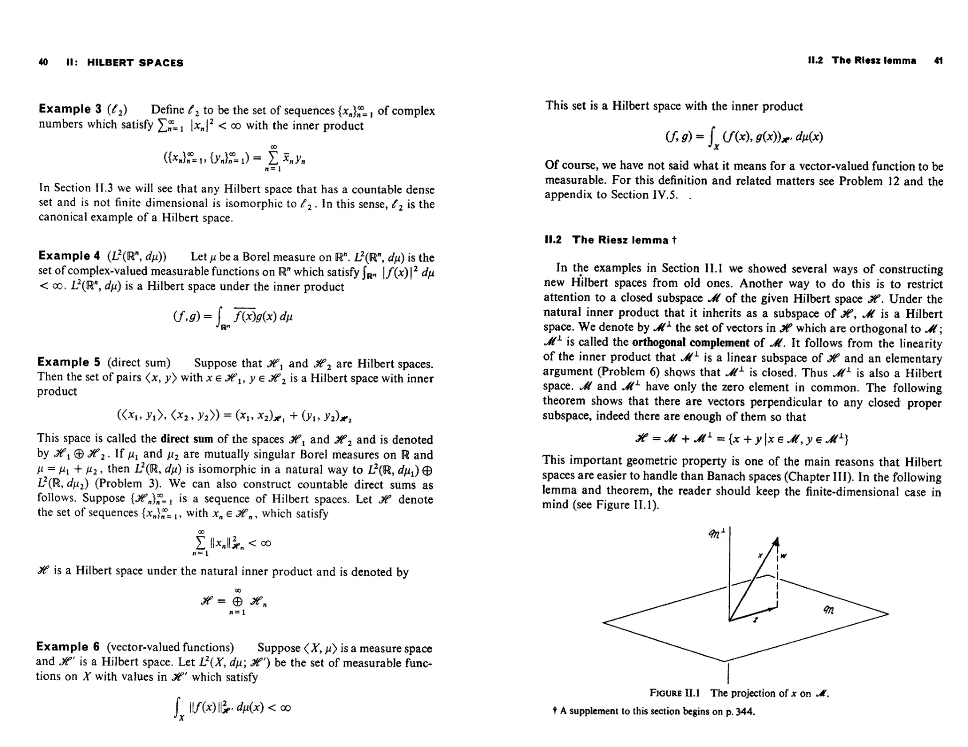
/.	The geometry of Hilbert space	36
2,	The Riesz lemma	41
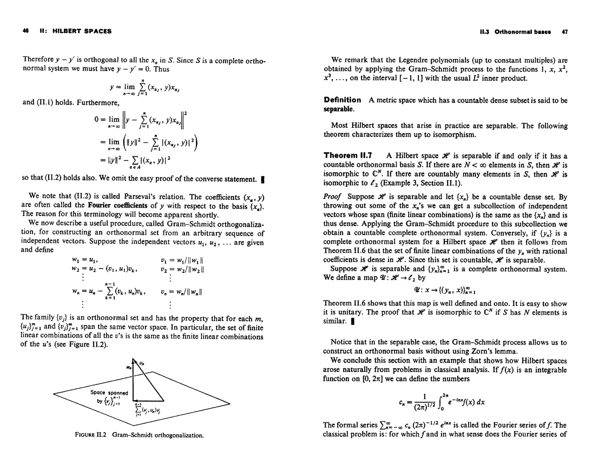
3.	Orthonormal bases	44
4.	Tensor products of Hilbert spaces	49
5.	Ergodic theory: an introduction	54
Notes	60
Problems	63
xi
xii CONTENTS
III:	BANACH SPACES
1.	Definition and examples	67
2.	Duals and double duals	72
3.	The Hahn-Banach theorem	75
4.	Operations on Banach spaces	78
5.	The Baire category theorem	and its consequences	79
Notes	84
Problems	86
IV:	TOPOLOGICAL SPACES
1.	General notions	90
2.	Nets and convergence	95
3.	Compactness	97
Appendix The Stone-Weierstrass theorem	103
4.	Measure theory on compact spaces	104
5.	Weak topologies on Banach spaces	111
Appendix Weak and strong measurability	115
Notes	117
Problems	119
V:	LOCALLY CONVEX SPACES
/. General properties	124
2.	Frechet spaces	131
3.	Functions of rapid decease and the tempered distributions 133
Appendix The N-representation for and Sf’	141
4.	Inductive limits: generalized functions and weak solutions of
partial differential equations	145
5.	Fixed point theorems	150
6.	Applications of fixed point theorems	153
7.	Topologies on locally convex spaces: duality theory and the
strong dual topology	162
Appendix Polars and the Mackey-Arens theorem	167
Notes	169
Problems	173
Contents xiii
VI:	BOUNDED OPERATORS
/.	Topologies on bounded operators	182
2.	Adjoints	185
3.	The spectrum	188
4.	Positive operators and the polar decomposition	195
5.	Compact operators	198
6.	The trace class and Hilbert-Schmidt	ideals	206
Notes	213
Problems	216
VII:	THE SPECTRAL THEOREM
1.	The continuous functional calculus	221
2.	The spectral measures	224
3.	Spectral projections	234
4.	Ergodic theory revisited:	Koopmanism	237
Notes	243
Problems	245
VIII:	UNBOUNDED OPERATORS
1.	Domains, graphs, adjoints, and spectrum	249
2.	Symmetric and self-adjoint operators: the basic criterion
for self-adjointness	255
3.	The spectral theorem	259
4.	Stone’s theorem	264
5.	Formal manipulation is a touchy business: Nelson’s
example	270
6.	Quadratic forms	276
7.	Convergence of unbounded operators	283
8.	The Trotter product formula	295
9.	The polar decomposition for closed operators	297
10.	Tensor products	298
11.	Three mathematical problems in quantum mechanics	302
Notes	305
Problems	312
Xiv CONTENTS
THE FOURIER TRANSFORM
7. The Fourier transform on «^(R") and ^'(R"), convolutions 318
2. The range of the Fourier transform: Classical spaces	326
3. The range of the Fourier transform: Analyticity	332
Notes	338
Problems	339
SUPPLEMENTARY MATERIAL
11	.2. Applications of the Riesz lemma	344
Ill	.l. Basic properties of Lp spaces	348
IV	.3. Proof of Tychonoff s theorem	351
I	V.4. The Riesz-Markov theorem for X = [0, 7 ]	353
IV	.5. Minimization of functionals	354
V.5	. Proofs of some theorems in nonlinear functional analysis	363
VI.5	. Applications of compact operators	368
VI	I 1.7. Monotone convergence for forms	372
V	I11.8. More on the Trotter product formula	377
Uses of the maximum principle	382
Notes	385
Problems	387
List of Symbols
Index
393
395
Contents of Other Volumes
Volume II: Fourier Analysis, Self-Adjointness
IX The Fourier Transform
X Self Adjointness and the Existence of Dynamics
Volume III: Scattering Theory
XI Scattering Theory
Volume IV: Analysis of Operators
XII Perturbation of Point Spectra
XIII Spectral Analysis
XV

I: Preliminaries
The beginner... should not be discouraged if... he finds that he does not have the prerequisites
for reading the prerequisites.	P. Halmos
1.1 Sets and functions
We assume that the reader is familiar with sets and functions but it is
appropriate to standardize our terminology and to introduce here abbrevia-
tions that will occur throughout the book.
If X is a set, x e X means that x is an element of X; x ф X means that x is
not in X. The clause “for all x in X" is abbreviated (Vxe X) and “there
exists an xgX such that” is abbreviated (3xeX). The symbol {x|P(x)}
stands for the set of x obeying the condition (or conditions) P(x). If A is a
subset of X (denoted А с X), the symbol Х\Л represents the complement of
A in X, that is Х\Л = {x e X | x ф A}. More generally, if A and В are subsets
of X, then A\B = {x|x e A, x ф В}. When we discuss sets with a topology, A
will always denote the closure of the set A. Finally, the set of ordered pairs
{<x, У> I * e X, У e Y} is called the Cartesian product of X and У and is
denoted X x У.
We will use the words “function” and “mapping” interchangeably. In
order to emphasize that certain functions f depend on two variables, we will
sometimes write /(•,•)• The symbol denotes the function of one
variable obtained by picking a fixed value of у for the second variable. A
1
2 I: PRELIMINARIES
linear function will also be called an operator or a linear transformation. Our
functions will always be single valued; so a function from a set X to another
set Y, denoted by/: X -» У or xZ> Y or x i-+/(x) will have one and only one
value in У for each x e X. If A a X, then/[Л] = {/(x)|x e A} is a subset of
У and /~х[5] = {x|/(x) 6 B} is a subset of X if В с: У. /[X] will usually be
called the range of f and will be denoted Ran /. X is called the domain of /
A function / will be called injective (or one-one) if for each у e Ran / there
is at most xeX such that /(x) = y; f is called surjective (or onto) if
Ran /= У. If / is both injective and surjective, we will say it is bijective. The
restriction of / to a subset A of its domain will be denoted by/fX.
If X о A we define the characteristic function /^(x) as
, ч (1 if x e A
XaW ~ |0 x A
There are two set theoretic notions which are slightly deeper than mere
notation, so we will discuss them to some extent. A relation R on a set X is a
subset R of X x X; if <x, уУ e R, we say that x is related (or R-related) to
у and write xRy.
Definition A relation R is called an equivalence relation if it satisfies:
(i)	(Vx e X) xRx [reflexive]
(ii)	(Vx, у e X) xRy implies yRx [symmetric]
(iii)	(Vx, y, z e X) xRy and yRz implies xRz [transitive]
The set of elements in X that are related to a given x e X is called the
equivalence class of x, denoted usually as [x].
It is easy to prove:
Theorem 1.1 Let R be an equivalence relation on a set X. Then each
x e X belongs to a unique equivalence class.
Thus, under an equivalence relation, a set divides up in a natural way into
disjoint subsets.
Example 1 (the integers mod 3) Let X be the integers and write xRy
if x — у is a multiple of 3. This equivalence relation divides the integers into
three equivalence classes:
[0] = {..., -6, -3,0, 3, 6,...}
[!] = {..., -5, -2,1,4, 7,...}
[2) = {..., —4, -1,2, 5, 8,...}
1.2 Metric and normed linear spaces 3
Example 2 (the real projective line) Let R denote the real line and let
X be the nonzero vectors in R2 (= R x R). We write xRy if there is some
a e R with x = ay. The equivalence classes are lines through the origin (with
<0, 0> removed).
Next, we discuss Zorn’s lemma.
Definition A relation on a set X which is reflexive, transitive, and anti-
symmetric (that is, xRy and yRx implies x = y) is called a partial ordering.
If J? is a partial ordering, we often write x < у instead of xRy.
Example 3 Let X be the collection of all subsets of a set У. Define
A -< В if A с: B. Then -< is a partial ordering.
We use the word “ partial ” in the above definition because two elements
of X need not obey x -< у or у -< x. If for all x and у in X, either x -</ or
у -< x, X is said to be linearly ordered. For example, R with its usual order <
is linearly ordered.
Now suppose X is partially ordered by -< and У c X. An element p e X
is called upper bound for У if у -< p for al lye У. IfweY and m -< x implies
x = m, we say m is a maximal element of X.
Depending on one’s starting point, Zorn’s lemma is either a basic assump-
tion of set theory or else derived from the basic assumptions (it is equivalent
to the axiom of choice). We take Zorn’s lemma and the rest of set theory as
given.
Theorem 1.2 (Zorn’s lemma) Let X be a nonempty partially ordered set
with the property that every linearly ordered subset has an upper bound in X.
Then each linearly ordered set has some upper bound that is also a maximal
element of X.
Finally, we will use Halmos’ | to indicate the conclusion of a proof.
1.2 Metric and normed linear spaces
Throughout this work, we will be dealing with sets of functions or operators
or other objects and we will often need a way of measuring the distance
4 I: PRELIMINARIES
between the objects in the sets. It is reasonable to define a notion of distance
that has the most important properties of ordinary distance in R3.
Definition A metric space is a set M and a real-valued function d(-, •)
on M x M which satisfies:
(i)	d(x, у) > 0
(ii)	d(x, 7) = 0 if and only if x = у
(iii)	d(x, y) = d(y, x)
(iv)	d(x, z) £ d(x, + d(y, z) [triangle inequality]
The function d is called a metric on M.
We often call the elements of a metric space points. Notice that a metric
space is a set M together with a metric function tZ; in general, a given set X
can be made into a metric space in different ways by employing different
metric functions. When it is not clear from the context which metric we are
talking about, we will denote the metric space by <M, d), so that the metric
is explicitly displayed.
Example 1 Let M = R" with the distance between two points x =
<xls..., x„> and у = <yn ..., yn> given by
d(x, y) = J(xt - yd2 + •• + (*«- K)2
Example 2 Let M be the unit circle in R2, that is, the set of all pairs of
real numbers <a, with a2 + ]32 = 1, and let
<A««, 0>, <«', Д'» = V(« - a')2 + (Д - Я2
Another possible metric is d2[p, />'] = arc length between the points p, p'
(see Figure 1.1).
Figure LI The metrics di and d2.
1.2 Metric and normed linear spaces 5
Example 3 Let M = C[0, 1], the continuous real-valued functions on
[0, 1 ] with either of the metrics
9) = max | f(x) - g(x) j d2(f g) = P | f(x) - g(x) | dx
X€[O,1]
Now that we have a notion of distance, we can say what we mean by
convergence.
Definition A sequence of elements {*„}“= x of a metric space <M, d) is
said to converge to an element x e M, if d(x, x„) -»0 as n -» oo. We will often
denote this by xn—d—> x or Пт„_ю xn = x. If xn does not converge to x, we
will write xn—/_> x.
In Example 2, dfjy, p'~) < d2(p, p') ^ndfp, p') which we will write
< d2 < rjf. Thuspn.	> p if and only if I2...>/>. But in Example 3, the
metrics induce distinct notions of convergence. Since d2 < dt iL^/implies
f„___f, but the converse is false. A counterexample is given by the functions
gn defined in Figure 1.2, which converge to the zero function in the metric d2
Figure 1.2 The graph of ^„(x).
but which do not converge in the metric dv This may be seen by introducing
the important notion of Cauchy sequence.
Definition A sequence of elements {*„} of a metric space <M, d) is
called a Cauchy sequence if (Ve > 0)(3JV) n, m > N implies d(x„, xm) < e.
Proposition Any convergent sequence is Cauchy.
Proof Given xn -> x and e, find N so n > N implies d(xn, x) < e/2. Then
n, m > N implies d(xn, xm) < d(x„, x) + d(x, xm) < |e +	|
6 I: PRELIMINARIES
We now return to the functions in Figure 1.2. It is easy to see that if n m,
{9n	= 1 • Thus g„ is not a Cauchy sequence in <C[0,1 ], dx > and therefore
not a convergent sequence. Thus, the sequence {p„} converges in <C[0, 1], t/2>
but not in <C[0, 1], f/j).
Although every convergent sequence is a Cauchy sequence, the following
example shows that the converse need not be true. Let Q be the rational
numbers with the usual metric (that is, d(x, y) = | x — у |) and let x* be any
irrational number (that is, x* e R\Q). Find a sequence of rationale x„ with
x„ -► x* in R. Then x„ is a Cauchy sequence of numbers in Q, but it cannot
converge in Q to some у e О (for, if x„ -+y in Q, then xn -+y in R, so we
would have у = x*).
Definition A metric space in which all Cauchy sequences converge is
called complete.
For example, R is complete, but Q is not. It can be shown (Sections 1.3 and
1.5) that <C[0, 1], d^ is complete but <C[0, 1], f/2> is not. The example of Q
and R suggests what we need to do to an incomplete space X to make it
complete. We need to enlarge X by adding “ all possible limits of Cauchy
sequences.” The original space X should be dense in the larger space X
where:
Definition A set В in a metric space M is called dense if every m e M is a
limit of elements in B.
Of course, if the incomplete space is not already contained in a larger
complete space (like Q is contained in R) it is not clear what “ all possible
limits” means. That this “completion” can be done is the content of a
theorem that we shall shortly state; but first some definitions:
Definition A function f from a metric space <X, d} to a metric space
< У, p) is called continuous at x if /(xB) <y,p> » /(x) whenever x# 	> x.
We have already had an example of a sequence of elements in C[0,1] with
fn d2 > 0 but 0. Thus the identity function from <C[0, 1], <Z2> to
<C[0, I], Ji) is not continuous but the identity from <C[0, 1], d^ to
<C[0, 1], d2y is continuous.
1.2 Metric and normed linear spaces 7
Definition A bijection h from <X, tZ> to <У, p> which preserves the
metric, that is,
р(Л(х), h(y)) = d(x, y)
is called an isometry. It is automatically continuous. (X, cT) and < У, p> are
said to be isometric if such an isometry exists.
Isometric spaces are essentially identical as metric spaces; a theorem con-
cerning only the metric structure of <X, d) will hold in all spaces isometric
to it.
We now state precisely in which sense an incomplete space can be fattened
out to be complete:
Theorem 1.3 If <M, dy is an incomplete metric space, it is possible to
find a complete metric space M so that M is isometric to a dense subset of M.
Sketch of proof Consider the Cauchy sequences {x„} of elements of M. Call
two sequences, {x„}, {ym}, equivalent if !im^s d(x„, y„) = 0. Let Л? be the
family of equivalence classes of Cauchy sequences under this equivalence
relation. One can show that for any two Cauchy sequences d(x„} у„)
exists and depends only on the equivalence classes of {x„} and {y„}. This limit
defines a metric on M and M is complete. Finally, map M into M by taking x
into the constant sequence in which each x„ equals x. M is dense in X? and
the map is isometric. |
To complete our discussion of metric spaces, we want to introduce the
notions of open and closed sets. The reader should keep the example of open
and closed sets on the real line in mind.
Definition Let <X, be a metric space:
(a)	The set {x | x e X, d(x, y) < r} is called the open ball, B(y; r), of radius
r about the point y.
(b)	A set О cz X is called open if (Xfy e O)(3r > 0) B(y; r) <zz O.
(c)	A set N с X is called a neighborhood of у e N if B(y; r) cz N for some
r > 0.
(d)	Let E с X. A point x is called a limit point of E, if (Vr > 0)
B(x: r) n (£\{x}) 0, that is, x is a limit point of £ if £ contains points
other than x arbitrarily near x.
(e)	A set F cz X is called closed if F contains all its limit points.
(f)	If G cz X, x e G is called an interior point of G, if G is a neighborhood
of x.
8 I: PRELIMINARIES
The reader can prove for himself the following collection of elementary
statements:
Theorem 1.	4 Let <X, d") be a metric space:
(a)	A set, O, is open if and only if X\O is closed.
(b)	xm ——» x if and only if for each neighborhood N of x, there exists an
M so that m> M implies xm e N.
(c)	The set of interior points of a set is open.
(d)	The union of a set E with its limit points is a closed set (denoted by Ё
and called the closure of E).
(e)	A set is open if and only if it is a neighborhood of each of its points.
One of the main uses of open sets is to check for convergence using
Theorem I.4.b and in particular to check for continuity via the following
criteria, the proof of which we leave as an exercise:
Theorem 1.	5 A function /(•) from a metric space X to another space У
is continuous if and only if for all open sets Ос У, f ~1 (ii) [O] is open.
Finally, we warn the reader that often in incomplete metric spaces, closed
sets may not appear to be closed at first glance. For example, [|, 1) is closed in
(0, 1) (with the usual metric).
We complete this section with a discussion of two of the central concepts of
functional analysis: normed linear spaces and bounded linear transformations.
Definition A normed linear space is a vector space, V, over R (or C)
and a function, ||’|| from V to R which satisfies:
(i)	|| v || >0 for all у in	К
(ii)	|| v || = 0 if and only	if	v — 0
(iii)	||ay|| = |a| ||y|| for	all	v in V and	a	in R	(or C)
(iv)	||v 4- w|| < || v|| 4- ||w||	for all	v	and	w in	V
Definition A bounded linear transformation (or bounded operator) from
a normed linear space <7,, || ||t> to a normed linear space <K2, || ||2> is a
function, T, from to V2 which satisfies:
(i) T(av 4- /?w) = <xT(v) 4- flT(w) (Vy, w e F)(Va, 06 IR or C)
(ii) For some C > 0, ||Ty||2 < C||y||i
1.2 Metric and normed linear spaces 9
The smallest such C is called the norm of T, written ||T|| or ||T||1>2 • Thus
11П = sup ||Tr||2
IM 1 = 1
Since we will study these concepts in detail later, we will not give many
examples now but merely note that R" with the norm
||<Х1,...,Хл>|| = У|Х1|2 + -'-+ i*„|2
and C[0, 1 ] with either the norm
(1Лоо= sup |/(x)| or ll/lli = f |/(x)| dx
xe[O,l]	•'O
are normed linear spaces. Observe also that any normed linear space <7, || • ||>
is a metric space when given the distance function d(v, w) — ||v — w ||. There
is thus a notion of continuity of functions, and for linear functions this is
precisely captured by bounded linear transformations. The proof of this fact
is left to the reader.
Theorem 1.	6 Let T be a linear transformation between two normed
linear spaces. The following are equivalent:
(a)	T is continuous at one point.
(b)	T is continuous at all points.
(с)	T is bounded.
Definition We say </, || • ||> is complete if it is complete as a metric
space in the induced metric.
If <X, || • ||> is a normed linear space, then X has a completion as a metric
space by Theorem 1.3. Using the fact that X is dense in J?, it is easy to see that
X can be made into a normed linear space in exactly one natural way.
All these concepts are well illustrated by the following important theorem
and its proof:
Theorem 1.	7 (the B.L.T. theorem) Suppose T is a bounded linear trans-
formation from a normed linear space (K15 || • to a complete normed linear
space </2, II *ll2>- Then T can be uniquely extended to a bounded linear
transformation (with the same bound), T, from the completion of E to
<V2, ||-||2>.
10 I: PRELIMINARIES
Proof Let be the completion of Vt. For each x in P), there is a sequence
of elements {x„} in with xn -* x as n -* oo. Since xn converges, it is Cauchy,
so given £, we can find N so that n,m> N implies ||x„ — Ih < e/ ||T||. Then
\\Txn - Txm||2 = ||T(xn - xm)||2 <, ||T|| ||x„ - xmlb < e which proves that
Tx„ is a Cauchy sequence in V2. Since V2 is complete, Tx„ -»у for some y. Set
Tx = y. We must first show that this definition is independent of the sequence
xn~* x chosen. If x„ -+ x and x'n -> x, then the sequence x2, xj, x2, x2 x
so Tx,. Тх'х,... -»у for some у by the above argument. Thus lim Тхп = у =
lim Tx„. Moreover, we can show T so defined is bounded because
||Tx |j2 = lim ||Txrt||2 (see Problem 8)
Л’» OO
< Tim C || xn || t (see Appendix to 1.2)
И-+ 00
= C||x||t
Thus T is bounded. The proofs of linearity and uniqueness are left to the
reader. |
We can use this theorem to give a very elegant definition of the Riemann
integral. Let PC[a, b] be the family of bounded piecewise continuous func-
tions on [a, ft], which are continuous from the right, that is, limxiy /(x) = /(y)
and for which IimxTj, /(x) exists at each у and is equal to f(y) for all but
finitely many y. Norm PC with the norm
ll/IL = sup |/(x)|
x e [a, b]
Let x0,..., x„ be a partition of the interval [a, ft], x0 = a, x„ ~ b. Let x,(x)
be the characteristic function of [^M,x,) except for /„(x) which is the
characteristic function of	A function on [a, ft] of the form
1 ^x/x) with si real *s called a step function (to see why, draw its graph).
The set of all step functions for all possible finite partitions is a normed
linear space with the norm
= sup	max |sf|
i= 1	oo x e [a, t>]	i=l,...,n
Denote this space by S[a, ft]. It is a nice exercise (Problem 10) to prove that
S(a, ft] is dense in PC[a, ft]. For any step function,	we define
I ( f SiZi(x)) = Z Фа ~ xf- J
the intuitive value of the integral f /;(х)] dx. I is a linear transformation
from S[a, ft] to the real numbers, and because
Appendix to 1.2 Lim sup and lim inf 11
f E5iXi) = IE-xi-i)|
\i = 1	/
n
<	max | \ | £ I xi ” x> -11
। = i
<	||EsiX>-||oo(6 - «)
I is a bounded linear transformation. Since the real numbers are complete, I
can be uniquely extended to S, the completion of S (by the B.L.T. theorem).
The extended transformation Z(/), restricted to PC is called the Riemann
integral and is denoted by
/(/) = f7^
J a
While this method does not appear as the most intuitive definition of the
Riemann integral, it wifi be seen upon reflection that the proof is really just
the “usual” proof put into the language of completion and the B.L.T.
theorem. It illustrates a main point of general philosophy in functional
analysis: In order to define something on a normed linear space, it is often
convenient to define it on a dense set and extend it by the B.L.T. theorem.
The reader should try his hand at constructing the Riemann-Stieltjes integral
(Problem 11). By using the same method, we can define the Riemann integral
for continuous functions taking values in any complete normed linear space,
in particular, for complex-valued functions.
Appendix to 1.2 Lim sup and lim inf
Lim sup and lim inf are notions which may be unfamiliar to the reader, so
we summarize their definition and properties.
Definition Let A <= R be a nonfinite bounded set. Let lim pt(/4) = set of
limit points of A. Then the limit superior of A is defined by
lim sup A ~ Tim A = sup{x | x e lim pt(/l)}
Similarly
lim inf A = lim(^) = inf{x|x e lim pt(Z)}
Remarks 1. When A is bounded, lim pt(T) is always nonempty by the
Bolzano-Weierstrass theorem.
12 I: PRELIMINARIES
2. If A is not bounded above, one defines Um A = +oo. If A is bounded
above and lim pt(T) = 0 one defines fim A = — co.
3. Um A is actually in lim pt(^4). For let b = lim A and let £ > 0 be given.
We can find a e lim pt(^) so |d — a| < fi/2. Since a e lim pt(J), we can find
de A with |a — <У| < fi/2; so given e, we find de A with |Z> — d\ < e, that is,
b e lim pt(/4).
Urn A has a very simple alternative characterization, whose proof we leave
to the reader.
Proposition Let b = fim A. Then for г > 0, A n {aja > b + fi} is finite
and A n {a | <7 > b — e} is infinite.
For a sequence {an}, we say b e lim pt{a„) if for all N and all e, there is an
n > N with j b ~ a„ | < e. We define fim(a„) = sup{&| b e lim pt{a„}}.
Finally, let us summarize the properties of fim (all for bounded sets; it is a
useful exercise to decide which extend to unbounded sets).
Proposition
(a)	fim(a„ + Z>„) < fim an + lim bn
(b)	Hm an bn < (fim a„)(Iim £>„) if an, bn > 0
(c)	hm(c4?n) — c fim an if c > 0
(d)	lim(cnn) — c lim an if c < 0
1.3 The Lebesgue integral
We have just seen that C[a, Z>] has two quite reasonable metrics on it. In
Section 1.5 we will see that it is a complete metric space in the metric
(f, 9> = sup j fix) - g(x) |
x e [a, b]
In the other metric we considered, d2(f, g) — \\f — д\\л with UAlfi =
| h(x) | dx, C[a, Z>] is not complete. To see this for C[0, 1], let f„ be given as
in Figure 1.3. It is not hard to see that f„ is Cauchy in || * ||j, but it does not
converge to any function in C[a, 6]; rather, in an intuitive sense, it “ converges ”
to the characteristic function of [|, (which is, of course, not in C[0, 1 ]!).
1.3 The Lebesgue integral 13
Figure 1.3 The graph of f„.
We can always complete C[a, h] in || - lli realizing elements of the completion
as equivalence classes of Cauchy sequences of continuous functions; this
realization is not noteworthy for its transparency. The example above
suggests we might also be able to realize elements of the completion as
functions. If we do realize them as functions, we should be able to define the
integral J* | f(x) | dx (merely as d2(f, 0)!) for any /in the completion.
The simplest way to realize elements of the completion as functions is to
turn the above analysis around: one introduces an extended notion of integral
on a bigger space than C[a, Z>]; call it l}[a, Z>]. We will prove L1 is complete, so
by general arguments the closure of C in I) is complete (and it turns out
C = L*).
Mow, how can one extend the notion of Riemann integral? The usual
definition of the Riemann integral is based on dividing the domain of / into
finer and finer pieces. For “ nasty ” functions, this method does not work and
The Lebesgue integral
Figure 1.4
14 I: PRELIMINARIES
so a different method is needed—the simplest modification is to divide the
range into finer and finer pieces (Figure 1.4). This method depends more on
the function and so has the possibility of working for more types of functions.
We are thus interested in sets f~x[a, 6] and their size. We suppose we have
a size function p. on sets which generalizes p([a, b]) = b — a. We will shortly
return to this size function and see that not all sets have a “ size.” We will then
restrict the types of/by demanding that Z>] have a “size.” Looking at
Figure 1.4, we define for f > 0
00 m /
L(/)= Z -Лг1 (ii) (iii)
tn
n
m + 1
n

Then Yin (/) > Ел (/) so that £2» (/) = supn (£2„ (/)) exists (it may
be co). This limit is defined to be f f dx. We remark that for technical purposes
(that is, proving theorems!) one makes a different definition which can be
shown to agree with this definition only after a lot of work. The definition
as lim Yi" (/) is however the best to keep in mind when thinking intuitively.
Thus, we have transferred the problem to one of defining an extended
notion of size. We must first decide what sets are to have a size. Why not all
sets ? There is a classical example (see also Problem 13) which shows that not
al I sets in R3 can have a size if we want that size to be invariant under rotations
and translations (and not to be trivial, such as assigning zero to ail sets):
it is possible to break up a unit bail into a finite number of wild pieces, move
the pieces around by rotation and translation and reassemble the pieces to
get two balls of radius one (Banach-Tarski paradox). Thus, ail sets cannot
have a size, and so some family & of sets will be the “measurable sets.” What
properties do we want 38 to have? We would like both f~1 [[0, a)] and
f~1 [[a, oo)] to be measurable (/ > 0) so we would like to have the property:
A e 38 implies К\Л e Also, when /is continuous, we want/-1 [(a, £)] to
be in so 38 should contain the open sets. Finally, we want to have
U = E ХЛ)
\л= 1	/ и=1
if the An are mutually disjoint (to meet our intuitive notion of size) so we
would like г A„ e 38 if each An is in
Definition The Borel sets of R is the smallest family of subsets of R with
the following properties:
(i) The family is closed under complements.
(ii) The family is closed under countable unions.
(iii) The family contains each open interval.
1.3 The Lebesgue integral 15
To see that such a smallest family exists we note that if {^a}ae A is a collec-
tion of families obeying (i), (ii), and (iii), then so does Qae A &a. Thus the
intersection of all families obeying (i)-(iii) is the smallest such family.
Now we define the Lebesgue measures of sets in the Borel sets in R.
Definition Let J be the family of all countable unions of disjoint open
intervals (which is just the family of open sets) and let
U (a< > bj) = ^(ь£-ад
(which may be infinite). For any define
д(В)=т£д(/)
This notion of size has four crucial properties:
Theorem 1.8
(a)	X0) = O
(b)	If {/f„}®=i <= & and the A„ are mutually disjoint (An n Am — 0, all
m * n), then m(U“= i = & i KAn)-
(c)	^(B) = inf{/x(Z) | В с I, I is open}
(d)	/z(B) = sup{ju(C) | С с В, C is compact}
The infinite sum in (b) contains only positive terms, so it either converges
to a finite number or diverges to infinity, in which case we set it equal to oo.
(c) and (d) say that any Borel set can be approximated “ from the outside ”
by open sets and from the inside by compact sets. We remind the reader that
on the real line a set is compact if and only if it is closed and bounded.
We have thus extended the usual notion of size of intervals and we define
the family of functions we will consider in the obvious way:
Definition	A function f is called a Borel function if and only if f 1 [(a, b)]
is a Borel set for all a, b.
It is often convenient to allow our functions to take the values + oo on
small sets in which case we require/-1[{±oo}] to be Borel.
Proposition f is a Borel if and only if, for all В e /'][B]e^
(see Problem 14).
16 I: PRELIMINARIES
This last proposition implies that the composition of two Borel functions
is Borel. Many books deal with a slightly larger class of functions than the
Borel class. They first define a set M to be measurable if one can write
M и Ax — В и A2 where В is Borel and <= with B, Borel and /i(Bt) = 0
(thus they add and subtract “ unimportant ” sets from Borel sets). A measur-
able function is then defined as a function, f, for which/~J[(a, #)] is always
measurable. It is no longer true that f о g is measurable if f and g are, and
many technical problems arise. In any event, we deal only with Borel sets and
functions and use the words Borel and measurable interchangeably.
Borel functions are closed under many operations:
Proposition (a) If / g are Borel, then so are f + g,fg, max{/ g} and
min{/ g}. If /is Borel and Л e R, z/is Borel.
(b) If each /„ is Borel, n= 1,2,..., and /n(p)->/(p) for all p, then f
is Borel.
Since |/| = max{/ —/}, \f | is measurable if /is.
As we sketched above, given/> 0, one can define jf dx (which may be oo).
If j | /1 dx < oo, we write/e and define f f dx == J/+ dx — j/_ dx where
/+ = max{/ 0}; /_ = max{—/ 0). f£x(a, b) is the set of functions on (a, b)
which are in if we extend them to the whole real line by defining them to
be zero outside of (a, b). If /e SP'fa, b), we write \fdx = /dx. We then
have:
Theorem 1.9 Let/and g be measurable functions. Then
(a)	If fge <&*(д, b), so are/+ g and 2/ for all Лей.
(b)	If |0| </and/e JS?1, then g e &.
(c)	f (/+ 9) dx — jfdx + f 9 dx if/and g are in
(d)	jj/Jx| < J i/i dx if/is in
(e)	If / < g, then dx < f g dx, if / and g are in J?1.
(f)	If / is bounded and measurable on —00 < a < b <co, then/e	and
sup |/(x)|
a<x£ b
This theorem shows that f has all the nice properties of the Riemann
integral even though it is defined for a larger class of functions.
The properties that make the space L1 (which we will shortly define)
complete are the following absolutely essential convergence theorems:
1.3 The Lebesgue integral 17
Theorem 1.1	0 (monotone convergence theorem) Let f, > 0 be measur-
able. Suppose /„(p) -*/(p) for each p and that /n+s(p) >/„(p) all p and n (in
which case we write fn/f). If J /я(р) dp < C for all n, then /б and
J 1/(р)-/я(р)|ф->0 as «->oo.
Theorem 1.1	1 (dominated convergence theorem) Let /,(p)->/(p) for
each p and suppose (/n(p)| G(p) for all n and some G e jSf1. Then
and J | f(p)	J dp -> 0 as n -> oo.
In the latter case, we say G dominates the pointwise convergence. That a
dominating function exists is crucial. For example, let ffx) = (1/п)х(_„п](х).
Then fn(x) -* 0 for each x, but j | f„ | dx = 2 so f | ffx) j dx does not go to
zero. In this case, it is not hard to see that sup„ |/„(x)| = G(x) is not in ^f!.
We are almost ready to define jSf1 as a metric space by letting p(f, g) =
J I f — 91 dx. We cannot quite do this because J | f — g | dx = 0 does not
imply f^g (for example, f and g might differ at a single point). Thus, we
first define the notion of almost everywhere (a.e.):
Definition We say a condition C(x) holds almost everywhere (a.e.) if
{x | C(x) is false} is a subset of a set of measure zero.
Definition We say two functions f g e are equivalent if fix) = g(x)
a.e. (this is the same as saying j \ f — p| dx = 0).
Definition The set of equivalence classes in is denoted by as L1.
L1 with the norm Ц/Ц, — J ]/| dx is a normed linear space.
Thus an element of L1 is an equivalence class of functions equal a.e. In
particular when f e L1, the symbol f(x) for a particular x does not make sense.
Nevertheless we continue to write “/(x)” but only in situations where state-
ments are independent of a choice from the equivalence class. Thus, for
example, /n(x) -> f(x) for almost all x is independent of the representatives
chosen for/and/„. By this replacement of pointwise convergence with point-
wise convergence almost everywhere, the two convergence theorems carry
over from J5T1 to L1.
Having cautioned the reader that /(x) is “technically meaningless” for
/e L1, we remark that in certain special cases it is meaningful. Suppose f 6 L1
18 I: PRELIMINARIES
has a representative / (that is, / is a function; f an equivalence class of func-
tions) which is continuous. Then no other representative of f is continuous,
so it is natural to write f(x) for /(x).
The critical fact about L1 is:
Theorem 1.1	2 (Riesz-Fisher) L1 is complete.
Proof Let fn be Cauchy in L1. It is enough to prove some subsequence
converges (see Problem 3) so pass to a subsequence (also labeled /„) with
IIA-/n+Ilh<2-". Let
gm(x) = f !/»(*) — Л+1(Х>|
Л=1
Let д?л be the infinite sum (which may be oo). Then gm/ g^ and
f l&nl E„=i ll/B ~/n+ill so by the monotone convergence theorem,
g^ e L1. Thus |рда(х)| < oo a.e. As a result
m— 1
Ш	-/.*.(*))
n=l
converges pointwise a.e. to a function /(x). Moreover, |/M(x) J <
l/i(*) 1 + 5oo(x) e L1 so /и ->/ in If by the dominated convergence theorem. |
This proof has a corollary (see Problem 17):
Corollary If fn -*/in L1, then some subsequence f„t converges pointwise
a.e. to f
As a final result which brings us full circle to our original motivation:
Proposition C[u, b] is dense (in |{-jli) in /[a, d], i.e. L1 is the com-
pletion of C.
Proof See Problem 18.
We defined 1? [«, as a space of real-valued functions. It is often con-
venient to deal with complex-valued functions, f whose real and imaginary
1.4 Abstract measure theory 19
parts are in Il [a, В]. When no confusion arises, we will denote this space, with
the norm
ll/lli = f I f\ dx
also by Ll[a, 6]. The integral of a complex-valued function is defined by
ffdx = JRe(/) dx + if Im(/) dx
1.4 Abstract measure theory
One of the most important tools which one combines with abstract func-
tional analysis in the study of various concrete models is “general” measure
theory, that is, the theory of the last section extended to a more abstract
setting.
The simplest way to generalize the Lebesgue integral is to work with
functions on the real line and with Borel sets but to generalize the underlying
measure; we consider this special case of abstract measure theory first. Recall
that the Lebesgue integral was constructed as follows. We started with a
notion of size for intervals, ц([а, Z>]) = b — a, and extended this in a unique
way to a notion of size for arbitrary Borel sets. Armed with this notion of
size for Borel sets, the integral of Borel functions was obtained by measuring
sets of the form &]). We found the vector space 13([0, 1], dx) con-
structed in the last section is just the completion of C[0, 1] with the metric
d2(f,g) = jo l/(*) — #(*)l dx, where we needed only the Riemann integral
to define d2.
Now suppose an arbitrary monotone function oc(x) is given (that is, x > у
implies a(x) 2: a(j>))- It is not hard to see that the limit from the right,
lime_0 a(x + jej) and the limit from the left, lime_0 a(x — |e|) exist; we write
them as a(x + 0) and a(x — 0) respectively. Since (a, b) does not include the
points a and b, it is natural to define дв((а, 6)) = a(Z> - 0) — a(a + 0). From
this notion of size for intervals, one can construct a measure on Borel sets
of R, that is, a map /za: SS -► [0, oo] with /ze ((JB,) = i ga(Bt) if B, n Bj = 0
and ga(0) = 0. By construction, this measure has the regularity property
^a(B) = sup {/1(C) | С с: В, C compact}
= inf{g(O) (В с О, О open}
20 I: PRELIMINARIES
Also, p(C) < co for any compact set C. A measure with these two regularity
properties is called a Borel measure. In particular, pa([a, b]) = a(b 4- 0) —
a(u — 0). One can then construct an integral /-* J/dy.a (we will also write
J/tZa) which has properties (a)-(e) of Theorem 1.9; it is called a Lebesgue-
Stieltjes integral. 1?([а, b], c/a) and L^R, tZa) can be formed as before. These
spaces of equivalence classes of functions are complete in the metric p(/, g) —
J |/ — p| da, and analogues of the monotone and dominated convergence
theorems hold. The continuous functions C[a, b] form a dense subspace of
1?([а, b], da); put differently, b], da) is the completion of C[a, b] with
the metric pa(/, g) — | f — g [ da. where we need only use the Riemann-
Stieltjes integral to define pa (see Problem 11).
Let us consider three examples which illustrate the variety of Lebesgue-
Stieltjes measures.
Example 1 Suppose a is continuously differentiable. Then b) =
(tZa/tZx) dx where dx is Lebesgue measure, so it is to be expected (and is
indeed true!) that
Thus, these measures can essentially be described in terms of Lebesgue
measure.
Example 2 Suppose that a(x) is the characteristic function of [0, oo).
Then pe(a, b) = 1 if 0 e (a, b) and is 0 if 0 ф (a, b). The measure one gets
out is very easy to describe: pa(B) =1 if 0 e B, and pe(B) = 0 if 0 ф В. The
reader is invited to construct explicitly the integral and convince himself that
=/(0)
This measure da is known as the Dirac measure (since it is just like a
5 function). Let us consider L^R, da) in this case. In JS?1 we have p(f, g) =
| /(0) — p(0) | so p(/, g) = 0 if and only if/(0) = p(0). As a result, we see that
the equivalence classes in L1 are completely described by the value/(0) so that
L*(R, da) is just a one-dimensional vector space! Notice how different this is
from the case of L^R, dx) where the value of a “function” at a single point
is not defined (since elements of L1 are equivalence classes).
Example 3 Our last example makes use of a fairly pathological function,
a(x), which we first construct. Let S be the subset of [0, 1]
5 = (j, f) u (|, f) и (%, f) и (^, u • • •
1.4 Abstract measure theory 21
0
2
Figure 1.5 The Cantor set.
that is, remove the middle third of what is not in S at each stage and add it
to 5, see Figure 1.5. The Lebesgue measure of S is -j- + 2(£) + 4(-^y) +
Let C - [0, 1 ]\S. It has Lebesgue measure 0. C, which is known as the Cantor
set, is easy to describe if we write each x e [0, 1 ] in its base three decimal
expansion. Then x e C if and only if this base 3 expansion has no Ts. Thus C
is an uncountable set of measure 0. To see this, map C in a one-one way onto
[0, 1] by changing 2’s into 1’s and viewing the end result as a base 2 number.
Now construct a(x) as follows: set а(л)=у on (у, у); a(x)=y on (y, f);
a(x) — on (§-, f), etc.; see Figure 1.6. Extend a to [0, 1] by making it con-
0
Figure 1.6 The Cantor function.
tinuous. Then a is a nonconstant continuous function with the strange
property that a'(x) exists a.e. (with respect to Lebesgue measure) and is zero
a.e. Now, we can form the measure . Since a is continuous, /ia({p}) = 0
for any set {p} with only one point. Nevertheless, pa is concentrated on the set
C in the sense that дв([0, 1 ]\C) = pa(S) = 0. On the other hand, the Lebesgue
measure of C is zero. Thus рл and Lebesgue measure “live” on completely
different sets.
In a sense we now make precise, these three examples are models of the
most general Lebesgue-Stieltjes measures. Suppose д is a Borel measure on R.
22 I: PRELIMINARIES
First, let P = {x| д({х}) / 0}, that is, P is the set of pure points of p. Since p is
Borel [д(С) < oo for any compact set], P is a countable set. Define
xeP n X
Then /ipp is a measure and /zcon( = jz - /zpp is positive. дсоп{ has the property
/zcont({pj) = 0 for all p, that is, it has no pure points and ppp has only pure
points in the sense that /zpp(X) = £xex MPP(W)-
Definition A Borel measure p on К is called continuous if it has nip pure
points, p is called a pure point measure if p(X) = £xeX p(x) for any Borel
set X.
Thus, we have seen:
Theorem 1.13 Any Borel measure can be decomposed uniquelyinto a
sum p = ppp + pcont where /zcont is continuous and ppp is a pure point measure.
We have thus generalized Example 2 by allowing sums of Dirac measures.
Is there any generalization of Examples 1 and 3 ?
Definition We say that p is absolutely continuous with respect to (w.r.t.)
Lebesgue measure if there is a function,/, locally I) (that is, J} | /(x) j dx < oo
for any finite interval (a, b)) so that
§gdp = §gfdx
for any Borel function g in Z3(R, dp). We then write dp = fdx.
This definition generalizes Example 1; we will eventually make a different
(but equivalent!) definition of absolute continuity.
Definition We say p is singular relative to Lebesgue measure if and only
if p(S) = 0 for some set S where has Lebesque measure 0.
The fundamental result is:
Theorem 1.14 (Lebesgue decomposition theorem) Let p be a Borel
measure. Then p - pac + /zsing in a unique way with /zac absolutely continuous
w.r.t. Lebesgue measure and with /zsing singular relative to Lebesgue measure.
1.4 Abstract measure theory 23
Thus Theorems 1.13 and 1.14 tell us that any measure д on R has a canonical
decomposition д = дрр + дас + /zsing where дрр is pure point, дас absolutely
continuous with respect to Lebesgue measure, and /zsing is continuous and
singular relative to Lebesgue measure. This decomposition will recur in a
quantum-mechanical context where any state will be a sum of bound states,
scattering states, and states with no physical interpretation (one of our
hardest jobs will be to show that this last type of state does not occur; that
is, that certain measures have да1пв = 0; (see Chapter XIII).)
This completes our study of measures on R. The next level of generalization
involves measures on sets with some underlying topological structure; we will
return to study this case of intermediate generality in Section IV.4. The most
general setting lets us deal with an arbitrary set. We first need an abstraction
of Borel sets:
Definition A nonempty family 2% of subsets of a set M is called a ст-ring
if and only if
(a)	Af e &, i = 1, 2,... implies x e 31.
(b)	If A, В e then A\B e 31.
If M e we say that is a ст-field.
The definition of measure is obvious(l):
Definition A measure on a set M with ст-ring is a map д: -* [0, oo]
with the properties:
(a)	X0) = O
(b)	if Atr.Aj = 0 forall i
\i=l / i=l
We shall often speak of the measure space <M, д> without explicitly men-
tioning but the ст-ring is a crucial element of the definition. Occasionally, we
will write <M, 31, g}. For certain pathologically “big” spaces, one wants to
use the notion of ст-ring rather than ст-field, but to keep things simple, we
will consider measures on ст-fields and will suppose the whole space isn’t
too big in the sense:
Definition A measure д on a ст-field & is called ст-finite if and only if
M = (Jv" i Ai with each д(Л () < oo.
We will suppose all our underlying measures are ст-finite.
24 I: PRELIMINARIES
Definition Let M, N be sets with ст-fields S and S. A map T: M -> N
is called measurable (w.r.t. and S) if and only if УЛ e S, Т-1[Л] e A
map f: M -* R is called measurable if it is measurable w.r.t. and the Borel
sets of R.
Given a measure p on a measure space M, we can define Jf dp for any
positive real-valued measurable function on M and we can form dp),
the set of integrable functions and I1(M, dp), the equivalence classes of func-
tions in equal a.e.[/д]. As in the case <M, dp) = <R, dx), the following
crucial theorems hold:
Theorem 1.1	5 (monotone convergence theorem) If f„ e SfM, dp),
0 <f(x) <f2(x) < • • • and fix) = Нш^ю/Л(х), then /e <£' if and only if
lim„^ ||/„Us < oo and in that case lim^^ \\f- fn= 0 and Ити^да HZ» Hi =
ll/llp
Theorem 1.1	6 (dominated convergence theorem) If /„e l){M, dp),
lim„rfoo/n(x) = /(x) a.e.[/i], and if there is a G e L1 with | f„(x)| < G(x) а.е.[д],
for all n, then fell and Нтл^00 /„Hi =0-
Theorem 1.1	7 (Fatou’s lemma) If /„e.?1, each fB(x) > 0 and if
limНЛHi < co> then/(x) = lim/n(x) is in & and \\f |!x < lim||/„||1.
Note In Fatou’s lemma nothing is said about limЦ/-ЛН1-
Theorem 1.1	8 (Riesz-Fisher theorem) 1)(M, dp) is complete.
One also has the idea of mutually singular:
Definition Let p, v be two measures on a space M with ст-field ?Л. We
say that p and v are mutually singular if there is a set A e S. with p(A) = 0,
v(M\A) = 0.
It is useful to take a Weaker looking definition of absolute continuity which
is essentially the opposite of singular:
Definition We say v is absolutely continuous w.r.t. p if and only if
p(A) = 0 implies v(J) = 0.
That this definition is the same as the previous one is a consequence of:
1.4 Abstract measure theory 25
Theorem 1.1	9 (Radon-Nikodym theorem) v is absolutely continuous
w.r.t. и if and only if there is a measurable function f so that
v(^) = J/(jc)zx(x) d^(x)
for any measurable set Л./is uniquely determined a.e. (w.r.t. ц).
Finally the Lebesgue decomposition theorem has an abstract form:
Theorem 1.2	0 (Lebesgue decomposition theorem) Let д, v be two
measures on a measure space <M, Then v can be written uniquely as
v = vac + vsing where д and vsiog are mutually singular and vac is absolutely
continuous w.r.t. j.i.
There is one final subject in measure theory which we must consider and
that involves changing the order of integration in a multiple integral. We first
must consider what functions can be multiply integrated:
Definition Let <M,	<W, be two sets with associated tr-fields.
Then the cr-field, ® J27 of subsets of M x N is defined to be the smallest
cr-field containing {/? x F\ R e FeF}.
Notice that if f: M x R is measurable (w.r.t. ^®^), then for any
meM, the function n n) is measurable (w.r.t. ,F). If v is a measure
on N such that $f(m, ri) dv(ri) exists for all m, then one can show that
m h-> J/(m, ri) dv(ri) is measurable (w.r.t. ^). There is a direct analogue of the
fact that absolute convergent sums can be rearranged at will:
Theorem 1.2	1 (Fubini’s theorem) Let f be a measurable function on
M x N. Let д be a measure on M, v a measure on N. Then
if and only if
I I \f(m, n)j tZv(n)| dn(m) < oo
M V N	/
I \f(m, w)| <7д(т)| dv(n) < oo
N\~ M	/
and if one (and thus both) of these integrals is finite, then
N\J M
dv(n) = I /(nt, ri) dv(n) I d[i(m)
26 I: PRELIMINARIES
In Problem 25, the reader will see that the finiteness of the integral of the
absolute value is critical.
Fubini’s theorem can be put into perspective by the notion of product
measure:
Theorem 1.2	2 Let p be a а-finite measure on <Af, and v a cr-finite
measure on <jV, J7). Then, there is a unique measure //®von <Af x N,
® obeying
(д® v)(/? x F) = /i(/?)v(F)
(where 0 • oo = 0). If f is a measurable function on M x N, then
f | f \f(m> «)I	< oo
JM\JN	/
if and only if
[	1/1 d(p® v) < oo
*N
and in that case
f	v) = f (f /dv) dp
One can describe the measure p®v quite explicitly. If Me^xJ7 and
Af <= (J® j R; x Fi we have (g® v)(Af) < x p(Ri)v(Fi). In fact, for any
M e x Л
(g ® v)(Af) = inf | У p(R^v(Fi) Af co (J .Rj x F,l
u=i	I f=l J
In particular, we can approximate M with a countable union of rectangles
making an arbitrarily small error.
1.5 Two convergence arguments
In this section we single out two “ tricks ” which we will have occasion to
use over and over. While they are elementary and the reader may well have
seen them, it seems reasonable to discuss them explicitly.
The first argument, which we will call the e/3 argument, is best seen in the
proof of:
1.5 Two convergence arguments 27
Theorem 1.23 Let C[u, Л] be the continuous functions on [a, with the
metric
dAf,g)= sup |/(x)-^(x)|
induced by the norm ||/*||0O ~	0). Then C[a, with the norm || •!}«, is
complete.
Proof Let f„ be a ||*||e-Cauchy sequence. Then, for any fixed xe[a, 5],
|/n(x) -/m(x)| < ||/n -/„.и -»0 as n, m -> co so/„(x) is a Cauchy sequence
of real numbers. Since the reals are complete, for each x there is a number,
f(x), with/„(x) -> f(x). Given g, find N so n,m> N implies	< s.
Then
sup |/(x) - fw(x)| = sup Нт|Л(х)-/л(х)|
eSxSb	a^x^b n-»oo
< sup sup 1Л(х)-Л(х)|
asix^bn^N
= sup \\f„ -7/vU < e
niN
Thus, if we can show that f e C[u, Z>], we can conclude that //-/„ [|x -► 0 so
/n->/in C[a, 6].
We are thus left with proving that f is continuous, or put differently that
“ a uniform limit of continuous functions is continuous.” Fix x e [a, Z>] and
s > 0. We want to find <5 so |x —	<5 implies |/(x) — f(y) | < s. Pick n so
that ||/и — /Ида < s/3. Now, since f„ is continuous, pick 3 so that |x —	<5
implies |/n(x) - fn(y)| < s/3. Then |x —	<3 implies
!/(%) -f(y)I < j/W ~Ш\ + |/„(x)	+ |Ш -f(y)\
<|e +
Thus f is continuous. |
What is the essence of the e/3 argument? We had a family of convergent
sequences /„(x) -> f(x) for each x and had uniform control on the rate of con-
vergence, that is, control independent of the object x that parametrized the
family. We also had some information on the behavior of f„(x) for fixed n
as the parameter x varied but this information was not necessarily uniform in n.
What we did is pictorially indicated in Figure 1.7; one could also call the g/3
argument the “ up, over, and around ” proof. In the next section we will
consider what happens when one has no uniform information on the rate of
convergence but instead has uniform control on how f„(x) behaves as x varies
(uniform in ri). There we will see an s/3 argument also works. For further
examples of the s/3 trick, see Problems 27, 29.
28 I: PRELIMINARIES
KU)- 4(/}|
KU)-/4x)|

Figure 1.7 The c/3 argument.
The second argument which we refer to as the “ diagonal sequence trick ”
is illustrated in:
Theorem 1.24 Let fn(m) be a sequence of functions on the positive
integers which is uniformly bounded, i.e. | fn(rri) | < C for all n, m. Then
there is a subsequence {/й{0(л?)}^i so that for each fixed /л,/й(0(ти) converges
as i-+ oo.
Proof Consider the sequence/,(l). It is a bounded set of numbers, so we can
find a subsequence so /„lti)(l) ->/^(1), for some number /^(1). Now
consider the sequence /П1(0(2). We can find a subsequence /„2(i)(2) -*/^(,2) as
i -> oo. Proceeding inductively, we find successive subsequences,/„k(i) so that
(а)Лк + 1(0 is a subsequence of/M0 and (b)/„k{0(£) -•>/«,(&) as i -> co. Thus, in
particular,/Лк(0(у) -> f^ij) as i oo for у = 1, 2, ..., к. To get a subsequence
/й(0 converging for each j, one is tempted to try to take the limit of the
horizontal sequence (see Figure I.8a) but that won’t work! (for it may happen
nft(l) -> oo). The simple way out is to take the diagonal sequence H(k) =
nk(k). Then /Ш) ,/й(к + 1),... is a subsequence of /„k(i) so f^fk) as
i -> oo for any k. |
1.6 Equicontinuity
We have just seen that one can control the x dependence of lim„_ «,/,(*)
if one is given information on the approach to the limit which is uniform in x.
In this section we study what happens when the given information is instead
uniform in n; what we will see is that one can obtain not only information
about the x behavior of the limit but that one can also turn weak information
about the approach to the limit into stronger information. We first isolate
the notion of “control on the x behavior uniform in w.”
1.6 Equicontinuity 26
(a)
Figure 1.8 The diagonal trick.
Definition Let S' be a family of functions from a metric space <X, p> to
another metric space <У, d"). We say S' is an equicontinuous family if and
only if
(Vg)(Vx e X)(3<5)(V/e	p(x, x') < 8	implies	tZ(/(x),/(x')) < «•
We say J* is a uniformly equicontinuous family if and only if
(Ve)(d<5)(Vx e X)(V/e	p(x, x') < 5	implies	t/(/(x),/(x')) < g.
For comparison sake, note that to say all /e S' are continuous means
(Vg)(Vx e X)(V/e &)(38)р(х, x1) < 8 implies af(/(x),/(x')) < £• Thus, for
mere continuity, 8 can depend on f and x (as well as e), while equicontinuity
says 8 is independent of/; finally uniform equicontinuity says 5 is dependent
only on g.
As promised, it is easy to turn information about f„(x), uniform in n into
information about the limit:
Theorem 1.25 Let f„ be a sequence of functions from one metric space
to another with the property that the family {/„} is equicontinuous. Suppose
that /„(x) ->/(x) pointwise for each x. Then /is continuous.
Proof Given g and x, choose 8 so p(x, x') < 8 implies d(f„(x),f„(x'y) < |g for
all n. Since d is continuous, we have d(f(x),f(x')) = limn_x б/(/„(х),/„(х')) so
p(x, x') < 8 implies f?(/(x),/(x')) e/2 < g. |
The proof makes it clear that if {/„.„} is an equicontinuous family and for
each m, Iim„_	=/M exists, then {/m} is an equicontinuous family.
Equicontinuity has a crucial consequence which we will see combines nicely
with the diagonal sequence trick:
Theorem 1.2	6 Let {/„} be an equicontinuous family of functions from
one metric space <X, p> to another < У, dy with У complete. Suppose that for
30 I: PRELIMINARIES
a dense set D <z X, we know/„(.r) converges for all x e D. Thtnffx) converges
for all x e X. (Note that by Theorem 1.25, the limit function is continuous.)
Proof See Problem 29.
Theorem 1.26 tells us that, in general, pointwise convergence on a dense set
combined with equicontinuity implies pointwise convergence everywhere.
More spectacularly, for a sequence of functions on [0,1] (see Problem 30),
uniform equicontinuity and pointwise convergence imply uniform con-
vergence:
Theorem 1.2	7 Let {/„} be a uniformly equicontinuous family of functions
on [0, 1]. Suppose that /„(x)~*/(x) for each x in [0, 1]. Then fn(x) ->/(x)
uniformly in x.
Proof Let s be given. Choose ё so that | x — у ( <6 implies |/„(x) ~fn(y) I <
e/3 for all n. Now choose yx,..., ym so that every point of [0,1] is within
ё of some yi. Since ..., >>m is a finite set, we can find n so n > N implies
1Л(и) -Ли)I < e/3; f = 1, ...» m. By an e/3 argument, ||/ж -/||да < s for
all n > N. |
For functions on [0, 1], every equicontinuous family is uniformly equi-
continuous (Problem 31).
We can combine the convergence theorems (Theorems 1.26 and 1.27), the
diagonalization trick of Section 1.5 and the above remark (Problem 31) to
prove the beautiful:
Theorem 1.2	8 (Ascoli’s theorem) Let/„ be a family of uniformly bounded
equicontinuous functions on [0,1]. Then some subsequence f„(i} converges
uniformly on [0, 1].
Proof Let ... be a numbering of the rationale. Since the /„’s are
uniformly bounded, |/,(<?„,) I < C for all m and n. Thus, by the diagonalization
trick, we can find a subsequence with/„(<)(^„) converging as i -> oo for each m.
By Theorem 1.26, the f„{i) converge pointwise everywhere and then by
Theorem 1.27, they are uniformly convergent. |
At this point, we discuss no applications in detail. However, we mention
two examples to which we shall return which show the variety of applications:
In Section V.l, we define a metric on all functions, analytic in a region
D. In Theorem V.25 we use equicontinuity arguments to prove that certain
Notes 31
subsets of ®D are compact. In Chapter XX, we will discuss the limit of
the free energy per unit volume of a “ lattice gas ” in a box as the volume
goes to infinity. Our proof that this limit exists for a large class of interactions
will proceed in three steps: (1) The interactions will be given a metric and it
will be shown that strictly finite range interactions are dense in all “ allowable ”
interactions in this metric. (2) If for fixed volume Л the free energy per unit
volume Fa is treated as a function on the metric space of allowable interactions,
the {Гл} are equicontinuous. (3) The ГЛ(Ф) will be shown to exist if
Ф is a finite range interaction. Then equicontinuity arguments will be used
to tell us that Нтд^^ ГЛ(Ф) exists for any allowable interaction Ф (and the
limit will be continuous in Ф).
NOTES
Section 1.1 For a discussion of the subtleties of Zorn’s lemma, the axiom of choice,
etc. intended for the novice, we recommend: P. R. Halmos, Naive Set Theory, Van Nos-
trand-Reinhold, Princeton,-New Jersey, 1960.
Section 1.2 For additional discussion of metric space notions, see A. Gleason, Intro-
duction to Abstract Analysis, Addison-Wesley, Reading, Massachusetts, 1966, or A. Kolmo-
gorov and S. Fomin, Elements of the Theory of Functional Analysis, Vol. I, Graylock Press,
1957. For normed linear spaces (and in particular for our discussion of the Riemann inte-
gral) see J. Dieudonne, Foundations of Modern Analysis, Academic Press, New York and
London, 1960 or L. Loomis and S. Sternberg, Advanced Calculus, Addison-Wesley, Reading,
Massachusetts, 1968.
Sections 1.3,1.4 For a discussion of Lebesgue Integration, see J. Williamson, Intro-
duction to the Lebesgue Integral, Holt, New York, 1962 or W. Rudin, Principles of Modern
Analysis, McGraw-Hill, New York, 1963. For abstract measure theory we particularly rec-
ommend S. K. Berberian, Measure and Integration, Macmillan, New York, 1965 and
H. Royden, Real Analysis, Macmillan, New York, 1968. See also P. Halmos: Measure
Theory, Van Nostrand, Reinhold, Princeton, New Jersey, 1950; N. Dunford and J. Schwartz,
Linear Operators, Chapter 3, Wiley (Interscience), New York, 1958.
For a discussion of the Banach-Tarski paradox, see R. Rosenblum, Elements of Mathe-
matical Logic, p. 150, Dover, New York, 1950, or R. Robinson, Fund. Math., 34(1947),
246.
We note that one can construct all Borel sets as follows: Start with the open sets and their
complements, the closed sets. Add countable unions of closed sets, called Fa sets and their
complements (countable intersections of open sets) called Gt sets. Then add countable unions
of Gt's called Gtfs and their complements Fai's. Next add GSaS, etc. After countably many
steps one is still not done, for a union of one Gt, one FttS, one GM,  • • may not have been
included. In the end transfinite induction up to the first uncountable ordinal is needed.
As the problems show, the Borel functions are the smallest family closed under pointwise
32 I: PRELIMINARIES
limits and containing all continuous functions. As with the Borel sets, their construction
requires transfinite induction. We note however that, given any Borel measure /л, any Borel
function f is equal almost everywhere (w.r.t. /x) to a pointwise limit of continuous functions
(Problems 18 and 19).
By removing the middle 2"-ths at the nth step in [0, 1], one can construct a closed set of
positive measure with an empty interior.
The approach to measures on topological spaces (rather than abstract spaces) which we
discuss in Section IV.4, is fashionable with the French School. See N. Bourbaki, Integration,
Chapters 1-8, Hermann, Paris, (1952, 1956, 1959, 1963) or (for a beautiful and brief dis-
cussion) L. Nachbin, The Haar Integral, Chapter I, Van Nostrand-Reinhold, Princeton,
New Jersey, 1965.
Section 1.6 The natural setting for Ascoli’s theorem is functions on an arbitrary com-
pact metric space, or more generally, a second countable compact uniform space (which is
actually always metrizable), for example, a compact topological group.
The idea of using equicontinuity in establishing the existence of the thermodynamic limit
goes back at least as far as R. B. Griffiths: “A Proof that the Free Energy of a Spin System
Is Extensive,” J. Math. Phys. 5 (1964), 1215-1222. The proof we outlined for lattice gases,
which we discuss in Chapter XX, is due to G. Gallavotti and S. Miracle: “Statistical
Mechanics of Lattice Systems,” Commun. Math. Phys. 5 (1967), 317-324.
In analytic function theory, equicontinuity is really behind one of the proofs of the
Riemann mapping theorem, see e.g. L. Ahlfors, Complex Analysis, pp. 172-174, McGraw-
Hill, New York, 1953, wheresets of equicontinuous functions are called “normal families.”
PROBLEMS
1. Find a counterexample to the statement: Every symmetric, transitive relation is re-
flexive. What is wrong with the proof “xRy and yRx implies xRx (by transitivity)”?
t2. Verify that the proposed metrics of Examples 1-3 in Section 1.2 are in fact metrics.
3.	Let xK be a Cauchy sequence in a metric space <Y, p>. Suppose that for some subse-
quence xn(i), x„(o x® . Prove that x„->x®.
4.	Let x„ be a sequence in a metric space and let x® be given. Suppose that every sub-
sequence of x„ has a sub-subsequence converging to x®. Prove that хл->х®.
f5. Fill in the details of the proof of Theorem 1.3.
f6. Prove Theorems 1.4 and 1.5.
f7, Prove Theorem 1.6.
8.	Prove: If x„ -► x® in a metric space <Y, d), then for any x, limn_,® d(x, x„) — d(x, x®).
t9. Complete the proof of Theorem 1.7.
f/0. Prove S[a, 6] is dense in PC[a, b} in the || • II® norm.
Problems 33
11. (a) Let a be a function on [0, 1]. a is said to be of bounded variation if there is a Cso
that
S |a(x/+l) - a(x()| < C
i W 1
for any sequence 0 < xt < x2 < • • • <хл < i. Prove that any monotone function
is of bounded variation.
(b) Define Ia on S[0, 1 ] by
/J X = S - «Gacr-i)]
v= 1 J	f в 1
Prove Ia is a B.L.T. if and only if a is of bounded variation.
(c) Let a be of bounded variation on [0, 1]. Construct a Riemann-Stieltjes integral
f det.
]12. Prove the various properties of lim and lim given in the appendix to Section 1.2.
13. Construct a set V(the Vitali set) as follows: Call two numbers x, у e [0, 1) equivalent
if x — у is rational. Let Vconsist of exactly one number from each equivalence class.
Let ft be Lebesgue measure. Prove V is not Lebesgue measurable. (Hint; Prove [0,1)
is a disjoint union of “translates” of K)
i!4. (a) Let /be a Borel function Prove/~ !LB] e & for any В e
(b) Let /and g be Borel functions. Prove that f° g is Borel.
75.	(a) Let r„ = r for r„, r real numbers. Prove that
r — sup(inf r„)
m л > m
(b)	Prove that if f„ is a sequence of functions and/(x) = inf/„(x), then
/"’[[a, °°)]= A /Лк co)] /-1[(a, oo)] = J /-‘[[0+1/m, =o)]
n =1	ms 1
Conclude that the infimum of any sequence of Borel functions is Borel.
(c)	Using (a) and (b), prove that any pointwise limit of a sequence of Borel functions
is a Borel function.
(d)	Using (a), prove the dominated convergence theorem from the monotone con-
vergence theorem.
*16. Prove that the bounded Borel functions on [0, 1] are the smallest family & which in-
cludes C[0, 1] and has the property: If /„ is a sequence of uniformly bounded functions
in & and fn ->/pointwise, then f e SF.
f/7. Prove the corollary to Theorem 1.12.
f/5. (a) Prove that for any open set A in [0, 1], is an L' limit of continuous functions.
(b) Let В be a Borel set in [0, I ]. Prove ye is an L1 limit of functions у 4 with A open
(use the regularity of Lebesgue measure).
(c) Prove C[a, />] is dense in Ll[a, bj.
34 I: PRELIMINARIES
*19. (a) Let/, -*/pointwise with/„ continuous. Prove/- *[(a> °0)] *s a Fa set (that is, a union
of closed sets). (Hint; Use Problem 15a.)
(b) Prove that every Borel set on the real line is equal a.e. (w.r.t. Lebesgue measure)
to an F„ set and also equal a.e. to a Gt set.
*20. A function / is called a jump function if it is monotone and continuous except at a
countable number of points (jumps) and if /is piecewise constant on the complement of
these jumps. / is called singular if /' exists a.e. and is zero a.e. / is called absolutely
continuous if, given £, we can find 8 so that for any n
52 I X2‘ + 1 ~	< $
1x0
for points x0< Xi < . •• < x2<1+1 implies
52 l/(X2f+l) ~/(x2f)( <£
/ ж 0
Prove that any monotone function a on [0,1] can be written (uniquely) a =
<xpp +a,ioj + a,c where app is a jump function, a,iot is singular and continuous, and
a.c is absolutely continuous.
21. Let a be a monotone function. Suppose a'(x) exists a.e. Prove a(Z>) — a(a) > j"J a'(x) dx.
Does equality always hold?
t22. Prove that ст-rings are closed under countable intersections.
23. (a) Let SF be a family of substs of M. Prove there is a smallest ст-field S' with У c S'.
We say S’ generates SF
(b) Let T; bf -* N where M, N have associated ст-fields 31, S. Let 5F generate &.
Prove T is measurable if and only if T-1[S] c & for all 5 £ $F.
*24. Let p, v be two finite measures. Prove v is a.e.w.r.t. p if and only if (Vfi)(38) p(A) < 8
implies v(A) < £.
25.	Consider the function /(x y) on R2 given by
( 1,	x>0, у > 0,	0 < x — у < 1
/(x,y)=l —1,	x>0, y>0,	0<y—x<l
( 0,	otherwise
Co mpute J ® (f ® „ /(x, y) dy) dx and f ® »(f ? « /(x, y) dx) dy and comment on Fubini’s
theorem and Theorem 1.22.
26.	Construct a sequence of functions,/,,, which are continuous and pointwise convergent
to a function/which is not continuous. Prove directly: (a) the convergence/„(x) -*/(x)
is not uniform in x, (b) the fn are not equicontinuous.
27.	Use an c/3 argument to prove the following: Let В be a complete normed linear space
and suppose Tn is a sequence of linear maps T„: В -> В with two properties: (i) The T„
are bounded uniformly in n, that is, ||TK|| < C for some C independent of л. (ii) For a
dense set L> c B, T„x converges if x e D. Then T„ x converges for each x and the
limiting function, Tx, so defined is a bounded linear map.
Problems 35
28.	Construct a sequence f„(x) of bounded functions on [0, 1] converging to zero in Ll so
that f„ converges at no point in [0, 1],
f29. Use an e/3 argument to prove Theorem 1.26.
30.	A metric space X is called totally bounded if for every e, X can be covered by finitely
many £-balls. Prove that a pointwise convergent uniformly equicontinuous sequence
of functions on a totally bounded metric space is uniformly convergent.
31.	(a) Using the Heine-Borel property, prove that a continuous function on [0,1] is
uniformly continuous.
(b) Prove that an equicontinuous family of functions on [0,1] is uniformly equicontin-
uous.
32.	Let F(x,y) be a continuous function on [0,1] x [0, 1] and consider the map
C[0, IJ^CIO, 1]given by
(FfXx)=^F(x,y)f(y)dy
Prove that {&/| ilfЦд, < 1} is an equicontinuous family so that any given sequence f„
with H/JI < 1, all n, has a subsequence Л«> with uniformly convergent.
Remark. It is this last subsequence property that makes °F what is known as a compact
operator (a class we discuss in Section VI.5). The classical Fredholm theory of integral
equations works because & is a compact operator.
*33. (a) Let D be a domain in the complex plane. Let & be a family of analytic function on
D so that, for any compact set C <= D, {|/(z) | |/e	ze C} is bounded. Prove that
& is an equicontinuous family by using the Cauchy integral formula.
(b)	Prove the Vitali convergence theorem: If D is a connected domain of the complex
plane and if fn is a sequence of analytic functions on D uniformly bounded on
compact subsets of D and if f„(z) converges pointwise for all z lying in some subset
of Z> with a limit point in Z),then/„ converges uniformly on compact subsets to an
analytic function. (Hint: Use Problem 4.)
(c)	Prove Vitali’s theorem by a Taylor series and analytic continuation argument.
Remark. For a discussion of Vitali’s theorem from the point of view of (c), see
E. C. Titchmarsh, Theory of Functions, Oxford Univ. Press, London and New
York, 1939, pp. 168-170.
II: Hilbert Spaces
Gentlemen: there's lots of room left in Hilbert space
S. Mac Lane
11.1 The geometry of Hilbert space
Finite-dimensional vector spaces have three kinds of properties whose
generalizations we will study in the next four chapters: linear properties,
metric properties, and geometric properties. In this chapter we study vector
spaces that have an inner product, a generalization of the usual dot product
on finite dimensional vector spaces. The geometric properties of these spaces
follow from the notion of angle which is implicit in the definition of inner
product.
Definition A complex vector space V is called an inner product space if
there is a complex-valued function (-, •) on V x V that satisfies the following
four conditions for all x, y, z e V and a e C:
(i)	(x, x) > 0 and (x, x) = 0 if and only if x = 0
(ii)	(x, у + z) = (x, y) + (x, z)
(iii)	(x, ay) = a(x, y)
(iv)	(x, y) = (y, x)
The function (•, •) is called an inner product.
36
11.1 The geometry of llwuirt space 37
We note that (ii), (iii), and (iv) imply that (x, ay + /?z) = a(x, y) 4- z)
and that (ax, y) — a(x, y). The reader should be aware that some texts use
a convention different from the one introduced in (iii); they take the inner
product to be linear in the first vector and conjugate-linear in the second.
Example 1 (Ся) Let C denote the set of all л-tuples of complex num-
bers. For x = <x},..., x„> and у = <yn ..., y„> in C" define
(x,y)~ E
Example 2 Let C[a, Л] denote the complex-valued continuous functions
on the interval [a, Z>]. For f(x), g(x) e C[a, define
Г f(x)g(x)dx
Ja
We now develop those geometrical notions that extend to arbitrary inner
product spaces.
Definition Two vectors, x and y, in an inner product space V are said to
be orthogonal if (x, y) = 0. A collection {xj of vectors in V is called an
orthonormal set if (x{, xj = 1 for all i, and (x,, x;) = 0 if i # j.
We introduce the shorthand f|x|| = >/(x, x). We will shortly see that
|| • || is in fact a norm.
Theorem 11.1 (Pythagorean theorem) Let {x„}„=1 be an orthonormal
set in an inner product space V. Then for all x e V,
hll2 = £ l(*» *n)|2 + X - £ (x„, x)x,
N
2
Proof We write x as
N	/ N
X = £ (хл, x)x„ 4- x - £ (x„, x)x,
A short computation using the properties of inner products shows that
N	N
£ (x„,x)x„ and X- YAxn,x)x„
38 II: HILBERT SPACES
are orthogonal. Thus,
(x, x) =
N
£(л„,х)хл +
N	2
x E , x)x„
л= 1
i
N
= E l(x„,x)|2 +
я = 1
2
I
N
E (*»>*)*»
л= 1
Corollary (Bessel’s inequality) Let {x„}Ei be an orthonormal set in
an inner product space, V. Then for all xeV,
iixii2> E I (*>*») 12
n= 1
Corollary (the Schwarz inequality) If x and у are vectors in an inner
product space V, then
|(*,y)| < IMllyll
Proof The case у = 0 is trivial, so suppose у 0. The vector y/||y || by itself
forms an orthonormal set, so applying Bessel’s inequality to any x e V we get
IMI2> |(x, y/||y||)|2 =
from which |(x, y)l < ||x|| ||y|| follows. |
Another useful geometric equality is the parallelogram law (Problem 4):
Их + у ||2 + ||x - у II2 = 2||x||2 + 2 ||y II2
In Section 1.2 we defined normed linear spaces and observed that every
normed linear space is a metric space. The following theorem shows that
every inner product space is a normed linear space.
Theorem 11.2 Every inner product space V is a normed linear space
with the norm ||x || = (x, x)1/2
Proof Since И is a vector space, we need only verify that || -|| has all the
properties of a norm. All of these properties, except the triangle inequality,
follow immediately from the properties (i)- (iv) of inner products. Suppose
x, у e V. Then
||x + y||2 = (x, x) + (x, y) + (y, x) + (y, y)
= (x, x) + 2 Re(x, y) + (y, y)
(x, x) + 2 |(x, y) | + (y, y)
< (x, x) + 2(x, x)1/2(y, y)1/2 + (y, y)
11.1 The geometry of Hilbert space 39
by the Schwarz inequality. Thus
II* + y||2 < (||x|| + Hy||)2
which proves the triangle inequality. |
This theorem shows that we have a natural metric,
d(x,y)~y/(x- y,x- y)
in К We thus have the notions of convergence, completeness, and density
defined for metric spaces in Section 1.2. In particular, we can always complete
К to a normed linear space P in which V is isometrically embedded as a
dense subset. In fact, P is also an inner product space since the inner product
can be extended from V to P by continuity (Problem 1).
Definition A complete inner product space is called a Hilbert space.
Inner product spaces are sometimes called pre-Hilbert spaces.
Definition Two Hilbert spaces 3%\ and 2 are said to be isomorphic
if there is a linear operator U from onto such that (Ux, Uy)#* =
(x, y)X1 for all x, у e p Such an operator is called unitary.
We elaborate these ideas and show the reader what types of Hilbert spaces
he is likely to meet by a series of examples.
Example 2 (revisited) Define L2[a, d] to be the set of complex-valued
measurable functions on [a, b], a finite interval, that satisfy j* |/(x)|2 dx < oo.
We define an inner product by
(/,#)=[ f(x)ff(x) dx
Observe that the inner makes sense since
1/СФС*) I < i |/(*) 12 + i IX*) 12
so that f(x)g(x) is in Ll[a, 6]. A proof similar to the Riesz-Fisher theorem
(Theorem 1.12) shows that L2[a, b] is complete and is therefore a Hilbert
space. It is not too difficult to show (Problem 2) that L2[a, b] is the com-
pletion of C[a, b] in the norm
/,ь	\1/2
11/11= f
40 II: HILBERT SPACES
Example 3 (if2) Define t2 to be the set of sequences {xn}“=1 of complex
numbers which satisfy £*el Jx„j2 < oo with the inner product
(WB“ 1> Wn* i) = Z xnyn
n = 1
In Section II.3 we will see that any Hilbert space that has a countable dense
set and is not finite dimensional is isomorphic to f2 • In this sense, <f2 is the
canonical example of a Hilbert space.
Example 4 (L2(RB, dp)) Let p be a Borel measure on R". L2(R", dp) is the
set of complex-valued measurable functions on R” which satisfy fRn |/(x) |2 dp
< oo. L2(RB, dp) is a Hilbert space under the inner product
= f f(x)g(x)dp
•'R"
Example 5 (direct sum) Suppose that and are Hilbert spaces.
Then the set of pairs <x, y) with x e у e j^2 is a Hilbert space with inner
product
(O1, У1>, <x2, у2» = (x1? x2)j?t + (уь Уг)лг2
This space is called the direct sum of the spaces and 2 and is denoted
by i ф 2. If pY and p2 are mutually singular Borel measures on R and
p = Pi + P2, then L2(R, dp) is isomorphic in a natural way to L?(R, dp2) ф
L2(R, dp2) (Problem 3). We can also construct countable direct sums as
follows. Suppose {i is a sequence of Hilbert spaces. Let У? denote
the set of sequences {,v„}*=,, with xn e which satisfy
f IWIk < co
л= 1
Ж is a Hilbert space under the natural inner product and is denoted by
®
л= 1
Example 6 (vector-valued functions) Suppose <Xy рУ is a measure space
and is a Hilbert space. Let I?(X, dp; Ж') be the set of measurable func-
tions on X with values in W which satisfy
f	< co
11.2 The Rlesz lemma 41
This set is a Hilbert space with the inner product
(/, = f (f(x), fft*))*' dn(x)
Jx
Of course, we have not said what it means for a vector-valued function to be
measurable. For this definition and related matters see Problem 12 and the
appendix to Section IV.5.
11.2 The Riesz lemma t
In the examples in Section II. 1 we showed several ways of constructing
new Hilbert spaces from old ones. Another way to do this is to restrict
attention to a closed subspace Л of the given Hilbert space 3^. Under the
natural inner product that it inherits as a subspace of 3^y Л is a Hilbert
space. We denote by Лк the set of vectors in Ж which are orthogonal to Л\
Л1- is called the orthogonal complement of Л. It follows from the linearity
of the inner product that Лк is a linear subspace of and an elementary
argument (Problem 6) shows that Лу is closed. Thus Лу is also a Hilbert
space, Л and Лу have only the zero element in common. The following
theorem shows that there are vectors perpendicular to any closed proper
subspace, indeed there are enough of them so that
3tf = Л + Лк = {x + у |x e Л, у e Л1-}
This important geometric property is one of the main reasons that Hilbert
spaces are easier to handle than Banach spaces (Chapter III). In the following
lemma and theorem, the reader should keep the finite-dimensional case in
mind (see Figure II. 1).
t A supplement to this section begins on p. 344.
42 II: HILBERT SPACES
Lemma Let / be a Hilbert space, Л a closed subspace of and
suppose x e Then there exists in Л a unique element z closest to x.
Proof Let d — infye^ ||x — y||. Choose a sequence {уп}, y„ e Л., so that
llx - y„||->tZ
Then
11л - Л № = ll(yB -	x) - (ym - x) I!2
= 2||y„ -	x||2 +	2||ym - x||2 -	||-2x	+ y„	+	ym||2
= 2||y„ -	x||2 +	2 ||ym - x||2 -	4 ||x	-	|(y„	+	yffl)||2
< 2||y„ -	x||2 +	2||уж - xj|2 -	4J2
—> 2d2 + 2d2 - 4<Z2 = 0
m-* oo
ff-*C0
The second equality follows from the parallelogram law; the inequality
follows from the fact that |(y„ + ym) e Л. Thus {y„} is Cauchy and since
Л is closed, {y„} converges to an element z of Л. It follows easily that
||x — z || = d. Uniqueness is left as an exercise. |
Theorem 11.3 (the projection theorem) Let Ж be a Hilbert space, Л
a closed subspace. Then every x e Ж can be uniquely written x = z + w
where z e Л and w e Лк.
Proof Let x be in Л. Then by the lemma there is a unique element z e Л
closest to x. Define w = x — z, then we clearly have x = z + w. Let у e Л
and t e R. If d = ||x — z ||, then
d2 < )|x - (z + ty)||2 = ||w - ty||2
= d2 — 2t Re(w, y) + t2 ||y ||2
Thus, — 2t Re(w, y) + t2|jy||2 > 0 for all t, which implies Re(w, y) = 0. A
similar argument using ti instead of t shows that Im(w, y) == 0. Thus, w e Л1.
Uniqueness is left as an exercise. |
The projection theorem sets up a natural isomorphism between Л ф Лг
and Ж given by
<z,	4- w
We will often suppress the isomorphism and simply write Л = Л ф Лк.
We have already defined in Section 1.2 what we mean by a bounded linear
transformation from one Hilbert space Л to another Л*. We will denote by
11.2 The Rieiz lemma 43
, 30”) the set of such transformations. 3^') is clearly a vector
space and it becomes a Banach space under the norm
||T||= sup ||Тх||ж,
The proof of this fact, though not difficult, is postponed until Chapter Ш
where it is proven in greater generality. For the time being we are interested
in the special case where 3^' — C:
Definition The space C) is called the dual space of X and is
denoted by rf*. The elements of 3tf* are called continuous linear functionals.
The following important theorem which characterizes is due to
F. Riesz and M. Frdchet.
Theorem 11.4 (the Riesz lemma) For each T e 3f*, there is a unique
yT g such that T(x) = (yr, x) for all x g Ж In addition }|уг!1х — ||Т||Х».
Proof Let Ж be the set of x g such that T(x) = 0. By the continuity of
T, JT is a closed subspace. If Ж = Jf, then T(x) = 0 = (0, x) for all x and
we are finished; so assume Ж is not all of 3tf\ Then by the projection theorem
there is a nonzero vector x0 in Ж1. Define yT = T(x0)||x0H“2x0. We will
verify that the vector yT has the right properties. First, if x g Ж, then T(x) =
0 = (yr, x). Further, if x = ax0, then
T(x) = T(ax0) = aT(x0) = (T(x0) ||x01| 2x0, ax0) = (yr, ax0)
Since the functions T( ) and (yT, •) are linear and agree on and x0, they
must agree on the space spanned by ЛГ and x0. But and x0 span Ж since
every element у g can be written
У = У “ *o I
\	T(x0) ]
T(y)
TV--A *0
Thus T(x) = (yT, x) for all x g If T(x) = (/, x) also, then Ц/ — yT||2 =
T(y' — Уг) — T(y' — уг) = 0 so у' = ут, proving uniqueness.
То prove that ЦТЦ^ф = ЦууЦх we observe that
||T|| = sup | T(x)| = sup |(yr, x)| < sup ||yT|| ||x|| = ||yT||
11*11 SI	ll*l|si	11*11 si
and
|| T|| = sup |T(x)l >
11*11 si
Tl Ут \
\11уг11/
Ут
Ут \
11уг11/
= llyrll I
44 II: HILBERT SPACES
We note that the Schwarz inequality shows that the converse of the Riesz
lemma is true. Namely, each у e Ж defines a continuous linear functional
Ty on by Ty(x) = (у, я). The Riesz lemma has the following corollary
which is very important in applications.
Corollary Let B(-, •) be a function from x.?ftoC which satisfies:
(i)	B(x, ay + flz) = aB(x, y) + fiB(xt z)
(ii)	B(ax + fiy, z) = aB(x, z) + $B(y, z)
(iii)	|Я(х,у)|<С|И ||y|i
for all x, y, z e , a, e C. Then there is a unique bounded linear transfor-
mation A, from to so that
B(x, y) = (Ax, y) for all x, у e
The norm of A is the smallest constant C such that (iii) holds.
Proof Fix x, then (i) and (iii) show that B(x, *) is a continuous linear
functional on Ж. Thus by the Riesz lemma there is an x' e Ж so that
B(x, y) = (x', y) for all у e Ж
Define Ax = x'. It is not difficult to show that A is a continuous linear operator
with the right properties (Problem 8). |
A bilinear function on Ж obeying (i) and (ii) is called a sesquilinear form.
11.3 Orthonormal bases
We have already defined what it means for a set of vectors to be ortho-
normal. In this section we develop this idea further; in particular we want to
extend the idea of a “ basis,” so useful for finite-dimensional vector spaces, to
complete inner product spaces. If S is an orthonormal set in a Hilbert space
and no other orthonormal set contains 5 as a proper subset, then S is
called an orthonormal basis (or a complete orthonormal system) for
Theorem 11.5 Every Hilbert space has an orthonormal basis.
Proof Consider the collection # of orthonormal sets in V. We order # by
inclusion; that is, we say -< S2 if c52. With this definition of
is partially ordered; it is also nonempty since if v is any element of V, the
11.3 Orthonormal bases 45
set consisting only of v/||v|| is an orthonormal set. Now let {S'e}eeX be any
linearly ordered subset of Then (Je6X5e is an orthonormal set which
contains each and is thus an upper bound for {Se}ee x. Since every linearly
ordered subset of # has an upper bound, we can apply Zorn’s lemma (Theorem
1.2) and conclude that # has a maximal element; that is, an orthonormal
system not properly contained in any other orthonormal system. |
The following theorem shows that as in the finite-dimensional case every
element of a Hilbert space can be expressed as a linear combination (possibly
infinite) of basis elements.
Theorem 11.6 Let 3% be a Hilbert space and S’ = {xe}ee x an orthonormal
basis. Then for each у e ,
y = E (wk	(H i)
«еЛ
and
M2= Z l(*.,>')|2	(II.2)
aeA
The equality in (П.1) means that the sum on the right-hand side converges
(independent of order) to у in Ж Conversely, if Е«6л kJ2 < °0’ c* e then
Е«ел caxa converges to an element of Jf.
Proof We have already shown in Section II.l (Bessel’s inequality) that for
any finite subset A' c A, !(*«» У)|2 llyll2- Thus (xa, у) 0 for at
most a countable number of a’s in A which we order in some way an a2,
a3,.... Furthermore, since 1(*а.рУ) 12 is monotone increasing and
bounded, it converges to a finite limit as oo. Let yn = (xtj, y)xej.
Then for n > m,
In	2 n
Ё (^»У)^ = £ l(Xej,y)|2
J —m+1	Jsm+1
Therefore {ynJ is a Cauchy sequence and converges to an element y' of .
Observe that
(У ” У'. xaJ - lim b - Y (xaj, УК,,
n-*ao \ J=i	/
= (y, xaJ - (у,	= 0
And if а Ф ctf for some i we have
(У - У\ x^ = lim (y - f (xaj, y)xa>, хя) = 0
n-*0O \	J=1	/
46 II: HILBERT SPACES
Therefore у — у' is orthogonal to all the xa in S. Since S is a complete ortho-
normal system we must have у — у' = 0. Thus
У = lim E (xaj, y)xaj
п-юо j~ 1
and (II. 1) holds. Furthermore,
n	2
0= lim у —
Л-»00	J=1
= lim (llyll2 - E ltaj,j)l2)
«-♦00 \	J=1	/
= И2- Elta,y)l2
«€ A
so that (11.2) holds also. We omit the easy proof of the converse statement. |
We note that (IL2) is called Parseval’s relation. The coefficients (xe, j)
are often called the Fourier coefficients of у with respect to the basis {xa}.
The reason for this terminology will become apparent shortly.
We now describe a useful procedure, called Gram-Schmidt orthogonaliza-
tion, for constructing an orthonormal set from an arbitrary sequence of
independent vectors. Suppose the independent vectors ult u2, ... are given
and define
^i=«i,	= Wi/ЦиЯ
w2 = «2 - (»b «14, f2 = W2/||w2||
n— 1
= «л - E (Vk > Un)vk ,	Vn = W„/ II W„ ||
k= 1
The family {гД is an orthonormal set and has the property that for each m,
and {уД7=1 span the same vector space. In particular, the set of finite
linear combinations of ail the u’s is the same as the finite linear combinations
of the «’s (see Figure II.2).
Figure II.2 Gram-Schmidt orthogonalization.
11.3 Orthonormal base* 47
We remark that the Legendre polynomials (up to constant multiples) are
obtained by applying the Gram-Schmidt process to the functions 1, x, x2,
x3, ..., on the interval [-1, 1] with the usual L2 inner product.
Definition A metric space which has a countable dense subset is said to be
separable.
Most Hilbert spaces that arise in practice are separable. The following
theorem characterizes them up to isomorphism.
Theorem 11.7 A Hilbert space is separable if and only if it has a
countable orthonormal basis S. If there are N < oo elements in S, then & is
isomorphic to CN. If there are countably many elements in 5, then is
isomorphic to (Example 3, Section II. 1).
Proof Suppose is separable and let {*„} be a countable dense set. By
throwing out some of the x„’s we can get a subcollection of independent
vectors whose span (finite linear combinations) is the same as the {%„} and is
thus dense. Applying the Gram-Schmidt procedure to this subcollection we
obtain a countable complete orthonormal system. Conversely, if {y„} is a
complete orthonormal system for a Hilbert space then it follows from
Theorem II.6 that the set of finite linear combinations of the with rational
coefficients is dense in Since this set is countable, is separable.
Suppose is separable and {y„}*=1 is a complete orthonormal system.
We define a map -+ by
^'x-^{(yn, x)}B°°=i
Theorem II.6 shows that this map is well defined and onto. It is easy to show
it is unitary. The proof that 3^ is isomorphic to CN if S' has # elements is
similar. |
Notice that in the separable case, the Gram-Schmidt process allows us to
construct an orthonormal basis without using Zorn’s lemma.
We conclude this section with an example that shows how Hilbert spaces
arose naturally from problems in classical analysis. If f(x) is an integrable
function on [0,2n] we can define the numbers
The formal series £*=-00 c„ (2л)~1/2 е‘пл is called the Fourier series of/. The
classical problem is: for which/and in what sense does the Fourier series of
48 II: HILBERT SPACES
f converge to/? This problem which originated with Fourier in 1811 has had
a rich and eventful history. It has given rise to an entire branch of modern
mathematics (abstract harmonic analysis). Furthermore, some of the nicest
results on the classical case have just been proven recently (see the Notes). As
an example of a classical result we state (Problems 14 and 15):
Theorem 11.8 Suppose that f(x) is periodic of period 2л and is con-
tinuously differentiable. Then the functions c„etltx converge uniformly
to f(x) as M-* oo.
This theorem gives sufficient conditions for the Fourier series of a function
to converge uniformly. But, finding the exact class of functions whose
Fourier series converge uniformly or converge pointwise has proved to be a
hard problem. We can, however, get a nice answer to this question if we
change our notion of “convergence” and this is just where Hilbert spaces
come in. The collection of functions, {(2л)-1/2 is clearly an ortho-
normal set in L2[0, 2л]. If we knew that it was a complete orthonormal set,
then Theorem II.6 would allow us to conclude that for all functions in
L2[0, 2n],
/00-lim £(2пУ"г
M —• az — M
where convergence means convergence in the l3 norm. In fact, {(2 л)-1/2
is complete. We will give a proof that relies on the classical theorem stated
above.
Theorem 11.9 If /eL2[0, 2л], then Х-м cn (2л)~1/2 einx converges to
f in the L2 norm as oo.
Proof We need to know that the periodic, continuously differentiable func-
tions Cp{0, 2л] are dense in L2[0, 2л]. In Problem 2 the reader is asked to show
that the step functions are dense. But a step function can be approximated
(in L2) by a C*[0, 2л] function by rounding off the corners in a smooth way
and by changing it at one end to make it periodic. The reader should con-
vince himself that this can be done so that the resulting function is arbitrarily
close to the step function in L2 norm.
To show that {(2л)-1/2 e1"*}®*, is a complete set we need only show that
(eWJr, g) = 0 for all n implies g — 0. Suppose/e С*[0, 2л], then by Theorem
II.8
м
-M
11.4 Tensor products of Hilbert spaces 4S
uniformly and thus in the if sense also. Therefore,
(/, g) = lim ( J cn (2л)" i/2einx, Л = 0
if (е'лх, g) — 0 for all n. But, then g is orthogonal to all f in the dense set
C*[0, 2л] which implies g = 0. Thus {(2л)"1/2 is a complete ortho-
normal set, and it follows from Theorem 11,6 that the Fourier series of every
L2[0, 2л] function converges in the L2-norm to the function. |
This theorem shows that the “ natural” notion of convergence for Fourier
series is L2 convergence and illustrates one of the basic principles of functional
analysis: namely, to choose an abstract space and a notion of convergence that
is appropriate to the problem at hand, a space in which one can prove nice
theorems. By doing this one avoids some hard problems; this has both
advantages and disadvantages.
11.4 Tensor products of Hilbert spaces
We described in Sections II. 1 and II.2 several ways of making new Hilbert
spaces from old ones. In this section we describe the tensor product ®
of two Hilbert spaces and 3% г. The construction of the tensor product
which we use is not the most elegant, but is very direct. The reader can
easily extend our proofs to construct the tensor product t 0 Ж2 0 •  •
® 3^„ of finitely many Hilbert spaces.
Let and 3^2 be Hilbert spaces. For each (рхез#\, <p2ejf2, let
<Pi 0 (Рг denote the conjugate bilinear form which acts on x by
(<Pi 0 Ф2ХФ1, Ф2> = (Фи <Р1)(Ф2, <Рг)
Let £ be the set of finite linear combinations of such conjugate linear forms;
we define an inner product (*, •) on $ by defining
(<P 0 ф,ri 0 g) = (<p, ц)(ф, g)
and extending by linearity to
Proposition 1	(•, •) is well defined and positive definite.
Proof To show that (•, •) is well defined, we must show that (2, 2') does not
depend on which finite linear combinations are used to express 2 and 2'. To
50 II: HILBERT SPACES
do this it is sufficient to show that if д is a finite sum which is the zero form,
then (у, д) = 0 for all rj e To see that this is true, let rj =	® ф:),
then
(n	\
E ci(<Pi	m)
i = l	/
N
= E Ф,>
i= 1
= 0
since д is the zero form. Thus, (•, •) is well defined.
Now, suppose 1 = Е£14МЮ< Then {rf=1 and {rf=1 span sub-
spaces c j^i and M2 a. respectively. If we let {(р$±! and t be
orthonormal bases for Mt and M2, we can express each qk in terms of the
(p/s and each цк in terms of the ф/s obtaining
Mt,M2
E
j= i
/= i
But,
(Л, A) = (£	® «//z), E cim((Pi ® фт))
Фт)
Ш
it
so if (A, A) = 0, then all the cjt, - 0 and A is the zero form. Thus (, ) is positive
definite. |
Definition We define ®	2 to be the completion of under the
inner product (•, •) defined above. ® 3^2 is called the tensor product of
Jfi and #f2.
Proposition 2 If {<pk} and {ФА are orthonormal bases for and jf2
respectively, then {<pk ® ФА is an orthonormal basis for ® Jf2 -
Proof To simplify notation, we consider the case in which both 3%\ and 2
are infinite dimensional and separable. The other cases are similar. The set
{<pk ® фА is clearly orthonormal and therefore we need only show that 8 is
contained in the closed space S spanned by {<pk ® ФА- Let <p ® ф e <?. Since
{<pk} and {фА are bases, <p = £ ck<pk and ф = ^^фг where E Iе* 12 < 00
and J |fZJ2 < oo. Thus E*,/1ck dA2 < °0- Therefore by Theorem П.6, there
11.4 Tensor products of Hilbert space* 51
is a vector ц ~ ^к,гск dt<Pk ® 07 in S. By direct computation
IIФ ® Ф - £ ck d,<pk ® ф,\\ -*0
k<M
e<N
as M, N-♦ oo. |
To show how the tensor product arises naturally, we will show how it is
related to Hilbert spaces with which the reader is already familiar. First, let
<Л/Пand <Л/2,д2> be measure spaces. We suppose that L2(Afnrf/it)
and L2(M2, dfi2) are separable (see Problems 24 and 25 of this chapter and
Problem 43 of Chapter IV). Let {<?*(*)} and {ф^(у)} be bases for I?(MU dfi^
and L2(Af2, ф2) respectively. Then (<рк(х)ф;(у)} is certainly an orthonormal
set in L2(Afj x M2, d^ ® dn2). The fact that {(рк(х)ф,(у)} is actually a basis
can be seen as follows. Suppose that f(x, y) e L2(Afj x M2, dp.t ® d/x2), and
Я f(x, у)(рк(х)ф,(у) d^x) dn2(y) = 0
Mi xM2
for all к and t. By Fubini’s theorem this can be rewritten
Ж У№к(х) d/h<x) ФМ df.i2(y) = 0
Since {ф,} is a basis for L2(M2, д2), this implies that
1м,Ж У)<Рк(х) Ф1(х) = 0
except on a set Sk c M2 with n2(Sk) = 0. Thus, for у ф (J Sk, fM1 f(x, y) x
<pk(x) dpti(x) = 0 for all k, which implies that f(x, y) = 0, a.e. [/ij. Thus,
/(x, у) = 0 a.e. ® д2]. So, {<рк(х)ф,(у)} is a basis for
L2(Mt x M2, dfa ® ф2)
Now, let
(7: <pk ® фе -» ф*(хШу)
Then U takes an orthonormal basis for l3(Mlf d^) ® l3(M2, dp.2) onto an
orthonormal basis for L2(Mi x M2, d^ ® d/x2) and extends uniquely to a
unitary mapping of
ff/ij ® L2(M2, ф) onto L2(M! x M2, d^ ® dpi2).
52 II: HILBERT SPACES
Notice that if f e L2(M15 g e L2(M2, dg2), then
U(f® 9) = Щ Ck 4>k ® E d, ф,)
= флйкШ
\к,г	/
= Yfkdt<pk(x)il//y)
=f{x)g(y)
Because of this property, we often say that x M2, dgk ® dg2) and
dg^® l}(M2<> dg2) are “naturally” isomorphic. Let Mt = К and
/x, = Lebesgue measure, then we have shown that L2(R2) is naturally iso-
morphic to L2((R) (x) L2(R).
Let us return for a moment to Example 6 of Section II. 1: <M, д') is a
measure space and Ж a separable Hilbert space with basis {<pk}. In Problem
12, the reader is asked to show that each g e L2(M, dg; 2^') is a limit
t?(x) = lim Е(фк,^))х'Ф*
A'->oo k= 1
of finite linear combinations of vectors of the form fk(x)(pk, fk(x) e L2(M, dg).
We now define
N	N
U - £ fk(x) ®(pk^> £ fk(x)(pk
к = 1	к = 1-
Then U is a well-defined map from a dense set in L?(M, dg) ® onto a
dense set in ll(M,dg; W) which preserves norms, so U extends uniquely
to a unitary operator from L2(M, dg)®Jf' to L2(M, dg; 2ff'). Notice that
under this map, Z7(/(x) ® <p) = /(x)<p for all (p e Ж'. In this sense, U is called
the natural isomorphism between ll(M,dg)® 2%" and l3(M,dg; 2#”). We
summarize this discussion in a theorem:
Theorem 11.10 Let <M15 gk)> and <M2, g2y be measure spaces so that
L2(M1s dgt) and L2(M2, dg2) are separable. Then
(a)	There is a unique isomorphism from 1}(МЪ dg{) ® I?(M2, dg2) to
l3(Ml x M2, dg^ ® J/i2) so that f ®g^fg-
(b)	If 2tf” is a separable Hilbert space, then there is a unique isomorphism
from L2(A/i, dgv) ® 2tf" to L2(Mn dgk; Jf') so that f(x) ® (рь-»/(х)<р.
(c)	There is a unique isomorphism from L2(Mj x M2, dg! ® dg2) to
L2(A/j, dgi; L2(M2, dg2)) suchthat/(x, y) is taken into the function	).
11.4 Tensor products of Hilbert spaces 53
Example 1 The Hilbert space in the quantum-mechanical description
of a single Schrodinger particle of spin one-half is L2(IR3, dx; C2), that is, the
set of pairs {Ф1(х), i/f2(x)} of square-integrable functions (dx is Lebesgue
measure). By what we have shown above, L2(R3, dx; C2) is naturally isomor-
phic to L2(R3) ® C2.
Example 2 (Fock spaces) Let be a Hilbert space and denote by Jf"
the л-fold tensor product з^я = зР ®	0 • * • 0 . Set = C and
define
J^) = ®
n = 0
is called the Fock space over 3tf; it will be separable if 3^ is. For
example, if 3% = L2(R), then an element ф e ^(jf) is a sequence of functions
Ф = {Фо, Ф1М, ф2(хг, x2), ф2(Хц x2, x3),...}
so that
l’Aoi2+E f	“-dx„< oo
n = 1 •'R"
Actually, it is not ^(3^) itself, but two of its subspaces which are used
most frequently in quantum field theory. These two subspaces are constructed
as follows: Let fPn be the permutation group on n elements and let {<?*} be a
basis for Jf. For each ст g , we define an operator (which we also denote
by ст) on basis elements of <я) by
® <Pfc2 О ’ * ‘ О <Ркя) =	® 9k.<a) ’ ‘ * О <Pk„<p)
ст extends by linearity to a bounded operator (of norm one) on 3fn so we can
define S„ = (l/n!) X<re^„ It is an easy exercise (Problem 23) to show that
S2 = S„ and S* = S„, so S„ is an orthogonal projection (the reader unfamiliar
with adjoints and orthogonal projections should look up their definitions and
elementary properties in Chapter VI). The range of is called the n-fold
symmetric tensor product of In the case where 3% = L2(R) and JT" =
L2(R) 0 • • • 0 L2(R) - L2(R"), Sn is just the subspace of L2(R") of all
functions left invariant under any permutation of the variables. We now define
jrs(^)= ф
n= 0
^s(jf) is called the symmetric Fock space over 3% or the Boson Fock space
over .
54 II: HILBERT SPACES
Let e(-) be the function from P„ to {1, — 1} which is one on even permuta-
tions and minus one on odd permutations. Define A„ — (1/«!)Х<те^„ £(СГ)€Г»
then A is an orthogonal projection on 3^n. Aa У£п is called the w-fold anti-
symmetric tensor product of Ж. In the case where = L2(R), A„ 3^n is just
the subspace of L2(R") consisting of those functions odd under interchange
of two coordinates. The subspace
w=
n = 0
is called the antisymmetric Fock space over Ж or the Fermion Fock space
over Ж
11.5 Ergodic theory: an introduction
In this section we give a brief introduction to ergodic theory. For our
discussion we need several concepts not formally defined until Chapter VI:
adjoint operators, projection operators, and the kernel and range of an
operator. Any reader not already familiar with these concepts should consult
Chapter VI. We give this discussion here because ergodic theory illustrates
nicely the power and limitations of Hilbert-space methods and serves as a
nice example of the main theme of these books, namely the interplay between
functional analysis and mathematical physics. We will see that it is useful to
reformulate the question of why macroscopic systems approach equilibrium
in terms of abstract spaces, but that one must pay a price: The natural
question in the abstract setting is slightly different from the original question
and one may be tempted to accept weaker results.
The statement “ any system approaches an equilibrium state” is sometimes
known as the zeroth law of thermodynamics. From a microscopic point of
view it is perhaps surprising that any system should approach equilibrium
since microscopically there is no steady state and therefore no equilibrium.
Nevertheless, any attempt at a microscopic justification of thermodynamics
must explain why the zeroth laws holds macroscopically. There is far from
universal agreement among physicists as to what constitutes a justification
of the zeroth law, but we would like to avoid a discussion of the pros and cons
of the many different approaches which have been suggested (however, see
the Notes). The approach that we use is generally accepted by most physicists.
The first basic idea is that thermodynamical systems undergo fluctuations
(see Problem 17); put differently, by their very nature the laws of thermo-
11.5 Ergodic theory: an Introduction 55
dynamics are not absolute statements about a system at a fixed time but are
statements about measurements made over time periods long with respect
to some characteristic times such as relaxation or collision times. Thus,
thermodynamics deals with average measurements of observables over a time
period T. Since the collision times, etc., are dependent on the dynamics, one
can only hope to prove thermodynamic statements about the limit as Т-» co.
How large T has to be for the average over the interval T to be approximately
equal to the limit is a detailed dynamical question, but in specific cases one
would hope to be able to prove something.
Let us suppose that we describe the state of a classical mechanical system
by a point in some phase space Г. For each time /; there is a map Tt : Г Г,
where Ttx is the state which results by taking a state x at t0 and waiting until
t0 +1 (we are assuming time-translation invariance so tQ never enters).
Obviously, Tr+s = Tt Ts. In classical mechanics, the observables of the system
like energy or angular momentum are functions on phase space. So, our
discussion above suggests that we study
lim (1/T) Cf(Ttx)dt
T-*oo	J0
We would like to show that the limit exists, at least for continuous functions.
Typically Г is a metric space, so “continuous” has a meaning. Not only
would we like the limit to exist, but it should be independent of the initial
point x or at least only dependent on a few “macroscopic” observables we
can associate with an equilibrium state. For systems which are time-transla-
tion independent, the energy is a conserved quantity, so the average energy is
the initial energy—thus we cannot hope for measurements to be independent
of the initial energy. Therefore, for each energy E we look at the constant
energy surface, fl£, in phase space, and for each w e Q£ and each continuous
function f on 0£ we hope that
lim (1/T) [T/(T,w)di
exists and is a number, д(/), independent of w. The map f	д(/) clearly has
three properties:
(a)	XD=I
(b)	ц is linear.
(с)	ХЛ > 0 if/> 0.
We will eventually see (Section IV.4) that such а ц is always associated with
a measure Д on П£ with = 1, so that
v(f) = f ft*) <W)
JaE
56 II: HILBERT SPACES
From now on we denote the linear functional p and the measure fl, by the
same letter p.
To summarize: We have shown that if
lim (1/T) C f(Ttw) dt
exists for each fixed ir and is independent of w e O£, then there is a measure
p on Qe so that
lim (МП Гж w) dt = f /(w) Jp(w)	(II.3)
T-*ao J0	JSlE
The measure p has a very important property. Let 5 be fixed and suppose
is the characteristic function of a measurable set F cz fi£. Then
d/Т) CxTa-rF(Ttw)dt = (\/T) CxF(TsT(W)dt
so if the iimTJr exists, then р(Т~*Р) — p(F), that is, the measure is invariant.
We also say that T is measure preserving. Classical mechanical systems come
equipped with a natural invariant measure: if Г = R6N (N is the number of
particles), the measure d3Nqd3Np is known to be invariant under the Hamil-
tonian flow (Liouville’s theorem). This measure has a restriction to Q£ given
formally by
,<№= f KHfp.ql-Ejd^pd^q
JF
where is the Hamiltonian. Explicitly, if we pick a set of local co-
ordinates at x e Q£, say £?i,..., Q6n-i, which are orthogonal and normalized,
then
dpE = CdhN^Q/\gradH\
C is picked so that p£(Q£) = 1. Thus, the goal in justifying the zeroth law
is to consider
MT(/)(w) = (I/T) C f(T,w)dt
Jo
and to prove that in a suitable sense the function	converges as
T -* 00 to the constant function with value
f f(w) dpE(w)
JnE
Notice that if we can prove this, we will have proven much more; not only will
we have shown that measurements over long periods of time are independent
11.5 Ergodic theory: an introduction 57
of the initial conditions (except for the energy), but we will have shown that the
equilibrium state is described by a measure in phase space and this measure is
f 5(H(p,q)-E)d™Pd™q
JF
the “ microcanonical ensemble.”
Hilbert space methods are so powerful that as soon as one has a measure,
it is tempting to try to reformulate the problem in terms of I?(£lEidpE).
Therefore, if f g L2(Q£, /x£), we define a map f ° Tt, that is,
(^/)(*>) ==/(?>)
Lemma (Koopman’s lemma) Ut is a unitary map of L2(Q£, <Z/i£) onto
L2(Q£, dpf).
Proof (Utf, Utg) = f(Tt w)g(Tt w) dpE(w)
= [ Лу)д(у^РЕ(Т,~'у) = f f(y)g(y)dpE(y)
JaE	j»e
where we have used the invariance of the measure pE. Since Ut U_t — UQ = I,
U is invertible and thus unitary. |
We want to study
7. [	dp(w)
but it is simpler to consider the discrete analogue
The following elegant result settles the convergence question in the discrete
case. Problem 18 extends the discrete result to the continuous case.
Theorem 11.11 (mean ergodic theorem, or von Neumann’s ergodic theorem)
Let U be a unitary operator on a Hilbert space Ж Let P be the orthogonal
projection onto {ф \ф e Ж, иф — ф]. Then, for any /g ,
I N-l
lim- £ Wf~Pf
N-*ao /V n = 0
We first prove an elementary technical lemma:
58 II: HILBERT SPACES
Lemma (a) If U is unitary, Uf=f if and only if U*f=f
(b) For any operator on a Hilbert space (Ran /I)1 = Ker A*.
Proof To prove (a), notice that both conditions are equivalent to f = U~*f.
To prove (b), observe that ф e Ker A* means that (<p, А*ф) = 0 for all
(p in Ж But, ф e (Ran A)1 means that (Ар, >Д) = 0 for all g Ж (b) now
follows from the definition of adjoint. |
Proof of the mean ergodic theorem First let/= <7 - Ug, that is,/g Ran(Z— U).
Then,
1 JV- 1
- £ сл/
N » = 0
i (9 - U"g)
2||g||
N
as 00. By an e/3 argument
I N-l
- У ^/->0
N n = o J
for any /g Ran(/ — U). By the lemma, (Ran(/ — f/))1 = Ker(Z - U*) =
{ф | и*ф = ф] = {ф \ иф = ф}. Therefore, Pf = 0 if and only if/G Ran/ — U).
Now, suppose Pf = f. Trivially,
1 w-i
N U'f = f
/V n = o
converges to / = Pf Thus the limit statement holds on Ran(Z — LT) and on
Ker(Z — U*) and therefore on Ran(/ — U) ® Ker(Z — (7*), which is ali of
by the projection theorem and (b) above. |
In the continuous case Utf=f°Tt, what are the functions in L2(Q£, dgE)
which satisfy' U,f=f^ Clearly, the constant functions are invariant.
Definition Tt is called ergodic if the constant functions are the only
functions in L2(Qe, dgE) for which / ° T, = / (as L2 functions) for all t.
Given the continuous analogue of the mean ergodic theorem (Problem 18)
we have:
Corollary Let Tt be ergodic. Then for any/e L2(QE, dgE),
L2 - lim i f f(Tt w) dt = f /(y) dgE(y)	(II.4)
r-от i Jo
11.5 Ergodic theory: an introduction 59
Proof In this case {ф | Lty = ф} is one dimensional. Thus Рф is a constant C
and
c = (i,iA)=f Ф(*)сЫ*>)1
Notice that if (11.4) holds then Рф is constant so that Tt must be ergodic;
thus ergodicity is necessary and sufficient for (П.4) to hold.
It is sometimes useful to express ergodicity in terms of the measure.
Proposition T, is ergodic if and only if for all measurable sets F<= ClE
Tf'F = F for all t implies nE(F) = 0 or pE(F) = 1.
Proof Suppose Tt is ergodic and Tt~lF=F for all t. Then f = Xf is an
invariant function so Xf *s constant a.e., which implies p(F) = 0 or p(F) = 1.
Conversely, suppose that the second condition holds. Then	< a}
is invariant under Tt so f(w) < a a.e. or f(w) > a a.e. Since this is true for
all a, f(w) is constant a.e. |
The condition that T^F— F implies nE(F) = 0 or [iE(F) = 1 is sometimes
called metric transitivity.
Let us take stock of what we have proven. We have derived a necessary and
sufficient condition on the flow Ts so that
lim i f f(Ttw)dt
T-*<x> 1 •'O
is precisely what we want it to be, but not in the sense of convergence for
each w; instead, we have I? convergence of (1/T) jof(Tt w) di to the constant
function
f /О) Ш
This is not surprising since pointwise convergence is not an If notion. By
using Hilbert space methods we have given up the chance of proving that
1 fr/(T,w)rfl
i
converges pointwise for each w as T-> oo. Actually, the pointwise limit does
exist but this must be proven by entirely different methods. We state the
result:
60 II; HILBERT SPACES
Theorem 11.12 (individual or Birkhoff ergodic theorem) Let T be a
measure preserving transformation on a measure space <Q, /t>. Then for any
p),
lim -J- Z /C7"*)
N-0 -/V n=o
exists pointwise a.e. and is some function f* e L!(Q, satisfying f*(Tx) —
f*(x). If < oo, then
f /*(x)dXx) = f /(x)^(x)
Furthermore, if is ergodic and /t(Q) = 1, then
IN-1	f
for almost all x.
This theorem is closer to what one wants to justify statistical mechanics
than the von Neumann theorem, and it is fashionable to say that the von
Neumann theorem is unsuitable for statistical mechanics. We feel that this is
an exaggeration. If we had only the von Neumann theorem we could probably
live with it quite well. Typically, initial conditions are not precisely measurable
anyway, so that one could well associate initial states with measures f dp.
where dp = 1, in which case the von Neumann theorem suffices. However,
the Birkhoff theorem does hold and is clearly a result that we are happier to
use in justifying the statement that phase-space averages and time averages
are equal.
Finally, one should ask whether classical mechanical flows on constant
energy surfaces are in fact ergodic. Little is known about this interesting but
difficult question. However, Sinai has shown recently that a gas of hard
spheres in a box is an ergodic system.
NOTES
Section II. I A good reference for material on Hilbert spaces is the first chapter of the
book, Introduction to Hilbert Space by Paul Halmos, Chelsea, Bronx, New York, 1957. His
book, A Hilbert Space Problem Book, Van Nostrand-Reinhold, Princeton, New Jersey,
1967, which consists of problems, hints, and solutions, is very advanced but is a useful
learning device as the reader becomes more sophisticated. The standard reference, Functional
Notes 61
Analysis, Ungar, New York, 1955 by F. Riesz and B. Sz.-Nagy has applications to integral
equations.
Section U.2 The Riesz Lemma was proved independently by F. Riesz, “ Sur une
espece de geometric analytiques des systems de fonctions summable,” C. R. Acad. Sci. Paris,
144 (1907), 1409-1411, and by M. Frdchet in “Sur les ensembles de fonctions et les opera-
tions lindaires,” C. R. Acad. Sci. Paris, 144 (1907), 1414-1416. The Riesz lemma can be used
to give a short proof of the existence of adjoint operators in the case of Hilbert spaces. The
general definition of adjoint for Banach spaces is given in Chapter VI.
Section II.3 It may seem at first a little strange that £2[0,1] is separable since the
functions take values at uncountably many points. However, these values cannot be assigned
arbitrarily since the function must be measurable, a strong restriction, and furthermore we
have identified functions which differ only on a set of measure zero.
The following question often puzzles students of functional analysis. If all infinite-
dimensional separable Hilbert spaces are the same (that is, isomorphic to /2) why do we talk
about them ? That is, why worry separately about £2(R", dp) if, as a Hilbert space, it is iso-
morphic to . The answer is that we are often interested not just in the space but in some
other structures, for example some bounded operators on the space. It is true that under the
isomorphism these operators go over into bounded operators on , but their structure may
be easy to analyze on £2(R, dp) while it is difficult analyze on /2. This is one of the general
features of functional analysis: One tries to choose a representation of the structures with
which one is dealing so that the structures are easy to analyze. As a very simple example the
reader should think of the principal axis theorem (spectral theorem) for C" which says that
given a self-adjoint transformation, one can choose an orthonormal basis in C" so that the
matrix of the transformation in that basis is diagonal. That is, if one chooses the right iso-
morphic copy of C" (change of basis) then the operator becomes especially simple. As the
reader will see, this example is the first note of a rather long symphony.
The first proof of the convergence of Fourier series for a large class of functions was given
by Dirichlet in 1829. A good reference for both the classical theory and the modem approach
is An Introduction to Harmonic Analysis, Wiley, New York, 1968, by Y. Katznelson. Recently
Carleson has proven the spectacular result that the Fourier series of a function in L2 [0, 2-n-J
converges pointwise a.e. in “ On the Convergence and Growth of Partial Sums of Fourier
Series,” Acta Math. 116 (1966), 135-157, and R. Hunt has extended this result to various
L? spaces in “ On the Convergence of Fourier Series ” appearing in Orthogonal Expansions
and their Continuous Analogues (D. Haimo, ed.), pp. 235-237, Southern Illinois Univ.
Press, 1968.
Section II.4	A description of finite tensor products of Hilbert spaces was first given by
J. von Neumann and F. Murray in “On Rings of Operators,” Ann. Math. (2) 37, (1936),
116-229, though tensor products of finite-dimensional spaces were known long before that.
For a modern treatment of tensor products, see F. Trdves, Topological Vector Spaces, Dis-
tributions and Kernels, Academic Press, New York, 1967, or R. Schatten, A Theory of Cross
Spaces, Princeton University Press, Princeton, N.J., 1950.
The definition and use of the spaces we have called Fock spaces goes back to the original
paper by V. Fock: “Konfigurationsraum und Zweite Quantelung," Z. Phys. 75 (1932),
622-647. In Chapter X a Fock space is used in the construction of the free field, a field
theory satisfying the Wightman axioms.
62 II: HILBERT SPACES
Section 11.5 For a discussion of thermodynamics from a nonstatistical point of view,
that is, as a basically empirical subject, see A. B. Pippard, The Elements of Classical Thermo-
dynamics, Cambridge Univ. Press, London and New York, 1957.
For a discussion of points of view regarding the zeroth law of thermodynamics which do
not embrace the ergodic theorem, see L. P. Landau and E. M. Lifshitz, Statistical Physics,
Chapter 1, Pergamon, Oxford, 1958, or F. Strocchi: “ Microscopic and Macroscopic Quanti-
ties in Statistical Mechanics,” Il Nuovo Cimento, 65B (1970), 239-265.
For a proof of Liouville's theorem, see M. Goldstein, Classical Mechanics, pp. 266-268,
Addison-Wesley, Reading, Massachusetts, 1950, or R. Abraham, Foundations of Mechanics,
p. 108, Benjamin, New York, 1967.
The idea of using Hilbert space methods to study classical mechanical systems first ap-
peared in В. O. Koopman, “ Hamiltonian Systems and Transformations in Hilbert Spaces,”
Proc. Nat. Acad. Sci. (U.S.A.) 17 (1931), 315-318.
The von Neumann ergodic theorem was first proven in J. von Neumann, “Proof of the
Quasiergodic Hypothesis,” Proc. Nat. Acad. Sci. (U.S.A.) 18 (1932) 70-82. Our proof is
due to F. Riesz, “Sur la thdorie ergodique,” Comm. Math. Helv. 17 (1945), 221-239.
The Birkhoff ergodic theorem was proven by G. D. Birkhoff, “Proof of the Ergodic
Theorem,” Proc. Nat. Acad. Sci. (U.S.A.) 17 (1931), 656-660. F. Riesz (op. cit.) provided an
alternate and simple proof based on the “maximal ergodic theorem ” of N. Wiener, “The
Ergodic Theorem,” Duke Math. J. 5 (1939), 1-18, and of K. Yoshida and S. Kakutani,
“ Birkhoff’s Ergodic Theorem and the Maximal Ergodic Theorem,” Proc. Imp. Acad. Tokyo
15 (1939), 165-168. A further simplification in the proof of the maximal ergodic theorem
may be found in A. M. Garsia, “A Simple Proof of E. Hopf’s Maximal Ergodic Theorem,”
J. Math. Meeh. 14 (1965), 381-382.
For a delightful discussion of the mathematics of ergodic theory, see P, R. Halmos,
Lectures in Ergodic Theory, Chelsea, Bronx, New York, 1956, and for a historical summary
of the subject see P. R. Halmos, “ Measurable Transformations,” Bull. Amer. Math. Soc.
55, (1948), 1015-1034.
For a discussion of the mean ergodic theorem in a Banach space setting (which includes
L₽-mean ergodic theorems for 1 < p < oo), see E. Lorch, Spectral Theory, pp. 54-56, Oxford
Univ. Press, London and New York, 1962.
There are deep connections between notions from information theory and ergodic theory:
for a pleasant, readable treatment, see P. Billingsley, Ergodic Theory and Information,
Wiley, New York, 1965.
Sinai’s result on the ergodicity of a hard sphere gas was announced in Ya. Sinai, “ On the
Foundations of the Ergodic Hypothesis for a Dynamical System of Statistical Mechanics,”
Dokl. Akad. Nauk. 153 (1963) [Sot;. Math. Dokl. 4, (1963), 1818-1822]. A sketch of the
proof appears in Ya. Sinai, “ Ergodicity of Boltzmann’s Gas Model” in Statistical Mechanics,
Foundations and Applications (T. Bak, ed.), Benjamin, New York, 1967. His proof uses
important ideas of Krylov, Kolmogorov, and Anosov.
An alternative property to ergodicity which has some of its consequences is proposed in
R. Prosser, “ Spectral Analysis of Classical Central Force Motion,” J. Math. Phys. 10 (1969),
2233-2239. Ideal gases with no collisions are shown to have this property.
For many purposes, one wants thermodynamical systems to possess a stronger property
than ergodicity known as mixing; this stronger notion expresses the “irreversibility” of
thermodynamic systems and it is this stronger notion that Sinai proves. We return to mixing
briefly in Chapter VII. For a discussion of the hierarchy of notions related to ergodicity, see
V. I. Arnold and A. Avez, Ergodic Problems of Classical Mechanics, Benjamin, New York,
1968 and A. S. Wightman, “Statistical Mechanics and Ergodic Theory: An Expository
Problems 63
Lecture,” in Statistical Mechanics at the Turn of the Decade, (E. Cohen, ed.), Ungar, New
York, 1970.
We have been slightly cavalier in our statement that the question of how big Tmust be for
Jo
to be close to its limit is a detailed dynamical question. In a general ergodic system the time
necessary for the limit to be reached should be a typical “ recurrence time,” that is, the typical
time needed for the system to return close to its initial state. Usually, in macroscopic sys-
tems this time is astronomically long. Thus, an important question to ask is what properties
mechanical systems have that make the “relaxation time”; that is, the time to approach
equilibrium, so much smaller than the recurrence time. While this is certainly a detailed
dynamical question, it suggests there is an additional mechanism at work which one would
like to understand.
PROBLEMS
f/. (a) Let И be an inner product space. Prove that the inner product can be extended to
P as follows: First, show that if x, у e P, x„, y„ e F and x„->x, уя->у, then
(*«>}«) converges. Define (x, y) = limn_®(x,, yn) and show that it is independent
of which convergent sequences are chosen. Finally, show that (•, •) has the right
properties.
(b) Prove the statement in (a) by applying the B.L.T. theorem twice.
*2. (a) A simple function is a finite linear combination of the characteristic functions of
disjoint measurable sets. Show that the simple functions are dense in L2[a, b].
(b)	Show that any simple function on [a, ft] can be approximated arbitrarily closely
(in the L2 sense) by a step function.
(c)	Show that any step function can be approximated arbitrarily closely (in the L2
sense) by a continuous function and thus conclude that C[a, b] is dense in L2[a, 6]
in the L2 norm.
3.	Prove that if and are mutually singular Borel measures on R and /x = /xj -r /x2,
then L2(R, dp.) is naturally isomorphic to L2(R, dpt) ©L2(R, dp2). (Hint: let A be a
set with /х,(Л) — 0 and /хг(й\Л) — 0 and map/to <(1 — Хи)Л Xx/>.)
4.	(a) Prove that the inner product can be recovered from the norm by the polarization
identity
(x, y) = H(l|x4- y||2 - ||x - y||2) - i((|x + />||2 - (|x - iy||2)}
*(b) Prove that a normed linear space is an inner product space if and only if the norm
satisfies the parallelogram law.
5.	Let V be an inner product space and let {x„}*=1 be an orthonormal set. Prove that
и-Е «’«J
Il n=i II
is minimized by choosing c„ = (x„, x).
64 II: HILBERT SPACES
f 6. Let Л be any linear subset of a Hilbert space XP. Prove that is a closed linear sub-
space and that Л — (v^2)1.
f7. Prove the uniqueness statements in Theorem 11.3 and the preceding lemma.
fS. Complete the proof of the corollary to the Riesz Lemma.
9.	Let uf be a subspace of a Hilbert space XP. Let f: Л C be a linear functional on
Л with bound C. Prove that there is a unique extension of f to a continuous linear
functional on J? with the same bound. (We note that the existence part of this state-
ment is just the Hahn-Banach theorem for Hilbert spaces, see Section Ш.З.)
10.	Apply the Gram-Schmidt process to the functions 1, x, x2, x3 on the interval [—1, 1]
with the L2 inner product and obtain the first four Legendre polynomials (up to con-
stant multiples).
77.	Prove that L2(R) is separable. (Hint: see Problem 2.)
f72. (Example 6, Section II.l) We say that a vector-valued function/from a measure space
< Д', |U> to a separable Hilbert space, Xе”, is measurable if (y, f(x))#> is measurable for
each у e '.
(a)	Show that if /(x) and g(x) are measurable vector-valued functions, then ||/(x)
and (/(x), g(x))yf’ are measurable.
(b)	Let i be a basis for Prove that if g e L2(X, dp.-, 3P), then
N
E	<pk-+g
к = 1
and if f e L2(X,dp', X?')
(/.0) = Z f (/(^).<P*)jr (<P*»^(x))jr <4t(x)
*=i Jx
(c)	Assume that L\X, dp) is separable and prove that L2(X, dp-, Xf') is separable.
13. Using direct sums, construct an inseparable Hilbert space and an uncountable ortho-
normal basis.
*14. The goal of this exercise is to prove that the Fourier series of a continuous function is
pointwise Cesaro summable to f. View [0, 2тг] as a group with addition mod 2ir
and write Jo" as f- Let f(0) e L2[0, 2тг] and ся — (е‘па/\/2тт, f).
(a)	LetSH/) с„е1п91\/2тт. Prove that
2тт J	sm(x/2)
(b)	Let (£„(/))(#) = [1/(N+ l)]£o S„(/)(^) (Cesaro sum). Prove that
tank _ > p(x+e)	dx
/	2tt(V+1)J	sm2(x/2)
(c)	Let
sin2[(N r l)/2]x
N X 2rr(N + l)sin2(x/2)
Problem* 65
Prove that for any 8 > 0, KN(x) 0 uniformly in [8, 2tt — 8}.
(d)	Prove that (52n(/))($o) -►/(0o) if/is bounded and continuous at 0O.
(e)	Prove that if /is continuous and periodic, then {£«(/))($)-*-/(0) uniformly in 0.
(Hint: Recall that f continuous on (0, 2тт] implies that/is uniformly continuous.)
(f)	Show that Ilf — SN(f)II2 < II/—£„(/)||2 and conclude that	/if /is con-
tinuous.
f/5. Suppose /е СЦ0, 2тт] and let c„ = (einx!X''2rrtf), b„ —	2тг,/'(х)).
(a)	Prove 52112 < oo and conclude that 52 n21 c„ |J < oo.
(b)	Prove that £ | c„ | < oo.
(c)	Prove that 52-м сяе‘ях1\/2тт is uniformly convergent as Л/-> co.
(d)	Use 14(/) to conclude that52-м с„е‘ня/‘\/2тт is uniformly convergent to/.
16.	Show that the unit ball in an infinite dimensional Hilbert space contains infinitely
many disjoint translates of a bail of radius V2/4. Conclude that one cannot have a
nontrivial translation invariant measure on an infinite dimensional Hilbert space.
17.	Prove the Poincare recurrence theorem: Given a measure preserving map, T, on a set
Q with ^.(Q) < oo, then for any measurable set E c Q, Tnx e E infinitely often for
almost all x e E. This result says that almost every state returns arbitrarily close to its
initial position infinitely often (thus assuring that fluctuations continue to take place).
Hint: Let F = {xe£]T"x^£ for any n > 0}. Show {T""f} are disjoint and prove
thereby that F has measure zero.
18.	Let Tt be a one-parameter group of measure-preserving transformations of a measure
space <0, /л>. Apply the discrete mean ergodic theorem to ^f{Ttw)dt to prove the
mean ergodic theorem for Ьтт_в (1/T) /(T, w) dt.
19.	Let V be an operator in a Hilbert space satisfying ||И"|| < C for all n. Prove that
(1/Лг)52я-о к'"/ -* £/ for all / e where P is a (not necessarily orthogonal) projec-
tion onto {/| Vf— f}.
20.	Consider the unit circle, {ze C| |z| = 1} with Lebesgue measure. Let T(z) = e2"‘*z.
Show that T is ergodic if and only if 0 is irrational.
21.	Suppose Q is a compact metric space with metric p and some measure p. Let T be a
measure-preserving ergodic transformation with the additional property that p(Tx, Ту)
— p(x,y). (For example, the map Tin Problem 20 when 0 is irrational.) Show that if/is
a continuous function on Q, then (1//V)52* = o /(T"w) converges uniformly to jnfdp.
(Hint: Prove that the family
(MNf)(w) = 1 /(TM
N e«o
is uniformly equicontinuous and then use the mean ergodic and Ascoli theorems.)
*22. Let - oo be a set of vectors in a Hilbert space, JT, so that a„m = ) (r]„, т}„) | is the
matrix (in the natural basis) of an operator A on ^2(— да, да). Prove that
f |(/,^)|2<IWIIIIf||2
Л as — 00
for any/e .
66 II: HILBERT SPACES
23.	Let S„ be the operator defined in Example 2 of Section 4.
(a)	Prove that Sn is independent of the basis {<pt}.
(b)	Prove that Si = Sn and = S? (Hint: show that cr* = cr-1).
(c)	Do parts (a) and (b) for An.
*24 Let <Л/,	/x> be a o-fin:te measure space. Let StF — {Уе St\p(X) < oo}. Call
X, Ye 3?F equivalent if and only if p(X Д У) — 0 where X A Y = (X\ Y)<J ( У\У).
Let 3tF be the family of equivalence classes of ^F under this relation.
(a)	Prove that /х(У Д У) only depends on the equivalence classes of X and У in &F.
(b)	Prove that 3tF with the function p(X, У) = p(X д У) is a metric space.
(c)	Prove that L2(Af, dp) is separable if and only if &F with the metric p is a separable
metric space.
*25. Find a finite measure space (that is, <M, 31, /i> with /x(Af) < co) with L2(M, dp) non-
separable. (Hint: Take an uncountable Cartesian product of sets of the form [0, 1].)
26. Prove that part (c) of Theorem II. 10 follows from parts (a) and (b).
27. Prove the projection theorem using the existence of orthonormal bases.
Ill: Banach Spaces
Reductio ad absurdum is one of a mathematician's finest weapons. It is a far finer gambit than
any chess gambit: a chess player may offer the sacrifice of a pawn or even a piece, but a
mathematician offers the game.
G. H. Hardy
111.1 Definition and examples f
We defined normed linear spaces in Section 1.2. Since normed linear
spaces are metric spaces, they may have the property of being complete.
Definition A complete normed linear space is called a Banach space.
Banach spaces have many of the properties of R": they are vector spaces,
they have a notion of distance provided by the norm, and every Cauchy
sequence has a limit. In general the norm does not arise from an inner product
(see Problem 4 of Chapter II), so Banach spaces are not necessarily Hilbert
spaces and will not have all of the same nice geometrical properties. In order
to acquaint the reader with the types of Banach spaces he is likely to en-
counter, we discuss several examples in detail.
Example 1 (L“(R) and its subspaces) Let L®(R) be the set of (equivalence
classes of) complex-valued measurable functions on R such that | f(x) | < M
a.e. with respect to Lebesgue measure for some M < <x> (f ~ g means f(x) =
g(x) a.e.). Let ||/|| w be the smallest such M. It is an easy exercise (Problem 1) to
t A supplement to this section begins on p. 348.
67
68 III: BANACH SPACES
show that L*(R) is a Banach space with norm IHI® • The bounded continuous
functions C(R) is a subspace of L®(R) and restricted to C(R) the H^-norm is
just the usual supremum norm under which C(R) is complete (since the uniform
limit of continuous functions is continuous). Thus, C(R) is a closed subspace
of L®(R).
Consider the set k(R) of continuous functions with compact support,
that is, the continuous functions that vanish outside of some closed interval.
k(R) is a normed linear space under |HIW but is not complete. The completion
of k(R) is not all of C(R); for example, if /is the function which is identically
equal to one, then / cannot be approximated by a function in k(R) since
II/ — <7llw > 1 for all ge k(R). The completion of k(R) is just C00(R), the
continuous functions which approach zero at +oo (Problem 5). Some of the
most powerful theorems in functional analysis (Riesz-Markov, Stone-
Weierstrass) are generalizations of properties of C(R) (see Sections IV.3 and
IV.4).
Example 2 (£F spaces) Let <JV, рУ be a measure space and p > 1. We
denote by LP(X, dp) the set of equivalence classes of measurable functions
which satisfy:
<00
Two functions are equivalent if they differ only on a set of measure zero.
The following theorem collects many of the standard facts about Lp spaces.
Theorem 111.1 Let 1 < p < co, then
(a)	(the Minkowski inequality) If/, g e LP(X, dp), then
IIZ+^llp < ll/ll₽ + il^llp
(b)	(Riesz-Fisher) L?(X, dp) is complete.
(c)	(the Holder inequality) Let p, q, and r be positive numbers satisfying
p, q, r > 1 and p’1 +	1 = r-1. Suppose/e LP(X, dp), g e Lq(X, dp). Then
fg e U(X, dp) and
Ш1, < ll/llp kll.
Proofs of many of the basic facts about Lp spaces, including these in-
equalities, can be found in the second supplemental section. The Minkowski
inequality shows that LP(X, dp) is a vector space and that ||-||p satisfies the
111.1 Definition and examples 69
triangle inequality. Combined with (b) this shows that LP(X, dp) is a Banach
space. We have given the proof of (b) for the case where p = 1, X = R and
p = Lebesgue measure; the proof for the general case is similar.
Example 3 (sequence spaces) There is a nice class of spaces which is
easy to describe and which we will often use to illustrate various concepts.
In the following definitions,
a = {a„}*=!
always denotes a sequence of complex numbers.
hlU = sup|dj < oo
n
lim a„ = 0
n-*O0
lim npan = 0 for all positive integers p
Л-+ QO
/= a = 0 for all but a finite number of n
It is clear that as sets f <= s c с c0 c .
The spaces and c0 are Banach spaces with the IHL norm; is a Banach
space with the ||*||j> norm (note that this follows from Example 2 since
/p = Zf(IR, dp) where p is the measure with mass one at each positive integer
and zero everywhere else). It will turn out that r is a Frechet space (Section
V.2). One of the reasons that these spaces are easy to handle is that/is dense
in (in || • ||p; p < oo) and is dense in c0 (in the Ц-Цда norm). Actually, the set
of elements of / with only rational entries is also dense in and c0. Since this
set is countable, and c0 are separable. is not separable (Problem 2).
Example 4 (the bounded operators) I n Section 1.3 we defined the concept
of a bounded linear transformation or bounded operator from one normed
linear space, X, to another Y; we will denote the set of all bounded linear
operators from У to У by &(X, У). We can introduce a norm on &(X, У) by
defining
Mil = sup ——
xeX, x * 0 ||x||x
This norm is often called the operator norm.
70 III: BANACH SPACES
Theorem 111.2 If У is complete, &(X, Y) is a Banach space.
Proof Since any finite linear combination of bounded operators is again
bounded operator, &(X, У) is a vector space. It is easy to see that ||-|| is
norm; for example, the triangle inequality is proven by the computation
||(Л + В)х|| Mx|| + IIBxll
A + B]| ~ sup------—-------< sup----------------
a
a
Mx|| ||Bx||
< sup ——— + sup - 
= Mil + Mil
To show that ^(X, Y) is complete, we must prove that if Мл}*=1 is a
Cauchy sequence in the operator norm, then there is a bounded linear
operator A so that М» — Al -*0. Let {A)”= i be Cauchy in the operator
norm; we construct A as follows. For each x g X, {A„ x}”= t is a Cauchy
sequence in У. Since Y is complete, A„x converges to an element ye Y.
Define Ax = y. It is easy to check that Я is a linear operator. From the
triangle inequality it follows that
IMJI-MJII < IIA-A.il
so {IIAII}*=i is a Cauchy sequence of real numbers converging to some real
number C. Thus,
||Лх||у = lim M„x|lr <	II All l|x||x
Л-* oo	Л-* oo
= CIWIx
so A is a bounded linear operator. We must still show that A„ -* A in the
operator norm. Since Ц(Л - AM = Iimm_cc ||(Лт — Л„)х||, we have
IIM - A)x|l
l|x||
< lim Mm - All
»-* 00
which implies
M - All = sup —	< lim Mm - All
хФО IIX	m-»co
which is arbitrarily small for n large enough. The triangle inequality shows
that the norm of A is actually equal to C. |
It is important to have criteria to determine whether normed linear spaces
are complete. Such a criterion is given by the following theorem (whose
proof is left to Problem 3). A sequence of elements {x„}”= t in a normed linear
111.1 Definition and examples 71
space X is called absolutely summable if ! ||xj| < oo. It is called summable
if j x„ converges as /V -♦ oo to an x e JV.
Theorem 111.3 A normed linear space is complete if and only if every
absolutely summable sequence is summable.
For a typical application of this theorem, see the construction of quotient
spaces in Section 111.4. We conclude this introductory section with some
definitions.
Definition A bounded linear operator from a normed linear space X to
a normed linear space Y is called an isomorphism if it is a bijection which is
continuous and which has a continuous inverse. If it is norm preserving, it is
called an isometric isomorphism (any norm preserving map is called an
isometry).
For example, we proved in Section 11.3 that all separable, infinite-di-
mensional Hilbert spaces are isometric to «f2. Two Banach spaces which are
isometric can be regarded as the same as far as their Banach space properties
are concerned.
We will often encounter a situation in which we have two different norms
on a normed linear space.
Definition Two norms, Hi and ||’||2, on a normed linear space X are
called equivalent if there are positive constants C and C' such that, for all
x e X,
Cllxlh < ||x||2 < C'lWii
For example, the following three norms on R2 are all equivalent:
II<X, y>||2 = V|X|2 + |y |2
IK*, />111 = 1*1 + I/
IK*,>>llco = max{|x|, ly|}
In fact, all norms on R2 are equivalent; see Problem 4. The usual situation we
will encounter is an incomplete normed linear space with two norms. The
completions of the space in the two norms will be isomorphic if and only if the
norms are equivalent. An example is provided by the sequence spaces of
Example 3. The completion of/in the Ц'Н norm is c0 while the completion in
the ||-||p norm is tfp. Two norms, ||and ||-||2, on a normed linear space X
are equivalent if and only if the identity map is an isomorphism from
<X ||’|li> to <У, ||-||2>.
72 III: BANACH SPACES
111.2 Duals and double duals
In the last section we proved that the set of bounded linear transformations
from one Banach space X to another Y was itself a Banach space. In the
case where Y is the complex numbers, this space 33(X, C) is denoted by X*
and called the dual space of X. The elements of X* are called bounded linear
functionals on X. In this chapter when we talk about convergence in X* we
always mean convergence in the norm given in Theorem III.2. If Л e X*, then
IIA || =	sup |л(х)|
xeX, ||x|| S 1
In Section IV.5, we discuss another notion of convergence for X*.
Dual spaces play an important role in mathematical physics. In many
models of physical systems, whether in quantum mechanics, statistical mech-
anics, or quantum field theory, the possible states of the system in question
can be associated with linear functionals on appropriate Banach spaces.
Furthermore, linear functionals are important in the modern theory of partial
differential equations. For these reasons, and because they are interesting in
their own right, dual spaces have been studied extensively. There are two
directions in which such study can proceed: either determining the dual spaces
of particular Banach spaces or proving general theorems relating properties
of Banach spaces to properties of their duals. In this section we study several
examples of special interest and prove one general theorem. For an example of
another general theorem see Theorem 111.7.
Example 1 (L₽ spaces) Suppose that 1 < p < oo and p~* +q~y = 1. If
f e LP(!R) and g e L’(R) then, according to the Holder inequality (Theorem
III.l),/# is in [}(№). Thus,
I* g(x)f(x) dx
J—®
makes sense. Let g e L’(R) be fixed and define
G(n = Г 9fdx
for each f e L₽(R). The Holder inequality shows that (?(•) is a bounded linear
functional on £f([R) with norm less than or equal to ||^||fl; actually the norm
is equal to ||^||,. The converse of this statement is also true. That is, every
bounded linear functional on Lp is of the form (?(•) for some g g 13. Further-
more, different functions in 13 give rise to different functionals on 13. Thus,
111.2 Duals and double duals 73
the mapping that assigns to each g e 13 the corresponding linear functional,
G(-), on If(IR) is a (conjugate linear) isometric isomorphism of 13 onto
(13)*. In this sense, 13 is the dual of 13. Since the roles of p and q in the
expressionp-1 + q~* — 1 are symmetric, it is clear that 13 = (13)* = ((13)*)*.
That is, the dual of the dual of 13 is again 13.
The case where p — 1 is different. The dual of LX(R) is L°°(R) with the
elements of L°°(R) acting on functions in in the natural way given by
the above integral. However, the dual of L°°(R) is not L?(IR) but a much larger
space (see Problems 7 and 8). As a matter of fact, we will prove later (Chapter
XVI) that LJ(R) is not the dual of any Banach space. The duality statements
in this example hold for I3(X, dp) where <У, p> is a general measure space
except that I1(X) may be the dual of I3°(X) if <X, p> is trivially small.
Example 2 (Hilbert spaces) If we let p = 2 in Example 1, then q = 2
and we obtain the result that L2(R) = L2(R)*, that is, L2(R) is its own dual
space. In fact, we have already shown (the Riesz lemma) in Section II.2
that this is true for all Hilbert spaces. The reader is cautioned again that the
map which identifies with its dual is conjugate linear. If g e then
the linear functional G corresponding to g is G(f) = (g,f).
Example 3 (3^ = /*,3X — e*) Suppose that {Лк}®= t e 3k. Then for each
{rf-i ec0
k= 1
converges and A(') is a continuous linear functional on c0 with norm equal
to ££°=1 |AJ. To see that all continuous linear functionals on c0 arise in this
way, we proceed as follows. Suppose Лес* and let ek be the sequence in c0
which has all its terms equal to zero except for a one in the fcth place. Define
Лк — Л(ек) and let fe = i(Rk [/Ak)ek. If some Ak is zero, we simply omit that
term from the sum. Then for each 3,f' e c0 and f|/X0 = ’ • Since,
W= Z 141 and W')l S lirilJK0.
k=l
we have
Z I4H Wl„.
k~l
Since this is true for all 3, j | Ak j < oo and
Л(М°=1)= £Лкак
k= 1
74 III: BANACH SPACES
is a well-defined linear functional on c0. However, Л(-) and A(-) agree on
finite linear combinations of the ek. Because such finite linear combinations
are dense in c0, we conclude that A = A. Thus every functional in c© arises
from a sequence in and the reader can check for himself that the norms in
and c* coincide. Thus Zj = c*. A similar proof shows that = Z*.
Since the dual X* of a Banach space is itself a Banach space (Theorem
Ш.2), it also has a dual space, denoted by X**. X** is called the second dual,
the bidual, or the double dual of the space X. In Example 3, is the first dual
of c0 and Za is the second dual. It is not a priori evident that X* is always
nonzero and if X* = {0} then X** = {0} too. However, this situation does not
occur; dual spaces always have plenty of linear functionals in them. We prove
this fact in the next section. Using a corollary also proven there we will
prove that X can be regarded in a natural way as a subset of X**.
Theorem 111.4 Let X be a Banach space. For each x e X, let x(-) be the
linear functional on X* which assigns to each A e X* the number 2(x). Then
the map J: x -* x is an isometric isomorphism of X onto a (possibly proper)
subspace of X**.
Proof Since
1ад1 = |ад| < uwwix
i is a bounded linear functional on X* with norm < ||x||x. It follows
from Theorems III.5 and III.6 that, given x, we can find a A 6 X* so that
mil x* = 1 and 2(x) = ||x||j
This shows that
||x||x«= sup |x(X)| > ||x||x
ЛеХ*. ЦЛ)| Si
which implies that
IWIx** = Wx
Thus, J is an isometry of X into X**. |
Definition If the map J, defined in Theorem III.4, is surjective, then X
is said to be reflexive.
The LP(R) spaces are reflexive for 1 < p < oo since (£?)** = (L4)* = If, but
I?(R) is not reflexive. AH Hilbert spaces are reflexive. c0 is not reflexive, since
its double dual is Z^. The theory of reflexive spaces is developed further in
Problems 22 and 26 of this chapter and Problem 15 of Chapter V.
111.3 The Hahn-Banach theorem 75
111.3 The Hahn-Banach theorem
In dealing with Banach spaces, one often needs to construct linear func-
tionals with certain properties. This is usually done in two steps: first one
defines the linear functional on a subspace of the Banach space where it is
easy to verify the desired properties; second, one appeals to (or proves) a
general theorem which says that any such functional can be extended to the
whole space while retaining the desired properties. One of the basic tools of
the second step is the following theorem, whose variants will reappear in
Section V.l and Chapter XIV.
Theorem 111.5 (Hahn-Banach theorem) Let X be a real vector space,/? a
real-valued function defined on X satisfying p(ax + (1 — a)y) < ap(x) +
(1 — a)p(y) for all x and у in X and all a e [0, 1]. Suppose that A is a linear
functional defined on a subspace У of X which satisfies A(x) <, p(x) for all
x e Y. Then, there is a linear functional Л, defined on X, satisfying A(x) <;
p(x) for all x e X, such that Л(х) = л(л) for all x e У.
Proof The idea of the proof is the following. First we will show that if
z e X but z ф Y, then we can extend A to a functional having the right proper-
ties on the space spanned by z and Y. We then use a Zorn’s lemma argument
to show that this process can be continued to extend Л to the whole space X.
Let У denote the subspace spanned by Y and z. The extension of Л to Y,
call it X, is specified as soon as we define X(z) since
Z(az + y) = oa(z) + z(y)
Suppose that yn y2 e Y, a, /? > 0. Then
№) + аЛ(у2) = Л(ру! + ay2) = (a + Р)л(-~г yt + —— y2)
\a + p a + p /
<	(a +	(У1 - az) + —(y2 + 0z)\
\a + p	a + p	/
<	Рр(У1 ” az) + <xp(y2 + $z)
Thus, for all a, /? > 0 and ylf y2 e Y,
l-Xh ~ a^) + AfyO] < ~ [/?(y2 + fiz) - A(y2)]
76 III: BANACH SPACES
We can therefore find a real number a such that
sup
уеУ
-(-p(y - аг) + Л(у))
а
< a < inf
уеУ
a> 0
- (p(y + az) - Л(у))
a
a > 0
We now define A(z) — a. It may be easily verified that the resulting extension
satisfies X(x) < p(x) for all x e F. This shows that A can be extended one
dimension at a time.
We now proceed with the Zorn’s lemma argument. Let $ be the collection
of extensions e of A which satisfy e(x) < p(x) on the subspace where they are
defined. We partially order § by setting -< e2 if e2 is defined on a larger set
than ег and e2(x) = efx) where they are both defined. Let {ев}а e л be a linearly
ordered subset of let Xa be the subspace on which is defined. Define e
on (JaeA Xa by setting e(x) = ea(x) if x e Xa. Clearly ea -<e so each linearly
ordered subset of S has an upper bound. By Zorn’s lemma, S has a maximal
element A, defined on some set X', satisfying A(x) < p(x) for x e X'. But, X'
must be all of X, since otherwise we could extend A to a A on a larger space
by adding one dimension as above. Since this contradicts the maximality
of A, we must have X = X'. Thus, the extension A is everywhere defined. |
In the theorem we have just proven, X is a real vector space. We now extend
the theorem to the case where X is complex.
Theorem III.6 (complex Hahn-Banach theorem) Let X be a complex
vector space, p a real-valued function defined on X satisfying p(ax + fly) <
|ajp(x) + | fi\p(y) for all x,yeX, and а, /? e C with |a| + |/?| =1. Let A
be a complex linear functional defined on a subspace Y of X satisfying
| A(x) | < p(x) for all x e Y. Then, there exists a complex linear functional A,
defined on X, satisfying |A(x)| < p(x) for all x e X and A(x) = A(x) for all
xe Y.
Proof Let zf(x) = Re{A(x)}. ( is a real linear functional on Y and since
Z(zx) = Re{A(zx)} = Re{z7(x)} = — Im{2(x)}
we see that 2(x) = zf(x) — zZ(fx). Since £ is real linear and /?(ах + (1 — а)у) <
ар(х) + (1 — a)z’(y) for а e [0, 1],Z has a real linear extension L to all of X
obeying L(x) < p(x) (by Theorem 111.5). Define A(x) = L(x) — iL(ix). A
clearly extends A and is real linear. Moreover, A(zx) - L(zx) — iL(—x) =
iA(x), so A is also complex linear. To complete the proof, we need only show
111.3 The Hahn-Banach theorem 77
that |Л(х)| < Xх)- First, note that p(ax) — p(x) if |oc| = 1. If we let
в = Arg{A(x)} and use the fact that Re A = L, we see that
| A(x) | = e-"A(x) = A(e~"x) = L(e‘i0x)
<p(e"i0x) =p(x) |
Corollary 1 Let У be a normed linear space, Y a subspace of X, and A
an element of Y*. Then there exists a A e X* extending A and satisfying
ИЛЬ = |Ц|| .
Proof Choosep(x) = ||A||y.||x|| and apply the above theorems. |
Corollary 2 Let у be an element of a normed linear space X. Then there
is a nonzero A e X* such that A(y) = ||A||x*||y||.
Proof Let Y be the subspace consisting of all scalar multiples of у and define
A(ay) = a||y||. By using Corollary I, we can construct A with ||A|| = ||A|| ex-
tending A to all of X. But, since A(y) = ||y||, ||A|| = 1 and therefore
Л(у) = ||ЛЫ|у|| |
Corollary 3 Let Z be a subspace of a normed linear space X and
suppose that у is an element of X whose distance from Z is d. Then there
exists а Л e X* so that ||A|| < 1, A(y) = d, and A(z) = 0 for all z in Z.
The proof of the third corollary is left to the reader (Problem 10). To show
how useful these corollaries are we prove the following general theorem.
Theorem 111.7 Let У be a Banach space. If X* is separable, then X is
separable.
Proof Let {A„} be a dense set in X*. Choose xn e X, ||x„|| = 1, so that
WxJI IIW
Let & be the set of all finite linear combinations of the {x„} with rational
coefficients. Since 2 is countable, it is sufficient to show that 2 is dense in X.
If is not dense in X, then there is a у e X\® and a linear functional A e X*
so that A(y) 0, but A(x) = 0 for all x e @ (Corollary 3). Let {A„fc} be a sub-
sequence of {A„} which converges to A. Then
||A-Ank||x.> )(A — A„k)(xJ|
= UJxJI > ||Aj|/2
78 III: BANACH SPACES
which implies ||2Лк||-»0 as к -> oo. Thus 2 = 0 which is a contradiction.
Therefore Q is dense and X is separable. |
The example of ifj and shows that the converse of this theorem does not
hold. Incidently, Theorem Ш.7 provides a proof that is not the dual of
ж, since 11 is separable and is not.
111.4 Operations on Banach spaces
We have already seen several ways in which new Banach spaces can arise
from old ones. The successive duals of a Banach space are Banach spaces and
the bounded operators from one Banach space to another form a Banach
space. Also, any closed linear subspace of a Banach space is a Banach space.
There are two other ways of constructing new Banach spaces which we will
need: direct sums and quotient spaces.
Let A be an index set (not necessarily countable), and suppose that for
each a e A, Xa is a Banach space. Let
X {{-’“oJa e A I Xa Xa ,	< °®}
a e A
Then X with the norm
= Z KU
ле A
is a Banach space. It is called the direct sum of the spaces Xa and is often
written Аг = фаеХ Хл. We remark that the Hilbert space direct sum and
the Banach space direct sum are not necessarily the same. For example, if we
take a countable number of copies of C, the Banach space direct sum is
while the Hilbert space direct sum is zf2. However, if one has a finite number
of Hilbert spaces, their Hilbert space direct sum and their Banach space
direct sum are isomorphic in the sense of Section III. 1.
Let M be a closed linear subspace of a Banach space X. If X were a Hilbert
space, we could write X = Af ф M1. The Banach space that we now define
can sometimes take the place of Af1 in the Banach space case where there
is no orthogonality. If x and у are elements of X, we will write x ~ у if
x — у e Af. The relation ~ is an equivalence relation; we denote the set of
equivalence classes by X/M. As usual we denote the equivalence class contain-
ing x by [x]. We define addition and scalar multiplication of equivalence
classes by
a[x] + /?[y] = [ax + 0y]
111.5 The Baire category theorem and its consequences 79
which makes sense since the equivalence class on the right only depends on
the equivalence classes from which x and у are chosen, not on the elements
themselves. With these operations X/M, becomes a complex vector space
(the class M is the zero element). Now define
IIMIIi = inf ||x-m||x
m eM
It is not hard to show that Ц-Hi is a norm on X/M. || [x]|| = 0 implies [x] = 0
because M is closed. We will show that X/M with this norm is complete by
using Theorem III.3. Let {[x„]}*=i, be an absolutely summable sequence in
X/M. That is,
Y inf ||x„ - m|| < co
n=1 me M
For each n, choose m„ e M so that
||xB - m„|| £ 2 inf ||x„ - m||
meM
Then {x„ — m„} is absolutely summable in X. Since X is complete, {x„ — mn} is
summable. Let
у = lim
N-* co
N
n= 1
Then
N	IN	N
n— 1	jl л= 1	n= 1
-* 0 as N -* oo
This proves that {[x„]} is summable. Using Theorem III.3 again we conclude
that X/M is complete. X/M is called the quotient space of X by M. The reader
should work out the easy details of the following example.
Example Let X = C[0, 1] and let M = {/| /(0) = 0}. Then X/M = C.
III.5 The Baire category theorem and
its consequences
Many questions in Banach space theory involve proving that sets have
nonempty interiors. For example:
80 III: BANACH SPACES
Proposition Let X and Y be normed linear spaces. Then a linear map
T: X -* У is bounded if and only if
T'^O’lllyllr < 1}]
has a nonempty interior.
Proof Suppose that T is given and the set in question contains the ball
{л| ||x - x0||x < £}
Then ||лг|| < e implies
11 Tx\\ < 1|T(x + x0)[| + I)Tx0|| < 1 + ИT(x0)ll
since x + x0 is in the ball of radius £ about x0. Thus for all x e X,
IITxIl <£-1(||Tx0|| + l)||x||
so T is bounded. The converse is easy. |
It is thus of great interest to know when sets must have nonempty interiors.
There is an extraordinary theorem about complete metric spaces. Before
stating it, we make the following definition.
Definition A set 5 in a metric space M is called nowhere dense if S has an
empty interior.
Theorem II	I.8 (Baire category theorem) A complete metric space is
never the union of a countable number of nowhere dense sets.
Proof The idea of the proof is simple. Suppose that M is the complete metric
space and M = |J®= j An with each A„ nowhere dense. We will construct a
Cauchy sequence {xm} which stays away from each An so that its limit point x
(which is in M by completeness) is in no A„, thereby contradicting the state-
ment M = (J®=1 A„.
Since Ax is nowhere dense, we can find xt ф APick an open ball Bx about
Xi so that Bx n Ai = 0 and so that the radius of Bt is smaller than one.
Since A2 is nowhere dense, we can find x2 e #ЛЛ2. Let B2 be an open ball
about x2 so that B2 a B{, B2 n A2 = 0, and with radius smaller than
Proceeding inductively, we pick х„е5Л_1\Яп and choose an open ball Bn
about x„ satisfying Bn c B„_t, B„ r, A„ = 0, and having a radius smaller
than 21 ~n. Now {x„}“= j is a Cauchy sequence since n, m > N implies that x„,
xm e BN so
p(xn,xm)<2i'N+21-N = 22-^Q
III.5 The Baire category theorem and its consequences 81
as N -+ oo. Let x = x„. Since x„ e BN for n > N, we have
хе^сЯ^
Thus x $ An-! for any N which contradicts M = У t . |
The Baire category theorem tells us that if M = (J,% j A„, then some of the
sets An must have nonempty interior. In practice, one rarely uses the Baire
category theorem directly but rather one of the following consequences. The
first is known as the Banach-Steinhaus theorem or the principle of uniform
boundedness.
Theorem 11	1.9 (principle of uniform boundedness) Let A'be a Banach
space. Let SF be a family of bounded linear transformations from X to some
normed linear space У Suppose that for each хеУ, {||Tx||y | T e &} is
bounded. Then {||T|| | T e is bounded.
Proof Let Bn = {x 11|7x|| < n for all T e By the hypothesis each x is
in some Bn, that is, X = t Bn. Moreover each B„ is closed (since each T is
continuous). By the Baire category theorem, some B„ has a nonempty
interior. By mimicking the argument in the proposition at the beginning of
this section, we conclude that the ||T||’s are uniformly bounded. |
As a typical application of this theorem we have (see also Problem 13):
Corollary Let X and У be Banach spaces and let !?(•, •) be a separately
continuous bilinear mapping from X x У to C, that is, for each fixed x, B(x, •)
is a bounded linear transformation, and for each fixed y, B(>, y) is a bounded
linear transformation. Then £(•, •) is jointly continuous, that is, if x„ -> 0 and
y„->0then5(x„,yn)-*0.
Proof Let T„(y) — B(xn, y). Since B(x„, •) is continuous, each T„ is bounded.
Since x„->0 and B(',y) is bounded, {||T„(y)||} is bounded for each fixed y.
Therefore, there exists C so that
Шу)|| < СЦу||
for all n. Thus
И(х„,уя)|| = ||Тя(уи)|| < C||y„|| ->0
as n oo. |
82	111: BANACH SPACES
We remark that even on R2, for nonlinear functions separate continuity
does not imply joint continuity. The standard example is
/(*,	= x2~+yi if <x> У> * <°> °>
/(0,0) = 0
The second application of the Baire category theorem is to the following
series of results.
Theorem 111	.10 (open mapping theorem) Let T:	Y be a bounded
linear transformation of one Banach space onto another Banach space Y.
Then if M is an open set in X, T[M] is open in Y.
Proof We make a series of remarks which will simplify the proof. We need
only show that, for every neighborhood N of x, T[jV] is a neighborhood of
T(x). Since T[x + /V] = T(x) + T[/V] we need only show this for x = 0.
Since neighborhoods contain balls it is sufficient to show that T[B*] =>B* for
some r' where
В* = {x e X | ||x|| < r}
However, sinceT[B*] = rT[Bf], we need only show that T[2?*] is a neighbor-
hood of zero for some r. Finally, by the “translation argument” of the
proposition, it is sufficient to show that Т[В*] has a nonempty interior for
some r.
Since T is onto,
>=0 mi
n= 1
so some T(Bn) has a nonempty interior. Now the hard work begins, since we
want T(B„) to have a nonempty interior. By scaling and translating we can
suppose that BL is contained in T[5J; we will show that c T[jB2]
which will complete the proof.
Let у e TLBJ. Pickxj e B} soy - Tx{ e Bc/2 T[B1/2]. Now pick x2 e Bi/2
so that
У ~ Tx2 - Tx2 eB£/4
By induction, we choose x„ e B2l-n so that
У~ f TxjeBe2l-n
Hi.5 The Baire category theorem and its consequences 83
Then x =£{11 Xi exists and is in B2 and
У = f TXi = Tx
Thus у g T[B2]. |	Jl
Theorem 111.11 (inverse mapping theorem) A continuous bijection of
one Banach space onto another has a continuous inverse.
Proof T is open so T~l is continuous. |
For an application of this result see Problem 19.
Definition Let T be a mapping of a normed linear space X into a normed
linear space Y. The graph of T, denoted by Г(Т), is defined as
F(T) = {<x,	| <x, g X x У, y=Tx}
Theorem 111.12 (closed graph theorem) Let X and У be Banach spaces
and T a linear map of X into У. Then T is bounded if and only if the graph of
T is closed.
Proof Suppose that Г(Т) is closed. Then, since T is linear, Г(Т) is a subspace
of the Banach space X ф У. By assumption Г(Т) is closed and thus is a
Banach space in the norm
||<x, Tx>|| = ||x|| + ||Tx\\
Consider the continuous maps П2,
IIj:	Tx>->л,	П2: <x, Tx> -> Tx
ITj is a bijection so by the inverse mapping theorem Tlf1 is continuous. But
T = П2 ° Пр1, so T is continuous. The converse is trivial. |
To avoid future confusion, we emphasize that the T in this theorem is
implicitly assumed to be defined on all of X. We will later deal with trans-
formations defined on algebraic subspaces of X (not all of X) with closed
graphs which are not continuous. To appreciate what the closed graph
theorem really does, consider the three statements:
(a)	x„ converges to some element x.
(b)	Txn converges to some element y.
(c)	Tx = y.
84 III: BANACH SPACES
A priori, to prove that T is continuous one must show that (a) implies (b)
and (c). What the closed graph theorem says is that it is sufficient to prove
that (a) and (b) imply (c).
The following corollary of the closed graph theorem has important conse-
quences in mathematical physics.
Corollary (the Hellinger-Toeplitz theorem) Let A be an everywhere-
defined linear operator on a Hilbert space УС with (x, Ay) = (Ax,у) for all
x and у in jf. Then A is bounded.
Proof We will prove that Г(Л) is closed. Suppose that <x„, Axf) -♦ <x, y").
We need only prove that <x, уУ e Г(Л), that is, that у = Ax. But, for any
z e Ж,
(z, y) = lim (z, Ax„) = lim (Az, x„)
П-* OO	Л-» 00
= (Az, x) = (z, Ax)
Thus у = Ax andT(/l) is closed. |
As we shall see, this theorem is the cause of much technical pain because
in quantum mechanics there are operators (like the energy) which are un-
bounded but which we want to obey
(x, Ay) = (Ax, y)
in some sense. The Hellinger-Toeplitz theorem tells us that such operators
cannot be everywhere defined. Thus such operators are defined on subspaces
D(A) of yf and defining what one means by A + В or AB may be difficult.
For example, A 4- В is a priori only defined on D(A) n D(B) which may
equal {0} even in the case where both D(A) and D(B) are dense. We return
to these questions in Chapters VIII and X.
NOTES
Section III.I The name Banach space honors the important work of S. Banach on
normed linear spaces during the 1920’s culminating in his book, Theorie des Operations
Lineaires, Monografie Math., I, Warsaw, 1932. A good elementary reference for the material
in this chapter is the book Foundations of Modern Analysis by A. Friedman, Holt, New York,
1970. In the second supplement we prove Holder's inequality only in the case r = 1. To prove
the general case where p” ’ + q~l = r~l observe that
\fg\f =
Notes 85
and use the Hdlder inequality for the special case where
1 I
(Plr) + (<7/U
obtaining
r/«
or

Suppose X is a Banach space. One of the ways of studying the Banach space of operators
from X to itself, ¥{X, X}, is to use the fact that it is also an algebra. Thus, one can use alge-.
braic notions like ideals and commutators to investigate the structure of &{X, X). In Section
VI.6 certain important ideals of ^'(Jt'’, ^f),where 3tf is a separable Hilbert space, are studied.
The general theory of operator algebras is studied in later volumes.
Section IIL2 The proof that (L₽)* = L* may be found in Royden’s book (see the
Notes for Chapter I) or may be proven using the notion of uniformly convex space (see
Problems 25 and 26 of Chapter III and Problem 15 of Chapter V). In Section VI.6 we
discuss the duals of several subalgebras of Xf, 3^).
Section Ш.З The Hahn-Banach theorem dates back to the work of Helly in “ Uber
Lineare Funktional Operationen,” Sitzgsber, Akad. Wiss. Wien Math-Nat. Kl. 121 Ila,
(1912), 265-297, and “ Uber Systeme linearer Gleichungen mit Unendlich Vielen Unbekann-
ten,” Monatsh. Math. Phys. 31. (1921), 60-91. The modern version is due to H. Hahn, “Uber
lineare Gleichungssystem in linearen Raumen,” J. Reine Angew. Math. 157, (1926), 214-229.
and S. Banach, “Sur les fonctionelles lindaires, I, II,” Studia Math. 1 (1929), 211-216,
223-239, A nice example of the concrete applications of the Hahn-Banach theorem may be
found in the book by Friedman mentioned above. There it is shown how to use the Hahn-
Banach theorem to prove the existence of a Green’s function for the Dirichlet problem in
two dimensions.
Section II1.5 The Baire theorem was proven in R. Baire, “Sur les fonctions de variables
reelles,” Annali di Mat. Ser. 3 3(1899), 1-123. The general case is in C. Kuratowski," La propriete
de Baire dans les espaces metriques,”Fun(/. Math. 16 (1930), 390-394. and S. Banach.“Theoremes
sur les ensembles de premieres categoric,” Fund. Math. 16. (1930). 395-398. The Banach-Stein-
haus theorem was proven by S. Banach and H. Steinhaus in “Sur le principe de la condensation
de singularites.” Fund. Math. 9, (1927), 50-61. There is a discussion of the Baire theorem and its
consequences in Lorch’s book (see the Notes for Section П.5). The term category comes from the
following: A countable union of ndwhere dense sets is called a first category set. All other sets
are called second category. The Baire theorem says that any complete metric space is second
category.
Complements of first category sets are often called residuals. A residual set is thus a set
containing a countable intersection of dense open sets. The Baire theorem implies that any
residual in a complete metric space is dense (Problem 21).
86 III: BANACH SPACES
In metric spaces, one sometimes says something is “ true almost everywhere” if it is true
on a residual; thereby, first category sets play the role of “ sets of measure zero”. There are
some amusing results on this notion of a.e. in G. Choquet’s book, Lectures in Analysis,
Vol. I, pp. 120-126, Benjamin, New York, 1969. Warning: There exist sets X a [0,1] which
are first category with measure 1! Thus the two notions of a.e., Lebesgue and Baire, are
quite different.
Other topological spaces besides complete metric spaces have the property that residuals
are dense; such spaces are called Baire spaces. For example, every locally compact space is
Baire. For additional discussion, see Choquet’s book, pp. 105-120.
PROBLEMS
17.	Prove that L°°(R) is a Banach space.
f2. (a) Prove that and c0 are separable but is not.
(b) Prove that 5 for all p.
t.?. Prove that a normed linear space is complete if and only if every absolutely summable
sequence is summable. (Hint for the “if” part: To show that a Cauchy sequence con-
verges it is only necessary to show that a subsequence converges.)
*4. Prove that all norms on R" are equivalent. (Hint: Use the fact that the unit sphere is
compact in the Euclidean topology.)
|5. Prove that C№ (R) is the completion of *(R).
6.	Prove that if {Л*}Г=1 e Л then the linear functional on c0 given by
A({aJ£°=l)=£Akfl*
has norm£r=I]Aj.
7.	Prove that but that /Л by using the Hahn-Banach theorem.
8.	(a) Prove that there is a nonzero bounded linear functional on £®(R) which vanishes
on C(R).
(b) Prove that there is a bounded linear functional A on L®(R) such that A(/) =/(0)
for each f e C(R).
9.	Suppose that is a Hilbert space and that A is a bounded linear functional on Л, a
not necessarily closed subspace. Describe the continuous extensions of A.
170. Prove the third corollary to the Hahn-Banach theorem.
11. Prove that there is a linear functional A on ^(R) so that
lim a„ < A({a„}“-,) < lim att
п-*<ю	л-*со
<c(R) = {a I a e , a„ e R for all л}.
Problem* 87
f72. Prove the statement in the example at the end of Section 4.
13. Use the uniform boundedness principle to provide an alternative proof of the Hellinger-
Toeplitz theorem.
*14. Let Abe a Banach space. Give an example of an everywhere-defined but discontinuous
linear functional A. Show directly that A is not closed.
75. Let ЛГ be a separable Hilbert space with an orthonormal basis {хв}®ж i. Let {>„} be a
sequence of elements of and prove that the following two statements are equivalent.
(a)	(x,y„) -+ 0, Vxe^T.
л-* co
(b)	(xm, y„) -► 0, for each m = 1, 2,..., and {||ynil}®,= i is bounded.
n-»G0
16.	A subset S of a Banach space is called weakly bounded if and only if for all A g X*,
supxeS |A(x)| < oo. S is called strongly bounded if and only if supxeS ||x|l< °®-
Prove that a set is strongly bounded if and only if it is weakly bounded (see Section V.7).
17.	Prove that a separately continuous multilinear functional on a Banach space is jointly
continuous.
18.	Extend the Hellinger-Toeplitz theorem to include pairs of operators At В satisfying:
(Лх, у) = (x, By).
19.	Let A'be a Banach space in either of the norms IHli or fl-1|2. Suppose that |Hh < CIHI2
for some C. Prove that there is a D with IHI2 < D |(* Ih.
20.	Why doesn’t a one-point space violate the Baire theorem ?
*27. Prove that any countable intersection of dense open sets in a complete metric space is
dense.
22.	(a) Prove that a Banach space X is reflexive if and only if X* is reflexive. (Hint: If
X / A** find a bounded linear functional on X** which vanishes on A').
(b) Prove that whenever A1 is a nonreflexive Banach space, (• • •(A'*)*-• •)* is not re-
flexive.
23.	Let A" be a Hilbert space and let be a closed subspace. Show that the restriction of
the natural map тг : A-* АДА is an isomorphism of and Х/Л.
24.	Let (fbe a linear functional on a real Banach space X. Prove that A/ker f is isomorphic
to R with the usual norm and that the natural projection 77: A->A/ker«f== R is
related to by t = ± ||/||it.
25.	A Banach space is called uniformly convex if for each e > 0, there is a 8 > 0, so that
l|x|| = ||y||~ 1 and Ili(x + y)||> 1 — 8 imply j[x-y||<e; thus the unit ball is
uniformly round. We will see in Problem 15 of Chapter V, that every uniformly
convex space is reflexive.
88 III: BANACH SPACES
(a)	Prove directly that L’(R) and L®(R) are not uniformly convex.
(b)	Prove that any Hilbert space is uniformly convex.
*(c) Prove that LP(X, dp) is uniformly convex for p > 2. Hint: Prove that for a, /J e C,
one has Ja +	+ |a — /?|₽ < 2₽“1(|a|₽ + |/3|₽) by first proving
(|a + £|₽+ |a-£r)i/₽<V2(|a|2+ I/3I2)1'2
Notes: 1. Lp is actually uniformly convex for all 1 < p < oo, but the proof for 1 <
p < 2 is harder; c.f. G. Kothe: Topological Vector Spaces, I, Springer (1969), 358-359.
2.	Uniformly convex spaces were introduced by J. Clarkson,’14Uniformly convex
spaces,” Trans. A.M.S. 40 (1936), 396-414.
3.	M. Day has given examples of reflexive Banach spaces which are not uniformly
convex in "Reflexive Banach spaces not isomorphic to uniformly convex spaces,”
Bull. A.M.S. 47 (1941), 313-317; see also Kothe, pp. 360-363.
26. (a) A pair of Banach spaces, X and Y, are said to be in strict duality if there is a map
f: X~+Y* which is isometric, so that the induced map /*: Y->X* is also iso-
metric. Prove that if X and Yare in strict duality and X is reflexive, then Y = X*
and X = Y*. (Hint: Use the Hahn-Banach theorem.)
(b)	Prove that LP(X, dp) and L^X, dp) are in strict duality if p~l 4- q~* = 1.
(c)	Prove that LP(X, dp)* = L9(X, dp) if 1 < p < co and p~l 4- q~l = 1. (Hint: Use
Problem 25 and Problem 15 of Chapter V).
*27. Prove the Banach-Schauder theorem: Let T be a continuous linear map, T: E-^-F,
where E and Fare Banach spaces. Then either T[A] is open in TfE] for each open A <= £,
or T[£] is of first category in £[£] (see the notes to Section 5 for the definition of first
category).
28.	(a) Prove that every quotient of Л by a closed subspace is isometrically isomorphic to
either or C" for some N.
(b) Prove that is not topologically isomorphic to any quotient space of if2.
29.	Let A" be a separable Banach space. Let {Xj,..., xn,...} be a dense subset of the unit
ball in X. Map -* X by
A: <«!, ..., a„, ...>-> X
rt = J
(a)	Prove that A is well defined and continuous.
(b)	Prove that Ker A is closed and that A44 lifts” to a continuous map A: Л/Кег A -> X.
(c)	Prove Ran A — Ran A is all of X. Hint: Given x with ||x|| = 1, choose x„(l)
recursively by requiring
Ik - <512~r+ljf',u>ll -2~k
(d)	Conclude that any separable Banach space is topologically isomorphic to some
quotient space of ft.
(e)	By using (c) with 2 replaced by 3, 4,..., show that A is actually an isometry.
Problems 89
30.	Let X be a Banach space and let У be a closed subspace of X. Let Y* in X* be defined by
Given a bounded linear functional /on X/ Y, define тт*(/) e X* by [rr*(/)}(x)
Prove that tt* is an isometric isomorphism of (X/ Y)* onto У*
31.	(a) Let E be a Banach space with separable dual and <Л/, /х> a measure space with
LP(M, dp) separable for all I < p < oo. Develop the theory of LP(M, dp; £) anal-
ogous to the theory of L2(M, dp; 3?) discussed in Sections II.l and II.4.
(b) Prove LP(M x N, dp®dv) and LP(M, dp; L”(N, dv)) are naturally isomorphic.
*(c) Let E** be a separable Banach space and let I <p < oo. Prove that LP(M, dp, E)*
is naturally isometrically isomorphic to LP(M, dp, £♦) (Hint: First show that it is
enough to prove that every bounded linear transformation T of E into L4(M, dp)
is of the form [Т(х)](т) = [/(m)](x) for some f e L“(M, dp; £*). Prove this in the
special case where E= Л. Finally use Problems 29 and 30 to treat the general
separable Banach space, E.)
*32. Let S be a closed linear subspace of Ll [0,1 ]. Suppose that f&S implies that /e £₽[0,1 ]
for some p > 1. Prove that £ c £*[0,1 ] for some p> 1.
IV: Topological Spaces
Everyone knows what a curve is, until he has studied enough mathematics to become confused
through the countless number of possible exceptions.	F. Klein
IV.1 General notions
The abstract notions of limit and convergence are the bread and butter of
functional analysis. The purely metric space formulations that we have used
thus far are sadly lacking in some cases, so it is necessary to introduce more
general concepts. It is possible to describe what is known as a topological
space purely in terms of convergence, but it is very awkward. Instead, one
usually defines a topological space by abstracting the notion of open sets in
metric spaces. Convergence then becomes a derived concept. We discuss
convergence in Section IV.2.
This section consists primarily of definitions as we introduce an extensive
language needed to describe topological notions. We urge the reader to learn
the language by returning to this section when necessary rather than by
brute memorization.
Definition A topological space is a set 5 with a distinguished family of
subsets У called open sets with the properties:
(i) 2Г is closed under finite intersections, that is, if A, Bef, then
A c\ Be.
90
IV.1 General notions 91
(ii) f is closed under arbitrary unions, that is, if АаеУ for all a in some
index set /, then Aa g
(iii) 0 g У and 5e
2Г is called a topology for 5. We will occasionally write <5, for a topologi-
cal space.
In contradistinction to Borel structure, topological structures are not
symmetric between intersection and union and involve not merely countable
operations but arbitrary operations.
The prime example of a topological space is a metric space. The open
sets, 3^, are those sets, M cz S, with the property (Vx g M)(3r > 0)
y) < r} cz M. After discussing continuous functions, we will describe
another family of examples. We first mention, however, two trivial examples:
Given a set 5, the family of all subsets of S is a topology; it is called the dis-
crete topology. — {0, 5} is also a topology; it is called the indiscrete
topology.
The family of all topologies on a set 5 is ordered in a natural way -< ST2
if <= Ж2 in sense of set-theoretic inclusion. If < ЗГг, we saY
is a weaker topology than ЗГ г • (The term weaker comes from the fact that
more sequences converge in than in 2Г2; so 30 convergence is a weaker
notion than 30 convergence.)
Definition A family 3$ <= ЗГ is called a base if and only if any T g 33 is
of the form T = |JaJ5e for some family cz 3$.
For example, the balls in a metric space are always a base. We now take a
whole family of definitions directly from metric spaces:
Definition A set N is called a neighborhood of a point x e S, a topological
space, if there exists an open set U with x g V cz N,
A family Ж of subsets of S, a topological space, is called a neighborhood
base at x if each N g 33 is a neighborhood of x and if given any neighborhood
M of x, there is an N e Ж with N cz M, Equivalently, Ж is a neighborhood
base at x if and only if {A/|jVc: M for some АеЖ} is the family of all
neighborhoods of x. For example, if is a base for {N e 3&\x e N} is a
neighborhood base at x. We emphasize that neighborhoods need not be
open. In a metric space, the closed balls of radius greater than zero are a
neighborhood base.
92 IV: TOPOLOGICAL SPACES
Definition A set С c 5, a topological space, is called closed if and only
if it is the complement of an open set.
The properties of the family of all closed sets can be read off from the
properties of ST.
Definition Let A c 5, a topological space. The closure of A, A, is the
smallest closed set containing A. The interior of A, A°, is the largest open set
contained in A. The boundary of A is the set A\A° =A n
That a smallest closed set containing A exists follows from the fact that
is closed under arbitrary unions.
As examples, we consider several topologies on R2:
Example 1 The ordinary metric topology.
Example 2 Consider the family of sets of the form {<x, y> |x e 0} where
у is fixed and О is an open set of R in the usual topology. This family of sets is
the base for a topology whose open sets are the sets C such that for each
у e R, {x| <x, y) e 0} is open in R in the usual topology. In an intuitive sense,
which we shall shortly make precise, this topology is the “product” of the
usual topology in one factor and the discrete topology in the other factor.
Example 3 Let ST consist of the empty set and all sets containing
<0, 0). A neighborhood base for <x, in this topology is the single (!) set
{<0, 0>, <x, y>}.
Our experience with metric spaces suggests that continuous functions will
play a major role.
Definition Let (S', 3") and (T,^> be two topological spaces. A function
f'. S-> T is called continuous if /-1|Я] e ЗГ for every ЛеФ; that is, if the
inverse image of any open set is open./is called open if /[j5] is open for each
В e ST. If f is open and continuous, it is called bicontinuous. A bicontinuous
bijection is called a homeomorphism.
Homeomorphisms are the “isomorphisms” of topological spaces. A
topological notion is some notion (or object) invariant under homeomor-
IV.1 General notions 93
phism. As an example, the intervals ( — 00, 00) and (— 1, 1) are homeomor-
phic under the homeomorphism xi-*x/(l + x2). They are not isometric in the
usual metric; in fact, only one of them is complete. This demonstrates that
completeness is not a topological notion. However, most metric space
notions that are useful in analysis are topological notions.
Continuity is often used to define topologies:
Definition Let Ж be a family of functions from a set S' to a topological
space <7,The Ж-weak (or simply weak) topology on S is the weakest
topology for which all the functions/е Ж are continuous.
To construct the Ж-weak topology, take the family of all finite intersections
of sets of the form /’*[17] where f e Ж and U e Ql, These sets form a base for
the Ж-weak topology. If Ж is a family of functions on a set S but with values
in different topological spaces, we define the Ж-weak topology in the obvious
way.
Example 4 Consider C[a, d], the continuous functions on [a, b]. The
topology of pointwise convergence on C[a, £>] is the weak topology given by
the family of functions f	That is, for each x e [a, 6], let Ex(f) = f(x)
so the Ex( ) are maps of C [a, b] to R. As we will see, the topology of point-
wise convergence is the topology on C[u, Z>] for which fn -♦/if and only if
f„(x) ->/(x) for each x.
Example 5 Let Ж be a Hilbert space. The “weak topology” is the
weakest topology making <pi—► (<Д, <p)x continuous for each ф in Ж. A neigh-
borhood base for 0 is given explicitly by the sets
W1........= {<p|l(<Ai, <p)i <ef, /=!,...,«}
where e, > 0,	,..., ф„ are arbitrary, and n - 1,2....Thus, the neighbor-
hoods in the weak topology are cylinders in all but finitely many dimensions.
That is, there is a subspace M (the orthogonal complement of , фп)
whose complement, M x, is finite dimensional and so that <pe N, це M implies
(p + t] e N.
Example 6 On R2 consider the maps nlt n2 given by я1(х,у) = х;
л2(х, y) = y. The weak topology defined by тц and n2 and the usual topology
on R has rectangles (a, b) x (c, d) as a base for its open sets and thus the weak
topology is the “usual” topology on R2.
94 IV: TOPOLOGICAL SPACES
Exam pie 7	The weak topology can be used to topologize Cartesian
products. Recall if {5a}ae/ is a family of sets, S — \aeI Sa is the family
of all {д:а}аеГ with xa e Sa. For each a, we have a map ла: S -> Sa given by
яа({х^}^е/) = xa. If each 5a has a topology we define the product
topology, X«e/ as th* weak topology generated by the projections ла.
We now return to our listing of definitions by classifying spaces by how
well open sets separate points and closed sets:
Definition
(a)	A topological space is called a Tt space if and only if for all x and y,
y, there is an open set О with у e О, x ф 0. Equivalently, a space is
Tj if and only if {*} is closed for each x.
(b)	A topological space is called Hausdorff (or T2) if and only if for all x
and y, x / y, there are open sets O2 such that x e Ol} у e O2, and
O. n O2 = 0.
(c)	A topological space is called regular (or T3) if and only if it is 7] and
for all x and C, closed, with x ф C, there are open sets Ou O2 such that
*i e С с О2, and n O2 = 0. Equivalently, a space is T3 if the
closed neighborhoods of any point are a neighborhood base.
(d)	A topological space is called normal (or 7"4) if and only if it is 1\ and
for all C15 C2, closed, with Ct n C2 = 0, there are open sets Olt O2
with C, cO), C2 c O2. and Os n O2 — 0.
Obviously:
Proposition
T^T3^T2=>T\
We remark that the two most important notions are Hausdorff and normal.
At this time, we avoid discussing another way of separating sets, namely
with continuous functions. Urysohn’s lemma (Theorem IV.7) deals with this
question.
We next consider various countability criteria:
Definition
(i)	A topological space S' is called separable if and only if it has a countable
dense set.
(ii)	A topological space 5 is called first countable if and only if each point
xe S has a countable neighborhood base.
(iii)	A topological space 5 is called second countable if and only if S has a
countable base.
IV.2 Nets and convergence 95
The relation between these topological notions and metric spaces is set
forward in the elementary:
Proposition (a) Every metric space is first countable.
(b) A metric space is second countable if and only if it is separable.
(c) Any second countable topological space is separable.
Warning There are separable spaces that are not second countable (see
Problem 7). To add to the confusion, some authors use “ separable” to mean
second countable. By separable we always mean that there exists a countable
dense set.
The geometric idea of being connected has a topological formulation:
Definition A topological space S' is called disconnected if and only if it
contains a nonempty proper subset, C, which is both open and closed; equiv-
alently, S is disconnected if and only if it can be written as the union of two
disjoint nonempty closed sets. If S is not disconnected, it is called connected.
We examine connectivity in Problems 3 and 6. As a final topological
notion, we consider restricting topologies to subsets.
Definition Let <5, be a topological space and let A c S. The
relative topology on A is the family of sets ЗГ A = {О л A | О e У}. A subset
В <= A is called relatively open if В e A and relatively closed if A\B 61T~A.
IV.2 Nets and convergence
In this section we introduce new objects, called nets, in order to handle
limit operations in general topological spaces. Although nets seem on first
acquaintance to be bizarre, the propositions in this section show how
natural they are.
Definition A directed system is an index set I together with an ordering
-< which satisfies:
(i) If a, /? e I, then there exists у e I so that у > a and у >- /J.
(ii) -< is a partial ordering.
96 IV: TOPOLOGICAL SPACES
Definition A net in a topological space 5 is a mapping from a directed
system I to S; we denote it by {хя}яе/.
If we choose the positive integers with the usual order as a directed system,
the nets on that directed system are just sequences in 5, so nets are a generaliza-
tion of the notion of sequence. If P(a) is a proposition depending on an
index a in a directed set I we say P(a) is eventually true if there is a in I with
P(a) true if а > 0. We say P(a) is frequently true if it is not eventually false,
that is, if for any there is an а > /? with P(a) true.
Definition A net {xa}ae z in a topological space 5 is said to converge to a
point xe S (written xa-+ x) if for any neighborhood N of x, there is a
ft e I so that xa e N if а > /?.
Thus xa -* x if and only if xa is eventually in any neighborhood of x. If xa
is frequently in any neighborhood of x, we say that x is a cluster point of
{хя}. Notice that the notions of limit and cluster point generalize the same
notions for sequences in a metric space.
Theorem IV.1 Let A be a set in a topological spaced. Then, a point x is
in the closure of A if and only if there is a net {xa}aeZ with xa e A, so that
Proof We first observe that A is just the set of points x such that any
neighborhood of x contains a point of A. This set certainly contains A and
its complement is the largest open set not containing any points of A.
Now suppose xa -> x where each xa e A. Then any neighborhood of x contains
some xa and hence some points of A, that is, x is a limit point of A, so x e A.
Conversely, suppose x e A. Let I be the collection of neighborhoods of x
with the ordering At < N2 if N2 c For each Nel, let xN be a point in
A n N, Then {xN}N e z is a net and xN x. |
In spaces that are first countable, we can construct the closures of sets by
using only sequences. Such is the case in metric spaces. The following example
is a case where sequences are not enough:
Example Let S = [0, 1]; the nonempty open sets will be the subsets of
[0, 1] whose complements contain at most a countable infinity of points. Let
A = [0, 1). Then A = S since {1} is not open. But, let {x„}”= t be any sequence
of points of [0, 1). {x„}®=1 cannot converge to 1 since the complement of the
points {xn}„°°=i is an open set containing 1.
IV.3 Compactness 97
Although the above example seems artificial, spaces that are not first
countable play a large role in functional analysis. Usually, they arise when
dual spaces of Banach spaces are considered with topologies weaker than the
norm topology (Section IV. 5).
We state two facts about nets whose proofs are not difficult and are left
as problems:
Theorem I V.2 (a) A function f from a topological space S to a topolo-
gical space T is continuous if and only if for every convergent net {xa}ae7 in
iS, with xa -* x, the net {/(xa))ee r converges in T to /(x).
(b) Let 5 be a Hausdorff space. Then a net {xe}ae f in S' can have at most
one limit; that is, if xa -* x and xa -+ y, then x - y.
Analogous to the concept of a subsequence we have the following definition:
Definition A net {xa}e6/ is a subnet of a net {y^ej if and only if there is
a function F: I -* J such that
0) xa = yF(a} for each a g I.
(ii) For all g J, there is an a' e Z such that a >- a' implies F(a) >- /?' (that is,
F(a) is eventually larger than any fixed ft g J).
We then have the following proposition which shows that the above
definition is the right one.
Proposition A point x in a topological space S is a cluster point of a net
{xa} if and only if some subnet of {xa} converges to x.
Of course, subsequences are subnets of sequences. But it is also possible for
a sequence in a topological space to have no convergent subsequences but to
have convergent subnets (see Problem 12).
IV.3 Compactness f
The reader no doubt remembers the special role that closed bounded subsets
of R" played in elementary analysis. In this section we will study the topologi-
cal abstraction of this concept:
t A supplement to this section begins on p. 35!1.
98 IV: TOPOLOGICAL SPACES
Definition We say a topological space <5, ZT) is compact if any open
cover of S has a finite subcover, that is, if for any family cz S' with
S’ = IJueiz U, there is a finite subset {Ulf ..., U„} with 5 = (J"=1
A subset of a topological space is called a compact set if it is a compact space
in the relative topology.
Henceforth in our discussion we will always suppose that all compact
spaces are Hausdorff, although occasionally we will repeat this condition for
emphasis.
Since we have a considerable amount of material to discuss, it is perhaps
useful to describe briefly the contents of the next two sections. After studying
some equivalent formulations of compactness and some elementary proper-
ties of compact spaces, we turn to some of the pillars of functional analysis.
We first state and discuss Tychonoff’s theorem. We then turn to the study
of continuous functions on compact sets. After showing that a compact
Hausdorff space X has lots of continuous functions (Urysohn’s lemma), we
discuss the Banach space C(X) of continuous functions. We state the
Stone-Weierstrass theorem but defer its instructive proof to an appendix. In
the next section, we determine the dual of C(X). Using the Riesz-Markov
theorem, we will prove that C(X)* is identical with Jt(X), the family of
signed measures on X.
We first reformulate the notion of compactness by taking complements of
open sets:
Definition A topological space S' is said to have the finite intersection
property (f.i.p.) if and only if any family of closed sets S' with Ft & 0
for any finite subfamily {FJ"= t c S' satisfies y F 0.
Proposition (f.i.p. criterion) S is compact if and only if S has the f.i.p.
Proof Let S' be given and let = {S’\F|Fe S'}. Then S' has the property
that Q"= j F,- # 0 if and only if Щ has no finite subcover and the property
that Qfsjt F# 0 if and only if is not a cover. The reader is invited to
wend his way through the double negatives to complete the proof. |
A somewhat deeper reformulation is:
Theorem IV.3 (The Bolzano-Weierstrass theorem) A space S' is com-
pact if and only if every net in S has a convergent subnet.
Proof Suppose that every net has a convergent subnet and let be an open
cover. Let us suppose that has no finite subcover and derive a contradiction.
1V.3 Compactness 99
Order the finite subfamilies <5 of by inclusion; 3 is thereby a directed set.
For each & = {Fn ..., Fw} e 6, pick x? ф j Ft. By assumption, the net
X# has a cluster point x. Since is a cover, we can find U e all with x e U.
Since x^r is frequently in U we can find a finite subfamily 6 so that
{U} -< and Xy e U. Since {U} -<<&, U <=: (JGe? G, and so x9 e (JGe^ Gt
which is a contradiction.
Suppose that S is compact and let {^e}ae/ be a net. If {yj has no cluster
points, then for any x e S, there is an open set Ux containing x and an ax e I
with ya ф Ux if a > ал. The family {Ux| x e S) is an open cover of S, so we can
find jq, so that (J-= j UXI = S. Since I is directed, we can find a0 >
for i = 1, n, But	i= 1, n, which is impossible since
(J"=i UXi = S'. This contradiction establishes that {уа}яе / has a cluster point
and thus a convergent subnet. |
Second countable spaces are compact if and only if every sequence has а
convergent subsequence (this can be shown by mimicking the above proof).
Example 1 The unit ball in /2 is not compact in the metric topology. No
subset of a sequence of orthonormal elements can converge.
Example 2 Let S = {{an}e/’2| |anJ < l/л}. It is easy to see that a
sequence of elements of S' converges if and only if each component converges.
Using the diagonalization trick, we conclude that every sequence has a con-
vergent subsequence. Therefore, by the Bolzano-Weierstrass theorem, S' is
compact.
Warning Compact is not the same as closed and bounded in a general
Banach space. In fact the unit ball in a Banach space is compact (in the norm
topology) if and only if the space is finite dimensional (see Problem 4 of
Chapter V).
We now mention two simple “hereditary” properties of compact spaces
(see Problem 38):
Proposition (a) A closed subset of a compact space is compact in the
relative topology.
(b) A continuous image of a compact space is compact.
Corollary Any continuous function on a compact space takes on its
maximum and minimum values. That is, there are x± so that
/(x+) = sup f(x) and /(*-) = inf
xeC	xeC
100 IV: TOPOLOGICAL SPACES
The following theorem is often useful:
Theorem IV.4 Let S and Г be compact Hausdorff spaces; let f : S -+T
be a continuous bijection. Then/is a homeomorphism.
We need the following lemma:
Lemma If T is Hausdorff and S <= T is compact, then S' is closed.
Proof. Let x e S. We can find a net {xa}ae {in S' with xa -* x. Since limits are
unique in Hausdorff spaces, x is the only cluster point of the net. But since S
is compact, the net has a cluster point in S, that is, xeS. Thus 5 = S. |
Proof of Theorem 1V.4 We need only prove /is open or equivalently, since
/is a bijection, that/[C ] is closed if C is closed. But if C a S is closed, then C
is compact. By the last proposition,/[C] is compact. The result now follows
from the lemma. |
Proposition If is a family of compact sets, then X?=i with
the product topology is compact.
Proof Let {*a}a6 j be a net in A = X”= i Af, xa = <x‘, x2,..., Since Ji
is compact, we can find a subnet {xa(0}teD1 so that {xa(j)} converges to an
XjeHp By a finite induction, we can find a subnet {xa(r)}ieDn so that xJa(i}
converges to an Xj e Aj for each / Then {xa(0} converges in A to x —
, ?cn>, so A is compact by the Bolzano-Weierstrass criterion. |
This last proposition is not deep; what is deep is that it remains true for an
arbitrary product of compact spaces:
Theorem IV.5 (Tychonoff’s theorem) Let {A*}aeI be a collection of
compact spaces. Then Xaer is compact in the product (that is weak)
topology.
Since this theorem has a mildly complicated proof well-treated in the text-
book literature, we refer the reader to the references given in the Notes. Let us,
however, make several comments. We first remark that it is this theorem that
supports the feeling that the weak topology is the “natural” topology for
Xa Aa. Another a priori candidate, the “ box topology,” which is generated
by sets of the form Xa ^4, where each t/a is open in Aa is not a topology for
IV.3 Compactness 101
which Tychonoff’s theorem holds. Secondly, we note that this theorem depends
crucially on the axiom of choice (Zorn’s lemma). In fact it is known that, set
theoretically speaking, Tychonoff’s theorem implies Zorn’s lemma. Finally,
we note that in the special case of countably many metric spaces, Theorem IV. 5
can be proven by the method of the proposition and the diagonal trick of
Section 1.5.
Next, we would like to discuss functions on compact Hausdorff spaces. We
first show that compact Hausdorff spaces have strong separation properties in
the sense of separating closed sets with open sets. We then use these separation
properties to construct continuous functions:
Theorem IV.6 Any compact Hausdorff space X is normal (T^).
Proof We first prove X is regular (T3). Let p e X and let С <= X be closed
with рфС. Since X is Hausdorff, we can find, for any у e C, open and disjoint
sets, Uy and Vy, so that у e Uy, and pe Vy. The {Uy}yeC cover C, which is
compact. Thus Uyi,..., Uyn cover C. Let U = (J"= i Uyi; v = i Vyi 
Then U and Vare open and disjoint with C <= U and peV. This shows that X is
regular. Now let C, D be closed and disjoint. By repeating the above argument
with D replacing/? and “ since Xis regular ” replacing “ since Xis Hausdorff,”
we prove that X is normal. |
Normal spaces always have lots of continuous functions for:
Theorem IV.7 (Urysohn’s lemma) Let Cand D be closed disjoint sets
in a normal space, X. Then, there is a continuous function from X to К with
0 < f(x) < 1 for all x such that f(x) = 0 if x e C and /(x) — 1 if x e D.
Sketch of proof Using the normality of X, one constructs by induction for
each dyadic rational (that is, r = k/2", k, n integers, 0 < к < 2") open sets,
Ur, with C cz Ur <= Ur c Us с: Us c X\D if r < s. One uses the Ur to define a
function with/(x) < r if and only if x e Ur .f can be shown to be continuous.
For details, see the references discussed in the notes. |
We will see below that one can prove even stronger function theoretic
results (Theorem IV. 11).
As a final result about the general properties of functions on X we will
prove that certain families are dense in CR(X), the family of all real-valued
continuous functions on X. We first note that our proof in Section 1.5 for
C[a, Z>] holds on any compact set:
102 IV: TOPOLOGICAL SPACES
Theorem IV.8 Let C(X) be the family of all continuous complex-valued
functions on a compact Hausdorff space, X, endowed with the norm
II/IL = 5ирЛбХ |/(x)|. Let CR(X)«{/eC(X)|/ is real-valued}. Then
C(X) is a complex Banach space and CR(Xj is a real Banach space.
The density theorem we state generalizes a classical theorem of Weierstrass
which says that any real-valued continuous function on [0, 1] is a uniform
limit (on [0, 1]) of polynomials (see Problems 19 and 20). Note that CR(X)
has a natural multiplication given by = f(x)g(x). A subalgebra of
CR(X) is a subspace closed under multiplication:
Theorem IV.9 (Stone-Weierstrass theorem) Let В be a subalgebra of
CR(X) which is closed in || • IL • We say that В separates points if, given any
x, у g X, we can find f e В with f(x) f(y). If В separates points, then either
В = CR(X) or for some xQe X, В — {f e CR(X) |/(x0) = 0}. If 1 g B, and
В separates points, В = CR(X).
We defer the instructive lattice-theoretic proof to an appendix.
The fact that we deal with CR(X) and not C(X) is crucial (see Problem 15),
but, by adding an extra hypothesis we can easily extend Theorem IV.9 to the
complex case.
Theorem IV.10 (complex Stone-Weierstrass theorem) Let В be a sub-
algebra of C(X) with the property that rf/is in B, then the complex conjugate,
J, is in В also. If В is closed and separates points, then В = C(X) or В =
{/!/(*) = 0} for some fixed x.
The complex conjugate condition is crucial. For example, let D be the
unit disc in the complex plane. The functions analytic in the interior of D,
continuous on all of Z>, are a closed subalgebra of D containing 1 and separa-
ting points which is not C(D). It is, however, not closed under complex
conjugation.
As an example of how to use the Stone-Weierstrass theorem as well as an
example of how several functional analytic theorems can combine in a very
powerful way, we prove an extension theorem for functions in С(У) for
Y с X when X is compact and Y is closed. Actually, this theorem is true if X is
merely normal (Problem 18):
Theorem I V.11 (Tietze extension theorem) Let X be a compact space
and let Y с X be closed. Let /be any continuous real-valued function on Y.
Then there is an /g Cr(X) so that f(y) = JD for all у g Y.
Appendix to IV.3 The Stone-Weierstrass theorem 103
Proof Consider the map p: CR(X) -* CR( Y) given by p(f) =f[Y. The
theorem is equivalent to the statement that p is onto. Clearly, Ran p is a sub-
algebra of CR( У) and 1 g Ran p. Moreover, by Urysohn’s lemma, Ran p
separates points. If we can show that Ran p is closed in ||  ||C(y) we can com-
plete the proof by using the Stone-Weierstrass theorem.
Let I = Ker p. Then I is clearly closed in CR(X), so we can form the
quotient Banach space CR(X)/Z. By elementary algebra, p “ lifts ” to a bijec-
tion, p: C^X)/I Ran p. If we can prove ||p([/])llcR(y) = Н1Л HcRw/r.
Ran p will be a Banach space and thus closed.
Clearly, l|p(/)||CR{y)^ l!/llcR(X)» so llp(l/l)llcR(y) — lit/]llcR(X)/r • Thus, it is
enough to show that given g e Ran p, we can find f e CR(X) with g = p(/) and
!lp||cR(y) = ll/llcR(x) (remember the definition of quotient norm!). Since
g e Ran p, we know that g = p(/q) for some hx e CR(X). Let
=min{||^||CR(y), AJ
so that p(A2) = g and h2(x) < ||p llcR(y)for ail x- Let лз = max{- hp!lcR<x) > hi\-
Then, [|A3||Cr(X) = !lp|lcR(y) and p(A3) = g. This completes the proof. |
Appendix to IV.3 The Stone-Weierstrass theorem
In this appendix we prove Theorem IV.9 in the case I e B, The general proof
is left as an exercise. Interestingly enough, the first step in the proof is the
proof of the classical Weierstrass theorem (which is a special case of the
general theorem!)
Lemma 1 The polynomials are dense in CR[a, A] for any finite real num-
bers a, b.
Proof See Problems 19 and 20.
This can now be used to prove that В is a lattice, where:
Definition A subset S <= CR(X) is called a lattice if for all f g e S',
f л g = min{/, g} and /v g = max{/, g} are in S.
Lemma 2 Any closed subalgebra В of CR(X) with 1 e В is a lattice.
104 IV: TOPOLOGICAL SPACES
Proof We show that iff e B, then | f | e B. The result then follows from the
formulas: /v g = ||/~	+ |(/ + g), f лд = — [(—/) v (-£)]. Without
loss suppose that Ц/А < 1. By the classical Weierstrass theorem, we can find
a sequence of polynomials P„(x) converging uniformly to |x| on [—1, 1], for
example | P„(x) - |x| | < 1/n for all x in [0, 1]. Since Ц/IA < 1, it follows
that HP//) - |/| ||w < \/n, i.e. | f | = lim^^ P„(/). Since В is an algebra
with 1 e B, P„(f) 6 B. Since В is closed, | f | e B. |
Finally, the full Stone-Weierstrass theorem is a consequence of Lemma 2
and the following theorem which is of some interest in itself:
Theorem IV.12 (Kakutani-Krein theorem) Let I be a compact
Hausdorff space. Any lattice SB c CR(X) which is a closed subspace contain-
ing I and which separates points is all of CR(X).
Proof Let h e CR(X) and let e be given. We seek f e SB with \\h —f\\<e.
Suppose we can show for any x e X, there is fx e SB with fx(x) = h(x) and
h <fx 4- £. Then for each x, find Ux, an open neighborhood of x with
h(y) > fx(y) - £ for all у e Ux (by the continuity of h — /x). The Ux cover X so
let UXi, ..., UXn be a subcover. Then f=fXt л  • • л fXm obeys f(y) + £ =
min/A/y) + e) S: h(y). Moreover, since any у e Ux. for some /, f(y) — £
<Ш - £ Mt)- Thus II/- h\\^ < £.
It remains to find some fx with the desired properties. Since SB separates
points and 1 e SB, for any x and у in X, we can find fxy e SB with A/x) —
A(x) and fxfy} = h(y). For each y, we can find Vy, an open set about у with
fxy(z) + £ > h(z) for z e Vy.	,..., УУп will cover X for suitable yu..., y„. If
we take A =fxy, v • • • v fxyn, then A(x) = /?(x), and for any z e X
fx{z} + s = max {/„Д) + £} > A(z)
i=
This completes the proof. |
IV.4 Measure theory on compact spaces t
In this section, we wish to discuss several aspects of measure theory which
are special for compact spaces. In particular, we will see that the dual of
C(X) can be interpreted as a space of measures (the Riesz-Markov theorem).
Since many of the measure-theoretic proofs are not enlightening, we will not
prove all of the theorems.
t A supplement to this section begins on p. 353.
IV.4 Measure theory on compact spaces 105
The first question that arises is what to pick as the ст-field of measurable
sets. Let us begin with a minimal family. We clearly want to integrate con-
tinuous functions f e C(X). This might lead one to suspect that we want to
allow all closed (and open) sets to be measurable but this is not necessary:
Definition A G& set is a set which is a countable intersection of open
sets.
Proposition Let X be a compact Hausdorff space and let f e СЯ(Х).
Then f~1 ([ст, oo)) is a compact G6 set.
Proof f~\\a, oo)) is closed and thus compact. Since
/"Чк oo)) = П - IM, 00))
n= 1
it is a Gs. |
Thus, to integrate continuous functions, we need only have compact
Ga’s in our ст-field.
Definition The ст-field generated by the compact Gs’s in a compact space
X is called the family of Baire sets. The functions f: X-*R (or C) measur-
able relative to this ст-field are called Baire functions. A measure on the Baire
sets is called a Baire measure if in addition it is finite, that is p(X) < oo.
As in the case of the finite intervals of the real line and Lebesgue measure:
Theorem IV. 13 If д is a Baire measure, then C(X) <= LP(X, dp) for all p
and C(X) is dense in Ьг(Х, dp) or any Lp space for p < oo (but not L* except
in pathological cases where C(X) is already all of L°°!).
Despite the fact that Baire sets are all that are needed, the reader no doubt
wants to repress G/s and consider all Borel sets, i.e. the ст-field generated by
all open sets. The question of extending Baire measures to Borel measures,
that is, measures on all Borel sets, is answered by the following remarks:
(1)	Every Baire measure is automatically regular, that is,
p( У) — inf{jz(G) | Y q О, О open and Baire}
= sup{ji(C) | C c Y, C compact and Baire}
106 IV: TOPOLOGICAL SPACES
(2)	In general, a Baire measure has many extensions to all Borel sets but
there is exactly one regular extension to a Borel measure. A Borel measure is
called regular if
p( Y) = inf{^(O) j Y cz О, О open}
= sup{/z(C) | С с О, C compact and Borel}
Thus there is a one-one correspondence between Baire measures and regular
Borel measures.
(3)	If д is a Borel measure, then C(X) is dense in Ll(X, dp) if and only if p
is regular. If p is regular, every Borel set is almost everywhere a Baire set in
the sense that given a Borel set Y, there is a a Baire set Y with
Jlxr- x? I ^ = м(г\Р) + Х?\П = о
In addition, every Borel function is equal, after a change on a Borel set of
measure zero, to a Baire function.
(4)	In certain cases, every compact set is a Gd, so the Baire and Borel sets
are identical. This is the case if A' is a compact metric space (see Problem 30).
Henceforth, we will use the word measure in the context of a compact set,
X, to mean Baire (or equivalently regular Borel) measure unless we specifi-
cally indicate otherwise.
Now, let X be compact and let p be a measure on X. Consider the map
C(X) -* C given by f =)/dp. is clearly linear and
so z/ is a continuous linear functional on C(X). In fact, |ZMllc(X)* = for
take/ = 1. Moreover, / is positive in the sense:
Definition A positive linear functional on C(X) is a (not necessarily a
priori continuous) linear functional / with /(/) > 0 for all / with /;> 0 point-
wise.
In the more general context of C*-algebras, positive linear functionals will
again arise; see Chapter XVII. They have the following nice property (for
other properties of positivity, see Problem 37):
Proposition Let I be a positive linear functional. Then zf is continuous
and Ц/ = <^(1)-
IV.4 Measure theory on compact spaces 107
Proof Suppose first that f is real. Since -11/11» ^/^ IL/’lloo* we have
-^(l)HZIIoo AZ) ^(1)IIZIU; that is, It(f)\ < HZIIocAl). If/is arbitrary,
A/) = e^r with r real an£i positive, so
IWI =	£ ||Re(e-'*/)M(l) < <W ll/ll. I
We have seen that any Baire measure provides an example of a positive linear
functional on C(X); that these are the only examples is the content of:
Theorem IV. 14 (the Riesz-Markov theorem) Let X be a compact
Hausdorff space. For any positive linear functional t on C(X) there is a
unique Baire measure p on X with
<V) = fa
While we will not give a detailed proof, let us show how ц may be recovered
from A similar process allows one to construct a measure from any
positive linear functional, even if one does not know a priori that it is of the
form . Since ц is inner regular (that is, n(Y) = sup{/i(C)| C cz Y, C com-
pact}), we need only find ц(С) for C compact to “recover” ц. We claim
}л{С) = inf{A(/)|/e C(X),f> xc}. Since ц is positive, it is clear that
if f^.Xc‘, thus, we need only show that, given e, we can find
/e C(X) with Xc^f and A»(Z) — AO + e- Since /z is outer regular, given e
we can find О open with ii(O\C} < £ and С с O. By Urysohn’s lemma, we can
find fe C(X) with 0 </< l,/(x) = 1 if x e C and/(x) - 0 if x 6 X\O. Thus
A/) — AO <	+ £- This shows /z can be recovered from A, and so it is
not too surprising that a measure can be constructed from an arbitrary Z.
The Riesz-Markov theorem is the usual way that measures arise in func-
tional analysis. For example, we have already intimated that measures on R
are associated with quantum mechanical Hamiltonians and they, in turn, arise
from certain positive linear functions and the use of the Riesz-Markov
theorem (or rather its extension to locally compact spaces which we will
discuss shortly).
In general, a pointwise limit of a net of Baire functions is not a Baire
or even a Borel function (Problem 13). However, if {/a}aeZ is a net of func-
tions with each fa continuous and {/} is increasing in the sense that fa >ffi
if a > Д, then / = lima/a = supa/a is a Borel function because
r1[(<2,co)] = U/.-1[fe co)]
a
is open. The monotone convergence theorem has the following net generaliza-
tion:
108 IV: TOPOLOGICAL SPACES
Theorem IV. 15 (monotone convergence theorem for nets) Let g be a
regular Borel measure on a compact Hausdorff space X. Let {f9}aej be an
increasing net of continuous functions. Then f = lima/a e L\X, dg) if and only
if supa H/Jli < oo and in that case lima Ц/-/Л = 0.
Before leaving measure theory on compact spaces, we should identify the
dual space of C(X). Of course, not every continuous linear functional on
C(X) is a positive linear functional, but the major result we are heading
toward is that any £ e CR(X)* is the difference of two positive linear func-
tionals. This depends on a simple “lattice-theoretic” result about CR(X):
Lemma Let/,^еСй(Х) with f,g > 0. Suppose h e CR(X) and 0 < h </ + g.
Then, we can write h =	+ h2 with 0 < Ax </ 0 < h2 < g> h2 e CR(X).
Proof Let At = min{/ h}. Then 0 < hv < f and if h2 = h — hx, then h2 :> 0.
Moreover, if hfx) = h(x), then A2(x) = 0 < p(x) and if hfx) = /(x), then
A2(x) = A(x) -/(x) </(x) + g(x) -/(x) = g(x), so h2 < g. |
Theorem IV.16 Let £ e CR(X)*. Then £ can be written £ = £+—£_
with £+ and if_ positive linear functionals. Moreover, Z+(l)-b if_(l) =
lie'll and this uniquely determines £+ and .
Proof Forfe C(X)+ = {fe C(X) \f^ 0), define <f+(/) = sup{«f(A)) h e C(X);
0 < h </}. Since |<f(A)] < !|/’|] КАЦ^ < |/|| |!/||да, this supremum is finite.
Clearly £+(t/) = t£+(f) for any scalar t > 0 and if+(/) if(0) = 0 for all
f e C(X)+ . Let f, gE C(X)+ . Then, by the lemma:
if+(/+5) = sup{ef(A)[O<A</ + ^}
= sup^AJ + if(A2) j 0 < Ai </, 0 < A2 <
= if+(/) + <f+G?)
For any f e C(X), define f+ = max{/, 0} and f_ = - min{/ 0), so/ = f+ — /_ .
Define Z+(/) = £+(/+) — £+(/-). It is then easy to show is linear on
C(X). By definition <f+(/)^if(/) if /> 0 so £ JJ) = £+(f) - £(f) is a
positive linear functional. We have thus written £ = £+ — £„ as the difference
of positive linear functionals.
To prove zf+(l) + if_(l) = ЦЛ1, we note first Ц/Ц < |jzf + || + ||<f_ || = tf+(l)
+ £ - (1). For the inequality in the other direction, we first rewrite £ _ in a way
symmetric to £ + . For/^0
Z_(/) = sup{Z(A) - £{f}\§<h<f}
= sup{Z(A) | -f < к < 0}
IV.4 Measure theory on compact spaces 109
where к ~ h —f. Thus:
t+(1) +	= sup{tf(A) | 0 < h < 1} + sup№) | - 1 < к < 0}
= sup{^) | -1 < g < 1}
< ll^llsuptll^lU I -1	< 1}
= IKil
The proof of uniqueness is left to the reader (Problem 31). |
Definition A complex Baire measure is a finite linear complex combin-
ation of Baire measures.
An easy consequence of Theorem IV. 14 and Theorem IV. 16 is:
Theorem IV.17 Let A' be a compact space. Then the dual C(X)* of
C(X) is the space of all complex Baire measures.
Definition We write JZ(X) = C(X)*; Л+(Х) = g e JZ(X)| t is a
positive linear functional} and Л + <1(X) = {S e Л + |	= 1}.
In some cases, it is important to think of measures not merely as individual
objects but instead as elements of Л(Х), so that we can employ geometric
ideas. To give the reader a feel for this sort of reasoning we conclude our
discussion of Л(Х) by a simple convexity theorem.
Definition A set A in a vector space Y is called convex if x and ye A
and 0 <: t <, 1 implies tx + (1 — t)y e A. Thus A is convex if the line segment
between x and у is in A whenever x and у are in A (Figure IV. 1). A is called a
cone if x e A implies tx e A for all t > 0. If A is convex and a cone, it is called
a convex cone.
.Z f y i
/	У?*+	Figure IV. 1 A convex set.
I y’ZAf +
X
110 IV: TOPOLOGICAL SPACES
Proposition Let I be a compact Hausdorff space. Then ^+il(X)
is convex and ^t+(X) is a convex cone.
Proof A convex combination of positive linear functionals is clearly a posi-
tive linear functional. Moreover, ||/|| = tf(l) if ( is a positive linear functional
SO + (1 — ty2ll = 1, if ^2 G +.1- I
At first sight, this geometric fact may appear a little strange since the
reader is used to thinking of the unit sphere, {x | ||x|| = 1} as “round” and
here we are saying a piece of it is absolutely flat! The moral is that every norm
is not the Euclidean norm (the parallelogram law implies that in a Hilbert
space, if ||x(| = 1И — 1, and x^y, then Цгх 4- (1 — /)у|| < 1). In fact, R"
with the norm , x„>||	^as a ип^ sphere with flat faces,
see Figure IV.2. This is not a coincidence; {1,...,«} is a compact set when
given the discrete topology, and Rn with the norm considered is precisely
Figure IV.2 The unit sphere in R2
when ||<x,y>|| = |x| + |j|.
Now, we want to extend “ topological measure theory” to a larger class of
spaces:
Definition A topological space, X is called locally compact if and only
if every point p e X, has a compact neighborhood.
By thinking of Lebesgue measure on R, we realize that we want to relax the
condition p(X) < co which we required when X was compact. We first define
the Baire sets in X, a locally compact space, to be the a-ring 38 generated by
compact G& sets. Note that, in general, X may not be a set of 38. However, if
X is а-compact, that is, a countable union of compact sets, X is in 38.
Definition A Baire measure on X, a locally compact space, is a measure
on the Baire sets for which < co for any compact Baire set C.
IV.5 Weak topologies on Banach spaces 111
Given any Baire measure p on X, and given a compact Gd set С X, there
is induced by restriction a Baire measure дс on C. Conversely, it is easy to see
that a family of measures {дс}, one for each compact Ga set, with the property
that дс(У) = Др(У) if Y <= C n D, defines a Baire measure. This association
allows us to prove theorems in the locally compact case from their compact
case analogues.
Definition Let X be a locally compact space. k(X), the algebra of con-
tinuous functions of compact support, is the set of functions that vanish
outside some compact set. Сда(Х), the algebra of continuous functions vanish-
ing at oo, is the set of/e C(X) with the property that for any £ > 0, there is a
compact set Dt cz X such that |/(x)| < e if x ф Dt. Thus
k(X)c:C^X)<=C(X)
With this definition, Theorem IV. 14 implies
Theorem IV. 18 (Riesz-Markov) Let X be a locally compact space.
A positive linear functional on к(Х) is of the form /(/) — f /dp for some Baire
measure, p. A positive linear functional on C00(X) comes from a measure
p with total finite mass, that is, supXeaf p(A) < oo.
In the next chapter, we will find a topology on k(X) for which the dual is
just the complex Baire measures. Notice that this topology is not given by
|| •	. к(Х) is not complete in the norm || •	; its completion is Сда(Х) and
its dual in || • is the finite measures.
1V.5 Weak topologies on Banach spaces t
Definition Let X be a Banach space with dual space X*. The weak
topology on X is the weakest topology on X in which each functional / in X* is
continuous.
Thus a neighborhood base at zero for the weak topology is given by the sets
of the form
Nf/n ..., e) = {x | |ZXx)| < e; /=!,...,«}
t A supplement to this section begins on p. 354-
112 IV: TOPOLOGICAL SPACES
that is, neighborhoods of zero contain cylinders with finite-dimensional open
bases. A net {xa} converges weakly to x, written xa x, if and only if ^(хх) -*
tf(x) for all / 6 X*.
For infinite dimensional Banach spaces, the weak topology does not arise
from a metric. This is one of the main reasons we have introduced topological
spaces. Before considering examples, let us note three elementary properties of
the weak topology:
Proposition (a) The weak topology is weaker than the norm topology,
that is, every weakly open set is norm open.
(b) Every weakly convergent sequence is norm bounded.
(c) The weak topology is a Hausdorff topology.
Proof (a) follows from j f(x) j < 1ИН Ilx||; (b) is a consequence of the uniform
boundedness principle; and (c) follows from the Hahn-Banach theorem. We
leave the details to the reader. |
We emphasize that (b) is only true for sequences. In Problem 39, the reader
is asked to construct a counterexample to the analogous net statement.
Let us consider two examples; in both of them, we will describe what it
means for sequences to converge. This does not completely describe the
topology, but it will give the reader an impressionistic view of the underlying
topology.
Example 1 Let be a Hilbert space. Let {<pe}aeZ be an orthonormal
basis for Given a sequence фп e let ^J,a) = <<pa, be the coordinates
of ф„. We claim -> ф in the weak topology if and only if (а) ф^ фм for
each a and (b) \\ф„\\ is bounded. For suppose ф„^ф; then (a) follows by
definition and (b) comes from (ii) of the proposition. On the other hand,
let (a) and (b) hold and let F a be the subspace of finite linear combinations
of the q>a. By (a),	ф^) -> <<p, фу if <p e F. Using the fact that X is dense,
(b), and an e/3 argument, the weak convergence follows.
Example 2 Let % be a compact Hausdorff space and consider the weak
topology on C(X). Let {/,} be a sequence in C(X). We claim/, -+ /in the weak
topology if and only if (a)/(x) -»/(x) for each x e X, and (b) Ц/, || is bounded.
For if fn /, then (a) holds since / >-* /(x) is an element of C(X)* and (b)
comes from (ii) of the proposition. On the other hand, if (a) and (b) hold,
then |/(x) | < sup„ ll/lloo which is Z? with respect to any Baire measure ц.
IV.5 Weak topologies on Banach spaces 113
Thus, by the dominated convergence theorem, for any ц e Л+(2f), J/n dp
jfdfi. Since any £ еЛ{Х} is a finite linear combination of measures in
Jt+ , we conclude that fn-*f weakly.
We have seen that the weak topology is weaker than the norm topology;
actually, it is very weak indeed! To see this, we note that having few open sets
is the same as having few closed sets and this is the same as big closures. In
Problem 40, the reader will prove that the weak closure of the unit sphere,
{x g X | |[x|| = 1}, in Xis the unit ball, {x | ||x|| < I}, in any infinite dimensional
Banach space.
We will shortly study general “dual” topologies. As a special case of
Theorem IV.20, we state;
Theorem IV.19 A linear functional t on a Banach space is weakly con-
tinuous if and only if it is norm continuous.
While this theorem follows from Theorem IV.20, it has a simple direct
proof (Problem 42).
Finally, we should like to discuss the weak-* topology and prove a com-
pactness theorem which will often be of use to us. Suppose Y = X* is the
dual of some Banach space X. У* = X**, of course, induces the weak topology
on Y, but we may instead consider the topology induced by X acting on X*;
explicitly:
Definition Let X* be the dual of a Banach space. The weak-* topology
is the weakest topology on X* in which all the functions Zf-»/(x), x e X, are
continuous.
Notice that the weak-* topology is even weaker than the weak topology. As
one might expect, X is reflexive if and only if the weak and weak-* topologies
coincide, and many characterizations of reflexivity depend on relations
involving the weak and weak-* topologies.
To avoid confusion and to be able to state our next theorem in its natural
setting, let us introduce a new notion:
Definition Let A" be a vector space and let У be a family of linear func-
tionals on X which separates points of X. Then the Y-weak topology on X,
written а(Х, У), is the weakest topology on X for which all the functionals in
У are continuous.
114 IV: TOPOLOGICAL SPACES
Because Y is assumed to separate points, a(X, У) is a Hausdorff topology
on X. For example, the weak topology on X is the cr(X, X*) topology while
the cr(X*, X) topology is the weak-* topology ©n X*. The ег(Х, У) topology
depends only on the vector space generated by У, so we henceforth suppose
that У is a vector space.
Example The weak-* topology on .7Z(X), X a compact Hausdorff
space, is often called the vague topology. To get an idea of how weak it is,
let us show the linear combinations of point masses are weak-* dense in
In Problem 41, the reader is asked to show they are actually norm
closed. Suppose that д is a given measure. We must show that every weak
neighborhood of у contains a sum of point measures, or equivalently, given
fi,... ,fn and 8, that we can find a,,..., and xls..., xm so that
\M - f <E for
For then £ will be in the vague neighborhood N(f, e) + Д-
Without loss, suppose that/1( are linearly independent. For each x,
consider the vector fx = </i(x), ..., fn(xf) & R". If the {fx} do not span R"
there is an a = <a15..., un> Ф 0 e R” with a • fx = 0 for all x, that is,
aifi ~ contradicting linear independence. Thus, the fx span R".
So, we can find x15..., x„ and oq, ..., a„ with
<W|)..............=
i=l
So, y(f) = Z"=i ay/i(xj)’ which proves our claim.
The a(X*, X) topology is of course weaker than the norm topology on X*
so all the <r(X*, X)-continuous linear functionals are in X**. In general,
however, not all of X** is weak-* continuous on X*; in fact:
Theorem IV.20 The ст(Х, У) continuous linear functionals on X are
precisely У; in particular the only weak-* continuous functionals on X* are
the elements of X.
Proof Suppose that / is а <т(Х, У) continuous functional on X. Then
{x 11zf(x)| < 1} {x | jyj(x)j < 8; i = 1, ...,/?} for some e and some yls ...,
y„ e У. Now suppose that y,(x) - 0 for i = 1, n. Then |/(£-1x)| < 1 for
all e > 0, which implies that Z(x) = 0. As a result, £ lifts to a functional Z
on X/X where К = {х)у,(х) = 0, / =	Elementary abstract algebra
shows _pi, ..., y„ span the dual space of X/X. Thus Z = £f=1 о^у,-, so that
Appendix to IV.5 Weak and strong measurability 115
Finally, we conclude this section with its most important result, a result
which is perhaps the most important consequence of Tychonoff’s theorem:
Theorem IV. 21 (the Banach-Alaoglu theorem) Let X* be the dual
of some Banach space, X. Then the unit ball in X* is compact in the weak-*
topology.
Proof For each x e X, let Bx = {Л e C 11A | < ||x||}. Each Bx is compact, so,
by Tychonoff’s theorem, В = \xeX Bx is compact in the product topology.
Now what is Bl An element of В is just an assignment of a number b(x) e Bx
for each x in X, that is, b is a function from X to C with | £>(x)| < ||x||. In
particular, the unit ball (X*)! is a subset of B, namely those be В which are
linear. What is the relative topology induced on (X*)t by the product topology
on Bl It is precisely the weakest topology making »/(x) continuous for
each x, that is, the weak-* topology.
Thus, we must only show that (X*)f is closed in the product topology.
Suppose that is a net in (X*)i with -> (. Since |/(x) | < ЦхII, we need only
show £ is linear. But this is easy; if x,y e X and fg g C, then
/(Ax + gy) - lim /a(Ax + цу) = lim AZa(x) + g£fy)
a	a
= UM + nW) |
Appendix to IV.5 Weak and strong measurability
In Section II. 1, we briefly discussed vector-valued measurable functions
with values in an infinite dimensional Hilbert space	f was called measur-
able (in Problem 12 of Chapter II) if (>>, /(•)) was a complex-valued measur-
able function for each у e Xf. This notion might be called weak measurability.
Another natural candidate for measurability is the a priori stronger notion of
measurability which requires that /-1[C] be measurable for each open set
С c Throughout this book, by a vector-valued measurable function, we will
mean a function measurable in the weak sense. However, to satisfy the reader’s
natural curiosity, a brief comparison of the various notions of measurability
of vector-valued functions seems in order.
Definition Let f be a function on a measure space <M, g, taking
values in a Banach space E.
116 IV: TOPOLOGICAL SPACES
(i)	f is called strongly measurable if and only if there is a sequence of
functions fn so that /n(x)->/(x) in norm for a.e. xeM and each f„
takes only finitely many values, each value being taken on a set in 38.
(ii)	f is called Borel measurable if f~1 [C] e for each open set C in E (in
the metric space topology on £).
(iii)	/is called weakly measurable if and only if /(/(x)) is a complex-valued
measurable function for each t e E*.
Proposition (a) A pointwise limit of a sequence of Borel measurable
functions is a Borel measurable function.
(b) Let / be a function from M to E. If / is strongly measurable, then f is
Borel measurable.
(c) Let /be a function from M to E. If /is Borel measurable, it is weakly
measurable.
Proof (a) Let f„ -> / pointwise in norm. Let C be an open set in E. Let
Ck = с C} where B* is the ball of radius e about x. Then,
CO 00
/*ra= и и
к = 1 n = 1 m> n
so / is Borel measurable.
(b) This is a direct consequence of (a) and the definitions.
(c) The composition of Borel functions is Borel. |
Theorem I V.22 Let be a separable Hilbert space. Let / be a function
from a measure space (Л/, p, to Jf’. Then the following three statements are
equivalent:
(a)	/ is strongly measurable.
(b)	/is Borel measurable.
(c)	/is weakly measurable.
Proof By the last proposition, we need only show that (c) implies (a). Let
be an orthonormal basis for Let an = (<A„,/(x)). Each aa is a
complex-valued measurable function. It is easy to construct an m(x) finite
valued, |a„>m(x)| < | a„(x) | for all x and limm_o0 a„>m(x) = a„(x) for all xe X.
Define fN =	 fn is finite valued and /N -»/ in norm so / is
strongly measurable. |
Example Let Cr be a copy of the complex numbers C and let
Xf = @te R Ct, that is, consists of functions tp on R, nonzero at only count-
Notes 117
ably many t with £ГбЯ ]ф(?)|2 < 00 • Let <ps be given by
zv	П	ift = 5
™	|0	otherwise
Then is an orthonormal basis for Jf. Let f:	be defined by
f(s) = <ps. For any ф g Ж, = 0 except for a countable set so
is measurable. Thus f(s) is weakly measurable. But/is not strongly measur-
able; for if /= lim f„ pointwise in norm, then Ranf e |J Ran fn. If each fn
were finite valued, Ran / would be separable, which it is not.
NOTES
Section IV. 1 For the reader who wishes to delve further into the realm of general
point set topology, we recommend J. Kelley’s General Topology, Van Nostrand-Reinhold,
Princeton, New Jersey, 1955, most enthusiastically. The best way to read the book is to do
all the problems; it is time consuming but well worth the effort if the reader can afford the
time. Other good references on elementary (and sophisticated) topological notions include:
K. Kuratowski, Topology, Vol. I, Academic Press, New York, 1966, W. Pervin, Foundations
of General Topology, Academic Press, New York, 1964, and W. Thron, Topological Struc-
tures, Holt, New York, 1966.
The notion of topological spaces grew out of work of Frechet and Hausdorff. The Tj-T*
classification is due to P. Alexandroff and H. Hopf, in Topologie I, Berlin, 1935.
The concept of “Cauchy sequence” does not extend to an arbitrary topological space.
However, one can add a “ uniform structure” to the topological structure and thereby have
spaces in which Cauchy sequence and completeness make sense. One thinks of neighbor-
hoods of x as describing closeness to x. To have a notion of “ closeness to x ” uniform in x,
we need a family of subsets of X x X each containing the set Д = {<x, x> |x e Y}. We
need enough conditions on # so that =	with Ux = {y \ <.x, y) e U} is a
neighborhood system for a topology. The canonical example is to let # be the family of all
sets in X x X containing a set of the form {<x, y> |p(x, y) < e} with p a metric. If G is a
topological group (in particular, if G is a topological vector space), there is also a natural
uniform structure given by Ф = {UN\Ne 77} where 77 the family of neighborhoods of the
identity and UN — {<x, y>Ixy-1 e N}. Given a uniform structure 4K, a net {xe | a e D} is called
a Cauchy net if and only if for each U e Ф, there is an a0 e so that a, fl > a0 implies
<x,, xp> e U,
The notion of uniform space was first formalized in A. Weil, “Sur les espaces a structure
uniforme et sur la topologie generale,” Actualites Sci. Ind. 551, Paris (1937). For a modern
treatment of uniform spaces, see Kelley, Chapter 6, or G. Choquet, Lectures on Analysis,
Benjamin, New York, §5.
Section IV.2 Nets were first introduced in E. H. Moore and H.L.Smith,“A General
Theory of Limits,” Amer. J. Math. 44 (1922), 102, and the theory is sometimes called Moore-
Smith convergence in the older literature. See Kelley, Chapter 2, for additional discussion.
118 IV; TOPOLOGICAL SPACES
There is an alternate approach to convergence in topological spaces popularized by
Bourbaki. For a discussion of this theory of filters see Choquet, §4, or Bourbaki, Topologie
generate, Chapter 1. We find the filter theory of convergence very unintuitive and prefer the
use of nets in all cases.
Section IV.3 It was Tychonoff who realized the utility of the product topology (and
proved the Tychonoff theorem) in two fundamental papers: ‘‘Uber die topologische
Erweiterung von Raumen,” Math. Ann. 102 (1929), 544-556, and “ Uber einen Funktionen-
raum,” Math. Ann. Ill (1935), 762-766. The usual proof of Tychonoff’s theorem (c.f.
Kelley), depends on the f.i.p. criterion and is a little complicated. The machinery of filters,
especially ultrafilters is ideal for a simpler looking proof of the theorem (cf. Choquet). This
filter theoretic proof has a net theory translation which we should like to sketch. (1) A net
{xa} in a space X is called universal if for any А с X, xa e A eventually or xa e A'\/( eventually.
Note: A is arbitrary and the definition of universal net makes no mention of topology. (2) If
x is a cluster point of a universal net, one has xa -^x, for it cannot happen that хл 6 A
frequently without xt g A eventually. (3) Any net has a universal subnet. This is the technical
heart of the proof and requires the axiom of choice. (4) X is compact if and only if every
universal net converges. Given (3), this is just the Bolzano-Weierstrass theorem. (5) To prove
Tychonoff’s theorem, let {xa}a a 0 be a universal net in X( (z At with each At compact. Write
xa = {x^’h ti with x^’ g At. Since {xa} is universal, {x(P} is universal for each i. Since At is
compact, x^’-^x*0 for some x<oe At. Let x be the element {x(O}ft/ in X(,f At. Then
x, -r x, so every universal net converges. We first learned this proof from О. E. Lanford, III,
Les Houches lectures, 1970.
When does a topological space have a topology given by a metric? In general, there is not
a simple answer, but for compact Hausdorff spaces, X is metrizable (has a topology given by
a metric) if and only if it is second countable. In Section V.2, we see that a similar result
holds for topological vector spaces. Both the compact and the vector space results are best
understood in the context of uniform spaces; see Kelley, Chapter 6.
K. Weierstrass’ original proof of the polynomial approximation theorem can be found
on page 5 of Vol. 3 of his Mathematische Werke, Mayer and Muller, Berlin, 1903. Stone’s
generalization first appeared in M. H. Stone, “Applications of the Theory of Boolean Rings
to General Topology,” Trans. Amer. Math. Soc. 41 (1937), 325-481, and a simplified proof
was given in his classic article “The Generalized Weierstrass Approximation Theorem,”
Math. Mag. 21 (1947/48), 167-184; 237-254.
Section IV.4 For a brief readable discussion of measure theory on compact spaces
we especially recommend the first chapter of L. Nachbin, The Haar Integral, Van Nostrand-
Reinhold, Princeton, New Jersey, 1965. For a more comprehensive discussion see N. Bour-
baki, Integration, Chapters 1-4.
Much of our discussion on positive linear functionals goes through for vector spaces with
an order allowing finite inf’s and sup’s, that is for vector lattices. For the deep relations be-
tween order notions and topology, see L. Nachbin, Topology and Order, Van Nostrand-
Reinhold, Princeton, New Jersey, 1965.
For additional discussion of measure theory on locally compact spaces, see the quoted
references of Nachbin and Bourbaki, or, for a discussion more similar to our approach,
Choquet’s book (see notes to Section IV. 1).
Section IV.5	We will eventually prove a stronger result than our claim that the linear
combinations of Dirac measures are vaguely dense in Jt(X). We will actually show that the
Problems 119
linear combinations in uf+(i(X) are vaguely dense in ^#+д(А'). Thus any positive measure
p with p(X) = 1 can be vaguely approximated by measures i гяЗЛя with 0 < t„ < 1,
£ r„ = 1. This will follow from the Krein-Milman theorem which we discuss in Section
XIV. 1. The Banach-AJaoglu theorem was proven in L, Alaoglu: “Weak Topologies of
Normed Linear Spaces,” Ann. Math. 41 (1940), 252-267.
Theorem IV.22 can be extended to an arbitrary separable Banach space. More generally,
one has Pettis’ theorem: A vector-valued function is strongly measurable if and only if it is
weakly measurable and almost separably valued (in the sense that after changing/on a set
of measure zero, Ran/is separable). This theorem was first proven in B. J. Pettis, “On
Integration in Vector Spaces,” Trans. Amer. Math. Soc. 44 (1938), 277-304.
One can define the integral of a strongly measurable function by methods analogous to
the methods used for real-valued functions. This Bochner integral is discussed in K. Yosida,
Functional Analysis, Springer, New York, 1965 and in many other texts. It was invented by
S. Bochner in “Integration von Funktionen, deren Wertedie Elementeeines Vektoraumes
sind,” Fund. Math. 20 (1933), 262-276. The Bochner integral obeys a norm dominated
convergence theorem. Throughout this book, we use the weak integral defined by Л//(x) dp)
— f ^(/(x)) dp. The Bochner integral has nicer properties than this weak integral but we
will not need these extra properties so we settle for the simpler weak integral.
PROBLEMS
1.	Prove that the family of all topologies on a space is a complete lattice, that is, that any
family of topologies has a least upper bound and a greatest lower bound.
2.	(Kuratowski closure axioms) Show that the operation A i—»A in a topological space has
the properties:
(i)	(Л) = Л
(ii)	A В = A u В
(iii)	/£_<= д
(iv)	0 = 0
Conversely, suppose that" : 2*->2* is given (2х s all subsets of X) obeying (i)-(iv).
Show the family of sets В with X\B — X\B forms a topology for which the closure
operation is .
Reference'. Kelley, pp. 42-43.
3.	(a) Let 2 be the topological space {0, 1} with the discrete topology. Prove that a topo-
logical space X is connected if and only if any continuous function /; Y->2 is
constant.
(b)	Prove that any product of connected spaces is connected.
(c)	Let S be a topological space. Suppose that A, В <= S are connected in the relative
topology and A c\B? 0', Av B- S. Show that S is connected.
(d)	Let S be a topological space. Suppose that S = 75 and D is connected. Prove that
5 is connected.
(e)	Prove that a continuous image of a connected space is connected.
120 IV: TOPOLOGICAL SPACES
(f)	Prove the intermediate value theorem of freshman calculus, that is, if/is a con-
tinuous function on [a, b}, then for any /(o) < x </(£>), there is a c e [a, with
f(c) = x.
Hint : Use (a) to prove (b)-(e).
4,	(a) A topological space X is called Lindelof if every open cover has a countable sub-
cover. Prove that any second countable space is Lindelof.
(b) Prove that a second countable, regular (that is Tf> space is normal (that is T«).
Reference: Kelley, pp. 49, 113.
5.	(a) Prove that US and RB are not homeomorphic for any n > 1,
(b) Prove that R # X x X for any topological space X.
Hint: What happens to R if a single point is removed?
6.	A topological space X is called arcwise connected if given x, у e X, there is a continu-
ous function (an arc!)/: [0, 1] -> X with/(0) = x,/(1) = y.
(a)	Show that if X is arcwise connected, it is connected.
(b)	Let Xo be the graph of the function у — sin 1/x on R — {0}, given the relative topo-
logy as a subset of the plane. Let X = XQ	{<x, y> |x = 0}. Show that Y is con-
nected but not arcwise connected.
7.	Let X = R with the topology S’ generated by all sets of the form {[a, b)ja, b e R}
which is actually a base for S. Prove that
(a)	<X, S'у is separable.
(b)	<X, S"> is first countable.
(c)	<X, S~y is not second countable.
8.	Prove that a subspace of a separable metric space is separable.
9,	Let У be R2 with the product topology given by taking the topology S' of Problem 7
on each factor. Prove that:
(а)	У is separable.
(b)	The line x + ,y = 1 is not separable in the relative topology.
10.	Let X be any uncountable set and let S' be the topology consisting of 0 and comple-
ments of finite sets. Prove that
(a)	X is separable.
(b)	X is compact.
(c)	A'is Ti but not T2.
(d)	X is neither first nor second countable.
t?/. Prove Theorem IV.2.
12.	Let X be the Banach space and consider the sequence 8b 82,... in X* given by
Prove that {§„},... has no weak-* convergent subsequence but that it has a weak-* con-
vergent subnet.
Problems 121
13.	Give an example to show that a pointwise limit of a net of Borel functions on R may
not be Borel.
14.	Show that the space of the example in Section IV.2 is not compact but is Lindelof
(see Problem 4).
15.	Let jd be the family of continuous functions on [0, 2rr] with the property Jo’e^/fx) = 0
if A is a negative integer. Prove -sd is an algebra which is closed and separates points
with 1 e sd but for which j/ / C[0, 2тт].
t!6. Prove the conclusion of the Stone-Weierstrass theorem in the case where we do not
suppose 1 e St.
*17. Let be an ideal of Cr(X) which is closed. Let Y = {x e .Y|/(x) = 0 for all fe S}.
Prove that Y is closed and that Я = {/e Cr(%)|/= 0 on У}.
18.	Prove the Tietze theorem in the case when X is merely assumed normal. (See the hints
given in Kelley, Chapter 7, Problem O.)
79.	Let f be a continuous function on [—j, j] with /($) = /(—i) = 0. Let jt(x) be a
sequence of functions with J L i j*(x) dx •« 1, each s* > 0 so that for any 3 > 0,
lim J*(x) = 0
Prove that
lim f ^,2/25*(х - y)f(y) dy = f(x)
k-*cc
for any x e [—i, i] and that the convergence is uniform.
20.	Let sk(x) = (/*)" '(1 — x2)* where 7* = f21 (1 — x2)* dx. Using Problem 19, prove that
any continuous function on [—J, is a limit of polynomials uniformly on [—J, J],
27.	Use the Stone-Weierstrass theorem to prove that:
(a)	{eax}*°» - « are a complete orthogonal set for £2[0, 2тт].
(b)	The Legendre polynomials are a complete orthogonal set for £2[— 1, 1 ].
*(c) The spherical harmonics are a complete orthonormal set for L2 of the sphere.
(Hint: Use your knowledge of Clebsch-Gordon coefficients!)
22.	Prove Dini's theorem: Let X be a compact Hausdorff space. Suppose f„ is a monotone
decreasing family of functions; let f„(x) ->/(x) pointwise. Then/, converges uniformly
if and only if /is continuous.
23.	Let X be a locally compact Hausdorff space. Consider X = Xu {oo} where oo is a
“ point ” not in X. Call О <= Я open if either co 4 0 and О is open in X or oo e О and
is compact. Prove that X is a compact Hausdorff space; it is called the one-point
compactification of X.
24.	Prove the Stone-Weierstrass theorem for a locally compact space X: If sd is a closed
subalgebra of the continuous real-valued functions vanishing at co, and if sd
separates points and for each x e X, there is /6 Jd with /(x) # 0, then jd = C.^(X).
122 IV: TOPOLOGICAL SPACES
25.	Let X be a locally compact Hausdorff space. Prove that for C, D с X, D closed, C
compact, there is a continuous function f, 0 <f < 1, on X with /[C] = 0, /[D] — I.
Remark. Use the space X of Problem 23 to solve 24 and 25.
26.	(a) Prove that any locally compact Hausdorff space is T3 .
(b)	Prove that any second countable, locally compact Hausdorff space is normal.
(c)	Prove that any a-compact, locally compact Hausdorff space is normal.
Remark. There exist locally compact spaces which are Hausdorff but not normal, see
Kelley, Chapter 4, Problem E.
27.	A group G with a topology is called a topological group if the map <x,	>xy-’ of
G x G -+ G is jointly continuous. A function /on a topological group G is called uni-
formly continuous if, for any £, we can find a neighborhood of e e G (the identity)
with |/(x) — fly)| < e if xy~1 e . Prove that any continuous function on acompact
topological group is uniformly continuous.
*28. (a) Let j/ be an algebra of real-valued bounded continuous functions on R which
separates points and is closed in IHI®. Form X^ = x {x e Rj |x| < j|/||®}
with the product topology. Map R -> X^ by letting x go into the point whose co-
ordinates are {/(x)}/e^- Prove that the image of R in X^ is homeomorphic to R
if and only if contains the functions of compact support.
(b) A topological space X with a map /: R -> X is called a compactification of R if/is
a homeomorphism of R and its image, if the image is dense in X and if A' is a
compact Hausdorff space. Two compactifications/: R -* X and g: R ->• Fare con-
sidered identical if there is a homeomorphism h; X Y with h ° f = g. Prove that
there is a one-one correspondence between compactifications of R and algebras
c cR obeying the conditions of (a).
(c) If we take лг/ — C(R), the compactification we obtain via the construction in (a) is
called the Stone-Cech compactification, R. Prove that R is a universal compacti-
fication of R in the following sense: Given any compactification /:	X and
given the Stone-Cech compactification д'. R -> R we can find h: R -> Xcontinuous
and surjective with h ° g = /
29. Let <A', d> be a metric space with no isolated points. Suppose that every continuous
function on X is uniformly continuous. Show that X is compact.
30. (a) Prove that every metric space is normal.
(b) Prove that every closed set in a metric space is a Gs.
jJZ. Prove the uniqueness statement of Theorem IV. 16.
32.	Let {a„} be a sequence of numbers with the following property: If £«=<> a„x" > 0 for
all x e [0, 1 ] thenX"=o a"e« - 0- Prove that there is a unique, (positive) measure p on
[0, 1 ] with a„ = Jo x" dp.
33.	Let X be a vector space with У a family of functionals separating points. Prove that if
the <т( X. У) topology comes from a metric, then У has a countable algebraic dimension.
An algebraic basis for У is a subset whose finite linear combinations span У. The
algebraic dimension is the number of elements in a minimal algebraic basis.
Problems 123
34.	Let X be a real Banach space and let C be the unit ball of X* with the weak-* topology.
Prove that a continuous function on C can be uniformly approximated by polynomials
in the elements of X acting as linear functionals on X*.
35.	Let X be a Banach space, A'* its dual. Let Ln, n > I be elements of X* with L„ -» L e X*
in the weak-* sense. Let	x in norm. Is it necessarily true that	£(x)?
36.	Prove that X is dense in X** in the cr(X**, X*) topology.
37.	Let T: C(X) -+ C(Y) be linear. We say T is positivity preserving (or positive) if Tf> 0
whenever f> 0. If T is positive, we write T> 0. If S — T> 0 we write T < S.
(a)	Prove that any T> 0 is automatically continuous and that II T|| = II Г1 II® .
(b)	Let Sa be an increasing family of maps. Prove that S„ converges in operator norm
if and only if SH1 converges in function norm.
Prove the first proposition in Section IV.2.
139. Find a Banach space and a weakly convergent net which is not norm bounded.
f40. Let X be an infinite-dimensional Banach space with the weak topology. Prove that the
closure of the unit sphere is the unit ball.
141.	Let AT be a compact Hausdorff space. Prove that the set of convergent infinite linear
combinations of point measures is norm closed in .Af(X).
142.	Prove Theorem IV. 19 directly.
*43. (a) Let X be a compact set with a countable basis. Let p be a Baire measure on X.
Prove that LP(X, dp) is separable for all p < oo, (Hint: Let Aa be a countable basis
of sets. For all n, m with A n Am = 0, find m e C(AT) with /= 0 on Л„ /= I
on Am. Use the f„, „ to construct a countable dense set in C(X). Then use the fact
that C(X) is dense in LP(X, dp)).
(b) Extend the result of (a) to the case where X is only locally compact (Hint: Prove
that X is ст-compact).
*44. Do any fifty problems in Kelley’s book,
V: Locally Convex Spaces
Mathematicians are like Frenchmen: whatever you say to them they translate into their own
language and forthwith it is something entirely different.	J. W. Goethe
V.1 General properties
We have already discussed several nonnormed topologies on vector spaces
in the investigation of weak topologies in Section IV.5. We have also
alluded to the fact that if X is a locally compact topological space, the Baire
measures on X are the dual space of the continuous functions of compact
support, k(X), when it is given a suitable nonnormed topology. Our goal in
this chapter is to discuss a general class of topologized vector spaces which
includes these examples and also the spaces of distributions which arise in a
wide variety of functional situations and physical problems.
The idea behind the topologies we discuss is quite simple. Suppose that,
instead of one norm, we have a family of norms {pa}aeA where A is some
index set. We should like a topology in which a net {x^} converges to x
if and only if рв(хр — x) -> 0 for each fixed a e A. However, it is useful to
weaken one condition on the norm. Recall that ||x|| = 0 implies x = 0 and
that this condition is needed for limits to be unique, that is, for the induced
topology to be Hausdorff. Suppose that {pe}aeX is a family of objects obey-
ing all the norm conditions except x = 0 when pe(x) = 0 for some a. But
suppose instead that x = 0 whenever pa(x) == 0 for all a; then it is easy to see
124
V.1 General properties 125
limits are unique in a topology where convergence means pe(xfi — x) 0 for
each fixed a. We thus define:
Definition A seminorm on a vector space К is a map p: И-+ [0, oo)
obeying:
(i)	P(x + y)< p(x) + p(y)
(ii)	p(ax) = }a|p(x) for a e C (or R).
A family of seminorms {pa}aeA is said to separate points if
(iii)	pa(x) — 0 for all ct e A implies x = 0.
Definition A locally convex space is a vector space X (over IR or C) with
a family {pe}eeX of seminorms separating points. The natural topology on a
locally convex space is the weakest topology in which all the pe are con-
tinuous and in which the operation of addition is continuous.
We temporarily defer giving examples or the explanation of the term
“ locally convex.” We also note that many authors do not require the semi-
norms to separate points but add it as an extra condition. The significance of
the separation condition is that it implies (Problem 6a):
Proposition The natural topology of a locally convex space (with our
definition!) is Hausdorff.
A neighborhood base at 0 for the natural topology is given by the sets
J cq.............a„ e A; £ > 0} where
= {*|рЯД) <£, 1= 1,
Thus, a net -> x if and only if ря(хр — x) -> 0 for all a e A. The notion of
completeness extends naturally:
Definition A net {x^} in a locally convex space X is called Cauchy if
arid only if, for all e > 0, and for each seminorm pe there is a /?0 so that
pe(x^ - xy) < £ if Д у >	. X is called complete if every Cauchy net
converges.
The important structure on a locally convex space is the natural topology
rather than the particular seminorms used to generate the topology. We call
126 V: LOCALLY CONVEX SPACES
two families of seminorms {p«}aeX and в on a vector space X equivalent
if they generate the same natural topology. It is often useful to know
(Problem 6b):
Proposition Let {p3}aeA and {dB}fieB be two families of seminorms. The
following statements are equivalent:
(a)	The families are equivalent families of seminorms.
(b)	Each pa is continuous in the (/-natural topology and each d? is con-
tinuous in the p-natural topology.
(c)	For each a e A, there are /?15 ..., /?в e В and C > 0 so that for all
x g X
pa(x) < C(dfil(x) + • ♦ • + dfin(x))
and for each /? g B, there are a1?..., am e A and D > 0 so that for all x e X
dp(x) < D(p9i(x) + • • • + Ргт(х))
The appearance of expressions like C(dPt(x) + • • • + dfin(x)) is quite common
in the theory of locally convex spaces. It is thus useful to consider families
of seminorms with a special property:
Definition A family {pa}aeA of seminorms on a vector space V is called
directed if and only if for all a, Д g A there is a у g A and a C so that
pfx) + p/x) < Cpfx)
for all xe К Equivalently, by induction, for all a1}..., a„ e A there is a у
and D so that
pai(x) + ’ • • + pe„(x) < Dpfx)
for all x e К
For example, if {pa}a6 A is a directed family, then {{x[pa(x) < | a e A, e > 0}
is a neighborhood base at 0. One can always find directed sets of seminorms:
Proposition Every locally convex space has a directed family of semi-
norms equivalent to the family defining the space.
Proof If {рДхел defines the space, let В be the set of finite subsets of A. If
FeB, let dF = ^aeF pa. Then {dF}FtB is directed and equivalent to the
initial set. |
V.1 General properties 127
We consider briefly two examples. In Sections V.3 and V.4 we will discuss
several other examples; in particular, the technical appendix of Section V.3
is useful to the reader desiring experience with equivalent semi-norms and
directed sets of seminorms.
Example 1 Let X be a vector space and suppose that У is a set of linear
functionals on X separating points. In Section IV.5, we introduced the
ст(Х,У)-topology. It is precisely the locally convex topology generated by the
seminorms {pz | zf e У) where p/x) = | £(x) j. While this topology is given by
seminorms, it is never given by norms if Y has infinite algebraic dimension
(Problem 2).
Example 2 Let D be a region of the complex plane, that is, D is con-
nected and open. Let be the vector space of all (single-valued) analytic
functions in P. For any compact С с P, let pc(f) = supzeC |/(z)|.
topologized by the seminorms pc, is a locally convex space which is complete.
For suppose fa is a pc-Cauchy net for all C. Then, /e(z) -♦ /(z) uniformly
on compacts sets. By a classical theorem of Weierstrass, f is analytic (essentially
because/is analytic if and only if it obeys the Cauchy integral formula which
is preserved by uniform limits). Let
Pc V) = Д I	+ iy) 12 dx dy
x+iyeC
The families {pc2)} and {pc} are equivalent families (Problem 7).
We are now prepared to discuss the reason for the name locally convex and
the associated geometrical ideas and construction. The neighborhoods
have special geometric properties:
Definition A set C <z V, a vector space, is called convex if x and у e V,
0 <; t < 1, implies tx + (1 — t)y e С. C is called balanced (or circled) if x e C
and | A | = 1 implies Ax e C. Finally, C is called absorbing (or absorbent) if
U«>o & = К that is, if for every x e V, sx e C for some s > 0.
If C is convex and У is a vector space over the reals, balanced means only
that — x e C whenever x e C; if V is a vector space over the complex numbers,
balanced means elflx e C whenever 0 e [0, 2n) and x e C (so circled is a more
suitable name).
It is an elementary application of the definitions to see that the
are convex; in fact:
128 V: LOCALLY CONVEX SPACES
Proposition If рв|, ...,рвп are seminorms on a vector space V then
{x| |pai(x)| <£,..., |pefx)| < e} is a balanced, convex, absorbing set.
This proposition is a one-half of the basic theorem:
Theorem V.1 Let V be a vector space with a Hausdorff topology in
which addition and scalar multiplication are separately continuous. Then V
is a locally convex space (that is, has a topology given by a family of semi-
norms) if and only if 0 has a neighborhood base of balanced, convex,
absorbing sets.
The proof of the other half of the theorem, that is, that V has a topology
generated by seminorms if 0 has a neighborhood base of balanced, convex,
absorbing sets relies on the following technical device:
Definition Let C be an absorbing subset of a vector space V with the
additional property that if x e C and 0 < t < 1, then tx 6 C. The Minkowski
functional or gauge of C is the map p:	[0, oo) given by
p(x) = inf{Z|x e AC}
= [sup{p|px 6 C}]"1
Lemma
(a)	If t > 0, then p(tx) = tp(x) for the gauge of any set C.
(b)	p obeys p(x + y) < p(x) + p(y) if C is convex.
(c)	p obeys p(Ax) = | A|p(x) if C is circled.
(d)	{x|p(x) < 1} с C <= {x |p(x) < 1}.
The proof of this beautiful lemma is left to the problems.
Proof of Theorem KI Let be a neighborhood base at 0 containing only
convex, balanced, absorbing sets; for each Ue let pv be the gauge of U.
By (b) and (c) of the lemma, p is a seminorm and by (d) the neighborhoods
of 0 in the original topology are the same as those in the locally convex
topology given by the seminorms {ри | U e У1}. Since addition is separately
continuous in both topologies, the neighborhoods about any point are
identical in the two topologies. |
V.1 General properties 129
In normed linear spaces, a linear map from X to У is continuous if and
only if it is bounded. A similar result holds in locally convex spaces
(Problem 9):
Theorem V.2 Let X and Y be locally convex spaces with families of
semi-norms {pa}a 6 A and {dp)PeB. Then a linear map T: X -+ Y, is continuous
if and only if for all /J e B, there are cq, ..., a„ e A and C > 0 with
dfi(Tx) < C(pai(x) + • • • + p«„(x))
If the {ра)аеЛ are directed, then T is continuous if and only if for all Д g В
d^Tx) < Z)pa(x)
for some a g A, and D > 0.
Finally, we conclude this introduction by discussing two applications of
the Hahn-Banach theorem (Theorem III.5) to locally convex spaces. First:
Theorem V.3 Let X be a locally convex space and let Y с X be a sub-
space. Let Л Y -► R (or C if X is a complex space) be linear and continuous.
Then, there is a continuous linear map L: X -> R (or C) with L f У = A
Proof The relative topology on У is given by the restrictions of the con-
tinuous seminorms to У. Thus, |^(х)| <Cp(x) for some continuous semi-
norm. Applying Theorem III.5 or III.6, we obtain our result. |
Thus, locally convex spaces possess many continuous linear functionals; in
fact, enough to separate points. We denote by X* the family of continuous
linear functionals on X and call it the topological dual.
The second application of the theorem is more geometric in nature and is
related to the idea of slipping a closed hyperplane between disjoint convex
sets; see Figure V.l. A hyperplane is the set of points where Z(x) = a for some
real-valued linear functional (even in the complex case).
Definition We say that two sets A and В in a locally convex space are
separated by a hyperplane if there is a continuous real-valued functional I
and an a e R with f(x) < a for x g A and t(x) > a for x g B. If Z(x) < a for
x g A and f(x) > a for x e B, we say that A and В are strictly separated.
130 V: LOCALLY CONVEX SPACES
Figure V.l
Theorem V.4 (Separating hyperplane theorem) Let A and В be dis-
joint convex sets in a locally convex space X. Then:
(a)	If A is open, they can be separated by a hyperplane.
(b)	If A and В are both open, they can be strictly separated by a hyper-
plane.
(c)	If A is compact and В is closed, they can be strictly separated by a
hyperplane.
Proof (a) Pick ~x e A ~ В = {y — z\y e A, z e B}. Let С = A — В + {x}.
Then C is open and thus absorbing, convex, 0 e C and x ф C since A and В
are disjoint. Let pc be the Minkowski functional for C. Then pc(z + y) <
pc(z) + pc(y) and pc{az) = apc(z) if a > 0. Define C on {Ax|AeR} by
tf(2x) = Since x ф C, P(fx) > I so that Дх) < pc(x). Thus, by Theorem IIL5,
I has an extension to all of X with Ду) < pc(y)- Since Cn(-C)c
*[-1, 1], is continuous. By the inequality, Ду) < 1 if у e C. Thus for any
a e A and be В, Да) < Д5) + (1 — Дх)). Since Дх) = 1,
sup Да) < inf ДЬ)
aeA	be В
so C separates A and B.
(b) It is easy to see that if Z’ is a nonzero linear functional and A is open,
then S[A] is open. Since f[A] and ДВ] are open and intersect in at most one
point, they are automatically disjoint.
(c) Since A and В are disjoint, 0 ф В — A s. S. Since A is compact, it is
easy to see that 5 is closed. Thus there is an open convex set U disjoint from
S with 0 c U. Let A' = A + and В' = В — |LL Then A' and B' are disjoint,
open, convex sets that may be strictly separated by a hyperplane by (b).
Since A <=. A' and В g B', this hyperplane also separates A and B. |
V.2 Fr^chet spaces 131
In Chapter XIV we will discuss an “algebraic Hahn-Banach theorem,” i.e.
a form of the separation theorem which makes no mention of open sets or
continuous functions.
V.2 Frechet spaces
In Section III.5, we saw that complete metric spaces have special properties
which imply strong results for Banach spaces. It is thus of interest to single
out those locally convex spaces that are also complete metric spaces. First, we
must ask which locally convex spaces are metrizable, that is, have a topology
generated by a metric. These are not only the spaces whose topology is given
by a norm, for if p is a metric, p(x, 0) need not be a norm since p(fx, 0) need
not equal Ap(x, 0).
Theorem V. 5 Let X be a locally convex space. The following are
equivalent:
(a)	X is metrizable.
(b)	0 has a countable neighborhood base.
(c)	The topology on X is generated by some countable family of semi-
norms.
Proof We show (a) => (b) => (c) => (a).
(a)	=> (b) is a property of any metric space.
(b)	=► (c) follows from the fact that if is any neighborhood base of convex,
balanced sets, the gauges of U e generate the topology and the fact that if
0 has a countable neighborhood base, we can find a countable neighborhood
base of convex, balanced sets.
(c)	=> (a). Let {p„}„=i ,2.be a family of seminorms generating the topology.
Define p on X x X by
P<x,y)- f 2-4-^~y)-~1	(V.l)
» = 1 U + pfx - y)J
Since a/(l + a) < I for any a > 0, p(x, y) < co. It is easy to see that p is a
metric and that it generates the same topology as the {p„}*= i (Problem 10a). |
In addition, the two notions of complete are the same (Problem 10b):
132 V: LOCALLY CONVEX SPACES
Proposition A net {xa} is Cauchy in the metric p of (V.l) if and only if it
is Cauchy in each pn. Thus a metrizable locally convex space X is complete
as a metric space if and only if it is complete as a locally convex space.
Definition A complete metrizable locally convex space is called a
Frechet space.
As complete metric spaces, Frechet spaces obey the Baire category theorem,
and thus one can prove theorems analogous to those found in Section III.5:
Theorem V.6 If X and У are Frechet spaces and /: X -> У is a con-
tinuous linear surjection, then f is open.
Theorem V.7 Let X and У be Frechet spaces; let & be a family of
continuous linear maps from X to У so that for continuous seminorm p on У
and every x e X, {p(F(x)) J F e is bounded. Then, for each p there is a con-
tinuous seminorm d on X and a C > 0 so that
p(Fx) <, Cd(x)
for all x e X and Fe SF.
For an application of Theorem V.6, see Problem 12. As an application of
Theorem V.7, we first notice that the corollary of Theorem III.9 goes through
without change:
Corollary If X is a Frechet space, a separately continuous bilinear
functional, B, is jointly continuous, that is, | B(f g) j < Cpff)p2(g) for
some continuous seminorms p1( p2 .
We can also prove the following corollary of Theorem V.7 whose proof
can be viewed as Theorem 1.27 in disguise:
Theorem V.8 Let X be a Frechet space and let fn e X* be a sequence
converging to f e X* in the ct(X*, X)-topology. Then fn-*f uniformly on
compact subsets of X.
Proof Since fn(x) is convergent, it is bounded, so we can find a continuous
seminorm p on X so that | f„(x) | < Cp(x). Given a compact subset D of X,
and an e, pick a finite cover of D by sets Ц, ..., Um so that x, у e Uk implies
V.3 Functions of rapid decrease and the tempered distributions 133
p(x — у)<, г/ЗС. Now pickx* e Uk and Nson > N implies |/„(x;) — /(x()| <
e/3 for i = I,..., m. Then an e/3 argument proves
sup |Л(*) -/(*)! < £ if n > N |
xeD
V.3 Functions of rapid decrease and the
tempered distributions
We want to discuss a very convenient space of functions, the functions of
rapid decrease У and its dual, the tempered distributions. To make the
definitions flow more smoothly, we first introduce some notation. We will
write functions on IR" merely as/(x), x = <xls..., x„>. Г+ will always denote
the set of all «-tuples of nonnegative integers a — <an ..., a„> and
|a| = £"=i 04;	= 1+ . Further,
D1 will denote
dx“* • • • dx“"
and x“ denotes x®1 • • • x“".
Definition The functions of rapid decrease У'(К'1) is the set of infinitely
differentiable complex-valued functions q>(x) on R” for which
ll<pll«,/» = sup |x®ZAp(x)| < 00
xeR"
for all a, /? e Г+ .
Thus, the functions in «5^ are those functions which together with their
derivatives fall off more quickly than the inverse of any polynomial.
Theorem V.9 The vector space ^(IR") with the natural topology given
by the seminorms || • (L. д is a Frechet space.
Proof The reader can easily check that ||  ||в>д is a seminorm. Since there are
countably many of them, is metrizable (Theorem V.5). Thus we need
only show that «^(IR") is complete. Suppose that fm is Cauchy in each [|' IL, д •
Then xaD&fm-+ ga p uniformly as m -> 00 since C(1R") is complete. If we can
show g = g00 is C00 and ga fi = xaD$g, then g will be in У and
134 V: LOCALLY CONVEX SPACES
will be g in the topology of У*. Let us prove that g is C1 and dgjdx = дол
in the case of y’CR1). The general case is proven by similar means. We know
that
Л(х) = Л(0)+
•'о
Since f'n ->^o, i uniformly,
^(x) = ^(0) + I" MM
Jo
Thus g is C1 and g’ = g0< P |
For technical reasons, we often want a directed family of seminorms, so
we define for к,шЕЦ and f e «^(R"),
liyilfc.m” Z ll/IL,,
laTl*
Definition The (topological) dual space of 6^(R"), denoted by
is called the space of tempered distributions.
For a linear functional T on ^(Rn) to be in ^'(R”), it must be continuous.
By Theorem V.2, this is equivalent to the existence of a seminorm II * Ik, m with
|T(<p)| <C||<plk,m for all <p g .Z(RB). We discuss several examples in the
case n = 1; the reader can easily extend them to the case of general n.
Example 1 (У) Let g g ^(R1) and define a functional #(•) on & by
g(x)<?(x} dx	(V.2)
#(•) is clearly linear and
1X01 < llj? lit*(я) ll^lloo
and ||<pHe, is a continuous seminorm. Moreover, if gx # as functions in 5^,
^i(’) 92C) as elements in 5*". For У’ is dense in L2 so that g2 in У*
implies gx # g2 in I? implies gt Ф g2 in (L2)* implies gx Ф g2 in «5^'.
We thus see that «9* is embedded naturally in У. This imbedding is con-
tinuous when У is given the <7(У', «5^) topology since we will see that
1Ик>(й) is a continuous seminorm on «5Л Moreover, У is dense in У” in the
X0 = J
V.3 Functions of rapid decrease and the tempered distributions 135
сг(У', У) topology (see Problems 16 and 19 or Corollary 1 to Theorem V.14
in the appendix to this section). This suggests extending continuous maps
T:	to $?’ as follows: Since the natural map i of У -»У' is continuous
i ° T: & -* У' is continuous from & to У'. Since У is dense in У', there is
at most one continuous extension of i ° T: У -> У'. To find this continuous
extension we need some way of constructing continuous maps of У' -»У'.
There is one simple method. Suppose S: У -> У is continuous. Define the
adjoint S': Sf' -* 5*", Z’i->S'(/’), by requiring that [S'(^)](^) = t(Sg) for all g
in Sf. It is evident that if -> i in the У) topology, then S'(^e) -> S'(f)
in the	topology. Thus, to extend T, we seek a map S: -* Sf so
that S' f У = Tand then extend T by using S'. When no confusion arises, we
will denote this extension also by T. Adjoints are further discussed in
Section VI.2.
This idea will become clearer as we discuss examples below. We will discuss
another topology on in Section V.7 (the /?(У', У) = т(У', У) topology)
and we will see that the adjoints S' are continuous when this topology is put
on both the domain and range (see Problem 17).
Example 2 (If) У is a subset of each L₽(R) and the identity mapping of
У into If is continuous. For p— 1, we note that
ll/ll, = Г (1 + х2)-‘[(1 + x2)|/|] dx & «(ll/ll. + ||X2/||J
J “ 00
and for general p, we notice that
i/i,s	imPiriii""’
If g e Id, q-1 + p-1 = I and 9 e 5^ we have
р(х)<р(х)Лс| Itedljhpllp
Thus <p -> J g(x)(p(x) dx is a continuous map of У into C. This defines a
continuous imbedding of If into У'.
Thus У' contains the images of many spaces of functions under natural
injections. We usually ignore the injections and refer to the function g(x) e У'.
Example 3 (the delta function) Let b e R. Define 3b to be the linear
functional 8b((p) = <p(b). Since |5ь(ф)1 < ||ф||о.о, ^ь(')e «^'(R). There is no
136 V: LOCALLY CONVEX SPACES
function g(x} with <5b(<p) = f g(x)<p(x) dx for all <p g although there is a
measure ць (the pure point measure) with
= J <P(x) ^ь(х)
but the symbolism of (V.2) is so suggestive that one often writes
«»(«>)- faxyS(x-b)<ix	(V.3)
<5(x — b) is not a function; (V.3) should be treated merely as a symbolic
expression. <5(x — b) is called the delta function at b.
Example 4	(polynomially bounded measures) Suppose v is any finite
measure. Then	dv is a linear functional on 5^ and since
|	< v(R)il/lloo this functional is in У. In general, if v is a measure on
R so that v([- D, Z>]) < C(Dtt + 1) for some C and n, and all D g R+, then
is in ST.
Example 5	(derivative of 5(x)) To see that not every ge&" comes
from a linear combination of measures, consider <5'(/) = —/'(0)- This is a
continuous linear functional, but it does not comes from a measure (Pro-
blem 21).
Example 6	(^(1/x)) The Cauchy principle part integral is given by
To see that this is finite for any f g «^(R1) and is in fact a distribution, we
note that
-f(x) dx =	--------------dx
J ]x | itX	J t	X
Since [/(x) —/(—x)]/x -* 2/'(0) as x -* 0, we can write
r°°/W-/(-x)
I -------------dx
0	X
which proves it is finite. Since
- (/« - /(-X)] < - Г !/'(<)! dt < 2||/']|
X	X j-x

V.3 Functions of rapid decrease and the tempered distributions 137
we have
©•i	I л03 dx
(/) £2 jo||/'||00rfx + £ (x/(x))^
2||/||Ii0 + H/llo.i
Thus У(1/х) is a distribution. The famous formula
lim-----!----—	11 _ in$(x — Xq)	(V.4)
eioX-Xo + ifi \X - Xq/
holds if all the objects are viewed as distributions and lime 10 is interpreted in
the <т(У', topology (Problem 22).
Example 7 (O^) Let OnM denote the set of infinitely differentiable
functions on OF which together with their derivatives are polynomially
bounded, that is, f eOm means that f is C® and for each a e Г+ , there is an
N(a) and a C(a) with
IGTOI ^C[l +x2f
where x2 = £”= i xf. OM <=
The set OM is useful for another reason. If Fe OM, it is not hard to see
that Ff e У if/еУ and the map f a continuous map of У-+У
(Problem 23a). In fact, a measurable function F defines a continuous map
fi-^Ffoi Sf -> У if and only if Fe OM (Problem 23b).
Let Fe Om. Then multiplication by Ftakes У into У continuously. This
provides the first test of the philosophy expounded following Example 1. Can
we find a map S: У -> У so that for any f^geS?, (Ff)(g) = (Sf)(g) = f(Sg),
that is, so that f F(x)f(x)g(x) dx — jf(x)(Sg(x)) dx. The answer is obvious:
take (Sg)(x) = F(x)g(x).
Operation 1 Let Fe O”m and let ТеУ'(В"). We define ГТеУ'(ИГ) by
(FT)(<p) = ВД
У was chosen partially to ensure that f -> D*f would be continuous.
Notice that ||Z>e/||7>e = ll/||y3+e where 5 + a = <5X + an ..., 5„ 4- an>. To
extend D* to У' we seek T: У -> У so that for f,getF, (PtfXg) = f(Sg),
that is, J (Daf)(x)g(x) dx = f/(x)(S^)(x) dx. At first sight this appears
difficult but integration by parts implies that f (IFf)g— (~l)|ai {/(/>“#) so
we take S = C—1) ,atiZ>z.
138 V: LOCALLY CONVEX SPACES
Operation 2 Let T бУ"(1йп), aef" . The weak derivative, Z)“T, or the
derivative in the sense of distributions is defined by
(OT)(/) = (- DwIW)
In symbolic notation:
J(DTXx)/(x) dx = (-1)14 JT(x)(ax«,a /)(x) dx
We have thus defined a notion of derivative which coincides with the
ordinary derivative on and for which integration by parts without
boundary terms at oo holds by fiat.
Example 8 Let
/ x (x,	x ;> о „
9(x) = (o,	xso	XeK
Then g is continuous but is not everywhere differentiable in the classical sense.
Since g(x)<p(x) dx < ||x<p ||Li, g e 5^' so it has a derivative in 5^'. By defini-
tion
/ d \	/d<p\	г00
h"5|(<P)=	“ | x<p'(x) dx
\dx /	\ax/
-oo
= <p(x) dx
Jo
Thus dg(x)jdx = H(x) where H is the Heaviside function
_ p»	x — o
(О,	x < 0
H is not even continuous, but it too has a derivative in У” given by
(d \	fd(o\	r™
~-H\((p)=—Hi—\ = —\ <p'(x) dx = <p(0)
dx /	\dxj	Jo
so dHjdx = d. 5, too has a derivative; it is described in Example 5.
This last example shows that even a nonfunction like 5 is the second
derivative of a continuous function. This is typical of tempered distributions,
for
V.3 Functions of rapid decrease and the tempered distributions 139
Theorem V. 10 (regularity theorem for distributions) Let T e ^'(R").
Then T = Dfig for some polynomially bounded continuous function g and
some j? e Г+ , that is,
T(p) - J(-	<*"*
for all ф e У*.
The proof is given in the appendix to this section (or see Problems 24
and 25).
Another operation is induced by translation. Let Ua:	-+ У by (Uaf)(x) =
f(x - a). Then J (Uaf)(x)g(x) dx = jf(x)(U_eg)(x) dx iff,gc Thus
Operation 3 (translation) Ua T is defined for ТеУ' by (Ua T)((p) =
пи-.аф).
Similarly, if A is an invertible linear map of R" -* R", we define V(A): У -*
by (V(A)f)(x) — f(A~lx). Then, one has:
Operation 4 (linear coordinates changes) If T e , V(A)T is given by
[У(Л)Т](ф) = | det A ( T(V(A ~ ЗД
This extends V(A) from У’ to (see Problem 28a).
In Chapter IX we discuss two other operations on У', convolution, and
Fourier transform.
It is meaningless to say that a distribution vanishes at a point x, but vanish-
ing in a neighborhood of x makes sense:
Definition Let £2 be an open set of R". We say that T e ^'(R") vanishes
in £2 if T((p) = 0 whenever <p has support in £2 (that is, whenever q> vanishes
outside £2). The support of T, supp T, is the complement of the largest open
set on which T vanishes. If T — S vanishes on £2, we say T = S on £2.
These notions extend those of ordinary functions <p e & (Problem 28b).
Moreover, one has the following simple and intuitive result (Problem 29):
Theorem V.11 Let ТеУ"(К") and suppose that supp T = {0}. Then
T = Y c£irS)
|a| Sm
for suitable ca and m.
140 V: LOCALLY CONVEX SPACES
Example9 ((l/x)+ renormalized) Consider the function (l/x)+ =
Я(х)х-1. Since Jo (1/x) dx = oo, (l/x)+ does not define a distribution. Let
<^(IR\0) — {fe SF | supp/e R\0}. If f e <9^(R\0), J (l/x)+f(x) dx makes sense.
Thus (l/x)+ does define a linear functional on 5^(R\0) which is continous as
we shall see. By the Hahn-Banach theorem, this functional on 5^(R\0) has
extensions to all of У’(К) which we call “renormalizations of (l/x)+.” As
explicit examples, consider
\X/ 4*, M *0	%	X
Since these maps are continuous on (l/x)+ is continuous on «$^(IR\0). How
much arbitrariness is there in the renormalization? If T and S are two
renormalizations of (l/x)+, then T — S vanishes on «^(ЩО) and so has
support {0}; thus T — S = caDa <5?>For example,
(-) - (-) =
\X/ +,M	\x/+,N \N /
With this definition of renormalization, there are an infinity of free constants
in the renormalization of (I/x)+ . However, one could argue that as long as
/e^ and/(0) = 0, J“ [/(x)/x] dx < oo; so we really want to extend (1/x)+
from {f e S? |/(0) = 0} to Sf. If we adopt this requirement, the only real re-
normalizations of (l/x)+ are the (l/x) + >M ind there is only one free constant
in the renormalization (see Problem 32 for a link between these definitions).
Bogoliubov and Hepp have treated the renormalization of x space Feynman
graphs in the spirit of Example 9; the renormalization constants, for example,
the renormalized mass and charge, enter as the free constants analogous to
the ln(M/7V) in Example 9. For more details, see the references in the Notes.
There is one final theorem about У and У' which is often useful. To
appreciate its significance, let us first consider the case of IF where the analogous
theorem fails. Suppose p~x + q~x — 1, p < oo, q < oo, and let Fe L’(R2) =
[L'(R x R)]* Let / g e LP(R); then/(x)#(y) e L₽(R2) so
Д/ 9) = J y)/(x>(y) dx dy < co
Moreover
w,0)l ИЛь.да, ll/ll,llsllP
so F defines a continuous bilinear form on Lp. Not every bilinear form is of
this. type. For example, if p = 2, the bilinear form (/ g) — \f(x)g(x) dx
Appendix to V.3 The ^representation for У and if' 141
cannot be expressed as (J, g) = J F(x, y)f(x)g(y) dx dy for some Fe L2(R2).
The situation for ^(R) and У(К x R)* = «^'(R2) is very different:
Theorem V.12 (kernel or nuclear theorem) Let B(f, g) be a separately
continuous bilinear functional on ^(R") x 5^(RM). Then there is a unique
tempered distribution T e У(Ц”+т) with B(f,g)= T(f® g) where
(f®	x„+m) =/(xn..., х„Жхл+1,xn+m)
That separate continuity implies joint continuity is a consequence of the
fact that У is Frechet (Theorem V.9) and the corollary of Theorem V.7. We
prove that jointly continuous functionals have the requisite form in the
appendix to this section (Corollary 4 to Theorem V.14). Theorem V.12 can
be extended to multilinear functionals (Problems 34 and 35).
Appendix to V.3 The A'-representation
for if and У"
In this appendix, we will prove some of theorems about У and fP'.
These proofs rely on the realization of SP and therefore as sequence spaces
(in fact as the space j of Section III.1). This realization depends in turn on
two elements. The first element is topologizing У’ by an equivalent family of
L2 norms. To forcefully distinguish these norms from the IHL./j norms we
write
ll/ILtJJ,CO = Н^Л»
rather than merely || • ||e> д and define
Then:
Lemma 1 The families of seminorms {|| • lU.f,«} and {II ’ IL.д, 2} on ^(R")
are equivalent.
Proof We provide the proof in the case n = 1 for simplicity of notation.
Since (1 + x2)'1 e L2, IIZIIz IK1 + *2)-1 II211(1 + *2)Лоо so
НЛа.0,2 ^(ll/lla.jr.co + НЛв+2,0,®)
142 V: LOCALLY CONVEX SPACES
On the other hand,/(x) = Ji* f'(x) dx, so
ll/Lll/'lli < IIO +*2)/Ъ11(1 +*2)"1i;2
Since (xaZ)^/)' = ax*"1/^/ +	f we have
ll/ll«,/!. oo £ CWIIa-^,2 + НУ lie,/! +1,2 + «IIZIL-Ы ,fi,2 + ИЛ1в + 2,/Г+1,2)	I
The second element involves some special properties of Hermite functions
(the eigenfunctions of the harmonic oscillator). Consider the maps
A: У’(й) ^(R) and Af: У’(К) -> ^(R) given by
A 1 /	d\	xt 1 / d\
A = -—= I x + —-I	Лт = —7=(x ——)
72 \ dx/ yft \ dx/
and N = A* A. Let ||/||n= ||(N + l)n/||2 which is a seminorm on SA.
Lemma 2 The seminorms {|| ||fl} are a directed family equivalent to the
{II* Па,д. 2} family of seminorms on SP.
Proof One need only use the inequality ЦЛ* • • • A*f\\2 < H(# + m}ml2f ||3
where A * stands for either A or A1. The details are left to the reader (Prob-
lem 36).
Now consider the function ф0 defined by Аф0 — 0 and (ф0)2 dx == 1,
that is, фо(х) = я “*«**’ and let
(d Xя
У e~x2
dx]
The {</>„}*= 0 are called the Hermite functions or the harmonic oscillator wave
functions since
/	d2	,\
( - — + x2 )</>„ = (2« + 1)0„
\ dx	]
One has:
Lemma 3 The set {ф„}^=0 is an orthonormal basis for L2(R).
Proof See Problems 6 and 7 of Chapter IX or Problems 30 and 31 of
Chapter X.
Notice that 1>1фп = пфп. Suppose f g SP and consider the L2-convergent
expansion /=^=оа»Фи where ая = (</>„,/) ^ J*„ ф„(х)/(х) dx. Since
Appendix to V.3 The У-representation for 9 and 9'	143
N”fe$P and thus in L2. But NV-so
£„% lanl2n2m < co. In particular sup„ |a„]nm < oo. We have thus proven the
first part of:
Theorem V.13 (the N-representation theorem for SP) Let sk be the set
of multisequences {ae}aeJtk with the property
sup |ae| |a|m <oo
aer+*
for each m. Topologize sk with the seminorms
IIWII? = Z (a +
where fie Ik+ and (a + l)2/? = t (а; + l)2^. Let f e «^(R*). Then the
sequence {aa}, aa = (0a, f) with фа(х) = i Ф^(х^ is in sk and the
map f i-»{ae} is a topological isomorphism. The Hermite expansion
/ = £aваФа converges in «5^. The {ae} are called Hermite coefficients.
Proof We give the details in the case к = 1. By our previous discussion, if
feSP and an — (фп,/)> then {a„} e s. Moreover, ||{a„}||m = Ц/||m in the notation
of Lemma 2. Since the || j|m are norms on SP, the map/ь->{ая) is injective. Now
let {a„}^=o £ s and let/w = апфп. A simple computation shows that
£ |o.|2(» + l)2"^0
ji=N+1
as A, M -> oo. Thus fN is Cauchy in each of || ||M and thus in У* (by Lemmas 1
and 2). Since У’ is complete, fN->f for some fe SP. But then fN ->f in L2 so
(ф„ if) — an • Thus the image of our map of SP -»s is all of s. The equivalence
of the topologies follows from the equality of the norms || • ||ж on SP and s. |
We can now identify SP' with a sequence space also:
Theorem V. 14 (the N-representation theorem for SP') Let Te 5^'(Rk).
Let ba — Т(фл) for each a e Ik+ . Then for some fi e Ik+ , |Z>a| < C(a + 1)^ for
all a. Conversely, if jda| < C(a + 1/ for all a, there is a unique T e SP' with
Ш) = ba. If T eSP' and Ьл ~ Т(фл) are its Hermite coefficients, then
Ф» converges in the <j(SP', SP) topology to T.
Proof Again, we consider only k—1. Let T eSP’. Then |T(<£)| < C||^||m
for some m and C since {IHlml is a directed set. \\ф„||ю = (n + l)m, so
144 V: LOCALLY CONVEX SPACES
< C(n + l)w. Conversely, suppose jb„| < C(n + 1)M. For {a„} g s define
•Then
|B(W)I i £ IM IM 5 C f (и + 1)"IM
n — 0	n = 0
(oo	\ 1/2 I oo	\ 1/2
£(н + l)2"+2|M2	Z(»+I)-2I
n = 0	/ \n = 0	/
_2
=S 7- C||{MII.+ 1
Thus В defines a continuous linear functional on 5. Under the association of
Sf and 5, there is а ГеУ' with T(J^°e0 апфп) = £*=0 a„b„; in particular,
Т(фп) = b„. The weak convergence of Ьпфа to Tis easy. |
We can now easily prove many interesting theorems about У with this
machinery which has two important simplifications: (1) Sequences are
easier to deal with than functions. (2) The two conditions in У, fall-off at co
and the C® condition, are replaced by a single fall-off condition in 5.
Corollary 1 У is dense in У' in the <т(У', У) topology.
Proof £|в|£/^афвеУ an^ converges weakly to T g У' as N co if
Ь«=Т(фв). |
Corollary 2 У is separable in the Frechet topology. У' is separable in
the <т(У', У) topology (and also in the т(У', У) topology we introduce in
Section V.7).
Corollary 3 The regularity theorem for distributions—Theorem V. 10.
Proof Again we only consider the case к = 1. Since Ц/Ц^ <, C ||(1 + x2)/'||2
we conclude that < C'(n + 1)3/2, using A and and the estimate in
the proof of Lemma 2. (More detailed studies of the ф„ show Цф,,^ ~
D(n + 1)”,/12). Let T g У' and let {£>n} be its Hermite coefficients. Then
\bn\ < E(n + 1)** for some m. Letu„ = (n + l)_m"36n. Then £ |a„|	<
E £ (n-+ 1)“3/2 < oo, so ^апфп converges uniformly to some continuous
function F on R. F has Hermite coefficients (as an element of У'), {«„}•
Extend A1, A and N = |(—d2/dx2 + x2 — 1) to У'. Then
1 / d2	\’"+3
T = (N+ir + 2F= — ^__+x2+|j F
V.4 Inductive limits: generalized functions and weak solutions 145
Thus T can be written as a sum of polynomials times weak derivatives of
polynomially bounded continuous functions. Simple manipulations (Problem
37) now complete the proof. |
Corollary 4 (nuclear theorem) Every jointly continuous bilinear func-
tional B(y •) on x УСК"') is of the form B(f,g) — T(f®g) for some
ТеУ'(!Ип+т).
Proof Since В is jointly continuous, [В(/, a) I < C|l/[L!(o |L for some г e Г+ ,
self Then \В(фа, ф,)\ < C(a + 1)Г(Д + l)s = C[<a, 0) + 1 where
<a,jS>-<a,......a../?,,	...,ЮеГ/"
As a result = В(фв, фр) аге the Hermite coefficients of a distribution
Te^'(K'*+m) with Т(ф<а>р>) = Т(фа® фр) = b<effl>. Let /= £ аафа, g =
^срФр- Since these expansions converge in У.
T(f® g) = Y,a* cfi Т(Ф» ® Фр) = Z CP b<*,P> = В(Л 9) I
a,P	a,p
V.4 Inductive limits: generalized functions
and weak solutions of partial differential
equations
In an intuitive sense, the distributions of the last section had the restriction
of being polynomially bounded at infinity. We saw this in Theorem V.10
which told us any T e У' is the derivative of a polynomially bounded function.
The growth of a tempered distribution T e У” is in some sense dual to the
decrease restrictions imposed on functions f eSP. This suggests we construct
“distributions” without any growth restriction at oo as the dual of a space
with the severest possible decrease conditions at oo, that of vanishing outside
of a compact set. That is, we want to topologize the C°° functions of compact
support, Cq (R”), so that it is a complete locally convex space. If К is a com-
pact set in R", the functions CJ(X) which are CT' and have support in К
have a natural topology given by ||/||a>ю = supRrt \D*f\. C®(R") is not com-
plete when given the {||-||«, family of norms (see Problem 38), even
though Co (K) is for each compact set K. In some sense, we want to think of
Cq(R") as (JmC”(Km) for some family of compact sets	with
(Jm Km = R", and topologize it with a “limit” topology. To do this we
describe a general construction.
146 V: LOCALLY CONVEX SPACES
Theorem V.15 Let X be a complex (or real) vector space. Let X„ be a
family of subspaces with X„ Xn + i, X =	X„. Suppose that each Xn
has a locally convex topology so that the restriction of the topology of X„+t
to Xn is the given topology on Xn. Let be the collection of balanced,
absorbing, convex sets (9 in X for which (9-n Xn is open in X„ for each n.
Then:
(a)	is a neighborhood base at 0 for a locally convex topology.
(b)	The topology generated by is the strongest locally convex topology
on X so that the injections Xn -* X are continuous.
(c)	The restriction of the topology on /r to each Xn is the given topology
on X„.
(d)	If each X„ is complete, so is X.
We require a technical lemma for the proof of Theorem V.15:
Lemma Let X be a locally convex space and let X! be a subspace with
the relative topology (which is automatically locally convex). Let И be an
open, convex, balanced subset of XP Then there is an open, convex, balanced
set Z cz X so that Z n X} = V.
Proof Since Xt has the relative topology we can find an open set (9 <= X so
0 n Xj — V, Since (9 is a neighborhood of 0 e X and X is locally compact,
we can find (9j c (9 which is balanced, convex, and open in X. Let
Z = {ax 4- fty\xe <9t, yeV, |a| + |/?| = 1}
= U (0У + |a|^t)
yeV, |a| + |0| = 1. «*0
As a union of open sets, Z is open. Since f cZ, V c(Zn ХД but if
ax + fty e Xj n Z, then x e Xx n a: Xj n 0 = V so ax + fly e V; that is,
ZnX! с И This proves the lemma. |
Proof of Theorem V. 15 is closed under finite intersectionsand dilatations,
so we need only prove that the generated jppology is Hausdorff to conclude
(a). But if we can prove (c), it will follow that X is Hausdorff. For if x e X„ is
given, we can find an X„-open set (9 abovj 0 e X„ with x £ (9 and then, once
(c) is proven, we can find U open in X with U n X„ = (9. Thus (c) implies (a).
Given a neighborhood <9t of 0 e X„ find a balanced, convex open set N„ с: <9Р
Now, using the lemma, find N,,+i <= Xn+1, convex, balanced, and open in
Nn+1,sothatNn+1 n X„ = and by induction, Nk (k > n) so that Nk is convex,
balanced, and open in Xk and Nk n X^ = Let	Nk, It is
V.4 Inductive limits: generalized functions and weak solutions 147
easy to see e % and Nn n Xk a 0l. Thus is a neighborhood in the
relative topology. That the relative topology is finer than the given topology
follows from the definition of This proves (c) and thus (a), (b) is easy. A
reference for (d) is given in the notes. |
Definition The locally convex space X constructed in Theorem V.15
is called the strict inductive limit of the spaces Xn.
We remark that if each Xn is a proper closed subspace of X„ +,, then X is
not metrizable (Problem 45). One of the nice properties of strict inductive
limits is:
Theorem V.16 Let X be the strict inductive limit of the locally convex
spaces {X„}*=|. Then a linear map T from X to a locally convex space Y is
continuous if and only if each of the restrictions T Г X„ is continuous.
Proof If Tis continuous, each restriction is continuous. Conversely, suppose
each restriction is continuous. Let N be a balanced, convex, open set in У.
Then T-1[jV] n X„ = (T (	is open in since T f Xn is continuous.
Since T-1[N] is balanced and convex, it is open, so T is continuous. |
Example 1 Let k(R) be the continuous functions on R which have
compact support. Let кп be those functions in k(R) with support in [—n, я],
normed with Topologize к with the inductive limit topology. By the
last theorem, the dual of к with this topology is precisely the complex Baire
measures on R. This construction works for k(X) when X is any cr-compact
locally compact space.
Now let Q be an open connected set in R", Cq (Q) the infinitely differentiable
functions with compact support in Q. Let K„ be an increasing family of
compact sets with = Q. Put the Frechet topology on Cq(K„) generated
by the IlfJ’/lloo norms. The set C^(O) with the inductive limit topology
obtained by CJ(O) = (JCq (K„) is denoted . This topology is independent
of the choice of the K„ (Problem 46). Sequential convergence in is fairly
simple.
Theorem V.17 Suppose that X = (JX„ has a strict inductive limit
topology and that each X„ is a closed proper subspace of Xn + 1. Then a
sequence fmEX converges to f e X if and only if all the fm are in some Xn
148 V: LOCALLY CONVEX SPACES
and fm -*f in the topology of that X„. In particular, a sequence f e
converges to f if and only if all the fm anv/ have support inside some fixed
compact К and Z)“/m converges uniformly to Daf for each multiindex a.
Proof Let fm-*f and suppose for all a, that there is an fm with fm$ X„. Then
it is easy to construct subsequences of the fm, say = fm(i} and the Xn, say
Yi = Xn(i} with gi e У{+1\У{. Since Y, is closed, we can use the Hahn -Banach
theorem to find e X* so that = 0 on У, and fn(g„) = n —	’ /fe(<7„). Let
Z = £*= । f.. On any Xn, this sum is effectively finite, so / is continuous on
each X„, and hence, by Theorem V.16, on X. Since gm -> f, and / e X*, <f(#m)
converges. But = w; this contradiction proves that all the fm are in
some Xn. |
We are now ready to define the distributions on Q:
Definition A generalized function (or distribution) is a continuous linear
functional on The space of all continuous linear functionals on is
denoted by Q) and & will denote and respectively.
Theorem V.16 translates directly into:
Corollary A linear functional T on is continuous if and only if for
each compact К c R", there is a constant C and an integer j so that
|TW|<C £ ||D>||„
l®l s J
for all (p 6 CJ(K).
Example 2 Let /be an arbitrary continuous function on R", and define
Daf e 2' by:
(£>•/)(«>) = (-1)1*1 J/(x)(Z>V)W dx
Then for each compact set К and <p e С" K)
2 CII^H. sup |/(x)|
x e К
so	Thus contains the weak derivatives of all continuous
functions.
Example 3 Consider Let 6R(x - a): Os -» C by <5n(x — a)(/) = Dnf(d).
Then y/=0 <5”(x - я) = T is in 2‘. For let (p e С/[-те, m], Then
|Т(ф)|- S(d’W)
< Ё 1Ю>11
п = О
л = О
V.4 Inductive limits: generalized functions and weak solutions 149
This last example shows that contains distributions T which are not
the ath derivative of any continuous function. Thus, there is no direct
analogue of Theorem V.10 for but there is a local regularity theorem
(Problem 26). There is also a nuclear theorem for 2 (see Problems 59, 60).
One can also carry operations from to by the method used in
Section V.3. Thus, for example, if p(xi3 ..., x„) is a polynomial of total
degree к in n variables, p(xY, ..., xfl) = Xi«|s*	partial differential
operator p{D) = £|e) ал D* extends to by the formula
(p(D)T)(<p) = T

(V.5)
Formula (V.5) may also be used if the ая are x-dependent C00 functions.
The extension of partial differential operators to is particularly useful
in the theory of partial differential equations. Let /be a continuous function.
A к-times continuously differentiable function и (we write и e C*) for which
p(D)u =/ is called a strict solution. If T e 9* and p(D)T = / with p(D)T
defined by (V.5), then T is called a weak solution of the partial differential
equation. The difference between strict and weak solutions is only smoothness,
for:
Proposition If и e Ck, then p(D)u defined by (V.5) is equal to the classical
value of p(D)u. In particular, if и e Ck and/is continuous, и is a weak solution
of p(D)u =/if and only if it is a strict solution.
Proof An elementary integration by parts. |
The following example shows that not every weak solution is a strict
solution:
Example Let /(x) be the characteristic function of [0, 1]. We will show
that u(x, f) — f(x - ct) is a weak solution of ult - c2uxx = 0. Rather than use
the definition (V.5) directly (which is a useful exercise), we make use of the
fact that the operator p(D) in (V.5) is continuous on 2’. Since /e L‘(R), we
can find a sequence fn in with /„-»/in L^R). It is then easy to see that
un(x, t) =fn(x — ct) -> u(x, f) in <r(^', ^). But p(D)un can be computed
classically, that is,
d2	,	d2
тд un(x, t) = c2ff(x - ct) u„(x, t) =f„"(x ~ Ct)
or	ax
Thus
2 d2	d2 2 d2
—у u„ — c —» u„ = 0 so	—г u — cz —г и — 0
dt2 dx2	di2 dx2
150 V: LOCALLY CONVEX SPACES
In Problem 47, we discuss the notion of a distribution being only a function
of x — ct and prove that any such distribution T satisfies
a2 , d2
^T-c2-1T^Q
dt2 dx2
The concept of weak solution is particularly useful because it is often easy
to prove weak solutions exist (see Section IX.5 for the constant coefficient
case). In the case of elliptic equations (see Section IX.6), one can prove a
regularity theorem which assures that under certain conditions, every weak
solution is a strict solution. Combining these two techniques one concludes
the existence of strong solutions for elliptic partial differential equations.
Because of the phenomenon of the last example, the case of hyperbolic
equations is not so easy.
V.5 Fixed point theorems t
We wish to consider the solution of equations of the form x = Tx in a
variety of types of applications. For example, an inhomogeneous integral
equation f(x) = g(x) + f K(x,y)f(y) dy is of the form f—Tf with
Tf = g + Kf, an affine linear map. The famous “bootstrap” equations
proposed in particle physics are of the forms S = T(S) where S is the
S matrix and Tis a very complicated operator. A Lorentz invariance condition
on vacuum expectation values takeSThe form
Жв(хг,...,хп)= ^n(Axis...,Axn)
where A is a fixed Lorentz transformation.
We want to discuss a variety of existence theorems for such equations
—so-called fixed point theorems—and in Section V.6 we discuss some
applications. We study them here because several of them are stated quite
naturally in the language of locally convex spaces. We first consider “ non-
linear ” theorems, that is, theorems that make no assumptions on the linearity
of the map T involved, and then one simple theorem which employs
linearity.
Definition Let Tt X -> X be a map on a set X. A point x e X for which
Tx = x is called a fixed point of T.
The first nonlinear theorem is very simple and is probably familiar to the
reader:
t A supplement to this section begins on p. 363.
V.5 Fixed point theorems 151
Definition Let <S, p> be a metric space. A map T: S->S for which
p(Tx, Ту) < p(x, y) is called a contraction. If there is a К < 1 for which
p(Tx, Ту) < Kp{x, у), T is called a strict contraction.
Theorem V.18 (contraction mapping principle) A strict contraction on
a complete metric space has a unique fixed point.
Proof First, let us prove uniqueness. If Tx = x, Ту = y, then p(x, >’) =
p(Tx, Ту) <, Kp(x, y). Since К < 1 and p(x, y) 0, we conclude p(x, y) = 0,
i.e. x = y. To prove existence, we first note that T is automatically continuous
since p(x, y) < K~ie implies p(Tx, Ту) <e. Now, let x0 be arbitrary and
let T"x0 = x„. We will show that {хл} is Cauchy.
P(xn, x„+1) = p(Txn_t, Tx„_2) < Kp(x^ly x_2)
<К2р(хп-2,хя-з)
"• < Кп~1р(Х1,х0)
Thus if n > m,
р(хя, xm) < £ p(xj, Xj^j) < Km(l - K)~!p(x0, xj -> 0 as m -> oo
j = m + 1
Thus {x„} is Cauchy, so x„-*x for some x. Since T is continuous, Tx =
lim Txn = lim хи+1 = x which proves the theorem. |
The second theorem is much more difficult to prove and we have no inten-
tion of proving it here (see the notes); it generalizes the Brouwer fixed-point
theorem which says that a continuous map of the closed unit ball in R" into
itself has at least one fixed point, a theorem which is already quite deep.
Theorem V.19 (Leray-Schauder-Tychonoff theorem) Let C be a non-
empty compact convex subset of a locally convex space X. Let T: С -» C be a
continuous map. Then Thas a fixed point.
As preparation for our last general fixed point theorem, we will prove
Theorem V.19 in one special case (see the lemma below).
Definition Let X and У be vector spaces, C a convex subset of X. A
map T: С -> У is called an affine linear map on C if
T(tx + (1 - t)y) = tTx + (1 - t)Ty
for all x, у e C and al! 0 <; t < 1.
152 V: LOCALLY CONVEX SPACES
Unlike the case of linear functionals on subspaces, continuous affine
functionals on convex sets may not have continuous extensions to all of X
(Problem 49).
Lemma Let Tbe a continuous affine map of C into itself where C is a
compact convex subset of a locally convex space X. Then Thas a fixed point.
Proof Let
1 n"1 .
= - E T‘x0
n i=0
where x0 is picked in C. Since C is convex, each x„ e C. Since C is compact,
some subnet xn(ay converges to a limit x. We wish to show Tx == x. By the
Hahn-Banach theorem, it is enough to show £(Tx) = Z(x) for any t e X*.
Since C is compact, supX6C |/(x) | =	< oo for any fixed Thus
2
<~M^Q
n
k(Tx„-x„)| =
Tnx0 Xq
\n n
as
n —> oo
As a result ^(Tx — x) = lima/(Txn(a) — xn(a)) = 0. |
The last fixed-point theorem that we consider deals with a whole family of
maps:
Definition A family of maps S from a set X to itself is said to possess
a common fixed point if there is an x в X so that Tx = x for all T 6 S.
Theorem V.20 (Markov-Kakutani theorem) Let S be a family of
commuting continuous affine maps of C into itself where C is a compact
convex subset of a locally convex space; that is, TSx = STx for all S, Те S
and x e C. Then S has a common fixed point.
Proof For each finite subset Fc: S, let fF = {xe C| Tx = x for all ТеF}.
Since the T are all continuous, each fF is closed and clearly fFi n fF1 =
fFl w f2. Thus, if we can show each fF is nonempty, / 0 by the f.i.p.
criterion, so there is an x with Tx = x for all T e S. Since the TeS
are affine linear each fF is convex, x efF implies Sx e fF for each S e S
because TeF implies T(Sx) = S(Tx) = Sx when Tx — x. Since fF is
convex, compact, and S: fF-+fF, there is an xsfF with Sx = x, that is,
Zfu{S} 0 if A t6 0- By induction, each fF is nonempty so (}FfF^0.
As remarked above, this implies S has a common fixed point. |
V.6 Applications of fixed point theorems 153
In Chapter XIV, we return to the special properties of compact, convex
subsets of locally convex spaces; in particular, in Section XIV.6, we extend
Theorem V.20 to a variety of noncommutative cases (see also Problem 50).
V.6 Applications of fixed point theorems
A. Ordinary differential equations
Let F be a continuous function from R x R" to R". We are interested in
solving the differential equation у s dyfdt = F(t,y} with initial conditions;
i.e. given y0 e R”, we want to find a continuously differentiable function,
y(t), on R for which y(0) = y0 and y(0 = F(t, y(t)) for all t e R. We will
discuss how the fixed point theorems of Section V.5 can be applied to prove
the existence of local solutions, that is, given y0, we will And & and a function,
y(t) on (—<5, 5) obeying y(0) = 0 and y(t) — F(t, y(t)) for all 11| < 5. We
remark that a pth order equation y(p} = F(t, y, y, ... ,У₽-1)) on R* can be
translated into a first-order equation on R*p by letting У be the column
vector
(J \	/У1\	/ y2 \
I = I ?2 I and solving Y — I ^.3 I
У(р-1}/ \Ур/	\F(t, yi, ..., yp)/
Differentiation makes functions less smooth—it cannot usually be defined
as a map from a space to itself unless the space contains only C00 functions.
Integration is a much smoother operation—it takes continuous functions on an
interval into themselves. Therefore, it is useful to rewrite the differential
equation in integral form:
И0 = Уо +	(V.6)
It is easy to see that a continuous function y(t) on (—<5, 5) obeys (V.6) if and
only if it is a local solution of y(t) — F(t, y(t)) with the initial condition
y(0) = Jo •
Thus given y0 and 5, we consider the map G: C[—<5, 5] ->C[ — <5, 5], on the
continuous functions from [ — <5, <5] to Rn, given by
[ОДНО = Jo + f ^)) ds
154 V: LOCALLY CONVEX SPACES
Solving (V.6) is equivalent to finding a fixed point of G!
Consider, first the case where F is Lipschitz continuous; that is, given y0,
there is a K, 5, and £ so that ||y — y0|| < e, | f | < d implies ||F(y, t) — F(z, t)||^
K||y-z|| if ||z- Police. II * Ii denotes the Euclidean norm on R". By
shrinking 5 we can be sure that
5 max ||F(t, y)||<fi and 6K < |
hl <s
Ii у yo II < e
Now, let
s = G C[-<M]111^(0 - Л) Il < U Vt 6 (-a, <5)}.
S is a complete metric space under ||• ||да and <5 max||.F(z, y)|| <£ implies that
G(g) & S if g e 5. The conditions SK < | and ||.F(y, t) — F(z, t) II Я||у — z||
imply ||G(^1)-G(^2)II«> <111Л-^2ll«>, if	Thus G is a strict
contraction on 5, so there is a unique geS which satisfies (V.6) by Theorem
V.18. It is not hard to see that any solution of (V.6) must obey ||^(t) — y0||
for t small and so must agree with the unique solution in S when t is
small. In this case, we thus prove local existence and uniqueness.
Now suppose F is merely continuous. Given y0, pick <5 so that
max |F(t, y)| <
|r|<<5
lly-yoll < 1
Let
Co = {g e ci-6,d]| ||p(r) - y0|| < 1, Vi e (-5,4)}
Then G(g) e Co, if g e Co. Actually, more can be said; let
G ={^еС0| Ыг)~Х-011< к--И max |F(f, y)j, W, jg(-<5, <5)}
|r|<a
II у - yoll < i
Then geC0 implies G(g)e Ct. Thus G; ->Cj. G is continuous and Ct
is convex and compact by equicontinuity arguments. Thus G has a fixed point
by Theorem V.19.
Notice that the second method gives existence of local solutions, but not
uniqueness also. In fact, when F is continuous but not Lipschitz, uniqueness
may not hold: for example, if F(t, y) = 2y/y, the equation у = 2y/y,
y(O) = 0, has the two solutions, y(t) = 0 and y(f) = t2, which differ in any
neighborhood of t — 0. The compactness of Ct depends on the finite dimen-
sionality of R" where the unit ball is compact. However, the contraction in
the Lipschitz case does not use compactness and thus goes through imme-
diately for ordinary differential equations for functions with values in a
Banach space.
The question of when local solutions can be continued to global solutions
is much touchier.
V.6 Applications of fixed point theorems 155
B. Haar measure on commutative compact groups
One can use the Markov-Kakutani theorem for an easy construction of an
invariant measure on a compact abelian group. Let G be a compact topo-
logical space which is also an abelian group and suppose that all the group
operations are continuous. We wish to construct a measure д e	so
that jfdg —^fg Ф for any g e G and f e C(G) where fg is the translate of
=f(h - g). For any д e J(+1 t(G), let Tg p be defined by Tg p.(f) = g(fg).
Then	v#+>1(G) and is continuous in the vague (weak-*)
topology. -#+il is convex and is compact by the Banach-Alaoglu theorem.
The various Tg commute since G is abelian. They are affine, so Theorem V.20
implies the existence of a common fixed point дНяаг with the desired invariance
property. In this case the fixed point theorem implies existence; uniqueness
must be proven by a distinct argument.
C. Bootstrap equations
Without going into details, either technical or physical, we will describe an
application of the Leray-Schauder-Tychonoff theorem to proving the con-
sistency of certain bootstrap schemes.
In order to describe the bootstrap idea, let us fall back on potential scatter-
ing where there are fewer complications. Consider the scattering of two equal
mass particles. Since the total momentum P is conserved and we will suppose
that all forces depend only on the relative position of the particles, we can
describe the scattering in a coordinate frame where P = 0 (see Figure V.2).
Figure V.2 Scattering when P = 0.
For simplicity, we take m = f where m is the mass of the particles. The
natural variables in the nonrelativistic case are the energy E — Pj = Pj and
the scattering angle 0, but for the proper relativistic correspondence, we take
instead s = 4£ and the momentum transfer t = — (P, — P2)2 = 2E (cos 0 — 1).
In quantum mechanics, scattering is basically a wave phenomenon and is
thus described by the magnitude of the scattered wave and its phase relative
156 V: LOCALLY CONVEX SPACES
to the incident wave; that is, by a complex number /lphys(5, f), the scattering
amplitude discussed in Section XI.6. It is defined in the region E > 0,
- I < cos 0 < 1, or equivalently 0 < 5 < oo, — s < t < 0. As we shall see in
Section XI.7, for a large variety of potentials the amplitude ^phys(^, 0) is the
boundary value of a function analytic in the cut 5 plane (Figure V.3). In
Figure V.3 The curve C in the cut j
plane.
general there may be poles along the negative axis which we ignore for
simplicity. Thus, /fphys (5. 0) = Iim£ i0/1(5 + ze, 0) =/1(5 +/0, 0) for some
analytic function in {sjarg 5 0}. Moreover, /1(5,0) is real for 5 < 0, so the
Schwarz reflection principle implies that the physical amplitude obeys
Im A(s + /0,0) = i [/4(5 + /0, 0) - /1(5 - if), 0)]
2/
Suppose, again for simplicity, that /1(5,0) -> 0 at infinity. In general, this
is false and one must modify the argument below by what is known as making
subtractions (see Section XI.7). Then, by the Cauchy integral theorem,
1 г Afs, 0)J
2th J c s — s0
where C is the contour in Figure V.3. If we now make the large circle bigger
and bigger, it will make no contribution since we assumed /1(5, 0) -> 0 as
5 -+ 00. By shrinking the straight sections to the real axis, we find
/l(s, t0 = 0) = i Г tQ = Q) ds	(V.7a)
Tt •'0	5 — s0
where D(s, t0 = 0) = (1/2/)[/l(5 + /0, 0) — /1(5 - /0, 0)] = Im /1(5 + if), 0) is
the “discontinuity” of A.
This “dispersion relation” (V.7a) can be proven to hold with t = t0 for
all real positive t0 for a small class of potentials. This class includes sums of
Yukawa potentials which are thought to be the nonrelativistic analogues of
nuclear forces. Moreover, in that case, for 50 fixed, Dfs0, t) is the boundary
value of an analytic function in a plane cut from t = a(s) to 00. zr(5) is a
V.6 Applications of fixed point theorems 157
function depending on the potential which is explicitly known and is called
the Mandelstam boundary. We can write a dispersion relation for D
*o) — ~	~	~~
Tt	*	*Q
dt
where p(s, t) =	t + /0) — D(s, t — /0)] is called the “double
spectral function.”
Putting our two dispersion relations together, we obtain the “ Mandelstam
representation ” for A
A(s, I) = i f“ds' [“ dt' ,	(V.7b)
n2 Jo J«(S3 (s' - s)(i' - 1)
This linear relation is essentially a statement of the analyticity properties of A.
The second element of the bootstrap scheme is the “unitarity of the
S matrix.” Let us temporarily revert to the (E, 0) variables and write A(E, 0)
for the amplitude at 5 = 4E; t = —2E(1 — cos в). Unitarity is an expression
of the fact that as many particles should leave the scattering region as enter it.
Put differently, the number of particles scattered out of a beam must be the
number.lost from the beam (for a deeper discussion, see Section XI.4),
Quantum mechanically, the decrease in the number of particles in the beam
is due to interference between the scattered wave and the unscattered wave.
This interference is proportional to Im A(E, 0) while the amount scattered
out of the beam is proportional to | A j2. Thus, one finds the nonlinear relation
Im Л(Е, 0) = c J | Л(£\ 0)l2 dQ
where c(E) is a function of E dependent on normalization of A and d£l is the
angular measure on the sphere. One can extend this relation to nonzero 0 and
thus obtain a nonlinear integral relation between D(s, f) and A(s't f) (quadratic
in A). By taking the discontinuity of D and using the Mandelstam representa-
tion for A one finds the relation
P=T(p)
where Tis an explicit but complicated function of p. If p obeys p — T(p) and
has the proper decrease to make certain integrals converge, then one can
show that A defined by (V.7b) obeys unitarity. Thus, the existence of A(s, t)
with the right analyticity and unitarity properties is equivalent to the existence
of fixed points of T. Of course, in the non relativistic case, one knows that such
p exist since one can show that the scattering amplitude for a superposition
of Yukawa potentials has the right analyticity and unitarity properties.
In the relativistic case, for example, n°7r° scattering, there are two addi-
tional complications:
158 V: LOCALLY CONVEX SPACES
(/) Crossing symmetry Replace the momenta pn p2 in Figure V.l by
the energy-momentum four-vectors pt — <^/p2 + p2, p;> where д is the mass
of the pion. Given a four-vector a = (aQ, a>, we define a2 ~ al — a2; for
example, p2 = p2, an expression of the relativistic energy-momentum
relation. Now one defines the Mandelstam variables, s = (pt + p3)2 »
4(p2 + д2) if p is the center of mass momentum, t = (pt — p2)2 =
i(s - 4д2)(сов в — 1) and и = (/?! — P4.)2 = |(s — 4д2)(—cos 0 — 1). Of
course, 5, t, and и are not independent for 5 + t + и = 4д2. Crossing symmetry
expresses a deep fact of relativistic quantum theory, namely that the analy-
tically continued amplitude for say л°п0 -> я°я° is a symmetric function of
5 and t, and a symmetric function of 5 and и when the change of variables
<j,	-» <5, «> is made by using и = 4p2 — s — t. This automatically implies
additional branch cuts in the domain of the function A(s, t). For example,
analogous to the cut in the domain of the non relativistic amplitude, running
from E = 0 to E = 00, is a cut in A(s, 0) running from 5 = 4p2 to s = 00.
Crossing symmetry implies that there must also be a cut running from
и = 4p2 to и = oo, or equivalently, since t = 0, from s = 0 to s = — 00. The
analogue of nonrelativistic Mandelstam analyticity is then expressed by the
relativistic Mandelstam relation
1
4($o, to) = —	dt p(s, t)
Я	'rr(s)
[ 1 _____________________________1______________
L(s - s0)(t - t0) (s - s0)(t + s0 + t0 - 4д2)
_____________1_____________'
(s + s0 + t0 - 4д2)(1 - t0).
In this formula
..	. { 4s 16s I
ct(s) = mini----—j,--------
(s — 16/r s - 4/rJ
and p must obey p(s, t) — p(t, s). The last two terms are just
p(s, u)	p(t, u)
-------—--------	 and --—---------
(s - s0)(u - u0)--------------------------------(t - t0)(u - u0)
after change of variable. This Mandelstam relation is just the expression of
crossing symmetry plus certain analyticity properties.
(n) Inelastic processes It is characteristic of relativistic systems that if
there is sufficient energy available, large numbers of particles can be produced.
For example if s > 16д2, the reaction я0 + я0 -> я0 4- я0 + я0 + я0 is
V.6 Applications of fixed point theorems 159
possible. Unitarity comes from a connection between the interference of the
scattered and unscattered waves and the total amount scattered in all pro-
cesses. It thus gives a relation between an A(s, 0) and a sum of terms, one of
which comes from л° + n° -+ л° + n°. Even when 4p2 < a < 16/?, an in-
elastic process я0 + л ° -► л+ + л“ is possible. A complete treatment would
require consideration of all the л + n -► it + л amplitudes. For simplicity we
consider a model when there are no л+ and л-. Unitarity is thus a nonlinear
equality on A only when 4g2 < s < 16/i2.
The “ bootstrap hypothesis ” of Chew and Mandelstam is the philosophical
idea that there is only one set of amplitudes for all processes with the “ usual ”
analyticity properties and which obey all the unitarity equations (coupling
various processes). In practice, one approximates the equations, for example
by replacing the coupled unitarity equations with inequalities when 5 16д2
as we have done above. Whether one accepts the bootstrap philosophy or
not, the various bootstrap equations are of interest since they can be viewed
as an expression of the constraints placed by unitarity, crossing symmetry, and
analyticity on the amplitude. Even if these do not determine the amplitude
(and we do not subscribe to the bootstrap philosophy), they do put severe
restrictions on the amplitude. In fact, it is not clear, a priori, that any functions
Л(^, t) exist which obey the requisite analyticity and crossing symmetry,
elastic unitarity if 4д < s < 16д2, and the unitarity inequalities for 16д2 <; 5.
The existence of such functions has been established by Atkinson in a
beautiful application of the Leray-Schauder-Tychonoff theorem. The basic
idea of the proof is the following. One seeks a function p(j, t) to put into the
Mandelstam representation. If A obeyed elastic unitarity everywhere, one
would have
p(S, t) = (Tcip)(s, t)
where T*1 is a complicated nonlinear map. Since elastic unitarity is only
obeyed in certain regions, one has this equality only in certain regions of the
s-t plane. In general p(s, f) = (Telp)(s, t) + v(s, t) where setting v = 0 in
certain regions is equivalent to elastic unitarity. If v obeys certain other
conditions, any solution of p = Tclp + v obeying certain integrability condi-
tions yields an A obeying elastic unitarity in 4д2 < s < 16д2 and the inelastic
unitarity inequalities in j> 16д2. Thus, the existence of solutions of these
approximate bootstrap equations would follow if p = Tp had a solution with
Tp = Telp + v. What Atkinson does is to construct a convex set Su, depending
on v, of uniformly bounded, equicontinuous functions which is compact in the
|| • ||ю topology and so that T: S -> S and is continuous. The Leray-Schauder-
Tychonoff theorem then provides the existence of solutions of of the approxi-
mate bootstrap equations.
160	V: LOCALLY CONVEX SPACES
D. Determining the phase of the scattering amplitude
According to quantum scattering theory (see Chapter XII), the “differ-
ential ” scattering cross section at fixed energy is given by a function
D(0) = |F(0)|2
where F(0) is a complex-valued function of the scattering angle 0. At energies
where there is only elastic scattering, F must obey the nonlinear “unitarity
relation’’
Im F(0) = JF(01)T'(02) sin d9l d<pt
where 62 is the function of 0^ 0, and <pl determined by the spherical geometry
in Figure V.4. z2 = cos 02 is given in terms of z = cos 0, zx ~ cos and
Ф1 by
z2 = zzx + (1 — z2)1/2(l — z2)1/2 cos (pi
Figure V.4 The angle в.
In experiments, one measures D(0) while F(0) is of great theoretical interest.
There are two questions one immediately wants to ask: (1) Does the unitarity
relation place any restrictions on the possible functions D(0) which come from
functions F obeying the unitarity relation. (2) Given Z)(0), is Fdetermined by
the condition |F(0)| = jD(0)|I/2 and the unitarity condition. The reader
should realize by now that these questions are really the existence and
uniqueness aspects of a single question.
Introduce the variables z, = cos . Let K(zH z2; z) be the Jacobian of the
transformation from <Zj,^!> to <zltz2>. Let B(z) = ]Z>(0)|1/2 be given
and write the putative F(0) = B(z)e*vM. Then
sin V(z) = [' [' K(z„ z2; z)	rfz, dz2
J- i J-1	B(z)
or (V.8)
<p(z) = sin
rr	B(z ,)B(z2)
J K(zj, z2; z)-——cos[^(zj) - <p(z2)] dZi dz2
V.6 Applications of fixed point theorems 161
Let
M = Я lK(2l> Z2',Z)I	dzi dz2
J J	£>(Z)
Suppose M < 1. Then for any continuous function <p(z) on [—1,1] the
function &<p given by
(^<p)(z) « sin"1 [Я K(zi, z2 J г)В~^У ~ cos[<p(zi) - <p(z2y] dzx dz2
is well defined. Question (1) has a positive answer if and only if & has a
fixed point. (2) is related to uniqueness as follows: Let д = sin-1(M). First
note that if the branch of sin-1 with — n/2 < sin"1 x < я/2 is chosen, & takes
the functions <p on [—1, 1] with ||ф< д into themselves. Also, if <p satisfies
(V.8), is continuous, and | <p(0) | < л/2, then ЦфН^ <; д. Finally, we remark
that <p(z) satisfies (V.8) if and only if <p(z) = n — <p(z) satisfies (V.8). Thus
&<p = (p has exactly two solutions if and only if there is only one solution with
| <p(z) | < д for all z.
If M < 0.79, Martin has shown that is a contraction on
{<pj II<Z>IIco <P continuous}
with a suitable metric. This implies uniqueness and existence. For the general
M < 1, existence (but not uniqueness) has been shown by an application of
the Leray-Schauder-Tychonoff theorem.
E. Existence of correlation functions at low density
Finally we will briefly discuss the application of a very simple fixed-point
theorem to statistical mechanics. The theorem is (Problem 51):
Theorem V.21 Let К be a linear map of a Banach space onto itself with
||K || < 1. Then, for any g, f = g + Kf has a unique solution f = Kng.
Let Km be a sequence of such maps so that ||Km — K|| -♦ 0 and ||КЖ|| < I. If
9m -+gjm = 9m + ^mfm and f = g + Kf, then fm -+f.
In equilibrium statistical mechanics, one introduces “correlation functions,”
P(*i)> Рг(х1! x2),..., p„(xj,..., xn),.... In the infinite volume limit, where the
boundary effects stop playing a role, pn(xi,..., x„) is the probability density
for finding particles at	Thus, for example, p,(x) should be a
constant equal to the density.
In a box Л of finite size, elementary statistical mechanics gives an explicit
formula for the correlation functions ..., x„; z) where j? = (kT)"1
162 V: LOCALLY CONVEX SPACES
is the inverse temperature, z = e** is the fugacity, and д is the chemical
potential, z is small when the density is low, i.e. when the system is a gas. One
goal of classical statistical mechanics is to prove the existence of
lim p^fa,..., x„, z)
Л-* oo
at least for small z and/or /?, i.e., for high temperature and/or low density
where the system should be a gas, so there are no problems associated with
the presence of several phases. This can be accomplished by the use of
Theorem V.21. In a finite box, one shows that {plA>}”=) obeys a system of
coupled integral equations (the Kirkwood-Salzburg equations):
P1AV1) = SiA)(xt) + £	уy„)p‘A)(y.........,k)
n= 1 J
. . . , Xm) = $LA)(X1» • • • > Xm)Pm- 1(*2
+ E • • • dynK{^„ (xt • ♦• xm; yt •• • к)
X p<A)m_ xm;yi,...,yn)
Introducing a vector p = (ри ..., p„,...), these can be written schematically
p(A) = g(A) + K(A)p(A)
It turns out that one can introduce a norm on the set of p so that K(A) is a
bounded operator. For small z and/or /?, one has g(A)->g and K(A)~»K in
the infinite volume limit, and all K<A), К have norm less than one. By
Theorem V.21, p<A) converges in the limit of infinite volume to the unique
solution of the infinite volume Kirkwood-Salzburg equations.
With regard to these last three examples, we caution the reader against
thinking he has any real understanding of the technical details. We have tried
to explain in a vague sense how fixed-point theorems arise—but all the hard
work is in the choice of “suitable” norms or spaces and the proofs of bounds
or continuity of maps. We have not considered these details at all.
V.7 Topologies on locally convex spaces:
duality theory and the strong dual topology
In this section, we want to consider relations among various locally convex
topologies on a vector space X. These topologies will not be used until
Chapter XIV but their study develops useful intuition and illuminates the
choice of topology on У and
V.7 Topologies on locally convex spaces 163
Let X be a vector space and Y a space of linear functionals on X which
separates points; such a pair <X, У) is called a dual pair. We already know
that X has a locally convex topology, <r(X, Y), in which the topological dual
is precisely Y (Theorem IV.20). We first want to ask what other locally convex
topologies on X produce Y as the topological dual.
Definition Let <X, У> be a dual pair. The Mackey topology on X,
т(Х, У), is the topology of uniform convergence on сг(У, X)-compact convex
sets of У; that is, xg »*—-> x if and only if y(xa) -» >’(x) uniformly as у runs
through any fixed а(У, X)-compact convex subset of У.
Alternatively, for each <т(У, X)-compact convex subset C of У, define the
seminorm pc on X by
pc(x)= sup |y(*)l
yeC
The family of seminorms {pcj C is сг(У, X)-compact convex subset of У} on
X generates the т(Х, У) topology. If C is compact, then
€ = {A/| И <l,yeC}
is also compact (because {Л| |Л| <; 1} is compact) and pc~Pc- Thus, we
need only consider balanced, convex, а(У, X)-compact sets, C.
Since single points in У are compact in the weak topology, if x9 •T(X,r)» x,
then xa "<Х’Г'»х, that is, the weak topology is weaker than the Mackey
topology.
Example 1 Let X be a Banach space. Let X* be its dual space. We
claim that the r(X, X*) topology is just the norm topology on X. For the
Banach-Alaoglu theorem (Theorem 1V.21) tells us that the unit ball, X*,
in X* is cr(X*, X) compact, so
Px’(x)= sup |y(x)|
У€ Ли
is a Mackey seminorm. And, the Hahn-Banach theorem implies px*(') — || • ||x •
On the other hand, if С с X* is <r(X*, X)-compact, then for any x e X,
ун+у(х) is bounded on C so С c {y| ||y|| < m} for some m by the Banach-
Steinhaus principle. Thus pc(x) < m ||x |!x. This shows that the Mackey
topology is generated by || • ||x.
Example 2 We will see in Problem 52 that any Frechet space, X, has
the Mackey topology, r(X, X*). And, any strict inductive limit of Frdchet
164 V: LOCALLY CONVEX SPACES
spaces also has the Mackey topology (Problem 52a,d). In particular, the
spaces У?([КЛ) and ^(Rn) have the Mackey topology.
We return to the question of finding ail dual <X, Y> topologies. A locally
convex topology 9" on X is called a duaI-(X , Y> topology if the topological
dual of <X, У> is Y.
The basic duality theorem which identifies all dual topologies says:
Theorem V.22 (Mackey-Arens theorem) Let <X, Y> be a dual pair. A
locally convex topology У on X is a dual-(X, Y) topology if and only if
<r(X, Y) с у c x(X, Y)
Proof For the geometric proof, see the appendix to this section.
Thus the dual topologies are precisely those between the weak topology
and the Mackey topology (inclusive).
We have seen how to recover the norm topology on a Banach space X
in terms of the dual pair <X, X*>. How about the norm topology on X*? It
is not the т(Х*, X) topology unless X is reflexive, for the t(X*, X) dual is X.
Clearly, the norm topology on X* is the topology of uniform convergence on
the unit ball in X and so we need a locally convex notion that singles out sets
contained inside balls. This need is met by the notion of bounded set. Before
defining this notion, we note:
Theorem V.23 Let £ be a locally convex space with dual F. The following
are equivalent for a set A cz E:
(a)	For any neighborhood, U, of 0 e £, A c n U — {nx j x e U} for some n.
(b)	The polar of A, A° (which we define in the appendix to this section),
is absorbing.
(c)	For any continuous seminorm p on £, supiej< p(x) < co,
(d)	For any e £, supxeX j«f(x)| < oo.
Proof The equivalence of (a) and (c) and of (b) and (d) are essentially
matters of definition. Theorem V.4 says that (c) implies (d). So suppose (d)
holds and a continuous seminorm p is given. Let Kp = {x 6 £|p(x) = 0} and
let Ep be the vector space EfKp. Then p “ lifts ” to a norm on Ep. Let n be
the canonical map of £->£p and let Ap = я[А]. It is easy to see that
УЛ Topologies on locally convex spaces 165
suPx6aP(x) < 00 if and only if supX€Xpp(x) < oo. Let Ep be the completion
of Ep. Ep is a Banach space. Let ( e (£p)*. Then Z ° n e E* so
sup |Z(x)I = sup |(Z о 7f)(x)| < 00
л eA	xeA
Thus by the Banach-Steinhaus principle, supxeApp(x) < oo. |
Definition A set A g E, a locally convex space, is called bounded if and
only if one, and hence all, of the conditions (a)-(d) of Theorem V.23 hold.
Condition (d) makes it clear that the notion of boundedness is the same in
all <E, £>-dual topologies and is thus a notion associated most naturally with
a duality on E rather than a single topology on E.
Example 3 If X is a Banach space, A g X is bounded if and only if
sup xeX ||x || < oo, which holds if and only if A is contained in some multiple
of the unit ball. Thus for any bounded linear map on X,
sup ||Тл|| < QIITII
ле A
Example 4 Let X be a strict inductive limit of spaces X„ with X„ a
proper closed subspace of Хй+1. If is a sequence with xn ф X„, by using the
construction in the proof of Theorem V.17, we can find a linear functional,
Z e X* with supn Z(x„) = oo. Thus any bounded set A g X must actually be a
bounded subset of some Xn. Thus, for example, A g is bounded if and
only if: (i) there is a compact К g Q so that supp/cK when /eJ;
(ii) supxeX ll^/lloo < co for any a 6 I* .
The first example tells us how to generalize the norm topology on X*:
Definition Let E be a locally convex space. Let F be its dual. The
strong topology, E) on F is the topology of uniform convergence on
bounded subsets of E; that is, the topology generated by the seminorms
{PaI A c E is bounded} where pA(f) = supXGX |/(x)|.
Any a(E, F)-compact set C of E is bounded because the f e F are con-
tinuous functions on C. Thus the strong topology fi(F\ E) is stronger than the
Mackey topology.
We have found a topology fi(F, E) only dependent on the dual pair <F, £>
so that the norm topology on X* is the X) topology when X is a
166 V: LOCALLY CONVEX SPACES
Banach space. Given £, a locally convex space, we can form its dual £* and
put the P(E*. E) topology on it. The dual of E* in this topology is called the
double dual of E and is denoted by £** when it is given the f!(E**, £*) topo-
logy. One can map £ into £** by the standard duality map, p: £-> £** by
p(x)(f) = <f(x). This map is not always continuous (Problem 54). If it is a
topological isomorphism, we say £ is reflexive, that is, £ is reflexive if:
(i)	The /?(£♦, £) dual of £* is £.
(ii)	The /?(£, £*) topology on £ is the given topology.
The following criterion for reflexivity is often useful:
Lemma Let £ be a locally convex space. Then £ is reflexive if and only
if all of the following hold:
(a)	Every <?(£, £*)-closed, bounded set of £ is <r(£, £*) compact.
(b)	Every <?(£*, £)-closed, bounded set of £* is cr(£*, £) compact.
(c)	£ has the Mackey (that is, t(£, £♦)) topology.
Proof It is not hard to see (Problem 55) that (a) holds if and only if the
/?(£*, £) and t(£*, £) topologies are identical and (b) says the /?(£, £*) and
r(£, £*) topologies are the same. Now, let £ be reflexive. Since £ = £**, the
/?(£*, £) topology is a dual topology, so p(E*, E) с t(£*, £) by the Mackey-
Arens theorem. Since, т с /?, /?(£*, £) = t(£*, £). Similarly, since the dual
of £ is £* and £ has the /?(£, £*) topology, Д(£, £*) = т(£, £*) and £ has the
Mackey topology. Conversely, let (a)-(c) hold. By (a), £ = £*♦ as vector
spaces since /?(£*, £) = t(E*, £) in that case, and the Mackey topology is a
dual topology by Theorem V.22. By (b) and (c), £ has the /?(£, £*) topology.
Thus £ is reflexive. |
Using this lemma, one can prove (Problems 56, 57) that:
Theorem V.24 The spaces .^(R"), and C'D are reflexive.
In general, the Mackey topology on a space is much stronger than the weak
topology, so it is much harder for a set to be Mackey compact than weakly
compact. For example, the unit ball in an infinite-dimensional Banach space
is never norm compact (Problem 4) but it is weakly compact if X is reflexive.
Thus general theorems on compactness in the Mackey topology are parti-
cularly strong statements. A most useful one is:
Theorem V.25 In <^’(R”), S>Q, and <9D, any closed bounded set is com-
pact (in the usual Frechet topology).
Appendix V.7 Polars and the Mackey-Arens theorem 167
Proof Let C cz У(1й) be closed and bounded. Since sup /eC ||/' Il«> = E < co,
|/(x) — /(y) | <E|x — у | whenever feC. As a result, C is a uniformly
equicontinuous family of uniformly bounded functions. Similarly,
are uniformly equicontinuous and uniformly bounded. By the Ascoli theorem
and a diagonalization trick, any sequence in C has a convergent subsequence.
Since C is closed and the topology is metric, this proves that C is compact.
The proofs for ^(R") and 0D are similar. For C cz , we note that since C
is bounded, C cz С°°(К) for some К and then use the above argument. |
A particularly useful consequence of this last theorem and Theorem V.8 is:
Theorem V.26 A sequence in <Z', 2)' or converges in the weak
topology if and only if it converges in the strong topology.
Proof For and @'D this follows directly from Theorems V.8 and Theorem
V.25. In the case of 0', we notice that any bounded set C cz 2$ lies in C$ (K),
which is a Frechet space and then apply Theorem V.8 and Theorem V.25. |
Even though Theorem V.26 is essentially a corollary to Theorem V.25, we
single it out as a theorem because it is very useful in applications. We caution
the reader to heed the word sequence. The theorem does not hold if “net”
replaces “sequence.”
Appendix to V.7 Polars and the Mackey-Arens theorem
In this technical appendix, we prove the Mackey-Arens theorem by
introducing the machinery of polar sets:
Definition Let <E, be a dual pair. Let A cz E. The polar of A, A°, is
{/e F| | /(e) | < 1 Ve e A}. If we want F to be explicit, we write (A)p.
Examples (1) Let be a Hilbert space in duality with itself. If A is a
subspace, A° = A\
(2) If E is a Banach space and F its dual,
{x| IMIs <k}° = 0>|
It is easy to prove the following simple properties of polar sets:
168 V: LOCALLY CONVEX SPACES
Lemma 1 Let <£, F> be a dual pair. Then
(a)	A° is convex, balanced, and o(F, E) closed.
(b)	If A clB, then Bc <= A°.
(c)	If A О, (АЛ)0 = |Л|-1Л°.
(d)
Polar sets are simply related to duals:
Theorem V.27 Let E be a locally convex space and a neighborhood
base at 0. Consider the dual pair, <£, £*Ig>, where £*Ig, the algebraic dual, is
the set of all linear maps of E into C. Then the topological dual of E is
Ui/еФ where the polars are taken relative to £*lg.
Proof / e £*!g is continuous if and only if [/(x) | < 1 for all x in some U e Ql,
i.e. if and only if A e U° for some U e |
Theorem V.28 (the bipolar theorem) Let £ and E be a dual pair. Then
using the cr(£, F)-topology on £, we have
£00 = a.c.h. (£)
where a.c.h.(£), the absolutely convex hull of £, is the smallest balanced
convex set containing £, that is,
7 N	n	\
a.c.h.(£) = X xt,...,x„eE, X W = ЛГ= 1, 2,...
In = 1	n= 1	)
and the closure is in the a(£, F) topology.
Proof Let Ec = a.c.h.(£). Clearly £ c £°° and since (£°)° is convex,
balanced, and cr(£, F)-closed, Ec c (£°)°. On the other hand, if хф Ec, we
can find f e F with Re A(e) < 1 for e e Ec and Re A(x) > 1 (Theorem V.4).
Since £c is balanced, supee£c (A(e)| <1 so A e £°. But then |A(x)| > 1
implies x £ £°°. |
Lemma 2 The Mackey topology is a dual topology.
Proof We use Theorem V.27 to compute the r(£, F)-dual of £. The {pc} as C
runs through all a(F, £)-compact, absolutely convex sets of F generate the
t(£, F)-topology. Consider CcFc£*]g. Since the restriction of the
a(£*lg, £) topology to F is <r(F, £), C is cr(£*lg, £)-compact and so <r(£*Ig, £)-
Notes 169
closed in E*g. Thus, by Theorem V.28, (C°)^lt = C. But C° = {xj | pc(x) |
< l}.The sets
{C° | C is a convex, balanced o(F, E)-compact subset of F}
thus form a neighborhood base at 0 e E for t(E, F). Therefore,
c	c
Lemma 3 (the Bourbaki-Alaoglu theorem) Let U c E be a balanced,
convex neighborhood of 0 in some <E, F) dual topology. Then Up is a
a(E, E)-compact set in F.
Proof This is essentially a restatement of the Banach-Alaoglu theorem
(Theorem IV.21); see Problem 58.
Lemma 4 Every dual topology is weaker than the Mackey topology.
Proof Let p be a seminorm on E in some given dual topology. We will show
that p = pc for some a{F, E)-compact, convex subset, C, in F. Let
U = {x| lp(x) I <; 1}. Then U is balanced, convex and cr(E, Enclosed by an
application of Theorem V.4 (see Problem 20c). Thus,(l/°)° = U by the double
polar theorem. Let C = U° <= F. By Lemma 3, C is cf(F, E)-compact and it is
convex. By definition (U°)° = {x | |pc(x)| <, 1} U, so pc ~ p. I
We are now ready for:
Proof of Theorem V.22 Since the <r(E, F) and r(E, F) topologies are dual
topologies (Lemma 2 and Theorem IV.20) any 2Г in between is also a dual
topology. By definition, cr(E, F) is the weakest possible dual topology and
by Lemma 4, r(E, F) is the strongest possible dual topology. |
NOTES
Section V.l For general references on locally convex spaces, see: Choquet’s book
(ref. to Section IV.l); J. Kelley and I. Namioka, Linear Topological Spaces, Van Nostrand-
Reinhold, Princeton, New Jersey, 1963; G. Kothe, Topological Vector Spaces, Springer-
Verlag, Berlin and New York, 1969; A. and W. Robertson, Topological Vector Spaces,
Cambridge Univ. Press, London and New York, 1964; H. Schaeffer, Topological Vector
Spaces, Macmillan, New York, 1966.
170 V: LOCALLY CONVEX SPACES
The Robertsons' book is a delightful 154 page monograph, and of the remaining books
we find the translation of Kothe’s German classic the most readable. For those who like
problems, the Kelley-Namioka book has many, but it is not as superb as Kelley’s topology
book.
The first formulation of the Hahn-Banach theorem in terms of separating convex sets
is in S. Mazur, "Uber konvexe Mengen in linearen normierten Raumen,” Studia Math, 4
(1933), 70-84. The more modern form (Theorem V.4) is due to M. Eidelheit, "Zur Theorie
der konvexen Mengen in linearen normierten Raumen,” Studia Math. 6 (1936), 104-111,
and S. Kakutani, "Ein Beweis der Satzes von M. Eidelheit uber konvexe Mengen,” Proc.
Imp. Acad. Tokyo 13 (1937), 93-94.
Locally convex spaces are topological vector spaces in which the Hahn-Banach theorem
holds and thus are spaces with large topological duals. The Lp spaces, 0 < p < 1, serve as
examples of spaces without any continuous linear functionals; see Kothe, pp. 156-158.
Section V.2 The term "Frechet space” was coined by Banach in his classic book.
Theorem V.5 is a special case of a general theorem on the metrizability of uniform spaces;
see Kelley’s General Topology, pp. 184-190.
Sections V.3 and V.4. The theory of general and tempered distributions was first
formalized by L. Schwartz and is very well described in his classic: Theorie des distributions,
Vols. I—II, Hermann, Paris, 1957, 1959. The five volumes by Gel’fand and co-workers,
Generalized Functions, Academic Press, New York, 1964-1967, are also quite readable.
Informally, many of the notions were already discussed by Bochner, Friedrichs, and Sobolev
in the 1930s.
The treatment of renormalization of Feynman amplitudes mentioned in Section V.3 is
discussed in N. N. BogoliubovandO. S. Parasiuk," Uber die Multiplikation derKausalfunk-
tionen in der Quantentheorie der Felder,” Acta. Math 97 (1957), 227-266; K. Hepp, “ Proof
of the Bogoliubov-Parasiuk Theorem on Renormalization,” Commun. Math. Phys. 2(1966),
301-326; and E. Speer, Generalized Feynman Amplitudes, Ann. Math. Study #62.
The nuclear theorem (Theorem V. 12) is the starting point of a general discussion of spaces
in which such theorems hold. The theory of such nuclear spaces was first developed in A.
Grothendieck: “ Produits tensoriels topologiques et espaces nucleaires,” Mem. Amer. Math.
Soc. No. 16 (1955). See also Schaeffer (ref. to Section V.l), pp. 92-107, Gel’fand, Vol. 4,
and F. Treves, Topological Vector Spaces, Distributions and Kernels, Academic Press, New
York, 1967.
The discussion in Appendix V.3 follows that in B. Simon, "Distributions and Their
Hermite Expansions,” J. Math. Phys. 12 (1971), 140-148. A representation of У by entire
functions which also allows a proof of the nuclear theorem is discussed in the paper of
V. Bargmann: “On a Hilbert Space of Analytic Functions and an Associated Integral
Transform; II: A Family of Related Function Spaces. Application to Distribution Theory,”
Comm. Pure App. Math. 20 (1967), 1-102.
The notion of inductive limit was first discussed systematically by the French school of
L. Schwartz, J. Dieudonne, and A. Grothendieck. There is a generalization of the notion of
strict inductive limit which only requires that the injection X„ ^Х„и be continuous (rather
than continuous and open). In addition, in defining this " inductive limit,” the indexing set
may be any directed set. For additional discussion, see Kothe, pp. 215-233, and Robertson
and Robertson, pp. 76-100, 127-130. In particular, (d) of Theorem V.15 is proven in the
Robertsons’ book, p. 128.
Notes 171
For additional discussion of weak solutions of partial differential equations the reader
may consult the following (listed in order of increasing sophistication required): I. Stakgold,
Boundary Value Problems of Mathematical Physics, Vol. 1 and 2, Macmillan, New York,
1968; A. Friedman, Partial Differential Equations, Holt, New York, 1969; S. Agmon,
Lectures on Elliptic Boundary Value Problems, Van Nostrand-Reinhold, Princeton, New
Jersey, 1965; L. Hormander, Linear Partial Differential Operators, Springer-Verlag, Berlin,
1963.
Section V.5 For a general discussion of fixed point theorems in nonlinear contexts,
see T. L. Saaty and J. Bram, Nonlinear Mathematics, McGraw-Hill, New York, 1964, or
M. A, Kransnosel’ski, Topological Methods in the Theory of Nonlinear Integral Equations,
Pergamon, New York, 1964. Of particular interest are attempts to apply notions from alge-
braic topology to infinite dimensional spaces; see A. Granas, Introduction to Topology of
Function Spaces, Univ, of Chicago Math. Notes, 1961, or J, Cronin, Fixed Points and Topo-
logical Degree in Nonlinear Analysis, Amer. Math. Soc., Providence, Rhode Island, 1964.
The proof of Theorem V.19 may be found in N. Dunford and J. Schwartz, Linear Operators.
Vol. I, pp. 453-457, Wiley (Interscience), 1957. The deepest part of the theorem relies on
Brouwer’s theorem on the closed unit ball—an “analytic proof” of the theorem can be
found on pp. 468-470 of Dunford-Schwartz. For a more “ natural ” algebraic topological
proof, see any text on homology theory, e.g. P. Hilton and S. Wylie, Homology Theory,
Cambridge Univ. Press, London and New York.
That the Brouwer theorem extends to some infinite dimensional spaces was first noted by
G. D. Birkoff and O. D. Kellogg, “ Invariant Points in Function Space,” Trans. Amer. Math.
Soc. 23 (1922), 96-115. In two papers, J. Schauder, “Zur Theorie Stetiger Abbildungen in
Funktionalraumen,”Ma/A.Z. 26(1927), 47-65,417-431; “ Der Fixpunktsatz in Funktional-
raumen,” Studia Math. 2 (1930), 171-180, the case where X is a Banach space was proven.
The general theorem was proved by A. Tychonoff, “Ein Fixpunktsatz,” Math. Ann. Ill
(1935), 767-776.
The Markov-Kakutani theorem was first proven in A. Markov, “ Quelques theoremes
sur les ensembles abeliens,” Dokl. Akad. Nauk. SSSP 10(1936), 311-314, using Tychonoff’s
theorem on products of compact sets. The proof we give is that given by S. Kakutani, “Two
Fixed-Point Theorems Concerning Bicompact Convex Sets,” Proc. Imp. Akad. Tokyo 14
(1938), 242-245.
There is a rather large literature on additional fixed point theorems. For example E. Begle
“A Fixed Point Theorem,” Ann. Math. 51 (1950), 544-550; H. Bohenhwst and S. Karlin,
“ On a Theorem of Ville,” in Contributions to the Theory of Games (H. W. Kuhn and A. W.
Tucker, eds.), Princeton Univ. Press, Princeton, New Jersey, 1950; F. Browder, “Asymp-
toticFixed Point Theorems," Math. Ann. 185 (1970), 38-61; S. EilenbergandD. Montgomery,
“ Fixed Point Theorems for Multi-valued Transformations,” Amer. J. Math. 68, (1946), 214-
222; K. Fan,“A Generalization of Tychonoff’s Fixed Point Theorem,” Math. Ann. 142
(1961), 305-310; I. Glicksberg, “A Further Generalization of the Kakutani Fixed Point
theorem with Applications to Nash Equilibrium Points,” Proc. Amer. Math. Soc. 3, (1952),
170-174; W. Horn, “ Some Fixed Point Theorems for Compact Maps and Flows in Banach
Spaces,” Trans. Amer. Math. Soc. 149 (1970), 391-404; S. Kakutani, “A Generalization of
Brouwer's Fixed Point Theorem,” Duke Math. J. 8 (1941), 457-459; J. Leray, “Theorie des
points fixes, indice total et nombre de Lefschetz,” Bull. Soc. Math. France 87 (1959), 221-
233; R. Nussbaum, “Some Fixed Point Theorems,” Bull. Amer. Math. Soc. 77 (1971),
360-365.
172 V: LOCALLY CONVEX SPACES
Section V.6 For a discussion of the application of fixed point theorems to the theory
of ordinary differential equations, see L. Loomis and S. Sternberg, Advanced Calculus,
pp. 266-304, Addison-Wesley, Reading, Massachusetts, 1968, who also discuss an applica-
tion of the contraction mapping theorem to differential calculus (pp. 166-167; 230-234),
or C. Goffman, “ Preliminaries to Functional Analysis,” in Studies in Modern Analysis,
(R. C. Buck, ed.), pp. 149-150, 153-154, Prentice Hall, Englewood Cliffs, New Jersey,
1962. Goffman gives a proof of our existence theorem employing equicontinuity and the
Stone-Weierstrass theorem but avoiding the Leray-Schaudei-Tychonoff theorem.
We discuss the Haar integral in more detail in Chapter XIV. For its history, see the
notes to that chapter.
For a general discussion of the bootstrap philosophy, see G. Chew, The Analytic S-Matrix,
Benjamin, New York, 1966.
The Mandelstam representation was first proposed by S. Mandelstam in “Determination
of the Pion-Nuclear Scattering Amplitude from Dispersion Relations and Unitarity, General
Theory,” Phys. Rev. 112 (1958), 1344-1360. In potential scattering, it was first proven by
R. Blankenbecker, M. L. Goldberger, N. N. Khuri, and S. A. Treiman, “Mandelstam
Representation for Potential Scattering,” Ann. Phys. 10 (I960), 62-93. For additional dis-
cussion of the potential scattering case, see V. de Alfaro and T. Regge, Potential Scattering,
North-Holland Publ., Amsterdam, 1965.
The work of Atkinson which we discuss in Section V.6c can be found in D. Atkinson:
“A Proof of the Existence of Functions that Satisfy Exactly Both Crossing and Unitarity,’*
I, П, HI, IV, Nucl. Phys. B7 (1968), 375-408; B8 (1968), 377-390; B13 (1969), 415-436;
B23 (1970), 397-412. For additional discussion of fixed point theorems applied to integral
equations in high energy physics, see C. Lovelace, “ Uniqueness and Symmetry Breaking in
S-Matrix Theory,” Commun. Math. Phys. 4 (1967), 261-302; J. Kupsch, “ Scattering Ampli-
tudes that Satisfy a Mandelstam Representation with One Subtraction and Unitarity,”
Nucl. Phys. Bll (1969). 573-587, or R. L. Warnock, “ Nonlinear Analysis Applied to S-
Matrix Theory,” Boulder Lectures in Theoretical Physics, 1968. pp. 72-86, Benjamin, New
York, 1969.
The work of Martin on determining the phase of the scattering amplitude from its magni-
tude and unitarity may be found in A. Martin, “Construction of the Scattering Amplitude
from Differential Cross Sections,” Nuovo Cimento 59A (1969), 131-151. A discussion of the
Martin results and some of the Atkinson bootstrap results using only the contraction map-
ping theorem may be found in D. Atkinson, “Introduction to the Use of Non-Linear
Techniques in S-Matrix Theory,” Acta Phys. Austriaca Suppl. 7 (1970), 32-70. The first
person to use fixed point theorems to study the problem seems to be R. G. Newton in
“Determination of the Amplitude from the Differential Cross Section by Unitarity,”
J. Math. Phys. 9 (1968), 2050-2055. Examples of differential cross sections with non-unique
associated amplitudes (and M > 1 in the notation we use in Example (d)) are constructed in
J. Crichton, “Phase-Shift Ambiguities for Spin-Independent Scattering,” Nuovo Cimento
45A (1966), 256-258.
Discussion of fixed-point theorems in statistical mechanics can be found in: D. Ruelle,
Statistical Mechanics, pp. 72-86, Benjamin, New York, 1969; J. Groenveld, “ Two Theorems
on Classical Many-Particle Systems,” Phys. Lett. 3 (1962), 50-51; O. Penrose, “ Convergence
of Fugacity Expansions for Fluids and Lattice Gases,” J. Math. Phys. 4 (1963), 1312-1320;
D. Ruelle, “ Correlation Functions of Classical Gases," Ann. Phys. 25 (1963), 109-1230; and
G. Gallavotti and S. Miracle-Sole, “Correlation Functions of a Lattice System,” Commun.
Math. Phys. 7 (1968), 274-288.
Problems 173
Section V.7 The notion of dual pair is due to J. Dieudonne and G. Mackey. The
Mackey-Arens theorem was first proven by G. Mackey, “ On Convex Topological Linear
Spaces,” Trans, Amer. Math. Soc. 60 (1946), 519-537, and by R. F, Arens, “Duality in
Linear Spaces,” Duke Math. J. 14 (1947), 787-794.
A space in which every closed convex, balanced, absorbing set is a neighborhood of zero
is called barrelled. By the Baire theorem, every Frechet space is barrelled and, by an ele-
mentary argument, any strict inductive limit of Frechet spaces is barrelled. A barrelled space
in which any closed bounded set is compact is called a Montel space. Thus Theorem V.25
says certain spaces are Montel spaces. Montel spaces are automatically reflexive (so Theo-
rem V.24 follows from Theorem V.25) and their duals are also Montel spaces when given
the Mackey (strong) topology. See Kothe, pp. 369-372 for details. In particular, У" and
S' are also Montel spaces.
Often, the polar, A°, is defined to be A0 = {/e F| Re/(e) > — 1 for all e e A). If A is
convex and balanced, this agrees with the definition we gave. When A is a cone, this new
definition is much more useful. For example, with the definition in the text, the polar of
{/e C(JV)|/> 0} is {0} while for the new definition, the polar is all positive measures.
PROBLEMS
1.	(a) Prove that a locally convex space has a topology given by a single norm if the
topology is generated by finitely many seminorms.
(b) Prove that a locally convex space has a topology generated by a single norm if
and only if 0 has a bounded neighborhood.
2.	Let X be an infinite dimensional locally convex space and X* its dual. Prove that no
ofy, X*)-continuous semi-norm is actually a norm; so seminorms are essential.
3.	(a) Let {/>«}<,«л be a family of seminorms so that some finite sum pM 4- ••• + px„ is
actually a norm. Prove that {pa)e e л is equivalent to a family of norms.
(b)	Prove that any locally convex topology on R" is the usual topology. [Hint: Use
the equivalence of all norms on R" and the following construction: Pick a seminorm
pi / 0 and let Vi = {x\pt(x) = 0}; dim И < n — 1. If Vt {0}, pick Xi e H and
Pi so p2(xi) o. Let V2 = U|(pi + p2)(x) — 0}; dim V2 < n — 2; etc.J
(c)	Let X be a locally convex space. Show that any linear functional on a finite di-
mensional subspace of X has a continuous extension to all of X.
(d)	Prove that any finite dimensional subspace of a locally convex space is closed.
4.	The purpose of this exercise is to prove that every locally compact, locally convex space
is finite dimensional.
(a)	Let U be a compact neighborhood of 0. Show that one can find Xi,..., x„ so that
U c	an^ thus a finite dimensional space, M, with £/ c M + ££/.
(b)	Prove that U c M+ (|)ml7 for any m.
(c)	Prove that U <= Л7.
(d)	Conclude that X= M.
5.	Let X be a Banach space, X* and X** its dual and double dual. Let be the unit ball
of X and Xf* the unit ball in X**. Prove that
174 V: LOCALLY CONVEX SPACES
(a)	Xi is cr(A'**, %*) dense in Xf*. (Hint; Use theorem V.6(c) on X* with the
ofAf**, X*) topology.)
(b)	X is reflective if and only if its unit ball is a(X, %*)-compact.
fd. Prove the three propositions at the beginning of Section V. 1.
f7. Prove that the families {pc2>} and {pc} on are equivalent. (Hint: Use the Cauchy
integral formula integrated over an annular region.)
f5. Let C be an absorbing subset of V with tx g C if x e C and 0 < t < 1. Let p be the
Minkowski functional for C. Prove that
(a)	p(tx) == tp(x) if t > 0.
(b)	p(x + y) < p(x) + p(y) if and only if for all ut v e C and 0 < t < 1, t(|« + %v) g C.
(c) p(Ax) = | A!.p(x) if and only if for all и g C and A with | A{ < 1, Xu e C.
(d) U|p(x)<l}<=C<={x|p(x)<l}.
‘f 9. Prove Theorem V.2.
f 10. (a) Complete the proof of Theorem V.5.
(b)	Prove the proposition following Theorem V.5.
11.	Let A and В be absorbing sets with the property: If x e A (respectively B) and 0 < t < 1,
then tx e A (respectively B). Let pA , pB be their Minkowski functionals. Prove that
(a) pB < pA if and only if tA <= В for all 0 < t < 1.
(b)	pA « в = гпах(рл, рв).
(с)	рА^в^ min(p^,pB).
12.	In the theory of functions of several complex variables, one can have open sets 0, Ф'
in C" with properly contained, but with the property that every function
analytic in has a continuation to O'. In that case, let К <= 0 be compact and let
K=(zeO'l |/(z)| <supu,eK|/(H’)| for all f analytic in 0'}. It is a useful theorem in
the theory that
U
Kef
compact
(a)	Show that IjK — O' is implied by the equality of the topologies of uniform con-
vergence on compact subsets of О and compacts of O'.
(b)	Use Theorem V.6 to prove the equality of topologies mentioned in (a).
13.	Let Z be a metric space. Let X* be the dual of a Frechet space. Suppose that Z -> X*
is continuous when X* is given the сг(Х*, X) topology. Prove that it is continuous when
X* is given the -(%*, X) topology. (Hint: Use Theorem V.8.)
14.	If Z in Problem 13 is replaced with an arbitrary topological space, what happens to
the conclusion ?
15.	The purpose of this problem is to prove that every uniformly convex Banach space (see
Problem 25 of Chapter III for the definition of uniformly convex) is reflexive.
(a)	Let X be uniformly convex and let x, у g X, f e X*. Prove that, if i[x!| = ||/|J = ||Z [1
— I, Re 7(x) > 1 — S(e) and Re 7(у) > I — S(e), then — у || < e.
(b)	Let X be uniformly convex, and suppose that {xa} is a net in Xso thatx, -> x e X**
in the olA'**, X*) topology. Suppose that :x = I, < I for ail a. Using (a),
prove that xx is  •!-Cauchy.
(c)	Prove that X — X**. (Use Problem 5a.)
Problems 175
Remark: The theorem proven in Problem 15 is due to D. P. Milman, “ On some criteria
for the regularity of spaces of type (B)”, Dokl. Akad. Nauk SSSR 20 (1938), 243-246,
and B. J. Pettis, “A proof that every uniformly convex space is reflexive,” Duke Math,
J. 5 (1939), 249-253.
16.	(a) Let <p e У and let be the function in У defined by <p,(x) =qp(x — y). Prove that
the map y-><py is a C“ function from R" to ^(R") with D*\<p^ = (— 1)“(/>“y),.
To say у -><ру has derivative drpyldyj as a function with values in У means
Г N d	1
lim | у - y0| -1 у,-<р„ - £ — (<рг)  (у - УоЪ = О
у-у0	L	j~i ayj	J
in the topology of У
(b)	Let Те У. Let <p e У Define T* to be the function, T*(y) =• T(<p,), Prove that
T* e C*.
(c)	Let <pn e if with <p„ -> 3 in the weak topology on У. Prove that T*" -* T for all
Те У in the weak topology on У.
(d)	Prove that & is dense in У.
17.	Let X and Y be locally convex spaces and let X*, У* be their topological duals. Sup-
pose that T: A'-* Y is linear and continuous. Define the adjoint T': У*-* X* by
[T'(y*)](x) =« y*(Tx). Prove that
(a)	If X* and У* are given the а(Х*, X} and сг(У*, У) topology, then T'is continuous,
(b) If X and У are given the ст(%, X*) and <т( У, У*) topology, then T is continuous,
(c) If X* and У* are given the r{X*, %) and т(У*, У) topology, then T'is continuous.
(Hint: use (b).)
(d)	T takes bounded subsets of X into bounded subsets of У.
(e)	If X* and У* are given the j8(X*, A) and /J( У*, У) topology, then T' is continuous.
18.	Let T: X-+ У, locally convex spaces, with T linear and continuous. Put the weak
topology on both X* and У* so that (.¥♦)* ~ X; (У*)* = У.
(a)	Prove that (T')' = T in this case.
(b)	Conclude that Tis continuous from A' to У when they are given the т(Ал, X*) and
т( У, У*) topologies.
(c)	Conclude that Tis continuous from Ito У when they are given the /3(Х, X*") and
/3(У, У*) topologies.
19.	Let T: X-+ У locally convex spaces with T linear and continuous. Let Г be the adjoint
map from У* -* X*. Prove that
(a)	T' is injective if and only if Ran T = У.
(b)	Ran T' = X* in the o(X*, X) or t(X*, Jf) topology if and only if T is injective.
(c)	Let i: У -> У be the natural map of & into У, then t is continuous when & is
given the У) topology and У is given the <№', У) topology.
(d)	Prove i'=t!
(e)	Conclude ЖУ} is dense in У in the т(5*”, У) and the tr(^/, У) topology.
20.	Let IT be a locally convex space, with dual X*.
(a)	Prove that any closed subspace in X is a(X, X*) closed.
(b)	Prove that all dual-< Д', У> topologies have the same closed subspaces.
(c)	Let C be a closed convex subset of X. Prove that C is <т(Х, X*) closed. (Hint: Use
the separation theorem.)
176 V: LOCALLY CONVEX SPACES
(d)	Prove that all dual-(А', У> topologies have the same closed convex sets.
(e)	Do all dual-(A\ Y) topologies have the same compact convex sets?
+2/. Prove directly that 8' (Example 5 of Section V.3) is in У. Prove that 8' does not come
from a measure.
|22. (a) Prove that
tlO (x-x0)24-£2 \x — x0
in the weak topology on У.
(b)	Let <p„ be a sequence of bounded functions on R so that	<P„(x) dx -»0 as
n -> oo for each e > 0, <p„(x) > 0, and J <p„(x) dx = c independent of n. Prove that
<p„ -* c6(x — x0) in the topology of У.
(c)	Prove that
|jm ----— =7t8(x - Xo)
£~o(x- x0)2 + E2
(d)	Prove formula (V.4).
t25. (a) Let £e OM . Prove that	a bounded map of У into У.
(b) Let £ be a measurable function so that Ffe У’ for all /e У. Prove that F is C“.
(c) If /-->£/is continuous, prove that Fe OM.
24. Let Те У>'(К) with [T(/)| < C£;.,=o Wx^djdxYfW^ . Map У -> C„(R)® • • •© C„(R)
(n + 1 times) by /-> </,/',... ,/<n)> where C„(R) is the Banach space of continuous
functions, /, with sup ||x*/fL < °o for a = 1,..., я with norm =X««o llx’/IL .
Use the Hahn-Banach and Riesz-Markov theorems to prove that T can be written
T/= t SDefd^
0 = 0 J
where /xo,..., /x„ are complex measures of polynomial growth.
23. (a) Let p be a polynomially bounded measure and let F(x) = dp; (7(x) = Jo F(x) dx.
Prove that p = G” in the sense of distributions.
(b) Prove the regularity theorem for ^"(R) using Problems 24 and 25(a).
26. By mimicking Problems 24 and 25, prove the local regularity theorem for : Given
T e S'(R") and a compact set C <= R", there is a continuous function F on C and an a
so that Tf—(— l)a J F(x)(I>4/)(x) for all/e ^(Rn) with supp/с C.
27. Let Ue be translation by a as an operator on ^'(R). Let djdx be the derivative operation
on У. Prove that (Ua -• l)a-1 converges pointwise in the о(У, У) topology to d/dx.
i28. (a) Prove that V(A) defined by Operation 4 in Section V.3 agrees with (И(Л)<р)(х) =
<р(А~*х) if ср e У is regarded as an element of У.
(b)	Show that the support of a function <pe У as a distribution is identical to
{x |<p(x)	0}.
Problems 177
t-29. (a) Let <p e ySi") with <p(0) = 0. Prove that there exist {<pt} e & with 0 £ supp <pk for
all к so that j|xe(<p* — <p) ||«> ->0 for ail as/’.
(b)	Let <p e <5^(R”) with (De<f>)(Q) — 0 for all fl e I” with | ft | < tn. Prove that there are
{<pk} <= У with 0 i supp g?t for all к so that	— <p) ||e -> 0 for all ae /' and
ft with | Д | < m.
(c)	Let T g ^'(R") with
|T(/)|<C £ lix’DViloo
l«|sn
Suppose that supp T « {0} and let <p e У with De(p(0) = 0 for | /? j < m. Prove that
W = 0.
(d)	Let Те $"(R") obey
|Т(-)|<СУ ||хФЧ»
IflTsm
l«|S"
Let supp T = {0}. Find constants {СДД| so that
т(ф)= £ (-ircfl(z>W)
|0| Sn
for all ф e У Hint: Pick e У, identically 1 near 0 and let
|4|smp!
(e)	Prove Theorem V. 11.
30.	Let Fe 0M(R), Tg ^'(R). Let ' denote the derivative on У. By manipulating the
definitions of multiplication and prove (FT)' — F'T + FT'.
31.	A map S'. У У is called local if supp.S^^Q whenever supp<pc£l. A map
S': У' -> У' is called local if supp ST c Q whenever supp T c Q.
(a)	Let S’: У -> У be local. Prove that S": У У is local.
(b)	Which of the operations 1-4 are local?
*32. A distribution T e У is said to be of order at most n if
Wl <c £ i^z^i
l«| S к
101 S»
for some C and k. It is said to be of order at most л" if for some fixed j and for any
D > 0, there are к and C so that
|T(9>)| <Dl iix*z>M + c £
lflj-я	|0| sb-r
We say Tis of order n, if it is of order at most n, but not of order at most л". We say
T is of order n~, if it is of order at most n~ but not of order at most л — 1.
(a)	Prove that the renormalizations (l/x)+,M of Example 9 are of order 1".
(b)	Prove that any other renormalization of (l/x)+ has order not less than 1.
*33. Prove that not every bilinear form on Lf(W) (1 <p< co) is of the form F(ftg)~
J F(x, y)f(x)g(y) dx dy for some F(x, y) e L’(R2).
178 V: LOCALLY CONVEX SPACES
[Hint: If p>2, let F(f, g) = f G(x)f(x)g(x) dx for some GeLT; ]/r + 2lp = 1; if
1 < P < 2, let F(f, g) = j G(x - y)f(x)g(y) dx dy with G e Lr, l/r = 2(1 — l/p).j
Remarks. 1) The 1 <p < 2 example suggested in the hint requires Young’s inequality
which we prove in Section IX.4.
2)	The nuclear theorem is true for L^R), that is, every bilinear form on £‘(R) is of the
form F(f, g) = J F(x, y)f(x)g(y) dy for some Fe £®(R2). It is an interesting exercise to
prove this from the Dunford-Pettis theorem which says: Let £ be a separable Banach
space, T: £-> £®(R). Then there is a measurable function g on R with values in £* so
that sup.t<ra ||£(x)|| = ||T|| and [Т(е)](л) = [^(x)](^), a.e. x. For a proof of the
Dunford-Pettis theorem, see Treves, (ref. to Section V.3) pp. 469-473.
t34. Prove that a separately continuous multilinear form on Fi x • • • x F„, is jointly con-
tinuous if all the F, are Frechet spaces.
t35. Extend the proof of the nuclear theorem in the appendix of V.3 to multilinear func-
tionals; explicitly, if B(fi, is a separately continuous /r-linear functional on
^"*)х •x У’(К"к), there is a Tg y'(R"i+ ' + ni) with
£(/„...,/*)=T(/i®-'-®A).
Provide the details of the proof of Lemma 2 in the appendix to Section V.3.
t37. Complete the proof of Corollary 3 in the appendix to Section V.3.
38.	Define ^L®(R") = {/| /is a C® function on R" with all its derivatives in£®(R")}. Put
the seminorms {IHU.®} on ^Loo(R"), where H/ll®,® = IID’/IL.
(a) Prove that is complete.
t(b) Prove that Co (R") is not closed in and find its closure.
39.	Let ^(R") = {/I/a C® function on R"}. For any integer m and a e Ц, let
ll/ll(m)..= SUp|(D*/)(x)|
t*l sm
Norm <f(R") with	g шеЦ}.
(a)	Prove that S is complete.
(b)	Prove that the natural injection, i: 2 £ js continuous, so t': S' c ЗУ in a natural
way.
(c)	Prove that Те is in S' if and only if T has compact support.
40.	Prove that the natural map 0 <= У is continuous and conclude that У' <= Fb' in a
natural way. Prove that S’ <= У.
]4J. Prove part (b) of Theorem V.15.
42.	Extend Lemma 1 of the appendix to Section V.3 to prove that {|| • ||e, B, «>} and {|| • ||e, p, ₽}
are equivalent families for any fixed 1 <p < co if |]/||e_ p =	.
43.	*(a) Prove that sm and s„ are isomorphic, that is, there is a continuous linear bijection
with continuous inverse T: s„ -> s„.
(b) Prove that ^(R") and ^(R") are topologically isomorphic.
Problems 179
44.	Prove that the norms {IHk} and {||-Ц₽(₽} on are equivalent families if ||a||J;p =
Ste + IXKI'-
45.	Let X be a strict inductive limit of X„ with each X„ a proper closed subspace of X.
Suppose that {f/„} is a countable decreasing family of neighborhoods of 0. Pick
хяеЩХл.
(a)	Prove that {x„} is not bounded.
(b)	Show that {x„} would be bounded if U„ were a neighborhood base.
(c)	Conclude X is not metrizable.
t46. (a) Suppose X is the strict inductive limit of spaces X„. Suppose {Y„} is an increasing
family of subspaces of X so that for any n, there is an .Vwith Xn^ YN. Prove that
X is the strict inductive limit of the Y„.
(b) Let К c Q c R" with К compact and Q open. Prove that if	has a topology given
by some family {/Q, then the restriction of this topology to Co’(A') is the one given
by the BP1/!!® norms.
(c) Prove that the topology on is independent of the choice of the increasing
family Kn of compact sets.
\47. Let уj,..., yn be coordinates on R". We say a distribution Tе ^'(^") is independent of
y*+i,..., y, or is a function of ylt..., y* if and only if for any translation
U't+i....a„ :(yi, ..-,уп)“*(У1....y*,y*+1 +а„+ь ...,y„ + a„)
1,	...,аяТ~ T
(a)	Let F be a measurable function on R* which is locally Ll. Let T be the distribution
associated with the function F(yit..., yk) on R". Prove that T is independent of
+ ...,yn.
(b)	Let T be independent of y* + 1,..., y„. Prove that (cTjdy^ = 0 if i = к + 1,..., n.
[Hint: Look at Problem 27.]
(c)	Let T be a distribution in ®(R2) which is only a function of x-ct = yj. Prove this
notion is independent of what independent coordinate is taken for y2.
(d)	Let T be as in (c). Prove that (dT/St) = — c(8T/8x) and that cTi'tit is also a distri-
bution which is only a function of x-ct.
(e)	Conclude that
48.	Let T and S be commuting maps of a metric space into itself. Let fT — {x | Tx = x}.
(a)	Prove that Sx efT if x e fT.
(b)	Suppose that T is a strict contraction. Prove that S has a fixed point.
(c)	Let T" be a strict contraction for some n. Prove that T has a unique fixed point.
t49. Let {{x„} e |x„| < 1/3"}.
(a)	Prove that X is a compact convex subset of l2 
(b)	Let f: X-+C be given by /(x) =$2“=i 2"xn. Prove that f is a continuous affine
linear map on X.
(c)	Prove that /has no continuous extension to all of .
180 V: LOCALLY CONVEX SPACES
50.	Suppose that G is a group with an abelian subgroup A' so that G/N is abelian (for
example the family of rotations and translations of R2). Let C be a compact, convex
subset of a locally convex space X. For each g e G, let T9, an affine linear map of C
into C, be given so that T9 Тц — T9h.
(a)	Let CN = {x e C| Tnx — x for all n g A). Prove that CN is compact, convex, and
nonempty.
(b)	Suppose gt, g2 are in the same coset in G/N. Prove that [C,v = T92	.
(c)	Prove that there is x g C with T9 x = x for all g eG.
51.	Prove Theorem V.21 directly.
52.	A locally convex space X is called a Mackey space or a bornological space if for any
locally convex space Y, any linear map T: X~+ Y which takes bounded sets into
bounded sets is continuous.
(a)	Let Xbe a Mackey space. Prove that it has the Mackey topology, т{Х, X*). (Hint:
Consider id\ X-> <X, r>.)
(b)	Let x„->0 in a metrizable locally convex space. Prove that there exists {/>„} 6 R
with p„->co so p„x„^0. [Hint: Let Un be a countable neighborhood basis,
C„ + 1 <= U„. Pick nk so n > nk implies xn g (\/k)Uk. Pick p„ = к if nk < n < л* + 1.]
(c)	Prove that every metrizable locally convex space is a Mackey space. [Hint: Use (b)
and the fact that a convergent sequence is bounded.]
(d)	Prove that a strict inductive limit X = (JX with X„ a proper closed subspace of
JV„ + J is Mackey if each X„ is Mackey.
(e)	Prove that a strict inductive limit of Frechet spaces is a Mackey space.
(f)	Conclude that the natural topologies on У and are the Mackey topologies.
53.	Let E be a locally convex space. Define the natural topology ^(f**, E) on E** as
follows. Let % be the family of all balanced convex neighborhoods of 0 g E. For U g
let t7 be the E** polar of (/°c E*. The 0 generate the natural topology. Prove:
(a)	The natural topology is weaker than the /?(Е**, E*) topology, (Hint: Every U°
is bounded.)
(b)	The restriction of the natural topology on E** to E is the original topology on E,
that is, p: E-»<£**, rf> is continuous and open.
(c)	The inverse of the natural injection p: E-+ <E**, $> from Ran p to E is always
continuous.
54.	Let £ be a Banach space with the weak topology. Prove that the injection p: E -+
<E**, Д> is never continuous if E is infinite dimensional.
t55. Let <E, F> be a dual pair. Prove that every or(E, F)-closed bounded set of E is o(E, F)-
compact if and only if the r(F, E) and j3(F, E) topologies on Fare identical.
*56. (a) Let £ be a Frechet space. Prove that any a(E*, Enclosed bounded subset of E* is
a(E*, E)-compact. (Hint: Mimic the Banach-Alaoglu theorem, invoking the prin-
ciple of uniform boundedness at the crucial place.)
(b) Prove the conclusion of (a) when £ is a strict inductive limit of Frechet spaces.
157. Combine Problems 52 and 56 with Theorem V.25 to prove Theorem V.24.
t5S. Prove Lemma 3 in the appendix to Section V.7.
Problems 181
59. Let [—a, o] <= R. Let <р„(х) — (2a)~I/2 ехр(тплх/а); n — 0, ±1, ±2,.... Given
/e L2[—a, a], let a„ ~ (<pn, f). Prove that f e £2[—a, a] is in Co [—a, a] if and only if
n*oa-► 0 for all £(as л-* oo). Develop norm inequalities to prove that s and Co [—a, a]
are isomorphic. Prove that the closure of C“ [—a, a] is in
60. (a) Let B(-, •) be a bilinear functional on Co [—a, a] which is separately continuous,
Prove that there is a Те Co ([—a, o] x [—a, a])* with B(f,g) — T(f®g) by mimick-
ing the appendix to Section V.3 and using Problem 59,
(b) Let B(\ •) be a bilinear functional on ^r, which is separately continuous. Prove
that there is a T e ^2 with B(f, g) = T(f® g).
61, Prove that Co (R) is nonempty, that is, construct an explicit function of compact
support which is infinitely differentiable. Hint: First show that the function
— Xto,	is C* where x<0. is the characteristic function of (0, co).
VI: Bounded Operators
I was at the mathematical school, where the master taught his pupils after a method scarce
imaginable to us in Europe. The proposition and demonstration were fairly written on a thin
wafer, with ink composed of a cephalic tincture. This the student was to swallow upon a
fasting stomach, and for three days following eat nothing but bread and water. As the wafer
digested the tincture mounted to the brain, bearing the proposition along with it.
Jonathan Swift in Gulliver's Travels
VI.1 Topologies on bounded operators
We have already introduced f£(X, У), the Banach space of operators from
one Banach space to another. In this chapter we will study f£(X, Y) more
closely. We emphasize the case which will arise most frequently later, namely,
Jt”) = where Ж is a separable Hilbert space. Theorem III.2
shows that f£{X, У) is a Banach space with the norm
x*0 IWIx
The induced topology on f£(X, У) is called the uniform operator topology (or
norm topology). In this topology the map	of &{X, У)
x f£(Y, Z} -» f£(X, Z) is jointly continuous.
We now introduce two new topologies on ff\X, У), the weak and strong
operator topologies. There are other interesting and useful topologies on
У), but we delay their introduction until we need them in a later volume
(see however the discussion at the end of Section 6 and the Notes).
The strong operator topology is the weakest topology on &(X, У) such
that the maps
Ex : &(X, У) - Y
182
VI.1 Topologies on bounded operators 183
given by EX(T) = Tx are continuous for all x e X. A neighborhood basis at the
origin is given by sets of the form
{S|SeJ?(X Y), IbSxJly < c, z = l,...,n)
where {xj"= i is a finite collection of elements of X and £ is positive. In this
topology a net {Tx} of operators converges to an operator T (written Тя Д T)
if and only if ||7^ x — Tx|j -* 0 for all xe X. The map <Л, В) -> AB is sepa-
rately but not jointly continuous if X, Y, and Z are infinite dimensional (see
Problem 6a, b). We sometimes denote strong limits by the symbol s-lim.
The weak operator topology on &(Xt Y) is the weakest topology such that
the maps
Exy. &(X, У)-С
given by Ех г(Т) = t(Tx) are ail continuous for all x e X, £ e У*. A basis at the
origin is given by sets of the form
{S|5e^(y, Y), |/г(Тх7)| <£, / = 1,J =
where {xj"= t and {//}?«i are finite families of elements of X and У* respec-
tively. A net of operators {Tx} converges to an operator Tin the weak operator
topology (written Ta^> T) if and only if |/(Tex) — <f(Tx)|0 for each
zf g У* and xe X. Notice that in the case J^(^f), Ty -> T weakly just means
that the “ matrix elements ” (y, Ty x) converge to (y, Tx). In the weak topology
the map <Л, 2?) -► AB is separately, but not jointly continuous if X, Y, and
Z are infinite dimensional (see Problem 6c).
Remark The reader should not confuse the weak operator topology on
^f(Z, У) with the weak (Banach space) topology on &(X, У). The former is
the weakest topology such that the bounded linear functionals on &(X, У) of
the form <f(*x) are continuous for all xe X and t e У*. The latter is the
weakest topology such that all bounded linear functionals on &(X, У) are
continuous (see Section VI.6).
Notice that the weak operator topology is weaker than the strong operator
topology which is weaker than the uniform operator topology. In general,
the weak and strong operator topologies oh ^f(X У) will not be first countable
so that questions of compactness, net convergence, and sequential conver-
gence are complicated. The following simple example illustrates the different
topologies on JSf(/2).
184 VI: BOUNDED OPERATORS
Example Consider the bounded operators on Z2.
(i)	Let T„ be defined by
if,,-.-)
\n n /
Then T„ -> 0 uniformly.
(ii)	Let S„ be defined by
^n+i, eH+2,...)
n places
Then S„ -* 0 strongly but not uniformly.
(iii)	Let Wn be defined by
«'.«I, «2. •  ) = «ХО.-.-Л»,it, «2,  • •)
n places
Then Wn -+0 in the weak operator topology but not in the strong
or uniform topologies.
The followingresult in the Hilbert space case is sometimes useful and provides
a nice application of the uniform boundedness theorem.
Theorem VI.1 Let denote the bounded operators on a Hilbert
space Let T„ be a sequence of bounded operators and suppose that
(T„x, y) converges as n -> oo for each x, уеЖ. Then there exists Te JSf(jf)
such that T„ Л T.
Proof We begin by showing that for each x, sup„ ||T„x|| < oo. Since for any
xe (x, T„y) converges we have
sup |(T„x,y)| < oo
Л
For each n, T„x e , C), and since supn | (Tnx)(y)| c < oo, the uniform
boundedness theorem implies that the operator norms of the Tnx in C)
are uniformly bounded. But the norm of Tnx as an operator in C) is the
same as its norm in thus ЙТих|!^ is uniformly bounded.
Now, we use the uniform boundedness theorem again. Since
sup IIMbr < oo,
Л
we conclude
sup	< oo
VI.2 Adjoints 185
Define B(x, y) ~ limn (T„x, y). Then it is easily verified that B(x, y) is sesqui-
linear and
|B(x, y) | < lim | (Tnx, y) | £ !|x||||y ||(sup ||Tn||)
n	n
Thus B(x, y) is a bounded sesquilinear form on XT and so, by the corollary to
the Riesz lemma, there is a bounded operator Te JSf (Ж) such that B(x, y) =
(Tx,y). Clearly T„ZT. |
If a sequence of operators Tn on a Hilbert space has the property that Tnx
converges for each x e then there exists Te	such that Tn Л T. The
reader is asked to prove this theorem and various generalizations in Problem 3.
Let Те (У, У). The set of vectors x e X so that Tx — 0 is called the kernel
of T, written Ker T. The set of vectors у e Y so that у = Tx for some x e X is
called the range of T, written Ran T. Notice that both Ker T and Ran T are
subspaces. Ker T is necessarily closed, but Ran T may not be closed (Prob-
lem 7).
VI.2 Adjoints
In this section we define adjoints of bounded operators on Banach and
Hilbert spaces. The reader should be cautioned at the outset that the Hilbert
space adjoint of an operator T e is not equal to the Banach space
adjoint although it is closely related to it.
Definition Let X and Y be Banach spaces, T a bounded linear operator
from X to Y. The Banach space adjoint of T, denoted by T', is the bounded
linear operator from У* to X* defined by
(T7)(x) = /(Tx)
for all / е У*, x e X.
Example Let X ~	= У and let Tbe the right shift operator
т(^,^,...) = (о, eu2,...)
Then T':	-> € is the operator
In this example, ||T|| = 1 = ||T'||. In fact the norms of Tand T' are always
equal:
186 VI: BOUNDED OPERATORS
Theorem VI.2 Let X and У be Banach spaces. The map T-> T' is an
isometric isomorphism of &(Х, У) into X*).
Proof The map T-> T' is linear. The fact that T is bounded and that the map
is an isometry follows from the computation
= SUP Их||г
11*11 £ 1
= sup ( sup |Z(Tx)|) г<еУ*
llxll < 1 \!|/j| < 1	/
= sup I sup |(7V)(x)|
1И1|£1
= sup ||TV||
11*41 ss 1
— 1|Г|к(П, x*)
The second equality uses a corollary of the Hahn-Banach theorem. |
We are mostly interested in the case where Tis a bounded linear transforma-
tion of a Hilbert space УС to itself. The Banach space adjoint of T is then a
mapping of to *. Let C: -* Ж* be the map which assigns to each
yeJf, the bounded linear functional (y, •) in C is a conjugate linear
isometry which is surjective by the Riesz lemma. Now define a map T*:
by
T* = C~lT’C
Then T* satisfies
(x, Ту) = (Cx)(Ty) = (TCx)(y) = (С -1 T'Cx, y) = (T*x, y)
T* is called the Hilbert space adjoint of T, but usually we will just call it the
adjoint and let the * distinguish it from T'. Notice that the map T-> T* is
conjugate linear, that is, aT->aT*. This is because C is conjugate linear. We
summarize the properties of the map T-> T*:
Theorem VI.3 (a) T-> T* is a conjugate linear isometric isomorphism
of onto ^(X).
(b)	(TS)* = S*T*.
(c)	(T*)* = T.
(d)	If Thas a bounded inverse, T \ then T* has a bounded inverse and
(T*)~* =(T’1)*.
VI.2 Adjoints 187
(e)	The map T-* T* is always continuous in the weak and uniform opera-
tor topologies but is only continuous in the strong operator topology if is
finite dimensional.
(f)	||T*T|| = ||T||2.
Proof (a) follows from Theorem VI.2 and the fact that C is an isometry,
(b) and (c) are easily checked. Since T~lT= I — TT~l we have from (b)
T*(T~г)* = I* = I — I* = (T-i)*T*
which proves (d).
Continuity of Т-» T* in the weak and uniform operator topologies is trivial.
In the case , here is a counter example which shows that T-+ T* is not
continuous in the strong operator topology. The general infinite dimensional
case is similar. Let Wn be right shift on /2 by n places. Then W„ converges
weakly but not strongly to zero. However, И7* = V„ converges strongly to
zero. Thus Kn-^*0, but V* = W„ does not converge strongly to zero.
(f)	Note that ||T*T|| < ||T|| ||T*|| = ||T||2 and
||T*T|! > sup (x, T*7x) = sup ||Tx||2 = ||T||2. |
11*11=-!	||x|| = l
Definition A bounded operator T on a Hilbert space is called self-
adjoint if T= T*.
Self-adjoint operators play a major role in functional analysis and mathe-
matical physics and much of our time is devoted to studying them. Chapter
VII is devoted to proving a structure theorem for bounded self-adjoint
operators. In Chapter VIII we introduce unbounded self-adjoint operators
and continue their study in Chapter X. We remind the reader that on C", a
linear transformation is self-adjoint if and only if its matrix in any ortho-
normal basis is invariant under the operation of reflection across the diagonal
followed by complex conjugation.
An important class of operators on Hilbert spaces is that of the projections.
Definition If P e jSf(Jf) and P1 — P, then P is called a projection. If in
addition P = P*, then P is called an orthogonal projection.
Notice that the range of a projection is always a closed subspace on which P
acts like the identity. If in addition P is orthogonal, then P acts like the zero
operator on (Ran P)1. If x = у + z, with у e Ran P and z e (Ran P)\ is the
decomposition guaranteed by the projection theorem, then Px = у, P is called
the orthogonal projection onto Ran P. Thus, the projection theorem sets up a
188 VI: BOUNDED OPERATORS
one to one correspondence between orthogonal projections and closed
subspaces. Since orthogonal projections arise more frequently than non-
orthogonal ones, we normally use the word projection to mean orthogonal
projection.
VI.3 The spectrum
If T is a linear transformation on C, then the eigenvalues of T are the
complex numbers 2 such that the determinant of Al — T is equal to zero. The
set of such z is called the spectrum of T. It can consist of at most n points
since det(zZ — T) is a polynomial of degree n. If 2 is not an eigenvalue, then
zZ — Thas an inverse since det(zZ — T) / 0.
The spectral theory of operators on infinite-dimensional spaces is more
complicated, more interesting, and very important for an understanding of the
operators themselves.
Definition Let Te^'(A'). A complex number A is said to be in the
resolvent set p(T) of T if zZ — T is a bijection with a bounded inverse.
/?A(T) = (zZ — T)"1 is called the resolvent of Tat A. If А ф p(T), then A is said
to be in the spectrum cr(T) of T.
We note that by the inverse mapping theorem, Al — T automatically has
a bounded inverse if it is bijective. We distinguish two subsets of the spectrum.
Definition Let Те ^(У).
(a)	Anx#0 which satisfies Tx = Ax for some A e C is called an eigenvector
of T; A is called the corresponding eigenvalue. If A is an eigenvalue, then
Al - Tis not injective so A is in the spectrum of T. The set of all eigen-
values is called the point spectrum of T.
(b)	If A is not an eigenvalue and if Ran(AZ — T) is not dense, then A is said to
be in the residual spectrum.
At the end of this section we present an example which illustrates these
kinds of spectra. The reason that we single out the residual spectrum is that
it does not occur for a large class of operators, for example, for self-adjoint
operators (see Theorem VI.8).
VI.3 The spectrum 189
The spectral analysis of operators is very important for mathematical
physics. For example, in quantum mechanics the Hamiltonian is an unbounded
self-adjoint operator on a Hilbert space. The point spectrum of the Hamil-
tonian corresponds to the energy levels of bound states of the system. The
rest of the spectrum plays an important role in the scattering theory of the
system (see Chapter XII).
We will shortly prove that the resolvent set p(T) is open and that 7?z(T)is an
analytic operator-valued function on p(T). This fact allows one to use complex
analysis to study RX(T) and thus to obtain information about T. We begin
with a brief aside about vector-valued analytic functions.
Let X be a Banach space and let D be a region in the complex plane, i.e., a
connected open subset of C. A function, x(-), defined on D with values in X,
is said to be strongly analytic at z0 e D if the limit of (x(z0 + Л) — x(zQ))/h
exists in X as h goes to zero in C. Starting from this point one can develop a
theory of vector-valued analytic functions which is almost exactly parallel to
the usual theory; in particular, a strongly analytic function has a norm-
convergent Taylor series. We do not repeat this development here; see the
notes for references. We do want to discuss one important point. There is
another natural way to define Banach-valued analytic functions. Namely: a
function x(-) on D with values in X is said to be weakly analytic if £ (x(’)) is a
complex valued analytic function on D for each / e X*. Although this second
definition of analytic is a priori weaker than the first, the two definitions are
equivalent, a fact we will prove in a moment. This is very important, since
weak analyticity is often much easier to check.
Lemma Let У be a Banach space. Then a sequence {x„} is Cauchy if and
only if {/’(хя)} is Cauchy, uniformly for £ e X*, ||Z|| < 1.
Proof If {xn} is Cauchy, then k(x„) — Z(xm)! < ||x„ —xm|| for all tf with
||^|| <> I, so {Z(xn)} is Cauchy uniformly. Conversely,
K-xJI= sup I t(xn - xm) I
Ill’ll«I
Thus, if {Z(xn)} is Cauchy, uniformly for ||^|| < 1, then {x„} is norm-Cauchy. |
Theorem VI.4 Every weakly analytic function is strongly analytic.
Proof Let x(-) be a weakly analytic function on D with values in X. Let
190 VI: BOUNDED OPERATORS
z0 6 D and suppose that Г is a circle in D containing z0 whose interior is
contained in D. If / e X* then /(x(z)) *s analytic and
/x(z0 + h) - x(z0)\ d
4---------h------r^(x(Zo))
1 £ ГЧ 1	1 \	1 1 ,< (J
= Z-r <F 7 ------7---~77------------- 7----72 ^№)) dz
2tii J г ]_n \z — (z0 + h) z — Zq/ (z — z0) J
Since /’(x(z)) is continuous on Г and Г is compact, |/(x(z))| < Cz for all
z g Г. Regarding x(z) as a family of mappings x(z): X* -> C we see that x(z)
is pointwise bounded at each I so by the uniform boundedness theorem
supX€r ll*(z)[| < C < oo. Thus
/x(z0 + h) - x(z0)\ d
И---------7------ ~ T- /(x(z0))
\ n / dz
< (2я)’1 Ill'll (sup ||x(z)|A f ---—-i—----------- - —dz
\геГ / J г (Z - (ZO + h))(z - Z0) (Z - ZQy
This estimate shows that [x(z0 + h) — x(z0)]/A is uniformly Cauchy for
II/II < 1. By the Iemma, [x(z0 + h) - x(z0)]/A converges in X, proving that
x(-) is strongly analytic. |
We now prove the theorem we promised about the resolvent.
Theorem VI.5 Let X be a Banach space and suppose Tg &(X\ Then
p(T) is an open subset of C and /?Д(Т) is an analytic valued function on
each component (maximal connected subset) of D. For any two points z,
p g p(T), ./?Л(Т) and ЛР(Т) commute and
*л(Л - RfT) = Л)ЛДТ)^(Т)	(VI. 1)
Proof We begin with the following formal computation, temporarily ignor-
ing questions of convergence. Let 20 g p(T).
1 = 1 _ / 1 \ 1
Л. — T z — Aq + (Ao — T) \Л0 — Т/ / Aq — A \
“ Vo - Т/
(1	\ Г <» / j __ 2 \ n'
—J—I 1+ у p—1)
л0 - т/ L «=1 Vo - T} J
This suggests that we define
UT) =	+ f (Л> - OTMDrl
I n=l	f
VI.3 The spectrum 191
Since
IIUWT)]" II £ 11^(011"
the series on the right converges in the uniform operator topology if
|А-Л0| < H^CniP1
For such Л, ЯА(Т) is well defined, and it is easily checked that
(AZ - T)RX(T) = I = SAW - T)
This proves that A e p(T) if | A — Ao | < ||/?Ao(T) ||_ 1 and that &A(T) = RffT).
Thus p(T) is open. Since Z?A(T)has a power series expansion, it is analytic.
The expression
Ri(T) - R^T) = R^TXpI- T)R^T) - RtfWJ - Т)ЛД(Т)
proves (VI. 1). Interchanging p and A shows that R^{T) and R^T) commute. |
Equation (VI. 1) is called the first resolvent formula. A nice example of the
use of complex analytic methods is given by the proof of the following
corollary.
Corollary Let X be a Banach space, Te ^(X). Then the spectrum of T
is not empty.
Proof Formally,
1 = pi 1	=4i	у m
A-T U/l-T/A	A\	„=iW/
which suggests that for large values of | A|,
ЯЛ(Т) = 1{/+ f (jH	(VI.2)
л I B=i \A/ f
If | A | > ЦТ’11, then the series on the right converges in norm and it is easily
checked that for such A, its limit is indeed the inverse of (AZ — T). Thus, as
| A| -* oo, ЦЯЛ(Т)|| -* 0. If <r(T) were empty, R^T) would be an entire bounded
analytic function. By Lionville's theorem, 7?Л(Т) would be zero which is a
contradiction. Thus, o(T) is not empty. |
The series (VI.2) is called the Neumann series for R^(T). The proof of the
corollary shows that <r(T) is contained in the closed disc of radius ||T|I.
Actually, we can say more about <r(T).
192 VI: BOUNDED OPERATORS
Definition Let r(T) = sup |A|
Ae<r(T)
r(T) is called the spectral radius of T.
Theorem VI.6 Let Tbe a Banach space, Те J5f(Ar).Then Пт„^да ||T"||1/rt
exists and is equal to r(T). If У is a Hilbert space and A is self-adjoint, then
г(Л)= Mil.
Proof The reader can check that lim„^OT ||T"||1/n exists by following the
clever subadditivity argument outlined in Problem 11. The crux of the proof
of the theorem is to establish that the radius of convergence of the Laurent
series of RffT) about oo is just r(T)*1. First notice that the radius of con-
vergence cannot be smaller than r(T)-1 since we have proven that R&T) is
analytic on p(T) and {Л | | Л | > r(T)} a: p(T). On the other hand, (VI.2) is just
the Laurent series about oo and we have seen that where it converges abso-
lutely, /?ДТ) exists. Since a Laurent series converges absolutely inside the
circle of convergence, we conclude that the radius of convergence cannot be
larger than r(T)~l. That r(T) = Нти^да \\Tn||1/л follows from the vector-valued
version of Hadamard’s theorem which says that the radius of convergence of
(VI.2) is just the inverse of
lim l|ri|1/B = lim ||Г||1/я
n
Finally, if JV is a Hilbert space and A is self-adjoint, then ЦЛЦ2 = \\A21| by
part (/) of Theorem VI.3. This implies that ||Л2" || = ||Л (|2” so
r(A) = lim ||Л*|11/к = lim |И2"||2= ||Л|| |
k-»oc	n-*oo
The following theorem is sometimes useful in determining spectra.
Theorem VI. 7 (Phillips) Let X be a Banach space, TeJSf’(X). Then
cf(T) = <t(T) and R>fT'} = KA(T)'. If is a Hilbert space, then o*(T*) =
{2|2ea(T)}and R^T*) = R£T)*.
We note that the Hilbert space case follows from (d) of Theorem VI.3.
We now work out in some detail an example which illustrates the various
kinds of spectra.
Example Let Tbe the operator on which acts by
VI.3 The spectrum 193
The adjoint of T, T, acts on by
We first observe that ||T|| = ||7" || = 1, so that all Л with | A | > 1 are in p(T)and
p(T'). Suppose | A | < 1. Then the vector = (1, A, A2,...) is in and satisfies
(Al — Т)хл = 0. Thus all such A are in the point spectrum of T, Since the
spectrum is closed, <r(T) — {Aj | Л| < 1}, By Theorem VI.7 this set is also the
spectrum of T'.
We want to show that T' has no point spectrum. Suppose that {£„}“= i e
and (А/-Г){^} - 0. Then
лео = о
A^ - <o = 0
These equations together imply that {£,,}“= j = 0 so Al — T' is one to one and
T has no point spectrum. Next, suppose | A | <1. Then for all L e
[(AZ - T')£](xA) = L((AI - TM = 0.
where e Л is the eigenvector with eigenvalue A. By the Hahn-Banach
theorem we know that there is a linear functional in which does not vanish
on xA so the range of Al — T is not dense. Thus {A; | A | < 1} is in the residual
spectrum of T",
It remains to consider the boundary |A| = 1. Suppose that |A| = 1 and
(Al - T)gn} = 0 for some gj in Then
h = Ki
so {£„}*= j = £0(l, A, A2,...) which is not in Thus A is not point spectrum.
If the range of Al - T were not dense there would be a nonzero L e such
that L[(AI — T)x] = 0 for all x e Zp But then [(AZ — T')b](x) = 0 which would
imply that A is in the point spectrum of T' which we have proven cannot
occur. Thus, {A | J A| = 1} is neither in the point spectrum of T nor in the
residual spectrum of T.
Finally, we prove that {A | | A[ = 1} is in the residual spectrum of T' by
explicitly finding an open ball disjoint from Ran(A — Г')- If a = {#„} and
b = {bn} are in and obey a = (Al — T')b, then
a0 = Ab0
Qn — AZ>„ bn—i
194 VI: BOUNDED OPERATORS
so bn = (I)n + 1 Хж=о A“am. Let c = {c„} with c„ = Iя and suppose that </e
and ||(Z — clb <; |. Then
Re{14) > Re{A"e„} - ||J - dl*, > j
Thus, if (A — T')e = d for some e e , then since
= ar+iz
m = 0
| e„ | > «/2 which is impossible. Therefore, Ran(A — T') does not intersect the
ball of radius | about c so A is in the residual spectrum.
Operator Spectrum Point spectrum Residual spectrum
T	|A|<1	|Aj<l	0
Г	|A|<1	0	|Aj<l
As in the above example, one can prove in general
Proposition Let X be a Banach space and T e (X). Then,
(a)	If A is in the residual spectrum of T, then A is in the point spectrum of
Г.
(b)	If A is in the point spectrum of T, then A is in either the point or the
residual spectrum of T'.
Finally, we note:
Theorem VI.8 Let T be a self-adjoint operator on a Hilbert space
Then,
(a)	T has no residual spectrum.
(b)	a(7j is a subset of [R.
(c)	Eigenvectors corresponding to distinct eigenvalues of Tare orthogonal.
Proof If A and ц are real, we compute
||[T - (A + ф)]х||2 = ||(T - A)x||2 + M2hl|2
Thus ||[T — (A + i»]x||2 >	||x||2, so if p 0, then T — (A + ip) is one to
one and has a bounded inverse on its range, which is closed. If Ran (T —
(A + ip)) * Ж, then, by the above proposition, A — ip would be in the point
spectrum of T, which is impossible by the inequality. Thus if p / 0, A + ip is
in p(T). This proves (b). If a real A were in the residual spectrum of T, then
A = A would be in the point spectrum of T* = T, which is impossible since
the point and residual spectrum are disjoint by definition. This proves (a).
The easy proof of (c) is left as an exercise (Problem 8).	|
VI.4 Positive operators and the polar decomposition 195
VI.4 Positive operators and the poiar
decomposition
We want to prove the existence of a special decomposition for operators on
a Hilbert space which is analogous to the decomposition z = |z | eiarsz for
complex numbers. First we must describe a suitable analogue of the positive
numbers.
Definition Let be a Hilbert space. An operator 5e is called
positive if (5x, x) > 0 for all x e . We write В > 0 if В is positive and
Every (bounded) positive operator on a complex Hilbert space is self-
adjoint. To see this, notice that (x, Лх) = (x, Ax) = (Ax, x) if (Лх, x) takes
only real values. By the polarization identity (Chapter II, Problem 4),
(Ax, y) = (x, Ay) if (Ax, x) = (x, Лх) for all x. Thus, if A is positive, it is self-
adjoint. This is false on real Hilbert spaces because it is not possible to recover
(x, Лу) by knowing (x, Лх) for all x.
For any A g &(:ff), notice that Л*Л > 0 since (A* Ax, x) — ||Лх||2 > 0. Just
as |z\ = yjzz we would like to define |Л| = ^/ЛМ. To do this we must
show that we can take square roots of positive operators. We begin with a
lemma.
Lemma The power series for X/1 — z about zero converges absolutely for
all complex numbers z satisfying | z | < 1.
Proof Let — z = 1 + ctz + c2 z2 -1- • • • be the power series of ^/1 - z
about the origin. Since ^/1 — z is analytic for |z| < 1, the series converges
absolutely there. The derivatives of ^/1 — z at the origin are all negative, so
the are negative if i > 1. Thus
N
= 2 - lim £ c„x”
x-*l — л = О
2 - lim л/l - x
x-*l-
= 2
196 VI: BOUNDED OPERATORS
where limx means the limit as x approaches one from below. Since this is
true for all N, £jj°=0 |c„| <2, which implies that the series converges abso-
lutely for |zj = 1. I
Theorem VI.9 (square root lemma) Let	and A > 0. Then
there is a unique	with В > 0 and B2 = A. Furthermore, В
commutes with every bounded operator which commutes with A.
Proof It is sufficient to consider the case where || < 1. Since
||Z — Л || = sup |((Z — A~)(p, g>)| <1
lkll = i
the above lemma implies that the series 1 + cff — A) + c2(I — A)2 + • • • con-
verges in norm to an operator B. Since the convergence is absolute we can
square the series and rearrange terms which proves that B2 = A. Further-
more, since 0 < Z — A < Z we have 0 < (ep, (Z — Л)"ф) < 1 for all cp e with
il<p|| = 1. Thus
(<p, Bq>) = 1 + f c„(<p, (I - A)a(p)
»=i
>1+ £ cn = Q
«= i
where we have used the fact that cn < 0 and the estimate in the lemma. Thus,
В > 0. Since the series for В converges absolutely, it commutes with any
operator that commutes with A.
Suppose there is a B', with B' > 0 and (Z?')2 = A. Then since
B'A = (Л')3 = AB'
B' commutes with A and thus with B. Therefore
(В - B')B(B - Bf + (В - B')B'(B - В') = (B 2 - B'2)(B — B') = 0	(VL3)
Since both terms in (VI.3) are positive, they must both be zero, so their differ-
ence (В — B')3 = 0. Since В — В’ is self-adjoint, ||B — B' h4 — ||(B — B'f1| = 0,
so В — В' = 0. |
We are now ready to define J A |.
Definition Let A e Then \A | = y/A*A.
The reader should be wary of the emotional connotations of the symbol
| • |. While it is true that | ЛА | = |Л | | A [ for A e C, it is in general false that
VI.4 Positive operators and the polar decomposition 197
|AB\ — |Л| 151 or that |Л| = |A*|. Furthermore it is not true in general
that | A 4- 2?| < \A [ + |B| (Problem 16). In fact, while it is known that | * | is
norm continuous (see Problem 15), it is not known whether it is Lipschitz,
that is, whether || | A | — 12? j || < с ||Л — B|| for some constant c (however, see
Problem 17).
The analogue of the complex numbers of modulus one is a little more
complicated. At first one might expect that the unitary operators would be
sufficient, but the following example shows that this is not the case.
Example Let A be the right shift operator on Z2. Then | A | — yjA*A = I
so if we write A = U\A\ we must have U = A. However, A is not unitary
since (1, 0,0,...) is not in its range.
Definition An operator Ue is called an isometry if ||[/x|| = ||xl|
for all x e . U is called a partial isometry if U is an isometry when restricted
to the closed subspace (Ker t/)1.
Thus, if V is a partial isometry, can be written as — Ker £7© (Ker t/)1
and Ж = Ran (7© (Ran U)1 and U is a unitary operator between (Ker U)1,
the initial subspace of U, and Ran U, the final subspace of U. It is not hard to
see that U* is a partial isometry from Ran U to (Ker C/)1 which acts as
the inverse of the map U: (Ker L1)1 Ran U.
Proposition Let U be a partial isometry. ThenP, = U*UandP{ = UU*
are respectively the projections onto the initial and final subspaces of U.
Conversely, if V e ^(Jf) with U*U and UU* projections, then U is a partial
isometry.
The proof of the proposition is left to Problem 18. We are now ready to
prove the analogue of the decomposition z = |z| e/arg*.
Theorem VI.10 (Polar decomposition) Let A be a bounded linear
operator on a Hilbert space Jf. Then there is a partial isometry U such that
A = U \A |. U is uniquely determined by the condition that Ker U = Ker A.
Moreover, Ran U = Ran A.
Proof Define U: Ran | A | -* Ran A by U( | A | ф) = Аф, Since
II Ml’All2 = (&, Ml2 = (ф, А*Аф) = ||Л^||2
198 VI: BOUNDED OPERATORS
U is well-defined, that is, if | A | ф = | A | ф then Аф = Аф. U is isometric and
so extends to an isometry of Ran | A j to Ran A. Extend U to all of by
defining it to be zero on (Ran j A |)±. Since |Л| is self-adjoint, (Ran |Л|)± =
Ker | A |. Furthermore, |Л|^ = 0 if and only if Аф = 0 so that Ker |Л| =
Ker A, Thus Ker U = Ker A. Uniqueness is left to the reader. |
In Problem 20 of Chapter VII, the reader will prove that U is a strong limit
of polynomials in A and A* so that U is in the “von Neumann algebra”
generated by A.
VI.5 Compact operators t
Many problems in classical mathematical physics can be handled by refor-
mulating them in terms of integral equations. A famous example is the
Dirichlet problem discussed at the end of this section. Consider the simple
operator K, defined in C[0, 1] by
№>)(*) = f1 K(x, y)<p(y) dy	(VI.4)
Jo
where the function K(x, y) is continuous on the square 0 < x, у < 1. K(x, y) is
called the kernel of the integral operator K. Since
|(K<p)(x)| < ( sup |K(x, y)|V sup ]<p(y)|
\0<x,y<l	/\0<y£t
we see that
IlKtpJU <( sup | K(x, y)|) И*,
\0<x.y<l	/
so X is a bounded operator on С [0, 1]. К has another property which is very
important. Let BM denote the functions (p in C[0, 1] such that ||ф||в < M.
Since X(x, y) is continuous on the square 0 < x, у < 1 and since the square is
compact, K(x, y) is uniformly continuous. Thus, given an £ > 0, we can find
d > 0 such that | x — x' | <5 implies | K(x, y) — K(x', y) | < £ for all у e [0, 1 ].
Thus, if cp e BM
I ~ (K<P)(x') | < ( sup | K(x, y) - K(x', y) |) ||<p ||да
Veto, 1]	/
t A supplement to this section begins on p. 368-
VI.5 Compact operators 199
Therefore the functions are equicontinuous. Since they are also
uniformly bounded by НЛЦЛ/, we can use the Ascoli theorem (Theorem 1.28)
to conclude that for every sequence (pne BM, the sequence K<pn has a con-
vergent subsequence (the limit may not be in AT[5W]). Another way of saying
this is that the set is precompact; that is, its closure is compact in
C[0,1]. It is clear that the choice of M was not important so what we have
shown is that К takes bounded sets into precompact sets. It is this property
which makes the so called “Fredholm alternative” hold for nice integral
equations like (VI.4). This section is devoted to studying such operators.
Definition Let X and Y be Banach spaces. An operator Те JY(X, Y) is
called compact (or completely continuous) if T takes bounded sets in X into
precompact sets in Y. Equivalently, T is compact if and only if for every
bounded sequence {x„} с X, {7x„} has a subsequence convergent in Y.
The integral operator (VL4) is one example of a compact operator. Another
class of examples is:
Example (finite rank operators) Suppose that the range of T is finite
dimensional. That is, every vector in the range of T can be written Tx =
t а;/;, for some fixed family {уг}*=x in У. If x„ is any bounded sequence in
X, the corresponding a" are bounded since T is bounded. The usual sub-
sequence trick allows one to extract a convergent subsequence from {Tx„}
which proves that T is compact.
An important property of compact operators is given by (compare Prob-
lem 34):
Theorem VI.11	A compact operator maps weakly convergent sequences
into norm convergent sequences.
Proof Suppose xn—^ x. By the uniform boundedness theorem, the ||x„|| are
bounded. Let y„ = Txn. Then f(y„) — f(y) = (ТУ)(х„ - x) for any t e Y*.
Thus, y„ converges weakly to у = Tx in У. Suppose that y„ does not converge
to у in norm. Then, there is an e > 0 and a subsequence {y„k} of {y„} so that
1!Улк ~ У I! e- Since the sequence {x„k} is bounded and T is compact {/„J has a
subsequence which converges to а у # у. This subsequence must then also
converge weakly to y, but this is impossible since y„ converges weakly to y.
Thus y„ converges to у in norm. |
200 Vi: BOUNDED OPERATORS
We note that if X is reflexive then the converse of Theorem VI. 11 holds
(Problem 20). The following theorem is important since one can use it to
prove that an operator is compact by exhibiting it as a norm limit of compact
operators or as an adjoint of a compact operator.
Theorem VI.12 Let X and У be Banach spaces, TeSP(X, У).
(a)	If {T„} are compact and T„ —► T in the norm topology, then T is
compact.
(b)	T is compact if and only if T' is compact.
(c)	If S e У, Z) with Z a Banach space and if Tor S is compact, then
ST is compact.
Proof (a) Let {xm} be a sequence in the unit ball of X. Since Tn is compact
for each n, we can use the diagonalization trick of 1.5 to find a subsequence of
{xm}, call it so that Tnxmk yn for each n as к -» co. Since ||xmk || < 1 and
НТП — an g/3-argument shows that the sequence {_>>„} is Cauchy, so
y„ ->y. It is not difficult to show using an e/3 argument that Txmk ->y. Thus T
is compact.
(b) See the Notes and Problem 36.
(c) The proof is elementary (Problem 37). |
We are mostly interested in the case where Tis a compact operator from a
separable Hilbert space to itself, so we will not pursue the general case any
further (however, see the discussion in the Notes). We denote the Banach
space of compact operators on a separable Hilbert space by Com(jf). By the
first example and Theorem VI.12 the norm limit of a sequence of finite rank
operators is compact. The converse is also true in the Hilbert space case.
Theorem VI.13	Let JF be a separable Hilbert space. Then every compact
operator on Jf7 is the norm limit of a sequence of operators of finite rank.
Proof Let {(pj}f= i be an orthonormal set in УР. Define
2„ = sup \\тф\\
.... <p„] 1
11*11 “ 1
Clearly, {2„} is monotone decreasing so it converges to a limit 2 > 0. We first
show that 2 = 0. Choose a sequence фп e [ф,,..., ф„]х, ||«A„|| = 1, with
VI.5 Compact operators 201
||Т^„|| > 2/2. Since Тфп -+0 by Theorem VI.I1. Thus, 2 = 0. As a
result
t (<Pj, )Ту^Т
j = i
in norm since Л„ is just the norm of the difference. |
We have discussed a wide variety of properties of compact operators but
we have not yet described any property which explains our special interest in
them. The basic principle which makes compact operators important is the
Fredholm alternative: If A is compact, then either Аф = ф has a solution
or (I— A)~l exists. This is not a property shared by all bounded linear
transformations. For example, if A is the operator (J<p)(x) = x<p(x) onL2[0,2],
then Ay = у has no solutions but (Z - A)~x does not exist (as a bounded
operator). In terms of “solving equations” the Fredholm alternative is
especially nice: It tells us that if for any у there is at most one ф with ф =
у + Аф, then there is always exactly one. That is, compactness and uniqueness
together imply existence; for an example, see the discussion of the Dirichlet
problem at the end of the section.
As one might expect, since the Fredholm alternative holds for finite-
dimensional matrices, it is possible to prove the Fredholm alternative for
compact operators (in the Hilbert space case) by using the fact that any
compact operator A can be written as A = F + R where Fhas finite rank and
7? has small norm. Compactness combines very nicely with analyticity so we
first prove an elegant result which is of great use in itself (see Sections XI.6,
XI.7, XIII.4, and ХШ.5).
Theorem VI.14 (analytic Fredholm theorem) Let D be an open con-
nected subset of C. Let/: Z) -> ^(J^) be an analytic operator-valued function
such that f(z) is compact for each z e D. Then, either
(a)	(Z — /(z))’1 exists for no z e D.
or
(b)	(Z — /(z))’1 exists for all z e D\S where S' is a discrete subset of D
(i.e. a set which has no limit points in Z>). In this case, (Z — /(z))”1 is mero-
morphic in D, analytic in D\S, the residues at the poles are finite rank opera-
tors, and if z e S' then/(г)ф = ф has a nonzero solution in .
Proof We will prove that near any z0 either (a) or (b) holds. A simple con-
nectedness argument allows one to convert this into a statement about all of D
202 VI: BOUNDED OPERATORS
(Problem 21). Given z0 e D, choose an r so that \z — z0| <r implies
||/(z) ~ Ж)Н < i and pick F, an operator with finite rank so that
IL/>o) - Л < 1
Then, for z e Dr, the disc of radius r about z0, \\j\z} — F|| < 1. By expanding
in a geometric series we see that (7 — /(z) 4- F)-1 exists and is analytic.
Since F has finite rank, there are independent vectors ф1, ..., so that
F((p) =	The а,С) are bounded linear functionals on so by
the Riesz lemma there are vectors <k, ..., (bN so that F(<p) = У*. (ф-., (p^F
for all J. Let фи(г) = ((/ -/(z) + F)~ *)*$,, and
N
д(г) = FfJ -f(z) + F)-‘ = £ (0„(z), -)ф„
n = 1
By writing
(I ~f(z)) = (7 - 5(z))(7 -/(z) + F)
we see that I —f(z) is invertible for z e Dr if and only if 1 — g(z) is invertible
and that ф = /(г)ф has a nonzero solution if and only if <p = g(z)tp has a
solution.
If g(z)q> = <p, then <p = £*= t Дп фп and the satisfy
л’
Л- E (ф.(2),W.	(VI.5a)
m = 1
Conversely, if (VI.5a) has a solution ..., /?N>, then (p = Рпфп is a
solution of д(г)(р = (p. Thus g{z)(p = <p has a solution if and only if the
determinant
J(z) = det{<5„,„ - (</>„(z), фт)} = 0
Since ($„(z), ф,^ is analytic in Dr so is d(z) which means that either Sr =
{z | z 6 Dr, d(z) = 0} is a discrete set in Dr or Sr = Dr. Now, suppose d(z) # 0.
Then, given ф, we can solve (7 — g(z))(p — ф by setting (p = ф +	! $пф„ if
we can find satisfying
N
P. =	« + £ (Ф.(а),	(Vi.5b)
m= 1
But, since d(z) / 0, this equation has a solution. Thus (7 — gtz))"1 exists if and
only if z ф Sr.
The meromorphic nature of (7—/(z))-1 and the finite rank residues follow
from the fact that there is an explicit formula for the in (VI.5b) in terms of
cofactor matrices. |
This theorem has four important consequences:
VI.S Compact operators 2&3
Corollary (the Fredholm alternative) If A is a compact operator on Л,
then either (I — A)'1 exists or Аф = ф has a solution.
Proof Take f(z) = zA and apply the last theorem at z = 1. |
Theorem VI.15 (Riesz -Schauder theorem) Let J be a compact operator
on then <r(J) is a discrete set having no limit points except perhaps
Л = 0. Further, any nonzero к e a(A) is an eigenvalue of finite multiplicity
(i.e. the corresponding space of eigenvectors is finite dimensional).
Proof Let /(z) = zA. Then f(z) is an analytic compact operator-valued
function on the entire plane. Thus {г\гАф = ф has a solution ф # 0} is a
discrete set (it is not the entire plane since it does not contain z = 0) and if
l/Л is not in this discrete set then
1 /	1 \ ~l
(Л-J)’1 =-
Л \	A /
exists. The fact that the nonzero eigenvalues have finite multiplicity follows
immediately from the compactness of A. |
Theorem VI.16 (the Hilbert-Schmidt theorem) Let A be a self-adjoint
compact operator on Jf. Then, there is a complete orthonormal basis,
{ф„}, for so that Аф„ = k„ ф„ and kn -* 0 as n -> oo.
Proof For each eigenvalue of A choose an orthonormal basis for the set of
eigenvectors corresponding to the eigenvalue. The collection of all these
vectors, {ф„}, is an orthonormal set since eigenvectors corresponding to
distinct eigenvalues are orthogonal. Let Л be the closure of the span of {<£„}.
Since A is self-adjoint and A: Л Л, A: Л" -» df. Let A be the restriction
of A to Then A is self-adjoint and compact since A is. By the Riesz-
Schauder theorem, if any к / 0 is in <т(Я), it is an eigenvalue of Я and thus of
A. Therefore the spectral radius of Я is zero since the eigenvectors of A are in
Л. Because A is self-adjoint, it is the zero operator on Лу by Theorem VL6.
Thus, Лк = {0} since if <p e Л\ then A<p — 0 which implies that q> e Л.
Therefore, Л = Ж.
The fact that k„ -> 0 is a consequence of the first part of the Riesz-Schauder
theorem which says that each nonzero eigenvalue has finite multiplicity and
the only possible limit point of the k„ is zero. |
Theorem VI.17 (canonical form for compact operators) Let A be
a compact operator on Jf. Then there exist (not necessarily complete)
204 VI: BOUNDED OPERATORS
orthonormal sets {фп}„=1 and {фя}*=1 and positive real numbers with
-* 0 so that
A = f Шп, ')Фп	(VI.6)
л — I
The sum in (VI.6), which may be finite or infinite, converges in norm. The
numbers, {>.„}, are called the singular values of A.
Proof Since A is compact, so is A*A (Theorem VI. 12). Thus A*A is compact
and self-adjoint. By the Hilbert-Schmidt theorem, there is an orthonormal set
{фп}„ =! so that А*Афп — цп ф„ with цп # 0 and so that A*A is the zero operator
on the subspace orthogonal to {фп}„= P Since A*A is positive, each > 0. Let
z„ be the positive square root of ц„ and set фп = Афп/лп. A short calculation
shows that the ф„ are orthonormal and that
N
Аф=£ Ц.Ф,,,Ф)Фп I
n= 1
The proof shows that the singular values of A are precisely the eigenvalues
of | A |.
We conclude with a classical example.
Example (Dirichlet problem) The main impetus for the study of
compact operators arose from the use of integral equations in attempting to
solve the classical boundary value problems of mathematical physics. We
briefly describe this method. Let D be an open bounded region in !Rt3 with a
smooth boundary surface dD. The Dirichlet problem for Laplace’s equation
is: given a continuous function f on dD, find a function u, twice differentiable
in D and continuous on D, which satisfies
Au(x) = 0	xe D
u(x)=f(x)	x&dD
Let K(x, у) = (x — у, пу)/2п\х — Я3 where ny is the outer normal to dD at
the point у e dD. Then, as a function of x, K(x, >’) satisfies K(x, y) = 0 in
the interior which suggests that we try to write и as a superposition
u(x) = ( K(x, y)<p(y) dS(y)	(VI.6a>
J6D
where <p(y) is some continuous function on dD and dS is the usual surface
measure. Indeed, for xe D, the integral makes perfectly good sense and
VI.5 Compact operators 205
Ди(х) = 0 in D. Furthermore, if x0 is any point in dD and x -* x0 from
inside D, it can be proven that
u(x) -> - <p(x0) + f K(x0, y)q>(y) dS(y)	(VI.6b)
JdD
If x -> x0 from outside D, the minus is replaced by a plus. Also,
f K(x0, y)tp(y) dS(y)
J6D
exists and is a continuous function on dD if <p is a continuous function on
dD, The proof depends on the fact that the boundary of D is smooth which
implies that for x, у e dD, (x — у, ny) & c\x — y\2 as x ->y.
Since we wish u(x) = f(x) on dD, the whole question reduces to whether we
can find cp so that
f(x) = - <p(x) + Г K(x, у)ф(у) dS(y), xedD
JgD
Let T: C(dD) C(dD) be defined by
Тф= K(x, y)<p(y) dS(y)
JBD
Not only is Tbounded but (as we will shortly see) Tis also compact. Thus, by
the Fredholm alternative, either Л = 1 is in the point spectrum of Tin which
case there is а ф e C(dD) such that (I — Т)ф — 0, or — f = (I — T)(p has a
unique solution for each f e C(dD). If и is defined by (VI.6a) with ф replacing
q>, then и = 0 in D by the maximum principle. Further, dufdn is continuous
across dD and therefore equals zero on dD, By an integration by parts this
implies that и s 0 outside dD. Therefore, by (VI.6b), 2ф(х) = 0 on dD, so
the first alternative does not hold.
The idea of the compactness proof is the following. Let
K6(x, z) =
(x - z, лг)
Jx — z|3 + 5
If d > 0, the kernel K6 is continuous, so, by the discussion at the beginning of
this section, the corresponding integral operators Ts, are compact. To prove
that Tis compact, we need only show that ЦТ— Тэ||-+0 as <5-*0. By the
estimate
I (Г>Л(х) - (T/)(x) | £ II/ IU f | K(x, z) - КДх, z) I ds(z)
J8D
206 VI: BOUNDED OPERATORS
we must only show that the integral converges to zero uniformly in x as
3 -* 0. To prove this, divide the integration region into the set where |x—zj >e
and its complement. For fixed e, the kernels converge uniformly on the first
region. By using the fact that К is integrable, the contribution from the
second region can be made arbitrarily small for e sufficiently small.
VI.6 The trace class and Hilbert-Schmidt ideals
In the last section we saw that compact operators have many nice properties
and are useful for applications. It is therefore important to have effective
criteria for determining when a given operator is compact or, better yet,
general statements about whole classes of operators. In this section we will
prove that the integral operator
(T/)W= [ K(x,y)f(y)dn(y)
on L2(M,dp) is compact if K(-, •) e L2(M x M, dp ® dpi). First we will
develop the trace, a tool which is of great interest in itself. Theorem VI.12
shows that Com(j^), the compact operators on a separable Hilbert space
form a Banach space. At the conclusion of the section, we will compute the
dual and double dual of ComQ^). These calculations illustrate the difference
between the weak Banach space topology on and the weak operator
topology and give a foretaste of the structure of abstract von Neumann
algebras which we will study later.
The trace is a generalization of the usual notion of the sum of the diagonal
elements of a matrix, but because infinite sums are involved, not all operators
will have a trace. The construction of the trace is analogous to the construction
of the Lebesgue integral where one first defines dp for/> 0; it has values
in [0, oo], including oo. Then & is defined as those f so that j |/| dp < oo.
is a vector space and dp a. linear functional. Similarly we first define
the trace, tr(-), on the positive operators; A -> tr A has values in [0, oo]. We
then define the trace class, to be all A 6 <£(&) such that tr | A | < oo. We
will then show that tr(-) is a linear functional on with the right properties.
Theorem VI.18 Let be a separable Hilbert space, an ortho-
normal basis. Then for any positive operator A e we define tr A =
i (фя, A(pn). The number tr A is called the trace of A and is independent
of the orthonormal basis chosen. The trace has the following properties:
VI.6 The trace class and Hilbert-Schmidt ideals 207
(a)	tr(A 4- B) - tr A + tr B.
(b)	tr(AJ) = Л tr A for all Л 0.
(c)	tr(UAU ’"!) = tr A for any unitary operator U,
(d)	If 0 < A < B, then tr A < tr B.
Proof Given an orthonormal basis define trv(>l) = £*=1 (<p„, A(ptl).
If j is another orthonormal basis then
tr«,(A)= f (<p„,A(p„)= f ||Л1/2ф„||2
л~ 1	л=1
= E ( f \(Фт> Л1/2ф„)|2]
л = 1 \m = 1	/
go / oo	\
- x (XIG4‘'4..%)I2
m= 1
= S («Am, АФт)
m= 1
= M‘4)
Since all the terms are positive, interchanging the sums is allowed.
Properties (a), (b), and (d) are obvious. To prove (c) we note that if {<p„}
is an orthonormal basis, then so is {U<p„}. Thus,
iTfC/Air') = XrWv)(UAU-‘) = tr,M) = tr(^). |
Definition An operator A e ^(Ж) is called trace class if and only if
tr j A | <oo. The family of all trace class operators is denoted by
The basic properties of are given in the following:
Theorem VI.19	is a *-ideal in that is,
(a)	is a vector space.
(b)	If A e and В e ^(Ж), then AB e and BA e
(c)	If A e then A* e
Proof (a) Since |ЛЛ| = |Л| |Л| for ЛеС, is closed under scalar
multiplication. Now, suppose that A and В are in we wish to prove that
208 VI: BOUNDED OPERATORS
A + В e J x. Let (/, V, and W be the partial isometries arising from the polar
decompositions
A + B — UjA + Bj
A = V\A\
Then
X (<P„, M + В|фя) = £ (<p„, 17*(Л + B)<pn)
n= 1	n= 1
N	N
s; £ 1(0., UTMIoJI + z 1(0», U‘^|B|o.)l
/1=1	n— 1
However,
N	N
£ |(о.,У*ИЛ1о,)| s £|| Ml	II MI''V,II
n=1	n= 1
(N	\ 1/2 /	\ 1/2
£ || Ml^Vuyj2) £ || мl1/2<M2
n= 1	/ \n = I	/
Thus, if we can show
f ИМ11/2>'*СШ2 <tr Ml	(VI-7)
n = 1
we can conclude that
£(<?„, | A + В|(pn) < tr | A | +tr [Л| <oo
n- 1
and thus A + В e To show (VL7), we need only prove that
tr(i/*r| A | Г* U) < tr | A |
Picking an orthonormal basis, {<p„} with each <p„ in Ker U or (Ker t/)1 we see
that tr(C/*(K| A | И*)С/) < tr(K| A | /♦). Similarly, picking an orthonormal
basis, {</%}, with each фт in Ker V* or (Ker И*)1 we find и(И|Л| К*)
tr |A |.
(b) By the lemma proven below, each В e can be written as a linear
combination of four unitary operators so by (a) we need only show that
A e implies UA 6 and AU e if U is unitary. But | UA | = | A | and
| A [/] = U -11 AjU, so by part (c) of Theorem VI. 18, A U and UA are in УР
(c) Let A = l/| A | and A* = И| A* | be the polar decompositions of A and
A*. Then | Л*| = к"*|>4| U*. If A then | A | e so by part (b) M*l 6
У1 and A* = Г|А*| e/P |
VI.6 The trace class and Hilbert-Schmidt ideals 209
To complete the proof of part (b) above we need the following lemma
which we will use in other contexts later.
Lemma Every В e can be written as a linear combination of four
unitary operators.
Proof Since В =	+ B*) — {[/(5 — 5*)], В can be written as a linear
combination of two self-adjoint operators. So, suppose A is self-adjoint and
without loss of generality assume ЦЛ ||	1. Then A + iff — A2 are unitary
and A = j(A 4- i^/-A2) + }(A - ijl - A2). I
The proof of the following theorem is left to the reader (Problem 23).
Theorem VI.20 Let || • Ih be defined in by ЦЛ ||t = tr | Л |. Then
Уj is a Banach space with norm || • ||t and || A || < || A ||P
We note that is not closed under the operator norm || • ||. The connection
between the trace class operators and the compact operators is simple:
Theorem VI.21	Every Aef is compact. A compact operator A is in
if and only if	1 Л„ < oo where {An}£°= j are the singular values of A.
Proof Since ЛеУ^ |Л|2 so £г(|Л|2) =	||Лф„||2 < oo for any
orthonormal basis {<?„}*= P Suppose ф e Ф#]1 and ||^|| = 1, then we
have
N
II Аф\\2 < tr(] A12) - £ ||Лф„Н2
л = 1
since {<pif (p2,...,	, ф} can always be completed to an orthonormal basis.
Thus
sup{|M^|](^ e [ф!....НИ = l}->0 as V->co
Therefore £*=1 (<pn, ')A<p„ is norm convergent to A. Thus A is compact.
The second part of the theorem follows easily from the canonical form
derived in Theorem VI. 17 (Problem 24). |
Corollary The finite rank operators are || • ||rdense in
The second class of operators which we will discuss are the Hilbert-
Schmidt operators, the analogue of
210 VI: BOUNDED OPERATORS
Definition An operator Te is called Hilbert-Schmidt if and only
if tr T*T< oo. The family of all Hilbert-Schmidt operators is denoted by
Л-
By arguments analogous to those we used for one can prove.
Theorem VI.22	(а) У2 is a ♦-ideal.
(b)	If А, В e У2, then for any orthonormal basis {<?„},
f (<pn, A*B(p„)
n= 1
is absolutely summable, and its limit, denoted by (A, B)2, is independent of
the orthonormal basis chosen.
(c)	J2 with inner product (•, -)2 is a Hilbert space.
(d)	If Ii A ||2 = v'UJh = (tr(^M))1'2, then
Mil < ||Л||2 < |MII, and |M||2 = mi2
(e)	Every A e J 2 is compact and a compact operator, A, is in У2 if and
only if Y.n= i < 00 where are the singular values of A.
(f)	The finite rank operators are || • ||2-dense in </2.
(g)	A e J2 if and only if {|| A<pn ||} e /2 for some orthonormal basis {<pn}.
(h)	A e J. if and only if A - BC with В, C in J2 .
We note that J2 is not || • ^-closed. The important fact about J2 is that
when JP = L2(M, dp), J2 has a concrete realization.
Theorem VI.23 Let <Af, p) be a measure space and Ж — L2(M, dp).
Then A e ^(J4^) is Hilbert-Schmidt if and only if there is a function
with
Moreover,
К e L2(M x M, dp® dp)
M/X*) = J K(x, y)f(y) dp(y)
IM Hl = J I K(x, у) 12 dp(x) dp(y)
Proof Let КeL2(M x M, dp® dp) and let AK be the associated integral
operator. It is easy to see (Problem 25) that AK is a well-defined operator on
and that
IMkII< №
(VL8)
VI.6 The trace class and Hilbert-Schmidt ideals 211
Let {<?„}“=! be an orthonormal basis for L2(M, dp). Then	i
is an orthonormal base for L2(M x M, dp® dp) so
K= £ a„„<pn(*)<PM
n, m= I
Let
N	_____
Z Zn.m<Pn(x)(pm(y)
n, m = 1
Then each KN is the integral kernel of a finite rank operator. In fact, =
E„%=i xnmC<Pm, '}<Pn- Since )|7^ - К ||£J -> 0 we have - AKn ||-> 0 as
TV -> oo by (VI.8). Thus AK is compact and in fact
trUS/t*)- f МкФ.112= f f l°U! = IIKIIp
n=I	n= 1 m=1
Thus A% g 2 and || A & || 2 = Ii К IIlz .
We have shown that the map К -* AK is an isometry of L2(M x M, dp® dp)
into У2» so its range is closed. But the finite rank operators clearly come from
kernels and since they are dense in the range of AK is all of Jг • I
This theorem provides a simple sufficient condition for an operator to be
compact and is therefore very useful. Notice that the condition is not neces-
sary. Also, we have a sufficient condition for an operator on = L2(M, dp) to
be an integral operator. This condition is also not necessary. Now, we return
to defining the trace on Уs.
Theorem VI.24	If A e and {<?„}£= i is any orthonormal basis, then
i	converges absolutely and the limit is independent of the
choice of basis.
Proof We write A = U | A |1/21A |1/2. Then
1(фя, Л<р„)| < || | Л | i/2Z7*<p„|| ||| Л|1/2фл||
Thus
oo	/ oo	\ 1/2 / co	\ 1 / 2
L л<р„)| < (£ и ।л11/2су*<рл||2j ( x у ।л। l/2<pn|i2)
n= 1	\л = 1	/ \и= 1	/
so since | A |1/2 U* and | A |1/2 are in У2, the sum converges. The proof of the
independence of basis is identical to that for tr A when A 0. |
Definition The map tr: A ”* C given by tr A =	(<p„, A(pn) where
{<?„} is any orthonormal basis is called the trace.
212 VI: BOUNDED OPERATORS
We remark that it is not true that X”=i 1(Фп» Л<рп)| < oo for some ortho-
normal basis implies A e For A to be in the sum must be finite for all
orthonormal bases. The spectral theorem which we will prove in the next
chapter will tell us that any self-adjoint A can be written A = A+ — A- where
both A± and A_ are positive and A+A_ =0. Not surprisingly, AeJx if
and only if tr(?l+) < oo, tr(?l_) < oo and in this case tr A = tr A+ — tr A- .
We collect the properties of the trace.
Theorem VI.25	(a) tr(•) is linear.
(b) tr A * = tr A .
(c) tr AB = tr BA if A e and В e
Proof (a) and (b) are obvious. To prove (c) it is sufficient to consider the
case where В is unitary since any bounded operator is the sum of four unitaries.
In that case
tr AB = f (<p„, AB<pn)
n= 1
= £ (В*./,,,
n= 1
= Z OAn’ ВАФп)
n= 1
= tr
where = Brpn for all n. |
If A e Уj, the map 2?н-► tr AB is a linear functional on These are
not all the continuous linear functionals on but such functionals do
yield the entire dual of Com(j^), the compact operators. We can also hold
В e ) fixed and obtain a linear functional on given by the map
А и-► tr BA, The set of these functionals is just the dual of (with the operator
norm topology). We state this as a theorem; the interested reader can follow
the outline of the proof given in Problem 30.
Theorem VI.26	(a)	=[Com(.?^)]’. That is, the map A i->tr(H •) is
an isometric isomorphism of onto [Com (J^)]*.
That is, the map B^tr(B-) is an isometric isomorphism
of onto Л*.
Notes 213
We now return to the distinction between the weak operator topology on
(see Section VI.I) and the weak Banach space topology, i.e. the
topology. If J^is the family of finite rank operators, then
and each Fe & can be realized as linear functional on via the
dual action of on The topology on ^(Ж) generated by these
functionals, that is, cr(^(^), .^) is just the weak operator topology. The set
is not closed in the ^(jf)*-norm. As a matter of fact, the norm on
is just н • Hi so the closure of & in this norm is just The weak topology
on generated by the functionals in Уb that is, сг(^(Ж), J^), is called
the ultraweak topology on JSf(Jf’). Notice that it is stronger than the weak
operator topology, since more functionals are required to be continuous, but
weaker than the weak Banach space topology on since Jx is not the
entire dual of In fact, since JSf(Jf) = </*, the ultraweak topology on
is just the weak-* topology. This realization of as the dual of
the Banach space of linear functionals continuous in the cr(^(J^), topology
is valid for a larger class of algebras than just Problem 31 gives another
example: the multiplication algebra on Lz. We will study such algebras in
detail in Chapter XVIII. We study the .Pp spaces for p 1, 2, oo in Sections
IX.4 and XIII. 17.
NOTES
Section VI. I The reader may be bewildered by the many topologies we have introduced
on	the weak, strong, and uniform operator topologies, the weak Banach space
topology, the ultraweak topology (Section VI.6). Later on we will even encounter the ultra-
strong topology. Why is it necessary to introduce all these topologies? The answer is that
many of the operators we are interested in are given as some sort of limit of simpler oper-
ators. It is important to know exactly what one means by “some sort” and to know what
properties of the limiting operator follow from properties in the sequence, for example, the
uniform limit of compact operators is compact. Furthermore, when one begins a problem
one doesn’t always know in what sense limits will exist, so it is useful to have a wide range of
topologies at hand. In general it is the weak, strong, and uniform operator topologies which
are important in Volumes I and II. The ultraweak and ultrastrong topologies will play a role
when we deal with von Neumann algebras. The weak, strong, and ultrastrong operator
topologies were introduced in J. von Neumann, “Zur Algebra der Functionaloperationen
und Theorie der Normalen Operatoren,” Math, Ann. 102 (1929-1930), 370-427.
Section VI.2 The spectral theorem for self-adjoint operators on finite dimensional
vector spaces is nicely described in P. R. Halmos, Finite Dimensional Vector Spaces, Van
Nostrand-Reinhold, Princeton, New Jersey, 1958.
Section VI.3 The definitions of various kinds of spectra will also be used for unbounded
operators. Theorem VI.5 holds as long as we require that T be closed. If T is bounded it is,
of course, automatically closed.
214 VI: BOUNDED OPERATORS
The theory of Banach space-valued analytic functions is described in great detail in
Functional Analysis and Semi-groups, Amer. Math. Soc., Providence, Rhode Island, 1957, by
E. Hille and R. S. Phillips. They also discuss the more difficult notion of analytic functions
from one Banach space to another. A proof of Theorem VI.7 can be found in Functional
Analysis, Academic Press, New York, 1965, by K. Yosida.
Some authors (for example: Yosida or Hille, Phillips) use the term “continuous spect-
rum ” to denote any Л e o(T) which is neither in the point spectrum, nor in the residual
spectrum. Other authors (such as Kato or Riesz, Nagy) use the definition that we give in
Section VII.2. One important distinction is that with our definition the continuous spectrum
and the point spectrum need not be disjoint.
Section VIA The polar decomposition has a simple geometric meaning for linear
transformations on R". Any linear transformation A on R" can be written as A = OS where
О is orthogonal and 5 is self-adjoint. By the spectral theorem, S can be thought of as a
dilation, contraction, or annihilation in certain preferred orthogonal directions.
The notion of positivity has a natural generalization to operator algebras and will play
an important role in our investigations in Volume III.
The statement that the triangle inequality fails for | • |, that is, \A 4- B\ may not be less
than or equal to |Л| 4- (see Problem 16) is a statement that f(x) — |x* is not a convex
operator-valued function, that is, for 0 < t < 1, f(tA + (1 — t)J3) < tf{A} 4- (1 — t)f(B) can
be false for general operators A and В despite the fact that f(tx — (1 — r)y) < tf(x) +
(1 — t)f(y} is true for x and у real and 0 < t < 1. Exactly which matrix and operator valued
functions are convex has been studied in: F. Krauss, “Ober konvexe Matrixfunktionen,”
Math. Z. 41 (1936) 18-42, and J. Bendat and S. Sherman, “ Monotone and Convex Operator
Functions,” Trans. Amer. Math, Soc. 79 (1955), 58-71.
Section VI.5 The proof of the second part of Theorem VI.12 can be found in Yosida’s
book; it is a nice application of the Ascoli-Arzela and Alaoglu theorems (see also Problem
36).
In a very real sense, the theory of compact operators goes back to Fredholm’s great paper
on integral operators, "Sur une class d’equations fonctionnelles,” Acta Math. 27(1903), 365-390.
Fredholm considered solving equations of the form
/(x) = g(x) + Л f K(x, y)f(y) dy
J a
where g and К are given continuous functions and — co < a<b< <x>. Fredholm showed
that there exists an explicit entire function d(X\ not identically zero, and an explicit func-
tion Zb(x, y), entire in Л and continuous in x and y, so that if d(X) # 0, then f(x) — g(x) 4-
d(X)~1 Je Рл(х, y)g(y) dy solves the equation. Moreover, he showed that when d(X) = 0, then
/(*) = A J K(x, y)f(y) dy
has a solution /VO. Fredholm thus had Theorem VI. 15 and the preceding corollary in this
special case. Readable expositions of the Fredholm theory may be found in W, Lovitt:
Linear Integral Equations, Dover, New York (reprinted 1950; original edition, McGraw-Hill,
Notes 215
New York, 1926), and F, Smithies, Integral Equations, Cambridge Univ. Press, London and
New York, 1958.
Fredholm’s work produced considerable interest among Hilbert and his school and led to
the abstraction of many notions we now associate with Hilbert space theory. Hilbert first
defined completely continuous operators in a manner whose modern form would be the
criterion of Theorem VI. 11: D. Hilbert, “Grundziige einer allgemeinen Theorie der linearen
Integralgleichungen, I-VI,” Nachr. Akad. Wiss. Gottingen Math.-Phys. KI. 49-91 (1904),
213-259, 307-388 (1905); 157-222, 439-480 (1906); 355-417 (1910); esp. IV. The exten-
sion of the notion of compact operator to arbitrary Banach spaces by the precompactness
criteria is due to F. Riesz "Uber lineare Functionalgleichungen,” Acta. Math. 41 (1918),
71-98.
Theorem VI. 12b is due to J. Schauder: “ Ober lineare, vollstetigeFunctionaloperationen,”
Studio Math. 2 (1930), 183-196.
The idea of using Theorem IV. 13 to develop the general theory is due to E. Schmidt,
“Auflosung der allgemeinen linearen Integralgleichung," Math. Ann. 64 (1907), 161-174.
While it is true that compact operators in most explicit Banach spaces are norm limits of finite
rank operators, there are Banach spaces where this is false. The earliest examples were constructed
by P. Enflo. For extensive discussion, see M. M. Day, Normed Linear Spaces. Springer. Berlin.
1973, and J. Lindenstrauss and L. Tzafriri, Classical Banach Spaces, Springer Lecture Notes in
Math 388, Springer-Ver lag, 1973.
Theorem VI. 14, its corollary, and Theorem VI. 15 hold in an arbitrary Banach space. For
their proof in that case, see N. Dunford and J. Schwartz, Linear Operators, Vol. I. Wiley
(Interscience), 1958. Our technique of proof for Theorem VI. 14 is taken from a technical
appendix in W. Hunziker, "On the Spectra of Schrodinger Multiparticle Hamiltonians,”
Helv. Phys. Acta. 39 (1966), 451-462. A similar approach can be found in an appendix of
G. Tiktopolous, “Analytic'Continuation in Complex Angular Momentum and Integral
Equations,” Phys. Rev. 133B (1964), 1231-1238. One part of Theorem VI. 14 is not proven
in the general case in Dunford-Schwartz; a discussion of this extra point can be found in
S. Steinberg, “ Meromorphic Families of Compact Operators,” Arch. Rat. Meeh. Anal. 31
(1968), 372-379. For extensions to locally convex spaces, see J. Leray, " Valeurs propres et
vecteurs propres d’un endomorphisme conpletement continu d’un espace vectoriel a voisi-
nages convexes,” Acta Sci. Math. Szcg. 12, Part B, (1950), 177-186. Theorem VI.15 was
first proven by Riesz and Schauder in the above cited works (Schauder filled in some details
for the general case) and Theorem VI. 16 is due to Hilbert and Schmidt in the aforementioned
papers.
For a discussion of the use of integral equations in the solution of Dirichlet problem, see
Boundary Value Problems of Mathematical Physics, Vol. 2, (especially sections 6.4 and 6.5),
Macmillan, New York, 1968, by Ivor Stakgold and Volume II of R. Courant and D. Hilbert,
Methods of Mathematical Physics, Wiley (Interscience).
Section VI.6 For a discussion on Ji, and the analogues, see R. Schatten,
Norm Ideals of Completely Continuous Operators, Springer-Verlag, Berlin and New York,
1960. Jp is defined as those A with Tr(| A |”) < oo and is equivalently those compact oper-
ators with £ ||p < oo. For further discussion, see Sections IX.4 and XIII.17.
These norm ideals have been extended to other situations with traces (von Neumann
algebras) and more general settings in a manner emphasizing the analogy with Lp by I. Segal:
“A Non-Commutative Extension of Abstract Integration,” Ann. Math. 57 (1953), 401—457;
58 (1953), 595-596, and R. A. Kunze, "Lp Fourier Transforms on Locally Compact Uni-
modular Groups,” Trans. Amer. Math. Soc. 89 (1958), 519.
216 VI: BOUNDED OPERATORS
PROBLEMS
ТЛ Prove that the weak operator topology is weaker than the strong operator topology
which is weaker than the uniform operator topology.
Prove the statements in the example in Section VI. 1.
3.	(a) Let X and Y be Banach spaces. Prove that if T„ e &(X, У) and {Tn x) is a Cauchy
sequence for each хе X, then there exists а Те ^(X, У) so that T„~>T strongly.
*(b) Is the theorem in (a) true if T„ is replaced by a net Ta 1
4.	(a) Let X and У be Banach spaces. Prove that a theorem for -f(X, У) analogous to
Theorem VI. I holds if У is weakly sequentially complete (which means that every
weakly Cauchy sequence has a weak limit.)
(b) Prove that if a Banach space is reflexive, then it is weakly sequentially complete.
5.	(a) Let T, be the operator T,: <p(x)-> q>(x + t) on L2((R). What is the norm of 7)? To
what operator does T, converge as t -> oo and in what topology ?
(b) Answer the same question for T, if the Hilbert space is L2(R, e~xl dx).
6.	(a) Let Jf'" be an infinite dimensional Hilbert space. Suppose , фя orthonormal
are given and that Е,ф are given. Show there are /land# with ||/10(|| < e, ||B^|| = e;
i = 1,..., n, but that НЛВгДп > 1.
(b)	Prove that multiplication from x	is not jointly continuous
when is given the strong topology.
(c)	Suppose {Ла}3 61 and {Bx}„ ef are nets. Let A * 4- А*, Вв Л B. Prove that AXBX AB.
(d) Let A„, Bn be sequences so that An-^ A, B„-^- B. Prove that A„B„-^-AB.
(e)	Let A„, B„ be sequences so that An	A, B„ Д- B. Give an example where AnBn AB
is false.
7.	Give an example to show that the range of a bounded operator need not be closed.
Prove that if Tis bounded, everywhere defined, and an isometry, then Ran Tis closed.
f<$. (a) Let A be a self-adjoint bounded operator on a Hilbert space. Prove that the eigen-
values of A are real and that the eigenvectors corresponding to distinct eigenvalues
are orthogonal.
(b) From the proof of Theorem VI.8 derive a universal (but Л-dependent) bound for
the norm of the resolvent of a self-adjoint operator at a nonreal Л g C.
9. (a) Let A be a self-adjoint operator on a Hilbert space, Ж Prove that
|И II = sup | (Ax, x) |
и * n = i
Hint: First note that
Re(0, Аф) = %[(ф 4- ф, А(ф + ф)) -(ф -ф, А(ф — ф))}
Then using
I (ч Ат]) | < ||т?||2 sup 1(17,^17)!
Ilvll = 1
and the parallelogram law, prove that
|(^, Аф)\ < sup I(77, At))\
inn = 1
if ll<pll= 11^11=1.
Problems 217
(b) Find an example which shows that the conclusion of (a) need not be true if A is
not self-adjoint.
JO. Show that the spectral radius of the Volterra integral operator
(T/Xx)= f f(y)dy
Jo
as a map on C[0, 1] is equal to zero. What is the norm of Г?
f//. Let Те -27(Ar). Prove that ||T"||exists and is equal to inf„n7’"lii/" as follows:
(a)	Set a„ = log ЦТ" || and prove that aM+„ < a,„ + aK.
(b)	For a fixed positive integer m set n = mq 4- r where q and r are positive integers
and 0 < r < m — 1. Using (a) conclude that
(c)	Prove that lim,,-.® a„/n — inf„a„/n and thus the desired equality.
|72. Prove the proposition at the end of Section VI.3.
13.	(a) Give an example which shows that a linear transformation on C" can be positive
without all the entries in a given matrix representation being positive.
*(b) Derive a necessary and sufficient condition for a n x n matrix to be positive.
14.	(a) Prove that if Ая > 0, A„-+ A in norm, then A„ -> VA norm.
(b) Suppose strongly for a sequence {Л„}. Prove that л/лп->л/A strongly.
15.	(a) Let A„ -* A in norm. Prove that | A„ | -> | A | in norm.
(b)	Suppose A„-+ A and A* ->A* strongly where An is a sequence. Prove that \A„| ->
| A | strongly.
(c)	Find an example which shows that |-1 is not weakly continuous on -И+Н.
16.	Let <r3 = (o -i), °i — (? £)• Prove that it is false that
|(a3 + 1) + (Oi - 1)! < !(o3 + 1)| + l(at - 1)|
Remark '. This example is due to E. Nelson.
17.	Show that it is not necessarily true that
(Hint: See Problem 16.)
t7S. (a) Prove the proposition preceding Theorem VI. 10.
(b) Prove the uniqueness in Theorem VI.10.
19.	Write the matrix (_ i ~ 1) as the product of a rotation and a positive symmetric matrix.
*20. Suppose that A' is a reflexive Banach space and that Г: Л"- > Л"а bounded linear oper-
ator. Prove that if T takes weakly convergent sequences into norm convergent se-
quences, then T is compact.
t27. Complete the proof of Theorem VI.14 by extending the result to all of D.
218 VI: BOUNDED OPERATORS
22. Using the Stone-Weierstrass theorem prove that every Fredholm integral operator on
(7TXx)=J K(x,y)f(y)dy
where К is continuous, is a norm limit of operators of finite rank.
+25. (a) Prove that ЦЛЦ < Mill.
(b) Suppose {Л„} is an ||• Ili-Cauchy sequence. Show that {Ля} hasa II• ||-limit A and that
tr | A | < oo. Then conclude the proof of Theorem VI.20 by showing that A is the
fl-Ili-limit of {A„}.
\24. (a) Use the canonical form given by Theorem VI. 17 to prove the second statement in
Theorem VI.21.
(b) Prove the corollary to Theorem VI.21.
t25. Let КeL2(M x M,dp® dp) and let AK be the integral operator
(Лк<р)М= f K(x, y)<p(y) dp(y)
Prove that AK is well defined and 11 < ll^lka •
26. (a) Prove that if£®=11 (A<p„, <p„)| < co for all orthonormal bases, then Яе./,.
(b) Find an/l? / so that£r=	< 00 ^OT some fixed orthonormal basis.
27. Prove that tr(/U?) = tr(2M) if А, В e Л2.
28. Prove that (а) ЦЛВН1 < \\A || ЦЖ
(b) mbii2 < inn hbii2
(c) MB||!< ||Л||2||В||2
29.	Prove that A e if and only if A = BC with В and C in >2.
'30. The goal of this problem is to prove Theorem VI.26.
(a)	Let /be a bounded linear functional on Com(^). Let (ф, )ф be the operator on
J? which takes t] into {ф, т/)ф. Show that there is a unique bounded linear operator,
B, with
(ф,Вф)~Д(ф, )ф]
(b)	Using the fact that
£ (ифк,-)фя
n*l	n*1
prove that Be/ and HBIk < ||/flcoTO(Jr)* •
(c)	Prove that A w tr(fi/l) is a bounded linear functional on Com( Jf7) which is in fact
equal to /(•).
(d)	Prove that ||j5||i = ||/licOm(jr)*.
(e)	Let g be a bounded linear functional on >2. Show that there is a unique bounded
linear operator, B, with
(ф,Вф) = д[(ф, )ф]
(f)	Prove that At—>tr(5/4) is a bounded linear functional on which agrees with g
and that ll^ll/.i = ||B||.
Problems 219
31.	Let <_M, /л> be a measure space and let £®(Af, rfjx) act on = L2(M, dp) by
(Tz<jpX^) =/UMx>
Prove that the topology on £да induced by the weak operator topology on JSf(Jf) is
identical to the weak-* topology induced on £* by Ll.
32.	Let C[0,1] act on £2(0,1) as in Problem 31. Find a sequence in C[0,1] convergent in
the weak operator topology on C[0,1 ] to /e C[0,1 ] which is not convergent in the
weak Banach space topology on C[0,1 ].
33.	Consider J2 as a Hilbert space with inner product (A, B)2 = tr(A*B). Let /1н+£х and
A^Ra be the maps of into ^f(^2) given by
LAB) = AB, RAB) = BA*
(a)	Prove that /tw£x is a homomorphism of into ^(У2).
(b)	Prove that A RA is a conjugate linear homomorphism of &(jf) into -^(^2).
(c)	Suppose that Ce ^(У2) and obeys C£X = £XC for all A e ^?(JP). Prove that
C = Rb for some В e
*34. Show that in a Hilbert space, a map T: 3? -+ 3P is continuous if the domain is given
the weak topology and the range the norm topology (that is, xa * x implies Tx, "J1 Tx
for arbitrary nets) if and only if T has finite rank! (Compare with Theorem VI. 11.)
35.	(a) Suppose T is an operator in Jt) so that хя "J1 x implies Tx„ * Tx. Prove T is
bounded (so Tx„ 'U1 Tx).
(b) Identify the continuous linear maps of ^(Jf) into itself if both the domain and
range are given the weak topology.
36.	Use (c) of Theorem VI. 12 and the polar decomposition to prove (b) of Theorem VI. 12
when X = У is a Hilbert space.
t37. Prove part (c) of Theorem VI. 12.
38.	Let P and Q be orthogonal projections onto subspaces -Al and Л ' in a Hilbert space
AT. Suppose that PQ — QP.
(a)	Prove 1 — P, 1 — Q, PQ, P + Q — PQ and P + Q — 2PQ are orthogonal pro-
jections.
(b)	How are the ranges of the projections in (a) related to Л and Ж.
*39. Let P and Q be orthogonal projections onto subspaces Л and	in a Hilbert space AT.
Prove that s-lim (PQ)" exists and is the orthogonal projection onto Л r>
*40. Let J be a norm closed ideal in 5f(3f), У 0. Prove Com(JP) c / by proving that
any finite rank operator is in
Remark -. We will see (Chapter VII, Problem 31) that the only norm closed ideals when
Jf’ is separable are {0}, Com(3f), 5f(3P).
41.	Find a projection on R2 which is not an orthogonal projection.
42.	Let A g 5P(X). Prove that the set of A such that A is in a(A) but not an eigenvalue
and Ran(A/ — A) is closed but not all of X is a open subset of C.
220 VI: BOUNDED OPERATORS
43.	Let M and N be subspaces of a Banach space X such that M + N = X and M r\ N =
{0}. Let P be the projection of X onto M. Prove that P is bounded if and only if both
M and A are closed.
44.	(a) Define the numerical range, N(T), of a bounded operator, T, on a Hilbert space,
JT, by N(T) = {(0, Тф)\ф e JT, \\ф || = 1}. Prove that a(T) c A(fj. (Hint: First
show that if A is an eigenvalue of Tor T*, then A e A'(T); then show that if A £ o(T)
and A is not an eigenvalue of Tor T*, we can find ф„ e XP so that ||(T — Х)фя || -> 0.)
(b)	Find an example where N(T) is not closed and o(T) Ф N(T).
(c)	Find an example where o(T) Ф A(T) = N(T).
Remark: There is a deep result of Hausdorff that A(T) is convex.
45.	(a) Let {фп}^ i be an orthonormal basis for a Hilbert space XP. Let A be an operator
with
sup 11^11-^0 as л->со.
n*n = i
Prove that A is compact.
(b) Let {фв}?а i be any orthonormal basis for a Hilbert space XP and let A be compact.
Prove that
sup	1И0Ц->0	as n->oo.
Ф j,..., 4>п1Х
46.	(a) Let A > 0 with A compact. Prove that Л1/2 is compact. (Hint: Use Problem 45.)
(b) Let 0 < A < B. Prove that A is compact if В is compact. (Hint: Prove that Л1/2
is compact using Problem 45 and part (a).)
47.	Let XP and XP' be two Hilbert spaces. If T is a bounded linear map from XP to XP'
we define T* : XP' -> XP by (Т*ф, ф)# »» (ф, Тф). Т is called Hilbert-Schmidt if and
only if T*T: XP -> XP is trace class. Let T be Hilbert-Schmidt. Prove that there are
real numbers, A„ > 0, and orthonormal sets {<£„}*= i c XP, {ф„}Ц, i e XPr so that
Тф = X > Ф)Ф-
Л=1
48.	Let JP and XP' be the two Hilbert spaces and let X2{XP, XP') denote the Hilbert-
Schmidt operators from XP to XP'.
(a)	Prove that X 2{XP, XP') with the inner product
(S, T) = Trjr(S*T)
is a Hilbert space.
(b)	Given ф e XP, ф e XP' define 1(ф, ф) e X2(XP*, XP') by 1(ф, фу = Р(ф)ф for any
P e Xi1*. Prove that the map J, taking ф ®ф into 1(ф, ф), is well defined and extends
to an isometry of XP ® XP' and X 2{XP*, XP').
(c)	Given e XP ® XP' show that there exist reals, A„>0, and orthonormal sets
{фя}п=1 c XP, {ф„}%=1 <= XP' with N finite or infinite, so that
N	N
XJAn|2 = !M2 and £ Ая ф„ ® ф„ = i}.
VII: The Spectral Theorem
Mathematical proofs, like diamonds, are hard as well as clear, and will be touched with
nothing but strict reasoning. John Locke in Second Reply to the Bishop of Worcester
VII.1 The continuous functional calculus
In this chapter, we will discuss the spectral theorem in its many guises.
This structure theorem is a concrete description of all self-adjoint operators.
There are several apparently distinct formulations of the spectral theorem.
In some sense they are all equivalent.
The form we prefer says that every bounded self-adjoint operator is a
multiplication operator. (We emphasize the word bounded since we will deal
extensively with unbounded self-adjoint operators in the next chapter; there
is a spectral theorem for unbounded operators which we discuss in Section
VIII.3.) This means that given a bounded self-adjoint operator on a Hilbert
space we can always find a measure ц on a measure space M and a
unitary operator L7: Ж L2(M, <7д) so that
(UAlT'fXx) = F(x)f(x)
for some bounded real-valued measurable function F on M.
This is clearly a generalization of the finite-dimensional theorem, which
says any self-adjoint n x n matrix can be diagonalized, or in an abstract
form: Given self-adjoint operator A on an «-dimensional complex space V,
221
222 VII: THE SPECTRAL THEOREM
there is a unitary operator U: K-+ C" and real numbers Л1}..., so that
(С/ЛГГ1/),.^/
for each/ = </,... ,/„> in C".
In practice, M will be a union of copies of R and F will be x, so the core
of the proof of the theorem will be the construction of certain measures.
This will be done in Section VII.2 by using the Riesz-Markov theorem. Our
goal in this section will be to make sense out of f(A), for f a continuous
function. In the next section, we will consider the measures defined by the
functionals f н-*<ф,/(Л)ф> for fixed ф e .
Given a fixed operator A, for which f can we define First, suppose
that A is an arbitrary bounded operator. Iff(x) = i anx" is a polynomial,
we want f(A) = i a^n. Suppose that f(x) = спхл is a power series
with radius of convergence R. If ||Л|| < R, then	converges in
^f(Jf) so it is natural to set f(A) = c„An. In this last case, f was a
function analytic in a domain including all of сг(Л). In general, one can make
a reasonable definition for f{A~) if/is analytic in a neighborhood of &(A) (see
the Notes).
The functional calculus we have talked about thus far works for any
operator in any Banach space. The special property of self-adjoint operators
(or more generally normal operators; see Problems 3, 5) is that ||Р(Л)|| =
supAe<J(X) lP(A)| for any polynomial P, so that one can use the B.L.T.
theorem to extend the functional calculus to continuous functions. Our major
goal in this section is the proof of:
Theorem VII.1 (continuous functional calculus) Let Я be a self-adjoint
operator on a Hilbert space Then there is a unique map ф: С(ст(Л))->
J^C#7) with the following properties:
(а)	ф is an algebraic *-homomorphism, that is,
<Kfg) = Ф(Ше) ФШ) = Лф(/)
Ф(1) = / Ф(Л = Ф(/)*
(Ь)	ф is continuous, that is, !^(/)U(jr) < СЦ/IL.
(c)	Let /be the function /(x) = x; then ф(/) = A.
Moreover, ф has the additional properties:
(d)	If Аф = Лф, then ф(/)ф = /(Л)ф.
(e)	сг[ф(/)] = {/(Л) | Л е ст(Я)} [spectral mapping theorem].
(f)	If/> 0, then ф(/) > 0.
(g)	ИФ(/)И = II/На, [this strengthens (b)].
VII.1 The continuous functional calculus 223
We sometimes write фл(Л or f(A) for </>(/) to emphasize the dependence
on A.
The idea of the proof which we give below is quite simple, (a) and (c)
uniquely determine ф(Р) for any polynomial P(x). By the Weierstrass theorem,
the set of polynomials is dense in С(сг(Л)) so the heart of the proof is showing
that
И(Л)||	sup |Р(Л)|
Ле а(Л)
The existence and uniqueness of ф then follow from the B.L.T. theorem.
To prove the crucial equality, we first prove a special case of (e) (which
holds for arbitrary bounded operators):
Lemma 1 Let P(x) = X«=o anxn- Let Р(Л) = anAn. Then
да)) = {Р(1)|2еа(Л)}
Proof Let A e a(A). Since x = A is a root of P(x) — P(A), we have P(x) — P(A)
— (x — A)Q(x), so P(A) — P(A) = (Л — А)б(Л). Since (A — A) has no inverse
neither does P(/l) — P(A), that is, P(A) e <r(P(/l)).
Conversely, let деа(Р(Л)) and let Aj,...,An be the roots of P(x) — ji,
that is, P(x) ~ fi = a(x — AJ • • • (x — A„). If Alt..., A„ £ <г(Л), then
(P(A) - дГ1 = a-'U - Aj)~1 • • • (A - A„)“1
so we conclude that some A{ e tr(J), that is, ц = P(A) for some A e сг(Л). |
Lemma 2 Let A be a bounded self-adjoint operator. Then
||Р(Л)||= sup [P(A)j
Proof ||P(A)II2 = ||Р(Л)*.Р(Л)||
-	|(й>)(Л)||
=	sup |Л| (by Theorem VI.6)
AetKPPC*»
—	sup | PP(A) | (by Lemma 1)
A e v(A >
/	\ 2
-	sup|P(A)| |
Proof of Theorem VII.l Let ф(Р) = P{A). Then \\ф(Р)\\^} = ||7>|1с«г(л)) so
ф has a unique linear extension to the closure of the polynomials in C(cr(A)).
Since the polynomials are an algebra containing 1, containing complex
224 VII: THE SPECTRAL THEOREM
conjugates, and separating points, this closure is all of С(а(Л)). Properties (a),
(b), (c), (g) are obvious and if $ obeys (a), (b), (c) it agrees with ф on poly-
nomials and thus by continuity on С(а(Л)). To prove (d), note that ф(Р)ф =
Р(А)ф and apply continuity. To prove (f), notice that if/> 0, then f = g1 with
g real and g e С(сг(Л)). Thus ф(/) = ф(д)2 with ф(д) self-adjoint, so </>(/) ;> 0.
(e) is left for the reader (Problem 8). |
Before turning to some examples, we make several remarks:
(1)	ф(/} > 0 if and only if/> 0 (Problem 9).
(2)	Since fg = gf for ail f, g, [f(A)\f e С(сг(Л))} forms an abelian algebra
closed under adjoints. Since ||/(Л)|| = ll/ll,» and С(<т(Я)) is complete,
{/(Л) |/е С(а(Я))} is norm-closed. It is thus an abelian C* algebra of
operators.
(3)	Ran ф is actually the C* algebra generated by A, that is, the smallest
C*-algebra containing A (Problem 10).
(4)	This result, that С(ст(Л)) and the C*-algebra generated by A are
isometrically isomorphic, is actually a special case of the “commutative
Gelfand-Naimark theorem ’’ which we discuss in Chapter XV.
(5)	(b) actually follows from (a) and abstract nonsense (Problem 11).
Thus (a) and (c) alone determine ф uniquely.
Finally, we consider two specific examples of 0(/):
Example 1 As a corollary, we have a new proof of the existence half
of the square-root lemma (Theorem VI.9) for if A > 0, then a(A) c [0, oo)
(Problem 12). Iff(x) = xl/z, then f(A)2 — A.
Example 2 From (g) of Theorem VII.1 we see that ||(Л — 2)"Mi =
[dist(A, <т(Я))]~1 if A is bounded, self-adjoint, and Л ф ст(Л).
VII.2 The spectral measures
We a^e now ready to introduce the measures we have anticipated so often
before. Let us fix Л, a bounded self-adjoint operator. Let ф e . Then /ь-*
(ф,/(А)ф) is a positive linear functional on С(<т(Л)). Thus, by the Riesz-
Markov theorem (Theorem IV. 14), there is a unique measure g# on the
compact set а(Л) with (ф,/(А)ф) =	/(A) dg^.
VII.2 The spectral measures 225
Definition The measure is called the spectral measure associated with
the vector ф.
The first and simplest application of the is to allow us to extend the
functional calculus to ^(R), the bounded Borel functions on R. Let g e ^(R).
It is natural to define g(A) so that (<Д, д(А)ф) = g(ty dg^(X). The polariza-
tion identity lets us recover ОД, д(А)ф) from the proposed (ф, д(А)ф) and
then the Riesz lemma lets us construct g(A). The properties-of this “measur-
able functional calculus” are given in (Problem 13):
Theorem VII.2 (spectral theorem—functional calculus form) Let A bea
bounded self-adjoint operator on There is a unique тарф: ^(R) -» ^(Ж)
so that
(а)	ф is an algebraic *-homотorphism.
(b)	ф is norm continuous: ||ф(/)||^(Х) <Jl/||« .
(c)	Let /be the function f(x) = x; then $(f) = A.
(d)	Suppose fn(x) -+/(x) for each x and Ц/,11»’s bounded. Then $(fn)
<?(/) strongly.
Moreover ф has the properties:
(e)	If Аф = Хф, then ф(/)ф = /(Х)ф.
(f)	If/> 0, then $(/):> 0.
(g)	If BA = AB, then ф(/)В = Вф(Л.
Theorem VII.2 can be proven directly by extending Theorem VII. 1; part
(d) requires the dominated convergence theorem. Or, Theorem VII.2 can be
proven by an easy corollary of Theorem VH.3 below. The proof of Theorem
VII.3 uses only the continuous functional calculus, ф extends ф and as before
we write /(/) = f(A), As in the continuous functional calculus, one has
f(A)g(A) = g(A)f(A).
Since ^(R) is the smallest family closed under limits of form (d) containing
all of C(R), we know that any $(/) is in the Smallest C*-algebra containing A
which is also strongly closed; such an algebra is called a von Neumann or
W*-algebra. When we study von Neumann algebras in Chapter XVIII we will
see that this follows from (g).
The norm equality of Theorem VII.1 carries over if we define ||/||« to be
the L°°-norm with respect to a suitable notion of “almost everywhere.”
Namely, pick an orthonormal basis {фп} and say that a property is true a.e.
if it is true a.e. with respect to each Then ||ф(/)||^(^) = 11/11» •
In the next section, we will return to the operators XnM) where Xnis a
characteristic function; this is the most important set of operators in the
226 VII: THE SPECTRAL THEOREM
measurable but not in the continuous functional calculus. For the time being,
we turn to using the spectral measures to form ll spaces. We first define:
Definition A vector ф e Ж is called a cyclic vector for A if finite
linear combinations of the elements {Апф}?=0 are dense in 3%.
Not all operators have cyclic vectors (Problem 14), but if they do:
Lemma 1 Let A be a bounded self-adjoint operator with cyclic vector ф.
Then, there is a unitary operator U: 3f -* L2(a(A), with
(UAU~\nw = W)
Equality is in the sense of elements of 1?(<7(Л), dgf).
Proof Define U by иф(/)ф = / where f is continuous. U is essentially the
inverse of the map ф of Theorem VII. 1. To show that U is well defined we
compute
WWII2 = «s Ф*(ЛФ(Ш - (Ф, Ф<ЗШ
= _[|/(Л)|2ф,
Therefore, if f — g a.e. with respect to , then ф(/)ф = ф(д)ф. Thus U is
well defined on {ф(.Г)ф [ f e C(cr(A))} and is norm preserving. Since ф is cyclic
{Ф(ЛФ l/e С(<т(Л))} = so by the B.L.T. theorem U extends to an iso-
metric map of into 1?(сг(Л), dg^). Since С(сг(Л)) is dense in L2, Ran U =
L?(o(A), dgf). Finally, iff e C(a(A)),
(UAU-fXl) = [иАф(ЛЮ)
= tutm
= W)
By continuity, this extends from fe C(a(A")) to f e L2. |
To extend this lemma to arbitrary A, we need to know that A has a family
of invariant subspaces spanning 3f so that A is cyclic on each subspace:
Lemma 2 Let A be a self-adjoint operator on a separable Hilbert space
Ж. Then there is a direct sum decomposition	„ with N = 1,
2,..	., or oo so that:
(a)	A leaves each „ invariant, that is, ф e 3tfn implies Аф e .
(b)	For each n, there is а фп e which is cyclic for A f	„, i.e. 3tfn
VII.2 The spectral measures 227
Proof A simple Zornication (Problem 15).
We can now combine Lemmas 1 and 2 to prove the form of the spectral
theorem which we regard as the most transparent:
Theorem VII.3 (spectral theorem—multiplication operator form) Let A
be a bounded self-adjoint operator on a separable Hilbert space. Then,
there exist measures {//„}«=i (A = 1,2,... or oo) on cr(/f) and a unitary
operator
N
и-.Ж^ Ф L2(R, <^„)
Л — 1
so that
{UAU~^)n(k} = ВД)
where we write an element ф e L2(R, фл) as an TV-tuple <^i(A), ...,
This realization of A is called a spectral representation.
Proof Use Lemma 2 to find the decomposition and then use Lemma 1 on
each component. |
This theorem tells us that every bounded self-adjoint operator is a multi-
plication operator on a suitable measure space; what changes as the operator
changes are the underlying measures. Explicitly:
Corollary Let A be a bounded self-adjoint operator on a separable
Hilbert space Then there exists a finite measure space <<Vf, p), a bounded
function F on M, and a unitary map, U: -* L2(M, <///), so that
(или-ух^-адд/и)
Proof Choose the cyclic vectors ф„ so that ||</>n|| = 2-n. Let Af =
i.e. the union of N copies of R. Define д by requiring that its restriction to the
nth copy of Rbe/i„. Since ДМ) =	< oo, p is finite. |
We also notice that this last theorem is essentially a rigorous form of the
physicists’ Dirac notation. If we write фп(х) = ф(х; n), we see that in the
“new representation defined by £7” one has
OA, Ф) = E J ; л)ФМ;«)
(Ф, Аф) =
ф&; п)Хф(Х; п)
228 VII: THE SPECTRAL THEOREM
These are the Dirac type formulas familiar to physicists except that the
formal sums of Dirac are replaced with integrals over spectral measures,
where we define:
Definition The measures dfin are called spectral measures; they are just
d^ for suitable ф.
These measures are not uniquely determined and we will eventually discuss
this nonuniqueness question. First, let us consider a few examples:
Example 1 Let A be an n x n self-adjoint matrix. The “usual” finite-
dimensional spectral theorem says that A has a complete orthonormal set of
eigenvectors, ..., with	= A^. Suppose first that the eigenvalues
are distinct. Consider the sum of Dirac measures,	t <5(л — z;).
L2(R, df) is just C” since fell is determined by /= (/(АД .. . ,/(A„)>.
Clearly, the function А/corresponds to then-tuple <A1/(A1),..A„/(A„)>,
so A is multiplication by A on L2(K, d{if If we take Д =	<5(x — A;) with
a15 ..., a„ > 0, A can also be represented as multiplication by A on L2(IR, dfif
Thus, we explicitly see the nonuniqueness of the measure in this case. We
can also see when more than one measure is needed: one can represent a
finite-dimensional self-adjoint operator as multiplication on L2(K, ф) with
only one measure if and only if A has no repeated eigenvalues.
Example 2 Let A be compact and self-adjoint. The Hilbert-Schmidt
theorem tells us there is a complete orthonormal set of eigenvectors
{Фп)п= i with Афп = Хпфп. If there is no repeated eigenvalue, j 2~пё(х — Ал)
works as a spectral measure.
Example 3 Let iff = if2( — co, co), that is, the set of sequences,
with ||2 < co. Let L: ff -> ff Ъу (La)n = a„+1, that is, L shifts to
the left. L* = R with (Rd)„ = Let A = R + L which is self-adjoint. Can
we represent A as a multiplication operator? Map ff into L2[0, 1] by U: {<?„}
-> £Г=_Х ane2n,nx. Then ULU~X is multiplication by e"2’t<* and URU~*
is multiplication by e+2”* so UAU"1 is multiplication by 2 cos(2nx). The
necessary transformations needed to represent A as multiplication by x on
L2(R, d^i) ф L2(R, dn2) are left for the problems. and p2 have support in
[-2, 2].
VII.2 The spectral measures 229
Example 4 Consider i~ *d]dx on L2(IR, dx). This is an unbounded opera-
tor and thus not strictly within the context of this section, but we will prove
an analogue of Theorem VIL3 in Section VIII.3. We thus seek an operator V
and a measure dp (it turns out that only one g. is needed) with U: L2(R, dx) -+
L2(R, dg{k)) so that
uC-4-f\(k) = kUf(k)
\i dx J
The Fourier transform (Uf){k) = (2л)-1''2 J f(x)e~ikx dx which we study in
Chapter IX precisely does the trick. Thus, the Fourier transform is one
example of a spectral representation.
We now investigate the connection between spectral measures and the
spectrum.
Definition If {д„}*=1 is a family of measures, the support of {/./„} is the
complement of the largest open set В with p.a(B) = 0 for all n; so
__
supp {li„} = U supp /!„
n= 1
Proposition Let A be a self-adjoint operator and a family of
spectral measures. Then
<т(Л) = supp {/U*=i
There is also a simple description of <?(Л) in terms of the more general
multiplication operators discussed after Theorem VH.3:
Definition Let F be a real-valued function on a measure space /x>.
We say Л is in the essential range of F if and only if
ц{т | Л — e < F(m) < Л + c) > 0
for all e > 0.
Proposition Let F be a bounded real-valued function on a measure
space , д>. Let TF be the operator on L?(M, ф) given by
(Tf #)(m) = F(m)g(m)
Then cr(Tr) is the essential range of F.
Proof See Problem 17b.
230 VII: THE SPECTRAL THEOREM
We can now see exactly what information is contained in the spectrum.
A unitary invariant of a self-adjoint operator A is a property P so that
P(A) = P(UAU~X) for all unitary operators U. Thus, unitary invariants are
“intrinsic” properties of self-adjoint operators, that is, properties inde-
pendent of “representation.” An example of such a unitary invariant is the
spectrum g(A). However, the spectrum is a poor invariant: for example,
multiplication by x on L2([0, 1], dx) and an operator with a complete set of
eigenfunctions having ail rationals in [0, 1] as eigenvalues are very different
even though both have spectrum [0, 1].
At the conclusion of this section, we will see that there is a canonical
choice of “spectral measures” which forms a complete set of unitary in-
variants, that is, a set of properties which distinguish two self-adjoint opera-
tors A and В unless A = UBU~* for some unitary operator U. This explains
why a(A) is such a bad invariant for different sorts of measures can have the
same support. If we wish to find better invariants which are, however,
simpler than measures, it is reasonable to first decompose spectral measures
in some natural way and then pass to supports. Recall Theorem 1.13
which says that any measure /.i on R has a unique decomposition into
P = Ppp + Рас + Psing where /jpp is a pure point measure, piac is absolutely
continuous with respect to Lebesgue measure, and /rsing is continuous and
singular with respect to Lebesgue measure. These three pieces are mutually
singular so
L2(R, dfi) = L2(R, dnp?) ® L2(R, d}iac) ® L2(R, ^sing)
It is easy to see (Problem 18) that any ф e L2(R, du) has an absolutely con-
tinuous spectral measure d^ if and only if ф e I?(R, <fyac), and similarly
for pure point and singular measures. If i is a family of spectral measures,
we can sum ®*=1 L2(R, dnn.ac) by defining:
Definition Let A be a bounded self-adjoint operator on Let =
{ф | Цф is pure point}, Жac = {ф | д* is absolutely continuous}, J^sing =
{ф\^Ф is continuous singular}.
We have thus proven:
Theorem VII.4	= J^pp ®.^ac ©^sing. Each of these subspaces is
invariant under А. А has a complete set of eigenvectors, A f has
only absolutely continuous spectral measures and A f J^slng has only con-
tinuous singular spectral measures.
VII.2 The spectral measures 231
Definition <трр(Л) = {A[A is an eigenvalue of A}
<7cont(^) = Г ^cont =^SiOg
ffac(A) = a(A Г^ас)
*SingC4) = <?(A Г Jf sing)
These sets are called the pure point, continuous, absolutely continuous, and
singular (or continuous singular) spectrum respectively.
While it may happen that crac (J crsing (J crpp tr, this is only true because
we did not define app as a(A [" Jfpp) but rather as the actual set of eigenvalues.
One always has
Proposition <rcont(^) = <7ас(Л) (J crsing(/4)
oVO = U
The sets need not be disjoint, however. The reader should be warned that
o^ngfA) may have nonzero Lebesgue measure (Problem 7). For many pur-
poses, breaking up the spectrum in this way gives useful information. In
Section VII.3, we introduce another breakup which is also useful.
As we discussed in the notes to Section VI.3, some authors use a notion
of “continuous spectrum” which is distinct from the above, namely they
define the continuous spectrum to be the set of A e a(T) which are neither in
the point spectrum nor in the residual spectrum. To illustrate the difference
between the two definitions we let = C ® L1 2[0, 1] and define A: <a,/(x)> -+
<|a, With our definition, the point A = | is in both the pure point and
the continuous spectrum. The other authors assign A = |to the point spectrum
and their continuous spectrum is [0, j) u (|, 1].
Finally, we turn to the question of making canonical choices for the
spectral measures, a subject which goes under the title of “multiplicity
theory.” We will describe the basic results without proof:
1. Multiplicity free operators
We must first ask when A is unitarily equivalent to multiplication by x on
L2(R, dp), that is, when only one spectral measure is needed. A look at
Example 1 tells us this happens in the finite-dimensional case only when A
has no repeated eigenvalues, so we define:
232 VII: THE SPECTRAL THEOREM
Definition A bounded self-adjoint operator A is called multiplicity free
if and only if A is unitarily equivalent to multiplication by Л on I?(R, dp) for
some measure p.
One is interested in intrinsic characterizations of “multiplicity free” and
there are several:
Theorem VII.5 The following are equivalent:
(a)	A is multiplicity free.
(b)	A has a cyclic vector.
(c)	{B\AB — BA} is an abelian algebra.
2.	Measure classes
Next we must ask about the nonuniqueness of the measure in the multi-
plicity free case. The situation in the finite-dimensional multiplicity free case
was seen in Example 1: the “ acceptable ” measures were j a„ <5(Л — zn)
with each a„ # 0. There is a natural generalization. Suppose dp on R is given
and let F be a measurable function which is positive and nonzero a.e. with
respect to p and locally Z?(R, dp), that is, fc |F| dp < oo for every compact
set Сей, Then dv — F dp is a Borel measure and the map, U,
U: L2(R, dv) -> L2(R, dp)
given by (t//)(A) = J F(X)j\X) is unitary (onto since F 0 a.e.) and X(Uf) =
U(Xf). Thus, an operator A with a spectral representation in terms of p could
just as well be represented in terms of v. By the Radon-Nikodym theorem,
dv = F dp with F a.e. nonzero if and only if v and p have the same sets of
measure zero. This suggests the definition:
Definition Two Borel measures p and v are called equivalent if and only
if they have the same sets of measure zero. An equivalence class </z> is called
a measure class.
Then, the nonuniqueness question is answered by:
Proposition Let p and v be Borel measures on К with bounded support.
Let A^ be the operator on L2(1R, dp) given by (Ац f)(X) = Af(A) and similarly
for Av on L2(K, dv). Then Ац and Av are unitarily equivalent if and only if p
and v are equivalent measures.
VI 1.2 The spectral measures 233
3.	Operators of uniform multiplicity
If one wants a canonical listing of the eigenvalues of a matrix, it is natural
to list ail eigenvalues of multiplicity one, all eigenvalues of multiplicity two,
etc. We thus need a way of saying that A is an operator of uniform multi-
plicity two, three, etc. It is natural to take:
Definition A bounded self-adjoint operator A is said to be of uniform
multiplicity m if A is unitarily equivalent to multiplication by A on L2(R, dp)
© • • • © L2(R, dp) where there are m terms in the sum and p is a fixed Borel
measure.
That this is a good definition is shown by
Proposition If A is unitarily equivalent to multiplication by A on
I?(R, dp) © • • • © L2(R, dp) (m times) and on L2(R, dv) © •  • © L2(R, dv)
(n times), then m = n and p and v are equivalent measures.
4.	Disjoint measure classes
In listing eigenvalues of multiplicity one, two, three, etc. in the finite-
dimensional case, we must add a requirement that prevents us from counting
an eigenvalue of multiplicity three once as an eigenvalue of multiplicity one
and once as an eigenvalue of multiplicity two. In the finite-dimensional case,
we avoid this “error1’ by requiring the lists to be disjoint. The analogous
notion for measures is:
Definition Two measure classes <я> and <v> are called disjoint if any
pi e </r> and Vj e <v) are mutually singular.
5.	The multiplicity theorem
We can now state the basic theorem:
Theorem VII. 6 (commutative multiplicity theorem) Let A be a bounded
self-adjoint operator on a Hilbert space . Then there is a decomposition
JT =	© •  • © a, so that
(a)	A leaves each invariant.
(b)	А Г Ж m has uniform multiplicity m.
234 VII: THE SPECTRAL THEOREM
(c)	The measure classes associated with the spectral representation
of A I4 are mutually disjoint.
Moreover, the subspaces 15...,	..., (some of which may be
zero) and the measure classes ..., <pM>, • • •, {^ХУ are uniquely deter-
mined by (a)-(c).
The spectral theorem with the multiplicity theory just described is thus
one of those gems of mathematics: a structure theorem, that is, a theorem
that describes all objects of a certain sort up to a natural equivalence. Each
bounded self-adjoint operator A is described by a family of mutually
disjoint measure classes on [— ||J||,	; two operators are unitarily equiva-
lent if and only if their spectral multiplicity measure classes are identical.
VI1.3 Spectral projections
In the last section, we constructed a functional calculus,/i—►/(Л) for any
Borel function f and any bounded self-adjoint operator A. The most important
functions gained in passing from the continuous functional calculus to the
Borel functional calculus are the characteristic functions of sets.
Definition Let A be a bounded self-adjoint operator and Q a Borel set
of R. Pn = xn(/l) is called a spectral projection of A.
As the definition suggests, Pn is an orthogonal projection since Xn — Xn =
Xn pointwise. The properties of the family of projections {PnjQ an arbitrary
Borel set} is given by the following elementary translation of the functional
calculus (Problem 22).
Proposition The family {Рй} of spectral projections of a bounded
self-adjoint operator, A, has the following properties:
(a)	Each Pn is an orthogonal projection.
(b)	P0 = 0; Р(_л,л) = I for some a.
(c)	If О = Jn°°= j with n = 0 for all n / m, then
(N \
n = 1	/
(d)	Pq! Pqj = Pfl! n n2
VII.3 Spectral projections 235
Condition (c) is very reminiscent of the condition defining a measure and
in fact one defines:
Definition A family of projections obeying (a)-(c) is called a (bounded)
projection-valued measure (p.v.m.).
We remark that (d) follows from (a) and (c) by abstract considerations
(Problem 22).
As one might guess, one can integrate with respect to a p.v.m. If Pn is a
p.v.m., then (ф, Рлф) is an ordinary measure for any ф. We will use the
symbol й?(0, Рлф) to mean integration with respect to this measure. By
standard Riesz lemma methods, there is a unique operator В with (ф, Вф) =
Thus:
Theorem VII.7 If/>n is a p.v.m. and f a bounded Borel function on
supp Pn, then there is a unique operator В which we denote j/(A) dP> so
that
(Ф, Вф) = pV) л ф),	'/фез?
Example If A is a bounded self-adjoint operator and {Pn} its associated
p.v.m., it is easy to see (Problem 23) that f(A) = j/(z) dPx. In particular
A^^dP,.
Now, suppose a bounded p.v.m. Pa is given and we form A = J /-dP^.
Not surprisingly (Problem 23), is just the p.v.m. associated with A.
Summarizing:
Theorem VII.8 (spectral theorem—p.v.m. form) There is a one-one
correspondence between (bounded) self-adjoint operators A and (bounded)
projection valued measures {Pn} given by:
Н'У’М
{/>п)!-»л = р</рл
It is through this theorem and its generalization to unbounded operators
that self-adjoint operators arise in quantum mechanics, for the observables
occur most naturally as projection-valued measures (see Section VIII.3 for
236 VII: THE SPECTRAL THEOREM
the generalization and the notes to Section VIII. 11 for the quantum-
mechanical explanation).
Spectral projections can be used to investigate the spectrum of A:
Proposition Л g a(A) if and only if Р(Л_С( А+£)(Л) Ф 0 for any a > 0.
The essential element of the proof is that ||(Л — 2)“11| = (dist(A, <г(Л))] ”1
The details are left to Problem 24.
This suggests that we distinguish between two types of spectrum:
Definition We say 2 e <ress(^), the essential spectrum of Л, if and only if
Р(л-£, л+£)(Л) is infinite dimensional for all £ > 0. If 2 e a (A), but Р(Л_£> А+г)(Л)
is finite dimensional for some s > 0, we say 2 g <rdisc(/l), the discrete spectrum
of A. P is infinite dimensional means Ran P is infinite dimensional.
Thus, we have a second decomposition of a(A). Unlike the first, it is a
decomposition into two necessarily disjoint subsets. We note that o"disc is not
necessarily closed, but:
Theorem VII.9 tress(J) is always closed.
Proof Let 2n -* 2 with each 2„ g <ress(A). Since any open interval I about 2
contains an interval about some 2„, Pt(A) is infinite dimensional. |
The following three theorems give alternative descriptions of <7disc and aess;
their proofs are left to the reader (Problem 26).
Theorem VII.10 2 g ffdisc if and only if both the following hold:
(a)	2 is an isolated point of <г(Л), that is, for some £, (2 — e, 2 + e) n
^U) = {2}.
(b)	2 is an eigenvalue of finite multiplicity, i.e., {ф\Аф ~ 2^} is finite
dimensional.
Theorem Vil.11 2eaess if and only if one or more of the following
holds:
(a)	2 g <7C0nl(J) = аас(Л) u <rsing(/l).
(b)	2 is a limit point of срр(Л).
(c)	2 is an eigenvalue of infinite multiplicity.
VII.4 Ergodic theory revisited: Koopmanism 237
Theorem VII.12 (Weyl’s criterion) Let A be a bounded self-adjoint
operator. Then Ле<г(Л) if and only if there exists {$„}?= i so that \\фп\\ — 1
and lin),,^^ ||(Л ~ А)фп\\ = 0. A e <7ess(^) and only the above {ф„} can be
chosen to be orthogonal.
As one might guess, the essential spectrum cannot be removed by essentially
finite dimensional perturbations. In Section XIIL4, we will prove a general
theorem which implies that о-еи(Л) = ffeM(B) if A — В is compact.
Finally, we discuss one useful formula relating the resolvent and spectral
projections. It is a matter of computation to see that
(0	/>]
ft(x) “* U x = a or x = b
fl xe (a, b)
if £ | 0 where
/,(») = ^ f (--------J---:--------;—r)<u
2ni Ja \x — A — IE	x — A + ieJ
Moreover, |/£(x)| is bounded uniformly in e, so by the functional calculus,
one has:
Theorem VII.13 (Stone’s formula) Let A be a bounded self-adjoint
operator. Then
s-lim (2тп*)“1 f [(Л - A - is)~1 — (A — A + is)~!] dA = bl 4- P{0(6)]
VII.4 Ergodic theory revisited: Koopmanism
In Section II.4 we defined ergodicity for a measure preserving bijective
map, T: £1 -> £1 where Q is a measure space with a finite measure д, and
ц(Т~1(МУ) = д(М) for any measurable set M <= £2. Koopman’s lemma
told us that the map U defined by (Uf)(w) = f(Tw), is a unitary operator
on L2(£2, е/д). T was called ergodic if and only if 1 was a simple eigenvalue of U
(that is, an eigenvalue of multiplicity one). In this section, we wish to examine
in detail the idea of Koopman that interesting properties of Tcan be described
in terms of spectral properties of U.
238 VII: THE SPECTRAL THEOREM
To appreciate the notion of mixing which we will shortly introduce, let us
first consider an example:
Example 1 Let Q be the surface of a torus: We can think of Q as all
pairs of numbers <x, y) with 0<х<1;0<>><1 topologized so neighbor-
hoods of 0 include points near 1. We consider two pairs <x, y) and <z, of
reals as equivalent if x — z and у — w are integral. Then Q is also all equiva-
lence classes of pairs. Let us define a two-parameter family of maps Ta bi
Q -> Q by Ta< fe<x, y> = <x + а, у + Л>. Ta b is Lebesgue measure preserving.
When is Tab ergodic relative to Lebesgue measure? If one uses the definition
of ergodic which requires that there be no invariant sets of measure different
from 1 or 0, it is not clear which TaJ} are ergodic. However, if one looks at
(l/Oift/)(x. = f(x + a, у + b), one notices that it has a complete family of
eigenvectors, <pnm(x, у) — ехр[2л/(пх + my)]. Uab(pn,m = exp[2ni(na + mb)]
x ipnm. When is 1 a simple eigenvalue ? Obviously, if and only if na + mb = к
has no solution with n, m and к integral, except for n = m — 0 (e.g. when
a = л, b = ^/2),
Thus ТЯ) v2 is ergodic, so space averages equal time averages in this case.
This happens because the images {T"tvj и» e Q} are a set which is dense and
fairly uniform rather than because T" takes a small neighborhood of w and
Figure VII.I The intuitive idea of thermodynamic behavior in phase space.
VII.4 Ergodic theory revisited: Koopmanism 239
spreads it all out as in Figure VII. 1. In fact T* is "shape preserving in this
case.” We expect "irreversibility” to mean that nearby points w and и are
not nearby after many iterates of T.
How can we describe what it means to have a set M spread out “ uniformly ”
upon iteration? One should expect a point to " forget ” at what time it started
in A, that is, the probability of being in T”A and another set В should approach
an л-independent limit.
Definition A measure preserving transformation T: fi -* О on a
measure space (D, with ^(Q) = 1 is called mixing if and only if for all
measurable sets A and В in Q:
lim p(TnA n B) = fi(A)fi(B)
Л-* QO
If T is ergodic, then by the mean ergodic theorem:
lim 1 £‘xT"XnJ)= lim 1	z,)
л—*00 П m = 0	n-*eo H m~0
= (ZxJ)(hXB)
=
Thus, ergodicity is equivalent to the mixing limit existing in a Cesaro sense,
so that mixing implies ergodicity. Alternatively, we can see this directly.
If T[J] = A, then lim,,.^ n A) = p(A) so mixing implies that ^t(A)2 =
/i(A), i.e. /i(A) = 0 or 1. Before stating that mixing implies ergodicity as a
formal proposition we introduce an intermediate notion:
Definition A measure preserving transformation T: Q -> Q on a
measure space <Q, with /t(Q) = 1 is called weakly mixing if and only if for
all measurable sets A and В in Q:
Um -	‘ | д(Т"Я nJ)- д(Л)я(Д)| = 0
л-*оо П m = 0
Clearly:
Proposition Mixing => weakly mixing => ergodicity.
Let us first consider an example which we will shortly prove is mixing.
We will see that Example 1 is not mixing.
240 VII; THE SPECTRAL THEOREM
Example 2 (the Baker’s transformation) Let Q be the torus. Let
ч (<2x, Ь>
T(x, y) =
l<2x-l,i + V>
ifO <x<|
if j <. x < 1
(see Figure VIL2). One can explicitly see the sets being “ripped apart” by
T and “spread around.”
Figure VII.2 The Baker’s transformation.
Weakly mixing and mixing have simple descriptions in terms of the
associated unitary U:
Theorem VI 1.14 Let T be a measurable transformation and U the
associated unitary operator. Then:
(a)	U is mixing if and only if
и’-lim Un = Px
Л-* OO
where Pj is the projection onto the constants, i.e. if and only if
lim(/, С7^)=(/,1)(1^)
л-* ос
(b)	U is weakly mixing if and only if U has no eigenvalue other than one
and one is a simple eigenvalue.
Proof (a) Mixing is clearly implied by (/, Ung) (f, 1)(1,^) for take
f = and g = Xb- Conversely, if T is mixing, the limit statement is true if
f and g are characteristic functions, and thus also if they are finite linear
combinations of characteristic functions. Since these are dense, || С7Л|| = 1,
and UPJI - 1, the result follows.
(b)	See references in the Notes. |
VII.4 Ergodic theory revisited: Koopmanism 241
Example 1 is not mixing since иф — кф implies that w-lim ипф
if Л Ф 1.
There is a spectral condition on U which often is useful in proving mixing.
One can prove a spectral theorem for normal (and thus unitary) operators
(Problems 3 and 5) so the notion of absolutely continuous spectrum makes
good sense.
Theorem VII.15 Let T be a measure preserving transformation and U
the associated unitary operator. Then
(a)	If U has purely absolutely continuous spectrum on {I}1, that is, if
•^ac = {/|(/, 1) = Sfdp = °)’then T is mixing.
(b)	If {I}1 has an orthonormal basis {<?„,„}, — oo < я < oo, 1 < m <
N 4- 1, where N may be finite or infinite, so that Uq>ni m = cpH+1t m, then U has
purely absolutely continuous spectrum on {I}1, and T is mixing.
Proof (a) It is quite easy to see that U" Д Pt if and only if (f Ung) -> 0
for all fge {I}1. Suppose that {/has purely absolutely continuous spectrum.
Then we can find functions {Fm}£=1 and realizations of /e{l}i as f=
(Л^),...,/^),...) so that
N 2n ________
(f.V’g)- £ f
m= 1 J0
-2*
= f ein6Q(e) de
where jo* | £?(0)| de < oo. By the Riemann-Lebesgue lemma which we prove
in Section IX.2, (/, Ung) -* 0.
(b)	On {I}1, U is just N copies of the right shift on /2(— go, oo). We have
analyzed this shift in Example 4 of Section VII.2 and seen that it has abso-
lutely continuous spectrum. |
Example 2 (revisited) It is intuitively reasonable that the Baker’s trans-
formation is mixing and we now have the tools to prove that it is. Let us
reexpress T. Write <x, g Qin a base two decimal expansion x = . XjX2 ‘ * •;
У = 'У1У21 *' with each xi = 0 or 1 and each yt = 0 or 1. Then
T: (.xtx2 • • •,	••)-* (.x2x3 • • ,	,
i.e. if we write a point in Q as (..., y2, y2, yt, xt, x2, ...) T is just a left
shift. Warning: this is not the same as saying V is a left shift’ This suggests
what we should do. Define the functions yn(x, У) on Q as follows: If n > 0
242 VII: THE SPECTRAL THEOREM
and x„ = 0, let /„(x, y) = 1 and if xn = 1, let /n(x, y) = — 1. If n < 0 and
.У-л + i = 0, let x„(x, y) = 1 and if^_n+i = I, let /„(x, j) = -1. If «J
is a finite set of integers, define
X{n
Define x0 = 1. Then:
m
,пт}(х,У)= ПХпк(х,у)
k = I
(a)	Xa Xb = Xa дв where А Д В = (Л\В) u (B\A)
f j j	if	/ 0
(b)	jf
(c)	The Xa are an orthonormal set, by (a) and (b).
(d)	If m, n, к and j are integers with 0 < m < 2”, 0 < к < 2J, then the
characteristic function of
/in — 1 ml /к — 1 к ’
\ 2J ’ Pj X \ 2j ’ 2<
can be written as a finite product [[*=iO±X»J for suitable integers,
HI, ..., nm .
(e)	The xA are an orthonormal basis for L2(Q dx ® dy) for the linear
combinations of the characteristic functions of (d) are dense.
(0	^X(n,..nm} = Х{л1 + 1,...,Вм+1}- Thus {I}1 has an orthonormal basis
фП1т with U^n m = m runs through a countably infinite sequence.
Thus the map in Example 2 is mixing.
Ergodicity, mixing and spectral notions are important not only in statistical
mechanical contexts but also in studying the following problem: Let <Af,
and <W, v> be measure spaces and let T: M -* M and S: Л' -+ JVbe measurable
transformations which are invertible and measure preserving. When are they
equivalent? That is, when is there a R: М~+Лг so that T = R~l SRI R is
required to be bijective almost everywhere (i.e. p{x \Ry = Rx for some у x} =
0 and w{Ar\Ran R} = 0) and measure preserving. This is analogous to the
unitary equivalence problem for self-adjoint operators which is solved by the
multiplicity theorems, but it has not been completely solved. In Problem 29
we construct various maps equivalent to the Baker’s transformation.
The unitary equivalence problem for self-adjoint operators was solved
by finding a complete set of invariants. Koopmanism immediately gives a
whole family of invariants of measure preserving maps, for if T: M -* M
and S: N-> N are equivalent, the induced unitaries are unitarily equivalent.
Given a measure preserving transformation, T, the multiplicity measure
classes of the associated unitary operator are invariants for T, i.e. if 5 and T
Notes 243
are related by T = R~lSR, then their classes are the same. Since ergodicity
and mixing are expressible in terms of the induced Koopman unitaries they
are not additional invariants. Are these invariants associated with the induced
unitaries complete? That is, if the induced unitaries are unitarily equivalent,
is it necessarily true that there exists an R so that T = R~lSR? Under some
special additional assumptions, the answer is yes.
Theorem VII.16 (Halmos, von Neumann) Let T:M -> Mand S:N-> N
be measure-preserving ergodic transformations, Us and VT the induced
unitaries. Suppose Us and VT have only pure point spectrum. Then Tand 5
are measure theoretically equivalent if and only if Us and VT are unitarily
equivalent.
On the other hand, Kolmogorov and Sinai have constructed an invariant
(called the entropy) for a class of mixing measurable transformations called
К-systems. On {1 }x, the unitary induced by a К-system has an orthonormal
basis {ф„ m}*w=_00 with Ui//n>m = 1Д„+] m. Thus, the unitaries induced by
К-systems are all unitarily equivalent to one another. But, there exist K-
systems with different entropy so the invariants of the induced unitaries do
not distinguish all measure-preserving transformations.
NOTES
Section VII.I For a proof and discussion of the finite dimensional spectral theorem
see P. R. Halmos, Finite Dimensional Vector Spaces, Van Nostrand-Reinhold, Princeton
New Jersey, 1958.
For a related but slightly different proof of Theorem VI1.1, see E. Nelson, Topics in
Dynamics, Vol. I, Princeton Univ. Press, Princeton, New Jersey, 1969.
The general functional calculus, Л-—♦/(/!) for functions/analytic in a neighborhood of
ст(Л) which we alluded to is often called the Dunford functional calculus after its appearance
in N. Dunford, *’ Spectral Theory I, Convergence to Projections,” Trans. Amer. Math. Soc,
54 (1943), 185-217. The basic idea is to pick a contour C in the domain of/with cr(A) con-
tained within C. Then one takes f{A) — (2ir/)-1 f(z)(z — A)~l dz. Thus, for example,
the resolvent identity (z — /0-l(w — A)~l = (w — z)"’[(z ~ Л)-1 ~~ (w ~ A)~'] implies
(fff)(A) = f(A)ff(A). For further discussion, see N. Dunford and J. Schwartz, Linear
Operators, Part I, pp. 556-577, Wiley (Interscience), New York, 1958 (also Problem 1).
Section VH.2 For a summary of the history of the spectral theorem, see the article
by E. Hellinger and O. Toeplitz, in Encyklop. Math. Wiss. I1C 13 (1928), 1335-1616.
The derivation of the functional calculus form of the spectral theorem is also discussed in
244	V»: THE SPECTRAL THEOREM
J. Diximier, Les Algebres d'Operateurs dans TEspace Hilbertien, Gauthier, Paris, 1957,
Appendix. The multiplication operator form is discussed in Nelson (ref. to Section VII.1)
pp. 66-74.
There has arisen an extensive literature on a “rigorous” Dirac notation which attempts
to capture the flavor of bras and kets more fully. For the original Dirac notation, see
P. A. M. Dirac, The Principles of Quantum Mechanics, Oxford Univ. Press (Clarendon),
London and New York, 1935. For the rigorous forms in terms of “rigged Hilbert spaces”
see K. Maurin, General Eigenfunction Expansions and Unitary Representations of Topological
Groups, Polish Scientific Publ., 1968; J. Roberts," The Dirac Bra and Ket Formalism,”
J. Math. Phys. 7 (1966), 1097-1104; “Rigged Hilbert Spaces in Quantum Mechanics,”
Commun. Math. Phys. 3 (1966), 98-119; or J. P. Antoine, “ Dirac Formalism and Symmetry
Problems in Quantum Mechanics I, П,” J- Math. Phys. 10 (1969), 53-69, 2277-2290. We
must emphasize that we regard the spectral theorem as sufficient for any argument where a
nonrigorous approach might rely on Dirac notation; thus, we only recommend the abstract
rigged space approach to readers with a strong emotional attachment to the Dirac formalism.
For an additional discussion of аэс, c\,nj, app, see T. Kato, Perturbation Theory for
Linear Operators, pp. 516-519. Springer-Verlag, Berlin and New York, 1966.
The multiplicity theory for self-adjoint operators dates back at least as far as: H. Hahn,
“ Uber die Integrate des Herrn Hellinger und die orthogonalinvarianten der quadratischen
Formen von unendlichen Veranderlichen,” Monatsh. Math. Phy. 23 (1912), 161-224 and E.
Hellinger. “Neue Begrundung der Theorie quadratischen Formen von unendlichvielen
Veranderlichen," J. Reine Angew. Math. 136 (1907), 210-271. For a modern readable ap-
proach. see Nelson (ref. to VII.I) pp. 77-97. The notion of measure class is often the correct
continuous analogue to the notion of subset of a discrete set. This idea has been emphasized
especially by G. W. Mackey, see Group Representations and Applications, pp. 48-80, Oxford
Lectures.
Almost all the spectral theory we discuss has a suitable generalization to the nonseparable
case. It is for convenience and brevity that we only discuss the separable case.
Section VII.3	For a discussion of the spectral theorem in p.v.m. form and the related
“resolution of the identity form,” see M. Naimark, Normed Rings, Nordhoff, New York,
1964 or E. Lorch. Spectral Theory, Oxford Univ. Press, London and New York. Lorch’s
method of proof is closely linked to the Dunford functional calculus and Stone’s formula.
See Kato’s book (ref. to Section VIL2) for a related point of view.
Stone’s formula goes back at least as far as M. Stone’s classic book, Linear Transformations
in Hilbert Space and Their Applications to Analysis, Amer. Math. Soc., Providence, Rhode
Island, 1932.
The term essential spectrum goes back to Weyl’s famous analysis of singular differential
operators. “ Uber gewohnliche Differential-gleichungen mit Singularitaten und die zugehor-
igen Entwicklungen Willkurlicher Functionen,” Math. Ann. 68(1910), 220-269; for example,
if H = —d1!dx2 4- V is in the limit point case at infinity and the operators are the various
extensions of H on Z?(0, x) with different boundary conditions, Weyl called Q
the essential spectrum, that is, the spectrum independent of boundary conditions. It turns
out that <rrss(//z) is the same for each A and is just the Weyl essential spectrum. For dis-
cussion of this phenomenon, see Section XIIL4.
Section VII.4 Koopmanism dates back to the fundamental paper of Koopman (see
notes to Section II.4). Much of what we discuss may be found in the review article by Wight-
man and the books of Avez-Arnold and Halmos (notes to.Section П.4). In particular,
proofs of Theorems VII.14(b) and Vil.16 may be found in Halmos’ book.
Problems 245
Mixing was introduced by E. Hopf in his note: “Complete Transitivity and the Ergodic
Principle,” Proc. Nat. Acad. Sci. 18 (1932), 204-209.
The theorem of Halmos and von Neumann (Theorem VII. 16) was first proven in J. von
Neumann, “Zur Operatoren methode in der Klassichen Mechanik,” Ann. Math. 33 (1932),
587-642. Simplifications and additions may be found in P. R. Halmos and J. von Neumann,
“Operator Methods in Classical Mechanics, II,” Ann. Math. 43 (1942), 332-350. Halmos
and von Neumann also prove that the possible discrete spectra of ergodic transformations
are all countable subgroups of the circle.
Entropy for К-systems was introduced in A. N. Kolmogorov, “ On the Entropy per Time
Unit as a Metric Invariant of Automorphisms,” Dokl. Akad. Nauk. 124 (1959), 754-755.
It generalizes the idea of C. Shannon, “A Mathematical Theory of Communication,” Bell.
System Tech. J. 27 (1948), 379-423,623-656 and is further discussed in J. Sinai, “ Dynamical
Systems with Countably Multiple Lebesgue Spectrum, I,” Izv. Akad. Nauk. SSSR Mat. 25
(1961),899-924[Engl. Transl.: Amer.Math.Soc. 7га/?5/.(2)39(1964), 83-110]. Fora readable
introduction to the theory, see P. Billingsley, Ergodic Theory and Information, Wiley, New
York, 1965.
In an important series of papers, D. Ornstein has clarified the extent to which entropy is
a distinguishing invariant. The basic paper in the series is “Bernoulli Shifts with the Same
Entropy are Isomorphic,” Advan. Math. 4 (1970), 337-352.
PROBLEMS
*/. Let/be analytic in a neighborhood of cr(/f) where A is a bounded operator and let C
be a contour as shown in Figure VII.3. Let f(A) be defined by
ЛЛ)=Л.£ fWz-Ay'dz
2tti J r
Prove that fg(A) = f(A)g(A).
Domain
of f /	Figure VII.3	The contour C.
2. Suppose <r(z4) is not connected, say cr(A) -cti'J a2 where cr( and a2 are disjoint
and closed. Consider the function / which is I in a neighborhood of cti and 0 in a
neighborhood of a2. Prove that P — f(A) defined as in Problem 1 is a projection
and that PA = AP. Prove that — Ran P is an invariant subspace for A and that
a(A f
246 VII: THE SPECTRAL THEOREM
3. (a) Prove that if A is normal, that is, AA* = A*A, then
Mil = sup |A| = г(Л)
А€<Т(Л)
Hinf. Use UA ||2 = IIA*AU and the formula r(A) = lim M"ll1/n.
(b) Prove that for any polynomial P and any normal operator А, ||Р(Л)|| =
supA«eM)|P(A)|.
*4. Let At,..., A„ be commuting bounded self-adjoint operators on a separable
Hilbert space.
(a)	Let hi,.... Q„ be Borel sets on R. Prove that Рпг(А2),.... Рпя(Ап) all
commute.
(b)	Let/be a function on R" which is a linear combination of characteristic functions
of rectangles (that is, sets of the form Q = x • • • x O„). Show that / can be
written
with nO)nfi(;i=0 if i^j
i= I
(c)	For /of the above form, define
/Mi,..., Л) = i CiP^'KA^ • • • Pn^(An)
where Qo> ~ Qi° x • • • x
(d)	By using the B.L.T. theorem, construct a continuous functional calculus,
f{Ai,..., A„) for continuous functions on [— Mi II, Mi 111 x • ” x [— Mnll, MJIL
(e)	Construct a Borel functional calculus.
(f)	Show there is a U\	dp) for some finite measure space <_M, p~) and
bounded real-valued Borel functions Fj(m),..., F„(m) on M with
[(UAtU^fjim) — Ffm)f(m)
5. Let A be a normal operator. Prove:
(a)	A—B + iC where В and C are commuting self-adjoint operators.
(b)	There is a U:	L2(M, dp) for some finite measure p on some space M and a
bounded Borel function, F(m) (in general, complex valued) so that
{UAU-2f\m) = F(m)f(m)
Reference for Problems 4, 5: Nelson (see the Notes to Section VII.1).
*6. Extend Problem 4 to the case of countably many A„. Hint: Use the product topology
on X[-M„ll, M„ll].
f7. Find a self-adjoint operator A for which [0, I] cz стИп#(Л) (Hint'. Take A multiplicity
free with a spectral measure which is an infinite weighted sum of translates of Cantor
measures.)
t<S. Let A be a bounded self-adjoint operator and let/be a continuous function on oM).
(a)	If A £ Ran /, let g = (/ —A)-1. Prove that f>{g) = (<£(/) — A)-1.
(b)	Let A e Ran/М). Prove that there are ф e JP, with \\ф\\ = 1 and ||(<£(/) — А)<Д||
arbitrarily small so that A 6 ct(</>(/)).
(c)	Conclude (e) of Theorem VII. 1.
Problems 247
Suppose that /is continuous and /is not nonnegative on ст(Л) where A is a bounded
self-adjoint operator. Show that there is a e with (ф, ф(/)ф) < 0.
ilO.	Prove that the range of the continuous functional calculus is the C* algebra generated
by A if A is self-adjoint (Theorem VII. 1) or normal (Problem 5).
11.	Suppose that /: C(X)-> ^(J^) is an algebraic *-homomorphism, X a compact
Hausdorff space:
(a)	Prove that <£(/) > 0 if / > 0.
(b)	Prove |$(/)ii< ll/IU.
f/2. Let A > 0. Prove that (A — A)“1 exists if A < 0.
t/3. Fill in the details of the proof of Theorem VII.2.
14. Prove that a self-adjoint operator on a finite-dimensional space has a cyclic vector if
and only if it has no repeated eigenvalue.
f 15. Prove Lemma 2 needed for Theorem VI 1.3.
16. Complete the reduction of Example 3 of Section VII.2 to a multiplication operator.
Does this operator have uniform multiplicity? What is it?
f77. (a) Prove that a(/t) = supp if are the spectral measures. (The first
proposition after Theorem VII.3.)
(b) Let Tf be the operator of multiplications by F, a real-valued bounded measurable
function. Prove that o(7>) is the essential range of F.
^18. Let A be multiplication by x on I?(R, dp) = £’(R, ф«) © L 2(1R, фРР) © L2(R, dpi}nt).
Let ф e £2(R, dp). Prove that dp* is absolutely continuous if and only if ф 6 £2(K, dptc).
*19. Is it possible to have a measure on [0, 1] absolutely continuous w.r.t. dx with support
[0,1] but which is not equivalent to dx, that is, is supp </x> a distinguishing invariant
for measure classes absolutely continuous w.r.t. dx?
20. Let A = (7Ml be the polar decomposition of A. Let /„ be defined by /я(х) = \/x if
x > 1 /w and f„(x) — 1 /n if x < 1 /n. Prove that U = s-lim A fB( \A |). Conclude that U is
in the von Neumann algebra generated by A, that is, the smallest strongly closed
«-algebra containing A,
^21. (a) Prove that conditions (a) and (b) of Theorem VII.5 are equivalent.
*(b) Prove condition (a) of Theorem VII.5 implies condition (c) in general. (Hinf. Prove
that {B\AB=BA} = £=°(Л£ dp).)
(c) Prove (c) implies (a) in the finite-dimensional case.
t22. (a) Prove that the properties (a)-(d) of a p.v.m. hold for the spectral projections of an
operator A.
(b) Prove that condition (d) for a p.v.m. follows from (a) and (c).
+25. (a) Supply the details of the proof of Theorem VII.7.
(b) Prove that f(A) = f/(A) dP, if Pn = XnM).
(c) If A = f A dPx, prove that Pn = уп(Л).
}24. Prove A 6 ст(Л) if and only if л+о (Л) / 0 for all e.
248 VII: THE SPECTRAL THEOREM
25. By considering compact operators, prove that crdisc is not always closed.
+26. (a) Prove Theorem VII. 10.
(b) Prove Theorem VII. 11.
27.	Let C be self-adjoint and compact. What is cr„s(C)? How is this related to the invari-
ance property of ots, described at the end of Section VIII.3 ?
28.	(a) Suppose that p. is a measure of unit mass with the property: Given 0 < x < 1,
there is a set A’ c Л/ with p(.'V) = x. Let T: M-+ M be measure preserving with
Tk — 1 for some k. Prove that T is not ergodic.
(b) Prove directly that Ta, * of Example 1 of Section VII.4 is not ergodic if na + mb = r
has a solution with r integral and <«, m} <0, 0> (that is, without recourse to
the unitary U).
29.	Show that the following measurable transformations are all equivalent to the Baker’s
transformation:
(a)	M ~ A„ where each A„ is the two-point set {H„,T„} = /t„[Heads, Tails].
P is the product measure /x = ® - «> jun where	j = /a,({T„}). Let
T: M-+ M by shifting to the right. (This is called the honest coin toss space.)
(b)	M = X nx=_ a B„ where each B„ is the three-point space, В = {0, 1, 2}. p is the pro-
duct measure p == Sx=_ x vn where vu({0}) = j = v„({2}); v„({l}) = 0, T is a right
shift.
(с)	M is the square with the product of the Cantor measure with itself. T is given by
[<3x, b>>	if 0<x<|
Т<х,уУ = <3x- 1,V+ j> if
(<3x-2, V + i> if $<x<l
30.	Let <M, /л> be a measure space with T: M-> M. Define T® T: M x M x M by
(T®T)<x,y> = <Тх,ТуУ.
(a)	Show that p ® p is an invariant measure for T® T if p is an invariant measure
for T.
(b)	Find an example which shows that T® Tmay be not ergodic for <Л7 x M, p® рУ
even if T is ergodic for <Af, рУ. \Hint: Look at Example 1 of Section VII.4,]
(c)	Show that T® T is mixing for <M x M, p ® рУ if T is mixing for <Л/, рУ.
(d)	Show, once more, that Example 1 is not mixing by using (c).
Remark; It is known that T® T is ergodic if and only if T is weakly mixing.
31.	Prove that the only closed *-ideals in -Й’(^), where JP is separable, are {0}, Com( J^),
and Я). Hint'. If the ideal J strictly contains Com(J^), find a self-adjoint, non-
compact, operator A e J. Show that for any interval (a, b), with 0 $ (a, b),P(eib)(A) e J.
Conclude that •/ contains an infinite-dimensional projection and thus that I e У.
32.	(a) Let A be self-adjoint and let t/A be the partial isometry in U^A — A| = A — A.
Prove that U> = Pa, x) — P(_x> >> and that Р(_ж, A) — limMtjt|(l — l/u) and
Л-*. >.i = lim„ui(l - W-
(b) Given a self-adjoint operator, use the polar decomposition and the formula of (a)
to prove the spectral theorem without recourse to the functional calculus.
VIII: Unbounded Operators
/ tell them that if they will occupy themselves with the study of mathematics they will find in it
the best remedy against the lusts of the flesh. Thomas Mann in The Magic Mountain
VIII.1 Domains, graphs, adjoints, and spectrum
It is a fact of life that many of the most important operators which occur
in mathematical physics are not bounded. In this chapter we will introduce
some of the basic definitions and theorems necessary for dealing with
unbounded operators on Hilbert spaces. The Hellinger-Toeplitz theorem
(see Section III.5) says that an everywhere-defined operator A which satisfies
(Atp, ф) = (ср, Аф) is necessarily a bounded operator suggesting that a general
unbounded operator T will only be defined on a dense linear subset of the
Hilbert space Thus an operator on a Hilbert space is a linear map
from its domain, a linear subspace of Ж, into Ж. Unless we specify otherwise,
we will always suppose that the domain is dense. This subspace, which we
denote by D(T), is called the domain of the operator T. So, to identify an
unbounded operator on a Hilbert space one must first give the domain on
which it acts and then specify how it acts on that subspace.
Example 1 (the position operator) Let iff — £2(R) and let £>(T) be the
set of functions <p in L2(K) which satisfy Ja x11 <p(x) |2 dx < oo. For <p e D(T)
define (lip'fix) = xcp(x). It is clear that T is unbounded since if we choose <p to
249
250 VIII: UNBOUNDED OPERATORS
have support near plus or minus infinity, we can make |[T<p || as large as we
like while keeping ||p|| = 1. Of course, even if <p ф D(T), x<p(x) has a well-
defined meaning as a function, but it is not in £2(R). Thus, if we want to deal
only with the Hilbert space Z.2(R) we must restrict the domain of T. The
domain we have chosen is the largest one for which the range is in L2(R).
Example 2 Let = L2(R) and D(T) = ^(R). On D(T) define Тф =
~ф"(х) + х2ф(х). If <p„(x) is the nth Hermite function (see the appendix
to Section V.3), then <рп(х) g D(T) and Tq>a(x) = (In + l)<p„(x). Thus T must
be unbounded since it has arbitrarily large eigenvalues.
The notion of the graph of a linear transformation, introduced by von Neu-
mann, is very useful for studying unbounded operators.
Definition The graph of the linear transformation T is the set of pairs
{(ф.ШеВД
The graph of T, denoted by Г(Т), is thus a subset of 3P x which is a
Hilbert space with inner product
(<<Pi, »h>, <<p2. ^2» = (<Pi.	+ Gh, <h)
T is called a closed operator if Г(Т) is a closed subset of 3tf x 3ff.
Definition Let T\ and T be operators on Ж. If T(Ti) => Г(Т), then
is said to be an extension of T and we write	T. Equivalently, о Tif and
only if D(7\) D(T) and T\(p = Tip for all g D(T).
Definition An operator T is closable if it has a closed extension. Every
closable operator has a smallest closed extension, called its closure, which we
denote by T.
A natural way to try to obtain a closed extension of an operator, T, is to
take the closure of its graph in 3^ x . The trouble with this is that T(T)may
not be the graph of an operator (for example, see Problem 1). However, most
operators which we deal with will be symmetric operators (introduced in
Section VIII.2) and we will see that they always have closed extensions.
Proposition If T is closable, then Г(Т) = Г(Т).
Proof Suppose that S' is a closed extension of T. Then T(T) <z T(S) so if
<0, фУ e Г(Т) then ф - 0. Define R with D(R) = {ф [ {ф, фу e Г(Т) for some
VIII.1 Domains, graphs, adjoints, and spectrum SSI
<Pt(x) = J
ф} by Кф = ф where ф e J? is the unique vector so that (ф, ф) e Г(Т). Then
r(jR) = Г(Т) so R is a closed extension of T. But К <= S which is an arbitrary
closed extension, so R = T. |
The following example illustrates the concepts we have just introduced.
Example 3 Let = L2(R), D(T) = C?(R), and D(Ti) = C$(R), the
once continuously differentiable functions with compact support. Let
Tf = if'(x) iff e Z)(T)and T\f = if'(x) iff e D(TX). 7\ is an extension of T. We
will show that Г(Т) => Г(ТХ). When we prove that T is symmetric and there-
fore closable, it will follow that Textends 1\. First we introduce the approxi-
mate identity, {jfx)}. Let j(x) be any positive, infinitely differentiable function
with support in (—1, 1) so that J-даЛх) dx = 1. Define jt(x) — £~lj(x/e). If
<p e set
Jt(x - t)<p(t) dt
Then
I <PeO) - <?(*)! JaC* - 01 <P(0 - <P(x)i dt
< I sup I <p(t) - q>(x) 11 I jt(x - t) dt
\{tI ix-tl£e}	/ JR
= sup |<p(t)- <p(x)|
{«[ Ix-llSt)
Since <p has compact support, it is uniformly continuous which implies that
<pt -♦ <p uniformly. Since the <pe have support in a fixed compact set, <pt -> <p
in L2(R). Similarly,
d	d
= j i- t)(p(t) dt
(iX	* — oo wX
f00 Id	\
= dt
r®	d
= J - f)i — (p(t) dt
j-<k>	dt
r2(R) . d
252 VIII: UNBOUNDED OPERATORS
Since Jt(x) has compact support and is infinitely differentiable, <p£ e Cq (IR).
Thus, cpr e D(T) for each e > 0. What we have shown above is that
L2(R)	L2(R)
--------* <P and T<pt-----► for any <p e D(Tt). Thus, the closure of the
graph of T contains the graph of
The notion of adjoint operator can be extended to the unbounded case.
Definition Let T be a densely defined linear operator on a Hilbert space
Jf5. Let D(T*) be the set of © e / for which there is an f] e УТ with
(Тф, (p) = n) for all ф e D(T)	(VIII. 1)
For each such <p e D(T*), we define T*(p — rj. T* is called the adjoint of T. By
the Riesz lemma, (p e D(T*) if and only if | (Тф, <p) | < С || ф || for all ф e D(T).
We note that ScT implies T* c 5*.
Notice that for tj to be uniquely determined by (VIII. 1) we need the fact
that D(T) is dense. Unlike the case of bounded operators, the domain of T*
may not be dense as the following example shows. As a matter of fact it is
possible to have D(T*) - {0}.
Example 4 Suppose that /is a bounded measurable function, but that
f ф Z?(!R). Let D(T) = {ф eL2(R) | j |/(x)i^(x)| dx < oo}. D(T) certainly
contains all the L2 functions with compact support so Z>(T) is dense in L2(R).
Let фо be some fixed vector in £2(R) and define Тф = (f, ф)фо for ф e D(T).
Suppose that <p e D(T*), then
(ф, T*<p) = (Тф, q>) = ((f, ф)ф0, <p)
= Ц7ф)(Фо,Л
= (Ф, (Ф0,<р)Л
for all ф 6 D(T). Thus T*q> = (фа, (p) f Since/ф L2(R), (ф0, <p) ~ 0. Thus any
<p e D(T*), is orthogonal to ф0, so D(T*) is not dense. In fact, D(T*) is just
the vectors perpendicular to ф0, and on that domain T* is the zero operator.
If the domain of T* is dense, then we can define T** = (T*)*. There is a
simple relationship between the notions of adjoint and closure.
Theorem VII 1.1 Let T be a densely defined operator on a Hilbert space
Jf. Then:
VIII.1 Domains, graphs, adjoints, and spectrum 253
(a)	T* is closed.
(b)	T is closable if and only if D(T*) is dense in which case T = T**.
(c)	If T is closable, then (T)* = T*.
Proof We define a unitary operator V on 3& x by
m = ф>
Since V is unitary, F[£x] = (K[£])x for any subspace E, Let Г be a linear
operator on and suppose <ф, x Then <0, if) e F[T(T)]X if and
only if «ф, if), { — Тф, фУ) = 0 for all ф e D(T) which holds if and only if
(ф, Тф) = (ij, ф) for all ф e D(T), that is, if and only if {ф, rf) e Г(Т*). Thus
Г(Т*) = V [Г(Т)]Х. Since К[Г(Т)]Х is always a closed subspace of Ж x Ж, this
proves (a).
To prove (b), observe that Г(Т) is a linear subset of x so
ЦТ) »(Г(Т)Х)Х
=Х^2Г(т)х)х
= (F(PT(T))X)X
= (КГ(Т*))Х
Thus, by the proof of (a), if T* is densely defined, Г(Т) is the graph of T**.
Conversely, suppose that D(T*) is not dense and that ф e D(T*)X. A
simple computation shows that {ф, 0> e [Г(Т*)]Х so К[Г(Т*)]Х is not the
graph of a (single-valued) operator. Since Г(Т) = (ИГ(Т*))Х, we see that T is
not closable.
To prove (c), notice that if T is closable,
Г* = (f*) = T*** = (T)* |
Definition Let T be a closed operator on a Hilbert space . A complex
number A is inthe resolvent set,p(T),if Л/— Tis a bijection of D(T)onto J^with
a bounded inverse. If A e p(T), RfT) = (Al — T)~l is called the resolvent of T
at A.
For a point to be in the resolvent set of T, several conditions must be satis-
fied. These conditions are not all independent. For example, if Al — T is a
bijection of 2)(T) onto , by the closed-graph theorem, its inverse is auto-
matically bounded. For other relationships, see Problem 2.
The definitions of spectrum, point spectrum, and residual spectrum are the
same for unbounded operators as they are for bounded operators. We will
sometimes refer to the spectrum of nonclosed, but closable operators. In this
case we always mean the spectrum of the closure.
254 VIII: UNBOUNDED OPERATORS
Theorem VIII.2 Let T be a closed densely defined linear operator. Then
the resolvent set of T is an open subset of the complex plane on which the
resolvent is an analytic operator-valued function. Furthermore,
{^(П|Лер(Т)}
is a commuting family of bounded operators satisfying
ЕД(Т) - КДТ) = (p - Л)ЯДТ)Ял(Т)	(VIII.2)
The proof of this theorem is exactly the same as the proof of the bounded
case (Theorem VI.5).
It may seem to the reader that many of the questions about domains and
closures of unbounded operators are just a technical inconvenience; that one
need only choose any dense domain which is small enough so that the unbounded
operator makes sense and that is good enough. However, the choice of an
appropriate domain is often intimately connected with the physics of the
situation being described; see, for example, the discussion in Section X.l.
Further, many of the properties of operators which are important are very
sensitive to the choice of domain. The following example shows that the
spectrum is such a property. In the example we use the notion of “ absolutely
continuous function” and the corresponding fundamental theorem of calcu-
lus. The reader who is unfamiliar with the definition and theorem can find
them in the notes.
Example 5 We denote by ЛС[0, 1] the set of absolutely continuous
functions on [0, 1] whose derivatives are in L2[0, 1]. Let 1\ and T2 be the
operation i d/dx with domains
ад) = {ф|<реЛС[0, 1]}
Л(Г2) = {ф|фбЯС[0,1] and <p(0) = 0}
Both D(Ti) and D(T2) are dense in L2[0, 1] and both of the operators are
closed. But:
(a)	The spectrum of is C.
(b)	The spectrum of T2 is empty.
The proof that T\ and T2 are closed is left as an exercise (Problem 3). To see
that the spectrum of T\ is the whole plane we observe that
(if - TJe"iAx = 0 and e'6
for all Л e C. As for T2, the operator
(S2g)(x) = i f e~U(x~^g(s)ds
Jo
VIII.2 Symmetric and self-adjoint operators 255
satisfies (AZ - T2)S2 -1 and S2(M - T2) is the identity on D(T2). Moreover,
1|5дв||^=[‘|(5л9)(х)|2</х
*'0
<	( sup | (SA 0)(x)A
Ue[0,1]	/
/	.x	\2
<	| sup I |e iA(l S)^(s)| ds)
\l£[O, 1] J0	/
<	( sup (f le-U(x~s>|2 ds)W sup f |fif(s)|2ds
we[0, 1] VO	// \xe[0, 1] J0
<	C(A) Ы1
so is bounded. By the remark immediately after the definition of resolvent
set, we need only have shown that AZ — T2 is a bijection to conclude that SA
is bounded. So, we could have avoided the above computation.
VIII.2 Symmetric and self-adjoint operators:
the basic criterion for self-adjointness
Definition A densely defined operator T on a Hilbert space is called
symmetric (or Hermitian) if T с T*, that is, if D(T) <= Z>(T*) and Ту — T*(p
for all <p e D(T). Equivalently, T is symmetric if and only if
(T<p, ф) = (ф, Тф) for all <р,феП(Т)
Definition T is called self-adjoint if T = Г*, that is, if and only if T is
symmetric and Z>(T) ® P(T*).
A symmetric operator is always closable, since Z>(T*) => D{T) is dense in .
If Tis symmetric, T* is a closed extension of Г, so the smallest closed extension
T** of Tmust be contained in T*. Thus for symmetric operators, we have
Tcz T** с T*
For closed symmetric operators,
T= T** c T*
And, for self-adjoint operators,
T— T** = T*
256 VIII: UNBOUNDED OPERATORS
From this one can easily see that a closed symmetric operator T is self-
adjoint if and only if T* is symmetric.
The distinction between closed symmetric operators and self-adjoint
operators is very important. It is only for self-adjoint operators that the
spectral theorem holds (see Section VIII.3) and it is only self-adjoint operators
that may be exponentiated to give the one-parameter unitary groups (see
Section VII 1.4) which give the dynamics in quantum mechanics. Chapter X is
mainly devoted to studying methods for proving that operators are self-
adjoint. We content ourselves here with proving the basic criterion for self-
adjointness. First, we introduce the useful notion of essential self-adjointness.
Definition A symmetric operator T is called essentially self-adjoint if its
closure Tis self-adjoint. If Tis closed, a subset D a D(T) is called a core for T
if T Г D = T.
If T is essentially self-adjoint, then it has one and only one self-adjoint
extension, for suppose that 5 is a self-adjoint extension of T. Then, S' is closed
and thereby, since S T, S zdT**. Thus, S = S* с (T**)* = T**, and so
S’ = T**. The converse is also true; namely, if Thas one and only one self-
adjoint extension, then T is essentially self-adjoint (see Section X.l). Since
T* = T* — T***, T is essentially self-adjoint if and only if
Тс T** = T*
The importance of essential self-adjointness is that one is often given a
nonclosed symmetric operator T. If T can be shown to be essentially self-
adjoint, then there is uniquely associated to Ta self-adjoint operator T= T**.
Another way of saying this is that if A is a self-adjoint operator, then to
specify A uniquely one need not give the exact domain of A (which is often
difficult), but just some core for A,
Now, suppose that T is a self-adjoint operator and that there is a
<p e D(T*) = D(T) so that T* <p — i(p. Then T(p = itp and
ф) = (i<p, <p) = (Tq>, tp) = (<p, T*(p) = (<p, T<p) = i((p, (p)
so (p — 0. A similar proof shows that T*<p = — i<p can have no solutions. The
converse statement, that if T is a closed symmetric operator and T*<p =
+ i<p has no solutions, then T is self-adjoint, is the basic criterion of self-
adjointness.
Theorem VIII.3 (the basic criterion for self-adjointness) Let T be a
symmetric operator on a Hilbert space Then the following three state-
ments are equivalent:
VIII.2 Symmetric and self-adjoint operators 257
(a)	Tis self-adjoint.
(b)	T is closed and Ker(T* ± i) «{0}.
(cl Ran(T±/) = Ж
Proof We have just seen that (a) implies (b). Suppose that (b) holds; we will
prove (c). Since T*(p = — i<p has no solutions, Ran(T—0 must be dense.
Otherwise, if ф e Ran(T — we would have ((T — i)(p, ф) = 0 for all
(p e D(T), so ф e £>(T*) and (T -	~ (T* + 1)ф = 0 which is impossible
since Т*ф = —1ф has no solutions. (Reversing this last argument we can show
that if Ran(T— i) is dense, the kernel of T* + i is {0}.) Since Ran(T— i) is
dense, we need only prove it is closed to conclude that Ran(T— i) — jf.But
for all <p e jD(T)
\\(T — i)<p\\2 — \\Т(р\\2 -V \\<p\\2
Thus if q>„ e D(T)and (T — i)<p„ ->ф0,ые conclude that (p„ converges to some
vector <p0, and Tq>„ converges too. Since Tis closed, <pQ e D(T} and (T— i)<p0 =
ф0 ,Thus,Ran(T - 0isclosed,soRan(T- i) = Ж Similarly, Ran(T + i) = Ж.
Finally, we will show that (c) implies (a). Let (p e Z)(T*). Since Ran(T — i) =
there is an ye D(T) so that (T — i)r] = (T* — i)(p. D(T) <= Z>(T*), so
(p — r} e D(T*) and
(T* - !)(Ф - rj) = 0
Since Ran(T + i) = 3tf, Ker(T* — i) = {0}, so (p — t] e D(T). This proves that
Z>(T*) = D(T), so T is self-adjoint. |
Corollary Let T be a symmetric operator on a Hilbert space. Then the
following are equivalent:
(a)	T is essentially self-adjoint.
(b)	Ker(T* ± 0 = {0}.
(c)	Ran(T ± i) are dense.
We conclude with an example which shows that a symmetric operator may
have many self-adjoint extensions. Lest the reader be misled we remark that a
symmetric operator may have no self-adjoint extensions (see Problem 4 and
Section X.l).
Example Let T — i d/dx with
D(T) = {<p\<p eAC[Q,\], <p(O) = O = <p(l)}
A simple integration by parts shows that as an operator on L2[0, 1], T is
symmetric. We begin by determining T*. Let jt be the function defined in
258 VIII: UNBOUNDED OPERATORS
Example 3 of Section VIII. 1. Fix 0 < a < ft < 1 and define
/“•'(x) = J,(x - 0)-j,(x - a)
#'(»)=
Let ф e D(T*). For e small enough, e D(T) so
{Тд^ф)~(^Т*ф)	(VII1.3)
As s -»Q,—g*’p converges to the characteristic function of (a, fl) in Z?(0, 1) so
л
(g‘e’fi, rV)->- j (T^)(x)dx
Ja
The basic estimate of Example 3 shows that
Jt (p = f Jt(x - t)(p(t) dt
Jo
converges in L2 to <p if <p is continuous. Moreover, each Je is a bounded
operator of norm not greater than one. For if ф g £2(0, 1), then
| (ф, Jt<p)\ < JJJt(x - t)| <p(t)| | |Д(х)| dx dt
= JJJJy) I <p(t) I I Ф(У + 01 dy dt
M ПН/л(у)dy
= M Ш
By an a/3 argument, <p for all q> e L2[0, 1]. Thus, the left side of (VIII.3)
converges to — 1(ф(Р) — ’AC*)) in mean square as e -* 0. So, for almost all a, /J
КФ(Ю-<К«У)=[ OW)*
Ja
This means that ф is absolutely continuous (see the Notes for Section VIII. 1)
and
i 4- Ф(х) = (Т*ф)(х)
dx
Thus, ф e ЛС[0, 1] and Т*ф = idф(x)|dx. Conversely, integration by parts
shows that any ф еЯС[0,1] is in the domain of T* and Т*ф = id^jdx.
Therefore T* = idfdx on £>(T*) = ЛС[0, 1].
It is easy to see that T is not essentially self-adjoint since
e±xeD(T*) and i4~e±x=+ie±x
dx
VIII.3 The spectral theorem £19
In fact, T is closed (Problem 6) so T is a closed, symmetric but not self-adjoint
operator.
Does Г have any self-adjoint extensions? Yes, uncountably many different
ones! Let a e C, |a| =1, and define Ta = idldx on
D(Ta) ~{<p\<p e JC[0, 1], <p(0) = a<p(l)}
Each of these operators Тл is a different self-adjoint extension of T(Problem 7).
Of course, each Ta is in turn extended by T*. These extensions are depicted in
Figure VIII. 1. The reason why there is exactly a circle of different possible
extensions will be made clear in Section X.l.
Figure VIII. 1 The self-adjoint extensions of T.
VIII.3 The spectral theorem
A good definition should be the hypothesis of a theorem.
J. Glimm
In this section we will show how the spectral theorem for bounded self-
adjoint operators which we developed in Chapter VII can be extended to
unbounded self-adjoint operators. To indicate what we are aiming for, we
first prove the following:
Proposition 1 Let be a measure space with д a finite measure.
Suppose that f is a measurable, real-valued function on M which is finite
a.e.[j^]. Then the operator у-p on L2(M, dfi) with domain

is self-adjoint and <7(7}) is the essential range off
Proof Tf is clearly symmetric. Suppose that ф e D(T*) and let
(1 if |/(m)| < N
10 otherwise
260 VIII: UNBOUNDED OPERATORS
Then, using the monotone convergence theorem,
= limh^T^II
N—* co
= lim	| sup |(ф,	)
N-oo	\||ф|| = 1	/
= lim	( sup \(TfxN<p, <A)|)
N-<x>	\||<рЦ = 1	/
= lim I sup \((р,Хы/Ф)\]
N->ao \||4>|| = 1	/
= Hm llxjv/tf'll
N-» cc
Thus, /ф e L2(M, p), so ipeD(Tf) and therefore Tf is self-adjoint. That
cr(Tj-) is the essential range of/follows as in the bounded case (Problem 17 of
Chapter VII). |
With more information about /, one can say something about the domains
on which Tf is essentially self-adjoint:
Proposition 2 Let / and Tf obey the conditions in Proposition 1.
Suppose in addition that/e LP(M, dp) for 2 < p < oo. Let D be any dense set
in L4(M, dp) where q~l + p~* = 1/2. Then D is a core for 7y.
Proof Let us first show that 13 is a core for Tf. By Holder’s inequality
1Л < 111II,№11,and ||/9||2 < ИЛ,Ml,sol’ <= D(Tf).Moreover,if9e D(T.),
let g„ be that function which is zero where |<?(w)l > л and equal to g other-
wise. By the dominated convergence theorem, gn-*g and fgn ->fg in L2.
Since each gn is in Le, we conclude that 13 is a core for Tf.
Now let D be dense in 13 and let g e 13. Find gne D with gn-+g in 13.
Since ilg„-g||2< |Щ|ркЛ-*?|Ц and \\Tf(gn - ^)||2 < !|/IIP К - Pll,,
g e D(Tf f D). Thus L4 c D(Tf P D) so D is a core. |
Unless f e	p) the operator Tf described in Propositions 1 and 2
will be unbounded. Thus, we have found a large class of unbounded self-
adjoint operators. In fact, we have found them all.
Theorem VIII. 4 (spectral theorem—multiplication operator form) Let
A be a self-adjoint operator on a separable Hilbert space Ж with domain D(A).
Then there is a measure space (M, p) with p a finite measure, a unitary
VIII.3 The spectral theorem 261
operator U:	L2(M, dp), and a real-valued function f on M which is
finite a.e. so that
(а)	ф e D(A) if and only if /(•)(fV)(‘) e L2(M, dp).
(b)	If ip e U[Z)(/4)], then (UAU~xip)(m) = f(m)<p(in).
Proof In the proof of Theorem VIII.3 it was shown that A 4- i and A — i are
one to one and Ran(?4 + i) — 2^. Since A + i are closed, (A + if1 are closed
and therefore bounded (Theorem III.12). By Theorem VIH.2, (A 4- i)-1 and
(A — i)'1 commute. The equality
((Л - /)<Д, (A + i)-1U + i)<P) = «Л - 0-1(Л “ W, (Л +
and the fact that Ran(/1 ± i) = Ж shows that ((Л 4- i)-1)* = (A — i)"1. Thus
(Л 4- /)-1 is normal.
We now use the easy extension of the spectral theorem for bounded self-
adjoint operators to bounded normal operators. The proof of this extension
is outlined in Problems 3,4, and 5 of Chapter VII. We conclude that there is a
measure space p) with p a finite measure, a unitary operator U: -*
L2(M, p), and a measurable, bounded, complex-valued function g(m) so that
U(A 4- i)~1U~i(p(m) = g(m)<p(m) for all ф e L2(M, dp).
Since Ker(J 4-i)-1 is empty, ^(m)/0 a.e.f/t], so the function f(m) =
g(ni\~x — i is finite а.е.[д]. Now, suppose ф e D(A). Then ф = (A 4-
for some ф e / and иф ~ gU(p. Since fg is bounded, we conclude that
/(иф) e L2(M, dp). Conversely, if/(иф) e L2(M, dp), then there is a <p e	so
that U<p = (f 4- 1)иф. Thus, gU<p = g(f 4- 1)иф = иф, so ф = (A 4- 1)~*<р,
which shows that ф e D(A). This proves (a).
To prove (b) notice that if ф e D(A), then ф = (А + Г)~г(р for some
фе and Аф = q> — 1ф. Therefore,
(иАф)(т) = (U<p)(m) -1(иф)(т)
= (^(w)”1 - Г)(иф)(т)
=/(т)(иф)(т)
Finally, if Im(/) > 0 on a set of nonzero measure, there is a bounded set В in
the upper half plane so that S = {x| f(x) e B} has nonzero measure. If % is the
characteristic function of S', then fx e L2(M, dp) and Im(x,/z) > 0. This
contradicts the fact that multiplication by /is self-adjoint (since it is unitarily
equivalent to A), Thus/is real-valued. |
There is a natural way to define functions of a self-adjoint operator by
using the above theorem. Given a bounded Borel function h on R we define
h(A) = U-'T^ U
262 VIII: UNBOUNDED OPERATORS
where Th(f) is the operator on L2(M, dg) which acts by multiplication by the
function	Using this definition the following theorem follows easily
from Theorem VIII.4.
Theorem VIII. 5 (spectral theorem—functional calculus form) Let J be
a self-adjoint operator on Then there is a unique map ф from the bounded
Borel functions on R into so that
(а)	ф is an algebraic *-homomorphism.
(b)	ф is norm continuous, that is, [|^(А)|^(лГ) < НАЦ^.
(c)	Let hn(x) be a sequence of bounded Borel functions with hn(x) - x
for each x and |A„(x)| < |x| for all x and n. Then, for any ф e D(A),
lim ф(Ь„)ф = Аф.
л** ос
(d)	If hn(x) -> h(x) pointwise and if the sequence IfAJj^ is bounded, then
Ж) strongly.
In addition:
(e)	If Аф = Ьф, ф(И)ф = И(Х)ф.
(f)	If А > 0, then $(А) > 0.
The functional calculus is very useful. For example, it allows us to define
the exponential eltA and prove easily many of its properties as a function of t
(see the next section). In the case where A is bounded we do not need the
functional calculus to define the exponential since we can define e‘,A by the
power series which converges in norm.
The functional calculus is also used to construct spectral measures and can
be used to develop a multiplicity theory similar to that for bounded self-
adjoint operators. A vector ф is said to be cyclic for A if {д(А)ф\д g C^CR)}
is dense in jf. If ф is a cyclic vector, then it is possible to represent as
L2(R, dg^) where g# is the measure satisfying
f g(x) dg^(x) = (ф, д(А)ф)
in such a way that A becomes multiplication by x. In general, decomposes
into a direct sum of cyclic subspaces so the measure space, M, in Theorem
VIII.4 can be realized as a union of copies of R. As in the case of bounded
operators we can define <rac(?l), <грр(Л), о\!п8(Я), and decompose
accordingly.
Finally, the spectral theorem in its projection-valued measure form follows
easily from the functional calculus. Let Pn be the operator /П(Л) where is
the characteristic function of the measurable set c= R. The family of opera-
tors {Pn} has the following properties:
VIII.3 The spectral theorem 263
(a)	Each Pa is an orthogonal projection.
(b)	Р0=О,Р(_ю.оо) = /
(c)	If Q = (J»= i 0» with Q„r\Qm = 0 if n / m, then
PQ = s-iinijv-»^ £*=! РЛя
(d)	?£11-^Я2 ~ All
Such a family is called a projection-valued measure (p.v.m.). This is a gener-
alization of the notion of bounded project!on-valued measure introduced in
Chapter VII in that we only require А-».») — / rather than P(-a,a} = 1 for
some a. For (p e Ж, (tp, Pq<p) is a well-defined Borel measure on К which we
denote by d(<p, Pi<p) as in Chapter VIL The complex measure d(g>, Рхф) is
defined by polarization. Thus, given a bounded Borel function g we can
define g(A) by
g{ftd(<p,Pxq>)	(VIII.4)
(<p, g(A)tp) = j
It is not difficult to show that this map g t-*g(A) has the properties (a)-(d) of
Theorem VIII.5, so g(A) as defined by (VIII.4) coincides with the definition of
g(A) given by Theorem VIII.4. Now, suppose g is an unbounded complex-
valued Borel function and let
Dg = {<P I f I^G) 12 d(cp, Px <p) < 00}
J - oo
(VIII.5)
Then, D9 is dense in Jf and an operator g(A) is defined on Dy by
p
(<p, g(A)<p) = J
£(Л) d((p, Pi <p)
As in Chapter VII, we write symbolically

In particular, for (р,ф e D(A),
(<P> Аф) = f
W,/W)
If g is real-valued, then g(A) is self-adjoint on Dg. We summarize:
Theorem VIII.6 (spectral theorem—projection valued measure form)
There is a one-to-one correspondence between self-adjoint operators A and
project ion-valued measures {Pa} on , the correspondence being given by
r°°
A=\ XdPi
J “ 00
264 VIII: UNBOUNDED OPERATORS
= J
lf#() is a real-valued Borel function on R, then
"j^dP,
defined on De (VII 1.5) is self-adjoint. If g is bounded, g(A) coincides with
ф(д) in Theorem VII1.5.
We conclude with several remarks. First, Stone’s formula, given in Theorem
VII.13, relates the resolvent and the projection-valued measure associated
with any self-adjoint operator. The proof is the same as in the bounded case.
The spectrum of an unbounded self-adjoint operator is an unbounded
subset of the real axis. One can define discrete and essential spectrum; they
are still characterized by Theorems VII.9, VII.10, and VII.11. Theorem VIL12
(Weyl’s criterion) still holds if one adds the criterion that the vectors {ф„} must
be in the domain of A.
Finally, we note that the measure space of Theorem VIII.4 can always be
chosen so that Proposition 2 is applicable:
Proposition 3 Let J be a self-adjoint operator on a separable Hilbert
space Ж Then the measure space <M, and the function f of Theorem
VIII.4 can be chosen so that/e L?(M, dp) for allp with 1 <p < oo.
Proof By Theorem VIII.4, we know that A is unitarily equivalent to Tf on
some measure space <M, v> with v(M) < oo. Let p be the measure given by
dp = e~fl dv
Then Tf on L2(M, dp) is unitarily equivalent to Tf on L2(M, dv) under
V: L2(M, dv) -* L2(M, dp) given by Vg(m) — (e+/2/2/)(wi). Moreover, fe
l?(M, dp) for any 1 < p < oo. |
VIII.4 Stone's theorem
In this section we prove a theorem due to Stone which, like the spectral
theorem, is fundamental for quantum mechanics. Suppose that A is a self-
adjoint operator on Ж. If A is bounded, we can define the exponential of A by
VIII.4 Stone's theorem 265
since the series converges in norm. If A unbounded and self-adjoint, we cannot
use the power series directly, but we can use the functional calculus developed
in the last section to define eitA.
Theorem VIII.7 Let J be a self-adjoint operator and define — eltA.
Then
(a)	For each t e iR, U(t) is a unitary operator and U(t 4- j) = U(t)U(s) for
all s, t g [R.
(b)	If (p e and t -*• t0, then U(f)(p—> U(t0)(p.
U(t)ib — ф
(c)	For ф e D(A)y-----—- —» (Аф as t -> 0.
— ф
(d)	If lim--------- exists, then ф e D(A).
но t
Proof (a) follows immediately from the functional calculus and the corre-
sponding statements for the complex-valued function eia. To prove (b) observe
that
|[eitA<p — <p ||2 = f | eitX — 112 d(Px (py <p)
Since |eia — 1 ]2 is dominated by the integrable function gif) = 2 and since
I e‘a — 1 [2-----> 0 for each Я g IR
we conclude that ||<7(/)ф — 9>ll2 -*0 by the Lebesgue dominated-convergence
theorem. Thus />-* U(f) is strongly continuous at t = 0, which by the group
property proves U(f) is strongly continuous everywhere. The proof of (c),
which again uses the dominated convergence theorem and the estimate
j elx — 11 < | x|, is left to the reader (Problem 11). To prove (d), we define
t7(0iA - ф
D(B) — {ф | lim---------— exists}
t~»Q t
and let (Вф = limt_0 [и(()ф — ф]/(. A simple computation shows that В is
symmetric. By (с), В => A, so В — A. |
Definition An operator-valued function U(t) satisfying (a) and (b) is
called a strongly continuous one-parameter unitary group.
The following theorem says that every strongly continuous unitary group
arises as the exponential of a self-adjoint operator.
266 VIII: UNBOUNDED OPERATORS
Theorem VIII.8 (Stone’s theorem) Let U(f) be a strongly continuous
one-parameter unitary group on a Hilbert space Then, there is a self-
adjoint operator Я on / so that U(t) = ettA.
Proof Part (d) of Theorem VIII.7 suggests that we obtain A by differentiating
U(f) at t = 0. We will show that this can be done on a dense set of especially
nice vectors and then show that the limiting operator is essentially self-
adjoint by using the basic criterion. Finally, we show that the exponential
of this limiting operator is just U(t).
Let f e Cq(R) and for each <pe / define
f(t)U(f)<p dt
— oo
Since 17(0 is strongly continuous the integral can be taken to be a Riemann
integral. Let D be the set of finite linear combinations of all such <pf for
/ and /eC*(R). If je(x) is the approximate identity introduced in
Section VIII. i, then
<P/=J
11фл-фН =
f Л(0 W)<p ~ ф) dt
J - 00
Л(О^) sup ||(7(0ф-ф|1
- oo	/ re[-e,e]
Since (7(0 is strongly continuous, D is dense in Ж. We have used the inequal-
ity ’J^(0 dt\\ < j\\h(t)\\dt for Banach space-valued continuous functions on
the real line (which can be proven using the approximate partial sums as in
the real-valued case).
For (pf e D, we compute
f W(s + /) - V(t)\ .
---------- Ф/ =	/(>) 	 Ф dt
\ S /	•* — oo \	5	/
/(r-s)-/(r)
17(т)<р dr
'(0V(t)<p dr
since [/(t — 5) — /(t)]/j converges to —/'(t) uniformly. For <pf e D, we define
A(pf =	. Notice that U(t): D -» D, A :D-~*D, and U(f)A(pj =
VIII.4 Stone's theorem 267
AU(t)(pf for (pf e D. Furthermore, if (pfi (ps e D, we have
//(J(s)-A	\
, (pg) = hm -----:----}(pf, <pg
s-0 \\	/	/
= lim Ф/, --------------\<pg\
s->0 \	\ IS ]	/
/ 1 \
= ypf’-jv-e')
= (<P/> A<P9)
so A is symmetric.
Now we show that A is essentially self-adjoint. Suppose that there is a
и e D(A*) so that A*u = iu. Then for each (p e Р(Л) = D,
~ (U(t)<p, u) =(iAU(t)(p, u)
at
= — i(U(t)(p, A*u)
= -i(U(t)<p, iu)
= (U(t)<p, u)
Thus, the complex-valued function f(t) = (U(t)<p, u) satisfies the ordinary
differential equation/' =/so f(t) = /(O)c'. Since U(t) has norm one, | f(t) | is
bounded, which implies that /(0) = {(p, u) = 0. Since D is dense, и = 0. A
similar proof shows that A* и — — iu can have no nonzero solutions. There-
fore, by the corollary to Theorem VIII.3, A is essentially self-adjoint on D.
Let V(t) = It remains to show that U(t) — V(t). Let <p e D. Since
(pe D(A), y(t)(pe D(A) and V'(t)<p = iAVCtyp by (c) of Theorem VIII.7.
We already know that U(t)(p e D <= D(A) for all t. Let w(t) = U(t)<p — V(t)<p.
Then w(t) is a strongly differentiable vector-valued function and
w'(t) = iAU(f)(p — iAV(t)(p
= iA w(t)
Thus
IMOII2 = ~i(Aw(t), w(t)) + i(w(t), Aw(t))
at
= 0
Therefore w{t) — 0 for all t since iv(0) = 0. This implies that U(t)<p = V(t)<p
for all t e R, (p c D. Since D is dense, U{t) = V(t). |
268 VIII: UNBOUNDED OPERATORS
Definition If U(t) is a strongly continuous one-parameter unitary
group, then the self-adjoint operator A with U(f) = e,tA is called the infinitesi-
mal generator of U(t).
Suppose that U(t) is a weakly continuous one-parameter unitary group.
Then
iUd)<p -<i>\\2 =	||2 - Wtyp, <p) - (</>,	+ im2
^2WI2-2IW2=0
as t-*0. Thus U(f) is actually strongly continuous. As a matter of fact, to
conclude that U(t) is strongly continuous one need only show that U(t) is
weakly measurable, that is, that ф) is measurable for each tp and ф.
This startling result, proven by von Neumann, is sometimes useful since
in applications one can often show that ф) is the limit of a sequence of
continuous functions; (1/(0<р, ф) is therefore measurable and by von Neu-
mann’s theorem U(f) is then strongly continuous.
Theorem VIII.9 (von Neumann) Let l/(t) be a one-parameter group of
unitary operators on a separable Hilbert space . Suppose that for all <p,
ф e (и(1)ф, <p) is measurable. Then U(t) is strongly continuous.
Proof Let ф e . Then for all <p e (и(Г)ф, <p) is a bounded measurable
function and
f (1Ю)ф, <p) dt
Jo
is a linear functional on of norm less than or equal to а\\ф i|. Thus, by the
Riesz lemma there is а фа e so that
(Фа, <P) = f (fl)dt
Jo
Now,
JG
= 1* (L/(t + Ь)ф, <p) dt
Jo
-a+b
= f
Jb
VI 11.4 Stone's theorem 269
Thus
\(и(Ь)фа, <p) - (ф0, <p)\ =	<p)dt +
Jo
pU т и
<p) dt
< 2Ь\\<Р\\ Ш
Therefore,
lim (и(Ь)фа, tp) = (фа, tp)
t>-*o
so that U(b) is weakly and therefore strongly continuous on the set of vectors
of the form {фа\ ф e 3^}. It remains only to show that this set is dense, since by
by an e/3 argument we can then conclude that 1U(t) is strongly continuous
on Ж. Suppose that <p g {фа\ ф g Ж, a e R}1 and let {фм} be an orthonormal
basis for X. Then for each n,
0 =	<P) = f(U(tWn\ <p) dt
Jo
for all a which implies that (U(f№in\ <p) = 0 except for t e S„, a set of measure
zero. Choose t0 ф (J®sl S„. Then	(p) = 0 for all n which implies
that <p — 0, since C(t0) is unitary. |
The proof of essential self-adjointness in Theorem VIII.8 directly implies the
following self-adjointness criterion.
Theorem VIII.10 Suppose that U(t) is a strongly continuous one-param-
eter unitary group. Let D be a dense domain which is invariant under (/(/)
and on which U(t) is strongly differentiable. Then i"1 times the strong deriva-
tive of U(t) is essentially self-adjoint on D and its closure is the infinitesimal
generator of U(t).
This theorem has a reformulation which is sufficiently important that we
state it as a theorem.
Theorem Vlli.11 Let J be a self-adjoint operator on and D be a
dense linear set contained in D(/4). If for all t, eltA: D-> D, then D is a core
for A.
Finally, we have the following generalization of Stone’s theorem.
270 VIII: UNBOUNDED OPERATORS
Theorem VIII.12 Let t -*	= U(tY,..., tn) be a strongly continuous
map of R" into the unitary operators on a separable Hilbert space satis-
fying </(t + s) = t/(t)t/(s) and t/(0) = /. Let D be the set of finite linear com-
binations of vectors of the form
<Pz=f	<рез?> feC£(Rn)
Jr"
Then D is a domain of essential self-adjointness for each of the generators
of the one-parameter subgroups 1/(0, 0,..., tj,..., 0), each Aj:	-> D and
the Aj commute,	n. Furthermore, there is a projection-valued
measure Pa on R" so that
(<p, l/(t) ф) = f e**d(<p, Pt ф)
•'R"
for all (p, ф e
Proof Let Aj be the infinitesimal generator of Uftf) = <7(0,..., tj,..., 0).
The procedure used in the proof of Theorem VII1.8 shows that D cz D(Aj),
Aj-: D-* Д and D D. Theorem VIII. 11 shows that Aj is essentially
self-adjoint on D. Because of the relation U(t + s) = 6'(t)L(s), com-
mutes with for all , tj e R. Therefore, it follows from Theorem
VIII.13, that Ai and Aj commute in the sense defined in the next section; that
is, their spectral projections commute.
Let P^ be the projection-valued measure on R corresponding to Aj. Define
a projection valued measure Pn on R" by defining it first on rectangles
r^bjx x (an,b„) by Л = Ла.-мЛ* г.«и)	and then let’
ting Рц be the unique extension to the smallest a-algebra containing the rect-
angles, namely the Borel sets. Notice that, by Theorem VIII. 13, the PJnj
commute since the groups If commute. For each <p, ф e .tf, ((p, Р^ф) is a
complex-valued measure of finite mass which we denote by dfp, Р^ф).
Applying Fubini’s theorem we easily conclude that
= (ф, им I
VIII.5 Formal manipulation is a touchy
business: Nelson's example
From the theorems proven in the last two sections it may seem to the
reader that unbounded operators are just like bounded operators except that
one needs to be a little careful about domains. First, of all, it is sometimes
VIII.5 Formal manipulation is a touchy business 271
difficult to determine the domain of a self-adjoint operator exactly, and it is
not always enough to check statements on a core. Furthermore, formal
calculations can be misleading. These statements are illustrated by the question
of commutativity and the surprising example of Nelson which show how
difficult it is to deal with unbounded operators.
Suppose that A and В are two unbounded self-adjoint operators on a
Hilbert space У?. We would like to find a reasonable meaning for the state-
ment “Л and В commute.” This cannot be done in the straightforward way
since AB — BA may not make sense on any vector in ; for example, one
might have (Ran A) r\ D(B) = {0} in which case BA does not have a meaning.
This suggests that we find an equivalent formulation of commutativity for
bounded self-adjoint operators. The spectral theorem for bounded self-
adjoint operators A and В shows that in that case AB — BA = 0 if and only if
all their projections, {Pp} and {Pp}, commute. We take this as our definition
in the unbounded case.
Definition Two (possibly unbounded) self-adjoint operators A and В
are said to commute if and only if all the projections in their associated pro-
jection-valued measures commute.
The spectral theorem shows that if A and В commute, then all the bounded
Borel functions of A and В also commute. In particular, the resolvents
/?А(Л) and РДВ) commute and the unitary groups eitA and commute.
The converse statement is also true and this shows that the above definition
of “commute” is reasonable:
Theorem VIII.13 Let A and В be self-adjoint operators on a Hilbert
space Ж. Then the following three statements are equivalent:
(a)	A and В commute.
(b)	If Im A and Im p are nonzero, then R^AjR^B) — Ви(В)Вл(А).
(c)	For all j, I e 5?, eitAe'iB = eisBeltA.
Proof The fact that (a) implies (b) and (c) follows from the functional
calculus. The fact that (b) implies (a) easily follows from the formula which
expresses the spectral projections of A and В as strong limits of the resolvents
(Stone’s formula) together with the fact that
s-lim ieRa+u(A) =
«10
To prove that (c) implies (a), we use some simple facts about the Fourier
272 VIII: UNBOUNDED OPERATORS
transform proven in Section IX. 1. Let f e <^(R). Then, by Fubini’s theorem,
Г	ф) dt = Г /(<)( Г e-^pfo, ф)\ dt
= Jbt £j(Z) dtfltp, ф)
Thus, using (c) and Fubini’s theorem again,
(<р,?(А)д(В)ф) = f f f(t)g(s)((p,e~itAe~isB$)dsdt
- oo J - 00
= (Ф, §(В)/(А)ф)
so,	for all f, де У’(К). f (A)g (B) — g(B)f(A) = 0. Since the Fourier trans-
form maps У(й) onto У’(К) we conclude that f(A)g(B) = g(B)f(A) for
all f,g e У(й). But, the characteristic function, X(fl, ь) can be expressed as the
pointwise limit of a sequence /„ of uniformly bounded functions in <Z.
By the functional calculus,
Similarly, we find uniformly bounded gn g A converging pointwise to X(C, <n and
gn(B)^PBc> d)
Since the /„ and g„ are uniformly bounded and
fn(A)gn(B) =gn(B)fR(A)
for each n, we conclude that PAa> b) and PBC> d) commute which proves (a). |
Although the above theorem shows that the definition of “commute” is
reasonable, it is not always easy to deal with. In practice, one is usually given
A and В on sets of essential self-adjointness, £>0(A) and D0(B), and it may be
very difficult to construct the spectral projections, the resolvents, or the
groups corresponding to A and B. Thus, one would like to have a criterion in
terms of the operators themselves. In Problem 13, the reader is asked to find
disjoint domains of essential self-adjointness for the operators x and x2 on
L2(R), so such a commutativity criterion could never be necessary, but with
enough restrictions might be sufficient. Here are two conjectures which seem
reasonable but which are false:
1.	Let D be a dense subspace in which is contained in the domains of
A and B. Suppose further that A: D-» D and B: D-+ D. Then, if
AB(p — BAcp = 0 for each ф g D, A and В commute (FALSE!).
VIII.5 Formal manipulation I* a touchy business 273
2.	Let D be a dense domain of essential self-adjointness for A and B. Sup-
pose further that A: D D and B: D -> D. Then, if AB(p — BA<p — 0
for all <p e D, A commutes with В (FALSE!).
Both of these statements are false, the hypotheses are not sufficient to guarantee
commutativity. This is surprising for several reasons. First, the conditions
seem reasonable. Secondly, in condition (2), D is assumed to be a domain of
essential self-adjointness for both A and B, so the action of A and В on D
should provide enough information to determine whether A and В com-
mute. Finally, in a formal sense
ei,A
(HA)1
n!
e!sB
(isB)'
n!
(VIII.6)
Since it follows from the conditions in (1) and (2) that AnBm(p — ВтАв<р = 0
for all (p e D, one might expect that eitA and eisB commute for all r and t. By
Theorem VIII. 13 this would imply that A and В commute. The trouble with
this argument is that the expressions in (VIII.6) are only formal and may
have meaning on no vectors in D since A and В are unbounded. The finite
sums make sense on D and
(> * i «)(< * f  M vlM a.
but we cannot conclude from this that eitA and eisB commute. The following
example is due to Nelson.
Example 1 Suppose that M is the Riemann surface of the yfz and
= L2(M) with Lebesgue measure (locally). Let A = -id fix and B-
-id/dy on the domain D which consists of all infinitely differentiable func-
tions with compact support not containing the origin. Then
(a)	A and В are essentially self-adjoint on D.
(b)	A: D-*D, B: D->D
(c)	AB<p = BA<p for <p e D
(d)	e*tA and eisB do not commute.
The proofs of (b) and (c) are obvious. To prove (a), first observe that integra-
tion by parts shows that A and В are symmetric. Let Dx <=. D be the functions
in D whose support does not contain the x axis on either sheet. Dx is also
dense in L2(M). On Dx define (U(t)<p)(x, y) = <p(x + t,y). Then U(t) is a
norm-preserving map with dense range and so extends to a unitary operator on
274 VIII: UNBOUNDED OPERATORS
£2(Л/). Since U(j) is strongly continuous on Dx, U(t) is strongly continuous on
L2(M). Now, on Dx, U(t) is strongly differentiable and i-1 times its strong
derivative is A. Thus, by Theorem VIII. 10, A is essentially self-adjoint on Dx
and therefore on D (Problem 14) and its closure generates U(t). A similar
proof shows that the closure of В is the infinitesimal generator of translation
in the у direction defined by extension from a domain Dy. This proves (a).
To prove (d), let cp be an infinitely differentiable function with support
contained in a small circle about the point ( — — |) on the first sheet. Then
C7(l)K(i)<p niw)?
since the functions will have their support around (|, |) on different sheets. |
Example 2 (canonical commutation relations)	A pair P, Q of self-adjoint
operators is said to “ satisfy ” the canonical commutation relations if
PQ—QP——H	(VIII.7)
P and Q cannot both be bounded. For, if they were, the relation PQa — QnP =
— inQn~1 [which follows directly from (VIII.7)] would imply
«ж"-1	и
So for all n, 2\\P (I ligll > n, which is a contradiction. Thus, either P or Q
or both must be unbounded so we cannot discuss the relation (VIII.7) without
worrying about domains. The standard realization or “representation” used
in quantum mechanics is the Schrodinger representation where Ж = L2(IR)
and P and Q are the closures of i' ^djdx and multiplication by x on У’(К).
5^(R) is a domain of essential self-adjointness for i~^djdx and x,
I d
- — : y’(R) -* <^(R),	x: <^(R) -> У’(К)
i dx
and for <p e У’(й),
1 d , ч /1 d \
- — (xtp) - x - — (p = -icp
i dx \i dx /
The question is: in what sense is the Schrodinger representation the “only”
representation of the relation (VIII.7). One method of dealing with (VIII.7) is
with the unitary groups. If U(f) = eltp and V(s) = etsQ, then a formal calcula-
tion using (VIII.7) and the formal power series expansion for eitP and eisQ
yields
U(f)V(s) = eitsV(s)U(f)
(VIII.8)
VIII.5 Formal manipulation is a touchy business
275
The reader should not be surprised to learn that the two problems, solving the
relation (VIII.7) and solving the relation (VIII.8), which are related by a
formal calculation are not equivalent. Let us first discuss (VIII.8), which is an
easier problem because we need deal only with bounded operators. Two con-
tinuous one-parameter groups satisfying (VIII.8) are said to satisfy the
Weyl relations. The reader can easily check that in the Schrodinger representa-
tion, the groups e'tp and e,sQ do satisfy the Weyl relations; e'tP is just transla-
tion to the left by t, and e'sQ is multiplication by etsx. The following theorem
states that up to multiplicity and unitary equivalence, the Weyl relations
have only one solution .(for a proof see Theorem XI. 84 or Problem 30 in
Chapter X).
Theorem VIII.14 (von Neumann) Let U(t) and V(s) be one-parameter,
continuous, unitary groups on a separable Hilbert space Ж satisfying the
Weyl relations. Then, there are closed subspaces so that
(a)	= ©/= i (N a positive integer or oo)
(b)	U(t):	V(s):	for all rjeR.
(c)	For each /, there, is a unitary operator 7): Ж ( -> L2(IR) such that
Tzl7(t)77-1 is translation to the left by t and T/V(s)TJ'i is multiplication by
eiSX.
Corollary Let U(t) and L(^) be continuous one-parameter unitary
groups satisfying the Weyl relations on a separable Hilbert space Let P be
the generator of (7(f), Q the generator of F(s). Then there is a dense domain
D <= so that
(a)	P: D->D, Q :	D
(b)	PQ<p — QP<p = — i<p for all (p e D
(с)	P and Q are essentially self-adjoint on D.
This corollary (whose easy proof is given as Problem 36) shows that any
solution of the Weyl relations has infinitesimal generators which satisfy the
canonical commutation relations in the sense given by (a), (b), and (c). The
converse of this statement is not true as is shown by the following slight pertur-
bation of Nelson’s example. Let — /?(Л7) as in Example 1,
„ 1 д	л 1 a
p = - —	Q = x + - —
i dx	1 dy
on the domain D given there. P and Q satisfy properties (a), (b), and (c). The
proof of self-adjointness is similar to the proof in Example 1. But the groups
they generate do not satisfy the Weyl relations.
276 VIII: UNBOUNDED OPERATORS
One point of this section was to show that formal calculations with the
formal power series expansion for e,tA can lead to false conclusions. This does
not imply that one can never make sense out of the formal series for eitA if A is
unbounded. In fact, suppose that A is an unbounded self-adjoint operator and
is the corresponding projection-valued measure. Then the set Dc of vectors
of the form	where <p e and M is arbitrary but finite, is a dense
set contained in D(A”) for all n and A is essentially self-adjoint on Dc. Fur-
thermore, if ф = Р[-м,м)фу then \\А"ф|| < so
“ t"||AVH
n=o n!
oo
(VIII.9)
for all t. Therefore, if ф e Dc the series (И)пАпф/п1 converges. Vectors фе
D(An) which satisfy (VIII.9) for some t > 0 are called analytic vectors
for A. On such vectors the power series for е,гАф makes sense and converges
to е'!Аф as long as t is sufficiently small. We will return to analytic vectors
in Section X.6 where we prove a theorem of Nelson that if a symmetric
operator A has a dense set of analytic vectors in its domain D then A is essen-
tially self-adjoint.
VIII.6 Quadratic forms
One consequence of the Riesz lemma is that there is a one-to-one corre-
spondence between bounded quadratic forms and bounded operators; that is,
any sesquilinear map q\ x C which satisfies \qty, ф)\ < M ||<p|| \\ф\\
is of the form <?(<?, ф) = ty, Аф) for some bounded operator A. As one might
expect, the situation is more complicated if one removes the boundedness
restriction. It is the relationship between unbounded forms and unbounded
operators which we study briefly in this section.
Definition A quadratic form is a map q: Q(q) x Qty)-> C, where Q(^)
is a dense linear subset of 3^ called the form domain, such that q(-, ф) is
conjugate linear and qty, •) is linear for <p, ф e Qty). If qty, ф) — qty, (p) we
say that q is symmetric. If qty, <p) > 0 for all e Q, q is called positive, and
if qty, <p) > —M ||(p||2 for some M, we say that q is semibounded.
Notice that if q is semibounded, then it is automatically symmetric if 3^
is complex.
VIII.6 Quadratic forms 277
Example 1 Let = L2(R) and Q(q) = Co(R) with q(f,g) = J(0)#(0).
Then q is a positive quadratic form. Since q( f, g) = 5(Jg) one could formally
write q(fg) — {f Ag) where A\ b(x)g(x). Since multiplication by <5(x) is
not an operator, q is an example of a quadratic form not likely to be associated
with an operator.
Example 2 Let A be a self-adjoint operator on №. Let us pass to a
spectral representation of A, so that A is multiplication by x on ®„=1
£2(IR, д„). Let
Q(s) = Wx)}!=i EJ Ж(х)12^<<»
and for (p e Q(q) define
N	_____
q(<P, Ф) = E х(рп(х)ф„(х) dg„
л=1 •'-00
We call q the quadratic form associated with A and write Q{q) — (?(Л);
Q(A) is called the form domain of the operator A, For ф, (pe Q(A), we will
often write q((p, ф) = (<p, Аф) although A does not make sense on all ф g £(Л).
Q(A) is in some sense the largest domain on which q can be defined.
To investigate the deep connection between self-adjointness and semi-
bounded quadratic forms we need to extend the notion of “closed” from
operators to forms. An operator A is closed if and only if its graph is closed
which is the same as saying that £>(Л) is complete under the norm || ф ||x =
IM^II + ||Ф\\ (Problem 15). Analogously, we define:
Definition Let q be a semibounded quadratic form, д(ф> ф) >
— M JI^H2. q is called closed if Q(q) is complete under the norm
IIФIU, = Vd + fM + iWII2
If q is closed and D <= Q(q) is dense in Q(q) in the || • ||+1 norm, then D is
called a form core for q.
Notice that + i comes from the inner product
GA, ф)+1 = я(Ф, <p) + (M + 1)(ф, <p)
It is not hard to see (Problem 15) that q is closed if and only if whenever
<Pn e Q(q), (рп^Я> and q((p„ - <pm,<pn- <pm) 0, as n, m -> oo, then <p e Q(q)
and q((p„ — <p, (pn — <p)-> 0. This criterion and the dominated convergence
278 VIII: UNBOUNDED OPERATORS
theorem show that the form q associated with a semibounded self-adjoint
operator (Example 2) is closed. Furthermore, any operator core for A is a
form core for q (Problem 16).
Now, let q(f, g) = /(0)^(0) as in Example 1 and <pa be the Cq function
shown in Figure VIII.2. Then <p„^0, and q(<p„ — (pm, <p„ — <pm) -► 0, but
q((p„, (p„)	1 q(Q, 0) which proves that q has no closed extensions. There-
fore, even though q is positive (and therefore symmetric) there is no semi-
bounded self-adjoint operator A so that q{f,g) = (f, Ag) for all fg e Cq .
Figure VIH.2 The graph of <pn.
’	2
-2	4
п Л
n n
The deep fact about semibounded quadratic forms is that unlike the case
for operators, they cannot be closed and symmetric, yet not self-adjoint.
Theorem VIII.15 If q is a closed semibounded quadratic form, then q is
the quadratic form of a unique self-adjoint operator.
Proof We may assume without loss of generality that q is positive. Then,
since q is closed and symmetric, Q(q} is a Hilbert space, which we denote by
+1, under the inner product
(<p, ^)+i =?(ф, ф) + (<p, ф)
We denote by <#'_1 the space of bounded conjugate linear functionals on
J^+1. Let j, given by ф (•, ф), be the linear imbedding of Ж into
](ф) is bounded because
IL/CAW)! 1ЫИ!>А11< IIH+iWII
Since the identity map i embeds in Ж we have a “scale of spaces”
We now exploit the Riesz lemma. Given Ф e J^+t, let Al> be the element
of _x which acts by
[./?Ф](ф) = q{q>, Ф) + (<p, Ф)
VIII.6 Quadratic forms 279
By the Riesz lemma, Ё is an isometric isomorphism of +1 onto Let
D(B) — {фе 1S ф e Ranj}. Define В on D(B) by В =
—ч &>	Д J
Л ’ «этГ -j. j —> <л _ j <— Л
First, we prove that the range of j is dense in Jf-p If it were not, there would
be a A e i so that A / 0, and А[/(<Д)] = 0 for each ф e Ж. By the Riesz
Lemma, there is а (рл 0 in X+1 so that 0 = ^[j(O = [/(^)](фл) = (фл> Ф)
for all ф e Ж. Since <рл # 0, this is impossible. Therefore Ran j is dense in
Ж_р Since В is an isometric isomorphism we conclude that D(B) is || • ||+1
dense in JT+1. Further, since || • || <; || • ||+1 and ^+1 is norm dense in Jff,
D(B) is norm dense in Ж.
Suppose <p, ф e D(B"). Then
(<p, Вф) = ?(<p, ф) + (<p, ф)
= <](Ф, <Р) + (Ф, <Р)
= (Ф, Вер)
= (В<р, ф)
Thus, В is a densely defined symmetric operator.
We will prove that В is self-adjoint. Let С — Ё ~lj. C takes Ж into & and
is an everywhere defined symmetric operator. By the Hellinger-Toeplitz
theorem, C is a bounded self-adjoint operator. Moreover, C is injective. A
simple application of the spectral theorem in multiplication operator form
shows that C ~1: Ran C is a self-adjoint operator. But C ~1 = B.
We now define A = В — I. Then A is also self-adjoint on D(A) = D(B) and
for <p, ф 6 D(A), (<p, Аф) = q(<p, ф). Since D(A) is |] • ||+1-dense in Ж+j, q is the
quadratic form associated to A. Uniqueness is left as a problem. |
Thus, there is an interesting distinction between semi-bounded symmetric
operators and semi-bounded quadratic forms. For symmetric operators, there
is never any problem finding closed extensions. A smallest closed extension
always exists (the double adjoint), but it is possible that none of these closed
extensions is self-adjoint. On the other hand, semibounded forms need not
have any closed extensions, but when such extensions exist and are semi-
bounded, they are the quadratic forms associated with self-adjoint operators.
We caution the reader about several pitfalls.
(1) If A and are self-adjoint operators and D(A) c D(B) with D(A) =
A, then A = B. But it can happen that a and b are closed semi-
bounded quadratic forms and bf Q(a) x Q(a) — a without having a = b.
280 VIII: UNBOUNDED OPERATORS
(2) Let J be a symmetric operator that is semi bounded. Let q be the
quadratic form ф) = (<p, Аф) with Q(a) = D(A). Suppose that q
has a closure (it always will, see Section X.3)#, that is, a smallest closed
form which extends it. Then the self-adjoint operator A which cor-
responds to 4 (by Theorem VIII. 15) may be bigger than the operator
closure of A.
(3) While a general quadratic form may have no closed extensions, forms
that come directly from semibounded operators always have closures
and thus semibounded operators always have self-adjoint extensions:
see Section X.3.
The following example illustrates the first two of these phenomena.
Example 3 Let AC2[0, 1] denote the functions/е£2[0,1] such that/is
differentiable,/' is absolutely continuous and f” e L2[0, 1]. We define
Do = {/!/e AC2[0, 1], /(0) =/(l) = 0 =/(0) =/(!)}
Da.b = {/|/e ЛС2[0, 1], a/(0) +/'(0) = 0 = bf(\) +/'(!)}
^,Oo={/l/e^C2[0, 1], /(0) = 0 =/(!)}
D = {/|/e ЛС2[0, 1]}
and let To, Ta b, and Tbe the operation —d2/dx2 with domains Do,
Dab, and D respectively. Then
(a)	The operators To, Tab, T*, л, and T are closed. To is symmetric but
not self-adjoint; its adjoint is T.
(b)	Ta b( — co < a < co, — co < < co) and are all distinct self-
adjoint extensions of To (there are others!).
(c)	If t0(<p, ф) = (q>, To ф) for (p, ф e Do, the form l0 has a smallest closed
extension t0. This extension is the form associated with which
illustrates the remark (2) above.
(d)	The form ta b associated with TOtb has a form domain Q(ta b) which
contains the form domain Q(tx tO0) of tgo>the form associated with
Тоо.эд, and ta,b f С(?оо,оо) = too,®- This illustrates the remark (1)
above.
Finally, we extend some of the ideas we have considered to nonsymmetric
forms. Our use of the terms “ sectorial” and “accretive” is not precisely the
standard one (see the Notes).
VIII.6 Quadratic form* 281
Definition A quadratic form q is called strictly /и-accretive if
(i) q is closed in the sense that if tpn e Q(q), <pn <p, and
lim q(<Pn — <pm, <pn — <pm) = ®
nt m-* oo
then ф e Q(q) and q(<p„ -(p,(pn- <?)-* 0.
(ii) there is а в, 0 < 0 < л/2, with | arg[<?(<p, <p)] ( <0 for all <p e Q(q).
Now, suppose that q is strictly zn-accretive. Define a new quadratic form Rq
by
Л?(<Р, <A) = ~ |Re[^(<P + ф, <p + Ф)] - Re[?(<p - ф, <p - Ф)]
+1 Re[#(<p + 1ф, <p + гф)] -1 Re[?(<p - (p - ty)]|
Notice that Rq(<pf tp) = Refc(4>, <p)] so Rq is a closed positive form. We can
now use Rq to set up a scale of spaces a ' c:	as was done in the
proof of Theorem VIII.15, and obtain a map f:	-► Ж-j so that
[Тф](ф) = #(Ф, (p). By using the proof of Theorem VIII. 15, and by taking
Tto be a suitable restriction of T, one can prove:
Theorem VIII.16	Let q be a strictly m-accretive quadratic form. Then
there is a unique operator Гоп / such that
(a)	Tis closed.
(b)	D(T) cz Q(q), and if <p, ф e D(T), then q(<p, ф) — (<p, Тф).
Further, Z>(T) is a form core for q.
(c)	Z>(T*) c: Q(q) and if tp, ф e £>(T*), then q(<p, ф) — (T*<p, ф).
Further, £)(T*) is a form core for q.
The unique operator T given by the above theorem is called the operator
associated with the form q. Of course, T is called a strictly «-accretive operator.
Such operators have spectral properties which result from the properties of
the associated forms.
Lemma Let T be a strictly w-accretive operator. Then any Л with
Re Я < 0 is in p(T)and !|(T- Л)"1!! < (-Re Л)-1.
282 VIII: UNBOUNDED OPERATORS
Proof Let z = ц + iv with p < 0. Then
||(Т-Л)ф(|2 = ((Т-Л)ф, (Т-Л)Ф)
= (II T<p II2 - 2v Im(p, T<p) + V2 II (p II2) - 2д Re(<p, T(p) 4- p2 II (p ||2
>/llrf
since Re(<p, T<p) > 0 and
|| Tq> ||2 — 2v Im(<p, T(p) + v21| <p ||2
> || Wl2 - 2| v| IITHM+ v2!M2>0
As a result, T — Л is injective and Ran(T — A) is closed. Similarly,
11(Т-Л)*ф||>д2||ф||2
so (Ran(T— Л))1- = Ker(T — A)* = 0. Thus, T — Л is invertible and
ll(T-A)’1!! < (-д)"1 |
Before stating this lemma in slightly extended form as a theorem, we extend
the notion of accretive.
Definition A form q is called strictly m-sectorial if there are complex
numbers z and eia, with a real, so that el*q + z is strictly m-accretive. The
operator T associated with q is also called strictly m-sectorial.
Notice that if q is strictly w-sectorial, then the values of q((pt q>) lie in a sector
\ = {o|0o < arg(co — z) < 01} with |0i~ 0o|<7r}
Sq is called a sector for q.
Theorem VIII.17 Let q be a strictly w-sectorial form, Sq a sector for q,
and T the associated operator. If Л ф Sqt then Л e p(T) and ||(T— A)-1|| <
[dist(A, S,)]’1.
The idea of the proof is to translate and rotate Sq so that dist(A, S,) is
arbitrarily close to the real part of the translate of Л (see Figure VIII.3).
Example 4 Let HQ and V be positive self-adjoint operators with
С(Я0) n Q(V) dense. Let Q(h) = Q{Hq) n Q(V). Given j? e C\(-oo, 0),
define h(<p, ф) = (у, Ho ф) + (5(<р, Уф). Then h is closed and is a strictly
w-sectorial form so we can use Theorem VIII. 17 to gain information about
я = я0 + ^к
VII 1.7 Convergence of unbounded operators 283
Figure VIII.3
In the past, the symbol A + В meant the operator sum defined on D(A) n
D(B), or perhaps its operator closure. In Example 4, the plus in HQ + $V
indicates the operator associated with the sum of forms defined on Q(H0) n
6(F). In the future in cases where no confusion can arise we will write
A + В without being explicit about the meaning of +.
VIII.7 Convergence of unbounded operators!
One of the main difficulties with unbounded operators is that they are
only densely defined. This difficulty is especially troublesome when one
wants to find a notion of convergence for a sequence An -> A of unbounded
operators since the domains of the operators A„ may have no vector in
common. For example, if A„ = (1 — \/ri)x on L2((R), it is clear that in some
sense An A = x; yet we could have been given domains D(An) and D(A) of
essential self-adjointness for these operators which have no nonzero vector
in common (Problem 19). Of course, in this simple case the closures of A„ and
A ail have the same domain, but in general this will not be true, and in any
case, one is often forced to deal with domains of essential self-adjointness
since closures of operators are sometimes difficult to compute. It is very
natural to say that self-adjoint operators are “close” if certain bounded
functions of them are “close.” Most of this section is devoted to this
approach. However, we also introduce graph limits, a topic which will be
explored further in Section X.8.
t A supplement to this section begins on p. 372.
284 VIII: UNBOUNDED OPERATORS
Definition Let A„, n — 1, 2, ... and A be self-adjoint operators. Then
An is said to converge to A in the norm resolvent sense (or norm generalized
sense) if -> Кд(А) in norm for all A with Im Л 0. An is said to converge
to Я in the strong resolvent sense (or strong generalized sense) if /?Л(А) -Кд(^)
strongly for all A with Im 1^0.
We have not introduced the notion of weak resolvent convergence since
weak resolvent convergence implies strong resolvent convergence (Problem
20). The following theorem shows that norm resolvent convergence is the right
generalization of norm convergence for bounded self-adjoint operators. A
similar result holds for strong resolvent convergence (see Problem 28), but the
analogue for weak convergence is not true (Problem 30).
Theorem VIII.18	Let{J„}“=1 and A be a family of uniformly bounded
self-adjoint operators. Then A„ -> A in the norm resolvent sense if and only if
An -* A in norm.
Proof Let An -+ A in norm. Then if Im A # 0, (Л„ — A)(A — A)-1 -» 0 in
norm. Thus, using
(Л - Л)-1 = (A - Л)-(/+(А - л)(л - Л)-1)-1
we see that (An — A)-1 -* (A — A)-1 in norm.
Conversely, suppose An -* A in the norm resolvent sense. Then, since
An - A = (A„ - 0КЛ - 0’1 - (A„ -	- 0
and sup ||J„|| < oo, we conclude that
цл„ - л II (sup Ш1 + 1)||(Л - O’1 - (A„ - i)-11К1И11+1)
0 as n -► oo |
The following theorem shows that to prove generalized convergence one
need only show convergence of the resolvents at one point off the real axis.
Theorem VI11.19 Let {Лп}“= x and A be self-adjoint operators, and let Ao
be a point in C.
(a)	If Im Ao # 0 and ||7?Ло(Лл) - /гДо(Л) || -> 0, then Ап -> A in the norm
resolvent sense.
(b)	If Im Ao # 0 and if RXo(An)(p — RxfA)(p -> 0, for all <p e Jf, then
A„ -> A in the strong resolvent sense.
VIII.7 Convergence of unbounded operators 285
Proof (a) Both ЛД(Л) and are analytic in the half-plane containing 20
and have power series around z0,
f (А0-Л)”[КЯо(Л)Г+'
m = 0
m = 0
which converge in norm in the circle | Л — Ao | < | Im Ao | “*. Since /?Ло(Лп) ->
/?До(Л) in norm, -> RfA) in norm for Л in this circle. Therefore, by
repeating this process, we get convergence for all Л in the half-plane con-
taining л0. Furthermore, since
||ЛДо(Лп) - КДо(Л)|| = ||(КДо(Л„) - Ra0(A))*||
= НМЛ) - кАо(Л)||
—► 0	as п -* оо
the same argument shows that the resolvents converge in norm in the half-
plane containing z0.
(b) The proof is the same as the proof of (a) except for two things. First,
one considers the vector-valued functions RfAf)cp and RfAfp. Secondly,
since the map T~> T* is not continuous in the strong topology, one needs a
separate argument to get from one half-plane to the other. Suppose that Ло is
in the lower half-plane. Then, as in (a), we get convergence everywhere in the
lower half-plane, in particular at Л = — i. The formula
(4. - i)"‘-(4- i)"1
= [(4, + 1)(Л„ - i)-"][(4. + /)- - (A + >)-Ч((л + ыл - i)-1]
which follows from elementary manipulations, can then be used to prove that
(A„ — i)-1 converges strongly to (A — i)-1. The above argument then shows
that RfAn~) converges strongly to RfA) everywhere in the upper half-plane. |
For alternative ways of proving that strong convergence, 7?Д(ЛП)Л R/(A),
in one half-plane implies strong convergence in the other half-plane, see
Theorem VIIL26 or Problem 20b.
We will investigate several aspects of generalized convergence. First, we
ask how resolvent convergence is related to the convergence of other bounded
functions of A„ and A. Secondly, we investigate the relationship between the
spectra of An and the spectrum of A if A„ -► A in a generalized sense. Finally,
we give criteria on the operators A„, A themselves which are sufficient to
guarantee that A„ -> A in a generalized sense.
286 VIII: UNBOUNDED OPERATORS
Theorem VIII.20	Let An and A be self-adjoint operators.
(a)	If An -* A in the norm resolvent sense and/is a continuous function on
R vanishing at co, then !!/(Л„) — /(Л)|| -* 0.
(b)	If A„ -* A in the strong resolvent sense and/is a bounded continuous
function on R, then	-> f(A)(p for all (p e 2%.
Proof By the Stone -Weierstrass theorem, polynomials in (x + z)”1 and
(x — z)"1 are dense in ^(R), the continuous functions vanishing at infinity.
Thus, given e > 0, we can find a polynomial P{s, t) so that
l|/(x) - P((x + z)’1, (x - z)-1)llco < e/3
Therefore,
11/(4,) - P((4 + О’1, (Л - O’1)!! < e/3
and
11/(4) - P((A + i)-‘, (A -	< e/3
If A„ -> A in the norm resolvent sense, then
P((An + О’1, (4 - O’1)- (P((A + O’1, (A - O’1)
in norm as n-* co, and thus for n large enough, !1/(Л„) —/(A)ii < £. This
proves (a).
To prove (b) we first note that the same proof as above shows that if
A„ A in the strong resolvent sense and h e СЖ(К), then ЫА^ф -* h(A)(p.
Let ф e and e > 0 be given and define gm(x) = exp(—x2/m). Since
gm(x) f 1 pointwise, дт(А)ф ф by Theorem VIII.5, so we can find an m
with - ф\\ < «(бН/М**1. Furthermore sincegm e C«,(R), дт(Ап)ф ->
дт(А)ф by the remark above, so we can find an No, so that n > No implies
Ilft/A)/' - S„,(W|| < е(6II/ W1. Therefore, if n > No,
WW-fli WILT1
Since fgm is continuous and goes to zero at oo, there is an so that n >
implies
ll/(4.)ff„(4J1A -f(A)0„(A№l S e/3
Let N = max{N0, NJ. Then for n > N,
\\ДАп)ф-f(A№\ < \\f(AMAM-f(AMA)H
+ 11/(4,) II llft.(4W - И
+ 11/(4)11 fc(4)iA - /'ll
£
Since ф and e were arbitrary, this proves (b). |
Vlil.7 Convergence of unbounded operators 287
As an example of an application of part (a) let {Я„} and A be positive self-
adjoint operators. Then, if A„ -* A in the norm resolvent sense e ~tAn converges
in norm to e~tA for each positive t. To see that part (a) does not extend to all
of C(K), notice that on L2(R) the operators A„ = (1 — l/n)x converge to the
operator A = x in the norm resolvent sense but ||eix" — eiA |j = 1 for all n.
A very important application of part (b) is the following theorem.
Theorem V 111.21 (Trotter) Let {J„} and A be self-adjoint operators.
Then A„ -> A in the strong resolvent sense if and only if eitAn converges
strongly to ei,A for each t.
Proof Since eitx is a bounded continuous function of x, Theorem VIII.20
implies that if A„ A in the strong resolvent sense, then eitAn -► eitA strongly
for each t.
To prove the theorem in the other direction, we first derive a formula for
the resolvent of a self-adjoint operator A. Suppose that Im p < 0. Then, by the
functional calculus
(’A,	= f (—5) d0A, Ф)
•*-00 \P — X/
== f (if	<Z(iA, PA<p)
* — oo \ *0	/
= i	Рд?)1 dt
_ f	e'tA(p) dt
— I ф, i f е~,,цеиАф dn
\	•'0	/
Therefore,
Кд(Л)ф = i Ге~^еиА(р dt	(VIII.9)
•'0
where the integral is a Riemann integral. The third step in the computation
uses Fubini’s theorem. Applying (VIII.9) to the operators An and A
- Я„(Л)<И 2	dt
Jo
so if eitAn<p -* e'tAtp for each t,

288 VIII: UNBOUNDED OPERATORS
by the Lebesgue dominated convergence theorem. Using a formula similar to
(V111.9) one concludes in the same way that
1|ЯД(ЛИ)<Р - -Кд(4М~»0 for Im p > 0 |
We remark that it is possible to show (Problem 21) that if A„ -> A in the
strong resolvent sense, then e"An<p -* eitAtp for each (p, uniformly for t in any
finite interval. Next, we prove a related theorem.
Theorem VI1I.22 (Trotter-Kato) Let An be a sequence of self-adjoint
operators. Suppose that there exist points, Яо in the upper half-plane and /t0 in
the lower half-plane, so that RAfA„)(p and R^fA^tp converge for each q> e .
Suppose further that one of the limiting operators, TAo or Тдо, has a dense
range. Then there exists a self-adjoint operator A so that A„->A in the
strong resolvent sense.
Proof Since ||Ял<,(Ля)|| S	|1Г|0||< |Im Ло|-1, and so
Tx= f (2о-ЛГ(Тло)”+‘
л — 0
is well defined for | Я — Яо | < | Im Яо | “1.
Furthermore, since	TAo<p, -Кл(Лп)<р TAtp in the same circle.
Continuing in this way we can define an analytic operator valued function 7\
in the half-plane containing Яо which is the strong limit of Т?А(ЛП). Since the
half-plane is simply connected, the determination of TA at a point Я is inde-
pendent of the path taken from Яо to Я. The same argument for the half-plane
containing ц0 shows that we can extend the definition of to that half-plane
so that
TA (p = lim RfA„)<p УЯ with Im Я / 0
n-*co
The 7\ commute, satisfy the first resolvent equation, and T* = since these
statements are true for each Rx(An). It follows from the first resolvent formula
and the commutativity that the ranges of all the TA are equal; we denote this
common range by D. By hypothesis, D is dense and this implies that the
kernel of TA is empty, since Ker TA = (Ran Tf )* = (Ran Тд)1 = Dk = {0}.
We can therefore define A = Я/ —	1 on D and a short calculation with the
resolvent equation shows that this definition is independent of which Я, with
Im Я / 0, is chosen. Since Ran(/1 ± /) = Ran(—	= Ж, A is self-adjoint.
It is clear that the resolvent of A is TA. |
Notice that in the Trotter-Kato theorem we need convergence at two
points, one in the upper half-plane and one in the lower half-plane. For, we
VIII.7 Convergence of unbounded operator* 289
cannot use Theorem VIII. 19b until we know that the limiting operator is self-
adjoint, and the self-adjointness proof depends on the convergence in both
half-planes.
The Trotter-Kato theorem is important since its hypotheses do not assume
the a priori existence of a limiting operator A. It can be used to assert the
existence of a generalized limit of a sequence of self-adjoint operators. This
can also be done with the one-parameter groups (see Problem 23). To see why
it is necessary to use the resolvents or groups rather than the operators them-
selves to prove such an existence theorem consider the following example:
Let A be a closed symmetric operator which is not self-adjoint but which has a
self-adjoint extension A. Let Pn be the spectral projection of A corresponding
to the interval [—n,«]. Then Pn AP„ are bounded self-adjoint operators (and
therefore essentially self-adjoint on D(A)) such that for all <p e D(A)
PnAPn ф -> At? = A(p
Thus the PnAP„ are essentially self-adjoint on D(A) and the strong limit
exists but the limit is not essentially self-adjoint.
One of the most useful aspects of generalized convergence is that the
spectra and projections of the A„ are related to the spectrum and projections
of A. For applications of the following two theorems see Sections X.2 and
XI.5.
Theorem VIII.23	Let and A be self-adjoint operators and sup-
pose that A„ -> A in the norm resolvent sense. Then
(a)	If p ф о(Л), then д ф e(A„) for n sufficiently large and
(b)	Let a, b e R, a < b, and suppose that a e p(A), b e p(A). Then
11Р(в.ь)(Л)
Proof (a) We need only consider the case where p is real. Since p e p(A),
there is a b > 0 so that (p — Ь, p + 6) n <г(Л) = 0. Thus, by the functional
calculus, ||+iS/3(/4) || < l/b. Now, we can find N so that
WR^i^WW^l/b
for n > N, which implies that the power series for Аа(Л„) about p + ib/3 has
radius of convergence at least b/2. We already know that where the series
converges it is an inverse for An. So, p e p(A„) for n > N and
||Ад(Л„)-Лд(Л)|Н0
290 VIII: UNBOUNDED OPERATORS
To prove (b), we note that since a, be p(A), there exists £ < \{b—a) and an
N, so that
n^N
Therefore, by the functional calculus, <г(Ля) r\ (a, b) <= (a + e, b — e) for
n > N. Let /be a continuous function which equals one on (a + e, b — e) and
is equal to zero outside (a, b). Then
=/(-<) btfA
and so by Theorem VIII.20,
11Лв.Ь)(Л)-Ла,Ь)(^)1Н0 |
Theorem VIH.24 Let {Лп}®=1 and A be self-adjoint operatorsand sup-
pose that A„ -> A in the strong resolvent sense. Then
(a)	If a, b e R, a < h, and (a, b) r\ ст(Л„) = 0 for all n, then (a, b] c\
g(A) = 0. That is, if Л e ff(A), then there exists Л„ e a(A„) so that Л„ -> A.
(b)	If a, b e R, a < b, and a, b ф <трр(Л), then Р(в( b)(A„)(p -* P(a> bi(A)<p for
all (p e
Proof By the functional calculus, the statement that (a, b) n <т(Л) = 0 is
equivalent to the statement that
HGd - Ло)-1н
и — a
where
But (A„ — Ao)’1 converges strongly to (A - Ao)’1 so we have
||(Л-А0)~1|| <Пт ||(ЛЯ—Ao)
n	b - a
This proves (a).
To prove (b), we find uniformly bounded sequences of continuous functions
/„ and gn so that 0 <fn <>	, /я(х) / x(e,b)(x) pointwise and xfa,b] 9„,
9n(x)\i[atbfx) pointwise. Then fn{A)Р{а,b)(A) and ffn(A)-^P[atbfA}
strongly.
VIII.7 Convergence of unbounded operator* 291
Since а,Ьф trpp(A), PlOt b](A) = P(at b)(A) which means that given ф and
£ > 0, we can find continuous functions f, g, with f < x(a> b) < x[a> b] < g, so that
\\/(А)ф — д(А)ф || < e/5. By Theorem VIH.20b we can find N so that n> N
implies
Н/(Л> -Mt II <. e/5	\\g(A„W - д(А)ф II <; e/5
so by an e/3 argument
||/(AW'-ff(^K3e/5
Since the functional calculus implies
ll/W - Л., п(А)ф II <; ll/W - д(А)ф ||
another s/3 argument implies
\\Р^Ь)(Ап)ф^Р(в,Ь)(А)ф\]<е |
Part (a) of Theorem VIII.24 says that the spectrum of the limiting operator
cannot suddenly expand. It can, however, contract rather spectacularly as the
following example shows: Let A„ = x/n on L2(R); then An converges to the
zero operator in the strong resolvent sense. For each n, a(AB) — R, but the
spectrum of the limiting operator contains only the origin. An easy appli-
cation of part (a) is the statement that if the An are positive and A„ -♦ A
in the strong resolvent sense, then A is positive.
If A„ converges to A in norm resolvent sense, Theorem VIII.23 tells us that
the spectrum of the limiting operator cannot suddenly contract in the sense
that if Л e o(An) for all sufficiently large и, then A e <r(A), Notice that in the
example A„ = x/n above, A„ does not converge to A in the norm resolvent
sense.
The principle of noncontraction of the spectrum under norm resolvent
convergence remains true even when A„ and A are not self-adjoint. But the
principle of nonexpansion of the spectrum in the strong resolvent limit is not
always valid for general not-necessarily-self-adjoint operators. In fact, there
exists a norm convergent sequence of uniformly bounded operators An -> A
with the unit circle in C for each n and a(J) the entire unit disc. Thus the
reader should be careful to apply Theorem VIII.24 only in the self-adjoint
case.
In applications, one is usually given the operators {Лп} and A on domains
of self-adjointness or essential self-adjointness and it may be very difficult to
compute the resolvents. Thus, in order to use Theorems VIII.23 and VIII.24
one must have criteria on the operators A„, A themselves which guarantee
norm or strong resolvent convergence.
292 VIII: UNBOUNDED OPERATORS
Theorem VIII,25	(a) Let {Л„}“=1 and A be self-adjoint operators and
suppose that D is a common core for all An, A. If A„<p -> A<p for each (p e D,
then A„ -> A in the strong resolvent sense.
(b) Let {An}™= i and A be self-adjoint operators with a common domain, D.
Norm D with |j<p[|x = ||Л<р|| + ||<p||. If
sup |j(J„ -	>0
||Ф||Л= 1
then A„ -* A in the norm resolvent sense.
(c) Let {Л}“=! and A be positive self-adjoint operators with a common
form domain X + 1 which we norm with
1И+1 = >
If A„-> A in norm in the sense of maps from to that is, if
|(ф, (Л - Л.) ^»|	\(ф, (A — Л„)ф)\
0*t,<l>eD || <P ||+1 || Ф ll+i О^феЭ (ф,(А+\)ф)
then An -* A in the norm resolvent sense.
Proof (a) Let <p e D, ф = (A 4- i)(p, then
[U„ + O’1 - U + O’*]ф = U„ + i)-1U - An)(p
converges to zero as и-* co, since (A — An)tp-*O and the (Л„4-0-1 316
uniformly bounded. Since D is a core for J, the set of such ф is dense so
{An 4- i)~ l<p -> (Л + i)’ lq>	for all ф e
A similar proof works for (A„ — i)-1.
We sketch the proofs of (b) and (c). For (b), first one proves that the
hypothesis is equivalent to (A„ — A)(A + i)"1 -»0 in the ordinary j^-operator
norm. Thus (Z + (A„ — A)(A + z)-1)-1 exists and converges to I in norm as
n -> oo. As a result
U„ 4- i)"1 = (A + iy1(F+ (A„ - A)(A + i)’1)"1 - (A 4- i)-1
in norm. Similarity (A„ — z)-1 -»(A — z)-1.
To prove (c), one first proves that the hypothesis is equivalent to
(A + Z)~1/2U„ - A)(A + Z)~1/2 - 0
in the ordinary operator norm. Using
U„ 4- Z)’1 = (A + iy1/2(14- (A 4- /)’1/2Un ~ A)(A 4- ТУ^У^А 4- 7)"1/2
one then follows the proof of (b). |
VIII.7 Convergence of unbounded operators 293
Finally, we introduce graph limits and compare them with generalized
limits. Graph limits will be discussed again in Section X.8.
Definition Let An be a sequence of operators on a Hilbert space We
say that <p> e x is in the strong graph limit of An if we can find
фпеО(Ап) so that фп-*ф, А„ф„->(р. We denote the set of pairs in the
strong graph limit by ГД . If is the graph of an operator A we say that A is
the strong graph limit of An and write A = st. gr.-lim An.
First, we consider the case where all the An are self-adjoint and A is also
self-adjoint.
Theorem VIII.26 Suppose that {An} and A are self-adjoint operators.
Then An -► A in the strong resolvent sense if and only if A = st. gr.-lim A„.
Proof Suppose first that (A„ + i)~1 -> (A 4- i)~1 strongly. Suppose <p e D(A}.
Then (ptt s (A„ + i)~1(A + i)<p -+ ф and A„(pn = (A + i)(p — i<pn Aq>, so
<Ф, A<p) еГ’. Thus Г(Л) сГ’. On the other hand, suppose (p„ e D(A„),
Ф„-* <p and A„q>n -> ф. If we let qn « (A + 0-1(4. + i)<p„ e D(A), then
Ъ, “ <Pn = IU + 0"1 - (A + О’ЧКЛ + 0ф«]
= [(Л + О"1 ” (Л + О'ЧКЛ + i)<PH - Ф - ty]
+ [(А + О”1 - (А„ + О’1]^ + /<р]
-* 0 as п -> оо
Thus, -> (р and Atj„ = (А„ + t)<pn — irjn -> ф, so since A is closed <ф, ф) e
Г(Л). Thus, Г(А) = TX.
Conversely, suppose that A = st. gr.-lim An. Let <p e D(A). Then there
exist q>„ e D(A„) so that q>„ -> <p and A„ (p„ -»A<p. Thus,
[(4, + O’1 - (A + O"1]^ + Оф-
= (A + 0-1[(^ + Оф “ (Лп + 0фв] - (ф - Фи)
—►О as п -* оо
since ||(Лл + 0”1II 1 j (^л + ОФл -► (Л + Оф> and <р„ -► <р. Since Яап(Л + z) =
Jf, the strong convergence of (An + z)-1 to (A + i)'1 follows. |
Thus, we see that if the limit is self-adjoint, then strong graph and strong
resolvent convergence are the same. It is in the case when we do not know
a priori that the limit is self-adjoint that strong graph limits are particularly
294 VIII: UNBOUNDED OPERATORS
interesting. For example, in Section X.8 we will see that the existence of graph
limits can sometimes be combined with other information to prove that the
limit is self-adjoint.
Theorem VI1I.27 Let {A„} be a sequence of symmetric operators.
(a)	Let = {<A| <<A, <р>еГ« for some <p}. If is dense, then is the
graph of an operator.
(b)	Suppose that is dense and let A = st. gr.-lim A„.
Then A is symmetric and closed.
Proof We will prove (a); the proof of (b) is left as an exercise (Problem 24).
Suppose <p„, <p'n e D(An) and <pn -><p, у',,-* <p,	-> ф, and A„(p'„ -> ф'. Let
tjeDf Then there is an e /)(ЛП), so that tjn -> rj and An -> p. Thus,
(Ф - Ф', tl) = iim (An(<Pn ~ ФпЪ Пп)
и-* 00
= Нт(<рп-ф,;,Л^)
= 0
so ф = фг, since is dense. |
One can also define weak graph limits. We give the definition and state one
theorem.
Definition Let A„ be a sequence of operators on Jf. We say that
(ф, e Ж x 3% is in the weak graph limit Г * if we can find фп e Z)(.4n) so
that фп 11'11, ф and А„ф„-*(р weakly. If Г * is the graph of an operator, A,
we say that A is the weak graph limit of An\ A = w. gr.-lim An.
Theorem VIII.28 Let An be a sequence of symmetric operators. If
D*=W\ Ж <p} e Г* for some <p)
is dense, then Г* is the graph of a symmetric operator.
Finally we note that if A„ is a uniformly bounded sequence of operators
then A = w. gr.-lim A„ if and only if 'An -> A in the weak operator topology
(Problem 26). This fact combined with Problems 20 and 28 shows that the
notions of weak graph limit and weak resolvent convergence are distinct. It is
not true that weak graph limits are necessarily closed if each A„ is symmetric.
VIII.8 The Trotter product formula 295
VIII.8 The Trotter product formula t
In this section we prove a useful approximation theorem for exp t(A + 2?)
in terms of exp tA and exp tB. It is illuminating to first consider finite-
dimensional matrices for which one has the classical theorem of Lie:
Theorem VIII.29 (Lie product formula) Let A and В be finite-dimen-
sional matrices. Then
ехр(Л 4- В) = lim [exp(J/n) exp(B/n)]B
Л-* 00
Proof Let S„ = ехр[(Л -I- В)/«)], T„ = exp(A/n) exp(B/n). Then
s;-n=
m=0
SO
IK - Г.Ц < n(max{||5,||, ||Г,||})"-‘ ||S, - T.||
<л||5,-Гп||ехр(ЦЛ||+ ||Д||)
Since
IIS - Tti = V ± (А+ву _ / - J_ /А\т\/ - _1_ /B\m\
" n	n J U=om’U/	)
< C/n2 (C depends on || A || and || B||)
we conclude that ||S" — T”||-»0. |
This theorem and its proof can be extended to the case where A and B are
unbounded self-adjoint operators and A + В is self-adjoint on D(A) r\ D(B).
Theorem VIII. 30 Let A and В be self-adjoint operators on and sup-
pose that A + В is self-adjoint on D = D(A) n D(B). Then
s-lim	= ек(л+в)
n-* co
Proof Let ф e D. Then
=	щ + s-ieisA(ei,B _	+
and
_ ^ф i(A + Вуф
+ A supplement to this section begins on p. 377.
296 VIII: UNBOUNDED OPERATORS
as s-+0. Letting K(s) = s~1(etsAelsB — eIS(-A+B)) we see that К($)ф—>0 as
5 -* 0, for each ф e D. Since A + В is self-adjoint on D, D is a Banach space
under the norm
lhAiL<+B= il(A +W||+ Ш!
Each of the maps K(s): D -> is bounded and К(з)ф 0 as 5 -+ 0 or oo for
each ф e D. Thus, we conclude from the uniform boundedness theorem that
the K(s) are uniformly bounded, that is, there is a constant C so that
||K(5)^|| < С	for all s e IR and 6 Z>
Therefore, an e/3 argument shows that on ||- j|A+jB compact subsets of D,
К($)ф -> 0 uniformly.
Since A + В is self-adjoint on D, e,s(AiS)i//e D if ф e D. Moreover,
s+ is a continuous map of (R into D when D is given the ||- ||л+в
norm topology. Thus {е'4Л + В)ф | s e [ — 1, 1]} is a || • |1л + в compact set in D for
each fixed ф.
We are now ready to mimic the proof of the Lie product formula. We know
that
t ’1 [e,MeifS - eit(A+A+В)Ф -► 0
uniformly for 5 e [— I, 1]. Therefore, we write
[(?M/V,B/n)n - (е"{А + В)/п)п]ф
n- 1
k = 0
The norm of the right hand side is less than or equal to
|t| max	_ еил1пеиВ1пуе^(,л+b)^
||\n/
and so we conclude that
(е'1А/пег,В1п)пф —eit(A+В)ф, as n -> oo if ф e D
Since D is dense and the operators are bounded by one, this statement holds
on all of Ж. |
The above proof shows that on a fixed vector the convergence is uniform
for t in a compact subset of (R.
The same argument can be used to show that
s-lim (e~tA/ne~,B!n)n = e’,(x + B)
П-* 00
VIII.9 The polar decomposition for closed operators 297
if A and В satisfy the same hypotheses and in addition are semibounded. The
following result is considerably stronger than Theorem VIII.30 since it only
requires essential self-adjointness of A + В on D(A) r\ D(B). The proof is
quite different from the proof of Theorem VI 11.30 (see the notes for refer-
ences).
Theorem VIII.31 (the Trotter product formula) If A and В are self-
adjoint operators and A + В is essentially self-adjoint on D(A) n D(B), then
s-lim	= ei(A+B)t
Moreover, if A and В are bounded from below, then
s-lim (e"M/ne",B/")B = в-»М+в)
П-* 00
For applications of the Trotter product formula the reader should see
Section X.10 (Feynman path integrals), Section X.7 (hypercontractive semi-
groups), or Chapter XIX (the section on constructive quantum field theory).
VIII.9 The polar decomposition for closed operators
In Section VI.4, we saw that an arbitrary bounded operator T can be
written T = U | T | where | T | is positive and self-adjoint and U is a partial
isometry. Moreover, the conditions that Ker|T| = Ker T and that the
initial space of U equals (Ker T)1 uniquely determine | T | and U. In this
section we want to extend this result to closed unbounded operators. As in the
bounded case, Uis easy to construct once | T| has been constructed and, as in
the bounded case, we will let | T| = y/T*T. In the bounded case, the hard
part was the construction of the square root. Now that we have the spectral
theorem, it is easy to construct ^/T*T if we can prove that T*T is a positive
self-adjoint operator. It is this fact that is hard in the unbounded case.
A priori, it is not clear that {ф\ф e D(T) and Тф g Z>(T*)} is different from
{0}. In fact, this set is dense (Problem 45), but our approach using the theory
of semi-bounded quadratic forms does not require us to prove this.
Theorem VIII.32 (the polar decomposition) Let T be an arbitrary
closed operator on a Hilbert space . Then, there is a positive self-adjoint
operator ] T], with Z)(| T|) = D(T) and a partial isometry U with initial space,
298 VIII: UNBOUNDED OPERATORS
(Ker T)1, and final space, Ran T, so that T — l/| T|. | T| and U are uniquely
determined by these properties together with the additional condition
Ker( | T j) = Ker(T).
Proof Define the quadratic form 5 on D(T) by j(^, ф) = (Тф, Тф). s is
clearly positive. Now suppose ||^n — ^J|+1 -*0. Then |||ДП —	->0 and
11П<Аи “	~*0- Since T is closed there is а ф e D(T) with \[фп — ф\\ +
||Т(фп - ф)\\ -»0, i.e. \\ф„ — ф\\ +1 -> 0. Thus is a closed form. Therefore, by
Theorem VIII. 15, there is a unique, positive self-adjoint operator S with
2(S) = D(T) and ф) = (ф, S<f) in the sense of forms. Let |T| — Si/2.
Then Z)(| T|) = Q(S) = D(T) and by construction || |T|i^||2 = з(ф, ф) —
||Тф||2 so ker j T| = ker T. Define U: Ran | T| -»• Ran T by U| T| ф = Тф.
Since I! | Т||Д|| = ||7VH, V is well defined and norm preserving. Thus U
extends to a partial isometry from Ran j T | to Ran T. Finally, since | T | is
self-adjoint, Ran |T| = (Ker | T|)x = (Ker T)1. Uniqueness is left to the
reader (Problem 44). |
VIII,10 Tensor products
In this section we describe some aspects of the theory of tensor products of
operators on Hilbert spaces. Let A and. В be densely defined operators on
Hilbert spaces and respectively. We will denote by D(A) ® Z>(B) the
set of finite linear combinations of vectors of the form ф ® ф where ф e D(A)
and ф e Z)(B). D(X) ® D(B) is dense in <g)	. We define A ® В on
D(A)®D(B) by
(A (x) В)(ф ® ф) = Аф ® Вф
and extend by linearity.
Proposition The operator A® В is well defined. Further, if A and В
are closable, so is A ® B.
Proof Suppose that £ ф, ® and £ dy фу ® ф} are two representations
of the same vector f e D(A) ® D(B). Using Gram-Schmidt orthogonalization
we can obtain bases {>/k} and {0J for the spaces spanned by {ф^ и {<£•} and
{фу} и {ф}} respectively so that tjk e D(A) and e D(B). ф{® фt and ф'у ® ф}
can be expressed
Ф) ® Ф} = J ®
VIII.10 Tensor products 299
Since the two expressions for f give the same vector,	dfib for
each pair (k,
Thus,
(Л ® B) £	® ^) = £ (£ Cf <&)(Aqk ® В6г)
м i
и j
= (А®В)^^(Ф^Ф'^
so A® В is well defined.
If g is any vector in Z>(J*) ® Z>(B*), then (A ®Bf,g)~ (f, A* ® B*g) so
£>(A*) ® D(B*) c D((A ® B)*)
If A and В are closable, D(A*) and Z)(B*) are dense. Therefore, in that case
(A ® B)* is densely defined which proves that A ® В is closable. |
Similarly, if A and В are closable then A ® Z + I® B, defined on D(A)®
D(B), is closable.
Definition Let A and В be closable operators on Hilbert spaces and
2^2 • The tensor product of A and В is the closure of the operator A ® В
defined on V(A) ® Z3(B). We will denote the closure by A ® В also. Usually
A + В will denote the closure of y4®Z+Z®B on В(Л) ® £>(B).
Proposition Let A and В be bounded operators on Hilbert spaces
and Then ||Л ® ВЦ = ЦЛ || |jB||.
Proof Let {фк} and {фг} be orthonormal bases for and Ж2 and suppose
E см Фк ® is a finite sum. Then
И(Л ® Г) £ cMk ® Ol2 = E III <^Л<М2
e к
Mil21 kvl2
= MI|2|lE скгФк ® ФЛ2
Since the set of such finite sums is dense in ® (Section 11.4, Proposi-
tion 2), we conclude that ЦЛ (g)Z|| <; ||Л||. Thus
ЦЛ ®B|! <; ЦЛ ®Z|| ||Z®BKMH ||B||
300 VIII: UNBOUNDED OPERATORS
Conversely, given £ > 0, there exist unit vectors ф e ф e s0 ^at
МФИ > IIAII - £ and IIBiAII > ||B|| - £. Then,
\](А®В)(ф®ф)\\ = \\Аф\\ ||ЗД|
> М|| ||B|| - £|M|| - e||B|| + £2
Since £ > 0 is arbitrary M®B|| > ||Л|| ||B|| which concludes the proof. |
We remark that both of the above propositions have natural generaliza-
tions to arbitrary finite tensor products of operators. This can be proven
directly or by using the associativity of the tensor product of Hilbert spaces.
We turn now to questions of self-adjointness and spectrum. Let {A}f=i be a
family of operators, Ak self-adjoint on We will denote the closure of
Д ®	® Ak ® • - • I on D = ®D(A^ by Ak also. Let P(xl}... xN) be a
polynomial with real coefficients of degree nk in xk. Then, the operator
P(Alf..., AN) makes sense on ®k D(A"k) since D(Ank) a D(A') for all t < nk.
In fact, P is essentially self-adjoint on that domain.
Theorem VIII.33 Let Ak be a self-adjoint operator on tfk. Let
P(xx,..., A'iV) be a polynomial with real coefficients of degree nk in the Zrth
variable and suppose that Dek is a domain of essential self-adjointness for Akk.
Then,
(a)	P(Alt..., An) is essentially self-adjoint on
N
De = ®Dek
k= 1
(b)	The spectrum of P(Ak,..., AN) is the closure of the range of P on
the product of the spectra of the Ak. That is
a(/>(4-,4)) =P(^A1),...,a(AN))
Proof We will first prove that P(AX,..., AN) is essentially self-adjoint on
D = ®k=! Z>(Ak)< By the spectral theorem, there is a measure space (Mk, дк>
so that Ak is unitarily equivalent to multiplication by a real-valued measurable
function fk on l}(Mk, <fyik). By Proposition 3 in Section VIII.3 we may assume
that y.k is finite and that A e П i <P<«	Furthermore, by Theorem
II.10(a), ®k = rL2(Mk, dfik)is naturally isomorphicto L2(X*= ®k=i ф*).
Under this isomorphism P(A1}..., AN) corresponds to multiplication by
P(f, and D corresponds to the set of finite linear combinations of
finite linear combinations of functions фг(т1')ф2(т2) • •  ф^гп^ such that
VIII.10 Tensor products 301
To prove essential self-adjointness we use Proposition 2 of Section VIII.3.
First, since д* is finite and fkk e If(Mk, dpk) we conclude that fk e Lp(Mk, фк)
for 1 < p < oo. From this it follows immediately that P(fit... ,fN) is in If for
all such p\ in particular P(fi,	I?()(k = iMk, ®k=i dpk). Since fkk is
self-adjoint on Dk, Dk contains the characteristic functions of measurable
sets in Mk. Thus D contains all finite linear combinations of the characteristic
functions of rectangles. The remarks on product measures at the end of Sec-
tion 1.4 show that the characteristic function of any measurable set in X*= iMk
is equal to such a finite linear combination except on a set of arbitrarily small
®k=i dpk measure. Thus the simple functions on \k=lMk can be approxi-
mated in the If sense (1 < p < oo) by elements of D. In particular D is dense
in L4(X*= tMk, I dpk). Essential self-adjointness now follows from Propo-
sition 2.
To show that P is essentially self-adjoint on De we need only show (by
Problem 14) thatP f De extends P f D. Suppose	D. Then фке
D(Akk), so since Dek is a domain of essential self-adjointness of Akk there
is a sequence {фк}^=1 so that фк-> фкУ and Аккфк -> Аккфк. An easy estimate
shows that this implies that Акфк -> Ak фк for all 1 < m < nk. Therefore
®"к=1Фк and P(A{...................AN)(®Nk = M-^P(Aly...,AN)(®^M.
The same argument works for finite linear combinations of vectors of the form
®?=1фк so P f De extends P f D. This completes the proof of (a).
To prove (b), suppose that A e P(a(Aj),..., &(AN)). If 7is any open interval
about A then Р~*(1) contains a product X*=iA °? °Pen intervals so that
4 n c(Ak) * ф. Since ст(Лк) = ess range./?*, д*КЛ"к)-ЧЛ)! # 0 so
*(/)]* о.
That is, A e ess range P(/i,..., fN) which equals <r(P(Aly..., AN)) by the first
proposition in Section VIII.3. Conversely if А ф Р^А^,..., о’(И^)) then
(2 — P(fit... ,Д))-1 is bounded a.e. on Xk = iMk so A e p(P(Aly..., /iN)). |
If Au ..., An are bounded, P(<7(?4), ..., cr(An)) is closed, but in general it is
not (Problem 43). The following corollary displays the two most important
special case of Theorem VIII.33.
Corollary Let Ait..., AN be self-adjoint operators on .... jPn and
suppose that, for each k, Dk is a domain of essential self-adjointness for Ak.
Then,
(a)	The operators A* = Ai ®	® AN and At = At + • - • + AN are
essentially self-adjoint on D = ®k=lDk. ____________
(b)	a(A„) = []^=1ст(Лк) and ff(A) = £?=1<г(Лк).
302 VIII: UNBOUNDED OPERATORS
Example 1 Suppose that V(x) is a potential so that = —Дх 4- V(x)
is essentially self-adjoint on ^(R3). Then H2 =	+ K(x) 4—4- V(y)
is essentially self-adjoint on the set of finite sums of products ф(х)ф(у), with
ф, ф e ^(R3). Further a(H2) =	4- <r(^).
Example 2 (second quantization of the free Hamiltonian) Let Jf’ be a
Hilbert space, the associated Fock space over Ж (see Section II.4).
Suppose that J is a self-adjoint operator on with a domain of essential
self-adjointness Z). Corresponding to each such A we can define an operator
г/Г(Л) on cF(^) as follows. Let Ам = Л ® Z • • • ® Z 4-	®	® Z“ • 4-
Z® • • • ® A on ®£=1Z>. Let DA c ^(J^) be the set of ф = {ф0, ф1,...} such
that фп = 0 for n large enough and фп e ®JJ=1Z) for each n. DA is dense in
^(Jf) since D is dense in tf. Define A(0) = 0 and ЩЛ) = £л0О=0Л(п). dT\A)
makes sense on DA and easily seen to be symmetric. By Theorem VIII.33,
is essentially self-adjoint on ®"=1Z). Thus AM 4- pi has a dense range on
®"=! D whenever p e R and p 0. From this it follows quickly that dT\A) ± i
has a dense range on DA. Thus </Г(Л) is essentially self-adjoint on DA. If A
is the quantum mechanical operator which corresponds to the free energy,
£ZT(J) is called the second quantization of the free energy. </Г(Л) commutes
with the projections onto the symmetric and antisymmetric Fock spaces and
it follows that <УГ(А) (.Fs(.?f) and dr(A) f ^О(Ж) are essentially self-adjoint
on D н ^(Ж) and D n .^a(j^) respectively.
Part (b) of Theorem VIII.33 holds when Alf..., AN are allowed to be
arbitrary bounded operators. Because of the techniques involved, we delay
the proof until Chapter XIII, where we will also discuss some cases where
Alf..., An are unbounded but not self-adjoint.
VIII.11 Three mathematical problems in
quantum mechanics
Our purpose in this short section is to describe briefly the mathematical
model of quantum mechanics and to describe three general mathematical
problems which arise. In the Notes we discuss how the model can be “ derived ”
from various axiomatic schemes.
Quantum mechanical systems are described by operators and vectors in a
separable Hilbert space tf. Corresponding to every vector of norm one in tf
there is a physical state. Two such vectors correspond to the same state
Vlll.11 Three mathematical problems in quantum mechanics 303
if and only if they differ by a complex multiple of absolute value one. Cor-
responding to each observable, there is a self-adjoint operator A on If the
system is in the state (p and we measure the observable corresponding to A, the
probability distribution of the value of the measurement is d(<p,Px<p) where
is the projection-valued measure associated to A. That is, the probability
that the value of the measurement will lie in the interval [a, £], a, b e R, is
(<P> Ple, Ь1(р). The dynamics of the system is given by a continuous one-
parameter group of unitary operators U(t). If the system is in the state <p at
time t = 0, then it is in the state U(t0)(p at time t ~ t0. For most systems,
there is a particularly useful realization of Ж as L2(M, ф) and a simple
correspondence between classical observables and their quantum-mechanical
counterparts, self-adjoint operators on L2(M, p) (see the example).
The self-adjoint generator H of the group U(t) is of special interest. It is
called the Hamiltonian and is the operator corresponding to the classical
energy observable. For vectors ф e D(H) we have
d
~r [С7(Г)ф] = /Я[С7(ОФ]
dt
which is called the Schrodinger equation. The point spectrum of H is of
interest because the corresponding eigenfunctions are stationary states of the
system; the typical reaction of the system to outside stimuli is to move from
one stationary state to another emitting light whose frequency is proportional
to the difference between the corresponding point spectra.
There are three general mathematical problems which arise in any quantum
mechanical model:
(1)	Self-adjointness: In most cases, physical reasoning gives a formal
expression for the Hamiltonian and other observables as operators on
a realization of as L2(A/, dp). We use the word “ formal ” because
domains are not specified. It is usually easy to find a domain on which
a given formal expression is a well-defined symmetric operator. The
first mathematical problem is to prove essential self-adjointness or,
if the operator is not essentially self-adjoint, to investigate the various
self-adjoint extensions and choose the " right one ” to be the observ-
able.
(2)	Spectral analysis'. The second problem is to investigate the spectra of
the observables (in particular, the Hamiltonian) and to estimate the
position and multiplicity of the point spectra.
(3)	Scattering theory'. The third problem is to describe in some way the
behavior of the system for large t.
304 VIII: UNBOUNDED OPERATORS
The development and application of techniques for resolving these prob-
lems occupies much of Volumes II—IV. Self-adjointness is studied in Chapter
X, spectral analysis in Chapters ХП and XIII, and scattering theory in
Chapter XI.
We do not mean to imply that all interesting mathematical problems
associated with quantum mechanics fall under one of these three headings, far
from it. But, these three problems are central to a rigorous mathematical
description of quantum mechanics.
Example («-electron atom)	We will very briefly describe an approximate
model for the «-electron atom. The classical energy of the n electrons is
h = у (Px)2 +(Py)2 + (p?)2 у "g2 у g2
2m	|r*| |rk -	|
к <. (,
where p*, p*, p\ are the x, y, and z components of the momentum of the kth
electron, rk = (хк, yk, zky its position, m and e its mass and charge. The term
—«e2/|rk| is the potential energy of the &th electron due to the attraction of
the protons in the nucleus; the term e2/\rk — r,j is the contribution to the
potential energy due to the repulsion between the £th and /’th electrons.
We take as our Hilbert space Ж — Т2(И?3л) and make the following cor-
respondence between the classical observables and operators on Jf’ (we
choose units in which the rationalized Planck’s constant ft, is equal to one):
k 1 d k 1 d . 1 d
i dxk	i dyk	i dzk
xk. yk. zk correspond to multiplication by xk, ykf zk respectively,
m J
h^H = - £ — Afc + V(rt..............rk)
k=i 2m
where
A a2 a2 a2
^k	— ~ +	7“2 +	T~2
<7xt	ay;	oz2k
and V denotes the operator which acts by multiplication by the function
"	ne2	"	e2
*=i	Ы +	k<( lr* - M
All of the operators are essentially self-adjoint on У’(!Й3л), though the proof
in the case of H is not at all immediate (see Section X.2). The dynamics is
Notes 305
given by the unitary group U(t) = If (p e ||ф|| = 1, is the state of the
system at t = 0, then
f f 1ф(*1	"'dzn
J.xk~a •'R3'*" >
is the probability at t = 0, that the x coordinate of the kth particle will be
in the interval (a, b) and
f f IWMixi, z„)|2 dxt ••• dz„
J*k = a J»in~ 1
is the probability at t — t0. It is clear that the spectral analysis of H and the
large t behavior of e~itH are difficult mathematical problems.
We remark that this model is a rather crude approximation to the «-electron
atom for several reasons: We have ignored electron spin and the Pauli
exclusion principle. We have also ignored the motion of the nucleus, treating
it as fixed. And finally, the model is nonrelativistic.
NOTES
Section Vlll.l. The theory of unbounded operators was stimulated by attempts in the
late 1920s to put quantum mechanics on a rigorous mathematical foundation. The sys-
tematic development of the theory is due to von Neumann, “Allgemeine Eigenwerttheorie
Hermitescher Functionaloperatoren,” Math. Ann. 102, 49-131 (1929-1930) and M. Stone,
“Linear Transformations in Hilbert Spaces and their Applications to Analysis,” Amer.
Math. Soc. Colloq. Publ. 15, New York, 1932. The technique of using the graph to analyze
unbounded operators was introduced by von Neumann in “ Ober Adjungierte Funktional-
operatoren,” Ann. Math. (2) 33 (1936), 294-310.
A function on [a, 6] c R is said to be absolutely continuous if, given e > 0, there is a 8 > 0
so that
Z !/(*»)- /(xi)l <£
*=i
for every finite collection of disjoint intervals [xf, x'J satisfying
S |xj -x(| <8.
1 = 1
We then have the Fundamental Theorem of Calculus-. If/is absolutely continuous on [a, b],
then / is differentiable a.e.,/'(x) 6 lf\a, b], and /is the indefinite integral of/'(x). Conversely,
if g(x) e £’ [a, b], then the indefinite integral, G(x), of g(x) is absolutely continuous and
G'(x) = g(x) a.e.
306 VIII: UNBOUNDED OPERATORS
Section VIII.2. Theorem VIII.3 which is due to von Neumann (in the first paper
cited above) is a special case of Theorem X.2 and its corollary. In his paper, von Neumann
attributes the isolation of the notion of self-adjointness to E. Schmidt. We remark that
von Neumann calls symmetric operators “ Hermitian ” and self-adjoint operators “ hyper-
maximal Hermitian.”
Section VIII.3. The fact that Hilbert’s spectral resolution would not carry through
for arbitrary symmetric operators was made clear by Carleman’s book Sur les equations
integrates singulieres a noyau reel et symetrique, Almquist and Wilesells, Uppsala, 1923.
Von Neumann first discussed the spectral decomposition of unbounded operators in his
investigation of the mathematical problems of quantum theory. The systematic proofs first
appeared in the works of Von Neumann and Stone mentioned above and in F. Reisz,
” Uber die linearen Transformation des komplexen Hilbertschen Raumes,” Acta Sci. Math.
(Szeged) 5 (1930-1932), 23-54. Many of the ideas of spectral analysis already appear in
matrix form in the work of A. Wintner.
One can develop a theory of integration with respect to vector-valued measures. This
theory can then be applied to the projection-valued measure associated to any self-adjoint
operator A. In particular, one can prove that for any tp e D(A),
A<p= JA d(P^tp)
where this integral converges strongly, that is, the Riemann-Stieltjes sumsconverge in norm
to A<p. This is a stronger notion of convergence that we used in Section VIII.3 where the
integral converged weakly.
Section VIII.4. Stone’s theorem was announced in his paper “ Linear Transformations
in Hilbert Space, III,” Proc. Nat. Acad. Sci. U.S.A. 15 (1929), 198-200, and was proved in
“ On One-Parameter Unitary Groups in Hilbert Space,” Ann. Math. (2) 33 (1932), 643-648.
Theorem VIII.9 appeared in von Neumann, “ Uber einen Satz von Herrn M. H. Stone,”
Ann. Math. (2) 33 (1932), 567-573. Our proof of Stone’s theorem is due to Girding and
Wightmann (unpublished). The idea of using the group invariance to prove essential self-
adjointness is due to Nelson, “Analytic Vectors,” Ann. Math. 70 (1959), 572-614.
Let G be a locally compact Lie group and let U(g) be a continuous unitary representation
of G on JT, dg Haar measure on G. Then the set D of finite linear combinations of vectors
of the form
<P/ = f f(&)U(g)<p dg, tpeJf, fe C?(G)
^G
is a dense set contained in the domains of the generators of all one-parameter subgroups of
G and these generators take D into itself. This statement is due to L. Girding, “ Notes on
Continuous Representations of Lie Groups,” Proc. Nat. Acad. Sci. U.S.A. 33 (1947), 331-
332 and D is often called the “Girding domain.” The existence of the Girding domain
is important because it allows one to get a representation of the Lie algebra of G on D.
Section VIII.5. The example due to Nelson is unpublished but a similar example ap-
pears in the “Analytic Vectors” paper cited above. Nelson also proves that if A and В are
symmetric. D a dense set contained in D(A) D(B) and invariant under A and B, ABtp —
BAcp — 0 for <p e D, and A2 H B2 is essentially self-adjoint on D, then A and В are essentially
Notes 307
self-adjoint on D and their closures commute. The original proof of Theorem VIII. 14 may
be found in J. von Neumann, “Die Eindeutigkeit der Schrodingerschen Operatoren,”
Math. Ann. 104 (1931), 570-578. A more modern proof can be found in Kastler, “The
C*-Algebra of a Free Boson Field, I,” Commun. Math. Phys. I (1965), 14-48. The Weyl
relations were introduced in H. Weyl, “Quantenmechanik und Gruppentheorie,” Z. Phys.
46 (1927), 1-46. We prove Theorem VIII. 14 in Chapter XIV (see also Problem 30 in Chapter
X).
Concerning the question of a converse to the corollary to Theorem VIII. 14 it is known
that if P and Q are symmetric on D and (a) and (b) hold and P2 + Q1 is essentially self-
adjoint on Z>, then P and Q are essentially self-adjoint on D and the groups satisfy the Weyl
relations. For a proof and a discussion of the generalization to n degrees of freedom see
J. Dixmier, “ Sur la Relation i (PQ — QP) ~ I," Compos. Math. 13 (1956), 263-269. Also of
interest is B. Fuglede, “On the Relation PQ — QP = /7,” Math. Scand. 20 (1967), 79-88.
Section VIII.6. The spectral theory for bounded operators was originally expressed in
terms of quadratic forms. It is an interesting historical fact that the simple properties of
quadratic forms which are semibounded were not really appreciated until twenty-five years
after the spectral theory had been extended to unbounded objects by using operators in-
stead of forms. The idea of the relations of forms and operators is implicit in the work of
Friedrichs discussed in the notes to Section X.3 (especially in Freudenthal’s proof) but the
Friedrichs extension theorem was always expressed in terms of operators before 1950. In the
1950s, Theorems VIII.15 and VIII.16 were independently discussed and discovered by a
variety of authors: particularly by P. Lax and A, Milgram in “Parabolic Equations,” Ann.
Math. Study 33 (1954), 167-190; T. Kato in " Quadratic forms in Hilbert spaces and asymp-
totatic perturbation series,” Tech. Rep. No. 9, Univ, of Calif. (1955), and by J. Lions in his
work Equations differentielles operationnelles et problemes aux limites, Springer, New York,
1961. The discussion and proof of Theorem VIII. 15 in terms of scales of spaces was empha-
sized by Nelson, see, e.g. E. Nelson, Topics in Dynamics, Vol. I, Princeton Univ. Press,
Princeton, New Jersey, 1970 for additional discussion. There is also an exhaustive study of
quadratic forms in Chapter 6 of T. Kato, Perturbation for Linear Operators, Springer-Verlag,
Berlin and New York, 1966, and a nice discussion in Chapter 12 of M. Schechter, Principles
of functional Analysis, Academic Press, New York, and London 1971.
The term “accretive” originally appeared in K. Friedrichs “Symmetric Positive Linear
Differential Equations," Comm. Pure. Appl. Math. 11(1958), 333-418 as something of a joke,
but it caught on. It referred to operators with Re(w, Au) > 0 for all и e D(A). The study of
the such operators was essentially initiated by R. S. Phillips in “ Perturbation Theory for
Semigroups of Linear Operators,” Trans. Amer. Math. Soc. 74 (1954), 199-221 (Phillips
studied dissipative operators, that is, operators A with Re(w, Au) < 0 for all и e P(J)).
Sectorial was then used if {(«, Au)} c {z| |arg(z — w)| <0} for some w and some d < n/2.
These definitions are often carried over to the forms, that is, what we have called strictly
accretive is often called sectorial. Since rotated as well as translated sectors often arise in
applications, we have introduced the term “strictly accretive” and extended the notion of
“ sectorial.”
m-accretive operators are maximal accretive operators in the same sense that self-
adjoint operators are maximal symmetric operators. We return to this question in Section
X.6.
Section VIII.7. For much of this section, the reader can consult Kato's book cited
above for additional discussion.
308 VIII: UNBOUNDED OPERATORS
The notion of norm resolvent convergence is the restriction to self-adjoint operators of a
natural topology on closed operators from one Banach space to another. Krein and co-
workers introduced a natural metric on closed subspaces of a Banach space in the 1940s.
Explicitly, given Л/ and TV in a Banach space X, one defines
d(M,N)= sup ( inf |!m — t>i|)
исМ,||и11 = 1 ctK, Ill'll = 1
Then M N if and only if d(M, .V) = 0. If d{M, /V) = max[d(M, N), d(N,M)], d is a metric
on all closed subspaces. If Г(Т) is the graph of T, one can introduce a metric on all
closed operators from X to Y, by p(T, 5) = г/(Г(7'), Г(5)), where, say, ||<x, y>||x x r —
xPx + I у. This produces a topology on the closed operators first introduced by J. New-
burgh in "A Topology for Closed Operators,” Ann. Math. 53(1951), 250-255. When restricted
to the self-adjoint operators, this is precisely the topology of norm resolvent convergence.
Theorems VIII.21 and VIII.22 are stated most naturally in terms of the theory of semi-
groups of operators on an arbitrary Banach space. Theorem VII1.21 seems to have been first
proven explicitly (in the general semigroup language) in H. Trotter, “Approximation of
Semigroups of Operators” Pacific J. Math. 8 (1959), 887-919 although it was something of a
folk theorem at the time. Theorem V1H.22 was also proven by Trotter in the above paper
although one point in his proof was clarified by T. Kato in “ Remarks onPseudo-Resolvents
and Infinitesimal Generators of Semigroups,” Proc. Jap. Acad. 35(1959), 467-468. Theorem
VIII.21 is sometimes called the Trotter-Kato theorem also. For a discussion of norm and
strong convergence of operators which are not necessarily self-adjoint, see Kato’s book:
Section IV.2 (norm), Sections VIII.1 and VIII.3 (strong).
Theorems like Theorems VIII.23 and VII1.24 were first proven in F. Rellich, "Storungs-
theorie der Spektralzerlegung, II,” Math. Ann. 113 (1936), 667-685. Extensions of Rellichs’
results appear in Sz.-Nagy " Perturbations des transformations autoadjointes dans I’espace
de Hilbert," Comm. Math. Helv. 19 (1946-1947), 347-366; and E. Heinz, “Beitrage zur
Stbrungstheorie der Spektralzerlegung." Math. Ann. 123 (1951), 415-438.
The systematic study of graph limits was begun in J. Glimm and A. Jaffe, "Singular
Perturbations of Self-Adjoint Operators,” Comm. Pure Appl. Math. 22 (1969), 401-414. We
return to their ideas in Section X.10.
Section VI 11.8. The extension of Lie’s theorem to infinite dimensional cases was first
made by H. Trotter, “ On the Product of Semigroups of Operators,” Proc. Amer. Math. Soc.
10 (1959), 545-551. He proved Theorem VIII.31 in the general context of semigroups on a
Banach space. His proof was later simplified in P. R.Chernoff, “ Noteon Product Formulas
for Operator Semigroups,” J. Func. Anal. 2 (1968), 238-242.
The proof we give to Theorem VIII.30 is given in E. Nelson, “ Feynman Integrals and the
Schrodinger Equation,” J. Math. Phys. 5 (1964), 332-343.
Extensions of Trotters formula to various special cases where A + В is not essentially
self-adjoint but has a definition as a sum of forms have been given by W. Faris, "The Prod-
uct Formula for Semigroups Defined by Friedrichs Extensions,” Pacific J. Math. 22 (1967),
47-70 and P. R. Chernoff, “Semigroup Product Formulas and Addition of Unbounded
Operators,” Bull. Amer. Math. Soc. 76 (1970), 395.
Section V1H.10. The first mathematical treatment of second quantization may be
found in J. Cook, “The Mathematics of Second Quantization,” Trans. Amer. Math. Soc.
74. 222-245. For more information see I. Segal, "Tensor Algebras over Hilbert Spaces, I,”
Trans. Amer. Math. Soc. 81 (1956) 106-134.
Notes 309
The notation “t/Г” arises in the following way. 3\э№) is an algebra in a natural way
with a product defined so that ® • • • ®фя)‘ (фп+i ® ' •1 ® фя+к)— Ф1 ® • • • ® фя+к-
This product is denoted by ®. Thus ф®ф is defined for all ф, ф E^(Jf). The
natural “automorphisms” of &(Jf) are invertible linear, norm preserving maps, И,
obeying У(ф ® ф) = Уф ® Уф. The natural automorphisms of are just the unitaries.
With each unitary, t7, one can associate uniquely an automorphism, Г(С7) on Jf) obeying
Г(С/) = U on -FT by requiring that on Jf"" = ®t =.!•&, Г({7) be just U ® • • • ® U (n times).
Thus Г maps the group of unitaries on •#' into the group of automorphisms on in
a strongly continuous manner. t/Г is then defined by requiring eitir^ = Г(е"х); that is
for any self-adjoint A on </Г(Л) is the infinitesimal generator of the strongly continuous
unitary group Г(е,гХ). In the language of Lie theory, dT is differential of Г as a map on
the “ Lie algebra ” of the group of unitaries in -FT to the Lie algebra of the group of unitaries
on JT). That the dV defined in the text has a closure equal to dT as defined in the above
paragraph is a simple exercise.
In the usual physicist’s notation, if — L2(R3, dx) and A is defined by (Af)(x) —
a>(x)f(x), then dP(J) is what is written jcy(x)a*(x)a(x) dx.
The proof of Theorem VIII.33 shows how the spectral theorem allows one to use Lp
techniques on abstract Hilbert space problems. By using the spectral theorem one can often
formulate the given problem in terms of L2(M, dp) for some convenient measure space
<M, jx>. After this has been done the standard theorems and estimates of Lf theory can
often be used.
Section VIII.11. Attempts at an a priori justification of the quantum mechanical
picture we discuss go back to von Neumann’s famous Mathematische Grundlagen der
Quantenmechanik, Springer, New York, 1932 (reissued by Springer-Verlag, Berlin and New
York, 1968; English transl. published by Princeton Univ. Press, Princeton, New Jersey,
1955). The approach ofG. Mackey in The Mathematical Foundations of Quantum Mechanics,
Benjamin, New York, 1963 and Induced Representations of Groups and Quantum Mechanics,
Benjamin, New York, 1968 emphasizes the similarity with classical statistical mechanics and
isolates the ad hoc elements of any axiomatic approach to quantum mechanics.
Mackey presents the following picture of classical statistical mechanics: The basic states
of a classical mechanical system are points in a “ phase space,” M. Statistical states, are just
measures of total mass 1 on M. Observables are just measurable functions on M. Given a
state p and an observable/the measure vlti { on R given by v)1< f(Q) = /х(/~!(О)) represents
the probability a measurement of/ produces a value in П. The first remark of Mackey is that
the points of M do not really enter in this picture; rather the family £ of Borel sets enter as
the basic objects. The states p are really functions on 2 and to form < one only needs/-1
which is a function from the Borel sets of R to 2. The abstract structure on 2 needed for
vUt f to be a probability measure (total mass 1) on R is:
(i)	£ has a partial order <(A < В if A is a subset of B) with a largest element, I (we have
M = 1) and a smallest element 0 (we have 0 = 0).
(ii)	2 has a complementation ' (A' is just the complement M\A), with the basic properties
(A')' ~ A; A < В if and only if B' < A’; 1' = 0.
(iii)	£ is a countable lattice; that is, given At,..., A„, ... e 2 there exists
A = V A„
n «i
with A > An for all n and A < В whenever В > A„ for all n.
Gv) The lattice and complementation structures are related by А У A' = 1.
310 VIII: UNBOUNDED OPERATORS
An abstract set 2 with properties (i)-(iv) is called an orthocomplemented lattice. When one
has such an object, A, В e £ are called disjoint if A < B'. A measure on 2 is a map p: 2 -> R+
= {a e 0? |a > 0} with /z(l) — 1, and
H V Л| = Z pdA^
\ Л» 1 f ЛИ 1
if At and Aj are disjoint for all i and j. An 2-valued measure is a map P'. dS —> 2 where 33 is
the family of Borel sets of R obeying P(R) = 1,
^0-4 = 74 and P(RV4) = P(A').
у 1*1
Thus Mackey’s description of classical statistical mechanics leads to an abstract notion of
statistical system as an orthocomplemented lattice. The observables are then £-valued
measures and the states are measures on £. Given a state p. and an observable 6 the Borel
measure e(O) = р(в(£1)) on R is interpreted as the probability that a measurement of
the observable в in the state p. will yield a value in Q.
In the first quoted Mackey reference, there is a description of a set of reasonable axioms
for the notion of measurement in a statistical system which lead to this orthocomplemented
lattice. To obtain quantum mechanics, one might add the ad hoc postulate to the basic
lattice picture: £ is just the family, 2^, of closed subspaces of a separable Hilbert space
with the operations: A <B\f and only if A £ B\ A' = /4 х, and V i = ЛГ» i 1 = ^4
0 = {0}. One is thus left with the problem of trying to justify this ad hoc postulate. Important
partial progress towards this result was obtained in C. Piron, “Axiomatique Quantique,”
Helv. Phys. Acta 37 439-468 (1964). See also the discussion in the Jauch monograph
mentioned below.
Once one has the ad hoc postulate, one can determine the states and observables in a
more explicit form. A. Gleason in “ Measures on the Closed Subspaces of a Hilbert Space,” J.
Math. Meeh. 6, 885-894 (1957) proved that every measure on 2^ has the following form:
Each subspace Л e 2^ is naturally associated with an orthogonal projection P with Ran P —A.
Gleason proved that every measure p on 2^ has p(A) ™ tr (pp) where p is some positive
trace class operator with tr p — 1. By Theorems VI. 17 and VI.21, we can find an orthonormal
basis, {Фя}*„1 and at,.... a„,... > 0 with t a„= l.sothatp = £“=t ая(Ф„, .)Ф„. Thus,
arbitrary states are just sums of vector states, p.(P) = (Ф„, РФИ) (in the language of Section
XIV. 1, these vector states are just the extreme points of the family of all states). As a result,
one may analyze all states by considering only vector states.
£ ^-valued measures are precisely projection valued measures! Thus, by the spectral
theorem (Theorem VIII.6), an observable is naturally associated with a self-adjoint operator
A. The probability of obtaining a value in (2, if A is measured in the vector state ф is just
(ф, Рпф) where Pn is the p.v.m. for A.
Thus we see how the basic static elements of the picture in SectionVIII. 11 arise from the
ad hoc postulate. The picture of the dynamics enters from the following analysis!:
(1)	For each time t there should be a map at on the set of all states, so that at takes a
state at time s into the state at time 5 + t. Since a, a_t = a0 = I, each ar should be a bi-
jection. Moreover a(pj + p2) should be a(pi) + a(p2).
+ For further discussion of this picture, see B. Simon: “ From Automorphism to Hamiltonian,”
pp. 305-326 in Studies in Mathematical Physics (E. H, Lieb, B. Simon, and A. S. Wightman, eds.).
Princeton Univ. Press. Princeton. New Jersey, 1976.
Notes 311
(2)	Because any state is a sum of vector states, we only need to know how a behaves on
vector states. Vector states are uniquely determined by the property that they are extreme
points, so a must take vector states into themselves since a is invertible. Thus, a is a map of
unit rays (that is, families of vectors of the form {е1вф\9е (0, 2tt]}) into themselves. It is
not quite arbitrary since there are vector states p91,..., with
and it is necessary that
For example, if Ф1 and Ф2 are orthogonal and
Ф3 = 2~1/2(Ф2 + Ф2) Ф4 = 2’1?2(Ф1 — Ф2)
we can use the above to conclude а(Ф2) is orthogonal to а(Ф2). In general, one shows that a
map on the rays yields an automorphism of all the states, if and only if |(а(ФД а(Ф2))| **
|(Фь Ф2)| for all unit rays Фь Ф2.
(3)	An analysis of E. Wigner in Group Theory and Its Applications to the Quantum
Mechanics of Atomic Spectra, Academic Press, New York, 1959 [see also V. Bargmann,
“ Note on Wigner’s Theorem on Symmetry Operations,” J. Math. Phys. 5, 862-868 (1964)]
uses the analysis of (2) to prove that every automorphism of the rays is of the form а(Ф) =
иФ with U unitary or antiunitary. Up to an overall change of phase, U et0U, U is uniquely
determined by a.
(4)	Since a, = (ar/2)2, the Ut of (3) must be unitary. It is natural to suppose that a((p)
is continuous. By a theorem of V. Bargmann “ On the Unitary Ray Representations of Con-
tinuous Groups,” Ann. Math. 59,1-46, (1954) and E. Wigner “ Unitary Representations of
the Inhomogeneous Lorentz Group,” Ann. Math. 40,149-204 (1939), it is possible to choose
the phases left arbitrary in (3) so that Ut is strongly continuous in t.
(5)	Since at a, at+J we can conclude Ut U, = A(r, s)Ut +j where |A(t, s)| = 1. (There is
still some arbitrariness left in phases.) A further analysis of Bargmann and Wigner (see the
references cited above) implies that A(r, s) = p(t +	for some measurable
function /x with | p,(f) | — 1. Letting P(r) = p,(t)U(f) we obtain a strongly continuous one-
parameter group of unitaries which can then be analyzed by Stone’s theorem as discussed in
the text.
There is one further element of the picture which one can justify on the basis of more basic
assumptions: this is the particular realization of as L2(R") with p = i~l8/8x etc. and the
free Hamiltonian given by Ho » — (2zn) '1A. The realization of as £2(R") is connected,
of course, with von Neumann’s theorem on the uniqueness of solutions of the canonical
commutation relations (see Section V1II.5). On a more fundamental level, it is connected
with Euclidean invariance (symmetry under spatial translation and rotation) and position
operators: this is discussed in the second Mackey reference and in A. Wightman, “On the
Localizability of Quantum Mechanical Systems,” Rev. Mod. Phys. 34, 845-872. (1962). The
fact that Ho is — (2m)-1 Д is connected with Gallilean invariance as discussed in the second
Mackey reference, Bargmann’s Ann. Math, article (above), E. Indnu and E. Wigner “ Rep-
resentations of the Galilei Group,” Nuovo Cimento 9 (1952), 705-718 and C. Piron, “ Sur le
quantification du systeme de deux particles,” Helv. Phys. Acta. 38 (1965), 104-108.
We have just discussed in detail one approach to quantum axiomatics. For additional
discussion and other approaches, see G. Birkhoff and J. von Neumann, “ The Logic of Quan-
tum Mechanics,” Ann. Math. 37 (1936), 823-843; G. Dahn, “Attempt of an Axiomatic
312 VIII: UNBOUNDED OPERATORS
Foundation of Quantum Mechanics and More General Theories, IV," Commun. Math. Phys.
9 (1968), 192-211; E. B. Davies, "Quantum Stochastic Processes," Commun. Math. Phys,
15 (1969). 277-304; E. B. Davies and J. T. Lewis, “An Operational Approach to Quantum
Probability," Commun. Math. Phys. 17 (1970), 239-260; С. M. Edwards, “The Operational
Approach to Algebraic Quantum Theory, I,” Commun. Math. Phys, 16 (1970), 207-230;
J. Gunson, “On the Algebraic Structure of Quantum Mechanics," Commun. Math. Phys.
6 (1967), 262-285; К. E. Hellwig and K. Kraus, “Operations and Measurements, I, II,”
Commun. Math. Phys. 11 (1969), 214-220; 16 (1970), 142-147; J. Jauch, Foundations of
Quantum Mechanics, Addison-Wesley, Reading, Massachusetts, 1968; P. Jordan, J. von
Neumann, and E. Wigner “On the Algebraic Generalization of the Quantum Mechanical
Formalism," Ann. Math. 35 (1934), 29-64; G. Ludwig, “Attempt at an Axiomatic Foundation
of Quantum Mechanics and more General Theories, I-Ш," Z. Phys. 181 (1964), 223-260;
Commun. Math. Phys. 4 (1967), 331-348; 9 (1968), 1-12; B. Mielnile, “ Geometry of Quan-
tum States,” Commun. Math. Phys. 9(1968), 55-80; R. J. Plymon,“A Modification of Piron’s
Axioms," Helv. Phys. Acta 41 (1968), 69-74; R. J, Plymon, “ C*-Algebras and Mackey’s
Axioms,” Commun. Math. Phys. 8 (1968), 132-146; J. Pool, “Baer *-Semigroups and the
Logic of Quantum Mechanics,” Commun. Math. Phys. 9 (1968), 118-141; J. Pool, “Semi-
modularity and the Logic of Quantum Mechanics," Commun. Math. Phys.9(YM>8), 212-228;
E. Prugovedki, Quantum Mechanics in Hilbert Spaces, Academic Press, New York, 1971;
I. Segal, “Postulates for General Quantum Mechanics,” Ann. Math. 48(1947), 930-940;
V. Varadarajan, Geometry of Quantum Theory, Van Nostrand-Reinhold, Princeton, New
Jersey, 1968; H. Weyl, The Theory of Groups and Quantum Mechanics, Dover, New York,
1931; N. Zierler, “Axioms for Non-relativistic Quantum Mechanics,” Pacific J. Math, 11
(1961), 1151-1169.
Despite the rather enormous literature on these “first level” foundations of quantum
theory, there is no definitive theory of quantum axiomatics. Probably the most important
result of the attempts to axiomatize quantum theory is the mathemetical “spin-off” that
has resulted: the theory of unbounded self-adjoint operators, Jordan algebras, and the
C*-aIgebra approach to quantum theory (discussed in Chapters XIX and XX), all have
their origin in attempts at quantum axiomatization.
PROBLEMS
1. Let be an orthonormal basis for a Hilbert space J# and let e.,, be a vector in JAf
which is not a finite linear combination of the . Let D be the set of finite linear com-
bination of dements of {<?„} and ex , and on D define
N
T(bex + £ cf <pt) = bex
Show that Г(Г) contains both (e^, e«> and <e«>, 0> and thus is not the graph of
a linear operator.
2. Let 5 be an operator from J>(S) to which is injective. Consider the following
additional statements about S:
(1)	S is a closed operator.
Problems 313
(2)	Ran S' is dense.
(3)	Ran 5 is closed.
(4)	For some constant C and all ф e Z)(S), ||S^|| > Clip'll.
(a)	Prove that (1)-(3) imply (4) (Hint: Apply the closed graph theorem to S~').
(b)	Prove that (2)-(4) imply (1)
(c)	Prove that (1) and (4) imply (3)
Remark. Let T be a closed operator. Applying (a) to A — T we see that A 6 p(T) if and
only if A " Tis bijective, (b) also has a “translation” of this sort.
t3. Prove that the operators in Example 5 of Section VIII. 1 are closed.
4.	(a) Suppose that C is a symmetric operator, C => A and that Ran(J 4- /) =
Ran(C +/). Prove that C— A.
(b) Suppose that A is a symmetric operator with Ran(/1 4- /) but Ran(/I — /)
3tf. Prove that A has no self-adjoint extensions.
5.	Let . Let Р(Л) == {a e for some N,Xm=o a* — 0 and an — 0 if n > V}. For
a e D(A~), define Aa e 3^ by
(Aa)„ = i
(a)	Prove that Z>(/4) is dense in Af.
(b)	Prove that A is symmetric. Hint: if an~ 0, then
>1-1	N
(^®)л t ^2
(c)	Prove that Ran(4 4- i) is dense in A.
(d)	Prove that (1,0,0,...) e D(A*) and that (A* 4- 0(1 > 0, 0,...) = 0
(e)	Prove that A has no self-adjoint extensions. (Hint : Apply Problem 4b to A}.
1'6. Prove that the operator T in the example of Section VIII.2 is closed.
t7. Prove that the operators Te in the example of Section VIII.2 are self-adjoint. (Hint : It
follows from what was already proven that фе D(T?) implies that фе ЛС[0,1] and
Т?ф == i с1ф1(1х.)
8.	Consider T ~ —d2)dx2 as an operator on L2[5?J with domain C®(R). What is the
adjoint of T? Is Tessentially self-adjoint?
9.	Consider T= id/dx as an operator on L2(0, oo) with domain Co [0, °o], the infinitely
differentiable functions with compact support away from the origin. Is T essentially
self-adjoint ?
10.	Suppose that A is a densely defined symmetric operator which is positive, that is,
(tp, A<p) > 0 if <p e D(A).
(a)	Prove that ||(Л 4- Z)<p||2 > |ф||2 4- |И<рII2.
(b)	Show that Ran(4 4- Z) is closed if A is a closed operator.
(c)	Prove that A is essentially self-adjoint if and only if the equation А*ф= —ф has no
nonzero solutions.
til. Prove part (c) of Theorem VIII.7.
314 VIII: UNBOUNDED OPERATORS
+ 72. Prove Theorem VIII.11 directly without using Theorem VIII.10.
13. Find two dense, linear subspaces of L2(R), Di and D2, with Dj. n D2 = {0}, so that x
is essentially self-adjoint on Dj and x2 is essentially self-adjoint on D2 
^14. Let A be a symmetric operator with domain D Let Di^Dbea dense linear
subset of ,* and suppose that А fD, is essentially self-adjoint. Prove that A is essentially
self-adjoint and A = AfDi.
+75. (a) Prove that an operator A is closed if and only if its domain, D{A), is complete under
the norm
\\ф\\л=\\Аф\\ + IhH
(b) Prove that a semibounded quadratic form is closed if and only if whenever
jf
e Q{q), <pn ф, and qty„ — фт,фя — фт) -+ О,
л(т-+ so
then ф е Q{q) and q{<pn - ф, фп — <р)	0.
+76. (a) Show that the quadratic form q associated with a semibounded self-adjoint
operator A (Example 2 of Section V1II.6) is closed.
(b) Prove that any operator core for J is a form core for q.
^17. Prove the statements (a)-(d) in Example 3 of Section VIII.6.
|75. Fill in the details of Theorem VIII.16.
19. Let A„ ~ (1 — 1 /n)x on L2(R) and A — x. Show that one can choose domains of essential
self-adjointness for An and A which have no nonzero vector in common but that An -> A
in the norm resolvent sense.
20. (a) Let {/!„} and A be self-adjoint operators and suppose that for all <р,феЗ? and all
A with Im A / О, (7?л (Ля)<р, ф) {К2{А)ф, ф). Prove that A„-> A in the strong re-
solvent sense. {Hint: You will need the first resolvent fomula.)
(b) Let (Л„) and A be self-adjoint operators. Use part (a) to prove that if /?Д(ЛИ) con-
verges strongly to RA.A} in the lower half-plane then Т?А(ЛЯ) also converges strongly
to 7?д(Л) in the upper half-plane.
+27. Extend the proofs of Theorems VIII.20 and VIII.21 to show that if An -* A in the strong
resolvent sense, then еиАпф->е1гЛф uniformly for t in any finite interval.
+22. Fill in the details of the proofs of parts (b) and (c) of Theorem VIII.25.
23. (a) Let An be a sequence of self-adjoint operators and suppose that for each фе
and each t e R, е1'Лпф converges in JP. Prove that there exists a self-adjoint oper-
ator A so that Лл > Л in the strong resolvent sense. {Hint: You will need to use
von Neumann’s theorem from Section VIII.4.)
(b) Give an example to show that the conclusion of (a) may not hold if eitAn converges
weakly instead of strongly.
+24. Prove Theorem VIII.27b.
+25. Prove Theorem VIII.28.
Problems 315
26. Let {A„} be a uniformly bounded sequence of self-adjoint operators. Let A be a bounded
self-adjoint operator. Prove that A == w.gr.-lim A„ if and only if A„—>A in the weak
operator topology.
27. Let {?!„} and A be positive self-adjoint operators. Prove that A„-->A in the strong re-
solvent sense if and only if (A„ 4- 7)-1 -+(A 4- Z)-1 strongly.
Prove that if {A„} and A are uniformly bounded self-adjoint operators, then Ля->/1
in the strong resolvent sense if and only if Aa -> A strongly.
29.	Let A be self-adjoint.
(a)	Prove that tA ->t0 A in the norm resolvent sense as t -> t0 / 0.
(b)	Prove that et,A -> etto* in norm if and only if A is bounded.
JO.f(a) Prove that if {Ля} and A are uniformly bounded self-adjoint operators and An A
but AH —> A, then A„ does not converge to A in the weak resolvent sense.
(b)	Where does the weak analogue of Theorem VIII. 18 breakdown ?
31.	Is the form analogue of part (a) of Theorem VIIL25 true?
32.	Prove that A„ — nl has a strong graph limit as n -> <x> which is not the graph of an
operator,
33.	Let {Al be a constant sequence of symmetric operators (that is, A„ —B, V«). Show that
the strong graph limit of the AH is the closure of B.
34.	Let R be the right shift operator on . Prove that the w.gr.-lim R* is the zero operator
while the st.gr.-lim R” is the graph {<0, 0».
35.	Prove directly (without using the Fourier transform) that i'^d/dx) is essentially self-
adjoint on <^(R).
f36. Prove the corollary to Theorem VIII. 14.
f37. Fill in all the details of the proof of Theorem VIH.22.
38.	(a) Let {Ля} and A be positive self-adjoint operators and suppose that e~tA”-+e~,A
strongly for each t > 0. Prove that AH -* A in the strong resolvent sense.
(b) Prove the analogue of (a) if strong convergence is replaced by norm convergence.
39.	Let U(t), t > 0, be a family of self-adjoint operators satisfying (i) || U(t) il < eEt for some
E e R,(ii) £/(r)t/(s) = U(t 4- s), (iii) the map r-> (7(/)is strongly continuous, (iv) 17(0) =
I. Then
(a)	By mimicking our proof of Stone’s theorem prove that U(t) = e~AI for a unique
self-adjoint operator A.
(b)	Reach the same conclusion using the functional calculus.
(c)	Prove that A > — E.
40.	Let <Af, /x> be a measure space and = L2(M, dp). A map T of L2(M, dp) into itself
will be called positivity preserving if (Tf)(x) > 0 a.e. whenever f(x) > 0 a.e. Let A, В be
self-adjoint operators on & and suppose that e~tAt and e~,Bt are positivity preserving
for all t e R and that A 4- В is essentially self-adjoint on D(A) n D(B). Prove that
eKAt+»t) js p0Sitivity preserving for each t e R.
316 vni: UNBOUNDED OPERATORS
41.	Let HQ and V be closed, positive quadratic forms and let ft e C\(— oo, 0]. Suppose that
Q(H0) n Q(V') is dense in 3f. Prove that Ho + defined as a quadratic form on
<2(H0) n Q(V) is closed and sectorial.
42.	Let T be a self-adjoint densely defined operator on a Hilbert space JP. Suppose that for
some Ao G p(T), Rjl0(T) is a compact operator. Prove that Л/Т) is compact for all
A e p(T) and discuss the various kinds of spectra that T can have.
Remark. We study operators with compact resolvent in Chapter XIII.
43.	(a) Give an example to show that the closure of the range of P on Xj = i cr(A) may
be needed to obtain the whole spectrum of P(Ai,AN).
(b) Prove that if Ai...AN are bounded then the closure is not necessary.
44.	Prove the uniqueness statement of Theorem VIII.32.
45.	Let T be a closed operator. Prove that M = {ф\ф e £>(T), Тф e D(T*)} is dense and
that T*T defined on M is self-adjoint {Hint-. Let S be the operator constructed in
Theorem VIII. 32. Show that D(S) c Mand that T*T is a symmetric extension of 5).
46.	Let T be a closed operator on a Hilbert space. Define, N(T), the numerical range of T
by V(T) = {{ф~~тф)\ф^ 1ХГУ.\\ф\\ = 1}.	_________
(a)	Prove o(T) N(T)u V(T*)* where V(T*)* is the set {(ф, Т*ф)\фе D(T}}.
(b)	Find aTwith ofTj^/VfTjand thus with N(T) / V(T*)*. (Hint: TakeTsymmetric!)
47.	Let A be self-adjoint on D(A) in and В be self-adjoint on D(B) in . Use
Theorem VIII.10 to prove that A ® 1+ I ® В is essentially self-adjoint on Z>(/1)
® D(B).(Hint: eitA ® el,B leaves £>(Л) ® D(B) invariant.)
48.	Let A be a closed symmetric operator with A A*. Let a and b be the quadratic
forms with
Q(a) = D(A)	а(ф, <p) = (Аф, A<p)
Q(b) = D(A*)	Ь(ф, <p) = (А*ф, A*<p)
Show that a c b but a # b despite the fact that a and b are positive symmetric forms.
49.	A self-adjoint operator, A, is said to have purely discrete spectrum in (a, b) if (a, b) n
а(Л) = (a, b) n adisc (Л).
(a)	Prove that A has purely discrete spectrum in (a, b) if and only if Pia+t, b-t> is
compact for all small £ where {Л4 is the family of spectral projections for A.
(b)	Prove that A has purely discrete spectrum in (a, b) if and only if f(A) is compact
for every C* function/with supp/<= (a, b). (Hint: Use Problem 45 of Chapter VI.)
(c)	Let Ая -> A in the norm resolvent sense. Suppose that each Aa has purely discrete
spectra in (a, b). Prove that A has purely discrete spectra in (a, b).
50.	Let A be a positive self-adjoint operator
(a)	Prove that ||(Л + и>)~11! < и»-1 for > 0
(b)	Prove that
лоо
dw
exists for all <p g Ran A.
Problems 317
(c)	Prove that
1 f®	1
Л + 1/20= - w~li2(A + w)-1 dw l Аф for any ф e D(A).
TT Jq	j
(d)	In the same way prove that
А*ф=--------- j we~ ‘(A + h0~ ’ dw Аф for any ф e D(A),
ifO<a<l.
(e)	Prove that
lim------\ф = (log А)ф for any ф e D(A)
a JO a
51.	If A and В are self-adjoint operators with А, В > 0, we say A > В if Q(B)zz Q(A)
and <ф, ВфУ < <0, Афу, for all ф e D(A).
(a)	If 0 < A < B, prove that A(A + tv)-1 < B(B+ и»)-1 if >v > 0.
(b)	Prove that Ал < B* if A < В and 0 < a < 1.
(c)	Prove that log A < log В if A < B.
*52. Extend the proof of the spectral theorem in Problem 32 of Chapter VII to the un-
bounded case by using the polar decomposition for closed operators. Be sure to check
that you can prove the polar decomposition without using the spectral theorem in
the unbounded case. (Hint -. You will need Problem 50).
Reference for Problem 52: Kato’s book, pp. 281-282, 322-324, 334-335.
The Fourier Transform
We have therefore the equation of condition
F(x) = | dqQ cos qx
If we substituted for Q any function of q, and conducted the integration from q = 0 to q = oo,
we should find a function of x: it is required to solve the inverse problem, that» is to say, to
ascertain what function of q, after being substituted for Q, gives as a result the function F(x),
a remarkable problem whose solution demands attentive examination.	Joseph Fourier
IX.1 The Fourier transform on ^(R") and y'(R"),convolutions
The Fourier transform is an important tool of both classical and modern
analysis. We begin by defining it, and the inverse transform, on y’(IJV),
the Schwartz space of C°° functions of rapid decrease.
Definition
f given by
Suppose f 6 y(R"). The Fourier transform of/is the function

where x-X = £"=1 хД, The inverse Fourier transform of / denoted by
/ is the function

We will occasionally write/ = jF/
318
The Fourier transform on and y"(R"h convolutions 319
Since every function in Schwartz space is in £,*([$"), the above integrals
make sense. Many authors begin by discussing the Fourier transform on
We start with Schwartz space for two reasons: First, the Fourier
transform is a one-to-one map of Schwartz space onto itself (Theorem IX. 1).
This makes it particularly easy to talk about the inverse Fourier transform,
which of course turns out to be the inverse map. That is, on Schwartz
space, it is possible to deal with the transform and the inverse transform
on an equal footing. Though this is also true for the Fourier transform on
L2(R") (see Theorem IX.6), it is not possible to define the Fourier transform
on L2(R") directly by the integral formula since L2(R") functions may not
be in Z?(RM); a limiting procedure must be used. Secondly, once we know
that the Fourier transform is a one-to-one, bounded map of ^(R’) onto
^(R"), we can easily extend it to y"(Rn). It is this extension that is funda-
mental to the applications in Sections 5, 6, and 8.
We will use the standard multi-index notation. A multi-index
a = <a3, ...,an>
is an n-tuple of nonnegative integers. The collection of all multi-indices
will be denoted by Г+ . The symbols |a|, x“, D“, and x2 are defined as follows:
|«| -
i= 1
Xя = xf>x|2 • • • Xя"
a|e|
jy =..-....-....—
dx?> <9x“J ‘ ’ • dx“*
J Z	и
x2 = fx,2
i = 1
In preparation for the proof that " and * are inverses, we prove:
Lemma The maps and " are continuous linear transformations of
^(R*) into ^(R"). Furthermore, if a and are multi-indices, then
((йГ/У7)(л) =	(ix.i)
Proof The map * is clearly linear. Since
= pipdx
320 THE FOURIER TRANSFORM
1 /л
s (Stp751.1
We conclude that
ll?L, = sup|A’(D’7)U)| < f |ZW)I < oo
Л	(2я) J
so takes into y(Rn), and we have also proven (IX. 1). Furthermore,
if к is large enough, f (1 + x2)-* dx < oo so that
(2^2Jr<.(T+ x2)"*	dx
(1 + x2)~k t/xjsup{(l + x2)+*|D“( — гхУУ(ж)j}
Using Leibnitz’s rule we easily conclude that there exist multi-indices a;,
and constants Cj so that
i = 1
Thus, is bounded and by Theorem V.4 is therefore continuous. The
proof for is the same. |
We are now ready to prove the Fourier inversion theorem. The proof
we give uses the original idea of Fourier.
Theorem IX.1 (Fourier inversion theorem) The Fourier transform is a
linear bicontinuous bijection from У(1Й") onto ^(R”). Its inverse map is
X	c
the inverse Fourier transform, i.e.,/=/ = /
Proof We will prove that f = f The proof that f ~f is similar./=/implies
that is surjective and /=/ implies that is injective. Since and ~ are
continuous maps of S'/tR") into ^(IR"), it is sufficient to prove that /=/
for / contained in the dense set Co(Rn). Let Ct be the cube of volume
(2/с)л centered at the origin in R*. Choose £ small enough so that the
support of/ is contained in Ce. Let
Ke = {k e IR | each к./ле is an integer)
Then
f(x) = S (&)nl2eik f)&)nl2eik ’x
ke Kc
is just the Fourier series of/ which converges uniformly in Ce to/since /is
continuously differentiable (Theorem II.8). Thus
rw = E (ле)"	(IX-2)
ke Kc (2л)
The Fourier transform on У(&”) and y”(R'), convolution* 321
Since 8?" is the disjoint union of the cubes of volume (яе)" centered about
the points in Ke, the right-hand side of (IX.2) is just a Riemann sum for
the integral of the function/(k)e‘k' x/{2it)ni2. By the lemma,/(k)etk'x e ^(Rn),
so the Riemann sums converge to the integral. Thus /=/ |
Corollary	Suppose f e	Then
f |/(x)|2dx=[ |7(k)|2dA
J R"	J R"
Proof This is really-a corollary of the proof rather than the statement of
Theorem IX. 1. If /has compact support, then for e small enough,
f(x) = x (Йе)л/2е‘к ’f(x))(2£)nl2eik ‘x
keK,
Since {(%£)nl2e‘k' K[ is an orthonormal basis for L2(C£),
f |/(x)|2t/x=f |/(x)|2dx
J R’	J Ct
= Z |(йг)"'2е“\/(х))|2
k€ K,
= E l/WW
fee Kc
J R"
This proves the corollary for fe Cq. Since ' and || • ||2 are continuous on
У' and Co is dense, the result holds for all of У’. |
Example 1 We compute the Fourier transform of/(x) = е~л*г/2 e y((R)
where a > 0.
e-axa/2g-M  x j
R -4=J y/2n JR _ e-^2a Г y/an •'1 e~;2/2a r у/an Л	/2	/ 2 . . l2\ , - expl — r — itA /-I dt / - M2; exp — t + i —== dt ii	\	v2a/ p-x2/2a e-fldt = --7=-
322 THE FOURIER TRANSFORM
The next to last step follows from the Cauchy integral formula and the
exponential decrease of e~z* along lines parallel to the x axis.
We now define the Fourier transform on y"(ff?n).
Definition Let T e Then the Fourier transform of T, denoted by
T, is the tempered distribution defined by T(<p) = T((p).
Suppose that h, tpe 5^(0?"), then by the polarization identity and the
corollary to Theorem IX. 1 we have (h, <p) = (Д, (p). Substituting g = g for h,
we obtain
Tg(<l>) = | g(x)<p(x) dx = j g(x)(p(x) dx = Tg(<p) = Tg(<p)
where Tg and Tg are the distributions corresponding to the functions g and g
respectively. This shows that the Fourier transform on //'(R”) extends the
transform we previously defined on
Theorem IX.2 The Fourier transform is a one-to-one linear bijection
from y”(!Rn) to <9’,(^n) which is the unique weakly continuous extension of
the Fourier transform on y’(UF).
Proof If (pn £ <p, then by Theorem IX. 1, <pn tp, so Т(фя) -* T(fp) for each T
in y'([Rn). Thus Т(фя) -> T(<p), which shows that T is a continuous linear
functional on y’flR"). Furthermore, if T„ Tt then T„ Z T because
Tn(<p) -»• T{(p) implies t„(<p) -> t(cp). Thus T i-* t is weakly continuous.
The remaining properties of follow immediately from the correspond-
ing statements on y’fff?") (see Problem 19 in Chapter V). |
Example 2 We compute the Fourier transform of the derivative of the
delta function at b e ff?:
= <%(<?)
у С4Д /
= ^((2^ I e-Ux(-ix)<p(x) Jxj
, lixe~'bx\
= ( (—/==Иф(х)Жс
So, the Fourier transform of &b is the function ixe -“•‘/'fa
♦ * *
IX.1 The Fourier transform on y(R") and У"(R*), convolution»	323
We now introduce a new operation on functions.
Definitions Suppose that / де У(!$л). Then the convolution off and g,
denoted by f * g, is the function
(/♦ в)(у) = f f{y ~ x)g(x) dx
JR«
The convolution arises in many circumstances (we have already used it in
discussing closed operators in Section VIII. 1). In Section 4 we use interpola-
tion theorems to prove I? estimates on the convolution /♦ g in terms of
f and g. In this section we concentrate on the properties of the convolution
as a map from y(Rr’) x У(КП) to y(Rn). Using these properties we show
that the convolution can be extended to a map from У'(К”) x У(1ЙЯ) to
OnM, the polynomially bounded C00 functions. Convolutions frequently
occur when one uses the Fourier transform because the Fourier transform
takes products into convolutions (Theorem IX.3b and Theorem IX.4c).
Theorem IX.3
(a)	For each f e У(Е?Л), g-*f * g is a continuous map of У(КЛ) into
У(Г).
(b)	fg — (2л)’”/2/* g axrifftg = (2n)nl2fg.
(c)	For/ g, h, in У(йя), f*g = g */and /* (g * h) = (/ * g) * h.
Proof From the polarization identity and the corollary to Theorem IX. 1
we find that (<p, ф) = (<p, ф} for <р, ф e У (R”). Letting у e R" be fixed, we
apply this identity to eiy' XJ(x) and g obtaining (eiy xf g) = (e,y */ g). But
(eiy ’ xf g) = f e~iyxf (x)g(x) dx
J R"
and
(eiy ’ */ g) = f ((2л) n/2 f e~ u ‘x+ iy' Xf(x) dxb(A) dX
J R" \	J R"	/
= f
J
which proves that fg ~ (2n)~n/2f* g. Using the inverse Fourier transform
this formula may be stated as
(2л)"/2^=/*^
324 THE FOURIER TRANSFORM
This shows that convolution is the composition of the inverse Fourier
transform, multiplication by (2л)л/2У, and the Fourier transform. It follows
that convolution is continuous.
The statements in (c) follow trivially from (b). |
In order to extend the map Cf : g -*f* g to У", we look for a continuous
map ff : if -> if so that (ff f if = Cf. We then define C'f to be convolution
on if'.
Definition Suppose that /g y’fR"), T g У'(К") and let }(x) denote the
function,/(-x). Then, the convolution of T and f denoted T * f, is the
distribution in .y”(R") given by
(T ./)(«>) = T(J • <p)
for ail (p e
The fact that g~>}* g is a continuous transformation guarantees that
T * f g У'(Н”). The following theorem summarizes the properties of this
extended convolution.
Let fy denote the function fy(x) =f(x — y) and }y the function f(y — x).
When f is given by a large expression (•••), we will sometimes write (•••)"'
rather than (•'•).
Theorem IX.4 For each	the map T-+T *f is a weakly
continuous map of y”(Rn) into which extends the convolution on
y(R"). Furthermore,
(a)	T * f is a polynomially bounded C°° function, i.e. T * fe OnM. In fact,
(T *f)(y) = T(fy) and
D^T * /) = (IfT) * f	(IX.3)
(b)	(Т,/)*д=Т*(/ч)
(с)	T?/ = (2яГ2/Т
Proof Since T-»T */is defined as the adjoint of a bounded map from У’
to if, it is automatically weakly continuous. The fact that it extends the
convolution on if is just a change of variables. The statements (IX.3), (b),
and (c), all follow immediately from the corresponding statements for T g if
and the facts that if is weakly dense in if and that Cf, multiplication
by ], and convolution are all weakly continuous on if.
IX.1 The Fourier transform on y’fR") and У (R"), convolutions 325
It remains to prove the first part of (a). Since T e ^'(IR"), it follows
from the regularity theorem (Theorem V.10) that there is a bounded
continuous function h, a positive integer r, and a multi-index so that
T(7,) = f h(x)(l + x2)W)(>’ - x) dx
J ПЙ
Since Def e У, T(Jy) is an infinitely differentiable function of y. The change
of variables r = у — x shows that
IH7,)| S ||h||. [ (I + х2Л WXy - x)| dx
JR*
= W.[ (1 + (y-r)2)W«l Л
Jr-
from which it follows easily that	is polynomially bounded.
A similar proof works for the derivatives of ун* T(Jy). Thus T(Jy) e OnM.
Suppose that a distribution S e y'([R'’) is given by a polynomially
bounded continuous function s. Then, using Fubini’s theorem we find that
for (p e «^(IR")
(s./)WsS(7.«>)
= j s(x)lj 7(x - y)<p(y) dyj dx
= j (j s(x)}y(x) dxj<i>(y) dy
= (S(7,))(<?)
so S »/= S(7,). By the regularity theorem T = DaS for some such S. Thus
by (IX.3)
T»/ = (DaS)»/ = S»py
= S(WK)
= (-l)i«IS(IT(71,))
= irs&)
= T(7r)
This completes the proof. |
326 THE FOURIER TRANSFORM
Theorem IX.5 Let ТеГ(Г) and /еУ’(Г). Then •fTeO”M and
fT(k)~ (2it)~nl2T(fe~ik x). In particular, if T has compact support and
ф e У(Й") is identically one on a neighborhood of the support of T, then
t(k) == (2к)~п12Т(фе~'кх)
Proof By Theorem IX.4c and the Fourier inversion formula we have
fT « (2я)-"/27* t Thus fT e 0nM and
ff(k) = (2я)-'2Т(/,)
= {2nyn!2T(e'ik xf) |
We remark that one can also define the convolution of a distribution
T e with an/e £2(R") by (T * f)(y) = T(fy). A proof similar to the
proof of Theorem IX.4 shows that T * f is a (not necessarily polynomially
bounded) C® function and that (IX.3) holds.
We have already introduced the term “approximate identity” in Section
VIII. 1; we now define it formally.
Definition Let j(x) be a positive C00 function whose support lies in the
sphere of radius one about the origin in R" and which satisfies J j(x) dx — 1.
The sequence of functions jc(x) = £~7(x/e) is called an approximate identity.
Proposition Suppose T e У'(№”) and let jfx) be an approximate iden-
tity. Then T *f->Tweakly as e -+ 0.
Proof If g y{R"), then (T *	= T(jt ♦ <p), so it is sufficient to show
that j£ * <p To do this it is sufficient to show that (2л)”/2/£ф &ф.
Since j£(z) = j(s2) and J(0) = (2тг) л'2, it follows that (2л)"/2/£(х) converges
to 1 uniformly on compact sets and is uniformly bounded. Similarly,
EFf converges uniformly to zero. We conclude that (2n}n,2jt ф £ ф. |
IX.2 The range of the Fourier transform: Classical spaces
We have defined the Fourier transform on y(R”) and y'(R"). In this
section, Section IX.3, and Section IX.9, we investigate the range of the
Fourier transform when it is restricted to various subsets of y”(R"). These
IX.2 The rang* of th* Fourier transform: Classical spaces 327
questions are natural and have historical interest, but more important,
characterizing the range of the Fourier transform is very useful. One is often
able to obtain information about the Fourier transform of a function and
one would like to know what this says about the function itself. We begin
with two theorems which follow easily from the work that we have already
done in Section IX. 1.
Theorem IX.6 (the Plancherel theorem) The Fourier transform extends
uniquely to a unitary map of L2(R") onto L2(R"). The inverse transform
extends uniquely to its adjoint.
Proof The corollary to Theorem IX. 1 states that if /ey(R"), then
||/||2 = ||7||2  Since = У’, is a surjective isometry on L2(R"). |
Theorem IX.7 (the Riemann-Lebesgue lemma) The Fourier transform
extends uniquely to a bounded map from into CW(R"), the continuous
functions vanishing at oo.
Proof For f e ^(R"), we know that f e «Z(Rn) and thus / e C^R"). The
estimate
11711» (2n)'”/2||/||1
is trivial. The Fourier transform is thus a bounded linear map from a
dense set of L^R") into C^JR"). By the B.L.T. theorem, * extends
uniquely to a bounded linear transformation of L1(R'*) into C^fR"). |
We remark that the Fourier transform takes L*(R") into, but not onto
C00(R") (Problem 16).
A simple argument with test functions shows that the extended transform
on L^R") and L2(R") is the restriction of the transform on y”(Rn), but
it is useful to have an explicit integral representation. For / e L^R"), this
is easy since we can find /mey,(R") so that |j f ~ /w||i-*0- Then, for
each Л,
7(A) = lim (Л(А))
= lim fezwl e~Uxfm(x)dx
m-*co\(A7C)	•'R"	]

328 THE FOURIER TRANSFORM
So, the Fourier transform of a function in L1^") is given by the usual
formula.
Next, suppose f e L2(!R") and let
Then Хя/е ^(HT) and %Rf	so by the Plancherel theorem
13	>
Хя /""я-оГ*/- For XR f we have the usual formula; thus
/(Л) = 1л.т.(2я)-в/2 f e~iXxf(x)dx
R — эо	]x| £ R
where by “l.i.m.” we mean the limit in the L2-norm. Sometimes we will
dispense with |x| < R and just write
/(Л) = 1л.т.(2л)-в/2 j e~axf(x) dx
for functions f e L2(Rn).
We have proven above that L2(8?B) -> L2(R") and L!(1RB) -> L°°(RB) and
in both cases is a bounded operator. It is exactly in situations like this
that one can use the interpolation theorems which we will prove in the
Appendix to Section 4.
Theorem IX.8 (Hausdorff-Young inequality) Suppose 1 < q < 2, and
p~l + q~l = 1. Then the Fourier transform is a bounded map of I?(1RB)
to and its norm is less than or equal to (2тг)ви/2~1/?>.
Proof We use the Riesz-Thorin theorem (Theorem IX.17) with q0 — 2 =
Po, = oo, and qt = 1. Since ||7||2 = ||/||2 and < (2я)’в/2||/||н we
conclude that ||7||Pi < Ct|| f ||9j where pt 1 = (1 - t)/2, qt 1 = (1 — t)/2 + t —
1 — pf~ \ and log Cr = t log(2n)-n/2. |
* * *
We now come to another natural question. What are the Fourier trans-
forms of the finite positive measures on RB? Suppose that we define
Д(2) = (2л)" ”/2 [ е~‘л'x dp(x)
J st '
IX.2 Th* rang* of th* Fouri*r transform: Classical spaces 329
Then, if q> e ^(R’),
f д(Л)ф(Л) dA = (2л)-л/2 [ e~a 'x ^(x))<p(2) dA
J R.	J R.	f
~ (2n)~nl2 f /f e",2x^(A) dpt(x)
= I Ф(х) dfi(x)
-R"
so this definition coincides with the restriction of the Fourier transform
on <5^'(!Rn) to the positive measures. Suppose Xt, ..., XjVelRn and =
<i\, e2,...,^>eC''.Then
N	N
£	~ yij= f £ e-^ •x
j=l	J i=l
2
dp(x) > 0
This shows that the function д(Х) has the property that for any
Xv e R", {Д(Х,- — kj)} is the matrix of a positive operator on CN. Furthermore,
by the dominated convergence theorem, Д is continuous, and since
|д(Л)| < (2n)'nl2 ( |e ft’x|d^(x)
•’r
= (2tc)-"/2^(R")
Д( ) is also bounded.
Definition A complex-valued, bounded, continuous function/on Rn that
has the property that {/(kf — is a positive matrix on CN for each N
and all Xi,..., XN e !Rn is called a function of positive type.
There are three properties of functions of positive type which follow
easily from the definition. Letting N = 1, x e Rw,
(1)	/(0)>0
since /(0) is a positive operator on Cl. Letting N = 2, and choosing
/li = x, A2 = 0, we see that the matrix
/ /(0) f(*)\
f(0)/
must be positive and therefore self-adjoint with positive determinant. This
implies that
(2)	/(x) = 7P7)
(3)	I7(x)| </(0)
330 THE MHR1ER TRANSFORM
Notice that in proving these three properties we did not use the fact that
f(x) is bounded, so we could have left out the word bounded in the
definition and recovered boundedness from (3) above. It is clear that any
convex combinations or scalar multiples of functions of positive type again
give functions of positive type, so these functions form a cone.
Theorem IX.9 (Bochner’s theorem) The set of Fourier transforms of
the finite, positive measures on R" is exactly the cone of functions of
positive type.
Proof We do not give Bochner’s original proof but rather an easy,
interesting argument based on Stone’s theorem. We have already shown
that the Fourier transforms of finite positive measures are functions of
positive type. We need to prove the converse. Suppose /is of positive type.
Let denote the set of complex-valued functions on R" which vanish
except at a finite number of points. Then
OA,<P)/ = X /(x - y)’A(xW)
x. у e R"
has all the properties of a well-defined inner product except that we may
have (q>, (p)j- = 0 for some (p # 0. If we let Ж be the set of such then
jf /Ж is a well-defined pre-Hilbert space under (•, -)f. Suppose that teR*
and define Ut on by (L7t<p)(x) = <p(x — t). Since Ut preserves the form
(•, )y, it takes equivalence classes into equivalence classes and thus
restricts to an isometry on Since the same is true of U_t, this
isometry has dense range and thus extends to a unitary operator Ut on
= Jf/Ж. Furthermore, Ui+s = t7t Cs, UQ = I, and because of the con-
tinuity of/	is strongly continuous. Thus the map t -> Ut satisfies the
hypotheses of Theorem VIII.12 (the generalization of Stone’s theorem).
Therefore, there is a projection-valued measure , on R” so that
(<p,	d((p, P^)f
R«
Let ф0 denote the equivalence class containing the function
11,	x = 0
ф°(х) = io,	X * 0
Then
/(t)= Фо)/ = (<Po> #-t0o)r = \ e~U'* d($0iPx$0)f
so we have displayed / as the Fourier transform of a finite positive
measure. |
IX.2 The range of the Fourier transform: Clas^^Mspaces 331
The notion of positive type may be generalized to distributions. If/(x)
is a bounded continuous function, then/(x) will be of positive type if and
only if
j j/(x - у)ф(у)ф(х) dx dy > О	(IX.4)
for all <p e Co (R"). To see this one need only approximate the integral in
(IX.4) by a Riemann sum. This condition can be rewritten as
[J /(T)<P(X “ T)<P(X) dr dx — j /(т)(<р * <р)(т) dx > О	(IX.5)
where ф is the function <p(x) = <p( ~ x). This suggests the following definition.
Definition A distribution T e ^'(R") is said to be of positive type if
Т(ф * (p) > 0 for all (p e ^(Rn).
The following generalization of Bochner’s theorem is due to Schwartz.
This theorem is particularly interesting since it implies that certain ordinary
distributions must be tempered. The proof is sketched in Problem 20 (or
see the Notes for a reference).
Theorem IX.10 (the Bochner-Schwartz theorem) A distribution
T e <^'(R") is a distribution of positive type if and only if T e У,'(^л) and
T is the Fourier transform of a positive measure of at most polynomial
growth.
If /(x) is a function of positive type, then this theorem implies that the
weak derivatives ( —A)m/ are all distributions of positive type. For 7= д,
a finite measure by Theorem IX.9, and (—A)ny == |х|2тд, a positive measure
of polynomial growth.
Finally, we determine which bounded measurable functions are distribu-
tions of positive type. A bounded measurable function f on Rn is said to
be of weak positive type if (IX.4) holds. Since (IX.5) follows from (IX.4),
the distribution
Tf((p) = j f(x)<p(x) dx
is of positive type and therefore 7} = д, a polynomially bounded positive
332 THE FOURIER TRANSFORM
measure. If jg(x) is an approximate identity that is symmetric about the
origin, then
If f II oo > 7}(Л *Л) =
= (2я)"/2/4|Л(х)|2)
= (2тг)л/2 J |J£(x)|2 ^(x)
On each compact subset of Rn, y£(x) converges uniformly to (2n)~"/2 as
e -* 0, so the ^-measure of any compact set is less than (2я)"/2||/||00, so
ц is finite.
We now come to the interesting point. Since ц is finite, its Fourier
transform is a continuous function of positive type. Since ц and f must
coincide a.e., we have proven:
Proposition A bounded function of weak positive type is equal almost
everywhere to a continuous function of positive type.
IX.3 The range of the Fourier transform: Analyticity
In this section we investigate the connection between the decay properties
of a function or distribution at infinity and the analyticity properties of its
Fourier transform. The most extreme form of decay at infinity is to have
compact support. We will prove the Paley-Wiener and Schwartz theorems
which characterize explicitly the Fourier transforms of C°° functions and
distributions with compact support. We then state two theorems relating
exponential decay to analyticity properties of the Fourier transform. We
close the section by characterizing the Fourier transforms of tempered
distributions whose supports lie in symmetric cones. There are many other
theorems of this genre; some of them are discussed in the Notes.
Suppose that f e Co (R"). Then for all £ = <Ci> •••, О e C", the integral
7(C) = (2я)~"/2| e“ic7(x) dx
is well defined. Furthermore,/(() is an entire analytic function of the n
complex variables Ci, Cz, • C„ since we can differentiate under the
IX.3 The range of the Fourier transform: Analyticity 333
integral sign. In addition, if the support of f is contained in the sphere of
radius R, then an integration by parts yields
П (Q?(0 = (2*)" "/2 f	e-K •	dx
i=l
Taking the absolute value of both sides and using the fact that J(£) is
bounded on the set {£| |Im £| < e}, we easily conclude that for each N,
C
1/(01 forallCeC”
where CN is a constant that depends on N and f The interesting fact is
that these estimates are not only necessary but also sufficient for f to be in
сдал).
Theorem IX.11 (the Paley-Wiener theorem) An entire analytic function
of n complex variables g(C) is the Fourier transform of a Co (1R") function
with support in the ball {x | |x| < K} if and only if for each N there is a
CN so that
Ш1	(K.6)
for all c e ci.
Proof We have already proven the “only if” part. Suppose that g is entire
and satisfies estimates of the form (IX.6). Let £ = A + it], where A, rj e Rn.
Then for each rjf g(A + fy) is in <$^(IRB) as a function of A, since the derivatives
fall off polynomially by (IX.6) and the Cauchy formula. Let
f(x) = (2л)-”'2 f W.)dl	(IX.7)
J or
Then by Theorem IX.l,/e y’ftR”) and g(A) = /(A). We want to show that
/(x) has support in the ball of radius R. Because of the estimates (IX.6)
and Cauchy’s theorem, we can shift the region of integration in (IX.7) so that
/(x) = (2n)~n/2 f e,(A+i,) • xg(X + ty) dX	(IX.8)
Thus, by (IX.6)
1^)1
334 THE FOURIER TRANSFORM
where we have chosen N large enough so that the integral on the right is
finite. Now,/(x) does not depend on у, so if we let rj -+ oo in an appropriate
direction, we conclude that |/(x)| = 0 if |x| > R. |
This theorem has a natural generalization to the distributions with
compact support. Recall that a distribution T e ^'((Rn) has support in a
closed set К if and only if T(<p) — 0 for every test function (p with support
in If К is compact, then T is said to have compact support The set
of distributions with compact support is the dual space of (see
Problems 39 and 40 of Chapter V).
Theorem IX.12 A distribution T e «9”'([Rn) has compact support if and
only if T has an analytic continuation to an entire analytic function of n
variables T(£) that satisfies
|f(C)| < C(1 + |C|)V^'I	(IX.9)
for all (eC" and some constants C, N, R. Moreover, if (IX.9) holds, the
support of T is contained in the ball of radius R.
Proof Suppose that T e У”(Й") has compact support and let <p be a Cq (Rn)
function which is equal to one on the support of T. Define F(£) =
Т[(2п)-',/2е_’Хф(х)]. By Theorem IX.5, F(z + iO) is the Fourier transform
of T Furthermore, since
/ехР^~^хХч + /?J +	~ e~* Xq>(x)\
’	hj	)
and T 6 ^'(^")> ^(0 *s differentiable in the complex sense in each variable
and is thus entire.
Since T e ^'(R"),
|П/)| <Ct E
|«|<N
for some N and Ct and all f e ^(R"). Thus, if tp has support in the
sphere of radius R, then
|F(C)| < C2(l + K")(l + |?
Conversely, suppose that F(£) is an entire function satisfying the estimate
(IX.9). Then F(z. + Ю) e У"(й”), so it is the Fourier transform of some
T e y'(R"). Let ;£(x) be an approximate identity. Then by Theorem IX.4,
IX.3 The range of the Fourier transform: Analyticity 335
T ♦ j£ = (2я)“"/2/г(А)К(2). Since je has compact support in {x| |x| < e}, we
know by the Paley-Wiener theorem, that for each M we can find a
constant CM so that
I j (HI <---Cm---------
|AV>/| — (j |yv + м c
Therefore
С г>(я+Е)11п1 Cl
|(2я)-"'2ЛКИС)| £ u(l + |qr
which implies (again by the Paley-Wiener theorem) that the support of
T * is contained in the sphere of radius R + e. Since s is arbitrary and
(T * jt) -♦ T weakly, we conclude that the support of T is contained in the
sphere of radius R about the origin. |
One natural way to extend the above theorems is to replace “compact
support ” with some weaker notion of decay at infinity. The following pair
of theorems (whose proofs are outlined in Problem 76) will be used in
Chapter XIII to prove the exponential decay of bound states of atomic
Hamiltonians.
Theorem IX.13 Let f be in L2(R"). Then eb[x]f e L2(R") for all b < a if and
only if /has an analytic continuation to the set {£ | |Im £| < a} with the
property that for each e R" with \t] \ <<?,/(• + irj) e l3(Rn) and for any
b < a
sup||/(- + w?)||2 < oo
bl st»
Theorem IX.14 Let T be in У'(К”). Suppose that t is a function with an
analytic continuation to the set {£ | |Im £ | < a} for some a > 0. Suppose
further that for each rje R" with |q| < a, t(' + itj)e L^R”) and for any
b < a, sup)fJ|<b || T‘(- 4- ty)|| i < oo. Then T is a bounded continuous function
and for any b < a, there is a constant Cb so that
|T(x)| < Cbe"^f
Paley-Wiener theorems are useful for understanding certain kinds of
analytic completion theorems in the theory of several complex variables. The
basic phenomenon is illustrated in the following simple example: Let Dr be the
336 THE FOURIER TRANSFORM
polydisk {<z, w>J|z| < r, |w| < r} in C2. Suppose that f is an analytic func-
tion of two variables in the “polyannulus” D1\Di. Then for each z with
| < | z | < 1, 0z(w) = f(z, w) is analytic in the unit disk and for each z with
|z| — 2, 3z(w) is analytic in the annulus | < w < 1. Thus for each z there is
a Laurant expansion
= Y a„(z)wn
Л = ~ 00
with an(z) = 0 for n < 0 and 1 > |z| > j. But the a„(z) are easily seen to be
analytic functions of z so that a„(z) — 0 for n <0 and |z | < 1. It follows that f
has a continuation from to all of DJ This is in striking contrast to the
case of one variable where given any open connected set fl <= C, one can find
an f that is analytic on fl and on no larger set.
Definition An open connected set fl <= <C" is called a holomorphy domain
if and only if for any w ф Q, there exists a function f analytic in fl with no
continuation to w. Given open connected sets fl <= О с C", we say that fl is
the analytic completion or holomorphy envelope of fl if and only if:
(i) 0 is a holomorphy domain;
(ii) every function analytic in fl has a continuation to ail of ft
With this definition, not every open connected set will have an analytic
completion, although if one extends the definition to allow Q to have a
multisheeted structure, then every fl does have a unique analytic completion.
In the example above D x is the analytic completion of D i \£>*. We have already
seen that Di obeys property (ii). To see that (i) holds, we note:
Proposition If fl с C" is an open, connected, convex set, then fl is a
holomorphy domain.
Proof Given w ф fl, we can find (by the Hahn-Banach theorem) a real linear
functional Z from C" -* R so that /(w) > Z(z) for all z e fl. Let
L(z) = /(z) — z'Z’(iz)
and /(z) = (L(z) — L(w))-1. Then f is analytic on fl since ReL(z) #
Re L(w) for z e fl, but f is singular at w. |
Paley-Wiener ideas are useful in discussing the analytic completions of
certain special domains.
IX.3 The range of the Fourier transform: Analyticity 337
Definition Let S cz R" be open. The tube over S, denoted by ^"(S), is
defined by:
^~(S) = {x + iy |x e R", у e S}
Theorem IX.14.1 (Bochner’s tube theorem) Let S cz R” be open and let
S be its (open) convex hull. Then ^"(S) is the analytic completion of ^~(S).
Sketch of Proof It follows from the proposition that each ^~(S} is a holo-
morphy domain, so it suffices to show property (i). We shall sketch a proof of
the slightly weaker fact that any polynomially bounded function f(z) on
.9"(S) extends to ^(S). Since we could replace f by, for eaxmple, e~z2f(z),
this is not really much of a restriction, and one can recover the full result from
this special case. By translating, we can suppose, without loss, that 0 e S. Let
gy(x) — f(x + iy). For each ye S,gy is a tempered distribution, so let Ty = $y.
By the Paley-Wiener method, Ty(x) = exyTQ(x). Thus TQ is a tempered
distribution with exyTQ(x) tempered for all у e S. By the lemma below, this is
true for all у e S and thus, turning the Paley-Wiener argument around, To is
analytic in <^(S).	|
Lemma Let T ey’XR"). Then the set of у so that e* yT(x)e<9’'(Rn) is a
convex set.
Proof Since convexity is defined in terms of line segments, it is not hard to
see that it suffices to show that if T and еАТ(Л) are in «9”(R), then е0АТ(Л) is in
^'(K) for all 0 e (0, 1). Let <pn be the nth Hermite function of the Appendix to
Section V.3 (where the sequence space representation of and ,<Z' is dis-
cussed). Define
9.(z) =
which is entire since eizA<pn(A) e У. Since T, елТ(Л) e <9”, we have that
|ря(х)| < C(1 + n2)"(2 + x2)m
l0n(x - 0! £ C(1 + n2F(2 + x2r
for suitable C and m. Applying the maximum principle to (2 + z2)~m~ {g„(z),
we see that |^n(—i0)| П(1 + n2)w for all 0 in (0,1) so евАТ(Л) e <9”.	|
This method is ideal for dealing with certain “degenerate cases.” In the
result below the reader should keep in mind the case S = {<Уп y2> 1У1 = 0 or
y2 = 0; IУ11 + |Уз I < 1}» which is not an open set.
338 THE FOURIER TRANSFORM
Theorem IX.14.2 (degenerate tube theorem) Let Ti(x1,z2) and
T2(z15 *2) be tempered distributions in the x variables (xeR") and poly-
nomially bounded analytic functions in the z variables in {z € C"| | Im z| < 1},
i.e., for each z2, Ti(xj, z2) is a distribution in jq and f g(xi)T(xl, z2) dxt is
analytic. Suppose that ТДхр x2 + iO) = T2(X} + Ю, x2) as distributions in
the two variables. Then there exists a function /(zn z2) analytic in <^"(5) with
5 = {<У1, У2>|1У11 + |у2! < 1} so that
T'lUn z2) = f(xi + iO, z2) and T2(zn x2) =/(z15 x2 + iO)
Proof Let gr(A) = fi(-, • + iO). Then, by hypothesis, eekig(X) and e^gtf)
are in Sf' for — 1 < 0 < 1 so ea*g(X)e£f' for laj + |u2| < 1, proving the
result. I
NOTES
Section IX.1 J. Fourier’s original argument for the inversion formula appears in his
classic La Theorie Analytique de Chaleur, Didot, Paris, 1822. Although his argument would
not be considered a “rigorous proof” by modern standards, it contained the main ideas of
the proof we have presented. The approach of first defining the Fourier transform on У(0?в)
and У”^") and then restricting to the classical IS spaces is due to L. Schwartz and is
described in Theorie des Distributions, Vol. II, Hermann, Paris, 1954. Schwartz’s lucid book
is the basic reference for the study of the Fourier transform on spaces of distributions and
the theory of convolutions of distributions.
The Hermite expansion discussed in the Appendix to Section V.3 can be used to provide
short proofs of the Fourier inversion and Planchere! theorems since <p„(k) = (- i)”(pn(k).
Section IX.2	The Riemann-Lebesgue lemma was first proven for a restricted class of
functions in B. Riemann, “Ueber der Darstellbarkeit einer Function durch einen trigono-
metrische Reihe” in Math. Werke, Teubner, 1876, pp. 213-253, and for all of £? in
H. Lebesgue, “Sur les Series Trigonometriques,” Ann. Sci. Ecole Norm. Sup. 20 (1903),
453-485. The Plancherel theorem appears in M. Plancherel, “Contribution a 1’etude de la
representation d’un fonction arbitraire par des integrates definies,” Rend. Circ. Mat. Palermo
30 (1910), 289-335. The Hausdorff-Young theorem was first proven in W. Young: “Sur la
generalisation du theoreme de Parseval,” C. R. Acad. Sci. Paris Ser. A~B 155 (1912), 30-33;
and extended in F. Hausdorff, “Eine Ausdehnung des Parselvalschen Satzes fiber Fourier-
reihen,” Math. Z. 16 (1923), 163-169.
The original proof of Bochner’s theorem appears in S. Bochner, Vorlesungen uber
Fouriersche Integrate, Akademie-Verlag, Berlin, 1932. For a proof of the generalization to
distributions, see Schwartz’s book. The proof of Bochner’s theorem which we give depends
on Stone’s theorem. Conversely, it is possible to derive Stone’s theorem from Bochner’s
theorem, see E. Hopf: Ergodentheorie, Springer-Verlag, Berlin, 1937, or F. Riesz and
B. Sz.-Nagy: Functional Analysis, Ungar, New York, 1955.
In some sense, the “natural” setting for the IF theory of the Fourier transform is on an
arbitrary locally compact abelian group; see Chapters XIV and XV.
Problems 339
Section 1X3 The close relationship between the support properties of a function and the
analyticity properties of its Fourier transform was first developed by R. Paley and N. Wiener
in Fourier Transforms in the Complex Domain, Amer. Math. Soc. Colloqium Publication,
Providence, Rhode Island, 1934. Their work concerned L2 functions and L2 boundary values
(see below). Nevertheless, a whole class of theorems relating support properties to analyticity
properties are usually called Paley-Wiener theorems. The connection between analyticity and
the Fourier Transform was further studied by E. C. Titchmarsh, Introduction to the Theory
of Fourier Integrals, Oxford Univ. Press (Clarendon), London and New York, 1937. The
generalization to distributions with compact support was first proven in L. Schwartz,
“Transformation de Laplace des distributions,” Comm. Sem. Math. Lund, tome suppl. dedie
a M. Riesz (1952). A more detailed relation between support and analyticity for functions
supported on compact, convex, balanced sets is given in Problem 22.
For additional discussion of the phenemona of analytic completion, see: S. Bochner and
W. T. Martin, Several Complex Variables, Princeton Univ. Press, Princeton, New Jersey, 1948;
R. Gunning and H. Rossi, Analytic Functions of Several Complex Variables. Prentice-Hail,
Englewood Cliffs, New Jersey, 1965; L. Nachbin, Holomorphic Functions, Domains of Holo-
morphy and Local Properties, North Holland, Amsterdam, 1970; L. Hdrtnander, An Introduction
to Complex Analysis in Several Variables, Van Nostrand, Princeton, New Jersey, 1966. For
applications to quantum field theory, see the Epstein article and Wightman’s J. Indian Math. Soc.
article quoted in the Notes to Section IX.8.
Bochner’s tube theorem is due to S. Bochner, “A Theorem on Analytic Continuation of
Functions in Several Variables,” Ann. Math. 39 (1938), 14-19. The connection between tube
theorems and the Paley-Wiener theorem has been noted by E. Stein and collaborators; see
E. M. Stein and G. Weiss, Introduction to Fourier Analysis on Euclidean Spaces, Princeton Univ.
Press, Princeton, New Jersey, 1971. In particular, the degenerate tube theorem was proven using
these ideas by R. A. Kunze and E. M. Stein in “Uniformly Bounded Representations, II,”
Amer. J. Math. 83 (1961), 723-786 (see Lemma 21). Independently, Malgrange and Zerner
proved this result using more classical methods; see H. Epstein’s article.
PROBLEMS
1. Find the Fourier transform of 3x2 + 1.
|2. Give the details of the convergence of the Riemann sum to the integral at the end of
the proof of Theorem IX.I.
3.	(a) Let R be a rotation and R’ its transpose. Let f e Sf. Prove that f ° R =f° R*.
(b)	Let Dx be the map Dxx = Лх on R". Let/e ^(R"). Prove that
f^D^-'t'D^
(c)	Let T e y^R"). Prove that
(t7r) = T о R',	= ГпТ о Da_,
4.	Compute the Fourier transform of ^(l/x), the Cauchy principle part, by using
Equation (V.4).
5.	Compute the Fourier transform off(x) =	as follows:
(a)	Prove that — 2/(2) = a t/(2)/t/2 and conclude that/(2) = ce~ll,2t
340 THE FOURIER TRANSFORM
(b)	Use the Plancherel theorem to prove c =
(c)	Check the Fourier inversion formula explicitly in this example.
6.	Let Ж = f?(R, e~xl dx) and define |ДЯ = хл e for n = 0, 1.......
(a)	Prove that	((ik)m/'m')il/„ ——*e,kx in the norm topology on
(b)	Suppose tj e and (x", rj) - 0 for all m. Prove (p — 0. (Hint: show that tje“*2 «= 0.)
(b') Reach the conclusion of (b) without recourse to the Fourier transform. (Hint: Use the
fact that the functions (x + i)“" are total in CX(R) and the formula (x + i)-1 =
i Jo e'V” ds).
(c)	Let {H,} be the orthonormal set obtained from {ф„} by Gram-Schmidt orthogona-
lization. Prove that {H„} is a basis for Ж.
(d)	Prove that {Н„(х)е~*2/2}®=0 is an orthonormal basis for L2(R, dx).
(e)	Prove that Hn(x)e“l2/2 is just the nth Hermite function (defined in the Appendix
to Section V.3).
7.	Let {.4„(л)} be the polynomials determined by the formula
a" ,
£ ли) . = £,“*+
n = o «!
Define </>„(>) = (2"n!)" 1'2Лп(А)е'д2/2.
(a)	Prove that
so that the ф„(л) are just the Hermite functions of the Appendix to Section V.3.
(b)	If/e L2(R, dx) and (/, ф„) = 0 for all n = 0, 1, ..., prove that for all a,
j /(x)e~u"a>2/2 dx = 0
(c)	Use the Fourier transform to show that if JH f(x)e~ix~a}112 dx — Q for all a,
then 0.
(d)	Conclude that {фп} is a basis for L2(R, dx).
8.	The purpose of this problem is to prove the Plancherel theorem and the inversion
formula by using the Hermite functions. Let
(a)	If/e <Z(R")_prove A7(A) = -i(x7)(A).
(b)	Prove that ф„ ~ (-1)пф„.
(c)	Supposing the fact that the Hermite functions are a basis for L2(R), prove the
Plancherel theorem and the inversion formula.
9.	Suppose that C is a continuous map of y(R") into C®(R") which commutes with
translations. Prove that there is a T e <7”(R") so that C(<p) = T * <p, for all <p e У(К").
(Hint: If T e У'(Й") and <p e ^(R"), then T(cp) = (T * <p)(°)-)
Problems 341
10.	Prove directly (without using the Fourier transform) that for fixed f e «/’(R"), the map
g is a continuous linear transformation of ZfR") into y(R").
11.	Let pr and p2 be finite Borel measures on R" and define
(Mi ♦ /i2)(£) = [ pt(E - y) dp2(y)
(a)	Prove that /tt ♦ д2 is a finite Borel measure on R", that pt * p2 = Яг * Mi> and that
for any f € CoJR")
(Mi ♦ Mz)(/) = f f f(x + y) dpt(x) d/t2(y)
• R-
(b)	Prove that ^i * Mz’s absolutely continuous with respect to Lebesgue measure if
either or /z2 is absolutely continuous with respect to Lebesgue measure. Give
an example where * p2 is not absolutely continuous.
12.	The Fourier transforms of Borel measures of mass one on R" are sometimes called
“characteristic functions.” A characteristic function Е(Л) is said to be infinitely divisible
if for all positive integers n, there exists a characteristic function E„(A) so that
E(A) = (Е„(Л))".
(a)	Let p be a Borel measure of mass one on R and let £ be the corresponding
characteristic function. Prove that £ is infinitely divisible if and only if for all n
there is a Borel measure of mass one, , so that
M = цп* Мл* ••• * Мл
n times
(b)	Show that
£(A) = ехр(|'аЛ - j/ti2) + j (eiix - 1) dp
— 00
is an infinitely divisible characteristic function if a e R, Д 0, and p is a Borel
measure of finite mass on R. Give a (convolution) formula for the corresponding
measure in terms of a, /?, and p. What is the corresponding measure if p = 0?
What is the corresponding measure if а = 0 = Д and p = $(x - x0)?
Remark: There is a characterization of the Fourier transforms of all infinitely
divisible distributions known as the Levy-Khinchin formula. See, for example,
L. Breiman, Probability, Addison Wesley, Reading, Massachusetts, 1968, 193-195.
13.	Let Q be an open set in R", К a compact subset of fl Prove that there is a function
in Cq (Q) which is equal to one on K. (Hint : See Problem 61 of Chapter V.)
14.	The purpose of this exercise is to prove the Fourier inversion formula by an
alternative method. Suppose that f e y(R”).
(a)	Prove that limt: 0 J£1;I ((sin x)/x) dx exists. Call it d. Now, show that
( llt sin Rx	n л
lim ------------dx - d for any R > 0
i I 0 г *
(Hint: Use facts about telescoping series.)
342 THE FOURIER TRANSFORM
(b) Prove that
-u)+f{y + u)
----2--------
sin Ru
------du
и
0
(Use the Riemann-Lebesgue lemma.)
(c)	Using (b) conclude that
4d/(y) = lim |	(f e'<’’“'Jtl */(Ic) dkj dx
Я-* co - да v * Я	f
(d)	Prove that /(y) = (^/in/dd)	e“y/(y) dk.
(e)	By letting/(x) = e~x‘!2, conclude that d = n/2.
15.	The purpose of this exercise is to provide an alternative proof of the Plancherel
theorem.
(a)	Prove directly that if/, g e y’fR")
fZg = {2n)nl2f g
(b)	Letting/(x) = /( — x), prove that
(/*7)(.v)= [ \ f {k)\2e’ky dk
(c)	Set у = 0 and conclude that
j|/(x)|2dx = j'|7«^
*16. Prove that the map L‘(R") -> C^/R") is not onto by exhibiting a function in Coc(R")
which is not in its range.
17.	The purpose of this problem is to develop the Fourier transform on L^R") without
reference to <Z(R").
(a)	If/e L*(R"), prove directly that
7(z) = (2я)-л/2 f e~'ixf{x)dx
'R"
is a bounded continuous function. {Hint: Use the dominated convergence theorem.)
(b)	If /eL’(R"), prove that f{k}->0 as |л|-»оо. (Him: Prove that 2/(A) =
(2л)-"'2 f e~ix2{f{x) —f(x - 7d/|z.|2)dx.
(c)	Prove directly that (2л)в/27<) =f*g-
18.	Find a function f{x) that satisfies all the conditions in the definition of “functions of
positive type” except continuity. To which function of positive type is /(x) equal a.e.?
19.	Display a distribution of positive type that is not a function. What is its Fourier
transform?
*20. Prove the Bochner-Schwartz theorem (Theorem IX. 10). {Hint: Mimic our proof of
Bochner’s theorem using the inner product (tp, ф) ~ Tffi * ф) and the formula
T(^ * tp ,) = (T * Tp * 0)(x).)
Problems 343
21. What does the generalization of the Paley -Wiener theorem to distributions with
compact support say about the Fourier transform of distributions with support at the
origin? Compute the same result directly by using Theorem V.ll.
22. Let C be a convex, compact, balanced set in R". Let
C° = {k\k-x > -1 for all x e C}
be its polar. Let p be the Minkowski functional of C°, i.e.,
p(fj) = sup(f? • x) = inf {z | A e R, e C°}
xeC	л>о
Prove the following version of the Paley-Wiener theorem;
A function f e ^(R") has support in C if and only if ] is the restriction to R" of
an entire function /(z) which obeys the condition that for any n there is a constant
D„ so that
< £)„(! +
Supplementary Material
Supplement to 11.2 Applications of the Riesz lemma
There are a number of applications of the Riesz lemma (Theorem IL4)
illustrating the power of abstract methods.
Application 1 (Von Neumann’s proof of the Radon-Nikodym theorem)
The following result implies both the Radon-Nikodym theorem (Theorem
1.19) and the Lebesgue decomposition theorem (Theorem L20) when all of
the underlying measures are finite. To go from the finite to the cr-finite case is
not hard (Problem 1).
Theorem S.1 Let p and v be finite measures on a measure space 02).
Then, there exists a set A e02 with v(M\A) = 0 and f e Ll(M, dv) so that
f > 0 and
№)= ( f(x)dv(x)
for all В cz A.
344
Applications of the Riesz lemma 345
Proof Let a be the measure д + v. Define the linear functional L on
L2(M, da) by
Ug) =
By the Schwarz inequality,
< (Jl0l2 da) MW1
so L is a bounded linear functional on L2(M, da). Thus, by the Riesz lemma,
there is a function F with
m(C) - Mxc) = £F(x) ***)	<s.l)
Fix у > 1 and let Cy = {x |F(x) > y}. Then, by (S.l),
д(Су) > y(/t(Q + v(c0)
from which it follows that
д(Су) = v(Cy) = 0
so that F < 1 a.e. (with respect to а, д, and v). Since (S.l) holds with v replacing
д and 1 — F replacing F, we see that F > 0 a.e. also.
Let
An = {x|l - n-1 < F(x) < 1 - (n + I)’1}
and
4= Cm.
n= i
Then, since F(x) = 1 on M\A,
fi(M\A) = f F da = д(М\А) + v(M\A)
Jm\a
so v(M\A) = 0.
346 SUPPLEMENTARY MATERIAL
Define £„(x) = F(x)(l — F(x)) 1 for xg A„, and g„(x) = 0 for x$An.
Then for any В and h = the characteristic function of B,
(g„hdv = j*AF(l - FT - F)d«
= [hF*A. = f/A.dfi
= /t(B n A„)
Taking В = M, we see that J 9* dv ~ p.(A) < co, so f = £®=0 g„ is in
L! by the monotone convergence theorem. Moreover, if В c: A,
f f dv = X 1*0^ dv = £ ц(В n An) = ц(В) |
JB	nJ	n
Application 2 (the Bergmann reproducing kernel) Let Q be a bounded
open subset of C. We want to introduce a natural object associated with the
analytic structure of Q. Write z = x + iy and let d2z = dx dy. Let j/(Q) be
the set of functions f e L2(fi, d2z) that are analytic in Q.
Lemma For all f e j/(Q) and z e Q,
|/(z)|<7r-4dist(z,an)]-1||/||2	(S.2)
and $/(Q) is a closed subset of L2(Q).
Proof First, suppose Q = {zj|z|<l}. Then, by the Cauchy integral
formula,
1 f2"
/(0) = 5- f{re*)dB
Alt Jq
for any r < 1. It follows that
1 Г1 Г2п
l/(0)| = - f(rel0)r dr dQ
Tt Jo Jo
< 11Л12я"1л* = я"*11Л12
By scaling and translation, if {z 11 z — z0 [ < r} cz £1, then
|/(z0)| < л"*г"х||Л12
so that (S.2) follows.
Applications of the Riesz lemma 347
(S.2) implies that whenever /„ ->/ in L2 and fn e j/, then fn converges to
f uniformly on compact subsets of ft. Therefore, by a theorem of Weierstrass
(which follows from the Cauchy integral formula), f is in j/. |
Theorem S.2 Let ft be a bounded open subset of C. Then, there exists a
function K(z, w) on ft x ft so that:
(a)	К is analytic in z and w
(b)	|K(z, w)| < я"^distCr, dft)]~ ![dist(w, aft)]'1
(c)	K(z, w) = K(w, z)______
(d)	For any fixed z, K(z, w) g j/(ft)
(e)	For any f g <c/(ft)
/(z)= fK(z,H>)/(W)</2w	(S.3)
Proof By the Iemma, j/(ft) is a Hilbert space. By (S.2),/ -* /(z) is a bounded
linear functional on j/ for each fixed z e ft. So, by the Riesz lemma, there
exists hz g j/(ft) such that
/(2) = (/!„/)	(S.4)
for any f Gjrf and
||M < jT*[dist(z, aft)]'1	(S.5)
Let P be the orthogonal projection from L2(ft) to j/(ft) (projections are
defined in Section VI.2, but their existence depends only on Theorem II.3).
Since hz g jrf, for any g g L2,
(hz, g) = (Phz,g) = (hz, Pg) = (Pg)(z)
It follows (using Theorem VI.4) that z -» hz is antianalytic in z. Now define
K(z, w) = (hz, hw)
Using (S.5) and the above, (a)-(c) are obvious. Moreover, by (S.4),
K(z, w) = (hw) hz) = hz(w)
so (d) is evident and (S.4) implies (S.3).	|
Because of (S.3), К is called the Bergmann reproducing kernel for ft.
348 SUPPLEMENTARY MATERIAL
Example Let {g„(z)}®= 0 be an orthonormal basis for j/(ft) (orthonormal
bases are defined in Section II. 3). Then
K(z,w) = Y (hsig„)(g„,h„)
n = 0
= E	(S.6)
n = 0
By Theorem IL6, the expression (S.6) converges to K(z, w) for each fixed z and
w. But, since the finite sums are uniformly bounded on compact subsets and
analytic in z and w, the Vitali convergence theorem implies that (S.6) is
uniformly convergent on compact subsets of ft.
Consider the case ft = {z||z| < 1}. Then {z"(2n + 2)*(2л)~*}®= 0 is an
orthonormal set, and it is not hard to see that it is a basis (Problem 2). Thus,
by (S.6),
K(z, w) = £ 7t~	+ l)(zw)" =	г(1 — zw)~2
n = 0
in the case where ft is the unit disk.
Supplement to III.1 Basic properties of Lp spaces
In this supplement we prove some of the basic facts about Lp spaces which
are presented without proof in Sections III. 1 and III.2.
Theorem S.3 (Holder’s inequality) Let 1 < p < co, p-1 + q~l = 1.
Let f eLpt(jE L9. Then fggL1 and
Wfgh < ll/Msll,	(S.7)
Moreover, if neither /nor g are a.e. zero, equality holds in (S.7) if and only if
|g| is a.e. a constant multiple of |/(x)|p_ *.
Proof We begin by proving an inequality on positive numbers:
ab < app~x + b9q~x	(S.8)
To prove this, consider the graph of the function
a = F(b) == b9~1
Basic properties of Lp spaces 349
or equivalently
b = F~l(a) = ap~1
since (p — l)(q — 1) — 1. (S.8) is geometrically obvious from Figure S.l: for
the area of region I is clearly equal to Jg ap~1 da — ap/p and the area of region
II is less than (o b9~1 db = b9/q.
Now we can prove (S.7). It is easy to prove if / or g is a.e. zero. By replacing
/by/11/11 p 1 and g by 0И0Ц7\ we need only prove (S.7) when ||/||p = ||g||e
= 1. Then, by (S.8),
Jl/(x)ff(x)| dx < p-1 Jl/(x)|p dx + q~' J|p(x)|’dx
= p'1 + q~l = 1
This proves (S.7). That equality holds when | g(x) | = | /(x) |p"1 is easy. That it
only holds in this case is left to the reader (Problem 4).	|
Corollary 1
Let / e Lp, 1 < p < co. Then
ll/llp = S«P{l!/3lll I llffllg = 1}
(S.9)
Proof. That ||/||p is greater than or equal to the sup follows from (S.7). To
get equality, take g to be a suitable multiple of |/(x)|p" L |
Corollary 2 (Minkowski’s inequality) Let 1 < p < co. Then
ll/+0llP< ll/b+ ll<
350 SUPPLEMENTARY MATERIAL
Proof By (S.9) and the triangle inequality for ||*|| t,
II/+ Slip = sup{||(/ + в)Л||1|||Л||, = 1}
<	supdl/АЦ, + ||9A||,|W,= 1}
<	sup{||/7i||, | ||/i||, = 1} + sup{||fir/i||, | ||/i||, = 1}
= 11711,+ llsll, I
Theorem S.4 Let <X, д> be a а-finite measure space, 1 < p < oo, and
L be an element of LP(X, dp)*. Then there exists ge Lq(X, dp) with ]|^||в —
||L||(Lp). so that
Uf) = 3(x)/(x) dp(x)
(S.10)
Thus (Lp)* is isometrically isomorphic to Lq.
Proof By Theorem S.3, the L in (S. 10) is a bounded linear functional on Lp if
geLq with norm ||L||(tP). < ||^||?. In fact, ||L||(LP)» = by Corollary 1.
Thus, we need only prove the existence of g, given L.
Suppose that p(X) < oo and that we are given an Le(Lp)* which is
positive in the sense that L(/) > 0 for f > 0. Define a function v on measur-
able sets by
v(4) = L(xa)
where yA is the characteristic function of A. Since p < oo, iM = U*=>
with At disjoint, then X»=o Xa„ Xa *n Lp by the monotone convergence
theorem. Thus
v(4) = lim L EzJ= Z v<>4„)
N -»oo \n = 1	/	n = 1
so v defines a measure. If p(A) — 0, then = 0 in Lp so v(X) = 0. Therefore,
by the Radon-Nikodym theorem, there exists g e Ll with g > 0 so that
UXa) = j gOOXxOO dp(x)
for any A. Now let h be bounded and positive. One can find hn so that
/1д(х) f h(x), ||- h||p -> 0, and each hn is a finite linear combination of x/s.
Thus, by the monotone convergence theorem,
L(h) = Jh(x)g(x) dp(x)
Proof of Tychonoff’s theorem 351
Fix К and let h(x) = |^(x)|9 1 (resp. 0) if |^(x)| <; К (resp. |^(x)| > K), Then
f |^(x)|9 <Щх) = L(h) < ||L|! ( f |6F(x)^(x)Y/₽
•'lewis*	V lewis К	/
G>
|0(x)|«^(x)
lawi s к	/
Therefore,
! ls(x)IWx)< IILII*
lewis к
Since ||Lj| < oo, and g is a.e. finite, we conclude that g e L9.
This proves the result if L is positive and /r(X) < co. The argument in the
proof of Theorem IV. 16 shows that any L e (Lp)* is a finite linear combination
of positive L’s (Problem 6), and it is also easy to extend the result to the g-
finite case (Problem 7).	|
Supplement to IV.3 Proof of Tychonoff’s theorem
In this supplement we provide a proof of Tychonoff’s theorem, Theorem
IV.5, fleshing out the proof sketched in the notes to Section I V.3.
Definition A net {ха}ве/ of points in some set X is called a universal net
if and only if for every subset А <= X either eventually xa e A or else eventually
xa e X\A.
Notice that the notion of universal net makes no mention of topology. Also
notice that this is a very strange notion. For example, the sequence {x„ = 1/n)
is not universal, for suppose that A = {l/2n}. In fact, no sequence which is not
eventually constant is a universal net (Problem 8). The point of the definition
is the following obvious result.
Lemma 1 Any cluster point of a universal net is the limit of the net.
Universal nets are so strange that it is not clear that any exist. Indeed, the
existence of a universal subnet for the sequence {x„ = n}neZ is equivalent to
the axiom of choice. Using this axiom, we can construct lots of universal nets.
352 SUPPLEMENTARY MATERIAL
Clearly, for every A cz X, we must make a choice of either A or Х\Л. These
choices are not quite independent, since if xa is eventually in both A and B,
then it is eventually in A n В so A n В 0. This motivates:
Definition A filter is a family & of subsets of X obeying:
(i)	0e.F;
(ii)	if Л.Вел theiMo Be J;
(iii)	if A <= В and Ae.f, then В 6 SF.
An ultrafilter is a maximal filter, i.e., a filter that is not strictly contained in any
other filter.
Example 1 Fix x0. Then {A |x0 e A} is an ultrafilter.
Example 2 Let {xa}ae/ be any net. Then Ф = {Л |xa is eventually in A}
is a filter.
Lemma 2 Any filter is contained in an ultrafilter.
Proof A simple application of Zorn’s lemma. |
The following lemma shows the connection between ultrafilters and uni-
versal nets.
Lemma 3 If is an ultrafilter, then for any А с X, either AgW or
X\A e <
Proof Suppose that P is any filter and Вс X obeys В n C # 0 for all
C e J^.Then {C n D|C e В cz D} is a filter containing jF and B. Therefore,
if is an ultrafilter, and В $ JU, then there is a C e with В n C = 0.
Thus if A i # and Х\Л ф we can find C, with A n C = 0 and
(Х\Л) n D = 0. Therefore,
= [(C n D) n Л] и [(C n D) n (Х\Л)]
= 0
which is not allowed since C and D are in fy. Thus, to avoid contradiction,
either A e or Х\Л e tJU. |
The Riesz-Markov theorem for X = [0, 1] 353
The following lemma contains all the hard work in the proof of Tychonoff s
theorem.
Lemma 4 Any net has a universal subnet.
Proof Let {xe}ae/ be the net and let be an ultrafilter containing the filter,
Ф of Example 2. Let J = {<a, A>|ae I, A etfl, xae A}. Order J by <a, A>
> <Д, B) if a > $ and A B. The following argument shows that J is directed:
If A 6 7/, then xa is frequently in A for if it were not, then X\A e 3F c ll. Thus,
given any A, B, a, ft, there is у > a, so that xy e A n B, i.e., J is directed. Let
F: J -» / by F(a, A) = a. Then у<в,л> = xa is a subnet of {xa}ae/. Moreover,
given any A e7//, find a with xe e A. If </?, B) > <a, A>, then y<^iB> e A so у is
eventually in A. By Lemma 3, we conclude that у is a universal net. |
Lemma 5 A Hausdorff topological space X is compact if and only if all
universal nets converge.
Proof If X is compact, then by the Bolzano-Weierstrass theorem, any
universal net has a cluster point and so, by Lemma 1, a limit. Conversely, by
Lemma 4, if all universal nets converge, then every net has a convergent subnet
so X is compact by the Bolzano-Weierstrass theorem. |
Proof of Tychonoff’s theorem (Theorem I V.5) Let {xw}^6/ be a universal
net in X — X where each Хл is compact. Then {x^’}^e/ is universal in Xa,
so by Lemma 5, x{f} -> x^r00) for some xl®‘ 6 Xa. Thus, there is x<co) in X with
xw -* x(00). By Lemma 5 again, X is compact. |
Supplement to IV.4 The Riesz-Markov theorem for X = [0, 1]
Functions of bounded variation and Riemann-Stieltjes integrals are defined
in Problem 11 of Chapter 1. In this supplement we prove:
Theorem S.5 Let Le(CR[0,1])*. Then, there exists a function a of
bounded variation so that
L(/)= ('fdx
Jo
for any / еСй[0, 1].
354 SUPPLEMENTARY MATERIAL
The questions of the uniqueness of a and the positivity of da if L is positive
are left to the reader (Problems 9 and 10). Our proof is very special in that it
does not extend naturally to more general spaces. We give it for two reasons:
Most applications that we give, in particular the spectral theorem, require
only the case X = [0, 1] or the case X = ( — oo, oo) which is a simple exten-
sion. Secondly, the proof is a nice illustration of the power of the Hahn-
Banach theorem.
Proof of Theorem S.5 Let PCR[0, 1] be the space defined in Section 1,2. By
the Hahn-Banach theorem, L extends to a bounded linear functional £
on PCR[0, 1]. Let x[x denote the characteristic function of [x, y). Define
a(x) = £(xto, x>) if * < 1
a(l) = £(X[o. i])
We first claim that a is of bounded variation. Fix 0 = x0<x1 < • • < x„ = 1
and let у, = y[Xi_1Xi) except for г = n, for which we take = Х^-ьхл- Then,
for any a},..., a„ e IFS,
lXaiCaU>) ~ «(**-1)11 = SUl>iXi)l
< ||£|| sup|af|
i
From this it follows that
£ |a/x() - a(Xi„i)| < ||£||
by taking each a, = +1. Thus a has bounded variation.
Now, given f e C[0, 1], let x*'0 be the above functions for x, = i/n and let
РСГ01]	—
Then, fn -----/. Moreover, L(fn) = J fn da by construction. Thus
L(/) = lim £(/„) = lim f f„ da = f f da |
Supplement to IV.5 Minimization of functionals
In this supplement we want to show how the Banach-Alaoglu theorem can
be used to prove that certain functionals on Banach spaces take on their
minimum value. Such minimization problems often occur, for example, in
Minimization of functionals 355
the problem of finding geodesics, i.e., curves of minimum length. They also
enter in the context of solving equations of the form
T(u) = 0	(S.ll)
where Tis a map from X to X*. For suppose that T is the gradient of a map F
from X to SR in the sense that
F(u + Av)
= (T(«))(v)
z = 0
Then, if и minimizes F, it obeys (S.l 1).
An attractive method for showing that a function takes its minimum value
is to show that it is a continuous function on a compact set. For this, the norm
topology is not usually suitable, since only rather small subsets of Banach
spaces are compact in the norm topology. On the other hand, the Banach
Alaoglu theorem suggests that, when X is reflexive, the weak topology is an
attractive possibility. The only problem with this is that lots of natural
functions are not weakly continuous. For example, the norm is not weakly
continuous for if it were, then {x 11 x | = 1} would be weakly closed and it is not
(Problem 40 of Chapter IV). However, if x„ x weakly, then
M = sup{№)lkeX‘;M = i)
= sup{lim|/’(x,)||^eX», |K|| = 1}
< sup{!inj||/|| ||x„||} =
This shows that || || is weakly lower semicontinuous where:
Definition A function F from a topological space X to R is called
lower semicontinuous (l.s.c.) if and only if xe -»x implies that F(x) lim F(xa).
One can show (Problem 11) that F is l.s.c. if and only if {x[F(x) < a} is
closed for all a. The point of this definition is the following:
Proposition A lower semicontinuous function F on a compact space is
bounded from below and takes its minimum value.
Proof Let A = inf, F(x), If A > — oo, pick x„ with
F(x„) < A + n 1
356 SUPPLEMENTARY MATERIAL
and if A = — oo. pick xn with F(x„) < -n. Let x be a cluster point of the x„
and let xn(3) be a subnet converging to x. Then, by lower semicontinuity,
F(x) < Hm F(xn{a}) = A
Thus A - co and F(x) = A. |
The Banach-Alaoglu theorem therefore implies the following basic result:
Theorem S.6 Let M be a weakly closed subset of a reflexive Banach
space X. Suppose that F is a function from M to R obeying:
(i) for some a, {x e M | F(x) < a} is a bounded nonempty subset of X;
(ii) F is weakly lower semicontinuous.
Then, F is bounded from below and there exists x0 e M with
F(x0) = min F(x)
xeM
Notice that there are no changes in the above if we allow F to take the value
+ oo. Henceforth we allow this.
It is important to have a large supply of weakly l.s.c. functions. The follow-
ing is often useful:
Definition A function F on a vector space V is called convex if
F(2x + (1 - A)y) < AF(x) + (1 - 2)F(y)
for all x, у e V and A g [0, 1].
Theorem S.7 Let F be a function from a Banach space X to ( — oo, oo]
(with + oo allowed). Suppose that {x g X |F(x) < oo} = V is a subspace, that
F is convex on И, and that F is norm l.s.c. Then F is weakly l.s.c.
Proof Since F is convex, {x|F(x) < «} is convex. It is norm closed by
Problem 11 since F is norm l.s.c. By general principles (Problem 12) such a set
is weakly closed. Thus, by Problem 11 again, F is weakly l.s.c. |
Example 1 Let G: C -> [0, oo) be convex and let <M, be a measure
space. Then the functional
F(u) = J G(u(x)) d/.i(x)
Minimization of functionals 357
(F may be + oo) is weakly i.s.c. on all the Lp spaces, p < oo. For F is clearly
convex and therefore it suffices to prove that F is norm l.s.c. Let un -> и in
Lp norm. Pick a subsequence with lim( F(un(0) = lim F(u„) and then a further
subsequence so that u„0)(x) -» u(x) pointwise a.e. Then G(u„(i)(x)) -> G(u(x))
pointwise since a convex function is automatically continuous. So, by Fatou’s
lemma (Theorem 1.17),
F(u) < lim F(unM)
This establishes that F is weakly l.s.c. Notice that a special case of this example
is the fact that the Lr norm is weakly l.s.c. on Lp for any p and r < oo.
We want to sketch some applications of these ideas. Occasionally, we shall
use terminology not defined until Chapter V or Volume II.
Example 2 (a nonlinear elliptic equation) Given a real-valued function
f g С”(Rv), we shall show the existence of a real-valued function и e L2(IRV)
such that
— Au 4- u | w J + и = f
(S.12)
where — Au is interpreted in the sense of distributions. Once one knows that
this equation has a solution in L2, the regularity methods of Section IX.6 show
that и is, in fact, C3. To solve (S.12) we define F: L2 -* ( — oo, oo] by
F(u) — a Jl VuI2 dx + з J|u|3 dx + | J|u|2 ~ Jf(x)u(x) dx
where we set F(u) = oo if и ф L3 or if Vu ф L2. If g e C”(Rv) and F(u) < oo,
then F(u + Лр) is differentiable in Л and
d
— F(u + Лр)
«Л	л=0
J^U)[-Au(x) + |u(x)|u(x) + u(x) - /(x)] dx
If u minimizes F, then the left-hand side is zero. Since this is true for all
g 6 С®, м satisfies (S.12). Thus, we wish to show that F takes on its minimum
value.
By the Schwarz inequality,
F(u) > |||u||l - ||u||2||/||2 > i||u||i - n/iii
Thus, {u g L2 |F(u) < 1} is bounded, and it is nonempty since F(0) = 0. As a
result, by Theorem S.6, it suffices to prove that F is weakly l.s.c. The last term is
358 SUPPLEMENTARY MATERIAL
obviously weakly continuous, and the second and third terms are weakly Ls.c.
by Theorem S.7. As for the first term, let u„ -* и weakly; then
IIVull, = sup) |(./. V«)||/ e O'. Il./'ll2 = 11
= sup{ |(V  f, u)\\fe CS, Ш2 = О
< sup|lim|(V /, u„)|| / e Q’, II./||2 = 1)
\ П	J
= sup|lim|(/, Vun)||/eC“, ||/||2 = ll
V л	)
< liml|Vu„||2
n
This proves the existence of solutions of (S.12).
The proof that we used above depends very strongly on the form of the
nonlinear term g(u) — (j и | + l)u. In particular, it depends on the fact that g is
the derivative of a convex function. This is certainly necessary for the method
to work. However, our proof above would not work if g(u) = |u|u, even
though |z|3 is convex, since we would not know that {u|F(u) < 1} is bounded
in L2. Also it would not work if g(u) = u3 + u, for in that case we could not
argue that и e L2 implies that g(u) is a distribution (i.e., an function).
However, both of these difficulties are easy to overcome (Problem 15) if one
realizes that L2 is not sacred. In fact, for |g(u)| < |u|p~ \ the natural space to
take is U n Hx where Hx = (ue L2|Vue L2} with the norm (HVuH2 +
||u|| j)*. That this space is the dual space of Lq + //* follows from general
principles (Problem 14).
Example3 (the Thomas-Fermi equations) Fix z1,...,zk> 0 and
Rj,..., Rk e (й3 and let
V(r)= £z,|r-R,r‘
t= t
The Thomas-Fermi equations are
p = max(<p, 0)*
= F(x) - jp(y)|x - уГ1 dy	(S.13)
Occasionally, this is written as the differential equation
к
— Аф + 4л[тах(ф, 0)]* = 4я ^z,-5(r ~ К/)
Minimization of functionals 359
To solve this, we let
Др) = Jp*(x)dx - J V(x)p(x)dx + i	dx ciy (s-!4)
defined on {p|p g M, p e K, p > 0}, where К is the completion of CJ in the
norm
.. „	( fp(xW) . . V
That the integral in question is positive follows from the fact that ||p||x =
limoi0 4n(p, (—Д + a)-1p). By general principles (Problem 14), L* n К is
the dual space of the sum of functionals in /J and X*. The first and third
terms of (S.14) are weakly l.s.c. by general arguments (Theorem S.7). We leave
it to the reader (Problem 16) to prove that the middle term is a linear func-
tional in L* 4- K*. It follows that Др) takes its minimum value and, as in
Example 2, the minimizing p solves (S.13). The reason that max{«p, 0} enters
is that we know that
— £(p + Лд)
= 0
л =o
only for g with |p | < cp. For general g > 0, we only know that
d
~ S(p + Лд)
> 0
A = 0
It can be proven using special features of this problem that cp > 0 if <p is
the minimizing function (see the reference in the notes).
Example 4 (Hartree equations for helium) We seek solutions of the
equations
- Ди - 2|X|” lU + ^(x)» =
— Av — 2! x Г 1 и + PF2(x)p = e,v
x g R3, with the subsidiary conditions
llwllz = Ma = 1	(S.l 6)
and
B\(x) = ||x - уГЧу) dy
1F2(x)= f|x - уГ!и(у)Д
360 SUPPLEMENTARY MATERIAL
The physical significance of the equations is that formally (S.15) comes from
minimizing
Ди, v) = (|Vu|2 + |Vv|2) dx — 2 M-1(|u|2 + |v|2)
+ |a(x)|2!Ky)l2|x - yl { dx dy
(S.17)
with the subsidiary condition (S. 16); the £, are just Lagrange multipliers. For и
and v obeying (S.16), one sees that
Ди, v) = (ф, Нф)
ф(х, у) = u(x)v(y)
where
2	2
H = -Aa. - Ay - — - —
И Ы
1
I* - y|
so that solutions of (S.15), (S.16) can be expected to give approximate
solutions of Нф — Еф in some vague sense.
The new feature of this example is the subsidiary condition (S.16), for the
set of functions obeying (S.16) is not weakly closed. Thus, once one shows that
is weakly lower semicontinuous on//j © //, withf/j = {u|VueL2,ueL2}
(see the reference in the Notes for this), one can use Theorem S.6 to show only
that S takes its minimum subject to the subsidiary conditions
IM2 < 1, M2 < 1	(S.18)
for this set is the weak closure of the set obeying (S.16). However, one can
actually show that the minimizing function subject to (S. 18) obeys (S. 16). For,
let u<°> and v(0’ minimize 8 subject to (S.18). Then
Ди, y(0)) — c + (u, hu)
where
h = — A + Дх)
ИО) = ~ + fly(0V)l2l* - yp1 dy
I I J
Let и be the function that is the lowest eigenvector of h = — A — [x|-1.Then
(u, hu) — (u, hu) + (t/0), IFp(0))
Minimization of functionals 361
where
W(x) = -И'1 + JlwOOl2!* ~ УГ1 dy
= -|*r! + Jl u(y)|2[max{ |y |, |x|}] "1 dy < 0
since u is spherically symmetric. Thus
(u, hu) < 0
It follows that (u<0), hu(or) < 0, for if not, then we would have /(«, vw) <
<£(ui0\ vw). If ||u(0>h = a, then
Да" l«<0\ vw) = Д«(0), v<0>) + (a’2 - l)(u<0), huw)
Since <u(0), v(0)> minimizes Ди<0), y(0)) over all <u<0), t/0)> with ||«<0)|| < 1,
||p(0)|] < 1, we have that a = 1, so ||u<0)||2 — 1.
The above is typical of applications with subsidiary conditions in that extra
structure must be taken into account. Sometimes the extra structure is not
present. For example, if one tries to minimize Др), given by (S.14), with the
condition j p(x) dx — Л, then a minimum exists if and only if A < "£!i= i zi
(see the reference in the Notes).
Example 5 (existence of geodesics) Let M be a closed subset of for
example, a smoothly embedded surface. A continuous curve y: [0, 1]
M c IRV is called rectifiable if and only if its distributional derivative (thinking
of у as a function on [0,1] with values in (Rv), Vy, lies in L l([0, 1], Rv)- For any
rectifiable curve, one defines its length L(y) by
L(y)= plVyts)!^
Jo
We want to prove:
Theorem S.8 Let M be a closed subset of Kv and let x and у be in M.
Suppose that there is a rectifiable curve lying in M with y(0) = x, y(l) = y.
Then there is a curve у with these properties so that
Ь(у) = dXiy = inf{L(y)|y lies in M, y(0) = x, y(l) = y}.
Such a minimizing curve is called geodesic.
362 SUPPLEMENTARY MATERIAL
Proof One cannot try to use Theorem S.6 directly on L(y) because Ll is not
reflexive. In fact, there is good reason why one cannot do this. For consider a
reparametrization. Let f be a positive L1 function on [0,1] with Jo J(s) ds
= 1. Define
t(s) = f /(t) dt
Jo
y(s) = y(z(s))
Then Vy = [(Vy) ° t]/. Thus
L(y) =	= |'1|(Vy)oT|Jr = L(y)
Jo	Jo
Of course, this invariance of length is what makes length such a natural object.
But it means the following: Let y„ be a sequence of curves with Цун) -> dxy.
Let yn be a curve which is a reparametrization of y„ with the property that
.fo/n I Vyn | ds = | (this can be done with a piecewise linear reparametrization).
Then L(y„) also converges to dxy, but y„ cannot have a reasonable limit. This
says that one cannot hope to deal directly with L(y) by just being clever in the
choice of space.
The way around this difficulty is what mathematicians often call “ Dirichlet’s
principle” and what a physicist would describe by saying that “a free particle
on a curved surface moves along geodesics at constant velocity.” We define
EW= f |Vy(s>|2ds
Jo
We shall use Theorem S.6 to find a curve y0 that minimizes E and then verify
that L(y0) My) for апУ У (ie., У о is a geodesic). Along the way we shall show
that | Vy0(s) | is a constant (constant speed).
We begin by setting
Y = /gZ?([0, 1]; dx)
x + f f(t)dt = y(/)(s) € Af
Jo
for all s e [0, 1], and y(n(D = У
and
i(D = Г|Л5)|2Л = £(7,л)
Jo
Proofs of some theorems in nonlinear functional analysis 363
Clearly E(J) is weakly lower semicontinuous and for any a,	<, a}
is bounded. We defer the proof that it is nonempty for some a. Notice that
Jo
is a continuous linear functional on L2([0, 1J; Rv, dx) so, since M is closed,
we have that Y is weakly closed. Hence there exists a y0 minimizing E.
Given any rectifiable curve у define a function T by
П^МтГ C|Vy(OI^
Jo
We claim there is a continuous curve y* so that
y*(T(s)) = y(s)
To see this, note that T(s0) = Т($х) if and only if у is constant on [s0, sj. y* is
called the geodesic reparametrization of y, although in the special case that
|Vy| == 0 on an interval, it is not a reparametrization! However,
My*) = My)
since у is always a reparametrization of y*. Next notice that
|Vy*(s>| = L(y)
since | Vy*(t)| dt = T(s)L(y) for any T(s). In particular, E(y*) < oo, so
that if there are rectifiable curves, there are also curves of finite energy. This
shows that the set У above is nonempty.
Next notice that by the Schwarz inequality, for any y,
E(y) > Uy)2 = My*)2 = E(y*)
with equality only if у = y*! Thus, the curve of minimum energy has | Vy01 =
constant. Moreover, for any other y,
My) = My*)1 > Myo)1 = Myo)
so y0 is indeed a geodesic. |
Supplement to V.5 Proofs of some theorems in nonlinear
functional analysis
In this supplement we shall sketch the proof of the Leray-Schauder-
Tychonoff theorem in the case where C has a separable topology, and we shall
364 SUPPLEMENTARY MATERIAL
state and prove the implicit function theorem. The Leray Schauder-
TychonofTtheorem is already highly nontrivial in the finite-dimensional case.
We use some machinery which we take from algebraic topology. We state the
following Theorem without proof:
Theorem S.9 For n = 0, 1, 2,..., there is a map H„ from the set of
topological spaces to the set of abelian groups d so that for each X g J,
У e.f and continuous function f: X -> Y, there is a group homomorphism /*
from H„(X) to H„(Y) satisfying:
(i)	If/: X -+ Y and g: Y -> Z, then (g ° /)* = g* о /*.
(ii)	If id: X -> X is the identity map on X, then (id)* is the identity map on
Hn{X\
(iii)	If Dm is the ж-dimensional disk, {x e	| |x| < 1}, and Sm 1 is its
boundary, then for m > 2,	= {0}, the group consisting of a
single element, and /S'"-1) = Z, the integers. For n = 1, H0(D1)
= Z and H0(S°) = 7L^>7L.
Hn(X) is called the nth homology group of X. It is a measure of the number
and type of (n + 1/dimensional “holes” in X.
Theorem S.10 (Brouwer fixed point theorem) Let C be a compact convex
subset of Rn and suppose that f: C -* C is continuous. Then / has a fixed
point.
Proof Suppose first that C = Dn, the n-disk, and suppose that / has no fixed
point. Given xeC, let g(x) be the point at which the line from f(x) to x
intersects S'1-’; i.e., g(x) is determined by the conditions g(x) — /(x) +
a(x — /(x)) for some a > 0, and |gr(x)| =; 1. Since /(x) is assumed to be
always distinct from x, it is easy to see that x -> g(x) is a continuous map of
Dn into Sn~ \ and it is clear that this map leaves points in S”~1 fixed. Let h be
the natural map of S"”1 into D” obtained by inclusion. Then g°h = id.
Thus, by parts (i) and (ii) of Theorem S.9, g* ° h* = id* on homology. But for
n > 1, it*: Z -> {0} and g*: {0} -> Z so that g* о h* could not possibly be the
identity on Z. For n = 1, /i*: Z © Z -> Z and g*: Z -> Z © Z so again g* о h*
cannot be the identity. Thus, we have a contradiction and conclude that /
must have a fixed point if C = Dn.
Given a compact, convex C g R", we can find a plane P of minimal dimen-
sion m and a vector i’o so that С c i?0 + P. It is not hard to prove (Problem 20)
that if we think of C as a topological subspace of vQ 4- P, it has an interior
point x0. Thus, for any ve P, |t?| = 1, the set {t > 0|xo + tveC} is a non-
Proofs of some theorems in nonlinear functional analysis 365
empty closed interval [0, h(v)] since C is convex and closed. Further, h(v) > 0
since x0 is an interior point of C in v0 + P. h is a continuous map of the unit
sphere Sm~1 to R+ and the map
F• У -►	- х0)/1У - *o I)]" Чу ~ x0)
is a homeomorphism of C onto Dm. Thus, the theorem for disks implies the
general finite-dimensional case since all compact convex sets are homeo-
morphic to disks. |
Proofof Theorem V.19 (in the case where C has a countable base) Let {x„} be
the countable dense set that we are assuming exists. For each n and m, we can
find by the Hahn-Banach theorem an eX* so that /nm(xn) /	Since
each /nm is bounded on C we can normalize the fnm so that supyeC | Z„m(y) | <
2~n~m. Introduce a metric d on C by
фс»У)« 2Жт(*“У)|2
Since d separates the x„ from one another, it is easy to see that it separates
points. Moreover, d is continuous. Thus, the identity map from C with its
original topology to C with the metric topology is a continuous bijection from
a compact space to a Hausdorff space, and hence a homeomorphism.
By the definition of d, it is easy to see that it obeys the parallelogram law
since this law is obeyed by each fn„,(x — y)| term separately. By mimicking
the proof of the lemma to Theorem II.3, one sees that for each compact convex
subset D of C and each x e C there is a unique point nD(x) in D closest to C and
that nD is continuous.
Now, given e > 0, we can find, by compactness, a finite subset yt,..., yN
of C so that any point in C lies within £ of some y, . Let D be the set of points
ky, + ••• +v.iose.s i; = il
L	i= 1 J
D is a compact convex subset of C homeomorphic to a convex subset of some
(m < ri). Moreover,
d(nD(x), x) < £	(S. 19)
for all x e C. Let g: D -* D by g(y) = nD(f(y)). By Theorem S.10, g has a fixed
point xe. By (S.19), d(f(xe), xe) <, £. If x0 is a limit point of the sequence x1/B,
then d(f (x0), x0) — 0, i.e., x0 is a fixed point of f. |
♦ * *
366 SUPPLEMENTARY MATERIAL
To illustrate the uses of the contraction mapping theorem, we shall prove
the implicit function theorem in Banach spaces. First, we define:
Definition Let X and Y be Banach spaces. We say that a function f from
a neighborhood No of x0 in X to Y is differentiable at xQ if and only if there
exists a linear map T e ^(X, Y) so that
lim||x||-,[/(x0 + x) - /(x0) - Tx] = 0
x -0
We write T = (D/)(x0). If N is open, if f is differentiable at all points in N, and
if x (£>/ )(x) is a norm continuous map of N into &(X, Y), we say that f is
C'onN.
Theorem S.11 (implicit function theorem) Let X and УЬе Banach spaces
and let MQ and No be neighborhoods of x0 g X and y0 e T, respectively. Let
F: Mo x No -» Y be a Cl function. From the definitions it follows that for
each <x], yt> g Mo x No, there are bounded operators D, g Jzf(X, У) and
£>2с^(У. У) so that DFix^yf) is the linear operator given by <x, y> ->
Dtx + D2y. At the point <Х!,у(> = <x0,y0>, we set T — Dlt S = D2.
Suppose that F(x0, j’o) = 0 and that S has a bounded inverse. Then, there
are neighborhoods <= MQ and Nt c No of x0 and y0 and a Cl map
g:	-> Nj So that F(x, g(x)) = 0 for all x g and for each xgM,, g(x)
is the unique point у in satisfying F(x, y) = 0.
Proof We shall prove the existence and uniqueness of g. The verification that
g is Ci is left to the reader (Problem 21). First, choose and <5 so that
= {x| ||x - x0|| < £$} cz Mo, Nt = {y| ||y - y0|| < <5} c No
and, for <x, y> g M2 x Ni,
||/-S^£>2|| <1
Such a choice is possible since S” lD2 is norm continuous as <x, y) varies and
equals I at <x0, y0>. Now, set
a= sup
<x, e М2 x N1
and let Mi = {x| ||x — x0|| < e2} where e2 is chosen so that e2 < £i and
as2 < £(5. We claim that for any fixed x j g M j , there exists exactly one у g N,
with F(xv, y) = 0. By the fundamental theorem of calculus, for any C’
function G.
||G(«, b) - G(d, b')\\ < с, ||a - e'|| + c2\\b - b'\\	(S.20)
Proofs of some theorems in nonlinear functional analysis 367
where
cj = sup	+ (1 - 0)a', b')||
and
c2 = sup ||Z>2 G(a, 0b + (1 - Wil
o<e<, t
Given jCj g Mj as above, let
H(y)^ y- S-’F(x„y)
Using (S.20), we see that
IIH(y0) - Уо11 ahi - II <
Moreover, by (S.20) again,
Wy) - Н(У'П < Illy - /II
if у and y' are in Nt. Thus, H maps Nj into itself and is a contraction. Notice
that if N\ is the open ball about y0 of radius <5' < 6 where |<5' — <51 is small, then
this same argument shows that H takes N\ into itself. Thus H has a unique
fixed point y, in N\ c NSince Н(у{) = yt, we have F(xn yj = 0.	|
Corollary 1 (inverse function theorem) Let У be a Banach space and
suppose that/: N -*> У is a C1 mapping where N is a neighborhood of y0 e У.
If (D/)(y0) is invertible, then there are neighborhoods Nt of f(y0) and N2
ofy0 and a CJ map g :	-> N2 so that f °g — I and g(y) is the only point in
N2 with/G/y)) = y.
Proof Let F: N x N -> У by F(x, y) = x — f(y). Then D2F = —Df is
invertible at </(y0), №>• Now apply the implicit function theorem. |
Corollary 2 (implicit function theorem—extended form) Let X. У, and
Z be Banach spaces and let No and A/o be neighborhoods of x0 6 X and y0 g У,
respectively. LetF: Mo x No -> Zbea CJ function.Thus if T= (О/)(х0,у0),
there are R e F£(X, Z) and S g JSf( У, Z) so that T<x, y> = Rx + Sy. Suppose
that F(x0, y0) = 0.
Suppose that S is onto Z and that there is a closed subspace У[ c Tso that
У, + Ker S = У, n Ker S = {0}. Then, there is a neighborhood of x0
and a C1 function g: M, -> У with g(x0) = y0 so that F(x, g(x)) = 0 for all
x g Mt.
368 SUPPLEMENTARY MATERIAL
Proof Pick £ so that {y| ||y — y0|| < e} c NG and let G be the mapping of
Mo x {ye У] | |[y|| < £} into Z given by G(x, y) = F(x, y0 + y). Then
^2^1<х0.о> = S Г УР By construction, S Г Yj is one to one, onto, and con-
tinuous. Thus is isomorphic to Z and S f is invertible. By the basic
implicit function theorem applied to G, g exists, |
Notice that the g(x) in this last corollary need not be unique; it is unique if
one adds the condition g(x) — y0 e УР Two cases where a suitable У, exists
whenever S is onto are the case dim У < oo and the case where У is a Hilbert
space.
Supplement to VI.5 Applications of compact operators
In Section VI.4 we outlined the application of compact operators to the
solution of the Dirichlet problem for bounded regions in R2. In this supple-
ment we give two simpler applications. Consider the following initial-
boundary value problem in partial differential equations (q is continuous):
иг(х, t) — илл(х, t) + q(x)u(x, t) = 0,	0 < x < 1
u(x, 0) = /(x)	(S.21)
u(0, t) = 0 = u(l, t)
There are various physical situations that are modeled by this equation. For
example, u(x, t) could be the density at x at time t of a gas in a pipe of length
one. If q(x) is zero, then we have the usual diffusion equation with diffusion
constant one. If q(x) is positive, then q(x)u(x, t) units of gas per unit length
per unit time are removed at <x, t> by a chemical reaction with other material
in the pipe. It is reasonable that the amount removed at <x, t) be dependent on
the local density u(x, t) and on the position in the pipe through q(x). The
condition u(x, 0) = f (x) gives the gas density at t = 0, and the boundary
conditions reflect a situation where the gas can freely escape at the ends so
that the density at the ends is effectively zero.
Following the method of eigenfunction expansions, one first tries to find
solutions of the differential equation and boundary conditions of the form
^(t)</)(x). Plugging into the differential equation, we find that

<p"(x)
<p(x)
- $(*)
Applications of compact operators 369
for all x and t, so both sides equal a constant, call it — Л. Thus, we must solve
the differential equation
+ A^(t) = 0
and the eigenvalue problem
- <p"(x) + q(x)<p(x) - Лср(х) = 0	(S.22)
<p(0) = 0 == Ф(1)
Recall what happens in the case q(x) = 0. In that case we can solve the
differential equation explicitly, and we find that the eigenvalue problem has a
solution if and only if А = A„ s (ня)2, n = 1, 2,..., in which case
<p(x) = <p„(x) = y/2 sin ntix and	= e~{nn}2t
Thus, for each n, ф„(1)(р„(х) solves the differential equation and boundary
conditions in (S.21). Since the differential equation is linear and the boundary
conditions are homogeneous, any linear combination of these solutions is
again a solution of the differential equation and the boundary conditions. So,
one tries to write the solution of (S.21) in the form
u(x,t)= £
n= i
and tries to choose the coefficients {«„} so that
/(x) = u(x, 0) = f a„<p„(x)	(S.23)
n = 1
The fact that one can do this is just the classical fact that every (sufficiently nice)
function f(x) can be represented by a convergent Fourier (sine) series.
Now, consider the case where q(x) is not identically zero. At first sight the
problem seems almost impossible. It is not immediately evident that the
eigenvalue problem will have solutions for a discrete set of Л„. Even if it did, we
would not expect to be able to compute the Л„ or the corresponding eigen-
functions q>„ explicitly. And, even if we could compute the <p„ explicitly, how
could we expect them to obey the many identities for sine and cosine which
are used in proving the classical Fourier series theorem? Notice, however,
that if the eigenvalue problem (S.22) does have solutions Л„,(р„, then
f <Р«(х)фт(х) dx = 0
VO
370 SUPPLEMENTARY MATERIAL
if n / m and Л„ / Лт. This can easily be checked (Problem 22) by substituting
using the differential equation, and integrating by parts. Thus, the eigen-
functions, if they exist, are orthogonal in the sense of (real) L2[0, 1]. This
suggests that we reformulate our problem as a Hilbert space problem. What
we are really asking is whether (S.22) has a set of solutions {ф„(х)}, with
corresponding eigenvalues Л„, which are an orthonormal basis for L2[0, 1].
If this is true, then every / g L2[0, 1] can be written in the form (S.22). Further,
the <p„(x) are automatically twice continuously differentiable. Also, one can
show by integration by parts (Problem 22) that any Л„ that do exist must
satisfy > inf q(x). In the proof below it turns out that the Л„ can have no
finite limit point, so only finitely many of them can be nonpositive. Therefore
the series
u(x,t) = Yane~^ipn(x)
n= 1
will converge very rapidly for t > 0, so that one can check that u(x, t) satisfies
the differential equation (S.21) for t > 0. u(x, i) satisfies the boundary con-
ditions since the <pn(x) do, and u satisfies the initial condition in the sense that
||u(x, 0- /(x)||2-> 0
as t 10. Thus, we can solve our original problem in partial differential
equations if we show that (S.22) has a family of solutions {<?„} which are a
basis for L2[0, 1].
For simplicity, we shall assume that q(x) is continuous and that </(x) :> 0.
The positivity hypotheses is easily removed (see Problem 22). Let un(x) be a
nonzero solution of —u"(x) + q(x)u(x) = 0 that satisfies mo(0) = 0 and let
и j (x) be a nonzero solution that satisfies щ (1) = 0. The Wronskian of the two
solutions W = uj/x^/x) — u0(x)uj(x) is constant on [0, 1] and equals zero
if and only if u0(x) = au/x) for some a. But if this is so, uo(0) == 0 — u0(l) so
(u'o)2 dx = — «о u0 dx = —	<?(x)uq dx
Jo	Jo	Jo
which implies that Uq(x) = 0 so u0(x) *s constant. But since uo(0) = 0, we
would have u0(x) = 0. This contradiction shows that W 0. Thus, for
у g [0, 1], we can define
Ju0(x)u1(y)W'_ \	x<y
k(x,y) = < , . / ЧМ/-1
(uo(y)Wt(x)^ ,	x > у
and set
(T^)(x) = f k(x, у)ф(у) dy
Jo
Applications of compact operators 371
(T^)(x)= W^^x)
d^	f
^(W = lF-*«](x) J
Then, by Theorem VI.23, T is a Hilbert-Schmidt (and therefore com-
pact) operator on L2[0, 1]. We shall show that T is a right inverse to
L = —d2/dx2 + q(x). Suppose that ф(х) e L2[0, 1] and write
“oOW(y) dy + W-1u0(x) f
)	Jx
Since ф e L2, the indefinite integrals are absolutely continuous and
d	Cx	f1
^-(T^)(x) = W ’м'^х) и0(у)ф(у)Лу + W ’uo(x)
ax	Jo	Jx
Again we see that (d/dx)(Tij/)(x) is absolutely continuous and
и0(у)Ф(у) dy + JT-1Uo(x) [ иМФ(у)Лу
)	Jx
4- №~\1{(х)и0(х)ф(х) - W~ 1ио(х)и1(х)ф(х)
= q(x) f k(x, у)ф(у) dy - ф(х)
Jo
Thus, (Тф)(х) is twice differentiable, with second derivative in L2[0, 1] and
d2
---2(Тф}(х) + q(x)CW(x) = ф(х)
dx
that is, ЬТф = ф. Notice also that, because uo(O) = 0 = ut(l), Тф satisfies
(T^)(0) = 0 = (Тф)(Г). In the terminology of Chapter VIII, we would say
that T takes L2[0,1] into the domain of ~(d2/dx2) + q(x).
As pointed out above, T is compact and since /с(х, у) — k(y, x), T is
self-adjoint. Thus by the Hilbert-Schmidt theorem (Theorem VI. 16), there is
an orthonormal basis {<p„} and a sequence of numbers {/zn} so that
T<p„ = ц„<рп
LT — 7, so we have
= LT<P„ = PnL(pn
which shows that ц„ / 0 and
-<Pn(x) + q(x)(pn(x) = - (pn
P-n
and, since (p„ is in the range of T, we automatically have
<Z>n(0) = 0 = <p„(l)
372 SUPPLEMENTARY MATERIAL
Notice that //„ -> 0 since T is compact. Thus the Л„ cannot have any finite
limit point. Since they are bounded below (Problem 22), we have z„ -> oo.
We summarize:
Theorem S.12 Suppose that q(x) is a continuous function on [0,1]. Then
there exists an orthonormal basis {</>„} for L2[0, 1] consisting of twice con-
tinuously differentiable functions and a sequence of numbers A„ -* oo such
that
+ Q(x)(p„(x) = Л„<р„(х)
In Problem 23 some of these ideas are extended to space dimension three.
The unbounded operator L discussed above has a compact resolvent at A = 0
and therefore, by the first resolvent formula, L has a compact resolvent for all
Леp(L). Operators with compact resolvent are discussed in Section ХШ.14.
As a second application of compact operators we prove the following
classical theorem of Weyl:
Theorem S.13 Suppose that A and В are self-adjoint operators on a
Hilbert* space such that A - В is compact. Then cress(A) = <?ess(B).
Proof cress( ) is defined in Section VII.3 and according to Weyl’s criterion
(Theorem VI1.12), Л e <ress(A) if and only if there is an orthonormal sequence
{ф„} such that ||(A — Л)^„Ц -> 0. Suppose that this is the case. Since the фп
are orthonormal, they converge weakly to zero. By Theorem VI.ll, this
implies that ||(Л — В)«Д„|[ -> 0 since A — В is compact. Thus,
\\(B - Л)ф„\\ < ||(Л -	+ ||(Л - В)« - о
Therefore, by Weyl’s criterion, Л e (resfB). This shows that tfcss(A) <= cress(B).
By symmetry, aess(B) <= cress(/l). |
Various generalizations of this theorem as well as applications are dis-
cussed in Section XIII.4.
Supplement to Vltl.7 Monotone convergence for forms
In this supplement we prove some very useful approximation theorems for
positive self-adjoint operators.
Monotone convergence for forms 373
Definition Let t and 5 be two positive quadratic forms on a Hilbert space
Jtf'. We say that t < s if and only if Q(t) Q(s) and t(cp, <p) < s((p, (p) for all
<P 6 2(s).
Note that this definition says that if t is an extension of s to a larger domain,
then t < s. In particular, t < t for any closable form t.
Theorem S.1	4 Let rlt t2,..., tn,... be a sequence of closed, positive
quadratic forms satisfying 0 < t, < • • • < tn <   •. Suppose that
Q(U) = < <P e sup <p) < co >
t K	J
is dense. Then the quadratic form
t*>(<P, <P) = Hm tn(q>, <p) = sup tn(<p, (p)
n-* CO	Л
with domain is closed. Moreover, if TB, are the operators corre-
sponding to these forms, then Tn in strong resolvent sense.
We give two proofs of this theorem below. Note that by the Schwarz in-
equality applied to t„(cp, cp), QCt^) is a vector space and that, by polarization,
the values of (p) determine those of t^q), ф).
To state the second convergence theorem, we need some preliminaries.
We say that a form t is closable if and only if it has a closed extension. Then
there always exists a smallest closed extension which we call f, that is, a closed
extension whose domain is contained in the domains of all other closed
extensions.
Theorem S.1	5 Let t be any positive quadratic form. Then, there exists a
largest closable quadratic form tr that is smaller than t.
We can now state:
Theorem S.1	6 Let , t„,.,. be a sequence of closed, positive,
quadratic forms with tt > t2 > • • • > 0. Let 2(U) = (Jn Q(t„) and
too(<P, Ф) = lim tn((p, (p) = inf t„(q>, q>)
п	Л
Let T„ be the operator corresponding to t„ and let S' correspond to the closure
of (Га,),.. Then T„ -> S in strong resolvent sense.
374 SUPPLEMENTARY MATERIAL
Notice that part of the first convergence theorem has no analog in the
second.
Example Let Q = {/ e = L2( — oo, oo)|/'e L2( — oo, oo)}. It can be
shown (see Example 3 in Section X.2) that any / e Q is continuous and that
the t„ defined on Q by
Uf <?) = n~l f f\x)g'(x) dx + /(0)0(0)
v - QO
are closed, positive, quadratic forms. Clearly tj > t2 > • • • and =
/(0)0(0). But re is not closed or even closable. In fact (rx)r = 0 so S = 0 in this
case.
The following result, which is of independent interest, is relevant to the
monotone convergence theorems.
Theorem S.1	7 Let S and Tbe two positive self-adjoint operators and let
s, t be the corresponding quadratic forms. Then s < t if and only if (T + 1)~1
<(5+ I)’1.
Proof Suppose that s < t. Then for any tp, (T + Г)~'(рей(Т) c Q(t) c
Q(s), so
(.<!>,(T + l)-'<p) = ((S+	1)*(T+ !)•'«>)
<(^>,(S+ 1)-1ф)*((Т+ 1)-*9>,(S+ 1)(T+
<(<p,(S + l)-‘<p)*((T+ I)"'</>, (T + 1)(T+ I)’'</>)<
< О, ($ + 1)-W(T +1)’1?)1
proving that (T 4- I)-1 < (S + 1)~!. The first inequality is just the Schwarz
inequality and the second uses s < t.
Conversely, suppose that (T + I)-1 <(S+ I)-1. Let r] e 2(s). Then
IK? + i)-\s + i)Ml2 = (($ + D4(T + i)-1(s + DM
< (($ + i)M(s+ D~’(s + DM
= fa
Thus (T + 1)~*(S + 1)* is a bounded map of norm at most one from Q(s)
to Ж It follows that its adjoint is everywhere defined and has norm at most
one, i.e., Ran((T + I)- *) = Q(t) c Q(s) and for any g = (T + 1)Q(t\
(s + !)(„, >1) = ||(S + 1)*(T + 1)-M! < Ikll2 = (I + !)(>/, 4)	I
Monotone convergence for forms 375
Our first proof of Theorem S.14 depends on the notion of lower semi-
continuous function defined in the supplement to Section IV.5.
Theorem S.1	8 Let t be a positive quadratic form. Define t(<p) on by
l( }	if Ф € Q(t)
W (oo if <p$Q(t)
Then t is closed if and only if I is lower semicontinuous.
Proof Given any positive quadratic form t, we can define +1( to be the
completion of Q(t) in the norm [t(<p, <p) + (tp, tp)]*. The bounded linear map
(p <p of Q(t) into Ж extends to a map i of + j t into . It is not hard to see
(Problem 24 and Section X.3) that t is closable if and only if i is one to one, and
in that case t has domain Ran i with t((p, ф) = (i~ !(<p), i" 4^)) + i ~ (ф» ’A)-
If t is not closable, we can find tp e , j with i(tp) = 0, i.e., (pn in Q(t) so that
<p„ -> 0 and t(<pn — ipmy <p„ — (pm) -> 0 but with limn t((p„, q>„) nonzero, say 2.
We can pass to a subsequence with t((ptt — (pm, <p„ — <pm) < | and t(cp„, (p„)
> 1. Let rj„ = (Pi — (pn. Then -* <pr but > 1 > | > lim ?(»?„) so I is
not lower semicontinuous.
Suppose next that t is closable but not closed. Then, we can find (p *2(0,
<Pn e Q(t) with (pn-*(p and t(<pn - <pmy <p„ - <pm) -> 0. Then t(<p„) is Cauchy,
and so it has a finite limit a; thus t(<p) = oo > a = lim l(<p„). Again, I is not
lower semicontinuous.
Thus, we see that if I is lower semicontinuous, then t is closed. Conversely,
suppose that t is closed. Let T denote the corresponding self-adjoint operator.
Let T„ = TP„ where Pn is the spectral projection of T for the interval [0, ri).
Let <pm-+ <p and fix n. Noticing that T„ < T and T*<pm -> T*q> since Tn is
bounded, we have that
(<p, Tn<p) = lim(<pM, Tn<pm) < lim(<pM, T<pM)
m
Since l(<p) — limn(<p, T„<p) by the monotone convergence theorem for the
spectral measure we have that
?(<p) < lim K<pm)
i.e., I is lower semicontinuous. |
First Proof of Theorem S.J4 By definition l№(<p) — sup„ ln{(p) for any <p
where 5 is defined in Theorem S.18. By that theorem, each l„ is lower semi-
continuous. Thus, if <pm -> <p, then
Цф) < lim < lim
376 SUPPLEMENTARY MATERIAL
since ?„ < ?cc. Taking the sup over n, we see that is lower semicontinuous
and thus is closed.
Now let Tx be the operator corresponding to By Theorem S.15,
(<p, (T„ + l)"1^) > (<p, (Too + 1)-1ф) and (</>, (T„ + is monotone
decreasing. It follows that
lim(<p,(T„ +	= inf(<p, (T„ + 1)-1ф)
n	n
has a nonzero value, so we can find a self-adjoint A with zero kernel so that
(T„ + 1) 1 A weakly. Let s be the quadratic form of S = A~1 — 1. Since
(T„ + l)-! > A > (Too + O'l, we have tn < s < Since = sup„ln,
we have that s =	i.e., A = (Тда + I)'1. Thus (T„ + I)-1 converges
weakly to (Т» + 1)"l. By a similar argument this holds if 1 is replaced by any
c > 0; and then by analyticity we have weak convergence of the resolvents on
C\[0, oo). As noted in Section VIII.7, this implies strong resolvent conver-
gence. |
Proof of Theorem S.I5 Let Ж +j and i be as defined in the proof of Theorem
S. 18. Let P be the projection (orthogonal in the natural inner product on + x)
onto Ker i and let Q = 1 — P. For (p e Q(f), let j(<p) be its natural image in
J^+1, so that i-j = 1 and О’(ф),У(ф))+1 = г(ф, ф) + (ф, ф)- Define
*г(ф, Ф) = (0/(ф)> Ж)+1 ~ (ф, Ф)
ts(<P, Ф) = (РК<р),КФ))
We claim that tr is closable; indeed, the 1 associated to tr is just Ran Q and
the corresponding i is just the above i restricted to Ran Q. Since Ran Q n
Ran P - {0}, this i is one to one.
Next, we note that tr > 0. For iQ = i(l — P) = i since Ran P Ker i.
Thus, for any <p e Q(f),
(Ф, (p) = (i i
= (iQJ(<p), i<2/(«P))
< (0/(ф), 0(ф))+1
since i is norm decreasing from to Ж
Now suppose that h is a positive closable form and h < t. By the corollary
to Theorem П.4, there exists a unique positive operator A on with
(h + !)((/>, ф) = О'(ф), 4/(^))+1- Let (p e Ran P <= Jf+l. Pick e Q(t) with
= <pn-^ (p. Then i(<pf) = tin *(ф) — 0- Moreover, since the <pn are
Cauchy in Ж+1, they will be Cauchy in the h norm. Since h is closable,
А(ф„, (pn) 0, i.e., A(p) — 0. It follows that h(<p, <p) = h(Q(p, Q(p) <
(Q(P, Q(p) +1, so that h < tr. Thus tr is the largest closable form less than t. |
More on the Trotter product formula 377
Second Proof of Theorem S.14 We give a second proof only of the fact that
top is closed. The rest of the proof is identical to the first proof.
Clearly < t^; and since tn is closable, we have that t„ But then
sup„ ф) < (гда),(ф, ф), i.e.,	= (to,),, so t® is closable and therefore
?®	t®. Moreover, given фт e 2(t«), such that фт -+ ф in the гда norm, we
have that фт -» ф in t„ norm, so t„(^, ф) < гда(^, ф), i.e., tn < Ц. Thus, as
above = t^. I
Proof of Theorem S.16 As in the proof of Theorem S.14, T„ converges in
strong resolvent sense to an operator S given by
(Ф, (S + 1)-M = зир(ф, (Tn + 1) хф)
Let s be the quadratic form of S. By Theorem S.17, s < t„ so s < Since
s = sr, s <, (tj, and thus, as in the last proof, s < (t^),. On the other hand, if
Too corresponds to (too),, then, since (too), t^ < tn, we have that (T^ + I)-1
> (T„ + 1) ‘l. Taking limits in n, (Тф + 1)"1 > (S + I)-1 so s > (:«,),, i.e.
s = I
Supplement to VIII.8 More on the Trotter product formula
In this section we want to consider positive self-adjoint operators A and В
and prove that
s-lim(e',x/"e-'B/7 = e~tC
(S.24)
ft-* 00
for suitable C under various hypotheses. As we explain in the Notes, some of
the ideas below can be used to prove the Trotter product formula for general
contraction semigroups on Banach spaces including Theorem VIII.30.
Theorem S.19 (Chernofif’s theorem; self-adjoint case) Let A be a posi-
tive self-adjoint operator and let /(t) be a family of self-adjoint operators with
0 < f(t) < 1. Define S(f) = / ‘(1 - /(t)). If S(t) converges in strong re-
solvent sense to A as t j, 0, then for any fixed t,
s-lim f(- j = e tA
(S.25)
00
378 SUPPLEMENTARY MATERIAL
Proof By hypothesis and Theorem VIII.20,
s-lim exp
П-» 00
e
-lA
so we need only show that
s-lim
Я-* CO
exp(_,s(«))" 4").
= s-lim Q(n, t) = 0
л~*оо
(S.26)
But, since tS(t/n) = n(l — /(t/и)) obeys 0 < tSitjn) < n, we have that
Q(n, t) =
where
G„(x) =
0 < x < n
e x,
X > n
Thus (S.26) follows if we show that lim„|| G„|| ю = 0. This is easily established
by using the fact that G„(x) -> 0 pointwise, and therefore, since
|G;«l = |e-’-|l--Y ‘| < 1
\ «/
it goes to zero uniformly on bounded intervals. Moreover,
(x\n Г/ 1\“
1 — I < sup 1-I
nJ a> 1 Lx a/ .
since u(x) = (1 — x ’)x obeys
(lnu)'(x)= f 4(1 -Й >0
k = 1 x \ K!
on (1, oo) and lim*-.^ u(x) — e |
It is now easy to prove the last half of Theorem VIII.31.
Theorem S.20 (Trotter product formula, self-adjoint case) Let A and В
be positive self-adjoint operators such that A + В is essentially self-adjoint
on D(/i) n D(B). Then (S.24) holds where C is the closure of A -I- B.
More on the Trotter product formula 379
Proof Let /(t) = e~tAI2e tBe ,A!2 and suppose that rj e D(A) n D(B). Then,
Г *(1 - f(t))q = e~iAI2e~tB[t~l(l - e’tA/2)ifi
4-	4- t~41 “ e~tA/2)ri
Using the fact that the product of uniformly bounded, strongly convergent
sequences of operators is strongly convergent,
for eZ>(4) n D(B). By Theorem VIIL25a, t-1(l — /(0) converges to C in
strong resolvent sense so, by Theorem S.19, s-lim f(t/n)n = e~,c.
Since s-limf_0/(t) = I, we have that f(tlri)n — f(t/nf~l — /(t/n)"”1 x
(f(t/n) — 1) converges strongly to zero. But
(е-и/ле-1В/Я)Я = е-м/2у^^л-1е-гл/2«е-<в/я
so (S.24) holds since products of uniformly bounded convergent sequences are
convergent. |
Theorem S.20 can be strengthened:
Theorem S.21 (Kato’s strong Trotter product formula) Let A and В be
positive self-adjoint operators with 2(4) n Q(B) dense. Then the quadratic
form <<p, |Д> -> (<p, Аф) + (<p, Вф) with domain Q(A) r\ Q(B) is closed. Let C
be the corresponding self-adjoint operator. Then (S.24) holds.
Proof That the given form is closed is easy and left to the problems (Problem
25). By the same argument as at the end of the last proof, it suffices to show that
s-lim f{t/n)n = e~iC where
/(t) - e~iAt2e'tBe~tAI2
By Chernoff’s theorem, we need only show that
S(t) = t~ 41 - /(0)
converges to C in strong resolvent sense. Define
Л(Г) = Г 41 - e~At), B(t) = Г 41 - e~Bt)
and C(t) = 4(|t) + B(t). Notice that
IM(t)|| <! 1; l|tB(t)U < 1	(S.27)
s-lim tA(t) = s-lim tB(t) = 0	(S.28)
no	ЦО
380 SUPPLEMENTARY MATERIAL
Moreover, since f-1(l e~xt) = x e~xls ds is positive and monotone
decreasing in t for x fixed, we see that 4(f) and B(t) are monotone increasing to
A and B, respectively, as 110. It follows from the first monotone convergence
theorem for forms (Theorem S.14) that for b > 0,
(b + C(z))1 - (6 + C)“ 1	0
(S.29)
Rewriting S(t) in terms of 4(r) and B(r), we see that
S(r) = C(t) + E(t)
where
E(t) = i A(0(1 - wQ - A^BV - B(t)A§
Fix b > 0 and let
2(0 = (C(0 + &)“*E(0(C(0 + b)~i
We claim that
/2
(<p,C(r)<p)a -^-M2	(S.30)
and
s-lim Q(t) = 0
no
(S.31)
Accepting (S.30) and (S.31) for the moment, we can complete the proof. Since
all operators involved are bounded, we have that
(S(r) + />)-= (C(f) + (,)-»(! + бМГЧОД + Ы*
Thus,
(ЭД + Ы1 -(C(0 + fe)-1 = -(C(0 + b)-+(l + 2(0)“ *2(0(ОД+ Ы*
By (S.30), Ii(l + 2(0)“ 11! < 2/(2 - 72) so since ||(C(t) + b)"*|| < b~\ we
need only that s-limIJ0 2(0 (C(0 + b)~* = 0. This follows from (S.29) and
(S.31). Thus
s-lim[(S(0 + by! - (C(0 + ЬГ 4 = 0
no
so, by (S.29), S(t) converges to C in strong resolvent sense.
More on the Trotter product formula 381
Therefore, we need only prove (S.30) and (S.31). We begin by noting that the
first term of E(t) is positive, so
(<P.	> -Re (C(0 + tA - B(r)(C(r) + />)-♦«>

\c«) + b)~iV
x ||В(()‘(С(Г) + 6ГМ
- “ 2 ((C(0 + ЬГ^’ A
+ B(l) (C(t) + ЬГ‘«>
s/2z 4
S - 2 (**• 9)
where in the last step we used ||C(t)(C(t) + b)~11| < 1, and in the step before
that the inequality xy < |(x2 4- y2). This proves (S.30).
To prove (S.31), first note that
(c(°+
= M2
+ ||B(i)*(C(t) + fe)~ *<pll2 + b|l(C(t) + i)'M2
(S.32)
(S.32) implies in the first place that
||B(t)(C(t) + fi)-*|| < 1	(S.33)
Moreover, the analog of (S.32) for А, В, C replacing Л(|0, B(t), C(t), shows
that weak convergence of the three operators in (S.32) as 110 implies strong
convergence (Problem 26). Because of (S.33), one only needs
(Ф, B(t)*(C(t) + 6)"ty) - (<p, B\C + 6)"ty)
for q> in a dense set. This convergence for (p in D(B) and any i// follows from
(S.29). Thus
s-lim B(t)*(C(t) + b)~* = B*(C + b)'i
uo
and similarly for A(jt) and A. Now, to prove (S.31), take a typical term in the
sum like
(C(0 + «-* i A (1 - 1В(0)Л^(С(1) + b)-*
382 SUPPLEMENTARY MATERIAL
and write it as aflyde with
a = (C(t) + b)~*A
7 = (1 - tB(t))
and
s = A(t)4C(t) +
a, fl, y, b, and £ are uniformly bounded and since e is strongly convergent, and
д -> 0 strongly as t -> 0, the product converges strongly to zero. |
Additional supplement Uses of the maximum principle
It is not evident from looking at the basic definitions in functional analysis
that the theory of analytic functions should play any role in the subject at all.
That complex variable techniques are applicable is due mainly to the analytic-
ity of the resolvent (Theorem VL5) and to the analyticity properties of the
Fourier transforms of functions with restricted support (see Section IX.3).
Since analytic functions have such strong properties, it is not surprising
that theorems from complex analysis are useful, indeed central, when many
of the basic objects under study have analyticity properties. One of the most
useful of these theorems is the maximum principle which states: Let /be an
analytic function on an open bounded subset D of C and suppose that / is
continuous on D. Then j /1 achieves its maximum on the boundary. Often,
it is not the maximum principle itself which is applied, but a corollary of it
or an extended maximum principle for an unbounded domain. See, for
example, the three line lemma (in the Appendix to Section IX.4), Theorem
XI.89, Theorem XII. 18, the lemma to Corollary 4 in Section ХП1.4 (this is
equivalent to Example 2 below via a conformal mapping), Carlson’s theorem
(the lemma to Theorem XIII.61), and the Borel-Caratheodory theorem
(Lemma 5 in Section XIII. 17).
Uses of the maximum principle 383
In this section we want to acquaint the reader with a nice trick which is
the main device for proving many of the extended maximum principles and
corollaries of the maximum principle. Here is the idea: Let f be analytic in D
and continuous on 5. If h is another analytic function in D which is continuous
on Л and which satisfies h(z0) ~ 1 for some z0 e D, then
l/(zo)l = |h(z0)/(z0)| < sup |h(w) | |/(w)|
we 3D
By choosing h cleverly one can arrange to give more weight to some parts of
the boundary where we have more information. We can let h depend on z0
and often it depends on an auxiliary parameter. We illustrate this idea by
two examples.
Example 1 Let /(z) be a function which is continuous in the region
R = {z|0 < Re z < 1, Imz 2: 0}, analytic in the interior. Suppose that
supZ€j? I /CO! < 00 and that Нту_да|/(гу)| = 0. Then, for each £ > 0,
lim sup \f(x + iy)| = 0	(S.34)
y-»00 0 s X < 1 - E
To prove this, let C = supzeJl | /(z)| and let z0 = x0 + iy0 be a point in R.
Let the region D(y0) be given by
£>(y0) — {z 6 R |0 < Re z < 1, |y0 < Im z < iy0}
and take
h(z) = е{г~го)2~В(г~г^
where В is a positive constant to be chosen in a moment. Since h is analytic
and h(z0) = 1, the maximum principle for D implies that
l/(z0)l < max{at, u2, a3, u4}
where
«i = max |/(1 + iy)/i(l + iy)| < Ce~BU -Ao)+1
iyo £ у < iyo
a2 = max |/(x 4- Уу0)Кх + |iy0)| < CeB
Os 1
= max |/(x + liyQ)h(x + iiy0)| < CeB" (^/4)+1
a4 = max | f(iy)h(iy) | < CeB *1 max | f(iy) |
tyofiysiyo	y&iyo
We now choose В (depending on y0) so that
e-2B = e-y&* max|/(iy)|
y^iyo
384 SUPPLEMENTARY MATERIAL
This implies that В < y^/8, so а2(Уо) -* 0 and a3(y0) -► 0 as y0 -> oo. Also,
B(>’0) -►oo as y0 -► so a4(y0) -► 0 since eB maxy>fJ/(j»| = e~B -
eB-(y^i4} pjna|iy, fll(Vo) -> 0 as yQ -> oo uniformly for all x0 < 1 — r., so
(S.34) holds.
Example 2 Let {/„(z)}“= j be a sequence of functions which are analytic
in the unit disc Я = {z| |z| < 1} and which satisfy supnijz|< J /n(z)| == C < oo.
Fix some 0O > 0 and suppose that for each n,f„ can be extended to be con-
tinuous on
R u {z| |z| = 1, |arg z| < 0O}, and that lim sup |/п(е,в)| = 0
n-»00 |0| <9o
We shall show that for each 3 > 0,
lim sup |/„(z)| = 0	(S.35)
n~* oc |z | < 1 - <5
Let D6o - {z e R| (arg z\ < 0O} and define gn(z) = /n(z2eo/”) for z e Dn/2 u
{z| |z| = 1, |arg z| < n/2}. Then sup„iZ6Djt/z |ря(г)| < C and
lim sup |g„(eifl)| = 0
n —oo 10 j < n/ 2
On the straight piece of the boundary of Dn/2 we have no information except
boundedness of the boundary values of g„. Take z e D„l2 and set h(z) =
eB(:~2o) for /? > о fixed. Then, by the maximum principle for D„/2,
|0п(?о)1 < sup |eB(z“Zo)g„(z)|
г
<C'(B) sup + Ce~Bx°
Thus, |gfn(z0)| < Ce~Bxo and since В is arbitrary, we conclude that
Нтл_да |g„(z0)| = 0. Thus, lim„^00 |/„(z0)| = 0 for z0 e Ddo. Standard meth-
ods in complex function theory now permit one to show easily that fn(z) -> 0
uniformly on compact subsets of D6q and analytic continuation then allows
one to conclude (S.35). The reader is asked to provide these details in
Problem 28.
We remark that in functional analysis the maximum principle and its
extensions are typically applied to Banach space-valued analytic functions.
This generalization causes no problems as the reader is asked to show in
Problem 29. In Problem 30, the reader can use the technique of this section
to prove a maximum principle for an unbounded domain.
Notes 385
NOTES
Supplement II.2 Theorem S.l and its proof by these means is due to J. von Neumann,
“On Rings of Operators, III,” Ann. Math. 41 (1940), 127. The Bergmann kernel is named
after the work of S. Bergman, “Ueber Hermitische unendliche Formen, die zu einem Bereich
gehdren, nebst Anwendungen auf Fragen der Abbildung durch Funktionen zweier komplexen
Veranderlichen,” Math. Z. 29 (1929), 640-677. For further discussion and applications to partial
differential equations and several complex variables, see S. Bergman, The Kernel Function and
Conformal Mapping, Amer. Math. Soc. Survey, No. 5 (2nd ed., 1970), Amer. Math. Soc.,
Providence, Rhode Island.
Supplement IV.5 Theorem S.6 is a basic technique in nonlinear functional analysis some-
times called the direct method of the calculus of variations. It is a descendent of ideas of Hilbert.
The existence properties of the Thomas-Fermi equations are discussed in E. Lieb and B. Simon,
“The Thomas-Fermi Theory of Atoms, Molecules and Solids,” Advances in Mathematics 23
(1977), 22-116, and of the Hartree equation in E. Lieb and B. Simon, “The Hartree-Fock
Theory for Coulomb Systems,” Commun. Math. Phys. 53 (1977), 185-194.
For further discussion and examples of this method, see Chapter 6 of M. Berger, Nonlinearity
and Functional Analysis, Academic Press, New York, 1977.
There is a readable discussion of the existence of geodesics which does not use Theorem S.6
but which uses instead ideas from differential geometry in M. Spivak, A Comprehensive Intro-
duction to Differential Geometry, Vol. I, Publish or Perish, Cambridge, Massachusetts, 1970.
Theorem S.8 is closely related to what is usually called the Hopf-Rinow theorem.
Our proof of the existence of geodesics actually shows that there is a minimizing path in
each homotopy class (see Problem 18). For a beautiful application of this result to prove the
existence of periodic orbits in certain classical mechanical systems, see p. 248 of V. I. Arnold,
Mathematical Methods of Classical Mechanics, Springer-Verlag, New York, 1978.
Supplement V.5 For a discussion of homology and the Brouwer fixed point theorem, see
any book on algebraic topology, e.g., the book of Hilton and Wylie quoted in the notes to
Section V.5 or J. Vick, Homology Theory, Academic Press, New York, 1973. There is an
“elementary” proof of the Brouwer theorem in J. Milnor, “Analytic proofs of the ‘hairy ball
theorem’ and the Brouwer fixed point theorem," Amer. Math. Mon. 85 (1978), 521-524, with
more details in J. Franklin, Methods of Mathematical Economics, Springer, New York, 1980.
Supplement VIII.7 Versions of the monotone convergence theorems that suppose that
te is closed go back at least as far as Kato’s book quoted in the Notes to Section VI! 1.6. That tx
is automatically closed in the increasing case is due to D. Robinson, The Thermodynamic
Pressure in Quantum Statistical Mechanics, Springer Lecture Notes in Physics 9 (1971), Springer-
Verlag, New York, where an essentially equivalent result appears. Unaware of this work, E. B.
Davies found Theorem S.l 8 and the resulting proof of Theorem S.l 4 which we give as the first
proof in “A Model for Absorbtion or Decay,” Helv. Phys. Acta 48 (1975), 365-382, as did T.
Kato (quoted in the next mentioned paper). See also B. Simon, “Lower Semicontinuity of
Positive Quadratic Forms,” Proc. Roy. Soc. Edinburgh 29 (1977), 267-273.
The decomposition Theorem S.15 and the identification of the limit in Theorem S. 16 are due
to B. Simon, “A Canonical Decomposition for Quadratic Forms with Applications to Monotone
Convergence Theorems,” J. Functional Anal. 28 (1978), 377-385.
386 SUPPLEMENTARY MATERIAL
There is a version of the first monotone convergence theorem even in the case where Q(jf)
is not dense; see Simon’s two papers quoted on page 385.
Supplement V!II.8 ChernofTs theorem was proven in his J. Functional Anal, paper
quoted in the Notes to Section VIII.8. He proves it when A is the generator of any contraction
semigroup on any Banach space and f(t) any family of contractions (operators with || f(t)\\ < 1).
One advantage of the form of his theorem is that it implies that for many real-valued functions
F and G,
e.g., under the hypotheses of Theorem S.20,
The proofs in this section are such that it is easy to verify the uniformity of convergence in
the t variable as t runs through compact subsets of [0,<x>).
Kato’s strong version of the product formula is proven in T. Kato, "Trotter's Product
Formula for an Arbitrary Pair of Self-Adjoint Contraction Semigroups,” in Topics in Functional
Analysis (G. C. Rota, ed.), Academic Press, New York, 1978, pp. 185—195, Extension to more
than two factors and some nonlinear operators can be found in T. Kato and K. Masuda,
"Trotter’s Product Formula for Nonlinear Semigroups Generated by the Subdifferentials of
Convex Functionals," J. Math. Soc. Japan 30 (1978), 169-178. Extensions to include generators
of holomorphic semigroups can be found in Kato's paper and a kind of Trotter product formula
for unitary groups under the hypotheses of Theorem S.21 is proven in T. Ichinose, “A Product
Formula and Its Application to the Schrodinger Equation,” to appear.
Kato actually proves a stronger result than we prove in Theorem S.21. Namely, he proves that
whenever A and В are positive self-adjoint operators on a Hilbert space, then s-lim(e" л/в e~Bln)n
= P where P is the projection onto £?(/!) n Q(B) and C is the obvious operator on Ran P.
There has been a considerable amount of work on nonlinear product formulas. See, for
example: H. Brezis and A. Pazy. "Semigroups of Nonlinear Contractions on Convex Sets,”
J. Functional Anal. 5(1970), 237-281; H. Brezis and A. Pazy, “Convergence and Approximation
of Semigroups of Nonlinear Operators in Banach Spaces,” J. Functional Anal. 9 (1972), 63-74;
Paul R. Chernoff, "Product Formulas, Nonlinear Semigroups, and Addition of Unbounded
Operators,” Memoirs of the American Mathematical Society, Number 140; A. J. Chorin,
T. J. R. Hughes, M. F. McCracken, and J. E. Marsden, “Product Formulas and Numerical
Algorithms,” Comm. Pure Appl. Math. XXXI (1978), 205-256; M. G. Crandall and T. M.
Liggett, “Generation of Semi-Groups of Nonlinear Transformations on General Banach
Spaces,” Amer. J. Math. 93 (1971), 265-298; J. Marsden, “ On Product Formulas for Nonlinear
Semigroups,” J. Functional Anal. 13 (1973), 51-72; Eric Schechter, “Well-Behaved Evolutions
and Trotter Products,” Thesis, University of Chicago, 1978; G. F. Webb, “Exponential
Representation of Solutions to an Abstract Semi-Linear Differential Equation,” Pacific J.
Math. 70 (1977), 269-279; and Fred B. Weissler, “Construction of Non-Linear Semi-Groups
Using Product Formulas.” Israel J. Math. 29 (1978), 265-275. These product formulas play
an important role in the existence theorems for certain classes of nonlinear partial differential
equations.
Problems 387
Additional Supplement The results of this section and Problem 25 are often called
Phragmen-Lindelof theorems. Some of the original papers are : J. Hadamard, “ Sur les fonctions
entieres,” Bull. Soc. Math. France 24 (1896), 186-187; E. Phragmen, “Sur une extension d’un
theoreme ciassique de la theorie des fonctions,” Acta Math. 28 (1904), 351-368; E. Lindelof and
E. Phragmen, “Sur une extension d’un principe ciassique de 1’analyse et sur quelque proprietes
des fonctions monogenes dans le voisinage d’un point singulier.” Ada Math. 31 (1908), 381-406;
E. Lindelof, "Sur un principe general d'analyse el ses applications a la theoriede la representation
conforme,” Acta Soc. Sci. Finn. 46(4) (1915), 1-35. For simple proofs see L. Ahlfors, “On
Phragmen-Lindelof’s principle,” Trans. Amer. Math. Soc. 41 (1937), 1-8.
PROBLEMS
1.	Use Theorem S.l to prove Theorems 1.19 and 1.20 in the general a-finite case.
2.	(a) Let ft = {z||z| < 1} and define Tr: L2(ft) - L2(ft) by
(W)(z) = /(zr)
for 0 < r < 1. Prove that Ttf / as r -* 1 for any/ e L2. (Hint: Prove it for/ e C(ft)
and use an e/3 argument.)
(b)	If/is analytic in {z | |z | < 1 + e} for some e > 0, prove that the Taylor series for/about
z = 0 converges to / in L2(ft).
(c)	Conclude that {z"}®=0 is a basis for j/(ft).
3.	Let К be the Bergmann reproducing kernel for some set ft.
(a)	Prove that | K(z, w)| <, K(zy z)*K(w, w)*.
(b)	Prove that K(z, z) + K(w, w) — K(z, w) — K(w, z) > 0.
(c)	Fix z eft Let
д д	I
a,Xz) =	+ ix2> J4 + t>2)	+
Prove that a = {а(Д is a positive definite matrix.
Remark {n./z)} defines a metric in the sense of Riemann geometry and introduces a
natural geometric structure into ft. For example, if ft is the unit disk, the resulting geometry
is one of the standard non-Euclidean geometries.
4. (a) Prove that equality holds in (S.8) only if a — b4~!.
(b) Suppose that ||/||p = j|^||, = 1. Prove that equality in (S.7) holds if and only if |^| =
(c) Prove that equality holds in general in (S.7) only if g is zero (a.e.) or if
g(x) = Ш/МГ1
for some fixed 2 e C.
(d) Let h e L*. Prove that j h dp = ||h||; if and only if h is a.e. nonnegative.
(e) Prove that |f/(x)g(x) dp(x) | < ||/l!p|^||, with equality only if g = |/|p~ 1 sgn/where
sgn / - f/\f\ at points where f 0 and sgn / = 0 otherwise.
388 SUPPLEMENTARY MATERIAL
5. Use the method of the proof of (S.8) to prove Young’s inequality: xy < e* + у log у — у
for all x > 0, у > 0.
t6. By mimicking the proof of Theorem IV. 16 and its lemma, prove that any L e (Lp)* is a finite
linear combination of positive functionals.
t7. (a) Let X be a-finite and let У с X. Given L e LP(X, dp)*, define L e LP(Y, dp)* by If/) =
L(/) where /is the function on X obtained by extending/to be zero on Х"\У. Prove that
Hill < IILII-
(b) Given Theorem S.4 for finite measure spaces, prove the same result in the ст-finite case,
8.	Prove that no sequence that is not eventually constant can be a universal net.
9.	(a) Let a be a function of bounded variation on [0,1]. Prove that for any t e [0,1], aft — 0)
= limsT, afs) and aft + 0) = lim1Jr afs) exist.
(b)	Show that aft - 0) = aft + 0) for all but at most countably many t’s.
(c)	Show that among all a’s leading to the same Riemann-Stieltjes integral, there is pre-
cisely one with a(0) = 0 and aft) = aft — 0) for al! f.
(d)	Show that if a obeys a(0) = 0, da = da where a is the function of part (c), and
Variation (a) = Variation(a), then for any z, either
aft - 0) < afz) < afz + 0) or aft + 0) < afz) < aft - 0)
10.	Let a be of bounded variation. Show that
(a)	(h - u)“1 (x - a) da - a(b - 0) - afx) dx]fb - a)-! and use Problem 9a to
show that
lim(b — a)'1 f (x - a) da = 0
h Jd	*a
(b)	Fix a < c and for <5 small let /A be given by
x < a or x > c
a < x < a + 8
a + 8<x<c — <5
c — d < x < c
Show that
lim J da(x) = a(c — 0) — afa + 0)
л jo J
(c)	Prove that if j • da is a positive Riemann-Stieltjes integral on C[0, 1], then the a with
aft) = aft — 0) is monotone nondecreasing so that corresponding Lebesgue-Stieltjes
measure is positive.
f/L Let F: X ->(-oc, эс]. Show that F is lower semicontinuous if and only if for all a, {x|F(x)
< a} is closed.
t/2. Let C be a convex subset of a locally convex space X. Use the separating hyperplane
theorem (Theorem V.4) to show that C is closed in the topology of X if and only if C is
closed in the weak ftrfX. X*)) topology.
Problems 389
13.	A. function F on a vector space V is called strictly convex if and only if Fff.x + (1 — A)y) <
AF(x) + (1 - A)F(y) for x /у and 0 < A < 1. Show that a strictly convex function has at
most one point where its minimum value is taken and that any stationary point of F is its
minimizing point. Use these ideas to show that (S.12) has a unique L2 solution.
14.	Let H(0) and |j( 11 be consistent norms on a vector space V in the sense of Section IX.4. Let
1ИГ =inf{M,0’+ ||z||“’|x = y + z}
Let Xo, Xlt X + be the completions of V in the norms H<0>, ll-JI *• Let Ц-||(ом IHlfij be
the norm of X%, Xf. Prove that Xf = Xg n Xf with the norm
KII = max{||Z||(0), IHliuJ
15.	Let H be a C1 convex function on ( — x, x) with |Я(м)| < C|u|p for some p > I. Let
/ e C®. Show that
— Ди 4* H'(u) = f
has a solution in Lp n L2.
16.	Let h(x) = [max{ 1, |x|}]" * and g{x) = |x|~ * - h(x). In the language of Example 3 of the
supplement to Section IV.5, prove that he K* and that g e /А Conclude that
f - J./ (x)F(x) dx
is an element of L* + K*.
fl 7. Fill in the missing details of Examples 2 and 4 of the supplement to Section IV.5.
18.	Let M be a closed subset of and suppose that {y in M | y(0) = x, y(l) = y} lies in several
homotopy classes. Fix one such class c and let
К = {fe Y\yi/yec}
where Y and are given in the proof of Theorem S.8. Show that T is weakly closed and
conclude that there is a curve in c minimizing the length among all curves in c.
19.	Prove Theorem S.8 “directly” by showing that if y„ is such that L(y„) -* inf{L(y)} and that
if y„ is geodesically parametrized, then {y„} is equicontinuous and so by the Ascoli-Arzela
theorem, there exists a subsequence уи -» y®.
20.	Let C be a compact convex subset of 0?" so that 0 e C and the vectors in C span R". Prove
that C has nonempty interior.
21.	Verify that the map g in Theorem S.11 is Cf
22.	(a) Show that if A„, <p„(x) and Am, <pm(x) are solutions of (S.22) and Л„ -F 2„, then
f <pB(x)<p„(x) dx = 0
(b)	Prove that any Л for which there is a <p(x) satisfying (S.22) must satisfy
A > min q(x)
OSKS 1
(c)	Using part (b), extend the proof of Theorem S. 12 to the case where q(x) can be negative.
390 SUPPLEMENTARY MATERIAL
23.	The purpose of this problem is to extend Theorem S.12 to three dimensions. Let Q <z R3bea
bounded open region with smooth boundary SQ. Let G0(x, у) = (4я|х — у |)“ ’.
(a)	Let у 6 О. We suppose that the Dirichlet problem is solvable (see Section VI.4) and let
H(x, y) be the solution of - ЛхН(х, y) = 0, H(x, y) = G0(x, y) for x on 5Q. Let
Gd(x. y) = G0(x, y) — H(x, y). Using the maximum principle, show that
0 < Go(x, y) < G0(x, y)
(b)	For feC$(Cl) define (T0/)(x) = fu GD(x, y)/(y) dy. Prove that (-Д)Т0/ = f =
Т0(-~Д)/ and (T0/)(x) = 0 for x on М2. Conclude that GB is symmetric.
(c)	Prove that To is Hilbert-Schmidt on L2(Q).
(d)	Show that any eigenvalue of To is positive and, since To is compact, conclude that To is a
positive operator.
(e)	Suppose that q(z) > 0 for all z e Q and that q is C®. Using the fact that To is positive,
prove that
/(x) = - f Gd(x, z)q(z)f(z) dz
J»
has no solutions. Conclude that there is a unique solution k(x, y) of
k(x. y) = Gd(x, y) - [ Gfl(x, z)q(z)k(z, y) dz
for all у e Q.
(f)	Use the maximum principle to prove that 0 < k(x, y) < GD(x, y) and conclude that
k(x, y) is the kernel of a Hilbert-Schmidt operator T.
(g)	Prove that Tis a two-sided inverse for — Д + q with the boundary condition J Г SCI = 0.
Show that the eigenvalue problem
— Дн(.х) + q{v)m(x) - Au(x) = 0	for xeQ
u(x) — 0	for x e М2
has an L2 basis of eigenfunctions.
24.	Fill in the details of the Ж+ li( construction of Theorem S.l8,
t25. Let A and В be closed semibounded quadratic forms with Q = Q( A) n Q(B) dense. Prove
that the form <ф, фу -»(<p, Аф) + (<p, Вф) on Q x Q defines a closed semibounded
quadratic form.
t26. (a) Let <p„ -* <p weakly and ||<pn|| -> Prove that -»<p in norm (Hint: Compute
ll<P - <M2-)
(b) Let <pf„l1 -»11.....<рУ -* weakly and
Zna2- zip’ll2
i =I	i=l
Prove that -»in norm.
27. Let A and В be semibounded self-adjoint operators with A + В essentially self-adjoint on
D(A) n D(B). Let C be the operator associated to the form of Problem 25. Prove that
C = A~+~B.
Problems 391
128. Complete the complex variables argument outlined at the end of Example 2 in the additional
supplement.
29. Let X be a Banach space and let D be a bounded open subset of C. Let f: D -» X in such
a way that for each I e X*. i ° f is analytic in D and continuous on 6. Prove that
sup||/(z)|| = sup||/(z)||
2€ D
30. Suppose that f is analytic in the wedge N = {z11z| > 0,« < arg z < fi}, where ft - tx < n,
and continuous on N. Suppose further that |/(z)| < CjeC2i:| for all z e N and some con-
stants С,, C2. Prove that /obeys an extended maximum principle
|/(2)[ < max{|/(re'®)|, |/(r?0)|}
r
(Hint: Consider the case -n/2 < a < P < я/2 and let h(z) = e~”“ for an appropriate ц.)

List of Symbols
A*	142	l.s.c.	355
AC[O, 1]	254	12	40
C	the complex numbers			69
Co	69		69
C(X)	102	Ll	17
CR(X)	101, 102	L2	39
CoU)	111	L*	67
C?(R")	145	LP(X, dp)	68
d(-, •)	4	L2(X,dp; X")	40
Z)() (domain)	249	L’(M,dp.\E)	89
0O,0R„,^	147		16
^h, ^'л», 0'	148		182
	178	&(X, У)	69
6, S'	178		310
Id	318	At+(X),	,(.¥)	109
f(A) (continuous functional		<?o	127
calculus)	222	№	137
f *9	323	Рп(Л), РЙ	234
Fe	31	?1\	
^(JO,	53, 54		136
	318	<X«)	276
Ga	31, 105	R	the real numbers	
H„(x) (homology group)	364	Лл(Т) (resolvent)	188
JT	39	Ran	185
•** pp > ‘”K> •”»inp	230	5	69
	207	^(R")	133
J 2	208	^'(R")	134
Ker	185	tr()	207, 212
393
394 LIST OF SYMBOLS
£(£, £)	165
Г(Т) (graph)	250
Г()	309
rflV)	302
r/(E” E)	180
k(X)	111
P*	225
p(T)	188
a(T)	188
a(X, Y)	113
^PP 9 ^cont »	» &»1В|	231
O'disc » <*«»	236
r(X, Y)	163
ф„	(Hermite functions)	143
X*	2
II* II	8
II * Hi	9
II* II»	9
II* И«,д	133
II ' lie. fit 2	141
II lie, 0, <x>	141
©		40, 78
	(measures)	26
	(Hilbert spaces)	49
	(functions)	141
	(operators)	299
<	(quadratic forms)	373
	(closure)	92
о	(interior)	92
о	(polar)	167
4	(adjoint)	187
4	(dual space)	72
4	(convolution)	323
	(adjoint)	185
д	(symmetric difference)	66
II'll		> 	>	182, 183
1'1	(absolute value of an operator)	196
X	(orthogonal complement) 41	
	(set difference)	1
/	(quotient)	78, 79
<*, •>	(ordered pair)	1
(*,*)	(inner product)	36
Index
A
Absolute value of an operator, 196
Absolutely continuous subspace, 230
Absorbing, 127
Adjoint, Banach space, 185
Adjoint, Hilbert space, 186
Adjoint of unbounded operator, 252
Affine linear map, 151
Almost everywhere (a.e.,), 17
Analytic completion, 336
Analytic Fredholm theorem, 201
Analytic function, vector-valued, 189-190
Approximate identity, 251, 326
Ascoli’s theorem, 30
Atomic model, 304
В
Baire category theorem, 80
Baire functions, 105
Baire measure, 105,110
Baire sets, 105,110
Balanced, 127
Banach -Alaoglu theorem, 115
applications, 354- 363
Banach space, 67
Banach- Steinhaus principle, see Principle
of uniform boundedness
Base for a topological space, 91
Bergmann kernel, 347
Bessel’s inequality, 38
Bicontinuous, 92
Bijective, 2
Bipolar theorem, 168
B.L.T. theorem, 9
Bochner integral, 119
Bochner-Schwartz theorem, 331
Bochner’s theorem, 330
Bochner’s tube theorem, 337
Bolzano-Weierstrass theorem, 98
Borel function, 15
Borel sets, 14,105
Boson Fock space, 53
Boundary, 92
Bounded linear transformation, 8
Bounded operator, 8
Bounded set, 165
Bounded variation, 33
Brouwer fixed point theorem, 364
C
Canonical form for compact operators, 203
Cantor function, 21
Cantor set, 20
Cartesian product, 1
Cauchy net, 125
Cauchy principal value, 136
Cauchy sequence, 5
ChemofTs theorem, 377
Circled, 127
Closable form, 373
Closable operator, 250,252- 253
Closed graph theorem, 83
Closed operator, 250
Closed quadratic form, ТП
Closure. 92
of an operator, 250
395
396 INDEX
Cluster point, 96
Commuting (unbounded) operators, 271 -
272
Compact operator, 199
applications, 204-206, 368-372
Compact space, 98
Compact support, functions of. 111
Completely continuous operator, see Com-
pact operator
Completion, 7,9
Cone, 109
Connected, 95
Continuity of the functional calculus, 286-
287
Continuous function, 6,92
Continuous functional calculus. 222
Contraction mapping theorem, 151
Convex cone, 109
Convex function, 356
strictly, 389
Convex set, 109
Convolution, 323, 324
Core, 256
Countable
first, 94
second,94
Cyclic vector, 226
D
Degenerate tube theorem, 338
Dense, 6
Direct sum
of Banach spaces, 78
of Hilbert spaces, 40
Directed family of semi norms, 126
Directed system, 95
Dirichlet problem, 204- 206
Dirichlet’s principle, 362
Distribution, see Generalized function;
Tempered distributions
Domain, 2
of an unbounded operator. 249
Dominated convergence theorem, 17, 24
Dual space, 43, 72
Dunford functional calculus, 245
Dunford-Taylor formula, 316
E
Eigenvalue, 188
Eigenvector, 188
e/3 argument, 26-27
Equicontinuous, 29, 28-30
Equivalence relation, 2
Equivalent family of seminorms, 126
Ergodic, 58
Ergodic theorem
Birkhoff, 60
von Neumann, 57
Essential range, 229
Essentially self-adjoint, 256
“Eventually,” 96
Exaggeration, 60,1-400
Extension of an operator, 250
F
Fatou’s lemma, 24
Fermion Fock space, 54
Filter, 352
f.i.p., 98
First resolvent formula, 191
Fock space, 53
Form core, 277
Form domain, 276
of operator, 277
Fourier coefficients, 46
Fourier inversion theorem, 320
Fourier transform, 318
FnSchet space, 132
Fredholm alternative, 203
“Frequently,” 96
Fubini’s theorem, 25- 26
Functional calculus, 222, 225,245,263,
286-287
Functions of rapid decrease, 133
G
Gauge, see Minkowski functional
Generalized convergence, see Norm resol-
vent sense; Strong resolvent sense
Generalized function, 148
of compact support, 334
Index 397
Geodesic, 361
Graph,83,250
Graph limit, 293- 294
H
Haar measure, 155
Hahn- Banach theorem, 75-77, 130
Hartree equations, 359
Hausdorff space, 94
Hausdorff-Young inequality, 328
Hellinger-Toeplitz theorem, 84
Hermitian, see Symmetric operator
Hilbert-Schmidt operators, 210
Hilbert- Schmidt theorem, 203
Hilbert space, 39
Holder’s inequality, 68,84, 348
Holomorphy domain, 336
Holomorphy envelope, 336
Homeomorphism, 92
Homology group, 364
I
Implicit function theorem, 366
Infinitely divisible, 341
Injective, 2
Inner product, 36
Interior, 92
Inverse Fourier transform, 318
Inverse function theorem, 367
Inverse mapping theorem, 83
Isometric isomorphism, 71
Isometry, 7
К
Kakutani-Krein theorem, 104
Kato’s strong Trotter product formula^ 379
Kernel, 185, 198
L
Lebesgue decomposition theorem, 22-23,
25
Lebesgue measure, 15,13-18
Lebesgue-Stieltjes integral, 19-21
Leray-Schauder-Tychonoff theorem, 151,
365
lim inf (lim), 11,12
lim sup (lim), 11,12
Linear transformation, 2
Linearly ordered, 3
Locally compact, 110
Locally convex spaces, 125
Lower semicontinuous, 355
Lp spaces, 68,348- 351
Lusts of the flesh, 249
M
Mackey-Arens theorem, 164, 167-169
Mackey topology, 163
Mapping, 1
Markov-Kakutani theorem. 152
Maximum principle, 382- 384
Measurable functions, 15- 16
Measure, 23,104-111
absolutely continuous, 22,24
continuous, 22
pure point, 22
singular, 22,24
Measure class, 232
Metric space, 5
Metric transitivity, 59
Minimization of functionals, 354- 363
Minkowski functional, 128
Minkowski’s inequality, 68, 349
Mixing, 239
Monotone convergence theorems
for forms, 372-377
for functions, 17, 24
for nets, 106
Monte! space, 173
Multiplicity free operators, 231
Multiplicity theory, 231-234
N
Neighborhood, 91
Neighborhood base,91
Nets, 96, 351
398 INDEX
Neumann series, 191
Norm, 8
equivalent. 71
Norm resolvent sense, convergence in, 284,
284-291
Normal operator, 246
Normal space, 94
Normed linear space, 8
Nuclear theorem. 141, 144
О
One-parameter unitary group. 265
Open function. 92
Open mapping theorem, 82.132
Open set, 91
Operator. 2
of uniform multiplicity, 233
Orthocomplemented lattice, 309-310
Orthogonal, 37
Orthogonal complement, 41
Orthonormal, 37
Orthonormal basis, 44, 44- 46
P
Paley-Wiener theorem, 333
Parallelogram law, 38, 63
Parseval’s relation, 45,46
Partial isometry, 197
Partial ordering, 3
Pettis’ theorem, 119
Phragmtfn-Lindelof theorems, 382-384,
391
Plancherel theorem, 327
Polar, 167
Polar decomposition, 197,297- 298
Polarization identity, 63
Positive linear functional, 106, 350
Positive operator, 195
Positive quadratic form, 276
Positive type
distribution of, 331
function of. 329
weak, 331
Principle of uniform boundedness, 81,
132
Product topology, 94
Projection, 187
orthogonal, 187
Projection theorem, 42
Projection-valued measure (p.v.m.), 234-
235,262- 263
Pythagorean theorem, 37
Q
Quadratic form, 276
Quantum mechanics, 302-305
Quotient space, 78- 79
R
Radon - Nikodym theorem, 25, 344
Range, 2
Rectifiable, 361
Reflexive space, 74,167,174
Regular space, 94
Regularity theorem for tempered distribu-
tions, 139,144
Relative topology, 95
Relatively open, 95
Reproducing kernel, 347
Resolvent, 188,253
Resolvent set, 188,253
Riemann- Lebesgue lemma, 327
Riemann - Stieltjes integral, 33
Riesz lemma, 43,41-44
applications, 344-348
Riesz-Markov theorem, 107, 111,353-354
Riesz - Schauder theorem, 203
S
Schrodinger representation, 274
Schwarz inequality, 38
Second dual, 74
Second quantization, 302, 309
Self-adjoint operator
bounded,187
unbounded,255
Self-adjointness, basic criterion for, 256- 257
Semibounded quadratic form, 276
Seminorm, 125
Separable, 47, 95
Index 399
Separating hyperplane theorem, BO- Bl
Sesquilinear form, 44
cr-field, 23
^finite, 23
erring, 23
Singular subspace, 230
Singular value of a compact operator, 203-
204
Spectral mapping theorem, 222
Spectral measures, 228
associated with a vector, 225
Spectral projections, 234
Spectral radius, 192
formula, 192
Spectral representation, 227
Spectral theorem
functional calculus form, 225,263
multiplication operator form, 225,263
p.v.m. form, 235,263-264
Spectrum, 188
absolutely continuous, 231
continuous, 231
continuous singular, 231
discrete, 236
essential, 236
point, 188,231
residual, 188
Square root lemma, 196
Stieltjes integral, see Lebesgue-Stieltjes in-
tegral
Stone’s formula, 237
Stone’s theorem, 266,265-267
Stone-Weierstrass theorem, 102,104
complex, 102
Strict inductive limit, 146-147
Strict solution of a partial differential equa-
tion, 149
Strictly m-accretive form, 281
Strictly m-accretive operator, 281
Strictly m-sectorial form, 282
Strong graph limit, 293
Strong measurability, see Strongly measur-
able
Strong operator topology, 182
Strong resolvent sense, convergence in, 284,
284- 291
Strong (dual) topology, 165
Strongly analytic, 189
Strongly measurable, 116
Subnet, 97
Support of a distribution, 139
Surjective, 2
Symmetric operator, 255
Symmetric quadratic form, 276
T
Tt, Тг, T3, Tt, 94
Tempered distributions, 134
Tensor product
of Hilbert spaces, 50,49- 54
of operators, 299- 302
Thomas-Fermi equations, 358
Tietze extension theorem, 102- 103,121
Topological dual, 129
Topological space, 90-91
Topology, 91
weaker, 91
Trace, 207,211-212
Trace class, 207,207- 210
Trotter-Kato theorem, 288
Trotter product formula, 295- 297, 377-
382
Trotter’s theorem, 287
Tube, 337
Tube theorems, 337,338
Tychonoff’s theorem, 100,118,351-353
U
Ultrafilter, 352
Uniform boundedness principle, see Princi-
ple of uniform boundedness
Uniform operator topology, 182
Uniformly convex spaces, 87- 88,174
Unitary operator, 39
Universal net, 351
Urysohn’s lemma, 101
V
Vague topology, 114
Von Neumann’s theorem, 268
Von Neumann’s uniqueness theorem, 275
400 INZ/EX
w	Weakly measurable (vector-valued) func- tion, 114 Weyl’s criterion, 237
Weak derivative, 138 Weak graph limit, 294 Weak measurability, see Weakly measurable function Weak mixing, 239 Weak operator topology, 183 Weak solution of partial differential equa- tion, 149 Weak topology, 93, 111 Weak-* topology, 113 Weakly analytic (vector-valued) function, 189	Weyl’s theorem, 372 Y Young’s inequality, 338 Z Zorn’s lemma, 3