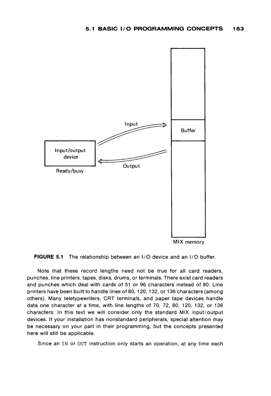
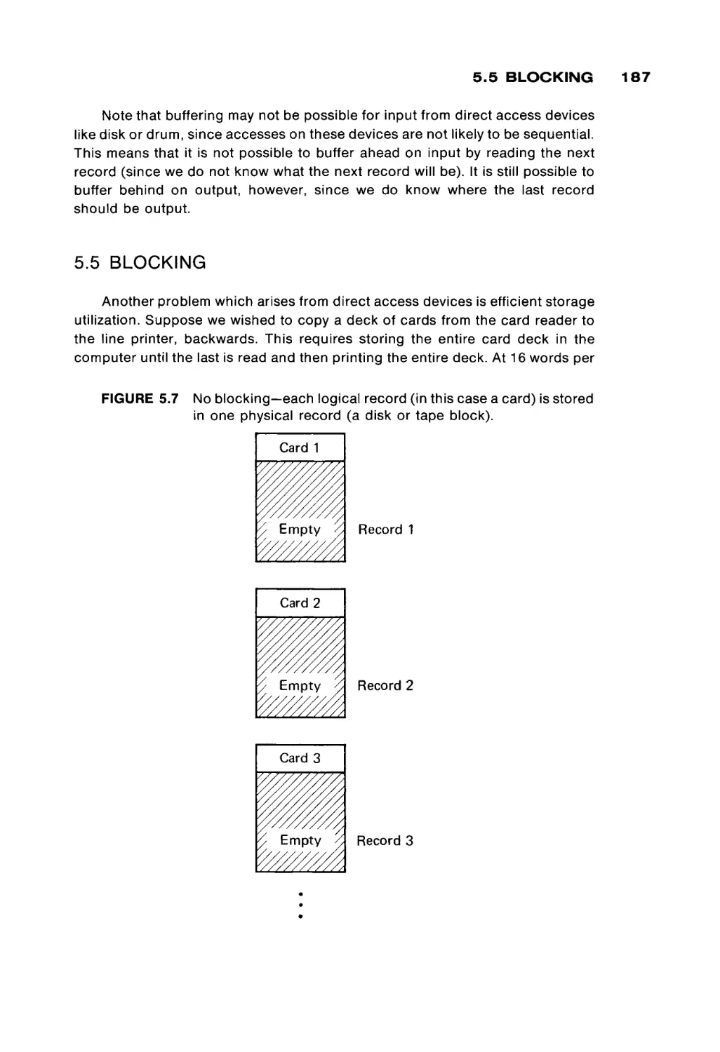
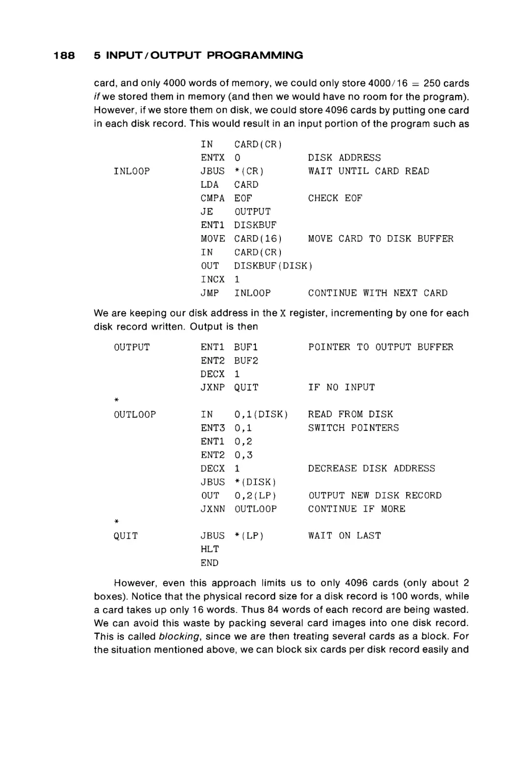
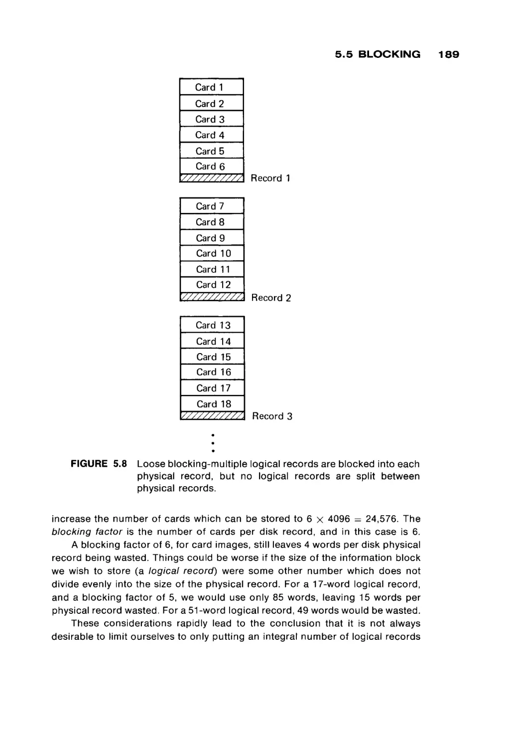
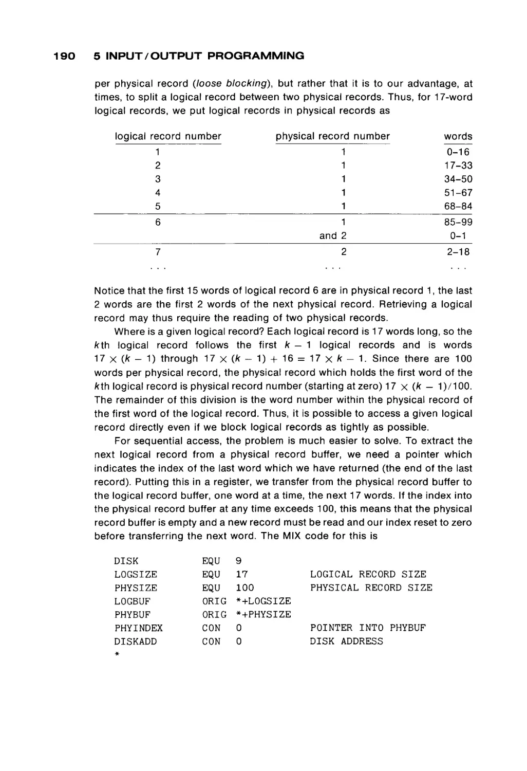
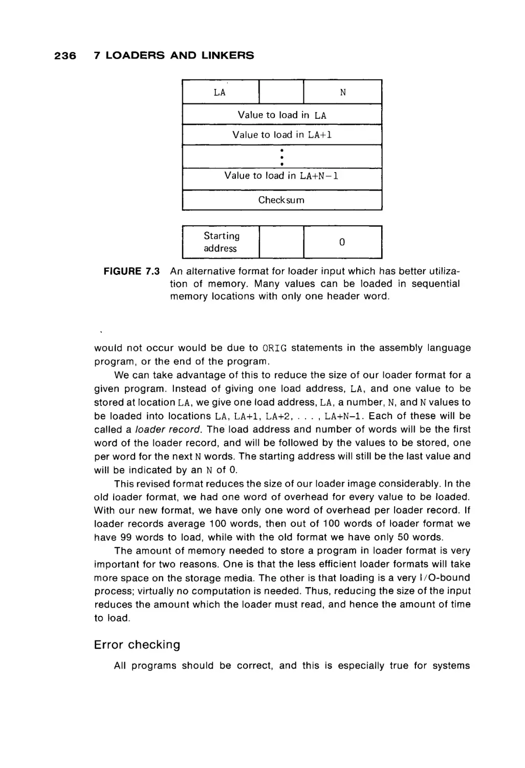
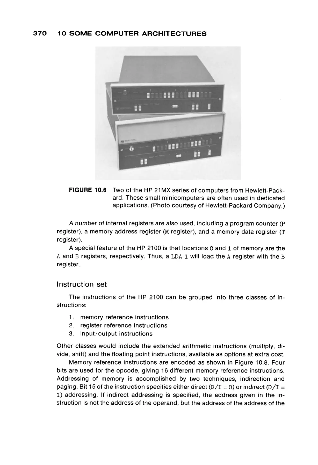
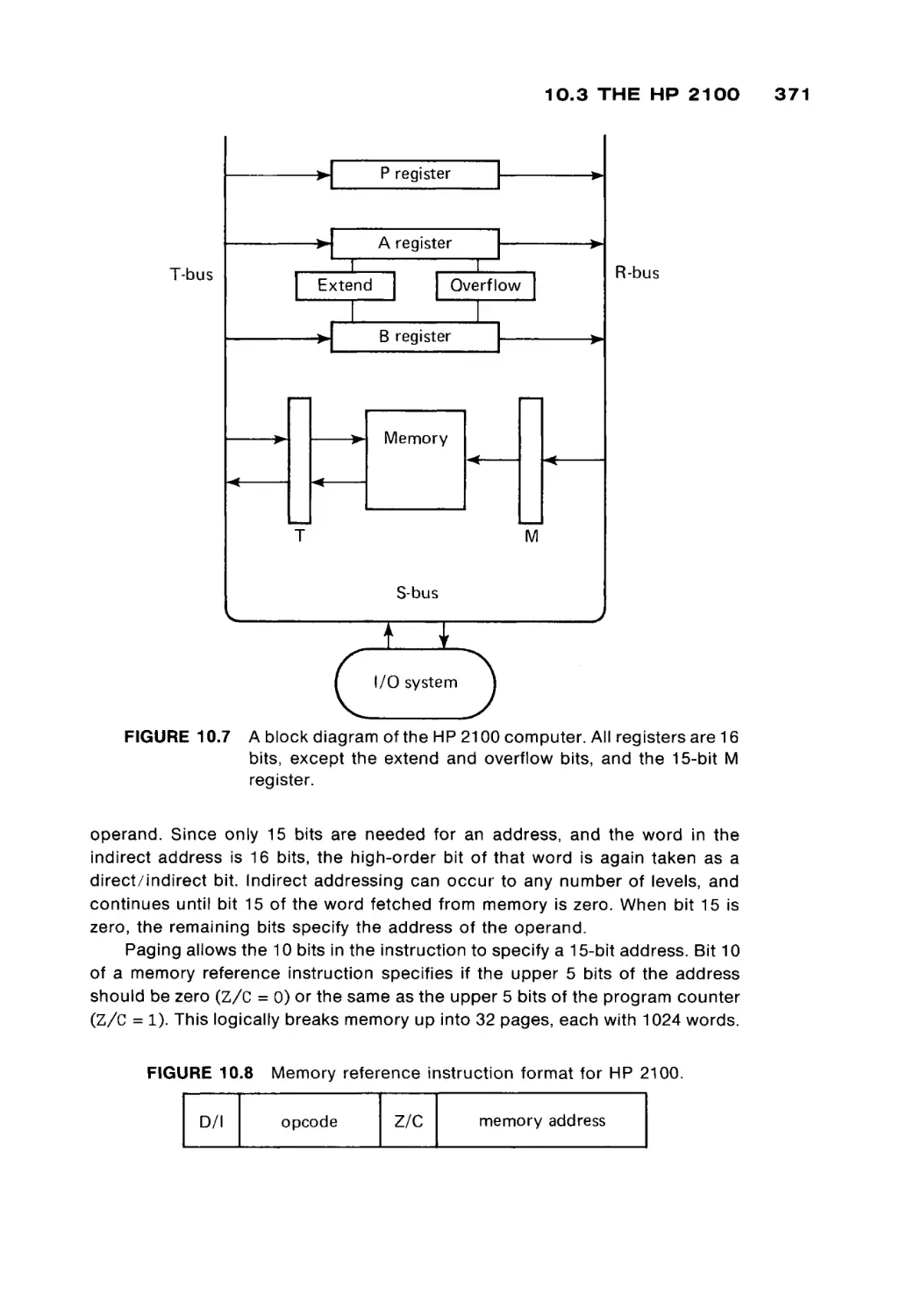
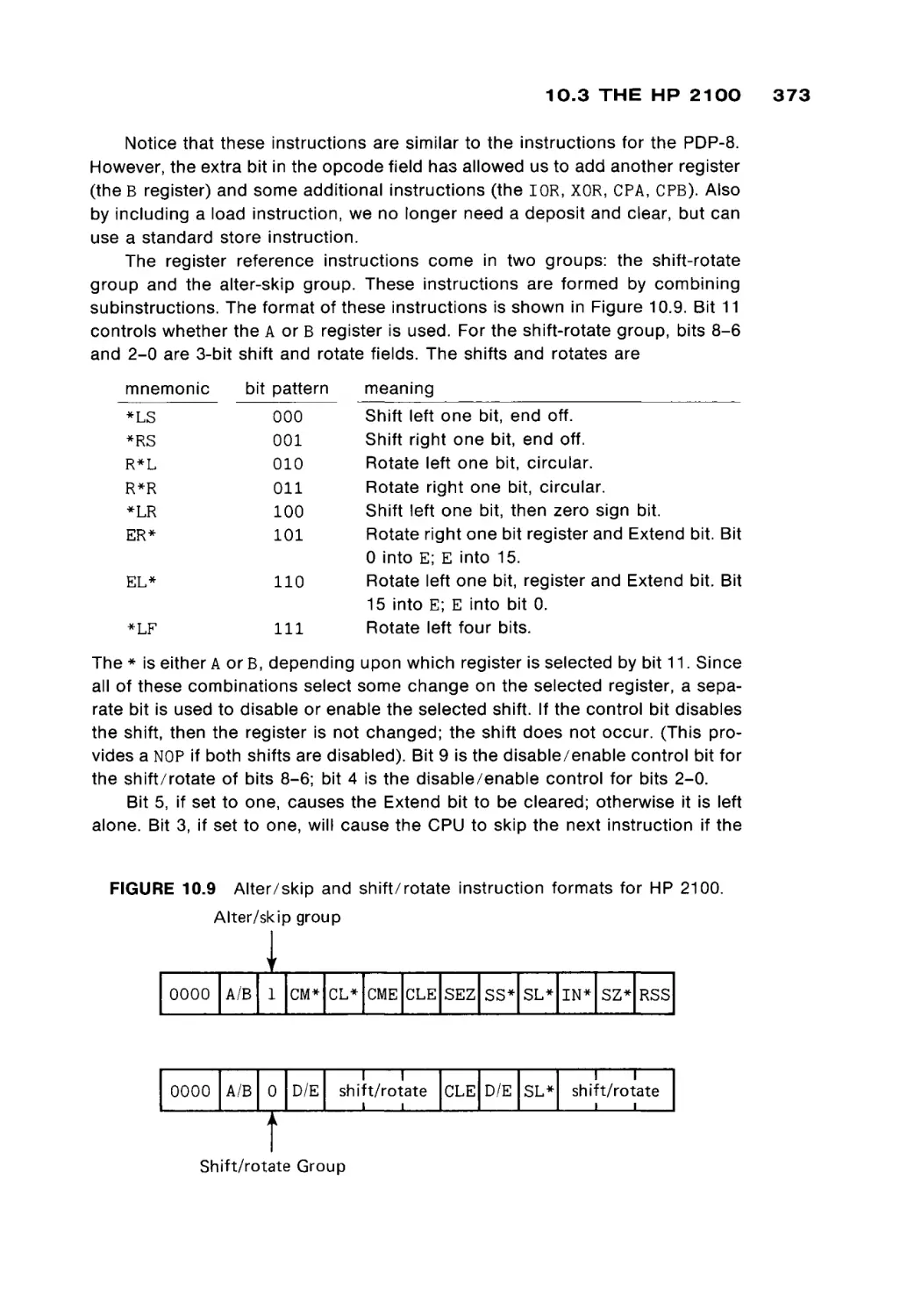
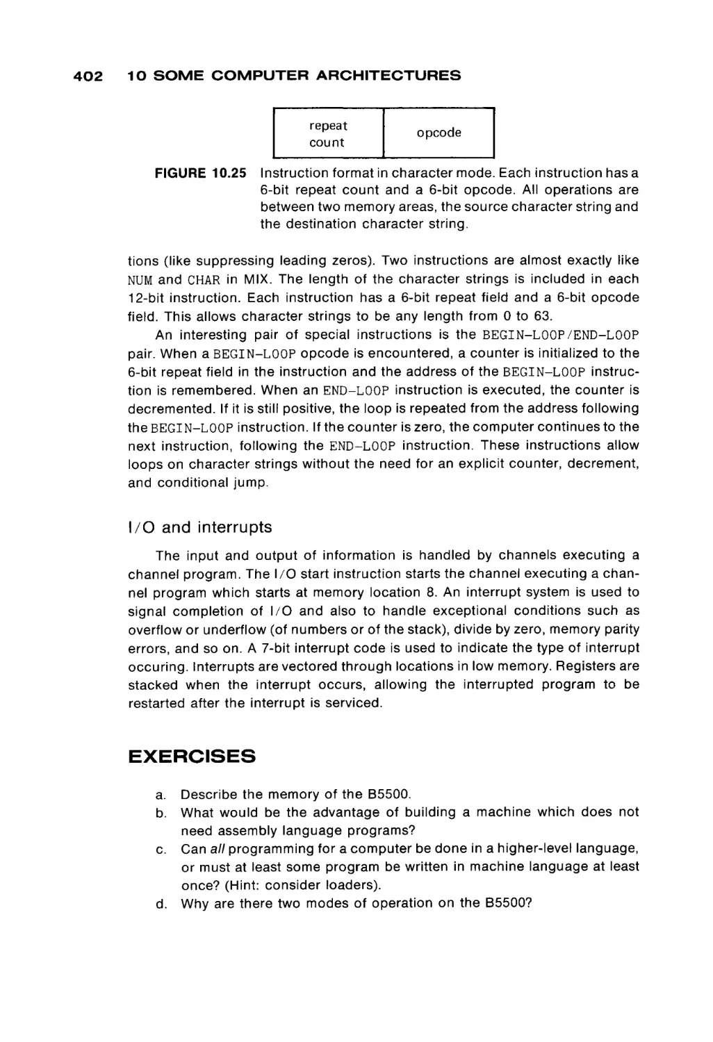
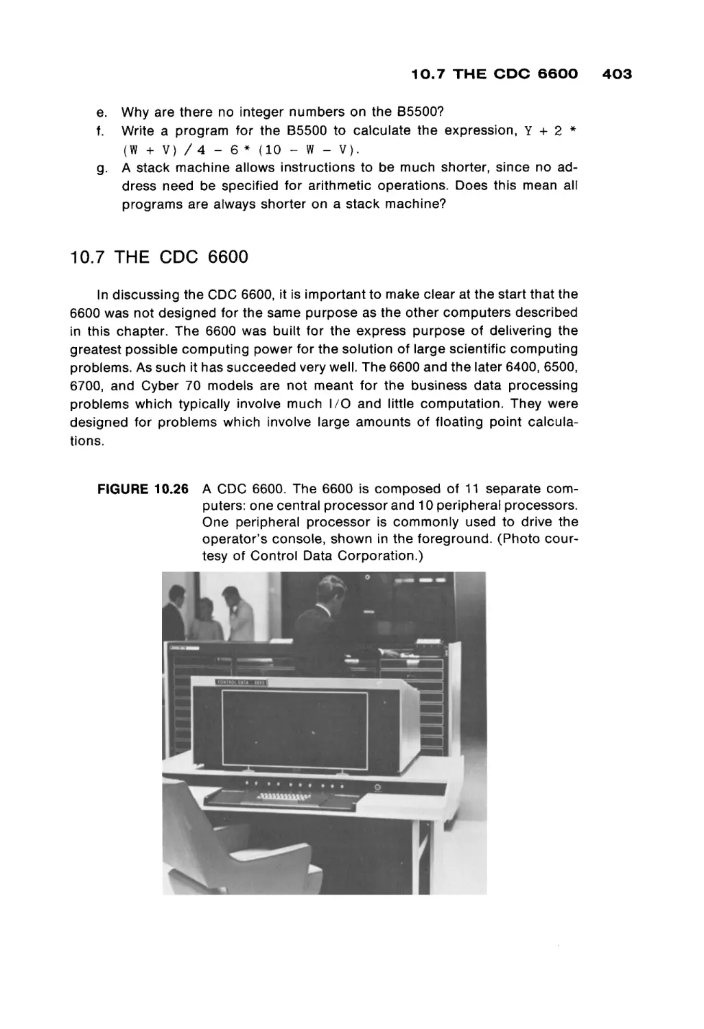
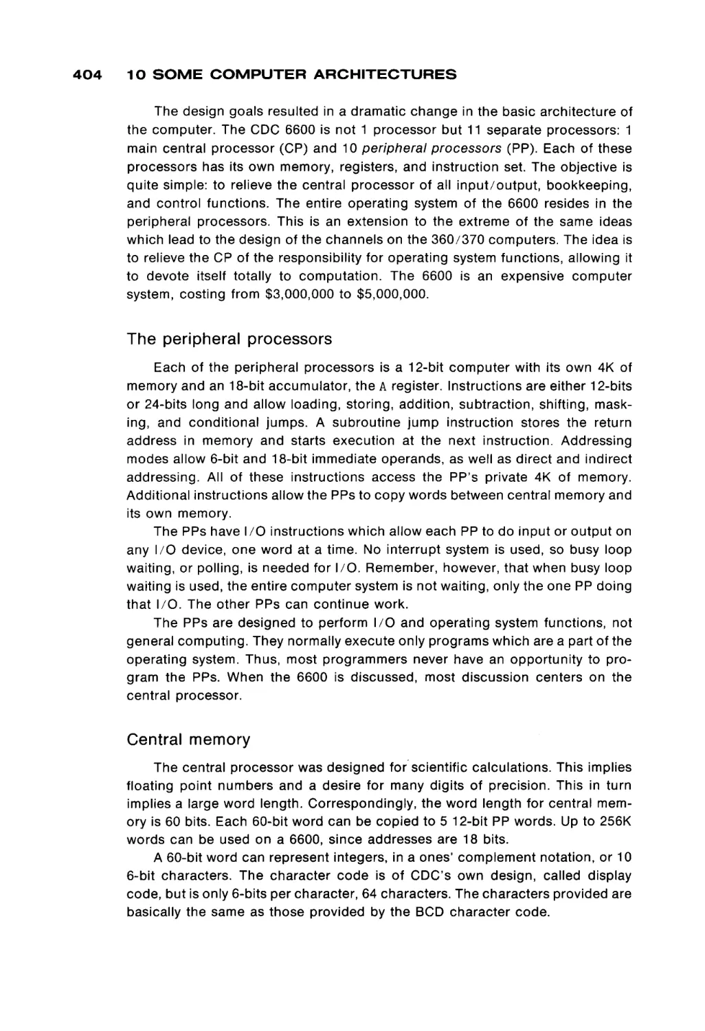
/


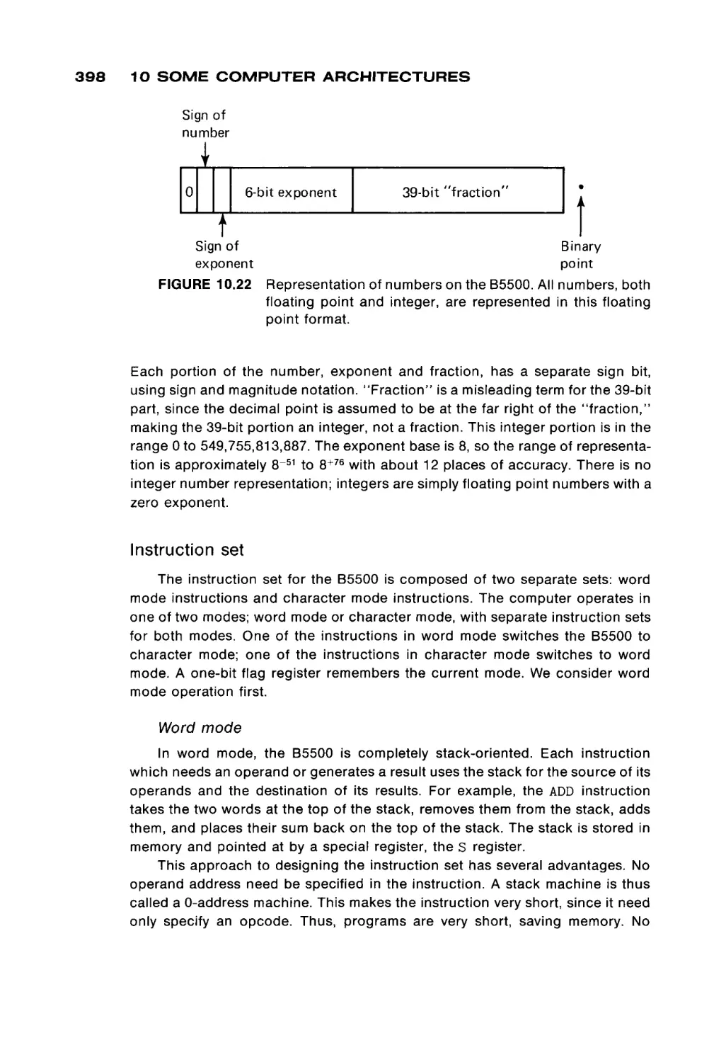
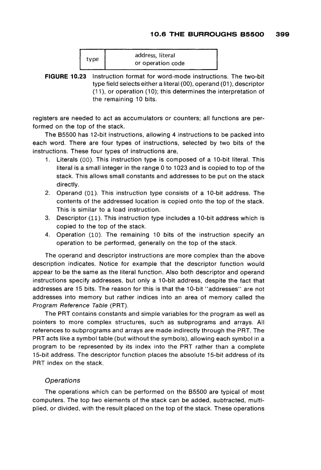
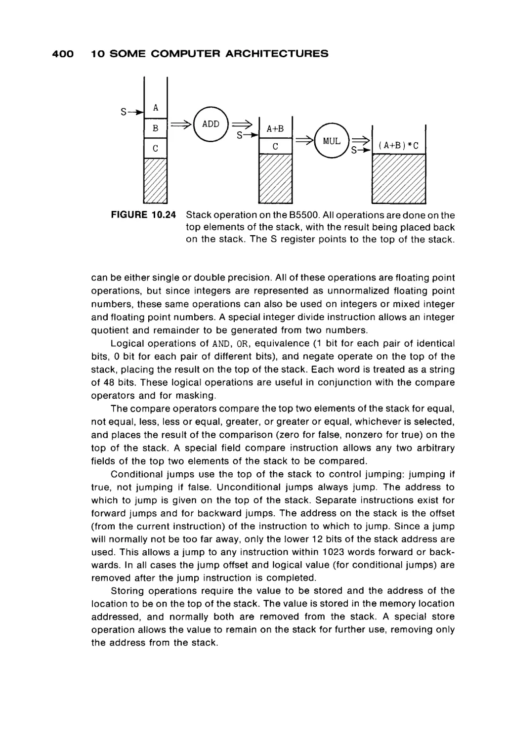
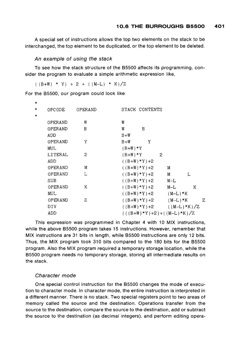

Автор: Peterson James L. Rheinboldt Werner
Теги: programming computer technology
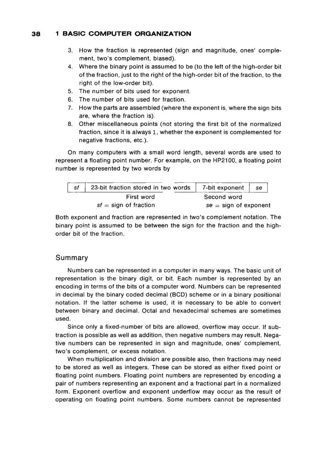
ISBN: 0-12-552250-9
Год: 1978


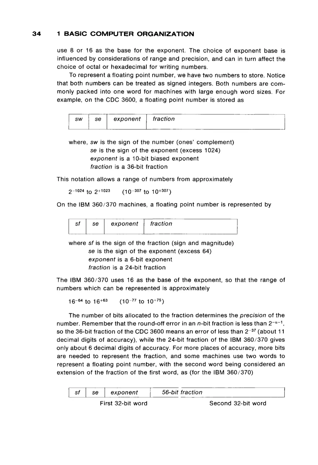
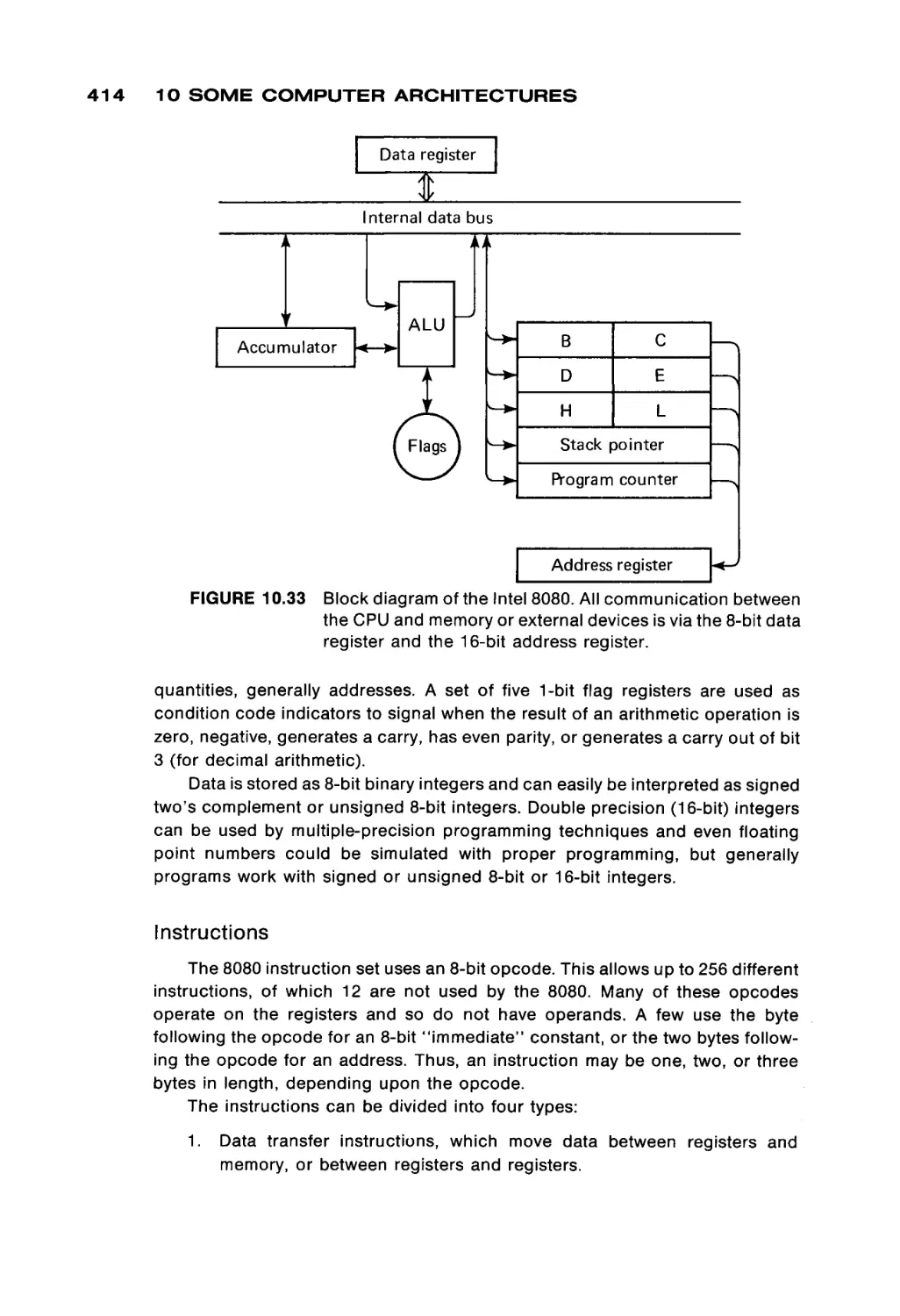
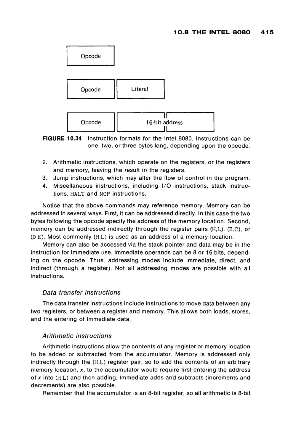
Текст
This is a volume in
COMPUTER SCIENCE AND APPLIED MATHEMATICS
A Series of Monographs and Textbooks
EDITOR: WERNER RHEINBOLDT
COMPUTER
ORGANIZATION
AND ASSEMBLY
LANGUAGE
PROGRAMMING
JAMES L. PETERSON
UNIVERSITY OF TEXAS AT AUSTIN
NEW YORK
ACADEMIC PRESS
SAN FRANCISCO
LONDON
A Subsidiary of Harcourt Brace Jovanovich, Publishers
COPYRIGHT © 1978, BY ACADEMIC PRESS, INC.
ALL RIGHTS RESERVED
NO PART OF THIS PUBLICATION MAY BE REPRODUCED OR
TRANSMITTED IN ANY FORM OR BY ANY MEANS, ELECTRONIC
OR MECHANICAL, INCLUDING PHOTOCOPY, RECORDING, OR ANY
INFORMATION STORAGE AND RETRIEVAL SYSTEM, WITHOUT
PERMISSION IN WRITING FROM THE PUBLISHER
ACADEMIC PRESS, INC.
111 FIFTH AVENUE, NEW YORK, NEW YORK 10003
UNITED KINGDOM EDITION PUBLISHED BY
ACADEMIC PRESS, INC. (LONDON) LTD.
24/28 OVAL ROAD, LONDON NW1
ISBN: 0-12-552250-9
LIBRARY OF CONGRESS CATALOG CARD NUMBER:
PRINTED IN THE UNITED STATES OF AMERICA
77-91331
PREFACE
This book has been designed and used as a text for a second course in
computer programming. It has developed from class notes for a course offered at
the University of Texas at Austin to undergraduate students. These students have
had one previous programming course and should know, from that first course,
the basic operation of computers, in general, and have some basic skills in
converting problem statements into programs in a higher level language, such as
Fortran. The second course, and this text, assumes that the student knows how
to program, i.e., how to find an algorithm to solve a problem and convert that
algorithm into a program.
The purpose of this book is to teach the student about lower level computer
programming: machine language and assembly language, and how these lan
guages are used in the typical computer system. This is meant to give the student
a basic understanding of the fundamental concepts of the organization and
operation of a computer. Even if the student never again programs in assembly
language (and we would hope that they never have to!) it is important that they
understand what the computer is doing at the machine language level. A good
understanding of computer organization translates into a better understanding
ix
x
PREFACE
of the features and limitations of all computer facilities, since all systems must
eventually rest on the underlying hardware machine.
The content of this text follows the recommendations of the ACM Curriculum
68 for Course B2 "Computers and Programming." After a brief review of the
general concepts of computers in Chapter 1, the remainder of the text uses the
MIX computer to provide an example machine for illustrating computer organi
zation and programming. Chapter 2 and Chapter 3 present the architecture of
the MIX computer, its machine language and the MIXAL assembly language.
Programming techniques in assembly language are covered in Chapters 4 and 5
with Chapter 5 concentrating mostly on input/output programming. The use and
implementation of the subroutine concept is investigated in Chapter 6.
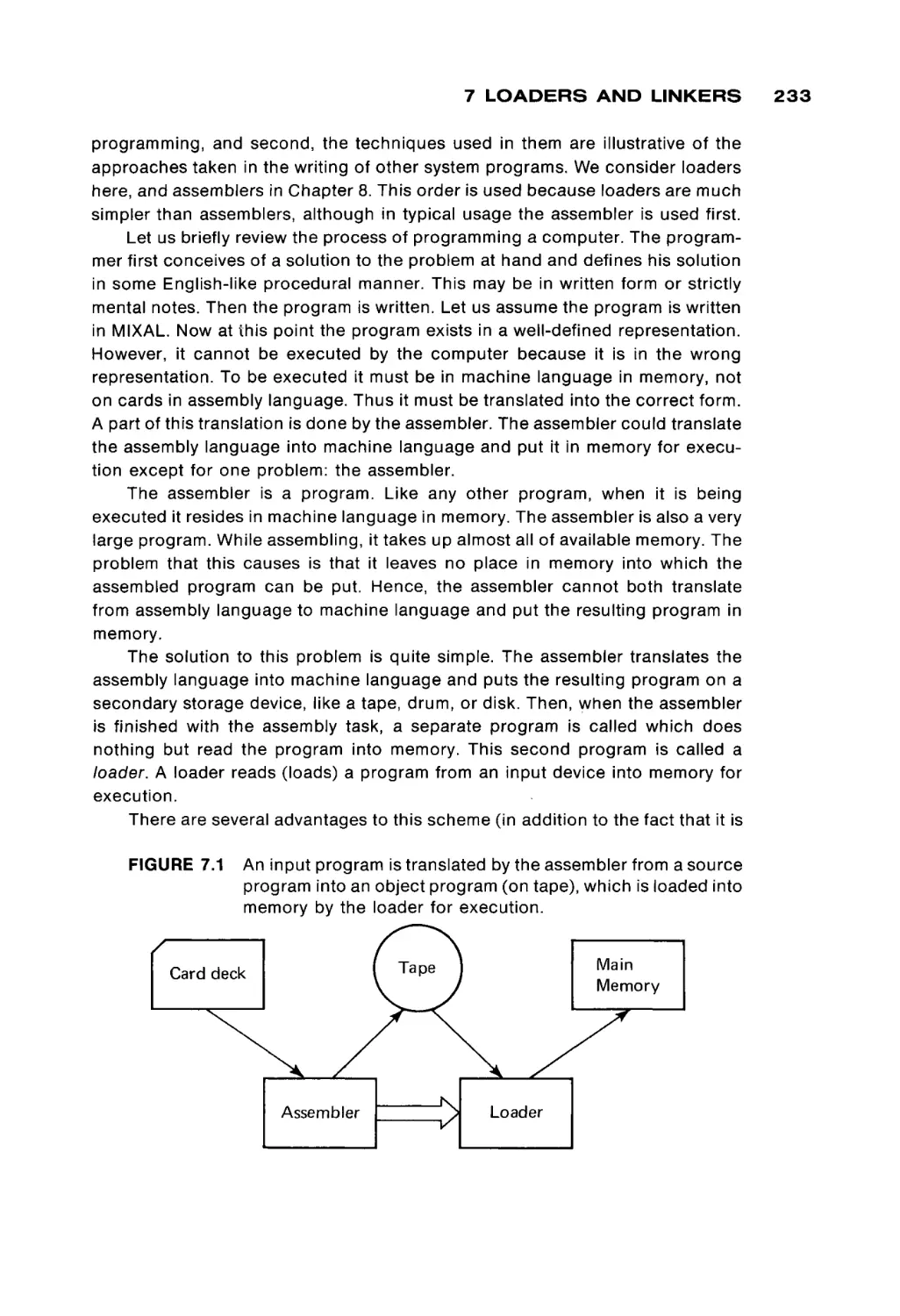
Systems programs are considered in the next three chapters. Chapter 7
explores loaders, while Chapter 8 discusses assemblers. In Chapter 7 the code
for a simple, but real, absolute loader is given; in Chapter 8, the code for a MIXAL
assembler is given. These two programs provide an opportunity for the student
to see and study a real loader and assembler, and not simply the concepts in the
abstract. Chapter 9 briefly discusses other system programs, macro assemblers,
compilers, interpreters, and operating systems.
From these chapters, the basic concepts of assembly language program
ming and programs should be evident to the student. Chapter 10 then proceeds
to present a brief description of several other computers, to introduce the stu
dent to both the similarities and differences among computer systems.
In our one-semester course, these concepts are reinforced by numerous
programming assignments. The early assignments emphasize basic program
ming techniques such as simple arithmetic, input/output, character manipula
tion and array handling. The later assignments have included writing either a
relocatable loader and two-pass assembler for a subset of the MIX computer, or
writing an interpreter and one-pass load-and-go assembler for a simple mini
computer (16 instructions, four general registers, etc.). All of these assignments
are programmed in MIXAL. The last assignment is to write a simple program in
the new assembly language of their own assembler. Thus, students should see
that they know how to program in assembly language, in general, and not simply
in MIXAL.
The major question in your mind now is undoubtedly: Why MIX? MIX is a
pseudo computer, not a real one. This is at once both its major drawback and its
major advantage. The major drawback to MIX is, of course, that it is not real; this
implies that the use and programming of the MIX computer will include a certain
air of artificiality which may annoy and confuse some students.
However, from an educational point of view, MIX is ideal. It is simple, easy to
understand, and yet typical of many computers. Machine and assembly lan
guages are different for each computer. However, the techniques of assembly
language programming are largely machine independent. Thus, learning one
assembly language provides the basis for quickly and easily learning any other
PREFACE
assembly language. This is emphasized by the descriptions of other computers
in Chapter 10.
Also consider the alternative to teaching MIX: teaching the structure and
language of a real computer. As Knuth has written, in the Preface to Volume 1 of
The Art of Computer Programming (Addison-Wesley, Reading, Mass., 1973),
"Given the decision to use a machine-oriented language, which lan
guage should be used? I could have chosen the language of a particular
machine X, but then those people who do not possess machine X would
think this book is only for X-people. Furthermore, machine X probably
has a lot of idiosyncrasies which are completely irrelevant to the material
in this book, yet which must be explained; and in two years the manu
facturer of machine X will put out machine X + 1 or machine 10X, and
machine X will no longer be of interest to anyone".
Knuth continues that it is very unlikely that programmers will only use one
computer in their life. Each new machine can be easily learned once the first
machine is understood, but the ability to change smoothly from one computer to
another is an important skill for a programmer. Thus, teaching first MIX and then
another, real, computer is preferable, since it immediately forces the student to
understand how to move from machine to machine. In my own, so far short
career, I have programmed on several different computers (IBM 1620, CDC 3600,
CDC 6500, PDP-11/20, HP 2116, CDC 1700, IBM 360/370, DEC-10, SDS Sigma
5, Nova 3/D).
From an economic viewpoint also, the MIX machine is an advantage over a
real computer. It is often said that a simulated machine is much more expensive
than a real machine, and for production computation this is undeniably true.
However, for a student environment, most of the computer time is in assembly
and debugging, not execution. The simple MIXAL assembler, written as a cross
assembler for the machine at hand, generating load-and-go code for a simulator
with good trace, dump, and error detection facilities will provide a much better
instructional tool at a lower price than most real assemblers with their extensive
pseudo instructions, macros, relocatable code, and operating system input/
output, most of which cannot and need not be used in an introductory course.
The construction of a MIXAL assembler/simulator is, although nontrivial,
within the range of a senior year or early graduate student project. The complex
ities are derived mainly from the need for an event driven simulator to allow CPU
and I/O overlap, and the need to provide the best possible debugging facilities.
Properly written, the design and code for these systems would be easily trans
ported over the years to new computer systems.
One further benefit from the use of MIX is the ability to easily pick up and use
The Art of Computer Programming books by D. E. Knuth. These are very handy
in later courses as references and texts. More can be learned from them with a
good knowledge of MIX.
xi
xii
PREFACE
In summary, we feel that MIX is preferable to any real machine for teaching a
beginning course in machine language, assembly language and computer orga
nization. The major problem we have faced in using MIX has been the lack of an
adequate text, a problem which we hope has now been solved.
I would especially like to express my gratitude to the reviewers—Stan Benton, Montclair State College; Michel Boillot, Pensacola Junior College; Werner
Rheinboldt, University of Maryland; and Robert C. Uzgalis, University of Califor
nia—Los Angeles; whose comments and suggestions helped greatly in guiding
the manuscript to its final form.
Austin, Texas
August 11, 1977
James Peterson
1
BASIC
COMPUTER
ORGANIZATION
Computers, like automobiles, television, and telephones, are becoming more
and more an integral part of our society. As such, more and more people come
into regular contact with computers. Most of these people know how to use their
computers only for specific purposes, although an increasing number of people
know how to program them, and hence are able to solve new problems by using
computers. Most of these people know how to program in a higher-level lan
guage, such as Basic, Fortran, Cobol, Algol, or PL/I. We assume that you know
how to program in one of these languages.
However, although many people know how to use automobiles, televisions,
telephones, and now computers, few people really understand how they work
internally. Thus, there is a need for automotive engineers, electronics specialists,
and assembly language programmers. There is a need for people who under
stand how a computer system works, and why it is designed the way that it is. In
the case of computers, there are two major components to understand: the
hardware (electronics), and the software (programs). It is the latter, the software,
that we are mainly concerned with in this book. However, we also consider how
the hardware operates, from a programmer's point of view, to make clear how it
influences the software.
1 BASIC COMPUTER ORGANIZATION
Computation
Memory
unit
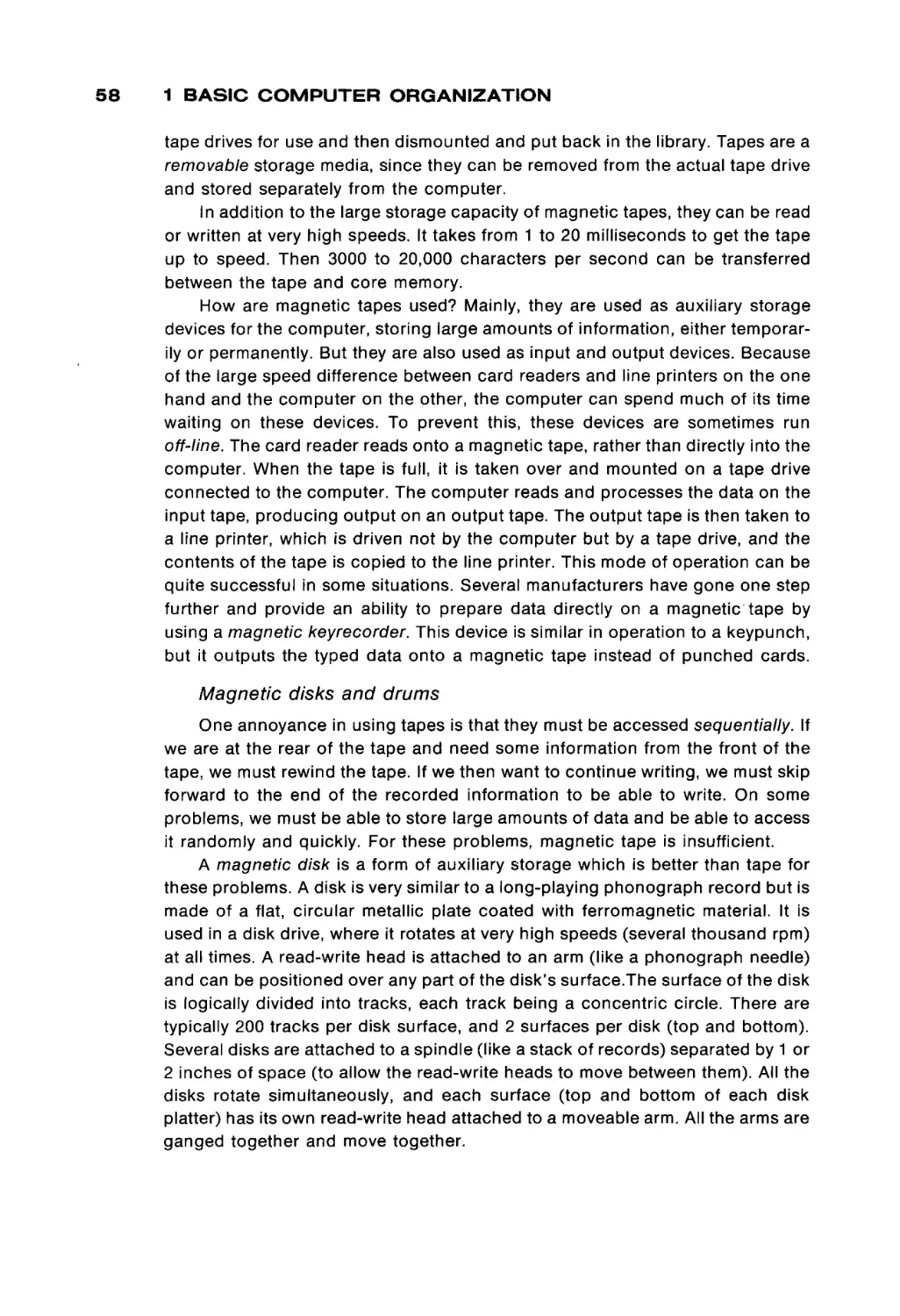
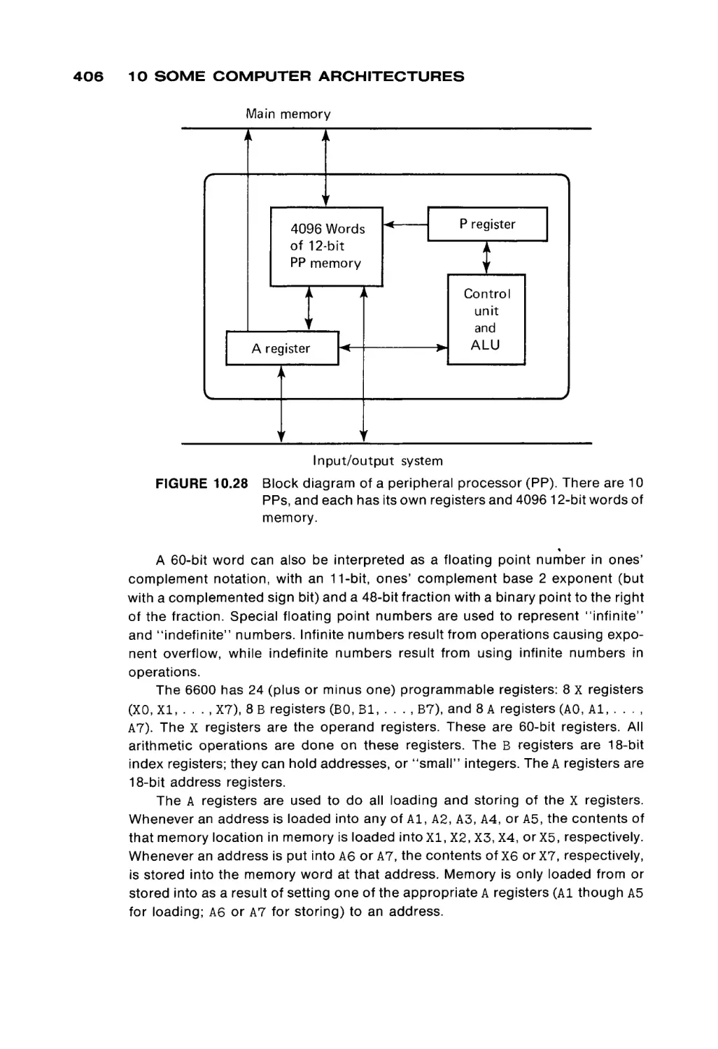
FIGURE 1.1
Input/output
system
Outside world
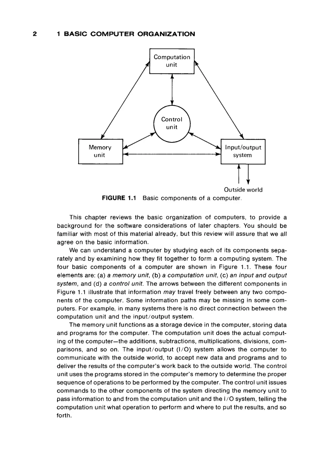
Basic components of a computer.
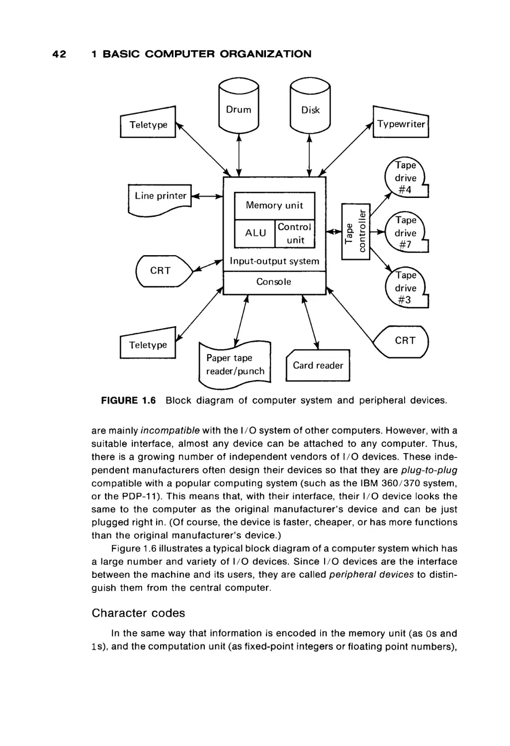
This chapter reviews the basic organization of computers, to provide a
background for the software considerations of later chapters. You should be
familiar with most of this material already, but this review will assure that we all
agree on the basic information.
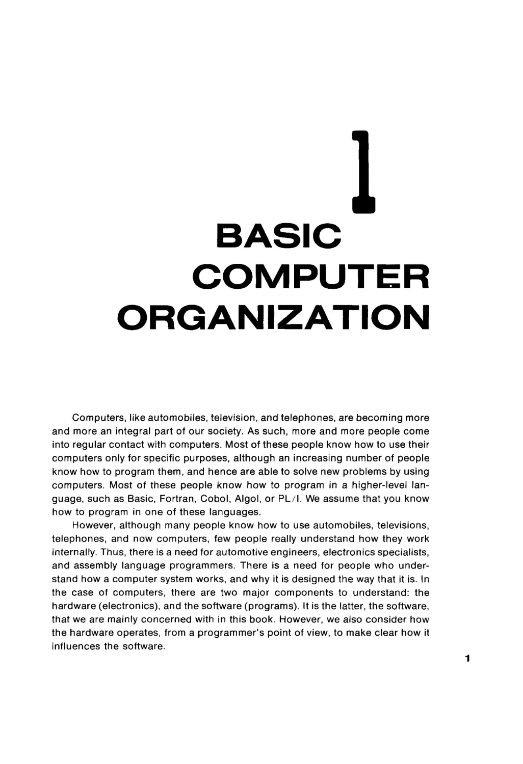
We can understand a computer by studying each of its components sepa
rately and by examining how they fit together to form a computing system. The
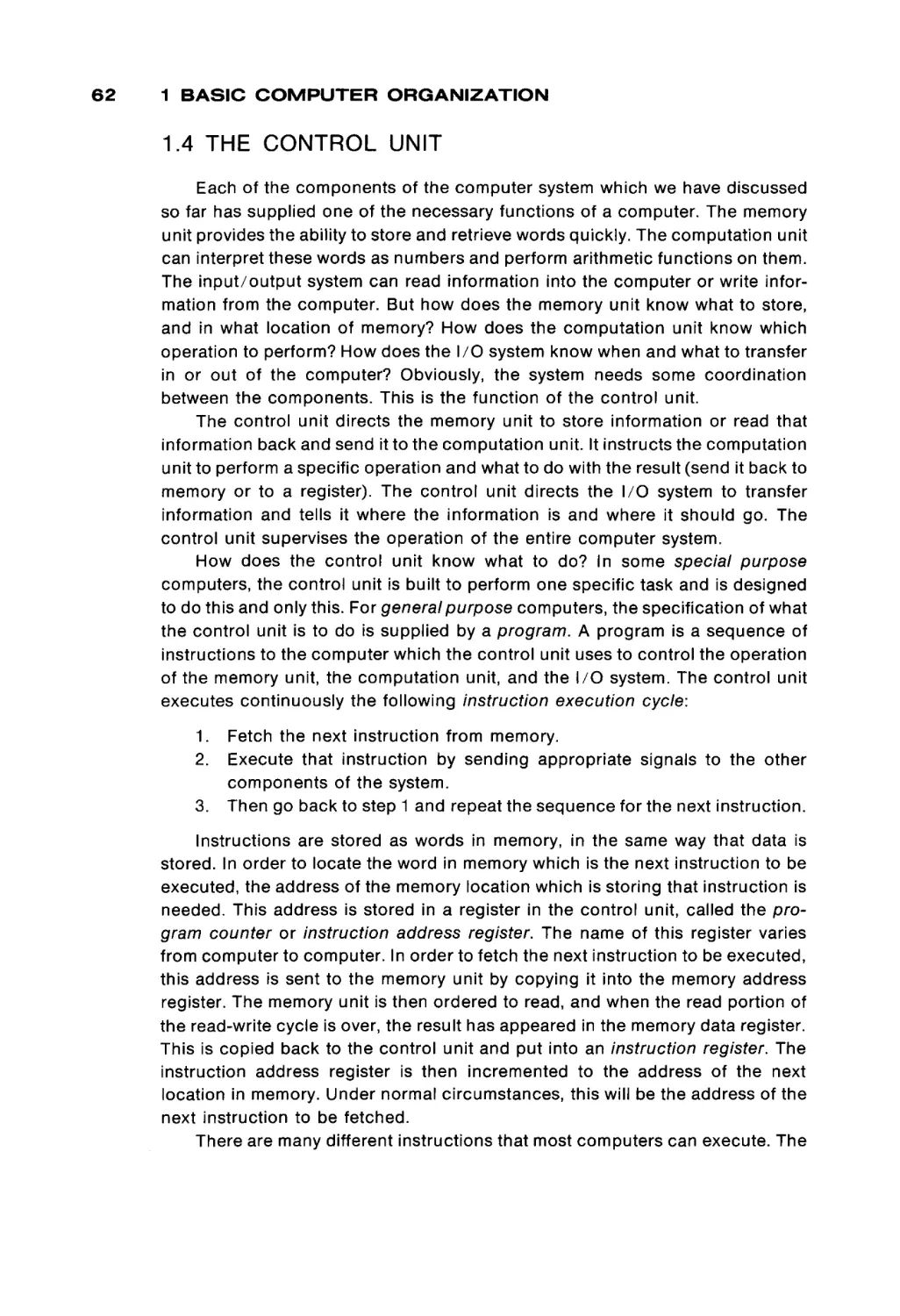
four basic components of a computer are shown in Figure 1.1. These four
elements are: (a) a memory unit, (b) a computation unit, (c) an input and output
system, and (d) a control unit. The arrows between the different components in
Figure 1.1 illustrate that information may travel freely between any two compo
nents of the computer. Some information paths may be missing in some com
puters. For example, in many systems there is no direct connection between the
computation unit and the input/output system.
The memory unit functions as a storage device in the computer, storing data
and programs for the computer. The computation unit does the actual comput
ing of the computer—the additions, subtractions, multiplications, divisions, com
parisons, and so on. The input/output (I/O) system allows the computer to
communicate with the outside world, to accept new data and programs and to
deliver the results of the computer's work back to the outside world. The control
unit uses the programs stored in the computer's memory to determine the proper
sequence of operations to be performed by the computer. The control unit issues
commands to the other components of the system directing the memory unit to
pass information to and from the computation unit and the I/O system, telling the
computation unit what operation to perform and where to put the results, and so
forth.
1.1 THE MEMORY UNIT
Each of these components is discussed in more detail below. Every com
puter must have these four basic components, although the organization of a
specific computer may structure and utilize them in its own manner. We are
therefore presenting general organizational features of computers, at the mo
ment. In Chapters 2, 3, and 10 we consider specific computers and their organi
zation.
1.1 THE MEMORY UNIT
A very necessary capability for a computer is the ability to store, and retrieve,
information. Memory size and speed are often the limiting factors in the opera
tion of modern computers. For many of today's computing problems it is essen
tial that the computer be able to quickly access large amounts of data stored in
memory.
We consider the memory unit from two different points of view. We first
consider the physical organization of a memory unit. This will give us a founda
tion from which we can investigate the logical organization of the memory unit.
Physical organization of computer memory
For the past twenty years, the magnetic core has been the major form of
computer memory. More recently, semiconductor memories have been devel
oped to the point that most new computer memories are likely to be semicon
ductor memories rather than core memories. The major deciding factors be
tween the two have been speed and cost. Semiconductor memories are
undeniably faster, but until recently have also been more expensive.
Core memories have been used for many years and will undoubtedly con
tinue to be used widely. They have been the main form of computer main
memory for almost twenty years. Since semiconductor memories have been
trying to replace core memories, they have been built to look very much like core
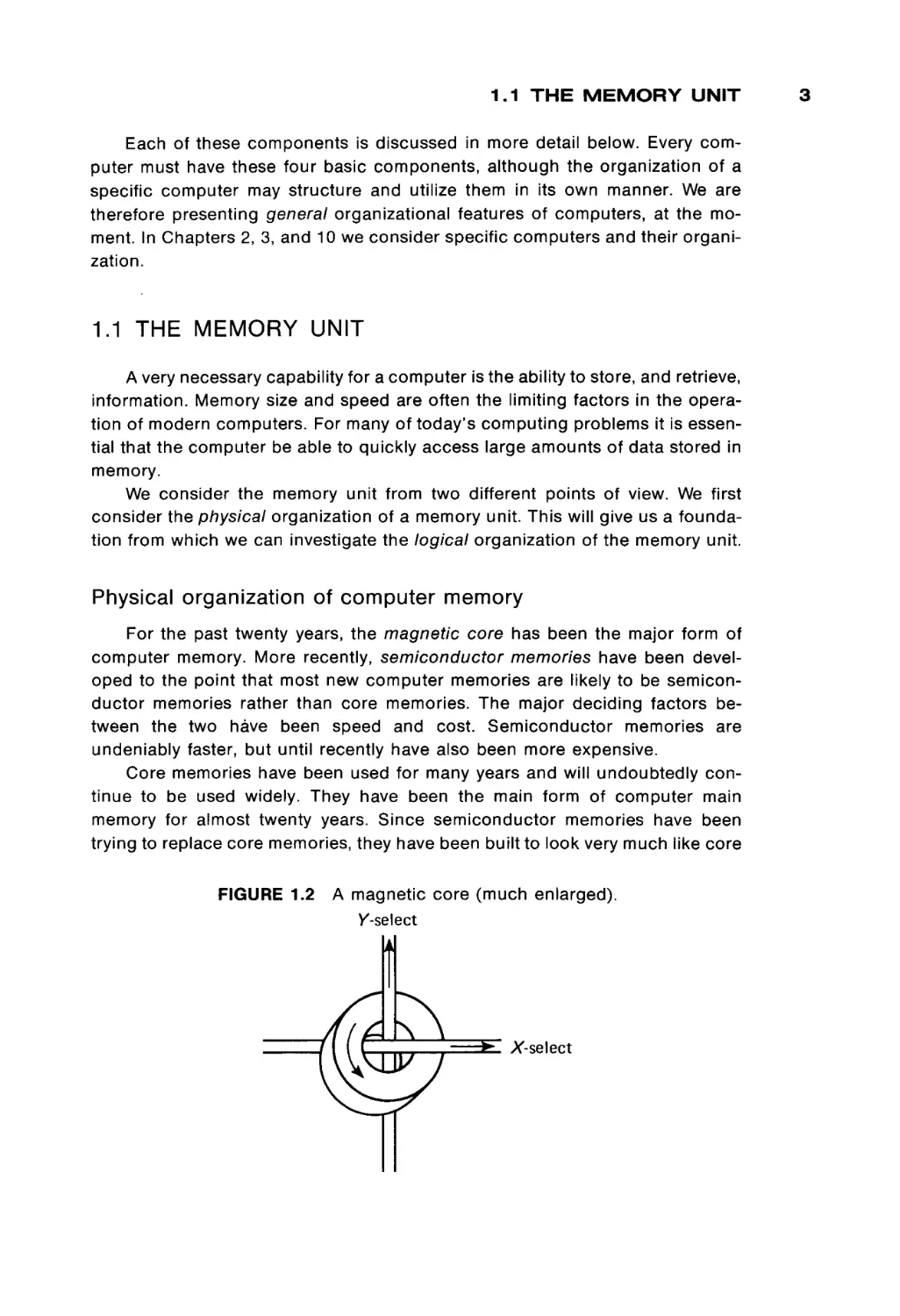
FIGURE 1.2
A magnetic core (much enlarged).
/-select
3
1 BASIC COMPUTER ORGANIZATION
memories, from a functional point of view. Therefore, we present some basic
aspects of computer memories in terms of core memories first, and then we
consider semiconductor memories.
Core memories
Figure 1.2 is a drawing of a magnetic core. Cores are very small (from 0.02 to
0.05 inches in diameter) doughnut-shaped pieces of metallic ferrite materials
which are mainly iron oxide. They have the useful property of being able to be
easily magnetized in either of two directions: clockwise or counterclockwise. A
core can be magnetized by passing an electrical current along the wire through
the hole in the center of the core for a short time. Current in one direction ( + )
will magnetize the core in one direction (clockwise), and current in the opposite
direction ( - ) will magnetize the core in the opposite direction (counterclock
wise). Once the core has been magnetized in a given direction, it will remain
magnetized in that direction for an indefinitely long time (unless it is deliberately
remagnetized in the opposite direction, of course). This allows a core to store
either of two states, which can be arbitrarily assigned the symbols 0 and 1 (or +
and - , or A and B, etc.).
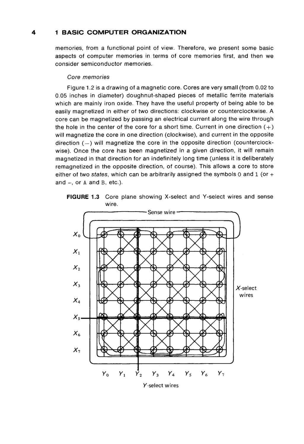
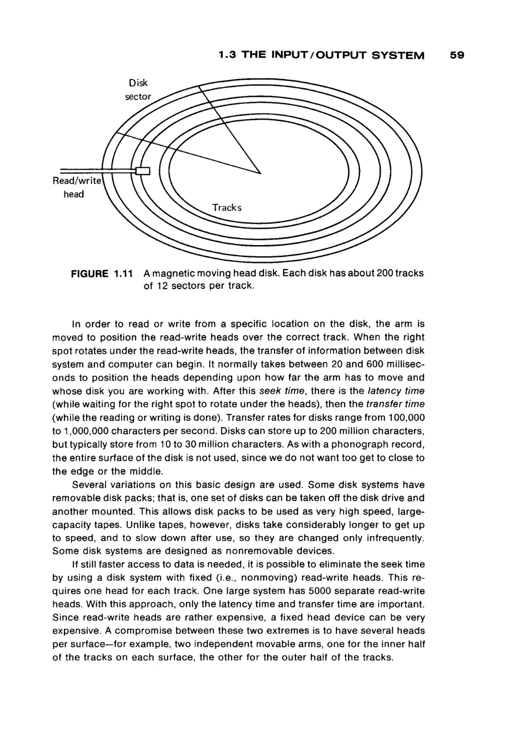
FIGURE 1.3
Xo
Core plane showing X-select and Y-select wires and sense
wire.
■
■
Sense wire —
(7P1v
K^ääl
o ψ*Χ-\
L-rr
x2
Xi
I X-select
wires
x,
XsXe
Xi
v
Pak* ^
I'toi
Vo
Yi
3 4/
s
Y2
*^YÌ
Ys
Y4
/-select wires
Ys
Ye
Yi
)
1.1 THE MEMORY UNIT
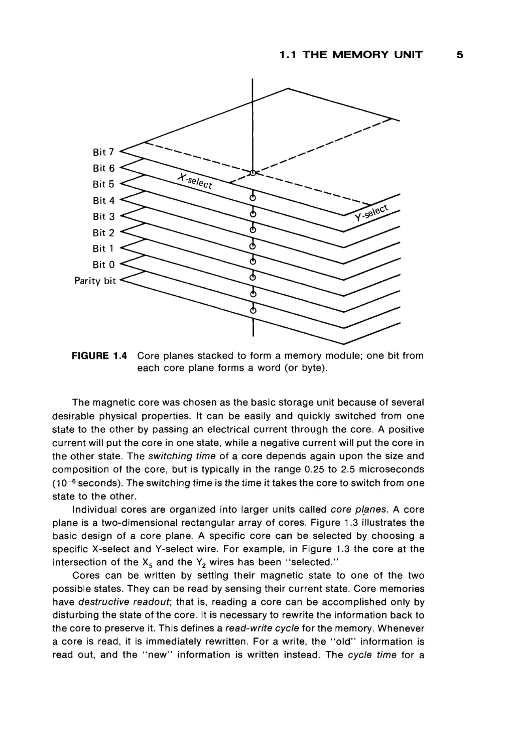
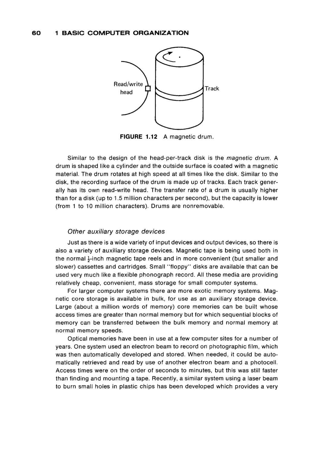
FIGURE 1.4
Core planes stacked to form a memory module; one bit from
each core plane forms a word (or byte).
The magnetic core was chosen as the basic storage unit because of several
desirable physical properties. It can be easily and quickly switched from one
state to the other by passing an electrical current through the core. A positive
current will put the core in one state, while a negative current will put the core in
the other state. The switching time of a core depends again upon the size and
composition of the core, but is typically in the range 0.25 to 2.5 microseconds
(10 - 6 seconds). The switching time is the time it takes the core to switch from one
state to the other.
Individual cores are organized into larger units called core planes. A core
plane is a two-dimensional rectangular array of cores. Figure 1.3 illustrates the
basic design of a core plane. A specific core can be selected by choosing a
specific X-select and Y-select wire. For example, in Figure 1.3 the core at the
intersection of the X5 and the Y2 wires has been "selected."
Cores can be written by setting their magnetic state to one of the two
possible states. They can be read by sensing their current state. Core memories
have destructive readout; that is, reading a core can be accomplished only by
disturbing the state of the core. It is necessary to rewrite the information back to
the core to preserve it. This defines a read-write cycle for the memory. Whenever
a core is read, it is immediately rewritten. For a write, the " o l d " information is
read out, and the "new" information is written instead. The cycle time for a
5
6
1 BASIC C O M P U T E R
ORGANIZATION
memory is at least twice its switching time, and typical core memory cycle times
are 0.5 to 5 microseconds. Notice that the access time (time to read information)
is generally only half the cycle time.
Core planes are " s t a c k e d , " one on top of another, to form memory
modules.
All the cores selected by a specific pair of X and Y wires (one core from each
core plane) are used to form a word of memory. To read or write a w o r d from
memory, one core from each core plane is read and written, simultaneously. The
specific core in each core plane is selected by a memory address register which
specifies the X-select and Y-select wires to be used. The result from a read is put
into a memory data register. The contents of this register are then used to restore
the selected w o r d . In a write operation, the result of the read operation is not
used to set the memory data register, but is simply discarded. The word in
memory is then written from the memory data register.
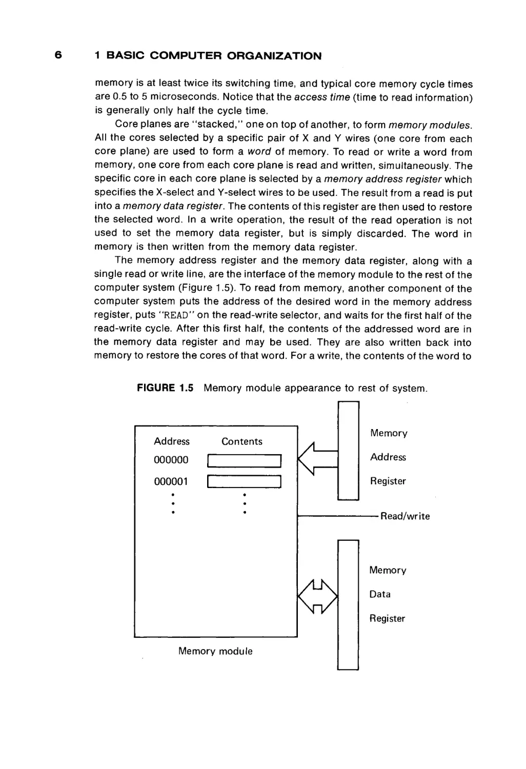
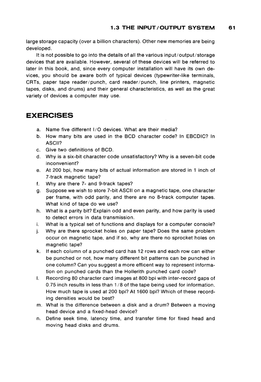
The memory address register and the memory data register, along with a
single read or write line, are the interface of the memory module to the rest of the
computer system (Figure 1.5). To read from memory, another c o m p o n e n t of the
computer system puts the address of the desired w o r d in the memory address
register, puts "READ" on the read-write selector, and waits for the first half of the
read-write cycle. After this first half, the contents of the addressed w o r d are in
the memory data register and may be used. They are also written back into
memory to restore the cores of that w o r d . For a write, the contents of the w o r d to
FIGURE 1.5
Memory module appearance to rest of system.
Address
Contents
Memory
000000
|
Address
000001
|
Register
■ Read/write
Memory
Data
Register
Memory module
1.1 THE MEMORY UNIT
be written are put in the memory data register, and the read-write wire is set to
"WRITE". After the entire read-write cycle is over, the addressed word will have
its new contents.
Semiconductor
memory
The basic element in a core memory is the core. The parameters of the core
define the parameters of the memory. Specifically, the size of the core deter
mines its switching time, and switching time defines access time and cycle time.
To achieve faster memories, it is necessary to make the cores smaller and
smaller. There is a practical limit, given current manufacturing techniques, to the
size, and hence, speed, of core memories.
Semiconductor memories use electrical rather than magnetic means to store
information. The basic element of a semiconductor memory is often called a
flip-flop. Like the core, it has two basic states: on/off, o r O / 1 , or + / - , and so on.
The basic idea is to replace the magnetic cores of a memory with the electrical
flip-flops. However, the functional view of memory is the same. Each memory
module has a memory address register, a memory data register, and a read-write
function selector. The difference lies in how the information is stored in the
memory module. Many different kinds of semiconductor memories have been
developed.
Bipolar memories are the fastest memories available, with switching times as
low as 100 nanoseconds (10~9 seconds). MOS (metallic-oxide semiconductor)
memories are slower (500 to 1000 nanoseconds) but cheaper. These memories
are made on "chips" which correspond roughly to a core plane. Memory mod
ules are constructed by placing a number of chips on a memory board.
One major problem with semiconductor memories is the volatility of the
stored information. In core memories, information is stored magnetically, while
semiconductor memories store information electrically. If the power to a semi
conductor memory is turned off, the contents of the memory are lost. This means
that power is never intentionally turned off, unless all useful information has been
stored elsewhere. However, if power is cut off due to an accident, a power
failure, or a "brown-out," the consequences can be a major catastrophe. A
temporary alternate power supply (such as a battery) can solve this problem, and
most systems now have this protection.
Another form of this same volatility exhibits itself in some semiconductor
memories. Static memories use transistor-like memory elements which store
information by the " o n " or "off" state of the transistor. Dynamic memories store
information by the presence or absence of an electrical charge on a capacitor.
The problem is that the electrical charge will leak off over time, and so dynamic
memories must be refreshed at regular intervals. Refreshing a memory requires
reading every word and writing it back in place. Special circuitry is used to
constantly refresh a dynamic memory.
Almost the opposite of a dynamic memory is a read-only memory (ROM).
Read-only memories are very static. In fact, as their name implies, they cannot be
7
8
1 BASIC COMPUTER ORGANIZATION
written (except maybe the first time, and even that is often difficult). Read-only
memories are used for special functions; information is stored once and never
changed. For example, read-only memories are often used to store bootstrap
loaders (Chapter 7) and interpreters (Chapter 9), programs which are supplied
with the computer and are not meant to ever be changed. Most hand calculators
are small computers with a special program, stored in ROM, which is executed
over and over.
Some read-only memories can in fact be rewritten, but while access time for
reading may be only 100 nanoseconds, writing may take several microseconds.
These memories are called programmable read-only memories (PROMs) and
electrically programmable read-only memories (EPROMS), among others.
Even more advanced forms of semiconductor memories which may be used
in the near future include magnetic bubbles and charge-coupled devices
(CCDs). The important fact about all of these forms of memory, however, is that
despite their various types of physical construction, their interface to the rest of
the computer system is the same: an address register, a data register, and a
read-write signal. Memory modules can be constructed in many different ways
and with many different materials: cores, semiconductors, thin magnetic films,
magnetic bubbles, and so on. However, because of the uniform and simple
interface to the rest of the computing system, we need not be overly concerned
with the physical organization of the memory unit. We need only consider its
logical organization.
Logical organization of computer memory
All (current) computer memories are composed of basic units which can be
in either of two possible states. By arbitrarily assigning a label to each of these
two states, we can store information in these memory devices. Traditionally, we
assign the label 0 to one of these states and 1 to the other state. The actual
assignment is important only to the computer hardware designers and builders.
We do not care if a 0 is assigned to a clockwise magnetized core and 1 to a
counterclockwise magnetized core, or vice-versa. What we do want is that if we
say to write a 1 into a specific cell, then a subsequent read of that cell returns a
1, and if we write a 0, we will then read a 0. We can then consider memory to
store 0s and I s and may ignore how they are physically stored.
Each 0 or 1 is called a binary digit, or a bit. Each bit can be either a 0 or a
1. A word is a fixed number of bits. The number of bits per word varies from
computer to computer. Some small computers have only 8 bits per word, while
others have as many as 64 bits per word. Typical numbers of bits per word are 12,
16, 18, 24, 32, 36, 48, and 60, with 16 and 32 being the most common. Each word
of memory has an address. The address of a word is the bit pattern which must
be put into the memory address register in order to select that word in the
memory module. In general, every possible bit pattern in the memory address
register will select a different word in memory. Thus, the maximum size of the
1.1 T H E M E M O R Y U N I T
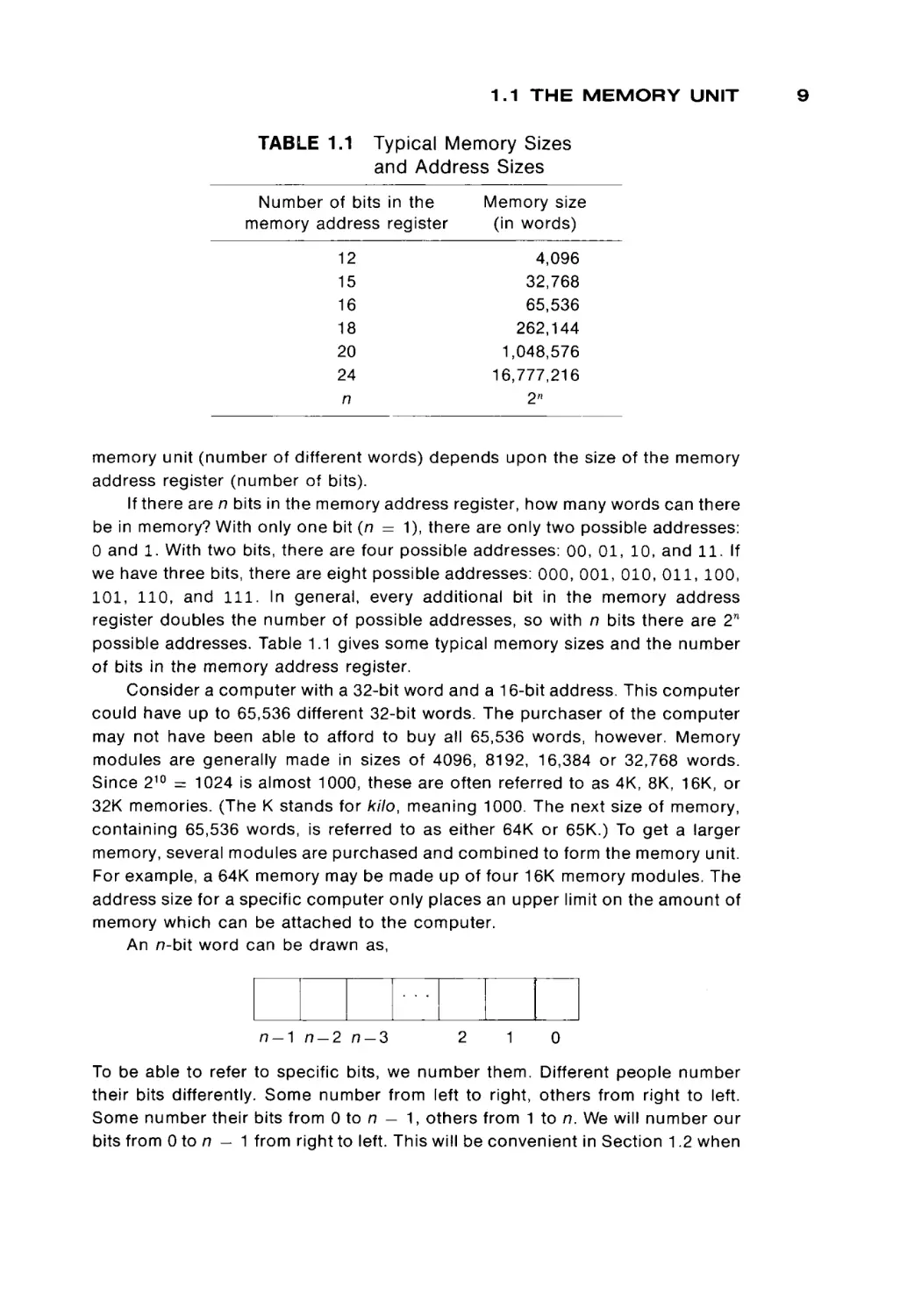
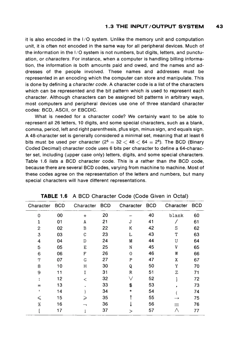
TABLE 1.1
Typical Memory Sizes
and Address Sizes
Number of bits in the
memory address register
Memory size
(in words)
12
15
16
18
20
24
n
4,096
32,768
65,536
262,144
1,048,576
16,777,216
2n
memory unit (number of different words) depends upon the size of the memory
address register (number of bits).
If there are n bits in the memory address register, how many words can there
be in memory? With only one bit (n = 1), there are only two possible addresses:
0 and 1. With two bits, there are four possible addresses: 00, 0 1 , 10, and 11. If
we have three bits, there are eight possible addresses: 000, 001, 010, 011, 100,
101, 110, and 111. In general, every additional bit in the memory address
register doubles the number of possible addresses, so with n bits there are 2W
possible addresses. Table 1.1 gives some typical memory sizes and the number
of bits in the memory address register.
Consider a computer with a 32-bit word and a 16-bit address. This computer
could have up to 65,536 different 32-bit words. The purchaser of the computer
may not have been able to afford to buy all 65,536 words, however. Memory
modules are generally made in sizes of 4096, 8192, 16,384 or 32,768 words.
Since 210 = 1024 is almost 1000, these are often referred to as 4K, 8K, 16K, or
32K memories. (The K stands for kilo, meaning 1000. The next size of memory,
containing 65,536 words, is referred to as either 64K or 65K.) To get a larger
memory, several modules are purchased and combined to form the memory unit.
For example, a 64K memory may be made up of four 16K memory modules. The
address size for a specific computer only places an upper limit on the amount of
memory which can be attached to the computer.
An n-bit word can be drawn as,
η-λ
n-2
n-3
2
1
0
To be able to refer to specific bits, we number them. Different people number
their bits differently. Some number from left to right, others from right to left.
Some number their bits from 0 to n — 1, others from 1 to n. We will number our
bits from 0 to n — 1 from right to left. This will be convenient in Section 1.2 when
10
1 BASIC COMPUTER ORGANIZATION
we discuss number systems. The right-hand bits are called the low-order bits,
while the left-hand bits are called high-order bits.
Many computers consider their words to be composed of bytes. A byte is a
part of a word composed of a fixed number (usually 6 or 8) of bits. A 32-bit word
could be composed of four 8-bit bytes. These would be bits 0-7, 8-15, 16-23,
and 24-31. The usefulness of byte-sized quantities will become apparent in
Section 1.3, when we discuss I/O and character codes.
In addition to the words of the memory unit, a computer will probably have a
small number of high-speed registers. These are generally either the same size
as a word of memory or the size of an address. Most registers are referred to by
a name, rather than an address. For example, the memory address r e g i e r might
be called the MAR, and the memory data register the MDR. Typical other regis
ters may include an accumulator (A register) of the computation unit, and the
program counter (P register) of the control unit. These registers provide memory
for the computer, but they are used for special purposes.
Memory for a computer consists of a large number of fixed-length words.
Each word is composed of a fixed number of bits. Words can be stored at
specific locations in the memory unit and later read from that location. Each
location in memory is one word and has its own unique address. A machine with
n-bit addresses can have up to 2 n different memory locations.
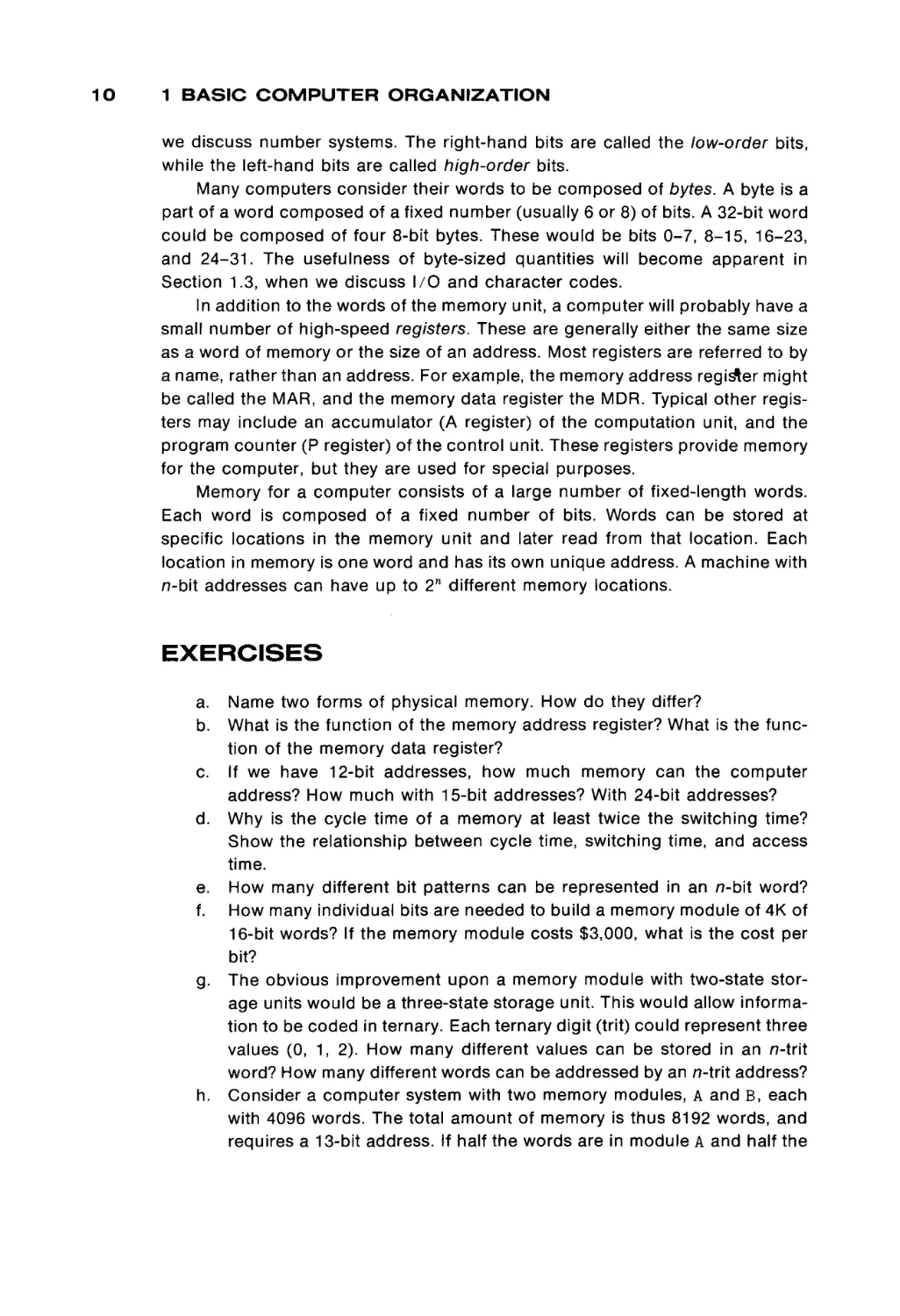
EXERCISES
a.
b.
Name two forms of physical memory. How do they differ?
What is the function of the memory address register? What is the func
tion of the memory data register?
c. If we have 12-bit addresses, how much memory can the computer
address? How much with 15-bit addresses? With 24-bit addresses?
d. Why is the cycle time of a memory at least twice the switching time?
Show the relationship between cycle time, switching time, and access
time.
e. How many different bit patterns can be represented in an n-bit word?
f. How many individual bits are needed to build a memory module of 4K of
16-bit words? If the memory module costs $3,000, what is the cost per
bit?
g. The obvious improvement upon a memory module with two-state stor
age units would be a three-state storage unit. This would allow informa
tion to be coded in ternary. Each ternary digit (trit) could represent three
values (0, 1, 2). How many different values can be stored in an n-trit
word? How many different words can be addressed by an n-trit address?
h. Consider a computer system with two memory modules, A and B, each
with 4096 words. The total amount of memory is thus 8192 words, and
requires a 13-bit address. If half the words are in module A and half the
1.2 THE COMPUTATION UNIT
i.
j.
words are in module B, then 1 bit is needed to determine which memory
module has a specific word, and the remaining 12 bits address one of
the words within the selected module. If the high-order bit of the address
is used to select module A or module B, which addresses are in which
module? Which words are in which module if the low-order bit is used to
select the module?
What is the difference between dynamic and static semiconductor mem
ory?
Is a read-only memory volatile? Why?
1.2 THE COMPUTATION UNIT
The computation unit contains the electronic circuitry which manipulates the
data in the computer. It is here that numbers are added, subtracted, multiplied,
divided, and compared. The computation unit is commonly called the arithmetic
and logic unit (ALU).
Since the main function of the computation unit is to manipulate numbers,
the design of the computation unit is determined mainly by the way in which
numbers are represented within the computer. Once the scheme for represent
ing numbers has been decided upon, the construction of the computation unit is
an exercise in electronic switching theory.
The representation of numbers
Mathematicians have emphasized that a number is a concept. The concept
of a specific number can be represented by a numeral. A numeral is simply a
convenient means of recording and manipulating numbers. The specific manner
in which numbers are represented has varied from culture to culture and from
time to time. Early representations of numbers by piles of sticks gave way to
making marks in an organized manner (I, II, III, Nil, INN, . . .). This method in turn
eventually was replaced by Roman numerals (I, II, III, IV, V, . . .) and finally by
Arabic numerals (1, 2, 3, 4, 5, . . .). Notice that we have Roman numerals and
Arabic numerals, not Roman numbers or Arabic numbers. The symbols which
are used to represent numbers are called digits.
The choice of a number system depends on many things. One important
factor is the convenience of expressing and operating on the numerals. Another
important idea is the expressive power of the system (Roman numerals, for
example, have no representation for zero, or for fractions). A third determining
factor is convention. A representation of a number is used both to remember
numbers and to communicate them. In order for the communication to succeed,
all parties must agree on how numbers are to be represented.
Computers, of course, have only two symbols which can be used as digits.
These two digits are the 0 and the 1 symbols which can be stored in the com-
11
12
1 BASIC COMPUTER ORGANIZATION
puter's memory unit. We are limited to representing our numbers only as combi
nations of these symbols. Remember that with n bits we can represent 2 n differ
ent bit patterns. Each of these bit patterns can be used to represent a different
number. (If we were to use more than one bit pattern to represent a number, or
one bit pattern to represent more than one number, using the numbers might be
more difficult.)
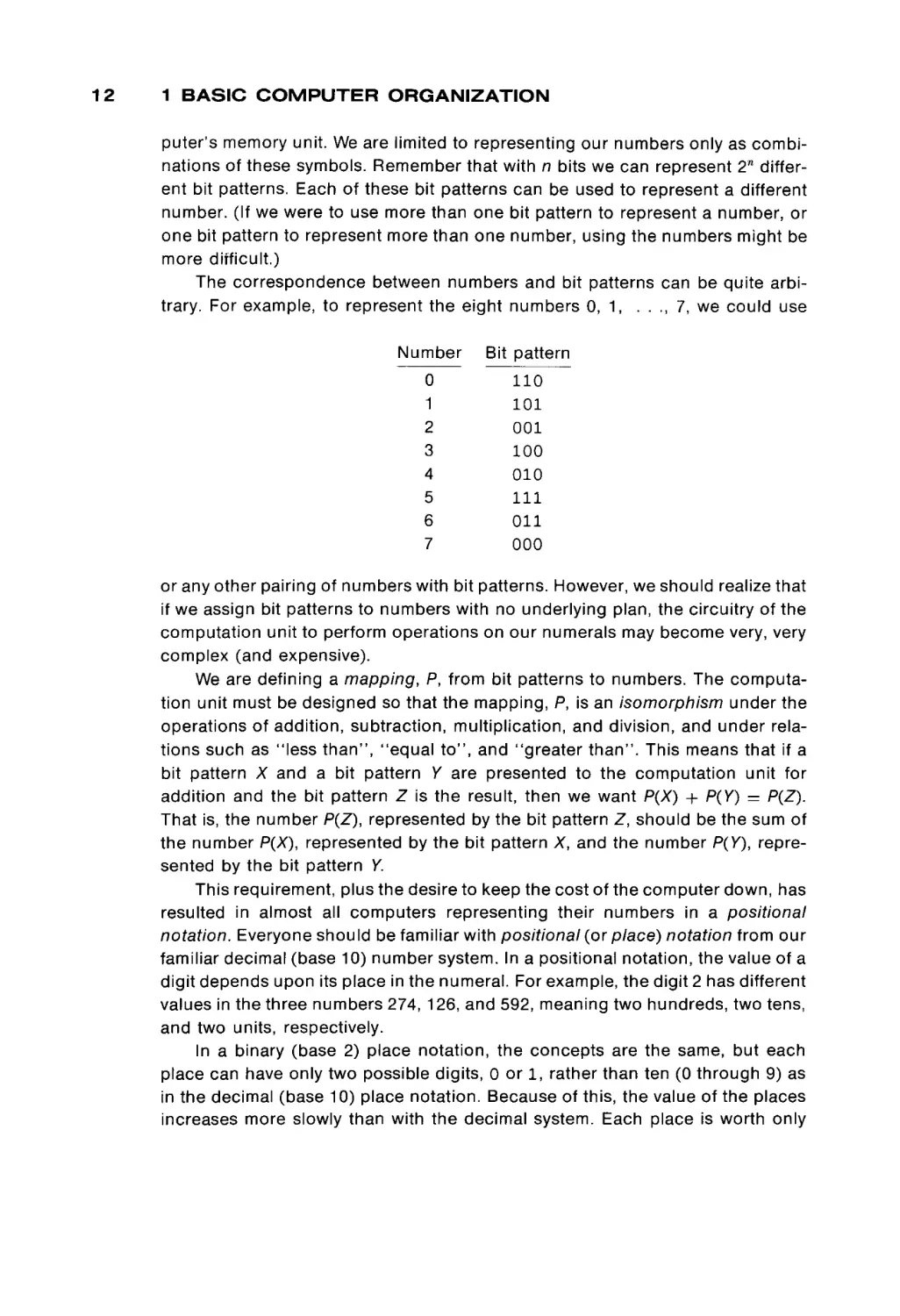
The correspondence between numbers and bit patterns can be quite arbi
trary. For example, to represent the eight numbers 0 , 1 , . . ., 7, we could use
mber
Bit pattern
0
110
1
101
2
001
100
3
4
5
010
111
6
7
011
000
or any other pairing of numbers with bit patterns. However, we should realize that
if we assign bit patterns to numbers with no underlying plan, the circuitry of the
computation unit to perform operations on our numerals may become very, very
complex (and expensive).
We are defining a mapping, P, from bit patterns to numbers. The computa
tion unit must be designed so that the mapping, P, is an isomorphism under the
operations of addition, subtraction, multiplication, and division, and under rela
tions such as "less than", "equal to", and "greater than". This means that if a
bit pattern X and a bit pattern Y are presented to the computation unit for
addition and the bit pattern Z is the result, then we want P(X) + P(Y) = P(Z).
That is, the number P(Z), represented by the bit pattern Z, should be the sum of
the number P(X), represented by the bit pattern X, and the number P(Y), repre
sented by the bit pattern Y.
This requirement, plus the desire to keep the cost of the computer down, has
resulted in almost all computers representing their numbers in a positional
notation. Everyone should be familiar with positional (or place) notation from our
familiar decimal (base 10) number system. In a positional notation, the value of a
digit depends upon its place in the numeral. For example, the digit 2 has different
values in the three numbers 274, 126, and 592, meaning two hundreds, two tens,
and two units, respectively.
In a binary (base 2) place notation, the concepts are the same, but each
place can have only two possible digits, 0 or 1, rather than ten (0 through 9) as
in the decimal (base 10) place notation. Because of this, the value of the places
increases more slowly than with the decimal system. Each place is worth only
1.2 THE COMPUTATION UNIT
twice the value of the place to its right, rather than ten times the value as in the
decimal system. The rightmost place represents the number of units; the next
rightmost, the number of twos; the next, the number of fours; and so forth.
Counting in the binary positional number system proceeds
0,
0,
1,
1,
10,
2,
11,
3,
100,
4
101,
5,
110,
6,
111,
7,
1000,
8,
1001,
9,
The decimal system
We stopped at 9 above, because at 10 two major methods of representing
numbers in a computer show their differences. One method, the binary system
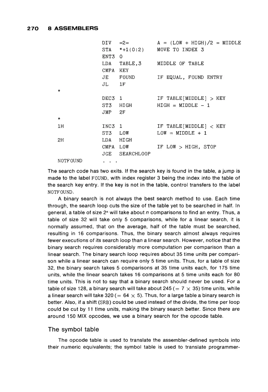
(discussed in the following section), continues as above. The other system, the
decimal system uses the above bit patterns to represent the digits from 0 to 9,
and then uses these digits to represent all other numbers. The decimal system
represents numbers in the familiar decimal place system, replacing the digits 0
through 9 with 0000, 0001, 0010, 0011, 0100, 0101, 0110, 0111, 1000, 1001,
respectively. This is known as a binary coded decimal (BCD) representation. For
example, the numbers 314,159 and 271,823 are represented in BCD by
314,159 10 = 0011
271,823 10 = 0010
0001
0111
0100
0001
0001
1000
0101
0010
1001BCD
0011BCD
The subscripts indicate what kind of representation scheme is being used. The
10 means standard base 10 positional notation; BCD means a binary coded
decimal representation. The blanks between digits in the BCD representation
would not be stored, but are only put in to make the number easier to under
stand.
To add these numbers, we add each digit of the addend to the correspond
ing digit of the augend to give the sum digit. Each digit is represented in binary,
so binary arithmetic is used. For binary addition, the addition table is
0
1
0
1
+0=0
+0=1
+1=1
+ 1 = 0 with a carry into the next higher place
Thus, adding the two numbers 314,159 (base 10) and 271,823 (base 10) is
0011 0001 0100 0001 0101 1001 (BCD)
+ 0010 0111 0001 1000 0010 0011 (BCD)
0101 1000 0101 1001 0111 1100 (BCD)
Notice that in the low-order digit we have added 1001 (9) and 0011 (3) to yield a
sum digit of 1100. This is the binary equivalent of12(1 χ δ + 1 χ 4 + 0 χ 2 +
13
14
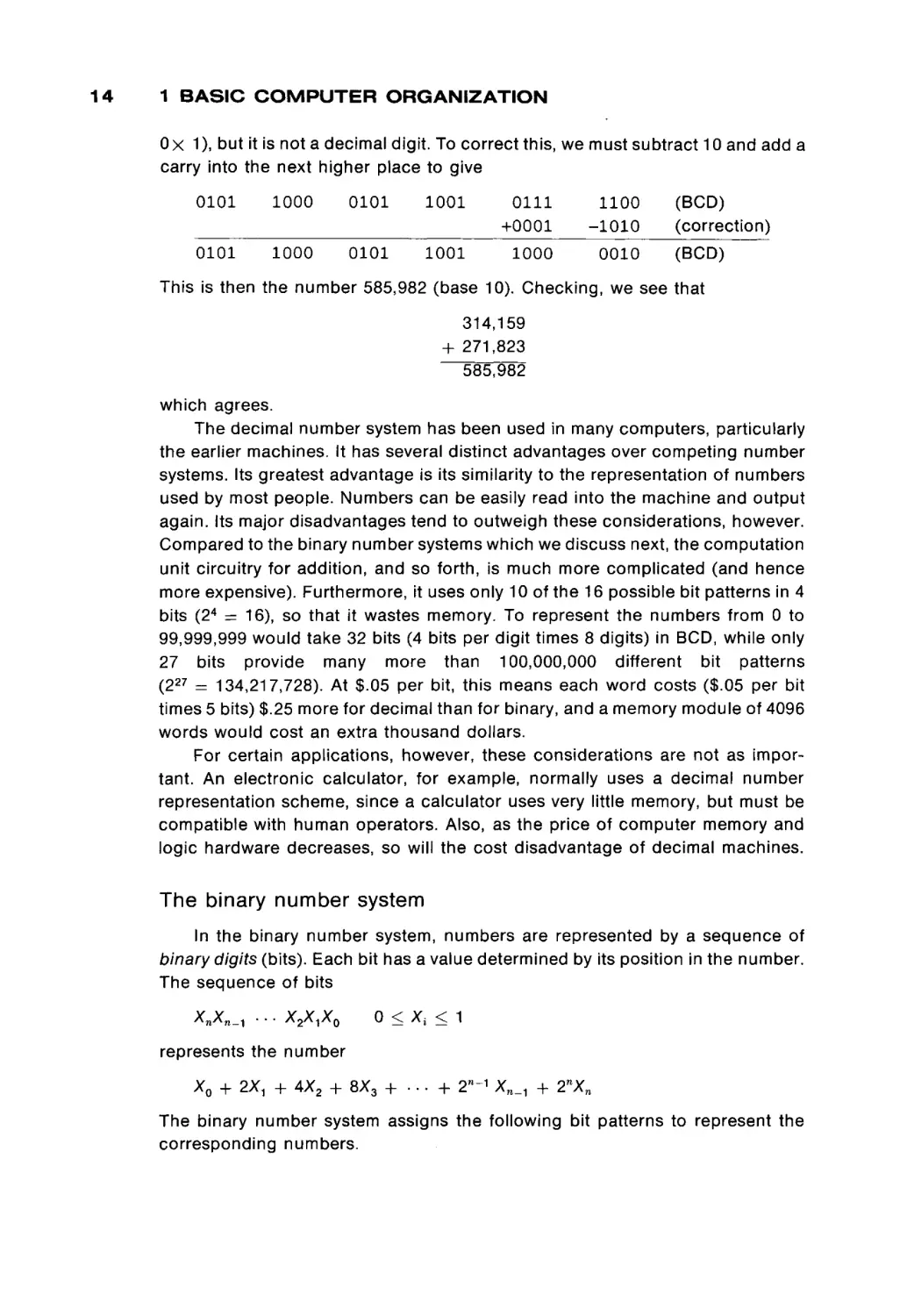
1 BASIC COMPUTER ORGANIZATION
Οχ 1), but it is not a decimal digit. To correct this, we must subtract 10 and add a
carry into the next higher place to give
0101
1000
0101
1001
0111
+0001
1100
-1010
0101
1000
0101
1001
1000
0010
(BCD)
(correction)
(BCD)
This is then the number 585,982 (base 10). Checking, we see that
314,159
+ 271,823
585,982
which agrees.
The decimal number system has been used in many computers, particularly
the earlier machines. It has several distinct advantages over competing number
systems. Its greatest advantage is its similarity to the representation of numbers
used by most people. Numbers can be easily read into the machine and output
again. Its major disadvantages tend to outweigh these considerations, however.
Compared to the binary number systems which we discuss next, the computation
unit circuitry for addition, and so forth, is much more complicated (and hence
more expensive). Furthermore, it uses only 10 of the 16 possible bit patterns in 4
bits (24 = 16), so that it wastes memory. To represent the numbers from 0 to
99,999,999 would take 32 bits (4 bits per digit times 8 digits) in BCD, while only
27 bits provide many more than 100,000,000 different bit patterns
(227 = 134,217,728). At $.05 per bit, this means each word costs ($.05 per bit
times 5 bits) $.25 more for decimal than for binary, and a memory module of 4096
words would cost an extra thousand dollars.
For certain applications, however, these considerations are not as impor
tant. An electronic calculator, for example, normally uses a decimal number
representation scheme, since a calculator uses very little memory, but must be
compatible with human operators. Also, as the price of computer memory and
logic hardware decreases, so will the cost disadvantage of decimal machines.
The binary number system
In the binary number system, numbers are represented by a sequence of
binary digits (bits). Each bit has a value determined by its position in the number.
The sequence of bits
Xn^n-ì * ' * ^ V M ^ O
0 < Aj < 1
represents the number
X0 + 2ΧΛ + 4X2 + 8X3 + .. - + 2W"1 Xn_, + 2nXn
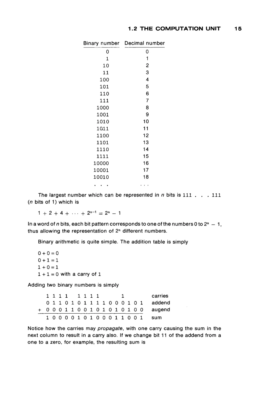
The binary number system assigns the following bit patterns to represent the
corresponding numbers.
1.2 THE COMPUTATION UNIT
Binary number
Decimal number
0
1
10
11
100
101
110
111
1000
1001
1010
1011
1100
1101
1110
1111
10000
10001
10010
0
1
2
3
4
5
6
7
8
9
10
11
12
13
14
15
16
17
18
The largest number which can be represented in n bits is 111 . . . I l l
(n bits of 1) which is
1
+
2 + 4 + . · · + 2n~1 = 2n - 1
In a word of n bits, each bit pattern corresponds to one of the numbers 0 to 2 n — 1,
thus allowing the representation of 2n different numbers.
Binary arithmetic is quite simple. The addition table is simply
0 +0=0
0+1=1
1+0 = 1
1 + 1 = 0 with a carry of 1
Adding two binary numbers is simply
1111
1111
1
0 1 1 0 1 0 1 1 1 1 0 0 0 1 0 1
+ 0 0 0 1 1 0 0 1 0 1 0 1 0 1 0 0
1 0 0 0 0 1 0 1 0 0 0 1 1 0 0 1
carries
addend
augend
sum
Notice how the carries may propagate, with one carry causing the sum in the
next column to result in a carry also. If we change bit 11 of the addend from a
one to a zero, for example, the resulting sum is
15
16
1 BASIC COMPUTER ORGANIZATION
+
1 1 1 1
1
0 1 1 0 0 0 1 1 1 1 0 0 0 1 0 1
0 0 0 1 1 0 0 1 0 1 0 1 0 1 0 0
carries
addend
augend
0 1 1 1 1 1 0 1 0 0 0 1 1 0 0 1
sum
The value of the high-order bit of a sum depends upon the value of all lowerorder bits. Since the value of the high-order bit is greatest, it is called the most
significant bit. The low-order bit is the least significant bit.
The hardware to build a computational unit for a binary machine is quite
simple and easy to design and build. The major disadvantage with binary systems
is their inconvenience and unfamiliarity to humans (Quick! Is 010101110010
[base 2] greater or less than 1394 [base 10]?). The large number of symbols
(zeros and ones) which must be used to represent even "small" numbers is also
cumbersome. Hence, very few programmers prefer to work in binary. But the
computer must work completely in binary. It has no choice, due to the binary
nature of computer hardware. What is needed is a quick and easy way to convert
between binary and decimal. Unfortunately, there is no quick and easy conver
sion algorithm between these two bases.
Conversions between bases
In an arbitrary base B (B > 0) a sequence of digits
ΧηΧη_Λ .. · X2X,X0
(0 < X, < B)
represents the number
Χ0 + β χ λ
1 +
8
2
χ Χ
2
+ . . . +
8-- 1 χ Χη_λ
+β«χΧη
Now if we wish to express the number in another base, A, we can do it in either of
two ways, depending upon whether we want to use the arithmetic of base A or of
base B. For example, if we wish to convert a number from binary (base B = 2) to
decimal (base A = 10), we want to use decimal arithmetic (base A). If we wish to
convert from decimal (base B = 10) to binary (base A = 2), we want to use
decimal arithmetic (base B). The computer, on the other hand, always wants to
use binary arithmetic. Thus, we need two different algorithms for conversion.
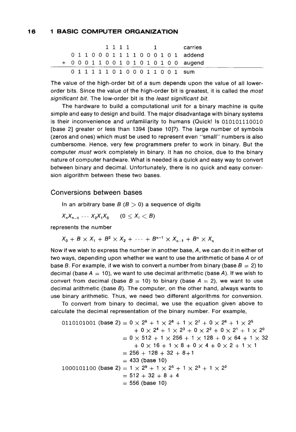
To convert from binary to decimal, we use the equation given above to
calculate the decimal representation of the binary number. For example,
0110101001 (base 2) = 0 χ
+
= 0 x
+
= 256
= 433
1000101100 (base 2) = 1 χ
= 512
= 556
29 + 1 χ 28 + 1 χ 27 + 0 χ 26 + 1 χ 25
0χ24 + 1χ23 + 0χ22 + 0χ21 + 1χ2°
512 + 1 χ 256 + 1 χ 128 + 0 χ 64 + 1 χ 32
0χ16 + 1χ8 + 0χ4 + 0χ2 + 1χ1
+ 128 + 32 + 8 + 1
(base 10)
29 + 1 χ 25 + 1 χ 2 3 + 1 χ 22
+ 32 + 8 + 4
(base 10)
1.2 T H E C O M P U T A T I O N U N I T
TABLE 1.2
2n
1
2
4
8
16
32
64
128
256
512
Powers of Two
2^
n
8192
16,384
32,768
65,536
131,072
262,144
524,288
1,048,576
2,097,152
4,194,304
8,388,608
16,777,216
33,554,432
13
14
15
16
17
18
19
20
21
22
23
24
25
n
0
1
2
3
4
5
6
7
8
9
1024 10
2048 11
4096 12
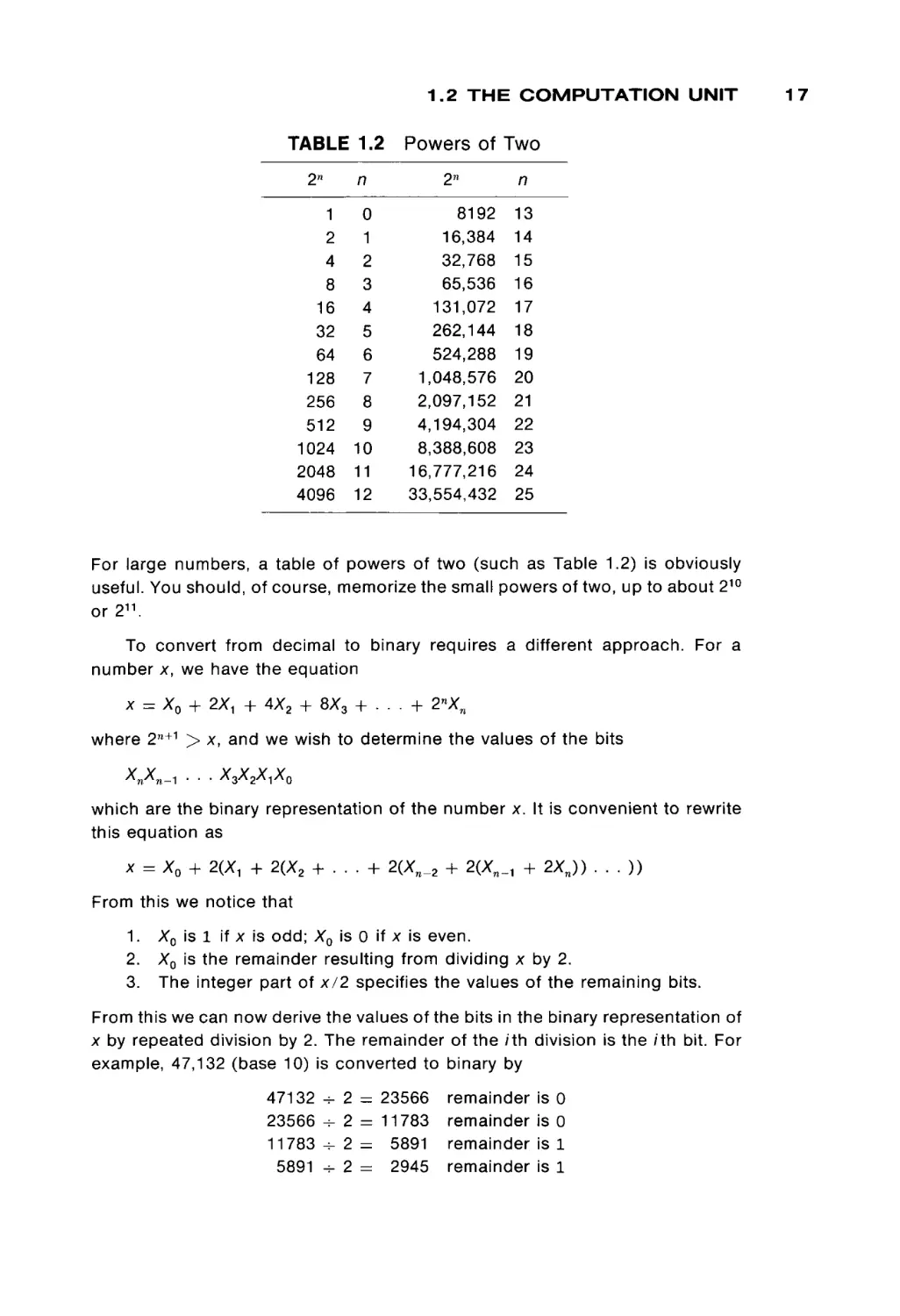
For large numbers, a table of powers of two (such as Table 1.2) is obviously
useful. You should, of course, memorize the small powers of two, up to about 210
or2 1 1 .
To convert from decimal to binary requires a different approach. For a
number x, we have the equation
x = X0 + 2ΧΛ + 4X2 + 8X3 + . . . + 2nXn
where 2 n+1 > x, and we wish to determine the values of the bits
which are the binary representation of the number x. It is convenient to rewrite
this equation as
x = X0 + 2(X, + 2(X2 + . . . + 2(Xn_2 + 2(XW_1 + 2XJ) . . . ))
From this we notice that
1.
2.
3.
X0 is 1 if x is odd; X0 is 0 if x is even.
X0 is the remainder resulting from dividing x by 2.
The integer part of x/2 specifies the values of the remaining bits.
From this we can now derive the values of the bits in the binary representation of
x by repeated division by 2. The remainder of the /th division is the /th bit. For
example, 47,132 (base 10) is converted to binary by
47132 + 2 = 23566
23566 - 2 = 11783
1 1 7 8 3 - 2 = 5891
5891 -- 2 = 2945
remainder
remainder
remainder
remainder
is
is
is
is
0
0
1
1
17
18
1 BASIC COMPUTER ORGANIZATION
2945
1472
736
368
184
92
46
23
11
5
2
1
-------------
2
2
2
2
2
2
2
2
2
2
2
2
= 1472 remainder is 1
736 remainder is 0
=
= 368 remainder is 0
184 remainder is 0
=
92 remainder is 0
=
46 remainder is 0
=
23 remainder is 0
=
11 remainder is 1
=
5 remainder is 1
=
2 remainder is 1
=
=
1 remainder is 0
0 remainder is 1
—
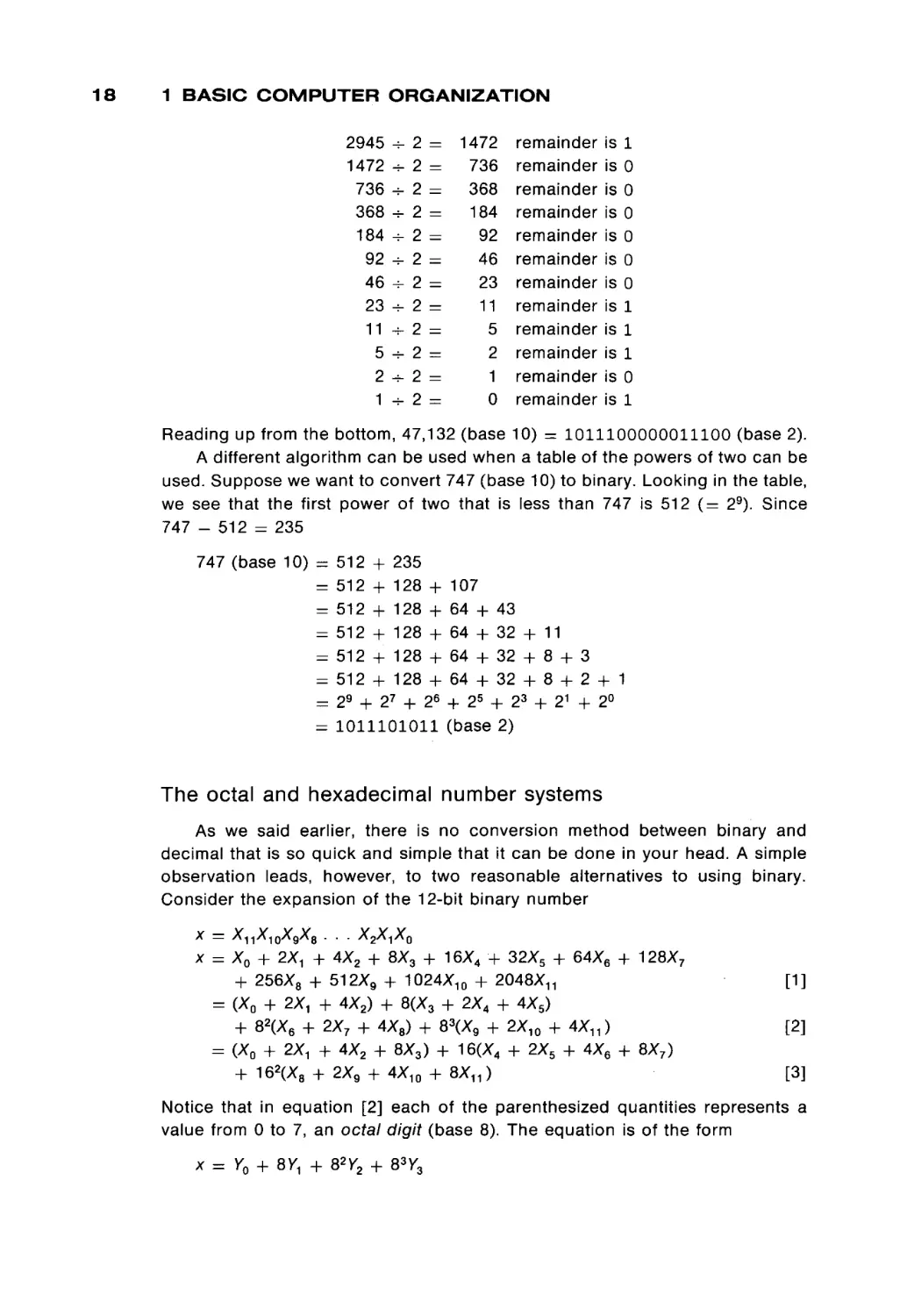
Reading up from the bottom, 47,132 (base 10) = 1011100000011100 (base 2).
A different algorithm can be used when a table of the powers of two can be
used. Suppose we want to convert 747 (base 10) to binary. Looking in the table,
we see that the first power of two that is less than 747 is 512 ( = 29). Since
747 - 512 = 235
747 (base 10) =
=
=
=
=
=
=
=
512 + 235
512 + 128 +
512 + 128 +
512 + 128 +
512 + 128 +
512 + 128 +
29 + 27 + 26
1011101011
107
64 + 43
64 + 32 + 11
64 + 32 + 8 + 3
64 + 32 + 8 + 2 + 1
+ 25 + 23 + 21 + 2°
(base 2)
The octal and hexadecimal number systems
As we said earlier, there is no conversion method between binary and
decimal that is so quick and simple that it can be done in your head. A simple
observation leads, however, to two reasonable alternatives to using binary.
Consider the expansion of the 12-bit binary number
x — X11X10X9X8 . . .
X2X^XQ
x = XQ + 2ΧΛ + 4X
---«2 +■ 8X3
- o +. 16X
- - - ,4 +■ 32X,
- 5 + 64X6 + 128X7
+ -ww,
256X88 -r
+ 512X
" ™ 9 +' 1024X
< " " " 10 +■ 2048Χ
™'ov η
-r
= (X0 + 2Χλ + 4X2) + 8(X3 + 2X4 + 4X5)
+ 82(X6 + 2X7 + 4X8) + 83(X9 + 2X10 + 4 X „ )
= (X0 + 2ΧΛ + 4X2 + 8X3) + 16(X4 + 2X5 + 4X6 + 8X7)
+ 162(X8 + 2X9 + 4X10 + 8XT1)
[1]
[2]
[3]
Notice that in equation [2] each of the parenthesized quantities represents a
value from 0 to 7, an octal digit (base 8). The equation is of the form
x = Y0 + 8V, + 82Y2 + 83V3
1.2 THE COMPUTATION UNIT
where the parenthesized groups of bits define the octal digits for the representa
tion of the number x in base 8 (octal). Similarly, equation [3] is of the form
x = Z 0 + 16Ζλ + 16 2 Z 2
and each Zi is in the range 0 to 15, a hexadecimal digit (base 16).
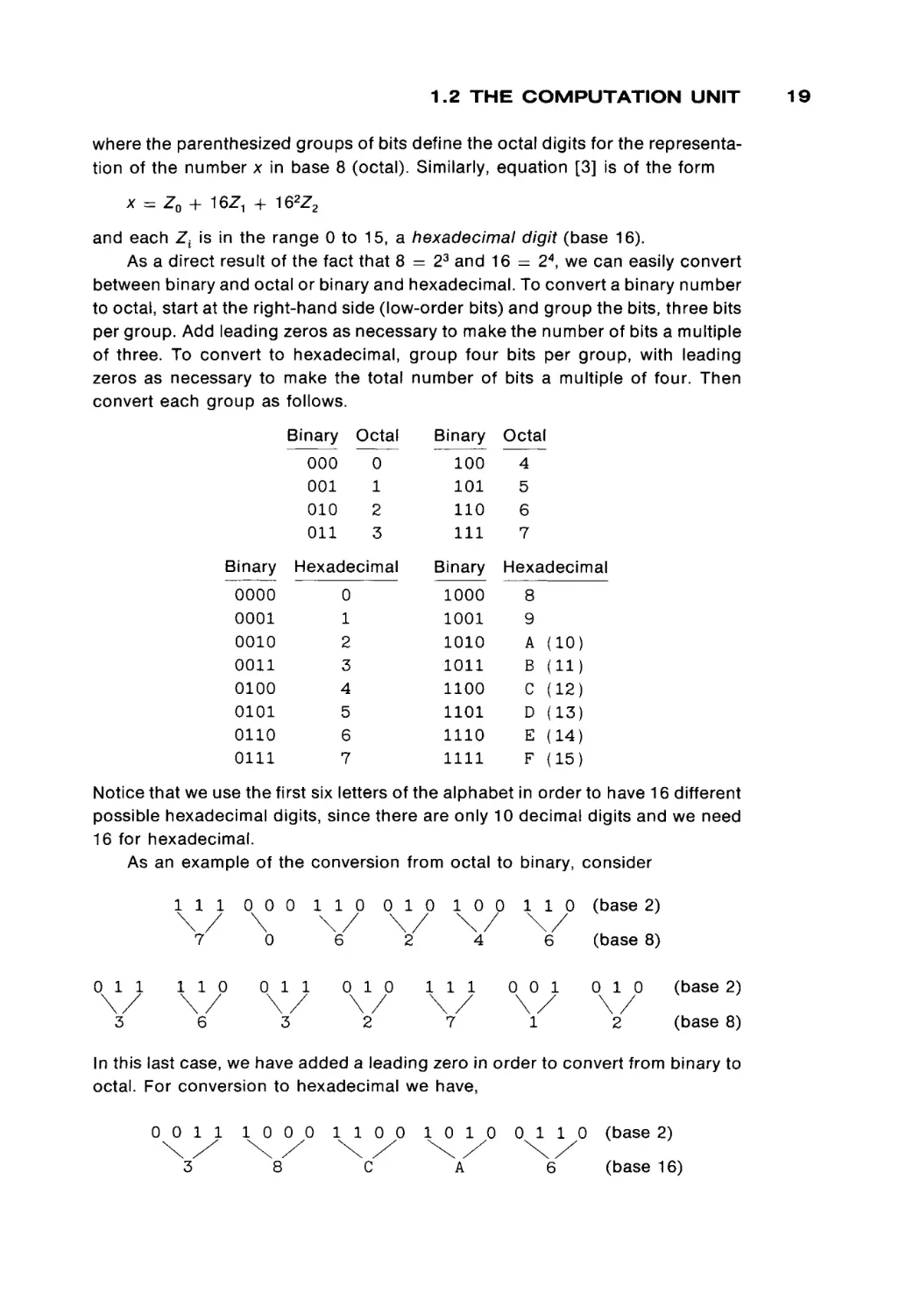
As a direct result of the fact that 8 = 23 and 16 = 24, we can easily convert
between binary and octal or binary and hexadecimal. To convert a binary number
to octal, start at the right-hand side (low-order bits) and group the bits, three bits
per group. Add leading zeros as necessary to make the number of bits a multiple
of three. To convert to hexadecimal, group four bits per group, with leading
zeros as necessary to make the total number of bits a multiple of four. Then
convert each group as follows.
Binary '
Binary
1Octal
100
101
110
111
0
1
2
3
000
001
010
011
Binary
Hexadecimal
Binary
0000
0001
0010
0011
0100
0101
0110
0111
0
1
2
3
4
5
6
7
1000
1001
1010
1011
1100
1101
1110
1111
Octal
4
5
6
7
Hexadecimal
8
9
A
B
C
D
E
F
(10)
(11)
(12)
(13)
(14)
(15)
Notice that we use the first six letters of the alphabet in order to have 16 different
possible hexadecimal digits, since there are only 10 decimal digits and we need
16 for hexadecimal.
As an example of the conversion from octal to binary, consider
111
\ /
7
011
\ /
3
110
\ /
6
000
\
0
011
\ /
3
110
\ /
6
010
\ /
2
010
\ /
2
100
\ /
4
111
\ /
7
110
\ /
6
0 0 1
\ /
1
(base 2)
(base 8)
010
\ /
2
(base 2)
(base 8)
In this last case, we have added a leading zero in order to convert from binary to
octal. For conversion to hexadecimal we have,
0 0 1 1
1 0 0 0
3
8
\ /
\X
1 1 0 0
\ /
C
1 0 1 0
\X
A
0 1 1 0
\ /
6
(base 2)
(base 16)
19
20
1 BASIC COMPUTER ORGANIZATION
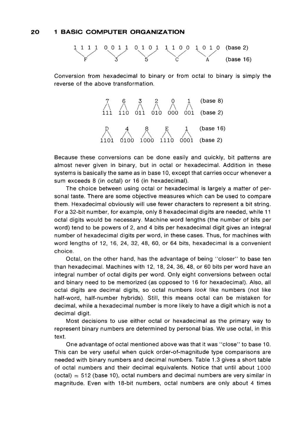
1 1 1 1 0 0 1 1 0 1 0 1 1 1 0 0 1 0 1 0 (base2)
\/
F
\/
3
\/
5
\/
C
\/
A
(base 16)
Conversion from hexadecimal to binary or from octal to binary is simply the
reverse of the above transformation.
(base 8)
111 110
011
010
000
001
(base 2)
(base 16)
Because these conversions can be done easily and quickly, bit patterns are
almost never given in binary, but in octal or hexadecimal. Addition in these
systems is basically the same as in base 10, except that carries occur whenever a
sum exceeds 8 (in octal) or 16 (in hexadecimal).
The choice between using octal or hexadecimal is largely a matter of personal taste. There are some objective measures which can be used to compare
them. Hexadecimal obviously will use fewer characters to represent a bit string.
For a 32-bit number, for example, only 8 hexadecimal digits are needed, while 11
octal digits would be necessary. Machine word lengths (the number of bits per
word) tend to be powers of 2, and 4 bits per hexadecimal digit gives an integral
number of hexadecimal digits per word, in these cases. Thus, for machines with
word lengths of 12, 16, 24, 32, 48, 60, or 64 bits, hexadecimal is a convenient
choice.
Octal, on the other hand, has the advantage of being “closer” to base ten
than hexadecimal. Machines with 12, 18, 24, 36, 48, or 60 bits per word have an
integral number of octal digits per word. Only eight conversions between octal
and binary need to be memorized (as opposed to 16 for hexadecimal). Also, all
octal digits are decimal digits, so octal numbers look like numbers (not like
half-word, half-number hybrids). Still, this means octal can be mistaken for
decimal, while a hexadecimal number is more likely to have a digit which is not a
decimal digit.
Most decisions to use either octal or hexadecimal as the primary way to
represent binary numbers are determined by personal bias. We use octal, in this
text.
One advantage of octal mentioned above was that it was “close” to base 10.
This can be very useful when quick order-of-magnitude type comparisons are
needed with binary numbers and decimal numbers. Table 1.3 gives a short table
of octal numbers and their decimal equivalents. Notice that until about 1000
(octal) = 512 (base l o ) , octal numbers and decimal numbers are very similar in
magnitude. Even with 18-bit numbers, octal numbers are only about 4 times
1.2 T H E C O M P U T A T I O N U N I T
TABLE 1.3
A Table of Octal Numbers and Their
Decimal Equivalents
Octal
Decimal
10
40
100
200
400
8
32
64
128
256
Decimal
Octal
1
4
10
100
1 000
000
000
000
000
000
2
4
32
262
512
048
096
768
144
smaller than they should be. Hence, a very crude way to interpret a binary
number is to convert it to octal, and then treat that octal number as a decimal
number.
Of course, this crude conversion gives only order-of-magnitude results. To
know exactly the value of an octal number, we need to follow the same multipli
cative algorithm which we saw earlier for base 2, but now we are working with
base 8, so the multiplicative factor is eight. For example
1742 (octal) = 1 χ 8 3 + 7 χ 8 2 + 4 χ 8 +
= 512 + 448 + 32 + 2
= 994 (base 10)
2χ1
4 0 6 5 3 (octal) = 4 χ 8 4 + 0 χ 8 3 + 6 χ 8 2 + 5 χ 8 +
= 16384 + 0 + 384 + 40 + 3
= 16811 (base 10)
3χ1
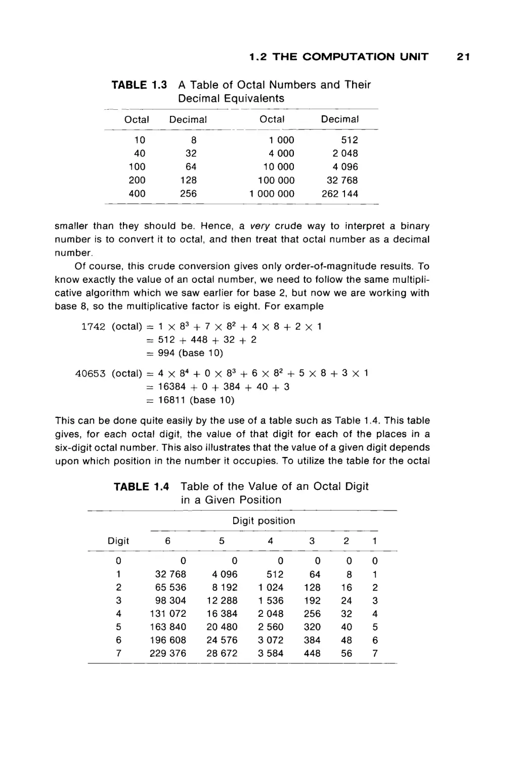
This can be done quite easily by the use of a table such as Table 1.4. This table
gives, for each octal digit, the value of that digit for each of the places in a
six-digit octal number. This also illustrates that the value of a given digit depends
upon which position in the number it occupies. To utilize the table for the octal
Table of the Value of an Ocl:al Digit
TABLE 1.4
in a Given Position
Digit position
Digit
0
1
2
3
4
5
6
7
5
6
32
65
98
131
163
196
229
0
768
536
304
072
840
608
376
4
8
12
16
20
24
28
0
096
192
288
384
480
576
672
4
3
2
1
0
512
1 024
1 536
2 048
2 560
3 072
3 584
0
64
128
192
256
320
384
448
0
8
16
24
32
40
48
56
0
1
2
3
4
5
6
7
21
22
1 BASIC COMPUTER ORGANIZATION
number 574, for example, we look up the entry for digit 5, place 3 (320), and add
to that the value for digit 7, place 2 (56), and add to that the value of digit 4, place
1 (4), to give 574 (octal) = 320 + 56 + 4 = 380 (base 10).
A different method of conversion is to express the original equation of a
conversion as
x = X0 + 8X, + B2X2 + ß3X3 + . . . + BnXn
= X0 + Β(ΧΛ + B(X2 + B(X3 + · · · + BXn . . .)))
Using this form of the conversion equation, we can convert 3756 (octal) to
decimal by
3756 (octal) =
=
=
=
6 + 8(5 + 8(7 + 8-3))
6 + 8(5 + 8-31)
6 + 8 X 253
2030 (base 10)
To convert back from decimal to octal, we repeatedly divide the decimal
number by 8. The remainder at each step is the octal digit, with low-order digits
produced first. Thus, converting 2030 (base 10) to octal gives
2030
253
31
3
-i- 8 = 253,
-r- 8 = 31,
-=- 8 =
3,
-T- 8 =
0,
remainder = 6
remainder = 5
remainder = 7
remainder = 3
and so 2030 (base 10) = 3756 (octal).
Similar algorithms can be used to convert between decimal and hexadeci
mal.
Computer addition
Now that we are familiar with the use of the different number systems, how
do we use this information to represent numbers in the computer? A number is
represented by setting the bits in a word of the computer memory to the binary
representation of the number. To perform arithmetic operations on two numbers
(for example, to add them), the words containing the binary representation of the
two numbers are read from memory, or registers, and copied to the computation
unit. The computation unit is instructed (by the control unit) as to which opera
tion is to be performed, and when the operation is complete the result is stored
back in memory or a register.
The different operations which the computation unit may be asked to do vary
from computer to computer, but almost every computer can at least add two
numbers. Like reading or writing information in memory, the operations done by
the computation unit take time. Generally the computation unit operates some
what faster than the memory cycle time. The time to do an addition (the add time)
1.2 THE COMPUTATION UNIT
varies from machine to machine due to different hardware designs and compo
nents, and also due to different word lengths. Longer words mean longer waiting
for carries to propagate. Add times typically are from 0.3 to 2 microseconds.
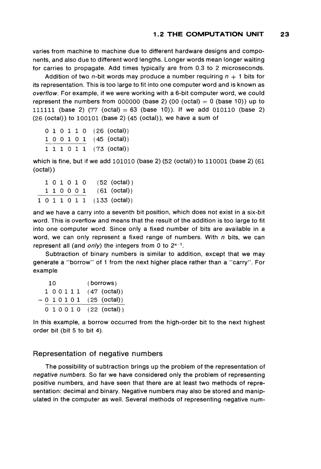
Addition of two π-bit words may produce a number requiring n + 1 bits for
its representation. This is too large to fit into one computer word and is known as
overflow. For example, if we were working with a 6-bit computer word, we could
represent the numbers from 000000 (base 2) (00 (octal) = 0 (base 10)) up to
111111 (base 2) (77 (octal) = 63 (base 10)). If we add 010110 (base 2)
(26 (octal)) to 100101 (base 2) (45 (octal)), we have a sum of
0 1 0 1 1 0
10 0 1 0 1
1 1 1 0 11
(26 (octal))
(45 (octal))
(73 (octal))
which is fine, but if we add 101010 (base 2) (52 (octal)) to 110001 (base 2) (61
(octal))
10 1 0 1 0
1 1 0 0 0 1
10
1 1 0 11
(52 (octal))
(61 (octal))
(133 (octal))
and we have a carry into a seventh bit position, which does not exist in a six-bit
word. This is overflow and means that the result of the addition is too large to fit
into one computer word. Since only a fixed number of bits are available in a
word, we can only represent a fixed range of numbers. With n bits, we can
represent all (and only) the integers from 0 to 2 n _ 1 .
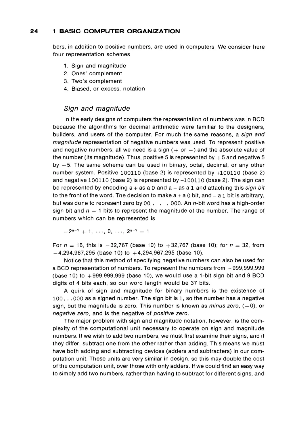
Subtraction of binary numbers is similar to addition, except that we may
generate a "borrow" of 1 from the next higher place rather than a "carry". For
example
10
10 0 111
- 0 1 0 1 0 1
0 10 0 10
(borrows)
(47 (octal))
(25 (octal))
(22 (octal) )
In this example, a borrow occurred from the high-order bit to the next highest
order bit (bit 5 to bit 4).
Representation of negative numbers
The possibility of subtraction brings up the problem of the representation of
negative numbers. So far we have considered only the problem of representing
positive numbers, and have seen that there are at least two methods of repre
sentation: decimal and binary. Negative numbers may also be stored and manip
ulated in the computer as well. Several methods of representing negative num-
23
24
1 BASIC COMPUTER ORGANIZATION
bers, in addition to positive numbers, are used in computers. We consider here
four representation schemes
1.
2.
3.
4.
Sign and magnitude
Ones' complement
Two's complement
Biased, or excess, notation
Sign and magnitude
In the early designs of computers the representation of numbers was in BCD
because the algorithms for decimal arithmetic were familiar to the designers,
builders, and users of the computer. For much the same reasons, a sign and
magnitude representation of negative numbers was used. To represent positive
and negative numbers, all we need is a sign ( + or —) and the absolute value of
the number (its magnitude). Thus, positive 5 is represented by + 5 and negative 5
by —5. The same scheme can be used in binary, octal, decimal, or any other
number system. Positive 100110 (base 2) is represented by +100110 (base 2)
and negative 100110 (base 2) is represented by -100110 (base 2). The sign can
be represented by encoding a + as a 0 and a - as a 1 and attaching this sign bit
to the front of the word. The decision to make a + aO bit, and - a 1 bit is arbitrary,
but was done to represent zero by 00 . . . 000. An n-bit word has a high-order
sign bit and n — 1 bits to represent the magnitude of the number. The range of
numbers which can be represented is
_2*~ 1 + 1, . . . , o, · . . , 2"- 1 - 1
For n = 16, this is -32,767 (base 10) to +32,767 (base 10); for n = 32, from
-4,294,967,295 (base 10) to +4,294,967,295 (base 10).
Notice that this method of specifying negative numbers can also be used for
a BCD representation of numbers. To represent the numbers from -999,999,999
(base 10) to +999,999,999 (base 10), we would use a 1-bit sign bit and 9 BCD
digits of 4 bits each, so our word length would be 37 bits.
A quirk of sign and magnitude for binary numbers is the existence of
100. . . 000 as a signed number. The sign bit is 1, so the number has a negative
sign, but the magnitude is zero. This number is known as minus zero, ( — 0), or
negative zero, and is the negative of positive zero.
The major problem with sign and magnitude notation, however, is the com
plexity of the computational unit necessary to operate on sign and magnitude
numbers. If we wish to add two numbers, we must first examine their signs, and if
they differ, subtract one from the other rather than adding. This means we must
have both adding and subtracting devices (adders and subtracters) in our com
putation unit. These units are very similar in design, so this may double the cost
of the computation unit, over those with only adders. If we could find an easy way
to simply add two numbers, rather than having to subtract for different signs, and
1.2 T H E C O M P U T A T I O N U N I T
a way to find the negative of a number, then we could utilize the fact that
x - y = x + ( - y ) and dispense with the subtracter (or the adder, since
x + y = x - (-y))·
Ones' complement
notation
Ones' complement notation was devised to make the adding of two numbers
with different signs the same as for two numbers with the same sign. The com
plement of a binary number is the number which results from changing all Os to
1s and all 1s to Os in the original number. For example, in a 12-bit machine, the
complement of 0110100111010011 is 1001011000101100, and the comple
ment of 1110111101011011 is 0001000010100100. The complement of
00. . . 000 is 1 1 . . . I l l and the complement of 1 1 . . . I l l is 0 0 . . . 000. In octal,
the complement of each octal digit is
Octal
0
1
2
3
4
5
6
7
Binary
Complement
Binary
Octal
111
110
7
5
4
101
101
100
011
010
110
111
001
000
000
001
010
011
100
6
3
2
1
0
The complement of a number is very easy to create. Also notice that the comple
ment of the complement of a number is the original number, a very important
property for a method of representing negatives. The ones' complement notation
represents the negative of a number by its complement. Thus, for an 8-bit word,
the number 100 (base 10) is represented by 01100100, and negative 100 (base
10) by 10011011. The high-order bit is still treated as the sign bit and not as a
part of the number. A 0 sign bit is a positive number, and a 1 sign bit is a negative
number.
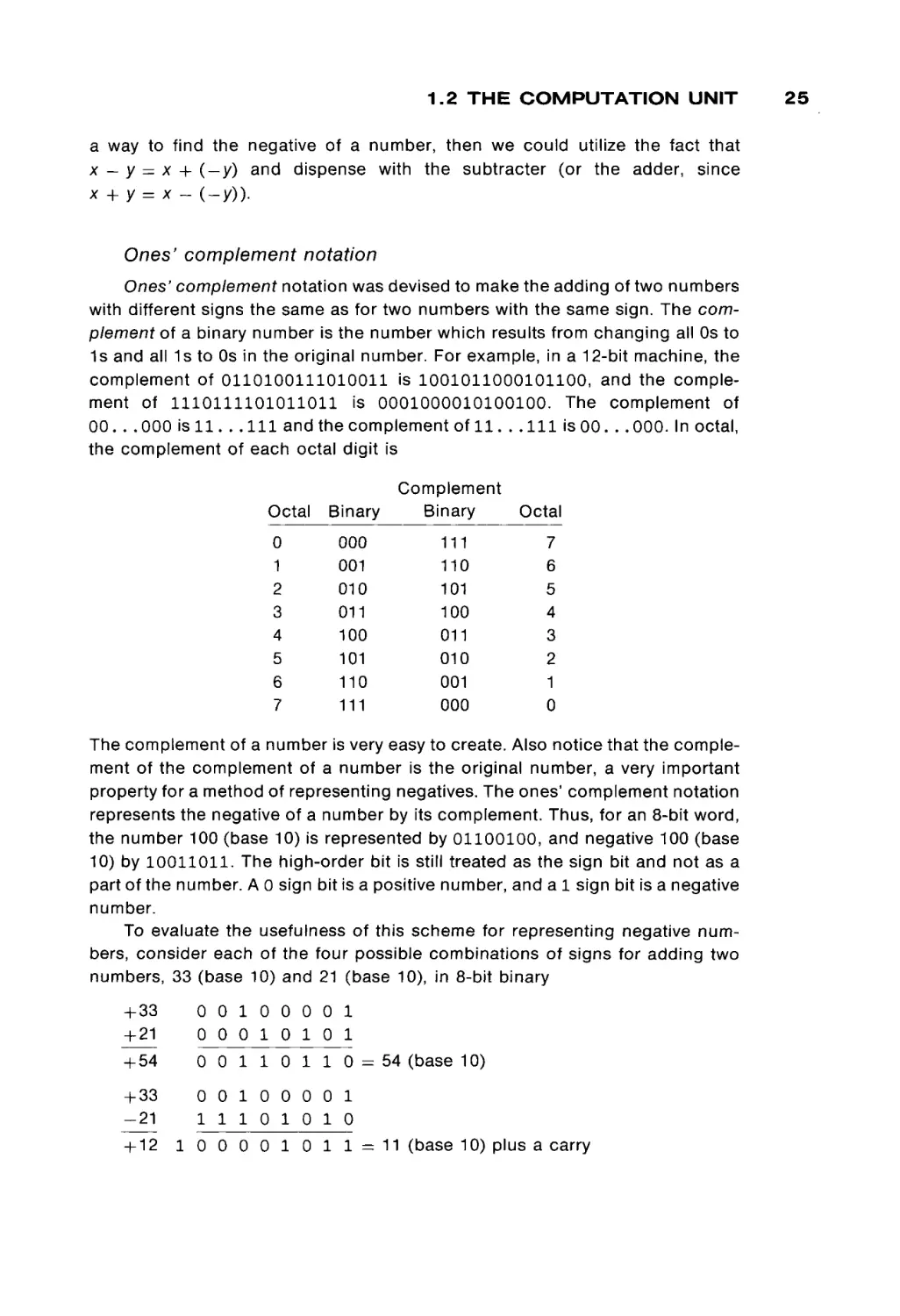
To evaluate the usefulness of this scheme for representing negative num
bers, consider each of the four possible combinations of signs for adding two
numbers, 33 (base 10) and 21 (base 10), in 8-bit binary
+ 33
+ 21
0 0 1 0 0 0 0 1
0 0 0 10 10 1
+ 54
0 0 1 10
+ 33
-21
0 0 1 0 0 0 0 1
1 1 1 0 10 10
+ 12
1 1 0
1 0 0 0 0 1 0 1 1
= 11 (base 10) plus a carry
25
26
1 BASIC COMPUTER ORGANIZATION
-33
+ 21
-12
1 1 0 1 1 1 1 0
0 0 0 1 0 1 0 1
1 1 1 1 0 0 1 1 = -12 (base 10)
-33
-21
-54
1 1 0 1 1 1 1 0
1 1 1 0 1 0 1 0
1 1 1 0 0 1 0 0 0 =
- 5 5 (base 10) plus a carry
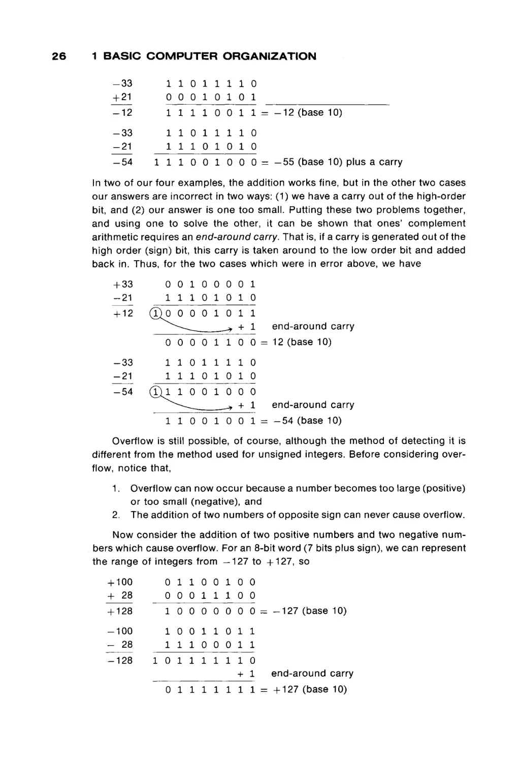
In two of our four examples, the addition works fine, but in the other two cases
our answers are incorrect in two ways: (1) we have a carry out of the high-order
bit, and (2) our answer is one too small. Putting these two problems together,
and using one to solve the other, it can be shown that ones' complement
arithmetic requires an end-around carry. That is, if a carry is generated out of the
high order (sign) bit, this carry is taken around to the low order bit and added
back in. Thus, for the two cases which were in error above, we have
+ 33
-21
+ 12
-33
-21
-54
0 0 1 0 0 0 0 1
1 1 1 0 1 0 10
(£)0
0 0 0 1 0
11
end-around carry
-* + 1
0 0 0 0 1 1 00 0 = 12 (base 10)
1 1 0 1 1 1 1 0
1 1 1 0 1 0 10
(£j l
1 0 0 1 0 0 0
end-around carry
-* + 1
1 1 0 0 1 0 0 1 = - 5 4 (base 10)
Overflow is still possible, of course, although the method of detecting it is
different from the method used for unsigned integers. Before considering over
flow, notice that,
1.
2.
Overflow can now occur because a number becomes too large (positive)
or too small (negative), and
The addition of two numbers of opposite sign can never cause overflow.
Now consider the addition of two positive numbers and two negative num
bers which cause overflow. For an 8-bit word (7 bits plus sign), we can represent
the range of integers from —127 to +127, so
+ 100
+ 28
0 1 1 0 0 1 0 0
0 0 0 1 1 1 0 0
+ 128
1 0 0 0 0 0 0 0
-100
- 28
1 0 0 1 1 0 1 1
1 1 1 0 0 0 1 1
-128
1 0 1 1 1 1 1 1 0
+ 1
0 1 1 1 1 1 1 1
=z - 1 2 7 (base 10)
end-around carr
= + 1 2 7 (base 10)
1.2 T H E C O M P U T A T I O N U N I T
There are several ways to state the condition for overflow. One method is to
notice that the sign of the output is different from the sign of the inputs. Overflow
occurs in ones' complement if—and only if—the signs of the inputs are both the
same and differ from the sign of the output. Another statement of this is that
overflow occurs if there is a carry into the sign bit and no carry out of the sign bit
(no end-around carry), or if there is no carry into the sign bit and there is a carry
out (the carry out of the sign bit differs from the carry into the sign bit).
Ones' complement allows simple arithmetic with negative numbers. It does
suffer from one problem that sign and magnitude notation has: negative zero.
The complement of zero (00 . . . 000) is negative zero (11 . . . 111).
Because of the end-around carry, the properties of negative zero are the same as
the properties of positive zero, as far as arithmetic is concerned. For example,
307 (octal) + ( - 0 ) on a 10-bit word is
0 0 1 1 0 0 0 1 1 1
+ 1 1 1 1 1 1 1 1 1 1
1 0 0 1 1 0 0 0 1 1 0
+ 1
0 0 1 1 0 0 0 1 1 1
end-around carry
= 307 (octal)
But the hardware to test for zero must check for both representations of zero,
making it more complicated.
Two's complement
notation
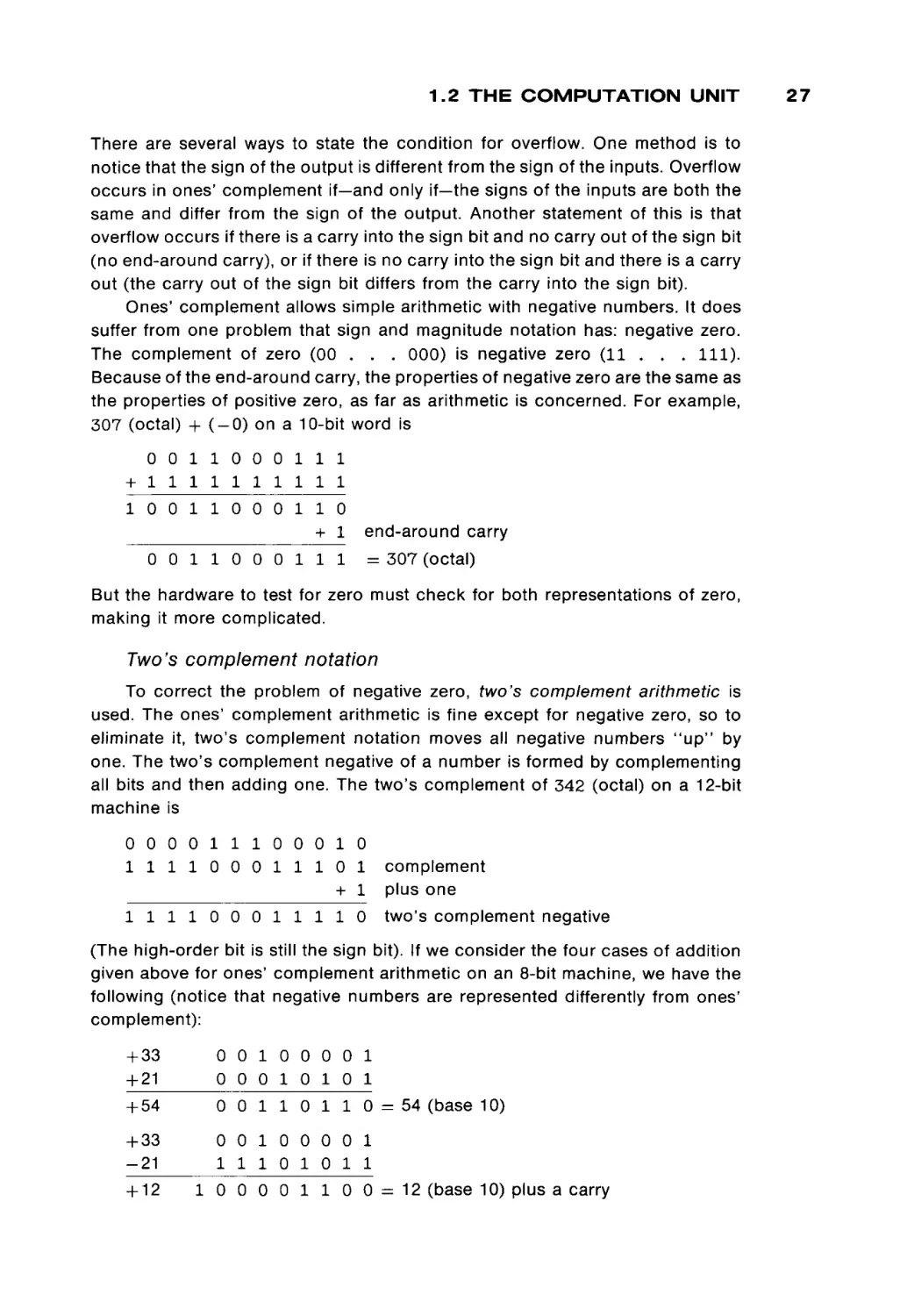
To correct the problem of negative zero, two's complement arithmetic is
used. The ones' complement arithmetic is fine except for negative zero, so to
eliminate it, two's complement notation moves all negative numbers " u p " by
one. The two's complement negative of a number is formed by complementing
all bits and then adding one. The two's complement of 342 (octal) on a 12-bit
machine is
0 0 0 0 1 1 1 0 0 0 1 0
1 1 1 1 0 0 0 1 1 1 0 1
complement
+ 1 plus one
1 1 1 1 0 0 0 1 1 1 1 0
two's complement negative
(The high-order bit is still the sign bit). If we consider the four cases of addition
given above for ones' complement arithmetic on an 8-bit machine, we have the
following (notice that negative numbers are represented differently from ones'
complement):
+ 33
+ 21
+ 54
+ 33
-21
+ 12
0 0 1 0 0 0 0 1
0 0 0 1 0 1 0 1
0 0 1 1 0 1 1 0 = 54 (base 10)
0 0 1 0 0 0 0 1
1 1 1 0 1 0 1 1
1 0 0 0 0 1 1 0 0 = 12 (base 10) plus a carry
27
28
1 BASIC C O M P U T E R
-33
+ 21
-12
1 1 0 1 1 1 1 1
0 0 0 1 0 1 0 1
1 1 1 1 0 1 0 0 = - 1 2
-33
-21
-54
ORGANIZATION
(base 10)
1 1 0 1 1 1 1 1
1 1 1 0 1 0 1 1
1 1 1 0 0 1 0 1 0 =
- 5 4 (base 10) plus a carry
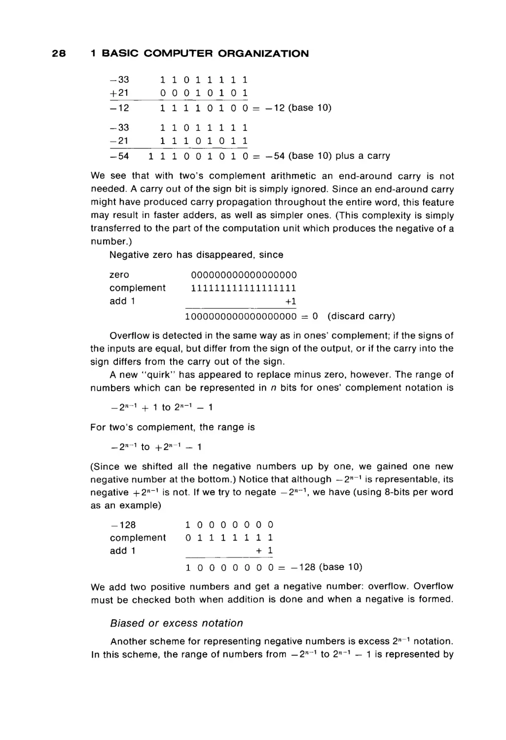
We see that with two's complement arithmetic an end-around carry is not
needed. A carry out of the sign bit is simply ignored. Since an end-around carry
might have produced carry propagation throughout the entire word, this feature
may result in faster adders, as well as simpler ones. (This complexity is simply
transferred to the part of the computation unit which produces the negative of a
number.)
Negative zero has disappeared, since
zero
complement
add 1
000000000000000000
111111111111111111
+1
1000000000000000000 = 0
(discard carry)
Overflow is detected in the same way as in ones' complement; if the signs of
the inputs are equal, but differ from the sign of the output, or if the carry into the
sign differs from the carry out of the sign.
A new "quirk" has appeared to replace minus zero, however. The range of
numbers which can be represented in n bits for ones' complement notation is
-2 W ~ 1 + 1 to 2η~Λ - 1
For two's complement, the range is
_ 2 n - i to +2 M ~ 1 - 1
(Since we shifted all the negative numbers up by one, we gained one new
negative number at the bottom.) Notice that although — 2 n_1 is representable, its
negative + 2W_1 is not. If we try to negate — 2n~\ we have (using 8-bits per word
as an example)
-128
complement
add 1
1 0 0 0 0 0 0 0
0 1 1 1 1 1 1 1
+ 1
10
0 0 0 0 0 0 = - 1 2 8 (base 10)
We add two positive numbers and get a negative number: overflow. Overflow
must be checked both when addition is done and when a negative is formed.
Biased or excess
notation
Another scheme for representing negative numbers is excess 2n~1 notation.
In this scheme, the range of numbers from - 2 n _ 1 to 2 n_1 - 1 is represented by
1.2 THE COMPUTATION UNIT
biasing each number by 2 n_1 . Biasing is done by adding the bias (2 n_1 in this
case) to the number to be biased. This transforms the represented numbers to
the range 0 to 2n - 1. These biased numbers can be represented in the normal
n-bit unsigned binary notation. Excess notation is identical to two's complement
notation, but with the sign bit complemented (a 0 sign bit means a negative
number, a 1 sign bit a positive number; the opposite of a normal sign bit).
The major advantage of excess notation is with comparisons. For the normal
sign bit definition (0 = + , 1 = —), signed and unsigned numbers must be
compared differently. If 0100 and 1011 are unsigned integers, then 1011 >
0100, but if they are signed, then 0100 > 1011, since 0100 is positive and 1011
is negative. By reversing the sign bit definition, both signed and unsigned num
bers can be compared in the same way, since 1 > 0 and + > —. (On the other
hand, the adder now has to treat the sign bit differently from the other bits when
addition is being done.)
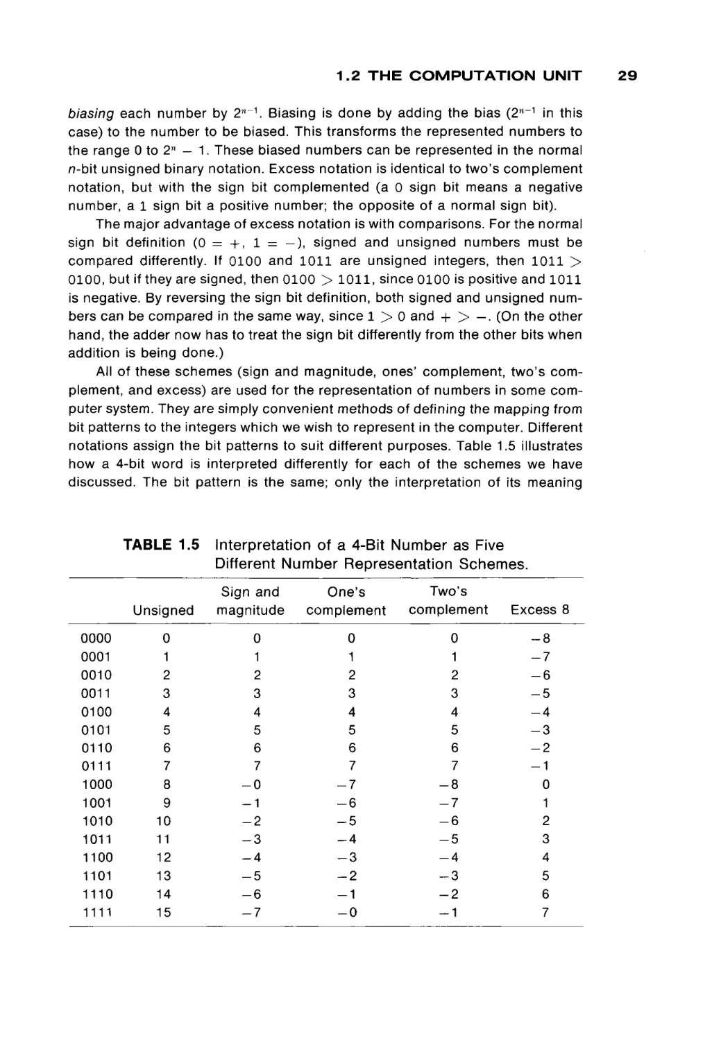
All of these schemes (sign and magnitude, ones' complement, two's com
plement, and excess) are used for the representation of numbers in some com
puter system. They are simply convenient methods of defining the mapping from
bit patterns to the integers which we wish to represent in the computer. Different
notations assign the bit patterns to suit different purposes. Table 1.5 illustrates
how a 4-bit word is interpreted differently for each of the schemes we have
discussed. The bit pattern is the same; only the interpretation of its meaning
TABLE 1.5
0000
0001
0010
0011
0100
0101
0110
0111
1000
1001
1010
1011
1100
1101
1110
1111
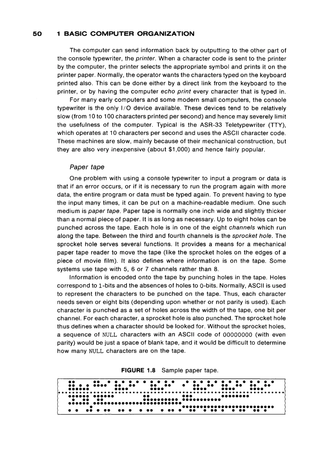
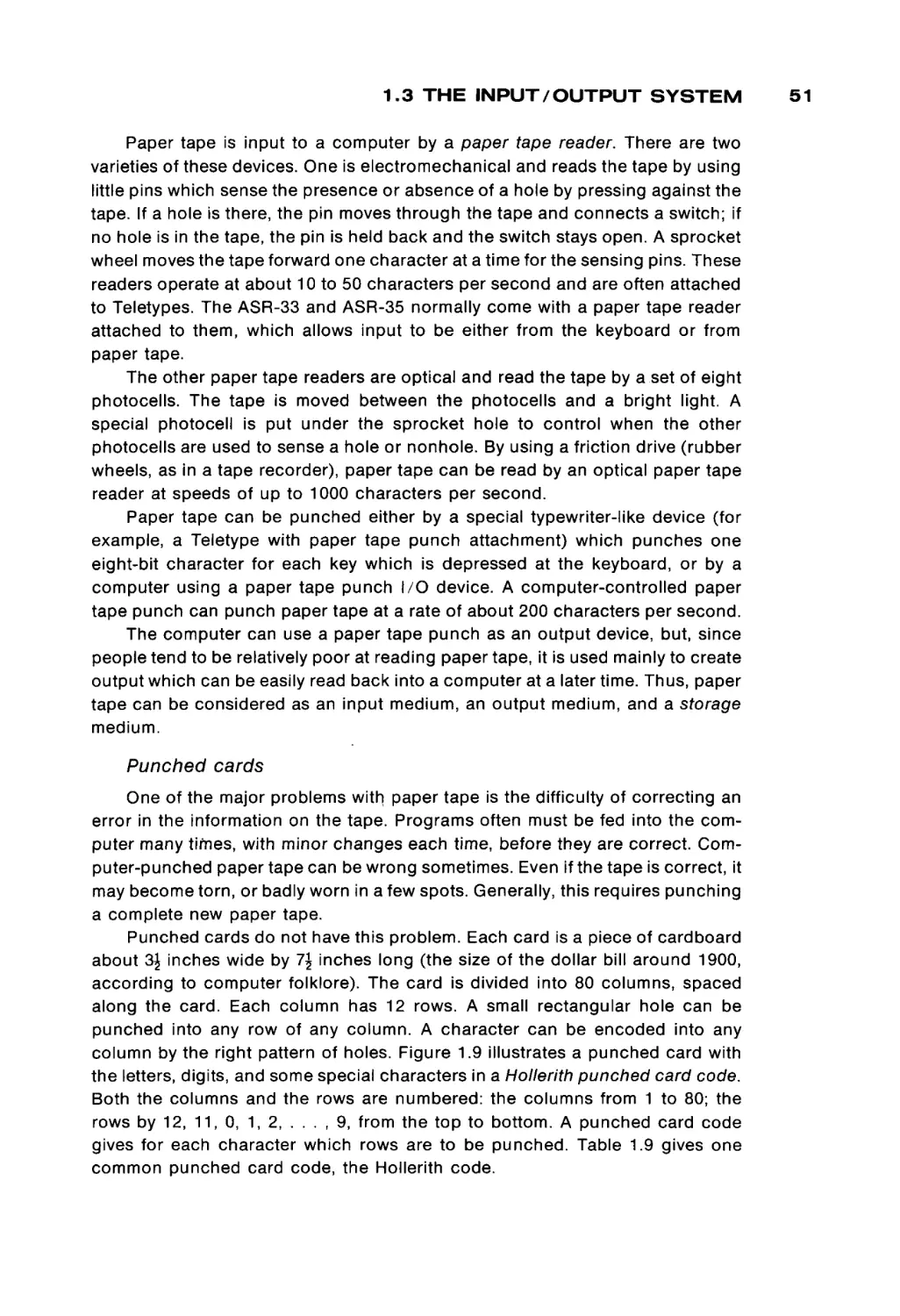
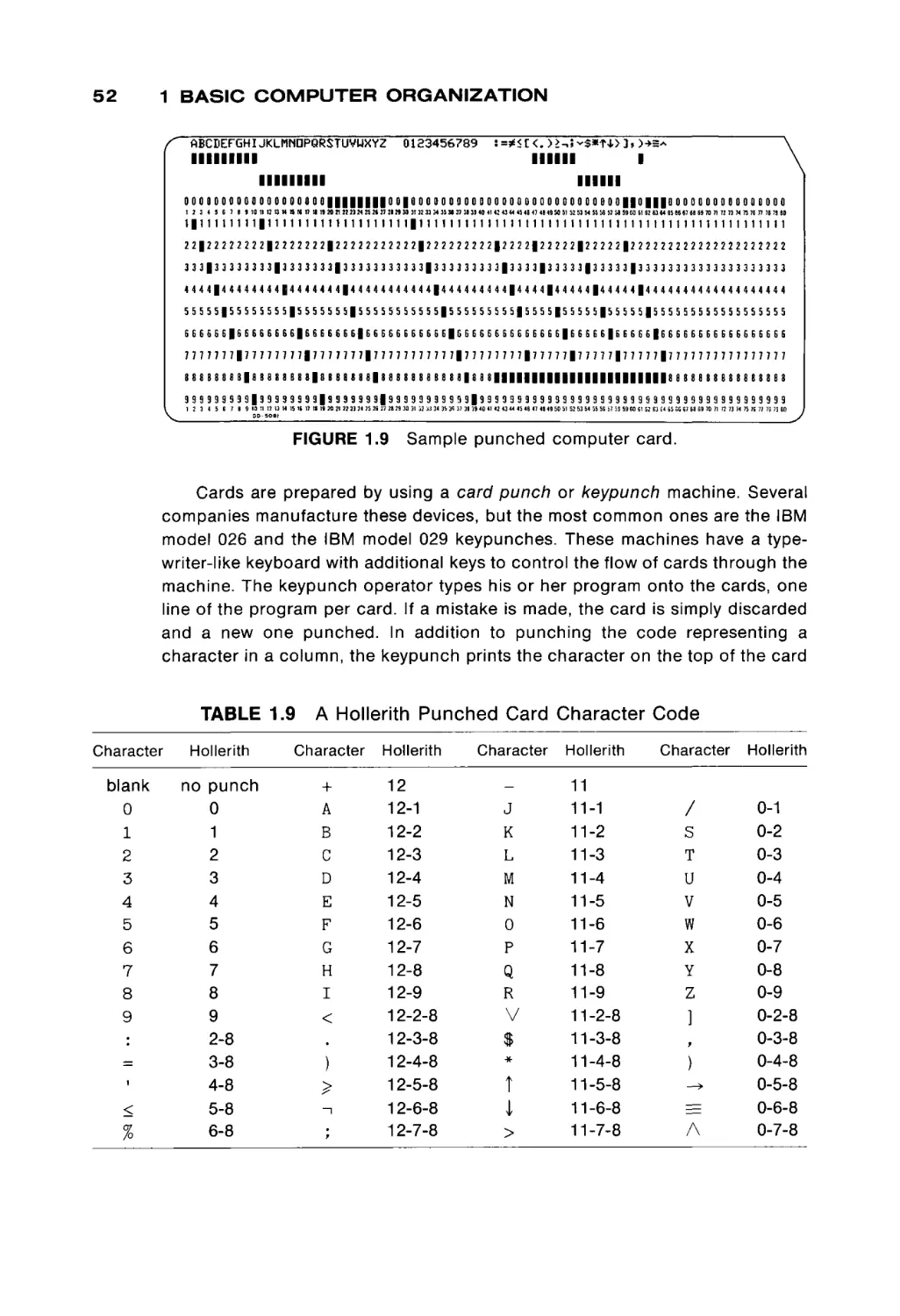
Interpretation of a 4-Bit Number as Five
Different Number Representation Schemes.
Unsigned
Sign and
magnitude
One's
complement
Two's
complement
Excess 8
0
1
2
3
4
5
6
7
8
9
10
11
12
13
14
15
0
1
2
3
4
5
6
7
-0
-1
-2
-3
-4
-5
-6
-7
0
1
2
3
4
5
6
7
-7
-6
-5
-4
-3
-2
-1
-0
0
1
2
3
4
5
6
7
-8
-7
-6
-5
-4
-3
-2
-1
-8
-7
-6
-5
-4
-3
-2
-1
0
1
2
3
4
5
6
7
29
30
1 BASIC COMPUTER ORGANIZATION
differs. Most computer systems use only one of these methods for representing
integers so that the same interpretation can be applied to all words.
Addition and subtraction are two very common operations in a computer,
and the computation unit provides the ability to perform these operations on
binary numbers. As we hinted earlier, most computers do not provide separate
adding and subtracting devices, but only an adder (or subtracter) and a device to
complement or negate numbers. This requires that subtraction be done by
negation and addition (or that addition be done by negation and subtraction).
Multiplication and division
Multiplication and division do not occur as frequently as addition and sub
traction, so many of the smaller computers do not provide hardware to multiply
or divide, but require that the programmer implement multiplication by repeated
additions.and division by repeated subtraction. Larger computers, however, do
generally provide multiplication and division hardware. Both of these functions
normally take more time to perform than addition.
In addition to the increased time required for multiplication, the problem of
overflow becomes more important. When two π-bit numbers are added, overflow
may occur because the result may generate a carry out of the high-order bit. The
largest number which can be represented in an unsigned /7-bit number is 2 n - 1,
and so the sum of any two numbers can be no larger than 2W - 1 + 2 n - 1 =
2 n+1 — 2, which requires n + 1 bits for its representation. For multiplication, the
largest possible result is (2 n - 1) χ (2 n - 1) = 2 2n - 2 n+1 + 1 which requires 2n
bits, or twice as many bits. In decimal, for example, 99 x 99 = 9801, so the
product of two two-digit numbers may be a four-digit number. To represent the
entire product, a double-length register is used. This is commonly done by using
two single-length registers and considering them as one long register with twice
the normal number of bits. If the result of a multiplication is to be used further,
with addition, subtraction, or further multiplication, the high-order bits had best
be all zeros (or all ones, if the product is negative and represented in ones'
complement or two's complement). Otherwise, the product is a number which is
too large to be represented in one word of memory and hence cannot be
operated on by the normal arithmetic operations.
For division, the opposite phenomenon occurs. A 2n-bit dividend divided by
an π-bit divisor may result in an n-bit quotient plus an n-bit remainder. For
example, the four-digit number 1478 divided by the two-digit number 55 yields
the two-digit quotient 26 and the two-digit remainder 48. Thus, many computa
tion units require a double-length dividend and produce two single-length re
sults, the quotient and the remainder. If a single length dividend is desired, it is
extended to a double-length representation for the division. For sign and magni
tude, this involves simply inserting additional high-order (leading) zeros. For
ones' complement, two's complement, and excess notation, this is done by sign
extension. The sign bit is replicated as the new high-order bits. For example, in
1.2 THE COMPUTATION UNIT
ones' complement, a 6-bit representation of 13 (base 10) is 001101 (base 2),
while a 12-bit representation is 000000001101 (base 2). For - 1 3 (base 10), we
have 110010 for a 6-bit representation and 111111110010 for a 12-bit repre
sentation. Only the high order 6 bits differ between the 6-bit and 12-bit represen
tations, and each of these bits is the same as the sign bit. If the quotient which
results from a division exceeds the normal word length, it can be treated either as
overflow or as a double-length quotient, according to how the computation unit
is built. The remainder of a division by an n-bit divisor is never more than n-bits.
Fractions and fixed-point numbers
The divide operation discussed above is often called an integer divide, since
it divides one integer by another and produces an integer quotient and integer
remainder. An alternative way to represent the result would be to give the
quotient as a fraction. How do we represent fractions? In common decimal
mathematical notation, fractions can be represented in two different forms, as
alb or as a decimal fraction, O.xxxx . . . xx. A decimal fraction is another exam
ple of positional notation, but with weights of negative powers of ten (the base)
associated with the places. For example
0.357 = 3 x 10- 1 + 5 χ ^02
+ 7 χ 10~ 3
Similarly, we can define binary fractions as a sequence of binary digits after a
binary point. A binary point looks like a decimal point, but the base of the
numbers is 2, not 10. Thus,
0 . 1 0 1 1 (base 2) = 1 χ 2" 1 + 0 χ 2~2 + 1 χ 2~ 3 + 1 χ 2~4
= 0.5 + 0.125 + 0.0625
= 0.6875 (base 10).
Integers and fractions can be combined, as in
1 1 0 0 . 0 1 1 (base 2) = 1 χ 2 3 + 1 χ 2 2 + 0 χ 21 + 0 χ 2°
+ 0 χ 2- 1 + 1 χ 2" 2 + 1 χ 2-3
= 12.375 (base 10)
Conversion from binary fractions to decimal can be done in several ways.
One method is, as demonstrated above, to expand the number as a sum of
products of powers of two and simply evaluate the resulting expression. A table
of negative powers of two can help. Alternatively, common powers of two can be
factored out, as in (using 2~1 = J)
0.01101
(base 2) =
=
=
=
=
=
(0 + (1 + (1 + (0 + 1 / 2 ) / 2 ) / 2 ) / 2 ) / 2
(0 + (1 + (1 + (0 + 0 . 5 ) / 2 ) / 2 ) / 2 ) / 2
(0 + (1 + (1 + 0.25)/2)/2)/2)
(0 + (1 + 0.625)/2)/2
(0 + 0.8125)/2
0.40625 (base 10)
31
32
1 BASIC COMPUTER ORGANIZATION
Or, considering that multiplication by two simply shifts the binary point by one
place to the right, we can convert by
0 . 1 0 1 1 1 1 (base 2) =
=
=
=
=
0 . 1 0 1 1 1 1 X 2 6 χ 2~6
101111 X 2- 6
47/26
47/64
0.734375 (base 10)
Conversion from decimal fractions to binary is easily done by a simple
iterative multiplication scheme. Assume we have a fraction, x, which we wish to
express in binary. Then we wish to solve for the bits in
x = Χ_Λ2~λ + X_22~2 + X_ 3 2- 3 + · · · + X-m2~m
We can immediately derive that
2 x x = Χ_Λ + X_ 2 2" 1 + X_ 3 2- 2 + . . . + X_ m 2-- + 1
and the first bit (Χ_λ) is the integer part of the result. Separating this from the
remaining fraction, we can derive the second bit by multiplying by two again, and
so on. Thus, for 0.435 (base 10), we have
2 x 0.435 = 0.87
2 x 0.87 = 1.74
2 x 0.74 = 1.48
2 x 0.48 = 0.96
2 x 0.96 = 1.92
2 x 0.92 = 1.84
2 x 0.84 = 1.68
2 x 0.68
2 x 0.36
2 x 0.72
= 1.36
= 0.72
= 1.44
first bit =
next bit =
=
=
=
0
1
1
0
1
= 1
= 1
= 1
= 0
= 1
and so on. Thus,
0.435 (base 10) = 0 . 0 1 1 0 1 1 1 1 0 1 0 1 1 1 0 0 0 0 1 0 1 0 0 0 1 1 1 1
where the underlined portion repeats forever, in the same way that the decimal
fraction for 1/3 = 0.33333333333333333. This illustrates both the conversion
process and that not all decimal numbers can be exactly represented in a finite
number of bits. Some nonrepeating decimal fractions are repeating fractions in
binary, just as the fraction 1/3 is a repeating fraction in decimal. No matter how
many bits we allow in a word to represent a binary fraction, we may not be able to
represent some decimal fractions exactly. By adding more and more bits, we can
come closer and closer, but we may always be incorrect by some small amount.
For 0.435, for example, if we allow only two bits of precision, then we can
represent only 0.00, 0 . 0 1 , 0.10, and 0 . 1 1 (base 2) (0, 0.25, 0.5 and 0.75 [base
1.2 THE COMPUTATION UNIT
10]) and we would chose 0.10 as the closest approximation to 0.435. With 9 bits,
we can represent 0.011011110 (base 2) (=0.43359375 [base 10]) and
0.011011111 (base 2) ( = 0.435536875 [base 10]) but not 0.435. Obviously, as
we keep increasing the number of bits used, the precision of our numbers gets
better and better. In fact, if the closest binary fraction of n bits is used to
represent a decimal fraction, the round-off error in representation is less than
2~n-i with 9 bits to represent 0.435, the closest representation is 0.011011111
(base 2) ( = 0.435546875 (base 10)) and the error is
0.435546875 - 0.435 = 0.000546875 < 0.0009765625 = 2" 1 0
When the position of the binary point is assumed to be in the same location
for all numbers, the resulting representation is called a fixed-point number.
Integers are a special case of fixed-point numbers where the binary point is
assumed to be just to the right of the low-order bit. Fixed-point numbers can
always be treated as if they were just integers whenever addition or subtraction is
done because of the distributive law of multiplication over addition. If a and b
have the binary point n bits from the right, then a x 2 n and b x 2 n are integers
and
a + b = (a + b) χ 2n χ 2~η
= (a x 2n + b x 2 n ) x 2~n
(This is just saying that when you add dollars and cents, you do not have to add
the cents by any special rule, but can just add as if the decimal point is not there,
and then replace the decimal point after the addition.)
Floating point representation
A different way to represent fractions allows the position of the binary point
to vary from one number to another. This is called floating point representation. If
this is done, then we need to know both the fraction and where the binary point
is. So a floating point number consists of two parts, one part to give the magni
tude of the number and the other to indicate the location of the binary point.
Binary floating point numbers are generally thought of as equivalent to scientific
notation for decimal numbers. Scientific notation, as you remember, represents a
number as a fraction times a power of 10. Thus, Avogadro's number is expressed
as 6.0225 χ 1023, rather than as 602250000000000000000000. Planck's constant
is 1.0545 x 10- 27 , rather than 0.0000000000000000000000000010545. Similarly,
we can express numbers in binary as 0.101101 χ 215 to represent
101101000000000 (base 2), and 0.111101 x 2~3 to represent 0.000111101
(base 2).
For each floating point number, we need to store only two numbers: the
exponent (or characteristic) and the fraction (or mantissa). The same base can
be used for all floating point numbers and need not be stored. The most popular
base for floating point numbers is 2 (for obvious reasons), but some machines
33
34
1 BASIC COMPUTER ORGANIZATION
use 8 or 16 as the base for the exponent. The choice of exponent base is
influenced by considerations of range and precision, and can in turn affect the
choice of octal or hexadecimal for writing numbers.
To represent a floating point number, we have two numbers to store. Notice
that both numbers can be treated as signed integers. Both numbers are com
monly packed into one word for machines with large enough word sizes. For
example, on the CDC 3600, a floating point number is stored as
sw
se
exponent
fraction
where, sw is the sign of the number (ones' complement)
se is the sign of the exponent (excess 1024)
exponent is a 10-bit biased exponent
fraction is a 36-bit fraction
This notation allows a range of numbers from approximately
2-1024
t 0
2+1023
( 1 0 - 3 0 7 to 10+307)
On the IBM 360/370 machines, a floating point number is represented by
sf
se
exponent
fraction
where sf is the sign of the fraction (sign and magnitude)
se is the sign of the exponent (excess 64)
exponent is a 6-bit exponent
fraction is a 24-bit fraction
The IBM 360/370 uses 16 as the base of the exponent, so that the range of
numbers which can be represented is approximately
16" 64 to 16 +63
(10- 77 to 10 +75 )
The number of bits allocated to the fraction determines the precision of the
number. Remember that the round-off error in an n-bit fraction is less than 2~ n_1 ,
so the 36-bit fraction of the CDC 3600 means an error of less than 2 - 3 7 (about 11
decimal digits of accuracy), while the 24-bit fraction of the IBM 360/370 gives
only about 6 decimal digits of accuracy. For more places of accuracy, more bits
are needed to represent the fraction, and some machines use two words to
represent a floating point number, with the second word being considered an
extension of the fraction of the first word, as (for the IBM 360/370)
sf
se
exponent
First 32-bit word
56-bit fraction
Second 32-bit word
1.2 THE COMPUTATION UNIT
By increasing the number of bits used to represent the fraction in this way, the
round-off error is less than 2~57, giving about 16 decimal digits of accuracy. This
latter form is known as a double precision floating point number, while the
normal, one-word format is called single precision.
The exponents are generally stored as biased integers, using the excess 2 n_1
representation, while the fraction is stored in either ones' or two's complement,
or even sign and magnitude. The interpretation of a bit pattern as a floating point
number can be quite complex. For example, on the CDC 3600, the exponent is
stored as a biased, excess 1024 number, while the fraction is stored in ones'
complement. To make things even more complex, if the fraction is negative, the
entire word (including the exponent) is complemented. Thus, if the word
10111111101101011111111111111111111111111111111111
is to be interpreted as a floating point number on the CDC 3600, we first note that
the sign bit is 1, so the number is negative. To determine its magnitude, we first
complement the entire word to get
01000000010010100000000000000000000000000000000000
Then we extract the exponent (10000000100) and the fraction ( 1 0 1 0 0 0 0 . . . 0).
The exponent is 1028, which is + 4 , since it is biased by 1024. The binary point is
assumed to lie just to the left of the fraction so the fraction is 0.101000. . .0.
The number represented is then 0.101 x 24 = 1010 (base 2) = 10 (base 10).
Since the original number was negative, the bit pattern given above represents
- 1 0 (base 10).
As another example, try
00111111110111100000000 . . .
00
The sign is positive. The exponent is 01111111101 (base 2) = 1021
(base 10), which with a bias of 1024 gives a true exponent of —3. The fraction is
0.111000. . .0. The entire number is 0.111 x 2~3 = 0.000111 = 0.109375
(base 10).
There are several ways to store the number 0.111 x 2~3 as a floating point
number. We could store it as 0. I l l x 2~3, or 0.0111 x 2~2 or 0.000111 x 2°
or 0.0000000000111 x 27. Which representation do we use? All we are doing in
the alternative definitions is introducing leading zeros. Leading zeros make no
contribution to the accuracy of our number; they are not significant digits. Zeros
after the first nonzero digit can be significant. Thus, the trailing zeros on
0.1110000000 x 2~3 distinguish this number from 0.1110000001 x 2~3, or
0.1110000010 x 2~3. If we have only a limited number of bits to represent a
floating point number, we want to store only the significant digits, not the leading
zeros. This is accomplished by shifting our fraction and adjusting the exponent
so that the first digit after the binary point is nonzero. This is the normalized form
of a floating point number. Only zero has no one bits. It is treated as a special
case with both an exponent and fraction of zero.
35
36
1 BASIC COMPUTER ORGANIZATION
In general, for a base B of the exponent of a floating point number, the
number is normalized if the first digit (in base B) after the radix point is nonzero.
For a base 16 exponent, only the first hexadecimal digit of the fraction need be
nonzero; the first bits may be zero, as in the normalized number
0.1A8 1 6 X 16 4 = 0 . 0 0 0 1 1 0 1 0 1 0 0 0 2 X 16 4
For a general base B, this means that a floating point number
frac x Ββχρ
0 < frac < 1
is normalized if either (i) it is zero, or (ii) the exponent, exp, has been adjusted so
that the fraction, frac, satisfies
1/e < frac < 1
Floating point arithmetic
Arithmetic with floating point numbers is more complex than with integer or
fixed-point numbers. Addition consists of several steps. First, the binary points of
the two numbers must be aligned. This is done by shifting the number with the
smaller exponent to the right until exponents are equal. As an example, to add
0 . 1 1 1 0 1 0 1 0 0 X 24
+ 0 . 1 1 1 0 0 0 1 1 1 X 22
we first align the binary points by shifting the number with the smaller exponent
right as many places as the difference in exponents, in this case, two places:
0.111010100
+ 0.00111000111
X 24
X 24
1.00100010111
X 24
This result will need to be postnormalized to place the binary point before the
first significant digit. Also, we see that the result has more bits than the original
operands. Since we cannot store these bits (having only a fixed number of bits
per word), something must be done with them. One approach is to just ignore
them. This is called truncation, and in this case yields the answer
0.100100010 x 25 (truncated to nine bits for the fractional part). Truncation
always results in a number which is less than or equal to the correct answer (in
absolute value). Hence any inaccuracy in computation caused by the limited
number of bits used to represent numbers tends to accumulate, and the accu
racy of the result of repeated operations may be quite limited.
An alternate policy is to round the result by adding 1 to the least significant
digit if the first bit which cannot be kept is 1. This results in an addition like
1.2 THE COMPUTATION UNIT
0. Original operands
1. Align operands
2. Add
3. Round result
4. Normalize result
0,.111010100
+ 0,.111000111
0,.111010100
+ 0,.00111000111
1,.00100010111
+0,.00000001
1,.00100011111
0,.100100011
X
X
X
X
X
24
22
24
24
24
X 24
X 25
Another problem for floating point numbers is overflow. Just as with inte
gers, the addition of two large (in magnitude) numbers may produce a number
which is too large to be represented in the machine. For example, if we have a
7-bit biased exponent and a 24-bit fraction, and try to add two numbers like
01111111110000000000000000000000
+ 01111111100000000000000000000000
we get (since the exponents are equal, no alignment is necessary)
1. Operands
2. Add
3. Normalize
. . .
00
x 263
+ 0.100000 . . .
00
x 2 63
1.010000 . . .
0.101000 . . .
00
00
X 263
x 264
0.110000
The biased exponent is 64 plus the bias of 64 = 128, which cannot be repre
sented in 7 bits (0 to 127). This is exponent overflow. For floating point numbers,
a number which is too large to represent results in a requirement for an exponent
which is too large to represent, so overflow occurs due to overflow of the
exponent.
A similar problem can happen when the difference between two very small
numbers is being computed. For example, the difference between
0.101000000 X 2" 63 and 0.101000001 X 2~63 is only 0 .000000001 X 2~63, or
when normalized, 0.100000000 x 2 - 7 1 . If we are limited to a seven-bit biased
exponent, this exponent is too large (in a negative direction) to be represented.
This is exponent underflow. Normal practice for exponent underflow is to replace
the result with zero, since although this is not the correct answer, it is very close
to the correct answer.
The fraction of a floating point number cannot overflow, since this is cor
rected by adjusting the exponent, in postnormalization. Adjusting the exponent
may cause exponent overflow or underflow, however.
The representation of floating point numbers is different for almost every
computer. The variations which are possible include,
1.
2.
The base of the exponent part (2, 8, 10, 16).
How the exponent is represented (sign and magnitude, ones' comple
ment, two's complement, biased).
37
38
1 BASIC COMPUTER ORGANIZATION
3.
How the fraction is represented (sign and magnitude, ones' comple
ment, two's complement, biased).
Where the binary point is assumed to be (to the left of the high-order bit
of the fraction, just to the right of the high-order bit of the fraction, to the
right of the low-order bit).
The number of bits used for exponent.
The number of bits used for fraction.
How the parts are assembled (where the exponent is, where the sign bits
are, where the fraction is).
Other miscellaneous points (not storing the first bit of the normalized
fraction, since it is always 1, whether the exponent is complemented for
negative fractions, etc.).
4.
5.
6.
7.
8.
On many computers with a small word length, several words are used to
represent a floating point number. For example, on the HP2100, a floating point
number is represented by two words by
sf
23-bit fraction stored in two words
First word
sf — sign of fraction
7-bit exponent
se
Second word
se = sign of exponent
Both exponent and fraction are represented in two's complement notation. The
binary point is assumed to be between the sign for the fraction and the highorder bit of the fraction.
Summary
Numbers can be represented in a computer in many ways. The basic unit of
representation is the binary digit, or bit. Each number is represented by an
encoding in terms of the bits of a computer word. Numbers can be represented
in decimal by the binary coded decimal (BCD) scheme or in a binary positional
notation. If the latter scheme is used, it is necessary to be able to convert
between binary and decimal. Octal and hexadecimal schemes are sometimes
used.
Since only a fixed-number of bits are allowed, overflow may occur. If sub
traction is possible as well as addition, then negative numbers may result. Nega
tive numbers can be represented in sign and magnitude, ones' complement,
two's complement, or excess notation.
When multiplication and division are possible also, then fractions may need
to be stored as well as integers. These can be stored as either fixed point or
floating point numbers. Floating point numbers are represented by encoding a
pair of numbers representing an exponent and a fractional part in a normalized
form. Exponent overflow and exponent underflow may occur as the result of
operating on floating point numbers. Some numbers cannot be represented
1.2 THE COMPUTATION UNIT
exactly as binary fractions with a given number of bits, so the precision and
accuracy of the results of computation should be considered. This is influenced
by the use of either truncated or rounded arithmetic.
EXERCISES
1.
2.
What is the difference between a number, a numeral, and a digit?
What is the largest unsigned number that can be represented in 16
bits?
3. If n bits can represent 2W different numbers, why is the largest unsigned
number only 2n - 1 and not 2n?
4. Represent 41,972 in BCD.
5. In what base is 13426?
6. What number(s) have the same representation in octal, binary, and
decimal?
7. What hexadecimal numbers of four digits or less can also be inter
preted as English words?
8. Add the following numbers:
Binary
1011010
+0101011
1001000111
+
110010
11101011
+100100101
Octal
567674
+776571
77651
+1623507
3472010
+
7743
Hexadecimal
143AF
+2E135
F9A8C7B
+ 9A67B
4FF58
+141508
Convert the following numbers between the indicated bases so that
each row of the table is the same number represented in each base.
Binary
Decimal
Octal
Hexadecimal
1101
100110010
13
15
D
144
144
101101
CAB
127
43
144
39
40
1 BASIC COMPUTER ORGANIZATION
10.
11.
12.
13.
14.
15.
How many octal digits are necessary to represent 35 bits? How many
binary digits can be represented by this number of octal digits? Is there
a difference between the 35 bits we started with and the answer to the
second question? Why?
Define a base 4 representation. Show how to convert from binary to
base 4 and back.
Show how Table 1.4 can be used to convert from decimal to octal.
Consider any three-digit number, abc. Show that abc represents a
smaller number if it is interpreted as an octal number, as compared to
interpreting it as a decimal number. That is, show that abc (base
8) < abc (base 10).
Show that a binary number can be multiplied by 2 by shifting all bits left
one bit. What should be shifted into the low-order bit, zero or one?
Show that a binary number can be divided by 2 by shifting all bits right
one bit. What is the significance of the value of the bit shifted out of the
low-order bit?
Represent the following decimal numbers in (a) sign and magnitude,
(b) two's complement, (c) ones' complement, and (d) excess-128, for
an eight-bit machine (seven bits plus sign).
93
16.
17.
18.
19.
20.
21.
22.
23.
24.
-93
-13
-14
47
128
-128
0
-0
What range of numbers can be represented in 8 bits with an excess-3
notation?
Write all possible bit patterns for a three-bit word. Interpret each of
these bit patterns as a signed number in sign and magnitude, two's
complement, ones' complement, and excess-4 notation, and also as
unsigned numbers.
What is an end-around carry? Why is it needed?
How can a number represented in n bits be transformed into the same
number, but represented in 2n bits? Consider if the number is inter
preted as unsigned, sign and magnitude, two's complement, or excess
notation.
Show that the complement of the complement of a number in two's
complement notation is the original number again.
How is overflow detected for ones' complement arithmetic? For two's
complement arithmetic?
Does division of a double-length dividend by a single-length divisor
always yield a single-length quotient? A single-length remainder?
In converting from a decimal fraction to a binary fraction, why do we
always eventually arrive at a repeating pattern? What is the maximum
length of the pattern, for a decimal with at most n decimal fraction
places?
Not every decimal fraction can be represented exactly by a finite num
ber of binary digits. Why can every binary fraction be represented
exactly by a finite number of decimal digits?
1.3 THE INPUT/OUTPUT S Y S T E M
25.
26.
27.
28.
29.
30.
Convert 10101.111010 (base 2) to decimal.
Define overflow and underflow.
What is a normalized floating point number (in contrast to an unnormalized floating point number)?
Convert 3.1416 to a normalized binary floating point number, assuming
that the high-order bit is the sign for the number, followed by a 7-bit
signed excess-64 exponent for a power of two, followed by a 16-bit
fraction with the binary point between the exponent and the fraction
(i.e., the fraction is less than 1 and greater than or equal to 0.5). Assum
ing that 011111011100000000000000 is a floating point number in this
same representation, convert it to decimal.
Why would the exponent of a floating point number be represented in
an excess notation, while the entire number uses two's complement?
Can BCD be used to represent fractions? Fixed-point or floating point?
1.3 THE INPUT/OUTPUT SYSTEM
The largest memory unit and fastest computation unit in the world would be
useless if there was no way to get information into the computer or to get results
back from the computer. In fact, the usefulness of many present computers is
severely limited by the way in which new programs and data can be put into and
results displayed from the computer. Thus, the input/output (I/O) system is an
integral component of a computer system. We will see that there exist a large
number of radically different devices which the computer may use for this pur
pose. This makes it very difficult to discuss all aspects of an I/O system. In this
section, we consider first some general concepts important to an understanding
of I/O, and then some specific common I/O devices.
The function of an I/O system is to allow communication between the
computer system and its environment. This may mean communication with
people (operators, programmers, users) and also with other machines. These
other machines may be other computers (such as in a computer network),
laboratory measuring devices, manufacturing equipment, switching equipment,
or almost anything which can produce or receive electrical signals. Computers
interact with other machines by sending electrical signals on cables. The cables
are attached to the computer by interface boards which plug into slots in the
computer chassis. Interface boards are flat pieces of plastic which contain the
electronic circuitry to convert between the binary words of the computer and the
electrical signals which go to and from the devices. Some devices are used for
both input and output, while others are only input devices or output devices. For
each different kind of device, a new interface board is needed.
The organization of the I/O system within the computer itself varies from
machine to machine. We examine some specific organizations later. Generally,
each computer manufacturer provides a collection of I/O devices which are
specifically designed for use with its particular line of computers. These devices
41
42
1 BASIC COMPUTER ORGANIZATION
FIGURE 1.6
Block diagram of computer system and peripheral devices.
are mainly incompatible with the I/O system of other computers. However, with a
suitable interface, almost any device can be attached to any computer. Thus,
there is a growing number of independent vendors of I/O devices. These inde
pendent manufacturers often design their devices so that they are plug-to-plug
compatible with a popular computing system (such as the IBM 360/370 system,
or the PDP-11). This means that, with their interface, their I/O device looks the
same to the computer as the original manufacturer's device and can be just
plugged right in. (Of course, the device is faster, cheaper, or has more functions
than the original manufacturer's device.)
Figure 1.6 illustrates a typical block diagram of a computer system which has
a large number and variety of I/O devices. Since I/O devices are the interface
between the machine and its users, they are called peripheral devices to distin
guish them from the central computer.
Character codes
In the same way that information is encoded in the memory unit (as 0s and
is), and the computation unit (as fixed-point integers or floating point numbers),
1.3 THE I N P U T / O U T P U T S Y S T E M
it is also encoded in the I/O system. Unlike the memory unit and computation
unit, it is often not encoded in the same way for all peripheral devices. Much of
the information in the I/O system is not numbers, but digits, letters, and punctu
ation, or characters. For instance, when a computer is handling billing informa
tion, the information is both amounts paid and owed, and the names and ad
dresses of the people involved. These names and addresses must be
represented in an encoding which the computer can store and manipulate. This
is done by defining a character code. A character code is a list of the characters
which can be represented and the bit pattern which is used to represent each
character. Although characters can be assigned bit patterns in arbitrary ways,
most computers and peripheral devices use one of three standard character
codes: BCD, ASCII, or EBCDIC.
What is needed for a character code? We certainly want to be able to
represent all 26 letters, 10 digits, and some special characters, such as a blank,
comma, period, left and right parenthesis, plus sign, minus sign, and equals sign.
A 48-character set is generally considered a minimal set, meaning that at least 6
bits must be used per character (25 = 32 < 48 < 64 = 26). The BCD (Binary
Coded Decimal) character code uses 6 bits per character to define a 64-character set, including (upper case only) letters, digits, and some special characters.
Table 1.6 lists a BCD character code. This is a rather than the BCD code,
because there are several BCD codes, varying from machine to machine. Most of
these codes agree on the representation of the letters and numbers, but many
special characters will have different representations.
TABLE 1.6
A BCD Character Code (Code Given in Octal)
Character
BCD
Character
BCD
Character
BCD
Character
BCD
0
1
2
3
4
5
6
7
8
9
;
=
00
01
02
03
04
05
06
07
10
11
12
13
14
15
16
17
+
A
B
C
D
E
F
G
H
I
<
20
21
22
23
24
25
26
27
30
31
32
33
34
35
36
37
J
K
L
M
N
0
P
Q
R
V
$
*
40
41
42
43
44
45
46
47
50
51
52
53
54
55
56
57
blank
60
61
62
63
64
65
66
67
70
71
72
73
74
75
76
77
I
<
%
[
)
>
—,
'
î
1
>
/
S
T
u
V
w
X
Y
z
]
t
(
=
Λ
43
44
1 BASIC COMPUTER ORGANIZATION
Although BCD is satisfactory for many purposes, it is too small a set of
characters if upper and lower case letters and additional special characters are
desired. This means at least a seven-bit code. The American Standard Code for
Information Interchange (ASCII) is a seven-bit character code which allows
representation of upper and lower case letters, the decimal digits, a wide variety
of special symbols, and a collection of control characters for use in telecommu-
TABLE 1.7
The ASCII Character Code
ASCII
Character
ASCII
Character
ASCII
Character
ASCII
000
001
002
003
004
005
006
007
NULL
S OH
040
041
042
043
044
045
046
047
blank
100
101
102
103
104
105
106
107
140
141
142
143
144
145
146
147
050
051
052
053
054
055
056
057
060
061
062
063
064
065
066
067
070
071
072
073
074
075
076
077
(
)
*
+
@
A
B
C
D
E
F
G
H
I
J
K
L
M
N
0
P
Q
R
S
T
U
V
W
X
Y
010
011
012
013
014
015
016
017
020
021
022
023
024
025
026
027
030
031
032
033
034
035
036
037
STX
ETX
EOT
ENQ
ACK
BELL
BS
HT
LF
VT
FF
CR
SO
SI
DLE
DC1
DC2
DC3
DC4
NACK
SYNC
ETB
CNCL
EM
SS
ESC
FS
GS
RS
US
I
»!
#
$
%
&
»
t
.
/
0
1
2
3
4
5
6
7
8
9
•
y
<
=
>
?
110
111
112
113
114
115
116
117
120
121
122
123
124
125
126
127
130
131
132
133
134
135
136
137
z
[
\
]
Λ
150
151
152
153
154
155
156
157
160
161
162
163
164
165
166
167
170
171
172
173
174
175
176
177
Character
»
a
b
c
d
θ
f
g
h
i
j
k
1
m
n
0
P
q
r
s
t
u
V
w
X
y
z
{
1
}
-1
Dl
1.3 THE I N P U T / O U T P U T S Y S T E M
nications. Table 1.7 gives the ASCII character code (in octal). The two- and
three-letter codes (000 to 037) are control codes, mainly for use on computer
typewriter-like terminals. BEL, for example, rings a bell on a teletype.
Seven bits provide for up to 128 different characters—enough to satisfy most
computer users. But 7 is an awkward number, since it is not a power or multiple
of 2. Thus, many computers use an eight-bit character code. Since ASCII has an
acceptable character set, the question is what to do with the extra bit. Mostly it
is just left as a zero, or a one, and ignored, but for many applications it can be
used to increase the reliability of the computer. For this use, the extra bit is used
as a parity bit and helps to detect incorrect information.
Incorrect information can be introduced into a computer in several ways. If
information is sent across wires (like telephone lines) from one location to
another, static and interference can cause the information to be received incor
rectly. If it is stored magnetically for a long period of time, it may change due to
flaws in the magnetic medium or external magnetic fields (caused by static
electricity or electrical storms, for example). Or an electronic component in the
computer itself may break and cause incorrect results. In all these cases, the
potential damage done by the changing of even one bit is great. For example, if
the bit number 2 of the first " E " in "PETERSON" were to switch from a 1 to a 0,
the " E " would change into an "A" ("E" = 1000101 > 1000001 = "A"), and a
Mr. Paterson might be billed, paid, credited, or shot instead of Mr. Peterson!
Parity allows this kind of error (a change of one bit) to be detected. Once the
error is detected, the appropriate steps to correct the error are not immediately
obvious, but that is another problem. Parity can be either even or odd. For odd
parity, the extra bit is set so that the total number of 1 bits in the code for a
character is an odd number. Thus, for the characters given below, the parity bit
is as shown.
Character
ASCII code
Parity
ASCII with
Odd Parity
A
E
R
Z
4
1000001
1000101
1010010
1011010
0110100
0101100
0100000
1
0
0
1
0
0
1
11000001
01000101
01010010
11011010
00110100
00101100
10100000
t
(blank)
For even parity, the parity bit is set so that the total number of one bits per
character is even. Thus, an even parity bit is the complement of an odd parity bit.
Now suppose the same error described above happened, but the character
is represented in odd parity. An ' Έ " is represented by the bit pattern 01000101
and after bit 2 changes, the pattern is 01000001. This is no longer an "A"
(11000001), and in fact, is not a legal bit pattern at all, since it has an even
number of 1 bits. Since we are using odd parity, this is an error, and is called a
45
46
1 BASIC COMPUTER ORGANIZATION
parity error. Although we know that the character is illegal, we do not know what
the original character was. It might have been an " E " , but it could also have been
an " I " (01001001) whose bit 3 changed, or an "A" whose parity bit changed.
Also, notice that if two bits change, the parity of the result is still correct. Hence,
parity bits allow us to detect some, but not all, errors. Hopefully, the more
common errors will be detected.
Adding parity bits to the 7-bit ASCII code gives an 8-bit code, but only 128
characters are available. With 8 bits, up to 256 characters are possible. Although
this many characters are not needed now, they undoubtedly will be someday. For
this and other reasons, a third code, EBCDIC (Extended Binary Coded Decimal
Interchange Code) is used by IBM for their 360/370 computers and peripherals.
Table 1.8 lists some of this code. This code, as its name indicates, is similar to the
BCD code.
Why are there different character codes? Part of the reason is historical. The
original BCD code was defined to allow easy translation from the Hollerith
punched card code (see Table 1.9) to the BCD code. This explains the strange
grouping of 0-9, A - I , J-R, and S-Z. Special characters sort of filled in the
left-over spaces. ASCII was defined with telecommunications in mind, so the
letters, digits, and so forth can be put wherever convenient, trying to keep
control characters, letters, digits, and so on together as much as possible to
allow easy programming. EBCDIC tries to combine both of these features into its
code.
What difference does it make which code is used? Within the computer, very
little. Some codes are more convenient than others for some purposes. For
simple English text, a BCD code requires only six bits per character rather than
eight bits per character for ASCII with parity or EBCDIC; thus, only 3/4 as many
bits are needed to store a given sequence of characters. We could store one
character per word, but this would be intolerably wasteful of memory for large
words, or long strings of characters. Hence, several characters are normally
packed in each word. The number of bits needed to represent a character is
called a byte. On a 24-bit machine, for example, each word has 4 6-bit bytes, or
3 8-bit bytes. The character code often influences the length of word (or vice
versa). Hence 16-bit computers almost always use an 8-bit byte with an 8-bit
ASCII code. The CDC 6600, with its 60-bit words, uses a 6-bit character code,
while if its words had been 64 bits long, it probably would have used an 8-bit
code. The IBM 360/370, with 32-bit words, uses the 8-bit byte with an EBCDIC
code.
The character code also influences another function of the machine. It is
often convenient to output lists of names in alphabetical order. It is convenient
within the computer to consider each character as the unsigned integer number
defined by its character code. Thus, "A" < " B " < "C" < · · · in all the charac
ter codes. But what about the digits, special symbols, and blanks? If the charac
ter code is used for names containing combinations of letters, digits, and special
characters (like 3M, IBM 360, I/O), the alphabetical order may not be obvious
5
ω
h
(0
>(0
h
D
0.
h
D
0
h
D
za
m
x
h
co
ω
■σ
o
O
__
<D
O
CO
__
C
O
-_:
O
1_
Φ
+-·
Ü
CO
_o
_
c
JZ
O
Ü
û
O
CÛ
LU
__
ω
■I-»
CO
Q
Ü
__
O
û
o
co
O
CO
JZ
__
C
u
LU
Ü
O
CO
JZ
__
ω
·*->
o
co
LU
Cu
JZ
__
O
O
ϋ
CO
O
ÛÛ
Ü
ω
Q
LU
o
JC
+->
O)
^c
"«4—
»
CO
!_i
Ό
d)
σ>
;g
<
C
<
CO
-—
LU
-1
m
<
H
CU
LU
O
Q
O
<DQOQP-IC-,03:M
Ό
CD**-·
bdO J2
-H
OT-CMCO^lfì(DNCOO)
O
O O Ü Ü O Ü Ü Ü O Ü
CdJ2
OC X
X
^t
<
^
CÛ Ü
<*■ ^
Û
_J
"*■
LULL
Tj--^-
. v — +—
O T - W C O ^ I O C O N C O O )
COCOCOCOCOCOCOCOCOCO
cd
o
J
O r - M C O ^ r m C D S O O O )
o o o o o o o o o o
^^-jszooucyc*:
t-\
c o a c r ^
i-cMco^rmcoNooo)
Û Q Û Û Û Q Û Û Û
->-> X
T - C N J C O ^ L O C O r ^ C O O )
0 ) 0 ) 0 ) 0 ) 0 ) 0 ) 0 ) 0 ) 0 )
l i ) CO
N
00 O)
T - T -
Z
CÛ O
û
LU LL
m i O L O L O L O L O
— m * — ·- r
<
CO
CM CO T f
τ-Ι C\2
T-
--------------
W E H D > ^ X ^ N
<
^
<
°2
<
OH
li)
^
(O N
<C ^
^
(TI O
>H te H co
CÙ _j ω ω
00 O)
<^ ^
I Λ *·
< CÛ Ü û LU LL
CO CO CO CO CO CO
S
<
W - P ^ > ^ X > S N
T - C J C O ^ l O ( O N C O O )
L U L U L U L U L U L U L U L U L U
^
CO
o co
CO Cr.
r - C M C O ^ l O ( O S C 0 O )
CMCMCMCMCMCMCMCMCM
O ^ H C \ 2 t O \ T l O C D t > C X ) C D
i - C M C O ^ - m O N C O O ì
U - L L L L L L L L L L L L L L L L
z co o o
a. oc D ω
H
< CÛ Ü Û LU LL
ι^ h» h- h- h- h-
^
Ο τ - C M C O ^ - L O C O r ^ C O O )
CÛCÛCÛCÛCÛCÛCÛCÛCÛCÛ
2
>H
co
O r C A l C O ^ l O C O N O O O )
COCOCOCOCOCOCOCOCOCO
ω
JZ
o
o
a)
■σ
Ü
CO
JZ
co
JZ
CD
o
■o co
ω E
c Ό
co
co
"O
co
co
X
c CD
ω JZ
CD e
n
co e
co ω
j_
ω
>
JZ
o
__
CD Ό)
CO
"o
CO ω
CO ■o
o
JZ
o Ü
e
o
co co
e _.
co co
Φ JZ
a) ■d
CD
_.
E Ü
o
co
_.
co
_-
co
co
Φ
-.
Φ
"o CO
co
_. + J
co
.e o
o e
>>
Q.
E
CD
C
<
o
JZ
48
1 BASIC C O M P U T E R
ORGANIZATION
and is generally left up to the character code. Thus, on some machines A l is
before AA alphabetically, while on others A l is after AA. The order of the charac
ters in the character code is called the collating sequence. If the character code
in use matches our expectation for the collating sequence, then no problems
arise. If not, then placing words in alphabetical order may become very compli
cated (or we adjust our expectations to what is easy for the computer).
The character code can also influence the ease of using various peripheral
devices. A computer which is set up to use a six-bit BCD code may not be able to
easily use an I/O device using ASCII or EBCDIC. Being able to use only a
character set of 64 characters can limit how concepts are expressed to the
computer, if these concepts are naturally expressed in terms of characters or
symbols not available on the machine.
Specific I/O devices
Many different I/O devices are currently in use with computer systems.
Despite this wide variety, however, there are certain classes of devices which are
common to many computer installations. In order to be able to understand the
constraints which are placed on the computer by its peripheral devices, we
consider the typical characteristics of the common I/O devices. Individual de
vices will differ, and specific information can be obtained only from the vendors'
manuals.
The
console
Although most people do not consider the console of a computer as an input
or output device, it can be a very useful means of communicating with a com
puter. The console generally consists of a collection of display lights, switches,
and buttons. It is designed for utility and, sometimes, impressiveness. Typically,
at least the following features are available on the computer console:
1.
An ON/OFF switch for turning the computer power on and off. For some
small computers, the electrical power to the computer is turned off
whenever it is not needed. For larger computers, power may never be
turned off.
2. A GO/HALT button, which starts and stops the execution of instructions.
This is often called a RUN or EXECUTE switch.
3. A switch register. This is a set of switches which can be set to one of two
positions (0/1) and can be read by the computer. It is often used to
define addresses or contents of words.
4. A set of display lights, which can be used to display the contents of
selected words of memory or registers. One light is provided for each bit
in a word or address and indicates by its on /off state whether the
corresponding bit is 1 or 0.
5. A set of status lights, which indicate whether the power is on or off,
1.3 THE I N P U T / O U T P U T S Y S T E M
6.
whether the computer is running or halted, and perhaps other state
information.
A set of control switches, which allow the state of the computer and its
memory to be manipulated. Common control buttons include a button
which when pushed will read the console switches as an address and
remember that address (LOAD ADDRESS); a button which will display in
the status lights the contents of an addressed location of memory (DIS
PLAY/EXAMINE); a button which will store the switch register value into
an addressed location of memory (DEPOSIT/STORE); a button to allow a
program to be executed one instruction at a time, one instruction exe
cuted every time the button is pushed (SINGLE STEP); and so on.
The console is normally designed so that an operator sitting at the console
has total control over the entire computer. The display lights allow the operator
to monitor the contents of all memory locations and registers. Using the switch
register to give addresses and data, the operator may change the contents of
selected memory locations or registers.
In the early days of computing, a programmer normally debugged programs
by sitting at the console and following them through, step by step, instruction by
instruction. But as computers became more expensive, this was no longer possi
ble, and programmers had to learn to debug programs from listings and dumps
of memory. The console is generally used now only by the operator. Even the
operator seldom uses the console display much for most computers, using
instead a console typewriter. The console typewriter is really two devices in one.
An input device, the keyboard, is basically a set of typewriter keys. When the
operator depresses one of the keys, the character code corresponding to that
character is sent to the computer. This allows the operator to input information to
a program in the computer.
FIGURE 1.7 A typical operator's console for a small computer.
DISPLAY
LIGHTS
7
3
o o o o o o o o o o o o oo
11 10 9
8
6
5
4
2
1
0
-
0
0
Status
S S S S S S S S S S S S Lg
i hts
SWITCH
S
S
Reset
S
Deposit
Examine
REGISTER
S
Load
Address
S
S
Run
Halt
Single
Step
©
Power I
On/Off/Lock]
50
1 BASIC C O M P U T E R
ORGANIZATION
The computer can send information back by outputting to the other part of
the console typewriter, the printer. When a character code is sent to the printer
by the computer, the printer selects the appropriate symbol and prints it on the
printer paper. Normally, the operator wants the characters typed on the keyboard
printed also. This can be done either by a direct link from the keyboard to the
printer, or by having the computer echo print every character that is typed in.
For many early computers and some modern small computers, the console
typewriter is the only I/O device available. These devices tend to be relatively
slow (from 10 to 100 characters printed per second) and hence may severely limit
the usefulness of the computer. Typical is the ASR-33 Teletypewriter (TTY),
which operates at 10 characters per second and uses the ASCII character code.
These machines are slow, mainly because of their mechanical construction, but
they are also very inexpensive (about $1,000) and hence fairly popular.
Paper
tape
One problem with using a console typewriter to input a program or data is
that if an error occurs, or if it is necessary to run the program again with more
data, the entire program or data must be typed again. To prevent having to type
the input many times, it can be put on a machine-readable medium. One such
medium is paper tape. Paper tape is normally one inch wide and slightly thicker
than a normal piece of paper. It is as long as necessary. Up to eight holes can be
punched across the tape. Each hole is in one of the eight channels which run
along the tape. Between the third and fourth channels is the sprocket hole. The
sprocket hole serves several functions. It provides a means for a mechanical
paper tape reader to move the tape (like the sprocket holes on the edges of a
piece of movie film). It also defines where information is on the tape. Some
systems use tape with 5, 6 or 7 channels rather than 8.
Information is encoded onto the tape by punching holes in the tape. Holes
correspond to 1-bits and the absences of holes to 0-bits. Normally, ASCII is used
to represent the characters to be punched on the tape. Thus, each character
needs seven or eight bits (depending upon whether or not parity is used). Each
character is punched as a set of holes across the width of the tape, one bit per
channel. For each character, a sprocket hole is also punched. The sprocket hole
thus defines when a character should be looked for. Without the sprocket holes,
a sequence of NULL characters with an ASCII code of 00000000 (with even
parity) would be just a space of blank tape, and it would be difficult to determine
how many NULL characters are on the tape.
FIGURE 1.8
Sample paper tape.
·· · · ···· ·· ··
·· ·· · ·· ·· ·· ·· ·· ··
······
····
····
····
····
····
······ ······
··
···
········
• ·· ··
·········· ···········
1.3 T H E I N P U T / O U T P U T S Y S T E M
Paper tape is input to a computer by a paper tape reader. There are two
varieties of these devices. One is electromechanical and reads the tape by using
little pins which sense the presence or absence of a hole by pressing against the
tape. If a hole is there, the pin moves through the tape and connects a switch; if
no hole is in the tape, the pin is held back and the switch stays open. A sprocket
wheel moves the tape forward one character at a time for the sensing pins. These
readers operate at about 10 to 50 characters per second and are often attached
to Teletypes. The ASR-33 and ASR-35 normally come with a paper tape reader
attached to them, which allows input to be either from the keyboard or from
paper tape.
The other paper tape readers are optical and read the tape by a set of eight
photocells. The tape is moved between the photocells and a bright light. A
special photocell is put under the sprocket hole to control when the other
photocells are used to sense a hole or nonhole. By using a friction drive (rubber
wheels, as in a tape recorder), paper tape can be read by an optical paper tape
reader at speeds of up to 1000 characters per second.
Paper tape can be punched either by a special typewriter-like device (for
example, a Teletype with paper tape punch attachment) which punches one
eight-bit character for each key which is depressed at the keyboard, or by a
computer using a paper tape punch I/O device. A computer-controlled paper
tape punch can punch paper tape at a rate of about 200 characters per second.
The computer can use a paper tape punch as an output device, but, since
people tend to be relatively poor at reading paper tape, it is used mainly to create
output which can be easily read back into a computer at a later time. Thus, paper
tape can be considered as an input medium, an output medium, and a storage
medium.
Punched
cards
One of the major problems with paper tape is the difficulty of correcting an
error in the information on the tape. Programs often must be fed into the com
puter many times, with minor changes each time, before they are correct. Com
puter-punched paper tape can be wrong sometimes. Even if the tape is correct, it
may become torn, or badly worn in a few spots. Generally, this requires punching
a complete new paper tape.
Punched cards do not have this problem. Each card is a piece of cardboard
about 3J inches wide by 1\ inches long (the size of the dollar bill around 1900,
according to computer folklore). The card is divided into 80 columns, spaced
along the card. Each column has 12 rows. A small rectangular hole can be
punched into any row of any column. A character can be encoded into any
column by the right pattern of holes. Figure 1.9 illustrates a punched card with
the letters, digits, and some special characters in a Hollerith punched card code.
Both the columns and the rows are numbered: the columns from 1 to 80; the
rows by 12, 11, 0, 1, 2, . . . , 9, from the top to bottom. A punched card code
gives for each character which rows are to be punched. Table 1.9 gives one
common punched card code, the Hollerith code.
51
1 BASIC COMPUTER ORGANIZATION
0123456789
ABCDEFGHIJKLMNDPQRSTUVUXYZ
HIHIHI
HIHI
HIHIHI
I
HIHI
0000000000000000000||||||||00|0000000000000000000000000000||0|||0000000000000000
1 2 3 4 S S 7 1 ί 10 11 12 0 M IS It 17 M » 20 71 M23 24 25 26 27 21 » 30 31 32 33 34 35 N 37 38 39 40 41 42 43 44 45 48 47 48 49 50 51 52 53 54 55 58 57 58 59 60 61 62 63 64 65 66 67 68 69 70 71 72 73 74 75 76 77 78 79 80
i|iiiimi|imiiiiiiiiiimii|iiiimiiiiiiiii]iiiiiiimtiiiimiiiiiiiiiiiiii
22|22222222|2222222|22222222222|222222222|2222|22222|2
2222|222222222222222222222
333|33333333|3333333|33333333333|333333333|3333|33333|33333|33333333333333333333
4444|44444444|4444444|44444444444|444444444|4444|44444|44444|4444444444444444444
55555|55555555|5555555|5555
5555555|555555555|5555|55555|55555|555555555555555555
666666|66666666|6666666|66666666666|66666666666666|66666|66666|66666666666666666
7777777|77777777|7777777|77777777777|77777777|77777|77777|77777|7777777777777777
88888388|88888888|8888888|88888888888|888|||||||||||||||||||||||8888888888888888
\
999999999|99999999|9999999|99999999999l99999999999999999999999999999999999999999
12 3 4 5 6 7 8 9 10 11 12 13 14 15 16 17 18 19 20 21 22 23 24 25 26 27 28 29 30 31 32 JJ 34 35 31 37 38 39 40 41 42 43 44 45 46 47 48 49 50 51 52 53 54 55 56 57 58 59 60 61 62 63 64 65 66 67 68 69 70 71 72 73 74 75 76 77 73 79 60
FIGURE 1.9
Sample punched computer card.
Cards are prepared by using a card punch or keypunch machine. Several
companies manufacture these devices, but the most common ones are the IBM
model 026 and the IBM model 029 keypunches. These machines have a type
writer-like keyboard with additional keys to control the flow of cards through the
machine. The keypunch operator types his or her program onto the cards, one
line of the program per card. If a mistake is made, the card is simply discarded
and a new one punched. In addition to punching the code representing a
character in a column, the keypunch prints the character on the top of the card
TABLE 1.9
A Hollerith Punched Card Character Code
Character
Hollerith
Character
blank
no punch
0
A
0
1
2
3
4
5
6
7
8
9
•
=
»
<
%
+
1
2
3
B
4
5
E
F
G
H
I
6
7
8
9
2-8
3-8
4-8
5-8
6-8
C
D
<
.
)
^
~~I
f
Hollerith
12
12-1
12-2
12-3
12-4
12-5
12-6
12-7
12-8
12-9
12-2-8
12-3-8
12-4-8
12-5-8
12-6-8
12-7-8
Character
—
Hollerith
Character
Hollerith
J
11
11-1
/
0-1
K
L
11-2
11-3
S
T
0-2
M
N
11-4
11-5
11-6
11-7
u
0
P
Q
R
V
$
*
î
1
>
V
w
X
11-8
11-9
Y
11-2-8
11-3-8
11-4-8
11-5-8
]
11-6-8
11-7-8
z
t
)
->
^Ξ
Λ
0-3
0-4
0-5
0-6
0-7
0-8
0-9
0-2-8
0-3-8
0-4-8
0-5-8
0-6-8
0-7-8
ι
1.3 THE I N P U T / O U T P U T S Y S T E M
(above row 12), making it relatively easy for a human to read the information on a
card also.
Punched cards have been used for a long time, well before the invention of
computers. Their first use in data processing operations was in the 1890 U.S.
census. The population had been increasing so fast that data from the 1880
census took nearly eight years to process by hand, and it was projected that the
processing of the 1890 census would not be finished before it was time for the
1900 census. Herman Hollerith invented the techniques used for encoding infor
mation onto punched cards and the machines to process them. He later founded
a company which eventually merged with others to become the International
Business Machines Corporation.
In addition to the keypunch, there are many other machines which can be
used to process information punched on cards, without the help of a computer.
Card sorters, duplicators, listers, verifiers, and interpreters are the more common
pieces of simple card processing machines. More sophisticated machines in
clude the collator (which can merge two card decks into one) and the tabulator,
or accounting machine, which can perform simple computations to produce
totals and subtotals for reports.
Because of this long history, the basic punched card code is standard for
letters, digits, and certain special characters (such as " $ " , " . " , and ",")■ For
the more recent special characters, however, different punches are used by
different computer systems. Even the codes for the IBM 026 and the IBM 029
keypunches may differ. This is one of the problems in moving a program or data
from one computer to another.
Cards are read by an input device called a card reader. Each card is read,
one at a time, and the information for each column is sent to the computer. Cards
can be read either in an alphabetic mode, where each column is interpreted as a
character according to a Hollerith code, or in column binary mode, where each
column is interpreted as 12 binary digits (hole = 1, no hole = 0) and these 12
bits are sent to the computer with no interpretation as characters, digits, etc.
Cards can be read either by an optical card reader, which uses a set of
photocells to detect the holes in each row, or by using a metallic brush (one
brush for each row) which contacts a charged metal plate behind the card if
there is a hole, or is insulated from it by the card if there is no hole. Either
technique produces an electric current for a hole (1) and no current for no hole
(0). Card readers can read from 200 to 1000 cards per minute or, at 80 charac
ters per card and 60 seconds per minute, from 250 to 1300 characters per
second.
Cards can be punched by hand, or if the information is already in the
computer, by a computer card punch output device. A computer-controlled card
punch will punch either the alphanumeric Hollerith code or column binary in a
form which can be read back into a computer later, but often without the printing
on the top of the card to allow a person to read it. Card punches operate at a
speed of about 200 cards per minute (250 characters per second).
53
54
1 BASIC C O M P U T E R
Line
ORGANIZATION
printers
In addition to being able to get information into a computer by using a
Teletype, paper tape, or punched cards, it is sometimes useful to be able to get
information out of the computer. The printer of a Teletype can be used for this
purpose, but it is normally quite slow. A card punch can be used, but this
requires running the punched cards through another machine to print the infor
mation punched in them on paper, or on the cards themselves. The most com
mon form of computer output device is the line printer. A line printer is a printer
which prints, not one character at a time, but an entire line at a time. The length
(or width) of a line varies from 80 to 136 characters. Each character is 1/10 inch
wide, so the paper for a line printer varies from about 10 inches to 15 inches
across. On each edge is a set of sprocket holes to allow the line printer to easily
and accurately move the paper for each line to be printed. A page of computer
paper typically has 66 to 88 lines for printing (6 or 8 lines per inch, on 11-inch
paper) and each page is serrated to allow easy separation.
The line printer prints each character much the same as a typewriter would.
An ink-impregnated ribbon extends along the length of the page. On one side of
the ribbon is the paper; on the other, the metallic image of the character. An
electrically controlled hammer (solenoid) strikes the type for the selected char
acter, printing the character. The major difference is that where a typewriter
prints one character at a time, the line printer prints all the characters at once.
Sometimes they "cheat" and print first all the odd columns, then all the even
columns. Some of the more inexpensive line printers separately print the first
twenty characters, then the next twenty, and so forth.
The character type pieces are organized in two ways. One is as a set of type
wheels (one for each character position on the line) which rotate until the correct
character is opposite the paper and then print that character. With this system, it
is somewhat difficult to assure that each character is positioned exactly right, so
some vertical displacement sometimes occurs, which produces an output line
that wiggles slightly across the page. An alternative method organizes the char
acters in a long circular horizontal chain which rotates at high speed along the
length of the print line. When the proper character is between the hammer and
the ribbon for a particular print position, the hammer fires, to print the character.
This may cause some horizontal displacement, so that the character spacing is
not exact, but the eye tends not to notice this. To prevent having to wait too long
for a given character to appear, characters are repeated on the chain at regular
intervals, so that four copies of an "A" may appear on the chain.
Normal computer paper can be used in the line printer, or special forms may
be used to print checks, reports, letters, bills, books, and so on. Unlike the other
devices we have seen, there is no input device which corresponds naturally with
this output device. The line printer is mainly used to present the results of a
computer program to users for their reading.
1,3 T H E I N P U T / O U T P U T S Y S T E M
Nonmechanical printers are also in use. These devices employ heat or
radiation to "print" on specially processed paper and can print at speeds of up
to 30,000 lines per minute.
Other input and output
devices
The devices and media which we have just seen are by far the most common
input and output devices in use with computers today, but they are by no means
the only devices. An increasingly common output device is the cathode-ray tube
(CRT), commonly connected with a keyboard to replace a console typewriter or
Teletype. A CRT is basically an oscilloscope or TV tube with additional electron
ics to allow it to interface with the computer. This device uses an electron beam
to "draw" pictures on the phosphorus-coated screen, or simply to display char
acters. A screen can typically display 24 lines of 80 characters and imitates a
Teletype by "scrolling" (a new line appears at the bottom, pushing all other lines
up, and the top line disappears). CRTs are quiet, fast, and easy to use, since they
are completely electronic, but they suffer from their inability to produce "hard
copy" (printed copy) which can be kept for reference.
CRTs were originally connected to computers to serve as graphic output
devices, for plotting functions, charts, and diagrams. Another device used for
this same purpose, but capable of giving hard copy output, is the plotter. A
plotter controls the movement of an ink pen over a piece of paper. The paper is
either stationary on a flat surface, with the pen moving back and forth across it,
or the paper moves along the surface of a cylinder, called a drum, and the pen
can move left and right as the paper goes back and forth. The pen can either
move in a " d o w n " position, where the pen is touching the paper and a line is left
as the pen moves, or in an " u p " position, with no line being drawn. Plotters can
be quite useful in displaying the results of a computation in an easily understood
visual manner.
In addition to output devices, there are additional input devices. Mark sense
card readers and page readers use a reflective light photocell to be able to read
marks made with the standard, number 2 pencil on special mark sense forms.
This eliminates the need for a keypunch, since rather than punching a hole in the
form, it is only necessary to mark where the hole should be. Optical character
readers are being developed which can read some types of printed characters.
IBM has introduced a 96-character punched card that is only one-third the
size of a Hollerith card, but which uses 3 sets of 6 rows of 32 columns to
represent up to 96 characters. Each set of 6 rows encodes a character in a 6-bit
BCD code and are read in column binary mode.
Television cameras, loudspeakers, mechanical arms, toy trains, robots, and
other strange devices have been attached to computers to allow communication
between them and their environment, although mainly for research purposes. A
large variety of devices can be attached to a computer to provide it with input
and output facilities.
55
56
1 BASIC C O M P U T E R
Magnetic
ORGANIZATION
tape
Very early in the use of computers, it became obvious that there simply was
not enough core memory to store all the information which we wanted to proc
ess. Punching the information out on paper tape or cards was both expensive
(since the medium could not be reused) and slow. A fast, relatively inexpensive
means of storing large amounts of data was needed. The magnetic tape was the
answer.
Magnetic tape is a long (2400 feet) reel of a flexible plastic, about \ inch in
width and coated with an iron oxide. Information is recorded by magnetizing little
spots on the tape, allowing one bit of information to be recorded per spot. As
with paper tape, the tape is recorded in channels, or tracks. Tapes are recorded
as either seven- or nine-track tapes. This allows seven or nine bits to be recorded
vertically along the width of the tape, accommodating a six- or eight-bit character
code plus a parity bit. Each set of seven or nine tracks is called a frame. Along
the length of the tape, information can be recorded at low density (200 bits per
inch), medium density (556 bits per inch), high density (800 bits per inch) or
hyper density (1600 bits per inch). The wording "bits per inch" (bpi) really means
"frames per inch". Since each bit along the tape is 7 or 9 bits high, each bit
along the tape can represent one character and hence, at high density, we can
store 800 characters per inch of tape. If an entire tape were used to store
information at 800 bpi, 23,040,000 characters could be recorded. In practice,
however, it is best not to record too close to either end of the tape, and it is not
practical to record information continuously on the tape.
A magnetic tape is mounted on a magnetic tape drive or tape transport to be
read or written. In order to work properly, the tape must be travelling past the
read-write heads of the tape drive at a fixed speed. This requires some time for
the tape to "get up to speed" before reading or writing, and to stop after reading
or writing. With only 1/800 inch per character, the tape drive cannot stop be
tween characters. Thus, tape is written in blocks, or records, of information,
which are read or written at one time and separated by inter-record gaps. An
inter-record gap is simply a span of blank tape, typically about 3/4-inch long.
The inter-record gap allows enough space for the tape drive to stop after one
record and get started again before the next record. This can considerably
reduce the amount of information on a tape, however.
For example, if we copy 80 character card images to a tape, one card image
per record, then at 800 bpi, a card image will take only 0.1 inch of tape. Separat
ing each record by an inter-record gap of 0.75 inch means that less than 1 /8 of
the tape is being used to store information. This allows the storage of about
30,000 cards per tape.
Most tape drives have the same functions that an audio tape recorder has.
They can read or write, rewind, fast forward (called skipping forward), or skip
backwards. Some tape drives can also read and write tape backwards.
Magnetic tape can be reused; that is, written and then rewritten. One prob-
1.3 THE I N P U T / O U T P U T S Y S T E M
Record
FIGURE 1.10
Record
V..:::....ii.iiiuiij
F!!iii!!!!!!!!!!!!!!l
End-ofrecord gap
End-ofrecord gap
i m! m
V
" "i l"l i"l i"· .". 'i l"l !» ^
End-ofrecord gap
Magnetic tape—information is recorded in variable-length
records which are separated by inter-record gaps.
lem with normal tape drives, however, is that to write on the tape, the information
which was there must be erased first. This is done automatically by an erase
head that erases the tape in front of the write head, which writes the new
information on the tape. The old information which was written on the tape in
front of the space just written may be partially erased. Thus, magnetic tape
cannot be read beyond the end of the most recent write on the tape. New or
corrected information can only be added to the end of a tape. If it must be added
in the middle, the entire tape must be recopied.
Another feature of magnetic tape is that the only way to determine where the
information is on the tape (as opposed to just blank tape) is by having at least
one 1 bit in each frame on the tape. Blank tape looks just like a character of all
zeros. (This is like a paper tape with no sprocket hole.) Because of this, either
odd parity must be used, or the all-zero code cannot be recorded on the tape.
For the BCD code, if this code is written in even parity it is automatically con
verted to a 12 (octal) code, and all 12 (octal) codes are read back in as a 00
(octal) code. Thus, the character " : " , which normally corresponds to a 12
(octal) code cannot be stored on a magnetic tape. In fact, there are two separate
BCD codes: internal BCD, used for representing characters in memory; and
external BCD, used for representing characters on tape. This is of little impor
tance except to cause additional difficulty and confusion in the transporting of
data or programs from one computer installation to another.
Tapes can be recorded in either even or odd parity. The parity bit is of great
value with magnetic tapes, since the likelihood of a parity error on a magnetic
tape is nonnegligible. The actual error rate per bit is quite small, but one tape can
easily store a million characters, which is 7 or 9 million bits. Also, tapes are
susceptible to damage from heat, dust, magnetic fields, or simple wear and tear.
Whenever working with magnetic tapes, you should consider the possiblity of
parity errors.
Many computer systems store large amounts of data on tape and have
extensive tape libraries. Hundreds or thousands of tapes may be mounted on the
57
58
1 BASIC C O M P U T E R
ORGANIZATION
tape drives for use and then dismounted and put back in the library. Tapes are a
removable storage media, since they can be removed from the actual tape drive
and stored separately from the computer.
In addition to the large storage capacity of magnetic tapes, they can be read
or written at very high speeds. It takes from 1 to 20 milliseconds to get the tape
up to speed. Then 3000 to 20,000 characters per second can be transferred
between the tape and core memory.
How are magnetic tapes used? Mainly, they are used as auxiliary storage
devices for the computer, storing large amounts of information, either temporar
ily or permanently. But they are also used as input and output devices. Because
of the large speed difference between card readers and line printers on the one
hand and the computer on the other, the computer can spend much of its time
waiting on these devices. To prevent this, these devices are sometimes run
off-line. The card reader reads onto a magnetic tape, rather than directly into the
computer. When the tape is full, it is taken over and mounted on a tape drive
connected to the computer. The computer reads and processes the data on the
input tape, producing output on an output tape. The output tape is then taken to
a line printer, which is driven not by the computer but by a tape drive, and the
contents of the tape is copied to the line printer. This mode of operation can be
quite successful in some situations. Several manufacturers have gone one step
further and provide an ability to prepare data directly on a magnetic tape by
using a magnetic keyrecorder. This device is similar in operation to a keypunch,
but it outputs the typed data onto a magnetic tape instead of punched cards.
Magnetic
disks and
drums
One annoyance in using tapes is that they must be accessed sequentially. If
we are at the rear of the tape and need some information from the front of the
tape, we must rewind the tape. If we then want to continue writing, we must skip
forward to the end of the recorded information to be able to write. On some
problems, we must be able to store large amounts of data and be able to access
it randomly and quickly. For these problems, magnetic tape is insufficient.
A magnetic disk is a form of auxiliary storage which is better than tape for
these problems. A disk is very similar to a long-playing phonograph record but is
made of a flat, circular metallic plate coated with ferromagnetic material. It is
used in a disk drive, where it rotates at very high speeds (several thousand rpm)
at all times. A read-write head is attached to an arm (like a phonograph needle)
and can be positioned over any part of the disk's surface.The surface of the disk
is logically divided into tracks, each track being a concentric circle. There are
typically 200 tracks per disk surface, and 2 surfaces per disk (top and bottom).
Several disks are attached to a spindle (like a stack of records) separated by 1 or
2 inches of space (to allow the read-write heads to move between them). All the
disks rotate simultaneously, and each surface (top and bottom of each disk
platter) has its own read-write head attached to a moveable arm. All the arms are
ganged together and move together.
1.3 THE INPUT/OUTPUT S Y S T E M
FIGURE 1.11
A magnetic moving head disk. Each disk has about 200 tracks
of 12 sectors per track.
In order to read or write from a specific location on the disk, the arm is
moved to position the read-write heads over the correct track. When the right
spot rotates under the read-write heads, the transfer of information between disk
system and computer can begin. It normally takes between 20 and 600 millisec
onds to position the heads depending upon how far the arm has to move and
whose disk you are working with. After this seek time, there is the latency time
(while waiting for the right spot to rotate under the heads), then the transfer time
(while the reading or writing is done). Transfer rates for disks range from 100,000
to 1,000,000 characters per second. Disks can store up to 200 million characters,
but typically store from 10 to 30 million characters. As with a phonograph record,
the entire surface of the disk is not used, since we do not want too get to close to
the edge or the middle.
Several variations on this basic design are used. Some disk systems have
removable disk packs; that is, one set of disks can be taken off the disk drive and
another mounted. This allows disk packs to be used as very high speed, largecapacity tapes. Unlike tapes, however, disks take considerably longer to get up
to speed, and to slow down after use, so they are changed only infrequently.
Some disk systems are designed as nonremovable devices.
If still faster access to data is needed, it is possible to eliminate the seek time
by using a disk system with fixed (i.e., nonmoving) read-write heads. This re
quires one head for each track. One large system has 5000 separate read-write
heads. With this approach, only the latency time and transfer time are important.
Since read-write heads are rather expensive, a fixed head device can be very
expensive. A compromise between these two extremes is to have several heads
per surface—for example, two independent movable arms, one for the inner half
of the tracks on each surface, the other for the outer half of the tracks.
59
60
1 BASIC C O M P U T E R
ORGANIZATION
FIGURE 1.12
A magnetic drum.
Similar to the design of the head-per-track disk is the magnetic drum. A
drum is shaped like a cylinder and the outside surface is coated with a magnetic
material. The drum rotates at high speed at all times like the disk. Similar to the
disk, the recording surface of the drum is made up of tracks. Each track gener
ally has its own read-write head. The transfer rate of a drum is usually higher
than for a disk (up to 1.5 million characters per second), but the capacity is lower
(from 1 to 10 million characters). Drums are nonremovable.
Other auxiliary
storage
devices
Just as there is a wide variety of input devices and output devices, so there is
also a variety of auxiliary storage devices. Magnetic tape is being used both in
the normal J-inch magnetic tape reels and in more convenient (but smaller and
slower) cassettes and cartridges. Small "floppy" disks are available that can be
used very much like a flexible phonograph record. All these media are providing
relatively cheap, convenient, mass storage for small computer systems.
For larger computer systems there are more exotic memory systems. Mag
netic core storage is available in bulk, for use as an auxiliary storage device.
Large (about a million words of memory) core memories can be built whose
access times are greater than normal memory but for which sequential blocks of
memory can be transferred between the bulk memory and normal memory at
normal memory speeds.
Optical memories have been in use at a few computer sites for a number of
years. One system used an electron beam to record on photographic film, which
was then automatically developed and stored. When needed, it could be auto
matically retrieved and read by use of another electron beam and a photocell.
Access times were on the order of seconds to minutes, but this was still faster
than finding and mounting a tape. Recently, a similar system using a laser beam
to burn small holes in plastic chips has been developed which provides a very
1.3 THE INPUT/OUTPUT S Y S T E M
large storage capacity (over a billion characters). Other new memories are being
developed.
It is not possible to go into the details of all the various input/output/storage
devices that are available. However, several of these devices will be referred to
later in this book, and, since every computer installation will have its own de
vices, you should be aware both of typical devices (typewriter-like terminals,
CRTs, paper tape reader/punch, card reader/punch, line printers, magnetic
tapes, disks, and drums) and their general characteristics, as well as the great
variety of devices a computer may use.
EXERCISES
a.
b.
Name five different I/O devices. What are their media?
How many bits are used in the BCD character code? In EBCDIC? In
ASCII?
c. Give two definitions of BCD.
d. Why is a six-bit character code unsatisfactory? Why is a seven-bit code
inconvenient?
e. At 200 bpi, how many bits of actual information are stored in 1 inch of
7-track magnetic tape?
f. Why are there 7- and 9-track tapes?
g. Suppose we wish to store 7-bit ASCII on a magnetic tape, one character
per frame, with odd parity, and there are no 8-track computer tapes.
What kind of tape do we use?
h. What is a parity bit? Explain odd and even parity, and how parity is used
to detect errors in data transmission.
i. What is a typical set of functions and displays for a computer console?
j.
Why are there sprocket holes on paper tape? Does the same problem
occur on magnetic tape, and if so, why are there no sprocket holes on
magnetic tape?
k. If each column of a punched card has 12 rows and each row can either
be punched or not, how many different bit patterns can be punched in
one column? Can you suggest a more efficent way to represent informa
tion on punched cards than the Hollerith punched card code?
I. Recording 80 character card images at 800 bpi with inter-record gaps of
0.75 inch results in less than 1 /8 of the tape being used for information.
How much tape is used at 200 bpi? At 1600 bpi? Which of these record
ing densities would be best?
m. What is the difference between a disk and a drum? Between a moving
head device and a fixed-head device?
n. Define seek time, latency time, and transfer time for fixed head and
moving head disks and drums.
61
62
1 BASIC COMPUTER ORGANIZATION
1.4 THE CONTROL UNIT
Each of the components of the computer system which we have discussed
so far has supplied one of the necessary functions of a computer. The memory
unit provides the ability to store and retrieve words quickly. The computation unit
can interpret these words as numbers and perform arithmetic functions on them.
The input/output system can read information into the computer or write infor
mation from the computer. But how does the memory unit know what to store,
and in what location of memory? How does the computation unit know which
operation to perform? How does the I/O system know when and what to transfer
in or out of the computer? Obviously, the system needs some coordination
between the components. This is the function of the control unit.
The control unit directs the memory unit to store information or read that
information back and send it to the computation unit. It instructs the computation
unit to perform a specific operation and what to do with the result (send it back to
memory or to a register). The control unit directs the I/O system to transfer
information and tells it where the information is and where it should go. The
control unit supervises the operation of the entire computer system.
How does the control unit know what to do? In some special purpose
computers, the control unit is built to perform one specific task and is designed
to do this and only this. For general purpose computers, the specification of what
the control unit is to do is supplied by a program. A program is a sequence of
instructions to the computer which the control unit uses to control the operation
of the memory unit, the computation unit, and the I/O system. The control unit
executes continuously the following instruction execution cycle:
1.
2.
3.
Fetch the next instruction from memory.
Execute that instruction by sending appropriate signals to the other
components of the system.
Then go back to step 1 and repeat the sequence for the next instruction.
Instructions are stored as words in memory, in the same way that data is
stored. In order to locate the word in memory which is the next instruction to be
executed, the address of the memory location which is storing that instruction is
needed. This address is stored in a register in the control unit, called the pro
gram counter or instruction address register. The name of this register varies
from computer to computer. In order to fetch the next instruction to be executed,
this address is sent to the memory unit by copying it into the memory address
register. The memory unit is then ordered to read, and when the read portion of
the read-write cycle is over, the result has appeared in the memory data register.
This is copied back to the control unit and put into an instruction register. The
instruction address register is then incremented to the address of the next
location in memory. Under normal circumstances, this will be the address of the
next instruction to be fetched.
There are many different instructions that most computers can execute. The
1.4 T H E C O N T R O L U N I T
set of instructions which a computer can execute is called its instruction set, or
instruction repertoire. Each computer tends to have its own instruction set,
although many computers have similar or compatible repertoires. Since instruc
tions are stored in memory, they must be encoded into a binary representation.
As with all the other encodings of information, the decision as to how the
encoding is done is strictly arbitrary; it can be done in many different ways. Some
ways make the subsequent construction of the control unit easier, others make it
more difficult. We consider now some of the general systematic methods used to
encode instructions, but this general review does not cover all the many different
ways instructions are represented.
One of the first problems is to decide what is an instruction. One approach is
to consider every operation which differs from another in any way to be a
different, unique, instruction. Thus, storing a zero word in location 21 of the
memory is a different instruction from storing a zero word in location 47. More
commonly, these are considered to be the same instruction, with the address of
the location to be set to zero treated as an operand. Some instructions may have
several operands. For example, an " a d d " instruction may have three operands:
the location of the augend, the location of the addend, and the location in which
the sum is to be put. Thus, a specific instruction is made up of an operation and a
number (perhaps zero) of operands. The operations are assigned operation
codes (opcodes), which are generally binary numbers. The operands are speci
fied by the address of a location in memory, an integer number, or a register
name.
The different components of an instruction are specified by different por
tions of the computer word which specifies a particular instruction. A word is
composed of fields, one field specifying the opcode, and the others specifying
modifications of the operation, or operands of the instruction. The instruction
format defines where each field is in a word, how large it is, and what it is used
for. For example, on the HP2100, the instruction format is
D/I
opcode
Z/C
operand address
where,
D / I (bit 15) and Z/C (bit 10) are one-bit fields
which modify how the operand address is computed;
opcode is a 4-bit opcode (16 instructions); and
operand address is 10 bits long.
Example:
0010110010101110
D/I = 0
opcode = 0101
Z/C = 1
operand address = 0010101110
The number of bits which are available for the opcode field determines the
number of different instructions which can be in a computer instruction set.
64
1 BASIC COMPUTER ORGANIZATION
Thus, the HP2100 can have up to 16 different instructions because it has a 4-bit
opcode field.
Some machines have different instruction formats for different opcodes. For
example, on the IBM 7090, five different instruction formats were used, with the
decision between different formats made on the basis of the opcode. This allows
different operations to have a varying number and kind of operands. For exam
ple, an instruction which halts the computer need have no operand, while an
instruction which stores a zero in a memory location needs one operand, which
is the address of the memory location, and an add instruction like the one
described above may need three operands. In addition to being of different
formats, instructions may also be of different lengths, with some instructions
occupying two or three words of memory, rather than just one.
When a computer is being designed, the specification of the instruction set
is one of the major problems that must be considered. The desire to have a large
set of instructions must be balanced against the difficulty of building the control
hardware to execute those instructions. The instruction set is sometimes tailored
to be able to efficiently solve specific kinds of problems. On the IBM 360, for
example, two different, but similar, instruction sets—the business instruction set
and the scientific instruction set—were developed. Most of the instructions were
the same in both sets, but some additional instructions for character handling
and decimal arithmetic were included in the business set, while floating point
operations were added to the scientific set. The instruction set is one of the
major differences between computers.
On the other hand, although specific instructions vary from computer to
computer, almost every computer has similar instructions. Instructions can be
grouped into classes of similar instructions. Typical classes are
1.
2.
3.
4.
5.
Load and Store Instructions. These instructions transfer words between
the registers of the computer and the memory unit. The address of the
memory location to be used and the register involved are specified as
operands.
Arithmetic Instructions. These instructions specify an arithmetic opera
tion (such as addition, subtraction, multiplication, or division), its oper
ands, and where to put the result.
Input/Output Instructions. This class of instructions causes the I/O
system to begin operation, halt operation, or allows the state of the I/O
devices to be tested. Operands may include a memory address, a device
number, and a function (input, output, test, rewind, and so on).
Comparison, Test, and Jump Instructions. Sometimes it is necessary to
execute two different sequences of instructions, depending upon prop
erties of the data. These instructions allow the program to specify a
condition to test and a new memory address where execution of the next
instruction should continue if the condition is true.
Other, Miscellaneous Instructions. This group includes all the instruc-
1.5 S U M M A R Y
tions which will not fit conveniently into any other group. It includes
instructions like the instruction to halt the computer and the "no opera
tion" instruction.
These classes of instructions are by no means well-defined or complete.
Some instructions may belong to several classes (like the instruction which tests
the status of an I/O device and is hence both an I/O instruction and a Test
instruction). The classes could also be further refined into more specific sets of
instructions, but this could result in a very large number of classes. These
classes should give you an idea of the types of instructions which are typical.
For all computers, the basic instruction execution cycle is the same. With the
additional information about instructions we have now gained, we can give a
better statement of the instruction execution cycle which the control unit follows:
1.
2.
3.
4.
5.
Fetch the next instruction.
Decode the instruction.
Fetch the operands (if any) needed for the instruction.
Execute the instruction.
Go back to step 1 and repeat for the next instruction.
An even more detailed statement of the instruction cycle can be given for any
specific machine, but this general outline is the same for all machines.
EXERCISES
a.
b.
c.
d.
e.
f.
What are the four basic components of a computer?
What is the function of the control unit?
What is the basic instruction execution cycle for all stored-program
computers?
What is the difference between a general purpose and a special purpose
computer? How does each know what to do next?
What is the use of a program counter or instruction address?
Suppose a computer has 37 different instructions. How many bits would
be in its opcode field?
1.5 SUMMARY
So far we have been considering general principles that apply to all com
puters. As we have seen, there are many decisions which need to be made in the
design of a computer. The basic parts of a computer are the memory unit, the
65
66
1 BASIC COMPUTER ORGANIZATION
computation unit, the input/output system, and the control unit, but in any given
computer these units will be designed and built in a specific way. The specific
design of both the components of a computer and their interconnections defines
the architecture of the computer. The architecture of a computer defines what
registers are used and for what, what the pathways in the computer are for, data
and instruction formats, and how the basic units are connected.
Most books for a course on assembly language programming have intro
ductory chapters discussing the general structure of computers. Ullman (1976)
and Gear (1974) are such books. More complete and detailed information is
contained in Sloan (1976), Tanenbaum (1976), and Stone (1975). These books
are concerned solely with the organization and architecture of computer sys
tems.
In order to learn how the architecture affects the ways computers are used,
what computers can do, and how they do it, a specific computer design, the MIX
computer, is examined (Chapters 2 and 3). After the background information
necessary for a good understanding of this particular computer is presented,
some other computer designs are presented (Chapter 10) to illustrate how these
systems are different from and similar to the MIX computer.
Ξ
T H E MIX
COMPUTER
SYSTEM
The MIX computer system first appeared in 1968, although prototype models
were undoubtedly in use before this. The MIX machine was designed to be both
powerful and simple. It incorporates many of the useful and common features of
a large class of computers. Although you may never have an opportunity to
program in MIX machine language after this text, the MIX machine is so similar to
many other computers that you will be able to learn and program the machine
language for any new computer easily if you are able to program well for the MIX
computer.
Although we will talk about the MIX computer, there is not just one MIX
computer, but rather a family of computers. The basic machine, the MIX 1009, is
available in a number of models. The choice of which model should be used is an
important decision and is affected by the problems for which the computer will
be programmed and the funds available (the bigger models cost more). All MIX
machines have the same basic instruction set and architecture. This basic ma
chine is the MIX 1009. To this basic machine can be added I/O devices, addi
tional memory, and additional instructions to increase the speed, capacity, and
convenience of the basic machine. We shall introduce some of these extensions
67
68
2 THE MIX COMPUTER S Y S T E M
as we discuss the MIX machine, in order to show how the capabilities of the
machine can be increased. Most of our discussion is applicable to all MIX
computers, with one exception.
The original design of the MIX machine reveals a certain ambiguity as to
whether it is a binary machine or a decimal machine. This is to its credit, since, as
we have seen, both systems have their advantages and disadvantages. With the
rapid technological changes which are occurring in the design and use of
computer hardware, a machine which is too closely tied to a particular hardware
technology may rapidly become obsolete. The MIX machine was designed to be
a flexible computer which can be implemented in many different hardware
technologies. Thus, it will be able to evolve and improve while maintaining
compatibility of programs which are written for different models of the computer.
Most programs can be written so that they will work properly on any MIX ma
chine, be it binary, decimal, hexadecimal, or any other underlying number sys
tem. MIX programs should be written to execute correctly for a variety of memo
ries, computation units, and I/O devices.
There are certain properties of a specific model of the MIX machine which
can be exploited, however, to increase considerably the efficiency and clarity of
a program. It is important, for example, that the techniques for handling binary
data be well understood, since so many computers are binary. Because of these
considerations, we will sometimes use, not the basic MIX 1009 computer, but the
MIX 1009B binary computer for our examples.
The MIX 1009B is a binary MIX computer with the same basic architecture as
the MIX 1009, but with an explicitly binary representation of instructions and
data. The instruction set has been extended to include instructions which exploit
the binary data representation. These instructions are seldom needed, so most
programs for the MIX 1009B computer will execute correctly on the MIX 1009D
decimal computer as well as the basic MIX 1009 computer. Programs which use
only the instructions which are available on all three machines are using the
common instruction set. We state when the binary nature of the MIX 1009B
computer is used in any of our programs.
A considerable amount of our early discussion of the MIX computer will deal
with the representation of data and instructions in the computer. Since more
computers represent information in binary than in decimal, we will likewise use
binary to show our data representations. The contents of memory and encodings
will thus be presented in binary (octal, actually).
2.1 THE MIX COMPUTER ARCHITECTURE
We turn now to examining the basic architecture of the MIX computer. The
presentation of the specific properties of the MIX computer follows the general
presentation of Chapter 1. We consider first the memory unit and registers of the
MIX machine, its number representation scheme, its input/output system, char-
2.1 THE MIX COMPUTER ARCHITECTURE
acter code, and instruction set. After a brief introduction to the instruction set,
we turn to a description of the MIXAL assembly language for the MIX computers.
Chapter 3 presents a very detailed discussion of the instruction set for the MIX
computer.
The MIX architecture
The basic MIX machine has 4000 words of memory. These are addressed by
the addresses 0 , 1 , 2 , . . . , 3999. Each word of memory consists of five bytes plus
a sign. Each byte is six bits (on a binary machine). Thus, a MIX word is 31 bits,
consisting of a one-bit sign and 5 six-bit bytes. Bytes are numbered from 0 to 5,
left to right, with "byte" 0 being the sign bit.
sign
Byte
byte
1
byte
byte
byte
byte
The MIX machine has nine registers. The A (accumulator) register and the X
(extension) register are both five bytes plus sign, like the words of memory. The A
register is called rA; the X register, rX.Six index registers are named I I , 12, 13,
14, 15, 16. Index registers are only two bytes plus sign. The J (Jump) register is
only two bytes and is identified by r J . In addition to these nine registers, the MIX
FIGURE 2.1 The MIX memory (4000 words; 5 bytes plus sign).
69
70
2 THE MIX COMPUTER S Y S T E M
±
A regis ter
X register
1
±
1
Index 2
1 1
ndex 4
1
1
Index 2
Index 1
*
1 1
ndex 6
/
j_
J register
on/off
#
Overflow
V
toggle
FIGURE 2.2
1
*
Index 5
Λ~.
.-,ι
equal
1
\
greater]
Comparison indicator
The MIX registers.
machine has an overflow toggle (OT) and a comparison indicator (CI). The
overflow toggle is one bit, being either ON or OFF, while the comparison indicator
has three states: LESS, EQUAL, and GREATER. The usage of these registers will
become clear later.
Numbers are represented in sign and magnitude notation. With six bits per
byte
one
two
three
four
five
byte
bytes
bytes
bytes
bytes
can
can
can
can
can
represent
represent
represent
represent
represent
0
0
0
0
0
through
through
through
through
through
63.
4095.
262,143.
16,777,215.
1,073,741,823.
With a sign bit, the A register, the X register and each MIX memory word can
represent the range of integers from -1,073,741,823 to +1,073,741,823. Index
registers can represent any number in the range - 4 0 9 5 to +4095. The J register
can represent only 0 to 4095, since it has no sign bit.
Floating point numbers are represented by storing a biased (excess 32) base
64 exponent in byte 1 (the high-order byte) and the fractional part in bytes 2
through 5. The MIX word
±
e
U
represents the floating point number
±0.W3f4
X 64 e - 32
k
h
u
2.1 THE MIX COMPUTER ARCHITECTURE
A floating point number is normalized when (a) it is zero, or (b) the leading
fractional digit (^) is not zero. This representation allows a range of floating point
numbers from about 64 - 3 2 to 6431 (about 10 - 5 8 to 1056) with an accuracy of about
five or six decimal places.
Double precision floating point numbers on the MIX computer extend both
the range and accuracy of representation by using two MIX words as
±
e2
«1
h
U
h
•
u
h
fs
f7
h
which represents
±0.f,f2f3fAf5f6f7fB X 64^2-2048
The sign of the number is determined by the sign of the first word; the sign bit of
the second word is ignored. This representation gives about 12 places of accu
racy and a range from approximately 10~3700 to 103700.
The MIX machine has provision for several different input/output devices.
The basic MIX machine has room for up to 20 separate devices. These are
nominally used for eight magnetic tape units, eight disk or drum units, a card
reader, a card punch, a line printer, and a typewriter/paper tape device. Each
device is identified by a unit number from 0 to 19. This corresponds to the slot in
the MIX computer chassis in which the interface card for the device is plugged
in. The disks, drums, and tapes store information in 100-word fixed length
TABLE 2.1
The Mix Character Set
Character
MIX«
Character
MIX
Character
MIX
Character
MIX
blank
00
01
02
03
04
05
06
07
08
09
10
11
12
13
M
N
0
P
Q
R
Φ
Π
S
T
14
15
16
17
18
19
20
21
22
23
24
25
26
27
Y
Z
0
1
2
3
4
5
6
7
8
9
.
28
29
30
31
32
33
34
35
36
37
38
39
40
41
(
)
+
*
/
=
$
<
>
@
42
43
44
45
46
47
48
49
50
51
52
53
54
55
A
B
C
D
E
F
G
H
I
θ
J
Κ
L
α
u
V
w
X
Codes are given in decimal.
t
>
l
1
71
72
2 THE MIX COMPUTER S Y S T E M
records. The card reader, card punch, line printer, and typewriter/paper tape
units are character oriented and use the MIX character code shown in Table 2.1.
Each byte of a MIX word can store one character, so each word can store
5 characters. The card reader and card punch have 16 word (80 character)
records, while the line printer uses 24 words per record (120 characters). The
typewriter/paper tape unit transmits 70 characters (14 words) at a time.
The instruction set of the MIX machine is represented in the following format
Byte
±
0
A
A
1 2
I
3
F
4
C
5
Byte 5, C, is the operation code (opcode) specifying the basic operation. F (byte
4) is a modifier byte which gives additional information about the operation to be
performed. The ± A A field (bytes 0, 1, and 2) is the operand for the operation,
and I (byte 3) modifies the operand.
There are eight classes of instructions for the MIX machine. Loading Opera
tors copy information from memory into the registers, while the storing operators
copy from the registers back to memory. These are necessary because all
arithmetic operations operate on the registers. A set of immediate operators
allow the registers to be modified by small constants. Data can be tested by a set
of comparison operators which set the comparison indicator. Jump instructions
can transfer control to different instructions based upon the comparison indica
tor or the state of the registers. Input/Output operations allow information to flow
between memory and the input/output devices. A set of miscellaneous opera
tions includes instructions to move information from memory to memory, shift
information in the registers, and convert between the character code and binary
representation of numbers.
The MIX instruction set, briefly
An assembly language or machine language programmer must be very
familiar with the instruction set of the machine which is being used. However,
often some of the instructions are used only rarely, in certain special circum
stances. Some instructions may also be rather complex. Because of this an
assembly language programmer always programs with a computer reference
manual at hand. The computer reference manual lists all the instructions for the
computer and exactly what they do. In Chapter 3, we give a reference manual for
the MIX computer. This is a rather technical and lengthy description of the MIX
instruction set and may require several readings before it is completely under
stood. This is normal. Whenever you are programming, you may want to refer to
the description of the MIX instruction set often.
Each instruction is specified by its numeric opcode (C) and the opcode
modifier (F). The computer hardware interprets the contents of the C and F fields
of the instruction and performs the instruction specified. Thus, if the opcode is
2.1 THE MIX COMPUTER ARCHITECTURE
10 (octal) and the F field is 05, then the hardware knows that it is to take the
contents of the location specified by the address part of the instruction and copy
it into the A register.
It is difficult to memorize all the different numeric opcodes of a computer and
their corresponding instruction. Because of this, assembly language program
mers do not use the numeric opcode of an instruction to identify the instruction
but use a short name which tries to describe the effect of the instruction. This is
a symbolic opcode. It is also called a mnemonic opcode. For example, the
instruction which copies the contents of a memory location into the A register is
denoted by "LDA" which stands for "LoaD the A register". Machine language
programs are developed with symbolic opcodes, rather than numeric opcodes.
After the program is written, it is necessary only to look up in a table the corre
sponding numeric opcode for each symbolic opcode, in order to produce the
final machine language program (in binary).
The choice of which symbolic opcodes stand for which numeric opcodes is
completely arbitrary. However, most symbolic opcodes are a natural abbreviation
for the machine instruction in order to make them easier to remember. Also,
since programmers want to be able to talk to each other about their programs,
everyone who is working with a given machine generally uses the same symbolic
opcodes. The symbolic opcodes are almost always assigned by the computer
manufacturer and everyone uses these standard symbolic opcodes.
We give now a brief description of the MIX instruction set.
There are 16 loading operators. These loading operators are used to copy
the contents of a memory location (or the negative of the contents) into the
registers of the MIX machine. The address of the location to be copied from is
specified by the address part of the instruction. There is a separate instruction to
allow loading of the A register, the X register, and the six index registers, and
another separate instruction for loading the negative of the contents of a memory
location into each of these eight registers.
In addition to being able to load from memory into the registers, we need to
be able to store information from the registers into memory. The storing opera
tors allow this to be done. These storing operators are almost the opposite of the
loading operators. The contents of the A register, the X register, and the six index
registers can be stored into any memory location. In addition to these instruc
tions, we can also store the J register. Another special store instruction allows us
to easily set any memory location to zero, a very important value in programming.
Being able to move information between memory and the registers is of little
use if we cannot do useful computations with the information. The arithmetic
operators provide the four standard arithmetic operations of addition, subtrac
tion, multiplication and division for both integers (ADD, SUB, MUL, DIV) and
floating point numbers (FADD, FSUB, FMUL, FDIV). These operations are all
binary operations; that is, they operate on two operands. But notice that we have
only one address per instruction, and hence we can only specify one operand
per instruction. This problem is resolved by defining all arithmetic operations to
73
74
2 THE MIX COMPUTER S Y S T E M
perform their operation on the A register and the memory location given in the
instruction, leaving their result in the A register. Thus, an ADD instruction adds
the contents of the memory location specified by the address part of the instruc
tion to the A register, and the sum is left in the A register. The A register is often
called the accumulator because of this.
In addition to being able to modify the A register by full-word addition and
subtraction, it is often desirable to be able to modify the A register, the X register,
and index registers by "small" integers. Commonly, it is necessary to add or
subtract 1, for example. This capability can, of course, be achieved by storing a
word in memory whose contents are an integer 1, and then adding or subtracting
by using ADD or SUB, but the MIX machine provides a more convenient method
with its immediate operators. For the normal arithmetic operators, the address
field of the instruction specifies the address of a location in memory whose
contents are the operand for the instruction. These operations are called mem
ory reference instructions. With immediate operators, the address field specifies
the operand itself. This means that the operand must be the same size as an
address, so it is limited to being in the range —4095 to +4095, a "small" integer.
Immediate operators allow the operand to be entered directly into the A, X, or
index registers; or for the negative of the operand to be entered (in analogy to
the "load" and "load negative" instructions) or for the operand to be added (an
increment) or subtracted (a decrement) from the registers.
In addition to being able to perform computations on the registers, it is
necessary in programming to be able to compare results in order to perform
different computations for different types of input. The comparison operators are
used to compare the contents of a register to the contents of a memory location
and set the comparison indicator to indicate the result of the comparison. The
comparison indicator has three possible values: LESS, EQUAL, and GREATER. The
value of the comparison indicator changes only when a compare instruction is
executed. There are instructions to compare a memory location to the A, X, or
index registers as integers, or to the A register as a floating point number.
Once the comparison is done, we may wish to execute one of two different
sequences of instructions, depending upon the result of the comparison. The
jump operators allow the program to transfer control to a different location if the
condition tested for is true, or to continue execution at the next location if the
condition is false. Jump instructions allow the comparison indicator to be used to
cause a jump, or to jump on the positive, negative, or zero state of the A, X, or
index registers. Two special remarks need to be made about the jump operators.
If a jump is made (for any of the jump instructions except JSJ), then the J register
is set equal to the address of the instruction which immediately follows the jump
instruction. This allows us to determine where we would have been if we had not
jumped and is useful for subroutine calls. The JOV and JNOV instructions allow
us to test the state of the overflow toggle and, in addition, always leave the
overflow toggle off.
Any sequence of instructions which performs some useful computation must
2.2 MACHINE LANGUAGE
have input data and output results. The input/output instructions start the move
ment of data between the memory of the MIX computer and an external I/O
device. The I/O system for the MIX machine is very simple and is controlled by
only five instructions. The use of these instructions is covered in more detail in
Chapter 5.
There are a few instructions that are left over, which do not fit comfortably
into any of the above categories. These include operators which convert from
character code to binary (NUM), and from binary to character code (CHAR), which
copy a block of words starting at one location in memory to another location in
memory (MOVE), and which shift the contents of the A and X registers left or right.
These last instructions are the shift instructions and can shift the A register
end-off, or the A and X register (as a unit) end-off or circularly. The sign bits are
not affected by any of the shift instructions.
There are also a few control operations, such as HLT, which halts the
computer, and NOP, which does nothing.
This very brief description of the MIX instruction set should give you an idea
of the types of instructions which are available on the MIX machine, and the level
of detail which is necessary when working in machine language. In fact, the level
of detail needed to write programs in machine language is quite great, and in
order to be able to program well for a computer it is necessary to understand the
internal structure of the computer. The next chapter is a reference section which
describes, in detail, the actual operation of the MIX computer.
Once you are familiar with the architecture and instruction set of the MIX
computer, you can begin to program. In this section we present two ways to
program: machine language and assembly language. These two programming
languages are very similar and are often confused for each other. There is,
however, a definite difference between the two, and almost no one voluntarily
programs in machine language. After giving an example of machine language
programming, we present the MIX assembly language, MIXAL, to provide the
assembly language which is used in the remainder of this text.
2.2 MACHINE LANGUAGE
Machine language is the only language which the MIX machine can execute:
binary. Every instruction must be encoded in the proper numeric binary repre
sentation in order for the MIX computer to understand it. All computers can
speak only machine language and, to make things worse, the machine language
for most computers is different for each computer. The machine language is
defined by the instruction set and instruction format of the computer.
For example, in MIX, the instruction to load the X register with the contents
of location 1453 is, in binary
+001100101011000000000101001111
75
76
2 THE MIX COMPUTER S Y S T E M
or, in octal
+1453000517
(Although the computer machine language must be in binary, we shall express it
in octal for convenience.)
A program in machine language is a set of addresses of instructions and
data and the contents of these memory locations. To illustrate machine language
programming, let us write a machine language program for a very simple prob
lem, such as adding two numbers and printing their sum.
Even solving this very simple problem requires careful thought. How are the
two numbers to be input? What should the output look like? Where does our
program go in memory? These questions are actually relatively minor, compared
with the actual programming, and so they will be answered later. We will basically
assume that the two numbers to be added are on an input card and the sum will
be printed on the line printer. The general outline of our program is given by the
following algorithm.
Step
Step
Step
Step
I
Input the two numbers (IN)
II Add the two numbers (ADD)
III Output the sum (OUT)
IV Stop (HLT)
This is an algorithm for solving our problem, but it leaves a lot unsaid. In
most higher level languages (such as Fortran, PL/I, Algol, and Pascal), each of
the above steps could be expressed as a single statement in the higher-level
language. In machine language, however, things are more difficult.
After each step of the above program, we have listed the (symbolic) opcode
in MIX which will do roughly what we want. Upon careful examination, however,
we find that these instructions are not quite sufficient. First, the IN and OUT
instructions only start an I/O operation; the numbers will not be input or output
until the device is not busy again. Also, both the card reader and line printer use
a character code representation of data, while the ADD instruction must have its
data in numeric binary. Thus, we must refine our statement of what is to be done
in steps I and III, for the input and output. Our second version of a solution to this
problem is, then,
Step I
Input the two numbers
1.1 Begin reading the numbers (IN)
1.2 Wait until input complete (JBUS or JRED)
1.3 Convert the two numbers to binary from character code (NUM)
Step II
Add the two numbers (ADD)
Step III
Output the sum
111.1 Convert the sum to character code (CHAR)
111.2 Begin the output of the sum (OUT)
111.3 Wait until output complete (JRED or JBUS)
2.2 MACHINE LANGUAGE
Step IV Stop (HLT)
This improves our solution, making it closer to actual machine language in
structions, but there are still some problems.
When working with data in a computer, there are two properties of the data
which must be kept in mind. One is the type of the data; that is, how it is
represented. Data can be represented in many ways. The number 5, for example,
can be represented as an integer number (+0000000005), as a floating point
number (+4105000000), in character code (+3636363643), in character code
for the Roman numeral representation (+3100000000), and so on. The same
piece of data may exist in different representations at different times in the
computer. For example, a CHAR instruction will convert a binary integer repre
sentation into a character code representation. Thus, the type of a piece of data
is a dynamic property of the data; it may change with the execution of the
program.
The other property which must be kept in mind when programming is the
location of the data: where is it stored? Data may be stored in memory (which
location?), in a register (which register?), or on an I/O device (which unit and
where on that unit?). Data may exist in several places at the same time. After a
LDA instruction, the data is in both the A register and in memory. Data may also
exist in several different places, in different representations at the same time or at
different times. It should be remembered that each piece of memory in a com
puter has one and only one value at any given time, so that two different items or
two different representations of the same item cannot exist in the same location
at the same time. The most common location for data is in one of the registers or
in memory. Since the registers are needed for performing arithmetic, data is
often kept in memory and loaded into a register only when needed.
But, to get back to the problem at hand, the algorithm above does not
consider the problem of where our data is stored, or the effect of our operations
upon these storage locations. We now should add whatever instructions are
needed to put information in the right place for our instructions.
First, we note that the I N instruction will read our card into memory, while
the NUM instruction wants its operands to be in the A and X register. Thus, our
program for step 1.3 needs to be refined. We need to convert the first number,
then the second number, from character code to numeric.
1.3
Convert the two numbers to binary from character code
a.
b.
c.
d.
e.
f.
Load first 5 bytes of character code of the first number
into A register, second 5 bytes into X register (LDA, LDX)
Convert to numeric (NUM)
Store first number back into memory to free registers for
next conversion (STA)
Load first 5 bytes of second number into A register, sec
ond 5 into X (LDA, LDX)
Convert to numeric (NUM)
Store second number in memory (STA)
77
78
2 THE MIX COMPUTER S Y S T E M
This code now moves the two numbers from memory back into memory in a
converted form. Now to do the ADD, we need to load one number into the A
register and add the other to it.
Step II
Add the two numbers
11.1 Load first number into A register (LDA)
11.2 Add second number (ADD)
11.3 Store sum back in memory (STA)
The conversion for output uses the CHAR instruction. This instruction as
sumes that its operand is in the A register and puts the character code represen
tation of this number back into the A and X registers. The OUT for step III.2
assumes that the sum (in character code) is in memory. This means we need to
refine MM, as
III.1
Convert sum to character code
a.
b.
c.
Load sum from memory (LDA)
Convert to character code (CHAR)
Store both A and X register into memory for output (STA,
STX)
After these refinements, our entire algorithm looks like:
Step I
Input the two numbers.
1.1
1.2
1.3
Begin reading the numbers (IN)
Wait until input complete (JBUS or JRED)
Convert the two numbers to binary
a.
b.
c.
d.
e.
f.
Step II
Load first number into A and X registers (LDA, LDX)
Convert to numeric (NUM)
Store first number (STA)
Load next number into A and X (LDA, LDX)
Convert to numeric (NUM)
Store second number back in memory (STA)
Add the two numbers
11.1 Load first number from memory (LDA)
11.2 Add the second number (ADD)
11.3 Store sum back in memory (STA)
Step III
Output the sum
III.1
Convert sum to character code
a.
b.
Load sum from memory (LDA)
Convert to character code (CHAR)
2.2 MACHINE LANGUAGE
e.
Store A and X registers for output (STA, STX)
111.2 Begin the output of the sum (OUT)
111.3 Wait until output is complete (JBUS or JRED)
Step IV Stop (HLT)
This gives us a complete set of instructions for our program. Looking them
over, we should notice at once that some of the instructions are not needed.
Specifically, the STA in step 11.3 is followed by an LDA in step 111.1a of the same
information. Since the STA of step II.3 does not change the contents of the A
register, we can drop the LDA altogether. As soon as we do this, we notice that
the store in II.3 is now no longer needed either. Hence, we eliminate both the STA
in II.3 and the LDA in III.1a.
Similarly, if we consider that addition is commutative (i.e., a + b = b + a),
we realize that, since the NUM of step l.3e leaves its result in the A register and the
ADD wants one of its operands in the A register, we can eliminate the STA in l.3f
and the load in 11.1, changing II.2 to adding the first number (from memory) to the
second (in ine A register).
These types of considerations are known as local optimizations, since we
are improving the program (in terms of number of instructions, execution time,
and number of data locations needed) by making only small changes in the
program. These small changes only affect a small amount of the program, and
take advantage of the local, temporary flow of data within the computer. This is in
contrast to global optimization, which tries to improve the program by consider
ing the entire program at once.
The next problem we need to face is: Where do we put our data? This is
called storage allocation. It is necessary to use memory for our input, our output,
and the temporary storage of the first number in memory. (Notice that our local
optimization eliminated the need for memory to store either the second number
or the sum.) For the input card, we will need 16 memory locations; the output line
will require 24 memory locations. We need one location to store one of the
numbers. If we start our program at location 0000 of memory, then we can
allocate memory for our data either before or after our instructions. If we put
our data before the program, then we can reserve locations 0000 to 0017 for
the input card, 0020 for the number, and 0021 to 0050 for the output line image.
Our instructions then begin at location 0051, and continue to (counting 16 in
structions) 0070. Alternatively, we can put our 16 instructions at locations
0000 to 0017, our card image at 0020 to 0037, our first number at 0040,
and our line image from 0041 to 0070. Since it makes no difference, we flip
a coin, and it comes up, . . . tails! So we will put our data before our instruc
tions.
Now, we can write what instruction goes into each memory location. We
assume that the two numbers we are to add will be right-justified in columns 1 to
10 and 11 to 20 of the input card. We put the output sum in columns 1 to 10 of
the line printer image.
79
80
2 THE MIX COMPUTER S Y S T E M
0000-0017
0020
0021-0050
0051
0052
0053
0054
0055
0056
0057
0060
0061
0062
0063
0064
0065
0066
0067
0070
Card image
Storage location for one number
Line printer line image
Begin input into locations 0000 to 0017 from card reader
(IN)
Wait until the card reader is done by jumping to this instruc
tion until card reader is not busy (JBUS)
Load first five columns of card from 0000 into A (LDA)
Load second five columns from 0001 into X (LDX)
Convert to numeric (NUM)
Store first number in 0020 (STA)
Load first five bytes of second number, columns 11-15, from
location 0002 into A (LDA)
Load columns 16-20 from location 0003 into X (LDX)
Convert to number (NUM)
Add first number (in 0020) to A register (ADD)
Convert the sum (in A) to character code (CHAR)
Store first 5 bytes of sum in location 0021 (STA)
Store second 5 bytes of sum in location 0022 (STX)
Begin output of line image in locations 0021 to 0050 to line
printer (OUT)
Wait until output is complete by jumping to this instruction
until line printer is ready (JBUS)
Stop (HLT)
Now that we have our program designed, we can convert this into machine
language. This involves giving the (octal) machine language representation of
each instruction. For the first one, we have an IN instruction, whose opcode is
44. The F field is the device which is the card reader, device number 16 (20
octal). The address field is the address of the first location to read into, in this
case 0000. So our first instruction is
0051
+0000 00 20 44
Our next instruction is a JBUS (opcode = 42) to location 0052 for device 16, or
0052
+0052 00 20 42
Continuing, we can write our entire program, in machine language, as follows.
On each line we give the address of the instruction, the numeric octal represen
tation of the instruction, and a short comment about what the instruction should
do.
0051
0052
0053
0054
+0000
+0052
+0000
+0001
00
00
00
00
20
20
05
05
44
42
10
17
Begin reading a card
Wait until read done
Put part of number in A
Put rest in X
2.3 INTRODUCTION T O ASSEMBLY LANGUAGE
0055
0056
0057
0060
0061
0062
0063
0064
0065
0066
0067
0070
+0000
+0020
+0002
+0003
+0000
+0020
+0000
+0021
+0022
+0021
+0067
+0000
00
00
00
00
00
00
00
00
00
00
00
00
00
05
05
05
00
05
01
05
05
22
22
02
05
30
10
17
05
01
05
30
37
45
42
05
Convert to numeric
Store for later ADD
Do the same for the
Second number
Convert to numeric
Add the two numbers
Convert sum to characters
Store first 5 characters
And second 5 characters
Start print of sum
Wait until print is done
Stop
This is a MIX machine language program to read two numbers from a card and
print their sum. It is difficult to follow, long, obscure, and probably wrong. The
input numbers must be right-justified in columns 1 to 10 and 11 to 20 of the input
card. Overflow is not considered. Only the sum is printed, not the input numbers
and their sum. It is not a very easy way to add two numbers. If we only wanted to
add two numbers, it would be better to do it by hand. However, if a million pairs
of numbers are to be added, then a program similar to the above might be
reasonable. It is in these cases that writing a computer program is worth the
effort and trouble.
Machine language is hardly worth the effort, however. Any little change
would require us to rewrite the entire program. To add an instruction to test for
overflow, for example, requires inserting a J0V instruction right after the ADD
instruction at location 0011. This would require all the addresses of instructions
and data which follow the ADD to be increased by one, and result in changing
many of the address fields in the program. Also the last step of actually convert
ing our program into machine language was very simple from an intellectual
point of view, but dull, monotonous, and error prone. (I made at least five errors
in the first translation into machine code for this example.)
These problems, among others, make it very difficult to program in machine
language. However, machine language is very powerful, in the sense that if the
computer can possibly do a certain thing, it can be done in machine language
simply by creating the correct instruction or instruction sequence. Assembly
language is a computer programming language which allows the programmer to
exercise total control over the computer, as can be done in machine language,
but also relieves the programmer of some of the hassles of machine language.
2.3 INTRODUCTION TO ASSEMBLY LANGUAGE
One of these hassles is the final translation of the program from a descriptive
(but detailed) statement of the program into the actual numeric binary machine
language. Notice that our writing of the machine language program was divided
81
82
2 THE MIX COMPUTER S Y S T E M
into two steps. The first was the creative one, deciding what the steps of the
solution would be, which instructions to use, where to allocate space for data
and where to allocate space for the instructions, considering the type and
location of the data.
The second step was the relatively trivial, mechanical process of translating
the program which resulted from the first step into machine language. This
translation step requires no creativity, only the ability to derive, from our descrip
tion of the program, the four fields of each instruction and assemble them into
one machine language statement. The only difficult part is determining from our
description what the four fields (opcode, field, index and address) of the instruc
tion should be. If we would accept writing this description in a special formatone that explicitly states each field—then the actual construction of each in
struction would be very easy and could even be done by a computer. This is the
basic idea behind an assembler.
An assembler is a computer program which translates from assembly lan
guage into machine language. Assembly language is a simple way of describing
instructions for a machine language program which is more convenient than
machine language. The assembler reads these descriptions and translates them
into a machine language instruction. After this translation, called assembly, is
complete, the resulting machine language program can be executed by the
computer.
The assembler needs one assembly language statement for each machine
language statement. For MIX, we must specify four fields for each instruction:
1.
2.
3.
4.
The
The
The
The
opcode (byte 5)
field specification (byte 4)
indexing modes (byte 3)
address field (bytes 0:2)
In the assembly language for MIX, these are defined by an assembly language
statement of the form
opcode
address,index(field)
From this assembly language statement, the assembler creates the following
machine language instruction
address
Bytes
0
1
2
index
field
opcode
3
4
5
This is some help, but the assembler does more. Each of the fields is, in
machine language, a binary number, and the assembly language must specify
what these numbers are. People, and programmers, have difficulty working with
numbers all the time, however, and are more comfortable with symbolic, word
like quantities. Thus, assembly language uses symbolic opcodes to specify the
opcode of an instruction. The assembler has a table which gives, for each
2.3 INTRODUCTION TO ASSEMBLY LANGUAGE
symbolic opcode, the corresponding numeric opcode. This allows the assembly
language programmer to write
ST3
+1453,0(05)
and the assembler will automatically translate the symbolic opcode "ST3" into its
numeric equivalent " 3 3 " and produce the machine language instruction
+1453
00
05
33
Another convenience provided by the assembler is the ability to express the
address field of the instruction by a symbolic name, rather than an actual num
ber. In our example of the last section, we had three data items: the number
stored in memory, the input card, and the output line. Rather than giving numeric
addresses for each of these, we can use a symbolic name (such as FIRSTNUM,
CARD, LINE) to represent the numeric address and have the assembler automati
cally substitute the numeric address for the symbolic address during assembly.
This allows us to write an assembly language statement like
CMPA
FOUR,0(05)
and the assembler will assemble the correct machine language statement, given
that the symbol FOUR has been given a value. This requires some means of
defining our symbolic addresses. The MIX assembler uses a label to specify the
symbol which is used to address a location in memory. The label is written as the
first item of an assembly language statement as in
LOOP
ENTI
DECI
J1P
14
1
LOOP
LOOP is a label on the second statement and a symbolic address in the third.
Several other conveniences can be provided by the assembler. For most of
our instructions, the index field will be 00 and the field specification will be 05.
Rather than having to specify these fields for each instruction, the assembler
allows these fields to not be specified; they are optional. If the contents of a field
are not specified, its default value (00 for the index field and 05 for most field
specifications) is used.
Another convenience is in the specification of numbers. Rather than requir
ing numbers to be specified in binary or octal, the assembler expects numbers to
be written in decimal, and will convert these decimal numbers to binary for the
programmer. This relieves the programmer of the burden of converting numbers
(which are thought of in decimal) into octal for the program, but has the contrary
result of requiring that numbers thought of in octal must be converted to decimal
for the assembler (which then converts them back into octal for the machine
language program).
There are many other properties of assemblers, and each assembler will be
83
84
2 THE MIX COMPUTER S Y S T E M
different from each other assembler in some way. This is because different
computers have different instruction sets and instruction formats. Also, it is
because assemblers are programs, written by programmers, and hence reflect
how the writer of the assembler views how things should be done. Assembly
language is defined by the assembler and may thus be full of arbitrary decisions.
It is necessary to write programs in the conventions defined by the assembly
language only if you want to use that assembler. If you do not want to write
programs in the way that the assembler says they must be written, you should
feel free to write in machine language, write your own assembler, or use some
other assembler. Some computers do have several assemblers.
In this text, from now on, we use the MIX assembly language, MIXAL. We
give now a definition of that language.
2.4 MIXAL: MIX ASSEMBLY LANGUAGE
The MIX assembler reads assembly language programs, normally prepared
on punched cards, and produces a numeric machine language program and a
listing of the input program. The listing is printed on a line printer and consists of
the assembled machine language program and the original assembly language
program. Each line of the output listing corresponds to one input card image.
TABLE 2.2
The Assembly Process
Numeric machine language
Symbolic assembly language
THIS PROGRAM WILL READ TWO N U M B E R S FROM A
C A R D IN T H E C A R D R E A D E R A N D P R I N T T H E I R
SUM ON T H E L I N E P R I N T E R .
THE NUMBERS MUST
BE IN D E C I M A L , R I G H T - J U S T I F I ED IN C O L U M N S
1-10 A N D 1 1 - 2 0 OF T H E I N P U T C A R D . T H E
SUM IS P R I N T E D IN D E C I M A L .
NUMBERS MUST
BE P O S I T I V E ; O V E R F L O W IS N O T C H E C K E D .
CR
LP
EQU
16
EQU
18
CARD
NUMBER
LINE
ORIG
* + 16
BEGIN
CARD READER UNIT NUMBER
LINE PRINTER UNIT
^
~7
CON
0
ORIG
* + 24
IN
CARD(CR)
JBUS
LDA
LDX
NUM
STA
LDA
LDX
NUM
ADD
MCR)
CARD
CARD+1
NUMBER
CARD+2
CARD+3
NUMBER
CHAR
LINE
LINE+1
LINE(LP)
JBUS M L P )
HLT
END BEGIN
STA
STX
OUT
FOR INPUT CARD IMAGE
LOCATION TO STORE ONE NUMBER
FOR LINE PRINTER IMAGE
BEGIN READING A CARD
WAIT UNTIL READ DONE
PUT PART OF NUMBER IN A
PUT REST IN X
CONVERT TO NUMERIC
STORE FOR LATER ADD
DO THE SAME FOR THE
SECOND NUMBER
CONVERT TO NUMERIC
ADD THE TWO NUMBERS
CONVERT SUM TO CHARACTERS
STORE FIRST 5 CHARACTERS
AND SECOND 5 CHARACTERS
START PRINT OF SUM
WAIT UNTIL PRINT IS DONE
STOP
0051
0052
0053
0054
0055
0056
0057
0060
0061
0062
0063
0064
0065
0066
0067
0070
+ 0000
+ 0052
+ 0000
+ 0001
+ 0000
+ 0020
+ 0002
+ 0003
+ 0000
+ 0020
+ 0000
+ 0021
+ 0022
+ 0021
+ 0067
+ 0000
00
00
00
00
00
00
00
00
00
00
00
00
00
00
00
00
20
20
05
05
00
05
05
05
00
05
01
05
05
22
22
02
44
42
10
17
05
30
10
17
05
01
05
30
37
4b
42
05
2.4 MIXAL: MIX ASSEMBLY LANGUAGE
Statement format
An assembly language program is made up of a sequence of assembly
language statements. Each statement is one card or line image. There are two
types of statements: comments and noncomments. If a MIXAL statement has an
" * " in column 1 of the input card, it is a comment card. Comment cards are not
used by the assembler to generate an instruction in the machine language
program, but should be included by the assembly language programmer to
describe, for himself and future programmers, what the program is doing and
how. Comment cards are copied to the output listing of the program but have no
other effect on the assembler.
Noncomment cards are all statements without an " * " in column 1. These are
the statements which result in machine language instructions. These cards are
prepared in an assembly language statement format. This format consists of four
fields in the following order.
label
opcode
operand
comments
The label field is optional. If present it must begin in column 1, and consist of a
symbol. A symbol in MIX is a string of one to ten letters or digits with at least one
letter. Symbols are like variable names in other languages, but may be more
general. Remember that most higher-level languages require that variable names
begin with a letter. In MIXAL this is not necessary; it is only required that at least
one letter exist in the symbol someplace, to allow the MIXAL assembler to
differentiate between numbers and symbols.
After the label field is the opcode field. This field contains the symbolic
opcode for the machine language instruction to be assembled. The symbolic
opcodes which are used in MIXAL are listed in Appendixes B, C, and D.
The next field is the operand field. The operand field specifies the operand
for the instruction. For most instructions (the memory reference instructions),
this consists of three (optional) subfields: the address field, the indexing field,
and the partial field specification. For immediate instructions, the operand field
specifies the operand and any indexing. (The contents of byte 4 of the machine
language instruction, the opcode modifier, is not a partial field specification, but
identifies which of the immediate instructions is given.) The form of this field will
be considered in more detail below.
The last of the four fields is the comment field. This field allows each and
every statement in an assembly language program to be commented. This field
should be used often, in a descriptive way, to aid the reader of a program to
understand what a program is doing and how this particular instruction is being
used to help the program work. Comments are very important to good programs,
and particularly to assembly language programs.
The placement of the fields in an assembly language on an input card can be
done in two general ways: fixed-format and free-format. A fixed-format assem
bler requires that each field be contained within specific columns of the input
85
86
2 THE MIX COMPUTER S Y S T E M
card. Some MIXAL assemblers are fixed-format, and for these assemblers, the
input format is:
Columns
Field
Comments
1-10
Label
If a label is given, it must be left-justified, with blank
fill (i.e., the symbol starts in column 1 and continues
for as many columns as necessary, but no more
than 10. The rest of the field is left blank).
12-15
Opcode
Each symbolic opcode has been defined so that it is
3 or 4 characters long, so no more than 4 columns
are needed.
17-?
Operand
Starts in column 17 and continues for as many
columns as needed, but not beyond column 80.
This field is terminated by the first blank column.
?-80
Comment
Follows the operand field and is separated from it by
at least one blank; continues to the end of the card.
Many assemblers reserve columns 73-80 for sequencing and identification in
formation, so, for these assemblers, the operand and comment field may have to
stop before column 73.
Column 11 (between the label and the opcode field) and column 16 (be
tween the opcode and operand field) are left blank to improve the readability of
the program, by insuring at least one blank between each field.
Notice how the comment field cannot be defined to occupy only certain
columns, the way the label and opcode fields can. This is because the operand
field may be of varying complexity and length. Normally, the operand field will be
less than twenty columns in length, so one can almost always assign columns
17-36 for the operand and 38-80 for the comment field. Occasionally the oper
and may be longer, but most of the time it is shorter. Thus, the operand field is
not terminated by a specific column but by the first occurrence of a blank, with
the comment field being able to begin immediately after the delimiting blank. This
idea can also be applied to the other fields of the statement, and is the basis of
free-format input.
Since a blank cannot be a part of a symbol or a number, it can be used as a
delimiter. For free-format input, the fields are separated by one or more blanks
and are not constrained to begin in any specific set of columns. The label field
starts in column 1, and ends with the first blank. The opcode field begins with the
next nonblank character and is terminated by the first following blank. The
operand field begins with the next nonblank and is terminated by the next blank;
the rest of the card is the comment field. The label field is optional. If it is not
present, the delimiting blank must still be included, so a blank in column 1
specifies that the label field is not present (or is blank). If column 1 is nonblank,
2.4 MIXAL: MIX A S S E M B L Y L A N G U A G E
then either it is a comment (* in column 1) or a label (symbol begins in column 1
and continues until the first blank).
Free-format input is almost always easier to prepare than fixed-format input,
while it is easier for the assembler to input only fixed-format. Your assembler may
be either. Notice, though, that a free-format assembler can accept programs
which have been prepared in a fixed format, but not generally vice-versa. Also,
fixed-format input produces a listing which is attractively laid out in columns.
Thus, most assembly language programs are prepared in fixed-format. The use
of a program drum on a keypunch or the tab mechanism of a typewriter or
computer terminal can make it quite easy to prepare fixed-format assembly
language programs.
Symbol definition and use
The major advantage of using an assembly language is the ability to use
symbolic names rather than numeric constants. Two types of symbols are used:
symbolic opcodes (defined by the assembler) and symbols defined by the user.
The assembler has a table of each kind of symbol. The table contains, at least,
the name of the symbol and its value. When the assembler is examining the
opcode field of a statement, it searches the opcode table. If a symbolic opcode is
found in the table which is equal to the symbolic opcode of the assembly lan
guage statement, then the value associated with that symbolic opcode is the
numeric opcode and standard field specification for the assembled machine
language statement.
Similarly, another table contains the user defined symbols and their (userdefined) values. The value of a symbol is normally an address. As the assembler
reads the program, and translates it, card by card, into a machine language
program, new symbols may be defined and put into this symbol table, along with
their values. Then if a symbol is used, later in the program, the symbol table is
TABLE 2.3
A Symbol Table
Symbols
Values
ABCD
TRI
5XY7KD3
ONE
437
-1
263
100005
NOW
0
87
88
2 THE MIX COMPUTER S Y S T E M
searched and the value of that symbol is used where the symbol occurs. Symbols
may be defined only once, and so always have the same value once they are
defined.
There are two ways to define symbols, with the EQU statement (which we will
discuss later) and with the label field of an instruction. Since most symbols are
symbolic addresses, they are used as the label for the location whose address is
their value. Remember that each instruction in a machine language program
goes in a specific memory location. To specify an instruction, it is necessary to
give both its address and its numeric machine language representation. Most
programs are placed in consecutive locations in memory, one after another. To
minimize the need for the programmer to specify the address of every instruc
tion, the assembler uses a special variable called the location counter to deter
mine the address into which each assembled instruction should be put. After an
instruction is assembled and printed on the output listing, the assembler reads in
another card, and increments the location counter by one. It assembles that
card, prints it, reads in the next one, increments its location counter, and so on,
until the end of the assembly program is reached. The location counter is a
variable in the assembler whose value is the address at which the current assem
bly language instruction is to be placed in memory. When a label is encountered
on an assembly language statement, the symbol which is the label is entered into
the symbol table with a value which is the current value of the location counter;
that is, the address of the labelled instruction. As an example, consider the
following sequence of instructions
LOOP
CMPA TABLE,3
INC3 1
JNE
LOOP
CHECK FOR ELEMENT IN TABLE
I F NOT FOUND, TRY NEXT
If the location counter value is +2465 when the first card, with the label LOOP is
assembled, then LOOP will be entered into the symbol table with a value of
+2465. Later, this value will be retrieved to assemble the machine language
instruction +2465001047 for the JNE LOOP statement which will be assembled
for location 2467.
The major use of symbols is in the specification of the operand field of a
MIXAL instruction. The operand field is composed of three fields: the address
field, the index field, and the field specification. The contents of these fields can
be specified in very general ways, but it is best to keep in mind that the resulting
value for each subfield must be an integer number which is in the correct range
for the part of the MIX instruction which it specifies. Thus, the address part must
be in the range - 4 0 9 5 to +4095, and the index and field specification values
must be in the range 0 to 63.
The basic components for specifying the operand of an instruction are of two
types: numbers and symbols. A number can be considered a self-defining sym
bol, in that its value is represented by itself. All numbers are interpreted as
decimal integers and must be less than the maximum integer which a MIX word
2.4 MIXAL: MIX ASSEMBLY LANGUAGE
can represent. When a number is used in an operand, the assembled instruction
will use that number. The other basic component is a symbol. The value of a
symbol is the value which has been stored in the symbol table for that symbol.
In addition to these two types of values, numbers and programmer-defined
symbols—one other symbol can be used in operand field specifications. This is
the symbol " * " . * (pronounced star) has as its value the value of the location
counter, the address of the instruction currently being assembled. This is useful
in such situations as waiting for a device to finish an I/O operation, as in
IN
JBUS
CARD(16)
*(16)
READ A CARD
WAIT UNTIL IT I S READ
Any of these three (number, symbol, or *) may be used for the operand field
of an assembly language statement. In addition to being used singly, they may be
combined in expressions. An expression is any number of numbers, symbols, or
*s, combined by any of the five binary operators + , - , * , / , :, with an optional
leading plus or minus sign. The value of the expression is determined from the
value of its components. The value of a number is that number; of a symbol, the
value stored in the symbol table; and of *, the address of the current instruction.
If these are combined by operators, the evaluation of the expressions "a + b",
"a - b", "a * b", and "a / b", is the normal result of addition, subtraction, multi
plication and (integer) division, on the MIX machine. The result of any expression
evaluation may not exceed five bytes plus sign. The expression a:b is evaluated
as (8 x a) + b. This is used mainly for specifying the contents of index fields and
partial field specifications, but may be used more generally. (Notice that if a and
b are 0 < a, b < 7, then a:b is the octal number whose "eights" digit is a and
whose units digit is b).
The evaluation of expressions is strictly left to right. No parenthesis can be
used to group subexpression evaluation and no operator has precedence over
another. Thus, the expression
1+2-3*4/5
is evaluated as
((((1 + 2) - 3) x 4) / 5) = 0
and 2 * 4 - 2 * 4 = 24. Strictly left to right.
Examples:
4+5
3+5*6
7+2:6
7+2:6+1
equals
equals
equals
equals
9
48
78
79
Each subfield of the operand field of an assembly language statement may
be an expression (with the constraint that the resulting value must be in the
89
90
2 THE MIX COMPUTER S Y S T E M
proper range). Each field may also be absent. The form of the operand field is
"address,index(field)". If a particular subfield is absent, then its delimiter is also.
Thus, if the index field is missing, zero is assumed and the comma separating the
address and index fields is not present. If the field specification is missing, then
the default is the standard field setting (0:5 for all memory reference instructions
except STJ, for which it is 0:2). If the address is missing, it is assumed to be zero.
Assembler operation
The assembly process can now be described in considerable detail. It will be
examined in more detail in Chapter 8, but a brief walk-through of the assembly
process here will make it easier to understand assembly language programming.
Each card is handled separately. First, a card is read. If column 1 is a " * " , the
card is copied to the printer, and we have completed this card and may start the
next. For a noncomment card, the label field is examined. If it is nonblank,
the symbol in the label field is entered into the symbol table with a value of the
location counter. Next, the opcode is translated into its numeric form for byte
(5:5) of the machine language instruction and the standard field setting defined
for byte (4:4). The operand field expressions are evaluated, looking symbols up in
the symbol table and using the value of the location counter for*, as needed. This
specifies bytes (0:2), (3:3), and sometimes (4:4) of the instruction. All of these are
assembled to form the machine language instruction which is output. The input
assembly statement and the assembled machine language instruction are also
printed on the line printer. Then the assembler increments the location counter,
reads the next card, and repeats this entire process for the next card.
Several points still need to be considered. At several places in the assem
bler, errors can occur. Most of these are treated in a reasonable way. If a symbol
is defined in the label field of a statement, and that symbol already exists in the
symbol table, then the symbol is doubly defined, or more generally, multiply
defined. The second definition is ignored and the output line is flagged to
indicate the error. If the opcode cannot be found in the opcode table, it is an
undefined opcode or an illegal opcode and is treated as a NOP instruction. If the
operand field, or any of its subfields, is botched (by two operators next to each
other, undefined symbols, results too large for the field, or results which exceed
5 bytes plus sign in an intermediate step), the default values are normally used. In
all cases, the statement is flagged on the output listing and often the machine
language program will not be executed.
One special case comes up in evaluating the address subfield of the oper
and. Suppose we wish to write the following
POSITIVE
JAP
POSITIVE
ENTA 0
STA
VR1
2.4 MIXAL: MIX ASSEMBLY LANGUAGE
When the address field of the JAP is evaluated, the symbol is not yet defined.
This is known as a forward reference. Forward references are allowed in MIXAL
only because the assembler treats them as a special case. However, they can
only be used by themselves; they cannot be used in expressions. They also
cannot be used in the index, or partial field subfields. Forward references can
only be used in the address field of an instruction, and not as part of an expres
sion.
Pseudo-instructions
A number of questions can still be raised concerning the assembler opera
tion. How does it stop? What is the initial value of the location counter? How are
data values specified? These and other questions reveal the need to be able to
give the assembler information other than simply the assembly language state
ments which are to be converted into machine language instructions. This
control information could be specified in several ways, but for esthetic reasons it
is felt to be nice if all input to the assembler has (roughly) the same format. Thus,
a number of assembly instructions have been defined which resemble in their
appearance the format of the machine instructions given above. These assem
bler instructions are not machine operations, so their symbolic notation cannot
be called opcodes. However, their resemblance to opcodes has resulted in their
being called pseudo-instructions. The MIXAL language has five pseudo-instruc
tions: ORIG, CON, ALF, EQU, and END. The treatment of each of these is quite
different from the treatment of the machine opcodes, and so we discuss each in
some detail.
ORIG
The placement of machine language instructions in memory is controlled by
the value of the location counter, . The location counter starts initially at zero,
0000, at the very beginning of the program and is normally increased by one
after each machine language statement is generated. Occasionally, it is neces
sary to reset the location counter to another value. For example, if we wish our
program to be placed in memory starting at location 3000, rather than at 0000.
This can be accomplished by the ORIG pseudo-instruction. The format of the
ORIG statement is
[label]
ORIG
expression
[comment]
The brackets [ ] around the label indicate it is optional. The label, if present, is
given the value of the location counter before it is changed. Then the expression
is evaluated and the location counter is set equal to the value of the expression.
The expression cannot contain any forward references and must be a legal
address (i.e., from 0 to 3999). The next assembled location will be assembled at
91
92
2 THE MIX COMPUTER S Y S T E M
the location whose address is the operand of the ORIG statement (not the
expression plus one). For example
P
Q
R
ORIG 1000
LDA Q
ORIG 2000
ENTA P
STA
P
The symbol P will have the value 1000, the symbol Q will have the value 2000 and
the symbol R will have the value 2001.
This statement can be used to reserve memory locations whose initial value
is not important. For example
ARRAY
ORIG
ORIG
LDA
2140
*+20
ARRAY,3
The first ORIG sets the location counter to 2140. The label ARRAY is entered into
the symbol table and given a value before the second ORIG takes effect, so its
value will be 2140. For the second ORIG, the evaluation of the expression is *
(whose current value is 2140) plus 20, or 2160, so the location counter * is reset
to be 2160. The LDA then is assembled into location 2160, leaving 20 empty
memory locations, addressable as ARRAY, ARRAY+1, ARRAY+2, . . . , ARRAY+19.
CON
A program is made up of two parts: instructions and data. We have already
seen how instructions may be specified by using a symbolic opcode and expres
sion. What about data? The ORIG statement can be used, as illustrated above, to
reserve memory space for variables whose initial value is not important, but,
sometimes, the initial value is important. For example, if we are running an index
register, say 15, in a loop from 1 to 16, we need to be able to compare the
contents of 15 with 16. There is no immediate compare instruction, so it is
necessary to create a memory location someplace whose contents are 16. If we
give this the label SIXTEEN, we can then write
CMP5
SIXTEEN
To define the memory location whose initial contents are a specific number, we
use the CON statement. The format of the CON statement is
[label]
CON
w-value
[comments]
The label, if present, is assigned the value of the address of the location counter.
In this location will be put one word, then the location counter will be incre
mented for the next instruction and the next card read and assembled. The
contents of the word are specified by the w-value. A w-value is used to describe a
2.4 MIXAL: MIX ASSEMBLY LANGUAGE
full-word MIX constant. In the simplest case, this is just an expression and the
expression is put into the word which is assembled. However, we may want to
define specific values for specific bytes or fields of the constant being assem
bled. As an example, suppose we wish to store two numbers in one MIX word,
one number in bytes (1:2) and the other in bytes (4:5). If we want to put 17 into
bytes (4:5) and 43 into bytes (1:2), we can write
CON
17(4:5),43(1:2)
In general the form of a w-value is
expr^(field^),expr2(field2),
. . . , exprk(fieldk)
The word which results is the result of taking a zero word of MIX memory and
placing the value of exprA in fieldv then the value of expr2 in field2, then . . . , and
finally the value of exprk in fieldk. All expressions (and field expressions) must be
evaluatable; that is, no forward references are allowed. Any field in the MIX word
which is not set by any field will be zero; the sign bit will be " + " if not otherwise
specified. If a field specification is absent, (0:5) is assumed. If an expression is
absent, it is assumed zero. Remember that the evaluation of expressions and
storage in fields is strictly left to right, so if the partial fields overlap, the rightmost
one will be used. Thus, the result of
ABC
ORIG
CON
1736
100(3:4),23(4:5)
is the word
+
00
00
01
00
27
stored in location 1736 with label "ABC". Remember first that numbers in MIXAL
are decimal, while the numbers given above for the MIX word are octal. The
100(3:4), puts an octal 0144 in bytes 3:4, but then the 23(4:5) puts a 0027 in
bytes 4:5, erasing the 44 in byte 4 put there by the 100(3:4).
The CON pseudo-instruction affects only the initial value of the location
defined by it. If we define
PDQ
CON
13
and then write and execute the instructions
ENTA
STA
-5
PDQ
then the value of location labelled PDQ will not be 13 but —5. (The value was 13
until after the STA instruction was executed.)
93
94
2 THE MIX COMPUTER S Y S T E M
ALF
In addition to wanting to define numeric constants, it is sometimes neces
sary to define alphanumeric character code constants. This is accomplished by
the ALF instruction. Each word in MIX memory is made up of five bytes and each
byte can hold one character. The ALF pseudo-instruction takes as its operand
five characters and assembles one word whose contents will be the character
code for these five characters. For example
Statement
ALF
ABCDE
ALF
MIXAL
ALF
12345
Resulting MIX word
+0102030405
+1611330115
+3740414243
The format of the ALF statement is
[label]
ALF
5 characters [comments]
The label, if present, is given a value of the address of this word.
For a fixed-format assembler, the five characters are the contents of col
umns 17-21 of the input card. For a free-format assembler, however, it is not so
easy. In a free-format assembler, the fields are separated by one or more blanks,
because for all instructions (except ALF) blanks are not important and cannot
appear within a symbol or expression. For the ALF instruction, blanks can be
very important. Suppose we want to construct two alphabetic constants, one of
an A followed by four blanks, the other of one blank, then an A, followed by three
blanks. In a free-format assembler, the leading blank of the second constant
would be thought to be part of the delimiting blanks between the ALF pseudoinstruction and its operand string, and hence it would be ignored, unless ALF is
treated specially. This problem is common to other assemblers and can be
solved in several ways. The simplest is to state that the ALF pseudo-instruction is
always followed by exactly two blanks and then the five characters to be put in
the MIX word. (Two blanks allows the operand to start in the same column as
everything else if a fixed-format is being used.) Thus, to create the two constants
mentioned above we would write (where we are using a " . " to represent a blank
in order to emphasize the spacing)
ALF..A
ALF...A...
+0100000000
+0001000000
Another approach is to introduce a special delimiter which is used to
surround and delimit the five characters which are to be used for the ALF. For
example, if a quote is the delimiter, then the two above constants are
ALF
"A
ALF
" A
"
Notice that the second delimiter is not really needed if there must always be
2.4 MIXAL: MIX ASSEMBLY LANGUAGE
exactly five characters in a MIX word. If this restriction is not made, the word is
generally padded out with blanks to the right to fill a whole word. With this
approach, special steps must be taken to allow the delimiter to appear within an
ALF operand. (How do we do an ALF of three quotes?)
Other variations are also possible. The specific method used by your assem
bler may vary from those presented here. The ALF pseudo-instruction is one
reason why a fixed-format input is often used; it avoids these problems.
EQU
We have already seen that one way to define a symbol is to place it in the
label field of an instruction. The symbol so defined then has a value which is the
address of the memory location for which that instruction is assembled. There
are other times, however, when we wish to use symbols whose values do not
correspond to memory addresses. These values may be device numbers (16 for
the card reader; 18 for the line printer), lengths of tables or arrays, special values
for flags or switches, or any of a number of other purposes. The EQU pseudoinstruction is a means of defining a symbol and putting it in the symbol table
without affecting the location counter or assembling any code. The format of the
EQU pseudo-instruction is
[label]
EQU
w-value
[comments]
If the label field is nonblank (it really does not make sense for it to be blank), the
w-value in the operand field is evaluated to give a five-byte-plus-sign value. Then
the symbol in the label field is entered into the symbol table with a value of the
evaluated w-value. The w-value cannot have any forward references. The value
of the location counter is unchanged. No machine language instruction is gen
erated.
Examples:
CR
LP
N
M
P
EQU
EQU
EQU
EQU
EQU
16
18
4
3+2
M*N
END
Appropriately enough, the last pseudo-instruction is the END pseudoinstruction. The END pseudo-instruction signals to the assembler that the last
assembly language statement has been read, and the program is now completely
input. The assembler then terminates its operation, having completed the trans
lation of the assembly language program into a machine language program. The
format of the END statement is
[label]
END
[w-value]
[comments]
95
96
2 THE MIX COMPUTER S Y S T E M
If a label is given on the END card, it is given a value of the address of the first
location beyond the end of the program. Thus, if the program ends with
LAST
JMP
END
LOOP
and the JMP instruction is at location 3798, then the symbol LAST will have the
value 3799. Notice that all references to it must be forward references.
If an operand (the w-value) is given on the END card, it is taken to be the
address where execution of the program should begin. If no operand is given,
the program will be started at location 0000.
If there are any undefined symbols in the program (i.e., forward references
which never did appear as labels), the assembler will define them as CON 0
statements occurring just before the END card. Undefined symbols are generally
considered programming errors and should be avoided, but if you do forget
some, the assembler will assume that you meant to define them as the label of a
CON 0 at the end of your program.
An example
As an example, we present the assembly language program which is equiva
lent to the machine language program presented in Section 2.2. This program
reads two numbers from the card reader and prints their sum on the line printer.
The assembler translates the following assembly language program into the
machine language program of Section 2.2.
THIS PROGRAM WILL READ TWO NUMBERS FROM A
CARD IN THE CARD READER AND PRINT THEIR
SUM ON THE LINE PRINTER. THE NUMBERS MUST
BE IN DECIMAL, RIGHT-JUSTIFIED IN COLUMNS
1-10 AND 1 1 - 2 0 OF THE INPUT CARD. THE
SUM I S PRINTED IN DECIMAL. NUMBERS MUST
BE POSITIVE; OVERFLOW I S NOT CHECKED.
CR
LP
*
*
CARD
NUMBER
LINE
*
BEGIN
EQU
EQU
16
18
0RIG *+16
CON 0
0RIG *+24
IN
CARD READER UNIT NUMBER
LINE PRINTER UNIT
FOR INPUT CARD IMAGE
LOCATION TO STORE ONE NUMBER
FOR LINE PRINTER IMAGE
CARD(CR) BEGIN READING A CARD
2.4 MIXAL: MIX ASSEMBLY LANGUAGE
JBUS
LDA
LDX
NUM
STA
LDA
LDX
NUM
ADD
*(CR)
CARD
CARD+1
NUMBER
CARD+2
CARD+3
NUMBER
CHAR
STA
JBUS
LINE
LINE+1
LINE(LP
*(LP)
HLT
END
BEGIN
S TX
OUT
WAIT UNTIL READ DONE
PUT PART OF NUMBER IN A
PUT REST IN X
CONVERT TO NUMERIC
STORE FOR LATER ADD
DO THE SAME FOR THE
SECOND NUMBER
CONVERT TO NUMERIC
ADD THE TWO NUMBERS
CONVERT SUM TO CHARACTERS
STORE FIRST 5 CHARACTERS
AND SECOND 5 CHARACTERS
START PRINT OF SUM
WAIT UNTIL PRINT IS DONE
STOP
Literals and local symbols
Many of the features of assembly language are provided to make program
ming more convenient. The ability to use symbolic opcodes and operands, to
specify numbers in decimal, and other features are both a convenience, and to
some degree, necessary to make assembly language programming a reasonable
task. In this section we discuss two more features of MIXAL which are conven
ient, but not as necessary; they simply make programming easier by allowing us
to program in terms which are closer to the way in which we think of the
programming task.
When we are programming, it is sometimes necessary to refer to a constant
value which should be stored somewhere in memory. For example, if we have an
index register, say 4, which is controlling the number of times that a loop is
executed by ranging from 1 to 24, we would want to compare the register against
the constant 24. We could do this by writing
CMP4
TWENTYFOUR
and elsewhere in our program, defining
TWENTYFOUR
CON
24
Instead of this three step process—thinking up a name, using that name in the
instruction, and defining the memory location ourselves—we can let the assem
bler do it for us by the use of a literal. A literal is a symbol which is a special form,
so that the assembler can tell that it is to be a constant value stored in memory
someplace. The form of a literal is a w-value enclosed in a pair of equal signs,
" = " . The w-value must be less than 10 characters in length. In the example
97
98
2 THE MIX COMPUTER S Y S T E M
above, we could just write
CMP4
=24=
The assembler, when it finds a literal, stores it in the symbol table as a
forward referenced symbol. When the END card is read, the symbol table is
searched both for undefined symbols (as explained above) which are defined as
CON 0 statements just before the END statement, and for literals. All literals are
also defined as memory locations just before the END card. The contents of the
memory location is the value of the w-value which defined the literal. If the literal
symbol is =w=, this will result in the generation of an assembly language state
ment
CON
w
LITERAL =w=
and the address of this memory location will be used as the value of the literal
symbol. For example, the program
BEGIN
ORIG
LDA
HLT
END
0
=63(3:3)=(1:5)
BEGIN
is exactly equivalent to the program
BEGIN
LITERAL
ORIG
LDA
HLT
CON
END
0
LITERAL(1:5)
63(3:3)
BEGIN
and will result in the generation of the following machine language program,
0000
0001
0002
+0002001510
+0000000205
+0000770000
The program begins at location 0000.
Literals are quite useful, since they allow the reader of an assembly language
program to see at once both the instruction and the contents of the literal,
instead of seeing a label and having to search throughout the program for that
label to discover the contents of the location. Literals also help avoid accidentally
forgetting to define symbols with a resultant CON 0 being generated instead.
Examples:
=100=
=N+1 =
=BEGIN+3=
=ADDR(0:2)=
2.4 MIXAL: MIX ASSEMBLY LANGUAGE
A second convenience in MIXAL is local symbols. For all loops or jumps, it is
necessary to use a label in order to have an address to jump to. For short loops
or branches this may result in a large number of labels, each of which must be
unique. Normally, the label should be picked to reflect the meaning of the code
which it labels, but often it becomes difficult to think of unique names which may
describe code which is basically the same except for subtle differences. To solve
this, MIXAL provides local symbols. Local symbols are the 10 symbols OH, IH, 2H,
. . . , 9H. They are referenced by the symbols OF, I F , 2F
9F when the local
symbol is a forward reference, and by OB, I B , 2B, . . . , 9Β when the local symbol
is a backward reference. The H stands for "Here," the F for "Forward," and the B
for "Back." The digit is used to allow 10 different local symbols. When a refer
ence to /B is encountered (for /' = 0, 1, . . . , 9), the assembler uses as the value
of the local symbol the value of the most recently encountered /H symbol; when a
reference to /'F is encountered, the assembler treats it as a forward reference to
the next /H symbol it finds. Because of this convention, the /H local symbols may
be used many times in a program without resulting in multiply defined symbols.
For example
CARD
*
3H
IH
2H
ORIG 1000
ORI G *+16
IN
0
0
READ A CARD
WAIT UNTIL READ
WORD COUNTER 0..15
CHARACTER COUNTER 0..4
CMPA
CARD,1
=0=(l:l)
CHECK IF CHARACTER IS BLANK
JE
IF
SLA
1
JBUS
ENTI
ENT2
LDA
IH
CARD(16)
IB(16)
INC2 1
CMP2 =5 =
JL
IH
2H
RESERVE SPACE FOR INPUT CARD
IB
1
INC1
CMP1
=16=
JL
JMP
2B
2F
HLT
JMP
END
3B
3B
SHIFT TO NEXT CHARACTER
INCREASE COUNTER
IF MORE CHARACTERS THIS WORD
OR MORE WORDS THIS CARD
NO BLANKS ON CARD
BLANK FOUND, HALT
READ NEXT CARD
Remember that the label on a card is processed before the operand field, hence,
in the following 5B refers to itself, while the 5F refers to the next instruction.
99
100
2 THE MIX COMPUTER S Y S T E M
5H
5H
5H
5H
LDA
JAN
JAP
STA
ZED(1:5)
5B
5F
ZED
2.5 SUMMARY
The MIX computer is a small, general purpose computer whose architecture
was defined by Knuth (1968). In this chapter, we first briefly described the
architecture of the MIX computer, and then we presented an example of how
machine language programs are written, showing the difficulty of programming
in machine language.
An assembler is a program which translates from assembly language into
machine language. With the exception of the assembler pseudo-instructions of
ORIG, EQU, and END, each and every assembly language statement results in one
machine language instruction or data value. The assembly language statement is
composed of several fields in either a fixed-format or a free-format. The label
field defines a symbol which may be used as the operand of other statements to
reference the labelled instruction. The opcode and operand fields specify the
machine language opcode, indexing, field specification, and address fields for
the assembled instruction.
The assembler pseudo-instructions allow the location counter for assembly
to be set (ORIG), numerical constants (CON) or alphanumeric character code
constants (ALF) to be defined, symbols entered into the symbol table with a value
other than an address (EQU), and define the end of the assembly program (END).
Literals and local symbols make assembly language programming easier.
MIXAL was defined by Knuth (1968). However, each MIX computer system
will have its own MIXAL assembler. This means that the operation and some of
the specifics of your MIXAL assembler may differ from the assembler described
here or in Knuth (1968). Check with your instructor for a manual or report
describing your specific MIXAL assembler and its use.
Chapter 3 describes the MIX computer in more detail.
EXERCISES
1.
How many words of memory does the MIX machine have? What are the
addresses of these words?
2. What are the registers of the MIX machine?
3. What are the fields of a MIX instruction?
4. What I/O devices can be attached to a MIX computer?
5. How does a MIX 1009B differ from a MIX 1009D?
6. Name the six different types of MIX instructions.
7. List three advantages of assembly language over machine language.
2.5 SUMMARY
8.
9.
10.
Explain the difference between MIX and MIXAL.
What is the difference between an END and a HLT in MIXAL?
Contrast the following MIXAL instructions:
LDA =5=
11.
12.
13.
17.
18.
19.
20.
21.
EQU
CON
1435
1435
EQU
ORIG
100
*+2*N
NUMBER OF WORDS IN TABLE
RESERVE N TWO WORD ENTRIES
But the program does not work. Can you suggest his error?
Consider the END card. If it has a label, the text says that all references
to that label are forward references. Why?
Discuss what would happen if you stuck an ORIG * - 1 0 0 card some
where in the middle of a friend's MIXAL program.
Suppose we want the octal number +2145030000 to be in our pro
gram. Give three assembly language instructions which will generate
this value.
In MIX there are many ways to do nothing at execution time: NOP,
INCA 0, JSJ * + l , and so on. Give a way to do nothing at assembly
time. For example, a comment card does nothing at assembly time. (We
want an assembly language instruction that we could put any place in
our program and which would not affect the generated machine lan
guage in any way.)
Literals cannot be involved in expressions in the address field of an
instruction (i.e., LDA =47=+l). Why?
Write the equivalent of
2H
2H
2H
22.
ENTA =5=
What does the symbol * mean in MIXAL?
A programmer wanted to reserve space for a table of floating point
numbers, FTAB. He needed double precision, so each entry in the table
is two words long. He wrote the following code
N
FTAB
16.
LDA 5
What is the difference (if any) between a program counter and a loca
tion counter?
Contrast the use of an enter instruction (such as ENTA n) with the use of
a load instruction with a literal operand (such as LDA =n=). What are the
advantages of both?
What is the difference (if any) between the following two statements?
ERG
ERG
14.
15.
ENTA 5
EQU
MOVE
EQU
10
2F(2B)
2B-2
without using any local symbols.
Some assembly language statements are instructions to the assembler
101
102
2 THE MIX COMPUTER S Y S T E M
and are executed at assembly time, while others are instructions for the
MIX machine and so are executed at execution time. When are the
following statements executed?
X
23.
STJ
26.
OF
TRACE
EXIT
Give the octal code and the symbol table which would result from the
following MIXAL program (i.e., give the machine language for this
assembly language).
ORIG
ORIG
EQU
LDA
STA
STJ
HLT
END
25.
100
100
100
100
Suppose we had a defective MIXAL assembler which would allow labels
only on EQU statements. How could we write a program where we
wanted a statement equivalent to:
FIND
24.
ORIG
JMP
EQU
ENTX
HLT
END
JXN
ALF
100
*+l
X-10
X,1(0:2)
Y,7
X+2
BEGIN
Suppose you are given the contents of some memory locations of the
MIX computer. Can you reconstruct the assembly language program
which asembled into these memory words? Is this assembly program
unique? Explain.
Assume that a dump of locations 0 to 7 of MIX memory showed (all
numbers are octal):
0000
0001
0002
0003
0004
0005
0006
0007
+0004002044
+0001002042
+0004002245
+0017040262
+0000020406
+3736000267
+0015000406
+0000000205
2.5 S U M M A R Y
27.
What is a possible assembly language program to have generated this
MIX memory? This process is called deassembling.
What is the contents of the A register when the HLT instruction is
executed below?
BEGIN
LDA
WORD
WORD
CON
5
HLT
END
28.
29.
30.
31.
32.
33.
34.
35.
BEGIN
Write a machine language program to input three numbers and print
their product.
Write a machine language program to read three number from cards
and print their maximum. What changes would be necessary to this
program if we wanted to find the maximum of four numbers?
What does the MIXAL assembler do?
What are the default values for the fields of an assembly language
statement?
What is the difference between a free-format and a fixed-format assem
bler?
Name five possible errors in a MIXAL program.
What is a forward reference?
Are both the ALF and the CON pseudo-instructions needed? Why are
they both part of the assembly language?
103
3
A DETAILED
DESCRIPTION OF
THE MIX
COMPUTER
In this chapter, we give a detailed description of the instruction set of the
MIX computer. This description considers the detailed specifications of the
execution of each instruction. Much of assembly language programming is
concerned with the small details of the computer organization and instruction
set. Thus, it is necessary to be very familiar with the exact meaning of each
instruction.
Before we can give a complete explanation of what the MIX instruction set is,
we need to first look at how a program is executed by the computer. This is
followed by a consideration of the common features of the execution of a large
class of instructions—the memory reference instructions. Finally, we examine the
complete instruction set.
3.1 INSTRUCTION INTERPRETATION AND EXECUTION
How does the MIX computer actually execute instructions? What does it do
at what time and why? To answer these questions, it is necessary to look beneath
104
3.1 INSTRUCTION INTERPRETATION AND EXECUTION
the description of the MIX computer as a computer with 4000 words of memory
and nine registers, an overflow toggle, comparison indicator, and I/O devices.
We know that the basic instruction execution cycle is composed of the following
four steps:
1.
2.
3.
4.
Fetch the next instruction.
Decode the instruction.
Fetch the operands (if any).
Execute the instruction.
All computers do nothing more than continuously repeat this basic instruction
execution cycle. If we want to be able to truly understand the operation of the
MIX machine, however, we need to know more about what is done in each of the
above steps, and how it happens. This requires looking at the inside of the MIX
computer and seeing how it is actually put together.
Figure 3.1 gives a block diagram of the internal structure of the MIX com
puter. Notice that the four basic components (memory, ALU, control unit, and
I/O system) are present. There are also a number of registers which we did not
tell you about in our earlier description of the MIX computer. These are the
internal registers and are not directly accessible by the programmer. They are
registers which have been used by the computer designers to build the MIX
machine and are dedicated to specific internal functions; they are not meant to
be used by the programmer. In fact, there are no instructions in the instruction
set of the MIX machine which would allow them to be used.
Specifically the internal registers are,
1.
2.
3.
4.
MAR (memory address register) A two-byte register which holds the
address of every referenced memory location.
MDR (memory data register) A five-byte-plus-sign register which contains
the contents of memory locations (the data) which are read from or
written to the memory.
P (program counter) The contents of the program counter is the address
of the next (or current) instruction to be executed. The P register is two
bytes, just enough to hold an address.
I (instruction register) The instruction register is used to hold the in
struction which is being executed (five bytes plus sign). It is used by the
control unit.
The instruction execution cycle for the MIX computer is quite simple. When
the machine is started, the following steps are executed over and over again,
until the computer executes a halt instruction, or someone presses the STOP
button on the MIX console.
1.
The first thing which must be done is to fetch the instruction to be
executed. The P register has the address of the next instruction, so the
contents of the P register are copied into the MAR register.
105
o
4000 words
of
MIX memory
MDR
MAR
FIGURE 3.1
M
κ=^
The internal registers of the MIX computer.
Control
unit
Arithmetic
and logic
unit ( A L U )
P register
Input/output
system
X register
16
14
π^
15
12
11
A register
3.1 I N S T R U C T I O N I N T E R P R E T A T I O N A N D E X E C U T I O N
2.
Next, the memory unit reads the contents of the memory location ad
dressed by the contents of the MAR. These contents are put into the
MDR.
3. When the read has been performed, the instruction which has been read
into the MDR is copied into the I register so that it can be decoded into
the control signals needed to execute the instruction.
4. Now that the current instruction has been fetched, the contents of the p
register are increased by 1 to be ready to fetch the next instruction after
the current one is executed.
5. Once the instruction has been fetched and copied into the I register and
the P register incremented, the control unit can decode the instruction
and start its execution.
Byte 5 of all MIX instructions is the opcode of the instruction and is examined
first. Based upon the value of the opcode, the remainder of the instruction may
be interpreted in different ways. For each of the different interpretations, the
control unit performs different operations in order to execute the instruction.
There are two main types of instructions: those which specify an operand
and those which need no operand. Instructions such as, HLT (halt the computer),
NUM (convert the AX register from character code to numeric in the A register),
NOP (no operation), and others need no operand. These instructions, determined
by their opcode (C field, byte 5) and opcode modifier (F field, byte 4) are exe
cuted immediately, and the control unit returns to step 1 to fetch the next
instruction (unless the instruction was a HLT, of course).
For operations with an operand, the operand must be determined. The
operand is specified by the address field (bytes 0, 1, and 2) as modified by the I
field (byte 3) of the instruction. The modification of the address field by the I field
is called the effective operand calculation and is described in Section 3.2. This
produces the effective operand, m. The effective operand is used in two ways.
For immediate operations, jumps, and I/O instructions, the effective operand is
the operand, a two-byte-plus-sign integer number. For memory reference in
structions (the loading, storing, arithmetic, and comparison operations), the
effective operand is the address of the operand. For these instructions, the
control unit copies the effective operand into the MAR and fetches the contents of
the addressed memory location into the MDR. This full-word (five bytes plus sign)
quantity is then used as the operand.
In either case, memory reference or nonmemory reference, the instruction is
FIGURE 3.2
The MIX opcode format.
—'1
±AA
Byte
0
1
1
1
2
1
F
C
3
4
5
107
108
3 A DETAILED DESCRIPTION OF THE MIX COMPUTER
executed once the operand is obtained. Fetching an operand from memory for a
memory reference instruction means that these instructions take longer to exe
cute than the operations which use the effective address as their operand. Once
the execution is complete the control unit returns to step 1 to repeat this se
quence for the next instruction.
3.2 EFFECTIVE OPERAND CALCULATION
Most of the instructions for the MIX computer specify an operand in the
address field (bytes 0 through 2) of the instruction. This operand is modified
according to the contents of the I field (byte 3) of the instruction. Many, but not
all, instructions use the resulting operand as an address. The immediate and the
shift instructions treat the operand as an integer number. However, the load,
store, compare, jump, arithmetic, and (some) I/O instructions treat the operand
which results from the original operand and the modification specified by byte 3
as an address, the effective address. Because these instructions are more com
mon, the standard terminology refers to the operand as an address. (Hence,
bytes 0, 1, and 2 are called the address field instead of the operand field.) Thus,
although we are concerned with the calculation of the effective operand and the
operand is only used as an address most of the time, we present our discussion
in terms of an effective address calculation. We denote the effective operand (or
effective address) by m.
The I field of an instruction determines the mode of the effective address
calculation. The simplest mode is direct addressing. Direct addressing is indi
cated by a zero value for the I field. In this case the effective address is equal to
the address given in the instruction. No modification is needed. This is the most
common and useful addressing mode.
The other addressing mode of every MIX computer is an indexed addressing
mode. If the value of the I field is between 1 and 6 (inclusive) then the effective
address is the sum of the contents of the address field of the instruction and the
contents of the index register whose number is given in the I field. Letting AA be
the contents of the address field, and / be the number given in the I field, then
m — AA + contents of index register /.
FIGURE 3.3
Direct addressing (the effective address is the address field of
the instruction).
Γr
I i
'
±AA
00
F
c
i
Effective address
3.2 EFFECTIVE OPERAND CALCULATION
I >
■
± AA
I i
i
F
C
i
Effective
address
Adder )
►
Index
register i
FIGURE 3.4 Indexing (the effective address is the sum of the contents of the
address field of the instruction and the index register).
As an example, let the index registers have the (octal) values
11
12
13
14
15
16
=
=
=
=
=
=
+0100
+0200
-0001
+0001
-0500
+6666
Then for each of the following LDA (opcode = 10, F field = 05), instructions we
have the effective address given
AA
+0013
+1472
+1472
+0001
+0014
+0000
1
00
00
01
02
03
04
F
05
05
05
05
05
05
C
10
10
10
10
10
10
m
+0013
+1472
+1572
+0201
+0013
+0001
no indexing (direct)
no indexing
indexing by 11
indexing by 12
indexing by 13
indexing by 14
Notice, however, that the indexing field is one byte (six bits) in size, and we
have only specified the addressing mode for the values of the index field equal to
0, 1, 2, 3, 4, 5, 6. Many owners of MIX computers have bought an option for the
CPU which increases the number and kind of addressing modes. This additional
unit treats the index field as a pair of octal digits: ab. Each of these two digits
specifies an addressing mode. The effective address calculation is performed by
109
110
3 A DETAILED DESCRIPTION OF THE MIX COMPUTER
first modifying the address by the addressing mode specified by a and then using
this effective address as the address to be modified by the addressing mode
given by b. Since we have 3 bits per octal digit, we have 8 values for each of a
and b, and 64 possible combination addressing modes. The interpretation of the
addressing modes for each of the octal digits of the indexing field is
Digit
0
1
2
3
4
5
6
7
Mode
direct addressing (no modification)
indexing by 11
indexing by 12
indexing by 13
indexing by 14
indexing by 15
indexing by 16
indirect addressing
The first seven addressing modes have already been discussed. Indirect
addressing (a = 7 or b = 7) is another addressing technique which is a common
addressing mode for computers. With indirect addressing, the address which we
already have (initially the address field of the instruction, AA) is not the effective
address (as in direct addressing) but the address of a word in memory which
contains (in its address field) the effective address.
Consider for a minute the difference between an immediate instruction and a
memory reference instruction. If the address were +0100 for an immediate
instruction, then the operand for the instruction is +0100. For a memory refer
ence instruction, the operand is not +0100 but the contents of location +0100 in
memory. For an indirect addressing mode, the operand is not +0100, nor is it the
contents of location +0100. Rather, for indirect addressing, it is the contents of
FIGURE 3.5
Indirect addressing (the effective address is the contents of the
address field of the memory location addressed by the address
field of the instruction).
n—i—i—i—i—i
°
Ir
Effective
address
11
I 1
3999
MIX memory
3.2 EFFECTIVE OPERAND CALCULATION
the memory location whose address is the contents of location +0100. Thus, in
order for the MIX computer to execute the instruction, it requires either 0, 1, or 2
memory references:
(0) For an immediate instruction, the effective address is calculated and the
instruction is executed immediately, using this number as operand.
(1) For a memory reference instruction, the effective address is calculated. This
address is sent to the memory unit and the instruction is executed on the
contents of the location addressed by the effective address.
(2) For a memory reference instruction with indirect addressing, the effective
address is calculated first. This address is sent to the memory unit (first
memory reference). The resulting word which is read from memory is not the
operand but the address of the operand, so the contents of the fetched
location are given back to the memory unit as an address, and this new
location is read out (second memory reference). The instruction is then
executed on the contents of this memory location.
The presence of two address modifier digits (a and b) in each instruction
allows for three classes of effective addresses:
1.
2.
No modification. Both a and b are zero. The effective address is the
address given in the instruction.
Simple modification. One of a or b is zero, but the other is nonzero. This
results in either,
i.
ii.
3.
simple indexing (if the nonzero indicator is between 1 and 6, inclu
sive). In this case, the effective address is the address field of the
instruction plus the contents of the specified index register.
simple indirection (if the nonzero indicator is 7). The effective ad
dress is the effective address of the location whose address is given
in the instruction.
Complex modification. Both a and b are nonzero. In this case, the
address modification specified by a is performed first, resulting in a
partially calculated effective address. This address is then modified by
the address modification technique specified by b. The different combi
nations of indexing and indirection result in four kinds of complex
address modifications:
i.
double indexing. If 1 < a < 6 and 1 < b < 6, then the effective
address is the address (given in the instruction) plus the contents of
the two index registers specified by a and b. For example, if
11 = +0143
12 = +0010
13 = -1000
111
112
3 A DETAILED DESCRIPTION OF THE MIX COMPUTER
then the following LDA instructions have the listed effective addresses:
Instruction
+0040 12 05 10
+1000 32 05 10
+3000 33 05 10
Effective address
+0040 + 0143 + 0010 = +0213
+1000 - 1000 + 0010 = +0010
+3000 - 1000 - 1000 = +1000
ii.
preindexed indirection. If 1 < a < 6 and b = 7, the indexing opera
tion is performed first and then this indexed address is used for
indirection.
iii. postindexed indirection. If a = 7 and 1 < b < 6, then the first ad
dress modification is indirection. The contents of the location speci
fied by the address given in the instruction is fetched as the (partial)
effective address for the indirection stage. Then the contents of the
index register specified by b is added to the indirectly specified
address to form the effective address.
iv. double indirection. If both a = 7 and b = 7, then the modification
being specified is double indirection. Because of certain features of
the MIX indirection feature (see below), this is not allowed. If an
instruction attempts to use double indirection, the MIX machine will
halt.
One major aspect of MIX indirect addressing has not been mentioned yet.
Remember that there are 4000 memory locations in the MIX memory, addressed
from 0000 to 7637. Thus, an address can be specified in two bytes. The address
field of the instruction allows for two bytes plus a sign, while a word in memory is
five bytes plus sign.
Which bytes of a memory word are used to specify an indirect address?
There are two reasonable ways to specify a two-byte address in a five-byte
memory word. One would be to use the lower two bytes (bytes 4 and 5) of the
memory word, ignoring the high order bytes, or requiring them to be zero. The
other method would be to interpret the memory word as if it were an instruction
and use the upper two bytes (the address field of the instruction) as the indirectly
specified address. This approach also makes it reasonable to allow the I field of
the indirect word to modify the address field. This is the approach to indirect
addressing taken by the MIX computer. The indirect address is used to fetch a
word from memory. The effective address is then the result of applying the
effective address calculation to this memory word. This may, of course, involve
further indirection and/or indexing.
For example, assume that the (octal) contents of the following memory
locations are
Location
Contents
1013
1014
1015
+0017 00 00 00
+0200 01 00 00
+0000 21 00 00
3.2 EFFECTIVE OPERAND CALCULATION
1016
1017
1020
+1013 07 00 00
- 0 0 0 1 17 00 00
+1017 71 00 00
and the contents of I I = +1017 and 12 = +0005. Then, for an instruction such
as +1013 00 05 10, no modification is specified (a = 0, b = 0), and the effective
address is +1013. If the instruction were +1013 02 05 10, then indexing by index
register 2 is specified, and the effective address is +1013 + (12) =
+1013 + 0005 = 1020.
For an instruction, +1013 07 05 10, indirection has been specified (b = 7)·
To calculate the effective address for this instruction, we must calculate the
effective address of location 1013 of memory. The effective address of 1013 is
an unmodified +0017 (since no modification is specified in byte 3 of location
1013). Thus, the effective address for the instruction is +0017. For an instruction
+1014 07 05 10, we indirect through location +1014. This specifies an address
of +0200 indexed by register I I , so the effective address is +0200 + 1017 =
1217. An indirect reference to location 1015 results in double indexing to give an
effective address of +0000 + (12) + ( I I ) = +1024.
For an instruction +1016 07 05 10, we have indirection through location
1016, so the effective address is the effective address of location 1016. The
effective address of location 1016 specifies another level of indirection, through
location 1013, so the effective address is +0017.
Consider the effective address calculation of the instruction +0000 17 05 10.
This instruction does indexing first by I I (a = 1). This gives a partially computed
address of +0000 + ( I I ) = +1017. Then indirection occurs (b = 7), so we fetch
location 1017 and apply the effective address calculation to it. Location 1017
FIGURE 3.6
Multiple levels of indirection (this example has three levels of
indirection).
+0642 07 00 00
+ 1016
07
05
10
+0017 00 00 00
->- 1016 +0437 07 00 00
MIX memory
Effective
address
^+0017
113
114
3 A DETAILED DESCRIPTION OF THE MIX COMPUTER
specifies preindexing of -0001 by I I , and then indirection again. The partially
computed address is -0001 + ( I I ) = +1016. Going indirect through 1016 will
take us (indirectly) to 1013 giving a final effective address of +0017 after three
levels of indirection and two indexing operations.
An instruction like +1013 27 05 10 will result in four levels of indirection with
both preindexing and postindexing, resulting eventually in an effective address
of +1036.
The effective address calculation for the MIX computer can seem quite
complex. It is based on the two simple techniques of indexing and indirection,
which are used in many computers. The more complex forms of the effective
address calculation seldom occur in programming. Most addresses are either
direct or indexed with an occasional double indexing or simple one-level indi
rection. The other forms of effective address calculation must be used with great
care, but can be quite useful in special circumstances. It is most important that
you understand the effective address calculation procedure thoroughly in order
to be able to read and write good MIX programs.
3.3 PARTIAL FIELD SPECIFICATIONS
For immediate instructions, the effective address calculation produces the
operand which is to be used for the instruction. For memory reference instruc
tions, however, the effective address is only the address of the operand and the
operand must now be fetched from this location in memory. The contents of the
addressed location is, of course, five bytes plus sign. Sometimes it is desirable to
operate not on the entire memory word, but only on a part of a word (particularly
when characters are being manipulated). To allow this, the F field (byte 4) of
memory reference instructions is used to give a field specification which de
scribes which part of the addressed memory location is to be used by the
memory reference instruction.
A field specification specifies two byte numbers, which are the left and right
byte numbers of the field. The field is the left byte and the right byte and all bytes
in between. These are encoded into one byte in the same way that the I field
(byte 3) encodes both a and b, as the two octal digits of a byte. If the F field is the
two octal digits LR then L is the left byte number and R is the right byte number.
Since the bytes are numbered 0 through 5, we must have 0 < L < R < 5 t o
specify a valid field. The following list gives some examples of partial fields.
F field
05
00
02
15
45
55
Partial field specified
the whole word
the sign bit only
the first two bytes plus sign
the whole word except the sign
bytes 4 and 5
byte 5 only
3-3 PARTIAL FIELD SPECIFICATIONS
To make it easier to specify partial fields, we use the colon (" : ") to separate
the left and right byte numbers of a partial field, as in 0:5, 0:0, 0:2, 1:5, 4:5, 5:5,
and L:R.
Being able to specify only a part of a word of memory can be very useful· but
it requires that the description of the instructions which can use partial fields be
more complex, in order to describe how the partial fields are used. There are
three ways that partial fields are used.
1.
For the loading and arithmetic instructions, the partial field is treated as
the low-order bytes of a complete five-byte-plus-sign word. The highorder bytes of the operand are treated as zero. If the sign byte is in
cluded in the field (L = 0), then it is used otherwise a positive sign (+) is
used.
2. For a storing instruction, the low-order bytes of the register are stored
into the specified field of the word. The remaining bytes of the memory
location are unchanged. If the sign byte is included, then the sign of the
register is stored in the sign of the memory location.
3. For a comparison instruction, the same specified field of both register
and memory are compared.
As examples, consider a MIX memory with the contents of location 0452 =
+1122334455 and 0453 = -0102030405. Then an instruction +0452 00 24 10
FIGURE 3.7
Partial field loading and storing (for loading, the L:R field of
memory is copied into the low-order bytes of the register; for
storing, the low-order bytes of the register are copied into the
L:R field of memory).
Load operations
Store operations
MIX memory
115
116
3 A DETAILED DESCRIPTION OF THE MIX COMPUTER
MIX memory
Register
FIGURE 3.8
Less
Equal
Greater
Comparing partial fields (the same fields of the register and
memory word are compared and the comparison indicator is
set).
will load into the A register (opcode = 10) from the contents of the effective
address 0452 (no modification, since byte 3 is zero). A partial field is specified by
byte 4 ( = 2:4), so bytes 2, 3, and 4 of location 0452 will be copied into bytes 3,
4, and 5, respectively, of the A register. Bytes 1 and 2 of A will be set to zero, and
the sign byte will be set " + " . Thus, the A register will be +0000223344. If we then
execute the instruction +0453 00 02 30, we will store (opcode = 30) the sign
plus bytes 4 and 5 of the A register into the sign and bytes 1 and 2 (partial field
specification in byte 4 of instruction = 0:2) of location 0453 (the effective ad
dress resulting from bytes 0:3 of the instruction), changing location 0453 from
-0102030405 to +3344030405. The A register is not changed by the store.
For nonmemory reference instructions, the F field is not used to specify
partial fields but is used to distinguish between instructions with the same
numeric opcode in the C field. For example, an opcode of 64 specifies an
immediate operation on register 4. The F field determines whether the instruction
is an INC4 (F = 00), a DEC4 (F = 01), an ENT4 (F = 02), or an ENN4 (F = 03).
For jump instructions, the F field determines which conditions will be tested for
the jump. The F field specifies the I/O device unit number for I/O instructions.
Also, some field specifications which do not specify partial fields are used for
3.4 LOADING OPERATORS
memory reference instructions of special kinds. For example, a field of 06 is used
with opcodes 0 1 , 02, 03, and 04 (ADD, SUB, MUL, and DIV) to designate a floating
point operation (FADD, FSUB, FMUL, FDIV). This allows the same opcode to be
used for both integer and floating point operands, with the F field specifying
which type of operand is meant.
This completes our description of the instruction execution steps for the MIX
computer. We have presented the main ideas of a common instruction execution
cycle, effective address calculation, and partial field specification. We now pres
ent a detailed description of the operation performed by each instruction.
3.4 LOADING OPERATORS
There are two kinds of loading operators in the MIX computer, the load (LD*)
instruction and the load negative (LD*N) instruction. For both of these instruc
tions, * specifies the register into which the new value will be loaded, and can be
either A, 1, 2, 3, 4, 5, 6, or X, to refer to the appropriate register. The register is
first set to zero with a positive sign. Then the bytes specified by the partial field
specification in the F field are loaded into the register. In the case of the LD*N
instructions, the sign is complemented (+ to - , - to +) after the loading operation.
The contents of the memory location addressed by the effective address of the
instruction are not changed. The previous value of the register is lost.
The index registers are only two bytes plus sign. The two bytes correspond
TABLE 3.1
)code
10
11
12
13
14
15
16
17
20
21
22
23
24
25
26
27
Loading Instructions for the MIX Computer
Field
Mnemonic
*
*
*
*
*
*
*
*
*
*
*
*
*
*
*
*
LDA
LD1
LD2
LD3
LD4
LD5
LD6
LDX
load
load
load
load
load
load
load
load
A with
11 with
I2 with
I3 with
I4 with
I5 with
I6 with
X with
(m)
(m)
(m)
(m)
(m)
(m)
(m)
(m)
LDAN
LD1N
LD2N
LD3N
LD4N
LD5N
LD6N
LDXN
load
load
load
load
load
load
load
load
A with
11 with
I2 with
I3 with
I4 with
I5 with
I6 with
X with
negative
negative
negative
negative
negative
negative
negative
negative
Instruction
of
of
of
of
of
of
of
of
(m)
(m)
(m)
(AT?)
(m)
(m)
(m)
(m)
11 7
118
3 A DETAILED DESCRIPTION OF THE MIX COMPUTER
to bytes 4 and 5 of a five-byte MIX word; bytes 1, 2, and 3 are missing. If an
attempt is made to load nonzero information into these bytes, an error exists and
the MIX machine will halt. To prevent this, it is wise to use a partial field specifi
cation for loading index registers, which results in only a two-byte-plus-sign field.
Partial field specifications for load instructions may or may not include the
sign byte (byte 0). If it is included in the partial field specification, the sign of the
memory word is loaded into the sign of the register; if not, the sign of the register
is set to " + " . The remaining bytes (nonsign) are loaded into the low-order bytes
of the register being loaded. So, if L is not zero, the L:R bytes of memory
location m are copied to the L-R + 5:5 bytes of the destination register.
For the load negative (LD*N) instructions, the sign is complemented after the
above load has been performed. Thus, if the field specification includes the sign
byte of the memory word, the sign of the register will be the opposite. If the field
specification does not include the sign, then the sign of the register will be " - " .
3.5 STORING OPERATORS
The storing operators are almost the inverses of the loading operators. The
store instructions are named ST*, where * = A, 1, 2, 3, 4, 5, 6, X specifies the
register to be stored into the memory location specified by the effective address,
m. The contents of the register are left unchanged.
If a partial field specification is used, only those bytes of the memory location
addressed by the effective address are changed. If the sign byte is included in
the partial field specification, the sign byte of the register is stored in the sign
byte of the memory location. For 1 < L < R < 5, the 5-R+L:5 bytes of the
register are stored in the L : R bytes of the memory location. That is, the low order
bytes of the register are stored into the partial field specified by the instruction. If
a partial field specification for storing an index register includes bytes 1, 2, or 3
of the index register, zeros are stored for these bytes.
TABLE 3.2
Storing Instructions for the MIX Computer
Opcode
Field
Mnemonic
30
31
32
33
34
35
36
37
40
41
*
*
*
*
*
*
*
*
*
*
STA
STI
ST2
ST3
ST4
ST5
ST6
S TX
STJ
STZ
Instruction
store
store
store
store
store
store
store
store
store
store
A into location m
11 into location m
I2 into location m
I3 into location m
I4 into location m
I5 into location m
I6 into location m
X into location m
J register into location m
zero into location m
3.6 INTEGER AND ARITHMETIC INSTRUCTIONS
In addition to store instructions for the arithmetic (A, X) and index registers,
two special store instructions are available in the MIX instruction repertoire. STJ
stores the J register into a memory location. The j register is always treated as
having a positive sign, and bytes 1, 2, and 3 are zero. Partial fields can be used
as with any of the other store instructions.
Since zero is an important value in computers, a special store instruction,
STZ, can be used to store a (positive) zero in a memory location. Partial field
specifications can be used to zero only selected bytes and to set sign bits to " + " .
3.6 INTEGER ARITHMETIC INSTRUCTIONS
For ADD (and SUB), the partial field of the memory location specified by the
effective address of the instruction is added to (or subtracted from) the contents
of the A register. The contents of the memory location are unchanged.
If the result of an ADD or SUB instruction is too large to be stored in the A
register, then overflow occurs, and the overflow toggle is turned on. The result in
the A register is the lower five bytes of the result (plus the correct sign). Overflow
occurs if the magnitude (either positive or negative) of the result is greater than
1,073,741,823. Since the largest numbers which could be added (or subtracted)
would be 1,073,741,823 + 1,073,741,823 (or -1,073,741,823 - 1,073,741,823),
the result can never be greater in magnitude than 2,147,483,646. So, only one bit
is unable to fit into the A register. The value of this bit can be determined by
testing the overflow toggle.
The MIX computer also provides integer multiplication and division opera
tions. MUL multiplies the contents of the A register by the partial field contents of
the memory location addressed by the effective address and places the result
back in the A and X registers. The low-order five bytes are in the X register, and
the high-order 5 bytes are in the A register. Both signs are set to the sign of the
product.
The double register result is produced, since if two n-bit numbers are multi
plied, the result can require 2n bits. Thus, for any two 30-bit numbers on the MIX
machine, the product could be up to 60 bits long. The X register has been added
to the MIX machine for this specific purpose. When a multiply instruction is
TABLE 3.3
Arithmetic Instructions for the MIX Computer
Opcode Field Mnemonic
01
02
03
04
*
*
*
*
ADD
SUB
MUL
DIV
Instruction
add (m) to register A
subtract (m) from A
multiply (m) by A, giving AX
divide (m) into AX, giving
A (quotient) and X (remainder)
119
1 20
3 A DETAILED DESCRIPTION OF THE MIX COMPUTER
executed, the contents of the A register are multiplied by the contents of the
addressed memory location and the result is placed in both register A and
register X. The low-order bytes are put into the X register, and the high-order
bytes are put into the A register. If the product of two numbers should never be
too great to store in one word of MIX memory, then the A register should always
be zero, after the multiplication.
Division is the inverse of multiplication, and so it expects a double register
dividend in register A and register X (high-order bytes in the A register; low-order
bytes in theX register; sign of A is used; sign of X is ignored) and returns both an
integer quotient (in the A register) and an integer remainder (in the X register). If
the dividend is only one word, the A register must be set to zero, and the dividend
loaded into the X register, with the proper sign in the A register.
If the quotient is more than five bytes in magnitude (or the divisor is zero),
the contents of A and X are undefined and the overflow toggle is turned on. The
sign of the X register is the same as the original sign of the dividend (in the A
register). The sign of the quotient (in the A register) is positive if both divisor and
dividend had the same sign and negative if they did not. If we let AX be the
10-byte dividend and C be the divisor, then the new contents of the A and X
registers are related by
AX = A X C + X
with 0 < X < C (if 0 < C), or C < X < 0 (if C < 0).
3.7 FLOATING POINT ARITHMETIC INSTRUCTIONS
The MIX computer instruction set provides for five floating point arithmetic
instructions (FADD, FSUB, FMUL, FDIV, and FLOT). Floating point operators are
similar to the integer operations in that the A register is used as an accumulator.
The overflow toggle is also set if exponent overflow or underflow occurs. Be
cause of the nature of floating point numbers, however, multiplication and divi
sion do not result in, or require, more bits in the fractional part of the floating
TABLE 3.4
Floating Point Instructions for the MIX Computer
Opcode
Field
Mnemonic
Instruction
01
02
03
04
56
05
06
06
06
06
06
06
FADD
FSUB
FMUL
FDIV
FCMP
FL0T
add (AT?) to A as floating point numbers
subtract (m) from A as floating point numbers
floating point multiply of (m) by A; result in A
floating point divide of (m) into A; quotient in A
compare A and (m); set condition indicator
convert the integer in A to floating point
representation
3.8 COMPARISON OPERATORS
point, but only an adjustment in the exponent. Thus, theX register is not used for
floating point instructions. The floating point hardware works best on normalized
numbers, and always returns a normalized result. The operator FLOT converts an
integer number in the A register into the corresponding floating point represen
tation and leaves this floating point number in the A register.
Most of our work in this text will deal with integer arithmetic, since (almost)
all computers provide integer arithmetic operators, while floating point hardware
is often not provided for the MIX machine. In fact, the floating point hardware for
the MIX machine is not provided with the basic MIX 1009 computer but is an
option available at extra cost. The instruction set has been defined with floating
point operators included, however. If these instructions are included in a pro
gram which is run on a MIX computer without the floating point hardware option,
they are treated as illegal instructions and will cause the MIX machine to halt.
3.8 COMPARISON OPERATORS
The comparison operators, CMP*, allow * to specify any of the eight registers
A, 1, 2, 3, 4, 5, 6, X to be compared against the partial field in the memory
location specified by the effective address. The same bytes of the register and
memory are always compared. Thus, a CMPA with field specification 1:3 will
compare bytes 1:3 of the A register to bytes 1:3 of memory. The values of any
other bytes in memory or the register are not important. If the sign bit is not
included, a positive sign is used.
The register is compared to memory and the comparison indicator is set to
either GREATER, EQUAL, or LESS as,
GREATER
EQUAL
LESS
The register is greater than the memory location
The register is equal to the memory location
The register is less than the memory location
Remember that positive zero is equal to negative zero. Thus, a comparison with
partial field (0:0) will always result in an EQUAL comparison indicator. Since bytes
TABLE 3.5
Comparison Instructions for the MIX Computer
Opcode
Field
Mnemonic
70
71
72
73
74
75
76
77
L:R
L:R
L:R
L:R
L:R
L:R
L:R
L:R
CMPA
CMP1
CMP2
CMP3
CMP4
CMP5
CMP6
CMPX
Instruction
compare
compare
compare
compare
compare
compare
compare
compare
A and (m), set comparison
11 and (m), set comparison
I2 and (m), set comparison
I3 and (m), set comparison
I4 and (m), set comparison
I5 and (m), set comparison
I6 and (m), set comparison
X and (m), set comparison
indicator
indicator
indicator
indicator
indicator
indicator
indicator
indicator
121
122
3 A DETAILED DESCRIPTION OF THE MIX COMPUTER
1, 2, and 3 of all index registers are zero, using afield specification of (0:0), (0:1),
(0:2), or (0:3) allows these bytes of memory to be compared with zero, to deter
mine the positive, zero, or negative nature of memory.
3.9 JUMPS
The comparison operators are used to set the comparison indicator. The
results of a comparison can be used to affect the flow of control in a program by
a jump. Jump instructions will change the value of the program counter to the
effective address if the test condition is satisfied. The following jump instructions
test the current value of the comparison indicator.
JG
JE
JL
JLE
JNE
JGE
Jump
Jump
Jump
Jump
Jump
Jump
if
if
if
if
if
if
comparison
comparison
comparison
comparison
comparison
comparison
indicator
indicator
indicator
indicator
indicator
indicator
is
is
is
is
is
is
GREATER
EQUAL
LESS
LESS or EQUAL
LESS or GREATER
GREATER or EQUAL
These instructions do not change the value of the comparison indicator.
In addition, programs can test the state of the A register, X register, or index
TABLE 3.6
Jump Instructions for the MIX Computer"
Opcode
Field
Mnemonic
47
47
47
47
00
01
02
03
JMP
JSJ
J0V
JN0V
jump
jump
jump
jump
to
to
to
to
m
m (but do not change register J)
m if overflow on, turn overflow off
m if overflow off, turn overflow off anyway
47
47
47
47
47
47
04
05
06
07
10
11
JL
JE
JG
JGE
JNE
JLE
jump
jump
jump
jump
jump
jump
to
to
to
to
to
to
m
m
m
m
m
m
if
if
if
if
if
if
comparison
comparison
comparison
comparison
comparison
comparison
5*
5*
5*
5*
5*
5*
00
01
02
03
04
05
J*N
J*Z
J*P
J*NN
J*NZ
J*NP
jump
jump
jump
jump
jump
jump
to
to
to
to
to
to
m
m
m
m
m
m
if
if
if
if
if
if
*
*
*
*
*
*
a
Instruction
is
is
is
is
is
is
indicator
indicator
indicator
indicator
indicator
indicator
is
is
is
is
is
is
less
equal
greater
greater or equal
not equal
less or equal
negative
zero
positive
nonnegative
nonzero
nonpositive
The * in the last six jump instructions can be replaced by either A, X, 1 , 2, 3 , 4 , 5, or 6, giving
48 of these types of jump instructions.
3.10 IMMEDIATE OPERATORS
registers directly and transfer control without the use of a comparison instruction
by the following jumps, where * may be A, 1, 2, 3, 4, 5, 6, or X to specify the
register being tested.
J*N
J*Z
J*P
J*NN
J*NZ
J*NP
Jump
Jump
Jump
Jump
Jump
Jump
if
if
if
if
if
if
register
register
register
register
register
register
*
*
*
*
*
*
is
is
is
is
is
is
negative (but not negative zero)
zero (positive zero or negative zero)
positive (but not positive zero)
nonnegative (positive or zero)
nonzero (positive or negative)
nonpositive (zero or negative)
In all these tests, negative zero and positive zero are zero, and are not consid
ered to be positive or negative numbers.
JOV and JNOV will transfer control to the effective address if the overflow
toggle is on (overflow) or off (no overflow), respectively. In either case, for both
of these instructions, the overflow toggle is turned off after the instruction is
executed.
JMP is an unconditional jump. It always transfers control to the effective
address.
In all these cases, the J register is always set to the value of the program
counter before the program counter is set to the effective address if the condi
tion is satisfied and the jump occurs. (If the jump does not occur, both the J and
P registers are unchanged.) Since the program counter is already advanced to
point to the next instruction, the J register will always contain the address of the
instruction which follows the most recent successful jump.
In certain cases this may not be desired. The JSJ instruction is an uncondi
tional jump, but the value of the J register is not changed.
3.10 IMMEDIATE OPERATORS
The load, store, arithmetic, comparison and jump instructions all treat the
effective address as an address of a location in memory. The immediate opera
tors do not treat the effective address as an address but as a signed integer. This
signed integer can be entered (placed, loaded) into a register (ENT*), added to a
register (INC*), subtracted from a register (DEC*), or its negative entered into a
register (ENN*). In any of these instructions, the register involved can be A, X, or
any of the index registers.
The ENT* and ENN* instructions are directly analogous to the LD* and LD*N
instructions allowing any register to be loaded with a small constant (in the range
- 4 0 9 5 to +4095) directly from the instruction without needing to load from
memory. Bytes 1 to 3 are always zero after an enter or enter negative instruction.
The increment and decrement are similar to ADD and SUB but can affect any of
the eight central registers by the addition or subtraction of a small constant
(-4095 to +4095) without fetching it from memory. Overflow may occur and will
123
1 24
3 A DETAILED DESCRIPTION OF T H E MIX C O M P U T E R
TABLE 3.7
Immediate Instructions for the MIX Computer
Opcode
Field
Mnemonic
Instruction
60
60
60
60
00
01
02
03
INCA
DECA
ENTA
ENNA
increment A by m
decrement A by m
enter m into A
enter negative of m into A
61
61
61
61
00
01
02
03
INC1
DECI
ENTI
ENN1
increment 11 by m
decrement 11 by m
enter m into 11
enter negative of m into 11
62
62
62
62
00
01
02
03
INC2
DEC2
ENT2
ENN2
increment I2 by m
decrement I2 by m
enter m into I2
enter negative of m into I2
63
63
63
63
00
01
02
03
INC3
DEC3
ENT3
ENN3
increment I3 by m
decrement I3 by m
enter m into I3
enter negative of m into I3
64
64
64
64
00
01
02
03
INC4
DEC4
ENT4
ENN4
increment I4 by m
decrement I4 by m
enter m into I4
enter negative of m into I4
65
65
65
65
00
01
02
03
INC5
DEC5
ENT5
ENN5
increment I5 by m
decrement I5 by m
enter m into I5
enter negative of m into I5
66
66
66
66
00
01
02
03
INC6
DEC6
ENT6
ENN6
increment I6 by m
decrement I6 by m
enter m into I6
enter negative of m into I6
67
67
67
67
00
01
02
03
INCX
DECX
ENTX
ENNX
increment X by m
decrement X by m
enter m into X
enter negative of m into X
3.11 INPUT/OUTPUT INSTRUCTIONS
cause the overflow toggle to be set, in the case of the A or X register. The index
registers cannot be set outside the range of - 4 0 9 5 to + 4095 (two bytes plus
sign). An attempt to increment or decrement an index register outside this range
is an error and will halt the computer.
3.11 INPUT/OUTPUT INSTRUCTIONS
The input/output system for the MIX machine is quite simple and uses only
three instructions (IN, OUT, IOC). Byte 4 of the instruction specifies the device
which is being used with the instruction.
The IN instruction starts the input of information from an input device. The
address given as the operand of the instruction is the address of the first location
of a group of contiguous memory words into which information from the device
will be read. Each device always reads a fixed amount of information. Each of
these items is called a record. For example, a record for a card reader is one
card, or 80 characters. At 5 characters per word (one character per byte), a card
reader record is 16 words long. The record length is 16 words. The record length
for tape, disk, and drum units is 100 words.
When an IN instruction is executed, the device (specified in byte 4) is
notified that it should read one record and put it in memory, starting at the
memory location given by the effective address, m.
Most I/O devices are very slow relative to the central processing unit (CPU).
The fastest card reader still takes about 50 milliseconds to read a card, while the
CPU takes on the order of microseconds to execute an instruction. Thus, the IN
instruction only starts to read the card and then it continues to the next instruc
tion. The device will become busy for as long as it takes to input a record and
then will again become ready (idle), waiting for the next IN instruction. Before
the CPU can use the information which is being read in, it must be certain that
the I N instruction which started the reading is complete. This will happen when
the device becomes ready (not busy) again. To test this, two jump instructions
exist. JBUS (jump if device is busy) will jump if the device (whose device number
is in byte 4) is busy. If the device is not busy, execution continues to the next
instruction. The JRED (jump if ready) will jump if the device is ready, that is, not
TABLE 3.8
I n p u t / O u t p u t Instructions for the MIX Computer
Opcode
Field
Mnemonic
Instruction
42
43
44
45
46
N
N
N
N
N
JBUS
IOC
IN
OUT
JRED
jump to location m if unit N is busy
issue I/O control signal to unit N
start input transfer from unit N
start output transfer from unit N
jump to location m if unit N is ready
125
1 26
3 A DETAILED DESCRIPTION OF THE MIX COMPUTER
doing anything now and ready to perform an I/O operation if so instructed. Both
of these instructions will change the J register if the jump occurs; otherwise,
execution continues at the next instruction.
The OUT instruction is very similar to the IN. The device is requested to begin
outputting information from the block of memory beginning at the memory
location specified by the effective address. As with the IN instruction, the amount
of information which is transferred is always exactly one record, the length of a
record depending on the device. The line printer, for example, has 120 charac
ters per line and a record length therefore of 24 words. The card punch has a
record of 16 words.
Also, as with the IN instruction, the transfer of information caused by the
OUT instruction is only started by the OUT instruction. It cannot be considered
complete until a JBUS or JRED instruction indicates that the device is ready for
another instruction. This is true with one exception. For both the IN and OUT
instructions, if an I/O instruction occurs for a busy device (busy because of a
previous I/O instruction which is not yet complete), then the CPU waits until the
previous operation is complete before starting the new I/O operation and going
on to the next instruction.
The IOC (Input/Output Control) instruction is provided in MIX to allow
different I/O devices to be controlled. Each I/O device is unique in how it
operates and although the basic functions which they perform are those of Input
and Output, some devices can also do other functions. The IOC instruction
instructs the I/O device to begin one of these additional functions. If the device
is busy, the CPU waits until it is ready before executing the instruction and
continuing. The effective address is a parameter to the device.
The greatest use of IOC comes with magnetic tapes. The IOC command is
used to position a tape. The effective address, m, specifies how. If m = 0, the
tape is rewound. If m > 0, the tape skips forward m records; if m < 0 then the
tape skips backwards — m records (or to the beginning of the tape, whichever
comes first). For other devices, the effect of the IOC command depends on the
device.
3.12 SHIFT INSTRUCTIONS
Six shift instructions are provided to shift information in the A and X regis
ters. Three shift instructions shift left, and three shift right. The effective address
specifies the number of bytes to shift. SLA and SRA are end-off shifts which affect
only the A register, while SLAX and SRAX shift the A and X registers as one large
10-byte double register. (A is the high-order 5 bytes; X is the low-order 5 bytes.)
Zeros are shifted in from the left (for a SRA or SRAX) or from the right (for an SLA
or SLAX), since these are end-off shifts. The SRC and SLC shift the A and X
registers (again as a double register) circularly with the bytes which are shifted
off one end being shifted back in at the other end. The signs of the A and X
registers are not changed by any shift instruction.
3.13 MISCELLANEOUS C O M M A N D S
TABLE 3.9
127
Shift Instructions for the MIX Computer
Opcode
Field
Mnemonic
Instruction
06
00
SLA
shift A m bytes left, end-off
06
01
SRA
shift A m bytes right, end-off
06
02
SLAX
shift AX m bytes left, end-off
06
06
03
04
SRAX
SLC
shift AX m bytes right, end-off
06
05
SRC
shift AX m bytes right, circular
shift AX m bytes left, circular
3.13 MISCELLANEOUS COMMANDS
A number of commands do not fit easily into the categories of instructions
presented above. These miscellaneous commands perform various important
tasks.
The HLT instruction stops the computer. The computer can be restarted only
by pushing the BEGIN button on the MIX console.
NOP is an instruction which does nothing. It is similar to a CONTINUE state
ment in Fortran.
MOVE is a very complicated but useful instruction. It copies the contents of a
block of memory locations into another block of memory locations, effecting a
memory-to-memory transfer capability. Byte 4 specifies the number of words to
move, while the effective address specifies the address from which the contents
should be copied. Index register 1 contains the address where the contents
should be copied to. The copy is done one word at a time, and I I is increased as
the copy is executed, so that at the end of the move, I I has been increased by
the number of words moved. Words are moved one at a time, and the blocks of
words being copied to and from can overlap.
The input/output system has many devices which treat information as al
phabetic characters, not as numeric quantities, while the CPU operates only on
numeric data, of course. To simplify the conversion between binary and charac
ter code, two conversion instructions, NUM and CHAR, are included in the MIX
instruction set. The NUM operator converts the contents of the A and X register,
TABLE 3.10
Miscellaneous Instructions for the MIX Computer
Opcode
Field
Mnemonic
Instruction
05
05
05
00
01
02
NUM
CHAR
HLT
A is converted to 10-byte decimal characters in AX
halt the MIX machine
00
00
NOP
no operation
07
N
MOVE
move N w o r d s starting from m to (11), add N to 11
10-byte decimal in AX converted to binary in A
1 28
3 A DETAILED DESCRIPTION OF THE MIX COMPUTER
considered as one large 10-byte register (A is high-order; X is low order), from a
10-character character code representation of an integer number (right justified,
zero filled) to the binary representation of that number, and puts the numeric
representation into the A register. The X register and the sign bytes of both
registers remain unchanged. Each byte of the A and X register is the character
code for one digit of the number. The digit specified by a byte is the remainder of
the byte divided by 10. Thus, 00, 10, 20, . . ., 60 all are converted to the digit 0;
01, 11, 21, . . ., 61 convert to the digit 1; and 09, 19, 29, . . ., 59 convert to 9.
Since the largest number which can be stored in one word is 1,073,741,823,
there are (ten-character) numbers which cannot be converted to binary, and
overflow results in these cases.
Conversion in the other direction, from numeric binary to character code is
performed by the CHAR instruction. When the CHAR instruction is executed, the
contents of the A register are converted from numeric binary into a 10 digit
(decimal) character code (with leading zeros if necessary). The high-order 5
characters are put into the A register, and the low-order five characters are put
into the X register. The signs of the A and X register are unchanged.
For both the NUM and the CHAR instructions, the effective address (bytes 0:3)
of the instruction is ignored.
3.14 BINARY INSTRUCTIONS
As an option (at extra cost), purchasers of the binary MIX 1009B computer
can have added to their instruction set several special instructions specifically
designed for a binary machine. These instructions are only for binary computers
and treat a MIX word not as 5 bytes plus sign, but as a word of 30 bits plus sign.
SRB and SLB shift the A and X register, treated as a double register, right or
TABLE 3.11
Binary Instructions for the MIX Computer
Opcode
Field
Mnemonic
Instruction
01
07
0RR
inclusive or of (m) with A
02
07
X0R
exclusive or of (AT?) with A
03
07
AND
logical and (m) into A
06
06
06
07
SLB
SRB
shift AX m bits left, end-off
shift AX m bits right, end-off
50
50
06
07
JAE
JA0
jump to m if Z is even
jump to m if A is odd
57
57
06
07
JXE
JX0
jump to m if X is even
jump to m if X is odd
3.15 INSTRUCTION EXECUTION TIMES
left the number of bits specified by the effective address. A shift left of one bit is
equivalent to multiplying by two; a shift left by two bits, multiplying by four; and
so on. These shifts are end-off, with zeros shifted in.
The AND, ORR, and XOR operations are called boolean instructions. They
perform the "logical", or boolean, operations on the A register and the contents
of the memory location addressed by the effective address. These operations are
those of "and", "or", and "exclusive-or". They are applied bitwise; so, for an
AND instruction bit 0 of the A register is ANDed with bit 0 of memory and the result
is put in bit 0 of the A register; bit 1 of the A register is ANDed with bit 1 of memory
and put in bit 1 of the A register; and so on. The AND, ORR, and XOR functions on
each of the four possible operand pairs (one from the A register, and the other
from memory) are
Operand 1
0
0
1
1
Operand 2
0
1
0
1
AND
0
0
0
1
ORR
0
1
1
1
XOR
0
1
1
0
3.15 INSTRUCTION EXECUTION TIMES
One important property of a computer program is how long it takes to
execute. This is determined to a large extent by the algorithm which the program
uses, but also by which instructions it uses. Since arithmetic unit and control unit
circuitry is electronic, it can operate at very high speeds, and so the time it takes
to execute an instruction is determined mainly by how many memory references
are made. The immediate, jump, NOP, NUM, and CHAR instructions all take one
time unit, since only the instruction need be fetched from memory. The memory
reference instructions (load, store, arithmetic, and compare instructions) need
two memory references (one for the instruction and one for the operand), and so
take two time units. MUL and DIV instructions are an exception, since they are so
complex; MUL takes 10 time units and DIV takes 12. Shift instructions take two
TABLE 3.12
Execution Times for the Instructions
of the MIX Computer
Instructions
Time
• All load, store, compare, and shift instructions:
•The ADD and SUB arithmetic operations:
• The MUL arithmetic operation:
• The DIV arithmetic operation:
• The MOVE operation, to MOVE n words in memory:
• All other instructions:
2 units
2 units
10 units
12 units
2n + 1 units
1 unit
129
130
3 A DETAILED DESCRIPTION OF THE MIX COMPUTER
time units, even though they only reference memory once. The MOVE instruction
requires 2n + 1 memory references to move n words, and so takes 2n + 1 time
units (one for the instruction fetch, and one to load and one to store each of the
n words).
The IN, OUT, and IOC instructions only take one unit p/us any time they must
wait because of a busy device. This extra time is called the interlock time and is
often on the order of thousands of time units.
The actual length of a time unit varies according to the technology used to
build the MIX computer. Old MIX machines may have time units of 3 or 4
microseconds, while the newer models, using semiconductor memory, have time
units of 500 to 800 nanoseconds. Since we wish to discuss all MIX machines, we
discuss all execution timings in terms of the memory cycle time of the MIX
machine, which we call one time unit.
3.16 SUMMARY
The MIX computer is a small general purpose computer whose design has
been influenced by a number of contemporary computers. It has 4000 words of
memory, with each memory location being composed of 5 bytes plus a sign.
Registers include the A and X registers (five bytes plus sign), six index registers
(two bytes plus sign), the J register (two bytes), overflow toggle (ON/OFF) and
comparison indicator (GREATER/EQUAL/LESS). Instructions allow loading and
storing registers, addition, subtraction, multiplication, division, shifts, immediate
operations, compares, jumps, input/output, conversion between (decimal) char
acter code and numeric binary, and a few miscellaneous commands. The oper
ands for memory reference instructions may be partial fields of a memory loca
tion. The effective address may be given in the instruction with no modification,
indexing, double indexing, indirection, preindexed indirection, or postindexed
indirection. Binary MIX machines can be equipped with special binary instruc
tions.
The MIX machine was originally defined by Knuth in the first volume of The
Art of Computer Programming, Knuth (1968), and repeated in the second vol
ume, Knuth (1969). A short paperback, entitled MIX, was published in 1970 to
serve as a reference for the MIX system. This was a reprint of the defining pages
of Knuth (1968). There may be a locally prepared manual or report which de
scribes your particular MIX computer system; check with your instructor or
computation center.
EXERCISES
a. Why does the MIX machine need the X register?
b. What are the contents of the A and X registers after a multiply? After a
divide?
3.16 SUMMARY
c.
d.
e.
f.
g.
Why does it take longer to execute a load instruction than an enter
instruction?
What is the difference between a memory reference instruction and an
immediate instruction? Describe the instruction excution cycle for each
on the MIX machine.
Describe the effective address calculation procedure without indirection.
How does (or doesn't) an increment of n differ from a decrement of — n?
Why would both instructions be provided?
Write a single machine language instruction to do each of the following
operations. Assume that your instruction will go in location 2734 (octal).
1.
2.
3.
4.
5.
6.
Put 10 (decimal) into index register 15.
Set the A register to zero.
Subtract the contents of 13 from the A register.
Put the sum of index registers I I and 12 into 12.
Put the address of the current instruction into the A register.
Rewind tape unit 1.
h. What is double indexing? Give a MIX machine language instruction
which uses double indexing by I I and 12.
i. Most computers have a NOP (no operation) instruction. Why? Discuss its
possible uses, if any. Can you think of any other instructions which have
no more effect on the computer but add one to the program counter?
j.
Appendices C and D list 159 different MIX instructions. How many bits
are needed to represent 159 different things? How does MIX get by with
only a six-bit opcode field?
k. For a load, store, and compare instruction with a partial field specifica
tion of L:R, which bytes of the register and which bytes of the memory
location are affected and how?
I. Why are partial fields not allowed with immediate instructions?
m. Is the MOVE instruction necessary, or could its function be done with an
appropriate combination of other instructions?
n. Give the instruction execution times for the MIX instruction set. If the
MOVE instruction only moves n words, why does it take more than n time
units?
131
L,
ASSEMBLY
LANGUAGE
PROGRAMMING
TECHNIQUES
In some sense, the programming process is independent of the language
which is used for programming, but in a more realistic sense different languages
encourage different programming techniques to be used. The machine which is
being used for assembly language programming, since it affects the instruction
set, also affects the type of programming which can be easily done. The result of
this is that there is a body of general programming techniques which can be
used for programming in assembly language for most machines, but the details
must depend upon the particular machine being used. The basic concepts and
techniques are the same for most computers. In this chapter we present some of
these techniques to illustrate how to program in assembly language. By and
large, many of these techniques will only be learned by their use, however, and
as you program you will learn new techniques which are not presented here.
Writing a program is an art, and no one way to program is correct for all
situations. Recent discussions have lead to general agreement on several points,
however. First, an important distinction exists between programming and cod
ing. Programming is the process of converting a vague description of a problem
into a specific algorithm for solving the problem. This involves defining appropri-
4 ASSEMBLY LANGUAGE PROGRAMMING TECHNIQUES
ate data structures, determining what information is to be input and output and
the flow of control within the program.
Defining the flow of control can be helped by the use of top-down program
ming techniques. A top-down approach starts with a general statement of the
problem and successively refines its components by considering each of these
to be a separate problem. This is somewhat difficult to explain, but easier to
illustrate. Look back at how the program to add two numbers together and print
their sum, in Section 2.2, was developed. First the top-most level was defined:
Input, Add, Output, Halt. Then each step at this level was examined and broken
down into its components until each step of the program could be converted
directly into machine language. Typically, the top-down refinement process
continues until each step can be solved by a single machine language instruc
tion, subroutine (see Chapter 6), or macro (see Chapter 9).
The translation of each step of a program into a machine readable format
and machine instruction is coding. Coding is a necessary but not generally
exciting activity.
The process of coding is itself composed of several steps. The data loca
tions which are to be used must be decided upon and allocated. Then the
instructions must be written to manipulate this data and perform the function for
which the program is being written. In practice these two steps are often inter
mixed, with new variables being found to be needed as the result of newly written
code. The data and the code must be well separated in the final program,
however. A common mistake made by novice programmers is to allocate storage
for variables as they find they are needed, as in
D
LDA
B
ADD
C
COMPUTE B + C
STA
D
STORE I N D
CON
0
ALLOCATE STORAGE FOR D
LDA
E
SUB
D
NOW SUBTRACT
(B+C)
FROM E
What is the problem with this? In the assembly of this code, no problem develops;
six words are assembled, the five instructions and the data value for D. But
during the execution of the program, the program counter will be incremented by
one after each instruction is executed in order to fetch the next instruction. This
will result in the LDA being fetched and executed, then the ADD, then the STA and
then the next location (containing the data value for D) will be fetched, decoded
and executed as an instruction. The result of this is completely dependent upon
the number stored in that location by the previous STA D instruction. For exam
ple, if B = 24 and C = 15, then their sum will be 39 and this will be stored in D as
+ 00 00 00 00 47
which is a JMP to +0000!
To prevent this kind of error, programmers use several methods. One
133
134
4 ASSEMBLY LANGUAGE PROGRAMMING TECHNIQUES
method is to program with two sheets of paper, one for the instructions and a
separate one for the variables and other data items. Then if new data items are
discovered to be needed while writing instructions, the declarations for them are
written on the appropriate sheet with other data items. Another approach is to
first sit down and write all the code, ignoring the data declarations, and then after
the instructions have been written, go back and write down data declarations
and allocations for all variables which are used.
In either case, one arrives at the end with two lists, the instructions and the
data. These are then combined to form the program. They can be combined in
either of two ways: code and then data, or data and then code. In many instances
the order is not important, but it is generally best, in MIXAL, to put your data
before your code. This avoids many forward references and possible limitations
on the use of symbols due to this. (Remember that forward references cannot be
used in ORIG, EQU, or CON pseudo-instructions, in literals or in address expres
sions). Also the wise use of mnemonic variable names and comments can
explain the use of the variables, preparing the reader of the program for the code
which follows.
We do not generally present entire programs here, but only small fragments
of code. This is because we wish to focus our attention on only specific aspects
of the coding problem. This allows us to present coding techniques specifically
applicable to that aspect of programming under study only. This may sometimes
result in undefined symbols being used. It is assumed that the reader will be able
to understand from their use how they should be defined. Most often it will be a
simple variable which can be defined by a CON 0 or an ORIG * + l .
4.1 ARITHMETIC
Computers were originally built to automate arithmetic calculations, and
many people still believe this is their major function. Thus the coding of arith
metic expressions is a logical place to start. (In fact, actual arithmetic computa
tion is only a minor part of what computers do. Remember that in the machine
language program of Section 2.2, only 1 instruction out of 16 was an arithmetic
computation; the others were input/output, conversion, loads and stores, etc).
Here we assume we have a set of integer numbers upon which we wish to
compute some simple arithmetic expression.
To start, consider a simple addition. We wish to compute the sum of the
value of the variables CAT and DOG and store the sum in the variable FIGHT. This
code might look like
CAT
CON
0
DOG
CON
0
FIGHT
CON
0
DATA LOCATION FOR CAT
4.1 ARITHMETIC
(code to give CAT and DOG values)
LDA
ADD
STA
CAT
DOG
FIGHT
SET FIGHT = CAT + DOG
If we wanted FIGHT = CAT - DOG, we have (assuming the data declara
tions above)
LDA
SUB
STA
CAT
DOG
FIGHT
SET FIGHT = CAT - DOG
For ZOO = DOG * CAT, the code needs to consider that the product of two
5-byte numbers will be a 10-byte number with the upper 5 bytes in the A register
and the lower 5 bytes in the X register. If we expect that the product will always
be no more than 5 bytes in magnitude, we can write
LDA
DOG
MUL
CAT
PUTS PRODUCT IN AX
STX
ZOO
ZOO = D0G*CAT LOWER 5 BYTES
Notice that this code fragment does not worry about overflow. If we fear that the
product D0G*CAT may be too large for five bytes, we can write
LDA
CAT
MUL DOG
JANZ TOOLARGE
STX ZOO
AX = DOG * CAT
CHECK FOR PRODUCT TOO BIG
For this code, if the product is greater than five bytes, the A register will have
the upper five bytes, which will be nonzero. In this case the program will jump to
the location whose label is TOOLARGE and execute the code there. If the A
register is zero, the product is small enough to fit in five bytes (and is in the X
register), so this is stored in the memory location ZOO. Remember, we still have to
write the code for TOOLARGE. This code might be a simple
TOOLARGE
HLT
0
OVERFLOW, STOP
or more complicated (and better) code which prints a message saying what went
wrong and informs the user of the program what steps can be taken to correct
the problem (change data, rewrite program, or such).
Division must also be coded carefully. If we want RATIO = NMEN / NWOMEN,
we need the dividend (NMEN in this case) as a 10-byte quantity in register AX for
theDIV operator. Normally.this means putting the dividend in thex register and
zero in the A register. This can be done in several ways. The major constraint in
how it is done is that the sign of the dividend is the sign of the A register. Thus, if
135
136
4 ASSEMBLY LANGUAGE PROGRAMMING TECHNIQUES
you know that your dividend is positive, division can be
LDX
NMEN
ENTA
0
DIV
NWOMEN
COMPUTE NMEN/NWOMEN
If the sign of the dividend can be either positive or negative, then code can be
LDA
NMEN(0:0)
PUT SIGN IN A
LDX
NMEN
LOAD NUMBER IN X
DIV
NWOMEN
DIVIDE NMEN BY NWOMEN
which loads the sign into the A register (setting the rest to zero) and the rest of
the dividend into the X register, or the code can be,
LDA
NMEN
LOAD NUMBER IN A
SRAX
5
SHIFT INTO X,
DIV
NWOMEN
DIVIDE
LEAVING SIGN
In this case the number is loaded into the A register and shifted into X. SRAX is an
end-off shift, so zeros are shifted into the A register and the old contents of the X
register are lost. The sign bits do not participate in the shift, so the sign of the
dividend remains in the sign bit of the A register.
Once the division has been done, the quotient will be in the A register, and
the remainder in the X register. Thus, these two quantities can be used, as
desired, and the same code can be used to compute either the quotient or the
remainder (or both). Remember that the DIV operator is an integer division.
Fractions would require the use of floating point arithmetic.
Once these basic operations are understood, it is possible to compute much
more complicated expressions, like X I = I + J * L 1 . This expression would be
programmed to first perform the multiplication, then the addition. To do the
multiplication, we would
LDA
MUL
J
LI
AX = L1*J
Now we have J * L 1 , but it is in thex register. The ADD operator only adds to the A
register, so we must get our result into the A register for the addition. This could
be done by
STX
TEMP
LDA
TEMP
TRANSFER FROM X TO A
where TEMP is a temporary variable, or we could simply
SLAX
5
SHIFT X INTO A
which is faster (2 time units instead of 4) and shorter (1 instruction instead of 2).
Notice that we are taking advantage of the sign bits of the A and X registers as set
by the MUL operator. Now we can add and store. Our complete code is then
4.1 ARITHMETIC
LDA
MUL
SLAX
ADD
STA
J
LI
5
I
XI
COMPUTE J * L 1
MOVE X TO A
XI = I + J*L1
Even more complicated expressions may be computed. Consider the ex
pression
((B+W)*Y) + 2 +
((L-M)*(-K))/Z
This is the sum of three terms. This means that at least one term must be stored
in memory, in a temporary, while the other term is being computed. The addition
by 2 can be done by either
ADD
=2=
INCREASE A BY 2
INCA
2
INCREASE A BY 2 .
or
Since the latter is shorter and faster, we use it. (Shorter because although both
instructions are the same length, the ADD also requires a literal, which is one
memory location).
Since the first term is simpler, let us attack it first. We can write
LDA
ADD
MUL
B
W
Y
A = B+W
AX = (B+W)*Y
Now we can add the 2, but remember the result of the MUL will be in AX, so we
INCX
2
X = (B+W)*Y + 2
This is even better than we had thought, over the ADD approach, since it prevents
having to move the product from the X register to the A register for the ADD. Now
we need to store this while we compute the next term.
STX
TEMP
SAVE PARTIAL TERM
Next we compute ( ( L - M ) * ( - K ) )/Z. This can be done easiest by noting that
( ( L-M) * ( -K ) ) = ( ( M-L ) * K ), which removes one operation, and we can now
write,
LDA
SUB
MUL
DIV
M
L
K
Z
M-L
(M-L) * K
((M-L)*K) / Z.
Notice that the MUL leaves the AX register just right for a DIV. This is one reason
for doing our multiply first. Another reason is due to the integer nature of the
137
138
4 ASSEMBLY LANGUAGE PROGRAMMING TECHNIQUES
division. If ( M-L ) = 100, K = 50, and Z = 100, consider the result of computing
( M - L ) * ( K / Z ) instead of ( ( M - L ) * K ) / Z . For (M-L)*(K/Z), K/Z = 0 and the
product is 0, while for ( ( M-L ) *K ) / Z , the product is 5000 and the quotient is 50.
This illustrates the wide difference which can result from carelessness with the
order of multiplication and division.
Once the division is done, we can add from our temporary, TEMP, to the
quotient, which is conveniently in the A register. Cur complete code is then
LDA
ADD
MUL
INCX
STX
LDA
SUB
MUL
DIV
ADD
B
W
Y
2
TEMP
M
L
K
Z
TEMP
B
B+W
(B+W)*Y
((B+W)*Y)+2
TEMP = ((B+W) * Y) + 2
M
M-L
(M-L) * K
((M-L)*K) / Z
((B+W)*Y) + 2 + ((M-L)*K)/Z
Overflow is a problem which we have not considered in this code. Notice
that at any (arithmetic) instruction overflow could occur (except for the DIV, but
if Z = 0, this will act the same as overflow). One of the nice features of MIX is that
the overflow toggle is turned on whenever overflow occurs, but is not turned off
when it does not occur. This means that if it is off before we begin to execute this
code, and is on after the code is executed then overflow has occurred some
where in the expression. Often it is not important to know exactly where overflow
has occurred, but only if it has occurred at any time during the evaluation of the
expression. This can be tested by one test at the end of the expression computa
tion as,
J0V
OVERFLOW
Remember that this will also turn the overflow toggle off so that it can be used for
the next segment of code. This approach to testing overflow requires that the
overflow toggle be off before the computation of the arithmetic expression is
begun. How do we guarantee that it is off? The easiest way is to test for overflow
whenever it may occur. This assures that as soon as it happens, it will be
recognized and appropriate action taken. Alternatively, we will need to turn the
overflow toggle off explicitly. Searching the list of machine instructions, we find
that there is no instruction to turn off the overflow toggle. But consider
J0V
*+l.
This instruction will not jump if the overflow is off, and if it is on, it will turn the
overflow off, and jump to * + l . In either case the next instruction will be at * + l ,
with the overflow toggle off.
4.2 JUMPS
4.2 JUMPS
The discussion of overflow brings up the subject of jumps and particularly
conditional jumps. These instructions allow us to compute different functions
based on the value of our data. Consider the absolute value function
if n < 0 then absolute value of n = -n
otherwise absolute value of n = n.
To compute this we could write the following code
IH
LDA
N
JANN
LDAN
IF
N
I F NOT NEGATIVE LEAVE ALONE
BUT OTHERWISE LOAD - N
EQU
*
A REGISTER HAS ABS OF N
When execution reaches the label IH, the A register has the absolute value
of N. The JANN will jump directly to IH if the contents of the A register is positive
or zero. If N was negative, then the LDAN would load the negative of N into the A
register and then "drop through" to IH.
Tests on the sign of a number or on the zero/nonzero nature of a number
can be done by loading into a register and testing the register. The jump instruc
tions allow the A and X registers and the index registers to be tested directly for
positive, negative, zero, nonzero, nonpositive, and nonnegative states.
We can use these instructions to compute the sign function. The sign
function of a number p is + 1 if p is positive, zero if p is zero and - 1 if p is
negative. If we want to leave the sign function of p in the A register, we can write
LDA
P
2H
JAZ
JAP
ENTA
JMP
ENTA
IF
2F
-1
IF
+1
IH
EQU
*
NEGATIVE NUMBER
POSITIVE NUMBER
Follow this code for each of the three cases (p < 0, p = 0, p > 0) to make sure
that it is correct.
Comparisons between two numbers, and computations based on this com
parison, generally use the CMPA or CMPX instruction. For example, to execute the
code at FGREAT if F > G, or FLESS if F < G, we can write
LDA
F
CMPA G
JG
FGREAT
JL
FLESS
139
140
4 ASSEMBLY LANGUAGE PROGRAMMING TECHNIQUES
What happens if F = G? In the above code, we "drop through" the tests. If we
wanted to take the FGREAT path, then we should have written
LDA
F
CMPA G
JGE
FGREAT
JL
FLESS
and the JL could have been replaced by a JMP.
To compute the maximum of two numbers p and W, we could write
IH
LDA
CMPA
JGE
LDA
EQU
P
W
IF
W
*
This code leaves the maximum of P and w in the A register.
4.3 LOOPS
Jumps are a very important part of computers. Code which does not have
any jumps is called straight-line code, since it is executed in a linear manner, one
statement after another. Jumps are used in two ways. One is to produce condi
tional execution of code similar to an I F statement. The other use of jumps is to
create loops. Loops allow code to be repeated until some condition is met. The
condition may be that a particular property holds, or that the loop has been
executed a certain number of times. Both of these are programmed by the use of
conditional jumps.
Suppose we wish to find a number / such that i2 < N < (/ + 1)2. We can do
this by a loop which can be described as,
set / t o 1.
if / χ / > N then /'—1 is our number
otherwise set / to / + 1
and repeat the test again.
In MIXAL this would be
*
IH
ENTA
STA
1
I
LDA I
MUL
I
CMPX N
JG
FOUND
SET I TO 1
AX = 1*1
COMPARE LOWER 5 BYTES
I F GREATER, QUIT LOOP
4.3 LOOPS
LDA
INCA
STA
JMP
*
FOUND
I
1
I
IB
LDA
I
DECA 1
SET I TO 1+1
REPEAT LOOP
WANT 1-1
This is a straightforward coding of the previous algorithm. We would hope that
some local optimization would be able to improve that code, but the only obvious
improvement is to move the label IH back one location to the STA I in order to
eliminate the second STA I before the JMP I B .
Another kind of loop is the equivalent of the DO-loop of Fortran. In this kind
of loop, we repeat execution of the loop a fixed number of times, as counted by
an index variable. The DO-loop was specifically designed to allow its index
variable to be stored in an index register. Thus the DO-loop
10
DO 10 I = 1 , N
<D0-loop body)
CONTINUE
can be written in MIX code as (letting index register 3 be the index variable I )
IH
ENT3
EQU
<MIX
INC3
CMP3
JLE
1
*
code for DO-loop body)
1
N
IB
CHECK FOR END OF LOOP
For example, to add the numbers from 1 to N, we could write
IH
ENT3
ENTA
INCA
INC3
CMP3
JLE
1
0
0,3
1
N
IB
LOOP INDEX = 1..N
ACCUMULATOR OF SUM
INCREASE A BY CONTENTS OF 13
SET FOR NEXT LOOP
IF ANY
A HAS SUM OF 1 TO N
Notice that since addition is commutative, we could also add our numbers
backwards, from N to 1. The advantage of this is that our index can then be
tested against zero, which eliminates the CMP3 instruction, making the code
slightly shorter (and faster) as
IH
LD3
N
ENTA 0
INCA 0,3
ACCUMULATOR FOR SUM
A = A 4- INDEX 3
141
142
4 ASSEMBLY LANGUAGE PROGRAMMING TECHNIQUES
DEC3 1
J3P
IB
*
CHECK FOR END OF LOOP
A HAS SUM OF 1 TO N.
Loops can be nested. When loops are nested, different index registers
should be used to control the loops, of course.
4.4 ARRAYS
One of the primary reasons for the use of loops is the repetition of a piece of
code on each element of an array. An array is a linear list of similar items which is
indexed to specify any particular element. Arrays are represented in MIX pro
grams by sequential locations in memory. Memory is allocated for an array by the
ORIG pseudo-instruction. For example, an array of 100 integers can be declared
by
BASE
ORIG
*+100.
This statement moves the location counter of the assembly program ahead 100
locations, leaving 100 locations of memory for the array. The elements are
accessed by BASE, BASE+1, BASE+2, . . . , BASE+99. The label (BASE in this
case) is called the base address. To avoid having to write out each address
separately, we use indexing to specify the address of each element in the array
relative to the base address. To initialize an entire array to zero, we could use
FIGURE 4.1
Storage allocation and accessing for an array.
ARRAY
Index
register 3
n words
> reserved
for array
4.4 ARRAYS
code such as
IH
ENT3
STZ
INC3
CMP3
JL
0
ARRAY,3
1
=N=
IB
INDEX FOR ARRAY REFERENCING
SET ELEMENT 13 TO ZERO
CHECK FOR END OF ARRAY
where the symbol N has been defined as the length of the array, as for example,
N
EQU
176
LENGTH OF ARRAY I S 176
and the array ARRAY has been defined as
ARRAY
ORIG
*+N.
Notice that an actual number may be used instead of the symbol. For example,
for an array of length 238 called XRAY,
XRAY
7H
ORIG *+238
RESERVE SPACE FOR XRAY
ENT6
STZ
INC6
CMP6
JL
INDEX FOR LOOP AND SUBSCRIPT
0
XRAY, 6
1
=238=
7B
CHECK FOR END OF ZERO LOOP
The symbol is used rather than the actual number because (a) it can be more
descriptive, and (b) if the length of the array must be changed later, only the
value of the symbol need be changed (one card) if a symbol is used, instead of
many lines of code (one for every time the length of the array is used).
As with the loops seen above, the index variable can often be manipulated to
make the code simpler by running the index towards zero, rather than a nonzero
quantity. For an array 3DIM of length 27, for example, we could zero it by
3LENGTH
3DIM
2H
EQU
27
LENGTH OF 3DIM ARRAY
ORIG *+3LENGTH
ENT2
STZ
DEC2
J2NN
3LENGTH-1 LENGTH MINUS ONE
3DIM,2
ZERO 3DIM
1
2B
CHECK FOR ENTIRE ARRAY DONE
We can also index our array by quantities other than 0 to (the length of the
array minus one). If we want an array called YEAR which is indexed from 1900 to
1984, we can declare it as
YEAR
ORIG
*+85
Then the label YEAR refers to the first location of the array. We want this to
correspond to an index value of 1900, so the correspondence between ad-
143
144
4 ASSEMBLY LANGUAGE PROGRAMMING TECHNIQUES
dresses and index values is
address
YEAR
YEAR+1
YEAR+2
index value
1900
1901
1902
YEAR+84
1984
If index register 3 has the index value, then the address expression to access
that element of the array is YEAR-1900,3. This is the quantity YEAR-1900 plus
the contents of register 3. Since the index value is between 1900 and 1984, we
have
and
1900 < 13 < 1984,
YEAR < YEAR-1900+I3 < YEAR+84,
so our address will be in range. To illustrate it more concretely, suppose the
array YEAR begins at location 1000 and continues to location 1084, then the
address YEAR-1900, 3 is 1000 - 1900,3 = - 9 0 0 , 3 . From 1900 < 13 < 1984, we
have 1000 < - 9 0 0 , 3 < 1084, again showing that the address which eventually
results from the indexed address is correct.
The most common form of this type of array indexing is with arrays indexed
from 1 to M, rather than 0 to M - l . For this case the address is (using index
register 5 to hold the index value), ARRAY-1,5.
The types of processing which can be done on an array are almost endless,
as are the variations of coding which can be used. For example, consider the
array XRAY mentioned earlier, of length 238. XRAY can be zeroed by the code
2H
ENT5 238
STZ
XRAY-1,5
DEC5 1
J5P
2B
Notice our index runs from 238 down to 1, as the locations zeroed vary from
XRAY-1+238 down to XRAY-1+1.
Consider how long this code takes to execute. The ENT5 is executed once
and takes 1 unit of MIX time. The STZ takes 2 units, DEC5 1 unit, and J5P 1 unit,
with each of these being executed 238 times. The total time is then
1 + 238(2 + 1+1) = 953 units.
Now consider the code
2H
ENT5
STZ
238
XRAY-1,5
STZ XRAY-2,5
DEC5 2
J5P 2B
ZERO TWO ELEMENTS AT ONCE
4.4 ARRAYS
This code zeros the array the same as the previous loop, but it does it two
elements at a time. Notice that it is one instruction longer, but the loop is only
executed 119 times (238/2) rather than 238 times. The execution time is then
1 + 119(2 + 2 + 1 +1) = 715 units, saving 238 units over our first code. (How
ever, it should be pointed out that 238 units is much less than a millisecond, so
unless this code was to be executed millions of times, the effort to save the
computer time would take much longer than the savings). This is an example of a
space-time tradeoff. We can trade one extra location in memory for 238 units of
time (in this case). It is almost always possible to make a program run faster by
making it more complex and hence longer in terms of the amount of space it
uses. Similarly, it is generally possible to make a program use less space by
making it take more time to execute. These tradeoffs (more time/less space; less
time/more space) are most often the result of using different algorithms. Consid
eration of the time-versus-space tradeoffs of particular algorithms is very impor
tant when programming, since often the machine may have very limited memory
available, or computer time is very expensive (or both).
Array loops need not be executed a fixed number of times. Suppose we have
an array NAME ORIG *+500 and we want to search the first 37 entries for an entry
whose value is in the A register, because we wish to know the index of such an
item. Searching for an item in the A register can be
4H
ENTI
CMPA
JE
INC1
CMPl
JL
0
NAME,1
FOUND
1
=37=
4B
INDEX FOR SEARCH
MATCH FOUND
OTHERWISE INCREASE INDEX
I F S T I L L MORE TO CHECK
If the code "drops through", then the item is not in the first 37 elements of the
array; if the code jumps to the label FOUND (someplace else in the program),
index register 1 has the index of the item in the array NAME.
Now a "smart" programmer comes along and says "I can speed that up by
running my index from 37 down to 1 rather than from 0 to 36." He proceeds to
write the code
4H
ENTI 37
CMPA N A M E - 1 , 1
JE
FOUND
DECI 1
JIP
4B
Now several questions arise. First, how much time has been saved? Only the
loop is changed, and it now has a DECI instead of an INC1 (but these take the
same time) and a J I P instead of a CMPl, JL (saving 2 units and 1 memory
location, plus the literal). Since the loop is executed 38 times, this saves 76 units.
(Consider how much real time this is). Another question is, does the code do the
145
146
4 ASSEMBLY LANGUAGE PROGRAMMING TECHNIQUES
same thing? Well, no, not quite. Notice that if FOUND is reached in this version,
the value of index register 1 is one more than the value of index register 1 from
the first version. This means that either all references which were ΝΑΜΕ,Ι must
now be changed to NAME-1,1, or we need to modify the code slightly to run our
index from 36 to 0 rather than 37 to 1, as
ENTI 36
CMPA ΝΑΜΕ,Ι
JE
FOUND
DECI l
JINN 4B
4H
This makes the code the same except in one, not necessarily unlikely case.
Suppose there are two (or more) items in the array which are equal to the A
register. Our first code, running the index register from 0 to 36, would find the
entry that matched which had the lowest index, since it searches from smallest
index to largest. The code above would find the match with the highest index.
This may make a very large difference to the code at FOUND.
Another difference between these two pieces of code is in the average time
that it takes them to execute. Notice that for this code two times are important:
how long it takes to execute if the item is not found, and how long it takes to
execute if an item is found. If the items searched for tend to be at the beginning
of the table most of the time, then searching from the front will be faster (on
average), while if the items searched for tend to be towards the end of the table,
then the search from the back will be faster (on average). Most often we may not
know where our searched for items will tend to be (front or back), and so the
choice between these two techniques should be made on other considerations
(such as indicated above). Notice however that our not knowing which code will
be faster does not mean that they both will take the same time; one of them will
be faster on average, we just do not know which. The problem of selecting
efficient searching and sorting algorithms has received considerable attention
and is the subject of many other books.
Arrays need not be constructed of only one-word elements. Multiple-word
elements are also possible. These arrays are sometimes called tables. Each
element of a table is a record with several fields. For example, the MIXAL
assembler builds a symbol table which is used to translate symbols in an assem
bly language program into their values. This requires two parts to each item, the
name and the value. The name may be up to 10 characters long, so we need two
words for it, plus one word for the value. Thus each record is three words long,
with a format such as
first
5
second
characters
5
of
characters
value
of
name
name
of
name
4.4 ARRAYS
Suppose that the symbol table is an array of up to 500 such records declared
by
SYMBOL
ORIG
3*500+*
SAVE 5 0 0 ENTRIES 3 WORDS EACH
and LENGTH is a variable whose value is the number (from 3 to 1500) which is the
number of words in the symbol table. The table is originally empty (LENGTH = 0)
and as each new symbol is entered into it, the length is increased by 3. LENGTH
then has the index of the next empty spot in the symbol table. Then we can
search the symbol table for a name whose first five characters are in the A
register and whose second five characters are in the X register by
IH
2H
ENTI
CMPA
JNE
CMPX
JE
INC1
CMP1
JL
0
SYMBOL,1
2F
SYMB0L+1,1
FOUND
3
LENGTH
IB
COMPARE SECOND HALF OF NAME
3 WORDS PER RECORD
If the program drops through, the name in the AX register is not in the table; if
control transfers to FOUND, the value of the name in AX is at SYMBOL+2,1.
One problem with the above might be if instead of LENGTH being the number
of words in the table, suppose we only had NITEMS whose value was the number
of records in the table. (So LENGTH = 3*NITEMS). From this we could compute
the number of words by a multiplication or we could run our loop with two index
registers, one for counting the number of items ( 1 , 2 , . . ., NITEMS) and the other
for indexing the symbol table (0, 3, 6,. . ., 3* ( NITEMS-1 ) ). This can be coded as
IH
2H
ENTI
ENT3
CMP1
CMP1
JG
CMPA
JNE
CMPX
JE
INC3
INC1
JMP
COUNT NUMBER OF ITEMS
1
INDEX FOR SYMBOL TABLE
0
NITEMS
END OF TABLE?
NITEMS
NOTFOUND
CHECK FIRST HALF
SYMBOL,3
2F
SYMB0L+1 ,3 CHECK SECOND HALF
FOUND
3
NOT YET, INCREMENT INDEX
1
IB
Here we have made some other changes also. Control transfers to either
FOUND or NOTFOUND, depending on whether the symbol is found or not. We have
moved the test for completion of loop ( I I > NITEMS) to before the comparison
to allow for a table with zero entries. If the item is found, SYMBOL+2,3 is the
147
148
4 ASSEMBLY LANGUAGE PROGRAMMING TECHNIQUES
address of the value of the name in AX; if it is not found, 13 has the index of the
first empty location in the table.
4.5 STACKS
One common use for an array is to implement a stack. A stack is a data
structure along with a specific way of entering data onto and removing data from
the stack. The classical example is a stack of plates or trays in a cafeteria. As
plates are washed, they are added to the top of the stack; as they are needed
they are removed from the top of the stack. This type of adding to the top and
removing from the top mechanism is often very useful in computer systems (for
example, with subroutines as explained in Chapter 6), and so we show here how
a stack would be coded.
Two data structures are needed for a stack: an array, to store the stack and a
variable to indicate the current number of items in the stack (top of stack
pointer). As with tables, the items in a stack may be several words long, but for
simplicity we assume that each item to be stacked is only one word. To provide
storage for a stack, we define
TOP
STACK
CON
ORIG
0
*+LENGTH
TOP OF STACK INDEX
SPACE FOR STACK
Notice that although the stack may have a variable number of elements in the
stack, we must allocate a fixed amount of space for the stack. Thus, it is neces
sary to estimate the maximum size that the stack will ever grow to be, and
allocate that much memory (or even a little more). This can be done by a LENGTH
EQU n, where n is the amount of space wanted. By using a symbolic stack length
indicator, we need only change the EQU statement if we decide we need more or
less stack space.
FIGURE 4.2
Stack operations: the PUSH operation adds a new element to
the top of the stack; the POP operation removes it.
Bottom of
stack
TOP
Old-top
Bottom of
stack
4.6 CHARACTER MANIPULATION
Two operations are possible on a stack: PUSH and POP (or STACK/UNSTACK,
ADD/REMOVE, etc.). The PUSH operation involves adding a new element to the top
of the stack. This requires storing the element on the top of the stack and
increasing the number of elements by one. Assuming the element is in the A
register and index 15 is not in use, the code for this would be,
LD5
TOP
CMP5 =LENGTH=
JGE
OVERFLOW
TOP OF STACK POINTER
CHECK I F STACK I S FULL
I F SO, STACK OVERFLOW
STA
STACK,5
INC5 1
ST5
TOP
STACK NEW ELEMENT
SET TOP = TOP + 1
This code checks to see that we do not store more elements in the stack than we
have allocated space for. This type of error checking is good programming
practice.
To remove an element from the stack and put it into the A register requires a
similar sequence of code. This time we check to make sure that the stack is not
empty before we remove an element from the stack. Also since the top-of-stack
index (TOP) is the index of the next empty space in the stack array, we decrement
it before loading the stack element.
LD5 TOP
DEC5 1
J5N UNDERFLOW
SET TOP = TOP + 1
CHECK I F STACK I S EMPTY
LDA
ST5
LOAD TOP OF STACK
RESTORE TOP INDEX
STACK,5
TOP
An additional function on a stack would be a test for an empty stack.
4.6 CHARACTER MANIPULATION
In addition to arrays of multiple-word items, arrays may be of partial-word
elements, and particularly of single characters (one byte). The techniques which
are used for manipulating arrays of characters (called strings) are very important.
One character requires one byte for storage, thus it would be very wasteful to
use an entire word to store only one character. Also, certain I/O devices, such as
the card reader and line printer, use character strings which are packed five
characters per word. For computational purposes, however, we wish to use the
string one character at a time, generally. This requires unpacking the string and
extracting one character from it. Two techniques are commonly used on the MIX
computer: partial field specifications and shifting.
149
150
4 ASSEMBLY LANGUAGE PROGRAMMING TECHNIQUES
Five characters per word
J
I
I
L
N O W
I
I
L
S ,
T H E
,
T
.
' .
M
.
E
One character per word
Unpacking
N
o|
^
Packing
I
I
I
I
W
I
S
'
'
'
'
I
.
I
I
HM
I
I
I
I
E
. I
I
*
•
FIGURE 4.3 Packed and unpacked strings of characters (characters must
be packed for input and output, but it is more convenient to
program unpacked characters).
As an example, suppose we have an input card in the 16 locations CARD,
CARD+1, . . ., CARD+15, and we wish to count the number of blank characters on
the card. We want to examine each of the 5 bytes in each of the 16 words of the
card. Letting index register 2 be our counter, we can write the following code to
do this, using partial field specifications.
IH
ENT2
ENTI
LDA
CMPA
JNE
INC2
LDA
CMPA
JNE
INC2
LDA
CMPA
0
0
CARD,1(1:1)
BLANK
*+2
1
CARD,1(2:2)
BLANK
*+2
1
CARD,1(3:3)
BLANK
COUNTER FOR BLANKS
INDEX FOR WORDS, 0..15
CHECK FIRST BYTE
FOUND A BLANK, COUNT IT
CHECK SECOND BYTE
THIRD BYTE
4.6 CHARACTER MANIPULATION
JNE
INC2
LDA
CMPA
JNE
INC2
LDA
CMPA
JNE
INC2
*+2
1
CARD,1(4 :4) FOURTH BYTE
BLANK
*+2
1
CARD,:1(5::5) FIFTH BYTE
BLANK
*+2
1
FINISHED WORD
INDEX FOR NEXT WORD
INC1 1
CHECK FOR LAST WORD
CMP1 =16=
IB
JL
*
INDEX 2 HAS BLANK COUNT
This is a very simplistic approach which has its advantages but is very tiring
in terms of writing code. The only varying portion is the field specification of the
LDA instruction. There are several approaches to shortening the code. One is
through instruction modification. In this approach we notice that the field speci
fication is stored in byte 4 of the load instruction and we want this to be suc
cessively (1:1), (2:2), (3:3), (4:4), (5:5). The following code does this by keeping in
index register 3 the partial field we want to use and changing the LDA instruction
for each execution of the loop.
IH
2H
ENT2
ENTI
ENT3
ENT3
S
T3
ST3
LDA
CMPA
JNE
INC2
INC3
CMP3
JLE
INC1
CMP1
JL
0
0
1
:1
1:1
**+l(4:4)
+l(4:4)
CARD,1(7:7
BLANK
*+2
1
1:1
=5:5=
2B
1
=16=
IB
COUNTER OF BLANKS
INDEX FOR WORDS
FIRST BYTE
MODIFY LDA FIELD
PARTIAL FIELD SET AT * - l
COUNT A BLANK
INCREASE FIELD SPECIFICATION
CHECK END OF WORD
I F END OF WORD, INCREASE INDEX
CHECK END OF CARD
INDEX 2 HAS BLANK COUNT
This shortens the code but is more difficult to follow. The problem is that in
debugging this code, the instructions which are executed are not the instruc
tions which are written in the assembly program listing. You cannot tell by
looking at the listing what the instruction which used to be LDA CARD , 1 ( 7 : 7 ) is
151
152
4 ASSEMBLY LANGUAGE PROGRAMMING TECHNIQUES
in fact when it is executed. This makes it very difficult to debug a program and is
considered a poor programming practice.
The more common approach to character manipulation is through shifting.
Consider the word
A
B
C
D
E
If we load this into the A register, the (1:1) byte will have the first character we
wish to use. Then if we SLA 1, we have
B
C
D
E
00
and the second character we want is now in the (1:1) byte. Another SLA 1 gives
us
c
D
E
00
00
Another SLA 1 gives us
D
E
00
00
00
and finally a last SLA 1 gives
E
00
00
00
00
This allows us to examine each character in the (1:1) byte of the A register
without needing to do partial loads. The code to count blanks using this tech
nique can be
ENT2 0
NUMBER OF BLANKS
ENTI 0
WORD INDEX 0..15
ENT3 5
BYTE COUNTER 5..0
7H
LDA
CARD,1
PICK UP 5 BYTES
CMPA BLANK(1:1]
IH
BLANK HAS BLANK CHAR
JNE *+2
FOUND A BLANK
INC2 1
SHIFT NEXT BYTE INTO (1:1)
SLA 1
DECREASE BYTE COUNT
DEC3 1
J3P IB
IF STILL MORE BYTES THIS WORD
INC1 1
NEXT WORD
CMP1 =16=
IF ANY LEFT
JL
7B
INDEX 2 HAS BLANK COUNT
4.6 CHARACTER MANIPULATION
Other shift instructions can be used to vary the position of the character
which we are processing. If we load into the X register and SLAX 1 before
processing, Then the characters appear in byte (5:5) of the A register for
processing as
T U
V
w
T
u
V
w
00
u
V
w
00
00
S
SLAX 1
SLAX 1
Or we can load into the A register and shift circularly (SLC 1) into the X register.
This approach is fine for processing the characters sequentially from left to
right, but what if we need only the 37th character from the card? The 37th
character will be in word CARD+7, byte (2:2). How do we access it? First, how did
we determine its location? Looking at the card as it is stored in memory
COLUMN OF CARD
WORD
BYTE
1 2 3 4 5 6 7 8 9 1 0 . . .80
0 0 0 0 0 1 1 1 1 1
. . . 1 5
1 2 3 4 5 1 2 3 4 5
. . .
5
To obtain the word and byte number of a given column of the card, we notice
that COLUMN NUMBER = BYTE NUMBER + 5*W0RD NUMBER. If we divide the column
number by 5, this almost gives us what we want in the quotient and remainder,
but column 5 divided by 5 gives word 1 instead of word 0, so we subtract one
from the column number first to give
WORD NUMBER = (COLUMN NUMBER-1) / 5
BYTE NUMBER = 1 + REMAINDER OF (COLUMN N U M B E R - 1 ) / 5
Notice that the DIV instruction returns both of these numbers, one in the A
register and the other in the X register.
Once we know the word number, we can use that as an index to load the
appropriate word. Then, to get the correct byte we shift the loaded word so that
the byte we want is in some convenient location (generally byte 1 or 5 of the A or
X registers). For example, if we load into the X register and shift left the number
of bytes which is the byte number (1, 2, 3, 4, or 5), the desired byte will be in byte
5 of the A register. To illustrate, suppose register 15 has the column number of
the character we want. Then our code can be as follows. First, put the column
number minus one in the X register and zero the A register for the DIV.
153
154
4 ASSEMBLY LANGUAGE PROGRAMMING TECHNIQUES
ENTA 0
ENTX -1,5
DIV =5 =
COLUMN NUMBER MINUS ONE
Now the A register has the quotient and the X register has the remainder. Both of
these need to go into index registers. Unfortunately, MIX does not provide
convenient ways to move information from the A or X registers to the index
registers, except via memory. One way to do this would be to store them in a
temporary as
STA
LD2
STX
LD3
TEMP
TEMP
TEMP
TEMP
Another way is self-modifying code.
STA
*+l(0:2)
ENT2 0
STX
*+l(0:2)
ENT3 0
The address fields of the ENT2 and ENT3 instructions are modified at execution
time to the values of the A and X registers, respectively. This saves one memory
location (TEMP) and is only six time units instead of eight.
Once we have the word number in 12 and the byte number in 13, we can
obtain the character we want by
LDX
CARD,2
SLAX 1 , 3
The character is now in byte 5 of the A register. We could have put it in byte 1 of
the A register by
LDA
SLA
CARD,2
0,3
or by
LDX CARD,2
SLAX 5,3
or by
LDA
SLC
CARD,2
10,3
among others.
Code such as the above allows us to specify characters by a character or
column number, and hence ignore the packed nature of the characters in mem
ory. However, notice that this takes a fair amount of computer time (the DIV
4.6 CHARACTER MANIPULATION
instruction has the longest execution time of any instruction in MIX) and it also
requires the use of both the A and X registers and two index registers. Thus, it
may be better to break the processing of a card into two parts: first, unpack the
card, and second, process the unpacked form. This allows the character number
to be used as an index into the unpacked character array. After being processed,
the data may need to be packed again for output.
Consider a program which reads a card and squeezes out all multiple blanks
between the words on a card. The input might be English text which was pre
pared on a keypunch whose space bar sticks and sometimes inserts several
blanks, between words. Our overall approach for the program could be to first
read the card into a 16-word array CARD. Then it is unpacked into the 80-word
array CHAR. From this array we move the card to an array OUTPUT without
multiple blanks, and then finally pack it into an array called LINE for output (say
to a card punch). Ignoring the actual input and output (which is the subject of
Chapter 5), we can write the following code.
CARD
CHAR
OUTPUT
LINE
DATA
ELEMENTS
ORI G
ORIG
ORI G
ORIG
*+16
*+80
*+80
*+16
INPUT CARD IMAGE
UNPACKED INPUT IMAGE
UNPACKED COMPRESSED OUTPUT
PACKED OUTPUT
<code to read into CARD)
UNPACK THE CARD IMAGE OF 16 WORDS,
5 CHARACTERS PER WORD FROM CARD INTO CHAR.
UNPACKING IS DONE RIGHT TO LEFT TO ALLOW
REGISTERS TO BE TESTED AGAINST ZERO.
REGISTER USAGE
11 = WORD COUNTER FOR CARD 15..0
12 = BYTE COUNTER 4..0
NEWWORD
NEXTCHAR
13 = INDEX FOR CHAR 79..0
A = LOADED WORD SHIFTED TO GIVE THE RIGHT
CHARACTER IN BYTE 5
CHARACTER COUNTER 79..0
ENT3 79
COUNTER OF WORDS 15..0
ENTI 15
LDA
CARD,1
COUNTER OF BYTES 4..0
ENT2 4
STA
CHAR,3(5:5)
155
156
4 ASSEMBLY LANGUAGE PROGRAMMING TECHNIQUES
DEC3
SRA
DEC2
J2NN
DECI
JINN
1
1
1
NEXTCHAR
1
NEWWORD
DECREASE INDEX INTO CHAR
SHIFT WORD IN A RIGHT ONE
ONE LESS BYTE
ONE LESS WORD
MOVE CHARACTERS FROM CHAR TO OUTPUT ONE AT A
TIME. IF A BLANK IS FOUND, SET A FLAG TO
PREVENT ANY MORE BLANKS FROM BEING STORED. II
IS INDEX FOR CHAR, 12 INDEX FOR OUTPUT. FLAG
FOR MULTIPLE BLANKS IS HELD IN REGISTER 13.
CODE MAKES USE OF MIX CODE FOR BLANK BEING
ZERO.
ENTI -80
ENT2 0
ENT3 STOREBLK
ANOTHER
STOREBLK
INDEX FOR CHAR -80..-1
INDEX FOR OUTPUT 0..79
FIRST BLANK SHOULD BE STORED
LDA
JMP
CHAR+80,1 LOAD NEXT CHARACTER
PROCESS THIS CHARACTER
0,3
AT STOREBLK OR NOSTORE.
JANZ STORE
STORE ALL, BUT IF BLANK SET
ENT3 NOSTORE
TO SKIP ANY FUTURE BLANKS
JMP STORE
NOSTORE
JAZ SKIP
ENT3 STOREBLK
IF BLANK, SKIP IT
IF NOT SET TO STORE NEXT
STORE
STA
INC2
INC1
JIN
STORE THE CHAR IN OUTPUT
SKIP
OUTPUT,2
1
1
ANOTHER
MOVE TO NEXT CHARACTER
LINE NOW COMPRESSED, MOVE TO LINE ARRAY.
FIRST BLANK THE ENTIRE ARRAY
ENTI LINE+1
STZ LINE
MOVE LINE(15)
ZERO (BLANK) LINE ARRAY
NOW PACK CHARACTERS BACK INTO ARRAY LINE FROM
OUTPUT. 12 HAS THE LENGTH OF THE ARRAY OUTPUT.
SINCE EXTRA BLANKS HAVE BEEN DELETED, MAY BE
4,7 LEXICAL SCANNING
157
LESS THAN 80. II WILL INDEX THE PACKED WORDS
OF LINE, 14 INDEXES OUTPUT. CHARACTERS WILL
BE LOADED INTO BYTE 5 OF A, SHIFTED TO BYTE 1
OF A AND THEN SHIFTED INTO THE X REGISTER.
PACKWORD
*
ENT4 0
ENTI 0
ENT3 4
WORDS OF LINE 0. .15
NUMBER OF BYTES IN THIS WORD
PACKNEXT
LDA
INC4
SLA
SLC
DEC2
J2NP
DEC3
J3NN
STX
INC1
JMP
0UTPUT,4(5:5)
FETCH NEXT CHARACTER NEXT TIME
1
SHIFT CHAR INTO BYTE 1
4
SHIFT INTO X
1
1
COUNTER OF CHARACTERS IN CHAR
LASTONE
BYTE
COUNT
1
PACKNEXT
WHEN 5 BYTES PACKED STORE IN
LINE,1
NEXT WORD INDEX
1
PACKWORD
LASTONE
SLC
STX
0,3
LINE,1
JUSTIFY LAST PARTIAL WORD
<code to output LINE)
4.7 LEXICAL SCANNING
A very common form of character manipulation is lexical analysis. Many
programs operate on character data which is constructed from free-format
multicharacter words or symbols. The words or symbols are separated by blanks,
special characters, or other delimiters. To operate on them, it is necessary to
group together contiguous characters into words or symbols. This is lexical
analysis, or lexical scanning.
For example, the entire text of this book has been stored on magnetic tape.
To insure that there are no spelling errors, a program was written which pro
duced a list of all of the different words in this book. This list was scanned for
misspelled words. To produce the list, it was necessary to scan a line of charac
ters and identify where each word began and ended. Then these individual
characters were packed into a single item and stored in a table.
Assume that no single word or symbol (called a token) is more than 10
characters long. It could be packed into the A and X registers, using shift
158
4 ASSEMBLY LANGUAGE PROGRAMMING TECHNIQUES
instructions as shown in the last section. Then, to find all the words on a card, we
could write a program such as
*
*
READ A CARD
NEXTCARD
#
<code to read a card into the array CARD)
*
*
*
UNPACK THE CARD INTO THE ONE CHARACTER PER WORD
FORMAT IN THE ARRAY CHAR.
*
*
*
*
*
*
*
*
*
*
NEXTOKEN
#
*
*
*
*
*
*
IH
(code to unpack CARD into CHAR)
NOW SCAN THE CHARACTER ARRAY CHAR UNTIL THE FIRST
ALPHABETIC CHARACTER IS FOUND. TREAT BLANKS (00)
AND SPECIAL CHARACTERS (>39) AS DELIMITERS.
INDEX REGISTER 6 POINTS TO THE END OF A TOKEN,
WHILE INDEX REGISTER 5 POINTS TO THE BEGINNING.
ENT6 -1
SKIP LEADING DELIMITERS FIRST
INC6 1
CMP6 =80=
JGE NEXTCARD
LDA
JAZ
CMPA
JGE
CHAR,6
NEXTOKEN
=40=
NEXTOKEN
TEST END OF CARD
GET NEXT CHARACTER
BLANK
OR SPECIAL
FOUND NONBLANK, NONSPECIAL
SET INDEX REGISTER 5
THEN LOOK FOR NEXT BLANK OR SPECIAL
ENT5 0,6
INC6
LDA
JAZ
CMPA
JL
1
CHAR,6
ENDTOKEN
=40=
IB
CHECK NEXT CHARACTER
IF BLANK
OR SPECIAL
4.8 SUMMARY
*
*
*
TOKEN IS IN CHAR,5 TO CHAR-1,6
ENDTOKEN
*
(pack token into A and X register)
(process new token)
*
JMP
NEXTOKEN
REPEAT WITH NEXT
4.8 SUMMARY
In this chapter, we have presented many different assembly language pro
gramming techniques. The techniques presented include how to compute arith
metic expressions, how to program conditionals and loops, examples of the use
of arrays and tables, and some simple character manipulation techniques. Most
of these concepts are easy and should quickly become a matter of habit. These
are basic programming techniques; there are many others equally simple, and
also a large number of more advanced techniques. The more practice you have
in programming, the more skilled you will become at the art of assembly lan
guage programming. Additional programming concepts will be introduced
throughout the remainder of this text.
Most assembly language programming techniques are developed by assem
bly language programmers by trial and error and are not written down for study.
Many are passed from programmer to programmer informally, and many are
picked up by reading the programs of a more experienced programmer. The
program segments in the three volumes of The Art of Computer Programming by
Knuth (1968, 1969, 1973) are good sources for MIX. Gear (1974) has a chapter
on programming techniques, as does Eckhouse (1975). Stone and Siewiorek
(1976) have many examples. In all cases except Knuth, however, these examples
are for a computer other than the MIX computer. Thus, it is generally necessary
to understand the computer instruction set and assembly language being used
as the example language of that book before the programming techniques can
be transferred to your MIX programs.
EXERCISES
a. What is the difference between programming and coding?
b. Write MIXAL code to compute the value of the expression,
(J*LOGICAL)/PHYSICAL + BASE.
c. Write the MIXAL code to compute Z = Y+2* (W+V)/4-6* ( 10-W-V).
d. Section 4.2 gives a four-statement program to compute the absolute
1 59
160
4 ASSEMBLY LANGUAGE PROGRAMMING TECHNIQUES
value of a number. This was done to illustrate the use of jumps. Can you
give one statement which calculates the absolute value of a number?
e. Section 4.2 also gives a seven-statement program to compute the sign
function. Can you give a shorter program to do the same, but without
jumps?
f. Why would a programmer write
LABEL
EQU
*
rather than just attaching the label to the next instruction?
Write a code segment which simulates the MOVE instruction, but without
using the MOVE instruction.
h. Why are some loops run backwards? Consider the two loops in Section
4.3 to compute the sum of the numbers from 1 to N. How much time does
each take to execute for N = 3? For N = 10? For N = n?
i. How does an array differ from a table?
j.
Consider the following code to index an array with a subscript in the
range 400 to 800.
g.
ARRAY
k.
I.
m.
n.
o.
p.
q.
0RIG
*+401
LD1
INDEX
DECI 400
LDA
ARRAY,1
Can you improve on this code? How is your code better?
What is a space-time tradeoff?
Write the code to add two double-precision integers in MIX. Define your
data representation.
The stacks shown in Section 4.5 grow up, from low memory to high
memory. Give the code for the PUSH and POP operations which would
manipulate a stack which grows down from high memory to low memory.
Three different pieces of code were given to count the number of blanks
on a card. How much time and how much space does each take?
Write a program to read a sequence of numbers and compute their
maximum, minimum, and average. What problems arise in computing
the average?
Write a program to read a set of numbers, calculate their sum, and then
print the numbers and, for each number, its percentage of the sum. Do
the printed percentages add up to 100? If not, why?
Write a program to read a text file and produce a table of all of the
different words, and the number of times they occur. Consider printing
the list either alphabetically or in order of decreasing frequency of
words.
s
INPUT/OUTPUT
PROGRAMMING
A very important part of assembly language programming deals with the
input and output of information to and from peripheral devices. The program
ming techniques of Chapter 4 deal mainly with the computing aspect of pro
gramming, but this aspect is useless unless data can be input for computation
and the results of computation can be output for examination and use. In this
chapter, we present some of the basic techniques for input/output program
ming.
As with the techniques of Chapter 4, the concepts discussed in this chapter
are generally applicable to most computers. However, the specific instructions or
instruction sequences for coding these techniques will vary with the instruction
set, input/output system and devices available on a given computer. Each
computer and each problem will need to be considered for its own properties.
5.1 BASIC I/O PROGRAMMING CONCEPTS
Input/output for most modern computers is asynchronous. This means that
the timing of the operation of the central processor and each I/O device is
independent. The central processor is internally synchronous; each action is
161
162
5 INPUT/OUTPUT PROGRAMMING
controlled by the control unit and each action is performed at exact specific
times as determined by a central clock in the CPU. Every operation in the CPU
occurs at well-specified times and the duration of each operation is exactly
specified in terms of the number of ticks of the clock needed for that operation.
With input/output devices, this is not true. The input/output instructions
(IN, OUT, IOC) only initiate an operation; the actual operation takes an indeter
minable time depending on the nature of the I/O device, its state, and the
operation. This is caused by the physical nature of the I/O devices and the
necessity of mechanical operation in order to perform I/O functions. Mechanical
operations simply cannot be built to the rigid timing specifications that electronic
circuits can be built to. This uncertainty requires careful consideration of the way
in which I/O devices and the CPU interact. Physically, this is done by building,
for each device, a controller. A controller is a piece of electronic circuitry which
controls the attached I/O device for the CPU. A controller may well be a small
computer (a microcomputer or minicomputer) programmed exclusively for this
purpose, or it may be a special-purpose device designed and built specifically as
a controller. The CPU sends commands to the controller to perform I/O, and the
controller sees that it is actually done.
The actual input/output instructions for the MIX computer are limited to only
three: IN, OUT, and IOC. For each of these, the F field of the instruction (byte 4)
specifies the unit number of the device which is to be used for the I/O. The
effective address calculated from bytes 0:3 (the address and index fields) is used
as a parameter for the instruction. For the IN and OUT instructions, the effective
address is the address of a buffer in memory which should be used in the transfer
of information between the I/O device and memory. The IN instruction initiates
the input of information into memory, storing in the memory locations beginning
with the effective address and continuing for one record. The previous contents
of the memory locations used by an IN instruction are destroyed by the storage
of the new information. The OUT instruction sends information to an output
device. The information is transferred from memory, beginning at the address
specified by the effective address of the OUT instruction. Since the contents of
memory are simply read and sent to the I/O device, the contents of memory
remain unchanged.
For both the IN and OUT instructions, the amount of memory transferred is
determined by the I/O device selected. Each IN or OUT instruction begins the
transfer of one record of information. A record is the (physical) unit of informa
tion which is naturally handled by a device. The record for a card reader or card
punch is one card; for a line printer, one line. Thus the size of a record for a card
reader or card punch is 80 characters long; for a line printer, 120 characters
long. Since 5 characters can fit in one word on the MIX computer, this requires
16 words of memory for a record of a card reader or card punch, and 24 words
for a record of a line printer. The magnetic tape, disk, and drum devices for MIX
computers all have records of 100 words. The typewriter and paper tape unit has
70-character (14-word) records.
5.1 BASIC I / O PROGRAMMING CONCEPTS
Input
Input/output
device
Ready/busy
Output
MIX memory
FIGURE 5.1
The relationship between an I/O device and an I/O buffer.
Note that these record lengths need not be true for all card readers,
punches, line printers, tapes, disks, drums, or terminals. There exist card readers
and punches which deal with cards of 51 or 96 characters instead of 80. Line
printers have been built to handle lines of 80, 120,132, or 136 characters (among
others). Many teletypewriters, CRT terminals, and paper tape devices handle
data one character at a time, with line lengths of 70, 72, 80, 120, 132, or 136
characters. In this text we will consider only the standard MIX input/output
devices. If your installation has nonstandard peripherals, special attention may
be necessary on your part in their programming, but the concepts presented
here will still be applicable.
Since an IN or OUT instruction only starts an operation, at any time each
163
164
5 INPUT/OUTPUT PROGRAMMING
device may be in either of two states: ready for a new command, or busy with a
previous one. Each device alternates between these two states. Initially, the state
of the device is ready; it is waiting for a command to do something. When the
CPU executes an I/O instruction which selects this device, the device begins
work on the task which it is assigned, becoming busy. After as long a time as
needed to perform the task requested of it by the CPU, it finishes and becomes
ready again, able to perform another I/O command. One bit for each device
records the state of the device, as ready or busy. The setting and clearing of this
bit are controlled completely by the device.
The ready/busy bit is used in several ways. First, it may be tested by the
JRED and JBUS instructions which can be used to control the execution of the
CPU. The JRED and JBUS instructions specify a device unit number in their F
field, and will jump to the effective address if the device is ready (JRED) or busy
(JBUS). The state of the device is not affected in any way.
The other use of the busy/ready bit is in controlling the IN, OUT, and IOC
instructions. When an IN, OUT, or IOC instruction is decoded by the control unit,
it will mean that a new I/O command is to be issued to the (controller of the)
device specified by the unit number given in byte 4 of the instruction. If that
device is ready, the new command can be issued and the CPU can continue to
the next instruction. If the device is busy, however, the new command cannot be
issued. I/O devices (and their controllers) are generally rather simple devices
and so they can only do one thing at a time. Because of this, it is only possible to
have one outstanding I/O request per device at a time. If the control unit
decodes an I/O command (IN, OUT, IOC) for a busy device, it must wait until that
device becomes ready before it can issue the new command.
Thus, if a device is ready when an I/O instruction is executed for that device,
it only takes one time unit to execute. If, however, the device is busy, the
execution time for that instruction can take an arbitrarily long and unpredictable
length of time, however long it takes until the device finishes its last command
and becomes ready (only to become busy again with the new command). This
extra time is called interlock time.
We have discussed the IN, OUT, JRED, and JBUS instructions so far and have
avoided mention of the IOC instruction. The IOC instruction is used to provide
special-purpose control functions for some I/O devices; its use and meaning is
entirely dependent upon the device with which it is used. It is the instruction
which allows all of the special device-dependent functions we may need to do
but do not really need a separate instruction for. We would like to be able to tell
the tape units to rewind, but a rewind command would not make much sense for
most other devices. (Rewind a line printer?) The IOC instruction has a different
interpretation for each device, and allows us to skip to the top of a page on the
line printer, position magnetic tapes forward or backward, move the read-write
head of a moving head disk to a new track, or rewind a roll of paper tape. The
specific coding of the IOC instruction for each device is covered below when we
discuss the programming of each MIX I/O device.
5.2 PROGRAMMING MIX I / O DEVICES
5.2 PROGRAMMING MIX I/O DEVICES
The standard programming for MIX I /O devices varies from device to device.
Because of this we give here a short description of the standard programming
techniques used for each of the normal MIX I/O devices: card reader, card
punch, line printer, magnetic tape, magnetic disk and drum, teletype, and paper
tape reader/punch.
Input devices
These devices are the main source of input for a program. They are all
character-oriented and transmit the six-bit MIX character code. The only differ
ence in their programming is in their record lengths. For the card reader, the
input record is one card, 80 characters, 16 words; for the teletype and paper tape
reader, the input record is one line, 70 characters, 14 words. This affects only the
size of the buffer which needs to be allocated and the values of indices used in
loops to use the input data. For convenience of explanation, we discuss all of
these devices in terms of the card reader. The changes for the other devices only
involve changing the device numbers and record lengths.
Input is initiated by the IN instruction. If we have defined a 16-word buffer
CARD (CARD ORIG *+16), then we can read a card into it by
IN
JBUS
CARD(16)
*(16)
BEGIN READING CARD
WAIT UNTIL READ
The card reader is device number 16. The IN instruction sends a command from
the control unit through the I/O system to the controller of the card reader,
telling it to read a card into memory beginning at location CARD. The controller of
the card reader begins the action of reading a card while the computer continues
with the next instruction. Notice that the IN instruction only began the input of a
card. In order to use the card, we must wait until it has actually been read into
memory. Since the card reader will be in a busy state until the card has been
read, we need only wait until the device is not busy; then we will know that the
card has been read and can be used. We program this by a very short loop (a
tight loop) which does nothing but repetitively test the device state, waiting for it
to become nonbusy (JBUS *(device)).
While the computer is executing the JBUS instruction, the card reader is
reading characters off the card one at a time as they pass in front of the reading
station in the card reader. These are sent, one at a time, to the card reader
controller. When the controller has five characters, it packs them into one MIX
word, sets the sign bit to " + " and stores this word in the next buffer location in
MIX memory. The controller has an internal register which is used to remember
the address of the next memory location into which the next word will be stored.
After each new word is stored in memory, this register is incremented by one.
Thus successive five character groups are packed together and stored in sue-
165
166
5 INPUT / O U T P U T PROGRAMMING
cessive locations in memory as they are read. Each character may take from 100
to 600 MIX time units to be read. When the entire card is safely placed in
memory, the controller sets its ready/busy bit back to ready and waits for a new
command from the computer.
All this time the CPU is executing the JBUS * ( 16 ) instruction over and over
again. When the controller finally sets its state to ready, the jump test fails and we
drop out of the wait loop and can proceed to use the newly read card. When we
want another card, we can repeat this code.
A programmer must always be very careful that the input device is done with
an input operation before attempting to use the data being read in. For example
if we were to write
IN
ENTI
LDA
CARD(16)
0
CARD,1
READ A CARD
INDEX INTO CARD 0 . . 1 5
LOAD FIRST FIVE CHARACTERS
The contents of the A register would not be the contents of the first five columns
of the card read by the I N . It will take 500 to 3000 time units before that new data
is read and put in memory. In the meantime the previous contents of the buffer
locations remain there, and so the LDA, coming only two time units after the card
started to be read, will load these old values into the A register. However, this
should not be depended upon either. Card readers, like all I/O devices, are
asynchronous and have no concept of CPU time. Also, the design of the card
reader may be such that its timing is almost unpredictable. Card reader control
lers have been built which have little 80-character memories built into them.
When the card reader is turned on, they automatically read the first card into this
internal memory. When an I N instruction is issued, they immediately transfer this
previously read card into memory and start to read the next into their private
80-character memory, trying to always keep one card ahead of the input re
quests. If a new I N instruction occurs before the next card is read, however
(which is likely), the controller reverts to the old way of reading and storing into
MIX memory as before. The important point is simply to never make any assump
tions about the I/O speeds of I/O devices. Being off by only one time unit can
ruin the entire program.
Output devices
The card reader, teletype keyboard, and paper tape reader are the standard
input devices, while the line printer, card punch, teletype printer, and paper tape
punch are the standard output devices. As with the input devices, the program
ming of these output devices varies only with respect to their record lengths and
speeds. The record lengths (120 characters for the line printer, 80 characters for
the card punch, 70 characters for the teletype printer and paper tape punch) only
determine the amount of space needed for the buffers for these devices; thus, we
will limit our discussion to the line printer. The concepts apply equally to the
other devices.
5.2 PROGRAMMING MIX I / O DEVICES
Outputting to the line printer is essentially the same as reading from the card
reader, with the exception that since we are outputting, the programming to
create the output line must be programmed and executed before the line is
output. Once this is done, and the appropriate character codes are stored in
memory—for example, in a buffer called LINE—we simply write
OUT
JBUS
LINE(18)
*(18)
PRINT A LINE
LINE PRINTER I S DEVICE 18
The OUT will start the output and the JBUS will assure that it is complete before
continuing. The controller for the output device loads five characters (one word)
at a time from memory and prints or punches them. The sign bit of each word is
ignored. When the entire record has been output, the state of the device is reset
from busy to ready.
An IOC 0(18) will cause the line printer to skip to the top of a page.
IOC 0(19) will rewind the paper tape. IOC has no effect on a card reader or card
punch.
The main effort in I/O programming for these devices is not the actual I/O
but rather in the conversion between numeric and character code representation
of data, and formatting input and output. The format of our input and output is
simply a statement of what it looks like.
For input, the format of the data is the form in which the data is expected to
be by the program which is inputting the data. Examples: two decimal integer
numbers, one in columns 4 and 5, the other in columns 9 and 10, with all other
columns blank; or a 10-character name in columns 1 to 10, with a description of
any kind (i.e., any sequence of characters) in columns 15 to 72, columns 11 to 14
should be blank. It is the problem of the programmer to interpret this input
correctly. This generally becomes a problem of character manipulation. The only
help that MIX offers is the NUM instruction. If a character code representation of a
number (up to 10 characters long) is put into the A and X registers, the NUM
instruction will convert this to numeric binary and put the result in the A register.
The signs of both registers and the contents of the X register are unchanged. An
example of the use of this instruction: Suppose we have a number punched in
columns 11-20 of a card. To read it and use it, we write
IN
JBUS
CARD(16)
*(16)
READ CARD
LDA
LDX
NUM
STA
CARD+2
CARD+3
COLUMNS 11-15
COLUMNS 16-20
CONVERT CHARACTER TO NUMERIC
NUMBER
This code will read a card, wait until it is read, then convert the character code
representation of the number in columns 11 through 20 into a numeric represen
tation and store in the memory location labelled NUMBER.
What happens if columns 11-20 have nonnumeric punches? The NUM in-
167
168
5 INPUT /OUTPUT PROGRAMMING
struction works anyway, by treating each character, numeric or not, as having a
value equal to the units digit of its character code expressed in decimal. Thus the
characters "A", " J " , " 1 " , comma, and " > " all have a value of 1 for the NUM
instruction, while " B " , "K", " S " , " 2 " , " ( " , and " @ " have the value 2.
For output, the conversion is performed in the opposite direction, numeric to
character code, by the CHAR instruction. If we have a number in the location
NUMBER, we can convert it to character code and print it by
LDA NUMBER
CHAR
STA
LINE+2
STX
LINE+3
OUT LINE(18)
JBUS * ( 1 8 )
CONVERT NUMBER TO CHARACTERS
STORE IN OUTPUT COLUMNS 1 1 - 2 0
START PRINT
WAIT UNTIL PRINT DONE
The CHAR instruction converts a numeric integer in the A register into a 10-byte
decimal character code representation. This character representation can be
stored into an output line image and printed. Note that the programmer has
complete control over where in the output line the characters to be printed are
put. The format of the output line is determined by the programmer. The prepa
ration of the output line may involve some character manipulation.
Magnetic tape
The I/O devices which we have considered so far have been for the input
and output of character representation of data. Magnetic tape, on the other
hand, is basically a storage I/O device. Information can be written to tape and
then read back into the computer, but it is very difficult for a human to either read
or write magnetic tape. Because of this, programming of magnetic tape devices
differs from the devices which we have already considered.
The writing of information to a tape is done by the OUT instruction as
(construct a buffer of information in TAPEBUF)
OUT TAPEBUF (unit)
JBUS *(unit)
WAIT UNTIL IT I S OUTPUT
where unit is the device number of the tape drive being used. This information
can later be read back in with
IN
JBUS
TAPEBUF (unit)
*(unit)
The record for a magnetic tape is always 100 words long and the entire word,
including sign, is transmitted.
The magnetic tape at any given time has a number of records on it. Each time
a new record is read or written, the tape moves so that the read-write heads are
positioned after the most recently read-written record and before the next one.
5.2 PROGRAMMING MIX I/O DEVICES
Magnetic tape
1
Previous
record À
Next
record
^
^
Current
Position
IOC-A?
IOC 0
FIGURE 5.2
I0C + A7
Magnetic tape usage on the MIX system.
Typical use of a tape is to write out successively a number of records. Then the
tape is rewound and the records are read back in.
The IOC instruction is used to position the tape, relative to its current
position. The effective address, M, is used to specify the direction the tape should
be moved. If M is less than zero, the tape is moved backwards; if M is greater than
zero, the tape is moved forward. The magnitude of M specifies the number of
physical 100 word records to move. Thus, 10C - 1 ( 2 ) moves tape unit number 2
back one physical record, while 10C +3 ( 1 ) moves tape unit 1 forward 3 records.
IOC 0(n) would mean to not move the tape (forward or backward) and hence is
meaningless, so this code (effective address = 0) is used to mean to rewind the
tape. To position a tape just before the first record on the tape, we would simply
IOC 0 ( n ) ; if we wanted to position before the second record, we would IOC
0(n) and then IOC + l ( n ) .
Since the effective address is used to determine the positioning it can be
indexed. This allows code like the following to be used. Assume that index
register 4 contains the number of the record before which we are currently
positioned on tape unit 5 (after a rewind, register 14 would contain 1, and after
each read 14 would be incremented by one). Index register 1 contains the record
number of the record we want to read in next. Then we can execute the following
code to position tape 5 correctly
ENT2
DEC2
J2Z
IOC
IN
ENT4
0,1
0,4
*+2
0,2(5)
TAPEBUF(5)
1,1
INDEX 2 = INDEX 1
INDEX 2 = INDEX 1 - INDEX 4
I F ALREADY POSITIONED RIGHT
MOVE TAPE TO RIGHT SPOT
READ IN DESIRED RECORD
NEW TAPE POSITION
The first two lines of code set index register 2 to the difference between the
current position and the desired position. The J2Z instruction is included to
prevent a rewind (effective address zero) when no repositioning is desired (index
register 4 = index register 1).
169
170
5 INPUT / O U T P U T PROGRAMMING
Remember that, because of the nature of magnetic tape, a write (OUT)
instruction destroys all information from the point of the write to the physical end
of the tape. Hence, at any given time it is possible to read only as far as the last
record written; the remainder of the tape is garbage. This constraint applies to
positioning also. The tape cannot be positioned beyond the end of the most
recently written record on the tape.
Magnetic disks and drums
Magnetic tape is by its nature a sequentially accessed device; records are
accessed from the beginning to the end, one at a time. This is due to the physical
nature of the device. Disk and drum storage devices have been constructed to
allow any given record to be directly accessible, however, so these are called
direct access, or sometimes random access devices, as opposed to the sequen
tially accessed magnetic tape devices.
The differences between disks and drums are mainly physical. A drum is
constructed as a recording surface on the side of a cylinder, while a disk unit has
perhaps several flat disc-shaped objects with recording being done on both the
top and bottom surfaces of each disk. Each device has a number of tracks which
are broken up into 100-word sectors. There are 4096 sectors per device. Each
sector corresponds to a record for that device: 100 words (including sign).
The real difference between these two types of devices concerns how the
read-write heads are used. Just as with magnetic tape, it is necessary to move
the recording surface past a read-write head to convert between the magnetic
form of information on the disk/drum and the electronic form of information used
in the CPU. This is accomplished in two ways. In the one case, usually used for
FIGURE 5.3
Disk structure for the MIX system. Each disk has 64 tracks, with
5.2 PROGRAMMING MIX I / O DEVICES
drums, each track has its own head. This is known as a fixed-head device. When
a particular record is to be read or written, the head for that track is selected and
the device controller waits until the sector for that record rotates beneath the
heads, then the data is transferred (to the device for a write; to memory for a
read). The time waiting for the device to rotate is called latency time; the time for
the actual read or write is called transfer time.
This architecture can be very expensive. With one head per track, a drum
with 200 tracks requires 200 read-write heads, and heads are not cheap. The
most common solution to this is the moving-head device (generally a disk). In
these devices, there is only one head per surface (for a single disk platter, this
requires two heads: one for the top surface and the other for the bottom). The
heads are attached to a movable arm. An I/O operation requires several steps.
First the heads are moved to be over the desired track. This is called a seek
operation, and the time to perform it is seek time. Once the head is positioned
over the correct track, the controller waits until the correct sector rotates under
the head (latency time) and then begins the requested I/O operation (transfer
time).
For either fixed-head or moving-head devices, every I/O operation must
supply the addresses of the locations involved in the transfer: the address of the
memory buffer of 100 words in MIX memory, and the address of the sector to be
used. The address in memory is the effective address given in the IN or OUT
instruction; the address on the disk/drum is specified by bytes 4 and 5 of the X
register. When the IN or OUT instruction is executed by the control unit for a disk
or drum, the contents of the lower two bytes of the X register are copied into the
disk/drum controller which then performs a seek operation (if the device is
moving-head), waits for latency, and finally performs the transfer. This can be
programmed by
LDX
OUT
DISKADD
BUFFER (unit)
ADDRESS FOR SECTOR TO USE
JBUS
*{unit)
WAIT UNTIL OUTPUT COMPLETE
where unit is the device number of the disk or drum unit. If we have a loop which
is outputting repeated records to the disk, this can look like
STZ
DISKADD
I N I T I A L I Z E TO SECTOR 0
LDX
OUT
JBUS
DISKADD
BUFFER (unit)
*(unit)
OUTPUT BUFFER TO DISK
LOOP
INCX
1
STX
DISKADD
JMP
LOOP
INCREASE X TO NEXT SECTOR
171
172
5 INPUT/OUTPUT PROGRAMMING
In this code, we output to each successive physical record on the disk. To
read this information back into memory, we simply set DISKADD back to zero and
read back in from the same disk addresses that we wrote out to, incrementing
DISKADD after each read, of course.
Disk records need not be accessed strictly sequentially either. In an infor
mation storage system for names, we might store all names starting with "A" in
records 0 to 9, all names starting with " B " in records 10 to 19, and so on. Then,
to update a record for a given name, we can write
LDA
NAME(1:1)
DECA 1
MUL
=10=
2H
*
*
N0TF0UND
*
FOUND
FIRST CHARACTER
A=0,B=1,C=2,...
A=0,B=10,C=20, . . .
IN
BUFFER(DISK) MUL LEAVES ANSWER IN X
JBUS *(DISK)
(search for NAME in this record)
INCX 1
JMP
2B
TRY NEXT RECORD
(update information in BUFFER)
OUT
JBUS
BUFFER(DISK)
*(DISK)
PUT UPDATED INFO BACK ON DISK
We assume in this code that the search for the name and the updating do not
change the X register, so that we simply leave in it the address of the sector we
are using. If this was not the case, then we would simply need to STX TEMPX
before changing X and then LDX TEMPX before our IN and OUT to the disk. Also,
we are using a symbolic constant DISK for the specific unit we want, so earlier in
the program we would have a DISK EQU 9, or DISK EQU 13, or whatever unit we
wish to use.
An IOC for a disk or drum initiates a seek instruction. The seek time for a
moving-head disk or drum can be quite long, on the order of 10 to 100 millisec
onds, and much longer than either latency or transfer time. Because of this, it is
sometimes possible, and advantageous, to seek ahead by moving the head to the
track which contains the sector to be used next, so that the head will already be
there before the actual IN or OUT is issued. The effective address of the IOC
should be zero. The track to seek to is given by bytes 4:5 of theX register. An IOC
for a fixed-head disk or drum is ignored, since no seek is needed. For example,
to access records sequentially
STZ
DISKADD
ZERO I N I T I A L VALUE
LDX
DISKADD
SECTOR ADDRESS
5.3 A SIMPLE I / O PROGRAM
IN
INCX
STX
IOC
BUFF(DISK)
1
DISKADD
O(DISK)
ADDRESS OF NEXT SECTOR
START SEEK TO NEXT RECORD
Notice that it is still necessary to load the disk address into the X register for any
IN or OUT instructions (since we may have changed our minds about where we
want to IN or OUT from). However, we no longer need a JBUS * ( DISK ) since the
IOC automatically waits until the previous operation (the I N in this case) is
complete before the IOC can be issued to the controller, and the control unit can
continue to the next instruction.
5.3 A SIMPLE I/O PROGRAM
Consider a simple, but useful problem: we have a deck of cards and we wish
to copy them from the card reader onto the line printer in order to get a listing of
them. In order to do this, we must first read a card, then print it on the line printer,
read the next card, print it, and so forth until the last card is read.
How do we tell when the last card is read? The MIX card reader has no way
FIGURE 5.4
Input/output structure—basic structure of a simple program to
input data, process it, and output the results.
Input
buffer
Process
Output
buffer
173
174
5 I N P U T / O U T P U T PROGRAMMING
of telling the CPU that there are no more cards, so we must find some way to
mark the end of our input. This will be done by an end-of-file card, a special card
which marks the end of our deck. Since it is easy to compare an entire word at
once, we will use a card with *E0F* in columns 1-5 to mark the end of a card
deck. We could use any set of letters in any columns, but we want to avoid any
end-of-file marker which might be expected to occur in the input. If the input to
be listed were to accidentally contain the end-of-file marker as part of the normal
deck, the listing would stop prematurely, which can be most frustrating. Thus we
do not want to interpret a card which is blank in column 1 as the end-of-file,
since this is very likely to happen in most decks.
Now that we have made this decision, we can begin to write our program.
The general flow is:
1.
2.
3.
Read a card.
Print the card.
If not the last card, go back to 1.
Notice that this program will print the *E0F* card so that we can easily see that
the entire deck has been printed. Expanding this description of the program into
code, we will need two buffers, one to read into and one to write from. Thus our
declarations are
CARD
LINE
EOF
ORIG *+16
ORIG *+24
*E0F*
ALF
INPUT BUFFER
OUTPUT BUFFER
EOF MARKER
IN
JBUS
ENTI
MOVE
OUT
JBUS
LDA
CMPA
JNE
HLT
END
READ CARD
WAIT UNTIL READ
and our code is
COPY
CARD(16)
*(16)
LINE
CARD(16)
LINE(18)
*(18)
CARD
EOF
COPY
MOVE INPUT TO OUTPUT
OUTPUT LINE
CHECK FOR EOF
IF NOT EOF, REPEAT
COPY
This program shows the basics of reading from the card reader and writing
on the line printer. To input from a device, first define an array as large as the
record for that device as
X
ORIG *+record length
Then, to read into that array
IN
X(device number)
5.3 A SIMPLE I / O PROGRAM
175
This initiates the input. To wait until the input is complete
JBUS
* ( device number)
To output, the same procedure is followed, but OUT is used instead of IN.
A number of improvements of the above copy program are possible. First,
notice that there is no need to move the input card from CARD to LINE; we can
output directly from our input buffer (or input directly into our output buffer).
Second, the *E0F* constant is used to compare against the first word of the
input record, which requires loading one of them into the A register (or the X
register). In the above, we chose to load the first word of the input. If we load
*E0F* instead, it need never be reloaded, since the A register is not used for
anything else. Third, notice that the above card-reader-to-line-printer copy pro
gram will work equally well for a card-reader-to-card-punch copy program if we
simply change the unit numbers. In fact, the unit numbers are only an artifact of
the standard unit numbers assigned by the factory; they may be changed for
another MIX computer system. For these reasons, it is better to use symbolic
constants for unit numbers rather than numeric unit numbers.
With these modifications, we can rewrite COPY as
CR
LP
BUFFER
EOF
COPY
LOOP
EQU
EQU
ORIG
ALF
LDA
IN
JBUS
OUT
JBUS
CMPA
JNE
HLT
END
16
18
*+24
*E0F*
EOF
BUFFER(CR)
*(CR)
BUFFER(LP)
MLP)
BUFFER
LOOP
INPUT DEVICE NUMBER
OUTPUT DEVICE NUMBER
BUFFER FOR LARGEST RECORD SIZE
SET A REGISTER FOR COMPARE
START READ
WAIT UNTIL DONE
NOW OUTPUT
WAIT UNTIL OUTPUT COMPLETE
CHECK FOR END
COPY
A slightly more complicated program will also give us line numbers for each
line, to give us a count of the number of cards read. Noticing that (for a cardto-printer copy) each input record is 80 characters, while each output is 120, we
have 40 columns of spacing and line numbers to use. Assuming that no more
that 99,999 cards will be listed, we only need a five-character line number. Thus,
we can format our output line as
Columns 1-5
6-10
11-15
16-95
blank
line number
blank
input card image
This format has been chosen to be both convenient to program and pleasing to
look at.
176
5 INPUT/OUTPUT
PROGRAMMING
For this program, we must introduce a counter and instructions to convert
the counter from binary to character code for output. We can still read our card
directly into the locations used for the output buffer, and most of the above
program remains the same.
CR
LP
BUFFER
COUNT
EQU
EQU
ORIG
CON
16
18
*+24
0
INPUT DEVICE NUMBER
OUTPUT
INPUT/OUTPUT BUFFER
COUNTER FOR LINES
BLANK
EOFLINE
EOF
ORIG
ALF
ALF
ALF
ALF
ALF
ALF
ALF
ALF
ALF
ORIG
*+24
BLANK LINE FOR SPACING
LAST LINE FOR PRINTING
EOF MARKER
NCARDS
*
COPY
LOOP
*E0F*
NUMBE
R OF
CARDS
READ
=
*+15
STZ
IN
JBUS
LDA
CMPA
JE
COUNT
BUFFER+3(C1
*(CR)
BUFFER+3
EOF
EOFOUND
LDA
INCA
STA
CHAR
STX
OUT
JBUS
JMP
COUNT
1
COUNT
REST OF LAST LINE
INITIALIZE COUNT
I READ A CARD
CHECK FOR LAST CARD
YES, LAST CARD
■*
*
EOFOUND
OUT
LDA
CHAR
STX
OUT
JBUS
HLT
END
BUFFER+1
BUFFER(LP)
MLP)
LOOP
BLANK(LP)
COUNT
NCARDS
EOFLINE(LP
MLP)
COPY
INCREASE CARD COUNT BY ONE
CONVERT COUNT TO CHARACTERS
CHARACTERS FOR COUNT
WRITE BUFFER PLUS COUNT
PRINT ONE BLANK LINE
NUMBER OF CARDS READ
(EXCLUDING *E0F* )
STORE IN LAST OUTPUT LINE
5.4 OVERLAPPED I / O
In this program, we have done several things differently. In addition to
numbering the cards, we have added special code to print the number of cards
read (excluding the *E0F* card) after the listing, separated from it by one blank
line. Notice that we are outputting from three different output buffers and that a
JBUS is not needed after the OUT BLANK since the OUT EOFLINE(LP) will auto
matically wait for it to finish. Some local optimization can be done. The last CHAR
sequence (in E0F0UND+1 and E0F0UND+2) is unnecessary, since the character
code for COUNT is still in the X register from the previous output. The CHAR
destroys both the A and X registers, which prevents keeping the EOF marker in a
register for comparison, and since the index registers can only count to 4095,
they cannot be used to store the counter (which can be as large as 99,999).
5.4 OVERLAPPED I/O
Local optimizations can only decrease the time to execute by microseconds
or milliseconds, however. An entirely different form of optimization is needed to
produce an effective speed-up in a program such as the above COPY routines.
Consider our second, and shortest, COPY program. The loop which copied cards
consists of IN, JBUS, OUT, CMPA, JNE. Thus the execution time for this program is
the number of cards times (five time units for the I N , OUT, CMPA, and JNE plus
however many times the JBUSs are executed). The time to execute the JBUSs is
essentially the time to read a card and print a line.
If we assume that we have a fast card reader, we can read 1000 cards per
minute, or one card every 60 milliseconds. If a MIX time unit is 1 microsecond,
then it takes 60,000 time units to read a card. A slower card reader (like 300
cards per minute) will take longer (like 200,000 MIX time units). Line printer times
are comparable. This is to emphasize that mechanical input/output operations
are extremely slow, compared to electronic computing speeds. Programs such
as the above COPY programs will spend only a very, very small fraction of their
time doing any computation; the rest of the time is spent waiting on the I/O
devices. These programs are known as l/O-bound programs. Many data proc
essing and business application programs are l/O-bound. Many scientific pro
grams, on the other hand, may input and output only a small amount of data, but
may spend large amounts of time computing. These programs are computebound or CPU-bound. There are also programs which are neither l/O-bound nor
CPU-bound, but so few that there is not even a special name for this kind of
program.
Most programs do at least some I/O, and since I/O is so incredibly slow, it
is necessary to try to take advantage of time spent waiting for I/O to perform
other, more useful tasks. This results in I/O overlap. There are two kinds of
overlap: l/O-l/O overlap, and CPU-I/O overlap. I/O-I/O overlap is the result of
programming to try to keep several I/O devices busy at the same time, by
overlapping the time to input or output on one device with the time to input or
output on another device. CPU-I/O overlap tries to overlap the time to compute
177
178
5 INPUT/OUTPUT PROGRAMMING
something with the time to perform input or output. An efficient program will
often use both.
As an example of l/O-l/O overlap, consider the second COPY program
CR
LP
BUFFER
EOF
COPY
LOOP
EQU
EQU
ORIG
ALF
LDA
IN
JBUS
OUT
JBUS
CMPA
JNE
HLT
END
16
18
*+24
*E0F*
EOF
BUFFER(CR)
NCR)
BUFFER(LP)
*(LP)
BUFFER
LOOP
INPUT/OUTPUT BUFFER
END OF DECK FLAG
READ A CARD
PRINT A CARD
CHECK FOR EOF
COPY
In this program, only one I/O device is operating at any given time. A card is first
read, then printed, then the next card is read. While a card is being read, the
printer is idle; while a line is being printed, the card reader is idle. If we assume
that the time to read a card is r time units and the time to print a line is p time
units then this program takes
3 + n(5 + r + p)
time units to copy n cards from the card reader to the printer. Remember we are
talking of r and p on the order of 50,000 to 200,000 time units. If we assume r is
approximately equal to p, then this is roughly 2nr time units.
Now suppose we notice that while this program is executing both the card
FIGURE 5.5
Input
Process
A time chart of the execution of a simple program with no
overlap of I/O with other I/O or processing.
Input
record 2
Input
record 1
Process
record 1
Process
record 2
Output
record 1
Output
Output
record 2
^
Time
5.4 OVERLAPPED I / O
179
reader and the line printer are idle half the time. To read n cards takes only nr
time units, so if the total program takes 2nr time units, the reader must be idle
(i.e., ready, not busy) the other nr time units. Similarly for the line printer. Since
these I/O devices are the slowest units in the system, they are the bottlenecks.
Hence, we want to keep them busy as much as possible. Our approach is to keep
both units busy all the time. This is done by a program which executes like
1.
Read first card.
2.
Next, read the second card, and print the first card at the same time.
3.
Read the third card and print the second card at the same time.
■n.
Read the nth card and print the (n - 1)st card at the same time.
n + 1. Print the nth card.
The implementation of this idea can take many forms. First, we note that
since we are reading and writing simultaneously, we must have two separate
buffers, one for reading and the other for writing. This results in the necessity of
moving our input card from the input buffer to the output buffer as
LP
CR
CARD
LINE
EOF
*
EQU
EQU
ORI G
ORI G
ALF
18
16
*+24
*+24
*E0F*
OUTPUT UNIT
INPUT UNIT
INPUT CARD BUFFER
OUTPUT LINE IMAGE
EOF MARKER
COPY
IN
LDA
CARD(CR)
EOF
READ FIRST CARD
SET UP FOR EOF COMPARISON
THE FOLLOWING LOOP PRINTS THE ITH CARD AND
READS THE (I+1)ST CARD, SIMULTANEOUSLY.
LOOP
JBUS
CMPA
JE
ENTI
JBUS
MOVE
IN
OUT
JMP
*(CR)
CARD
QUIT
LINE
MLP)
CARD(16)
CARD(CR)
LINE(LP)
LOOP
WAIT UNTIL READ COMPLETE
CHECK FOR LAST CARD
FOR MOVE
WAIT UNTIL PREVIOUS WRITE DONE
MOVE CARD I TO OUTPUT
READ NEXT CARD
AND OUTPUT PREVIOUS
LAST CARD READ. PRINT FROM INPUT BUFFER.
180
5 INPUT/OUTPUT
QUIT
PROGRAMMING
OUT
JBUS
HLT
CARD(LP)
MLP)
END
PRINT LAST CARD
WAIT
COPY
In this program, we move the input out of the input buffer as soon as
possible (as soon as it is read and the previous one is printed), and begin the
input of the next card immediately. Similarly, as soon as the previous output is
complete, we move the next line into the output buffer and start to print it. This
keeps both units busy almost all the time.
What does this do to our execution time? Well, the first card is read by itself
and the last card is printed by itself. However, the reading of the last n — 1 cards
and the printing of the first n - 1 lines overlap almost completely (the input
actually starts one instruction ahead of the output). Thus, rather than taking 2nr
time units, the program now takes only r + (n - 1) χ (max(r,p) + m) + p,
where m is the amount of time it takes to move the record from the input buffer to
the output buffer (33 units in this case). If p is approximately equal to r and m is
very small, compared to r, then this is approximately (n + 1)r and for n greater
than just a few cards, we have effectively cut the execution time for the copy
approximately in half. Not completely half, but almost.
There are other techniques for the same basic idea. Notice that the time it
takes to move the data from one buffer to another cannot be overlapped. As with
some of the previous programs, it is faster if we just read directly into the
locations where we wish the data to be rather than reading into a buffer and then
moving it. Rather than moving the data to (or from) the buffer, we simply use a
different buffer. For this simple COPY, we need two buffers, one for input and one
FIGURE 5.6
Input
Process
Output
A time chart of the execution of a program with overlap of I/O
with other I/O and processing. Note that each record must still
be input, processed, and output, in that order; but at any given
time we can work with three different records, simultaneously.
Input
record 1
Input
record 2
Process
record 1
Input
record 3
Process
record 2
Output
record 1
Time
Input
record 4
Process
record 3
Output
record 2
Input
record 5
Process
record 4
Output
record 3
5.4 OVERLAPPED I/O
for output, but now when input is complete for one buffer, we immediately start to
output from that buffer and then input into another buffer. When this second
input is complete, we can output it and begin to input back into our first buffer
again, and so on. This can be coded as
CR
LP
BUFI
BUF2
EOF
EQU
EQU
ORIG
ORIG
ALF
16
18
*+24
*+24
*E0F
END OF FILE FLAG
THIS PROGRAM COPIES CARDS TO THE PRINTER BY
USING TWO BUFFERS AND SWITCHING INPUT AND
OUTPUT BETWEEN THEM.
COPY
·*
LOOP
*
LDA
EOF
FOR COMPARISON
IN
JBUS
CMPA
JE
OUT
BUFl(CR)
*(CR)
BUFI
QUIT1
BUFl(LP)
READ CARD INTO BUFI
IN
JBUS
CMPA
JE
OUT
BUF2(CR)
*(CR)
BUF2
QUIT2
BUF2(LP)
JMP
LOOP
*
CHECK END OF FILE
OUTPUT FROM BUFI
NOW SWITCH BUFFERS
INPUT INTO BUF2
CHECK END IN BUF2
OUTPUT FROM BUF2
NOW SWITCH BUFFERS
AND INPUT INTO BUFI
■*
QUIT1
*
QUIT2
*
OUT BUFl(LP)
JBUS MLP)
HLT
FINISH LAST
OUT BUF2(LP)
JBUS MLP)
HLT
LAST ONE IN BUF2
END
COPY
Notice that in this program we have taken advantage of the way that an OUT
automatically waits for a previous OUT to be complete so that we may begin the
next output and, as a side benefit, reuse the old output buffer as the new input
buffer.
181
182
5 INPUT/OUTPUT PROGRAMMING
An advantage of this approach is that the MOVE is no longer necessary, and
so the total time to copy a deck is less than for the previous versions with the
MOVE. A disadvantage is the necessity of writing almost two complete sets of
code, one for when we are inputting into BUFI and outputting from BUF2, and
almost the same code for when we are inputting into BUF2 and outputting from
BUFI.
This latter disadvantage can be overcome by taking advantage of the effec
tive address calculation of the MIX computer. The only real difference between
the two sets of code written above is in the addresses, which differ. We define
two variables INBUFADD and OUTBUFADD which will contain, in bytes 1:2, the
address of the buffer which is being used for input (for INBUFADD) and for output
(for OUTBUFADD). When we want to input, we use indirection to indicate where
the next card should be read
IN
INBUFADD,7(CR)
OUT
OUTBUFADD,7(LP)
Similarly, for output
To switch buffers, we simply
LDA
INBUFADD
LDX
OUTBUFADD
STA
OUTBUFADD
STX
INBUFADD
Our entire copy routine is now
CR
LP
EQU
EQU
BUFI
BUF2
INBUFADD
OUTBUFADD
ORIG *+24
ORI G *+24
CON BUFI(0:2)
CON BUF2(0:2)
ALF *E0F*
EOF
*
COPY
*
16
18
UNIT NUMBERS
BUFFERS
POINTERS TO BUFFERS
END-OF-FILE FLAG
IN
JBUS
INBUFADD,7(CR) READ CARD
*(CR)
LDA
LDX
STA
STX
INBUFADD
OUTBUFADD
OUTBUFADD
INBUFADD
OUT
LDA
OUTBUFADD,7(LP)
OUTBUFADD,7 CHECK EOF
*
SWITCH
BUFFERS
5-4 OVERLAPPED I/O
CMPA
EOF
JNE
COPY
I F NOT CONTINUE
JBUS
HLT
*(LP)
WAIT FOR LAST CARD TO PRINT
END
COPY
An alternative implementation of the same method is to use indexing instead
of indirection. In this version, we use index register 5 to point to the input buffer
and index register 6 to point to the output buffer.
COPY
ENT5
BUFI
ENT5 BUFI
I N I T I A L I Z E REGISTERS
ENT6 BUF2
LDA EOF
LOOP
IN
0,5(CR)
IN
0,5(CR)
JBUS *(CR)
READ CARD INTO INPUT BUFFER
ENT4
ENT5
ENT6
OUT
SWITCH
BUFFER
0,5
0,6
0,4
0,6(LP)
POINTERS
OUTPUT FROM NEW OUTPUT BUFFER
CMPA 0,6
JNE LOOP
CHECK FOR END-OF-FILE
JBUS MLP)
HLT
END COPY
WAIT FOR LAST PRINT
This code is a little shorter, since an index register swap is somewhat easier than
a memory-to-memory swap and somewhat faster, since indexing is faster than
indirection, but it ties up more registers, leaving them unavailable for other uses.
The COPY program we have been studying is a very special case demon
strating l/O-l/O overlap. More generally, some computation will need to be done
on the input before it can be used as output. Thus, in addition to trying to do
input and output simultaneously, we will also try to do computing at the same
time. If we consider the time involved, let / be the time to do the input, C the time
to do the computing, and O the time to do output. If we input a card, compute on
it, and then output the card before going back to read another card (no overlap),
then the total execution time will be on the order of / + C + O for each card. If,
on the other hand, we read a card and, while computing on that card, we also
read the next card, and while printing the first card, are computing on the second
and reading the third, then the total time will be more like max(l,C,0) per card.
183
184
5 INPUT/OUTPUT
PROGRAMMING
This will require at least three buffers, one for input, one for computing, and one
for output. The data can be moved between buffers, or the buffers can be
swapped, using index registers or indirection to point to the appropriate buffer
for each activity. An example is the following program, which counts the number
of blank spaces on a card, stopping when an *E0F* card is read.
*
*
*
*
*
*
*
*
*
THIS PROGRAM INPUTS A DECK OF CARDS FROM THE
CARD READER AND PRINTS EACH CARD WITH THE
NUMBER OF BLANK SPACES WHICH OCCUR ON THAT
CARD. I/O BUFFERING IS USED TO OVERLAP THE
READING OF THE CARDS, THE COUNTING OF BLANKS,
AND THE PRINTING OF THE OUTPUT LINES. LEADING
ZEROS IN THE NUMBER OF BLANKS ARE SUPPRESSED
BY CONVERTING THEM INTO BLANKS (LEADING-ZEROSUPPRESSION).
CR
EQU
EQU
LP
*
16
18
CARD READER UNIT
LINE PRINTER UNIT
BUFI
BUF2
BUF3
ORI G *+24
ORIG *+24
ORIG *+24
SET OF I/O BUFFERS
BLANK
ZERO
CON
CON
ALF
FOR LEADING ZERO SUPPRESSION
FOR COMPARISON
EOF MARKER
EOF
00(1:1)
30(1:1)
*E0F*
START FIRST INPUT. THEN SET UP REGISTERS
14, 15, AND 16 TO POINT TO BUFFERS FOR
INPUT, COMPUTE, AND OUTPUT, RESPECTIVELY.
START
NEXTCARD
IN
ENT4
ENT5
ENT6
BUF1+8(CR)
BUFI
BUF2
BUF3
ENT3 0,6
ENT6 0,5
ENT5 0,4
ENT4 0,3
IN
8,4(CR)
INPUT INTO BUFFER
POINTERS TO BUFFERS
SWITCH
BUFFER
POINTERS
INPUT NEXT CARD
COUNT THE NUMBER OF CHARACTERS THAT ARE BLANK
LINES ARE EXAMINED BACKWARDS TO SPEED END OF
5.4 O V E R L A P P E D I/O
LOOP CHECKS. X COUNTS THE NUMBER OF BLANKS.
A HAS THE NEXT WORD, INDEX 1 INDEXES THE WORDS
AND RUNS FROM 16..0, INDEX 2 COUNTS THE BYTES
IN EACH WORD (IN A) AND RUNS 5..0, INDEX 5
POINTS TO THE BUFFER TO WORK ON (COMPUTE).
NEXTWORD
NEXTBYTE
ENTX
ENTI
LDA
ENT2
0
16
7,1:5
5
BLANK COUNTER
WORD INDEX
LOAD WORD FROM BUFFER+8-1+11
BYTE COUNTER
CMPA
JNE
INCX
SLA
DEC2
J2P
BLANK(1:1
*+2
1
1
1
NEXTBYTE
CHECK IF NEXT BLANK
DECI 1
J1P NEXTWORD
FOUND A BLANK, INCREASE COUNT
SHIFT TO NEXT CHARACTER
STILL MORE BYTES?
FINISHED WORD
STILL MORE WORDS?
NUMBER OF BLANKS IN X, CONVERT TO CHARACTERS.
SLAX 5
CHAR
MOVE X TO A FOR CHAR
SUPPRESS LEADING ZEROS. II HAS BYTE COUNT
IH
NONZERO
ONLY CHECK LEADING 9 DIGITS
CHECK FOR LEADING ZERO
ENTI
CMPA
JNE
SLAX
DECI
J1P
9
ZER0(1:1]
NONZERO
1
1
IB
SHIFT OFF LEADING ZERO
SLC
STA
STX
1,1
1,5
2,5
II HAS NUMBER NONZERO DIGITS
STORE HIGH ORDER BYTES
AND LOW ORDER BYTES
OUT
JBUS
LDA
CMPA
JNE
0,5(LP)
*(CR)
8,4
EOF
NEXTCARD
PRINT (AND WAIT IF NECESSARY)
NEXT CARD
CHECK EOF
IF STILL MORE DIGITS
185
186
5 INPUT/OUTPUT PROGRAMMING
*
JBUS
HLT
END
*(LP)
0
START
WAIT LAST PRINT
Computer programs are not restricted to just being of the form: "read a card,
compute on that card, print a line of output," however. The program may read
several cards before outputting anything or may output many lines while reading
nothing. Still, we can attempt to overlap any required I/O as much as possible.
All of the programs we have studied so far read into a buffer, and output from a
buffer. For sequential devices, such as card readers, card punches, line printers,
and magnetic tapes, we can use buffering to overlap our I/O time with computa
tion time. Buffering is simply reading or writing with one buffer while other
processing is being done with another buffer.
Double buffering is the simplest case of buffering. In double buffering, we
have two buffers for each device. For input, we take our input out of one buffer
while the other is being read into by the input device. When the one buffer is
empty, we wait until the other buffer is filled (JBUS *) and then start the input of
the next record into the empty buffer while we use the newly read one. This can
be done either by moving from the one buffer into the other, or merely by
switching pointers. For output, we place our output image in one buffer and
when this is full, we begin its output (OUT) and immediately begin to place our
new output into another buffer. When this new buffer is full we wait for the
previous OUT to finish (JBUS *) and then OUT from the newly filled buffer while
our program fills the newly emptied buffer with new material to be output. This
results in programs such as
BEGIN
IN
INBUF(CR)
INPUT F I R S T CARD
JBUS
ENTI
*(CR)
0THERBUF
WAIT FOR LAST INPUT
MOVE
IN
INBUF(16)
INBUF(CR)
MOVE NEW DATA OUT OF INBUF
Similarly, for output
JBUS * ( L P )
ENTI OUTBUF
MOVE 0NEBUF(24)
OUT OUTBUF(LP)
WAIT UNTIL LAST PRINTED
MOVE TO OUTPUT BUFFER
AND START PRINT
Both of these examples use the MOVE technique. The pointer approach (index
registers or indirection) is also possible, and generally slightly faster (by millisec
onds).
5.5 BLOCKING
Note that buffering may not be possible for input from direct access devices
like disk or drum, since accesses on these devices are not likely to be sequential.
This means that it is not possible to buffer ahead on input by reading the next
record (since we do not know what the next record will be). It is still possible to
buffer behind on output, however, since we do know where the last record
should be output.
5.5 BLOCKING
Another problem which arises from direct access devices is efficient storage
utilization. Suppose we wished to copy a deck of cards from the card reader to
the line printer, backwards. This requires storing the entire card deck in the
computer until the last is read and then printing the entire deck. At 16 words per
FIGURE 5.7
No blocking—each logical record (in this case a card) is stored
in one physical record (a disk or tape block).
Record 1
Record 2
Record 3
187
188
5 I N P U T / O U T P U T PROGRAMMING
card, and only 4000 words of memory, we could only store 4000/16 = 250 cards
if we stored them in memory (and then we would have no room for the program).
However, if we store them on disk, we could store 4096 cards by putting one card
in each disk record. This would result in an input portion of the program such as
INL00P
IN
ENTX
JBUS
LDA
CMPA
JE
ENTI
MOVE
IN
OUT
INCX
JMP
CARD(CR)
DISK ADDRESS
0
WAIT UNTIL CARD READ
*(CR)
CARD
CHECK EOF
EOF
OUTPUT
DISKBUF
MOVE CARD TO DISK BU:
CARD(16)
CARD(CR)
DISKBUF(DISK)
1
CONTINUE WITH NEXT C.
INL00P
We are keeping our disk address in the X register, incrementing by one for each
disk record written. Output is then
OUTPUT
0UTL00P
QUIT
ENTI
ENT2
DECX
JXNP
BUFI
BUF2
1
QUIT
IN
ENT3
ENTI
ENT2
DECX
JBUS
OUT
JXNN
0,1(DISK)
0,1
0,2
0,3
1
*(DISK)
0,2(LP)
0UTL00P
JBUS
HLT
END
(LP)
POINTER TO OUTPUT BUFFER
I F NO INPUT
READ FROM DISK
SWITCH POINTERS
DECREASE DISK ADDRESS
OUTPUT NEW DISK RECORD
CONTINUE I F MORE
WAIT ON LAST
However, even this approach limits us to only 4096 cards (only about 2
boxes). Notice that the physical record size for a disk record is 100 words, while
a card takes up only 16 words. Thus 84 words of each record are being wasted.
We can avoid this waste by packing several card images into one disk record.
This is called blocking, since we are then treating several cards as a block. For
the situation mentioned above, we can block six cards per disk record easily and
5.5 BLOCKING
[
|
Card 1
]
Card 2
I
Card 3
I
Card 4
I
Card 5
I
Card 6
|
Record 1
\//////////λ
I
Card 7
I
|
Card 8
|
|
Card 9
|
I
Cardio
|
Card 11
|
Card 12
|
Record 2
\//////////A
I
Card 13
I
I
Card 14
I
Card 15
|
Card 16
Card 17
I
Card 18
V/////////A
FIGURE 5.8
Record 3
Loose blocking-multiple logical records are blocked into each
physical record, but no logical records are split between
physical records.
increase the number of cards which can be stored to 6 χ 4096 = 24,576. The
blocking factor is the number of cards per disk record, and in this case is 6.
A blocking factor of 6, for card images, still leaves 4 words per disk physical
record being wasted. Things could be worse if the size of the information block
we wish to store (a logical record) were some other number which does not
divide evenly into the size of the physical record. For a 17-word logical record,
and a blocking factor of 5, we would use only 85 words, leaving 15 words per
physical record wasted. For a 51-word logical record, 49 words would be wasted.
These considerations rapidly lead to the conclusion that it is not always
desirable to limit ourselves to only putting an integral number of logical records
189
190
5 INPUT / O U T P U T PROGRAMMING
per physical record (loose blocking), but rather that it is to our advantage, at
times, to split a logical record between two physical records. Thus, for 17-word
logical records, we put logical records in physical records as
logical record number
physical record number
1
1
1
1
1
1
1
2
3
4
5
6
and 2
words
0-16
17-33
34-50
51-67
68-84
85-99
0-1
2-18
Notice that the first 15 words of logical record 6 are in physical record 1, the last
2 words are the first 2 words of the next physical record. Retrieving a logical
record may thus require the reading of two physical records.
Where is a given logical record? Each logical record is 17 words long, so the
/cth logical record follows the first k - 1 logical records and is words
17 x (/c - 1) through 17 χ (k - 1) + 16 = 17 χ k - 1. Since there are 100
words per physical record, the physical record which holds the first word of the
k\h logical record is physical record number (starting at zero) 17 χ (k — 1)/100.
The remainder of this division is the word number within the physical record of
the first word of the logical record. Thus, it is possible to access a given logical
record directly even if we block logical records as tightly as possible.
For sequential access, the problem is much easier to solve. To extract the
next logical record from a physical record buffer, we need a pointer which
indicates the index of the last word which we have returned (the end of the last
record). Putting this in a register, we transfer from the physical record buffer to
the logical record buffer, one word at a time, the next 17 words. If the index into
the physical record buffer at any time exceeds 100, this means that the physical
record buffer is empty and a new record must be read and our index reset to zero
before transferring the next word. The MIX code for this is
DISK
L0GSIZE
PHYSIZE
L0GBUF
PHYBUF
PHYINDEX
DISKADD
EQU
EQU
EQU
0RIG
0RIG
CON
CON
9
17
100
*+L0GSIZE
*+PHYSIZE
0
0
LOGICAL RECORD SIZE
PHYSICAL RECORD SIZE
POINTER INTO PHYBUF
DISK ADDRESS
5.5 BLOCKING
Card 1
1
Card 2
1
Card 3
|
Card 4
|
Card 5
|
Card 6
|
Card 7
Card 8
|
Card 9
|
Cara 10 |
Card 11
Card 12
Card 13
Card 14
Card 15
Card 16
Card 17
I
Card 18
>Card 19
FIGURE 5.9
Tight blocking—multiple logical records are blocked into each
physical record, and some logical records may be split between
physical records.
STZ
ENTX
IN
STZ
JBUS
PHYINDEX
SET INDEX TO ZERO
0
PHYBUF(DISK)READ FIRST PHYSICAL BUF
DISKADD
*(DISK)
WAIT UNTIL READ DONE
TRANSFER NEXT LOGICAL RECORD FROM PHYSICAL
RECORD BUFFER TO LOGICAL RECORD BUFFER.
191
192
5 INPUT/OUTPUT PROGRAMMING
INDEX 2 HOLDS THE INDEX INTO THE PHYSICAL
BUFFER ( 0 . . 9 9 ) . INDEX 5 HOLDS THE INDEX
INTO THE LOGICAL RECORD BUFFER ( 0 . . 1 6 ) .
2H
IH
LOGICAL INDEX
ENT5
LD2
CMP2
JL
0
PHYINDEX
=PHYSIZE=
IF
LDX
INCX
IN
STX
DISKADD
1
READ NEXT PHYSICAL RECORD
PHYBUF(DISK)
DISKADD
JBUS
ENT2
*(DISK)
0
LDA
STA
INC5
INC2
CMP5
JL
PHYBUF,2
L0GBUF,5
1
1
=LOGSIZE=
2B
ST2
PHYINDEX
CHECK IF END OF BUFFER
NO
WAIT UNTIL READ COMPLETE
RESET INDEX TO ZERO
INCREASE BOTH INDEXES
CHECK END OF LOGICAL RECORD
RESTORE UPDATED INDEX
We have purposely used a very simple I/O scheme without buffering here to
illustrate how unblocking (or deblocking) is done. You should be able to easily
modify this code to buffer ahead.
There are two other points which should be made. First, how do we know
where the end of the data on the disk is (particularly since it may end in the
middle of a physical record)? One method would be to use a special value for the
logical record, such as the *E0F* marker we have used for card decks. As each
logical record is used, we can check to see if it is the last one. A variant on this,
for the case of alphanumeric character code information stored on the disk
would be to use the sign bit (which is always set to " + " by the card reader) to
signal the last logical record by setting the sign bit of the first word of a logical
record to " + " for all logical records except the last one, for which the sign is set
to " - " .
A more general idea is to store at the beginning of the physical record a
count of the number of information-bearing words in the physical record. If the
value of this counter were 37 for a particular record, this would indicate that the
first 37 words are valid and the other words (the last 62) are garbage. Notice that
5.6 SUMMARY
this reduces the effective size of the physical record by one word. Also, for most
records, the value of this word will be constant (at 99); only the last physical
record will have a different value.
The number stored in the first word could also be the number of valid logical
records, the number of unused words, the beginning index of the last valid
logical record, and so on.
5.6 SUMMARY
Input/output is a crucial part of most programs, since few programs operate
in isolation from the outside world. At least the results of the program must be
output, either to a person or for another program or computer. Input/output is
basically asynchronous. Each device has a busy state and a ready state. The
JBUS and JRED instructions allow this to be tested. The I N and OUT instructions
start the transfer of information between the device and the memory of the MIX
computer. Each device is programmed using its own techniques. Buffering is
used to reduce the real time that it takes to execute a program by overlapping the
execution of the CPU and input/output operations and to overlap the operation
of different I/O devices. Blocking is a technique for making maximal use of disk,
drum, or tape space by packing several logical records into a physical record.
Because I/O is so very slow relative to CPU operations, I/O programming
must be very carefully done. Gear (1974), Stone and Siewiorek (1975), and
Eckhouse(1976) all have a complete chapter on I/O programming. Knuth (1968)
also devotes a section to I/O. These treatments are especially concerned with
overlapped I/O.
A very important improvement over the ideas presented in this chapter is the
technique of interrupts. Interrupts is a hardware feature which can help with I/O.
MIX does not have an interrupt system, so we delay discussion of this topic until
Chapter 10, where it will be presented in terms of other computer systems.
EXERCISES
a.
b.
c.
What are the physical record sizes of the following MIX devices:
1. card reader
2. line printer
3. disk
4. drum
5. tape
How is the track and sector address determined for an I/O instruction
for a disk or drum?
What is a buffer?
193
194
5 INPUT/OUTPUT PROGRAMMING
d. What is I/O interlock time?
e. What is buffering and why is it used?
f. What is blocking and why is it used?
g. Define seek time, latency time,and transfer time for a moving head disk.
h. Why is the JBUS * ( 16) in the following code?
IN
JBUS
LDX
i.
Describe the results of the following program.
BUF
ALF DATA
ORIG *+23
IN
OUT
j.
BUF(16)
*(16)
BUF+5
BUF(16)
BUF-1(18)
Suppose you see the two lines
WAIT
JBUS
IN
WAIT (16)
CARD(16)
in a MIXAL program. Can you always replace them with
WAIT
IN
CARD(16)
and still be assured of the same results?
If we wish to copy a card deck to drum, and reading a card takes 50
milliseconds, processing it takes 10 microseconds, and writing it to the
drum, one card per drum record, takes 1 millisecond, and we do not
overlap any processing or I/O, how long does it take to copy 1000
cards? What would be the effect on timing of overlapping the CPU
processing and the drum and card I/O? What would be the effect of
blocking multiple card images per drum record?
I. We want to copy a card deck to disk, and also make a listing of it. It takes
50 milliseconds to read or print a card and 1 millisecond to write a block
to disk. In the best case, how much time would it take to process n
cards?
m. What is the blocking factor (logical records per physical record) and the
number of wasted words per physical disk block, if we store logical
records of 7, 13, 18, 41, or 500 words on a MIX disk? Consider the cases
of no blocking, loose blocking, and tight blocking.
n. Write a MIXAL program which reads cards and prints the card images
after squeezing out multiple blanks. Any sequence of blanks should be
replaced by one blank. Overlap I/O with I/O and CPU processing.
o. Write a program to read a file and print it backwards. How much I/O
overlap can you do?
k.
5.6 S U M M A R Y
p.
q.
r.
What is the difference between a sequential access device and a direct
access device? Can we simulate one type of device on the other?
What are the differences between moving information between buffers
and simply switching pointers to the buffers?
Can buffering be used for a direct access input device? For a direct
access output device?
195
E
SUBROUTINES
AND
PARAMETERS
After a programmer has written a few assembly language programs, a num
ber of things become obvious. One is the repetitive nature of assembly language
programming. For almost every program, code must be written for inputting data
and converting from character code, and code must be written for formatting
and outputting results. This code is often very similar from program to program.
It may be necessary to input or output at several points in the algorithm being
programmed, so within the same program similar code must be written in several
places.
This problem is compounded by the very low level of instructions available in
assembly language. The operations performed by an assembly language state
ment are very simple, and to program even the simplest computations may take
tens or hundreds of these simple instructions. To have to write the code neces
sary to effect some logically simple higher-level operation (such as summing the
elements of an array, or counting the number of blanks in a line, or searching an
array for the maximum element, and so on) more than once becomes tedious
and boring.
6 SUBROUTINES AND PARAMETERS
For these reasons, subroutines are a standard programming technique of
assembly language programmers (among others). A subroutine is a sequence of
instructions which is a logical unit. Subroutines are also called procedures or
functions. Their original and main purpose is to reduce the amount of code
which must be repetitively written for a program. This makes assembly language
programming easier and faster. Subroutines also allow code by another pro
grammer to be used in a different program than it was originally written for.
Another effect of subroutines is to free the assembly language programmer
from thinking only in terms of the instructions and data types provided by the
hardware computer. Subroutines can provide the programmer with the opportu
nity to think and design a program in terms of abstract data types and instruc
tions for these data types. For instance, MIX provides only the basic data types of
integer numbers, floating point numbers, and characters (bytes). It does not
provide arrays, or instructions to manipulate arrays. However, if we write a set of
subroutines which add, subtract, compare, copy, input, and output arrays, then
we can program in an extended instruction set, an instruction set which does
have instructions to manipulate arrays. When it is necessary to actually operate
on an array, the instruction is written as a call to the appropriate subroutine.
Thus, subroutines free the programmer from some of the constraints of assembly
language programming.
In this chapter, we consider many of the ideas, techniques and conventions
which have developed regarding subroutines and their use. We are interested
simply in the mechanics of how to write a subroutine and how to use it. Much of
this information is applicable to both assembly language programming and
higher-level language programming.
FIGURE 6.1
A main program and its set of subroutines (the main program
calls two subroutines; each of these may then call other sub
routines).
EXPRESS
EVAL
MAIN
■ ^
ROEMAT
PRINT
SEARCH
197
198
6 SUBROUTINES AND PARAMETERS
6.1 SUBROUTINE STRUCTURE
A subroutine is a closed piece of a program which has some logical function.
It is executed by transferring control to its entry point. The subroutine executes,
performing the task for which it was written and then returns to the program
which called it. A subroutine may be completely self-contained and have the
code to do everything itself, or it may call another subroutine.
A program is made up of a main program and subroutines. These subrou
tines are the subroutines which the main program calls, the subroutines which
are called by the subroutines which are called by the main program, the subrou
tines which are called by the subroutines which are called by the subroutines
which are called by the main program, and so on. Both the main program and the
subroutines can be called routines. For each call, two routines are involved: the
calling routine and the called routine.
Return addresses
A subroutine normally has a name. The name of the subroutine is often also
the name of its entry point, the address where execution of the subroutine should
begin. A subroutine is called by transferring control to the entry point of the
subroutine. When the subroutine completes its execution, it will return control
back to the calling routine. Normally, control is returned to the instruction imme
diately following the call in the calling routine. The address of this instruction is
called the return address. Notice that if the subroutine is called from two different
locations in the calling routine (or from two different calling routines) it will need
to return control to two different addresses after it is through with its execution.
This requires that every call of a subroutine not only transfer control to the entry
point of the subroutine but also supply it with a return address where it should
transfer control upon completion of its code.
On the MIX machine, subroutine calls are made by using the jump instruc
tions to transfer control to a subroutine. The J register has been specifically
designed to be used for supplying the return address to the called routine. When
a JMP is executed to the entry point of a subroutine, the address of the instruc
tion following the JMP is put into the J register. Thus the J register has the return
address for the subroutine call.
The called routine must save the J register, and when the subroutine fin
ishes its task, return to that address. This is done by
ENTRY
EXIT
STJ
EXIT
<code for subroutine)
JMP
*
The STJ instruction stores the contents of the J register (the return address) into
the address field (bytes 0:2) of the JMP instruction at EXIT. Thus, when the
instruction at EXIT is executed, the address to which control is transferred will
6.1 SUBROUTINE STRUCTURE
JMP
SUB-
JMP
SUB
rJ=A
SUB
STJ
EXIT
JMP
EXIT
*
Called routine
Calling routine
FIGURE 6.2 Illustration of the relationship between a calling routine and a
called routine, and how the return address is passed.
be the return address for the call. Notice that this form of linkage is a self
modifying program.
As a simple example of a subroutine, consider a subroutine which computes
the sum of the elements of an array INCOME of length 10. The subroutine could
be
SUMMER
LOOP
EXITSUM
STJ
EXITSUM
SAVE RETURN ADDRESS
ENTA
0
SUM = 0
ENTI
9
ADD
INCOME,1
II = 9, . . . , 0
ADD INCOME(II)
DECI
1
JINN
LOOP
JMP
*
CHECK FOR END OF LOOP
THIS INSTRUCTION MODIFIED
This subroutine can be called by the simple instruction
JMP
SUMMER
SUM INCOME ARRAY
and returns with the A register being the sum of the elements in the array
INCOME.
Register saving and restoring
The subroutine given above (SUMMER) used the A register and index register
1 in the computation of the sum. It is possible that the calling routine was also
using these registers to store important values for its own computations. When
the subroutine is called, it is necessary to save these registers and restore them
199
200
6 SUBROUTINES AND PARAMETERS
before the calling routine is resumed. If we let P be the set of registers used by
the calling routine which need to be saved and Q be the set of registers used by
the called routine, then the intersection of P and Q, those registers used by both
the calling and called routines, are the only registers which need to be saved.
Any register which is not used by the calling program, or is not used by the called
program, or is not used by either, need not be saved.
There are two places that the saving and restoring of registers can be done.
The registers can be saved in the calling program before the subroutine is called
and restored after the subroutine returns. Alternatively, they can be saved in the
subroutine before it modifies anything, and restored right before the subroutine
returns to the calling routine. Notice that only the intersection of the set of
registers used by calling and called routines need be saved. However neither
routine may know what the other routine uses. Often different routines are
programmed by different programmers, or at different times. It is considered
poor programming practice to make assumptions about how a subroutine works
internally. Thus, since neither routine knows the registers used by the other, they
are forced to save all the registers they use. If the calling routine saves and
restores registers, then it should save all of the registers that it uses. If the called
routine saves and restores registers, then it should save all of the registers it may
need to use.
The question as to which routine, called or calling, saves registers can be
decided either way. If the calling routine generally needs only a few registers
saved, then it may save them. On the other hand, if the called routine only uses a
few registers, it may save them itself. Different routines may save registers or
assume that they are saved by someone else as long as the decisions are
consistent. It is even acceptable (although wasteful) for both the calling and
called routine to save the registers. What must be avoided is a situation where
the calling routine assumes that the called routine will save registers, and vice
versa, resulting in neither routine saving them.
To prevent any possible problem of forgetting to save and restore a register,
many programmers adopt a personal rule to always save all registers used in a
called routine, in that called routine. This convention means that the calling
program need not worry about the value of the registers when it calls a subrou
tine, and eliminates a major source of errors in assembly language programming.
Using this rule, we would rewrite our subroutine SUMMER given above as
follows
SUMMER
LOOP
STJ
EXITSUM
STI
SUMTEMP1
ENTA 0
ENTI
ADD
DECI
JINN
9
INCOME, 1
1
LOOP
SAVE RETURN ADDRESS
6.1 SUBROUTINE S T R U C T U R E
EXITSUM
SUMTEMPl
LD1 SUMTEMPl
JMP #
ORIG *+l
RESTORE 11
Notice that we still did not save and restore the A register. This is because the A
register is being used to pass the result of executing the subroutine back to the
calling routine. This is typically the case for a function. A function is a subroutine
which returns a value, generally in a register. A subroutine which does not return
a value is called a procedure, or simply a subroutine.
In the above code, we stored the value of index register 1 in the temporary
variable SUMTEMPl. This extra temporary variable could have been eliminated by
saving and restoring the index register as follows.
SUMMER
IH
SUMT1
EXITSUM
STJ
STI
ENTA
ENTI
ADD
DECI
JINN
ENTI
JMP
EXITSUM
SUMT1(0:2)
0
9
INCOME,1
1
IB
*
*
MODIFIED BY STI
MODIFIED BY STJ
The extra code which has been added to the beginning of the subroutine
which is only necessary because the code is a subroutine is called the prologue
of the subroutine; the code at the end is the epilogue. The prologue typically
consists of instructions to store the return address and save registers. The
epilogue consists of code to restore the registers and transfer control back to the
calling program.
Variables
If the registers are to be saved and/or if the computation is long enough or
complicated enough, the subroutine may very well need to store values in mem
ory for its own private use. At the same time, it may be necessary for the subrou
tine to access some variables in the main program. Variables which are meant
solely for the internal coding of the subroutine and are never used by any other
routine are local to that routine. Variables which may be accessed by many
routines are called global variables. Global variables are external to the routines
which access them.
In the writing of a program of many subroutines, global variables are often
declared first. Then the code for subroutines is included, followed by the main
program. The code for each subroutine would consist of first the declarations of
its local variables, and then its prologue, code, and epilogue. Variations from this
basic scheme are not uncommon. Each subroutine should be written as a
201
202
6 SUBROUTINES AND PARAMETERS
Calling
routine
Called
routine
Global variables (global variables are shared by several rou
tines in a program; many routines may load and store from
these global locations).
FIGURE 6.3
separate package and should be well commented. A short paragraph at the
beginning of the subroutine should explain what the subroutine does, what it
assumes, what registers it affects, and what other subroutines are called.
Following this format, would require rewriting subroutine SUMMER.
*
*
*
*
*
*
*
*
*
FUNCTION SUMMER
*
*
*
*
*
*
*
THIS SUBROUTINE SUMS THE VALUES OF TEN
*
*
ELEMENTS OF THE ARRAY, INCOME. THE SUM I S
RETURNED IN THE A REGISTER.
*
*
*
*
REGISTERS:
*
SUBROUTINES CALLED: NONE
*
*
A -
RETURNS SUM OF ARRAY;
PREVIOUS VALUE LOST.
OT - MAY BE SET I F OVERFLOW.
*
INDEX I I
*
I T I S SAVED AND RESTORED. ARRAY I S SUMMED
*
BACKWARDS FROM 9 DOWN TO 0 .
SUMMER
STJ
STI
#
IH
*
I S USED TO INDEX THROUGH THE ARRAY.
EXITSUM
TEMP1SUM
SAVE RETURN ADDRESS
I) AND REGISTER I I
ENTA 0
ENTI 9
SUM = 0
ADD
SUM = SUM + INCOME(I)
INCOME,!
INDEX FROM 9 TO 0
6.2 PARAMETERS
*
TEMP1SUM
EXITSUM
DECI
JINN
1
IB
ENTI *
JMP *
LOOP TEN TIMES
RESTORE INDEX 1
AND EXIT.
6.2 PARAMETERS
The subroutine SUMMER used as an example in the last section is indeed a
bona fide subroutine, but it is a very special purpose one. It always sums exactly
10 elements of the array INCOME. If we wanted to sum only the first five elements
of INCOME, we would have to write another subroutine. If we wanted to sum the
first 10 elements of some other array, we would again have to write another
subroutine.
Rather than write separate subroutines for all of these basically similar
functions, we write one general purpose subroutine. Parameters are used to
specify those parts of the subroutine which may vary. For the SUMMER function, it
is reasonable to assume that the array being summed and the length of the array
may differ from one call of the subroutine to another. Thus, we define a function,
called SUM, with two parameters. Parameters are also called arguments.
To refer to the parameters, we give them names. There are two types of
parameter names. When we discuss the general subroutine, we use formal
parameters, which are simply the names of the parameters. For any particular
call of the subroutine, it is necessary to specify the specific variables to be used
with the subroutine for this call. These specific variables are the actual parame
ters.
One of the major problems with subroutines is how to pass parameters. The
calling routine knows, for each call, what the actual parameters are. It is neces
sary to transmit this information from the calling routine to the called routine
somehow. The problem is, how? As with many problems in programming, many
different solutions to the problem have been proposed. Each method may re
quire a small amount of code in the calling routine to set up the parameters. This
is called the calling sequence of the subroutine.
Passing parameters in registers
One of the most common solutions for assembly language programs is to
pass parameters in the programmable registers of the central processor. In MIX,
the A and X registers can be used to pass two five-byte-plus-sign numbers, or up
to 10 characters. The index registers can pass small numbers or addresses. The
return address can be considered as just another parameter which, for the MIX
computer, is always passed in the J register. A function value is a parameter
203
204
6 SUBROUTINES AND PARAMETERS
which is passed back from the function to the calling routine through the regis
ters.
If values are passed into or out of a subroutine in the A and X registers, they
can be accessed directly and used in the subroutine immediately. Often, how
ever, a parameter may not fit into the A or X register. For example, for a subrou
tine which adds the elements of an array, we need the length of the array (a
number easily passed in a register) and the array elements. However, the array
cannot be put in the registers (unless it was a very small array), so a pointer to
the array, its address in memory, is passed instead. This requires the elements of
the array to be accessed indirectly, generally by using indexed or indirect ad
dressing.
If registers are used to pass the address and length of the array to be
summed, we can write a SUM subroutine which will add the elements of the array
and return the value in the A register as follows.
*
*
*
SUM: FUNCTION TO ADD THE ELEMENTS OF AN ARRAY'
AND RETURN THE VALUE IN THE A REGISTER.
ON INPUT, 11 = IADDRESS OF THE ARRAY
12 = ILENGTH OF THE ARRAY
SUM
IH
STJ
ST2
SUMEXIT
TEMP2(0:2)
ENTA
0
ADD
-1,1:2
DEC2 1
J2P
TEMP2
SUMEXIT
ADD ELEMENT OF ARRAY
IB
ENT2 *
JMP
SAVE RETURN ADDRESS
AND REGISTER
*
RESTORE INDEX 2
EXIT
An alternative subroutine which does not use double indexing is
SUM
STJ
SUMEXIT
ST2
TEMP2(0:2)
ENTA 0
IH
ADD
0,1
INC1 1
DEC2 1
J2P
TEMP2
SUMEXIT
IB
ENT2 *
JMP
SAVE RETURN ADDRESS
AND REGISTER
*
NEXT ELEMENT OF ARRAY
ADD FOR EACH ELEMENT OF ARRAY
RESTORE REGISTER
AND EXIT
If desired, index register i l could also be saved and restored.
6.2 PARAMETERS
The calling sequence for passing parameters in registers requires that the
registers be properly loaded before the JMP to the subroutine is executed. For
the SUM function above, we could sum the two arrays P and Q, whose lengths are
equal and equal to the contents of location N, by
*
ENTI P
LD2
N
JMP SUM
STA
SUMP
ADDRESS OF ARRAY
LENGTH OF ARRAY
ENTI Q
LD2
N
JMP SUM
STA
SUMQ
ADDRESS OF ARRAY Q
INDEX 2 STILL HAS N IN IT
SAVE SUM
SAVE SUM OF Q
The calling routine has the responsibility of making sure that any values which
are in the registers used for parameter passing are correct when the subroutine
is called. This may mean that the calling routine will need to save some registers.
Global variables
Another way to pass parameters is to use global variables. In this method,
special global variables are declared which serve as the parameters for the
subroutine. When a routine wishes to call the subroutine, it copies the actual
parameters into the special global variables and then simply jumps to the sub
routine. The subroutine accesses the parameters through the global variables.
For our array summing subroutine, we could declare two global variables,
ARRAYADD and LENGTH.
GLOBAL PARAMETERS FOR SUM SUBROUTINE
ARRAYADD
LENGTH
ORIG *+l
ORIG *+l
becomes
ENTA
STA
LDA
STA
JMP
P
ADDRESS OF
ARRAYADD(0::2)
N
VALUE OF N
LENGTH
SUM
The subroutine itself iss then
SUM
STJ
ST2
SUMEXIT
TEMP2(0:2)
ENTA
0
205
206
6 SUBROUTINES AND PARAMETERS
#
IH
TEMP2
SUMEXIT
LD2
LENGTH
DEC2
ADD
J2P
ENT2
JMP
1
ARRAYADD,7:2
IB
*
*
This version requires indirect addressing, and specifically post-indexed
indirection. This could be eliminated, as the double indexing was above, by
loading from ARRAYADD into I I and then incrementing register I I in the loop. Or
the program can modify itself by substituting the actual parameter into the code
before executing it. In this case, SUM would be written as
SUM
IH
2H
TEMP2
SUMEXIT
STJ
ST2
LD2
ST2
LD2
ENTA
DEC2
ADD
J2P
ENT2
JMP
SUMEXIT
TEMP2(0:2)
ARRAYADD(0 :2)
2F(0:2)
LENGTH
0
1
*,2
ADDRESS OF ARRAY SUBSTITUTED
IB
*
*
Substituting the parameter directly into the code may be acceptable if the pa
rameter is used in only a few instructions in the subroutine, but generally index
ing or indirection is a better method of accessing a parameter.
The use of global variables to pass parameters is similar to the use of
registers to pass parameters, since registers are essentially just global variables
with certain special properties and faster access times. However, use of global
variables means that the number and size of parameters are not limited by the
number and size of the registers. If a subroutine in MIX had 10 parameters, we
could not pass the parameters in the registers, since there are only 8 registers.
We would not be able to pass even three parameters if these parameters were
each a full five bytes plus sign, since index registers are too small for such
parameters. Only the A and X registers can be used to pass full-size parameters.
Thus the use of global variables has certain advantages over the use of registers.
Passing parameters in the called routine
There are some problems with the use of global variables, however. Some
times it is difficult, or inconvenient, to have to allocate global variables. Both the
calling and called routines (which may be written by different programmers) must
6.2 PARAMETERS
agree upon the location and names of these global parameters. Thus it is not
possible to simply pick up a subroutine and use it; it is necessary to also allocate
the appropriate global variables.
An alternative method of passing the parameters is to have the space for
them be allocated in the subroutine to be called. This means that the subroutine
is self-contained and need not reference, nor have allocated, global variables.
Notice that the same amount of space is needed, and the parameters would still
be accessed in the same manner; the question is simply where to put the param
eters. One possibility is in global memory space, another is local to the called
routine.
But if the parameters are to be put in the called routine, how is the calling
routine to refer to the memory locations where the parameters are to be put? A
subroutine should be treated as a black box. No other routine should make any
assumptions about how it is internally structured. To do so invites possible errors
in the program if the subroutine must be rewritten. The only information about a
subroutine which should be necessary outside that subroutine is the location of
the entry point, the parameters needed, and the function of the subroutine. It
would be possible to require the definition of two entry points for each subrou
tine: one as the address of the code to which control should be passed to start
execution of the subroutine, and the other the beginning address of a block of
memory where the parameters should be put.
More often, however, these two addresses are combined, so that only one
address need be defined to use a subroutine. To execute the subroutine, control
is transferred to the entry point. This same address is also the address of the first
location after the locations where the parameters are to be put. Thus the block of
memory locations for passing parameters is just before the entry point to the
FIGURE 6.4
Parameters passed before the entry point (parameters are
passed by placing them in the memory location before the entry
point).
Calling routine
Called routine
Parameters
SUB STJ EXT
JMP SUB
EXT JMP *
207
208
6 SUBROUTINES AND PARAMETERS
subroutine. For a subroutine with an entry point SUB, for example, control is
transferred to the subroutine by a JMP SUB. The first parameter is passed in
SUB-1, the second parameter in SUB-2, the third in SUB-3, and so forth.
For our array summing routine, SUM, the code would look like
*
SUM
IH
ORIG * + l
ORIG * + l
STJ
ST2
ENTA
LD2
DEC2
ADD
J2P
TEM2
SUMEXIT
ENT2
JMP
SUMEXIT
TEM2(0:2)
0
SUM-2
1
SUM-1,7:2
IB
SAVE SPACE FOR ARRAY LENGTH
SAVE SPACE FOR ARRAY ADDRESS
LENGTH
INDIRECT ACCESS OF ARRAY
*
*
The calling sequence is
ENTA P
STA
LDA
STA
JMP
SUM-1(0:2)
N
SUM-2
SUM
STORE IN ADDRESS FIELD
Parameter passing in the calling routine
For a system like the MIX computer, however, passing the parameters just
before the entry point can cause definite problems. Specifically, if the subroutine
is a forward reference then we cannot use expressions like SUB-1, SUB-2 in our
program. Also (as we will see later in Chapter 7), some loaders do not allow
expressions which involve entry points. Thus there may be problems with pass
ing parameters in the calling routine.
Still the parameters must be passed from calling routine to called routine in
some locations which are mutually accessible by both routines. If the parameters
are not passed globally, or in the called routine, the natural place is the calling
routine.
If the parameters are passed in the calling routine, the calling routine will
have no difficulty accessing them. How does the called routine find them, how
ever? What information does the called routine typically have about the calling
routine? Only one thing: the return address. How can the return address be used
to locate the parameters? The parameters cannot be put before the return
address (as they were put before the entry point when passed in the called
routine), since this will be the code which is executed just before the subroutine
is called. Thus they must be placed after the call to the subroutine.
6.2 PARAMETERS
Calling routine
Called routine
SUB STJ EXT
JMP SUB
Parameters
EXT JMP *
FIGURE 6.5
Parameters passed after the subroutine call (either the main
program or the subroutine must remember to jump around the
parameters).
This causes one minor problem: how does the subroutine return control to
the calling routine without executing its parameters as instructions, by mistake?
There are two standard solutions. One is to place a jump around the parameters
immediately after the call to the subroutine. In this case, our calling sequence is
LDA
STA
JMP
JMP
CON
ORIG
LENGTH
*+4
SUM
*+3
P(0:2)
*+l
SAVE LENGTH PARAMETER
JUMP AROUND PARAMETERS
ADDRESS OF ARRAY
LENGTH OF ARRAY
To access parameters, we must fetch them indirectly through the return
address. Often the return address is loaded into a register to facilitate this. For
example, our SUM subroutine (for the calling sequence above) might be
SUM
IH
STJ
STI
ST2
LDI
LD2
LD1
SUMEXIT
TEMI(0:2)
TEM2(0:2)
SUMEXIT(0:2)
2,1
1,1
ENTA
DEC2
ADD
INC1
J2P
0
1
0,1
1
IB
RETURN ADDRESS
LENGTH OF ARRAY
ADDRESS OF ARRAY
209
6 SUBROUTINES AND PARAMETERS
TEMI
TEM2
SUMEXIT
RESTORE REGISTERS
ENTI
ENT2
JMP
Notice that accessing the parameters is somewhat more complicated than in
previous versions of SUM. To access an element of the array, it is necessary to
first use the return address to fetch the address of the array, and then index with
this address.
The other standard solution to the problem of keeping the parameters from
being executed is to require a subroutine with n parameters to return, not to the
address R which is passed as the return address (in the J register) but to return
to the address R + n. In this way, the parameters are skipped over by the
subroutine. This allows a calling sequence like
LDA
STA
JMP
CON
ORIG
LENGTH
*+3
SUM
P
*+l
LENGTH OF ARRAY
ARRAY ADDRESS
SPACE FOR LENGTH
Control from the subroutine will return to the instruction after the ORIG, rather
than the instruction after the JMP. The subroutine SUM could be
SUM
STJ
STI
ST2
SUMEXIT
TEMI(0:2)
TEM2(0:2)
LDI SUMEXIT(0::2) RETURN ADDRESS
INC1 2
IS 2 BEYOND J REGISTER
STI SUMEXIT(0::2) RESTORE FOR EXIT
IH
TEMI
TEM2
SUMEXIT
LD2
LDI
-1,1
-2,1
ENTA
DEC2
ADD
INC1
J2P
0
1
0,1
1
IB
LENGTH OF ARRAY
ADDRESS OF ARRAY
ENTI *
ENT2 *
*
JMP
Again, it is necessary to be very careful when accessing the parameters to be
sure when you have the value of the parameter and when you have the address
of the parameter or the address of the address of the parameter.
6.2 PARAMETERS
Passing parameters in a table
The technique of passing parameters in the calling routine, as described in
the last section, is widely used. In addition to a number of other advantages, the
calling sequence is shorter than many of the other techniques. Since the param
eter list is known at the time that the subroutine call is written, and is constant for
that call, it can often be written directly after the call, eliminating the need to
move the parameters into registers, global variables, or the called routine.
For many programs, an examination of the subroutine calls shows that the
same parameter list is being used over and over again for different calls, some
times even to different subroutines. Consider a program which manipulates
vectors. We may have the following subroutines (among others),
ADD(p,q,n)
SUB(p,q,n)
C0MP(p,q,n)
Add the vector p to the vector q.
Subtract the vector p from the vector q.
Compare the vector p to the vector q. Set the condition
indicator.
If there were a program with 14 calls to these routines, all with actual parameters
XO and YO, of length 27, then using the calling sequence
JMP
CON
CON
CON
ADD, SUB, or COMP
XO
YO
27
there would be 14 sets of identical parameter lists in memory, one for each call.
This seems somewhat wasteful of space.
To prevent this waste of memory, another parameter passing technique is to
pass the parameters in a table. One table is allocated for every different set of
actual parameters, thus there are never more tables than subroutine calls. The
FIGURE 6.6
Parameters passed in a table (the address of the table is placed
in a register—typically, an index register).
Calling routine
Called routine
SUB STJ EXT
EXT JMP *
211
212
6 SUBROUTINES AND PARAMETERS
table is simply a list of the actual parameters of the subroutine call. The address
of this table is put in one of the index registers before control is transferred to the
subroutine. Thus, the calling sequence is
ENTI
JMP
(address of parameter table)
(subroutine entry point)
For the example above, the calling sequence would be
TABLE7
CON
CON
CON
X0
Y0
27
TABLE OF PARAMETERS
ENTI TABLE7
JMP ADD
ENTI TABLE7
JMP COMP
JLE
SMALL
The subroutine accesses the parameters by indexing, through the register
pointing at the table, to get the specific parameter desired. Notice that passing
parameters immediately after the call in the calling routine is basically the same
idea, except that the two addresses passed in the table method, the address of
the table and the return address, are combined into simply the return address,
which is passed in the J register.
Passing parameters on a stack
On machines or systems which facilitate the use of stacks, parameters are
generally passed on a stack. A little thought shows that the last-in-first-out (LIFO)
nature of the stack structure matches the last-called-first-returned nature of
subroutine calls.
A stack calling sequence consists of the calling routine pushing onto the
stack all parameters. The called routine pops these parameters off the stack and
uses them. The return address can also be passed on the stack.
The real advantage with using stacks for passing parameters is when sub
routines are nested. Since parameters are always added to the top of the stack, a
subroutine need not consider which subroutines call it, nor what subroutines it
calls, as long as each subroutine removes from the stack everything that it puts
on the stack.
Other methods of passing parameters
Each of the methods of passing parameters which we have explained has
been used by assembly language programmers, and each one has its advan-
6.3 CALL BY VALUE, REFERENCE, OR NAME
JMP
CON
CON
SUB2
A
*
TO BE SET AT TIME OF CALL
A similar problem is caused by expressions. If the call is CALL POLY ( P+Q*2,
RESULT), the value of the expression P+Q*2 is quite easily calculated, so a call
by value approach is straightforward. For call by reference, we must pass an
address, and an expression has no obvious address associated with it. This
problem is resolved by computing the value of the expression and storing that
value in a temporary variable. Then the address of the temporary variable is
passed to the subroutine. Thus, for the above call to POLY, a calling sequence is
LDA
MUL
SLAX
ADD
STA
JMP
CON
CON
Q
=2 =
5
P
TEMP
POLY
TEMP
RESULT
A = Q
PRODUCT IN X
MOVE PRODUCT TO A
P + 2*Q
ADDRESS OF EXPRESSION VALUE
With this approach, the subroutine need not worry about what the parameter is
that is being passed in (variable, constant, array element, or expression). In all
cases, call by reference supplies an address.
In some subtle cases, call by reference and the lack of concern in the
subroutine for what kind of parameter is being passed in can cause rather
obscure bugs in a program. One of the problems with call by value is that it has
no provision for output parameters, parameters whose value should be set by the
subroutine. Call by value/result has provision for output parameters, but may
result in a lot of unnecessary copying. By passing an address to the subroutine,
as in call by reference, the subroutine can easily load and store in any parameter.
And that is the problem. The subroutine can load and store in any parameter,
including those in which it is not intended that it should store by the calling
routine.
The classic example of this is as follows. Consider the subroutine,
SUBROUTINE ZERO (N)
N=0
RETURN
END
When call by reference is used, the MIX code for this subroutine would be
(assuming the address of the parameter were passed in index register 1),
ZERO
ZEROEXIT
STJ
STZ
JMP
ZEROEXIT
0,1
*
ZERO PARAMETER
AND RETURN
217
218
6 SUBROUTINES AND PARAMETERS
And the call for CALL ZERO(J) would be
ENTI
J
PUT ADDRESS OF J IN I I
JMP
ZERO
AND CALL SUBROUTINE
Follow through the execution of the call and the subroutine for the above. Notice
that it works exactly as it should. The address of the parameter is passed in index
register 1, and the contents of the parameter are set to zero by the indexed STZ.
Now consider the same subroutine for a CALL ZER0(5). The calling se
quence is
ENTI
JMP
=5=
ZERO
ADDRESS OF LITERAL 5
But what happens when this is executed? Our literal with a value of 5, now has a
value of zero. If we later say P = 5*Q, this will result in
LDA
Q
MUL
=5 =
STX
P
and the value of p will be zero, independent of the value of Q. This is known as
clobbering a constant. It has been the source of unknown numbers of bugs in
programs (and probably still is). The problem is that the calling routine has no
knowledge or control over which of the parameters are input parameters and
which are output parameters for the subroutine, and once a subroutine has an
address, it can either load or store as it wishes. Even more disastrous results can
occur when the address of a simple variable is supplied to a subroutine which
treats that address as the base address of an output array.
The simple variable and constant clobbering problem can be solved by
treating these values as expressions, and copying them to temporary variables
whose addresses are passed to the subroutine. If these are clobbered, there is
no problem, as these values are never used by the calling routine. This is similar
to call by value/result, only with addresses instead of values.
Call by name
The problems of call by reference bring up a larger problem relating to
subroutines in higher-level languages and how they are implemented. Given a
definition of a subroutine, what does a call on that subroutine mean? This is a
subtle question and not an easy one to understand or answer. But consider the
subroutine ZERO defined above. The meaning of CALL ZERO ( J ) is obvious: set
the variable J to zero. But what is the meaning of CALL ZERO ( 5 ) or CALL ZERO
(P+Q)? Some programming languages never really worry about the problem,
assuming that "strange" subroutine calls are errors, and hence, let the pro
grammer beware! Others have carefully defined what a subroutine call should
mean. Algol has one of the most commonly referred to definitions.
The rules of the Algol programming language state that when a subroutine is
6.2 PARAMETERS
Called routine
Calling routine
SUB STJ EXT
POP-*
'^
Parameters
Stack
FIGURE 6.7
Parameters passed on a stack (parameters are passed to the
called routine by pushing them onto a stack; the called routine
accesses them by popping the stack).
tages and disadvantages. But assembly language programmers are not re
stricted to only these techniques; they have the freedom to use any logically
consistent method of passing parameters. Often programmers use a mixture of
these techniques, passing several parameters through the registers while pass
ing others as global variables or in the calling or called routine. The only impor
tant thing is that both the calling and called routine agree on how the parameters
are to be passed. An assembly language programmer has the freedom to choose
an appropriate method for each different subroutine.
This also calls for the responsibility to check that parameters are passed
correctly in all cases. If each different subroutine has a different method of
passing parameters, then this can become a major source of errors. To avoid
this, programmers often adopt one standard calling sequence for the entire
program. This eliminates a number of potential problems for the programmer,
and hence means the program is more likely to be finished sooner.
Another source of standard calling sequences are subroutine libraries and
compilers for higher-level languages. In the first case, a standard calling se
quence increases the usability of the set of subroutines in the library. If you wish
213
214
6 SUBROUTINES AND PARAMETERS
to use one of the subroutines in the library, you need only use the standard
calling sequence to access it.
For compilers, when a higher-level language instruction calls a subroutine,
the correct calling sequence must be generated, and when a subroutine ac
cesses a parameter, the code which is generated must be consistent with the
calling sequence. Thus, for most compilers, one standard calling sequence is
used for all subroutines and functions. Often these calling sequences are pub
lished and available to any programmer who is interested. This allows the as
sembly language programmer to combine routines written in the higher-level
language and assembly language.
A typical situation in which this is done is when a central computation is
crucial to the speed of a program and must be carefully programmed to take an
absolute minimal amount of time. In these cases, the central computation may be
written as an assembly language subroutine which is called by a higher-level
language main program. This allows the most important code to be written in
assembly language without making it necessary to code the entire program
(which might be quite large) in assembly language.
Another situation may involve I/O. I/O is often difficult in assembly lan
guage, since it requires considerable code to properly format, block, and buffer
data for input or output. In this case it is often convenient to have an assembly
language main program call subroutines written in a higher-level language to
perform the I/O.
Notice that when combining routines in different languages, the higher-level
language compiler normally has a fixed method of passing parameters, which
ever method seemed best at the time that the compiler was written. Thus, such
routines can be combined with assembly language routines only because the
assembly language routine can be written to match the higher-level language
calling sequence. This means that it is generally not possible to combine routines
written in different higher-level languages or even compiled by different compil
ers for the same language. For example, the RUN Fortran compiler for the
CDC 6600 computer passes parameters in its registers, unless there are more
than six, when the extra parameters are passed before the entry point in the
called routine. The FTN Fortran compiler for the same computer, on the other
hand, uses a table. Thus routines compiled by these two compilers cannot be
combined, because they use different standard calling sequences.
6.3 CALL BY VALUE, REFERENCE, OR NAME
In the previous section, we considered how information could be passed to a
subroutine. In this section, we consider what information should be passed. The
decision as to what information should be passed to a subroutine about a
parameter often helps to determine how that parameter is passed. For example,
the two most common kinds of information about a parameter are its address
6.3 CALL BY VALUE, REFERENCE, OR NAME
and its value. If its value is passed, then it may be necessary to utilize the A and X
registers to pass the parameters. If more than two parameters are passed, this
may mean that the parameters cannot be passed in the registers. On the other
hand, if addresses are passed, then they can easily be passed in the index
registers, allowing six or eight (if the A and X registers are used also) parameters
to be passed in the registers.
Notice that although we are discussing what information should be passed
to a subroutine, we do not address here the problem of what the parameters of a
subroutine should be. That is a creative decision which is part of the program
ming problem. Here we are concerned only with how to code a problem once the
program has been defined.
Input and output parameters
Parameters can be defined to have one of three kinds of effects on a
subroutine. They can be input parameters, output parameters, or both input and
output parameters. An input parameter is a parameter whose initial value (the
value of the parameter at the time of the subroutine call) is used in the program.
Both the array parameters and the length of the array parameter in the SUM
subroutine used as an example in Section 6.2 were input parameters. An output
parameter is a parameter whose value is defined by the called routine and
returned to the calling routine. The sum of the elements of the array was an
output parameter of the SUM subroutine. Some parameters may be both input
and output parameters. Notice that if a parameter is neither an input parameter
nor an output parameter, it need not be a parameter.
These different types of parameters result in different types of information
being passed between routines.
Call by value
One type of information about a parameter which can be passed is its value.
If the parameter is a simple variable or an element of an array, its value is loaded
from memory and passed to the subroutine. Often the value is passed in a
register.
Notice that this type of subroutine call, a call by value, is most suitable for
input parameters. If a value of a parameter is passed into a subroutine for an
output parameter, we have wasted our efforts to pass it in, since it will not be
used. Furthermore, the subroutine lacks the ability to change the value of the
parameter. At best, it can change the copy of the value of the variable which is
passed in, but it cannot change the value of the actual parameter, which is in
memory. The subroutine does not know where in memory the parameter is; it
knows only the value that the parameter had when the subroutine was called.
To allow for output parameters, a variation on call by value is used. In this
variation, call by value/result, the values of input parameters are passed into the
215
216
6 SUBROUTINES AND PARAMETERS
subroutine, and the subroutine passes out the values of the output parameters
which may then be used or stored by the calling routine. This allows both input,
output, and input/output parameters. It is typically used by assembly language
programmers.
Still there are some problems with call by value. Specifically, it is difficult to
use call by value, or call by value/result when the parameter is an array or table.
To pass an array by value would require copying the entire array and passing
each element into the subroutine. This would be prohibitively expensive, in both
time and space, for most situations.
Call by reference
A second type of information about a parameter which can be passed is its
address. This form of passing parameters is call by reference, or call by address.
The address of the parameter is passed to the subroutine. If this parameter is an
input parameter, its value can be determined by loading indirectly through this
address; if it is an output parameter, its new value can be stored indirectly
through the passed address.
Call by reference is typically used whenever arrays or tables are passed as
parameters. In this case, the base address of the array is passed into the subrou
tine. The subroutine can then index into the array and reference individual
elements of the array without the entire array needing to be copied.
Call by reference can be easily used with any of the parameter passing
mechanisms considered in Section 6.2, and so is often used as a standard
calling technique. It is particularly common for compilers, like Fortran and PL/I
compilers, to use call by reference. For a Fortran compiler, the code for a
subroutine call such as CALL SUB(A,B,C,D,5), which uses call by reference
and a calling sequence which lists the parameters in the calling routine, be
comes simply
JMP
CON
CON
CON
CON
CON
SUB
A
B
C
D
=5=
ADDRESS OF FIRST PARAMETER
ADDRESS OF LITERAL FOR CONSTANT
Some problems with this approach do occur however. Since parameters in
Fortran are allowed to be array elements, the call might be CALL SUB2(A,B(J ) )
where B is an array, and J an integer index. For call by reference, the address of
B ( J ) is computed at the time of the call, and stored in the parameter list. Thus
the code for this, using a parameter list in the calling routine as above, is
ENTA B - l
ADD J
STA
*+3
BASE ADDRESS OF B
B ( l ) I S B, B ( 2 ) I S B + l , ETC
6 . 3 C A L L BY V A L U E , R E F E R E N C E , O R N A M E
executed, the results of that execution should be identical to the execution of the
body of the subroutine with all occurrences of the formal parameters replaced by
the names of the actual parameters. This means that the effect of a subroutine
call should be the same as if the subroutine call were removed and the text of the
subroutine body were copied into the calling routine where the call was, substi
tuting the strings of characters which define the actual parameters everywhere
that the corresponding formal parameter occurs. This is called the copy rule or
the replacement rule.
As an example, consider
SUBROUTINE SUB4(A,B,C)
A = A+l
C = B+A
RETURN
END
According to the copy rule, the following code
X = 0
CALL SUB4
J = J+1
(X,
G(J),
G(J+1))
is equivalent to
X = 0
X = X + 1
G(J+1)
= G(J)
+ X
J = J + 1
where we have copied the text of the subroutine into the calling routine, substi
tuting "X", "G( J ) ", and "G( J+1 ) " for all occurrences of the formal parameters
A, B, and C, respectively, in the subroutine.
This is a simple and seemingly reasonable definition of what a subroutine
call should mean. It corresponds to what most people think subroutines should
mean. However, there are some subtle complexities which are often overlooked.
Consider the subroutine SWAP(A,B) defined by
SUBROUTINE SWAP(A,B)
TEMP = A
A = B
B = TEMP
RETURN
END
For a simple CALL SWAP ( P,Q ), this would result in, according to the copy rule
TEMP = P
P = Q
Q = TEMP
219
220
6 SUBROUTINES AND PARAMETERS
which is what was expected. But consider a case where we wish to swap J
and G(J), so that G(J) = J and J will have the old value of G(J). If we say
S W A P ( G ( J ) , J ) , this is
TEMP = G ( J )
G(J) = J
J = TEMP
which is what we wanted. But SWAP ( A, B) should be the same asSWAP(B,A), so
consider SWAP ( J , G ( J ) ).
TEMP = J
J = G(J)
G(J)
= TEMP
Notice that the value of J (initially j) has changed and so we are swapping not J
andG(y'), but setting J to G(y) and G(G(y) ) toy. (Let G be the array (4,3,2,1) and
J = 1, and try it.)
This simple example should illustrate not only that the copy rule may result in
unexpected results, but also that it cannot be implemented by call by value or
call by reference. For either call by value or call by reference, the values or
addresses of the parameters are calculated and fixed at the time of call. To
properly implement the copy rule, a new parameter passing technique, call by
name, is used. For call by name the values or addresses of parameters may
change during the execution of the subroutine. This means that it is necessary to
recalculate the value or address of each parameter each time it is used in the
subroutine. This is done by creating a small subroutine with no parameters for
each parameter. This subroutine is called a thunk. The thunk for a parameter is
called by the subroutine whenever the parameter is about to be used. The thunk
calculates the current address of the parameter and returns it to the subroutine.
The subroutine then uses this address to access the parameter.
As an example, consider the above SWAP routine. Assume that each thunk
for a parameter will leave the current address of that parameter in index register
6, and that the calling sequence is to put the addresses of the thunks of the
parameters immediately after the call in the calling routine. Then the calling
sequence for CALL SWAP(J,G(J) ) is
JMP
CON
CON
SWAP
THUNK1
THUNK2
THUNK FOR J
THUNK FOR G(J)
code for the thunks is
THUNK1
STJ
EXITTHK1
ENT6 J
JMP *
THUNK2
STJ
EXITTHK1
EXITTHK2
ADDRESS OF J
6.3 CALL BY VALUE, REFERENCE, OR NAME
EXITTHK2
LD6 J
INC6 G-l
JMP *
VALUE OF J
ADDRESS OF G
and the code for SWAP is
TEMPA
TEMP
CON
CON
0
0
TEMPORARY VARIABLE
SWAP
STJ
STA
STI
ST2
ST6
EXITSWAP
TEMPA
TEMPI(0:2)
TEMP2(0:2)
TEMP6(0:2)
SAVE REGISTERS TO BE USED
LD1
EXITSWAP(0:2)
INC1
STI
LD2
LDI
2
REAL RETURN ADDRESS
EXITSWAP(0::2)
ADDRESS OF THUNK2
-1,1
ADDRESS OF THUNK1
-2,1
JMP
LDA
STA
0,1
0,6
TEMP
CALL THUNK1
VALUE OF FIRST PARAMETER
(TEMP = FIRST)
JMP
LDA
JMP
STA
0,2
0,6
0,1
0,6
CALL THUNK2
VALUE OF SECOND
CALL THUNK1
(FIRST = SECOND)
LDA
JMP
STA
TEMP
0,2
0,6
ADDRESS OF SECOND
(SECOND = TEMP)
LDA
ENT6
ENT2
ENTI
JMP
TEMPA
*
*
*
*
RETURN ADDRESS
-X-
#
*
*
TEMP6
TEMP2
TEMPI
EXITSWAP
RESTORE REGISTERS
This code is admittedly longer and more complex than call by reference or call by
value. But this is what is necessary to implement call by name and the copy rule.
Some improvements can be made. Indirect addressing (with preindexing)
can eliminate the need for index register 2. But the overhead of the code and
calls for the thunks is fundamental to call by name, so minor improvements
221
222
6 SUBROUTINES AND PARAMETERS
cannot really help much. Also, some systems require two subroutines per pa
rameter, one to return the value of the parameter and the other to store a new
value into the parameter. This seeks to prevent undesired storing into parame
ters in the way that call by value prevents illegal stores which are possible in call
by reference.
Given the desire to implement the copy rule, the use of thunks is necessary.
However, thunks are a very expensive way to access parameters. Thus call by
name is seldom used. Call by reference is the most common technique with call
by value or call by value/result also enjoying reasonable popularity. As always,
an assembly language programmer has the freedom to pick and choose as
appropriate. The techniques can even be mixed in assembly language so that of
three parameters, one may be call by name, another call by reference, and the
third call by value/result. Typically, expressions and simple variables are passed
by value, where possible, while arrays and tables are passed by reference.
6.4 THE COST OF SUBROUTINES
The cost of a particular programming technique is generally measured in
two ways: space and time. We have said that call by name is a very expensive
method of passing parameters. Can we formalize that statement to some degree
by showing just how expensive the use of call by name is, relative to call by
reference or some other scheme? Yes, we can, but let us first consider the cost
of using subroutines at all, versus not using them.
Consider a program which uses a subroutine to perform some task. Looking
first at space, suppose that the subroutine is called from m different places in the
text of the program, and that the body of the subroutine is k words long. The
body of the subroutine does not include the prologue or epilogue of the subrou
tine. Now, if the subroutine were to be bodily written out in each of the m
different places where it is called, then mk words would be needed for the
subroutine part of the program. By using a subroutine, however, we reduce the
code for each of the m calls to 1 word each, plus the body of the subroutine (k
words) plus the prologue and epilogue. The prologue saves the return address
(STJ) and the epilogue returns to the calling program (JMP). So with the subrou
tine, the number of words needed is m + k + 2. For the cases where m + k + 2
is less than mk, using a subroutine takes less space. Obviously, for m = 1
(subroutine only called from one place) or k = 1 (subroutine only one word
long), we should not use a subroutine, /Y we are worried about space.
These equations are, in fact, too simple. The subroutine probably has pa
rameters (p of them) and needs to save and restore registers (r of them). The
prologue is at least 1 + r words, the epilogue is 1 + r words, and the calling
sequence is p + 1. In addition, if call by name is used we must consider the
space needed for the thunks (at least three words per parameter) and the
6-5 OTHER TOPICS ABOUT SUBROUTINES
additional code that is needed to access the parameters (if any). Thus the actual
space used by a subroutine is relatively complex. In general, however, as long as
your subroutine is longer than your calling sequence (/c > p + 1) and your
subroutine is called in more places than the number of words in the prologue
and epilogue (m > 2r + 2), then using a subroutine probably saves space.
Another major consideration is time, and it may be more important than
space. More computer systems charge for time than space, so as long as your
program can fit in core, time is often of crucial importance. To calculate the
amount of time needed for a subroutine, we need to know the number of times it
is called, n. Notice that the number of times it is called is different from the
number of places where it is called. Given that there are m different calls to the
subroutine, some of these may be skipped due to conditional branching, and
others may be in loops so that the subroutine is called over and over again
although it is called from only one place. Thus we may have m > n, m = n, or
m < n.
Now for each call of the subroutine, the subroutine will take some average
execution time, t, to execute the body of the subroutine. Thus if no subroutine is
used, the program will take nt time units to execute the function of the subrou
tine. If a subroutine is used, each call now takes 1 time unit for the JMP to the
subroutine, 2 time units for the STJ, t time units for the subroutine body, and 1
time unit for the return jump. Thus, if a subroutine is used, our time is n(t + 4),
and in all cases, the use of a subroutine takes more execution time. The times
become even worse when you add the additional time to set up the calling
sequence, save and restore the registers, and fetch parameters.
If using subroutines always takes longer, why are they used? First, consider
that if t is on the order of 1000 or 1000000 time units, the extra 4 or so time units
per call are of minimal importance. Second, we have considered only execution
time in this analysis. For a complete view of the cost of not using subroutines, the
extra cost of programming time, keypunching time, assembly time, load time, and
debug time, all of which tend to be larger for larger programs, must be consid
ered. Except for trivial subroutines, the relative cost of using subroutines is
generally far outweighed by the convenience of using subroutines. Subroutines
make programs easier to read, to write, and to understand (hence debug) when
used properly. Although one must be careful as to how to write subroutines and
how to pass parameters, subroutines are considered good programming prac
tice.
6.5 OTHER TOPICS ABOUT SUBROUTINES
There are several other aspects of subroutines which a good programmer
should be aware of, although the use of these techniques is relatively rare. We
discuss them briefly here simply to acquaint you with the ideas.
223
224
6 SUBROUTINES AND PARAMETERS
Multiple entry points
It is sometimes convenient to write the body of one subroutine which is used
by several entry points. This saves unnecessary duplication of code. For exam
ple, consider a pair of subroutines to calculate the sine and cosine of an angle in
radians. These routines could be written as two separate subroutines. However,
it is well known that sine(x) = cosine(x + pi/2). This can be exploited by writing
one subroutine with two entry points. The cosine entry point adds pi/2 to its
parameter and then jumps directly to the code for the sine calculation. The basic
structure for this in MIX might be, assuming that the parameter is passed by
value in the A register.
COSINE
SINE
EXIT
FADD PI0VER2
STJ
EXIT
{calculate sine of A register)
JMP
*
Multiple entry points can also be written as separate routines which call a
common subroutine to do the common calculations. The JSJ instruction in MIX
is sometimes used with multiple entry points,
Multiple exits
Some subroutines function as decision makers, testing some condition. The
result of the test requires the execution of different code in the calling routine for
each outcome. On the MIX machine, it is possible to effect this by having the
subroutine set the condition indicator before it exits. The condition indicator can
then be tested in the calling routine after the call. For example, to compare two
vectors, P and Q, of length N, we could use a calling sequence
JMP
CON
CON
CON
JL
JG
JE
CMPV
P
Q
N
PLTQ
PGTQ
PEQQ
P LESS THAN Q
P GREATER THAN Q
P EQUAL TO Q
An alternative to this approach is to pass the addresses of the branches to
the subroutine as parameters, and allow it to transfer control directly to the
appropriate code. In this case the subroutine does not always transfer to the
location following the call, but has multiple exits.
A combination of multiple entry points and multiple exit points can also be
used. Suppose we wish to write a generalized search subroutine. The subroutine
will search a table for a particular value (passed in the A register) and, if found,
return its index in index register 1. An error condition exists if the value is not
6.5 OTHER TOPICS A B O U T SUBROUTINES
found. We construct a subroutine with two entry points. One entry point is used
for performing a search. The other entry point is used to define where control
should transfer to if the value is not found. It requires one parameter, the error
address. This entry point sets internal variables so that if the other entry point is
called later and the value is not found, the search subroutine will not return to the
location after the entry point, but rather return to the error address defined by the
call to the other entry point. This routine would have multiple entry points and
multiple exits.
Variable number of parameters
Another variation on subroutine calling sequences is to allow a variable
number of parameters. For some subroutines this may be very useful, as in a
subroutine to calculate the maximum value of its parameters. It would be ridicu
lous to have to write separate subroutines for finding the maximum of 2, 3, 4, 5,
6, or more parameters. What is needed is one subroutine which allows a variable
number of parameters.
Another use for this feature is with subroutines which have a long parameter
list, most of which will not change from call to call. In these cases, the parame
ters are ordered so that the least frequently changing (or those assumed to be
the least frequently changing) occur last in the list. Then if the last k parameters
are the same as the previous call, they are simply not listed.
To properly effect this, two things are needed. First, the subroutine must
keep copies of the previous parameters for possible use in subsequent calls.
Second, there must be some way of determining the number of parameters. The
first problem is simply a problem for the programmer of the subroutine to look
after by storing copies of all parameters in local variables. The second may
require the changing of the calling sequence.
Basically, what is done is to add another parameter which indicates the
number of parameters in the parameter list. One technique places a special value
after the last parameter in the parameter list. For example, in call by reference, all
parameters are addresses. On the MIX machine, all addresses must be in the
range 0 to 3999. Thus, we can use either a negative number, or a number larger
than 3999 to indicate the end of the parameter list. For this approach, a call to a
MAX function with parameters 0, X, and Z might be
JMP
MAX
CON
CON
CON
=0=
X
Z
ADDRESS OF LITERAL 0
CON
-1
END OF PARAMETER LIST
Another approach is to make the first parameter the number of parameters in
the list. This has the advantage of being usable for either call by name, call by
reference or call by value and careful coding can mean that no extra space is
225
226
6 SUBROUTINES AND PARAMETERS
needed for a flag at the end of the list. In the simple case, the calling sequence is
simply
JMP
MAX
CON
CON
CON
CON
3
=0=
X
Z
NUMBER OF PARAMETERS
Special coding techniques can be used for the calling sequence which requires
the calling routine to jump around the parameters (as opposed to the above
where the called routine must calculate the correct return address). In this case
the calling sequence is
JMP
L
MAX
JMP
*+4
CON
=0=
CON
X
CON
Z
The jump around the parameters has been labeled L to allow us to refer to it
easily. The return address, supplied to MAX in the J register, is L. At L we have a
JMP to L+4. Thus the number of parameters is the address field (bytes 0:2) of
location L minus the address L (minus one). This can be easily computed by the
subroutine by
MAX
*
STJ
EXITMAX
STI
TEMPI(0:2)
ST2
TEMP2(0:2)
LD1
EXITMAX(0:2)
LD2
0,1(0:2)
GET ADDRESS OF JUMP
DEC2
1,1
COMPUTE P = L + P + l -
GET L
1 - L
1 2 HAS NUMBER OF PARAMETERS
Subroutines or functions as parameters
In some situations, the variable part of a subroutine is not a variable or
constant that is used, but a subroutine or function which is called. This would
seem to rule out the use of a subroutine, but in fact a subroutine or function can
be passed as a parameter to a subroutine quite easily. Call by reference or call by
name are almost always used since what is needed is the address of the function
parameter so that it may be called. (Thunks are simply special functions which
are passed, by reference, to another subroutine.)
The major problem which arises is in the calling sequence of a function
which is passed as a parameter. Since the function is not known by name when it
is called, the calling sequences for all functions which may be the actual param
eter for the formal parameter must be the same. Often a thunk is created for each
6.5 OTHER TOPICS A B O U T SUBROUTINES
function, so that the calling sequence for the function in the subroutine is the
simplest possible, with at most one parameter, or more commonly with none.
Passing a function as a parameter is a technique sometimes used in programs
for numerical analysis.
Reentrant and recursive subroutines
In addition to the different types of parameters (call by value, call by refer
ence, call by name) and different ways of passing them (in registers, globally, in
called routine, in calling routine, in a table), there are different types of subrou
tines. These classifications are made on the basis of the programming tech
niques which are used, rather than on the subject matter of the subroutine.
One of the easiest to define but sometimes most difficult to implement is the
reentrant subroutine. A subroutine is reentrant if it is non-self-modifying. Nonself-modifying means that the subroutine never changes. This is also called pure
code, and requires quite simply that there be no store instructions whose oper
and is an instruction of the subroutine.
On the MIX computer, reentrant programs are quite difficult to write, since
the standard subroutine call mechanism generally involves a STJ instruction to
save the return address. Also, the saving and restoring of registers often involves
storing index register values directly into the instructions which restore them.
Both of these coding practices are invalid for reentrant programming.
How can subroutines be written which never store? They probably cannot be
written, but luckily this is not quite the restriction. The restriction is that a
subroutine cannot store in the subroutine, but it can store outside the subrou
tine. Typically, what is done is that the calling routine is required to pass, as a
parameter, by reference, in one of the index registers, a large array which can be
used by the reentrant subroutine for the temporary storage of data, return
addresses and old register values. This allows the storage of variables outside
the subroutine itself, meaning that the subroutine itself can be pure code.
Reentrant routines are useful in relatively rare circumstances. One situation
where they are useful is in a computer system with multiple CPUs. Each CPU
would have its own ALU, control unit, and registers, but they may share memory.
To avoid having two copies of the same program, that program can be written as
a reentrant program. Each CPU can execute the same code, at the same time,
but with different work areas pointed at by their different register sets.
By analogy, consider a program to be like a cookbook. When a cook uses a
recipe, he may need to take notes about what is done and at what time (local
variables). If he writes these in the margins of the book, then his notes may
confuse another cook trying to use the same recipe at the same time, especially
if that cook is taking her own notes by erasing the first cooks notes and writing
her own in the same place. For the cooks to be able to share the cookbook, the
cookbook must be reentrant, with all notes being kept on a separate piece of
paper for each cook.
227
228
6 SUBROUTINES AND PARAMETERS
Similarly, each CPU can execute the same subroutine or program only if all
variables are kept in separate work areas and the code is pure and reentrant.
A less stringent requirement for a subroutine is serial reentrancy. A subrou
tine is serially reentrant if it works correctly whenever it is executed, perhaps by
multiple processors, so that each processor executes the subroutine completely
before the next processor starts executing it. That is, as long as only one
processor at a time is executing the code, it works correctly. In terms of our
cook/cookbook analogy, this means that several cooks can use the same cook
book but only one can use it at a time. Obviously, a cook can make notes in the
cookbook, as long as either they are erased before she finishes with the cook
book and gives it to another cook, or the next cook erases them before he starts.
A serially reentrant subroutine can store information in local variables in a
subroutine, as long as these local variables are properly initialized before the
subroutine is executed again. Thus the STJ method of using the return address
is acceptable, since the next time the subroutine is called that location will be
reset properly for the call.
A simple example of a nonserially reentrant program is the following routine
to return the A register as the sum of the array whose base address is in index
register I I and whose length is in index register 12.
TOTAL
CON
SUM
STJ
EXITSUM
LOOP
LDA
TOTAL
EXITSUM
0
ADD
-1,1:2
STA
TOTAL
DEC2
1
J2P
LOOP
LDA
TOTAL
JMP
*
Ignore for the moment that this is rather inefficient code. This subroutine will
work correctly the first time. But notice that the second time, the value returned
will be the sum of the array plus the sum of the first array; the third time, the sum
will be the sum of all three, and so on. The variable TOTAL is not being reset back
to zero before the subroutine is executed again. Thus this subroutine is not
serially reentrant. It can be made serially reentrant by including STZ TOTAL either
after the STJ or before the JMP *.
Another type of subroutine is the recursive subroutine. A recursive subrou
tine is a subroutine which may call itself. Recursive subroutines are almost never
written in assembly language and cannot be written even in some higher-level
languages, such as Fortran. The problem is of course that the second call on the
subroutine may clobber the return address passed to the subroutine by the first
call, and hence the subroutine will never know how to return to the first call.
Recursive subroutines are often written as reentrant subroutines and use a stack
to hold return addresses and local variables.
6.6 SUMMARY
Coroutines
Coroutines are another special type of subroutine, or rather a subroutine is a
special type of coroutine. A called and calling routine exist in a specific relation
ship. The calling routine calls the called routine and the called routine returns
control to the calling routine. The called routine is, in some sense, subservient to
the calling routine. Hence the name subroutine.
A coroutine or a set of coroutines do not restrict themselves to a callingcalled relationship but rather work more as equals. A coroutine does not simply
call another coroutine, but also supplies a return address to which the called
coroutine should return. When the called coroutine returns, it also passes an
address which is where it should be resumed next. Thus each coroutine is equal,
calling the other where it left off and specifying the address where it should be
resumed.
For MIX, coroutines are quite easy to implement. A restart address is associ
ated with each coroutine. A coroutine call involves resetting the coroutine restart
address for the current coroutine and then jumping, indirectly through the restart
address, to the next coroutine.
Although coroutines have their advantages, they seem not to have been
adopted by assembly language programmers.
6.6 SUMMARY
Subroutines are a very important programming technique, especially for
assembly language programmers. Subroutines allow redundant code to be
grouped together and written only once, saving computer memory and program
ming time. Most subroutines require parameters to be passed to them, and many
methods are used to do so. Parameters can be passed in registers, in global
variables, in special parameter areas before the entry point or after the call, or in
a table. The parameters themselves may be call by value, call by reference, or
call by name, requiring that the value of, the address of, or the address of a thunk
for, respectively, the parameter be passed.
Subroutines can save space but always require more time to execute than
simply writing out the code repetitively. Subroutines may have multiple entry
points or multiple exit points or both. The address of a subroutine or function can
even be passed as a parameter to another subroutine.
Subroutines can be reentrant, serially reentrant, recursive, or none of these.
Coroutines are programming structures related to subroutines.
Subroutine programming techniques have developed over the years and are
part of the common knowledge of programmers. Knuth (1968) has a treatment of
subroutines and coroutines, as do the books by Gear (1974) and Stone and
Siewiorek (1975). The definition of thunks is due to Ingermann (1961), while
coroutines are generally credited to Conway (1963).
229
230
6 SUBROUTINES AND PARAMETERS
EXERCISES
a. Give two reasons for writing subroutines.
b. What is a calling sequence?
c. Give one reason to save registers in the calling routine and one reason
to save registers in the called routine.
d. Why does the J register exist?
e. List five methods of passing parameters for call by reference parame
ters.
f. The following code has been proposed as a simple subroutine in MIXAL.
Comment on its probable usefulness, with reasons.
SUB
ENTI X
ENT2 Y
JMP
SUB
LDA
0,1
STA 0 , 2
JMP RTN
RTN
g.
Write a subroutine which will input the address of an array in I I and the
length of the array in 12, and produce in the A register, the minimum
value of the array, and in I I the address of that element.
h. Define call by value, call by reference, and call by name.
i. Suppose that the only parameters which are allowed to be passed to a
subroutine are simple variables; no expressions, constants, arrays, array
elements, and so on. It is desired to use the copy rule. Which of the
calling methods can be used to implement the copy rule correctly?
j . In a Fortran-like language, suppose we had the program segment
1 = 1
J = 2
A ( l ) = 100
A(2) = 0
CALL SUB ( I , J , A ( I ) ,
A(J))
and subroutine SUB is defined as
SUBROUTINE SUB (A,B,C,D)
A =B
C =D
RETURN
END
k.
I.
What is the value of I , J , A ( 1 ), and A ( 2 ) after the subroutine has been
executed, assuming that parameters were passed by call by value, call
by reference, and call by name?
Why are there thunks?
Explain briefly, but clearly, the terms: self-modifying code, serially re
entrant, recursive, coroutines, pure code, reentrant.
6.6 S U M M A R Y
m. A recursive subroutine normally needs what kind of a data structure?
n. Is a reentrant subroutine always serially reentrant? Is it always pure
code? Is it position independent? Must it be recursive?
o. Draw a Venn diagram showing the relationships between the sets of
subroutines which are recursive, serially reentrant, self-modifying, posi
tion independent, coroutines, reentrant, and pure.
p. What is the advantage of using pure procedures on a computer that is
used by many people at the same time?
231
7
LOADERS
A N D LINKERS
With the programming techniques which have been presented in Chapters 4,
5, and 6 fully understood, you have the basic information needed to program the
MIX computer. In the next few chapters, we change our focus somewhat to
consider not how to program the MIX machine, but rather its operation in normal
use. The MIX computer, like all computers, is merely a simple electronic machine
which can do no more than execute the simple instructions in its instruction set,
although at very high speed. To make the computer useful, however, requires
software. It is the software, the programs, which allows the computer to perform
its many and varied functions.
Remember that all programs must be in the main memory of the computer, in
machine language, in order for them to be executed. It is difficult to program in
machine language, and so a number of programs have been written to ease the
programming problem by allowing programs to be written in assembly or
higher-level language, and then translated by the computer into the machine
language required for execution.
We examine two of these programs in great detail: loaders and assemblers.
These are considered for two reasons: first, they are widely used as tools for
7 LOADERS AND LINKERS
programming, and second, the techniques used in them are illustrative of the
approaches taken in the writing of other system programs. We consider loaders
here, and assemblers in Chapter 8. This order is used because loaders are much
simpler than assemblers, although in typical usage the assembler is used first.
Let us briefly review the process of programming a computer. The program
mer first conceives of a solution to the problem at hand and defines his solution
in some English-like procedural manner. This may be in written form or strictly
mental notes. Then the program is written. Let us assume the program is written
in MIXAL. Now at this point the program exists in a well-defined representation.
However, it cannot be executed by the computer because it is in the wrong
representation. To be executed it must be in machine language in memory, not
on cards in assembly language. Thus it must be translated into the correct form.
A part of this translation is done by the assembler. The assembler could translate
the assembly language into machine language and put it in memory for execu
tion except for one problem: the assembler.
The assembler is a program. Like any other program, when it is being
executed it resides in machine language in memory. The assembler is also a very
large program. While assembling, it takes up almost all of available memory. The
problem that this causes is that it leaves no place in memory into which the
assembled program can be put. Hence, the assembler cannot both translate
from assembly language to machine language and put the resulting program in
memory.
The solution to this problem is quite simple. The assembler translates the
assembly language into machine language and puts the resulting program on a
secondary storage device, like a tape, drum, or disk. Then, when the assembler
is finished with the assembly task, a separate program is called which does
nothing but read the program into memory. This second program is called a
loader. A loader reads (loads) a program from an input device into memory for
execution.
There are several advantages to this scheme (in addition to the fact that it is
FIGURE 7.1
An input program is translated by the assembler from a source
program into an object program (on tape), which is loaded into
memory by the loader for execution.
/
Card deck
Assembler
a
Loader
233
234
7 LOADERS AND LINKERS
necessary). The main advantage is that to execute a program it is no longer
necessary to have an assembly language version of the program and reassemble
it every time it is to be executed. Instead, it is only necessary to save the output of
the assembler and execute the loader to load it into memory for execution. Thus,
if for example the assembler writes the machine language out on magnetic tape,
the reel of tape can be dismounted and stored for an indefinite period of time
before execution. It can also be executed repetitively by simply mounting the
tape and executing the loader to reload the same program. For programs which
are run over and over, this can result in substantial savings in computer time.
Most computers have methods of loading from punched cards or punched paper
tape in addition to magnetic tape, drum, or disk.
There are several different types of loaders. The simplest is an absolute
loader. By making the loader more sophisticated, more complex functions can
be done by the loader, resulting in even better utilization of the computer. We
consider the absolute loader first, and then based on some problems in the use
of the absolute loader, discuss more sophisticated loaders.
7.1 ABSOLUTE LOADERS
An absolute loader is the simplest of loaders. Its function is simply to take the
output of the assembler and load it into memory. The output of the assembler
can be stored on any machine-readable form of storage, but most commonly it is
stored on punched cards or magnetic tape, disk, or drum.
Absolute load format
The input to an absolute loader is generally not quite in machine language.
Machine language is really defined only in terms of a program in memory. The
input is in loader format, a form of representation for a program which is so close
to machine language that the loader need do nothing more than store the
program in the appropriate memory locations.
How does the loader know which addresses the instructions (and data)
should be loaded into? The assembler is told by ORIG statements written by the
programmer, and this information must be passed on to the loader by the
assembler. Thus the input to the loader must consist of two pieces of informa
tion: the instruction or data to be loaded, and the address where it should be
loaded.
In addition, the loader will need to know when to stop loading, so we need
some kind of an end-of-file marker at the end of the loader input. When the
loader stops, it should transfer control to the newly loaded program. This means
that a starting address is also needed.
All of these considerations lead to the following statement of the input to an
absolute loader: a sequence of pairs of addresses and the values to be loaded
7.1 A B S O L U T E L O A D E R S
0:2
5:5
Address
1
Value to be loaded
Address
1
Value to be loaded
Address
1
Value to be loaded
Starting
address
FIGURE 7.2
0
A simple format for the output of a translator for input to the
loader. Each word in memory requires two words, one for the
address and one for the value to be loaded.
into those addresses, followed by a starting address. The loader loads the values
into the addresses until the starting address is reached, at which point it jumps to
the starting address. This defines the basic structure of the loader program, and
indicates what format the loader input should be in.
One approach would be to use two words for each word to be loaded by the
loader. The first word contains the address where the value is to be loaded and
the second contains the value to be loaded. Thus loader input would be a
sequence of these pairs. A flag is needed to signal the end. We could use the
sign bit to signal the end by setting it to " + " for the address/value pairs and " - "
for the starting address (which comes at the end). However, if the address were
zero, it would be difficult to distinguish a positive sign from a negative sign, so
instead let us put the address in bytes 0:2 and use byte 5 to signal an address/
value pair (byte 5 = 1 ) or the starting address (byte 5 = 0). Notice that by putting
the address in bytes 0:2, it may be possible to use indirect addressing to use the
address.
Our load format can thus be as diagrammed in Figure 7.2. This load format
certainly supplies the loader with all the information it needs to load. However, it
is probably not very efficient about it. Consider the sequence of addresses where
words should be loaded. Suppose the loader has just finished loading a word
into location 1000. What is the most likely address for the next load? Probably
1001. And after 1001 ? Probably 1002. And so on. Most of the code and data to be
loaded will be placed in sequential locations in memory. The only reason why this
235
236
7 LOADERS AND LINKERS
LA
N
Value to load in LA
Value to load in LA+1
Value to load in LA+N-1
Checksum
Starting
address
FIGURE 7.3
0
An alternative format for loader input which has better utiliza
tion of memory. Many values can be loaded in sequential
memory locations with only one header word.
would not occur would be due to ORIG statements in the assembly language
program, or the end of the program.
We can take advantage of this to reduce the size of our loader format for a
given program. Instead of giving one load address, LA, and one value to be
stored at location LA, we give one load address, LA, a number, N, and N values to
be loaded into locations LA, LA+1, LA+2, . . . , LA+N-1. Each of these will be
called a loader record. The load address and number of words will be the first
word of the loader record, and will be followed by the values to be stored, one
per word for the next N words. The starting address will still be the last value and
will be indicated by an N of 0.
This revised format reduces the size of our loader image considerably. In the
old loader format, we had one word of overhead for every value to be loaded.
With our new format, we have only one word of overhead per loader record. If
loader records average 100 words, then out of 100 words of loader format we
have 99 words to load, while with the old format we have only 50 words.
The amount of memory needed to store a program in loader format is very
important for two reasons. One is that the less efficient loader formats will take
more space on the storage media. The other is that loading is a very l/O-bound
process; virtually no computation is needed. Thus, reducing the size of the input
reduces the amount which the loader must read, and hence the amount of time
to load.
Error checking
All programs should be correct, and this is especially true for systems
7.1 ABSOLUTE LOADERS
programs. Systems programs are used by many computer users, not just by the
programmer who writes them. Thus errors in systems programs may result in
expensive malfunctions of the computer which cost dearly in both time and
money (and sometimes life). It is therefore wise to take a very conservative
approach to writing systems programs.
Absolute loaders are relatively simple programs and hence most of the
errors which may occur are limited to errors in the input to the loader. The input
to the loader is normally produced as the output of an assembler, compiler, or
other program, but even so, it may have errors. These errors must be checked for
and appropriate steps taken if they are discovered.
What are appropriate steps? Almost all loader errors will result in being
unable to correctly load the program. Hence in the case of loader errors, it would
seem most reasonable to halt the loading process, after printing an appropriate
error message.
There are two types of errors which can occur in loader input. One is the
result of incorrect generation by the program which produces the loader input,
and the other is the result of incorrect storage or transmission by the I/O devices
involved. The errors of the first type which could occur would consist mainly of
illegal load addresses or illegal values of N.The load address, LA, being an
address, should obviously be greater than or equal to zero and less than 4000.
Similarly, the number of values to be loaded, N, should be greater than or equal
to zero, and less than or equal to 4000. In addition, since the last value loaded
will be loaded at address LA+N-1, this address must be less than 4000 also. Thus
we have the following requirements:
0 < LA < 4000,
0 < N < 4000,
LA+N-1 < 4000
Notice that if N = 0, then LA is the starting address and the above restrictions still
hold. It is possible for the starting address to be zero, so that LA+N-1 would be
- 1 , but no value is loaded in this case anyway.
In fact, the restrictions on addresses must be even stronger. Certainly it is
the case that each address must be a legitimate machine address, but in addi
tion, we cannot allow a load address or start address which would be an address
in the loader either. The loader is a program and resides in memory. Since its
code must remain correct in order for its function to be correctly carried out, we
must prevent user code from being loaded into those locations which the loader
occupies.
This may cause a problem, since this limits the size of user programs. The
limitation is in fact quite reasonable. An absolute loader is quite small, occupying
less than several hundred words. Thus most of memory is available for user
programs. If all of memory is needed by a program, then it may be possible to
overlay the loader with a large array, table, or I/O buffer whose initial value is
unimportant. There are few programs that consist of 4000 words of solid code.
237
238
7 LOADERS AND LINKERS
To allow the loader to stay out of the way of most user programs, it is
generally written to occupy the last locations of memory. Most programmers
write their programs to start at location 0. Thus placing the loader in high core
means that it will seldom interfere with the user program. This effectively
changes the limit 4000 in the above inequalities to 4000 - (size of the loader).
The second kind of error which can occur is an error by the I/O devices
involved in the output, storage, and input of the loader input. It is not unknown
for paper tape readers, or card readers, to misread a hole as a nonhole or vice
versa, or to shift the position of a hole. Magnetic tape is generally more immune
to this sort of problem due to parity checks, but still failures are known to have
occurred. The errors may even occur in the CPU rather than in the I/O devices
or in the electronics between the two devices.
Errors caused by storage or transmission of the loader input may cause
illegal addresses or counts to be used, and hence would be detected by the
above checks. However, it is more likely that they will occur in the values to be
stored in memory, and hence be unnoticed, until the loaded program executes
the incorrect instruction. Any possible number is permissible for the values to be
loaded, and so no simple check (such as a range check) can be put on them to
catch I/O errors.
The method most commonly used to detect I/O errors in loader input is a
checksum. The idea of a checksum is similar to the idea of parity. A checksum is
computed and stored by the assembler with each block of loader input. The
computation of a checksum is quite easy: the sum of the entire block is com
puted (ignoring overflows). This sum (the checksum) is generally stored as the
last word of the loader record. When the block is read back in, the checksum is
computed on the input and compared with the stored checksum. If they match,
no error has occurred; if they do not match, a checksum error has occurred.
To show that a checksum helps to prevent errors, assume that any one value
changes. Then the sum of the values changes and so the stored checksum will
not match a checksum which is computed when the block is read back in. Thus
the error is detected. For an error to be undetected, multiple changes will need to
occur in such a way that the arithmetic sum is unchanged; this is very unlikely.
A checksum is strictly an error detection technique. If a checksum error
occurs, it is not possible to know which word (or words) have changed, or from
what. In order to correct the error, it is necessary to go back to the original
assembly language source and reassemble, producing new (and hopefully cor
rect) input values for the loader.
An absolute loader
With all of the considerations of the above sections on loader formats and
error checking, we can now turn to writing the code for an absolute loader. Our
general algorithm is
7.1 ABSOLUTE LOADERS
1.
2.
3.
239
Fetch the first word of a block and define N, the number of words in the
block, as the value in bytes 4:5, and LA, the load address, as the value in
bytes 0:2. Check for correct values of N and LA.
If N = 0, then go to 3. Otherwise, initialize the checksum value, and
move the next N words to LA, LA+1, . . . , LA+N-1. As each word is
moved, add it to the checksum value. When the entire block of N words
has been loaded, compare the computed checksum with the stored
checksum. Then return to step 1 for another block.
Since N = 0, LA is the starting address. Begin execution by jumping to
the starting address.
If any errors are detected, an appropriate error message should be printed and
the loader halted.
An absolute loader is heavily l/O-bound and so double buffering should be
used. Also, the loader format is device independent and can be used with any
device which can store words. Thus, for modularity we use a subroutine to
properly handle all I/O. The subroutine, whenever it is called, returns the next
word of the loader input. Thus, if a different I/O device is used, only this one
subroutine need be changed. The subroutine will return the next word in the A
register.
For example, if input were from magnetic tape, the input subroutine could be
*
*
DATA FOR INPUT SUBROUTINE
TAPE
ADDR
COUNT
BUFI
BUF2
INPUTBUF
USINGBUF
EQU
ORIG
CON
ORIG
ORIG
CON
CON
0
*+l
0
*+100
*+100
BUFI
BUF2
DEVICE NUMBER
ADDRESS OF NEXT WORD TO RETURN
COUNT OF NUMBER OF WORDS
BUFFERS FOR
DOUBLE BUFFERING
BUFFER TO READ INTO
BUFFER TO USE
INPUT SUBROUTINE FOR MAGNETIC TAPE.
100 WORD PHYSICAL RECORDS ARE READ FROM
TAPE AND RETURNED TO THE LOADER ONE WORD
AT A TIME, IN A REGISTER. DOUBLE BUFFERING
IS USED. NO REGISTERS, OTHER THAN A, ARE
CHANGED.
FIRST IN BUFI(TAPE) SHOULD BE EXECUTED IN MAIN
PROGRAM TO START DOUBLE BUFFERING.
240
7 LOADERS AND LINKERS
INPUT
STJ
EXITINPUT
STI
TEMPI(0:2)
ST2
TEMP2(0:2)
SAVE REGISTERS
LD1
COUNT
CHECK I F WORDS LEFT I N BUFFER
J1P
RETURNWORD
WORDS IN USINGBUF ALL GONE. INPUT MORE INTO
THAT BUFFER, AND SWITCH BUFFER POINTERS.
ALSO RESET COUNT AND ADDRESS FOR RETURN WORDS.
LD1
IN
USINGBUF
0,1(TAPE)
READ NEW BLOCK
LD2
INPUTBUF
USINGBUF
SWITCH BUFFER POINTERS
ST2
ST2
STI
ADDR
ENTI
100
INPUTBUF
BUFFER BEING INPUT TO
COUNTER
RETURN THE NEXT WORD.
ADDRESS IN 1 2 , COUNT IN I I
RETURNWORD
LD2
LDA
ADDR
0,2
INC2 1
ADDR
ST2
DECI 1
STI
COUNT
ADDRESS POINTER FOR NEXT WORD
SET FOR NEXT WORD
AND DECREMENT COUNTER
-*
TEMP2
TEMPI
EXITINPUT
ENT2 *
ENTI #
*
JMP
This should be easily written following the techniques of Chapter 5.
The loader itself is now very straightforward coding. The major coding is
actually error checking and messages.
LP
EQU
18
FIRST
ORIG
CON
3700
#
7.1 ABSOLUTE LOADERS
DATA AND VARIABLES FOR LOADER
CHKSUM
HEADER
FOR CHECKSUM COMPUTATION
HEADER FOR ERRORS
ORIG
ORIG
ERROR MESSAGE PRINTING
CHKMSG
HDRMSG
*
ALF
ALF
ALF
ALF
ALF
ALF
CHECK
SUM E
RROR
ERROR
IN H
EADER
*
ERRORLINE
ERRORMSG
ALF
ERRORLA
ERRORN
*
ORIG *+3
ALF
ALF
ALF
ERRORBLK
*
■
SPACE FOR MESSAGE
BLO
CK =
ORIG
ALF
*+l
ALF
ALF
HEAD
ER =
ORIG
*+l
ALF
ALF
(LA),
*+l
(N)
ORIG *+8
ORIG
*
LOAD ADDRESS
NUMBER OF WORDS
ALF
AN ABSOLUTE LOADER FOR A MIX MACHINE
LOADER INPUT IS ASSUMED TO BE ON TAPE O AS A
SEQUENCE OF BLOCKS. THE FIRST WORD OF EACH
BLOCK IS A HEADER, CONTAINING THE NUMBER OF
WORDS TO BE LOADED (N), AND THEIR LOAD
ADDRESS (LA), FOLLOWED BY THE WORDS TO
BE LOADED AND A CHECKSUM. AN EMPTY BLOCK
(N = 0) MEANS THAT LA IS THE STARTING ADDRESS.
241
242
7 LOADERS AND LINKERS
INITIALIZATION
LOADER
IN
BUFI(TAPE)
ENT3 0
START DOUBLE BUFFERING
BLOCK COUNTER
START NEXT BLOCK. INPUT LOAD ADDRESS AND
NUMBER OF WORDS. INITIALIZE CHECKSUM.
INCREMENT BLOCK NUMBER STORED IN 13.
NEXTBLOCK
JMP
STA
STA
INC3
INPUT
CHKSUM
HEADER
1
INITIAL CHECKSUM VALUE
SAVE HEADER FOR POSSIBLE ERROR
USE II FOR LOAD ADDRESS
AND 12 FOR NUMBER OF WORDS
LD1
LD2
JIN
CMP1
JGE
HEADER(0:2)
HEADER(4:5)
HDRERROR
CHECK FOR 0 < LA
FIRST
AND LA < LOADER
HDRERROR
ENTA
INCA
CMPA
JGE
-1,2
0,1
FIRST
HDRERROR
N-l
LA+N-1
J2Z
0,1
IF N=0, 11 IS SI
LOAD THE NEXT N WORDS INTO LA, LA+1, .
COMPUTE THE CHECKSUM AS WE GO.
LOADLOOP
*
*
*
JMP
STA
INC1
ADD
STA
DEC2
J2P
INPUT
0,1
1
CHKSUM
CHKSUM
1
LOADLOOP
GET WORD
LOAD INTO MEMORY
CONTINUE FOR MORE WORDS
BLOCK IS LOADED. GET CHECKSUM AND COMPARE
JMP
INPUT
7.1 ABSOLUTE LOADERS
*
*
*
CHKSUMERR
*
HDRERROR
*
CMPA
CHKSUM
JE
NEXTBLOCK
ERROR HANDLING. PRINT MESSAGE AND HALT
ENT2 CHKMSG
JMP
ERROR
CHECKSUM ERROR
PRINT AND HALT ROUTINE
ENT2 HDRMSG
HEADER ERROR
JMP
FALL THROUGH TO ERROR ROUTINE
ERROR
ERROR ROUTINE. FORMAT ERROR MESSAGE WITH
MESSAGE (ADDRESS IN 12), BLOCK NUMBER (IN 13),
LA AND N (FROM HEADER). PRINT AND HALT.
ERROR
ENTI
MOVE
ENTA
CHAR
STX
LDA
CHAR
STX
LDA
CHAR
STX
ERRORMSG
0,2(3)
0,3
OUT
ERRORLINE(LP)
MESSAGES OF 3 WORDS
BLOCK NUMBER
ERRORBLK
HEADER(0:2)
ERR0RLA(2:5)
HEADER(4:5) NUMBER N
ERR0RN(2:5)
PRINT LINE
HLT
END
LOADER
Some minor points still need to be considered for the assembly of the loader.
The loader should be ORIGed to the end of memory, but where is that? There are
two ways to tell. One is to count the number of words used by the loader, by
hand. The other is to submit the program to the assembler and then look at the
output listing. Either way, we can then compute the length of the loader and the
proper ORIG address.
A more important problem is testing the loader. The loader is one of the most
often used programs in the system and because of this should be very carefully
coded. It is wise to both examine the written code by hand for possible errors
and also to carefully test the code. A special driver program should be written to
produce tapes for testing the loader. These test tapes should include both
legitimate loader input and all possible error cases. The performance of the
243
244
7 LOADERS AND LINKERS
loader should be checked for both correctness, speed, and usefulness of error
messages.
7.2 RELOCATABLE LOADERS
Absolute loaders have a number of advantages: they are small, fast and
simple. But they have a number of disadvantages, too. The major problem deals
with the need to assemble an entire program all at once. Since the addresses for
the program are determined at assembly time, the entire program must be
assembled at one time in order for proper addresses to be assigned to the
different parts. This means that a small change to one subroutine requires
reassembly of the entire program. Also, standard subroutines, which might be
kept in a library of useful subroutines and functions, must be physically copied
and added to each program which uses them.
There is one possible alternative to constant reassembly of unchanged
subroutines. Given an estimate of the lengths of the subroutines involved, we
can ORIG each subroutine separately, and assemble each one individually. Then
we can load the subroutines into their predefined locations by feeding the
separate loader files into the loader. A change in a single subroutine requires
reassembly of only that subroutine and a new loader file to be loaded with the
others which need not be reassembled.
The approach can work, but only with care, foresight, and a lot of luck. The
problem is in knowing how big each subroutine will be. Since the subroutines
cannot be allowed to overlap, we must not estimate too little, so to be safe, we
must overestimate. This results in wasted, unused space between the subrou
tines. Also, if a subroutine needs changing it may grow in size. This may result in
it overlapping the subroutine which follows it in memory, which would require
reassembly of that routine with a different ORIG statement, but this might cause
that subroutine to overlap the subroutine following it, and so forth.
For library subroutines, this can be even a greater problem. At the time that
the library routines are written, it is nearly impossible to decide where they
should go in memory. The subroutine should be placed in memory so that it does
not overlap any other subroutine, user-written or library, which may be in mem
ory at the same time, and so that little memory is wasted between routines. For
any sizable collection of subroutines, this is a nearly impossible task.
The problem here is one of binding time. Remember that one of the pur
poses of assembly language is to allow symbolic addresses to be used. These
symbolic addresses are being bound to physical addresses at assembly time. To
bind an address is simply to associate it with a physical memory location. The
assembler is, using ORIG statements and its symbol table, assigning physical
addresses to symbolic addresses. But this negates one of the possible benefits of
assembly language, the ability of the assembly language programmer to ignore
7.2 RELOCATABLE LOADERS
physical machine addresses. The binding of symbolic addresses to physical
addresses is really important only when the program is actually loaded into
memory. Thus, we would like to delay address binding until load time.
A relocatable loader is a loader which allows this delay of binding time. A
relocatable loader accepts as input a sequence of segments, each in a special
relocatable load format, and loads these segments into memory. The addresses
into which segments are loaded are determined by the relocatable loader, not by
the assembler or the programmer.
Each segment is a subroutine, function, main program, block of global data,
or some similar set of memory locations which the programmer wishes to group
together. Segments are loaded into memory one after the other, to use as little
space as possible. The relocatable load format is defined so that separate
segments can be assembled or compiled separately and combined at load time.
Relocation
The relocation implied in the name "relocatable loader" refers to the fact
that on two separate loads, the same segment can be loaded into two different
locations in memory. If any of the segments which are loaded into memory
before a segment change in size due to recoding and reassembly between the
two loads, then the addresses in memory into which the segment is loaded will
change by the same amount.
FIGURE 7.4
0|
An example of the use of a relocatable loader to load three
separately assembled segments into memory.
1
i
10
57
58
71
72
106
Relocatable segments
Main memory
245
246
7 LOADERS AND LINKERS
How can this be done? Consider the following simple program
BEGIN
LOOP
LD2
IN
OUT
LENGTH
BUFFER(16)
BUFFER(18)
DEC2 1
J2P LOOP
LENGTH
BUFFER
HLT
CON
10
ORI G *+24
END BEGIN
This program has four symbols, BEGIN, LOOP, LENGTH, and BUFFER. If the
program were to be loaded into memory starting at location 0, then the values of
these symbols would be 0, 1, 6, and 7, respectively. If the starting address were
1000, the values of the symbols would be 1000, 1001, 1006, and 1007; if the base
address were 1976, the values would be 1976, 1977, 1982, and 1983. In all cases,
the addresses, for a base BASE, would be BASE+0, BASE+1, BASE+6, and
BASE+7. Thus, to relocate the program from starting at an address BASE to
starting at an address NEWBASE merely involves adding NEWBASE - BASE to the
values of all of the symbols. If the assembler would produce all code as if it had a
base of 0, then relocating this code would involve only adding the correct base.
Knowing this, how does a change in the values of the symbols affect the
code generated by the assembler? The symbols which refer to addresses are
used in the address field of an instruction. Thus, changing the value of a symbol,
as a result of changing the base address for the program, means changing the
address field of any instruction which refers to an address in the program.
For our sample program above, the addresses generated, assuming that the
program starts at zero, would be
code
BEGIN
LOOP
LD2
IN
OUT
LENGTH
BUFFER(16)
BUFFER(18)
DEC2 1
J2P LOOP
LENGTH
BUFFER
HLT
CON
10
0RIG *+24
END BEGIN
address generated
6
7
7
1
1
0
10
0
If we were to start the program at 1000, the addresses would be
7.2 RELOCATABLE LOADERS
code
BEGIN
LOOP
LENGTH
BUFFER
LD2
IN
OUT
DEC2
J2P
HLT
CON
ORIG
END
LENGTH
BUFFER (16)
BUFFER(18)
1
LOOP
10
*+24
BEGIN
address generated
1006
1007
1007
1
1001
0
10
1000
Notice that not all of the address fields changed. Only those address fields
whose contents were defined in terms of relocatable symbols changed. Not all
symbols are relocatable. For example, if we had included some symbolic con
stants such as
CR
LP
N
EQU
EQU
EQU
16
18
10
IN
OUT
CON
BUFFER(CR)
BUFFER(LP)
N
and used them as
LENGTH
the values of the fields defined by these absolute symbols would not change.
Thus, we see that in a relocatable program, there are two types of symbols,
relocatable and absolute. Later a third type, external symbols, will be added to
this list.
The dichotomy between absolute and relocatable symbols means that when
a program is loaded into memory with a base other than zero, some, but not all,
of the address fields must be changed by addition of the correct base address.
These addresses must be distinguished in some manner, so that the loader can
correctly modify them during loading. Various techniques for this are used, and
we discuss them shortly. The addresses used in the program when assembled
are relocatable or relative addresses, since they are only the addresses relative
to the base address.
The general flow of a relocatable loader can now be defined. A variable,
LOADBASE, stores the value of the base address for the segment currently being
loaded. As that segment is loaded, all relative addresses are modified by the
addition of the base address. When the segment is loaded, LOADBASE is in
creased by the length of the segment to be ready for use as the base address of
the next segment. Thus segments are loaded into memory one after another,
with no overlap and no wasted space, just as desired.
247
248
7 LOADERS AND LINKERS
Linking
At this point we might pause a moment to consider the usefulness of a
relocatable loader. The objective is to allow separate subroutines and functions
to be prepared and assembled separately and loaded together. The relocatable
loader does this, but it provides no means for one subroutine to call another.
Consider the three assembly statements for calling a subroutine SUM with two
parameters
ENTI ARRAY
ENT2 10
JMP SUM
where ARRAY ORIG *+10 occurs elsewhere in the routine with the above code.
The address of the ENTI ARRAY instruction is relative and the assembler can
produce the offset from the base of the routine for the loader. The loader can
add the correct base address for this routine to correctly modify it. The ENT2 10
instruction has an absolute address field which requires no modification. But
what about the JMP SUM instruction? Its address is not absolute; neither is it
relative to the calling routine. It is external to that segment; it is in another
segment somewhere.
Thus there are three types of addresses in a relocatable program: absolute,
relative, and external. The treatment of absolute and relative addresses has
already been discussed. Let us now consider externals. An external symbol in
one segment must be an entry point in some other segment. For example, the
subroutine name SUM used above as an external is an entry point in a separate
segment. The loader must link up the reference to the external symbol SUM with
the definition of the entry point SUM in a separate segment. The linking means
that the address of SUM, in its segment, must be stored in the address field of the
instruction which referenced SUM as an external, in its segment. This linking
function is performed by a linking loader, or simply, a linker. Since it makes no
sense to relocate programs in memory unless they have the ability to reference
each other (which is what linking allows), most relocatable loaders are relocata
ble linking loaders. We follow standard practice by referring to a relocatable
linking loader as a relocatable loader.
Relocatable assembly language
The changes that are necessary for use of a relocatable loader have impli
cations for the assembly language which produces the input for the loader. The
MIXAL language which is used on the MIX computer is an absolute assembly
language; it is used in connection with an assembler which produces loader
input for an absolute loader. It has no provisions for generating relocatable
loader code. A relocatable MIXAL would vary in several respects.
One variation would be in the ORIG statement; it would be allowed in only
7.2 RELOCATABLE LOADERS
limited ways, if at all. A programmer would no longer be able to ORIG her code to
an arbitrary absolute address. The only uses which would be permitted would be
relative ORIGs, like ORIG *+10, ORIG N*2+*, and so forth. Many assemblers thus
replace the ORIG statement with a BSS statement. The BSS statement stands for
"Block Storage Save" and takes one expression in its operand field. A BSS 10 is
identical to an ORIG 10+*, a BSS N*2 to an ORIG N*2+*, and so on.
Another change is in allowed address expressions. Each symbol is either
absolute or relocatable. Expressions can also be typed as absolute or relocata
ble. An absolute symbol is an absolute expression, and a relocatable symbol is a
relocatable expression. The sum, difference, product, and quotient of absolute
expressions are absolute expressions. Relocatable expressions are more difficult
to define. A relocatable expression is one whose final value depends upon the
base address in the same way as a relocatable symbol. The binding from relocat
able to absolute should be a simple addition of a base. Let R be a relocatable
symbol or expression, and let A be an absolute symbol, constant, or expression.
Then the expressions, R+A, R-A, and A+R are relocatable. An expression like R-R
is absolute. Expressions like R+R, R*R, R/R, A*R, or R/A are neither relocatable
nor absolute and hence are not allowed.
Notice that either R or A can be an expression, and so expressions like
R-R-A+R+A-R+R are allowed (and are relocatable). To determine if an expres
sion is either relocatable or absolute, replace all relocatable symbols by R and all
absolute symbols by A. Then check that no relocatable symbols are involved in
multiplications or divisions. Finally combine subexpressions such as R+A, A+R,
R-A and substitute with R, and A+A, A-A, A/A, A*A, and R-R, substituting with an
A until the entire expression is reduced as far as possible. If the result is either R
or A, the expression is valid and of the indicated type; otherwise it is illegal.
One other change is concerned with externals and entry points. To the
assembler of a segment, any reference to an external will appear to be a refer
ence to an undefined symbol, which is not what is meant. One possible approach
to this would be to treat all undefined symbols as externals, but this would result
in truly undefined symbols being treated incorrectly. Thus a new pseudo-instruc
tion is introduced which is used to notify the assembler that a symbol is meant to
be an external symbol, not an undefined one. This new pseudo-instruction, EXT,
could be of the form
EXT
<list of external symbols)
EXT
{operand field ignored)
or alternatively
<symbol)
Many assemblers require external symbols to be declared as such before their
first use in the segment and often place restrictions on the use of externals in
address expressions, allowing only an external by itself, or plus or minus an
absolute expression.
Corresponding to the externals are entry points and they are treated in much
249
250
7 LOADERS AND LINKERS
the same
sponding
assembly
ENT. The
way. In order for the loader to correctly link externals with the corre
entry point, the loader must know where the entry points are. Thus
languages often include an entry point declaration pseudo-instruction
form of this pseudo instruction is often
ENT
<list of entry point symbols)
Any symbol listed in an ENT pseudo-instruction must be defined as a relocatable
symbol elsewhere in the segment, and can then be used by the loader for linking.
In addition to these programmer-visible changes in assembly language
programs, the assembler itself must also produce relocatable, not absolute,
loader code.
Relocatable load format
Many different formats can be used for relocatable loader input and each of
the formats may have its own advantages and disadvantages. The basic informa
tion which must be provided by the assembler to the loader is,
1.
For each segment, its length, its block of instructions and data, and an
indication of the end of the segment.
2. For each code word, an indication of whether its address field is abso
lute, relative, or external, and if external, which external symbol.
3. The names and locations of all entry points.
4. The end of loader input.
5. The starting address.
As a simple approach to the problem, we can use a loader format very similar
to the absolute loader format of Figure 7.2 above. All input to the relocatable
loader will consist of a sequence of codes which identify what information
follows it. The codes will be stored in byte 3 of a header word, and are,
Code
0
1
2
3
4
5
6
7
Meaning
Start of a segment
Absolute address (no relocation needed)
Relocatable address (needs BASE added)
Entry point symbol
External symbol
Starting address
End of segment
End of loader input.
The remainder of the header word will contain various information depending
upon the code. Specifically,
Code
0
Meaning
Start of segment. A segment name of up to 10 characters follows in
the next two words.
7.2 RELOCATABLE LOADERS
1
Absolute. Bytes 0:2 of the header contain a relative address. The
following word is an absolute value which should be loaded into
memory at the relative address.
2
Relocatable. Bytes 0:2 of the header contain a relative address.
The following word should be loaded into that location and the
address field of the loaded value should be modified by the addi
tion of the base address of the current segment.
3
Entry point. The next two words contain the 10-character symbolic
name of an entry point. Its relative address is in bytes 0:2 of the
header word.
4
External. The next two words contain the 10-character symbolic
name of an external. The instruction (which must already have
been loaded) which is at the relative address given in bytes 0:2 of
the header uses this external.
5
Starting address. Bytes 0:2 contain the relative address in the
current segment where execution should begin.
6
End of segment. Bytes 0:2 contain the length of the segment.
7
End of loader input. Control can now be transferred to the starting
address.
As before, with our absolute loader input, we should consider the efficiency
of this representation. Each instruction to be loaded here takes two words, at the
least, plus additional words for segment definitions, entry points, and externals.
This needs to be reduced if possible. There will probably be few entry points,
externals, starting addresses or segments, so we can ignore those codes for now
and concentrate on the representation of codes 1 and 2; these will be the bulk of
our loader input.
With the input to the absolute loader, it was reasonable to assume that there
would be a large number of contiguous locations to be loaded, and that one
header word could serve a block of contiguous words as well as one word. For
relocatable input, that is not strictly true, however. While it is reasonable to
assume that blocks of contiguous words will need to be loaded, it is not reasona
ble to assume that blocks of contiguous absolute words or blocks of contiguous
relocatable words will be loaded. Rather, it is more likely that relocatable and
absolute words will be intermixed.
With the exception of adding the base address to the address field of a
relocatable instruction, however, relocatable and absolute instructions can be
treated the same. Thus, rather than an entire header word, only one extra bit per
instruction is needed to distinguish between relocatable and absolute instruc
tions. If that bit were supplied separately, then the loader could accept blocks of
input instructions, loading them as if they were absolute, and then later returning
251
252
7 LOADERS AND LINKERS
to convert the address fields of some instructions from relative to absolute by the
addition of the base address. This is the approach we take here. To reduce the
size of the loader input, and consequently the amount of I/O time needed to load
it, we allow each header word to prefix a block of words. The number of words is
given in bytes 4:5 of the header word. Thus, we redefine the code 1 input as
1
Absolute. Bytes 0:2 of the header contain a relative address; bytes 4:5
contain a number of words (N). Load the N following words into mem
ory at the relative address given in 0:2. Some of these words may be
later modified as external or relocatable references.
Code 2 input must be redefined in light of this approach. What is needed is
simply the (relative) addresses of all instructions which need relocation. One
approach would be to simply list the addresses of the relocatable instructions,
one after another, with bytes 4:5 specifying the number of such addresses. The
addresses could also be packed two to a word, to reduce the amount of space
needed.
A slightly different approach is more commonly used on binary computers.
From examinations of typical programs, you notice that most instructions use an
address and most of these are relocatable. Thus, many instructions are relocata
ble and contiguous to other relocatable instructions. Hence a list of addresses of
relocatable instructions would be a list of addresses which could typically differ
only by one or two locations. Thus rather than an address for each, we need only
the address of the first (which can be stored in bytes 0:2 of the header) and an
indicator, for each of the following words, whether it is or is not relocatable. This
requires only one bit per word, so that the need for relocation of 30 words can be
packed into one 5-byte word on a binary MIX machine. Consider the binary word
b29b28b27
. . . b^b0
and a header word with an address of 1000 in bytes 0:2. If bit zero were 1, then
the address field of location 1000 would need relocation, if bit 1 were 1, then the
address field of location 1001 would need relocation, . . ., if bit / were 1, then the
address field of location 1000 + /would need relocation. This relocation could be
done in a simple loop similar to the following (assuming index register 1 has the
address of the first of the 30 words, the A register has the relocation bits, and
index register 6 has the relocation base)
IH
2H
JAE
JAE
LD3
INC3
ST3
SRB
INC1
JANZ
2F
2F
0,1(0::2)
0,6
0,1(0::2)
1
1
IB
BIT IS
I S ZERO IF
I F A EVEN
LOW ORDER BIT
ADDRESS FIELD FOR
RELOCATIONS
SHIFT A RIGHT ONE BIT
INCREMENT ADDRESS
A NONZERO MEANS STILL
1 ]BIT
Notice that this technique requires the ability to test and shift bits and so is only
really suitable for binary machines. For a decimal machine, or a binary machine
7.2 R E L O C A T A B L E L O A D E R S
without the extended instruction set, it would be necessary to divide by 2 to shift
right one bit and examine the remainder to determine whether the low-order bit
was zero or one.
Whichever representation is used for the code 2 information on relocation
addresses, it should be clear how to write the code for relocating addresses in a
program to be loaded. If we assume the list of addresses approach, then the
loader code for the subroutine
TEMI
SUM10
LOOP
EXITSUM
NAME
ENT
EXT
BSS
SUM10
SUM10
ARRAY
1
STJ
STI
ENTI
ENTA
ADD
DECI
J1P
LDI
JMP
END
EXITSUM
TEMI
10
0
ARRAY-1,1
1
LOOP
TEMI
*
ENTRY POINT DEFINITION
EXTERNAL
would be
+0000 00 0002
+2630163736
+0000000000
CODE 0: START OF SEGMENT
NAME OF SEGMENT: SUM10
+0001
+0011
+0000
+0012
+0000
-0001
+0001
+0005
+0000
+0011
01
00
00
00
00
01
00
00
00
00
0011
0240
0231
0261
0260
0501
0161
0251
0211
0047
CODE 1: 9 ABSOLUTE WORDS
TO BE LOADED AT RELATIVE +0001
+0000
+0000
+0000
+0000
+0000
+0000
02
00
00
00
00
00
0005
0001
0002
0007
0010
0011
CODE 2: LIST OF 5 ADDRESSES TO
BE RELOCATED
253
254
7 LOADERS AND LINKERS
+0001 03 0002
+2630163736
+0000000000
CODE 3: ENTRY POINT AT RELATIVE +0001
NAME OF ENTRY POINT SUM10
+0005 04 0002
+0123230134
+0000000000
CODE 4: EXTERNAL USED AT RELATIVE +0005
NAME OF EXTERNAL ARRAY
+0012 06 0000
CODE 6: END OF SEGMENT OF LENGTH 10 WORDS
Techniques for linking
The programming techniques which are used for linking entry points to
externals are similar to techniques used in other system programs, particularly
assemblers and compilers. Both entry points and externals are defined by their
symbolic names. The problem is to match the definitions of these symbols, as
entry points, to their uses, as externals.
This matching is performed by the use of a data structure called a symbol
table, or in this case, an entry point table. This table is a list of the known entry
points, both their symbolic name and their address in memory. This table is
defined by the collection of all code 3 entry point definitions in the input. As each
entry point definition is found, the name of the new entry point and its absolute
address are entered into the entry point table. When a reference to an external
(code 4) is found, the entry point table is searched for the correspondingly
named entry point, and the address of that entry point is then used to modify the
address field of the instruction which used that external/entry point.
This solution to the linking problem works very well, except for one problem:
forward references. If an external reference to an entry point is encountered
before the definition of that entry point is encountered, then the search of the
entry point table will not find an address for the external. Since an entry point can
be declared after it is used as an external, it cannot be known for certain if an
external reference which finds no corresponding entry point is a reference to an
undefined entry point (an error) or simply a reference to an entry point which is
yet to be defined (a forward reference). This can be known only when the end of
loader input (code 7) is encountered. At that point, any undefined externals are
errors.
As always, there are many techniques for solving the problem of forward
references. The simplest is to use a two-pass loader. After inputting all of the
loader input once, all entry points are defined. On the first pass through the
loader input, we can ignore all loader input except the entry point definitions and
the length of the segments (so we can convert the relative addresses of the entry
point definitions to absolute addresses). When the end of loader input is en
countered, the loader input is read a second time (pass two). This time the
segments are loaded into memory, and all external references are resolved.
Forward references will not be a problem, since all entry points were defined and
7.2 R E L O C A T A B L E L O A D E R S
Loaded
program
X memory
f
(
Entry \
point J
V table J
FIGURE 7.5
A two-pass loader; pass 1 creates the entry point table which is
used by the second pass to properly link segments together.
entered into the symbol table during pass one. Any forward reference during
pass two is a reference to an undefined external, and is an error.
The mechanics of a two-pass loader depend upon the I/O devices involved.
If the loader input is on a mass storage device (magnetic tape, disk, or drum),
then the loader can reread the input by rewinding or repositioning the input to
the beginning for the second pass. If input is on cards or paper tape, it is often
copied to a mass storage device during pass one, and then read back from this
device during pass 2. If no mass storage is available, the loader input must simply
be read into the computer twice.
A two-pass solution to forward references is conceptually simple, and hence
easy to write. However, it requires twice as much I/O as might be desired, and
since loading is an l/O-bound process anyway, will produce a slow loader. This
is quite unfortunate, since the loader is so frequently used. Thus, other ap
proaches have been tried to reduce the amount of I/O which is necessary.
One variant is to notice that all of the loading functions (storing in memory,
relocation, entry point table definition) can be accomplished in one pass, except
external reference resolution. Even this can be done except for forward refer
ences. Thus, instead of inputting the entire loader input twice, on pass one we do
all possible loading. If forward external references are encountered, then the
(absolute) address of the reference and the name of the referenced external are
written to mass storage. Pass two consists of nothing more than rewinding this
device and rereading it. The amount of I/O during pass two is reduced consider
ably.
A more radical approach is to eliminate the second pass entirely, rather than
simply trying to reduce it in size. In this case, rather than storing the external
references on a mass storage device, they are stored in memory. Two tables are
255
256
7 LOADERS AND LINKERS
constructed during pass one, an entry point table, and an external reference
table (often call a use table). The external reference table stores, for each
(forward) external reference, the name of the external and the (absolute) address
where it is used. Pass two now no longer need do any I/O, and need not even be
a separate pass. During pass one, if a forward external reference is found, then it
is entered into the external reference table. When an entry point is defined, the
external reference table is searched, and any references to this newly defined
entry point are resolved (i.e., the address of the entry point is used to modify the
address field of the referencing instruction). The entry in the external reference
table is then deleted. When pass one is completed, the external reference table
should be empty. Any remaining entries are references to externals which were
never defined as entry points.
The problem is now reduced to the construction and maintenance of the two
tables, the entry point table and the external reference table. The entry point
table is an easier table to construct and maintain since deletions are never made
FIGURE 7.6
The entry point table and external reference table of a one-pass
loader. The entry point table records where entry points are
defined to be; the external reference table records where they
are used.
Entry point table
External reference table
MIX memory
7.2 RELOCATABLE LOADERS
from it. Thus only search and enter subroutines are needed. The external refer
ence table is much more difficult. The table must be able to add entries, search
for entries, and delete entries. This requires care that deleted entries are not
used after they are deleted. Also, the memory space they occupied should be
reused if possible to reduce the total amount of memory needed. This requires
very careful design of an appropriate data structure.
Some loaders have merged the entry point table and the external reference
table into one table. Each entry in this table consists of several fields. One field is
a name, another is a bit. If the bit is 0, then the name is the name of an external
reference which has not yet been defined as an entry point (a forward external
reference). If the bit is 1, the name is the name of an entry point. For an entry
point, we need an absolute address for that entry point. For an external refer
ence, we need a list of all the addresses which reference that external. The
problem is that the length of this list is variable and unbounded. How much
space should be allocated for the list?
Since the list is of variable length, the standard approach is to use a linked
list. In the table entry itself, we do not store the list, but only a pointer to the list.
This means that each table entry is a name, an address, and a bit. The bit
distinguishes between forward external references and entry point table entries.
For forward external references, the word is the external name and the address
is the address of a list of addresses which reference the external; for entry points,
the word is the entry point name and the address is the address of the entry point
in memory.
Where should the list be stored? One approach is to store the list in a large
array of available memory. Another is to restrict the assembly language, so that
external references cannot be used in expressions, but only by themselves. Thus
LDA EXTERNAL is acceptable, but LDA EXTERNAL+1 is not. In this case, resolving
an external reference consists in simply storing the address of the entry point in
the address field of the instruction. That means that the address field has no
necessary information and hence can be used as temporary storage until the
external reference is resolved. This allows the list of external references to be
stored in the address fields of the instructions which reference the externals.
This technique is known as chaining.
In chaining, the first reference to a forwardly referenced external stores in its
address field a special value (like 4095 or — 1 or any other value which cannot be
interpreted as a legal address). The entry point/external table entry points to this
by saving the address of this instruction. When the loader finds the next refer
ence, it sets the address field of the second reference to point to the first
reference, and the address of the second reference is stored in the table. The
third reference would point to the second reference, and so on. Thus, when the
entry point is finally defined, the table entry points to the last reference, which
points to the previous reference, . . ., which points to the first reference, which
has a special easily recognizable pointer. The loader must follow down this chain
of addresses, replacing them all with the address of the entry point.
Another technique is to set all external reference addresses to refer indi-
257
258
7 LOADERS AND LINKERS
External reference
table
FIGURE 7.7
MIX memory
Chaining (rather than storing the addresses of the uses of an
external symbol in the external reference table, the uses are
chained together by a linked list).
rectly through the entry point table entry. The address of the entry point table
entry can be defined as soon as the name of the symbol is known. Since at
execution time the addresses of all entry points will have been put into the entry
point table, every access to an external can simply be made indirectly through
the entry point table. In this case the entry point table is an example of a transfer
vector.
All of these linking techniques have their advantages and disadvantages. A
two-pass loader is relatively simple, but takes more time than a one-pass loader.
The transfer vector approach is straightforward, but requires additional memory
at execution time for the transfer vector and additional time due to the indirect
references. Indexing or indirection on externals may not occur correctly with the
transfer vector approach. Chaining can be done in one pass without additional
memory, but the coding for resolving the chain must be carefully written to avoid
errors, and the use of external references must be restricted. The use of an
external reference table may require considerable memory for the table, but
allows the loader to produce a cross reference table for entry points and ex
ternals, showing where every entry point is and the addresses of all of its uses.
An entry point cross reference listing generally accompanies a memory map.
A memory map lists the names, lengths, and load address of all segments and
7.3 VARIATIONS OF LOADERS
entry points. A memory map and cross reference listing can be very valuable aids
in debugging a program.
Relocatable load errors
As with the absolute loader, a relocatable loader must check carefully for
possible errors in loading. The errors which an absolute loader checked for were
relatively obvious, while the errors of a relocatable loader are more complex.
Certainly the relocatable loader must insure that all absolute addresses are legal
and do not overlap the relocatable loader. To assure this, the relocatable loader
is again generally placed in high memory, while user programs are loaded into
low memory. The tables for the loader are of variable size and so generally start
just below the loader and grow towards the user's programs. Thus a large
program with few symbols or a small program with many symbols will have no
problem being loaded.
In addition, some other errors which may be detected by a relocatable loader
include,
1.
2.
3.
4.
5.
6.
Multiply defined segments. Two or more segments may have the same
name.
Multiply defined entry points. Two different segments may have entry
points with the same name.
Undefined external. An external reference is made to a symbol which is
never declared as an entry point.
Load attempt out of segment. A relative load address may exceed the
segment length. If a segment is of length L, then all (relative) load
addresses should be in the range 0 to L - l .
No starting address or multiple starting addresses. There should be one
and only one starting address per program.
Incorrect loader input. Loader blocks may come out of order. For exam
ple, following the end of a segment (code 6), the next code should be
either a code 0 (start of next segment) or a code 7 (end of loader input).
Any other code would be in error.
Other strange conditions may or may not be errors depending upon your
philosophy. Should one segment be allowed to declare the same symbol both
external and an entry point?
7.3 VARIATIONS OF LOADERS
Linkage editors
A variation on the idea of a relocatable linking loader is a linkage editor. A
linkage editor can be thought of as a relocatable linking nonloading loader. Its
purpose is to input a number of segments in a relocatable load format, and to
259
260
7 LOADERS A N D LINKERS
106
Combined
relocatable segment
o t ^ - — — J Relocatable segments
FIGURE 7.8
A linkage editor inputs several relocatable segments and
outputsone relocatable segment which combines the code and
entry points of all its inputs.
output a new segment which is the combination of the input segments. In so
doing, some relocation is done, and some linkage.
As an example, consider two segments, MAIN and ZERO. MAIN is 43 words
long, has one entry point, START, and references the externals ONE and TWO.
ZERO is 15 words long, has two entry points, TWO and ZERO, and references the
externals START and STOP. A linkage editor which receives as input MAIN and
ZERO would produce as output a new segment which would consist of both
segments MAIN and ZERO, so it would be 58 words long. In addition, all ad
dresses in ZERO would be relocated by 43 words, so that they would be correct
for following MAIN. Any externals in one segment which are entry points in the
other would be resolved and would no longer appear as externals, while all the
entry points of both segments would appear as entry points of the new segment.
Thus, the new segment would have three entry points, START, TWO and ZERO. It
would reference two externals, ONE and STOP. The references to TWO in MAIN
would be linked to the entry point in ZERO, the references to START in ZERO
would be linked to the entry point in MAIN. These references would now appear
like any other relocatable memory references.
The reasons for wanting a linkage editor vary. From a user point of view, the
7.3 VARIATIONS OF LOADERS
repetitive linking of many routines can be quite expensive. If these routines are
not changing, then they could be linked together, once and for all, by the linkage
editor, while the remainder of the program is modified, reassembled, relinked,
and debugged as needed. Thus a linkage editor may save valuable time.
From a system point of view the use of a linkage editor can separate the
linking function from the loading function. That is, a user may need to run his
entire program first through the linkage editor, until no externals remain to be
linked. Then, although the program remains in relocatable format, the relocation
for it for loading is zero. Thus it can be loaded by what is essentially an absolute
loader. This means the loader can be considerably smaller and faster than a
relocating linking loader, since it need do no linking (and generally no reloca
tion).
A linkage editor is normally a two-pass linker. Since the program is not being
loaded into memory, we cannot use chaining or an in core fix-up for externals.
We must make one pass first to define the entry point table and then another
pass to link and relocate the segments together.
Overlays
Sometimes a program is too large to fit in memory. There is only a fixed
amount of memory on a MIX machine and some problems can only be solved by
programs which require more than 4000 words of memory. However, often it is
the case that the program can easily be partitioned into separate sections which
are never needed at the same time. In this case, if a mass storage device is
available, the program may still be able to be written and executed.
The idea of overlaying is to store the entire program only on the mass
storage device. In memory is kept only the common (global) data that the sec
tions use and any heavily used subroutines. At any given time, only one of the
sections will be in main memory. When control needs to transfer from one
section to another, a jump is made to a small special subroutine called an overlay
monitor. The overlay monitor loads the next section from the mass storage
device into memory in the same memory locations as the previous section. The
sections are called overlays.
On the MIX machine, for example, assume that the common data and
overlay monitor took 2000 words of memory and each of three overlays took
2000 words of memory. Although only 4000 words of memory are available, an
overlay system could run this program, although it would take 8000 words to run
without overlays. (What we gain in space, we lose in time, since bringing in
overlays requires considerable input/output time.)
Loaders are involved with overlays in two ways. First, the overlay monitor is
obviously a loader of sorts, prepared to load any of several overlay sections as
directed. Second, a linkage-editor-type loader is generally used to link and
relocate the program into the form needed for the overlay monitor on the direct
access device.
261
262
7 LOADERS AND LINKERS
Bootstrap loaders
Suppose the computer is executing your program. You now know how that
program got into memory. It was loaded by the relocatable linking loader. You
also know (or can guess) that the relocatable loader was loaded into memory by
an absolute loader. How did the absolute loader get into memory? It was obvi
ously loaded, but by what?
On most machines someone has written a small special purpose loader
program which is meant only for loading the absolute loader. This program is
used to load the absolute loader. But, you continue, how did this program get
into memory? Answer: it loaded itself into memory (with a little help from its
friends).
The bottom line in loaders is a special program called a bootstrap loader. A
bootstrap loader loads itself into memory. Obviously, however, it cannot do this
all by itself. The first few instructions of a bootstrap loader are I/O instructions
which read into memory from a specific I/O device. The I/O is done into the
memory locations which directly follow these few instructions. The information
read in by these few instructions is the remainder of the bootstrap loader. For
example, if the bootstrap loader is written on a magnetic tape on tape drive 1,
then the following instructions are enough to get the bootstrap loader started.
IN
JBUS
*+2(l)
*(1 )
When the I/O is complete, control will drop through the JBUS to the newly read
in bootstrap loader.
These first few instructions were loaded into the computer by hand. The
computer operator, when a computer is first turned on, must enter these instruc
tions, by hand, in binary, through the console of the computer. When these
instructions are executed, they read in the remainder of the bootstrap loader,
which then loads the absolute loader, which then loads the relocatable loader,
which then loads your program.
Many computers now have special options which provide a bootstrap loader
in special memory which can be read but not written (read-only memory), so that
the loader cannot be clobbered, intentionally or unintentionally. This relieves the
operator of needing to enter the bootstrap loader by hand.
Subroutine libraries
On most computer systems there exists a set of subroutines which have
been written and are used by many programmers. Subroutines for common
mathematical functions and for input/output are typical. This set of subroutines
is often grouped into a library. A loader uses this library to try to satisfy any
7.4 SUMMARY
unsatisfied externals when the end of a relocatable load results in undefined
externals.
A programmer can use any of these subroutines simply by declaring them to
be external. When loading of user input is complete, the loader checks for any
unsatisfied external references. If there are any, each reference causes the
loader to search the library of subroutines, looking for an entry point for any of
these subroutines which matches the unsatisfied external. If none is found, we
have an error as before. If one is found, however, it is then loaded into memory
and the external reference resolved.
Since blind searching of the entire library may be quite time consuming, the
library is generally structured so that the searching can be more efficient. The
names of all entry points and the name and location of their segments are stored
in a directory which is at the front of the library. It is possible to then search for
an entry point and load it very quickly.
A linkage editor uses a library in much the same manner.
7.4 SUMMARY
As you can tell, there are a number of different approaches to loading a
program into memory. Typically, the standard loader is either an absolute loader
or a relocatable loader. The absolute loader is very simple and may be all that is
needed or can be afforded for small computers. A relocatable loader is more
complicated but allows programs to be written as separate subroutines which
may be assembled or compiled by different translators at different times.
The relocatable loader must combine the many different segments, relocat
ing addresses and linking external references and entry points. There are many
different possible input formats and the format produced by the assembler must
be appropriate for the loader to be used. A relocatable loader may use many
techniques for linking as either a two-pass or a one-pass loader. If the loader is
one-pass, it may link through a transfer vector, chaining, or an external reference
table.
A linkage editor links many small segments into one large segment, with the
same output format as input format. Thus the output of a linkage editor may be
input into a relocatable loader or back into itself for combination with other
segments.
Bootstrap loaders and overlay loaders are special purpose loaders.
Several books include a chapter on loaders and linkers, including Donovan
(1972), Graham (1975), and Ullman (1976). Barron (1969) gives a brief treatment
of loaders, in general, while Presser and White (1972) concentrate on the loader
and linkage editor for the IBM 360/370 systems. Knuth(1968) gives a bootstrap
loader for MIX in Volume 1.
263
264
7 LOADERS AND LINKERS
EXERCISES
a.
b.
Name four kinds of loaders or linkers.
Describe the information in each logical record given to an absolute
loader.
c. What is the name for a location within a routine which is used by another
routine? Could it be called anything else? What determines which name
is used for a location?
d. What is the purpose of a checksum?
e. Suppose that one of the logical operations of AND, ORR or XOR were
used, instead of addition, to compute the checksum for loader input.
Comment on how useful you think each operation would be.
f. What is a bootstrap loader? Under what circumstances is a bootstrap
loader needed? Is a bootstrap loader normally an absolute loader or a
relocatable loader?
g. Name two techniques for handling forward references in a linking
loader.
h. Indicate which of the following assembly language statements should be
marked as relocatable by the assembler in order for this subroutine to be
properly loaded by a relocatable loader. What would you think would be
the entry points and externals?
I
N
*
SQRT
IH
FOUND
EXIT
i.
CON
CON
0
43
STJ
STZ
LDA
MUL
CMPX
JG
LDA
INCA
STA
JMP
LDA
JMP
EXIT
I
I
I
N
FOUND
I
1
I
IB
I
*
Assume that the following three routines had the indicated entry points
and externals.
MAIN
ENTRY POINTS
BEGIN
ARY
EXTERNALS
N
CS
FORE
7.4 SUMMARY
FUN
TURKEY
j.
k.
N
FOD
NIX
CS
CS
TOD
(none)
What would be the entry points and externals of the combined module
which would result from processing the above three routines with a
linkage editor?
How many passes are there in each of the following types of loaders?
Absolute loader. Relocatable loader. Linkage editor. Bootstrap loader.
Assume that the input to a MIX relocatable loader is of the form
address
type
contents
where the "contents" is a MIX word which should be loaded at "ad
dress." If type = ABS, then nothing needs to be done to "contents," but
if type = REL, then the address field of the instruction needs to be
relocated. The "address" field is always a relocatable address.
If the input to the loader is
0000
0003
0004
0005
0006
ABS
REL
REL
ABS
REL
+0000000000
+0000000510
+0001000530
+0001000260
+0002003430
and the program is to be relocated to start at location 0432, what is
loaded and where?
I. What is the latest binding time possible for the symbols in relocatable,
absolute, or machine language programs?
m. Can a loader be relocating without being linking? Would it make sense if
it were possible?
n. How does a linkage editor differ from a linking loader?
o. Suppose that you have just been put in charge of loaders for the new
improved XCD-12A computer. In what order would you write the follow
ing loaders/linkers?
1.
2.
3.
4.
5.
p.
q.
Linkage editor
Bootstrap loader
Absolute loader
Linking loader
Relocatable loader
Write a relocatable loader which loads relocatable MIXAL programs from
tape unit 1.
What changes are needed in the assembly language for a relocatable
loader, as compared with an absolute loader?
265
a
ASSEMBLERS
Assemblers are the simplest of a class of systems programs called transla
tors. A translator is simply a program which translates from one (computer)
language to another (computer) language. In the case of an assembler, the
translation is from assembly language to object language (which is input to a
loader). Notice that an assembler, like all translators, adds nothing to the pro
gram which it translates, but merely changes the program from one form to
another. The use of a translator allows a program to be written in a form which is
convenient for the programmer, and then the program is translated into a form
convenient for the computer.
Assembly language is almost the same as machine language. The major
difference is that assembly language allows the declaration and use of symbols
to stand for the numeric values to be used for opcodes, fields, and addresses. An
assembler inputs a program written in assembly language, and translates all of
the symbols in the input into numeric values, creating an output object module,
suitable for loading. The object module is output to a storage device which
allows the assembled program to be read back into the computer by the loader.
This is an external view of an assembler. Now we turn our attention to an
8.1 DATA STRUCTURES
internal view, in order to see how the assembler is structured internally to
translate assembly programs into object programs.
8.1 DATA STRUCTURES
Appropriate data structures can make a program much easier to under
stand, and the data structures for an assembler are crucial to its programming.
An assembler must translate two different kinds of symbols: assembler-defined
symbols and programmer-defined symbols. The assembler-defined symbols are
mnemonics for the machine instructions and pseudo-instructions. Programmerdefined symbols are the symbols which the programmer defines in the label field
of statements in his program. These two kinds of symbols are translated by two
different tables: the opcode table, and the symbol table.
The opcode table
The opcode table contains one entry for each assembly language mne
monic. Each entry needs to contain several fields. One field is the character code
of the symbolic opcode. In addition, for machine instructions, each entry would
contain the numeric opcode and default field specification. These are the mini
mal pieces of information needed. With an opcode table like this, it is possible to
search for a symbolic opcode and find the correct numeric opcode and field
specification.
Pseudo instructions require a little more thought. There is no numeric op
code or field specification associated with a pseudo-instruction; rather, there is a
function which must be performed for each pseudo-instruction. This can be
encoded in several ways. One method is to include in the opcode table, a type
field. The type field is used to separate pseudo-instructions from machine in
structions and to separate the various pseudo-instructions. Different things need
to be done for each of the different pseudo-instructions, and so each has its own
type. All machine instructions can be handled the same, however, so only one
type is needed for them. One possible type assignment is then,
type
instruction class
1
2
3
4
5
6
Machine instruction
ORIG pseudo-instruction
CON pseudo-instruction
ALF pseudo-instruction
EQU pseudo-instruction
END pseudo-instruction.
Other type assignments are also possible. For example, in the above assign
ment, all machine instructions have one type, and are treated equally. This allows
267
268
8 ASSEMBLERS
both instructions such as
LDA
X(0:3)
ENTA
X(0:3)
and
But the ENTA instruction is encoded as an opcode of 60 and a field of 02. Thus, it
is not correct to specify a field with an ENTA. This reasoning can lead to separat
ing memory reference instructions (which may have field specifications) from
nonmemory reference instructions (which should not have field specifications).
Even further classification could separate the I/O instructions (which use the F
field for a device number) and the MOVE instruction. The idea of attaching a type
to a table entry is quite general.
Another approach to separating the pseudo-instructions in the opcode table
is to consider how the type field of the above discussion would be used. It would
be used in a jump table. In this case, rather than using the type to specify the
code address through a jump table, we could store the address of the code
directly in the opcode table. In each opcode table entry, we can store the
address of the code to be executed for proper treatment of this instruction,
whether it is a machine instruction or a pseudo-instruction. This is a commonly
used technique for assemblers.
Other opcode table structures are possible also. Some assemblers have
separate tables for machine instructions and for pseudo-instructions. Others will
use a type field of one bit to distinguish between machine instructions and
pseudo-instructions, and then store a numeric opcode and field specification for
the machine instructions or an address of code to execute for pseudo-instruc
tions.
For simplicity, let us assume that we store, for each entry, the symbolic
mnemonic, numeric opcode, default field specification and a type, as defined
above. For pseudo-instructions, the numeric opcode and default field specifica
tion of the entry will be ignored. How should we organize our opcode table
entries? The opcode table should be organized to minimize both search time and
table space. These two goals may not be achievable at the same time. The fastest
access to table entries would require that each field of an entry be in the same
FIGURE 8.1
Opcode table entry (each opcode table entry contains the
symbolic opcode, numeric opcode and field specification, and
a type field).
1:4
5:5
Mnemonic
Type
Field
Opcode
4:4
5:5
8.1 DATA STRUCTURES
relative position of a memory word, such as in Figure 8.1. But notice that, in this
case, three bytes of each entry are unused, so that the table includes a large
amount of wasted space. (Actually, three bytes, two signs, and the upper three
bits of the type byte are unused.) To save this space would require more code
and longer execution times for packing and unpacking operations. Thus, to save
time it seems wise to accept this wasted space in the opcode table.
To a great extent this wasted space is due to the design of the assembly
language mnemonics. If the mnemonics had been defined as a maximum of
three characters (instead of four), it would have been possible to store the
mnemonic, field specifications, and opcode in one word. The sign bit would be
"+"for machine instructions and " - " for pseudo-instructions. Pseudo instruc
tions could have a type field or address in the lower bytes while machine instruc
tions would store opcode and field specifications. On the other hand, once the
decision is made that four character mnemonics are needed, then it is necessary
to go to a multiword opcode table entry. In this case, we could allow mnemonics
of up to seven characters, by using the currently unused three bytes of the
opcode table entry. On the other hand, there may be no desire to have opcode
mnemonics of more than four characters; mnemonics should be short.
Another consideration is the order of entries in the table. This relates to the
expected search time to find a particular entry in the table. The simplest search is
a linear search starting at one end of the table and working towards the other
end until a match is found (or the end of the table is reached). In this case, one
should organize the table so that the more common mnemonics will be com
pared first. If, as expected, the LDA mnemonic is the most common instruction,
then it should be put at the end of the table which is searched first.
Rather than use a linear search, it can be noted that.the opcode table is a
static structure; it does not change. The opcode table is like a dictionary explain
ing the numeric meaning of symbolic opcodes. Like a dictionary, it can be
usefully organized in an alphabetical order. By ordering the entries, the table can
be searched with a binary search. A binary search is the method commonly used
to look for an entry in a dictionary, telephone book, or encyclopedia. First the
middle of the book is compared with the entry being searched for (the search
key). If the search key is smaller than the middle entry, then the key must be in
the first half of the book, if it is larger it must be in the latter half of the book. After
this comparison, the same idea can be repeated on the half of the book which
still needs to be searched. Each comparison splits the remaining section of the
book in half.
In MIX, this might be coded as follows. Location KEY contains the value for
which we are searching. LOW contains our low index, while HIGH contains our
high index. Initially, LOW would point to the first entry of the table; HIGH would
point to the last entry. The search loop would then be
SEARCHLOOP
LDA
LOW
ADD
SRAX
HIGH
5
A = LOW + HIGH
269
270
8 ASSEMBLERS
DIV
STA
ENT3
LDA
CMPA
JE
JL
=2=
*+l(0
0
TABLE
KEY
FOUND
IF
DEC3 1
ST3 HIGH
JMP 2F
IH
2H
INC3
ST3
LDA
CMPA
1
LOW
HIGH
LOW
JGE
SEARCHLOOP
A = (LOW + H I G H ) / 2 = MIDDLE
MOVE TO INDEX 3
MIDDLE OF TABLE
I F EQUAL, FOUND ENTRY
I F TABLE[MIDDLE] > KEY
HIGH = MIDDLE -
1
I F TABLE[MIDDLE] < KEY
LOW = MIDDLE + 1
I F LOW > HIGH, STOP
NOTFOUND
The search code has two exits. If the search key is found in the table, a jump is
made to the label FOUND, with index register 3 being the index into the table of
the search key entry. If the key is not in the table, control transfers to the label
NOTFOUND.
A binary search is not always the best search method to use. Each time
through, the search loop cuts the size of the table yet to be searched in half. In
general, a table of size 2 n will take about n comparisons to find an entry. Thus, a
table of size 32 will take only 5 comparisons, while for a linear search, it is
normally assumed, that on the average, half of the table must be searched,
resulting in 16 comparisons. Thus, the binary search almost always requires
fewer executions of its search loop than a linear search. However, notice that the
binary search requires considerably more computation per comparison than a
linear search. The binary search loop requires about 35 time units per compari
son while a linear search can require only 5 time units. Thus, for a table of size
32, the binary search takes 5 comparisons at 35 time units each, for 175 time
units, while the linear search takes 16 comparisons at 5 time units each for 80
time units. This is not to say that a binary search should never be used. For a
table of size 128, a binary search will take about 245 (= 7 χ 35) time units, while
a linear search will take 320 ( = 64 χ 5). Thus, for a large table a binary search is
better. Also, if a shift (SRB) could be used instead of the divide, the time per loop
could be cut by 11 time units, making the binary search better. Since there are
around 150 MIX opcodes, we use a binary search for the opcode table.
The symbol table
The opcode table is used to translate the assembler-defined symbols into
their numeric equivalents; the symbol table is used to translate programmer-
8.1 DATA STRUCTURES
defined symbols into their numeric equivalents. Thus, these two tables can be
quite alike. A symbol table, like an opcode table, is a table of many entries, one
entry for each programmer-defined symbol. Each entry is composed of several
fields.
For the symbol table, only two fields are basically needed. It is necessary to
store the symbol and the value of the symbol. A symbol in a MIXAL program can
be up to 10 characters in length. This requires two MIX words. In addition, the
value of the symbol can be up to five bytes plus sign, requiring another MIX
word. Thus, each entry in the symbol table takes at least three words. Additional
fields may be added for some assemblers. A bit may be needed to indicate if the
symbol has been defined or is undefined (i.e., a forward reference). Another bit
may specify whether the symbol is an absolute symbol or a relative symbol
(depending on whether the output is to be used with a relocatable or absolute
loader). Other fields may also be included in a symbol table entry, but for the
moment let us use only the two fields, for the symbol and its value.
As with the opcode table, the organization of the symbol table is very impor
tant for proper use. But the symbol table differs from the opcode table in one
important respect: it is dynamic. The opcode table was static; it is never
changed, neither during nor between executions of the assembler. It is the same
for each and every assembly program for the entire assembly process. The
symbol table is dynamic; each program has its own set of symbols with their own
values and new symbols are added to the symbol table as the assembly process
proceeds. Initially the symbol table is empty; no symbols have been defined. By
the time assembly is completed, however, all symbols in the program have been
entered into the symbol table.
This requires the definition of two subroutines to manipulate the symbol
table: a search routine and an enter routine. The search routine searches the
symbol table for a symbol (its search key) and returns its value (or an index into
the table to its value). The enter subroutine puts a new symbol and its value into
the table.
These two subroutines need to be designed together, since both of them
affect the symbol table. A binary search might be quite efficient, but it requires
that the table be kept ordered. This means that the enter subroutine would have
to adjust the table for each new entry, so that the table was always sorted into the
correct order. Thus, although a binary search might be quick, the combination of
a binary search plus an ordered enter might be very expensive.
Also consider that a linear search is more efficient than a binary search for
small tables. Many assembly language programs have less than 200 different
symbols, and so a linear search may be quite reasonable. A linear search allows
the enter routine to simply put any new symbol and its value at the end of the
table. Thus, both the search and enter routines are simple.
Many other table management techniques have been considered and are
used. Some of these are quite complex and useful only for special cases. Others
have wide applicability. One of the most commonly used techniques is hashing.
The objective of hashing is quite simple. Rather than have to search for a symbol
271
272
8 ASSEMBLERS
at all, we would prefer to be able to compute the location in the table of a symbol
from the symbol itself. Then, to enter a symbol, we compute where it should go,
and define that entry. For accessing, we compute the address of the entry and
use the value stored in the table at that location.
As a simple example, assume that all of our symbols were one-letter symbols
(A, B, C, . . . , Z). Then if we simply allocated a symbol table of 26 locations, we
could index directly to a table entry for each symbol by using its character code
for an index. No searching would be needed. If our symbols were any two-letter
symbols, we could apply the same idea if we had a symbol table of 676
( = 26 x 26) entries, where our hash function would be to multiply the character
code of the first letter by 26 and add the character code of the second (and
subtract 26 to normalize). However, for three-letter symbols, we would need
17,576 spaces in our symbol table. This is clearly impossible. (Our MIX memory is
only 4000 words long.) It also is not necessary, since we assume that at most
only a few hundred symbols will be used in each different assembly program.
What is needed is a function which produces an address for each different
symbol, but maps them all into a table of several hundred words.
Many different hashing functions can be used. For example, we can add
together the character codes for the different characters of the symbol, or
multiply them, or shift some of them a few bits and exclusive-or them with the
other characters, or whatever we wish. Then, after we have hashed up the input
characters to get some weird number, we can divide by the length of the table
and use the remainder. The remainder is guaranteed to be between 0 and the
length of the table and hence can be used as an index into the table. For a binary
machine and a table whose length is a power of two, the division can be done by
simply masking the low-order bits.
The objective of all this calculation is to arrive at an address for a symbol
which hopefully is unique for each symbol. But since there are millions of 10character symbols, and only a few hundred table entries, it must be the case that
two different symbols may hash into the same table entry. For example, if we use
a hash function which adds together the character codes of the letters in the
symbol, then both EVIL and LIVE will hash to the same location. This is called a
collision. The simplest solution to this problem is to then search through succes
sive entries in the table, until an empty table entry is found. (If the end of the table
is found, start over at the beginning).
The search and enter routines are now straightforward. To enter a new
symbol, compute its hash function, and find an empty entry in the table. Enter the
new symbol in this entry. To search for a symbol, compute its hash function and
search the table starting at that entry. If an empty entry is found, the symbol is
not in the table. Otherwise, it will be found before the first empty location.
The problem with using hashing is defining a good hash function. A good
hash function will result in very few collisions. This means that both the search
and enter routines will be very fast. In the worst case, all symbols will hash to the
same location and a linear search will result. Hashing is sometimes also used for
8.2 GENERAL FLOW OF AN ASSEMBLER
opcode tables, where, since the opcode table is static and known, a hashing
function can be constructed which guarantees no collisions.
More about hashing can be found in the paper by Morris (1968), or in Knuth
(1973), Volume 3.
Other data structures
The opcode table and the symbol table are the major data structures for an
assembler, but not the only ones. The other data structures differ from assembler
to assembler, depending upon the design of the assembly language and the
assembler.
A buffer is probably needed to hold each input assembly language state
ment, and another buffer is needed to hold the line image corresponding to that
statement for the listing of the program. In addition buffers may be needed to
create the object module output for the loader, and to perform double buffering
in order to maximize CPU-I/O overlap. Various variables are needed to count the
number of cards read, the number of symbols in the symbol table, and so on.
One variable in particular is important. This is the location counter. The
location counter is a variable which stores the address of the location into which
the current instruction is to be loaded. The value of the location counter is used
whenever the symbol " * " is used, and this value can be set by the ORIG pseudoinstruction. Normally the value of the location counter is increased by one after
each instruction is assembled, in order to load the next instruction into the next
location in memory. The value of the location counter for each instruction is used
to instruct the loader where to load the instruction.
8.2 GENERAL FLOW OF AN ASSEMBLER
With a familiarity with the basic data structures of an assembler (the opcode
table, the symbol table, and the location counter), we can now describe the
general flow of an assembler. Each input assembly statement, each card, is
handled separately, so our most general flow would be simply, "Process each
card until an END pseudo-instruction is found."
More specifically, consider what kind of processing is needed for each card:
1.
2.
3.
4.
5.
Read in a card.
If the card is a comment (column 1 is an " * " ) then skip over processing
to step 4 for printing.
For noncomment cards, get the opcode and search the opcode table for
it. Using the type field of the opcode table entry, process this card.
After the card has been processed, print a line of listing for this card.
If the opcode was not an END pseudo-instruction, go back to step 1 to
process the next card.
273
274
8 ASSEMBLERS
Start
Initialize
Read a card
i
Get the opcode
i
Search the opcode table
1
I
Process the input card
Machine opcode
ALF
CON
ORIG
EQU
END
Print output line
Finish
FIGURE 8.2
The general flow of an assembler (for MIXAL). Refinement of
this general design resulted in the assembler described in
Section 8.3.
This much of the assembly process is c o m m o n to all of the input cards. The
important processing is in step 3, where each card is processed according to its
type. This level of the assembler provides an organizational framework for further
development.
Machine language instructions
Continuing then, what processing needs to be done for each type of op
code? Consider a machine language instruction. For a machine language in
struction, we need to determine the contents of each of the four fields of a
machine language instruction. In addition, we must define any label which is in
the label field. Let us define the label first. Defining a label is simply a matter of
entering the label (if any) in the label field of the assembly language statement
8.2 GENERAL FLOW OF AN ASSEMBLER
into the symbol table with a value which is the value of the current location
counter.
Now we need to determine the fields of the machine language instruction.
The opcode field (byte 5:5) and the field specification (byte 4:4) are available in
the opcode table entry which has already been found. To find the other fields
(address and index), let us assume that we have a subroutine which will evaluate
an expression. This subroutine will be written later. Then, to define the address
field, we call our expression evaluator. The value it returns is the contents of the
address field (bytes 0:2). When it returns, we check the next character. If the next
character is a comma " , ", then an index part follows and we call the expression
evaluator again to evaluate the index part. If the next character is not a comma,
then the index part is zero (default). When the index has been processed, we
check the next character. If it is a left parenthesis, then the expression which
follows is a field specification, and we call the expression evaluator again.
Otherwise, we use the default specification from the opcode table.
Basically, we have defined an assembly language statement to be of the form
LABEL
OP
EXPRESSION,EXPRESSION(EXPRESSION)
and have written one subroutine which will evaluate each expression. From this
we can determine the value of each of the fields of the machine language
instruction to be generated for this assembly language instruction. Now, we
assemble the generated word
LDA
STA
LDA
STA
LDA
STA
LDA
STA
OPCODE
MACHLANG(5 :5)
:
FIELD
MACHLANG(4::4)
INDEX
MACHLANG(3::3)
ADDRESS
MACHLANG(0:•2)
and output it for the loader, to be loaded at the address indicated by the location
counter. Then we advance the location counter and we are ready for the next
input card.
Pseudo instruction processing
The processing for each pseudo-instruction is generally easy.
For an ORIG instruction, no code is generated. Rather, only two things need
be done. First, if a label is present, it should be defined. Its value is the value of
the location counter. Second, the expression in the operand field is evaluated
and the value of the expression is stored as the new value of the location
counter. We can use the same expression evaluator that is used for evaluation of
the machine language operands.
275
276
8 ASSEMBLERS
The EQU pseudo-instruction is similarly straightforward. For an EQU instruc
tion, we first evaluate the operand expression (using the expression evaluator as
before), and then we enter the symbol in the label field into the symbol table with
a value of the expression.
The ALF pseudo-instruction is even easier. In this case we first define the
label of the instruction. Then we pick up the character code of the five charac
ters of the ALF operand and issue them as a generated word, incrementing the
location counter after we do so.
The most complicated pseudo-instruction is probably the CON instruction.
The general form of this instruction is
CON
exp^fexp,),exp2(fexp2),
. . . ,expn(fexpn)
Notice that again we can use our expression evaluation routine. With this sub
routine, the assembler code to handle a CON instruction is simply,
1.
2.
3.
4.
5.
Initialize the generated word to zero.
Evaluate the next expression.
If the next character is a left parenthesis, then evaluate the next expres
sion to get a field specification; otherwise use a field specification of 0:5.
Store the expression from step 2 in the indicated field of the generated
word.
If the next character is a comma, then go back to step 2, to repeat for the
next part of the CON instruction.
Once the operand of the CON instruction has been generated, it can be
output for loading and the location counter can be incremented.
The last pseudo-instruction the assembler will encounter is the END
pseudo-instruction. For this pseudo-instruction, we first define the label. Then
we evaluate the operand expression and output it to the loader as the starting
address.
As you can see, each pseudo-instruction requires its own section of code for
correct processing, and the pseudo-instruction processing for each is different.
However, the processing for each individual pseudo-instruction, considered
separately, is not overly complicated. The basic functions used in processing all
assembly language instructions involve defining labels, evaluating expressions,
and generating code. The first of these was discussed in Section 8.1, so now let
us consider the evaluation of expressions.
Expression evaluation
An expression in MIXAL is composed of two basic elements: operands and
operators. The operators are addition (+), subtraction (-), multiplication (*),
division (/), and "multiplication by eight and addition" (:). The operands are of
three types: numbers, symbols, and " * " . Numbers have a value which is defined
by the number itself, interpreted as a decimal number. Symbols are defined by
8.2 GENERAL FLOW OF AN A S S E M B L E R
the value field of their symbol table entry. The value of * is the value of the
location counter.
The operators are applied to the operands strictly left to right, without
precedence. This allows a very simple expression evaluation routine whose code
is basically as follows.
1.
2.
3.
4.
Evaluate the first operand. Save its value in VALUE1.
If the next character is an operator, remember it and go on to step 3.
Otherwise stop. VALUE1 is the value of the expression.
Evaluate the second operand. Save its value in VALUE2.
Apply the operator to VALUE1 and VALUE2, saving the result in VALUE1.
Then go back to step 2.
And that is all that there is to it. Expressions for MIXAL have been defined in
such a way that their evaluation is quite simple. Only one problem has been
ignored. That problem is forward references.
Forward references
The forward referencing problem arises in a very simple way: the expression
evaluator attempts to evaluate an operand which is a symbol by searching the
symbol table, and finds that the symbol is not in the symbol table. The symbol is
not defined, the expression cannot be evaluated, and the assembly language
statement cannot be assembled. What can be done?
One solution is to disallow forward references. MIXAL uses this approach in
several places. No pseudo-instruction can make a forward reference. Forward
references are not allowed in the index or field specification fields of an instruc
tion. However, a restriction to no forward references would be extremely incon
venient and so two other solutions are more commonly used for allowing some
forward references. These two solutions result in two classes of assemblers: one
pass assemblers and two-pass assemblers. Since two pass assemblers are
conceptually simpler, we consider them first.
Two pass
assemblers
A two-pass assembler makes two passes over the input program. That is, it
reads the program twice. On the first pass, the assembler constructs the symbol
table. On the second pass, the complete symbol table is used to allow expres
sions to be evaluated without problems due to forward references. If any symbol
is not in the symbol table during an expression evaluation, it is an error, not a
forward reference.
Briefly, for a two-pass assembler, the first pass constructs the symbol table;
the second pass generates object code. This causes a major change in the basic
flow of an assembler, and results in another important data structure: the inter
mediate text. Since two passes are being made over the input assembly Ian-
277
278
8 ASSEMBLERS
Intermediate
Text
S
Card
Deck
FIGURE 8.3
—►
Pass Ί
A block diagram of a two-pass assembler. Pass 1 produces a
symbol table and a copy of the input source program for pass
2. Pass 2 produces loader code and a listing.
guage, it is necessary to save a copy of the program read for pass 1, to be used
in pass two. Notice that since the assembly listing includes the generated ma
chine language code, and the machine language code is not produced until pass
2, the assembly listing is not produced until pass 2. This requires storing the
entire input program, including comments, and so forth, which are not needed
by the assembler during pass 2.
The intermediate text can be stored in several ways. The best storage
location would be in main memory. However, since MIX memory is so small, this
technique is not possible on the MIX computer. On other machines, with more
memory, this technique is sometimes used for very small programs. Another
approach, used for very small machines, is to simply require the programmer to
read his program into the computer twice, once for pass 1, and again for pass 2.
A PDP-8 assembler has used this approach, even going so far as to require the
program be read in a third time if a listing is desired.
A more common solution is to store the intermediate text on a secondary
storage device, such as tape, drum, or disk. During pass 1, the original program
is read in, and copied to secondary storage as the symbol table is constructed.
Between passes, the device is repositioned (rewound for tapes, or the head
moved back to the first track for moving head disk or drum). During pass 2, the
program is read back from secondary storage for object code generation and
printing a listing. (Notice that precautions should be taken that the same tape is
not used for both storage of the intermediate text input for pass 2 and the
storage of the object code produced as output from pass 2 for the loader.)
The general flow of a two-pass assembler differs from that given above, in
that now each card must be processed twice, with different processing on each
pass. It is also still necessary to process each type of card differently, depending
upon its opcode type. This applies to both pass 1 and pass 2.
8.2 GENERAL FLOW OF AN ASSEMBLER
For machine instructions, pass 1 processing involves simply defining the
label (if any) and incrementing the location counter by one. ALF and CON
pseudo-instructions are handled in the same way. ORIG statements must be
handled exactly as we described above, however, in order for the location
counter to have the correct value for defining labels. Similarly, EQU statements
must also be treated on pass 1. This means that no matter what approach is
used, no forward references can be allowed in ORIG or EQU statements, since
both are processed during pass 1. The END statement needs to have its label
defined and then should jump to pass 2 for further processing.
During pass 2, EQU statements can be treated as comments. The label field
can likewise be ignored. ALF, CON, and machine instructions will be processed as
described above, as will the END statement.
The need to make two passes over the program can result in considerable
duplication in code and computation during pass 1 and pass 2. For example, on
both passes, we need to find the type of the opcode; on pass 1, to be able to treat
ORIG, EQU, and END statements; on pass 2, for all types. This can result in having
to search the opcode table twice for each assembly language statement. To
prevent this, we need only save the index into the opcode table of the opcode
(once it is found during pass 1) with each instruction. Also, consider that since
the operand " * " may be used in the expressions evaluated during pass 2, it is
necessary to duplicate during pass 2 the efforts of pass 1 to define the location
counter, unless we can simply store with each assembly language statement the
value of the location counter for that statement.
These considerations can result in extending the definition of the intermedi
ate text to be more than simply the input to pass 1. Each input assembly lan
guage statement can be a record containing (at least) the following fields.
1.
2.
3.
the input card image.
the index of the opcode into the opcode table.
the location counter value for this statement.
Additional fields may include error flags, a pointer to the column in which the
operand starts (for free-format assemblers), a line number, and so on; whatever
is conveniently computed on pass 1 and needed on pass 2.
Even more can be computed during pass 1. For example, ALF and CON
statements can be completely processed during pass 1. The opcode field, field
specification, and index field for a machine instruction can be easily computed
during pass 1, and most of the time the address field, too, can be processed on
pass 1. It is only the occasional forward reference which causes a second pass
to be needed. Most two-pass assemblers store a partially digested form of the
input source program as their intermediate text for pass 2.
Assemblers, like loaders, are almost always l/O-bound programs, since the
time to read a card generally far exceeds the time to assemble it. Thus, requiring
two passes means an assembler takes twice as long to execute as an assembler
which only uses one pass.
279
280
8 ASSEMBLERS
One pass
assemblers
It is these considerations which have given rise to one-pass assemblers. A
one-pass assembler does everything in one pass through the program, much as
described earlier. The only problem with a one-pass assembler is caused by
forward references, of course. The solutions to this problem are the same as
were presented earlier for one-pass relocatable linking loaders: use tables or
chaining.
In either case, use table or chaining, it is not possible to completely generate
the machine language statement which corresponds to an assembly language
statement; the address field cannot always be defined. Thus, some later program
must fix-up those instructions with forward reference. In a two-pass assembler,
this program is pass 2. In a one-pass assembler, there is no second pass, and so
the program which must fix-up the forward references is the loader. The loader
resolves forward references for a one-pass assembler.
If use tables are used to solve the future reference problem, then the assem
bler keeps track of all forward references to each symbol. After the value of the
symbol is defined, the assembler generates special loader instructions to tell the
loader the addresses of all forward references to a symbol and its correct value.
When the loader encounters these special instructions during loading, it will
fix-up the address field of the forward reference instruction to have the correct
value.
A variation of this same idea is to use chaining. With chaining, the entries in
the use table are kept in the address fields of the instructions which forward
reference symbols. Only the address of the most recent use must be kept. When
a new forward reference is encountered, the address of the previous reference is
used, and the address of the most recent reference is kept. When a symbol is
defined which has been forward referenced (or at the end of the program),
special instructions are again issued to the loader to fix-up the chains which
have been produced.
Variations on this basic theme are possible also. For example, if the standard
loader will not fix-up forward references, it would be possible for the assembler
to generate some special instructions which would be executed first, after load
ing, but before the assembled program is executed to fix-up forward references.
But the basic idea remains the same: a one-pass assembler generates its object
code for the loader in such a way that the loader, or the loaded program itself,
will fix-up forward references.
Other considerations
Listings
Throughout the discussion of the assembly process, so far, we have ignored
many of the (relatively) minor points concerning the writing of an assembler. One
of the most visible of these considerations is the assembly listing. The assembly
8.2 GENERAL FLOW OF A N A S S E M B L E R
listing gives, for each input assembly line, the correspondingly generated ma
chine language code. Notice, however, that not all assembly language state
ments result in the generation of machine language code, and not all code is
meant to be interpreted in the same way (some are instructions, others numbers
or character code).
For a machine language statement, useful information which can be listed
includes the card image, card number, location counter, and generated code,
broken down by field. For an ORIG, EQU, or END statement, on the other hand, no
code is generated, but the value of the operand expression would be of interest.
A CON or ALF statement would need to list the generated word, but as a number,
not broken down by fields, as an instruction. Forward references in a one-pass
assembler might be specially marked, as might a relocatable address field in a
relocatable assembly program.
In addition to the listing of the input assembly, some assemblers also print a
copy of their symbol table after it is completed. This symbol table listing would
include the defined symbols, their values,and perhaps the input card number
where they were defined. Some assemblers will also produce a cross reference
listing, which is a listing, for each symbol, of the card numbers or memory
locations in the program of all references to that symbol. Most symbol table
listings and cross reference listings are ordered alphabetically by symbol to aid
in finding a particular symbol.
Errors
Another concern is the problem of errors. Many programs have assembler
errors in them. These are errors not in what the program does, but in its form.
These can be caused by mistakes in writing the program, or in the transcription
of the program into a machine-readable form, like keypunching. The assembler
must check for errors at all times. Typical errors include, multiply-defined sym
bols (using the same symbol in the label field twice), undefined symbols (using a
symbol in the operand field of a statement, but never defining it in the label field),
undefined opcodes (opcode cannot be found in the opcode table), illegal use of
a forward reference, an illegal value for a field (index or field specification value
not between 0 and 63, or address expression not between - 4 0 9 5 and +4095),
and so on.
For each possible error, two things must be decided: (1) how to notify the
programmer of the error, and (2) what to do next. The notification is often
simplest. An error symbol or error number is associated with each type of error.
The degree of specification of the exact error varies. One approach is to simply
declare "error in assembly" or "error in xxxx part", where xxxx may be replaced
by "label", "opcode", or "operand." However, these approaches may not give
the programmer enough information to find and correct the error. The opposite
approach is also sometimes taken, over-specifying the error to the extent that the
user's manual lists thousands of errors, most of which are equivalent (from the
point of view of the programmer), and with each error highly unlikely.
281
282
8 ASSEMBLERS
More typically, the major errors are classified and identified, while more
obscure and unlikely errors are grouped into a category such as "syntax error in
operand part." The listing line format may include a field in which errors are
flagged, or a statement with an error may be followed by an error message.
In any case, the writer of the assembler must check for all possible errors in
the input assembly program. If one is found, a decision must be made as to what
to do next. This often may depend upon the type of error which is found, and the
error handling code for each error is generally different. For a multiply-defined
label, the second definition is often ignored, or the latest definition may always
be used. An undefined opcode may be assumed to be a comment card, or
treated like a HLT or NOP instruction. Illegal values for any of the fields of an
instruction can result in default values being used.
Whatever the specific approach taken to a specific error, a general approach
must also be taken. From the way in which an assembly language program is
written, each input statement is basically a separate item to be translated. Thus,
an error in one statement still allows the assembler to continue its assembly of
the remaining program by simply ignoring the statement which is in error. This is
in contrast to some systems which cease all operations whenever the first error is
found. An assembler can always continue with the next card, after an error is
found in the current card.
A more subtle point is whether or not an assembler should attempt to
continue assembling the card in which the error occurs. If the opcode is unde
fined, the assembler may misinterpret the label field or operand field, causing it
to appear that there are more (or fewer) errors than exist, once the incorrect
opcode is corrected. (For example, a typing error on an ALF card may result in
an undefined opcode. If the operand field of the incorrect ALF is treated as if the
opcode were a machine instruction, then the character sequence for the ALF
may result in an apparent reference to an undefined symbol.) On the other hand,
attempting to continue assembling a card after an error may identify additional
errors which would save the programmer several extra assemblies to find.
Relocatable
versus absolute
assembly
The discussion of loaders and linkers in Chapter 7 mentioned several differ
ences between an assembly language which is used with a relocatable loader
and an assembly language for an absolute loader. These differences show up in
the assembly language in terms of the pseudo-instructions available and also in
restrictions on the types of expressions (absolute or relocatable) which can be
used.
It should be relatively obvious that the changes in the assembler for absolute
and relocatable programs are not major changes, but consist mainly in the
writing of some new code to handle the new pseudo-instructions and some
changes in code generation format to match the input expected by a relocatable
loader. Extra tables may be required for listing entry points and external symbols,
8.3 AN EXAMPLE ASSEMBLER
and a type field will need to be added to the symbol table to distinguish between
absolute symbols, relocatable symbols, entry points, and external symbols.
Load-and-go
assemblers
Another type of assembler, in addition to relocatable versus absolute and
one-pass versus two-pass, is the load-and-go assembler. These assemblers are
typically used on large computers for small programs (like programs written by
students just learning the assembly language). The idea of a load-and-go as
sembler is to both assemble and load a program at the same time. The major
problem with this, on most machines, including the MIX computer, is the size of
memory and the size of the assembler. There is simply not enough room for both
a program and the assembler in memory at the same time.
However, for a simple assembly language, giving rise to a simple and small
assembler, and with a large memory, it is possible to write an assembler which,
rather than generating loader code, loads the program directly into memory as it
is assembled. The assembler acts as both an assembler and a loader at the same
time. These load-and-go systems often are one-pass, absolute assemblers, but
can just as well be two-pass and/or relocatable assemblers.
Where they are possible, load-and-go systems are generally significantly
faster than nonload-and-go systems, since they save on I/O.
8.3 AN EXAMPLE ASSEMBLER
To demonstrate the techniques which have been discussed in this Chapter,
we present here the actual code for a one-pass absolute assembler for MIXAL.
The assembler accepts a MIXAL program from the card reader. It produces a
listing on the line printer, and object code similar to that accepted by the abso
lute loader of Section 7.1 (with modifications for fix-ups).
The assembler is presented from the bottom up. That is, the simpler routines,
which do not call other routines, are written first. Then we write routines which
may call these routines, and so forth until the main program is written. This order
of writing the assembler is possible mainly because the discussion in Section 8.2
has shown which routines we need for the assembler and how they fit together.
Each routine is written to be an independent function, as much as possible.
Registers should be saved and restored by each routine as needed, with the
exception of registers 15 and 16. Register 16 is used as the location counter of
the assembly program. Register 15 is a column indicator for the lexical scan
portion of the assembler.
Tape output routines
Since the loader output is being written to tape, but is produced one word at
a time by the assembler, several routines are needed to handle the tape output.
283
FIGURE 8.4
READCARD
INITIALIZE -*
FINISHUP
FINISHBUF
SEARCHSYM
The subroutine structure of the example MIXAL assembler. Each name is the name of a
subroutine, and an arrow from one subroutine to another indicates that one subroutine
may call the other in the course of its program. For example EXPRESSION may call
EVALSYM, which may call GETSYM SEARCHSYM, and DEFINESYM.
GETSYM
MAIN
8.3 AN EXAMPLE ASSEMBLER
The first two routines TAPEOUT and FINISHBUF are standard blocking routines
such as discussed in Chapter 5. TAPEOUT accepts as a parameter one word, in
the A register. These words are stored into a buffer of 100 words (one physical
record) until the buffer is full. When the buffer is full, TAPEOUT calls FINISHBUF,
which simply outputs the current buffer and resets the buffer pointers to allow
double buffering. FINISHBUF can also be called to empty the last, partially filled
buffer before the assembler halts.
Variables for these routines would include the two buffers (BUFI and BUF2),
pointers to these two buffers for double buffering, and a counter of the number
of words in the buffer.
TAPE BUFFER
BUFI
BUF2
STOREBUF
TAPEBUF
TAPEBUFPTR
TAPECNTR
ORI G
ORIG
CON
CON
CON
CON
*+100
*+100
BUFI
BUF2
BUFI
100
VARIABLES
BUFFERS
POINTER TO BUFFER FOR STORING
POINTER TO BUFFER FOR OUTPUT
CURRENT WORD POINTER
NUMBER OF WORDS LEFT
SUBROUTINE FINISHBUF
LOADER WORDS TO BE WRITTEN TO TAPE FOR
LOADING ARE STORED IN A BUFFER UNTIL 100
WORDS ARE ACCUMULATED. THEN THIS ROUTINE
IS CALLED TO DUMP THE BUFFER TO TAPE. DOUBLE
BUFFERING I S USED.
FINISHBUF
FIBSAVE1
FIBSAVE2
STJ
STI
ST2
FIBEXIT
FIBSAVE1(0:2)
FIBSAVE2(0:2)
LD1
OUT
LD2
ST2
ST2
STI
STOREBUF
0,1(TAPE)
TAPEBUF
STOREBUF
TAPEBUFPTR
TAPEBUF
ENTI *
ENT2 *
SAVE REGISTERS
CURRENT BUFFER
WRITE BUFFER TO TAPE
SWITCH BUFFER POINTERS
AND RESET POINTER
RESTORE REGISTERS
285
286
8 ASSEMBLERS
FIBEXIT
JMP
SUBROUTINE TAPEOUT
THIS SUBROUTINE ACCEPTS ONE WORD TO BE
WRITTEN TO THE TAPE FOR THE LOADER AND
STORES IT IN THE BUFFER UNTIL THE BUFFER IS
FULL. THEN IT CALLS FINISHBUF TO EMPTY
THE BUFFER.
INPUT WORD IS IN THE A REGISTER
TAPEOUT
STJ
STI
TOEXIT
SAVE REGISTERS
T0SAVE1(0:2)
LDI
STA
INC1
STI
TAPEBUFPTR
0,1
1
TAPEBUFPTR
NEXT WORD POINTER
SAVE WORD
LDI
DECI
J1P
JMP
ENTI
TAPECNTR
1
STILLROOM
FINISHBUF
100
CHECK FOR FULL BUFFER
BUFFER FULL
RESET COUNTER
STILLROOM
STI
TAPECNTR
RESTORE COUNTER
T0SAVE1
TOEXIT
ENTI *
JMP *
UPDATE POINTER
Loader code generation routines
The TAPEOUT routine is called mainly by the routines which create the loader
output. These routines are mainly concerned with formatting the output from the
assembler. The loader output is a series of logical records, as described in
Chapter 7. For a one-pass absolute loader, we need three types of loader rec
ords: (a) words to be stored in memory, (b) chain addresses for forward refer
ence fix-up, and (c) the start address of the assembled program. Each block is
identified by a header word of the format shown in Figure 8.5.
8.3 AN EXAMPLE ASSEMBLER
LA
FIGURE 8.5
T
N
0:2
3:3
4:5
The format of the header word for a loader record.
Byte 3 (T) is a type byte which is used to indicate the type of information in N
(bytes 4:5) and LA (bytes 0:2). They can have only a value of 0, 1, or 2, as follows,
1.
2.
3.
T = 0. The address LA is a load address. The next N words on the tape
should be loaded into locations LA, LA+1, . . . , LA+N-1. A checksum
follows these N words.
T = 1. The address LA is the first address of a chain of addresses of
locations which were forward references. The value N should be used to
fix-up this chain of forward references.
T = 2. The address LA is the starting address of the program. N should
be zero.
Most of the output to the tape will be of type 0. These words are produced by
the assembler one at a time and need to be blocked into N word groups with a
header in front and a checksum following. Notice that the header cannot be
output until the value of N is known. So words are stored in a buffer (LDRBLOCK)
until a discontinuity in load addresses occurs, or the buffer is full. Then the
FIGURE 8.6
The three types of loader records. The type of record is deter
mined by byte 3:3.
Load
address
N
00
N words for loading
Checksum
Symbol
value
01
Starting
address
02
Fix up
chain address
0
287
288
8 ASSEMBLERS
header and checksum are attached and the entire block written to tape by use of
the routine TAPEOUT. The variables and code for this are
*
*
LOADER BLOCK VARIABLES
BLCKLENGTH
LDRBLOCK
NXTLOADLOC
CON
63
ORIG *+64
CON
0
LENGTH OF LDRBLOCK
BLOCK FOR LOADER RECORDS
INDEX INTO LDRBLOCK
Two routines are used; one (GENERATE) puts the words into the loader
record block (LDRBLOCK), while the other (FINISHBLCK) will empty the buffer,
output it to tape, and compute the checksum.
GENERATE
GENERATE A WORD OF LOADER OUTPUT.
THE LOADER WORD IS IN VALUE. REGISTER 16 HAS
THE ADDRESS OF THE LOCATION WHERE IT SHOULD
BE LOADED. IF THIS WORD IS A CONTINUATION
OF THE CURRENT BUFFER, IT IS SIMPLY STORED.
IF THE WORD IS NONCONTIGUOUS OR FILLS THE
BUFFER, THE BUFFER IS EMPTIED.
GNSAVEA
ORIG *+l
GENERATE
STJ
STA
STI
GENEXIT
GNSAVEA
GNSAVE1(0:2)
CMP6 NXTLOADLOC
FINISHBLCK
CHECK IF CONTIGUOUS
IF NOT, FINISH OLD BLOC
LDI
LDRBLOCK(4:5)
NUMBER OF WORDS
INC1
1
STI
LDRBLOCK(4:5)
LDA
STA
VALUE
LDRBLOCK,1
JNE
INC6 1
NXTLOADLOC
ST6
STORE GENERATED WORD
INCREASE LOCATION COUNTER
8.3 AN EXAMPLE ASSEMBLER
GNSAVE1
GENEXIT
CMP1
JGE
LDA
ENTI
JMP
BLCKLENGTH
FINISHBLCK
GNSAVEA
*
*
CHECK FOR END OF BLOCK
IF SO, FINISH BLOCK
RESTORE REGISTER
SUBROUTINE FINISHBLCK
OUTPUT TO THE LOADER THE BLOCK IN LDRBLOCK.
NUMBER OF WORDS IS IN BYTE 4:5 OF FIRST WORD.
(MAY BE ZERO, IN WHICH CASE IGNORE CALL).
COMPUTE CHECKSUM AND OUTPUT IT TOO
CHECKSUM
FLBSAVEA
FINISHBLCK
*
*
ORIG
ORIG
STJ
STA
STI
*+l
*+l
FLBEXIT
FLBSAVEA
FLBSAVElfO::2)
LDI
J1Z
LDRBLOCK(4::5)
FLBQUIT
I
IF BLOCK IS EMPTY
STZ CHECKSUM
ENTI 0
BLOCKOUT
*
*
FLBQUIT
LDA
JMP
ADD
STA
INITIALIZE
CHECKSUM
I
INDEX
AND" COUNTER
I
LDRBLOCK,1
TAPEOUT
OUTPUT EACH WORD
CHECKSUM!1:5)
CHECKSUM)1:5) AND COMPUTE CHECKSUM
INC1 1
CMP1 LDRBLOCK(4:5) CHECK ALL WORD OUT
JLE BLOCKOUT
LDA
JMP
CHECKSUM)1:5) OUTPUT CHECKSUM
TAPEOUT
JOV
*+l
STZ
ST6
LDRBLOCK
NEW HEADER WORD
LDRBLOCK(0:2)
TURN OVERFLOW OFF (IF ON)
289
290
8 ASSEMBLERS
FLBSAVE1
FLBEXIT
LDA FLBSAVEA
ENTI *
JMP #
RESTORE REGISTERS
Input routines
Subroutine READCARD will read one card and unpack it into a one-character-per-word card image form. Double buffering is used.
INBUF
CARD
CARDNUMBER
ORIG *+16
ORIG *+80
CON 0
NUMBER OF CARDS READ
SUBROUTINE READCARD
READ THE NEXT CARD FROM THE CARD READER AND
UNPACK IT INTO THE CHARACTER ARRAY CARD. THE
CARD IS READ INTO THE BUFFER INBUF AND WE
TRY TO KEEP THE CARD READER BUSY BY THIS
DOUBLE BUFFERING.
RCSAVEA
*
READCARD
ORIG *+l
STJ
STA
STI
ST2
ST3
RCEXIT
SAVE REGISTERS
RCSAVEA
RCSAVE1(0:2)
RCSAVE2(0:2)
RCSAVE3(0:2)
JBUS *(CR)
ENTI 79
ENT2 15
WAIT TILL CARD READ
79..0 CHARACTER COUNTER
15..0 WORD COUNTER
UNPACK CARD FROM RIGHT TO LEFT
NEXTWORD
NEXTCHAR
LDA INBUF,2
DEC2 1
ENT3 4
STA
CARD,1(5:5)
4..0 NUMBER OF CHARACTERS
8.3 AN EXAMPLE ASSEMBLER
DECI
JIN
DEC3
J3N
SRA
JMP
1
CARDDONE
1
NEXTWORD
1
NEXTCHAR
IN
LDA
INCA
STA
INBUF(CR)
CARDNUMBER
1
CARDNUMBER
START NEXT READ
LDA
ENTI
ENT2
ENT3
JMP
RCSAVEA
*
*
*
*
RESTORE REGISTERS
I F ALL DONE
OR NEW WORD NEEDED
ELSE SHIFT AND CONTINUE
■£
CARDDONE
INCREMENT NUMBER OF CARDS
-K-
RCSAVE1
RCSAVE2
RCSAVE3
RCEXIT
Lexical scan routines
GETSYM is the main lexical scan routine. Using index register 15 as a pointer
to the card image in CARD, GETSYM packs the next symbol into SYM. SYM is 2
words, to allow up to 10 characters per symbol. A symbol is delimited by any
nonalphabetic, nonnumeric character. If the current character is nonalphanumeric, then SYM will be blank. The variable LETTER is used to indicate if the
symbol is strictly numeric (LETTER zero) or contains an alphabetic character
(LETTER nonzero). Numeric symbols are right-justified (to allow NUMing), while
symbols with letters are left-justified.
SYM
LETTER
ORIG *+2
ORIG * + l
SYMBOL
NUMERIC=ZER0
SUBROUTINE GETSYM
GET THE NEXT SYMBOL FROM CARD(15) AND PACK
IT INTO SYM UNTIL A DELIMITER. 15 WILL BE
MOVED TO POINT TO THE DELIMITER. LETTER I S
ZERO I F NO LETTER FOUND.
GSSAVEA
ORIG * + l
291
292
8 ASSEMBLERS
GSSAVEX
*
GETSYM
ORIG *+l
STJ
STA
STX
STI
ST2
GSEXIT
SAVE REGISTERS
GSSAVEA
GSSAVEX
GSSAVE1(0:2)
GSSAVE2(0:2)
ENTI
STZ
ENTX
ENTA
10
LETTER
0
0
LD2
CMP2
JL
CMP2
JG
CMP2
JGE
STJ
CARD,5
CHARA(5:5)
ENDSYM
CHAR9(5:5)
ENDSYM
CHAR0(5:5)
*+2
LETTER(4:5)
DECI
JIN
SLAX
INCX
INC5
JMP
1
*+3
1
0,2
1
SCANSYM
DECREMENT NUMBER OF CHARACTERS
SYMERROR
JMP
JMP
BADSYM
GSQUIT
BAD SYMBOL (TOO LONG)
NO JUSTIFICATION NEEDED
ENDSYM
JIN
LD2
J2Z
SLAX
SYMERROR
LETTER
*+2
0,1
CHECK IF TOO LONG
CHECK IF NEED JUSTIFY
STA
STX
SYM
SYM+1
SCANSYM
GSQUIT
GSSAVE1
LDA GSSAVEA
LDX GSSAVEX
ENTI *
MAXIMUM NUMBER OF CHARACTERS
BLANK AX
MUST BE AT LEAST A
AND NOT MORE THAN 9
ALSO CHECK IF 0..9
LETTER FOUND
ADD NEW CHARACTER TO SYMBOL
NEXT COLUMN
REGISTER 1 HAS COUNT
SAVE SYMBOL
8.3 AN EXAMPLE ASSEMBLER
GSSAVE2
GSEXIT
ENT2
JMP
GETSYM is used by GETFIELDS (among others). GETFIELDS gets the label
and opcode fields of an assembly language program for later processing. This
MIXAL assembler accepts only fixed-format input, and GETFIELDS reflects this.
Notice that the change to a free-format assembler would require only that this
one subroutine need be changed.
LABEL
OP
ORIG
ORIG
*+2
SPACE FOR LABEL (IF ANY)
AND OPCODE
SUBROUTINE GETFIELDS
GET THE FIELDS FOR THE ASSEMBLY LANGUAGE.
FIELDS ARE LABEL, OPCODE AND OPERAND. LABEL
MAY BE MISSING. REGISTER 15 IS LEFT
POINTING JUST BEFORE THE OPERAND.
THE EXPRESSION ROUTINE WILL SKIP ONE COLUMN
TO BEGIN EVALUATION, SO LEAVE 15 ONE BEFORE
THE START OF THE OPERAND.
FIXED FIELD
GFSAVEA
*
ORIG *+l
GETFIELDS
STJ
STA
STI
LEGALLABEL
GFEXIT
SAVE REGISTERS
GFSAVEA
GFSAVE1(0:2)
STZ
LABEL
LDA
CARD
JAZ
NOLABEL
ENT5 0
JMP
GETSYM
DEFAULT IS BLANK LABEL
CHECK COLUMN ONE
LDA
LETTER
JANZ LEGALLABEL
JMP
BADSYM
JMP
NOLABEL
ERROR CHECKING
ENTI
MOVE LABEL FROM SYM
LABEL
COLUMN OF LABEL
NUMERIC SYMBOL
293
294
8 ASSEMBLERS
MOVE SYM(2)
NOLABEL
ENT5
JMP
LDA
STA
11
GETSYM
SYM(1:4)
OP
ENT5 15
GFSAVE1
GFEXIT
OPCODE
FOUR CHAR OPCODE
READY FOR OPERAND
(COLUMN 17)
LDA
GFSAVEA
ENTI *
JMP *
Table search and enter routines
Both the opcode table and symbol table need search routines, and the
symbol table needs an enter routine.
Each entry of the opcode table is two words. The symbolic opcode is in
bytes 1:4 of the first word. Byte 5:5 is a type field. For machine instructions, word
2 has the default field and the numeric opcode in bytes 4 and 5, while word 2 is
ignored for pseudo-instructions.
OPTAB
EQU
ALF
ADD
ALF
CON
ALF
CHAR
ALF
CMPA
ALF
CMPX
ALF
CMP1
ALF
CMP2
*
ADD
ALF C
0
CHAR
CMPA
CMPX
CMP1
CMP2
ALF
ENT6
ENT6
ALF
EQU D
CON
0
8.3 AN EXAMPLE ASSEMBLER
EQU
*-0PTAB/2
HLT
ALF
HLT
ALF
IN
IN
INCA
ALF
INCA
HLTINDEX
ALF
ST6
ALF
SUB
ST6
NUMBEROPS
EQU
*-0PTAB/2
OPTYPE
CON
0
VALUE
ORIG
*+l
INDEX OF HLT
SUB
•K-
2 LOCATIONS
Each entry of the symbol table takes four words. The name of the symbol is
stored in the first two words, and the value in the third word. If there were any
forward references to this symbol, the fourth word contains the address of the
last forward reference in bytes 4:5. Forward references are chained through this
address.
The sign bit of the first word (D) is used to indicate if the symbol has been
defined (D = +) or undefined (D = - ) . A symbol is undefined only if there has
been a (forward) reference to it but it has not yet appeared in the label field.
NSYMBOL
SYMINDEX
FIGURE 8.7
CON
ORIG
0
*+l
NUMBER OF SYMBOLS (TIMES 4)
A symbol table entry (each entry contains the 10-character
symbol, value, and a fix-up address, along with a
defined/forward reference bit, D).
D
jyiTiDOl
Value of symbol
Fix up
chain address
295
296
8 ASSEMBLERS
SYMTAB
ORIG
4*MAXSYMB0L+*
SYMBOL TABLE
The opcode table search routine uses a binary search on the ordered
opcode table. If the opcode is not found, an error is flagged and a HLT instruc
tion is assumed as the opcode. The division by two in the binary search could be
replaced by a right shift by one bit if a binary MIX machine is used.
*
*
*
*
*
*
*
*
*
*
SEARCH THE OPCODE TABLE (OPTAB) FOR THE
OPCODE IN OP. A BINARY SEARCH IS USED. IF
THE OPCODE IS NOT FOUND, AN UNOP ERROR
OCCURS. A HLT IS USED FOR UNOP ERRORS. THE
VALUE OF THE SECOND WORD IS STORED IN
VALUE AND THE TYPE OF THE OPCODE IN
OPTYPE.
SOPSAVEA
SOPSAVEX
OPHIGH
OPLOW
OPMID
ORIG
ORIG
ORIG
ORIG
ORIG
*+l
*+l
*+l
*+l
*+l
SEARCHOP
STJ
STA
STX
STI
SAVE REGISTERS
SOPEXIT
SOPSAVEA
SOPSAVEX
S0PSAVE1(0:2)
SUBROUTINE SEARCH OP
ENTI NUMBEROPSST1 OPHIGH
STZ OPLOW
SOPLOOP
LDA
ADD
SRAX
DIV
STA
LD1
INC1
OPLOW
OPHIGH
5
TWO
OPMID
OPMID
0,1
INITIALIZE HIGH AND LOW
COMPUTE OPMID = (HIGH+L0W)/2
2*0PMID (TWO WORDS PER ENTRY)
LDA 0PTAB,1(1:4)
CMPA OP
COMPARE OPCODES
JE
SOPFOUND
8.3 A N EXAMPLE ASSEMBLER
DOWNHIGH
UPLOW
JL
LD1
DECI
STI
JMP
LD1 OPMID
INC1 1
STI OPLOW
JMP
SOPDONE
*
SOPFOUND
SOPSAVE1
SOPEXIT
UPLOW
OPMID
1
OPHIGH
SOPDONE
OP < OPTAB[OPMID]
SO HIGH = OPMID - 1
OP > OPTAB[MID]
SO LOW = OPMID + 1
SOPDONE
LDA OPHIGH
CMPA OPLOW
JGE SOPLOOP
CHECK FOR END
JMP UNOP
ENTI 2*HLTINDEX
OPCODE NOT FOUND IN OPTAB
DEFAULT OPCODE
CHECK FROM LOW TO HIGH
LDA
STA
LD1
STI
OPTAB+1,1
NUMERIC OPCODE
VALUE
OPTAB,1(5:5) OPCODE TYPE
OPTYPE
LDA
LDX
ENTI
JMP
SOPSAVEA
SOPSAVEX
*
*
RESTORE REGISTERS
A linear search is used for the symbol table. This is not the best search
possible, but it is relatively simple. Since the search is done only in this one
routine, it can be changed later, if we find a linear search to be too slow. The
symbol definition routine simply adds symbols to the end of the table.
*
SUBROUTINE DEFINESYM
DEFINE A SYMBOL. PUT IT IN THE SYMBOL
TABLE. THE A REGISTER HAS ITS VALUE. THE
FORWARD REFERENCE FIELD IS SET TO INDICATE
NO FORWARD REFERENCES (YET) BY SETTING IT
TO CHAINEND.
297
298
8 ASSEMBLERS
DEFINESYM
STJ
STI
DSEXIT
SAVE REGISTERS
DSSAVE1(0:2)
LDI
STA
LDA
STA
LDA
STA
LDA
STA
NSYMBOL
NEXT SYMBOL TABLE SPACE
SYMTAB+2,1 SYMBOL VALUE
SYM
SYMTAB,1
FIRST FIVE CHARS
SYM+1
SYMTAB+1,1 SECOND FIVE
CHAINEND
SYMTAB+3,1(4:5) FORWARD REFERENCE
*
*
STI
SYMINDEX
INC1 4
STI NSYMBOL
SYMBOL INDEX
LDA
RESTORE A REGISTER
UPDATE NUMBER OF SYMBOLS
*
DSSAVE1
DSEXIT
SYMTAB-2,1
ENTI
JMP
SUBROUTINE SEARCHSYM
SEARCH SYMBOL TABLE. SYMBOL TABLE
IS SEARCHED FROM THE BACK TO THE FRONT.
THE RESULT OF THE SEARCH IS RETURNED IN
SYMINDEX. SYMINDEX IS AN INDEX INTO SYMTAB
IF FOUND, OR NEGATIVE
SSSAVEA
SSSAVEX
ORI G *+l
ORI G *+l
SEARCHSYM
STJ
STA
STI
SSEXIT
SAVE REGISTERS
SSSAVEA
SSSAVEX
SSSAVE1(0:2
LDA
LDX
LDI
SYM+1
NSYMBOL
S TX
*
SYM
SYMBOL TO SEARCH FOR
SYMTAB INDEX
■*
SYMLOOP
DECI 4
JIN SYMDONE
IF NEGATIVE, NOT FOUND
8.3 AN EXAMPLE ASSEMBLER
*
SYMDONE
*
SSSAVE1
SSEXIT
*
CMPA
JNE
CMPX
JNE
SYMTAB,1(1:5) COMPARE
SYMLOOP
SYMTAB+1,1(1:5) AND COMPARE
SYMLOOP
STI
SYMINDEX
ENTI
LDA
LDX
JMP
*
SSSAVEA
SSSAVEX
*
EITHER FOUND OR NOT
Expression evaluation
Expression evaluation for the MIXAL language is relatively simple since it
involves only three types of operands (symbols, numbers, and *) and evaluation of
operators is strictly left to right. After checking first for a *, the EVALSYM routine
uses GETSYM to get the next symbol from the input card. If the symbol has no
letters (LETTER = 0), it is numeric and is converted from character code to a
numeric value by the NUM instruction. If the symbol has letters, then the symbol
table is searched and the value of the symbol in the symbol table is used.
The evaluation of a symbol is actually more complicated due to forward
references. Two special cases may arise in the symbol table search. First, the
symbol may not be there. In this case, it must be entered into the table (using
DEFINESYM). Then it can be treated like the second case, which involves sym
bols in the table, but not defined. These are symbols which have previously
appeared as forward references. They are distinguished by a " - " sign in the sign
bit of the first word of the symbol table entry. In this case, the "value" of the
symbol is the previous reference address and the reference address is updated
to be this instruction. Since forward references are not always allowed, the
undefined nature of the symbol is noted by setting the variable UNDEFSYM to
nonzero.
EVALSYM is used by EXPRESSION to evaluate the components of an expres
sion. EXPRESSION evaluates the first component (using EVALSYM) and then
examines the next character. If it is a delimiter, the evaluation stops; if it is an
operator, the evaluation continues. This decision is made by the use of an array
(OPERATOR) which is indexed by the character code of the next character. If the
value is zero, the character is a delimiter. If it is nonzero, then the character is an
operator and the value is in the range 1 to 5, to be used in a jump table for
interpreting that operator. Thus, since the character code for " + " is 44,
0PERAT0R+44 is 1, OPERATOR+45 is 2 ( " - " ) , OPERATOR+46 is 3 ( " * " ) ,
0PERAT0R+47 is 4 ( " / " ) , and 0PERAT0R+54 is 5 (" : "). All other values are zero.
If the character following an evaluated symbol is an operator, EVALSYM is
299
300
8 ASSEMBLERS
called again and the two values are combined according to the operator. This
process of finding operators, calling EVALSYM to evaluate the symbol, and com
bining its value with the previously computed value, continues until a delimiter is
found.
Several problems must be attended to. Forward references are only allowed
when NOFORWARD is zero. UNDEFSYM is used to tell when a symbol is a forward
reference. Overflow must also be checked and flagged as an error. This includes
expressions which exceed the range which is appropriate for their intended use.
(An expression for an index or field specification can only be in the range 0 to
63.) These upper and lower bounds are passed as a parameter to EXPRESSION.
The address of the lower bound is passed in register i l ; the upper bound follows
at 1 , 1 .
*
UNDEFSYM
NOFORWARD
ORIG * + l
CON
1
*
UPPER AND LOWER BOUNDS FOR EXPRESSIONS
HLBYTE
CON
0
CON
CON
CON
CON
CON
CON
CON
63
0
ADDRESSES (ORIG, END)
3999
-4095
ADDRESS FIELD
+4095
-1073741823 MIN AND MAX WORD
+1073741823
ORIG
CON
CON
CON
CON
ORIG
CON
ORIG
*+44
1
2
3
4
*+6
5
*+10
HLADDR
HL2BYTE
HLWORD
*
#
OPERATOR
*
*
*
*
*
*
*
NONZERO, NO FORWARDS
INDEX,
FIELD
FIRST 44 ZEROS
ADD
SUBTRACT
MULTIPLY
DIVIDE
COLON OPERATOR
SUBROUTINE EVALSYM
EVALUATE THE NEXT SYMBOL. VALUE RETURNED
IN A. UNDEFSYM IS NONZERO IF VALUE IS
UNDEFINED. SYMBOLS MAY BE *, NUMBER
8.3 AN EXAMPLE ASSEMBLER
OR SYMBOL. GETSYM IS USED TO GET NUMBERS
OR SYMBOLS.
ESSAVEX
*
EVALSYM
ORIG *+l
STJ
STI
STX
ESEXIT
SAVE REGISTERS
ESSAVE1(0:2)
ESSAVEX
LDA CARD,5
CMPA CHARSTAR
JNE NOTSTAR
CARD(COLUMN)
CHECK FOR *
ISSTAR
INC5
ENTA
STZ
JMP
INCREASE COLUMN COUNTER
VALUE
DEFINED
NOTSTAR
JMP GETSYM
LD1 LETTER
J1NZ ISSYMBOL
ISNUMBER
ISSYMBOL
*
ISDEFINED
ISNOTTHERE
1
0,6
UNDEFSYM
ESQUIT
GET SYMBOL
LETTER NONZERO MEANS SYMBOL
LDA
LDX
NUM
JOV
STZ
JMP
SYM
SYM+1
EXPOV
UNDEFSYM
ESQUIT
IF OVERFLOW, ERROR
DEFINED
JMP
LDI
JIN
LDA
JAN
SEARCHSYM
SYMINDEX
ISNOTTHERE
SYMTAB,1
ISNOTDEF
SEARCH FOR SYMBOL
LDA
STZ
JMP
SYMTAB+2,1
UNDEFSYM
ESQUIT
ENTA
JMP
LD1
STA
NOT IN SYMBOL TABLE, ENTER
-1
ARBITRARY VALUE)
DEFINESYM
SYMINDEX
SYMTAB,!(0:0) MARK NEGATIVE: FORWARD REF
CONVERT SYMBOL TO NUMERIC
NOT IN SYMBOL TABLE
IF IN TABLE, NOT DEFINED
DEFINED
301
302
8 ASSEMBLERS
ISNOTDEF
LDA
STJ
ST6
SYMTAB+3,1 FORWARD REFERENCE
UNDEFSYM(4:5) UNDEFINED VALUE
SYMTAB+3,1 UPDATE CHAIN ADDRESS
ESQUIT
EQU
LDX
ESSAVEX
ESSAVE1
ESEXIT
*
ENTI *
JMP
*
SUBROUTINE EXPRESSION
EVALUATE THE NEXT EXPRESSION. EXPRESSION
STARTS AT COLUMN+1 (COLUMN IN 15). (THE
PLUS ONE IS TO SKIP OVER THE LAST DELIMITER)
OPERANDS ARE EVALUATED BY EVALSYM.
OPERATORS ARE + - * / :
AND ARE APPLIED LEFT TO RIGHT UNTIL A
DELIMITER IS FOUND.
VALUE1
VALUE2
EXPSAVEX
ORIG *+l
ORIG *+l
ORIG *+l
EXPRESSION
STJ
STI
ST2
S TX
EXPEXIT
SAVE REGISTERS
EXPSAVE1(0:2)
EXPSAVE2(0:2)
EXPSAVEX
INC5 1
JMP
EVALSYM
EXPLOOP
LD2
LD2
J2NP
CARD,5
OPERATOR,2
EXPOVER
EVALUATE FIRST OPERAND
CHECK NEXT COLUMN
FOR OPERATOR
LDI
UNDEFSYM
J1NZ FORERROR
NO UNDEFS AND OPERATORS
FORWARD REFERENCE ERROR
INC5
STA
JMP
STA
LDA
SKIP OPERATOR
1
VALUE1
EVALSYM
VALUE2
VALUE1
SECOND OPERAND
8.3 AN EXAMPLE ASSEMBLER
JMP
JMP
JMP
JMP
JMP
JMP
*,2
OPADD
OPSUB
OPMUL
OPDIV
0P8ADD
APPROPRIATE OPERATOR
OPADD
ADD
JMP
VALUE2
NEXTOP
VALUE1 = VALUE1 + VALUE2
OPSUB
SUB
JMP
VALUE2
NEXTOP
VALUE1 = VALUE1 - VALUE2
OPMUL
MUL
JANZ
SLAX
JMP
VALUE2
EXPOV
5
NEXTOP
VALUE1 = VALUE1 * VALUE2
IF A NONZERO, OVERFLOW
PUT VALUE IN A
OPDIV
SRAX 5
DIV VALUE2
JMP NEXTOP
VALUE1 = VALUE1 / VALUE2
0P8ADD
MUL
JANZ
SLAX
ADD
JMP
EIGHT
EXPOV
5
VALUE2
NEXTOP
VALUE1 = 8*VALUE1 + VALUE2
NEXTOP
JOV
JMP
EXPOV
EXPLOOP
CHECK OVERFLOW
EXPOVER
LD1
J1Z
LD1
J1NZ
UNDEFSYM
EXPQUIT
NOFORWARD
ILLFOR
EQU
ENTI
CMPA
JGE
JMP
LDA
CMPA
JLE
*
*
0,1
*+3
EXPOV
0,1
1,1
*+3
FORERROR
*
EXPQUIT
EXPSAVE1
CHECK IF UNDEFINED
AND FORWARD REFERENCES
NOT ALLOWED = > ERROR
RESTORE INDEX 1
CHECK LOWER BOUND
LESS THAN LOWER
CHECK UPPER
303
304
8 ASSEMBLERS
EXPSAVE2
EXPEXIT
JMP
LDA
EXPOV
1,1
EXCEEDS UPPER
STJ
N0F0RWARD(4:5) FORWARDS NOT ALLOWED
LDX EXPSAVEX
ENT2 *
JMP *
Formatting print lines
The print routine is relatively straightforward, although lengthy. Each input
statement generates an output line in the listing. The most common format is the
format of a machine instruction, which is
Location
counter
Generated
instruction
Card image
+3516
+3514 00 05 30
STA ERRSAVEA
Card number
469
Since the individual fields for an instruction are of interest, these fields are
separated by a blank.
For other types of assembly language statements, this format is not always
appropriate. For the CON and ALF statements, the generated code is not normally
interpreted as an instruction, so it could be better presented as a five-byte signed
value. For the EQU statement, no code is generated, and no location counter can
thus be meaningfully associated with the statement, but the operand expression
should be printed. The ORIG and END statements likewise do not generate code,
but their operand expressions, which are addresses (not five-byte values) should
be printed. Thus, there are several different formats for output, depending upon
the type of the opcode. These are encoded in the PRTFMT table.
The PRINTLINE routine formats the output line in LINE according to the
entry in PRTFMT determined by OPTYPE. LINE is then packed into PRTBUF and
printed. By positioning the CARD array in the LINE array, the copying from CARD
to LINE is not needed for the card image. Since the location counter may have
been changed by the time that the line is formatted and printed, a separate
variable, PRINTLOC, is used to store the location to be printed on the output line.
PRINTER SELECTION FORMAT VARIABLES
PRT
ADR
VAL
INST
CON
EQU
EQU
EQU
0
4:4
3:3
2:2
PRINT
PRINT
PRINT
PRINT
FORMAT HOLDING VARIABLE
VALUE AS ADDRESS
VALUE AS WORD
VALUE AS INSTRUCTION
8.3 AN EXAMPLE ASSEMBLER
LOC
EQU
1:1
CON
CON
CON
CON
CON
CON
CON
0
PRINT LOCATION C
Mr
PRTFMT
*
PRTBUF
LINE
CARD
l(LOC) ,1(INST)
l(LOC) ,1(ADR)
l(LOC) ,1(VAL)
l(LOC) ,1(VAL)
l(VAL)
l(LOC) ,1(ADR)
COMMENT PRINT
MACHINE
ORIG
CON
ALF
EQU
END
ORIG *+24
ORIG *+30
ORIG *+80
ORIG *+10
PRINTER BUFFER
FIRST 30 COLUMNS
CARD IMAGE
CARD NUMBER
ORIG *+l
LOCATION COUNTER
■X-
PRINTLOC
On a binary machine, it is most useful to print the output in octal, not
decimal. Since the CHAR instruction converts from numeric into decimal charac
ter code, a separate routine, OCTCHAR, is used to convert into octal character
code. Notice that by simply changing the divide by 8 to a divide by 10, decimal
output can be generated.
*
*
*
SUBROUTINE OCTCHAR
*
*
*
*
*
*
*
CONVERTS A NUMBER FROM A NUMERIC FORMAT INTO
AN OCTAL CHARACTER REPRESENTATION.
CHARACTERS ARE STORED ONE PER WORD., SIGN FIRST,
ZERO FILL. THE NUMBER IS IN THE A REGISTER,
THE NUMBER OF CHARACTERS TO BE USED IN 12
AND THE ADDRESS IN WHICH THEY SHOULD BE
STORED IN REGISTER II.
OCSAVEX
OCTEMPA
*-
ORIG *+l
ORIG *+l
OCTCHAR
STJ
*
OCEXIT
OCSAVEX
SAVE REGISTERS
S TX
STA
STA
OCTEMPA
*+l(0:0)
SAVE
SAVE
PLUS
PLUS
ENTA 1
ENTX 44
VALUE
SIGN FOR TESTING
OR MINUS
SIGN'
305
306
8 ASSEMBLERS
STORESIGN
NXTDIGIT
JAP
ENTX
STX
LDA
STORESIGN
45
MINUS SIGN
0,1
FIRST CHARACTER IS SIGN
0CTEMPA(1:5) MAGNITUDE ONLY
INC1 0,2
LOW ORDER CHARACTERS FIRST
SRAX
DIV
INCX
STX
SHIFT TO X FOR DIVIDE
OCTAL
X HAS DIGIT, CONVERT TO CHAR
STORE CHARACTER
5
EIGHT
30
0,1
DECI 1
DEC2 1
J2P NXTDIGIT
OCEXIT
LDX
JMP
OCSAVEX
*
NUMBER OF CHARACTERS
RESTORE REGISTERS
SUBROUTINE PRINTLINE
PRINT A LINE FOR THE OUTPUT LISTING.
LINES CAN BE OF DIFFERENT TYPES.
THE FORMAT OF EACH LINE IS
DETERMINED BY PRTFMT(OPTYPE).
PLSAVEA
PLSAVEX
ORIG *+l
ORIG *+l
PRINTLINE
STJ
STA
STX
STI
ST2
ST3
PLEXIT
SAVE REGISTERS
PLSAVEA
PLSAVEX
PLSAVE1(0::2
PLSAVE2(0::2
PLSAVE3(0::2
LDI
STZ
LDA
STA
OPTYPE
OPTYPE
PRTFMT,1
PRT
*■
LAST USE OF OPTYPE, RESET
PRINT FORMAT FOR THIS TYPE
CHECK IF LOCATION COUNTER TO BE PRINTED.
8.3 AN EXAMPLE ASSEMBLER
IF SO PRINT IN COLUMNS 8 - 1 3 .
NOLOCPRT
LDA
JAZ
LDA
ENTI
ENT2
JMP
EQU
PRT(LOC)
NOLOCPRT
PRINTLOC
LINE+7
4
OCTCHAR
*
LOCATION COUNTER
PRINT VALUE
FOUR CHARACTERS (PLUS SIGN)
CHECK IF VALUE SHOULD BE PRINTED AS NUMBER
NOVALPRT
LDA
JAZ
LDA
ENTI
ENT2
JMP
EQU
PRT(VAL)
NOVALPRT
VALUE
LINE+17
10
OCTCHAR
*
VALUE AS NUMBER
VALUE HAS VALUE
COLUMNS 18 - 27
PRINTVALUE AS AN ADDRESS FOR ORIG AND END
NOADRPRT
LDA
JAZ
LDA
ENTI
ENT2
JMP
EQU
PRT(ADR)
NOADRPRT
VALUE
LINE+23
4
OCTCHAR
*
VALUE HAS ADDRESS
COLUMNS 24 - 28
CHECK IF VALUE SHOULD BE AN INSTRUCTION
LDA
JAZ
LDA
ENTI
ENT2
JMP
PRT(INST)
NOOPPRT
VALUE(0:2)
LINE+14
4
OCTCHAR
LDA
ENTI
ENT2
JMP
VALUE(3:3)
LINE+19
2
OCTCHAR
ADDRESS FIELD
COLUMNS 15 - 19
INDEX FIELD
COLUMNS 20-22 BUT
307
308
8 ASSEMBLERS
STZ
LINE+19
CLEAR SIGN
LDA
ENTI
ENT2
JMP
STZ
VALUE(4:4)
LINE+22
2
OCTCHAR
LINE+22
FIELD SPECIFICATION
COLUMNS 23-25 BUT
LDA
ENTI
ENT2
JMP
STZ
VALUE(5:5)
LINE+25
2
OCTCHAR
LINE+25
OPCODE FIELD
COLUMNS 26-28 BUT
CLEAR SIGN
CLEAR SIGN
NOOPPRT
EQU
*
*
*
*
*
CARD IMAGE IS ALREADY IN LINE IMAGE IN CARD.
NOW APPEND CARD NUMBER. CARD NUMBER IS
DECIMAL, SO WE USE CHAR, BUT THEN MUST
SUPPRESS LEADING ZEROS.
*
LEADZERO
STRCHR
ENDCARDNUM
LDA CARDNUMBER
CHAR
ENTI LINE+110
COLUMNS 111-120
STZ
INC1
ENTA
SLC
CMPA
JE
0,1
1
0
1
CHARO(5:5)
LEADZERO
BLANK
STA
JXZ
INC1
ENTA
SLC
JMP
EQU
0,1
ENDCARDNUM
1
0
1
STRCHR
*
STORE NONZERO CHARACTER
CHECK FOR LEADING ZEROS
NEXT CHARACTER
JBUS *(LP)
NOW OUTPUT LINE MUST BE PACKED INTO BUFFER
ENTI 119
120 CHARACTERS
8.3 AN EXAMPLE ASSEMBLER
PCKWORD
PCKCHAR
PLSAVE1
PLSAVE2
PLSAVE3
PLEXIT
ENT2 24
NUMBER OF WORDS
ENT3 5
ENTX 0
PACK BACKWARDS
LDA
STZ
DECI
SRC
DEC3
J3P
DEC2
STX
J2P
LINE,1
LINE,1
1
1
1
PCKCHAR
1
PRTBUF,2
PCKWORD
OUT
PRTBUF(LP)
LDA
ADD
STA
STZ
LINERROR
NERROR
NERROR
LINERROR
LDA
LDX
ENTI
ENT2
ENT3
JMP
PLSAVEA
PLSAVEX
*
*
*
*
NEXT CHARACTER
BLANK FOR NEXT TIME
GET NEXT CHARACTER
NUMBER OF ERRORS THIS LINE
TOTAL NUMBER OF ERRORS
Error routines
Any system program must check its input carefully for possible errors, and
an assembler has many opportunities for errors. Thus, errors must be checked
for continuously, throughout the program.
When an error is detected, it should be signalled to the programmer some
how. For this assembler, we have elected to place flags in the first five characters
to indicate any errors. If the first five characters of an output line are blank, no
errors were found. If errors are found, the type of error can be identified by the
character in the first five columns.
M
Multiply-defined label. This label has been previously defined.
L
Bad symbol or label. A symbol exceeds ten characters in length or the
label is numeric.
309
8 ASSEMBLERS
Undefined opcode. The symbolic opcode in the opcode field cannot be
found in the opcode table.
Illegal forward reference. A forward reference occurs in an expression
or where it is not allowed (EQU, CON, ORIG or END, or in I or F field).
Expression overflow. The expression evaluation resulted in a value
which exceeded one MIX word, or exceeded the allowable range of the
expression.
Illegal syntax. The assembly language statement does not have correct
syntax; it is not of the correct form.
LINERROR
CON
NUMBER OF ERRORS THIS LINE
SUBROUTINE ERROR
THIS SUBROUTINE PUTS AN ERROR FLAG INTO THE
OUTPUT LINE IMAGE AND COUNTS THE NUMBER OF
ERRORS PER L I N E . UP TO 5 ERROR FLAGS WILL BE
SIGNALLED. THE ERROR FLAG I S THE CHARACTER IN
BYTE 1 : 1 OF THE WORD FOLLOWING THE CALL TO
ERROR.
ERRSAVA
ERROR
ORIG
*+l
STJ
*+3(0:2)
STA
ERRSAVA
SAVE REGISTERS
STI
ERRSAVE1(0:2)
ENTI
*
RETURN ADDRESS
LDA
INC1
STI
0,1(1:1)
1
ERREXIT(0:2)
ACTUALLY FLAG ADDRESS
INCREASE ADDRESS
STORE REAL RETURN ADDRESS
LD1
LINERROR
INC1
1
STI
LINERROR
DECI 5
J1P *+2
STA
LINE+5,1
INCREASE NUMBER OF
ERRORS IN THIS LINE
CHECK IF MORE THAN 5
STORE ERROR FLAG IN OUTPUT
8.3 AN EXAMPLE ASSEMBLER
ERRSAVE1
ERREXIT
LDA ERRSAVEA
ENTI *
JMP #
311
RESTORE REGISTERS
A SEPARATE ERROR ROUTINE FOR EACH TYPE.
MULDEF
STJ
JMP
ALF
JMP
*+3
ERROR
M
*
MULTIPLY-DEFINED LABELS
BADSYM
STJ
JMP
ALF
JMP
*+3
ERROR
L
*
BAD SYMBOL (TOO LONG, NUMERIC)
UNOP
STJ
JMP
ALF
JMP
*+3
ERROR
U
*
UNDEFINED OPCODE
ILLFOR
STJ
JMP
ALF
JMP
*+3
ERROR
F
*
ILLEGAL FORWARD REFERENCE
EXPOV
STJ
JMP
ALF
JMP
*+3
ERROR
0
*
OVERFLOW IN EXPRESSION
ILLSYN
STJ
JMP
ALF
JMP
*+3
ERROR
S
#
ILLEGAL SYNTAX
L FOR LABEL
Label definition
One additional routine which is useful is DEFINELAB. This routine uses
DEFINESYM to define a label for an assembly language statement. It does not
simply call DEFINESYM, however, but must first call SEARCHSYM to check for
312
8 ASSEMBLERS
multiply-defined symbols, or symbols which have been forward referenced. The
label is taken out of the variable LABEL, where it was put by GETFIELDS. The
value of the label is in the A register.
*
*
*
*
*
*
*
*
DEFINELAB
*
*
SUBROUTINE DEFINELAB
DEFINE A LABEL IF THERE IS ONE. THE VALUE
OF THE LABEL IS IN THE A REGISTER. FIRST
SEARCH THE SYMBOL TABLE FOR MULTIPLY
DEFINED LABELS OR FORWARD REFERENCES.
STJ
STI
ST2
DLEXIT
SAVE REGISTERS
DLSAVE1(0:2)
DLSAVE2(0:2)
LD1
J1Z
LABEL)1:1)
DLSAVE1
CHECK IF THERE IS LABEL
NO LABEL
ENTI SYM
MOVE LABEL(2)
MOVE LABEL TO SYM
JMP
SEARCHSYM
SEARCH TABLE FOR LABEL
LD1
JIN
SYMINDEX
NEWLABDEFN
NOT FOUND
LD2
J2P
SYMTAB,1(0:1) CHECK SIGN FOR DEFINED/NOT
MULDEF
MULTIPLY-DEFINED
STA
STZ
JMP
SYMTAB+2,1 SAVE VALUE OF FORWARD REF
SYMTAB,1(0:0)
DLSAVE1
NEWLABDEFN
JMP
D
DEFINESYM
DLSAVE1
DLSAVE2
DLEXIT
ENTI *
ENT2 *
JMP *
*
*
*
*
DEFINE NEW LABEL
Main loop code
With these subroutines to perform most of the processing, the main assem
bler code is now quite simple. The main loop is
8.3 AN EXAMPLE ASSEMBLER
*
#
MAIN
*
MAINLOOP
MAIN LOOP STARTS HERE
JMP
INITIALIZE
JMP
READCARD
LDA CARD
CHECK FOR COMMENT
CMPA CHARSTAR(5:5)
JE
PRTLINE
IF COMMENT JUST PRINT
*
*
ENDCASE
*
PRTLINE
Machine
JMP
JMP
GETFIELDS
SEARCHOP
GET LABEL, OP, OPERAND
SEARCH FOR OPCODE
ST6
PRINTLOC
SAVE LOCATION COUNTER FOR PRT
LD1
JMP
JMP
JMP
JMP
JMP
JMP
JMP
JMP
OPTYPE
*+l,l
PRTLINE
MACHINEOP
ORIGOP
CONOP
ALFOP
EQUOP
ENDOP
JUMP TABLE ON TYPE OF OPCODE
COMMENT
MACHINE OPCODE
ORIG
CON
ALF
EQU
END
LDA CARD,5
JANZ ILLSYN
AFTER PROCESSING COLUMN SHOUl
BE BLANK, IF NOT, ERROR
JMP
LDA
JAZ
JMP
HLT
END
PRINT
CHECK FOR END
PRINTLINE
ENDASSEM
MAINLOOP
FINISHUP
FINISH ASSEMBLY
MAIN
instructions
Each opcode type has its own section of code to process each assembly
language statement. For a machine opcode, this involves first defining the label
(JMP DEFINELAB). Then the address expression is evaluated (JMP EXPRESSION)
and saved in the 0:2 field of the word to be generated (VALUE). If the next
character is a comma, an index field is evaluated; if the next character is a left
parenthesis, a field specification is evaluated. Finally, the word is generated.
313
8 ASSEMBLERS
MACHINEOP
ENTA 0,6
JMP DEFINELAB
ENTI
STZ
JMP
STA
*
*
IPART
NOIPART
NOFPART
HL2BYTE
NOFORWARD
EXPRESSION
VALUE(0:2)
VALUE OF LABEL IS *
FORWARDS ALLOWED
GET ADDRESS PART
LDA CARD,5
CMPA CHARCOMMA
JNE NOIPART
CARD(COLUMN)
IS IT COMMA?
ENTI
JMP
STA
EQU
HLBYTE
EXPRESSION
VALUE(3:3)
*
I FIELD IS ONE BYTE
LDA
CMPA
JNE
ENTI
JMP
STA
CARD,5
CHARLEFTP
NOFPART
HLBYTE
EXPRESSION
VALUE(4:4)
LDA
CMPA
JNE
INC5
EQU
CARD,5
CHARRIGHTP
ILLSYN
1
*
JMP
JMP
GENERATE
ENDCASE
CHECK FOR ( FOR FIELD
F FIELD IS ONE BYTE
CHECK FOR TRAILING )
SKIP OVER )
EQU statements
EQU statements are even simpler. The expression is evaluated, and the label
defined to have this value.
EQUOP
ENTI
JMP
STA
JMP
JMP
HLWORD
EQU VALUE CAN BE ANY WORD
EXPRESSION
VALUE
DEFINELAB DEFINE LABEL
ENDCASE
8.3 A N EXAMPLE ASSEMBLER
ORI G
statements
ORIG statements are almost as simple as EQUs.
*
ORIGOP
*
ENTA 0,6
JMP DEFINELAB
DEFINE LABEL FIRST
ENTI HLADDR
JMP
EXPRESSION
ORIG VALUE IS ADDRESS
STA
LD6
VALUE
VALUE
(FOR PRINT)
SET LOCATION COUNTER
JMP
ENDCASE
*
*
*
ALF
statements
ALF statements are processed by simply picking up the five characters in
columns 17 through 21 and packing them into VALUE.
*
ALFOP
*
*
NXTALFCHAR
*
*
CON
ENTA 0,6
JMP DEFINELAB
DEFINE LABEL
ENTI 16
LDA
CARD,1
ENT2 4
COLUMN 17
FOUR MORE
I NCI
SLA
ADD
DEC2
J2P
1
1
SHIFT OVER CHARACTERS
CARD,1(5:5) AND ADD IN NEXT
1
ONE LESS CHARACTER
NXTALFCHAR
STA
JMP
JMP
VALUE
GENERATE
ENDCASE
OUTPUT WORD
statements
The CON statement is perhaps the most complicated of the pseudo-instruc
tions. It consists of evaluating the first expression, and checking for a field
specification. If a field is given, the value is stored in that field. This repeats until
no more expressions are found. The major complexity in the code comes from
the necessity of checking that the field specification given is valid.
316
8 ASSEMBLERS
CONTEMPVAL
CONTEMP
ORIG *+l
ORIG *+l
TEMPORARY VARIABLES
CONOP
ENTA 0,6
JMP DEFINELAB
DEFINE LABEL FIRST
STZ
DEFAULT VALUE
VALUE
ENTI HLWORD
JMP EXPRESSION
EXPRESSION ARE ANY VALUE
LDX
CMPX
JE
STA
JMP
CARD,5
CHARLEFTP
CONF
VALUE
NOF
CHECK FOR (FIELD)
CONERROR
JMP
JMP
ILLSYN
NOFSTORE
ERROR IN CON
CONF
STA CONTEMPVAL
ENTI HLBYTE
JMP EXPRESSION
SAVE EXPRESSION
UNTIL FIELD EVALUATED
STA
FM0D(4:4)
CHANGE FIELD OF STORE
SRAX
DIV
CMPX
JG
STA
CMPX
JL
LDA
STA
5
EIGHT
FIVE
CONERROR
CONTEMP
CONTEMP
CONERROR
CONTEMPVAL
VALUE(O)
CHECK IF 0 < L < R < 5
L IN A, R IN X
NOFSTORE
LDA
CMPA
JNE
INC5
EQU
CARD,5
CHARRIGHTP
ILLSYN
1
*
SYNTAX ERROR
NOF
LDA
CARD,5
CHECK FOR COMMA
NEXTCON
FMOD
*
NO FIELD IS (0:5)
R > 5
L >R
EXPRESSION
FIELD TO BE CHANGED
CHECK FOR )
8.3 A N EXAMPLE ASSEMBLER
CMPA CHARCOMMA
NEXTCON
JE
JMP
JMP
END
I F SO, DO NEXT PART
GENERATE
ENDCASE
statements
The last pseudo-instruction processed will be an END statement. First, any
label is defined. Then the starting address is evaluated and an end-of-assembly
flag is set.
ENDASSEM
STARTADD
CON
CON
0
0
STARTING ADDRESS
*
ENDOP
ENTA 0,6
JMP DEFINELAB
DEFINE LABEL
■X-
ENTI
JMP
STA
STA
STJ
JMP
STARTING ADDRESS IS AE
HLADDR
EXPRESSION
FOR PRINT
VALUE
STARTADD
FOR LOADER
ENDASSEM(4::5) SET NONZERO TO STOP
ENDCASE
Initialization and termination
With most of the assembler written, we can easily see what needs to be
initialized. The first card input should be started, the loader tape should be
rewound, and the location counter set to zero. All other variables were initialized
by CON statements when they were declared.
INITIALIZE
INITEXIT
STJ
IN
IOC
ENT6
JMP
INITEXIT
INBUF(CR)
O(TAPE)
0
*
READ FIRST CARD
REWIND TAPE
SET LOCATION COUNTER TO ZERO
In addition, we need to define the following symbols and constants.
318
8 ASSEMBLERS
EQU
EQU
EQU
0
16
18
TAPE UNIT NUMBER FOR LOADER
MAXSYMBOL
*
EQU
250
MAXIMUM NUMBER OF SYMBOLS
CHARA
CHARO
CHAR9
CHARSTAR
CHARLEFTP
CHARRIGHTP
CHARCOMMA
ALF
ALF
ALF
ALF
ALF
ALF
ALF
CON
CON
CON
CON
AAAAA
00000
99999
*****
CHARACTER CONSTANT
TAPE
CR
LP
*
TWO
FIVE
EIGHT
CHAINEND
INPUT CARD READER
OUTPUT LINE PRINTER
(<(((
))))>
t
t
f
f
t
2
5
8
4095
Termination is more complicated. First, any unfinished loader block should
be finished. Then the symbol table needs to be searched. Any undefined symbols
are defined, and fix-up codes are output to the loader tape for symbols which
were forward referenced. Finally, the start address is output and the last tape
buffer written to tape.
ASMDEF
ALF
ORIG *+l
PRINT LINE FOR SYMBOLS
WHICH ARE DEFINED BY ASSEMBLER
ALF
ORIG
*+5
ALF
ALF
ORIG
*+l
ORIG *+3
ALF SYMBO
ALF L DEF
ALF I NED
ALF BY AS
ALF SEMBL
ALF ER
ORIG *+5
SUBROUTINE FINISH UP
8.3 AN EXAMPLE ASSEMBLER
319
WHEN AN END CARD IS READ, WE MUST FINISH
LAST LOADER BLOCK, OUTPUT FORWARD REFERENCE
FIX-UP COMMANDS, AND START ADDRESS.
FINTEMP
ORIG *+5
FOR CHARACTERS FOR LOCATION
FINISHUP
STJ
JMP
FINISH LAST BLOCK
FINEXIT
FINISHBLCK
CHECK FOR UNDEFINED SYMBOLS AND DEFINE THEM
NEXTSYM1
ENTA 1
STA VALUE(0:3)
TYPE FIELD FOR LOADER FIX-UPS
ENT3 0
LDA SYMTAB,3
JAP DENFDSYM
COUNTER TO SYMBOL TABLE
LOAD DEFINED FLAG (SIGN)
IF DEFINED
STA
STA
LDA
STA
STA
ENTA
JMP
INC6
LABEL(1:5)
ASMDEF+6(1:5) FOR PRINT
SYMTAB+1,3 SECOND PART OF NAME
LABEL+1
ASMDEF+7
VALUE FOR DEFINING SYMBOL
0,6
DEFINELAB
1
INCREASE * FOR NEXT
ENTA
ENTI
ENT2
JMP
-1,6
FINTEMP
4
OCTCHAR
LDA
STA
LDA
STA
LDA
STA
LDA
STA
LDA
STA
FINTEMP
ASMDEF+1(3:3)
FINTEMP+1
ASMDEF+1(4:4)
FINTEMP+2
ASMDEF+1(5:5)
FINTEMP+3
ASMDEF+2(1:1)
FINTEMP+4
ASMDEF+2(2:2) INSERT * OCTAL IN PRT LINE
OUT
ASMDEF(LP)
TEMPORARY FOR OCTAL CHARACTERS
CONVERT * TO OCTAL FOR PRINT
PRINT ASSEMBLER DEFINED
320
8 ASSEMBLERS
JBUS
DENFDSYM
(LP)
SYMBOL IS DEFINED
EQU
LDA SYMTAB+3,3(4:5) CHECK FOR CHAIN
CMPA CHAINEND
UPSYM1
IF NOT, GO ON TO NEXT
JE
STA
LDA
STA
LDA
JMP
UPSYM1
FINEXIT
VALUE(4:5) PREPARE VALUE FOR LOADER
SYMTAB+2,3(4:5) ADDRESS OF SYMBOL
VALUE(0:2)
VALUE
TAPEOUT
OUTPUT FIX-UP COMMAND
INC3 4
CMP3 NSYMBOL
JL
NEXTSYM1
LDA
STA
ENTA
STA
STZ
LDA
JMP
STARTADD
VALUE(0:2)
2
VALUE(3:3)
VALUE(4:5)
VALUE
TAPEOUT
JMP
FINISHBUF
CHECK END OF TABLE
STARTING ADDRESS
TYPE FOR STARTING ADDRESS
BYTES 4:5 ZERO
OUTPUT STARTING ADDRESS
CLEAR LAST BUFFER TO TAPE
JMP
Evaluation
The MIXAL assembler which we have presented in this chapter is a relatively
simple one, despite its length. A number of improvements can be made. How
ever, the basic structure of the assembler is such that most improvements can be
made by only local modifications to a few subroutines. The entire assembler will
not need to be rewritten.
1.
2.
By changing only the GETFIELDS routine, the assembler could be
changed from a fixed-format to a free-format assembler.
Literals were not included. However, the introduction of literals would
involve only changing EVALSYM, to recognize a literal by its preceeding
and terminating equal signs, adding code to FINISHUP to define them
8.3 AN EXAMPLE ASSEMBLER
3.
4.
5.
6.
7.
and a decision on whether to store literals in the symbol table or in a
separate literal table. Notice that the definition of literals as being limited
to no more than nine characters would allow them to be stored in the
symbol table, and distinguished by their leading equal sign. The trailing
equal sign is not needed.
Local symbols (/Ή, /F, /B) would similarly require only a change in
EVALSYM and DEFINESYM plus a local symbol table.
Additional error checking should be added to consider the problems of
symbol table overflow, additional types of syntax errors, and programs
which attempt to use more than 4000 words of memory.
The binary and floating point opcodes could be added.
The input program, output listing, and loader tape routines could be
modified to allow input or output from tape, disk, or drum and to pro
duce loader output on cards, tape, disk, or drum as desired by the
programmer.
The FINISHUP subroutine could be extended to print a symbol table
following the assembly program listing. With a nontrivial amount of new
code, a cross reference listing could be added.
These are just a few of the changes which can be, or should be made. One
of the major evaluation criteria is the ability of a programmer, other than its
author, to understand a program, and be able to correctly modify it.
Another evaluation criteria is performance. This can be measured in terms of
either memory size or speed. For a 4000-word MIX memory, the assembler
occupies about 1600 words for its code and opcode table. This leaves over half
of memory for the symbol table, allowing the symbol table to hold a maximum of
about 600 symbols. Reducing the size of a symbol table entry to 3 words would
increase this to 800 symbols.
Since card input, listing output, and tape output are all double buffered, and
overlap most of the computation, the speed of the assembler is bounded mainly
by the speed of the I/O devices. The assembler took 80.9 seconds to assemble
itself (1579 cards) on a 1-microsecond-per-time-unit MIX computer, with a 1200card-per-minute card reader, and a 1200-line-per-minute line printer. Of this
time, 76.1 seconds were spent waiting for I/O devices. This means that only 5.8
percent of the total execution time was needed for the assembly of the program,
the remainder of the time is all I/O. Assemblers are typically very I/O bound
programs.
This simple measurement means that it would be very difficult to significantly
speed up the assembler. A number of minor modifications can be made to speed
up the assembler (such as a better symbol table search algorithm, better use of
registers, and not saving registers which are not needed). But the effect of these
changes on the total processing time would be minimal at best, and hence they
are probably not worth the bother.
321
322
8 ASSEMBLERS
8.4 SUMMARY
The basic function of an assembler is to translate a program from assembly
language into loader code for loading. The major data structures which assist in
this translation are the opcode table, which is used to translate from symbolic
opcode to numeric opcode, and the symbol table, which is used to translate
programmer-defined symbols to their numeric values.
With these major data structures and subroutines to search and enter these
tables, as necessary, to evaluate symbols, to evaluate expressions, to print lines,
to handle errors, to buffer and block loader output, to read cards and get
symbols, to initialize and terminate the assembler, the code for assembling each
type of assembly language statement is relatively easy to write and understand.
The major problem for an assembler is forward references. These can be
handled by either a two-pass assembler or a one-pass assembler. A one-pass
assembler requires the loader to fix-up forward references.
Assemblers are a major topic for books on systems programming, and
chapters on assemblers are included in Stone and Siewiorek (1975), Graham
(1975), Hsiao (1975), and Donovan (1972). Gear (1974) and Ullman (1976) also
discuss assemblers. The book by Barron (1969) has an extensive description of
assemblers and how they work. For a look at the insides of a real assembler, try
the Program Logic Manual for the assembler for the IBM 360 computers (IBM
order number GY26-3716).
EXERCISES
a.
Hand assemble the following MIXAL program. Use two passes. First
construct the symbol table, then assemble the program into octal ma
chine language.
MAXSYM
SYMBOL
EQU 100
ORIG 2*MAXSYM+2
SEARCH
STJ
ST2
STA
LD2
INC2
EQU
DEC2
CMPA
JNE
ENTI
ENT2
2H
SAVSEAR
ENDSEAR
SAVSEAR(0:2)
0,1
1,1
2,2
*
2
0,1:2
2B
0,2
*
8.4 SUMMARY
ENDSEAR
*
JMP
*
b.
Hand assemble the above MIXAL program in one pass. Show the as
sembled code in octal. Chain all forward references in the address fields
of instructions with forward references. Use +7777 as the end of the list
of forward references to a symbol. Explain any errors discovered. Give
the symbol table at the end of assembly.
c. A friend of mine complained that she had two MIX routines. One was
prepared for fixed-format MIXAL; the other for free-format MIXAL. She
wants to combine the two subroutines in one program. Which will have
to be reformatted for a fixed-format assembler? Which will need refor
matting for a free-format assembler?
d. A free-format assembler will often include the nonfree-format restriction
that any label in the location field must begin in column 1. Can this
restriction be relaxed? What are the problems?
e. What would be the result of using only one table for both the symbol
table and the opcode table?
f. What information is kept in the symbol table of a one-pass assembler?
g. Assume that an assembler uses a linear search for a symbol table.
Entries into the symbol table are made by adding to the end of the table.
Symbols are added to the table whenever they occur in the label field.
Multiply-defined symbols are allowed. If the first defined value of a
multiply-defined symbol is wanted, how should the search routine
search? What if the most recently defined value is desired?
h. Suppose it were very easy to read the time of day. Would this be useful in
computing a hash function?
i. For a two-pass assembler, which of these functions must be done on
pass 1, which must be done on pass 2, which can be done on either, and
which must be done on both?
1.
2.
3.
4.
5.
6.
7.
8.
9.
10.
j.
construct the symbol table.
output code to the loader.
scan for the opcode.
print the listing.
process ORIG pseudo-instructions.
search the symbol table.
update the program location counter.
treat an LDA different from an STA.
process a CON pseudo-instructions.
process the label field.
What can be done on the first pass of a two-pass assembler if a symbol
in the location field has already been entered into the symbol table (i.e.,
it is multiply-defined)?
323
324
8 ASSEMBLERS
k.
On which pass of a two-pass assembler would you detect the following
types of errors?
1.
2.
3.
4.
5.
undefined symbol
undefined opcode
multiply-defined symbol
ORI G to a forward reference
expression value too large for address field
I.
Name three techniques for handling forward references in an assem
bler?
m. An assembler gives a listing of the symbol table before listing the assem
bly program and assembled code. How many passes is it?
n. Suppose you had available (already written) both a one-pass and a
two-pass assembler for a particular machine, and suppose that any
program accepted by one was also acceptable to the other. Give one
advantage you might expect the one-pass assembler to have, and one
advantage you might expect the two-pass assembler to have.
o. A one-pass assembler cannot handle forward references in expressions.
Thus, the following is illegal in MIXAL.
X
Y
p.
q.
EQU
EQU
A two-pass assembler can do this without problems, since on pass 1 it
finds the value of Y, and on pass 2 it can compute the value of X, enter it
in its symbol table, and use it in the remainder of the program. Does this
mean that a two-pass assembler has no restrictions on forward refer
ences? If it does not, show an example to demonstrate a problem which
even a two-pass assembler cannot handle.
An assembler is assembling for a relocating linking loader. What internal
tables and data structures must it have that an absolute assembler need
not have?
Suppose we want to extend MIXAL by adding the following new sym
bolic opcodes.
LDN*
r.
Y+l
0
* = A,
1,
2,
3,
4,
5,
6, X
These new opcodes should be treated like the LD/N opcodes.
That is, both the opcodes should generate the same code and accept
the same form of operand. How would we need to modify the existing
MIXAL assembler to allow these new opcodes?
Consider a restricted MIX machine with only the A register and X register
(no index registers). Eliminate all indexing and partial field considera
tions and all mnemonics involving index registers. Write a fixed-format
assembler for this restricted assembly language. Allow only symbols or
constants (no expressions) for operands.
SYSTEMS
PROGRAMS
The loaders and assemblers of the last two chapters are only a few of the
many systems programs which are used on most computers. Like most systems
programs, their main purpose is to make the writing and running of other pro
grams easier. However, they are far from being the best programming tools. As
more and more programs are written, the usefulness of other system programs
becomes evident.
Historically, as the desire for more sophisticated systems programs grew, so
too did the capability of the computer systems available to support these pro
grams. These larger computers are more capable of supporting the larger and
more complex systems programs and their data structures. Today almost all
large computers have at least one system program of each of the types de
scribed in this chapter, and many smaller computers do also. However, many of
the smaller computer systems may not have sufficient memory, primary or sec
ondary, to support some of these programs. This is generally the case for MIX
machines. Since most programmers use many different machines in their ca
reers, it is probable though that these systems will be available to you at some
point in your programming.
326
9 S Y S T E M S PROGRAMS
9.1 MACRO ASSEMBLERS
When writing a large assembly language program, like the assembler of
Chapter 8, it is not uncommon to encounter sections of repetitive coding. Con
sider, as an example, the error subroutines. Six small subroutines (MULDEF,
BADSYM, UNOP, ILLFOR, EXPOV, ILLSYN) were all four statements long, of the
form
STJ
JMP
ALF
JMP
*+3
ERROR
x
*
The letter x in the ALF statement varied according to the kind of error. Other
instances of short pieces of repetitive code can be found in the assembler. It
would ease the programming task if we could simply say that the section of code
listed above is a schema, or form, called ERR. When we write ERR U, it would be
the same as writing
STJ
JMP
ALF
JMP
*+3
ERROR
U
*
SUBSTITUTE THE U FOR X
This sort of a feature would allow us to write programs faster.
The standard means of eliminating repetitive code is to use subroutines. But
often, as in the example above, the repetitive code is too short for subroutines to
be effective in reducing the amount of code to be written. Remember also that
calling a subroutine with p parameters will require at least p + 1 instructions, so
if the code segment is short, a subroutine call may take more code than the code
itself. In many cases, in fact, the repetitive code is itself a subroutine call, the
repetition being caused by the use of a standard calling sequence.
The execution time for using a subroutine call to replace repetitive code
must also be considered. From our simple analysis of the cost of using a subrou
tine (Section 6.4), it was obvious that although a subroutine can sometimes save
space, it always takes more time to execute a subroutine than to just write the
code out. In some cases this additional time is of crucial importance, as when the
code will be executed millions of times.
Thus, what is needed is a means of reducing the repetitive writing of similar
sections of code without introducing the cost of calling a subroutine. A macro
assembler provides this facility. A macro is a named sequence of instructions.
The macro assembler generates the sequence of instructions whenever it en
counters the macro name. A macro name is thus an abbreviation for the se
quence of instructions. (The name "macro" comes from thinking of the se
quence of instructions as a macro-instruction.)
Macros are sometimes called in-line or open subroutines to distinguish them
9.1 MACRO ASSEMBLERS
from the standard closed subroutine concepts of Chapter 6. When a subroutine
is used, the code for the subroutine is located out of the way of the main line of
code. Hence the subroutine is out of line. Since a subroutine is only to be
entered at its entry point and its internal structure is of no concern to the rest of
the program, a subroutine is closed, like a black box. A macro, on the other
hand, places its code right where it is called, in-line, and it is part of the routine in
which it occurs. Thus, its internal structure is part of that routine and open to that
routine.
Macro usage
As with a subroutine, macro usage consists of two things: a macro definition
and a macro call. The macro definition defines the name of the macro and the
sequence of statements for which that name stands. The macro call causes
macro expansion to occur, with the sequence of instructions for which the
macro name stands replacing the macro name in the program. Also, as with
subroutines, macros may have parameters. Actual parameters, given in each
call, replace the formal parameters used in the macro definition during macro
expansion.
MIXAL does not provide for macros. To illustrate how macros typically are
used, we extend MIXAL to M ACRO-MIX AL, a macro assembly language for the
MIX computers, based on MIXAL. MACRO-MIXAL is upwards compatible with
MIXAL; that is, any MIXAL program is also a legal MACRO-MIXAL program.
Thus, all of the features and facilities of MIXAL are included in MACRO-MIXAL,
and the syntax is almost the same.
The extensions to MIXAL in MACRO-MIXAL are to allow the definition and
use of macros. These require the introduction of two new pseudo-instructions,
MACR and ENDM. The MACR pseudo-instruction indicates the start of a macro
definition, and the ENDM pseudo-instruction indicates the end of the macro
definition.
A macro definition consists of three parts: a macro header, a macro body,
and a macro trailer. The macro header is one assembly language instruction
whose opcode field is the MACR pseudo-instruction. The label field of the macro
header has the name of the macro and the operand field has a (possibly empty)
list of formal parameters for the macro, separated by commas.
name
MACR p1,p2,. . .,pn
<macro body)
ENDM
The macro body is composed of those assembly language statements which are
to be assembled whenever the macro is called. The formal parameters may be
used in the macro body wherever a symbol may appear. This includes the label
field, the opcode field, or the operand field. The macro trailer is simply the ENDM
statement.
327
328
9 S Y S T E M S PROGRAMS
Once a macro has been defined, it may be called by simply writing its name
in the opcode field of an assembly language statement. Actual parameters are
specified by listing them in the operand field, separated by commas. Any label is
processed by entering it in the symbol table with a value equal to the value of the
location counter at the time that the macro call was encountered.
As a simple example, assume that the value of the variable C must be
incremented at several places in a program. The macro definition for this func
tion might be
UPC
MACR
LDA
C
INCA
1
STA
C
ENDM
After this definition, the three lines of the macro body can be generated simply by
writing UPC as an opcode. This macro has no parameters. A more general macro,
which could be used for the same purpose, could make the name of the variable
to be incremented a parameter.
UP
MACR N
LDA
N
INCA 1
STA
N
ENDM
A call of this macro might look like
UP
C
UP
COLUMN
or
LOOP
This latter call is equivalent to writing the lines
LOOP
LDA
INCA
STA
COLUMN
1
COLUMN
Macros can be used to introduce new instructions. For example, the BSS
pseudo-instruction can be used with a macro assembler which provides only the
ORIG pseudo-instruction but does not provide the BSS, by defining the macro
BSS
MACR N
ORIG N+*
ENDM
Macro calls can be nested; that is, a macro may call another macro. A macro
can be defined to save all registers upon entry to a subroutine by
9.1 MACRO ASSEMBLERS
ENTRY
NAME
MACR
BSS
STA
STX
STI
ST2
ST3
ST4
ST5
ST6
ENDM
NAME
8
*-8
*-8
*-8
*-8
*-8
*-8
*-8
*-8
SPACE FOR REGISTERS
When this macro is called, it immediately calls another macro, the BSS macro
defined above. After the BSS macro is expanded, expansion of the ENTRY macro
continues.
In addition to the introduction of two new pseudo-instructions, macros
require one other change to the MIX assembly language. Notice that the name of
a macro is defined by placing it in the label field. Hence it is possible to define a
macro with a name of up to 10 characters. A macro call, on the other hand,
requires putting the name of the macro in the opcode field of the assembly
language instruction. Since the opcode field is only four characters wide, prob
lems may arise. These problems may be solved in either of two ways. One
method is to restrict macro names to four characters or less. This can make it
difficult to use meaningful macro names, and so the alternative solution is more
common: change to a free-format input. Most macro assemblers are free-format
assemblers. This allows the length of macro names to be longer than the typically
short opcode mnemonics. Assembly language statements are still composed of
four fields: a label field, an opcode field, an operand field, and a comment field. A
label, if present, begins in column 1 and continues to the first blank. Fields are
separated by one or more blanks.
Parameter passing for macros is by name. The character string which de
fines the actual parameter is substituted for each occurrence of the formal
parameter. The actual parameter in the macro call is not evaluated in any way
until the expanded macro is assembled. This allows parameters to be used which
would appear ill-formed if they were evaluated before substitution, as in the
following example.
WEIRD
MACR P I , P2
PI
P2)
ENDM
With this definition, the macro call
WEIRD
M0VE,ARR(7
will yield the expansion
MOVE ARR(7)
329
330
9 S Y S T E M S PROGRAMS
which is perfectly correct, although neither the sequence P2) nor ARR(7 is a
correct syntactic entity by itself.
Occasionally it is convenient to include commas or blanks within parame
ters. Extra measures must be taken if this is the case since commas normally
separate parameters and blanks terminate a line. In these cases, the parameter is
enclosed in parenthesis. When the parameter substitution is done, the outermost
parentheses are removed before any substitution occurs. For example, consider
the macro, XCH, defined by
XCH
MACR
LDA
LDX
STA
STX
ENDM
P1,P2
PI
P2
P2
PI
If we wish to use this macro to generate the assembly lines
LDA
LDX
STA
STX
X, 1
Y, 2
Y,2
Χ,Ι
we must call the macro as
XCH
(X,1),(Y,2)
If we were to write XCH X, 1 , Y, 2, we would appear to be calling a macro of two
parameters with four actual parameters.
The inclusion of blanks in a parameter is illustrated by the following macro,
which performs an operation on each of the elements of the 100-element array X.
ALLX
2H
MACR OP
ENTI 99
LDA
X,l
OP
STA
X,l
DECI 1
JINN 2B
ENDM
To add one to all the elements of the X array, we simply write
ALLX
(INCA 1 )
ENTI
LDA
INCA
99
X,l
1
which expands to
2H
9.1 MACRO ASSEMBLERS
STA
DECI
JINN
X,l
1
2B
To perform more complicated operations, we can define a macro and pass
the name of that macro to ALL X as a parameter. To insure that all X are within the
range from LOW to HIGH, we could define the macro
TSTR
MACR
CMPA HIGH
JLE
LDA
CMPA
JGE
LDA
*+2
HIGH
LOW
*+2
LOW
ENDM
and call the ALLX macro by
ALLX TSTR
This expands to
2H
ENTI 99
LDA
x,i
TSTR
STA
x,i
DECI 1
JINN 2B
This in turn expands to
2H
ENTI 99
LDA
x,i
CMPA HIGH
JLE
LDA
CMPA
JGE
LDA
STA
*+2
HIGH
LOW
*+2
LOW
x,i
DECI 1
JINN 2B
Some care must be taken with nested macros and local symbols. Consider
what would have happened to ALLX TSTR: if TSTR had been defined as
TSTR
MACR
CMPA HIGH
331
332
9 S Y S T E M S PROGRAMS
JLE
LDA
2H
2H
2F
HIGH
CMPA LOW
JLE
2F
LDA
LOW
EQU
*
ENDM
When the ALLX macro and the TSTR macro are both expanded, the 2B in ALLX
does not refer the the 2H in the ALLX macro, but rather to the second 2H in the
expanded TSTR macro.
Macros are also very useful in defining data structures. The opcode table in
the assembler, for example, had most of the entries of the form
ALF
op
op
Thus, the number of lines needed to define the opcode table could be reduced
by half, with the definition of a macro such as
MACHOP
MACR OP
ALF
OP
OP
ENDM
Macro implementation
How are macros implemented? What changes to the assembler are neces
sary to allow macro processing? Several changes are needed, including both the
modification of some existing code and the introduction of some new data
structures.
The major new data structure is a macro table. The macro table contains the
symbolic name of each defined macro and additional information to allow the
body of the macro to be found. This can be done in several ways. One of the
most straightforward is to have each entry of the macro table include the macro
body. Thus, each macro table entry consists of the name of the macro, followed
by the macro body. Macro bodies may differ in size, and so each entry must also
include length information. This allows the macro table to be searched for a
given macro name by using the length information to skip over macro bodies,
looking only at macro names.
The variable length of macro table entries in the above scheme causes
problems in searching the macro table. (The macro table must be linearly
searched.) To allow more efficient search techniques, fixed-size macro table
entries are desired. To this end, an alternative approach utilizes two data struc
tures: a macro name table, and a macro body table. The macro name table
contains entries which specify the macro name, its length, number of pararne-
9.1 MACRO ASSEMBLERS
ters, and so on, and a pointer to the beginning of the macro body in the macro
body table. The macro body table is a large array in which macro bodies are
stored as they are defined. This approach separates the fixed-length macro
information (in the macro name table) from the variable-length macro informa
tion (in the macro body table).
Parameters can similarly be handled in several ways. The formal parameter
names can be stored in the macro body table as the first N symbols of each
macro body table entry, before the macro body itself. The macro name table
entry would include N, the number of parameters. During expansion of the
macro, every symbol in the macro would be compared against the list of formal
parameters. If one is found, the actual parameter would be used instead. This
approach minimizes the amount of work at macro definition time, but increases
the work done at expansion time.
Another approach to parameters increases the work at definition time, in
exchange for more efficient macro expansion. In this approach, each parameter
is assigned a number, according to its position in the list of parameters in the
macro header. When the macro body is being stored, during macro definition,
the macro is scanned for formal parameters. If a formal parameter is found, it is
replaced by a special character which is not otherwise allowed in the assembly
language, followed by the number of the parameter. In MACRO-MIXAL, for
example, notice that the character " $ " is not used for any special purpose. If we
simply declare that the $ is an illegal character (and check all input to be sure
that a $ does not occur), then we can replace all occurrences of the first
parameter by $A (the character code for A is 1), all occurrences of the second
parameter by $B, etc.
As the macro is expanded, the assembler need only check each character in
the macro to see if it is a $. When a $ is found, the next character can be used to
index into the list of actual parameters for substitution. Using this convention, the
macro definition
CALL2
MACR
SUB,PARMI,PARM2
JMP
SUB
NOP
PARMI
NOP
ENDM
PARM2
would be stored internally as
JMP
NOP
NOP
$A
$B
$C
Notice that different methods of handling the substitution of actual parame
ters for formal parameters may result in subtly different results, in much the same
way that the different subroutine calling conventions (call by value, call by
reference, call by name) could give different results in some cases. Some of
333
334
9 S Y S T E M S PROGRAMS
these differences may show up at the programmer level, such as not being
allowed to use the character $, or not being allowed over 64 parameters (the
maximum number which can be held in the one byte following a $). Other
differences are more subtle. Consider the two macros XPLl and XPL2, defined by
XPLl
XPL2
MACR
A
ENTI
XPL2
STA
ENDM
MACR
LDA
INC1
ENDM
A,B,C
*+l(0:2)
*
C
B
N
N
C
If the search for parameters is done at execution time, then the expansion of the
macro call
XPLl
STA,X,Y
would result in substituting the actual parameters STA, X, Y for the formal param
eters A, B, C. The expansion of the inner macro call to XPL2 would result in the C
of the definition of XPL2 being recognized as a formal parameter of the macro
XPLl. The assembly code generated by the macro expansion would thus be
STA
*+l(0:2)
ENTI *
LDA Y
INC1 Y
STA X
If the parameter substitution is done when the macro is defined, replacing an
occurrence of the /th p^'ameter by $/, then the two macros would be stored as
XPLl
$A
ENTI
XPL2
STA
XPL2
*+l(0:2)
*
$C
$B
LDA $A
INC1 C
Thus, a macro call XPLl STA,X,Y would result in the expanded assembly code
STA
ENTI
*+l(0:2)
*
9.1 MACRO ASSEMBLERS
LDA
INC1
STA
Y
C
X
The symbol C in the XPL2 macro would not be substituted for, since it was not
known to be a parameter at macro definition time when parameters were identi
fied and replaced by the $i representation.
In addition to these basic concerns, other programming techniques can be
used to improve the efficiency of a macro assembler. One common technique is
the use of compressed text. When a macro definition is stored for later expan
sion, not all of the input text is stored. Remember that for a standard assembly
language input statement, most of the 80-character input is comments or blank.
A typical input card may have only 10 to 20 useful characters on it. Thus, when
the card is stored in the macro body table there is no need to store the entire
card. Only the label, opcode, and operand fields need be saved, and multiple
blanks between fields can be reduced to only one blank between fields.
The use of compressed text has several results. First, it increases the num
ber or size of macros which can be stored in the fixed amount of memory
available for the macro body table by 4 to 10 times. Second, it increases the
complexity of macro expansion. Consider that the card images that are to be
manipulated now are no longer of fixed length, but rather are of variable length.
This requires special programming techniques for the representation and ma
nipulation of variable-length strings of characters. Typically, this is done by
appending the length of the string to the front of it (just as the length of the
loader blocks was contained in a header word at the first of each block), or the
use of a special end-of-line character or characters at the end of the line. Still,
the extra efficiency in the use of memory by the assembler is generally consid
ered to be worth the additional cost of using variable-length strings.
A rough idea of how macros are implemented should now be apparent to
you. As with everything else in programming, there are many ways of actually
writing a macro assembler. One of the simplest is to add another pass to an
existing assembler to expand all macros. Thus, an existing two-pass assembler
can be converted into a three-pass macro assembler. The first pass expands all
macros, the second pass defines the symbol table, and the third pass generates
the loader output.
The macro expansion pass copies all assembly language statements except
macro definitions and macro calls. A macro definition is entered into the macro
name table, and the assembly language statements which follow are stored, in
compressed text form, in the macro body table until an ENDM statement is en
countered. When a macro call is found the body of the macro is copied out onto
the secondary storage device which holds the copy of the program for input to
pass 2 of the assembler. Parameter substitution is performed as the macro body
is copied out for pass 2. Nested macros require some additional programming
care.
335
336
9 S Y S T E M S PROGRAMS
A little thought shows that there is nothing in the second pass of a threepass assembler (symbol table definition) which cannot be done in the first pass
along with the macro expansion. Similarly, it is possible to create a one-pass
assembler which assembles a macro assembly language program in one pass.
Because of the complexity of these assemblers, however, they must be very
carefully designed, written, and documented.
The concept of macros need not be applied only to assembly languages, but
can be applied more generally to any arbitrary file of characters. PL/I programs
have a limited form of macros.Some computer systems have a program called a
general purpose macro processor, which will input a text file, possibly with
macro definitions and macro calls, and will output the text file which results from
expanding all macro calls. (In business offices, macros are generally called form
letters.)
The ideas behind a general purpose macro processor are discussed in
Strachey (1965), while Brown (1969) gives a survey of macro processors. Kent
(1969) emphasizes the characteristics of the macro assembly language for the
IBM System 360/370.
9.2 CONDITIONAL ASSEMBLY
A professional systems programmer often writes a program in such a way
that it may be usable in a wider set of circumstances than is necessary. He knows
that certain aspects of the environment in which the program is to be run may
change. These changes may include device numbers or types, the amount of
memory available, and so forth. In writing a program, this type of information is
provided to the program in such a way that the program can be easily changed, if
necessary. The EQU statement provides one mechanism for this type of program
ming. Unit numbers (like CR, LP, or TAPE in the assembler) or the size of large
tables (like the symbol table of the assembler) are defined in terms of symbolic
constants, rather than their (current) numeric values. This allows these values to
be changed easily if the configuration of the computer changes.
Motivation for conditional assembly
The EQU statement often suffices for small changes, but more drastic
changes may require complete changes in the way in which a program is written.
Consider the assembler of Chapter 7. This assembler was written with a binary
MIX computer in mind. This is reflected in the use of an octal representation for
the listing of assembled instructions, and the limitations on the ranges of num
bers which can be represented in one byte, two bytes, or an entire word. By just
changing these few values and the code for generating listing output, we can
have an assembler for a decimal MIX computer.
Typically, making these changes will result in two separate programs, one an
9.2 CONDITIONAL ASSEMBLY
assembler for a MIX 1009B, the other for a MIX 1009D. This requires twice as
much storage space, and any changes or modifications to the assembler must be
made in both programs. Experience with this arrangement indicates that after a
while small changes will be made in one assembler but not in the other, so that
the two supposedly equivalent programs become different.
Another problem may deal with the use of different algorithms depending
upon some property of a variable. For example, in our discussion of the opcode
table, we indicated that either a linear or a binary search can be used; the choice
between these two algorithms is made on the basis of the size of the opcode
table. When the search routine was written, however, we did not know the exact
size of the opcode table, except that it had NUMBEROPS opcodes. It would be
possible to write our search routine so that, at execution time, the value of
NUMBEROPS would be tested, and if greater than 32 (say), a jump would be made
to a binary search; if less than 32, a jump would be made to a linear search.
However, the value of NUMBEROPS is fixed at assembly time and hence for any
particular assembly the nonselected search algorithm would never be used; it
would only take up valuable space.
Both of these problems, and others, can be solved using conditional assem
bly. Conditional assembly refers to the ability, during assembly, to have the
assembler test a condition. On the basis of the results of that test, assembly
language statements may either be assembled (as normal) or not assembled
(treated as comments). The important concept in conditional assembly is that the
test is done during assembly, not during execution.
A conditional assembly feature is added to an assembly language by the
introduction of additional pseudo-instructions. Two things need to be specified:
the test to be performed and the assembly language statements to be condition
ally assembled or skipped. The complexity and sophistication of these types of
statements varies widely.
A simple conditional assembly feature
Probably the simplest form of conditional assembly would be the provision of
a single new pseudo-instruction of the form
IF
expression, expression
This pseudo-instruction, when encountered by the assembler, evaluates the first
expression in the operand field. If this expression is zero, then the next n lines
are skipped, where n is the value of the second expression. If the expression is
nonzero, the n lines following the I F pseudo-instruction are assembled normally.
To illustrate the use of this new pseudo-instruction, consider the problem of
modifying the assembler for both binary and decimal MIX computers. We define
a variable BINARY which is 0 for a binary machine and 1 for a decimal machine
BINARY
BINARY
EQU
EQU
0
1
BINARY ASSEMBLER
DECIMAL ASSEMBLER
337
338
9 S Y S T E M S PROGRAMS
Then we can write
HLBYTE
CON
IF
CON
IF
CON
0
BINARY-1,1
63
BINARY,1
99
HIGH AND LOW FOR BYTE
BINARY MACHINE
DECIMAL MACHINE
If BINARY is zero, then BINARY-1 is nonzero, so the CON 63 is assembled. The
second I F has a zero expression, however, so it skips 1 line, the CON 99 state
ment. Thus, if BINARY is zero, the above code is identical to
HLBYTE
CON
CON
0
63
On the other hand, if BINARY is 1, the CON 63 is skipped and the CON 99 is
assembled. Thus, the assembled code would be
HLBYTE
CON
CON
0
99
Similar conditional code could be used in the other few places where an assem
bler for a binary MIX machine would differ from an assembler for a decimal MIX
machine.
The implementation of a conditional assembly feature such as the above is
very simple. To the one-pass assembler of Chapter 8, it would be necessary only
to,
1.
2.
3.
Add the new pseudo-instruction to the opcode and give it an opcode
type of 7.
Add a jump to IFOP to the jump table of the main loop which separates
out opcode types.
Add code to interpret the I F pseudo-instruction by first calling the
EXPRESSION routine. If the value of the expression is nonzero, return
control back to the end of the main loop. Otherwise evaluate the second
expression and skip that many cards by calling READCARD repetitively.
Then return to the end of the main loop.
IFOP
ENTI
JMP
JANZ
HLW0RD
EXPRESSION
ENDCASE
FIRST EXPRESSION ANY VALUE
I F NONZERO, CONTINUE
*
*
*
*
I F EXPRESSION WAS ZERO, SKIP N CARDS.
FIRST DETERMINE N, PUT IN I I .
ENTI
JMP
HLADDR
EXPRESSION
SKIP MAX OF 4 0 0 0 CARDS.
9.2 CONDITIONAL ASSEMBLY
STA
SKIPCARDS
*
ENTI
JMP
DECI
J1P
JMP
*+l(0:2)
*
READCARD
1
SKIPCARDS
ENDCASE
MOVE A TO II
More sophisticated conditional assembly
The simple form of conditional assembly introduced in the previous Section
can easily be introduced into any assembler. However, it is unsatisfactory for a
number of reasons. First, the requirement of providing the number of input cards
to skip is, while simple for the assembler, troublesome for the programmer. The
programmer must carefully count the number of cards to skip. If any changes are
made in code which is conditionally assembled which may increase or decrease
the number of cards, the programmer must remember to change the skip counts
on the I F instructions also.
This problem is generally eliminated by introducing a new pseudo-instruc
tion, ENDI. When an I F pseudo-instruction is encountered and the assembler
decides to skip, it skips cards until it encounters an ENDI pseudo-instruction. If
an ENDI is encountered when the assembler is not skipping due to conditional
assembly, it is simply treated as a comment and ignored.
In addition, the form of the I F pseudo-instruction is generally more complex.
Rather than allow only a test for zero or nonzero, conditional assembly often
allows tests for zero, nonzero, positive, negative, nonpositive, or nonnegative of
an expression. These could be written as
IF
IF
IF
IF
IF
IF
Z, expression
NZ, expression
P expression
N, expression
NP ,expression
NN, expression
In each case, the expression is evaluated. If the condition is true, then the
following lines are assembled; if the condition is false, the lines which follow, up
to and including the next ENDI, are skipped and treated as comments.
Even more complex conditional assembly forms allow the comparison of two
expressions for equal, not equal, less than, less than or equal, greater than, and
greater than or equal. In addition, it is sometimes possible to test for equality or
nonequality of character strings (generally passed as parameters to macros).
Another type of conditional assembly allows a symbol to be tested for a
defined or undefined characteristic. This is easily done by a simple search of the
339
340
9 S Y S T E M S PROGRAMS
symbol table, and is most useful in macros, when a parameter may or may not be
defined. For example, consider a macro to exchange the values of the A and X
registers. This can be written as
AXCH
TEMPA
TEMPX
MACR
STA
STX
LDA
LDX
JMP
CON
CON
ENDM
TEMPA
TEMPX
TEMPX
TEMPA
*+3
0
0
TEMPORARY SPACE
However, notice that if this macro is ever called twice, the second call will result
in the labels TEMPA and TEMPX being doubly defined. To avoid this we can write,
assuming that the IFD pseudo-instruction will skip until an ENDI if the symbol is
defined
AXCH
TEMPA
TEMPX
MACR
STA
STX
LDA
LDX
IFD
JMP
CON
CON
ENDI
ENDM
TEMPA
TEMPX
TEMPX
TEMPA
TEMPA
*+3
0
0
This macro will not generate the last three lines of code (the JMP and two CONs) if
the symbol TEMPA is defined. This prevents multiply-defined labels from multiple
uses of the macro.
Even more sophisticated pseudo-instructions can be added to an assembler
to control what instructions are generated. These pseudo-instructions can result
in only a minor change to the assembler, or can require additional passes for
correct processing. Although each of these additional features may be very
useful, and even necessary in some cases, they often make the use of such a
sophisticated assembler much more expensive (in both time and memory) than a
simpler assembler. The important concept is that a certain amount of control
over what code is generated can be exercised at assembly time. The assembler
itself can make decisions to include or exclude blocks of assembly language
statements in order to generate more efficient, compact, or useful machine
language programs.
9.3 COMPILERS AND HIGHER LEVEL LANGUAGES
9.3 COMPILERS AND HIGHER LEVEL LANGUAGES
Assemblers are used because programming in machine language is too
boring, dull, and error-prone to be fun or cost-effective. Assemblers allow the
programmer to express the specification of a program in a symbolic rather than a
numeric form. This allows the programmer to create a program in a more con
venient form, one closer to the way in which the algorithm for solving the
problem was conceived.
Assembly language is still a very primitive, computer-oriented means of
writing a program. To ease the programmer's task even more, higher-level
languages have been defined. Algol, Cobol, PL/I, Fortran, Pascal, and Basic are
all examples of higher-level languages. These languages attempt to be more
human-oriented than computer-oriented, and, compared to assembly languages,
succeed.
Still, all computer programs must be expressed in machine language in
order to be executed. A compiler is a program which translates from a higherlevel programming language into machine language. (Actually, of course, a
compiler, like an assembler, translates into loader code and then a loader trans
lates this loader code into machine language.) A compiler is a translator.
A higher-level language program is composed of a sequence of statements.
Each statement corresponds to possibly many machine language (or assembly
language) instructions. This is the major difference between the definition of an
assembler (which is basically a one assembly language statement to one ma
chine language instruction translator) and a compiler. A compiler may generate
many machine language instructions for a statement in a higher-level language.
Also, a program written in a higher-level language is relatively machine inde
pendent. It does not deal with bits, registers, or addresses, but rather with
variables and statements which operate on these and more complex data struc
tures.
The statements of a higher-level language are specified in two ways. First,
each statement has its own syntax. The syntax of a statement defines the form or
forms that a statement can take. For example, in Fortran the syntax of an
assignment statement is
(variable name) = (expression)
The same type of statement in Algol or Pascal has a different form
(variable n a m e ) : = (expression);
The meaning of these two statements is the same, but the syntax is different. The
items in brackets are syntactic entities, items whose syntax is also defined in the
syntactic definition of a higher-level language.
In addition to syntax, a higher-level language defines for each statement its
semantics, or meaning. The semantics of a statement or other syntactic unit
341
342
9 S Y S T E M S PROGRAMS
define what that statement means when it is written in a program. The semantics
of the assignment statement in Fortran are that the value of the expression on
the right of the equal sign should be evaluated and the value of the variable
named on the left of the equal sign is set equal to the value of the expression. (In
fact, the semantics of the assignment statement are considerably more complex
due to such things as type conversions between different types of variables and
expressions.)
The problem for a compiler is to generate code which, when executed,
correctly reflects the semantics of a program with correct syntax. To do so, a
compiler has great latitude in the type of code it generates. A compiler has
complete control over (and responsibility for) how storage is allocated for varia
bles, how registers are used, subroutine calling sequences, code generation,
and so on.
To compile a program, each statement passes through several phases. First,
there is a lexical phase. This phase groups together characters from the input
statement into variable names, operators, separators, and other lexical entities.
One of the important classes of lexical entities is the class of reserved words or
keywords. Keywords are used in the next phase of a compiler: the syntactic
analysis. Syntactic analysis identifies the type and components of a statement
and checks for errors in the form of the statement. This is also called parsing.
The result of the syntactic analysis determines the input to the semantic
phase. In this phase further error checking occurs to insure that proper types of
variables and expressions are used in that statement. Then the machine code to
be executed is generated, and the compiler continues with the next statement.
Code optimization routines may go back over the generated code and try to
improve it by better register allocation and use of instructions.
Many different techniques are used to compile programs. The older lan
guages, like Cobol and Fortran, generally use ad-hoc techniques which make
heavy use of the keywords in the language. In Fortran, for example, every
statement except the assignment statement starts with a keyword. Thus, a com
piler need only check the first few characters of a statement. If it is a keyword,
then the type of the statement has been identified; if it is not a keyword, then the
statement is an assignment statement, and again its type has been identified.
Once the type of the statement is identified, the expected syntax of the remainder
of the statement is known, and can be used to direct the parsing. Basic is
another language which requires each statement to begin with a keyword.
Other languages have been designed in such a way that special compiling
techniques can be used with them. The compilers for these languages determine
what code to generate from the sequence of lexical entities which the compiler
sees. These compilers are called syntax directed compilers. Algol and Pascal are
examples of these languages.
Compiling techniques and programming languages are subjects for study in
themselves. We do not consider them in this book. The basic concepts are the
same as with assemblers: the input program is read and an equivalent program in
9-4 INTERPRETERS
loader format is output, along with a listing of the input program. Some compilers
are one-pass, load-and-go systems, while others take multiple passes to produce
their output loader code. (Rumor has it that there exists a twenty-pass Cobol
compiler.) Compilers allow programmers to concentrate more on the problem to
be solved, instead of having to constantly consider the idiosyncrasies of the
computer on which the problem is to be solved.
The books by Gries (1971) and Aho and Ullman (1973) are excellent and
comprehensive treatments of how to write compilers. Less formal treatments are
in Donovan (1972) and Graham (1977).
9.4 INTERPRETERS
All of the systems programs we have examined so far could be classified as
translators, in that they only transform a program from one form to another; they
do not add anything to the program which was not there before. A different class
of programs is the class of interpreters. Where a translator only translates from
one language to another, an interpreter actually executes the program. Most
often an interpreter executes the machine language for some computer, or
sometimes executes a higher-level language directly.
There are many reasons for using an interpreter. For a machine language
interpreter, the machine which is being simulated may not have been built yet.
Having a simulator or interpreter available allows the basic software (loaders,
assemblers, compilers) to be written at the same time that the machine is being
built. This allows the computer to be useful for programming months earlier than
if software development had to wait until the hardware was available.
Another use for interpreters is to allow the evaluation of a proposed com
puter design before committing the resources needed to actually build one. If the
design is not easy to program, or does not perform well on typical programs, it
may need to be redesigned or discarded altogether.
Perhaps the largest use of interpreters, however, is for education. Since, as
of this writing, there are no real MIX machines, the "computer" which you have
been programming is most likely a simulator which interprets the MIX instruction
set. The MIX machine is used because it is typical of a number of real machines
(as we shall see in Chapter 10), but does not have the hard-to-explain properties
of real computers that are caused by the realities of engineering.
In addition it is possible to add to an interpreter features which make the
debugging of programs much easier than debugging on a real machine. Rou
tines which dump simulated memory when a error is found, that trace the execu
tion of certain instructions by printing the program counter, instruction being
executed, and contents of the affected registers and memory locations, that stop
the program when certain conditions occur (program counter equal to one of a
set of values, a given memory location is read from or written to, a certain
opcode is encountered), or that can even print the instructions which were
343
344
9 S Y S T E M S PROGRAMS
executed just before any of the above conditions occurred; all these features can
be programmed into an interpreter, but would be difficult to add to the hardware
of a real computer. Also, these features are really only needed when a program is
being debugged, not when it is being run in a production environment.
Writing an interpreter is relatively simple. Knuth (1968), in Volume 1 of his
The Art of Computer Programming presents the basic idea by presenting an
interpreter for MIX, written in MIXAL. The basic data structures are an array
which is used to simulate MIX memory, and variables which simulate the MIX
registers. The general flow of the the interpreter is to read an instruction from
memory, decode the instruction according to its opcode, and then branch to
short code segments which simulate each type of instruction in the MIX instruc
tion set. If you have an opportunity, review Knuth's program. It is an example of
the work of a master of the art of computer programming.
9.5 OPERATING SYSTEMS
You may have noticed that the number of programs which have been dis
cussed is getting large, and we have not begun to discuss programs for solving
differential equations, for playing chess, for computing your tax returns, for
learning French, for compiling a list of all distinct words in Shakespeare's plays,
and so on. As more and more programs are written and the procedure for
executing them becomes more and more varied, it is necessary to write a program
to organize and control the use of the computer. This program is called an
operating system. An operating system is a large program, or collection of
programs, whose only purpose is to make the use of the computer more conven
ient and more efficient.
The convenience occurs in many ways. The operating system performs
services for the user of the computer. Most operating systems do all the I/O for
their users. The I/O is automatically buffered and blocked to keep the I/O
devices as busy as possible while relieving the user from having to write the code
for this task for each new program.
In addition, this I/O is device independent. User programs perform I/O on
named collections of data called files. A file generally looks to the user like a
magnetic tape; it can be read, written, or rewound. The physical implementation
may be a tape, or a card reader (for an input only file), or a line printer (for an
output only file), or magnetic disk or drum. The user need not worry about which
device his information is stored on, nor (for disk and drum) where on the device it
is. The operating system maintains a symbol table, called a file directory, which
maps symbolic file names onto numeric device unit numbers and (for disk and
drum) track and sector numbers.
Another convenience offered to the user of an operating system is control
cards. Without an operating system, an assembly language programmer must
first load the bootstrap loader, then load the absolute loader, then the assembler,
9.5 OPERATING S Y S T E M S
then the relocatable loader, then the assembled program. This can take a lot of
work even for very simple programs. An operating system relieves the program
mer of most of this work by defining a control card language which allows the
most commonly requested uses of the computer to be specified with only one (or
a few) control cards. For example, the control card
MIXAL.
might cause the MIXAL assembler to be loaded and begin reading a program
from the card reader, printing a listing on the line printer and putting loader code
on a file called RUN. Then the control card
RUN.
could load and begin execution of the assembled program. The control card
interpreter is the part of the operating system which reads the control cards and
causes the computer to perform the correct actions.
For small computers, this may be all the operating system which is needed.
The operating system may be either a batch system, if it accepts its input from a
card reader, or an interactive system, if it accepts its input from a terminal like a
typewriter or CRT. For large computers, however, the operating systems become
much more complex in an effort to use the computer as efficiently as possible.
Typically, the cost of a large computer is $200 to $500 an hour. (Cost of the
purchase price of the system divided by its expected lifetime plus operating
expenses of power, paper, programmers, and people.)
To justify such large costs, the computer should be busy all the time. To
increase the efficiency, such machines are often multiprogrammed; that is,
several programs are executed together for short periods of time, to share the
computer. The main idea is to execute one program until it has to wait for I/O,
then, rather than sitting idly by, the computer begins to execute another pro
gram, until the I/O for the first program is complete; then it switches back to the
first program. Later it will continue the second program where it was interrupted.
The computer is so fast (and I/O is so slow) that often four to eight programs can
be executed this way without any one program being executed any slower than if
it had the computer to itself. An extreme case of this is a time-sharing system,
where possibly 50 people, sitting at typewriter or CRT terminals, each give the
computer commands to execute and each think that they have the computer all
to themselves.
Like the subject of compilers, the subject of operating systems is a field of
study in itself. A great deal of work has been and is being done concerning the
services which an operating system should provide, how it should be designed,
and how it should be implemented. The introductory texts by Madnick and
Donovan (1974) and Tsichritzis and Bernstein (1974) have good treatments of
general operating system problems and solutions. Wilkes (1968) concentrates on
time-sharing systems.
345
346
9 S Y S T E M S PROGRAMS
9.6 OTHER SYSTEMS PROGRAMS
The major systems for a computer system are the loaders, assemblers,
compilers and operating systems, but there are more.
A text editor is a system program for manipulating files of text. The text files
may be programs, data, output, or any other set of textual material which is
machine-readable. Typically, these programs are written for time-sharing sys
tems, although a few have been written for batch systems. The objective of a text
editor is to allow a user of the computer who has some text file to modify that file
easily without the necessity of using cards.
A text editor is an interpreter. It inputs commands from the user and exe
cutes them, modifying the text file as instructed. Text editors allow characters
and lines to be inserted, deleted, replaced, searched for, substituted for, and
moved about in the file. Some editors allow macros of the basic editing com
mands to be defined and called allowing very complex editting functions to be
done by a single macro command. A good text editor in a time-sharing system
will allow programs to be written, compiled, debugged, corrected, and docu
mented entirely in the computer.
Much of the use of text editors is for the writing of programs, but some uses
are for simple text such as papers and books. This book was written, revised, and
edited entirely on a computer. This allowed changes to be easily made as
necessary. To assure an attractive appearance, another program, a text for
matter was used. The text formatter read an input text file and produced a nicely
formatted output file. The output file had proper indention and spacing, centered
titles, automatic line counting for paging, and right-justification. Right-justifica
tion is the property of having all complete lines ending evenly at the right margin.
This is fairly difficult to do on a typewriter but can be easily coded in a computer
program with a little character manipulation.
Text formatters are generally driven by commands imbedded in the text to be
formatted. These commands control spacing, margins, paging, paragraphing,
indenting, centering, underlining, and so on. The more sophisticated text for
matters allow macros of commands to be defined and used and some allow
conditional formatting.
There are many more, useful systems programs. Most of these are not often
treated in printed sources, but mainly are developed as needed for each new
system. The book by Kernighan and Plauger (1976) is probably the best pub
lished treatment of systems programs and how they should be designed and
coded.
9.7 SYSTEMS P R O G R A M M I N G LANGUAGES
The vast majority of systems programs are written in assembly language.
There are many reasons for this. One reason is simply historical—systems pro-
9.7 S Y S T E M S PROGRAMMING LANGUAGES
grams have always been written in assembly language—but the primary reasons
are function and speed. A higher-level language, such as Fortran, generally does
not allow the programmer to express easily those functions which are common
to systems programs, such as character manipulation or the use of absolute
addresses. Higher-level languages are generally meant to be machine independ
ent, preventing the systems programmer from exploiting the particular features
of the particular computer being used. This is especially critical in interrupt
handling and I/O instructions.
Just as important is the fact that no compiler can generate code which is
better than the code that the best assembly language programmer can write.
Consider simply that any code which a compiler can produce can also be written
by a programmer, but the programmer may be able to apply local or global
optimizations to improve the speed of the code or to reduce its size. On many
small computers, like MIX, the problem of limited memory space may be quite
severe, and this is a constraint that compilers tend to be unable to consider.
There are also arguments against using assembly language. First, assembly
language demands great attention to detail, which complicates the programming
process. This makes assembly language programs difficult to write, debug, and
understand. It is particularly difficult to try to read an assembly language pro
gram which has been written by another programmer. Second, assembly lan
guage is specific to a particular machine, which means that programs written in
assembly language for one computer cannot be transported to a different com
puter; they must be completely rewritten.
Finally, although compiler-generated code may not be better than the best
assembly language code produced by the best assembly language program
mers, all programmers are not assembly language experts; most are average
programmers writing average code. Compilers can often generate reasonably
good, average code. Further, the real determining factor in efficient program
ming is not the coding but the algorithm design. A good algorithm, with average
code, will far out perform a poor algorithm, with excellent code. For example, a
binary search on a large table will take far less time than a linear search, no
matter how well the linear search is coded.
These considerations have resulted in the development of a number of new
languages, called systems programming languages (or machine-oriented lan
guages, or systems implementation languages). These languages lie between
the low-level assembly languages and the higher-level procedure-oriented lan
guages. One early language was PL360 for the IBM 360 (and IBM 370) com
puters. It was designed by Wirth (1968) to include the advantages of both
assembly language (in terms of control over generated code) and higher-level
languages (in terms of ease of reading and coding). PL360 allows a program to
be written in a syntax similar to PL/I or Algol, but allows anything which can be
written in assembly language to be written in PL360.
Many other systems programming languages have been developed, includ
ing some, like the SIMPL language of Basili and Turner (1975) which are reason-
347
348
9 S Y S T E M S PROGRAMS
ably transportable; that is, they can be used on several different computers. A
systems programming language exists for many current computers, so that many
systems programs need no longer be written in assembly language. Knuth (1968)
mentions PL/MIX, a systems programming language for the MIX computer which
will be described in Chapter 9 of his set of books, The Art of Computer Program
ming.
9.8 SUMMARY
The first pieces of system software which are developed for a computer are
the loaders and assemblers. As the use of a computer grows, the sophistication
of the software generally does also. A macro assembler with conditional assem
bly features can make assembly language programming easier. Text editors,
compilers, text formatters, and operating systems are programs which help the
user of the computer to accomplish useful work without being forced to write
assembly language programs. Systems programming languages can give the
programmer the power of an assembly language but with the syntax of a higherlevel language.
EXERCISES
a.
What is the primary difference between a subroutine and a macro? Give
an advantage of subroutines over macros and an advantage of macros
over subroutines.
b. A macro
1.
2.
3.
4.
5.
6.
7.
c.
d.
e.
f.
is an open subroutine.
is an inline subroutine.
is a closed subroutine.
is a reeentrant subroutine.
passes parameters by value.
passes parameters by name.
passes parameters by address.
Assume that we have a three-pass macro assembler. What is the most
likely purpose for each pass?
Why isn't a macro checked for errors when it is first defined?
Some macro generators permit assembly language operations to be
redefined as macros. How could this feature be used advantageously in
debugging?
If an assembler allows recursive macro calls, what else must it allow?
(For example: Nested macro definitions? Conditional assembly? Forward
references in expressions? Default parameters?)
9.8 SUMMARY
g.
Explain how macros are implemented in an assembler. What new data
structures are needed?
h. What is the name of the system software which,
1.
2.
3.
4.
i.
j.
makes one computer act like another?
translates Fortran into machine language?
translates MIXAL into machine language?
coordinates and controls the entire computer and its use?
What is an interpreter?
Some systems have a form of conditional loading (similar to conditional
assembly) that works like this: Input to the loader is a collection of
segments with defined entry points and externals (as discussed in
Chapter 7). In addition, associated with each segment is a special bit. If
this bit is on, then loading proceeds as normal. If this bit is off, then this
segment is loaded only if there is a reference to an entry point of this
segment by some other segment which is loaded.
This allows library subroutines to be included, and if they are never
used, they will not be loaded into memory. For example, if the segment
for a SQRT function is marked to be conditionally loaded, it will be loaded
only if it is used by a segment which is loaded.
Notice that loading a segment which was marked for conditional loading
may require that other conditionally loaded segments be loaded also.
How many passes would a loader need to be to implement conditional
loading?
k. What are some advantages of higher-level languages over assembly
languages? Of assembly languages over higher-level languages? How
do systems programming languages fit in with these other languages?
I. Are there reserved words in MIXAL?
m. Why would programs be run on an interpreter rather than a real com
puter?
n. What is the purpose of control cards?
o. What is device independent I/O? What is a file?
p. Why can't a compiler generate better code than an assembly language
programmer? How does a systems programming language approach this
problem?
349
ID
SOME
COMPUTER
ARCHITECTURES
As was admitted in the last chapter, there is no real MIX computer. MIX
computers are simulated on other machines. However, the MIX computer is very
similar to many existing computers. To illustrate this, we present here a descrip
tion of some of the more common computers in use today. We do not attempt to
teach you how to program in the assembly language of each of these computers;
we present them for two reasons. First, after your extensive work with MIX, and
the brief description of the computer given here, it should be obvious that, given
about a week to familiarize yourself with a reference manual describing the
hardware instruction set and the assembly language, you could be programming
on any of these computers as well as you currently program for the MIX com
puter. Second, it is unlikely that you will only work on one computer in your life.
Thus, this chapter will give you a familiarity with the different types of computers
which currently exist. This will allow you to move easily from machine to ma
chine, including new designs or machines which you have not seen before.
We begin with a brief history and survey of recent computers.
10.1 A HISTORY OF COMPUTERS IN THE UNITED STATES
10.1 A HISTORY OF COMPUTERS IN THE UNITED
STATES
The first commercial computer sold in the United States was the Univac I in
1951. The Univac I was produced by the Univac division of the Remington Rand
Corporation (later to become Sperry Rand). The Univac I was a very sophisti
cated machine, for its time, and established Univac as the leader in the computer
market. The Univac I was followed up by the Univac II in 1957 and the Univac III
in 1960. These were all commercial machines aimed towards business data
processing.
Univac was also building computers for the scientific research market. In
1952, the Univac 1103 was built, followed later by the 1107. These were early
vacuum tube computers, and were eventually replaced by the larger, faster 1108
and 1106 in 1964. In 1970, the 1110 was announced. The Univac 1108 and 1110
are very powerful scientific computers which normally execute under the EXEC-8
operating system.
Univac was not the only computer manufacturer in the early 1950s, however.
The International Business Machines Corporation (IBM) had for a long time sold
punched card equipment as well as general office equipment. Their early 701
(1952) computer was later replaced by the 704 (1954) and the 709 (1957). These
vacuum tube computers were superseded by the 7070 and the 7090 (1958) and
7094 (1962). The 7090 and 7094 computers were very popular and considered
the best scientific computers of their day. The 1401 (1959) and 1410(1960) were
very successful for commercial data processing problems.
IBM, by 1960, could see the tremendous market which was developing for
computers and computer services. They could also see that there was a wide
range of uses for computers, so that one computer would not be able to meet the
diverse demands of small businesses and large scientific computing. But each
different computer required its own hardware, maintenance, and software. To try
to limit the cost of producing different software and hardware for different com
puters, IBM in 1964 announced its System 360 family of computers. Originally six
models (30, 40, 50, 60, 62, 70) were announced to handle the range of comput
ing problems from small systems (the model 30), through medium sized systems
(models 40 and 50), and on to larger systems (the models 60, 62, and 70). The
entire family utilized the same hardware, architecture, and instruction set and
I/O devices (with some exceptions). Any program which was programmed for
one model could also be used on another model. Thus, IBM could provide
excellent support for a large range of computing problems with one family of
internally compatible computers.
This approach was immensely successful, with the 360 establishing itself as
the major computer on the market. Some models were dropped and others
added as technology and demand changed, but the basic architecture remained
the same. A user could, if his workload increased, move up from his current
351
352
IO SOME COMPUTER ARCHITECTURES
model to the next larger model and still retain his existing software and I/O
devices. Compilers, assemblers, loaders, and the operating systems (DOS/360
and OS/360) all run on all of the models (more or less). The larger models were
simply faster and could support more services than the smaller models. Eventu
ally fourteen models were produced (20, 22, 25, 30, 40, 44, 50, 65, 67, 75, 85, 91,
95, 195).
In 1970, IBM announced their 370 series (models 115, 125, 135, 138, 145,
148, 155, 158, 165, 168), which represented an evolutionary compatible improve
ment over the 360 family. Some problems of the 360 design were corrected, and
some new features added. The technology of construction was changed so that
the 370s are faster, but from an architectural point of view the 370s are simply a
continuation of the 360 line.
Although the basic idea of using one family of computers to span the range
of demand for computers is reasonable, economic realities make it nearly impos
sible to achieve in practice. The major problem is at the low end, where very
simple, inexpensive systems are needed by small businesses. The IBM System/3
(1969) is aimed at this market and has been relatively successful. Recently the
System/32 has been introduced as an even smaller system, aimed at situations
where there is no resident programming staff (like the typical office). Similar
demands for small to medium scientific computers resulted in the IBM 1620 and
its successor the IBM 1130. The IBM 1800 and the follow-on System/7 were also
aimed at process control and scientific laboratory requirements. The Series/1
(1977) is aimed at this market too.
At the other end of the computer market are the users of large scientific
computers. The 370/168 is IBM's main machine in this area. One of the principal
designers of the 360, Gene Amdahl, left IBM after the announcement of the 370
series. He formed his own company which is now producing its own computer,
the Amdahl 470V/6. The Amdahl computer uses the same instruction set as the
IBM 360/370 series (thus allowing software developed for the IBM computers to
be run on the Amdahl computer), but is about twice as fast as the IBM 370/168 at
a slightly lower price (from $4 million to $6 million, depending on the amount of
memory wanted).
The forming of a competing company by ex-employees of a company is not
unheard of in the computer field. As early as 1957, a group of Univac employees
left Univac and formed their own company, Control Data Corporation (CDC).
Their first computer was the CDC 1604 (1960), followed by the 3600 in 1963.
These were medium-sized machines. In 1964, however, CDC announced their
CDC 6600 computer, the largest and fastest computer system then available. The
6600 (and other 6000 series machines, the 6400, 6500, and 6700) was aimed at
the large scientific computer market and particularly the need for massive com
puting power of the Atomic Energy Commission. In 1968, the 7600, successor to
the 6600 was announced. The 7600 was 7 to 8 times faster (20 million instruc
tions per second) than the 6600 and generally cleaned up some of the design
10.1 A HISTORY OF COMPUTERS IN THE UNITED STATES
problems of the 6600. The 6000 and 7000 series were renamed the Cyber 70
series in 1970, but this was mainly a marketing move.
In 1972, the chief designer of the CDC 6600, Seymour Cray, left CDC to form
his own company (backed in part by CDC and Fairchild, a leading semiconductor
component manufacturer). Cray Research, Inc., has now produced the CRAY-1
computer, a very large powerful scientific computer. Unlike the Amdahl com
puter, however, which is identical to IBM's 370 in architecture, the CRAY ma
chine has an architecture and instruction set which, although vaguely similar,
differs from the CDC computers. Thus, entirely new software will need to be
developed.
Many other companies also manufacture computers. The Burroughs Corpo
ration has built computers for many years. Their most popular large machine was
the B5500, a successor to the B5000. The B5500 was succeeded by the larger,
newer B6500, B7500, and B8500 computers. All of these machines were de
signed with both hardware and software in mind and represent architecturally
different concepts from the standard register machines. The Burroughs ma
chines are stack machines. A stack machine is particularly appropriate for exe
cuting code written in a high level language like Algol, so that no assembly
language programming need be done on the Burroughs machines; there are no
assemblers. All programming is done in a higher-level language, or an interme
diate language called a systems programming language. Even the operating
system, MCP (Master Control Program), is written in the systems programming
language.
Univac, IBM, and Burroughs are all companies which have entered the
computer field from the business side of computing, having been involved in
office machines, forms, and service before producing computing equipment. The
other side is, of course, the electronics field. General Electric, RCA, and Honey
well were all well-established electronics firms before entering the computer
field.
General Electric produced three lines of computers: the 200 series, 400
series, and 600 series. Some significant software was developed for these sys
tems. The Basic programming language was originally developed at Dartmouth
College for a GE 235 computer, and has since spread to almost all computer
systems. The 600 series, the larger computers in GE's product line, gave rise to
the GECOS operating systems and the MULTICS operating system of MIT's
Project MAC. However, GE's computer division consistently lost money, and so
in 1970 GE withdrew from the commercial computer manufacturing market. Its
computer division was sold to Honeywell, which has merged it into its own
computer operations.
RCA was an early pioneer in computer technology, but never seemed to be
able to take advantage of this position. Its major computer line, the Spectra 70
series, was compatible with the IBM System 360 family, having the same archi
tecture and instruction set. Although there were some price/performance ad-
353
354
10 SOME COMPUTER ARCHITECTURES
vantages to some of the RCA models, sales did not go well, and in 1972 RCA sold
its computer division to Univac.
A more complicated history starts with the Scientific Data Systems (SDS)
computer firm. This California-based company produced two lines of computers.
The 900 series started in 1962 with the 910 and 920, and continued with the 930,
940, and 945 models. These computers were used for some of the early time
sharing systems. In 1965, to compete with IBM's System 360, SDS produced the
Sigma line of computers. The Sigma 2 and Sigma 7 were superseded by the
Sigma 3 and Sigma 5. The users of these computers thought highly of their
design as medium-sized scientific computers.
In 1969, Xerox Corporation bought SDS, changing its name to Xerox Data
Systems (XDS), in an attempt to enter the computer field. New computer models
were introduced in 1973, the Xerox 530 to replace the Sigma 3 and the 550 and
560 to replace the Sigma 5. However, these did not sell well, and in 1975 Xerox
withdrew from the computer field, selling its computer division to Honeywell.
The major problem in the medium and large computer market is, of course,
competing with IBM. The most successful strategies have been to concentrate
on a particular segment of the computer field, and not try to cover the entire
market. This has been particularly successful in the minicomputer market where
computers are used as laboratory and control devices.
The Digital Equipment Corporation (DEC), is the IBM of the minicomputer
market. One of its most successful computers is the PDP-8 (1965). This small
machine is extremely limited, but also very inexpensive. (Originally under
$10,000 and now around $2,000). It has become, and remains, very popular. The
PDP-11 (1969) has also become a very popular computer. These smaller com
puters complement the DEC-10, a large time-sharing computer whose roots lie in
the PDP-10 and PDP-6 computers.
DEC is not the only minicomputer manufacturer, however; far from it. Data
General (DG) started in 1968, by a group of ex-DEC employees, produces the
NOVA line of minicomputers. Hewlett-Packard's 2116 developed in 1967 to
compete with the PDP-8, was followed by the HP 2100 and HP 21 MX computers.
The Interdata Corporation's 7/32 computer is architecturally similar to an IBM
360. Minicomputers are also produced by General Automation, Varian, Prime,
Modular Computer Systems, Computer Automation, Harris, Datum, Cincinnati
Milacron, Lockheed Electronics, Tandem Computers, MITS, Texas Instruments,
Raytheon Data Systems, and many more.
Even smaller computers, the microcomputers, are now being produced. The
heart of these systems is a microprocessor which puts all the functions of a
central processing unit on just one or a few semiconductor chips. The Intel 8080
and Motorola 6800 microprocessors seem to be the two most popular micro
processors. The Intersil IM6100 executes the PDP-8 instruction set, and the
PDP-11 instruction set is available in an LSI-11 microprocessor. Microprocessors
are being used in many applications where simple control functions can be easily
programmed, and also by a growing number of people who build and program
their own computers as a hobby.
10.2 THE PDP-8
This discussion gives you some familiarity with the names of common com
puters. Now, we briefly present the architecture of a selected set of common
computers to give you a better understanding of their structure.
10.2 THE PDP-8
The PDP-8 is a small but easy to use and simple computer. It was first sold in
1965 Since then several versions have been manufactured as new hardware
technology became available. The PDP-8/I, PDP-8/E, PDP-8/S, PDP-8/L and
PDP-8/A are all models of this same computer. The PDP-8 is a product of the
Digital Equipment Corporation. It is mainly used in dedicated data collecting or
control functions, like running steel mills, medical laboratory experiments or
monitoring air pollution. The PDP-8/A is available with a CRT terminal for about
$5,000.
Memory
The PDP-8 is a 12-bit binary machine. It uses two's complement arithmetic.
With 12-bit addresses, up to 4096 words of memory can be addressed, so most
PDP-8's have 4K of main memory. There are two registers in the PDP-8, the A
FIGURE 101
A PDP-8A computer, the most recent version of the very
successful PDP-8 architecture. The two boards in the fore
ground are the central processor (left) and the memory
(right) (Photo courtesy of Digital Equipment Corporation.)
355
356
10 SOME COMPUTER ARCHITECTURES
Memory
address
register
Program
counter
4096
12-bit
words of
memory
+
Link
^
w
M emor y
data
register
I/O
devices
Accumulator
FIGURE 10.2 A block diagram of the PDP-8. All registers except the Link bit
are 12 bits.
register (a 12-bit accumulator) and the Link bit. There is also a 12-bit program
counter, but this is not directly accessible to the programmer. A block diagram of
the PDP-8 is shown in Figure 10.2.
Instruction set
The PDP-8 has eight instructions. These can be grouped into three classes:
1.
2.
3.
memory reference instructions
operate instruction
input-output instruction
For eight instructions, a 3-bit opcode is needed. In a 12-bit instruction, this
leaves 9 bits to specify a memory address. But 9 bits will address only 512 words,
so special addressing techniques must be used.
One technique is indirect addressing. One bit associated with each memory
reference instruction specifies whether the address in the instruction is (0) the
address of the memory location wanted (no indirection), or (1) the address of the
address of the memory location (indirect addressing). Indirect addressing is at
most one level. In order to specify the entire 4K memory, all 12 bits of a memory
location are needed, so there is no bit left over in a 12-bit word to indicate if
further indirection is needed.
10.2 THE PDP-8
Opcode
11
FIGURE 10.3
9
D/I
z/c
8
7
Page address bits
6
0
Memory reference instruction format (PDP-8)
This leaves us with eight bits in the instruction with which to specify an
address. One more bit is used to specify a page. Memory is considered to be split
into 32 pages. The first page is addresses 0000 to 0177 (octal), the next page is
from 0200 to 0377 (octal), 0400 to 0577 (octal), and so forth. In effect, a 12-bit
address is broken into two parts: a 5-bit page number and a 7-bit location within
a page.
Each memory reference instruction has one bit which is used to specify what
page the address is on. This bit specifies that the address is either (0) on the zero
page (locations 0000 to 0177) or on the current page (same page as the current
instruction). The remaining seven bits in the instruction specify the location in
the page. This scheme allows certain locations (zero page) to be accessed by
any instruction (allowing global variables), while the current page can be used to
store local variables.
The memory reference instruction format is given in Figure 10.3. To interpret
the instruction at location P, the Z/C bit is examined. If Z/C is zero, the highorder five bits of the memory address are zero (zero page); if Z/C is one, the high
order five bits of the memory address are the same as the high order 5 bits of the
address P (current page). The low-order seven bits are the address field of the
instruction. This specifies a 12-bit memory address. Now if the D / I bit is zero,
then this is the effective address (direct addressing); if the D / I bit is one, then
the contents of the memory address are fetched, and these contents are the
effective address (indirect addressing). The effective address is used in all mem
ory reference instructions.
There are six memory reference instructions:
Instruction
Mnemonic
Opcode
Logical AND
AND
0
Two's complement add
TAD
ISZ
2
Increment and skip if zero
Deposit and clear accumulator
J u m p to subroutine
Jump
DCA
JMS
JMP
1
3
4
5
Time
2
2
2
2
2
1
The time for each instruction is the number of memory cycles needed. The
actual time varies from 1.5 to 8 microseconds per memory cycle, depending
upon the model. Indirect addressing adds another memory cycle, of course.
In more detail, the instructions are
AND
The contents of the effective address are ANDed with the A register.
357
358
10 SOME COMPUTER ARCHITECTURES
ANDing is done bitwise. The result is left in the A register; memory is
not changed.
TAD
The contents of the effective address are added to the A register.
Addition is 12-bit, two's complement integer arithmetic. The result is
left in the A register; memory is not changed. A carry out of the
high-order bit (sign bit) will complement the Link bit.
ISZ
The contents of the effective address are incremented by one and
put back in the same memory location. If the result of the increment
is zero, the next instruction is skipped (i.e., the program counter is
incremented by 2, rather than 1).
DCA
Store the contents of the A register in the effective address and clear
the A register (i.e., set A register to zero). The original contents of
the memory location are lost.
JMS
The address of the next location (program counter plus one) is
stored at the effective address and the program counter is set to the
effective address plus one.
JMP
The program counter is set to the effective address.
These instructions are a little different, but very similar to some instructions
in the MIX machine. TAD is addition to the A register. DCA is a store into memory.
AND is used for masking. JMP allows transfer of control. JMS stores the return
address in the first word of the subroutine and starts execution at the next
location; a JMP indirect through the entry point will return to the main program.
The ISZ instruction is used for loops. The negative of the number of loop
iterations wanted is stored in memory some place, then the ISZ instruction
counts each loop. If the count is nonzero, the next instruction (a JMP to start of
loop) is executed; when count is zero, we skip over the JMP and continue. For
example, to multiply the A register by 10, (where X has - 1 0 , and Y is a tempo
rary)
DCA
TAD
ISZ
JMP
Y
Y
X
*-2
/STORE A IN Y TO CLEAR I T
/ADD OLD VALUE FROM Y TEN TIMES
/ X STARTS WITH NEGATIVE TEN
/REPEAT JUMP BACK TEN TIMES
/ A REGISTER NOW HAS TEN TIMES OLD A
There are still a large number of things we want to do as programmers. The
Operate instruction is a special instruction which allows for many different
functions. These functions are encoded in a very few bits. The operate instruc
tion specifies operations which affect only the A register, Link bit, and program
counter. Thus, the space used in memory reference instructions for specifying a
memory address can be used for other purposes. There are two formats for the
operate instruction; these are called group 1 and group 2 operate instructions.
10.2 T H E PDP-8
For group 1:
11
10
9
£I
1
1
1
0
^*^v^^^'
op code =7
f
1
6
5
4
3
2
1
0
CLA CLL CMA CML RAR RAL 0/1 IAC
Group 1
1
0 = Rotate one place
1 = Rotate t w o places
Group 2
For group 2:
1
1
1
1
CLA SMA SZA SNL RSS DSR HLT
0
op code=7
FIGURE 10.4
Format of the operate instruction of the PDP-8.
Bit 8 distinguishes between these two groups. The instruction format is s h o w n in
Figure 10.4.
The effect of the operate instruction is determined by which of the subinstructions are selected. Each subinstruction is selected by setting the corre
s p o n d i n g bit to one. The subinstructions are:
CLA
Clear the A register; set it to zero.
CLL
Clear the Link bit.
CMA
Complement the A register (bit by bit, c h a n g e 1 to 0 and 0 to 1).
CML
Complement the Link bit.
RAR
Rotate the A register right (one bit if bit 1 of the instruction is zero;
two bits if bit 1 of the instruction is one). A rotate is a circular shift of
the A register and Link bit. The Link bit is shifted into bit 11 of the A
register, and bit 0 of the A register is shifted into the Link bit.
RAL
Rotate the A register left. Rotate one bit if bit 1 of the instruction is
zero; two bits if bit 1 of the instruction is one.
RTR
Special mnemonic for rotating two bits right (sets bit 1 in the in
struction).
RTL
Special mnemonic for rotating two bits left.
IAC
A d d 1 to the A register.
359
360
10 SOME COMPUTER ARCHITECTURES
SMA
Skip on Minus A. If the A register is negative, skip the next instruc
tion.
SZA
Skip on Zero A. If the A register is zero, skip the next instruction.
SNL
Skip on Nonzero Link. If the Link bit is one, skip the next instruction.
RSS
Reverse Skip Sense. If this bit is one, the SMA, SZA, and SNL subin
structions will skip on the opposite condition. That is, SMA skips on
positive or zero, SZA skips on nonzero, and SNL skips if the Link is
zero.
OSR
OR from the Switch Register. The contents of the switch register on
the console are ORed into the A register.
HLT
Halt.
These subinstructions can be combined independently of each other to form
more complicated instructions. Thus,
CLA
CLA CLL
CLA CMA
CMA IAC
CLL RAL
SMA SZA
CLA SZA
Clear the A register.
Clear both the A register and the Link.
Clear the A register, then complement (set the A register to all
ones).
Complement and add 1 (two's complement).
Clear Link; rotate one place left (multiply the A register by two;
put sign bit in Link).
Skip if the A register is less than or equal to zero.
First, test if A is zero or not. Then clear A. If A was zero, skip
next instruction.
This last example points out that the order in which the subinstructions are
executed is very important. The PDP-8 interprets these instructions for group 1
as follows:
1.
CLA and CLL (if selected of course)
2.
CMA and CML
3. IAC
4. RAR, RAL, RTR, and RTL
For group 2,
1.
2.
3.
4.
5.
Test SMA, SZA, SNL. If any of these are selected and the condition is true,
set the Skip flag. If all selected conditions are false, clear the Skip flag.
(If none are selected, the Skip flag is cleared.)
If RSS is selected, complement the Skip flag.
CLA
OSR
HLT
10.2 THE PDP-8
Notice that subinstructions can only be selected from one group, group 1 or
group 2. These different groups cannot be combined in one instruction.
Possible combinations are
CLA,
SMA,
CLL,
SZA,
CMA,
SNL,
CIVIL,
RSS,
IAC,
CLA,
(RAR,
OSR,
RAL,
HLT
RTR, or RTL)
Any subset of the instructions may be selected, but only one of the RAR, RAL,
RTR, or RTL subinstructions may be selected per operate instruction.
Bit 0 of a group 2 operate instruction is always zero. Setting this bit to one
(leaving bits 11, 10, 9, and 8 one) specifies an additional set of instructions which
are executed by an Extended Arithmetic Element (EAE) for doing multiplies,
divides, and shifts. The EAE is an optional feature of the PDP-8 (and costs extra).
Assembly language
Several assembly languages for the PDP-8 exist. One is the PAL-MI assem
bler. It is extremely simple, since the assembler must run on such a small
computer. Most assembly language statements are of the form:
label,
opcode I operand
/comments
Any field may be omitted. A label, if it occurs, is the first symbol on the line and is
followed by a comma. Symbols can be up to six characters long, must start with a
letter, and cannot be opcodes or the letter I . The opcodes are any of the
mnemonics presented in the last section plus a few extras. Additional mnemonic
instructions have been added to the assembler for commonly used combinations
of the operate instruction.
NOP
SPA
SNA
SZL
SKP
CIA
LAS
STL
No instructions selected; no operation
SMA RSS (Skip on Positive A register)
SZA RSS (Skip on Nonzero A register)
SNL RSS (Skip on Zero Link)
RSS (Always skip)
CMA IAC (Complement and Increment A register)
CLA OSR (Load A register from Switch Register)
CLL CML (Set Link)
Some mnemonics are also added for common I/O instructions and EAE instruc
tions.
Comments are indicated by the slash and continue to the end of the card.
Indirect addressing is indicated by the letter I . The symbol " . " (period) refers to
the value of the location counter. Fields can be either symbols or octal numbers
or the period.
Only two pseudo-instructions are recognized. The ORIG function in MIX is
accomplished in the PDP-8 by an assembly language statement of the form,
*nnnn
361
362
IO SOME COMPUTER
ARCHITECTURES
where nnnn is an octal number. This resets the value of the location counter to
nnnn. The END function of MIX is simply a card with a S on it for PAL-MI.
Constants can be defined by omitting an opcode, as
C100,
144
/CONSTANT 100
Remember that all constants are octal. There are no literals, local symbols,
character strings (ALF), or EQUs.
The PAL-MI assembler is a two-pass assembler (or three-pass if you want a
listing). Only one symbol table is used, including opcodes and user symbols into
this one table. (This is why you cannot use I or mnemonics for labels). The
assembly language is admittedly very simple, but even so, it is an improvement
over machine language and has enough features to allow reasonable assembly
language programs to be written.
Programming techniques
Even though there are very few instructions on the PDP-8, there are enough.
Below we list some of the fundamental programming techniques.
Loading
One major obvious lack is the absence of a load instruction. Loading the A
register is done by first clearing the A register and then adding the storage
location to be loaded. For example, to load the A register with the contents of
location X, either
DCA
TAD
some place
X
or
CLA
TAD
Subtraction
Subtraction is done by complementing and adding. To subtract Y from X,
and leave the difference in z
CLA
TAD
CMA
TAD
DCA
Y
IAC
X
Z
/ A I S ZERO
/ 0+Y=Y
/ -Y
/ X-Y
/ Z=X-Y, A = 0
Ì A register can be done in two ways: (1) sirr
DCA
TAD
TEMP
X
/ SAVE A REGISTER
/ X
10-2 THE PDP-8
CMA
TAD
TEMP
IAC
/ -X
/ A-X
CMA
TAD
CMA
IAC
X
IAC
/ -A
/ X-A
/ -(X-A) =A-X
I) clever
Comparisons
To compare two numbers X and Y, we use the old "subtract and compare
difference to zero" trick.
CLA
TAD
CMA
TAD
SNA
JMP
Y
IAC
X
/ A=Y
/ A = -Y
/ X-Y
EQUAL
/ X-Y = 0 , X=Y
GREATER
LESS
/ X-Y > 0 , X>Y
/ X-Y < 0 , X<Y
S MA
JMP
JMP
Loops
The ISZ instruction is the easy way to execute a loop. For example to search
a list of numbers starting at location X, for one equal to the A register with the
length of the list in the variable N
DCA
TAD
CMA
DCA
/
LOOP,
TAD
CMA
TAD
SNA
JMP
ISZ
ISZ
JMP
TEMP
/ SAVE A
N
IAC
LOOPN
L00PN
/ -N FOR ISZ
X
IAC
TEMP
CLA
FOUND
LOOP
LOOPN
LOOP
/
/
/
/
-X
A-X
SKIP IF NOT EQUAL, CLEAR A
FOUND IT
/ MODIFY ADDRESS OF X
/ TEST END OF LOOP
/ NOT FOUND IN LIST
Notice that we use the fact that the SNA test is done before the CLA to assure that
the test is done correctly and that the A register is zero when we get back to
LOOP. Also notice that we are using address modification. There are no index
registers on the PDP-8, so addressing through a loop must be done either by
363
364
10 SOME COMPUTER
ARCHITECTURES
modifying the address portion of an instruction (as above) or by indirection, as
follows.
LOOP,
DCA
TAD
CMA
DCA
TAD
DCA
TAD
CMA
TAD
SNA
JMP
ISZ
ISZ
JMP
TEMP
N
IAC
LOOPN
XADR
ADDR
I ADDR
IAC
TEMP
CLA
FOUND
ADDR
LOOPN
LOOP
/ SAVE A FOR COMPARISON
/
/
/
/
LOOP COUNTER = -N
ADDRESS OF LIST
FOR INDIRECTION
INDIRECT LOAD
/ A REGISTER - X
/ INCREMENT ADDRESS
/ LOOP COUNTER
/ NOT FOUND IN LIST
where XADR has the address of X as its contents.
A special feature on the PDP-8 is auto-indexing. In page 0, locations 0010
through 0017 (octal) automatically increment their contents by one before they
are used as the address of the operand when it is addressed indirectly. Thus, if
we assign ADDR to location 0010 in the above code, we do not need the ISZ
ADDR, since this will be done automatically. We do need to store, not the address
ofx, but one less than the address of X (since auto-indexing is done before using
the address for indirection).
Subroutines
With as simple a machine as the PDP-8, subroutines are used a lot. Subrou
tine linkage is done by the JMS, which stores the return address in its operand
and starts execution at the next location. For example, a subroutine to decre
ment one from the A register:
DECI,
NOP
CMA
CMA
JMP
IAC
I DECI
/
/
/
/
WILL BE RETURN ADDRESS
-K
- (-K) - 1
INDIRECT RETURN
The call is simply
JMS
DECI
We can make this a decrement and skip if zero by
DSZ,
NOP
CMA
/ RETURN ADDRESS
IAC
10.2 THE PDP-8
CMA
SNA
ISZ
JMP
/ INCREMENT ADDRESS I F ZERO
DSZ
I DSZ
Parameters are almost always passed by reference, after the call to the subrou
tine, or in global variables on the zero page.
Input/output
The one instruction we have ignored so far is the Input/Output transfer
(IOT) instruction. It has an opcode of 6 and two fields, a 6-bit device number and
a 3-bit function field. A device can have up to eight different functions and each
device can have any eight functions which are appropriate for that device. Each
device normally has a one-bit device flag. If the flag is 0, the device is busy; if the
flag is 1, the device is ready. The ASCII character code is used. Most I/O
transfers go through the A register, one character at a time.
To illustrate the use of the input/output instructions, consider the functions
of a Teletype input keyboard.
Function
Mnemonic
Explanation
0
1
KCF
KSF
Clear the flag, but do not start the device
Skip next instruction if flag is 1
Clear the A register and flag
Read a character from device into A register
Read a character into A register; clear flag.
KCC
2
4
KRS
KRB
6
For the Teletype printer,
Function
Mnemonic
Explanation
0
1
2
4
6
TFL
TSF
TCF
TPC
TLS
Set flag
Skip if Flag is 1
Clear Flag
Output character and start printing it.
Clear Flag and Output Character.
To input one character from the keyboard and echo print it on the printer
/ CLEAR FLAG ON KEYBOARD
/ WAIT UNTIL CHARACTER READ
KCC
KSF
JMP
FIGURE 10.5 Instruction format for opcode 6, I/O instructions.
110
11
device
9 8
function
3 2
365
366
10 SOME COMPUTER ARCHITECTURES
KRB
TLS
TSF
JMP
/ READ CHARACTER INTO A
/ OUTPUT CHARACTER TO PRINTER
.-1
/
WAIT UNTIL DONE
This program first clears the flag for the keyboard. Clearing the flag is a signal for
the keyboard to input a character. When a key is hit on the keyboard, the
keyboard reads the key, constructs the appropriate ASCII character code, and
saves it in a buffer register. Then the flag is set. In the meantime, the CPU has
been repetitively testing the flag, waiting for it to become set. When the flag is
set, the CPU reads the character from the buffer register into the A register. Then
it outputs this character to the buffer register for the printer, and clears the flag,
telling the printer to print the character in its buffer register. The CPU waits until
the printer signals that it has printed the character by setting the flag.
Normally, the program would try to overlap its input, output, and computing,
of course.
Suppose we have several different I/O devices, d1, d2, d3 and d4, and we
want to do I/O on all of them simultaneously. We also have some computing to
do. We can do all our I/O on each device one at a time or try to overlap them.
Suppose we are inputting from d1 and d2 into buffers in memory and outputting
from buffers to d3 and d4. All of the devices operate at different speeds. If we
program them as above for the Teletype we will spend most of our time in loops
like
KSF
JMP
/
I S KEYBOARD READY
.-1
What we need is to test each device at regular intervals; if any device is ready, we
will service it; if not, we will go compute for a while, and come back to check
again later. The KSF and TSF commands are like Skip if ready, so we will say
SKR di for device di. We can then write a subroutine
POLL,
NOP
SKR
SKP
JMS
SKR
SKP
JMS
SKR
SKP
JMS
SKR
SKP
JMS
JMP
Dl
SERVD1
D2
SERVD2
D3
SERVD3
D4
SERVD4
I POLL
/
/
/
/
/
/
/
/
/
/
/
/
/
RETURN ADDRESS
IS Dl READY
NO
YES, SERVICE IT
IS D2 READY
NO
YES, SERVICE IT
IS D3 READY
NO
YES, SERVICE IT
IS D4 READY
NO
YES, SERVICE IT
1 0 . 2 T H E ΡΌΡ-β
In our main program we can now add JMS POLL at regular intervals. The length of
the interval depends upon how long we are willing to tolerate having an I/O
device finish and not be served. In the worst case (must respond to each device
finishing as soon as possible), this may be after each instruction.
DCA
TEMP
JMS
TAD
JMS
CMA
POLL
N
POLL
IAC
JMS
POLL
This is called polling. Although it is better than busy loop waiting (JBUS * ) , it
takes a lot of time.
Interrupts do this polling in hardware. Each device has an interrupt request
flag. The interrupt system can be either on or off. If it is off, execution is just as
we have always thought it to be. If the interrupt system is on, however, the
following changes take place (on the PDP-8).
After every instruction is executed, the CPU looks at all of the interrupt
request flags. If they are all off, the CPU continues to the next instruction. If any
flag is on, the CPU
1.
2.
executes a JMS 0, storing the program counter in location 0 and execut
ing the instruction at location 1, and
turns the interrupt system off.
This allows the programmer to be informed immediately that one of the I/O
devices needs attention. After the I/O device is serviced, and the programmer
wishes to resume the computation which had been executing when the I/O
interrupt occurred, it is necessary to only do a JMP I 0. Thus, an interrupt forces
a subroutine jump to location 0.
The normal use of the interrupt system for I/O is,
1.
2.
3.
Start all I/O devices.
Turn on the interrupt system. (On the PDP-8, the interrupt system is
device 0, so I/O instructions are used to turn it on and off.)
Go do some computation, or twiddle your thumbs (JMP .) if you have
nothing to do, while you wait for an interrupt.
When an interrupt occurs,
1.
2.
3.
The address of the current instruction is stored in location 0. The inter
rupt system is turned off to prevent interrupting an interrupt.
The instruction in location 1 is executed. This is normally a JMP to an
interrupt service routine.
Save all registers.
367
368
IO SOME COMPUTER ARCHITECTURES
4.
5.
Determine what device caused the interrupt.
Service that device, possibly restarting it on something new (next char
acter).
6. Check if any other devices want service too; if so, go back to 5.
7. Restore the registers.
8. Turn the interrupt system back on.
9. Return to the interrupted program by a JMP I 0.
The addition of an interrupt system to the design of a computer system is
necessary if I/O is to be effectively overlapped with computation and other I/O.
Almost all modern computers have an interrupt system. The major features of the
interrupt system are that it can be turned on or off, and that interrupts cause a
forced jump to some location in such a way that the interrupted program can be
restarted without knowing that it was interrupted. Thus, the background compu
tation can proceed correctly, without special programming being necessary
because of the frequent interrupts of the CPU to service I/O devices.
The best source of more complete information on the PDP-8 is from its
manufacturer, Digital Equipment Corporation. DEC publishes several manuals
about the PDP-8. Of particular interest are the "Introduction to Programming"
and "Small Computer Handbook" manuals.
EXERCISES
a.
Describe the memory and registers of the PDP-8. What is the word size?
What is the address size?
b. How is the memory of the PDP-8 logically organized? Describe the
effective address calculation for a memory reference instruction.
c. The PDP-8 has only a 3-bit opcode. Does this mean that it only has eight
instructions? If so, why are there more than eight mnemonics in the
assembly language?
d. Are all of the instructions for the PDP-8 necessary, or could the number
of instructions be reduced even more? For example, are the ISZ and
JMS instructions really necessary? If not, why do you think they were
included in the instruction set of the PDP-8?
e. What is the meaning of the PDP-8 instructions
1.
2.
f.
CMA.IAC
SMA,CLA,IAC
We wish to test the high-order bit of the switch register on the PDP-8.
One student wrote
CLA,0SR,SMA,RSS
<JMP for sign bit on)
Why does this not work?
10.3 THE HP 2 1 0 0
g.
The MIX computer is much more powerful than the PDP-8 because the
MIX computer has a much larger instruction set. To show this, consider
both the MIX code and the PDP-8 code needed to jump to NNEG if a
location labeled TEA is nonnegative and jump to NGE if not. The MIX
code is
LDA
JANN
JMP
TEA
NNEG
NGE
Write the PDP-8 code to do this same function. (Assume the A register
may have any initial value.)
h. The last problem showed that the MIX computer is better than the
PDP-8. However, for some purposes the PDP-8 may be better. Write the
MIX code and the PDP-8 code which would add one to a variable TOPS
and jump to LOOP if the resulting sum (which should be stored back in
TOPS) is nonzero, or continues on at the next instruction (falls through) if
TOPS is zero.
i. Write a subroutine for the PDP-8 to add the elements of an array. Call
your subroutine SUM. Define an appropriate calling sequence. How does
your code compare with the subroutine SUMMER in Chapter 6?
10.3 THE HP 2100
The HP 2100 (1972), manufactured by the Hewlett-Packard Company, is a
new model of the HP 2116. The HP 2116 was brought out in 1967 to compete
with the PDP-8. It was designed and built with the design of the PDP-8 in mind
and hence has some similarities to the PDP-8. The designers tried to correct
what were felt to be the major limitations of the PDP-8. Like the PDP-8, the HP
2100 is used mainly in process control and laboratory systems, but it also is used
to provide simple time-sharing in Basic for up to 32 terminals.
The HP 2100 was produced in two models, the 2100A and the 2100S. These
computers have generally been replaced by the newer 21 MX computers (Mseries, K-series, and E-series); however, these newer models are basically the
same as the 2100 architecturally.
Memory
The HP 2100 is a 16-bit binary computer. It uses two's complement integer
arithmetic. With 16-bit words, integers from -32,678 to +32,767 can be repre
sented. Addresses are 15 bits, allowing up to 32K words to be addressed. Two
16-bit registers, the A and B registers, function as accumulators, while two
one-bit registers, E (the Extend bit) and 0 (the Overflow bit) are also provided.
The Extend bit acts the same as the Link bit on the PDP-8; the Overflow bit acts
like the overflow toggle of the MIX computer.
369
370
I O SOME COMPUTER ARCHITECTURES
FIGURE 10.6 Two of the HP 21 MX series of computers from Hewlett-Pack
ard. These small minicomputers are often used in dedicated
applications. (Photo courtesy of Hewlett-Packard Company.)
A number of internal registers are also used, including a program counter (P
register), a memory address register (M register), and a memory data register (T
register).
A special feature of the HP 2100 is that locations 0 and 1 of memory are the
A and B registers, respectively. Thus, a LDA 1 will load the A register with the B
register.
Instruction set
The instructions of the HP 2100 can be grouped into three classes of in
structions:
1.
2.
3.
memory reference instructions
register reference instructions
input/output instructions
Other classes would include the extended arithmetic instructions (multiply, di
vide, shift) and the floating point instructions, available as options at extra cost.
Memory reference instructions are encoded as shown in Figure 10.8. Four
bits are used for the opcode, giving 16 different memory reference instructions.
Addressing of memory is accomplished by two techniques, indirection and
paging. Bit 15 of the instruction specifies either direct ( D / I = 0) or indirect ( D / I =
1) addressing. If indirect addressing is specified, the address given in the in
struction is not the address of the operand, but the address of the address of the
10.3 THE HP 2 1 0 0
P register
A register
T-bus
T
Overflow
Extend
R-bus
B register
Memory
M
S-bus
I/O system
FIGURE 10.7
J
A block diagram of the HP 2100 computer. All registers are 16
bits, except the extend and overflow bits, and the 15-bit M
register.
operand. Since only 15 bits are needed for an address, and the word in the
indirect address is 16 bits, the high-order bit of that word is again taken as a
direct/indirect bit. Indirect addressing can occur to any number of levels, and
continues until bit 15 of the word fetched from memory is zero. When bit 15 is
zero, the remaining bits specify the address of the operand.
Paging allows the 10 bits in the instruction to specify a 15-bit address. Bit 10
of a memory reference instruction specifies if the upper 5 bits of the address
should be zero (Z/C = 0) or the same as the upper 5 bits of the program counter
(Z/C = 1). This logically breaks memory up into 32 pages, each with 1024 words.
FIGURE 10.8
D/l
Memory reference instruction format for HP 2100.
opcode
Z/C
memory address
371
372
10 SOME COMPUTER ARCHITECTURES
The 1024 words on the zero page or the 1024 words on the current page can be
accessed directly at any time. The remaining pages must be accessed indirectly.
The effective address calculation for the HP 2100 is thus as follows.
1.
2.
3.
(Paging) The initial address is composed of the lower 10 bits of the
instruction with an upper 5 bits of zero (if the Z/C bit of instruction is 0)
or the upper 5 bits of the program counter (if the z/C bit of the instruc
tion is 1).
(Indirection) If the D / I bit of the instruction is zero, this initial address is
the effective address; if the D / I bit is one, then the contents of the
memory location addressed by the initial address is fetched.
(Multiple levels of indirection) As long as bit 15 of this fetched memory
word is 1, the lower 15 bits are used as an address to fetch a new
memory word. When bit 15 is finally 0, the lower 15 bits of the fetched
memory word are the effective address.
The instruction set is then (expressing the opcode as an octal number)
02 AND
AND the contents of the effective address to the A register,
leaving the results in the A register.
04 X0R
Exclusive-OR the contents of the effective address to the A
register, leaving the results in the A register.
06 I OR
lnclusive-0R the contents of the effective address to the A regis
ter, leaving the results in the A register.
03 JSB
Jump to subroutine. Store the address of the next instruction in
the effective address and jump to the effective address plus one.
05 JMP
Jump to the effective address.
07 ISZ
Add 1 to the contents of the effective address and store the sum
back in the effective address. Skip the next instruction if the
stored sum is zero.
10 ADA
Add the contents of the effective address to the A register.
11 ADB
Add the contents of the effective address to the B register.
12 CPA
Compare the contents of the effective address to the A register.
Skip the next instruction if they are equal.
13 CPB
Compare the contents of the effective address to the B register.
Skip the next instruction if they are equal.
14 LDA
Load the contents of the effective address into the A register.
15 LDB
Load the contents of the effective address into the B register.
16 STA
Store the contents of the A register into the effective address.
17 STB
Store the contents of the B register into the effective address.
10.3 THE HP 2 1 0 0
Notice that these instructions are similar to the instructions for the PDP-8.
However, the extra bit in the opcode field has allowed us to add another register
(the B register) and some additional instructions (the IOR, XOR, CPA, CPB). Also
by including a load instruction, we no longer need a deposit and clear, but can
use a standard store instruction.
The register reference instructions come in two groups: the shift-rotate
group and the alter-skip group. These instructions are formed by combining
subinstructions. The format of these instructions is shown in Figure 10.9. Bit 11
controls whether the A or B register is used. For the shift-rotate group, bits 8-6
and 2-0 are 3-bit shift and rotate fields. The shifts and rotates are
mnemonic
bit pattern
meaning
*LS
*RS
R*L
R*R
*LR
ER*
000
001
010
Oil
100
101
Shift left one bit, end off.
Shift right one bit, end off.
Rotate left one bit, circular.
Rotate right one bit, circular.
Shift left one bit, then zero sign bit.
Rotate right one bit register and Extend bit. Bit
EL*
110
Rotate left one bit, register and Extend bit. Bit
*LF
111
Rotate left four bits.
0 into E; E into 15.
15 into E; E into bit 0.
The * is either A or B, depending upon which register is selected by bit 11. Since
all of these combinations select some change on the selected register, a sepa
rate bit is used to disable or enable the selected shift. If the control bit disables
the shift, then the register is not changed; the shift does not occur. (This pro
vides a NOP if both shifts are disabled). Bit 9 is the disable/enable control bit for
the shift/rotate of bits 8-6; bit 4 is the disable/enable control for bits 2-0.
Bit 5, if set to one, causes the Extend bit to be cleared; otherwise it is left
alone. Bit 3, if set to one, will cause the CPU to skip the next instruction if the
FIGURE 10.9
Alter/skip and shift/rotate instruction formats for HP 2100.
Alter/skip group
>f
0000
A/B 1 CM* CL* CME CLE SEZ SS* SL* IN* SZ* RSS
0000 A/B 0 D/E
i
i ■ Ï
shift/rotate
<
Shift/rotate Group
1
l
CLE D/E S L *
1
1
shift/rotate
1
1
1
373
374
10 SOME COMPUTER ARCHITECTURES
least significant bit (bit 0) of the selected register is zero; the next instruction is
executed as normal if bit 3 is zero or bit 0 of the selected register is nonzero.
These two functions (clear E; skip if low-order bit zero) occur after the shift
function selected by bits 9, 8, 7, 6 and before the shift function of bits 4, 2, 1, 0.
These subinstructions can be combined according to the following:
(Any Shift/Rotate),
CLE, SL*, (Any Shift/Rotate)
The register used in all the subinstructions in one register reference instruction
must be the same, of course. The ability to select two shifts in one instruction
allows a great deal of flexibility. For example, in one instruction we can rotate 1,
2, 3, 4, 5, or 8 bits left or right by combining the rotate one and rotate four
functions appropriately. By combining end-off and circular shifts, a bit in a
register can be selectively cleared, or tested by moving it into the E bit or
low-order bit, and then moving it back, in the same instruction.
The alter-skip group provides the following subinstructions, where the *
represents either A or B, as selected by
CL*
CM*
SEZ
CLE
CME
SS*
SL*
IN*
SZ*
RSS
Clear register
Complement register
Skip on E zero
Clear E
Complement E
Skip if register is positive
Skip if low-order bit is zero
Increment register
Skip if register is zero
Reverse skip sense.
These subinstructions can be combined according to the following chart.
CL*,
SS*,
CM*, SEZ, CLE, CME,
SL*, IN*, SZ*, RSS
Subinstructions are executed left to right.
Assembly language
The assembler for the HP 2100 is a three-pass assembler like the assembler
for the PDP-8. The first pass creates the symbol table, the second the output
loader code, and the third a program listing.
The input to the assembler is free-format, consisting of a label field, opcode
field, operand field, and comment field, delimited by spaces. The label field is
optional; it must start in column 1 if it is present. The operand field may be an
expression formed from symbols, decimal numbers, or " * " (the location counter
value). Expression operators are addition and subtraction. Octal numbers are
indicated by using the letter B as a suffix. Literals may also be used. Indirection is
10.3 THE HP 2 1 0 0
indicated by following the operand with a comma and the letter I , as
LABEL
LDA
SAM,I
INDIRECT ACCESS
Pseudo-instructions for the HP assembler include ORG (to define the origin
of a program or reset the location counter), END, EQU, DEC (to define a decimal
constant), OCT (to define an octal constant), and BSS (to reserve storage loca
tions). Pseudo-instructions also exist for creating relocatable programs with
entry points (ENT), and external symbols (EXT). Primitive conditional assembly
and some listing pseudo-instructions are also provided.
Input/output
Programming for the HP 2100 is very similar to programming either the
PDP-8 or MIX computers. The additional register allows some code to be simpler
on the HP 2100 than on the PDP-8. The longer word length increases the range
of numbers which can be represented, the number of opcodes, and the amount
of memory which can be addressed. The major changes are in the I/O system.
Each I/O device has two bits to control I/O operations. One bit is called the
control bit; the other is the flag bit. The setting of the control bit initiates an I/O
operation; the control bit cannot be changed by the device. The flag bit is set by
the I/O device when a transfer is complete. Normal I/O operation is to clear the
flag and set the control bit to initiate the I/O operation. When the I/O device
finishes the I/O operation, it sets the flag bit. Each device has its own interface
card, with control and flag and buffer registers. Information is normally trans
ferred between the A and B registers and the device interface buffer.
I/O instructions have four fields. The A/B bit selects either the A or B
register; the H/C bit will clear the flag bit of the selected device if the H/C bit is
one. The device field is a 6-bit field which indicates the selected I/O device. A
3-bit operation field specifies an I/O operation to be performed on the selected
device. These are,
Mnemonic
Bit pattern
HLT
STF,CLF
SFC
SFS
MI*
LI*
0T*
STCCLC
1000
Halt the computer
Clear or set the flag (bit 9 says which)
Skip on flag clear
Skip on flag set
Inclusive OR interface buffer to register
Load interface buffer into register
Output from register to interface buffer
Set or Clear (bit 11) the control bit
000
001
010
011
100
101
110
111
FIGURE 10.10
A/B
Meaning
Input/output instruction format for HP 2100.
1
H/C
function
device number
375
376
10 SOME COMPUTER ARCHITECTURES
Input or output can be done under flag control using busy wait loops, as in
MIX. For example, to output one character
LDA
OTA
STC
SFS
JMP
CHAR
DEVICE
DEVICE,C
DEVICE
*-l
GET CHARACTER
OUTPUT CHARACTER TO DEVICE
SET CONTROL AND CLEAR FLAG
SKIP WHEN FLAG IS SET
WAIT UNTIL FLAG SET
Input is similar. (Set control/clear flag, wait until flag is set by device, then load
or merge character into A or B register.) Most I/O is character-by-character
(ASCII character code) through the A and B registers. Polling can also be used.
Two major improvements were made over the PDP-8 I/O. In addition to the
busy loop I/O technique illustrated above, the HP 2100 has an interrupt system.
The PDP-8 had an interrupt system which would, when any device requested an
interrupt, store the address of the next instruction is location 0, and begin
execution at location 1. The interrupting device could be determined by polling.
The HP 2100 eliminates the need for polling by having a vectored interrupt
system. Instead of all interrupts causing a forced transfer to a fixed address,
each device on the HP 2100 interrupts to a different location. The device number
indicates the address to interrupt to. Thus, device 20 interrupts to location 20;
device 21 interrupts to location 21 ; and so on. The action which occurs when an
interrupt occurs is somewhat different also. Instead of automatically executing a
subroutine jump (as on the PDP-8), the contents of the interrupt location for the
interrupting device is fetched and executed as an instruction. No registers are
changed before the fetched instruction is executed. Typically, the instruction
executed is a subroutine jump.
For example, if we have a JSB 300 in location 20, are executing the instruc
tion at location 1734, and an interrupt request arrives from device 20, the execu
tion proceeds as follows. The execution of the instruction at location 1734
continues until it is completed, since it had already begun. Interrupt requests are
honored only between instructions, never in the middle of an instruction execu
tion. The program counter is incremented to 1735. Now the computer pauses
before fetching the instruction at 1735 to look for interrupt requests. Seeing a
request from device 20, it fetches the contents of location 20, decodes it, and
executes it (intending to continue at 1735 after this one instruction). The instruc
tion at 20 is a jump to subroutine at location 300, so the program counter (with
1735 in it) is stored in location 300, and then reset to 301. Execution continues at
location 301. Control can be returned to the interrupted program by an indirect
jump through location 300.
Notice that, since each device interrupts to a different location, each device
interrupt can be serviced immediately. There is no need to poll all the devices to
determine which caused the interrupt. An additional feature of the HP interrupt
system is its priority interrupt structure. On the PDP-8, the interrupt system is
automatically turned off when an interrupt occurs. On the HP 2100, when an
interrupt from device x is requested, interrupts from all higher numbered devices
10.3 THE HP 2 1 0 0
are disabled, but all lower numbered devices may still interrupt. Thus, a priority
scheme is established where higher priority (lower device numbered) devices
can interrupt lower priority (higher device numbered) devices. Generally, higher
speed devices are given higher priority so that they will not have to wait for lower
speed devices to be serviced before continuing.
An interrupt is requested anytime the interrupt system is on, and a flag is set.
Setting the flag disables interrupt requests from lower priority devices. These
requests are held pending. When the flag of a interrupting device is cleared, the
next lower priority pending request becomes enabled and can cause a new
interrupt for that device.
With a 6-bit device select field, up to 64 different device codes are possible.
Some of these are used for special purposes. Device 0 is the interrupt system,
device 1 is the overflow bit and switch register. Devices 4 and 5 are used to
indicate interrupts caused by a power failure (4) or a parity error in memory (5).
The addition of a priority vectored interrupt system is one major feature of
the HP 2100 I/O system. The other is the direct memory access (DMA) feature.
High-speed I/O devices, such as disks, drums, and magnetic tapes, can some
times transfer information faster than the computer can handle it if all information
must go through the A or B register when being transferred between memory and
the I/O device. At best, because of instruction fetches, incrementing pointers,
the lack of index registers, comparisons, and such, only one word every seven
memory cycles can be input or output. Even this takes all available CPU time. To
change this situation, a special "device" is available on the HP 2100 which
allows DMA transfer between memory and a high speed I/O device which by
passes the CPU completely.
A DMA processor is a special purpose processor which is built for one
purpose and one purpose only, to transfer information between memory and an
I/O device. To start a DMA transfer, the DMA device is told (a) which device is
involved, (b) whether the transfer is an input or an output, (c) the address in
memory for the transferred words, and (d) the number of words. The DMA
processor then supervises fetching words from memory and sending them to the
I/O device, or vice-versa, as fast as the I/O device and memory can handle them.
This continues until all words are transferred (or an error occurs). While this is
going on, the CPU may continue computing. (The I/O for MIX consists of DMA
transfers). The I/O can proceed at the speed of the I/O device. The DMA device
does cycle-stealing by using memory read-write cycles as necessary when the
CPU is not using memory. If both the CPU and DMA want a word from memory at
the same time, one of them must wait, and it is generally the CPU which does the
waiting.
The HP 2100 is a considerable improvement over the PDP-8. It has a longer
word length, additional register, more instructions, and more sophisticated I/O
system, including a priority, vectored interrupt system and DMA transfers. These
additional features are not free, however. A minimal HP 2100 system with CPU
and 4K of memory costs around $6,000.
As with the PDP-8, the best source of further information is the manufac-
377
378
10 SOME COMPUTER ARCHITECTURES
turer. Hewlett-Packard publishes the "Pocket Guide to the 2100 Computer," a
manual which covers the basic hardware for the HP 2100 as well as the assem
bler, Fortran, Basic, and a simple operating system.
EXERCISES
a.
b.
c.
d.
e.
f.
Describe the memory of the HP 2100. What is its word size? What is its
address size? Why are these two (word size and address size) different?
Describe the registers of the HP 2100.
What is the fundamental difference between the instruction set of the
PDP-8 and the HP 2100?
How does the I/O system of the HP 2100 differ from the PDP-8?
What is DMA?
What is a vectored interrupt system?
10.4 THE PDP-11
The PDP-11, first announced in 1969, is not just one computer, but has
developed over the years into a family of computers. All PDP-11 computers have
the same instruction set. The various models may have different options availa
ble, are manufactured from different hardware technologies, use memories of
different speeds, and cost different amounts. The models vary from the LSI-11
(less than $1,000), 11/04, and 11/10, at the small, slow, and cheap end, through
the medium size 11/40, and 11/45 to the moderately fast 11/70 ($55,000), the
top of the line. The 11 /04 can have from 4K to 28K words of memory and is used
mainly for process control and laboratory use. The 11 /70 on the other hand can
have up to 2 million words of memory and is used as a general purpose comput
ing machine.
Memory and registers
Memory for the PDP-11 is designed to handle the desire to access both
words and bytes. Memory consists of 16-bit words, each of which is composed of
two 8-bit bytes, an upper (high-order) and lower (low-order) byte. Memory is
byte-addressable, meaning that each byte has its own unique address. Words
are addressed by the address of the low-order byte. Thus, addresses of sequen
tial memory locations are 0, 2, 4, 6, 8, and so on. The word at location n (where n
is an even number) is composed of the bytes with addresses n and n + 1.
Addresses are 16 bits.
Each byte can hold an integer from 0 to 255 which can be either a small
integer or a character code. The ASCII character code is most commonly used.
Each 16-bit word can be either two characters or an integer number. Instructions
treat 16-bit integers as either unsigned integers or signed two's complement
10.4 THE PDP-11
FIGURE 10.11
A PDP-11 computer system. The processor in this system is
the PDP-11 /35. Also shown is a set of peripherals including
magnetic tape, disks, cassette tapes, paper tape reader,
CRT, and printer. (Photo courtesy of Digital Equipment
Corporation.)
numbers. Floating point numbers are represented by either two words (with sign,
8-bit excess 128 exponent, and 23-bit fraction) or four words (with sign, 8-bit
excess 128 exponent, and 55-bit fraction). Floating point numbers are always
normalized, so the leading one bit just after the binary point in the fraction is not
stored.
FIGURE 10.12
Memory on the PDP-11 is byte-addressable. Words are two
bytes, so word addresses are even.
Word 0
byte 1
byte 0
Word 2
byte 3
byte 2
Word 4
byte 5
byte 4
•
•
•
Word 2A?
byte odd
byte even
379
380
10 SOME COMPUTER ARCHITECTURES
The PDP-11 has eight (or seven or six) 16-bit general purpose registers. A
general purpose register can be used as either an accumulator or an index
register, or both, or anything else that a 16-bit register can be used as. The
vagueness over the number of registers comes from the fact that two of these
registers are used for special purposes: register 7 is the program counter, and
register 6 is used as a stack pointer. Thus, although the instructions allow
registers 6 and 7 to be used as any other register, they are normally not used as
general purpose registers.
In addition to the general purpose registers, a collection of bits indicate the
status of overflow, carry, and comparisons. These bits are grouped together and
collectively called the condition code. The condition code consists of four bits (N,
Z, V, C) which roughly are used to indicate the following information about the
last CPU operation,
Z
N
C
V
=
=
=
=
1 if
1 if
1 if
1 if
the result was zero.
the result was negative.
a carry out of the high-order bit resulted.
there was an arithmetic overflow.
8 General
purpose registers
ik
>r
Processor
status
register
Arithmetic and
logic unit
î.
memory
i
f
>r
Unibus
t
Γ
Y
I/O devices
FIGURE 10.13
Block structure of a PDP-11. The CPU, memory, and all I/O
devices communicate by using the UNIBUS. The UNIBUS is
a set of 56 wires which allow data and addresses to be
transmitted between any two devices, memories, or CPUs on
the bus.
10.4 THE PDP-11
Instruction set
The PDP-11 has a very rich instruction set, which makes it that much more
difficult to describe, and that much easier to program when the entire instruction
set is understood. The instructions can be grouped into the following categories
1.
2.
3.
4.
double operand instructions
single operand instructions
jumps
miscellaneous
The double and single operand instructions may address memory. For the
double operand instructions, two addresses need to be specified; for single
operand instructions, only one address need be specified. Since memory ad
dresses are 16 bits long, how can one instruction specify two 16-bit addresses in
one 16-bit word? The answer is that it often does not, but the solution to the
problem is actually somewhat more complex.
Instructions sometimes specify addresses in different ways. On the MIX
computer, addresses could be direct, indexed, indirect, or combinations of
these. Each different way of specifying the address is an addressing mode. The
PDP-11 has eight addressing modes. A register is used with each addressing
mode. Each address is thus six bits long, three bits to specify one of eight modes
and three bits to specify one of the eight general purpose registers. These eight
modes and their assembler syntax are
FIGURE 10.14
Double operand
opcode
15
14
13
12
Instruction formats for the PDP-11.
Source operand
Mode
Register
I
11 10 9 8 7 6
Single operand opcode
Destination operand
Mode
Register
5
4
3
I
I
2
1 0
Destination operand
Mode
Register
i
Branch opcode
Offset f r o m current PC
I
381
382
10 SOME COMPUTER ARCHITECTURES
Assembler
syntax
Numeric
mode
Meaning
Rn
0
General purpose register n.
(Rn)
l
The contents of register n is the address of the
operand.
(Rn)+
2
The contents of register n is the address of the
operand, and after the contents is used as an
address it is incremented (auto-increment).
@(Rn)+
3
Indirect auto-increment.
-(Rn)
4
The contents of register n is decremented and
then used as the address of the operand (autodecrement).
@-(Rn)
5
Indirect auto-decrement.
X(Rn)
6
The contents of the next word in memory are
added to the contents of register n to yield the
address of the operand (indexing).
@X(Rn)
7
Indirection after indexing.
These eight modes allow for a great flexibility in programming. Operands
can be registers, or pointed at by registers, or pointed at by the address in words
pointed at by registers. In addition pointer registers can be incremented or
decremented automatically to allow operations on tables, arrays, or character
strings. The auto-decrement before and the auto-increment after were specifi
cally designed for use with stacks. Using the program counter (register 7) in
mode 6 allows addresses to be specified as program counter relative. The
advantage of this mode is that the instruction need not be changed if the pro
gram is loaded in a different set of locations (relocated). Code with this feature is
called position independent code.
Double operand
instructions
One major group of instructions is the double operand instruction group.
These instructions have two operands: a source and a destination. The highorder bit indicates if the operands are bytes or words. The source and destina
tion fields each specify one of the addressing modes listed above and a register.
The opcodes are
MOV
1
CMP
2
Copy the contents of the source to the destination.
Compare the source and destination and set the c o n d i
tion code.
10.4 T H E PDP-11
BIT
3
AND the source and destination and set the condition
code. Do not change either the source or destination.
BIC
4
Clear the bits in the destination which correspond to
one bits in the source.
BIS
5
Set the bits in the destination that correspond to one
bits in the source.
ADD/SUB
6
Add or subtract (bit 15 says which) the contents of the
source to the contents of the destination, storing the
result back in the destination.
Notice that the MOV instruction eliminates the need for load and store instructions
to transfer information between memory and registers, and can even eliminate
the need for using the registers in many cases. Consider that on the MIX com
puter, to copy from one location to another requires
LDA
P
STA
Q
On the PDP-11, this can be simply
MOV
P,Q
which assembles to two program counter relative indexed addressing modes,
occupying three words of memory (one for the instruction and one for the index
for each operand).
The single operand
instructions
The single operand instructions use the same address modes as the double
o p e r a n d instructions but only operate on one o p e r a n d . Most of these instruc
tions are instructions w h i c h , on the PDP-8 or HP 2100, use one of the registers
as an o p e r a n d . On the PDP-11, one of the registers, or any memory location, can
be the operand for the instruction.
CLR
COM
INC
DEC
NEG
TST
ASR
ASL
ROR
Clear. Set the contents of the o p e r a n d to zero.
Complement the contents of the o p e r a n d .
Increment by 1 the contents of the o p e r a n d .
Decrement by 1 the contents of the o p e r a n d .
Negate the operand ( c o m p l e m e n t and add one).
Test the contents of the o p e r a n d and set the condition code.
Arithmetic shift right.
Arithmetic shift left.
Rotate right.
ROL
Rotate left.
383
384
10 S O M E COMPUTER
ARCHITECTURES
These shifts and rotates are all by one bit and include the carry bit.
ADC
SBC
Add carry.
Subtract carry.
These two instructions use the carry bit in the condition code and are used for
multiple precision arithmetic.
Jump
instructions.
All the test and compare instructions set the condition code. To jump on the
outcome of a test, a branch (or jump) instruction is used. Separate branch
instructions are available for almost every interesting condition code value. The
format of the jump instruction includes five bits which determine the test to be
used to determine if a jump should take place (branch on equal, not equal, plus,
minus, and so on). The address to jump to is defined by an 8-bit offset (inter
preted as an 8-bit signed two's complement number) plus the program counter.
Thus, a branch instruction can transfer control up to 128 words backwards, or
127 words forwards. All branches are automatically position independent.
For longer transfers of control, the JMP instruction is used. Both the JMP and
JSR (jump to subroutine) instructions allow their operands to be specified in any
of the PDP-11 addressing modes. The JSR also specifies a register. The return
address is put in the register and the previous contents of the register are
pushed onto the stack pointed at by register 6. An RTS (return from subroutine)
instruction reverses the operations, jumping to the address contained in a regis
ter and reloading the register from the top of the stack.
Miscellaneous
instructions
This last classification includes HALT and WAIT (wait for an interrupt) in
structions as well as an entire set of of instructions for setting or clearing the
condition code bits. Additional instructions are used mainly with operating sys
tems to cause and return from interrupts.
Assembly language
The assembly language for the PDP-11 is more similar to the assembly
language for the PDP-8 than MIXAL. An assembly language statement still has
four fields: label, opcode, operand, and comment. Input is free-format. A label is
followed by a colon (:). Comments are preceded by a semicolon (;). Operand
formats depend upon the type of opcode and the mode of the addressing.
Double operand instructions are of the form
LOOP:
MOV
SRC,DST
; COMMENT
where SRC is the source operand and DST is the destination operand. The
assembler will automatically generate additional words for the indexed and
10-4 THE PDP-11
indirect indexed addressing modes. All other instructions have only one oper
and. For branch instructions, the assembler automatically calculates the proper
offset. The location counter is referenced by the period (.).
The pseudo-instructions for the PDP-11 are distinguished from machine
instructions by all starting with a period. The assembler includes the normal
pseudo-instructions
.GLOBL
Declares each symbol on its operand list to be either an entry
point or an external. The assembler knows which, since entry
points will be defined in this program, and externals will not.
.WORD
Acts like a CON for full word values
.BYTE
Acts like a CON for bytes.
.ASCII
Defines an ASCII character coded string.
.EVEN
Assures that the location counter is even (so that it addresses a
word).
=
The equal sign is used for an EQU pseudo-instruction.
I/O and interrupts
The PDP-11 has no I/O instructions. I/O is performed in a manner which
allows the normal instruction set to do all necessary I/O functions. This is done
by assigning all I/O devices, not a device number, but an address, or set of
addresses in memory. All I/O device control registers, buffer registers, and
status registers are assigned addresses in the PDP-11. (In the HP 2100, the A and
B registers were assigned addresses 0 and 1 in memory. The registers were not
really in memory, but simply could be accessed by the addresses 0 and 1.) On
the PDP-11, the upper 4K words of memory, from addresses 160000 to 177777
(octal) are reserved for I/O device addresses.
For example, if a PDP-11 has a card reader attached, that card reader has
two registers associated with it, a control register and a data register. The control
register will have address 177160, and the data register, address 177162. A line
printer will have addresses 177514 (control and status) and 177516 (data). An
RF11 disk uses the addresses from 177400 to 177416 for various status regis
ters, word counts, track address registers, memory addresses, and so on.
I/O is performed differently for each device. For simple devices, however the
interface is generally provided by two registers: a control register and a data
register. For output a character is put in the data register (using the M0V or M0VB
instructions). Then a bit is set in the control registers (using the BIS instruction).
When a bit is cleared by the device, the output is complete. For higher-speed
devices, DMA transfers are made.
The PDP-11 has a priority vectored interrupt system. Two types of interrupts
can occur: I/O interrupts and traps. A trap is an interrupt caused by the CPU. In
385
386
10 SOME COMPUTER ARCHITECTURES
the PDP-11, traps can occur for many reasons, including illegal opcodes, refer
encing nonexistent memory, using an odd address to fetch word data or instruc
tions, power failure, and even some instructions. Traps cannot be turned off;
they will always cause an interrupt. I/O interrupts will only be recognized when
the priority of the I/O device exceeds the priority of the CPU.
The CPU priority is kept with the condition code bits in a special register
called the processor status. The processor priority is a three-bit number, allow
ing eight priority levels in the PDP-11. Each device has its own (fixed) three-bit
priority. An interrupt request from a device will be recognized if the device
priority is greater than the current CPU priority.
Interrupt processing on the PDP-11 is more complex than on the HP 2100.
Notice that there are no device numbers and that sequential memory addresses
refer to single bytes, while addresses are two bytes long and instructions may be
several words long. On the PDP-11, each device is assigned an interrupt loca
tion. Interrupt locations are in low memory, starting at address 4 and counting at
4-byte intervals up to address 192. Each interrupt location is two words (4 bytes)
and consists of a new processor status (priority and condition code) and an
address. The address is the address where control should be transferred when
an interrupt occurs. When an interrupt occurs, the current processor status and
program counter are pushed onto the stack pointed to by register 6. Then a new
processor status and a new value for the program counter are loaded from the
interrupt vector, in low core, for the interrupting device. Execution now contin
ues at the new program counter. A special instruction, RTI (Return from Inter
rupt) is used to reload the old processor status and program counter when the
interrupt processing is over.
The PDP-11 has been a highly successful computer. Many people think that
it is one of the better designed computers in years, that it is easy to program and
easy to use. A number of relatively sophisticated programming techniques
(stacks, reentrant code, position independent code) can be routinely used on the
the PDP-11. The I/O system has been designed to allow I/O programming to be
a natural extension of ordinary programming, while the interrupt system provides
a fast means of handling I/O to achieve maximum response to external I/O
events.
Manuals published by Digital Equipment Corporation about the PDP-11
include processor handbooks for each of the models of the PDP-11. Separate
handbooks describe available software and peripheral devices. The PDP-11 is
also discussed in Gear (1974), Eckhouse (1975), and Stone and Siewiorek
(1975), which use the PDP-11 as an example machine to teach assembly lan
guage programming in the same way we have used the MIX computer.
EXERCISES
a.
Describe the memory of the PDP-11. What is the word size? What is the
address size?
10.5 THE IBM S Y S T E M 360 A N D S Y S T E M 370
b.
Why would the PDP-11 want each byte to be addressable, rather than
each word?
c. What are the registers of the PDP-11? What are their uses?
d. Double operand instructons require two addresses per instruction. Why
might this be better than a one address instruction set?
e. Why do you think all pseudo-instructions for the PDP-11 start with a
period?
f. Why are recursive programs easy to write on the PDP-11?
g. Describe the interrupt structure of the PDP-11.
10.5 THE IBM SYSTEM 360 AND SYSTEM 370
The IBM system 360 and system 370 line of computers is probably the most
important computer system today, and no description of computer systems
would be complete without including these machines. The 360 was announced
in 1964, and is one of the first third-generation computers, using solid state
circuitry with a low level of integration. The range of machines was an attempt to
satisfy all customers with one basic architecture. This strategy has been suc
cessful for the most part.
The 370 series was brought out in 1970 to replace the aging 360 machines
by newer computers with a compatible instruction set, but implemented in newer
technology to give faster internal performance, increased reliability, and ex
tended capabilities in some areas. For purposes of our discussion, the 360 and
FIGURE 10.15
An IBM Model 168. One of the most powerful computers
available from IBM is shown here with a complete set of
peripheral devices. (Photo courtesy of IBM Corporation.)
387
388
10 SOME COMPUTER ARCHITECTURES
370 computers are identical. Most 360s have been replaced by 370s by now, so
we will refer to the IBM 370. A small 370/115 system will cost about $250,000,
while a 370/168 can cost as much as $5,000,000.
Memory and registers
As with the PDP-11, memory in the 370 is byte addressable. Memory is
composed of 8-bit bytes, and memory size is generally quoted in units of bytes,
not words. 370 systems have from a low of 64 kilo-bytes to a maximum of 16,384
kilo-bytes (16 mega-bytes) of memory. Each byte can hold an integer from 0 to
255, or one EBCDIC character.
Although memory is byte-addressable, it is generally used in larger quanti
ties. A word on the 370 is 32 bits (4 bytes). Since memory is byte addressable,
word addresses are all multiples of 4 (0, 4, 8, 12, 16, . . . ). In addition, memory
can be accessed by half-words (16 bits, 2 bytes, addresses multiples of 2), or
double-words (64 bits, 8 bytes, addresses multiples of 8). Memory addresses are
24 bits long, allowing up to 16 mega-bytes of memory.
Number representation schemes on the 370 are many. The basic represen
tation is two's complement integer. This representation can be used in a halfword or fullword memory unit. Bytes are treated as unsigned integers.
Floating point numbers in fullword memory units are stored as sign and
magnitude numbers with a 7-bit excess-64 base 16 biased exponent, and a 24-bit
fraction. A long floating point form increases the precision of the number to a
56-bit fraction. There is even an extended precision format which gives a 112-bit
fraction (about 34 decimal places of accuracy).
The integer and floating point data representations on the 370 computers
are normally found on general purpose computers. The integer format is used for
counters and pointers. Floating point numbers are generally used in scientific
computing. For commercial data processing, other data formats are useful,
however. Since the 370 design was to be used for all computing functions, it
includes other data representations. Strings of characters, from 1 to 256 charac
ters (bytes) in length can be easily manipulated. Decimal numbers are repre
sented in either of two formats. Packed decimal format uses four bits to repre
sent one decimal digit. Two decimal digits can be packed in one byte. A sign and
magnitude format is used with the sign stored in the low-order 4 bits of the last
byte.
Another decimal format is the zoned decimal number format. This format is
based on the Hollerith punched card character code, where most characters
consist of one of the digit punches (0-9) and a zone punch (rows 0, 11 and 12).
In the zoned decimal format, the lower four bits of each byte represent one
decimal digit, while the upper four bits represent the zone punch. The sign is
encoded in the upper four bits (zone) of the last byte.
The 370 has two sets of registers. The most commonly used set consists of
16 general purpose registers. These 32-bit registers, numbered 0 to 15, can be
09
(0
ω
Doublewords:
Full-words:
Half-words:
Bytes:
0000
0000
0000
0000
0001
0003
0004
0004
0004
0005
0006
0006
0007
FIGURE 10.16 Organization of bytes, half-words, full-words, and doublewords in main storage of the IBM 370.
0002
0002
0008
0008
0008
0008
0009
0010
0010
390
10 S O M E COMPUTER
ARCHITECTURES
High-order byte
Low-order byte
digit j digit
i
digit |
zone j digit
zone
l
FIGURE 10.17
digit | digit
digit | sign
i
zone | digit
sign I digit
I
_L
J_
Representation of decimal numbers on the IBM 370 is in two
formats, packed and zoned.
used as accumulators, index registers, pointers, and so forth. In addition, four
64-bit floating point registers (numbered 0, 2, 4, and 6) are used for floating point
operations. Separate instructions control the use of the floating point and gen
eral purpose registers.
In addition to the general purpose and floating point registers, the 370 has a
program counter (called the instruction address) and a condition code. These,
along with other information, are stored in a program
status word (PSW). The
other information in the PSW deals mainly with interrupt enabling and disabling.
Instruction set
The designers of the 360 and 370 were faced with the same problem that
other designers have: how to provide the largest set of useful instructions en
c o d e d into the least number of bits. This problem was solved in several ways.
FIGURE 10.18
Block structure of an IBM 360 or 370. Channels are spe
cial-purpose processors for performing input and output
from memory.
Main memory
Arithmetic and
logic unit
16
General
registers
4 Floating
point
registers
10.5 THE IBM S Y S T E M 3 6 0 AND S Y S T E M 3 7 0
First, an 8-bit opcode is used, providing up to 256 different instruction opcodes.
In addition, different types of instructions are provided. Some instructions oper
ate only on registers, others between memory and registers, still others between
memory and memory. Since only 4 bits are needed to specify a register, and 24
bits are needed for a memory address, this results in instructions of varying
length. Register-to-register instructions need only specify an opcode (one byte)
and two registers (one byte), while memory-to-memory instructions take six bytes
for opcode and two addresses.
Another technique used was to group the instructions according to function.
Not all models include all instructions. For example, the small commercial mod
els may not include the Floating Point Instructions, while the larger scientific
machines may not include the decimal instructions. If these instructions are used
on machines which are not equipped for them, they are treated as illegal instruc
tions and a trap occurs.
The major problem for a computer designer is memory accessing. Since the
360/370 design was to be good for many years, it was designed with very large
memory addresses, 24 bits. (Even so, some models have been modified to allow
32-bit addresses.) But if two 24-bit addresses are stored in an instruction, the
instructions become very long. And, since few computer centers would have the
funds to buy the entire 16 mega-bytes of memory, most of the addresses which
were used would have up to 8 bits of leading zeros. Even if the maximum memory
existed, few programs would need to use all of it.
These two contradictory goals (large address space, and short instructions)
were solved by using a base-displacement addressing technique. All addresses
are described by 16 bits: a 4-bit base register and a 12-bit displacement. The
address is computed by adding the contents of the selected register to the
displacement. The lower 24 bits of this sum is the memory address. (The exten
sion to 32-bit addresses is obvious.)
Register 0 cannot be used as a base register. If register 0 is used as the base
register, the contents of the register are ignored and a zero is used as the base
address. Thus, the lower 4096 bytes may be accessed directly without setting a
base register. To access any other byte in memory, it is necessary to use at least
one register as a base register. Most commonly, one or two registers are used as
base registers to allow access to instructions in the current subroutine (needed
for local variable accessing and jump addresses), and one or two are used for
accessing global variables, arrays, tables, and other data structures. Notice that
this can reduce the number of generally available registers from 16 to 12 or 13.
The instruction formats for the different instructions are shown in Figure
10.19. The RX-formatted instructions, which include most memory reference
instructions, allow indexing by any general register (except register 0) in addition
to the base-displacement address calculation. Although we cannot discuss all of
the instructions, here are some of them.
The load instructions copy information from memory to the registers. Load
ing instructions allow the general registers to be loaded with another register
391
392
10 SOME COMPUTER ARCHITECTURES
First half -word
Second half-word
Third half-word
Register
operands
1
2
RR format
Opcode
R
R
Storage
operand
2
Register
operand
1
RX format
Opcode
R
X
B
Register
operands
1
3
RS format
Opcode
R
R
Storage
operand
B
Immediate
operand
2
SI format
Opcode
Opcode
1
FIGURE 10.19
1
D
Storage
operand
Storage
operand
1
Operand
lengths
1
2
SS format
D
Storage
operand
Ί
B
1
D
B
D
2
^
^
B
D
The five basic instruction formats of the IBM 360 and 370.
(LR), a fullword (L), a half-word with sign extension (LH), and load an immediate
quantity, like an ENTA (LA). Additional loads between registers allow load com
plement (LCR), load and test, setting the condition code (LTR), load positive
(LPR), and load negative (LNR). Multiple registers can be loaded from memory at
once (LM), allowing all general purpose registers to be loaded with one instruc
tion. Similar instructions allow the floating point registers to be loaded, single or
double precision, from memory or a register, positive, negative, tested or
rounded.
Storing can be done by character (STC), halfword (STH), fullword (ST), or
multiple registers (STM).
Arithmetic operations can be between registers or memory, fullword or
halfword, and include addition (A, AR, AH, AL), subtraction (s, SR, SH, SL),
multiplication (M, MR, MH), division (D, DR), and comparisons (C, CR, CH, CL, CLR,
10.5 THE IBM S Y S T E M 360 A N D S Y S T E M 370
CLI). Multiplication and division involve double-length integers and so need
double-length registers. This is done by grouping even and odd registers to
gether as even-odd pairs. Register 0 is paired with register 1, register 2 with
register 3, and so on. The comparison instructions set the condition code.
Floating point arithmetic instructions operate on long or short floating point
numbers in the floating point registers.
Jump instructions (called branch instructions) allow jumps to any address in
memory on any setting of the condition code. Branch instructions also can be
used to increment a register, compare against another register and branch if
greater (BXH), or branch if less than or equal (BXLE), or decrement and branch if
nonzero (BC, BCR). Subroutine jumps are made by a branch and link (BAL)
instruction which puts the return address in a register.
Logical AND, OR and exclusive-OR instructions can be used on the general
purpose registers for masking, as can a set of left or right, single or double
(even-odd pairs), end-off shifts by any number of bits (0 to 63).
Decimal instructions all operate directly on numbers stored in memory and
allow addition, subtraction, multiplication, division, and comparisons as well as
instructions for converting between binary and packed decimal, and between
packed decimal and zoned decimal. Fancy editing instructions allow leading
zero suppression, check protection, and addition of commas and periods in
decimal numbers for output.
Character strings can be manipulated by instructions which copy strings of
bytes from memory to memory, that translate from one character code to an
other, or that search for particular characters.
Assembly language
The assembly language for the 370 is similar to the other assembly lan
guages we have seen, but larger. The large number of different instructions,
instruction formats, and data representations all make the assembler a very
complex program. There are, in fact, at least six assemblers for the 370 assem
bly language, ranging from a two-pass load-and-go assembler to a four-pass
assembler.
The basic assembly language statement format is the same as for a freeformat MIXAL program. An optional label (up to eight characters, starting with a
letter) may start in column one. The opcode field may be any of the symbolic
mnemonic opcodes for 370 instructions, an assembler pseudo-instruction, or a
macro call. The operand field format depends upon the opcode. The operand
field may be followed by a comment field. All fields are separated by blanks. An
asterisk in column 1 indicates a comment card.
One of the major problems in writing 370 programs is addressing. The
base-displacement form of address calculation is a good hardware design but
requires that the machine language programmer constantly calculate displace
ments. This is solved in assembly language by maintaining a base register table
393
394
10 SOME COMPUTER ARCHITECTURES
in the assembler. Whenever a symbol is used in an operand field where basedisplacement in needed, the assembler searches the base register table for the
base register closest to the symbol. The displacement from this base register is
calculated, and code is generated using this displacement and base register.
Entries are added to the base register table by the USING pseudo-instruction. It
has the format
USING address,register
When this pseudo-instruction is encountered, it is entered into the base register
table to allow that register to be used as a base register if necessary. A DROP
pseudo-instruction will remove the register from the table. It should be used
whenever the contents of base registers are changed. Remember that all this
calculation is done at assembly time and affects only the generation of assem
bled code. If a programmer lies with his USING or DROP pseudo-instructions, the
assembler will generate the code it thinks is correct, but this code will probably
not execute correctly.
Other pseudo-operations include EQU, DC (a complex version of the CON
statement), DS (a BSS statement), ENTRY and EXTRN (for relocatable programs),
ORG, MACRO and MEND, listing control (define a title, start a new page, space), and
many others.
The 370 assembly language, particularly its macro and conditional assembly
features, is very powerful. A truly excellent programmer can write very sophisti
cated programs in 370 assembly language. The rest of us tend to ignore a large
number of these features.
I/O and interrupts
Six classes of interrupts can occur in the 370. These are I/O, external (an
interrupt from a clock or power failure), program (illegal opcode, addressing
error, illegal data, overflow or underflow, or translation errors), supervisor call (a
special instruction to allow programs to communicate with the operating sys
tem), machine check (hardware failure) and restart (operator pushes the restart
button on the console). Each type of interrupt has two doublewords assigned to
it in low core. When an interrupt occurs, a new PSW is loaded from the first
doubleword assigned to this type of interrupt; the old PSW is saved in the other
doubleword (old PSW).
Each type of interrupt has a priority associated with it. If two interrupts are
requested at the same time, the higher priority request takes precedence. In
addition, four bits in the PSW allow I/O, external, machine check, and program
interrupts to be enabled or disabled separately. Supervisor calls and restart
interrupts are always possible.
Another field in the PSW records information on the specific interrupt which
occurred. The device number and channel number are stored for I/O interrupts.
10.5 THE IBM S Y S T E M 360 A N D S Y S T E M 370
In addition, the length of the last instruction is stored in the PSW to allow the
computer to "back up" and try again if need be.
The I/O system of the 370 is quite sophisticated. All I/O is done directly to
memory. This requires a processor, as on the HP 2100 and PDP-11, to control
the transfer of information between the I/O devices and memory, to count the
number of words transferred, and to keep track of the address where each word
should go. On the HP 2100 and PDP-11, this was a relatively simple specialpurpose processor. On the 370, this processor is more complex. It is called a
channel. A channel on the 370 is a special purpose computer which can execute
channel programs.
Channel programs, like CPU programs, are made up of instructions. The
channel, after initiation by the CPU, executes a channel program by executing
each instruction in the channel program, one after another. The channel pro
gram is stored in main memory along with normal CPU programs. The channel
fetches each instruction from memory as necessary. The CPU initiates I/O
activity by starting a channel with a Start I/O (SI0) instruction. When an SI0
instruction is executed, the addressed channel loads the address of the first
instruction in its channel program from location 72 in memory, and starts to
execute its channel program. The CPU continues to execute programs inde
pendent of channel activity. Two other instructions, Test I/O (TIO) and Halt I/O
(HIO), can be used by the CPU to interact with a channel.
A channel is a special purpose processor. Since it is meant to do I/O and
nothing else, it does not need arithmetic instructions or conditional instructions
or similar instructions which are necessary for computation. Each instruction to
a channel is called a channel command word (CCW) and is a doubleword (see
Figure 10.20). The fields of a CCW are its command code (read, write, read
backwards, sense, control, and jump), a memory address of the memory buffer
for the I/O transfer, a count of the number of bytes to transfer, and a set of flag
bits. The flags contain various options including one to not store data during
reads, to request an interrupt after each CCW (instead of only after the entire
program is completed or an error occurs), and a chain bit. The chain bit in a
channel command word is the opposite of a halt bit. As long as the chain bit in a
CCW is on, the channel processor will continue to fetch the next doubleword in
memory as a new CCW when the current CCW is completely executed. The first
CCW which is encountered with a zero chain bit causes the channel processor to
stop and request an interrupt of the CPU.
There are several different kinds of channels available. Multiplexor channels
are used for slow-speed devices, while selector channels are used for high
speed devices. Channels, with their direct memory access and ability to execute
relatively simple sequences of I/O actions, relieve the CPU of the need to keep
complete track of all activity itself, just as a secretary allows an executive to be
more effective by taking over some of the routine work.
"IBM System/370 Principles of Operation" (IBM Order number GA22-7000)
395
396
10 SOME COMPUTER ARCHITECTURES
command
code
0
memory address for data
7 8
flags
00
31
(unused)
32 37 38 39 40
FIGURE 10.20
47 48
byte count
63
Channel command word format. The flags field includes a
chain bit.
is the definitive reference on the 370 computers, while "IBM System/370 System
Summary" (IBM Order number GA22-7001) gives a good overview of the differ
ent models, their features, and their peripherals. Several textbooks use the 360
and 370 computers to teach assembly language programming, including Struble
(1975).
EXERCISES
a.
Describe the memory and registers of the IBM 370 family of computers.
What is the word size? What is the address size? How is memory ad
dressed?
b. What is the difference between a System 360 model 30 and a System 370
model 168?
c. Describe the effective address calculation for the 370.
d. Describe the instruction set of the 370. Include the size of the opcode
field, the instruction length, number representations, and types of oper
ands for the different instructions.
e. What are the USING and DROP pseudo-instructions for?
f. How is I/O do^e on the 370? What is the advantage of this approach
over the approach of the MIX or PDP-8 computers?
10.6 THE BURROUGHS B5500
The B5000, announced by Burroughs in 1961, is a radical departure from the
architecture of most computers. Most computers are register-oriented, from the
programmer's point of view, while the Burroughs' computers are stack-oriented
(see Section 4.5). The B5000 was the first of this line of computers. The B5500
(1965) was a second edition which solved some of the problems of the B5000.
More recent computer systems, including the B2700, B3700 and B4700, and the
B2800, B3800, and B4800, have followed the same general architectural design,
10.6 THE BURROUGHS B 5 5 0 0
FIGURE 10.21
A Burroughs B5500 computer system. The B5500 was a very
successful computer system based on a stack architecture.
(Photo courtesy of Burroughs Corporation.)
although with new technology. We describe here the B5500, as the classic model
of a stack machine.
One point should be kept in mind during the discussion of the architecture
of the B5500: there is virtually no assembly language programming for the
B5500. In fact, there is no assembly language. This remarkable fact is a result of
a conscious decision on the part of the designers of the Burroughs' computers.
The designers saw the computer hardware as only a part of the overall comput
ing system, composed of hardware and software. Thus, the B5500 was designed
to efficiently execute higher-level languages, particularly Algol-like languages.
Since it does this so well, there is no need for assembly language, and all code
for Burroughs' computers is written in a higher-level language. This includes
even the operating system, MOP.
With this in mind, we present a description of the Burroughs B5500.
Memory
The B5500 is a 48-bit machine with 15-bit addresses, allowing up to 32K
words of memory. Each word can be either data or instructions. Data words can
be interpreted in two ways. A 48-bit word can be interpreted as eight 6-bit
characters; the character code is a variant of BCD.
Alternatively, the data word can be interpreted as a number. Numbers are
represented in floating point notation, with a 6-bit exponent and a 39-bit fraction.
397
398
10 S O M E COMPUTER
ARCHITECTURES
Sign of
number
i
0
6-bit exponent
Sign of
exponent
FIGURE 10.22
39-bit ' ' f r a c t i o n "
Binary
point
Representation of numbers on the B5500. All numbers, both
floating point and integer, are represented in this floating
point format.
Each portion of the number, exponent and fraction, has a separate sign bit,
using sign and magnitude notation. "Fraction" is a misleading term for the 39-bit
part, since the decimal point is assumed to be at the far right of the "fraction,"
making the 39-bit portion an integer, not a fraction. This integer portion is in the
range 0 to 549,755,813,887. The exponent base is 8, so the range of representa
tion is approximately 8~51 to 8 +76 with about 12 places of accuracy. There is no
integer number representation; integers are simply floating point numbers with a
zero exponent.
Instruction set
The instruction set for the B5500 is composed of two separate sets: word
mode instructions and character mode instructions. The computer operates in
one of two modes; word mode or character mode, with separate instruction sets
for both modes. One of the instructions in word mode switches the B5500 to
character mode; one of the instructions in character mode switches to word
mode. A one-bit flag register remembers the current mode. We consider word
mode operation first.
Word
mode
In word mode, the B5500 is completely stack-oriented. Each instruction
which needs an operand or generates a result uses the stack for the source of its
operands and the destination of its results. For example, the ADD instruction
takes the two words at the top of the stack, removes them from the stack, adds
them, and places their sum back on the top of the stack. The stack is stored in
memory and pointed at by a special register, the S register.
This approach to designing the instruction set has several advantages. No
operand address need be specified in the instruction. A stack machine is thus
called a 0-address machine. This makes the instruction very short, since it need
only specify an opcode. Thus, programs are very short, saving memory. No
10.6 THE BURROUGHS B5500
tv
FIGURE 10.23
Pe
address, literal
*■
or operation code
Instruction format for word-mode instructions. The two-bit
type field selects either a literal (00), operand (01 ), descriptor
(11 ), or operation (10); this determines the interpretation of
the remaining 10 bits.
registers are needed to act as accumulators or counters; all functions are per
formed on the top of the stack.
The B5500 has 12-bit instructions, allowing 4 instructions to be packed into
each word. There are four types of instructions, selected by two bits of the
instructions. These four types of instructions are,
1. Literals (00). This instruction type is composed of a 10-bit literal. This
literal is a small integer in the range 0 to 1023 and is copied to top of the
stack. This allows small constants and addresses to be put on the stack
directly.
2. Operand (01). This instruction type consists of a 10-bit address. The
contents of the addressed location is copied onto the top of the stack.
This is similar to a load instruction.
3. Descriptor (11). This instruction type includes a 10-bit address which is
copied to the top of the stack.
4. Operation (10). The remaining 10 bits of the instruction specify an
operation to be performed, generally on the top of the stack.
The operand and descriptor instructions are more complex than the above
description indicates. Notice for example that the descriptor function would
appear to be the same as the literal function. Also both descriptor and operand
instructions specify addresses, but only a 10-bit address, despite the fact that
addresses are 15 bits. The reason for this is that the 10-bit "addresses" are not
addresses into memory but rather indices into an area of memory called the
Program Reference Table (PRT).
The PRT contains constants and simple variables for the program as well as
pointers to more complex structures, such as subprograms and arrays. All
references to subprograms and arrays are made indirectly through the PRT. The
PRT acts like a symbol table (but without the symbols), allowing each symbol in a
program to be represented by its index into the PRT rather than a complete
15-bit address. The descriptor function places the absolute 15-bit address of its
PRT index on the stack.
Operations
The operations which can be performed on the B5500 are typical of most
computers. The top two elements of the stack can be added, subtracted, multi
plied, or divided, with the result placed on the top of the stack. These operations
399
400
10 SOME COMPUTER ARCHITECTURES
FIGURE 10.24
Stack operation on the B5500. All operations are done on the
top elements of the stack, with the result being placed back
on the stack. The S register points to the top of the stack.
can be either single or double precision. All of these operations are floating point
operations, but since integers are represented as unnormalized floating point
numbers, these same operations can also be used on integers or mixed integer
and floating point numbers. A special integer divide instruction allows an integer
quotient and remainder to be generated from two numbers.
Logical operations of AND, OR, equivalence (1 bit for each pair of identical
bits, 0 bit for each pair of different bits), and negate operate on the top of the
stack, placing the result on the top of the stack. Each word is treated as a string
of 48 bits. These logical operations are useful in conjunction with the compare
operators and for masking.
The compare operators compare the top two elements of the stack for equal,
not equal, less, less or equal, greater, or greater or equal, whichever is selected,
and places the result of the comparison (zero for false, nonzero for true) on the
top of the stack. A special field compare instruction allows any two arbitrary
fields of the top two elements of the stack to be compared.
Conditional jumps use the top of the stack to control jumping: jumping if
true, not jumping if false. Unconditional jumps always jump. The address to
which to jump is given on the top of the stack. Separate instructions exist for
forward jumps and for backward jumps. The address on the stack is the offset
(from the current instruction) of the instruction to which to jump. Since a jump
will normally not be too far away, only the lower 12 bits of the stack address are
used. This allows a jump to any instruction within 1023 words forward or back
wards. In all cases the jump offset and logical value (for conditional jumps) are
removed after the jump instruction is completed.
Storing operations require the value to be stored and the address of the
location to be on the top of the stack. The value is stored in the memory location
addressed, and normally both are removed from the stack. A special store
operation allows the value to remain on the stack for further use, removing only
the address from the stack.
10.6 THE BURROUGHS B5500
A special set of instructions allows the top two elements on the stack to be
interchanged, the top element to be duplicated, or the top element to be deleted.
An example
of using the stack
To see how the stack structure of the B5500 affects its programming, con
sider the program to evaluate a simple arithmetic expression like,
( (B+W) * Y) + 2 + ( (M-L) * K ) / Z
For the B5500, our program could look like
OPCODE
OPERAND
OPERAND
ADD
OPERAND
MUL
LITERAL
ADD
OPERAND
OPERAND
SUB
OPERAND
MUL
OPERAND
DIV
ADD
OPERAND
W
B
Y
2
M
L
K
Ζ
STACK CONTENTS
W
W
B
B+W
B+W
Y
(B+W)*Y
2
(B+W)*Y
((B+W)*Y)+2
M
((B+W)*Y)+2
M
L
((B+W)*Y)+2
M-L
((B+W)*Y)+2
M-L
K
((B+W)*Y)+2
(M-L)*K
((B+W)*Y)+2
(M-L)*K
((B+W)*Y)+2
((M-L)*K)/Z
((B+W)*Y)+2
(((B+W)*Y)+2)+ ((M-L)*K)/Z
This expression was programmed in Chapter 4 with 10 MIX instructions,
while the above B5500 program takes 15 instructions. However, remember that
MIX instructions are 31 bits in length, while B5500 instructions are only 12 bits.
Thus, the MIX program took 310 bits compared to the 180 bits for the B5500
program. Also the MIX program required a temporary storage location, while the
B5500 program needs no temporary storage, storing all intermediate results on
the stack.
Character
mode
One special control instruction for the B5500 changes the mode of execu
tion to character mode. In character mode, the entire instruction is interpreted in
a different manner. There is no stack. Two special registers point to two areas of
memory called the source and the destination. Operations transfer from the
source to the destination, compare the source to the destination, add or subtract
the source to the destination (as decimal integers), and perform editing opera-
401
402
10 SOME COMPUTER ARCHITECTURES
repeat
count
FIGURE 10.25
opcode
Instruction format in character mode. Each instruction has a
6-bit repeat count and a 6-bit opcode. All operations are
between two memory areas, the source character string and
the destination character string.
tions (like suppressing leading zeros). Two instructions are almost exactly like
NUM and CHAR in MIX. The length of the character strings is included in each
12-bit instruction. Each instruction has a 6-bit repeat field and a 6-bit opcode
field. This allows character strings to be any length from 0 to 63.
An interesting pair of special instructions is the BEGIN-LOOP/END-LOOP
pair. When a BEGIN-LOOP opcode is encountered, a counter is initialized to the
6-bit repeat field in the instruction and the address of the BEGIN-LOOP instruc
tion is remembered. When an END-LOOP instruction is executed, the counter is
decremented. If it is still positive, the loop is repeated from the address following
the BEGIN-LOOP instruction. If the counter is zero, the computer continues to the
next instruction, following the END-LOOP instruction. These instructions allow
loops on character strings without the need for an explicit counter, decrement,
and conditional jump.
I/O and interrupts
The input and output of information is handled by channels executing a
channel program. The I/O start instruction starts the channel executing a chan
nel program which starts at memory location 8. An interrupt system is used to
signal completion of I/O and also to handle exceptional conditions such as
overflow or underflow (of numbers or of the stack), divide by zero, memory parity
errors, and so on. A 7-bit interrupt code is used to indicate the type of interrupt
occuring. Interrupts are vectored through locations in low memory. Registers are
stacked when the interrupt occurs, allowing the interrupted program to be
restarted after the interrupt is serviced.
EXERCISES
a.
b.
c.
d.
Describe the memory of the B5500.
What would be the advantage of building a machine which does not
need assembly language programs?
Can all programming for a computer be done in a higher-level language,
or must at least some program be written in machine language at least
once? (Hint: consider loaders).
Why are there two modes of operation on the B5500?
10.7 THE CDC 6 6 0 0
e.
f.
g.
Why are there no integer numbers on the B5500?
Write a program for the B5500 to calculate the expression, Y + 2 *
(W + V) / 4 - 6 * (10 - W - V).
A stack machine allows instructions to be much shorter, since no ad
dress need be specified for arithmetic operations. Does this mean all
programs are always shorter on a stack machine?
10.7 THE CDC 6600
In discussing the CDC 6600, it is important to make clear at the start that the
6600 was not designed for the same purpose as the other computers described
in this chapter. The 6600 was built for the express purpose of delivering the
greatest possible computing power for the solution of large scientific computing
problems. As such it has succeeded very well. The 6600 and the later 6400, 6500,
6700, and Cyber 70 models are not meant for the business data processing
problems which typically involve much I/O and little computation. They were
designed for problems which involve large amounts of floating point calcula
tions.
FIGURE 10.26
A CDC 6600. The 6600 is composed of 11 separate com
puters: one central processor and 10 peripheral processors.
One peripheral processor is commonly used to drive the
operator's console, shown in the foreground. (Photo cour
tesy of Control Data Corporation.)
403
404
10 SOME COMPUTER ARCHITECTURES
The design goals resulted in a dramatic change in the basic architecture of
the computer. The CDC 6600 is not 1 processor but 11 separate processors: 1
main central processor (CP) and 10 peripheral processors (PP). Each of these
processors has its own memory, registers, and instruction set. The objective is
quite simple: to relieve the central processor of all input/output, bookkeeping,
and control functions. The entire operating system of the 6600 resides in the
peripheral processors. This is an extension to the extreme of the same ideas
which lead to the design of the channels on the 360/370 computers. The idea is
to relieve the CP of the responsibility for operating system functions, allowing it
to devote itself totally to computation. The 6600 is an expensive computer
system, costing from $3,000,000 to $5,000,000.
The peripheral processors
Each of the peripheral processors is a 12-bit computer with its own 4K of
memory and an 18-bit accumulator, the A register. Instructions are either 12-bits
or 24-bits long and allow loading, storing, addition, subtraction, shifting, mask
ing, and conditional jumps. A subroutine jump instruction stores the return
address in memory and starts execution at the next instruction. Addressing
modes allow 6-bit and 18-bit immediate operands, as well as direct and indirect
addressing. All of these instructions access the PP's private 4K of memory.
Additional instructions allow the PPs to copy words between central memory and
its own memory.
The PPs have I/O instructions which allow each PP to do input or output on
any I/O device, one word at a time. No interrupt system is used, so busy loop
waiting, or polling, is needed for I/O. Remember, however, that when busy loop
waiting is used, the entire computer system is not waiting, only the one PP doing
that I/O. The other PPs can continue work.
The PPs are designed to perform I/O and operating system functions, not
general computing. They normally execute only programs which are a part of the
operating system. Thus, most programmers never have an opportunity to pro
gram the PPs. When the 6600 is discussed, most discussion centers on the
central processor.
Central memory
The central processor was designed for scientific calculations. This implies
floating point numbers and a desire for many digits of precision. This in turn
implies a large word length. Correspondingly, the word length for central mem
ory is 60 bits. Each 60-bit word can be copied to 5 12-bit PP words. Up to 256K
words can be used on a 6600, since addresses are 18 bits.
A 60-bit word can represent integers, in a ones' complement notation, or 10
6-bit characters. The character code is of CDC's own design, called display
code, but is only 6-bits per character, 64 characters. The characters provided are
basically the same as those provided by the BCD character code.
σι
o
PP1
I/O devices
PPO
FIGURE 10.27
PP2
PP4
PP5
A6 A7
PP6
PP8
t
PP9
I/O devices
LJ
PP7
Block structure of the CDC 6600. I/O devices are attached
through a large switch to each of the peripheral processors,
which can pass information on to the central processor
through main memory.
Y
I/O devices
PP3
Main memory
A1 A2 A3 A4 A5
Central processor
406
10 SOME COMPUTER ARCHITECTURES
Main memory
4096 Words
of 12-bit
PP memory
P register
A
T
Control
unit
and
ALU
A register
Input/output system
FIGURE 10.28
Block diagram of a peripheral processor (PP). There are 10
PPs, and each has its own registers and 4096 12-bit words of
memory.
A 60-bit word can also be interpreted as a floating point number in ones'
complement notation, with an 11-bit, ones' complement base 2 exponent (but
with a complemented sign bit) and a 48-bit fraction with a binary point to the right
of the fraction. Special floating point numbers are used to represent "infinite"
and "indefinite" numbers. Infinite numbers result from operations causing expo
nent overflow, while indefinite numbers result from using infinite numbers in
operations.
The 6600 has 24 (plus or minus one) programmable registers: 8 X registers
(X0, X I
X7), 8 B registers (BO, B l , . . . , B7), and 8 A registers (AO, A l
A7). The X registers are the operand registers. These are 60-bit registers. All
arithmetic operations are done on these registers. The B registers are 18-bit
index registers; they can hold addresses, or "small" integers. The A registers are
18-bit address registers.
The A registers are used to do all loading and storing of the X registers.
Whenever an address is loaded into any of A l , A2, A3, A4, or A5, the contents of
that memory location in memory is loaded into X I , X2, X3, X4, orX5, respectively.
Whenever an address is put into A6 or A7, the contents of X6 or X7, respectively,
is stored into the memory word at that address. Memory is only loaded from or
stored into as a result of setting one of the appropriate A registers (Al though A5
for loading; A6 or A7 for storing) to an address.
10,7 THE CDC 6 6 0 0
Arithmetic and
logic unit
Main memory
FIGURE 10.29
The central processor of a CDC 6600. The A and B registers
are 18-bit registers for holding counters and addresses; the
X registers are 60-bit registers for holding integer, character,
and floating point operands.
A few of the registers are special. AO and XO are not connected nor do they
cause loading or storing. AO is essentially an extra index register, while XO is a
"free" operand register. BO is always zero. It is possible to "store" into BO any
value, but it will always be read out as zero. This is actually very useful, and many
programmers go one step farther, initializing B l to 1 and leaving it as 1 for the
duration of their programs.
Instruction set
The 6600 has two types of instructions. The short form is 15 bits with an
opcode field (6 bits), and three 3-bit register fields (/', /, and k). The register fields
select one of the eight registers for the instruction. The opcode determines
whether the A, X, or B registers should be used. The long form of instruction has
FIGURE 10.30
Instruction formats for the CDC 6600. Several instructions
are packed into each word. The opcode defines the length
of the instruction. K is an 18-bit constant; the other fields (i,
j , k) select one of eight registers.
Opcode
i
j
Opcode
i
j
k
15-Bit instruction format
K
30-Bit instruction
format
407
408
10 SOME COMPUTER ARCHITECTURES
the same format, except the k field is an 18-bit ones' complement number,
denoted as K. The K field most often holds an 18-bit address.
Having instructions of varying lengths is not unusual, but notice that both
instruction lengths are smaller than the size of the basic addressable memory
unit (in this case a 60-bit word), not larger, as in the PDP-11 and IBM 370.
Multiple instructions are packed into each word. In the best case, four 15-bit
instructions can be packed into one 60-bit word. Alternatively, two 30-bit instruc
tions, or two 15-bit and one 30-bit instruction can be packed into one word. If, in
writing a program, you encounter the situation of having three 15-bit instructions
(or one 15-bit and one 30-bit instruction) in a word, and the next instruction is 30
bits, then the last 15 bits of the word are padded with a no-operation (NOP), and
the next word gets the 30-bit instruction in its upper 30 bits. If an instruction is to
be jumped to, it must be the first instruction in a new word. This can result in a
word being padded with up to three NOPs.
The instruction set itself is quite simple. With only 6 bits for the opcode field,
only 64 opcodes are possible. The instructions can be split into three groups: the
set instructions, the jump instructions, and the computational instructions.
The set instructions are used to put values into the A, B, and X registers. The
values are 18-bit quantities which result from addition or subtraction of the
contents of A, B, and X registers, or (in the long format instructions) the number
K. Any A/', B/, or X/' register can be set to
1. The contents of an A register plus K (Ay + K)
2. The contents of a B register plus K (By + K)
3. The contents of an X register plus K (Xy + K)
4. The contents of an X register plus the contents of a B register (Xy + B/c)
5. The contents of an A register plus the contents of a B register (Ay + B/c)
6. The contents of an A register minus the contents of a B register (Ay - B/c)
7. The sum of the contents of two B registers (By + B/c)
8. The difference of the contents of two B registers (By — B/c)
Remember that the B register involved can be BO, which is always zero. This
allows any A/, B/, or xi to be set to any Ay, By, Xy, K, -B/c or zero.
The contents of registers can be tested and a jump made on the result by the
jump instructions. The jumps allow X registers to be tested for positive, negative,
zero, nonzero, indefinite, or infinite values. If the condition is true for the selected
X register, a jump is made to the address K given in the instruction. In addition,
jumps can be made as the result of comparing any two B registers for equality,
nonequality, greater than or equal, or less than. Since one of these registers can
be BO, this allows jumps if a B register is positive, negative, zero, nonzero,
nonnegative, or nonpositive. Two other jumps are an unconditional jump and a
subroutine jump. A subroutine jump to location K from location p will result in a
jump instruction to location P+l being stored in location K, and execution
continuing at K + l . A return to the calling program is effected by jumping to K
(which jumps back to P+l).
10.7 THE CDC 6 6 0 0
The remaining instructions are the computational ones. These are the in
structions which actually compute. They include boolean operations (AND, OR,
and exclusive-OR of X registers and their complements), shifts (left or right,
end-off or circular), addition, subtraction, multiplication, and division (both inte
ger and floating point). Additional instructions help to multiply and divide double
precision numbers and to convert between integers and floating point numbers.
The contents of X registers can be copied from register to register by ANDing
or ORing the source register with itself. This is probably the most common use of
the boolean instructions: to move values between registers.
A few miscellaneous instructions allow the CP to do nothing (NOP) or stop
(PS).
And that is all the instructions for the 6600 (give or take a few). There are no
load or store instructions (this is done by setting A registers), no character
handling instructions (done by shifting and masking with the Boolean opera
tions), and no I/O instructions (done by the PP's). The instruction set is very
simple, possessing a kind of elegance for its simplicity. This makes the computer
relatively easy to program (once you get used to it).
However, it should be admitted that although it is possible to program the
6600 in a very straightforward manner, this is seldom done. The main reason for
this is that very large increases in speed can be obtained by careful use of
registers, selection of operations, and ordering of instructions. Only the very
sophisticated programmer can consider all of these factors and produce truly
optimal code.
Assembly language and programming
Since there are two computers with two separate instruction sets for the
CDC 6600 (CP and PP), two assemblers would be expected. However, since
most of the code in an assembler is independent of the instruction set, only one
assembler is used. A pseudo-instruction selects the PP opcode table for PP
programs; normally the opcode table for the CP is used. This assembler runs on
the CP, but not on the PPs. Thus, the PPs have no assembler for PP assembly
language which runs on a PP. The CP assembler for PP assembly language is a
cross-assembler, an assembler which runs on one computer and produces code
to be executed on another computer.
The statement format for the 6600 assembly language is the same as for
many other computers: free-format, composed of four fields: label, opcode,
operand, and comment. The label field must start in column 1 or 2, if there is a
label. (Labels are allowed to start in column 2 because the operating system uses
the Fortran convention of using column 1 for carriage control information when a
file is printed. Thus, if labels started in column 1, and the program were simply
copied onto the printer, the first letter of each label would be interpreted as a
carriage control character.)
The central processor assembler recognizes the special symbols AO, A l , . . .
409
10 SOME COMPUTER ARCHITECTURES
A7, BO, B l , . . . , B7 and XO, X I , . . . , Χ7 as the names of the corresponding
registers. The opcode field plus the form of the operand field are used to deter
mine the opcode and assembled instruction. For example, all set instructions use
the mnemonic " S " followed immediately by the register to be set. The type of set
and the other registers involved are indicated by the form of the operand. The
following examples might illustrate this
SAI A1+B1
SAI B2+B5
SX1 B2+B5
SET Al TO THE SUM OF Al AND Bl. OPCODE = 54.
SET Al TO THE SUM OF B2 AND B5. OPCODE = 56.
SET XI TO THE SUM OF B2 AND B5. OPCODE = 76.
When an instruction is used with a constant (SB3 B3+1), the constant can be
numeric (decimal or octal if suffixed by B), symbolic, * (location counter), or an
expression. Expression operators are + - * and / , with * and / having prece
dence over + or - ; otherwise evaluation is left to right. Literals are allowed.
A large number of pseudo-instructions are used. Each program is preceded
by an IDENT pseudo-instruction (which identifies and names the program), and
terminates with an END pseudo-instruction. DATA or CON pseudo-instructions can
be used to define constants; DIS defines strings of characters (like ALF), and
BSS reserves memory locations. ORG is used to set the location counter, but
almost all programs are relocatable, so it is seldom used. ENTRY and EXT
pseudo-instructions declare entry points and externals. The EQU defines a sym
bol for the symbol table. Conditional assembly and macro instructions are also
available.
Some of the more unusual pseudo-operations include BASE, which can be
used to define the base in which numeric constants are interpreted (octal or
decimal); PPU which declares the program which follows to be a PP program and
not a CP program; and OPDEF, which allows the programmer to define his own
entries for the opcode table. The assembler is two-pass.
Programming the 6600 is somewhat different from programming other com
puters. All operations are done on registers and loading and storing operations
are done in a somewhat unconventional manner. Most of these problems disap
pear as experience and familiarity with the machine are gained. The more impor
tant problems deal with the coordination of the CP and the ten PPs to allow a
program to perform both computation and I/O as necessary. Since the CP can
do no I/O, it must request the PPs to do all I/O for it. This leads to some
interesting problems in operating system design, but is beyond the scope of this
book.
As with most computers, the reference manuals published by the manufac
turer provide the most authoritative description of the hardware and assembler
for the computer. For the 6600, these are the "Control Data 6000 Series Com
puter Systems Reference Manual," and the "Compass Reference Manual".
Another source is the excellent book by one of the designers of the 6000 series
of computers, Thornton (1970), which describes the 6600 and its hardware
design. Programming techniques for the central processor are described in the
text by Grishman (1974).
10,8 THE INTEL 8 0 8 0
EXERCISES
a.
Describe the memory and registers of the CDC 6600 central processor.
What is the word size? What is the address size?
b. The CDC 6600 central processor has no LOAD or STORE operations. How
is information transferred between memory and the registers?
c. Both MIX and the 6600 have index registers; why doesn't the 370?
d. Since the 6600 has no interrupts, how does the computer know when
devices have completed requested I/O operations? Which processor(s)
in the 6600 actually do the I/O?
e. The 6600 peripheral processors (PPs) each have 4K of 12-bit words and
an 18-bit accumulator. Why would they have an 18-bit accumulator
when they have only 12-bit words?
f. IBM uses hexadecimal for the IBM 370, while CDC promotes octal for the
6600. Can you suggest reasons why?
10.8 THE INTEL 8080
One of the major concerns which must be considered in designing a com
puter is the available technology. Charles Babbage was unable to complete his
Analytical Engine in the nineteenth century not because of faulty design, but
simply because his design exceeded by almost a century the technology to
implement his ideas. Within the last five years, however, the technology of
electronic circuits has improved to the point that an entirely new type of com
puter is possible: the microcomputer.
The transistor started the semiconductor revolution, allowing computers to
replace the bulky vacuum tubes with the smaller, faster, and more reliable solid
state devices. Originally these devices (transistors, resistors, capacitors, diodes)
were used as discrete components, but soon they were combined into combina
tions of devices produced as an entity. This is known as small-scale integration
(SSI). SSI allowed several gates to be put on a single silicon chip. Medium-scale
integration (MSI) increased the number of components that could be placed on a
single chip, so that an entire register might be one chip. Most recently, largescale integration (LSI) has allowed thousands of components to be put on a
single chip. In particular, LSI makes possible the construction of an entire CPU
on one chip. This includes the ALU, registers, and control logic. Separate chips
can be used to provide memory and I/O driver circuits.
One of the first computers-on-a-chip, or microprocessors, to be developed
was the Intel 8008. This was used to control an "intelligent" CRT terminal. The
8008 was replaced by the Intel 8080. The 8080 has more instructions than the
8008 and is faster, but is also upwards compatible, so any 8008 program will also
run on the 8080. The 8080 has been upgraded to the 8080A and recently the
8085 has been announced. The 8085 is compatible with the 8080, but runs 50
percent faster.
411
412
10 SOME COMPUTER ARCHITECTURES
FIGURE 10.31
The Intel 8080 CPU. This small chip of semiconductor
material includes all of the logic for the arithmetic and logic
unit and control unit for the 8080. The entire chip is less than
1
/2 inch on each side. (Photo courtesy of Intel Corporation.)
The 8080 is certainly not the only microprocessor. The Motorola M6800 is
another popular 8-bit microprocessor, while the Intersil IM6100 is a 12-bit PDP-8
compatible processor, and the LSI-11 microprocessor is a 16-bit PDP-11 com
patible processor. Zilog Corporation makes the Z80 which is 8080-compatible
but twice as fast and uses less power. RCA manufactures the COSMAC micro
processor; Data General manufactures the microNOVA microprocessor; and so
on. We have chosen to describe the 8080, not because it is best, but only
because it is well-known, widespread, and similar to many other microproces
sors.
Memory
The 8080 is an 8-bit machine, so memory is made up of 8-bit bytes. Each
byte has a separate address (byte-addressable). If 8-bit bytes were used as
addresses, only 256 bytes would be addressable, so 16-bit addresses are used.
This allows up to 65,536 bytes of memory to be used.
The 8080 chip does not have memory on it; memory is available on other
chips, such as the 8102 chip with 1024 bits of memory. Typically, an 8080 will
10.8 THE INTEL 8 0 8 0
have from 4K to 16K bytes of memory. For dedicated applications, programs
could be in read only memory (ROM) with only a small amount of read-write
random access memory (RAM) for storing data and variables.
Registers
The 8080 has several registers. A 16-bit program counter contains the
address of the next instruction, and a 16-bit stack pointer contains the address of
the top of a stack in memory. The stack is used for subroutine return addresses
and can also be used for temporary storage and parameters.
The 8-bit accumulator (A) is used for arithmetic functions. In addition there
are six 8-bit general registers: B, C, D, E, H, and L. These registers can be used to
store 8-bit bytes or used as register pairs (B,C), (D,E), and (H,L) to hold 16-bit
FIGURE 10.32
An Intel 8080 CPU chip. This photomicrograph shows the
structure of a single chip which includes registers (upper
left), an arithmetic and logic unit (lower half), and control
circuits. (Photo courtesy of Intel Corporation.)
10 SOME COMPUTER ARCHITECTURES
Data register
Internal data bus
AA
ALU
Accumulator
H
Stack pointer
Program counter
Address register
FIGURE 10.33 Block diagram of the Intel 8080. All communication between
the CPU and memory or external devices is via the 8-bit data
register and the 16-bit address register.
quantities, generally addresses. A set of five 1-bit flag registers are used as
condition code indicators to signal when the result of an arithmetic operation is
zero, negative, generates a carry, has even parity, or generates a carry out of bit
3 (for decimal arithmetic).
Data is stored as 8-bit binary integers and can easily be interpreted as signed
two's complement or unsigned 8-bit integers. Double precision (16-bit) integers
can be used by multiple-precision programming techniques and even floating
point numbers could be simulated with proper programming, but generally
programs work with signed or unsigned 8-bit or 16-bit integers.
Instructions
The 8080 instruction set uses an 8-bit opcode. This allows up to 256 different
instructions, of which 12 are not used by the 8080. Many of these opcodes
operate on the registers and so do not have operands. A few use the byte
following the opcode for an 8-bit "immediate" constant, or the two bytes follow
ing the opcode for an address. Thus, an instruction may be one, two, or three
bytes in length, depending upon the opcode.
The instructions can be divided into four types:
1.
Data transfer instructions, which move data between registers and
memory, or between registers and registers.
10.8 T H E INTEL 8 0 8 0
Opcode
Literal
Opcode
Opcode
FIGURE 10.34
2.
3.
4.
i—
"
"
16-bit address
... for the Intel
II 8080. Instructions can be
InstructionI formats
one, two, or three bytes long, depending upon the opcode.
Arithmetic instructions, which operate on the registers, or the registers
and memory, leaving the result in the registers.
Jump instructions, which may alter the flow of control in the program.
Miscellaneous instructions, including I/O instructions, stack instruc
tions, HALT and NOP instructions.
Notice that the above commands may reference memory. Memory can be
addressed in several ways. First, it can be addressed directly. In this case the two
bytes following the opcode specify the address of the memory location. Second,
memory can be addressed indirectly through the register pairs (H,L), (B,C), or
(D,E). Most commonly (H,L) is used as an address of a memory location.
Memory can also be accessed via the stack pointer and data may be in the
instruction for immediate use. Immediate operands can be 8 or 16 bits, depend
ing on the opcode. Thus, addressing modes include immediate, direct, and
indirect (through a register). Not all addressing modes are possible with all
instructions.
Data transfer
instructions
The data transfer instructions include instructions to move data between any
two registers, or between a register and memory. This allows both loads, stores,
and the entering of immediate data.
Arithmetic
instructions
Arithmetic instructions allow the contents of any register or memory location
to be added or subtracted from the accumulator. Memory is addressed only
indirectly through the (H,L) register pair, so to add the contents of an arbitrary
memory location, x, to the accumulator would require first entering the address
of x into (H,L) and then adding. Immediate adds and subtracts (increments and
decrements) are also possible.
Remember that the accumulator is an 8-bit register, so all arithmetic is 8-bit
416
10 S O M E COMPUTER
ARCHITECTURES
arithmetic. To allow multiple-precision arithmetic to be programmed easily, the
carry bit records the carry (for addition) or the borrow (for subtraction) out of the
high-order bit. Instructions allow this carry to be added to the accumulator.
Thus, to add two unsigned 16-bit integers, a program would first add the loworder 8-bit bytes of each operand, store the sum back in memory, and then add
the two high-order 8-bit bytes and the carry from the low-order addition. If there
was a carry from this addition, overflow has occurred.
The logical operators of AND, OR, and XOR are available also. These instruc
tions operate between the accumulator and any register, memory [indirect
through the (H,L) register pair], or immediate operand. Rotate instructions allow
the contents of the accumulator to be rotated (circular shift) left or right one bit
position, with or without the carry bit. The accumulator can also be comple
mented.
Another set of instructions allow any register or memory location [addressed
indirect through the (H,L) register pair] to be incremented (by one) or decremented
(by one). This is particularly useful for counters and index addresses.
Finally, the accumulator can be compared with any other register or memory
location [addressed indirectly through the (H,L) register pair], or an immediate
operand. The results of this comparison are used to set the condition flags.
Jump
instructions
The jump instructions allow the program to jump, either conditionally or
unconditionally, to any memory location. The jump address is contained in the
two bytes following the jump opcode. Conditional jumps are based on the value
of the condition flags, which may be set on the basis of a compare, addition,
subtraction, or logical operation.
Subroutine linkage is performed by two special instructions, CALL and RET.
These allow a subroutine to be called and later return. The return address of the
call is automatically pushed by the CALL instruction onto the stack pointed to by
the stack pointer register. The RET instruction then pops the top two bytes off the
stack and jumps to that address to return from the subroutine call. This mecha
nism makes it easy to write recursive subroutines. The designers of the 8080 then
went one step farther and allowed subroutine calls and returns to be conditional
as well as unconditional. A subroutine call or return can be conditional on the
value of the condition flags in the same way as the conditional jumps.
Miscellaneous
instructions
In addition to being used by CALL and RET, the stack can be used directly.
Specific instructions allow register pairs to be pushed onto or popped from the
stack. The accumulator and condition flags can also be saved and restored
using the stack. This allows convenient saving and restoring of registers in
subroutines or interrupt handlers.
Instructions for halting the CPU and doing nothing (NOP) are also provided.
10.8 THE INTEL 8 0 8 0
I/O
operation
Four instructions control input and output. An IN instruction moves one
8-bit byte from an I/O device to the accumulator, while an OUT instruction moves
one 8-bit byte from the accumulator to an I/O device. The device number is
specified in the byte following the opcode, allowing up to 256 I/O devices. These
instructions are similar to the MIX I/O commands, but there is one major differ
ence: the MIX system provides the JBUS and JRED instructions to determine
when the I/O devices are busy or ready; the 8080 has no such instructions.
There are several ways to solve this problem. One would be to assign two
device numbers to each I/O device. The even device number would be used for
control and status information and the odd device number for data. This effec
tively reduces the number of different I/O devices to 128, still a reasonably large
number, and the additional control circuitry is not great.
Another approach that has been suggested is to assign I/O devices to
memory addresses. Thus, when an address is sent from the CPU, ostensibly to
memory, special circuitry separates the addresses into some which are sent on
to the memory modules and others that are sent to I/O devices. For example,
using the high-order bit to choose between memory addresses and I/O devices
would allow up to 32,768 bytes of memory and 32,768 different I/O devices. This
scheme is similar to the approach of the PDP-11.
There are two other I/O techniques which can be used with the 8080. For
high-speed devices, DMA transfers can be made directly to memory. To avoid
interference at the memory between the I/O device doing the DMA transfer and
the CPU, it may be necessary to suspend all CPU operations during the transfer.
This will be necessary only if the memory cycle time is too long to allow the
memory units to service both the CPU and the DMA I/O device.
Finally, the 8080 has an interrupt structure. Two instructions allow the inter
rupt system to be turned on and off. When the interrupt system is on, and a
request for an interrupt is made by an I/O device, the interrupt system is turned
off and an interrupt phase is entered. The interrupting I/O device is requested to
provide one 8-bit opcode to the 8080 processor. After this instruction is exe
cuted, the 8080 continues its normal instruction execution cycle.
The instruction supplied by an interrupting I/O device can be any 8080
instruction, but, of course, what is desired is a jump to an interrupt routine in
such a way that control can be resumed at the interrupted instruction; that is, a
subroutine jump to an interrupt routine. The problem is that all jumps and
subroutine calls require an address, meaning that subroutine call instructions
are three bytes in length. To remedy this problem, a special instruction has been
included in the instruction set. This instruction, called a restart, has a 3-bit field
in the 8-bit opcode which specifies one of the 8 addresses, 0, 8, 16, 24, . . ., 56.
The restart instruction cause a subroutine call to the address specified by its
3-bit field. This pushes onto the stack the address of the interrupted instruction.
Typically then an interrupt instruction is a restart to one of the 8 restart
417
418
10 SOME COMPUTER ARCHITECTURES
addresses. At each of these addresses is a short program segment which saves
registers and then jumps to another section of code to service the interrupt. After
the interrupt has been serviced, the interrupt system is turned back on, and
processing is returned to the interrupted instruction. By storing interrupt return
addresses and registers on the stack, it is possible to allow interrupts to occur
during interrupt handling subroutines.
Assembly language
Several assembly languages for the 8080 exist and more are being devel
oped. One sizable market for the 8080, and other microprocessors, is the com
puter hobbyist. Since a complete 8080-based computer costs less than $500,
many people are buying them for personal experimentation and use. Since
assemblers are relatively straightforward to write (as shown in Chapter 8), many
people are writing their own. We describe here the assembly language provided
by Intel.
Each assembly language statement has four fields, as usual: the label field,
the opcode field, the operand field, and the comment field. Input is free-format.
The general form of an assembly language statement is:
LABEL:
OPCODE
OPERAND
; COMMENT
The colon following the LABEL defines it as a label and not an opcode. One or
more blanks must separate the opcode and its operand.
The operand field may or may not be needed, depending upon the opcode.
It can contain a constant, a symbol, or an expression. Constants can be specified
as decimal, octal, hexadecimal, binary, or an ASCII character. Symbols are one
to five characters (the first character being alphabetic) and must appear as labels
somewhere. The special symbol $ is the value of the current location counter.
Expressions are constructed from constants and symbols and the operators of +,
- , *, / , MOD (modulo), NOT, AND, OR, X0R, SHR (shift right), and SHL (shift left).
Parentheses can be used to force the order of evaluation; otherwise evaluation is
by precedence of operators, similar to most higher level languages.
Pseudo-instructions include
DB
DW
DS
0RG
EQU
SET
END
Define a byte of data
Define a word of data
Reserve storage (like a BSS)
Define the location counter value
Define a symbol value
Like EQU but the symbol can be redefined later
End of assembly
Conditional assembly is provided by I F and ENDIF pseudo-instructions. The
expression in the operand field is evaluated, and if it is zero, the statements
10.9 S U M M A R Y
between the I F and the ENDIF are ignored. If the expression value is nonzero,
the statements are assembled.
Macros are available by using the MACRO and ENDM pseudo-instructions for
macro definition. The MACRO pseudo-instruction specifies the macro name (in the
label field) and a (possibly empty) list of parameter names in the operand field.
For an instruction set as primitive as thé 8080, macros are very important for
convenient programming.
Programming techniques
Most of the programming techniques for the 8080 are very similar to those of
the PDP-8, although the instruction set is actually more powerful for the 8080.
Complex instructions like multiplications and division are programmed either as
macros or subroutines, as space and time demand. Array processing is easiest
by keeping the base address in a register pair and incrementing or decrementing
to move through the entire array. Subroutine calls use the stack for return
addresses. Parameters can be passed in the registers, on the stack or in mem
ory. The use of subroutines and macros is very important in the production of
good assembly language programs.
EXERCISES
a.
b.
c.
d.
e.
f.
Describe the memory of the Intel 8080.
Why would the designers of the 8080 limit the word size to 8 bits?
Describe how multiple precision arithmetic would be coded on the 8080.
Compare the interrupt processing of the 8080 with the PDP-8 and HP
2100.
The assembler for the 8080 is a cross-assembler. Define what this means
and why this would be the case.
Compare the I/O instructions of the 8080 with the I/O instructions of the
MIX computer.
10.9 SUMMARY
By this point, we hope you are aware of both the basic similarities among
computer systems and the points of difference. Each new computer should be
considered for the following design points.
Memory and registers
What is the basic unit of memory (word, byte) and its size (8 to 128 bits)?
What are the variations on this basic unit (bytes, halfwords, fullwords, double-
419
420
10 SOME COMPUTER ARCHITECTURES
words)? How big can memory be and what is the address size (8 to 32 bits)? What
forms of data are represented (integers, floating point, decimal, character
strings) and in what representation (ones' complement, two's complement,
packed, zoned, etc.)?
What registers are available for use by the programmer, their size and usage
(accumulators, index registers, floating point registers, general purpose regis
ters, condition codes)?
Instruction set
What is the instruction set and its format? What addressing modes are
available (direct, indirect, indexed, auto-increment or decrement)? Are the in
structions three-address (A = B op C), two-address (A = A op B), one-address
(register = register op A), or zero-address (all operations use the top elements of
a stack and replace their results on the stack)? How is loading, storing, testing,
and arithmetic handled? What jump conditions are available and how is a sub
routine jump done? How man bits, bytes, words) does each instruction format
take?
Assembly language
What is the assembly language statement format? What is the maximum
symbol length and any other restrictions on the naming of symbols? How are
fields of the statement defined? What are the mnemonic opcodes and the
pseudo-instructions? What forms of expressions are allowed? What is the symbol
for the location counter?
I/O and interrupts
How is I/O performed (CPU, DMA, channels)? What are the I/O instructions?
Is there an interrupt structure and what kind (vectored, priority)? What happens
when there is an interrupt? Are some device numbers interpreted in a special
way, and if so, what way?
These are the questions which need to be asked about a new computer.
With a familiarity with the computers considered in this book, you should be able
to both ask these questions and to understand their answers. Within a short
period of time, you can then be programming in assembly language on any new
computer that you find.
10.9 S U M M A R Y
EXERCISES
a.
The following computer companies were founded by ex-employees of
other computer companies. Identify the company from which the found
ers of the following companies came.
1.
2.
3.
4.
b.
c.
d.
e.
f.
g.
Amdahl Corporation
Control Data Corporation
Data General Corporation
Cray Research, Inc.
The PDP-8 has a 3-bit opcode field and has eight instructions. The IBM
370 has an 8-bit opcode and has about 160 legal instructions (plus about
90 which are not used). The MIX machine has a 6-bit opcode field, but
the list of instructions in Appendix B has almost 180 different instruc
tions. Explain why MIX has more than 64.
Give the instruction execution cycle for a computer with interrupts.
Why would some machines have a conditional skip instruction (like the
PDP-8), while other machines have a conditional jump instruction (like
MIX).
What is the advantage of having a lot of registers in a computer?
Which of the following is a stack machine?
1. a 3-address computer
2. the IBM 360 or IBM 370
3. a 0-address computer
4. a 1-address computer
5. the MIX computer
6. a Burroughs B5500
What sort of machine would be able to execute code such as
LOAD
A
LOAD
B
LOAD
C
ADD
MPY
STORE
h.
i.
j.
D
What does the above code compute?
Define microprogramming. Why is it a reasonable way to build com
puters?
Give the main reason for interrupts.
What is a branch initiated by the control unit in response to an error
called?
421
422
10 SOME COMPUTER ARCHITECTURES
k.
Fill in the blanks in the following table.
MIX
Word Size
(in bits)
Addressable
Memory Unit
Integer Number
Representation
Major
Registers
Bits in
Address
Opcode Size
(in bits)
PDP-8
HP2100 PDP-11 IBM 370 CDC 6600
HPPENOIX fl
REFERENCES
1.
2.
3.
4.
5.
6.
7.
8.
9.
10.
Aho, A. V. and Ullman, J. D., "The Theory of Parsing, Translation and
Compiling," Volumes 1 and 2, Prentice-Hall, Englewood Cliffs, New
Jersey, 1973.
Barron, D. W., "Assemblers and Loaders," MacDonald-Elsevier, New
York, 1969.
Basili, V. R. and Turner, A. J., A Transportable, Extendable Compiler,
Software, Practice and Experience, Volume 5, Number 3, (July 1975),
pp. 269-278.
Bell, C. G., and Newell, A., "Computer Structures: Readings and Exam
ples," McGraw-Hill, New York, 1971.
Brown, P. J., A Survey of Macro Processors, Annual Review of Auto
matic Programming, Volume 6, Part 2 (1969), pp. 37-88.
Conway, M., Design of a Separable Transition Compiler, Communica
tions of the ACM, Volume 6, Number 7, (July 1963), pp. 396-408.
Donovan, J. J., "Systems Programming," McGraw-Hill, New York, 1972.
Eckhouse, R. H., Jr., "Minicomputer Systems," Prentice-Hall, Engle
wood Cliffs, New Jersey, 1975.
Gear, C. W., "Computer Organization and Programming," Second Edi
tion, McGraw-Hill, New York, 1974.
Graham, R. M., "Principles of Systems Programming," Wiley, New York,
1975.
424
APPENDIX A
11. Grishman, R., "Assembly Language Programming for the Control Data
6000 Series and the Cyber 70 Series," Algorithms Press, New York,
1974.
12. Gries, D., "Compiler Construction for Digital Computers," Wiley, New
York, 1971.
13. Hsiao, D. K., "Systems Programming," Addison-Wesley, Reading, Mas
sachusetts, 1975.
14. Ingermann, P. Z., Thunks, Communications of the ACM, Volume 4,
Number 1 (January 1961), pp. 55-108.
15. Kent, W., Assembler Language Macroprogramming, Computing Sur
veys, Volume 1, Number 4 (December 1969), pp. 183-196.
16. Kernighan, B. W. and Plauger, P. J., "Software Tools," Addison-Wesley,
Reading, Massachusetts, 1976.
17. Knuth, D. E., "The Art of Computer Programming, Volume One, Funda
mental Algorithms," Addison-Wesley, Reading, Massachusetts, 1968;
Second Edition, 1973.
18. Knuth, D. E., "The Art of Computer Programming, Volume Two, Seminumerical Algorithms," Addison-Wesley, Reading, Massachusetts, 1969.
19. Knuth, D. E., "The Art of Computer Programming, Volume Three, Sort
ing and Searching," Addison-Wesley, Reading, Massachusetts, 1973.
20. Madnick, S. E. and Donovan, J. J., "Operating Systems," McGraw-Hill,
New York, 1974.
21. Morris, R., Scatter Storage Techniques, Communications of the ACM,
Volume 11, Number 1 (January 1968), pp. 38-44.
22. Presser, L. and White, J. R., Linkers and Loaders, Computing Surveys,
Volume 4, Number 3 (September 1972), pp. 149-168.
23. Rosen, S., Electronic Computers: A Historical Survey, Computing Sur
veys, Volume 1, Number 1 (March 1969), pp. 7-36.
24. Sloan, M. E., "Computer Hardware and Organization, An Introduction,"
SRA, Chicago, Illinois, 1976.
25. Stone, H. S. (Editor), "Introduction to Computer Architecture," SRA,
Palo Alto, California, 1975.
26. Stone, H. S. and Siewiorek, D. P., "Introduction to Computer Organiza
tion and Data Structures: PDP-11 Edition," McGraw-Hill, New York,
1975.
27. Strachey, C , A General Purpose Macrogenerator, Computer Journal,
Volume 8, Number 3 (October 1965), pp. 225-241.
28. Struble, G. W., "Assembler Language Programming, the IBM Sys
tem/360 and 370," Addison-Wesley, Reading, Massachusetts, 1975.
29. Tanenbaum, A. S., "Structured Computer Organization," Prentice-Hall,
Englewood Cliffs, New Jersey, 1976.
30. Thornton, J. E., "Design of a Computer, The Control Data 6600," Scott,
Foresman and Company, Glenview, Illinois, 1970.
REFERENCES
31. Tsichritzis, D. C. and Bernstein, P. A., "Operating Systems," Academic
Press, New York, 1974.
32. Ullman, J. D., "Fundamental Concepts of Programming Systems," Addison-Wesley, Reading, Massachusetts, 1976.
33. Wilkes, M. V., "Time-Sharing Computer Systems," Second Edition,
American Elsevier, New York, 1972.
34. Wirth, N., PL360, A Programming Language for the 360 Computers,
Journal of the ACM, Volume 15, Number 1 (January 1968), pp 37-74.
425
RPPENOIX B
THE MIX
INSTRUCTION S E T
The instruction set of the MIX computer is described below. The instructions
are grouped by function. In describing the instructions, the following notation is
used:
A
X
AX
11,12,13,14,15,16
J
MEM0RY[q]
REG[*]
q —» r
g(L:R)
m
the A register
the X register
the 10-byte double-length register composed of the A
and X register, with the A register being the upper 5
bytes and the X register being the lower 5 bytes.
the 6 index registers
the J register
the memory word whose address is q (0 < q < 4000)
the *th register, where REG[0] is A, REG[1] is I I ,
REG[2] is 12, REG[3] is 13
REG[6] is 16, and
REG[7] is X
the contents of register or memory word q, or the
value of the expression q, is copied to the register or
memory word r
the L:R bytes of memory word or register q
the effective address of the instruction being exe
cuted
MIX INSTRUCTION SET
the program counter
the instruction register; holds the instruction while it is
being executed
The instruction execution cycle for the MIX computer is:
1.
(Fetch instruction) MEM0RY[P] - » I .
2.
3.
4.
5.
(Increment program counter) p + 1 _ » p .
(Calculate effective address) effective a d d r e s s ( l ) ^ m.
(Execute instruction) execute(l).
(Repeat until HLT instruction.) If the instruction was not a HLT, return to
step 1.
The effect of execute ( I ) depends upon bytes 5 and 4 of the instruction
register I as follows. (All numbers are octal.)
For each instruction, the assembler mnemonic, octal numeric opcode and
field specifications are given, along with a short description of the instruction.
When the same instruction applies to the eight registers, A, X, I I , 1 2 , 1 3 , 1 4 , 1 5 ,
and 16 in the same way, the symbol " * " is used to stand for the register to be
used. For mnemonics, the * should be replaced by A, 1, 2, 3, 4, 5, 6, X; for
opcodes by 0, 1, 2, 3, 4, 5, 6, 7, as appropriate.
Loading
Instructions
LD*
10+*
L:R
LD*N
20+*
L:R
MEMORY [m] ( L : R ) - > R E G [ *
-MEM0RY[H7] ( L : R ) ^ R E G [
Storing Instructions
ST*
30+*
L:R
STJ
40
L:R
STZ
41
L:R
01
L:R
if L=0, then REG[* ] ( 0 : 0 ) -» MEM0RY[m]
( 0 : 0 ) andREG[*] ( 6 - R : 5 ) ->MEMORY[m]
(1:R) ; i f L > 0 , thenREG[*] (5-R+L:5) ->
MEM0RY[m] (L:R)
if L=0, then "+" -> MEMORY [m] ( 0 : 0 ) and
J ( 6 - R : 5 ) -*MEM0RY[m] ( l : R ) ; if L > 0 ,
then J ( 5 - R + L : 5 ) -* MEMORY [m] (L:R)
+0 -» MEMORY [m] (L :R)
Arithmetic
ADD
A + MEMORY [m] ( L : R ) -> A; if t h e magnit u d e of this s u m is t o o large, "ON" -> Overflow t o g g l e
427
428
APPENDIX
B
SUB
02
L:R
MUL
DIV
03
04
L:R
L:R
A - MEMORY [m] ( L : R ) - * A ; if the magni
tude of this difference is too large, " O N " - »
Overflow toggle
A X MEMORY[f77] ( L : R ) - » AX
the quotient of AX / MEMORY[m] ( L : R ) ->
A ; the remainder - ^ x ; if the magnitude of
the quotient is too large, or MEMORY[m]
( L : R ) = 0 , then " O N " - > Overflow toggle
Immediate Instructions
INC*
DEC*
ENT*
ENN*
60+*
60+*
60+*
60+*
00
01
02
03
REG[*] +m^REG
REG[*] - m - * R E G
m-»REG[*]
_A77-^REG[*]
Comparison Instructions
CMP*
70+*
L:R
i f R E G [ * ] (L:R)<MEM0RY[AT7] ( L : R ) , t h e n
" L E S S " - » Comparison indicator;
i f R E G [ * ] ( L : R ) =MEMORY[/77] ( L : R ) , t h e n
"EQUAL" -> Comparison indicator;
i f R E G [ * ] (L:R)>MEM0RY[AT7] ( L : R ) , t h e n
"GREATER" - » Comparison indicator
JMP
JSJ
J0V
47
47
47
00
01
02
P - » J a n d m^
m-+ p
JN0V
47
03
JL
47
04
JE
47
05
JG
47
06
JGE
47
07
Jumps
p
if Overflow toggle = "ON", then " 0 F F " ^ >
Overflow toggle and p -> j and m - * p
if Overflow toggle = " 0 F F " , then p - » J and
m-+P;
if Overflow toggle = " O N " , then
" O F F " - » Overflow toggle
if Comparison Indicator = " L E S S " , then
P - » J and m —> p
if Comparison Indicator = "EQUAL", then
P - » J and m - » p
if
Comparison
Indicator = "GREATER",
then p -> j and m —» p
if Comparison Indicator = "GREATER" or
MIX INSTRUCTION SET
JNE
47
10
JLE
47
11
J*N
J*Z
J*P
J*NN
J*NZ
J*NP
JBUS
JRED
50+*
50+*
50+*
50+*
50+*
50+*
42
46
00
01
02
03
04
05
N
N
Input/Output
IN
44
OUT
45
IOC
43
Comparison Indicator = "EQUAL", then
P -* J and m -+ p
if Comparison Indicator = "GREATER" or
Comparison
Indicator = "LESS",
then
P -» J and m -^ p
if Comparison Indicator = "LESS" or Com
parison Indicator = "EQUAL", then p -» J
and m -> p
if REG [ * ] < 0, then p -> J and m -» p
if REG [ * ] = 0, then P -> J and m -> p
if REG [ * ] > 0, then P ^ J a n d m ^ P
if REG [ * ] > 0, then p -> J and rr? -» P
if REG [ * ] T* 0, then P -> J and m -> P
if REG [ * ] < 0, then P -> J and m -> P
if unit N is busy, then p -> J and m -» P
if unit N is not busy, then p -^ J and rr? - * P
Instructions
if unit N is busy, then wait until it is not busy;
then issue an input command to unit N with
memory address m.
if unit N is busy, then wait until it is not busy;
then issue an output command to unit N
with memory address m.
if unit N is busy, then wait until it is not busy;
then issue a control command to unit N with
parameter m.
Shift Instructions
SLA
SRA
SLAX
SRAX
SLC
SRC
06
06
06
06
06
06
Miscellaneous
NUM
05
00
01
02
03
04
05
shift
shift
shift
shift
shift
shift
A left m bytes, end-off, zero fill
A right m bytes, end-off, zero fill
AX left m bytes, end-off, zero fill
AX right m bytes, end-off, zero fill
AX left m bytes, circular
AX right m bytes, circular
Instructions
00
convert from decimal character c o d e in AX
to binary numeric in A
429
430
APPENDIX B
CHAR
05
01
convert from binary numeric in A to decimal
HLT
05
02
halt the computer
NOP
00
00
do nothing, simply continue with the next
MOVE
07
N
copy the N words at m, m + 1 , m + 2 , . . . ,
character code in AX
instruction
m+N-1to 1 1 , 1 1 + 1 , 11+2, . . . , I 1 + N - 1 ,
one at a time, leaving I I + N -> I I
Floating Point Instructions
FADD
FSUB
FMUL
FDIV
FCMP
01
02
03
04
70
06
06
FL0T
05
A + MEMORY [ m ] -+ A
A - MEMORY [ m ] -+ A
06
A X MEMORY [ m ] -> A
06
A / MEMORY [ m ] -± A
06
if A < MEMORY[m], then "LESS" -+ Com
parison indicator
if A = MEMORY [m], then "EQUAL" -* Com
parison indicator
if A > MEMORY [m] , then "GREATER" -*
Comparison indicator
06
convert the integer number in A to a floating
point number of the same value, and leave
the floating point representation in A
03
04
05
06
07
06
07
06
07
A and MEMORY [ m ] A or MEMORY [ m ] ->
A xor MEMORY [ m ] ->
shift AX left m bits
shift AX right m bits
if A is even, then p - » J and m - » P
if A is o d d , then P —> J and m -> p
if X is even, then p - » J and m —> p
if X is o d d , then P -* J and m - > P
Binary Instructions
AND
0RR
XOR
SLB
SRB
JAE
JAO
JXE
JXO
05
05
05
06
06
50
50
57
57
APPENDIX C
MIX SYMBOLIC
A L P H A B E T I C ORDER
Notation: m is the computed effective address
(m) is the contents of location m
code
field
symbol
instruction
01
03
05
70
77
71
72
73
74
75
76
60
67
L:R
07
01
L:R
L:R
L:R
L:R
L:R
L:R
L:R
L:R
01
01
ADD
AND
CHAR
CMPA
CMPX
CMP1
CMP2
CMP3
CMP4
CMP5
CMP6
DECA
DECX
add (m) to register A
logical and (m) into A
A is converted to 10-byte decimal characters in AX
compare A and (m), set comparison indicator
compare X and (m), set comparison indicator
compare I I and (m), set comparison indicator
compare 12 and (m), set comparison indicator
compare 13 and (m), set comparison indicator
compare 14 and (m), set comparison indicator
compare 15 and (m), set comparison indicator
compare 16 and (m), set comparison indicator
decrement A by m
decrement X by m
432
APPENDIX C
61
62
63
64
65
66
04
60
67
61
62
63
64
65
66
60
67
61
62
63
64
65
66
01
70
04
05
03
02
05
44
60
67
61
62
63
64
65
66
43
50
50
50
50
01
01
01
01
01
01
L:R
03
03
03
03
03
03
03
03
02
02
02
02
02
02
02
02
06
06
06
06
06
06
02
DECl
DEC2
DEC3
DEC4
DEC5
DEC6
DIV
ENNA
ENNX
ENNl
ENN2
ENN3
ENN4
ENN5
ENN6
ENTA
ENTX
ENTl
ENT2
ENT3
ENT4
ENT5
ENT6
FADD
FCMP
FDIV
FLOT
FMUL
FSUB
HLT
N
00
00
00
00
00
00
IN
INCA
I NCX
INCl
INC2
INC3
I NC4
INC5
INC6
I oc
JAE
JAN
JANN
JANP
00
00
N
06
00
03
05
decrement I1 by m
decrement I 2 by m
decrement I 3 by m
decrement I 4 by m
decrement I5 by m
decrement I 6 by m
divide ( m ) into AX giving A (quotient) and X (remainder)
enter negative of m into A
enter negative of m into x
enter negative of m into 11
enter negative of m into 12
enter negative of m into I 3
enter negative of m into I 4
enter negative of m into I5
enter negative of m into I 6
enter m into A
enter m into X
enter m into I1
enter m into I 2
enter m into I 3
enter m into I 4
enter m into I5
enter m into I 6
floating point add ( m ) to A
floating point compare ( m ) to A , set comparison indicator
floating point divide of A by ( m )
convert A from integer to floating point in A
floating point multiply of A by ( m )
floating point subtract ( m ) from A
halt the MIX machine
start input transfer from unit N
increment A by m
increment X by m
increment I1 by m
increment I 2 by m
increment I 3 by m
increment I 4 by m
increment I 5 by m
increment I 6 by m
issue 1/0 control signal to unit N
jump to m if A is even
jump to m if A is negative
jump to m if A is nonnegative
jump to m if A is nonpositive
OPCODES—ALPHABETIC ORDER
50
50
50
50
42
47
47
47
47
47
47
47
47
47
46
47
57
57
57
57
57
57
57
57
51
51
51
51
51
51
52
52
52
52
52
52
53
53
53
53
53
53
54
54
04
07
02
01
N
05
06
07
04
11
00
10
03
02
N
01
06
00
03
05
04
07
02
01
00
03
05
04
02
01
00
03
05
04
02
01
00
03
05
04
02
01
00
03
JANZ
JAO
JAP
JAZ
JBUS
JE
JG
JGE
JL
JLE
JMP
JNE
JNOV
JOV
JRED
JSJ
JXE
JXN
JXNN
JXNP
JXNZ
JXO
JXP
JXZ
JIN
JINN
J1NP
J1NZ
J1P
J1Z
J2N
J2NN
J2NP
J2NZ
J2P
J2Z
J3N
J3NN
J3NP
J3NZ
J3P
J3Z
J4N
J4NN
jump
jump
jump
jump
jump
jump
jump
jump
jump
jump
jump
jump
jump
jump
jump
jump
jump
jump
jump
jump
jump
jump
jump
jump
jump
jump
jump
jump
jump
jump
jump
jump
jump
jump
jump
jump
jump
jump
:
ump
:
ump
:
ump
:
ump
jump
jump
:o m if A is nonzero
:o m if A is odd
:o m if A is positive
:o m if A is zero
:o location m if unit N is busy
o m if comparison indicator is equal
:o m if comparison indicator is greater
o m if comparison indicator is greater or equal
o m if comparison indicator is less
o m if comparison indicator is less or equal
om
o m if comparison indicator is not equal
o m if overflow off, turn overflow off anyway
o m if overflow on, turn overflow off
o location m if unit N is ready
o m (but do not change register J)
o m if X is even
o m if X is negative
o m if X is nonnegative
o m if X is nonpositive
o m if X is nonzero
o m f X is odd
o m if X is positive
o m f X is zero
o m f i l s negative
o m f i l s nonnegative
o m f i l s nonpositive
o m f i l s nonzero
o m f i l s positive
o m f i l s zero
o m f 12 s negative
o m f 12 s nonnegative
o m f 12 s nonpositive
o m f 12 s nonzero
o m f 12 s positive
o m f 12 s zero
o m f 13 s negative
o m f 13 s nonnegative
o m f 13 s nonpositive
o m f 13 s nonzero
o m f 13 s positive
o m f 13 s zero
o m f 14 s negative
:o m f 14 s nonnegative
433
434
APPENDIX C
54
54
54
54
55
55
55
55
55
55
56
56
56
56
56
56
10
20
17
27
11
21
12
22
13
23
14
24
15
25
16
26
07
03
00
05
05
01
45
06
06
06
06
06
05
04
02
01
00
03
05
04
02
01
00
03
05
04
02
01
L:R
L:R
L:R
L:R
L:R
L:R
L:R
L:R
L:R
L:R
L:R
L:R
L:R
L:R
L:R
L:R
N
L:R
00
00
03
07
N
00
02
06
04
01
J4NP
J4NZ
J4P
J4Z
J5N
J5NN
J5NP
J5NZ
J5P
J5Z
J6N
J6NN
J6NP
J6NZ
J6P
J6Z
LDA
LDAN
LDX
LDXN
LD1
LD1N
LD2
LD2N
LD3
LD3N
LD4
LD4N
LD5
LD5N
LD6
LD6N
MOVE
MUL
NOP
NUM
OCT
ORR
OUT
S LA
SLAX
SLB
SLC
SRA
jump to m if 14 is nonpositive
jump to m if 14 is nonzero
jump to m if 14 is positive
jump to m if 14 is zero
jump to m if 15 is negative
jump to m if 15 is nonnegative
jump to m if 15 is nonpositive
jump to m if 15 is nonzero
jump to m if 15 is positive
jump to m if 15 is zero
jump to m if 16 is negative
jump to m if 16 is nonnegative
jump to m if 16 is nonpositive
jump to m if 16 is nonzero
jump to m if 16 is positive
jump to m if 16 is zero
load A with (m)
load A with negative of (m)
load X with (m)
load X with negative of (m)
load I I with (m)
load I I with negative of (m)
load 12 with (m)
load 12 with negative of (m)
load 13 with (m)
load 13 with negative of (m)
load 14 with (m)
load 14 with negative of (m)
load 15 with (m)
load 15 with negative of (m)
load 16 with (m)
load 16 with negative of (m)
move N words starting from m to ( I I ) , add N to I I
multiply (m) by A giving AX
no operation
10-byte decimal in AX converted to binary in A
A is converted to 10-byte octal characters in AX
inclusive or of (m) with A
start output transfer from unit N
shift A m bytes left, end-off
shift AX m bytes left, end-off
shift AX m bits left, end-off
shift AX m bytes left, circular
shift A m bytes right, end-off
OPCODES—ALPHABETIC ORDER
06
06
06
30
40
37
41
31
32
33
34
35
36
02
02
03
07
05
L:R
L:R
L:R
L:R
L:R
L:R
L:R
L:R
L:R
L:R
L:R
07
SRAX
SRB
SRC
STA
STJ
S TX
STZ
STI
ST2
ST3
ST4
ST5
ST6
SUB
XOR
shift AX m bytes right, end-off
shift AX m bits right, end-off
shift AX m bytes right, circular
store A into location m
store J register into location m
store X into location m
store zero into location m
store I I into location m
store 12 into location m
store 13 into location m
store 14 into location m
store 15 into location m
store 16 into location m
subtract (m) from A
exclusive or of (m) with A
435
APPENDIX D
MIX SYMBOLIC
N U M E R I C ORDER
1Motation: AT? is th e computed effective address
(AT?) is 1
the contents of location AT?
codes field
symbol
instruction
00
NOP
ADD
FADD
add (AT?) to register A
floating point add (AT?) to A
01
01
01
02
02
00
L:R
06
07
L:R
no operation
0RR
SUB
FSUB
inclusive or of (AT?) with A
subtract (AT?) from A
exclusive or of (AT?) with A
floating point subtract (AT?) from A
02
03
06
07
L:R
X0R
MUL
03
03
04
06
07
L:R
FMUL
AND
DIV
04
FDIV
05
06
00
logical and (AT?) into A
divide (AT?) into AX giving A (quotient) and X (remainder)
floating point divide of A by (AT?)
05
01
NUM
CHAR
10-byte decimal in AX converted to binary in A
A is converted to 10-byte decimal characters in AX
05
02
HLT
halt the MIX machine
multiply (AT?) by A giving AX
floating point multiply of A by (AT?)
OPCODES—NUMERIC ORDER
05
05
06
06
06
06
06
06
06
06
07
10
11
12
13
14
15
16
17
20
21
22
23
24
25
26
27
30
31
32
33
34
35
36
37
40
41
42
43
44
45
46
47
47
03
06
00
01
02
03
04
05
06
07
N
L R
L R
L R
L R
L R
L R
L R
L R
L R
L R
L R
L R
L R
L R
L R
L R
L R
L R
L R
L R
L R
L R
L R
L R
L R
L R
N
N
N
N
N
00
0]L
OCT
FLOT
SLA
SRA
SLAX
SRAX
SLC
SRC
S LB
SRB
MOVE
LDA
LD1
LD2
LD3
LD4
LD5
LD6
LDX
LDAN
LD1N
LD2N
LD3N
LD4N
LD5N
LD6N
LDXN
STA
STI
ST2
ST3
ST4
ST5
ST6
S TX
STJ
STZ
JBUS
IOC
IN
OUT
JRED
JMP
JSJ
A is converted to 10-byte octal characters in AX
convert A from integer to floating point in A
shift A m bytes left, end-off
shift A m bytes right, end-off
shift AX m bytes left, end-off
shift AX m bytes right, end-off
shift AX m bytes left, circular
shift AX m bytes right, circular
shift AX m bits left, end-off
shift AX m bits right, end-off
move N words starting from m to ( I I ) , add N to I I
load A with (AT?)
load I I with (m)
load 12 with (m)
load 13 with (m)
load 14 with (m)
load 15 with (m)
load 16 with (m)
load X with (m)
load A with negative of (m)
load I I with negative of (m)
load 12 with negative of (m)
load 13 with negative of (m)
load 14 with negative of (m)
load 15 with negative of (m)
load 16 with negative of (m)
load X with negative of (m)
store A into location m
store I I into location m
store 12 into location m
store 13 into location m
store 14 into location m
store 15 into location m
store 16 into location m
store X into location m
store J register into location m
store zero into location m
jump to location m if unit N is busy
issue I/O control signal to unit N
start input transfer from unit N
start output transfer from unit N
jump to location m if unit N is ready
jump to m
jump to m (but do not change register J)
437
438
APPENDIX D
47
47
47
47
47
47
47
47
50
50
50
50
50
50
50
50
51
51
51
51
51
51
52
52
52
52
52
52
53
53
53
53
53
53
54
54
54
54
54
54
55
55
55
55
02
03
04
05
06
07
10
11
00
01
02
03
04
05
06
07
00
01
02
03
04
05
00
01
02
03
04
05
00
01
02
03
04
05
00
01
02
03
04
05
00
01
02
03
JOV
JNOV
JL
JE
JG
JGE
JNE
JLE
JAN
JAZ
JAP
JANN
JANZ
JANP
JAE
JAO
J1N
J1Z
J1P
J1NN
J1NZ
J1NP
J2N
J2Z
J2P
J2NN
J2NZ
J2NP
J3N
J3Z
J3P
J3NN
J3NZ
J3NP
J4N
J4Z
J4P
J4NN
J4NZ
J4NP
J5N
J5Z
J5P
J5NN
jump
jump
jump
jump
jump
jump
jump
jump
jump
jump
jump
jump
jump
jump
jump
jump
jump
jump
jump
jump
jump
jump
jump
jump
jump
jump
jump
jump
jump
jump
jump
jump
jump
jump
jump
jump
jump
jump
jump
jump
jump
jump
jump
jump
to m if
to m if
to m if
to m if
to m if
to m if
to m if
to m if
to m if
to m if
to m if
to m if
to m if
to m if
to m if
to m if
to m if
to m if
to m if
to m if
to m if
to m if
to m if
to m if
to m if
to m if
to m if
to m if
to m if
to m if
to m if
to m if
to m if
to m if
to m if
to m if
to m if
to m if
to m if
to m if
to m if
to m if
to m if
to m if
overflow on, turn overflow off
overflow off, turn overflow off anyway
comparison indicator is less
comparison indicator is equal
comparison indicator is greater
comparison indicator is greater or equal
comparison indicator is not equal
comparison indicator is less or equal
A s negative
A s zero
A s positive
A s nonnegative
A s nonzero
A s nonpositive
A s even
A s odd
II s negative
II s zero
II s positive
II s nonnegative
II s nonzero
II s nonpositive
12 s negative
12 s zero
12 s positive
12 s nonnegative
12 s nonzero
12 s nonpositive
13 s negative
13 s zero
13 s positive
13 s nonnegative
13 s nonzero
13 s nonpositive
14 s negative
14 s zero
14 s positive
14 s nonnegative
14 s nonzero
14 s nonpositive
15 s negative
15 s zero
15 s positive
15 s nonnegative
OPCODES-NUMERIC
55
55
56
56
56
56
56
56
57
57
57
57
57
57
57
57
60
60
60
60
61
61
61
61
62
62
62
62
63
63
04
05
00
63
02
63
03
00
01
02
03
00
01
02
03
00
01
02
03
64
64
64
64
65
65
65
65
66
66
66
66
01
02
03
04
05
00
01
02
03
04
05
06
07
00
01
02
03
00
01
02
03
00
01
02
03
00
01
J5NZ
J5NP
J6N
J6Z
J6P
JGNN
J6NZ
J6NP
JXN
JXZ
JXP
JXNN
JXNZ
JXNP
JXE
JXO
INCA
DECA
ENTA
ENNA
INCl
DECl
ENTl
ENNl
INC2
DEC2
ENT2
ENN2
INC3
DEC3
ENT3
ENN3
INC4
DEC4
ENT4
ENN4
INC5
DEC5
ENT5
ENN5
INC6
DEC6
ENT6
ENN6
jump to m if I 5 is nonzero
jump to m if I 5 is nonpositive
jump to m if I6 is negative
jump to m if I6 is zero
jump to m if I 6 is positive
jump to m if I 6 is nonnegative
jump to m if I 6 is nonzero
jump to m if I 6 is nonpositive
jump to m if X is negative
jump to m if X is zero
jump to m if X is positive
jump to m if x is nonnegative
jump to m if X is nonzero
jump to m if X is nonpositive
jump to m if X is even
jump to m if X is odd
increment A by rn
decrement A by m
enter m into A
enter negative of rn into A
increment I1 by m
decrement I1 by m
enter m into I1
enter negative of m into I1
increment I 2 by m
decrement I 2 by m
enter m into I 2
enter negative of m into I 2
increment I3 by m
decrement I 3 by m
enter m into I 3
enter negative of m into 1 3
increment I 4 by m
decrement I4 by m
enter m into I 4
enter negative of m into 14
increment I 5 by rn
decrement 15 by m
enter m into I 5
enter negative of m into I 5
increment I 6 by m
decrement I 6 by rn
enter m into I 6
enter negative of m into I6
ORDER
439
440
APPENDIX D
67
67
67
67
70
70
71
72
73
74
75
76
77
00
01
02
03
L:R
06
L:R
L:R
L:R
L:R
L:R
L:R
L:R
INCX
DECX
ENTX
ENNX
CMPA
FCMP
CMP1
CMP2
CMP3
CMP4
CMP5
CMP6
CMPX
increment X by m
decrement X by m
enter m into X
enter negative of m into X
compare A and (m), set comparison indicator
floating point compare A and (AT?), set comparison indicator
compare I I and (m), set comparison indicator
compare 12 and (m), set comparison indicator
compare 13 and (m), set comparison indicator
compare 14 and (m), set comparison indicator
compare 15 and (m), set comparison indicator
compare 16 and (m), set comparison indicator
compare X and (m), set comparison indicator
APPENDIX E
MIX
CHARACTER
character
decimal
octal
character
decimal
octal
blank
00
01
02
03
04
05
06
07
08
09
10
11
12
13
14
00
01
02
03
04
05
06
07
10
11
12
13
14
15
16
N
0
P
Q
R
15
16
17
18
19
20
21
22
23
24
25
26
27
28
29
17
20
21
22
23
24
25
26
27
30
31
32
33
34
35
A
B
C
D
E
F
G
H
I
Θ
J
Κ
L
M
Φ
Π
S
T
u
V
w
X
Y
z
441
442
MIX CHARACTER CODE
character
decimal
octal
character
decimal
octal
0
1
2
3
4
5
6
7
8
9
.
30
31
32
33
34
35
36
37
38
39
40
41
42
36
37
40
41
42
43
44
45
46
47
50
51
52
)
+
*
/
=
$
<
>
@
43
44
45
46
47
48
49
50
51
52
53
54
55
53
54
55
56
57
60
61
62
63
64
65
66
67
t
(
t
:
»
INDEX
* (star), 89, 273
A Register, 69, 73-74
Absolute assembly, 282-283
Absolute loaders, 234-244
Absolute load format,
234-236
Absolute symbols, 247
Abstract data types, 197
Abstract instructions, 197
Access time, 6
Actual parameters, 201
ADD (integer addition),
76-79, 119, 427
Adders, 24
Addition, 134-135
Address, 8
effective, 107-114
modification, 363
Addressing modes, 108,
381-382
Add time, 22-23
Aho, A., 343, 423
ALF (alphanumeric
constant), 94-95, 276,
294-295
ALF statement assembly,
315
Algol, 341, 218-219
Alignment, 36
Alphabetical order, 46
opcodes, 431-435
ALU (arithmetic and logic
unit), 11
Amdahl, G., 352
Amdahl 470V/6, 352
AND (and to a register),
128-129, 430
Arguments, 203
Arithmetic instructions,
73-74, 119-120,
427-428
Arithmetic and logic unit
(ALU), 11
Arithmetic programming,
134-138
Array indexing, 142-148
Arrays, 142-148
ASCII, 44-46, 365-366, 376,
378
ASR-33 (TTY), 50, 51
Assemblers, 82-84, 90-91,
266-322
data structures, 267-273
error handling, 309-311
expression evaluation, 276
initialization, 317-320
input routines, 290-291
listings, 280-281, 304-309
load-and-go, 283
macro, 326-336
main loop, 312-317
one-pass, 280
operation, 90-91, 273-283
pseudo-instructions,
91-96
termination, 317-320
two-pass, 277-279
Assembly errors, 281-282
Assembly language, 81-100,
420
CDC 6600, 409-410
expressions, 89
HP 2100, 374-375
IBM 360/370, 393-394
Intel 8080, 418-419
MIX, 84-100
PDP-8, 361-362
PDP-11, 384-385
programming techniques,
132-159
443
444
INDEX
statement format, 85
symbol definition, 87-90
Asynchronous, 161
Atomic Energy Commission,
352
Auto-decrement, 382
Auto-increment, 382
Auto-indexing, 364
Babbage, C , 411
Barron, D., 263, 322, 423
Base address of arrays, 142
Base-displacement
addressing, 391
Basic, 341, 353
Basili, V., 347, 423
Batch systems, 345
BCD (binary coded
decimal), 13, 43, 57
Bell, C , 423
Bernstein, P., 345, 425
Biased exponent, 35
Biased notation, 28-29
Binary
addition, 13
arithmetic, 15
fractions, 31
instructions, 128-129, 430
number system, 14-18
search, 269-270,
296-297, 337
Binary coded decimal
(BCD), 13, 43
Binary digit (Bit), 8, 14
Binding time, 244
Bipolar memory, 7
Bit (binary digit), 8, 14
Bit pattern, 8
Bits per inch (bpi), 56
Bits
significant, 16
Blocking, 187-193
Blocking factor, 189
Boolean instructions, 129
Bootstrap loaders, 262
Brown, P., 336, 423
BSS (block storage save),
249, 328
Buffer, 162
Buffering, 179-187
double, 186
Burroughs B5500, 396-402
character mode, 401-402
input/output, 402
instruction set, 398-402
memory, 397-398
stack operations, 399-401
word mode, 398-401
Burroughs computers, 353
Burroughs Corporation, 353
Byte-addressable memory,
378, 388
Bytes, 10, 43, 69, 378, 388,
412
Call by address, 216
Call by name, 218-222
Call by reference, 216-218
Call by value, 215-216
Call by value/result, 216
Calling sequence, 203, 213
Card punch, 52, 167
Card reader, 53, 165
Carry propagation, 15, 28
Cartridges, 60
Cassettes, 60
Cathode-ray tube (CRT),
' 55, 345
CCW (channel control
word), 395-396
CDC 3600, 34, 35, 352
CDC 6600, 46, 403-410
assembly language,
409-410
central memory, 404-407
central processor (CP),
404-410
central registers, 406-407
cost, 404
instruction set, 407-409
peripheral processors,
(PP), 404-405
CDC computers, 352, 353
Chaining, 257-258, 280, 395
Channel, 50, 395-396, 402
Channel command word
(CCW), 395-396
Channel programs, 395
CHAR (convert to character
code), 75, 76-79,
127-128, 168, 430
Character code constants
(ALF), 94-95
Character codes, 42-48
Characteristic, 33
Character manipulation,
149-157
Charge-coupled devices
(CCD), 8
Checksum, 238
Cincinnati milacron, 354
Clobbering a constant, 218
Closed subroutines, 327
CMP* (compare), 74,
121-122, 139-140, 428
Cobol, 341, 343
Coding, 132
Collating sequence, 48
Colon operator (:), 89, 115
Column binary, 53
Comment card, 85
Comparing partial fields,
115
Comparison indicator (CI),
70
Comparison instructions, 74,
121-122, 428
Compatible I/O devices, 42
Compilers, 213-214,
341-343
Complement, 25
Compressed text, 335
Computation unit, 2
Compute-bound, 177
Computer
addition, 22-23
architecture, 2, 66,
350-420
automation, 354
division, 30-31
forms, 54
multiplication, 30
subtraction, 23
CON (constant definition),
92-93, 134, 276
CON statement assembly,
315-317
Condition code, 380, 414
Conditional assembly,
336-340
Conditional jumps, 122-123,
139-140
Console, 48-50
Console printer, 50
Console typewriter, 49
Constants, 97
Control card interpreter, 345
Control cards, 344-345
Control characters, 44
Control Data Corporation
(CDC), 352
Control switches, 49
Control unit, 2, 62-65
Conversion
binary and decimal, 16-18
binary and hexadecimal,
19
binary and octal, 19
octal and decimal, 21-22
Conversions
between bases, 16-18,
19-22
fractions, 31-33
Conway, M., 229, 423
INDEX
COPY program, 173-186
Copy rule, 219
Core planes, 5
Coroutines, 229
COSMAC, 412
Cost of subroutines,
222-223
CPU-bound, 177
CRAY-1, 353
Cray Research Inc., 353
Cray, S., 353
Cross reference table, 258
Cross-assembler, 409
CRT (cathode-ray tube), 55,
345
Current page, 357, 370-371
Cycle time, 5
Cycle-stealing, 377
Data general, 354, 412
Datum, 354
DEC* (decrement), 123-125,
141-142, 428
Decimal
addition, 13
fractions, 31
number representation,
13-14, 388
Default values, 83
Delimiters, 86
Destructive readout, 5
Device independent I/O,
344
Digital Equipment
Corporation (DEC), 10,
354, 368
Direct access devices, 170
Direct addressing, 108
Direct memory access
(DMA), 377, 385, 417,
420
Disk, 58-59, 170-173
Display lights, 48
DIV (integer divide), 120,
136, 153, 428
Division, 135-136
DMA (direct memory
access), 377, 385, 417,
420
Donovan, J., 263, 322, 343,
345, 423, 424
DOS/360, 352
Double buffering, 186
Double indexing, 111-112,
204
Double indirection, 112
Double-length registers, 30
Double precision floating
point numbers, 35, 71
Doubly-defined symbols, 90
DROP, 394
Drop-through, 139, 145
Drum, 87, 170-173
Dynamic memory, 7
Dynamic tables, 271
EBCDIC, 46, 388
Echo print, 50
Eckhouse, R., 159, 193,
386, 423
Effective address, 108
calculation, 107-114
Effective operand, 107
calculation, 107-114
END, 95-96, 276
End of file, 174
END statement assembly,
317
End-around carry, 26
ENDI (end IF), 339-340
ENDM (end macro), 327
ENN* (enter negative),
123-125, 428
ENT* (enter), 123-125, 201,
428
ENT (entry point), 250
Entry point, 198, 248
table, 254
Epilogue, 201
EQU (equivalence), 88, 95,
134, 175, 276
EQU statement assembly,
314
Error checking, 236-238,
281
Error routines, 309-311
Excess-M notation, 28-29
Exchange macro (XCH), 330
EXEC-8 operating system,
351
Exponent, 33
overflow, 37
underflow, 37
Expression evaluation,
276-277, 299-304
Expressions, 89
EXT (external), 249
Extended arithmetic element
(EAE), 361
External BCD, 57
External reference table,
256
Externals, 248
F field definition, 114-117
FADD (floating point
445
addition), 120-121, 430
FCMP (floating point
comparison), 120-121,
430
FDIV (floating point
division), 120-121, 430
Field specifications,
114-117
Fields, 146
File directory, 344
Files, 344
Fixed-format, 85-87
Fixed-head device, 171
Fixed-point numbers, 31-33
Flip-flop, 7
Floating point
arithmetic, 36-38
instructions, 73-74,
120-121, 430
numbers, 33-38
Floppy disks, 60
FL0T (convert integer to
floating point), 120-121,
430
Flow
of an assembler, 273-283
FMUL (floating point
multiplication), 120-121,
430
Formal parameters, 201
Fortran, 214, 216-218, 341
Forward references, 91,
134, 277-280
Fraction representation,
31-39
Free-format, 85-87
FSUB (floating point
subtraction), 120-121,
430
Functions, 196-229
as parameters, 226-227
Gear, C , 66, 159, 193, 229,
322, 386, 423
GE computers, 353
GECOS Operating System,
353
General automation, 354
General purpose macro
processor, 336
Global optimization, 79
Global variables, 201-202
Graham, R., 263, 322, 343,
423
Gries, D., 343, 424
Grishman, R., 410, 424
Harris, 354
446
INDEX
Hash collision, 272
Hashing, 271-273
Hewlett-Packard Company
(HP), 354, 369
Hexadecimal
digit, 19
number system, 18-20
Higher-level languages,
341-343
High-order bits, 10
HLT (halt), 75, 127, 430
Hollerith, H., 53
Hollerith punched card
code, 46, 51-52
Honeywell, 353, 354
HP 2100, 38, 63, 354,
369-378
assembly language,
374-375
cost, 377
input/output, 375-378
instruction set, 370-374
memory, 369-370
registers, 369-370
HP computers, 354, 369
Hsiao, D., 322, 424
IBM, 53, 351-352
IBM 360/370, 34, 46, 263,
322, 336, 347, 387-396
assembly language,
393-394
cost, 388
input/output, 394-396
instruction set, 390-393
memory, 388-389
registers, 388-390
IBM computers, 351-352
I F (conditional assembly)
337-340
IFD (if defined), 340
Illegal opcodes, 90
Immediate instructions, 74,
123-125, 428
IN (start input), 125, 162,
165-166, 429
INC* (increment), 123-125,
141, 428
Index registers, 69,
108-110, 142-148, 183
Indexed addressing,
108-110
Indirect addressing,
110-114, 182-183, 356,
370, 382
Ingermann, P., 229, 424
In-line subroutines, 326
Input parameters, 215
Input/output (I/O), 41-61,
161-193, 420
B5500, 402
buffer, 162
controller, 162
devices, 48-61
formatting, 168
HP 2100, 375-378
IBM 360/370, 394-396
instructions, 74-75,
125-126, 429
Intel 8080, 417-418
overlap, 177
PDP-8, 365-368
PDP-11, 385-386
programming, 161-193
record lengths, 125-126
record, 162
system, 2, 41-61
Instruction
address, 62
execution cycle, 62, 65
execution times, 129-130
format, 63
lengths, 64
modification, 151
register (I), 62, 105
repertoire, 63
Instruction set, 63, 420
B5500, 398-402
CDC 6600, 407-409
HP 2100, 370-374
IBM 360/370, 390-393
MIX, 72-75, 426-431
PDP-8, 356-361
PDP-11, 380-384
Integer arithmetic
instructions, 73-74,
119-120, 427-428
Intel 8080, 354, 411-419
assembly language,
418-419
input/output, 417-418
instructions, 414-418
memory, 412-413
registers, 413-414
Interactive systems, 345
Interdata Corporation, 354
Interface boards, 41
Interfacing assembly
language and
higher-level languages,
214
Interlock time, 130, 164
Internal BCD, 57
Interpreters, 343-344
Inter-record gap, 56
Interrupts, 367-368,
376-377, 394-395, 402,
417, 420
Intersil IM6100, 354, 412
I/O bound, 177, 279
I/O (input/output), 41-61,
161-193, 420
IOC (input/output control),
126, 162, 164, 169, 429
J register, 69, 198
JAE (jump if A even),
128-129, 430
JA0 (jump if A odd),
128-129, 430
JBUS (jump if busy), 125,
164, 429
JE (jump if equal), 122,
139-140, 428
JG (jump if greater), 122,
139-140, 428
JGE (jump if greater or
equal), 122, 139-140,
428
JL (jump if less), 122,
139-140, 428
JLE (jump if less or equal),
122, 139-140, 429
JMP (jump), 123, 139-140,
428
J*N (jump if negative), 123,
139-140, 429
JNE (jump if not equal), 122,
139-140, 429
J*NN (jump if non-negative),
123, 139-140, 429
JN0V (jump on
non-overflow), 74, 428
J*NP (jump if non-positive),
123, 139-140, 429
J*NZ (jump if non-zero),
123, 139-140, 429
J0V (jump if overflow), 74,
138, 428
J*P (jump if positive), 123,
139-140, 429
JRED (jump if ready), 125,
164, 429
JSJ (jump but save J
register), 74, 123, 224,
428
Jumps, 74, 122-123,
139-140, 428-429
JXE (jump is X even),
128-129, 430
JX0 (jump if X odd),
128-129, 430
INDEX
J*Z (jump if zero), 123,
139-140, 429
Kent, W., 336, 424
Kernighan, B., 346, 424
Keyboard, 49
Keypunch, 52
Keywords, 342
Knuth, D., 100, 130, 159,
193, 229, 263, 273, 344,
348, 424
Local variables, 201
Location counter, 88, 273
Lockheed Electronics, 354
Logical organization of
memory, 3, 8-10
Logical record, 189
Loops, 140-142
index, 141
Loose blocking, 189-190
Low-order bits, 10
LSI-11, 254, 412
Label definition, 311-312
Large-scale integration
(LSI), 411
Latency time, 59, 171
LD* (load), 77-79, 117-118,
427
LD*N (load negative),
117-118, 427
Lexical
analysis, 157-159
scanning, 157-159
scan routines, 291-294
token, 157
Library, 262-263, 213-214
Line printer, 54, 167
Linear search, 269,
297-299, 337
Linkage editor, 259-261
Linkers, 232-263
Linking, 248
loaders, 248
techniques, 254-259
Listings, 280-281, 304-309
Literals, 97-98, 134
Load-and-go assemblers,
283
Loader code generation
routines, 286-290
Loader format, 234
Loader record, 236
Loaders, 232-263, 280
absolute, 234-244
bootstrap, 262
linking, 248
one-pass, 256-258
overlay, 261
relocatable, 244-259
two-pass, 254-255
Loading instructions, 73,
117-118, 427
Loading partial fields, 115
Load negative operators
(LD*N), 118
Local optimization, 79,
145-146
Local symbols, 99-100
Machine instruction
assembly, 313-314
Machine language, 75-81
instructions, 274-275
programming, 75-81
MACR (macro definition), 327
Macro
assemblers, 326-336
body, 327
call, 327
definition, 327
expansion, 327
header, 327
implementation, 332-336
parameters, 333-335
trailer, 327
MACRO-MIXAL, 327
Macros, 326-336
Madnick, S., 345, 424
Magnetic
bubbles, 8
core memory, 3-7
disk, 58-59, 170-173
drum, 60, 170-173
keyrecorder, 58
tape, 56-58, 126, 168-170
Mantissa, 33
MAR (memory address
register), 6, 105
Mark sense readers, 55
Master control program
(MCP), 353, 397
MCP (master control
program), 353, 397
MDR (memory data register),
6, 105
Memory, 2, 3-10, 419-420
address register (MAR), 6,
105
B5500, 397-398
CDC 6600, 404-407
cycle time, 22
data register (MDR), 6, 105
HP 2100, 369-370
IBM 360/370, 388-389
447
Intel 8080, 412-413
interleaving, 10
map, 258
MIX, 69
PDP-8, 355-356
PDP-11, 378-379
MicroNOVA, 412
Minus zero, 24
MITS, 354
MIX
addressing modes, 108
arithmetic instructions,
427-428
assembly language
(MIXAL), 84-100
character code, 71, 441
computer system, iv-vi,
67-100,104-130
double indexing, 111-112
double indirection, 112
double precision floating
point numbers, 71
effective operand
calculation, 107-114
F field definition, 114-117
field specifications,
114-117
floating point instructions,
117
floating point numbers, 70
indirect addressing,
110-114
input devices, 165-166
instruction execution
times, 129-130
instruction execution,
104-108
instruction interpretation,
104-108
instruction set, 72-75,
426-431
internal registers, 105,
106
I/O devices, 71, 165-173
memory, 69
number representation, 70
output devices, 166-168
partial field specifications,
114-117
postindexed indirection,
112
preindexed indirection,
112
registers, 69-70
symbolic opcodes,
431-435, 436-440
time unit, 129-130
MIXAL, 84-100
448
INDEX
Mixing assembly and
higher-level languages,
214
Mnemonic opcodes, 73
Modular computer systems,
354
Morris, R., 273, 424
MOS memory, 7
Motivation for conditional
assembly, 336-337
Motorola M6800, 354, 412
MOVE (move words in
memory), 75, 127, 174,
430
Moving-head device, 171
MUL (integer multiplication),
119, 135, 428
MULTICS operating system,
353
Multiple
CPUs, 227
entry points, 224
exits, 224-225
Multiple-word arrays,
146-147
Multiplication, 135
Multiply-defined symbols, 90
Multiprogramming, 345
Negative
number representation,
23-30
zero, 24, 27
Nested loops, 142
Nested macros, 328-329
Nested subroutines, 198
Newell, A., 423
NOP (no operation), 75, 101,
127, 430
Normalized floating point
numbers, 35-36
Nova series computers, 354
NUM (convert to numeric),
75, 127-128, 167-168,
429
Number representation,
11-39
Numbering of bits, 9
Numbers, 11
Numeral, 11
Numeric opcodes, 436-440
Octal digit, 18
Octal number system, 18-21
One-pass assemblers, 280
One-pass loader, 256-258
Ones' complement notation,
25-27, 29
Opcode table, 267-270
Opcodes, 426-440
Open subroutines, 326
Operating systems, 344-345
Optical character readers,
55
Optical memory, 60
Optional fields, 83
0RIG (define origin), 91-92,
134, 234, 248-249, 275
ORIG statement assembly,
315
0RR (or to a register),
128-129, 430
OS/360, 352
OUT (start output), 126, 162,
167-168, 429
Output parameters, 216
Overflow, 23, 26, 28, 37,
138, 149
toggle (0T), 70
overlapped I/O, 177-187
overlays, 261
overview, iv
Packed arrays, 149
Pages, 356, 370
PAL-MI, 361
Paper tape, 50-51
punch, 167
reader, 165
Parameters, 196-229
passing, 203-214
Parity, 45, 57
bits, 45
error, 45-46, 57
Parsing, 342
Partial field specifications,
114-117
Pascal, 341
Passing parameters
in the called routine,
206-208
in the calling routine,
208-210
in global variables,
205-206
in registers, 203-205
on a stack, 212
in a table, 211-212
PDP-8, 278, 354, 355-368,
412
assembly language,
361-362
cost, 355
input/output, 365-368
instruction set, 356-361
memory, 355-356
programming techniques,
362-368
registers, 355-356
PDP-11, 354, 378-386, 412
assembly language,
384-385
cost, 378
input/output, 385-386
instruction set, 380-384
memory, 378-379
registers, 380
Pending interrupts, 377
Peripheral devices, 42
Physical organization of
memory, 3-8
Physical record, 189
PL360, 347
Placement
of loaders in memory, 237
Place notation, 12
Plauger, P., 346, 424
PL/I, 336, 341
PL/MIX, 348
Plotter, 55
Polling, 366-367, 376
POP (stack), 148-149
Position independent code,
382
Positional notation, 12
Positive zero, 24
Postindexed indirection, 112
Postnormalization, 36
Precision, 32-33, 34
Preindexed indirection, 112
Presser, L., 263, 424
Prime, 354
Priority interrupt system,
385-386, 376-377
Procedures, 196-229
as parameters, 226-227
Program counter (P), 62,
105
Program counter relative
addressing, 382
drum, 87
reference table (PRT),
399
status word (PSW), 390,
394-395
Programming, 132
techniques, 132-231
Project MAC, 353
Prologue, 201
Pseudo-instructions, 91-96,
275-276
INDEX
PSW (program status word),
390, 394-395
Punched cards, 51
Pure code, 227
PUSH (stack), 148-149
Quote, 94
Random access devices,
170
Raytheon data systems, 354
RCA, 353, 412
Read-only memory, (ROM),
7, 262
Read-write cycle, 5
Records, 56, 146, 162
Recursive, 228
Reentrant, 227-228
Register
exchanging, 183
restoring, 199-201
saving, 199-201
Registers, 10, 419-420
CDC 6600, 406-407
HP 2100, 369-370
IBM 360/370, 388-390
Intel 8080, 413-414
MIX, 69-70, 105, 106
PDP-8, 355-356
PDP-11, 380
Relative addresses, 247
Relocatable
assembly language,
248-250, 282-283
linking loader, 248
load errors, 259
load format, 250-254
loader, 244-259
symbols, 247
Relocation, 245-248
Remington Rand, 351
Repeating fractions, 32
Replacement rule, 219
Representation
of floating point numbers,
33-38
of fractions, 31-39
of negative numbers,
23-30
of numbers, 11-39
Reserved words, 342
Restoring registers, 199-201
Return address, 198-199
ROM (read only memory),
7, 262
Rosen, S., 424
Rounding, 36
Round-off error, 33
Saving registers, 199-201
Scientific data systems
(SDS), 354
Scientific notation, 33
SDS computers, 354
Searching an array, 145
Sectors, 170
Seek time, 59, 171
Semantics, 341
Semiconductor memory, 3,
7-8
Sequential access, 168-170
Serial reentrancy, 227
Serially reentrant, 227
Shift instructions, 75,
126-127, 429
Siewiorek, D., 159, 193,
229, 322, 386, 424
Sign and magnitude
notation, 24-25, 29, 70
Sign bit, 24
Sign extension, 30
Significant bits, 16
Significant digits, 35
SIMPL, 347
Single precision numbers,
35
SLA (shift left A), 126-127,
152, 429
SLAX (shift left A and X),
126-127, 153, 429
SLB (shift left bits), 128-129,
430
SLC (shift left circular),
126-127, 153, 429
Sloan, M„ 66, 424
Software, 1
Space-time tradeoff, 145
Special purpose computers,
62
Speed
of assembler, 321
of core memory, 5
of semiconductor
memory, 7
Sperry Rand, 351
Sprocket holes, 50, 54
SRA (shift right A), 126-127,
429
SRAX (shift right A and X),
126-127, 136, 429
SRB (shift right bits),
128-129, 252, 430
SRC (shift right circular),
126-127, 429
449
ST* (store), 77-79, 118-119,
427
Stack, 148-149
machine, 353, 396-401
overflow, 149
underflow, 149
Standard calling sequences,
213
Star (*), 89, 273
Statement format, assembly
language, 85
Static
memory, 7
tables, 271
Status lights, 48
STJ (store J), 119, 198, 427
Stone, H., 66, 159, 193, 229,
322, 386, 424
Storage allocation, 79,
133-134, 142
Storing
instructions, 73, 118-119,
427
partial fields, 115
Strachey, C , 336, 424
Straight-line code, 140
Strings, 94, 149
Struble, G., 396, 424
STZ (store zero), 119,
143-145, 427
SUB (integer subtraction),
119, 135, 428
Subroutines, 196-229
library, 213-214, 262-263
as parameters, 226-227
structure, 198-203
Subtracters, 24
Subtraction, 30, 135
Summary, 10, 38-39, 61,
65-66, 100, 130, 159,
193, 229, 263, 322, 348,
419
Supervisor calls, 394
SWAP subroutine, 219-221
Switch register, 48
Switching time, 5
Symbol definition, 87-90
Symbol table, 87, 254,
270-273, 344
Symbolic names, 83
Symbolic opcodes, 73, 82,
426-440
Synchronous, 161
Syntax, 341
directed compilers, 342
Systems programming
languages, 346-348
Systems programs, 232-348
450
INDEX
Tab, 87
Table enter routines,
294-299
Table search routines,
294-299
Tables, 146
Tandem computers, 354
Tanenbaum, A., 66, 424
Tape, 50-51, 56-58, 126,
168-170
drive functions, 56
frames, 56
library, 57-58
output routines, 283-286
Techniques for linking,
254-259
Teletype printer, 167
Teletype (TTY), 50, 55, 165
Temporary variable, 136
Ternary digits, 10
Testing, 243-244
Texas Instruments, 354
Text editor, 346
Text formatter, 346
Thornton, J., 410, 424
Thunk, 220-222
Tight blocking, 190-191
Time-sharing systems, 345
Token, 157
Top-down programming,
75-81, 133
Tracks, 170
Transfer time, 59, 171
Transfer vector, 258
Translators, 266
Traps, 385-386
True exponent, 35
Truncation, 36
Tsichritzis, D., 345, 425
TTY (teletype), 50, 55, 165
Turner, A., 347, 423
Two-pass assemblers,
277-279
Two-pass loader, 254-255
Two's complement notation,
27-28, 29
Typical memory sizes, 9
Ullman, J., 66, 263, 322,
343, 423, 425
Unconditional jump, 123
Undefined opcodes, 90
Underflow
stack, 149
Univac computers, 351
Unpacked arrays, 149
Unpacking, 149-155
Unsigned notation, 29
Use table, 256
USING, 394
Variable number of
parameters, 225
Varian, 354
Vectored interrupt system,
376, 385-386
White, 263
Wilkes, M., 345, 425
Wirth, N., 347, 425
Word, 8
w-value, 92, 95, 96, 98
X register, 69, 119-120,
171-173
Xerox computers, 354
Xerox Corporation, 354
Xerox data systems (XDS),
354
X0R (exclusive-or to A
register), 128-129, 430
Z80, 412
Zero address machine, 398,
420
Zero page, 356, 370-371
Zilog corporation, 412
3
4
5
6
F7
G8
H9
10
Jl