DONALD E. KNUTH Stanford University
:']¦
ADDISON-WESLEY
An Imprint of Addison Wesley Longman, Inc.

Volume 1 / Fundamental Algorithms
THE ART OF
COMPUTER PROGRAMMING
THIRD EDITION
Reading, Massachusetts • Harlow, England • Menlo Park, California
Berkeley, California • Don Mills, Ontario • Sydney
Bonn • Amsterdam • Tokyo • Mexico City

is a trademark of the American Mathematical Society
METflFONT is a trademark of Addison-Wesley
Library of Congress Cataloging-in-Publication Data
Knuth, Donald Ervin, 1938-
The art of computer programming : fundamental algorithms / Donald
Ervin Knuth. — 3rd ed.
xx,650 p. 24 cm.
Includes bibliographical references and index.
ISBN 0-201-89683-4
1. Electronic digital computers—Programming. 2. Computer
algorithms. I. Title.
QA76.6.K64 1997
005.1—dc21 97-2147
CIP
Internet page http://www-cs-faculty.stanford.edu/~knuth/taocp.html contains
current information about this book and related books.
Copyright © 1997 by Addison Wesley Longman
All rights reserved. No part of this publication may be reproduced, stored in a
retrieval system, or transmitted, in any form, or by any means, electronic, mechanical,
photocopying, recording, or otherwise, without the prior consent of the publisher.
Printed in the United States of America. Published simultaneously in Canada.
ISBN 0-201-89683-4
Text printed on acid-free paper
123456789 MA 00999897
First printing, May 1997

PREFACE
Here is your book, the one your thousands of letters have asked us
to publish. It has taken us years to do, checking and rechecking countless
recipes to bring you only the best, only the interesting, only the perfect.
Now we can say, without a shadow of a doubt, that every single one of them,
if you follow the directions to the letter, will work for you exactly as well
as it did for us, even if you have never cooked before.
— McCall's Cookbook A963)
The PROCESS of preparing programs for a digital computer is especially attrac-
attractive, not only because it can be economically and scientifically rewarding, but
also because it can be an aesthetic experience much like composing poetry or
music. This book is the first volume of a multi-volume set of books that has been
designed to train the reader in various skills that go into a programmer's craft.
The following chapters are not meant to serve as an introduction to computer
programming; the reader is supposed to have had some previous experience. The
prerequisites are actually very simple, but a beginner requires time and practice
in order to understand the concept of a digital computer. The reader should
possess:
a) Some idea of how a stored-program digital computer works; not necessarily
the electronics, rather the manner in which instructions can be kept in the
machine's memory and successively executed.
b) An ability to put the solutions to problems into such explicit terms that a
computer can "understand" them. (These machines have no common sense;
they do exactly as they are told, no more and no less. This fact is the
hardest concept to grasp when one first tries to use a computer.)
c) Some knowledge of the most elementary computer techniques, such as loop-
looping (performing a set of instructions repeatedly), the use of subroutines, and
the use of indexed variables.
d) A little knowledge of common computer jargon—"memory," "registers,"
"bits," "floating point," "overflow," "software." Most words not denned in
the text are given brief definitions in the index at the close of each volume.
These four prerequisites can perhaps be summed up into the single requirement
that the reader should have already written and tested at least, say, four pro-
programs for at least one computer.
I have tried to write this set of books in such a way that it will fill several
needs. In the first place, these books are reference works that summarize the

vi PREFACE
knowledge that has been acquired in several important fields. In the second place,
they can be used as textbooks for self-study or for college courses in the computer
and information sciences. To meet both of these objectives, I have incorporated
a large number of exercises into the text and have furnished answers for most
of them. I have also made an effort to fill the pages with facts rather than with
vague, general commentary*
This set of books is intended for people who will be more than just casually
interested in computers, yet it is by no means only for the computer specialist.
Indeed, one of my main goals has been to make these programming techniques
more accessible to the many people working in other fields who can make fruitful
use of computers, yet who cannot afford the time to locate all of the necessary
information that is buried in technical journals.
We might call the subject of these books "nonnumerical analysis." Comput-
Computers have traditionally been associated with the solution of numerical problems
such as the calculation of the roots of an equation, numerical interpolation
and integration, etc., but such topics are not treated here except in passing.
Numerical computer programming is an extremely interesting and rapidly ex-
expanding field, and many books have been written about it. Since the early
1960s, however, computers have been used even more often for problems in which
numbers occur only by coincidence; the computer's decision-making capabilities
are being used, rather than its ability to do arithmetic. We have some use
for addition and subtraction in nonnumerical problems, but we rarely feel any
need for multiplication and division. Of course, even a person who is primarily
concerned with numerical computer programming will benefit from a study of
the nonnumerical techniques, for they are present in the background of numerical
programs as well.
The results of research in nonnumerical analysis are scattered throughout
numerous technical journals. My approach has been to try to distill this vast
literature by studying the techniques that are most basic, in the sense that they
can be applied to many types of programming situations. I have attempted to
coordinate the ideas into more or less of a "theory," as well as to show how the
theory applies to a wide variety of practical problems.
Of course, "nonnumerical analysis" is a terribly negative name for this field
of study; it is much better to have a positive, descriptive term that characterizes
the subject. "Information processing" is too broad a designation for the material
I am considering, and "programming techniques" is too narrow. Therefore I wish
to propose analysis of algorithms as an appropriate name for the subject matter
covered in these books. This name is meant to imply "the theory of the properties
of particular computer algorithms."
The complete set of books, entitled The Art of Computer Programming, has
the following general outline:
Volume 1. Fundamental Algorithms
Chapter 1. Basic Concepts
Chapter 2. Information Structures

PREFACE vii
Volume 2. Seminumerical Algorithms
Chapter 3. Random Numbers
Chapter 4. Arithmetic
Volume 3. Sorting and Searching
Chapter 5. Sorting
Chapter 6. Searching
Volume 4. Combinatorial Algorithms
Chapter 7. Combinatorial Searching
Chapter 8. Recursion
Volume 5. Syntactical Algorithms
Chapter 9. Lexical Scanning
Chapter 10. Parsing
Volume 4 deals with such a large topic, it actually represents three separate books
(Volumes 4A, 4B, and 4C). Two additional volumes on more specialized topics
are also planned: Volume 6, The Theory of Languages; Volume 7, Compilers.
I started out in 1962 to write a single book with this sequence of chapters,
but I soon found that it was more important to treat the subjects in depth rather
than to skim over them lightly. The resulting length of the text has meant that
each chapter by itself contains more than enough material for a one-semester
college course; so it has become sensible to publish the series in separate volumes.
I know that it is strange to have only one or two chapters in an entire book, but
I have decided to retain the original chapter numbering in order to facilitate
cross-references. A shorter version of Volumes 1 through 5 is planned, intended
specifically to serve as a more general reference and/or text for undergraduate
computer courses; its contents will be a subset of the material in these books,
with the more specialized information omitted. The same chapter numbering
will be used in the abridged edition as in the complete work.
The present volume may be considered as the "intersection" of the entire set,
in the sense that it contains basic material that is used in all the other books.
Volumes 2 through 5, on the other hand, may be read independently of each
other. Volume 1 is not only a reference book to be used in connection with the
remaining volumes; it may also be used in college courses or for self-study as a
text on the subject of data structures (emphasizing the material of Chapter 2),
or as a text on the subject of discrete mathematics (emphasizing the material
of Sections 1.1, 1.2, 1.3.3, and 2.3.4), or as a text on the subject of machine-
language programming (emphasizing the material of Sections 1.3 and 1.4).
The point of view I have adopted while writing these chapters differs from
that taken in most contemporary books about computer programming in that
I am not trying to teach the reader how to use somebody else's software. I am
concerned rather with teaching people how to write better software themselves.
My original goal was to bring readers to the frontiers of knowledge in every
subject that was treated. But it is extremely difficult to keep up with a field

vili PREFACE
that is economically profitable, and the rapid rise of computer science has made
such a dream impossible. The subject has become a vast tapestry with tens of
thousands of subtle results contributed by tens of thousands of talented people
all over the world. Therefore my new goal has been to concentrate on "classic"
techniques that are likely to remain important for many more decades, and to
describe them as well as I c'an. In particular, I have tried to trace the history
of each subject, and to provide a solid foundation for future progress. I have
attempted to choose terminology that is concise and consistent with current
usage. I have tried to include all of the known ideas about sequential computer
programming that are both beautiful and easy to state.
A few words are in order about the mathematical content of this set of books.
The material has been organized so that persons with no more than a knowledge
of high-school algebra may read it, skimming briefly over the more mathematical
portions; yet a reader who is mathematically inclined will learn about many
interesting mathematical techniques related to discrete mathematics. This dual
level of presentation has been achieved in part by assigning ratings to each of the
exercises so that the primarily mathematical ones are marked specifically as such,
and also by arranging most sections so that the main mathematical results are
stated before their proofs. The proofs are either left as exercises (with answers
to be found in a separate section) or they are given at the end of a section.
A reader who is interested primarily in programming rather than in the
associated mathematics may stop reading most sections as soon as the math-
mathematics becomes recognizably difficult. On the other hand, a mathematically
oriented reader will find a wealth of interesting material collected here. Much of
the published mathematics about computer programming has been faulty, and
one of the purposes of this book is to instruct readers in proper mathematical
approaches to this subject. Since I profess to be a mathematician, it is my duty
to maintain mathematical integrity as well as I can.
A knowledge of elementary calculus will suffice for most of the mathematics
in these books, since most of the other theory that is needed is developed herein.
However, I do need to use deeper theorems of complex variable theory, probability
theory, number theory, etc., at times, and in such cases I refer to appropriate
textbooks where those subjects are developed.
The hardest decision that I had to make while preparing these books con-
concerned the manner in which to present the various techniques. The advantages of
flow charts and of an informal step-by-step description of an algorithm are well
known; for a discussion of this, see the article "Computer-Drawn Flowcharts"
in the ACM Communications, Vol. 6 (September 1963), pages 555-563. Yet a
formal, precise language is also necessary to specify any computer algorithm,
and I needed to decide whether to use an algebraic language, such as ALGOL
or FORTRAN, or to use a machine-oriented language for this purpose. Per-
Perhaps many of today's computer experts will disagree with my decision to use a
machine-oriented language, but I have become convinced that it was definitely
the correct choice, for the following reasons:

PREFACE ix
a) A programmer is greatly influenced by the language in which programs are
written; there is an overwhelming tendency to prefer constructions that are
simplest in that language, rather than those that are best for the machine.
By understanding a machine-oriented language, the programmer will tend
to use a much more efficient method; it is much closer to reality.
b) The programs we require are, with a few exceptions, all rather short, so with
a suitable computer there will be no trouble understanding the programs.
c) High-level languages are inadequate for discussing important low-level de-
details such as coroutine linkage, random number generation, multi-precision
arithmetic, and many problems involving the efficient usage of memory.
d) A person who is more than casually interested in computers should be well
schooled in machine language, since it is a fundamental part of a computer.
e) Some machine language would be necessary anyway as output of the software
programs described in many of the examples.
f) New algebraic languages go in and out of fashion every five years or so, while
I am trying to emphasize concepts that are timeless.
From the other point of view, I admit that it is somewhat easier to write programs
in higher-level programming languages, and it is considerably easier to debug
the programs. Indeed, I have rarely used low-level machine language for my
own programs since 1970, now that computers are so large and so fast. Many
of the problems of interest to us in this book, however, are those for which
the programmer's art is most important. For example, some combinatorial
calculations need to be repeated a trillion times, and we save about 11.6 days
of computation for every microsecond we can squeeze out of their inner loop.
Similarly, it is worthwhile to put an additional effort into the writing of software
that will be used many times each day in many computer installations, since the
software needs to be written only once.
Given the decision to use a machine-oriented language, which language
should be used? I could have chosen the language of a particular machine X,
but then those people who do not possess machine X would think this book is
only for X-people. Furthermore, machine X probably has a lot of idiosyncrasies
that are completely irrelevant to the material in this book yet which must be
explained; and in two years the manufacturer of machine X will put out machine
X + 1 or machine 10X, and machine X will no longer be of interest to anyone.
To avoid this dilemma, I have attempted to design an "ideal" computer
with very simple rules of operation (requiring, say, only an hour to learn), which
also resembles actual machines very closely. There is no reason why a student
should be afraid of learning the characteristics of more than one computer; once
one machine language has been mastered, others are easily assimilated. Indeed,
serious programmers may expect to meet many different machine languages in
the course of their careers. So the only remaining disadvantage of a mythical
machine is the difficulty of executing any programs written for it. Fortunately,
that is not really a problem, because many volunteers have come forward to

X PREFACE
write simulators for the hypothetical machine. Such simulators are ideal for
instructional purposes, since they are even easier to use than a real computer
would be.
I have attempted to cite the best early papers in each subject, together with
a sampling of more recent work. When referring to the literature, I use standard
abbreviations for the names of periodicals, except that the most commonly cited
journals are abbreviated as follows:
CACM = Communications of the Association for Computing Machinery
JACM = Journal of the Association for Computing Machinery
Comp. J. = The Computer Journal (British Computer Society)
Math. Comp. = Mathematics of Computation
AMM = American Mathematical Monthly
SICOMP = SIAM Journal on Computing
FOCS = IEEE Symposium on Foundations of Computer Science
SODA = ACM-SIAM Symposium on Discrete Algorithms
STOC = ACM Symposium on Theory of Computing
Crelle = Journal fur die reine und angewandte Mathematik
As an example, "CACM 6 A963), 555-563" stands for the reference given in a
preceding paragraph of this preface. I also use "CMatii" to stand for the book
Concrete Mathematics, which is cited in the introduction to Section 1.2.
Much of the technical content of these books appears in the exercises. When
the idea behind a nontrivial exercise is not my own, I have attempted to give
credit to the person who originated that idea. Corresponding references to the
literature are usually given in the accompanying text of that section, or in the
answer to that exercise, but in many cases the exercises are based on unpublished
material for which no further reference can be given.
I have, of course, received assistance from a great many people during the
years I have been preparing these books, and for this I am extremely thankful.
Acknowledgments are due, first, to my wife, Jill, for her infinite patience, for
preparing several of the illustrations, and for untold further assistance of all
kinds; secondly, to Robert W. Floyd, who contributed a great deal of his time
towards the enhancement of this material during the 1960s. Thousands of other
people have also provided significant help — it would take another book just
to list their names! Many of them have kindly allowed me to make use of
hitherto unpublished work. My research at Caltech and Stanford was gener-
generously supported for many years by the National Science Foundation and the
Office of Naval Research. Addison-Wesley has provided excellent assistance and
cooperation ever since I began this project in 1962. The best way I know how
to thank everyone is to demonstrate by this publication that their input has led
to books that resemble what I think they wanted me to write.

PREFACE xi
Preface to the Third Edition
After having spent ten years developing the I^X and METRFONT systems for
computer typesetting, I am now able to fulfill the dream that I had when I began
that work, by applying those systems to The Art of Computer Programming.
At last the entire text of this book has been captured inside my personal com-
computer, in an electronic form that will make it readily adaptable to future changes
in printing and display technology. The new setup has allowed me to make
literally thousands of improvements that I have been wanting to incorporate for
a long time.
In this new edition I have gone over every word of the text, trying to retain
the youthful exuberance of my original sentences while perhaps adding some
more mature judgment. Dozens of new exercises have been added; dozens of old
exercises have been given new and improved answers.
The Art of Computer Programming is, however, still a work in progress.
Therefore some parts of this book are headed by an "under construction"
icon, to apologize for the fact that the material is not up-to-date. My files are
bursting with important material that I plan to include in the final, glorious,
fourth edition of Volume 1, perhaps 15 years from now; but I must finish
Volumes 4 and 5 first, and I do not want to delay their publication any more
than absolutely necessary.
Most of the hard work of preparing the new edition was accomplished by
Phyllis Winkler and Silvio Levy, who expertly keyboarded and edited the text
of the second edition, and by Jeffrey Oldham, who converted nearly all of the
original illustrations to METRPOETT format. I have corrected every error that
alert readers detected in the second edition (as well as some mistakes that, alas,
nobody noticed); and I have tried to avoid introducing new errors in the new
material. However, I suppose some defects still remain, and I want to fix them
as soon as possible. Therefore I will cheerfully pay $2.56 to the first finder of
each technical, typographical, or historical error. The webpage cited on page iv
contains a current listing of all corrections that have been reported to me.
Stanford, California D. E. K.
April 1997
Things have changed in the past two decades.
— BILL GATES A995)

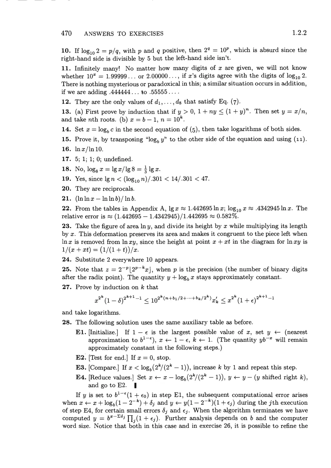
1. Start in
2. Read
pp. xvii-xix
18. Relax
No
f 17. N<12?J
16. Increase N
15. Sleep
Yes
14. Tired? J
13. Check
answers
Flow chart for reading this set of books.

Procedure for Reading
This Set of Books
1. Begin reading this procedure, unless you have already begun to read it.
Continue to follow the steps faithfully. (The general form of this procedure
and its accompanying flow chart will be used throughout this book.)
2. Read the Notes on the Exercises, on pages xv-xvii.
3. Set N equal to 1.
4. Begin reading Chapter N. Do not read the quotations that appear at the
beginning of the chapter.
5. Is the subject of the chapter interesting to you? If so, go to step 7; if not,
go to step 6.
6. Is N < 2? If not, go to step 16; if so, scan through the chapter anyway.
(Chapters 1 and 2 contain important introductory material and also a review
of basic programming techniques. You should at least skim over the sections
on notation and about MIX.)
7. Begin reading the next section of the chapter; if you have already reached
the end of the chapter, however, go to step 16.
8. Is section number marked with "*"? If so, you may omit this section on
first reading (it covers a rather specialized topic that is interesting but not
essential); go back to step 7.
9. Are you mathematically inclined? If math is all Greek to you, go to step 11;
otherwise proceed to step 10.
10. Check the mathematical derivations made in this section (and report errors
to the author). Go to step 12.
11. If the current section is full of mathematical computations, you had better
omit reading the derivations. However, you should become familiar with the
basic results of the section; they are usually stated near the beginning, or
in slanted type right at the very end of the hard parts.
12. Work the recommended exercises in this section in accordance with the hints
given in the Notes on the Exercises (which you read in step 2).
13. After you have worked on the exercises to your satisfaction, check your
answers with the answer printed in the corresponding answer section at the
xiii

xiv PROCEDURE FOR READING THIS SET OF BOOKS
rear of the book (if any answer appears for that problem). Also read the
answers to the exercises you did not have time to work. Note: In most cases
it is reasonable to read the answer to exercise n before working on exercise
n + 1, so steps 12-13 are usually done simultaneously.
14. Are you tired? If not, go back to step 7.
15. Go to sleep. Then, wake up, and go back to step 7.
16. Increase N by one. If N — 3, 5, 7, 9, 11, or 12, begin the next volume of
this set of books.
17. If N is less than or equal to 12, go back to step 4.
18. Congratulations. Now try to get your friends to purchase a copy of Volume 1
and to start reading it. Also, go back to step 3.
Woe be to him that reads but one book.
GEORGE HERBERT, Jacula Prudentum, 1144 A640)
Le defaut unique de tous les ouvrages
c'est d'etre trop longs.
— VAUVENARGUES, Reflexions, 628 A746)
Books are a triviality. Life alone is great.
— THOMAS CARLYLE, Journal A839)

CONTENTS
Chapter 1—Basic Concepts 1
1.1. Algorithms 1
1.2. Mathematical Preliminaries 10
1.2.1. Mathematical Induction 11
1.2.2. Numbers, Powers, and Logarithms 21
1.2.3. Sums and Products 27
1.2.4. Integer Functions and Elementary Number Theory 39
1.2.5. Permutations and Factorials 45
1.2.6. Binomial Coefficients 52
1.2.7. Harmonic Numbers 75
1.2.8 Fibonacci Numbers 79
1.2.9 Generating Functions 87
1.2.10 Analysis of an Algorithm 96
*1.2.11 Asymptotic Representations 107
*1.2.11.1 The O-notation 107
*1.2.11.2 Euler's summation formula Ill
*1.2.11.3 Some asymptotic calculations 116
1.3 MIX 124
1.3.1. Description of MIX 124
1.3.2. The MIX Assembly Language 144
1.3.3. Applications to Permutations 164
1.4. Some Fundamental Programming Techniques 186
1.4.1. Subroutines 186
1.4.2. Coroutines 193
1.4.3. Interpretive Routines 200
1.4.3.1. A MIX simulator 202
*1.4.3.2. Trace routines 212
1.4.4. Input and Output 215
1.4.5. History and Bibliography 229
Chapter 2—Information Structures 232
2.1. Introduction 232
2.2. Linear Lists 238
2.2.1. Stacks, Queues, and Deques 238
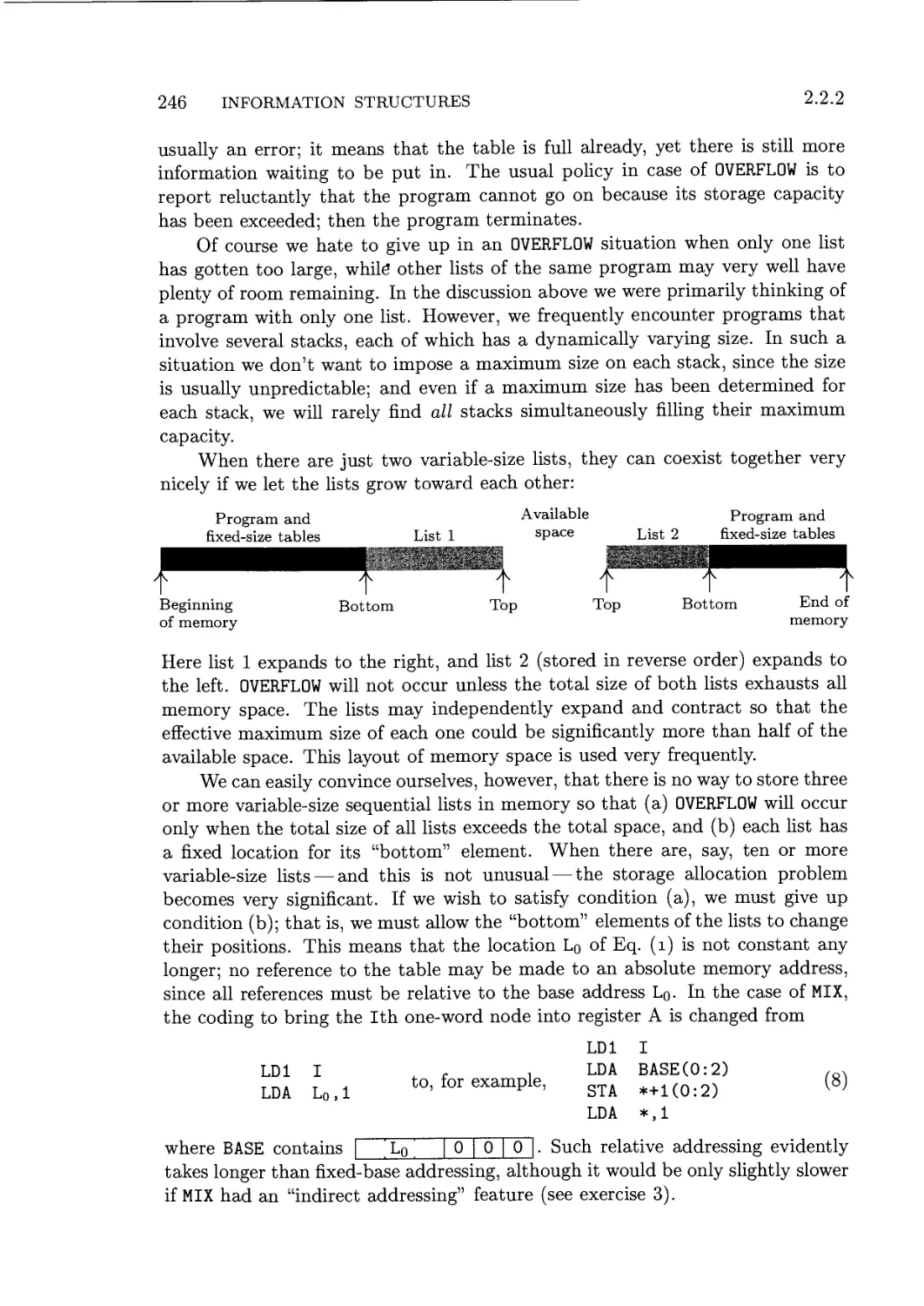
2.2.2. Sequential Allocation 244
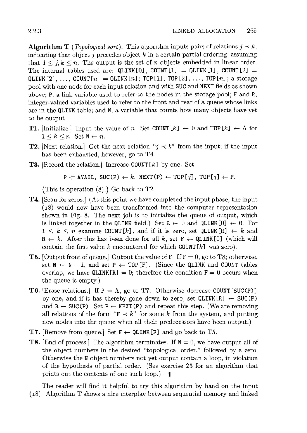
2.2.3. Linked Allocation 254
xviii

CONTENTS xix
2.2.4. Circular Lists 273
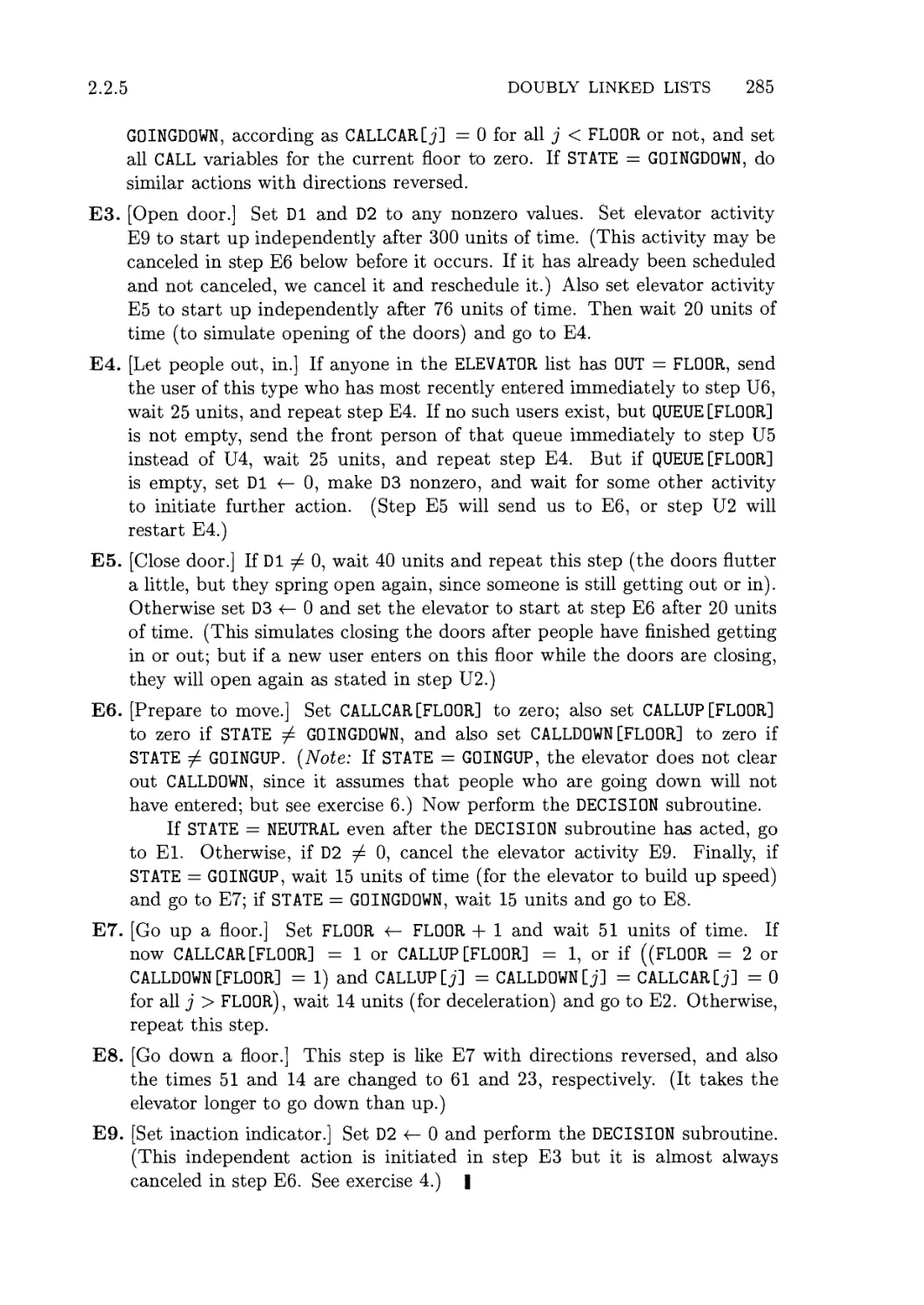
2.2.5. Doubly Linked Lists 280
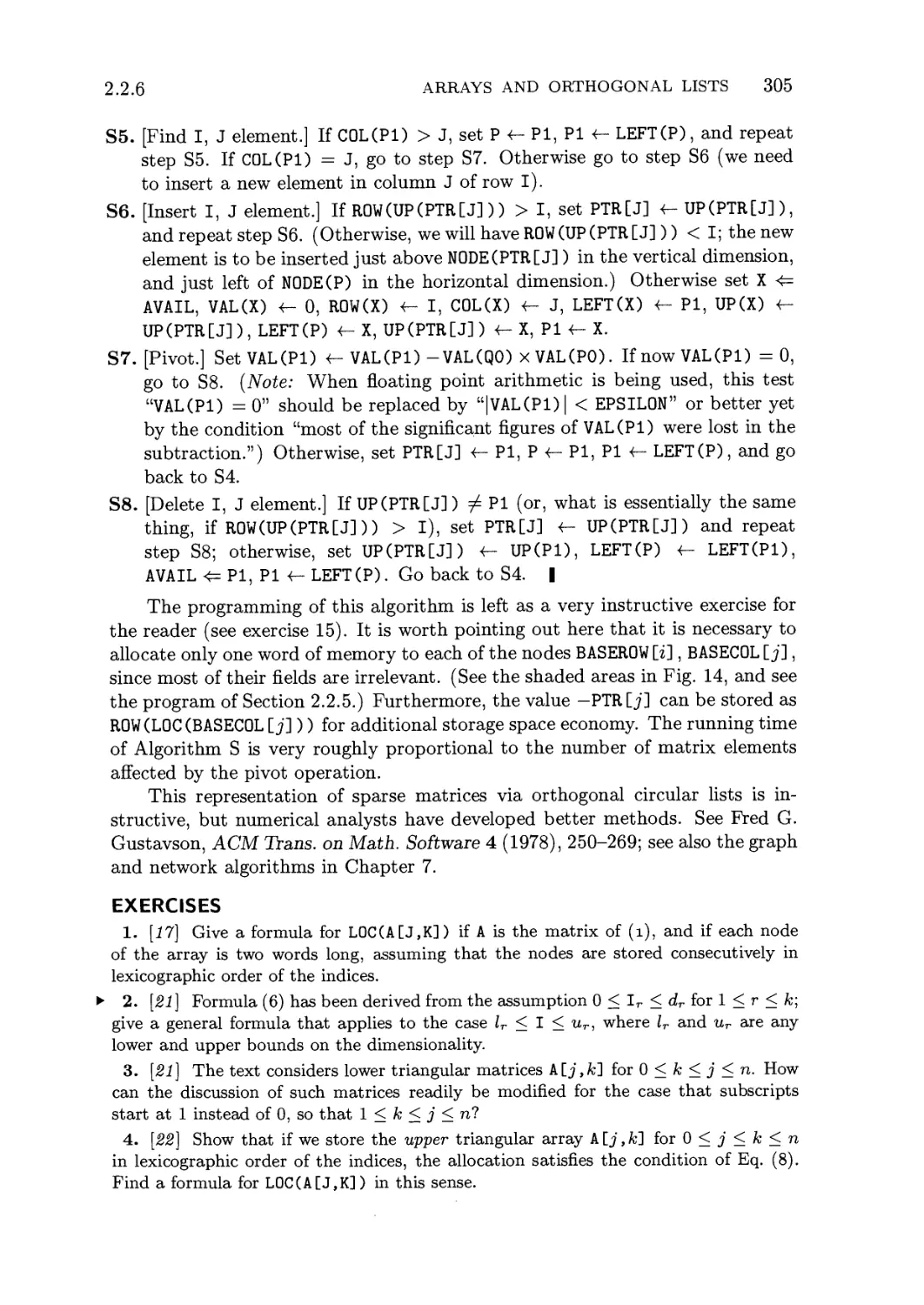
2.2.6. Arrays and Orthogonal Lists 298
2.3. Trees 308
2.3.1. Traversing Binary Trees 318
2.3.2. Binary Tree Representation of Trees 334
2.3.3. Other Representations of Trees 348
2.3.4. Basic Mathematical Properties of Trees 362
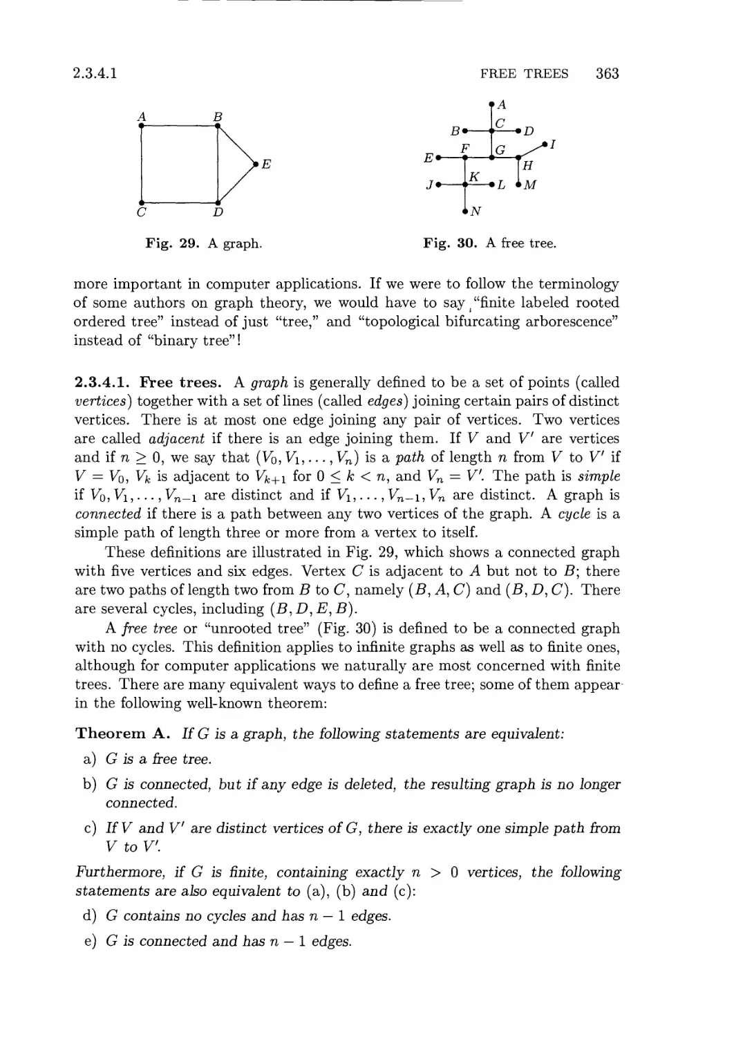
2.3.4.1. Free trees 363
2.3.4.2. Oriented trees 372
*2.3.4.3. The "infinity lemma" 382
*2.3.4.4. Enumeration of trees 386
2.3.4.5. Path length 399
*2.3.4.6. History and bibliography 406
2.3.5. Lists and Garbage Collection 408
2.4. Multilinked Structures 424
2.5. Dynamic Storage Allocation 435
2.6. History and Bibliography 457
Answers to Exercises 466
Appendix A — Tables of Numerical Quantities 619
1. Fundamental Constants (decimal) 619
2. Fundamental Constants (octal) 620
3. Harmonic Numbers, Bernoulli Numbers, Fibonacci Numbers . . . 621
Appendix B — Index to Notations 623
Index and Glossary 628

CHAPTER ONE
BASIC CONCEPTS
Many persons who are not conversant with mathematical studies
imagine that because the business of [Babbage's Analytical Engine] is to
give its results in numerical notation, the nature of its processes must
consequently be arithmetical and numerical, rather than algebraical and
analytical. This is an error. The engine can arrange and combine its
numerical quantities exactly as if they were letters or any other general
symbols; and in fact it might bring out its results in algebraical notation,
were provisions made accordingly.
— AUGUSTA ADA, Countess of Lovelace A844)
Practice yourself, for heaven's sake, in little things;
and thence proceed to greater.
— EPICTETUS (Discourses IV. i)
1.1. ALGORITHMS
The notion of an algorithm is basic to all of computer programming, so we
should begin with a careful analysis of this concept.
The word "algorithm" itself is quite interesting; at first glance it may look
as though someone intended to write "logarithm" but jumbled up the first four
letters. The word did not appear in Webster's New World Dictionary as late as
1957; we find only the older form "algorism" with its ancient meaning, the process
of doing arithmetic using Arabic numerals. During the Middle Ages, abacists
computed on the abacus and algorists computed by algorism. By the time of the
Renaissance, the origin of this word was in doubt, and early linguists attempted
to guess at its derivation by making combinations like algiros [painful] + arithmos
[number]; others said no, the word comes from "King Algor of Castile." Finally,
historians of mathematics found the true origin of the word algorism: It comes
from the name of a famous Persian textbook author, Abu 'Abd Allah Muhammad
ibn Musa al-KhwarizmT (c. 825) —literally, "Father of Abdullah, Mohammed,
son of Moses, native of Khwarizm." The Aral Sea in Central Asia was once
known as Lake Khwarizm, and the Khwarizm region is located in the Amu
River basin just south of that sea. Al-KhwarizmT wrote the celebrated book
Kitab aljabr wa'1-muqabala ("Rules of restoring and equating"); another word,
"algebra," stems from the title of his book, which was a systematic study of the
solution of linear and quadratic equations. [For notes on al-Khwarizml's life and
work, see H. Zemanek, Lecture Notes in Computer Science 122 A981), 1-81.]

2 BASIC CONCEPTS 1.1
Gradually the form and meaning of algorism became corrupted; as ex-
explained by the Oxford English Dictionary, the word "passed through many
pseudo-etymological perversions, including a recent algorithm, in which it is
learnedly confused" with the Greek root of the word arithmetic. This change
from "algorism" to "algorithm" is not hard to understand in view of the fact
that people had forgotten the original derivation of the word. An early German
mathematical dictionary, Vollstk'ndiges mathematisches Lexicon (Leipzig: 1747),
gave the following definition for the word Algorithmus: "Under this designation
are combined the notions of the four types of arithmetic calculations, namely
addition, multiplication, subtraction, and division." The Latin phrase algorith-
algorithmus infinitesimalis was at that time used to denote "ways of calculation with
infinitely small quantities, as invented by Leibniz."
By 1950, the word algorithm was most frequently associated with Euclid's
algorithm, a process for finding the greatest common divisor of two numbers
that appears in Euclid's Elements (Book 7, Propositions 1 and 2). It will be
instructive to exhibit Euclid's algorithm here:
Algorithm E (Euclid's algorithm). Given two positive integers m and n, find
their greatest common divisor, that is, the largest positive integer that evenly
divides both m and n.
El. [Find remainder.] Divide m by n and let r be the remainder. (We will have
0<r <n.)
E2. [Is it zero?] If r = 0, the algorithm terminates; n is the answer.
E3. [Reduce.] Set m <- n, n <- r, and go back to step El. |
Of course, Euclid did not present his algorithm in just this manner. The
format above illustrates the style in which all of the algorithms throughout this
book will be presented.
Each algorithm we consider has been given an identifying letter (E in the
preceding example), and the steps of the algorithm are identified by this letter
followed by a number (El, E2, E3). The chapters are divided into numbered
sections; within a section the algorithms are designated by letter only, but when
algorithms are referred to in other sections, the appropriate section number is
attached. For example, we are now in Section 1.1; within this section Euclid's
algorithm is called Algorithm E, while in later sections it is referred to as
Algorithm 1.1E.
Each step of an algorithm, such as step El above, begins with a phrase in
brackets that sums up as briefly as possible the principal content of that step.
This phrase also usually appears in an accompanying flow chart, such as Fig. 1,
so that the reader will be able to picture the algorithm more readily.
After the summarizing phrase comes a description in words and symbols
of some action to be performed or some decision to be made. Parenthesized
comments, like the second sentence in step El, may also appear. Comments are
included as explanatory information about that step, often indicating certain
invariant characteristics of the variables or the current goals at that step. They

1.1 ALGORITHMS
El. Find remainder
No
E3. Reduce
E2. Is it zero?
I Yes
Fig. 1. Flow chart for Algorithm E.
do not specify actions that belong to the algorithm, but are meant only for the
reader's benefit as possible aids to comprehension.
The arrow "<—" in Step E3 is the all-important replacement operation,
sometimes called assignment or substitution: "m <— n" means that the value of
variable m is to be replaced by the current value of variable n. When Algorithm E
begins, the values of m and n are the originally given numbers; but when it
ends, those variables will have, in general, different values. An arrow is used
to distinguish the replacement operation from the equality relation: We will
not say, "Set m = n," but we will perhaps ask, "Does m = n?" The " = "
sign denotes a condition that can be tested, the "<— " sign denotes an action
that can be performed. The operation of increasing n by one is denoted by
"n <r- n + 1" (read "n is replaced by n + 1" or "n gets n + 1"). In general,
"variable <— formula" means that the formula is to be computed using the present
values of any variables appearing within it; then the result should replace the
previous value of the variable at the left of the arrow. Persons untrained in
computer work sometimes have a tendency to say "n becomes n + 1" and to
write un ^ n + 1" for the operation of increasing n by one; this symbolism can
only lead to confusion because of its conflict with standard conventions, and it
should be avoided.
Notice that the order of actions in step E3 is important: "Set m <— n,
n <— r" is quite different from "Set n <— r, m <~ n," since the latter would imply
that the previous value of n is lost before it can be used to set m. Thus the
latter sequence is equivalent to "Set n <— r, m <— r." When several variables
are all to be set equal to the same quantity, we can use multiple arrows; for
example, "n <— r, m <— r" may be written "n <— m <— r." To interchange the
values of two variables, we can write "Exchange m ^ n"; this action could also
be specified by using a new variable t and writing "Set t <— m, m <— n, n <— t."
An algorithm starts at the lowest-numbered step, usually step 1, and it
performs subsequent steps in sequential order unless otherwise specified. In step
E3, the imperative "go back to step El" specifies the computational order in an
obvious fashion. In step E2, the action is prefaced by the condition "If r = 0";
so if r / 0, the rest of that sentence does not apply and no action is specified.
We might have added the redundant sentence, "If r ^ 0, go on to step E3."
The heavy vertical line " | " appearing at the end of step E3 is used to
indicate the end of an algorithm and the resumption of text.
We have now discussed virtually all the notational conventions used in the
algorithms of this book, except for a notation used to denote "subscripted" or

4 BASIC CONCEPTS 1.1
"indexed" items that are elements of an ordered array. Suppose we have n
quantities, i>i,i>2, • ¦ • ,vn; instead of writing Vj for the jth element, the notation
v[j] is often used. Similarly, a[i,j] is sometimes used in preference to a doubly
subscripted notation like a^. Sometimes multiple-letter names are used for
variables, usually set in capital letters; thus TEMP might be the name of a variable
used for temporarily holding a computed value, PRIME [K] might denote the Kth
prime number, and so on.
So much for the form of algorithms; now let us perform one. It should be
mentioned immediately that the reader should not expect to read an algorithm
as if it were part of a novel; such an attempt would make it pretty difficult to
understand what is going on. An algorithm must be seen to be believed, and the
best way to learn what an algorithm is all about is to try it. The reader should
always take pencil and paper and work through an example of each algorithm
immediately upon encountering it in the text. Usually the outline of a worked
example will be given, or else the reader can easily conjure one up. This is a
simple and painless way to gain an understanding of a given algorithm, and all
other approaches are generally unsuccessful.
Let us therefore work out an example of Algorithm E. Suppose that we are
given m = 119 and n = 544; we are ready to begin, at step El. (The reader
should now follow the algorithm as we give a play-by-play account.) Dividing
m by n in this case is quite simple, almost too simple, since the quotient is zero
and the remainder is 119. Thus, r <— 119. We proceed to step E2, and since
r / 0 no action occurs. In step E3 we set m <— 544, n <— 119. It is clear that if
m < n originally, the quotient in step El will always be zero and the algorithm
will always proceed to interchange m and n in this rather cumbersome fashion.
We could add a new step:
EO. [Ensure m> n] If m < n, exchange m <-? n.
This would make no essential change in the algorithm, except to increase its
length slightly, and to decrease its running time in about one half of all cases.
Back at step El, we find that fff = 4^, so r «- 68. Again E2 is
inapplicable, and at E3 we set m <- 119, n «- 68. The next round sets r <- 51,
and ultimately m <- 68, n <- 51. Next r <- 17, and m <~ 51, n <- 17. Finally,
when 51 is divided by 17, we set r <— 0, so at step E2 the algorithm terminates.
The greatest common divisor of 119 and 544 is 17.
So this is an algorithm. The modern meaning for algorithm is quite similar to
that of recipe, process, method, technique, procedure, routine, rigmarole, except
that the word "algorithm" connotes something just a little different. Besides
merely being a finite set of rules that gives a sequence of operations for solving
a specific type of problem, an algorithm has five important features:
1) Finiteness. An algorithm must always terminate after a finite number of
steps. Algorithm E satisfies this condition, because after step El the value of r
is less than n; so if r ^ 0, the value of n decreases the next time step El is
encountered. A decreasing sequence of positive integers must eventually termi-
terminate, so step El is executed only a finite number of times for any given original

1.1 ALGORITHMS 5
value of n. Note, however, that the number of steps can become arbitrarily large;
certain huge choices of m and n will cause step El to be executed more than a
million times.
(A procedure that has all of the characteristics of an algorithm except that it
possibly lacks finiteness may be called a computational method. Euclid originally
presented not only an algorithm for the greatest common divisor of numbers, but
also a very similar geometrical construction for the "greatest common measure"
of the lengths of two line segments; this is a computational method that does
not terminate if the given lengths are incommensurable. Another example of a
nonterminating computational method is a reactive process, which continually
interacts with its environment.)
2) Definiteness. Each step of an algorithm must be precisely defined; the ac-
actions to be carried out must be rigorously and unambiguously specified for each
case. The algorithms of this book will hopefully meet this criterion, but they
are specified in the English language, so there is a possibility that the reader
might not understand exactly what the author intended. To get around this
difficulty, formally defined programming languages or computer languages are
designed for specifying algorithms, in which every statement has a very definite
meaning. Many of the algorithms of this book will be given both in English
and in a computer language. An expression of a computational method in a
computer language is called a program.
In Algorithm E, the criterion of definiteness as applied to step El means that
the reader is supposed to understand exactly what it means to divide m by n
and what the remainder is. In actual fact, there is no universal agreement about
what this means if m and n are not positive integers; what is the remainder of
—8 divided by —tt? What is the remainder of 59/13 divided by zero? Therefore
the criterion of definiteness means we must make sure that the values of m and n
are always positive integers whenever step El is to be executed. This is initially
true, by hypothesis; and after step El, r is a nonnegative integer that must be
nonzero if we get to step E3. So m and n are indeed positive integers as required.
3) Input. An algorithm has zero or more inputs: quantities that are given to it
initially before the algorithm begins, or dynamically as the algorithm runs. These
inputs are taken from specified sets of objects. In Algorithm E, for example, there
are two inputs, namely m and n, both taken from the set of positive integers.
4) Output. An algorithm has one or more outputs: quantities that have a
specified relation to the inputs. Algorithm E has one output, namely n in step E2,
the greatest common divisor of the two inputs.
(We can easily prove that this number is indeed the greatest common divisor,
as follows. After step El, we have
m = qn + r,
for some integer q. If r = 0, then m is a multiple of n, and clearly in such a case
n is the greatest common divisor of m and n. If r / 0, note that any number
that divides both m and n must divide m — qn — r, and any number that divides

6 BASIC CONCEPTS 1.1
both n and r must divide qn + r = m; so the set of divisors of {m, n} is the
same as the set of divisors of {n, r}. In particular, the greatest common divisor
of {m,n} is the same as the greatest common divisor of {n,r}. Therefore step
E3 does not change the answer to the original problem.)
5) Effectiveness. An algorithm is also generally expected to be effective, in the
sense that its operations must all be sufficiently basic that they can in principle
be done exactly and in a finite length of time by someone using pencil and
paper. Algorithm E uses only the operations of dividing one positive integer
by another, testing if an integer is zero, and setting the value of one variable
equal to the value of another. These operations are effective, because integers
can be represented on paper in a finite manner, and because there is at least
one method (the "division algorithm") for dividing one by another. But the
same operations would not be effective if the values involved were arbitrary real
numbers specified by an infinite decimal expansion, nor if the values were the
lengths of physical line segments (which cannot be specified exactly). Another
example of a noneffective step is, "If 4 is the largest integer n for which there is
a solution to the equation wn + xn +yn = zn in positive integers iu, x, y, and z,
then go to step E4." Such a statement would not be an effective operation until
someone successfully constructs an algorithm to determine whether 4 is or is not
the largest integer with the stated property.
Let us try to compare the concept of an algorithm with that of a cookbook
recipe. A recipe presumably has the qualities of finiteness (although it is said
that a watched pot never boils), input (eggs, flour, etc.), and output (TV dinner,
etc.), but it notoriously lacks definiteness. There are frequent cases in which a
cook's instructions are indefinite: "Add a dash of salt." A "dash" is defined
to be "less than 1/% teaspoon," and salt is perhaps well enough defined; but
where should the salt be added — on top? on the side? Instructions like "toss
lightly until mixture is crumbly" or "warm cognac in small saucepan" are quite
adequate as explanations to a trained chef, but an algorithm must be specified
to such a degree that even a computer can follow the directions. Nevertheless,
a computer programmer can learn much by studying a good recipe book. (The
author has in fact barely resisted the temptation to name the present volume
"The Programmer's Cookbook." Perhaps someday he will attempt a book called
"Algorithms for the Kitchen.")
We should remark that the finiteness restriction is not really strong enough
for practical use. A useful algorithm should require not only a finite number
of steps, but a very finite number, a reasonable number. For example, there is
an algorithm that determines whether or not the game of chess can always be
won by White if no mistakes are made (see exercise 2.2.3-28). That algorithm
can solve a problem of intense interest to thousands of people, yet it is a safe
bet that we will never in our lifetimes know the answer; the algorithm requires
fantastically large amounts of time for its execution, even though it is finite. See
also Chapter 8 for a discussion of some finite numbers that are so large as to
actually be beyond comprehension.

1.1 ALGORITHMS 7
In practice we not only want algorithms, we want algorithms that are good
in some loosely denned aesthetic sense. One criterion of goodness is the length
of time taken to perform the algorithm; this can be expressed in terms of the
number of times each step is executed. Other criteria are the adaptability of the
algorithm to different kinds of computers, its simplicity and elegance, etc.
We often are faced with several algorithms for the same problem, and we
must decide which is best. This leads us to the extremely interesting and
all-important field of algorithmic analysis: Given an algorithm, we want to
determine its performance characteristics.
For example, let's consider Euclid's algorithm from this point of view. Sup-
Suppose we ask the question, "Assuming that the value of n is known but m is
allowed to range over all positive integers, what is the average number of times,
Tn, that step El of Algorithm E will be performed?" In the first place, we need
to check that this question does have a meaningful answer, since we are trying
to take an average over infinitely many choices for m. But it is evident that
after the first execution of step El only the remainder of m after division by n is
relevant. So all we must do to find Tn is to try the algorithm for m = 1, m = 2,
..., m = n, count the total number of times step El has been executed, and
divide by n.
Now the important question is to determine the nature of Tn\ is it approxi-
approximately equal to |n, or ^/n, for instance? As a matter of fact, the answer to this
question is an extremely difficult and fascinating mathematical problem, not yet
completely resolved, which is examined in more detail in Section 4.5.3. For large
values of n it is possible to prove that Tn is approximately (l2(ln2)/7r2) Inn,
that is, proportional to the natural logarithm of n, with a constant of propor-
proportionality that might not have been guessed offhand! For further details about
Euclid's algorithm, and other ways to calculate the greatest common divisor, see
Section 4.5.2.
Analysis of algorithms is the name the author likes to use to describe
investigations such as this. The general idea is to take a particular algorithm
and to determine its quantitative behavior; occasionally we also study whether
or not an algorithm is optimal in some sense. The theory of algorithms is another
subject entirely, dealing primarily with the existence or nonexistence of effective
algorithms to compute particular quantities.
So far our discussion of algorithms has been rather imprecise, and a mathe-
mathematically oriented reader is justified in thinking that the preceding commentary
makes a very shaky foundation on which to erect any theory about algorithms.
We therefore close this section with a brief indication of one method by which the
concept of algorithm can be firmly grounded in terms of mathematical set theory.
Let us formally define a computational method to be a quadruple (Q,I,Q, /),
in which Q is a set containing subsets I and f?, and / is a function from Q
into itself. Furthermore / should leave Q pointwise fixed; that is, f(q) should
equal q for all elements q of Q. The four quantities Q, I, fi, / are intended
to represent respectively the states of the computation, the input, the output,
and the computational rule. Each input x in the set / defines a computational

8 BASIC CONCEPTS 1.1
sequence, xq, xi, x2, ¦ ¦ •, as follows:
xq = x and Xk+i = f(xk) for A; > 0. (l)
The computational sequence is said to terminate in k steps if A; is the smallest
integer for which Xk is in 0,, and in this case it is said to produce the output
Xk from x. (Note that if Xk is in 0,, so is Xk+i, because Xk+i = Xk in such a
case.) Some computational sequences may never terminate; an algorithm is a
computational method that terminates in finitely many steps for all x in /.
Algorithm E may, for example, be formalized in these terms as follows: Let Q
be the set of all singletons (n), all ordered pairs (m, n), and all ordered quadruples
(m,n,r, 1), (m,n,r, 2), and (m, n,p, 3), where m, n, and p are positive integers
and r is a nonnegative integer. Let / be the subset of all pairs (m, n) and let U
be the subset of all singletons (n). Let / be defined as follows:
/((m,n))=(m,n, 0,1); /((n)) = (n);
f((m,n,r, 1)) = (m, n, remainder of m divided by n, 2);
/((m, n,r, 2)) = (n) if r = 0, (m, n,r, 3) otherwise;
/((m,n,p,3)) = (n,p,p, 1).
The correspondence between this notation and Algorithm E is evident.
This formulation of the concept of an algorithm does not include the re-
restriction of effectiveness mentioned earlier. For example, Q might denote infinite
sequences that are not computable by pencil and paper methods, or / might
involve operations that mere mortals cannot always perform. If we wish to
restrict the notion of algorithm so that only elementary operations are involved,
we can place restrictions on Q, /, Q, and /, for example as follows: Let A be
a finite set of letters, and let A* be the set of all strings on A (the set of all
ordered sequences x±x2 ¦ • • xn, where n > 0 and Xj is in A for 1 < j < n). The
idea is to encode the states of the computation so that they are represented by
strings of A*. Now let JV be a nonnegative integer and let Q be the set of all
(cr, j), where a is in A* and j is an integer, 0 < j < N; let / be the subset of Q
with ,7 = 0 and let fi be the subset with j = N. If 6 and a are strings in A*, we
say that 6 occurs in cr if cr has the form a6u) for strings a and uj. To complete
our definition, let / be a function of the following type, defined by the strings
9j, 4>j and the integers a,j, bj for 0 < j < N:
/(cr, j) = (cr, <2j) if 6j does not occur in cr;
/(cr, j) = (a(f)jU), bj) if a is the shortest possible string for which a = a6jU\
C)
Such a computational method is clearly effective, and experience shows
that it is also powerful enough to do anything we can do by hand. There are
many other essentially equivalent ways to formulate the concept of an effective
computational-method (for example, using Turing machines). The formulation
above is virtually the same as that given by A. A. Markov in his book The

1.1 ALGORITHMS 9
Theory of Algorithms [Trudy Mat. Inst. Akad. Nauk 42 A954), 1-376], later
revised and enlarged by N. M. Nagorny (Moscow: Nauka, 1984; English edition,
Dordrecht: Kluwer, 1988).
EXERCISES
1. [10] The text showed how to interchange the values of variables m and n, using
the replacement notation, by setting t 4- m, m 4- n, n 4- t. Show how the values of
four variables (a, b, c, d) can be rearranged to F, c, d, a) by a sequence of replacements.
In other words, the new value of a is to be the original value of b, etc. Try to use the
minimum number of replacements.
2. [15] Prove that m is always greater than n at the beginning of step El, except
possibly the first time this step occurs.
3. [20] Change Algorithm E (for the sake of efficiency) so that all trivial replacement
operations such as "m 4— n" are avoided. Write this new algorithm in the style of
Algorithm E, and call it Algorithm F.
4. [16] What is the greatest common divisor of 2166 and 6099?
5. [12] Show that the "Procedure for Reading This Set of Books" that appears in
the preface actually fails to be a genuine algorithm on three of our five counts! Also
mention some differences in format between it and Algorithm E.
6. [20] What is T5, the average number of times step El is performed when n = 5?
7. [M21] Suppose that m is known and n is allowed to range over all positive integers;
let Um be the average number of times that step El is executed in Algorithm E. Show
that Um is well defined. Is Um in any way related to Tm?
8. [M25] Give an "effective" formal algorithm for computing the greatest common
divisor of positive integers m and n, by specifying 6j, (f>j, clj, bj as in Eqs. C). Let the
input be represented by the string ambn, that is, m a's followed by n fe's. Try to make
your solution as simple as possible. [Hint: Use Algorithm E, but instead of division in
step El, set r 4— \m — n\, n 4— min(m, n).]
9. [M30] Suppose that Ci = (Qi,/i,Qi,/i) and C2 = (Q2,/2,^2,/2) are computa-
computational methods. For example, C\ might stand for Algorithm E as in Eqs. B), except
that m and n are restricted in magnitude, and C2 might stand for a computer program
implementation of Algorithm E. (Thus Qi might be the set of all states of the machine,
i.e., all possible configurations of its memory and registers; fi might be the definition
of single machine actions; and h might be the initial state, including the program for
determining the greatest common divisor as well as the values of m and n.)
Formulate a set-theoretic definition for the concept "C2 is a representation of Ci"
or "C2 simulates Ci." This is to mean intuitively that any computation sequence of C\
is mimicked by C2, except that C2 might take more steps in which to do the computation
and it might retain more information in its states. (We thereby obtain a rigorous
interpretation of the statement, "Program X is an implementation of Algorithm Y")

10 BASIC CONCEPTS 1.2
1.2. MATHEMATICAL PRELIMINARIES
In this section we shall investigate the mathematical notations that occur
throughout The Art of Computer Programming, and we'll derive several basic
formulas that will be used repeatedly. Even a reader not concerned with the
more complex mathematical derivations should at least become familiar with
the meanings of the various formulas, so as to be able to use the results of the
derivations.
Mathematical notation is used for two main purposes in this book: to
describe portions of an algorithm, and to analyze the performance character-
characteristics of an algorithm. The notation used in descriptions of algorithms is quite
simple, as explained in the previous section. When analyzing the performance
of algorithms, we need to use other more specialized notations.
Most of the algorithms we will discuss are accompanied by mathematical
calculations that determine the speed at which the algorithm may be expected
to run. These calculations draw on nearly every branch of mathematics, and a
separate book would be necessary to develop all of the mathematical concepts
that are used in one place or another. However, the majority of the calculations
can be carried out with a knowledge of college algebra, and the reader with a
knowledge of elementary calculus will be able to understand nearly all of the
mathematics that appears. Sometimes we will need to use deeper results of
complex variable theory, group theory, number theory, probability theory, etc.;
in such cases the topic will be explained in an elementary manner, if possible, or
a reference to other sources of information will be given.
The mathematical techniques involved in the analysis of algorithms usually
have a distinctive flavor. For example, we will quite often find ourselves working
with finite summations of rational numbers, or with the solutions to recurrence
relations. Such topics are traditionally given only a light treatment in mathe-
mathematics courses, and so the following subsections are designed not only to give a
thorough drilling in the use of the notations to be defined but also to illustrate
in depth the types of calculations and techniques that will be most useful to us.
Important note: Although the following subsections provide a rather extensive
training in the mathematical skills needed in connection with the study of com-
computer algorithms, most readers will not see at first any very strong connections
between this material and computer programming (except in Section 1.2.1). The
reader may choose to read the following subsections carefully, with implicit faith
in the author's assertion that the topics treated here are indeed very relevant; but
it is probably preferable, for motivation, to skim over this section lightly at first,
and (after seeing numerous applications of the techniques in future chapters)
return to it later for more intensive study. If too much time is spent studying
this material when first reading the book, a person might never get on to the
computer programming topics! However, each reader should at least become
familiar with the general contents of these subsections, and should try to solve a
few of the exercises, even on first reading. Section 1.2.10 should receive particular
attention, since it is the point of departure for most of the theoretical material

1.2.1 MATHEMATICAL INDUCTION 11
developed later. Section 1.3, which follows 1.2, abruptly leaves the realm of
"pure mathematics" and enters into "pure computer programming."
An expansion and more leisurely presentation of much of the following
material can be found in the book Concrete Mathematics by Graham, Knuth,
and Patashnik, second edition (Reading, Mass.: Addison-Wesley, 1994). That
book will be called simply CMath when we need to refer to it later.
1.2.1. Mathematical Induction
Let P(n) be some statement about the integer n; for example, P(n) might be
"n times (n + 3) is an even number," or "if n > 10, then 2n > n3." Suppose we
want to prove that P(n) is true for all positive integers n. An important way to
do this is:
a) Give a proof that P(l) is true.
b) Give a proof that "if all of P(l), PB),..., P{n) are true, then P(n + 1) is
also true"; this proof should be valid for any positive integer n.
As an example, consider the following series of equations, which many people
have discovered independently since ancient times:
l + 3 = 22,
1 + 3 + 5 = 32,
l + 3 + 5 + 7 = 42,
1 + 3 + 5 + 7 + 9 = 52. (i)
We can formulate the general property as follows:
l + 3 + --- + Bn-l) = n2. B)
Let us, for the moment, call this equation P(n); we wish to prove that P(n) is
true for all positive n. Following the procedure outlined above, we have:
a) "P(l) is true, since 1 = I2."
b) "If all of P(l),..., P(n) are true, then, in particular, P(n) is true, so Eq. B)
holds; adding In + 1 to both sides we obtain
1 + 3 + • • • + Bn - 1) + Bn + 1) = n2 + 2n + 1 = (n + IJ,
which proves that P(n + 1) is also true."
We can regard this method as an algorithmic proof procedure. In fact, the
following algorithm produces a proof of P(n) for any positive integer n, assuming
that steps (a) and (b) above have been worked out:
Algorithm I (Construct a proof). Given a positive integer n, this algorithm
will output a proof that P(n) is true.
II. [Prove P(l).] Set k 4- 1, and, according to (a), output a proof of P(l).

12 BASIC CONCEPTS 1.2.1
12. [k = n?] li k = n, terminate the algorithm; the required proof has been
output.
13. [Prove P(k + 1).] According to (b), output a proof that "If all of P(l),...,
P(k) are true, then P(k + 1) is true." Also output "We have already proved
P(l),..., P(fc); hence P(k + 1) is true."
14. [Increase k.} Increase A: by 1 and go to step 12. |
II. Prove P(l)
12. fc = n?
Yes
13. Prove P(k + 1)
14. Increase k
Fig. 2. Algorithm I: Mathematical induction.
Since this algorithm clearly presents a proof of P(n), for any given n, the
proof technique consisting of steps (a) and (b) is logically valid. It is called proof
by mathematical induction.
The concept of mathematical induction should be distinguished from what
is usually called inductive reasoning in science. A scientist takes specific observa-
observations and creates, by "induction," a general theory or hypothesis that accounts
for these facts; for example, we might observe the five relations in (l), above,
and formulate B). In this sense, induction is no more than our best guess about
the situation; mathematicians would call it an empirical result or a conjecture.
Another example will be helpful. Let p(n) denote the number of partitions
of n, that is, the number of different ways to write n as a sum of positive integers,
disregarding order. Since 5 can be partitioned in exactly seven ways,
we have pE) = 7. In fact, it is easy to establish the first few values,
l, pB) = 2, pC) = 3, pD) = 5, pE) = 7.
At this point we might tentatively formulate, by induction, the hypothesis that
the sequence pB), pC), ... runs through the prime numbers. To test this
hypothesis, we proceed to calculate pF) and behold! pF) = 11, confirming
our conjecture.
[Unfortunately, pG) turns out to be 15, spoiling everything, and we must
try again. The numbers p(n) are known to be quite complicated, although
S. Ramanujan succeeded in guessing and proving many remarkable things about
them. For further information, see G. H. Hardy, Ramanujan (London: Cam-
Cambridge University Press, 1940), Chapters 6 and 8.]
Mathematical induction is quite different from induction in the sense just
explained. It is not just guesswork, but a conclusive proof of a statement; indeed,
it is a proof of infinitely many statements, one for each n. It has been called
"induction" only because one must first decide somehow what is to be proved,

1.2.1
MATHEMATICAL INDUCTION
13
1
3
5
7
g
11
Fig. 3. The sum of odd
numbers is a square.
before one can apply the technique of mathematical induction. Henceforth in
this book we shall use the word induction only when we wish to imply proof by
mathematical induction.
There is a geometrical way to prove Eq. B).
Figure 3 shows, for n = 6, n2 cells broken into
groups of 1 + 3 + • • • + Bn — 1) cells. However, in
the final analysis, this picture can be regarded as a
"proof" only if we show that the construction can
be carried out for all n, and such a demonstration
is essentially the same as a proof by induction.
Our proof of Eq. B) used only a special case
of (b); we merely showed that the truth of P(n)
implies the truth of P(n +1). This is an important
simple case that arises frequently, but our next
example illustrates the power of the method a little
more. We define the Fibonacci sequence Fq, Fi,
F2, - • • by the rule that Fq = 0, Fi = 1, and every further term is the sum of
the preceding two. Thus the sequence begins 0, 1, 1, 2, 3, 5, 8, 13, ...; we will
investigate it in detail in Section 1.2.8. We will now prove that if 0 is the number
A + \/5)/2 we have
Fn < r-1 C)
for all positive integers n. Call this formula P(n).
If n = 1, then i*\ = 1 = 0° = 0n~\ so step (a) has been done. For step (b)
we notice first that PB) is also true, since F2 = 1 < 1-6 < 01 = 02. Now, if all
of P(l), PB), ..., P(n) are true and n > 1, we know in particular that P(n — 1)
and P(n) are true; so Fn-\ < 0n~2 and Fn < <pn~1. Adding these inequalities,
we get
Fn-\-l = Fn — \ + Fn <: 0™" + 0™" = 0™" (l + 0)- D)
The important property of the number 0, indeed the reason we chose this number
for this problem in the first place, is that
1 + 0 = 02.
E)
Plugging E) into D) gives Fn+i < 0n, which is P(n + 1). So step (b) has
been done, and C) has been proved by mathematical induction. Notice that we
approached step (b) in two different ways here: We proved P(n+1) directly when
n = 1, and we used an inductive method when n > 1. This was necessary, since
when n = 1 our reference to P(n — 1) = P@) would not have been legitimate.
Mathematical induction can also be used to prove things about algorithms.
Consider the following generalization of Euclid's algorithm.
Algorithm E (Extended Euclid's algorithm). Given two positive integers m
and n, we compute their greatest common divisor d and two integers a and 6,
such that am + bn = d.
El. [Initialize.] Set a' <- b 4- 1, a <- b' 4- 0, c <- m, d
n.

14 BASIC CONCEPTS 1.2.1
E2. [Divide.] Let q and r be the quotient and remainder, respectively, of c
divided by d. (We have c = qd + r and 0 < r < d.)
E3. [Remainder zero?] If r = 0, the algorithm terminates; we have in this case
am + bn = d as desired.
E4. [Recycle.] Set c <^ d, d 4- r, t 4- a', a' 4- a, a 4- t — qa, t 4- b', b' 4- b,
b <- t - qb, and go back to E2. |
If we suppress the variables a, 6, a', and b' from this algorithm and use m
and n for the auxiliary variables c and d, we have our old algorithm, 1.1E. The
new version does a little more, by determining the coefficients a and b. Suppose
that m = 1769 and n = 551; we have successively (after step E2):
a'
1
0
1
-4
a
0
1
-4
5
b'
0
1
-3
13
b
1
-3
13
-16
c
1769
551
116
87
d
551
116
87
29
q
3
4
1
3
r
116
87
29
0
The answer is correct: 5 x 1769 - 16 x 551 = 8845 - 8816 = 29, the greatest
common divisor of 1769 and 551.
The problem is to prove that this algorithm works properly, for all m and n.
We can try to apply the method of mathematical induction by letting P(n) be
the statement "Algorithm E works for n and all integers m." However, that
approach doesn't work out so easily, and we need to prove some extra facts.
After a little study, we find that something must be proved about a, 6, a', and
b', and the appropriate fact is that the equalities
a'm + b'n = c, am + bn = d F)
always hold whenever step E2 is executed. We may prove these equalities directly
by observing that they are certainly true the first time we get to E2, and that
step E4 does not change their validity. (See exercise 6.)
Now we are ready to show that Algorithm E is valid, by induction on n: If
m is a multiple of n, the algorithm obviously works properly, since we are done
immediately at E3 the first time. This case always occurs when n = 1. The
only case remaining is when n > 1 and m is not a multiple of n. In such a
case, the algorithm proceeds to set c <— n, d <— r after the first execution, and
since r < n, we may assume by induction that the final value of d is the gcd
of n and r. By the argument given in Section 1.1, the pairs {m,n} and {n,r}
have the same common divisors, and, in particular, they have the same greatest
common divisor. Hence d is the gcd of m and n, and am + bn = d by F).
The italicized phrase in the proof above illustrates the conventional lan-
language that is so often used in an inductive proof: When doing part (b) of the
construction, rather than saying "We will now assume P(l), PB),..., P(n), and
with this assumption we will prove P(n + 1)," we often say simply "We will now
prove P(n); we may assume by induction that P(k) is true whenever 1 < A; < n."

1.2.1
MATHEMATICAL INDUCTION
15
El.
a i— 0 a' •*— 1 c<-m
6 «- 1 b'-f-O
9 ^~ quotient (c -f- d)
r 4— remainder (c -i- d)
No
m>0, n>0.
: c = m>0, d = n>0,
a = 6'=0, a'=6=1.
¦A3: am + bn = d, a'm + b'n = c= qd + r,
0<r<d, gcd(c, d) = gcd(m, n).
: am + 6n = d = gcd(m, n).
<r
ci-d, di-r;
E4. t<-a', a' 4-a, ai-t — qa;
t<-b',b' <-b,b<-t — qb.
-A5: am + bn = d, a'm + b'n = c= qd + r,
0<r<d, gcd(c, d) = gcd(m, n).
<•¦
¦ A6: am + bn = d, a'm + b'n = c, d>0,
gcd(c, d) = gcd(m, n).
Fig. 4. Flow chart for Algorithm E, labeled with assertions that prove the validity of
the algorithm.
If we examine this argument very closely and change our viewpoint slightly,
we can envision a general method applicable to proving the validity of any
algorithm. The idea is to take a flow chart for some algorithm and to label
each of the arrows with an assertion about the current state of affairs at the
time the computation traverses that arrow. See Fig. 4, where the assertions
have been labeled Al, A2, ..., A6. (All of these assertions have the additional
stipulation that the variables are integers; this stipulation has been omitted to
save space.) Al gives the initial assumptions upon entry to the algorithm, and
A4 states what we hope to prove about the output values a, b, and d.
The general method consists of proving, for each box in the flow chart, that
if any one of the assertions on the arrows leading into the box
is true before the operation in that box is performed, then all of
the assertions on the arrows leading away from the box are true
after the operation.
Thus, for example, we must prove that either A2 or A6 before E2 implies A3
after E2. (In this case A2 is a stronger statement than A6; that is, A2 implies
A6. So we need only prove that A6 before E2 implies A3 after. Notice that the
condition d > 0 is necessary in A6 just to prove that operation E2 even makes
sense.) It is also necessary to show that A3 and r = 0 implies A4; that A3 and
r ^ 0 implies A 5; etc. Each of the required proofs is very straightforward.
Once statement G) has been proved for each box, it follows that all assertions
are true during any execution of the algorithm. For we can now use induction
G)

16 BASIC CONCEPTS 1.2.1
on the number of steps of the computation, in the sense of the number of arrows
traversed in the flow chart. While traversing the first arrow, the one leading from
"Start", the assertion Al is true since we always assume that our input values
meet the specifications; so the assertion on the first arrow traversed is correct.
If the assertion that labels the nth arrow is true, then by G) the assertion that
labels the (n + l)st arrow'is also true.
Using this general method, the problem of proving that a given algorithm
is valid evidently consists mostly of inventing the right assertions to put in the
flow chart. Once this inductive leap has been made, it is pretty much routine to
carry out the proofs that each assertion leading into a box logically implies each
assertion leading out. In fact, it is pretty much routine to invent the assertions
themselves, once a few of the difficult ones have been discovered; thus it is very
simple in our example to write out essentially what A 2, A3, and A5 must be,
if only Al, A4, and A6 are given. In our example, assertion A6 is the creative
part of the proof; all the rest could, in principle, be supplied mechanically. Hence
no attempt has been made to give detailed formal proofs of the algorithms that
follow in this book, at the level of detail found in Fig. 4. It suffices to state
the key inductive assertions. Those assertions either appear in the discussion
following an algorithm or they are given as parenthetical remarks in the text of
the algorithm itself.
This approach to proving the correctness of algorithms has another aspect
that is even more important: It mirrors the way we understand an algorithm.
Recall that in Section 1.1 the reader was cautioned not to expect to read an
algorithm like part of a novel; one or two trials of the algorithm on some sample
data were recommended. This was done expressly because an example run-
through of the algorithm helps a person formulate the various assertions mentally.
It is the contention of the author that we really understand why an algorithm is
valid only when we reach the point that our minds have implicitly filled in all the
assertions, as was done in Fig. 4. This point of view has important psychological
consequences for the proper communication of algorithms from one person to
another: It implies that the key assertions, those that cannot easily be derived
by an automaton, should always be stated explicitly when an algorithm is being
explained to someone else. When Algorithm E is being put forward, assertion
A6 should be mentioned too.
An alert reader will have noticed a gaping hole in our last proof of Algo-
Algorithm E, however. We never showed that the algorithm terminates; all we have
proved is that if it terminates, it gives the right answer!
(Notice, for example, that Algorithm E still makes sense if we allow its
variables m, n, c, and r to assume values of the form u + v \/2, where u and v
are integers. The variables q, a, b, a', b' are to remain integer-valued. If we start
the algorithm with m = 12 - 6 \/2 and n = 20 - 10 \/2, say, it will compute a
"greatest common divisor" d = 4 - 2 y/2 with a = +2, b = — 1. Even under this
extension of the assumptions, the proofs of assertions Al through A6 remain
valid; therefore all assertions are true throughout any execution of the algorithm.
But if we start the procedure with m = 1 and n — \/2, the computation never

1.2.1 MATHEMATICAL INDUCTION 17
terminates (see exercise 12). Hence a proof of assertions Al through A6 does
not logically prove that the algorithm is finite.)
Proofs of termination are usually handled separately. But exercise 13 shows
that it is possible to extend the method above in many important cases so that
a proof of termination is included as a by-product.
We have now twice proved the validity of Algorithm E. To be strictly logical,
we should also try to prove that the first algorithm in this section, Algorithm I,
is valid; in fact, we have used Algorithm I to establish the correctness of any
proof by induction. If we attempt to prove that Algorithm I works properly,
however, we are confronted with a dilemma — we can't really prove it without
using induction again! The argument would be circular.
In the last analysis, every property of the integers must be proved using
induction somewhere along the line, because if we get down to basic concepts, the
integers are essentially defined by induction. Therefore we may take as axiomatic
the idea that any positive integer n either equals 1 or can be reached by starting
with 1 and repetitively adding 1; this suffices to prove that Algorithm I is valid.
[For a rigorous study of fundamental concepts about the integers, see the article
"On Mathematical Induction" by Leon Henkin, AMM 67 A960), 323-338.]
The idea behind mathematical induction is thus intimately related to the
concept of number. The first European to apply mathematical induction to
rigorous proofs was the Italian scientist Francesco Maurolico, in 1575. Pierre
de Fermat made further improvements, in the early 17th century; he called it
the "method of infinite descent." The notion also appears clearly in the later
writings of Blaise Pascal A653). The phrase "mathematical induction" appar-
apparently was coined by A. De Morgan in the early nineteenth century. [See AMM
24 A917), 199-207; 25 A918), 197-201; Arch. Hist. Exact Sci. 9 A972), 1-21.]
Further discussion of mathematical induction can be found in G. Polya's book
Induction and Analogy in Mathematics (Princeton, N.J.: Princeton University
Press, 1954), Chapter 7.
The formulation of algorithm-proving in terms of assertions and induction,
as given above, is essentially due to R. W. Floyd. He pointed out that a semantic
definition of each operation in a programming language can be formulated as a
logical rule that tells exactly what assertions can be proved after the operation,
based on what assertions are true beforehand [see "Assigning Meanings to Pro-
Programs," Proc. Symp. Appl. Math., Amer. Math. Soc, 19 A967), 19-32]. Similar
ideas were voiced independently by Peter Naur, BIT 6 A966), 310-316, who
called the assertions "general snapshots." An important refinement, the notion
of "invariants," was introduced by C. A. R. Hoare; see, for example, CACM 14
A971), 39-45. Later authors found it advantageous to reverse Floyd's direction,
going from an assertion that should hold after an operation to the "weakest
precondition" that must hold before the operation is done; such an approach
makes it possible to discover new algorithms that are guaranteed to be correct,
if we start from the specifications of the desired output and work backwards.
[See E. W. Dijkstra, CACM 18 A975), 453-457; A Discipline of Programming
(Prentice-Hall, 1976).]

18 BASIC CONCEPTS 1.2.1
The concept of inductive assertions actually appeared in embryonic form in
1946, at the same time as flow charts were introduced by H. H. Goldstine and
J. von Neumann. Their original flow charts included "assertion boxes" that are
in close analogy with the assertions in Fig. 4. [See John von Neumann, Collected
Works 5 (New York: Macmillan, 1963), 91-99. See also A. M. Turing's early
comments about verification in Report of a Conference on High Speed Automatic
Calculating Machines (Cambridge Univ., 1949), 67-68 and figures; reprinted
with commentary by F. L. Morris and C. B. Jones in Annals of the History of
Computing 6 A984), 139-143.]
The understanding of the theory of a routine
may be greatly aided by providing, at the time of construction
one or two statements concerning the state of the machine
at well chosen points. ...
In the extreme form of the theoretical method
a watertight mathematical proof is provided for the assertions.
In the extreme form of the experimental method
the routine is tried out on the machine with a variety of initial
conditions and is pronounced fit if the assertions hold in each case.
Both methods have their weaknesses.
— A. M. TURING, Ferranti Mark I Programming Manual A950)
EXERCISES
1. [05] Explain how to modify the idea of proof by mathematical induction, in case
we want to prove some statement P(n) for all nonnegative integers — that is, for n = 0,
1,2,... instead of for n = 1, 2, 3,
2. [15] There must be something wrong with the following proof. What is it?
"Theorem. Let a be any positive number. For all positive integers n we have
a71 = 1. Proof. If n = 1, a71'1 = a1 = a0 = 1. And by induction, assuming
that the theorem is true for 1, 2, ..., n, we have
i n a"'1 x a-1 1 x 1
so the theorem is true for n + 1 as well."
3. [18] The following proof by induction seems correct, but for some reason the
equation for n = 6 gives ^ + ^ + ^ + ^ + ^ = |on the left-hand side, and § - -| = |
on the right-hand side. Can you find a mistake? "Theorem.
11 13 1
~r *" " ~r
1x22x3 (n-l)xn 2 n
Proof. We use induction on n. For n = 1, clearly 3/2 — 1/n = 1/A x 2); and, assuming
that the theorem is true for n,
1 +¦••+, I + :
1x2 (n - 1) x n n x (n + 1)
= 5 _ I , 1 = 3 _ 1 A _ _J_\ = 3 _ _J_ „
2 n n(n + l) 2 n \n n + lj 2 n + 1'
4. [20] Prove that, in addition to Eq. C), Fibonacci numbers satisfy Fn > 4>n.

1.2.1
MATHEMATICAL INDUCTION
19
5. [21] A prime number is an integer > 1 that has no exact divisors other than 1
and itself. Using this definition and mathematical induction, prove that every integer
> 1 may be written as a product of one or more prime numbers.
6. [20] Prove that if Eqs. F) hold before step E4 is performed, they hold afterwards
also.
7. [23] Formulate and prove by induction a rule for the sums I2, 22 - I2, 32 - 22 +12,
2 2 2 2 2 2 2 2 ^
42 _ 32 + 22 _ l2j 52 _ 42 + 32 _ 22 + ^
> 8. [25] (a) Prove the following theorem of Nicomachus (A.D. c. 100) by induction:
I3 = 1, 23 = 3 + 5, 33 = 7 + 9 + 11, 43 = 13 + 15 + 17 + 19, etc. (b) Use this result to
prove the remarkable formula I3 + 23 -\ h n3 = A + 2 H \- nJ.
[Note: An attractive geometric interpretation of this formula, suggested to the author
by R. W. Floyd, is shown in Fig. 5. The idea is related to Nicomachus's theorem and
Fig. 3. Other "look-see" proofs can be found in books by Martin Gardner, Knotted
Doughnuts (New York: Freeman, 1986), Chapter 16; J. H. Conway and R. K. Guy,
The Book of Numbers (New York: Copernicus, 1996), Chapter 2.]
Side = 5 + 5 + 5 + 5 + 5 + 5 = 5- E + 1)
Side = 5 + 4 + 3 + 2 + 1 + 1 + 2 + 3 + 4 + 5
Area = 4-12+4-2-22+4-3-32+4-5-52
Fig. 5. Geometric version of exercise 8(b).
— -
- —
9. [20] Prove by induction that if 0 < a < 1, then A - a)n > 1 - na.
10. [M22] Prove by induction that if n > 10, then 2n > n3.
11. [M30] Find and prove a simple formula for the sum
l_
I4 + 4 34 + 4 54 + 4 Bn + IL + 4 "
12. [M25] Show how Algorithm E can be generalized as stated in the text so that
it will accept input values of the form u + vy/2, where u and v are integers, and the
computations can still be done in an elementary way (that is, without using the infinite
decimal expansion of V2). Prove that the computation will not terminate, however, if
m — 1 and n = y/2.
> 13. [M25] Extend Algorithm E by adding a new variable T and adding the operation
"T «— T+l" at the beginning of each step. (Thus, T is like a clock, counting the number
of steps executed.) Assume that T is initially zero, so that assertion Al in Fig. 4
becomes "m > 0, n = 0, T = 0." The additional condition "T = 1" should similarly be
appended to A2. Show how to append additional conditions to the assertions in such a
way that any one of Al, A2, ..., A6 implies T < 3n, and such that the inductive proof
can still be carried out. (Hence the computation must terminate in at most 3n steps.)

20 BASIC CONCEPTS 1.2.1
14. [50] (R. W. Floyd.) Prepare a computer program that accepts, as input, programs
in some programming language together with optional assertions, and that attempts to
fill in the remaining assertions necessary to make a proof that the computer program
is valid. (For example, strive to get a program that is able to prove the validity of
Algorithm E, given only assertions Al, A4, and A6. See the papers by R. W. Floyd
and J. C. King in the IFIP.Congress proceedings, 1971, for further discussion.)
> 15. [HM28] (Generalized induction.) The text shows how to prove statements P(n)
that depend on a single integer n, but it does not describe how to prove statements
P(m,n) depending on two integers. In these circumstances a proof is often given by
some sort of "double induction," which frequently seems confusing. Actually, there
is an important principle more general than simple induction that applies not only to
this case but also to situations in which statements are to be proved about uncountable
sets — for example, P(x) for all real x. This general principle is called well-ordering.
Let "-<" be a relation on a set 5, satisfying the following properties:
i) Given x, y, and z in 5, if x -< y and y -< z, then x -< z.
ii) Given x and y in S, exactly one of the following three possibilities is true: x -< y,
x = y, or y -< x.
iii) If A is any nonempty subset of 5, there is an element x in A with x <y (that is,
x -< y or x = y) for all y in A.
This relation is said to be a well-ordering of S. For example, it is clear that the positive
integers are well-ordered by the ordinary "less than" relation, <.
a) Show that the set of all integers is not well-ordered by <.
b) Define a well-ordering relation on the set of all integers.
c) Is the set of all nonnegative real numbers well-ordered by <?
d) (Lexicographic order.) Let S be well-ordered by -<, and for n > 0 let Tn be the
set of all n-tuples (xi, X2,. • ¦, xn) of elements xj in S. Define (xi, X2, ¦ ¦., xn) -<
(yi, y2,. .., yn), if there is some k, 1 < k < n, such that Xj = yj for 1 < j < k, but
Xk -< yk in S. Is -< a well-ordering of Tnl
e) Continuing part (d), let T = \jn>1Tn\ define (xi,x2,... ,xm) -< (yi,y2, ¦ ¦ ¦ ,yn) if
xi = Vj for 1 < j < k and Xk -< yk, for some k < min(m,n), or if m < n and
X3 = Vi f°r 1 ^ 3 S. m- Is -< a well-ordering of T?
f) Show that -< is a well-ordering of S if and only if it satisfies (i) and (ii) above and
there is no infinite sequence xi, X2, ?3, • • • with Xj+i -< Xj for all j > 1.
g) Let S be well-ordered by -<, and let P(x) be a statement about the element x of S.
Show that if P(x) can be proved under the assumption that P(y) is true for all
y -< x, then P(x) is true for all x in S.
[Notes: Part (g) is the generalization of simple induction that was promised; in the case
S = positive integers, it is just the simple case of mathematical induction treated in the
text. In that case we are asked to prove that P(l) is true if P(y) is true for all positive
integers y < 1; this is the same as saying we should prove P(l), since P(y) certainly is
(vacuously) true for all such y. Consequently, one finds that in many situations P(l)
need not be proved using a special argument.
Part (d), in connection with part (g), gives us a powerful method of n-tuple
induction for proving statements P(mi,..., mn) about n positive integers mi, ..., mn.
Part (f) has further application to computer algorithms: If we can map each state x
of a computation into an element /(x) belonging to a well-ordered set 5, in such a way
that every step of the computation takes a state x into a state y with /(y) -< /(x), then

1.2.2 NUMBERS, POWERS, AND LOGARITHMS 21
the algorithm must terminate. This principle generalizes the argument about strictly
decreasing values of n, by which we proved the termination of Algorithm 1.1E.]
1.2.2. Numbers, Powers, and Logarithms
Let us now begin our study of numerical mathematics by taking a good look at
the numbers we are dealing with. The integers are the whole numbers
..., -3, -2, -1,0, 1,2, 3, ...
(negative, zero, or positive). A rational number is the ratio (quotient) of two
integers, p/q, where q is positive. A real number is a quantity x that has a
decimal expansion
x = n + O.dicfocfo ..., (l)
where n is an integer, each di is a digit between 0 and 9, and the sequence of
digits doesn't end with infinitely many 9s. The representation (l) means that
d\ d2 dk d\ d2 dk 1 , .
+ + + + 5^< + + + + + w
for all positive integers k. Examples of real numbers that are not rational are
7r = 3.14159265358979..., the ratio of circumference to diameter in a circle;
4> = 1.61803398874989..., the golden ratio A + y/l)/2 (see Section 1.2.8).
A table of important constants, to forty decimal places of accuracy, appears in
Appendix A. We need not discuss the familiar properties of addition, subtrac-
subtraction, multiplication, division, and comparison of real numbers.
Difficult problems about integers are often solved by working with real
numbers, and difficult problems about real numbers are often solved by working
with a still more general class of values called complex numbers. A complex
number is a quantity z of the form z = x + iy, where x and y are real and i is
a special quantity that satisfies the equation i2 = — 1. We call x and y the real
part and the imaginary part of z, and we define the absolute value of z to be
\z\ = ^/x2 +y2. C)
The complex conjugate of z is ~z = x — iy, and we have z~z = x2 + y2 = \z\2. The
theory of complex numbers is in many ways simpler and more beautiful than
the theory of real numbers, but it is usually considered to be an advanced topic.
Therefore we shall concentrate on real numbers in this book, except when real
numbers turn out to be unnecessarily complicated.
If u and v are real numbers with u < v, the closed interval [u..v] is the set
of real numbers x such that u < x < v. The open interval (u.. v) is, similarly,
the set of x such that u < x < v. And half-open intervals [u .. v) or (u .. v] are
defined in an analogous way. We also allow u to be — 00 or v to be 00 at an
open endpoint, meaning that there is no lower or upper bound; thus (—00 .. 00)
stands for the set of all real numbers, and [0 .. 00) denotes the nonnegative reals.

22 BASIC CONCEPTS 1.2.2
Throughout this section, let the letter b stand for a positive real number. If
n is an integer, then bn is defined by the familiar rules
b° = 1, bn = bn~lb if n > 0, bn = bn+1/b if n < 0. D)
It is easy to prove by induction that the laws of exponents are valid:
' E)
whenever x and y are integers.
If u is a positive real number and if m is a positive integer, there is always
a unique positive real number v such that vm = u; it is called the mth root of v,
and denoted v = ^/u.
We now define br for rational numbers r as follows:
This definition, due to Oresme (c. 1360), is a good one, since bap/aq = bp/q, and
since the laws of exponents are still correct even when x and y are arbitrary
rational numbers (see exercise 9).
Finally, we define bx for all real values of x. Suppose first that b > 1; if x is
given by Eq. A), we want
f)n+d1/10+-+dk/10k < yc < ^n+d1/l0+---+dfc/10fc + l/10fc / \
This defines bx as a unique positive real number, since the difference between the
right and left extremes in Eq. G) is b"+di/io+-+dfc/iofc(&i/iofc _ -g. by exercise 13
below, this difference is less than bn+1(b— l)/10fc, and if we take k large enough,
we can therefore get any desired accuracy for bx.
For example, we find that
1Qo.3oio2999 = 1.9999999739... ( 1Qo.3Oio3ooo _ 2.0000000199...; (8)
therefore if b = 10 and x = 0.30102999..., we know the value of 10x with an
accuracy of better than one part in 10 million (although we still don't even know
whether the decimal expansion of 10x is 1.999... or 2.000...).
When b < 1, we define bx = A/&)~X; and when b = 1, lx = 1. With these
definitions, it can be proved that the laws of exponents E) hold for any real
values of x and y. These ideas for defining bx were first formulated by John
Wallis A655) and Isaac Newton A669).
Now we come to an important question. Suppose that a positive real number
y is given; can we find a real number x such that y = bxl The answer is "yes"
(provided that 6^1), for we simply use Eq. G) in reverse to determine n and
di,d,2,... when bx = y is given. The resulting number x is called the logarithm
of y to the base b, and we write this asa; = logby. By this definition we have
x = bl°z»x = \ogb(bx). (9)
As an example, Eqs. (8) show that
logl02 = 0.30102999... . A0)

1.2.2 NUMBERS, POWERS, AND LOGARITHMS 23
Prom the laws of exponents it follows that
Iogb(a;j/) = log6a; + log6j/, if x > 0, y > 0 (n)
and
\ogb(cy) = y \ogbc, if c > 0. A2)
Equation A0) illustrates the so-called common logarithms, which we get
when the base is 10. One might expect that in computer work binary logarithms
(to the base 2) would be more useful, since most computers do binary arithmetic.
Actually, we will see that binary logarithms are indeed very useful, but not only
for that reason; the reason is primarily that a computer algorithm often makes
two-way branches. Binary logarithms arise so frequently, it is wise to have a
shorter notation for them. Therefore we shall write
lgx = log2a:, A3)
following a suggestion of Edward M. Reingold.
The question now arises as to whether or not there is any relationship
between \gx and log10x; fortunately there is,
by Eqs. (9) and A2). Hence \gx = Iog10x/log102, and in general we find that
Equations (n), A2), and A4) are the fundamental rules for manipulating log-
logarithms.
It turns out that neither base 10 nor base 2 is really the most conve-
convenient base to work with in most cases. There is a real number, denoted by
e = 2.718281828459045 ..., for which the logarithms have simpler properties.
Logarithms to the base e are conventionally called natural logarithms, and we
write
ill x — iug,ex. \LD)
This rather arbitrary definition (in fact, we haven't really defined e) probably
doesn't strike the reader as being a very "natural" logarithm; yet we'll find that
In re seems more and more natural, the more we work
with it. John Napier actually discovered natural
logarithms (with slight modifications, and without
connecting them with powers) before the year 1590,
many years before any other kind of logarithm was \ , ,
known. The following two examples, proved in ev-
every calculus text, shed some light on why Napier's
logarithms deserve to be called "natural": (a) In
Fig. 6 the area of the shaded portion is lnx. (b) If a A*0) (x*o)
bank pays compound interest at rate r, compounded Fig 6 Natural logarithm,
semiannually, the return on each dollar is A + r/2J

24 BASIC CONCEPTS 1.2.2
dollars; if it is compounded quarterly, you get A + r/4L dollars; and if it is
compounded daily you probably get A + r/365K65 dollars. Now if the interest
were compounded continuously, you would get exactly er dollars for every dollar
(ignoring roundoff error). In this age of computers, many bankers have now
actually reached the limiting formula.
The interesting history of the concepts of logarithm and exponential has
been told in a series of articles by F. Cajori, AMM 20 A913), 5-14, 35-47,
75-84, 107-117, 148-151, 173-182, 205-210.
We conclude this section by considering how to compute logarithms. One
method is suggested immediately by Eq. G): If we let bx = y and raise all parts
of that equation to the 10fc-th power, we find that
bm < y10" < bm+1, A6)
for some integer m. All we have to do to get the logarithm of y is to raise y to
this huge power and find which powers (m, m + 1) of 6 the result lies between;
then m/10fc is the answer to k decimal places.
A slight modification of this apparently impractical method leads to a simple
and reasonable procedure. We will show how to calculate log10 x and to express
the answer in the binary system, as
log10 x = n + 6i/2 + 62/4 + 63/8 + • • •. A7)
First we shift the decimal point of x to the left or to the right so that we have
1 < x/10n < 10; this determines the integer part, n. To obtain b\, b2, ..., we
now set xq = x/10n and, for k > 1,
bk = 0, xk= x\_x, if x\_x < 10;
U 1 T _ T2 /in :f X2 > in U°)
L>k — -L, J^k — ^k—\i'1 k 1
The validity of this procedure follows from the fact that
1 < Xk = X
for k = 0,1,2,..., as is easily proved by induction.
In practice, of course, we must work with only finite accuracy, so we cannot
set xk = x\_x exactly. Instead, we set Xk = x\_Y rounded or truncated to a
certain number of decimal places. For example, here is the evaluation of log10 2
rounded to four significant figures:
Xq
Xi
x2
X-i
X4
x5
= 2.000;
= 4.000,
= 1.600,
= 2.560,
= 6.554,
= 4.295,
61
b2
63
64
h
= 0;
= 1;
= 0;
= 0;
= l;
x6
x7
xs
Xq
x10
= 1.845,
= 3.404,
= 1.159,
= 1.343,
= 1.804,
be
b7
bs
b9
ho
= l;
= 0;
= l;
= 0;
= 0;
etc.
Computational error has caused errors to propagate; the true rounded value of
is 1.798. This will eventually cause 619 to be computed incorrectly, and

1.2.2 NUMBERS, POWERS, AND LOGARITHMS 25
we get the binary value 0.0100110100010000011..., which corresponds to the
decimal equivalent 0.301031... rather than the true value given in Eq. A0).
With any method such as this it is necessary to examine the amount of
computational error due to the limitations imposed. Exercise 27 derives an
upper bound for the error; working to four figures as above, we find that the
error in the value of the logarithm is guaranteed to be less than 0.00044. Our
answer above was more accurate than this primarily because xq, x\, X2, and x%
were obtained exactly.
This method is simple and quite interesting, but it is probably not the
best way to calculate logarithms on a computer. Another method is given in
exercise 25.
EXERCISES
1. [00] What is the smallest positive rational number?
2. [00] Is 1 + 0.239999999 ... a decimal expansion?
3. [02] What is (-3)~3?
> 4. [05] What is @.125)~2/3?
5. [05] We defined real numbers in terms of a decimal expansion. Discuss how we
could have defined them in terms of a binary expansion instead, and give a definition
to replace Eq. B).
6. [10] Let x = m + O.dicfe • • • and y = n + O.eie2 ... be real numbers. Give a rule
for determining whether x = y, x < y, or x > y, based on the decimal representation.
7. [Mj23] Given that x and y are integers, prove the laws of exponents, starting from
the definition given by Eq. D).
8. [25] Let m be a positive integer. Prove that every positive real number u has a
unique positive mth root, by giving a method to construct successively the values n,
di, d,2, ... in the decimal expansion of the root.
9. [M23] Given that x and y are rational, prove the laws of exponents under the
assumption that the laws hold when x and y are integers.
10. [18] Prove that log10 2 is not a rational number.
> 11. [10] If b = 10 and x ~ log10 2, to how many decimal places of accuracy will we
need to know the value of x in order to determine the first three decimal places of
the decimal expansion of 6X? (Note: You may use the result of exercise 10 in your
discussion.)
12. [02] Explain why Eq. A0) follows from Eqs. (8).
> 13. [M2S] (a) Given that a; is a positive real number and n is a positive integer, prove
the inequality \/l + x — 1 < x/n. (b) Use this fact to justify the remarks following G).
14. [15] Prove Eq. A2).
15. [10] Prove or disprove:
log6 x/y = log6 x - log6 y, if x, y > 0.
16. [00] How can log10 x be expressed in terms of In x and In 10?
> 17. [05] What islg32? log?r tt? lne? log61? logb(-l)?

26 BASIC CONCEPTS 1.2.2
18. [10] Prove or disprove: log8 x = \ lga;.
> 19. [20] If n is an integer whose decimal representation is 14 digits long, will the value
of n fit in a computer word with a capacity of 47 bits and a sign bit?
20. [10] Is there any simple relation between log10 2 and log2 10?
21. [15] {Logs of logs.) Express logblogba: in terms of In In a;, In In b, and In b.
> 22. [20] (R. W. Hamming.) Prove that
lga; rj In a; + log10 x,
with less than 1% error! (Thus a table of natural logarithms and of common logarithms
can be used to get approximate values of binary logarithms as well.)
23. [MS5] Give a geometric proof that Inxy = Inx + lny, based on Fig. 6.
24. [15] Explain how the method used for calculating logarithms to the base 10 at
the end of this section can be modified to produce logarithms to base 2.
25. [22] Suppose that we have a binary computer and a number x, 1 < x < 2.
Show that the following algorithm, which uses only shifting, addition, and subtraction
operations proportional to the number of places of accuracy desired, may be used to
calculate an approximation to y = logb x:
LI. [Initialize.] Set y <— 0, z 4— x shifted right 1, k <— 1.
L2. [Test for end.] If x = 1, stop.
L3. [Compare.] If x — z < 1, set z <— z shifted right 1, k <— k + 1, and repeat this
step.
L4. [Reduce values.] Set x <- x-z, z <- x shifted right k,y <- y+logbBfc/Bfc-l)),
and go to L2. |
[Notes: This method is very similar to the method used for division in computer
hardware. The idea goes back in essence to Henry Briggs, who used it (in decimal
rather than binary form) to compute logarithm tables, published in 1624. We need
an auxiliary table of the constants logb 2, logbD/3), logb(8/7), etc., to as many values
as the precision of the computer. The algorithm involves intentional computational
errors, as numbers are shifted to the right, so that eventually x will be reduced to 1
and the algorithm will terminate. The purpose of this exercise is to explain why it will
terminate and why it computes an approximation to logba;.]
26. [M27] Determine upper bounds on the accuracy of the algorithm in the previous
exercise, based on the precision used in the arithmetic operations.
> 27. [M25] Consider the method for calculating log10 x discussed in the text. Let x'k
denote the computed approximation to Xk, determined as follows: x(l — 5) < lOna:o <
x(l + e); and in the determination of x'k by Eqs. A8), the quantity yk is used in place
of (x^J, where D-iJ(l - S) < yk < D-iJ(l + <0 and 1 < yk < 100. Here 5
and e are small constants that reflect the upper and lower errors due to rounding or
truncation. If log' x denotes the result of the calculations, show that after k steps we
have
log10 x + 2 logl0(l - 5) - l/2fc < log' x < log10 x + 2 Iog10(l + e).
28. [M30] (R. Feynman.) Develop a method for computing bx when 0 < x < 1, using
only shifting, addition, and subtraction (similar to the algorithm in exercise 25), and
analyze its accuracy.

1.2.3 SUMS AND PRODUCTS 27
29. [HM20] Let xbea real number greater than 1. (a) For what real number b > 1 is
b logb x a minimum? (b) For what integer b > 1 is it a minimum? (c) For what integer
b > 1 is (b + 1) logb x a minimum?
1.2.3. Sums and Products
Let ai, (Z2,... be any sequence of numbers. We are often interested in sums such
as a\ + a,2 + ¦ ¦ ¦ + an, and this sum is more compactly written using either of the
following equivalent notations:
J or
If n is zero, the value of this summation is denned to be zero. In general, if R(j)
is any relation involving j, the symbol
RU)
means the sum of all a,j where j is an integer satisfying the condition R(j). If
no such integers exist, notation B) denotes zero. The letter j in A) and B)
is a dummy index or index variable, introduced just for the purposes of the
notation. Symbols used as index variables are usually the letters i, j, fc, m, n, r,
s, t (occasionally with subscripts or accent marks). Large summation signs like
those in A) and B) can also be rendered more compactly as X)?=i aj or ^Ir(j) ar
The use of a ]T) and index variables to indicate summation with definite limits
was introduced by J. Fourier in 1820.
Strictly speaking, the notation Yli<j<naj 1S ambiguous, since it does not
clarify whether the summation is taken with respect to j or to n. In this
particular case it would be rather silly to interpret it as a sum on values of
n :> j] but meaningful examples can be constructed in which the index variable
is not clearly specified, as in 5Zj<A: ii^k)- ^n sucn cases *ne context must make
clear which variable is a dummy variable and which variable has a significance
that extends beyond its appearance in the sum. The example in the preceding
sentence would presumably be used only if either j or k (not both) has exterior
significance.
In most cases we will use notation B) only when the sum is finite — that is,
when only a finite number of values j satisfy R(j) and have aj 7^ 0. If an infinite
sum is required, for example
with infinitely many nonzero terms, the techniques of calculus must be employed;
the precise meaning of B) is then
\ / \
C)

28 BASIC CONCEPTS 1.2.3
provided that both limits exist. If either limit fails to exist, the infinite sum is
divergent; it does not exist. Otherwise it is convergent.
When two or more conditions are placed under the ^ sign, as in C), we
mean that all conditions must hold.
Four simple algebraic operations on sums are very important, and familiarity
with them makes the solution of many problems possible. We shall now discuss
these four operations.
a) The distributive law, for products of sums:
*)(e6;)=e(eW)- D)
«@
To understand this law, consider for example the special case
2 \ / 3 x
6s)
a2b2 + a2b3)
It is customary to drop the parentheses on the right-hand side of D); a double
mation such as J2R^ (
b) Change of variable:
summation such as J2R^ (Z)s(j) ai^ is written simPly Z)jz(i) Z)s(j)
E)
R(pU))
This equation represents two kinds of transformations. In the first case we are
simply changing the name of the index variable from % to j. The second case is
more interesting: Here p(j) is a function of j that represents a permutation of
the range; more precisely, for each integer i satisfying the relation R(i), there
must be exactly one integer j satisfying the relation p(j) = i. This condition is
always satisfied in the important cases p(j) = c + j and p(j) = c — j, where c is
an integer not depending on j, and these are the cases used most frequently in
applications. For example,
Y^ a-j =
The reader should study this example carefully.
The replacement of j by p(j) cannot be done for all infinite sums. The
operation is always valid if p(j) = c ± j, as above, but in other cases some
care must be used. [For example, see T. M. Apostol, Mathematical Analysis
(Reading, Mass.: Addison-Wesley, 1957), Chapter 12. A sufficient condition to

1.2.3 SUMS AND PRODUCTS 29
guarantee the validity of E) for any permutation of the integers, p(j), is that
M exists-]
c) Interchanging order of summation:
Let us consider a very simple special case of this equation:
2
Y aii = Y (flil
2
Y
Y Y
j=\ R(i)
By Eq. G), these two are equal; this says no more than
where we let hi = an and c; = a;2-
The operation of interchanging the order of summation is extremely useful,
since it often happens that we know a simple form for X)iz(i) aij > ^u* no* f°r
^2s(j)aij' We frequently need to interchange the summation order also in a
more general situation, where the relation S(j) depends on i as well as j. In such
a case we can denote the relation by uS(i,j)." The interchange of summation
can always be carried out, in theory at least, as follows:
R(i) S(i,j) S'(j) R'(i,j)
where S'(j) is the relation "there is an integer i such that both R(i) and S(i,j)
are true"; and R'(i,j) is the relation "both R(i) and S(i,j) are true." For
example, if the summation is ]CILi Yl)=i au> then S'(j) is the relation "there is
an integer i such that 1 < i < n and 1 < j < i" that is, 1 < j < n; and R'(i,j)
is the relation  <i<n and 1 < j < i" that is, j <i < n. Thus,
i=\ j=\ j=\ i=j
[Note: As in case (b), the operation of interchanging order of summation is not
always valid for infinite series. If the series is absolutely convergent — that is, if
]C.R(i) ^2s(j) laul exists — it can be shown that Eqs. G) and (9) are valid. Also
if either one of R(i) or S(j) specifies a finite sum in Eq. G), and if each infinite
sum that appears is convergent, then the interchange is justified. In particular,
Eq. (8) is always true for convergent infinite sums.]

30 BASIC CONCEPTS 1-2.3
d) Manipulating the domain. If R(j) and S(j) are arbitrary relations, we
have
J= Y aJ +
_ j and
For example,
^—r
aj +
m<j<n
assuming that 1 < m < n. In this case uR(j) and S(j)" is simply uj = m," so we
have reduced the second sum to simply "aTO." In most applications of Eq. A1),
either R(j) and S(j) are simultaneously satisfied for only one or two values of j,
or else it is impossible to have both R(j) and S(j) true for the same j. In the
latter case, the second sum on the right-hand side of Eq. A1) simply disappears.
Now that we have seen the four basic rules for manipulating sums, let's
study some further illustrations of how to apply these techniques.
Example 1.
aj by rule
0<j<n 0<j<n 0<j<n
jeven jodd
= Y
Y a2i+ Y a^+i by rule
0<2j<n 0<2j+l<n
2j even 2j+lodd
= Y a2J+ Y
/2 0<j<n/2
The last step merely consists of simplifying the relations below the
Example 2. Let
n i n n
Si = YJ YJ aiaj = YJ YJ aiaj by rule (c) [see Eq. (io)]
i=0 j=0 j=0 i=j
i=0 j=i
interchanging the names i and j and recognizing that ajai = aiaj. If we denote
the latter sum by S2, we have
25i = Sx + S2= Y^ ( Y aiai + Z) aiflJ ) by
by rule (d)

1.2.3 SUMS AND PRODUCTS 31
i=0 j=0 i=0
H
;=o /
') by rule (b).
Thus we have derived the important identity
i=0 j=0
Example 3 (The sum of a geometric progression). Assume that x ^ 1, n > 0.
Then
a + ax + ¦ ¦ ¦ + axn = y. ax3 by definition B)
0<j<n
= a + 22 ax^ by rule (d)
2]
a + x 2] o,x^~l by a very special case of (a)
2_]
= a + x YJ ax-' by rule (b) [see Eq. F)]
= a + x \J ax^ — axn+1 by rule (d).
0<j<n
Comparing the first relation with the last, we have
ne* 1 \ rj rpJ — f\ ft
0<j<n
hence we obtain the basic formula
1 _ xn+l
0<j<n - X
A4)
Example 4 (The sum of an arithmetic progression). Assume that n > 0. Then
a + (a+b) + ¦ ¦ ¦ + (a + nb)
(a + bj) by definition B)
0<j<n

32 BASIC CONCEPTS 1.2.3
(a + b(n~ j)) by rule (b)
0<n—j<n
{a + bn — bj) by simplification
0<j<n
Ba + fen) - 2_, (a + h3) b^ E^ (8)
0<j<n 0<j<n
= (n + l)Ba + bn) - ^ (a + fej),
0<j<n
since the first sum simply adds together (n + 1) terms that do not depend on j.
Now by equating the first and last expressions and dividing by 2, we obtain
Y^ {a + bj) = a(n + 1) + \bn(n + 1). A5)
0<j<n
This is n + 1 times ^(a + (a + fen)), which can be understood as the number of
terms times the average of the first and last terms.
Notice that we have derived the important equations A3), A4), and A5)
purely by using simple manipulations of sums. Most textbooks would simply
state those formulas, and prove them by induction. Induction is, of course, a
perfectly valid procedure; but it does not give any insight into how on earth
a person would ever have dreamed the formula up in the first place, except by
some lucky guess. In the analysis of algorithms we are confronted with hundreds
of sums that do not conform to any apparent pattern; by manipulating those
sums, as above, we can often get the answer without the need for ingenious
guesses.
Many manipulations of sums and other formulas become considerably sim-
simpler if we adopt the following bracket notation:
, ,.1 f 1) if the statement is true; , „,
statement =<n .r,, , , *. • c i l1^)
L J [ 0, if the statement is false. v '
Then we can write, for example,
RU) 3
where the sum on the right is over all integers j, because the terms of that
infinite sum are zero when R(j) is false. (We assume that aj is denned for all j.)
With bracket notation we can derive rule (b) from rules (a) and (c) in an
interesting way:
R(pU))

1.2.3 SUMS AND PRODUCTS 33
A8)
The remaining sum on j is equal to 1 when R(i) is true, if we assume that p is a
permutation of the range as required in E); hence we are left with J2i «i[-R@]>
which is Y^ru) ai- This proves E). If p is not a permutation of the range, A8)
tells us the true value of ]Cr(p(j)) ap(j)-
The most famous special case of bracket notation is the so-called Kronecker
delta symbol,
introduced by Leopold Kronecker in 1868. More general notations such as A6)
were introduced by K. E. Iverson in 1962; therefore A6) is often called Iverson's
convention. [See D. E. Knuth, AMM 99 A992), 403-422.]
There is a notation for products, analogous to our notation for sums: The
symbols
n a3 B°)
RU)
stand for the product of all ctj for which the integer j satisfies R(j). If no such
integer j exists, the product is denned to have the value 1 (not 0).
Operations (b), (c), and (d) are valid for the Y[-notation as well as for the
^-notation, with suitable simple modifications. The exercises at the end of this
section give a number of examples of product notation in use.
We conclude this section by mentioning another notation for multiple sum-
summation that is often convenient: A single ^-sign may be used with one or
more relations in several index variables, meaning that the sum is taken over all
combinations of variables that meet the conditions. For example,
0<i<n 0<j<n 0<i,j<n 0<i<n
This notation gives no preference to one index of summation over any other, so
it allows us to derive A0) in a new way:
using the fact that [1 <i <n][l < j <i] = [l<j<i<n] = [l<j<n][j<i<n].
The more general equation (9) follows in a similar way from the identity
and S(i,j)] = [S'(j)] [R'(iJ)] . B1)

34 BASIC CONCEPTS 1.2.3
A further example that demonstrates the usefulness of summation with
several indices is
Yl aJi...Jn> B2)
3\-\ \-3n=ri
31>--->Jn>0
where a is an n-tuply subscripted variable; for example, if n = 5 this notation
stands for
+ ^21110 + 022100 + ^31100 + ^32000 + ^41000 +
(See the remarks on partitions of a number in Section 1.2.1.)
EXERCISES —First Set
1. [01] What does the notation 'Ylli<j<nai mean> if n = 3.14?
2. [10] Without using the ^-notation, write out the equivalent of
Y^ 1
0<n<5
and also the equivalent of
2n2 + 1 '
0<n2<5
> 3. [13] Explain why the two results of the previous exercise are different, in spite of
rule (b).
4. [10] Without using the ^-notation, write out the equivalent of each side of
Eq. A0) as a sum of sums for the case n = 3.
> 5. [HM20] Prove that rule (a) is valid for arbitrary infinite series, provided that the
series converge.
6. [HM20] Prove that rule (d) is valid for an arbitrary infinite series, provided that
any three of the four sums exist.
7. [HM23] Given that c is an integer, show that 5Zr(,) aj = 12r<c- ) ac-j, even if
both series are infinite.
8. [HM25] Find an example of infinite series in which Eq. G) is false.
> 9. [05] Is the derivation of Eq. A4) valid even if n = —1?
10. [05] Is the derivation of Eq. A4) valid even if n = —2?
11. [03] What should the right-hand side of Eq. A4) be if x = 1?
12. [JO] What is 1 + \ + ± + ^ H hD)"?
L J ^ ' 7 ' 49 ' 343 ' V 7 /
13. [JO] Using Eq. A5) and assuming that m < n, evaluate ]T]n=m j.
14. [11] Using the result of the previous exercise, evaluate ]T]™=m YH=r J^-
> 15. [M22] Compute the sum lx2 + 2x22+3x23H \- n2n for small values of n. Do
you see the pattern developing in these numbers? If not, discover it by manipulations
similar to those leading up to Eq. A4).

1.2.3 SUMS AND PRODUCTS 35
16. [M22] Prove that
. j nx — (n + l)xn + x
j=o ^ '
if x ^ 1, without using mathematical induction.
> 17. [MOO] Let S be a set of integers. What is 2^-gs 1?
18. [M20] Show how to interchange the order of summation as in Eq. (9) given that
R(i) is the relation "n is a multiple of i" and S(i,j) is the relation  < j < i."
19. [20] Whatis??=m(a,--a,-_i)?
> 20. [25] Dr. I. J. Matrix has observed a remarkable sequence of formulas:
9x1 + 2 = 11, 9x12 + 3 = 111, 9 x 123 + 4 = 1111, 9 x 1234 + 5 = 11111.
a) Write the good doctor's great discovery in terms of the ]T]-notation.
b) Your answer to part (a) undoubtedly involves the number 10 as base of the decimal
system; generalize this formula so that you get a formula that will perhaps work
in any base b.
c) Prove your formula from part (b) by using formulas derived in the text or in
exercise 16 above.
> 21. [M25] Derive rule (d) from rule (a), using the bracket notation A6).
> 22. [20] State the appropriate analogs of Eqs. E), G), (8), and A1) for products
instead of sums.
23. [10] Explain why it is a good idea to define E^m ai and II.Rm aj as zero and
one, respectively, when no integers satisfy R(j).
24. [20] Suppose that R(j) is true for only finitely many j. By induction on the
number of integers satisfying R(j), prove that logb n^m aj = E.Rm(loSb aj)> assuming
that all aj > 0.
> 25. [15] Consider the following derivation; is anything amiss?
y «= y y «=
l<i<n !<3<n
y = y y
° l<i< l<i< %
26. [25] Show that n"=o Il^o ai<x3 mav ^e expressed in terms of n"=o ai ^v mamP"
ulating the ^-notation as stated in exercise 22.
27. [M20] Generalize the result of exercise 1.2.1-9 by proving that
3=1 3=1
assuming that 0 < aj < 1.
28. [M22] Find a simple formula for n^C1-1//)•
> 29. [M30] (a) Express E"=o ELo Efc=o aiajak m terms of the multiple-sum notation
explained at the end of the section, (b) Express the same sum in terms of E"=oai'
E"=oai» and E"=oa? tsee Eq- A3)]-

36 BASIC CONCEPTS
1.2.3
> 30. [M23] (J. Binet, 1812.) Without using induction, prove the identity
- xky3).
l<j<fc<n
[An important special case arises when w\, ..., iyn, -Zi, • • •, zn are arbitrary complex
numbers and we set a.j = Wj, bj = ~Zj, Xj = Wj, y^ = Zj:
I |2 V^ I |2 \
The terms \vjjZk — WkZj\ are nonnegative, so the famous Cauchy-Schwarz inequality
is a consequence of Binet's formula.]
31. [MSO] Use Binet's formula to express the sum Yli<j<k<n(u3 ~ uk)(vj
terms of fl% i Uj vi, E"= i U3 > and E"= i V3 ¦
32. [M20] Prove that
in
...ai
> 33. [M30] One evening Dr. Matrix discovered some formulas that might even be
classed as more remarkable than those of exercise 20:
= 0,
= 0,
(a-b)(a-c) (b-a)(b-c) {c-a){c-b)
a b c
(a -b)(a-c) F - a)(b - c) (c-a){c- b)
a
(a-b)(a-c) (b-a)(b-c) {c-a)(c-b)
(a-b)(a-c) {b-a){b-c) {c-a)(c-b)
= 1,
= a + b + c.
Prove that these formulas are a special case of a general law; let xi, a?2, • • •, xn be
distinct numbers, and show that
0,
if 0 < r < n - 1;
i<k<
34. [M25] Prove that
=i ni
,(*-0

1.2.3
SUMS AND PRODUCTS
37
provided that 1 < m < n and x is arbitrary. For example, if n = 4 and m = 2, then
z(z-2)(z-3) (z + l)(z-l)(z-2) (z + 2)z(z-l) (x + 3)(x + l)x _
(_l)(-2)(-3) + (l)(-l)(-2) + B)A)(-1) + C)B)A) ~ •
35. [HM20] The notation sup^j a,j is used to denote the least upper bound of the
elements a,j, in a manner exactly analogous to the ]T]- and ^-notations. (When R(j)
is satisfied for only finitely many j, the notation maxR(j) a,j is often used to denote the
same quantity.) Show how rules (a), (b), (c), and (d) can be adapted for manipulation
of this notation. In particular discuss the following analog of rule (a):
(SUP«(.) a*) + (suPs(j) bi)
and give a suitable definition for the notation when R(j) is satisfied for no j.
EXERCISES —Second Set
Determinants and matrices. The following interesting problems are for the reader
who has experienced at least an introduction to determinants and elementary matrix
theory. A determinant may be evaluated by astutely combining the operations of: (a)
factoring a quantity out of a row or column; (b) adding a multiple of one row (or
column) to another row (or column); (c) expanding by cofactors. The simplest and
most often used version of operation (c) is to simply delete the entire first row and
column, provided that the element in the upper left corner is +1 and the remaining
elements in either the entire first row or the entire first column are zero; then evaluate
the resulting smaller determinant. In general, the cofactor of an element aij in an
n x n determinant is (—1I+:/ times the (n — 1) x (n — 1) determinant obtained by
deleting the row and column in which a^ appeared. The value of a determinant is
equal to ^2 aij ¦ cofactor(aij) summed with either i or j held constant and with the
other subscript varying from 1 to n.
If (bij) is the inverse of matrix (oy), then bij equals the cofactor of aji (not aij),
divided by the determinant of the whole matrix.
The following types of matrices are of special importance:
Vandermonde's matrix,
Combinatorial matrix,
a^ = y + 5ijX
/X\
x\
Kxl
x2 ¦¦
x\ ..
xn
¦ xn\
2
Cauchy 's
matrix,
/x
\
-+-
y
y
y
y
x + y ...
y
y
y
x +
\
y)
/l/(a;i+yi) l/(a;i+y2) ¦¦• l/(x1+yn)\
l/(a;2+yi) l/(a;2 + y2) ••• l/(x2+yn]
\l/(xn+yi) l/(xn+y2) ••• l/(xn+yn)J

38 BASIC CONCEPTS 1-2.3
36. [M23] Show that the determinant of the combinatorial matrix is xn~1(x + ny).
> 37. [M24] Show that the determinant of Vandermonde's matrix is
n x3 n fo ~Xi)-
> 38. [A/25] Show that the determinant of Cauchy's matrix is
39. [A/25] Show that the inverse of a combinatorial matrix is a combinatorial matrix
with the entries bij = (—y + 5ij (x + ny))/x(x + ny).
40. [M24] Show that the inverse of Vandermonde's matrix is given by
&y= > (-i)'^
l<fcl<---<fcn_j <n
fcl,...,fcn_j#i
Don't be dismayed by the complicated sum in the numerator — it is just the coefficient
of x^1 in the polynomial (xi — x)... (xn — x)/(x{ — x).
41. [M26] Show that the inverse of Cauchy's matrix is given by
l<fc<n
42. [Ml 8] What is the sum of all n2 elements in the inverse of the combinatorial
matrix?
43. [M24] What is the sum of all n2 elements in the inverse of Vandermonde's matrix?
[Hint: Use exercise 33.]
> 44. [M26] What is the sum of all n2 elements in the inverse of Cauchy's matrix?
> 45. [A/25] A Hilbert matrix, sometimes called an n x n segment of the (infinite) Hilbert
matrix, is a matrix for which a,ij = l/(i + j — 1). Show that this is a special case of
Cauchy's matrix, find its inverse, show that each element of the inverse is an integer,
and show that the sum of all elements of the inverse is n2. (Note: Hilbert matrices
have often been used to test various matrix manipulation algorithms, because they
are numerically unstable, and they have known inverses. However, it is a mistake
to compare the known inverse, given in this exercise, to the computed inverse of a
Hilbert matrix, since the matrix to be inverted must be expressed in rounded numbers
beforehand; the inverse of an approximate Hilbert matrix will be somewhat different
from the inverse of an exact one, due to the instability present. Since the elements
of the inverse are integers, and since the inverse matrix is just as unstable as the
original, the inverse can be specified exactly, and one could try to invert the inverse.
The integers that appear in the inverse are, however, quite large.) The solution to
this problem requires an elementary knowledge of factorials and binomial coefficients,
which are discussed in Sections 1.2.5 and 1.2.6.
> 46. [A/50] Let A be an m x n matrix, and let B be an n x m matrix. Given that
1 < h-,32, • • •, jm < n, let Aj1j2...jm denote the m x m matrix consisting of columns

1.2.4 INTEGER FUNCTIONS AND ELEMENTARY NUMBER THEORY 39
h, • • •, jm of A, and let Bj1j2...jm denote the mxm matrix consisting of rows j\,..., jm
of B. Prove the Binet-Cauchy identity
!<J1 <32<-"<3m<n
(Note the special cases: (i) m = n, (ii) m = 1, (iii) jB = AT, (iv) m > n, (v) m = 2.)
47. [M27] (C. Krattenthaler.) Prove that
+ q3) (x+pi)(x + q3) (x + pi)(x + p2)
det I (y + q2)(y + q3) (y + Pi)(v + 93) {y + pi)(y + P2)
+ q3) (z + Pl)(z + q3) (z + Pl)(z + p2)
= (x- y)(x - z)(y - z)(pi
and generalize this equation to an identity for an n x n determinant in 3n — 2 variables
xi, ..., xn, Pi, ¦ ¦ •, Pn-i, <Z2, • • •, <Zn- Compare your formula to the result of exercise 38.
1.2.4. Integer Functions and Elementary Number Theory
If x is any real number, we write
[a:J = the greatest integer less than or equal to x (the floor of x);
\x] = the least integer greater than or equal to x (the ceiling of x).
The notation [x] was often used before 1970 for one or the other of these functions,
usually the former; but the notations above, introduced by K. E. Iverson in the
1960s, are more useful, because both [zj and \x] occur about equally often in
practice. The function \_x\ is sometimes called the entier function, from the
French word for "integer."
The following formulas and examples are easily verified:
|y2j=l, [V2l=2, L+^J=O, ["-^1=0, L-|j = "I ("^* zero!);
\x] = |_a:J if and only if x is an integer,
\x] = [x\ + 1 if and only if x is not an integer;
[-x\ = -\x]; x - 1 < [x\ < x < \x\ < x + 1.
Exercises at the end of this section list other important formulas involving the
floor and ceiling operations.
If x and y are any real numbers, we define the following binary operation:
xmody = x — y[x/y\, if y ^ 0; :rmodO = :r. (i)
From this definition we can see that, when y ^ 0,
y LyJ y
Consequently
a) if y > 0, then 0 < x mod y < y;
b) if y < 0, then 0 > x mod y > y;

40 BASIC CONCEPTS 1.2.4
c) the quantity x - (x mod y) is an integral multiple of y.
We call x mod y the remainder when x is divided by y; similarly, we call [x/y\
the quotient.
When x and y are integers, "mod" is therefore a familiar operation:
5 mod 3 = 2,. 18 mod 3 = 0, -2 mod 3 = 1. C)
We have x mod y = 0 if and only if x is a multiple of y, that is, if and only if x is
divisible by y. The notation y\x, read "y divides x," means that y is a positive
integer and x mod y = 0.
The "mod" operation is useful also when x and y take arbitrary real values.
For example, with trigonometric functions we can write
tan x = tan (x mod tt) .
The quantity x mod 1 is the fractional part of x; we have, by Eq. A),
x = [x\ + (x mod 1). D)
Writers on number theory often use the abbreviation "mod" in a different
but closely related sense. We will use the following form to express the number-
theoretical concept of congruence: The statement
x = y (modulo z) E)
means that x mod z = y mod z\ it is the same as saying that x — y is an integral
multiple of z. Expression E) is read, ux is congruent to y modulo z."
Let's turn now to the basic elementary properties of congruences that will
be used in the number-theoretical arguments of this book. All variables in the
following formulas are assumed to be integers. Two integers x and y are said
to be relatively prime if they have no common factor, that is, if their greatest
common divisor is 1; in such a case we write x _L y. The concept of relatively
prime integers is a familiar one, since it is customary to say that a fraction is in
"lowest terms" when the numerator is relatively prime to the denominator.
Law A. If a = b and x = y, then a±x = & ± y and ax = by (modulo m),
Law B. If ax = by and a = b, and if a _L m, then x = y (modulo m).
Law C. a = b (modulo m) if and only if an = bn (modulo mn), when n^O.
Law D. If r _L s, then a = b (modulo rs) if and only if a = b (modulo r) and
a = b (modulo 5).
Law A states that we can do addition, subtraction, and multiplication
modulo m just as we do ordinary addition, subtraction, and multiplication.
Law B considers the operation of division and shows that, when the divisor
is relatively prime to the modulus, we can also divide out common factors. Laws
C and D consider what happens when the modulus is changed. These laws are
proved in the exercises below.
The following important theorem is a consequence of Laws A and B.

1.2.4 INTEGER FUNCTIONS AND ELEMENTARY NUMBER THEORY 41
Theorem F (Fermat's theorem, 1640). If p is a prime number, then dP = a
(modulo p) for all integers a.
Proof. If a is a multiple of p, obviously dP = 0 = a (modulo p). So we need
only consider the case a modp ^ 0. Since p is a prime number, this means that
olp. Consider the numbers
Omodp, amodp, 2a mod p, ..., (p — 1) a mod p. F)
These p numbers are all distinct, for if ax mod p = ay mod p, then by defini-
definition E) ax = ay (modulo p); hence by Law B, x = y (modulo p).
Since F) gives p distinct numbers, all nonnegative and less than p, we see
that the first number is zero and the rest are the integers 1, 2, ..., p— lin some
order. Therefore by Law A,
(a)Ba) ... ((p - l)a) = 1 • 2 ... (p - 1) (modulo p). G)
Multiplying each side of this congruence by a, we obtain
ap(l-2 ... (p-1)) =a(l-2 ... (p-1)) (modulo p); (8)
and this proves the theorem, since each of the factors 1, 2, ..., p — 1 is relatively
prime to p and can be canceled by Law B. |
EXERCISES
1. [00] What are [l.lj, L-1]. I"-1"!. L°-99999J, and [lg35J?
> 2. [01] What is \[x\]l
3. [MJO] Let n be an integer, and let xbe a real number. Prove that
a) |_a;J < n if and only if x < n; b) n < |_a;J if and only if n < x;
c) \x] < n if and only if x < n; d) n < \x] if and only if n < x;
e) L^J = n ii and only if x — 1 < n < x, and if and only if n < x < n + 1;
f) [a;] = n if and only ifa;<n<a; + l, and if and only if n — 1 < x < n.
[These formulas are the most important tools for proving facts about \_x\ and \x~\.]
> 4. [MJO] Using the previous exercise, prove that [—x\ = —\x].
5. [16] Given that a; is a positive real number, state a simple formula that expresses
x rounded to the nearest integer. The desired rounding rule is to produce [^J when
x mod 1 < I, and to produce [a;] when x mod 1 > |. Your answer should be a single
formula that covers both cases. Discuss the rounding that would be obtained by your
formula when x is negative.
> 6. [20] Which of the following equations are true for all positive real numbers x?
(a) Lv/H"J = Lv^J; (b) IVMl = r^l; (<0 Tv^l = [v^l-
7. [MJ5] Show that [x] + [yj < [x + y\ and that equality holds if and only if
x mod 1 + y mod 1 < 1. Does a similar formula hold for ceilings?
8. [00] What are 100 mod 3, 100 mod 7, -100 mod 7, -100 mod 0?
9. [05] What are 5 mod -3, 18 mod -3, -2 mod -3?
> 10. [10] What are 1.1 mod 1, 0.11 mod .1, 0.11 mod -.1?
11. [00] What does "x = y (modulo 0)" mean by our conventions?

42 BASIC CONCEPTS 1.2.4
12. [00] What integers are relatively prime to 1?
13. [MOO] By convention, we say that the greatest common divisor of 0 and n is \n\.
What integers are relatively prime to 0?
> 14. [12] If x mod 3 = 2 and x mod 5 = 3, what is x mod 15?
15. [10] Prove that z(x mod y) = (zx) mod (zy). [Law C is an immediate consequence
of this distributive law.]
16. [MJO] Assume that y > 0. Show that if (x — z)/y is an integer and if 0 < z < y,
then z = x mod y.
17. [Mi 5] Prove Law A directly from the definition of congruence, and also prove half
of Law D: li a = b (modulo rs), then a = b (modulo r) and a = b (modulo s). (Here r
and s are arbitrary integers.)
18. [Mi5] Using Law B, prove the other half of Law D: If a = b (modulo r) and a = b
(modulo s), then a = b (modulo rs), provided that rls.
> 19. [MJO] (Law of inverses.) If n _l_ m, there is an integer n such that nn = 1
(modulo m). Prove this, using the extension of Euclid's algorithm (Algorithm 1.2.IE).
20. [Mi5] Use the law of inverses and Law A to prove Law B.
21. [M22] (Fundamental theorem of arithmetic.) Use Law B and exercise 1.2.1-5 to
prove that every integer n > 1 has a unique representation as a product of primes
(except for the order of the factors. In other words, show that there is exactly one way
to write n = P1P2 ¦ ¦ -Pk, where each Pj is prime and p\ < p2 < • • • < Pk-
> 22. [MiO] Give an example to show that Law B is not always true if a is not relatively
prime to m.
23. [MiO] Give an example to show that Law D is not always true if r is not relatively
prime to s.
> 24. [MSO] To what extent can Laws A, B, C, and D be generalized to apply to
arbitrary real numbers instead of integers?
25. [MOS] Show that, according to Theorem F, ap~1 modp = [a is not a multiple
of p], whenever p is a prime number.
26. [Mi5] Let p be an odd prime number, let a be any integer, and let b = a^^2.
Show that b modp is either 0 or 1 or p — 1. [Hint: Consider (b + l)(b — 1).]
27. [Mi5] Given that n is a positive integer, let <^(n) be the number of values among
{0,1,... ,n — 1} that are relatively prime to n. Thus <p(l) = 1, <^B) = 1, <^C) = 2,
tpD) = 2, etc. Show that ip(p) = p — 1 if p is a prime number; and evaluate tp{pe)->
when e is a positive integer.
> 28. [M25] Show that the method used to prove Theorem F can be used to prove the
following extension, called Euler's theorem: a^' = 1 (modulo m), for any positive
integer m, when a _L m. (In particular, the number n in exercise 19 may be taken to
29. [M22] A function f(n) of positive integers n is called multiplicative if f(rs) =
f{r)f(s) whenever rls. Show that each of the following functions is multiplicative:
(a) /(n) = nc, where c is any constant; (b) f(n) = [n is not divisible by k2 for any
integer k > 1]; (c) f(n) = ck, where k is the number of distinct primes that divide n;
(d) the product of any two multiplicative functions.

1.2.4 INTEGER FUNCTIONS AND ELEMENTARY NUMBER THEORY 43
30. [M30] Prove that the function tp(ri) of exercise 27 is multiplicative. Using this
fact, evaluate (^A000000), and give a method for evaluating <^(n) in a simple way once
n has been factored into primes.
31. [M22] Prove that if f(n) is multiplicative, so is g(n) = Y,d\n f(d)-
32. [MiS] Prove the double-summation identity
d\n
\~^ fir
c\d
j\ _ \ "*
c\n
d\(n/c)
for any function f(x,y).
33. [MiS] Given that m and n are integers, evaluate (a) \_\{n + m)\ + \_\{n — m + 1)J;
(b) \\{n + m)] + \\{n — m + 1)]. (The special case m = 0 is worth noting.)
> 34. [MSJ] What conditions on the real number b > 1 are necessary and sufficient to
guarantee that |_l°gb ^J = U°Sb lx\ J f°r a^ rea^ x > 1?
> 35. [M20] Given that m and n are integers and n > 0, prove that
l(x + m)/n\ = [{[x\ +m)/n\
for all real x. (When m = 0, we have an important special case.) Does an analogous
result hold for the ceiling function?
36. [M23] Prove that Y2=i Ykl2\ = [nV^\ 5 also evaluate ??=1 [Jfc/2].
> 37. [M30] Let m and n be integers, n > 0. Show that
[ n
0<fc<n L
where d is the greatest common divisor of m and n, and x is any real number.
38. [M26] (E. Busche, 1909.) Prove that, for all real x and y with y > 0,
V U + -I = L^y+L^ + iJ([yl -v)\-
0<k<y~ V-
In particular, when y is a positive integer n, we have the important formula
LzJ + |a;+-|+---+|a;+ ^~— I = \nx\.
In] L n J
39. [HM35] A function / for which /(a;) + f(x + ±) + ¦ ¦ ¦ + f(x + ^-) = f(nx),
whenever n is a positive integer, is called a replicative function. The previous exercise
establishes the fact that [^J is replicative. Show that the following functions are
replicative:
a) J\X) = X ~ 2'
b) f(x) = [x is an integer];
c) f(x) = [x is a positive integer];
d) f(x) = [there exists a rational number r and an integer m such that x = rir+m];
e) three other functions like the one in (d), with r and/or m restricted to positive
values;
f) f(x) — log |2 sin7ra:|, if the value f(x) = —oo is allowed;
g) the sum of any two replicative functions;
h) a constant multiple of a replicative function;
i) the function g(x) = f(x — \_x\), where f(x) is replicative.

44 BASIC CONCEPTS 1-2.4
40. [HM4.6] Study the class of replicative functions; determine all replicative functions
of a special type. For example, is the function in (a) of exercise 39 the only continuous
replicative function? It may be interesting to study also the more general class of
functions for which
f(x)+f
Here an and bn are numbers that depend on n but not on x. Derivatives and (if bn = 0)
integrals of these functions are of the same type. If we require that bn = 0, we have,
for example, the Bernoulli polynomials, the trigonometric functions cot?ra; and esc irx,
as well as Hurwitz's generalized zeta function ?(s,a;) = Sfc>o V(^ + x)" ^or ^xe^ s-
With bn j^ 0 we have still other well-known functions, such as the psi function.
41. [M23] Let a\, a2, 03, ... be the sequence 1, 2, 2, 3, 3, 3, 4, 4, 4, 4, ...; find an
expression for an in terms of n, using the floor and/or ceiling function.
42. [M24] (a) Prove that
¦n n—1
^2 ak = nan — ^2 M°fc+i "" afc)> if n > 0.
fc=l fc=l
(b) The preceding formula is useful for evaluating certain sums involving the floor
function. Prove that, if b is an integer > 2,
J2\}ogbk\ = (n + l)Llogbnj -
fc=i
43. [M23] Evaluate ??=
44. [M24] Show that ?fc>0 Ei<j<b L(™ + ifefc)/fefc+1J = n, if 6 and n are integers,
n > 0, and b > 2. What is the value of this sum when n < 0?
> 45. [M2S] The result of exercise 37 is somewhat surprising, since it implies that
mk + x I v^ \ nk + x
0<k<n L J 0<fc<m L
This "reciprocity relationship" is one of many similar formulas (see Section 3.3.3). Show
that for any function /, we have
0<j<n VL J/ 0<7
In particular, prove that
( [mj/n\ + 1
k J ' z-' I m
' 0<j<m '
[Hint: Consider the change of variable r = [rnj/n\. Binomial coefficients (™) are
discussed in Section 1.2.6.]
46. [M29] {General reciprocity law.) Extend the formula of exercise 45 to obtain an
expression for ^0<.<an f{[mj/n\), where a is any positive real number.

1.2.5 PERMUTATIONS AND FACTORIALS 45
> 47. [M31] When p is an odd prime number, the Legendre symbol (|) is defined to
be +1, 0, or —1, depending on whether gtP)/2 mod p is 1, 0, or p — 1. (Exercise 26
proves that these are the only possible values.)
a) Given that q is not a multiple of p, show that the numbers
(-l)L2fc9/pJBA;gmodp), 0 < k < p/2,
are congruent in some order to the numbers 2, 4, .. ., p — 1 (modulo p). Hence
(I) = (-I)" where a = E0<fc<P/2L2^/pJ.
b) Use the result of (a) to calculate (-).
c) Given that q is odd, show that Z]0<fc<P/2L2fc9/PJ = *Z2o<k<P/2l.kq/p\ (modulo 2).
[Hint: Consider the quantity [(p — 1 — 2k)q/p\.]
d) Use the general reciprocity formula of exercise 46 to obtain the law of quadratic
reciprocity, (|) (|) = (—iyp~1>(q''1>'4j given that p and q are distinct odd primes.
48. [M-26] Prove or disprove the following identities, for integers m and n:
m+n-1 \ _ [ml . I n + 2 - |_n/25] I _ I 8n + 24
n J In l; (bj L 3 J L 25
49. [M30] Suppose the function f(x) satisfies the two laws (i) f(x + 1) = f(x) + 1;
(ii) f(x) = f(f(nx)/n) for all positive integers n. Prove that either f(x) = [x\ for all
rational x, or f(x) = \x~\ for all rational x.
1.2.5. Permutations and Factorials
A permutation of n objects is an arrangement of n distinct objects in a row.
There are six permutations of three objects {a, &, c}:
a be, acb, bac, be a, cab, cba. (i)
The properties of permutations are of great importance in the analysis of
algorithms, and we will deduce many interesting facts about them later in this
book.* Our first task is simply to count them: How many permutations of n
objects are possible? There are n ways to choose the leftmost object, and once
this choice has been made there are n — 1 ways to select a different object to place
next to it; this gives us n(n — 1) choices for the first two positions. Similarly, we
find that there are n — 2 choices for the third object distinct from the first two,
and a total of n(n — l)(n — 2) possible ways to choose the first three objects. In
general, if pnk denotes the number of ways to choose k objects out of n and to
arrange them in a row, we see that
pnk = n(n- l)...(n- k+ 1). B)
The total number of permutations is therefore pnn = n(n — 1) ... A).
The process of constructing all permutations of n objects in an inductive
manner, assuming that all permutations of n — 1 objects have been constructed,
* In fact, permutations are so important, Vaughan Pratt has suggested calling them
"perms." As soon as Pratt's convention is established, textbooks of computer science will
be somewhat shorter (and perhaps less expensive).

46 BASIC CONCEPTS 1.2.5
is very important in our applications. Let us rewrite A) using the numbers
{1,2,3} instead of the letters {a,b,c}; the permutations are then
12 3, 13 2, 2 13, 2 31, 312, 3 2 1. C)
Consider how to get from this array to the permutations of {1,2,3,4}. There
are two principal ways to go from n — 1 objects to n objects.
Method 1. For each permutation a\ a2 ... an_i of {1, 2,... ,n—1}, form n
others by inserting the number n in all possible places, obtaining
nai a2 ... an_i, aina2 ... an_i, • • • ¦> O1O2 ... nan_i, ai 02 ... an_i n.
For example, from the permutation 2 3 1 in C), we get 4 2 3 1, 2 4 3 1, 2 3 4 1,
2 3 14. It is clear that all permutations of n objects are obtained in this manner
and that no permutation is obtained more than once.
Method 2. For each permutation a\ a2 ... an_i of {1, 2,... ,n—1}, form n
others as follows: First construct the array
a\ a2 ¦ ¦ ¦ an_i |, ai a2 • •. an_i §, ..., ai a2 ... an_i (n - |).
Then rename the elements of each permutation using the numbers {1, 2,..., n},
preserving order. For example, from the permutation 2 3 1 in C) we get
2311, 2311, 2311, 231 J
and, renaming, we get
3421, 3412, 2413, 2314.
Another way to describe this process is to take the permutation O1O2 •.. an-i
and a number k, 1 < k < n; add one to each a,j whose value is > fc, thus
obtaining a permutation bi^ • • • bn-i of the elements {1,..., fc — 1, fc + 1,..., n};
then b\b2 ... bn-\k is a permutation of {1,..., n}.
Again it is clear that we obtain each permutation of n elements exactly once
by this construction. Putting k at the left instead of the right, or putting k in
any other fixed position, would obviously work just as well.
If pn is the number of permutations of n objects, both of these methods show
that pn = npn-i; this offers us two further proofs that pn = n(n — 1) ... A), as
we already established in Eq. B).
The important quantity pn is called n factorial and it is written
n! = 1 • 2 • ... • n = fj k. D)
fc=i
Our convention for vacuous products (Section 1.2.3) gives us the value
0! = 1, E)
and with this convention the basic identity
n\ = {n- 1)! n F)
is valid for all positive integers n.

1.2.5 PERMUTATIONS AND FACTORIALS 47
Factorials come up sufficiently often in computer work that the reader is
advised to memorize the values of the first few:
0! = 1, 1! = 1, 2! = 2, 3! = 6, 4! = 24, 5! = 120.
The factorials increase very rapidly; for example, 1000! is an integer with over
2500 decimal digits.
It is helpful to keep the value 10! = 3,628,800 in mind; one should remember
that 10! is about 31 million. In a sense, this number represents an approximate
dividing line between things that are practical to compute and things that are
not. If an algorithm requires the testing of more than 10! cases, it may consume
too much computer time to be practical. On the other hand, if we decide to
test 10! cases and each case requires, say, one millisecond of computer time,
then the entire run will take about an hour. These comments are very vague, of
course, but they can be useful to give an intuitive idea of what is computationally
feasible.
It is only natural to wonder what relation n! bears to other quantities in
mathematics. Is there any way to tell how large 1000! is, without laboriously
carrying out the multiplications implied in Eq. D)? The answer was found by
James Stirling in his famous work Methodus Differentialis A730), page 137; we
have
'n\n
G)
The "«" sign that appears here denotes "approximately equal," and "e" is the
base of natural logarithms introduced in Section 1.2.2. We will prove Stirling's
approximation G) in Section 1.2.11.2. Exercise 24 gives a simple proof of a less
precise result.
As an example of the use of this formula, we may compute
40320 = 8! » 4y^ (-) = 226v^e~8 » 67108864-1.77245-0.00033546 » 39902.
In this case the error is about 1%; we will see later that the relative error is
approximately l/A2n).
In addition to the approximate value given by Eq. G), we can also rather
easily obtain the exact value of n! factored into primes. In fact, the prime p is a
divisor of n! with the multiplicity
-P-
For example, if n = 1000 and p = 3, we have
1000 I I 1000 I I 1000 I I 1000 I I 1000 I I 1000 I
—J+ hrJ + i^rl+ Lid+ Ims-J + L wJ
= 333 + 111 + 37 + 12 + 4 + 1 = 498,
so 1000! is divisible by 3498 but not by 3499. Although formula (8) is written as an
infinite sum, it is really finite for any particular values of n and p, because all of

48 BASIC CONCEPTS 1.2.5
the terms are eventually zero. It follows from exercise 1.2.4-35 that [n/pk+1\ =
[[n/pkj/p\; this fact facilitates the calculation in Eq. (8), since we can just
divide the value of the previous term by p and discard the remainder.
Eq. (8) follows from the fact that [n/pk\ is the number of integers among
{1,2,... ,n} that are multiples of pk. If we study the integers in the product
D), any integer that is* divisible by pJ but not by pJ+1 is counted exactly j
times: once in Ln/pJj once in [n/p2\, ..., once in [n/p^\. This accounts for all
occurrences of p as a factor of n\.
Another natural question arises: Now that we have defined n! for non-
negative integers n, perhaps the factorial function is meaningful also for rational
values of n, and even for real values. What is (|)'-, for example? Let us illustrate
this point by introducing the "termial" function
fc, (9)
fc=i
which is analogous to the factorial function except that we are adding instead
of multiplying. We already know the sum of this arithmetic progression from
Eq. 1.2.3-(i5):
n? = |n(n + l). A0)
This suggests a good way to generalize the "termial" function to arbitrary n,
by using A0) instead of (9). We have (!)? = §•
Stirling himself made several attempts to generalize n! to noninteger n. He
extended the approximation G) into an infinite sum, but unfortunately the sum
did not converge for any value of n; his method gave extremely good approxi-
approximations, but it couldn't be extended to give an exact value. [For a discussion
of this somewhat unusual situation, see K. Knopp, Theory and Application of
Infinite Series, 2nd ed. (Glasgow: Blackie, 1951), 518-520, 527, 534.]
Stirling tried again, by noticing that
~ h.+ h. ~ si)n(n ~1)(n -2) + • • • • (")
(We will prove this formula in the next section.) The apparently infinite sum
in Eq. A1) is in reality finite for any nonnegative integer n; however, it does
not provide the desired generalization of n!, since the infinite sum does not exist
except when n is a nonnegative integer. (See exercise 16.)
Still undaunted, Stirling found a sequence 01,02,... such that
Inn! = ain +a2n(n - 1) + • • • = ^afc+i JJ (n — j). A2)
fc>0 0<j<k
He was unable to prove that this sum defined n! for all fractional values of n,
although he was able to deduce the value of (|)! =

1.2.5 PERMUTATIONS AND FACTORIALS 49
At about the same time, Leonhard Euler considered the same problem, and
he was the first to find the appropriate generalization:
mnm\
Euler communicated this idea in a letter to Christian Goldbach on October 13,
1729. His formula defines n! for any value of n except negative integers (when
the denominator becomes zero); in such cases n! is taken to be infinite. Exercises
8 and 22 explain why Eq. A3) is a reasonable definition.
Nearly two centuries later, in 1900, C. Hermite proved that Stirling's idea
A2) actually does define n! successfully for nonintegers n, and that in fact Euler's
and Stirling's generalizations are identical.
Many notations were used for factorials in the early days. Euler actually
wrote [n], Gauss wrote IIn, and the symbols \n_ and _nj were popular in England
and Italy. The notation n!, which is universally used today when n is an
integer, was introduced by a comparatively little known mathematician, Chris-
Christian Kramp, in an algebra text [Elemens d'Arithmetique Universelle (Cologne:
1808)].
When n is not an integer, however, the notation n! is less common; instead
we customarily employ a notation due to A. M. Legendre:
nl = T{n + l)=nT(n). A4)
This function T(x) is called the gamma function, and by Eq. A3) we have the
definition
()
A graph of T(x) is shown in Fig. 7.
Equations A3) and A5) define factorials and the gamma function for com-
complex values as well as real values; but we generally use the letter z, instead of n
or x, when thinking of a variable that has both real and imaginary parts. The
factorial and gamma functions are related not only by the rule z\ = T(z + 1) but
also by
which holds whenever z is not an integer. (See exercise 23.)
Although F(z) is infinite when z is zero or a negative integer, the function
1/F(z) is well defined for all complex z. (See exercise 1.2.7-24.) Advanced
applications of the gamma function often make use of an important contour
integral formula due to Hermann Hankel:
- l Ietdt
~ 2™ J ~t^
r(z)
the path of complex integration starts at —00, then circles the origin in a
counterclockwise direction and returns to —00. [Zeitschrift fur Math, und Physik
9 A864), 1-21.]

50
BASIC CONCEPTS
1.2.5
A.1)
3,2)
X
D,6),
B,1
-4 -3 -2-10 1
Fig. 7. The function T(x) = (x — 1)!. The local minimum at X has the coordinates
A.4616321449 68362 34126 26595, 0.88560 31944 10888 7002788159).
Many formulas of discrete mathematics involve factorial-like products known
as factorial powers. The quantities x- and xk (read, ux to the k falling" and "x
to the k rising") are defined as follows, when k is a positive integer:
fc-i
x*=x{x-l)...(x-k + l) = Y[{x- j); A8)
3=0
fc-1
xk = x{x+ l)...(x + k- 1) = JJ(x + j);
3=0
Thus, for example, the number pnk of B) is just nk. Notice that we have
xk =
A9)
B0)
The general formulas
xk- =
XI
-k _ T(x
k)
{x-k)\: " T{x)
can be used to define factorial powers for other values of k. [This notation xk is
due to A. Capelli, Giornale di Matematiche di Battaglini 31 A893), 291-313.]
The interesting history of factorials from the time of Stirling to the present
day is traced in an article by P. J. Davis, "Leonhard Euler's integral: A historical
profile of the gamma function," AMM 66 A959), 849-869. See also J. Dutka,
Archive for History of Exact Sciences 31 A984), 15-34.

1.2.5 PERMUTATIONS AND FACTORIALS 51
EXERCISES
1. [00] How many ways are there to shuffle a 52-card deck?
2. [10] In the notation of Eq. B), show that pn(n-i) = Pnn, and explain why this
happens.
3. [10] What permutations of {1, 2, 3,4, 5} would be constructed from the permuta-
permutation 3 12 4 using Methods 1 and 2, respectively?
> 4. [13] Given the fact that log10 1000! = 2567.60464..., determine exactly how
many decimal digits are present in the number 1000!. What is the most significant
digit? What is the least significant digit?
5. [15] Estimate 8! using the following more exact version of Stirling's approxi-
approximation:
12nJ
> 6. [17] Using Eq. (8), write 20! as a product of prime factors.
7. [M10] Show that the "generalized termial" function in Eq. A0) satisfies the
identity x? = x + (x — 1)? for all real numbers x.
8. [HM15] Show that the limit in Eq. A3) does equal n\ when n is a nonnegative
integer.
9. [M10] Determine the values of T(\) and T(-\), given that (\)\ = yW2-
> 10. [HM20] Does the identity T(x + 1) = xT(x) hold for all real numbers xl (See
exercise 7.)
11. [M15] Let the representation of n in the binary system be n = 2ei +262 -\ |-2er,
where ex > e2 > ¦ ¦ ¦ > eT > 0. Show that n\ is divisible by 2n~r but not by 2n"r+1.
> 12. [M22] (A. Legendre, 1808.) Generalizing the result of the previous exercise, let
p be a prime number, and let the representation of n in the p-ary number system be
n = akpk + afc-ipk + • • • + a\p + ao- Express the number /i of Eq. (8) in a simple
formula involving n, p, and a's.
13. [M23] (Wilson's theorem, actually due to Leibniz, 1682.) If p is prime, then
(p — 1)! modp = p — 1. Prove this, by pairing off numbers among {1,2,..., p — 1}
whose product modulo p is 1.
> 14. [MSS] (L. Stickelberger, 1890.) In the notation of exercise 12, we can determine
n\ modp in terms of the p-ary representation, for any positive integer n, thus general-
generalizing Wilson's theorem. In fact, prove that n!/pM = (—l)Mao! ax\... afc! (modulo p).
15. [HM15] The permanent of a square matrix is defined by the same expansion as
the determinant except that each term of the permanent is given a plus sign while the
determinant alternates between plus and minus. Thus the permanent of
a b c
d e f
g h i
is aei + bfg + cdh + gee + hfa + idb. What is the permanent of
/lxl 1x2 ... lxn\
2x1 2x2 ... 2xn
Vnxl nx2 ... n x n)

52 BASIC CONCEPTS 1-2.5
16. [HM15] Show that the infinite sum in Eq. (n) does not converge unless n is a
nonnegative integer.
17. [HM20] Prove that the infinite product
n(n + ai) ... (n + Qtk)
(n+- RA Cti+ RA
equals r(l + /?i) ... T(l+ /3fc)/r(l + ai) ... r(l + afc), if ai + • • • + ak = fa + • • • + Ck
and if none of the /3's is a negative integer.
18. [M20] Assume that tt/2 = \ • § • f • § • § • § • • • •. (This is "Wallis's product,"
obtained by J. Wallis in 1655, and we will prove it in exercise 1.2.6-43.) Using the
previous exercise, prove that (|)! = \fn /2.
19. [HM22] Denote the quantity appearing after "limm_H3O" in Eq. A5) by Tm(x).
Show that
A- —) tx-1dt = mx (l-
_ \ mj Jo
20. [HM21] Using the fact that 0 < e~* - A - t/m)m < t2e"Vm, if 0 < t < m, and
the previous exercise, show that T(x) = /0°° e~ttx~1 dt, if x > 0.
21. [HM25] (L. F. A. Arbogast, 1800.) Let Dkxu represent the fcth derivative of a
function u with respect to x. The chain rule states that D\w = D^w D^u. If we apply
this to second derivatives, we find D\w = D^u;(D^wJ + D^w D\u. Show that the
general formula is
3-° fci+fc2H \-kn=j
ki+2k2-\ \-nkn=n
fcl,fc2,...,fcTi>0
> 22. [HM20] Try to put yourself in Euler's place, looking for a way to generalize n\
to noninteger values of n. Since (n + \)\/n\ times ((n + \) + \)]-/{n + |)! equals
(n + l)!/n! = n + 1, it seems natural that (n + |)!/n! should be approximately y/n.
Similarly, (n+ |)!/n! should be ~ \/n. Invent a hypothesis about the ratio (n + x)\/n\
as n approaches infinity. Is your hypothesis correct when x is an integer? Does it tell
anything about the appropriate value of x\ when x is not an integer?
23. [HM20] Prove A6), given that ttz Fl^riC1 ~ *2/) = si
> 24. [.HMSi] Prove the handy inequalities
nn nn+1
^ n' ^ „_-, , integer n > 1.
en-i —
[iftnt: 1 + x < ex for all real x; hence (fc + l)/fc < e1/fc < fc/(fc - 1).]
25. [MU0] Do factorial powers satisfy a law analogous to the ordinary law of expo-
exponents, xm+n =xmxn?
1.2.6. Binomial Coefficients
The combinations of n objects taken k at a time are the possible choices of
k different elements from a collection of n objects, disregarding order. The

1.2.6 BINOMIAL COEFFICIENTS 53
combinations of the five objects {a, b, c, d, e} taken three at a time are
abc, abd, abe, acd, ace, ade, bed, bee, bde, cde. A)
It is a simple matter to count the total number of ^-combinations of n objects:
Equation B) of the previous section told us that there are n(n — 1)... (n — k +1)
ways to choose the first k objects for a permutation; and every fc-combination
appears exactly k\ times in these arrangements, since each combination appears
in all its permutations. Therefore the number of combinations, which we denote
n\ n(n - 1)... (n - k + 1)
fc(fc - 1)... A) •
For example,
/5\ 5-4-3
which is the number of combinations we found in A).
The quantity Q), read "n choose fc," is called a binomial coefficient; these
numbers have an extraordinary number of applications. They are probably the
most important quantities entering into the analysis of algorithms, so the reader
is urged to become familiar with them.
Equation B) may be used to define (?) even when n is not an integer. To
be precise, we define the symbol (?) for all real numbers r and all integers k as
follows:
r(r - 1)... (r - k + 1) r- y-p r + 1 - j
3 '
C)
r\
, = 0, integer k < 0.
kj
In particular cases we have
2— D)
Table 1 gives values of the binomial coefficients for small integer values of r
and k; the values for 0 < r < 4 should be memorized.
Binomial coefficients have a long and interesting history. Table 1 is called
"Pascal's triangle" because it appeared in Blaise Pascal's Traite du Triangle
Arithmetique in 1653. This treatise was significant because it was one of the first
works on probability theory, but Pascal did not invent the binomial coefficients
(which were well-known in Europe at that time). Table 1 also appeared in the
treatise Szu-yiian Yii-chien ("The Precious Mirror of the Four Elements") by the
Chinese mathematician Shih-Chieh Chu in 1303, where they were said to be an
old invention. The earliest known detailed discussion of binomial coefficients is
in a tenth-century commentary, due to Halayudha, on an ancient Hindu classic,
Pihgala's Chandah-sutra. [See G. Chakravarti, Bull. Calcutta Math. Soc. 24
A932), 79-88.] In about 1150 the Hindu mathematician Bhaskara Acharya gave

54
BASIC CONCEPTS
1.2.6
Table 1
TABLE OF BINOMIAL COEFFICIENTS (PASCAL'S TRIANGLE)
G) G) G) G) G) G) G) G) G) G)
o
i
2
3
4
5
6
7
JO
0
1
3
6
10
15
21
28
36
0
0
0
1
4
10
20
35
56
84
0
0
0
0
1
5
15
35
70
126
0
0
0
0
0
1
6
21
56
126
0
0
0
0
0
0
1
7
28
84
0
0
0
0
0
0
0
1
8
36
0
0
0
0
0
0
0
0
1
9
0
0
0
0
0
0
0
0
0
1
a very clear exposition of binomial coefficients in
his book LliavatI, Section 6, Chapter 4. For small
values of k, they were known much earlier; they
appeared in Greek and Roman writings with a
geometric interpretation (see Fig. 8). The nota-
notation (?) was introduced by Andreas von Ettings-
hausen in his book Die combinatorische Analysis
(Vienna: 1826).
The reader has probably noticed several in-
interesting patterns in Table 1. Binomial coeffi-
coefficients satisfy literally thousands of identities, and
for centuries their amazing properties have been
continually explored. In fact, there are so many
relations present that when someone finds a new
identity, not many people get excited about it any
more, except the discoverer. In order to manip- Fi&* 8- G^°2etric interPre~
ulate the formulas that arise in the analysis of tation of (n3 )> n = 4-
algorithms, a facility for handling binomial coefficients is a must, and so an
attempt has been made in this section to explain in a simple way how to
maneuver with these numbers. Mark Twain once tried to reduce all jokes to
a dozen or so primitive kinds (farmer's daughter, mother-in-law, etc.); we will
try to condense the thousands of identities into a small set of basic operations
with which we can solve nearly every problem involving binomial coefficients
that we will meet.
In most applications, both of the numbers r and k that appear in (?) will
be integers, and some of the techniques we will describe are applicable only in
such cases. Therefore we will be careful to list, at the right of each numbered
equation, any restrictions on the variables that appear. For example, Eq. C)
mentions the requirement that k is an integer; there is no restriction on r. The
identities with fewest restrictions are the most useful.

1.2.6 BINOMIAL COEFFICIENTS 55
Now let us study the basic techniques for operating on binomial coefficients:
A. Representation by factorials. From Eq. C) we have immediately
, = if ' mi' integer n > integer fc > 0. E)
\kj k\(n-k)\
This allows combinations of factorials to be represented as binomial coefficients
and conversely.
B. Symmetry condition. From Eqs. C) and E), we have
( I = ( I, integer n > 0, integer k. F)
\kJ \n — k)
This formula holds for all integers k. When k is negative or greater than n, the
binomial coefficient is zero (provided that n is a nonnegative integer).
C. Moving in and out of parentheses. From the definition C), we have
MO. G)
This formula is very useful for combining a binomial coefficient with other parts
of an expression. By elementary transformation we have the rules
/r\ _ /r-l\ l/r\_l/r-l
\k) =T\k-l)' r\k) ~ fcU-1
the first of which is valid for all integers k, and the second when no division by
zero has been performed. We also have a similar relation:
Let us illustrate these transformations, by proving Eq. (8) using Eqs. F)
and G) alternately:
r\_/ r N_ r / r — 1 \ r /r — 1
k) \r — kJ r — k\r — 1 — k) r — k\ k
[Note: This derivation is valid only when r is a positive integer ^ k, because of
the constraints involved in Eqs. F) and G); yet Eq. (8) claims to be valid for
arbitrary r 7^ k. This can be proved in a simple and important manner: We
have verified that
for infinitely many values of r. Both sides of this equation are polynomials in r.
A nonzero polynomial of degree n can have at most n distinct zeros; so (by
subtraction) if two polynomials of degree < n agree at n + 1 or more different
points, the polynomials are identically equal. This principle may be used to
extend the validity of many identities from integers to all real numbers.]

56 BASIC CONCEPTS 1.2.6
D. Addition formula. The basic relation
( ) = ( , ) ~M z~ )' integer fc, (9)
is clearly valid in Table 1 (every value is the sum of the two values above and
to the left) and we may easily verify it in general from Eq. C). Alternatively,
Eqs. G) and (8) tell us that
Equation (9) is often useful in obtaining proofs by induction on r, when r is an
integer.
E. Summation formulas. Repeated application of (9) gives
/r\ (r — 1\ /r —1\ (r — 1\ /r —2\ /r —2
or
/r\ /r —1\ /r —1\ /r —1\ /r —2\ /r — 2
Thus we are led to two important summation formulas that can be expressed as
follows:
\^fr + k\ (r\ fr~^^\ fr + n\ /r + n + l\
^-A k ) ~ \OJ \1/ \ n ) ~ \ n /'
fc=0
integer n > 0. A0)
?
z-J\mJ \mj \m.
integer m > 0, integer n > 0. A1)
Equation A1) can easily be proved by induction on n, but it is interesting
to see how it can also be derived from Eq. A0) with two applications of Eq. F):
Ef k \ ^^ /m + k\ ^^ / k k
\™) = \ rn ) = 2-, \ m
—m) + l\ fn
n^,/ \™) , \ rn ) 2-, \ m )+ ^ \ k
0<k<n 0<m+k<n -m<fc<0 0<k<n-m
V n-m J \m + lj'
assuming that n> m. If n < m, Eq. A1) is obvious.
Equation A1) occurs very frequently in applications; in fact, we have already
derived special cases of it in previous sections. For example, when m = 1, we
have our old friend, the sum of an arithmetic progression:

1.2.6 BINOMIAL COEFFICIENTS 57
Suppose that we want a simple formula for the sum I2 + 22 -\ \-n2. This
can be obtained by observing that k2 = 2B) + (j); hence
fc=O fc=O
And this answer, obtained in terms of binomial coefficients, can be put back into
polynomial notation if desired:
(<vi l_ I I <vi [ <vi I I I ori —1_ I I ori
i -r* 1---.-I-71 =l - + - -3n(n+2-)(n+ ). A2)
The sum I3 + 23 + ¦ • • + n3 can be obtained in a similar way; any polynomial
a0 + oifc + a2k2 + ¦ ¦ ¦ + amkm can be expressed as bo(o) + ^1 A) + ""' + ^(m)
for suitably chosen coefficients bo,..., bm. We will return to this subject later.
F. The binomial theorem. Of course, the binomial theorem is one of our
principal tools:
{x + y)r = ^Gk)xkyr~k, integer r > 0. A3)
k
For example, (x + yL = x4 + <ix3y + Qx2y2 + Axy3 + y4. (At last we are able to
justify the name "binomial coefficient" for the numbers (?).)
It is important to notice that we have written ?)fc in Eq. A3), rather than
Yll:=o as might have been expected. If no restriction is placed on k, we are
summing over all integers, — 00 < k < +00; but the two notations are exactly
equivalent in this case, since the terms in Eq. A3) are zero when k < 0 or
k > r. The simpler form ?^fc is to be preferred, since all manipulations with
sums are simpler when the conditions of summation are simpler. We save a
good deal of tedious effort if we do not need to keep track of the lower and/or
upper limits of summation, so the limits should be left unspecified whenever
possible. Our notation has another advantage also: If r is not a nonnegative
integer, Eq. A3) becomes an infinite sum, and the binomial theorem of calculus
states that Eq. A3) is valid for all r, if \x/y\ < 1.
It should be noted that formula A3) gives
0° = 1. A4)
We will use this convention consistently.
The special case y = 1 in Eq. A3) is so important, we state it specially:
k = A + x)r, integer r > 0 or \x\ < 1. A5)
The discovery of the binomial theorem was announced by Isaac Newton in
letters to Oldenburg on June 13, 1676 and October 24, 1676. [See D. Struik,
Source Book in Mathematics (Harvard Univ. Press, 1969), 284-291.] But he
apparently had no real proof of the formula; at that time the necessity for rigorous
proof was not fully realized. The first attempted proof was given by L. Euler

58 BASIC CONCEPTS 1-2.6
in 1774, although his effort was incomplete. Finally, C. F. Gauss gave the first
actual proof in 1812. In fact, Gauss's work represented the first time anything
about infinite sums was proved satisfactorily.
Early in the nineteenth century, N. H. Abel found a surprising generalization
of the binomial formula A3):
(x + y)n = ^2(T^Jx(x-kz)k-\y + kz)n-k, integer n > 0, x ^ 0. A6)
k
This is an identity in three variables, x, y, and z (see exercises 50 through 52).
Abel published and proved this formula in Volume 1 of A. L. Crelle's soon-
to-be-famous Journal fur die reine und angewandte Mathematik A826), pages
159-160. It is interesting to note that Abel contributed many other papers to the
same Volume 1, including his famous memoirs on the unsolvability of algebraic
equations of degree 5 or more by radicals, and on the binomial theorem. See
H. W. Gould, AMM 69 A962), 572, for a number of references to Eq. A6).
G. Negating the upper index. The basic identity
follows immediately from the definition C) when each term of the numerator is
negated. This is often a useful transformation on the upper index.
One easy consequence of Eq. A7) is the summation formula
This identity could be proved by induction using Eq. (9), but we can use Eqs. A7)
and A0) directly:
, .... . k J V n ) v ' \ n
k<n k<n
Another important application of Eq. A7) can be made when r is an integer:
( j = (—i)n~m I M ; integer n > 0, integer m. A9)
(Set r = n and k = n — m in Eq. A7) and use F).) We have moved n from the
upper position to the lower.
H. Simplifying products. When products of binomial coefficients appear, they
can usually be reexpressed in several different ways by expanding into factorials
and out again using Eq. E). For example,
/r\/m\ /r\ ( r — k \ .
(,=(,)( , , integer m, integer k. B0)
\mj\kj \kj \m — k)

1.2.6 BINOMIAL COEFFICIENTS 59
It suffices to prove Eq. B0) when r is an integer > m (see the remarks after
Eq. (8)), and when 0 < k < m. Then
fr\frn\ r\m\ r!(r —fc)! /r\/r —fc\
\m)\k) = m\ {r-m)\ k\ (m-k)\ = k\ (r-k)\ (m-k)\ (r-m)\ ~ \k)\m-k)'
Equation B0) is very useful when an index (namely m) appears in both the
upper and the lower position, and we wish to have it appear in one place rather
than two. Notice that Eq. G) is the special case of Eq. B0) when k = 1.
I. Sums of products. To complete our set of binomial-coefficient manipu-
manipulations, we present the following very general identities, which are proved in
the exercises at the end of this section. These formulas show how to sum over a
product of two binomial coefficients, considering various places where the running
variable k might appear:
j, integer n. B1)
— kj \ n /
r \ / s \ / r + s
n + k ) \r — m +
integer m, integer n, integer r > 0. B2)
k\ .r_k ( s \
](—1) = ( ), integer n, integer r > 0. B3)
\/ 1 \k t 1 \
m J\k — tJ \r — t — m/
integer t > 0, integer r > 0, integer m > 0. B4)
, „ . m J\ n J \m
fc=O
integer n > integer s > 0, integer m > 0, integer r > 0. B5)
— tk\ fs — t(n — k)\ r /r + s — tn
Is* I \ nrt Is* I rr> IK1 V Tl
fc>0
Of these identities, Eq. B1) is by far the most important, and it should be
memorized. One way to remember it is to interpret the right-hand side as the
number of ways to select n people from among r men and s women; each term
on the left is the number of ways to choose k of the men and n — k of the
women. Equation B1) is commonly called Vandermonde's convolution, since
A. Vandermonde published it in Mem. Acad. Roy. Sciences Paris A772), 489-
498. However, it had appeared already in Shih-Chieh Chu's 1303 treatise men-
mentioned earlier [see J. Needham, Science and Civilization in China 3 (Cambridge
University Press, 1959), 138-139].

60 BASIC CONCEPTS 1.2.6
If r = tk in Eq. B6), we avoid the zero denominator by canceling with
a factor in the numerator; therefore Eq. B6) is a polynomial identity in the
variables r, s, t. Obviously Eq. B1) is a special case of Eq. B6) with t = 0.
We should point out a nonobvious use of Eqs. B3) and B5): It is often
helpful to replace the simple binomial coefficient on the right-hand side by the
more complicated expression on the left, interchange the order of summation,
and simplify. We may regard the left-hand sides as expansions of
s \ . . , fs + k
I in terms 01 I
n+a) \ n
Formula B3) is used for negative a, formula B5) for positive a.
This completes our study of binomial-coefficientology. The reader is advised
to learn especially Eqs. E), F), G), (9), A3), A7), B0), and B1) — frame them
with your favorite highlighter pen!
With all these methods at our disposal, we should be able to solve almost
any problem that comes along, in at least three different ways. The following
examples illustrate the techniques.
/ 7* \ / s
Example 1. When r is a positive integer, what is the value of \_]\ u ) ( u
Solution. Formula G) is useful for disposing of the outside k: k
(I)G)(I)(:i)
k k k
Now formula B2) applies, with n = —1. The answer is therefore
Example 2. What is the value of >( , )( , )-——, if n is a nonnegative
integer? ^\ 2k J\k)k+V
Solution. This problem is tougher; the summation index k appears in six places!
First we apply Eq. B0), and we obtain
k J\kJk + l
k
We can now breathe more easily, since several of the menacing characteristics
of the original formula have disappeared. The next step should be obvious; we
apply Eq. G) in a manner similar to the technique used in Example 1:
\ k JU + J^TT- B7)
Good, another k has vanished. At this point there are two equally promising
lines of attack. We can replace the (n^k) by (n^fc), assuming that k > 0, and

1.2.6
BINOMIAL COEFFICIENTS
61
evaluate the sum with Eq. B3):
^-A n )\k
fc>0
n
fc>0
n
{ }
n-l
n
n+l
-1
n+l
n
n + l
n
The binomial coefficient (n~1) equals zero except when n = 0, in which case it
equals one. So we can conveniently state the answer to our problem as [n = 0],
using Iverson's convention (Eq. 1.2.3-(i6)), or as <5no, using the Kronecker delta
(Eq. 1.2.3-(i9)).
Another way to proceed from Eq. B7) is to use Eq. A7), obtaining
E
k
n
n
We can now apply Eq. B2), which yields the sum
0
m + 2k
2k
k
> f°r positive inte-
n + 1 - 1 + 0 / \nj n+ 1
Once again we have derived the answer:
+ k\ /2k\(-l)k
k
(
gers m and n? fc
Solution. If m were zero, we would have the same formula to work with that
we had in Example 2. However, the presence of m means that we cannot even
begin to use the method of the previous solution, since the first step there was
to use Eq. B0) —which no longer applies. In this situation it pays to complicate
things even more by replacing the unwanted (J^fc) ^ a sum °^ terms of the
form i^2k)' since our problem will then become a sum of problems that we know
how to solve. Accordingly, we use Eq. B5) with
r = n + k — 1, m = 2k, s = 0, n = m — 1,
and we have
E E
fc 0<j<n+fc-l
n
k-1-
2k

62 BASIC CONCEPTS 1.2.6
We wish to perform the summation on k first; but interchanging the order of
summation demands that we sum on the values of k that are > 0 and > j — n+1.
Unfortunately, the latter condition raises problems, because we do not know the
desired sum if j >n. Let us save the situation, however, by observing the terms
of B9) are zero when n<j<n + k—l. This condition implies that k > 1; thus
0 < n + k — 1 — j < k — 1 < 2k, and the first binomial coefficient in B9) will
vanish. We may therefore replace the condition on the second sum by 0 < j < n,
and the interchange of summation is routine. Summing on k by Eq. B8) now
gives
0<j<n
and all terms are zero except when j = n — 1. Hence our final answer is
\m-lJ
The solution to this problem was fairly complicated, but not really myste-
mysterious; there was a good reason for each step. The derivation should be studied
closely because it illustrates some delicate maneuvering with the conditions in
our equations. There is actually a better way to attack this problem, however;
it is left to the reader to figure out a way to transform the given sum so that
Eq. B6) applies (see exercise 30).
Example 4. Prove that
^2Ak(r,t)An-k(s,t) = An(r + s,t), integer n > 0, C0)
fc
where An(x, t) is the nth degree polynomial in x that satisfies
An(x,t)=( -, forz^ni.
V n J x — nt
Solution. We may assume that r ^ kt ^ s for 0 < k < n, since both sides of
C0) are polynomials in r, s, t. Our problem is to evaluate
r — kt\ fs — (n—k)t\ r s
k J \ n — k ) r — kt s — (n — k)t'
which, if anything, looks much worse than our previous horrible problems! Notice
the strong similarity to Eq. B6), however, and also note the case t = 0.
We are tempted to change
r — kt\ r fr — kt—l\r
k Jr-kt \ k-1 Jk
except that the latter tends to lose the analogy with Eq. B6) and it fails when
k = 0. A better way to proceed is to use the technique of partial fractions,

1.2.6 BINOMIAL COEFFICIENTS 63
whereby a fraction with a complicated denominator can often be replaced by a
sum of fractions with simpler denominators. Indeed, we have
1 1 1/1 1 \
r — kt s — (n — k)t r + s — nt \r — kt s — (n — k)t.
Putting this into our sum we get
— (n— k)t
r + s — nt ^—J V k J \ n — k ) r — kt
k
^ / r — kt\ ( s — [n —
r + s-nt ^\ k J\ n-k J s - (n - k)t'
and Eq. B6) evaluates both of these formulas if we change k to n — k in the
second; the desired result follows immediately. Identities B6) and C0) are due
to H. A. Rothe, Formulae de Serierum Reversione (Leipzig: 1793); special cases of
these formulas are still being "discovered" frequently. For the interesting history
of these identities and some generalizations, see H. W. Gould and J. Kaucky,
Journal of Combinatorial Theory 1 A966), 233-248.
Example 5. Determine the values of ao, fli, a2, •.. such that
n! = ao + a\n + ci2n(n — 1) + 0371G1 — l)(n — 2) + • • • C1)
for all nonnegative integers n.
Solution. Equation 1.2.5-(n), which was presented without proof in the previous
section, gives the answer. Let us pretend that we don't know it yet. It is clear
that the problem does have a solution, since we can set n = 0 and determine ao,
then set n = 1 and determine 01, etc.
First we would like to write Eq. C1) in terms of binomial coefficients:
(I) C2)
k
The problem of solving implicit equations like this for a& is called the inversion
problem, and the technique we shall use applies to similar problems as well.
The idea is based on the special case s = 0 of Eq. B3):
VfrV )(-1Y~k = ( )=$nr, integer n, integer r > 0. C3)
~'\kJ\n/ \n — r J
k
The importance of this formula is that when n ^ r, the sum is zero; this enables
us to solve our problem since a lot of terms cancel out as they did in Example 3:
\m — n
= m\am.

64 BASIC CONCEPTS 1.2.6
Notice how we were able to get an equation in which only one value am appears,
by adding together suitable multiples of Eq. C2) for n = 0,1,.... We have now
am =
1 m\\n J Z-J (m - n)\ *-*> n\
n>0 0<n<m V ' 0<n<m
This completes the solution to Example 5. Let us now take a closer look at
the implications of Eq. C3): When r and m are nonnegative integers we have
since the other terms vanish after summation. By properly choosing the coeffi-
coefficients Cj, we can represent any polynomial in k as a sum of binomial coefficients
with upper index k. We find therefore that
-1)r~fcF° + blk + •"" + hrk^ = r! 6" integer r ^ °' C4)
where bo + ¦ ¦ ¦ + brkr represents any polynomial whatever of degree r of less.
(This formula will be of no great surprise to students of numerical analysis,
since ?)fc (?)(-l)r~fc/(a; + k) is the "rth difference" of the function f(x).)
Using Eq. C4), we can immediately obtain many other relations that appear
complicated at first and that are often given very lengthy proofs, such as
C5)
k
It is customary in textbooks such as this to give a lot of impressive examples
of neat tricks, etc., but never to mention simple-looking problems where the
techniques fail. The examples above may have given the impression that all
things are possible with binomial coefficients; it should be mentioned, however,
that in spite of Eqs. A0), A1), and A8), there seems to be no simple formula
for the analogous sum
.kj voj ¦ U/ + - + U' C6>
fc=0
when n < m. (For n = m the answer is simple; what is it? See exercise 36.)
On the other hand this sum does have a closed form as a function of n when
m is an explicit negative integer; for example,
fc-0
There is also a simple formula
E/mN / m\ m/m— 1
\k ) \ ~ 2 ) ~ 2V n
k=0
for a sum that looks as though it should be harder, not easier.

1.2.6 BINOMIAL COEFFICIENTS 65
How can we decide when to stop working on a sum that resists simplification?
Fortunately, there is now a good way to answer that question in many important
cases: An algorithm due to R. W. Gosper and D. Zeilberger will discover closed
forms in binomial coefficients when they exist, and will prove the impossibility
when they do not exist. The Gosper-Zeilberger algorithm is beyond the scope
of this book, but it is explained in CMath §5.8. See also the book A=B by
Petkovsek, Wilf, and Zeilberger (Wellesley, Mass.: A. K. Peters, 1996).
The principal tool for dealing with sums of binomial coefficients in a sys-
systematic, mechanical way is to exploit the properties of hypergeometric functions,
which are infinite series defined as follows in terms of rising factorial powers:
Fi
bx, ..., bn
z
= y %^™z-. C9)
^ hk hk k\
fc>0
An introduction to these important functions can be found in Sections 5.5 and
5.6 of CMath. See also J. Dutka, Archive for History of Exact Sciences 31 A984),
15-34, for historical references.
The concept of binomial coefficients has several significant generalizations,
which we should discuss briefly. First, we can consider arbitrary real values of the
lower index k in (?); see exercises 40 through 45. We also have the generalization
= (l-g*)(l-g*-i)"...(l-gi) ' DO)
which becomes the ordinary binomial coefficient (?) x = (?) when q approaches
the limiting value 1; this can be seen by dividing each term in numerator and
denominator by 1 — q. The basic properties of such "g-nomial coefficients" are
discussed in exercise 58.
However, for our purposes the most important generalization is the multi-
multinomial coefficient
The chief property of multinomial coefficients is the generalization of Eq. A3):
( ^ , W**'...*^. D2)
It is important to observe that any multinomial coefficient can be expressed in
terms of binomial coefficients:
kuk2,...,km ) V?fc J V k+k J'"\k + +k J1 U3j
so we may apply the techniques that we already know for manipulating binomial
coefficients. Both sides of Eq. B0) are the trinomial coefficient
r
k, m — k, r — m

66
BASIC CONCEPTS
1.2.6
Table 2
STIRLING NUMBERS OF BOTH KINDS
n
0
1
2
3
4
5
6
7
8
n
0
1
2
3
4
5
6
7
8
rni
UJ
1
0
0
0
0
0
0
0
0
1
0
0
0
0
0
0
0
0
[-nl
LiJ
0
1
1
2
6
24
120
720
5040
{"}
0
1
1
1
1
1
1
1
1
rni
UJ
. o
0
1
3
11
50
274
1764
13068
{"}
0
0
1
3
7
15
31
63
127
rni
UJ
0
0
0
1
6
35
225
1624
13132
{3}
0
0
0
1
6
25
90
301
966
rni
UJ
0
0
0
0
1
10
85
735
6769
{"}
0
0
0
0
1
10
65
350
1701
Tnl
UJ
0
0
0
0
0
1
15
175
1960
{5}
0
0
0
0
0
1
15
140
1050
Tnl
UJ
0
0
0
0
0
0
1
21
322
{e}
0
0
0
0
0
0
1
21
266
fnl
UJ
0
0
0
0
0
0
0
1
28
{"}
0
0
0
0
0
0
0
1
28
rni
UJ
0
0
0
0
0
0
0
0
1
18/
0
0
0
0
0
0
0
0
1
For approximations valid when n is large, see L. Moser and M. Wyman, J. London Math.
Soc. 33 A958), 133-146; DuJce Math. J. 25 A958), 29-43; D. E. Barton, F. N. David, and
M. Merrington, Biometrika 47 A960), 439-445; 50 A963), 169-176; N. M. Temme, Studies in
Applied Math. 89 A993), 233-243; H. S. Wilf, J. Combinatorial Theory A64 A993), 344-349;
H.-K. Hwang, J. Combinatorial Theory ATI A995), 343-351.
We conclude this section with a brief analysis of the transformation from
a polynomial expressed in powers of x to a polynomial expressed in binomial
coefficients. The coefficients involved in this transformation are called Stirling
numbers, and these numbers arise in the study of numerous algorithms.
Stirling numbers come in two flavors: We denote Stirling numbers of the first
kind by [?], and those of the second kind by {?}. These notations, due to Jovan
Karamata [Mathematica (Cluj) 9 A935), 164-178], have compelling advantages
over the many other symbolisms that have been tried [see D. E. Knuth, AMM
99 A992), 403-422]. We can remember the curly braces in {?} because curly
braces denote sets, and {^} is the number of ways to partition a set of n elements
into k disjoint subsets (exercise 64). The other Stirling numbers [?] also have
a combinatorial interpretation, which we will study in Section 1.3.3: [?] is the
number of permutations on n letters having k cycles.
Table 2 displays Stirling's triangles, which are in some ways analogous to
Pascal's triangle.

1.2.6 BINOMIAL COEFFICIENTS 67
Stirling numbers of the first kind are used to convert from factorial powers
to ordinary powers:
=E (-«""* [*]*'¦
k
For example, from Table 2,
x\ r§ 1
j = — = (x5 - 10x4 + 35x3 - 50x2 + 24x).
Stirling numbers of the second kind are used to convert from ordinary powers
to factorial powers:
This formula was, in fact, Stirling's original reason for studying the numbers
{?} in his Methodus Differentialis (London: 1730). From Table 2 we have, for
example,
x5 = xb- + 10a^ + 25x3 + 15x? + xl
We shall now list the most important identities involving Stirling numbers.
In these equations, the variables m and n always denote nonnegative integers.
Addition formulas:
'l-Cl*
n
\ 1 I'
m J LmJ Vm — U
D6)
m — -
Inversion formulas (compare with Eq. C3)):
k
Special values:

68 BASIC CONCEPTS 1-2.6
Expansion formulas:
k
k
2^(A,J(-1) fc =m!(mJ' ^
m — n\ fm + n\ (m + k\ r n 
n + fc/l fc / Ln — mJ'
m + n\ fm +
n + k J I k
E5)
_ f n
ln-
k<n k<n
Some other fundamental Stirling number identities appear in exercises 1.2.6-61
and 1.2.7-6, and in Eqs. B3), B6), B7), and B8) of Section 1.2.9.
Eq. D9) is just one instance of a general phenomenon: The Stirling num-
numbers [n™m] and {n^m} are polynomials in n of degree 2m, whenever m is a
nonnegative integer. For example, the formulas for m = 2 and m = 3 are
n 1 /n\ /n+l\ f n 1 fn+l
j ()+2( 4 )' {n-2} = ( 4
n 1 /
-3J=(
n\ /n+l\ ^/n+2\ f n } /n+2\ o/n+l
6)+8( 6 )+6( 6 )'{n-3}=( 6 )+8( 6
E7)
Therefore it makes sense to define the numbers [r^m] and {r^m} for arbitrary
real (or complex) values of r. With this generalization, the two kinds of Stirling
numbers are united by an interesting duality law

1.2.6 BINOMIAL COEFFICIENTS 69
which was implicit in Stirling's original discussion. Moreover, Eq. D5) remains
true in general, in the sense that the infinite series
converges whenever the real part of z is positive. The companion formula,
Eq. D4), generalizes in a similar way to an asymptotic (but not convergent)
series:
-l)kzr'k + 0{zr'm'1). F0)
(See exercise 65.) Sections 6.1, 6.2, and 6.5 of CMath contain additional informa-
information about Stirling numbers and how to manipulate them in formulas. See also
exercise 4.7-21 for a general family of triangles that includes Stirling numbers
as a very special case.
EXERCISES
1. [00] How many combinations of n things taken n — 1 at a time are possible?
2. [00] What is Q?
3. [00] How many bridge hands A3 cards out of a 52-card deck) are possible?
4. [10] Give the answer to exercise 3 as a product of prime numbers.
> 5. [05] Use Pascal's triangle to explain the fact that II4 = 14641.
> 6. [10] Pascal's triangle (Table 1) can be extended in all directions by use of the
addition formula, Eq. (9). Find the three rows that go on top of Table 1 (i.e., for
r = -1, -2, and -3).
7. [12] If n is a fixed positive integer, what value of k makes (?) a maximum?
8. [00] What property of Pascal's triangle is reflected in the "symmetry condition,"
Eq. F)?
9. [01] What is the value of (")? (Consider all integers n.)
> 10. [M25] lip is prime, show that:
a) ) = — (modulo p).
\p J LpJ
b) (P\ = 0 (modulo p), for 1 < k < p - 1.
c) (P ~ 1 \ = (-l)fe (modulo p), for 0 < k < p - 1.
d) (P + 1 \ = 0 (modulo p), for 2 < k < p - 1.
e) (E. Lucas, 1877.)
( n\ — ( \.n/p\ \ (n m°dp\ ,
\k) ~ \[k/p\ J \k mod p)
i) If the p-ary number system representations of n and k are
n = arpr + • • • + dip + ao, ,,
7r rr then
k = brpr + • • • + b\p + Oo,

70 BASIC CONCEPTS 1.2.6
> 11. [M20] (E. Kummer, 1852.) Let p be prime. Show that if p" divides
but pn+1 does not, then n is equal to the number of carries that occur when a is added
to b in the p-ary number system. [Hint: See exercise 1.2.5-12.]
12. [M22] Are there any positive integers n for which all the nonzero entries in the
nth row of Pascal's triangle are odd? If so, find all such n.
13. [Mi5] Prove the summation formula, Eq. (io).
14. [M21] Evaluate ??=0 it4.
15. [Mi5] Prove the binomial formula, Eq. A3).
16. [Mi5] Given that n and k are positive integers, prove the symmetrical identity
-k
> 17. [MiS] Prove the Chu-Vandermonde formula B1) from Eq. A5), using the idea
that A + x)r+' = A + x)r{\ + x)a.
18. [M15] Prove Eq. B2) using Eqs. B1) and F).
19. [M18] Prove Eq. B3) by induction.
20. [M20] Prove Eq. B4) by using Eqs. B1) and A9), then show that another use of
Eq. A9) yields Eq. B5).
> 21. [M05] Both sides of Eq. B5) are polynomials in s; why isn't that equation an
identity in s?
22. [M20] Prove Eq. B6) for the special case s = n-l-r + nt.
23. [Mi5] Assuming that Eq. B6) holds for (r,s,t,n) and (r, s — t, t, n — 1), prove
it for (r, s + 1, t, n).
24. [Mi 5] Explain why the results of the previous two exercises combine to give a
proof of Eq. B6).
25. [HM30] Let the polynomial An(x,t) be denned as in Eq. C0). Let z — xt+1 — x1.
Prove that ]T]fc Ak(r, t)zk = xr, provided z is small enough. [Note: If t = 0, this result
is essentially the binomial theorem, and this equation is an important generalization
of the binomial theorem. The binomial theorem A5) may be assumed in the proof.]
Hint: Start with the identity
26. [HM25] Using the assumptions of the previous exercise, prove that
..H-l
xr
27. [HM21] Solve Example 4 in the text by using the result of exercise 25; and prove
Eq. B6) from the preceding two exercises. [Hint: See exercise 17.]

1.2.6 BINOMIAL COEFFICIENTS 71
28. [M25] Prove that
+ tk\ /s-tk\ _\^fr + s-k\ k
k ){n-k)-^o{ n-k r '
if n is a nonnegative integer.
29. [M20] Show that Eq. C4) is just a special case of the general identity proved in
exercise 1.2.3-33.
> 30. [M24] Show that there is a better way to solve Example 3 than the way used in
the text, by manipulating the sum so that Eq. B6) applies.
> 31. [M20] Evaluate
k J\ n — k J\m + nJ
in terms of r, s, m, and n, given that 771 and n are nonnegative integers. Begin by
replacing
m + nj *-^ \m + n — j/ \j
32. [M20] Show that Xlfctfc]2^ = ^"j where xn is the rising factorial power defined in
Eq. 1.2.5-(i9).
33. [M20] (Capelli's sum.) Show that the binomial formula is valid also when it
involves rising factorial powers instead of the ordinary powers; that is, prove the identity
34. [M23] (Torelli's sum.) In the light of the previous exercise, show that Abel's
generalization, Eq. A6), of the binomial formula is true also for rising powers:
n~^k
35. [M23] Prove the addition formulas D6) for Stirling numbers directly from the
definitions, Eqs. D4) and D5).
36. [Mi0] What is the sum ]T]fc (?) of the numbers in each row of Pascal's triangle?
What is the sum of these numbers with alternating signs, ]T]fc (?)(—l)fe?
37. [M10] From the answers to the preceding exercise, deduce the value of the sum
of every other entry in a row, (q) + (") + D) + ''" •
38. [HMSO] (C. Ramus, 1834.) Generalizing the result of the preceding exercise, show
that we have the following formula, given that 0 < k < m:
n
m j m
0<j<m
For example,
+ ... = I(V + 2cos(n-2Or
3 V 3
[Hint: Find the right combinations of these coefficients multiplied by mth roots of
unity.] This identity is particularly remarkable when m > n.

72 BASIC CONCEPTS 1.2.6
39. [M10] What is the sum ]CjJfc] °^ tne numbers in each row of Stirling's first
triangle? What is the sum of these numbers with alternating signs? (See exercise 36.)
40. [HM17] The beta function B(x,y) is defined for positive real numbers x, y by the
formula B(x,y) = J* tx~l{\ - t)y'x dt.
a) Show that B(z,l) = B(l,z) = 1/x.
b) Show that B(x + 1, y) + B(x, y + 1) = B(x, y).
c) Show that B(x, y) = {{x + y)/y) B(z, y + 1).
41. [HM22] We proved a relation between the gamma function and the beta function
in exercise 1.2.5-19, by showing that Tm(x) = mxB(x,m+1), if m is a positive integer.
a) Prove that
b) Show that
B(x y) = r
B[X'y) T(x + y)
42. [HM10] Express the binomial coefficient (?) in terms of the beta function defined
above. (This gives us a way to extend the definition to all real values of k.)
43. [HM20] Show that B(l/2,1/2) = tt. (Prom exercise 41 we may now conclude that
P(l/2) = V5F.)
44. [HM20] Using the generalized binomial coefficient suggested in exercise 42, show
that
7
45. [HM21] Using the generalized binomial coefficient suggested in exercise 42, find
k
(rk)/rk.
> 46. [M2i] Using Stirling's approximation, Eq. 1.2.5-G), find an approximate value
of (x+y), assuming that both x and y are large. In particular, find the approximate
size of B^*) when n is large.
47. [M21] Given that k is an integer, show that
Give a simpler formula for the special case r = —1/2.
> 48. [M25] Show that
= =
k + x x(x + l)...(x + n) {nY
if the denominators are not zero. [Note that this formula gives us the reciprocal of a
binomial coefficient, as well as the partial fraction expansion of l/x(x + 1)... (x + n).]
49. [M20] Show that the identity A + x)r = A - x2)r(l - x)~r implies a relation on
binomial coefficients.
50. [M20] Prove Abel's formula, Eq. A6), in the special case x + y = 0.
51. [M2i] Prove Abel's formula, Eq. A6), by writing y = (x + y) — x, expanding the
right-hand side in powers of (x + y), and applying the result of the previous exercise.

1.2.6 BINOMIAL COEFFICIENTS 73
52. [HM11] Prove that Abel's binomial formula A6) is not always valid when n is not
a nonnegative integer, by evaluating the right-hand side when n = x = — 1, y = z = 1.
53. [M25] (a) Prove the following identity by induction on m, where m and n are
integers:
\kJ\nkJ \m + lj \n-m
fe=O
(b) Making use of important relations from exercise 47,
/-l/2\ (-lT/2n\ /l/2\_ (-1)-1 Bn\ = (-1)-1 /2n-l\
\ n ) 22" \n)' \n) 22"Bn-l) V n ) 22"Bn-l) I n ) )
show that the following formula can be obtained as a special case of the identity in
part (a):
-lW2n-2fc\ -1 _n-m/2mW2n-2m\ 1/2n\
k )\n-kj2k-l~ 2n \m )\ n-m ) UnJ"
fe=O
(This result is considerably more general than Eq. B6) in the case r = —1, s = 0,
t = -2.)
54. [M2i] Consider Pascal's triangle (as shown in Table 1) as a matrix. What is the
inverse of that matrix?
55. [M2i] Considering each of Stirling's triangles (Table 2) as matrices, determine
their inverses.
56. [20] (The combinatorial number system.) For each integer n = 0, 1, 2, ..., 20,
find three integers a, b, c for which n = (") + (?) + C) and 0 < a < b < c. Can you see
how this can be continued for higher values of n?
> 57. [M22] Show that the coefficient am in Stirling's attempt at generalizing the fac-
factorial function, Eq. 1.2.5-(i2), is
58. [M25] In the notation of Eq. D0), prove the "g-nomial theorem":
<zfe(fe-i}/v.
Find g-nomial generalizations of the fundamental identities A7) and B1).
59. [M25] A sequence of numbers Ank, n > 0, k > 0, satisfies the relations Ano = 1,
AOk = 80k, Ank = -A(n_i)fc + A(n_i)(fc_i) + (?) for nk > 0. Find Ank.
60. [M25] We have seen that (™) is the number of combinations of n things, k at
a time, namely the number of ways to choose k different things out of a set of n.
The combinations with repetitions are similar to ordinary combinations, except that we
may choose each object any number of times. Thus, the list A) would be extended to
include also aaa, aab, aac, aad, aae, abb, etc., if we were considering combinations with
repetition. How many ^-combinations of n objects are there, if repetition is allowed?

74 BASIC CONCEPTS 1.2.6
61. [M25] Evaluate the sum
thereby obtaining a companion formula for Eq. E5).
> 62. [M25] The text gives formulas for sums involving a product of two binomial
coefficients. Of the sums involving a product of three binomial coefficients, the following
one and the identity of exercise 31 seem to be most useful:
/ 7 1 \ / >w-w-> 1 «»-. \ / yv-i 1 7 \ / 7 1 >w-w-> 1 yv-i \ I
/J-1) A , u)( , u)( ¦ u = 71 11' integer Z,m,n>0.
^—' V I + k ) \m + k) \n + k) l\m\n\
k
(The sum includes both positive and negative values of k.) Prove this identity.
[Hint: There is a very short proof, which begins by applying the result of exercise 31.]
63. [M30] If I, m, and n are integers and n > 0, prove that
+ IJ \j J \k) V 7Ti — j J \n-\-lJ\m — n —
> 64. [M20] Show that {^} is the number of ways to partition a set of n elements
into 771 nonempty disjoint subsets. For example, the set {1,2,3,4} can be partitioned
into two subsets in {^} = 7 ways: {1,2,3}{4}; {1,2,4}{3}; {1,3,4}{2}; {2,3,4}{1};
{1,2}{3,4}; {1,3}{2,4}; {1,4}{2,3}. Hint: Use Eq. D6).
65. [HM35] (B. F. Logan.) Prove Eqs. E9) and F0).
66. [M29] Let n be a positive integer, and suppose x and y are real numbers satisfying
n<y<x<y + l. Then („»,) < (n*+1) < (^) = („»,) + (»), so there is a unique
real number z such that
Prove that
nj ~ ~y
n-
[Hint: Consider the expansion (^ = ('+J) + ?fe>0 (^1*) {*-'k+l+k)]
> 67. [M20] We often need to know that binomial coefficients aren't too large. Prove
the easy-to-remember upper bound
?) < f^f, whenn>it>0.
kj V kJ
68. [M25] (A. De Moivre.) Prove that, if n is a nonnegative integer,

1.2.7 HARMONIC NUMBERS 75
1.2.7. Harmonic Numbers
The following sum will be of great importance in our later work:
This sum does not occur very frequently in classical mathematics, and there is
no standard notation for it; but in the analysis of algorithms it pops up nearly
every time we turn around, and we will consistently call it Hn. (Besides Hn,
the notations hn and Sn and tp(n + 1) + 7 are found in mathematical literature.
The letter H stands for "harmonic," and we speak of Hn as a harmonic number
because A) is customarily called the harmonic series.)
It may seem at first that Hn does not get too large when n has a large value,
since we are always adding smaller and smaller numbers. But actually it is not
hard to see that Hn will get as large as we please if we take n to be big enough,
because
H2™>1 + —. B)
This lower bound follows from the observation that, for m > 0, we have
11 1
Hom.+i = H2™ H 1 1 +
2m + l
1
So as m increases by 1, the left-hand side of B) increases by at least |.
It is important to have more detailed information about the value of Hn
than is given in Eq. B). The approximate size of Hn is a well-known quantity
(at least in mathematical circles) that may be expressed as follows:
^i ^?, 0 < e < ^-j. C)
Here 7 = 0.5772156649... is Euler's constant, introduced by Leonhard Euler in
Commentarii Acad. Sci. Imp. Pet. 7 A734), 150-161. Exact values of Hn for
small n, and a 40-place value for 7, are given in the tables in Appendix A. We
shall derive Eq. C) in Section 1.2.11.2.
Thus Hn is reasonably close to the natural logarithm of n. Exercise 7(a)
demonstrates in a simple way that Hn has a somewhat logarithmic behavior.
In a sense, Hn just barely goes to infinity as n gets large, because the similar
sum
1 + ? + ? + -- + ^ D)
stays bounded for all n, when r is any real-valued exponent greater than unity.
(See exercise 3.) We denote the sum in Eq. D) by Hn .
When the exponent r in Eq. D) is at least 2, the value of Hnr' is fairly close
to its maximum value Hso, except for very small n. The quantity H& is very

76 BASIC CONCEPTS 1.2.7
well known in mathematics as Riemann's zeta function:
If r is an even integer, the value of ((r) is known to be equal to
H? = l\Br\{^f, integer r/2 > 1, F)
where Br is a Bernoulli number (see Section 1.2.11.2 and Appendix A). In
particular,
90' ^00 Q45> ^00 9450- {7)
These results are due to Euler; for discussion and proof, see CMath, §6.5.
Now we will consider a few important sums that involve harmonic numbers.
First,
n
J2 -n. (8)
This follows from a simple interchange of summation:
nfc1 n n ^ n 1
V^ V~^ 1 V^ V~^ 1 V^ n + 1 — J
fc=l j=l^
Formula (8) is a special case of the sum Y^k=i im)Hk, which we will now
determine using an important technique called summation by parts (see exer-
exercise 10). Summation by parts is a useful way to evaluate Ylakbk whenever the
quantities ^ a^ and (frfc+i — fyt) have simple forms. We observe in this case that
mJ \m + lJ Vm
and therefore
m
hence
T^\m) \\m + lj Vm
n
fn + 1
\m +
M
fc=0

1.2.7 HARMONIC NUMBERS 77
Applying Eq. 1.2.6-(n) yields the desired formula:
^KmJ Vm + l/V m +
AC — J.
(This derivation and its final result are analogous to the evaluation of
rn nm+1 ( 1 \ 1
/ xm hi x dx = (In n ) + - —
Jx m + lV m + lJ (m + 1J
using what calculus books call integration by parts.)
We conclude this section by considering a different kind of sum, Y^
which we will temporarily denote by Sn for brevity. We find that
X On -\ • — y [ )X .
n + 1 f^\ k J
fc>i
Hence 5n+i = (x + l)Sn + ((x + l)n+1 - l)/(n + 1), and we have
Sn+1 _ Sn 1 1
(x + l)n+x ~ (x + l)n n + 1 ~ (n + l)(x + l)n+1'
This equation, together with the fact that Si = x, shows us that
The remaining sum is part of the infinite series for InA/A - l/(x + 1)))
ln(l + I/a;), and when x > 0, the series is convergent; the difference is
k(x + l)k < (n + l)(x + l)n+1 ^ (x + l)k ~ (n + l)(x + l)nx'
fc>0
This proves the following theorem:
Theorem A. If x > 0, then
AC— J.
where 0 < e < l/(x(n
EXERCISES
1. [01] What are HQ, Hu and H21
2. [i5] Show that the simple argument used in the text to prove that Hi™ > l + m/2
can be slightly modified to prove that H?™. < 1 + m.

78 BASIC CONCEPTS 1.2.1
3. [M2i] Generalize the argument used in the previous exercise to show that, foi
r > 1, the sum Hn remains bounded for all n. Find an upper bound.
> 4. [10] Decide which of the following statements are true for all positive integers n:
(a) Hn < Inn. (b) Hn > Inn. (c) Hn > Inn + 7.
5. [15] Give the value of -H10000 to 15 decimal places, using the tables in Appendix A.
6. [Mi5] Prove that the harmonic numbers are directly related to Stirling's numbers,
which were introduced in the previous section; in fact,
7. [M2i] Let T(m,n) = Hm + Hn — Hmn. (a) Show that when 771 or n increases,
T(m,n) never increases (assuming that 771 and n are positive), (b) Compute the
minimum and maximum values of T(m, n) for 771, n > 0.
8. [HM18] Compare Eq. (8) with ^j^lnfe; estimate the difference as a function
of n.
> 9. [MiS] Theorem A applies only when x > 0; what is the value of the sum consid-
considered when x = — 1?
10. [M20] (Summation by parts.) We have used special cases of the general method
of summation by parts in exercise 1.2.4-42 and in the derivation of Eq. (9). Prove the
general formula
/ _, (cifc+i — a,k)bk — anbn — aibi — 2_^
l<fc<n l<fc<n
11. [M21] Using summation by parts, evaluate
>
l<fe<n
> 12. [M10] Evaluate h?000) correct to at least 100 decimal places.
13. [M22] Prove the identity
t
(Note in particular the special case x — 0, which gives us an identity related to exercise
1.2.6-48.)
14. [M22] Show that ?Li Hk/k = \{Hl + H^), and evaluate ??=1 Hk/(k + 1).
> 15. [M23] Express YZ=i Hl in terms of n and Hn.
16. [18] Express the sum 1 + | + • • • + 2ti1_1 in terms of harmonic numbers.
17. [M24] (E. Waring, 1782.) Let p be an odd prime. Show that the numerator of
Hp-i is divisible by p.
18. [M55] (J. Selfridge.) What is the highest power of 2 that divides the numerator
> 19. [M30] List all nonnegative integers n for which Hn is an integer. [Hint: If Hn
has odd numerator and even denominator, it cannot be an integer.]

1.2.8 FIBONACCI NUMBERS 79
20. [HM22] There is an analytic way to approach summation problems such as the one
leading to Theorem A in this section: If f{x) = Ylk>o akXk, and this series converges
for x = xo, prove that
21. [M24] Evaluate J22=iHk/(n+I-k).
22. [M28] Evaluate J2l=oHkHn-k-
23. [HM20] By considering the function T'(x)/T(x), show how we can get a natural
generalization of Hn to noninteger values of n. You may use the fact that F'(l) = —7,
anticipating the next exercise.
24. [HM21] Show that
1
(Consider the partial products of this infinite product.)
1.2.8. Fibonacci Numbers
The sequence
0, 1, 1, 2, 3, 5, 8, 13, 21, 34, ..., A)
in which each number is the sum of the preceding two, plays an important role
in at least a dozen seemingly unrelated algorithms that we will study later. The
numbers in the sequence are denoted by Fn, and we formally define them as
Fo = 0; Fx = 1; Fn+2 = Fn+1 + Fn, n> 0. B)
This famous sequence was published in 1202 by Leonardo Pisano (Leonardo
of Pisa), who is sometimes called Leonardo Fibonacci (Filius Bonaccii, son of
Bonaccio). His Liber Abaci (Book of the Abacus) contains the following exercise:
"How many pairs of rabbits can be produced from a single pair in a year's time?"
To solve this problem, we are told to assume that each pair produces a new pair
of offspring every month, and that each new pair becomes fertile at the age of
one month. Furthermore, the rabbits never die. After one month there will be
2 pairs of rabbits; after two months, there will be 3; the following month the
original pair and the pair born during the first month will both usher in a new
pair and there will be 5 in all; and so on.
Fibonacci was by far the greatest European mathematician of the Middle
Ages. He studied the work of al-Khwarizmi (after whom "algorithm" is named,
see Section 1.1) and he added numerous original contributions to arithmetic and
geometry. The writings of Fibonacci were reprinted in 1857 [B. Boncompagni,
Scritti di Leonardo Pisano (Rome, 1857-1862), 2 vols.; Fn appears in Vol. 1, 283-
285]. His rabbit problem was, of course, not posed as a practical application to
biology and the population explosion; it was an exercise in addition. In fact,
it still makes a rather good computer exercise about addition (see exercise 3);

80 BASIC CONCEPTS . 1-2.8
Fibonacci wrote: "It is possible to do [the addition] in this order for an infinite
number of months."
Before Fibonacci wrote his work, the sequence Fn had already been discussed
by Indian scholars, who had long been interested in rhythmic patterns that
are formed from one-beat and two-beat notes or syllables. The number of
such rhythms having n beats altogether is Fn+i; therefore both Gopala (before
1135) and Hemachandra (c. 1150) mentioned the numbers 1, 2, 3, 5, 8, 13,
21, ... explicitly. [See P. Singh, Historia Math. 12 A985), 229-244; see also
exercise 4.5.3-32.]
The same sequence also appears in the work of Johann Kepler, 1611, who
was musing about the numbers he saw around him [J. Kepler, The Six-Cornered
SnowBake (Oxford: Clarendon Press, 1966), 21]. Kepler was presumably unaware
of Fibonacci's brief mention of the sequence. Fibonacci numbers have often been
observed in nature, probably for reasons similar to the original assumptions of
the rabbit problem. [See Conway and Guy, The Book of Numbers (New York:
Copernicus, 1996), 113-126, for an especially lucid explanation.]
A first indication of the intimate connections between Fn and algorithms
came to light in 1837, when E. Leger used Fibonacci's sequence to study the
efficiency of Euclid's algorithm. He observed that if the numbers m and n in
Algorithm LIE are not greater than Fk, step E2 will be executed at most k + 1
times. This was the first practical application of Fibonacci's sequence. (See
Theorem 4.5.3F.) During the 1870s the mathematician E. Lucas obtained very
profound results about the Fibonacci numbers, and in particular he used them to
prove that the 39-digit number 2127 —1 is prime. Lucas gave the name "Fibonacci
numbers" to the sequence {Fn), and that name has been used ever since.
We already have examined the Fibonacci sequence briefly in Section 1.2.1
(Eq. C) and exercise 4), where we found that (f>n~2 < Fn < cf)n~'1 if n is a positive
integer and if
0=|A + V5). C)
We will see shortly that this quantity, 4>, is intimately connected with the
Fibonacci numbers.
The number (j) itself has a very interesting history. Euclid called it the
"extreme and mean ratio"; the ratio of A to B is the ratio of A + B to A, if the
ratio of A to B is (j). Renaissance writers called it the "divine proportion"; and
in the last century it has commonly been called the "golden ratio." Many artists
and writers have said that the ratio of ^ to 1 is the most aesthetically pleasing
proportion, and their opinion is confirmed from the standpoint of computer
programming aesthetics as well. For the story of (f>, see the excellent article "The
Golden Section, Phyllotaxis, and Wythoff's Game," by H. S. M. Coxeter, Scripta
Math. 19 A953), 135-143; see also Chapter 8 of The 2nd Scientific American
Book of Mathematical Puzzles and Diversions, by Martin Gardner (New York:
Simon and Schuster, 1961). Several popular myths about (f> have been debunked
by George Markowsky in College Math. J. 23 A992), 2-19. The fact that the
ratio Fn+i/Fn approaches (j) was known to the early European reckoning master

1.2.8 FIBONACCI NUMBERS 81
Simon Jacob, who died in 1564 [see P. Schreiber, Historia Math. 22 A995),
422-424].
The notations we are using in this section are a little undignified. In much
of the sophisticated mathematical literature, Fn is called un instead, and <$> is
called r. Our notations are almost universally used in recreational mathematics
(and some crank literature!) and they are rapidly coming into wider use. The
designation <$> comes from the name of the Greek artist Phidias who is said
to have used the golden ratio frequently in his sculpture. The notation Fn is in
accordance with that used in the Fibonacci Quarterly, where the reader may find
numerous facts about the Fibonacci sequence. A good reference to the classical
literature about Fn is Chapter 17 of L. E. Dickson's History of the Theory of
Numbers 1 (Carnegie Inst. of Washington, 1919).
The Fibonacci numbers satisfy many interesting identities, some of which
appear in the exercises at the end of this section. One of the most commonly
discovered relations, mentioned by Kepler in a letter he wrote in 1608 but first
published by J. D. Cassini [Histoire Acad. Roy. Paris 1 A680), 201], is
which is easily proved by induction. A more esoteric way to prove the same
formula starts with a simple inductive proof of the matrix identity
Fn+1 Fn\_n i
Fn Fn-J-\i o
We can then take the determinant of both sides of this equation.
Relation D) shows that Fn and Fn+i are relatively prime, since any common
divisor would have to be a divisor of (—l)n.
From the definition B) we find immediately that
Fn+3 = Fn+2 + Fn+i = 2Fn+i + Fn; Fn+4 = 3Fn+i + 2Fn;
and, in general, by induction that
= FmFn+i + Fm_iFn F)
for any positive integer m.
If we take m to be a multiple of n in Eq. F), we find inductively that
Fnk is a multiple of i7^.
Thus every third number is even, every fourth number is a multiple of 3, every
fifth is a multiple of 5, and so on.
In fact, much more than this is true. If we write gcd(m, n) to stand for the
greatest common divisor of m and n, a rather surprising theorem emerges:
Theorem A (E. Lucas, 1876). A number divides both Fm and Fn if and only
if it is a divisor of Fd, where d = gcd(m,n); in particular,
gcd(Fm, Fn) = Fgcd(min). G)

82 BASIC CONCEPTS 1.2.8
Proof. This result is proved by using Euclid's algorithm. We observe that
because of Eq. F) any common divisor of Fm and Fn is also a divisor of Fn+m;
and, conversely, any common divisor of Fn+m and Fn is a divisor of FmFn+1.
Since Fn+i is relatively prime to Fn, a common divisor of Fn+m and Fn also
divides Fm. Thus we have proved that, for any number d,
d divides Fm 'and Fn if and only if d divides Fm+n and Fn. (8)
We will now show that any sequence, Fn, for which statement (8) holds and for
which Fo = 0, satisfies Theorem A.
First it is clear that statement (8) may be extended by induction on k to
the rule
d divides Fm and Fn if and only if d divides Fm+kn and Fn,
where k is any nonnegative integer. This result may be stated more succinctly:
d divides Fmmodn and Fn if and only if d divides Fm and Fn. (9)
Now if r is the remainder after division of m by n, that is, if r = m mod n,
then the common divisors of {Fm, Fn} are the common divisors of {Fn, Fr}. It
follows that throughout the manipulations of Algorithm 1.1E the set of common
divisors of {Fm, Fn} remains unchanged as m and n change; finally, when r = 0,
the common divisors are simply the divisors of Fo = 0 and FgCd(m,n)- I
Most of the important results involving Fibonacci numbers can be deduced
from the representation of Fn in terms of <p, which we now proceed to derive.
The method we shall use in the following derivation is extremely important, and
the mathematically oriented reader should study it carefully; we will study the
same method in detail in the next section.
We start by setting up the infinite series
G{z) = Fo + Fxz + F2z2 + F3z3 + F4z4 + ¦ ¦ ¦
= z + z2 + 2zz + 3z4 + ---. A0)
We have no a priori reason to expect that this infinite sum exists or that the
function G(z) is at all interesting — but let us be optimistic and see what we
can conclude about the function G(z) if it does exist. The advantage of such a
procedure is that G(z) is a single quantity that represents the entire Fibonacci
sequence at once; and if we find out that G(z) is a "known" function, its
coefficients can be determined. We call G(z) the generating function for the
sequence {Fn).
We can now proceed to investigate G(z) as follows:
zG{z) = Foz + FlZ2 + F2z3 + F3z4 + ¦ ¦ ¦,
z2G(z) = F0z2 + FlZ3 + F2z4 + ¦¦¦;
by subtraction, therefore,
A - z - z2)G(z) = Fo + {Fx - F0)z + {F2 - *\ - F0)z2
+ (F3 -F2- Fx)z3 + (F4 -F3- F2)z4 + ¦¦¦.

1.2.8 FIBONACCI NUMBERS 83
All terms but the second vanish because of the definition of Fn, so this expression
equals z. Therefore we see that, if G(z) exists,
G(z) = z/(l-z-z2). A1)
In fact, this function can be expanded in an infinite series in z (a Taylor series);
working backwards we find that the coefficients of the power series expansion of
Eq. (n) must be the Fibonacci numbers.
We can now manipulate G(z) and find out more about the Fibonacci se-
sequence. The denominator 1 — z — z2 is a quadratic equation with the two roots
|(—1 ± \/5); after a little calculation we find that G(z) can be expanded by the
method of partial fractions into the form
where
? = 1-0= |A-V5). A3)
The quantity 1/A — <f>z) is the sum of the infinite geometric series 1 + <$>z +
(f>2z2 + ¦ ¦ •, so we have
G(z) = 4= A + 4>z + 4>2z2 + ..--l-fiz- fi2z2 -•••)•
v5
We now look at the coefficient of zn, which must be equal to Fn, and we find
that
Fn = -^ ^ ~ r )• A4)
VO
This is an important closed form expression for the Fibonacci numbers, first
discovered by A. De Moivre early in the eighteenth century. (See De Moivre's
Miscellanea Analytica (London: 1730), 26-42, where the solution to general linear
recurrences is obtained in essentially the way we have derived A4).)
We could have merely stated Eq. A4) and proved it by induction. However,
the point of the rather long derivation above was to show how it would be
possible to discover the equation in the first place, using the important method
of generating functions, which is a valuable technique for solving a wide variety
of problems.
Many things can be proved from Eq. A4). First we observe that ? is a
negative number (—0.61803...) whose magnitude is less than unity, so <f>n gets
very small as n gets large. In fact, the quantity <^n/\/5 is always small enough
so that we have
-Fn = </>n/V5 rounded to the nearest integer. A5)
Other results can be obtained directly from G(z); for example,

84 BASIC CONCEPTS 1.2.8
and the coefficient of zn in G(zJ is J^k=o -Pfc-^n-fc- We deduce therefore that
= | ((n + l)(Fn + 2Fn_i) - 2Fn+1)
(The second step in this derivation follows from the result of exercise 11.)
EXERCISES
1. [10] What is the answer to Leonardo Fibonacci's original problem: How many
pairs of rabbits are present after a year?
> 2. [20] In view of Eq. A5), what is the approximate value of F1000? (Use logarithms
found in Appendix A.)
3. [25] Write a computer program that calculates and prints F\ through F1000 in
decimal notation. (The previous exercise determines the size of numbers that must be
handled.)
> 4. [14] Find all n for which Fn = n.
5. [20] Find all n for which Fn = n2.
6. [HM10] Prove Eq. E).
> 7. [15] If n is not a prime number, Fn is not a prime number (with one exception).
Prove this and find the exception.
8. [15] In many cases it is convenient to define Fn for negative n, by assuming that
Fn+2 = Fn+i + Fn for all integers n. Explore this possibility: What is F_i? What is
F_2? Can F-n be expressed in a simple way in terms of Fn?
9. [M20] Using the conventions of exercise 8, determine whether Eqs. D), F), A4),
and A5) still hold when the subscripts are allowed to be any integers.
10. [15] Is <fin/y/5 greater than Fn or less than Fn?
11. [M20] Show that 4>n - Fn4> + Fn-i and $n = Fn$ + Fn-i, for all integers n.
> 12. [M26] The "second order" Fibonacci sequence is defined by the rule
Tq =0, T\ = 1, J^n+2 = Fn + l + Tn + Fn ¦
Express Tn in terms of Fn and Fn+i. [Hint: Use generating functions.]
> 13. [M22] Express the following sequences in terms of the Fibonacci numbers, when
r, s, and c are given constants:
a) a0 = r, ai = s; an+2 = an+i + an, for n > 0.
b) b0 = 0,bi= 1; bn+2 = bn+i +bn + c, for n > 0.
14. [M28] Let 771 be a fixed positive integer. Find an, given that
ao = 0, ai = 1; an+2 = an+i + an + Q), for n > 0.
15. [M22] Let /(n) and g(n) be arbitrary functions, and for n > 0 let
ao = 0, ai = 1, an+2 = fln+i + an + /(^);
bo = 0, 61 = 1, 6n+2 = bn+i + bn + g(n);
co = 0, ci = 1, cn+2 = cn+i +cn +x/(n) +yg(n).
Express cn in terms of a;, y, an, bn, and Fn.

1.2.8
FIBONACCI NUMBERS
85
16. [M20] Fibonacci numbers appear implicitly in Pascal's triangle if it is viewed from
the right angle. Show that the following sum of binomial coefficients is a Fibonacci
number: n ,
hS k >'
17. [M24] Using the conventions of exercise 8, prove the following generalization of
Eq. D): Fn+kFm_k - FnFm = (-l)nFm_n_fcFfc.
18. [20] Is F% + F%+1 always a Fibonacci number?
19. [M27] What is cos 36°?
20. [Ml6] Express Xlfc=o ^k m terms of Fibonacci numbers.
21. [M25] What is ??=0 Fkxkl
22. [M20] Show that ]Tfc (l)Fm+k is a Fibonacci number.
23. [M23] Generalizing the preceding exercise, show that
always a Fibonacci number.
24. [HM20] Evaluate the n x n determinant
/I -1 0 0 ... 0 0 0\
1 1-1 0 ... 0 0 0
0 1 1 -1 ... 0 0 0
? FfS]1
Fm+k is
0
0
0
0
0 ...
0 ...
1
0
1
1
-1
iy
25. [M21] Show that
fcodd
> 26. [M20] Using the previous exercise, show that Fp = 5(p 1)/2 (modulo p) if p is an
odd prime.
27. [M20] Using the previous exercise, show that if p is a prime different from 5, then
either Fp_i or Fp+i (not both) is a multiple of p.
28. [M21] What is Fn+1 - 0Fn?
> 29. [M25] (Fibonomial coefficients.) Edouard Lucas defined the quantities
k
'n\ - F»F"-i • • ¦ F^-k+i =
FfeFfc-L.-Fi A1\ F
=n
-k+j
in a manner analogous to binomial coefficients, (a) Make a table of (?)_. for 0 < k <
n < 6. (b) Show that (?) is always an integer because we have
n-l
> 30. [M5S] (D. Jarden, T. Motzkin.) The sequence of mth powers of Fibonacci num-
numbers satisfies a recurrence relation in which each term depends on the preceding m + 1
terms. Show that
TTl1 =0, if m > 0.
For example, when m = 3 we get the identity F2 - 2F^+1 - 2F^+2 + F^+3 = 0.

86 BASIC CONCEPTS 1.2.8
31. [M20] Show that F2n(p mod 1 = 1- (j)~2n and F2n+i(j> mod 1 = 0-2".
32. [M24] The remainder of one Fibonacci number divided by another is ± a Fibo-
Fibonacci number: Show that, modulo Fn,
{Fr, if m mod 4 = 0;
(-l)r+1Fn_r, if m mod 4 = 1;
(-l)nFr, if m mod 4 = 2;
r) if m mod 4 = 3.
33. [HM24] Given that z = tt/2 + iln<?, show that sinnz/s'mz = il~nFn.
> 34. [M24] (The Fibonacci number system.) Let the notation k 3> m mean that A; >
m + 2. Show that every positive integer n has a unique representation n = Fkx + Fk2 +
• ¦ • + Fkr, where fci » k2 » ¦ ¦ ¦ » Av » 0.
35. [M24] (A phi number system.) Consider real numbers written with the digits 0
and 1 using base 0; thus A00.1)^ = 02 + 4>~l. Show that there are infinitely many
ways to represent the number 1; for example, 1 = (.11)<? = (.011111...)^. But if
we require that no two adjacent Is occur and that the representation does not end
with the infinite sequence 01010101..., then every nonnegative number has a unique
representation. What are the representations of integers?
> 36. [M32] (Fibonacci strings.) Let Si = "a", S2 = ", and Sn+2 = 5n+i5n, n > 0;
in other words, Sn+2 is formed by placing Sn at the right of Sn+i- We have 53 = a",
54 = a6", 55 = "babba", etc. Clearly 5n has Fn letters. Explore the properties of
Sn- (Where do double letters occur? Can you predict the value of the kth. letter of 5n?
What is the density of the fe's? And so on.)
> 37. [M35] (R. E. Gaskell, M. J. Whinihan.) Two players compete in the following
game: There is a pile containing n chips; the first player removes any number of chips
except that he cannot take the whole pile. From then on, the players alternate moves,
each person removing one or more chips but not more than twice as many chips as the
preceding player has taken. The player who removes the last chip wins. (For example,
suppose that n = 11; player A removes 3 chips; player B may remove up to 6 chips,
and he takes 1. There remain 7 chips; player A may take 1 or 2 chips, and he takes 2;
player B may remove up to 4, and he picks up 1. There remain 4 chips; player A now
takes 1; player B must take at least one chip and player A wins in the following turn.)
What is the best move for the first player to make if there are initially 1000 chips?
38. [55] Write a computer program that plays the game described in the previous
exercise and that plays optimally.
39. [M24] Find a closed form expression for an, given that ao = 0, ai = 1, and
an+2 — an+i + 6an for n > 0.
40. [M25] Solve the recurrence
/(l) = 0; f(n) = min taax(l + f (k), 2 + f (n - k)), for n > 1.
0<fe<n
> 41. [M25] (Yuri Matiyasevich, 1990.) Let f(x) = [x + <p~l\. Prove that if n =
Fkx + • • • + Fkr is the representation of n in the Fibonacci number system of exercise 34,
then Ffc1+i + • ¦ ¦ + Fkr+i = f((pn). Find a similar formula for Fkx-i -\ + Fkr-\.
42. [M26] (D. A. Klarner.) Show that if m and n are nonnegative integers, there is a
unique sequence of indices fci > fe > ¦ • ¦ > t such that
m = Fkl + Fk2 + ¦ ¦ ¦ + Fkr, n = Fkl+1 + Fk2+i + ¦¦¦ + Ffcr+1.
(The fc's may be negative, and r may be zero.)

1.2.9 GENERATING FUNCTIONS 87
1.2.9. Generating Functions
Whenever we want to obtain information about a sequence of numbers (an) =
ao, ai, a2,..., we can set up an infinite sum in terms of a "parameter" z,
G(z) = a0 + aiz + a2z2 H = ]Pan2:n. (l)
n>0
We can then try to obtain information about the function G. This function is a
single quantity that represents the whole sequence; if the sequence (an) has been
denned inductively (that is, if an has been denned in terms of ao, ai,..., an_i)
this is an important advantage. Furthermore, we can recover the individual
values of ao, a\, ... from the function G(z), assuming that the infinite sum in
Eq. (l) exists for some nonzero value of z, by using techniques of differential
calculus.
We call G(z) the generating function for the sequence ao, a\, a2, .... The
use of generating functions opens up a whole new range of techniques, and
it broadly increases our capacity for problem solving. As mentioned in the
previous section, A. De Moivre introduced generating functions in order to solve
the general linear recurrence problem. De Moivre's theory was extended to
slightly more complicated recurrences by James Stirling, who showed how to
apply differentiation and integration as well as arithmetic operations [Methodus
Differentialis (London: 1730), Proposition 15]. A few years later, L. Euler began
to use generating functions in several new ways, for example in his papers on
partitions [Commentarii Acad. Sci. Pet. 13 A741), 64-93; Novi Comment. Acad.
Sci. Pet. 3 A750), 125-169)]. Pierre S. Laplace developed the techniques further
in his classic work Theorie Analytique des Probabilites (Paris: 1812).
The question of convergence of the infinite sum (i) is of some importance.
Any textbook about the theory of infinite series will prove that:
a) If the series converges for a particular value of z = zq , then it converges for
all values of z with \z\ < \zq\.
b) The series converges for some z ^ 0 if and only if the sequence (\/\an\) is
bounded. (If this condition is not satisfied, we may be able to get a conver-
convergent series for the sequence (an/n\) or for some other related sequence.)
On the other hand, it often does not pay to worry about convergence of
the series when we work with generating functions, since we are only exploring
possible approaches to the solution of some problem. When we discover the
solution by any means, however sloppy, we may be able to justify the solu-
solution independently. For example, in the previous section we used a generating
function to deduce Eq. A4); yet once such an equation has been found, it is a
simple matter to prove it by induction, and we need not even mention that we
used generating functions to discover it. Furthermore one can show that most
(if not all) of the operations we do with generating functions can be rigorously
justified without regard to the convergence of the series. See, for example, E. T.
Bell, Trans. Amer. Math. Soc. 25 A923), 135-154; Ivan Niven, AMM 76 A969),

88 BASIC CONCEPTS 1.2.9
871-889; Peter Henrici, Applied and Computational Complex Analysis 1 (Wiley,
1974), Chapter 1.
Let us now study the principal techniques used with generating functions.
A. Addition. If G(z) is the generating function for (an) = ao,ai,... and
H(z) is the generating function for (bn) = bo, b\,..., then aG(z) + CH(z) is the
generating function for (aan + Cbn) = aao + Cbo, aa\ + Cb\, ...:
a
n>0 n>0 n>0
B. Shifting. If G(z) is the generating function for (an) = ao,a\,... then
zmG(z) is the generating function for (an_TO) = 0,..., 0, ao, a\,...:
ant" = 2_j an-mZn. C)
n>0 n>m
The last summation may be extended over all n > 0 if we regard an = 0 for any
negative value of n.
Similarly, (G(z) -ao-aiz arn-izrn~1)/zm is the generating function
for (an+m) = am, am+i,...:
z-rn \ a zn = \ an+mZn. (A.)
n>m n>0
We combined operations A and B to solve the Fibonacci problem in the
previous section: G(z) was the generating function for (Fn), zG(z) for (Fn_i),
z2G(z) for (Fn_2), and A - z - z2)G(z) for (Fn - Fn^ - Fn_2). Then, since
Fn — Fn_i — Fn_2 is zero when n > 2, we found that A — z — z2)G(z) is a
polynomial. Similarly, given any linearly recurrent sequence, that is, a sequence
where an = C\an-\ + ¦ ¦ • + cman_m, the generating function will be a polynomial
divided by A - c\Z - • • • - cmzm).
Let us consider the simplest example of all: If G(z) is the generating func-
function for the constant sequence 1,1,1,..., then zG(z) generates 0,1,1,..., so
A — z)G(z) = 1. This gives us the simple but very important formula
l + z + z2 + .-.. E)
1-z
C. Multiplication. If G(z) is the generating function for ao, a\,... and H(z)
is the generating function for bo, b\,..., then
G(z)H(z) = (ao + a\z + a2z2 + ¦ ¦ ¦ )(bo + b\z + b2z2 + ¦ ¦ ¦)
= (a0 + 60) + (a-obi + aibo)z + (aob2 + ai&i + a2b0)z2 + • • •;
thus G(z)H(z) is the generating function for the sequence Cq,C\, ..., where
n
Cn = / J 0-kbn-k- F)
k=0

1.2.9 GENERATING FUNCTIONS 89
Equation C) is a very special case of this. Another important special case occurs
when each bn is equal to unity:
G{z) = ao + (a0 + ai)z + (a0 + ai + a2)z2 H . G)
Here we have the generating function for the sums of the original sequence.
The rule for a product of three functions follows from F); F{z)G(z)H{z)
generates d0, ^1, d2, • • •, where
dn = Yl CLibjCk. (8)
i+j+k=n
The general rule for products of any number of functions (whenever this is
meaningful) is
a-jhZ = y z > flofcnflifci • • • • (Q)
n>0 fco,A;i,...>O
ko+k1+---=n
When the recurrence relation for some sequence involves binomial coeffi-
coefficients, we often want to get a generating function for a sequence Cq, C\,... denned
by
k
In this case it is usually better to use generating functions for the sequences
(an/n\), Fn/n!), (cn/n\), since we have
()
where cn is given by Eq. A0).
D. Change of z. Clearly G(cz) is the generating function for the sequence
ao, cai, c2a2,.... As a particular case, the generating function for 1, c, c2,c3,...
is 1/A -cz).
There is a familiar trick for extracting alternate terms of a series:
\(G(z) + G(-z)) = aQ + a2z2 + aiZA + •••,
\(G(z)-G{-z))= axz + a3z3 + a5z5 + •¦•. (l2)
Using complex roots of unity, we can extend this idea and extract every mth
term: Let u = e27"/m = cosB7r/m) + isinB7r/m); we have
anzn = — Y^ u~krG{ukz), 0<r<m. A3)
Tit
n mod m=r 0<k<m
(See exercise 14.) For example, if m = 3 and r = 1, we have uj = — | + -^ri,
a complex cube root of unity; it follows that
a7z7 + • • • = J (G(z) + u~1G(ujz) + u~2G{uj2z)) .

90 BASIC CONCEPTS 1-2.9
E. Differentiation and integration. The techniques of calculus give us further
operations. If G(z) is given by Eq. A), the derivative is
G'{z) = ai+ 2a2z + 3a3z2 + ¦¦¦ = V7A: + l)ak+izk. A4)
The generating function fpr the sequence (nan) is zG'(z). Hence we can combine
the nth term of a sequence with polynomials in n by manipulating the generating
function.
Reversing the process, integration gives another useful operation:
11 \ 1
2 -a2z3 + ¦ ¦ ¦ = V 7afe_izfe. A5)
6 k
a1z +
2 6
As special cases, we have the derivative and integral of E):
L = 1 + 2z + 3z* + ¦¦¦ = Y,(k + l)zk. A6)
(i7)
z) k>o
We can combine the second formula with Eq. G) to get the generating function
for the harmonic numbers:
F. Known generating functions. Whenever it is possible to determine the
power series expansion of a function, we have implicitly found the generating
function for a particular sequence. These special functions can be quite useful
in conjunction with the operations described above. The most important power
series expansions are given in the following list.
i) Binomial theorem.
When r is a negative integer, we get a special case already reflected in Eqs. E)
and A6):
k
¦
There is also a generalization, which was proved in exercise 1.2.6-25:
r r(r ~ 2t - 1) 2 . ^/r —/e?\ r k
V A; Jr-kt ' K '
if x is the continuous function of z that solves the equation xt+1 = x1 + z, where
x = 1 when z = 0.

1.2.9 GENERATING FUNCTIONS 91
ii) Exponential series.
expz = ez = l + z+ — z2 H = ^2^^' ^
k>0
In general, we have the following formula involving Stirling numbers:
iii) Logarithm series (see A7) and A8)).
l»_... = ?(_&>, B4)
6
Stirling numbers, as in B3), give us a more general equation:
In- =zn + \zn+1 + --- = n\y \zkk\. B6)
1-zJ n + lL n J ^^LnJ ' K '
k
Further generalizations, including many sums of harmonic numbers, appear in
papers by D. A. Zave, Inf. Proc. Letters 5 A976), 75-77; J. Spiefi, Math. Comp.
55 A990), 839-863.
iv) Miscellaneous.
z{z + l)...{z + n-l) = Yi\"]zk, B7)
zn
-2z) ... A-nz)
B8)
— 1 "*" r 4- "*" r2 -I- • • — V" ~K" (r>n\
The coefficients ??& that appear in the last formula are the Bernoulli numbers;
they will be examined further in Section 1.2.11.2. A table of Bernoulli numbers
appears in Appendix A.
The next identity, analogous to B1), will be proved in exercise 2.3.4.4-29:
r 1 r(r + 2t) 2 ^rir + kt)*-1 k
xr = 1 + rz + V >z2 + ¦ ¦ ¦ = }2 j^T z >
if x is the continuous function of z that solves the equation x = ezx , where x = 1
when z = 0. Significant generalizations of B1) and C0) are discussed in exercise
4.7-22.

92 BASIC CONCEPTS 1-2.9
G. Extracting a coefficient. It is often convenient to use the notation
[zn] G(z) C1)
for the coefficient of zn in G{z). For example, if G(z) is the generating function
in A) we have [zn] G{z) = an and [zn]G(z)/(l - z) = ??=oafc. One of the
most fundamental results in the theory of complex variables is a formula of
A. L. Cauchy [Exercices de Math. 1 A826), 95-113 = (Euvres B) 6, 124-145,
Eq. A1)], by which we can extract any desired coefficient with the help of a
contour integral:
if G(z) converges for z = z0 and 0 < r < \zq\. The basic idea is that § =r zm dz
is zero for all integers m except m = — 1, when the integral is
f {rei6)-ld{reie) = i f dB =
J — n J —it
Equation C2) is of importance primarily when we want to study the approximate
value of a coefficient.
We conclude this section by returning to a problem that was only partially
solved in Section 1.2.3. We saw in Eq. 1.2.3-(i3) and exercise 1.2.3-29 that
In general, suppose that we have n numbers x\,X2, ¦ ¦ ¦, xn and we want the
sum
hm= Yl X3i ¦ ¦ ¦ xi™ ¦ C3)
If possible, this sum should be expressed in terms of Si, S2, ..., Sm, where
k> C4)
the sum of jth. powers. Using this more compact notation, the formulas above
become h2 = %S% + ±S2; h3 = ±S? + ^5i52 + |53.
We can attack this problem by setting up the generating function
G(z) = l + hlZ + h2z2 + ¦ ¦ ¦ = ]T hkzk. C5)

1.2.9 GENERATING FUNCTIONS 93
By our rules for multiplying series, we find that
G(z) = A + x\z + x\z2 H )A + x2z + x\z2 H )... A + xnz + x2nz2 H )
= r. C6)
So G(z) is the reciprocal of a polynomial. It often helps to take the logarithm
of a product, and we find from A7) that
In G(z) = In + • • • + In
1 - X\Z 1 - XnZ
C7)
Now \nG(z) has been expressed in terms of the S"s; so all we must do to obtain
the answer to our problem is to compute the power series expansion of G(z)
again, with the help of B2) and (9):
, \ / , S2z2 , S2V
/ j 1 fci !„ i ofcn ;„ 1 fc_ ;„ 1 ; \o°)
z,...,k
ki+2k2-\ \-mkm=m
The parenthesized quantity is hm. This rather imposing sum is really not
complicated when it is examined carefully. The number of terms for a particular
value of m is p(rn), the number of partitions of m (Section 1.2.1). For example,
one partition of 12 is
12 = 5 + 2 + 2 + 2 + 1;
this corresponds to a solution of the equation k\ + 2k2 + • • • + 12&12 = 12, where
kj is the number of j's in the partition. In our example k\ = 1, k2 = 3, k5 = 1,
and the other k's are zero; so we get the term
C C3 C 1
*J1 °2 J5 J- rt r,3 n
L! 233! 5U! 240 iao
as part of the expression for h\2. By differentiating C7) it is not difficult to
derive the recurrence
An enjoyable introduction to the applications of generating functions has
been given by G. Polya, "On picture writing," AMM 63 A956), 689-697; his
approach is continued in CMath, Chapter 7. See also the book generatingfunc-
tionology by H. S. Wilf, second edition (Academic Press, 1994).

94 BASIC CONCEPTS 1.2.9
A generating function is a clothesline
on which we hang up a sequence of numbers for display.
— H. S. WILF A989)
EXERCISES
1. [Ml2] What is the generating function for the sequence 2, 5,13, 35,... = Bn+3n)?
> 2. [Ml3] Prove Eq. (n).
3. [HM21] Differentiate the generating function A8) for (Hn), and compare this with
the generating function for (Yl^-o H-k)- What relation can you deduce?
4. [M01] Explain why Eq. A9) is a special case of Eq. B1).
5. [M20] Prove Eq. B3) by induction on n.
> 6. [HM15] Find the generating function for
differentiate it and express the coefficients in terms of harmonic numbers.
7. [M15] Verify all the steps leading to Eq. C8).
8. [M55] Find the generating function for p(n), the number of partitions of n.
9. [MJJ] In the notation of Eqs. C4) and C5), what is /14 in terms of Si, S2, S3,
and 54?
> 10. [M25] An elementary symmetric function is defined by the formula
am = y j Xjx ... Xjm.
(This is the same as hm of Eq. C3), except that equal subscripts are not allowed.) Find
the generating function for am, and express am in terms of the Sj in Eq. C4). Write
out the formulas for ai, a2, 0,3, and 04.
> 11. [M25] Equation C9) can also be used to express the 5's in terms of the h's: We
find Si = hi, S2 = 2h2 - h\, S3 = Zh3 - 3hih2 + h\, etc. What is the coefficient of
h11h22 ¦ ¦ ¦ h?r m this representation of Sm, when fci + 2k2 + • • • + mkm = ml
> 12. [M20] Suppose we have a doubly subscripted sequence amn for m,n = 0,1,...;
show how this double sequence can be represented by a single generating function of
two variables, and determine the generating function for the sequence amn = (n).
13. [HM22] The Laplace transform of a function f(x) is the function
e-stf(t)dt.
Given that ao,ai,a2,... is an infinite sequence having a convergent generating function,
let f(x) be the step function Ylk a* [0 < A: < x]. Express the Laplace transform of f{x)
in terms of the generating function G for this sequence.
14. [HM21] Prove Eq. A3).

1.2.9 GENERATING FUNCTIONS 95
15. [M55] By considering H(w) = ^2n>0Gn(z)wn, find a closed form for the gener-
generating function
k_
Z -
. k y
fe=0 fe=0
16. [M22] Give a simple formula for the generating function Gnr(z) =
where ankr is the number of ways to choose k out of n objects, subject to the condition
that each object may be chosen at most r times, (if r = 1, we have (?) ways, and if
r > k, we have the number of combinations with repetitions as in exercise 1.2.6-60.)
17. [M25] What are the coefficients of 1/A — z)w if this function is expanded into a
double power series in terms of both z and u>?
> 18. [M25] Given positive integers n and r, find a simple formula for the value of the
following sums: (a) Ei<fel<fe2<...<fer<n k^ ¦ ¦ ¦ kr\ (b) Ei<fel<fc2<...<fcr<n kik2 ... kr.
(For example, when n = 3 and r = 2 the sums are, respectively, 1-2 + 1-3 + 2-3 and
1-1 + 1-2 + 1-3 + 2-2 + 2-3 + 3-3.)
19. [HM32] (C. F. Gauss, 1812.) The sums of the following infinite series are well
known:
111 . rt , 1 1 1 n
!__ + ___ + . ..=ln2. !__+___ + ...= _.
Ill
Using the definition
x
found in the answer to exercise 1.2.7-24, these series may be written respectively as
i- 2^1/2' 3 ~ 4^1/4+ 4^3/4, ^ - g-«l/6+ g-«2/3-
Prove that, in general, Hp/q has the value
— cot -7T — In 2o + 2 > cos n ¦ In sin — tt,
P 2 q H /-^ q q
H 0<k<q/2 H H
when p and q are integers with 0 < p < q. [Hint: By Abel's limit theorem the sum is
n+p/q
Use Eq. A3) to express this power series in such a way that the limit can be evaluated.]
20. [M21] For what coefficients cmk is ?n>0 nmzn = YZ=o cmkzk/(l - z)fe+1?
21. [HM30] Set up the generating function for the sequence (n!) and study properties
of this function.
22. [M5J] Find a generating function G(z) for which

96 BASIC CONCEPTS 1-2.9
23. [M33] (L. Carlitz.) (a) Prove that for all integers m > 1 there are polynomials
fm(zi,..., zm) and gm(z\,..., zm) such that the formula
?
fei,...,fem>0
— f (. ~ \n"r Q (Z,
• — J m\6\i ¦ • ¦ i ^m) i/mV^l) • • •
is an identity for all integers n > r > 0.
(b) Generalizing exercise 15, find a closed form for the sum
Sn(z1,...1Zm)= T ( k\)( k\)---( *m. )«!fcl...«m"
^—' Vn — hi) \n — k3j \n — kiJ
kll...,km>0
in terms of the functions fm and gm in part (a).
(c) Find a simple expression for Sn(zi,..., zm) when z\ = • • • = zm = z.
24. [M55] Prove that, if G(z) is any generating function, we have
k
Evaluate both sides of this identity when G{z) is (a) 1/A — z); (b) (ez — l)/z.
> 25. [M23] Evaluate the sum J2k (I) Cl-T)^2^ bv simplifying the equivalent for-
forJn~2k
mula EfeK] (i - 2w)n [z"~fe] (i + zJ
26. [M40] Explore a generalization of the notation C1) according to which we might
write, for example, [z2 — 2z5] G(z) = 02 — 2as when G(z) is given by A).
1.2.10. Analysis of an Algorithm
Let us now apply some of the techniques of the preceding sections to the study
of a typical algorithm.
Algorithm M (Find the maximum). Given n elements X[l], X[2],..., X[n], we
will find m and j such that m = X[j] = maxi<i<nX[i], where j is the largest
index that satisfies this relation.
Ml. [Initialize.] Set j <— n, k <— n — 1, m <— X[ri\. (During this algorithm we
will have m = X[j] = max/j<i<n X[i\.)
M2. [All tested?] If k = 0, the algorithm terminates.
M3. [Compare.] If X[k] < m, go to M5.
M4. [Change m.] Set j <— /e, m <— X[/c]. (This value of m is a new current
maximum.)
M5. [Decrease k.] Decrease k by one and return to M2. |
This rather obvious algorithm may seem so trivial that we shouldn't bother
to analyze it in detail; but it actually makes a good demonstration of the way
in which more complicated algorithms may be studied. Analysis of algorithms
is quite important in computer programming, because there are usually several
algorithms available for a particular application and we would like to know which
is best.

1.2.10
ANALYSIS OF AN ALGORITHM
97
n-1
Ml. Initialize
.No
—>(M2. All tested?}—KJV13. Compare)—>j M4. Change m [—>|M5. Decrease k
Yes
n-1
m>X[k]
A
A
n-l-A
Fig. 9. Algorithm M. Labels on the arrows indicate the number of times each path
is taken. Note that "Kirchhoff 's first law" must be satisfied: The amount of flow into
each node must equal the amount of flow going out.
Algorithm M requires a fixed amount of storage, so we will analyze only the
time required to perform it. To do this, we will count the number of times each
step is executed (see Fig. 9):
Step number
Ml
M2
M3
M4
M5
Number of times
1
n
n-1
A
n-1
Knowing the number of times each step is executed gives us the information
necessary to determine the running time on a particular computer.
In the table above we know everything except the quantity A, which is the
number of times we must change the value of the current maximum. To complete
the analysis, we shall study this interesting quantity A.
The analysis usually consists of finding the minimum value of A (for op-
optimistic people), the maximum value of A (for pessimistic people), the average
value of A (for probabilistic people), and the standard deviation of A (a quanti-
quantitative indication of how close to the average we may expect the value to be).
The minimum value of A is zero; this happens if
X[n] = max X[k}.
l<k<n
The maximum value is n — 1; this happens in case
X[l] > X[2] > ¦¦¦> X[n}.
Thus the average value lies between 0 and n — 1. Is it ^n? Is it ^/n?
To answer this question we need to define what we mean by the average; and
to define the average properly, we must make some assumptions about the
characteristics of the input data X[l], X[2],..., X[n]. We will assume that the
X[k] are distinct values, and that each of the n! permutations of these values
is equally likely. (This is a reasonable assumption to make in most situations,
but the analysis can be carried out under other assumptions, as shown in the
exercises at the end of this section.)

98 BASIC CONCEPTS 1-2.10
The performance of Algorithm M does not depend on the precise values
of the X[k]; only the relative order is involved. For example, if n = 3 we are
assuming that each of the following six possibilities is equally probable:
Situation Value of A Situation Value of A
X[l] < X[2] < X[3] ' 0 X[2] < X[3] < X[l] 1
X[l] < X[3] < X[2] 1 X[3] < X[l] < X[2] 1
X[2] < X[l] < X[3] 0 X[3] < X[2] < X[l] 2
The average value of A when n = 3 comes to @ + 1 + 0 + 1 + 1 + 2)/6 = 5/6.
It is clear that we may take X[l], X[2],..., X[n] to be the numbers 1,2,..., n
in some order; under our assumption we regard each of the n! permutations as
equally likely. The probability that A has the value k will be
pnk = (number of permutations of n objects for which A = k)/n\. (i)
For example, from our table above, p30 = \, Vzi = |> P32 = |-
The average ("mean" or "expected") value is denned, as usual, to be
An = ^2kPnk- B)
k
The variance Vn is denned to be the average value of (A—AnJ; we have therefore
Vn = Y^{k - AnJPnk = ]T k2pnk - 2 An ]T kpnk + A2n
k k k k
= ]T k2Pnk - 2 AnAn + A2n = ^ k2Pnk -A2n. C)
k k
Finally, the standard deviation an is denned to be y/V^.
The significance of an can perhaps best be understood by noting that, for
all r > 1, the probability that A fails to lie within ran of its average value is
less than 1/r2. For example, \A — An\ > 2an with probability < 1/4. (Proof:
Let p be the stated probability. Then if p > 0, the average value of (A - AnJ
is more than p ¦ (ranJ + A - p) ¦ 0; that is, Vn > pr2Vn.) This is usually called
Chebyshev's inequality, although it was actually discovered first by J. Bienayme
[Comptes Rendus Acad. Sci. Paris 37 A853), 320-321].
We can determine the behavior of A by determining the probabilities pnk.
It is not hard to do this inductively: By Eq. A) we want to count the number of
permutations on n elements that have A = k. Let this number be Pnk = n\pnk.
Consider the permutations ?12:2 ¦ ¦ -xn on {1, 2,... ,n}, as in Section 1.2.5.
If ?1 = n, the value of A is one higher than the value obtained on X2 ¦ ¦ ¦ xn; if
X\ ^ n, the value of A is exactly the same as its value on x2 ¦ • -xn. Therefore
we find that Pnk = P(n_1)(A._1) + (n - l)P(n_fc)A., or equivalently
1 n-1
Pnk = -P(n_i)(fe_i) + —— P(n-l)k- D)

1.2.10
ANALYSIS OF AN ALGORITHM
99
0123456789 10 11
Fig. 10. Probability distribution for step M4, when n = 12. The mean is 58301/27720,
or approximately 2.10. The variance is approximately 1.54.
This equation will determine pnk if we provide the initial conditions
We can now get information about the quantities pnk by using generating
functions. Let
Gn(z) =PnO+PnlZ-\ =^2PnkZk- F)
k
We know that A < n — 1, so pnk = 0 for large values of k; thus Gn(z) is actually
a polynomial, even though an infinite sum has been specified for convenience.
From Eq. E) we have G\(z) = 1; and from Eq. D) we have
Gn{z) = - Gn-
n
G)
(The reader should study the relation between Eqs. D) and G) carefully.) We
can now see that
z+n-1 .. z+n-lz+n-2^
t-JnK.z) = un-\{z) =
n
n
n-1
1
= — (z + n - l)(z + n - 2)... {z + 1)
n!
Z + 71
(8)
z + n\ n
So Gn(z) is essentially a binomial coefficient!
This function appears in the previous section, Eq. 1.2.9-B7), where we have
Therefore pnk can be expressed in terms of Stirling numbers:
Pnk = , , J n\.
Vk + 1J /
Figure 10 shows the approximate sizes of pnk when n = 12.
(9)

100 BASIC CONCEPTS 1.2.10
Now all we must do is plug this value of pnk into Eqs. B) and C) and we
have the desired average value. But this is easier said than done. It is, in fact,
unusual to be able to determine the probabilities pnk explicitly; in most problems
we will know the generating function Gn(z), but we will not have any special
knowledge about the actual probabilities. The important fact is that we can
determine the mean and variance easily from the generating function itself.
To see this, let's suppose that we have a generating function whose coeffi-
coefficients represent probabilities:
G(z) =po+piz+p2z2 + ---.
Here pk is the probability that some event has a value k. We wish to calculate
the quantities
mean(G) = ^P/epfc, var(G) = ^^kfpk - (mean(G)) . A0)
k k
Using differentiation, it is not hard to discover how to do this. Note that
G(l) = l, A1)
since G(l) = p0 + px +p2 + • ¦ ¦ is the sum of all possible probabilities. Similarly,
since G'(z) = J2k kpkZk~l, we have
mean(G) = ^kpk = G'{1). A2)
k
Finally, we apply differentiation again and we obtain (see exercise 2)
var(G)=G"'(l)+G"(l)-G"(lJ. A3)
Equations A2) and A3) give the desired expressions of the mean and variance
in terms of the generating function.
In our case, we wish to calculate G'n{l) = An. From Eq. G) we have
G'n(z) = iGn Z + 
t
n!()
it it
From the initial condition G[(l) = 0, we find therefore
An = G'n(l) = Hn - 1. A4)
This is the desired average number of times step M4 is executed; it is approxi-
approximately Inn when n is large. [Note: The rth moment of A+l, namely the quantity
J2k(k + l)rPnfc, is [zn] A - z)~l ^2k {fc}(lnx3i)fc, and it has the approximate
value (lnn)r; see P. B. M. Roes CACM 9 A966), 342. The distribution of A
was first studied by F. G. Foster and A. Stuart, J. Roy. Stat. Soc. B16 A954),
1-22.]
We can proceed similarly to calculate the variance Vn. Before doing this,
let us state an important simplification:

J
III
h
1.2.10 ANALYSIS OF AN ALGORITHM 101
Theorem A. Let G and H be two generating functions with G(l) = H(l) = 1.
If the quantities mean(G) and var(G) are defined by Eqs. A2) and A3), we have
me<m(GH) = mean(G) + mean(#); var(G#) = var(G) + var(#). A5)
We will prove this theorem later. It tells us that the mean and variance of
a product of generating functions may be reduced to a sum. |
Letting Qn(z) = (z + n- l)/n, we have Q'n{l) = l/n, Qn{l) = 0; hence
1 11
mean(Qn) = -, var(Qn) = ~ •
Finally, since Gn(z) = Ilfc=2 Qk{z), it follows that
n n 1
mean(Gn) = ^ mean(Qfc) = ^ — = Hn — 1
k=2 k=2
var(Gn) =
k=2
Summing up, we have found the desired statistics related to quantity A:
A = f min 0, ave Hn — 1, max n — 1, dev JHn — Hn J . A6)
The notation used in Eq. A6) will be used to describe the statistical character-
characteristics of other probabilistic quantities throughout this book.
We have completed the analysis of Algorithm M; the new feature that has
appeared in this analysis is the introduction of probability theory. Elementary
probability theory is sufficient for most of the applications in this book: The
simple counting techniques and the definitions of mean, variance, and standard
deviation already given will answer most of the questions we want to ask. More
complicated algorithms will help us develop an ability to reason fluently about
probabilities.
Let us consider some simple probability problems, to get a little more
practice using these methods. In all probability the first question that comes
to mind is a coin-tossing problem: Suppose we flip a coin n times and there is a
probability p that heads turns up after any particular toss; what is the average
number of heads that will occur? What is the standard deviation?
We will consider our coin to be biased; that is, we will not assume that
p = |. This makes the problem more interesting, and, furthermore, every real
coin is biased (or we could not tell one side from the other).
Proceeding as before, we let pnk be the probability that k heads will occur,
and let Gn(z) be the corresponding generating function. We have clearly
Pnk =PP(n-l)(fc-l) +?P(n-l)fc,
where q = 1 — p is the probability that tails turns up. As before, we argue from
Eq. A7) that Gn(z) = {q + pz)Gn-i{z)\ and from the obvious initial condition

102
BASIC CONCEPTS
1.2.10
A8)
Gi(z) = q + pz we have
Gn(z) = (q+pz)n.
Hence, by Theorem A,
mean(Gn) = n mean(Gi) = pn;
var(Gn) = n var(d) = (p — P2)n = pqn-
For the number of heads, we have therefore
(min 0, ave pn, max n, dev \/pqn).
Figure 11 shows the values of pnk when p = I, n = 12. When the standard devi-
ation is proportional to y/n and the difference between maximum and minimum
is proportional to n, we may consider the situation "stable" about the average.
0123456789 10 11 12
Fig. 11. Probability distribution for coin-tossing: 12 independent tosses with a chance
of success equal to 3/5 at each toss.
Let us work one more simple problem. Suppose that in some process there
is equal probability of obtaining the values 1, 2,..., n. The generating function
for this situation is
^ ^2 1 B_l z
n n n n z — 1
We find after some rather laborious calculation that
-z
B0)
G'(z) =
G"(z) =
nz
n + l _
n(z-lJ
n(n - l)zn+1 - 2(n
- l)zn + n(n
- 2
n{z - IK
Now to calculate the mean and variance, we need to know G'(l) and G"(l); but
the form in which we have expressed these equations reduces to 0/0 when we
substitute z = 1. This makes it necessary to find the limit as z approaches unity,
and that is a nontrivial task.
Fortunately there is a much simpler way to proceed. By Taylor's theorem
we have
2 + ---; Bi)

1.2.10 ANALYSIS OF AN ALGORITHM 103
therefore we merely have to replace z by z + 1 in B0) and read off the coefficients:
n z 2 6
It follows that G'(l) = \{n + 1), G"(l) = |(n + l)(n - 1), and the statistics for
the uniform distribution are
( ¦ 1 n + 1 ^ /(*+ i)("in / x
I mm 1, ave , max n, dev y I. B2)
In this case the deviation of approximately 0.289n gives us a recognizably un-
unstable situation.
We conclude this section by proving Theorem A and relating our notions
to classical probability theory. Suppose X is a random variable that takes on
only nonnegative integer values, where X = k with probability pk- Then G(z) =
Po + piz + P2Z2 + ¦ ¦ ¦ is called the probability generating function for X, and the
quantity G{elt) = po+pielt+p2e2lt+- ¦ ¦ is conventionally called the characteristic
function of this distribution. The distribution given by the product of two such
generating functions is called the convolution of the two distributions, and it
represents the sum of two independent random variables belonging to those
respective distributions.
The mean or average value of a random quantity X is often called its expected
value, and denoted by EX. The variance of X is then EX2 — (EXJ. In this
notation, the probability generating function for X is G(z) =Ezx, the expected
value of zx, in cases when X takes only nonnegative integer values. Similarly,
if X is a statement that is either true or false, the probability that X is true is
Pr(X) = E[X], using Iverson's convention (Eq. 1.2.3-(i6)).
The mean and variance are just two of the so-called semi-invariants or
cumulants introduced by Thiele in 1903. The semi-invariants «i, «2, «3, • • • are
denned by the rule
Kit ^t2 K3t3 t
u + ^r + ^r + ""' = lnG(e)- B3)
We have
in particular,
e'G'(e')
Kl =
= G
{e-) t=o
because G(l) = YlkPk = -*-> anc^
e2*G"(e*) e*G'(e*) e2*G'(e*J
«2 =
t=0
Since the semi-invariants are denned in terms of the logarithm of a generating
function, Theorem A is obvious, and, in fact, it can be generalized to apply to
all of the semi-invariants.

104 BASIC CONCEPTS 1.2.10
A normal distribution is one for which all semi-invariants are zero except
the mean and variance. In a normal distribution, we can improve significantly
on Chebyshev's inequality: The probability that a normally distributed random
value differs from the mean by less than the standard deviation is
that is, about 68.268949213709% of the time. The difference is less than twice
the standard deviation about 95.449973610364% of the time, and it is less than
three times the standard deviation about 99.730020393674% of the time. The
distributions specified by Eqs. (8) and A8) are approximately normal when n is
large (see exercises 13 and 14).
We often need to know that a random variable is unlikely to be much larger
or smaller than its mean value. Two extremely simple yet powerful formulas,
called the tail inequalities, provide convenient estimates of such probabilities.
If X has the probability generating function G(z), then
Pr(X < r) < x~rG{x) for 0 < x < 1; B4)
Pr(X > r) < x~rG{x) for x > 1. B5)
The proofs are easy: If G(z) = p0 + p\z + p2z2 + ¦ ¦ ¦, we have
Pr(X <r) =po+pi + ---+piri < x-rp0 + xl~rpi + ¦ ¦ ¦ + arLrJ-rpLrj < x~rG(x)
when 0 < x < 1, and
Pr(X > r) = pM +pM+1 + ¦ ¦ ¦ < xM-rprrl + iM+1">rl+1 + ¦ ¦ ¦ < x~rG{x)
when x > 1. By choosing values of x that minimize or approximately minimize
the right-hand sides of B4) and B5), we often obtain upper bounds that are
fairly close to the true tail probabilities on the left-hand sides.
Exercises 21-23 illustrate the tail inequalities in several important cases.
These inequalities are special cases of a more general principle first pointed out
by A. N. Kolmogorov in his book Grundbegriffe der Wahrscheinlichkeitsrechnung
(Springer, 1933): If f(t) > s > 0 for all t > r, then Pr(X > r) < 5E/(X)
whenever E/(X) exists. We obtain B5) when f(i) = xt and 5 = xr.
EXERCISES
1. [10] Determine the value of pno from Eqs. D) and E) and interpret this result
from the standpoint of Algorithm M.
2. [HM16] Derive Eq. A3) from Eq. A0).
3. [MJ5] What are the minimum, maximum, average, and standard deviation of
the number of times step M4 is executed, if we are using Algorithm M to find the
maximum of 1000 randomly ordered, distinct items? (Give your answer as decimal
approximations to these quantities.)
4. [M10] Give an explicit, closed formula for the values of pnk in the coin-tossing
experiment, Eq. A7).
5. [MIS] What are the mean and standard deviation of the distribution in Fig. 11?

1.2.10 ANALYSIS OF AN ALGORITHM 105
6. [HM27] We have computed the mean and the variance of the important probabil-
probability distributions (8), A8), B0). What is the third semi-invariant, K3, in each of those
cases?
> 7. [Mi? 7] In our analysis of Algorithm M, we assumed that all the X[k] were distinct.
Suppose, instead, that we make only the weaker assumption that X[l], X[2],..., X[n]
contain precisely m distinct values; the values are otherwise random, subject to this
constraint. What is the probability distribution of A in this case?
> 8. [M20] Suppose that each X[k] is taken at random from a set of M distinct
elements, so that each of the Mn possible choices for X[l], X[2],..., X[n] is considered
equally likely. What is the probability that all the X[k] will be distinct?
9. [M25] Generalize the result of the preceding exercise to find a formula for the
probability that exactly m distinct values occur among the X's. Express your answer
in terms of Stirling numbers.
10. [M20] Combine the results of the preceding three exercises to obtain a formula
for the probability that A = k under the assumption that each X is selected at random
from a set of M objects.
> 11. [MJ5] What happens to the semi-invariants of a distribution if we change G(z)
to F(z) = znG(z)l
12. [HM21] When G{z) — po +piz -\-p2z2 + • • • represents a probability distribution,
the quantities Mn = "^2k knpk and mn = J2k(k — M\)npk axe called the "nth moment"
and "nth central moment," respectively. Show that G(et) = 1 + Mit + M2t2/2\ -\ ;
then use Arbogast's formula (exercise 1.2.5-21) to show that
E (~1)fcl+fc2fc "'.^ifc^it1 + t !n!fcn+ ^ ~ 1Imi1M22 ¦ ¦ -M>.
fci,fe2,...,fen>o 1- " 2 n'n'
In particular, «i = Mi, K2 = Mi — M\ (as we already knew), K3 = M3 — 3MiM2 + 2Mi,
and K4 = Ma — AM\M$ + \2M\Mi — 3M| — QMf. What axe the analogous expressions
for Kn in terms of the central moments m,2, rrtz, ..., when n > 2?
13. [HM38] A sequence of probability generating functions Gn(z) with means /in and
deviations an is said to approach a normal distribution if
lim e~itfln/crnGn(eit/'rn) = e~t2/2
n—>oo
for all real values of t. Using Gn(z) as given by Eq. (8), show that Gn(z) approaches
a normal distribution.
Note: "Approaching the normal distribution," as defined here, can be shown to
be equivalent to the fact that
l- u u-i-j. (Xn—[ln \ 1 fX -t2/2 ,,
lim probability I < x = / e ' at,
n^°° \ CTn ) V27T i-oo
where Xn is a random quantity whose probabilities are specified by Gn(z). This is
a special case of P. Levy's important "continuity theorem," a basic result in mathe-
mathematical probability theory. A proof of Levy's theorem would take us rather fax afield,
although it is not extremely difficult [for example, see Limit Distributions for Sums
of Independent Random Variables by B. V. Gnedenko and A. N. Kolmogorov, tr. by
K. L. Chung (Reading, Mass.: Addison-Wesley, 1954)].

106 BASIC CONCEPTS 1.2.10
14. [HM30] (A. De Moivre.) Using the conventions of the previous exercise, show that
the binomial distribution Gn(z) given by Eq. A8) approaches the normal distribution.
15. [HM23] When the probability that some quantity has the value k is e~^(/j,k/k\),
it is said to have the Poisson distribution with mean \x.
a) What is the generating function for this set of probabilities?
b) What are the values of the semi-invariants?
c) Show that asn-^oo the Poisson distribution with mean np approaches the normal
distribution in the sense of exercise 13.
16. [M25] Suppose X is a random variable whose values are a mixture of the proba-
probability distributions generated by gi(z), 52B), ..., gr(z), in the sense that it uses gk{z)
with probability pk, where pi + p2 + ¦ ¦ ¦ + pr — 1- What is the generating function
for XI Express the mean and variance of X in terms of the means and variances of g\,
?2, ..., gr.
> 17. [M27] Let f(z) and g(z) be generating functions that represent probability dis-
distributions.
a) Show that h(z) = g(f(z)) is also a generating function representing a probability
distribution.
b) Interpret the significance of h(z) in terms of f(z) and g(z). (What is the meaning
of the probabilities represented by the coefficients of h(zO)
c) Give formulas for the mean and variance of h in terms of those for / and g.
18. [M28] Suppose that the distinct values taken on by X[l], X[2],..., X[n] in Algo-
Algorithm M include exactly fci ones, k2 twos, ..., kn n's, arranged in random order. (Here
fci + k2 + ¦ ¦ ¦ + kn = n.
The assumption in the text is that k\ = k2 = ¦ • ¦ = kn = 1.) Show that in this
generalized situation, the generating function (8) becomes
kn-iz + fcn_i + kn\ fhz + k2-\ V kn
kn-l + kn ) \ fcn-2 + fcn-l + K ) \ fcl + k2 -\ h fcr,
using the convention 0/0 = 1.
19. [M21] If ctfc > a,j for 1 < j < k, we say that ctfc is a left-to-right maximum of the
sequence a\ a2 ... an. Suppose on a2 ¦ ¦ ¦ an is a permutation of {1, 2,... ,n}, and let
bib2 ¦. ¦ bn be the inverse permutation, so that ctfc = / if and only if bi — k. Show that
ctfc is a left-to-right maximum of a\ a2 ... an if and only if k is a right-to-left minimum
of b\ b2 ... bn.
> 20. [M22] Suppose we want to calculate max{|ai — bi|, \a2 —b2\,... ,\an — bn\} when
bi < b2 < ¦ ¦ ¦ < bn. Show that it is sufficient to calculate max{mL, run,}, where
niL — max{afe — bk \ ak is a left-to-right maximum of cti, a2 ... an} ,
rriR = max{bfe — ak \ ak is a right-to-left minimum of a\, a2 ... an} .
[Thus, if the a's are in random order, the number of fc's for which a subtraction must
be performed is only about 2Inn.]
> 21. [HM21] Let X be the number of heads that occur when a random coin is flipped
n times, with generating function A8). Use B5) to prove that
when e > 0, and obtain a similar estimate for Fv(X < n(p — e)).

1.2.11.1 THE 0-NOTATION 107
> 22. [HM22] Suppose X has the generating function (qi +piz)(q2 +P2z)... (qn +pnz),
where pk + qk — 1 for 1 < k < n. Let /j, = E X = pi + pi + ¦ ¦ • + pn. (a) Prove that
Pr(X < nr) < {r^e7)", when 0 < r < 1;
Pr(X > nr) < (r^e^Y. when r > 1.
(b) Express the right-hand sides of these estimates in convenient form when r ~ 1.
(c) Show that if r is sufficiently large we have Pr(X > /j,r) < 2~Mr.
23. [HM23] Estimate the tail probabilities for a random variable that has the negative
binomial distribution generated by (q — pz)~n, where q = p + 1.
*1.2.11. Asymptotic Representations
We often want to know a quantity approximately, instead of exactly, in order to
compare it to another. For example, Stirling's approximation to n! is a useful
representation of this type, when n is large, and we have also made use of the
fact that Hn w Inn + 7. The derivations of such asymptotic formulas generally
involve higher mathematics, although in the following subsections we will use
nothing more than elementary calculus to get the results we need.
*1.2.11.1. The O-notation. Paul Bachmann introduced a very convenient
notation for approximations in his book Analytische Zahlentheorie A894). It is
the O-notation, which allows us to replace the "«" sign by "=" and to quantify
the degree of accuracy; for example,
) A)
n/
(Read, UH sub n equals the natural log of n plus Oiler's constant plus big-oh of
one over n.")
In general, the notation O(f(n)) may be used whenever /(n) is a function
of the positive integer n; it stands for a quantity that is not explicitly known,
except that its magnitude isn't too large. Every appearance of 0(/(n)) means
precisely this: There are positive constants M and no such that the number xn
represented by O(f(n)) satisfies the condition |xn| < M|/(n)|, for all integers
n > no- We do not say what the constants M and no are, and indeed those
constants are usually different for each appearance of 0.
For example, Eq. A) means that \Hn — Inn — 7I < M/n when n > no-
Although the constants M and no are not stated, we can be sure that the quantity
O(l/n) will be arbitrarily small if n is large enough.
Let's look at some more examples. We know that
I2 + 22 + • • ¦ + n2 = \n{n + |)(n + 1) = |n3 + |n2 + |n;
so it follows that
l2 + 22 + ---+n2 = O(n4), B)
l2+22 + ---+n2 = O(n3), C)
l2 + 22 + .-- + n2 = |n3 + O(n2). D)

108 BASIC CONCEPTS 1.2.11.1
Equation B) is rather crude, but not incorrect; Eq. C) is a stronger statement;
and Eq. D) is stronger yet. To justify these equations we shall prove that if
P(n) = ao+aiH \-amnm is any polynomial of degree m or less, P(n) = O(nm).
This follows because
\P(n)\ < \ao\ + M n + ¦ ¦ ¦ + \am\nm = (\ao\ /nm + \ai\ /n™-1 + ¦¦¦ + \am\)nm
nm,
when n > 1. So we may take M = |ao| + |ax| + • • • + \am\ and n0 = 1. Or we
could take, say, M = \ao\/2m + |ai|/2m-1 -\ \- \am\ and n0 = 2.
The O-notation is a big help in approximation work, since it describes briefly
a concept that occurs often and it suppresses detailed information that is usually
irrelevant. Furthermore, it can be manipulated algebraically in familiar ways,
although certain important differences need to be kept in mind. The most impor-
important consideration is the idea of one-way equalities: We write |n2 +n = O(n2),
but we never write 0{n2) = |n2 + n. (Or else, since |n2 = O(n2), we might
come up with the absurd relation |n2 = \n2 +n.) We always use the convention
that the right-hand side of an equation does not give more information than the
left-hand side; the right-hand side is a "crudification" of the left.
This convention about the use of "=" may be stated more precisely as
follows: Formulas that involve the O(/(n))-notation may be regarded as sets
of functions of n. The symbol O(f(n)) stands for the set of all functions g of
integers such that there exist constants M and no with |<?(n)| < M\f(n)\ for
all integers n > no- If S and T are sets of functions, then S + T denotes the
set {g + h I g <E S and h € T}; we define S + c, S - T, S ¦ T, logS, etc., in a
similar way. If a(n) and /3(n) are formulas that involve the O-notation, then
the notation a(n) = E{n) means that the set of functions denoted by a(n) is
contained in the set denoted by /3(n).
Consequently we may perform most of the operations we are accustomed to
doing with the "=" sign: If a(n) = /3(n) and C{n) = 7G1), then a(n) = 7G1).
Also, if a(n) = C{n) and if 5(n) is a formula resulting from the substitution of
P(n) for some occurrence of a(n) in a formula 7G1), then 7G1) = 5(n). These two
statements imply, for example, that itg(x\,X2, • ¦ •, xm) is any real function what-
whatever, and if ak{n) = /3fc(n) for 1 < k < m, then g(ai(n), 0:2 (n),... ,am{n)) =
(
Here are some of the simple operations we can do with the O-notation:
/(n) = 0(/(n)), E)
c- O[f(n)) = 0{f(n)), if c is a constant, F)
(8)
O(f(n))O{g(n))=O{f(n)g(n)), (9)
O(f(n)g(n))=f(n)O{g(n)). A0)

1.2.11.1 THE 0-NOTATION 109
The O-notation is also frequently used with functions of a complex variable z,
in the neighborhood of z = 0. We write O[f(z)) to stand for any quantity g(z)
such that \g(z)\ < M \f(z)\ whenever \z\ < r. (As before, M and r are unspecified
constants, although we could specify them if we wanted to.) The context of O-
notation should always identify the variable that is involved and the range of
that variable. When the variable is called n, we implicitly assume that O(f(n))
refers to functions of a large integer n; when the variable is called z, we implicitly
assume that O[f(z)) refers to functions of a small complex number z.
Suppose that g(z) is a function given by an infinite power series
k>0
that converges for z = zq. Then the sum of absolute values Ylk>o \akzk\ also
converges whenever \z\ < \zq\. If zq ^ 0, we can therefore always write
g(z) = ao + alZ + ---+ amzm + 0{zm+1). (n)
For we have g(z) = ao + ai2;H \-amzm +zm+1(arn+i +am+2Z-\ ); we need
only show that the parenthesized quantity is bounded when \z\ < r, for some
positive r, and it is easy to see that |aTO+i| + |am+2| r + |am+3| r2 + • • • is an
upper bound whenever \z\ < r < \zq\.
For example, the generating functions listed in Section 1.2.9 give us many
important asymptotic formulas valid when z is sufficiently small, including
ez = 1 + z + ^z2 + ¦ ¦ ¦ + —.zm + 0{zm+1), A2)
2! ml
1 C
ln(l + z) = z - V + • • • + ^ zm + O(zm+1), A3)
?t lit
A + z)a = 1 + az + (a\z2 + ¦ ¦ ¦ + ( a )zm + O(zm+1), A4)
i L = z + e2z2 + ¦ ¦ ¦ + Hmzm + O(zm+1), A5)
in
x Z x Z
for all nonnegative integers m. It is important to note that the hidden constants
M and r implied by any particular O are related to each other. For example,
the function ez is obviously 0A) when \z\ < r, for any fixed r, since \ez\ < e'z';
but there is no constant M such that \ez\ < M for all value of z. Therefore we
need to use larger and larger bounds M as the range r increases.
Sometimes an asymptotic series is correct although it does not correspond
to a convergent infinite series. For example, the basic formulas that express
factorial powers in terms of ordinary powers,
m r r 1
nf=V \nr-k + 0(nr-m-1), A6)
t—*1 Ir — kl
k=0
m
r- = E (-
k=0

110 BASIC CONCEPTS 1.2.11.1
are asymptotically valid for any real r and any fixed integer m > 0, yet the sum
ni/2-fc
diverges for all n. (See exercise 12.) Of course, when r is a nonnegative integer,
nr and nr are simply polynomials of degree r, and A7) is essentially the same
as 1.2.6-D4). When r is a negative integer and \n\ > \r\, the infinite sum
YlT=o [r-fc] nr~k does converge to nr = \/(n — 1)—; this sum can also be written
in the more natural form J2T=o {kIr}nT~k> usinS E(l- l-2.6-(s8).
Let us give one simple example of the concepts we have introduced so far.
Consider the quantity y/n; as n gets large, the operation of taking an nth root
tends to decrease the value, but it is not immediately obvious whether y/n
decreases or increases. It turns out that y/n decreases to unity. Let us consider
the slightly more complicated quantity n(y/n — 1). Now (y/n — 1) gets smaller
as n gets bigger; what happens to n(yYn — 1)?
This problem is easily solved by applying the formulas above. We have
Vn = elnn/n = 1 + (In n/n) + 0((lnn/nJ), A8)
because In n/n —>• 0 as n —>• 00; see exercises 8 and 11. This equation proves our
previous contention that y/n —>• 1. Furthermore, it tells us that
n({Vn-l) = n(lnn/n + O((lnn/nJ)) = Inn + 0((lnnJ/n). A9)
In other words, n(y/n — 1) is approximately equal to Inn; the difference is
O ((In nJ/n), which approaches zero as n approaches infinity.
People often abuse O-notation by assuming that it gives an exact order of
growth; they use it as if it specifies a lower bound as well as an upper bound. For
example, an algorithm to sort n numbers might be called inefficient "because its
running time is O(n2)." But a running time of O(n2) does not necessarily imply
that the running time is not also O(n). There's another notation, Big Omega,
for lower bounds: The statement
g(n) = n(f(n)) B0)
means that there are positive constants L and no such that
\g(ri)\ > L\f(n)\ for all n > n0.
Using this notation we can correctly conclude that a sorting algorithm whose
running time is Q(n2) will not be as efficient as one whose running time is
O(nlogn), if n is large enough. However, without knowing the constant factors
implied by O and Q,, we cannot say anything about how large n must be before
the O(n log n) method will begin to win.
Finally, if we want to state an exact order of growth without being precise
about constant factors, we can use Big Theta notation:
g(n) = e(f(n)) <=> g(n) = O(f(n)) and g(n) = Q(f(n)). B1)

1.2.11.2 EULER'S SUMMATION FORMULA 111
EXERCISES
1. [HM01] What is limn^oo O(n~1/3)?
> 2. [M10] Mr. B. C. Dull obtained astonishing results by using the "self-evident"
formula O(f(n)) — O(f(n)) = 0. What was his mistake, and what should the right-
hand side of his formula have been?
3. [M15] Multiply (inn + 7 + O(l/n)) by (n + O(y/n)), and express your answer in
O- not at ion.
> 4. [M15] Give an asymptotic expansion of n(^/a — 1), if a > 0, to terms O(l/n3).
5. [M20] Prove or disprove: O(f(n) + g{n)) = f(n) + O(g(n)), if f(n) and g(n) are
positive for all n. (Compare with A0).)
> 6. [M20] What is wrong with the following argument? "Since n = O(n), and 2n =
O(n), ..., we have
fe=i fe=i
7. [HM15] Prove that if m is any integer, there is no M such that ex < Mxm for
arbitrarily large values of x.
8. [HM20] Prove that as n -> 00, (Inn)m/n -> 0.
9. [HM20] Show that eo(zm) = 1 + O(zm), for all fixed m > 0.
10. [HM22] Make a statement similar to that in exercise 9 about ln(l + O(zm)).
> 11. [MJJ] Explain why Eq. A8) is true.
12. [HM25] Prove that [t !^f fe] n~~k does not approach zero as k -> 00 for any integer n,
using the fact that [^/f J = (-|)* [zk] {zez/(ez - 1)I/2.
> 13. [M10] Prove or disprove: g(n) = fl{f(n)) if and only if f(n) = O(g(n)).
*1.2.11.2. Euler's summation formula. One of the most useful ways to obtain
good approximations to a sum is an approach due to Leonhard Euler. His method
approximates a finite sum by an integral, and gives us a means to get better
and better approximations in many cases. [Commentarii Academiae Scientiarum
Petropolitanae 6 A732), 68-97.]
12 3 4 5 6 7
Fig. 12. Comparing a sum with an integral.
Figure 12 shows a comparison of J™ f(x) dx and 5Zfc=i /(^)> when n = 1.
Euler's strategy leads to a useful formula for the difference between these two
quantities, assuming that f(x) is a differentiate function.

112 BASIC CONCEPTS 1.2.11.2
For convenience we shall use the notation
{x} = x mod 1 = x — [x\. (i)
Our derivation starts with the following identity:
f(x) dx
pk + 1
+ /(*))-/ f(x)dx. (a)
Jk
(This follows from integration by parts.) Adding both sides of this equation for
1 < k < n, we find that
that is,
/(*) = [ Si?) dx - \ (f(n) - /(I)) + J" B1({x})//(x) dx, C)
where -Bi(x) is the polynomial x— |. This is the desired connection between the
sum and the integral.
The approximation can be carried further if we continue to integrate by
parts. Before doing this, however, we shall discuss the Bernoulli numbers, which
are the coefficients in the following infinite series:
The coefficients of this series, which occur in a wide variety of problems, were
introduced by Jacques Bernoulli in his Ars Conjectandi, published posthumously
in 1713. Curiously, they were also discovered at about the same time by Taka-
kazu Seki in Japan — and first published in 1712, shortly after his death. [See
Takakazu Seki's Collected Works (Osaka: 1974), 39-42.]
We have
?0 = l, B1 = -\, B2 = \, B3=0, BA = -±- E)
further values appear in Appendix A. Since
z z z ez + 1 z e~z + 1
+ - = -
ez - 1 ' 2 2 ez - 1 2 e~z - 1
is an even function, we see that
?3 = B5 = B7 = B9 = ¦ ¦ ¦ = 0. F)

1.2.11.2 EULER'S SUMMATION FORMULA 113
If we multiply both sides of the defining equation D) by ez — 1, and equate
coefficients of equal powers of z, we obtain the formula
(k) G)
k
(See exercise 1.) We now define the Bernoulli polynomial
If m = 1, then Bi(x) = Bqx + B\ = x — |, corresponding to the polynomial
used above in Eq. C). If m > 1, we have Bm(l) = Bm = Bm@), by G); in other
words, Bm({x}) has no discontinuities at integer points x.
The relevance of Bernoulli polynomials and Bernoulli numbers to our prob-
problem will soon be clear. We find by differentiating Eq. (8) that
k
m - 1
'^v
_1(x), (9)
and therefore when m > 1, we can integrate by parts as follows:
dx = ^-J_
From this result we can continue to improve the approximation, Eq. C), and we
obtain Euler's general formula:
? /(*) = T /(*) dx - \ (/(n) - /(I)) + |f (/'(n) - /'(I)) + • • •
I -1 \m rj
+ ^ j
lit •
n
(n) - /^-^ A)) + R
/ j
f(X)dx + J^ Tf (/^"^ W - /^^(l)) + /Zmn, AO)
fc=l 'C-
using F), where
[ \ / <°(x)<fc. (ll)
The remainder Rmn will be small when Bm({x})f^m\x)/m\ is very small, and
in fact, one can show that
Bm({x}) <\BJi _J_ , ,
m! - to! B7r)m l j

114 BASIC CONCEPTS 1.2.11.2
when m is even. [See CMath, §9.5.] On the other hand, it usually turns out that
the magnitude of /(m) (x) gets large as m increases, so there is a "best" value of
m at which |-Rmn| has its least value when n is given.
It is known that, when m is even, there is a number 6 such that
provided that /(m+2) (x) /(m+4) B) > 0 for 1 < x < n. So in these circumstances
the remainder has the same sign as, and is less than, the first discarded term. A
simpler version of this result is proved in exercise 3.
Let us now apply Euler's formula to some important examples. First, we
set f(x) = l/x. The derivatives are /(m) = (-l)mm!/xm+1, so we have, by
Eq. A0),
m B /I \
Hn_! = Inn + J2 -jri'1I ( ^ - l) + Rmn- A4)
n
fc=l
Now we find
fc = l
The fact that \imn->oo Rmn = ±/i°° Bm({x})dx/xrn+1 exists proves that the
constant 7 does in fact exist. We can therefore put Eqs. A4) and A5) together,
to deduce a general approximation for the harmonic numbers:
n
l t
I k +O(
knk \n
fc=i
Replacing m by m + 1 yields
Furthermore, by Eq. A3) we see that the error is less than the first term
discarded. As a particular case we have (adding 1/n to both sides)
^^ ^ - e, 0 B&
' 2n 12n2 120n4 ' 6n6 252n6'
This is Eq. 1.2.7-C). The Bernoulli numbers Bk for large k get very large
(approximately (—II+fc/22(fc!/B7r)fc) when k is even), so Eq. A6) cannot be
extended to a convergent infinite series for any fixed value of n.

1.2.11.2 EULER'S SUMMATION FORMULA 115
The same technique can be applied to deduce Stirling's approximation. This
time we set f(x) = \nx, and Eq. A0) yields
ln(n-l)!=nlnn-n + l-±lnn+ ? ^^j (^ - l) + Rmn. A7)
Proceeding as above, we find that the limit
?fc(_l)+
lim (In n! - n In n + n - ± In n) = 1 + > —r-^ h lim Rmn
n->oo 2 ' ^—' fcf/c — 1) n->oo
exists; let it be called a ("Stirling's constant") temporarily. We get Stirling's
result
Kk<m v
In particular, let m = 5; we have
12n 36unci Vn1-
Now we can take the exponential of both sides:
„ ^-/n\" / 1
n! =
Using the fact that ea = \p2^K (see exercise 5), and expanding the exponential,
we get our final result:
139 571 /I
T expf^
e/ F\l2n 360n3
n! =
2488320^
EXERCISES
1. [Ml 8} Prove Eq. G).
2. [HM20] Note that Eq. (9) follows from Eq. (8) for any sequence Bn, not only for
the sequence denned by Eq. D). Explain why the latter sequence is necessary for the
validity of Eq. A0).
3. [HM20] LetCmn = ((-lrBm/m^/^-1'^)-/1"'^)) be the mth correction
term in Euler's summation formula. Assuming that /'"^ (x) has a constant sign for
1 < x < n, prove that |i?mn| < |Cmn| when m = 2k > 0; in other words, show that the
remainder is not larger in absolute value than the last term computed.
> 4. [HM20] (Sums of powers.) When f(x) = xm, the high-order derivatives of / are
all zero, so Euler's summation formula gives an exact value for the sum
Sm(n)=
0<fe<n
in terms of Bernoulli numbers. (It was the study of Sm(n) for m = 1, 2, 3, ... that
led Bernoulli and Seki to discover those numbers in the first place.) Express Sm(n) in
terms of Bernoulli polynomials. Check your answer for m = 0, 1, and 2. (Note that
the desired sum is performed for 0 < k < n instead of 1 < k < n; Euler's summation
formula may be applied with 0 replacing 1 throughout.)

116 BASIC CONCEPTS 1.2.11.2
5. [HM30] Given that
\ej \ \n.
show that k = \p2/K by using Wallis's product (exercise 1.2.5-18). [Hint: Consider B^)
for large values of n.]
> 6. [HM30] Show that Stirling's approximation holds for noninteger n as well:
x > a > 0.
[Hint: Let f(x) = \n(x + c) in Euler's summation formula, and apply the definition of
T(x) given in Section 1.2.5.]
> 7. [HM32] What is the approximate value of 112233... nn?
8. [M25] Find the asymptotic value of ln(cm2 + bn)\ with absolute error O(n~2). Use
it to compute the asymptotic value of (c™ )/cn(^) with relative error O(n~2), when c
is a positive constant. Here absolute error e means that (truth) = (approximation) + e;
relative error e means that (truth) = (approximation) A + e)
> 9. [M25] Find the asymptotic value of B^) with a relative error of O(n~3), in two
ways: (a) via Stirling's approximation; (b) via exercise 1.2.6-47 and Eq. 1.2.11.l-(i6).
*1.2.11.3. Some asymptotic calculations. In this subsection we shall inves-
investigate the following three intriguing sums, in order to deduce their approximate
values:
P(n) = 1 + !lzl + !LlJ!Ll' +... = ?("-*>'("-*>', A)
n n n—1 *-^ n\
^, s n— 1 n — In — 2 v^. n! . .
Q[n) = H 1 1 => t --.—r, B)
Iv ft \lv n, I I ll
„, , n n n v-^ n\n
n + k))'
These functions, which are similar in appearance yet intrinsically different, arise
in several algorithms that we shall encounter later. Both P(n) and Q(n) are
finite sums, while R(n) is an infinite sum. It seems that when n is large, all
three sums will be nearly equal, although it is not obvious what the approximate
value of any of them will be. Our quest for approximate values of these functions
will lead us through a number of very instructive side results. (You may wish to
stop reading temporarily and try your hand at studying these functions before
going on to see how they are attacked here.)
First, we observe an important connection between Q(n) and R(n):

1.2.11.3 SOME ASYMPTOTIC CALCULATIONS 117
Stirling's formula tells us that n! en/nn is approximately y/2im, so we can guess
that Q(n) and R(n) will each turn out to be roughly equal to y//Kn/2.
To get any further we must consider the partial sums of the series for en.
By using Taylor's formula with remainder,
f(»)
n! y0 n!
we are soon led to an important function known as the incomplete gamma
function:
fx
7(a, x)= e'f dt. F)
./o
We shall assume that a > 0. By exercise 1.2.5-20, we have 7@, 00) = T(a); this
accounts for the name "incomplete gamma function." It has two useful series
expansions in powers of x (see exercises 2 and 3):
x°_ _ x°+^_ xa+2 _ ^ (-l)kxk+a
7(a,x) — - + - — > , G)
e 7(a,z)-—
2!(a + 2) ~ f-^ k\(k + a) '
xa+2 y- xk+a
From the second formula we see the connection with R(n):
This equation has purposely been written in a more complicated form than
necessary, since 7G1,71) is a fraction of 7G1, 00) = T(n) = (n — 1)!, and n! en/nn
is the quantity in D).
The problem boils down to getting good estimates of 7G1, n)/(n — 1)!. We
shall now determine the approximate value of 7B: + 1, x + y)/T(x + 1), when y
is fixed and x is large. The methods to be used here are more important than
the results, so the reader should study the following derivation carefully.
By definition, we have
Let us set
1
r(x +1
1 r(x
px+y
1 /
+ iO,
j
e-Hx
00
/»OO
f e'
rx+y
X
dt
Z (
' dt,
txdl
T{x
1
1
+ !)
-1 fx+y
— e-H*dt. A0)
+ !) Jx
and consider each integral in turn.

118 BASIC CONCEPTS 1.2.11.3
Estimate of I\: We convert I\ to an integral from 0 to infinity by substituting
t = x(l + u); we further substitute v = u — ln(l + w), dv = (l - 1/A + u)) du,
which is legitimate since v is a monotone function of u:
h = e~xxx f xe-xu(l + u)xdu = e-xxx [ xe~xv (l+ -) dv. (n)
Jo Jo ^ u'
In the last integral we will replace 1 + 1/u by a power series in v. We have
v = \u2 - \u* + \uA - \v* + ¦ ¦ ¦ = (u2/2)(l - |u + \u2 - lu3 + ¦ ¦ •).
Setting w = V%v, we have therefore
(This expansion may be obtained by the binomial theorem; efficient methods for
performing such transformations, and for doing the other power series manipu-
manipulations needed below, are considered in Section 4.7.) We can now solve for u as
a power series in w:
u = w + lw2 + i1"' -
O(UN);
In all of these formulas, the O-notation refers to small values of the argu-
argument, that is, |w| < r, \v\ < r, \w\ < r for sufficiently small positive r. Is this
good enough? The substitution of 1 + 1/u in terms of v in Eq. (n) is supposed
to be valid for 0 < v < oo, not only for \v\ < r. Fortunately, it turns out that
the value of the integral from 0 to oo depends almost entirely on the values of
the integrand near zero. In fact, we have (see exercise 4)
xe~xv
+ -)dv = 0{e-rx) A3)
U /
for any fixed r > 0 and for large x. We are interested in an approximation up
to terms O(x~m), and since O((l/er)x) is much smaller than O(x~m) for any
positive r and m, we need integrate only from 0 to r, for any fixed positive r. We
therefore take r to be small enough so that all the power series manipulations
done above are justified (see Eqs. 1.2.11.1-(n) and 1.2.11.3-(i3)).
Now
r°° 1 r°° 1
/ xe-xvvadv = — e-qqadq=—T(a + l), ifa>-l; A4)
Jo xOi Jo xOi
so by plugging the series A2) into the integral A1) we have finally

1.2.11.3 SOME ASYMPTOTIC CALCULATIONS 119
Estimate of h-' In the integral I2, we substitute t = u + x and obtain
rv / u\x
2 = e xa; / e [1 + -] du. A6)
Jo \ xJ
Now
- 7/3
e—u /1 1 u \ _ ^^ / „. 1 ™ 1^ 11 1 u \ \ _ ^^ r u_ _l J^ 1 /n^-3^
¦u2 w4 w3
for 0 < u < y and large x. Therefore we find that
Finally, we analyze the coefficient e~xxx/T(x + 1) that appears when we
multiply Eqs. A5) and A7) by the factor 1/T(x + 1) in A0). By Stirling's
approximation, which is valid for the gamma function by exercise 1.2.11.2-6, we
have
+ 1)
1 . ._ 1 .,. 1 _._ _.„
VO{x-7/2). A8)
And now the grand summing up: Equations A0), A5), A7), and A8) yield
Theorem A. For large values of x, and fixed y,
7(x + i,x + y) = 1 (y-2/3\ 1/2
f j
= ( (
T(x + l) 2f\^ j v^V270 12
+ O(x-5/2). I A9)
The method we have used shows how this approximation could be extended to
further powers of x as far as we please.
Theorem A can be used to obtain the approximate values of R(n) and Q(n),
by using Eqs. D) and (9), but we shall defer that calculation until later. Let us
now turn to P(n), for which somewhat different methods seem to be required.
We have
'<») = t ^ = ^f t *"
fc=0 fc=0
Thus to get the values of P(n), we must study sums of the form
k=0

120 BASIC CONCEPTS 1.2.11.3
Let f(x) = xn+l/2e~x and apply Euler's summation formula:
-x dx + |nn+1/2e-n + ^'^e'71 - R. B1)
k=0
A crude analysis of the remainder (see exercise 5) shows that it! = O(nne n);
and since the integral is an incomplete gamma function, we have
kn+1/2e-k = 7(n + |, n) + \nn+1'2e-n + O(nne-n). B2)
Our formula, Eq. B0), also requires an estimate of the sum
0<fc<n-l
and this can also be obtained by Eq. B2).
We now have enough formulas at our disposal to determine the approximate
values of P(n), Q(n), and R(n), and it is only a matter of substituting and
multiplying, etc. In this process we shall have occasion to use the expansion
(n + a)n+P = nn^ea (l + a(> - |) i + Oin'2)) , B3)
which is proved in exercise 6. The method of B1) yields only the first two terms
in the asymptotic series for P(n); further terms can be obtained by using the
instructive technique described in exercise 14.
The result of all these calculations gives us the desired asymptotic formulas:
The functions studied here have received only light treatment in the pub-
published literature. The first term \jTvnj2 in the expansion of P(n) was given by
H. B. Demuth [Ph.D. thesis (Stanford University, October 1956), 67-68]. Using
this result, a table of P(n) for n < 2000, and a good slide rule, the author
proceeded in 1963 to deduce the empirical estimate P(n) & y/im/2 - 0.6667 +
0.575/^/n. It was natural to conjecture that 0.6667 was really an approximation
to 2/3, and that 0.575 would perhaps turn out to be an approximation to
7 = 0.57721... (why not be optimistic?). Later, as this section was being
written, the correct expansion of P(n) was developed, and the conjecture 2/3
was verified; for the other coefficient 0.575 we have not 7 but ~y/-K/2 & 0.5744.
This nicely confirms both the theory and the empirical estimates.

1.2.11.3 SOME ASYMPTOTIC CALCULATIONS 121
Formulas equivalent to the asymptotic values of Q(n) and R(n) were first
determined by the brilliant self-taught Indian mathematician S. Ramanujan,
who posed the problem of estimating n! en/2nn — Q(n) in J. Indian Math. Soc.
3 A911), 128; 4 A912), 151-152. In his answer to the problem, he gave the
asymptotic series \ + -Az'nr1 — ^Wn~2 — ^?n~3 + • • •, which goes considerably
beyond Eq. B5). His derivation was somewhat more elegant than the method
described above; to estimate /1, he substituted t = x + uy/2x, and expressed
the integrand as a sum of terms of the form Cjk /0°° exp(—u2)u^x~k/2 du. The
integral I2 can be avoided completely, since 07@, x) = xae~x +^(a +1, x) when
a > 0; see (8). An even simpler approach to the asymptotics of Q(n), perhaps
the simplest possible, appears in exercise 20. The derivation we have used,
which is instructive in spite of its unnecessary complications, is due to R. Furch
[Zeitschrift fur Physik 112 A939), 92-95], who was primarily interested in the
value of y that makes j(x + 1, x + y) = T(x + l)/2. The asymptotic properties
of the incomplete gamma function were later extended to complex arguments by
F. G. Tricomi [Math. Zeitschrift 53 A950), 136-148]. See also N. M. Temme,
Math. Comp. 29 A975), 1109-1114; SIAM J. Math. Anal. 10 A979), 757-766.
H. W. Gould has listed references to several other investigations of Q(n) in AMM
75 A968), 1019-1021.
Our derivations of the asymptotic series for P(n), Q(n), and R(n) use only
simple techniques of elementary calculus; notice that we have used different
methods for each function! Actually we could have solved all three problems
using the techniques of exercise 14, which are explained further in Sections 5.1.4
and 5.2.2. That would have been more elegant but less instructive.
For additional information, interested readers should consult the beautiful
book Asymptotic Methods in Analysis by N. G. de Bruijn (Amsterdam: North-
Holland, 1961). See also the more recent survey by A. M. Odlyzko [Handbook
of Combinatorics 2 (MIT Press, 1995), 1063-1229], which includes 65 detailed
examples and an extensive bibliography.
EXERCISES
1. [HM20] Prove Eq. E) by induction on n.
2. [HM20] Obtain Eq. G) from Eq. F).
3. [M20] Derive Eq. (8) from Eq. G).
> 4. [HM10] Prove Eq. A3).
5. [HM24] Show that R in Eq. B1) is O(nne"n).
> 6. [HM20] Prove Eq. B3).
fy _ ( u\x
> 7. [HM30] In the evaluation of I2, we had to consider / e ui 1 -\ j du. Give an
asymptotic representation of °
,1/4
pyx
to terms of order O{x ), when y is fixed and x is large.

122 BASIC CONCEPTS 1.2.11.3
8. [HM30] If f{x) = O(xr) as x -» oo and 0 < r < 1, show that
1 a;7 yo ~"K V 2x ' 3a;2 ' mxrn~1
if m = [(s + 2r)/(l — r)]. [This proves in particular a result due to Tricomi: If
f{x) = 0{y/x), then
/¦/(*) / ,.\x /./(x)/v/2^ 2
/ e-u(l + -) du = v^ / e~* eft+ 0A).]
> 9. [HM36] What is the behavior of 7C: + 1, px)/T(x + 1) for large x? (Here p is a
real constant; and if p < 0, we assume that x is an integer, so that tx is well denned for
negative t.) Obtain at least two terms of the asymptotic expansion, before resorting
to O-terms.
10. [HM34] Under the assumptions of the preceding problem, with p / 1, obtain the
asymptotic expansion of 7C: + 1, px + py/(p — 1)) — j(x + 1, px), for fixed y, to terms
of the same order as obtained in the previous exercise.
> 11. [HM35] Let us generalize the functions Q(n) and R(n) by introducing a parame-
parameter x:
^ , , n — 1 n — 1 n — 2 2
Qx(n) = 1+ x + x2 + ¦¦¦,
n n n
v n+1 n+ln+2
Explore this situation and find asymptotic formulas when x / 1.
12. [HM20] The function JQX e~t ^ dt that appeared in connection with the normal
distribution (see Section 1.2.10) can be expressed as a special case of the incomplete
gamma function. Find values of a, b, and y such that bj(a, y) equals /Qx e~* I dt.
13. [HM42] (S. Ramanujan.) Prove that R(n) - Q(n) = f + 8/(l35(n + <9(n))),
where ^ < 9{n) < ^. (This implies the much weaker result R(n + 1) — Q{n + 1) <
R(n) - Q(n).)
> 14. [HM39] (N. G. de Bruijn.) The purpose of this exercise is to find the asymptotic
expansion of ^?=0 kn+ae~k for fixed a, as n -> 00.
a) Replacing k by n—k, show that the given sum equals nn+ae~nYlk=o e~k /2n/(^> n)>
where
=(l--j exp
3n2 4n3
b) Show that for all m > 0 and e > 0, the quantity f(k, n) can be written in the form
+ O(n(m+1)(/2+3e)), if 0 < k < nl'2+\
c) Prove that as a consequence of (b), we have
fc = 0 0<i<j<m fc>0
for all S > 0. [ffini: The sums over the range n1/2+e < k < 00 are O(n"r) for
all r.]

1.2.11.3 SOME ASYMPTOTIC CALCULATIONS 123
k /'
d) Show that the asymptotic expansion of J2k>o^te'k /'2" ^or freed t > 0 can be
obtained by Euler's summation formula.
e) Finally therefore
-k n + a. -n (?IKTI 1 / 1 1 1 2\ M^ , n( -l
n 6 {Ja+{ + a+a)+Oin
this computation can in principle be extended to O(n~r) for any desired r.
15. [HM20] Show that the following integral is related to Q(n):
+ -] e~zdz.
0 v n,
16. [M24] Prove the identity
E^~1)'C ( t ) kn~XQ(k) = (-!)"(« - !)!' when n > °-
k XkJ
17. [HM29] (K. W. Miller.) Symmetry demands that we consider also a fourth series,
which is to P(n) as R(n) is to Q(n):
| =
n + 1 n + 2 n + 2 ^ (n - 1)! (n + k)k '
What is the asymptotic behavior of this function?
18. [M25] Show that the sums Y2&)kk(n-k)n-k and J2(k)(k + 1)k(n-k)n~k can
be expressed very simply in terms of the Q function.
19. [HM30] (Watson's lemma.) Show that if the integral Cn = /0°° e~nxf(x) dx exists
for all large n, and if f(x) = O(xa) for 0 < x < r, where r > 0 and a > —1, then
CV^CKn-1-").
> 20. [.HM30] Let u = w + |i«2 + -^w3 - ^i«4 H = YlkLi Ckwk be the POwer series
solution to the equation w = (u2 — |u3 + |u4 — |u5 + • • • I^2, as in A2). Show that
m — l \1 —fc/2
Q(n) + 1 = E ^^(^2) (I) + Oin1'^2)
for all m > 1. [ffini: Apply Watson's lemma to the identity of exercise 15.]
/ feel as if I should succeed in doing something in mathematics,
although I cannot see why it is so very important.
— HELEN KELLER A898)

124 BASIC CONCEPTS 1.3
1.3. MIX
In many places throughout this book we will have occasion to refer to a com-
computer's internal machine language. The machine we use is a mythical computer
called "MIX." MIX is very much like nearly every computer of the 1960s and
1970s, except that it is, perhaps, nicer. The language of MIX has been designed
to be powerful enough tor allow brief programs to be written for most algorithms,
yet simple enough so that its operations are easily learned.
The reader is urged to study this section carefully, since MIX language
appears in so many parts of this book. There should be no hesitation about
learning a machine language; indeed, the author once found it not uncommon to
be writing programs in a half dozen different machine languages during the same
week! Everyone with more than a casual interest in computers will probably get
to know at least one machine language sooner or later. MIX has been specially
designed to preserve the simplest aspects of historic computers, so that its
characteristics are easy to assimilate.
/j>\ However, it must be admitted that MIX is now quite obsolete. Therefore
J_ MIX will be replaced in subsequent editions of this book by a new machine
called MMIX, the 2009. MMIX will be a so-called reduced instruction set computer
(RISC), which will do arithmetic on 64-bit words. It will be even nicer than MIX,
and it will be similar to machines that have become dominant during the 1990s.
The task of converting everything in this book from MIX to MMIX will take a
long time; volunteers are solicited to help with that conversion process. Mean-
Meanwhile, the author hopes that people will be content to live for a few more years
with the old-fashioned MIX architecture — which is still worth knowing, because
it helps to provide a context for subsequent developments.
1.3.1. Description of MIX
MIX is the world's first polyunsaturated computer. Like most machines, it has
an identifying number — the 1009. This number was found by taking 16 actual
computers very similar to MIX and on which MIX could easily be simulated, then
averaging their numbers with equal weight:
[C60 + 650 + 709 + 7070 + U3 + SS80 + 1107 + 1604 + G20 + B220
+ S2000 + 920 + 601 + H800 + PDP-4 + II)/16j = 1009. (i)
The same number may also be obtained in a simpler way by taking Roman
numerals.
MIX has a peculiar property in that it is both binary and decimal at the same
time. MIX programmers don't actually know whether they are programming a
machine with base 2 or base 10 arithmetic. Therefore algorithms written in
MIX can be used on either type of machine with little change, and MIX can be
simulated easily on either type of machine. Programmers who are accustomed
to a binary machine can think of MIX as binary; those accustomed to decimal
may regard MIX as decimal. Programmers from another planet might choose to
think of MIX as a ternary computer.

1.3.1 DESCRIPTION OF MIX 125
Words. The basic unit of information is a byte. Each byte contains an unspecified
amount of information, but it must be capable of holding at least 64 distinct
values. That is, we know that any number between 0 and 63, inclusive, can be
contained in one byte. Furthermore, each byte contains at most 100 distinct
values. On a binary computer a byte must therefore be composed of six bits; on
a decimal computer we have two digits per byte.*
Programs expressed in Mix's language should be written so that no more
than sixty-four values are ever assumed for a byte. If we wish to treat the
number 80, we should always leave two adjacent bytes for expressing it, even
though one byte is sufficient on a decimal computer. An algorithm in MIX should
work properly regardless of how big a byte is. Although it is quite possible to
write programs that depend on the byte size, such actions are anathema to the
spirit of this book; the only legitimate programs are those that would give correct
results with all byte sizes. It is usually not hard to abide by this ground rule,
and we will thereby find that programming a decimal computer isn't so different
from programming a binary one after all.
Two adjacent bytes can express the numbers 0 through 4095.
Three adjacent bytes can express the numbers 0 through 262,143.
Four adjacent bytes can express the numbers 0 through 16,777,215.
Five adjacent bytes can express the numbers 0 through 1,073,741,823.
A computer word consists of five bytes and a sign. The sign portion has
only two possible values, + and —.
Registers. There are nine registers in MIX (see Fig. 13):
The A-register (Accumulator) consists of five bytes and a sign.
The X-register (Extension), likewise, comprises five bytes and a sign.
The I-registers (Index registers) II, 12, 13, 14, 15, and 16 each hold two bytes
together with a sign.
The J-register (Jump address) holds two bytes; it behaves as if its sign is
always +.
We shall use a small letter "r", prefixed to the name, to identify a MIX register.
Thus, "rA" means "register A."
The A-register has many uses, especially for arithmetic and for operating
on data. The X-register is an extension on the "right-hand side" of rA, and it
is used in connection with rA to hold ten bytes of a product or dividend, or
it can be used to hold information shifted to the right out of rA. The index
registers rll, rI2, rI3, rI4, rI5, and rI6 are used primarily for counting and for
referencing variable memory addresses. The J-register always holds the address
of the instruction following the most recent "jump" operation, and it is primarily
used in connection with subroutines.
* Since 1975 or so, the word "byte" has come to mean a sequence of precisely eight binary
bits, capable of representing the numbers 0 to 255. Real-world bytes are therefore larger than
the bytes of the hypothetical MIX machine; indeed, MIX's old-style bytes are just barely bigger
than nybbles. When we speak of bytes in connection with MIX we shall confine ourselves to the
former sense of the word, harking back to the days when bytes were not yet standardized.

126
BASIC CONCEPTS
1.3.1
Register A
Register X
±
Al
A2
A3
A4
A5
±
XI
X2
X3
X4
X5
Register II
±
114
Register
±
124
Register
±
134
Register
±
144
Register
±
154
Register
±
164
Register
+
J4
115
12
125
13
135
14
145
15
155
16
165
J
J5
r?N Overflow
'-> toggle
(& Comparison
(L) (g) indicator
0000:
0001:
0002:
0003:
3998:
3999:
Memory cells
Magnetic tape units Disks and drums rji rj § L3'§ §* ^
uo
Ul
U7
U8
U14
U15
U16
U17
U18
U19
Fig. 13. The MIX computer.
Besides its registers, MIX contains
an overflow toggle (a single bit that is either "on" or "off");
a comparison indicator (having three values: LESS, EQUAL, or GREATER);
memory D000 words of storage, each word with five bytes and a sign);
and input-output devices (cards, tapes, disks, etc.).
Partial fields of words. The five bytes and sign of a computer word are
numbered as follows:
B)
0
±
1
Byte
2
Byte
3
Byte
4
Byte
5
Byte

1.3.1
DESCRIPTION OF MIX
127
0
1
2
± A A
i i
3
I
4
F
5
C
Most of the instructions allow a programmer to use only part of a word if desired.
In such cases a nonstandard "field1 specification" can be given. The allowable
fields are those that are adjacent in a computer word, and they are represented
by (L:R), where L is the number of the left-hand part and R is the number of
the right-hand part of the field. Examples of field specifications are:
@:0), the sign only.
@:2), the sign and the first two bytes.
@:5), the whole word; this is the most common field specification.
A:5), the whole word except for the sign.
D:4), the fourth byte only.
D:5), the two least significant bytes.
The use of field specifications varies slightly from instruction to instruction,
and it will be explained in detail for each instruction where it applies. Each
field specification (L: R) is actually represented inside the machine by the single
number 8L + R; notice that this number fits easily in one byte.
Instruction format. Computer words used for instructions have the following
form:
C)
The rightmost byte, C, is the operation code telling what operation is to
be performed. For example, C = 8 specifies the operation LDA, "load the A
register."
The F-byte holds a modification of the operation code. It is usually a field
specification (L:R) = 8L + R; for example, if C = 8 and F = 11, the operation
is "load the A-register with the A:3) field." Sometimes F is used for other
purposes; on input-output instructions, for example, F is the number of the
relevant input or output unit.
The left-hand portion of the instruction, ±AA, is the address. (Notice that
the sign is part of the address.) The I-field, which comes next to the address,
is the index specification, which may be used to modify the effective address.
If I = 0, the address ±AA is used without change; otherwise I should contain
a number i between 1 and 6, and the contents of index register Ii are added
algebraically to ±AA before the instruction is carried out; the result is used as
the address. This indexing process takes place on every instruction. We will use
the letter M to indicate the address after any specified indexing has occurred.
(If the addition of the index register to the address ±AA yields a result that
does not fit in two bytes, the value of M is undefined.)
In most instructions, M will refer to a memory cell. The terms "memory
cell" and "memory location" are used almost interchangeably in this book. We
assume that there are 4000 memory cells, numbered from 0 to 3999; hence every
memory location can be addressed with two bytes. For every instruction in which
M refers to a memory cell we must have 0 < M < 3999, and in this case we will
write CONTENTS (M) to denote the value stored in memory location M.

128
BASIC CONCEPTS
1.3.1
On certain instructions, the "address" M has another significance, and it
may even be negative. Thus, one instruction adds M to an index register, and
such an operation takes account of the sign of M.
Notation. To discuss instructions in a readable manner, we will use the notation
OP ADDRESS,I(F)
D)
to denote an instruction like C). Here OP is a symbolic name given to the
operation code (the C-part) of the instruction; ADDRESS is the ±AA portion; I
and F represent the I- and F-fields, respectively.
If I is zero, the ", I" is omitted. If F is the normal F-specification for this
particular operator, the "(F)" need not be written. The normal F-specification
for almost all operators is @:5), representing a whole word. If a different F is
normal, it will be mentioned explicitly when we discuss a particular operator.
For example, the instruction to load a number into the accumulator is called
LDA and it is operation code number 8. We have
Conventional representation
LDA 2000,2@:3)
LDA 2000,2A:3)
LDA 2000A:3)
LDA 2000
LDA -2000,4
Actual numeric instruction
+ 2000
—1—1—
+ 2000
—1 1—
+ 2000
—1 1—
+ 2000
—1 1—
- 2000
0
11
11
8
8
8
8
8
E)
The instruction "LDA 2000,2@:3)" may be read "Load A with the contents of
location 2000 indexed by 2, the zero-three field."
To represent the numerical contents of a MIX word, we will always use a box
notation like that above. Notice that in the word
+ 2000
2
3
8
the number +2000 is shown filling two adjacent bytes and sign; the actual
contents of byte A:1) and of byte B:2) will vary from one MIX computer to
another, since byte size is variable. As a further example of this notation for MIX
words, the diagram
- 10000
3000
represents a word with two fields, a three-byte-plus-sign field containing —10000
and a two-byte field containing 3000. When a word is split into more than one
field, it is said to be "packed."
Rules for each instruction. The remarks following C) above have defined
the quantities M, F, and C for every word used as an instruction. We will now
define the actions corresponding to each instruction.

1.3.1
DESCRIPTION OF MIX
129
Loading operators.
• LDA (load A). C = 8; F = field.
The specified field of CONTENTS (M) replaces the previous contents of register A.
On all operations where a partial field is used as an input, the sign is used
if it is a part of the field, otherwise the sign + is understood. The field is shifted
over to the right-hand part of the register as it is loaded.
Examples: If F is the normal field specification @:5), everything in location
M is copied into rA. If F is A:5), the absolute value of CONTENTS (M) is loaded
with a plus sign. If M contains an instruction word and if F is @:2), the "±AA"
field is loaded as
±
0
0
0
A A
-
80
3
5
4
-
+
+
-
+
-
+
80
80
0
0
0
0
0
0
0
0
0
0
3
3
3
5
5
5
80
0
0
0
0
0
0
4
4
4
3
5
0
?
Suppose location 2000 contains the word
~~~ F)
then we get the following results from loading various partial fields:
Instruction Contents of rA afterwards
LDA 2000
LDA 2000A:5)
LDA 2000C:5)
LDA 2000@:3)
LDA 2000D:4)
LDA 2000@:0)
LDA 2000A:1)
(The last example has a partially unknown effect, since byte size is variable.)
• LDX (load X). C = 15; F = field.
This is the same as LDA, except that rX is loaded instead of rA.
• LDi (load i). C = 8 + i; F = field.
This is the same as LDA, except that rli is loaded instead of rA. An index register
contains only two bytes (not five) and a sign; bytes 1, 2, 3 are always assumed
to be zero. The LDi instruction is undefined if it would result in setting bytes 1,
2, or 3 to anything but zero.
In the description of all instructions, "i" stands for an integer, 1 < i < 6.
Thus, LDi stands for six different instructions: LDI, LD2, ..., LD6.
• LDAN (load A negative). C = 16; F = field.
• LDXN (load X negative). C = 23; F = field.
• LDiN (load i negative). C = 16 + i; F = field.
These eight instructions are the same as LDA, LDX, LDi, respectively, except that
the opposite sign is loaded.

130
BASIC CONCEPTS
1.3.1
Storing operators.
• STA (store A). C = 24; F = field.
A portion of the contents of rA replaces the field of CONTENTS (M) specified by F.
The other parts of CONTENTS (M) are unchanged.
On a store operation the field F has the opposite significance from the load
operation: The number of bytes in the field is taken from the right-hand of
the register and shifted left if necessary to be inserted in the proper field of
CONTENTS (M). The sign is not altered unless it is part of the field. The contents
of the register are not affected.
Examples: Suppose that location 2000 contains
and register A contains
Then:
-
1
2
3
4
5
+
6
7
8
9
0
Contents of location 2000 afterwards
+
-
-
-
-
+
6
6
1
1
1
0
7
7
2
0
9
2
8
8
3
3
0
3
9
9
4
4
4
4
0
0
0
5
5
5
Instruction
STA 2000
STA 2000A:5)
STA 2000E:5)
STA 2000B:2)
STA 2000B:3)
STA 2000@:1)
• STX (store X), C = 31; F = field.
Same as STA, except that rX is stored rather than rA.
• STi (store i). C = 24 + i; F = field.
Same as STA, except that rli is stored rather than rA. Bytes 1, 2, 3 of an index
register are zero; thus if rll contains
it behaves as though it were
• STJ (store J). C = 32; F = field.
Same as STi, except that rJ is stored and its sign is always +.
With STJ the normal field specification for F is @:2), not @:5). This is
natural, since STJ is almost always done into the address field of an instruction.
• STZ (store zero). C = 33; F = field.
Same as STA, except that plus zero is stored. In other words, the specified field
of CONTENTS(M) is cleared to zero.
±
m
n
±
0
0
0
m
n

1.3.1 DESCRIPTION OF MIX 131
Arithmetic operators. On the add, subtract, multiply, and divide operations,
a field specification is allowed. A field specification of "@:6)" can be used to
indicate a "floating point" operation (see Section 4.2), but few of the programs
we will write for MIX will use this feature, since we will primarily be concerned
with algorithms on integers.
The standard field specification is, as usual, @:5). Other fields are treated
as in LDA. We will use the letter V to indicate the specified field of CONTENTS (M);
thus, V is the value that would have been loaded into register A if the operation
code were LDA.
• ADD. C = 1; F = field.
V is added to rA. If the magnitude of the result is too large for register A, the
overflow toggle is set on, and the remainder of the addition appearing in rA is as
though a " had been carried into another register to the left of A. (Otherwise
the setting of the overflow toggle is unchanged.) If the result is zero, the sign of
rA is unchanged.
Example: The sequence of instructions below computes the sum of the five
bytes of register A.
STA 2000
LDA 2000E:5)
ADD 2000D:4)
ADD 2000C:3)
ADD 2000B:2)
ADD 2000A:1)
This is sometimes called "sideways addition."
Overflow will occur in some MIX computers when it would not occur in
others, because of the variable definition of byte size. We have not said that
overflow will occur definitely if the value is greater than 1073741823; overflow
occurs when the magnitude of the result is greater than the contents of five bytes,
depending on the byte size. One can still write programs that work properly and
that give the same final answers, regardless of the byte size.
• SUB (subtract). C = 2; F = field.
V is subtracted from rA. (Equivalent to ADD but with —V in place of V.)
• MUL (multiply). C = 3; F = field.
The 10-byte product, V times rA, replaces registers A and X. The signs of rA
and rX are both set to the algebraic sign of the product (namely, + if the signs
of V and rA were the same, — if they were different).
• DIV (divide). C = 4; F = field.
The value of rA and rX, treated as a 10-byte number with the sign of rA, is
divided by the value V. If V = 0 or if the quotient is more than five bytes in
magnitude (this is equivalent to the condition that jrAj > jV|), registers A and X
are filled with undefined information and the overflow toggle is set on. Otherwise
the quotient ±[|rA/V|J is placed in rA and the remainder ±(|rA| mod |V|) is
placed in rX. The sign of rA afterwards is the algebraic sign of the quotient

132 BASIC CONCEPTS
1.3.1
(namely, + if the signs of V and rA were the same, — if they were different).
The sign of rX afterwards is the previous sign of rA.
Examples of arithmetic instructions: In most cases, arithmetic is done only
with MIX words that are single five-byte numbers, not packed with several fields.
It is, however, possible to operate arithmetically on packed MIX words, if some
caution is used. The following examples should be studied carefully. (As before,
? designates an unknown value.)
ADD 1000
SUB 1000
MUL 1000
MUL 1000A:1)
MUL 1000
DIV 1000
+
+
+
1234
100
1334
1
5
6
150
50
200
-
-
+
1234
2000
766
0
0
150
149
9
0
7
+
+
+
+
1
1
0
5
1
1
1
4
1
1
2
3
1
1
3
2
1
1
4
1
-
7
-
-
2
7
7
'
112
7
7
0
224
-
-
+
+
50
2
0
0
100
8
0
112
0
0
0
0
4
0
224
0
0
+
7
+
+
+
0
17
3
5
2
rA before
Cell 1000
rA after
rA before
Cell 1000
rA after
rA before
Cell 1000
rA after
rX after
rA before
Cell 1000
rA after
rX after
rA before
Cell 1000
rA after
rX after
rA before
rX before
Cell 1000
rA after
rX after

1.3.1
DESCRIPTION OF MIX
133
DIV 1000
-
+
-
+
-
1235
0
0
0
0
0
0
617
0
0
3
2
?
?
0
1
0
?
1
rA before
rX before
Cell 1000
rA after
rX after
(These examples have been prepared with the philosophy that it is better to give
a complete, baffling description than an incomplete, straightforward one.)
Address transfer operators. In the following operations, the (possibly in-
indexed) "address" M is used as a signed number, not as the address of a cell in
memory.
• ENTA (enter A). C = 48; F = 2.
The quantity M is loaded into rA. The action is equivalent to "LDA" from a
memory word containing the signed value of M. If M = 0, the sign of the
instruction is loaded.
Examples: "ENTA 0" sets rA to zeros, with a + sign. "ENTA 0,1" sets rA
to the current contents of index register 1, except that —0 is changed to +0.
"ENTA -0,1" is similar, except that +0 is changed to —0.
• ENTX (enter X). C = 55; F = 2.
• ENTi (enter i). C = 48 + i; F = 2.
Analogous to ENTA, loading the appropriate register.
• ENNA (enter negative A). C = 48; F = 3.
• ENNX (enter negative X). C = 55; F = 3.
• ENNi (enter negative i). C = 48 + i; F = 3.
Same as ENTA, ENTX, and ENTi, except that the opposite sign is loaded.
Example: "ENN3 0,3" replaces rI3 by its negative, although —0 remains —0.
• INCA (increase A). C = 48; F = 0.
The quantity M is added to rA; the action is equivalent to "ADD" from a memory
word containing the value of M. Overflow is possible and it is treated just as
in ADD.
Example: "INCA 1" increases the value of rA by one.
• INCX (increase X). C = 55; F = 0.
The quantity M is added to rX. If overflow occurs, the action is equivalent to
ADD, except that rX is used instead of rA. Register A is never affected by this
instruction.
• INCi (increase i). C = 48 + i; F = 0.
Add M to rli. Overflow must not occur; if M + rli doesn't fit in two bytes, the
result of this instruction is undefined.

134 BASIC CONCEPTS 1-3.1
• DECA (decrease A). C = 48; F = 1.
• DECX (decrease X). C = 55; F = 1.
• DECi (decrease i). C = 48 + i; F = 1.
These eight instructions are the same as INCA, INCX, and INCi, respectively,
except that M is subtracted from the register rather than added.
Notice that the operation code C is the same for ENTA, ENNA, INCA, and
DECA; the F-field is used to distinguish the various operations from each other.
Comparison operators. MIX's comparison operators all compare the value
contained in a register with a value contained in memory. The comparison
indicator is then set to LESS, EQUAL, or GREATER according to whether the value
of the register is less than, equal to, or greater than the value of the memory
cell. A minus zero is equal to a plus zero.
• CMPA (compare A). C = 56; F = field.
The specified field of A is compared with the same field of CONTENTS (M). If F
does not include the sign position, the fields are both considered nonnegative;
otherwise the sign is taken into account in the comparison. (An equal comparison
always occurs when F is @:0), since minus zero equals plus zero.)
• CMPX (compare X). C = 63; F = field.
This is analogous to CMPA.
• CMPi (compare i). C = 56 + i; F = field.
Analogous to CMPA. Bytes 1, 2, and 3 of the index register are treated as zero in
the comparison. (Thus if F = A:2), the result cannot be GREATER.)
Jump operators. Instructions are ordinarily executed in sequential order; in
other words, the command that is performed after the command in location P
is usually the one found in location P + 1. But several "jump" instructions
allow this sequence to be interrupted. When a typical jump takes place, the
J-register is set to the address of the next instruction (that is, to the address oi
the instruction that would have been next if we hadn't jumped). A "store J"
instruction then can be used by the programmer, if desired, to set the address
field of another command that will later be used to return to the original place
in the program. The J-register is changed whenever a jump actually occurs in
a program, except when the jump operator is JSJ, and it is never changed by
non-jumps.
• JMP (jump). C = 39; F = 0.
Unconditional jump: The next instruction is taken from location M.
• JSJ (jump, save J). C = 39; F = 1.
Same as JMP except that the contents of rJ are unchanged.
• JOV (jump on overflow). C = 39; F = 2.
If the overflow toggle is on, it is turned off and a JMP occurs; otherwise nothing
happens.
• JNOV (jump on no overflow). C = 39; F = 3.
If the overflow toggle is off, a JMP occurs; otherwise it is turned off.

1.3.1
DESCRIPTION OF MIX 135
• JL, JE, JG, JGE, JNE, JLE (jump on less, equal, greater, greater-or-equal,
unequal, less-or-equal). C — 39; F = 4, 5, 6, 7, 8, 9, respectively.
Jump if the comparison indicator is set to the condition indicated. For example,
JNE will jump if the comparison indicator is LESS or GREATER. The comparison
indicator is not changed by these instructions.
• JAN, JAZ, JAP, JANN, JANZ, JANP (jump A negative, zero, positive, nonnegative,
nonzero, nonpositive). C = 40; F = 0, 1, 2, 3, 4, 5, respectively.
If the contents of rA satisfy the stated condition, a JMP occurs, otherwise nothing
happens. "Positive" means greater than zero (not zero); "nonpositive" means
the opposite, namely zero or negative.
• JXN, JXZ, JXP, JXNN, JXNZ, JXNP (jump X negative, zero, positive, nonnegative,
nonzero, nonpositive). C = 47;F = 0,l,2,3,4,5, respectively.
• JiN, JiZ, JiP, JiNN, JiNZ, JiNP (jump i negative, zero, positive, nonnegative,
nonzero, nonpositive). C = 40 + i; F = 0, 1, 2, 3, 4, 5, respectively. These are
analogous to the corresponding operations for rA.
Miscellaneous operators.
• SLA, SRA, SLAX, SRAX, SLC, SRC (shift left A, shift right A, shift left AX, shift
right AX, shift left AX circularly, shift right AX circularly). C = 6; F = 0, 1, 2,
3, 4, 5, respectively.
These are the "shift" commands, in which M specifies a number of MIX bytes to
be shifted left or right; M must be nonnegative. SLA and SRA do not affect rX;
the other shifts affect both registers A and X as though they were a single 10-
byte register. With SLA, SRA, SLAX, and SRAX, zeros are shifted into the register
at one side, and bytes disappear at the other side. The instructions SLC and SRC
call for a "circulating" shift, in which the bytes that leave one end enter in at
the other end. Both rA and rX participate in a circulating shift. The signs of
registers A and X are not affected in any way by any of the shift commands.
Examples: Register A Register X
Initial
SRAX
SLA
SRC
SRA
SLC
contents
1
2
4
2
501
+
+
+
+
+
+
1
0
2
6
0
0
2
1
3
7
0
6
3
2
4
8
6
7
4
3
0
9
7
8
5
4
0
2
8
3
-
-
-
-
-
-
6
5
5
3
3
4
7
6
6
4
4
0
8
7
7
0
0
0
9
8
8
0
0
5
10
9
9
5
5
0
• MOVE. C = 7; F = number.
The number of words specified by F is moved, starting from location M to the
location specified by the contents of index register 1. The transfer occurs one
word at a time, and rll is increased by the value of F at the end of the operation.
If F = 0, nothing happens.
Care must be taken when the groups of locations involved overlap; for
example, suppose that F = 3 and M = 1000. Then if rll = 999, we transfer

136 BASIC CONCEPTS 1.3.1
CONTENTSA000) to CONTENTS(999), CONTENTS A001) to CONTENTSA000), and
CONTENTS A002) to CONTENTS A001); nothing unusual occurred here. But if rll
were 1001 instead, we would move CONTENTS A000) to CONTENTS A001), then
CONTENTS A001) to CONTENTS A002) , then CONTENTS A002) to CONTENTS A003) ,
so we would have moved the same word CONTENTS A000) into three places.
• NOP (no operation). C = 0.
No operation occurs, and this instruction is bypassed. F and M are ignored.
• HLT (halt). C = 5; F = 2.
The machine stops. When the computer operator restarts it, the net effect is
equivalent to NOP.
Input-output operators. MIX has a fair amount of input-output equipment
(all of which is optional at extra cost). Each device is given a number as follows:
Unit number Peripheral device Block size
t Tape unit number t @ < t < 7) 100 words
d Disk or drum unit number d (8 < d < 15) 100 words
16 Card reader 16 words
17 Card punch 16 words
18 Line printer 24 words
19 Typewriter terminal 14 words
20 Paper tape 14 words
Not every MIX installation will have all of this equipment available; we will
occasionally make appropriate assumptions about the presence of certain devices.
Some devices may not be used both for input and for output. The number of
words mentioned in the table above is a fixed block size associated with each unit.
Input or output with magnetic tape, disk, or drum units reads or writes full
words (five bytes and a sign). Input or output with units 16 through 20, however,
is always done in a character code where each byte represents one alphameric
character. Thus, five characters per MIX word are transmitted. The character
code is given at the top of Table 1, which appears at the close of this section and
on the end papers of this book. The code 00 corresponds to "u", which denotes
a blank space. Codes 01-29 are for the letters A through Z with a few Greek
letters thrown in; codes 30-39 represent the digits 0, 1, ..., 9; and further codes
40, 41, ... represent punctuation marks and other special characters. (Mix's
character set harks back to the days before computers could cope with lowercase
letters.) We cannot use character code to read in or write out all possible values
that a byte may have, since certain combinations are undefined. Moreover, some
input-output devices may be unable to handle all the symbols in the character
set; for example, the symbols E and n that appear amid the letters will perhaps
not be acceptable to the card reader. When character-code input is being done,
the signs of all words are set to +; on output, signs are ignored. If a typewriter is
used for input, the "carriage return" that is typed at the end of each line causes
the remainder of that line to be filled with blanks.

1.3.1 DESCRIPTION OF MIX 137
The disk and drum units are external memory devices each containing 100-
word blocks. On every IN, OUT, or IOC instruction as defined below, the particular
100-word block referred to by the instruction is specified by the current contents
of rX, which should not exceed the capacity of the disk or drum involved.
• IN (input). C = 36; F = unit.
This instruction initiates the transfer of information from the input unit specified
into consecutive locations starting with M. The number of locations transferred
is the block size for this unit (see the table above). The machine will wait at
this point if a preceding operation for the same unit is not yet complete. The
transfer of information that starts with this instruction will not be complete
until an unknown future time, depending on the speed of the input device, so a
program must not refer to the information in memory until then. It is improper
to attempt to read any block from magnetic tape that follows the latest block
written on that tape.
• OUT (output). C = 37; F = unit.
This instruction starts the transfer of information from memory locations start-
starting at M to the output unit specified. The machine waits until the unit is ready,
if it is not initially ready. The transfer will not be complete until an unknown
future time, depending on the speed of the output device, so a program must
not alter the information in memory until then.
• IOC (input-output control). C = 35; F = unit.
The machine waits, if necessary, until the specified unit is not busy. Then a
control operation is performed, depending on the particular device being used.
The following examples are used in various parts of this book:
Magnetic tape: If M = 0, the tape is rewound. If M < 0 the tape is skipped
backward —M blocks, or to the beginning of the tape, whichever comes first.
If M > 0, the tape is skipped forward; it is improper to skip forward over any
blocks following the one last written on that tape.
For example, the sequence "OUT 1000C); IOC -1C); IN 2000C)" writes
out one hundred words onto tape 3, then reads it back in again. Unless the
tape reliability is questioned, the last two instructions of that sequence are only
a slow way to move words 1000-1099 to locations 2000-2099. The sequence
"OUT 1000C); IOC +1C)" is improper.
Disk or drum: M should be zero. The effect is to position the device
according to rX so that the next IN or OUT operation on this unit will take
less time if it uses the same rX setting.
Line printer: M should be zero. "IOC 0A8)" skips the printer to the top
of the following page.
Paper tape: M should be zero. "IOC 0B0)" rewinds the tape.
• JRED (jump ready). C = 38; F = unit.
A jump occurs if the specified unit is ready, that is, finished with the preceding
operation initiated by IN, OUT, or IOC.
• JBUS (jump busy). C = 34; F = unit.
Analogous to JRED, but the jump occurs when the specified unit is not ready.

138 BASIC CONCEPTS
1.3.1
Example: In location 1000, the instruction
cuted repeatedly until unit 16 is ready.
'JBUS 1000A6)" will be exe-
The simple operations above complete Mix's repertoire of input-output in-
instructions. There is no "tape check" indicator, etc., to cover exceptional con-
conditions on the peripheral devices. Any such condition (e.g., paper jam, unit
turned off, out of tape, etc.) causes the unit to remain busy, a bell rings, and
the skilled computer operator fixes things manually using ordinary maintenance
procedures. Some more complicated peripheral units, which are more expensive
and more representative of contemporary equipment than the fixed-block-size
tapes, drums, and disks described here, are discussed in Sections 5.4.6 and 5.4.9.
Conversion Operators.
• NUM (convert to numeric). C = 5; F = 0.
This operation is used to change the character code into numeric code. M is
ignored. Registers A and X are assumed to contain a 10-byte number in character
code; the NUM instruction sets the magnitude of rA equal to the numerical value
of this number (treated as a decimal number). The value of rX and the sign of
rA are unchanged. Bytes 00, 10, 20, 30, 40, .. .convert to the digit zero; bytes
01, 11, 21, ... convert to the digit one; etc. Overflow is possible, and in this case
the remainder modulo b5 is retained, where b is the byte size.
• CHAR (convert to characters). C = 5; F = 1.
This operation is used to change numeric code into character code suitable for
output to punched cards or tape or the line printer. The value in rA is converted
into a 10-byte decimal number that is put into register A and X in character
code. The signs of rA and rX are unchanged. M is ignored.
Register A
Register X
-
-
-
-
00
30
00
30
31
32
39
12977700
12977699
31
32
39
+
+
+
+
37
37
37
37
57
57
57
37
47
47
47
36
30
30
30
39
30
30
30
39
Examples:
Initial contents
NUM 0
INCA 1
CHAR 0
Timing. To give quantitative information about the efficiency of MIX programs,
each of MIX's operations is assigned an execution time typical of vintage-1970
computers.
ADD, SUB, all LOAD operations, all STORE operations (including STZ), all shift
commands, and all comparison operations take two units of time. MOVE requires
one unit plus two for each word moved. MUL, NUM, CHAR each require 10 units and
DIV requires 12. The execution time for floating point operations is unspecified.
All remaining operations take one unit of time, plus the time the computer may
be idle on the IN, OUT, IOC, or HLT instructions.
Notice in particular that ENTA takes one unit of time, while LDA takes two
units. The timing rules are easily remembered because of the fact that, except

1.3.1 DESCRIPTION OF MIX 139
for shifts, conversions, MUL, and DIV, the number of time units equals the number
of references to memory (including the reference to the instruction itself).
MIX's basic unit of time is a relative measure that we will denote simply
by u. It may be regarded as, say, 10 microseconds (for a relatively inexpensive
computer) or as 10 nanoseconds (for a relatively high-priced machine).
Example: The sequence LDA 1000; INCA 1; STA 1000 takes exactly 5w.
And now I see with eye serene
The very pulse of the machine.
— WILLIAM WORDSWORTH,
She Was a Phantom of Delight A804)
Summary. We have now discussed all the features of MIX, except for its
"GO button," which is discussed in exercise 26. Although MIX has nearly 150
different operations, they fit into a few simple patterns so that they can easily
be remembered. Table 1 summarizes the operations for each C-setting. The
name of each operator is followed in parentheses by its default F-field.
The following exercises give a quick review of the material in this section.
They are mostly quite simple, and the reader should try to do nearly all of them.
EXERCISES
1. [00] If MIX were a ternary (base 3) computer, how many "trits" would there be
per byte?
2. [02] If a value to be represented within MIX may get as large as 99999999, how
many adjacent bytes should be used to contain this quantity?
3. [02] Give the partial field specifications, (L:R), for the (a) address field, (b) index
field, (c) field field, and (d) operation code field of a MIX instruction.
4. [00] The last example in E) is "LDA -2000,4". How can this be legitimate, in
view of the fact that memory addresses should not be negative?
5. [10] What symbolic notation, analogous to D), corresponds to F) if F) is re-
regarded as a MIX instruction?
> 6. [10] Assume that location 3000 contains
+ 51 200 15 .
What is the result of the following instructions? (State if any of them are undefined
or only partially defined.) (a) LDAN 3000; (b) LD2N 3000C:4); (c) LDX 3000A:3);
(d) LD6 3000;(e) LDXN 3000@:0).
7. [MJ5] Give a precise definition of the results of the DIV instruction for all cases
in which overflow does not occur, using the algebraic operations X mod Y and [X/FJ.
8. [15] The last example of the DIV instruction that appears on page 133 has "rX
before" equal to + 1235 0 3 1. If this were - 1234 0 3 1 instead, but
other parts of that example were unchanged, what would registers A and X contain
after the DIV instruction?

140
BASIC CONCEPTS
1.3.1
Table 1
Character code:
00
u
01
A
02
B
03
C
04
D
05
E
06
F
07
G
08
H
09
I
10
A
n
J
12
K
13
L
14
M
15
N
16
0
17
P
18
Q
19
R
20
E
21
n
22
s
23
T
24
u
00
1
No operation
NOP(O)
08
2
rA<-V
LDA@:5)
16
2
rAf- -V
LDAN@:5)
24
2
M(F) <- rA
STA@:5)
32
2
M(F) <- rJ
STJ@:2)
40
1
rA: 0, jump
JA[+]
48
1
rA <- [rA]?±M
INCA(O) DECA(l)
ENTAB) ENNAC)
56
2
CI<-rA(F):V
CMPA@:5)
FCMPF)
01
2
r A <- r A + V
ADD@:5)
FADDF)
09
2
rll <-V
LD1(O:5)
17
P
rll <- -V
LD1N(O:5)
25
2
M(F) <- rll
ST1(O:5)
33
2
M(F) <- 0
STZ@:5)
41
1
rll: 0, jump
JIM
49
1
rll <- [rIl]?±M
INCl(O) DECl(l)
ENTK2) ENNK3)
57
2
CI<-rIl(F):V
CMP1(O:5)
02
2
r A <- r A - V
SUB@:5)
FSUBF)
10
2
rI2<- V
LD2@:5)
18
2
rI2 <- -V
LD2N@:5)
26
2
M(F) <- rI2
ST2@:5)
34
1
Unit F busy?
JBUS(O)
42
1
rI2:0, jump
J2[+]
50
1
rI2 <- [rI2]?±M
INC2@) DEC2A)
ENT2B) ENN2C)
58
2
CI<-rI2(F):V
CMP2@:5)
03
10
rAX <-rAxV
MUL@:5)
FMULF)
11
2
rI3<- V
LD3@:5)
19
2
rI3 <- -V
LD3N@:5)
27
2
M(F) <- rI3
ST3@:5)
35
1 + T
Control, unit F
IOC(O)
43
1
rI3:0, jump
J3[+]
51
1
rI3 <- [rI3]? ± M
INC3@) DEC3A)
ENT3B) ENN3C)
59
2
CIf-rI3(F):V
CMP3@:5)
General form:
C = operation code, E:5) field of instruction
F = op variant, D:4) field of instruction
M = address of instruction after indexing
V = M(F) = contents of F field of location M
OP = symbolic name for operation
(F) = normal F setting
t — execution time; T = interlock time

1.3.1
DESCRIPTION OF MIX 141
25
V
26
W
27
X
28
Y
29
z
30
0
31
1
32
2
33
3
34
4
35
5
36
6
37
7
38
8
39
9
40
•
41
j
42
(
43
)
44
+
45
—
46
*
47
/
48
=
49
$
50
<
51
>
52
@
53
j
54
*
55
t
04
12
rA <- rAX/V
rX <— remainder
DIV@:5)
FDIVF)
12
2
rI4<- V
LD4@:5)
20
2
rI4 < V
LD4N@:5)
28
2
M(F) <- rI4
ST4@:5)
36
1 + T
Input, unit F
IN@)
44
1
rI4:0, jump
J4[+]
52
1
rI4 <- [rI4]?±M
INC4@) DEC4A)
ENT4B) ENN4C)
60
2
CI <- rI4(F): V
CMP4@:5)
05
10
Special
NUM(O)
CHAR(l)
HLTB)
13
2
rI5<-V
LD5@:5)
21
2
rI5 <- -V
LD5N@:5)
29
2
M(F) <- rI5
ST5@:5)
37
1 + T
Output, unit F
OUT(O)
45
1
rI5:0, jump
J5[+]
53
1
rI5<- [rI5]?±M
INC5@) DEC5A)
ENT5B) ENN5C)
61
2
CI<-rI5(F):V
CMP5@:5)
06
2
Shift M bytes
SLA(O) SRA(l)
SLAXB) SRAXC)
SLCD) SRCE)
14
2
rI6<- V
LD6@:5)
22
2
rI6 <- -V
LD6N@:5)
30
2
M(F) <- rI6
ST6@:5)
38
1
Unit F ready?
JRED(O)
46
1
rI6:0, jump
J6[+]
54
1
rI6<- [rI6]?±M
INC6@) DEC6A)
ENT6B) ENN6C)
62
2
CI<-rI6(F):V
CMP6@:5)
07
1 + 2F
Move F words
from M to rll
MOVE(l)
15
2
rX<- V
LDX@:5)
23
2
rX<--V
LDXN@:5)
31
2
M(F) <- rX
STX@:5)
39
1
Jumps
JMP(O) JSJ(l)
J0VB) JN0VC)
also [*] below
47 | 1
rX: 0, jump
JX[+]
55
1
rX <- [rX]?±M
INCX(O) DECX(l)
ENTXB) ENNXC)
63
2
CI<-rX(F):V
CMPX@:5)
rA = register A
rX = register X
rAX = registers A and X as one
rli = index register i, 1 < i < 6
rJ = register J
CI = comparison indicator
[*]:
JLD)
JEE)
JGF)
JGEG)
JNE(8)
JLE(9)
[+]:
< N@)
= Z(l)
> PB)
> NNC)
# NZD)
< NPE)

142 BASIC CONCEPTS 1.3.1
> 9. [15] List all the MIX operators that can possibly affect the setting of the overflow
toggle. (Do not include floating point operators.)
10. [15] List all the MIX operators that can possibly affect the setting of the compar-
comparison indicator.
> 11. [15] List all the MIX operators that can possibly affect the setting of rll.
12. [10] Find a single instruction that has the effect of multiplying the current con-
contents of rl3 by two and leaving the result in rI3.
> 13. [10] Suppose location 1000 contains the instruction "JOV 1001". This instruction
turns off the overflow toggle if it is on (and the next instruction executed will be in
location 1001, in any case). If this instruction were changed to "JN0V 1001, would
there be any difference? What if it were changed to "JOV 1000" or "JNOV 1000"?
14. [20] For each MIX operation, consider whether there is a way to set the ±AA,
I, and F portions so that the result of the instruction is precisely equivalent to NDP
(except that the execution time may be longer). Assume that nothing is known about
the contents of any registers or any memory locations. Whenever it is possible to
produce a NOP, state how it can be done. Examples: INCA is a no-op if the address and
index parts are zero. JMP can never be a no-op, since it affects rJ.
15. [10] How many alphameric characters are there in a typewriter or paper-tape
block? in a card-reader or card-punch block? in a line-printer block?
16. [20] Write a program that sets memory cells 0000-0099 all to zero and is (a) as
short a program as possible; (b) as fast a program as possible. [Hint: Consider using
the MOVE command.]
17. [26] This is the same as the previous exercise, except that locations 0000 through
N, inclusive, are to be set to zero, where N is the current contents of rI2. Your
programs (a) and (b) should work for any value 0 < N < 2999; they should start in
location 3000.
> 18. [22] After the following "number one" program has been executed, what changes
to registers, toggles, and memory have taken place? (For example, what is the final
setting of rll? of rX? of the overflow and comparison indicators?)
STZ
ENNX
STX
SLAX
ENNA
INCX
ENT1
SRC
ADD
DEC1
STZ
CMPA
MOVE
NUM
CHAR
HLT
> 19. [14]
1
1
1@:1)
1
1
1
1
1
1
-1
1
1
-1,1A)
1
1
1 |
What is the execution time of the program in the preceding exercise, not
counting the HLT instruction?

1.3.1
DESCRIPTION OF MIX 143
20. [20] Write a program that sets all 4000 memory cells equal to a "HLT" instruction,
and then stops.
> 21. [24] (a) Can the J-register ever be zero? (b) Write a program that, given a number
N in rI4, sets register J equal to iV, assuming that 0 < N < 3000. Your program should
start in location 3000. When your program has finished its execution, the contents of
all memory cells must be unchanged.
> 22. [28] Location 2000 contains an integer number, X. Write two programs that
compute X13 and halt with the result in register A. One program should use the
minimum number of MIX memory locations; the other should require the minimum
execution time possible. Assume that X13 fits into a single word.
23. [27] Location 0200 contains a word
+
a
b
c
d
e
write two programs that compute the "reflected" word
+
e
d
c
b
a
+
0
a
b
c
d
+
e
/
9
h
i
+
a
b
c
d
e
+
0
/
9
h
i
and halt with the result in register A. One program should do this without using Mix's
to load and store partial fields of words. Both programs should take the minimum pos-
possible number of memory locations under the stated conditions (including all locations
used for the program and for temporary storage of intermediate results).
24. [21] Assuming that registers A and X contain
and
respectively, write two programs that change the contents of these registers to
and
respectively, using (a) minimum memory space and (b) minimum execution time.
> 25. [30] Suppose that the manufacturer of MIX wishes to come out with a more
powerful computer ("Mixmaster"?), and he wants to convince as many as possible
of those people now owning a MIX computer to invest in the more expensive machine.
He wants to design this new hardware to be an extension of MIX, in the sense that
all programs correctly written for MIX will work on the new machines without change.
Suggest desirable things that could be incorporated in this extension. (For example,
can you make better use of the I-field of an instruction?)
> 26. [32] This problem is to write a card-loading routine. Every computer has its own
peculiar "bootstrapping" problems for getting information initially into the machine
and for starting a job correctly. In MIX's case, the contents of a card can be read only
in character code, and the cards that contain the loading program itself must meet this
restriction. Not all possible byte values can be read from a card, and each word read
in from cards is positive.
MIX has one feature that has not been explained in the text: There is a "GO
button," which is used to get the computer started from scratch when its memory
contains arbitrary information. When this button is pushed by the computer operator,
the following actions take place:
1) A single card is read into locations 0000-0015; this is essentially equivalent to the
instruction "IN 0A6)".

144 BASIC CONCEPTS 1-3.1
2) When the card has been completely read and the card reader is no longer busy, a
JMP to location 0000 occurs. The J-register is also set to zero.
3) The machine now begins to execute the program it has read from the card.
Note: MIX computers without card readers have their GO-button attached to another
input device. But in this problem we will assume the presence of a card reader, unit 16.
The loading routine to be written must satisfy the following conditions:
i) The input deck should begin with the loading routine, followed by information
cards containing the numbers to be loaded, followed by a "transfer card" that shuts
down the loading routine and jumps to the beginning of the program. The loading
routine should fit onto two cards,
ii) The information cards have the following format:
Columns 1-5, ignored by the loading routine.
Column 6, the number of consecutive words to be loaded on this card (a num-
number between 1 and 7, inclusive).
Columns 7-10, the location of word 1, which is always greater than 100 (so
that it does not overlay the loading routine).
Columns 11-20, word 1.
Columns 21-30, word 2 (if column 6 > 2).
Columns 71-80, word 7 (if column 6 = 7).
The contents of words 1, 2, ..., are punched numerically as decimal numbers. If a
word is to be negative, a minus (1-punch") is overpunched over the least significant
digit, e.g., in column 20. Assume that this causes the character code input to be 10,
11, 12, ..., 19 rather than 30, 31, 32, ..., 39. For example, a card that has
ABCDE31000012345678900000000010000000100
punched in columns 1-40 should cause the following data to be loaded:
1000: +0123456789; 1001: +0000000001; 1002: -0000000100.
iii) The transfer card has the format TRANSOnnnn in columns 1-10, where nnnn is the
place where execution should start.
iv) The loading routine should work for all byte sizes without any changes to the cards
bearing the loading routine. No card should contain any of the characters corresponding
to bytes 20, 21, 48, 49, 50, ... (namely, the characters E, n, =,$,<,...), since these
characters cannot be read by all card readers. In particular, the ENT, INC, and CMP
cannot be used; they can't necessarily be punched on a card.
1.3.2. The MIX Assembly Language
A symbolic language is used to make MIX programs considerably easier to read
and to write, and to save the programmer from worrying about tedious cleri-
clerical details that often lead to unnecessary errors. This language, MIXAL ("MIX
Assembly Language"), is an extension of the notation used for instructions in
the previous section. Its main features are the optional use of alphabetic names
to stand for numbers, and a location field to associate names with memory
locations.

1.3.2
THE MIX ASSEMBLY LANGUAGE
145
MIXAL can readily be comprehended if we consider first a simple example.
The following code is part of a larger program; it is a subroutine to find the
maximum of n elements X[l],..., X[n], according to Algorithm 1.2.10M.
Program M (Find the maximum). Register assignments: rA = m, rll = n,
rI2 = j, rI3 = k, X[i] = CONTENTS (X + i).
Assembled instructions Line no.
01
02
03
04
05
06
01
08
09
10
11
12
LOC
X
3000:
3001:
3002:
3003:
3004:
3005:
3006:
3007:
3008:
3009:
+
+
+
+
+
+
+
+
+
+
3009
0
3005
1000
3007
0
1000
1
3003
3009
0
1
0
3
0
3
3
0
0
0
2
2
0
5
7
2
5
1
2
0
32
51
39
56
39
50
08
51
43
39
OP
EQU
0RIG
MAXIMUM STJ
INIT ENT3
JMP
LOOP CMPA
JGE
CHANGEM ENT2
LDA
DEC3
J3P
EXIT JMP
ADDRESS
1000
3000
EXIT
0,1
CHANGEM
X,3
*+3
0,3
X,3
1
LOOP
Times Remarks
1 Subroutine linkage
1 Ml. Initialize, k <— n.
1 j<— n, m<— X[n], k <— n — 1.
n — 1 M3. Compare.
n-1 To M5 if m > X[k].
A + 1 M4. Change m. j <— k.
A + l nn-X[k}.
n M5. Decrease k.
n M2. All tested? To M3 if k> 0.
1 Return to main program. |
This program is an example of several things simultaneously:
a) The columns headed "LOC OP ADDRESS" are of principal interest; they con-
contain a program in the MIXAL symbolic machine language, and we shall explain
the details of this program below.
b) The column headed "Assembled instructions" shows the actual numeric
machine language that corresponds to the MIXAL program. MIXAL has been
designed so that any MIXAL program can easily be translated into numeric
machine language; the translation is usually carried out by another computer
program called an assembly program or assembler. Thus, programmers may
do all of their machine language programming in MIXAL, never bothering to
determine the equivalent numeric codes by hand. Virtually all MIX programs in
this book are written in MIXAL.
c) The column headed "Line no." is not an essential part of the MIXAL program;
it is merely included with MIXAL examples in this book so that we can readily
refer to parts of the program.
d) The column headed "Remarks" gives explanatory information about the
program, and it is cross-referenced to the steps of Algorithm 1.2.10M. The reader
should compare that algorithm (page 96) with the program above. Notice that
a little "programmer's license" was used during the transcription into MIX code;
for example, step M2 has been put last. The "register assignments" stated at
the beginning of Program M show what components of MIX correspond to the
variables in the algorithm.
e) The column headed "Times" will be instructive in many of the MIX programs
we will be studying in this book; it represents the profile, the number of times the
instruction on that line will be executed during the course of the program. Thus,

146 BASIC CONCEPTS 1.3.2
line 06 will be performed n—1 times, etc. From this information we can determine
the length of time required to perform the subroutine; it is E + 5n + 3A)u, where
A is the quantity that was carefully analyzed in Section 1.2.10.
Now let's discuss the MIXAL part of Program M. Line 01,
X EQU 1000,
says that symbol X is to be equivalent to the number 1000. The effect of this may
be seen on line 06, where the numeric equivalent of the instruction "CMPA X,3"
appears as
+
1000
3
5
56
that is, "CMPA 1000,3".
Line 02 says that the locations for succeeding lines should be chosen sequen-
sequentially, originating with 3000. Therefore the symbol MAXIMUM that appears in the
L0C field of line 03 becomes equivalent to the number 3000, INIT is equivalent
to 3001, LOOP is equivalent to 3003, etc.
On lines 03 through 12 the OP field contains the symbolic names of MIX
instructions: STJ, ENT3, etc. But the symbolic names EQU and 0RIG, which
appear in the OP column of lines 01 and 02, are somewhat different; EQU and
0RIG are called pseudo-operations, because they are operators of MIXAL but not of
MIX. Pseudo-operations provide special information about a symbolic program,
without being instructions of the program itself. Thus the line
X EQU 1000
only talks about Program M, it does not signify that any variable is to be set
equal to 1000 when the program is run. Notice that no instructions are assembled
for lines 01 and 02.
Line 03 is a "store J" instruction that stores the contents of register J into
the @:2) field of location EXIT. In other words, it stores rJ into the address part
of the instruction found on line 12.
As mentioned earlier, Program M is intended to be part of a larger program;
elsewhere the sequence
ENT1 100
JMP MAXIMUM
STA MAX
would, for example, jump to Program M with n set to 100. Program M would
then find the largest of the elements X[l],..., X[100] and would return to the
instruction "STA MAX" with the maximum value in rA and with its position, j,
in rI2. (See exercise 3.)
Line 05 jumps the control to line 08. Lines 04, 05, 06 need no further
explanation. Line 07 introduces a new notation: An asterisk (read "self") refers
to the location of the line on which it appears; "*+3" ("self plus three") therefore
refers to three locations past the current line. Since line 07 is an instruction that
corresponds to location 3004, the "*+3" appearing there refers to location 3007.
The rest of the symbolic code is self-explanatory. Notice the appearance of
an asterisk again on line 12 (see exercise 2).

1.3.2 THE MIX ASSEMBLY LANGUAGE 147
Our next example introduces a few more features of the assembly language.
The object is to compute and print a table of the first 500 prime numbers, with
10 columns of 50 numbers each. The table should appear as follows on the
line printer:
FIRST FIVE HUNDRED PRIMES
0002 0233 0547 0877 1229 1597 1993 2371 2749 3187
0003 0239 0557 0881 1231 1601 1997 2377 2753 3191
0005 0241 0563 0883 1237 1607 1999 2381 2767 3203
0007 0251 0569 0887 1249 1609 2003 2383 2777 3209
0011 0257 0571 0907 1259 1613 2011 2389 2789 3217
0229 0541 0863 1223 1583 1987 2357 2741 3181 3571
We will use the following method.
Algorithm P (Print table of 500 primes). This algorithm has two distinct
parts: Steps P1-P8 prepare an internal table of 500 primes, and steps P9-P11
print the answer in the form shown above. The latter part of the program uses
two "buffers," in which line images are formed; while one buffer is being printed,
the other is being filled.
PI. [Start table.] Set PRIME [1] <- 2, N <- 3, J <- 1. (In this program, N runs
through the odd numbers that are candidates for primes; J keeps track of
how many primes have been found so far.)
P2. [N is prime.] Set J <- J + 1, PRIME [J] <- N.
P3. [500 found?] If J = 500, go to step P9.
P4. [Advance N.] Set N <- N + 2.
P5. [K «— 2.] Set K «— 2. (PRIME [K] will run through the possible prime divisors
of N.)
P6. [PRIME [K] \N?] Divide N by PRIME [K]; let Q be the quotient and R the
remainder. If R = 0 (hence N is not prime), go to P4.
P7. [PRIME [K] large?] If Q < PRIME [K], go to P2. (In such a case, N must
be prime; the proof of this fact is interesting and a little unusual — see
exercise 6.)
P8. [Advance K.] Increase K by 1, and go to P6.
P9. [Print title.] Now we are ready to print the table. Advance the printer
to the next page. Set BUFFER [0] to the title line and print this line. Set
B <- 1, M <- 1.
P10. [Set up line.] Put PRIME [M], PRIME [50 + M], ..., PRIME [450 + M] into
BUFFER [B] in the proper format.
Pll. [Print line.] Print BUFFER[B]; set B <- 1 - B (thereby switching to the
other buffer); and increase M by 1. If M < 50, return to P10; otherwise the
algorithm terminates. |

148
BASIC CONCEPTS
1.3.2
PI. Start table
v
P8. Advance K
P2. N is prime
Yes
/p7. PRIME [K] large?V
Fig. 14. Algorithm P.
P6. PRIME[K]\N<M
Yes
(ps.
P9.
500 found?)
Yes
Print title
No
P4. Advance N
\?
P10. Set up line
P5. K-e-
Pll. Print
2
line
Done
Program P (Print table of 500 primes). This program has deliberately been
written in a slightly clumsy fashion in order to illustrate most of the features of
MIXAL in a single program, rll = J - 500; rI2 = N; rI3 = K; rI4 indicates B; rI5
is M plus multiples of 50.
TABLE OF PRIMES
The number of primes to find
Unit number of the line printer
Memory area for table of primes
Memory area for BUFFER [0]
Memory area for BUFFER [1]
Skip to new page.
PI. Start table. J <- 1.
N <- 3.
P2. N is prime. J «- J + 1.
PRIME [J] <-N.
P3. 500 found?
PA. Advance N.
P5. K <- 2.
P6. PRIME [K]\N?
rAX <- N.
rA <— Q, rX ^— R.
To P4 if R = 0.
P7. PRIME [K] large?
P8. Advance K.
To P6 if Q > PRIME [K].
Otherwise N is prime.
01
02
03
04
05
06
01
08
09
10
11
12
13
U
15
16
11
18
19
20
21
22
23
24
* EXAMPLE PROGRAM ...
*
L
EQU
PRINTER EQU
PRIME
BUF0
BUF1
START
2H
4H
6H
EQU
EQU
EQU
0RIG
IOC
LD1
LD2
INC1
ST2
J1Z
INC2
ENT3
ENTA
ENTX
DIV
JXZ
CMPA
INC3
JG
JMP
500
18
-1
2000
BUFO+25
3000
0(PRINTER)
= 1-L=
=3=
1
PRIME+L.l
2F
2
2
0
0,2
PRIME,3
4B
PRIME,3
1
6B
2B

1.3.2 THE MIX ASSEMBLY LANGUAGE 149
25
26
21
28
29
30
31
32
33
34
35
36
31
38
39
40
41
42
43
44
45
46
47
48
49
50
51
52
2H
2H
4H
OUT
ENT4
ENT5
INC5
LDA
CHAR
STX
DEC4
DEC5
J5P
OUT
LD4
J5N
HLT
TITLE(PRINTER)
BUF1+1O
-50
L+l
PRIME,5
0,4A:4)
1
50
4B
0,4(PRINTER)
24,4
2B
* INITIAL CONTENTS OF TABLES
TITLE
ORIG
CON
ORIG
: alf
ALF
ALF
ALF
ALF
ORIG
CON
ORIG
CON
END
PRIME+1
2
BUFO-5
FIRST
FIVE
HUND
RED P
RIMES
BUFO+24
BUF1+10
BUF1+24
BUFO+10
START
P9. Print title.
Set B <- 1.
Set M <- 0.
Advance M.
PIO. Set up line. (Right to left)
Convert PRIME [M] to decimal.
(rI5 goes down by 50 until
it becomes nonpositive)
Pll. Print line.
Switch buffers.
If rI5 = 0, we are done.
AND BUFFERS
The first prime is 2.
Alphabetic information for
title line
Each buffer refers to the other.
End of routine. 1
The following points of interest should be noted about this program:
1. Lines 01, 02, and 39 begin with an asterisk: This signifies a "comment"
line that is merely explanatory, having no actual effect on the assembled program.
2. As in Program M, the pseudo-operation EQU in line 03 sets the equivalent
of a symbol; in this case, the equivalent of L is set to 500. (In the program of lines
10-24, L represents the number of primes to be computed.) Notice that in line
05 the symbol PRIME gets a negative equivalent; the equivalent of a symbol may
be any signed five-byte number. In line 07 the equivalent of BUF1 is calculated
as BUFO+25, namely 2025. MIXAL provides a limited amount of arithmetic on
numbers; another example appears on line 13, where the value of PRIME+L (in
this case, 499) is calculated by the assembly program.
3. The symbol PRINTER has been used in the F-part on lines 25 and 35. The
F-part, which is always enclosed in parentheses, may be numeric or symbolic,
just as the other portions of the ADDRESS field are. Line 31 illustrates the partial
field specification "A:4)", using a colon.
4. MIXAL provides several ways to specify non-instruction words. Line 41
uses the pseudo-operation CON to specify an ordinary constant, "; the result

150 BASIC CONCEPTS 1.3.2
of line 41 is to assemble the word
Line 49 shows a slightly more complicated constant, "BUF1+10", which assembles
as the word
2035
A constant may be enclosed in equal signs, in which case we call it a literal
constant (see lines 10 and 11). The assembler automatically creates internal
names and inserts "CON" lines for literal constants. For example, lines 10 and 11
of Program P are effectively changed to
10 LD1 conl
11 LD2 con2
and then at the end of the program, between lines 51 and 52, the lines
51a conl CON 1-L
51b con2 CON 3
are effectively inserted as part of the assembly procedure. Line 51a will assemble
into the word
499
The use of literal constants is a decided convenience, because it means that
programmers do not have to invent symbolic names for trivial constants, nor
do they have to remember to insert constants at the end of each program.
Programmers can keep their minds on the central problems and not worry
about such routine details. (However, the literal constants in Program P aren't
especially good examples, because we would have had a slightly better program
if we had replaced lines 10 and 11 by the more efficient commands "ENT1 1-L"
and "ENT2 3".)
5. A good assembly language should mimic the way a programmer thinks
about machine programs. One example of this philosophy is the use of literal
constants, as we have just mentioned; another example is the use of "*", which
was explained in Program M. A third example is the idea of local symbols such
as the symbol 2H, which appears in the location field of lines 12, 25, and 28.
Local symbols are special symbols whose equivalents can be redefined as
many times as desired. A global symbol like PRIME has but one significance
throughout a program, and if it were to appear in the location field of more than
one line an error would be indicated by the assembler. But local symbols have a
different nature; we write, for example, 2H ( here") in the location field, and
2F ( forward") or 2B ( backward") in the address field of a MIXAL line:
2B means the closest previous location 2H;
2F means the closest following location 2H.

1.3.2 THE MIX ASSEMBLY LANGUAGE 151
Thus the F" in line 14 refers to line 25; the B" in line 24 refers back to line
12; and the B" in line 37 refers to line 28. An address of 2F or 2B never refers
to its own line; for example, the three lines of MIXAL code
2H EQU 10
2H MOVE 2FBB)
2H EQU 2B-3
are virtually equivalent to the single line
MOVE *-3A0).
The symbols 2F and 2B should never be used in the location field; the symbol
2H should never be used in the address field. There are ten local symbols, which
can be obtained by replacing " in these examples by any digit from 0 to 9.
The idea of local symbols was introduced by M. E. Conway in 1958, in
connection with an assembly program for the UNIVAC I. Local symbols relieve
programmers from the necessity of choosing symbolic names for every address,
when all they want to do is refer to an instruction a few lines away. There often
is no appropriate name for nearby locations, so programmers have tended to
introduce meaningless symbols like XI, X2, X3, etc., with the potential danger
of duplication. Local symbols are therefore quite useful and natural in an
assembly language.
6. The address part of lines 30 and 38 is blank. This means that the
assembled address will be zero. We could have left the address blank in line 17
as well, but the program would have been less readable without the redundant 0.
7. Lines 43-47 use the "ALF" operation, which creates a five-byte constant
in MIX alphameric character code. For example, line 45 causes the word
+
00
08
24
15
04
to be assembled, representing "UHUND"—part of the title line in Program P's
output.
All locations whose contents are not specified in the MIXAL program are
ordinarily set to zero (except the locations that are used by the loading routine,
usually 3700-3999). Thus there is no need to set the other words of the title line
to blanks, after line 47.
8. Arithmetic may be used together with 0RIG: See lines 40, 42, and 48.
9. The last line of a complete MIXAL program always has the OP-code "END".
The address on this line is the location at which the program is to begin, once
it has been loaded into memory.
10. As a final note about Program P, we can observe that the instructions
have been organized so that index registers are counted towards zero, and tested
against zero, whenever possible. For example, the quantity J-500, not J, is kept
in rll. Lines 26-34 are particularly noteworthy, although perhaps a bit tricky.

152 BASIC CONCEPTS 1.3.2
/^PRINTER EQU 18 \
/T COU 500 \ \
* EXAMPLE PROGRAM ... TABLE OF PRIMTS
II I I I III II I I II
I III III I I I I II I
222222222222222222222222|22222222222|2222222222222222222222222222222222222222272
3333333|3333333333|||3|33|333333333333333333333333333333333333333333333333333333
|4 444|4 444444444|4 4444444444444444|4 44444444444444444444444444444444444444444444
ss|sssss|sssssssssssssssss|ssssssss|ssssssssssssssssssssssssssssssssssssssssssss
ttttttttttttltttttttttltttttlltttttttttttttttttttttttttttttttttttttttttttttttttt
777|77|777|77|77777777777777777|777777777777777777777777777777777777777777777777
lllllllllllllllllllHlllllllllllllllllllllllllllllllllllllllllllllllllllllllllll
99 999999 999|9 9|9999 99 999 99 999 999||9 999 99 99 999 99 99 999 999 9999 9 99 9999 999 99 99 9999 99 9
* EXAMPLE PROGRAM ... TABLE OF PRIMES
*
L EQU 500
PRINTER EQU 18
PRIME EQU -1
BUFO EQU 2000
BUF1 EQU BUFO+25
ORIG 3000
START IOC 0(PRINTER)
LD1 =1-L=
Fig. 15. The first lines of Program P punched onto cards, or typed on a terminal.
It may be of interest to note a few of the statistics observed when Program P
was actually run. The division instruction in line 19 was executed 9538 times;
the time to perform lines 10-24 was 182144u.
MIXAL programs can be punched onto cards or typed on a computer terminal,
as shown in Fig. 15. The following format is used in the case of punched cards:
Columns 1-10 LOC (location) field;
Columns 12-15 OP field;
Columns 17-80 ADDRESS field and optional remarks;
Columns 11, 16 blank.
However, if column 1 contains an asterisk, the entire card is treated as a com-
comment. The ADDRESS field ends with the first blank column following column 16;
any explanatory information may be punched to the right of this first blank
column with no effect on the assembled program. (Exception: When the OP field
is ALF, the remarks always start in column 22.)
When the input comes from a terminal, a less restrictive format is used:
The LOC field ends with the first blank space, while the OP and ADDRESS fields
(if present) begin with a nonblank character and continue to the next blank; the
special OP-code ALF is, however, followed either by two blank spaces and five
characters of alphameric data, or by a single blank space and five alphameric

1.3.2 THE MIX ASSEMBLY LANGUAGE 153
characters, the first of which is nonblank. The remainder of each line contains
optional remarks.
The MIX assembly program accepts input files prepared in this manner and
converts them to machine language programs in loadable form. Under favorable
circumstances the reader will have access to a MIX assembler and MIX simulator,
on which various exercises in this book can be worked out.
Now we have seen what can be done in MIXAL. We conclude this section by
describing the rules more carefully, and in particular we shall observe what is not
allowed in MIXAL. The following comparatively few rules define the language.
1. A symbol is a string of one to ten letters and/or digits, containing at least
one letter. Examples: PRIME, TEMP, 20BY20. The special symbols dH, dF, and
dB, where d is a single digit, will for the purposes of this definition be replaced
by other unique symbols according to the "local symbol" convention described
earlier.
2. A number is a string of one to ten digits. Example: 00052.
3. Each appearance of a symbol in a MIXAL program is said to be either a
"defined symbol" or a "future reference." A defined symbol is a symbol that has
appeared in the LOC field of a preceding line of this MIXAL program. A future
reference is a symbol that has not yet been defined in this way.
4. An atomic expression is either
a) a number, or
b) a defined symbol (denoting the numerical equivalent of that symbol, see
rule 13), or
c) an asterisk (denoting the value of ®; see rules 10 and 11).
5. An expression is either
a) an atomic expression, or
b) a plus or minus sign followed by an atomic expression, or
c) an expression followed by a binary operation followed by an atomic expres-
expression.
The six admissible binary operations are +, -, *, /, //, and : . They are
defined on numeric MIX words as follows:
C = A+B LDA AA; ADD BB; STA CC.
C = A-B LDA AA; SUB BB; STA CC.
C = A*B LDA AA; MUL BB; STX CC.
C = A/B LDA AA; SRAX 5; DIV BB; STA CC.
C = A//B LDA AA; ENTX 0; DIV BB; STA CC.
C = A:B LDA AA; MUL =8=; SLAX 5; ADD BB; STA CC.
Here AA, BB, and CC denote locations containing the respective values of the
symbols A, B, and C. Operations within an expression are carried out from left

154 BASIC CONCEPTS 1.3.2
to right. Examples:
-1+5 equals 4.
-1+5*20/6 equals 4*20/6 equals 80/6 equals 13 (going from left to right).
1//3 equals a MIX word whose value is approximately 65/3 where
b is the byte size; that is., a word representing the fraction |
with radix point at the left.
1:3 equals 11 (usually used in partial field specification).
*-3 equals © minus three.
*** equals ® times ® .
6. An A-part (which is used to describe the address field of a MIX instruction)
is either
a) vacuous (denoting the value zero), or
b) an expression, or
c) a future reference (denoting the eventual equivalent of the symbol; see
rule 13), or
d) a literal constant (denoting a reference to an internally created symbol; see
rule 12).
7. An index part (which is used to describe the index field of a MIX instruc-
instruction) is either
a) vacuous (denoting the value zero), or
b) a comma followed by an expression (denoting the value of that expression).
8. An F-part, which is used to describe the F-field of a MIX instruction, is
either
a) vacuous (denoting the normal F-setting, based on the OP field as shown in
Table 1.3.1-1), or
b) a left parenthesis followed by an expression followed by a right parenthesis
(denoting the value of the expression).
9. A W-value (which is used to describe a full-word MIX constant) is either
a) an expression followed by an F-part (in which case a vacuous F-part denotes
@:5)), or
b) a W-value followed by a comma followed by a W-value of the form (a).
A W-value denotes the value of a numeric MIX word determined as follows:
Let the W-value have the form % (Fi) ,E2(F2), ... ,En(Fn)", where n > 1,
the E's are expressions, and the F's are fields. The desired result is the final
value that would appear in memory location WVAL if the following hypothetical
program were executed:
STZ WVAL; LDA Ci; STA WVAL(Fi); ...; LDA Cn; STA WVAL(Fn).

1.3.2 THE MIX ASSEMBLY LANGUAGE 155
Here Ci, ..., Cn denote locations containing the values of expressions Ei, ...,
En. Each F; must have the form 8L; + R^ where 0 < L; < R; < 5. Examples:
1 is the word
1,-1000@:2) is the word
-1000@:2),! is the word
1000
—i—
1
H
10. The assembly process makes use of a value denoted by ® (called the
location counter), which is initially zero. The value of ® should always be a
nonnegative number that can fit in two bytes. When the location field of a line
is not blank, it must contain a symbol that has not been previous defined. The
equivalent of that symbol is then defined to be the current value of ®.
11. After processing the LOC field as described in rule 10, the assembly
process depends on the value of the OP field. There are six possibilities for OP:
a) OP is a symbolic MIX operator (see Table 1 at the end of the previous section).
The chart defines the normal C and F values for each MIX operator. In this
case the ADDRESS should be an A-part (rule 6), followed by an index part
(rule 7), followed by an F-part (rule 8). We thereby obtain four values: C,
F, A, and I. The effect is to assemble the word determined by the sequence
"LDA C; STA WORD; LDA F; STA WORD D:4); LDA I; STA WORD C:3); LDA A;
STA WORD@:2)" into the location specified by ®, and to advance ® by 1.
b) OP is "EQU". The ADDRESS should be a W-value (see rule 9). If the LOC field
is nonblank, the equivalent of the symbol appearing there is set equal to the
value specified in ADDRESS. This rule takes precedence over rule 10. The
value of ® is unchanged. (As a nontrivial example, consider the line
BYTESIZE EQU 1D:4)
which allows the programmer to have a symbol whose value depends on the
byte size. This is an acceptable situation so long as the resulting program
is meaningful with each possible byte size.)
c) OP is "ORIG". The ADDRESS should be a W-value (see rule 9); the location
counter, ®, is set to this value. (Notice that because of rule 10, a symbol
appearing in the LOC field of an ORIG line gets as its equivalent the value of
® before it has changed. For example,
TABLE ORIG *+100
sets the equivalent of TABLE to the first of 100 locations.)
d) OP is "CON". The ADDRESS should be a W-value; the effect is to assemble a
word, having this value, into the location specified by ®, and to advance ®
by 1.
e) OP is "ALF". The effect is to assemble the word of character codes formed
by the first five characters of the address field, otherwise behaving like CON.

156 BASIC CONCEPTS 1.3.2
f) OP is "END". The ADDRESS should be a W-value, which specifies in its D:5)
field the location of the instruction at which the program begins. The END
line signals the end of a MIXAL program. The assembler effectively inserts
additional lines just before the END line, in arbitrary order, corresponding
to all undefined symbols and literal constants (see rules 12 and 13). Thus a
symbol in the LOC field of the END line will denote the first location following
the inserted words.
12. Literal constants: A W-value that is less than 10 characters long may
be enclosed between "=" signs and used as a future reference. The effect is to
create a new symbol internally and to insert a CON line defining that symbol,
just before the END line (see remark 4 following Program P).
13. Every symbol has one and only one equivalent value; this is a full-
word MIX number that is normally determined by the symbol's appearance in
LOC according to rule 10 or rule ll(b). If the symbol never appears in LOC,
a new line is effectively inserted before the END line, having OP = "CON" and
ADDRESS = " and the name of the symbol in LOC.
Note: The most significant consequence of the rules above is the restriction
on future references. A symbol that has not yet been defined in the LOC field
of a previous line may not be used except as the A-part of an instruction. In
particular, it may not be used (a) in connection with arithmetic operations; or
(b) in the ADDRESS field of EQU, ORIG, or CON. For example,
LDA 2F+1
and
CON 3F
are both illegal. This restriction has been imposed in order to allow more efficient
assembly of programs, and the experience gained in writing this set of books has
shown that it is a mild limitation that rarely makes much difference.
Actually MIX has two symbolic languages for low-level programming: MIXAL,*
a machine-oriented language that is designed to facilitate one-pass translation
by a very simple assembly program; and PL/MIX, which more adequately reflects
data and control structures and which looks rather like the Remarks field of
MIXAL programs. PL/MIX will be described in Chapter 10.
EXERCISES —First set
1. [00] The text remarked that "X EQU 1000" does not assemble any instruction that
sets the value of a variable. Suppose that you are writing a MIX program in which you
wish to set the value contained in a certain memory cell (whose symbolic name is X)
equal to 1000. How could you write this in MIXAL?
2. [10] Line 12 of Program M says "JMP *", where * denotes the location of that line.
Why doesn't the program go into an infinite loop, endlessly repeating this instruction?
* The author was astonished to learn in 1971 that MIXAL is also the name of a laundry
detergent in Yugoslavia, developed for use with avtomate [automatics].

1.3.2 THE MIX ASSEMBLY LANGUAGE 157
> 3. [23] What is the effect of the following program, if it is used in conjunction with
Program M?
START IN X+l@)
JBUS *@)
ENT1 100
1H JMP MAXIMUM
LDX X,l
STA X,l
STX X,2
DEC1 1
J1P IB
OUT X+l(l)
HLT
END START |
> 4. [25] Assemble Program P by hand. (It won't take as long as you think.) What
are the actual numerical contents of memory, corresponding to that symbolic program?
5. [11] Why doesn't Program P need a JBUS instruction to determine when the line
printer is ready?
6. [HM20] (a) Show that if n is not prime, n has a divisor d with 1 < d < ^/n. (b) Use
this fact to show that the test in step P7 of Algorithm P proves that N is prime.
7. [10] (a) What is the meaning of B" in line 34 of Program P? (b) What effect,
if any, would be caused if the location of line 15 were changed to H" and the address
of line 20 were changed to B" ?
> 8. [24] What does the following program do? (Do not run it on a computer, figure
it out by hand!)
* MYSTERY PROGRAM
BUF ORIG *+3000
1H ENT1 1
ENT2 0
LDX 4F
2H
3H
ENT3
STZ
INC2
DEC3
J3P
STX
INC2
INC1
0,1
BUF,2
1
1
3B
BUF, 2
1
1
CMP1 =75=
JL 2B
ENN2 2400
OUT BUF+2400,2A8)
INC2 24
J2N *-2
HLT
4H ALF AAAAA
END IB I

158 BASIC CONCEPTS 1.3.2
EXERCISES —Second set
These exercises axe short programming problems, representing typical computer
applications and covering a wide range of techniques. Every reader is encouraged to
choose a few of these problems, in order to get some experience using MIX as well as
a good review of basic programming skills. If desired, these exercises may be worked
concurrently as the rest of Chapter 1 is being read.
The following list indicates the types of programming techniques that are involved:
The use of switching tables for multiway decisions: exercises 9, 13, and 23.
The use of index registers with two-dimensional arrays: exercises 10, 21, and 23.
Unpacking characters: exercises 13 and 23.
Integer and scaled decimal arithmetic: exercises 14, 16, and 18.
The use of subroutines: exercises 14 and 20.
Input buffering: exercise 13.
Output buffering: exercises 21 and 23.
List processing: exercise 22.
Real-time control: exercise 20.
Graphical display: exercise 23.
Whenever an exercise in this book says, "write a MIX program" or "write a MIX
subroutine," you need only write symbolic MIXAL code for what is asked. This code
will not be complete in itself, it will merely be a fragment of a (hypothetical) complete
program. No input or output need be done in a code fragment, if the data is to be
supplied externally; one need write only LOC, OP, and ADDRESS fields of MIXAL lines,
together with appropriate remarks. The numeric machine language, line number, and
"times" columns (see Program M) are not required unless specifically requested, nor
will there be an END line.
On the other hand, if an exercise says, "write a complete MIX program," it implies
that an executable program should be written in MIXAL, including in particular the
final END line. Assemblers and MIX simulators on which such complete programs can
be tested are widely available.
> 9. [25] Location INST contains a MIX word that purportedly is a MIX instruction.
Write a MIX program that jumps to location GOOD if the word has a valid C-field,
valid ±AA-field, valid I-field, and valid F-field, according to Table 1.3.1-1; your pro-
program should jump to location BAD otherwise. Remember that the test for a valid F-field
depends on the C-field; for example, if C = 7 (MOVE), any F-field is acceptable, but if C
= 8 (LDA), the F-field must have the form 8L + R where 0 < L < R < 5. The "±AA"-
field is to be considered valid unless C specifies an instruction requiring a memory
address and 1 = 0 and ±AA is not a valid memory address.
Note: Inexperienced programmers tend to tackle a problem like this by writing a
long series of tests on the C-field, such as "LDA C; JAZ IF; DECA 5; JAN 2F; JAZ 3F;
DECA 2; JAN 4F; ...". This is not good practice! The best way to make multiway
decisions is to prepare an auxiliary table containing information that encapsulates the
desired logic. If there were, for example, a table of 64 entries, we could write "LD1 C;
LD1 TABLE, 1; JMP 0,1" —thereby jumping very speedily to the desired routine. Other
useful information can also be kept in such a table. A tabular approach to the present
problem makes the program only a little bit longer (including the table) and greatly
increases its speed and flexibility.

1.3.2
THE MIX ASSEMBLY LANGUAGE 159
> 10. [31] Assume that we have a 9 x 8 matrix
/an
a28
0*21 0,22 0,23
Vagi CI92 O93 ...
stored in memory so that a,ij is in location 1000 + 8i+j. In memory the matrix therefore
appears as follows:
/A009) A010) A011) ... A016) \
A017) A018) A019) ... A024)
VA073) A074) A075) ... A080)/
A matrix is said to have a "saddle point" if some position is the smallest value in
its row and the largest value in its column. In symbols, a,ij is a saddle point if
an = min Oik = max a*.,-.
l<fc<8 l<fc<9
Write a MIX program that computes the location of a saddle point (if there is at least
one) or zero (if there is no saddle point), and stops with this value in rll.
11. [M29] What is the probability that the matrix in the preceding exercise has a
saddle point, assuming that the 72 elements are distinct and assuming that all 72!
arrangements are equally probable? What is the corresponding probability if we assume
instead that the elements of the matrix are zeros and ones, and that all 272 such matrices
are equally probable?
12. [M47] Two solutions are given for exercise 10 (see page 512), and a third is
suggested; it is not clear which of them is better. Analyze the algorithms, using each
of the assumptions of exercise 11, and decide which is the better method.
13. [28] A cryptanalyst wants a frequency count of the letters in a certain code. The
code has been punched on paper tape; the end is signaled by an asterisk. Write a
complete MIX program that reads in the tape, counts the frequency of each character
up to the first asterisk, and then types out the results in the form
A 0010257
B 0000179
D 0794301
etc., one character per line. The number of blanks should not be counted, nor should
characters for which the count is zero (like C in the above) be printed. For efficiency,
"buffer" the input: While reading a block into one area of memory you can be counting
characters from another area. You may assume that an extra block (following the one
that contains the terminating asterisk) is present on the input tape.
14. [31] The following algorithm, due to the Neapolitan astronomer Aloysius Lilius
and the German Jesuit mathematician Christopher Clavius in the late 16th century, is
used by most Western churches to determine the date of Easter Sunday for any year
after 1582.

160 BASIC CONCEPTS 1.3.2
Algorithm E (Date of Easter). Let Y be the year for which the date of Easter is
desired.
El. [Golden number.] Set G <- (Y mod 19) + 1. [G is the so-called "golden
number" of the year in the 19-year Metonic cycle.)
E2. [Century.] Set C <- [Y/100J + 1. (When Y is not a multiple of 100, C is the
century number; for*example, 1984 is in the twentieth century.)
E3. [Corrections.] Set X <- [3C/4J - 12, Z <- [{8C + 5)/25j - 5. (Here X is the
number of years, such as 1900, in which leap year was dropped in order to
keep in step with the sun; Z is a special correction designed to synchronize
Easter with the moon's orbit.)
E4. [Find Sunday.] Set D <- [5Y/4\-X-10. [March ((-?>) mod 7) actually will
be a Sunday.]
E5. [Epact.] Set E <- A1G + 20 + Z - X) mod 30. If E = 25 and the golden
number G is greater than 11, or if E = 24, then increase E by 1. (This number
E is the epact, which specifies when a full moon occurs.)
E6. [Find full moon.] Set N <- 44 - E. If N < 21 then set N <- N + 30. (Easter
is supposedly the first Sunday following the first full moon that occurs on or
after March 21. Actually perturbations in the moon's orbit do not make this
strictly true, but we are concerned here with the "calendar moon" rather than
the actual moon. The iVth of March is a calendar full moon.)
E7. [Advance to Sunday.] Set N <- N + 7 - ((D + N) mod 7).
E8. [Get month.] If N > 31, the date is (N - 31) APRIL; otherwise the date is
N MARCH. |
Write a subroutine to calculate and print Easter date given the year, assuming
that the year is less than 100000. The output should have the form "dd MONTH, yyyyy"
where dd is the day and yyyyy is the year. Write a complete MIX program that uses
this subroutine to prepare a table of the dates of Easter from 1950 through 2000.
15. [M30] A fairly common error in the coding of the previous exercise is to fail to
realize that the quantity A1G + 20 + Z — X) in step E5 may be negative; therefore the
positive remainder mod 30 might not be computed properly. (See CACM 5 A962),
556.) For example, in the year 14250 we would find G = 1, X = 95, Z = 40; so if
we had E — —24 instead of E — +6 we would get the ridiculous answer 2 APRIL".
Write a complete MIX program that finds the earliest year for which this error would
actually cause the wrong date to be calculated for Easter.
16. [SI] We showed in Section 1.2.7 that the sum 1 + \ + | + • • • becomes infinitely
large. But if it is calculated with finite accuracy by a computer, the sum actually
exists, in some sense, because the terms eventually get so small that they contribute
nothing to the sum if added one by one. For example, suppose we calculate the sum
by rounding to one decimal place; then we have 1 + 0.5 + 0.3 + 0.3 + 0.2 + 0.2 + 0.1 +
0.1 + 0.1 + 0.1 + 0.1 + 0.1 + 0.1 + 0.1 + 0.1 + 0.1 + 0.1 + 0.1 + 0.1 + 0.1 = 3.9.
More precisely, let rn(x) be the number x rounded to n decimal places; we define
rn(x) = [l0na; + |J/10n. Then we wish to find
we know that Si = 3.9, and the problem is to write a complete MIX program that
calculates and prints Sn for n = 2, 3, 4, and 5.

1.3.2 THE MIX ASSEMBLY LANGUAGE 161
Note: There is a much faster way to do this than the simple procedure of adding
rn(l/m), one number at a time, until rn(l/m) becomes zero. For example, we have
r5(l/m) = 0.00001 for all values of m from 66667 to 200000; it's wise to avoid
calculating 1/m all 133334 times! An algorithm along the following lines should rather
be used:
A. Start with mh = 1, 5 = 1.
B. Set me — rrih + 1 and calculate rn(l/me) = r.
C. Find rrih, the largest m for which rn(l/m) = r.
D. Add (mh — me + l)r to S and return to Step B.
17. [HM30] Using the notation of the preceding exercise, prove or disprove the formula
limn->oo(Sn+i - Sn) = In 10.
18. [25] The ascending sequence of all reduced fractions between 0 and 1 that have
denominators < n is called the "Farey series of order n." For example, the Farey series
of order 7 is
0111121231432534561
I' 7' 6' 5' 4' 7' 3' 5' 7' 2' 7' 5' 3' 7' 4' 5' 6' 7' 1'
If we denote this series by xo/yo, xi/yi, xijyi-, ¦ ¦ ¦, exercise 19 proves that
xo = 0, y0 = 1; x\ = 1, yi = n;
xk+2 = [{yk + n)/yk+i\xk+i - xk;
yk+2 = [(yk + n)/yfc+ijyfc+i - yk.
Write a MIX subroutine that computes the Farey series of order n, by storing the values
of Xk and yk in locations X + fc, Y + fc, respectively. (The total number of terms in the
series is approximately 3n2/7r2, so you may assume that n is rather small.)
19. [M50] (a) Show that the numbers Xk and yk defined by the recurrence in the
preceding exercise satisfy the relation Xk+iyk — Xkyk+i = 1- (b) Show that the fractions
Xk/yk are indeed the Farey series of order n, using the fact proved in (a).
> 20. [33] Assume that MIX's overflow toggle and X-register have been wired up to the
traffic signals at the corner of Del Mar Boulevard and Berkeley Avenue, as follows:
rXB:2) = Del Mar traffic light \
rXC:3) = Berkeley traffic light} ° °ff' X gVeen> 2 amber' 3 red;
1 = S61^^ PedeSttrian ^ 1 0 off, 1 "WALK", 2 "DON'T WALK".
) = Berkeley pedestrian light J
Cars or pedestrians wishing to travel on Berkeley across the boulevard must trip a
switch that causes the overflow toggle of MIX to go on. If this condition never occurs,
the light for Del Mar should remain green.
Cycle times are as follows:
Del Mar traffic light is green > 30 sec, amber 8 sec;
Berkeley traffic light is green 20 sec, amber 5 sec.
When a traffic light is green or amber for one direction, the other direction has a red
light. When the traffic light is green, the corresponding WALK light is on, except that

162 BASIC CONCEPTS
1.3.2
22
05
30
13
38
21
46
47
23
06
31
14
39
15
16
48
24
07
32
08
40
41
17
49
25
01
33
09
10
42
18
43
26
02
34
35
11
36
19
44
27
03
04
29
12
37
20
45
28
Fig. 16. A magic square.
Fig. 17. Josephus's problem, n = 8, m = 4.
DON'T WALK flashes for 12 sec just before a green light turns to amber, as follows:
~n SGC
\ sec
repeat 8 times;
DON'T WALK
off
DON'T WALK 4 sec (and remains on through amber and red cycles).
If the overflow is tripped while the Berkeley light is green, the car or pedestrian
will pass on that cycle, but if it is tripped during the amber or red portions, another
cycle will be necessary after the Del Mar traffic has passed.
Assume that one MIX time unit equals 10 ^usec. Write a complete MIX program
that controls this traffic light by manipulating rX, according to the input given by the
overflow toggle. The stated times are to be followed exactly unless it is impossible to
do so. Note: The setting of rX changes precisely at the completion of a LDX or INCX
instruction.
21. [28] A magic square of order n is an arrangement of the numbers 1 through n2 in
a square array in such a way that the sum of each row and column is n(n2 + l)/2, and so
is the sum of the two main diagonals. Figure 16 shows a magic square of order 7. The
rule for generating it is easily seen: Start with 1 jumt below the middle square, then go
down and to the right diagonally — when running off the edge imagine an entire plane
tiled with squares — until reaching a filled square; then drop down two spaces from the
most-recently-filled square and continue. This method works whenever n is odd.
Using memory allocated in a fashion like that of exercise 10, write a complete MIX
program to generate the 23 x 23 magic square by the method above, and to print the
result. [This algorithm is due to Manuel Moschopoulos, who lived in Constantinople
about 1300. For numerous other interesting magic square constructions, many of which
are good programming exercises, see W. W. Rouse Ball, Mathematical Recreations and
Essays, revised by H. S. M. Coxeter (New York: Macmillan, 1939), Chapter 7.]
22. [31] (The Josephus problem.) There are n men arranged in a circle. Beginning at
a particular position, we count around the circle and brutally execute every mth man;
the circle closes as men die. For example, the execution order when n = 8 and m = 4 is
54613872, as shown in Fig. 17: The first man is fifth to go, the second man is fourth,
etc. Write a complete MIX program that prints out the order of execution when n = 24,
m = 11. Try to design a clever algorithm that works at high speed when n and m are
large (it may save your life). Reference: W. Ahrens, Mathematische Unterhaltungen
und Spiele 2 (Leipzig: Teubner, 1918), Chapter 15.

1.3.2
THE MIX ASSEMBLY LANGUAGE
163
23. [37] This is an exercise designed to give some experience in the many applications
of computers for which the output is to be displayed graphically rather than in the usual
tabular form. In this case, the object is to "draw" a crossword puzzle diagram.
You are given as input a matrix of zeros and
ones. An entry of zero indicates a white square; a
one indicates a black square. The output should be a
diagram of the puzzle, with the appropriate squares
numbered for words across and down.
For example, given the matrix
/I 0 0 0 0 1\
0 0 10 0 0
0 0 0 0 10
0 10 0 0 0
0 0 0 10 0
Vi o o o o 1/
Fig. 18. Diagram corresponding
to the matrix in exercise 23.
the corresponding puzzle diagram would be as shown in Fig. 18. A square is numbered
if it is a white square and either (a) the square below it is white and there is no white
square immediately above, or (b) the square to its right is what and there is no white
square immediately to its left. If black squares occur at the edges, they should be
removed from the diagram. This is illustrated in Fig. 18, where the black squares at
the corners were dropped. A simple way to accomplish this is to artificially insert rows
and columns of — l's at the top, bottom, and sides of the given input matrix, then to
change every +1 that is adjacent to a —1 into a —1 until no +1 remains next to any — 1.
The following method should be used to print the final diagram on a line printer:
Each box of the puzzle should correspond to 5 columns and 3 rows of the output page,
where the 15 positions are filled as follows:
uuuu
Unnumbered
white squares: uuuu+
Number nn nnUu+
white squares: uuuu+
Black +++++
squares: +++++
"—1" squares, depending on whether there are —l's to the right or below:
LJUULP
LJUULT
uuuuu
uuuuu
+++++
uuuuu
uuuuu
uuuu+
uuuuu
uuuuu
uuuuu
+01
UUUUT
uuuu+
uuuu+
The diagram shown in Fig. 18 would then be printed as shown in Fig. 19.
The width of a printer line —120 characters —
is enough to allow up to 23 columns in the cross-
crossword puzzle. The data supplied as input will be a
23 x 23 matrix of zeros and ones, each row punched
in columns 1-23 of an input card. For example,
the card corresponding to the matrix above would
be punched 0000111111111111111111". The dia-
diagram will not necessarily be symmetrical, and it
might have long paths of black squares that are
connected to the outside in strange ways.
+02 +03 +
+04
++++++05 +
+06
+07
+08
++++++
++++++09 +
+10
+11 +12
++++++13 +
+14 +
Fig. 19. Representation of Fig. 18 on a line printer.

164 BASIC CONCEPTS 1-3.3
1.3.3. Applications to Permutations
In this section we shall give several more examples of MIX programs, and at the
same time introduce some important properties of permutations. These inves-
investigations will also bring out some interesting aspects of computer programming
in general.
Permutations were discussed earlier in Section 1.2.5; we treated the per-
permutation cdfbea as an arrangement of the six objects a, b, c, d, e, / in a
straight line. Another viewpoint is also possible: We may think of a permutation
as a rearrangement or renaming of the objects. With this interpretation it is
customary to use a two-line notation, for example,
fa b c d e f\ , ,
\c d f b e a)' [1)
to mean "a becomes c, b becomes d, c becomes /, d becomes b, e becomes e,
/ becomes a." Considered as a rearrangement, this means that object c moves
to the place formerly occupied by object a; considered as a renaming, it means
that object a is renamed c. The two-line notation is unaffected by changes in
the order of the columns; for example, the permutation (l) could also be written
f c d f b a e\
yfbadcej
and in 718 other ways.
A cycle notation is often used in connection with this interpretation. Permu-
Permutation (l) could be written
(acf)(bd), B)
again meaning "a becomes c, c becomes /, / becomes a, b becomes d, d be-
becomes 6." A cycle (x\ x2 ... xn) means ux\ becomes x2, • • •, xn-\ becomes xn,
xn becomes xi" Since e is fixed under the permutation, it does not appear
in the cycle notation; that is, singleton cycles like "(e)" are conventionally not
written. If a permutation fixes all elements, so that there are only singleton
cycles present, it is called the identity permutation, and we denote it by "()".
The cycle notation is not unique. For example,
(bd)(acf), (cfa)(bd), (db)(fac), C)
etc., are all equivalent to B). However, "(afc) (bd)n is not the same, since it
says that a goes to /.
It is easy to see why the cycle notation is always possible. Starting with
any element xi, the permutation takes X\ into X2, say, and X2 into ?3, etc., until
finally (since there are only finitely many elements) we get to some element xn+i
that has already appeared among xi,..., xn. Now xn+\ must equal x\. For if it
were equal to, say, X3, we already know that x2 goes into x$; but by assumption,
xn i=- x2 goes to xn+\. So xn+i = x\, and we have a cycle (xi x2 ¦¦¦ xn) as
part of our permutation, for some n > 1. If this does not account for the entire
permutation, we can find another element y\ and get another cycle (y\ y2 ¦ ¦ ¦ ym)

1.3.3 APPLICATIONS TO PERMUTATIONS 165
in the same way. None of the y's can equal any of the ar's, since X{ = yj implies
that Xi+\ = yj+i, etc., and we would ultimately find Xk = y\ for some k,
contradicting the choice of y\. All cycles will eventually be found.
One application of these concepts to programming comes up whenever some
set of n objects is to be put into a different order. If we want to rearrange
the objects without moving them elsewhere, we must essentially follow the cycle
structure. For example, to do the rearrangement A), namely to set
(a, 6, c, d, e, /) f- (c, d, /, 6, e, a),
we would essentially follow the cycle structure B) and successively set
t <- a, a 4- c, c <- /, f <-t; t <- b, b <- d, d <- t.
It is frequently useful to realize that any such transformation takes place in
disjoint cycles.
Products of permutations. We can multiply two permutations together, with
the understanding that multiplication means the application of one permutation
after the other. For example, if permutation A) is followed by the permutation
/a b c d e f\
\b d c a f e J '
we have a becomes c, which then becomes c; b becomes d, which becomes a; etc.:
fa b c d e f\ fa b c d e f\
\c d f b e a J \b d c a f e J
_ fa b c d e f\ fc d f b e a\
~ \c d f b e a J \c a e d f b J
_ fa b c d e f\ , .
~ \c a e d f b) ' Uj
It should be clear that multiplication of permutations is not commutative;
in other words, tti x tt2 is not necessarily equal to tt2 x tti when tt\ and W2 are
permutations. The reader may verify that the product in D) gives a different
result if the two factors are interchanged (see exercise 3).
Some people multiply permutations from right to left rather than the some-
somewhat more natural left-to-right order shown in D). In fact, mathematicians are
divided into two camps in this regard; should the result of applying transforma-
transformation Ti, then T2, be denoted by 7\T2 or by T2Ti? Here we use T{F2.
Equation D) would be written as follows, using the cycle notation:
{ac f) {bd) {abd) (e/) = {ace f b). E)
Note that the multiplication sign "x" is conventionally dropped; this does not
conflict with the cycle notation since it is easy to see that the permutation
(acf)(bd) is really the product of the permutations (acf) and (bd).

166
BASIC CONCEPTS
1.3.3
Multiplication of permutations can be done directly in terms of the cycle
notation. For example, to compute the product of several permutations
(a c f g) (bcd) (a e d) (f a de)(bg f a e),
F)
we find (proceeding from left to right) that "a goes to c, then c goes to d, then
d goes to a, then a goes 'to d, then d is unchanged"; so the net result is that
a goes to d under F), and we write down "(ad" as the partial answer. Now
we consider the effect on d: "d goes to b goes to #"; we have the partial result
u(adg". Considering g, we find that ug goes to a, to e, to /, to a", and so the
first cycle is closed: "(adg)". Now we pick a new element that hasn't appeared
yet, say c; we find that c goes to e, and the reader may verify that ultimately
the answer u(adg)(ceb)" is obtained for F).
Let us now try to do this process by computer. The following algorithm
formalizes the method described in the preceding paragraph, in a way that is
amenable to machine calculation.
1
Al. First pass
A2. Open
Done I ^_
A3. Set CURRENT
A6. Close
CURRENT
matched
A4. Scan formula
No
End
^reached
A5. CURRENT = START? j
Fig. 20. Algorithm A for multiplying permutations.
Algorithm A (Multiply permutations in cycle form). This algorithm takes a
product of cycles, such as F), and computes the resulting permutation in the
form of a product of disjoint cycles. For simplicity, the removal of singleton cycles
is not described here; that would be a fairly simple extension of the algorithm.
As this algorithm is performed, we successively "tag" the elements of the input
formula; that is, we mark somehow those symbols of the input formula that have
been processed.
Al. [First pass.] Tag all left parentheses, and replace each right parenthesis by
a tagged copy of the element that follows its matching left parenthesis. (See
the example in Table 1.)
A2. [Open.] Searching from left to right, find the first untagged element of the
input. (If all elements are tagged, the algorithm terminates.) Set START
equal to it; output a left parenthesis; output the element; and tag it.
A3. [See CURRENT.] Set CURRENT equal to the next element of the formula.
A4. [Scan formula.] Proceed to the right until either reaching the end of the
formula, or finding an element equal to CURRENT; in the latter case, tag it
and go back to step A3.

A3
A4
A4
A4
A5
A5
A5
A6
A2
A5
A5
A6
A6
a
a
a
a
a
a
a
a
a
c
c
c
c
/
c
c
d
a
d
9
a
a
a
e
b
c
f
1.3.3 APPLICATIONS TO PERMUTATIONS 167
Table 1
ALGORITHM A APPLIED TO F)
After
step START CURRENT (acfga(bcdb(aeda(fadef(bgfaeb Output
Al ( a c f g a { b c d b ( a e d a ( f a d e f { b g f a e h
i ixjc / g a ( b c d b [ a e d a ( fade f ( b g f a e h (a
( a cjj g a ( b c d h { a e d a i fadefibgfae h
( >.i c f g a ( b cjd b ( a e d a I f a d e / ( b g f a e h
i a c f g a ( b c d b I a e (Ijcs i / a d e / I b g f a e h
( a c f g a ( b c d h ( a e d a ( / txjd e f ( b g f a e h
I a c f g a ( b c d b ( a e d a (fudefibgfaebj^ d
f a c f g a ( b c d b ( a e <\ a f fade f { b g f a e
( u c f <j a (be d b ( a e d a ( / a- d t f ( b g f a e
( a c f c, a ( b c d b ( a e d a { f a d e f ( b g f a e
( c? <?J/ g a (be d b ( a e d a { fad c f ( b g f a e b (c
( ?<: c / y o, ( b c d b { a e d a ( f a d e / ( b g f a. e bj^ e
\ a c f g a ( 6 r: d b [ a e d a ( / a <l (¦¦ f ( 6 g f a t bj^ b
'' o c f g a ( 6 <:• <^ ft ( a e d a ( f a d e f f b g f a e 6j )
! a '¦ f y a { h c db ( a e da ( / a d e f i b i/ / a e 6j (/)
Here J^ represents a cursor following the element just scanned; tagged elements are light gray.
A5. [CURRENT = START?] If CURRENT ^ START, output CURRENT and go back to
step A4 starting again at the left of the formula (thereby continuing the
development of a cycle in the output).
A6. [Close.] (A complete cycle in the output has been found.) Output a right
parenthesis, and go back to step A2. |
For example, consider formula F); Table 1 shows successive stages in its
processing. The first line of that table shows the formula after right parentheses
have been replaced by the leading element of the corresponding cycle; succeeding
lines show the progress that is made as more and more elements are tagged.
A cursor shows the current point of interest in the formula. The output is
; notice that singleton cycles will appear in the output.
A MIX program. To implement this algorithm for MIX, the "tagging" can be
done by using the sign of a word. Suppose our input is punched onto cards in the
following format: An 80-column card is divided into 16 five-character fields. Each
field is either (a) "uuuu(", representing the left parenthesis beginning a cycle;
(b) ")uuuu", representing the right parenthesis ending a cycle; (c) "uuuuu",
all blanks, which may be inserted anywhere to fill space; or (d) anything else,
representing an element to be permuted. The last card of the input is recognized
by having columns 76-80 equal to "Uuuu="- For example, F) might be punched

168
BASIC CONCEPTS
1.3.3
on two cards as follows:
( A
( F
C
A
F
D
G )
E )
( B
( B
C
G
D
F
)
A
(
E
A
)
E
D )
=
The output of our program will consist of a verbatim copy of the input, followed
by the answer in essentially the same format.
Program A (Multiply permutations in cycle form). This program implements
Algorithm A, and it also includes provision for input, output, and the removing
of singleton cycles.
01
02
03
04
05
06
01
08
09
10
11
12
13
H
15
16
11
18
19
20
21
22
23
24
25
26
21
28
29
30
31
32
33
34
35
36
31
38
MAXWDS
PERM
ANS
OUTBUF
CARDS
PRINTER
BEGIN
1H
1H
2H
1H
EQU
ORIG
ORIG
ORIG
EQU
EQU
IN
ENT2
LDA
JBUS
CMPA
JE
IN
ENT1
JBUS
MOVE
OUT
JE
INC2
CMP2
JLE
HLT
INC2
ST2
ENT3
LDAN
CMPA
JNE
STA
INC3
LDXN
JXZ
CMPA
JNE
STX
INC3
CMP3
JL
1200
*+MAXWDS
*+MAXWDS
*+24
16
18
PERM(CARDS)
0
EQUALS
¦(CARDS)
PERM+15,2
*+2
PERM+16,2(CARDS)
OUTBUF
¦(PRINTER)
PERM,2A6)
OUTBUF(PRINTER)
IF
16
=MAXWDS-16=
IB
666
15
SIZE
0
PERM,3
LPRENA:5)
IF
PERM,3
1
PERM,3
*-2
RPRENA:5)
*+2
PERM,3
1
SIZE
2B
1
1
1
A
A
A
B
B
B
B
C
C
D
C
C
C
Maximum length of input
The input permutation
Place for answer
Place for printing
Unit number for card reader
Unit number for printer
Read first card.
Wait for cycle complete.
Is it the last card?
No, read another.
Print a copy of
the input card.
Repeat until input is complete.
Too much input!
At this point, rI2 words of
input are in PERM, PERM + 1,
Al. First pass.
Get next element of input.
Is it "("?
If so, tag it.
Put the next nonblank element
inrX.
Replace ")" by tagged rX.
Have all elements been process*

1.3.3
APPLICATIONS TO PERMUTATIONS
169
39
40
41 OPEN
42 1H
43
44
45
46
47 *
48 DONE
49
50
51
52
53
54
55
56
51
58
59 *
60 LPREN
61 RPREN
62 EQUALS
63 *
64 GO
65
66
61 SUCC
68
69
10
11
12 5H
13
74
15 4H
16
11 1H
18
19
80
81
82 CLOSE
83
84
85
86
81
LDA LPREN 1
ENT1 ANS 1
ENT3 0 E
LDXN PERM,3 F
JXN GO F
INC3 1 G
CMP3 SIZE G
JL IB G
CMP1 =ANS=
JNE *+2
MOVE LPRENB)
MOVE =0=
MOVE -1,1B2)
ENT3 0
OUT ANS,3(PRINTER)
INC3 24
LDX ANS,3
JXNZ *-3
HLT
ALF (
ALF )
ALF
MOVE LPREN H
MOVE PERM,3 H
STX START H
STX PERM,3 J
INC3 1 J
LDXN PERM,3A:5) J
JXN IF J
JMP *-3 0
STX 0,1 Q
INC1 1 Q
ENT3 0 Q
CMPX PERM,3A:5) X
JE SUCC K
INC3 1 L
CMP3 SIZE L
JL 4B L
CMPX STARTA:5) P
JNE 5B P
MOVE RPREN R
CMPA -3,1 i?
JNE OPEN R
INC1 -3 5
JMP OPEN 5
END BEGIN
Prepare for main program.
rll = place to store next answer
A2. Open.
Look for untagged element.
All are tagged. Now comes the output.
Is answer the identity permutation?
If so, change to "()".
Put 23 words of blanks after answer.
Print as many lines as necessary.
Constants used in the program
Open a cycle in the output.
Tag an element.
Move one step to the right.
A3. Set CURRENT (namely rX).
Skip past blanks.
Output CURRENT.
Scan formula again.
A4. Scan formula.
Element = CURRENT?
Move to right.
End of formula?
A5. CURRENT = START?
A6. Close.
Note: rA = "(".
Suppress singleton cycles.

170 BASIC CONCEPTS 1.3.3
This program of approximately 75 instructions is quite a bit longer than
the programs of the previous section, and indeed it is longer than most of the
programs we will meet in this book. Its length is not formidable, however, since
it divides into several small parts that are fairly independent. Lines 07-22 read
in the input cards and print a copy of each card; lines 23-38 accomplish step
Al of the algorithm, the preconditioning of the input; lines 39-46 and 64-86
do the main business of Algorithm A; and lines 48-57 output the answer. The
reader will find it instructive to study as many of the MIX programs given in
this book as possible — it is exceedingly important to acquire skill in reading
other people's computer programs, yet such training has been sadly neglected
in too many computer courses and it has led to some horribly inefficient uses of
computing machinery.
Timing. The parts of Program A that are not concerned with input-output
have been decorated with frequency counts, as we did for Program 1.3.2M; thus,
line 30 is supposedly executed B times. For convenience it has been assumed
that no blank words appear in the input except at the extreme right end; under
this assumption, line 71 is never executed and the jump in line 32 never occurs.
By simple addition the total time to execute the program is
, G)
plus the time for input and output. In order to understand the meaning of
formula G), we need to examine the fifteen unknowns A, B, C, D, E, F, G, H,
J, K, L, P, Q, i?, S and we must relate them to pertinent characteristics of the
input. We will now illustrate the general principles of attack for problems of this
kind.
First we apply "Kirchhoff s first law" of electrical circuit theory: The number
of times an instruction is executed must equal the number of times we transfer
to that instruction. This seemingly obvious rule often relates several quantities
in a nonobvious way. Analyzing the flow of Program A, we get the following
equations.
From lines We deduce
26,
33,
41,
42,
64,
67,
75,
82,
38
28
84, 86
46
43
70,76
79
72
A = l +
C = B +
E=l +
F = E +
H = F -
J = H +
K = Q +
R=P-
( S~1
\ O "
(_/!
R
(G
G
(K
¦ (L
Q
-i)
-B)
-1)
- (L - J))
~P)
The equations given by Kirchhoff's law will not all be independent; in the present
case, for example, we see that the first and second equations are obviously
equivalent. Furthermore, the last equation can be deduced from the others,

1.3.3 APPLICATIONS TO PERMUTATIONS 171
since the third, fourth, and fifth imply that H = R; hence the sixth says that
K — L — R. At any rate we have already eliminated six of our fifteen unknowns:
A = C, E = R + 1, F = R + G, H = R, K = L - R, Q = P - R. (8)
Kirchhoff's first law is an effective tool that is analyzed more closely in Section
2.3.4.1.
The next step is to try to match up the variables with important character-
characteristics of the data. We find from lines 24, 25, 30, and 36 that
B + C = number of words of input = 16X — 1, (9)
where X is the number of input cards. Prom line 28,
B = number of "(" in input = number of cycles in input. A0)
Similarly, from line 34,
D = number of ")" in input = number of cycles in input. A1)
Now A0) and A1) give us a fact that could not be deduced by Kirchhoff's law:
B = D. A2)
Prom line 64,
H = number of cycles in output (including singletons). A3)
Line 82 says R is equal to this same quantity; the fact that H = R was in this
case deducible from Kirchhoff's law, since it already appears in (8).
Using the fact that each nonblank word is ultimately tagged, and lines 29,
35, and 67, we find that
J = Y - 2B, A4)
where Y is the number of nonblank words appearing in the input permutations.
From the fact that every distinct element appearing in the input permutation is
written into the output just once, either at line 65 or line 72, we have
P = H + Q = number of distinct elements in input. A5)
(See Eqs. (8).) A moment's reflection makes this clear from line 80 as well.
Finally, we see from line 85 that
S = number of singleton cycles in output. A6)
Clearly the quantities B, C, H, J, P, and S that we have now interpreted
are essentially independent parameters that may be expected to enter into the
timing of Program A.
The results we have obtained so far leave us with only the unknowns G
and L to be analyzed. For these we must use a little more ingenuity. The scans
of the input that start at lines 41 and 74 always terminate either at line 47 (the
last time) or at line 80. During each one of these P + 1 loops, the instruction

172 BASIC CONCEPTS 1-3.3
"INC3 1" is performed B + C times; this takes place only at lines 44, 68, and 77,
so we get the nontrivial relation
G + J + L = {B + C){P + l) A7)
connecting our unknowns G and L. Fortunately, the running time G) is a func-
tionofG+L (it involves '¦¦¦ + SF + AG--- + SK+AL + --- = ¦¦¦ + 7G + --- + 7L + ---),
so we need not try to analyze the individual quantities G and L any further.
Summing up all these results, we find that the total time exclusive of input-
output comes to
A12NX + 30AX -2M -Y + 11*7 + 2V - ll)u; A8)
in this formula, new names for the data characteristics have been used as follows:
X = number of cards of input,
Y = number of nonblank fields in input (excluding final "="),
M = number of cycles in input,
N = number of distinct element names in input,
U = number of cycles in output (including singletons),
V = number of singleton cycles in output.
In this way we have found that analysis of a program like Program A is in many
respects like solving an amusing puzzle.
We will show below that, if the output permutation is assumed to be random,
the quantities U and V will be Hn and 1, respectively, on the average.
Another approach. Algorithm A multiplies permutations together much as
people ordinarily do the same job. Quite often we find that problems to be solved
by computer are very similar to problems that have confronted humans for many
years; therefore time-honored methods of solution, which have evolved for use
by mortals such as we, are also appropriate procedures for computer algorithms.
Just as often, however, we encounter new methods that turn out to be
superior for computers, although they are quite unsuitable for human use. The
central reason is that a computer "thinks" differently; it has a different kind of
memory for facts. An instance of this difference may be seen in our permutation-
multiplication problem: Using the algorithm below, a computer can do the
multiplication in one sweep over the formula, remembering the entire current
state of the permutation as its cycles are being multiplied. The human-oriented
Algorithm A scans the formula many times, once for each element of the output,
but the new algorithm handles everything in one scan. This is a feat that could
not be done reliably by homo sapiens.
What is this computer-oriented method for permutation multiplication?
Table 2 illustrates the basic idea. The column below each character of the cycle
form in that table says what permutation is represented by the partial cycles to
the right; for example, the fragmentary formula "... d e)(b g f a e)" represents

1.3.3 APPLICATIONS TO PERMUTATIONS 173
Table 2
MULTIPLYING PERMUTATIONS IN ONE PASS
( a c f g) (bed) (ae d) (fade) ( b g f ae )
a —> ddaaaaaaaaaaaddddddeeeeeeeeaa
b ->¦ ccccccccggggggggggggggggbbbbb
c—> eeeddddddcccccccccccccccccccc
d^-ggggggg) ) ) dd) ) ) bbbbbddddddddd
e^bbbbbbbbbbbbbbaaa))))bb)))))e
f -^-ffffeeeeeeeeeeeeeeaaaaaaaafff
9^a))))ffffffffffffffffffffgggg
the permutation
f a b c d e f g\
\e g cb ? a / J '
which appears under the rightmost d of the table.
Inspection of Table 2 shows that it can be created systematically, if we
start with the identity permutation on the right and work backward from right
to left. The column below letter x differs from the column to its right (which
records the previous status) only in row x\ and the new value in row x is the one
that disappeared in the preceding change. More precisely, we have the following
algorithm:
Algorithm B (Multiply permutations in cycle form). This algorithm accom-
accomplishes essentially the same result as Algorithm A. Assume that the elements per-
permuted are named Xi,X2, ¦ ¦ ¦ ,xn. We use an auxiliary table T[l],T[2],...,T[n\\
upon termination of this algorithm, Xi goes to Xj under the input permutation
if and only if T[i] = j.
Bl. [Initialize.] Set T[k] ^— k for 1 < k < n. Also, prepare to scan the input
from right to left.
B2. [Next element.] Examine the next element of the input (right to left). If
the input has been exhausted, the algorithm terminates. If the element is a
")", set Z <r- 0 and repeat step B2; if it is a "(", go to B4. Otherwise the
element is x^ for some i; go on to B3.
B3. [Change T[i\] Exchange Z ++ T[i\. If this makes T[i] = 0, set j <- i. Return
to step B2.
B4. [Change T[j}.} Set T[j] <- Z. (At this point, j is the row that shows a ")"
entry in the notation of Table 2, corresponding to the right parenthesis that
matches the left parenthesis just scanned.) Return to step B2. |
Of course, after this algorithm has been performed, we still must output the
contents of table T in cycle form; this is easily done by a "tagging" method, as
we shall see below.

174 BASIC CONCEPTS
1.3.3
Bl. Initialize
B2. Next element
Done
B3. Change T[i]
B4. Change T\j]
Fig. 21. Algorithm B for multiplying permutations.
Let us now write a MIX program based on the new algorithm. We wish to use
the same ground rules as those in Program A, with input and output in the same
format as before. A slight problem presents itself; namely, how can we implement
Algorithm B without knowing in advance what the elements ?i,?2,... ,xn are?
We don't know n, and we don't know whether the element named b is to be
Xi, or X2, etc. A simple way to solve this problem is to maintain a table of the
element names that have been encountered so far, and to search for the current
name each time (see lines 35-44 in the program below).
Program B (Same effect as Program A). rX = Z; rI4 = i; rll = j; rI3 = n, the
number of distinct names seen.
01
02
03
04
05
06
01
24
25
26
21
28
29
30
31
32
33
34
35
36
31
38
39
40
41
42
MAXWDS
X
T
PERM
ANS
OUTBUF
CARDS
1H
RIGHT
SCAN
2H
EQU
ORIG
ORIG
ORIG
EQU
ORIG
EQU
HLT
INC2
ENT3
ENTX
DEC2
LDA
JAZ
CMPA
JE
CMPA
JE
ENT4
STA
DEC4
CMPA
JNE
J4P
INC3
STA
1200
*+MAXWDS
*+MAXWDS
*+MAXWDS
PERM
*+24
16 )
666 J
15
1
0
1
PERM,2
CYCLE
RPREN
RIGHT
LPREN
LEFT
1,3
X
1
X,4
2B
FOUND
1
X,3
Same
1
1
A
B
B
B
C
C
D
D
E
E
F
F
F
G
H
H
Maximum length of input
The table of names
The auxiliary state table
The input permutation
Place for answer
Place for printing
as lines 05-22 of Program A
At this point, rI2 words of
input are in PERM, PERM +1, ...
and we haven't seen any names yet
Set Z <- 0.
B2. Next element.
Skip over blanks.
Is the next element ")"?
Is it "("?
Prepare for the search.
Store at beginning of table.
Search through names table.
Repeat until match found.
Has the name appeared before?
No; increase the table size.
Insert the new name xn.

1.3.3
APPLICATIONS TO PERMUTATIONS
175
43
44
45 FOUND
46
47
48
49
50
51 LEFT
52 CYCLE
53 *
54 OUTPUT
55
56 1H
57
58
59
60
61 2H
62
63
64
65
66
61 SKIP
68
69 *
10 DONE
ST3 T,3
ENT4 0,3
LDA T,4
STX T,4
SRC 5
JANZ SCAN
ENT1 0,4
JMP SCAN
STX T,l
J2P SCAN
ENT1
J3Z
LDAN
JAP
CMP3
JE
MOVE
MOVE
STA
LD3
LDAN
JAN
MOVE
DEC3
J3P
ANS
DONE
X,3
SKIP
T,3
SKIP
LPREN
X,3
X,3
T,3
X,3
2B
RPREN
1
IB
CMP1 =ANS=
84 EQUALS ALF
85 END
H
H
J
J
J
J
K
K
L
P
1
1
Q
Q
R
R
S
T
T
T
T
T
W
Z
z
Set T[n] <- n,
i 4— n.
B3. Change T\i}.
Store Z.
Set Z.
If Z was zero, set j <— i.
B4. Change T\j}.
Return to B2, unless finished.
All input has been scanned.
The x and T tables contain the answer.
Now we construct cycle notation.
Has name been tagged?
Is there a singleton cycle?
Open a cycle.
Tag the name.
Find successor of element.
Is it already tagged?
Yes, cycle closes.
Move to next name.
BEGIN
Same as lines 48-62 of Program A
I
Lines 54-68, which construct the cycle notation from the T table and the table
of names, make a rather pretty little algorithm that merits some study. The
quantities A, B, ..., R, S, T, W, Z that enter into the timing of this program
are, of course, different from the quantities of the same name in the analysis of
Program A. The reader will find it an interesting exercise to analyze these times
(see exercise 10).
Experience shows that the main portion of the execution time of Program B
will be spent in searching the names table — this is quantity F in the timing.
Much better algorithms for searching and building dictionaries of names are
available; they are called symbol table algorithms, and they are of great impor-
importance in computer applications. Chapter 6 contains a thorough discussion of
efficient symbol table algorithms.
Inverses. The inverse tt~ of a permutation tt is the rearrangement that undoes
the effect of tt; if i goes to j under tt, then j goes to i under tt~ . Thus the
product tttt~ equals the identity permutation, and so does the product tt~tt.

176 BASIC CONCEPTS 1.3.3
People often denote the inverse by ir~l instead of tt~ , but the superscript 1 is
redundant (for the same reason that x1 = x).
Every permutation has an inverse. For example, the inverse of
/a b c d e f\ . ( c d f b e a\ _ ( a b c d e f\
\c d f b e a J 1S \a b c d e f J ~ \f d a b e c ) '
We will now consider some simple algorithms for computing the inverse of a
permutation.
In the rest of this section, let us assume that we are dealing with permuta-
permutations of the numbers {1,2,..., n}. If X[l] X[2]... X[n] is such a permutation,
there is a simple method to compute its inverse: Set F[X[/c]] <r- k for 1 < k < n.
Then Y[l] Y[2]... Y[n] is the desired inverse. This method uses 2n memory cells,
namely n for X and n for Y.
Just for fun, however, let's suppose that n is very large and suppose also
that we wish to compute the inverse of X [1] X [2]... X [n] without using much
additional memory space. We want to compute the inverse "in place," so that
after our algorithm is finished the array X[l] X[2].. .X[n] will be the inverse
of the original permutation. Merely setting X[X[/c]] ^— k for 1 < k < n will
certainly fail, but by considering the cycle structure we can derive the following
simple algorithm:
Algorithm I (Inverse in place). Replace X[1]X[2]... X[n], a permutation of
{l,2,...,n}, by its inverse. This algorithm is due to Bing-Chao Huang [Inf.
Proc. Letters 12 A981), 237-238].
11. [Initialize.] Set m <r- n, j < 1.
12. [Next element.] Set i <— X[m]. If i < 0, go to step 15 (the element has
already been processed).
13. [Invert one.] (At this point j < 0 and i = X[m]. If m is not the largest ele-
element of its cycle, the original permutation had X[—j] = m.) Set X[m] <— j,
j < m, m <— i, i <— X[m].
14. [End of cycle?] If i > 0, go back to 13 (the cycle has not ended); otherwise
set i <r- j. (In the latter case, the original permutation had X[—j] = m, and
m is largest in its cycle.)
15. [Store final value.] Set X[m] < i. (Originally X[i] was equal to m.)
16. [Loop on m.] Decrease m by 1. If m > 0, go back to 12; otherwise the
algorithm terminates. |
See Table 3 for an example of this algorithm. The method is based on inversion
of successive cycles of the permutation, tagging the inverted elements by making
them negative, afterwards restoring the correct sign.
Algorithm I resembles parts of Algorithm A, and it very strongly resembles
the cycle-finding algorithm in Program B (lines 54-68). Thus it is typical
of a number of algorithms involving rearrangements. When preparing a MIX
implementation, we find that it is most convenient to keep the value of —i in a
register instead of i itself:

1.3.3 APPLICATIONS TO PERMUTATIONS 177
Table 3
COMPUTING THE INVERSE OF 62 1543 BY ALGORITHM I
After step: 12 13 13 13 15* 12 13 13 15 12 15 15 13 15 15
X[l] 6 6 6-3-3-3 -3 -3 -3 -3 -3 -3 -3 -3 3
X[2] 222222222222-4 22
X[3] 1 1-6-6 -6 -6 -6 -6-6-6-6 6 6 6 6
X[4] 5555555-5-5-5 55555
X[5] 444444-1-14444444
X[6] 3-1-1-111111111111
m631665455443221
j -1 -6 -3 -1 -1 -1 -5 -4 -4 -4 -4 -4 -2 -2 -2
i 3 1 6-1-1 4 5-1-4-5-5 -6 -4 -2 -3
Read the columns from left to right. At point *, the cycle A6 3) has been inverted.
Program I (Inverse in place), rll = m; rI2 = —i; rI3 = j; and n = N, a symbol
to be defined when this program is assembled as part of a larger routine.
01
02
03
04
05
06
01
08
09
10
11
12
13
INVERT
2H
3H
4H
5H
6H
ENT1
ENT3
LD2N
J2P
ST3
ENN3
ENN1
LD2N
J2N
ENN2
ST2
DEC1
J1P
N
-1
5F
0,1
0,2
3B
0,3
1
2B
1
1
N
N
N
N
N
N
N
C
N
N
N
11. Initialize, m <— n
j <- -1.
12. Next element, i ¦<¦
To 15 if i < 0.
13. Invert one. X[m]
j < m.
m <— i.
i <- X[m}.
14. End of cycle? To
Otherwise set i <— j.
15. Store final value.
16. Loop on m.
To 12 if m > 0. 1
- X[m].
<-]¦
13 if i > 0.
X[m] <- -
The timing for this program is easily worked out in the manner shown earlier;
every element X[m] is set first to a negative value in step 13 and later to a positive
value in step 15. The total time comes to A4JV + C + 2)u, where N is the size of
the array and C is the total number of cycles. The behavior of C in a random
permutation is analyzed below.
There is almost always more than one algorithm to do any given task, so
we would expect that there may be another way to invert a permutation. The
following ingenious algorithm is due to J. Boothroyd:
Algorithm J (Inverse in place). This algorithm has the same effect as Algo-
Algorithm I but uses a different method.
Jl. [Negate all] Set X[k] < X[k], for 1 < k < n. Also set m <- n.
J2. [Initialize j] Set j <— m.
J3. [Find negative entry.] Set i <— X[j]. If i > 0, set j 4— i and repeat this step.
J4. [Invert.] Set X[j] <- X[-i], X[-i] <r- m.
J5. [Loop on m.] Decrease m by 1; if m > 0, go back to J2. Otherwise the
algorithm terminates. |

178 BASIC CONCEPTS
Table 4
COMPUTING THE INVERSE OF 62 1543 BY ALGORITHM J
1.3.3
After step:
X[l]
X[2]
X[3]
X[4]
X[5]
X[6]
m
%
j
J2
-6
-2
-1
-5
-4
-3
6
6
J3
-6
-2
-1
-5
-4
-3
6
-3
6
J5
-6
-2
6
-5
-4
_]_
5
-3
6
J3
-6
-2
6
-5
-4
-1
5
-4
5
J5
-6
-2
6
5
-5
-1
4
-4
5
J3
-6
-2
6
5
-5
-1
4
-5
5
J5
-6
-2
6
5
4
-1
3
-5
5
J3
-6
-2
6
5
4
-1
3
-1
6
J5
3
-2
6
5
4
-6
2
-1
6
J3
3
-2
6
5
4
-6
2
-2
2
J5
3
2
6
5
4
-6
1
-2
2
J3
3
2
6
5
4
-6
1
-6
6
J5
3
2
6
5
4
1
0
-6
6
See Table 4 for an example of Boothroyd's algorithm. Again the method is
essentially based on the cycle structure, but this time it is less obvious that the
algorithm really works! Verification is left to the reader (see exercise 13).
Program J
01 INVERT
02
03
04
05
06 2H
01
08
09
10
11
12
13
U
(Analogous
ENN1
ST1
INC1
JIN
ENT1
ENN3
ENN2
LD3N
J3N
LDA
STA
ST1
DEC1
J1P
N
X+N+l
1
*-2
N
0,1
0,3
X,2
*-2
X,3
X,2
X,3
1
2B
to Program I)
1
,1@:0) N
N
N
1
N
A
A
A
N
N
N
N
N
. rll = m; rI2 = j; rI3 =
Jl. Negate all.
Set sign negative.
More?
m 4- n.
32. Initialize j. i 4— m.
j 4— i.
J3. Find negative entry.
i >0?
J4. Invert.
X[j]4-X[-i}.
X[—i] 4- m.
J5. Loop on m.
To J2 if m > 0. 1
—I.
To decide how fast this program runs, we need to know the quantity A; this
quantity is so interesting and instructive, it has been left as an exercise (see
exercise 14).
Although Algorithm J is deucedly clever, analysis shows that Algorithm I is
definitely superior. In fact, the average running time of Algorithm J turns out
to be essentially proportional to nlnn, while that of Algorithm I is essentially
proportional to n. Maybe some day someone will find a use for Algorithm J (or
some related modification); it is a bit too pretty to be forgotten altogether.
An unusual correspondence. We have already remarked that the cycle
notation for a permutation is not unique; the six-element permutation(l 6 3)D 5)
may be written E 4)C 1 6), etc. It will be useful to consider a canonical form
for the cyclic notation; the canonical form is unique. To get the canonical form,
proceed as follows:
a) Write all singleton cycles explicitly.

1.3.3 APPLICATIONS TO PERMUTATIONS 179
b) Within each cycle, put the smallest number first.
c) Order the cycles in decreasing order of the first number in the cycle.
For example, starting with C 1 6) E 4) we would get
(a): C 16) E 4) B); (b): A 6 3) D 5) B); (c): D 5) B) A 6 3). B0)
The important property of this canonical form is that the parentheses may
be dropped and uniquely reconstructed again. Thus there is only one way to
insert parentheses in  5 2 1 6 3" to get a canonical cycle form: One must insert
a left parenthesis just before each left-to-right minimum (namely, just before
each element that is preceded by no smaller elements).
This insertion and removal of parentheses gives us an unusual one-to-one
correspondence between the set of all permutations expressed in cycle form
and the set of all permutations expressed in linear form. For example, the
permutation 6 2 1 5 4 3 in canonical cycle form is D 5) B) A 6 3); remove
parentheses to get 4 5 2 16 3, which in cycle form is B 5 6 3) A 4); remove
parentheses to get 2 5 6 3 14, which in cycle form is C 6 4) A 2 5); etc.
This correspondence has numerous applications to the study of permutations
of different types. For example, let us ask "How many cycles does a permutation
of n elements have, on the average?" To answer this question we consider the set
of all n! permutations expressed in canonical form, and drop the parentheses; we
are left with the set of all n! permutations in some order. Our original question
is therefore equivalent to, "How many left-to-right minima does a permutation of
n elements have, on the average?" We have already answered the latter question
in Section 1.2.10; this was the quantity (A + 1) in the analysis of Algorithm
1.2.10M, for which we found the statistics
min
in 1, ave Hn, max n, dev WHn — Hn '. B1)
(Actually, we discussed the average number of right-to-left maxima, but that's
clearly the same as the number of left-to-right minima.) Furthermore, we proved
in essence that a permutation of n objects has k left-to-right minima with prob-
probability [)!]/^!; therefore a permutation ofn objects has k cycles with probability
We can also ask about the average distance between left-to-right minima,
which becomes equivalent to the average length of a cycle. By B1), the total
number of cycles among all the n\ permutations is n\ Hn, since it is n\ times the
average number of cycles. If we pick one of these cycles at random, what is its
average length?
Imagine all n! permutations of {1, 2,..., n} written down in cycle notation;
how many three-cycles are present? To answer this question, let us consider how
many times a particular three-cycle (xy z) appears: It clearly appears in exactly
(n — 3)! of the permutations, since this is the number of ways the remaining
n — 3 elements may be permuted. Now the number of different possible three-
cycles {xyz) is n(n — l)(n — 2)/3, since there are n choices for x, (n — 1) for y,
(n — 2) for z, and among these n(n — l)(n — 2) choices each different three-cycle

180 BASIC CONCEPTS 1-3.3
has appeared in three forms (xyz), (yzx), (zxy). Therefore the total number
of three-cycles among all n! permutations is n(n — l)(n — 2)/3 times (n — 3)!,
namely n!/3. Similarly, the total number of m-cycles is n\/m, for 1 < m < n.
(This provides another simple proof of the fact that the total number of cycles
is n!Hn; hence the average number of cycles in a random permutation is Hn,
as we already knew.) Exercise 17 shows that the average length of a randomly
chosen cycle is n/Hn, if we consider the n\Hn cycles to be equally probable; but
if we choose an element at random in a random permutation, the average length
of the cycle containing that element is somewhat greater than n/Hn.
To complete our analyses of Algorithms A and B, we would like to know
the average number of singleton cycles in a random permutation. This is an
interesting problem. Suppose we write down the n! permutations, listing first
those with no singleton cycles, then those with just one, etc.; for example, if
n = 4,
no fixed elements: 2143 2341 2413 3142 3412 3421 4123 4312 4321
one fixed element: 1342 1423 3241 4213 2431 4132 2314 3124
two fixed elements: 1243 1432 1324 4231 3214 2134
three fixed elements:
four fixed elements: 1234
(Singleton cycles, which are the elements that remain fixed by a permutation,
have been specially marked in this list.) Permutations with no fixed elements
are called derangements; the number of derangements is the number of ways to
put n letters into n envelopes, getting them all wrong.
Let Pnk be the number of permutations of n objects having exactly k fixed
elements, so that for example,
^40 = 9, P41 = 8, P42 = 6, P43 = 0, P44 = I-
An examination of the list above reveals the principal relationship between these
numbers: We can get all permutations with k fixed elements by first choosing
the k that are to be fixed (this can be done in (?) ways) and then permuting
the remaining n — k elements in all P(n_fcH ways that leave no further elements
fixed. Hence
Pnk = (, J P(n-kH- B2)
We also have the rule that "the whole is the sum of its parts":
n! = Pnn + Pn(n_i) + Pn(n-2) + Pn(n-3) H ¦ B3)
Combining Eqs. B2) and B3) and rewriting the result slightly, we find that
P P P20 , ,W ON -P30
, "POO , -PlO . / -.X P20 , ,W ON -P30 , / N
an equation that must be true for all positive integers n. This equation has
already confronted us before — it appears in Section 1.2.5 in connection with

1.3.3 APPLICATIONS TO PERMUTATIONS 181
Stirling's attempt to generalize the factorial function—and we found a simple
derivation of its coefficients in Section 1.2.6 (Example 5). We conclude that
m! 1! 2! m!
Now let pnk be the probability that a permutation of n objects has exactly
k singleton cycles. Since pnk — Pnk/n\, we have from Eqs. B2) and B5)
•0 =- d-I+±- 1 ( ir-fc l
P k\ V 1! 2! v ; (n-
The generating function Gn(z) = pn0 +pniz +pn2Z2 + •• • is therefore
n() ^) ^r
From this formula it follows that G'n(z) = Gn-i(z), and with the methods of
Section 1.2.10 we obtain the following statistics on the number of singleton cycles:
(min 0, ave 1, max n, dev 1), if n > 2. B8)
A somewhat more direct way to count the number of permutations having
no singleton cycles follows from the principle of inclusion and exclusion, which is
an important method for many enumeration problems. The general principle of
inclusion and exclusion may be formulated as follows: We are given N elements,
and M subsets, Si, S2, ¦ ¦ ¦, Sm, of these elements; and our goal is to count how
many of the elements lie in none of the subsets. Let \S\ denote the number of
elements in a set S; then the desired number of objects in none of the sets Sj is
\sinsjnsk\ + ---
+ (-i)M\s1n---nSM\. B9)
(Thus we first subtract the number of elements in Si,. ¦ ¦, Sm from the total
number, N; but this underestimates the desired total. So we add back the
number of elements that are common to pairs of sets, Sj H Sk, for each pair
Sj and Sk', this, however, gives an overestimate. So we subtract the elements
common to triples of sets, etc.) There are several ways to prove this formula,
and the reader is invited to discover one of them. (See exercise 25.)
To count the number of permutations on n elements having no singleton
cycles, we consider the N = n\ permutations and let Sj be the set of permutations
in which element j forms a singleton cycle. If 1 < ji < j'2 < • • • < jk < n> the
number of elements in Sjx Pi Sj2 fl • • • n Sjk is the number of permutations in
which ji,... ,jk are singleton cycles, and this is clearly (n — A;)!. Thus formula
B9) becomes
in agreement with B5).

182 BASIC CONCEPTS 1.3.3
The principle of inclusion and exclusion is due to A. De Moivre [see his
Doctrine of Chances (London: 1718), 61-63; 3rd ed. A756, reprinted by Chelsea,
1957), 110-112], but its significance was not generally appreciated until it was
popularized and developed further by W. A. Whitworth in the well-known book
Choice and Chance (Cambridge: 1867).
Combinatorial properties of permutations are explored further in Section 5.1.
EXERCISES
1. [02] Consider the transformation of {0,1,2,3,4, 5, 6} that replaces x by 2x mod 7.
Show that this transformation is a permutation, and write it in cycle form.
2. [10] The text shows how we might set (a, b, c, d, e, /) <— (c, d, /, b, e, a) by using a
series of replacement operations (x 4— y) and one auxiliary variable t. Show how to do
the job by using a series of exchange operations (x •<-> y) and no auxiliary variables.
3. [03] Compute the product (b^f/Ox(cd/bef)'and exPress the answer
in two-line notation. (Compare with Eq. D).)
4. [10] Express (abd)(e f)(a c f)(bd) as a product of disjoint cycles.
> 5. [M10] Equation C) shows several equivalent ways to express the same permuta-
permutation in cycle form. How many different ways of writing that permutation are possible,
if all singleton cycles are suppressed?
6. [M23] What changes are made to the timing of Program A if we remove the
assumption that all blank words occur at the extreme right?
7. [10] If Program A is presented with the input F), what are the quantities X,
V, M, N, U, and V of A9)? What is the time required by Program A, exclusive of
input-output?
> 8. [23] Would it be feasible to modify Algorithm B to go from left to right instead
of from right to left through the input?
9. [10] Both Programs A and B accept the same input and give the answer in
essentially the same form. Is the output exactly the same under both programs?
> 10. [M28] Examine the timing characteristics of Program B, namely, the quantities
A, B, ..., Z shown there; express the total time in terms of the quantities X, V, M, iV,
U, V defined in A9), and of F. Compare the total time for Program B with the total
time for Program A on the input F), as computed in exercise 7.
11. [15] Find a simple rule for writing tx~x in cycle form, if the permutation ix is given
in cycle form.
12. [M27] (Transposing a rectangular matrix.) Suppose an mxn matrix (aij), m 7^ n,
is stored in memory in a fashion like that of exercise 1.3.2-10, so that the value of a^
appears in location L + n(i — 1) + (j — 1), where L is the location of an. The problem is
to find a way to transpose this matrix, obtaining annxn matrix (bij), where bij = aji
is stored in location L + m(i — 1) + (j — 1). Thus the matrix is to be transposed "on
itself." (a) Show that the transposition transformation moves the value that appears
in cell L + x to cell L + (mx mod N), for all x in the range 0 < x < N = mn — 1.
(b) Discuss methods for doing this transposition by computer.
> 13. [M24] Prove that Algorithm J is valid.
> 14. [M34] Find the average value of the quantity A in the timing of Algorithm J.
15. [Ml2] Is there a permutation that represents exactly the same transformation
both in the canonical cycle form without parentheses and in the linear form?

1.3.3 APPLICATIONS TO PERMUTATIONS 183
16. [M15] Start with the permutation 1324 in linear notation; convert it to canonical
cycle form and then remove the parentheses; repeat this process until arriving at the
original permutation. What permutations occur during this process?
17. [M24] (a) The text demonstrates that there are n\Hn cycles altogether, among
all the permutations on n elements. If these cycles (including singleton cycles) are
individually written on n\ Hn slips of paper, and if one of these slips of paper is chosen
at random, what is the average length of the cycle that is thereby picked? (b) If we write
the n! permutations on n! slips of paper, and if we choose a number A; at random and
also choose one of the slips of paper, what is the probability that the cycle containing
the element k is an m-cycle? What is the average length of the cycle containing ki
> 18. [M27] What is pnkm, the probability that a permutation of n objects has exactly
k cycles of length m? What is the corresponding generating function Gnm{z)? What
is the average number of m-cycles and what is the standard deviation? (The text
considers only the case m — 1.)
19. [HM21] Show that, in the notation of Eq. B5), the number Pno of derangements
is exactly equal to n\/e rounded to the nearest integer, for all n > 1.
20. [M20] Given that all singleton cycles are written out explicitly, how many different
ways are there to write the cycle notation of a permutation that has 01 one-cycles, 02
two-cycles, ... ? (See exercise 5.)
21. [M22] What is the probability P(n; ai, Q2, • ¦ •) that a permutation of n objects
has exactly ct\ one-cycles, 02 two-cycles, etc.?
> 22. [HM34] (The following approach, due to L. Shepp and S. P. Lloyd, gives a con-
convenient and powerful method for solving problems related to the cycle structure of
random permutations.) Instead of regarding the number, n, of objects as fixed, and
the permutation variable, let us assume instead that we independently choose the
quantities 01,02,03 ... appearing in exercises 20 and 21 according to some probability
distribution. Let w be any real number between 0 and 1.
a) Suppose that we choose the random variables oi, 02,03,... according to the rule
that "the probability that om = k is f(w,m,k),n for some function f(w,m,k).
Determine the value of f(w,m,k) so that the following two conditions hold:
(i) ^2k>0 f{w,m,k) = 1, for 0 < w < 1 and m > 1; (ii) the probability that
Qi + 2q2 + 3c*3 + ••• = n and that 01 = k\, 02 = /C2, 03 = k%, ... equals
A — w)wnP(n; ki, ki, ks,,...), where P(n : ki, ki, kz,...) is defined in exercise 21.
b) A permutation whose cycle structure is 01,02,03,... clearly permutes exactly
01 +202 + 3o3 + • • • objects. Show that if the o's are randomly chosen according to
the probability distribution in part (a), the probability that oi+2o2+3o3H — n
is A — w)wn; the probability that 01 + 202 + 303 + • • • is infinite is zero.
c) Let 4>(a\, 02,...) be any function of the infinitely many numbers 01, 02, • • • • Show
that if the o's are chosen according to the probability distribution in (a), the
average value of 4> is A — w) E^o11'"^! ^ere §n denotes the average value of
0 taken over all permutations of n objects, where the variable Oj represents the
number of j-cycles of a permutation. [For example, if 0@1,02,...) = Qi, the
value of 4>n is the average number of singleton cycles in a random permutation of
n objects; we showed in B8) that (j>n = 1 for all n.}
d) Use this method to find the average number of cycles of even length in a random
permutation of n objects.
e) Use this method to solve exercise 18.

184 BASIC CONCEPTS 1.3.3
23. [HM42] (Golomb, Shepp, Lloyd.) If ln denotes the average length of the longest
cycle in a permutation of n objects, show that ln ~ An + |A, where A « 0.62433 is a
constant. Prove in fact that limn_>oo(^n — An — \A) = 0.
24. [M41] Find the variance of the quantity A that enters into the timing of Algo-
Algorithm J. (See exercise 14.)
25. [M22] Prove Eq. B9). *
> 26. [M24] Extend the principle of inclusion and exclusion to obtain a formula for
the number of elements that are in exactly r of the subsets S±, S2,¦¦¦, Sm- (The text
considers only the case r — 0.)
27. [M20] Use the principle of inclusion and exclusion to count the number of integers
n in the range 0 < n < am\mi ... mt that are not divisible by any of mi,m2,...,mt.
Here mi, m2, ..., mt, and a are positive integers, with rrij _L nik when j 7^ k.
28. [M21] (I. Kaplansky.) If the "Josephus permutation" defined in exercise 1.3.2-
22 is expressed in cycle form, we obtain A 5 3 6 8 2 4) G) when n = 8 and m = 4.
Show that this permutation in the general case is the product (n n—1 ... 2 l)m~l x
(n n-1 ... 2)m-1...(nn-l)m.
29. [M25] Prove that the cycle form of the Josephus permutation when m = 2 can be
obtained by first expressing the "doubling" permutation of {1, 2,..., 2n}, which takes
j into Bj) mod Bn + 1), in cycle form, then reversing left and right and erasing all
the numbers greater than n. For example, when n = 11 the doubling permutation
is A 2 4 8 16 9 18 13 3 6 12) E 10 20 17 11 22 21 19 15 7 14) and the Josephus
permutation is G 11 10 5) F 3 9 8 4 2 1).
30. [M24] Use exercise 29 to show that the fixed elements of the Josephus permutation
when m = 2 are precisely the numbers Bd~1 — l)Bn + l)/Bd — 1) for all positive
integers d such that this is an integer.
31. [HM33] Generalizing exercises 29 and 30, prove that the kth. man to be executed,
for general m and n, is in position x, where x may be computed as follows: Set x <— km,
then repeatedly set x 4— \[m{x — n) — l)/(m — 1)J until x < n. Consequently the
average number of fixed elements, for 1 < n < N and fixed m as N —> 00, approaches
Xlfe>i(m ~~ l)k/{rnk+1 — (m — 1)) . [Since this value lies between (m — l)/m and 1, the
Josephus permutations have slightly fewer fixed elements than random ones do.]
32. [M25] (a) Prove that any permutation tt = 7Ti7T2 ... 7^2m+i of the form
7T = B 3)e2 D 5)e4 ... Bm 2m+l)e2m A 2)ei C 4)e3 ... Bm-1 2mN2—1,
where each eu is 0 or 1, has \ixk — k\ < 2 for 1 < k < 2m + 1.
(b) Given any permutation p of {1,2,... ,n}, construct a permutation ix of the
stated form such that pix is a single cycle. Thus every permutation is "near" a cycle.
33. [M33] If m = 22 and n = 22l+1, show how to construct sequences of permutations
(aji, olj2, ..., ctjn; Cji, Cj2, ¦ ¦ ¦, Cjn) for 0 < j < m with the following "orthogonality"
property:
a f A2345), if i = j;
anpjiai2pj2 ¦ ¦ ¦ OLinCjn = \{) if % =? j
Each Qjfe and f5jk should be a permutation of {1, 2,3,4, 5}.
> 34. [M25] [Transposing blocks of data.) One of the most common permutations
needed in practice is the change from a/3 to Ca, where a and C are substrings of an array.

1.3.3 APPLICATIONS TO PERMUTATIONS 185
In other words, if xqx± ... xm-i = a and xmxm+i ¦ ¦ ¦ Xm+n-i — j3, we want to change
the array xqX\ ... xm+n-i = aj3 to the array xmxm+i ¦ ¦ ¦ xm+n-iXoXi ... xm-i — Ca;
this is the permutation on {0,1,..., m + n — 1} that takes k into (A; + m) mod (m + n).
Show that every such "cyclic-shift" permutation has a simple cycle structure, and
exploit that structure to devise a simple algorithm for the desired rearrangement.
35. [M30] Continuing the previous exercise, let xqx± .. .xi+m+n-i = a/37 where a,
/3, and 7 are strings of respective lengths I, m, and n, and suppose that we want to
change a/37 to 7/3a. Show that the corresponding permutation has a convenient cycle
structure that leads to an efficient algorithm. [Exercise 34 considered the special case
m — 0.] Hint: Consider changing (a/3)G/3) to G/3)(a/3).
36. [27] Write a MIX subroutine for the algorithm in the answer to exercise 35, and
analyze its running time. Compare it with the simpler method that goes from a/37 to
= ^RCRaR to 7/3a, where aR denotes the left-right reversal of the string a.

186 BASIC CONCEPTS 1.4
1.4. SOME FUNDAMENTAL PROGRAMMING TECHNIQUES
1.4.1. Subroutines
When a certain task is to be performed at several different places in a program,
it is usually undesirable to repeat the coding in each place. To avoid this
situation, the coding (calted a subroutine) can be put into one place only, and a
few extra instructions can be added to restart the outer program properly after
the subroutine is finished. Transfer of control between subroutines and main
programs is called subroutine linkage.
Each machine has its own peculiar manner for achieving efficient subroutine
linkage, usually involving special instructions. In MIX, the J-register is used for
this purpose; our discussion will be based on MIX machine language, but similar
remarks will apply to subroutine linkage on other computers.
Subroutines are used to save space in a program; they do not save any time,
other than the time implicitly saved by having less space — for example, less time
to load the program, or fewer passes necessary in the program, or better use of
high-speed memory on machines with several grades of memory. The extra time
taken to enter and leave a subroutine is usually negligible.
Subroutines have several other advantages. They make it easier to visualize
the structure of a large and complex program; they form a logical segmentation
of the entire problem, and this usually makes debugging of the program easier.
Many subroutines have additional value because they can be used by people
other than the programmer of the subroutine.
Most computer installations have built up a large library of useful sub-
subroutines, and such a library greatly facilitates the programming of standard
computer applications that arise. A programmer should not think of this as the
only purpose of subroutines, however; subroutines should not always be regarded
as general-purpose programs to be used by the community. Special-purpose
subroutines are just as important, even when they are intended to appear in
only one program. Section 1.4.3.1 contains several typical examples.
The simplest subroutines are those that have only one entrance and one exit,
such as the MAXIMUM subroutine we have already considered (see Section 1.3.2,
Program M). For reference, we will recopy that program here, changing it so
that a fixed number of cells, 100, is searched for the maximum:
* MAXIMUM OF X[l..100]
MAX100 STJ EXIT Subroutine linkage
ENT3
JMP
CMPA
JGE
ENT2
LDA
DEC3
J3P
JMP
100
2F
X,3
*+3
0,3
X,3
1
IB
*
Ml.
M3.
M4.
New
M5.
M2.
Initialize.
Compare.
Change m.
maximum found
Decrease k.
All tested?
Return to main progr
1H
(l)
2H
EXIT

1.4.1 SUBROUTINES 187
In a larger program containing this coding as a subroutine, the single instruction
"JMP MAX 100" would cause register A to be set to the current maximum value
of locations X + 1 through X + 100, and the position of the maximum would
appear in rI2. Subroutine linkage in this case is achieved by the instructions
"MAX100 STJ EXIT" and, later, "EXIT JMP *". Because of the way the J-register
operates, the exit instruction will then jump to the location following the place
where the original reference to MAX 100 was made.
Newer computers, such as the machine MMIX that is destined to replace MIX,
have better ways to remember return addresses. The main difference is that
program instructions are no longer modified in memory; the relevant information
is kept in registers or in a special array, not within the program itself. (See
exercise 7.) The next edition of this book will adopt the modern view, but for
now we will stick to the old-time practice of self-modifying code.
It is not hard to obtain quantitative statements about the amount of code
saved and the amount of time lost when subroutines are used. Suppose that
a piece of coding requires k locations and that it appears in m places in the
program. Rewriting this as a subroutine, we need an extra instruction STJ and
an exit line for the subroutine, plus a single JMP instruction in each of the m
places where the subroutine is called. This gives a total of m + k + 2 locations,
rather than mfc, so the amount saved is
(m - 1) (k - 1) - 3. B)
If k is 1 or m is 1 we cannot possibly save any space by using subroutines; this,
of course, is obvious. If k is 2, m must be greater than 4 in order to gain, etc.
The amount of time lost is the time taken for the extra JMP, STJ, and JMP
instructions, which are not present if the subroutine is not used; therefore if the
subroutine is used t times during a run of the program, 4i extra cycles of time
are required.
These estimates must be taken with a grain of salt, because they were given
for an idealized situation. Many subroutines cannot be called simply with a
single JMP instruction. Furthermore, if the coding is repeated in many parts of a
program, without using a subroutine approach, the coding for each part can be
customized to take advantage of special characteristics of the particular part of
the program in which it lies. With a subroutine, on the other hand, the coding
must be written for the most general case, not a specific case, and this will often
add several additional instructions.
When a subroutine is written to handle a general case, it is expressed in
terms of ¦parameters. Parameters are values that govern the subroutine's actions;
they are subject to change from one call of the subroutine to another.
The coding in the outside program that transfers control to the subroutine
and gets it properly started is known as the calling sequence. Particular values
of parameters, supplied when the subroutine is called, are known as arguments.
With our MAX100 subroutine, the calling sequence is simply "JMP MAX100", but

188 BASIC CONCEPTS 1.4.1
a longer calling sequence is generally necessary when arguments must be sup-
supplied. For example, Program 1.3.2M is a generalization of MAX100 that finds the
maximum of the first n elements of the table. The parameter n appears in index
register 1, and its calling sequence
LD1 =n= ENT1 n
• or
JMP MAXIMUM JMP MAXIMUM
involves two steps.
If the calling sequence takes c memory locations, formula B) for the amount
of space saved changes to
(m — 1) (k — c) — constant C)
and the time lost for subroutine linkage is slightly increased.
A further correction to the formulas above can be necessary because certain
registers might need to be saved and restored. For example, in the MAX100
subroutine, we must remember that by writing "JMP MAX100" we are not only
getting the maximum value in register A and its position in register 12; we are
also setting register 13 to zero. A subroutine may destroy register contents, and
this must be kept in mind. In order to prevent MAX 100 from changing the setting
of rI3, it would be necessary to include additional instructions. The shortest and
fastest way to do this with MIX would be to insert the instruction "ST3 3F @:2) "
just after MAX100 and then H ENT3 *" just before EXIT. The net cost would
be an extra two lines of code, plus three machine cycles on every call of the
subroutine.
A subroutine may be regarded as an extension of the computer's machine
language. With the MAX 100 subroutine in memory, we now have a single in-
instruction (namely, "JMP MAX 100") that is a maximum-finder. It is important
to define the effect of each subroutine just as carefully as the machine language
operators themselves have been denned; a programmer should therefore be sure
to write down the characteristics of each subroutine, even though nobody else
will be making use of the routine or its specification. In the case of MAXIMUM as
given in Section 1.3.2, the characteristics are as follows:
Calling sequence: JMP MAXIMUM.
Entry conditions: rll = n; assume that n > 1.
Exit conditions: rA = max CONTENTS (X + k) = CONTENTS (X + rI2);
Kk<n
D)
rI3 = 0; rj and CI are also affected.
(We will customarily omit mention of the fact that register J and the compar-
comparison indicator are affected by a subroutine; it has been mentioned here only
for completeness.) Note that rX and rll are unaffected by the action of the
subroutine, for otherwise these registers would have been mentioned in the exit
conditions. A specification should also mention all memory locations external
to the subroutine that might be affected; in this case the specification allows us
to conclude that nothing has been stored, since D) doesn't say anything about
changes to memory.

1.4.1 SUBROUTINES 189
Now let's consider multiple entrances to subroutines. Suppose we have a
program that requires the general subroutine MAXIMUM, but it usually wants to use
the special case MAX100 in which n = 100. The two can be combined as follows:
MAX100 ENT3 100 First entrance
MAXN STJ EXIT Second entrance
JMP 2F Continue as in (i). E)
EXIT JMP * Return to main program. |
Subroutine E) is essentially the same as A), with the first two instructions
interchanged; we have used the fact that "ENT3" does not change the setting of
the J-register. If we wanted to add a third entrance, MAX50, to this subroutine,
we could insert the code
MAX50 ENT3 50 /fix
JSJ MAXN ^ '
at the beginning. (Recall that "JSJ" means jump without changing register J.)
When the number of parameters is small, it is often desirable to transmit
them to a subroutine either by having them in convenient registers (as we have
used rI3 to hold the parameter n in MAXN and as we used rll to hold the parameter
n in MAXIMUM), or by storing them in fixed memory cells.
Another convenient way to supply arguments is simply to list them after
the JMP instruction; the subroutine can refer to its parameters because it knows
the J-register setting. For example, if we wanted to make the calling sequence
for MAXN be
JMP MAXN , x
CON n ^'
then the subroutine could be written as follows:
MAXN STJ *+l
ENT1 * rll 4r- rj.
LD3 0,1 rI3 <- n.
JMP 2F Continue as in A). (8)
J3P IB
JMP 1,1 Return. |
On machines like System/360, for which linkage is ordinarily done by putting the
exit location in an index register, a convention like this is particularly convenient.
It is also useful when a subroutine needs many arguments, or when a program
has been written by a compiler. The technique of multiple entrances that we
used above often fails in this case, however. We could "fake it" by writing
MAX100
1H
STJ
JMP
CON
JMP
IF
MAXN
100
*
but this is not as attractive as E).

190
BASIC CONCEPTS
1.4.1
A technique similar to that of listing arguments after the jump is normally
used for subroutines with multiple exits. Multiple exit means that we want the
subroutine to return to one of several different locations, depending on conditions
detected by the subroutine. In the strictest sense, the location to which a
subroutine exits is a parameter; so if there are several places to which it might
exit, depending on the circumstances, they should be supplied as arguments.
Our final example of the "maximum" subroutine will have two entrances and
two exits. The calling sequence is:
For general n
ENT3 n
JMP MAXN
Exit here if max < 0 or max > rX
Exit here if 0 < max < rX
For n = 100
JMP MAX100
Exit here if max < 0 or max > rX
Exit here if 0 < max < rX
(In other words, exit is made to the location two past the jump when the
maximum value is positive and less than the contents of register X.) The
subroutine for these conditions is easily written:
Entrance for n — 100
Entrance for general n
Continue as in (i).
MAX100
MAXN
EXIT
ENT3
STJ
JMP
J3P
JANP
STX
CMPA
JGE
ENT3
JMP
100
EXIT
2F
IB
EXIT
TEMP
TEMP
EXIT
1
*,3
Take normal exit if the max is < 0. (9)
Take normal exit if the max is > rX.
Otherwise take the second exit.
Return to proper place. |
Subroutines may call on other subroutines; in complicated programs it is not
unusual to have subroutine calls nested more than five deep. The only restriction
that must be followed when using linkage as described here is that no subroutine
may call on any other subroutine that is (directly or indirectly) calling on it. For
example, consider the following scenario:
[Main program]
JMP A
[Subroutine A]
A STJ EXITA
JMP B
EXITA JMP *
[Subroutine B]
B
STJ EXITB
JMP C
EXITB JMP *
[Subroutine C]
STJ EXIT C
JMP A
EXITC JMP * A0)
If the main program calls on A, which calls B, which calls C, and then C
calls on A, the address in EXITA referring to the main program is destroyed,
and there is no way to return to that program. A similar remark applies to all
temporary storage cells and registers used by each subroutine. It is not difficult

1.4.1 SUBROUTINES 191
to devise subroutine linkage conventions that will handle such recursive situations
properly; Chapter 8 considers recursion in detail.
We conclude this section by discussing briefly how we might go about writing
a complex and lengthy program. How can we decide what kind of subroutines
we will need, and what calling sequences should be used? One successful way to
determine this is to use an iterative procedure:
Step 0 (Initial idea). First we decide vaguely upon the general plan of
attack that the program will use.
Step 1 (A rough sketch of the program). We start now by writing the "outer
levels" of the program, in any convenient language. A somewhat systematic way
to go about this has been described very nicely by E. W. Dijkstra, Structured
Programming (Academic Press, 1972), Chapter 1, and by N. Wirth, CACM
14 A971), 221-227. We may begin by breaking the whole program into a
small number of pieces, which might be thought of temporarily as subroutines,
although they are called only once. These pieces are successively refined into
smaller and smaller parts, having correspondingly simpler jobs to do. Whenever
some computational task arises that seems likely to occur elsewhere or that has
already occurred elsewhere, we define a subroutine (a real one) to do that job.
We do not write the subroutine at this point; we continue writing the main
program, assuming that the subroutine has performed its task. Finally, when
the main program has been sketched, we tackle the subroutines in turn, trying
to take the most complex subroutines first and then their sub-subroutines, etc.
In this manner we will come up with a list of subroutines. The actual function
of each subroutine has probably already changed several times, so that the first
parts of our sketch will by now be incorrect; but that is no problem, it is merely
a sketch. For each subroutine we now have a reasonably good idea about how it
will be called and how general-purpose it should be. It usually pays to extend
the generality of each subroutine a little.
Step 2 (First working program). This step goes in the opposite direction
from step 1. We now write in computer language, say MIXAL or PL/MIX or
a higher-level language; we start this time with the lowest level subroutines,
and do the main program last. As far as possible, we try never to write any
instructions that call a subroutine before the subroutine itself has been coded.
(In step 1, we tried the opposite, never considering a subroutine until all of its
calls had been written.)
As more and more subroutines are written during this process, our con-
confidence gradually grows, since we are continually extending the power of the
machine we are programming. After an individual subroutine is coded, we should
immediately prepare a complete description of what it does, and what its calling
sequences are, as in D). It is also important not to overlay temporary storage
cells; it may very well be disastrous if every subroutine refers to location TEMP,
although when preparing the sketch in step 1, it was convenient not to worry
about such problems. An obvious way to overcome overlay worries is to have
each subroutine use only its own temporary storage, but if this is too wasteful

192 BASIC CONCEPTS 1.4.1
of space, another scheme that does fairly well is to name the cells TEMPI, TEMP2,
etc.; the numbering within a subroutine starts with TEMPj, where j is one higher
than the greatest number used by any of the sub-subroutines of this subroutine.
Step 3 (Reexamination). The result of step 2 should be very nearly a
working program, but it may be possible to improve on it. A good way is to
reverse direction again, studying for each subroutine all of the calls made on it.
It may well be that the subroutine should be enlarged to do some of the more
common things that are always done by the outside routine just before or after
it uses the subroutine. Perhaps several subroutines should be merged into one;
or perhaps a subroutine is called only once and should not be a subroutine at
all. (Perhaps a subroutine is never called and can be dispensed with entirely.)
At this point, it is often a good idea to scrap everything and start over
again at step 1! This is not intended to be a facetious remark; the time spent in
getting this far has not been wasted, for we have learned a great deal about the
problem. With hindsight, we will probably have discovered several improvements
that could be made to the program's overall organization. There's no reason to
be afraid to go back to step 1 — it will be much easier to go through steps 2
and 3 again, now that a similar program has been done already. Moreover, we
will quite probably save as much debugging time later on as it will take to rewrite
everything. Some of the best computer programs ever written owe much of their
success to the fact that all the work was unintentionally lost, at about this stage,
and the authors had to begin again.
On the other hand, there is probably never a point when a complex computer
program cannot be improved somehow, so steps 1 and 2 should not be repeated
indefinitely. When significant improvement can clearly be made, it is well worth
the additional time required to start over, but eventually a point of diminishing
returns is reached.
Step 4 (Debugging). After a final polishing of the program, including
perhaps the allocation of storage and other last-minute details, it is time to
look at it in still another direction from the three that were used in steps 1,
2, and 3 — now we study the program in the order in which the computer will
perform it. This may be done by hand or, of course, by machine. The author
has found it quite helpful at this point to make use of system routines that trace
each instruction the first two times it is executed; it is important to rethink the
ideas underlying the program and to check that everything is actually taking
place as expected.
Debugging is an art that needs much further study, and the way to approach
it is highly dependent on the facilities available at each computer installation.
A good start towards effective debugging is often the preparation of appropriate
test data. The most effective debugging techniques seem to be those that are
designed and built into the program itself—many of today's best programmers
will devote nearly half of their programs to facilitating the debugging process
in the other half; the first half, which usually consists of fairly straightforward
routines that display relevant information in a readable format, will eventually
be thrown away, but the net result is a surprising gain in productivity.

1.4.2 COROUTINES 193
Another good debugging practice is to keep a record of every mistake made.
Even though this will probably be quite embarrassing, such information is in-
invaluable to anyone doing research on the debugging problem, and it will also
help you learn how to reduce the number of future errors.
Note: The author wrote most of the preceding comments in 1964, after he
had successfully completed several medium-sized software projects but before
he had developed a mature programming style. Later, during the 1980s, he
learned that an additional technique, called structured documentation or literate
programming, is probably even more important. A summary of his current beliefs
about the best way to write programs of all kinds appears in the book Literate
Programming (Cambridge Univ. Press, first published in 1992). Incidentally,
Chapter 11 of that book contains a detailed record of all bugs removed from the
TgX program during the period 1978-1991.
Up to a point it is better to let the snags [bugs] be there
than to spend such time in design that there are none
(how many decades would this course take?).
— A. M. TURING, Proposals for ACE A945)
EXERCISES
1. [10] State the characteristics of subroutine E), just as D) gives the characteristics
of Subroutine 1.3.2M.
2. [10] Suggest code to substitute for F) without using the JSJ instruction.
3. [Mi5] Complete the information in D) by stating precisely what happens to
register J and the comparison indicator as a result of the subroutine; state also what
happens if register II is not positive.
> 4. [21] Write a subroutine that generalizes MAXN by finding the maximum value of
X[a] ,yLla + r],l/Lla + 2r] , ..., X[n] , where r and n are parameters and a is the smallest
positive number with a = n (modulo r), namely a = 1 + (n — 1) mod r. Give a special
entrance for the case r = 1. List the characteristics of your subroutine, as in D).
5. [21] Suppose MIX did not have a J-register. Invent a means for subroutine linkage
that does not use register J, and give an example of your invention by writing a MAX100
subroutine effectively equivalent to A). State the characteristics of this subroutine in
a fashion similar to D). (Retain MIX's conventions of self-modifying code.)
> 6. [26] Suppose MIX did not have a MOVE operator. Write a subroutine entitled MOVE
such that the calling sequence "JMP MOVE; NOP A,I(F)" has an effect just the same as
"MOVE A,I(F)" if the latter were admissible. The only differences should be the effect
on register J and the fact that the time to execute the subroutine will be somewhat
longer.
> 7. [20] Why is self-modifying code now frowned on?
1.4.2. Coroutines
Subroutines are special cases of more general program components, called co-
coroutines. In contrast to the unsymmetric relationship between a main routine
and a subroutine, there is complete symmetry between coroutines, which call on
each other.

194 BASIC CONCEPTS 1-4.2
To understand the coroutine concept, let us consider another way of thinking
about subroutines. The viewpoint adopted in the previous section was that a
subroutine merely was an extension of the computer hardware, introduced to
save lines of coding. This may be true, but another point of view is possible:
We may consider the main program and the subroutine as a team of programs,
each member of the team'having a certain job to do. The main program, in
the course of doing its job, will activate the subprogram; the subprogram will
perform its own function and then activate the main program. We might stretch
our imagination to believe that, from the subroutine's point of view, when it
exits it is calling the main routine; the main routine continues to perform its
duty, then "exits" to the subroutine. The subroutine acts, then calls the main
routine again.
This somewhat far-fetched philosophy actually takes place with coroutines,
for which it is impossible to distinguish which is a subroutine of the other.
Suppose we have coroutines A and B; when programming A, we may think of B as
our subroutine, but when programming B, we may think of A as our subroutine.
That is, in coroutine A, the instruction "JMP B" is used to activate coroutine B.
In coroutine B the instruction "JMP A" is used to activate coroutine A again.
Whenever a coroutine is activated, it resumes execution of its program at the
point where the action was last suspended.
The coroutines A and B might, for example, be two programs that play chess.
We can combine them so that they will play against each other.
With MIX, such linkage between coroutines A and B is done by including the
following four instructions in the program:
A STJ BX B STJ AX , ,
AX JMP Al BX JMP Bl ^
This requires four machine cycles for transfer of control each way. Initially AX and
BX are set to jump to the starting places of each coroutine, Al and Bl. Suppose we
start up coroutine A first, at location Al. When it executes "JMP B" from location
A2, say, the instruction in location B stores rJ in AX, which then says "JMP A2+1".
The instruction in BX gets us to location Bl, and after coroutine B begins its
execution, it will eventually get to an instruction "JMP A" in location B2, say. We
store rJ in BX and jump to location A2+1, continuing the execution of coroutine
A until it again jumps to B, which stores J in AX and jumps to B2+1, etc.
The essential difference between routine-subroutine and coroutine-coroutine
linkage, as can be seen by studying the example above, is that a subroutine is
always initiated at its beginning, which is usually a fixed place; the main routine
or a coroutine is always initiated at the place following where it last terminated.
Coroutines arise most naturally in practice when they are connected with
algorithms for input and output. For example, suppose it is the duty of corou-
coroutine A to read cards and to perform some transformation on the input, reducing
it to a sequence of items. Another coroutine, which we will call B, does further
processing of these items, and prints the answers; B will periodically call for the
successive input items found by A. Thus, coroutine B jumps to A whenever it

1.4.2 COROUTINES 195
wants the next input item, and coroutine A jumps to B whenever an input item
has been found. The reader may say, "Well, B is the main program and A is
merely a subroutine for doing the input." This, however, becomes less true when
the process A is very complicated; indeed, we can imagine A as the main routine
and B as a subroutine for doing the output, and the above description remains
valid. The usefulness of the coroutine idea emerges midway between these two
extremes, when both A and B are complicated and each one calls the other in
numerous places. It is rather difficult to find short, simple examples of coroutines
that illustrate the importance of the idea; the most useful coroutine applications
are generally quite lengthy.
In order to study coroutines in action, let us consider a contrived example.
Suppose we want to write a program that translates one code into another. The
input code to be translated is a sequence of alphameric characters terminated
by a period, such as
A2B5E3426FG0ZYW3210PQ89R. B)
This has been punched onto cards; blank columns appearing on these cards are
to be ignored. The input is to be understood as follows, from left to right: If the
next character is a digit 0, 1, ..., 9, say n, it indicates (n + 1) repetitions of the
following character, whether the following character is a digit or not. A nondigit
simply denotes itself. The output of our program is to consist of the sequence
indicated in this manner and separated into groups of three characters each,
until a period appears; the last group may have fewer than three characters. For
example, B) should be translated by our program into
ABB BEE EEE E44 446 66F GZY W22 220 OPQ 999 999 999 R. C)
Note that 3426F does not mean 3427 repetitions of the letter F; it means 4 fours
and 3 sixes followed by F. If the input sequence is '1.', the output is simply '.',
not '..', because the first period terminates the output. Our program should
punch the output onto cards, with sixteen groups of three on each card except
possibly the last.
To accomplish this translation, we will write two coroutines and a subrou-
subroutine. The subroutine, called NEXTCHAR, is designed to find nonblank characters
of the input, and to put the next such character into register A:
01 * SUBROUTINE FOR CHARACTER INPUT
Unit number of card reader
Place for input cards
Entrance to subroutine
Initially rX = 0
Initially rI6 = 0
Read next card.
Wait for completion.
Let rI6 point to the first word.
Get the next word of input.
Advance pointer.
02
03
04
05
06
01
08
09
10
11
READER
INPUT
NEXTCHAR
1H
2H
EQU
ORIG
STJ
JXNZ
J6N
IN
JBUS
ENN6
LDX
INC6
16
*+16
9F
3F
2F
INPUT(READER)
*(READER)
16
INPUT+16,6
1

196 BASIC CONCEPTS 1.4.2
12
13
H
15
3H
9H
ENTA
SLAX
JANZ
JMP
0
1
*
NEXTCHAR+1
Next character -
Skip blanks.
1
¦»rA.
This subroutine has the following characteristics:
•
Calling sequence: JMP NEXTCHAR.
Entry conditions: rX = characters yet to be used; rI6 points to next word, or
rI6 = 0 indicating that a new card must be read.
Exit conditions: rA = next nonblank character of input; rX and rI6 are set for
next entry to NEXTCHAR.
Our first coroutine, called IN, finds the characters of the input code with
the proper replication. It begins initially at location INI:
16 * FIRST COROUTINE
17 2H
18
19 INI
20
21
22
23
24
25
26
27
28
29
30
INCA
JMP
JMP
DECA
JAN
CMPA
JGE
STA
ENT5
JMP
JMP
DEC5
J5NN
JMP
30
OUT
NEXTCHAR
30
2B
=10=
2B
*+l@:2)
*
NEXTCHAR
OUT
1
*-2
INI
Nondigit found
Send it to OUT coroutine
Get character.
Is it a letter?
Is it a special character?
Digit n found
rI5 <— n.
Get next character.
Send it to OUT coroutine
Decrease n by 1.
Repeat if necessary.
Begin new cycle. |
(Recall that in MIX's character code, the digits 0-9 have codes 30-39.) This
coroutine has the following characteristics:
Calling sequence: JMP IN.
Exit conditions (when
jumping to OUT): rA = next character of input with proper replication; rI4
unchanged from its value at entry.
Entry conditions
(upon return): rA, rX, rI5, rI6 should be unchanged from their values
at the last exit.
The other coroutine, called OUT, puts the code into three-digit groups and
punches the cards. It begins initially at 0UT1:
31 * SECOND COROUTINE
32 ALF Constant used for blanking
33 OUTPUT 0RIG *+16 Buffer area for answers
34 PUNCH EQU 17 Unit number for card punch
35 0UT1 ENT4 -16 Start new output card.

1.4.2
COROUTINES
197
36
31
38
39
40
41
42
43
44
45
46
47
48
49
50
51
52
53
54
55
56
ENT1
MOVE
1H JMP
STA
CMPA
JE
JMP
STA
CMPA
JE
JMP
STA
CMPA
JE
INC4
J4N
9H OUT
JBUS
JNE
HLT
PERIOD ALF
OUTPUT
-1,1A6)
IN
OUTPUT+16,4A:1)
PERIOD
9F
IN
OUTPUT+16,4B:2)
PERIOD
9F
IN
OUTPUT+16,4C:3)
PERIOD
9F
1
IB
OUTPUT(PUNCH)
*(PUNCH)
OUT1
1 11 11 ll 1 .
Set output area to blanks.
Get next translated character.
Store it in the A:1) field.
Is it "."?
If not, get another character.
Store it in the B:2) field.
Is it "."?
If not, get another character.
Store it in the C:3) field.
Is it "."?
Move to next word in output buffer
End of card?
If so, punch it.
Wait for completion.
Return for more, unless
"." was sensed.
1
This coroutine has the following characteristics:
Calling sequence: JMP OUT.
Exit conditions (when
jumping to IN): rA, rX, rI5, rI6 unchanged from their value at entry; rll
possibly affected; previous character recorded in output.
Entry conditions
(upon return): rA = next character of input with proper replication; rI4
unchanged from its value at the last exit.
To complete the program, we need to write the coroutine linkage (see (i))
and to provide the proper initialization. Initialization of coroutines tends to be
a little tricky, although not really difficult.
57 * INITIALIZATION AND LINKAGE
58 START ENT6 0
59 ENTX 0
60 JMP 0UT1
61 OUT STJ INX
62 OUTX JMP 0UT1
63 IN STJ OUTX
64 INX JMP INI
65
END START
Initialize rI6 for NEXTCHAR.
Initialize rX for NEXTCHAR.
Start with OUT (see exercise 2).
Coroutine linkage
I
This completes the program. The reader should study it carefully, noting in
particular how each coroutine can be written independently as though the other
coroutine were its subroutine.

OUT
OUTX
IN
INX
STJ
STA
JMP
STJ
LDA
JMP
INX
HOLDA
OUT1
OUTX
HOLDA
INI
Store A
Restore
1
when leaving IN.
A when leaving OUT.
198 BASIC CONCEPTS 1.4.2
The entry and exit conditions for the IN and OUT coroutines mesh perfectly in
the program above. In general, we would not be so fortunate, and the coroutine
linkage would also include instructions for loading and storing appropriate regis-
registers. For example, if OUT would destroy the contents of register A, the coroutine
linkage would become
D)
There is an important relation between coroutines and multiple-pass algo-
algorithms. For example, the translation process we have just described could have
been done in two distinct passes: We could first have done just the IN coroutine,
applying it to the entire input and writing each character with the proper amount
of replication onto magnetic tape. After this was finished, we could rewind the
tape and then do just the OUT coroutine, taking the characters from tape in
groups of three. This would be called a "two-pass" process. (Intuitively, a
"pass" denotes a complete scan of the input. This definition is not precise,
and in many algorithms the number of passes taken is not at all clear; but the
intuitive concept of "pass" is useful in spite of its vagueness.)
Figure 22(a) illustrates a four-pass process. Quite often we will find that
the same process can be done in just one pass, as shown in part (b) of the figure,
if we substitute four coroutines A, B, C, D for the respective passes A, B, C, D.
Coroutine A will jump to B when pass A would have written an item of output on
tape 1; coroutine B will jump to A when pass B would have read an item of input
from tape 1, and B will jump to C when pass B would have written an item of
output on tape 2; etc. UNIXExit conditions (when users will recognize this as
a "pipe," denoted by "PassA I PassB I PassC | PassD". The programs for
Passes A, B, and C are sometimes referred to as "niters."
Conversely, a process done by n coroutines can often be transformed into an
n-pass process. Due to this correspondence it is worthwhile to compare multipass
algorithms with one-pass algorithms.
a) Psychological difference. A multipass algorithm is generally easier to create
and to understand than a one-pass algorithm for the same problem. Breaking a
process down into a sequence of small steps that happen one after the other is
easier to comprehend than an involved process in which many transformations
take place simultaneously.
Also, if a very large problem is being tackled and if many people are to
co-operate in producing a computer program, a multipass algorithm provides a
natural way to divide up the job.
These advantages of a multipass algorithm are present in coroutines as well,
since each coroutine can be written essentially separate from the others, and the
linkage makes an apparently multipass algorithm into a single-pass process.

1.4.2
COROUTINES
199
( Input J ^(Coroutine AJ
v
(Coroutine B
( Coroutine
ine CJ
Coroutine D J M Output)
Fig. 22. Passes: (a) a four-pass algorithm, and (b) a one-pass algorithm.
b) Time difference. The time required to pack, write, read, and unpack the
intermediate data that flows between passes (for example, the information on
tapes in Fig. 22) is avoided in a one-pass algorithm. For this reason, a one-pass
algorithm will be faster.
c) Space difference. The one-pass algorithm requires space to hold all the
programs in memory simultaneously, while a multipass algorithm requires space
for only one at a time. This requirement may affect the speed, even to a greater
extent than indicated in statement (b). For example, many computers have a
limited amount of "fast memory" and a larger amount of slower memory; if each
pass just barely fits into the fast memory, the result will be considerably faster
than if we use coroutines in a single pass (since the use of coroutines would
presumably force most of the program to appear in the slower memory or to be
repeatedly swapped in and out of fast memory).
Occasionally there is a need to design algorithms for several computer con-
configurations at once, some of which have larger memory capacity than others. In
such cases it is possible to write the program in terms of coroutines, and to let
the memory size govern the number of passes: Load together as many coroutines
as feasible, and supply input or output subroutines for the missing links.
Although this relationship between coroutines and passes is important, we
should keep in mind that coroutine applications cannot always be split into
multipass algorithms. If coroutine B gets input from A and also sends back
crucial information to A, as in the example of chess play mentioned earlier, the
sequence of actions can't be converted into pass A followed by pass B.
Conversely, it is clear that some multipass algorithms cannot be converted
to coroutines. Some algorithms are inherently multipass; for example, the second
pass may require cumulative information from the first pass (like the total

200 BASIC CONCEPTS 1-4.2
number of occurrences of a certain word in the input). There is an old joke
worth noting in this regard:
Little old lady, riding a bus. "Little boy, can you tell me how to get off
at Pasadena Street?"
Little boy. "Just watch me, and get off two stops before I do."
•
(The joke is that the little boy gives a two-pass algorithm.)
So much for multipass algorithms. We will see further examples of coroutines
in numerous places throughout this book, for example, as part of the buffering
schemes in Section 1.4.4. Coroutines also play an important role in discrete
system simulation; see Section 2.2.5. The important idea of replicated coroutines
is discussed in Chapter 8, and some interesting applications of this idea may be
found in Chapter 10.
EXERCISES
1. [10] Explain why short, simple examples of coroutines are hard for the author of
a textbook to find.
> 2. [20] The program in the text starts up the OUT coroutine first. What would
happen if IN were the first to be executed — that is, if line 60 were changed from
"JMP 0UT1" to "JMP INI"?
3. [20] True or false: The three "CMPA PERIOD" instructions within OUT may all be
omitted, and the program would still work. (Look carefully.)
4. [20] Show how coroutine linkage analogous to (i) can be given for real-life com-
computers you are familiar with.
5. [15] Suppose both coroutines IN and OUT want the contents of register A to remain
untouched between exit and entry; in other words, assume that wherever the instruction
"JMP IN" occurs within OUT, the contents of register A are to be unchanged when control
returns to the next line, and make a similar assumption about "JMP OUT" within IN.
What coroutine linkage is needed? (Compare with D).)
> 6. [22] Give coroutine linkage analogous to A) for the case of three coroutines, A, B,
and C, each of which can jump to either of the other two. (Whenever a coroutine is
activated, it begins where it last left off.)
> 7. [30] Write a MIX program that reverses the translation done by the program in the
text; that is, your program should convert cards punched like C) into cards punched
like B). The output should be as short a string of characters as possible, so that the
zero before the Z in B) would not really be produced from C).
1.4.3. Interpretive Routines
In this section we will investigate a common type of computer program, the
interpretive routine (which will be called interpreter for short). An interpretive
routine is a computer program that performs the instructions of another pro-
program, where the other program is written in some machine-like language. By a
machine-like language, we mean a way of representing instructions, where the
instructions typically have operation codes, addresses, etc. (This definition, like
most definitions of today's computer terms, is not precise, nor should it be; we

1.4.3 INTERPRETIVE ROUTINES 201
cannot draw the line exactly and say just which programs are interpreters and
which are not.)
Historically, the first interpreters were built around machine-like languages
designed specially for simple programming; such languages were easier to use
than a real machine language. The rise of symbolic languages for programming
soon eliminated the need for interpretive routines of that kind, but interpreters
have by no means begun to die out. On the contrary, their use has continued
to grow, to the extent that an effective use of interpretive routines may be
regarded as one of the essential characteristics of modern programming. The
new applications of interpreters are made chiefly for the following reasons:
a) a machine-like language is able to represent a complicated sequence of deci-
decisions and actions in a compact, efficient manner; and
b) such a representation provides an excellent way to communicate between
passes of a multipass process.
In such cases, special purpose machine-like languages are developed for use in
a particular program, and programs in those languages are often generated only
by computers. (Today's expert programmers are also good machine designers, as
they not only create an interpretive routine, they also define a virtual machine
whose language is to be interpreted.)
The interpretive technique has the further advantage of being relatively
machine-independent — only the interpreter must be rewritten when changing
computers. Furthermore, helpful debugging aids can readily be built into an
interpretive system.
Examples of interpreters of type (a) appear in several places later in this
series of books; see, for example, the recursive interpreter in Chapter 8 and the
"Parsing Machine" in Chapter 10. We typically need to deal with a situation in
which a great many special cases arise, all similar, but having no really simple
pattern.
For example, consider writing an algebraic compiler in which we want to gen-
generate efficient machine-language instructions that add two quantities together.
There might be ten classes of quantities (constants, simple variables, temporary
storage locations, subscripted variables, the contents of an accumulator or index
register, fixed or floating point, etc.) and the combination of all pairs yields 100
different cases. A long program would be required to do the proper thing in
each case. The interpretive solution to this problem is to make up an ad hoc
language whose "instructions" fit in one byte. Then we simply prepare a table
of 100 "programs" in this language, where each program ideally fits in a single
word. The idea is then to pick out the appropriate table entry and to perform
the program found there. This technique is simple and efficient.
An example interpreter of type (b) appears in the article "Computer-Drawn
Flowcharts" by D. E. Knuth, CACM 6 A963), 555-563. In a multipass program,
the earlier passes must transmit information to the later passes. This information
is often transmitted most efficiently in a machine-like language, as a set of
instructions for the later pass; the later pass is then nothing but a special purpose

202 BASIC CONCEPTS 1.4.3
interpretive routine, and the earlier pass is a special purpose "compiler." This
philosophy of multipass operation may be characterized as telling the later pass
what to do, whenever possible, rather than simply presenting it with a lot of
facts and asking it to figure out what to do.
Another example of a type-(b) interpreter occurs in connection with com-
compilers for special languages. If the language includes many features that are not
easily done on the machine except by subroutine, the resulting object programs
will be very long sequences of subroutine calls. This would happen, for example,
if the language were concerned primarily with multiple precision arithmetic. In
such a case the object program would be considerably shorter if it were expressed
in an interpretive language. See, for example, the book ALGOL 60 Implementa-
Implementation, by B. Randell and L. J. Russell (New York: Academic Press, 1964), which
describes a compiler to translate from ALGOL 60 into an interpretive language,
and which also describes the interpreter for that language; and see "An ALGOL
60 Compiler," by Arthur Evans, Jr., Ann. Rev. Auto. Programming 4 A964),
87-124, for examples of interpretive routines used within a compiler. The rise of
microprogrammed machines and of special-purpose integrated circuit chips has
made this interpretive approach even more valuable.
The T^X program, which produced the pages of the book you are now
reading, converted a file that contained the text of this section into an interpretive
language called DVI format, designed by D. R. Fuchs in 1979. [See D. E. Knuth,
TeX: The Program (Reading, Mass.: Addison-Wesley, 1986), Part 31.] The
DVI file that T^X produced was then processed by an interpreter called dvips,
written by T. G. Rokicki, and converted to a file of instructions in another inter-
interpretive language called PostScript® [Adobe Systems Inc., PostScript Language
Reference Manual, 2nd edition (Reading, Mass.: Addison-Wesley, 1990)]. The
PostScript file was sent to the publisher, who sent it to a commercial printer,
who used a PostScript interpreter to produce printing plates. This three-pass
operation illustrates interpreters of type (b); TgX itself also includes a small
interpreter of type (a) to process the so-called ligature and kerning information
for characters of each font of type [TjgX: The Program, §545].
There is another way to look at a program written in interpretive language:
It may be regarded as a series of subroutine calls, one after another. Such a pro-
program may in fact be expanded into a long sequence of calls on subroutines, and,
conversely, such a sequence can usually be packed into a coded form that is read-
readily interpreted. The advantages of interpretive techniques are the compactness of
representation, the machine independence, and the increased diagnostic capabil-
capability. An interpreter can often be written so that the amount of time spent in inter-
interpretation of the code itself and branching to the appropriate routine is negligible.
1.4.3.1. A MIX simulator. When the language presented to an interpretive
routine is the machine language of another computer, the interpreter is often
called a simulator (or sometimes an emulator).
In the author's opinion, entirely too much programmers' time has been
spent in writing such simulators and entirely too much computer time has been

1.4.3.1 A MIX SIMULATOR 203
wasted in using them. The motivation for simulators is simple: A computer
installation buys a new machine and still wants to run programs written for
the old machine (rather than rewriting the programs). However, this usually
costs more and gives poorer results than if a special task force of programmers
were given temporary employment to do the reprogramming. For example, the
author once participated in such a reprogramming project, and a serious error
was discovered in the original program, which had been in use for several years;
the new program worked at five times the speed of the old, besides giving the
right answers for a change! (Not all simulators are bad; for example, it is usually
advantageous for a computer manufacturer to simulate a new machine before it
has been built, so that software for the new machine may be developed as soon as
possible. But that is a very specialized application.) An extreme example of the
inefficient use of computer simulators is the true story of machine A simulating
machine B running a program that simulates machine C! This is the way to
make a large, expensive computer give poorer results than its cheaper cousin.
In view of all this, why should such a simulator rear its ugly head in this
book? There are two reasons:
a) The simulator we will describe below is a good example of a typical interpre-
interpretive routine; the basic techniques employed in interpreters are illustrated here.
It also illustrates the use of subroutines in a moderately long program.
b) We will describe a simulator of the MIX computer, written in (of all things)
the MIX language. This will facilitate the writing of MIX simulators for most
computers, which are similar; the coding of our program intentionally avoids
making heavy use of MIX-oriented features. A MIX simulator will be of advantage
as a teaching aid in conjunction with this book and possibly others.
Computer simulators as described in this section should be distinguished
from discrete system simulators. Discrete system simulators are important pro-
programs that will be discussed in Section 2.2.5.
Now let's turn to the task of writing a MIX simulator. The input to our
program will be a sequence of MIX instructions and data, stored in locations
0000-3499. We want to mimic the precise behavior of Mix's hardware, pretending
that MIX itself is interpreting those instructions; thus, we want to implement
the specifications that were laid down in Section 1.3.1. Our program will, for
example, maintain a variable called AREG that will hold the magnitude of the
simulated A-register; another variable, SIGNA, will hold the corresponding sign.
A variable called CLOCK will record how many MIX units of simulated time have
elapsed during the simulated program execution.
The numbering of Mix's instructions LDA, LD1, ..., LDX and other similar
commands suggests that we keep the simulated contents of these registers in
consecutive locations, as follows:
AREG, I1REG, I2REG, I3REG, I4REG, I5REG, I6REG, XREG, JREG, ZERO.
Here ZERO is a "register" filled with zeros at all times. The positions of JREG and
ZERO are suggested by the op-code numbers of the instructions STJ and STZ.

204
BASIC CONCEPTS
1.4.3.1
In keeping with our philosophy of writing the simulator as though it were not
really done with MIX hardware, we will treat the signs as independent parts of
a register. For example, many computers cannot represent the number "minus
zero", while MIX definitely can; therefore we will always treat signs specially
in this program. The locations AREG, I1REG, ..., ZERO will always contain the
absolute values of the corresponding register contents; another set of locations in
our program, called SIGNA, SIGN1, ..., SIGNZ will contain +1 or -1, depending
on whether the sign of the corresponding register is plus or minus.
An interpretive routine generally has a central control section that is called
into action between interpreted instructions. In our case, the program transfers
to location CYCLE at the end of each simulated instruction.
The control routine does the things common to all instructions, unpacks the
instruction into its various parts, and puts the parts into convenient places for
later use. The program below sets
rI6 = location of the next instruction;
rI5 = M (address of the present instruction, plus indexing);
rI4 = operation code of the present instruction;
rI3 = F-field of the present instruction;
INST = the present instruction.
Program M.
001 * MIX
002
003 BEGIN
004
005
006
001 CYCLE
008 TIME
009
010
Oil
012
013
014
015
016
Oil
018
019
020
021
022
023
024
025
026
SIMULATOR
ORIG 3500
STZ TIME@:2)
STZ OVTOG
STZ COMPI
ENT6 0
CLOCK
LDA
INCA 0
STA CLOCK
LDA
STA
0,6
INST
INC6 1
LDX INSTA:2)
SLAX 5
STA
LD2
J2Z
M
INSTC:3)
IF
DEC2 6
J2P INDEXERR0R
LDA SIGN6,2
LDX I6REG,2
SLAX 5
ADD M
CMPA ZEROA:3)
JNE ADDRERR0R
STA M
Simulated memory is in locations 0000 up.
OVTOG is the simulated overflow toggle.
COMPI, ±1 or 0, is comparison indicator.
Take first instruction from location zero.
Beginning of control routine:
This address is set to the execution time
of the previous instruction see line 033.
rA «— instruction to simulate.
Advance the location counter.
Get absolute value of the address.
Attach sign to the address.
Examine the index field.
Is it zero?
Illegal index specified?
Get sign of the index register.
Get magnitude of the index register.
Attach the sign.
Do signed addition for indexing.
Is the result too large?
If so, simulate an error.
Otherwise the address has been found.

.4.3.1
A MIX SIMULATOR 205
121 1H
128
129
130
131
132
133
134
135
LD3 INSTD:4)
LD5 M
LD4 INSTE:5)
DEC4 63
J4P 0PERR0R
LDA OPTABLE,4D:4)
STA TIME@:2)
LD2 0PTABLE,4@:2)
JNOV 0,2
JMP 0,2
rI3
rI5
rI4
F-field.
M.
C-field.
Is the op code > 64?
Get execution time from the table.
Get address of the proper routine.
Jump to operator.
(Protect against overflows.) |
The reader's attention is called particularly to lines 034-036: A "switching
;able" of the 64 operators is part of the simulator, allowing it to jump rapidly to
:he correct routine for the current instruction. This is an important time-saving
technique (see exercise 1.3.2-9).
The 64-word switching table, called 0PTABLE, gives also the execution time
for the various operators; the following lines indicate the contents of that table:
Operation code table;
typical entry is
"OP routine(time)"
031
038
039
040
041
042
043
044
045
046
051
052
053
054
060
061
069
010
011
012
013
014
015
016
011
084
085
N0P
ADD
SUB
MUL
DIV
HLT
SLA
MOVE
LDA
LD1
LD6
LDX
LDAN
LD1N
LDXN
STA
STJ
STZ
JBUS
IOC
IN
OUT
JRED
JMP
JAP
JXP
INCA
CYCLEA)
ADDB)
SUBB)
MULA0)
DIVC12)
SPEC(l)
SHIFTB)
M0VE(l)
LOADB)
LOAD,1B)
LOAD,1B)
LOADB)
L0ADNB)
L0ADN,lB)
L0ADNB)
STOREB)
ST0REB)
STOREB)
JBUS(l)
I0C(l)
INA)
0UT(l)
JRED(l)
JUMP(l)
REGJUMP(l)
REGJUMP(l)
ADDROP(l)

206
BASIC CONCEPTS
1.4.3.1
086
092
093
INC1 ADDROP.KD
INCX ADDROP(l)
CMPA COMPAREB)
100 OPTABLE CMPX COMPAREB) |
(The entries for operators LDi, LDiN, and INCi have an additional ", 1" to set the
C:3) field nonzero; this is used below in lines 289-290 to indicate the fact that
the size of the quantity within the corresponding index register must be checked
after simulating these operations.)
The next part of our simulator program merely lists the locations used to
contain the contents of the simulated registers:
Magnitude of A-register
Magnitude of index registers
Magnitude of X-register
Magnitude of J-register
Constant zero, for "STZ"
Sign of A-register
Sign of index registers
Sign of X-register
Sign of J-register
Sign stored by "STZ"
Instruction being simulated
Comparison indicator
Overflow toggle
Simulated execution time |
Now we will consider three subroutines used by the simulator. First comes
the MEMORY subroutine:
Calling sequence: JMP MEMORY.
Entry conditions: rI5 = valid memory address (otherwise the subroutine will
jump to MEMERROR).
Exit conditions: rX = sign of word in memory location rl5; rA = magnitude of
word in memory location rI5.
101
102
107
108
109
110
111
112
117
118
119
120
121
122
123
124
AREG
I1REG
I6REG
XREG
JREG
ZERO
SIGNA
SIGN1
SIGN6
SIGNX
SIGNJ
SIGNZ
INST
COMPI
0VT0G
CLOCK
CON
CON
CON
CON
CON
CON
CON
CON
CON
CON
CON
CON
CON
CON
CON
CON
0
0
0
0
0
0
1
1
1
1
1
1
0
0
0
0
125 * SUBROUTINES
126
127
128
129
130
131
132
MEMORY
STJ
J5N
CMP5
JGE
LDX
ENTA
SRAX
9F
MEMERROR
=BEGIN=
MEMERROR
0,5
1
5
Memory fetch subroutine:
The simulated memory is in
locations 0000 to BEGIN - 1.
rX •<— sign of word.

1.4.3.1
A MIX SIMULATOR
207
133
134
9H
LDA 0,5A:5) r A ¦<— magnitude of word.
JMP * Exit. |
The FCHECK subroutine processes a partial field specification, making sure
that it has the form 8L + R with L < R < 5.
Calling sequence: JMP FCHECK.
Entry conditions: rI3 = valid field specification (otherwise the subroutine will
jump to FERROR).
Exit conditions: rA = rll = L, rX = R.
135 FCHECK STJ 9F
Field check subroutine:
136
137
138
139
140
141
142
143
144
145 9H
146
ENTA
ENTX
DIV
CMPX
JG
STX
STA
LD1
CMPA
JLE
JMP
0
0,3
=8=
=5=
FERROR
R
L
L
R
*
FERROR 1
rAX <— field specification
rA <- L, rX <- R.
Is R > 5?
rll <- L.
Exit unless L > R.
1
The last subroutine, GETV, finds the quantity V (namely, the appropriate
field of location M) used in various MIX operators, as defined in Section 1.3.1.
Calling sequence: JMP GETV.
Entry conditions: rI5 = valid memory address; rI3 = valid field. (If invalid, an
error will be detected as above.)
Exit conditions: rA = magnitude of V; rX = sign of V; rll = L; rI2 = —R.
Second entrance: JMP GETAV, used only in comparison operators to extract a
field from a register.
147
148
149
150
151
152
153
154
155
156
157
158
GETAV
GETV
1H
2H
9H
STJ
JMP
STJ
JMP
JMP
J1Z
ENTX
SLA
SRA
LD2N R
SRA 5,2
JMP *
9F
IF
9F
FCHECK
MEMORY
2F
1
,1
-1,1
Special entrance, see line 300.
Subroutine to find V:
Process the field and set rll «— L.
rA <— memory magnitude, rX •<— sign.
Is the sign included in the field?
If not, set the sign positive.
Zero out all bytes to the left
of the field.
Shift right into the
proper position.
Exit. I
Now we come to the routines for each individual operator. These routines
are given here for completeness, but the reader should study only a few of them
unless there's a compelling reason to look closer; the SUB and JUMP operators are
recommended as typical examples for study. Notice the way in which routines

208
BASIC CONCEPTS
1.4.3.1
for similar operations can be neatly combined, and notice how the JUMP routine
uses another switching table to govern the type of jump.
Get the value of V in rA and rX.
Let rll indicate the A register.
Go to the "increase" routine.
Get the value of V in rA and rX.
Let rll indicate the A register.
Go to the "decrease" routine.
Get the value of V in rA and rX.
Are signs the same?
Set rX to the result sign.
Put it in both simulated registers.
Multiply the operands.
Store the magnitudes.
Set the sign of the remainder.
Get the value of V in rA and rX.
Are signs the same?
Set rX to the result sign.
Put it in the simulated rA.
Divide the operands.
Store the magnitudes.
Did overflow just occur?
If so, set the simulated
overflow toggle on.
Return to control routine.
Get the value of V in rA and rX.
rll ¦<— C — 16; indicates register.
Negate the sign.
Change LOADN to LOAD.
Get the value of V in rA and rX.
rll «— C — 8, indicates register.
Store the magnitude.
Store the sign.
159
160
161
162
163
164
165
166
167
168
169
170
171
172
173
174
175
176
177
178
179
180
181
182
183
184
185
186
187
188
189
190
191
192
193
194
195
196
197
198
199
200
201
202
203
204
* INDIVIDUAL
ADD
SUB
*
MUL
*
DIV
STOREAX
OVCHECK
*
LOADN
LOADN1
LOAD
L0AD1
JMP
ENT1
JMP
JMP
ENT1
JMP
JMP
CMPX
ENTX
JE
ENNX
STX
STX
MUL
JMP
LDA
STA
JMP
CMPX
ENTX
JE
ENNX
STX
STA
LDA
LDX
DIV
STA
STX
JNOV
ENTX
STX
JMP
JMP
ENT1
STX
LDXN
JMP
JMP
ENT1
STA
STX
OPERATORS
GETV
0
INC*
GETV
0
DEC
GETV
SIGNA
1
*+2
1
SIGNA
SIGNX
AREG
STOREAX
SIGNA
SIGNX
GETV
SIGNA
1
*+2
1
SIGNA
TEMP
AREG
XREG
TEMP
AREG
XREG
CYCLE
1
0VT0G
CYCLE
GETV
47,4
TEMP
TEMP
L0AD1
GETV
55,4
AREG,1
SIGNA,1

1.4.3.1
A MIX SIMULATOR
209
205
206
207
208
209
210
211
212
213
214
215
216
217
218
219
220
221
222
223
224
225
226
227
228
229
230
231
232
233
234
235
236
237
238
239
240
241
242
243
244
245
246
247
248
249
250
251
252
253
*
STORE
1H
*
JUMP
JMP
JTABLE
JOV
JNOV
LE
LS
NE
GR
GE
EQ
JMP
JMP
JMP
J1P
ENT1
LDX
LD2N
SRAX
LDA
SLAX
ENN2
SRAX
LDA
SRA
SRAX
STX
JMP
DEC3
J3P
LDA
JMP
ST6
JMP
JMP
JMP
JMP
JMP
JMP
JMP
JMP
JMP
LDX
JMP
LDX
DECX
STZ
JXNZ
JMP
JAZ
JAN
JMP
JAN
JAP
JMP
JAP
JAZ
JMP
SIZECHK
FCHECK
MEMORY
IF
1
SIGNA+39,4
R
5,2
AREG+39,4
5,2
0,1
6,2
0,5
6,2
,1
0,5
CYCLE
9
FERROR
COMPI
JTABLE,3
JREG
JSJ
JOV
JNOV
LS
EQ
GR
GE
NE
LE
OVTOG
*+3
OVTOG
1
OVTOG
JMP
CYCLE
JMP
JMP
CYCLE
JMP
JMP
CYCLE
JMP
JMP
CYCLE
Check if the magnitude is too large.
rll <- L.
Get contents of memory location.
Is the sign included in the field?
If so, change L to 1
and "store" the register's sign.
rI2 < R.
Save the area to the field's right.
Insert register in the field.
rI2 i L.
Restore the area to the field's left.
Attach the sign.
Store in memory.
Return to control routine.
Jump operators:
Is F too large?
rA <— comparison indicator.
Jump to appropriate routine.
Set the simulated J-register.
End of the jump table
Check whether to jump on
overflow.
Get complement of overflow toggle.
Shut off overflow toggle.
Jump.
Don't jump.
Jump if rA zero or negative.
Jump if rA negative.
Don't jump.
Jump if rA negative or positive.
Jump if rA positive.
Don't jump.
Jump if rA positive or zero.
Jump if rA zero.
Don't jump.

210
BASIC CONCEPTS
1.4.3.1
254
255
256
257
258
259
260
261
262
263
264
265
266
267
268
269
270
271
272
273
274
275
276
277
278
279
280
281
282
283
284
285
286
287
288
289
290
291
292
293
294
295
296
297
298
299
300
301
302
JSJ
*
REGJUMP
*
ADDROP
IH
DEC
INC
IH
2H
SIZECHK
*
COMPARE
JMP
ENT6
JMP
LDA
JAZ
LDA
DEC3
J3NP
JMP
DEC3
J3P
ENTX
JXNZ
LDX
ENTA
SRAX
LDA
ENT1
JMP
JMP
JMP
JMP
JMP
STX
LDXN
CMPX
JE
SUB
JANP
STX
JMP
ADD
STA
LD1
J1Z
CMPA
JE
JMP
JMP
SRAX
STX
LDA
LDX
JMP
SRAX
CMPX
MEMORY
0,5
CYCLE
AREG+23,4
*+2
SIGNA+23,4
5
JTABLE,3
FERROR
3
FERROR
0,5
*+2
INST
1
5
M(l:5)
15,4
IF,3
INC
DEC
L0AD1
L0ADN1
TEMP
TEMP
SIGNA.l
IF
AREG,1
2F
SIGNA.l
2F
AREG,1
AREG,1A:5)
0PTABLE,4C:3)
OVCHECK
ZEROA:3)
CYCLE
SIZEERROR
GETV
5
V
XREG,4
SIGNX,4
GETAV
5
V
Check for valid memory address.
Simulate a jump.
Return to main control routine.
Register jumps:
Is register zero?
If not, put sign into rA.
Change to a conditional JMP, unless
the F-specification is too large.
Address transfer operators:
Is F too large?
Find the sign of M.
rX «— sign of M.
rA «— magnitude of M.
rll indicates the register.
Four-way jump.
Increase.
Decrease.
Enter.
Enter negative.
Reverse the sign.
Reduce DEC to INC.
Addition routine:
Are signs the same?
No; subtract magnitudes.
Sign change needed?
Change the register's sign.
Add magnitudes.
Store magnitude of the result.
Have we just loaded an
index register?
If so, make sure that the result
fits in two bytes.
Get the value of V in rA and rX.
Attach the sign.
Get field F of the appropriate register.
Attach the sign.
Compare (note that —0 = +0).

1.4.3.1
A MIX SIMULATOR
211
303
304
305
306
307
308
309
310 *
311
STZ
JE
ENTA
JG
ENNA
STA
JMP
END
COMPI
CYCLE
1
*+2
1
COMPI
CYCLE
BEGIN
Set comparison indicator to
either zero, plus one,
or minus one.
Return to control routine.
I
The code above adheres to a subtle rule that was stated in Section 1.3.1: The
instruction "ENTA -0" loads minus zero into register A, as does ENTA -5,1" when
index register 1 contains +5. In general, when M is zero, ENTA loads the sign of the
instruction and ENNA loads the opposite sign. The need to specify this condition
was overlooked when the author prepared his first draft of Section 1.3.1; such
questions usually come to light only when a computer program is being written
to follow the rules.
In spite of its length, the program above is incomplete in several respects:
a) It does not recognize floating point operations.
b) The coding for operation codes 5, 6, and 7 has been left as an exercise.
c) The coding for input-output operators has been left as an exercise.
d) No provision has been made for loading simulated programs (see exercise 4).
e) The error routines
INDEXERROR, ADDRERROR, 0PERR0R, MEMERR0R, FERR0R, SIZEERROR
have not been included; they handle error conditions that are detected in
the simulated program.
f) There is no provision for diagnostic facilities. (A useful simulator should,
for example, make it possible to print out the register contents as a program
is being executed.)
EXERCISES
1. [14] Study all the uses of the FCHECK subroutine in the simulator program. Can
you suggest a better way to organize the code? (See step 3 in the discussion at the end
of Section 1.4.1.)
2. [20] Write the SHIFT routine, which is missing from the program in the text
(operation code 6).
> 3. [22] Write the MOVE routine, which is missing from the program in the text
(operation code 7).
4. [14] Change the program in the text so that it begins as though Mix's "GO button"
had been pushed (see exercise 1.3.1-26).
> 5. [24] Determine the time required to simulate the LDA and ENTA operators, com-
compared with the actual time for MIX to execute these operators directly.
6. [28] Write programs for the input-output operators JBUS, IOC, IN, OUT, and JRED,
which are missing from the program in the text, allowing only units 16 and 18. Assume

212
BASIC CONCEPTS
1.4.3.1
that the operations "read-card" and "skip-to-new-page" take T = 10000-u, while "print-
line" takes T = 750Ou. (Note: Experience shows that the JBUS instruction should be
simulated by treating "JBUS *" as a special case; otherwise the simulator seems to
stop!)
7. [32] Modify the solutions of the previous exercise in such a way that execution
of IN or OUT does not cause I/O transmission immediately; the transmission should
take place after approximately half of the time required by the simulated devices has
elapsed. (This will prevent a frequent student error, in which IN and OUT are used
improperly.)
8. [20] True or false: Whenever line 010 of the simulator program is executed, we
have 0 < rI6 < BEGIN.
*1.4.3.2. Trace routines. When a machine is being simulated on itself (as
MIX was simulated on MIX in the previous section) we have the special case of
a simulator called a trace or monitor routine. Such programs are occasionally
used to help in debugging, since they print out a step-by-step account of how
the simulated program behaves.
The program in the preceding section was written as though another com-
computer were simulating MIX. A quite different approach is used for trace programs;
we generally let registers represent themselves and let the operators perform
themselves. In fact, we usually contrive to let the machine execute most of
the instructions by itself. The chief exception is a jump or conditional jump
instruction, which must not be executed without modification, since the trace
program must remain in control. Each machine also has idiosyncratic features
that make tracing more of a challenge; in Mix's case, the J-register presents the
most interesting problem.
The trace routine given below is initiated when the main program jumps to
location ENTER, with register J set to the address for starting to trace and reg-
register X set to the address where tracing should stop. The program is interesting
and merits careful study.
01 * TRACE ROUTINE
02 ENTER
03
04
05
06
01 CYCLE
08 TEST
09
10 PREG
11
12
13
U
15
16
STX TEST@:2)
STX LEAVEX@:2)
STA AREG
STJ JREG
LDA JREG@:2)
STA PREG@:2)
DECA *
JAZ LEAVE
LDA *
STA INST
SRA 2
STA INSTK0-.3)
LDA INSTE:5)
DECA 38
JANN IF
Set the exit location.
Save the contents of rA.
Save the contents of rj.
Get the start location for tracing.
Store the location of the next instruction.
Is it the exit location?
Get the next instruction.
Copy it.
Store the address and index parts.
Get the operation code, C.
Is C > 38 (JRED)?

1.4.3.2
TRACE ROUTINES
213
*
*
17
18
19
20
21 JREG
22
23
24 2H
25
26
27 1H
28
29 3H
30
31 2H
32
33
34 INST
35
36 INCP
37
38
39 8H
40 JUMP
42
43
44
45
46 INSTl
47
48 LEAVE
-4P LEA VEX
50 AREG
INCA
JANZ
LDA
STA
ENTA
STA
JMP
DECA
JANZ
JMP
DECA
JAP
LDA
STA
LDA
NOP
STA
LDA
INCA
JMP
JSJ
LDA
SUB
JAZ
LDA
INCA
STA
ENTA
JMP
LDA
JMP
CON
6
2F
INST@:4)
*+2@:4)
*
*
INCP
2
2F
3F
9
2F
8F@:3)
INST@:3)
AREG
*
AREG
PREG@:2)
1
CYCLE
JUMP
8BD:5)
INSTD:5)
*+4
PREG@:2)
1
JREG@:2)
*
CYCLE
AREG
*
0
Is C ^ 32 (STJ)?
Change STJ to STA.
rA <— simulated rJ contents.
Is C ^ 34 (JBUS)?
Test for jump instructions.
Is C > 47 (JXL)?
We detected a jump instruction;
change its address to "JUMP".
Restore register A.
All registers except J now have proper
values with respect to the external program.
The instruction is executed.
Store register A again.
Move to the next instruction.
Constant for lines 29 and 40
A jump has occurred.
Was it JSJ?
If not, update the simulated
J-register.
Move to the address of the jump.
Restore register A.
Stop tracing.
Simulated rA contents |
The following things should be noted about trace routines in general and
this one in particular.
1) We have presented only the most interesting part of a trace program,
the part that retains control while executing another program. For a trace to
be useful, there must also be a routine for writing out the contents of registers,
and this has not been included. Such a routine distracts from the more subtle
features of a trace program, although it certainly is important; the necessary
modifications are left as an exercise (see exercise 2).
2) Space is generally more important than time; that is, the program should
be written to be as short as possible. Then the trace routine will be able to coexist
with extremely large programs. The running time is consumed by output anyway.
3) Care was taken to avoid destroying the contents of most registers; in fact,
the program uses only MIX's A-register. Neither the comparison indicator nor

214 BASIC CONCEPTS 1.4.3.2
the overflow toggle are affected by the trace routine. (The less we use, the less
we need to restore.)
4) When a jump to location JUMP occurs, it is not necessary to "STA AREG",
since rA cannot have changed.
5) After leaving the trace routine, the J-register is not reset properly. Exer-
Exercise 1 shows how to remedy this.
6) The program being traced is subject to only three restrictions:
a) It must not store anything into the locations used by the trace program.
b) It must not use the output device on which tracing information is being
recorded (for example, JBUS would give an improper indication).
c) It will run at a slower speed while being traced.
EXERCISES
1. [22] Modify the trace routine of the text so that it restores register J when leaving.
(You may assume that register J is not zero.)
2. [26] Modify the trace routine of the text so that before executing each program
step it writes the following information on tape unit 0.
Word 1, @:2) field: location.
Word 1, D:5) field: register J (before execution).
Word 1, C:3) field: 2 if comparison is greater, 1 if equal, 0 if less; plus 8 if overflow
is not on before execution.
Word 2: instruction.
Word 3: register A (before execution).
Words 4-9: registers 11-16 (before execution).
Word 10: register X (before execution).
Words 11-100 of each 100-word tape block should contain nine more ten-word groups,
in the same format.
3. [10] The previous exercise suggests having the trace program write its output
onto tape. Discuss why this would be preferable to printing directly.
> 4. [25] What would happen if the trace routine were tracing itself? Specifically,
consider the behavior if the two instructions ENTX LEA VEX; JMP *+l were placed just
before ENTER.
5. [28] In a manner similar to that used to solve the previous exercise, consider
the situation in which two copies of the trace routine are placed in different places in
memory, and each is set up to trace the other. What would happen?
> 6. [40] Write a trace routine that is capable of tracing itself, in the sense of exercise 4:
It should print out the steps of its own program at slower speed, and that program will
be tracing itself at still slower speed, ad infinitum, until memory capacity is exceeded.
> 7. [25] Discuss how to write an efficient jump trace routine, which emits much less
output than a normal trace. Instead of displaying the register contents, a jump trace
simply records the jumps that occur. It outputs a sequence of pairs (xi,yi), (?2,2/2),
¦.., meaning that the program jumped from location x\ to yi, then (after performing
the instructions in locations yi, yi + 1, ¦ • •, ?2) it jumped from X2 to y2, etc. [From
this information it is possible for a subsequent routine to reconstruct the flow of the
program and to deduce how frequently each instruction was performed.]

1.4.4 INPUT AND OUTPUT 215
1.4.4. Input and Output
Perhaps the most outstanding differences between one computer and the next are
the facilities available for doing input and output, and the computer instructions
that govern those peripheral devices. We cannot hope to discuss in a single
book all of the problems and techniques that arise in this area, so we will
confine ourselves to a study of typical input-output methods that apply to most
computers. The input-output operators of MIX represent a compromise between
the widely varying facilities available in actual machines; to give an example of
how to think about input-output, let us discuss in this section the problem of
getting the best MIX input-output.
Once again the reader is asked to be indulgent about the anachronistic
MIX computer with its punched cards, etc. Although such old-fashioned
devices are now quite obsolete, they still can teach important lessons. The MMIX
computer, when it comes, will of course teach those lessons even better.
Many computer users feel that input and output are not actually part of
"real" programming; input and output are considered to be tedious tasks that
people must perform only because they need to get information in and out of
a machine. For this reason, the input and output facilities of a computer are
usually not learned until after all other features have been examined, and it
frequently happens that only a small fraction of the programmers of a particular
machine ever know much about the details of input and output. This attitude
is somewhat natural, because the input-output facilities of machines have never
been especially pretty. However, the situation cannot be expected to improve
until more people give serious thought to the subject. We shall see in this section
and elsewhere (for example, in Section 5.4.6) that some very interesting things
arise in connection with input-output, and some pleasant algorithms do exist.
A brief digression about terminology is perhaps appropriate here. Although
dictionaries of English formerly listed the words "input" and "output" only as
nouns ("What kind of input are we getting?"), it is now customary to use them
grammatically as adjectives ("Don't drop the input tape.") and as transitive
verbs ("Why did the program output this garbage?"). The combined term
"input-output" is most frequently referred to by the abbreviation "I/O". In-
Inputting is often called reading, and outputting is, similarly, called writing. The
stuff that is input or output is generally known as "data" —this word is, strictly
speaking, a plural form of the word "datum," but it is used collectively as if it
were singular ("The data has not been read."), just as the word "information"
is both singular and plural. This completes today's English lesson.
Suppose now that we wish to read from magnetic tape. The IN operator
of MIX, as defined in Section 1.3.1, merely initiates the input process, and the
computer continues to execute further instructions while the input is taking
place. Thus the instruction "IN 1000E)" will begin to read 100 words from
tape unit number 5 into memory cells 1000-1099, but the ensuing program must
not refer to these memory cells until later. The program can assume that input
is complete only after (a) another I/O operation (IN, OUT, or IOC) referring

216 BASIC CONCEPTS 1-4.4
to unit 5 has been initiated, or (b) a conditional jump instruction JBUSE) or
JREDE) indicates that unit 5 is no longer "busy."
The simplest way to read a tape block into locations 1000-1099 and to have
the information present is therefore the sequence of two instructions
IN 1000E); JBUS *E). (l)
We have used this rudimentary method in the program of Section 1.4.2 (see lines
07-08 and 52-53. The method is generally wasteful of computer time, however,
because a very large amount of potentially useful calculating time, say lOOOu or
even lOOOOu, is consumed by repeated execution of the "JBUS" instruction. The
program's running speed can be as much as doubled if this additional time is
utilized for calculation. (See exercises 4 and 5.)
One way to avoid such a "busy wait" is to use two areas of memory for the
input: We can read into one area while computing with the data in the other.
For example, we could begin our program with the instruction
IN 2000E) Begin reading first block. B)
Subsequently, we may give the following five commands whenever a tape block
is desired:
ENT1 1000 Prepare for MOVE operator.
JBUS *E) Wait until unit 5 is ready.
MOVE 2000E0) B000-2049) -> A000-1049). C)
MOVE 2050E0) B050-2099)-> A050-1099).
IN 2000E) Begin reading next block.
This has the same overall effect as A), but it keeps the input tape busy while
the program works on the data in locations 1000-1099.
The last instruction of C) begins to read a tape block into locations 2000-
2099 before the preceding block has been examined. This is called "reading
ahead" or anticipated input—it is done on faith that the block will eventually be
needed. In fact, however, we might discover that no more input is really required,
after we begin to examine the block in 1000-1099. For example, consider the
analogous situation in the coroutine program of Section 1.4.2, where the input
was coming from punched cards instead of tape: A "." appearing anywhere in
the card meant that it was the final card of the deck. Such a situation would
make anticipated input impossible, unless we could assume that either (a) a
blank card or special trailer card of some other sort would follow the input deck,
or (b) an identifying mark (e.g., ".") would appear in, say, column 80 of the final
card of the deck. Some means for terminating the input properly at the end of
the program must always be provided whenever input has been anticipated.
The technique of overlapping computation time and I/O time is known as
buffering, while the rudimentary method A) is called unbuffered input. The
area of memory 2000-2099 used to hold the anticipated input in C), as well as
the area 1000-1099 to which the input was moved, is called a buffer. Webster's
New World Dictionary defines "buffer" as "any person or thing that serves to
lessen shock," and the term is appropriate because buffering tends to keep I/O

1.4.4 INPUT AND OUTPUT 217
devices running smoothly. (Computer engineers often use the word "buffer" in
another sense, to denote a part of the I/O device that stores information during
the transmission. In this book, however, "buffer" will signify an area of memory
used by a programmer to hold I/O data.)
The sequence C) is not always superior to A), although the exceptions are
rare. Let us compare the execution times: Suppose T is the time required to
input 100 words, and suppose C is the computation time that intervenes between
input requests. Method A) requires a time of essentially T + C per tape block,
while method C) takes essentially max(C, T) + 202u. (The quantity 202u is the
time required by the two MOVE instructions.) One way to look at this running
time is to consider "critical path time" —in this case, the amount of time the
I/O unit is idle between uses. Method A) keeps the unit idle for C units of time,
while method C) keeps it idle for 202 units (assuming that C <T).
The relatively slow MOVE commands of C) are undesirable, particularly
because they take up critical path time when the tape unit must be inactive.
An almost obvious improvement of the method allows us to avoid these MOVE
instructions: The outside program can be revised so that it refers alternately
to locations 1000-1099 and 2000-2099. While we are reading into one buffer
area, we can be computing with the information in the other; then we can begin
reading into the second buffer while computing with the information in the first.
This is the important technique known as buffer swapping. The location of the
current buffer of interest will be kept in an index register (or, if no index registers
are available, in a memory location). We have already seen an example of buffer
swapping applied to output in Algorithm 1.3.2P (see steps P9-P11) and the
accompanying program.
As an example of buffer swapping on input, suppose that we have a computer
application in which each tape block consists of 100 separate one-word items. The
following program is a subroutine that gets the next word of input and begins
to read in a new block if the current one is exhausted.
01
02
03
04
05
06
01
08
09
10
11
12
13
U
W0RDIN
2H
IH
INBUF1
INBUF2
STJ
INC6
LDA
CMPA
JNE
IN
LD6
JMP
0RIG
CON
CON
0RIG
CON
CON
IF
1
0,6
=SENTINEL=
*
-100,6(U)
1,6
2B
*+100
SENTINEL
*+l
*+100
SENTINEL
INBUF1
Store the exit location.
Advance to the next word.
Is it the end of the
buffer?
If not, exit.
Refill this buffer.
Switch to the other
buffer and return.
First buffer
Sentinel at end of buffer
Address of other buffer
Second buffer
Sentinel at end of buffer
Address of other buffer 1
D)
In this routine, index register 6 is used to address the last word of input; we
assume that the calling program does not affect this register. The symbol U

218 BASIC CONCEPTS 1-4.4
refers to a tape unit, and the symbol SENTINEL refers to a value that is known
(from characteristics of the program) to be absent from all tape blocks.
Several things about this subroutine should be noted:
1) The sentinel constant appears as the 101st word of each buffer, and it
makes a convenient test for the end of the buffer. In many applications, however,
the sentinel technique will not be reliable, since any word may appear on tape.
If we were doing card input, a similar method (with the 17th word of the buffer
equal to a sentinel) could always be used without fear of failure; in that case,
any negative word could serve as a sentinel, since MIX input from cards always
gives nonnegative words.
2) Each buffer contains the address of the other buffer (see lines 07, 11,
and 14). This "linking together" facilitates the swapping process.
3) No JBUS instruction was necessary, since the next input was initiated
before any word of the previous block was accessed. If the quantities C and T
refer as before to computation time and tape time, the execution time per tape
block is now max (C,T); it is therefore possible to keep the tape going at full
speed if C < T. (Note: MIX is an idealized computer in this regard, however,
since no I/O errors must be treated by the program. On most machines some
instructions to test the successful completion of the previous operation would be
necessary just before the "IN" instruction here.)
4) To make subroutine D) work properly, it will be necessary to get things
started out right when the program begins. Details are left to the reader (see
exercise 6).
5) The WORDIN subroutine makes the tape unit appear to have a block length
of 1 rather than 100 as far as the rest of the program is concerned. The idea
of having several program-oriented records filling a single actual tape block is
called blocking of records.
The techniques that we have illustrated for input apply, with minor changes,
to output as well (see exercises 2 and 3).
Fig. 23. A circle of buffers (N = 6).
Multiple buffers. Buffer swapping is just the special case N = 2 of a general
method involving N buffers. In some applications it is desirable to have more
than two buffers; for example, consider the following type of algorithm:

1.4.4 INPUT AND OUTPUT 219
Step 1. Read five blocks in rapid succession.
Step 2. Perform a fairly long calculation based on this data.
Step 3. Return to step 1.
Here five or six buffers would be desirable, so that the next batch of five blocks
could be read during step 2. This tendency for I/O activity to be "bunched"
makes multiple buffering an improvement over buffer swapping.
Suppose we have N buffers for some input or output process using a single
I/O device; we will imagine that the buffers are arranged in a circle, as in
Fig. 23. The program external to the buffering process can be assumed to have
the following general form with respect to the I/O unit of interest:
ASSIGN
RELEASE
ASSIGN
RELEASE
in other words, we can assume that the program alternates between an action
called "ASSIGN" and an action called "RELEASE", separated by other computa-
computations that do not affect the allocation of buffers.
ASSIGN means that the program acquires the address of the next buffer area;
this address is assigned as the value of some program variable.
RELEASE means that the program is done with the current buffer area.
Between ASSIGN and RELEASE the program is communicating with one of the
buffers, called the current buffer area; between RELEASE and ASSIGN, the pro-
program makes no reference to any buffer area.
Conceivably, ASSIGN could immediately follow RELEASE, and discussions of
buffering have often been based on this assumption. However, if RELEASE is done
as soon as possible, the buffering process has more freedom and will be more
effective; by separating the two essentially different functions of ASSIGN and
RELEASE we will find that the buffering technique remains easy to understand,
and our discussion will be meaningful even if N = 1.
To be more explicit, let us consider the cases of input and output separately.
For input, suppose we are dealing with a card reader. The action ASSIGN means
that the program needs to see information from a new card; we would like to set
an index register to the memory address at which the next card image is located.
The action RELEASE occurs when the information in the current card image is no
longer needed — it has somehow been digested by the program, perhaps copied

220 BASIC CONCEPTS 1-4.4
to another part of memory, etc. The current buffer area may therefore be filled
with further anticipated input.
For output, consider the case of a line printer. The action ASSIGN occurs
when a free buffer area is needed, into which a line image is to be placed for
printing. We wish to set an index register equal to the memory address of such
an area. The action RELEASE occurs when this line image has been fully set up
in the buffer area, in a form ready to be printed.
Example: To print the contents of locations 0800-0823, we might write
JMP ASSIGNP (Sets rI5 to buffer location)
ENT1 0,5 / s
MOVE 800B4) Move 24 words into the output buffer. ^
JMP RELEASEP
where ASSIGNP and RELEASEP represent subroutines to do the two buffering
functions for the line printer.
In an optimal situation, from the standpoint of the computer, the ASSIGN
operation will require virtually no execution time. This means, on input, that
each card image will have been anticipated, so that the data is available when
the program is ready for it; and on output, it means that there will always be
a free place in memory to record the line image. In either case, no time will be
spent waiting for the I/O device.
To help describe the buffering algorithm, and to make it more colorful, we
will say that buffer areas are either green, yellow, or red (shown as G, Y, and R
in Fig. 24).
Green means that the area is ready to be ASSIGNed; this means that it has
been filled with anticipated information (in an input situation), or that it is a
free area (in an output situation).
Yellow means that the area has been ASSIGNed, not RELEASEd; this means
that it is the current buffer, and the program is communicating with it.
Red means that the area has been RELEASEd; thus it is a free area (in an
input situation) or it has been filled with information (in an output situation).
Figure 23 shows two "pointers" associated with the circle of buffers. These
are, conceptually, index registers in the program. NEXTG and NEXTR point to
the "next green" and "next red" buffer, respectively. A third pointer, CURRENT
(shown in Fig. 24), indicates the yellow buffer when one is present.
The algorithms below apply equally well to input or output, but for defi-
niteness we will consider first the case of input from a card reader. Suppose that
a program has reached the state shown in Fig. 23. This means that four card
images have been anticipated by the buffering process, and they reside in the
green buffers. At this moment, two things are happening simultaneously: (a) The
program is computing, following a RELEASE operation; (b) a card is being read
into the buffer indicated by NEXTR. This state of affairs will continue until the
input cycle is completed (the unit will then go from "busy" to "ready"), or until
the program does an ASSIGN operation. Suppose the latter occurs first; then the
buffer indicated by NEXTG changes to yellow (it is assigned as the current buffer),

1.4.4
INPUT AND OUTPUT
221
NEXTR,
NEXTG
Fig. 24. Buffer transitions, (a) after ASSIGN, (b) after I/O complete, and (c) after
RELEASE.
NEXTG moves clockwise, and we arrive at the position shown in Fig. 24(a). If
now the input is completed, another anticipated block is present; so the buffer
changes from red to green, and NEXTR moves over as shown in Fig. 24(b). If the
RELEASE operation follows next, we obtain Fig. 24(c).
For an example concerning output, see Fig. 27 on page 226. That illustration
shows the "colors" of buffer areas as a function of time, in a program that opens
with four quick outputs, then produces four at a slow pace, and finally issues two
in rapid succession as the program ends. Three buffers appear in that example.
The pointers NEXTR and NEXTG proceed merrily around the circle, each at an
independent rate of speed, moving clockwise. It is a race between the program
(which turns buffers from green to red) and the I/O buffering process (which
turns them from red to green). Two situations of conflict can occur:
a) if NEXTG tries to pass NEXTR, the program has gotten ahead of the I/O device
and it must wait until the device is ready.
b) if NEXTR tries to pass NEXTG, the I/O device has gotten ahead of the program
and we must shut it down until the next RELEASE is given.
Both of these situations are depicted in Fig. 27. (See exercise 9.)
Fortunately, in spite of the rather lengthy explanation just given of the ideas
behind a circle of buffers, the actual algorithms for handling the situation are
quite simple. In the following description,
N = total number of buffers;
n = current number of red buffers.
F)
The variable n is used in the algorithm below to avoid interference between
NEXTG and NEXTR.
Algorithm A (ASSIGN). This algorithm includes the steps implied by ASSIGN
within a computational program, as described above.
Al. [Wait for n < N.\ If n = N, stall the program until n < N. (If n = N,
no buffers are ready to be assigned; but Algorithm B below, which runs in
parallel with this one, will eventually succeed in producing a green buffer.)

222 BASIC CONCEPTS 1.4.4
A2. [CURRENT <- NEXTG.] Set CURRENT <- NEXTG (thereby assigning the current
buffer).
A3. [Advance NEXTG.] Advance NEXTG to the next clockwise buffer. |
Algorithm R (RELEASE). This algorithm includes the steps implied by RELEASE
within a computational program, as. described above.
Rl. [Increase n.] Increase n by one. |
Algorithm B (Buffer control). This algorithm performs the actual initiation
of I/O operators in the machine; it is to be executed "simultaneously" with the
main program, in the sense described below.
Bl. [Compute.] Let the main program compute for a short period of time; step
B2 will be executed after a certain time delay, at a time when the I/O device
is ready for another operation.
B2. [n = 0?] If n = 0, go to Bl. (Thus, if no buffers are red, no I/O action can
be performed.)
B3. [Initiate I/O.] Initiate transmission between the buffer area designated by
NEXTR and the I/O device.
B4. [Compute.] Let the main program run for a period of time; then go to
step B5 when the I/O operation is completed.
B5. [Advance NEXTR.] Advance NEXTR to the next clockwise buffer.
B6. [Decrease n.] Decrease n by one, and go to B2. |
In these algorithms, we have two independent processes going on "simultane-
"simultaneously," the buffering control program and the computation program. These pro-
processes are, in fact, coroutines, which we will call CONTROL and COMPUTE. Coroutine
CONTROL jumps to COMPUTE in steps Bl and B4; coroutine COMPUTE jumps to
CONTROL by interspersing "jump ready" instructions at sporadic intervals in its
program.
Coding this algorithm for MIX is extremely simple. For convenience, assume
that the buffers are linked so that the word preceding each one is the address of
the next; for example, with N = 3 buffers we have CONTENTS (BUF1 - 1) = BUF2,
C0NTENTS(BUF2 - 1) = BUF3, and C0NTENTS(BUF3 - 1) = BUF1.
Program A (ASSIGN, a subroutine within the COMPUTE coroutine). rI4 =
CURRENT; rI6 = n; calling sequence is JMP ASSIGN; on exit, rX contains NEXTG.
ASSIGN STJ 9F Subroutine linkage
1H JRED CONTROL (U) Al. Wait for n < N.
9H
CMP6
JE
LD4
LDX
STX
JMP
=N=
IB
NEXTG
-1,4
NEXTG
*
A2.
A3.
Exit
CURRENT
Advance
. 1
<- NEXTG.
NEXTG.

1.4.4
INPUT AND OUTPUT
223
ASSIGN
RELEASE
Al.
Wait for n<N
s
A2.
CURRENTVNEXTG
BUFFER CONTROL
A3.
Advance NEXTG
\
/ Bl. \_
\ Compute / '
B3.
Initiate I/O
_J B4. \
'^Compute /
—>
B5.
Advance
NEXTR
Rl.
Increase n
B6.
Decrease n
Fig. 25. Algorithms for multiple buffering.
Program R (RELEASE, code used within the COMPUTE coroutine). rI6 = n. This
short code is to be inserted wherever RELEASE is desired.
INC6 1
JRED CONTROL(U)
Rl. Increase n.
Possible jump to CONTROL coroutine |
Program B (The CONTROL coroutine). rI6 = n, rl5 = NEXTR.
C0NT1 JMP COMPUTE Bl. Compute.
IH J6Z *-l B2. n = 0?
B3. Initiate I/O.
B4. Compute.
B5. Advance NEXTR.
B6. Decrease n.
Besides the code above, we also have the usual coroutine linkage
J6Z
IN
JMP
LD5
DEC6
JMP
*-l
0,5(U)
COMPUTE
-1,5
1
IB |
CONTROL STJ COMPUTEX
CONTROLX JMP C0NT1
COMPUTE STJ CONTROLX
COMPUTEX JMP C0MP1
and the instruction "JRED CONTROL (U)" should be placed within COMPUTE about
once in every fifty instructions.
Thus the programs for multiple buffering essentially amount to only seven
instructions for CONTROL, eight for ASSIGN, and two for RELEASE.
It is perhaps remarkable that exactly the same algorithm will work for both
input and output. What is the difference — how does the control routine know
whether to anticipate (for input) or to lag behind (for output)? The answer lies
in the initial conditions: For input we start out with n = N (all buffers red) and
for output we start out with n = 0 (all buffers green). Once the routine has been
started properly, it continues to behave as either an input process or an output
process, respectively. The other initial condition is that NEXTR = NEXTG, both
pointing at one of the buffers.
At the conclusion of the program, it is necessary to stop the I/O process (if
it is input) or to wait until it is completed (for output); details are left to the
reader (see exercises 12 and 13).

224 BASIC CONCEPTS 1-4.4
It is important to ask what is the best value of iV to use. Certainly as iV
gets larger, the speed of the program will not decrease, but it will not increase
indefinitely either and so we come to a point of diminishing returns. Let us refer
again to the quantities C and T, representing computation time between I/O
operators and the I/O time itself. More precisely, let C be the amount of time
between successive ASSIGN?, and let T be the amount of time needed to transmit
one block. If C is always greater than T, then N = 2 is adequate, for it is not
hard to see that with two buffers we keep the computer busy at all times. If
C is always less than T, then again N = 2 is adequate, for we keep the I/O
device busy at all times (except when the device has special timing constraints
as in exercise 19). Larger values of N are therefore useful chiefly when C varies
between small values and large values; the average number of consecutive small
values, plus 1, may be right for N, if the large values of C are significantly longer
than T. (However, the advantage of buffering is virtually nullified if all input
occurs at the beginning of the program and if all output occurs at the end.)
If the time between ASSIGN and RELEASE is always quite small, the value of iV
may be decreased by 1 throughout the discussion above, with little effect on
running time.
This approach to buffering can be adapted in many ways, and we will
mention a few of them briefly. So far we have assumed that only one I/O device
was being used; in practice, of course, several devices will be in use at the
same time.
There are several ways to approach the subject of multiple units. In the
simplest case, we can have a separate circle of buffers for each device. Each
unit will have its own values of n, N, NEXTR, NEXTG, and CURRENT, and its own
CONTROL coroutine. This will give efficient buffering action simultaneously on
every I/O device.
It is also possible to "pool" buffer areas that are of the same size, so that two
or more devices share buffers from a common list. This can be handled by using
the linked memory techniques of Chapter 2, with all red input buffers linked
together in one list and all green output buffers linked together in another. It
becomes necessary to distinguish between input and output in this case, and
to rewrite the algorithms without using n and N. The algorithm may get
irrevocably stuck, if all buffers in the pool are filled with anticipated input;
so a check should be made that there is always at least one buffer (preferably
one for each device) that is not input-green; only if the COMPUTE routine is stalled
at step Al for some input device should we allow input into the final buffer of
the pool from that device.
Some machines have additional constraints on the use of input-output units,
so that it is impossible to be transmitting data from certain pairs of devices at
the same time. (For example, several units might be attached to the computer by
means of a single "channel.") This constraint also affects our buffering routine;
when we must choose which I/O unit to initiate next, how is the choice to be
made? This is called the problem of "forecasting." The best forecasting rule for
the general case would seem to give preference to the unit whose buffer circle

1.4.4 INPUT AND OUTPUT 225
NEXTP ^
\V S—~<
T p j
( G)
NEXTR^
J R I
\ G J
NEXTGj
( R )
f Y \
)k—^
CURRENT
Fig. 26. Input and output from the same circle.
has the largest value of n/N, assuming that the number of buffers in the circles
has been chosen wisely.
Let's conclude this discussion by taking note of a useful method for doing
both input and output from the same buffer circle, under certain conditions.
Figure 26 introduces a new kind of buffer, which has the color purple. In this
situation, green buffers represent anticipated input; the program ASSIGNS and
a green buffer becomes yellow, then upon RELEASE it turns red and represents
a block to be output. The input and output processes follow around the circle
independently as before, except that now we turn red buffers to purple after
the output is done, and convert purple to green on input. It is necessary to
ensure that none of the pointers NEXTG, NEXTR, NEXTP pass each other. At
the instant shown in Fig. 26, the program is computing between ASSIGN and
RELEASE, while accessing the yellow buffer; simultaneously, input is going into
the buffer indicated by NEXTP; and output is coming from the buffer indicated
by NEXTR.
EXERCISES
1. [05] Would sequence C) still be correct if the MOVE instructions were placed before
the JBUS instruction instead of after it? What if the MOVE instructions were placed after
the IN command?
2. [10] The instructions "OUT 1000F); JBUS *F)" may be used to output a tape
block in an unbuffered fashion, just as the instructions A) did this for input. Give a
method analogous to B) and C) that buffers this output, by using MOVE instructions
and an auxiliary buffer in locations 2000-2099.
3. [22] Write a buffer-swapping output subroutine analogous to D). The subroutine,
called W0RD0UT, should store the word in rA as the next word of output, and if a buffer
is full it should write 100 words onto tape unit V. Index register 5 should be used to
refer to the current buffer position. Show the layout of buffer areas and explain what
instructions (if any) are necessary at the beginning and end of the program to ensure
that the first and last blocks are properly written. The final block should be filled out
with zeros if necessary
4. [M20] Show that if a program refers to a single I/O device, we might be able to
cut the running time in half by buffering the I/O, in favorable circumstances; but we
can never decrease the running time by more than a factor of two, with respect to the
time taken by unbuffered I/O.

226 BASIC CONCEPTS
1.4.4
Output
unit
Com-
Computer
9
AA
AA
Mil rn
RRR
CO
uffer
CQ
cs
uffer
n
mil
fferl
«¦
1
o
o
o
o
o
¦
1
M
Mm
¦
¦
!>
~1~
o
o
o
1O
o
o
1
A
--H-
R
HI
h
I
¦
o
o
o
o
r—1
O
i
1
flu-¦
si
¦
¦
o
o
o
1O
T—1
Ban
HBP"
1
1
I
o
o
o
o
cs
o
1
1
1
1
R
Hi
I
E
m
o
o
o
IO
o
1
1
A
1
|
E
IB
»»-
1
o
o
o
o
CO
R
I
¦
!§¦»
¦»*
~r
o
o
o
1O
CO
o
1
A
E
ilia
¦
o
o
o
o
C
R
Item*"
m
m
i
o
o
o
IO
¦^
A
I
n
T~
o
o
o
o
1
¦
1
o
o
o
1O
o
1
1
1
R
¦HI
mSp*
m
1
o
o
o
o
<o
c
1
1
AA
1 1 1
i I I
R
IF
1
_¦
1
I
i
o
o
o
IO
1
1
R
iiililB
^^
^Biyi
r^
o
o
o
o
O
1
ten—
•
O
O
o
B»»-
!>
1
o
o
o
o
00
o
o
o
1O
00
Time
Legend
B
Green
buffer
Yellow
buffer
Red
buffer
Red buffer
being output
Device active
¦ Device idle
--A Assign
--R Release
--O Initiate output
Fig. 27. Output with three buffers (see exercise 9).
5. [MUi] Generalize the situation of the preceding exercise to the case when the
program refers to n I/O devices instead of just one.
6. [12] What instructions should be placed at the beginning of a program so that
the WORDIN subroutine D) gets off to the right start? (For example, index register 6
must be set to something.)
7. [22] Write a subroutine called WORDIN that is essentially like D) except that it
does not make use of a sentinel.
8. [11] The text describes a hypothetical input scenario that leads from Fig. 23
through parts (a), (b), and (c) of Fig. 24. Interpret the same scenario under the
assumption that output to the line printer is being done, instead of input from cards.
(For example, what things are happening at the time shown in Fig. 23?)
9. [21] A program that leads to the buffer contents shown in Fig. 27 may be char-
characterized by the following list of times:
A, 1000, R, 1000, A, 1000, R, 1000, A, 1000, R, 1000, A, 1000, R, 1000,
A, 7000, R, 5000, A, 7000, R, 5000, A, 7000, R, 5000, A, 7000, R, 5000,
A, 1000, R, 1000, A, 2000, R, 1000.
This list means "assign, compute for 1000w, release, compute for lOOOiz, assign, ...,
compute for 2000w, release, compute for lOOOw." The computation times given do not
include any intervals during which the computer might have to wait for the output
device to catch up (as at the fourth "assign" in Fig. 27). The output device operates
at a speed of 7500w per block.

1.4.4
INPUT AND OUTPUT
227
Action
ASSIGN(BUF1)
RELEASE, OUT BUF1
ASSIGN(BUF2)
RELEASE
ASSIGN(BUF3)
RELEASE
ASSIGN (wait)
BUF1 assigned, OUT BUF2
RELEASE
ASSIGN (wait)
BUF2 assigned, OUT BUF3
RELEASE
OUT BUF1
ASSIGN(BUF3)
OUT BUF2
RELEASE
Time
38500
40000
46000
47000
52000
54500
59000
64000
65000
66000
66500
68000
69000
74000
81500
Action
OUT BUF3
ASSIGN(BUF1)
Output stops.
RELEASE, OUT BUF1
ASSIGN(BUF2)
Output stops.
RELEASE, OUT BUF2
ASSIGN(BUF3)
RELEASE
ASSIGN(BUF1)
OUT BUF3
RELEASE
Computation stops.
OUT BUF1
Output stops.
The following chart specifies the actions shown in Fig. 27 as time passes:
Time
0
1000
2000
3000
4000
5000
6000
8500
9500
10500
16000
23000
23500
28000
31000
35000
The total time required was therefore 81500w; the computer was idle from 6000-8500,
10500-16000, and 69000-81500, or 20500w altogether; the output unit was idle from
0-1000, 46000-47000, and 54500-59000, or 6500w.
Make a time-action chart like the above for the same program, assuming that there
are only two buffers.
10. [21] Repeat exercise 9, except with four buffers.
11. [21] Repeat exercise 9, except with just one buffer.
12. [24] Suppose that the multiple buffering algorithm in the text is being used for
card input, and suppose the input is to terminate as soon as a card with "." in column
80 has been read. Show how the CONTROL coroutine (Algorithm B and Program B)
should be changed so that input is shut off in this way.
13. [20] What instructions should be included at the end of the COMPUTE coroutine
in the text, if the buffering algorithms are being applied to output, to ensure that all
information has been output from the buffers?
> 14. [20] Suppose the computational program does not alternate between ASSIGN and
RELEASE, but instead gives the sequence of actions ... ASSIGN... ASSIGN... RELEASE...
RELEASE. What effect does this have on the algorithms described in the text? Is it
possibly useful?
> 15. [22] Write a complete MIX program that copies 100 blocks from tape unit 0 to
tape unit 1, using just three buffers. The program should be as fast as possible.
16. [29] Formulate the "green-yellow-red-purple" algorithm, suggested by Fig. 26,
in the manner of the algorithms for multiple buffering given in the text, using three
coroutines (one to control the input device, one for the output device, and one for the
computation).
17. [40] Adapt the multiple-buffer algorithm to pooled buffers; build in methods that
keep the process from slowing down, due to too much anticipated input. Try to make
the algorithm as elegant as possible. Compare your method to nonpooling methods,
applied to real-life problems.

228 BASIC CONCEPTS 1.4.4
> 18. [30] A proposed extension of MIX allows its computations to be interrupted, as
explained below. Your task in this exercise is to modify Algorithms and Programs A,
R, and B of the text so that they use these interrupt facilities instead of the "JRED"
instructions.
The new MIX features include an additional 3999 memory cells, locations —3999
through —0001. The machine, has two internal "states," normal state and control state.
In normal state, locations —3999 through —0001 are not admissible memory locations
and the MIX computer behaves as usual. When an "interrupt" occurs, due to conditions
explained later, locations —0009 through —0001 are set equal to the contents of MIX's
registers: rA in -0009; rll through rI6 in -0008 through -0003; rX in -0002; and rJ,
the overflow toggle, the comparison indicator, and the location of the next instruction
are stored in —0001 as
+
next
inst.
ov,
CI
rj
the machine enters control state, at a location depending on the type of interrupt.
Location —0010 acts as a "clock": Every 1000w of time, the number appearing
in this location is decreased by one, and if the result is zero an interrupt to location
—0011 occurs.
The new MIX instruction "INT" (C = 5, F = 9) works as follows: (a) In normal state,
an interrupt occurs to location —0012. (Thus a programmer may force an interrupt,
to communicate with a control routine; the address of INT has no effect, although the
control routine may use it for information to distinguish between types of interrupt.)
(b) In control state, all MIX registers are loaded from locations —0009 to —0001, the
computer goes into normal state, and it resumes execution. The execution time for INT
is 2u in each case.
An IN, OUT, or IOC instruction given in control state will cause an interrupt to occur
as soon as the I/O operation is completed. The interrupt goes to location —@020+
unit number).
No interrupts occur while in control state; any interrupt conditions are "saved"
until after the next INT operation, and interrupt will occur after one instruction of the
normal state program has been performed.
> 19. [M2S] Special considerations arise when input or output involves short blocks on
a rotating device like a magnetic disk. Suppose a program works with n > 2 consecutive
blocks of information in the following way: Block k begins to be input at time tk, where
ii = 0. It is assigned for processing at time Uk > tk + T and released from its buffer at
time Vk = Uk + C. The disk rotates once every P units of time, and its reading head
passes the start of a new block every L units; so we must have tk = (k — l)L (modulo P).
Since the processing is sequential, we must also have Uk > Vk-i for 1 < k < n. There
are N buffers, hence tk > Vk-N for N < k < n.
How large does N have to be so that the finishing time vn has its minimum possible
value, T + C + (n — 1) max(L, C)l Give a general rule for determining the smallest
such N. Illustrate your rule when L = 1, P - 100, T = .5, n = 100, and (a) C = .5;
(b) C = 1.0; (c) C = 1.01; (d) C = 1.5; (e) C = 2.0; (f) C = 2.5; (g) C = 10.0;
(h) C = 50.0; (i) C = 200.0.

1.4.5 HISTORY AND BIBLIOGRAPHY 229
1.4.5. History and Bibliography
Most of the fundamental techniques described in Section 1.4 have been developed
independently by a number of different people, and the exact history of the ideas
will probably never be known. An attempt has been made to record here the
most important contributions to the history, and to put them in perspective.
Subroutines were the first labor-saving devices invented for programmers.
In the 19th century, Charles Babbage envisioned a library of routines for his
Analytical Engine [see Charles Babbage and His Calculating Engines, edited by
Philip and Emily Morrison (Dover, 1961), 56]; and we might say that his dream
came true in 1944 when Grace M. Hopper wrote a subroutine for computing
sin x on the Harvard Mark I calculator [see Mechanization of Thought Processes
(London: Nat. Phys. Lab., 1959), 164]. However, these were essentially "open
subroutines," meant to be inserted into a program where needed instead of being
linked up dynamically. Babbage's planned machine was controlled by sequences
of punched cards, as on the Jacquard loom; the Mark I was controlled by a
number of paper tapes. Thus they were quite different from today's stored-
program computers.
Subroutine linkage appropriate to stored-program machines, with the return
address supplied as a parameter, was discussed by Herman H. Goldstine and
John von Neumann in their widely circulated monograph on programming,
written during 1946 and 1947; see von Neumann's Collected Works 5 (New York:
Macmillan, 1963), 215-235. The main routine of their programs was responsible
for storing parameters into the body of the subroutine, instead of passing the
necessary information in registers. In England, A. M. Turing had designed
hardware and software for subroutine linkage as early as 1945; see Proceedings of
a Second Symposium on Large-Scale Digital Calculating Machinery (Cambridge,
Mass.: Harvard University, 1949), 87-90; B. E. Carpenter and R. W. Doran,
editors, A. M. Turing's ACE Report of 1946 and Other Papers (Cambridge,
Mass.: MIT Press, 1986), 35-36, 76, 78-79. The use and construction of a
very versatile subroutine library is the principal topic of the first textbook of
computer programming, The Preparation of Programs for an Electronic Digital
Computer, by M. V. Wilkes, D. J. Wheeler, and S. Gill, 1st ed. (Reading, Mass.:
Addison-Wesley, 1951).
The word "coroutine" was coined by M. E. Conway in 1958, after he had
developed the concept, and he first applied it to the construction of an assembly
program. Coroutines were independently studied by J. Erdwinn and J. Merner,
at about the same time; they wrote a paper entitled "Bilateral Linkage," which
was not then considered sufficiently interesting to merit publication, and un-
unfortunately no copies of that paper seem to exist today. The first published
explanation of the coroutine concept appeared much later in Conway's article
"Design of a Separable Transition-Diagram Compiler," CACM 6 A963), 396-
408. Actually a primitive form of coroutine linkage had already been noted briefly
as a "programming tip" in an early UNIVAC publication [The Programmer 1,2
(February 1954), 4]. A suitable notation for coroutines in ALGOL-like languages
was introduced in Dahl and Nygaard's SIMULA I [CACM 9 A966), 671-678],

230 BASIC CONCEPTS 1-4.5
and several excellent examples of coroutines (including replicated coroutines)
appear in the book Structured Programming by O.-J. Dahl, E. W. Dijkstra, and
C. A. R. Hoare, Chapter 3.
The first interpretive routine may be said to be the "Universal Turing
Machine," a Turing machine capable of simulating any other Turing machines.
Turing machines are not actual computers; they are theoretical constructions
used to prove that certain problems are unsolvable by algorithms. Interpretive
routines in the conventional sense were mentioned by John Mauchly in his
lectures at the Moore School in 1946. The most notable early interpreters, chiefly
intended to provide a convenient means of doing floating point arithmetic, were
certain routines for the Whirlwind I (by C. W. Adams and others) and for the
Illiac I (by D. J. Wheeler and others). Turing took a part in this development
also; interpretive systems for the Pilot ACE computer were written under his
direction. For references to the state of interpreters in the early fifties, see
the article "Interpretative Sub-routines" by J. M. Bennett, D. G. Prinz, and
M. L. Woods, Proc. ACM Nat. Conf. A952), 81-87; see also various papers
in the Proceedings of the Symposium on Automatic Programming for Digital
Computers A954), published by the Office of Naval Research, Washington, D.C.
The most extensively used early interpretive routine was probably John
Backus's "IBM 701 Speedcoding system" [see JACM 1 A954), 4-6]. This
interpreter was slightly modified and skillfully rewritten for the IBM 650 by
V. M. Wolontis and others of the Bell Telephone Laboratories; their routine,
called the "Bell Interpretive System," became extremely popular. The IPL
interpretive systems, which were designed beginning in 1956 by A. Newell, J. C.
Shaw, and H. A. Simon for applications to quite different problems (see Section
2.6), were used extensively for list processing. Modern uses of interpreters, as
mentioned in the introduction to Section 1.4.3, are often mentioned in passing
in the computer literature; see the references listed in that section for articles
that discuss interpreters in somewhat more detail.
The first tracing routine was developed by Stanley Gill in 1950; see his
interesting article in Proceedings of the Royal Society of London, series A,
206 A951), 538-554. The text by Wilkes, Wheeler, and Gill mentioned above
includes several programs for tracing. Perhaps the most interesting of them is
subroutine C-10 by D. J. Wheeler, which includes a provision for suppressing
the trace upon entry to a library subroutine, executing the subroutine at full
speed, then continuing the trace. Published information about trace routines
is quite rare in the general computer literature, primarily because the methods
are inherently oriented to a particular machine. The only other early reference
known to the author is H. V. Meek, "An Experimental Monitoring Routine
for the IBM 705," Proc. Western Joint Computer Conf. A956), 68-70, which
discusses a trace routine for a machine on which the problem was particularly
difficult. Nowadays the emphasis on trace routines has shifted to software that
provides selective symbolic output and measurements of program performance;
one of the best such systems was developed by E. Satterthwaite, and described
in Software Practice & Experience 2 A972), 197-217.

1.4.5 HISTORY AND BIBLIOGRAPHY 231
Buffering was originally performed by computer hardware, in a manner
analogous to the code 1.4.4-C); an internal buffer area inaccessible to the pro-
programmer played the role of locations 2000-2099, and the instructions 1.4.4-C)
were implicitly performed behind the scenes when an input command was given.
During the late 1940s, software buffering techniques that are especially useful for
sorting were developed by early programmers of the UNIVAC (see Section 5.5).
For a good survey of the prevailing philosophy towards I/O in 1952, see the
proceedings of the Eastern Joint Computer Conference held in that year.
The DYSEAC computer [Alan L. Leiner, JACM 1 A954), 57-81] introduced
the idea of input-output devices communicating directly with memory while a
program is running, then interrupting the program upon completion. Such a
system implies that buffering algorithms had been developed, but the details
went unpublished. The first published reference to buffering techniques in the
sense we have described gives a highly sophisticated approach; see O. Mock
and C. J. Swift, "Programmed Input-Output Buffering," Proc. ACM Nat. Conf.
A958), paper 19, and JACM 6 A959), 145-151. (The reader is cautioned that
both articles contain a good deal of local jargon, which may take some time
to understand, but neighboring articles in JACM 6 will help.) An interrupt
system that enabled buffering of input and output was independently developed
by E. W. Dijkstra in 1957 and 1958, in connection with B. J. Loopstra's and
C. S. Scholten's X-l computer [see Comp. J. 2 A959), 39-43]. Dijkstra's doc-
doctoral thesis, "Communication with an Automatic Computer" A958), discussed
buffering techniques, which in this case involved very long circles of buffers since
the routines were primarily concerned with paper tape and typewriter I/O;
each buffer contained either a single character or a single number. He later
developed the ideas into the important general notion of semaphores, which are
basic to the control of all sorts of concurrent processes, not just input-output
[see Programming Languages, ed. by F. Genuys (Academic Press, 1968), 43-112;
BIT 8 A968), 174-186; Ada Informatica 1 A971), 115-138]. The paper "Input-
Output Buffering and FORTRAN" by David E. Ferguson, JACM 7 A960), 1-9,
describes buffer circles and gives a detailed description of simple buffering with
many units at once.
About 1000 instructions is a reasonable upper limit
for the complexity of the problems new envisioned.
— HERMAN GOLDSTINE and JOHN VON NEUMANN A946)

CHAPTER TWO
INFORMATION STRUCTURES
/ think that I shall never see
A poem lovely as a tree.
— JOYCE KILMER A913)
Yea, from the table of my memory
I'll wipe away all trivial fond records.
— Hamlet (Act I, Scene 5, Line 98)
2.1. INTRODUCTION
Computer programs usually operate on tables of information. In most cases
these tables are not simply amorphous masses of numerical values; they involve
important structural relationships between the data elements.
In its simplest form, a table might be a linear list of elements, when its
relevant structural properties might include the answers to such questions as:
Which element is first in the list? Which is last? Which elements precede and
follow a given one? How many elements are in the list? A lot can be said about
structure even in this apparently simple case (see Section 2.2).
In more complicated situations, the table might be a two-dimensional array
(a matrix or grid, having both a row and a column structure), or it might be
an n-dimensional array for higher values of n; it might be a tree structure,
representing hierarchical or branching relationships; or it might be a complex
multilinked structure with a great many interconnections, such as we may find
in a human brain.
In order to use a computer properly, we need to understand the structural
relationships present within data, as well as the basic techniques for representing
and manipulating such structure within a computer.
The present chapter summarizes the most important facts about information
structures: the static and dynamic properties of different kinds of structure;
means for storage allocation and representation of structured data; and efficient
algorithms for creating, altering, accessing, and destroying structural informa-
information. In the course of this study, we will also work out several important examples
that illustrate the application of such methods to a wide variety of problems.
The examples include topological sorting, polynomial arithmetic, discrete system
simulation, sparse matrix transformation, algebraic formula manipulation, and
applications to the writing of compilers and operating systems. Our concern
will be almost entirely with structure as represented inside a computer; the
232

2.1 INTRODUCTION 233
conversion from external to internal representations is the subject of Chapters 9
and 10.
Much of the material we will discuss is often called "List processing," since
a number of programming systems such as LISP have been designed to facilitate
working with general kinds of structures called Lists. (When the word "list"
is capitalized in this chapter, it is being used in a technical sense to denote
a particular type of structure that is highlighted in Section 2.3.5.) Although
List processing systems are useful in a large number of situations, they impose
constraints on the programmer that are often unnecessary; it is usually better to
use the methods of this chapter directly in one's own programs, tailoring the data
format and the processing algorithms to the particular application. Many people
unfortunately still feel that List processing techniques are quite complicated (so
that it is necessary to use someone else's carefully written interpretive system or
a prefabricated set of subroutines), and that List processing must be done only
in a certain fixed way. We will see that there is nothing magic, mysterious, or
difficult about the methods for dealing with complex structures; these techniques
are an important part of every programmer's repertoire, and we can use them
easily whether we are writing a program in assembly language or in an algebraic
language like FORTRAN, C, or JAVA.
We will illustrate methods of dealing with information structures in terms
of the MIX computer. A reader who does not care to look through detailed
MIX programs should at least study the ways in which structural information is
represented in Mix's memory.
It is important at this point to define several terms and notations that we
will be using frequently from now on. The information in a table consists of a
set of nodes (called "records," "entities," or "beads" by some authors); we will
occasionally say "item" or "element" instead of "node." Each node consists of
one or more consecutive words of the computer memory, divided into named
parts called fields. In the simplest case, a node is just one word of memory, and
it has just one field comprising that whole word. As a more interesting example,
suppose the elements of our table are intended to represent playing cards; we
might have two-word nodes broken into five fields, TAG, SUIT, RANK, NEXT, and
TITLE:
+ TAO STTTT RANK WPYT
(l)
(This format reflects the contents of two MIX words. Recall that a MIX word
consists of five bytes and a sign; see Section 1.3.1. In this example we assume
that the signs are + in each word.) The address of a node, also called a link,
pointer, or reference to that node, is the memory location of its first word. The
address is often taken relative to some base location, but in this chapter for
simplicity we will take the address to be an absolute memory location.
The contents of any field within a node may represent numbers, alphabetic
characters, links, or anything else the programmer may desire. In connection
with the example above, we might wish to represent a pile of cards that might
+
+
TAG
SUIT
RANK
TITLE
NEXT

234 INFORMATION STRUCTURES
2.1
appear in a game of solitaire: TAG = 1 means that the card is face down, TAG = 0
means that it is face up; SUIT = 1, 2, 3, or 4 for clubs, diamonds, hearts, or
spades, respectively; RANK = 1, 2, ..., 13 for ace, deuce, ..., king; NEXT is a link
to the card below this one in the pile; and TITLE is a five-character alphabetic
name of this card, for use in printouts. A typical pile might look like this:
Computer representation
100:
101:
386:
387:
242:
243:
Actual
B
V
cards
)
]
¦ ¦
z
+
+
1
u
1
1
10
0
A
(
u C
+
+
0
u
4
u
3
3
100
1
u S
i
+
+
0
u
2
u
2
2
386
u D
The memory locations in the computer representation are shown here as 100,
386, and 242; they could have been any other numbers as far as this example
is concerned, since each card links to the one below it. Notice the special link
"A" in node 100; we use the capital Greek letter Lambda to denote the null link,
the link to no node. The null link A appears in node 100 since the 10 of clubs
is the bottom card of the pile. Within the machine, A is represented by some
easily recognizable value that cannot be the address of a node. We will generally
assume that no node appears in location 0; consequently, A will almost always
be represented as the link value 0 in MIX programs.
The introduction of links to other elements of data is an extremely important
idea in computer programming; links are the key to the representation of complex
structures. When displaying computer representations of nodes it is usually
convenient to represent links by arrows, so that example B) would appear thus:
TOP
+
+
0
u
2
u
2
2
•—
1
u D
u u 3 u S
1 1 1 1
+
+
1
u
1
10
0
•
I
u D
1
C)
The actual locations 242, 386, and 100 (which are irrelevant anyway) no longer
appear in representation C). Electrical circuit notation for a "grounded" wire
is used to indicate a null link, shown here at the right of the diagram. Notice
also that C) indicates the top card by an arrow from "TOP"; here TOP is a link
variable, often called a pointer variable, namely a variable whose value is a link.
All references to nodes in a program are made directly through link variables (or
link constants), or indirectly through link fields in other nodes.

2.1 INTRODUCTION 235
Now we come to the most important part of the notation, the means of
referring to fields within nodes. This is done simply by giving the name of the
field followed by a link to the desired node in parentheses; for example in A),
B), and C) we have
RANKA00) = 10; SUIT(TOP) = 2;
D)
TITLE(TOP) = "UU2UD"; RANK(NEXT(TOP))= 3.
The reader should study these examples carefully, since such field notations
will be used in many algorithms of this chapter and the following chapters. To
make the ideas clearer, we will now state a simple algorithm for placing a new
card face up on top of the pile, assuming that NEWCARD is a link variable whose
value is a link to the new card:
Al. Set NEXT (NEWCARD) <- TOP. (This puts the appropriate link into the new
card node.)
A2. Set TOP <- NEWCARD. (This keeps TOP pointing to the top of the pile.)
A3. Set TAG (TOP) <- 0. (This marks the card as "face up.") |
Another example is the following algorithm, which counts the number of cards
currently in the pile:
Bl. Set N •<— 0, X <- TOP. (Here N is an integer variable, X is a link variable.)
B2. If X = A, stop; N is the number of cards in the pile.
B3. Set N <- N + 1, X <- NEXT(X), and go back to step B2. |
Notice that we are using symbolic names for two quite different things in
these algorithms: as names of variables (TOP, NEWCARD, N, X) and as names of
fields (TAG, NEXT). These two usages must not be confused. If F is a field name
and L 7^ A is a link, then F(L) is a variable; but F itself is not a variable — it
does not possess a value unless it is qualified by a nonnull link.
Two further notations are used, to convert between addresses and the values
stored there, when we are discussing low-level machine details:
a) CONTENTS always denotes a full-word field of a one-word node. Thus
CONTENTS A000) denotes the value stored in memory location 1000; it is a
variable having this value. If V is a link variable, CONTENTS (V) denotes the
value pointed to by V (not the value V itself).
b) If V is the name of some value held in a memory cell, L0C(V) denotes the
address of that cell. Consequently, if V is a variable whose value is stored in a
full word of memory, we have CONTENTS (L0C(V)) = V.
It is easy to transform this notation into MIXAL assembly language code,
although MIXAL's notation is somewhat backwards. The values of link variables
are put into index registers, and the partial-field capability of MIX is used to refer

236 INFORMATION STRUCTURES 2.1
to the desired field. For example, Algorithm A above could be written thus:
NEXT EQU 4: 5 Definition of the NEXT
TAG EQU 1:1 and TAG fields for the assembler
LD1 NEWCARD Ah rll «- NEWCARD.
LDA TOP rA «- TOP. E)
STA O,1(NEXT) NEXT (rll) <- rA.
ST1 TOP AZ TOP «- rll.
STZ 0,1 (TAG) A3, TAG (rll) ^ 0. |
The ease and efficiency with which these operations can be carried out in a
computer is the primary reason for the importance of the "linked memory"
concept.
Sometimes we have a single variable that denotes a whole node; its value is
a sequence of fields instead of just one field. Thus we might write
CARD <- NODE(TOP), F)
where NODE is a field specification just like CONTENTS, except that it refers to an
entire node, and where CARD is a variable that assumes structured values like
those in A). If there are c words in a node, the notation F) is an abbreviation
for the c low-level assignments
CONTENTS (LOC (CARD) + j) <- CONTENTS (TOP + j) , 0 < j < c. G)
There is an important distinction between assembly language and the no-
notation used in algorithms. Since assembly language is close to the machine's
internal language, the symbols used in MIXAL programs stand for addresses
instead of values. Thus in the left-hand columns of E), the symbol TOP actually
denotes the address where the pointer to the top card appears in memory; but
in F) and G) and in the remarks at the right of E), it denotes the value of
TOP, namely the address of the top card node. This difference between assembly
language and higher-level language is a frequent source of confusion for beginning
programmers, so the reader is urged to work exercise 7. The other exercises also
provide useful drills on the notational conventions introduced in this section.
EXERCISES
1. [04] In the situation depicted in C), what is the value of (a) SUIT (NEXT (TOP));
(b) NEXT(NEXT(NEXT(TDP)))?
2. [10] The text points out that in many cases CONTENTS (LDC(V)) = V. Under what
conditions do we have LDC (CONTENTS (V)) = V?
3. [11] Give an algorithm that essentially undoes the effect of Algorithm A: It
removes the top card of the pile (if the pile is not empty) and sets NEWCARD to the
address of this card.
4. [18] Give an algorithm analogous to Algorithm A, except that it puts the new
card face down at the bottom of the pile. (The pile may be empty.)
5. [21] Give an algorithm that essentially undoes the effect of exercise 4: Assuming
that the pile is not empty and that its bottom card is face down, your algorithm should

.1 INTRODUCTION 237
3move the bottom card and make NEWCARD link to it. (This algorithm is sometimes
ailed "cheating" in solitaire games.)
6. [06] In the playing card example, suppose that CARD is the name of a variable
rhose value is an entire node as in F). The operation CARD <— NODE (TOP) sets the
elds of CARD respectively equal to those of the top of the pile. After this operation,
/hich of the following notations stands for the suit of the top card? (a) SUIT (CARD);
b) SUIT(LOC(CARD)); (c) SUIT(CONTENTS(CARD)); (d) SUIT(TOP)?
7. [04] In the text's example MIX program, E), the link variable TOP is stored in the
IIX computer word whose assembly language name is TOP. Given the field structure A),
vhich of the following sequences of code brings the quantity NEXT (TOP) into register A?
Explain why the other sequence is incorrect.
a) LDA TOP (NEXT) b) LD1 TOP
LDA 0,1(NEXT)
8. [18] Write a MIX program corresponding to Algorithm B.
9. [23] Write a MIX program that prints out the alphabetic names of the current
contents of the card pile, starting at the top card, with one card per line, and with
parentheses around cards that are face down.

238 INFORMATION STRUCTURES 2.2
2.2. LINEAR LISTS
2.2.1. Stacks, Queues, and Deques
Data usually has much more structural information than we actually want to
represent directly in a computer. For example, each "playing card" node in the
preceding section had a NEXT field to specify what card was beneath it in the pile,
but we provided no direct way to find what card, if any, was above a given card,
or to find what pile a given card was in. And of course we totally suppressed
most of the characteristic features of real playing cards: the details of the design
on the back, the relation to other objects in the room where the game was being
played, the individual molecules within the cards, etc. It is conceivable that such
structural information would be relevant in certain computer applications, but
obviously we never want to store all of the structure that is present in every
situation. Indeed, for most card-playing situations we would not need all of the
facts retained in the earlier example; the TAG field, which tells whether a card is
face up or face down, will often be unnecessary.
We must decide in each case how much structure to represent in our tables,
and how accessible to make each piece of information. To make such decisions,
we need to know what operations are to be performed on the data. For each
problem considered in this chapter, therefore, we consider not only the data
structure but also the class of operations to be done on the data; the design of
computer representations depends on the desired function of the data as well as
on its intrinsic properties. Indeed, an emphasis on function as well as form is
basic to design problems in general.
In order to illustrate this point further, let's consider a related aspect of
computer hardware design. A computer memory is often classified as a "random
access memory," like Mix's main memory; or as a "read-only memory," which
is supposed to contain essentially constant information; or a "secondary bulk
memory," like Mix's disk units, which cannot be accessed at high speed al-
although large quantities of information can be stored; or an "associative memory,"
more properly called a "content-addressed memory," for which information is
addressed by its value rather than by its location; and so on. The intended
function of each kind of memory is so important that it enters into the name of
the particular memory type; all of these devices are "memory" units, but the
purposes to which they are put profoundly influence their design and their cost.
A linear list is a sequence of n > 0 nodes X[l], X[2], ..., X[n] whose
essential structural properties involve only the relative positions between items
as they appear in a line. The only things we care about in such structures are the
facts that, if n > 0, X [1] is the first node and X [n] is the last; and if 1 < k < n,
the kth node X [k~\ is preceded by X \_k — 1] and followed by X [k + 1].
The operations we might want to perform on linear lists include, for example,
the following.
i) Gain access to the kth node of the list to examine and/or to change the
contents of its fields.

2.2.1 STACKS, QUEUES, AND DEQUES 239
ii) Insert a new node just before or after the kth. node,
iii) Delete the kth node.
iv) Combine two or more linear lists into a single list,
v) Split a linear list into two or more lists,
vi) Make a copy of a linear list,
vii) Determine the number of nodes in a list,
viii) Sort the nodes of the list into ascending order based on certain fields of the
nodes.
ix) Search the list for the occurrence of a node with a particular value in some
field.
In operations (i), (ii), and (iii) the special cases k = 1 and k = n are of principal
importance, since the first and last items of a linear list may be easier to get at
than a general element is. We will not discuss operations (viii) and (ix) in this
chapter, since those topics are the subjects of Chapters 5 and 6, respectively.
A computer application rarely calls for all nine of these operations in their
full generality, so we find that there are many ways to represent linear lists
depending on the class of operations that are to be done most frequently. It
is difficult to design a single representation method for linear lists in which all
of these operations are efficient; for example, the ability to gain access to the
kth node of a long list for random k is comparatively hard to do if at the same
time we are inserting and deleting items in the middle of the list. Therefore we
distinguish between types of linear lists depending on the principal operations to
be performed, just as we have noted that computer memories are distinguished
by their intended applications.
Linear lists in which insertions, deletions, and accesses to values occur almost
always at the first or the last node are very frequently encountered, and we give
them special names:
A stack is a linear list for which all insertions and deletions (and usually all
accesses) are made at one end of the list.
A queue is a linear list for which all insertions are made at one end of the
list; all deletions (and usually all accesses) are made at the other end.
A deque ("double-ended queue") is a linear list for which all insertions and
deletions (and usually all accesses) are made at the ends of the list.
A deque is therefore more general than a stack or a queue; it has some properties
in common with a deck of cards, and it is pronounced the same way. We also
distinguish output-restricted or input-restricted deques, in which deletions or
insertions, respectively, are allowed to take place at only one end.
In some disciplines the word "queue" has been used in a much broader sense,
to describe any kind of list that is subject to insertions and deletions; the special
cases identified above are then called various "queuing disciplines." Only the
restricted use of the term "queue" is intended in this book, however, by analogy
with orderly queues of people waiting in line for service.

240 INFORMATION STRUCTURES
Output from stack
2.2.1
Input to stack
Fig. 1. A stack represented as a rail-
railway switching network.
Sometimes it helps to understand the mechanism of a stack in terms of an
analogy from the switching of railroad cars, as suggested by E. W. Dijkstra (see
Fig. 1). A corresponding picture for deques is shown in Fig. 2.
This track closed on input-restricted deque
m
Input
From deque
This track closed on output-restricted deque
Fig. 2. A deque represented as a railway switching network.
With a stack we always remove the "youngest" item currently in the list,
namely the one that has been inserted more recently than any other. With a
queue just the opposite is true: The "oldest" item is always removed; the nodes
leave the list in the same order as they entered it.
Many people who have independently realized the importance of stacks and
queues have given them other names: Stacks have been called push-down lists,
reversion storages, cellars, nesting stores, piles, last-in-first-out ("LIFO") lists,
and even yo-yo lists. Queues are sometimes called circular stores or first-in-first-
out ("FIFO") lists. The terms LIFO and FIFO have been used for many years
by accountants, as names of methods for pricing inventories. Still another term,
"shelf," has been applied to output-restricted deques, and input-restricted deques
have been called "scrolls" or "rolls." This multiplicity of names is interesting in
itself, since it is evidence for the importance of the concepts. The words stack
and queue are gradually becoming standard terminology; of all the other words
listed above, only "push-down list" is still reasonably common, particularly in
connection with automata theory.
Stacks arise quite frequently in practice. We might, for example, go through
a set of data and keep a list of exceptional conditions or things to do later; after
we're done with the original set, we can then do the rest of the processing by

2.2.1
STACKS, QUEUES, AND DEQUES 241
coming back to the list, removing entries until it becomes empty. (The "saddle
point" problem, exercise 1.3.2-10, is an instance of this situation.) Either a stack
or a queue will be suitable for such a list, but a stack is generally more convenient.
We all have "stacks" in our minds when we are solving problems: One problem
leads to another and this leads to another; we stack up problems and subproblems
and remove them as they are solved. Similarly, the process of entering and
leaving subroutines during the execution of a computer program has a stack-like
behavior. Stacks are particularly useful for the processing of languages with a
nested structure, like programming languages, arithmetic expressions, and the
literary German "Schachtelsatze." In general, stacks occur most frequently in
connection with explicitly or implicitly recursive algorithms, and we will discuss
this connection thoroughly in Chapter 8.
Delete
Insert
1
i
Next to top
V Third from top
Fourth from top
Bottom
Front
Second Third
(b) Queue
Rear
Second Second
Leftmost from left from right Rightmost
Insert or
delete
Insert or
delete
(a) Stack ueie"e (c) Deque
Fig. 3. Three important classes of linear lists.
Special terminology is generally used when algorithms refer to these struc-
structures: We put an item onto the top of a stack, or take the top item off (see
Fig. 3a). The bottom of the stack is the least accessible item, and it will not be
removed until all other items have been deleted. (People often say that they push
an item down onto a stack, and pop the stack up when the top item is deleted.
This terminology comes from an analogy with the stacks of plates often found in
cafeterias. The brevity of the words "push" and "pop" has its advantages, but
these terms falsely imply a motion of the whole list within computer memory.
Nothing is physically pushed down; items are added onto the top, as in haystacks
or stacks of boxes.) With queues, we speak of the front and the rear of the queue;
things enter at the rear and are removed when they ultimately reach the front po-
position (see Fig. 3b). When referring to deques, we speak of the left and right ends
(Fig. 3c). The concepts of top, bottom, front, and rear are sometimes applied

242 INFORMATION STRUCTURES 2.2.1
to deques that are being used as stacks or queues, with no standard conventions
as to whether top, front, and rear should appear at the left or the right.
Thus we find it easy to use a rich variety of descriptive words from English in
our algorithms: "up-down" terminology for stacks, "waiting in line" terminology
for queues, and "left-right" terminology for deques.
A little bit of additional notation has proved to be convenient for dealing
with stacks and queues: We write
A <= x A)
(when A is a stack) to mean that the value x is inserted on top of stack A,
or (when A is a queue) to mean that x is inserted at the rear of the queue.
Similarly, the notation
x <= A B)
is used to mean that the variable x is set equal to the value at the top of stack A
or at the front of queue A, and this value is deleted from A. Notation B) is
meaningless when A is empty — that is, when A contains no values.
If A is a nonempty stack, we may write
top(A) C)
to denote its top element.
EXERCISES
1. [06] An input-restricted deque is a linear list in which items may be inserted at
one end but removed from either end; clearly an input-restricted deque can operate
either as a stack or as a queue, if we consistently remove all items from one of the two
ends. Can an output-restricted deque also be operated either as a stack or as a queue?
> 2. [15] Imagine four railroad cars positioned on the input side of the track in Fig. 1,
numbered 1, 2, 3, and 4, from left to right. Suppose we perform the following sequence
of operations (which is compatible with the direction of the arrows in the diagram and
does not require cards to "jump over" other cars): (a) move car 1 into the stack; (b)
move car 2 into the stack; (c) move car 2 into the output; (d) move car 3 into the stack;
(e) move car 4 into the stack; (f) move car 4 into the output; (g) move car 3 into the
output; (h) move car 1 into the output.
As a result of these operations the original order of the cars, 1234, has been
changed into 2431. It is the purpose of this exercise and the following exercises to
examine what permutations are obtainable in such a manner from stacks, queues, or
deques.
If there are six railroad cars numbered 123456, can they be permuted into the
order 325641? Can they be permuted into the order 154623? (In case it is possible,
show how to do it.)
3. [25] The operations (a) through (h) in the previous exercise can be much more
concisely described by the code SSXSSXXX, where S stands for "move a car from the
input into the stack," and X stands for "move a car from the stack into the output."
Some sequences of S's and X's specify meaningless operations, since there may be no
cars available on the specified track; for example, the sequence SXXSSXXS cannot be
carried out, since we assume that the stack is initially empty.

2.2.1 STACKS, QUEUES, AND DEQUES 243
Let us call a sequence of S's and X's admissible if it contains n S's and n X's, and
if it specifies no operations that cannot be performed. Formulate a rule by which it is
easy to distinguish between admissible and inadmissible sequences; show furthermore
that no two different admissible sequences give the same output permutation.
4. [M3^] Find a simple formula for an, the number of permutations on n elements
that can be obtained with a stack like that in exercise 2.
> 5. [M28] Show that it is possible to obtain a permutation P1P2 ¦ ¦ ¦ pn from 12 ... n
using a stack if and only if there are no indices i < j < k such that pj < pk < Pi-
6. [00] Consider the problem of exercise 2, with a queue substituted for a stack.
What permutations of 12 ... n can be obtained with use of a queue?
> 7. [25] Consider the problem of exercise 2, with a deque substituted for a stack,
(a) Find a permutation of 1234 that can be obtained with an input-restricted deque,
but it cannot be obtained with an output-restricted deque, (b) Find a permutation
of 1234 that can be obtained with an output-restricted deque but not with an input-
restricted deque. [As a consequence of (a) and (b), there is definitely a difference
between input-restricted and output-restricted deques.] (c) Find a permutation of 1234
that cannot be obtained with either an input-restricted or an output-restricted deque.
8. [22] Are there any permutations of 12 ... n that cannot be obtained with the use
of a deque that is neither input- nor output-restricted?
9. [M20] Let bn be the number of permutations on n elements obtainable by the use
of an input-restricted deque. (Note that 64 = 22, as shown in exercise 7.) Show that
bn is also the number of permutations on n elements with an cmipni-restricted deque.
10. [M25] (See exercise 3.) Let S, Q, and X denote respectively the operations of in-
inserting an element at the left, inserting an element at the right, and emitting an element
from the left, of an output-restricted deque. For example, the sequence QQXSXSXX
will transform the input sequence 1234 into 1342. The sequence SXQSXSXX gives the
same transformation.
Find a way to define the concept of an admissible sequence of the symbols S, Q,
and X, so that the following property holds: Every permutation of n elements that
is attainable with an output-restricted deque corresponds to precisely one admissible
sequence.
> 11. [M^O] As a consequence of exercises 9 and 10, the number bn is the number of
admissible sequences of length 2n. Find a closed form for the generating function
12. [HM34] Compute the asymptotic values of the quantities an and bn in exercises
4 and 11.
13. [M^S] How many permutations of n elements are obtainable with the use of a
general deque? [See Rosenstiehl and Tarjan, J. Algorithms 5 A984), 389-390, for an
algorithm that decides in O(n) steps whether or not a given permutation is obtainable.]
> 14. [26] Suppose you are allowed to use only stacks as data structures. How can you
implement a queue efficiently with two stacks?

244 INFORMATION STRUCTURES 2.2.2
2.2.2. Sequential Allocation
The simplest and most natural way to keep a linear list inside a computer is to
put the list items in consecutive locations, one node after the other. Then we
will have
LOC (X [ j + 1] ) = LOC (X [ jl) + c,
where c is the number of words per node. (Usually c = 1. When c > 1, it is
sometimes more convenient to split a single list into c "parallel" lists, so that
the kth word of node X[j] is stored a fixed distance from the location of the
first word of X[j], depending on k. We will continually assume, however, that
adjacent groups of c words form a single node.) In general,
LOC(X[j]) =L0 + cj, (l)
where Lo is a constant called the base address, the location of an artificially
assumed node X [0].
This technique for representing a linear list is so obvious and well-known
that there seems to be no need to dwell on it at any length. But we will be
seeing many other "more sophisticated" methods of representation later on in
this chapter, and it is a good idea to examine the simple case first to see just
how far we can go with it. It is important to understand the limitations as well
as the power of the use of sequential allocation.
Sequential allocation is quite convenient for dealing with a stack. We simply
have a variable T called the stack pointer. When the stack is empty, we let T = 0.
To place a new element Y on top of the stack, we set
T<-T + l; X[T] <- Y. B)
And when the stack is not empty, we can set Y equal to the top node and delete
that node by reversing the actions of B):
Y<-X[T]; T<-T-l. C)
(Inside a computer it is usually most efficient to maintain the value cT instead
of T, because of A). Such modifications are easily made, so we will continue our
discussion as though c = 1.)
The representation of a queue or a more general deque is a little trickier. An
obvious solution is to keep two pointers, say F and R (for the front and rear of
the queue), with F = R = 0 when the queue is empty. Then inserting an element
at the rear of the queue would be
R<-R+l; X[R] <- Y. D)
Removing the front node (F points just below the front) would be
F<-F + l; Y<-X[F]; if F = R, then set F <- R <- 0. E)
But note what can happen: If R always stays ahead of F (so that there is
always at least one node in the queue) the table entries used are X[l], X[2],
..., X [1000], ..., ad infinitum, and this is terribly wasteful of storage space.
The simple method of D) and E) should therefore be used only in the situation

2.2.2 SEQUENTIAL ALLOCATION 245
when F is known to catch up to R quite regularly — for example, if all deletions
come in spurts that empty the queue.
To circumvent the problem of the queue overrunning memory, we can set
aside M nodes X [1],..., X [M] arranged implicitly in a circle with X [1] following
X[M]. Then processes D) and E) above become
if R = M then R <- 1, otherwise R <- R + 1; X [R] <- Y. F)
if F = M then F <- 1, otherwise F <- F + 1; Y <- X [F] . G)
We have, in fact, already seen circular queuing action like this, when we looked
at input-output buffering in Section 1.4.4.
Our discussion so far has been very unrealistic, because we have tacitly
assumed that nothing could go wrong. When we deleted a node from a stack or
queue, we assumed that there was at least one node present. When we inserted
a node into a stack or queue, we assumed that there was room for it in memory.
But clearly the method of F)and G) allows at most M nodes in the entire queue,
and methods B), C), D), E) allow T and R to reach only a certain maximum
amount within any given computer program. The following specifications show
how the actions should be rewritten for the common case where we do not assume
that these restrictions are automatically satisfied:
T <- T + 1;
X <^= Y (insert into stack): <j if T > M, then OVERFLOW; Ba)
X [T] <- Y.
if T = 0, then UNDERFLOW;
Y <= X (delete from stack): { Y <- X [T] ; Ca)
T <- T- 1.
( if R = M, then R i- 1, otherwise R -f- R + 1;
X 4= Y (insert into queue): < if R = F, then OVERFLOW; Fa)
I X[R] <- Y.
r if F = R, then UNDERFLOW;
Y <= X (delete from queue): < if F = M, then F -f- 1, otherwise F -f- F + 1; Ga)
I Y <- X [F] .
Here we assume that X [1],..., X [M] is the total amount of space allowed for the
list; OVERFLOW and UNDERFLOW mean an excess or deficiency of items. The initial
setting F = R = 0 for the queue pointers is no longer valid when we use Fa) and
Ga), because overflow will not be detected when F = 0; we should start with
F = R = 1, say.
The reader is urged to work exercise 1, which discusses a nontrivial aspect
of this simple queuing mechanism.
The next question is, "What do we do when UNDERFLOW or OVERFLOW oc-
occurs?" In the case of UNDERFLOW, we have tried to remove a nonexistent item;
this is usually a meaningful condition — not an error situation — that can be
used to govern the flow of a program. For example, we might want to delete
items repeatedly until UNDERFLOW occurs. An OVERFLOW situation, however, is

246 INFORMATION STRUCTURES 2.2.2
usually an error; it means that the table is full already, yet there is still more
information waiting to be put in. The usual policy in case of OVERFLOW is to
report reluctantly that the program cannot go on because its storage capacity
has been exceeded; then the program terminates.
Of course we hate to give up in an OVERFLOW situation when only one list
has gotten too large, while* other lists of the same program may very well have
plenty of room remaining. In the discussion above we were primarily thinking of
a program with only one list. However, we frequently encounter programs that
involve several stacks, each of which has a dynamically varying size. In such a
situation we don't want to impose a maximum size on each stack, since the size
is usually unpredictable; and even if a maximum size has been determined for
each stack, we will rarely find all stacks simultaneously filling their maximum
capacity.
When there are just two variable-size lists, they can coexist together very
nicely if we let the lists grow toward each other:
Program and Available Program and
fixed-size tables List 1 space List 2 fixed-size tables
t t
Beginning Bottom Top Top Bottom End of
of memory memory
Here list 1 expands to the right, and list 2 (stored in reverse order) expands to
the left. OVERFLOW will not occur unless the total size of both lists exhausts all
memory space. The lists may independently expand and contract so that the
effective maximum size of each one could be significantly more than half of the
available space. This layout of memory space is used very frequently.
We can easily convince ourselves, however, that there is no way to store three
or more variable-size sequential lists in memory so that (a) OVERFLOW will occur
only when the total size of all lists exceeds the total space, and (b) each list has
a fixed location for its "bottom" element. When there are, say, ten or more
variable-size lists — and this is not unusual — the storage allocation problem
becomes very significant. If we wish to satisfy condition (a), we must give up
condition (b); that is, we must allow the "bottom" elements of the lists to change
their positions. This means that the location Lo of Eq. (i) is not constant any
longer; no reference to the table may be made to an absolute memory address,
since all references must be relative to the base address Lo. In the case of MIX,
the coding to bring the Ith one-word node into register A is changed from
LD1 I
LD1 I LDA BASE@:2) ,_.
LDA Lo.l to, for example, STA #+1@.2) (8)
LDA *,1
where BASE contains | " Lo [ [ 0 | 0 | 0~|. Such relative addressing evidently
takes longer than fixed-base addressing, although it would be only slightly slower
if MIX had an "indirect addressing" feature (see exercise 3).

2.2.2 SEQUENTIAL ALLOCATION 247
An important special case occurs when each of the variable-size lists is a
stack. Then, since only the top element of each stack is relevant at any time, we
can proceed almost as efficiently as before. Suppose that we have n stacks; the
insertion and deletion algorithms above become the following, if BASE [z] and
TOP [z] are link variables for the zth stack, and if each node is one word long:
Insertion: TOP [z] «- TOP [z] + 1; if TOP [z] > BASE[z + 1], then
OVERFLOW; otherwise set CONTENTS (TOP [z]) <- Y. (9)
Deletion: if TOP [z] = BASE[z], then UNDERFLOW; otherwise
set Y <- CONTENTS (TOP [z]), TOP [z] <- TOP [z] - 1. A0)
Here BASE[z + l] is the base location of the (z + l)st stack. The condition
TOP [z] = BASE [z] means that stack i is empty.
In (9), OVERFLOW is no longer such a crisis as it was before; we can "repack
memory," making room for the table that overflowed by taking some away from
tables that aren't yet filled. Several ways to do the repacking suggest themselves;
we will now consider some of them in detail, since they can be quite important
when linear lists are allocated sequentially. We will start by giving the simplest
of the methods, and will then consider some of the alternatives.
Assume that there are n stacks, and that the values BASE [z] and TOP [z] are
to be manipulated as in (9) and A0). These stacks are all supposed to share a
common memory area consisting of all locations L with Lo < L < L^. (Here Lo
and Lqo are constants that specify the total number of words available for use.)
We might start out with all stacks empty, and
BASE[j] = TOP[j] = Lo for 1 < j < n. A1)
We also set BASE [n + 1] = L^ so that (9) will work properly for i — n.
When OVERFLOW occurs with respect to stack z, there are three possibilities:
a) We find the smallest k for which i < k < n and TOP [fc] < BASE [fc + 1], if
any such k exist. Now move things up one notch:
Set CONTENTS (L + 1) <- CONTENTS (L) , for TOP [Jfc] > L > BASE [z + 1] .
(This must be done for decreasing, not increasing, values of L to avoid losing
information. It is possible that TOP [fc] = BASE [z + 1], in which case nothing
needs to be moved.) Finally we set BASE[j] «- BASE[j] + 1 and TOP[j] «-
TOP[j] +1, for z <j<k.
b) No k can be found as in (a), but we find the largest k for which 1 < k < i
and TOP [fc] < BASE [A; + 1]. Now move things down one notch:
Set CONTENTS (L - 1) <- CONTENTS (L) , for BASE [fc + 1] < L < TOP [z] .
(This must be done for increasing values of L.) Then set BASE[j] -<—
BASE[j] - 1 and TOP[j] «- TOP[j] - 1, for k <j <i.
c) We have T0P[fc] = BASE [A; + 1] for all k ^ i. Then obviously we cannot
find room for the new stack entry, and we must give up.

248
INFORMATION STRUCTURES
2.2.2
1
2
3
4
5
6
7
¦
8
9
10
11
12
13
14
15
16
17
18
19
20
/\ /r\/fs /K/K JK /K 7k
n w
w
CQ
?
W
CQ
a.
?
W
PQ
a. w
CQ
a.
?
w
Fig. 4. Example of memory configuration after several insertions and deletions.
Figure 4 illustrates the configuration of memory for the case n = 4, Lo = 0,
o = 20, after the successive actions
T* T* T T*
1 1 4 2
T
T T* T* T
ll ll L2 L4
A2)
(Here Ij and Dj refer to insertion and deletion in stack j, and an asterisk refers
to an occurrence of OVERFLOW, assuming that no space is initially allocated to
stacks 1, 2, and 3.)
It is clear that many of the first stack overflows that occur with this method
could be eliminated if we chose our initial conditions wisely, instead of allocating
all space initially to the nth stack as suggested in (ii). For example, if we expect
each stack to be of the same size, we can start out with
BASE[j] =T0P[j] =
-Lo)
for 1 < j < n. A3)
Operating experience with a particular program may suggest better starting
values; however, no matter how well the initial allocation is set up, it can save
at most a fixed number of overflows, and the effect is noticeable only in the early
stages of a program run. (See exercise 17.)
Another possible way to improve the method above would be to make room
for more than one new entry each time memory is repacked. This idea has
been exploited by J. Garwick, who suggests a complete repacking of memory
when overflow occurs, based on the change in size of each stack since the last
repacking. His algorithm uses an additional array, called 0LDT0P [j], 1 < j < n,
which retains the value that TOP [j] had just after the previous allocation of
memory. Initially, the tables are set as before, with 0LDT0P [j] = TOP [j]. The
algorithm proceeds as follows:
Algorithm G (Reallocate sequential tables). Assume that OVERFLOW has oc-
occurred in stack i, according to (9). After Algorithm G has been performed,
either we will find the memory capacity exceeded or the memory will have been
rearranged so that the action N0DE(T0P[i]) -f- Y may be done. (Notice that
TOP [i] has already been increased in (9) before Algorithm G takes place.)
Gl. [Initialize.] Set SUM <- L^ - Lo, INC <- 0. Then do step G2 for 1 < j < n.
(The effect will be to make SUM equal to the total amount of memory space
left, and INC equal to the total amount of increases in table sizes since the
last allocation.) After this has been done, go on to step G3.

2.2.2 SEQUENTIAL ALLOCATION 249
G2. [Gather statistics.] Set SUM «- SUM - (TOP[j] - BASE[j]). If TOP[j] >
OLDTOP[j], set D[j] «- TOP[j] - OLDTOP [j] and INC <- INC + D [j];
otherwise set D [ j] -<— 0.
G3. [Is memory full?] If SUM < 0, we cannot proceed.
G4. [Compute allocation factors.] Set a <- 0.1 x SUM/n, C <- 0.9 x SUM/INC.
(Here a and C are fractions, not integers, which are to be computed to
reasonable accuracy. The following step awards the available space to indi-
individual lists as follows: Approximately 10 percent of the memory presently
available will be shared equally among the n lists, and the other 90 percent
will be divided proportionally to the amount of increase in table size since
the previous allocation.)
G5. [Compute new base addresses.] Set NEWBASECl] «- BASE[1] and a «-
0; then for j = 2, 3,..., n set r <- a + a + D [j - l]/3, NEWBASE[j] <-
NEWBASE[j - 1] + T0P[j - 1] - BASE[j - 1] + [r\ - [erj, and a <- r.
G6. [Repack.] Set TOP [i] «- T0P[z] - 1. (This reflects the true size of the ith
list, so that no attempt will be made to move information from beyond
the list boundary.) Perform Algorithm R below, and then reset T0P[z] -<—
T0P[z] + 1. Finally set OLDTOP [j] <- T0P[j] for 1 < j < n. |
Perhaps the most interesting part of this whole algorithm is the general
repacking process, which we shall now describe. Repacking is not trivial, since
some portions of memory shift up and others shift down; it is obviously important
not to overwrite any of the good information in memory while it is being moved.
Algorithm R (Relocate sequential tables). For 1 < j < n, the information
specified by BASE [j] and TOP [j] in accord with the conventions stated above
is moved to new positions specified by NEWBASE [ j], and the values of BASE [j]
and TOP [j] are suitably adjusted. This algorithm is based on the easily verified
fact that the data to be moved downward cannot overlap with any data that is
to be moved upward, nor with any data that is supposed to stay put.
Rl. [Initialize.] Set j <- 1.
R2. [Find start of shift.] (Now all lists from 1 to j that were to be moved down
have been shifted into the desired position.) Increase j in steps of 1 until
finding either
a) NEWBASE [j] < BASE[j]: Go to R3; or
b) j > n: Go to R4.
R3. [Shift list down.] Set 6 <- BASE[j] - NEWBASE [j]. Set CONTENTS (L - 6) <-
CONTENTS (L), for L = BASE [j] +1, BASE [j] + 2, ..., TOP [j]. (It is possible
for BASE[j] to equal T0P[j], in which case no action is required.) Set
BASE[j] *- NEWBASE [j], TOP [j] <- TOP [j] - S. Go back to R2.
R4. [Find start of shift.] (Now all lists from j to n that were to be moved up
have been shifted into the desired position.) Decrease j in steps of 1 until
finding either
a) NEWBASE [j] > NEWBASE [j]: Go to R5; or
b) j = 1: The algorithm terminates.

250 INFORMATION STRUCTURES 2.2.2
R5. [Shift list up.] Set 8 «- NEWBASE[j] -BASE[j]. Set CONTENTS(L + 6) ±-
CONTENTS(L), for L = TOP [j], TOP [j] -1, ..., BASEL j] +1. (As in step R3,
no action may actually be needed here.) Set BASE[j] <- NEWBASE[j],
TOP [ j] <- TOP [ j] + S. Go back to R4. |
Notice that stack 1 never needs to be moved. Therefore we should put the
largest stack first, if we know which one will be largest.
In Algorithms G and R we have purposely made it possible to have
0LDT0P [ j] = D [j] = NEWBASE [j + 1]
for 1 < j < n; that is, these three tables can share common memory locations
since their values are never needed at conflicting times.
We have described these repacking algorithms for stacks, but it is clear that
they can be adapted to any relatively addressed tables in which the current
information is contained between BASE [ j] and TOP [j]. Other pointers (for
example, FRONT [j] and REAR[j]) could also be attached to the lists, making
them serve as a queue or deque. See exercise 8, which considers the case of a
queue in detail.
The mathematical analysis of dynamic storage-allocation algorithms like
those above is extremely difficult. Some interesting results appear in the exercises
below, although they only begin to scratch the surface as far as the general
behavior is concerned.
As an example of the theory that can be derived, suppose we consider the
case when the tables grow only by insertion; deletions and subsequent insertions
that cancel their effect are ignored. Let us assume further that each table is
expected to fill at the same rate. This situation can be modeled by imagining
a sequence of m insertion operations ai, a2, •. •, am, where each a; is an integer
between 1 and n (representing an insertion on top of stack a;). For example,
the sequence 1, 1, 2, 2, 1 means two insertions to stack 1, followed by two
to stack 2, followed by another onto stack 1. We can regard each of the nm
possible specifications ai,a2, •.. ,am as equally likely, and then we can ask for
the average number of times it is necessary to move a word from one location to
another during the repacking operations as the entire table is built. For the first
algorithm, starting with all available space given to the nth stack, this question
is analyzed in exercise 9. We find that the average number of move operations
required is
Thus, as we might expect, the number of moves is essentially proportional to the
square of the number of times the tables grow. The same is true if the individual
stacks aren't equally likely (see exercise 10).
The moral of the story seems to be that a very large number of moves will
be made if a reasonably large number of items is put into the tables. This
is the price we must pay for the ability to pack a large number of sequential
tables together tightly. No theory has been developed to analyze the average

2.2.2 SEQUENTIAL ALLOCATION 251
behavior of Algorithm G, and it is unlikely that any simple model will be able to
describe the characteristics of real-life tables in such an environment. However,
exercise 18 provides a worst-case guarantee that the running time will not be
too bad if the memory doesn't get too full.
Experience shows that when memory is only half loaded (that is, when the
available space equals half the total space), we need very little rearranging of the
tables with Algorithm G. The important thing is perhaps that the algorithm
behaves well in the half-full case and that it at least delivers the right answers
in the almost-full case.
But let us think about the almost-full case more carefully. When the tables
nearly fill memory, Algorithm R takes rather long to perform its job. And to
make matters worse, OVERFLOW is much more frequent just before the memory
space is used up. There are very few programs that will come close to filling
memory without soon thereafter completely overflowing it; and those that do
overflow memory will probably waste enormous amounts of time in Algorithms G
and R just before memory is overrun. Unfortunately, undebugged programs will
frequently overflow memory capacity. To avoid wasting all this time, a possible
suggestion would be to stop Algorithm G in step G3 if SUM is less than Sm{n,
where the latter is chosen by the programmer to prevent excessive repacking.
When there are many variable-size sequential tables, we should not expect to
make use of 100 percent of the memory space before storage is exceeded.
Further study of Algorithm G has been made by D. S. Wise and D. C.
Watson, BIT 16 A976), 442-450. See also A. S. Praenkel, Inf. Proc. Letters 8
A979), 9-10, who suggests working with pairs of stacks that grow towards each
other.
EXERCISES
• 1. [15] In the queue operations given by Fa) and Ga), how many items can be in
the queue at one time without OVERFLOW occurring?
' 2. [22] Generalize the method of Fa) and Ga) so that it will apply to any deque with
fewer than M elements. In other words, give specifications for the other two operations,
"delete from rear" and "insert at front."
3. [21] Suppose that MIX is extended as follows: The I-field of each instruction is to
have the form 811 + I2, where 0 < Ii < 8, 0 < I2 < 8. In assembly language one writes
"OP ADDRESS,Ii:I2" or (as presently) "OP ADDRESS,I2" if Ii = 0. The meaning is to
perform first the "address modification" I\ on ADDRESS, then to perform the "address
modification" I2 on the resulting address, and finally to perform the OP with the new
address. The address modifications are defined as follows:
0: M = A
1: M = A + rll
2: M = A + rI2
6: M = A + rI6
7: M = resulting address defined from the "ADDRESS, Ii :I2" fields found in loca-
location A. The case I\ — I2 = 7 in location A is not allowed. (The reason
for the latter restriction is discussed in exercise 5.)

252 INFORMATION STRUCTURES 2.2.2
Here A denotes the address before the operation, and M denotes the resulting address
after the address modification. In all cases the result is undefined if the value of M
does not fit in two bytes and a sign. The execution time is increased by one unit for
each "indirect-addressing" (modification 7) operation performed.
As a nontrivial example, suppose that location 1000 contains "NOP 1000,1:7";
location 1001 contains "NOP 1000,2"; and index registers 1 and 2 respectively contain
1 and 2. Then the command "LDA 1000,7:2" is equivalent to "LDA 1004", because
1000,7:2= A000,1:7),2= A001,7), 2= A000,2),2 = 1002,2 = 1004.
a) Using this indirect addressing feature (if necessary), show how to simplify the
coding on the right-hand side of (8) so that two instructions are saved per reference to
the table. How much faster is your code than (8)?
b) Suppose there are several tables whose base addresses are stored in locations
BASE + 1, BASE + 2, BASE + 3, ...; how can the indirect addressing feature be used to
bring the Ith element of the Jth table into register A in one instruction, assuming that
I is in rll and J is in rI2?
c) What is the effect of the instruction "ENT4 X,7", assuming that the C:3)-field
in location X is zero?
4. [25] Assume that MIX has been extended as in exercise 3. Show how to give a
single instruction (plus auxiliary constants) for each of the following actions:
a) To loop indefinitely because indirect addressing never terminates.
b) To bring into register A the value LINK (LINK (x)), where the value of link variable
x is stored in the @:2) field of the location whose symbolic address is X, the value
of LINK(x) is stored in the @:2) field of location x, etc., assuming that the C:3)
fields in these locations are zero.
c) To bring into register A the value LINK(LINK(LINK(a;))), under assumptions like
those in (b).
d) To bring into register A the contents of location rll + rI2 + rI3 + rI4 + rI5 + rI6.
e) To quadruple the current value of rI6.
5. [35] The extension of MIX suggested in exercise 3 has an unfortunate restriction
that :7" is not allowed in an indirectly addressed location.
a) Give an example to indicate that, without this restriction, it would probably be
necessary for the MIX hardware to be capable of maintaining a long internal stack
of three-bit items. (This would be prohibitively expensive hardware, even for a
mythical computer like MIX.)
b) Explain why such a stack is not needed under the present restriction; in other
words, design an algorithm with which the hardware of a computer could perform
the desired address modifications without much additional register capacity.
c) Give a milder restriction than that of exercise 3 on the use of 7:7 that alleviates the
difficulties of exercise 4(iii), yet can be cheaply implemented in computer hardware.
6. [10] Starting with the memory configuration shown in Fig. 4, determine which of
the following sequences of operations causes overflow or underflow:
(a) Ii; (b) I2; (c) I3; (d) I4I4I4IJ4; (e) D2D2I2l2l2.
7. [12] Step G4 of Algorithm G indicates a division by the quantity INC. Can INC
ever be zero at that point in the algorithm?
8. [26] Explain how to modify (9), A0), and the repacking algorithms for the case
that one or more of the lists is a queue being handled circularly as in Fa) and Ga).

2.2.2 SEQUENTIAL ALLOCATION 253
> 9. [M27] Using the mathematical model described near the end of the text, prove
that Eq. A4) is the expected number of moves. (Note that the sequence 1, 1, 4, 2, 3,
I, 2, 4, 2, 1 specifies 0 + 0 + 0 + 1 + 1 + 3 + 2 + 0 + 3 + 6 = 16 moves.)
10. [MSS] Modify the mathematical model of exercise 9 so that some tables are
expected to be larger than others: Let pk be the probability that a,j = k, for 1 < j < m,
1 < k < n. Thus p\ -\-p2 + • • ¦ +Pn = 1; the previous exercise considered the special case
pk = \/n for all k. Determine the expected number of moves, as in Eq. A4), for this
more general case. It is possible to rearrange the relative order of the n lists so that
the lists expected to be longer are put to the right (or to the left) of the lists that are
expected to be shorter; what relative order for the n lists will minimize the expected
number of moves, based on p\, P2, ... , pn?
II. [M30] Generalize the argument of exercise 9 so that the first t insertions in any
stack cause no movement, while subsequent insertions are unaffected. Thus if t — 2,
the sequence in exercise 9 specifies 0 + 0 + 0 + 0 + 0 + 3 + 0 + 0 + 3 + 6 = 12 moves. What
is the average total number of moves under this assumption? [This is an approximation
to the behavior of the algorithm when each stack starts with t available spaces.]
12. [MUS] The advantage of having two tables coexist in memory by growing towards
each other, rather than by having them kept in separate independently bounded areas,
may be quantitatively estimated (to a certain extent) as follows. Use the model of
exercise 9 with n = 2; for each of the 2m equally probable sequences 0,1,0,2,.. ¦ ,am, let
there be ki Is and fo 2s. (Here fci and &2 are the respective sizes of the two tables
after the memory is full. We are able to run the algorithm with m = ki + fo locations
when the tables are adjacent, instead of 2max (fci,A;2) locations to get the same effect
with separate tables.)
What is the average value of max (ki, fo)?
13. [HM42] The value max(fci,A;2) investigated in exercise 12 will be even greater if
larger fluctuations in the tables are introduced by allowing random deletions as well as
random insertions. Suppose we alter the model so that with probability p the sequence
value aj is interpreted as a deletion instead of an insertion; the process continues until
ki +/c2 (the total number of table locations in use) equals m. A deletion from an empty
list causes no effect.
For example, if m = 4 it can be shown that we get the following probability
distribution when the process stops:
(kuk2)= @,4) A,3) B,2) C,1) D,0)
.., , , .,.. 1 1 6-6p + 2p2 1 1
with probability 16_l2p+4p2> 4. l6-l2p + 4p2' I' 16-I2p+V
Thus as p increases, the difference between fci and &2 tends to increase. It is not
difficult to show that in the limit as p approaches unity, the distribution of fci becomes
essentially uniform, and the limiting expected value of max(fci,A;2) is exactly |m +
^[m odd]. This behavior is quite different from that in the previous exercise (when
p = 0); however, it may not be extremely significant, since when p approaches unity,
the amount of time taken to terminate the process rapidly approaches infinity. The
problem posed in this exercise is to examine the dependence of max(fci, fo) on p and
m, and to determine asymptotic formulas for fixed p (like p = |) as m approaches
infinity. The case p = ^ is particularly interesting.

254
INFORMATION STRUCTURES
2.2.2
14. [HM43] Generalize the result of exercise 12 to arbitrary n > 2, by showing that,
when n is fixed and m approaches infinity, the quantity
m! y^ max(fci, fo,..., fcn)
has the asymptotic io?Ta.m/n+cny/rn+O(l). Determine the constants C2, C3, C4, and C5.
15. [40] Using a Monte Carlo method, simulate the behavior of Algorithm G under
varying distributions of insertions and deletions. What do your experiments imply
about the efficiency of Algorithm G? Compare its performance with the algorithm
given earlier that shifts up and down one node at a time.
16. [20] The text illustrates how two stacks can be located so they grow towards each
other, thereby making efficient use of a common memory area. Can two queues, or a
stack and a queue, make use of a common memory area with the same efficiency?
17. [30] If a is any sequence of insertions and deletions such as A2), let so(cr) be the
number of stack overflows that occur when the simple method of Fig. 4 is applied to a
with initial conditions A1), and let si(cr) be the corresponding number of overflows
with respect to other initial conditions such as A3). Prove that so(cr) < si^+Lqo — Lo-
> 18. [M50] Show that the total running time for any sequence of m insertions and/or
deletions by Algorithms G and R is O(m+n X^fcLi afc/(l~~afc))> where Qfc is the fraction
of memory occupied on the most recent repacking previous to the fcth operation; afc = 0
before the first repacking. (Therefore if the memory never gets more than, say, 90%
full, each operation takes at most O(n) units of time in an amortized sense, regardless
of the total memory size.) Assume that L^ — Lq > n2.
> 19. [16] @-origin indexing.) Experienced programmers learn that it is generally wise
to denote the elements of a linear list by X [0], X [1], ..., X In — 1], instead of using the
more traditional notation X[l], X[2], ..., X[n]. Then, for example, the base address
Lo in A) points to the smallest cell of the array.
Revise the insertion and deletion methods Ba), Ca), Fa), and Ga) for stacks and
queues so that they conform to this convention. In other words, change them so that
the list elements will appear in the array X[0], X[l], ..., X[M— 1], instead of X[l],
X[2], ..., X[M].
2.2.3. Linked Allocation
Instead of keeping a linear list in sequential memory locations, we can make use
of a much more flexible scheme in which each node contains a link to the next
node of the list.
Sequential allocation:
Address Contents
Lo-
Lo-
Lo-
Lo -
Lo-
h2c:
h3c:
I-4c:
h5c:
Item 1
Item 2
Item 3
Item 4
Item 5
Linked allocation:
Address Contents
A:
B:
C:
D:
E:
Item 1
Item 2
Item 3
Item 4
Item 5
B
C
D
r E
A

2.2.3
LINKED ALLOCATION
255
Here A, B, C, D, and E are arbitrary locations in the memory, and A is the null
link (see Section 2.1). The program that uses this table in the case of sequential
allocation would have an additional variable or constant whose value indicates
that the table is five items in length, or else this information would be specified
by a sentinel code within item 5 or in the following location. A program for
linked allocation would have a link variable or link constant that points to A; all
the other items of the list can be found from address A.
Recall from Section 2.1 that links are often shown simply by arrows, since
the actual memory locations occupied are usually irrelevant. The linked table
above might therefore be shown as follows:
FIRST
Item 1
Item 2
Item 3
Item 4
Item 5
i
Here FIRST is a link variable pointing to the first node of the list.
We can make several obvious comparisons between these two basic forms of
storage:
1) Linked allocation takes up additional memory space for the links. This
can be the dominating factor in some situations. However, we frequently find
that the information in a node does not take up a whole word anyway, so there
is already space for a link field present. Also, it is possible in many applications
to combine several items into one node so that there is only one link for several
items of information (see exercise 2.5-2). But even more importantly, there is
often an implicit gain in storage by the linked memory approach, since tables
can overlap, sharing common parts; and in many cases, sequential allocation will
not be as efficient as linked allocation unless a rather large number of additional
memory locations are left vacant anyway. For example, the discussion at the end
of the previous section explains why the systems described there are necessarily
inefficient when memory is densely loaded.
2) It is easy to delete an item from within a linked list. For example, to
delete item 3 we need only change the link associated with item 2. But with
sequential allocation such a deletion generally implies moving a large part of the
list up into different locations.
3) It is easy to insert an item into the midst of a list when the linked scheme
is being used. For example, to insert an item 2| into (i) we need to change only
two links:
FIRST
Item 1
Item 2
t
Item 3
Item 4
Item 5
Item 2\
i
By comparison, this operation would be extremely time-consuming in a long
sequential table.
4) References to random parts of the list are much faster in the sequential
case. To gain access to the fcth item in the list, when A; is a variable, takes a fixed
time in the sequential case, but we need k iterations to march down to the right

256 INFORMATION STRUCTURES 2.2.3
place in the linked case. Thus the usefulness of linked memory is predicated on
the fact that in the large majority of applications we want to walk through lists
sequentially, not randomly; if items in the middle or at the bottom of the list
are needed, we try to keep an additional link variable or list of link variables
pointing to the proper places.
5) The linked scheme makes it easier to join two lists together, or to break
one apart into two that will grow independently.
6) The linked scheme lends itself immediately to more intricate structures
than simple linear lists. We can have a variable number of variable-size lists;
any node of the list may be a starting point for another list; the nodes may
simultaneously be linked together in several orders corresponding to different
lists; and so on.
7) Simple operations, like proceeding sequentially through a list, are slightly
faster for sequential lists on many computers. For MIX, the comparison is between
"INC1 c" and "LD1 0,1 (LINK)", which is only one cycle different, but many
machines do not enjoy the property of being able to load an index register from
an indexed location. If the elements of a linked list belong to different pages in
a bulk memory, the memory accesses might take significantly longer.
Thus we see that the linking technique, which frees us from any constraints
imposed by the consecutive nature of computer memory, gives us a good deal
more efficiency in some operations, while we lose some capabilities in other cases.
It is usually clear which allocation technique will be most appropriate in a given
situation, and both methods are often used in different lists of the same program.
In the next few examples we will assume for convenience that a node has
one word and that it is broken into the two fields INFO and LINK:
INFO
LINK
The use of linked allocation generally implies the existence of some mecha-
mechanism for finding empty space available for a new node, when we wish to insert
some newly created information onto a list. This is usually done by having a
special list called the list of available space. We will call it the AVAIL list (or the
AVAIL stack, since it is usually treated in a last-in-first-out manner). The set of
all nodes not currently in use is linked together in a list just like any other list;
the link variable AVAIL refers to the top element of this list. Thus, if we want
to set link variable X to the address of a new node, and to reserve that node for
future use, we can proceed as follows:
X «- AVAIL, AVAIL «- LINK (AVAIL). D)
This effectively removes the top of the AVAIL stack and makes X point to the
node just removed. Operation D) occurs so often that we have a special notation
for it: "X <?= AVAIL" will mean X is set to point to a new node.
When a node is deleted and no longer needed, process D) can be reversed:
LINK(X) «- AVAIL, AVAIL «- X. E)

2.2.3 LINKED ALLOCATION 257
This operation puts the node addressed by X back onto the list of raw material;
we denote E) by "AVAIL <= X".
Several important things have been omitted from this discussion of the AVAIL
stack. We did not say how to set it up at the beginning of a program; clearly
this can be done by (a) linking together all nodes that are to be used for linked
memory, (b) setting AVAIL to the address of the first of these nodes, and (c)
making the last node link to A. The set of all nodes that can be allocated is
called the storage pool.
A more important omission in our discussion was the test for overflow: We
neglected to check in D) if all available memory space has been taken. The
operation X <?= AVAIL should really be defined as follows:
if AVAIL = A, then OVERFLOW;
otherwise X «- AVAIL, AVAIL «- LINK (AVAIL). F)
The possibility of overflow must always be considered. Here OVERFLOW generally
means that we terminate the program with regrets; or else we can go into a
"garbage collection" routine that attempts to find more available space. Garbage
collection is discussed in Section 2.3.5.
There is another important technique for handling the AVAIL stack: We
often do not know in advance how much memory space should be used for the
storage pool. There may be a sequential table of variable size that wants to
coexist in memory with the linked tables; in such a case we do not want the
linked memory area to take any more space than is absolutely necessary. So
suppose that we wish to place the linked memory area in ascending locations
beginning with Lo and that this area is never to extend past the value of variable
SEQMIN (which represents the current lower bound of the sequential table). Then
we can proceed as follows, using a new variable POOLMAX:
a) Initially set AVAIL «- A and POOLMAX «- Lo.
b) The operation X <?= AVAIL becomes the following:
"If AVAIL ^ A, then X «- AVAIL, AVAIL «- LINK (AVAIL).
Otherwise set X -f- POOLMAX and POOLMAX -f- X + c, where c is the G)
node size; OVERFLOW now occurs if POOLMAX > SEQMIN."
c) When other parts of the program attempt to decrease the value of SEQMIN,
they should sound the OVERFLOW alarm if SEQMIN < POOLMAX.
d) The operation AVAIL <?= X is unchanged from E).
This idea actually represents little more than the previous method with a special
recovery procedure substituted for the OVERFLOW situation in F). The net
effect is to keep the storage pool as small as possible. Many people like to
use this idea even when all lists occupy the storage pool area (so that SEQMIN is
constant), since it avoids the rather time-consuming operation of initially linking
all available cells together and it facilitates debugging. We could, of course, put
the sequential list on the bottom and the pool on the top, having POOLMIN and
SEQMAX instead of POOLMAX and SEQMIN.

258
INFORMATION STRUCTURES
2.2.3
Thus it is quite easy to maintain a pool of available
nodes, in such a way that free nodes can efficiently be
found and later returned. These methods give us a source
of raw material to use in linked tables. Our discussion
was predicated on the implicit assumption that all nodes
have a fixed size, c; the cases that arise when different
sizes of nodes are present are very important, but we
will defer that discussion until Section 2.5. Now we will
consider a few of the most common list operations in the
special case where stacks and queues are involved.
The simplest kind of linked list is a stack. Figure 5
shows a typical stack, with a pointer T to the top of the
stack. When the stack is empty, this pointer will have
the value A. Fig' 5' A linked stack
It is clear how to insert ("push down") new information Y onto the top of
such a stack, using an auxiliary pointer variable P.
P <^= AVAIL, INF0(P)«-Y, LINK(P) «- T, T <-P.
(8)
Conversely, to set Y equal to the information at the top of the stack and to "pop
up" the stack:
If T = A, then UNDERFLOW;
otherwise set P «- T, T «- LINK(P), Y <- INFO(P), AVAIL <= P. (9)
These operations should be compared with the analogous mechanisms for se-
sequentially allocated stacks, Ba) and Ca) in Section 2.2.2. The reader should
study (8) and (9) carefully, since they are extremely important operations.
Before looking at the case of queues, let us see how the stack operations can
be expressed conveniently in programs for MIX. A program for insertion, with
P = rll, can be written as follows:
INFO EQU
LINK EQU
LD1
J1Z
LDA
STA
LDA
STA
LDA
STA
ST1
0:3
4:5
AVAIL
OVERFLOW
0,1(LINK)
AVAIL
Y
0,1(INFO)
T
0,1(LINK)
T
Definition of the INFO field
Definition of the LINK field
P <- AVAIL.
Is AVAIL = A?
AVAIL 4-LINK(P).^
> P <^= f
INFO(P) «- Y.
LINK(P) <- T.
T<-P.
|
AVAIL
A0)
This takes 17 cycles, compared to 12 cycles for the comparable operation with a
sequential table (although OVERFLOW in the sequential case would in many cases
take considerably longer). In this program, as in others to follow in this chapter,
OVERFLOW denotes either an ending routine or a subroutine that finds more space
and returns to location rJ — 2.

2.2.3
LINKED ALLOCATION 259
A program for deletion is equally simple:
LD1 T P 4- T.
J1Z UNDERFLOW Is T = A?
LDA 0,1(LINK)
STA T T4-LINKCP).
LDA 0,1(INFO)
STA Y Y
LDA AVAIL
STA 0,1(LINK) LINK(P) «-
ST1 AVAIL AVAIL «- P.
INFO(P).
AVAIL.
A1)
AVAIL <^= P
I
It is interesting to observe that each of these operations involves a cyclic
permutation of three links. For example, in the insertion operation let P be the
value of AVAIL before the insertion; if P ^ A, we find that after the operation
the value of AVAIL has become the previous value of LINK(P),
the value of LINK(P) has become the previous value of T, and
the value of T has become the previous value of AVAIL.
So the insertion process (except for setting INFO(P) «— Y) is the cyclic permuta-
tion AVAIL
LINK(P)
Similarly in the case of deletion, where P has the value of T before the operation
and we assume that P ^ A, we have Y «— INFO(P) and
AVAIL
LINK(P)
The fact that the permutation is cyclic is not really a relevant issue, since any
permutation of three elements that moves every element is cyclic. The important
point is rather that precisely three links are permuted in these operations.
The insertion and deletion algorithms of (8) and (9) have been described
for stacks, but they apply much more generally to insertion and deletion in any
linear list. Insertion, for example, is performed just before the node pointed to
by link variable T. The insertion of item 2^ in B) above would be done by using
operation (8) with T = LINK(LINK(FIRST)).
Linked allocation applies in a particularly convenient way to queues. In this
case it is easy to see that the links should run from the front of the queue towards
the rear, so that when a node is removed from the front, the new front node is
directly specified. We will make use of pointers F and R, to the front and rear:
A2)
Except for R, this diagram is abstractly identical to Fig. 5 on page 258.

260
INFORMATION STRUCTURES
2.2.3
Whenever the layout of a list is designed, it is important to specify all
conditions carefully, particularly for the case when the list is empty. One of the
most common programming errors connected with linked allocation is the failure
handle empty lists properly; the other common error is to forget about changing
some of the links when a structure is being manipulated. In order to avoid the
first type of error, we should always examine the "boundary conditions" carefully.
To avoid making the second type of error, it is helpful to draw "before and after"
diagrams and to compare them, in order to see which links must change.
Let's illustrate the remarks of the preceding paragraph by applying them to
the case of queues. First consider the insertion operation: If A2) is the situation
before insertion, the picture after insertion at the rear of the queue should be
AVAIL
A3)
(The notation used here implies that a new node has been obtained from the
AVAIL list.) Comparing A2) and A3) shows us how to proceed when inserting
the information Y at the rear of the queue:
P <^= AVAIL, INF0(P)«-Y, LINK(P) «- A, LINK(R) «- P, R «- P. A4)
Let us now consider the "boundary" situation when the queue is empty: In
this case the situation before insertion is yet to be determined, and the situation
"after" is
F
i
A5)
AVAIL
It is desirable to have operations A4) apply in this case also, even if insertion
into an empty queue means that we must change both F and R, not only R.
We find that A4) will work properly if R = LOC(F) when the queue is empty,
assuming that F = LINK(L0C(F)); the value of variable F must be stored in the
LINK field of its location if this idea is to work. In order to make the testing for
an empty queue as efficient as possible, we will let F = A in this case. Our policy
is therefore that
an empty queue is represented by F = A and R = LOC(F).
If the operations A4) are applied under these circumstances, we obtain A5).
The deletion operation for queues is derived in a similar fashion. If A2) is
the situation before deletion, the situation afterwards is
A6)
For the boundary conditions we must make sure that the deletion operation
works when the queue is empty either before or after the operation. These

2.2.3 LINKED ALLOCATION 261
considerations lead us to the following way to do queue deletion in general:
If F = A, then UNDERFLOW;
otherwise set P <- F, F <- LINK(P) , Y <- INFO(P), AVAIL <= P, A7)
and if F = A, then set R «- LOC(F).
Notice that R must be changed when the queue becomes empty; this is precisely
the type of "boundary condition" we should always be watching for.
These suggestions are not the only way to represent queues in a linearly
linked fashion; exercise 30 describes a somewhat more natural alternative, and
we will give other methods later in this chapter. Indeed, none of the operations
above are meant to be prescribed as the only way to do something; they are
intended as examples of the basic means of operating with linked lists. The
reader who has had only a little previous experience with such techniques will
find it helpful to reread the present section up to this point before going on.
So far in this chapter we have discussed how to perform certain operations
on tables, but our discussions have always been "abstract," in the sense that
we never exhibited actual programs in which the particular techniques were
useful. People aren't generally motivated to study abstractions of a problem until
they've seen enough special instances of the problem to arouse their interest. The
operations discussed so far — manipulations of variable-size lists of information
by insertion and deletion, and the use of tables as stacks or queues — are of such
wide application, it is hoped that the reader will have encountered them often
enough already to grant their importance. But now we will leave the realm of
the abstract as we begin to study a series of significant practical examples of the
techniques of this chapter.
Our first example is a problem called topological sorting, which is an impor-
important process needed in connection with network problems, with so-called PERT
charts, and even with linguistics; in fact, it is of potential use whenever we have
a problem involving a partial ordering. A partial ordering of a set 5 is a relation
between the objects of S, which we may denote by the symbol "^", satisfying
the following properties for any objects x, y, and z (not necessarily distinct)
in 5:
i) If x -< y and y -< z, then x -< z. (Transitivity.)
ii) If x -< y and y^z, then x = y. (Antisymmetry.)
iii) x -< x. (Reflexivity.)
The notation x ¦< y may be read "x precedes or equals y." If x ^ y and x/y,
we write x ¦< y and say "x precedes y." It is easy to see from (i), (ii), and (iii)
that we always have
i') If x -< y and y -< z, then x -< z. (Transitivity.)
ii') If x -< y, then y/s. (Asymmetry.)
iii') x 7^ x. (Irreflexivity.)

262 INFORMATION STRUCTURES
2.2.3
The relation denoted by y / x means "y does not precede x." If we start with
a relation -< satisfying properties (i'), (ii'), and (iii'), we can reverse the process
above and define x ^ y if x -< y or x = y; then properties (i), (ii), and (iii) are
true. Therefore we may regard either properties (i), (ii), (iii) or properties (i'),
(ii'), (iii') as the definition of partial order. Notice that property (ii') is actually
a consequence of (i') and (iii'), although (ii) does not follow from (i) and (iii).
Partial orderings occur quite frequently in everyday life as well as in math-
mathematics. As examples from mathematics we can mention the relation x < y
between real numbers x and y\ the relation x C y between sets of objects;
the relation x\y (x divides y) between positive integers. In the case of PERT
networks, 5 is a set of jobs that must be done, and the relation "x -< y" means
"x must be done before y."
6
1
4
3
^\
^^
2
8
7
9
5
Fig. 6. A partial ordering.
We will naturally assume that 5 is a finite set, since we want to work with S
inside a computer. A partial ordering on a finite set can always be illustrated
by drawing a diagram such as Fig. 6, in which the objects are represented by
small boxes and the relation is represented by arrows between these boxes; x -< y
means there is a path from the box labeled x to box y that follows the direction
of the arrows. Property (ii) of partial ordering means there are no closed loops
(no paths that close on themselves) in the diagram. If an arrow were drawn from
4 to 1 in Fig. 6, we would no longer have a partial ordering.
The problem of topological sorting is to embed the partial order in a linear
order, that is, to arrange the objects into a linear sequence a\a2 ¦ ¦ - an such that
whenever aj -< a^, we have j < k. Graphically, this means that the boxes are to
be rearranged into a line so that all arrows go towards the right (see Fig. 7). It
is not immediately obvious that such a rearrangement is possible in every case,
although such a rearrangement certainly could not be done if any loops were
present. Therefore the algorithm we will give is interesting not only because it
does a useful operation, but also because it proves that this operation is possible
for every partial ordering.
As an example of topological sorting, imagine a large glossary containing
definitions of technical terms. We can write wi -< w\ if the definition of word wi

2.2.3
LINKED ALLOCATION 263
1
s
3
s
s
7
4
9
V
2
5
—-.
8
^^
6
Fig. 7. The ordering relation of Fig. 6 after topological sorting.
depends directly or indirectly on that of word wi- This relation is a partial
ordering provided that there are no "circular" definitions. The problem of
topological sorting in this case is to find a way to arrange the words in the
glossary so that no term is used before it has been defined. Analogous problems
arise in writing programs to process the declarations in certain assembly and
compiler languages; they also arise in writing a user's manual describing a
computer language or in writing textbooks about information structures.
There is a very simple way to do topological sorting: We start by taking an
object that is not preceded by any other object in the ordering. This object may
be placed first in the output. Now we remove this object from the set 5; the
resulting set is again partially ordered, and the process can be repeated until the
whole set has been sorted. For example, in Fig. 6 we could start by removing 1
or 9; after 1 has been removed, 3 can be taken, and so on. The only way in which
this algorithm could fail would be if there were a nonempty partially ordered set
in which every element was preceded by another; for in such a case the algorithm
would find nothing to do. But if every element is preceded by another, we could
construct an arbitrarily long sequence &i, 62,^3, ¦ • • m which bj+i -< bj. Since S
is finite, we must have bj = bk for some j < k; but this implies that b^ ¦< bj+i,
contradicting (ii).
In order to implement this process efficiently by computer, we need to
be ready to perform the actions described above, namely to locate objects
that are not preceded by any others, and to remove them from the set. Our
implementation is also influenced by the desired input and output characteristics.
The most general program would accept alphabetic names for the objects and
would allow gigantic sets of objects to be sorted — more than could possibly fit
in the computer memory at once. Such complications would obscure the main
points we are trying to make here, however; the handling of alphabetic data can
be done efficiently by using the methods of Chapter 6, and the handling of large
networks is left as an interesting project for the reader.
Therefore we will assume that the objects to be sorted are numbered from 1
to n in any order. The input of the program will be on tape unit 1: Each tape
record contains 50 pairs of numbers, where the pair (j, k) means that object j
precedes object k. The first pair, however, is @, n), where n is the number of
objects. The pair @,0) terminates the input. We shall assume that n plus the
number of relation pairs will fit comfortably in memory; and we shall assume
that it is not necessary to check the input for validity. The output is to be the
numbers of the objects in sorted order, followed by the number 0, on tape unit 2.

264 INFORMATION STRUCTURES
2.2.3
As an example of the input, we might have the pairs
9^2, 3^7, 7^5, 5^8, 8^6, 4^6, 1^3, 7^4, 9^5, 2^8. A8)
It is not necessary to give any more pairs than are needed to characterize the
desired partial ordering. Thus, additional relations like 9 -< 8 (which can be
deduced from 9 -< 5 and 5 -< 8) may be omitted from or added to the input
without harm. In general, it is necessary to give only the pairs corresponding to
arrows on a diagram such as Fig. 6.
The algorithm that follows uses a sequential table X[l], X[2], ..., X[n],
and each node X [A;] has the form
+
0
COUNT [fc]
TOP [fc]
Here COUNT [A;] is the number of direct predecessors of object k (the number
of pairs j < k that have appeared in the input), and TOP [A;] is a link to the
beginning of the list of direct successors of object k. The latter list contains
entries in the format
+
0
sue
NEXT
where SUC is a direct successor of k and NEXT is the next item of the list. As an
example of these conventions, Fig. 8 shows the schematic contents of memory
corresponding to the input A8).
k 1 2 3 4 5 6 7 8 9
COUNT[fc]
TOPCfc]
SUC
NEXT
SUC
NEXT
L?J
\ ' \ t \t \f
LJJ
\f
V
0
N f
Fig. 8. Computer representation of Fig. 6 corresponding to the relations A8).
Using this memory layout, it is not difficult to work out the algorithm.
We want to output the nodes whose COUNT field is zero, then to decrease the
COUNT fields of all successors of those nodes by one. The trick is to avoid doing
any "searching" for nodes whose COUNT field is zero, and this can be done by
maintaining a queue containing those nodes. The links for this queue are kept
in the COUNT field, which by now has served its previous purpose; for clarity in
the algorithm below, we use the notation QLINK [&;] to stand for COUNT [&;] when
that field is no longer being used to keep a count.

2.2.3 LINKED ALLOCATION 265
Algorithm T (Topological sort). This algorithm inputs pairs of relations j -< k,
indicating that object j precedes object A; in a certain partial ordering, assuming
that 1 < j, k < n. The output is the set of n objects embedded in linear order.
The internal tables used are: QLINK[0], COUNT [1] = QLINK[1], COUNT [2] =
QLINK [2], ..., COUNT [n] = QLINK [n]; TOP [1], TOP [2], ..., TOP [n]; a storage
pool with one node for each input relation and with SUC and NEXT fields as shown
above; P, a link variable used to refer to the nodes in the storage pool; F and R,
integer-valued variables used to refer to the front and rear of a queue whose links
are in the QLINK table; and N, a variable that counts how many objects have yet
to be output.
Tl. [Initialize.] Input the value of n. Set COUNT [A;] «- 0 and TOP [A;] «- A for
1 < k < n. Set N «- n.
T2. [Next relation.] Get the next relation "j -< A;" from the input; if the input
has been exhausted, however, go to T4.
T3. [Record the relation.] Increase COUNT [A;] by one. Set
P <= AVAIL, SUC(P) «- k, NEXT(P) «- T0P[j] , TOP [j] «- P.
(This is operation (8).) Go back to T2.
T4. [Scan for zeros.] (At this point we have completed the input phase; the input
A8) would now have been transformed into the computer representation
shown in Fig. 8. The next job is to initialize the queue of output, which
is linked together in the QLINK field.) Set R «- 0 and QLINK [0] «- 0. For
1 < k < n examine COUNT [A;], and if it is zero, set QLINK [R] «- k and
Rf- fc. After this has been done for all k, set F 4- QLINK [0] (which will
contain the first value k encountered for which COUNT [A;] was zero).
T5. [Output front of queue.] Output the value of F. If F = 0, go to T8; otherwise,
set N «- N - 1, and set P «- T0P[F]. (Since the QLINK and COUNT tables
overlap, we have QLINK [R] = 0; therefore the condition F = 0 occurs when
the queue is empty.)
T6. [Erase relations.] If P = A, go to T7. Otherwise decrease COUNT [SUC (P)]
by one, and if it has thereby gone down to zero, set QLINK [R] «— SUC(P)
and R «- SUC(P). Set P <- NEXT(P) and repeat this step. (We are removing
all relations of the form "F -< A;" for some k from the system, and putting
new nodes into the queue when all their predecessors have been output.)
T7. [Remove from queue.] Set F «- QLINK [F] and go back to T5.
T8. [End of process.] The algorithm terminates. If N = 0, we have output all of
the object numbers in the desired "topological order," followed by a zero.
Otherwise the N object numbers not yet output contain a loop, in violation
of the hypothesis of partial order. (See exercise 23 for an algorithm that
prints out the contents of one such loop.) |
The reader will find it helpful to try this algorithm by hand on the input
A8). Algorithm T shows a nice interplay between sequential memory and linked

266 INFORMATION STRUCTURES
2.2.3
memory techniques. Sequential memory is used for the main table X[l], ...,
X[n], which contains the COUNT [A;] and TOP [A;] entries, because we want to
make references to "random" parts of this table in step T3. (If the input were
alphabetic, however, another type of table would be used for speedier search, as
in Chapter 6.) Linked memory is used for the tables of "immediate successors,"
since those table entries have no particular order in the input. The queue of
nodes waiting to be output is kept in the midst of the sequential table by linking
the nodes together in output order. This linking is done by table index instead
of by address; in other words, when the front of the queue is X [A;], we have
F = k instead of F = L0C(X[A;]). The queue operations used in steps T4, T6,
and T7 are not identical to those in A4) and A7), since we are taking advantage
of special properties of the queue in this system; no nodes need to be created or
returned to available space during this part of the algorithm.
The coding of Algorithm T in MIX assembly language has a few additional
points of interest. Since no deletion from tables is made in the algorithm (because
no storage must be freed for later use), the operation P 4= AVAIL can be done
in an extremely simple way, as shown in lines 19 and 32 below; we need not
keep any linked pool of memory, and we can choose new nodes consecutively.
The program includes complete input and output with magnetic tape, according
to the conventions mentioned above, but buffering is omitted for the sake of
simplicity. The reader should not find it very difficult to follow the details of
the coding in this program, since it corresponds directly to Algorithm T. The
efficient use of index registers, which is an important aspect of linked memory
processing, is illustrated here.
Program T (Topological sort). In this program, the following equivalences
should be noted: rI6 = N, rI5 = buffer pointer, rI4 = k, rI3 = j and R, rI2 =
AVAIL and P, rll = F, T0P[j] = X +jD:5), C0UNT[j] =QLINK[A;] =X + fcB:3).
Definition of symbolic
names of fields
Input is on tape unit 1
Output is on tape unit 2
Tape buffer area
Sentinel at end of buffer
Tl. Initialize. Read in the first
tape block; wait for completion.
N «— n.
Set COUNT [A;] «- 0 and TOP [jfe] «- A,
for 0 < k < n.
(Anticipate QLINK[0] <- 0 in step T4.)
Available storage starts after X [n].
01
02
03
04
05
06
01
08
09
10
11
12
13
14
15
16
17
18
19
* BUFFER AREA AND FIELD DEFII
COUNT
QLINK
TOP
sue
NEXT
TAPEIN
TAPEOUT
BUFFER
* INPUT
TOPSORT
1H
EQU
EQU
EQU
EQU
EQU
EQU
EQU
ORIG
CON
2:3
2:3
4:5
2:3
4:5
1
2
*+100
-1
1 PHASE
IN
JBUS
LD6
ENT4
STZ
DEC4
J4NN
ENT2
BUFFER(TAPEIN)
*(TAPEIN)
BUFFER+1
0,6
X,4
1
*-2
X,6
IITIONS
1
1
1
n + 1
n + 1
n + 1
1

2.2.3
LINKED ALLOCATION
267
Tl. Initialize
V
T2. Next relation
No more
T3. Record
the relation
T4. Scan
for zeros
T5. Output front
of queue
T6. Erase
relations
Empty
T8. End of
process
No more
T7. Remove
from queue
V
Fig. 9. Topological sorting.
20
21
22
23
24
25
26
21
28
29
30
31
32
33
34
35
36
31
38
39
40
41
42
43
44
45
46
47
48
2H
3H
4H
4H
ENT5
LD3
J3P
J3Z
IN
JBUS
ENT5
JMP
LD4
LDA
INCA
STA
INC2
LDA
STA
ST4
ST2
INC5
JMP
IOC
ENT4
ENT5
ENT3
LDA
JAP
ST4
ENT3
DEC4
J4P
BUFFER+2
0,5
3F
4F
BUFFER(TAPEIN)
*(TAPEIN)
BUFFER
2B
1,5
X,4(COUNT)
1
X,4(COUNT)
1
X,3(T0P)
0,2(NEXT)
0,2(SUC)
X,3(T0P)
2
2B
0(TAPEIN)
0,6
-100
0
X,4(COUNT)
*+3
X,3(QLINK)
0,4
1
4B
1
m + b
m -\-b
b
b-1
b-1
b-1
m
m
m
m
m
m
m
m
m
m
m
1
1
1
1
n
n
a
a
n
n
Prepare to read the first pair (j, k).
T2. Next relation.
Is j > 0?
Is input exhausted?
Sentinel sensed; read another
tape block, wait for completion
Reset the buffer pointer.
T3. Record the relation.
COUNT [jfe]
+1
-»¦ COUNT [jfe].
AVAIL «- AVAIL + 1.
T0P[J]
->-NEXT(P).
k-> SUC(P).
P -*• TOP [ j] .
Increase buffer pointer.
Rewind the input tape.
T4. Scan for zeros, k «— n.
Reset buffer pointer for output.
R<- 0.
Examine COUNT [fc].
Is it nonzero?
QLINK[R] «- jfe.
R<- k.
n > jfe > 1.

268 INFORMATION STRUCTURES
2.2.3
49
50
51
52
53
54
55
56
51
58
59
60
61
62
63
64
65
66
61
68
69
10
11
12
13
n
15
*
5H
6H
7H
8H
X
SORTING PHASE
LD1
JBUS
ST1
J1Z
INC5
J5N
OUT
ENT5
DEC6
LD2
J2Z
LD4
LDA
DECA
STA
JAP
ST4
ENT3
LD2
J2P
LD1
JMP
OUT
IOC
HLT
END
X(QLINK)
*(TAPEOUT)
BUFFER+100,5
8F
1
*+3 '
BUFFER(TAPEOUT)
-100
1
X.l(TOP)
7F
0,2(SUC)
X,4(COUNT)
1
X,4(COUNT)
*+3
X,3(QLINK)
0,4
0,2(NEXT)
6B
X.KQLINK)
5B
BUFFER(TAPEOUT)
0(TAPEOUT)
0,6
TOPSORT
1
n + 1
n + 1
n
n
c-1
c-1
n
n
n
m
m
m
m
m
n — a
n — a
m
m
n
n
1
1
1
F «- QLINK [0].
T5. Output front of queue.
Store F in buffer area.
Is F zero?
Advance buffer pointer.
Test if buffer is full.
If so, output a tape block.
Reset the buffer pointer.
N <-N- 1.
P «- TOP[F].
T6. Erase relations.
rI4«-SUC(P).
COUNT [rI4]
-1
-*• COUNT [rI4].
Has zero been reached?
If so, set QLINK [R] <- rI4.
R «- rI4.
P -f-NEXT(P).
If P 7^ A, repeat.
T7. Remove from queue.
F <- QLINK (F), go to T5.
T8. End of process.
Output last block and rewind
Stop, displaying N on console.
Beginning of table area |
The analysis of Algorithm T is quite simple with the aid of Kirchhoff 's law;
the execution time has the approximate form cira + C2n, where m is the number
of input relations, n is the number of objects, and C\ and c-i are constants. It
is hard to imagine a faster algorithm for this problem! The exact quantities in
the analysis are given with Program T above, where a = number of objects with
no predecessor, b = number of tape records in input = \(m + 2)/50], and c =
number of tape records in output = \(n + l)/100]. Exclusive of input-output
operations, the total running time in this case is only C2m + 24n + 76+2c+16)w.
A topological sorting technique similar to Algorithm T (but without the
important feature of the queue links) was first published by A. B. Kahn, CACM 5
A962), 558-562. The fact that topological sorting of a partial ordering is always
possible was first proved in print by E. Szpilrajn, Fundamenta Mathematica 16
A930), 386-389; he proved it for infinite sets as well as finite sets, and mentioned
that the result was already known to several of his colleagues.
In spite of the fact that Algorithm T is so efficient, we will study an even
better algorithm for topological sorting in Section 7.4.1.
EXERCISES
1. [10] Operation (9) for popping up a stack mentions the possibility of UNDERFLOW
why doesn't operation (8), pushing down a stack, mention the possibility of OVERFLOW?

2.2.3 LINKED ALLOCATION 269
2. [22] Write a "general purpose" MIX subroutine to do the insertion operation, A0).
This subroutine should have the following specifications (as in Section 1.4.1):
Calling sequence: JMP INSERT Jump to subroutine.
NOP T Location of pointer variable
Entry conditions: rA = information to be put into the INFO field of a new node.
Exit conditions: The stack whose pointer is the link variable T has the new node on
top; rll = T; rI2, rI3 are altered.
3. [22] Write a "general purpose" MIX subroutine to do the deletion operation, (n).
This subroutine should have the following specifications:
Calling sequence: JMP DELETE Jump to subroutine.
NOP T Location of pointer variable
JMP UNDERFLOW First exit, if UNDERFLOW sensed
Entry conditions: None
Exit conditions: If the stack whose pointer is the link variable T is empty, the first
exit is taken; otherwise the top node of that stack is deleted, and exit
is made to the third location following "JMP DELETE". In the latter
case, rll = T and rA is the contents of the INFO field of the deleted
node. In either case, rI2 and rI3 are used by this subroutine.
4. [22] The program in A0) is based on the operation P <= AVAIL, as given in
F). Show how to write an OVERFLOW subroutine so that, without any change in the
coding (io), the operation P <= AVAIL makes use of SEQMIN, as given by G). For general-
purpose use, your subroutine should not change the contents of any registers, except
rJ and possibly the comparison indicator. It should exit to location rJ — 2, instead of
the usual rJ.
5. [24] Operations A4) and A7) give the effect of a queue; show how to define the
further operation "insert at front" so as to obtain all the actions of an output-restricted
deque. How could the operation "delete from rear" be defined (so that we would have
a general deque)?
6. [21] In operation A4) we set LINK(P) -f- A, while the very next insertion at the
rear of the queue will change the value of this same link field. Show how the setting of
LINK(P) in A4) could be avoided if we make a change to the testing of "F = A" in A7).
7. [23] Design an algorithm to "invert" a linked linear list such as A), that is, to
change its links so that the items appear in the opposite order. [If, for example, the
list A) were inverted, we would have FIRST linking to the node containing item 5; that
node would link to the one containing item 4; etc.] Assume that the nodes have the
form C).
8. [24] Write a MIX program for the problem of exercise 7, attempting to design your
program to operate as fast as possible.
9. [20] Which of the following relations is a partial ordering on the specified set 5?
[Note: If the relation "x ~< y" is defined below, the intent is to define the relation
"x ¦< y = (x -< y or x = y)," and then to determine whether ^ is a partial ordering.]
(a) 5 = all rational numbers, x -< y means x > y. (b) 5 = all people, x -< y means
x is an ancestor of y. (c) 5 = all integers, x -< y means a; is a multiple of y (that is,
x mod y = 0). (d) 5 = all the mathematical results proved in this book, x -< y means
the proof of y depends upon the truth of x. (e) 5 = all positive integers, x ¦< y means
x + y is even, (f) 5 = a set of subroutines, x ~< y means ux calls y," that is, y may be
in operation while x is in operation, with recursion not allowed.

270 INFORMATION STRUCTURES 2.2.3
10. [MSi] Given that "C" is a relation that satisfies properties (i) and (ii) of a partial
ordering, prove that the relation "X", defined by the rule "a? ¦< y if and only if x = y
or x C y," satisfies all three properties of a partial ordering.
> 11. [24] The result of topological sorting is not always completely determined, since
there may be several ways to arrange the nodes and to satisfy the conditions of
topological order. Find all possible ways to arrange the nodes of Fig. 6 into topological
order.
12. [M20] There are 2n subsets of a set of n elements, and these subsets are partially
ordered by the set-inclusion relation. Given two interesting ways to arrange these
subsets in topological order.
13. [M^S] How many ways are there to arrange the 2n subsets described in exercise 12
into topological order? (Give the answer as a function of n.)
14. [MSi] A linear ordering of a set 5, also called a total ordering, is a partial ordering
that satisfies the additional "comparability" condition
(iv) For any two objects x, y in 5, either x -< y or y -< x.
Prove directly from the definitions given that a topological sort can result in only one
possible output if and only if the relation ^ is a linear ordering. (You may assume that
the set 5 is finite.)
15. [M25] Show that for any partial ordering on a finite set S there is a unique set
of irredundant pairs of relations that characterizes this ordering, as in A8) and Fig. 6.
Is the same fact true also when 5 is an infinite set?
16. [M22] Given any partial ordering on a set 5 = {x±,..., xn}, we can construct its
incidence matrix (aij), where a%j — 1 if Xi -< Xj, and aij = 0 otherwise. Show that
there is a way to permute the rows and columns of this matrix so that all entries below
the diagonal are zero.
> 17. [21] What output does Algorithm T produce if it is presented with the input A8)?
18. [20] What, if anything, is the significance of the values of QLINK[0], QLINK[1],
..., QLINK [n] when Algorithm T terminates?
19. [18] In Algorithm T we examine the front position of the queue in step T5, but
do not remove that element from the queue until step T7. What would happen if we
set F <- QLINK [F] at the conclusion of step T5, instead of in T7?
> 20. [24 ] Algorithm T uses F, R, and the QLINK table to obtain the effect of a queue that
contains those nodes whose COUNT field has become zero but whose successor relations
have not yet been removed. Could a stack be used for this purpose instead of a queue?
If so, compare the resulting algorithm with Algorithm T.
21. [21 ] Would Algorithm T still perform a valid topological sort if one of the relations
" j -< k" were repeated several times in the input? What if the input contained a relation
of the form "j -< j"?
22. [23] Program T assumes that its input tape contains valid information, but a
program that is intended for general use should always make careful tests on its input so
that clerical errors can be detected, and so that the program cannot "destroy itself." For
example, if one of the input relations for k were negative, Program T may erroneously
change one of its own instructions when storing into X [A;]. Suggest ways to modify
Program T so that it is suitable for general use.

2.2.3
LINKED ALLOCATION 271
> 23. [27] When the topological sort algorithm cannot proceed because it has detected
a loop in the input (see step T8), it is usually of no use to stop and say, "There was
a loop." It is helpful to print out one of the loops, thereby showing part of the input
that was in error. Extend Algorithm T so that it will do this additional printing of a
loop when necessary. [Hint: The text gives a proof for the existence of a loop when
N > 0 in step T8; that proof suggests an algorithm.]
24. [24] Incorporate the extensions of Algorithm T made in exercise 23 into Pro-
Program T.
25. [47] Design as efficient an algorithm as possible for doing a topological sort of very
large sets 5 having considerably more nodes than the computer memory can contain.
Assume that the input, output, and temporary working space are done with magnetic
tape. [Possible hint: A conventional sort of the input allows us to assume that all
relations for a given node appear together. But then what can be done? In particular,
we must consider the worst case in which the given ordering is already a linear ordering
that has been wildly permuted; exercise 24 in the introduction to Chapter 5 explains
how to handle this case with O(lognJ passes over the data.]
26. [29] {Subroutine allocation.) Suppose that we have a tape containing the main
subroutine library in relocatable form, for a 1960s-style computer installation. The
loading routine wants to determine the amount of relocation for each subroutine used,
so that it can make one pass through the tape to load the necessary routines. The
problem is that some subroutines require others to be present in memory. Infrequently
used subroutines (which appear toward the end of the tape) may call on frequently
used subroutines (which appear toward the beginning of the tape), and we want to
know all of the subroutines that are required, before passing through the tape.
One way to tackle this problem is to have a "tape directory" that fits in memory.
The loading routine has access to two tables:
a) The tape directory. This table is composed of variable-length nodes having
the form
B
SPACE
SUB1
LINK
SUB2
B
SPACE
-t-
SUB1
LINK
SUB2
B
SUBn
0
1
B
SUB(n-l)
SUBn
or
where SPACE is the number of words of memory required by the subroutine; LINK is a
link to the directory entry for the subroutine that appears on the tape following this
subroutine; SUB1, SUB2, ..., SUBn (n > 0) are links to the directory entries for any
other subroutines required by this one; B = 0 on all words except the last, B = — 1 on
the last word of a node. The address of the directory entry for the first subroutine on
the library tape is specified by the link variable FIRST.
b) The list of subroutines directly referred to by the program to be loaded. This is
stored in consecutive locations X[l], X[2], ..., X[N], where N > 0 is a variable known
to the loading routine. Each entry in this list is a link to the directory entry for the
subroutine desired.
The loading routine also knows MLOC, the amount of relocation to be used for the
first subroutine loaded.

272 INFORMATION STRUCTURES
As a small example, consider the following configuration:
Tape directory List of subroutines needed
2.2.3
1000:
1001:
1002:
1003:
1004:
1005:
1006:
1007:
1008:
1009:
1010:
B
0
-1
-1
0
-1
-1
-1
0
0
-1
-1
SPACE
20
1002
30
200
1000
100
60
200
1005
1006
20
LINK
1005
0
1010
1007
1006
1003
1000
0
1002
0
1006
X[l] = 1003
X[2] = 1010
N = 2
FIRST = 1002
ML0C = 2400
The tape directory in this case shows that the subroutines on tape are 1002, 1010,
1006, 1000, 1005, 1003, and 1007 in that order. Subroutine 1007 takes 200 locations
and implies the use of subroutines 1005, 1002, and 1006; etc. The program to be loaded
requires subroutines 1003 and 1010, which are to be placed into locations > 2400. These
subroutines in turn imply that 1000, 1006, and 1002 must also be loaded.
The subroutine allocator is to change the X-table so that each entry X [1], X [2],...
has the form
+
0
BASE
SUB
(except the last entry, which is explained below), where SUB is a subroutine to be loaded,
and BASE is the amount of relocation. These entries are to be in the order in which the
subroutines appear on tape. One possible answer for the example above would be
X[l]:
X[2]:
X[3]:
BASE
2400
2430
2450
SUB
1002
1010
1006
X[4]:
X[5]:
X[61:
BASE
2510
2530
2730
SUB
1000
1003
0
The last entry contains the first unused memory address.
(Clearly, this is not the only way to treat a library of subroutines. The proper way
to design a library is heavily dependent upon the computer used and the applications
to be handled. Large modern computers require an entirely different approach to
subroutine libraries. But this is a nice exercise anyway, because it involves interesting
manipulations on both sequential and linked data.)
The problem in this exercise is to design an algorithm for the stated task. Your
allocator may transform the tape directory in any way as it prepares its answer,
since the tape directory can be read in anew by the subroutine allocator on its next
assignment, and the tape directory is not needed by other parts of the loading routine.
27. [25] Write a MIX program for the subroutine allocation algorithm of exercise 26.
28. [40] The following construction shows how to "solve" a fairly general type of two-
person game, including chess, nim, and many simpler games: Consider a finite set of
nodes, each of which represents a possible position in the game. For each position there
are zero or more moves that transform that position into some other position. We say
that position a; is a predecessor of position y (and y is a successor of x) if there is a
move from x to y. Certain positions that have no successors are classified as won or

2.2.4 CIRCULAR LISTS 273
lost positions. The player to move in position x is the opponent of the player to move
in the successors of position x.
Given such a configuration of positions, we can compute the complete set of won
positions (those in which the next player to move can force a victory) and the complete
set of lost positions (those in which the player must lose against an expert opponent)
by repeatedly doing the following operation until it yields no change: Mark a position
"lost" if all its successors are marked "won"; mark a position "won" if at least one of
its successors is marked "lost."
After this operation has been repeated as many times as possible, there may be
some positions that have not been marked at all; a player in such a position can neither
force a victory nor be compelled to lose.
This procedure for obtaining the complete set of won and lost positions can be
adapted to an efficient algorithm for computers that closely resembles Algorithm T.
We may keep with each position a count of the number of its successors that have not
been marked "won," and a list of all its predecessors.
The problem in this exercise is to work out the details of the algorithm that has
just been so vaguely described, and to apply it to some interesting games that do not
involve too many possible positions [like the "military game": E. Lucas, Recreations
Mathematiques 3 (Paris: 1893) 105-116; E. R. Berlekamp, J. H. Conway, and R. K.
Guy, Winning Ways 2 (Academic Press, 1982), Chapter 21].
29. [21] (a) Give an algorithm to "erase" an entire list like (l), by putting all of its
nodes on the AVAIL stack, given only the value of FIRST. The algorithm should operate
as fast as possible, (b) Repeat part (a) for a list like A2), given the values of F and R.
30. [17] Suppose that queues are represented as in A2), but with an empty queue
represented by F = A and R undefined. What insertion and deletion procedures should
replace A4) and A7)?
2.2.4. Circular Lists
A slight change in the manner of linking furnishes us with an important alter-
alternative to the methods of the preceding section.
A circularly linked list (briefly: a circular list) has the property that its last
node links back to the first instead of to A. It is then possible to access all of
the list starting at any given point; we also achieve an extra degree of symmetry,
and if we choose we need not think of the list as having a last or first node.
The following situation is typical:
PTR
(l)
Assume that the nodes have two fields, INFO and LINK, as in the preceding
section. There is a link variable PTR that points to the rightmost node of the
list, and LINK (PTR) is the address of the leftmost node. The following primitive
operations are most important:
a) Insert Y at left: P <= AVAIL, INFO(P) <- Y, LINK(P) <- LINK (PTR),
LINK (PTR) <-P.
b) Insert Y at right: Insert Y at left, then PTR <- P.
c) Set Y to left node and delete: P <- LINK (PTR), Y <- INFO(P), LINK (PTR) <-
LINK(P), AVAIL «=P.

274 INFORMATION STRUCTURES 2.2.4
Operation (b) is a little surprising at first glance; the operation PTR <- LINK(PTR)
effectively moves the leftmost node to the right in the diagram A), and this is
quite easy to understand if the list is regarded as a circle instead of as a straight
line with connected ends.
The alert reader will observe that we have made a serious mistake in oper-
operations (a), (b), and (c). What is it? Answer: We have forgotten to consider the
possibility of an empty list. If, for example, operation (c) is applied five times
to the list A), we will have PTR pointing to a node in the AVAIL list, and this
can lead to serious difficulties; for example, imagine applying operation (c) once
more! If we take the position that PTR will equal A in the case of an empty
list, we could remedy the operations by inserting the additional instructions "if
PTR = A, then PTR <- LINK (P) <- P; otherwise ..." after "INFO (P) <- Y" in (a);
preceding (c) by the test "if PTR = A, then UNDERFLOW"; and following (c) by "if
PTR = P, then PTR <- A".
Notice that operations (a), (b), and (c) give us the actions of an output-
restricted deque, in the sense of Section 2.2.1. Therefore we find in particular
that a circular list can be used as either a stack or a queue. Operations (a)
and (c) combined give us a stack; operations (b) and (c) give us a queue. These
operations are only slightly less direct than their counterparts in the previous
section, where we saw that operations (a), (b), and (c) can be performed on
linear lists using two pointers F and R.
Other important operations become efficient with circular lists. For example,
it is very convenient to "erase" a list, that is, to put an entire circular list onto
the AVAIL stack at once:
If PTR ^ A, then AVAIL ^ LINK (PTR) . B)
[Recall that the "<->" operation denotes interchange: P <— AVAIL, AVAIL <—
LINK (PTR), LINK (PTR) <- P.] Operation B) is clearly valid if PTR points any-
anywhere in the circular list. Afterwards we should of course set PTR <— A.
Using a similar technique, if PTRi and PTR2 point to disjoint circular lists Li
and L2, respectively, we can insert the entire list L2 at the right of Li:
If PTR2 ^ A, then
(if PTR: ^ A, then LINK (PTRi ) ^ LINK (PTR2 ) ; C)
set PTRi i- PTR2, PTR2 <- A).
Splitting one circular list into two, in various ways, is another simple opera-
operation that can be done. These operations correspond to the concatenation and
deconcatenation of strings.
Thus we see that a circular list can be used not only to represent inherently
circular structures, but also to represent linear structures; a circular list with one
pointer to the rear node is essentially equivalent to a straight linear list with two
pointers to the front and rear. The natural question to ask, in connection with
this observation, is "How do we find the end of the list, when there is circular
symmetry?" There is no A link to signal the end! The answer is that when we

2.2.4
CIRCULAR LISTS
275
are operating on an entire list, moving from one node to the next, we should stop
when we get back to our starting place (assuming, of course, that the starting
place is still present in the list).
An alternative solution to the problem just posed is to put a special, recog-
recognizable node into each circular list, as a convenient stopping place. This special
node is called the list head, and in applications we often find it is quite convenient
to insist that every circular list have exactly one node that is its list head. One
advantage is that the circular list will then never be empty. With a list head,
diagram A) becomes
List head
D)
References to lists like D) are usually made via the list head, which is often in
a fixed memory location. The disadvantage of list heads is that don't have a
pointer to the right end, so we must sacrifice operation (b) stated above.
Diagram D) may be compared with 2.2.3-(i) at the beginning of the previ-
previous section, in which the link associated with "item 5" now points to LOC (FIRST)
instead of to A; the variable FIRST is now thought of as a link within a node,
namely the link that is in NODE (LOC (FIRST)). The principal difference between
D) and 2.2.3-(i) is that D) makes it possible (though not necessarily efficient)
to get to any point of the list from any other point.
As an example of the use of circular lists, we will discuss arithmetic on
polynomials in the variables x, y, and z, with integer coefficients. There are
many problems in which a scientist wants to manipulate polynomials instead of
just numbers; we are thinking of operations like the multiplication of
(x4
2x3y
4xy3
by (x2 - 2xy + y2)
to get
Linked allocation is a natural tool for this purpose, since polynomials can grow to
unpredictable sizes and we may want to represent many polynomials in memory
at the same time.
We will consider here the two operations of addition and multiplication. Let
us suppose that a polynomial is represented as a list in which each node stands
for one nonzero term, and has the two-word form
COEF
±
B
LINK
E)
Here COEF is the coefficient of the term in xAyBzc. We will assume that the
coefficients and exponents will always lie in the range allowed by this format, and
that it is not necessary to check the ranges during our calculations. The notation
ABC will be used to stand for the ± A B C fields of the node E), treated as a single
unit. The sign of ABC, namely the sign of the second word in E), will always be

276 INFORMATION STRUCTURES
2.2.4
plus, except that there is a special node at the end of every polynomial that has
ABC = -1 and COEF = 0. This special node is a great convenience, analogous to
our discussion of a list head above, because it provides a convenient sentinel and
it avoids the problem of an empty list (corresponding to the polynomial 0). The
nodes of the list always appear in decreasing order of the ABC field, if we follow
the direction of the links, except that the special node (which has ABC = -1)
links to the largest value of ABC. For example, the polynomial x6 — 6xy5 + 5y6
would be represented thus: ptr
4-
+ 1
+
1
5
0
-6
•
+
0
6
0
+5
•
1
0 0
T
Algorithm A (Addition of polynomials). This algorithm adds polynomial(P)
to polynomial(Q), assuming that P and Q are pointer variables pointing to
polynomials having the form above. The list P will be unchanged; the list Q
will retain the sum. Pointer variables P and Q return to their starting points
at the conclusion of this algorithm; auxiliary pointer variables Ql and Q2 are
also used.
Al. [Initialize.] Set P <- LINK(P), Ql <- Q, Q <- LINK(Q). (Now both P and Q
point to the leading terms of their polynomials. Throughout most of this
algorithm the variable Ql will be one step behind Q, in the sense that Q =
LINK(Ql).)
A2. [ABC(P) :ABC(Q).] If ABC(P) < ABC(Q), set Ql <- Q and Q <- LINK(Q) and
repeat this step. If ABC(P) = ABC(Q), go to step A3. If ABC(P) > ABC(Q),
go to step A5.
A3. [Add coefficients.] (We've found terms with equal exponents.) If ABC (P) <0,
the algorithm terminates. Otherwise set COEF(Q) <- COEF(Q) + COEF(P).
Now if COEF(Q) = 0, go to A4; otherwise, set P <- LINK(P), Ql <- Q,
Q <— LINK(Q), and go to A2. (Curiously the latter operations are identical
to step Al.)
A4. [Delete zero term.] Set Q2 <- Q, LINK(Ql) <- Q <- LINK(Q), and AVAIL «=
Q2. (A zero term created in step A3 has been removed from polynomial (Q).)
Set P i- LINK(P) and go back to A2.
A5. [Insert new term.] (Polynomial (P) contains a term that is not present
in polynomial(Q), so we insert it in polynomial(Q).) Set Q2 4= AVAIL,
C0EF(Q2) i- COEF (P) , ABC (Q2) <- ABC (P) , LINK (Q2) <-Q, LINK(Ql) <- Q2,
Ql <- Q2, P <- LINK(P), and return to step A2. I
One of the most noteworthy features of Algorithm A is the manner in which
the pointer variable Ql follows the pointer Q around the list. This is very typical
of list processing algorithms, and we will see a dozen more algorithms with the
same characteristic. Can the reader see why this idea was used in Algorithm A?
A reader who has little prior experience with linked lists will find it very
instructive to study Algorithm A carefully; as a test case, try adding x + y + z
to x2 - 2y - z.

2.2.4
CIRCULAR LISTS 277
Given Algorithm A, the multiplication operation is surprisingly easy:
Algorithm M (Multiplication of polynomials). This algorithm, analogous to
Algorithm A, replaces polynomial(Q) by
polynomial(Q) + polynomial(M) x polynomial(P).
Ml. [Next multiplier.]
nates.
Set M <- LINK(M). If ABC(M) < 0, the algorithm termi-
M2. [Multiply cycle.] Perform Algorithm A, except that wherever the notation
"ABC(P)" appears in that algorithm, replace it by "if ABC(P) < 0 then -1,
otherwise ABC (P) +ABC (M)"; wherever "COEF (P)" appears in that algorithm
replace it by "COEF(P) x COEF(M)". Then go back to step Ml. |
The programming of Algorithm A in MIX language shows again the ease with
which linked lists are manipulated in a computer. In the following code we
assume that OVERFLOW is a subroutine that either terminates the program (due
to lack of memory space) or finds further available space and exits to rJ — 2.
Program A (Addition of polynomials). This is a subroutine written so that it
can be used in conjunction with a multiplication subroutine (see exercise 15).
Calling sequence: JMP ADD
Entry conditions: rll = P, rI2 = Q.
Exit conditions: polynomial(Q) has been replaced by polynomial(Q) + poly-
polynomial (P); rll and rI2 are unchanged; all other registers have
undefined contents.
In the coding below, P = rll, Q = rI2, Ql = rI3, and Q2 = rl6, in the notation of
Algorithm A.
01 LINK EQU 4:5 Definition of LINK field
02 ABC EQU 0:3 Definition of ABC field
03 ADD STJ 3F 1 Entrance to subroutine
04 1H ENT3 0,2 1 + m" Al. Initialize. Set Ql -f- Q.
05 LD2 1,3(LINK) 1 + m" Q «- LINK(Ql).
06 OH LD1 1,1 (LINK) 1+p P<-LINK(P).
01 SW1 LDA 1,1 1+p rA@:3) <- ABC(P).
08 2H CMPA 1,2 (ABC) x A2. ABC(P) :ABC(Q).
09 JE 3F x If equal, go to A3.
10 JG 5F p'+q' If greater, go to A5.
11 ENT3 0,2 q' If less, set Ql «- Q.
12 LD2 1,3 (LINK) q' Q<-LINK(Q1).
13 JMP 2B q' Repeat.
14 3H JAN * m +1 A3. Add coefficients.
15 SW2 LDA 0,1 m COEF(P)
16 ADD 0,2 m +COEF(Q)
11 STA 0,2 m -^COEF(Q).
18 JANZ IB m Jump if nonzero.

278 INFORMATION STRUCTURES
2.2.4
19
20
21
22
23
24
25
26 5H
21
28
29
30
31 SW3
32
33
34
35
36
ENT6
LD2
LDX
STX
ST6
ST2
JMP
LD6
J6Z
LDX
STX
STA
LDA
STA
ST2
ST6
ENT3
JMP
0,2
1,2(LINK)
AVAIL
1,6(LINK)
AVAIL
1,3(LINK)
OB
AVAIL
OVERFLOW
1,6(LINK)
AVAIL
1,6
0,1
0,6
1,6(LINK)
1,3(LINK)
0,6
OB
m
m'
m'
m'
m
m'
m'
P
p'
P'
P'
P
P'
P'
P
P'
P'
P'
A4. Delete zero term. Q2
Q -f-LINK(Q).
AVAIL 4= Q2.
LINK(Ql) «- Q.
Go to advance P.
A5. Insert new term.
> Q2 <= AVAIL.
ABC(Q2) «- ABC(P).
rA«- COEF(P).
C0EF(Q2) <- rA.
LINKCQ2) «- Q.
LINK(Ql) «- Q2.
Ql <- Q2.
Go to advance P. |
Note that Algorithm A traverses each of the two lists just once; it is not
necessary to loop around several times. Using Kirchhoff's law, we find that
an analysis of the instruction counts presents no difficulties; the execution time
depends on four quantities
m' = number of matching terms that cancel with each other;
m" = number of matching terms that do not cancel;
p' = number of unmatched terms in polynomial(P);
q' = number of unmatched terms in polynomial (Q).
The analysis given with Program A uses the abbreviations
m =
x =
m + p'
q';
the running time for MIX is B7m' + 18m" + 27p' + 8q' + 13)u. The total number
of nodes in the storage pool needed during the execution of the algorithm is at
least 2 +p + q, and at most 2 + p + q + p'.
EXERCISES
1. [21] The text suggests at the beginning of this section that an empty circular list
could be represented by PTR = A. It might be more consistent with the philosophy
of circular lists to have PTR = LOC (PTR) indicate an empty list. Does this convention
facilitate operations (a), (b), or (c) described at the beginning of this section?
2. [20] Draw "before and after" diagrams illustrating the effect of the concatenation
operation C), assuming that PTRi and PTR2 are ^ A.
> 3. [20] What does operation C) do if PTRi and PTR2 are both pointing to nodes in
the same circular list?
4. [20] State insertion and deletion operations that give the effect of a stack, using
representation D).

2.2.4
CIRCULAR LISTS 279
Al. Initialize
A2. ABC(P):ABC(Q)
A3. Add
coefficients
A4. Delete
zero term
A5. Insert
new term
Sentinel
Fig. 10. Addition of polynomials.
> 5. [21] Design an algorithm that takes a circular list such as (i) and reverses the
direction of all the arrows.
6. [18] Give diagrams of the list representation for the polynomials (a) xz — 3; (b) 0.
7. [10] Why is it useful to assume that the ABC fields of a polynomial list appear in
decreasing order?
> 8. [10] Why is it useful to have Ql trailing one step behind Q in Algorithm A?
> 9. [23] Would Algorithm A work properly if P = Q (i.e., both pointer variables point
at the same polynomial)? Would Algorithm M work properly if P = M, if P = Q, or if
M = Q?
> 10. [20] The algorithms in this section assume that we are using three variables x, y,
and z in the polynomials, and that their exponents individually never exceed 6—1
(where b is the byte size in MIX's case). Suppose instead that we want to do addition
and multiplication of polynomials in only one variable, x, and to let its exponent take
on values up to b3 — 1. What changes should be made to Algorithms A and M?
11. [24] (The purpose of this exercise and many of those following is to create a pack-
package of subroutines useful for polynomial arithmetic, in conjunction with Program A.)
Since Algorithms A and M change the value of polynomial(Q), it is sometimes desirable
to have a subroutine that makes a copy of a given polynomial. Write a MIX subroutine
with the following specifications:
Calling sequence: JMP COPY
Entry conditions: rll = P
Exit conditions: rI2 points to a newly created polynomial equal to polynomial (P);
rll is unchanged; other registers are undefined.
12. [21] Compare the running time of the program in exercise 11 with that of Algo-
Algorithm A when polynomial(Q) = 0.
13. [20] Write a MIX subroutine with the following specifications:
Calling sequence: JMP ERASE
Entry conditions: rll = P
Exit conditions: polynomial(P) has been added to the AVAIL list; all register contents
are undefined.
[Note: This subroutine can be used in conjunction with the subroutine of exercise 11
in the sequence "LD1 Q; JMP ERASE; LD1 P; JMP COPY; ST2 Q" to achieve the effect
"polynomial(Q) «— polynomial(P)".]

280
INFORMATION STRUCTURES
2.2.4
14. [22] Write a MIX subroutine with the following specifications:
Calling sequence: JMP ZERO
Entry conditions: None
Exit conditions: rI2 points to a newly created polynomial equal to 0; other register
contents are undefined.
15. [24] Write a MIX subroutine to perform Algorithm M, having the following specifi-
specifications:
Calling sequence: JMP MULT
Entry conditions: rll = P, rI2 = Q, rI4 = M.
Exit conditions: polynomial(Q) -f-polynomial(Q) + polynomial(M) x polynomial(P);
rll, rI2, rI4 are unchanged; other registers undefined.
(Note: Use Program A as a subroutine, changing the settings of SW1, SW2, and SW3.)
16. [M28] Estimate the running time of the subroutine in exercise 15 in terms of some
relevant parameters.
> 17. [22] What advantage is there in representing polynomials with a circular list as
in this section, instead of with a straight linear linked list terminated by A as in the
previous section?
> 18. [25] Devise a way to represent circular lists inside a computer in such a way that
the list can be traversed efficiently in both directions, yet only one link field is used
per node. [Hint: If we are given two pointers, to two successive nodes Xi-\ and Xi, it
should be possible to locate both Xi+i and Xi-2-]
2.2.5. Doubly Linked Lists
For even greater flexibility in the manipulation of linear lists, we can include two
links in each node, pointing to the items on either side of that node:
LEFT
i
i
RIGHT
A)
Here LEFT and RIGHT are pointer variables to the left and right of the list. Each
node of the list includes two links, called, for example, LLINK and RLINK. The
operations of a general deque are readily performed with such a representation;
see exercise 1. However, manipulations of doubly linked lists almost always
become much easier if a list head node is part of each list, as described in the
preceding section. When a list head is present, we have the following typical
diagram of a doubly linked list:
List head
The RLINK and LLINK fields of the list head take the place of LEFT and RIGHT
in (i). There is complete symmetry between left and right; the list head could
equally well have been shown at the right of B). If the list is empty, both link
fields of the list head point to the head itself.
The list representation B) clearly satisfies the condition
RLINK(LLINK(X)) = LLINK(RLINK(X)) = X C)

2.2.5
DOUBLY LINKED LISTS
281
if X is the location of any node in the list (including the head). This fact is the
principal reason that representation B) is preferable to A).
A doubly linked list usually takes more memory space than a singly linked
one does (although there is sometimes room for another link in a node that
doesn't fill a complete computer word). But the additional operations that can be
performed efficiently with two-way links are often more than ample compensation
for the extra space requirement. Besides the obvious advantage of being able to
go back and forth at will when examining a doubly linked list, one of the principal
new abilities is the fact that we can delete NODE(X) from the list it is in, given
only the value of X. This deletion operation is easy to derive from a "before and
after" diagram (Fig. 11) and it is very simple:
RLINK(LLINK(X)) <-RLINK(X),
AVAIL
LLINK(RLINK(X)) <-LLINK(X),
X.
D)
In a list that has only one-way links, we cannot delete NODE(X) without
knowing which node precedes it in the chain, since the preceding node needs to
have its link altered when NODE(X) is deleted. In all the algorithms considered in
Sections 2.2.3 and 2.2.4 this additional knowledge was present whenever a node
was to be deleted; see, in particular, Algorithm 2.2.4A, where we had pointer Ql
following pointer Q for just this purpose. But we will meet several algorithms
that require removing random nodes from the middle of a list, and doubly linked
lists are frequently used just for this reason. (We should point out that in a
circular list it is possible to delete NODE(X), given X, if we go around the entire
circle to find the predecessor of X. But this operation is clearly inefficient when
the list is long, so it is rarely an acceptable substitute for doubly linking the list.
See also the answer to exercise 2.2.4-8.)
Before
After
Fig. 11. Deletion from
a doubly linked list.
Similarly, a doubly linked list permits the easy insertion of a node adjacent
to NODE(X) at either the left or the right. The steps
P <^ AVAIL, LLINK(P) ^-X, RLINK(P) <- RLINK(X), (,
LLINK(RLINK(X)) <-P, RLINK(X)^-P ^
do such an insertion to the right of NODE(X); and by interchanging left and
right we get the corresponding algorithm for insertion to the left. Operation
E) changes the settings of five links, so it is a little slower than an insertion
operation in a one-way list where only three links need to be changed.

282 INFORMATION STRUCTURES 2.2.5
As an example of the use of doubly linked lists, we will now consider the
writing of a discrete simulation program. "Discrete simulation" means the
simulation of a system in which all changes in the state of the system may
be assumed to happen at certain discrete instants of time. The "system" being
simulated is usually a set of individual activities that are largely independent
although they interact with each other; examples are customers at a store, ships
in a harbor, people in a corporation. In a discrete simulation, we proceed by
doing whatever is to be done at a certain instant of simulated time, then advance
the simulated clock to the next time when some action is scheduled to occur.
By contrast, a "continuous simulation" would be simulation of activities that
are under continuous changes, such as traffic moving on a highway, spaceships
traveling to other planets, etc. Continuous simulation can often be satisfactorily
approximated by discrete simulation with very small time intervals between
steps; however, in such a case we usually have "synchronous" discrete simulation,
in which many parts of the system are slightly altered at each discrete time
interval, and such an application generally calls for a somewhat different type of
program organization than the kind considered here.
The program developed below simulates the elevator system in the Mathe-
Mathematics building of the California Institute of Technology. The results of such a
simulation will perhaps be of use only to people who make reasonably frequent
visits to Caltech; and even for them, it may be simpler just to try using the
elevator several times instead of writing a computer program. But, as is usual
with simulation studies, the methods we will use are of much more interest than
the answers given by the program. The methods to be discussed below illustrate
typical implementation techniques used with discrete simulation programs.
The Mathematics building has five floors: sub-basement, basement, first,
second, and third. There is a single elevator, which has automatic controls
and can stop at each floor. For convenience we will renumber the floors 0, 1,
2, 3, and 4.
On each floor there are two call buttons, one for UP and one for DOWN.
(Actually floor 0 has only UP and floor 4 has only DOWN, but we may ignore
that anomaly since the excess buttons will never be used.) Corresponding to
these buttons, there are ten variables CALLUP [ j] and CALLDOWN [ j], 0 < j < 4.
There are also variables CALLCAR[j], 0 < j < 4, representing buttons within
the elevator car, which direct it to a destination floor. When a person presses a
button, the appropriate variable is set to 1; the elevator clears the variable to 0
after the request has been fulfilled.
So far we have described the elevator from a user's point of view; the
situation is more interesting as viewed by the elevator. The elevator is in one of
three states: GOINGUP, G0INGD0WN, or NEUTRAL. (The current state is indicated
to passengers by lighted arrows inside the elevator.) If it is in NEUTRAL state and
not on floor 2, the machine will close its doors and (if no command is given by
the time its doors are shut) it will change to GOINGUP or G0INGD0WN, heading
for floor 2. (This is the "home floor," since most passengers get in there.) On
floor 2 in NEUTRAL state, the doors will eventually close and the machine will wait

2.2.5 DOUBLY LINKED LISTS 283
silently for another command. The first command received for another floor
sets the machine GOINGUP or GOINGDOWN as appropriate; it stays in this state
until there are no commands waiting in the same direction, and then it switches
direction or switches to NEUTRAL just before opening the doors, depending on
what other commands are in the CALL variables. The elevator takes a certain
amount of time to open and close its doors, to accelerate and decelerate, and
to get from one floor to another. All of these quantities are indicated in the
algorithm below, which is much more precise than an informal description can
be. The algorithm we will now study may not reflect the elevator's true principles
of operation, but it is believed to be the simplest set of rules that explain all
the phenomena observed during several hours of experimentation by the author
during the writing of this section.
The elevator system is simulated by using two coroutines, one for the pas-
passengers and one for the elevator; these routines specify all the actions to be
performed, as well as various time delays that are to be used in the simulation.
In the following description, the variable TIME represents the current value of
the simulated time clock. All units of time are given in tenths of seconds. There
are also several other variables:
FLOOR, the current position of the elevator;
Dl, a variable that is zero except during the time people are getting in or
out of the elevator;
D2, a variable that becomes zero if the elevator has sat on one floor without
moving for 30 sec or more;
D3, a variable that is zero except when the doors are open but nobody is
getting in or out of the elevator;
STATE, the current state of the elevator (GOINGUP, GOINGDOWN, or NEUTRAL).
Initially FLOOR = 2, Dl = D2 = D3 = 0, and STATE = NEUTRAL.
Coroutine U (Users). Everyone who enters the system begins to perform the
actions specified below, starting at step Ul.
Ul. [Enter, prepare for successor.] The following quantities are determined in
some manner that will not be specified here:
IN, the floor on which the new user has entered the system;
OUT, the floor to which this user wants to go (OUT ^ IN);
GIVEUPTIME, the amount of time this user will wait for the elevator before
running out of patience and deciding to walk;
INTERTIME, the amount of time before another user will enter the system.
After these quantities have been computed, the simulation program sets
things up so that another user enters the system at TIME + INTERTIME.
U2. [Signal and wait.] (The purpose of this step is to call for the elevator; some
special cases arise if the elevator is already on the right floor.) If FLOOR = IN
and if the elevator's next action is step E6 below (that is, if the elevator doors
are now closing), send the elevator immediately to its step E3 and cancel its

284 INFORMATION STRUCTURES 2.2.5
activity E6. (This means that the doors will open again before the elevator
moves.) If FLOOR = IN and if D3 ^ 0, set D3 <— 0, set Dl to a nonzero value,
and start up the elevator's activity E4 again. (This means that the elevator
doors are open on this floor, but everyone else has already gotten on or
off. Elevator step E4 is a sequencing step that grants people permission to
enter the elevator according to normal laws of courtesy; therefore, restarting
E4 gives this user a chance to get in before the doors close.) In all other
cases, the user sets CALLUP[IN] f- lor CALLD0WN[IN] <- 1, according as
OUT > IN or OUT < IN; and if D2 = 0 or the elevator is in its "dormant"
position El, the DECISION subroutine specified below is performed. (The
DECISION subroutine is used to take the elevator out of NEUTRAL state at
certain critical times.)
U3. [Enter queue.] Insert this user at the rear of QUEUE [IN], which is a linear
list representing the people waiting on this floor. Now the user waits
patiently for GIVEUPTIME units of time, unless the elevator arrives first —
more precisely, unless step E4 of the elevator routine below sends this user
to U5 and cancels the scheduled activity U4.
U4. [Give up.] If FLOOR 7^ IN or Dl = 0, delete this user from QUEUE [IN]
and from the simulated system. (The user has decided that the elevator is
too slow, or that a bit of exercise will be better than an elevator ride.) If
FLOOR = IN and Dl ^ 0, the user stays and waits (knowing that the wait
won't be long).
U5. [Get in.] This user now leaves QUEUE [IN] and enters ELEVATOR, which is
a stack-like list representing the people now on board the elevator. Set
CALLCAR[0UT] <- 1.
Now if STATE = NEUTRAL, set STATE <- GOINGUP or G0INGD0WN as
appropriate, and set the elevator's activity E5 to be executed after 25 units
of time. (This is a special feature of the elevator, allowing the doors to close
faster than usual if the elevator is in NEUTRAL state when the user selects a
destination floor. The 25-unit time interval gives step E4 the opportunity
to make sure that Dl is properly set up by the time step E5, the door-closing
action, occurs.)
Now the user waits until being sent to step U6 by step E4 below, when
the elevator has reached the desired floor.
U6. [Get out.] Delete this user from the ELEVATOR list and from the simulated
system. |
Coroutine E (Elevator). This coroutine represents the actions of the elevator;
step E4 also handles the control of when people get in and out.
El. [Wait for call.] (At this point the elevator is sitting at floor 2 with the doors
closed, waiting for something to happen.) If someone presses a button, the
DECISION subroutine will take us to step E3 or E6. Meanwhile, wait.
E2. [Change of state?] If STATE = GOINGUP and CALLUP[j] = CALLD0WN[j] =
CALLCAR[j] = 0 for all j > FLOOR, then set STATE <- NEUTRAL or STATE <-

2.2.5 DOUBLY LINKED LISTS 285
GOINGDOWN, according as CALLCAR[j] = 0 for all j < FLOOR or not, and set
all CALL variables for the current floor to zero. If STATE = GOINGDOWN, do
similar actions with directions reversed.
E3. [Open door.] Set Dl and D2 to any nonzero values. Set elevator activity
E9 to start up independently after 300 units of time. (This activity may be
canceled in step E6 below before it occurs. If it has already been scheduled
and not canceled, we cancel it and reschedule it.) Also set elevator activity
E5 to start up independently after 76 units of time. Then wait 20 units of
time (to simulate opening of the doors) and go to E4.
E4. [Let people out, in.] If anyone in the ELEVATOR list has OUT = FLOOR, send
the user of this type who has most recently entered immediately to step U6,
wait 25 units, and repeat step E4. If no such users exist, but QUEUE [FLOOR]
is not empty, send the front person of that queue immediately to step U5
instead of U4, wait 25 units, and repeat step E4. But if QUEUE [FLOOR]
is empty, set Dl <— 0, make D3 nonzero, and wait for some other activity
to initiate further action. (Step E5 will send us to E6, or step U2 will
restart E4.)
E5. [Close door.] If Dl ^ 0, wait 40 units and repeat this step (the doors flutter
a little, but they spring open again, since someone is still getting out or in).
Otherwise set D3 <— 0 and set the elevator to start at step E6 after 20 units
of time. (This simulates closing the doors after people have finished getting
in or out; but if a new user enters on this floor while the doors are closing,
they will open again as stated in step U2.)
E6. [Prepare to move.] Set CALLCAR [FLOOR] to zero; also set CALLUP [FLOOR]
to zero if STATE ^ GOINGDOWN, and also set CALLD0WN [FLOOR] to zero if
STATE ^ G0INGUP. (Note: If STATE = G0INGUP, the elevator does not clear
out CALLD0WN, since it assumes that people who are going down will not
have entered; but see exercise 6.) Now perform the DECISION subroutine.
If STATE = NEUTRAL even after the DECISION subroutine has acted, go
to El. Otherwise, if D2 ^ 0, cancel the elevator activity E9. Finally, if
STATE = G0INGUP, wait 15 units of time (for the elevator to build up speed)
and go to E7; if STATE = GOINGDOWN, wait 15 units and go to E8.
E7. [Go up a floor.] Set FLOOR <- FLOOR + 1 and wait 51 units of time. If
now CALLCAR [FLOOR] = 1 or CALLUP [FLOOR] = 1, or if ((FLOOR = 2 or
CALLD0WN [FLOOR] = 1) and CALLUP [j] = CALLD0WN[j] = CALLCAR [j] = 0
for all j > FLOOR), wait 14 units (for deceleration) and go to E2. Otherwise,
repeat this step.
E8. [Go down a floor.] This step is like E7 with directions reversed, and also
the times 51 and 14 are changed to 61 and 23, respectively. (It takes the
elevator longer to go down than up.)
E9. [Set inaction indicator.] Set D2 <— 0 and perform the DECISION subroutine.
(This independent action is initiated in step E3 but it is almost always
canceled in step E6. See exercise 4.) |

Table 1
SOME ACTIONS OF THE ELEVATOR SYSTEM
to
OO
O5
TIME
0000
0035
0038
0096
0136
0141
0152
0180
0180
0200
0256
0291
0291
0342
0364
0393
0444
0509
0509
0529
0540
0554
0589
0602
0673
0673
0693
0749
0784
0827
0868
0868
0876
0888
0913
0944
0979
1048
1063
1063
STATE
N
D
D
D
D
D
D
D
N
N
N
U
U
u
u
u
u
u
N
N
D
D
D
D
D
D
D
D
D
D
D
D
D
D
D
D
D
D
D
D
FLOOR
2
2
1
1
0
0
0
0
0
0
0
0
0
1
2
2
3
4
4
4
4
4
4
3
3
3
3
3
3
2
2
2
2
2
2
2
2
1
1
1
Dl
0
0
0
0
0
0
0
0
0
X
0
0
0
0
0
0
0
0
0
X
X
0
0
0
0
0
X
0
0
0
0
0
X
X
X
0
0
0
0
0
D2
0
0
0
0
0
0
0
0
X
X
X
X
X
X
X
X
X
X
X
X
X
X
X
X
X
X
X
X
X
X
X
X
X
X
X
X
X
X
X
X
D3
0
0
0
0
0
0
0
0
0
0
X
0
0
0
0
0
0
0
0
0
0
X
0
0
0
0
0
X
0
0
0
0
0
0
0
X
0
0
0
0
step
Ul
E8
Ul
E8
Ul
Ul
U4
E2
E3
E4
E5
Ul
E7
E7
Ul
E7
E7
E2
E3
U5
U4
E5
E8
Ul
E2
E3
U5
E5
E8
Ul
E2
E3
Ul
U5
U5
E5
E8
Ul
E2
E3
action
User 1 arrives at floor 0, destination is 2.
Elevator moving down
User 2 arrives at floor 4, destination is 1.
Elevator moving down
User 3 arrives at floor 2, destination is 1.
User 4 arrives at floor 2, destination is 1.
User 1 decides to give up, leaves the system.
Elevator stops.
Elevator doors start to open.
Doors open, nobody is there.
Elevator doors start to close.
User 5 arrives at floor 3, destination is 1.
Elevator moving up
Elevator moving up
User 6 arrives at floor 2, destination is 1.
Elevator moving up
Elevator moving up
Elevator stops.
Elevator doors start to open.
User 2 gets in.
User 6 decides to give up, leaves the system.
Elevator doors start to close.
Elevator moving down
User 7 arrives at floor 1, destination is 2.
Elevator stops.
Elevator doors start to open.
User 5 gets in.
Elevator doors start to close.
Elevator moving down
User 8 arrives at floor 1, destination is 0.
Elevator stops.
Elevator doors start to open.
User 9 arrives at floor 1, destination is 3.
User 3 gets in.
User 4 gets in.
Elevator doors start to close.
Elevator moving down
User 10 arrives at floor 0, destination is 4.
Elevator stops.
Elevator doors start to open.
TIME
1083
1108
1133
1139
1158
1179
1183
1208
1219
1233
1259
1294
1378
1378
1398
1423
1454
1489
1554
1554
1630
1665
4257
4384
4404
4424
4449
4484
4549
4549
4569
4625
4660
4744
4744
4764
4820
4840
STATE
D
D
D
D
D
D
D
D
D
D
D
D
D
U
U
u
u
u
u
u
u
u
N
N
N
N
u
u
u
N
N
N
D
D
N
N
N
N
FLOOR
1
1
1
1
1
1
1
1
1
1
1
1
0
0
0
0
0
0
1
1
1
1
2
2
2
2
2
2
3
3
3
3
3
2
2
2
2
2
Dl
X
X
X
X
X
X
X
X
X
X
0
0
0
0
X
X
0
0
0
0
0
0
0
0
0
X
0
0
0
0
X
0
0
0
0
X
0
0
D2
X
X
X
X
X
X
X
X
X
X
X
X
X
X
X
X
X
X
X
X
X
X
X
X
X
X
X
X
X
X
X
X
X
X
X
X
X
X
D3
0
0
0
0
0
0
0
0
0
0
X
0
0
0
0
0
X
0
0
0
X
0
0
0
0
0
X
0
0
0
0
X
0
0
0
0
0
0
step
U6
U6
U6
E5
U6
E5
U5
U5
E5
U5
E5
E8
E2
E3
U6
U5
E5
E7
E2
E3
E5
E7
El
Ul
E3
U5
E5
E7
E2
E3
U6
E5
E8
E2
E3
E4
E5
El
action
User 4 gets out, leaves the system.
User 3 gets out, leaves the system.
User 5 gets out, leaves the system.
Doors flutter.
User 2 gets out, leaves the system.
Doors flutter.
User 7 gets in.
User 8 gets in.
Doors flutter.
User 9 gets in.
Elevator doors start \o close.
Elevator moving down
Elevator stops.
Elevator doors start to open.
User 8 gets out, leaves the system.
User 10 gets in.
Elevator doors start to close.
Elevator moving up
Elevator stops.
Elevator doors start to open.
Elevator doors start to close.
Elevator moving up
Elevator dormant
User 17 arrives at floor 2, destination is 3.
Elevator doors start to open.
User 17 gets in.
Elevator doors start to close.
Elevator moving up
Elevator stops.
Elevator doors start to open.
User 17 gets out, leaves the system.
Elevator doors start to close.
Elevator moving down
Elevator stops.
Elevator doors start to open.
Doors open, nobody is there.
Elevator doors start to close.
Elevator dormant
13
O
pi
O
i
Pi
a
to
to
en

2.2.5 DOUBLY LINKED LISTS 287
Subroutine D (DECISION subroutine). This subroutine is performed at certain
critical times, as specified in the coroutines above, when a decision about the
elevator's next direction is to be made.
Dl. [Decision necessary?] If STATE =? NEUTRAL, exit from this subroutine.
D2. [Should door open?] If the elevator is positioned at El and if CALLUP[2],
CALLCAR[2] , and CALLD0WN[2] are not all zero, cause the elevator to start
its activity E3 after 20 units of time, and exit from this subroutine. (If
the DECISION subroutine is currently being invoked by the independent
activity E9, it is possible for the elevator coroutine to be positioned at El.)
D3. [Any calls?] Find the smallest j ^ FLOOR for which CALLUP [ j] , CALLCAR[j] ,
or CALLD0WN[j] is nonzero, and go on to step D4. But if no such j exists,
then set j <- 2 if the DECISION subroutine is currently being invoked by
step E6; otherwise exit from this subroutine.
D4. [Set STATE.] If FLOOR > j, set STATE <- G0INGD0WN; if FLOOR < j, set
STATE <- GOINGUP.
D5. [Elevator dormant?] If the elevator coroutine is positioned at step El, and
if j ^ 2, set the elevator to perform step E6 after 20 units of time. Exit
from the subroutine. |
The elevator system described above is quite complicated by comparison
with other algorithms we have seen in this book, but the choice of a real-life
system is more typical of a simulation problem than any cooked-up "textbook
example" would ever be.
To help understand the system, consider Table 1, which gives part of the
history of one simulation. It is perhaps best to start by examining the simple
case starting at time 4257: The elevator is sitting idly at floor 2 with its doors
shut, when a user arrives (time 4384); let's say the user's name is Don. Two
seconds later, the doors open, and Don gets in after two more seconds. By
pushing button " he starts the elevator moving up; ultimately he gets off at
floor 3 and the elevator returns to floor 2.
The first entries in Table 1 show a much more dramatic scenario: A user
calls the elevator to floor 0, but loses patience and gives up after 15.2 sec. The
elevator stops at floor 0 but finds nobody there; then it heads to floor 4, since
there are several calls wanting to go downward; etc.
The programming of this system for a computer (in our case, MIX) merits
careful study. At any given time during the simulation, we may have many
simulated users in the system (in various queues and ready to "give up" at various
times), and there is also the possibility of essentially simultaneous execution of
steps E4, E5, and E9 if many people are trying to get out as the elevator is
trying to close its doors. The passing of simulated time and the handling of
"simultaneity" may be programmed by having each entity represented by a node
that includes a NEXTTIME field (denoting the time when the next action for this
entity is to take place) and a NEXTINST field (denoting the memory address where
this entity is to start executing instructions, analogous to ordinary coroutine

288 INFORMATION STRUCTURES
WAIT
2.2.5
U4
QUEUE [1]
Fig. 12. Some lists used in the elevator simulation program. (List heads appear at
the left.)
linkage). Each entity waiting for time to pass is placed in a doubly linked list
called the WAIT list; this "agenda" is sorted on the NEXTTIME fields of its nodes, so
that the actions may be processed in the correct sequence of simulated times. The
program also uses doubly linked lists for the ELEVATOR and for the QUEUE lists.
Each node representing an activity (whether a user or an elevator action)
has the form
F)
+
+
+
+
IN
LLINK1
RLINK1
NEXTTIME
NEXTINST
OUT
0
LLINK2
0
39
RLINK2
Here LLINK1 and RLINK1 are the links for the WAIT list; LLINK2 and RLINK2 are
used as links in the QUEUE lists or the ELEVATOR. The latter two fields and the
IN and OUT field are relevant when node F) represents a user, but they are not
relevant for nodes that represent elevator actions. The third word of the node is
actually a MIX "JMP" instruction.
Figure 12 shows typical contents of the WAIT list, ELEVATOR list, and one of
the QUEUE lists; each node in the QUEUE list is simultaneously in the WAIT list
with NEXTINST = U4, but this has not been indicated in the figure, since the
complexity of the linking would obscure the basic idea.
Now let us consider the program itself. It is quite long, although (as with all
long programs) it divides into small parts each of which is quite simple in itself.

2.2.5
DOUBLY LINKED LISTS
289
First comes a number of lines of code that just serve to define the initial contents
of the tables. There are several points of interest here: We have list heads for the
WAIT list (lines 010-011), the QUEUE lists (lines 026-031), and the ELEVATOR list
(lines 032-033). Each of them is a node of the form F), but with unimportant
words deleted; the WAIT list head contains only the first two words of a node,
and the QUEUE and ELEVATOR list heads require only the last word of a node.
We also have four nodes that are always present in the system (lines 012-023):
USER1, a node that is always positioned at step Ul ready to enter a new user
into the system; ELEV1, a node that governs the main actions of the elevator
at steps El, E2, E3, E4, E6, E7, and E8; and ELEV2 and ELEV3, nodes that
are used for the elevator actions E5 and E9, which take place independently of
other elevator actions with respect to simulated time. Each of these four nodes
contains only three words, since they never appear in the QUEUE or ELEVATOR
lists. The nodes representing each actual user in the system will appear in a
storage pool following the main program.
Definition of fields
within nodes
001
002
003
004
005
006
007
008
009
010
011
012
013
014
015
016
011
018
019
020
021
022
023
024
025
026
027
028
029
030
031
* THE ELEVATOR SIMULATION
IN
LLINK1
RLINK1
EQU
EQU
EQU
NEXTINST EQU
OUT
LLINK2
RLINK2
EQU
EQU
EQU
* FIXED-SIZE
WAIT
USER1
ELEV1
ELEV2
ELEV3
AVAIL
TIME
QUEUE
CON
CON
CON
CON
JMP
CON
CON
JMP
CON
CON
JMP
CON
CON
JMP
CON
CON
EQU
CON
CON
CON
CON
CON
1:1
2:3
4:5
0:2
1:1
2:3
4:5
TABLES AND LIST HEADS
*+2(LLINKl),*+2(RLINKl)
0
¦-2CLLINK1),*-2(RLINKl)
0
Ul
0
0
El
0
0
E5
0
0
E9
0
0
*-3
*-3(LLINK2),*-3(RLINK2)
*-3(LLINK2),*-3(RLINK2)
*-3(LLINK2),*-3(RLINK2)
*-3(LLINK2),*-3(RLINK2)
*-3(LLINK2).*-3(RLINK2)
List head for WAIT list
NEXTTIME = 0 always
This node represents action
Ul and it is initially the
sole entry in the WAIT list.
This node represents the
elevator actions, except
for E5 and E9.
This node represents the
independent elevator
action at E5.
This node represents the
independent elevator
action at E9.
Link to available nodes
Current simulated time
List head for QUEUE [0]
List head for QUEUE [1]
All queues initially
are empty
List head for QUEUE [4]

290 INFORMATION STRUCTURES
2.2.5
032
033
034
035
036
037
038
039
040
041
042
043
044
045
046
047
048
049
ELEVATOR EQU
CON
CON
CON
CON
CON
CALL CON
CON
CON
CON
CON
CON
CON
CON
CON
Dl CON
D2 CON
D3 CON
*-3
*-3(LLINK2)
0
0
0
0
0
0
0
0
0
0
0
0
0
0
0
0
,*-3(RLINK2) List head for ELEVATOR
>
( "Padding" for CALL table
(see lines 183-186)
CALLUP[0], CALLCAR[0], CALLD0WN[0]
CALLUP[1] , CALLCAR[1] , CALLDOWN[1]
CALLUP[2], CALLCAR[2], CALLDOWN[2]
CALLUP[3], CALLCAR[3], CALLDOWN[3]
CALLUP[4] , CALLCAR[4] , CALLDOWN[4]
>
( "Padding" for CALL table
(see lines 178-181)
Indicates door open, activity-
Indicates no prolonged standst
Indicates door open, inactivity
I
The next part of the program coding contains basic subroutines and the
main control routines for the simulation process. Subroutines INSERT and DELETE
perform typical manipulations on doubly linked lists; they put the current node
into or take it out of a QUEUE or ELEVATOR list. (In the program, the "current
node" C is always represented by index register 6.) There are also subroutines for
the WAIT list: Subroutine SORTIN adds the current node to the WAIT list, sorting
it into the right place based on its NEXTTIME field. Subroutine IMMED inserts the
current node at the front of the WAIT list. Subroutine HOLD puts the current node
into the WAIT list, with NEXTTIME equal to the current time plus the amount in
register A. Subroutine DELETEW deletes the current node from the WAIT list.
The routine CYCLE is the heart of the simulation control: It decides which
activity is to act next (namely, the first element of the WAIT list, which we know
is nonempty), and jumps to it. There are two special entrances to CYCLE: CYCLE1
first sets NEXTINST in the current node, and HOLDC is the same with an additional
call on the HOLD subroutine. Thus, the effect of the instruction "JMP HOLDC" with
amount t in register A is to suspend activity for t units of simulated time and
then to return to the following location.
050 * SUBROUTINES AND CONTROL
051
052
053
054
055
056
057
058
059
060
INSERT
9H
DELETE
STJ
LD2
ST2
ST6
ST6
ST1
JMP
STJ
LD1
LD2
9F
3.KLLINK2)
3,6(LLINK2)
3.KLLINK2)
3,2(RLINK2)
3,6(RLINK2)
*
9F
3,6(LLINK2)
3.6(RLINK2)
ROUTINE
Insert NODE(C) to left of NODE(rll):
rI2 <-LLINK2(rIl).
LLINK2(C) <-rI2.
LLINK2(rIl) <- C.
RLINK2(rI2) <- C.
RLINK2(C) «-rIl.
Exit from subroutine.
Delete NODE(C) from its list:
P <- LLINK2(C).
Q <-RLINK2(C).

2.2.5
DOUBLY LINKED LISTS
291
LLINK2(Q) <-P.
RLINK2(P) <- Q.
Exit from subroutine.
Insert NODE(C) first in WAIT list:
Set NEXTTIME(C) <- TIME.
P <-L0C(WAIT).
Insert NODE(C) to right of NODE(P).
rA <- TIME + rA.
Sort NODE(C) into WAIT list:
Set NEXTTIME(C) <- rA.
P <-L0C(WAIT).
P <- LLINKl(P).
Compare NEXTTIME fields, right to left.
Repeat until NEXTTIME(C) > NEXTTIME(P).
Q «-RLINKl(P).
RLINKl(C) <- Q.
LLINKl(C) <-?.
RLINKl(P) <- C.
LLINKl(Q) <- C.
Exit from subroutine.
Delete NODE(C) from WAIT list:
(This is same as lines 058-063
except LLINK1, RLINK1 are used
instead of LLINK2, RLINK2.)
Set NEXTINST(C) «- rJ.
Set NEXTINST(C) <- rJ.
Insert NODE(C) in WAIT, delay rA.
Set current node C <- RLINKKLOC(WAIT)).
TIME <- NEXTTIME(C).
Remove NODE(C) from WAIT list.
Jump toNEXTINST(C). |
Now comes the program for Coroutine U. At the beginning of step Ul,
the current node C is USER1 (see lines 012-014 above), and lines 099-100 of the
program cause USER1 to be reinserted into the WAIT list so that the next user
will be generated after INTERTIME units of simulated time. The following lines
101-114 take care of setting up a node for the newly generated user; the IN and
OUT floors are recorded in this node position. The AVAIL stack is singly linked
in the RLINK1 field of each node. Note that lines 101-108 perform the action
"C <= AVAIL" using the P00LMAX technique, 2.2.3-G); no test for OVERFLOW is
necessary here, since the total size of the storage pool (the number of users in
the system at any one time) rarely exceeds 10 nodes D0 words). The return of
a node to the AVAIL stack appears in lines 156-158.
061
062
063
064
065
066
067
068
069
070
071
072
073
074
075
076
077
078
079
080
081
082
083
084
085
086
087
088
089
090
091
092
093
094
095
096
9H
IMMED
HOLD
S0RTIN
2H
9H
DELETEW
9H
CYCLE1
H0LDC
CYCLE
ST1
ST2
JMP
STJ
LDA
STA
ENT1
JMP
ADD
STJ
STA
ENT1
LD1
CMPA
JL
LD2
ST2
ST1
ST6
ST6
JMP
STJ
LD1
LD2
ST1
ST2
JMP
STJ
JMP
STJ
JMP
LD6
LDA
STA
JMP
JMP
3,2(LLINK2)
3.KRLINK2)
*
9F
TIME
1.6
WAIT
2F
TIME
9F
1.6
WAIT
0.KLLINK1)
1.1
*-2
O.l(RLINKl)
O,6(RLINK1)
O,6(LLINK1)
O.l(RLINKl)
O,2(LLINK1)
*
9F
O,6(LLINK1)
O,6(RLINK1)
O,2(LLINK1)
O.l(RLINKl)
*
2,6(NEXTINST)
CYCLE
2,6(NEXTINST)
HOLD
WAIT(RLINKl)
1.6
TIME
DELETEW
2,6

292
INFORMATION STRUCTURES
2.2.5
Throughout the program, index register 4 equals the variable FLOOR, and
index register 5 is positive, negative, or zero, depending on whether STATE =
GOINGUP, GOINGDOWN, or NEUTRAL. The variables CALLUP [j] , CALLCAR[j] , and
CALLDOWN[j] occupy the respective fields A:1), C:3), and E:5) of location
CALL + j.
Ul. Enter, prepare for successor.
Compute IN, OUT, GIVEUPTIME, INTERTIME.
INTERTIME is computed by VALUES subroutine.
Put NODE(C) in WAIT, delay INTERTIME.
C <- AVAIL.
If AVAIL ^ A, jump.
C <- POOLMAX + 4.
POOLMAX <- C.
Assume that memory overflow won't happen.
AVAIL <- RLINK1(AVAIL).
rll <- INFLOOR (computed by VALUES above).
IN(C) «- rll.
rI2 <- 0UTFL00R (computed by VALUES).
OUT(C) «-rI2.
Put constant 39 (JMP operation code)
into third word of node format F).
U2. Signal and wait. Set rA «— FLOOR.
FLOOR - IN.
Save value of C.
Jump if FLOOR ^ IN.
Set C<-LOC(ELEV1).
Is elevator positioned at E6?
If so, reposition it at E3.
Remove it from WAIT list
and reinsert it at front of WAIT.
Jump if D3 = 0.
Otherwise make Dl nonzero.
Set D3 <- 0.
Insert ELEV1 at front of WAIT list.
(rll and rI2 have changed.)
rI2 «- OUT - IN.
Jump if going up.
Set CALLDOWN[IN] <- 1.
Set CALLUP[IN] <- 1.
097
098
099
100
101
102
103
104
105
106
107
108
109
110
111
112
113
114
115
116
117
118
119
120
121
122
123
124
125
126
127
128
129
130
131
132
133
134
135
136
137
138
139
*
Ul
1H
U2
3H
4H
2H
COROUTINE U
JMP
LDA
JMP
LD6
J6P
LD6
INC6
ST6
JMP
LDA
STA
LD1
ST1
LD2
ST2
ENTA
STA
ENTA
DECA
ST6
JANZ
ENT6
LDA
DECA
JANZ
ENTA
STA
JMP
JMP
LDA
JAZ
ST6
STZ
JMP
JMP
DEC2
ENTA
J2P
STA
JMP
STA
LDA
VALUES
INTERTIME
HOLD
AVAIL
IF
POOLMAX
4
POOLMAX
*+3
O,6(RLINK1)
AVAIL
INFLOOR
0,6(IN)
0UTFL00R
3,6(OUT)
39
2,6
0,4
0,1
TEMP
2F
ELEV1
2,6(NEXTINST)
E6
3F
E3
2,6(NEXTINST)
DELETEW
4F
D3
2F
Dl
D3
IMMED
U3
0,1
1
*+3
CALL,1E:5)
*+2
CALL,1A:1)
D2

2.2.5
DOUBLY LINKED LISTS
293
If D2 = 0, call the DECISION subroutine.
If the elevator is at El, call
the DECISION subroutine.
U3. Enter queue.
rll <-L0C( QUEUE [IN]).
Insert NODE(C) at right end of QUEUE [IN],
Wait GIVEUPTIME units.
U4. Give up.
IN(C) - FLOOR.
FLOOR = IN(C).
See exercise 7.
U6. Get out. NODE(C) is deleted
from QUEUE or ELEVATOR.
AVAIL <= C.
Continue simulation.
U5. Get in. NODE(C) is deleted
from QUEUE.
Insert it at right of ELEVATOR.
Set CALLCAR[OUT(C)] <- 1.
Jump if STATE ^ NEUTRAL.
rI2 <-0UT(C) -FLOOR.
Set STATE to proper direction.
Set C <-L0C(ELEV2).
Remove E5 action from WAIT list.
Restart E5 action 25 units from now. |
The program for coroutine E is a rather straightforward rendition of the
semiformal description given earlier. Perhaps the most interesting portion is the
preparation for the elevator's independent actions in step E3, and the searching
of the ELEVATOR and QUEUE lists in step E4.
Set NEXTINST <- El, go to CYCLE.
El. Wait for call, (no action)
E2. Change of state?
State is GOINGUP.
Are there calls for higher floors?
140
141
142
143
144
145
146
147
148
149
150
151
152
153
154
155
156
157
158
159
160
161
162
163
164
165
166
167
168
169
170
171
172
U3
U4A
U4
U6
U5
JAZ
LDA
DECA
JAZ
LD6
LD1
ENT1
JMP
LDA
JMP
LDA
DECA
JANZ
LDA
JANZ
JMP
LDA
STA
ST6
JMP
JMP
ENT1
JMP
ENTA
LD2
STA
J5NZ
DEC2
ENT5
ENT6
JMP
ENTA
JMP
*+3
ELEV1+2(NEXTINST)
El
DECISION
TEMP
0,6(IN)
QUEUE,1
INSERT
GIVEUPTIME
HOLDC
0,6(IN)
0,4
*+3
Dl
U4A
DELETE
AVAIL
O,6(RLINK1)
AVAIL
CYCLE
DELETE
ELEVATOR
INSERT
1
3,6(OUT)
CALL,2C:3)
CYCLE
0,4
0,2
ELEV2
DELETEW
25
E5A
173
174
175
176
177
178
179
180
181
182
* COROUTINE E
E1A
El
E2A
E2
JMP
EQU
JMP
J5N
LDA
ADD
ADD
ADD
JAP
CYCLE1
*
HOLDC
IF
CALL+1,4
CALL+2,4
CALL+3,4
CALL+4,4
E3

294 INFORMATION STRUCTURES
2.2.5
183
184
185
186
187
188
189
196
197
198
199
200
201
202
203
204
205
206
207
208
209
210
211
212
213
214
215
216
217
218
219
220
221
222
223
224
225
226
227
228
229
230
231
232
233
234
235
1H
2H
E3
E4A
E4
1H
1H
2H
1H
LDA
ADD
ADD
ADD
JMP
LDA
ADD
ADD
ENN5
STZ
JANZ
ENT5
ENT6
LDA
JANZ
ENTA
JMP
ENT6
ENTA
JMP
ST6
ST6
ENTA
ENT6
JMP
ENTA
SLA
ENT6
LD6
CMP6
JE
CMPA
JNE
ENTA
JMP
LD6
CMP6
JE
JMP
ENTA
STA
JMP
ENTA
JMP
STZ
ST6
JMP
CALL-1,4C:3)
CALL-2,4C:3)
CALL-3,4C:3)
CALL-4,4C:3)
2F
CALL-1,4
CALL-2,4
CALL+4,4C:3)
0,5
CALL,4
E3
0
ELEV3
0,6
DELETEW
300
HOLD
ELEV2
76
HOLD
D2
Dl
20
ELEV1
HOLDC
0,4
4
ELEVATOR
3,6(LLINK2)
=ELEVATOR=
IF
3,6(OUT)
IB
U6
2F
QUEUE+3,4(RLINK2)
3,6(RLINK2)
IF
DELETEW
U5
2,6(NEXTINST)
IMMED
25
E4A
Dl
D3
CYCLE
If not, have passengers in the
elevator called for lower floors?
State is GOINGDOWN.
Actions are like lines 178-186.
Reverse direction of STATE.
Set CALL variables to zero.
Jump if called to the opposite direction;
otherwise set STATE <- NEUTRAL.
E3. Open door.
If activity E9 is already scheduled,
remove it from the WAIT list.
Schedule activity E9 after 300 units.
Schedule activity E5 after 76 units.
Set D2 nonzero.
Set Dl nonzero.
E4. Let people out, in.
Set OUT field of rA to FLOOR.
C<-LOC( ELEVATOR).
C<-LLINK2(C).
Search ELEVATOR list, right to left.
If C = LOC(ELEVATOR), search is complete.
Compare OUT(C) with FLOOR.
If not equal, continue searching;
otherwise prepare to send user to U6.
Set C «- RLINK2(LOC(QUEUE[FLOOR])).
Is C = RLINK2(C)?
If so, the queue is empty.
If not, cancel action U4 for this user.
Prepare to replace U4 by U5.
Set NEXTINST(C).
Put user at the front of the WAIT list.
Wait 25 units and repeat E4.
Set Dl <- 0.
Set D3 nonzero.
Return to simulate other events.

2.2.5
DOUBLY LINKED LISTS
295
236
237
238
239
240
241
242
243
244
245
246
247
248
249
250
251
252
253
254
255
256
257
258
259
260
261
262
263
264
265
266
267
268
269
270
271
272
273
274
275
276
E5A
E5
E6
E6B
E7A
E7
2H
1H
E8A
JMP
LDA
JAZ
ENTA
JMP
STZ
ENT6
ENTA
JMP
J5N
STZ
J5P
STZ
J5Z
J5Z
LDA
JAZ
ENT6
JMP
STZ
ENT6
ENTA
J5N
JMP
INC4
ENTA
JMP
LDA
JAP
ENT1
J1Z
LDA
JAZ
LDA
ADD
ADD
ADD
JANZ
ENTA
JMP
JMP
HOLDC
Dl
*+3
40
E5A
D3
ELEV1
20
HOLDC
*+2
CALL,4A
*+2
CALL,4C
DECISION
E1A
D2
*+4
ELEV3
DELETEW
ELEV3
ELEV1
15
E8A
HOLDC
1
51
HOLDC
CALL,4A
IF
,4
2F
CALL,4E
E7
CALL+1,4
CALL+2,4
CALL+3,4
CALL+4,4
E7
14
E2A
HOLDC
E5. Close door.
Is Dl = 0?
If not, people are still getting in or out.
Wait 40 units, repeat E5.
If Dl = 0, set D3 «-0.
Wait 20 units, then go to E6.
E6. Prepare to move.
If STATE 7^ GOINGDOWN, CALLUP and CALLCAR
on this floor are reset.
If ^ GOINGUP, reset CALLCAR and CALLDOWN.
Perform DECISION subroutine.
If STATE = NEUTRAL, go to El and wait.
Otherwise, if D2 7^ 0,
cancel activity E9
(see line 202).
Wait 15 units of time.
If STATE = GOINGDOWN, go to E8.
E7. Go up a floor.
Wait 51 units.
Is CALLCAR [FLOOR] or CALLUP [FLOOR]
0?
If not,
is FLOOR = 2?
If not, is CALLDOWN [FLOOR]
If not, repeat step E7.
0?
Are there calls for higher floors?
It is time to stop the elevator.
Wait 14 units and go to E2.
292 JMP E2A
293 E9 STZ 0,6
294 STZ D2
295 JMP DECISION
296 JMP CYCLE
(See exercise 8.)
E9. Set inaction indicator. (See line 202.)
D2 <- 0.
Perform DECISION subroutine.
Return to simulation of other events. |

BEGIN
POOLMAX
POOL
ENT4
ENT5
JMP
CON
END
2
0
CYCLE
POOL
BEGIN
296 INFORMATION STRUCTURES 2.2.5
We will not consider here the DECISION subroutine (see exercise 9), nor the
VALUES subroutine that is used to specify the demands on the elevator. At the
very end of the program comes the code
Start with FLOOR = 2
and STATE = NEUTRAL.
Begin simulation.
Storage pool follows literals, temp storage. |
The program above does a fine job of simulating the elevator system, as it
goes through its paces. But it would be useless to run this program, since there
is no output! Actually, the author added a PRINT subroutine that was called at
most of the critical steps in the program above, and this was used to prepare
Table 1; the details have been omitted, since they are very straightforward but
they only clutter up the code.
Several programming languages have been devised that make it quite easy
to specify the actions in a discrete simulation, and to use a compiler to translate
these specifications into machine language. Assembly language was used in this
section, of course, since we are concerned here with the basic techniques of linked
list manipulation, and we want to see the details of how discrete simulations can
actually by performed by a computer that has a one-track mind. The technique
of using a WAIT list or agenda to control the sequencing of coroutines, as we have
done in this section, is called quasi-parallel processing.
It is quite difficult to give a precise analysis of the running time of such a long
program, because of the complex interactions involved; but large programs often
spend most of their time in comparatively short routines doing comparatively
simple things. Therefore we can usually get a good indication of the overall
efficiency by using a special trace routine called a profiler, which executes the
program and records how often each instruction is performed. This identifies the
"bottlenecks," the places that should be given special attention. [See exercise
1.4.3.2-7. See also Software Practice & Experience 1 A971), 105-133, for
examples of such studies on randomly selected FORTRAN programs found in
wastebaskets at the Stanford Computer Center.] The author made such an
experiment with the elevator program above, running it for 10000 units of
simulated elevator time; 26 users entered the simulated system. The instructions
in the S0RTIN loop, lines 073-075, were executed by far the most often, 1432
times, while the S0RTIN subroutine itself was called 437 times. The CYCLE
routine was performed 407 times; so we could gain a little speed by not calling
the DELETEW subroutine at line 095: The four lines of that subroutine could be
written out in full (to save Au each time CYCLE is used). The profiler also showed
that the DECISION subroutine was called only 32 times and the loop in E4 (lines
216-218) was executed only 142 times.
It is hoped that some reader will learn as much about simulation from the
example above as the author learned about elevators while the example was
being prepared.

2.2.5 DOUBLY LINKED LISTS 297
EXERCISES
1. [21] Give specifications for the insertion and deletion of information at the left
end of a doubly linked list represented as in (l). (With the dual operations at the right
end, which are obtained by symmetry, we therefore have all the actions of a general
deque.)
> 2. [22] Explain why a list that is singly linked cannot allow efficient operation as a
general deque; the deletion of items can be done efficiently at only one end of a singly
linked list.
> 3. [22] The elevator system described in the text uses three call variables, CALLUP,
CALLCAR, and CALLDOWN, for each floor, representing buttons that have been pushed by
the users in the system. It is conceivable that the elevator actually needs only one or
two binary variables for the call buttons on each floor, instead of three. Explain how
an experimenter could push buttons in a certain sequence with this elevator system to
prove that there are three independent binary variables for each floor (except the top
and bottom floors).
4. [24] Activity E9 in the elevator coroutine is usually canceled by step E6; and
even when it hasn't been canceled, it doesn't do very much. Explain under what
circumstances the elevator would behave differently if activity E9 were deleted from
the system. Would it, for example, sometimes visit floors in a different order?
5. [20] In Table 1, user 10 arrived on floor 0 at time 1048. Show that if user 10 had
arrived on floor 2 instead of floor 0, the elevator would have gone up after receiving
its passengers on floor 1, instead of down, in spite of the fact that user 8 wants to go
down to floor 0.
6. [23] During the time period 1183-1233 in Table 1, users 7, 8, and 9 all get in the
elevator on floor 1; then the elevator goes down to floor 0 and only user 8 gets out.
Now the elevator stops again on floor 1, presumably to pick up users 7 and 9 who are
already aboard; nobody is actually on floor 1 waiting to get in. (This situation occurs
not infrequently at Caltech; if you get on the elevator going the wrong way, you must
wait for an extra stop as you go by your original floor again.) In many elevator systems,
users 7 and 9 would not have boarded the elevator at time 1183, since lights outside
the elevator would show that it was going down, not up; those users would have waited
until the elevator came back up and stopped for them. On the system described, there
are no such lights and it is impossible to tell which way the elevator is going to go until
you are in it; hence Table 1 reflects the actual situation.
What changes should be made to coroutines U and E if we were to simulate the
same elevator system, but with indicator lights, so that people do not get on the elevator
when its state is contrary to their desired direction?
7. [25] Although bugs in programs are often embarrassing to a programmer, if we
are to learn from our mistakes we should record them and tell other people about them
instead of forgetting them. The following error (among others) was made by the author
when he first wrote the program in this section: Line 154 said "JANZ CYCLE" instead
of "JANZ U4A". The reasoning was that if indeed the elevator had arrived at this user's
floor, there was no need to perform the "give up" activity U4 any more, so we could
simply go to CYCLE and continue simulating other activities. What was the error?
8. [21] Write the code for step E8, lines 277-292, which has been omitted from the
program in the text.

298 INFORMATION STRUCTURES 2.2.5
9. [23] Write the code for the DECISION subroutine, which has been omitted from
the program in the text.
10. [40] It is perhaps significant to note that although the author had used the
elevator system for years and thought he knew it well, it wasn't until he attempted
to write this section that he realized there were quite a few facts about the elevator's
system of choosing directions,that he did not know. He went back to experiment with
the elevator six separate times, each time believing he had finally achieved a complete
understanding of its modus operandi. (Now he is reluctant to ride it for fear that some
new facet of its operation will appear, contradicting the algorithms given.) We often
fail to realize how little we know about a thing until we attempt to simulate it on a
computer.
Try to specify the actions of some elevator you are familiar with. Check the
algorithm by experiments with the elevator itself (looking at its circuitry is not fair!);
then design a discrete simulator for the system and run it on a computer.
> 11. [21] (A sparse-update memory.) The following problem often arises in synchro-
synchronous simulations: The system has n variables V[l],..., V[n], and at every simulated
step new values for some of them are calculated from the old values. These calculations
are assumed done "simultaneously" in the sense that the variables do not change to
their new values until after all assignments have been made. Thus, the two statements
V[l] <-V[2] and V[2]«-V[l]
appearing at the same simulated time would interchange the values of V[l] and V[2];
this is quite different from what would happen in a sequential calculation.
The desired action can of course be simulated by keeping an additional table
NEWV[1], ..., NEWV[n]. Before each simulated step, we could set NEWV[fc] 4- V[fc] for
1 < k < n, then record all changes of V [fc] in NEWV [fc], and finally, after the step
we could set V[fc] 4— NEWV[fc], 1 < k < n. But this "brute force" approach is not
completely satisfactory, for the following reasons: A) Often n is very large, but the
number of variables changed per step is rather small. B) The variables are often not
arranged in a nice table V [1],..., V [n], but are scattered throughout memory in a
rather chaotic fashion. C) This method does not detect the situation (usually an error
in the model) when one variable is given two values in the same simulated step.
Assuming that the number of variables changed per step is rather small, design
an efficient algorithm that simulates the desired actions, using two auxiliary tables
NEWV [fc] and LINK [fc], 1 < k < n. If possible, your algorithm should give an error stop
if the same variable is being given two different values on the same step.
> 12. [22] Why is it a good idea to use doubly linked lists instead of singly linked or
sequential lists in the simulation program of this section?
2.2.6. Arrays and Orthogonal Lists
One of the simplest generalizations of a linear list is a two-dimensional or higher-
dimensional array of information. For example, consider the case of an m x n
matrix
/ A[l,l] A[l,2] ... A[l,n] \
A[2,l] A[2,2] ... A[2,n]
A)
\A[m,l] A[m,2] ... A[m,n] /

2.2.6 ARRAYS AND ORTHOGONAL LISTS 299
In this two-dimensional array, each node A [j, k] belongs to two linear lists: the
"row f list A [j, 1], A [ j, 2],..., A [j, n] and the "column fc" list A [1, fc], A [2, fc],
..., A [m, k~\. These orthogonal row and column lists essentially account for
the two-dimensional structure of a matrix. Similar remarks apply to higher-
dimensional arrays of information.
Sequential Allocation. When an array is stored in sequential memory loca-
locations, storage is usually allocated so that
L0C(A[J,K]) = a0 + aiJ + a2K, B)
where ao, a\, and a2 are constants. Let us consider a more general case:
Suppose we have a four-dimensional array with one-word elements Q [I, J, K, L]
for 0 < I < 2, 0 < J < 4, 0 < K < 10, 0 < L < 2. We would like to allocate
storage so that
L0C(Q[I,J,K,L]) = a0 + a^ + a2J + a3K + a4L. C)
This means that a change in I, J, K, or L leads to a readily calculated change in
the location of Q[I, J,K,L]. The most natural (and most commonly used) way
to allocate storage is to arrange the array elements according to the lexicographic
order of their indices (exercise 1.2.1-15(d)), sometimes called "row major order":
Q[0,0,0,0], Q[0,0,0,1], Q[0,0,0,2], Q[0,0,1,0], Q[0,0,1,1], ...,
Q[0,0,10,2], Q[0,1,0,0], ..., Q[0,4,10,2], Q[l,0,0,0], ...,
Q[2,4,10,2].
It is easy to see that this order satisfies the requirements of C), and we have
L0C(Q[I,J,K,L]) =L0C(Q[0,0,0,0]) + 1651 + 33J + 3K + L. D)
In general, given a fc-dimensional array with c-word elements A[Ii ,12, ... ,
for
0<Ii<di, 0<I2<d2, ..., 0<Ifc<dfc,
we can store it in memory as
= L0C(A[0,0,...,0])
where
ar = c Y[ (da + l). F)
r<s<k
To see why this formula works, observe that ar is the amount of memory needed
to store the subarray A[Ii, ... ,Ir, Jr+i, ... , J/J if Ii,..., Ir are constant and
Jr+i,. .., Jfc vary through all values 0 < Jr+i < dr+\,..., 0 < J^ < dk\ hence
by the nature of lexicographic order the address of A[I1;..., I*.] should change
by precisely this amount when Ir changes by 1.

300 INFORMATION STRUCTURES 2.2.6
Formulas E) and F) correspond to the value of the number Ii I2 ... I& in a
mixed-radix number system. For example, if we had the array TIME [W,D, H,M, S]
with 0 < W < 4, 0 < D < 7, 0 < H < 24, 0 < M < 60, and 0 < S < 60, the
location of TIME[W,D,H,M,S] would be the location of TIME[0,0,0,0,0] plus
the quantity "W weeks + D days + H hours + M minutes + S seconds" converted to
seconds. Of course, it takes a pretty fancy application to make use of an array
that has 2,419,200 elements.
The normal method for storing arrays is generally suitable when the array
has a complete rectangular structure, so that all elements A[Ii ,12, ... , IaJ are
present for indices in the independent ranges l\ < I\ < iti, I2 < I2 < ^2, ...,
h < Ifc < Uk- Exercise 2 shows how to adapt E) and F) to the case when the
lower bounds (l\, I2,. •., h) are not @,0,..., 0).
But there are many situations in which an array is not perfectly rectangular.
Most common is the triangular matrix, where we want to store only the entries
A [ j, k] for, say, 0 < k < j < n:
/A[0,0] \
A[1,0] A[1,1]
VA[n,0] A[n,l] ... A[n,n]/
G)
We may know that all other entries are zero, or that A[j,fc] = A[fc,j], so that
only half of the values need to be stored. If we want to store the lower triangular
matrix G) in |(n + l)(n + 2) consecutive memory positions, we are forced to
give up the possibility of linear allocation as in Eq. B), but we can ask instead
for an allocation arrangement of the form
L0C(A[J,K]) =ao + /i(J)+/2(K) (8)
where /1 and $2 are functions of one variable. (The constant a§ may be absorbed
into either f\ or $2 if desired.) When the addressing has the form (8), a random
element A [ j, fc] can be quickly accessed if we keep two (rather short) auxiliary
tables of the values of f\ and $2\ therefore these functions need to be calculated
only once.
It turns out that lexicographic order of indices for the array G) satisfies
condition (8), and with one-word entries we have in fact the simple formula
L0C(A[J,K]) =L0C(A[0,0]) + J(J + 1' + K. (9)
But there is actually a far better way to store triangular matrices, if we are
fortunate enough to have two of them with the same size. Suppose that we want
to store both A [j, fc] and B [j, k~\ for 0 < k < j < n. Then we can fit them both
into a single matrix C[j ,k~\ for 0<j<n, 0 < fc < n + 1, using the convention
A[j,fc] =C[j,fc], B[j,fc] =C[fc,j + l]. A0)

2.2.6
ARRAYS AND ORTHOGONAL LISTS 301
Thus
/C[0,0]
C[0,2] ...C[0,n + l]\
VC[n,0]
C[n,2]
/A[0,0] B[0,0]
...B[n,0]\
VA[n,0]
A[n,2]
The two triangular matrices are packed together tightly within the space of
(n + l)(n + 2) locations, and we have linear addressing as in B).
The generalization of triangular matrices to higher dimensions is called a
tetrahedral array. This interesting topic is the subject of exercises 6 through 8.
As an example of typical programming techniques for use with sequentially
stored arrays, see exercise 1.3.2-10 and the two answers given for that exercise.
The fundamental techniques for efficient traversal of rows and columns, as well
as the uses of sequential stacks, are of particular interest within those programs.
Linked Allocation. Linked memory allocation also applies to higher-dimen-
higher-dimensional arrays of information in a natural way. In general, our nodes can contain
k link fields, one for each list the node belongs to. The use of linked memory is
generally for cases in which the arrays are not strictly rectangular in character.
w
_J S3 S3 J
W < W 3 U W
j s -Hcscn-^oo pouts!
-a! W CNCNCNCNCN JoSDS-a!
*—> l-fc-l
O Q OS
j [i] <H
oa oS q
PERSON[6]
PERSON[5]
PERSON[4]
PERSON[3]
PERSON[2]
PERSON[1]
<
I
1
i
¦
1
1
<
1
i
1
1
1
I
1
1
*
Female, age 21, brown eyes, dark hair
Male, age 24, brown eyes, dark hair
Female, age 22, green eyes, blonde hair
Male, age 28, hazel eyes, blond hair
Female, age 22, blue eyes, red hair
Female, age 21, blue eyes, blonde hair
Fig. 13. Each node in four different lists.
As an example, we might have a list in which every node represents a person,
with four link fields: SEX, AGE, EYES, and HAIR. In the EYES field we link together
all nodes with the same eye color, etc. (See Fig. 13.) It is easy to visualize efficient
algorithms for inserting new people into the list; deletion would, however, be
much slower, unless we used double linking. We can also conceive of algorithms
of varying degrees of efficiency for doing things like "Find all blue-eyed blonde
women of ages 21 through 23"; see exercises 9 and 10. Problems in which each
node of a list is to reside in several kinds of other lists at once arise rather
frequently; indeed, the elevator system simulation described in the preceding
section has nodes that are in both the QUEUE and WAIT lists simultaneously.

302 INFORMATION STRUCTURES
2.2.6
As a detailed example of the use of linked allocation for orthogonal lists,
we will consider the case of sparse matrices (that is, matrices of large order in
which most of the elements are zero). The goal is to operate on these matrices
as though the entire matrix were present, but to save great amounts of time
and space because the zero entries need not be represented. One way to do
this, intended for random references to elements of the matrix, would be to use
the storage and retrieval methods of Chapter 6, to find A[j,fc] from the key
u[j, k]"; however, there is another way to deal with sparse matrices that is often
preferable because it reflects the matrix structure more appropriately, and this
is the method we will discuss here.
The representation we will discuss consists of circularly linked lists for each
row and column. Every node of the matrix contains three words and five fields:
ROW
COL
UP
LEFT
VAL
Here ROW and COL are the row and column indices of the node; VAL is the value
stored at that part of the matrix; LEFT and UP are links to the next nonzero
entry to the left in the row, or upward in the column, respectively. There are
special list head nodes, BASEROW [i] and BASECOL [j], for every row and column.
These nodes are identified by
COL(LOC(BASEROW [i])) < 0 and ROW(LOC (BASECOL [ j])) < 0.
As usual in a circular list, the LEFT link in BASEROW [i] is the location of the
rightmost value in that row, and UP in BASECOL [j] points to the bottom-most
value in that column. For example, the matrix
A2)
would be represented as shown in Fig. 14.
Using sequential allocation of storage, a 200 x 200 matrix would take 40000
words, and this is more memory than many computers used to have; but a
suitably sparse 200 x 200 matrix can be represented as above even in Mix's
4000-word memory. (See exercise 11.) The amount of time taken to access a
random element A [j, k~\ is also quite reasonable, if there are but few elements
in each row or column; and since most matrix algorithms proceed by walking
sequentially through a matrix, instead of accessing elements at random, this
linked representation often works faster than a sequential one.
As a typical example of a nontrivial algorithm dealing with sparse matrices
in this form, we will consider the pivot step operation, which is an important
part of algorithms for solving linear equations, for inverting matrices, and for
( 50
10
0
V-30
0
0
0
0
0
20
0
-60
0>
0
0

2.2.6
ARRAYS AND ORTHOGONAL LISTS 303
-1
-f-
1 1 50
2 1 10
-1
-f
-1 L '.:!*>.'
-1
2 3 20
4 1 -30
4 3 -60
4 4 5
Fig. 14. Representation of matrix A2), with nodes in the format
List heads appear at the left and at the top.
LEFT UP
ROW
COL
VAL
solving linear programming problems by the simplex method. A pivot step is
the following matrix transformation:
/
Pivot row
Any other row
•
•
Before pivot step
After
Any
Pivot other Pivot
column column column
: : \ / :
a • ¦ • b • • •
c ¦ ¦ ¦ d
••• I/a
• ¦ • —c/a
pivot step
Any
other
column
•
b/a
• ¦ • d — be/a
\
It is assumed that the pivot element, a, is nonzero. For example, a pivot step
applied to matrix A2), with the element 10 in row 2 column 1 as pivot, leads to
/-5 0 -100 0\
0.1 0 2 0
0 0 0 0
V 3 0 0 5/

304 INFORMATION STRUCTURES 2.2.6
Our goal is to design an algorithm that performs this pivot operation on
sparse matrices that are represented as in Fig. 14. It is clear that the trans-
transformation A3) affects only those rows of a matrix for which there is a nonzero
element in the pivot column, and it affects only those columns for which there
is a nonzero entry in the pivot row.
The pivoting algorithm is in many ways a straightforward application of
linking techniques we have already discussed; in particular, it bears strong
resemblances to Algorithm 2.2.4A for addition of polynomials. There are two
things, however, that make the problem a little tricky: If in A3) we have b / 0
and c / 0 but d = 0, the sparse matrix representation has no entry for d and we
must insert a new entry; and if b 7^ 0, c / 0, d / 0, but d — bc/a = 0, we must
delete the entry that was formerly there. These insertion and deletion operations
are more interesting in a two-dimensional array than in the one-dimensional case;
to do them we must know what links are affected. Our algorithm processes the
matrix rows successively from bottom to top. The eflicient ability to insert and
delete involves the introduction of a set of pointer variables PTR[ j], one for each
column considered; these variables traverse the columns upwards, giving us the
ability to update the proper links in both dimensions.
Algorithm S (Pivot step in a sparse matrix). Given a matrix represented as
in Fig. 14, we perform the pivot operation A3). Assume that PIVOT is a link
variable pointing to the pivot element. The algorithm makes use of an auxiliary
table of link variables PTR[j], one for each column of the matrix. The variable
ALPHA and the VAL field of each node are assumed to be floating point or rational
quantities, while everything else in this algorithm has integer values.
51. [Initialize.] Set ALPHA <- 1.0/VAL(PIVOT), VAL(PIVOT) <- 1.0, and
10 <- ROW(PIVOT), P0 «- L0C(BASER0W [10]);
JO <- COL(PIVOT), Q0 <- L0C(BASEC0L[JO]).
52. [Process pivot row.] Set P0 4- LEFT(PO), J <- C0L(P0). If J < 0, go on
to step S3 (the pivot row has been traversed). Otherwise set PTR[J] «-
L0C(BASEC0L[J]) and VAL(PO) <- ALPHA x VAL(PO), and repeat step S2.
53. [Find new row.] Set Q0 <- UP(QO). (The remainder of the algorithm deals
successively with each row, from bottom to top, for which there is an entry
in the pivot column.) Set I <- ROW(QO). If I < 0, the algorithm terminates.
If I = 10, repeat step S3 (we have already done the pivot row). Otherwise
set P «- L0C(BASER0W[I]), PI <- LEFT(P). (The pointers P and PI will now
proceed across row I from right to left, as P0 goes in synchronization across
row 10; Algorithm 2.2.4A is analogous. We have P0 = L0C(BASER0W[I0])
at this point.)
54. [Find new column.] Set P0 <- LEFT(PO), J <- COL(PO). If J < 0, set
VAL(QO) i ALPHA x VAL(QO) and return to S3. If J = JO, repeat step S4.
(Thus we process the pivot column entry in row I after all other column
entries have been processed; the reason is that VAL(QO) is needed in step S7.)

2.2.6 ARRAYS AND ORTHOGONAL LISTS 305
55. [Find I, J element.] If COL(Pl) > J, set P <- PI, PI <- LEFT(P), and repeat
step S5. If COL (PI) = J, go to step S7. Otherwise go to step S6 (we need
to insert a new element in column J of row I).
56. [Insert I, J element.] If R0W(UP(PTR[J])) > I, set PTR[J] <- UP(PTR[J]),
and repeat step S6. (Otherwise, we will have R0W(UP(PTR[J])) < I; the new
element is to be inserted just above N0DE(PTR[J]) in the vertical dimension,
and just left of NODE(P) in the horizontal dimension.) Otherwise set X 4=
AVAIL, VAL(X) <- 0, ROW(X) <- I, COL(X) <- J, LEFT(X) <- PI, UP(X) <-
UP(PTR[J]), LEFT(P) <-X, UP(PTR[J]) <- X, PI <- X.
57. [Pivot.] Set VAL(Pl) <- VAL(Pl) -VAL(QO) xVAL(PO). IfnowVAL(Pl) = 0,
go to S8. (Note: When floating point arithmetic is being used, this test
"VAL(Pl) = 0" should be replaced by "|VAL(P1)| < EPSILON" or better yet
by the condition "most of the significant figures of VAL(Pl) were lost in the
subtraction.") Otherwise, set PTR[J] «- PI, P <- PI, PI «- LEFT(P), and go
back to S4.
58. [Delete I, J element.] If UP(PTR[J]) / PI (or, what is essentially the same
thing, if R0W(UP(PTR[J])) > I), set PTR[J] <- UP(PTR[J]) and repeat
step S8; otherwise, set UP(PTR[J]) <- UP(P1), LEFT(P) 4- LEFT(Pl),
AVAIL <$= PI, PI <- LEFT(P). Go back to S4. I
The programming of this algorithm is left as a very instructive exercise for
the reader (see exercise 15). It is worth pointing out here that it is necessary to
allocate only one word of memory to each of the nodes BASEROW [z], BASECOL [ j],
since most of their fields are irrelevant. (See the shaded areas in Fig. 14, and see
the program of Section 2.2.5.) Furthermore, the value —PTR[j] can be stored as
ROW (LOC (BASECOL [ j])) for additional storage space economy. The running time
of Algorithm S is very roughly proportional to the number of matrix elements
affected by the pivot operation.
This representation of sparse matrices via orthogonal circular lists is in-
instructive, but numerical analysts have developed better methods. See Fred G.
Gustavson, ACM Trans, on Math. Software 4 A978), 250-269; see also the graph
and network algorithms in Chapter 7.
EXERCISES
1. [17] Give a formula for L0C(A[J,K]) if A is the matrix of (l), and if each node
of the array is two words long, assuming that the nodes are stored consecutively in
lexicographic order of the indices.
> 2. [21] Formula F) has been derived from the assumption 0 < Ir < dr for 1 < r < k;
give a general formula that applies to the case lr < I < ur, where lr and ur are any
lower and upper bounds on the dimensionality.
3. [21] The text considers lower triangular matrices A[j,fc] for 0 < k < j < n. How
can the discussion of such matrices readily be modified for the case that subscripts
start at 1 instead of 0, so that 1 < k < j < n?
4. [22] Show that if we store the upper triangular array A[j,fc] for 0 < j < k < n
in lexicographic order of the indices, the allocation satisfies the condition of Eq. (8).
Find a formula for L0C(A[J,K]) in this sense.

306 INFORMATION STRUCTURES 2.2.6
5. [20] Show that it is possible to bring the value of A[J,K] into register A in one
MIX instruction, using the indirect addressing feature of exercise 2.2.2-3, even when
A is a triangular matrix as in (9). (Assume that the values of J and K are in index
registers.)
> 6. [M24] Consider the "tetrahedral arrays" A[i,j,fc], B[i,j,fc], where 0 < k < j <
i < n in A, and 0 < i < j .< k < n in B. Suppose that both of these arrays are
stored in consecutive memory locations in lexicographic order of the indices; show that
L0C(A[I,J,K]) = a0 + /i(D + /2U) + /s(K) for certain functions /1, /2, /3. Can
L0C(B[I, J,K]) be expressed in a similar manner?
7. [M23] Find a general formula to allocate storage for the fc-dimensional tetrahedral
array kUi,i2,--- ,ifc], where 0 < u < • • • < i? < h < n.
8. [33] (P. Wegner.) Suppose we have six tetrahedral arrays A[I,J,K], B[I,J,K],
C[I, J,K], D[I, J,K], E[I, J,K], and F[I, J,K] to store in memory, where 0 < K < J <
I < n. Is there a neat way to accomplish this, analogous to A0) in the two-dimensional
case?
9. [22] Suppose a table, like that indicated in Fig. 13 but much larger, has been
set up so that all links go in the same direction as shown there (namely, LINK(X) < X
for all nodes and links). Design an algorithm that finds the addresses of all blue-eyed
blonde women of ages 21 through 23, by going through the various link fields in such
a way that upon completion of the algorithm at most one pass has been made through
each of the lists FEMALE, A21, A22, A23, BLOND, and BLUE.
10. [26] Can you think of a better way to organize a personnel table so that searches
as described in the previous exercise would be more efficient? (The answer to this
exercise is not merely "yes" or "no.")
11. [11] Suppose that we have a 200 x 200 matrix in which there are at most four
nonzero entries per row. How much storage is required to represent this matrix as in
Fig. 14, if we use three words per node except for list heads, which will use one word?
> 12. [20] What are VAL(QO), VAL(PO), and VAL(Pl) at the beginning of step S7, in
terms of the notation a, b, c, d used in A3)?
> 13. [22] Why were circular lists used in Fig. 14 instead of straight linear lists? Could
Algorithm S be rewritten so that it does not make use of the circular linkage?
14. [22] Algorithm S actually saves pivoting time in a sparse matrix, since it avoids
consideration of those columns in which the pivot row has a zero entry. Show that
this savings in running time can be achieved in a large sparse matrix that is stored
sequentially, with the help of an auxiliary table LINK [ j], 1 < j < n.
> 15. [29] Write a MIXAL program for Algorithm S. Assume that the VAL field is a
floating point number, and that MIX's floating point arithmetic operators FADD, FSUB,
FMUL, and FDIV can be used for operations on this field. Assume for simplicity that
FADD and FSUB return the answer zero when the operands added or subtracted cancel
most of the significance, so that the test "VAL(Pl) = 0" may safely be used in step S7.
The floating point operations use only rA, not rX.
16. [25] Design an algorithm to copy a sparse matrix. (In other words, the algorithm
is to yield two distinct representations of a matrix in memory, having the form of
Fig. 14, given just one such representation initially.)
17. [26] Design an algorithm to multiply two sparse matrices; given matrices A and B,
form a new matrix C, where C[i,j] = ]T]fc A[i,fc]B[fc,j]. The two input matrices and
the output matrix should be represented as in Fig. 14.

2.2.6 ARRAYS AND ORTHOGONAL LISTS 307
18. [22] The following algorithm replaces a matrix by the inverse of that matrix,
assuming that the entries are A[i,j], for 1 < i, j < n:
i) For k = 1, 2,... ,n do the following: Search row k in all columns not yet used
as a pivot column, to find an entry with the greatest absolute value; set C [fc] equal to
the column in which this entry was found, and do a pivot step with this entry as pivot.
(If all such entries are zero, the matrix is singular and has no inverse.)
ii) Permute rows and columns so that what was row k becomes row C[fc], and
what was column C[fc] becomes column k.
The problem in this exercise is to use the stated algorithm to invert the matrix
by hand calculation.
19. [31] Modify the algorithm described in exercise 18 so that it obtains the inverse
of a sparse matrix that is represented in the form of Fig. 14. Pay special attention to
making the row- and column-permutation operations of step (ii) efficient.
20. [20] A tridiagonal matrix has entries dij that are zero except when \i — j\ < 1,
for 1 < i:j < n. Show that there is an allocation function of the form
L0C(A[I,J]) =ao+aiI + a2J, |I - J| < 1,
which represents all of the relevant elements of a tridiagonal matrix in Cn — 2) consec-
consecutive locations.
21. [20] Suggest a storage allocation function for n x n matrices where n is variable.
The elements A [I, J] for 1 < I, J < n should occupy n2 consecutive locations, regardless
of the value of n.
22. [M25] (P. Chowla, 1961.) Find a polynomial p(h,...,ik) that assumes each
nonnegative integer value exactly once as the indices (i\,...,ik) run through all k-
dimensional nonnegative integer vectors, with the additional property that i\+- ¦ -+ik <
ji-\ h jk implies p(ii,... ,ik) < p(ji,- ¦ -,jk)-
23. [23] An extendible matrix is initially lxl, then it grows from size m x n either
to size (m + 1) x n or to size m x (n + 1) by adding either a new row or a new column.
Show that such a matrix can be given a simple allocation function in which the elements
A [I, J] occupy ran consecutive locations, for 0 < I < m and 0 < J < n; no elements
change location when the matrix grows.
> 24. [25] (The sparse array trick.) Suppose you want to use a large array for random
access, although you won't actually be referring to very many of its entries. You want
k[k] to be zero the first time you access it, yet you don't want to spend the time to
set every location to zero. Explain how it is possible to read and write any desired
elements A[fc] reliably, given k, without assuming anything about the actual initial
memory contents, by doing only a small fixed number of additional operations per
array access.

308 INFORMATION STRUCTURES 2.3
2.3. TREES
We now turn to a study of trees, the most important nonlinear structures
that arise in computer algorithms. Generally speaking, tree structure means a
"branching" relationship between nodes, much like that found in the trees of
nature.
Let us define a tree formally as a finite set T of one or more nodes such that
a) there is one specially designated node called the root of the tree, root(T);
and
b) the remaining nodes (excluding the root) are partitioned into m > 0 disjoint
sets Ti,..., Tm, and each of these sets in turn is a tree. The trees T\,..., Tm
are called the subtrees of the root.
The definition just given is recursive: We have defined a tree in terms of
trees. Of course, there is no problem of circularity involved here, since trees
with one node must consist of only the root, and trees with n > 1 nodes are
defined in terms of trees with fewer than n nodes; hence the concept of a tree
with two nodes, three nodes, or ultimately any number of nodes, is determined
by the definition given. There are nonrecursive ways to define trees (for example,
see exercises 10, 12, and 14, and Section 2.3.4), but a recursive definition seems
most appropriate since recursion is an innate characteristic of tree structures.
The recursive character of trees is present also in nature, since buds on young
trees eventually grow into subtrees with buds of their own, and so on. Exercise 3
illustrates how to give rigorous proofs of important facts about trees based on a
recursive definition such as the one above, by using induction on the number of
nodes in a tree.
It follows from our definition that every node of a tree is the root of some
subtree contained in the whole tree. The number of subtrees of a node is called
the degree of that node. A node of degree zero is called a terminal node, or
sometimes a leaf. A nonterminal node is often called a branch node. The level
of a node with respect to T is defined recursively: The level of root(T) is zero,
and the level of any other node is one higher than that node's level with respect
to the subtree of root(T) containing it.
These concepts are illustrated in Fig. 15, which shows a tree with seven
nodes. The root is A, and it has the two subtrees {B} and {C, D, E, F, G}. The
tree {C, D, E, F, G} has node C as its root. Node C is on level 1 with respect to
the whole tree, and it has three subtrees {-D}, {E}, and {F, G}; therefore C has
degree 3. The terminal nodes in Fig. 15 are B, D, ?", and G; F is the only node
with degree 1; G is the only node with level 3.
If the relative order of the subtrees T\,..., Tm in (b) of the definition is
important, we say that the tree is an ordered tree; when m > 2 in an ordered
tree, it makes sense to call T2 the "second subtree" of the root, etc. Ordered trees
are also called "plane trees" by some authors, since the manner of embedding
the tree in a plane is relevant. If we do not care to regard two trees as different
when they differ only in the respective ordering of subtrees of nodes, the tree
is said to be oriented, since only the relative orientation of the nodes, not their

2.3
Level 3
Level 2
Level 1 (B
TREES 309
Level 0
Fig. 15. A tree.
Fig. 16. Another tree.
order, is being considered. The very nature of computer representation defines
an implicit ordering for any tree, so in most cases ordered trees are of greatest
interest to us. We will therefore tacitly assume that all trees we discuss are
ordered, unless explicitly stated otherwise. Accordingly, the trees of Figs. 15
and 16 will generally be considered to be different, although they would be the
same as oriented trees.
A forest is a set (usually an ordered set) of zero or more disjoint trees.
Another way to phrase part (b) of the definition of tree would be to say that the
nodes of a tree excluding the root form a forest.
There is very little distinction between abstract forests and trees. If we
delete the root of a tree, we have a forest; conversely, if we add just one node to
any forest and regard the trees of the forest as subtrees of the new node, we get a
tree. Therefore the words tree and forest are often used almost interchangeably
during informal discussions about data structures.
Fig. 17. How shall we draw a tree?
Trees can be drawn in many ways. Besides the diagram of Fig. 15, three of
the principal alternatives are shown in Fig. 17, depending on where the root is
placed. It is not a frivolous joke to worry about how tree structures are drawn
in diagrams, since there are many occasions in which we want to say that one
node is "above" or "higher than" another node, or to refer to the "rightmost"
element, etc. Certain algorithms for dealing with tree structures have become
known as "top down" methods, as opposed to "bottom up." Such terminology
leads to confusion unless we adhere to a uniform convention for drawing trees.
It may seem that the form of Fig. 15 would be preferable simply because that
is how trees grow in nature; in the absence of any compelling reason to adopt

310 INFORMATION STRUCTURES
2.3
Anne ——
Edwyn —
Anne ——
William -
Henrietta
Oswald
Charlotte
Thomas
Augusta
Adolphus
Claudine
Alexander
Louise
Christian IX
Victoria
Albert
Victoria
Albert
Elisabeth
Charles
Sophie
Maurice
Wilhelmina
Louis II
Louise
Joseph
Charlotte
Nicholas I
Charlotte
William
Louise
William
Cecilia ¦
Claude -
Mary ¦
George V -
Victoria -
Louis
Olga-
Elizabeth
George VI
O
Alice
Andrew
George I -
i Gomer
¦ Magog
- Madai
I Japheth — Javan =
Christian IX /
(a)
Meschech
Tiras
i Cush:
Noah"
• Ham
¦ Mizraim ;
1 Phut
' Canaan;
• Ashkenaz
¦ Riphath
¦ Togarmah
- Elishah
- Tarshish
- Kittim
¦ Dodanim
- Seba
- Havilah
¦Sabtah
Raamah ^
- Sabtechah
¦ Nimrod
- Ludim
• Anamim
• Lehabim
¦ Naphtuhim
- Pathrusim
1 Casluhim
• Caphtorim
i Sidon
. Heth
> Jebusite
¦ Amorite
- Girgasite
¦ Hivite
¦ Arkite
" Sinite
v Arvadite
' Zemarite
1 Hamathite
Sheba
Dedan
Fig. 18. Family trees: (a) pedigree;
(b) lineal chart. [References: Burke's
Peerage A959); Almanach de Gotha
A871); Genealogisches Handbuch des
Adels: Fiirstliche Hauser, 1; Genesis
10:1-25.]
1 Shem :
•Elam
• Asshur
• Arphaxad — Salah -
Lud
1 Aram
• Eber :
¦ Peleg
- Joktan
(b)

2.3 TREES 311
any of the other three forms, we might as well adopt nature's time-honored
tradition. With this in mind, the author consistently followed a root-at-the-
bottom convention as the present set of books was being prepared, but after
two years of trial it was found to be a mistake: Observations of the computer
literature and numerous informal discussions with computer scientists about a
wide variety of algorithms showed that trees were drawn with the root at the
top in more than 80 percent of the cases examined. There is an overwhelming
tendency to make hand-drawn charts grow downwards instead of upwards (and
this is easy to understand in view of the way we write); even the word "subtree,"
as opposed to "supertree," tends to connote a downward relationship. From
these considerations we conclude that Fig. 15 is upside down. Henceforth we
will almost always draw trees as in Fig. 17(b), with the root at the top and
leaves at the bottom. Corresponding to this orientation, we should perhaps call
the root node the apex of the tree, and speak of nodes at shallow and deep levels.
It is necessary to have good descriptive terminology for talking about trees.
Instead of making somewhat ambiguous references to "above" and "below," we
generally use genealogical words taken from the terminology of family trees.
Figure 18 shows two common types of family trees. The two types are quite
different: A pedigree shows the ancestors of a given individual, while a lineal
chart shows the descendants.
If "cross-breeding" occurs, a pedigree is not really a tree, because different
branches of a tree (as we have defined it) can never be joined together. To
compensate for this discrepancy, Fig. 18(a) mentions Queen Victoria and Prince
Albert twice in the sixth generation; King Christian IX and Queen Louise
actually appear in both the fifth and sixth generations. A pedigree can be
regarded as a true tree if each of its nodes represents, not a person, but "a
person in the role of mother or father of so-and-so."
Standard terminology for tree structures is taken from the second form of
family tree, the lineal chart: Each root is said to be the parent of the roots of
its subtrees, and the latter are said to be siblings; they are children of their
parent. The root of the entire tree has no parent. For example, in Fig. 19,
C has three children, D, E, and F; E is the parent of G; B and C are siblings.
Extension of this terminology — for example, A is the great-grandparent of G;
B is an aunt or uncle of F; H and F are first
cousins — is clearly possible. Some authors use the
masculine designations "father, son, brother" in-
instead of "parent, child, sibling"; others use "mother,
daughter, sister." In any case a node has at most
one parent or progenitor. We use the words ancestor
and descendant to denote a relationship that may
span several levels of the tree: The descendants of C pig. 19. Conventional
in Fig. 19 are D, E, F, and G; the ancestors of G tree diagram,
are ?", C, and A.
The pedigree in Figure 18(a) is an example of a binary tree, which is another
important type of tree structure. The reader has undoubtedly seen binary trees

312 INFORMATION STRUCTURES
2.3
in connection with tennis tournaments or other sporting events. In a binary tree
each node has at most two subtrees; and when only one subtree is present, we
distinguish between the left and right subtree. More formally, let us define a
binary tree as a finite set of nodes that either is empty, or consists of a root
and the elements of two disjoint binary trees called the left and right subtrees
of the root.
This recursive definition of binary tree should be studied carefully. Notice
that a binary tree is not a special case of a tree; it is another concept entirely
(although we will see many relations between the two concepts). For example,
the binary trees
and
are distinct — the root has an empty right subtree in one case and a nonempty
right subtree in the other — although as trees these diagrams would represent
identical structures. A binary tree can be empty; a tree cannot. Therefore we
will always be careful to use the word "binary" to distinguish between binary
trees and ordinary trees. Some authors define binary trees in a slightly different
manner (see exercise 20).
Tree structure can be represented graphically in several other ways bearing
no resemblance to actual trees. Figure 20 shows three diagrams that reflect the
structure of Fig. 19: Figure 20(a) essentially represents Fig. 19 as an oriented
tree; this diagram is a special case of the general idea of nested sets, namely
a collection of sets in which any pair of sets is either disjoint or one contains
the other. (See exercise 10.) Part (b) of the figure shows nested sets in a line,
much as part (a) shows them in a plane; in part (b) the ordering of the tree is
also indicated. Part (b) may also be regarded as an outline of an algebraic
formula involving nested parentheses. Part (c) shows still another common
way to represent tree structure, using indentation. The number of different
representation methods in itself is ample evidence for the importance of tree
structures in everyday life as well as in computer programming. Any hierarchical
classification scheme leads to a tree structure.
(a)
(b)
Fig. 20. Further ways to show tree structure: (a) nested sets; (b) nested parentheses;
(c) indentation.

2.3 TREES 313
An algebraic formula defines an implicit tree structure that is often conveyed
by other means instead of, or in addition to, the use of parentheses. For example,
Figure 21 shows a tree corresponding to the arithmetic expression
a-b{c/d + e/f). B)
Standard mathematical conventions, according to which multiplication and divi-
division take precedence over addition and subtraction, allow us to use a simplified
form like B) instead of the fully parenthesized form "a — (b x ((c/d) + (e//)))".
This connection between formulas and trees is very important in applications.
Fig. 21. Tree representation of formula B).
Notice that the indented list in Fig. 20(c) looks very much the table of
contents in a book. Indeed, this book itself has a tree structure; the tree structure
of Chapter 2 is shown in Fig. 22. Here we notice a significant idea: The method
used to number sections in this book is another way to specify tree structure.
Such a method is often called "Dewey decimal notation" for trees, by analogy
with the similar classification scheme of this name used in libraries. The Dewey
decimal notation for the tree of Fig. 19 is
1 A; 1.15; 1.1.1 H; 1.1.2 J; 1.2 C;
1.2.1 D; 1.2.2 E; 1.2.2.1 G; 1.2.3 F.
Dewey decimal notation applies to any forest: The root of the fcth tree in the
forest is given number k; and if a is the number of any node of degree m, its
children are numbered a.l,a.2,... ,a.m. The Dewey decimal notation satisfies
many simple mathematical properties, and it is a useful tool in the analysis
of trees. One example of this is the natural sequential ordering it gives to the
nodes of an arbitrary tree, analogous to the ordering of sections within this book.
Section 2.3 precedes Section 2.3.1, and follows Section 2.2.6.
There is an intimate relation between Dewey decimal notation and the
notation for indexed variables that we have already been using extensively. If
F is a forest of trees, we may let F[l] denote the subtrees of the first tree, so
that i?[l][2] = F[l, 2] stands for the subtrees of the second subtree of F[l], and
F[l, 2,1] stands for the first subforest of the latter, and so on. Node a.b.c.d in
Dewey decimal notation is parent(F[a, 6, c, d]). This notation is an extension of
ordinary index notation, because the admissible range of each index depends on
the values in the preceding index positions.

314 INFORMATION STRUCTURES
2.3
2 Information
Structures
2.1 Introduction
2.2 Linear
lists
2.2.1 Stacks, queues,
and deques
2.2.2 Sequential
allocation
2.2.3 Linked
allocation
2.2.4 Circular lists
2.2.5 Doubly linked
lists
2.2.6 Arrays and
orthogonal lists
2.3.1 Traversing
binary trees
2.3.2 Binary tree repre-
representation of trees
2.3.3 Other represen-
representations of trees
2.3 Trees
2.3.4 Basic mathematical
properties of trees
2.3.4.1
2.3.4.2
2.3.4.3
2.3.4.4
2.3.4.5
2.3.4.6
Free trees
Oriented trees
The infinity lemma
Enumeration
Path length
History
2.3.5 Lists and garbage
collection
2.4 Multilinked
structures
2.5 Dynamic storage
allocation
2.6 History and
bibliography
Fig. 22. The structure of Chapter 2.

2.3 TREES 315
Thus, in particular, we see that any rectangular array can be thought of
as a special case of a tree or forest structure. For example, here are two
representations of a 3 x 4 matrix:
A \1
xx 1 -L j
A[2,
A[3,
1]
1]
1]
A \1
XX 1 X.
A[2,
A[3,
2]
2]
2]
A fi
XX ±. j
A[2,
A[3,
,00,
,00,
,00,
-tx 1 -L j
A[2,
A[3,
4]
4]
4]
w //w //w
T-H O>1 CO "^ T-H O>1 CO "^ T-H O>1 CO "^
JZi^JiijzL ?i.1?L.?L?L ,co~ ,co~, ,co~ ,co~
It is important to observe, however, that this tree structure does not faithfully
reflect all of the matrix structure; the row relationships appear explicitly in the
tree but the column relationships do not.
A forest can, in turn, be regarded as a special case of what is commonly
called a list structure. The word "list" is being used here in a very technical
sense, and to distinguish the technical use of the word we will always capitalize it:
"List." A List is denned (recursively) as a finite sequence of zero or more atoms
or Lists. Here "atom" is an undefined concept referring to elements from any
universe of objects that might be desired, so long as it is possible to distinguish
an atom from a List. By means of an obvious notational convention involving
commas and parentheses, we can distinguish between atoms and Lists and we
can conveniently display the ordering within a List. As an example, consider
L = (a, F, a, 6), ( ), c, ((B)))), C)
which is a List with five elements: first the atom a, then the List F, a, 6), then
the empty List ( ), then the atom c, and finally the List ((B))). The latter List
consists of the List (B)), which consists of the List B), which consists of the
atom 2.
The following tree structure corresponds to L:
D)
The asterisks in this diagram indicate the definition and appearance of a List,
as opposed to the appearance of an atom. Index notation applies to Lists as it
does to forests; for example, L[2] = (b, a, b), and L[2,2] = a.
No data is carried in the nodes for the Lists in D) other than the fact that
they are Lists. But it is possible to label the nonatomic elements of Lists with
information, as we have done for trees and other structures; thus
A=(a:(b,c),d:())

316 INFORMATION STRUCTURES 2.3
would correspond to a tree that we can draw as follows:
*
a* a*
./ \
b c
m
The big difference between Lists and trees is that Lists may overlap (that
is, sub-Lists need not be disjoint) and they may even be recursive (may contain
themselves). The List
M = (M) E)
corresponds to no tree structure, nor does the List
N = (a:M,b:M,c,N). F)
(In these examples, capital letters refer to Lists, lower case letters to labels and
atoms.) We might diagram E) and F) as follows, using an asterisk to denote
each place where a List is defined:
*[N]
a*[M] b[M] c [N] G)
[M]
Actually, Lists are not so complicated as the examples above might indicate.
They are, in essence, a rather simple generalization of the linear lists that we
have considered in Section 2.2, with the additional proviso that the elements of
linear Lists may be link variables that point to other linear Lists (and possibly
to themselves).
Summary: Four closely related kinds of information structures — trees, for-
forests, binary trees, and Lists — arise from many sources, and they are therefore
important in computer algorithms. We have seen various ways to diagram these
structures, and we have considered some terminology and notations that are
useful in talking about them. The following sections develop these ideas in
greater detail.
EXERCISES
1. [18] How many different trees are there with three nodes, A, B, and C?
2. [20] How many different oriented trees are there with three nodes, A, B, and C?
3. [M20] Prove rigorously from the definitions that for every node X in a tree there is
a unique path up to the root, namely a unique sequence of k > 1 nodes X\, X2,..., Xk
such that Xi is the root of the tree, Xk = X, and Xj is the parent of Xj+i for 1 < j' < k.
(This proof will be typical of the proofs of nearly all the elementary facts about tree
structures.) Hint: Use induction on the number of nodes in the tree.
4. [01] True or false: In a conventional tree diagram (root at the top), if node X has
a higher level number than node Y, then node X appears lower in the diagram than
node Y.

2.3 TREES 317
5. [02] If node A has three siblings and B is the parent of A, what is the degree
of Bl
6. [21] Define the statement "X is an mth cousin of Y, n times removed" as a
meaningful relation between nodes X and 7ofa tree, by analogy with family trees, if
m > 0 and n > 0. (See a dictionary for the meaning of these terms in regard to family
trees.)
7. [23] Extend the definition given in the previous exercise to all m > —1 and to all
integers n > — (m + 1) in such a way that for any two nodes X and Y of a tree there
are unique m and n such that X is an mth cousin of Y, n times removed.
8. [03] What binary tree is not a tree?
9. [00] In the two binary trees of (i), which node is the root (B or A)?
10. [M20] A collection of nonempty sets is said to be nested if, given any pair X, Y
of the sets, either XCYotX^YotX and Y are disjoint. (In other words, X HY
is either X, Y, or 0.) Figure 20(a) indicates that any tree corresponds to a collection
of nested sets; conversely, does every such collection correspond to a tree?
11. [HM32] Extend the definition of tree to infinite trees by considering collections of
nested sets as in exercise 10. Can the concepts of level, degree, parent, and child be
defined for each node of an infinite tree? Give examples of nested sets of real numbers
that correspond to a tree in which
a) every node has uncountable degree and there are infinitely many levels;
b) there are nodes with uncountable level;
c) every node has degree at least 2 and there are uncountably many levels.
12. [MS5] Under what conditions does a partially ordered set correspond to an un-
unordered tree or forest? (Partially ordered sets are defined in Section 2.2.3.)
13. [10] Suppose that node X is numbered a\ .a^. ¦ ¦ ¦ .a,k in the Dewey decimal system;
what are the Dewey numbers of the nodes in the path from X to the root (see
exercise 3)?
14. [M22] Let S be any nonempty set of elements having the form "l.ai. •••.afc",
where k > 0 and a\,..., a,k are positive integers. Show that S specifies a tree when it
is finite and satisfies the following condition: "If a.m is in the set, then so is a.{m — 1)
if m > 1, or a if m = 1." (This condition is clearly satisfied in the Dewey decimal
notation for a tree; therefore it is another way to characterize tree structure.)
15. [20] Invent a notation for the nodes of binary trees, analogous to the Dewey
decimal notation for nodes of trees.
16. [20] Draw trees analogous to Fig. 21 corresponding to the arithmetic expressions
(a) 2(a - b/c); (b) a + 6 + 5c.
17. [01] If F is Fig. 19 regarded as a forest, what node is parent(F[l, 2, 2])?
18. [08] In List C), what is L[5,1,1]? What is L[3,1]?
19. [15] Draw a List diagram analogous to G) for the List L = (a, (?))• What is L[2]
in this list? What is L[2,1,1]?
20. [MSi] Define a 0-2-tree as a tree in which each node has exactly zero or two
children. (Formally, a 0-2-tree consists of a single node, called its root, plus 0 or 2
disjoint 0-2-trees.) Show that every 0-2-tree has an odd number of nodes; and give a
one-to-one correspondence between binary trees with n nodes and (ordered) 0-2-trees
with 2n + 1 nodes.

318 INFORMATION STRUCTURES
2.3
21. [M22] If a tree has n\ nodes of degree 1, 77.2 nodes of degree 2, ..., and nm nodes
of degree m, how many terminal nodes does it have?
> 22. [21] Standard European paper sizes AO, Al, A2, ... are rectangles whose sides
are in the ratio \/2 to 1. Therefore if we cut a sheet of An paper in half, we get two
sheets of A(n + 1) paper. Use this principle to design a graphic representation of binary
trees, and illustrate your idea* by drawing the representation of 2.3.1-(i) below.
2.3.1. Traversing Binary Trees
It is important to acquire a good understanding of the properties of binary
trees before making further investigations of trees, since general trees are usually
represented in terms of some equivalent binary tree inside a computer.
We have defined a binary tree as a finite set of nodes that either is empty,
or consists of a root together with two binary trees. This definition suggests a
natural way to represent binary trees within a computer: We can have two links,
LLINK and RLINK, within each node, and a link variable T that is a "pointer to
the tree." If the tree is empty, T = A; otherwise T is the address of the root node
of the tree, and LLINK (T), RLINK (T) are pointers to the left and right subtrees of
the root, respectively. These rules recursively define the memory representation
of any binary tree; for example,
A)
is represented by
B)
*^
T
E
•—
-•
F
-
This simple and natural memory representation accounts for the special
importance of binary tree structures. We will see in Section 2.3.2 that general
trees can conveniently be represented as binary trees. Moreover, many trees
that arise in applications are themselves inherently binary, so binary trees are of
interest in their own right.

2.3.1 TRAVERSING BINARY TREES 319
There are many algorithms for manipulation of tree structures, and one
idea that occurs repeatedly in these algorithms is the notion of traversing or
"walking through" a tree. This is a method of examining the nodes of the tree
systematically so that each node is visited exactly once. A complete traversal
of the tree gives us a linear arrangement of the nodes, and many algorithms are
facilitated if we can talk about the "next" node following or preceding a given
node in such a sequence.
Three principal ways may be used to traverse a binary tree: We can visit
the nodes in preorder, inorder, or postorder. These three methods are defined
recursively. When the binary tree is empty, it is "traversed" by doing nothing;
otherwise the traversal proceeds in three steps:
Preorder traversal Inorder traversal
Visit the root Traverse the left subtree
Traverse the left subtree Visit the root
Traverse the right subtree Traverse the right subtree
Postorder traversal
Traverse the left subtree
Traverse the right subtree
Visit the root
If we apply these definitions to the binary tree of A) and B), we find that the
nodes in preorder are
ABDCEGFHJ. C)
(First comes the root A, then comes the left subtree
in preorder, and finally we traverse the right subtree in preorder.) For inorder we
visit the root between visits to the nodes of each subtree, essentially as though
the nodes were "projected" down onto a single horizontal line, and this gives the
sequence
DBAEGCHFJ. D)
The postorder for the nodes of this binary tree is, similarly,
DBGEHJFCA. E)
We will see that these three ways of arranging the nodes of a binary tree into
a sequence are extremely important, as they are intimately connected with most
of the computer methods for dealing with trees. The names preorder, inorder,
and postorder come, of course, from the relative position of the root with respect
to its subtrees. In many applications of binary trees, there is symmetry between
the meanings of left subtrees and right subtrees, and in such cases the term
symmetric order is used as a synonym for inorder. Inorder, which puts the root

320
INFORMATION STRUCTURES
2.3.1
i
Tl. Initialize
s/
A
T2. P
Yes/
T4. P <?= Stack
I Empty
Y
\
r
P-S-LLINK(P)
No
T3. Stack <?=P
. P-i-RLINK(P)
T5. Visit P
Fig. 23. Algorithm T for inorder traversal.
in the middle, is essentially symmetric between left and right: If the binary tree
is reflected about a vertical axis, the symmetric order is simply reversed.
A recursively stated definition, such as the one just given for the three basic
orders, must be reworked in order to make it directly applicable to computer
implementation. General methods for doing this are discussed in Chapter 8; we
usually make use of an auxiliary stack, as in the following algorithm:
Algorithm T (Traverse binary tree in inorder). Let T be a pointer to a binary
tree having a representation as in B); this algorithm visits all the nodes of the
binary tree in inorder, making use of an auxiliary stack A.
Tl. [Initialize.] Set stack A empty, and set the link variable P «— T.
T2. [P = A?] If P = A, go to step T4.
T3. [Stack <= P.] (Now P points to a nonempty binary tree that is to be
traversed.) Set A <= P; that is, push the value of P onto stack A. (See
Section 2.2.1.) Then set P «- LLINK(P) and return to step T2.
T4. [P 4= Stack.] If stack A is empty, the algorithm terminates; otherwise set
P4= A.
T5. [Visit P.] Visit NODE(P). Then set P «- RLINK(P) and return to step T2. |
In the final step of this algorithm, the word "visit" means that we do
whatever activity is intended as the tree is being traversed. Algorithm T runs like
a coroutine with respect to this other activity. The main program activates the
coroutine whenever it wants P to move from one node to its inorder successor.
Of course, since this coroutine calls the main routine in only one place, it is
not much different from a subroutine (see Section 1.4.2). Algorithm T assumes
that the external activity deletes neither NODE(P) nor any of its ancestors from
the tree.
The reader should now attempt to play through Algorithm T using the
binary tree B) as a test case, in order to see the reasons behind the procedure.
When we get to step T3, we want to traverse the binary tree whose root is
indicated by pointer P. The idea is to save P on a stack and then to traverse the
left subtree; when this has been done, we will get to step T4 and will find the

2.3.1 TRAVERSING BINARY TREES 321
old value of P on the stack again. After visiting the root, NODE(P), in step T5,
the remaining job is to traverse the right subtree.
Algorithm T is typical of many other algorithms that we will see later, so
it is instructive to look at a formal proof of the remarks made in the preceding
paragraph. Let us now attempt to prove that Algorithm T traverses a binary tree
of n nodes in inorder, by using induction on n. Our goal is readily established if
we can prove a slightly more general result:
Starting at step T2 with P a pointer to a binary tree of n nodes and with
the stack A containing A [1] ... A [m] for some m > 0, the procedure of steps
T2-T5 will traverse the binary tree in question, in inorder, and will then
arrive at step T4 with stack A returned to its original value A [1] ... A [m].
This statement is obviously true when n = 0, because of step T2. If n > 0,
let Po be the value of P upon entry to step T2. Since Po / A, we will perform
step T3, which means that stack A is changed to A [1] ... A [m] Po and P is set
to LLINK(Po). Now the left subtree has fewer than n nodes, so by induction we
will traverse the left subtree in inorder and will ultimately arrive at step T4 with
A [1] ... A [m] Po on the stack. Step T4 returns the stack to A [1] ... A [m] and
sets P -f- Po. Step T5 now visits N0DE(P0) and sets P -f- RLINK(Po). Now the
right subtree has fewer than n nodes, so by induction we will traverse the right
subtree in inorder and arrive at step T4 as required. The tree has been traversed
in inorder, by the definition of that order. This completes the proof.
An almost identical algorithm may be formulated that traverses binary trees
in preorder (see exercise 12). It is slightly more difficult to achieve the traversal
in postorder (see exercise 13), and for this reason postorder is not as important
for binary trees as the others are.
It is convenient to define a new notation for the successors and predecessors
of nodes in these various orders. If P points to a node of a binary tree, let
P* = address of successor of NODE(P) in preorder;
P$ = address of successor of NODE(P) in inorder;
Ptt = address of successor of NODE(P) in postorder;
*P = address of predecessor of NODE (P) in preorder;
$P = address of predecessor of NODE(P) in inorder;
ttP = address of predecessor of NODE (P) in postorder.
If there is no such successor or predecessor of NODE(P), the value LOC(T) is
generally used, where T is an external pointer to the tree in question. We have
*(p*) = (*p)* = p, $(p$) = ($p)$ = p, and tt(Ptt) = (ttP)tt = P. As an example of
this notation, let INFO(P) be the letter shown in NODE(P) in the tree B); then
if P points to the root, we have INFO(P) = A, INF0(P*) = B, INF0(P$) = E,
INF0($P) = B, INFO(ttP) = C, and Ptt = *P = LOC(T).
At this point the reader will perhaps experience a feeling of insecurity about
the intuitive meanings of P*, P$, etc. As we proceed further, the ideas will
gradually become clearer; exercise 16 at the end of this section may also be of
help. The "$" in "P$" is meant to suggest the letter S, for "symmetric order."

322 INFORMATION STRUCTURES
2.3.1
There is an important alternative to the memory representation of binary
trees given in B), which is somewhat analogous to the difference between circular
lists and straight one-way lists. Notice that there are more null links than other
pointers in the tree B), and indeed this is true of any binary tree represented by
the conventional method (see exercise 14). But we don't really need to waste all
that memory space. For exa*mple, we could store two "tag" indicators with each
node, which would tell in just two bits of memory whether or not the LLINK or
RLINK, or both, are null; the memory space for terminal links could then be used
for other purposes.
An ingenious use of this extra space has been suggested by A. J. Perlis
and C. Thornton, who devised the so-called threaded tree representation. In this
method, terminal links are replaced by "threads" to other parts of the tree, as
an aid to traversal. The threaded tree equivalent to B) is
G)
Here dotted lines represent the "threads," which always go to a higher node of the
tree. Every node now has two links: Some nodes, like C, have two ordinary links
to left and right subtrees; other nodes, like H, have two thread links; and some
nodes have one link of each type. The special threads emanating from D and J
will be explained later. They appear in the "leftmost" and "rightmost" nodes.
In the memory representation of a threaded binary tree it is necessary to
distinguish between the dotted and solid links; this can be done as suggested
above by two additional one-bit fields in each node, LTAG and RTAG. The threaded
representation may be defined precisely as follows:
Unthreaded representation
LLINK(P) = A
LLINK(P) = Q # A
RLINK(P) = A
RLINK(P) = Q ^ A
Threaded representation
LTAG(P) = 1, LLINK(P) = $P
LTAG(P) =0, LLINK(P) =Q
RTAG(P)=1, RLINK(P)=P$
RTAG(P) =0, RLINK(P) =Q
According to this definition, each new thread link points directly to the
predecessor or successor of the node in question, in symmetric order (inorder).
Figure 24 illustrates the general orientation of thread links in any binary tree.
In some algorithms it can be guaranteed that the root of any subtree always
will appear in a lower memory location than the other nodes of the subtree.
Then LTAG(P) will be 1 if and only if LLINK(P) < P, so LTAG will be redundant.
The RTAG bit will be redundant for the same reason.

2.3.1
TRAVERSING BINARY TREES
323
General k
k =
k = 0
Fig. 24. General orientation of left and right thread links in a threaded binary tree.
Wavy lines indicate links or threads to other parts of the tree.
The great advantage of threaded trees is that traversal algorithms become
simpler. For example, the following algorithm calculates P$, given P:
Algorithm S (Symmetric (inorder) successor in a threaded binary tree). If P
points to a node of a threaded binary tree, this algorithm sets Q -f— P$.
51. [RLINK(P) a thread?] Set Q «- RLINK(P). If RTAG(P) = 1, terminate the
algorithm.
52. [Search to left.] If LTAG(Q) = 0, set Q «- LLINK(Q) and repeat this step.
Otherwise the algorithm terminates. |
Notice that no stack is needed here to accomplish what was done using a
stack in Algorithm T. In fact, the ordinary representation B) makes it impossible
to find P$ efficiently, given only the address of a random point P in the tree. Since
no links point upward in an unthreaded representation, there is no clue to what
nodes are above a given node, unless we retain a history of how we reached that
point. The stack in Algorithm T provides the necessary history when threads
are absent.
We claim that Algorithm S is "efficient," although this property is not
immediately obvious, since step S2 can be executed any number of times. In
view of the loop in step S2, would it perhaps be faster to use a stack after all,

324 INFORMATION STRUCTURES
2.3.1
as Algorithm T does? To investigate this question, we will consider the average
number of times that step S2 must be performed if P is a "random" point in
the tree; or what is the same, we will determine the total number of times that
step S2 is performed if Algorithm S is used repeatedly to traverse an entire tree.
At the same time as this analysis is being carried out, it will be instructive
to study complete programs'for both Algorithms S and T. As usual, we should
be careful to set all of our algorithms up so that they work properly with empty
binary trees; and if T is the pointer to the tree, we would like to have LOC(T)*
and L0C(T)$ be the first nodes in preorder or symmetric order, respectively. For
threaded trees, it turns out that things will work nicely if N0DE(L0C(T)) is made
into a "list head" for the tree, with
LLINK(HEAD) = T,
RLINK(HEAD) = HEAD,
LTAG(HEAD) = 0,
RTAG(HEAD) = 0.
(8)
(Here HEAD denotes LOC(T), the address of the list head.) An empty threaded
tree will satisfy the conditions
LLINK(HEAD) = HEAD, LTAG(HEAD) = 1. (9)
The tree grows by having nodes inserted to the left of the list head. (These
initial conditions are primarily dictated by the algorithm to compute P*, which
appears in exercise 17.) In accordance with these conventions, the computer
representation for the binary tree A), as a threaded tree, is
List head
AO)
1
D
»—
H
i
J
1
With these preliminaries out of the way, we are now ready to consider MIX
versions of Algorithms S and T. The following programs assume that binary tree
nodes have the two-word form
LTAG
RTAG
LLINK
RLINK
INF01
H 1-
INF02
In an unthreaded tree, LTAG and RTAG will always be "+" and terminal links will
be represented by zero. In a threaded tree, we will use "+" for tags that are 0
and "-" for tags that are 1. The abbreviations LLINKT and RLINKT will be used
to stand for the combined LTAG-LLINK and RTAG-RLINK fields, respectively.

2.3.1
TRAVERSING BINARY TREES
325
/&\ Tie two tag bits occupy otherwise-unused sign positions of a MIX word, so
jl they cost nothing in memory space. Similarly, with the MMIX computer we
will be able to use the least significant bits of link fields as tag bits that come
"for free," because pointer values will generally be even, and because MMIX will
make it easy to ignore the low-order bits when addressing memory.
The following two programs traverse a binary tree in symmetric order (that
is, inorder), jumping to location VISIT periodically with index register 5 pointing
to the node that is currently of interest.
Program T. In this implementation of Algorithm T, the stack is kept in loca-
locations A + l, A + 2, ..., A + MAX; rI6 is the stack pointer and rI5 = P. OVERFLOW
occurs if the stack grows too large. The program has been rearranged slightly
from Algorithm T (step T2 appears thrice), so that the test for an empty stack
need not be made when going directly from T3 to T2 to T4.
01
02
03
04
05
06
07
08
09
10
11
12
13
n
15
16
17
18
LLINK
RLINK
Tl
T2A
T3
T2B
T4
T5
T2C
DONE
EQU
EQU
LD5
J5Z
ENT6
DEC6
J6NN
INC6
ST5
LD5
J5NZ
LD5
DEC6
JMP
LD5
J5NZ
J6NZ
1:2
1:2
HEAD(LLINK)
DONE
0
MAX
OVERFLOW
MAX+1
A,6
0,5(LLINK)
T3
A,6
1
VISIT
1,5(RLINK)
T3
T4
1
1
1
n
n
n
n
n
n
n
n
n
n
n
a
Tl. Initialize. Set P <- T.
Stop if P = A.
T3. Stack <= P.
Has that stack reached capacity?
If not, increase the stack pointer.
Store P in the stack.
P «-LLINK(P).
To T3 if P ^ A.
T4. P <= Stack.
Decrease the stack pointer.
T5. Visit P.
P «- RLINK(P).
T2. P = A?
Test if the stack is empty.
1
Program S. Algorithm S has been augmented with initialization and termina-
termination conditions to make this program comparable to Program T.
01 LLINKT EQU 0:2
02
03
04
05
06
07
08
09
10
11
12
13
RLINKT
SO
S3
SI
S2
2H
IH
EQU
ENT5
JMP
JMP
LD5N
J5NN
ENN6
ENT5
LD6
J6P
ENT6
J6NZ
0:2
HEAD
2F
VISIT
1,5(RLINKT)
IF
0,5
0,6
0,5(LLINKT)
S2
-HEAD,5
S3
n
n
n
n
n
1
1
n
n
n
—
n
+
+
+
+
a
1
1
1
1
SO. Initialize. Set P «- HEAD.
S3. Visit P.
SI. RLINK(P) a thread?
Jump if RTAG(P) = 1.
Otherwise set Q <- RLINK(P).
S2. Search to left. Set P <- Q.
Q«- LLINKT(P).
If LTAG(P) = 0, repeat.
Visit unless P = HEAD. 1

326 INFORMATION STRUCTURES 2.3.1
An analysis of the running time appears with the code above. These quan-
quantities are easy to determine, using Kirchhoff's law and the facts that
i) in Program T, the number of insertions onto the stack must equal the number
of deletions;
ii) in Program S, the LLINK and RLINK of each node are examined precisely
once;
iii) the number of "visits" is the number of nodes in the tree.
The analysis tells us Program T takes 15n + a + 4 units of time, and Program S
takes lln — a + 7 units, where n is the number of nodes in the tree and a is the
number of terminal right links (nodes with no right subtree). The quantity a
can be as low as 1, assuming that n/0, and it can be as high as n. If left and
right are symmetrical, the average value of a is (n + l)/2, as a consequence of
facts proved in exercise 14.
The principal conclusions we may reach on the basis of this analysis are that
i) Step S2 of Algorithm S is performed only once on the average per execution
of that algorithm, if P is a random node of the tree.
ii) Traversal is slightly faster for threaded trees, because it requires no stack
manipulation.
iii) Algorithm T needs more memory space than Algorithm S because of the
auxiliary stack required. In Program T we kept the stack in consecutive
memory locations; therefore we needed to put an arbitrary bound on its
size. It would be very embarrassing if this bound were exceeded, so it must
be set reasonably large (see exercise 10); thus the memory requirement
of Program T is significantly more than Program S. Not infrequently a
complex computer application will be independently traversing several trees
at once, and a separate stack will be needed for each tree under Program T.
This suggests that Program T might use linked allocation for its stack (see
exercise 20); its execution time then becomes 30n + a + 4 units, roughly
twice as slow as before, although the traversal speed may not be terribly
important when the execution time for the other coroutine is added in. Still
another alternative is to keep the stack links within the tree itself in a tricky
way, as discussed in exercise 21.
iv) Algorithm S is, of course, more general than Algorithm T, since it allows us
to go from P to P$ when we are not necessarily traversing the entire binary
tree.
So a threaded binary tree is decidedly superior to an unthreaded one, with
respect to traversal. These advantages are offset in some applications by the
slightly increased time needed to insert and delete nodes in a threaded tree. It
is also sometimes possible to save memory space by "sharing" common subtrees
with an unthreaded representation, while threaded trees require adherence to a
strict tree structure with no overlapping of subtrees.
Thread links can also be used to compute P*, $P, and ttP with efficiency
comparable to that of Algorithm S. The functions *P and Ptt are slightly harder

2.3.1 TRAVERSING BINARY TREES 327
to compute, just as they are for unthreaded tree representations. The reader is
urged to work exercise 17.
Most of the usefulness of threaded trees would disappear if it were hard to
set up the thread links in the first place. What makes the idea really work is that
threaded trees grow almost as easily as ordinary ones do. We have the following
algorithm:
Algorithm I (Insertion into a threaded binary tree). This algorithm attaches
a single node, NODE(Q), as the right subtree of NODE(P), if the right subtree is
empty (that is, if RTAG(P) = 1); otherwise it inserts NODE(Q) between NODE(P)
and NODE(RLINK(P)), making the latter node the right child of NODE(Q). The
binary tree in which the insertion takes place is assumed to be threaded as in
A0); for a modification, see exercise 23.
11. [Adjust tags and links.] Set RLINK(Q) <- RLINK(P), RTAG(Q) <- RTAG(P),
RLINK(P) <- Q, RTAG(P) <- 0, LLINK(Q) <- P, LTAG(Q) <- 1.
12. [Was RLINK(P) a thread?] If RTAG(Q) = 0, set LLINK(Q$) <- Q. (Here Q$ is
determined by Algorithm S, which will work properly even though LLINK(Q$)
now points to NODE(P) instead of NODE(Q). This step is necessary only when
inserting into the midst of a threaded tree instead of merely inserting a new
leaf.) |
By reversing the roles of left and right (in particular, by replacing Q$ by $Q
in step 12), we obtain an algorithm that inserts to the left in a similar way.
Our discussion of threaded binary trees so far has made use of thread links
both to the left and to the right. There is an important middle ground between
the completely unthreaded and completely threaded methods of representation:
A right-threaded binary tree combines the two approaches by making use of
threaded RLINKs, while representing empty left subtrees by LLINK = A. (Simi-
(Similarly, a left-threaded binary tree threads only the null LLINKs.) Algorithm S does
not make essential use of threaded LLINKs; if we change the test "LTAG = 0" in
step S2 to "LLINK ^ A", we obtain an algorithm for traversing right-threaded
binary trees in symmetric order. Program S works without change in the right-
threaded case. A great many applications of binary tree structures require only
a left-to-right traversal of trees using the functions P$ and/or P*, and for these
applications there is no need to thread the LLINKs. We have described threading
in both the left and right directions in order to indicate the symmetry and
possibilities of the situation, but in practice one-sided threading is much more
common.
Let us now consider an important property of binary trees, and its con-
connection to traversal. Two binary trees T and T" are said to be similar if they
have the same structure; formally, this means that (a) they are both empty, or
(b) they are both nonempty and their left and right subtrees are respectively
similar. Similarity means, informally, that the diagrams of T and T" have the
same "shape." Another way to phrase similarity is to say that there is a one-to-
one correspondence between the nodes of T and T" that preserves the structure:

328 INFORMATION STRUCTURES 2.3.1
If nodes U\ and u<i in T correspond respectively to u[ and u'2 in T", then u\ is in
the left subtree of u2 if and only if u[ is in the left subtree of u'2, and the same
is true for right subtrees.
The binary trees T and T" are said to be equivalent if they are similar and if
corresponding nodes contain the same information. Formally, let info(w) denote
the information contained «in a node u; the trees are equivalent if and only if
(a) they are both empty, or (b) they are both nonempty and info(root(T)) =
info(root(T")) and their left and right subtrees are respectively equivalent.
As examples of these definitions, consider the four binary trees
in which the first two are dissimilar. The second, third, and fourth are similar
and, in fact, the second and fourth are equivalent.
Some computer applications involving tree structures require an algorithm
to decide whether two binary trees are similar or equivalent. The following
theorem is useful in this regard:
Theorem A. Let the nodes of binary trees T and T" be respectively
Ui,u2,...,un and u\,u'2,...,u'n
in preorder. For any node u let
l(u) = 1 if u has a nonempty left subtree, l(u) = 0 otherwise; , ,
r(u) = 1 if u has a nonempty right subtree, r(u) = 0 otherwise. ^ '
Then T and T" are similar if and only if n = n' and
1(uj) = l{u'j), r(uj) = r(u'j) for 1 < j < n. A2)
Moreover, T and T" are equivalent if and only if in addition we have
info(wj) = info(iij) for 1 < j < n. A3)
Notice that I and r are the contents of the LTAG and RTAG bits in a threaded
tree. This theorem characterizes any binary tree structure in terms of two
sequences of Os and Is.
Proof. It is clear that the condition for equivalence of binary trees will follow
immediately if we prove the condition for similarity; furthermore the conditions
n = n' and A2) are certainly necessary, since corresponding nodes of similar
trees must have the same position in preorder. Therefore it suffices to prove that
the conditions A2) and n = n' are sufficient to guarantee the similarity of T
and T". The proof is by induction on n, using the following auxiliary result:

2.3.1 TRAVERSING BINARY TREES 329
Lemma P. Let the nodes of a nonempty binary tree be u\, U2, ¦ ¦ ¦, un in preorder,
and let f(u) = l(u) + r(u) - 1. Then
n) = -l, and f(Ul) + --- + f{uk)>0, l<k<n. A4)
Proof. The result is clear for n = 1. If n > 1, the binary tree consists of its
root tti and further nodes. If /(wi) = 0, then either the left subtree or the right
subtree is empty, so the condition is obviously true by induction. If f(u\) = 1,
let the left subtree have ni nodes; by induction we have
0 forl <k<m, f{u1) + -" + f{ui+1) = 0, A5)
and the condition A4) is again evident. |
(For other theorems analogous to Lemma P, see the discussion of Polish
notation in Chapter 10.)
To complete the proof of Theorem A, we note that the theorem is clearly
true when n = 0. If n > 0, the definition of preorder implies that u\ and u\ are
the respective roots of their trees, and there are integers n; and n\ (the sizes of
the left subtrees) such that
u2, ¦ • •, un +1 and u'2,.. ¦, u'n,+1 are the left subtrees of T and T";
un +2,..., un and u'n>+2,..., u'n are the right subtrees of T and T".
The proof by induction will be complete if we can show nt = n\. There are three
cases:
if l(u\) = 0, then nl = 0 = nj;
if l(u\) = 1, r(ui) = 0, then n; = n — 1 = n{;
if l(u\) = r(u\) = 1, then by Lemma P we can find the least k > 0 such
that f{ui) -\ 1-/(life) = 0; and nt = k - 1 = n\ (see A5)). I
As a consequence of Theorem A, we can test two threaded binary trees for
equivalence or similarity by simply traversing them in preorder and checking
the INFO and TAG fields. Some interesting extensions of Theorem A have been
obtained by A. J. Blikle, Bull, de l'Acad. Polonaise des Sciences, Serie des
Sciences Math., Astr., Phys., 14 A966), 203-208; he considered an infinite class
of possible traversal orders, only six of which (including preorder) were called
"addressless" because of their simple properties.
We conclude this section by giving a typical, yet basic, algorithm for binary
trees, one that makes a copy of a binary tree into different memory locations.
Algorithm C (Copy a binary tree). Let HEAD be the address of the list head
of a binary tree T; thus, T is the left subtree of HEAD, reached via LLINK(HEAD).
Let N0DE(U) be a node with an empty left subtree. This algorithm makes a copy
of T and the copy becomes the left subtree of NODE (U). In particular, if NODE (U)
is the list head of an empty binary tree, this algorithm changes the empty tree
into a copy of T.
Cl. [Initialize.] Set P <- HEAD, Q <- U. Go to C4.

330 INFORMATION STRUCTURES 2.3.1
C2. [Anything to right?] If NODE(P) has a nonempty right subtree, set R •«=
AVAIL, and attach NODE(R) to the right of NODE(Q). (At the beginning of
step C2, the right subtree of NODE(Q) was empty.)
C3. [Copy INFO.] Set INFO(Q) <- INFO(P). (Here INFO denotes all parts of the
node that are to be copied, except for the links.)
•
C4. [Anything to left?] If NODE(P) has a nonempty left subtree, set R <= AVAIL,
and attach NODE(R) to the left of NODE(Q). (At the beginning of step C4,
the left subtree of NODE(Q) was empty.)
C5. [Advance.] Set P «- P*, Q «- Q*.
C6. [Test if complete.] If P = HEAD (or equivalently if Q = RLINK(U), assuming
that NODE(U) has a nonempty right subtree), the algorithm terminates;
otherwise go to step C2. |
This simple algorithm shows a typical application of tree traversal. The
description here applies to threaded, unthreaded, or partially threaded trees.
Step C5 requires the calculation of preorder successors P* and Q*; for unthreaded
trees, this generally is done with an auxiliary stack. A proof of the validity
of Algorithm C appears in exercise 29; a MIX program corresponding to this
algorithm in the case of a right-threaded binary tree appears in exercise 2.3.2-13.
For threaded trees, the "attaching" in steps C2 and C4 is done using Algorithm I.
The exercises that follow include quite a few topics of interest relating to
the material of this section.
Binary or dichotomous systems, although regulated by a principle,
are among the most artificial arrangements
that have ever been invented.
— WILLIAM SWAINSON, A Treatise on the Geography and
Classification of Animals A835)
EXERCISES
1. [01] In the binary tree B), let INFO(P) denote the letter stored in NODE(P). What
is INFO(LLINK(RLINK(RLINK(T))))?
2. [11] List the nodes of the binary tree © <3) in (a) preorder; (b) symmetric
order; (c) postorder.
3. [20] Is the following statement true or false? "The terminal nodes of a binary
tree occur in the same relative position in preorder, inorder, and postorder."
> 4. [20] The text defines three basic orders for traversing a binary tree; another
alternative would be to proceed in three steps as follows:
a) Visit the root,
b) traverse the right subtree,
c) traverse the left subtree,
using the same rule recursively on all nonempty subtrees. Does this new order bear
any simple relation to the three orders already discussed?

2.3.1 TRAVERSING BINARY TREES 331
5. [22] The nodes of a binary tree may be identified by a sequence of zeros and
ones, in a notation analogous to "Dewey decimal notation" for trees, as follows: The
root (if present) is represented by the sequence ". Roots (if present) of the left
and right subtrees of the node represented by a are respectively represented by aO
and al. For example, the node H in (l) would have the representation 110". (See
exercise 2.3-15.)
Show that preorder, inorder, and postorder can be described conveniently in terms
of this notation.
6. [M22] Suppose that a binary tree has n nodes that are u\U2 ¦ • .un in preorder
and uPl uP2 .. .uPn in inorder. Show that the permutation pip2 • ¦ . Pn can be obtained
by passing 12 ... n through a stack, in the sense of exercise 2.2.1—2. Conversely, show
that any permutation P1P2 ¦ ¦ -pn obtainable with a stack corresponds to some binary
tree in this way.
7. [22] Show that if we are given the preorder and the inorder of the nodes of a
binary tree, the binary tree structure may be constructed. Does the same result hold
true if we are given the preorder and postorder (instead of inorder)? Or if we are given
the inorder and postorder?
8. [20] Find all binary trees whose nodes appear in exactly the same sequence in
both (a) preorder and inorder; (b) preorder and postorder; (c) inorder and postorder.
9. [M20] When a binary tree having n nodes is traversed using Algorithm T, state
how many times each of the steps Tl, T2, T3, T4, and T5 is performed (as a function
of n).
10. [20] What is the largest number of entries that can be in the stack at once,
during the execution of Algorithm T, if the binary tree has n nodes? (The answer
to this question is very important for storage allocation, if the stack is being stored
consecutively.)
11. [HMJf.1] Analyze the average value of the largest stack size occurring during the
execution of Algorithm T as a function of n, given that all binary trees with n nodes
are considered equally probable.
12. [22] Design an algorithm analogous to Algorithm T that traverses a binary tree
in preorder, and prove that your algorithm is correct.
13. [24] Design an algorithm analogous to Algorithm T that traverses a binary tree
in postorder.
14. [22] Show that if a binary tree with n nodes is represented as in B), the total
number of A links in the representation can be expressed as a simple function of n; this
quantity does not depend on the shape of the tree.
15. [15] In a threaded-tree representation like A0), each node except the list head has
exactly one link pointing to it from above, namely the link from its parent. Some of the
nodes also have links pointing to them from below; for example, the node containing C
has two pointers coming up from below, while node E has just one. Is there any
simple connection between the number of links pointing to a node and some other
basic property of that node? (We need to know how many links point to a given node
when we are changing the tree structure.)
¦ 16. [22] The diagrams in Fig. 24 help to provide an intuitive characterization of the
position of N0DE(Q$) in a binary tree, in terms of the structure near NODE(Q): If NODE(Q)
has a nonempty right subtree, consider Q = $P, Q$ = P in the upper diagrams; N0DE(Q$)

332 INFORMATION STRUCTURES 2.3.1
is the "leftmost" node of that right subtree. If NODE(Q) has an empty right subtree,
consider Q = P in the lower diagrams; N0DE(Q$) is located by proceeding upward in the
tree until after the first upward step to the right.
Give a similar "intuitive" rule for finding the position of N0DE(Q*) in a binary tree
in terms of the structure near NODE(Q).
> 17. [22] Give an algorithm, analogous to Algorithm S for determining P* in a threaded
binary tree. Assume that the tree has a list head as in (8), (9), and A0).
18. [24] Many algorithms dealing with trees like to visit each node twice instead of
once, using a combination of preorder and inorder that we might call double order.
Traversal of a binary tree in double order is defined as follows: If the binary tree is
empty, do nothing; otherwise
a) visit the root, for the first time;
b) traverse the left subtree, in double order;
c) visit the root, for the second time;
d) traverse the right subtree, in double order.
For example, traversal of A) in double order gives the sequence
Ax Bx Di D2 B2 A2 d Ex E2 d G2 C2 Fi Hi H2 F2 h J2,
where A\ means that A is being visited for the first time.
If P points to a node of the tree and if d = 1 or 2, define (P, d)A = (Q, e) if the
next step in double order after visiting NODE(P) the dth. time is to visit NODE(Q) the eth
time; or, if (P, d) is the last step in double order, we write (P,d)A = (HEAD, 2), where
HEAD is the address of the list head. We also define (HEAD, 1)A as the first step in double
order.
Design an algorithm analogous to Algorithm T that traverses a binary tree in
double order, and also design an algorithm analogous to Algorithm S that computes
(P, d)A. Discuss the relation between these algorithms and exercises 12 and 17.
> 19. [27] Design an algorithm analogous to Algorithm S for the calculation of Pit in
(a) a right-threaded binary tree; (b) a fully threaded binary tree. If possible, the
average running time of your algorithm should be at most a small constant, when P is
a random node of the tree.
20. [23] Modify Program T so that it keeps the stack in a linked list, not in consecutive
memory locations.
> 21. [33] Design an algorithm that traverses an unthreaded binary tree in inorder
without using any auxiliary stack. It is permissible to alter the LLINK and RLINK fields
of the tree nodes in any manner whatsoever during the traversal, subject only to the
condition that the binary tree should have the conventional representation illustrated
in B) both before and after your algorithm has traversed the tree. No other bits in the
tree nodes are available for temporary storage.
22. [25] Write a MIX program for the algorithm given in exercise 21 and compare its
execution time to Programs S and T.
23. [22] Design algorithms analogous to Algorithm I for insertion to the right and
insertion to the left in a right-threaded binary tree. Assume that the nodes have the
fields LLINK, RLINK, and RTAG.
24. [M20] Is Theorem A still valid if the nodes of T and T' are given in symmetric
order instead of preorder?

2.3.1 TRAVERSING BINARY TREES 333
25. [M24] Let T be a set of binary trees in which the value of each info field belongs
to a given set S, where S is linearly ordered by a relation "i<" (see exercise 2.2.3-14).
Given any trees T, T" in T, let us now define T ^ T" if and only if
i) T is empty; or
ii) T and T" are not empty, and info(root(T)) -< info (root (T')); or
III) T and V are not empty, info(root(T)) = info(root(T')), left(T) < left(T'), and
left(T) is not equivalent to left(T'); or
iv) T and T" are not empty, info(root(T)) = info(root(T')), left(T) is equivalent to
left(T'), and right(T) ¦< right(T").
Here left(T) and right(T) denote the left and right subtrees of T. Prove that (a) T <T'
and T" -< T" implies T^ T"; (b) T is equivalent to T" if and only if T^ T" and T' ^ T;
(c) for any T, T' in T we have either T ^ T' or T" ^ T. [Thus, if equivalent trees in T
are regarded as equal, the relation ^ induces a linear ordering on T. This ordering has
many applications (for example, in the simplification of algebraic expressions). When
S has only one element, so that the "info" of each node is the same, we have the special
case that equivalence is the same as similarity.]
26. [M24] Consider the ordering T < T' defined in the preceding exercise. Prove
a theorem analogous to Theorem A, giving a necessary and sufficient condition that
T^ T', and making use of double order as defined in exercise 18.
> 27. [28] Design an algorithm that tests two given trees T and T' to see whether
T -< T\ T >- T", or T is equivalent to T', in terms of the relation defined in exercise 25,
assuming that both binary trees are right-threaded. Assume that each node has the
fields LLINK, RLINK, RTAG, INFO; use no auxiliary stack.
28. [00] After Algorithm C has been used to make a copy of a tree, is the new binary
tree equivalent to the original, or similar to it?
29. [M25] Prove as rigorously as possible that Algorithm C is valid.
> 30. [22] Design an algorithm that threads an unthreaded tree; for example, it should
transform B) into A0). Note: Always use notations like P* and P$ when possible,
instead of repeating the steps for traversal algorithms like Algorithm T.
31. [23] Design an algorithm that "erases" a right-threaded binary tree. Your algo-
algorithm should return all of the tree node except the list head to the AVAIL list, and make
the list head signify an empty binary tree. Assume that each node has the fields LLINK,
RLINK, RTAG; use no auxiliary stack.
32. [21] Suppose that each node of a binary tree has four link fields: LLINK and RLINK,
which point to left and right subtrees or A, as in an unthreaded tree; SUC and PRED,
which point to the successor and predecessor of the node in symmetric order. (Thus
SUC(P) = P$ and PRED(P) = $P. Such a tree contains more information than a threaded
tree.) Design an algorithm like Algorithm I for insertion into such a tree.
> 33. [30] There is more than one way to thread a tree! Consider the following repre-
representation, using three fields LTAG, LLINK, RLINK in each node:
LTAG(P): defined the same as in a threaded binary tree;
LLINK(P): always equal to P*;
RLINK (P): defined the same as in an unthreaded binary tree.
Discuss insertion algorithms for such a representation, and write out the copying
algorithm, Algorithm C, in detail for this representation.

334 INFORMATION STRUCTURES 2.3.1
34. [22] Let P point to a node in some binary tree, and let HEAD point to the list head
of an empty binary tree. Give an algorithm that (i) removes NODE(P) and all of its
subtrees from whatever tree it was in, and then (ii) attaches NODE(P) and its subtrees
to NODE(HEAD). Assume that all the binary trees in question are right-threaded, with
fields LLINK, RTAG, RLINK in each node.
35. [40] Define a ternary tree (and, more generally, a i-ary tree for any t > 2) in a
manner analogous to our definition of a binary tree, and explore the topics discussed
in this section (including topics found in the exercises above) that can be generalized
to i-ary trees in a meaningful way.
36. [M23] Exercise 1.2.1-15 shows that lexicographic order extends a well-ordering of
a set S to a well-ordering of the n-tuples of elements of S. Exercise 25 above shows that
a linear ordering of the information in tree nodes can be extended to a linear ordering
of trees, using a similar definition. If the relation -< well-orders S, is the extended
relation of exercise 25 a well-ordering of T?
> 37. [24] (D. Ferguson.) If two computer words are necessary to contain two link fields
and an INFO field, representation B) requires 2n words of memory for a tree with n
nodes. Design a representation scheme for binary trees that uses less space, assuming
that one link and an INFO field will fit in a single computer word.
2.3.2. Binary Tree Representation of Trees
We turn now from binary trees to just plain trees. Let us recall the basic
differences between trees and binary trees as we have denned them:
1) A tree always has a root node, so it is never empty; each node of a tree can
have 0, 1, 2, 3, ... children.
2) A binary tree can be empty, and each of its nodes can have 0, 1, or 2 children;
we distinguish between a "left" child and a "right" child.
Recall also that a forest is an ordered set of zero or more trees. The subtrees
immediately below any node of a tree form a forest.
There is a natural way to represent any forest as a binary tree. Consider
the following forest of two trees:
A)
The corresponding binary tree is obtained by linking together the children of
each family and removing vertical links except from a parent to a first child:
B)

2.3.2
BINARY TREE REPRESENTATION OF TREES 335
Then, tilt the diagram 45° and tweak it slightly, obtaining a binary tree:
(a)
C)
Conversely, it is easy to see that any binary tree corresponds to a unique forest
of trees by reversing the process.
The transformation from (i) to C) is extremely important; it is called the
natural correspondence between forests and binary trees. In particular, it gives
a correspondence between trees and a special class of binary trees, namely the
binary trees that have a root but no right subtree. (We might also change our
viewpoint slightly and let the root of a tree correspond to the list head of a binary
tree, thus obtaining a one-to-one correspondence between trees with n + 1 nodes
and binary trees with n nodes.)
Let F = (Ti,T2,... ,Tn) be a forest of trees. The binary tree B(F) corre-
corresponding to F can be denned rigorously as follows:
a) If n = 0, B(F) is empty.
b) If n > 0, the root of B(F) is root(Ti); the left subtree of B(F) is B(TU,T12,
¦ ¦ 1 Tim), where Tn, T12,..., T\m are the subtrees of root(Ti); and the right
subtree of B(F) is B(T2, ...,Tn).
These rules specify the transformation from A) to C) precisely.
It will occasionally be convenient to draw our binary tree diagram as in B),
without the 45° rotation. The threaded binary tree corresponding to A) is
D)
(compare with Fig. 24, giving the latter a 45° change in orientation). Notice
that right thread links go from the rightmost child of a family to the parent.

336 INFORMATION STRUCTURES 2.3.2
Left thread links do not have such a natural interpretation, due to the lack of
symmetry between left and right.
The ideas about traversal explored in the previous section can be recast
in terms of forests (and, therefore, trees). There is no simple analog of the
inorder sequence, since there is no obvious place to insert a root among its
descendants; but preorder and postorder carry over in an obvious manner. Given
any nonempty forest, the two basic ways to traverse it may be denned as follows:
Preorder traversal Postorder traversal
Visit the root of the first tree Traverse the subtrees of the first tree
Traverse the subtrees of the first tree Visit the root of the first tree
Traverse the remaining trees Traverse the remaining trees
In order to understand the significance of these two methods of traversal,
consider the following notation for expressing tree structure by nested parenthe-
SGS"
(A(B,C(K)),D(E(H),F(J),G)). E)
This notation corresponds to the forest A): We represent a tree by the informa-
information written in its root, followed by a representation of its subtrees; we represent
a nonempty forest by a parenthesized list of the representations of its trees,
separated by commas.
If A) is traversed in preorder, we visit the nodes in the sequence A B CKD
EHFJG; this is simply E) with the parentheses and commas removed. Preorder
is a natural way to list the nodes of a tree: We list the root first, then the
descendants. If a tree structure is represented by indentation as in Fig. 20(c),
the rows appear in preorder. The section numbers of this book itself (see Fig. 22)
appear in preorder; thus, for example, Section 2.3 is followed by Section 2.3.1,
then come Sections 2.3.2, 2.3.3, 2.3.4, 2.3.4.1,..., 2.3.4.6, 2.3.5, 2.4, etc.
It is interesting to note that preorder is a time-honored concept that might
meaningfully be called dynastic order. At the death of a king, duke, or earl, the
title passes to the first son, then to descendants of the first son, and finally if
these all die out it passes to other sons of the family in the same way. (English
custom also includes daughters in a family on the same basis as sons, except
that they come after all the sons.) In theory, we could take a lineal chart of all
the aristocracy and write out the nodes in preorder; then if we consider only the
people presently living, we would obtain the order of succession to the throne
(except as modified by Acts of Abdication).
Postorder for the nodes in A) is B K C A H E J F G D; this is analogous
to preorder, except that it corresponds to the similar parenthesis notation
((B,(K)C)A, {{H)E,(J)F,G)D), F)
in which a node appears just after its descendants instead of just before.
The definitions of preorder and postorder mesh very nicely with the natural
correspondence between trees and binary trees, since the subtrees of the first
tree correspond to the left binary subtree, and the remaining trees correspond to
the right binary subtree. By comparing these definitions with the corresponding

2.3.2
BINARY TREE REPRESENTATION OF TREES
337
definitions on page 319, we find that traversing a forest in preorder is exactly
the same as traversing the corresponding binary tree in preorder. Traversing a
forest in postorder is exactly the same as traversing the corresponding binary
tree in inorder. The algorithms developed in Section 2.3.1 may therefore be
used without change. (Note that postorder for trees corresponds to inorder,
not postorder, for binary trees. This is fortunate, since we have seen that it
is comparatively hard to traverse binary trees in postorder.) Because of this
equivalence, we use the notation P$ for the postorder successor of node P in a
tree, while it denotes the inorder successor in a binary tree.
As an example of the application of these methods to a practical problem,
we will consider the manipulation of algebraic formulas. Such formulas are
most properly regarded as representations of tree structures, not as one- or two-
dimensional configurations of symbols, nor even as binary trees. For example,
the formula y = 31n(:r + 1) — a/x2 has the tree representation
G)
Here the illustration on the left is a conventional tree diagram like Fig. 21, in
which the binary operators +, —, x, /, and t (the latter denotes exponentiation)
have two subtrees corresponding to their operands; the unary operator "In" has
one subtree; variables and constants are terminal nodes. The illustration on the
right shows the equivalent right-threaded binary tree, including an additional
node y that is a list head for the tree. The list head has the form described in
2.3.1-(8).
It is important to note that, even though the left-hand tree in G) bears
a superficial resemblance to a binary tree, we are treating it here as a tree,
and representing it by a quite different binary tree, shown at the right in G).
Although we could develop routines for algebraic manipulations based directly
on binary tree structures — the so-called "three-address code" representations of
algebraic formulas — several simplifications occur in practice if we use the general
tree representation of algebraic formulas, as in G), because postorder traversal
is easier in a tree.

338 INFORMATION STRUCTURES 2.3.2
The nodes of the left-hand tree in G) are
-x3\n + xl/ay[x2 in preorder; (8)
3:rl + lnxa:r2t/— in postorder. (9)
Algebraic expressions like (8) and (9) are very important, and they are known
as "Polish notations" because form (8) was introduced by the Polish logician,
Jan Lukasiewicz. Expression (8) is the prefix notation for formula G), and (9)
is the corresponding postfix notation. We will return to the interesting topic of
Polish notation in later chapters; for now let us be content with the knowledge
that Polish notation is directly related to the basic orders of tree traversal.
We shall assume that tree structures for the algebraic formulas with which
we will be dealing have nodes of the following form in MIX programs:
RTAG
RLINK
TYPE
LLINK
1
INFO
A0)
Here RLINK and LLINK have the usual significance, and RTAG is negative for thread
links (corresponding to RTAG = 1 in the statements of algorithms). The TYPE
field is used to distinguish different kinds of nodes: TYPE = 0 means that the node
represents a constant, and INFO is the value of the constant. TYPE = 1 means
that the node represents a variable, and INFO is the five-letter alphabetic name
of this variable. TYPE > 2 means that the node represents an operator; INFO is
the alphabetic name of the operator and the value TYPE = 2, 3, 4, ... is used to
distinguish the different operators +, —, x, /, etc. We will not concern ourselves
here with how the tree structure has been set up inside the computer memory
in the first place, since this topic is analyzed in great detail in Chapter 10; let us
merely assume that the tree already appears in our computer memory, deferring
questions of input and output until later.
We shall now discuss the classical example of algebraic manipulation, finding
the derivative of a formula with respect to the variable x. Programs for algebraic
differentiation were among the first symbol-manipulation routines ever written
for computers; they were used as early as 1952. The process of differentiation il-
illustrates many of the techniques of algebraic manipulation, and it is of significant
practical value in scientific applications.
Readers who are not familiar with mathematical calculus may consider this
problem as an abstract exercise in formula manipulation, defined by the following
rules:
D(x) = 1 A1)
D(a) =0, if a is a constant or a variable ^ x A2)
^(lnu) = D(u)/u, if u is any formula A3)
D(-u) = -D(u) A4)
D{u + v) = D{u) + D{v) A5)
D(u - v) = D(u) - D(v) A6)
D(u x v) = D(u) x v + u x D(v) A7)

2.3.2 BINARY TREE REPRESENTATION OF TREES 339
D(u I v) = D{u)/v - (u x D(v)) /{v t 2) A8)
D(u t v) = D(u) x(«x(ut(»- 1))) + ((lnu) x D(v)) x (u t v) A9)
These rules allow us to evaluate the derivative D(y) for any formula y composed
of the operators listed. The "—" sign in rule A4) is a unary operator, which
is different from the binary "—" in A6); we will use "neg" to stand for unary
negation in the tree nodes below.
Unfortunately rules (li)-(ig) don't tell the whole story. If we apply them
blindly to a rather simple formula like
y = 31n(:r + 1) - a/x2,
we get
D{y) = 0 • ln(a; + 1) + 3(A + 0)/(x + 1))
- @/x2 - (a(lBa:2-1) + ((lnz) • 0)a:2))/(a;2J), B0)
which is correct but totally unsatisfactory. To avoid so many redundant opera-
operations in the answer, we must recognize the special cases of adding or multiplying
by zero, multiplying by one, or raising to the first power. These simplifications
reduce B0) to
D{y) = 3A/A + 1)) - ((-(aBa;)))/(s2J), B1)
which is more acceptable but still not ideal. The concept of a really satisfactory
answer is not well-defined, because different mathematicians will prefer formulas
to be expressed in different ways; however, it is clear that B1) is not as simple
as it could be. In order to make substantial progress over formula B1), it is
necessary to develop algebraic simplification routines (see exercise 17), which
would reduce B1) to, for example,
D(y) = 3(x + iy1+ 2ax~3. B2)
We will content ourselves here with routines that can produce B1), not B2).
Our main interest in this algorithm is, as usual, in the details of how the
process is carried out inside a computer. Many higher-level languages and special
routines are available at most computer installations, with built-in facilities
to simplify algebraic manipulations like these; but the purpose of the present
example is to gain more experience in fundamental tree operations.
The idea behind the following algorithm is to traverse the tree in postorder,
forming the derivative of each node as we go, until eventually the entire derivative
has been calculated. Using postorder means that we will arrive at an operator
node (like "+") after its operands have been differentiated. Rules A1) through
A9) imply that every subformula of the original formula will have to be differen-
differentiated, sooner or later, so we might as well do the differentiations in postorder.
By using a right-threaded tree, we avoid the need for a stack during the
operation of the algorithm. On the other hand, a threaded tree representation
has the disadvantage that we will need to make copies of subtrees; for example,
in the rule for D(u t v) we might need to copy u and v three times each. If we

340 INFORMATION STRUCTURES 2.3.2
had chosen to use a List representation as in Section 2.3.5 instead of a tree, we
could have avoided such copying.
Algorithm D (Differentiation). If Y is the address of a list head that points to
a formula represented as described above, and if DY is the address of the list head
for an empty tree, this algorithm makes NODE(DY) point to a tree representing
the analytic derivative of Y with respect to the variable "X".
Dl. [Initialize.] Set P ¦<— Y$ (namely, the first node of the tree, in postorder,
which is the first node of the corresponding binary tree in inorder).
D2. [Differentiate.] Set PI <- LLINK(P); and if PI ^ A, also set Ql <- RLINK(Pl).
Then perform the routine DIFF[TYPE(P)], described below. (The routines
DIFF [0], DIFF [1], etc., will form the derivative of the tree with root P, and
will set pointer variable Q to the address of the root of the derivative. The
variables PI and Ql are set up first, in order to simplify the specification of
the DIFF routines.)
D3. [Restore link.] If TYPE(P) denotes a binary operator, set RLINK(Pl) <- P2.
(See the next step for an explanation.)
D4. [Advance to P$.] Set P2 <- P, P <- P$. Now if RTAG(P2) = 0 (that is, if
N0DE(P2) has a sibling to the right), set RLINK(P2) <- Q. (This is the tricky
part of the algorithm: We temporarily destroy the structure of tree Y, so
that a link to the derivative of P2 is saved for future use. The missing link
will be restored later in step D3. See exercise 21 for further discussion of
this trick.)
D5. [Done?] If P ^ Y, return to step D2. Otherwise set LLINK(DY) <- Q and
RLINK(Q) i- DY, RTAG(Q) <- 1. |
The procedure described in Algorithm D is just the background routine
for the differentiation operations that are performed by the processing routines
DIFF [0], DIFF [1], ..., called in step D2. In many ways, Algorithm D is like the
control routine for an interpretive system or machine simulator, as discussed in
Section 1.4.3, but it traverses a tree instead of a simple sequence of instructions.
To complete Algorithm D we must define the routines that do the actual
differentiation. In the following discussion, the statement "P points to a tree"
means that NODE(P) is the root of a tree stored as a right-threaded binary tree,
although both RLINK(P) and RTAG(P) will be meaningless so far as this tree is
concerned. We will make use of a tree construction function that makes new
trees by joining smaller ones together: Let x denote some kind of node, either a
constant, variable, or operator, and let U and V denote pointers to trees; then
TREE(:r,U,V) makes a new tree with x in its root node and with U and V
the subtrees of the root: W «= AVAIL, INFO(W) <- x, LLINK(W) <- U,
RLINK(U) <- V, RTAG(U) <- 0, RLINK(V) <- W, RTAG(V) <- 1.
TREE(:r,U) similarly makes a new tree with only one subtree: W <^= AVAIL,
INFQ(W) <- x, LLINK(W) <- U, RLINK(U) <- W, RTAG(U) <- 1.
TREE (a:) makes a new tree with x as a terminal root node: W <= AVAIL,
INFQ(W) <- x, LLINK(W) <- A.

2.3.2 BINARY TREE REPRESENTATION OF TREES 341
Furthermore TYPE(W) is set appropriately, depending on x. In all cases, the
value of TREE is W, that is, a pointer to the tree just constructed. The reader
should study these three definitions carefully, since they illustrate the binary
tree representation of trees. Another function, COPY(U), makes a copy of the
tree pointed to by U and has as its value a pointer to the tree thereby created.
The basic functions TREE and COPY make it easy to build up a tree for the
derivative of a formula, step by step.
Nullary operators [constants and variables). For these operations, NODE(P)
is a terminal node, and the values of PI, P2, Ql, and Q before the operation are
irrelevant.
DIFFEO]: (NODE(P) is a constant.) Set Q <- TREE(O).
DIFF[1]: (NODE(P) is a variable.) If INFO(P) = "X", set Q <- TREE(l);
otherwise set Q «- TREE(O).
Unary operators (logarithm and negation). For these operations, NODE(P) has
one child, U, pointed to by PI, and Q points to D(U). The values of P2 and Ql
before the operation are irrelevant.
DIFF[2]: (NODE(P) is "In".) If INFO(Q) ^0, set Q <-TREE("/".Q.C0PY(Pl)).
DIFFE3]: (NODE(P) is "neg".) If INFO(Q) ^ 0, set Q <- TREE("neg" ,Q).
Binary operators (addition, subtraction, multiplication, division, exponentia-
exponentiation). For these operations, NODE(P) has two children, U and V, pointed to
respectively by PI and P2; Ql and Q point respectively to D(U), D(V).
DIFFE4]: ("+" operation.) If INFO(Ql) = 0, set AVAIL <^= Ql. Otherwise if
INFO(Q) = 0, set AVAIL <^= Q and Q <- Ql; otherwise set Q <- TREE("+" ,Q1,Q).
DIFFE5]: ("-" operation.) If INFO(Q) = 0, set AVAIL <^= Q and Q <- Ql.
Otherwise if INFO(Ql) = 0, set AVAIL <^= Ql and set Q <- TREE("neg",Q);
otherwise set Q <- TREE("-" ,Q1,Q).
DIFFE6]: ("x" operation.) If INFO (Ql) ^ 0, set Ql <- MULT (Ql, COPY (P2)).
Then if INFO(Q) ^ 0, set Q <- MULT(COPY(PI),Q). Then go to DIFF[4].
Here MULT(U,V) is a new function that constructs a tree for U x V but also
makes a test to see if U or V is equal to 1:
if INF0(U) = 1 and TYPE(U) = 0, set AVAIL <^= U and MULT(U,V) <- V;
if INF0(V) = 1 and TYPE(V) = 0, set AVAIL <^= V and MULT(U,V) <- U;
otherwise set MULT(U,V) <- TREEC'x" ,U,V).
DIFFE7]: ("/" operation.) If INFO(Ql) ^ 0, set
Ql <- TREE("/",Q1,COPY(P2)).
Then if INFO (Q) ^ 0, set
Q i- TREE("/",MULT(COPY(P1),Q),TREE("f' > C0PY(P2),TREEB))).
Then go to DIFF [5].
DIFFE8]: ("f' operation.) See exercise 12.

342
INFORMATION STRUCTURES
2.3.2
We conclude this section by showing how all of the operations above are
readily transformed into a computer program, starting "from scratch" with only
MIX machine language as a basis.
Program D (Differentiation). The following MIXAL program performs Algo-
Algorithm D, with rll = P, rl,3 = P2, rI4 = PI, rI5 = Q, rI6 = Ql. The order of
computations has been rearranged a little, for convenience.
001
002
003
004
005
006
001
008
009
010
Oil
012
013
014
015
016
017
018
019
020
021
022
023
024
025
026
027
028
029
030
031
032
033
034
035
036
037
* DIFFERENTIATION
LLINK EQU 4:5
RLINK EQU 1:2
RLINKT EQU 0:2
TYPE EQU 3:3
* MAIN CONTROL ROUTINE
IN A RIGHT-THREADED TREE
Definition of fields, see A0)
Dl. Initialize.
Dl
1H
2H
D2
D3
D4
1H
D5
STJ
LD4
ENT2
LD4
J4NZ
LD1
JMP
JMP
JMP
JMP
JMP
JMP
JMP
JMP
JMP
JMP
ST3
ENT3
LD2
J2N
ST5
JMP
ENN2
ENT1
9F
Y(LLINK)
0,4
0,2(LLINK)
IB
0,2(TYPE)
CONSTANT
VARIABLE
LN
NEG
ADD
SUB
MUL
DIV
PWR
0,4(RLINK)
0,2
0,2(RLINKT)
IF
0,3(RLINK)
2B
0,2
-Y,2
Treat the whole procedure as a subroutine.
PI ¦*- LLINK(Y), prepare to find Y$.
P <-Pl.
PI ¦*- LLINK(P).
If PI 7^ A, repeat.
D2. Differentiate.
Jump toDIFF[TYPE(P)].
Switch to table entry for DIFF [0].
DIFF[1L
DIFF [2].
DIFF [3].
DIFF [4].
DIFF [5].
DIFF [6].
DIFF[7].
DIFF [8].
D3. Restore link. RLINK (PI) ¦*- P2.
D4. Advance to P$. P2 ¦*— P.
P -*-RLINKT(P).
Jump if RTAG(P) = 1;
otherwise set RLINK(P2) ¦<- Q.
Note that N0DE(P$) will be terminal.
D5. Done?
9H
LD4 0,2(LLINK)
LD6 0,4(RLINK)
J1NZ D2
ST5 DY(LLINK)
ENNA DY
STA 0,5(RLINKT)
JMP *
PI ¦*- LLINK(P), prepare for step D2.
Ql ^-RLINK(Pl).
Jump to D2 if P ^ Y;
otherwise set LLINK (DY) <- Q.
RLINK(Q) <- DY, RTAG(Q) <- 1.
Exit from differentiation subroutine.
I
The next part of the program contains the basic subroutines TREE and COPY. The
former has three entrances TREEO, TREE1, and TREE2, according to the number
of subtrees of the tree being constructed. Regardless of which entrance to the
subroutine is used, rA will contain the address of a special constant indicating

2.3.2
BINARY TREE REPRESENTATION OF TREES 343
what type of node forms the root of the tree being constructed; these special
constants appear in lines 105-124.
038
039
040
041
042
043
044
045
046
047
048
049
050
051
052
053
054
055
056
057
058
059
060
061
062
063
104
105
106
107
108
109
110
111
112
113
114
115
116
117
118
119
120
121
122
* BASIC
TREEO
TREE1
TREE2
3H
1H
SUBROUTINES FOR TREE
2H
9H
C0PYP1
C0PYP2
COPY
9H
C0N0
C0N1
C0N2
LOG
NEGOP
PLUS
MINUS
TIMES
SLASH
STJ 9F
JMP 2F
ST1 3F@:2)
JSJ IF
STX 3F@:2)
ST1 *(RLINKT)
STJ 9F
LDXN AVAIL
JXZ OVERFLOW
STX O.l(RLINKT)
LDX 3B@:2)
STA *+l@:2)
STX *(LLINK)
LD1 AVAIL
J1Z OVERFLOW
LDX O.l(LLINK)
STX AVAIL
STA *+l@:2)
MOVE *B)
DEC1 2
JMP *
ENT1 0,4
JSJ COPY
ENT1 0,3
STJ 9F
JMP *
CON 0
CON 0
CON 0
CON 1
CON 0
CON 2
CON 2(TYPE)
ALF LN
CON 3(TYPE)
ALF NEG
CON 4(TYPE)
ALF +
CON 5(TYPE)
ALF
CON 6(TYPE)
ALF *
CON 7(TYPE)
ALF /
CONSTRUCTION
TREE (rA) function:
TREE(rA,rll) function:
TREE(rA,rX,rIl) function:
RLINK(rX) <- rll, RTAG(rX) <- 0.
RLINK(rll) <- AVAIL, RTAG(rll) <- 1.
Set LLINK of next root node,
rll <= AVAIL.
Copy root info to new node.
Reset rll to point to the new root.
Exit from TREE, rll points to new tree.
COPY(Pl), special entrance to COPY
C0PY(P2), special entrance to COPY
COPY (rll) function:
(see exercise 13)
Exit from COPY, rll points to new tree.
Node representing the constant "
Node representing "
Node representing "
Node representing "In"
Node representing
Node representing "+"
Node representing "—"
"neg"
Node representing "x"
Node representing "/"

344 INFORMATION STRUCTURES
2.3.2
123 UP ARROW CON 8 (TYPE) Node representing "t"
124 ALF ** I
The remaining portion of the program corresponds to the differentiation routines
DIFF[0], DIFF[1], ...; these routines are written to return control to step D3
after processing a binary operator, otherwise they return to step D4.
125 * DIFFERENTIATION 'ROUTINES
VARIABLE LDX 1,2
ENTA C0N1
Is INFO(P) = "X"?
If so, call TREE A).
Call TREE@).
126
121
128
129
130
131
132
133
134
135
136
137
138
139
140
141
142
143
144
145
146
147
148
149
150
151
152
153
154
155
156
157
158
159
160
161
162
163
I64
165
166
167
168
CONSTANT
1H
2H
LN
NEG
ADD
3H
1H
2H
1H
4H
SUB
CMPX
JE
ENTA
JMP
ENT5
JMP
ALF
LDA
JAZ
JMP
ENTX
ENTA
JMP
JMP
LDA
JAZ
ENTA
ENT1
JMP
JMP
LDA
JANZ
LDA
STA
ST6
JMP
LDA
JANZ
LDA
STA
ST5
ENT5
JMP
ENTA
ENTX
ENT1
JMP
ENT5
JMP
LDA
JAZ
2F
*+2
CONO
TREEO
0,1
D4
X
1,5
D4
C0PYP1
0,5
SLASH
TREE2
IB
1,5
D4
NEGOP
0,5
TREE1
IB
1,6
IF
AVAIL
0,6(LLINK)
AVAIL
D3
1,5
IF
AVAIL
0,5(LLINK)
AVAIL
0,6
D3
PLUS
0,6
0,5
TREE2
0,1
D3
1,5
2B
Q ¦<— location of new tree.
Return to control routine.
Return to control routine if INFO(Q) = 0;
otherwise set rll <- COPY(Pl).
rll <-TREE("/",Q,rll).
Q -<— rll, return to control.
Return if INFO (Q) =0.
rll -*-TREE("neg",Q).
Q <— rll, return to control.
Jump unless INFO(Ql) = 0.
AVAIL -<= Ql.
Return to control, binary operator.
Jump unless INFO(Q) = 0.
AVAIL <?= Q.
Return to control.
Prepare to call TREE("+" ,Ql,Q).
Q-*-TREE("±",Ql,Q).
Return to control.
Jump if INFO (Q) =0.

2.3.2
BINARY TREE REPRESENTATION OF TREES
345
169
170
111
172
173
174
175
176
177
178
179
180
181
182
183
184
185
186
187
188
189
190
191
192
193
194
195
196
197
198
199
200
201
202
203
204
205
206
207
208
209
210
211
212
213
214
215
216
217
1H
MUL
1H
MULT
1H
1H
2H
1H
8H
9H
LDA
JANZ
ENTA
ENT1
JMP
ENT5
JMP
ENTA
JMP
LDA
JAZ
JMP
ENTA
JMP
ENT6
LDA
JAZ
JMP
ENTA
ENT1
JMP
ENT5
JMP
STJ
STA
ST2
ENT2
LDA
DECA
JANZ
LDA
JAZ
LDA
DECA
JANZ
LDA
JANZ
ST1
ENT1
ENT2
LDA
STA
ST2
JMP
ENTA
ENTX
JMP
ENT2
JMP
1,6
IF
NEGOP
0,5
TREE1
0,1
3B
MINUS
4B
1,6
IF
C0PY2
0,6
MULT
0,1
1,5
ADD
C0PYP1
0,1
0,5
MULT
0,1
ADD
9F
1F(O:2)
8F@:2)
*
1,2
1
IF
0,2(TYPE)
2F
1,1
1
IF
0,1(TYPE)
IF
*+2@:2)
0,2
*
AVAIL
0,2(LLINK)
AVAIL
8F
TIMES
0,2
TREE2
*
*
Jump unless INFO(Ql) = 0.
Q ^-TREE("neg",Q).
AVAIL <= Ql and return.
Prepare to call TREE("-" ,Q1,Q
Jump if INFO (Ql) = 0;
otherwise set rll ¦*- C0PY(P2)
rll <- MULT(Ql,COPY(P2)).
Ql <-rIl.
Jump if INFO (Q) = 0;
otherwise set rll <- COPY (PI)
rll ^-MULT(COPY(P1),Q).
Q <- rll.
MULT(rA,rll) subroutine:
Let rA = U, rll = V.
Save rI2.
rI2 <- U.
Test if INFO (U) = 1
and if TYPE (U) = 0.
If not, test if INFO (V) = 1
and if TYPE (V) =0.
If so, interchange U -H- V.
AVAIL <i= U.
Result is V.
Result is TREE("x",U,V).
Restore rI2 setting.
Exit MULT with result in rll. 1

346 INFORMATION STRUCTURES 2.3.2
The other two routines DIV and PWR are similar and they have been left as
exercises (see exercises 15 and 16).
EXERCISES
> 1. [20] The text gives a formal definition of B(F), the binary tree corresponding to
a forest F. Give a formal de'finition that reverses the process; in other words, define
F(B), the forest corresponding to a binary tree B.
> 2. [20] We defined Dewey decimal notation for forests in Section 2.3, and for binary
trees in exercise 2.3.1-5. Thus the node "J" in (i) is represented by .2.1", and in
the equivalent binary tree C) it is represented by 1010". If possible, give a rule
that directly expresses the natural correspondence between trees and binary trees as a
correspondence between the Dewey decimal notations.
3. [22] What is the relation between Dewey decimal notation for the nodes of a
forest and the preorder and postorder of those nodes?
4. [19] Is the following statement true or false? "The terminal nodes of a tree occur
in the same relative position in preorder and postorder."
5. [23] Another correspondence between forests and binary trees could be defined by
letting RLINK(P) point to the rightmost child of NODE(P), and LLINK(P) to the nearest
sibling on the left. Let F be a forest that corresponds in this way to a binary tree B.
What order, on the nodes of B, corresponds to (a) preorder (b) postorder on F?
6. [25] Let T be a nonempty binary tree in which each node has 0 or 2 children. If
we regard T as an ordinary tree, it corresponds (via the natural correspondence) to
another binary tree T'. Is there any simple relation between preorder, inorder, and
postorder of the nodes of T (as defined for binary trees) and the same three orders for
the nodes of T'l
7. [M50] A forest may be regarded as a , if we say that each node precedes its
descendants in the tree. Are the nodes topologically sorted (as defined in Section 2.2.3)
when they are listed in (a) preorder? (b) postorder? (c) reverse preorder? (d) reverse
postorder?
8. [M20] Exercise 2.3.1-25 shows how an ordering between the information stored
in the individual nodes of a binary tree may be extended to a linear ordering of all
binary trees. The same construction leads to an ordering of all trees, under the natural
correspondence. Reformulate the definition of that exercise, in terms of trees.
9. [M2i] Show that the total number of nonterminal nodes in a forest has a simple
relation to the total number of right links equal to A in the corresponding unthreaded
binary tree.
10. [M23] Let F be a forest of trees whose nodes in preorder are u\, u2, • • •, Un, and
let F' be a forest whose nodes in preorder are u[, u'2,..., u'n,. Let d(u) denote the
degree (the number of children) of node u. In terms of these ideas, formulate and prove
a theorem analogous to Theorem 2.3.1A.
11. [15] Draw trees analogous to those shown in G), corresponding to the formula
V = e~x .
12. [M2i] Give specifications for the routine DIFF[8] (the "t" operation), which was
omitted from the algorithm in the text.

2.3.2 BINARY TREE REPRESENTATION OF TREES 347
> 13. [26] Write a MIX program for the COPY subroutine (which fits in the program
of the text between lines 063-104). [Hint: Adapt Algorithm 2.3.1C to the case of
right-threaded binary trees, with suitable initial conditions.]
> 14. [M2.Z] How long does it take the program of exercise 13 to copy a tree with n
nodes?
15. [23] Write a MIX program for the DIV routine, corresponding to DIFFC7] as speci-
specified in the text. (This routine should be added to the program in the text after line 217.)
16. [24] Write a MIX program for the PWR routine, corresponding to DIFFC8] as speci-
specified in exercise 12. (This routine should be added to the program in the text after the
solution to exercise 15.)
17. [M^0] Write a program to do algebraic simplification capable of reducing, for
example, B0) or B1) to B2). [Hints: Include a new field with each node, representing
its coefficient (for summands) or its exponent (for factors in a product). Apply algebraic
identities, like replacing ln(w f v) by v lnw; remove the operations —, /, t, and neg when
possible by using equivalent addition or multiplication operations. Make + and x into
n-ary instead of binary operators; collect like terms by sorting their operands in tree
order (exercise 8); some sums and products will now reduce to zero or unity, presenting
perhaps further simplifications. Other adjustments, like replacing a sum of logarithms
by the logarithm of a product, also suggest themselves.]
> 18. [25] An oriented tree specified by n links PARENTfj] for 1 < j < n implicitly defines
an ordered tree if the nodes in each family are ordered by their location. Design an
efficient algorithm that constructs a doubly linked circular list containing the nodes of
this ordered tree in preorder. For example, given
j=12345678
PARENT^'] = 38404834
your algorithm should produce
LLINK[j] =38467215
RLINKfj] = 76138452
and it should also report that the root node is 4.
19. [M55] A free lattice is a mathematical system, which (for the purposes of this
exercise) can be simply defined as the set of all formulas composed of variables and
two abstract binary operators "V" and "A". A relation "X y Y" is defined between
certain formulas X and Y in the free lattice by the following rules:
i) X V Y >z W A Z if and only HXVYyWoTXVYyZovXyWAZoT
Y >z W AZ;
ii) X A Y >z Z if and only if X y Z and Y t_ Z\
iii) X y Y V Z if and only if X t Y and X y Z;
iv) x y Y A Z if and only if x y Y or x y Z, when x is a variable;
v) X V Y y z if and only if X y z or Y y z, when z is a variable;
vi) x y y if and only if x = y, when x and y are variables.
For example, we find a A (b V c) y (a A b) V (a A c) ^ a A (b V c).
Design an algorithm that tests whether or not X y Y, given two formulas X and Y
in the free lattice.

348 INFORMATION STRUCTURES 2.3.2
> 20. [M22] Prove that if u and v are nodes of a forest, u is an ancestor of v if and only
if u precedes v in preorder and u follows v in postorder.
21. [25] Algorithm D controls the differentiation activity for binary operators, unary
operators, and nullary operators, thus for trees whose nodes have degree 2, 1, and 0; but
it does not indicate explicitly how the control would be handled for ternary operators
and nodes of higher degree. (For example, exercise 17 suggests making addition and
multiplication into operators with any number of operands.) Is it possible to extend
Algorithm D in a simple way so that it will handle operators of degree more than 2?
> 22. [M26] If T and T' are trees, let us say T can be embedded in T', written T C T',
if there is a one-to-one function / from the nodes of T into the nodes of T' such that
/ preserves both preorder and postorder. (In other words, u precedes v in preorder
for T if and only if f(u) precedes f(v) in preorder for T', and the same holds for
postorder. See Fig. 25.)
Id'
Fig. 25. One tree embedded in another (see exercise 22).
If T has more than one node, let l(T) be the leftmost subtree of root(T) and let
r(T) be the rest of T, that is, T with l(T) deleted. Prove that T can be embedded in
T" if (i) T has just one node, or (ii) both T and T' have more than one node and either
T C Z(T'), or T C r{T'), or (l(T) C 1{T') and r{T) C r(T')). Does the converse hold?
2.3.3. Other Representations of Trees
LLINK in tree There are many ways to represent tree structures inside a com-
computer besides the LLINK-RLINK (left child-right sibling) method given in the
previous section. As usual, the proper choice of representation depends heavily
on what kind of operations we want to perform on the trees. In this section we
will consider a few of the tree representation methods that have proved to be
especially useful.
First we can use sequential memory techniques. As in the case of linear lists,
this mode of allocation is most suitable when we want a compact representation
of a tree structure that is not going to be subject to radical dynamic changes in
size or shape during program execution. There are many situations in which we
need essentially constant tables of tree structures for reference within a program,
and the desired form of these trees in memory depends on the way in which the
tables are to be examined.
The most common sequential representation of trees (and forests) corres-
corresponds essentially to the omission of LLINK fields, by using consecutive addressing

2.3.3
OTHER REPRESENTATIONS OF TREES
349
instead. For example, let us look again at the forest
(A(B,C(K)), D(E(H)), F(J), G))
considered in the previous section, which has the tree diagrams
"" and ffi
(i)
The preorder sequential representation has the nodes appearing in preorder,
with the fields INFO, RLINK, and LTAG in each node:
RLINK
INFO
LTAG
A B, C K, D E H, F
C)
Here nonnull RLINKs have been indicated by arrows, and LTAG = 1 (for terminal
nodes) is indicated by "J". LLINK is unnecessary, since it would either be null
or it would point to the next item in sequence. It is instructive to compare (l)
with C).
This representation has several interesting properties. In the first place,
all subtrees of a node appear immediately after that node, so that all subtrees
within the original forest appear in consecutive blocks. [Compare this with the
"nested parentheses" in A) and in Fig. 20(b).] In the second place, notice that
the RLINK arrows never cross each other in C); this will be true in general, for
in a binary tree all nodes between X and RLINK (X) in preorder lie in the left
subtree of X, hence no outward arrows will emerge from that part of the tree.
In the third place, we may observe that the LTAG field, which indicates whether
a node is terminal or not, is redundant, since "J" occurs only at the end of the
forest and just preceding every downward pointing arrow.
Indeed, these remarks show that the RLINK field itself is almost redundant;
all we really need to represent the structure is RTAG and LTAG. Thus it is possible
to deduce C) from much less data:
RTAG
INFO
LTAG
A B
K. U E
# F J G
D)
As we scan D) from left to right, the positions with RTAG ^ ""j" correspond
to nonnull RLINKs that must be filled in. Each time we pass an item with
LTAG = "J", we should complete the most recent instance of an incomplete
RLINK. (The locations of incomplete RLINKs can therefore be kept on a stack.)
We have essentially proved Theorem 2.3.1 A again.
The fact that RLINK or LTAG is redundant in C) is of little or no help to
us unless we are scanning the entire forest sequentially, since extra computation
is required to deduce the missing information. Therefore we often need all of

350 INFORMATION STRUCTURES 2.3.3
the data in C). However, there is evidently some wasted space, since more than
half of the RLINK fields are equal to A for this particular forest. There are two
common ways to make use of the wasted space:
1) Fill the RLINK of each node with the address following the subtree below
that node. The field is now often called "SCOPE" instead of RLINK, since it
indicates the right boundary of the "influence" (descendants) of each node.
Instead of C), we would have
SCOPE
Hi I ri\ r^iH E)
INFO ABCKDEHFJG\
The arrows still do not cross each other. Furthermore, LTAG(X) = "J" is char-
characterized by the condition SCOPE (X) = X + c, where c is the number of words per
node. One example of the use of this SCOPE idea appears in exercise 2.4-12.
2) Decrease the size of each node by removing the RLINK field, and add
special "link" nodes just before nodes that formerly had a nonnull RLINK:
INFO * A * B, C K, D * E H, * F J, G, F)
LTAG J J J J J
Here "*" indicates the special link nodes, whose INFO somehow characterizes
them as links pointing as shown by the arrows. If the INFO and RLINK fields of
C) occupy roughly the same amount of space, the net effect of the change to F)
is to consume less memory, since the number of "*" nodes is always less than
the number of non-'V nodes. Representation F) is somewhat analogous to a
sequence of instructions in a one-address computer like MIX, with the "*" nodes
corresponding to conditional jump instructions.
Another sequential representation analogous to C) may be devised by omit-
omitting RLINKs instead of LLINKs. In this case we list the nodes of the forest in a new
order that may be called family order since the members of each family appear
together. Family order for any forest may be defined recursively as follows:
Visit the root of the first tree.
Traverse the remaining trees (in family order).
Traverse the subtrees of the root of the first tree (in family order).
(Compare this with the definitions of preorder and postorder in the previous sec-
section. Family order is identical with the reverse of postorder in the corresponding
binary tree.)
The family order sequential representation of the trees B) is
\ I y I 1
LLINK
INFO A D, E F G, J, H, B C, K, ^
RTAG J J J J J J
In this case the RTAG entries serve to delimit the families. Family order begins
by listing the roots of all trees in the forest, then continues by listing individual
families, successively choosing the family of the most recently appearing node
whose family has not yet been listed. It follows that the LLINK arrows will

2.3.3 OTHER REPRESENTATIONS OF TREES 351
never cross; and the other properties of preorder representation carry over in a
similar way.
Instead of using family order, we could also simply list the nodes from left
to right, one level at a time. This is called "level order" [see G. Salton, CACM 5
A962), 103-114], and the level order sequential representation of B) is
y y y
LLINK I f=T y. r r T ,Qx
INFO A D, B C. E F G, K, H, J, I8)
RTAG J J J J J J
This is like G), but the families are chosen in first-in-first-out fashion rather than
last-in-first-out. Either G) or (8) may be regarded as a natural analog, for trees,
of the sequential representation of linear lists.
The reader will easily see how to design algorithms that traverse and analyze
trees represented sequentially as above, since the LLINK and RLINK information
is essentially available just as though we had a fully linked tree structure.
Another sequential method, called postorder with degrees, is somewhat dif-
different from the techniques above. We list the nodes in postorder and give the
degree of each node instead of links:
DEGREE 0012010103 , ,
INFO BKCAHEJFGD [9)
For a proof that this is sufficient to characterize the tree structure, see exercise
2.3.2-10. This order is useful for the "bottom-up" evaluation of functions defined
on the nodes of a tree, as in the following algorithm.
Algorithm F (Evaluate a locally defined function in a tree). Suppose / is a
function of the nodes of a tree, such that the value of / at a node x depends only
on x and the values of / on the children of x. The following algorithm, using an
auxiliary stack, evaluates / at each node of a nonempty forest.
Fl. [Initialize.] Set the stack empty, and let P point to the first node of the forest
in postorder.
F2. [Evaluate /.] Set d <- DEGREE(P). (The first time this step is reached, d will
be zero. In general, when we get to this point, it will always be true that
the top d items of the stack are f(xd), • • •, /(^i) — from the top of the
stack downward — where x\, ..., Xd are the children of N0DE(P) from left
to right.) Evaluate /(N0DE(P)), using the values of f(xd), ..., /(zi) found
on the stack.
F3. [Update the stack.] Remove the top d items of the stack; then put the value
/(NODE(P)) on top of the stack.
F4. [Advance.] If P is the last node in postorder, terminate the algorithm.
(The stack will then contain /(root(Tm)), ..., /(root^)), from top to
bottom, where 7\, ..., Tm are the trees of the given forest.) Otherwise
set P to its successor in postorder (this would be simply P •<— P + 1 in the
representation (9)), and return to step F2. |

352 INFORMATION STRUCTURES
2.3.3
The validity of Algorithm F follows by induction on the size of the trees
processed (see exercise 16). This algorithm bears a striking similarity to the
differentiation procedure of the previous section (Algorithm 2.3.2D), which eval-
evaluates a function of a closely related type; see exercise 3. The same idea is used
in many interpretive routines in connection with the evaluation of arithmetic
expressions in postfix notation; we will return to this topic in Chapter 8. See
also exercise 17, which gives another important procedure similar to Algorithm F.
Thus we have seen various sequential representations of trees and forests.
There are also a number of linked forms of representation, which we shall now
consider.
The first idea is related to the transformation that takes C) into F): We
remove the INFO fields from all nonterminal nodes and put this information as
a new terminal node below the previous node. For example, the trees B) would
become
A0)
This new form shows that we may assume (without loss of generality) that
all INFO in a tree structure appears in its terminal nodes. Therefore in the
natural binary tree representation of Section 2.3.2, the LLINK and INFO fields
are mutually exclusive and they can share the same field in each node. A node
might have the fields
LTAG
LLINK or INFO
RLINK
where the sign LTAG tells whether the second field is a link or not. (Compare
this representation with, for example, the two-word format of A0) in Section
2.3.2.) By cutting INFO down from 6 bytes to 3, we can fit each node into one
word. However, notice that there are now 15 nodes instead of 10; the forest A0)
takes 15 words of memory while B) takes 20, yet the latter has 60 bytes of INFO
compared to 30 in the other. There is no real gain in memory space in A0)
unless the excess INFO space was going to waste; the LLINKs replaced in A0)
are removed at the expense of about the same number of new RLINKs in the
added nodes. Precise details of the differences between the two representations
are discussed in exercise 4.
In the standard binary tree representation of a tree, the LLINK field might
be more accurately called the LCHILD field, since it points from a parent node to
its leftmost child. The leftmost child is usually the "youngest" of the children
in the tree, since it is easier to insert a node at the left of a family than at the
right; so the abbreviation LCHILD may also be thought of as the "last child" or
"least child."

2.3.3
OTHER REPRESENTATIONS OF TREES
353
Many applications of tree structures require rather frequent references up-
upward in the tree as well as downward. A threaded tree gives us the ability to
go upward, but not with great speed; we can sometimes do better if we have a
third link, PARENT, in each node. This leads to a triply linked tree, where each
node has LCHILD, RLINK, and PARENT links. Figure 26 shows a triply linked
tree representation of B). For an example of the use of triply linked trees, see
Section 2.4.
Fig. 26. A triply linked tree.
INFO
LCHILD
PARENT
RLINK
It is clear that the PARENT link all by itself is enough to specify any oriented
tree (or forest) completely. For we can draw the diagram of the tree if we know all
the upward links. Every node except the root has just one parent, but there may
be several children; so it is simpler to give upward links than downward ones.
Why then haven't we considered upward links much earlier in our discussion?
The answer, of course, is that upward links by themselves are hardly adequate
in most situations, since it is very difficult to tell quickly if a node is terminal
or not, or to locate any of its children, etc. There is, however, a very important
application in which upward links are sufficient by themselves: We now turn to
a brief study of an elegant algorithm for dealing with equivalence relations, due
to M. J. Fischer and B. A. Galler.
An equivalence relation "=" is a relation between the elements of a set of
objects S satisfying the following three properties for any objects x, y, and z
(not necessarily distinct) in S:
i) If x = y and y = 2, then x = z. (Transitivity.)
ii) If x = y, then y = x. (Symmetry.)
iii) x = x. (Reflexivity.)
(Compare this with the definition of a partial ordering relation in Section 2.2.3;
equivalence relations are quite different from partial orderings, in spite of the fact
that two of the three defining properties are the same.) Examples of equivalence
relations are the relation "=", the relation of congruence (modulo m) for integers,
the relation of similarity between trees as defined in Section 2.3.1, etc.

354 INFORMATION STRUCTURES 2.3.3
The equivalence problem is to read in pairs of equivalences and to determine
later whether two particular elements can be proved equivalent or not on the basis
of the given pairs. For example, suppose that S is the set {1,2,3,4,5,6,7,8,9}
and suppose that we are given the pairs
1 = 5, 6 = 8, .7 = 2, 9 = 8, 3 = 7, 4 = 2, 9 = 3. (n)
It follows that, for example, 2 = 6, since 2 = 7 = 3 = 9 = 8 = 6. But we cannot
show that 1 = 6. In fact, the pairs (n) divide S into two classes
{1,5} and {2,3,4,6,7,8,9}, A2)
such that two elements are equivalent if and only if they belong to the same
class. It is not difficult to prove that any equivalence relation partitions its set S
into disjoint classes (called the equivalence classes), such that two elements are
equivalent if and only if they belong to the same class.
Therefore a solution to the equivalence problem is a matter of keeping track
of equivalence classes like A2). We may start with each element alone in its
class, thus:
{1} {2} {3} {4} {5} {6} {7} {8} {9} A3)
Now if we are given the relation 1 = 5, we put {1,5} together in a class. After
processing the first three relations 1 = 5,6 = 8, and 7 = 2, we will have changed
A3) to
{1,5} {2,7} {3} {4} {6,8} {9}. A4)
Now the pair 9 = 8 puts {6,8,9} together, etc.
The problem is to find a good way to represent situations like A2), A3),
and A4) within a computer so that we can efficiently perform the operations of
merging classes together and of testing whether two given elements are in the
same class. The algorithm below uses oriented tree structures for this purpose:
The elements of S become nodes of an oriented forest; and two nodes are
equivalent, as a consequence of the pairs of equivalences read so far, if and only if
they belong to the same tree. This test is easy to make, since two elements are in
the same tree if and only if they are below the same root element. Furthermore,
it is easy to merge two oriented trees together, by simply attaching one as a new
subtree of the other's root.
Algorithm E (Process equivalence relations). Let S be the set of numbers
{l,2,...,n}, and let PARENT[1], PARENT[2], ..., PARENT[n] be integer vari-
variables. This algorithm inputs a set of relations such as A1) and adjusts the PARENT
table to represent a set of oriented trees, so that two elements are equivalent as
a consequence of the given relations if and only if they belong to the same
tree. (Note: In a more general situation, the elements of S would be symbolic
names instead of simply the numbers from 1 to n; then a search routine, as in
Chapter 6, would locate nodes corresponding to the elements of S, and PARENT
would be a field in each node. The modifications for this more general case are
straightforward.)

2.3.3
OTHER REPRESENTATIONS OF TREES
355
El. [Initialize.] Set PARENT[fc] «- 0 for 1 < k < n. (This means that all trees
initially consist of a root alone, as in A3).)
E2. [Input new pair.] Get the next pair of equivalent elements "j = k" from the
input. If the input is exhausted, the algorithm terminates.
E3. [Find roots.] If PARENT [j] > 0, set j <- PARENT [j] and repeat this step.
If PARENT [fc] > 0, set k <- PARENT [fc] and repeat this step. (After this
operation, j and k have moved up to the roots to two trees that are to be
made equivalent. The input relation j = k was redundant if and only if we
now have j = k.)
E4. [Merge trees.] If j ^ k, set PARENT [j] <- k. Go back to step E2. |
The reader should try this algorithm on the input A1). After processing
1 = 5, 6 = 8, 7 = 2, and 9 = 8, we will have
PARENT Ik]:
k :
which represents the trees
5
1
0
2
0
3
0
4
0
5
8
6
2
7
0
8
8
9
A5)
A6)
After this point, the remaining relations of A1) are somewhat more interesting;
see exercise 9.
This equivalence problem arises in many applications. We will discuss
significant refinements of Algorithm E in Section 7.4.1, when we study the
connectivity of graphs. A more general version of the problem, which arises when
a compiler processes "equivalence declarations" in languages like FORTRAN, is
discussed in exercise 11.
Fig. 27. A ring structure.
There are still more ways to represent trees in computer memory. Recall that
we discussed three principal methods for representing linear lists in Section 2.2:
the straight representation with terminal link A, the circularly linked lists, and
the doubly linked lists. The representation of unthreaded binary trees described
in Section 2.3.1 corresponds to a straight representation in both LLINKs and

(a) Fields
(b) Polynomial = c (constant)
UP
LEFT
EXP
CV
RIGHT
DOWN
i
(c) Polynomial = g0 + gixei + g2Xe2 + ¦ ¦ ¦ + gnxen
oo
OS
(d) Example: 3 + x2 + xyz + z3 — 3xz3
v
Root
V
i
±
i
±
±
-3
CO
H
Pi
a
o
CO
Fig. 28. Representation of polynomials using four-directional links. Shaded areas of nodes indicate information that is irrelevant in
the context considered.
to
00
00

2.3.3
OTHER REPRESENTATIONS OF TREES 357
RLINKs. It is possible to get eight other binary tree representations by indepen-
independently using any of these three methods in the LLINK and RLINK directions. For
example, Fig. 27 shows what we get if circular linking is used in both directions.
If circular links are used throughout as in the figure, we have what is called a
ring structure; ring structures have proved to be quite flexible in a number of
applications. The proper choice of representation depends, as always, on the
types of insertions, deletions, and traversals that are needed in the algorithms
that manipulate these structures. A reader who has looked over the examples
given so far in this chapter should have no difficulty understanding how to deal
with any of these memory representations.
We close this section with an example of modified doubly linked ring struc-
structures applied to a problem we have considered before: arithmetic on polynomials.
Algorithm 2.2.4A performs the addition of one polynomial to another, given that
the two polynomials are expressed as circular lists; various other algorithms in
that section give other operations on polynomials. However, the polynomials
of Section 2.2.4 are restricted to at most three variables. When multi-variable
polynomials are involved, it is usually more appropriate to use a tree structure
instead of a linear list.
A polynomial either is a constant or has the form
0<j<n
9jX
where x is a variable, n > 0, 0 = eo < e\ < ¦ ¦ ¦ < en, and go,---,gn are
polynomials involving only variables alphabetically less than x; g\,..., gn are not
zero. This recursive definition of polynomials lends itself to tree representation
as indicated in Fig. 28. Nodes have six fields, which in the case of MIX might fit
in three words:
0
EXP
LEFT
UP
RIGHT
1
DOWN
CV
A7)
Here LEFT, RIGHT, UP, and DOWN are links; EXP is an integer representing an
exponent; and CV is either a constant (coefficient) or the alphabetic name of a
variable. The root node has UP = A, EXP = 0, LEFT = RIGHT = * (self).
The following algorithm illustrates traversal, insertion, and deletion in such
a four-way-linked tree, so it bears careful study.
Algorithm A (Addition of polynomials). This algorithm adds polynomial (P) to
polynomial(Q), assuming that P and Q are pointer variables that link to the roots
of distinct polynomial trees having the form shown in Fig. 28. At the conclusion
of the algorithm, polynomial(P) will be unchanged, and polynomial(Q) will
contain the sum.
Al. [Test type of polynomial] If DOWN(P) = A (that is, if P points to a
constant), then set Q <- DOWN(Q) zero or more times until DOWN(Q) = A

358 INFORMATION STRUCTURES 2.3.3
and go to A3. If DOWN(P) # A, then if DOWN(Q) = A or if CV(Q) < CV(P),
go to A2. Otherwise if CV(Q) = CV(P), set P <- DOWN(P), Q <- DOWN(Q)
and repeat this step; if CV(Q) > CV(P), set Q <- DOWN(Q) and repeat this
step. (Step Al either finds two matching terms of the polynomials or
else determines that an insertion of a new variable must be made into the
current part of polynomial (Q).)
A2. [Downward insertion.] Set R <= AVAIL, S <- DOWN(Q). If S ^ A, set
UP(S) <- R, S <- RIGHT(S) and if EXP(S) # 0, repeat this operation
until ultimately EXP(S) = 0. Set UP(R) <- Q, DOWN(R) <- DOWN(Q),
LEFT(R) <- R, RIGHT(R) <- R, CV(R) <- CV(Q) and EXP(R) <- 0. Finally,
set CV(Q) i- CV(P) and DOWN(Q) <- R, and return to Al. (We have inserted
a "dummy" zero polynomial just below NODE(Q), to obtain a match with
a corresponding polynomial found within P's tree. The link manipulations
done in this step are straightforward and may be derived easily using
"before-and-after" diagrams, as explained in Section 2.2.3.)
A3. [Match found.] (At this point, P and Q point to corresponding terms of
the given polynomials, so addition is ready to proceed.) Set CV(Q) <-
CV(Q) + CV(P). If this sum is zero and if EXP(Q) ^ 0, go to step A8. If
EXP(Q) =0, goto A7.
A4. [Advance to left.] (After successfully adding a term, we look for the next
term to add.) Set P <- LEFT(P). If EXP(P) = 0, go to A6. Otherwise
set Q «- LEFT(Q) one or more times until EXP(q) < EXP(P). If then
EXP(q) = EXP(P), return to step Al.
A5. [Insert to right.] Set R <= AVAIL. Set UP(R) <- UP(Q), D0WN(R) <- A,
CV(R) <- 0, LEFT(R) <- Q, RIGHT(R) <- RIGHT(Q), LEFT(RIGHT(R)) <- R,
RIGHT(q) <- R, EXP(R) <- EXP(P), and Q <- R. Return to step Al. (We
needed to insert a new term in the current row, just to the right of N0DE(q),
in order to match a corresponding exponent in polynomial (P). As in
step A2, a "before-and-after" diagram makes the operations clear.)
A6. [Return upward.] (A row of polynomial(P) has now been completely tra-
traversed.) Set P <r- UP(P).
A7. [Move q up to right level] If UP(P) = A, go to All; otherwise set
q i- UP(Q) zero or more times until CV(UP(Q)) = CV(UP(P)). Return
to step A4.
A8. [Delete zero term.] Set R <- Q, Q <- RIGHT(R), S <- LEFT(R), LEFT(q) <- S,
RIGHT(S) <- q, and AVAIL <= R. (Cancellation occurred, so a row element
of polynomial(q) is deleted.) If now EXP(LEFT(P)) = 0 and Q = S, go
to A9; otherwise return to A4.
A9. [Delete constant polynomial.] (Cancellation has caused a polynomial to
reduce to a constant, so a row of polynomial(q) is deleted.) Set R <— Q,
q «- UP(q), D0WN(q) <- D0WN(R), CV(q) <- CV(R), and AVAIL <^= R. Set
S <- D0WN(q); if S ^ A, set UP(S) <- Q, S <- RIGHT(S), and if EXP(S) ^ 0,
repeat this operation until ultimately EXP(S) = 0.

2.3.3 OTHER REPRESENTATIONS OF TREES 359
A10. [Zero detected?] If DOWN(Q) = A, CV(Q) = 0, and EXP(Q) ^ 0, set P <-
UP(P) and go to A8; otherwise go to A6.
All. [Terminate.] Set Q <- UP(Q) zero or more times until UP(Q) = A (thus
bringing Q to the root of the tree). |
This algorithm will actually run much faster than Algorithm 2.2.4A if poly-
nomial(P) has few terms and polynomial(Q) has many, since it is not necessary
to pass over all of polynomial(Q) during the addition process. The reader will
find it instructive to simulate Algorithm A by hand, adding the polynomial
xy — x2 — xyz — z3 + Sxz3 to the polynomial shown in Fig. 28. (This case does
not demonstrate the efficiency of the algorithm, but it makes the algorithm go
through all of its paces by showing the difficult situations that must be handled.)
For further commentary on Algorithm A, see exercises 12 and 13.
No claim is being made here that the representation shown in Fig. 28 is the
"best" for polynomials in several variables; in Chapter 8 we will consider another
format for polynomial representation, together with arithmetic algorithms using
an auxiliary stack, with significant advantages of conceptual simplicity when
compared to Algorithm A. Our main interest in Algorithm A is the way it
typifies manipulations on trees with many links.
EXERCISES
> 1. [20] If we had only LTAG, INFO, and RTAG fields (not LLINK) in a level order
sequential representation like (8), would it be possible to reconstruct the LLINKs? (in
other words, are the LLINKs redundant in (8), as the RLINKs are in C)?)
2. [22] (Burks, Warren, and Wright, Math. Comp. 8 A954), 53-57.) The trees B)
stored in preorder with degrees would be
DEGREE
INFO
2
A
0
B
1
C
0
K
3
D
1
E
0
H
1
F
0
J
0
G
[compare with (9), where postorder was used]. Design an algorithm analogous to
Algorithm F to evaluate a locally defined function of the nodes by going from right to
left in this representation.
3. [24] Modify Algorithm 2.3.2D so that it follows the ideas of Algorithm F, placing
the derivatives it computes as intermediate results on a stack, instead of recording their
locations in an anomalous fashion as is done in step D3. (See exercise 2.3.2-21.) The
stack may be maintained by using the RLINK field in the root of each derivative.
4. [18] The trees B) contain 10 nodes, five of which are terminal. Representation
of these trees in the normal binary-tree fashion involves 10 LLINK fields and 10 RLINK
fields (one for each node). Representation of these trees in the form A0), where LLINK
and INFO share the same space in a node, requires 5 LLINKs and 15 RLINKs. There are
10 INFO fields in each case.
Given a forest with n nodes, m of which are terminal, compare the total number of
LLINKs and RLINKs that must be stored using these two methods of tree representation.
5. [16] A triply linked tree, as shown in Fig. 26, contains PARENT, LCHILD, and RLINK
fields in each node, with liberal use of A-links when there is no appropriate node to
mention in the PARENT, LCHILD, or RLINK field. Would it be a good idea to extend this

360 INFORMATION STRUCTURES 2.3.3
representation to a threaded tree, by putting "thread" links in place of the null LCHILD
and RLINK entries, as we did in Section 2.3.1?
> 6. [24] Suppose that the nodes of an oriented forest have three link fields, PARENT,
LCHILD, and RLINK, but only the PARENT link has been set up to indicate the tree
structure. The LCHILD field of each node is A and the RLINK fields are set as a linear
list that simply links the nodes together in some order. The link variable FIRST points
to the first node, and the last node has RLINK = A.
Design an algorithm that goes through these nodes and fills in the LCHILD and
RLINK fields compatible with the PARENT links, so that a triply linked tree representation
like that in Fig. 26 is obtained. Also, reset FIRST so that it now points to the root of
the first tree in this representation.
7. [15] What classes would appear in A2) if the relation 9 = 3 had not been given
in A1)?
8. [15] Algorithm E sets up a tree structure that represents the given pairs of
equivalences, but the text does not mention explicitly how the result of Algorithm E
can be used. Design an algorithm that answers the question, "Is j = kT\ assuming
that 1 < j < n, 1 < k < n, and that Algorithm E has set up the PARENT table for some
set of equivalences.
9. [20] Give a table analogous to A5) and a diagram analogous to A6) that shows
the trees present after Algorithm E has processed all of the pairs of equivalences in A1)
from left to right.
10. [28] In the worst case, Algorithm E may take order n2 steps to process n equiv-
equivalences. Show how to modify the algorithm so that the worst case is not this bad.
> 11. [24] {Equivalence declarations.) Several compiler languages, notably FORTRAN,
provide a facility for overlapping the memory locations assigned to sequentially stored
tables. The programmer gives the compiler pairs of relations of the form "X[j] =
Y [fc]," which means that variable X [j + s] is to be assigned to the same location as
variable Y[fc + s] for all s. Each variable is also given a range of allowable subscripts:
"ARRAY X[Z:u]" means that space is to be set aside in memory for the table entries
X[Z], X[Z + 1], • • •, X[u]. For each equivalence class of variables, the compiler reserves
as small a block of consecutive memory locations as possible, to contain all the table
entries for the allowable subscript values of these variables.
For example, suppose we have ARRAY X [[0:10], ARRAY Y [3:10], ARRAY A [1:1], and
ARRAY Z[-2:0], plus the equivalences X[7] = Y[3], Z[0] = A[0], and Y[l] = A[8].
We must set aside 20 consecutive locations
Xo Xi X2 X3 X4 X5 X6 X7 Xg X9 X10
Z_2Z_! Z0 Ai Y3 Y4 Y5 Y6 Y7 Y8 Y9 Y10
for these variables. (The location following A [1] is not an allowable subscript value for
any of the arrays, but it must be reserved anyway.)
The object of this exercise is to modify Algorithm E so that it applies to the
more general situation just described. Assume that we are writing a compiler for
such a language, and the tables inside our compiler program itself have one node for
each array, containing the fields NAME, PARENT, DELTA, LBD, and UBD. Assume that
the compiler program has previously processed all the ARRAY declarations, so that if

2.3.3 OTHER REPRESENTATIONS OF TREES 361
"ARRAY X[Z:u]" has appeared and if P points to the node for X, then
NAME(P) = "X", PARENT(P) = A, DELTA(P) = 0,
LBD(P) =1, UBD(P) = u.
The problem is to design an algorithm that processes the equivalence declarations, so
that, after this algorithm has been performed,
PARENT (P) = A means that locations X[LBD(P)],. .., X[UBD(P)] are to be reserved
in memory for this equivalence class;
PARENT (P) = q ^ A means that location X[fc] equals location Y[fc + DELTA (P)],
where NAME(q) = "Y".
For example, before the equivalences listed above we might have the nodes
P NAME(P) PARENT(P) DELTA(P) LBD(P) UBD(P)
a X A 0 0 10
p
7
5
r the
a
P
7
5
Y
A
Z
equivalences
X
Y
A
Z
A
A
A
are processed,
A
a
5
a
0
0
0
the nodes
*
4
0
-3
3
1
-2
might appear
-5
*
*
*
10
1
0
thus:
14
*
*
*
("*" denotes irrelevant information.)
Design an algorithm that makes this transformation. Assume that inputs to your
algorithm have the form (P,j,Q,fc), denoting "X[j] = Y[fc]", where NAME(P) = "X"
and NAME(Q) = "Y". Be sure to check whether the equivalences are contradictory; for
example, X[l] = Y[2] contradicts X[2] = Y[l].
12. [21] At the beginning of Algorithm A, the variables P and Q point to the roots of
two trees. Let Po and Qo denote the values of P and Q before execution of Algorithm A.
(a) After the algorithm terminates, is Qo always the address of the root of the sum of
the two given polynomials? (b) After the algorithm terminates, have P and Q returned
to their original values Po and Qo?
> 13. [M25] Give an informal proof that at the beginning of step A8 of Algorithm A we
always have EXP(P) = EXP(q) and CV(UP(P)) = CV(UP(Q)). (This fact is important to
the proper understanding of that algorithm.)
14. [40] Give a formal proof (or disproof) of the validity of Algorithm A.
15. [40] Design an algorithm to compute the product of two polynomials represented
as in Fig. 28.
16. [M24] Prove the validity of Algorithm F.
> 17. [25] Algorithm F evaluates a "bottom-up" locally defined function, namely, one
that should be evaluated at the children of a node before it is evaluated at the node.
A "top-down" locally defined function / is one in which the value of / at a node x
depends only on x and the value of / at the parent of a;. Using an auxiliary stack,
design an algorithm analogous to Algorithm F that evaluates a "top-down" function /
at each node of a tree. (Like Algorithm F, your algorithm should work efficiently on
trees that have been stored in postorder with degrees, as in (9).)

362 INFORMATION STRUCTURES 2.3.3
> 18. [28] Design an algorithm that, given the two tables INFOl[j] and RLINK[j] for
1 < j < n corresponding to preorder sequential representation, forms tables INF02 [j]
and DEGREE [j] for 1 < j < n, corresponding to postorder with degrees. For example,
according to C) and (9), your algorithm should transform
j
INF01[j]
RLINK[j]
into
INF02[j]
DEGREE[7]
1
A
5
B
0
2
B
3
K
0
3
'C
0
C
1
4
K
0
A
2
5
D
0
H
0
6
E
8
E
1
7
If
0
J
0
8
F
10
F
1
9
J
0
G
0
10
G
0
D
3
19. [M27] Instead of using SCOPE links in E), we could simply list the number of
descendants of each node, in preorder:
DESC 3010510100
INFO ABCKDEHFJG
Let d\d2 . . . dn be the sequence of descendant numbers of a forest, obtained in this way.
a) Show that k + dk < n for 1 < k < n, and that k < j < k+dk implies j + dj < k + dk-
b) Conversely, prove that if d\d2 ... dn is a sequence of nonnegative integers satisfying
the conditions of (a), it is the sequence of descendant numbers of a forest.
c) Suppose dxd2 .. .dn and d\d'2 ... d'n are the descendant number sequences for two
forests. Prove that there is a third forest whose descendant numbers are
min(dl5 d'i) min(d2, d2)... min(dn, d'n).
2.3.4. Basic Mathematical Properties of Trees
Tree structures have been the object of extensive mathematical investigations for
many years, long before the advent of computers, and many interesting facts have
been discovered about them. In this section we will survey the mathematical
theory of trees, which not only gives us more insight into the nature of tree
structures but also has important applications to computer algorithms.
Nonmathematical readers are advised to skip to subsection 2.3.4.5, which
discusses several topics that arise frequently in the applications we shall study
later.
The material that follows comes mostly from a larger area of mathematics
known as the theory of graphs. Unfortunately, there will probably never be
a standard terminology in this field, and so the author has followed the usual
practice of contemporary books on graph theory, namely to use words that are
similar but not identical to the terms used in any other books on graph theory.
An attempt has been made in the following subsections (and, indeed, throughout
this book) to choose short, descriptive words for the important concepts, selected
from those that are in reasonably common use and that do not sharply conflict
with other common terminology. The nomenclature used here is also biased
towards computer applications. Thus, an electrical engineer may prefer to call a
"tree" what we call a "free tree"; but we want the shorter term "tree" to stand for
the concept that is generally used in the computer literature and that is so much

2.3.4.1
FREE TREES
363
C D
Fig. 29. A graph.
J*
Fig. 30. A free tree.
more important in computer applications. If we were to follow the terminology
of some authors on graph theory, we would have to say ("finite labeled rooted
ordered tree" instead of just "tree," and "topological bifurcating arborescence"
instead of "binary tree"!
2.3.4.1. Free trees. A graph is generally defined to be a set of points (called
vertices) together with a set of lines (called edges) joining certain pairs of distinct
vertices. There is at most one edge joining any pair of vertices. Two vertices
are called adjacent if there is an edge joining them. If V and V are vertices
and if n > 0, we say that (Vb> Vi,..., Vn) is a path of length n from V to V if
V = Vq, Vk is adjacent to Vk+\ for 0 < k < n, and Vn = V. The path is simple
if Vo, Vi,..., Vn-\ are distinct and if V\,..., Vn-i,Vn are distinct. A graph is
connected if there is a path between any two vertices of the graph. A cycle is a
simple path of length three or more from a vertex to itself.
These definitions are illustrated in Fig. 29, which shows a connected graph
with five vertices and six edges. Vertex C is adjacent to A but not to 5; there
are two paths of length two from B to C, namely (B, A, C) and (B, D, C). There
are several cycles, including (B,D,E,B).
A free tree or "unrooted tree" (Fig. 30) is defined to be a connected graph
with no cycles. This definition applies to infinite graphs as well as to finite ones,
although for computer applications we naturally are most concerned with finite
trees. There are many equivalent ways to define a free tree; some of them appear
in the following well-known theorem:
Theorem A. If G is a graph, the following statements are equivalent:
a) G is a free tree.
b) G is connected, but if any edge is deleted, the resulting graph is no longer
connected.
c) If V and V are distinct vertices of G, there is exactly one simple path from
V to V.
Furthermore, if G is finite, containing exactly n > 0 vertices, the following
statements are ako equivalent to (a), (b) and (c):
d) G contains no cycles and has n — 1 edges.
e) G is connected and has n — 1 edges.

364 INFORMATION STRUCTURES 2.3.4.1
Proof, (a) implies (b), for if the edge V — V is deleted but G is still connected,
there must be a simple path (V, Vi,..., V) of length two or more — see exer-
exercise 2 — and then (V, Vi,..., V, V) would be a cycle in G.
(b) implies (c), for there is at least one simple path from V to V. And if
there were two such paths (V, Vi,..., V) and (V, V{,..., V), we could find the
smallest k for which Vk ^ Vk'; deleting the edge Vk-\Vk would not disconnect
the graph, since there would still be a path (Vfe_1, Vk,..., V,..., Vk) from Vfc_1
to Vk that does not use the deleted edge.
(c) implies (a), for if G contains a cycle (V, Vi,..., V), there are two simple
paths from V to Vi.
To show that (d) and (e) are also equivalent to (a), (b), and (c), let us first
prove an auxiliary result: If G is any finite graph that has no cycles and at least
one edge, then there is at least one vertex that is adjacent to exactly one other
vertex. For we take an arbitrary vertex Vi and an adjacent vertex V^\ for k > 2
either Vk is adjacent to Vfc-i and no other, or it is adjacent to a vertex that
we may call Vk+\ ^ Vk-i- Since there are no cycles, Vi, V2,..., Vfc+i must be
distinct vertices, so this process must ultimately terminate.
Now assume that G is a tree with n > 1 vertices, and let Vn be a vertex that
is adjacent to only one other vertex, namely Vn_i. If we delete Vn and the edge
Vn_i — Vn, the remaining graph G' is a tree, since Vn appears in no simple path
of G except as the first or the last element. This argument proves (by induction
on n) that G has n — 1 edges; hence (a) implies (d).
Assume that G satisfies (d) and let Vn, Vn_i, G' be as in the preceding
paragraph. Then the graph G is connected, since Vn is connected to Vn_i,
which (by induction on n) is connected to all other vertices of G'. Thus (d)
implies (e).
Finally assume that G satisfies (e). If G contains a cycle, we can delete any
edge appearing in that cycle and G would still be connected. We can therefore
continue deleting edges in this way until we obtain a connected graph G' with
n — 1 — k edges and no cycles. But since (a) implies (d), we must have k = 0,
that is, G = G'. I
The idea of a free tree can be applied directly to the analysis of computer
algorithms. In Section 1.3.3, we discussed the application of Kirchhoff's first
law to the problem of counting the number of times each step of an algorithm
is performed; we found that Kirchhoff's law does not completely determine the
number of times each step is executed, but it reduces the number of unknowns
that must be specially interpreted. The theory of trees tells us how many
independent unknowns will remain, and it gives us a systematic way to find them.
It is easier to understand the method that follows if an example is studied,
so we will work an example as the theory is being developed. Figure 31 shows an
abstracted flow chart for Program 1.3.3A, which was subjected to a "Kirchhoff's
law" analysis in Section 1.3.3. Each box in Fig. 31 represents part of the
computation, and the letter or number inside the box denotes the number of
times that computation will be performed during one run of the program, using

2.3.4.1
FREE TREES
365
Fig. 31. Abstracted flow chart of Program 1.3.3A.
the notation of Section 1.3.3. An arrow between boxes represents a possible
jump in the program. The arrows have been labeled e\, e%, ¦ ¦ ¦, e27- Our goal is
to find all relations between the quantities A, B, C, D, E, F, G, H, J, K, L, P,
Q, R, and S1 that are implied by Kirchhoff's law, and at the same time we hope
to gain some insight into the general problem. [Note: Some simplifications have
already been made in Fig. 31; for example, the box between C and E has been
labeled ", and this in fact is a consequence of Kirchhoff's law.)
Let Ej denote the number of times branch ej is taken during the execution
of the program being studied; Kirchhoff's law is
sum of E's into box = value in box = sum of E's leaving box; (i)
for example, in the case of the box marked K we have
?19 + ?^20 = K — Eig + E\
21-
B)
In the discussion that follows, we will regard E\, E2, •.., E27 as the unknowns,
instead of A,B,.. .,S.
The flow chart in Fig. 31 may be abstracted further so that it becomes
a graph G as in Fig. 32. The boxes have shrunk to vertices, and the arrows
ei,e2,..- now represent edges of the graph. (A graph, strictly speaking, has
no implied direction in its edges, and the direction of the arrows should be
ignored when we refer to graph-theoretical properties of G. Our application
to Kirchhoff's law, however, makes use of the arrows, as we will see shortly.)
For convenience an extra edge eo has been drawn from the Stop vertex to the
Start vertex, so that Kirchhoff's law applies uniformly to all parts of the graph.
Figure 32 also includes some other minor changes from Fig. 31: An extra vertex
and edge have been added to divide ei3 into two parts e'13 and e'{3, so that the
basic definition of a graph (no two edges join the same two vertices) is valid; e^
has also been split up in this way. A similar modification would have been made
if we had any vertex with an arrow leading back to itself.
Some of the edges in Fig. 32 have been drawn much heavier than the others.
These edges form a free subtree of the graph, connecting all the vertices. It
is always possible to find a free subtree of the graphs arising from flow charts,
because the graphs must be connected and, by part (b) of Theorem A, if G is
connected and not a free tree, we can delete some edge and still have the resulting

366 INFORMATION STRUCTURES
2.3.4.1
Start
Fig. 32. Graph corresponding to Fig. 31, including a free subtree.
graph connected; this process can be iterated until we reach a subtree. Another
algorithm for finding a free subtree appears in exercise 6. We can in fact always
discard the edge eo (which went from the Stop to the Start vertex) first; thus we
may assume that eo does not appear in the subtree chosen.
Let G' be a free subtree of the graph G found in this way, and consider
any edge V — V of G that is not in G'. We may now note an important
consequence of Theorem A: G' plus this new edge V — V contains a cycle; and
in fact there is exactly one cycle, having the form (V, V,..., V), since there is
a unique simple path from V to V in G'. For example, if G' is the free subtree
shown in Fig. 32, and if we add the edge e2, we obtain a cycle that goes along
e2 and then (in the direction opposite to the arrows) along e4 and e3. This cycle
may be written algebraically as "e2 — e4 — e3", using plus signs and minus signs
to indicate whether the cycle goes in the direction of the arrows or not.
If we carry out this process for each edge not in the free subtree, we obtain
the so-called fundamental cycles, which in the case of Fig. 32 are
e6 + e7 + eg H
Co:
C2:
C5:
C8:
fii .
eo -+
e2 -
e5-
e8 +
-ei +
- e4 -
- e7 -
-e3 +
^e12
e3
es,
e6,
e4-
+ e
¦f e4
+ e6
i
13'
e7,
Cm
C)
19- e19 ~r e18 -|- e19,
^25'-

2.3.4.1 FREE TREES 367
Obviously an edge ej that is not in the free subtree will appear in only one of
the fundamental cycles, namely Cj.
We are now approaching the climax of this construction. Each fundamental
cycle represents a solution to Kirchhoff's equations; for example, the solution
corresponding to C2 is to let E2 = +1, ?4 = — 1, ?3 — — 1, and all other ?'s = 0.
It is clear that flow around a cycle in a graph always satisfies the condition
(l) of Kirchhoff's law. Moreover, Kirchhoff's equations are "homogeneous,"
so the sum or difference of solutions to (l) yields another solution. Therefore
we may conclude that the values of Eq, E2, ?5,..., ?25 are independent in the
following sense:
Ifx0, x2,. . . , ?25 are any real numbers (one Xj for each ej not in the free
subtree G'), there is a solution to Kirchhoff's equations A) such that D)
Eq = x0, E2 — X2, ¦ ¦ ¦, ?25 = x25.
Such a solution is found by going xq times around the cycle Cq, x2 times around
cycle C2, etc. Furthermore, we find that the values of the remaining variables
?1, ?3, ?4,... are completely dependent on the values ?0, E2,..., E25:
The solution mentioned in statement D) is unique. E)
For if there are two solutions to Kirchhoff's equations such that Eq = x0,...,
?25 = x2s, we can subtract one from the other and we thereby obtain a solution
in which Eo = E2 = ?5 = • ¦ ¦ = E2$ = 0. But now all Ej must be zero, for it is
easy to see that a nonzero solution to Kirchhoff's equations is impossible when
the graph is a free tree (see exercise 4). Therefore the two assumed solutions
must be identical. We have now proved that all solutions of Kirchhoff's equations
may be obtained as sums of multiples of the fundamental cycles.
When these remarks are applied to the graph in Fig. 32, we obtain the
following general solution of Kirchhoff's equations in terms of the independent
variables E0,E2,..., E25:
?i
?3
?4
Eq
?7
?9
?lO
?ll
?l2
= Eq,
= ?0-
= ?0-
= ?0-
= Eo-
= Eq,
= Eq,
= ?0 +
= ?0 +
771//
TP 1 TP
Cj2 ¦+¦ H/g,
Tp 1 Tp
hi2 + hi%,
?5 + ?8,
?5 + ?8,
TP TP
?/17 — ?L,2\
jp"
¦^131
?l4
?l5
?l6
?l8
^19
?22
?23
j ?24
E2Q
?27
— Eq,
= ?l7-
= ?l7-
— TP" 1
— -^19 +
rp"
= ?l7 +
= ?20j
= ?l7-
= ?25,
= ?l7 -
?21,
E2\,
?20-
?20-
E2\,
?21 —
?21,
?21,
?25-
F)
To obtain these equations, we merely list, for each edge ej in the subtree, all E^
for which Ej appears in cycle Ck, with the appropriate sign. [Thus, the matrix
of coefficients in F) is just the transpose of the matrix of coefficients in C).]

368 INFORMATION STRUCTURES 2.3.4.1
Strictly speaking, Cq should not be called a fundamental cycle, since it
involves the special edge eo- We may call Cq minus the edge eo a fundamental
path from Start to Stop. Our boundary condition, that the Start and Stop boxes
in the flow chart are performed exactly once, is equivalent to the relation
Eq = I- G)
The preceding discussion shows how to obtain all solutions to Kirchhoff's
law; the same method may be applied (as Kirchhoff himself applied it) to
electrical circuits instead of program flow charts. It is natural to ask at this
point whether Kirchhoff's law is the strongest possible set of equations that can
be given for the case of program flow charts, or whether more can be said: Any
execution of a computer program that goes from Start to Stop gives us a set of
values Ei, ?2, • • •, ?27 for the number of times each edge is traversed, and these
values obey Kirchhoff's law; but are there solutions to Kirchhoff's equations that
do not correspond to any computer program execution? (In this question, we do
not assume that we know anything about the given computer program, except
its flow chart.) If there are solutions that meet Kirchhoff's conditions but do
not correspond to actual program execution, we can give stronger conditions
than Kirchhoff's law. For the case of electrical circuits Kirchhoff himself gave
a second law [Ann. Physik und Chemie 64 A845), 497-514]: The sum of the
voltage drops around a fundamental cycle must be zero. This second law does
not apply to our problem.
There is indeed an obvious further condition that the ?'s must satisfy, if
they are to correspond to some actual path in the flow chart from Start to Stop;
they must be integers, and in fact they must be nonnegative integers. This is
not a trivial condition, since we cannot simply assign any arbitrary nonnegative
integer values to the independent variables ?2, ?5, • ¦ •, ?25; for example, if we
take ?2 = 2 and E8 = 0, we find from F) and G) that ?3 = -1. (Thus,
no execution of the flow chart in Fig. 31 will take branch e2 twice without
taking branch eg at least once.) The condition that all the ?'s be nonnegative
integers is not enough either; for example, consider the solution in which E"9 = 1,
E2 = E5 — ¦ ¦ ¦ = En = E20 = ?21 = ?25 = 0; there is no way to get to eig
except via ei5. The following condition is a necessary and sufficient condition
that answers the problem raised in the previous paragraph: Let ?2, ?5,..., ?25
be any given values, and determine ?1, ?3,..., ?27 according to F), G). Assume
that all the ?'s are nonnegative integers, and assume that the graph whose edges
are those ej for which Ej > 0, and whose vertices are those that touch such ej, is
connected. Then there is a path from Start to Stop in which edge ej is traversed
exactly Ej times. This fact is proved in the next section (see exercise 2.3.4.2-24).
Let us now summarize the preceding discussion:
Theorem K. If a Bow chart (such as Fig. 31) contains n boxes (including Start
and Stop) and m arrows, it is possible to find m — n + 1 fundamental cycles
and a fundamental path from Start to Stop, such that any path from Start
to Stop is equivalent (in terms of the number of times each edge is traversed)

2.3.4.1 FREE TREES 369
to one traversal of the fundamental path plus a uniquely determined number
of traversals of each of the fundamental cycles. (The fundamental path and
fundamental cycles may include some edges that are to be traversed in a direction
opposite that shown by the arrow on the edge; we conventionally say that such
edges are being traversed —1 times.)
Conversely, for any traversal of the fundamental path and the fundamental
cycles in which the total number of times each edge is traversed is nonnegative,
and in which the vertices and edges corresponding to a positive number of
traversals form a connected graph, there is at least one equivalent path from
Start to Stop. |
The fundamental cycles are found by picking a free subtree as in Fig. 32; if
we choose a different subtree we get, in general, a different set of fundamental
cycles. The fact that there are m — n + 1 fundamental cycles follows from
Theorem A. The modifications we made to get from Fig. 31 to Fig. 32, after
adding e0, do not change the value of m — n + 1, although they may increase
both m and n; the construction could have been generalized so as to avoid these
trivial modifications entirely (see exercise 9).
Theorem K is encouraging because it says that Kirchhoff's law (which con-
consists of n equations in the m unknowns E\, ?2, ¦ ¦ •, Em) has just one "redun-
"redundancy": These n equations allow us to eliminate n — 1 unknowns. However, the
unknown variables throughout this discussion have been the number of times the
edges have been traversed, not the number of times each 60a; of the flow chart
has been entered. Exercise 8 shows how to construct another graph whose edges
correspond to the boxes of the flow chart, so that the theory above can be used
to deduce the true number of redundancies between the variables of interest.
Applications of Theorem K to software for measuring the performance of
programs in high-level languages are discussed by Thomas Ball and James R.
Larus in ACM Trans. Prog. Languages and Systems 16 A994), 1319-1360.
EXERCISES
1. [14] List all cycles from B to B that are present in the graph of Fig. 29.
2. [M20] Prove that if V and V are vertices of a graph and if there is a path from
V to V', then there is a simple path from V to V'.
3. [15] What path from Start to Stop is equivalent (in the sense of Theorem K) to
one traversal of the fundamental path plus one traversal of cycle Ci in Fig. 32?
> 4. [M20] Let G' be a finite free tree in which arrows have been drawn on its edges
ei,... ,en_i; let Ei,... ,-En-i be numbers satisfying Kirchhoff's law A) in G'. Show
that Ei = --- = En-i = 0.
5. [20] Using Eqs. F), express the quantities A,B,...,S that appear inside the
boxes of Fig. 31 in terms of the independent variables E2, E5,..., E25.
> 6. [M27] Suppose a graph has n vertices Vi,..., Vn and m edges ei,..., em. Each
edge e is represented by a pair of integers (a, b) if it joins Va to Vj,. Design an algorithm
that takes the input pairs [a\, 61), ..., (am, bm) and prints out a subset of edges that
forms a free tree; the algorithm reports failure if this is impossible. Strive for an efficient
algorithm.

370 INFORMATION STRUCTURES
2.3.4.1
7. [22] Carry out the construction in the text for the flow chart
e2
using the free subtree consisting of edges ei, e2, e3, e4, eg. What are the fundamental
cycles? Express E\, E2, E3, E4, Eg in terms of E5, Ee, E7, and Es.
> 8. [M25] When applying Kirchhoff's first law to program flow charts, we usually are
interested only in the vertex flows (the number of times each box of the flow chart
is performed), not the edge flows analyzed in the text. For example, in the graph of
exercise 7, the vertex flows are A = E2 + E4, B = E5, C = E3 + E7 + E8, D = Ee+E9.
If we group some vertices together, treating them as one "supervertex," we can
combine edge flows that correspond to the same vertex flow. For example, edges ei
and e4 can be combined in the flow chart above if we also put B with D:
(Here eo has also been added from Stop to Start, as in the text.) Continuing this
procedure, we can combine e3 + ej, then {e3 + e-r) + es, then ee + eg, until we obtain
the reduced flow chart having edges s = e1? a = e<i + ei, b = es, c = e3 + e-r + eg,
d = e6 + eg, t = eo, precisely one edge for each vertex in the original flow chart:
A, B, D, Stop
By construction, Kirchhoff s law holds in this reduced flow chart. The new edge
flows are the vertex flows of the original; hence the analysis in the text, applied to the
reduced flow chart, shows how the original vertex flows depend on each other.
Prove that this reduction process can be reversed, in the sense that any set of
flows {a, b,...} satisfying Kirchhoff's law in the reduced flow chart can be "split up"
into a set of edge flows {eo, e\,...} in the original flow chart. These flows ej satisfy
Kirchhoff's law and combine to yield the given flows {a, b,...}; some of them might,
however, be negative. (Although the reduction procedure has been illustrated here for
only one particular flow chart, your proof should be valid in general.)
9. [M22] Edges ei3 and eig were split into two parts in Fig. 32, since a graph is not
supposed to have two edges joining the same two vertices. However, if we look at the
final result of the construction, this splitting into two parts seems quite artificial since
E[3 = E and E[9 = E['g are two of the relations found in F), while E'i'3 and E['9 are
two of the independent variables. Explain how the construction could be generalized
so that an artificial splitting of edges may be avoided.

2.3.4.1
FREE TREES 371
10. [16] An electrical engineer, designing the circuitry for a computer, has n terminals
Ti,T2,... ,Tn that should be at essentially the same voltage at all times. To achieve
this, the engineer can solder wires between any pairs of terminals; the idea is to make
enough wire connections to that there is a path through the wires from any terminal to
any other. Show that the minimum number of wires needed to connect all the terminals
is n — 1, and n — 1 wires achieve the desired connection if and only if they form a free
tree (with terminals and wires standing for vertices and edges).
11. [M27] (R. C. Prim, Bell System Tech. J. 36 A957), 1389-1401.) Consider the
wire connection problem of exercise 10 with the additional proviso that a cost c(i, j) is
given for each i < j, denoting the expense of wiring terminal Tj to terminal Tj. Show
that the following algorithm gives a connection tree of minimum cost: "If n = 1, do
nothing. Otherwise, renumber terminals {1,..., n — 1} and the associated costs so that
c(n — 1, n) = mini<i<n c(i,n); connect terminal Tn_i to Tn; then change c(j, n — 1)
to min(c(j, n — 1), c(j,n)) for 1 < j < n — 1, and repeat the algorithm for n — 1
terminals Ti,... ,Tn_i using these new costs. (The algorithm is to be repeated with
the understanding that whenever a connection is subsequently requested between the
terminals now called Tj and Tn_i, the connection is actually made between terminals
now called Tj and Tn if it is cheaper; thus Tn_i and Tn are being regarded as though
they were one terminal in the remainder of the algorithm.)" This algorithm may also
be stated as follows: "Choose a particular terminal to start with; then repeatedly make
the cheapest possible connection from an unchosen terminal to a chosen one, until all
have been chosen."
4<
(a)
Fig. 33. Free tree
of minimum cost.
(See exercise 11.)
1
T3
T7
1
T2
T6
T9
T8
(b)
0 12 3 4 5
For example, consider Fig. 33(a), which shows nine terminals on a grid; let the
cost of connecting two terminals be the wire length, namely the distance between them.
(The reader may wish to try to find a minimal cost tree by hand, using intuition instead
of the suggested algorithm.) The algorithm would first connect T8 to Tg, then Te to
T8, T5 to T6, T2 to Te, Ti to T2, T3 to Ti, T7 to T3, and finally T4 to either T2 or T6.
A minimum cost tree (wire length 7 + 2 a/2 + 2 a/5 ) is shown in Fig. 33(b).
> 12. [29] The algorithm of exercise 11 is not stated in a fashion suitable for direct
computer implementation. Reformulate that algorithm, specifying in more detail the
operations that are to be done, in such a way that a computer program can carry out
the process with reasonable efficiency.
13. [M?^] Consider a graph with n vertices and m edges, in the notation of exercise 6.
Show that it is possible to write any permutation of the integers {l,2,...,n} as
a product of transpositions (a,kxbkx) (a,k2bk2) ¦ ¦ ¦ (a,kt bkt) if and only if the graph is
connected. (Hence there are sets of n — 1 transpositions that generate all permutations
on n elements, but no set of n — 2 will do so.)

372 INFORMATION STRUCTURES 2.3.4.2
2.3.4.2. Oriented trees. In the previous section, we saw that an abstracted
flow chart may be regarded as a graph, if we ignore the direction of the arrows
on its edges; the graph-theoretic ideas of cycle, free subtree, etc., were shown to
be relevant in the study of flow charts. There is a good deal more that can be
said when the direction of each edge is given more significance, and in this case
we have what is called a "directed graph" or "digraph."
Let us define a directed graph formally as a set of vertices and a set of arcs,
each arc leading from a vertex V to a vertex V. If e is an arc from V to V
we say V is the initial vertex of e, and V is the final vertex, and we write
V = init(e), V = fin(e). The case that init(e) = fin(e) is not excluded (although
it was excluded from the definition of edge in an ordinary graph), and several
different arcs may have the same initial and final vertices. The out-degree of a
vertex V is the number of arcs leading out from it, namely the number of arcs e
such that init(e) = V; similarly, the in-degree of V is denned to be the number
of arcs with fin(e) = V.
The concepts of paths and cycles are defined for directed graphs in a manner
similar to the corresponding definitions for ordinary graphs, but some important
new technicalities must be considered. If e\, e2, ¦ ¦ ¦, en are arcs (with n > 1),
we say that (ei,e2,... ,en) is an oriented path of length n from V to V if
V = init(ei), V = fm(en), and fin(efc) = init(efc+i) for 1 < k < n. An oriented
path (ei,e2,..., en) is called simple if init(ei), ..., init(en) are distinct and
fin(ei), ..., fin(en) are distinct. An oriented cycle is a simple oriented path
from a vertex to itself. (An oriented cycle can have length 1 or 2, but such short
cycles were excluded from our definition of "cycle" in the previous section. Can
the reader see why this makes sense?)
As examples of these straightforward definitions, we may refer to Fig. 31 in
the previous section. The box labeled "J" is a vertex with in-degree 2 (because
of the arcs e\§, e2i) and out-degree 1. The sequence {en, eig,ei8, 622) is an
oriented path of length 4 from J to P; this path is not simple since, for example,
init(eig) = L = init(e22)- The diagram contains no oriented cycles of length 1,
but (ei8, eig) is an oriented cycle of length 2.
A directed graph is said to be strongly connected if there is an oriented path
from V to V for any two vertices V ^ V. It is said to be rooted if there is at
least one root, that is, at least one vertex R such that there is an oriented path
from V to R for all V ^ R. "Strongly connected" always implies "rooted," but
the converse does not hold. A flow chart such as Fig. 31 in the previous section
is an example of a rooted digraph, with R the Stop vertex; with the additional
arc from Stop to Start (Fig. 32) it becomes strongly connected.
Every directed graph G corresponds in an obvious manner to an ordinary
graph Go, if we ignore orientations and discard duplicate edges or loops. For-
Formally speaking, Go has an edge from V to V if and only if V ^ V and G has an
arc from V to V or from V to V. We can speak of (unoriented) paths and cycles
in G with the understanding that these are paths and cycles of Go; we can say
that G is connected — this is a much weaker property than "strongly connected,"
even weaker than "rooted" — if the corresponding graph Go is connected.

2.3.4.2
ORIENTED TREES
373
e[F]
An oriented tree (see Fig. 34), sometimes called
a "rooted tree" by other authors, is a directed graph
with a specified vertex R such that:
a) Each vertex V ^ R is the initial vertex of exactly
one arc, denoted by e[V].
b) R is the initial vertex of no arc;
c) R is a root in the sense defined above (that is,
for each vertex V ^ R there is an oriented path
from V to R).
It follows immediately that for each vertex Vj^R
there is a unique oriented path from V to R; and
hence there are no oriented cycles.
Our previous definition of "oriented tree" (at the beginning of Section 2.3)
is easily seen to be compatible with the new definition just given, when there
are finitely many vertices. The vertices correspond to nodes, and the arc e[V] is
the link from V to PARENT [V].
The (undirected) graph corresponding to an oriented tree is connected,
because of property (c). Furthermore, if (Vb, Vi,..., Vn) is an undirected cycle
with n > 3, and if the edge between Vb and V\ is e[Vi], then the edge between
V\ and V2 must be e[V2], and similarly the edge between Vfc-i and Vk must be
e[Vk] for 1 < k < n, contradicting the absence of oriented cycles. If the edge
between Vb and V\ is not e[Vi], it must be e[Vb], and the same argument applies
to the cycle
Fig. 34. An oriented tree.
Therefore there are no cycles; an oriented tree is a free tree when the direction
of the arcs is neglected.
Conversely, it is important to note that we can reverse the process just
described. If we start with any nonempty free tree, such as that in Fig. 30, we
can choose any vertex as the root R, and assign directions to the edges. The
intuitive idea is to "pick up" the graph at vertex R and shake it; then assign
upward-pointing arrows. More formally, the rule is this:
Change the edge V — V to an arc from V to V if and only if the simple
path from V to R leads through V, that is, if it has the form (Vb, V\,..., Vn),
where n>0,Vo = V,V1= V, Vn = R.
To verify that such a construction is valid, we need to prove that each edge
V — V is assigned the direction V <— V or the direction V —>¦ V; and this
is easy to prove, for if (V, V\,..., R) and (V, V{,..., R) are simple paths, there
is a cycle unless V = V{ or V1 = V. This construction demonstrates that the
directions of the arcs in an oriented tree are completely determined if we know
which vertex is the root, so they need not be shown in diagrams when the root
is explicitly indicated.

374 INFORMATION STRUCTURES
2.3.4.2
g* *h g* ^h »g
Fig. 35. Three tree structures.
We now see the relation between three types of trees: the (ordered) tree,
which is of principal importance in computer programs, as denned at the be-
beginning of Section 2.3; the oriented tree (or unordered tree); and the free tree.
Both of the latter two types arise in the study of computer algorithms, but not
as often as the first type. The essential distinction between these types of tree
structure is merely the amount of information that is taken to be relevant. For
example, Fig. 35 shows three trees that are distinct if they are considered as
ordered trees (with root at the top). As oriented trees, the first and second are
identical, since the left-to-right order of subtrees is immaterial; as free trees, all
three graphs in Fig. 35 are identical, since the root is immaterial.
An Eulerian circuit in a directed graph is an oriented path (ei, e2,..., em)
such that every arc in the directed graph occurs exactly once, and fin(em) =
init(ei). This is a "complete traversal" of the arcs of the digraph. (Eulerian
circuits get their name from Leonhard Euler's famous discussion in 1736 of the
impossibility of traversing each of the seven bridges in the city of Konigsberg
exactly once during a Sunday stroll. He treated the analogous problem for
undirected graphs. Eulerian circuits should be distinguished from "Hamiltonian
circuits," which are oriented cycles that encounter each vertex exactly once; see
Chapter 7.)
A directed graph is said to be balanced (see Fig. 36) if every vertex V has
the same in-degree as its out-degree, that is, if there are just as many edges
with V as their initial vertex as there are with V as their final vertex. This
condition is closely related to Kirchhoff's law (see exercise 24). If a directed
graph has an Eulerian circuit, it must obviously be connected and balanced —
unless it has isolated vertices, which are vertices with in-degree and out-degree
both equal to zero.
So far in this section we've looked at quite a few definitions (directed graph,
arc, initial vertex, final vertex, out-degree, in-degree, oriented path, simple
oriented path, oriented cycle, oriented tree, Eulerian circuit, isolated vertex,
and the properties of being strongly connected, rooted, and balanced), but there
has been a scarcity of important results connecting these concepts. Now we are
ready for meatier material. The first basic result is a theorem due to I. J. Good
[J. London Math. Soc. 21 A947), 167-169], who showed that Eulerian circuits
are always possible unless they are obviously impossible:

2.3.4.2 ORIENTED TREES 375
eoo
Fig. 36. A balanced directed graph.
Theorem G. A finite, directed graph with no isolated vertices possesses an
Eulerian circuit if and only if it is connected and balanced.
Proof. Assume that G is balanced, and let
P = (ei,...,em)
be an oriented path of longest possible length that uses no arc twice. Then if
V = fin(em), and if k is the out-degree of V, all k arcs e with init(e) = V must
already appear in P; otherwise we could add e and get a longer path. But if
init(ej) = V and j > 1, then fin(ej_i) = V. Hence, since G is balanced, we must
have
init(ei) = V = fin(em),
otherwise the in-degree of V would be at least k + 1.
Now by the cyclic permutation of P it follows that any arc e not in the path
has neither initial nor final vertex in common with any arc in the path. So if
P is not an Eulerian circuit, G is not connected. |
There is an important connection between Eulerian circuits and oriented
trees:
Lemma E. Let (ei,..., em) be an Eulerian circuit of a directed graph G having
no isolated vertices. Let R = fin(em) = init(ei). For each vertex V^ R let e[V]
be the last exit from V in the circuit; that is,
e[V] = 6j if init(ej) = V and init(efc) ^ V for j < k < m. (l)
Then the vertices of G with the arcs e[V] form an oriented tree with root R.
Proof. Properties (a) and (b) of the definition of oriented tree are evidently
satisfied. By exercise 7 we need only show that there are no oriented cycles
among the e[V]; but this is immediate, since if fin(e[V]) = V = init(e[V']),
where e[V] = ej and e[V] = ey, then j < j'. |
This lemma can perhaps be better understood if we turn things around and
consider the "first entrances" to each vertex; the first entrances form an un-
unordered tree with all arcs pointing away from R. Lemma E has a surprising and
important converse, proved by T. van Aardenne-Ehrenfest and N. G. de Bruijn
[Simon Stevin 28 A951), 203-217]:

376 INFORMATION STRUCTURES 2.3.4.2
Theorem D. Let G be a Unite, balanced, directed graph, and let G' be an
oriented tree consisting of the vertices of G plus some of the arcs of G. Let R
be the root of G' and let e[V] be the arc of G' with initial vertex V. Let e\ be
any arc of G with init(ei) = R. Then P = (ei, e2,..., em) is an Eulerian circuit
if it is an oriented path for which
i) no arc is used more than once; that is, ej ^ tk when j ^ k.
ii) e[V] is not used in P unless it is the only choice consistent with rule (i);
that is, if ej = e[V] and if e is an arc with init(e) = V, then e = e^ for some
k<j.
iii) P terminates only when it cannot be continued by rule (i); that is, ifinit(e) =
?.n(em), then e = e^ for some k.
Proof. By (iii) and the argument in the proof of Theorem G, we must have
fin(em) = init(ei) = R- Now if e is an arc not appearing in P, let V = fin(e).
Since G is balanced, it follows that V is the initial vertex of some arc not in P;
and if V ^ R, condition (ii) tells us that e[V] is not in P. Now use the same
argument with e = e[V], and we ultimately find that R is the initial vertex of
some arc not in the path, contradicting (iii). |
The essence of Theorem D is that it shows us a simple way to construct an
Eulerian circuit in a balanced directed graph, given any oriented subtree of the
graph. (See the example in exercise 14.) In fact, Theorem D allows us to count
the exact number of Eulerian circuits in a directed graph; this result and many
other important consequences of the ideas developed in this section appear in
the exercises that follow.
EXERCISES
1. [M20] Prove that if V and V are vertices of a directed graph and if there is an
oriented path from V to V', then there is a simple oriented path from V to V'.
2. [15] Which of the ten "fundamental cycles" listed in C) of Section 2.3.4.1 are
oriented cycles in the directed graph (Fig. 32) of that section?
3. [16] Draw the diagram for a directed graph that is connected but not rooted.
> 4. [MU0] The concept of topological sorting can be defined for any finite directed
graph G as a linear arrangement of the vertices Vi Vi... Vn such that init(e) precedes
fin(e) in the ordering for all edges e of G. (See Section 2.2.3, Figs. 6 and 7.) Not
all finite directed graphs can be topologically sorted; which ones can be? (Use the
terminology of this section to give the answer.)
5. [Ml6] Let G be a directed graph that contains an oriented path (ei,..., en) with
fin(en) = init(ei). Give a proof that G is not an oriented tree, using the terminology
defined in this section.
6. [MSi] True or false: A directed graph that is rooted and contains no cycles and
no oriented cycles is an oriented tree.
> 7. [M22] True or false: A directed graph satisfying properties (a) and (b) of the
definition of oriented tree, and having no oriented cycles, is an oriented tree.

2.3.4.2 ORIENTED TREES 377
8. [HM40] Study the properties of automorphism groups of oriented trees, namely
the groups consisting of all permutations it of the vertices and arcs for which we have
init(eTr) = init(eOr, fin(eTr) = fin(eOr.
9. [18] By assigning directions to the edges, draw the oriented tree corresponding to
the free tree in Fig. 30 on page 363, with G as the root.
10. [22] An oriented tree with vertices V\,..., Vn can be represented inside a computer
by using a table P[l],..., P[n] as follows: If Vj is the root, P[j] = 0; otherwise P[j] = k,
if the arc e[Vj] goes from Vj to V*,. (Thus P[l],..., P[n] is the same as the "parent"
table used in Algorithm 2.3.3E.)
The text shows how a free tree can be converted into an oriented tree by choosing
any desired vertex to be the root. Consequently, it is possible to start with an
oriented tree that has root R, then to convert this into a free tree by neglecting the
orientation of the arcs, and finally to assign new orientations, obtaining an oriented
tree with any specified vertex as the root. Design an algorithm that performs this
transformation: Starting with a table P[l],. ¦ ¦, P[n], representing an oriented tree, and
given an integer j, 1 < j < n, design the algorithm to transform the F table so that it
represents the same free tree but with Vj as the root.
> 11. [28] Using the assumptions of exercise 2.3.4.1-6, but with (ak,bk) representing
an arc from Vak to Vbk, design an algorithm that not only prints out a free subtree as
in that algorithm, but also prints out the fundamental cycles. [Hint: The algorithm
given in the solution to exercise 2.3.4.1-6 can be combined with the algorithm in the
preceding exercise.]
12. [M10] In the correspondence between oriented trees as defined here and oriented
trees as defined at the beginning of Section 2.3, is the degree of a tree node equal to
the in-degree or the out-degree of the corresponding vertex?
> 13. [M24] Prove that if R is a root of a (possibly infinite) directed graph G, then
G contains an oriented subtree with the same vertices as G and with root R. (As a
consequence, it is always possible to choose the free subtree in flow charts like Fig. 32
of Section 2.3.4.1 so that it is actually an oriented subtree; this would be the case in
that diagram if we had selected e'/3, e'1'9, e2o, and eir instead of e'13, e'19, e23, and eis.)
14. [21] Let G be the balanced digraph shown in Fig. 36, and let G' be the oriented
subtree with vertices Vb, Vi, V2 and arcs eoi, ei\. Find all paths P that meet the
conditions of Theorem D, starting with arc e\i.
15. [M20] True or false: A directed graph that is connected and balanced is strongly
connected.
> 16. [MU4] In a popular solitaire game called "clock," the 52 cards of an ordinary deck
of playing cards are dealt face down into 13 piles of four each; 12 piles are arranged
in a circle like the 12 hours of a clock and the thirteenth pile goes in the center. The
solitaire game now proceeds by turning up the top card of the center pile, and then
if its face value is k, by placing it next to the fcth pile. (The numbers 1, 2,..., 13 are
equivalent to A, 2,..., 10, J, Q, K.) Play continues by turning up the top card of the
fcth pile and putting it next to its pile, etc., until we reach a point where we cannot
continue since there are no more cards to turn up on the designated pile. (The player
has no choice in the game, since the rules completely specify what to do.) The game is
won if all cards are face up when play terminates. [Reference: E. D. Cheney, Patience
(Boston: Lee & Shepard, 1870), 62-65; the game was called "Travellers' Patience" in

378 INFORMATION STRUCTURES 2.3.4.2
England, according to M. Whitmore Jones, Games of Patience (London: L. Upcott
Gill, 1900), Chapter 7.]
Show that the game will be won if and only if the following directed graph is an
oriented tree: The vertices are Vi, V2,..., V13; the arcs are e\, ei,..., ei2, where ej goes
from Vj to Vfc if k is the bottom card in pile j after the deal.
(In particular, if the bottom card of pile j is a "j", for j ^ 13, it is easy to see
that the game is certainly lost, since this card could never be turned up. The result
proved in this exercise gives a much faster way to play the game!)
17. [M32] What is the probability of winning the solitaire game of clock (described
in exercise 16), assuming the deck is randomly shuffled? What is the probability that
exactly k cards are still face down when the game is over?
18. [M30] Let G be a graph with n +1 vertices Vo, Vi,..., Vn and m edges e\,..., em.
Make G into a directed graph by assigning an arbitrary orientation to each edge; then
construct the m x (n + 1) matrix A with
( +1, if init(ei) = V, ;
dij = < -1, if fin(ei) = Vj ;
( 0, otherwise.
Let Aq be the m x n matrix A with column 0 deleted.
a) If m = n, show that the determinant of Aq is equal to 0 if G is not a free tree, and
equal to ±1 if G is a free tree.
b) Show that for general m the determinant of A^A0 is the number of free subtrees
of G (namely the number of ways to choose n of the m edges so that the resulting
graph is a free tree). [Hint: Use (a) and the result of exercise 1.2.3-46.]
19. [M31] (The matrix tree theorem.) Let G be a directed graph with n + 1 vertices
Vo, Vi, ..., Vn. Let A be the (n + 1) x (n + 1) matrix with
_ ( — k, Hi ^ j and there are k arcs from Vi to Vj;
^ I i, if i = j and there are t arcs from Vj to other vertices.
(It follows that ato + an + ¦ ¦ • + ain = 0 for 0 < i < n.) Let Aq be the same matrix
with row 0 and column 0 deleted. For example, if G is the directed graph of Fig. 36,
we have
/ 2 -2 0\ / 3 -2
\ J ij * (?
\ J
a) Show that if aoo = 0 and ajj — 1 for 1 < j < n, and if G contains no arcs from a
vertex to itself, then det Aq = [G is an oriented tree with root Vo].
b) Show that in general, det Aq is the number of oriented subtrees of G rooted at Vo
(namely the number of ways to select n of the arcs of G so that the resulting
directed graph is an oriented tree, with Vo as the root). [Hint: Use induction on
the number of arcs.]
20. [M21] If G is an undirected graph onn + 1 vertices Vo,..., Vn, let B be the n x n
matrix defined as follows for 1 < i, j < n:
if i = j and there are t edges touching Vj;
if i 7^ j and Vi is adjacent to Vj;
otherwise.

2.3.4.2
ORIENTED TREES 379
For example, if G is the graph of Fig. 29 on page 363, with (Vb, VI, V2, V3, V4) =
(A, B, C, D, E), we find that
B =
/ 3 0-1 -1\
0 2-10
-1 -1 3 -1
\-l 0 -1 2/
Show that the number of free subtrees of G is det B. [Hint: Use exercise 18 or 19.]
21. [HM38] (T. van Aardenne-Ehrenfest and N. G. de Bruijn.) Fig. 36 is an example
of a directed graph that is not only balanced, it is regular, which means that every
vertex has the same in-degree and out-degree as every other vertex. Let G be a regular
digraph with n + 1 vertices Vb, Vi,..., Vn, in which every vertex has in-degree and
out-degree equal to m. (Hence there are (n + l)m arcs in all.) Let G* be the graph
with (n + l)m vertices corresponding to the arcs of G; let a vertex of G* corresponding
to an arc from Vj to Vk in G be denoted by Vjk- An arc goes from Vjk to Vj>k' in G*
if and only if k = j'. For example, if G is the directed graph of Fig. 36, G* is shown in
Fig. 37. An Eulerian circuit in G is a Hamiltonian circuit in G* and conversely.
Prove that the number of oriented subtrees of G* is rn^n+1^m~1^ times the number
of oriented subtrees of G. [Hint: Use exercise 19.]
Fig. 37. Arc digraph corresponding to Fig. 36. (See exercise 21.)

380 INFORMATION STRUCTURES 2.3.4.2
> 22. [M26] Let G be a balanced, directed graph with vertices Vi, V2,..., Vn and no
isolated vertices. Let <jj be the out-degree of Vj. Show that the number of Eulerian
circuits of G is
where T is the number of oriented subtrees of G with root Vi. [Note: The factor
(<rH \-an), which is the number of arcs of G, may be omitted if the Eulerian circuit
(ei,..., em) is regarded as equal to (ek,.. •, em, ei,..., efe_i).]
> 23. [M33] (N. G. de Bruijn.) For each sequence of nonnegative integers xi,...,xk
less than m, let /(xi,..., x*,) be a nonnegative integer less than m. Define an infinite
sequence as follows: X\ = Xi — ¦ ¦ ¦ = Xk = 0; Xn+k+i = f(Xn+k, ¦ ¦ ¦ ,Xn+i) when
n > 0. For how many of the mm possible functions / is this sequence periodic
with a period of the maximum length mkl [Hint: Construct a directed graph with
vertices (xi,..., Xk-x) for all 0 < Xj < m, and with arcs from (xi, X2, • • •, ?fc-i) to
(x2, • • ¦, Xfe-i, Xfe); apply exercises 21 and 22.]
> 24. [M20] Let G be a connected digraph with arcs eo, ei,..., em. Let Eo,E\,..., Em
be a set of positive integers that satisfy Kirchhoff 's law for G; that is, for each vertex V,
init(ej) = V fin(e,-) = V
Assume further that Eo — 1. Prove that there is an oriented path in G from fin(eo) to
init(eo) such that edge ej appears exactly Ej times, for 1 < j < m, while edge eo does
not appear. [Hint: Apply Theorem G to a suitable directed graph.]
25. [26] Design a computer representation for directed graphs that generalizes the
right-threaded binary tree representation of a tree. Use two link fields ALINK, BLINK
and two one-bit fields ATAG, BTAG; and design the representation so that: (i) there is
one node for each arc of the directed graph (not for each vertex); (ii) if the directed
graph is an oriented tree with root R, and if we add an arc from R to a new vertex H,
then the representation of this directed graph is essentially the same as a right-threaded
representation of this oriented tree (with some order imposed on the children in each
family), in the sense that ALINK, BLINK, BTAG are respectively the same as LLINK,
RLINK, RTAG in Section 2.3.2; and (iii) the representation is symmetric in the sense that
interchanging ALINK, ATAG, with BLINK, BTAG is equivalent to changing the direction on
all the arcs of the directed graph.
> 26. [HM39] (Analysis of a random algorithm.) Let G be a directed graph on the
vertices Vi, V2,..., Vn. Assume that G represents the flow chart for an algorithm,
where Vi is the Start vertex and Vn is the Stop vertex. (Therefore Vn is a root of G.)
Suppose each arc e of G has been assigned a probability p(e), where the probabilities
satisfy the conditions
0 < p(e) < 1; ^ p(e) = 1 for 1 < j < n.
init(e)=Vj
Consider a random path, which starts at V\ and subsequently chooses branch e of G
with probability p(e), until Vn is reached; the choice of branch taken at each step is to
be independent of all previous choices.

2.3.4.2 ORIENTED TREES 381
For example, consider the graph of exercise 2.3.4.1-7, and assign the respective
probabilities 1, \, \, |, 1, f, \, \, \ to arcs ei, e2,.. •, e9. Then the path "Start-A-
B-C-A-D-B-C-Stop" is chosen with probability l-|-l-|-|-|-l-i = tIs-
Such random paths are called Markov chains, after the Russian mathematician
Andrei A. Markov, who first made extensive studies of stochastic processes of this
kind. The situation serves as a model for certain algorithms, although our requirement
that each choice must be independent of the others is a very strong assumption. The
purpose of this exercise is to analyze the computation time for algorithms of this kind.
The analysis is facilitated by considering the n x n matrix A — (aij), where
aij = ^2p{e) summed over all arcs e that go from Vi to Vj. If there is no such arc,
a^ = 0. The matrix A for the example considered above is
0
0
0
0
Vo
1
0
0
1
2
0
0
0
1
2
0
0
3
4
0
0
0
1
0
0
0
0
1
2
0
1
4
0
0
O\
0
0
1
4
1
4
0/
It follows easily that (Ak)ij is the probability that a path starting at Vi will be at Vj
after k steps.
Prove the following facts, for an arbitrary directed graph G of the stated type:
a) The matrix G — A) is nonsingular. [Hint: Show that there is no nonzero vector x
with xAn = x.]
b) The average number of times that vertex Vj appears in the path is
G - A)ij- = cofactor,-iG - A)/detG - A), for 1 < j < n.
[Thus in the example considered we find that the vertices A, B, C, D are traversed
respectively ^, |, |, | times, on the average.]
c) The probability that Vj occurs in the path is
ay = cofactoryiG — A)/cofactoryyG — A);
furthermore, an = 1, so the path terminates in a finite number of steps with
probability one.
d) The probability that a random path starting at Vj will never return to Vj is
bj = det G — A)/cofactorjjG — A).
e) The probability that Vj occurs exactly k times in the path is ay(l — bj)k~1bj, for
k > 1, 1 < j < n.
27. [M30] (Steady states.) Let G be a directed graph on vertices Vi, ..., Vn, whose
arcs have been assigned probabilities p(e) as in exercise 26. Instead of having Start
and Stop vertices, however, assume that G is strongly connected; thus each ver-
vertex Vj is a root, and we assume that the probabilities p(e) are positive and satisfy
Sinit(e)=v- P(e) — 1 f°r a^ 3- A random process of the kind described in exercise 26 is
said to have a "steady state" (x\,..., xn) if
P(e)xinit(e), 1 < 3 < n.

+ ai2 ¦
0 a;
&n
621
631
+ CL\3 U
!0 + #21 + O22 ¦+
6l2
622
632
-a23
610 -
an
021
I-611 -
0
0
f 612
620 H
ai2
O22
0
r 621
0
+ 622
630 +
ai3
G23
0
0
631
382 INFORMATION STRUCTURES 2.3.4.2
Let tj be the sum, over all oriented subtrees Tj of G that are rooted at Vj, of the
products Yieer P(e)- Prove that (ii, ...,*„) is a steady state of the random process.
> 28. [M35] Consider the (m+n) x (m + n) determinant illustrated here for m = 2 and
n = 3:
/aio
det
V 631 632 0 0 630 + 631 + 632 /
Show that when this determinant is expanded as a polynomial in the a's and 6's, each
nonzero term has coefficient +1. How many terms appear in the expansion? Give a
rule, related to oriented trees, that characterizes exactly which terms are present.
*2.3.4.3. The "infinity lemma." Until now we have concentrated mainly on
trees that have only finitely many vertices (nodes), but the definitions we have
given for free trees and oriented trees apply to infinite graphs as well. Infinite
ordered trees can be defined in several ways; we can, for example, extend the
concept of "Dewey decimal notation" to infinite collections of numbers, as in
exercise 2.3-14. Even in the study of computer algorithms there is occasionally
a need to know the properties of infinite trees — for example, to prove by contra-
contradiction that a certain tree is not infinite. One of the most fundamental properties
of infinite trees, first stated in its full generality by D. Konig, is the following:
Theorem K. (The "infinity lemma.") Every infinite oriented tree in which
every vertex has finite degree has an infinite path to the root, that is, an infinite
sequence of vertices Vo, V\, V2, ... in which Vo is the root and fin(e[Vj+i]) = Vj
for all j > 0.
Proof. We define the path by starting with Vo, the root of the oriented tree.
Assume that j > 0 and that Vj has been chosen having infinitely many de-
descendants. The degree of Vj is finite by hypothesis, so Vj has finitely many
children Ui,..., Un. At least one of these children must possess infinitely many
descendants, so we take Vj+i to be such a child of Vj.
Now Vo, Vi, V2, ... is an infinite path to the root. |
Students of calculus may recognize that the argument used here is essentially
like that used to prove the classical Bolzano-Weierstrass theorem, "A bounded
infinite set of real numbers has an accumulation point." One way of stating
Theorem K, as Konig observed, is this: "If the human race never dies out,
somebody now living has a line of descendants that will never die out."
Most people think that Theorem K is completely obvious when they first
encounter it, but after more thought and a consideration of further examples
they realize that there is something profound about it. Although the degree of
each node of the tree is finite, we have not assumed that the degrees are bounded
(less than some number N for all vertices), so there may be nodes with higher
and higher degrees. It is at least conceivable that everyone's descendants will
ultimately die out although there will be some families that go on a million

2.3.4.3
THE "INFINITY LEMMA"
383
generations, others a billion, and so on. In fact, H. W. Watson once published a
"proof" that under certain laws of biological probability carried out indefinitely,
there will be infinitely many people born in the future but each family line will
die out with probability one. His paper [ J. Anthropological Inst. Gt. Britain and
Ireland 4 A874), 138-144] contains important and far-reaching theorems in spite
of the minor slip that caused him to make this statement, and it is significant
that he did not find his conclusions to be logically inconsistent.
The contrapositive of Theorem K is directly applicable to computer algo-
algorithms: If we have an algorithm, that periodically divides itself up into finitely
many subalgorithms, and if each chain of subalgorithms ultimately terminates,
then the algorithm itself terminates.
Phrased yet another way, suppose we have a set 5", finite or infinite, such
that each element of S is a sequence (:ri, ?2, • • •, xn) of positive integers of finite
length n > 0. If we impose the conditions that
i) if (xi,..., xn) is in S, so is (xi,..., Xk) for 0 < k < n;
ii) if (xi,... ,xn) is in S, only finitely many rrn+i exist for which (xi,...,
xn, xn+i) is also in S;
iii) there is no infinite sequence (xi,X2, ¦ ¦ ¦) all of whose initial subsequences
(x1,x2,-.. ,xn) lie in S;
then S is essentially an oriented tree, specified essentially in a Dewey decimal
notation, and Theorem K tells us that S is finite.
One of the most convincing examples of the potency of Theorem K arises in
connection with a family of interesting tiling problems introduced by Hao Wang.
A tetrad type is a square divided into four parts, each part having a specified
number in it, such as
(i)
The problem of tiling the plane is to take a finite set of tetrad types, with an
infinite supply of tetrads of each type, and to show how to place one in each
square of an infinite plane (without rotating or reflecting the tetrad types) in
such a way that two tetrads are adjacent only if they have equal numbers where
they touch. For example, we can tile the plane using the six tetrad types
B)
in essentially only one way, by repeating the rectangle
\
3
/
\
13
/
1
X
2
2
X
1
/
1
\
/
11
\
\
1
/
\
11
/
11
X
12
12
X
11
/
2
\
/
12
\
\
2
/
\
12
/
21
X
22
22
X
21
/
3
\
/
13
\
C)

384 INFORMATION STRUCTURES
2.3.4.3
over and over. The reader may easily verify that there is no way to tile the plane
with the three tetrad types
D)
Wang's observation [Scientific American 213,5 (November 1965), 98-106] is
that if it is possible to tile the upper right quadrant of the plane, it is possible
to tile the whole plane. This is certainly unexpected, since a method for tiling
the upper right quadrant involves a "boundary" along the x and y axes, and it
would seem to give no hint as to how to tile the upper left quadrant of the plane
(since tetrad types may not be rotated or reflected). We cannot get rid of the
boundary merely by shifting the upper-quadrant solution down and to the left,
since it does not make sense to shift the solution by more than a finite amount.
But Wang's proof runs as follows: The existence of an upper-right-quadrant
solution implies that there is a way to tile a 2n x 2ro square, for all n. The set
of all solutions to the problem of tiling squares with an even number of cells on
each side forms an oriented tree, if the children of each 2n x 2n solution x are
the possible Bn + 2) x Bn + 2) solutions that can be obtained by bordering x.
The root of this oriented tree is the 0x0 solution; its children are the 2x2
solutions, etc. Each node has only finitely many children, since the problem of
tiling the plane assumes that only finitely many tetrad types are given; hence by
the infinity lemma there is an infinite path to the root. This means that there
is a way to tile the whole plane (although we may be at a loss to find it)!
For later developments in tetrad tiling, see the beautiful book Tilings and
Patterns by B. Griinbaum and G. C. Shephard (Freeman, 1987), Chapter 11.
EXERCISES
1. [M10] The text refers to a set S containing finite sequences of positive integers,
and states that this set is "essentially an oriented tree." What is the root of this
oriented tree, and what are the arcs?
2. [20] Show that if rotation of tetrad types is allowed, it is always possible to tile
the plane.
> 3. [MS5] If it is possible to tile the upper right quadrant of the plane when given an
infinite set of tetrad types, is it always possible to tile the whole plane?
4. [M25] (H. Wang.) The six tetrad types B) lead to a toroidal solution to the
tiling problem, that is, a solution in which some rectangular pattern — namely C) —
is replicated throughout the entire plane.
Assume without proof that whenever it is possible to tile the plane with a finite
set of tetrad types, there is a toroidal solution using those tetrad types. Use this
assumption together with the infinity lemma to design an algorithm that, given the
specifications of any finite set of tetrad types, determines in a finite number of steps
whether or not there exists a way to tile the plane with these types.
5. [M40] Show that using the following 92 tetrad types it is possible to tile the plane,
but that there is no toroidal solution in the sense of exercise 4.

2.3.4.3 THE "INFINITY LEMMA" 385
To simplify the specification of the 92 types, let us first introduce some notation.
Define the following "basic codes":
a=(l, 2, 1, 2) ? = C,4,2,1) 7 = ( 2, 1, 3, 4) S = ( 4, 3, 4, 3)
a=(Q,D,P,R) 6=( , ,L,P) c=(U,Q,T,S) d = ( , ,S,T)
N = (Y, ,X, ) J = (D,U, ,X) K = ( ,Y,R,L) B = ( , , , )
R = ( , ,R,R) L = { , ,L,L) P = ( , ,P,P) 5 = ( , ,5,5)
T = ( , ,T,T) X = ( , ,X,X)
y = (y, y, , ) u = (u,u, , ) d = (d,d, , ) q = (q,q, , )
The tetrad types are now
a{a, b, c, d} [4 types]
C{Y{B,U,Q}{P,T}, {B,U,D,Q}{P,S,T}, K{B,U,Q}} [21 types]
-y{{{X,B}{L,P,S,T},R}{B,Q}, J{L,P,S,T}} [22 types]
5{X{L, P, 5, T}{5, Q}, y{B, [/, Q}{P, T}, iV{a, 6, c, d},
J{L, P, 5, T}, K{5, U, Q}, {R, L, P, 5, T}{B, U, D, Q}} [45 types]
These abbreviations mean that the basic codes are >to be put together component by
component and sorted into alphabetic order in each component; thus
f3Y{B,U,Q}{P,T}
stands for six types CYBP, CYUP, CYQP, CYBT, CYUT, CYQT. The type CYQT is
C,4,2,l)(y,y, , )(Q,Q, , )( , ,T,T) = CQY,4QY,2T,1T)
after multiplying corresponding components and sorting into order.
This is intended to correspond to the tetrad type shown on the right,
where we use strings of symbols instead of numbers in the four quarters
of the type. Two tetrad types can be placed next to each other only if
they have the same string of symbols at the place they touch.
A /3-tetrad is one that has a /3 in its specification as given above. To get started
on the solution to this exercise, note that any /3-tetrad must have an a-tetrad to its
left and to its right, and a 5-tetrad above and below. An aa-tetrad must have f3KB or
J3KU or J3KQ to its right, and then must come an ab-tetrad, etc.
(This construction is a simplified version of a similar one given by Robert Berger,
who went on to prove that the general problem in exercise 4, without the invalid
assumption, cannot be solved. See Memoirs Amer. Math. 5oc. 66 A966).)
6. [M23] (Otto Schreier.) In a famous paper [Nieuw Archief voor Wiskunde B) 15
A927), 212-216], B. L. van der Waerden proved the following theorem:
Ifk and m are positive integers, and if we have k sets S\,.. ¦, Sk of positive integers
with every positive integer included in at least one of these sets, then at least one
of the sets Sj contains an arithmetic progression of length m.
(The latter statement means there exist integers a and S > 0 such that a + 5, a+ 25,
..., a + mS are all in Sj.) If possible, use this result and the infinity lemma to prove
the following stronger statement:
If k and m are positive integers, there is a number N such that if we have k sets
5i,..., 5fc of integers with every integer between 1 and N included in at least one
of these sets, then at least one of the sets Sj contains an arithmetic progression of
length m.

386 INFORMATION STRUCTURES 2.3.4.3
> 7. [M30] If possible, use van der Waerden's theorem of exercise 6 and the infinity
lemma to prove the following stronger statement:
If k is a positive integer, and if we have k sets Si,...,Sk of integers with every
positive integer included in at least one of these sets, then at least one of the
sets Sj contains an infinitely long arithmetic progression.
> 8. [M39] (J. B. Kruskal.) If T and T' are (finite, ordered) trees, let the notation
T C T' signify that T can be embedded in T', as in exercise 2.3.2-22. Prove that if
Ti, T2, T3, ... is any infinite sequence of trees, there exist integers j < k such that
Tj C Tfc. (In other words, it is impossible to construct an infinite sequence of trees in
which no tree contains any of the earlier trees of the sequence. This fact can be used
to prove that certain algorithms must terminate.)
*2.3.4.4. Enumeration of trees. Some of the most instructive applications of
the mathematical theory of trees to the analysis of algorithms are connected with
formulas for counting how many different trees there are of various kinds. For
example, if we want to know how many different oriented trees can be constructed
having four indistinguishable vertices, we find that there are just 4 possibilities:
For our first enumeration problem, let us determine the number an of
structurally different oriented trees with n vertices. Obviously, a\ = 1. If n > 1,
the tree has a root and various subtrees; suppose there are j\ subtrees with 1
vertex, 22 with 2 vertices, etc. Then we may choose jk of the a^ possible k-vertex
trees in
/ ak + jk ~ 1 \
V 3k )
ways, since repetitions are allowed (exercise 1.2.6-60), and so we see that
V^ /ai+Jil\ fan-i +jn-i 1\ f ^, /N
an= ^ ( ]•¦•( J, forn>l. B)
=n-l V Jl / \ Jn-1 J
If we consider the generating function A(z) — ^2nanzn, with a0 = 0, we find
that the identity
A-Zr)a ^ \ j J
together with B) implies
This is not an especially nice form for A(z), since it involves an infinite product
and the coefficients ai,a2,... appear on the right-hand side. A somewhat more
aesthetic way to represent A(z) is given in exercise 1; it leads to a reasonably

2.3.4.4 ENUMERATION OF TREES 387
efficient formula for calculating the values an (see exercise 2) and, in fact, it also
can be used to deduce the asymptotic behavior of an for large n (see exercise 4).
We find that
A(z) = z + z2 +2z3 + 4z4 + 9z5 + 20z6 + 48z7 + 115z8
+ 286z9 + 719z10 + 1842Z11 + • • •. D)
Now that we have essentially found the number of oriented trees, it is quite
interesting to determine the number of structurally different free trees with n
vertices. There are just two distinct free trees with four vertices, namely
and E)
1. c'
1
D
> 1
G
»
because the first two and last two oriented trees of A) become identical when
the orientation is dropped.
We have seen that it is possible to select any vertex X of a free tree and to
assign directions to the edges in a unique way so that it becomes an oriented tree
with X as root. Once this has been done, for a given vertex X, suppose there are
k subtrees of the root X, with si, S2,..., Sfe vertices in these respective subtrees.
Clearly, k is the number of arcs touching X, and si + S2 + • • ¦ + sk = n — 1. In
these circumstances we say that the weight of X is max(si, S2, ¦ ¦ ¦, Sfe). Thus in
the tree
B E F
F)
J K H
the vertex D has weight 3 (each of the subtrees leading from D has three of the
nine remaining vertices), and vertex E has weight maxG,2) = 7. A vertex with
minimum weight is called a centroid of the free tree.
Let X and S\, S2,.. •, s*; be as above, and let Yi, Y25 • • •, Yk be the roots of
the subtrees emanating from X. The weight of Y\ must be at least n — si =
1 + S2 + • ¦ • + Sk, since when Y\ is the assumed root there are n — s\ vertices in
its subtree through X. If there is a centroid Y in the Y\ subtree, we have
weight(X) = max(si,s2,... ,Sk) > weight (Y) > 1 + s2 -\ + sk,
and this is possible only ifsi>S2 + --- + Sfc-A similar result may be derived if
we replace Y\ by Yj in this discussion. So at most one of the subtrees at a vertex
can contain a centroid.
This is a strong condition, for it implies that there are at most two centroids
in a free tree, and if two centroids exist, they are adjacent. (See exercise 9.)
Conversely, if si > s2 + • ¦ • + sk, there is a centroid in the Y\ subtree, since
weight (Yi) < max (si - 1, 1 + s2 + V Sk) < S\ = weight (X),

388 INFORMATION STRUCTURES 2.3.4.4
and the weight of all nodes in the Y2,..., Yk subtrees is at least si + 1. We have
proved that the vertex X is the only centroid of a free tree if and only if
sj<s1 + hSk-Sj, iorl<j<k. G)
Therefore the number of free trees with n vertices, having only one centroid,
is the number of oriented trees with n vertices minus the number of such oriented
trees violating condition G); the latter consist essentially of an oriented tree with
Sj vertices and another oriented tree with n — Sj < Sj vertices. The number with
one centroid therefore comes to
an - aian_i - a2an-2 «[n/2j a\n/2\ ¦ (8)
A free tree with two centroids has an even number of vertices, and the weight of
each centroid is n/2 (see exercise 10). So if n = 2m, the number of bicentroidal
free trees is the number of choices of 2 things out of am with repetition, namely
To get the total number of free trees, we therefore add \an/2{an/2 + 1) to (8)
when n is even. The form of Eq. (8) suggests a simple generating function, and
indeed, we find without difficulty that the generating function for the number of
structurally different free trees is
F(z) = A(z)-±A(zJ + ±A(z2)
= z + z2 + z3 + 2z4 + 3z5 + 6z6 + llz7 + 23z8
+ 47z9 + 106z10 + 235Z11 + • • •. (9)
This simple relation between F(z) and A(z) is due primarily to C. Jordan, who
considered the problem in 1869.
Now let us turn to the question of enumerating ordered trees, which are our
principal concern with respect to computer programming algorithms. There are
five structurally different ordered trees with four vertices:
a
A0)
The first two are identical as oriented trees, so only one of them appeared in A)
above.
Before we examine the number of different ordered tree structures, let us
first consider the case of binary trees, since this is closer to the actual computer
representation and it is easier to study. Let bn be the number of different binary
trees with n nodes. From the definition of binary tree it is apparent that bo = 1,
and for n > 0 the number of possibilities is the number of ways to put a binary

2.3.4.4
ENUMERATION OF TREES 389
tree with k nodes to the left of the root and another with n — l — k nodes to the
right. So
K = &0&n-l + hbn-2 H h&n-l&O, U > 1. (ll)
From this relation it is clear that the generating function
B(z) = b0 + biz + b2z2 + ¦¦¦
satisfies the equation
zB(zJ = B{z) - 1. A2)
Solving this quadratic equation and using the fact that -B(O) = 1, we obtain
:-4*)'
n>0
'2rT
n
= 1 + z + 2z2 + 5z3 + 14z4 4- 42z5 4- 132z6 4- 429z7
4- 1430z8 4- 4862z9 4- 16796z10
(See exercise 1.2.6-47.) The desired answer is therefore
J_ Bn\
n+1\nj'
. A3)
bn =
By Stirling's formula, this is asymptotically 4n/nv/7rn 4- ODnn 5//2). Some
important generalizations of Eq. A4) appear in exercises 11 and 32.
Returning to our question about ordered trees with n nodes, we can see that
this is essentially the same question as the number of binary trees, since we have
a natural correspondence between binary trees and forests, and a tree minus its
root is a forest. Hence the number of (ordered) trees with n vertices is 6n_i, the
number of binary trees with n — 1 vertices.
The enumerations performed above assume that the vertices are indistin-
indistinguishable points. If we label the vertices 1, 2, 3, 4 in A) and insist that 1 is to
be the root, we now get 16 different oriented trees:
I1
2'
3'
A'
ll
2'
A'
3<
li
3'
2
' 4
1(
3'
4
2
1(
4'
2
3
f 1?
4'
3
2
A f ^
2 3 4 A5)

390 INFORMATION STRUCTURES 2.3.4.4
The question of enumeration for labeled trees is clearly quite different from the
one solved above. In this case it can be rephrased as follows: "Consider drawing
three lines, pointing from each of the vertices 2, 3, and 4 to another vertex;
there are three choices of lines emanating from each vertex, so there are 33 = 27
possibilities in all. How many of these 27 ways will yield oriented trees with 1
as the root?" The answer, as we have seen, is 16. A similar reformulation of the
same problem, this time for the case of n vertices, is the following: "Let f(x) be
an integer-valued function such that /(I) = 1 and 1 < f(x) < n for all integers
1 < x < n. We call / a tree mapping if f^(x), that is, /(/(••• (f(x)) ¦¦•))
iterated n times, equals 1, for all x. How many tree mappings are there?" This
problem comes up, for example, in connection with random number generation.
We will find, rather surprisingly, that on the average exactly one out of every n
such functions / is a tree mapping.
The solution to this enumeration problem can readily be derived using the
general formulas for counting subtrees of graphs that have been developed in
previous sections (see exercise 12). But there is a much more informative way
to solve the problem, one that gives us a new and compact manner to represent
oriented tree structure.
Suppose that we've been given an oriented tree with vertices {1,2,..., n}
and with n — 1 arcs, where the arcs go from j to f(j) for all j except the root.
There is at least one terminal (leaf) vertex; let V\ be the smallest number of a
leaf. If n > 1, write down f(Vi) and delete both Vi and the arc V\ ->¦ /(Vi)
from the tree; then let V2 be the smallest number whose vertex is terminal in
the resulting tree. If n > 2, write down /(V2) and delete both V2 and the arc
V2 —> /(V2) from the tree; and proceed in this way until all vertices have been
deleted except the root. The resulting sequence of n — 1 numbers,
/(Vi), /(Va), • • •, f(Vn-!), 1 < f(V3) < n, A6)
is called the canonical representation of the original oriented tree.
For example, the oriented tree
A7)
with 10 vertices has the canonical representation 1, 3, 10, 5, 10, 1, 3, 5, 3.
The important point here is that we can reverse this process and go from
any sequence of n — 1 numbers A6) back to the oriented tree that produced it.
For if we have any sequence Xi, X2, • • • ,xn-i of numbers between 1 and n, let
V\ be the smallest number that does not appear in the sequence X\,..., xn-i\
then let V2 be the smallest number 7^ V\ that does not appear in the sequence
X2, ¦ ¦ ¦, xn-i; and so on. After obtaining a permutation V1V2 • • • Vn of the integers
{1,2,... ,n} in this way, draw arcs from vertex Vj to vertex Xj, for 1 < j < n.
This gives a construction of a directed graph with no oriented cycles, and by

2.3.4.4
ENUMERATION OF TREES 391
exercise 2.3.4.2-7 it is an oriented tree. Clearly, the sequence xi, x2,..., ?n_i is
the same as the sequence A6) for this oriented tree.
Since the process is reversible, we have obtained a one-to-one correspondence
between (n - l)-tuples of numbers {l,2,...,n} and oriented trees on these
vertices. Hence there are nn-1 distinct oriented trees with n labeled vertices. If
we specify that one vertex is to be the root, there is clearly no difference between
one vertex and another, so there are nn~2 distinct oriented trees on {1, 2,..., n}
having a given root. This accounts for the 16 = 44~2 trees in A5). From this
information it is easy to determine the number of free trees with labeled vertices
(see exercise 22). The number of ordered trees with labeled vertices is also easy to
determine, once we know the answer to that problem when no labels are involved
(see exercise 23). So we have essentially solved the problems of enumerating the
three fundamental classes of trees, with both labeled and unlabeled vertices.
It is interesting to see what would happen if we were to apply our usual
method of generating functions to the problem of enumerating labeled oriented
trees. For this purpose we would probably find it easiest to consider the quantity
r(n,q), the number of labeled directed graphs with n vertices, with no oriented
cycles, and with one arc emanating from each of q designated vertices. The
number of labeled oriented trees with a specified root is therefore r(n, n — 1). In
this notation we find by simple counting arguments that, for any fixed integer m,
(n,q) = ^( jr(m + k,k)r(n — m — k, q — k), ifQ<m<n-q, A8)
k
ifq = n-
A9)
The first of these relations is obtained if we partition the undesignated vertices
into two groups A and B, with m vertices in A and n — q — m vertices in B;
then the q designated vertices are partitioned into k vertices that begin paths
leading into A, and q — k vertices that begin paths leading into B. Relation A9)
is obtained by considering oriented trees in which the root has degree k.
The form of these relations indicates that we can work profitably with the
generating function
Gm(z) = r(m, 0) + r(m + 1,
+
r(m + 2, 2)z'
+
r(k + m, fc)zA
In these terms Eq. A8) says that Gn-q(z) = Grn(z)Gn-q-rn(z), and therefore by
induction on m, we find that Gm(z) = Gi(z)m. Now from Eq. A9), we obtain
= E
r(n, n — l)zn~
r(n — 1, n — 1 — k)z
n-l
k>0

392 INFORMATION STRUCTURES 2.3.4.4
In other words, putting G\(z) = w, the solution to our problem comes from
the coefficients of the solution to the transcendental equation
w = ezw. B0)
This equation can be solved with the use of Lagrange's inversion formula:
z = C//(C) implies that
where gn(Q = /(C)n> when / is analytic in the neighborhood of the origin, and
/@) 7^ 0 (see exercise 4.7-16). In this case, we may set ( = zw, /(() = e^, and
we deduce the solution
= E
n
z '
J
n>0
in agreement with the answer obtained above.
G. N. Raney has shown that we can extend this method in an important
way to obtain an explicit power series for the solution to the considerably more
general equation
solving for w in terms of a power series in y\,..., ys and z\,..., zs. For this
generalization, let us consider s-dimensional vectors of integers
n=
and let us write for convenience
?n = ni + n2 + V ns.
Suppose that we have s colors Ci, C2, • ¦., Cs, and consider directed graphs
in which each vertex is assigned a color; for example,
- D , 6 Yellow
7iRd ^K
7iRed
liBlu
Let r(n, q) be the number of ways to draw arcs and to assign colors to the
vertices {1, 2,..., n}, such that
i) for 1 < i < s there are exactly rii vertices of color C{ (hence n = X)n);
ii) there are q arcs, one leading from each of the vertices {1, 2,..., q};
iii) for 1 < i < s there are exactly qi arcs leading to vertices of color Cj (hence
7 ?q);
iv) there are no oriented cycles (hence q < n, unless q = n = 0).
Let us call this an (n,q)-construction.

2.3.4.4 ENUMERATION OF TREES 393
For example, if C\ = red, C2 = yellow, and C3 = blue, then B3) shows
a (C,2,2), A, 2,2))-construction. When there is only one color, we have the
oriented tree problem that we have already solved. Raney's idea is to generalize
the one-dimension construction to s dimensions.
Let n and q be fixed s-place vectors of nonnegative integers, and let n = X)n,
q — X)q. For each (n,q)-construction and each number k, 1 < k < n, we will
define a canonical representation consisting of four things:
a) a number t, with q <t < n;
b) a sequence of n colors, with n^ of color d;
c) a sequence of q colors, with qi of color d;
d) for 1 < i < s, a sequence of qi elements of the set {1,2,..., nj}.
The canonical representation is defined thus: First list the vertices {1, 2,..., q}
in the order Vi, V2, • ¦ ¦, Vq of the canonical representation of oriented trees (as
given above), and then write below vertex Vj the number f(Vj) of the vertex on
the arc leading from Vj. Let t = f(Vq); and let the sequence (c) of colors be the
respective colors of the vertices /(V"i),..., f(Vq). Let the sequence (b) of colors
be the respective colors of the vertices k, k + 1, ...,n, 1, ..., k — 1. Finally, let
the ith sequence in (d) be xn, Xi2, ¦ ¦ •, X{qi, where Xij = m if the jth Cj-colored
element of the sequence /(V"i),..., f(Vq) is the mth Cj-colored element of the
sequence k, k + 1, ..., n, 1, ..., k — 1.
For example, consider construction B3) and let k = 3. We start by listing
Vi,..., V5 and /(Vi),..., /(V5) below them as follows:
12 4 5 3
7 6 3 3 6
Hence t = 6, and sequence (c) represents the respective colors of 7, 6, 3, 3, 6,
namely red, yellow, blue, blue, yellow. Sequence (b) represents the respective
colors of 3, 4, 5, 6, 7, 1, 2, namely blue, yellow, red, yellow, red, blue, red.
Finally, to get the sequences in (d), proceed as follows:
elements this color elements this color encode column 3
color
red
yellow
blue
in 3,4,5
5,
4,
3,
,6,7,1,2
7,2
6
1
in 7,6
7
6,
3,
,3,3,6
6
3
by
column 2
2
2,2
1,1
Hence the (d) sequences are 2; 2,2; and 1,1.
From the canonical representation, we can recover both the original (n,q)-
construction and the number k as follows: From (a) and (c) we know the color of
vertex t. The last element of the (d) sequence for this color tells us, in conjunction
with (b), the position of t in the sequence k,..., n, 1,..., k - 1; hence we know
A; and the colors of all vertices. Then the subsequences in (d) together with
(b) and (c) determine /(Vi), /(V2),..., f(Vq), and finally the directed graph is
reconstructed by locating Vi,..., Vq as we did for oriented trees.

394 INFORMATION STRUCTURES 2.3.4.4
The reversibility of this canonical representation allows us to count the
number of possible (n,q)-constructions, since there are n - q choices for (a),
and the multinomial coefficient
(
\ni,...,ns
choices for (b), and
choices for (c), and nf nf... njs choices for (d). Dividing by the n choices for k,
we have the general result
, n- q n\ q\ q q
r(n<q) = —;^r^i^T7^n'n'-n-- B4)
Furthermore, we can derive analogs of Eqs. A8) and A9):
r(n,q)= ? ( ^*) r(t,k) r(n - t, q - k) if 0 < m < E(n - q), B5)
k,t
?(t-k)=m
with the convention that r@, 0) = 1, and r(n, q) = 0 if any rii or qi is negative
or if q > n;
s{, q—fcej) if En = 1 +Eq, B6)
2 = 1 k ^ ^ ^
where e; is the vector with 1 in position i and zeros elsewhere. Relation B5)
is based on breaking the vertices {q + 1,..., n} into two parts having m and
n — q — m elements, respectively; the second relation is derived by removing
the unique root and considering the remaining structure. We now obtain the
following result:
Theorem R (George N. Raney, Canadian J. Math. 16 A964), 755-762). Let
?/ni niUa 7qi 7Qa (ov)
Hi • ¦ • Us zi ¦ ¦ ¦ zs j \27)
n,q
E(n-q) =
wiere r(n, q) is defined by B4), and where n, q are s-dimensional integer vectors.
Then w satisfies the identity
w = yiez'w + y2eZ2W + ¦¦¦ + ysez°w. B8)
Proof. By B5) and induction on m, we find that
= x^
(n,q)
U (?q)!

2.3.4.4 ENUMERATION OF TREES 395
Now by B6),
i=l A; n.q
E(n-q) = l
(TaV Vl " s
E(n-q)=fc
The special case where s = 1 and z\ = 1 in B7) and B8) is especially
important in applications, so it has become known as the "tree function"
C0)
See Corless, Gonnet, Hare, Jeffrey, and Knuth, Advances in Computational
Math. 5 A996), 329-359, for a discussion of some of this function's remarkable
properties.
A survey of enumeration formulas for trees, based on skillful manipulations
of generating functions, has been given by I. J. Good [Proc. Cambridge Philos.
Soc. 61 A965), 499-517; 64 A968), 489]. More recently, a mathematical theory
of species developed by Andre Joyal [Advances in Math. 42 A981), 1-82] has
led to a high-level viewpoint in which algebraic operations on generating func-
functions correspond directly to combinatorial properties of structures. The book
Combinatorial Species and Tree-like Structures by F. Bergeron, G. Labelle, and
P. Leroux (Cambridge Univ. Press, 1997), presents numerous examples of this
beautiful and instructive theory, generalizing many of the formulas derived above.
EXERCISES
1. [M20] (G. Polya.) Show that
A(z) = z ¦ exp (A(z) + \A(z2) + \A(zz) + •••)•
[Hint: Take logarithms of C).]
2. [HM24] (R. Otter.) Show that the numbers an satisfy the following condition:
• • • + nansnn,
where
Snk =
l<j<n/fc
(These formulas are useful for the calculation of the an, since snk = S(n-fc)fc +a

396 INFORMATION STRUCTURES 2.3.4.4
3. [M^O] Write a computer program that determines the number of (unlabeled) free
trees and of oriented trees with n vertices, for n < 100. (Use the result of exercise 2.)
Explore arithmetical properties of these numbers; can anything be said about their
prime factors, or their residues modulo pi
> 4. [HM39] (G. Polya, 1937.) Using complex variable theory, determine the asymp-
asymptotic value of the number of oriented trees as follows:
a) Show that there is a real number a between 0 and 1 for which A(z) has radius of
convergence a and A(z) converges absolutely for all complex z such that \z\ < a,
having maximum value A(a) = a < oo. [Hint: When a power series has nonnega-
tive coefficients, it either is entire or has a positive real singularity; and show that
A(z)/z is bounded as z —> a—, by using the identity in exercise 1.]
b) Let
F{z, w) = exp (zw + -A(z2) + |A(z3) -\ ) - w.
Show that in a neighborhood of (z,w) = {a, a/a), F(z,w) is analytic in each
variable separately.
c) Show that at the point (z, w) = (a, a/a), we have dF/dw = 0; hence a = 1.
d) At the point (z,w) — (a, I/a) show that
dF -2 , v^ k~2 d2p
C +}a
— =C = a +}_^a A (a), and — = a.
fc>2
e) When \z\ — a and z ^ a, show that dF/dw / 0; hence A(z) has only one
singularity on \z\ = a.
f) Prove that there is a region larger than \z\ < a in which
- A(z) = -- y/2/3{l - z/a) + A - z/a)R(z),
z a
where R(z) is an analytic function of y/z — a.
g) Prove that consequently
an =
(Note: I/a « 2.955765285652, and a^JP/2-n « 0.439924012571.)
> 5. [M25] (A. Cayley.) Let cn be the number of (unlabeled) oriented trees having
n leaves (namely, vertices with in-degree zero) and having at least two subtrees at
every other vertex. Thus C3 = 2, by virtue of the two trees
Find a formula analogous to C) for the generating function
6. [Mj25] Let an "oriented binary tree" be an oriented tree in which each vertex has
in-degree two or less. Find a reasonably simple relation that defines the generating
function G(z) for the number of distinct oriented binary trees with n vertices, and find
the first few values.

2.3.4.4 ENUMERATION OF TREES 397
7. [HM40] Obtain asymptotic values for the numbers of exercise 6. (See exercise 4.)
8. [20] According to Eq. (9), there are six free trees with six vertices. Draw them,
and indicate their centroids.
9. [M20] From the fact that at most one subtree of a vertex in a free tree can contain
a centroid, prove there are at most two centroids in a free tree; furthermore if there are
two, then they must be adjacent.
> 10. [M22] Prove that a free tree with n vertices and two centroids consists of two free
trees with n/2 vertices, joined by an edge. Conversely, if two free trees with m vertices
are joined by an edge, we obtain a free tree with 2m vertices and two centroids.
> 11. [Mj2S] The text derives the number of different binary trees with n nodes A4).
Generalize this to find the number of different t-ary trees with n nodes. (See exercise
2.3.1-35; a t-ary tree is either empty or consists of a root and t disjoint t-ary trees.)
Hint: Use Eq. B1) of Section 1.2.9.
12. [M20] Find the number of labeled oriented trees with n vertices by using deter-
determinants and the result of exercise 2.3.4.2-19. (See also exercise 1.2.3-36.)
13. [15] What oriented tree on the vertices {1, 2,..., 10} has the canonical represen-
representation 3, 1, 4, 1, 5, 9, 2, 6, 5?
14. [10] True or false: The last entry, /(Vn_i), in the canonical representation of an
oriented tree is always the root of that tree.
15. [21] Discuss the relationships that exist (if any) between the topological sort
algorithm of Section 2.2.3 and the canonical representation of an oriented tree.
16. [25] Design an algorithm (as efficient as possible) that converts from the canonical
representation of an oriented tree to a conventional computer representation using
PARENT links.
> 17. [M26] Let f(x) be an integer-valued function, where 1 < f(x) < m for all integers
1 < x < m. Define x = y if f^(x) = f^(y) for some r, s > 0, where f^(x) = x and
/'r+1'(x) = f{fix))- By using methods of enumeration like those in this section,
show that the number of functions such that x = y for all x and y is mm~1Q(m),
where Q(m) is the function defined in Section 1.2.11.3.
18. [24] Show that the following method is another way to define a one-to-one cor-
correspondence between (n — l)-tuples of numbers from 1 to n and oriented trees with
n labeled vertices: Let the leaves of the tree be V\,..., Vfc in ascending order. Let
(Vi, Vfc+i, Vfc+2, • • •, Vq) be the path from V\ to the root, and write down the vertices
Vq,..., Vfc+2, Vfc+i. Then let (V2, Vq+\, Vq+2, ¦ ¦ ¦, Vr) be the shortest oriented path from
V2 such that Vr has already been written down, and write down Vr,... ,Vq+2,Vq+i.
Then let (V3, Vr+i, ¦ ¦ ¦, Vs) be the shortest oriented path from V3 such that Vs has
already been written, and write V3,... ,Vr+i; and so on. For example, the tree A7)
would be encoded as 3, 1, 3, 3, 5, 10, 5, 10, 1. Show that this process is reversible,
and in particular, draw the oriented tree with vertices {1,2,..., 10} and representation
3, 1, 4, 1, 5, 9, 2, 6, 5.
19. [M24] How many different labeled, oriented trees are there having n vertices, k of
which are leaves (have in-degree zero)?
20. [M24] (J- Riordan.) How many different labeled, oriented trees are there having
n vertices, ko of which have in-degree 0, ki have in-degree 1, &2 have in-degree 2, ... ?
(Note that necessarily ko + &i + &2 + • • • = n, and ki + 2fo + 3&3 + • ¦ ¦ = n — 1.)

398 INFORMATION STRUCTURES 2.3.4.4
> 21. [M21] Enumerate the number of labeled oriented trees in which each vertex has
in-degree zero or two. (See exercise 20 and exercise 2.3-20.)
22. [M20] How many labeled free trees are possible with n vertices? (In other words, if
we are given n vertices, there are 2\2' possible graphs having these vertices, depending
on which of the B) possible edges are incorporated into the graph; how many of these
graphs are free trees?)
23. [M21] How many ordered trees are possible with n labeled vertices? (Give a
simple formula involving factorials.)
24. [Mi5] All labeled oriented trees with vertices 1, 2, 3, 4 and with root 1 are shown
in A5). How many would there be if we listed all labeled ordered trees with these
vertices and this root?
25. [M20] What is the value of the quantity r(n,q) that appears in Eqs. A8) and
A9)? (Give an explicit formula; the text only mentions that r(n, n — 1) = n".)
26. [20] In terms of the notation at the end of this section, draw the (C, 2, 4), A, 4, 2))-
construction, analogous to B3), and find the number k that corresponds to the canon-
canonical representation having t = 8, the sequences of colors "red, yellow, blue, red, yellow,
blue, red, blue, blue" and "red, yellow, blue, yellow, yellow, blue, yellow", and the
index sequences 3; 1, 2, 2, 1; 2, 4.
> 27. [M28] Let Uu C/2, ¦ ¦ •, Up,..., Uq; V1,V2,...,Vr be vertices of a directed graph,
where 1 < p < q. Let / be any function from the set {p + 1,... ,q} into the set
{1, 2,... , r}, and let the directed graph contain exactly q — p arcs, from Uk to Vf^k) for
p < k < q. Show that the number of ways to add r additional arcs, one from each of the
V's to one of the C/'s, such that the resulting directed graph contains no oriented cycles,
is qr~1p. Prove this by generalizing the canonical representation method; that is, set
up a one-to-one correspondence between all such ways of adding r further arcs and the
set of all sequences of integers ai, 0,2,. ¦ ¦ ,ar, where 1 < a,k < q for 1 < k < r, and
1 < ar < p-
28. [M22] (Bipartite trees.) Use the result of exercise 27 to enumerate the number
of labeled free trees on vertices Ui, ..., Um, Vi, ..., Vn, such that each edge joins
Uj to 14 for some j and k.
29. [HM26] Prove that if Ek{r, t) = r(r + ktI/^., and if zx* = In a, then
xr =
fc>0
for fixed t and for sufficiently small \z\ and \x — 1|. [Use the fact that Gm(z) = G\(z)m
in the discussion following Eq. A9).] In this formula, r stands for an arbitrary real
number. [Note: As a consequence of this formula we have the identity
n
]T Ek(r, t)En-k{s, t) = En(r + s, t);
fc=0
this implies Abel's binomial theorem, Eq. A6) of Section 1.2.6. Compare also Eq. C0)
of that section.]
30. [M23] Let n, x, y, z\,..., zn be positive integers. Consider a set of x + y + z\ +
¦ ¦ ¦ + zn + n vertices n, Sjk, tj A < i < x + y, 1 < j < n, 1 < k < zj), in which arcs
have been drawn from Sjk to tj for all j and k. According to exercise 27, there are
(x + y)(x + y + z\ -\ + Zn)" ways to draw one arc from each of ?1,..., tn to other

2.3.4.5 PATH LENGTH 399
vertices such that the resulting directed graph contains no oriented cycles. Use this to
prove Hurwitz's generalization of the binomial theorem:
where the sum is over all 2™ choices of ei,..., en equal to 0 or 1.
31. [M24] Solve exercise 5 for ordered trees; that is, derive the generating function for
the number of unlabeled ordered trees with n terminal nodes and no nodes of degree 1.
32. [M37] (A. Erdelyi and I. M. H. Etherington, Edinburgh Math. Notes 32 A940),
7-12). How many (ordered, unlabeled) trees are there with no nodes of degree 0, n\ of
degree 1, ..., nm of degree m, and none of degree higher than ml (An explicit solution
to this problem can be given in terms of factorials, thereby considerably generalizing
the result of exercise 11.)
> 33. [M28] The text gives an explicit power series solution for the equation w =
yieziw + ¦ • • + yreZrW, based on enumeration formulas for certain oriented forests.
Similarly, show that the enumeration formula of exercise 32 leads to an explicit power
series solution to the equation
w = z\wei + Z2We2 + • • • + zrwer,
expressing w as a power series in zi,...,zr. (Here ei,...,er are fixed nonnegative
integers, at least one of which is zero.)
2.3.4.5. Path length. The concept of the "path length" of a tree is of great
importance in the analysis of algorithms, since this quantity is often directly
related to the execution time. Our primary concern is with binary trees, since
they are so close to actual computer representations.
In the following discussion we will extend each binary tree diagram by adding
special nodes wherever a null subtree was present in the original tree, so that
becomes
The latter is called an extended binary tree. After the square-shaped nodes have
been added in this way, the structure is sometimes more convenient to deal with,
and we shall therefore meet extended binary trees frequently in later chapters.
It is clear that every circular node has two children and every square node has
none. (Compare with exercise 2.3-20.) If there are n circular nodes and s square
nodes, we have n+s — 1 edges (since the diagram is a free tree); counting another

400 INFORMATION STRUCTURES 2.3.4.5
way, by the number of children, we see that there are 2n edges. Hence it is clear
that
s = n + 1; B)
in other words, the number of "external" nodes just added is one more than
the number of "internal", nodes we had originally. (For another proof, see
exercise 2.3.1-14.) Formula B) is correct even when n = 0.
Assume that a binary tree has been extended in this way. The external path
length of the tree, E, is defined to be the sum — taken over all external (square)
nodes — of the lengths of the paths from the root to each node. The internal
path length, I, is the same quantity summed over the internal (circular) nodes.
In A) the external path length is
# = 3 + 3 + 2 + 3 + 4 + 4 + 3 + 3 = 25,
and the internal path length is
7 = 2 + 1 + 0 + 2 + 3 + 1 + 2 = 11.
These two quantities are always related by the formula
E = I + 2n, C)
where n is the number of internal nodes.
To prove formula C), consider deleting an internal node Fata distance k
from the root, where both children of V are external. The quantity E goes down
by 2(k + 1), since the children of V are removed, then it goes up by k, since V
becomes external; so the net change in E is —k — 2. The net change in I is — k,
so C) follows by induction.
It is not hard to see that the internal path length (and hence the external
path length also) is greatest when we have a degenerate tree with linear structure;
in that case the internal path length is
(n - 1) + (n - 2) + • • • + 1 + 0 =
n2 —n
It can be shown that the "average" path length over all binary trees is essentially
proportional to n^/n (see exercise 5).
Consider now the problem of constructing a binary tree with n nodes that
has minimum path length. Such a tree will be important, since it will minimize
the computation time for various algorithms. Clearly, only one node (the root)
can be at zero distance from the root; at most two nodes can be at distance 1
from the root, at most four can be 2 away, and so on. Therefore the internal
path length is always at least as big as the sum of the first n terms of the series
0, 1, 1, 2, 2, 2, 2, 3, 3, 3, 3, 3, 3, 3, 3, 4, 4, 4, 4,... .
This is the sum $3fc=iUskJ> which we know from exercise 1.2.4-42 is
2, <?=[lg(n + l)J. D)

2.3.4.5
PATH LENGTH 401
The optimum value D) is n lg n+O(n), since q = lg n+O(l); it is clearly achieved
in a tree that looks like this (illustrated for n = 12):
(
/
16
8
n
)
\
17
(
/
18
9
n
)
\
19
(
/
20
10
n
)
\
(
/
22
11
)
\
23
(
/
24
12
r\
)
\
25
13
14
15
E)
A tree such as E) is called the complete binary tree with n internal nodes.
In the general case we can number the internal nodes 1,2,..., n; this numbering
has the useful property that the parent of node k is node [k/2\, and the children
of node k are nodes 2k and 2k + 1. The external nodes are numbered n + 1
through 2n + 1, inclusive.
It follows that a complete binary tree may simply be represented in sequen-
sequential memory locations, with the structure implicit in the locations of the nodes
(not in links). The complete binary tree appears explicitly or implicitly in many
important computer algorithms, so the reader should give it special attention.
These concepts have important generalizations to ternary, quaternary, and
higher-order trees. We define a t-ary tree as a set of nodes that is either empty
or consists of a root and t ordered, disjoint t-ary trees. (This generalizes the
definition of binary tree in Section 2.3.) The complete ternary tree with 12
internal nodes is
/
14
E)
15
\
16
/
17
(V)
18
\
19
/
20
(z)
21
\
22
/
23
(VJ
|24
\
25
/
26
(V)
27
\
28
/
29
fro)
|30
\
31
/
32
(ll)
33
\
34
/
35
(l2)
36
[37
13
F)
It is easy to see that the same construction works for any t > 2. In the complete
t-ary tree with internal nodes {l, 2,..., n}, the parent of node k is node
and the children of node k are
t(k-l) + 2, t(k-
S,
tk + 1.

402
INFORMATION STRUCTURES
2.3.4.5
This tree has the minimum internal path length among all i-ary trees with n
internal nodes; exercise 8 proves that its internal path length is
G)
These results have another important generalization if we shift our point
of view slightly. Suppose that we are given m real numbers w\, W2,..., wm;
the problem is to find an extended binary tree with m external nodes, and to
associate the numbers W\,..., wm with these nodes in such a way that the sum
^2 Wjlj is minimized, where lj is the length of path from the root and the sum is
taken over all external nodes. For example, if the given numbers are 2, 3, 4, 11,
we can form extended binary trees such as these three:
2
11
3
1 4
(8)
Here the "weighted" path lengths Y^ wjh are 34, 53, and 40, respectively. (There-
(Therefore a perfectly balanced tree does not give the minimum weighted path length
when the weights are 2, 3, 4, and 11, although we have seen that it does give the
minimum in the special case w\ = itf2 = • • • = wm = 1.)
Several interpretations of weighted path length arise in connection with
different computer algorithms; for example, we can apply it to the merging of
sorted sequences of respective lengths W\,W2,- ¦ ¦ ,wm (see Chapter 5). One of
the most straightforward applications of this idea is to consider a binary tree
as a general search procedure, where we start at the root and then make some
test; the outcome of the test sends us to one of the two branches, where we may
make further tests, etc. For example, if we want to decide which of four different
alternatives is true, and if these possibilities will be true with the respective
probabilities ^, ^, ^, and ^, a tree that minimizes the weighted path length
will constitute an optimal search procedure. [These are the weights shown in (8),
times a scale factor.]
An elegant algorithm for finding a tree with minimum weighted path length
was discovered by D. Huffman [Proc. IRE 40 A951), 1098-1101]: First find the
two iu's of lowest value, say W\ and W2- Then solve the problem for m — 1 weights
iui +W2, W3, ..., wm, and replace the node
(9)

2.3.4.5
PATH LENGTH 403
in this solution by
W2
A0)
As an example of Huffman's method, let us find the optimal tree for the
weights 2, 3, 5, 7, 11, 13, 17, 19, 23, 29, 31, 37, 41. First we combine 2 + 3,
and look for the solution to 5,5,7,... ,41; then we combine 5 + 5, etc. The
computation is summarized as follows:
2 3 5 7
5 5 7
10 7
17
11
Therefore the following tree
11
11
11
11
13
13
13
I1-1
Ico
24
24
24
17
17
17
17
11
34
34
34
corresponds
19
19
19
19
19
19
23
23
23
23
23
23
42
42
42
42
to Huffman
29
29
29
29
29
29
29
53
53
53
95
95
31
31
31
31
31
31
31
ICO
ll-1
65
65
65
37
37
37
37
37
37
37
37
37
41
41
41
41
41
41
41
41
41
78
78
143
238
's construction:
(ll)
(The numbers inside the circular nodes show the correspondence between this
tree and our computation; see also exercise 9.)
It is not hard to prove that this method does in fact minimize the weighted
path length, by induction on m. Suppose we have W\ < W2 < Wz < • • • < wm,
where m > 2, and suppose that we are given a tree that minimizes the weighted
path length. (Such a tree certainly exists, since only finitely many binary trees
with m terminal nodes are possible.) Let V be an internal node of maximum
distance from the root. If w\ and w<i are not the weights already attached to the

404 INFORMATION STRUCTURES 2.3.4.5
children of V, we can interchange them with the values that are already there;
such an interchange does not increase the weighted path length. Thus there is
a tree that minimizes the weighted path length and contains the subtree A0).
Now it is easy to prove that the weighted path length of such a tree is minimized
if and only if the tree with A0) replaced by (9) has minimum path length for
the weights w\ + W2, 103, *..., wm. (See exercise 9.)
Every time this construction combines two weights, they are at least as big as
the weights previously combined, if the given Wi were nonnegative. This means
that there is a neat way to find Huffman's tree, provided that the given weights
have been sorted into nondecreasing order: We simply maintain two queues, one
containing the original weights and the other containing the combined weights.
At each step the smallest unused weight will appear at the front of one of the
queues, so we never have to search for it. See exercise 13, which shows that the
same idea works even when the weights might be negative.
In general, there are many trees that minimize Ylwjh- ^ the algorithm
sketched in the preceding paragraph always uses an original weight instead of a
combined weight in case of ties, then the tree it constructs has the smallest value
of max/., and of YLh among all trees that minimize Ylwjh- ^ the weights are
positive, this tree actually minimizes Yl/Wjf{h) f°r any convex function /, over
all such trees. [See E. S. Schwartz, Information and Control 7 A964), 37-44;
G. Markowsky, Ada Informatica 16 A981), 363-370.]
Huffman's method can be generalized to t-avy trees as well as binary trees.
(See exercise 10.) Another important generalization of Huffman's method is
discussed in Section 6.2.2. Further discussion of path length appears in Sections
5.3.1, 5.4.9, and 6.3.
EXERCISES
1. [12] Are there any other binary trees with 12 internal nodes and minimum path
length, besides the complete binary tree E)?
2. [17] Draw an extended binary tree with terminal nodes containing the weights
I, 4, 9, 16, 25, 36, 49, 64, 81, 100, having minimum weighted path length.
3. [M24] An extended binary tree with m external nodes determines a set of path
lengths /1,12,..., lm that describe the lengths of paths from the root to the respective
external nodes. Conversely, if we are given a set of numbers 1%, I2, ¦ ¦ ¦, lm, is it always
possible to construct an extended binary tree in which these numbers are the path
lengths in some order? Show that this is possible if and only if X)"li ^~lj — 1-
4. [M25] (E. S. Schwartz and B. Kallick.) Assume that w\ < W2 < ¦ ¦ ¦ < wm. Show
that there is an extended binary tree that minimizes Yl wjlj and for which the terminal
nodes in left to right order contain the respective values wi, W2,.. ¦, wm. [For example,
tree A1) does not meet this condition since the weights appear in the order 19, 23,
II, 13, 29, 2, 3, 5, 7, 17, 31, 37, 41. We seek a tree for which the weights appear in
ascending order, and this does not always happen with Huffman's construction.]
5. [HM26] Let
B{w,z)= Y, bnpwpzn,
n,p>0

2.3.4.5 PATH LENGTH 405
where bnp is the number of binary trees with n nodes and internal path length p. [Thus,
B(w, z) = 1 + z + 2wz2 + {w2 + 4w3)z3 + Dw4 + 2w5 + 8w6)z4 + ¦¦¦;
B(l,z) is the function B(z) of Eq. A3) in Section 2.3.4.4.]
a) Find a functional relation that characterizes B(w, z), generalizing 2.3.4.4-(i2).
b) Use the result of (a) to determine the average internal path length of a binary tree
with n nodes, assuming that each of the -^~ B^) trees is equally probable.
c) Find the asymptotic value of this quantity.
6. [16] If a i-ary tree is extended with square nodes as in A), what is the relation
between the number of square and circular nodes corresponding to Eq. B)?
7. [M2l] What is the relation between external and internal path length in a t-ary
tree? (See exercise 6; a generalization of Eq. C) is desired.)
8. [M23] Prove Eq. G).
9. [M21] The numbers that appear in the circular nodes of A1) are equal to the
sums of the weights in the external nodes of the corresponding subtree. Show that the
sum of all values in the circular nodes is equal to the weighted path length.
10. [M26] (D. Huffman.) Show how to construct a t-ary tree with minimum weighted
path length, given nonnegative weights wi,W2,...,wm. Construct an optimal ternary
tree for weights 1, 4, 9, 16, 25, 36, 49, 64, 81, 100.
11. [16] Is there any connection between the complete binary tree E) and the "Dewey
decimal notation" for binary trees described in exercise 2.3.1-5?
12. [M20] Suppose that a node has been chosen at random in a binary tree, with each
node equally likely. Show that the average size of the subtree rooted at that node is
related to the path length of the tree.
13. [22] Design an algorithm that begins with m weights w\ < wi < • • • < wm and
constructs an extended binary tree having minimum weighted path length. Represent
the final tree in three arrays
... A[2m - 1], L[l]...L[m-l], R[l]... R[m - 1];
here L[i] and R[i] point to the left and right children of internal node i, the root is
node 1, and A[i] is the weight of node i. The original weights should appear as the
external node weights A[m], ..., A[2m — 1]. Your algorithm should make fewer than
2m weight-comparisons. Caution: Some or all of the given weights may be negative!
14. [25] (T. C. Hu and A. C. Tucker.) After k steps of Huffman's algorithm, the
nodes combined so far form a forest of m — k extended binary trees. Prove that this
forest has the smallest total weighted path length, among all forests oim — k extended
binary trees that have the given weights.
15. [M25] Show that a Huffman-like algorithm will find an extended binary tree that
minimizes (a) max(ioi +lx,... ,wm + lm); (b) w\xl1 + • • • + wmxlrn, given x > 1.
16. [M25] (F. K. Hwang.) Let wx < ¦ ¦ ¦ < wm and w[ < ¦ ¦ ¦ < w'm be two sets of
weights with
k k
J _- / J J — —
j=l 3=1
Prove that the minimum weighted path lengths satisfy YlT=i wjh — YlT=i wjl'j-

406 INFORMATION STRUCTURES 2.3.4.5
17. [HM30] (C. R. Glassey and R. M. Karp.) Let Si, ..., sm-i be the numbers
inside the internal (circular) nodes of an extended binary tree formed by Huffman's
algorithm, in the order of construction. Let s'l5 ..., s'm_i be the internal node weights
of any extended binary tree on the same set of weights {wi, ...,wm}, listed in any
order such that each nonroot internal node appears before its parent, (a) Prove that
J2^=i sj ^ Z^=i s'j for ! < k,< m- (b) The result of (a) is equivalent to
m — 1
E fM ^ E M)
3 = 1
for every nondecreasing concave function /, namely every function / with f'(x) > 0
and f"(x) < 0. [See Hardy, Littlewood, and Polya, Messenger of Math. 58 A939),
145-152.] Use this fact to show that the minimum value in the recurrence
F(n)=f{n)+ min (F(k) + F(n-k)), F(l) = 0
l<fe<Tl
always occurs when k = 2'lg^Tl/'3^, given any function f{n) with the property that
A/(n) = f(n + 1) - f(n) > 0 and A2f(n) = A/(n + 1) - A/(n) < 0.
*2.3.4.6. History and bibliography. Trees have of course been in existence
since the third day of creation, and through the ages tree structures (especially
family trees) have been in common use. The concept of tree as a formally denned
mathematical entity seems to have appeared first in the work of G. Kirchhoff
[Annalen der Physik und Chemie 72 A847), 497-508, English translation in
IRE Transactions CT-5 A958), 4-7]; Kirchhoff used free trees to find a set of
fundamental cycles in an electrical network in connection with the law that bears
his name, essentially as we did in Section 2.3.4.1. The concept also appeared at
about the same time in the book Geometrie der Lage (pp. 20-21) by K. G. Chr.
von Staudt. The name "tree" and many results dealing mostly with enumeration
of trees began to appear ten years later in a series of papers by Arthur Cayley [see
Collected Mathematical Papers of A. Cayley 3 A857), 242-246; 4 A859), 112-
115; 9 A874), 202-204; 9 A875), 427-460; 10 A877), 598-600; 11 A881), 365-
367; 13 A889), 26-28]. Cayley was unaware of the previous work of Kirchhoff
and von Staudt; his investigations began with studies of the structure of algebraic
formulas, and they were later inspired chiefly by applications to the problem of
isomers in chemistry. Tree structures were also independently studied by C. W.
Borchardt [Crelle 57 A860), 111-121]; J. B. Listing [Gottinger Abhandlungen,
Math. Classe, 10 A862), 137-139]; and C. Jordan [Crelle 70 A869), 185-190].
The "infinity lemma" was formulated first by Denes Konig [Fundamenta
Math. 8 A926), 114-134], and he gave it a prominent place in his classic book
Theorie der endlichen und unendlichen Graphen (Leipzig: 1936), Chapter 6.
A similar result called the "fan theorem" occurred slightly earlier in the work
of L. E. J. Brouwer [Verhandelingen Akad. Amsterdam 12 A919), 7], but this
involved much stronger hypotheses; see A. Heyting, Intuitionism A956), Sec-
Section 3.4, for a discussion of Brouwer's work.
Formula C) of Section 2.3.4.4 for enumerating unlabeled oriented trees was
given by Cayley in his first paper on trees. In his second paper he enumerated

2.3.4.6 HISTORY AND BIBLIOGRAPHY 407
unlabeled ordered trees; an equivalent problem in geometry (see exercise 1) had
already been proposed and solved by J. von Segner and L. Euler 100 years
earlier [Novi Commentarii Academiae Scientiarum Petropolitanse 7 A758-1759),
13-15, 203-210], and it was the subject of seven papers by G. Lame, E. Catalan,
O. Rodrigues, and J. Binet in Journal de mathematiques 3, 4 A838, 1839);
additional references appear in the answer to exercise 2.2.1-4. The corresponding
numbers are now commonly called "Catalan numbers." A Mongolian Chinese
mathematician, An-T'u Ming, had encountered the Catalan numbers before 1750
in his study of infinite series, but he did not relate them to trees or other
combinatorial objects [see J. Luo, Ada Scientiarum Naturalium Universitatis
Intramongolicae 19 A988), 239-245; Combinatorics and Graph Theory (World
Scientific Publishing, 1993), 68-70]. Catalan numbers occur in an enormous
number of different contexts; Richard Stanley explains more than 60 of them in
his magnificent book Enumerative Combinatorics 2 (Cambridge Univ. Press, to
appear), Chapter 6. Perhaps most surprising of all is the Catalan connection
to certain arrangements of numbers that H. S. M. Coxeter has called "frieze
patterns" because of their symmetry; see exercise 4.
The formula nn~2 for the number of labeled free trees was discovered by J. J.
Sylvester [Quart. J. Pure and Applied Math. 1 A857), 55-56], as a byproduct
of his evaluation of a certain determinant (exercise 2.3.4.2-28). Cayley gave
an independent derivation of the formula in 1889 [see the reference above];
his discussion, which was extremely vague, hinted at a connection between
labeled oriented trees and (n — l)-tuples of numbers. An explicit correspondence
demonstrating such a connection was first published by Heinz Priifer [Arch.
Math, und Phys. 27 A918), 142-144], quite independently of Cayley's prior work.
A large literature on this subject has developed, and the classical results are
surveyed beautifully in J. W. Moon's book, Counting Labelled Trees (Montreal:
Canadian Math. Congress, 1970).
A very important paper on the enumeration of trees and many other kinds
of combinatorial structures was published by G. Polya in Acta Math. 68 A937),
145-253. For a discussion of enumeration problems for graphs and an excellent
bibliography of the early literature, see the survey by Frank Harary in Graph
Theory and Theoretical Physics (London: Academic Press, 1967), 1-41.
The principle of minimizing weighted path length by repeatedly combining
the smallest weights was discovered by D. Huffman [Proc. IRE 40 A952), 1098-
1101], in connection with the design of codes for minimizing message lengths.
The same idea was independently published by Seth Zimmerman [AMM 66
A959), 690-693].
Several other noteworthy papers about the theory of tree structures have
been cited in Sections 2.3.4.1 through 2.3.4.5 in connection with particular topics.
EXERCISES
> 1. [21] Find a simple one-to-one correspondence between binary trees with n nodes
and dissections of an (n + 2)-sided convex polygon into n triangles, assuming that the
sides of the polygon are distinct.

408 INFORMATION STRUCTURES 2.3.4.6
> 2. [M26] T. P. Kirkman conjectured in 1857 that the number of ways to draw fc non-
overlapping diagonals in an r-sided polygon is (?+1) (rfe )/('" + fc).
a) Extend the correspondence of exercise 1 to obtain an equivalent problem about
the enumeration of trees.
b) Prove Kirkman's conjecture by using the methods of exercise 2.3.4.4-32.
> 3. [M30] Consider all ways, of partitioning the vertices of a convex n-gon into fc non-
nonempty parts, in such a way that no diagonal between two vertices of one part crosses
a diagonal between two vertices of another part.
a) Find a one-to-one correspondence between noncrossing partitions and an interest-
interesting class of tree structures.
b) Given n and fc, how many ways are there to make such a partition?
> 4. [M38] (Conway and Coxeter.) A frieze pattern is an infinite array such as
1111111111111111111
3131412313141231314
5222331522233152223
3315222331522233152
1412313141231314123
1111111111111111111
in which the top and bottom rows consist entirely of Is, and each diamond of adjacent
values abc d satisfies ad — be = 1. Find a one-to-one correspondence between n-node
binary trees and (n + l)-rowed frieze patterns of positive integers.
2.3.5. Lists and Garbage Collection
Near the beginning of Section 2.3 we denned a List informally as "a finite
sequence of zero or more atoms or Lists."
Any forest is a List; for example,
a e
b c d f \ (i)
h
may be regarded as the List
and the corresponding List diagram would be
*
C)
The reader should review at this point the introduction to Lists given earlier,
in particular C), D), E), F), G) in the opening pages of Section 2.3. Recall that,
in B) above, the notation "a: (b, c, d)" means that F, c, d) is a List of three atoms,
which has been labeled with the attribute "a". This convention is compatible

2.3.5
LISTS AND GARBAGE COLLECTION
409
with our general policy that each node of a tree may contain information besides
its structural connections. However, as was discussed for trees in Section 2.3.3,
it is quite possible and sometimes desirable to insist that all Lists be unlabeled,
so that all the information appears in the atoms.
Although any forest may be regarded as a List, the converse is not true.
The following List is perhaps more typical than B) and C) since it shows how
the restrictions of tree structure might be violated:
L=(a:N,b,c:(d:N),e:L), N = (/: (),g: (h: L,j: N))
D)
which may be diagrammed as
a* [AT]
/\
/* 9*
[L]
/
h[L]
\
[
c*
d[N]
E)
[Compare with the example in 2.3-G). The form of these diagrams need not be
taken too seriously.]
As we might expect, there are many ways to represent List structures within
a computer memory. These methods are usually variations on the same basic
theme by which we have used binary trees to represent general forests of trees:
One field, say RLINK, is used to point to the next element of a List, and another
field DLINK may be used to point to the first element of a sub-List. By a natural
extension of the memory representation described in Section 2.3.2, we would
represent the List E) as follows:
F)
Unfortunately, this simple idea is not quite adequate for the most common
List processing applications. For example, suppose that we have the List L =
[A, a, (A, A)), which contains three references to another List A = F, c, d). One
of the typical List processing operations is to remove the leftmost element of A,
so that A becomes (c, d); but this requires three changes to the representation
of L, if we are to use the technique shown in F), since each pointer to A points

410 INFORMATION STRUCTURES
2.3.5
to the element b that is being deleted. A moment's reflection will convince the
reader that it is extremely undesirable to change the pointers in every reference
to A just because the first element of A is being deleted. (In this example we
could try to be tricky, assuming that there are no pointers to the element c, by
copying the entire element c into the location formerly occupied by b and then
deleting the old element c But this trick fails to work when A loses its last
element and becomes empty.)
For this reason the representation scheme F) is generally replaced by another
scheme that is similar, but uses a List head to begin each List, as was introduced
in Section 2.2.4. Each List contains an additional node called its List head, so
that the configuration F) would, for example, be represented thus:
G)
The introduction of such header nodes is not really a waste of memory space
in practice, since many uses for the apparently unused fields — the shaded areas
in diagram G) — generally present themselves. For example, there is room for a
reference count, or a pointer to the right end of the List, or an alphabetic name,
or a "scratch" field that aids traversal algorithms, etc.
In our original diagram F), the node containing b is an atom while the node
containing / specifies an empty List. These two things are structurally identical,
so the reader would be quite justified in asking why we bother to talk about
"atoms" at all; with no loss of generality we could have denned Lists as merely
"a finite sequence of zero or more Lists," with our usual convention that each
node of a List may contain data besides its structural information. This point
of view is certainly defensible and it makes the concept of an "atom" seem very
artificial. There is, however, a good reason for singling out atoms as we have
done, when efficient use of computer memory is taken into consideration, since
atoms are not subject to the same sort of general-purpose manipulation that is
desired for Lists. The memory representation F) shows there is probably more
room for information in an atomic node, b, than in a List node, /; and when
List head nodes are also present as in G), there is a dramatic difference between
the storage requirements for the nodes b and /. Thus the concept of atoms is
introduced primarily to aid in the effective use of computer memory. Typical

2.3.5
LISTS AND GARBAGE COLLECTION 411
Lists contain many more atoms than our example would indicate; the example of
D)~G) is intended to show the complexities that are possible, not the simplicities
that are usual.
A List is in essence nothing more than a linear list whose elements may
contain pointers to other Lists. The common operations we wish to perform on
Lists are the usual ones desired for linear lists (creation, destruction, insertion,
deletion, splitting, concatenation), plus further operations that are primarily of
interest for tree structures (copying, traversal, input and output of nested infor-
information). For these purposes any of the three basic techniques for representing
linked linear lists in memory — namely straight, circular, or double linkage — can
be used, with varying degrees of efficiency depending on the algorithms being
employed. For these three types of representation, diagram G) might appear in
memory as follows:
Memory
location
010:
020:
030:
040:
050:
060:
070:
080:
090:
100:
110:
120:
130:
140:
Straight linkage
INFO
—
a
b
c
e
—
/
9
—
d
—
—
h
3
DLINK
head
060
atom
090
010
head
110
120
head
060
head
head
010
060
RLINK
020
030
040
050
A
070
080
A
100
A
A
130
140
A
Circular linkage
INFO
—
a
b
c
e
—
/
9
—
d
—
—
h
3
DLINK
head
060
atom
090
010
head
110
120
head
060
head
head
010
060
RLINK
020
030
040
050
010
070
080
060
100
090
110
130
140
120
INFO
—
a
b
c
e
—
/
9
—
d
—
—
h
3
Double
DLINK
head
060
atom
090
010
head
110
120
head
060
head
head
010
060
linkage
LLINK I
050
010
020
030
040
080
060
070
100
090
110
140
120
130
ILIN
020
030
040
050
010
070
080
060
100
090
110
130
140
120
(8)
Here "LLINK" is used for a pointer to the left in a doubly linked representation.
The INFO and DLINK fields are identical in all three forms.
There is no need to repeat here the algorithms for List manipulation in any
of these three forms, since we have already discussed the ideas many times. The
following important points about Lists, which distinguish them from the simpler
special cases treated earlier, should however be noted:
1) It is implicit in the memory representation above that atomic nodes are
distinguishable from nonatomic nodes; furthermore, when circular or doubly
linked Lists are being used, it is desirable to distinguish header nodes from the
other types, as an aid in traversing the Lists. Therefore each node generally
contain a TYPE field that tells what kind of information the node represents.
This TYPE field is often used also to distinguish between various types of atoms
(for example, between alphabetic, integer, or floating point quantities, for use
when manipulating or displaying the data).
2) The format of nodes for general List manipulation with the MIX computer
might be designed in one of the following two ways.

412
INFORMATION STRUCTURES
2.3.5
a) Possible one-word format, assuming that all INFO appears in atoms:
s
T
REF
RLINK
(9)
S (sign): Mark bit used in garbage collection (see below).
T (type): T = 0 for List head; T = 1 for sub-List element; T > 1 for atoms.
REF: When T = 0, REF is a reference count (see below); when T = 1,
REF points to the List head of the sub-List in question; when
T > 1, REF points to a node containing a mark bit and five bytes
of atomic information.
RLINK: Pointer for straight or circular linkage as in (8).
b) Possible two-word format:
LLINK
RLINK
INFO
A0)
S, T: As in (9).
LLINK, RLINK: The usual pointers for double linkage as in (8).
INFO: A full word of information associated with this node; for a
header node this may include a reference count, a running
pointer to the interior of the List to facilitate linear traversal,
an alphabetic name, etc. When T = 1 this information
includes DLINK.
3) It is clear that Lists are very general structures; indeed, it seems fair to
state that any structure whatsoever can be represented as a List when appropri-
appropriate conventions are made. Because of this universality of Lists, a large number
of programming systems have been designed to facilitate List manipulation, and
there are usually several such systems available at any computer installation.
Such systems are based on a general-purpose format for nodes such as (9) or
A0) above, designed for flexibility in List operations. Actually, it is clear that
this general-purpose format is usually not the best format suited to a partic-
particular application, and the processing time using the general-purpose routines
is noticeably slower than a person would achieve by hand-tailoring the system
to a particular problem. For example, it is easy to see that nearly all of the
applications we have worked out so far in this chapter would be encumbered by
a general-List representation as in (9) or A0) instead of the node format that was
given in each case. A List manipulation routine must often examine the T-field
when it processes nodes, and that was not needed in any of our programs so
far. This loss of efficiency is repaid in many instances by the comparative ease
of programming and the reduction of debugging time when a general-purpose
system is used.
4) There is also an extremely significant difference between algorithms for
List processing and the algorithms given previously in this chapter. Since a single

2.3.5 LISTS AND GARBAGE COLLECTION 413
List may be contained in many other Lists, it is by no means clear exactly when
a List should be returned to the pool of available storage. Our algorithms so far
have always said "AVAIL 4= X", whenever NODE(X) was no longer needed. But
since general Lists can grow and die in a completely unpredictable manner, it is
often quite difficult to tell just when a particular node is superfluous. Therefore
the problem of maintaining the list of available space is considerably more
difficult with Lists than it was in the simple cases considered previously. We will
devote the rest of this section to a discussion of the storage reclamation problem.
Let us imagine that we are designing a general-purpose List processing
system that will be used by hundreds of other programmers. Two principal
methods have been suggested for maintaining the available space list: the use
of reference counters, and garbage collection. The reference-counter technique
makes use of a new field in each node, which contains a count of how many
arrows point to this node. Such a count is rather easy to maintain as a program
runs, and whenever it drops to zero, the node in question becomes available.
The garbage-collection technique, on the other hand, requires a new one-bit field
in each node called the mark bit. The idea in this case is to write nearly all
the algorithms so that they do not return any nodes to free storage, and to let
the program run merrily along until all of the available storage is gone; then a
"recycling" algorithm makes use of the mark bits to identify all nodes that are
not currently accessible and to return them to available storage, after which the
program can continue.
Neither of these two methods is completely satisfactory. The principal
drawback of the reference-counter method is that it does not always free all
the nodes that are available. It works fine for overlapped Lists (Lists that
contain common sub-Lists); but recursive Lists, like our examples L and N in
D), will never be returned to storage by the reference-counter technique. Their
counts will be nonzero (since they refer to themselves) even when no other List
accessible to the running program points to them. Furthermore, the reference-
counter method uses a good chunk of space in each node (although this space is
sometimes available anyway due to the computer word size).
The difficulty with the garbage-collection technique, besides the annoying
loss of a bit in each node, is that it runs very slowly when nearly all the memory
space is in use; and in such cases the number of free storage cells found by the
reclamation process is not worth the effort. Programs that exceed the capacity
of storage (and many undebugged programs do!) often waste a good deal of time
calling the garbage collector several almost fruitless times just before storage is
finally exhausted. A partial solution to this problem is to let the programmer
specify a number k, signifying that processing should not continue after a garbage
collection run has found k or fewer free nodes.
Another problem is the occasional difficulty of determining exactly what
Lists are not garbage at a given stage. If the programmer has been using any
nonstandard techniques or keeping any pointer values in unusual places, chances
are good that the garbage collector will go awry. Some of the greatest mysteries
in the history of debugging have been caused by the fact that garbage collection

414 INFORMATION STRUCTURES 2.3.5
suddenly took place at an unexpected time during the running of programs
that had worked many times before. Garbage collection also requires that
programmers keep valid information in all pointer fields at all times, although
we often find it convenient to leave meaningless information in fields that the
program doesn't use — for example, the link in the rear node of a queue; see
exercise 2.2.3-6.
Although garbage collection requires one mark bit for each node, we could
keep a separate table of all the mark bits packed together in another memory
area, with a suitable correspondence between the location of a node and its mark
bit. On some computers this idea can lead to a method of handling garbage
collection that is more attractive than giving up a bit in each node.
J. Weizenbaum has suggested an interesting modification of the reference-
counter technique. Using doubly linked List structures, he puts a reference
counter only in the header of each List. Thus, when pointer variables traverse
a List, they are not included in the reference counts for the individual nodes. If
we know the rules by which reference counts are maintained for entire Lists, we
know (in theory) how to avoid referring to any List that has a reference count
of zero. We also have complete freedom to explicitly override reference counts
and to return particular Lists to available storage. These ideas require careful
handling; they prove to be somewhat dangerous in the hands of inexperienced
programmers, and they've tended to make program debugging more difficult due
to the consequences of referring to nodes that have been erased. The nicest part
of Weizenbaum's approach is his treatment of Lists whose reference count has just
gone to zero: Such a List is appended at the end of the current available list —
this is easy to do with doubly linked Lists — and it is considered for available
space only after all previously available cells are used up. Eventually, as the
individual nodes of this List do become available, the reference counters of Lists
they refer to are decreased by one. This delayed action of erasing Lists is quite
efficient with respect to running time; but it tends to make incorrect programs
run correctly for awhile! For further details see CACM 6 A963), 524-544.
Algorithms for garbage collection are quite interesting for several reasons.
In the first place, such algorithms are useful in other situations when we want to
mark all nodes that are directly or indirectly referred to by a given node. (For
example, we might want to find all subroutines called directly or indirectly by a
certain subroutine, as in exercise 2.2.3-26.)
Garbage collection generally proceeds in two phases. We assume that the
mark bits of all nodes are initially zero (or we set them all to zero). Now the first
phase marks all the nongarbage nodes, starting from those that are immediately
accessible to the main program. The second phase makes a sequential pass over
the entire memory pool area, putting all unmarked nodes onto the list of free
space. The marking phase is the most interesting, so we will concentrate our
attention on it. Certain variations on the second phase can, however, make it
nontrivial; see exercise 9.
When a garbage collection algorithm is running, only a very limited amount
of storage is available to control the marking procedure. This intriguing problem

2.3.5 LISTS AND GARBAGE COLLECTION 415
will become clear in the following discussion; it is a difficulty that is not appre-
appreciated by most people when they first hear about the idea of garbage collection,
and for several years there was no good solution to it.
The following marking algorithm is perhaps the most obvious.
Algorithm A (Marking). Let the entire memory used for List storage be
NODE(l), N0DEB), ..., NODE(M), and suppose that these words either are atoms
or contain two link fields ALINK and BLINK. Assume that all nodes are initially
unmarked. The purpose of this algorithm is to mark all of the nodes that can be
reached by a chain of ALINK and/or BLINK pointers in nonatomic nodes, starting
from a set of "immediately accessible" nodes, that is, nodes pointed to by certain
fixed locations in the main program; these fixed pointers are used as a source for
all memory accesses.
Al. [Initialize.] Mark all nodes that are immediately accessible. Set K •<— 1.
A2. [Does NODE(K) imply another?] Set Kl <- K + 1. If NODE(K) is an atom
or unmarked, go to step A3. Otherwise, if NODE (ALINK (K)) is unmarked:
Mark it and, if it is not at atom, set Kl <— min(Kl, ALINK(K)). Similarly,
if NODE (BLINK (K)) is unmarked: Mark it and, if it is not an atom, set
K<- min(Kl,BLINK(K)).
A3. [Done?] Set K <— Kl. If K < M, return to step A2; otherwise the algorithm
terminates. |
Throughout this algorithm and the ones that follow in this section, we will
assume for convenience that the nonexistent node "NODE(A)" is marked. (For
example, ALINK(K) or BLINK(K) may equal A in step A2.)
A variant of Algorithm A sets Kl <— M +1 in step Al, removes the operation
"Kl <— K + 1" from step A2, and instead changes step A3 to
A3'. [Done?] Set K <- K + 1. If K < M, return to step A2. Otherwise if Kl < M,
set K <— Kl and Kl •<— M+1 and return to step A2. Otherwise the algorithm
terminates.
It is very difficult to give a precise analysis of Algorithm A, or to determine
whether it is better or worse than the variant just described, since no meaningful
way to describe the probability distribution of the input presents itself. We can
say that it takes up time proportional to nM in the worst case, where n is the
number of cells it marks; and, in general, we can be sure that it is very slow
when n is large. Algorithm A is too slow to make garbage collection a usable
technique.
Another fairly evident marking algorithm is to follow all paths and to record
branch points on a stack as we go:
Algorithm B (Marking). This algorithm achieves the same effect as Algo-
Algorithm A, using STACK [1], STACK [2], ... as auxiliary storage to keep track of all
paths that have not yet been pursued to completion.
Bl. [Initialize.] Let T be the number of immediately accessible nodes; mark
them and place pointers to them in STACK [1] , ..., STACK [T] .

416 INFORMATION STRUCTURES 2.3.5
B2. [Stack empty?] If T = 0, the algorithm terminates.
B3. [Remove top entry.] Set K <- STACK [T] , T <- T - 1.
B4. [Examine links.] If NODE(K) is an atom, return to step B2. Otherwise, if
N0DE(ALINK(K)) is unmarked, mark it and set T <- T + 1, STACK[T] <-
ALINK(K); if NODE (BLINK (K)) is unmarked, mark it and set T <- T + 1,
STACK[T] <- BLINK(K).*Return to B2. |
Algorithm B clearly has an execution time essentially proportional to the
number of cells it marks, and this is as good as we could possibly expect; but it
is not really usable for garbage collection because there is no place to keep the
stack! It does not seem unreasonable to assume that the stack in Algorithm B
might grow up to, say, five percent of the size of memory; but when garbage
collection is called, and all available space has been used up, there is only a
fixed (rather small) number of cells to use for such a stack. Most of the early
garbage collection procedures were essentially based on this algorithm. If the
special stack space was used up, the entire program had to be terminated.
A somewhat better alternative is possible, using a fixed stack size, by com-
combining Algorithms A and B:
Algorithm C (Marking). This algorithm achieves the same effect as Algo-
Algorithms A and B, using an auxiliary table of H cells, STACK [0], STACK [1], ...,
STACK[H - 1].
In this algorithm, the action "insert X on the stack" means the following:
"Set T <- (T + 1) mod H, and STACK [T] <- X. If T = B, set B <- (B + 1) mod H and
Kl -c- min(Kl, STACK [B])." (Note that T points to the current top of the stack,
and B points one place below the current bottom; STACK essentially operates as
an input-restricted deque.)
Cl. [Initialize.] Set T <- H - 1, B <- H - 1, Kl <- M+ 1. Mark all the immediately
accessible nodes, and successively insert their locations onto the stack (as
just described above).
C2. [Stack empty?] If T = B, go to C5.
C3. [Remove top entry.] Set K <- STACK [T] , T <- (T - 1) mod H.
C4. [Examine links.] If NODE(K) is an atom, return to step C2. Otherwise, if
N0DE(ALINK(K)) is unmarked, mark it and insert ALINK(K) on the stack.
Similarly, if NODE (BLINK (K)) is unmarked, mark it and insert BLINK (K) on
the stack. Return to C2.
C5. [Sweep.] If Kl > M, the algorithm terminates. (The variable Kl represents
the smallest location where there is a possibility of a new lead to a node
that should be marked.) Otherwise, if NODE(Kl) is an atom or unmarked,
increase Kl by 1 and repeat this step. If NODE(Kl) is marked, set K <- Kl,
increase Kl by 1, and go to C4. |
This algorithm and Algorithm B can be improved if X is never put on the
stack when NODE(X) is an atom; moreover, steps B4 and C4 need not put items
on the stack when they know that the items will immediately be removed. Such

2.3.5 LISTS AND GARBAGE COLLECTION 417
modifications are straightforward and they have been left out to avoid making
the algorithms unnecessarily complicated.
Algorithm C is essentially equivalent to Algorithm A when H = 1, and to
Algorithm B when H = M; it gradually becomes more efficient as H becomes
larger. Unfortunately, Algorithm C defies a precise analysis for the same reason
as Algorithm A, and we have no good idea how large H should be to make this
method fast enough. It is plausible but uncomfortable to say that a value like
H = 50 is sufficient to make Algorithm C usable for garbage collection in most
applications.
Algorithms B and C use a stack kept in sequential memory locations; but we
have seen earlier in this chapter that linked memory techniques are well suited to
maintaining stacks that are not consecutive in memory. This suggests the idea
that we might keep the stack of Algorithm B somehow scattered through the
same memory area in which we are collecting garbage. This could be done easily
if we were to give the garbage collection routine a little more room in which
to breathe. Suppose, for example, we assume that all Lists are represented as
in (9), except that the REF fields of List head nodes are used for garbage collection
purposes instead of as reference counts. We can then redesign Algorithm B so
that the stack is maintained in the REF fields of the header nodes:
Algorithm D (Marking). This algorithm achieves the same effect as Algorithms
A, B, and C, but it assumes that the nodes have S, T, REF, and RLINK fields as
described above, instead of ALINKs and BLINKs. The S field is used as the mark
bit, so that S(P) = 1 means that NODE(P) is marked.
Dl. [Initialize.] Set TOP «— A. Then for each pointer P to the head of an
immediately accessible List (see step Al of Algorithm A), if S(P) = 0, set
S(P) <- 1, REF(P) <- TOP, TOP <- P.
D2. [Stack empty?] If TOP = A, the algorithm terminates.
D3. [Remove top entry.] Set P <- TOP, TOP <- REF(P).
D4. [Move through List.] Set P <- RLINK(P); then if P = A, or if T(P) = 0, go
to D2. Otherwise set S(P) <- 1. If T(P) > 1, set S(REF(P)) <- 1 (thereby
marking the atomic information). Otherwise (T(P) = 1), set Q <- REF(P);
if Q / A and S(Q) = 0, set S(Q) <- 1, REF(Q) <- TOP, TOP <- Q. Repeat
step D4. I
Algorithm D may be compared to Algorithm B, which is quite similar, and
its running time is essentially proportional to the number of nodes marked.
However, Algorithm D is not recommended without qualification, because its
seemingly rather mild restrictions are often too stringent for a general List-
processing system. This algorithm essentially requires that all List structures
be well-formed, as in G), whenever garbage collection is called into action.
But algorithms for List manipulations momentarily leave the List structures
malformed, and a garbage collector such as Algorithm D must not be used during
those momentary periods. Moreover, care must be taken in step Dl when the
program contains pointers to the middle of a List.

418 INFORMATION STRUCTURES
After
ALINK
2.3.5
After
BLINK
Fig. 38. Algorithm E for marking with no auxiliary stack space.
These considerations bring us to Algorithm E, which is an elegant marking
method discovered independently by Peter Deutsch and by Herbert Schorr and
W. M. Waite in 1965. The assumptions used in this algorithm are just a little
different from those of Algorithms A through D.
Algorithm E (Marking). Assume that a collection of nodes is given having the
following fields:
MARK (a one-bit field),
ATOM (another one-bit field),
ALINK (a pointer field),
BLINK (a pointer field).
When ATOM = 0, the ALINK and BLINK fields may contain A or a pointer to
another node of the same format; when ATOM = 1, the contents of the ALINK and
BLINK fields are irrelevant to this algorithm.
Given a nonnull pointer PO, this algorithm sets the MARK field equal to 1 in
NODE(PO) and in every other node that can be reached from NODE(PO) by a chain
of ALINK and BLINK pointers in nodes with ATOM = MARK = 0. The algorithm
uses three pointer variables, T, Q, and P. It modifies the links and control bits in
such a way that all ATOM, ALINK, and BLINK fields are restored to their original
settings after completion, although they may be changed temporarily.
El. [Initialize.] Set T -c- A, P -c- PO. (Throughout the remainder of this
algorithm, the variable T has a dual significance: When T / A, it points
to the top of what is essentially a stack as in Algorithm D; and the node
that T points to once contained a link equal to P in place of the "artificial"
stack link that currently occupies NODE(T).)
E2. [Mark.] Set MARK(P) <- 1.
E3. [Atom?] If ATOM(P) = 1, go to E6.
E4. [Down ALINK.] Set Q <- ALINK(P). If Q / A and MARK(Q) = 0, set
ATOM(P) <- 1, ALINK(P) <- T, T <- P, P <- Q, and go to E2. (Here the
ATOM field and ALINK fields are temporarily being altered, so that the list
structure in certain marked nodes has been rather drastically changed. But
these changes will be restored in step E6.)
E5. [Down BLINK.] Set Q <- BLINK(P). If Q / A and MARK(Q) = 0, set
BLINK(P) <- T, T <- P, P <- Q, and go to E2.

2.3.5
LISTS AND GARBAGE COLLECTION
419
a
ALINK
BLINK
ALINK
BLINK
ALINK
BLINK
ALINK
BLINK
ALINK
BLINK
[MARK] b[0]
[ATOM] c[0]
[MARK] -[0]
[ATOM] -[1]
[MARK] b[0]
[ATOM] d[0]
[MARK] e[0]
[ATOM] d[0]
[MARK] A[0]
[ATOM] c[0]
. b .
[1] . [0] A
. [1] . .
[1] ¦
a
d
T
P
— A a a A a a
— a b b a c c
¦ c[l]
¦ [1]
c d
i e
.
[1]
d
e
•
d
e
e
[0]
c
d
•
c
d
.
a
c
•
A
a
Next step El E2 E2 E6 E5 E2 E5 E2 E2 E5 E6 E5 E6 E6 E6
Nesting
Fig. 39. A structure marked by Algorithm E. (The table shows only changes that
have occurred since the previous step.)
E6. [Up.] (This step undoes the link switching made in step E4 or E5; the
setting of ATOM(T) tells whether ALINK (T) or BLINK(T) is to be restored.)
If T = A, the algorithm terminates. Otherwise set Q <- T. If ATOM(Q) = 1,
set ATOM(Q) <- 0, T <- ALINK(Q), ALINK(Q) <- P, P <- Q, and return to E5.
If ATOM(Q) =0, set T «- BLINK (Q), BLINK (Q) <- P, P <- Q, and repeat E6. I
An example of this algorithm in action appears in Fig. 39, which shows the
successive steps encountered for a simple List structure. The reader will find it
worthwhile to study Algorithm E very carefully; notice how the linking structure
is artificially changed in steps E4 and E5, in order to maintain a stack analogous
to the stack in Algorithm D. When we return to a previous state, the ATOM
field is used to tell whether ALINK or BLINK contains the artificial address. The
"nesting" shown at the bottom of Fig. 39 illustrates how each nonatomic node
is visited three times during Algorithm E: The same configuration (T,P) occurs
at the beginning of steps E2, E5, and E6.

420 INFORMATION STRUCTURES 2.3.5
A proof that Algorithm E is valid can be formulated by induction on the
number of nodes that are to be marked. We prove at the same time that P
returns to its initial value PO at the conclusion of the algorithm; for details, see
exercise 3. Algorithm E will run faster if step E3 is deleted and if special tests
for "ATOM(Q) = 1" and appropriate actions are made in steps E4 and E5, as
well as a test "ATOM(PO) =4" in step El. We have stated the algorithm in its
present form for simplicity; the modifications just stated appear in the answer
to exercise 4.
The idea used in Algorithm E can be applied to problems other than garbage
collection; in fact, its use for tree traversal has already been mentioned in
exercise 2.3.1-21. The reader may also find it useful to compare Algorithm E
with the simpler problem solved in exercise 2.2.3-7.
Of all the marking algorithms we have discussed, only Algorithm D is
directly applicable to Lists represented as in (9). The other algorithms all
test whether or not a given node P is an atom, and the conventions of (9) are
incompatible with such tests because they allow atomic information to fill an
entire word except for the mark bit. However, each of the other algorithms
can be modified so that they will work when atomic data is distinguished from
pointer data in the word that links to it instead of by looking at the word
itself. In Algorithms A or C we can simply avoid marking atomic words until
all nonatomic words have been properly marked; then one further pass over all
the data suffices to mark all the atomic words. Algorithm B is even easier to
modify, since we need merely keep atomic words off the stack. The adaptation of
Algorithm E is almost as simple, although if both ALINK and BLINK are allowed
to point to atomic data it will be necessary to introduce another 1-bit field in
nonatomic nodes. This is generally not hard to do. (For example, when there
are two words per node, the least significant bit of each link field may be used
to store temporary information.)
Although Algorithm E requires a time proportional to the number of nodes
it marks, this constant of proportionality is not as small as in Algorithm B;
the fastest garbage collection method known combines Algorithms B and E, as
discussed in exercise 5.
Let us now try to make some quantitative estimates of the efficiency of
garbage collection, as opposed to the philosophy of "AVAIL <= X" that was
used in most of the previous examples in this chapter. In each of the previous
cases we, could have omitted all specific mention of returning nodes to free
space and we could have substituted a garbage collector instead. (In a special-
purpose application, as opposed to a set of general-purpose List manipulation
subroutines, the programming and debugging of a garbage collector is more
difficult than the methods we have used, and, of course, garbage collection
requires an extra bit reserved in each node; but we are interested here in the
relative speed of the programs once they have been written and debugged.)
The best garbage collection routines known have an execution time essen-
essentially of the form CiN 4- C2M, where C\ and C2 are constants, N is the number of
nodes marked, and M is the total number of nodes in the memory. Thus M — N is

2.3.5 LISTS AND GARBAGE COLLECTION 421
the number of free nodes found, and the amount of time required to return these
nodes to free storage is (cxN + c2M)/(M — N) per node. Let N = pK; this figure
becomes (cip+C2)/(l—p). So if p = |, that is, if the memory is three-fourths full,
we spend 3ci + 4c2 units of time per free node returned to storage; when p = |,
the corresponding cost is only |ci + |c2. If we do not use the garbage collection
technique, the amount of time per node returned is essentially a constant, C3,
and it is doubtful that c^/ci will be very large. Hence we can see to what extent
garbage collection is inefficient when the memory becomes full, and how it is
correspondingly efficient when the demand on memory is light.
Many programs have the property that the ratio p = N/M of good nodes to
garbage is quite small. When the pool of memory becomes full in such cases,
it might be best to move all the active List data to another memory pool of
equal size, using a copying technique (see exercise 10) but without bothering to
preserve the contents of the nodes being copied. Then when the second memory
pool fills up, we can move the data back to the first one again. With this method
more data can be kept in high-speed memory at once, because link fields tend
to point to nearby nodes. Moreover, there's no need for a marking phase, and
storage allocation is simply sequential.
It is possible to combine garbage collection with some of the other methods
of returning cells to free storage; these ideas are not mutually exclusive, and some
systems employ both the reference counter and the garbage collection schemes,
besides allowing the programmer to erase nodes explicitly. The idea is to employ
garbage collection only as a "last resort" whenever all other methods of returning
cells have failed. An elaborate system, which implements this idea and also
includes a mechanism for postponing operations on reference counts in order to
achieve further efficiency, has been described by L. P. Deutsch and D. G. Bobrow
in CACM 19 A976), 522-526.
A sequential representation of Lists, which saves many of the link fields at
the expense of more complicated storage management, is also possible. See N. E.
Wiseman and J. O. Hiles, Comp. J. 10 A968), 338-343; W. J. Hansen, CACM
12 A969), 499-506; and C. J. Cheney, CACM 13 A970), 677-678.
Daniel P. Friedman and David S. Wise have observed that the reference
counter method can be employed satisfactorily in many cases even when Lists
point to themselves, if certain link fields are not included in the counts [Inf. Proc.
Letters 8 A979), 41-45].
A great many variants and refinements of garbage collection algorithms
have been proposed. Jacques Cohen, in Computing Surveys 13 A981), 341-
367, presents a detailed review of the literature prior to 1981, with important
comments about the extra cost of memory accesses when pages of data are
shuttled between slow memory and fast memory.
Garbage collection as we have described it is unsuitable for "real time"
applications, where each basic List operation must be quick; even if the garbage
collector goes into action infrequently, it requires large chunks of computer time
on those occasions. Exercise 12 discusses some approaches by which real-time
garbage collection is possible.

422 INFORMATION STRUCTURES 2.3.5
It is a very sad thing nowadays
that there is so little useless information,
— OSCAR WILDE A894)
EXERCISES
1. [M21] In Section 2.3.4 .we saw that trees are special cases of the "classical"
mathematical concept of a directed graph. Can Lists be described in graph-theoretic
terminology?
2. [20] In Section 2.3.1 we saw that tree traversal can be facilitated using a threaded
representation inside the computer. Can List structures be threaded in an analogous
way?
3. [M26] Prove the validity of Algorithm E. [Hint: See the proof of Algorithm
2.3.1T.]
4. [28] Write a MIX program for Algorithm E, assuming that nodes are represented as
one MIX word, with MARK the @:0) field ["+" = 0, "-" = 1], ATOM the A:1) field, ALINK
the B:3) field, BLINK the D:5) field, and A = 0. Also determine the execution time
of your program in terms of relevant parameters. (In the MIX computer the problem
of determining whether a memory location contains —0 or +0 is not quite trivial, and
this can be a factor in your program.)
5. [25] (Schorr and Waite.) Give a marking algorithm that combines Algorithms B
and E as follows: The assumptions of Algorithm E with regard to fields within the
nodes, etc., are retained; but an auxiliary stack STACK[1], STACK[2], ..., STACK[N] is
used as in Algorithm B, and the mechanism of Algorithm E is employed only when the
stack is full.
6. [00] The quantitative discussion at the end of this section says that the cost of
garbage collection is approximately ciN + C2M units of time; where does the "C2M" term
come from?
7. [24] (R. W. Floyd.) Design a marking algorithm that is similar to Algorithm E in
using no auxiliary stack, except that (i) it has a more difficult task to do, because each
node contains only MARK, ALINK, and BLINK fields — there is no ATOM field to provide
additional control; yet (ii) it has a simpler task to do, because it marks only a binary
tree instead of a general List. Here ALINK and BLINK are the usual LLINK and RLINK in
a binary tree.
8. [27] (L. P. Deutsch.) Design a marking algorithm similar to Algorithms D and E
in that it uses no auxiliary memory for a stack, but modify the method so that it
works with nodes of variable size and with a variable number of pointers having the
following format: The first word of a node has two fields MARK and SIZE; the MARK field
is to be treated as in Algorithm E, and the SIZE field contains a number n > 0. This
means that there are n consecutive words after the first word, each containing two
fields MARK (which is zero and should remain so) and LINK (which is A or points to the
first word of another node). For example, a node with three pointers would comprise
four consecutive words:
First word MARK = 0 (will be set to 1) SIZE = 3
Second word MARK = 0 LINK = first pointer
Third word MARK = 0 LINK = second pointer
Fourth word MARK = 0 LINK = third pointer.
Your algorithm should mark all nodes reachable from a given node P0.

2.3.5
LISTS AND GARBAGE COLLECTION
423
9. [28] (D. Edwards.) Design an algorithm for the second phase of garbage collection
that "compacts storage" in the following sense: Let NODE(l), ..., NODE(M) be one-word
nodes with fields MARK, ATOM, ALINK, and BLINK, as described in Algorithm E. Assume
that MARK = 1 in all nodes that are not garbage. The desired algorithm should relocate
the marked nodes, if necessary, so that they all appear in consecutive locations NODE(l),
..., NODE(K), and at the same time the ALINK and BLINK fields of nonatomic nodes
should be altered if necessary so that the List structure is preserved.
10. [28] Design an algorithm that copies a List structure, assuming that an internal
representation like that in G) is being used. (Thus, if your procedure is asked to copy
the List whose head is the node at the upper left corner of G), a new set of Lists having
14 nodes, and with structure and information identical to that shown in G), should
be created.)
Assume that the List structure is stored in memory using S, T, REF, and RLINK
fields as in (9), and that NODE(PO) is the head of the List to be copied. Assume further
that the REF field in each List head node is A; to avoid the need for additional memory
space, your copying procedure should make use of the REF fields (and reset them to A
again afterwards).
11. [MSO] Any List structure can be "fully expanded" into a tree structure by repeat-
repeating all overlapping elements until none are left; when the List is recursive, this gives an
infinite tree. For example, the List E) would expand into an infinite tree whose first
four levels are
/*
g* d* a* b c*
A /\ /\ I
h* j* /* g* /* g* d* a*
/l\\/\ /\ /\/\/\
c* e*
/A\
Design an algorithm to test the equivalence of two List structures, in the sense
that they have the same diagram when fully expanded. For example, Lists A and B
are equivalent in this sense, if
A = (a:C,b,a:{b:D))
B = (a:(b:D),b,a:E))
D = (a:(b:D))
E = (b:(
12. [30] (M. Minsky.) Show that it is possible to use a garbage collection method
reliably in a "real time" application, for example when a computer is controlling
some physical device, even when stringent upper bounds are placed on the maximum
execution time required for each List operation performed. [Hint: Garbage collection
can be arranged to work in parallel with the List operations, if appropriate care is
taken.l

424 INFORMATION STRUCTURES 2.4
2.4. MULTILINKED STRUCTURES
Now THAT WE have examined linear lists and tree structures in detail, the
principles of representing structural information within a computer should be
evident. In this section we will look at another application of these techniques,
this time for the typical case in which the structural information is slightly more
complicated: In higher-level applications, several types of structure are usually
present simultaneously.
A "multilinked structure" involves nodes with several link fields in each
node, not just one or two as in most of our previous examples. We have already
seen some examples of multiple linkage, such as the simulated elevator system
in Section 2.2.5 and the multivariate polynomials in Section 2.3.3.
We shall see that the presence of many different kinds of links per node does
not necessarily make the accompanying algorithms any more difficult to write
or to understand than the algorithms already studied. We will also discuss the
important question, "How much structural information ought to be explicitly
recorded in memory?"
The problem we will consider arises in connection with writing a compiler
program for the translation of COBOL and related languages. A programmer who
uses COBOL may give alphabetic names to program variables on several levels;
for example, the program might refer to files of data for sales and purchases,
having the following structure:
SALES
2 DATE
3 MONTH
3 DAY
3 YEAR
2 TRANSACTION
3 ITEM
3 QUANTITY
3 PRICE
3 TAX
3 BUYER
4 NAME
4 ADDRESS
1 PURCHASES
2 DATE
3 DAY
3 MONTH
3 YEAR
2 TRANSACTION
3 ITEM
3 QUANTITY
3 PRICE
3 TAX
3 SHIPPER
4 NAME
4 ADDRESS
A)
This configuration indicates that each item in SALES consists of two parts, the
DATE and the TRANSACTION; the DATE is further divided into three parts, and the
TRANSACTION likewise has five subdivisions. Similar remarks apply to PURCHASES.
The relative order of these names indicates the order in which the quantities
appear in external representations of the file (for example, magnetic tape or
printed forms); notice that in this example "DAY" and "MONTH" appear in opposite
order in the two files. The programmer also gives further information, not shown
in this illustration, that tells how much space each item of information occupies
and in what format it appears; such considerations are not relevant to us in this
section, so they will not be mentioned further.

2.4 MULTILINKED STRUCTURES 425
A COBOL programmer first describes the file layout and the other program
variables, then specifies the algorithms that manipulate those quantities. To
refer to an individual variable in the example above, it would not be sufficient
merely to give the name DAY, since there is no way of telling if the variable called
DAY is in the SALES file or in the PURCHASES file. Therefore a COBOL programmer
is given the ability to write "DAY OF SALES" to refer to the DAY part of a SALES
item. The programmer could also write, more completely,
"DAY OF DATE OF SALES",
but in general there is no need to give more qualification than necessary to avoid
ambiguity. Thus,
"NAME OF SHIPPER OF TRANSACTION OF PURCHASES"
may be abbreviated to
"NAME OF SHIPPER"
since only one part of the data has been called SHIPPER.
These rules of COBOL may be stated more precisely as follows:
a) Each name is immediately preceded by an associated positive integer called
its level number. A name either refers to an elementary item or it is the
name of a group of one or more items whose names follow. In the latter
case, each item of the group must have the same level number, which must
be greater than the level number of the group name. (For example, DATE
and TRANSACTION above have level number 2, which is greater than the level
number 1 of SALES.)
b) To refer to an elementary item or group of items named Aq, the general
form is
Aq OF A1 OF ... OF An,
where n > 0 and where, for 0 < j < n, Aj is the name of some item
contained directly or indirectly within a group named Aj+i. There must be
exactly one item Aq satisfying this condition.
c) If the same name Aq appears in several places, there must be a way to refer
to each use of the name by using qualification.
As an example of rule (c), the data configuration
1 AA
2 BB
3 CC B)
3 DD
2 CC
would not be allowed, since there is no unambiguous way to refer to the second
appearance of CC. (See exercise 4.)

426 INFORMATION STRUCTURES 2.4
COBOL has another feature that affects compiler writing and the application
we are considering, namely an option in the language that makes it possible to
refer to many items at once. A COBOL programmer may write
MOVE CORRESPONDING a TO C
which moves all items with corresponding names from data area a to data area j3.
For example, the COBOL statement
MOVE CORRESPONDING DATE OF SALES TO DATE OF PURCHASES
would mean that the values of MONTH, DAY and YEAR from the SALES file are to
be moved to the variables DAY, MONTH, YEAR in the PURCHASES file. (The relative
order of DAY and MONTH is thereby interchanged.)
The problem we will investigate in this section is to design three algorithms
suitable for use in a COBOL compiler, which are to do the following things:
Operation 1. To process a description of names and level numbers such
as (i), putting the relevant information into tables within the compiler for use
in operations 2 and 3.
Operation 2. To determine if a given qualified reference, as in rule (b), is
valid, and when it is valid to locate the corresponding data item.
Operation 3. To find all corresponding pairs of items indicated by a given
CORRESPONDING statement.
We will assume that our compiler already has a "symbol table subroutine"
that will convert an alphabetic name into a link that points to a table entry for
that name. (Methods for constructing symbol table algorithms are discussed in
detail in Chapter 6.) In addition to the Symbol Table, there is a larger table
that contains one entry for each item of data in the COBOL source program that
is being compiled; we will call this the Data Table.
Clearly, we cannot design an algorithm for operation 1 until we know what
kind of information is to be stored in the Data Table, and the form of the Data
Table depends on what information we need in order to perform operations 2
and 3; thus we look first at operations 2 and 3.
In order to determine the meaning of the COBOL reference
Ao OF Ax OF... OF An, n > 0, C)
we should first look up the name Ao in the Symbol Table. There ought to be
a series of links from the Symbol Table entry to all Data Table entries for this
name. Then for each Data Table entry we will want a link to the entry for the
group item that contains it. Now if there is a further link field from the Data
Table items back to the Symbol Table, it is not hard to see how a reference like
C) can be processed. Furthermore, we will want some sort of links from the
Data Table entries for group items to the items in the group, in order to locate
the pairs indicated by "MOVE CORRESPONDING".

2.4 MULTILINKED STRUCTURES 427
We have thereby found a potential need for five link fields in each Data
Table entry:
PREV (a link to the previous entry with the same name, if any);
PARENT (a link to the smallest group, if any, containing this item);
NAME (a link to the Symbol Table entry for this item);
CHILD (a link to the first subitem of a group);
SIB (a link to the next subitem in the group containing this item).
It is clear that COBOL data structures like those for SALES and PURCHASES above
are essentially trees; and the PARENT, CHILD, and SIB links that appear here are
familiar from our previous study. (The conventional binary tree representation
of a tree consists of the CHILD and SIB links; adding the PARENT link gives what
we have called a "triply linked tree." The five links above consist of these three
tree links together with PREV and NAME, which superimpose further information
on the tree structure.)
Perhaps not all five of these links will turn out to be necessary, or sufficient,
but we will try first to design our algorithms under the tentative assumption
that Data Table entries will involve these five link fields (plus further information
irrelevant to our problems). As an example of the multiple linking used, consider
the two COBOL data structures
1 A
3
3
3
B
7
7
E
F
4
C
D
G
1 H
5
5
5
F
8
B
C
9
9
9
G
E
D
G
D)
They would be represented as shown in E) (with links indicated symbolically).
The LINK field of each Symbol Table entry points to the most recently encoun-
encountered Data Table entry for the symbolic name in question.
The first algorithm we require is one that builds the Data Table in such
a form. Note the flexibility in choice of level numbers that is allowed by the
COBOL rules; the left structure in D) is completely equivalent to
1 A
2 B
3 C
3 D
2 E
2 F
3 G
because level numbers do not have to be sequential.

428
INFORMATION STRUCTURES
2.4
Symbol Table
LINK
Data Table
PREV PARENT NAME CHILD
SIB
A:
B:
C:
D:
E:
F:
G:
H:
Al
B5
C5
D9
E9
F5
G9
HI
Empty boxes indicate
additional information
not relevant here
A
A
A
A
A
A
A
A
F3
G4
B3
C7
E3
D7
G8
A
Al
B3
B3
Al
Al
F3
A
HI
F5
HI
HI
C5
C5
C5
A
B
C
D
E
F
G
H
F
G
B
C
E
D
G
B3
C7
A
A
A
G4
A
F5
G8
A
A
E9
A
A
A
HI
E3
D7
A
F3
A
A
A
B5
A
C5
A
D9
G9
A
E)
Al:
B3?
C7:
D7:
E3:
F3:
G4:
HI:
F5:
G8:
C5:
E9:
D9:
G9:
Some sequences of level numbers are illegal, however; for example, if the
level number of D in D) were changed to " (in either place) we would have
a meaningless data configuration, violating the rule that all items of a group
must have the same number. The following algorithm therefore makes sure that
COBOL's rule (a) has not been broken.
Algorithm A (Build Data Table). This algorithm is given a sequence of pairs
(L,P), where L is a positive integer "level number" and P points to a Symbol
Table entry, corresponding to COBOL data structures such as D) above. The
algorithm builds a Data Table as in the example E) above. When P points to a
Symbol Table entry that has not appeared before, LINK(P) will equal A. This
algorithm uses an auxiliary stack that is treated as usual (using either sequential
memory location, as in Section 2.2.2, or linked allocation, as in Section 2.2.3).
Al. [Initialize.] Set the stack contents to the single entry @,A). (The stack
entries throughout this algorithm are pairs (L, P), where L is an integer and
P a pointer; as this algorithm proceeds, the stack contains the level number
and pointers to the most recent data entries on all levels higher in the tree
than the current level. For example, just before encountering the pair  F"
in the example above, the stack would contain
@,A)
C,E3)
from bottom to top.)

2.4 MULTILINKED STRUCTURES 429
A2. [Next item.] Let (L, P) be the next data item from the input. If the input
is exhausted, however, the algorithm terminates. Set Q <= AVAIL (that is,
let Q be the location of a new node in which we can put the next Data Table
entry).
A3. [Set name links.] Set
PREV(Q) <- LINK(P), LINK(P) <- Q, NAME(Q) <- P.
(This properly sets two of the five links in NODE(Q). We now want to set
PARENT, CHILD, and SIB appropriately.)
A4. [Compare levels.] Let the top entry of the stack be (LI, Pi). If LI < L, set
CHILD (PI) <- Q (or, if PI = A, set FIRST <- Q, where FIRST is a variable
that will point to the first Data Table entry) and go to A6.
A5. [Remove top level.] If LI > L, remove the top stack entry, let (LI, Pi) be the
new entry that has just come to the top of the stack, and repeat step A5. If
LI < L, signal an error (mixed numbers have occurred on the same level).
Otherwise, namely when LI = L, set SIB (PI) «— Q, remove the top stack
entry, and let (LI, Pi) be the pair that has just come to the top of the stack.
A6. [Set family links.] Set PARENT(Q) <- PI, CHILD(Q) <- A, SIB(Q) <- A.
A7. [Add to stack.] Place (L, Q) on top of the stack, and return to step A2. |
The introduction of an auxiliary stack, as explained in step Al, makes this
algorithm so transparent that it needs no further explanation.
The next problem is to locate the Data Table entry corresponding to a
reference
Ao OF Ai OF ... OF An, n > 0. F)
A good compiler will also check to ensure that such a reference is unambiguous.
In this case, a suitable algorithm suggests itself immediately: All we need to do
is to run through the list of Data Table entries for the name Ao and make sure
that exactly one of these entries matches the stated qualification Ai,..., An.
Algorithm B (Check a qualified reference). Corresponding to reference F), a
Symbol Table subroutine will find pointers Po, P\,..., Pn to the Symbol Table
entries for Ao, A\,..., An, respectively.
The purpose of this algorithm is to examine Po, Pi,..., Pn and either to
determine that reference F) is in error, or to set variable Q to the address of the
Data Table entry for the item referred to by F).
Bl. [Initialize.] Set Q <- A, P <- LINK(P0)-
B2. [Done?] If P = A, the algorithm terminates; at this point Q will equal A if
F) does not correspond to any Data Table entry. But if P / A, set S «— P
and k 4— 0. (S is a pointer variable that will run from P up the tree through
PARENT links; k is an integer variable that goes from 0 to n. In practice, the
pointers Po,..., Pn would often be kept in a linked list, and instead of k, we
would substitute a pointer variable that traverses this list; see exercise 5.)

430 INFORMATION STRUCTURES
2.4
B3. [Match complete?] If k < n go on to B4. Otherwise we have found a
matching Data Table entry; if Q / A, this is the second entry found, so an
error condition is signaled. Set Q 4- P, P 4- PREV(P), and go to B2.
B4. [Increase k.] Set k 4— k + 1.
B5. [Move up tree.] Set S 4- PARENT(S). If S = A, we have failed to find a
match; set P = PREV(P) and go to B2.
B6. [Ak match?] If NAME(S) = Pk, go to B3, otherwise go to B5. |
Note that the CHILD and SIB links are not needed by this algorithm.
Bl. Initialize
—>( B2. Done?
B3. Match
complete? J
s ^/
B4. Increase k
At top
B5. Move up tree
Yes
Second
time s
Yes
No
f B6. Ak match? J
Error
Fig. 40. Algorithm for checking a COBOL reference.
The third and final algorithm that we need concerns "MOVE CORRESPONDING";
before we design such an algorithm, we must have a precise definition of what is
required. The COBOL statement
MOVE CORRESPONDING a TO j3 G)
where a and j3 are references such as F) to data items, is an abbreviation for
the set of all statements
MOVE a' TO C'
where there exists an integer n > 0 and n names Ao, Ai,..., An_i such that
a' = Ao OF Ai OF ... OF An_Y OF a
j3' = Ao OF AY OF ... OF An_! OF j3
and either a' or f3' is an elementary item (not a group item). Furthermore we
require that the first levels of (8) show complete qualifications, namely that Aj+i
be the parent of Aj for 0 < j < n; a' and C' must be exactly n levels farther
down in the tree than a and j3 are.
With respect to our example D),
MOVE CORRESPONDING A TO H
is therefore an abbreviation for the statements
MOVE B OF A TO B OF H
MOVE G OF F OF A TO G OF F OF H
The algorithm to recognize all corresponding pairs a', j3' is quite interesting
although not difficult; we move through the tree whose root is a, in preorder,
(8)

2.4
MULTILINKED STRUCTURES
431
simultaneously looking in the C tree for matching names, and skipping over
subtrees in which no corresponding elements can possibly occur. The names
Ao,..., An_i of (8) are discovered in the opposite order An_i,..., Ao.
Algorithm C (Find CORRESPONDING pairs). Given PO and QO, which point to
Data Table entries for a and C, respectively, this algorithm successively finds
all pairs (P,Q) of pointers to items (a',/3') satisfying the constraints mentioned
above.
Cl. [Initialize.] Set P «- PO, Q «- QO. (In the remainder of this algorithm, the
pointer variables P and Q will walk through trees having the respective roots
a and C.)
C2. [Elementary?] If CHILD (P) = A or CHILD (Q) = A, output (P, Q) as one of the
desired pairs and go to C5. Otherwise set P «- CHILD(P), Q «- CHILD (Q).
(In this step, P and Q point to items a' and C' satisfying (8), and we wish to
MOVE a' TO f3' if and only if either a' or C' (or both) is an elementary item.)
C3. [Match name.] (Now P and Q point to data items that have respective
qualifications of the forms
and
Ao OF A: OF ... OF An_i OF a
Bo OF Ai OF ... OF An_! OF/3.
The object is to see if we can make Bo = Ao by examining all the names
of the group Ax OF ... OF An^ OF C.) If NAME(P) = NAME(Q), go to C2
(a match has been found). Otherwise, if SIB(Q) ^ A, set Q 4- SIB(Q) and
repeat step C3. (If SIB(Q) = A, no matching name is present in the group,
and we continue on to step C4.)
C4. [Move on.] If SIB(P) / A, set P <- SIB(P) and Q «- CHILD (PARENT (Q)),
and go back to C3. If SIB(P) = A, set P <- PARENT (P) and Q <- PARENT(Q).
C5. [Done?] If P = PO, the algorithm terminates; otherwise go to C4. |
A flow chart for this algorithm is shown in Fig. 41. A proof that this algorithm
is valid can readily be constructed by induction on the size of the trees involved
(see exercise 9).
V Yes
Cl.
Initialize
J[ C2. A No .
'y Elementary? J '
Match
q<-siB(q)
V 1
C3.
Match name
No >
match
1 *
P-(-SIB(P)
C4.
on
1 "t*
P-(-PARENT(P)v^ q5
^ I Done?
V ^
No
I
Yes
Fig. 41. Algorithm for "MOVE CORRESPONDING."

432 INFORMATION STRUCTURES 2.4
At this point it is worthwhile to study the ways in which the five link fields
PREV, PARENT, NAME, CHILD, and SIB are used by Algorithms B and C. The
striking feature is that these five links constitute a "complete set" in the sense
that Algorithms B and C do virtually the minimum amount of work as they
move through the Data Table. Whenever they need to refer to another Data
Table entry, its address is immediately available; there is no need to conduct a
search. It would be difficult to imagine how Algorithms B and C could possibly
be made any faster if any additional link information were present in the table.
(See exercise 11, however.)
Each link field may be viewed as a clue to the program, planted there in
order to make the algorithms run faster. (Of course, the algorithm that builds
the tables, Algorithm A, runs correspondingly slower, since it has more links to
fill in. But table-building is done only once.) It is clear, on the other hand, that
the Data Table constructed above contains much redundant information. Let us
consider what would happen if we were to delete certain of the link fields.
The PREV link, while not used in Algorithm C, is extremely important for
Algorithm B, and it seems to be an essential part of any COBOL compiler unless
lengthy searches are to be carried out. A field that links together all items of
the same name therefore seems essential for efficiency. We could perhaps modify
the strategy slightly and adopt circular linking instead of terminating each list
with A, but there is no reason to do this unless other link fields are changed or
eliminated.
The PARENT link is used in both Algorithms B and C, although its use in
Algorithm C could be avoided if we used an auxiliary stack in that algorithm, or
if we augmented SIB so that thread links are included (as in Section 2.3.2). So we
see that the PARENT link has been used in an essential way only in Algorithm B. If
the SIB link were threaded, so that the items that now have SIB = A would have
SIB = PARENT instead, it would be possible to locate the parent of any data item
by following the SIB links; the added thread links could be distinguished either
by having a new TAG field in each node that says whether the SIB link is a thread,
or by the condition "SIB(P) < P" if the Data Table entries are kept consecutively
in memory in order of appearance. This would mean a short search would be
necessary in step B5, and the algorithm would be correspondingly slower.
The NAME link is used by the algorithms only in steps B6 and C3. In
both cases we could make the tests "NAME(S) = Pfc", NAME(P) = NAME(Q)"
in other ways if the NAME link were not present (see exercise 10), but this would
significantly slow down the inner loops of both Algorithms B and C. Here again
we see a trade-off between the space for a link and the speed of the algorithms.
(The speed of Algorithm C is not especially significant in COBOL compilers, when
typical uses of MOVE CORRESPONDING are considered; but Algorithm B should be
fast.) Experience indicates that other important uses are found for the NAME link
within a COBOL compiler, especially in printing diagnostic information.
Algorithm A builds the Data Table step by step, and it never has occasion
to return a node to the pool of available storage; so we usually find that Data
Table entries take consecutive memory locations in the order of appearance of

2.4 MULTILINKED STRUCTURES 433
the data items in the COBOL source program. Thus in our example E), locations
Al, B3, ... would follow each other. This sequential nature of the Data Table
leads to certain simplifications; for example, the CHILD link of each node is
either A or it points to the node immediately following, so CHILD can be reduced
to a 1-bit field. Alternatively, CHILD could be removed in favor of a test if
PARENT (P + c) = P, where c is the node size in the Data Table.
Thus the five link fields are not all essential, although they are helpful from
the standpoint of speed in Algorithms B and C. This situation is fairly typical
of most multilinked structures.
It is interesting to note that at least half a dozen people writing COBOL
compilers in the early 1960s arrived independently at this same way to maintain
a Data Table using five links (or four of the five, usually with the CHILD link
missing). The first publication of such a technique was by H. W. Lawson, Jr.
[ACM National Conference Digest (Syracuse, N.Y.: 1962)]. But in 1965 an
ingenious technique for achieving the effects of Algorithms B and C, using only
two link fields and sequential storage of the Data Table, without a very great
decrease in speed, was introduced by David Dahm; see exercises 12 through 14.
EXERCISES
1. [00] Considering COBOL data configurations as tree structures, are the data items
listed by a COBOL programmer in preorder, postorder, or neither of those orders?
2. [10] Comment about the running time of Algorithm A.
3. [22] The PL/I language accepts data structures like those in COBOL, except that
any sequence of level numbers is possible. For example, the sequence
1 A 1 A
3 B 2 B
5 C is equivalent to 3 C
4 D 3D
2 E 2 E
In general, rule (a) is modified to read, "The items of a group must have a sequence
of nonincreasing level numbers, all of which are greater than the level number of the
group name." What modifications to Algorithm A would change it from the COBOL
convention to this PL/I convention?
¦ 4. [26] Algorithm A does not detect the error if a COBOL programmer violates rule
(c) stated in the text. How should Algorithm A be modified so that only data structures
satisfying rule (c) will be accepted?
5. [20] In practice, Algorithm B may be given a linked list of Symbol Table references
as input, instead of what we called "Po, Pi,... ,Pn" Let T be a pointer variable such
that
INF0(T)=P0, INFO(RLINK(T))=.?!, ..., INFO(RLINKW(T)) =pnj RLINK[ri+1](T) = A.
Show how to modify Algorithm B so that it uses such a linked list as input.
6. [23] The PL/I language accepts data structures much like those in COBOL, but
does not make the restriction of rule (c); instead, we have the rule that a qualified
reference C) is unambiguous if it shows "complete" qualification — that is, if A»+i is

434 INFORMATION STRUCTURES 2.4
the parent of Aj for 0 < j < n, and if An has no parent. Rule (c) is now weakened
to the simple condition that no two items of a group may have the same name. The
second "CC" in B) would be referred to as "CC OF AA" without ambiguity; the three
data items .. .
2 A
3 A
would be referred to as "A", "A OF A", "A OF A OF A" with respect to the PL/I con-
convention just stated. (Note: Actually the word "OF" is replaced by a period in PL/I,
and the order is reversed; "CC OF AA" is really written "AA. CC" in PL/I, but this is not
important for the purposes of the present exercise.) Show how to modify Algorithm B
so that it follows the PL/I convention.
7. [15] Given the data structures in A), what does the COBOL statement "MOVE
CORRESPONDING SALES TO PURCHASES" mean?
8. [10] Under what circumstances is "MOVE CORRESPONDING a TO /3" exactly the
same as "MOVE a TO /3", according to the definition in the text?
9. [M23] Prove that Algorithm C is correct.
10. [23] (a) How could the test "NAME(S) = Pk" in step B6 be performed if there were
no NAME link in the Data Table nodes? (b) How could the test "NAME(P) = NAME(Q)"
in step C3 be performed if there were no NAME link in the Data Table entries? (Assume
that all other links are present as in the text.)
> 11. [23] What additional links or changes in the strategy of the algorithms of the text
could make Algorithm B or Algorithm C faster?
12. [25] (D. M. Dahm.) Consider representing the Data Table in sequential locations
with just two links for each item:
PREV (as in the text);
SCOPE (a link to the last elementary item in this group).
We have SCOPE(P) = P if and only if NODE(P) represents an elementary item. For
example, the Data Table of E) would be replaced by
PREV SCOPE PREV SCOPE PREV SCOPE
Al: A G4 F3: A G4 B5: B3 B5
B3: A D7 G4: A G4 C5: C7 G9
C7: A C7 HI: A G9 E9: E3 E9
D7: A D7 F5: F3 G8 D9: D7 D9
E3: A E3 G8: G4 G8 G9: G8 G9
(Compare with E) of Section 2.3.3.) Notice that NODE(P) is part of the tree below
NODE(Q) if and only if Q < P < SCOPE(Q). Design an algorithm that performs the
function of Algorithm B when the Data Table has this format.
> 13. [24] Give an algorithm to substitute for Algorithm A when the Data Table is to
have the format shown in exercise 12.
> 14. [28] Give an algorithm to substitute for Algorithm C when the Data Table has
the format shown in exercise 12.
15. [25] (David S. Wise.) Reformulate Algorithm A so that no extra storage is used
for the stack. [Hint: The SIB fields of all nodes pointed to by the stack are A in the
present formulation.]

2.5 DYNAMIC STORAGE ALLOCATION 435
2.5. DYNAMIC STORAGE ALLOCATION
We have seen how the use of links implies that data structures need not be
sequentially located in memory; a number of tables may independently grow and
shrink in a common pooled memory area. However, our discussions have always
tacitly assumed that all nodes have the same size — that every node occupies a
certain fixed number of memory cells.
For a great many applications, a suitable compromise can be found so that
a uniform node size is indeed used for all structures (for example, see exercise 2).
Instead of simply taking the maximum size that is needed and wasting space in
smaller nodes, it is customary to pick a rather small node size and to employ
what may be called the classical linked-memory philosophy: "If there isn't room
for the information here, let's put it somewhere else and plant a link to it."
For a great many other applications, however, a single node size is not
reasonable; we often wish to have nodes of varying sizes sharing a common
memory area. Putting this another way, we want algorithms for reserving and
freeing variable-size blocks of memory from a larger storage area, where these
blocks are to consist of consecutive memory locations. Such techniques are
generally called dynamic storage allocation algorithms.
Sometimes, often in simulation programs, we want dynamic storage alloca-
allocation for nodes of rather small sizes (say one to ten words); and at other times,
often in operating systems, we are dealing primarily with rather large blocks of
information. These two points of view lead to slightly different approaches to
dynamic storage allocation, although the methods have much in common. For
uniformity in terminology between these two approaches, we will generally use
the terms block and area rather than "node" in this section, to denote a set of
contiguous memory locations.
Several authors began about 1975 to call the pool of available memory a
"heap." But in the present series of books, we will use that word only in its
more traditional sense related to priority queues (see Section 5.2.3).
A. Reservation. Figure 42 shows a typical memory map or "checkerboard," a
chart showing the current state of some memory pool. In this case the memory is
shown partitioned into 53 blocks of storage that are "reserved," or in use, mixed
together with 21 "free" or "available" blocks that are not in use. After dynamic
storage allocation has been in operation for a while, the computer memory will
perhaps look something like this. Our first problem is to answer two questions:
a) How is this partitioning of available space to be represented inside the
computer?
b) Given such a representation of the available spaces, what is a good algorithm
for finding a block of n consecutive free spaces and reserving them?
The answer to question (a) is, of course, to keep a list of the available space
somewhere; this is almost always done best by using the available space itself to
contain such a list. (An exception is the case when we are allocating storage for
a disk file or other memory in which nonuniform access time makes it better to
maintain a separate directory of available space.)

436 INFORMATION STRUCTURES
2.5
00000
20000
40000
60000
80000
100000
120000
0 1000 2000 3000 4000 5000 6000 7000 8000 9000 10000
i i i i i
tm^m^mmmm+.
«ifr
H K*-—4--4«
^Mmmmm4
Reserved area:
Free area: I I
Fig. 42. A memory map.
Thus, we can link together the available segments: The first word of each
free storage area can contain the size of that block and the address of the next
free area. The free blocks can be linked together in increasing or decreasing order
of size, or in order of memory address, or in essentially random order.
For example, consider Fig. 42, which illustrates a memory of 131,072 words,
addressed from 0 to 131071. If we were to link together the available blocks in
order of memory location, we would have one variable AVAIL pointing to the
first free block (in this case AVAIL would equal 0), and the other blocks would
be represented as follows:
location
SIZE
LINK
0
632
73654
77519
101
42
1909
53553
632
1488
77519
A
[17 similar entries]
[special marker for last link]
Thus locations 0 through 100 form the first available block; after the reserved
areas 101-290 and 291-631 shown in Fig. 42, we have more free space in location
632-673; etc.
As for question (b), if we want n consecutive words, clearly we must locate
some block of m > n available words and reduce its size to m — n. (Furthermore,
when m = n, we must also delete this block from the list.) There may be several
blocks with n or more cells, and so the question becomes, which area should be
chosen?
Two principal answers to this question suggest themselves: We can use the
best-fit method or the first-fit method. In the former case, we decide to choose
an area with m cells, where m is the smallest value present that is n or more.
This might require searching the entire list of available space before a decision
can be made. The first-fit method, on the other hand, simply chooses the first
area encountered that has > n words.
Historically, the best-fit method was widely used for several years; this
naturally appears to be a good policy since it saves the larger available areas

memory
request
—
1000
1100
250
available areas,
first-fit
1300, 1200
300, 1200
300, 100
50, 100
available areas,
best-fit
1300, 1200
1300, 200
200, 200
stuck
2.5 DYNAMIC STORAGE ALLOCATION 437
for a later time when they might be needed. But several objections to the best-
fit technique can be raised: It is rather slow, since it involves a fairly long search;
if best-fit is not substantially better than first-fit for other reasons, this extra
searching time is not worthwhile. More importantly, the best-fit method tends
to increase the number of very small blocks, and proliferation of small blocks is
usually undesirable. There are certain situations in which the first-fit technique
is demonstrably better than the best-fit method; for example, suppose we are
given just two available areas of memory, of sizes 1300 and 1200, and suppose
there are subsequent requests for blocks of sizes 1000, 1100, and 250:
(i)
(A contrary example appears in exercise 7.) The point is that neither method
clearly dominates the other, hence the simple first-fit method can be recom-
recommended.
Algorithm A (First-fit method). Let AVAIL point to the first available block
of storage, and suppose that each available block with address P has two fields:
SIZE(P), the number of words in the block; and LINK(P), a pointer to the next
available block. The last pointer is A. This algorithm searches for and reserves
a block of N words, or reports failure.
Al. [Initialize.] Set Q 4— L0C(AVAIL). (Throughout the algorithm we use two
pointers, Q and P, which are generally related by the condition P = LINK(Q).
We assume that LINK(L0C(AVAIL)) = AVAIL.)
A2. [End of list?] Set P <- LINK(Q). If P = A, the algorithm terminates
unsuccessfully; there is no room for a block of N consecutive words.
A3. [Is SIZE enough?] If SIZE(P) > N, go to A4; otherwise set Q i- P and return
to step A2.
A4. [Reserve N.] Set K <- SIZE(P) - N. If K = 0, set LINK(Q) <- LINK(P)
(thereby removing an empty area from the list); otherwise set SIZE(P) «— K.
The algorithm terminates successfully, having reserved an area of length N
beginning with location P + K. |
This algorithm is certainly straightforward enough. However, a significant
improvement in its running speed can be made with only a rather slight change
in strategy. This improvement is quite important, and the reader will find it a
pleasure to discover it without being told the secret (see exercise 6).
Algorithm A may be used whether storage allocation is desired for small N
or large N. Let us assume temporarily, however, that we are primarily interested
in large values of N. Then notice what happens when SIZE(P) is equal to N + l in
that algorithm: We get to step A4 and reduce SIZE(P) to 1. In other words, an

438 INFORMATION STRUCTURES 2.5
available block of size 1 has just been created; this block is so small it is virtually-
useless, and it just clogs up the system. We would have been better off if we had
reserved the whole block of N + 1 words, instead of saving the extra word; it is
often better to expend a few words of memory to avoid handling unimportant
details. Similar remarks apply to blocks of N + K words when K is very small.
If we allow the possibility of reserving slightly more than N words it will be
necessary to remember how many words have been reserved, so that later when
this block becomes available again the entire set of N + K words is freed. This
added amount of bookkeeping means that we are tying up space in every block
in order to make the system more efficient only in certain circumstances when
a tight fit is found; so the strategy doesn't seem especially attractive. However,
a special control word as the first word of each variable-size block often turns
out to be desirable for other reasons, and so it is usually not unreasonable to
expect the SIZE field to be present in the first word of all blocks, whether they
are available or reserved.
In accordance with these conventions, we would modify step A4 above to
read as follows:
A4'. [Reserve > N.] Set K <— SIZE(P) — N. If K < c (where c is a small positive
constant chosen to reflect an amount of storage we are willing to sacrifice in
the interests of saving time), set LINK(Q) 4— LINK(P) and L «— P. Otherwise
set SIZE(P) <- K, L <- P + K, SIZE(L) <- N. The algorithm terminates
successfully, having reserved an area of length N or more beginning with
location L.
A value for the constant c of about 8 or 10 is suggested, although very little
theory or empirical evidence exists to compare this with other choices. When
the best-fit method is being used, the test of K < c is even more important than
it is for the first-fit method, because tighter fits (smaller values of K) are much
more likely to occur, and the number of available blocks should be kept as small
as possible for that algorithm.
B. Liberation. Now let's consider the inverse problem: How should we return
blocks to the available space list when they are no longer needed?
It is perhaps tempting to dismiss this problem by using garbage collection
(see Section 2.3.5); we could follow a policy of simply doing nothing until space
runs out, then searching for all the areas currently in use and fashioning a new
AVAIL list.
The idea of garbage collection is not to be recommended, however, for all
applications. In the first place, we need a fairly "disciplined" use of pointers if we
are to be able to guarantee that all areas currently in use will be easy to locate,
and this amount of discipline is often lacking in the applications considered here.
Secondly, as we have seen before, garbage collection tends to be slow when the
memory is nearly full.
There is another more important reason why garbage collection is not satis-
satisfactory, due to a phenomenon that did not confront us in our previous discussion
of the technique: Suppose that there are two adjacent areas of memory, both

2.5
DYNAMIC STORAGE ALLOCATION 439
of which are available, but because of the garbage-collection philosophy one of
them (shown shaded) is not in the AVAIL list.
&>*»
B)
In this diagram, the heavily shaded areas at the extreme left and right are
unavailable. We may now reserve a section of the area known to be available:
If garbage collection occurs at this point, we have two separate free areas,
C)
D)
Boundaries between available and reserved areas have a tendency to perpetuate
themselves, and as time goes on the situation gets progressively worse. But if
we had used a philosophy of returning blocks to the AVAIL list as soon as they
become free, and collapsing adjacent available areas together, we would have
collapsed B) into
and we would have obtained
E)
F)
which is much better than D). This phenomenon causes the garbage-collection
technique to leave memory more broken up than it should be.
In order to remove this difficulty, we can use garbage collection together
with the process of compacting memory, that is, moving all the reserved blocks
into consecutive locations, so that all available blocks come together whenever
garbage collection is done. The allocation algorithm now becomes completely
trivial by contrast with Algorithm A, since there is only one available block at all
times. Even though this technique takes time to recopy all the locations that are
in use, and to change the value of the link fields therein, it can be applied with.
reasonable efficiency when there is a disciplined use of pointers, and when there
is a spare link field in each block for use by the garbage collection algorithms.
(See exercise 33.)
Since many applications do not meet the requirements for the feasibility of
garbage collection, we shall now study methods for returning blocks of memory
to the available space list. The only difficulty in these methods is the collapsing
problem: Two adjacent free areas should be merged into one. In fact, when an
area bounded by two available blocks becomes free, all three areas should be
merged together into one. In this way a good balance is obtained in memory
even though storage areas are continually reserved and freed over a long period
of time. (For a proof of this fact, see the "fifty-percent rule" below.)
The problem is to determine whether the areas at either side of the returned
block are currently available; and if they are, we want to update the AVAIL list
properly. The latter operation is a little more difficult than it sounds.

440 INFORMATION STRUCTURES 2.5
The first solution to these problems is to maintain the AVAIL list in order of
increasing memory locations.
Algorithm B (Liberation with sorted list). Under the assumptions of Algo-
Algorithm A, with the additional assumption that the AVAIL list is sorted by memory
location (that is, if P points to an available block and LINK(P) ^ A, then
LINK(P) > P), this algorithm adds the block of N consecutive cells beginning
at location PO to the AVAIL list. We naturally assume that none of these N cells
is already available.
Bl. [Initialize.] Set Q 4- LOC(AVAIL). (See the remarks in step Al above.)
B2. [Advance P.] Set P 4- LINK(Q). If P = A, or if P > PO, go to B3; otherwise
set Q 4— P and repeat step B2.
B3. [Check upper bound.] If PO + N = P and P ^ A, set N 4- N + SIZE(P) and
set LINK(PO) 4- LINK(P). Otherwise set LINK(PO) 4- P.
B4. [Check lower bound.] If Q + SIZE(Q) = PO (we assume that
SIZE (L0C( AVAIL)) =0,
so this test always fails when Q = LOC(AVAIL)), set SIZE(Q) 4- SIZE(Q) + N
and LINK(Q) 4- LINK(PO). Otherwise set LINK(Q) 4- PO, SIZE(PO) 4- N. |
Steps B3 and B4 do the desired collapsing, based on the fact that the pointers
Q < PO < P are the beginning locations of three consecutive available areas.
If the AVAIL list is not maintained in order of locations, the reader can see
that a "brute force" approach to the collapsing problem would require a complete
search through the entire AVAIL list; Algorithm B reduces this to a search through
about half of the AVAIL list (in step B2) on the average. Exercise 11 shows how
Algorithm B can be modified so that, on the average, only about one-third of the
AVAIL list must be searched. But obviously, when the AVAIL list is long, all of
these methods are much slower than we want them to be. Isn't there some way
to reserve and free storage areas so that we don't need to do extensive searching
through the AVAIL list?
We will now consider a method that eliminates all searching when storage
is returned and that can be modified, as in exercise 6, to avoid almost all of
the searching when storage is reserved. The technique makes use of a TAG field
at both ends of each block, and a SIZE field in the first word of each block;
this overhead is negligible when reasonably large blocks are being used, although
it is perhaps too much of a penalty to pay in situations when the blocks have a
very small average size. Another method described in exercise 19 requires only
one bit in the first word of each block, at the expense of a little more running
time and a slightly more complicated program.
At any rate, let us now assume that we don't mind adding a little bit of
control information, in order to save a good deal of time over Algorithm B when
the AVAIL list is long. The method we will describe assumes that each block has

2.5
DYNAMIC STORAGE ALLOCATION 441
the following form:
Reserved block (TAG = "+") Free block (TAG = "-")
First word
Second word
SIZE
H h
SIZE-2 words
Last word
SIZE
LINK
—i—
LINK
SIZE
G)
The idea in the following algorithm is to maintain a doubly linked AVAIL list,
so that entries may conveniently be deleted from random parts of the list. The
TAG field at either end of a block can be used to control the collapsing process,
since we can tell easily whether or not both adjacent blocks are available.
Double linking is achieved in a familiar way, by letting the LINK in the first
word point to the next free block in the list, and letting the LINK in the second
word point back to the previous block; thus, if P is the address of an available
block, we always have
LINK(LINK(P) + 1) =P = LINK (LINK (P + D). (8)
To ensure proper "boundary conditions," the list head is set up as follows:
LOC(AVAIL):
LOC (AVAIL)+1:
0
0
0
0
to first block in available space list
to last block in available space list
(9)
A first-fit reservation algorithm for this technique may be designed very
much like Algorithm A, so we shall not consider it here (see exercise 12). The
principal new feature of this method is the way the block can be freed in
essentially a fixed amount of time:
Algorithm C {Liberation with boundary tags). Assume that blocks of locations
have the forms shown in G), and assume that the AVAIL list is doubly linked, as
described above. This algorithm puts the block of locations starting with address
PO into the AVAIL list. If the pool of available storage runs from locations mo
through mi, inclusive, the algorithm assumes for convenience that
TAG (m0 - 1) = TAG (mi + 1) = "+".
Cl. [Check lower bound.] If TAG(P0 - 1) = "+", go to C3.
C2. [Delete lower area.] Set P <- P0-SIZE(P0 - 1), and then set PI <- LINK(P),
P2 <- LINKCP + 1), LINKCPl + D <- P2, LINK(P2) <- PI, SIZE(P) <-
SIZE(P) + SIZE(PO), PO <- P.
C3. [Check upper bound.] Set P <- PO + SIZE(PO). If TAG(P) = "+", go to C5.
C4. [Delete upper area.] Set PI <- LINK(P), P2 <- LINK(P + 1), LINK(P1 + 1) <-
P2, LINK(P2) <- PI, SIZE(PO) <- SIZE(PO) + SIZE(P) , P <- P + SIZE(P) .

442 INFORMATION STRUCTURES 2.5
C5. [Add to AVAIL list.] Set SIZE(P - 1) <- SIZE(PO), LINK(PO) <- AVAIL,
LINKCPO + 1) <- LOC(AVAIL), LINK(AVAIL +1) <- PO, AVAIL <- PO,
TAG(PO) <- TAG(P - 1) <- "-". I
The steps of Algorithm C are straightforward consequences of the storage
layout G); a slightly longer algorithm that is a little faster appears in exercise 15.
In step C5, AVAIL is an abbreviation for LINK(LOC(AVAIL)), as shown in (9).
C. The "buddy system." We will now study another approach to dynamic
storage allocation, suitable for use with binary computers. This method uses one
bit of overhead in each block, and it requires all blocks to be of length 1, 2, 4,
8, or 16, etc. If a block is not 2k words long for some integer k, the next higher
power of 2 is chosen and extra unused space is allocated accordingly.
The idea of this method is to keep separate lists of available blocks of each
size 2k, 0 < k < m. The entire pool of memory space under allocation consists
of 2m words, which can be assumed to have the addresses 0 through 2m — 1.
Originally, the entire block of 2m words is available. Later, when a block of
2k words is desired, and if nothing of this size is available, a larger available
block is split into two equal parts; ultimately, a block of the right size 2k will
appear. When one block splits into two (each of which is half as large as the
original), these two blocks are called buddies. Later when both buddies are
available again, they coalesce back into a single block; thus the process can be
maintained indefinitely, unless we run out of space at some point.
The key fact underlying the practical usefulness of this method is that if we
know the address of a block (the memory location of its first word), and if we
also know the size of that block, we know the address of its buddy. For example,
the buddy of the block of size 16 beginning in binary location 101110010110000
is a block starting in binary location 101110010100000. To see why this must be
true, we first observe that as the algorithm proceeds, the address of a block of
size 2k is a multiple of 2k. In other words, the address in binary notation has at
least k zeros at the right. This observation is easily justified by induction: If it
is true for all blocks of size 2fc+1, it is certainly true when such a block is halved.
Therefore a block of size, say, 32 has an address of the form xx... xOOOOO
(where the x's represent either 0 or 1); if it is split, the newly formed buddy blocks
have the addresses xx... xOOOOO and xx... xlOOOO. In general, let buddy&(#) =
address of the buddy of the block of size 2k whose address is x; we find that
{t -L- 9fc if t moH 9fc+l — O
x-2k\ if x mod 2*+* = 2k. (l0)
This function is readily computed with the "exclusive or" instruction (sometimes
called "selective complement" or "add without carry") usually found on binary
computers; see exercise 28.
The buddy system makes use of a one-bit TAG field in each block:
TAG(P) = 0, if the block with address P is reserved; . .
TAG(P) = 1, if the block with address P is available. ^~X'

2.5 DYNAMIC STORAGE ALLOCATION 443
Besides this TAG field, which is present in all blocks, available blocks also have
two link fields, LINKF and LINKB, which are the usual forward and backward
links of a doubly linked list; and they also have a KVAL field to specify k when
their size is 2k. The algorithms below make use of the table locations AVAIL [0],
AVAIL [1], ..., AVAIL [m], which serve respectively as the heads of the lists of
available storage of sizes 1, 2, 4, ..., 2m. These lists are doubly linked, so as
usual the list heads contain two pointers (see Section 2.2.5):
AVAILF [fc] = LINKF(LOC(AVAIL [fc] ) ) = link to rear of AVAIL [fc] list; .
AVAILB [fc] = LINKB (LOC (AVAIL [k] ) ) = link to front of AVAIL Ik] list. ^>
Initially, before any storage has been allocated, we have
AVAILF [m] = AVAILB [m] = 0,
LINKF @) = LINKB @) = LOC (AVAIL [m] ), A3)
TAG(O) = 1, KVAL(O) = m
(indicating a single available block of length 2m, beginning in location 0), and
AVAILF Ik] = AVAILB Ik] = LOC (AVAIL Ik]), for 0 < k < m A4)
(indicating empty lists for available blocks of lengths 2k for all k < m).
Prom this description of the buddy system, the reader may find it enjoyable
to design the necessary algorithms for reserving and freeing storage areas before
looking at the algorithms given below. Notice the comparative ease with which
blocks can be halved in the reservation algorithm.
Algorithm R (Buddy system reservation). This algorithm finds and reserves
a block of 2k locations, or reports failure, using the organization of the buddy
system as explained above.
Rl. [Find block.] Let j be the smallest integer in the range k < j < m for
which AVAILF [j] ^ LOC (AVAIL [j] ), that is, for which the list of available
blocks of size 2J is not empty. If no such j exists, the algorithm terminates
unsuccessfully, since there are no known available blocks of sufficient size to
meet the request.
R2. [Remove from list.] Set L <- AVAILF [j], P <- LINKF (L), AVAILF [j] <- P,
LINKB (P) <- LOC (AVAIL [j]), and TAG(L) <- 0.
R3. [Split required?] If j — k, the algorithm terminates (we have found and
reserved an available block starting at address L).
R4. [Split.] Decrease j by 1. Then set P <- L + 2j, TAG(P) <- 1, KVAL(P) <- j,
LINKF(P) <- LINKB(P) <- LOC(AVAIL lj]), AVAILF [j] <- AVAILB[j] <- P.
(This splits a large block and enters the unused half in the AVAIL [j] list,
which was empty.) Go back to step R3. |
Algorithm S (Buddy system liberation). This algorithm returns a block of 2k
locations, starting in address L, to free storage, using the organization of the
buddy system as explained above.

444 INFORMATION STRUCTURES 2.5
51. [Is buddy available?] Set P <- buddyfc(L). (See Eq. A0).) If k = m or if
TAG(P) = 0, or if TAG(P) = 1 and KVAL(P) ^ k, go to S3.
52. [Combine with buddy.] Set
LINKF(LINKB(P)) <- LINKF(P), LINKB(LINKF(P)) <- LINKB(P).
(This removes block P-from the AVAIL [fc] list.) Then setki-k + 1, and if
P < L set L <- P. Return to SI.
53. [Put on list.] Set TAG (L) <-l, P<-AVAILF[fc], LINKF (L) <-P, LINKB (P) <-L,
KVAL(L) <-k, LINKB (L) <- L0C(AVAIL [fe] ), AVAILF[fc] <- L. (This puts
block L on the AVAIL [fc] list.) |
D. Comparison of the methods. The mathematical analysis of these dynamic
storage-allocation algorithms has proved to be quite difficult, but there is one
interesting phenomenon that is fairly easy to analyze, namely the "fifty-percent
rule":
If Algorithms A and B are used continually in such a way that the system
tends to an equilibrium condition, where there are N reserved blocks in
the system, on the average, each equally likely to be the next one deleted,
and where the quantity K in Algorithm A takes on nonzero values (or, more
generally, values > c as in step A4r) with probability p, then the average
number of available blocks tends to approximately \pN.
This rule tells us approximately how long the AVAIL list will be. When the
quantity p is near 1 — this will happen if c is very small and if the block sizes are
infrequently equal to each other — we have about half as many available blocks
as unavailable ones; hence the name "fifty-percent rule."
It is not hard to derive this rule. Consider the following memory map:
A B C C B A B B B C B B
This shows the reserved blocks divided into three categories:
A: when freed, the number of available blocks will decrease by one;
B: when freed, the number of available blocks will not change;
C: when freed, the number of available blocks will increase by one.
Now let ./V be the number of reserved blocks, and let M be the number of
available ones; let A, B, and C be the number of blocks of the types identified
above. We have
N=A+B+C
where e = 0, 1, or 2 depending on conditions at the lower and upper boundaries.
Let us assume that N is essentially constant, but that A, B, C, and e are
random quantities that reach a stationary distribution after a block is freed and a
(slightly different) stationary distribution after a block is allocated. The average
change in M when a block is freed is the average value of (C — A)/N; the average
change in M when a block is allocated is 1 — p. So the equilibrium assumption

2.5 DYNAMIC STORAGE ALLOCATION 445
tells us that the average value of C — A — N + pN is zero. But then the average
value of 2M is pN plus the average value of e, since 2M = N + A — C + e by A5).
The fifty-percent rule follows.
Our assumption that each deletion applies to a random reserved block will
be valid if the lifetime of a block is an exponentially distributed random variable.
On the other hand, if all blocks have roughly the same lifetime, this assumption
is false; John E. Shore has pointed out that type A blocks tend to be "older"
than type C blocks when allocations and liberations tend to have a somewhat
first-in-first-out character, since a sequence of adjacent reserved blocks tends to
be in order from youngest to oldest and since the most recently allocated block
is almost never type A. This tends to produce a smaller number of available
blocks, giving even better performance than the fifty-percent rule would predict.
[See CACM 20 A977), 812-820.]
For more detailed information about the fifty-percent rule, see D. J. M.
Davies, BIT 20 A980), 279-288; C. M. Reeves, Comp. J. 26 A983), 25-35;
G. Ch. Pflug, Comp. J. 27 A984), 328-333.
Besides this interesting rule, our knowledge of the performance of dynamic
storage allocation algorithms is based almost entirely on Monte Carlo exper-
experiments. Readers will find it instructive to conduct their own simulation ex-
experiments when they are choosing between storage allocation algorithms for a
particular machine and a particular application or class of applications. The
author carried out several such experiments just before writing this section (and,
indeed, the fifty-percent rule was noticed during those experiments before a
proof for it was found); let us briefly examine the methods and results of those
experiments here.
The basic simulation program ran as follows, with TIME initially zero and
with the memory area initially all available:
PI. Advance TIME by 1.
P2. Free all blocks in the system that are scheduled to be freed at the current
value of TIME.
P3. Calculate two quantities S (a random size) and T (a random lifetime), based
on some probability distributions, using the methods of Chapter 3.
P4. Reserve a new block of length S, which is due to be freed at (TIME + T).
Return to PI. |
Whenever TIME was a multiple of 200, detailed statistics about the performance
of the reservation and liberation algorithms were printed. The same sequence
of values of S and T was used for each pair of algorithms tested. After TIME
advanced past 2000, the system usually had reached a more or less steady state
that gave every indication of being maintained indefinitely thereafter. However,
depending on the total amount of storage available and on the distributions of
S and T in step P3, the allocation algorithms would occasionally fail to find
enough space and the simulation experiment was then terminated.

446 INFORMATION STRUCTURES 2.5
Let C be the total number of memory locations available, and let S and T
denote the average values of S and T in step P3. It is easy to see that the expected
number of unavailable words of memory at any given time is 5T, once TIME
is sufficiently large. When ST was greater than about §C in the experiments,
memory overflow usually occurred, often before C words of memory were actually
needed. The memory was.able to become over 90 percent filled when the block
size was small compared to C, but when the block sizes were allowed to exceed
|C (as well as taking on much smaller values) the program tended to regard the
memory as "full" when fewer than \C locations were actually in use. Empirical
evidence suggests strongly that block sizes larger than j^C should not be used
with dynamic storage allocation if effective operation is expected.
The reason for this behavior can be understood in terms of the fifty-percent
rule: If the system reaches an equilibrium condition in which the size / of an
average free block is less than the size r of an average block in use, we can expect
to get an unfillable request unless a large free block is available for emergencies.
Hence / > r in a saturated system that doesn't overflow, and we have C =
fM + rN > rM + rN « (|p + l)rN. The total memory in use is therefore
rN < C /(\p + l)\ when p«lwe are unable to use more than about | of the
memory cells.
The experiments were conducted with three size distributions for S:
E1) an integer chosen uniformly between 100 and 2000;
E2) sizes A, 2, 4, 8, 16, 32) chosen with respective probabilities (|, j, |,
_L _L 1 •
16' 32' 32^'
E3) sizes A0, 12, 14, 16, 18, 20, 30, 40, 50, 60, 70, 80, 90, 100, 150, 200,
250, 500, 1000, 2000, 3000, 4000) selected with equal probability.
The time distribution T was usually a random integer chosen uniformly between
1 and t, for fixed t = 10, 100, or 1000.
Experiments were also made in which T was chosen uniformly between 1 and
min([|[/J, 12500) in step P3, where U is the number of time units remaining
until the next scheduled freeing of some currently reserved block in the system.
This time distribution was meant to simulate an "almost-last-in-first-out" be-
behavior: For if T were always chosen < U, the storage allocation system would
degenerate into simply a stack operation requiring no complex algorithms. (See
exercise 1.) The stated distribution causes T to be chosen greater than U about
20 percent of the time, so we have almost, but not quite, a stack operation. When
this distribution was used, algorithms such as A, B, and C behaved much better
than usual; there were rarely, if ever, more than two items in the entire AVAIL
list, while there were about 14 reserved blocks. On the other hand, the buddy
system algorithms, R and S, were slower when this distribution was used, because
they tend to split and coalesce blocks more frequently in a stack-like operation.
The theoretical properties of this time distribution appear to be quite difficult
to deduce (see exercise 32).
Figure 42, which appeared near the beginning of this section, was the
configuration of memory at TIME = 5000, with size distribution (Si) and with the

2.5 DYNAMIC STORAGE ALLOCATION 447
0 1000 2000 3000 4000 5000 6000 7000 8000 9000 10000
00000
20000
40000
60000
80000
100000
120000
4...Pt...».....MH- ' -"I >»
«) ( | ¦ | > | I ¦ I •
¦>» » > "— --I I I <¦ ¦¦¦¦¦'¦ -,.— | | |
H h ¦ 4» i i i y ¦ —.»¦
H
+~>^-~^^
Fig. 43. Memory map obtained with the best-fit method. (Compare this with Fig. 42,
which shows the first-fit method, and Fig. 44, which shows the buddy system, for the
same sequence of storage requests.)
time distribution chosen randomly between 1 and 100, using the first-fit method
just as in Algorithms A and B above. For this experiment, the probability p
that enters into the "fifty-percent rule" was essentially 1, so we would expect
about half as many available blocks as reserved blocks. Actually Fig. 42 shows
21 available and 53 reserved. This does not disprove the fifty-percent rule:
For example, at TIME = 4600 there were 25 available and 49 reserved. The
configuration in Fig. 42 merely shows how the fifty-percent rule is subject to
statistical variations. The number of available blocks generally ranged between
20 and 30, while the number of reserved blocks was generally between 45 and 55.
Figure 43 shows the configuration of memory obtained with the same data
as Fig. 42 but with the best-fit method used instead of the first-fit method. The
constant c in step A4' was set to 16, to eliminate small blocks, and as a result
the probability p dropped to about 0.7 and there were fewer available areas.
When the time distribution was changed to vary from 1 to 1000 instead of
1 to 100, situations precisely analogous to those shown in Figs. 42 and 43 were
obtained, with all appropriate quantities approximately multiplied by 10. For
example, there were 515 reserved blocks; and 240 free blocks in the equivalent
of Fig. 42, 176 free blocks in the equivalent of Fig. 43.
In all experiments comparing the best-fit and first-fit methods, the latter
always appeared to be superior. When memory size was exhausted, the first-fit
method actually stayed in action longer than the best-fit method before memory
overflow occurred, in most instances.
The buddy system was also applied to the same data that led to Figs. 42
and 43, and Fig. 44 was the result. Here, all sizes in the range 257 to 512 were
treated as 512, those between 513 and 1024 were raised to 1024, etc. On the
average this means that about four thirds as much memory was requested (see
exercise 21); the buddy system, of course, works better on size distributions like
that of (S2) above, instead of (Si). Notice that there are available blocks of
sizes 29, 210, 211, 212, 213, and 214 in Fig. 44.
Simulation of the buddy system showed that it performs much better than
might be expected. It is clear that the buddy system will sometimes allow two
adjacent areas of the same size to be available without merging them into one

448 INFORMATION STRUCTURES
2.5
Fig. 44. Memory map obtained with the buddy system. (The tree structure indicates
the division of certain large blocks into buddies of half the size. Squares indicate
available blocks.)
(if they are not buddies); but this situation is not present in Fig. 44 and, in
fact, it is rare in practice. In cases where memory overflow occurred, memory
was 95 percent reserved, and this reflects a surprisingly good allocation balance.
Furthermore, it was very seldom necessary to split blocks in Algorithm R, or to
merge them in Algorithm S; the tree remained much like Fig. 44, with available
blocks on the most commonly used levels. Some mathematical results that give
insight into this behavior, at the lowest level of the tree, have been obtained by
P. W. Purdom, Jr., and S. M. Stigler, JACM 17 A970), 683-697.
Another surprise was the excellent behavior of Algorithm A after the modifi-
modification described in exercise 6; only 2.8 inspections of available block sizes were
necessary on the average (using size distribution (SI) and times chosen uniformly
between 1 and 1000), and more than half of the time only the minimum value,
one iteration, was necessary. This was true in spite of the fact that about
250 available blocks were present. The same experiment with Algorithm A
unmodified showed that about 125 iterations were necessary on the average
(so about half of the AVAIL list was being examined each time); 200 or more
iterations were found to be necessary about 20 percent of the time.
This behavior of Algorithm A unmodified can, in fact, be predicted as a
consequence of the fifty-percent rule. At equilibrium, the portion of memory
containing the last half of the reserved blocks will also contain the last half of
the free blocks; that portion will be involved half of the time when a block is
freed, and so it must be involved in half of the allocations in order to maintain
equilibrium. The same argument holds when one-half is replaced by any other
fraction. (These observations are due to J. M. Robson.)

2.5 DYNAMIC STORAGE ALLOCATION 449
The exercises below include MIX programs for the two principal methods
that are recommended as a consequence of the remarks above: (i) the boundary
tag system, as modified in exercises 12 and 16; and (ii) the buddy system. Here
are the approximate results:
Time for reservation Time for liberation
Boundary tag system: 33 + 1A 18, 29, 31, or 34
Buddy system: 19 + 25# 27 + 265
Here A > 1 is the number of iterations necessary when searching for an available
block that is large enough; R > 0 is the number of times a block is split in two
(the initial difference of j — k in Algorithm R); and S > 0 is the number of times
buddy blocks are reunited during Algorithm S. The simulation experiments
indicate that under the stated assumptions with size distribution (Si) and time
chosen between 1 and 1000, we may take A = 2.8, R= S = 0.04 on the average.
(The average values A = 1.3, R = S = 0.9 were observed when the "almost-last-
in-first-out" time distribution was substituted as explained above.) This shows
that both methods are quite fast, with the buddy system slightly faster in MIX's
case. Remember that the buddy system requires about 44 percent more space
when block sizes are not constrained to be powers of 2.
A corresponding time estimate for the garbage collection and compacting
algorithm of exercise 33 is about 104 units of time to locate a free node, assuming
that garbage collection occurs when the memory is approximately half full, and
assuming that the nodes have an average length of 5 words with 2 links per
node. The pros and cons of garbage collection are discussed in Section 2.3.5.
When the memory is not heavily loaded and when the appropriate restrictions
are met, garbage collection and compacting is very efficient; for example, on the
MIX computer, the garbage collection method is faster than the other two, if the
accessible items never occupy more than about one-third of the total memory
space, and if the nodes are relatively small.
If the assumptions underlying garbage collection are met, the best strategy
may be to divide the pool of memory into two halves and to do all allocation
sequentially within one half. Instead of freeing blocks as they become available,
we simply wait until the current active half of memory is full; then we can copy all
active data to the other half, simultaneously removing all holes between blocks,
with a method like that of exercise 33. The size of each half pool might also be
adjusted as we switch from one half to the other.
The simulation techniques mentioned above were applied also to some other
storage allocation algorithms. The other methods were so poor by comparison
with the algorithms of this section that they will be given only brief mention here:
a) Separate AVAIL lists were kept for each size. A single free block was
occasionally split into two smaller blocks when necessary, but no attempt was
made to put such blocks together again. The memory map became fragmented
into finer and finer parts until it was in terrible shape; a simple scheme like this
is almost equivalent to doing separate allocation in disjoint areas, one area for
each block size.

450 INFORMATION STRUCTURES 2.5
b) An attempt was made to do two-level allocation: The memory was divided
into 32 large sectors. A brute-force allocation method was used to reserve large
blocks of 1, 2, or 3 (rarely more) adjacent sectors; each large block such as this
was subdivided to meet storage requests until no more room was left within
the current large block, and then another large block was reserved for use in
subsequent allocations. Each large block was returned to free storage only when
all space within it became available. This method almost always ran out of
storage space very quickly.
Although this particular method of two-level allocation was a failure for
the data considered in the author's simulation experiments, there are other
circumstances (which occur not infrequently in practice) when a multiple-level
allocation strategy can be beneficial. For example, if a rather large program
operates in several stages, we might know that certain types of nodes are needed
only within a certain subroutine. Some programs might also find it desirable
to use quite different allocation strategies for different classes of nodes. The
idea of allocating storage by zones, with possibly different strategies employed
in each zone and with the ability to free an entire zone at once, is discussed by
Douglas T. Ross in CACM 10 A967), 481-492.
For further empirical results about dynamic storage allocation, see the arti-
articles by B. Randell, CACM 12 A969), 365-369, 372; P. W. Purdom, S. M. Stigler,
andT. O. Cheam, BIT 11 A971), 187-195; B. H. Margolin, R. P. Parmelee, and
M. Schatzoff, IBM Systems J. 10 A971), 283-304; J. A. Campbell, Comp. J.
14 A971), 7-9; John E. Shore, CACM 18 A975), 433-440; Norman R. Nielsen,
CACM 20 A977), 864-873.
*E. Distributed fit. If the distribution of block sizes is known in advance, and
if each block present is equally likely to be the next one freed regardless of when
it was allocated, we can use a technique that has substantially better memory
utilization than the general-purpose techniques described so far, by following the
suggestions of E. G. Coffman, Jr., and F. T. Leighton [J. Computer and System
Sci. 38, A989), 2-35]. Their "distributed fit" method works by partitioning
memory into roughly N + -^NlgN slots, where N is the desired maximum
number of blocks to be handled in steady state. Each slot has a fixed size,
although different slots may have different sizes; the main point is that any
given slot has fixed boundaries, and it will either be empty or contain a single
allocated block.
The first N slots in Coffman and Leighton's scheme are laid out according
to the assumed distribution of sizes, while the last y/NlgN slots all have the
maximum size. For example, if we assume that the block sizes will be uniformly
distributed between 1 and 256, and if we expect to handle N = 214 such blocks,
we would divide the memory into iV/256 = 26 slots of each size 1, 2, ..., 256,
followed by an "overflow area" that contains ViVlg N = 27 • 14 = 1792 blocks of
size 256. When the system is operating at full capacity, we expect it to handle
N blocks of average size 2|Z, occupying ^N = 221 +213 = 2,105,344 locations;
this is the amount of space we have allocated to the first N slots. We have also

2.5 DYNAMIC STORAGE ALLOCATION 451
set aside an additional 1792 • 256 = 458,752 locations to handle the effects of
random variations; this additional overhead amounts to O(N~1/>2 log N) of the
total space, rather than a constant multiple of N as in the buddy system, so it
becomes a negligible fraction when N —> oo. In our example, however, it still
amounts to about 18% of the total allocation.
The slots should be arranged in order so that the smaller slots precede the
larger ones. Given this arrangement, we can allocate blocks by using either the
first-fit or the best-fit technique. (Both methods are equivalent in this case,
because the slot sizes are ordered.) The effect, under our assumptions, is to
start searching at an essentially random place among the first N slots whenever
a new allocation request comes in, and to continue until we find an empty slot.
If the starting slot for each search is truly random between 1 and N, we will
not have to invade the overflow area very often. Indeed, if we insert exactly N
items starting at random slots, overflow will occur only O(\*rN) times, on the
average. The reason is that we can compare this algorithm to hashing with linear
probing (Algorithm 6.4L), which has the same behavior except that the search
for an empty cell wraps around from iV to 1 instead of going into an overflow
area. The analysis of Algorithm 6.4L in Theorem 6.4K shows that, when N
items have been inserted, the average displacement of each item from its hash
address is |(Q(JV) — 1) ~ y/nN/S:, by circular symmetry this average is easily
seen to be the same as the average number of times a search goes from slot k
to slot k + 1, for each k. Overflows in the distributed-fit method correspond to
searches that go from slot N to slot 1, except that our situation is even better
because we avoid some congestion by not wrapping around. Therefore fewer than
y/rcN/8 overflows will occur, on the average. This analysis does not take account
of deletions, which preserve the assumptions of Algorithm 6.4L only if we move
blocks back when deleting another block that intervened between their starting
slots and their allocated slots (see Algorithm 6.4R); again, however, moving
them back would only increase the chance of overflow. Our analysis also fails to
account for the effect of having more than N blocks present at once; this can
happen if we assume only that the arrival time between blocks is about one iVth
of the residence time. For the case of more than N blocks we need to extend the
analysis of Algorithm 6.4L, but Coffman and Leighton proved that the overflow
area will almost never need more than y/Nlg N slots; the probability of running
off the end is less than O(N~M) for all M.
In our example, the starting slot for the search during an allocation is not
uniform among slots 1, 2, ..., N; it is, instead, uniform among slots 1, 65, 129,
..., N — 63, because there are iV/256 = 64 slots of each size. But this deviation
from the random model considered in the previous paragraph makes overflow
even less likely than predicted. All bets are off, of course, if the assumptions
about block size distribution and occupancy time are violated.
F. Overflow. What do we do when no more room is available? Suppose there
is a request for, say, n consecutive words, when all available blocks are too small.
The first time this happens, there usually are more than n available locations

452 INFORMATION STRUCTURES 2.5
present, but they are not consecutive; compacting memory (that is, moving
some of the locations that are in use, so that all available locations are brought
together) would mean that we could continue processing. But compacting is slow,
and it requires a disciplined use of pointers; moreover, the vast majority of cases
in which the first-fit method runs out of room will soon thereafter run completely
out of space anyway, no matter how much compacting and re-compacting is
done. Therefore it is generally not worthwhile to write a compacting program,
except under special circumstances in connection with garbage collection, as
in exercise 33. If overflow is expected to occur, some method for removing
items from memory and storing them on an external memory device can be
used, with provision for bringing the information back again when it is needed.
This implies that all programs referring to the dynamic memory area must be
severely restricted with regard to the allowable references they make to other
blocks, and special computer hardware (for example, interrupt on absence of
data, or automatic "paging") is generally required for efficient operation under
these conditions.
Some decision procedure is necessary to decide which blocks are the most
likely candidates for removal. One idea is to maintain a doubly linked list of the
reserved blocks, in which a block is moved up to the front of the list each time
it is accessed; then the blocks are effectively sorted in order of their last access,
and the block at the rear of the list is the one to remove first. A similar effect
can be achieved more simply by putting the reserved blocks into a circular list
and including a "recently used" bit in each block; the latter is set to 1 whenever
the block is accessed. When it is time to remove a block, a pointer moves along
the circular list, resetting all "recently used" bits to 0 until finding a block that
has not been used since the last time the pointer reached this part of the circle.
J. M. Robson has shown [JACM 18 A971), 416-423] that dynamic storage
allocation strategies that never relocate reserved blocks cannot possibly be guar-
guaranteed to use memory efficiently; there will always be pathological circumstances
in which the method breaks down. For example, even when blocks are restricted
to be of sizes 1 and 2, overflow might occur with the memory only about § full,
no matter what allocation algorithm is used! Robson's interesting results are
surveyed in exercises 36-40, and in exercises 42-43 where he has shown that the
best-fit method has a very bad worst case by comparison with first-fit.
G. For further reading. A comprehensive survey and critical review of
dynamic storage allocation techniques, based on many more years of experience
than were available to the author when the material above was written, has
been compiled by Paul R. Wilson, Mark S. Johnstone, Michael Neely, and David
Boles, Lecture Notes in Computer Science 986 A995), 1-116.
EXERCISES
1. [20] What simplifications can be made to the reservation and liberation algo-
algorithms of this section, if storage requests always appear in a "last-in-first-out" manner,
that is, if no reserved block is freed until after all blocks that were reserved subsequently
have already been freed?

2.5 DYNAMIC STORAGE ALLOCATION 453
2. [HM23] (E. Wolman.) Suppose that we want to choose a fixed node size for
variable-length items, and suppose also that when each node has length k and when an
item has length I, it takes \l/(k — b)] nodes to store this item. (Here b is a constant,
signifying that b words of each node contain control information, such as a link to
the next node.) If the average length I of an item is L, what choice of k minimizes
the average amount of storage space required? (Assume that the average value of
(l/(k — b)) mod 1 is equal to 1/2, for any fixed k, as I varies.)
3. [40] By computer simulation, compare the best-fit, first-fit, and worst-fit methods
of storage allocation; in the latter method, the largest available block is always chosen.
Is there any significant difference in the memory usage?
4. [22] Write a MIX program for Algorithm A, paying special attention to making
the inner loop fast. Assume that the SIZE field is D:5), the LINK field is @:2), and
A<0.
> 5. [18] Suppose it is known that N is always 100 or more in Algorithm A. Would it
be a good idea to set c = 100 in the modified step A4'?
> 6. [23] (Next fit.) After Algorithm A has been used repeatedly, there will be a strong
tendency for blocks of small SIZE to remain at the front of the AVAIL list, so that it will
often be necessary to search quite far into the list before finding a block of length N or
more. For example, notice how the size of the blocks essentially increases in Fig. 42,
for both reserved and free blocks, from the beginning of memory to the end. (The
AVAIL list used while Fig. 42 was being prepared was kept sorted by order of location,
as required by Algorithm B.) Can you suggest a way to modify Algorithm A so that
(a) short blocks won't tend to accumulate in a particular area, and (b) the AVAIL list
may still be kept in order of increasing memory locations, for purposes of algorithms
like Algorithm B?
7. [10] The example A) shows that first-fit can sometimes be definitely superior to
best-fit. Give a similar example that shows a case where best-fit is superior to first-fit.
8. [21] Show how to modify Algorithm A in a simple way to obtain an algorithm for
the best-fit method, instead of first-fit.
> 9. [26] In what ways could a reservation algorithm be designed to use the best-fit
method, without searching through the whole AVAIL list? (Try to think of ways that
cut down the necessary search as much as possible.)
10. [22] Show how to modify Algorithm B so that the block of N consecutive cells
beginning at location P0 is made available, without assuming that each of these N cells
is currently unavailable; assume, in fact, that the area being freed may actually overlap
several blocks that are already free.
11. [M25] Show that the improvement to Algorithm A suggested in the answer to
exercise 6 can also be used to lead to a slight improvement in Algorithm B, which cuts
the average length of search from half the length of the AVAIL list to one-third this
length. (Assume that the block being freed will be inserted into a random place within
the sorted AVAIL list.)
> 12. [20] Modify Algorithm A so that it follows the boundary-tag conventions of
G)^(9)> uses the modified step A4' described in the text, and also incorporates the
improvement of exercise 6.
13. [21] Write a MIX program for the algorithm of exercise 12.

454 INFORMATION STRUCTURES 2.5
14. [21] What difference would it make to Algorithm C and the algorithm of exer-
exercise 12, (a) if the SIZE field were not present in the last word of a free block? or (b) if
the SIZE field were not present in the first word of a reserved block?
> 15. [24] Show how to speed up Algorithm C at the expense of a slightly longer
program, by not changing any more links than absolutely necessary in each of four
cases depending on whether .TAG(PO — 1), TAG(P0 + SIZE(PO)) are plus or minus.
16. [24] Write a MIX program for Algorithm C, incorporating the ideas of exercise 15.
17. [10] What should the contents of LOC (AVAIL) and LOC (AVAIL) +1 be in (9) when
there are no available blocks present?
> 18. [20] Figs. 42 and 43 were obtained using the same data, and essentially the same
algorithms (Algorithms A and B), except that Fig. 43 was prepared by modifying
Algorithm A to choose best-fit instead of first-fit. Why did this cause Fig. 42 to have a
large available area in the higher locations of memory, while in Fig. 43 there is a large
available area in the lower locations?
> 19. [24] Suppose that blocks of memory have the form of G), but without the TAG or
SIZE fields required in the last word of the block. Suppose further that the following
simple algorithm is being used to make a reserved block free again: Q «— AVAIL,
LINK(PO) «-Q, LINK(PO + 1) «- LOC(AVAIL), LINK(Q + 1) «-P0, AVAIL «- PO, TAG(PO) «-
"—". (This algorithm does nothing about collapsing adjacent areas together.)
Design a reservation algorithm, similar to Algorithm A, that does the necessary
collapsing of adjacent free blocks while searching the AVAIL list, and at the same time
avoids any unnecessary fragmentation of memory as in B), C), and D).
20. [00] Why is it desirable to have the AVAIL[fc] lists in the buddy system doubly
linked instead of simply having straight linear lists?
21. [HM25] Examine the ratio an/bn, where an is the sum of the first n terms of
1 + 2 + 4 + 4 + 8 + 8 + 8 + 8 + 16 + 16H , and bn is the sum of the first n terms of
1 + 2 + 3 + 4 + 5 + 6 + 7-I-8-I-9-I-10-I , asn goes to infinity.
> 22. [21 ] The text repeatedly states that the buddy system allows only blocks of size 2fc
to be used, and exercise 21 shows this can lead to a substantial increase in the storage
required. But if an 11-word block is needed in connection with the buddy system, why
couldn't we find a 16-word block and divide it into an 11-word piece together with two
free blocks of sizes 4 and 1?
23. [05] What is the binary address of the buddy of the block of size 4 whose binary
address is 011011110000? What would it be if the block were of size 16 instead of 4?
24. [20] According to the algorithm in the text, the largest block (of size 2m) has no
buddy, since it represents all of storage. Would it be correct to define buddym@) = 0
(namely, to make this block its own buddy), and then to avoid testing k = m in step Si?
> 25. [22] Criticize the following idea: "Dynamic storage allocation using the buddy
system will never reserve a block of size 2m in practical situations (since this would fill
the whole memory), and, in general, there is a maximum size 2" for which no blocks of
greater size will ever be reserved. Therefore it is a waste of time to start with such large
blocks available, and to combine buddies in Algorithm S when the combined block has
a size larger than 2"."
> 26. [21] Explain how the buddy system could be used for dynamic storage allocation
in memory locations 0 through M—1 even when M does not have the form 2m as required
in the text.

2.5 DYNAMIC STORAGE ALLOCATION 455
27. [24] Write a MIX program for Algorithm R, and determine its running time.
28. [25] Assume that MIX is a binary computer, with a new operation code XOR denned
as follows (using the notation of Section 1.3.1): "C = 5, F = 5. For each bit position in
location M that equals 1, the corresponding bit position in register A is complemented
(changed from 0 to 1 or 1 to 0); the sign of rA is unaffected. The execution time is 2u."
Write a MIX program for Algorithm S, and determine its running time.
29. [20] Could the buddy system do without the tag bit in each reserved block?
30. [M4#] Analyze the average behavior of Algorithms R and S, given reasonable
distributions for the sequence of storage requests.
31. [M^O] Can a storage allocation system analogous to the buddy system be designed
using the Fibonacci sequence instead of powers of two? (Thus, we might start with Fm
available words, and split an available block of Fk words into two buddies of respective
lengths Ffc_i and Ffc_2.)
32. [HM47] Determine lmin-^oo an, if it exists, where an is the mean value of tn in
a random sequence defined as follows: Given the values of tk for 1 < k < n, let tn be
chosen uniformly from {1, 2,..., gn}, where
gn = [ I min(l0000, f{tn-i - 1), /(tn_2 - 2), ..., f(tx - (n - l)))J,
and f(x) = x if x > 0, f(x) = 00 if x < 0. (Note: Some limited empirical tests indicate
that an might be approximately 14, but this is probably not very accurate.)
> 33. [28] (Garbage collection and compacting.) Assume that memory locations 1, 2,
..., AVAIL — 1 are being used as a storage pool for nodes of varying sizes, having the
following form: The first word of NODE(P) contains the fields
SIZE(P) = number of words in NODE(P);
T(P) = number of link fields in NODE(P); T(P) < SIZE(P);
LINK(P) = special link field for use only during garbage collection.
The node immediately following NODE(P) in memory is N0DE(P + SIZE(P)). Assume
that the only fields in NODE(P) that are used as links to other nodes are LINK(P + 1),
LINK(P + 2), ..., LINK(P + T(P)), and each of these link fields is either A or the address
of the first word of another node. Finally, assume that there is one further link variable
in the program, called USE, and it points to one of the nodes.
Design an algorithm that (i) determines all nodes accessible directly or indirectly
from the variable USE, (ii) moves these nodes into memory locations 1 through K —1, for
some K, changing all links so that structural relationships are preserved, and (iii) sets
AVAIL <- K.
For example, consider the following contents of memory, where INFO(L) denotes
the contents of location L, excluding LINK(L):
1: SIZE = 2, T = 1 6: SIZE = 2, T = 0 AVAIL = 11,
2: LINK = 6, INFO = A 7: CONTENTS = D USE = 3.
3: SIZE = 3, T = 1 8: SIZE = 3, T = 2
4: LINK = 8, INFO = B 9: LINK = 8, INFO = E
5: CONTENTS = C 10: LINK = 3, INFO = F
Your algorithm should transform this into
1: SIZE = 3, T = 1 4: SIZE = 3, T = 2 AVAIL = 7,
2: LINK = 4, INFO = B 5: LINK = 4, INFO = E USE = 1.
3: CONTENTS = C 6: LINK = 1, INFO = F

456 INFORMATION STRUCTURES 2.5
34. [29] Write a MIX program for the algorithm of exercise 33, and determine its
running time.
35. [22] Contrast the dynamic storage allocation methods of this section with the
techniques for variable-size sequential lists discussed at the end of Section 2.2.2.
> 36. [20] A certain lunch counter in Hollywood, California, contains 23 seats in a row.
Diners enter the shop in groups of one or two, and a glamorous hostess shows them
where to sit. Prove that she will always be able to seat people immediately without
splitting up any pairs, if no customer who comes alone is assigned to any of the seats
numbered 2, 5, 8, ..., 20, provided that there never are more than 16 customers present
at a time. (Pairs leave together.)
> 37. [26] Continuing exercise 36, prove that the hostess can't always do such a good
job when there are only 22 seats at the counter: No matter what strategy she uses,
it will be possible to reach a situation where two friends enter and only 14 people are
seated, but no two adjacent seats are vacant.
38. [MSJ] (J. M. Robson.) The lunch-counter problem in exercises 36 and 37 can be
generalized to establish the worst-case performance of any dynamic storage allocation
algorithm that never relocates reserved blocks. Let N(n, m) be the smallest amount of
memory such that any series of requests for allocation and liberation can be handled
without overflow, provided that all block sizes are < m and the total amount of space
requested never exceeds n. Exercises 36 and 37 prove that iVA6, 2) = 23; determine
the exact value of N(n, 2) for all n.
39. [HM23] (J. M. Robson.) In the notation of exercise 38, show that N(ni+ri2, m) <
N(ni, m) + N(ri2, m) + NBm — 2, m); hence for fixed m, limm-^oo N(n,m)/n = N(m)
exists.
40. [HM50] Continuing exercise 39, determine NC), -/VD), and limn-+oo N(m)/ Igm
if it exists.
41. [M27] The purpose of this exercise is to consider the worst-case memory usage
of the buddy system. A particularly bad case occurs, for example, if we start with an
empty memory and proceed as follows: First reserve n = 2r+1 blocks of length 1, which
go into locations 0 through n — 1; then for k = 1, 2, ..., r, liberate all blocks whose
starting location is not divisible by 2fc, and reserve 2~k~1n blocks of length 2fc, which
go into locations |A + k)n through §B + *0n ~~ 1- This procedure uses 1 + \r times
as much memory as is ever occupied.
Prove that the worst case cannot be substantially worse than this: When all
requests are for block sizes 1, 2, ..., 2r, and if the total space requested at any time
never exceeds n, where n is a multiple of 2r, the buddy system will never overflow a
memory area of size (r + l)n.
42. [M40] (J. M. Robson, 1975.) Let NBF(n,m) be the amount of memory needed to
guarantee non-overflow when the best-fit method is used for allocation as in exercise 38.
Find an attacking strategy to show that NsF(n, m) > mn — O(n + m2).
43. [HM35] Continuing exercise 42, let NFF(n,m) be the memory needed when the
first-fit method is used. Find a defensive strategy to show that Nff(ti, m) < Hmn/\n2.
(Hence the worst case of first-fit is not far from the best possible worst case.)
44. [MSJ] Suppose the distribution function F(x) = (probability that a block has
size < x) is continuous. For example, F(x) is (x — a)/(b — a) for a < x < b if the sizes
are uniformly distributed between a and b. Give a formula that expresses the sizes of
the first N slots that should be set up when we use the distributed-fit method.

2.6 HISTORY AND BIBLIOGRAPHY 457
2.6. HISTORY AND BIBLIOGRAPHY
Linear LISTS and rectangular arrays of information kept in consecutive memory
locations were widely used from the earliest days of stored-program computers,
and the earliest treatises on programming gave the basic algorithms for traversing
these structures. [For example, see J. von Neumann, Collected Works 5, 113-
116 (written 1946); M. V. Wilkes, D. J. Wheeler, S. Gill, The Preparation
of Programs for an Electronic Digital Computer (Reading, Mass.: Addison-
Wesley, 1951), subroutine V-l; and see especially also the work of Konrad Zuse,
Berichte der Gesellschaft fur Mathematik und Datenverarbeitung 63 (Bonn:
1972), written in 1945. Zuse was the first to develop nontrivial algorithms
that worked with lists of dynamically varying lengths.] Before the days of
index registers, operations on sequential linear lists were done by performing
arithmetic on the machine language instructions themselves, and the need to do
such arithmetic was one of the early motivations for having a computer whose
programs share memory space with the data they manipulate.
Techniques that permit variable-length linear lists to share sequential loca-
locations, in such a way that they shift back and forth when necessary as described
in Section 2.2.2, were apparently a much later invention. J. Dunlap of Digitek
Corporation developed such techniques before 1963 in connection with the de-
design of a series of compiler programs; about the same time the idea appeared
independently in the design of a COBOL compiler at IBM Corporation, and a
collection of related subroutines called CITRUS was subsequently used at various
installations. The techniques remained unpublished until after they had been
developed independently by Jan Garwick of Norway; see BIT 4 A964), 137-140.
The idea of having linear lists in nonsequential locations seems to have orig-
originated in connection with the design of computers with rotating drum memories.
After executing the instruction in location n, such a computer was usually not
ready to get its next instruction from location n + 1, because the drum had
already rotated past that point. Depending on the instruction being performed,
the most favorable position for the next instruction might be n + 7 or n + 18,
say, and the machine could operate up to six or seven times faster if its in-
instructions were located optimally rather than consecutively. [For a discussion
of the interesting problems concerning the best placement of instructions, see
the author's article in JACM 8 A961), 119-150.] Therefore an extra address
field was provided in each machine language instruction, to serve as a link to
the next command. This idea, called "one-plus-one addressing," was discussed
by John Mauchly in 1946 [Theory and Techniques for the Design of Electronic
Computers 4 (U. of Pennsylvania, 1946), Lecture 37]; it contained the notion
of linked lists in embryonic form, although the dynamic insertion and deletions
operations that we have used so frequently in this chapter were still unknown.
Another early appearance of links in programs was in H. P. Luhn's 1953 memo-
memorandum suggesting the use of "chaining" for external searching; see Section 6.4.
Linked memory techniques were really born when A. Newell, J. C. Shaw,
and H. A. Simon began their investigations of heuristic problem-solving by
machine. As an aid to writing programs that searched for proofs in mathematical

458 INFORMATION STRUCTURES 2.6
logic, they designed the first List-processing language, IPL-II, in the spring of
1956. (IPL was an acronym for Information Processing Language.) This was
a system that made use of pointers and included important concepts like the
list of available space, but the concept of stacks was not yet well developed.
IPL-III, designed a year later, included "push down" and "pop up" for stacks as
important basic operations.' [For references to IPL-II see IRE Transactions IT-2
(September 1956), 61-70; Proc. Western Joint Comp. Conf. 9 A957), 218-240.
Material on IPL-III first appeared in course notes given at the University of
Michigan in the summer of 1957.]
The work of Newell, Shaw, and Simon inspired many other people to use
linked memory, which was often referred to as NSS memory at the time, but
mostly for problems dealing with simulation of human thought processes. Grad-
Gradually, the techniques became recognized as basic computer-programming tools;
the first article describing the usefulness of linked memory for "down-to-earth"
problems was published by J. W. Can, III, in CACM 2, 2 (February 1959), 4-6.
Carr pointed out in this article that linked lists can readily be manipulated in
ordinary programming languages, without requiring sophisticated subroutines
or interpretive systems. See also G. A. Blaauw, "Indexing and control-word
techniques," IBM J. Res. and Dev. 3 A959), 288-301.
At first, one-word nodes were used for linked tables, but about 1959 the
usefulness of several consecutive words per node and "multilinked" lists was
gradually being discovered by several different groups of people. The first article
dealing specifically with this idea was published by D. T. Ross, CACM 4 A961),
147-150. At that time he used the term "plex" for what has been called a "node"
in this chapter, but he subsequently used the word "plex" in a different sense to
denote a class of nodes combined with associated algorithms for their traversal.
Notations for referring to fields within nodes are generally of two kinds: The
name of the field either precedes or follows the pointer designation. Thus, while
we have written "INFO(P)" in this chapter, some other authors write, for exam-
example, "P. INFO". At the time this chapter was prepared, the two notations seemed
to be equally prominent. The notation adopted here has the great advantage
that it translates immediately into FORTRAN, COBOL, or similar languages, if
we define INFO and LINK arrays and use P as the index. Furthermore it seems
natural to use mathematical functional notation to describe attributes of a node.
Note that "INFO(P)" is pronounced "info of P" in conventional mathematical
verbalization, just as f(x) is rendered "/ of x." The alternative notation P.INFO
has less of a natural flavor, since it tends to put the emphasis on P, although it
can be read "P's info"; the reason INFO(P) seems preferable is apparently the
fact that P is variable, but INFO has a fixed significance when the notation is
employed. By analogy, we could consider a vector A = (A[l], A[2],..., A[100])
to be a node having 100 fields named 1,2,..., 100. Now the second field would
be referred to as (P)" in our notation, where P points to the vector A; but
if we are referring to the jth element of the vector, we find it more natural to
write A[j], putting the variable quantity "j" second. Similarly it seems most
appropriate to put the variable quantity "P" second in the notation INF0(P).

2.6 HISTORY AND BIBLIOGRAPHY 459
Perhaps the first people to recognize that the concepts "stack" (last-in-first-
out) and "queue" (first-in-first-out) are important objects of study were cost
accountants interested in reducing income tax assessments; for a discussion of
the "LIFO" and "FIFO" methods of pricing inventories, see any intermediate ac-
accounting textbook, e.g., C. F. and W. J. Schlatter, Cost Accounting (New York:
Wiley, 1957), Chapter 7. In the mid-1940s, A. M. Turing developed a stack mech-
mechanism called Reversion Storage for subroutine linkage, local variables, and pa-
parameters. His names for "push" and "pop" were "bury" and "disinter/unbury."
(See the references in Section 1.4.5.) No doubt simple uses of stacks kept in
sequential memory locations were common in computer programming from the
earliest days, since a stack is such an intuitive concept. The programming of
stacks in linked form appeared first in IPL, as stated above; the name "stack"
stems from IPL terminology (although "pushdown list" was the more official IPL
wording), and it was also independently introduced by E. W. Dijkstra [Numer.
Math. 2 (I960), 312-318]. "Deque" is a term coined by E. J. Schweppe in 1966.
The origin of circular and doubly linked lists is obscure; presumably these
ideas occurred naturally to many people. A strong factor in the popularization
of such techniques was the existence of general List-processing systems based on
them [principally the Knotted List Structures, CACM 5 A962), 161-165, and
Symmetric List Processor, CACM 6 A963), 524-544, of J. Weizenbaum]. Ivan
Sutherland introduced the use of independent doubly linked lists within larger
nodes, in his Sketchpad system (Ph.D. thesis, Mass. Inst. of Technology, 1963).
Various methods for addressing and traversing multidimensional arrays of
information were developed independently by clever programmers since the ear-
earliest days of computers, and thus another part of the unpublished computer
folklore was born. This subject was first surveyed in print by H. Hellerman,
CACM 5 A962), 205-207. See also J. C. Gower, Comp. J. 4 A962), 280-286.
Tree structures represented explicitly in computer memory were originally
used for applications to algebraic formula manipulation. The machine language
for several early computers used a three-address code to represent the compu-
computation of arithmetic expressions; the latter is equivalent to the INFO, LLINK,
and RLINK of a binary tree representation. In 1952, H. G. Kahrimanian devel-
developed algorithms for differentiating algebraic formulas represented in an extended
three-address code; see Symposium on Automatic Programming (Washington,
D.C.: Office of Naval Research, May 1954), 6-14.
Since then, tree structures in various guises have been studied independently
by many people in connection with numerous computer applications, but the
basic techniques for tree manipulation (not general List manipulation) have
seldom appeared in print except in detailed description of particular algorithms.
The first general survey was made in connection with a more general study of
all data structures by K. E. Iverson and L. R. Johnson [IBM Corp. research
reports RC-390, RC-603, 1961; see Iverson, A Programming Language (New
York: Wiley, 1962), Chapter 3]. See also G. Salton, CACM 5 A962), 103-114.
The concept of threaded trees is due to A. J. Perlis and C. Thornton, CACM
3 A960), 195-204. Their paper also introduced the important idea of traversing

460 INFORMATION STRUCTURES 2.6
trees in various orders, and gave numerous examples of algebraic manipulation
algorithms. Unfortunately, this important paper was prepared hastily and it
contains many misprints. The threaded lists of Perlis and Thornton were only
"right-threaded trees" in our terminology; binary trees that are threaded in
both directions were independently discovered by A. W. Holt, A Mathematical
and Applied Investigation of Tree Structures (Thesis, U. of Pennsylvania, 1963).
Postorder and preorder for the nodes of trees were called "normal along order"
and "dual along order" by Z. Pawlak [Colloquium on the Foundation of Math-
Mathematics, Tihany, 1962 (Budapest: Akademiai Kiado, 1965), 227-238]. Preorder
was called "subtree order" by Iverson and Johnson in the references cited above.
Graphical ways to represent the connection between tree structures and cor-
corresponding linear notations were described by A. G. Oettinger, Proc. Harvard
Symp. on Digital Computers and their Applications (April 1961), 203-224. The
representation of trees in preorder by degrees, with associated algorithms relating
this representation to Dewey decimal notation and other properties of trees, was
presented by S. Gorn, Proc. Symp. Math. Theory of Automata (Brooklyn: Poly.
Inst., 1962), 223-240.
The history of tree structures as mathematical entities, together with a
bibliography of the subject, is reviewed in Section 2.3.4.6.
At the time this section was first written in 1966, the most widespread
knowledge about information structures was due to programmers' exposure to
List processing systems, which played a very important part in this history.
The first widely used system was IPL-V (a descendant of IPL-III, developed late
in 1959); IPL-V was an interpretive system in which a programmer learned a
machine-like language for List operations. At about the same time, FLPL (a set
of FORTRAN subroutines for List manipulation, also inspired by IPL but using
subroutine calls instead of interpretive language) was developed by H. Gelernter
and others. A third system, LISP, was designed by J. McCarthy, also in 1959.
LISP was quite different from its predecessors: Its programs were (and still
are) expressed in mathematical functional notation combined with "conditional
expressions," then converted into a List representation. Many List processing
systems came into existence during the 1960s; the most prominent among these
from a historical standpoint was J. Weizenbaum's SLIP, a set of subroutines that
implemented doubly linked Lists in FORTRAN.
An article by Bobrow and Raphael, CACM 7 A964), 231-240, may be
read as a brief introduction to IPL-V, LISP, and SLIP; it gives a comparison
of these systems. An excellent early introduction to LISP was published by
P. M. Woodward and D. P. Jenkins, Comp. J. 4 A961), 47-53. See also the
authors' discussions of their own systems, which are articles of considerable
historical importance: "An introduction to IPL-V" by A. Newell and F. M. Tonge,
CACM 3 A960), 205-211; "A FORTRAN-compiled List Processing Language"
by H. Gelernter, J. R. Hansen, and C. L. Gerberich, JACM 7 A960), 87-
101; "Recursive functions of symbolic expressions and their computation by
machine, I" by John McCarthy, CACM 3 A960), 184-195; "Symmetric List
Processor" by J. Weizenbaum, CACM 6 A963), 524-544. Weizenbaum's article

2.6 HISTORY AND BIBLIOGRAPHY 461
included a complete description of all of the algorithms used in SLIP. Of all these
early systems, only LISP had the necessary ingredients to survive the ensuing
decades of further progress. McCarthy has described LISP's early history in
History of Programming Languages (Academic Press, 1981), 173-197.
Several string manipulation systems also appeared during the 1960s; they
were primarily concerned with operations on variable-length strings of alphabetic
information — looking for occurrences of certain substrings and replacing them
by others, etc. The most important of these from a historical perspective were
COMIT [V. H. Yngve, CACM 6 A963), 83-84] and SNOBOL [D. J. Farber, R.
E. Griswold, and I. P. Polonsky, JACM 11 A964), 21-30]. String manipulation
systems were used widely, and they were composed primarily of algorithms like
the ones we have seen in this chapter, but they played a comparatively small
role in the history of the techniques of information structure representation; users
of such systems were isolated from the details of the actual internal processes
carried on by the computer. For a survey of early string manipulation techniques,
see S. E. Madnick, CACM 10 A967), 420-424.
The IPL-V and FLPL systems for List-processing did not use either a garbage
collection or a reference count technique for the problem of shared Lists; instead,
each List was "owned" by one List and "borrowed" by all other Lists that referred
to it, and a List was erased when its "owner" allowed it to disappear. Hence, the
programmer was enjoined to make sure that no List was still borrowing any Lists
that were being erased. The reference counter technique for Lists was introduced
by G. E. Collins, CACM 3 A960), 655-657, and explained further in CACM 9
A966), 578-588. Garbage collection was first described in McCarthy's article of
1960; see also Weizenbaum's remarks in CACM 7 A964), 38, and an article by
Cohen and Trilling, BIT 7 A967), 22-30.
An increasing realization of the importance of link manipulations led natu-
naturally to their inclusion in algebraic programming languages designed after 1965.
The new languages allowed programmers to choose suitable forms of data rep-
representation without resorting to assembly language or paying the overhead of
completely general List structures. Some of the fundamental steps in this de-
development were the work of N. Wirth and H. Weber [CACM 9 A966), 13-23,
25, 89-99]; H. W. Lawson [CACM 10 A967), 358-367]; C. A. R. Hoare [Symbol
Manipulation Languages and Techniques, ed. by D. G. Bobrow (Amsterdam:
North-Holland, 1968), 262-284]; O.-J. Dahl and K. Nygaard [CACM 9 A966),
671-678]; A. van Wijngaarden, B. J. Mailloux, J. E. L. Peck, and C. H. A.
Koster [Numerische Math. 14 A969), 79-218]; Dennis M. Ritchie [History of
Programming Languages— II (ACM Press, 1996), 671-698].
Dynamic storage allocation algorithms were in use several years before they
were ever described in print. A very readable discussion was prepared by W. T.
Comfort in 1961 and published in CACM 7 A964), 357-362. The boundary-
tag method, introduced in Section 2.5, was designed by the author in 1962 for
use in an operating system for the Burroughs B5000 computer. The buddy
system was first used by H. Markowitz in connection with the SIMSCRIPT
programming system in 1963, and it was independently discovered and published

462 INFORMATION STRUCTURES 2.6
by K. Knowlton, CACM 8 A965), 623-625; see also CACM 9 A966), 616-625.
For additional early discussions of dynamic storage allocation, see the articles
by Iliffe and Jodeit, Comp. J. 5 A962), 200-209; Bailey, Barnett, and Burleson,
CACM 7 A964), 339-346; A. T. Berztiss, CACM 8 A965), 512-513; and D. T.
Ross, CACM 10 A967), 481-492.
A general discussion of information structures and their relation to program-
programming was prepared by Mary d'Imperio, "Data Structures and their Representa-
Representation in Storage," Annual Review in Automatic Programming 5 (Oxford: Perga-
mon Press, 1969). Her paper is a valuable guide to the history of the topic, since
it includes a detailed analysis of the structures used in connection with twelve
List processing and string manipulation systems. See also the proceedings of two
symposia, CACM 3 A960), 183-234 and CACM 9 A966), 567-643, for further
historical details. (Several of the individual papers from those proceedings have
already been cited above.)
An excellent annotated bibliography of early work on symbol manipulation
and algebraic formula manipulation, having numerous connections with the ma-
material of this chapter, was compiled by Jean E. Sammet; see Computing Reviews
7 (July-August 1966), B1-B31.
In this chapter we have looked at particular types of information structures
in great detail, and (lest we fail to see the forest for the trees) it is perhaps
wise to take stock of what we have learned and to summarize briefly the general
subject of information structures from a broader perspective. Starting with the
basic idea of a node as an element of data, we have seen many examples that
illustrate convenient ways to represent structural relationships either implicitly
(based on the relative order in which nodes are stored in computer memory) or
explicitly (by means of links in the nodes, which point to other nodes). The
amount of structural information that ought to be represented within the tables
of a computer program depends on the operations that are to be performed on
the nodes.
For pedagogic reasons, we have largely concentrated on the connections
between information structures and their machine representations, instead of
discussing those issues separately. However, to gain a deeper understanding it is
helpful to consider the subject from a more abstract point of view, distilling off
several layers of ideas that can be studied by themselves. Several noteworthy ap-
approaches of this kind have been developed, and the following thought-provoking
papers are especially recommended from the early literature: G. Mealy, "Another
look at data," Proc. AFIPS Fall Joint Computer Conf. 31 A967), 525-534;
J. Earley, "Toward an understanding of data structures," CACM 14 A971), 617-
627; C. A. R. Hoare, "Notes on data structuring," in Structured Programming
by O.-J. Dahl, E. W. Dijkstra, and C. A. R. Hoare (Academic Press, 1972), 83-
174; Robert W. Engles, "A tutorial on data-base organization," Annual Review
in Automatic Programming 7 A972), 3-63.
The discussion in this chapter does not cover the entire subject of informa-
information structures in full generality; at least three important aspects of the subject
have not been treated here:

2.6 HISTORY AND BIBLIOGRAPHY 463
a) We often want to search through a table to find a node or set of nodes
possessing a certain value, and the need for such an operation often has a
profound effect on the structure of the table. This situation is explored in detail
in Chapter 6.
b) We have primarily been concerned with the internal representation of
structure within a computer; but that is obviously only part of the story, since
structure must also be represented in the external input and output data. In
simple cases, external structure can be treated by essentially the same techniques
that we have been considering; but the processes of converting between strings of
characters and more complex structures are also very important. Those processes
are analyzed in Chapters 9 and 10.
c) We have primarily discussed representations of structures within a high-
highspeed random-access memory. When slower memory devices such as disks or
tapes are being used, we find that all of the structural problems are intensified;
it becomes much more crucial to have efficient algorithms and efficient schemes
for data representation. Nodes that link to each other in such cases ought to
go into nearby areas of the memory. Usually the problems are highly dependent
on the characteristics of individual machines, so it is difficult to discuss them in
general. The simpler examples treated in this chapter should help to prepare the
reader for solving the more difficult problems that arise in connection with less
ideal memory devices; Chapters 5 and 6 discuss some of these problems in detail.
What are the main implications of the subjects treated in this chapter?
Perhaps the most important conclusion we can reach is that the ideas we have
encountered are not limited to computer programming alone; they apply more
generally to everyday life. A collection of nodes containing fields, some of which
point to other nodes, appears to be a very good abstract model for structural
relationships of all kinds. This model shows how we can build up complicated
structures from simple ones, and we have seen that corresponding algorithms for
manipulating the structure can be designed in a natural manner.
Therefore it seems appropriate to develop much more theory about linked
sets of nodes than we know at this time. Perhaps the most obvious way to
start such a theory is to define a new kind of abstract machine or "automaton"
that deals with linked structures. For example, such a device might be defined
informally as follows: There are numbers k, I, r, and s, such that the automaton
processes nodes containing k link fields and r information fields; it has I link
registers and s information registers, which enable it to control the processes
it is performing. The information fields and registers may contain any symbols
from some given set of information symbols; each of the link fields and link
registers either contains A or points to a node. The machine can (i) create
new nodes (putting a link to the node into a register), (ii) compare information
symbols or link values for equality, and (iii) transfer information symbols or link
values between registers and nodes. Only nodes pointed to by link registers
are immediately accessible. Suitable restrictions on the machine's behavior will
make it equivalent to several other species of automata.

464 INFORMATION STRUCTURES 2.6
A related model of computation was proposed by A. N. Kolmogorov as
early as 1952. His machine essentially operates on graphs G, having a specially
designated starting vertex vo. The action at each step depends only on the
subgraph G' consisting of all vertices at distance < n from v0 in G, replacing
G' in G by another graph G" = f{G'), where G" includes ^o and the vertices
at distance exactly n from vo, and possibly other vertices (which are newly
created); the remainder of graph G is left unaltered. Here n is a fixed number
specified in advance for any particular algorithm, but it can be arbitrarily large.
A symbol from a finite alphabet is attached to each vertex, and restrictions
are made so that no two vertices with the same symbol can be adjacent to a
common vertex. (See A. N. Kolmogorov, Uspekhi Mat. Nauk 8,4 A953), 175-
176; Kolmogorov and Uspensky, Uspekhi Mat. Nauk 13,4 A958), 3-28; Amer.
Math. Soc. Translations, series 2, 29 A963), 217-245.)
Linking automata can easily simulate graph machines, taking at most a
bounded number of steps per graph step. Conversely, however, it is unlikely that
graph machines can simulate arbitrary linking automata without unboundedly
increasing the running time, unless the definition is changed from undirected to
directed graphs, in view of the restriction to vertices of bounded degree. The
linking model is, of course, quite close to the operations available to programmers
on real machines, while the graph model is not.
Some of the most interesting problems to solve for such devices would be
to determine how fast they can solve certain problems, or how many nodes
they need to solve certain problems (for example, to translate certain formal
languages). At the time this chapter was first written, several interesting results
of this kind had been obtained (notably by J. Hartmanis and R. E. Stearns) but
only for special classes of Turing machines having multiple tapes and read/write
heads. The Turing machine model is comparatively unrealistic, so these results
tended to have little to do with practical problems.
We must admit that, as the number n of nodes created by a linking automa-
automaton approaches infinity, we don't know how to build such a device physically,
since we want the machine operations to take the same amount of time regardless
of the size of n; if linking is represented by using addresses as in a computer
memory, it is necessary to put a bound on the number of nodes, since the link
fields have a fixed size. A multitape Turing machine is therefore a more realistic
model when n approaches infinity. Yet it seems reasonable to believe that a
linking automaton as described above leads to a more appropriate theory of
the complexity of algorithms than Turing machines do, even when asymptotic
formulas for large n are considered, because the theory is more likely to be
relevant for practical values of n. Furthermore when n gets bigger than 1030
or so, not even a one-tape Turing machine is realistic: It could never be built.
Relevance is more important than realism.
Many years have passed since the author wrote most of the comments above,
and everybody can be glad that substantial progress has indeed been made on
the theory of linking automata (now called pointer machines). But of course
much still remains to be done.

2.6 HISTORY AND BIBLIOGRAPHY 465
General rules for programming have been discovered.
Most of them have been used in the
Kansas City freight yards for a long time.
— DERRICK LEHMER A949)
You will, I am sure, agree with me ... that if page
534 finds us only in the second chapter, the length of
the first one must have been really intolerable.
— SHERLOCK HOLMES, in The Valley of Fear A888)

ANSWERS TO EXERCISES
/ am not bound to please thee with my answers.
Shylock, in The Merchant of Venice (Act IV, Scene 1, Line 65)
NOTES ON THE EXERCISES
1. An average problem for a mathematically inclined reader.
4. See W. J. LeVeque, Topics in Number Theory 2 (Reading, Mass.: Addison-Wesley,
1956), Chapter 3; P. Ribenboim, 13 Lectures on Fermat's Last Theorem (New York:
Springer-Verlag, 1979); A. Wiles, Annals of Mathematics 141 A995), 443-551.
SECTION 1.1
1. t -f- a, a -f- b, b <— c, c <— d, d -f- t.
2. After the first time, the values of the variables m and n are the previous values of
n and r, respectively; and n > r.
3. Algorithm F (Euclid's algorithm). Given two positive integers m and n, find
their greatest common divisor.
Fl. [Remainder m/n.} Divide m by n and let m be the remainder.
F2. [Is it zero?] If m = 0, the algorithm terminates with answer n.
F3. [Remainder n/m] Divide n by m and let n be the remainder.
F4. [Is it zero?] If n = 0, the algorithm terminates with answer m; otherwise go
back to step Fl. |
4. By Algorithm E, n = 6099, 2166, 1767, 399, 171, 57. Answer: 57.
5. Not finite nor definite nor effective, perhaps no output; in format, no letter is given
before step numbers, no summary phrase appears, and there is no "|".
6. Trying Algorithm E with n = 5 and m = 1, 2, 3, 4, 5, we find that step El is
executed 2, 3, 4, 3, 1 times, respectively. So the average is 2.6 = T5.
7. In all but a finite number of cases, n > m. And when n > m, the first iteration of
Algorithm E merely exchanges these numbers; so Um = Tm + 1.
466

1.1 ANSWERS TO EXERCISES 467
8. Let A = {a, b,c], N = 5. The algorithm will terminate with the string ascd(m>").
J &j (bj bj dj
0 ab (empty) 1 2 Remove one a and one b, or go to 2.
1 (empty) c 0 0 Add c at extreme left, go back to 0.
2 a b 2 3 Change all a's to b's.
3 c a 3 4 Change all c's to a's.
4 b b 0 5 If b's remain, repeat.
9. For example we can say C2 represents C\ if there is a function g from I\ into 72,
a function h from Q2 into Qi taking fi2 into fli, and a function j from Q2 into the
positive integers, satisfying the following conditions:
a) If x is in h, C\ produces the output y from x if and only if there exists a y in fi2
for which C2 produces the output y from g(z) and h(y') = y.
b) If q is in Q2 then fi{h(q)) = h(f^q)](q)), where /|j(gI means that the function
/2 is to be iterated j(q) times.
For example, let C\ be as in B) and let C2 have 72 = {(m,n)}, fi2 = {(m,n,d)},
Q2 = 72 U fi2 U {(m, n, a, b, 1)} U {(m, n, a, b, r, 2)} U {(m, n, a, b, r, 3)} U {(m, n, a, b,
r, 4)} U {(m, n, a, b, 5)}. Let f2{{Tfi,n)) = (m,n,m,n,l); /2((m,n, d)) = Gn.,n,d);
/2((m,n,a, b, 1)) = (m,n,a, b, a mod b, 2); /2((m, n,a, b,r, 2)) = (m,n,b) if r = 0,
otherwise (m,n,a, b,r, 3); /2((m,n,a, b,r, 3)) = (m, n, b, b, r, 4); /2((m, n,a, b,r, 4)) =
(m,n,a,r,5); /2((m,n,a,b, 5)) = /2((m,n,a, b, 1)).
Now let h((m, n)) = g((m,n)) = (m,n); h((m,n,d)) = (d); h((m,n,a, b, 1)) =
(a, 6,0,1); fc((m,n,a,b,r,2)) = (a,b,r,2); ^i((m,n,a,b,r, 3)) = (a,b,r,3); h((m,n,a,
b,r,4)) = ^i(/2((m,n,a,b,r,4))); h{(m, n, a, b, 5)) = (a, b, b, 1); j((m, n, a, b, r, 3)) =
j((m,n, a, b, r, 4)) = 2, otherwise j(q) = 1. Then C2 represents Ci.
Notes: It is tempting to try to define things in a more simple way — for example,
to let g map Q\ into Q2 and to insist only that when xo,xi,... is a computational
sequence in C\ then g(xo), ^(xi),... is a subsequence of the computational sequence in
C2 that begins with g(xo). But this is inadequate; in the example above, C\ forgets
the original value of m and n but C2 does not.
If C2 represents C\ by means of functions g, h, j, and if C3 represents C2 by means
of functions g', h', f, then C3 represents C\ by means of functions g", h", j", where
t/ I *i/ I — (J I t/1 *i/ I } IL \ JU } — I L\ IL \ JU lit cLLLiJL I I (J I —
if qo = q and qk+i = f$ (qtc)- Hence the relation defined above is transitive. We
can say C2 directly represents C\ if the function j is bounded; this relation is also
transitive. The relation "C2 represents Ci" generates an equivalence relation in which
two computational methods apparently are equivalent if and only if they compute
isomorphic functions of their inputs; the relation "C2 directly represents Ci" generates
a more interesting equivalence relation that perhaps matches the intuitive idea of being
"essentially the same algorithm."
For an alternative approach to simulation, see R. W. Floyd and R. Beigel, The
Language of Machines (Computer Science Press, 1994), Section 3.3.

468 ANSWERS TO EXERCISES 1.2.1
SECTION 1.2.1
1. (a) Prove P@). (b) Prove that P@),..., P(n) implies P(n + 1), for all n > 0.
2. The theorem has not been proved for n = 2; in the second part of the proof, take
n = 1; we assume there that a-1 = 1. If this condition is true (so that a = 1), the
theorem is indeed valid.
3. The correct answer is 1*— 1/n. The mistake occurs in the proof for n = 1, when
the formula on the left either may be assumed to be meaningless, or it may be assumed
to be zero (since there are n — 1 terms).
5. If n is prime, it is trivially a product of one or more primes. Otherwise n has
factors, so n = km for some k and m with 1 < fc, m < n. Since both k and m are less
than n, by induction they can be written as products of primes; hence n is the product
of the primes appearing in the representations of k and m.
6. In the notation of Fig. 4, we prove A5 implies A6. This is clear since A5 implies
(a' — qa)m + (b' — qb)n = (a'm + b'n) — q(am + bn) = c — qd = r.
7. n2 - (n - IJ + (-1)2 = l + 2 + --- + n = n{n + l)/2.
8. (a) We will show (n2 —n + l) + (n2 -n + 3)-\ h(n2 + n-l) equals n3. The sum is
A + 3+- • . + (n2+n-l))-(l + 3+- • - + (n2-n-l)) = ((n2+n)/2J-((n2-n)/2J = n3.
We have used Eq. B); however, an inductive proof was requested, so another approach
should be taken! For n = 1, the result is obvious. Let n > 1; (n + IJ — (n + 1) =
n2 — n + 2n, so the first terms for n + 1 are 2n larger; thus the sum for n + 1 is the
sum for n plus
2n-\ + 2n+(n + IJ + (n + 1) - 1;
n times
this equals n3 + 2n2 + n2 + 3n + 1 = (n + IK, (b) We have shown that the first
term for (n + IK is two greater than the last term for n3. Therefore by Eq. B),
I3 + 23 -\ \-n3 = sum of consecutive odd numbers starting with unity = (number of
termsJ = A + 2 -\ hnf.
10. Obvious for n = 10. If n > 10, we have 2n+1 = 2 ¦ T > A + ^K2" and by
induction this is greater than A + l/nKn3 = (n + IK.
11. (-l)"(n
12. The only nontrivial part of the extension is the calculation of the integer q in E2.
This can be done by repeated subtraction, reducing to the problem of determining
whether u + v^/2 is positive, negative, or zero, and the latter problem is readily solved.
It is easy to show that whenever u + v\/2 = u' + v'y/2, we must have u = u and
v = v', since y/2 is irrational. Now it is clear that 1 and \/2 have no common divisor,
if we define divisor in the sense that u + vy/2 divides a(u + vy/2) if and only if a is an
integer. The algorithm extended in this way computes the regular continued fraction
of the ratio of its inputs; see Section 4.5.3.
(Note: However, if we extend the concept of divisor so that u-\-v^/2 is said to divide
a(u+vy/2) if and only if a has the form u' +v'^/2 foi integers u and v', there is a way to
extend Algorithm E so that it always will terminate: If in step E2 we have c = u + vV2
and d = u'+v'V2, compute c/d = c(v!—v'V2 )/{u2 — 2v'2) = x+yV2 where x and y are
rational. Now let q = u" +v"V2, where u" and v" are the nearest integers to x and y;
and let r = c-qd. If r = u'" + v'"V2, it follows that \u' -2v'\ < \u'2 -2v'2\, hence
the computation will terminate. For further information, see "quadratic Euclidean
domains" in number theory textbooks.)

1.2.2 ANSWERS TO EXERCISES 469
13. Add "T < 3(n — d) + k" to assertions A3, A4, A5, A6, where k takes the respective
values 2, 3, 3, 1. Also add ud > 0" to A4.
15. (a) Let A = 5 in (iii); every nonempty well-ordered set has a least element.
(b) Let x -< y if |x| < \y\ or if |x| = \y\ and x < 0 < y.
(c) No, the subset of all positive reals fails to satisfy (iii). (Note: Using the so-
called axiom of choice, a rather complicated argument can be given to show that every
set can be well-ordered somehow; but nobody has yet been able to define an explicit
relation that well-orders the real numbers.)
(d) To prove (iii) for Tn, use induction on n: Let A be a nonempty subset of Tn
and consider Ai, the set of first components of A. Since Ai is a nonempty subset of S,
and S is well-ordered, Ai contains a smallest element x. Now consider Ax, the subset
of A in which the first component equals x; Ax may be considered a subset of Tn_i
if its first component is suppressed, so by induction Ax contains a smallest element
(x, X2,.. -, xn) that in fact is the smallest element of A.
(e) No, although properties (i) and (ii) are valid. If S contains at least two distinct
elements, a -<; b, the set (b), (a, b), (a,a,b), (a, a,a, b), (a,a^a^^b),... has no least ele-
element. On the other hand T can be well-ordered if we define (xi,..., xm) -< (yi,•••, yn)
whenever m < n, or m = n and (xi ..., xn) -< (yi,..., yn) in Tn.
(f) Let 5 be well-ordered by -<. If such an infinite sequence exists, the set A
consisting of the members of the sequence fails to satisfy property (iii), for no element
of the sequence can be smallest. Conversely if -< is a relation satisfying (i) and (ii) but
not (iii), let A be a nonempty subset of S that has no smallest element. Since A is not
empty, we can find xi in A; since x\ is not the smallest element of A, there is X2 in A
for which x2 -< xi; since X2 is not the smallest element either, we can find X3 -< X2; etc.
(g) Let A be the set of all x for which -P(x) is false. If A is not empty, it contains a
smallest element xo. Hence P(y) is true for all y -< xo- But this implies P(xo) is true,
so xo is not in A (a contradiction). Therefore A must be empty: P(x) is always true.
SECTION 1.2.2
1. There is none; if r is a positive rational, r/2 is smaller.
2. Not if infinitely many nines appear in a row; in that case the decimal expansion
of the number is 1 + .24000000 ..., according to Eq. B).
3. -1/27, but the text hasn't defined it.
4. 4.
6. The decimal expansion of a number is unique, so x = y if and only if m = n and
di = ei for all i > 1. If x 7^ y, one may compare m vs. n, di vs. ei, cfe vs. e2, etc.; when
the first inequality occurs, the larger quantity belongs to the larger of {x,y}.
7. One may use induction on x, first proving the laws for x positive, and then for x
negative. Details are omitted here.
8. By trying n = 0,1, 2,... we find the value of n for which nm < u < (n + l)m.
Assuming inductively that n,di,..., dk-i have been determined, dk is the digit such
that m m
d\ dk \ -
9. ((&p/9)"/»)«" = ((FP/9)"/«)«)9 = ((bp/q)u)q = ((bp/q)q)u = bpu, hence (bp/q)u/v =
bpu/qv. This proves the second law. We prove the first law using the second: bp^qbu^v =
// //

470 ANSWERS TO EXERCISES 1.2.2
10. If log10 2 = p/q, with p and q positive, then 2q = 10p, which is absurd since the
right-hand side is divisible by 5 but the left-hand side isn't.
11. Infinitely many! No matter how many digits of x are given, we will not know
whether 10x = 1.99999 ... or 2.00000..., if x's digits agree with the digits of log10 2.
There is nothing mysterious or paradoxical in this; a similar situation occurs in addition,
if we are adding .444444... to .55555 ....
12. They are the only values of di,..., dg that satisfy Eq. G).
13. (a) First prove by induction that if y > 0, 1 + ny < A + y)n. Then set y = x/n,
and take nth roots, (b) x = b — 1, n = 10fc.
14. Set x = logb c in the second equation of E), then take logarithms of both sides.
15. Prove it, by transposing "logb y" to the other side of the equation and using A1).
16. lnx/lnlO.
17. 5; 1; 1; 0; undefined.
18. No, log8x = lgx/lg8= |lgx.
19. Yes, since lgn < (Iog10n)/.301 < 14/.301 < 47.
20. They are reciprocals.
21. (lnlnz-lnlnb)/lnb.
22. From the tables in Appendix A, lgx rs 1.442695 In x; log10 x « .4342945 In x. The
relative error is « A.442695 - 1.4342945)/1.442695 « 0.582%.
23. Take the figure of area lny, and divide its height by x while multiplying its length
by x. This deformation preserves its area and makes it congruent to the piece left when
lnx is removed from lnxy, since the height at point x + xt in the diagram for lnxy is
24. Substitute 2 everywhere 10 appears.
25. Note that z = 2~p|_2p~fczJ, when p is the precision (the number of binary digits
after the radix point). The quantity y + logbz stays approximately constant.
27. Prove by induction on k that
and take logarithms.
28. The following solution uses the same auxiliary table as before.
El. [Initialize.] If 1 — e is the largest possible value of x, set y -f- (nearest
approximation to b1-e), x <— 1 — e, k <— 1. (The quantity yb~~x will remain
approximately constant in the following steps.)
E2. [Test for end.] If x = 0, stop.
E3. [Compare.] If x < logbBfc/Bfc — 1)), increase k by 1 and repeat this step.
E4. [Reduce values.] Set x 4- x - logbBfc/Bfc - 1)), y -f- y - (y shifted right k),
and go to E2. |
If y is set to b1~e(l + eo) in step El, the subsequent computational error arises
when x <— x + logb(l — 2~k) + 5j and y <— y(l — 2~fc)(l + ej) during the jth execution
of step E4, for certain small errors 5j and ej. When the algorithm terminates we have
computed y = bx~^Sj !}•(! + ei)- Further analysis depends on b and the computer
word size. Notice that both in this case and in exercise 26, it is possible to refine the

1.2.3 ANSWERS TO EXERCISES 471
error estimates somewhat if the base is e, since for most values of k the table entry
lnBfc/Bfc - 1)) can be given with high accuracy: It equals 2~fc + ±2~2fc + |2~3fc -\ .
Note: Similar algorithms can be given for trigonometric functions; see J. E.
Meggitt, IBM J. Res. and Dev. 6 A962), 210-226; 7 A963), 237-245. See also T. C.
Chen, IBM J. Res. and Dev. 16 A972), 380-388; V. S. Linsky, Vychisl. Mat. 2 A957),
90-119; D. E. Knuth, METAFONT: The Program (Reading, Mass.: Addison-Wesley,
1986), §120-§147.
29. e; 3; 4.
SECTION 1.2.3
1. ai + a2 + 03.
2 I-l-I-l-I-l-1-!-1-!-1-1-!-1-!-!-!-1-!-!
Z> l + 3 + 5 + 7 + 9 + lT'9 + 3 + l + 3 + 9-
3. The rule for p(j) is violated; in the first place, n2 = 3 occurs for no n, and in the
second place r? = 4 occurs for two n. [See Eq. A8).]
4. (an) + @21 + 022) + @31 + a32 + a33) = (an + 021 + 031) + @22 + a32) + @33)-
5. It is only necessary to use the rule aE.R(i) Xi = E.R(i)(ax*):
R(i) / \S(j)
7. Use Eq. C); the two limits are interchanged and the terms between ao and ac
must be transferred from one limit to the other.
8. Let a(j+i)j = +1, and a;(;+i) = —1, for all i > 0, and all other a^- zero; let
R(i) = S(i) = ui > 0". The left-hand side is -1, the right-hand side is +1.
9. 10. No; the applications of rule (d) assume that n > 0. (The result is correct for
n = — 1 but the derivation isn't.)
11. (n + l)a.
12. I(l-l/7"+1).
13. m(n — m + 1) + |(n — m)(n — m + 1); or, ^{n(n + 1) — m(m — 1)).
14. \(n(n + 1) — m(m — l))(s(s + 1) — r(r — 1)), if m < n and r < s.
15. 16. Key steps:
& J2 ixjx = x
0<j<n
0<j<n
17. The number of elements in 5.
18. S'(j) =  < j < n". R'(i,j) = "n is a multiple of i and i > f.
19. an — am-i-
20. F - 1) Efe=o(n ~k)bk +n + l = ^Lo bk> this formula follows from A4) and the
result of exercise 16.
k) () ); now
use the fact that [R(j)] + TO)] = [i2(j) or S(j)] + [R(j) and S(j)]. In general, bracket
notation gives us the ability to manipulate "on the line" instead of "below the line."

472 ANSWERS TO EXERCISES 1.2.3
22. For E) and G), just change ? to fl- We also have YiR{i) biCi = (U.R(i) bi)(UR(i) c.)
and
23. 0 + x = x and 1 - x = x. This makes many operations and equations simpler, such
as rule (d) and its analog in the previous exercise.
25. The first step and last step are OK. The second step uses i for two different
purposes at once. The third step should probably be Y17=i n-
26. Key steps, after transforming the problem as in Example 2:
(
i=0 \j=0
(
i=0 \j=0
The answer is (FILo0*O^2-
28. (n + l)/2n.
29. (a) Eo<fc<:<i<ntti"i«- (b) Let Sr = T,?=oai- Solution: |53 + |5i52 + |5?.
The general solution to this problem, as the number of indices gets larger, may be
found in Section 1.2.9, Eq. C8).
30. Write the left side as J2i<j k<n ajbkXjHk, and do a similar thing on the right.
(This identity is the special case m = 2 of exercise 46.)
31. Set a.j = Uj, bj = 1, Xj = Vj, and yj = 1, to obtain the answer n^2n=1UjVj —
33. This can be proved by induction on n, if we rewrite the formula as
T / \ n T I \
3\ 3 n — 1/ ^ ^ 3\ 3 n I
Each of these sums now has the form of the original sum, except onn-1 elements,
and the values turn out nicely by induction when 0 < r < n — 1. When r = n, consider
the identity
where P(xj) is a polynomial of degree n — 2; from the solution for r = 0,1,..., n — 1
we obtain the desired answer.
Notes: Dr. Matrix was anticipated in this discovery by L. Euler, who wrote to
Christian Goldbach about it on 9 November 1762. See Euler's Institutionum Calculi
Integralis 2 A769), §1169; and E. Waring, Phil. Trans. 69 A779), 64-67. The following
alternative method of proof, using complex variable theory, is less elementary but more
elegant: By the residue theorem, the value of the given sum is
zr dz
2ivi J\Z\=R (z-xi)...{z- xr

1.2.3 ANSWERS TO EXERCISES 473
where R > |xi|,..., \xn\. The Laurent expansion of the integrand converges uniformly
on \z\ = R; it is
" \1 -xn/z/
= ZT~n + (XI + • • • + In)/-1 + (xl + X1X2 +¦¦¦ )^-"-2 + • • • .
Integrating term by term, everything vanishes except the coefficient of z~x. This
method gives us the general formula for an arbitrary integer r > 0:
l ¦ ¦ ¦ Xn ¦
[J. J. Sylvester, Quart. J. Math. 1 A857), 141-152.]
34. If the reader has tried earnestly to solve this problem, without getting the answer,
perhaps its purpose has been achieved. The temptation to regard the numerators as
polynomials in x rather than as polynomials in k is almost overwhelming. It would
undoubtedly be easier to prove the considerably more general result
v^ 2 -_-¦_-- - 1
which is an identity in 2n — 1 variables!
35. If R(j) never holds, the value should be — oo. The stated analog of rule (a) is based
on the identity a + max(b, c) = max(a + b, a + c). Similarly if all a;, bj are nonnegative,
we have
suPr@ ai suPs(j) bJ = suPr@ suPs(i) aib3-
Rules (b), (c) do not change; for rule (d) we get the simpler form
sup(supR(j) a,-, sups(j) aj) = supR(j)orS(j) a,-.
36. Subtract column one from columns 2,..., n. Add rows 2,..., n to row one. The
result is a triangular determinant.
37. Subtract column one from columns 2,..., n. Then subtract x\ times row k — 1
from row k, for k = n, n — 1,..., 2 (in that order). Now factor x\ out of the first column
and factor Xk — x\ out of columns k = 2,..., n, obtaining x\ (x2 — x\)... (xn — x\) times
a Vandermonde determinant of order n — 1. The process continues by induction.
Alternative proof, using "higher" mathematics: The determinant is a polynomial
in the variables xi,..., xn of total degree 1+2+- • -+n. It vanishes if Xj = 0 or if Xi = Xj
(i < j), and the coefficient of x\ x\ ... z™ is +1. These facts characterize its value. In
general, if two rows of a matrix become equal for Xi = Xj, their difference is usually
divisible by Xi — Xj, and this observation often speeds the evaluation of determinants.
38. Subtract column one from columns 2,..., n, and factor out
1^ ¦¦ (yi - yn)
from rows and columns. Now subtract row one from rows 2,..., n and factor out
(xi—X2). ¦ ¦ (x\— xn)(xi+y2)~1 ¦ ¦ ¦ {xi+yn)^1; we are left with the Cauchy determinant
of order n — 1.
39. Let I be the identity matrix (<5jj), and J the matrix of all ones. Since J2 = nJ,
we have (xl + yJ)((x + ny)I — yj) = x(x + ny)I.

474 ANSWERS TO EXERCISES 1.2.3
n /
40. ^2 bitx)=xj n (xfc ~x^ /Xi n (Xfe ~Xi)=^•
t = l l<fe<" ' l<fe<n
kjti k^i
41. This follows immediately from the relation of an inverse matrix to its cofactors.
It may also be interesting to give a direct proof here: We have
when x = 0. This is a polynomial of degree at most n — 1 in x. If we set x = Xj + ys,
1 < s < n, the terms are zero except when s = t, so the value of this polynomial is
/ /
j ~ Xk) = \\{x3 -xk-x)
k^i I
These polynomials of degree at most n — 1 agree at n distinct points x, so they agree
also for x = 0; hence
/
42. n/(x + ny).
43. 1 — rife=i(l ~ 1/acfe). This is easily verified if any Xi = 1, since the inverse of
any matrix having a row or column all of ones must have elements whose sum is 1.
If none of the Xi equals one, sum the elements of row i as in exercise 44 and obtain
Ylkjti(xk — 1)/xi Tl^iixk — Xi). We can now sum this on i using exercise 33, with
r = 0 (multiply numerator and denominator by (xi — 1)).
44. We find
n n j
cj=yi hi=n (^+^ /
x=l fc=l / l<fe<n
after applying exercise 33. And
3=1 j=l
= (xi + x2 -\ h xn) + (yi + yi -\ 1- yn).
45. Let Xi = i, yj = j — 1. Prom exercise 44, the sum of the elements of the inverse is
A + 2 H 1- n) + ((n - 1) + (n - 2) -\ 1- 0) = n2. Prom exercise 38, the elements
of the inverse are
u _ (-l)i+j(i + n - 1)\ (j + n - 1)\
"l3 ~ (i+j- l)(i - l)!2(j - l)!2(n- i)] (n-j)\-
This quantity can be put into several forms involving binomial coefficients, for example

1.2.3 ANSWERS TO EXERCISES 475
From the latter formula we see that bid- is not only an integer, it is divisible by i, j, n,
i + j — 1, i + n— 1, j + n — l,n — i + 1, and n — j + 1. Perhaps the prettiest formula
for bij is
n — i J\ n-j
The solution to this problem would be extremely difficult if we had not realized
that a Hilbert matrix is a special case of a Cauchy matrix; the more general problem is
much easier to solve than its special case! It is frequently wise to generalize a problem
to its "inductive closure," i.e., to the smallest generalization such that all subproblems
that arise in an attempted proof by mathematical induction belong to the same class. In
this case, we see that cofactors of a Cauchy matrix are Cauchy matrices, but cofactors
of Hilbert matrices are not Hilbert matrices. [For further information, see J. Todd,
J. Res. Nat. Bur. Stand. 65 A961), 19-22.]
46. For any integers fci, fc2, •.., km, let e(fci,..., km) = sign(ni<i<j<m(fci —fo)), where
signx = [x > 0] — [x < 0]. If (Zi,..., lm) is equal to (fci,..., km) except for the fact that
ki and kj have been interchanged, we have e(Zi,..., lm) = —e(ki,..., km). Therefore
we have the equation det(Bfel...fem) = e(fci,..., km) det(Bj1...Jm), if ji < • • • < jm are
the numbers fci,..., km rearranged into nondecreasing order. Now by definition of the
determinant,
det(AB) = ^ e(h, ...,lm)
\k=l J
l ¦ ¦ ¦ amkm ^2 e(h,---,lm)bkli1...bkmi
l<Ji,...,Jm<Tn
fci •••amfemdet(Bfe1...fem)
l<fcl,...,fcm<n
e(fci,...,fcm)aifel ...amfem det(Bjl...jm)
l<fel,...,fem<m
det(Ajl...jm)det(Bil...jm).
Finally, if two j's are equal, det(Aj1...Jm) = 0. [J. de VEcole Polytechnique 9 A813),
280-354; 10 A815), 29-112. Binet and Cauchy presented their papers on the same day
in 1812.]
47. Let a,ij = (rifc=i(a;»+Pfe))(nfc=j+i(a;» + 9fe))- Subtract column fc —1 from column fc
and factor out pk-j — Qfe, for fc = n, n — 1, ..., j + 1 (in that order), for j = 1,
2, ..., n — 1 (in that order). This leaves rii<i<j<Ti(Pi ~~ Qi) times det(bjj) where
b%o = YYk=j+^Xi + ^fc)- Now subtract qk+j times column fc + 1 from column fc for
k = 1, ..., n — j, and for j = 1, ..., n — 1; this leaves det(cjy), where dj = x™~J
essentially defines a Vandermonde matrix. We can now proceed as in exercise 37,
operating on rows instead of columns, obtaining
(x» ~ xo)(Pi —Qo)-
When pj = qj = yj for 1 < j < n, the matrix in this exercise is a Cauchy matrix
with row i multiplied by n"=i(xJ + Vo)- Therefore this result generalizes exercise 38
by adding n — 1 independent parameters. [Manuscripta Math. 69 A990), 177-178.]

476 ANSWERS TO EXERCISES 1.2.4
SECTION 1.2.4
1. 1, -2, -1, 0, 5.
2. [x\.
3. By definition, [x\ is the greatest integer less than or equal to x; therefore [x] is
an integer, [xj < x, and [x\ + 1 > x. The latter properties, plus the fact that when m
and n are integers we have m < n if and only if m < n — 1, lead to an easy proof of
propositions (a) and (b). Similar arguments prove (c) and (d). Finally, (e) and (f) are
just combinations of previous parts of this exercise.
4. x — 1 < \x\ < x; so — x + 1 > — |_zj > — x; hence the result.
5- Lx + |J- The value of (—x rounded) will be the same as — (x rounded), except
when x mod 1 = |. In the latter case, the negative value is rounded towards zero and
the positive value is rounded away from zero.
6. (a) is true: [^/x\ = n <=> n2 < x < (n + IJ <=> n2 < [x\ < (n + IJ <=>
\.V\-X\ J = n- Similarly, (b) is true. But (c) fails when x is, say, 1.1.
7. [x + yj = LL^J + x m°d i + \.y\ + y m°d ij = L^J + L?/J + Lx m°d i + y mod lj.
The inequality should be > for ceilings, and then equality holds if and only if either x
or y is an integer or x mod 1 + y mod 1 > 1.
8. 1, 2, 5, -100.
9. -1, 0, -2.
10. 0.1, 0.01, -0.09.
11. x = y.
12. All.
13. +1, -1.
14. 8.
15. Multiply both sides of Eq. (l) by z; the result is also easily verified if y = 0.
17. As an example, consider the multiplication portion of Law A: We have a = b + qm
and x = y + rm, for some integers q and r; so ax = by + (br + yq + qrm)m.
18. We have a — b = kr for some integer k, and also kr = 0 (modulo s). Hence by
Law B, k = 0 (modulo s), so a — b = qsr for some integer q.
20. Multiply both sides of the congruence by a'.
21. There is at least one such representation, by the previously proved exercise. If there
are two representations, n = pi .. .pk = q\ ¦ ¦ ¦ qm, we have q\ ... qm = 0 (modulo pi);
so if none of the q's equals p\ we could cancel them all by Law B and obtain 1 = 0
(modulo p\). The latter is impossible since p\ is not equal to 1. So some qj equals pi,
and njp\ = pi.. .pk = q\ ... qj^\qj+i... qm. Either n is prime, when the result is
clearly true, or by induction the two factorizations of njp\ are the same.
22. Let m = ax, where a > 1 and x > 0. Then ax = 0 but x =? 0 (modulo m).
24. Law A is always valid for addition and subtraction; Law C is always valid.
26. If b is not a multiple of p, then b2 — 1 is, so one of the factors must be.
27. A number is relatively prime to pe if and only if it is not a multiple of p. So we
count those that are not multiples of p and get <p(pe) = pe — pe~1.

1.2.4 ANSWERS TO EXERCISES 477
28. If a and b are relatively prime to m, so is ab mod m, since any prime dividing the
latter and m must divide a or b also. Now simply let xi,..., x?,(m) be the numbers
relatively prime to m, and observe that ax\ mod m,..., ax?,(m) mod m are the same
numbers in some order, etc.
29. We prove (b): If r _L s and if k2 divides rs, then p2 divides rs for some prime p,
so p divides r (say) and cannot divide s; so p2 divides r. We see that f(rs) = 0 if and
only if f(r) = 0 or f(s) = 0.
30. Suppose r _L s. One idea is to prove that the if(rs) numbers relatively prime to rs
are precisely the ip(r)ip(s) distinct numbers (sxi + ryj) mod (rs) where xi,..., x^r)
and yi, ¦. ¦ ,yv(s) are the corresponding values for r and s.
Since ip is multiplicative, <^A06) = <^B6)^E6) = B6 - 25)E6 - 55) = 400000.
And in general when n = p^ ... perr, we have <^(n) = (p^1 - Pi1-1) • • • (perr - perr~1) =
(Another proof appears in exercise 1.3.3-27.)
31. Use the fact that the divisors of rs may be uniquely written in the form cd where
c divides r and d divides s. Similarly, if f(n) > 0, one can show that the function
maxd\n f(d) is multiplicative (see exercise 1.2.3-35).
33. Either n + morn- m + 1 is even, so one of the quantities inside the brackets is
an integer; so equality holds in exercise 7, and we obtain (a) n; (b) n + 1.
34. b must be an integer > 2. (Set x = b.) The sufficiency is proved as in exercise 6.
The same condition is necessary and sufficient for |"logb x~\ = [~logb|"x~|~|.
Note: R. J. McEliece has pointed out the following generalization: Let / be a
continuous, strictly increasing function defined on an interval A, and assume that both
|_zj and [x] are in A whenever x is in A. Then the relation [f(x)\ = |_/(|_XJ)J holds
for all x in A if and only if the relation [/(x)] = [/([x])] holds for all x in A,
if and only if the following condition i satisfied for all x in A: "f(x) is an integer
implies x is an integer." The condition is obviously necessary, for if f(x) is an integer
and it equals |_/(LXJ)J or [/(M)! then x must equal |_zj or |"x~|. Conversely if, say,
I_/(LXJ)J < L/(X)J then by continuity there is some y with [x\ < y < x for which f(y)
is an integer; but y cannot be an integer.
x + m _ x + m 1 n— 1 |_xJ+m n — 1 \ \_x\ + m \ x + m
n n n n n n I n J n
apply exercise 3. Use of exercise 4 gives a similar result for the ceiling function. Both
identities follow as a special case of McEliece's theorem in exercise 34.
36. Assume first that n = It. Then
k I v^ I n + 1 — k
hence
^ + l-fc I \ 1 v> I 2t + l I 2 n2
by exercise 33. And if n = It + 1, we have t2 + \n/2\ = t2 + t = n2/A - 1/4. For the
second sum we get, similarly, \n(n + 2)/4~|.

478 ANSWERS TO EXERCISES 1.2.4
37. Y^ = — + x. Let {y} denote y mod 1; we must subtract
f—' n 2
0<fe<n
s= Y (mfc±?j.
/
1
n
This quantity 5 consists of d copies of the same sum, since if t = n/d we have
( mk + X  J 77l(fc + t) + X 1
I n ) I n J
Let u = m/d; then
f mfc + x
o<fe<t ^ J o<k<t
and since t _L u this sum may be rearranged to equal
x mod d I f x mod d 11 f x mod d . ? — 1
nT+
Finally, since (x mod d)/n < 1/t, the braces in this sum may be removed and we have
n 2
An application of exercise 4 yields the similar identity
E
0<fe<n
rmfc + xl = (m + l)(n-l) _ d-J. +
I n I 2 2
This formula would become symmetric in m and n if it were extended over the range
0 < k < n. (The symmetry can be explained by drawing the graph of the summand as
a function of k, then reflecting about the line y = x.)
38. Both sides increase by \y] when x increases by 1, so we can assume that 0 < x < 1.
Then both sides are zero when x = 0, and both sides increase by 1 when x increases
past the values 1 - k/y for y > k > 0. [Crelle 136 A909), 42; the case y = n is due to
C. Hermite, Ada Math. 5 A884), 315.]
39. Proof of part (f): Consider the more general identity no<fe<n2sin7r(x + ^ln) =
2sin7ma:, which can be demonstrated as follows: Since 2sin0 = (eld — e~ie)/i =
A — e~2ie)eie~in/2, the identity is a consequence of the two formulas
TT H _ e-27r(x+ifc/n)N = 1_ e-27rnx ^ TT e7r(x-(l/2) + (fc/n)) _ gir(ni-l/2)
0<fe<n 0<fe<n
The latter is true since the function x — | is replicative; and the former is true because
we may set z = 1 in the factorization of the polynomial zn — an = (z — a)(z — ua)...
(z - u^a), where u = e~2ni/n.
40. (Note by N. G. de Bruijn.) If / is replicative, f(nx + 1) - f(nx) = f(x + 1) - f(x)
for all n > 0. Hence if / is continuous, f(x + 1) — f(x) = c for all x, and g(x) =
f(x) — c[x\ is replicative and periodic. Now
f e2ninxg(x) dx = - T e27ryg(y) dy;
Jo n Jo

1.2.4 ANSWERS TO EXERCISES 479
expanding in Fourier series shows that g(x) = (x — |)a for 0 < x < 1. It follows
that f(x) = (x — |) a. In general, this argument shows that any replicative locally
Riemann-integrable function has the form (x—^)a+b max( [x\, 0)+c min( [x\, 0) almost
everywhere. For further results see L. J. Mordell, J. London Math. Soc. 33 A958), 371-
375; M. F. Yoder, Mquationes Mathematics 13 A975), 251-261.
41. We want an = fc when |fc(fc — 1) < n < |fc(fc + 1). Since n is an integer, this is
equivalent to
fc(fc-l) 1 fc(fc + 1) 1
-T" + 8 < n < —T" + 8'
i.e., k — | < -\/2n < fc + |. Hence an = \_V2n + |J, the nearest integer to y/2n. Other
correct answers are \y/2n- §], \(y/%n + 1 - l)/2], |_(V^n - 7 + l)/2j, etc.
42. (a) See exercise 1.2.7-10. (b) The given sum is n|_logbnj — 5, where
S= E k= E
l<fe<n
fe+1 is a power of b
43.
44. The sum is n + 1 when n is negative.
F 7*77 ~1 V (T* ~\~ 1 ) 71 ~1
45. Imjln\ = r if and only if — < j < — , and we find that the given
I m I I m I
sum is therefore
E ¦
0<r<m
The stated result follows by rearranging the latter sum, grouping the terms with a
particular value of \m/m~\. The second formula is immediate by the substitution
46- Eo<i<m f(lmj/n\) = Z0<r<am\rn/m-}(f(r - 1) - f(r)) + \an] f(\am] - 1).
47. (a) The numbers 2, 4, ..., p — 1 are the even residues (modulo p); since 2kq =
p[2kq/p\ + Bkq) modp, the number (—l)L2fc«/pJ (Bfcq) modp) will be an even residue
or an even residue minus p, and each even residue clearly occurs just once. Hence
(-l)aq(p-1)/22-4...(p-l) = 2-4...(p-l). (b) Let q = 2. Ifp = 4n + 1, a = n; if
p = An + 3, a = n + 1. Hence (-) = A, —1, —1,1) according as p mod 8 = A, 3,5, 7),
respectively, (c) For fc < p/4, we have
[{p-l-2k)q/p\ = q-\Bk+l)q/p] = q-l-[Bk + l)q/p\ = LBfc + l)q/pJ (modulo 2).
Hence we may replace the last terms [(p — l)q/p], [(p — 3)q/pJ,... by [q/p\, \2>q/p\,
etc (d) ?o<fc<P/2|fc<z/pJ + Eo<r<,/2l'rP/9l = [P/21([9/21 - 1) = (p + l)(q - l)/4.
Also Eo<k,/2 \rp/q] = Eo<r<,/2 LrP/«J + (« - i)/2- The idea of this Proof g°es back
to G. Eisenstein, Crelle 28 A844), 246-248; Eisenstein also gave several other proofs
of this and other reciprocity laws in the same volume.
48. (a) This is clearly not always true when n < 0; when n > 0 it is easy to verify,
(b) [(n + 2- |n/25j)/3j = \(n-[n/25])/3] = \(n + \-n/25])/3] = [[24n/25]/3l =
[8n/25] = L(8n + 24)/25j. The penultimate equality is justified by exercise 35.

480 ANSWERS TO EXERCISES 1.2.4
49. Since /@) = /(/@)) = /(/@) + 0) = /@) + /@), we have f(n) = n for all
integers n. If /(§) = k < 0, we have k = /(nWd ~ fc)) = /(l^(/(D ~ k)) =
/@) = 0. And if /(^) = 0 we have /(±) = /(±/(l + ^)) = /(^) = 0;
furthermore 1 < m < n implies /(^) = /(^/(^f)) = /(?) = 0, for a = [n/m"|,
by induction on m. Thus /(|) < 0 implies f(x) = [xj for all rational x. On the
other hand, if /(|) > 0 the.function c/(x) = —/(—x) satisfies (i) and (ii) and has
g(±) = 1 - /(§) < 0; hence /(x) = -g(-x) = -[-xj = [x] for all rational x.
[P. Eisele and K. P. Hadeler, AMM 97 A990), 475-477.]
It does not follow, however, that /(x) = [x\ or |"x] for all real values of x. If, for
example, h(x) is any function with h(l) = 1 and h(x + y) = h(x) + h(y) for all real x
and y, then the function /(x) = |_MX)J satisfies (i) and (ii); but h(x) may be unbounded
and highly erratic when 0 < x < 1 [G. Hamel, Math. Annalen 60 A905), 459-462].
SECTION 1.2.5
1. 52!. For the curious, this number is 806 58175 17094 38785 71660 63685 64037
66975 28950 54408 83277 82400 00000 00000. (!)
2. pnk = pn(fc-i)(rc — k + 1). After the first n — 1 objects have been placed, there is
only one possibility for the last object.
3. 53124, 35124, 31524, 31254, 31245; 42351, 41352, 41253, 31254, 31245.
4. There are 2568 digits. The leading digit is 4 (since log10 4 = 2 log10 2 as .602). The
least significant digit is zero, and in fact by Eq. (8) the low order 249 digits are all zero.
The exact value of 1000! was calculated by H. S. Uhler using a desk calculator and much
patience over a period of several years, and appears in Scripta Mathematica 21 A955),
266-267. It begins with 402 38726 00770 (The last step in the calculation, to
multiply the two numbers 750! and rife™75i ^, was performed on UNIVAC I by John W.
Wrench, Jr., "in the extraordinary time of 21/I2 minutes." Nowadays, of course, a
desktop machine easily produces 1000! in a fraction of a second, and we can confirm
that Uhler's value was 100% correct.)
5. C9902)(97/96) w 416 + 39902 = 40318.
6. 218 -38 -54 -72 -II- 13- 17-19.
8. It is limjn-^oo mnm\/((n + m)!/n!) = n\ lirxim^oo mn/((m + 1)... (m + n)) = n!,
since m/{m + k) ->• 1.
9. Vtt and —20F. (Exercise 10 used.)
10. Yes, except when x is zero or a negative integer. For we have
„, . -.x ,. mxm\ / 777. \
F(X + 1) = X lim —: -r -. r .
m->oo x(x + 1)... (x + m) \x + m + l/
x(x + 1)... (x + m)
11, 12. n = (afep^1 + • • • + ai) + (afepfc~2 + • • • + a2) + • • • + afe
= dkip1*-1 + ¦ ¦ ¦ +p + 1) + ¦ ¦ ¦ + ai = (afe(pfc - 1) + ¦ ¦ ¦ + ao(p° - l))/(p- 1)
= (n — cik ai —ao)/(p—1).
13. For each n, 1 < n < p, determine n' as in exercise 1.2.4-19. There is exactly
one such n, by Law 1.2.4D; and (n1)' = n. Therefore we can pair off the numbers in
groups of two, provided that n ^ n. If n' = n, we have n2 = 1 (modulo p); hence, as
in exercise 1.2.4-26, n = 1 or n = p — 1. So (p — 1)! = 1 ¦ 1... 1 ¦ (—1), since 1 and p — 1
are the only unpaired elements.

1.2.5 ANSWERS TO EXERCISES 481
14. Among the numbers {l,2,...,n} that are not multiples of p, there are [n/p\
complete sets of p — 1 consecutive elements, each with a product congruent to —1
(modulo p) by Wilson's theorem. There are also ao left over, which are congruent
to ao! (modulo p); so the contribution from the factors that are not multiples of p is
(_l)L™/pJao!_ The contribution from the factors that are multiples of p is the same as
the contribution in |_ri/pj!; this argument can therefore be repeated to get the desired
formula.
15. (n!K. There are n! terms. Each term has one entry from each row and each
column, so it has the value (n!J.
16. The terms do not approach zero, since the coefficients approach 1/e.
17. Express the gamma functions as limits by Eq. A5).
is TT n n
[Wallis's own heuristic "proof" can be found in D. J. Struik's Source Book in Mathe-
Mathematics (Harvard University Press, 1969), 244-253.]
19. Change of variable t = mt, integration by parts, and induction.
20. [For completeness, we prove the stated inequality. Start with the easily verified
inequality 1 +x < ex; set x = ±t/n and raise to the nth power to get A ±t/n)n < e±f.
Hence e~* > (l-t/n)n = e~l{l-t/n)nel > e-^l-t/n^il+t/nO1 = e-*(l-t2/n2)n >
e~*(l - t2/n) by exercise 1.2.1-9.]
Now the given integral minus Fm(x) is
As m —>¦ oo, the first of these integrals approaches zero, since tx 1 < e*'2 for large ?;
and the second is less than
J- / .x+l -t . L / .x+l -t j. . n
— / t e < — / t e at —>• U.
^ 7o m Vo
21. If c(n, j,ki,k2, ¦ ¦ ¦) denotes the appropriate coefficient, we find
by differentiation. The equations ki+k2 +• ¦ • = j and fci + 2k2 + ¦ ¦ ¦ = n are preserved
in this induction relationship. We can easily factor n!/(fci!(l!)felfc2'.B!)fc2 ...) out of
each term appearing on the right-hand side of the equation for c(n + 1, j, fci,...), and
we are left with fci + 2fc2 + 3fc3 + ¦ • • = n + 1. (In the proof it is convenient to assume
that there are infinitely many fc's, although clearly fcn+i = kn+2 = ¦ ¦ ¦ = 0.)
The solution just given makes use of standard techniques, but it doesn't give
a satisfactory explanation of why the formula has this form, nor how it could have
been discovered in the first place. Let us examine this question using a combinatorial
argument suggested by H. S. Wall [Bull. Amer. Math. Soc. 44 A938), 395-398]. Write
for convenience Wj = D^w, Uk = D^u. Then Dx(wj) = wj+iui and Dx(uk) = Uk+\.

482 ANSWERS TO EXERCISES
1.2.5
By these two rules and the rule for derivative of a product we find
Dxw = W1U1
DXW = (W2U1U1 + W1U2)
DXW = {[wzUlUiUl + W2U2U\ + W2U\U2) + AU2U1U2 + W1U3)), etc.
Analogously we may set up a corresponding tableau of set partitions thus:
V1 = {1}
?>3 = (({3}{2}{1} + {3,2}{1} + {2}{3,1}) + ({3}{2,1} + {3, 2,1})), etc.
Formally, if 03.02 .. -clj is a partition of the set {1, 2,..., n — 1}, define
T>a\a,2 ¦.. a-,- = {n}aiO2 ... a,j + (ai U {n})a2 .. ¦ a,j
+ 01@2 U {n})... dj; + ¦ • ¦ + 0102 ... (a,j U {n}).
This rule is an exact parallel of the rule
WjUriUr2 + l
WjUriUr2
if we let the term WjUrxur2 • ¦ ¦ ur- correspond to a partition 0102 ... a,j with Tt elements
in at, 1 < t < j. So there is a natural mapping from T>n onto Dxw, and furthermore
it is easy to see that T>n includes each partition of the set {1,2,..., n} exactly once.
(See exercise 1.2.6-64.)
From these observations we find that if we collect like terms in Dxw, we obtain a
sum of terms c(fci, fo, ¦ • • )wjul'lu2t2 ..., where j = fci +&2 H and n = k\ +2&2 +• ¦ •,
and where c(fci, fo, ¦ • •) is the number of partitions of {1,2,..., n} into j subsets such
that there are kt subsets having t elements.
It remains to count these partitions. Consider an array of kt boxes of capacity t:
The number of ways to put n different elements into these boxes is the multinomial
coefficient
n \ _ n'
, 1,..., 1,2,2,...,2, 3, 3,..., 3,4,.. J ~ l!*i2!*23!*3 .. /
To get c(fci, &2, &3, ¦ ¦ ¦) we should divide this by fci! fo! fo! • • ¦¦> since the boxes in each
group of kt are indistinguishable from each other; they may be permuted in kt\ ways
without affecting the set partition.
Arbogast's original proof [Du Calcul des Derivations (Strasbourg: 1800), §52] was
based on the fact that Dxu/kl is the coefficient of zk in u(x + z) and DLw/jl is the

1.2.6
ANSWERS TO EXERCISES 483
coefficient of yJ in w(u + y), hence the coefficient of zn in w(u(x + z)) is
n\
j\
2!
fel+2fe2-| \-nkn=n
fe1,fe2,...,fcn>0
His formula was forgotten for many years, then rediscovered independently by F. Faa
di Bruno [Quarterly J. Math. 1 A857), 359-360], who observed that it can also be
expressed as a determinant
("n )ui ( )U2 ("I )U3 ..- ("~o)un_l (™~-,)un \
= det
\
o
o
o
-l
where u3- = {DJxu) Du\ both sides of this equation are differential operators to be applied
to w. For a generalization of Arbogast's formula to functions of several variables, and
a list of references to other related work, see the paper by I. J. Good, Annals of
Mathematical Statistics 32 A961), 540-541.
22. The hypothesis that limn->oo(n+x)!/(n! nx) = 1 is valid for integers x; for example,
if x is positive, the quantity is (l+l/n)(l+2/n)... A+x/n), which certainly approaches
unity. If we also assume that x\ = x(x — 1)!, the hypothesis leads us to conclude
immediately that
= lim
x)\ ...
= x\ li
...
= x\ lim
! nx n->oo n! nx
which is equivalent to the definition given in the text.
23. z (-*)! T(z) = limm_oo fl^iC1 ~ ^hY1^ + ^n) by A3) and A5).
24. nn/n\ = I%ll{k + l)k/kk < UkZl« n\/nn+1 = YTkZ
l1
25. z^±2 = x-{x- m)-; xm+n = xm{x - m)n. These laws hold also when m and n
are nonintegers, by B1).
SECTION 1.2.6
1. n, since each combination leaves out one item.
2. 1. There's exactly one way to choose nothing from the empty set.
3. (II). The actual number is 635013559600.
4. 24 ¦ 52 ¦ 72 ¦ 17 ¦ 23 ¦ 41 • 43 • 47.
5. A0 + IL = 10000 + 4A000) + 6A00) + 4A0) + 1.
6. r = -3: 1-3 6 -10 15 -21 28 -36 ...
r = -2: 1 -2 3 -4 5-6 7 -8 ...
r = -1: 1 -1 1 -1 1-1 1 -1 ...
7. Ln/2J; or, alternatively, |~n/2~|. It is clear from C) that for smaller values the
binomial coefficient is strictly increasing, and afterwards it decreases to zero.

484 ANSWERS TO EXERCISES 1.2.6
8. The nonzero entries in each row are the same from left to right as from right to left.
9. One if n is positive or zero; zero if n is negative.
10. (a), (b) and (f) follow immediately from (e); (c) and (d) follow from (a), (b), and
Eq. (9). Thus it suffices to prove (e). Consider (™) as a fraction, given by Eq. C) with
factors in numerator and denominator. The first k mod p factors have no p's in the
denominator, and in the numerator and denominator these terms are clearly congruent
to the corresponding terms of
/ n mod p \
\k modp J'
which differ by multiples of p. (When dealing with non-multiples of p we may work
modulo p in both numerator and denominator, since if a = c and b = d and a/b, c/d
are integers, then a/b = c/d.) There remain k — k modp factors, which fall into [k/p\
groups of p consecutive values each. Each group contains exactly one multiple of p;
the other p — 1 factors in a group are congruent (modulo p) to (p — 1)! so they cancel
in numerator and denominator. It remains to investigate the [k/p\ multiples of p in
numerator and denominator; we divide each of them by p and are left with the binomial
coefficient
/ [(n -k mod p)/p]\
L*/pJ J "
If k mod p < n mod p, this equals
( \P/P\ \
V L*/pJ)
as desired; and if k mod p > n mod p, the other factor (? ™°^jp) is zero, so the formula
holds in general. [American J. Math. 1 A878), 229-230; see also N. J. Fine, AMM 54
A947), 589-592.]
11. If a = arpT + • • • + ao, b = brpr + ¦ ¦ ¦ + bo, and a + b = crpr + • ¦ • +Cq, the value
of n (according to exercise 1.2.5-12 and Eq. E)) is
(a0 H har + b0-\ \-br-c0 cr)/{p - 1).
A carry decreases Cj by p and increases Cj+i by 1, giving a net change of +1 in this
formula. [Similar results hold for q-nomial and Fibonomial coefficients; see Knuth and
Wilf, Crelle 396 A989), 212-219.]
12. By either of the two previous exercises, n must be one less than a power of 2. More
generally, (?) is never divisible by the prime p, 0 < k < n, if and only if n = apm — 1,
1 < a < p, m > 0.
VL rc3 n n(n + l)(n+ |)Cn2
|)Cn2 + 3n -
15. Induction and (9).
17. We may assume that r and s are positive integers. Also
fe
for all x, so the coefficients of xn must be identical.

1.2.6 ANSWERS TO EXERCISES 485
21. The left-hand side is a polynomial of degree n, the right-hand side is a polynomial
of degree m + n + 1. We have agreement at n + 1 points. This is not enough to prove
them equal (although when m = 0 it proves that the two sides are multiples of some
polynomial; and indeed in the case m = 0 we find that the equation is an identity in s,
since it is Eq. (n)).
22. Assume n > 0. The fcth term is
hi!k) II (r-tk-J) II
0<j<fe 0<j<n-k
n-|—r
11
0<j<k k<j<n
and the two products give a polynomial of degree n — 1 in k, so the sum over k is zero
by Eq. C4).
24. The proof is by induction on n. If n < 0 the identity is obvious. If n > 0, we
prove it holds for (r, n — r + nt + m, t, n), by induction on the integer m > 0, using the
previous two exercises and the validity for n — 1. This establishes the identity (r, s, t, n)
for infinitely many s, and it holds for all s since both sides are polynomials in s.
25. Using the ratio test and straightforward estimates for large values of k we can
prove convergence. (Alternatively using complex variable theory we know that the
function is analytic in the neighborhood of x = 1.) We have
k,J
r-
Now let x = 1/A +w), z = -w/(l+u;I+t. This proof is due to H. W. Gould [AMM 63
A956), 84-91]. See also the more general formulas in exercises 2.3.4.4-33 and 4.7-22.
26. We could start with identity C5) in the form
and proceed as in exercise 25. Another way is to differentiate the formula of that
exercise with respect to z; we get
\ k
k
hence we can obtain the value of
El1-
fc
27. For Eq. B6), multiply the series for xr+1/((t + l)x — t) by the series for xs, and
get a series for xT+s+1/((t + l)x — t) in which coefficients of z may be equated to the
coefficients arising from the series for x^r+s^+1/((t + l)x — t).

486 ANSWERS TO EXERCISES 1.2.6
28. Denoting the left-hand side by f(r, s,t,n), we find
n ) fj j *' *' " ~ X) =
by considering the identity
+ tfc\/a-tfc\ r , v-> /r + tfc\ /a - tfc\ tfc
fc
29. (-l)fc(l)/n\ = (-1)*/(*! (n -*)!) = (-1)"/ JI (fc " ^
30. Apply G), F), and A9) to get
-m-2k-l\Bk
. n-m-k A fc ^2fc
fc>0
Now we can apply Eq. B6) with (r, s, t, n) = A, m — 2n — 1, —2, n — m), obtaining
n — m
This result is the same as our previous formula, when n is positive, but when n = 0 the
answer we have obtained is correct while (^~\) is not. Our derivation has a further
bonus, since the answer (^) is valid for n > 0 and all integers m.
31. [This sum was first obtained in closed form by J. F. Pfaff, JVova Acta Acad. Scient.
Petr. 11 A797), 38-57.] We have
fc 0
'n + 7- — s\ / r \ (k
, n — fc yVm + n-jVVj.
-r + s\/n + r — s\ / r \ /m — r + s — j\
j J\ n — k )\m + n — j)\ k — j J
hs\/ r \(m + n-j\
J \m + n — j J \ n — j J'
j
Changing (m+r~j) to {m+Z~J) and applying B0) again, we get
3 "
32. Replace x by —x in D4).
33, 34._ [Giornade di Mat. Battaglini 31 A893), 291-313; 33 A895), 179-182.] We
have xn = n! (x+^~1)- The equation may therefore be transformed into
+ y + n-l\ _>^ f x + {1 - z)k\ fy - 1 + nz + (n - fc)(l - z)\ x
n )
which is a case of B6). Similarly, (x + y)u = ^k &)x(x - kz - l^(y + kz)^±.
35. For example, we prove the first formula:

1.2.6 ANSWERS TO EXERCISES 487
36. By A3), assuming that n is a nonnegative integer, we get 2" and 5no, respectively.
37. When n > 0, 2n~1. (The odd and even terms cancel, so each equals half the total
sum.)
38. Let u = e2ni/m. Then
0<j<m t 0<j<m
Now
Y^ ujt-' = m [r = 0 (modulo m)]
0<j<m
(it is the sum of a geometric progression), so the right-hand sum is m VJ ( j.
t mod m=fc
The original sum on the left is
0<j<m 0<j<m
Since the quantity is known to be real, we may take the real part and obtain the stated
formula.
The cases m = 3 and m — 5 have special properties discussed in CMath, exercises
5.75 and 6.57.
39. n!; 5no — 5n\. (The row sums in the second triangle are not so simple; we will find
(exercise 64) that J^fc {?} is the number of ways to partition a set of n elements into
disjoint sets, which is the number of equivalence relations on {1, 2,... ,n}.)
40. Proof of (c): By parts,
tx(l —
y
y
1
-/ tx-\l-t)ydt.
y J
Now use (b).
41. mxB(x, m + 1) —> T(x) as m —> 00, regardless of whether m runs through integer
values or not (by monotonicity). Hence, (m + y)xB(x, m + y + 1) —> T(x), and
42. l/((?- + l)B(fc + 1, r — k + 1)), if this is defined according to exercise 41(b). In
general when z and w are arbitrary complex numbers we define
( Z ) = lim lim ,./' , where C* = r(C + 1);
the value is infinite when z is a negative integer and w is not an integer.
With this definition, the symmetry condition F) holds for all complex n and k,
except when n is a negative integer and k is an integer; Eqs. G), (9), and B0) are
never false, although they may occasionally take indeterminate forms such as 0 • 00 or
00 + 00. Eq. A7) becomes
/ z \ sin tt(w — z — 1) / w — z — 1\
\w J sinTrz V w J
We can even extend the binomial theorem A3) and Vandermonde's convolution B1),
obtaining ?fc {ar+k)z°+k = A + z)r and ?fc (J^) (A) = CJ)'" theSe formulas hold
for all complex r, s, z, a, and ft whenever the series converge, provided that complex
powers are suitably defined. [See L. Ramshaw, Inf. Proc. Letters 6 A977), 223-226.]

488 ANSWERS TO EXERCISES 1.2.6
43. ? dt/(t^(l - tI/2) = 2^ du/(l - u2I/2 = 2 arcsin U|J = n.
1 (l-fc/r-)fe 1
a*, v i
45. For large r,
_ k/ry ~+ f(fcTT)'
V 2 V Jt\ y) \ n
47. Each quantity is 5ko when k < 0, and is multiplied by (r — fc)(i— ^ — fc)/(fc + IJ
when k is replaced by k + 1. When r = -| this implies (~\/2) = (-l/4)fcBfcfc).
48. This can be proved by induction, using the fact that
when n > 0. Alternatively, we have
B(x,n + 1)= j\x-\l-t)ndt = J](fc)(-1)fc f1tx+k-1dt.
(In fact, the stated sum equals B(x, n + 1) for noninteger n also, when the series
converges.)
@ (m:2J - <see
A;
50. The fcth summand is (^)(-l)"~fc(a; - fcz)"^. Apply Eq. C4).
51. The right-hand side is
The same device may be used to prove Torelli's sum (exercise 34).
Another neat proof of Abel's formula comes from the fact that it is readily trans-
transformed into the more symmetric identity derived in exercise 2.3.4.4-29:
Abel's theorem has been generalized even further by A. Hurwitz [Acta Mathema-
tica 26 A902), 199-203] as follows:
4'"-1 (y - eizi ?nzn)n-A-"(» = (x + y)n
where the sum is over all 2" choices of ei,... ,en — 0 or 1 independently. This is an
identity in x, y, z\,..., zn, and Abel's formula is the special case z\ = z2 = • • • = zn.
Hurwitz's formula follows from the result in exercise 2.3.4.4-30.

1.2.6 ANSWERS TO EXERCISES 489
52. Y^k>o(k + 1)~2 = ^V6- tM- L- J- Hautus observes that the sum is absolutely-
convergent for all complex x, y, z, n whenever z ^ 0, since the terms for large k
are always of order 1/fc2. This convergence is uniform in bounded regions, so we may
differentiate the series term by term. If f(x, y, r) is the value of the sum when z = 1, we
find (d/dy)f(x, y,n) = rf{x, y,n-l) and (d/dx)f(x, y, n) = nf(x - 1, y + 1, n - 1).
These formulas are consistent with /(a;, y, n) = (z+y)™; but actually the latter equality
seems to hold rarely, if ever, unless the sum is finite. Furthermore the derivative with
respect to z is almost always nonzero.]
53. For (b), set r — | and s = — | in the result of (a).
54. Insert minus signs in a checkerboard pattern as shown.
/ 1 -0 0-0
-1 1-0 0
1-2 1-0
\-l 3-3 1
This is equivalent to multiplying a,ij by (—1I+;?. The result is the desired inverse, by
Eq- C3)-
55. Insert minus signs in one triangle, as in the previous exercise, to get the inverse of
the other. (Eq. D7).)
56. 012 013 023 123 014 024 124 034 134 234 015 025 125 035 135 235 045 145 245
345 016. With c fixed, a and b run through the combinations of c things two at a time;
with c and b fixed, a runs through the combinations of b things one at a time.
Similarly, we could express all numbers in the form n = (") + B) + C) + D) with
0 < a < 6 < c < d; the sequence begins 0123 0124 0134 0234 1234 0125 0135 0235
We can find the combinatorial representation by a "greedy" method, first choosing the
largest possible d, then the largest possible c for n — (^), etc. [Section 7.2.1 discusses
further properties of this representation.]
58. By induction, since
n-l\ ,fn-l\ n-k fn-l\ k,(n-l
k )q+{k-l)qq ={ k )qq +{
\ ,fn-l\
It follows that the ^-generalization of B1) is
+ s
n
And the identity 1 — q1 = —g*(l — q *) makes it easy to generalize A7) to
fcr-fc(fc-l)/2
The q-nomial coefficients arise in many diverse applications; see, for example, Section
5.1.2, and the author's note in J. Combinatorial Theory A10 A971), 178-180.
Useful /acts: When n is a nonnegative integer, (?) is a polynomial of degree
k(n — k) in q with nonnegative integer coefficients, and it satisfies the reflective laws
kJQ Vn-fcA
fcVi"
If |g| < 1 and |x| < 1, the q-nomial theorem holds when n is an arbitrary real number,
if we replace the left-hand side by nfc>o((l + Qkx)l0- + Qn+kx))- Properties of power

490 ANSWERS TO EXERCISES 1.2.6
series make it necessary to verify this only when n is a positive integer, because we can
set qn = y\ the identity has then been verified for infinitely many values of y. Now we
can negate the upper index in the q-nomial theorem, obtaining
Agx) ( k ),* < i *) 1A k ,
a formula due to Cauchy [Comptes Rendus Acad. Sci. Paris 17 A843), 523] and Heine
[Crelle 34 A847), 285-328]. For further information, see G. Gasper and M. Rahman,
Basic Hypergeometric Series (Cambridge Univ. Press, 1990).
59. (n + l)®-^)
60. I ]. This formula can be remembered easily, since it is
V k )
n(n + 1)... (n + k - 1)
like Eq. B) except that the numbers in the numerator go up instead of down. A
slick way to prove it is to note that we want to count the number of integer solutions
(ai,...,afc) to the relations 1 < ai < a2 < ¦ • ¦ < a,k < n. This is the same as
0<ai <a2 + l<---<afc + fc — 1 < n + k; and the number of solutions to
0<b1<b2<---<bk<n + k
is the number of choices of k distinct things from the set {1, 2, ..., n + k — 1}. (This
trick is due to H. F. Scherk, Crelle 3 A828), 97; curiously it was also given by W. A.
Forstemann in the same journal, 13 A835), 237, who said "One would almost believe
this must have been known long ago, but I have found it nowhere, even though I have
consulted many works in this regard.")
61. If amn is the desired quantity, we have amn = nam(n--i) + 5mn by D6) and
D7). Hence the answer is [n>m] n\/m\. The same formula is also easily obtained
by inversion of E6).
62. Use the identity of exercise 31, with (m,n,r, s,k) «— (m + k, l — k, m + n, n + l, j):
+ m\ (m + n\ ( n + I
I + k J \m + k J \n + k
E(_-\\k(l + m\(l + k\( m-k Wm + n+A
{ } \l + k)\ j )\l-k-j)\ m + l J
21 - 2j)\j\ (m-l + j)\ (n + j- l)\'
by rearranging the factorial signs. The sum on k now vanishes unless j — I.
The case I = m = n of this identity was published by A. C. Dixon [Messenger
of Math. 20 A891), 79-80], who established the general case twelve years later [Proc.
London Math. Soc. 35 A903), 285-289]. However, L. J. Rogers had already published
a much more general formula in the meantime [Proc. London Math. Soc. 26 A895),
15-32, §8]. See also papers by P. A. MacMahon, Quarterly Journal of Pure and Applied
Math. 33 A902), 274-288, and John Dougall, Proc. Edinburgh Math. Society 25

1.2.6 ANSWERS TO EXERCISES 491
A907), 114-132. The corresponding q-nomial identities are
i\ /n + r-s\ /r + k\ m-r+a-k)(n-k) _ / r \ ( s\
H\ n — k )q\m + n)q \m)q\n)q'
r + s
k
l\qm\qn\q '
where n\q = IIaUiC1 + Q H I" Qk~1)-
63. See CMath, exercises 5.83 and 5.106.
64. Let f(n,m) be the number of partitions of {l,2,...,n} into m parts. Clearly
/(l,m) = Sim. If n > 1, the partitionings are of two varieties: (a) The element
n alone forms a set of the partition; there are f(n — 1, m — 1) ways to construct
partitions like this, (b) The element n appears together with another element; there
are m ways to insert n into any m-partition of {1, 2, ..., n — 1}, hence there are
mf(n — 1, m) ways to construct partitions like this. We conclude that f(n,m) =
f(n — 1, m — 1) + mf(n — 1, m), and f(n, m) = {m} by induction.
65. See AMM 99 A992), 410-422.
66. Notice first that (^j) < („+!)• This is obvious if z > n, since z < y; otherwise
n-1 < z <n, hence ( *) < 0 < ( y,,). Therefore (ZV,) = ( li) + (z) < ( U + H =
), and we have x > z + 1.
Now we can prove that every term of the sum
( x \ ( y \ _sr^( z-k\ _ (x - z -1 + k\ fy-z-1
[n + l) {n + l)-Z-i{n-k)tk' tk ~ \ fc + 1
fe>0
is nonnegative. The coefficient {^ZX) 1S nonnegative, since z > n — 1; and so is
(X~fc+i+fc)> since x>z + l. Therefore z<y<x implies {y~zk+\+k) < (x^fc
The desired result is obvious when x = y and z = n — 1. Otherwise
n-
is less than or equal to
fc>0
because to — 1 = x — y — 1 < 0. [L. Lovasz, Combinatorial Problems and Exercises,
Problem 13.31 (a).]
67. If k > 0, exercise 1.2.5-24 gives the slightly sharper (but less memorable) upper
bounds (I) = n-/fc! < nk/k\ < HIf)k < (iqrr) • The corresponding lower bound is
(n\ ^ ( (n-k)e\k 1
\k) ^\ k ) 7k-
68. Let tk = k(nk)pk{l - p)n+1-k; then tk - tk+l = {nk)pk(l - p)n~k(k - np). So the
stated sum is
(tk+i-tk)+ 22 (*fc
[De Moivre stated this identity in Misceiianea Analytica A730), 101, in the case that
np is an integer; H. Poincare proved the general case in his Calcul des Probabilites
A896), 56-60. See P. Diaconis and S. Zabell, Statistical Science 6 A991), 284-302, for
the interesting history of this identity and for a variety of similar formulas.]

492 ANSWERS TO EXERCISES 1.2.7
SECTION 1.2.7
1. 0, 1, and 3/2.
2. Replace each term l/Bm + k) by the upper bound l/2m.
3. Hg_! < Eo<fc<m2fc/2fcr; 2'-1/Br-1 - 1) is an upper bound.
4. (b) and (c).
5. 9.78760 60360 44382 ...
6. Induction and Eq. 1.2.6-D6).
7. T(m + l,n)-T(m,n) = l/(m + l)-l/(mn + l) l/(mn + n) < l/(m + l)-
(l/(mn + n) + • • • + l/(mn + n)) = l/(m + 1) — n/(mn + n) = 0. The maximum
value occurs at m = n = 1, and the minimum is approached when m and n get very-
large. By Eq. C) the greatest lower bound is 7, which is never actually attained. A
generalization of this result appears in AMM 70 A963), 575-577.
8. By Stirling's approximation, Inn! is approximately (n + |) Inn — n + ln-\/27r; also
Z)fc=i H* is approximately (n + 1) Inn—n(l—7) + G+§); the difference is approximately
7n+ ±lnn + .158.
9. -1/n.
10. Break the left side into two sums; change k to k + 1 in the second sum.
11. 2 - Hn/n - 1/n, for n > 0.
12. 1.000... is correct to more than three hundred decimal places.
13. Use induction as in the proof of Theorem A. Or use calculus: Differentiate with
respect to x, also evaluate at x = 1.
14. See Section 1.2.3, Example 2. The second sum is |(#n+i - #n+i)-
15. 53"=1(l/j) Efc= Hk can be summed by formulas in the text; the answer comes to
(n + l)Hl - Bn + l)Hn + 2n.
16. H2n-i - \Hn-i.
17. First solution (elementary): Taking the denominator to be (p — 1)!, which is a
multiple of the true denominator but not a multiple of p, we must show only that the
corresponding numerator, (p — 1)!/1 + (p — l)!/2 + • • • + (p — l)!/(p — 1), is a multiple
of p. Modulo p, (p — l)!/fc = (p — l)!^', where k' can be determined by the relation
kk' modp = 1. The set {1', 2',..., (p - 1)'} is just the set {1, 2, ..., p - 1}; so the
numerator is congruent to (p — 1)! A + 2 -\ + p — 1) = 0.
Second solution (advanced): By exercise 4.6.2-6, we have x** = xp — x (modulo p);
hence [?] = 5kP — Ski, by exercise 1.2.6-32. Now apply exercise 6.
The numerator of Hp-\ is in fact known to be a multiple of p2 when p > 3; see
Hardy and Wright, An Introduction to tie Theory of Numbers, Section 7.8.
18. If n = 2km where m is odd, the sum equals 22fcmi/m2 where mi and mi are both
odd. [AMM 67 A960), 924-925.]
19. Only n = 0, n = 1. For n > 2, let k = |_lgnj. There is precisely one term whose
denominator is 2fc, so 2k~1Hn — | is a sum of terms involving only odd primes in the
denominator. If Hn were an integer, 2k~1Hn — \ would have a denominator equal to 2.
20. Expand the integrand term by term. See also AMM 69 A962), 239, and an article
by H. W. Gould, Mathematics Magazine 34 A961), 317-321.
O1 IJ2 rrB)
zl. Mn+1 - nn+1.

1.2.8 ANSWERS TO EXERCISES 493
22. (n
23. r'(n + l)/r(n + 1) = 1/n + T'(n)/T(n), since r(z + 1) = xT(x). Hence Hn =
7 + r'(n + l)/r(n + 1). The function ^(z) = r'(z)/r(z) = #x_i - 7 is called the psi
function or the digamma function. Some values for rational x appear in Appendix A.
24. It is
t e
_ kJ ) n-+oo nxn\
Note: The generalization of Hn considered in the previous exercise is therefore equal
to Hx = Sfc>o(V('c + l)r ~ l/(^ + 1 + x)r)i when r = 1; the same idea can be used
for larger values of r. The infinite product converges for all complex x.
SECTION 1.2.8
1. After k months there are Fk+2 pairs, so the answer is Fn = 377 pairs.
2. \n(<plooo/V5) = 1000ln0 - |ln5 = 480.40711; log10 Fiooo is l/(lnl0) times this,
or 208.64; Fiooo is therefore a 209-digit number whose leading digit is 4.
4. 0,1, 5; afterwards Fn increases too fast.
5. 0, 1, 12.
6. Induction. (The equation holds for negative n also; see exercise 8.)
7. If d is a proper divisor of n, Fd divides Fn. Now Fd is greater than one and less
than Fn provided d is greater than 2. The only nonprime number that has no proper
factor greater than 2 is n = 4; F4 = 3 is the only exception.
8. F-i = 1; F-2 = -1; F-n = (-l)n+1Fn by induction on n.
9. Not A5). The others are valid, by an inductive argument that proves something
true for n — 1 assuming it true for n and greater.
10. When n is even, it is greater; when n is odd, it is less. (See Eq. A4).)
11. Induction; see exercise 9. This is a special case of exercise 13(a).
12. If g(z) = ^Jfn2", (l-z-z2)g(z) = z + F0z2 + FlZ3 + ¦¦¦ = z + z2G(z). Hence
T{z) = G(z) + zG(zJ; from Eq. A7) we find Tn = (Cn + 3)/5)Fn - (n/5)Fn+i.
13. (a) an = rFn-i + sFn. (b) Since (fen+2 + c) = (&n+i + c) + (bn + c), we may
consider the new sequence b'n = bn + c. Applying part (a) to b'n, we obtain the answer
14. an= Fm+1Fn-1 + (Fm+2 + l)Fn- ()(
15. cn = xan + ybn + A - x - y)Fn.
n« v t a .¦ a /« + !- k\ /n-k\./(n-l)-(k-l)\
16. Fn+1. Induction, and = , + ' \
\ k ) \ k ) \ fc-1 /
17. In general, the quantity (xn+k - yn+k)(xm-k - ym~k) - (xn - yn)(xm - ym) is
equal to (xy)n(xm-n-k - ym-n-k)(xk - yk). Set x = 0, y = $, and divide by (V5J-
18. It is F2n+i.
19. Let u = cos 72°, v = cos 36°. We have u = 2v2 - 1; v = 1 - 2sin218° = 1 - 2u2.
Hence u + v = 2(v2 - u2), i.e., 1 = 2{v - u) = 2v - Av2 + 2. We conclude that v = \<f>.
(Also u = \<t>~\ sin 36° = |51/40~1/2, sin 72° = |51/401/2-)

494 ANSWERS TO EXERCISES 1.2.8
20. Fn+2-l.
21. Multiply by x2 + x - 1; the solution is (xn+1 Fn+i + xn+2Fn - x)/{x2 + x - 1). If
the denominator is zero, x is 1/0 or l/<^; then the solution is
((n + l)xnFn+1 + (n + 2)zTl+1FTl - l)/Bz + 1).
22. Fm+2n; set t = 2 in the'next exercise.
= 4=(<
vo
24. Fn+i (expand by cofactors in the first row).
25. 2nVEFn = A + V5)n - A - VE)n.
26. By Fermat's theorem, 2p-1 = 1; now apply the previous exercise and exercise
()
27. The statement is true if p = 2. Otherwise Fp-iFp+i — F2 = —1; hence, from the
previous exercise and Fermat's theorem, Fp-iFp+i = 0 (modulo p). Only one of these
factors can be a multiple of p, since Fp+1 = Fp + Fp-\.
28. <fjn. Note: The solution to the recurrence an+i = Aan + Bn, ao = 0, is
an = (An - Bn)/{A -B)]?A^B, an = nA71'1 if A = B.
29- (a) Q)
10 0 0 0 0 0
110 0 0 0 0
1110 0 0 0
12 2 10 0 0
13 6 3 10 0
1 5 15 15 5 1 0
1 8 40 60 40 8 1
(b) follows from F). [E. Lucas, Amer. J. Math. 1 A878), 201-204.]
30. We argue by induction on m, the statement being obvious when m = 1:
7m—2
n+k
k
(c) Since (-l)fcFm_fc = Fk-iFm - FkFm-i and Fm ^ 0, we conclude from (a)
and (b) that ?fc {^(-1)^-^^F^F^ = 0.
(d) Since Fn+k = Fk-iFn + FkFn+i the result follows from (a) and (c). This
result may also be proved in slightly more general form by using the q-nomial theorem
of exercise 1.2.6-58. References: Dov Jarden, Recurring Sequences, 2nd ed. (Jerusalem,
1966), 30-33; J. Riordan, Duice Math. J. 29 A962), 5-12.
31. Use exercises 8 and 11.
32. Modulo Fn the Fibonacci sequence is 0,1,..., Fn-i, 0, Fn_i, —Fn_2,

1.2.8 ANSWERS TO EXERCISES 495
33. Note that cosz = |(elz + e~iZ) = —i/2, for this particular z; then use the fact
that sin(n + l)z + sin(n — l)z = 2 sinnz cos z, for all z.
34. Prove that the only possible value for Fkl is the largest Fibonacci number less
than or equal to n; hence n — Fkl is less than Fkl-i, and by induction there is a unique
representation of n — Fkl. The outline of this proof is quite similar to the proof of the
unique factorization theorem. The Fibonacci number system is due to E. Zeckendorf
[see Simon Stevin 29 A952), 190-195; Bull. Soc. Royale des Sciences de Liege 41
A972), 179-182]; generalizations are discussed in exercise 5.4.2-10.
35. See G. M. Bergman, Mathematics Magazine 31 A957), 98-110. To represent x >0,
find the largest fc with <pk < x and represent x as (j>k plus the representation of x — <pk.
The representation of nonnegative integers can also be obtained from the following
all-integer recursive rules, starting with the trivial representations of 0 and 1: Let
Ln = <pn + (f>n = Fn+i + Fn-i. The representation of L2n + m for 0 < m < L2n-\ and
n > 1 is (j>2n + (p~2n plus the representation of m. The representation of L2n+i + m
for 0 < m < L2n and n > 0 is 02n+1 + 4>~2n~2 plus the representation of m — 4>2n,
where the latter is obtained by applying the rule 4>k — 4>k~23 = cf)k~1 H h 4>k~2°+1.
It turns out that all strings a of 0s and Is, such that a begins with 1 and has no
adjacent Is, occur to the left of the radix point in the representation of exactly one
positive integer, except for the strings that end with 102fcl; the latter strings never
occur in such representations.
36. We may consider the infinite string Soo, since Sn for n > 1 consists of the first Fn
letters of Soo. There are no double a's, no triple fe's. The string Sn contains Fn-2 a's
and Fn-\ fe's. If we express m — 1 in the Fibonacci number system as in exercise 34,
the mth letter of Soo is a if and only if kT = 2. The fcth letter of Soo is b if and
only if |_(fc + 1H-1J — L^] = 1) the number of fe's in the first k letters is therefore
L(fc + l)(p~1\. Also, the fcth letter is b if and only if fc = [m(p\ for some positive
integer m. This sequence was studied by Jean Bernoulli III in the 18th century, by
A. A. Markov in the 19th, and by many other mathematicians since then; see K. B.
Stolarsky, Canadian Math. Bull. 19 A976), 473-482.
37. [Fibonacci Quart. 1 (December 1963), 9-12.] Consider the Fibonacci number
system of exercise 34; if n = F^ + ••¦ + Fkr > 0 in that system, let n{n) = Fkr. Let
/i@) = oo. We find that: (A) If n > 0, fi(n - \x(n)) > 2/i(n). Proof: fj,{n - fj,(n)) =
-Ffcr_i > Fkr+2 > 2Fkr since kr > 2. (B) If 0 < m < Fk, ^x(m) < 2(Fk -m). Proof: Let
/J,(m) = Fj] TV, < Fk-l + Fk-3 + h Fj + (k-l-j) mod 2 = ~-Fj-l + (fc-l-;() mod 2 + Fk <
-\Fj +Fk. (C) If 0 < m < fi(n), n{n - n{n) + m) < 2(/i(n) - m). Proof: This follows
from (B). (D) If 0 < m < n(n), n(n - m) < 2m. Proof: Set m = jj,{n) - m in (C).
Now we will prove that if there are n chips, and if at most q may be taken in the
next turn, there is a winning move if and only if n(n) < q. Proof: (a) If n(n) > q all
moves leave a position n', q' with (J,{n') < q. [This follows from (D), above.] (b) If
Mn) ^ 9> we can either win on this move (if q > n) or we can make a move that leaves
a position n', q with fj,(n') > q'. [This follows from (A) above: Our move is to take
n(n) chips.] It can be seen that the set of all winning moves, if n = Fkl + ¦¦¦ + Fkr,
is to remove Fkj + • • • + Fkr, for some j with 1 < j < r, provided that j = 1 or
(
V
The Fibonacci representation of 1000 is 987+13; the only lucky move to force a vic-
victory is to take 13 chips. The first player can always win unless n is a Fibonacci number.
The solution to considerably more general games of this type has been obtained
by A. Schwenk [Fibonacci Quarterly 8 A970), 225-234].

496 ANSWERS TO EXERCISES 1.2.8
39. C" -(-2)")/5.
40. We prove, by induction on m, that /(n) = m for Fm < n < Fm+1: First, f(n) <
max(l + f{Fm), 2 + f(n - Fm)) = rn. Second, if /(n) < m there is some k < n with
1 + f(k) < m (hence k < Fm-!) and 2 + f(n - fc) <m (hence n-k < Fm_2); but then
n < Fm-i + Fm-2. [Thus the Fibonacci trees denned in Section 6.2.1 minimize the
maximum root-to-leaf cost when a right branch costs twice as much as a left branch.]
41. Ffc1+i H h Fkr+i = 4>n + (<^fcl -\ h <^fcr) is an integer, and the parenthesized
quantity lies between fi3 + fi5 -\ = 0 - 1 and ^2 + ^4 H = <j>~x. Similarly,
Fkl-i-\ \-Fkr-! =0~1n + (^fcl H \-$kr) - fi^n). [Such Fibonacci shifting is
a convenient way to convert mentally between miles and kilometers; see CMath, §6.6.]
42. [Fibonacci Quarterly 6 A968), 235-244.] If such a representation exists, we have
-i + nFN = Fkl+N + Fk2+N H h Fkr+N (*)
for all integers N; hence two different representations would contradict exercise 34.
Conversely, we can prove the existence of such joint representations for all non-
negative m and n by induction. But it is more interesting to use the previous exercise,
and to prove that such joint representations exist for possibly negative integers m and n
if and only if m + <pn > 0: Let N be large enough so that \m^N~1 + n<fJN\ < cf)~2,
and represent tuFn-i + tiFn as in (*). Then tuFn + nFjv+i = 0(mFjv-i + nFjv) +
(m^N~1 +n^N) = f(<p(mFN-i + nFN)) = Fkl+N+1 -\ h Fkr+N+i, and it follows
that (*) holds for all N. Now set N = 0 and N = 1.
SECTION 1.2.9
1. 1/A -2z) + 1/A -3z).
2. It follows from F), since (I) = n\/k\(n - k)\.
3. G'{z) = ln(l/(l - z))/{\ - zf + 1/A - zf. From this and the significance of
G(z)/A - z), we have YllZl Hk = nH™ ~ n'-> this agrees with Eq. 1.2.7-(8).
4. Put t = 0.
5. The coefficient of zk is, by (n) and B2),
Now apply Eqs. 1.2.6-D6) and 1.2.6-E2). (Or, differentiate and use 1.2.6-D6).)
6. (ln(l/(l — z))) ; the derivative is twice the generating function for the harmonic
numbers; the sum is therefore 2Hn-\/n.
8. 1/(A - z)(l - z2)(l - z3)...). [This is historically one of the first applications
of generating functions. For an interesting account of L. Euler's eighteenth-century
researches concerning this generating function, see G. Polya, Induction and Analogy in
Mathematics (Princeton: Princeton University Press, 1954), Chapter 6.]
10. G(z) = A + x\z)... A + xnz). Taking logarithms as in the derivation of Eq. C8),
we have the same formulas except that B4) replaces A7), and the answer is exactly the
same except that 52, ^4, 56,... are replaced by —52, —54, —56, .... We have a\ = Si,
12 = ^l — ^52, O3 = g5x — 2<Sl52 + 3 53, 04 = 2^5! — j5152 + g52 + |5l53 — |54.
(See exercise 9.) The recurrence analogous to C9) is nan = Sian-i — 52an_2 + • • •.

1.2.9 ANSWERS TO EXERCISES 497
Note: The equations in this recurrence are called Newton's identities, since they were
first published in Isaac Newton's Arithmetica Universalis A707); see D. J. Struik's
Source Booic in Matiiematics (Harvard University Press, 1969), 94-95.
11. Since J2m>i Smzm/m = lnG(z) = Efc>i(-l)fc~1(^ + /*222 + - • • )k/k, the desired
coefficient is (-i)kl+k*+-+km-1m(k1 + k2 + ¦ ¦ ¦ + km - l)!/fci! fc2!... km\. [Multiply by
(—I)™" to get the coefficient of a*1 a*2- ¦ . cfy? when Sm is expressed in terms of the
a's of exercise 10. Albert Girard stated the formulas for Si, S2, S3, and 54 in terms
of ai, 02, a3, and 04 near the end of his Invention Nouvelle en Algebre (Amsterdam:
1629); this was the birth of the theory of symmetric functions.]
12. ^
m,n>0 m,n>0 n>0
13. /^+1 e~stf{t) dt = (a0 + • • • + an){e-sn - e~s{-n+l))/s. Adding these expressions
together for all n, we find L/(s) = G(e~s)/s.
14. See exercise 1.2.6-38.
15. Gn(z) = Gn-i(z) + zGn-2(z) + 5n0, so we find H(w) = 1/A -w- zw2). Hence,
ultimately, we find
G»W={{ 2i j -( 2 j J/^11711 when z^-J;
Gn(-\) = (n + l)/2" for n > 0.
/I — 2r+1\n
16. Gnr(^) = A + z H h 2r)" = ( —j ) . [Note the case r = oo.]
17.
'fc N '" ' fc '"v" ^y n,fc
(Alternatively, write it as ewlnA/A~z)) and expand first by powers of w.)
18. (a) For fixed n and varying r, the generating function is
by Eq. B7). Hence the answer is [n?^lr]- (b) Similarly, the generating function is
J- J- J- X "> I lv I fc—Tl
>z
1 ? 1 Or 1 Tjr ^—' I T7
fc
by Eq. B8), so the answer is {"^r}-
19- En>x(l/n ~ V(n +p/g))^+"9 = Efclo ^~fc
/(x) +ff(x), where cj = e2*i/q and
/(x) = Y uj~kp ln(l - ujkx), g(x) = A - zp) ln(l - x) + -xp - xp In ^——
ti

498 ANSWERS TO EXERCISES 1.2.9
Now linix-^i- g{x) = q/p — Ing. Prom the identity
(i6/2 -i9/2
2e*(«-)/2 I _i J = in 2 + \i{d - tt) + In sin |,
we may write f(x) = A + B where
fc = l
= — In 2 + —-
= Va;-fcplnsin-7r= V (uTfcp+uT(9-fc)p) lnsin-tt
fc=l H 0<fc<q/2
= 2 > cos TT-lnsin—7T.
0<fc<q/2
Finally,
i i i A+ujp\ i (w'-+(jJ r'-\ 1 p
—I = - I I = - I —; r- = - cot -7T.
2^(w-p-1) 2\1-(jpJ 2 \ujp/2 - lj-p/2 J 2 q
[Gauss derived these results in §33 of his monograph on hypergeometric series, Eq. [75],
but with insufficient proof; Abel provided a justification in Crelle 1 A826), 314-315.]
20. cmk = k\{™}, by Eq. 1.2.6-D5).
21. We find z2G'(z) + zG(z) = G{z) - 1. The solution to this differential equation is
G(z) = (-l/z)e~1/z{E1(-l/z) + C), where Ei(x) = /z°° e~* dt/t and C is a constant.
This function is very ill-behaved in the neighborhood of z = 0, and G(z) has no power
series expansion. Indeed, since \fn\ « n/e is not bounded, the generating function
does not converge in this case; it is, however, an asymptotic expansion for the stated
function, when z < 0. [See K. Knopp, Infinite Sequences and Series (Dover, 1956),
Section 66.]
22. G(z) = A + z)r{l + z2)r(l + z4)r(l + z8)r ... = A- z)~r. It follows that the
stated sum is (r+"-1).
23. When m = 1 this is the binomial theorem, with fi(z) = z and gi(z) = 1 + 2.
When m > 1 we can increase m by 1 if we replace zm by zm(l + z^+1) and let
fm+l(zi, . ¦ ¦ , Zm+l) = Zm+lfm{zi, ¦ • • ,Zm-l,Zm{l + Zm+1)), gm+l (zi, . ¦ . , Zm+l) =
Zm+igm(zi, ... ,Zm-l,Zm(l +^m+l))- Thus 92(^1,22) = Z\ + Zi + Z\Z2 and
gm{zi,...,zm) =1 fi
Jm\Z\, . . . , Zm) 2,~
1 +
1 +
Both polynomials fm and gm satisfy the same recurrence fm = zmfm-i + zm-i/m-2,
gm = zmgm-i+zm-igm-2, with the initial conditions /_i = 0, /0 = g-i = go = z0 = 1.
It follows that gm is the sum of all terms obtainable by starting with z\ ... zm and
striking out zero or more nonadjacent factors; there are Fm+2 ways to do this. A
similar interpretation applies to fm, except that z\ must remain. In part (b) we will
encounter the polynomial hm = zmgm-\ + zm-\jm-2\ this is the sum of all terms

1.2.9 ANSWERS TO EXERCISES 499
obtained from z\ ... zm by striking out factors that are not cyclically adjacent. For
example, h-$ = Z1Z2Z3 + z\Z2 + z\z-$ + Z2Z3.
(b) By part (a), Sn(zu ..., zm-U z) = [zm] E"=o zr z^~r f^~r grm; hence
Sn(zu...,zm)= }_^ ^ Jl g )a bed
0<<<
0<s<r<n
where a = zmgm-i, b = zm-i9m-2, c = zmfm-i, d = zm-ifm-2- Multiplying this
equation by zn and summing first on n, then on r, then on s, yields the closed form
A — az)(l — dz) — bcz2 p — a
where 1 — (a + d)z + (ad — bc)z2 = A — pz)(l — az). Here a + d = hm, and ad — be
simplifies to (—l)mzi ...zm. [We have, incidentally, established the recurrence Sn =
hmSn-i — (—l)mzi... ZmSn-2, a relation that is not easy to derive without the help
of generating functions.]
(c) Let pi = (z + Vz2 + 4z)/2 and en = (z - Vz2 + 4z)/2 be the roots when
m = 1; then pm = pm and am — crm.
Carlitz used this result to deduce a surprising fact: The characteristic polynomial
det(xl — A) of the n x n matrix
A =
( 0 0 ... 0 Q
0 0 ... ft) (\)
-o1) (V) ••• C:5) C:!
of "right justified binomial coefficients" is ]T)fc (^)^ (-l)r(n~fc)/2la;fc, with Fibonomial
coefficients (see exercise 1.2.8-30). He also showed, using similar methods, that
kl
zl-.-Z^h^-Z-L 1,...,— Zm1J - 421 ...2m
[Coiiectanea Math. 27 A965), 281-296.]
24. Both sides are equal to ?fc (?) [zn](zGB))fe. When G(z) = 1/A - z), the identity
becomes Efc (T) ClD = C"^). a case of l-2.6-Bi). When G(z) = (ez - l)/z, it
becomes T,kmh{l} = m"> E(i- l-2.6-D5).
25. ?>fc](l []( ) [] )fch](/( )
which equals [zn] A + zJn(l - 2z/(l + zJ)" = [zn] A + z2)" = (n%)[n even]. Sim-
Similarly, we find ?fc (fc)B^Ifcfc)(-4)fc = (-l)nB^). Many examples of this summation
technique can be found in G. P. Egorychev's book Integra] Representation and the
Computation of Combinatorial Sums (Amer. Math. Soc, 1984), translated from the
Russian edition of 1977.
26. [i?(^)] G(z) denotes the constant term of F(z~1)G(z). See the discussion by D. E.
Knuth in A Classical Mind (Prentice-Hall, 1994), 247-258.

500 ANSWERS TO EXERCISES 1.2.10
SECTION 1.2.10
1. Gn@) = l/n; this is the probability that X[n] is the largest.
2. G"(l) = ?fc k(k - l)pfc, G'(l) = Efc kPk-
3. (min 0, ave 6.49, max 999, dev 2.42). Note that ifi2) is approximately tt2/6; see
Eq. 1.2.7-G).
4. (tiP Qn
5. The mean is 36/5 = 7.2; the standard deviation is 6a/2/5 « 1.697.
6. For A8), the formula
ln(g+pet) = ln(l+pt + p^-+p^ + --- = pt + p(l - p)*— +p(l -p)(l - 2p)^- + • • •
tells us that Kzjn = p(l — p)(l — 2p) = pg(g — p). (This nice pattern does not continue
to the coefficient of t4.) Setting p = A; gives us K3 = Y12=2 k~l{l — k~1)(l — 2k~l) —
Hn - 3#?2) + 2ifi3) in the case of distribution (8). And for B0), we have lnG(e*) =
t + H(nt) - H(t) where H(t) = ln((e* - l)/t). Since if'(z) = e*/(e* - 1) - 1/t, we have
Kr = (nr — l)Br/r for all r > 2 in this case; in particular, K3 = 0.
7. The probability that A = fc is pmfc- For we may consider the values to be
1,2,..., m. Given any partitioning of the n positions into m disjoint sets, there are m!
ways to assign the numbers 1,..., m to these sets. Algorithm M treats these values as
if only the rightmost element of each set were present; so pmk is the average for any
fixed partitioning. For example, if n = 5, m = 3, one partition is
{X[1],X[4]} {X[2],X[5]} {X[3]};
the arrangements possible are 12312, 13213, 21321, 23123, 31231, 32132. In every
partition we get the same percentage of arrangements with A = k.
On the other hand, the probability distribution does change if more information
is given. If n = 3 and m = 2, for example, our argument in the previous paragraph
considers the six possibilities 122, 212, 221, 211, 121, 112; if we know that there are
two 2s and one 1, then only the first three of these possibilities should be considered.
But this interpretation is not consistent with the statement of the exercise.
8. M-/((M — n)! M"). The larger M is, the closer this probability gets to one.
9. Let qnm be the probability that exactly m distinct values occur; then from the
recurrence
M — m + 1 m
M M
we deduce that
qnm = M! I " \/{M - m)\ Mn.
See also exercise 1.2.6-64.
10. This is qnmpmk summed over all m, namely M~n Ylm (m){m) Lt+i]- Tnere does
not appear to be a simple formula for the average, which is one less than
-fc,-l
Hm ~ 2j (l ~ ^) m" = Hn + .L I [k.) ~l) BkM~ k
771 = 1 fc = l ^ '
11. Since this is a product, we add the semi-invariants of each term. If H(z) — 2",
H{et) = ent, so we find «i = n and all others are zero. Therefore, mean(F) = n +

1.2.10 ANSWERS TO EXERCISES 501
mean(G), and all other semi-invariants are unchanged. (This accounts for the name
"semi-invariant.")
12. The first identity is obvious by writing out the power series for ekt. For the second,
let u = 1 + M\t + M2t2/2\ + ¦¦¦; when t = 0 we have u = 1 and Dku = Mk. Also,
DJu(lnu) = (—iy~1(j — 1)!/V- By exercise 11, the same formula applies for central
moments except that we leave out all terms with fci > 0; thus «2 = rri2, K3 =
Av4 = 7714 — 3/712.
Let zn = eLtl°n. When n —> oo and t is fixed, we have zn —> 1; hence T(zn + 1) —> 1,
and
lim z-MnGn(zn) = lim exp
n—>-oo n—>-oo
/tlnn , ^
= lim exp + O
s: This is a theorem of Goncharov [Izv. Akad. Na.uk SSSR Ser. Math. 8 A944),
3-48]. P. Flajolet and M. Soria [Disc. Math. 114 A993), 159-180] have extended the
analysis to show that Gn(z) and a large family of related distributions not only are
approximately normal near their mean values, they also have uniformly exponential
tails, in the sense that
probability
( \
l
\ —ax
> x < e
)
for some positive constant a and for all n and x.]
14. e-Hpn/Vwfa+peit/y/pl^y = (qe-itp/y/p~^+peitq/y/p^y^ Expand the exponen-
(qp) (q)
tials in power series, to get (l-t2/2n + O(n~3/2))n = exp(nln(l-t2/2n + O(n~3/2))) =
exp(-t2/2 + O(n-1/2)) -> exP(-t2/2).
!5. (a) Efc>oe~M(^^)fc/fc! = e^z-x). (b) lne^6*-15 - A»(e* - 1), so all semi-invariants
equal \x. (c) exp(-ztnp/v/np) exp(np(it/v/np+ -t2/2np + O(n~3/2))) = exp(-t2/2 +
1/2
16. g(z) = J2kPk9k(z); mean(g) = ^fcpfc mean(gfc); and var(g) = EfcPfcvar(gfc) +
J2j<kPjPk(m(ian(9j) ~ mean(gfc)J.
17. (a) The coefficients of f(z) and g(z) are nonnegative, and /(I) = g(l) = 1. Clearly
h(z) shares these same characteristics, since h(l) = g(f(l)), and the coefficients of h are
polynomials in those of / and g, with nonnegative coefficients, (b) Let f(z) = J2P>°zk
where pk is the probability that some event yields a "score" of k. Let g(z) = J2ii<:Zk
where qfc is the probability that the event described by / happens exactly k times
(each occurrence of the event being independent of the others). Then h(z) = J^T-fcZ*',
where rk is the probability that the sum of the scores of the events that occurred
is equal to k. (This is easy to see if we observe that f(z)k = ^Stz*, where st is
the probability that a total score t is obtained in k independent occurrences of the
event.) Example: If / gives the probabilities that a man has k male offspring, and if
g gives the probabilities that there are k males in the nth generation, then h gives the
probabilities that there are k males in the (n + l)st generation, assuming independence,
(c) mean(/i) = mean(g)mean(/); var(/i) = var(g) mean2(/) + mean(g) var(/).

502 ANSWERS TO EXERCISES 1.2.10
18. Consider the choice of X[l],..., X[n] as a process in which we first place all the
n's, then place all the (n — l)'s among these n's,..., finally place the ones among the
rest. As we place the t-'s among the numbers r + 1,..., n, the number of local maxima
from right to left increases by one if and only if we put an r at the extreme right. This
happens with probability kr/(kr + kr+i + h kn).
19. Let afc = 1. Then afc-is a left-to-right maximum of a\...an <=>• j < k
implies a,j < I <^=> a.j > I implies j > k <?=>• j > I implies bj > k «=> k is
a right-to-left minimum of 6i ... bn.
20. We have tul = max{ai — 6i,... ,an — bn}. Proof: If not, let k be the smallest
subscript such that afc — bk > ttil- Then a*, is not a left-to-right maximum, so there is
a j < k with aj > ak- But then a-, — bj > ak — bk > tul, contradicting the minimality
of k. Similarly, ttir — max{fei —ai,..., bn — an}.
21. The result is trivial when e > q, so we may assume that e < q. Setting x = ^ ^
in B5) gives Pr(X > n(p + e) < ((^-e)^(^-e)^)\ Now (^)*+e < e~< since
t < e*-1 for all real t. And (q - e) In ^ = e - ^q'1 - ^e3q~2 < -^e2.
(A more detailed analysis yields the slightly stronger estimate exp(—e2n/Bpq)) when
p > 2; still further work yields the upper bound exp(—2e2n) for all p.)
By reversing the roles of heads and tails we find
Pr(X < n(p - e)) = Pr(n - X > n(q + e)) < e~^
(One should not confuse "tails" with the tail of a probability distribution.)
22. (a) Set x = r in B4) and B5), and note that qk + Pkr = 1 + (r - l)pfc < e(r~1)pfe.
[See H. Chernoff, Annals of Math. Stat. 23 A952), 493-509.]
(b) Let r = 1 + 5 where \5\ < 1. Then r~rer~1 = exp(-^52 + ^S3 ), which
is < es2/2 when 5 < 0 and < es2/3 when 5 > 0.
(c) The function r~1e1~r decreases from 1 to 0 as r increases from 1 to 00. If
r > 2 it is < \e1/2 < .825; if r > 4.32 it is < \.
Incidentally, the tail inequalities with x — v give precisely the same estimate
(r~rer~1Y when X has the Poisson distribution of exercise 15.
23. Setting x = ^^ in B4) gives Pr(X < n(p - e)) < ((^)p-e(^)9-?)" <
e-e2"/Bp9). Similarly, x = 2±? ^ yields Pr(X > n(p+e)) < ((^)P+«(i±?)«+«)». Let
/(e) = (q + e) ln(l + f) - (p + e) ln(l + |), and note that /'(e) = ln(l + f) - ln(l + f).
It follows that /(e) < -e2/Fpq).
SECTION 1.2.11.1
1. Zero.
2. Each O symbol represents a different approximate quantity; since the left-hand side
might be /(n) -(-/(n)) = 2/(n), the best we can say is O(f(n)) -O(f(n)) = O(f(n)),
which follows from F) and G). To prove G), note that if l^nl < M|/(n)| for n > no
and \x'n\ < M'\f(n)\ for n > n0, then \xn ±x'n\ < \xn\ + \x'n\ < (M + M')\f(n)\ for
n > max(no,no). (Signed, J. H. Quick, student.)
.3. n(lnn) + 771 + O(vrilnn).
4. In a + (lnaJ/2n + (lnaK/6n2 + O(n-3).
5. If /(n) = n2 and g(n) = 1, then n belongs to the set O(f(n) + g(n)) but not to
the set /(n) + O(g(n)). So the statement is false.

1.2.11.2 ANSWERS TO EXERCISES 503
6. A variable number, n, of O-symbols has been replaced by a single O-symbol, falsely
implying that a single value of M will suffice for each term \kn\ < Mn. The given sum is
actually ©(n3), as we know. The last equality, J2k=i ^(n) = ^(n2)' is perfectly valid.
7. If a; is positive, the power series 1.2.9-B2) tells us that ex > xm+1/(m + 1)!; hence
the ratio of ex/xm is unbounded by any M.
8. Replace n by e" and apply the previous exercise.
9. If |/(z)| < M\z\m for \z\ < r, then e/(z) < eM|z|m = 1 + \z\m{M + M2\z\m/2\ +
M3\z\2m/3\ + •••)< 1 + \z\m(M + M2rm/2\ + M3r2m/3\ + •••)•
10. ln(l + O(zm)) = O(zm), if m is a positive integer. Proof: If f(z) = O(zm), there
exist positive numbers r < 1, r' < 1, and a constant M such that \f{z)\ < M\z\m < r
when \z\ < r. Then |ln(l + f{z))\ < \f(z)\ + ±\f(z)\2 + ¦¦¦< \z\mM{l + \r' + •••)•
11. We can apply Eq. A2) with m = 1 and z = lnn/n. This is justified since In n/n < r
for any given r > 0, when n is sufficiently large.
12. Let f(z) = (zez/(ez-l)I/2. If [J/fJ were O(nk), the stated identity would show
that [zk] f{z) = 0(nk/(n — l)\), so f(z) would converge when z = 2ni. But fBni) = 00.
13. Proof: We may take L = 1/M in the definitions of O and fi.
SECTION 1.2.11.2
1. B0 + B1z + B2z2/2\-\ )ez = {Bo + B12 + B2z2/2\-\ ) + z; apply Eq. 1.2.9-(n).
2. The function Bm+i({x}) must be continuous, for the integration by parts.
3. \Rmn\ < \Bm/(m)\\f? \f(m){x)\dx. [Notes: We have Bm(x) = (-l)mBm(l - x),
and Bm{x) is m! times the coefficient of zm in zexz/(ez — 1). In particular, since
ez/2/(ez - 1) = l/(ez/2 - 1) - l/(ez - 1) we have Bm(±) = B1-m - l)Bm. It is not
difficult to prove that the maximum of \Bm—Bm(x)\ for 0 < x < 1 occurs at x = | when
m is even. Now when m = 2k > 4, let us write simply Rm and Cm for the quantities
Rmn and Cmn. We have Rm-2 = Cm + Rm = f?{Bm - Bm{{x}))f{-m\x)dx/m\,
and Bm — Bm({x}) is between 0 and B — 21~m)Bm; hence Rm-2 lies between 0 and
B - 21~m)Cm. It follows that Rm lies between -Cm and A - 21~m)Cm, a slightly
stronger result. According to this argument we see that if f^m+2\x) /^m+4^(x) > 0
for 1 < x < n, the quantities Cm+2 and Cm+4 have opposite signs, while Rm has the
sign of Cm+2 and Rm+2 has the sign of Cm+4 and |-Rm+2| < |Om+2|; this proves A3).
See J. F. Steffensen, Interpolation (Baltimore: 1937), §14.]
¦m.J-1 7Tl 7-» 1 -1 -1
4 V , m _ rc vA .Bfc m! m-fc+i _ 1 R / n 1 R
4* 7 re — . + > , , ,__ , , -,\,n — „_ , -, -Om+iyTl) nm+i.
0<fc<Tl fc
5. It follows that
2"
r- ,. 22"(n!J
k = V2 lim ^-v.^ \,;
2 n2(n-lJ...(lJ _,2-2-4-4-
4
6. Assume that c > 0 and consider X^o<fc<nm('i;"'"c)-
ln(c(c + 1)... (c + n - 1)) = (n + c) ln(n + c)-clnc-n-i ln(n + c) + \ In c
Bk(-l)k

504 ANSWERS TO EXERCISES 1.2.11.2
Also
ED,( 1 \k / 1 \ 1 f°° f> (I'rWrl'r
~TT, 7T 1 ~T—T / ™ •
1 <C fc^TTl
Now lnrn_i(c) = cln(n —l) + ln(n —1)! — ln(c... (c + n — 1)); substituting and letting
n —> oo, we get
lnF(c) = — c+ (c — ^r)lnc + a + }^ -rj- s . ., / T —r——•
Ailfli A. I \s «/O V I \s I
This shows that F(c+ 1) = celnr^c) has the same expansion we derived for c!.
7. An/2+n/2+1/12e~Tl2/4 where A is a constant. To obtain this result, apply Euler's
summation formula to J2"kZi kink. A more accurate formula is obtained if we multiply
the answer above by
exp(-B4/B • 3 • 4n2) B2t/{Bt - 2){2t - l)Bt)n2t) + O(l/n2t)).
The number A is "Glaisher's constant" 1.2824271... [Messenger of Math. 7 A877),
43-47], which can be shown to equal ei/i2-C'(-i) = B7re7~c'B)/cB)I/12 [de Bruijn,
Asymptotic Methods in Analysis, §3.7].
8. We have, for example, ln(an2 + bn) = 2Inn + lna + ln(l + b/(an)). Thus the
answer to the first question is found to be 2an2 In n + a(ln a — l)n2 + 2fen In n + fen In a +
Inn + b2/Ba) + a + Ca — fe2)fe/Fa2n) + O(n~2). Massive cancellation occurs when we
compute the quantity ln(cn2)! — ln(cn2—n)!— nine — Inn2! + ln(n2 —n)! = (c—l)/Bc) —
(c - l)Bc - l)/Fc2n) + O(n~2). The answer is therefore
e(c-l)/Bc)
Incidentally, {cr?)/cn(n*) can be written YYJZK1 + aJ/(n2 ~ j)) where a = 1 - 1/c.
9. (a) We have lnBn)! = Bn + |)ln2n - 2n + a + ^ + 0{n~3), and ln(n!J =
Bn + l)lnn - 2n + 2a + ±- + 0{n~3); hence Bn) = expBnln2 - ^lnTrn - j- +
O(n-3) = 22"Grn)-1/2(l-in-1 + Ti3n-2 + O(n-3)). (b) Since ffl = 22»(»-n1/2) and
("-y2) = r(n + l/2)/(nr(n)r(l/2)) = n^n1'2/^/tt, we obtain the same result from
1.2.11.1-(i6) because
Tl/21 _ [ 1/2 1 _ /l/2\ _ _1 [ 1/2 1 _ /l/2\ +2 _ J_
Ll^J-1' L-l/2j~l2j~ 8' L-3/2J ~ I 4 )+Z{ 4 )~ 128'
Method (b) explains why the denominators in
r?^_ rT^_ 5n~3 21n~4 399n~5 869n~6 _7
~ ~8~ + 128" + 1024 ~ 32768 ~ 262144 + 4194304 + ^ '
\n ) ^E \ 8 + 128 + 1024 32768 262144 + 4194304
are all powers of 2 [Knuth and Vardi, AMM 97 A990), 629-630].
SECTION 1.2.11.3
1. Integrate by parts.
2. Substitute the series for e~* in the integral.
3. See Eq. 1.2.9-(n) and exercise 1.2.6-48.

1.2.11.3 ANSWERS TO EXERCISES 505
4. 1 + 1/u is bounded as a function of v, since it goes to zero as v goes from r to
infinity. Replace it by M and the resulting integral is Me~rx.
5. f"(x) = f{x)({n + l/2)(n - l/2)/z2 - Bn + l)/x + l) changes sign at the point
r = n + 1/2 - y/Z+T/2, so |J2| = 0{fi \f"(x)\dx) = O(JQr /"(*) dz - /; f"(x) dx) =
O(f'(n) - 2/'(r) + /'@)) = 0{f{n)/yfa).
6. It is nn+l3 exp((n + /3)(a/n - a2/2n2 + O(n~3))), etc.
7. The integrand as a power series in x~1 has the coefficient of x~n as O(u2n). After
integration, terms in x~3 are Cu7/x3 = O(a;~5^4), etc. To get O(x~2) in the answer,
we can discard terms un/xm with Am — n > 9. Thus, an expansion of the product
exp(—u2/2x) exp(u3/3x2)... leads ultimately to the answer
8. (Solution by Miklos Simonovits.) We have |/(a;)| < x if x is large enough. Let
R(x) = J0/(x)(e~9("'x) - e~h^x)) du be the difference between the two given integrals,
where g(u,x) = u-x\n(l + u/x) and h(u,x) = u2/2x-u3/3x2-\ \-(-l)mum/mxm~1.
Notice that g(u,x) > 0 and h(u,x) > 0 when |u| < x; also g(u,x) = h(u,x) +
O(um+1/xm).
According to the mean value theorem, ea — eb = (a — b) ec for some c between
a and b. Therefore \ea — eb| < \a — b\ when a,fe < 0. It follows that
\R{x)\< / \g(u,x)-h(u,x)\du = O[ \
J-\f(x)\ \J-
um+1du
-Mxr
X'
9. We may assume that p^l, since p = 1 is given by Theorem A. We also assume
that p 7^ 0, since the case p = 0 is trivial.
Case 1: p < 1. Substitute t = px(l — u) and then v = — ln(l — u) — pu. We have
dv = (A — p + pu)/(l — u)) du, so the transformation is monotone for 0 < u < 1, and
we obtain an integral of the form
/ xe dv[
Jo \l-p + p
Since the parenthesized quantity is A — p)~1(l — v(l — p)~2 + •••), the answer is
Case 2: p > 1. This is 1 — J°^( ). In the latter integral, substitute t = px(l + u),
then v = pu — ln(l + u), and proceed as in Case 1. The answer turns out to be the
same formula as Case 1, plus one. Notice that pel~p < 1, so (pe1~p)x is very small.
The answer to exercise 11 gives another way to solve this problem.
11. First, xQx(n) + Ri/X(n) = n! (x/n)nen^x generalizes D). Next, we have Rx{n) =
n! (ex/nx)n^(n,nx)/(n — 1)!, generalizing (9). Since 07@, x) = 7@ + 1, x) + e~xxa we
can also write Rx(n) = 1 + (ex/nx)n~f(n + 1, ni), relating this problem to exercise 9.

506 ANSWERS TO EXERCISES 1.2.11.3
Moreover, we can tackle Qx(n) and Rx(n) directly by using Eqs. 1.2.9-B7) and B8)
to derive series expansions involving Stirling numbers:
n
fc>0 k,m
V;
= ^_jx n/(n + l) =2^~~^r-\ k )x •
fc>0 k,m
The sums over fc are convergent for fixed m when |x| < 1, and when \x\ > 1 we can use
the relation between Qx(n) and i?i/x(n); this leads to the formulas
x
Here
/x) _ //m\\x2m-1 + //m\)x2m~2 + ...
1 ; \\ o // \\ i //
and
, ,_//m\\ ^//m\\ a,
rm(x)"\\o/r+\\i/r +'"
are polynomials whose coefficients are "second-order Eulerian numbers" [CMath §6.2;
see L. Carlitz, Proc. Amer. Math. Soc. 16 A965), 248-252]. The case x = -1 is
somewhat delicate, but it can be handled by continuity, because the bound implied by
0{n~1~m) is independent of x when x < 0. It is interesting to note that R-i(n) —
Q-i(n) = (-l)nn!/ennn « (-l)nv/27rn/e2n is extremely small.
12. 7U, ^a
13. See P. Flajolet, P. Grabner, P. Kirschenhofer, and H. Prodinger, J. Computational
and Applied Math. 58 A995), 103-116.
15. Expanding the integrand by the binomial theorem, we obtain 1 + Q(n).
16. Write Q(k) as a sum, and interchange the order of summation using Eq. 1.2.6-E3).
17. S{n) = V/W2 + § ~ 5iV*J^i - if^1 + nfj\A/2n3 + O(n~2). [Note that
5(n + 1) + P(n) = ?fc>o fcn~fefc!/"!, while Q(n) + R{n) = Efc>0 n!/fc! nn~k]
18. Let 5n(x,j/) = Efc (fc)(^ + fc)fe(y + «-fc)n-fe- Then for n > Owe have Sn(x,y) =
*?fc (fc)(^ + fc)fe-1(y + n - k)n~k +nj:k (""^(x + 1 + fc)fe(y + n - 1 - fc)"-1-fe =
(x + y + n)n + nSn-i(x + 1, y) by Abel's formula 1.2.6-(i6); consequently Sn(x,y) =
Sfc (fc)k' (a? + y + n)n~k. [This formula is due to Cauchy, who proved it using the
calculus of residues; see his (Euvres B) 6, 62-73.] The stated sums are therefore equal
respectively to nn(l + Q{n)) and (n + l)nQ(n + 1).

1.3.1
ANSWERS TO EXERCISES 507
19. Suppose Cn exists for all n > N and |/(x)| < Mxa for 0 < x < r. Let F{x) =
x Nt
|Cn|< I' e~nx\f(x)\dx + f
Jo Jt
-(n-N)x-Nx.
<M e~nxxa dx + (n - AT)
/•oo
<M
Jo
= MT{a
(n-JV)sup|F(z)| f
x>r J t
x>r
[E. W. Barnes, Phil. Trans. A206 A906), 249-297; G. N. Watson, Proc. London Math.
Soc. 17 A918), 116-148.]
20. [C. C. Rousseau, Applied Math. Letters 2 A989), 159-161.] We have Q(n) +1 -
n joo e_nxA + xy dx = n joo e_n(x-in(i+x)) dx = n j°° e""«p(u) du, by substituting
tx = x — ln(l + x) and letting g(u) — dx/du. Notice that x — Yl'kLi cfcBu)fe^2 when u
is sufficiently small. Hence g{u) = J2T=i ck{2u)k/2~1 + O(txm/2~1), and we can apply
Watson's lemma to Q(n) + 1 - n /0°° e~nu Y^~i kck^uf2'1 du.
SECTION 1.3.1
1. Four; each byte would then contain 34 = 81 different values.
2. Five, since five bytes is always adequate but four is not.
3. @:2); C:3); D:4); E:5).
4. Presumably index register 4 contains a value greater than or equal to 2000, so that
a valid memory address results after indexing.
5. "DIV -80,3@:5)" or simply "DIV -80,3".
6. (a) rA <- - 5 1 200 15 . (b) rI2 i 200. (c) rX <- + 0 0 5 1 ? .
(d) Undefined; we can't load such a big value into an index register, (e) rX •<—
-
0
0
0
0
0
7. Let n — |rAX| be the magnitude of registers A and X before the operation, and
let d — | V| be the magnitude of the divisor. After the operation the magnitude of rA is
\n/d\, and the magnitude of rX is n mod d. The sign of rX afterwards is the previous
sign of rA; the sign of rA afterwards is + if the previous signs of rA and V were the
same, otherwise it is —.
Stating this another way: If the signs of rA and V are the same, rA «— [rAX/Vj
and rX +- rAX mod V. Otherwise rA +- frAX/V] and rX +- rAX mod -V.
8. rA
+
0
617
0
1
;rX
-
0
0
0
1
1
9. ADD, SUB, DIV, NUM, JOV, JNOV, INCA, DECA, INCX, DECX.
10. CMPA, CMP1, CMP2, CMP3, CMP4, CMP5, CMP6, CMPX. (Also FCMP, for floating point.)
11. MOVE, LD1, LD1N, INC1, DEC1, ENT1, ENN1.
12. INC3 0,3.

508 ANSWERS TO EXERCISES 1.3.1
13. "JOV 1000" makes no difference except time. "JNOV 1001" makes a different
setting of rJ in most cases. "JNOV 1000" makes an extraordinary difference, since
it may lock the computer in an infinite loop.
14. NOP with anything; ADD, SUB with F = @:0) or with address equal to * (the location
of the instruction) and F = C:3); HLT (depending on how you interpret the statement
of the exercise); any shift with address and index zero; SLC or SRC with index 0 and
address a multiple of 10; MOVE with F = 0; JSJ *+l; any of the INC or DEC instructions
with address and index zero. But "ENT1 0,1" is not always a no-op, because it might
change rll from —0 to +0.
15. 70; 80; 120. (The block size times 5.)
16. (a) STZ 0; ENT1 1; MOVE 0D9); MOVE 0E0). If the byte size were known to equal
100, only one MOVE instruction would have been necessary, but we are not allowed to
make assumptions about the byte size, (b) Use 100 STZ's.
17. (a) STZ 0,2; DEC2 1; J2NN 3000.
(b) STZ 0
ENT1 1
JMP 3004
C003) MOVE 0F3)
C004) DEC2 63
J2P 3003
INC2 63
ST2 3008D:4)
C008) MOVE 0
(A slightly faster, but quite preposterous, program uses 993 STZ's: JMP 3995; STZ 1,2;
STZ 2,2; ...; STZ 993,2; J2N 3999; DEC2 993; J2NN 3001; ENN1 0,2; JMP 3000,1.)
18. (If you have correctly followed the instructions, an overflow will occur on the ADD,
with minus zero in register A afterwards.) Answer: Overflow is set on, comparison is
set EQUAL, rA is set to
30
30
30
30
30
rX is set to
31
30
30
30
30
rll is
set to +3, and memory locations 0001, 0002 are set to +0. (Unless the program itself
begins in location 0000.)
19. 42u = B + 1 + 2 + 2 + 1 + 1 + 1 + 2 + 2 + 1 + 2 + 2 + 3 + 10 + 10)u.
20. (Solution by H. Fukuoka.)
C991) ENT1 0
MOVE 3995 (standard F for MOVE is 1)
C993) MOVE 0D3) C999 = 93 times 43)
JMP 3993
C995) HLT 0
21. (a) Not unless it can be set to zero by external means (see the "GO button",
exercise 26), since a program can set rJ «— N only by jumping from location N — 1.
(b) LDA -1,4
LDX 3004
STX -1,4
JMP -1,4
C004) JMP 3005
C005) STA -1,4

1.3.1
ANSWERS TO EXERCISES
509
22. Minimum time: If b is the byte size, the assumption that |X13| < b5 implies that
X2 < b, so X2 can be contained in one byte. The following ingenious solution due to
Y. N. Patt makes use of this fact. The sign of r A is a sign of X.
C000) LDA 2000
MUL 2000A:5) rA rX
STX 3500A:1) > A * * *
SRC 1
MUL 3500
STA 3501
ADD 2000
MUL 3501A:5)
STX 3501
MUL 3501A:5)
SLAX 1
HLT 0
C500) NOP 0
C501) NOP 0
space = 14; time = 54u.
At least five multiplications are "necessary," according to the theory developed in
Section 4.6.3, yet this program uses only four! And in fact there is an even better
solution below.
X2
0
X4
X4
X4
0
0
0
0
0
0
0
0
X8
X8
0
0
0
0
X
0
0
0
0
0
0
0
0
0
0
X5
X5
X13
0
0
0
0
0
0
0
0
0
0
0
0
0
0
0
0
0
0
0
0
0
0
0
0
0
0
0
Minimum space:
C000)
C002)
ENT4
LDA
MUL
SLAX
12
2000
2000
5
DEC4
J4P
HLT
1
3002
0
.
True minimum time: As R. W. Floyd points out, the conditions imply that |X| < 5,
so the minimum execution time is achieved by referring to a table:
C000) LD1 2000
LDA 3500,1
HLT 0
C495) (-5I3
C496) (-4I3
C505) (+5I3
space = 14; time = 4u.
23. The following solution by R. D. Dixon appears to satisfy all the conditions:
C000) ENT1 4 DEC1 1
C001) LDA 200 JINN 3001
SRA 0,1 SLAX 5
SRAX 1 HLT 0 |
24. (a) DIV 3500, where 3500 = ' ' ' ' ' ' '
(b) SRC 4; SRA 1; SLC 5.
+
1
0
0
0
0

510
ANSWERS TO EXERCISES
1.3.1
25. Some ideas: (a) Obvious things like faster memory, more input-output devices, (b)
The I field could be used for J-register indexing, and/or multiple indexing (to specify
two different index registers) and/or "indirect addressing" (exercises 2.2.2-3, 4, 5).
(c) Index registers and J register could be extended to a full five bytes; therefore
locations with higher addresses could be referred to only by indexing, but that would
not be so intolerable if multiple indexing were available as in (b). (d) An interrupt
capability could be added, us'ing negative memory addresses as in exercise 1.4.4-18.
(e) A "real time clock" could be added, in a negative memory address, (f) Bitwise
operations, jumps on register even or odd, and binary shifts could be added to binary
versions of MIX (see, for example, exercises 2.5-28, 5.2.2-12, and 6.3-9; also Program
4.5.2B, 6.4-B4), and Section 7.1). (g) An "execute" command, meaning to perform
the instruction at location M, could be another variant of C = 5. (h) Another variant
of C = 48,..., 55 could set CI«— register: M.
26. It is tempting to use a B:5) field to get at columns 7-10 of the card, but this cannot
be done since 2 • 8 + 5 = 21. To make the program easier to follow, it is presented here
in symbolic language, anticipating Section 1.3.2.
characters
00
01
02
03
04
05
06
01
08
09
10
11
12
13
U
15
16
11
18
19
20
21
22
23
24
25
26
21
28
BUFF
LOC
READ
=1=
=30=
LOOP
=25=
EQU
ORIG
IN
IN
LD1
JBUS
LDA
SLA
SRAX
NUM
STA
LDA
SUB
LD3
JAZ
STA
LDA
ADD
STA
LDA
SUB
STA
LDA
LDX
NUM
STA
MOVE
LDA
SUB
JAP
JMP
29
0
16A6)
BUFFA6)
0@:0)
*A6)
BUFF+1
1
6
30
LOC
BUFF+1A:1)
=30=@:2)
LOC
0,3
BUFF
LOC
=l=@:2)
LOC
BUFF+3,1E:5)
=25=@:2)
0,3@:0)
BUFF+2,1
BUFF+3,1
25
0,3A:5)
0,1B)
BUFF
=l=@:2)
LOOP
READ
Butter area is UU2y-UU44 p\
Read in second card.
Read next card.
rll ¦*- 0.
Wait for read to finish.
rA «— columns 6-10.
rAX «— columns 7-10.
LOC •<— starting location.
rI3 +- LOC.
Jump, if transfer card.
BUFF «— count.
L0C+-L0C + 1.
Store the sign.
Store the magnitude.
rll +- rll + 2. (!)
Decrease the count.
Repeat until the count is zero.
Now read a new card.
unched on card:
u0u06
uZuO6
LJUULjI
uCu04
ljOuEH
uAuljF
ljFljCF
uOuljE
LJULjEU
u0uIH
uGuBB
LJULjEJ
uuCA.
uZuEU
LJULjEH
LjEyBA
LJLJLjt*U
U2A-H
LjOyDD
uuCuU
U1AEH
U2AEN
uVuuE
uljCLU
uuABG
UZUEH
UEUBB
uuuB.
iAi ,9

1.3,2
ANSWERS TO EXERCISES
511
SECTION 1.3.2
1. ENTX 1000; STX X.
2. The STJ instruction in line 03 resets this address. (It is conventional to denote the
address of such instructions by "*", both because it is simple to write, and because it
provides a recognizable test of an error condition in a program, in case a subroutine
has not been entered properly because of some oversight. Some people prefer "*-*".)
3. Read in 100 words from tape unit zero; exchange their maximum with the last of
them; exchange the maximum of the remaining 99 with the last of those; etc. Eventually
the 100 words will become completely sorted into nondecreasing order. The result is
then written onto tape unit one. (Compare with Algorithm 5.2.3S.)
4. Nonzero locations:
3000:
3001:
3002:
3003:
3004:
3005:
3006:
3007:
3008:
3009:
3010:
3011:
3012:
3013:
3014:
3015:
3016:
3017:
3018:
3019:
3020:
+
+
+
+
+
+
+
+
+
+
-
+
-
+
+
+
+
+
-
+
-
0000
2051
2050
0001
0499
3016
0002
0002
0000
0000
0001
3006
0001
0001
3008
3003
1995
2035
0050
0501
0001
00
00
00
00
01
00
00
00
00
02
03
00
03
00
00
00
00
00
00
00
05
18
05
05
00
05
01
00
02
02
02
05
01
05
00
06
00
18
02
02
00
05
35
09
10
49
26
41
50
51
48
55
04
47
56
51
39
39
37
52
53
53
08
+
+
+
+
+
+
+
+
+
+
+
+
+
+
+
+
+
+
-
0000
0000
0001
0050
3020
0000
0024
3019
0000
06
00
00
19
19
09
06
08
05
09
00
04
00
00
00
04
04
00
00
19
09
24
04
14
01
12
01
01
02
18
05
00
02
22
25
15
00
05
05
31
52
53
45
37
12
45
05
2
23
05
04
17
22
2035
2010
3
499
3021:
3022:
3023:
3024:
3025:
3026:
3027:
3028:
3029:
0000:
1995:
1996:
1997:
1998:
1999:
2024:
2049:
2050:
2051:
(the latter two may be interchanged, with
corresponding changes to 3001 and 3002)
5. Each OUT waits for the previous printer operation to finish (from the other buffer).
6. (a) If n is not prime, by definition n has a divisor d with 1 < d < n. If d > y/n,
then n/d is a divisor with 1 < n/d < ^fn. (b) If N is not prime, N has a prime
divisor d with 1 < d < \/N- The algorithm has verified that N has no prime divisors <
p = PRIME [K]; also N = pQ + R<pQ+p<p2+p<(p+lJ. Any prime divisor of N is
therefore greater than p + 1 > -\/N-

512 ANSWERS TO EXERCISES
1.3.2
We must also prove that there will be a sufficiently large prime less than N when N
is prime, namely that the (k + l)st prime pk+i is less than p\ + pk\ otherwise K would
exceed J and PRIME [K] would be zero when we needed it to be large. The necessary
proof follows from "Bertrand's postulate": If p is prime there is a larger prime less
than 2p.
7. (a) It refers to the locati©n of line 29. (b) The program would then fail; line 14
would refer to line 15 instead of line 25; line 24 would refer to line 15 instead of line 12.
8. It prints 100 lines. If the 12000 characters on these lines were arranged end to
end, they would reach quite far and would consist of five blanks followed by five A's
followed by ten blanks followed by five A's followed by fifteen blanks ... followed by
5fc blanks followed by five A's followed by 5(fc + 1) blanks ... until 12000 characters
have been printed. The third-from-last line ends with AAAAA and 35 blanks; the final
two lines are entirely blank. The total effect is one of OP art.
9. The D:4) field of each entry in the following table holds the maximum F setting;
the A:2) field is the location of an appropriate validity-check routine.
B EQU
BMAX EQU
UMAX EQU
TABLE N0P
ADD
SUB
MUL
DIV
HLT
SRC
MOVE
LDA
STZ
JBUS
IOC
IN
OUT
JRED
JLE
JANP
JXNP
ENNA
ENNX
CMPA
CMP1
1D:4)
B-l
20
GOOD(BMAX)
FLOATE:5)
FL0ATE:5)
FLOATE:5)
FLOATE:5)
GOOD
GOOD
MEMORY(BMAX)
FIELDE:5)
FIELDE:5)
MEMORY(UMAX)
GOOD(UMAX)
MEMORY(UMAX)
MEMORY(UMAX)
MEMORY(UMAX)
MEMORY
MEMORY
MEMORY
GOOD
GOOD
FL0ATE:5)
FIELDE:5)
BEGIN
FLOAT
FIELD
MEMORY
VALID
LDA
CMPA
JG
LD1
DEC1
JINN
CMPA
JG
LD1
JMP
CMPA
JE
ENTA
LDX
DIV
STX
INCA
CMPA
JG
LDX
JXNZ
LDX
JXN
CMPX
JLE
JMP
CMPX
INST
VALIDC:3)
BAD
INSTE:5)
64
BAD
TABLE+64,1D:4)
BAD
TABLE+64,1A:2)
0,1
VALIDD:4)
GOOD
0
INSTD:4)
=9=
*+l@:2)
0
=5=
BAD
INSTC:3)
GOOD
INST@:2)
BAD
=3999=
GOOD
BAD
3999,6F)
I field > 6?
C field > 64?
F field > F max?
Jump to special
routine.
F = 6 allowed on
arithmetic op
This is a tricky
way to check
for a valid
partial field.
If I = 0,
ensure the
address is a
valid memory
location.
1
CMPX FIELDE:5)
10. The catch to this problem is that there may be several places in a row or column
where the minimum or maximum occurs, and each is a potential saddle point.

1.3.2
ANSWERS TO EXERCISES 513
Solution 1: In this solution we run through each row in turn, making a list of all columns
in which the row minimum occurs and then checking each column on the list to see if
the row minimum is also a column maximum. rX = current min; rll traces through the
matrix, going from 72 down to zero unless a saddle point is found; rI2 = column index
of rll; rI3 = size of list of minima. Notice that in all cases the terminating condition
for a loop is that an index register is < 0.
* SOLUTION 1
Location of aw
A10 EQU 1008
LIST EQU 1000
START ENT1 9*8
R0WMIN ENT2 8
2H
4H
1H
3H
LDX A10,1
ENT3 0
INC3
ST2
DEC1
DEC2
J2Z
1
LIST,3
1
1
COLMAX
COLMAX LD2
INC2
1H
YES
NO
CMPX A10.1
JL IB
JG 2B
JMP 4B
LIST,3
9*8-8
CMPX A10.2
JL NO
DEC2 8
J2P IB
INC1 A10+8,:
HLT
DEC3 1
J3P
J1P
HLT
COLMAX
ROWMIN
Begin at the lower right corner.
Now rll is at column 8 of its row.
Candidate for row minimum
List empty
Put column index in list.
Go left one.
Done with row?
Is rX still minimum?
New minimum?
Remember another minimum.
Get column from list.
Is row min < column element?
Done with column?
Yes; rll «— address of saddle.
Is list empty?
No; try again.
Have all rows been tried?
Yes; rll = 0, no saddle. |
Solution 2: An infusion of mathematics gives a different algorithm.
Theorem. Let R(i) = minj aij, C(j) — max
if and only if R(i0) = max; R(i) = C(jo) =
^. The element a,iojo is a saddle point
C(j).
Proof. If aiojo is a saddle point, then for any fixed i, R(io) = C(jo) > aiJ0 > R(i); so
R(io) = max.iR(i). Similarly C(jo) = mmjC(j). Conversely, we have R(j) < chj <
C(j) for all i and j; hence R(io) = C(jo) implies that a;ojo is a saddle point. |
(This proof shows that we always have maxi R(i) < minjC(j). So there is no
saddle point if and only if all the i?'s are less than all the Cs.)
According to the theorem, it suffices to find the smallest column maximum, then
to search for an equal row minimum. During Phase 1, rll = column index; rI2 runs
through the matrix. During Phase 2, rll = possible answer; rI2 runs through the
matrix; rI3 = row index times 8; rI4 = column index.

514 ANSWERS TO EXERCISES
1.3.2
* SOLUTION 2
CMAX EQU 1000
A10 EQU CMAX+8
PHASE1 ENT1 8
3H ENT2 9*8-8,1
JMP 2F
1H CMPX A10.2
JGE *+2
2H LDX A10.2
DEC2 8
J2P IB
STX CMAX+8,2
J2Z IF
CMPA CMAX+8,2
JLE *+2
1H LDA CMAX+8,2
DEC1 1
J1P 3B
PHASE2 ENT3 9*8-8
3H ENT2 8,3
ENT4 8
1H CMPA A10.2
JG NO
JL 2F
CMPA CMAX,4
JNE 2F
ENT1 A10.2
2H DEC4 1
DEC2 1
J4P IB
HLT
NO DEC3 8
ENT1 0
J3P 3B
HLT
Start at column 8.
Is rX still maximum?
New maximum in column
Store column maximum.
First time?
rA still min max?
Move left a column.
At this point rA = min,- C(j)
Prepare to search a row.
Is minj C(j) > a[i,j]?
No saddle in this row
Is
Remember a possible saddle point.
Move left in row.
A saddle point was found.
Try another row.
rll = 0; no saddle. |
We leave it to the reader to invent a still better solution in which Phase 1 records
all possible rows that are candidates for the row search in Phase 2. It is not necessary
to search all rows, just those io for which C(jo) = min,- C(j) implies a,iojo = C(jo).
Usually there is at most one such row.
In some trial runs with elements selected at random from {0,1, 2, 3, 4}, solution 1
required approximately 730u to run, while solution 2 took about 540u. Given a matrix
of all zeros, solution 1 found a saddle point in 137u, solution 2 in 524u.
If an m x n matrix has distinct elements, we can solve the problem by looking
at only O(m + n) elements and doing O(m log n) auxiliary operations. See Bienstock,
Chung, Fredman, Schaffer, Shor, and Suri, AMM 98 A991), 418-419.
11. Assume an m x n matrix, (a) By the theorem in the answer to exercise 10, all
saddle points of a matrix have the same value, so (under our assumption of distinct
elements) there is at most one saddle point. By symmetry the desired probability is

1.3.2
ANSWERS TO EXERCISES
515
mn times the probability that an is a saddle point. This latter is l/(mn)\ times the
number of permutations with a\2 > an, • • •, ain > an, o-n > 0-21, • • •, an > ami; this
is 1/G71 + n — 1)! times the number of permutations of m + n — 1 elements in which
the first is greater than the next G71 — 1) and less than the remaining (n — 1), namely
(m — 1)! (n — 1)!. The answer is therefore
mn(m — 1)! (n — l)!/(m + n — 1)! = (m + n)
m + n
n
)¦
In our case this is 17/ AJ'), only one chance in 1430. (b) Under the second assumption,
an entirely different method must be used since there can be multiple saddle points;
in fact either a whole row or whole column must consist entirely of saddle points.
The probability equals the probability that there is a saddle point with value zero
plus the probability that there is a saddle point with value one. The former is the
probability that there is at least one column of zeros; the latter is the probability that
there is at least one row of ones. The answer is (l - A - 2~m)n) + (l - A - 2~n)m);
in 924744796234036231 our case, 924744796234036231/18446744073709551616, about
1 in 19.9. An approximate answer is n2~m + m2~n.
13. * CRYPTANALYST PROBLEM (CLASSIFIED)
TAPE
TYPE
SIZE
OSIZE
TABLE
BUF1
BUF2
BEGIN
1H
2H
3H
EQU
EQU
EQU
EQU
EQU
0RIG
CON
0RIG
CON
0RIG
0RIG
CON
CON
0RIG
CON
CON
IN
ENT6
IN
LD6
ENT5
JMP
INCA
STA
SLAX
STA
ENT1
LDA
JANN
J1NZ
JXP
20
19
14
14
1000
TABLE
-1
TABLE+46
-1
2000
*+SIZE
-1
*+l
*+SIZE
-1
BUF1
BUF1(TAPE)
BUF2
0,6(TAPE)
SIZE+1,6
0,6
4F
1
TABLE,1
1
*+lB:2)
0
TABLE,1
2B
3F
3B
Input unit number
Output unit number
Input block size
Output block size
Table of counts
(initially zero
except entries for
blank space and
asterisk)
First buffer area
"Sentinel" at end of
Reference to second
Second buffer
"Sentinel"
buffer
buffer
Reference to first buffer
Input first block.
Input next block.
During this input, prepare
to process the previous one.
>
Update table entry.
rll ¦<— next char.
Normal character? t
Asterisk?
Skip over a blank.
main
loop,
should
run as
fast as
possible

516
ANSWERS TO EXERCISES
1.3.2
4H
3H
2H
1H
ANS
CHAR
FREQ
INC5
LDX
JXNN
JMP
ENT1
LDA
JANP
CHAR
JBUS
ST1
STA
STX
OUT
CMP1
INC1
JL
HLT
ALF
ALF
ALF
ALF
ORIG
END
1
0,5
3B
IB
1
TABLE,1
IF
*(TYPE)
CHARA:1)
CHARD:5)
FREQ
ANS(TYPE)
=63=
1
2B
C NN
NNNNN
ANS+OSIZE
BEGIN
rX«— five chars.
Jump if not a sentinel.
Done with block.
Begin the endgame: rll <- "A".
Skip zero answers.
Convert to decimal.
Wait till the typewriter is ready.
Type one answer.
Up to 63 character
codes are counted
The output buffer
Rest of buffer is blank
The literal constant =63= comes here. |
For this problem, buffering of output is not desirable since it could save at most lu of
time per line output. For information about letter frequencies, see Charles P. Bourne
and Donald F. Ford, "A study of the statistics of letters in English words," Information
and Control 4 A961), 48-67.
14. To make the problem more challenging, the following solution due in part to
J. Petolino uses a lot of trickery in order to reduce execution time. Can the reader
squeeze out any more microseconds?
* DATE OF EASTER
EASTER STJ
STX
ENTA
DIV
STX
LDA
MUL
INCA
STA
MUL
STA
CPLUS60 ENTA
MUL
GMINUS1 ENT2
ENT1
INC2
INC2
EASTX
Y
0
=19=
GMINUS1(O:2)
Y
=l//100+l=
61
CPLUS60(l:2)
=3//4+l=
XPLUS57A:2)
*
=8//25+l=
*
1,2
1,1
0,2
El.
E2.
(see
below)
rA-e- Z
E5.
rll +- G
Z + 24.

1.3.2
ANSWERS TO EXERCISES 517
XPLUS57
3H
2H
4H
20MINUSN
1H
2H
EASTX
MARCH
APRIL
ANS
DAY
MONTH
YEAR
INC2
INC2
INC2
INCA
SRAX
DIV
DECX
JXN
DECX
JXP
JXN
DEC1
J1NP
INCX
DECX
STX
LDA
MUL
ADD
SUB
ENN1
INCA
SRAX
DIV
SLAX
DECA
JAN
DECA
CHAR
LDA
JMP
CHAR
LDA
JBUS
STA
STX
LDA
CHAR
STX
OUT
JMP
ALF
ALF
ALF
ALF
ALF
ALF
ALF
ORIG
0,1
0,2
773,1
-*,2
5
=30=
24
4F
1
2F
3F
11
2F
1
29
20MINUSN@:2)
Y
=l//4+l=
Y
XPLUS57A:2)
*
67,1
5
=7=
5
-4,1
IF
31
MARCH
2F
APRIL
*A8)
MONTH
DAYA:2)
Y
YEAR
ANSA8)
*
MARCH
APRIL
DD
MMMMM
9
YYYYY
*+20
11G + 773.
11G + Z - X + 20 + 24 • 30 (> 0).
E.
E6.
E4.
E7.
E8.
D -47.
D + N
31 -N
Print

518 ANSWERS TO EXERCISES 1.3.2
BEGIN
ENTX 1950
ENT6 1950-2000
JMP EASTER
INC6 1
ENTX 2000,6
J6NP EASTER+1
HLT
END BEGIN
"driver"
routine,
uses the
subroutine
above.
1
A rigorous justification for the change from division to multiplication in several places
can be based on the fact that the number in rA is not too large. The program works
with all byte sizes.
[To calculate Easter in years < 1582, see CACM 5 A962), 209-210. The first
systematic algorithm for calculating the date of Easter was the canon paschalis due to
Victorius of Aquitania (A.D. 457). There are many indications that the sole nontrivial
application of arithmetic in Europe during the Middle Ages was the calculation of
Easter date, hence such algorithms are historically significant. See Puzzles and Para-
Paradoxes by T. H. O'Beirne (London: Oxford University Press, 1965), Chapter 10, for
further commentary; and see the book CaJendricaJ CaJcuiations by E. M. Reingold and
N. Dershowitz (Cambridge Univ. Press, 1997) for date-oriented algorithms of all kinds.]
15. The first such year is A.D. 10317, although the error almost leads to failure in
A.D. 10108 + 19fc for 0 < k < 10.
Incidentally, T. H. O'Beirne pointed out that the date of Easter repeats with
a period of exactly 5,700,000 years. Calculations by Robert Hill show that the most
common date is April 19 B20400 times per period), while the earliest and least common
is March 22 B7550 times); the latest, and next-to-least common, is April 25 D2000
times). Hill found a nice explanation for the curious fact that the number of times any
particular day occurs in the period is always a multiple of 25.
16. Work with scaled numbers, Rn = 10nrn. Then Rn{\/m) = R if and only if
10n/{R + |) < m < 10n/{R - ±); thus we find mh = [2 ¦ 10n/{2R - 1)J.
* SUM OF HARMONIC SERIES
BUF 0RIG *+24
START ENT2 0
ENT1 3 5-n
ENTA 20
OUTER MUL =10=
STX CONST 2 • 10n
DIV =2=
ENTX 2
JMP IF
INNER STA R
ADD R
DECA 1
STA TEMP 2R - 1
LDX CONST
ENTA 0
DIV TEMP
INCA 1
STA TEMP mh + 1

1.3.2
ANSWERS TO EXERCISES
519
SUB
MUL
SLAX
ADD
LDX
1H STA
STX
LDA
ADD
STA
LDA
ADD
SRAX
DIV
JAP
LDA
CHAR
SLAX
SLA
INCA
STA
STX
INC2
DEC1
LDA
JINN
OUT
HLT
END
The output is
M
R
5
S
TEMP
S
M
M
M
TEMP
CONST
M
CJl
TEMP
INNER
S
0,1
1
40
BUF.2
BUF+1,2
3
1
CONST
OUTER
BUFA8)
START
0006.16
Partial sum
771 = 77le
Compute R = Rn(l/m) =
LB-10n + m)/Bm)J.
R>0?
10nSn
Neat formatting
Decimal point
1
0008.449 0010.75(
0013.05363
in 65595u plus output time. (It would be faster to calculate Rn(l/m) directly when
m < 10n^2-v/2, and then to apply the suggested procedure.)
17. LetiV= [2-10n/Bm+l)J. Then Sn = iIJv + O(iV/10n)+?™=1(L2-10T7Bfc-l)J -
1
[2 • 107Bfc + l)J)fc/10n = Hn + Oim-1) + O(m/10n) - 1 + H2m - Hm = nlnlO +
27 - 1 + 2 In 2 + O(lCTn/2) if we sum by parts and set m « 10n/2.
Incidentally, the next several values are S6 = 15.356262, S7 = 17.6588276, S8 =
19.96140690, S9 = 22.263991779, and 5i0 = 24.5665766353; our approximation to S10
is « 24.566576621, which is closer than predicted.
18. FAREY STJ
STZ
ENTX
STX
STX
ST1
ENT2
9F
X
1
Y
X+l
Y+l
0
Assume that rll contains n, where n > 1
yo ¦«-
Xl 4
Vi +
-0.
- 1.
- 1.
- n.
0.

520 ANSWERS TO EXERCISES 1-3.2
1H
LDX
INCX
ENTA
DIV
STA
MUL
SLAX
SUB
STA
LDA
MUL
SLAX
SUB
STA
CMPA
INC2
JL
JMP
Y,2
0,1
0
Y+1,2
TEMP
Y+1,2
5
Y,2
Y+2,2
TEMP
X+1,2
5
X,2
X+2,2
Y+2,2
1
IB
*
[{yk + n)/yk+i\
yk+2
Xk+2
Test if Xk+2 < yk+2-
k<-k + l.
If so, continue.
Exit from subroutine.
9H JMP * Exit from subroutine. |
19. (a) Induction, (b) Let k > 0 and X = axk+i ~ Xk, Y = ayk+i — yk, where
a = [{Vk + n)/yk+i\- By part (a) and the fact that 0 < Y < n, we have X _L Y and
X/Y > Xk+i/yk+i- So if X/Y ^ xk+2/yk+2 we have, by definition, X/Y > Xk+2/yk+2-
But this implies that
— Yxk+i _ X
Yyk+i Yyk+i Y
Y
Yyk+2 yk+iyk+2 Yyk+iyk+2 Yyk+iyk+2 Yyk+i'
Historical notes: C. Haros gave a (more complicated) rule for constructing such
sequences, in J. de l'Ecole Polytechnique 4,11 A802), 364-368; his method was correct,
but his proof was inadequate. Several years later, the geologist John Farey indepen-
independently conjectured that Xk/yk is always equal to (xfc-i + Xk+i)/(yk-i + yk+i) [Philos.
Magazine and Journal 47 A816), 385-386]; a proof was supplied shortly afterwards by
A. Cauchy [Bull. Societe Philomathique de Paris C) 3 A816), 133-135], who attached
Farey's name to the series. For more of its interesting properties, see G. H. Hardy and
E. M. Wright, An Introduction to the Theory of Numbers, Chapter 3.
20. * TRAFFIC SIGNAL PROBLEM
BSIZE EQU 1D:4) Bytesize
2BSIZE EQU 2D:4) Twice bytesize
DELAY STJ IF If rA contains n,
DECA 6 this subroutine
DECA 2 waits max(n, l)u
JAP *-l exactly, not including
JAN *+2 the jump to the subroutine
NOP
1H JMP *

1.3.2
ANSWERS TO EXERCISES
521
22.
FLASH STJ
ENT2
1H LDA
JMP
DECX
LDA
JMP
INCX
DEC2
J2Z
LDA
JMP
1H LDA
JMP
2H JMP
WAIT JNOV
TRIP INCX
ENT1
JMP
LDX
LDA
JMP
LDX
LDA
JMP
INCX
ENT1
JMP
LDX
JOV
LDA
JMP
BEGIN LDX
LDA
JMP
JMP
AGREEN ALF
AAMBER ALF
BGREEN ALF
BAMBER ALF
END
* JOSEPHUS
N EQU 24
M EQU 11
2F
8
=49991=
DELAY
0,1
=49996=
DELAY
0,1
1
IF
*=
IB
=399992=
DELAY
*
*
BSIZE
2BSIZE
FLASH
BAMBER
=799995=
DELAY
AGREEN
=799996=
DELAY
1
2
FLASH
AAMBER
*+l
=499994=
DELAY
BGREEN
=1799994=
DELAY
WAIT
CABA
CBBB
ACAB
BCBB
BEGIN
PROBLEM
X ORIG *+N
OH ENT1 N-
1
STZ X+N-l
ST1 X-
DEC1 1
1,1
J1P *-2
4
5
7
8
9
2
3
4
1
2
4
5
4
5
6
5
6
1
2
8
2
3
5
2
3
4
1
2
8
1
3
4
6
2
3
4
N
N
N
This subroutine flashes the
appropriate DON'T WALK light
Turn light off.
"DON'T WALK"
Repeat eight times.
Get back in synch.
Set amber 2u after exit.
Del Mar green until tripped
DON'T WALK on Del Mar
Flash Del Mar.
Amber on boulevard
Wait 8 seconds.
Green for avenue
Wait 8 seconds.
DON'T WALK on Berkeley
Flash Berkeley.
Amber on avenue
Cancel redundant trip.
Wait 5 seconds.
Green on boulevard
Wait at least 18
seconds.
Green for avenue
Amber for avenue
Green for boulevard
Amber for boulevard
1
1 Set each cell to the
1 number of the next man
— 1 in the sequence.
- 1
- 1

522 ANSWERS TO EXERCISES
1.3.2
1
M-2
x,i (.
1 (.
*-2 (.
X,2
X,2D:5)
1
x,i
0,3
=N=
IB
X,1D:5)
XA8)
1
N-1
M -2)(N - ]
M - 2)(N - ]
M -2)(N - ]
. N-1
N-1
N-1
N-1
N-1
N-1
N-1
N-1
N-1
N-1
1
1
1
1
(Now rll = 0)
(Assume M > 2)
L) Count around
L) the circle.
rll = lucky man
rI2 = doomed man
rI3 = next man
Store execution number.
Take man from circle.
One man left;
he is clobbered too.
Print the answer.
ENTA
1H ENT2
LD1
DEC2
J2P
LD2
LD3
CHAR
STX
NUM
INCA
ST3
ENT1
CMPA
JL
CHAR
STX
OUT
HLT
END OB |
The last man is in position 15. The total time before output is D(iV— 1)(M+7.{
Several improvements are possible, such as D. Ingalls's suggestion to have three-word
packets of code "DEC2 1; J2P NEXT; JMP OUT", where OUT modifies the NEXT field so as
to delete a packet. An asymptotically faster method appears in exercise 5.1.1-5.
SECTION 1.3.3
1. A 2 4)C 6 5).
2. a -H- c, c -H- /; b -H- d. The generalization to arbitrary permutations is clear.
a b c d e f
d b f c a
4. (adcfe).
5. 12. (See exercise 20.)
6. The total time is increased by Au for every blank word with the preceding nonblank
word a "(", plus bu for every blank word with the preceding nonblank word a name.
Initial blanks and blanks between cycles do not affect the execution time. The position
of blanks has no effect whatever on Program B.
7. X = 2, Y = 29, M = 5, N = 7, U = 3, V = 1. Total, by Eq. A8), 2161u.
8. Yes; we would then keep the inverse of the permutation, so that Xi goes to Xj if
and only if T[j] = i. (The final cycle form would then be constructed from right to
left, using the T table.)
9. No. For example, given F) as input, Program A will produce "(ADG)(CEB)" as
output, while Program B produces "(CEB) (DGA)". The answers are equivalent but not
identical, due to the nonuniqueness of cycle notation. The first element chosen for a
cycle is the leftmost available name, in the case of Program A, and the last available
distinct name to be encountered from right to left, in Program B.

1.3.3 ANSWERS TO EXERCISES 523
10. A) Kirchhoff's law yields A = 1 + C - D; B = A+ J + P - 1; C = B - (P - L);
E = D - L; G = E; Q = Z; W = S. B) Interpretations: B = number of words of
input = 16X - 1; C = number of nonblank words = Y; D = C - M; E = D - M;
F = number of comparisons in names table search; H = N; K = M; Q = N; R = U;
S = R — V;T = N — V since each of the other names gets tagged. C) Summing up,
we have DF + 16V + 80X + 21N - 19 M + 9U- 16V)u, which is somewhat better than
Program A since F is certainly less than 16iVX The time in the stated case is 983u,
since F = 74.
11. "Reflect" it. For example, the inverse of (acf)(bd) is (db)(fca).
12. (a) The value in cell L+mn—1 is fixed by the transposition, so we may omit it from
consideration. Otherwise if x = n(i — 1) + (j — 1) < mn — 1, the value in L + x should
go to cell L + mx mod N = L + (mn(i — 1) + m(j — 1)) mod N = L + m(j — 1) + (i — 1),
since mn = 1 (modulo N) and 0 < m(j — 1) + (i — 1) < N. (b) If one bit in each
memory cell is available (for example, the sign), we can "tag" elements as we move
them, using an algorithm like Algorithm I. [See M. F. Berman, JACM 5 A958), 383-
384.] If there is no room for a tag bit, tag bits can be kept in an auxiliary table, or
else a list of representatives of all non-singleton cycles can be used: For each divisor
d of N, we can transpose those elements that are multiples of d separately, since m is
prime to N. The length of the cycle containing x, when gcd(a;, N) = d, is the smallest
integer r > 0 such that mr = 1 (modulo N/d). For each d, we want to find ip{N/d)/r
representatives, one from each of these cycles. Some number-theoretic methods are
available for this purpose, but they are not simple enough to be really satisfactory.
An efficient but rather complicated algorithm can be obtained by combining number
theory with a small table of tag bits. [See N. Brenner, CACM 16 A973), 692-694.]
Finally, there is a method analogous to Algorithm J; it is slower, but needs no auxiliary
memory, and it performs any desired permutation in situ. [See P. F. Windley, Comp. J.
2 A959), 47-48; D. E. Knuth, Proc. IFIP Congress A971), 1, 19-27; E. G. Cate and
D. W. Twigg, ACM Trans. Math. Software 3 A977), 104-110; F. E. Fich, J. I. Munro,
and P. V. Poblete, SICOMP 24 A995), 266-278.]
13. Show by induction that, at the beginning of step J2, X[i] = +j if and only if
j > m and j goes to i under tt; X[i] = —j if and only if i goes to j under 7rfc+1, where
k is the smallest nonnegative integer such that nk takes i into a number < m.
14. Writing the inverse of the given permutation in canonical cycle form and dropping
parentheses, the quantity A — N is the sum of the number of consecutive elements
greater than a given element and immediately to its right. For example, if the original
permutation is A 6 5)C 7 8 4), the canonical form of the inverse is C 4 8 7)B)A 5 6);
set up the array
34872156
and the quantity A is the number of "dots," 16. The number of dots below the fcth
element is the number of right-to-left minima in the first k elements (there are 3 dots
below 7 in the example above, since there are 3 right-to-left minima in 3487). Hence
the average is Hi + H2 -\ + Hn = (n + l)Hn — n.
15. If the first character of the linear representation is 1, the last character of the
canonical representation is 1. If the first character of the linear representation is m > 1,

524 ANSWERS TO EXERCISES 1.3.3
then "... lm..." appears in the canonical representation. So the only solution is the
permutation of a single object. (Well, there's also the permutation of no objects.)
16. 1324,4231, 3214,4213,2143,3412, 2413,1243, 3421,1324,....
17. (a) The probability that the cycle is an m-cycle is n\/m divided by n\Hn, so
pm = l/(mHn). The average length is pi + 2p2 +3p3 H = Em=i(m/m^) = n/Hn.
(b) Since the total number of m-cycles is n\/m, the total number of appearances of
elements in m-cycles is n\. Each element appears as often as any other, by symmetry,
so k appears n\/n times in m-cycles. In this case, therefore, pm = 1/n for all k and m;
the average is J2m=i m/n — (n + I)/2-
18. See exercise 22(e).
19. \PnQ — n\/e\ = l/(n + 1)! — l/(n + 2)! + • • •, an alternating series of decreasing
magnitudes, which is less than l/(n + 1)! < \.
20. There are ot\ + a2 + • • • cycles in all, which can be permuted among one another,
and each m-cycle can be independently written in m ways. So the answer is
21. l/(ai! laia2!2a2 ...) if n = ai + 2a2 H ; zero otherwise.
Proof. Write out a\ 1-cycles, a2 2-cycles, etc., in a row, with empty positions; for
example if a\ = 1, a2 = 2, q3 = q4 = • • ¦ = 0, we would have "(-) (—) (—)". Fill
the empty positions in all n\ possible ways; we obtain each permutation of the desired
form exactly qi! laia2! 2a2 ... times.
22. (a) If fci + 2fc2H = n, the probability in (ii) is rij>o f(wi3i ^j), which is assumed
to equal A - w)wn/fci! lfclfc2! 2fc2 ...; hence
f(w, m, km + 1)
Therefore by induction
Condition (i) now implies that
wm\k
1 fw\
f{w,m,k) = — y—J f(w,m,0).
[In other words, am is chosen with a Poisson distribution; see exercise 1.2.10-15.]
(b)
Ylf(w,j,kj)\ =(l-w)wn
fc1+2fc2+-- = j i2
fcl,fc2,..->0 fcl,fc2,...>0
= {l-w)wn.
Hence the probability that qi + 2q2 -\ < n is A — w){\ + w -\ \- wn) = 1 — wn+1.
(c) The average of 0 is
,fc2,...) Pr(ai =
>0

1.3.3 ANSWERS TO EXERCISES 525
(d) Let 0(qi,Q2, ...) = Q2 + «4 + «6 + ¦ • ¦ ¦ The average value of the linear
combination 0 is the sum of the average values of ai, c*4, c*6, • • • > and the average value
of am is
k
(w,m,k) — > — —t
fc>l V '
Therefore the average value of 0 is
fc>0 fc>l V '
2 4
The desired answer is |iJ|_n/2j ¦
(e) Set 0(qi,Q2, •..) = zam, and observe that the average value of 0 is
;,m, ^ ~ " lrn' w lz~1"m *"
fc>o " ' -~ - -- • m
1 V
7
Hence
i\\ m J ' ' mKk\ ^ j\ '
0<j<n/m 0<j<n/m-k
the statistics are (min 0, ave 1/m, max [n/m\, dev y/l/m), when n > 2m.
23. The constant A is /0°° exp(-t - Ei(t)) dt, where Ei(x) = /x°° e~*dt/t. See IVans.
Amer. Math. 5oc. 121 A966), 340-357, where many other results are proved, in par-
particular that the average length of the shortest cycle is approximately elnn. Further
terms of the asymptotic representation of ln have been found by Xavier Gourdon [to
appear]; the series begins
\n+ iA - ^n-1 + (ie* - |(-1)>-2 +
where w = e27"/3. William C. Mitchell has calculated a high-precision value of A =
.62432 99885 43550 87099 29363 83100 83724 41796+ [Math. Comp. 22 A968), 411-
415]; no relation between A and classical mathematical constants is known. The same
constant had, however, been computed in another context by Karl Dickman in Arkiv
for Mat., Astron. och Fys. 22A, 10 A930), 1-14; the coincidence wasn't noticed until
many years later [Theor. Comp. Sci. 3 A976), 373].
24. See D. E. Knuth, Proc. IFIP Congress A971), 1, 19-27.
25. One proof, by induction on N, is based on the fact that when the iVth element is
a member of s of the sets it contributes exactly
to the sum. Another proof, by induction on M, is based on the fact that the number
of elements that are in 5m but not in Si U • • ¦ U 5m-i is
\sM\- Yl \sj^sm\+ Yl \SjnsknsM\
l<j<fc<M

526 ANSWERS TO EXERCISES 1.3.3
26. Let No = N and let
Nk=
Then the desired formula is
This may be proved from the principle of inclusion and exclusion itself, or by using the
formula
as in exercise 25.
27. Let Sj be the multiples of rrij in the stated range and let N = ami .. .mt. Then
\Sj fl Sk\ = N/m,jmk, etc., so the answer is
J_ + W V _1 = N(l-i)..Yl-i
m. _• > ^ rrj.rrji. \ 771 j / \ 771 j
This also solves exercise 1.2.4-30, if we let mi,..., mt be the primes dividing N.
29. When passing over a man, assign him a new number (starting with n + 1). Then
the fcth man executed is number 2k, and man number j for j > n was previously
number Bj) mod Bn + 1).
31. See CMath, Section 3.3.
32. (a) In fact, k — l<7Tfc<fc + 2 when k is even; k — 2 < TTk < k + 1 when k is odd.
(b) Choose the exponents from left to right, setting efc = 1 if and only if k and k +1 are
in different cycles of the permutation so far. [Steven Alpern, J. Combinatorial Theory
B25 A978), 62-73.]
33. For I = 0, let {aOi,aO2]Poi,P02) = Gr,p;e,e) and (an,ai2;Ai, A2) = (e,e;?r,p),
where tt = A4)B 3), p= A5)B 4), and e = ().
Suppose we have made such a construction for some I > 0, where a|fc = /??fc = ()
f°r 0 < j < m and 1 < k < n. Then the permutations
<T~j3jn<T,. ..,<T~Cji<T, T~f3j>nT,...,T~Cj>1T;
a~Cjia,..., a~PJna, r'Pj'iT,..., T~Pj/nT,
a~ajncr,---,(T~aji(T, T~aj'nr,... ,r~olj'\t
have the property that
if i = j and i' = /, otherwise the product is (). Choosing a = B 3) D 5) and r = C4 5)
will make the product A2 345) as desired, when im + i' = jm + j'.
The construction that leads from I to I +1 is due to David A. Barrington [J. Comp.
Syst. Sci. 38 A989), 150-164], who proved a general theorem by which any Boolean

1.4.1 ANSWERS TO EXERCISES 527
function can be represented as a product of permutations of {1,2,3,4,5}. With a
similar construction we can, for example, find sequences of permutations (aji,..., ajn;
f3ji,..., f3jn) such that
* * /A2345), ifi<j;
Pj2 • • • QinPjn = j Q if j > j;
for 0 < i, j < m = 22' when n = 6l+1 - 4i+1.
34. Let N = m + n. If m L n there is only one cycle, because every element can be
written in the form am mod JV for some integer a. And in general if d — gcd(m,n),
there are exactly d cycles Co, C\, ..., Cd-i, where Cj contains the elements {j, j + d,
... ,j + N — d} in some order. To carry out the permutation, we can therefore proceed
as follows for 0 < j < d (in parallel, if convenient): Set t ¦<— Xj and k ¦<— j; then
while (k + m) mod JV ^ j, set Xk <- X(k+m) mod n and k <- (k + m) mod JV; finally
set Xk <— t. In this algorithm the relation (k + m) mod JV ^ j will hold if and only if
(k + m) mod JV > d, so we can use whichever test is more efficient.
35. Let M — l + m + n and N = 1 + 2m + n. The cycles for the desired rearrangement
are obtained from the cycles of the permutation on {0,1,..., JV — 1} that takes k to
(k + I + m) mod JV, by simply striking out all elements of each cycle that are > M.
(Compare this behavior with the similar situation in exercise 29.) Proof: When the
hinted interchange sets Xk ¦<— xy and xy <— xy> for some k with k' = (k + l+m) mod JV
and k" — (k' + I + m) mod JV and k' > M, we know that xk> = xk»; hence the
rearrangement a/?7 —> 7/3a replaces Xk by xy ¦
It follows that there are exactly d = gcd(Z + m, m + n) cycles, and we can use an
algorithm similar to the one in the previous exercise.
A slightly simpler way to reduce this problem to the special case in exercise 34 is
also noteworthy, although it makes a few more references to memory: Suppose 7 = 7'7"
where |-y"| = |a|. Then we can change aPj'j" to 7"'fij'a, and interchange 7" with
Pj'. A similar approach works if |a| > |—y|. [See J. L. Mohammed and C. S. Subi,
J. Algorithms 8 A987), 113-121.]
SECTION 1.4.1
1. Calling sequence: JMP MAXN; or, JMP MAX100 if n = 100.
Entry conditions: For the MAXN entrance, rI3 = n; assume n > 1.
Exit conditions: Same as in D).
2. MAX50 STJ EXIT
ENT3 50
JMP 2F
3. Entry conditions: n = rll if rll > 0; otherwise n = 1.
Exit conditions: rA and rI2 as in D); rll unchanged; rI3 = min@,rIl); rJ =
EXIT + 1; CI unchanged if n = 1, otherwise CI is greater, equal,
or less, according as the maximum is greater than X[l], equal
to X[l], and rI2 > 1, or equal to X[l] with rI2 = 1.
(The analogous exercise for (9) would of course be somewhat more complicated.)
4. SMAX1 ENT1 1 r = 1
SMAX STJ EXIT general r
JMP 2F continue as before

528
ANSWERS TO EXERCISES
1.4.1
DEC3 0,1
J3P IB
EXIT JMP *
decrease by r
exit.
Calling sequence: JMP SMAX; or, JMP SMAX1 if r - 1.
Entry conditions: rI3 = n, assumed positive; for the SMAX entrance, rll = r, assumed
positive. •
Exit conditions: rA = maxo<t<n/r CONTENTS(X + n - kr) = CONTENTS(X + rI2); and
rI3 = (n — 1) mod r + 1 — r = — ((—n) mod r).
5. Any other register can be used. For example,
Calling sequence: ENTA *+2
JMP MAX100
Entry conditions: None.
Exit conditions: Same as in D).
The code is like A), but the first instruction becomes "MAX100 STA EXIT@:2)".
6. (Solution by Joel Goldberg and Roger M. Aarons.)
MOVE STJ 3F
2H
6H
1H
5H
3H
4H
STA
ST2
LD2
LDA
STA
LD2
ENTA
LD2
LD2N
J2Z
DECA
STA
DEC1
ST1
LDA
STA
INC2
J2N
LDA
ENT2
JMP
CON
4F
5F@:2)
3F@:2)
0,2@:3)
*+2@:3)
5F@:2)
*
3F@:2)
0,2D:4)
IF
0,2
2F@:2)
0,2
6F@:2)
*,2
*,2
1
2B
4F
*
*
0 1
bave rA and rl2.
rI2 <- address of "NOP A,I(F)".
rA-s- "A,I".
Restore rI2, because I might be 2.
rA <— indexed address.
rI2 < F.
rll <- rll + F.
Increase rI2 until it becomes zero.
Restore rA and rI2.
Exit to the NOP instruction.
7. A) An operating system can allocate high-speed memory more efficiently if pro-
program blocks are known to be "read-only." B) An instruction cache in hardware will be
faster and less expensive if instructions cannot change. C) Same as B), with "pipeline"
in place of "cache." If an instruction is modified after entering a pipeline, the pipeline
needs to be flushed; the circuitry needed to check this condition is complex and time-
consuming. D) Self-modifying code cannot be used by more than one process at once.
E) Self-modifying code can defeat a jump-trace routine (exercise 1.4.3.2-7), which is
an important diagnostic tool for "profiling" (that is, for computing the number of times
each instruction is executed).

1.4.2 ANSWERS TO EXERCISES 529
SECTION 1.4.2
1. If one coroutine calls the other only once, it is nothing but a subroutine; so we
need an application in which each coroutine calls the other in at least two distinct
places. Even then, it is often easy to set some sort of switch or to use some property
of the data, so that upon entry to a fixed place within one coroutine it is possible to
branch to one of two desired places; again, nothing more than a subroutine would be
required. Coroutines become correspondingly more useful as the number of references
between them grows larger.
2. The first character found by IN would be lost. [We started OUT first because lines
58-59 do the necessary initialization for IN. If we wanted to start IN first, we'd have
to initialize OUT by saying "ENT4 -16", and clearing the output buffer if it isn't known
to be blank. Then we could make line 62 jump first to line 39.]
3. Almost true, since "CMPA =10=" within IN is then the only comparison instruction
of the program, and since the code for "." is 40. (!) But if the final period were
preceded by a replication digit, the test would go unnoticed. (Note: The most nitpick-
ingly efficient program would probably remove lines 40, 44, and 48, and would insert
"CMPA PERIOD" between lines 26 and 27. If the state of the comparison indicator is
to be used across coroutines, however, it must be recorded as part of the coroutine
characteristics in the documentation of the program.)
4. Here are examples from three rather different computers of historic importance:
(i) On the IBM 650, using SOAP assembly language, we would have the calling se-
sequences "LDD A" and "LDD B", and linkage "A STD BX AX" and "B STD AX BX"
(with the two linkage instructions preferably in core), (ii) On the IBM 709, using
common assembly languages, the calling sequences would be "TSX A,4" and "TSX B,4";
the linkage instructions would be as follows:
A SXA BX.4 B SXA AX.4
AX AXT 1-A1.4 BX AXT 1-B1.4
TRA 1,4 TRA 1,4
(iii) On the CDC 1604, the calling sequences would be "return jump" (SLJ 4) to A or B,
and the linkage would be, for example,
A: SLJ Bl; ALS 0
B: SLJ Al; SLJ A
in two consecutive 48-bit words.
5. "STA H0LDAIN; LDA H0LDA0UT" between OUT and 0UTX, and "STA H0LDA0UT; LDA
H0LDAIN" between IN and INX.
6. Within A write "JMP AB" to activate B, "JMP AC" to activate C. Locations BA, BC,
CA, and CB would, similarly, be used within B and C. The linkage is:
AB
BX
CB
STJ
JMP
STJ
JMP
AX
Bl
CX
BX
BC
CX
AC
STJ
JMP
STJ
JMP
BX
Cl
AX
CX
CA
AX
BA
STJ
JMP
STJ
JMP
CX
Al
BX
AX
(Note: With n coroutines, 2(n — l)n cells would be required for this style of linkage. If
n is large, a "centralized" routine for linkage could of course be used; a method with
3n + 2 cells is not to invent. But in practice the faster method above requires just 2m
cells, where m is the number of pairs (i,j) such that coroutine i jumps to coroutine j.
When there are many coroutines each independently jumping to others, the sequence
of control is usually under external influence, as discussed in Section 2.2.5.)

SHIFT J5N
DEC3
J3P
LDA
LDX
LD1
ST1
J5Z
2H SLA
DEC5
J5P
JMP
SLA
SRA
SLAX
SRAX
SLC
1H SRC
ADDRERROR
5
FERROR
AREG
XREG
IF,3D:5)
2FD:5)
CYCLE
1
1
2B
STOREAX
1
1
1
1
1
1 1
530 ANSWERS TO EXERCISES 1.4.3.1
SECTION 1.4.3.1
1. FCHECK is used only twice, both times immediately followed by a call on MEMORY.
So it would be slightly more efficient to make FCHECK a special entrance to the MEMORY
subroutine, and also to make it put —R in rI2.
2. SHIFT J5N ADDRERROR 3. MOVE J3Z CYCLE
JMP MEMORY
SRAX 5
LD1 I1REG
LDA SIGN1
JAP *+3
J1NZ MEMERROR
STZ SIGN1(O:O)
CMP1 =BEGIN=
JGE MEMERROR
STX 0,1
LDA CLOCK
INCA 2
STA CLOCK
INC1 1
ST1 I1REG
INC5 1
DEC3 1
JMP MOVE |
4. Just insert "IN 0A6)" and "JBUS *A6)" between lines 003 and 004. (Of course
on another computer this would be considerably different since it would be necessary
to convert to MIX character code.)
5. Central control time is 34w, plus 15w if indexing is required; the GETV subroutine
takes 52w, plus hu if L ^ 0; extra time to do the actual loading is llw for LDA or LDX,
13« for LDz, 21w for ENTA or ENTX, 23w for ENTi (add 2u to the latter two times if
M = 0). Summing up, we have a total time of 97u for LDA and 55w for ENTA, plus 15w
for indexing, and plus 5w or 2u in certain other circumstances. It would seem that
simulation in this case is causing roughly a 50:1 ratio in speeds. (Results of a test run
that involved 178w of simulated time required 8422w of actual time, a 47:1 ratio.)
7. Execution of IN or OUT sets a variable associated with the appropriate input device
to the time when transmission is desired. The "CYCLE" control routine interrogates
these variables on each cycle, to see if CLOCK has exceeded either (or both) of them;
if so, the transmission is carried out and the variable is set to oo. (When more than
two I/O units must be handled in this way, there might be so many variables that it
would be preferable to keep them in a sorted list using linked memory techniques; see
Section 2.2.5.) We must be careful to complete the I/O when simulating HLT.
8. False; rI6 can equal BEGIN, if we "fall through" from the location BEGIN - 1. But
then a MEMERROR will occur, trying to STZ into TIME! On the other hand, we always do
have 0 < rI6 < BEGIN, because of line 254.
SECTION 1.4.3.2
1. Change lines 48 and 49 to the following sequence:

1.4.3.2
ANSWERS TO EXERCISES
531
2.
XREG ORIG
LEAVE STX
ST1
LD1
LDA
LDX
STX
*+2
XREG
XREG+1
JREG@:2)
-1.1
IF
-1.1
operator "JSJ" here is, of c<
* TRACE ROUTINE
ORIG
BUF CON
ST1
PTR ENT1
JBUS
STA
STA
LDA
STA
LDA
STA
ST2
ST3
ST4
ST5
ST6
STX
LDA
*+99
0
lines 02-04
I1REG
lines 05-07
-100
*@)
BUF+1,1@:2)
lines 08-11
BUF+2,1
lines 12-13
AREG
BUF+3,1
I1REG
BUF+4,1
BUF+5,1
BUF+6,1
BUF+7,1
BUF+8,1
BUF+9,1
BUF+10,1
JREG@:2)
1H
LEAVEX
JMP
JMP
STA
LD1
LDX
LDA
JSJ
arly crucial.
1H
1H
1H
B4
STA
ENTA
JNOV
ADD
JL
INCA
JE
INCA
STA
INC1
JIN
OUT
ENT1
ST1
LD1
ST1
LD1
EQU
BIG CON
-1.1
*+l
-1.1
XREG+1
XREG
AREG
*
BUF+1,1D
8
IF
BIG
IF
1
IF
1
BUF+1,1C
10
IF
BUF-99@)
-100
PTR@:2)
lines
I1REG
lines
I1REG
lines
I1REG
lines
1A:1)
B4-8.B4-1
:5)
:3)
14-31
32-35
36-48
49-50
A:1) 1
A supplementary routine that writes out the final buffer and rewinds tape 0 should
be called after all tracing has been performed.
3. Tape is faster; and the editing of this information into characters while tracing
would consume far too much space. Furthermore the tape contents can be selectively
printed.
4. A true trace, as desired in exercise 6, would not be obtained, since restriction (a)
mentioned in the text is violated. The first attempt to trace CYCLE would cause a loop
back to tracing ENTER+1, because PREG is clobbered.
6. Suggestion: Keep a table of values of each memory location within the trace area
that has been changed by the outer program.
7. The routine should scan the program until finding the first jump (or conditional
jump) instruction; after modifying that instruction and the one following, it should
restore registers and allow the program to execute all its instructions up to that point,
in one burst. [This technique can fail if the program modifies its own jump instructions,
or changes non-jumps into jumps. For practical purposes we can outlaw such practices,
except for STJ, which we probably ought to handle separately anyway.]

532 ANSWERS TO EXERCISES 1.4.4
SECTION 1.4.4
1. (a) No; the input operation might not yet be complete, (b) No; the input operation
might be going just a little faster than the MOVE. This proposal is much too risky.
2. ENT1
JBUS
MOVE
MOVE
OUT
2000
*F)
1000E0)
1050E0)
2000F)
3. WORDOUT STJ
2H
1H
STA
INC5
CMP5
JNE
OUT
LD5
ST5
•
1
IF
0,5
1
BUFMAX
*
-100,500
0,5
BUFMAX
DEC5 100
JMP 2B
BUFMAX CON ENDBUF1
* BUFFER AREAS
0UTBUF1 ORIG *+100
ENDBUF1 CON ENDBUF2
0UTBUF2 ORIG *+100
ENDBUF2 CON ENDBUF1 |
At the beginning of the program, give the instruction "ENT5 0UTBUF1". At the end of
the program, say
LDA BUFMAX INC5 1
DECA 100,5 CMP5 BUFMAX
JAZ *+6 JNE *-3
STZ 0,5 OUT -100,5(V)
4. If the calculation time exactly equals the I/O time (which is the most favorable
situation), both the computer and the peripheral device running simultaneously will
take half as long as if they ran separately. Formally, let C be the calculation time for
the entire program, and let T be the total I/O time required; then the best possible
running time with buffering is max(C, T), while the running time without buffering is
C + T; and of course \{C + T)< max(C, T) <C + T.
However, some devices have a "shutdown penalty" that causes an extra amount
of time to be lost if too long an interval occurs between references to that unit; in such
a case, better than 2:1 ratios are possible. (See, for example, exercise 19.)
5. The best ratio is (n + 1):1.
R /IN INBUF1(U)\ /IN INBUF2(U)\
b. < > or < >
IENT6 INBUF2+99J IENT6 INBUF1+99J
(possibly preceded by IOC 0(U) to rewind the tape just in case it is necessary).
7. One way to use coroutines:
INC6 1
J6N 2B
IN INBUFl(U)
ENN6 100
JMP IB
W0RDIN STJ MAINX
WORDINX JMP W0RDIN1
MAIN STJ WORDINX
MAINX JMP * |
INBUF1
INBUF2
1H
W0RDIN1
2H
ORIG
ORIG
LDA
JMP
INC6
J6N
IN
ENN6
LDA
JMP
*+100
*+100
INBUF2+100.6
MAIN
1
IB
INBUF2(U)
100
INBUFl+100,6
MAIN

1.4.4
ANSWERS TO EXERCISES
533
Adding a few more instructions to take advantage of special cases will actually make
this routine faster than D).
8. At the time shown in Fig. 23, the two red buffers have been filled with line images,
and the one indicated by NEXTR is being printed. At the same time, the program is
computing between RELEASE and ASSIGN. When the program ASSIGNS, the green buffer
indicated by NEXTG becomes yellow; NEXTG moves clockwise and the program begins to
fill the yellow buffer. When the output operation is complete, NEXTR moves clockwise,
the buffer that has just been printed turns green, and the remaining red buffer begins
to be printed. Finally, the program RELEASES the yellow buffer and it too is ready for
subsequent printing.
9, 10, 11.
time
action (N = 1)
ASSIGN(BUFl)
RELEASE, OUT BUF1
ASSIGN (wait)
BUF1 assigned, output stops
RELEASE, OUT BUF1
ASSIGN (wait)
action (N = 2)
ASSIGN(BUFl)
RELEASE, OUT BUF1
ASSIGN(BUF2)
RELEASE
ASSIGN (wait)
BUF1 assigned, OUT BUF2
RELEASE
ASSIGN (wait)
0
1000
2000
3000
4000
5000
6000
7000
8000
8500
9500
10500
15500
and so on. Total time when N = 1 is 110000m; when N = 2 it
it is 81500u; and when N > 4 it is 76000w.
12. Replace the last three lines of Program B by
STA 2F
LDA 3F
CMPA 15,5E:5)
LDA 2F
-1,5
1
IB
COMPUTE
*-l (or JMP C0MPUTEX)
0
action (N = 4)
ASSIGN(BUF1)
RELEASE, OUT BUF1
ASSIGN(BUF2)
RELEASE
ASSIGN(BUF3)
RELEASE
ASSIGN(BUF4)
RELEASE
ASSIGN (wait)
BUF1 assigned, OUT BUF2
RELEASE
is 89000w; when N = 3
LD5
DEC6
JNE
JMP
JMP
2H CON
3H ALF
LJLJLJLJ-
I
13.
JRED CONTROL(U)
J6NZ *-l I
14. If N = 1 the algorithm breaks down (possibly referring to the buffer while I/O is
in progress); otherwise the construction will have the effect that there are two yellow
buffers. This can be useful if the computational program wants to refer to two buffers at
once, although it ties up buffer space. In general, the excess of ASSIGNS over RELEASES
should be nonnegative and not greater than JV.

534 ANSWERS TO EXERCISES 1.4.4
15. U
V
BUF1
BUF2
BUF3
TAPECPY
IH
EQU
EQU
ORIG
ORIG
ORIG
IN
ENT1
IN
OUT
0
1
*+100
*+100
*+100
BUFl(U)
99
BUF2(U)
BUFl(V)
IN
OUT
IN
OUT
DEC1
J1P
OUT
HLT
END
BUF3(U)
BUF2(V)
BUF1(U)
BUF3(V)
3
IB
BUFl(V)
TAPECPY
I
This is a special case of the algorithm indicated in Fig. 26.
18. Partial solution: In the algorithms below, t is a variable that equals 0 when the
I/O device is idle, and 1 when it is active.
Algorithm A (ASSIGN, a normal state subroutine).
This algorithm is unchanged from Algorithm 1.4.4A.
Algorithm R (RELEASE, a normal state subroutine).
Rl. Increase n by one.
R2. If t = 0, force an interrupt, goint to step B3 (using the INT operator). |
Algorithm B (Buffer control routine, which processes interrupts).
Bl. Restart the main program.
B2. If n = 0, set t <- 0 and go to Bl.
B3. Set t <— 1, and initiate I/O from the buffer area specified by NEXTR.
B4. Restart the main program; an "I/O complete" condition will interrupt it and
lead to step B5.
B5. Advance NEXTR to the next clockwise buffer.
B6. Decrease n by one, and go to step B2. |
19. If C < L we can have tk = (k — 1)L, Uk = tk + T, and Vk = Uk + C if and only if
NL >T + C. If C > L the situation is more complex; we can have Uk = (k — 1)C + T
and Vk = kC + T if and only if there are integers ai < ai < • • • < an such that
tk = (k — 1)L + akP satisfies Uk — T > tk > Vk-N for N < k < n. An equivalent
condition is that NC > bk for N < k < n, where bk = C + T + ((k- 1)(C-L)) mod P.
Let ci = max{6j+i,... ,bn, 0}; then ci decreases as I increases, and the smallest value
of N that keeps the process going steadily is the minimum I such that ci/l < C.
Since a < C + T + P and ci < L + T + n(C — L), this value of N never exceeds
[min{C + T + P,L + T + n(C- L)}/C]. [See A. Itai and Y. Raz, CACM 31 A988),
1339-1342.]
In the stated example we have therefore (a) N = 1; (b) N = 2; (c) N = 3,
cN = 2.5; (d) N = 35, cN = 51.5; (e) N = 51, cN = 101.5; (f) N = 41, cN = 102;
(g) N = 11, cN = 109.5; (h) N = 3, cN = 149.5; (i) N = 2, cN = 298.5.
SECTION 2.1
1. (a) SUIT(NEXT(T0P)) = SUIT(NEXTB42)) = SUITC86) = 4. (b) A.
2. Whenever V is a link variable (else CONTENTS(V) makes no sense) whose value is
not A. It is wise to avoid using LOC in contexts like this.
3. Set NEWCARD <- TOP, and if TOP ^ A set TOP <- NEXT (TOP).

2.1
ANSWERS TO EXERCISES
535
4. Cl. Set X ¦<— LOC(TOP). (For convenience we make the reasonable assumption
that TOP = NEXT(L0C(T0P)), namely that the value of TOP appears in the
NEXT field of the location where it is stored. This assumption is compatible
with program E), and it saves us the bother of writing a special routine for
the case of an empty pile.)
C2. If NEXT(X) ^ A, set X 4- NEXT(X) and repeat this step.
C3. Set NEXT(X) <- NEWCARD, NEXT(NEWCARD) <- A, TAG(NEWCARD) <- 1. |
5. Dl. Set X «- LOC(TOP), Y «- TOP. (See step Cl above. By hypothesis, Y ^ A.
Throughout the algorithm that follows, X trails one step behind Y in the sense
that Y = NEXT(X).)
D2. If NEXT(Y) ^ A, set X <- Y, Y <- NEXT(Y), and repeat this step.
D3. (Now NEXT(Y) = A, so Y points to the bottom card; also X points to the
next-to-last card.) Set NEXT(X) «- A, NEWCARD «- Y. |
6. Notations (b) and (d). Not (a)! CARD is a node, not a link to a node.
7. Sequence (a) gives NEXT(L0C(T0P)), which in this case is identical to the value of
TOP; sequence (b) is correct. There is no need for confusion; consider the analogous
example when X is a numeric variable: To bring X into register A, we write LDA X, not
ENTA X, since the latter brings LOC(X) into the register.
8. Let rA = N, rll = X.
ENTA 0 BL N <- 0. INCA 1 B3. N<-N + l.
LD1 TOP
J1Z *+4
9. Let rI2 ee
PRINTER
TAG
NEXT
NAME
PBUF
BEGIN
1H
2H
DONE
X<
B2.
X.
EQU
EQU
EQU
EQU
ALF
ALF
ORIG
LD2
J2Z
LDA
ENT1
JBUS
JAZ
MOVE
JMP
MOVE
LDA
STA
LD2
OUT
J2NZ
HLT
-TOP.
Is X = A?
18
1:1
4:5
0:5
PILE
EMPTY
PBUF+24
TOP
2F
0,2(TAG)
PBUF
¦(PRINTER)
*+3
PARENC)
*+2
BLANKSC)
1,2(NAME)
PBUF+1
0,2(NEXT)
PBUF(PRINTER)
IB
LD1 0,1 (NEXT) X-S-NEXT(X).
J1NZ *-2 |
Unit number for line printer
Definition of fields
Message printed in case
pile is empty
Set X <- TOP.
Is the pile empty?
rA-s-TAG(X).
Get ready for MOVE instruction.
Wait until printer is ready.
Is TAG = 0 (is card face up)?
No: Copy parentheses.
Yes: Copy blanks.
rA-s-NAME(X).
Set X-s-NEXT(X).
Print the line.
If X ^ A, repeat the print loop.

536 ANSWERS TO EXERCISES 2.1
PAREN ALF (
BLANKS ALF
ALF )
ALF |
SECTION 2.2.1
1. Yes. (Consistently insert all items at one of the two ends.)
2. To obtain 325641, do SSSXXSSXSXXX (in the notation of the following exercise).
The order 154623 cannot be achieved, since 2 can precede 3 only if it is removed from
the stack before 3 has been inserted.
3. An admissible sequence is one in which the number of X's never exceeds the number
of S's if we read from the left to the right.
Two different admissible sequences must give a different result, since if the two
sequences agree up to a point where one has S and the other has X, the latter sequence
outputs a symbol that cannot possibly be output before the symbol just inserted by
the S of the former sequence.
4. This problem is equivalent to many other interesting problems, such as the enumer-
enumeration of binary trees, the number of ways to insert parentheses into a formula, and the
number of ways to divide a polygon into triangles, and it appeared as early as 1759 in
notes by Euler and von Segner (see Section 2.3.4.6).
The following elegant solution uses a "reflection principle" due to D. Andre A878):
There are obviously B^) sequences of S's and X's that contain n of each. It remains
to evaluate the number of inadmissible sequences (those that contain the right number
of S's and X's but violate the other condition). In any inadmissible sequence, locate
the first X for which the X's outnumber the S's. Then in the partial sequence leading
up to and including this X, replace each X by S and each S by X. The result is
a sequence with (n + 1) S's and (n — 1) X's. Conversely for every sequence of the
latter type we can reverse the process and find the inadmissible sequence of the former
type that leads to it. For example, the sequence XXSXSSSXXSSS must have come
from SSXSXXXXXSSS. This correspondence shows that the number of inadmissible
sequences is (^J. Hence an = Bnn) - (^J.
Using the same idea, we can solve the more general "ballot problem" of probability
theory, which essentially is the enumeration of all partial admissible sequences with a
given number of S's and X's. This problem was actually resolved as early as 1708
by Abraham De Moivre, who showed that the number of sequences containing I A's
and m B's, and containing at least one initial substring with n more A's than B's, is
f(l,m,n) = (minJ+7-n))- In Particular, an = Bnn) - /(n,n,l) as above. (De Moivre
stated this result without proof [Philos. Trans. 27 A711), 262-263]; but it is clear from
other passages in his paper that he knew how to prove it, since the formula is obviously
true when I > m + n, and since his generating-function approach to similar problems
yields the symmetry condition f(l,m, n) = f(m + n,l — n,n) by simple algebra.) For
the later history of the ballot problem and some generalizations, see the comprehensive
survey by D. E. Barton and C. L. Mallows, Annals of Math. Statistics 36 A965),
236-260; see also exercise 2.3.4.4-32 and Section 5.1.4.
We present here a new method for solving the ballot problem with the use of
double generating functions, since this method lends itself to the solution of more
difficult problems such as the question in exercise 11.

2.2.1 ANSWERS TO EXERCISES 537
Let gnm be the number of sequences of S's and X's of length n, in which the
number of X's never exceeds the number of S's if we count from the left, and in which
there are m more S's than X's in all. Then an = <?Bn)o- Obviously gnm is zero unless
m + n is even. We see easily that these numbers can be defined by the recurrence
relations
9(n+l)m = 9n(m-l) +9n(m+l), TU > 0, Tl > Oj ?0m = <W-
Consider the double generating function G(x, z) = ~^2n rngnmXmzn, and let g(z) =
G@,z). The recurrence above is equivalent to the equation
^/ n zq(z) — x
i.e., G(x,z)= yv }
This equation unfortunately tells us nothing if we set x = 0, but we can proceed by
factoring the denominator as z(l — ri(z)a;)(l — r2(z)x) where
(Note that r\ + r2 = 1/z; nr? — 1.) We now proceed heuristically; the problem is to
find some value of g(z) such that G(x, z) as given by the formula above has an infinite
power series expansion in x and z. The function r2(z) has a power series, and r2@) = 0;
moreover, for fixed z, the value x = r2{z) causes the denominator of G(x, z) to vanish.
This suggests that we should choose g(z) so that the numerator also vanishes when
x — r2(z); in other words, we probably ought to take zg(z) — r2(z). With this choice,
the equation for G(x, z) simplifies to
r
z(l-r2{z)x)
n -1
x z
This is a power series expansion that satisfies the original equation, so we must have
found the right function g(z).
The coefficients of g(z) are the solution to our problem. Actually we can go further
and derive a simple form for all the coefficients of G(x, z): By the binomial theorem,
Let w = z2 and r2(z) = zf(w). Then f(w) = ^2k>0 Ak(l,—2)wk in the notation of
exercise 1.2.6-25; hence
-, — 2)wk.
fc>0
We now have
y2m+n
n,m
so the general solution is
2m
_! _ ( 2n \ _ ( 2n V
1 \n — mj \n — m — 1/
2n + 2\ 2m + 2 /2n+ 1\ / 2n

538 ANSWERS TO EXERCISES 2.2.1
5. If j < k and Pj < pk, we must have taken pj off the stack before pk was put on; if
Pj > Pk, we must have left pk on the stack until after pj was put on. Combining these
two rules, the condition i < j < k and pj < pk < Pi is impossible, since it means that
Pj must go off before pk and after pi, yet pi appears after pk-
Conversely, the desired permutation can be obtained by using the following algo-
algorithm: "For j = 1, 2, ..., n, input zero or more items (as many as necessary) until pj
first appears in the stack; then output pj." This algorithm can fail only if we reach a
j for which pj is not at the top of the stack but it is covered by some element pk for
k > j. Since the values on the stack are always monotone increasing, we have pj < pk-
And the element pk must have gotten there because it was less than pi for some i < j.
P. V. Ramanan [SICOMP 13 A984), 167-169] has shown how to characterize
the permutations obtainable when m auxiliary storage locations can be used freely in
addition to a stack. (This generalization of the problem is surprisingly difficult.)
6. Only the trivial one, 12 ... n, by the nature of a queue.
7. An input-restricted deque that first outputs n must simply put the values 1, 2,
..., n on the deque in order as its first n operations. An output-restricted deque that
first outputs n must put the values p\ pi .. .pn on its deque as its first n operations.
Therefore we find the unique answers (a) 4132, (b) 4213, (c) 4231.
8. When n < 4, no; when n = 5, there are four (see exercise 13).
9. By operating backwards, we can get the reverse of the inverse of the reverse of
any input-restricted permutation with an output-restricted deque, and conversely. This
rule sets up a one-to-one correspondence between the two sets, of permutations.
10. (i) There should be n X's and n combined S's and Q's. (ii) The number of X's
must never exceed the combined number of S's and Q's, if we read from the left, (iii)
Whenever the number of X's equals the combined number of S's and Q's (reading from
the left), the next character must be a Q. (iv) The two operations XQ must never be
adjacent in this order.
Clearly rules (i) and (ii) are necessary. The extra rules (iii) and (iv) are added to
remove ambiguity, since S is the same as Q when the deque is empty, and since XQ
can always be replaced by QX. Thus, any obtainable sequence corresponds to at least
one admissible sequence.
To show that two admissible sequences give different permutations, consider se-
sequences that are identical up to a point, and then one sequence has an S while the other
has an X or Q. Since by (iii) the deque is not empty, clearly different permutations
(relative to the order of the element inserted by S) are obtained by the two sequences.
The remaining case is where sequences A, B agree up to a point and then sequence A
has Q, sequence B has X. Sequence B may have further X's at this point, and by (iv)
they must be followed by an S, so again the permutations are different.
11. Proceeding as in exercise 4, we let gnm be the number of partial admissible
sequences of length n, leaving m elements on the deque, not ending in the symbol X;
hnm is defined analogously, for those sequences that do end with X. We have <7(n+i)m =
25n(m-i) + hn(m-.i)[m>l], and h(n+i)m = gn(m+i) + hn(m+i)- Define G(x, z) and
H(x, z) by analogy with the definition in exercise 4; we have
G(x, z) = xz + 2x2z2 + 4zV + (8a;4 + 2x2)zA + A6a;5 + 8a;3)/ -\ ;
H(x, z) = z2 + 2a;z3 + Da;2 + 2)z4 + (8a;3 + 6a;)z5 + • • •.

2.2.1 ANSWERS TO EXERCISES 539
Setting h(z) = H@, z), we find z~lG(x, z) = 2xG(x, z) + x(H(x, z) - h(z)) + x, and
z~1H(x,z) = x~1G(x,z) + x~1(H(x,z) — h(z)); consequently
_ xz(x - z - xh(z))
<KXZ)
As in exercise 4, we try to choose h(z) so that the numerator cancels with a factor of
the denominator. We find G(x, z) = xz/{\ — 2xr2(z)) where
1
r2(z) = ^-{z2 + l- y/(z* + IJ - 8z2 ).
Using the convention bo = 1, the desired generating function comes to
^C - z - \/l-6z + z2) = 1 + z + 2z2 + 6z3 + 22z4 + 90z5 + • • •.
By differentiation we find a recurrence relation that is handy for calculation: nbn =
3Bn - 3Nn_i - (n - 3Nn_2, n > 2.
Another way to solve this problem, suggested by V. Pratt, is to use context-free
grammars for the set of strings (see Chapter 10). The infinite grammar with produc-
productions 5 —>¦ qn(Bx)n, B —>¦ sqn(Bx)n+1B, for all n > 0, and B —>¦ e, is unambiguous,
and it allows us to count the number of strings with n x's, as in exercise 2.3.4.4-31.
12. We have an - An/Vwn? + ODnn~5/2) by Stirling's formula. To analyze bn, let
us first consider the general problem of estimating the coefficient of wn in the power
series for y/1 — w \/l — aw when \a\ < 1. We have
- a + a(l - w) = VT^
where 0 = a/(l - a); hence the desired coefficient is (-l)nV^zraJ>2kA/k2)Pk
Now
l/2\ = /n-fc-3/2\ = r(n-fc-l/2) =
n ) V n ) T(n + l)T(-k-l/2)
-k-xl2-i+O{rrk-3l2-m) by Eq. 1.2.11.1-(i6). Thus
we obtain the asymptotic series [wn] y/1 — io\/l — aw = con~3^2 + c\n~5^2 + ••• +
Cmn-m-3/2 + O(n-m~5/2) where
For 6n, we write 1 - Qz + 22 = (l - C + \/8)z)(l - C - \/8)z) and let w = C + \/8)z,
a = C — \/8)/C + \/8), obtaining the asymptotic formula
I)
2"
13. V. Pratt has found that a permutation is unobtainable if and only if it contains a
subsequence whose relative magnitudes are respectively
5,2,7,4,...,4fc+l,4fc-2,3,4fc,l or 5, 2, 7,4,..., 4fc+3, 4fc, 1, 4fc+2, 3
for some k > 1, or the same with the last two elements interchanged, or with the 1
and 2 interchanged, or both. Thus the forbidden patterns for k = 1 are 52341, 52314,
51342, 51324, 5274163, 5274136, 5174263, 5174236. [STOC 5 A973), 268-277.]

540 ANSWERS TO EXERCISES 2.2.1
14. (Solution by R. Melville, 1980.) Let R and S be stacks such that the queue runs
from top to bottom of R followed by bottom to top of S. When R is empty, pop the
elements of S onto R until S becomes empty. To delete from the front, pop the top
of R, which will not be empty unless the entire queue is empty. To insert at the rear,
push onto S (unless R is empty). Each element is pushed at most twice and popped
at most twice before leaving the queue.
SECTION 2.2.2
1. M — 1 (not M). If we allowed M items, as F) and G) do, it would be impossible to
distinguish an empty queue from a full one by examination of R and F, since only M
possibilities can be detected. It is better to give up one storage cell than to make the
program overly complicated.
2. Delete from rear: If R = F then UNDERFLOW; Y <- X[R]; if R = 1 then R <- M,
otherwise R 4- R — 1. Insert at front: Set X[F] «— Y; if F = 1 then F «— M, otherwise
F«-F-l;ifF = R then OVERFLOW.
3. (a) LD1 I; LDA BASE, 7:1. This takes 5 cycles instead of 4 or 8 as in (8).
(b) Solution 1: LDA BASE,2:7 where each base address is stored with Ii = 0,
I2 = 1. Solution 2: If it is desired to store the base addresses with Ii = I2 = 0, we
could write LDA 2,7:1 where location X2 contains NOP BASE,2:7. The second solution
takes one more cycle, but it allows the base table to be used with any index registers.
(c) This is equivalent to "LD4 X@:2)", and takes the same execution time, except
that rl4 will be set to +0 when X@:2) contains —0.
4. (i) NOP *,7. (ii) LDA X,7:7@:2). (iii) This is impossible; the code LDA Y,7:7
where location Y contains NOP X,7:7 breaks the restriction on 7:7. (See exercise 5.)
(iv) LDA X,7:l with the auxiliary constants
X NOP *+l,7:2
NOP *+l,7:3
NOP *+l,7:4
NOP 0,5:6
The execution time is 6 units, (v) INC6 X,7:6 where X contains NOP 0,6:6.
5. (a) Consider the instruction ENTA 1000,7:7 with the memory configuration
location
1000:
1001:
1002:
1003:
1004:
1005:
1006:
1007:
1008:
ADDRESS
1001
1004
1002
1001
1005
1006
1008
1002
1003
Ii
7
7
2
1
1
1
7
7
7
I2
7
1
2
1
7
7
7
1
2
and with rll = 1, rI2 = 2. We find that 1000,7,7 = 1001,7,7,7 = 1004,7,1,7,7 =
1005,1,7,1,7,7 = 1006,7,1,7,7 = 1008,7,7,1,7,7 = 1003,7,2,7,1,7,7 = 1001,1,1,2,7,1,7,7
= 1002,1,2,7,1,7,7 = 1003,2,7,1,7,7 = 1005,7,1,7,7 = 1006,1,7,1,7,7 = 1007,7,1,7,7 =
1002,7,1,1,7,7 = 1002,2,2,1,1,7,7 = 1004,2,1,1,7,7 = 1006,1,1,7,7 = 1007,1,7,7 = 1008,7,7
= 1003,7,2,7 = 1001,1,1,2,7 = 1002,1,2,7 = 1003,2,7 = 1005,7 = 1006,1,7 = 1007,7 =

2.2.2 ANSWERS TO EXERCISES 541
1002,7,1 = 1002,2,2,1 = 1004,2,1 = 1006,1 = 1007. (A faster way to do this derivation
by hand would be to evaluate successively the addresses specified in locations 1002,
1003, 1007, 1008, 1005, 1006, 1004, 1001, 1000, in this order; but a computer evidently
needs to go about the evaluation essentially as shown.) The author tried out several
fancy schemes for changing the contents of memory while evaluating the address, with
everything to be restored again by the time the final address has been obtained. Similar
algorithms appear in Section 2.3.5. However, these attempts were unfruitful and it
appears that there is just not enough room to store the necessary information.
(b,c) Let H and C be auxiliary registers and let N be a counter. To get the effective
address M, for the instruction in location L, do the following:
Al. [Initialize.] Set H «- 0, C «- L, N«- 0. (In this algorithm, C is the "current"
location, H is used to add together the contents of various index registers, and
N measures the depth of indirect addressing.)
A2. [Examine address.] Set M <- ADDRESS(C). If Ix (C) = j, 1 < j < 6, set
M <- M + rlj. If I2 (C) = j, 1 < j < 6, set H <- H + rlj. If Ix (C) = I2 (C) = 7,
set N-s-N+1, H<-0.
A3. [Indirect?] If either Ii(C) or I2(C) equals 7, set C <- M and go to A2.
Otherwise set M «- M + H, H «- 0.
A4. [Reduce depth.] If N > 0, set C <- M, N <- N - 1, and go to A2. Otherwise M is
the desired answer. |
This algorithm will handle any situation correctly except those in which Ii = 7
and 1 < I2 < 6 and the evaluation of the address in ADDRESS involves a case with
Ii = I2 = 7. The effect is as if I2 were zero. To understand the operation of Algo-
Algorithm A, consider the notation of part (a); the state "L,7,1,2,5,2,7,7,7,7" is represented
byCorM = L,N = 4 (the number of trailing 7s), and H = rll + rI2 + rI5 + rI2 (the
post-indexing). In a solution to part (b) of this exercise, the counter N will always be
either 0 or 1.
6. (c) causes OVERFLOW, (e) causes UNDERFLOW, and if the program resumes it causes
OVERFLOW on the final I2.
7. No, since T0P[z] must be greater than 0LDT0P[z].
8. With a stack, the useful information appears at one end with the vacant informa-
information at the other:
A B C
where A = BASE [j] , B — TOP [ j], C = BASE {j + 1]. With a queue or deque, the useful
information appears at the ends with the vacant information somewhere in the middle:
A B C D
or in the middle with the vacant information at the ends:
AC B D
where A = BASElj], B = REARlj], C = FRONT [j], D = BASE[j + 1]. The two cases
are distinguished by the conditions B < C and B > C, respectively, in a nonempty

542 ANSWERS TO EXERCISES 2.2.2
queue; or, if the queue is known not to have overflowed, the distinguishing conditions
are respectively B < C and B > C The algorithms should therefore be modified in an
obvious way so as to widen or narrow the gaps of vacant information. (Thus in case
of overflow, when B = C, we make empty space between B and C by moving one part
and not the other.) In the calculation of SUM and D[j] in step G2, each queue should
be considered to occupy one more cell than it really does (see exercise 1).
*
9. Given any sequence specification a,\, 02, •.., am there is one move operation re-
required for every pair (j, k) such that j < k and a,j > a,k. (Such a pair is called an
"inversion"; see Section 5.1.1.) The number of such pairs is therefore the number of
moves required. Now imagine all nm specifications written out, and for each of the
(™) pairs (j,k) with j < k count how many specifications have a,j > Ofc. Clearly this
equals B), the number of choices for ctj and a,k, times nm~ , the number of ways to fill
in the remaining places. Hence the total number of moves among all specifications is
O2) (-j)"™- Divide this by nm to get the average, Eq. A4).
10. As in exercise 9 we find that the expected value is
For this model, it makes absolutely no difference what the relative order of the lists
is! (A moment's reflection explains why; if we consider all possible permutations of a
given sequence a\,..., am we find the total number of moves summed over all these
permutations depends only on the number of pairs of distinct elements a,j j^ afc.)
11. Counting as before, we find that the expected number is
0<s<m r>t
Here s represents j — 1 in the terminology of the answer above, and r is the number
of entries in 0,1,0,2,... ,as that equal a,j. This formula can be simplified slightly, by
writing generating functions that correspond to it, until we arrive at
f^V k J\ 2 A n
fc=0
Is there a simpler way yet to give the answer? Apparently not, since the generating
function for given n and t is
12. If m = 2k, the average is 2~2k times
The latter sum is
i AU O2fc-1

2.2.2 ANSWERS TO EXERCISES 543
A similar argument may be used when m = 2k + 1. The answer is
m m ( m — 1 \
T + ^
13. A. C. Yao has proved that we have Emax(fci, ?2) = \fn + BttA — 2p))~
O(m-1/2(logmJ) for large m, when p < \. [SICOMP 10 A981), 398-403.] And
P. Flajolet has extended the analysis, showing in particular that the expected value is
asymptotically am when p = |, where
sin(n7r/2)co8h(nir/2) ^
Moreover, when p> \ the final value of k\ tends to be uniformly distributed aswu-oo,
so Emax(fci,fc2) « \m. [See Lecture Notes in Comp. Sci. 233 A986), 325-340.]
14. Let kj = n/m + ^/nxj. (This idea was suggested by N. G. de Bruijn.) Stirling's
approximation implies that
7TI
max(fci>
k\\. ..kn\
I fn~\X~n n/2 ( rn { /— /
= (v 27T) n I 1- y/m max(a;i,..., x
\ n
when ki + - • ¦ + kn = m and when the x's are uniformly bounded. The sum of the latter
quantity over all nonnegative k\,..., kn satisfying this condition is an approximation
to a Riemann integral; we may deduce that the asymptotic behavior of the sum is
an(m/n) + cny/m + O(l), where
expf-^ + .-.+z2,)) dx2...dxn,
xl+...+Xn=o v ^ '
cn = (V2Tr)l~nnn/2 I max(xi,...,xn)exp (-^(x2H hx2)) dx2...dxn,
since it is possible to show that the corresponding sums come within e of an and cn for
any e.
We know that an = 1, since the corresponding sum can be evaluated explicitly.
The integral that appears in the expression for cn equals nl\, where
h = / , xiexP(-^(x2 + ---+x2)) dx2...dxn.
^1>^2 ^n
We may make the substitution
xi = —{y2-\ \-yn), x2=xi-y2, x3 = xi-y3, ••-, xn=xi-yn;
n
then we find I\ = /2/n, where
h = / A/2 H + 2/n) expj-— ) dy2 ¦.. dyn,
^y2,---,yn>o \ ^ /

544 ANSWERS TO EXERCISES 2.2.2
and Q = n(y2 H 1- Vn) ~ 0/2 H 1- ynJ¦ Now by symmetry, I2 is (n - 1) times the
same integral with (y2 -\ \-yn) replaced by y2; hence I2 = (n - l)/3, where
h
= / (ra/2 - G/2 H + yn)) exp ( -— ) dy2 ...
= / exp(—^-j dy3 ¦ ¦ ¦ dyn;
Jy3,---,yn>o \ z 7
here Qo is Q with 1/2 replaced by zero. [When n = 2, let /3 = 1.] Now let zj =
Vn»j - (y3 + • • ¦ + yn)/(V2 + y/n), 3 < j < m. Then Qo = 4 + • • • + 4, and we
deduce that h = /4/n(n~3)/2\/2, where
h= I exp ( - — )
= an y exp ^_fi±_^^ ^ dz3 ...dZn = an
where an is the "solid angle" in (n — 2)-dimensional space spanned by the vectors
(n + v^n, 0,...,0) -A,1,...,1), ..., @J0,...,n + v^n)-(l,lJ...Jl)J divided by
the total solid angle of the whole space. Hence
_ (n — l)\/n
Cn ~ °
We have a2 = 1, 03 = |, 04 = tt arctan \/2 sa .304, and
13 1
05 = —I arctan —= sa .206.
8 4tt V8
[The value of C3 was found by Robert M. Kozelka, Annals of Math. Stat. 27 A956),
507-512, but the solution to this problem for higher values of n has apparently never
appeared in the literature.]
16. Not unless the queues meet the restrictions that apply to the primitive method of
D) and E).
17. First show that BASE Iji 0 < BASE Iji 1 at all times. Then observe that each overflow
for stack i in so(cr) that does not also overflow in si(cr) occurs at a time when stack i
has gotten larger than ever before, yet its new size is not less than the original size
allocated to stack i in s\(cr).
18. Suppose the cost of an insertion is a, plus bN + cn if repacking is needed, where
N is the number of occupied cells; let the deletion cost be d. After a repacking that
leaves N cells occupied and S = M — N cells vacant, imagine that each insertion until
the next repacking costs a + b + 10c + 10F + c)nN/S = O(l + na/(l — a)), where
a = N/M. If p insertions and q deletions occur before that repacking, the imagined
cost is p(a + b + 10c+10(b + c)nN/S) + qd, while the actual cost is pa + bN' + cn + qd <
pa +pb + bN + cn + qd. The latter is less than the imagined cost, because p > AS/n;
our assumption that M >n2 implies that cS/n + (b + c)N > bN + cn.
19. We could simply decrease all the subscripts by 1; the following solution is slightly
nicer. Initially T = F = R = 0.
Push Y onto stack X: If T = M then OVERFLOW; X [T] <- Y; T <- T + 1.
Pop Y from stack X: If T = 0 then UNDERFLOW; T<-T-1;Y<-X[T].

2.2.3
ANSWERS TO EXERCISES 545
Insert Y into queue X: X [R] <- Y; R <- (R + 1) mod M; if R = F then OVERFLOW.
Delete Y from queue X: if F = R then UNDERFLOW; Y <- X[F]; F <- (F + 1) mod M.
As before, T is the number of elements on the stack, and (R — F) mod M is the number
of elements on the queue. But the top stack element is now X [T — 1], not X [T].
Even though it is almost always better for computer scientists to start counting
at 0, the rest of the world will probably never change to 0-origin indexing. Even Edsger
Dijkstra counts -2-3-4 | 1-2-3-4" when he plays the piano!
SECTION 2.2.3
1. OVERFLOW is implicit in the operation P <J= AVAIL.
2. INSERT
1H
9H
3. DELETE
1H
9H
STJ IF
STJ 9F
LD1 AVAIL
J1Z OVERFLOW
LD3 0,1(LINK)
ST3 AVAIL
STA 0,1(INFO)
LD3 *@:2)
LD2 0,3
ST2 0,1(LINK)
STl 0,3
JMP *
STJ IF
STJ 9F
LD2 *@:2)
LD3 0,2
J3Z 9F
LD1 0,3(LINK)
STl 0,2
LDA 0,3(INFO)
LD2 AVAIL
ST2 0,3(LINK)
ST3 AVAIL
ENT3 2
JMP *,3
4. OVERFLOW STJ 9F
9H
8H
STl 8F@:2)
LD1 POOLMAX
STl AVAIL
INC1 c
STl POOLMAX
CMP1 SEqMIN
JG TOOBAD
Store location ot "NOP T".
Store exit location.
rll <*= AVAIL.
INFO(rll) <- Y.
rI3<s-L0C(T).
rI2 <- T.
LINK (rll) <- T.
T <- rll.
1
Store location of "NOP T".
Store exit location.
rI2 <-L0C(T).
rI3 <- T.
Is T = A?
rll <-LINK(T).
T <- rll.
rA <- INFO (rll).
AVAIL <= rI3.
Prepare for second exit.
1
Store setting of rj.
Save rll setting.
Set AVAIL to new location.
Increment POOLMAX.
Has storage been exceeded?
STZ -c.l(LINK) Set LINK(AVAIL) <- A.
ENT1 *
DEC1 2
STl *+2@:2)
ENT1 *
JMP *
Take rJ setting.
Subtract 2.
Store exit location.
Restore rll.
Return. |

546 ANSWERS TO EXERCISES 2.2.3
5. Inserting at the front is essentially like the basic insertion operation (8), with an
additional test for empty queue: P <^ AVAIL, INFO(P) <- Y, LINK(P) «- F; if F = A then
R<-P; F«-P.
To delete from the rear, we would have to find which node links to NODE(R), and
that is necessarily inefficient since we have to search all the way from F. This could be
done, for example, as follows:,
a) If F = A then UNDERFLOW, otherwise set P <- LOC(F).
b) If LINK(P) ^ R then set P <- LINK(P) and repeat this step until LINK(P) = R.
c) Set Y <- INFO(R), AVAIL 4= R, R <- P, LINK(P) <- A.
6. We could remove the operation LINK(P) <— A from A4), if we delete the commands
"F <- LINK(P)" and "if F = A then set R <- LOC(F)" from A7); the latter are to be
replaced by "if F = R then F <- A and R <- LOC(F), otherwise set F <- LINK(P)".
The effect of these changes is that the LINK field of the rear node in the queue will
contain spurious information that is never interrogated by the program. A trick like
this saves execution time and it is quite useful in practice, although it violates one of
the basic assumptions of garbage collection (see Section 2.3.5) so it cannot be used in
conjunction with such algorithms.
7. (Make sure that your solution works for empty lists.)
11. Set P <- FIRST, q <- A.
12. If P ^ A, set R<- q, q <-P, P <-LINK(Q), LINK(Q) <- R, and repeat this step.
13. Set FIRST «- Q. |
In essence we are popping nodes off one stack and pushing them onto another.
8.
1H
LD1
ENT2
J1Z
ENTA
ENT2
LD1
STA
J1NZ
ST2
FIRST
0
2F
0,2
0,1
0,2(LINK)
0,2(LINK)
IB
FIRST
1
1
1
n
n
n
n
n
1
IL P = rll <- FIRST.
q = rI2 <- A.
IZ If the list is empty, jump.
R = rA «- Q.
q <-p.
P <-LINK(q).
LINK(q) <-R.
Is P 7^ A?
13. FIRST «- Q. 1
2H
The time is {In + 6)u. Better speed En + constant)^ is attainable; see exercise 1.1-3.
9. (a) Yes. (b) Yes, if biological parenthood is considered; no, if legal parenthood
is considered (a man's daughter might marry his father, as in the song "I'm My Own
Grampa"). (c) No (—1 -< 1 and 1 -< —1). (d) Let us hope so, or else there is a circular
argument. (e) 1 -< 3 and 3 -< 1. (f) The statement is ambiguous. If we take the
position that the subroutines called by y are dependent upon which subroutine calls y,
we would have to conclude that the transitive law does not necessarily hold. (For
example, a general input-output subroutine might call on different processing routines
for each I/O device present, but these processing subroutines are usually not all needed
in a single program. This is a problem that plagues many automatic programming
systems.)
10. For (i) there are three cases: x = y; x C y and y — z; x C y and y C z. For (ii)
there are two cases: x — y; x ^ y. Each case is handled trivially, as is (iii).
11. "Multiply out" the following to get all 52 solutions: 13749B5 + 52)86 + A379 +
1397 +1937 + 9137)D258 + 4528 + 2458 + 5428 + 2548 + 5248 + 2584 + 5284N + A392 +
1932 + 1923 + 9123 + 9132 + 9213OD58 + 548 + 584N.

2.2.3 ANSWERS TO EXERCISES 547
12. For example: (a) List all sets with k elements (in any order) before all sets with
k + 1 elements, 0 < k < n. (b) Represent a subset by a sequence of Os and Is showing
which elements are in the set. This gives a correspondence between all subsets and the
integers 0 through 2n — 1, via the binary number system. The order of correspondence
is a topological sequence.
13. Sha and Kleitman, Discrete Math. 63 A987), 271-278, have proved that the
number is at most Yl*k=o (fe) • This exceeds the obvious lower bound rife=o (fe)' =
22"(n+o(i)) by a factor of 22"+o(n). they conjecture that the iower bound is closer to
the truth.
14. If ai a2 ... an and b\ bi... bn are two possible topological sorts, let j be minimal
such that dj y^ bj] then ak = bj and a,j = bm for some k,m > j. Now bj 2? a,j since
k > j, and a,j ¦? bj since m > j, hence (iv) fails. Conversely if there is only one
topological sort a\ ai... an, we must have a,j ¦< a,j+i for 1 < j < n, since otherwise a,j
and dj+i could be interchanged. This and transitivity imply (iv).
Note: The following alternative proofs work also for infinite sets, (a) Every partial
ordering can be embedded in a linear ordering. For if we have two elements with xo ¦? yo
and yo 2^ ^o we can generate another partial ordering by the rule "x ¦< y or x ¦< xo and
yo ^ y"- The latter ordering "includes" the former and has xo ¦< yo- Now apply Zorn's
lemma or transfinite induction in the usual way to complete the proof, (b) Obviously
a linear ordering cannot be embedded in any different linear ordering, (c) A partial
ordering that has incomparable elements xo and yo as in (a) can be extended to two
linear orderings in which xo ^ yo and yo ^ xo, respectively, so at least two linear
orderings exist.
15. If S is finite, we can list all relations a -< b that are true in the given partial
ordering. By successively removing, one at a time, any relations that are implied by
others, we arrive at an irredundant set. The problem is to show there is just one such
set, no matter in what order we go about removing redundant relations. If there were
two irredundant sets U and V, in which "a -< 6" appears in U but not in V, there are
k + 1 relations a -< ci -< • • • -< Cfe -< b in V for some k > 1. But it is possible to deduce
a -< ci and Ci -< b from U, without using the relation a -< b (since b ^ Ci and Ci ^ a),
hence the relation a -< b is redundant in U.
The result is false for infinite sets S, when there is at most one irredundant set
of relations. For example if S denotes the integers plus the element oo and we define
n -< n + 1 and n -< oo for all n, there is no irredundant set of relations that characterizes
this partial ordering.
16. Let xpi xP2 ... xPn be a topological sorting of S; apply the permutation pip2 ...pn
to both rows and columns.
17. If k increases from 1 to n in step T4, the output is 1932745860. If k decreases
from n to 1 in step T4, as it does in Program T, the output is 9123745860.
18. They link together the items in sorted order: QLINK[0] first, QLINK [QLINK [0]]
second, and so on; QLINK [last] = 0.
19. This would fail in certain cases; when the queue contains only one element in
step T5, the modified method would set F = 0 (thereby emptying the queue), but other
entries could be placed in the queue in step T6. The suggested modification would
therefore require an additional test of F = 0 in step T6.
20. Indeed, a stack could be used, in the following way. (Step T7 disappears.)

548 ANSWERS TO EXERCISES 2.2.3
T4. Set T <- 0. For 1 < k < n if COUNT [A;] is zero do the following: Set
SLINK [A;] <- T, T <- A;. (SLINK [A;] = QLINK [A;].)
T5. Output the value of T. If T = 0, go to T8; otherwise, set N <- N - 1, P <- TOP [T],
T «- SLINK [T].
T6. Same as before, except go to T5 instead of T7; and when COUNT[SUC(P)] goes
down to zero, set SLINK [SUC(P)] <- T and T <- SUC(P).
21. Repeated relations only make the algorithm a little slower and take up more space
in the storage pool. A relation "j -< f would be treated like a loop (an arrow from a
box to itself in the corresponding diagram), which violates partial order.
22. To make the program "fail-safe" we should (a) check that 0 < n < some appropri-
appropriate maximum; (b) check each relation j' -< A; for the conditions 0 < j, k < n; (c) make
sure that the number of relations doesn't overflow the storage pool area.
23. At the end of step T5, add "TOP [F] «- A". (Then at all times TOP [1],..., TOP In]
point to all the relations not yet canceled.) In step T8, if N > 0, print "LOOP DETECTED
IN INPUT:", and set QLINK [A;] <- 0 for 1 < k < n. Now add the following steps:
T9. For 1 < k < n set P <- TOP [A;], TOP [A;] <- 0, and perform step T10. (This
will set QLINK [j] to one of the predecessors of object j, for each j not yet
output.) Then go to Til.
T10. If P ^ A, set QLINK[SUC(P)] <- k, P <- NEXT(P), and repeat this step.
Til. Find a k with QLINK [A;] ^ 0.
T12. Set TOP Ik] <- 1 and k <- QLINK Ik]. Now if TOP Ik] = 0, repeat this step.
T13. (We have found the start of a loop.) Print the value of A;, set TOP [A;] «— 0,
A; «— QLINK [A;], and if TOP [A;] = 1 repeat this step.
T14. Print the value of A; (the beginning and end of the loop) and stop. (Note:
The loop has been printed backwards; if it is desired to print the loop in
forward order, an algorithm like that in exercise 7 should be used between
steps T12 and T13.) I
24. Insert three lines in the program of the text:
08a PRINTER EQU 18
Ua ST6 NO
59a STZ X.l(TOP) T0P[F] «-A.
Replace lines 74-75 by the following:
74
75
76
77
78
79
80
81 T9
82
83
84 T10
85
86
J6Z
OUT
LD6
STZ
DEC6
J6P
LD6
LD2
STZ
J2Z
LD1
ST6
LD2
DONE
LINE1(PRINTER)
NO
X,6(QLINK)
1
*-2
NO
X,6(T0P)
X,6(T0P)
T9A
0,2(SUC)
X,l(QLINK)
0,2(NEXT)
Print indication of loop.
QLINK [A;] «- 0.
n > k > 1.
P <- TOP Ik].
TOP Dfe] «- 0.
Is P = A?
rll «- SUC(P).
QLINK [rll] «- A;.
P <-NEXT(P).

2.2.3
ANSWERS TO EXERCISES 549
87
88
89
90
91
92
93
94
95
96
97
98
99
100
101
102
103
104
105
106
107
108
109
110
111
112
113
114
115
116
T9A
Til
T12
T13
LINE1
LINE2
VALUE
DONE
X
J2P
DEC6
J6P
INC6
LDA
JAZ
ST6
LD6
LD1
J1Z
ENTA
CHAR
JBUS
STX
OUT
J1Z
STZ
LD6
LD1
JMP
ALF
ALF
ALF
ALF
ALF
ALF
EQU
ORIG
HLT
END
T1O
1
T9
1
X,6(QLINK)
*-2
X,6(T0P)
X,6(QLINK)
X,6(T0P)
T12
0,6
*(PRINTER)
VALUE
LINE2(PRINTER)
DONE
X,6(T0P)
X,6(QLINK)
X,6(T0P)
T13
LOOP
DETEC
TED I
N INP
UT:
LINE2+3
LINE2+24
TOPSORT
Is P ^ A?
n > k > 1.
Find k with QLINK [A;] :
TOP [A;] <- k.
k <- QLINK [A;].
Is TOP [A;] = 0?
Convert A; to alpha.
Print.
Stop when TOP [A;] = 0.
TOP Dfe] «- 0.
k <- QLINK [A;].
Title line
Succeeding lines
End of computation
1
0.
Note: If the relations 9 -< 1 and 6^9 are added to the data A8), this program
will print "9, 6, 8, 5, 9" as the loop.
26. One solution is to proceed in two phases as follows:
Phase 1. (We use the X table as a (sequential) stack as we mark B = 1 or 2 for each
subroutine that needs to be used.)
AO.For 1 < J < N set B(X[J]) «-B(X[J]) +2, if B(X[J]) < 0.
Al. If N = 0, go to phase 2; otherwise set P <— X[N] and decrease N by 1.
A2. If |B(P)| = 1, go to Al, otherwise set P <- P + 1.
A3. If B(SUB1(P)) < 0, set N <- N+ 1, B(SUB1(P)) «- B(SUB1(P)) +2, X[N] «-
SUB1 (P). If SUB2(P) ^ 0 and B(SUB2(P)) < 0, do a similar set of actions with
SUB2(P). Go to A2. |
Phase 2. (We go through the table and allocate memory.)
Bl. Set P <- FIRST.
B2. IfP = A, set N «-N + l, BASE(LOC(X[N])) «- ML0C, SUB(L0C(X[N])) ^-0, and
terminate the algorithm.

550
ANSWERS TO EXERCISES
2.2.3
B3. If B(P) > 0, set N«-N+l, BASE(LOC(X[N] )) <- MLOC, SUB(LOC(X[N] )) <-P,
MLOC <- MLOC + SPACE (P) .
B4. Set P <- LINK(P) and return to B2. |
27. Comments on the following code are left to the reader.
B
SPACE
LINK
SUB1
SUB2
BASE
SUB
AO
1H
EQU
EQU
EQU
EQU
EQU
EQU
EQU
LD2
J2Z
LD3
LDA
JAP
INCA
STA
DEC2
J2P
LD1
0:1
2:3
4:5
2:3
4:5
0:3
4:5
N
Bl
X,2
0,3(B)
*+3
2
0,3(B)
1
IB
N
• Al
A2
A3
9H
J1Z
LD2
DEC1
LDA
DECA
JAZ
INC2
LD3
LDA
JAP
INC1
INCA
STA
ST3
LD3
J3Z
LDA
JAP
Bl
x,i
1
0,2A:1)
1
Al
1
O,2(SUB1)
0,3(B)
9F
1
2
0,3(B)
x,i
0,2(SUB2)
A2
0,3(B)
A2
Bl
B3
1H
B4
B2
INC1
INCA
STA
ST3
JMP
ENT2
LDA
JMP
LDX
JXNP
INC1
ST2
ADD
STA
LD2
J2NZ
STZ
1
2
0,3(B)
x,i
A2
FIRST
MLOC
IF
0,2(B)
B4
1
X.KSUB)
0,2(SPACE)
X+l.KBASE)
0,2(LINK)
B3
X+l.KSUB)
28. We give here only a few comments related to the military game. Let A be the
player with three men whose pieces start on nodes A13; let B be the other player. In
this game, A must "trap" B, and if B can cause a position to be repeated for a second
time we can consider B the winner. To avoid keeping the entire past history of the
game as an integral part of the positions, however, we should modify the algorithm in
the following way. Start by marking the positions 157-4, 789-B, 359-6 with B to move
as "lost" and apply the suggested algorithm. Now the idea is for player A to move
only to 5's lost positions. But A must also take precautions against repeating prior
moves. A good computer game-playing program will use a random number generator
to select between several winning moves when more than one is present, so an obvious
technique would be to make the computer, playing A, just choose randomly among
those move that lead to a lost position for B. But there are interesting situations
that make this plausible procedure fail! For example,
consider position 258-7 with A to move; this is a
won position. From position 258-7, player A might
try moving to 158-7 (which is a lost position for B,
according to the algorithm). But then B plays to
158-B, and this forces A to play to 258-B, after which
B plays back to 258-7; B has won, since the former
position has been repeated! This example shows that
the algorithm must be re-invoked after every move
has been made, starting with each position that has
previously occurred marked "lost" (if A is to move) or
"won" (if B is to move). The military game makes a
very satisfactory computer demonstration program.
Board for the "military game."

2.2.4
ANSWERS TO EXERCISES 551
29. (a) If FIRST = A, do nothing; otherwise set P <— FIRST, and then repeatedly set
P «- LINK(P) zero or more times until LINK(P) = A. Finally set LINK(P) «- AVAIL and
AVAIL «— FIRST (and probably also FIRST «— A), (b) If F = A, do nothing; otherwise
set LINK(R) «- AVAIL and AVAIL «- F (and probably also F <- A, R <- LOC(F)).
30. To insert, set P <?= AVAIL, INFO(P) «- Y, LINK(P) <- A, if F = A then F <- P
else LINK(R) <- P, and R <- P. To delete, do (9) with F replacing T. (Although it
is convenient to let R be undefined for an empty queue, this lack of discipline might
confuse a garbage collection algorithm, as in exercise 6.)
SECTION 2.2.4
1. No, it does not help; it seems to hinder, if anything. (The stated convention is not
especially consistent with the circular list philosophy, unless we put NODE(LOC(PTR))
into the list as its list head.)
2. Before: |PTPi |PTR2
PTRi
I
f
After:
PTRi
PTR2
3. If PTRi = PTR2, the only effect is PTR2 <- A. If PTRi ^ PTR2, the exchange of links
breaks the list into two parts, as if a circle had been broken in two by cutting at two
points; the second part of the operation then makes PTRi point to a circular list that
consists of the nodes that would have been traversed if, in the original list, we followed
the links from PTRi to PTR2.
4. Let HEAD be the address of the list head. To push down Y onto the stack: Set
P <?= AVAIL, INFO(P) <- Y, LINK(P) <- LINK (HEAD), LINK (HEAD) <- P. To pop up the
stack onto Y: If LINK (HEAD) = HEAD then UNDERFLOW; otherwise set P <- LINK (HEAD),
LINK (HEAD) <- LINK(P), Y <- INFO(P), AVAIL <= P.
5. (Compare with exercise 2.2.3-7.) Set Q <— A, P <- PTR, and then while P ^ A
repeatedly set R <- Q, Q <- P, P <- LINK(Q), LINK(Q) <- R. (Afterwards Q = PTR.)
6.
(a)
(b)
1 '
+
1
0
1 1
1
1
1
•
0 0
-
0
0
1
0
1
J
y
0
0
1
0
1
1
T
7. Matching terms in the polynomial are located in one pass over the list, so repeated
random searches are avoided. Also, increasing order would be incompatible with the
"-1" sentinel.
8. We must know what node points to the current node of interest, if we are going to
delete that node or to insert another one ahead of it. There are alternatives, however:
We could delete NODE(Q) by setting Q2 <- LINK(Q) and then setting NODE(Q) <-
N0DE(Q2), AVAIL <= Q2; we could insert a N0DE(Q2) in front of NODE(Q) by first
interchanging N0DE(Q2) f> NODE(Q), then setting LINK(Q) <- Q2, Q <- Q2. These

552 ANSWERS TO EXERCISES 2.2.4
clever tricks allow the deletion and insertion without knowing which node links to
NODE(Q); they were used in early versions of IPL. But they have the disadvantage that
the sentinel node at the end of a polynomial will occasionally move, and other link
variables may be pointing to this node.
9. Algorithm A with P = Q simply doubles polynomial(Q), as it should — except
in the anomalous case that ?0EF = 0 for some term with ABC > 0, when it fails
badly. Algorithm M with P = M also gives the expected result. Algorithm M with
P = Q sets polynomial(P) <— polynomial(P) times A + ti)(l +*2).-.(l + tk) if
M = t\ + ti + ¦ ¦ ¦ + tk (although this is not immediately obvious). When M = Q,
Algorithm M surprisingly gives the expected result, polynomial(Q) <- polynomial(Q)
+ polynomial(Q) x polynomial(P), except that the computation blows up when the
constant term of polynomial(P) is —1.
10. None. (The only possible difference would be in step M2, removing error checks
that A, B, or C might individually overflow; these error checks were not specified because
we assumed that they were not necessary.) In other words, the algorithms in this section
may be regarded as operations on the polynomial f(xb ,xb,x) instead of on f(x,y,z).
11.
COPY STJ
ENT3
LDA
1H LD6
J6Z
LDX
STX
STA
LDA
STA
9F
9F
1,1
AVAIL
OVERFLOW
1,6(LINK)
AVAIL
1,6
0,1
0,6
(comments
are
left
to
the
reader)
ST6
ENT3
LD1
LDA
JANN
LD2
ST2
9H JMP
8H CON
1,3(LINK)
0,6
1,1(LINK)
1,1
IB
8F(LINK)
1,3(LINK)
*
o 1
12. Let the polynomial copied have p terms. Program A takes B9p + 13)u, and to
make it a fair comparison we should add the time to create a zero polynomial, say 18u
with exercise 14. The program of exercise 11 takes B1p + 31)u, about | as much.
13. ERASE STJ
LDX
LDA
STA
STX
9H JMP
14. ZERO STJ
LD1
J1Z
LDX
STX
ENT2
15. MULT STJ
LDA
STA
LDA
STA
STA
9F
AVAIL
1,1(LINK)
AVAIL
1,1(LINK)
* 1
9F
AVAIL
OVERFLOW
1,1(LINK)
AVAIL
0,1
9F
5F
SW1
6F
SW2
SW3
MOVE IFB)
ST2 1,2(LINK)
9H JMP *
1H CON 0
CON -l(ABC)
Entrance to subroutine
Change settings of switches

2.2.5
ANSWERS TO EXERCISES
553
2H
1H
8H
JMP
JMP
LD4
LDA
JANN 2B
LDA 7F
STA
LDA
*+2
ADD
1,4(LINK)
1,4
SW1
8F
M2. Multiply cycle.
Ml. Next multiplier. M «- LINK(M).
To M2 if ABC (M) > 0.
Restore settings of switches.
9H
5H
STA
STA
JMP
JMP
LDA
MUL
LDA
JAN
ADD
SLA
STX
JMP
LDA
LDA
LDA
CON
SW2
SW3
*
0,1
0,4
1,1(ABC)
*+2
1,4(ABC)
2
OF
SW1+1
OF
1,1
0,1
0
Return.
New setting of SW1
rX<-C0EF(P) X COEF(M).
ABC(P)
+ ABC(M), if ABC(P) > 0.
Move into 0:3 field of rA.
Save rX for use in SW2 and SW3.
6H LDA OF New setting of SW2 and SW3
7H LDA 1,1 Usual setting of SW1
8H LDA 0,1 Usual setting of SW2 and SW3
OH CON 0 Temp storage |
16. Let r be the number of terms in polynomial(M). The subroutine requires 21pr +
38r + 29 + 27 ? m! + 18 X! rn" + 27 ? p' + 8 ? q' units of time, where the summations
refer to the corresponding quantities during the r activations of Program A. The
number of terms in polynomial(Q) goes up by p' — vnl each activation of Program A. If
we make the not unreasonable assumption that m! = 0 and p = ap where 0 < a < 1,
we get the respective sums equal to 0, A — a)pr, apr, and rq'o + ap(r(r — l)/2), where
q'o is the value of q' in the first iteration. The grand total is 4apr2 + 40pr + 4apr +
8q'or + 38r + 29. This analysis indicates that the multiplier ought to have fewer terms
than the multiplicand, since we have to skip over unmatching terms in polynomial(Q)
more often. (See exercise 5.2.3-29 for a faster algorithm.)
17. There actually is very little advantage; addition and multiplication routines with
either type of list would be virtually the same. The efficiency of the ERASE subroutine
(see exercise 13) is apparently the only important difference.
18. Let the link field of node Xi contain L0C(a:;+i) © L0C(:Ei_i), where "©" denotes
"exclusive or." Other invertible operations, such as addition or subtraction modulo the
pointer field size, could also be used. It is convenient to include two adjacent list heads
in the circular list, to help get things started properly. (The origin of this ingenious
technique is unknown.)
SECTION 2.2.5
1. Insert Y at the left: P <^= AVAIL; INF0(P) «- Y; LLINK(P) «- A; RLINK(P) <- LEFT;
if LEFT ^ A then LLINK(LEFT) <- P else RIGHT «- P; LEFT <- P. Set Y to leftmost and
delete: if LEFT = A then UNDERFLOW; P «- LEFT; LEFT <- RLINK(P); if LEFT = A then
RIGHT «- A, else LLINK(LEFT) <- A; Y «- INF0(P); AVAIL <= P.

554 ANSWERS TO EXERCISES 2.2.5
2. Consider the case of several deletions (at the same end) in succession. After each
deletion we must know what to delete next, so the links in the list must point away
from that end of the list. Deletion at both ends therefore implies that the links must
go both ways. On the other hand, exercise 2.2.4-18 explains how to represent two links
in a single link field; in that way general deque operations are possible.
3. To show the independence of CALLUP from CALLDOWN, notice for example that in
Table 1 the elevator did not stop at floors 2 or 3 at time 0393-0444 although there were
people waiting; these people had pushed CALLDOWN, but if they had pushed CALLUP the
elevator would have stopped.
To show the independence of CALLCAR from the others, notice that in Table 1, when
the doors start to open at time 1378, the elevator has already decided to be GOINGUP.
Its state would have been NEUTRAL at that point if CALLCAR [1] = CALLCAR [2] =
CALLCAR[3] = CALLCAR[4] = 0, according to step E2, but in fact CALLCAR[2] and
CALLCAR [3] have been set to 1 by users 7 and 9 in the elevator. (If we envision the
same situation with all floor numbers increased by 1, the fact that STATE = NEUTRAL
or STATE = GOINGUP when the doors open would affect whether the elevator would
perhaps continue to go downward or would unconditionally go upward.)
4. If a dozen or more people were getting out at the same floor, STATE might be
NEUTRAL all during this time, and when E9 calls the DECISION subroutine this may set
a new state before anyone has gotten in on the current floor. It happens very rarely
indeed (and it certainly was the most puzzling phenomenon observed by the author
during his elevator experiments).
5. The state from the time the doors start to open at time 1063 until user 7 gets in
at time 1183 would have been NEUTRAL, since there would have been no calls to floor 0
and nobody on board the elevator. Then user 7 would set CALLCAR [2] ¦<— 1 and the
state would correspondingly change to GOINGUP.
6. Add the condition "if OUT < IN then STATE ^ GOINGUP; if OUT > IN then STATE ^
G0INGD0WN" to the condition "FLOOR = IN" in steps U2 and U4. In step E4, accept
users from QUEUE [FLOOR] only if they are headed in the elevator's direction, unless
STATE = NEUTRAL (when we accept all comers).
[Stanford's math department has just such an elevator, but its users don't actually
pay much attention to the indicator lights; people tend to get on as soon as they can,
regardless of direction. Why didn't the elevator designers realize this, and design the
logic accordingly by clearing both CALLUP and CALLDOWN? The whole process would be
faster, since the elevator wouldn't have to stop as often.]
7. In line 227 this user is assumed to be in the WAIT list. Jumping to U4A makes sure
that this assumption is valid. It is assumed that GIVEUPTIME is positive, and indeed
that it is probably 100 or more.
8. Comments are left to the reader.
277 E8
278
279
280
281
282
283
281
DEC4
ENTA
JMP
LDA
JAP
ENT1
J1Z
LDA
1
61
H0LDC
CALL,4C:5)
IF
-2,4
2F
CALL,4A:1)

2.2.5
ANSWERS TO EXERCISES 555
9.
285
286
287
288
289
290
291
292
01
02
03
04
05
06
01
08
09
10
11
12
13
14
15
16
11
18
19
20
21
22
23
24
25
26
21
28
29
30
31
2H
1H
JAZ
LDA
ADD
ADD
ADD
JANZ
ENTA
JMP
DECISION
1H
1H
2H
8H
8H
9H
E8
CALL-1,4
CALL-2,4
CALL-3,4
CALL-4,4
E8
23
E2A
STJ 9F
J5NZ 9F
LDX ELEV1+2(NEXTINST)
DECX El
JXNZ IF
LDA CALL+2
ENT3 E3
JANZ 8F
ENT1 -4
LDA CALL+4,1
JANZ 2F
INC1 1
J1NP *-3
LDA 9F@:2)
DECA E6B
JANZ 9F
ENT1 -2
ENT5 4,1
DEC5 0,4
J5NZ *+2
JANZ IB
JXNZ 9F
J5Z 9F
ENT3 E6
ENTA 20
ST6 8F@:2)
ENT6 ELEV1
ST3 2,6(NEXTINST)
JMP HOLD
ENT6 *
JMP *
Store exit location.
Dl. Decision necessary?
D2. Should door open?
Jump if elevator not at El.
Prepare to schedule E3,
if there is a call on floor 2.
D3. Any calls?
Search for a nonzero call variable
rll = j - 4
All CALL [ j], j y? FLOOR, are zero
Is exit location = line 250?
Set j 4- 2.
D4. Set STATE.
STATE 4- j - FLOOR.
j = FLOOR not allowed in general.
D5. Elevator dormant?
Jump if not at El or if j = 2.
Otherwise schedule E6.
Wait 20 units of time.
Save rI6.
Set NEXTINST to E3 or E6.
Schedule the activity.
Restore rI6.
Exit from subroutine.
11. Initially let LINK [A;] = 0, 1 < k < n, and HEAD = —1. During a simulation step that
changes V[Af|, give an error indication if LINK [A;] ^ 0; otherwise set LINK [A;] 4— HEAD,
HEAD 4- k and set NEWV [A;] to the new value of V [A;]. After each simulation step, set
k 4- HEAD, HEAD 4 1, and do the following operation repeatedly zero or more times
until k < 0: set V[fc] 4- NEWV [A;], t 4- LINK [A;], LINK [A;] 4- 0, k 4- t.
Clearly this method is readily adapted to the case of scattered variables, if we
include a NEWV and LINK field in each node associated with a variable field V.
12. The WAIT list has deletions from the left to the right, but insertions are sorted
in from the right to the left (since the search is likely to be shorter from that side).

556 ANSWERS TO EXERCISES 2.2.5
Also we delete nodes from all three lists in several places when we do not know the
predecessor or successor of the node being deleted. Only the ELEVATOR list could be
converted to a one-way list, without much loss of efficiency.
Note: It may be preferable to use a nonlinear list as the WAIT list in a discrete
simulator, to reduce the time for sorting in. Section 5.2.3 discusses the general problem
of maintaining priority queues, or "smallest in, first out" lists, such as this. Several
ways are known in which only O(logn) operations are needed to insert or delete when
there are n elements in the list, although there is of course no need for such a fancy
method when n is known to be small.
SECTION 2.2.6
1. (Here the indices run from 1 to n, not from 0 to n as in Eq. F).) L0C(A[J,K]) =
L0C(A[0,0]) + 2nJ + 2K, where A [0,0] is an assumed node that is actually nonexistent.
If we set J = K = 1, we get X0C(A[1,1]) = L0C(A[0,0]) + 2n + 2, so the answer can
be expressed in several ways. The fact that L0C(A[0,0]) might be negative has led to
many bugs in compilers and loading routines.
2. L0C(A[Ii,...,Ife]) = L0C(A[0,...,0]) +Ei<r-<fea-1- = LOC(A[Zi ,...,/*]) +
Note: For a generalization to the structures occurring in programming languages
such as C, and a simple algorithm to compute the relevant constants, see P. Deuel,
CACM 9 A966), 344-347.
3. 1 < k < j < n if and only if 0 < A; — 1 < j — 1 < n — 1; so replace k, j, n
respectively by k — 1, j — 1, n — 1 in all formulas derived for lower bound zero.
4. L0C(A[J,K]) =L0C(A[0,0]) + nJ - J(J - l)/2+ K.
5. Let A0 = L0C(A[0,0]). There are at least two solutions, assuming that J is in
rll and K is in rI2. (i) "LDA TA2,1:7", where location TA2+j is "NOP j+l*j/2+A0,2";
(ii) "LDA Cl,7:2", where location Cl contains "NOP TA,1:7" and location TA+j says
"NOP j+l*j/2+A0". The latter takes one more cycle but doesn't tie the table down to
index register 2.
6. (a) L0C(A[I,J,K]) = L0C(A[0,0,0]) + (* + 2) + ( J +
(b) L0C(B[I,J,K]) =L0C(B[0,0,0])
hence the stated form is possible in this case also.
7. L0C(A[Ii, ... ,Ife])=L0C(A[0,...,0])+ V (\r +?~T). See exercise 1.2.6-56.
it<*Kl+k-r)
8. (Solution by P. Nash.) Let X[I,J,K] be defined for 0 < I < n, 0 < J < n + 1,
0 < K < n + 2. We can let A[I,J,K] = X[I,J,K]; B[I,J,K] = X[J,I + 1,K];
C[I,J,K] = X[I,K,J + 1]; D[I,J,K] = X[J,K,I + 2]; E[I, J,K] = X[K,I + 1, J + 1];
F[I,J,K] = X[K, J + 1,1 + 2]. This scheme is the best possible, since it packs the
(n + l)(n + 2)(n + 3) elements of the six tetrahedral arrays into consecutive locations
with no overlap. Proof: A and B exhaust all cells X[z,j,A;] with k = min(i, j, k);
C and D exhaust all cells with j — min(i,j,k) ^ k; E and F exhaust all cells with
(j) ^ j
(The construction generalizes to m dimensions, if anybody ever wants to pack the
elements of m! generalized tetrahedral arrays into (n+ l)(n + 2)... (n + m) consecutive

2.2.6 ANSWERS TO EXERCISES 557
locations. Associate a permutation a-^a^ ... am with each array, and store its elements
in X[Iai + 61 ,Ia2 + 62» • • • »Iam + bmi, where 6162 • • • bm is the inversion table for
a\a2 ¦ ¦ .am as defined in Section 5.2.1.)
9. Gl. Set pointer variables PI, P2, P3, P4, P5, P6 to the first locations of the lists
FEMALE, A21, A22, A23, BLOND, BLUE, respectively. Assume in what follows
that the end of each list is given by link A, and A is smaller than any other
link. If P6 = A, stop (the list, unfortunately, is empty).
G2. (Many possible orderings of the following actions could be done; we have
chosen to examine EYES first, then HAIR, then AGE, then SEX.) Set P5 <-
HAIR(P5) zero or more times until P5 < P6. If now P5 < P6, go to step G5.
G3. Set P4 «— AGE(P4) repeatedly if necessary until P4 < P6. Similarly do the
same to P3 and P2 until P3 < P6 and P2 < P6. If now P4, P3, P2 are all
smaller than P6, go to G5.
G4. Set PI <- SEX(Pl) until PI < P6. If PI = P6, we have found one of the young
ladies desired, so output her address, P6. (Her age can be determined from
the settings of P2, P3, and P4.)
G5. Set P6 <- EYES(P6). Now stop if P6 = A; otherwise return to G2. |
This algorithm is interesting but not the best way to organize a list for such a search.
10. See Section 6.5.
11. At most 200 + 200 + 3 • 4 • 200 = 2800 words.
12. VAL(QO) = c, VAL(PO) =b/a, VAL(Pl) = d.
13. It is convenient to have at the end of each list a sentinel that "compares low" in
some field on which the list is ordered. A straight one-way list could have been used, for
example by retaining just the LEFT links in BASEROW [i] and the UP links in BASECOL [j],
by modifying Algorithm S thus: In S2, test if P0 = A before setting J <— COL(PO); if
so, set P0 <- LOC(BASEROW [10]) and go to S3. In S3, test if Q0 = A; if so, terminate.
Step S4 should change by analogy with step S2. In S5, test if PI = A; if so, act as if
COL(Pl) < 0. In S6, test if UP(PTR[J]) = A; if so, act as if its ROW field were negative.
These modifications make the algorithm more complicated and save no storage
space except a ROW or COL field in the list heads (which in the case of MIX is no saving
at all).
14. One could first link together those columns that have a nonzero element in the
pivot row, so that all other columns could be skipped as we pivot on each row. Rows
in which the pivot column is zero are skipped over immediately.
15. Let rll = PIVOT, J, rI2 = P0, rI3 = Q0, rI4 = P, rI5 = P1,X; LOC (BASEROW [t]) =
BROW + i; LOC (BASECOL [j] ) = BCOL + j; PTR[j] = BCOL + j(l :3).
01 ROW EQU 0:3
02 UP EQU 4:5
03 COL EQU 0:3
04 LEFT EQU 4:5
05 PTR EQU 1:3
06 PIVOTSTEP STJ 9F Subroutine entrance, rll = PIVOT
07 SI LD2 0,1 (ROW) SI. Initialize.
08 ST2 10 10 <- ROW (PIVOT).
09 LD3 1,1(COL)

558 ANSWERS TO EXERCISES
2.2.6
10
11
12
13
14
15
16
17
18
19
20
21
22
23
24
25
26
21
28
29
30
31
32
33
34
35
36
31
38
39
40
41
42
43
44
45
46
47
48
49
50
51
52
53
54
55
56
51
58
2H
S2
S3
9H
S4A
S4
1H
S5
S6
2H
ST3
LDA
FDIV
STA
LDA
STA
ENT2
ENT3
JMP
ENTA
STA
LDA
FMUL
STA
LD2
LD1
JINN
LD3
LD4
J4N
CMP4
JE
ST4
ENT4
LD5
LD2
LD1
CMP1
JE
ENTA
SLA
JINN
LDAN
FMUL
STA
JMP
ENT4
LD5
CMPA
JL
JE
LD5
LDA
ENT6
LD5
CMPA
JL
LD5
J5Z
JO
= 1.0=
2,1
ALPHA
= 1.0=
2,1 .
BROW,2
BC0L.3
S2
BCOL.l
BCOL.KPTR)
2,2
ALPHA
2,2
1,2(LEFT)
1,2(COL)
2B
0,3(UP)
0,3(ROW)
*
10
S3
I(ROW)
BROW,4
1,4(LEFT)
1,2(LEFT)
1,2(COL)
JO
S4
0,1
2
S5
2,3
ALPHA
2,3
S3
0,5
1,4(LEFT)
1,5(COL)
IB
S7
BCOL,1(PTR)
I
0,5
0,6(UP)
0,5(ROW)
2B
AVAIL
OVERFLOW
JO <- COL(PIVOT).
Floating point constant 1
ALPHA «- 1/VAL(PIVOT).
VAL(PIVOT) «- 1.
PO <- LOC(BASEROW[IO]).
QO <- LOC(BASECOL[JO]).
PTR[J] «- LOC(BASECOL[J]).
VAL(PO) «- ALPHA x VAL(PO).
S2. Process pivot row. PO <- LEFT(PO:
J <-COL(PO).
If J > 0, process J.
S3. Find new row. QO <- UP(QO).
rI4<-R0W(Q0).
If rI4 < 0, exit.
If rI4 = 10, repeat.
I <- rI4.
P <-LOC(BASEROW[I]).
PI <-LEFT(P).
S4. Find new column. PO <— LEFT(PO)
J <- COL(PO).
Repeat if J = JO.
rA@:3) <- J.
If J < 0,
set VAL(QO) i ALPHA X VAL(QO).
P <-Pl.
PI <-LEFT(P).
S5. Find I, J element.
Loop until COL (PI) < J.
If =, go right to S7.
S6. Insert I, J element. rI5 ^— PTR[J]
rA@:3) <- I.
rI6 ^- rI5.
rI5 ^-UP(rI6).
Jump if R0W(rI5) > I.
X <?= AVAIL.

2.2.6
ANSWERS TO EXERCISES 559
59
60
61
62
63
64
65
66
67
68
69
70
71 S7
72
73
74
75
76
77
78
79 S8
80
81
82
83
84
85
86
87
88
89
90
91
92
LDA
STA
LDA
STA
LDA
STA
ST1
LDA
STA
STZ
ST5
ST5
LDAN
FMUL
FADD
JAZ
STA
ST5
ENT4
JMP
LD6
JMP
LD6
LDA
DECA
JANZ
LDA
STA
LDA
STA
LDA
STA
ST5
JMP
0,5(UP)
AVAIL
0,6(UP)
0,5(UP)
1,4(LEFT)
1,5(LEFT)
1,5(COL)
I(ROW)
0,5(ROW)
2,5
1,4(LEFT)
0,6(UP)
2,3
2,2
2,5
S8
2,5
BCOL,1(PTR)
0,5
S4A
BCOL,1(PTR)
*+2
0,6(UP)
0,6(UP)
0,5
*-3
0,5(UP)
0,6(UP)
1,5(LEFT)
1,4(LEFT)
AVAIL
0,5(UP)
AVAIL
S4A
UP(X) <-UP(PTR[J]).
LEFT(X) <-LEFT(P).
COL(X) «- J.
ROW(X) <- I.
VAL(X) <-0.
LEFT(P) «-X.
UP (PTR [J]) «-X.
S7. Pivot. -VAL(QO)
x VAL(PO)
+ VAL(P1).
If significance lost, to S8.
Otherwise store in VAL(Pl).
PTR[J] «-Pl.
P <- PI.
PI <- LEFT(P), to S4.
S8. Delete I, J element. rI6
rI6 «-UP(rI6).
Is UP(rI6) =P1?
Loop until equal.
UP(rI6) «-UP(Pl).
LEFT(P) <- LEFT(Pl).
AVAIL <?= PI.
PI <-LEFT(P). to S4. 1
PTR[J].
Note: Using the conventions of Chapter 4, lines 71-74 would actually be coded
LDA 2,3; FMUL 2,2; FCMP 2,5; JE S8; STA TEMP; LDA 2,5; FSUB TEMP;
with a suitable parameter EPSILON in location zero.
17. For each row i and each element k[i,k] ^ 0, add k[i,k~\ times row k of B to row i
of C. Maintain only the COL links of C while doing this; the ROW links are easily filled in
afterwards. [A. Schoor, Inf. Proc. Letters 15 A982), 87-89.]
18. The three pivot steps, in respective columns 3, 1, 2, yield respectively
1
2
3
2
1
2
1
2
1
2
1
2
°\
1 •
0/
/

V i
1
1
-2
0
1
0

560 ANSWERS TO EXERCISES 2.2.6
after the final permutations, we have the answer
1
0
0
-2
1
0
1
-2
1
20. a0 = LOC(A[1,1]) -3,-ai = 1 or 2, a2 = 3 - ai.
21. For example, M <- max(l,J), LOC(A[I,J]) = LOC(A[1,1]) + M(M - 1) + I - J.
(Such formulas have been proposed independently by many people. A. L. Rosen-
Rosenberg and H. R. Strong have suggested the following A:-dimensional generalization:
L0C(A[Ii, ... ,Ife]) =Lfe where Li =LOC(A[1, ... ,1]) +Ii -1, Lr = Lr_i + (Mr-Ir) x
(m;-1 - (Mr - IO""), and Mr = max(li,..., Ir) [IBM Tech. Disclosure Bull. 14 A972),
3026-3028]. See Current Trends in Programming Methodology 4 (Prentice-Hall, 1978),
263-311, for further results of this kind.)
22. According to the combinatorial number system (exercise 1.2.6-56), we can let
k
[Det Kongelige Norske Videnskabers Selskabs Forhandlinger 34 A961), 8-9.]
23. Let c[J] = L0C(A[0,J]) = LOC (A [0,0] )+mJ, if there were m rows when the matrix
grew from J to J + l columns; similarly, let r[l] = LOC (A [1,0]) = LOC (A [0,0]) +nl, if
there were n columns when we created row I. Then we can use the allocation function
¦ + r[l], otherwise.
It is not hard to prove that c[J] > r[l] implies c[J] > r[l] + J, and c[J] < r[l] implies
c[J] + I < r[i\; therefore the relation
LOC (A [I, J]) = max(l + LOC (A [0, J]), J + L0C(A [1,0]))
also holds. We need not restrict allocation to van consecutive locations; the only
constraint is that, when the matrix grows, we allocate morn consecutive new cells in
locations greater than those previously used. This construction is due to E. J. Otoo
and T. H. Merrett [Computing 31 A983), 1-9], who also generalized it to k dimensions.
24. [Aho, Hopcroft, and Ullman, The Design and Analysis of Computer Algorithms
(Addison-Wesley, 1974), exercise 2.12.] Besides the array A, maintain also a verification
array V of the same size, and a list L of the locations used. Let n be the number of
items in L; initially n = 0 and the contents of L, A, and V are arbitrary. Whenever you
want to access A [A;] for a value of k that you might not have used before, first check
whether 0 < V[A;] < n and L[V[A;]] = k. If not, set V[A;] 4- n, L[n] 4- k, A [A;] 4- 0,
and n 4- n + 1. Otherwise you can be sure that A [A;] already contains legitimate data.
(By a slight extension of this method, it is possible to save and eventually restore the
contents of all entries of A and V that change during the computation.)
SECTION 2.3
1. There are three ways to choose the root. Once the root has been chosen, say A,
there are three ways to partition the other nodes into subtrees: {B}, {C}; {C}, {B};
{B, C}. In the latter case there are two ways to make {B, C} into a tree, depending

2.3
ANSWERS TO EXERCISES 561
on which is the root. Hence we get
the four trees shown when A is the
root, and 12 in all. This problem is
solved for any number n of nodes
in exercise 2.3.4.4-23.
2. The first two trees in the answer to exercise 1 are the same, as oriented trees, so
we get only 9 different possibilities in this case. For the general solution, see Section
2.3.4.4, where the formula nn~1 is proved.
3. Part 1: To show there is at least one such sequence. Let the tree have n nodes. The
result is clear when n = 1, since X must be the root. If n > 1, the definition implies
there is a root Xi and subtrees Ti, T2,..., Tm; either X = X\ or X is a member of a
unique Tj. In the latter case, there is by induction a path X2,..., X where X2 is the
root of Tj, and since Xi is the parent of X2 we have a path Xi, X2, ¦ ¦., X.
Part 2: To show there is at most one such sequence. We will prove by induction
that if X is not the root of the tree, X has a unique parent (so that Xk determines Xk-i
determines Xk-2, etc.) If the tree has one node, there is nothing to prove; otherwise
X is in a unique Tj. Either X is the root of Tj, in which case X has a unique parent
by definition; or X is not the root of Tj, in which case X has a unique parent in Tj by
induction, and no node outside of Tj can be X's parent.
4. True (unfortunately).
5. 4.
6. Let parent'01 (X) denote X, and let parent[fe+1](X) = parent(parent[fe](X)), so
that parent'1'(X) is X's parent, and parent'2'(X) is X's grandparent; when k > 2,
parent'^(X) is X's "(great-)fe~2grandparent." The requested cousinship condition is
that parent[m+11(X) = parent[m+n+11(y) but parent[ml(X) ^ parent[m+nl(^). When
n > 0, this relation is not symmetrical with respect to X and Y, although people
usually treat it as symmetrical in everyday conversation.
7. Use the (unsymmetric) condition defined in exercise 6, with the convention that
parent^'(X) 7^ parent'fe'(F) if either j or k (or both) is —1. To show that this relation
is always valid for some unique m and n, consider the Dewey decimal notation for X
and Y, namely l.ai. • • • .ap.bi. ¦ ¦ ¦ .bq and l.a\. ¦ • ¦ .ap.c\. ¦ • • .cr, where p > 0, q > 0,
r > 0 and (if qr 7^ 0) fei 7^ Ci. The Dewey numbers of any pair of nodes can be written
in this form, and clearly we must take m — q — 1 and m + n = r — 1.
8. No binary tree is really a tree; the concepts are quite separate, even though the
diagram of a nonempty binary tree may look treelike.
9. A is the root, since we conventionally put the root at the top.
10. Any finite collection of nested sets corresponds to a forest as defined in the text, as
follows: Let A\,..., An be the sets of the collection that are contained in no other. For
fixed j, the sub-collection of all sets contained in Aj is nested; hence we may assume
that this sub-collection corresponds to a tree (unordered) with Aj as the root.
11. In a nested collection C let X = Y if there is some Z € C such that X U Y C Z.
This relation is obviously reflexive and symmetric, and it is in fact an equivalence
relation since W = X and X = Y implies that there are Z\ and Z2 in C with W C Z\,
X C Zi D Z2, and Y C Z2. Since Z\ D Z2 7^ 0, either Zx C Z2 or Z2 C Zi; hence
W U Y C Zi U Z2 & C. Now if C is a nested collection, define an oriented forest

562 ANSWERS TO EXERCISES 2.3
corresponding to C by the rule "X is an ancestor of Y, and Y is a descendant of X, if
and only if X D Y." Each equivalence class of C corresponds to an oriented tree, which is
an oriented forest with X = Y for all X, Y. (We thereby have generalized the definitions
of forest and tree that were given for finite collections.) In these terms, we may define
the level of X as the cardinal number of ancestors(X). Similarly, the degree of X is
the cardinal number of equivalence classes in the nested collection descendants(X). We
say X is the parent of Y, and Y is a child of X, if X is an ancestor of Y but there is
no Z such that X D Z D Y. (It is possible for X to have descendants but no children,
ancestors but no parent.) To get ordered trees and forests, order the equivalence classes
mentioned above in some ad hoc manner, for example by embedding the relation C
into linear order as in exercise 2.2.3-14.
Example (a): Let Sak — {x \ x = .dicfccfo • • • in decimal notation, where a =
.. in decimal notation, and dj = ej if j mod 2fe ^ 0}. The collection C =
k > 0, 0 < a < 1} is nested, and gives a tree with infinitely many levels and
uncountable degree for each node.
Example (b), (c): It is convenient to define this set in the plane, instead of in terms
of real numbers, and this is sufficient since there is a one-to-one correspondence between
the plane and the real numbers. Let Samn = {(a,y) | m/2n < y < (m + l)/2n},
and let Ta = {(x,y) \ x < a}. The collection C = {Samn | 0 < a < 1, n > 0,
0 < m < 2n} U {Ta | 0 < a < 1} is easily seen to be nested. The children of
Samn are SaBm)(n+i) and SaBm+i)(n+i), and Ta has the child Saoo plus the subtree
{S/3mn \ P < a} U {T/3 | ft < a}. So each node has degree 2, and each node has
uncountably many ancestors of the form Ta. This construction is due to R. Bigelow.
Note: If we take a suitable well-ordering of the real numbers, and if we define
Ta = {(x,y) | x >- a}, we can improve this construction slightly, obtaining a nested
collection where each node has uncountable level, degree 2, and two children.
12. We impose an additional condition on the partial ordering (analogous to that of
"nested sets") to ensure that it corresponds to a forest: If x ¦< y and x ¦< z then either
y X z or z X y. In other words, the elements larger than any given element are linearly
ordered. To make a tree, also assert the existence of a largest element r such that x ¦< r
for all x. A proof that this gives an unordered tree as defined in the text, when the
number of nodes is finite, runs like the proof for nested sets in exercise 10.
13. ai, ai.a2, •••, ai.a2----.ak-
14. Since S is nonempty, it contains an element l.a\. • • • .a.k where A; is as small as
possible; if k > 0 we also take ak as small as possible in S, and we immediately see that
k must be 0. In other words, S must contain the element 1. Let 1 be the root. All other
elements have k > 0, and so the remaining elements of S can be partitioned into sets
Sj = {I.JM2. - - - .ak}, 1 < j < m, for some m > 0. If m ^ 0 and Sm is nonempty, we
deduce by reasoning as above that l.j is in Sj for each Sj; hence each Sj is nonempty.
Then it is easy to see that the sets Sj = {I.a2- • • • -a-k \ 1.J.G2- • • • -ak is in Sj} satisfy
the same condition as S did. By induction, each of the Sj forms a tree.
15. Let the root be 1, and let the roots of the left and right subtrees of a be a.O
and Q.I, respectively, when such roots exist. For example, King Christian IX appears
in two positions of Fig. 18(a), namely 1.0.0.0.0 and 1.1.0.0.1.0. For brevity we may
drop the decimal points and write merely 10000 and 110010. Note: This notation is
due to Francis Galton; see Natural Inheritance (Macmillan, 1889), 249. For pedigrees,
it is more mnemonic to use F and M in place of 0 and 1 and to drop the initial 1;
thus Christian IX is Charles's MFFMF, his mother's father's father's mother's father.

2.3
ANSWERS TO EXERCISES
563
The 0 and 1 convention is interesting for another reason: It gives us an important
correspondence between nodes in a binary tree and positive integers expressed in the
binary system (namely, memory addresses in a computer).
16. (*\ (X) fM l + J rvr (+) nr (+)
17. parent(F[l]) = A; parent(F[l, 2]) = C; parent(F[l, 2, 2]) = E.
18. L[5,1,1] = B). L[3,1] is nonsense, since L[3] is an empty List.
19. *[L] L[2] = (L); L[2,l,l] = a.
y \
a *
I
20. (Intuitively, the correspondence between 0-2-trees and binary trees is obtained by
removing all terminal nodes of the 0-2-tree; see the important construction in Section
2.3.4.5.) Let a 0-2-tree with one node correspond to the empty binary tree; and let
a 0-2-tree with more than one node, consisting therefore of a root r and 0-2-trees Ti
and Tb, correspond to the binary tree with root r, left subtree T[, and right subtree T^
where Ti and Ti correspond respectively to T[ and T^.
21. 1 + 0 • m + 1 • 712 + • • • + (m — 1) • nm. Proof: The number of nodes in the tree
is no + ni + 712 + • • ¦ + rim., and this also equals 1 + (number of children in the tree)
22. The basic idea is to proceed recursively, with the representation of a nonempty
binary tree defined to be the representation of its root plus half-size-and-rotated rep-
representations of its left and right subtrees. Thus an arbitrarily large binary tree can be
represented on a single sheet of paper, if one has a sufficiently powerful magnifying glass.
Many variations on this theme are possible. For example, one idea is to represent
the root by a line from the center of a given landscape-oriented page to the top edge,
and to rotate the left-subtree representation by 90° clockwise in the left halfpage, the
right-subtree representation by 90° counterclockwise in the right halfpage. Each node
is then represented by a line. (When this method is applied to a complete binary tree
having 2fe — 1 nodes on k levels, it yields so-called "H-trees," which are the most efficient
layouts of such binary trees on a VLSI chip; see R. P. Brent and H. T. Kung, Inf. Proc.
Letters 11 A980), 46-48.)
D
B
A
C
J
H
F
E
H
1<
J
B
D
A
C
E
G

564 ANSWERS TO EXERCISES 2.3
Another idea is to represent an empty binary tree by some sort of box, and to rotate the
subtree representations of nonempty binary trees so that left subsubtrees are alternately
to the left of or below the corresponding right subsubtrees, depending on whether the
depth of recursion is even or odd. Then the boxes correspond to external nodes in
an extended binary tree (see Section 2.3.4.5). This representation, which is strongly
related to the 2-D trees and quadtrees discussed in Section 6.5, is especially appropriate
when the external nodes carry information but the internal nodes do not.
SECTION 2.3.1
1. INFO(T) = A, INFO(RLINK(T)) = C, etc.; the answer is H.
2. Preorder: 1245367; symmetric order: 4251637; postorder: 4526731.
3. The statement is true; notice, for example, that nodes 4, 5, 6, 7 always appear in
this order in exercise 2. The result is immediately proved by induction on the size of
the binary tree.
4. It is the reverse of postorder. (This is easily proved by induction.)
5. In the tree of exercise 2, for example, preorder is 1, 10, 100, 101, 11, 110, 111, using
binary notation (which is in this case equivalent to the Dewey system). The strings of
digits have been sorted, like words in a dictionary.
In general, the nodes will be listed in preorder if they are sorted lexicographically
from left to right, with "blank" < 0 < 1. The nodes will be listed in postorder if they
are sorted lexicographically with 0 < 1 < "blank". For inorder, use 0 < "blank" < 1.
(Moreover, if we imagine the blanks at the left and treat the Dewey labels as
ordinary binary numbers, we get level order, see 2.3.3-(8).)
6. The fact that P1P2 ¦. ¦ pn is obtainable with a stack is readily proved by induction
on n, or in fact we may observe that Algorithm T does precisely what is required in
its stack actions. (The corresponding sequence of S's and X's, as in exercise 2.2.1-3, is
the same as the sequence of Is and 2s as subscripts in double order; see exercise 18.)
Conversely, ifpi p2 ¦ ¦ -pn is obtainable with astack and ifpfe = 1, thenpi .. .pk-i is
a permutation of {2,..., k} and Pk+i... Pn is a permutation of {k + 1,..., n}; these are
the permutations corresponding to the left and right subtrees, and both are obtainable
with a stack. The proof now proceeds by induction.
7. From the preorder, the root is known; then from the inorder, we know the left
subtree and the right subtree; and in fact we know the preorder and inorder of the
nodes in the latter subtrees. Hence the tree is readily constructed (and indeed it
is quite amusing to construct a simple algorithm that links the tree together in the
normal fashion, starting with the nodes linked together in preorder in LLINK and in
inorder in RLINK). Similarly, postorder and inorder together characterize the structure.
But preorder and postorder do not; there are two binary trees having AB as preorder
and BA as postorder. If all nonterminal nodes of a binary tree have both branches
nonempty, its structure is characterized by preorder and postorder.
8. (a) Binary trees with all LLINKs null, (b) Binary trees with zero or one nodes.
(c) Binary trees with all RLINKs null.
9. Tl once, T2 2n+l times, T3 n times, T4 n+1 times, T5 n times. These counts
can be derived by induction or by Kirchhoff's law, or by examining Program T.
10. A binary tree with all RLINKs null will cause all n node addresses to be put in the
stack before any are removed.

2.3.1 ANSWERS TO EXERCISES 565
11. Let ank be the number of binary trees with n nodes for which the stack in
Algorithm T never contains more than k items. If gk{z) = X)n ankZn, we find gi(z) =
{)
qk-1(z)/qk(z) where q~i(z) = qo(z) = 1, qk+i(z) = qk(z) - zqk-1(z)-, hence 0fe(,z) =
(/i(*)fe+1 - f2(z)k+1)/(h(z)k+2 - f2(z)k+2) where /,-(*) = ±(l ± vT=4i). It can
now be shown that anfe = [un] A - w)(l + uJn(l - ufe+1)/(l - ufe+2); hence sn =
J2k>i Kank - an(fe_i)) is [un+1] A - uJ(l + uJn J2j>i u3/0- - uJ)' minus ann. The
technique of exercise 5.2.2-52 now yields the asymptotic series
O II /_
sn/ann = y/wn- - + 24 J- + O(n 2).
[N. G. de Bruijn, D. E. Knuth, and S. O. Rice, in Graph Theory and Computing, ed.
by R. C. Read (New York: Academic Press, 1972), 15-22.]
When the binary tree represents a forest as described in Section 2.3.2, the quantity
analyzed here is the height of that forest (the furthest distance between a node and a
root, plus one). Generalizations to many other varieties of trees have been obtained by
Flajolet and Odlyzko [J. Computer and System Sci. 25 A982), 171-213]; the asymptotic
distribution of heights, both near the mean and far away, was subsequently analyzed by
Flajolet, Gao, Odlyzko, and Richmond [Combinatorics, Probability, and Computing 2
A993), 145-156].
12. Visit NODE(P) between step T2 and T3, instead of between step T4 and T2. For the
proof, demonstrate the validity of the statement "Starting at step T2 with ... original
value A [1] ... A [m] ," essentially as in the text.
13. (Solution by S. Araujo, 1976.) Let steps Tl through T4 be unchanged, except
that a new variable Q is initialized to A in step Tl; Q will point to the last node visited,
if any. Step T5 becomes two steps:
T5. [Right branch done?] If RLINK(P) = A or RLINK(P) = Q, go on to T6;
otherwise set A <= P, P «— RLINK(P) and return to T2.
T6. [Visit P.] "Visit" NODE(P), set Q <- P, and return to T4.
A similar proof applies. (Steps T4 and T5 can be streamlined so that nodes are not
taken off the stack and immediately reinserted.)
14. By induction, there are always exactly n + 1 A links (counting T when it is null).
There are n nonnull links, counting T, so the remark in the text about the majority of
null links is justified.
15. There is a thread LLINK or RLINK pointing to a node if and only if it has a nonempty
right or left subtree, respectively. (See Fig. 24.)
16. If LTAG(Q) = 0, Q* is LLINK(Q); thus Q* is one step down and to the left. Otherwise
Q* is obtained by going upwards in the tree (if necessary) repeatedly until the first time
it is possible to go down to the right without retracing steps; typical examples are the
trips from P to P* and from Q to Q* in the following tree:

566
ANSWERS TO EXERCISES
2.3.1
17. If LTAG(P) = 0, set Q 4- LLINK(P) and terminate. Otherwise set Q 4- P, then set
Q 4- RLINK(Q) zero or more times until finding RTAG(Q) = 0; finally set Q 4- RLINK(Q)
once more.
18. Modify Algorithm T by inserting a step T2.5, "Visit NODE(P) the first time"; in
step T5, we are visiting NODE(P) the second time.
Given a threaded tree the traversal is extremely simple:
(P,1)A = (LLINK(P),1) if LTAG(P) =0, otherwise (P,2);
(P,2)A = (RLINK(P),1) if RTAG(P) =0, otherwise (RLINK(P),2).
In each case, we move at most one step in the tree; in practice, therefore, double order
and the values of d and e are embedded in a program and not explicitly mentioned.
Suppressing all the first visits gives us precisely Algorithms T and S; suppressing
all the second visits gives us the solutions to exercises 12 and 17.
19. The basic idea is to start by finding the parent Q of P. Then if P ^ LLINK(Q) we
have Ptt = Q; otherwise we can find Ptt by repeatedly setting Q 4- Q$ zero or more times
until RTAG(Q) = 1. (See, for example, P and Ptt in the tree shown.)
There is no efficient algorithm to find the parent of P in a general right-threaded
tree, since a degenerate right-threaded tree in which all left links are null is essentially a
circular list in which the links go the wrong way. Therefore we cannot traverse a right-
threaded tree in postorder with the same efficiency as the stack method of exercise 13,
if we keep no history of how we have reached the current node P.
But if the tree is threaded in both directions, we can find P's parent efficiently:
Fl. Set q 4- P and R 4- P.
F2. If LTAG(Q) = RTAG(R) = 0, set q 4- LLINK(Q) and R 4- RLINK(R) and repeat
this step. Otherwise go to F4 if RTAG(R) = 1.
F3. Set q 4- LLINK(q), and terminate if P = RLINK(q). Otherwise set R 4-
RLINK(R) zero or more times until RTAG(R) = 1, then set Q 4- RLINK(R) and
terminate.
F4. Set R 4- RLINK(R), and terminate with Q 4- R if P = LLINK(R). Otherwise set
Q 4- LLINK(Q) zero or more times until LTAG(Q) = 1, then set Q 4- LLINK(Q)
and terminate. |
The average running time of Algorithm F is 0A) when P is a random node of the tree.
For if we count only the steps Q 4— LLINK(Q) when P is a right child, or only the steps
R 4— RLINK(R) when P is a left child, each link is traversed for exactly one node P.

2.3.1 ANSWERS TO EXERCISES 567
20. Replace lines
T3 ENT4
LD6
J6Z
LDX
STX
ST5
ST4
06-09 by:
0,6
AVAIL
OVERFLOW
0,6(LINK)
AVAIL
0,6(INFO)
0.6(LINK)
Replace lines 12-13 by:
LD4
LD5
LDX
STX
ST6
ENT6
0,6(LINK)
0,6(INFO)
AVAIL
0,6(LINK)
AVAIL
0,4
If two more lines of code are added at line 06
T3 LD3 0,5(LLINK)
J3Z T5 To T5 if LLINK(P) = A.
with appropriate changes in lines 10 and 11, the running time goes down from C0n +
a + 4)u to B7a + 6n — 22)u. (This same device would reduce the running time of
Program T to A2a + 6n — 7)u, which is a slight improvement, if we set a = (n + l)/2.)
21. The following solution by Joseph M. Morris [Inf. Proc. Letters 9 A979), 197-200]
traverses also in preorder (see exercise 18).
Ul. [Initialize.] Set P <— T and R «— A.
U2. [Done?] If P = A, the algorithm terminates.
U3. [Look left.] Set Q <- LLINK(P). If Q = A, visit NODE(P) in preorder and go
toU6.
U4. [Search for thread.] Set Q «— RLINK(Q) zero or more times until either Q = R
or RLINK(Q) = A.
U5. [Insert or remove thread.] If Q ^ R, set RLINK(Q) <- P and go to U8. Otherwise
set RLINK(Q) <— A (it had been changed temporarily to P, but we've now
traversed P's left subtree).
U6. [Inorder visit.] Visit NODE(P) in inorder.
U7. [Go to right or up.] Set R <- P, P <- RLINK(P), and return to U2.
U8. [Preorder visit.] Visit NODE(P) in preorder.
U9. [Go to left.] Set P <- LLINK(P) and return to step U3. |
Morris also suggested a slightly more complicated way to traverse in postorder.
A completely different solution was found by J. M. Robson [Inf. Proc. Letters 2
A973), 12-14]. Let's say that a node is "full" if its LLINK and RLINK are nonnull,
"empty" if its LLINK and RLINK are both empty. Robson found a way to maintain a
stack of pointers to the full nodes whose right subtrees are being visited, using the link
fields in empty nodes!
Yet another way to avoid an auxiliary stack was discovered independently by G.
Lindstrom and B. Dwyer, Inf. Proc. Letters 2 A973), 47-51, 143-145. Their algorithm
traverses in triple order — it visits every node exactly three times, once in each of
preorder, inorder, and postorder — but it does not know which of the three is currently
being done.
Wl. [Initialize.] Set P <— T and Q <— S, where S is a sentinel value — any number
that is known to be different from any link in the tree (e.g., —1).
W2. [Bypass null.] If P = A, set P <- Q and Q <- A.
W3. [Done?] If P = S, terminate the algorithm. (We will have Q = T at termina-
termination.)

568 ANSWERS TO EXERCISES
2.3.1
W4. [Visit.] Visit NODE(P).
W5. [Rotate.] Set R <- LLINK(P), LLINK(P) <- RLINK(P), RLINK(P) <- Q, Q <- P,
P <- R, and return to W2. |
Correctness follows from the fact that if we start at W2 with P pointing to the root of
a binary tree T and Q pointing to X, where X is not a link in that tree, the algorithm
will triple traverse the tree and reach step W3 with P = X and Q = T.
If a(T) = x\x-z ... xsn is the resulting sequence of nodes in triple order, we have
a(T) = T a(LLINK(T)) T a(RLINK(T)) T. Therefore, as Lindstrom observed, the three
subsequences ?1X4 ... Z3n-2, X2X5 ... ?3n-i, ?3X6 • • • xzn each include every tree node
just once. (Since Xj+i is either the parent or child of xj, these subsequences visit the
nodes in such a way that each is at most three links away from its predecessor. Section
7.2.1 describes a general traversal scheme called prepostorder that has this property
not only for binary trees but for trees in general.)
22. This program uses the conventions of Programs T and S, with Q in rI6 and/or rI4.
The old-fashioned MIX computer is not good at comparing index registers for equality,
so variable R is omitted and the test "Q = R" is changed to "RLINK(Q) = P".
01
02
03
04
05
06
01
08
09
10
11
12
13
14
15
16
11
Ul
U2A
U3
U4
U5
U9
5H
U6
U7
U2
DONE
LD5
J5Z
LD6
J6Z
CMP 5
JE
ENT4
LD6
J6NZ
ST5
LD5
JMP
STZ
JMP
LD5
J5NZ
HEAD(LLINK)
DONE
0,5(LLINK)
U6
1,6(RLINK)
5F
0,6
1,6(RLINK)
U4
1,4(RLINK)
0,5(LLINK)
U3
1,6(RLINK)
VISIT
1,5(RLINK)
U3
1
1
n + a — 1
n + a — 1
2n-2b
2n-2b
2n-2b-a + l
2n-2b-a + l
2n-2b-a + l
a-1
a-1
a-1
a-1
n
n
n
Ul. Initialize. P «— T.
Stop if P = A.
U3. Look left. Q <- LLINK(P).
To U6 if q = A.
174. Search for thread.
Jump if RLINK(Q) = P.
rI4 <- q.
To U4 with q «- RLINK(Q) if it's ^ 0.
U5a. Insert thread. RLINK(Q) <- P.
U9. Go to left. P <- LLINK(P).
ToU3.
U5b. Remove thread. RLINK(Q) <- A.
176. Inorder visit.
U7. Go to right or up. P «- RLINK(P).
U2. Done? To U3 if P ^ A.
The total running time is 21n + 6a — 3 — 14b, where n is the number of nodes, a is
the number of null RLINKs (hence a — 1 is the number of nonnull LLINKs), and b is the
number of nodes on the tree's "right spine" T, RLINK(T), RLINK(RLINK(T)), etc.
23. Insertion to the right: RLINKT(Q) <- RLINKT(P), RLINK(P) <- q, RTAG(P) <- 0,
LLINK(Q) <- A. Insertion to the left, assuming LLINK(P) = A: Set LLINK(P) <- Q,
LLINK(Q) <- A, RLINK(Q) <- P, RTAG(Q) <- 1. Insertion to the left, between P and
LLINK(P) 7^ A: Set R <- LLINK(P), LLINK(Q) <- R, and then set R <- RLINK(R) zero or
more times until RTAG(R) = 1; finally set RLINK(R) <- Q, LLINK(P) <- Q, RLINK(Q) <- P,
RTAG(Q) <- 1.
(A more efficient algorithm for the last case can be used if we know a node F such
that P = LLINK(F) or P = RLINK(F); assuming the latter, for example, we could set
INFO(P) 4-> INFO(Q), RLINK(F) <- Q, LLINK(Q) <- P, RLINK(P) <- Q, RTAG(P) <- 1; this
takes a fixed amount of time, but it is generally not recommended because it switches
nodes around in memory.)

2.3.1 ANSWERS TO EXERCISES 569
24. No:
25. We first prove (b), by induction on the number of nodes in T, and similarly (c).
Now (a) breaks into several cases; write T^ T" if (i) holds, T ^2 T' if (ii) holds, etc.
Then T Xi T' and T' X T" implies T Xj T"; T ^2 T' and T' X T" implies T X2 T";
and the remaining two cases are treated by proving (a) by induction on the number of
nodes in T.
26. If the double order of T is (ui,di), (u2,d2), ..., («2n, d2n) where the u's are nodes
and the d's are 1 or 2, form the "trace" of the tree (vi, si), (v2, s2), ¦ ¦ ., (v2n, s2n), where
Vj = info(wj), and Sj = 1(uj) or r(uj) according as dj = 1 or 2. Now T^T' if and only
if the trace of T (as defined here) lexicographically precedes or equals the trace of T'.
Formally, this means that we have either n < n and (vj, Sj) = (v'j, s'j) for 1 < j < n,
or else there is a k for which (vj,sj) = (v'j, s'j) for 1 < j < k and either Vk -< v'k or
Vk = v'k and Sk < s'k.
27. Rl. [Initialize.] Set P <— HEAD, P' 4- HEAD'; these are the respective list heads of
the given right-threaded binary trees. Go to R3.
R2. [Check INFO.] If INFO(P) X INFO(P'), terminate (T X T'); if INFO(P) >-
INFO(P'), terminate (T y T').
R3. [Go to left.] If LLINK(P) = A = LLINK(P'), go to R4; if LLINK(P) =A^
LLINK(P'), terminate (T X T'); if LLINK(P) ^ A = LLINK(P'), terminate
(T >- T'); otherwise set P <- LLINK(P), P' <- LLINK(P') and go to R2.
R4. [End of tree?] If P = HEAD (or, equivalently, if P' = HEAD'), terminate
(T is equivalent to T').
R5. [Go to right.] If RTAG(P) = 1 = RTAG(P'), set P <- RLINK(P), P' <- RLINK(P'),
and go to R4. If RTAG(P) = 1 ^ RTAG(P'), terminate (T -< T'). If RTAG(P) ^
1 = RTAG(P'), terminate (T y T'). Otherwise, set P <- RLINK(P), P' ¦«-
RLINK(P'), and go to R2. |
To prove the validity of this algorithm (and therefore to understand how it works),
one may show by induction on the size of the tree To that the following statement is
valid: Starting at step R2 with P and P' pointing to the roots of two nonempty right-
threaded binary trees To and To, the algorithm will terminate if To and To' are not
equivaient, indicating whether To X Tq or To >- To'; the algorithm will reach step R4
if To and Tq are equivalent, with P and P' then pointing respectively to the successor
nodes of To and To in symmetric order.
28. Equivalent and similar.
29. Prove by induction on the size of T that the following statement is valid: Starting
at step C2 with P pointing to the root of a nonempty binary tree T and with Q pointing
to a node that has empty left and right subtrees, the procedure will ultimately arrive
at step C6 after setting INFO(Q) <— INFO(P) and attaching copies of the left and right
subtrees of NODE(P) to NODE(Q), and with P and Q pointing respectively to the preorder
successor nodes of the trees T and NODE(Q).

570 ANSWERS TO EXERCISES 2.3.1
30. Assume that the pointer T in B) is LLINK(HEAD) in A0).
LI. [Initialize.] Set q <- HEAD, RLINK(Q) <- Q.
L2. [Advance.] Set P 4- Qs. (See below.)
L3. [Thread.] If RLINK(q) = A, set RLINK(Q) <- P, RTAG(Q) <- 1; otherwise set
RTAG(Q) <- 0. If LLINK(P) = A, set LLINK(P) <- Q, LTAG(P) <- 1; otherwise
set LTAG(P) <- 0.
L4. [Done?] If P ^ HEAD, set Q <- P and return to L2. |
Step L2 of this algorithm implies the activation of an inorder traversal coroutine
like Algorithm T, with the additional proviso that Algorithm T visits HEAD after it has
fully traversed the tree. This notation is a convenient simplification in the description
of tree algorithms, since we need not repeat the stack mechanisms of Algorithm T over
and over again. Of course Algorithm S cannot be used during step L2, since the tree
hasn't been threaded yet. But the algorithm of exercise 21 can be used in step L2,
and this provides us with a very pretty method that threads a tree without using any
auxiliary stack.
31. XI. Set P <- HEAD.
X2. Set Q 4— P$ (using, say, Algorithm S, modified for a right-threaded tree).
X3. If P 7^ HEAD, set AVAIL <^= P.
X4. If q 7^ HEAD, set P <- q and go back to X2.
X5. Set LLINK(HEAD) <- A.
Other solutions that decrease the length of the inner loop are clearly possible, although
the order of the basic steps is somewhat critical. The stated procedure works because
we never return a node to available storage until after Algorithm S has looked at both
its LLINK and its RLINK; as observed in the text, each of these links is used precisely
once during a complete tree traversal.
32. RLINK(q) <- RLINK(P), SUC(Q) <- SUC(P), SUC(P) <- RLINK(P) <- Q, PRED(Q) <- P,
PRED(SUC(Q)) <- q.
33. Inserting NODE(Q) just to the left and below NODE(P) is quite simple: Set LLINKT(Q)
<- LLINKT(P), LLINK(P) <- Q, LTAG(P) <- 0, RLINK(Q) <- A. Insertion to the right is
considerably harder, since it essentially requires finding *Q, which is of comparable
difficulty to finding Qtt (see exercise 19); the node-moving technique discussed in ex-
exercise 23 could perhaps be used. So general insertions are more difficult with this
type of threading. But the insertions required by Algorithm C are not as difficult as
insertions are in general, and in fact the copying process is slightly faster for this kind
of threading:
Cl. Set P <— HEAD, Q <— U, go to C4. (The assumptions and philosophy of
Algorithm C in the text are being used throughout.)
C2. If RLINK(P) ^ A, set R <^ AVAIL, LLINK(R) <- LLINK(Q), LTAG(R) <- 1,
RLINK(R) <- A, RLINK(Q) <- LLINK(Q) <- R.
C3. Set INFO(q) <- INF0(P).
C4. If LTAG(P) = 0, set R <^ AVAIL, LLINK(R) <- LLINK(Q), LTAG(R) <- 1,
RLINK(R) <- A, LLINK(Q) <- R, LTAG(Q) <- 0.
C5. Set P <- LLINK(P), Q <- LLINK(Q).
C6. If P 7^ HEAD, go to C2. |
The algorithm now seems almost too simple to be correct!

2.3.2 ANSWERS TO EXERCISES 571
Algorithm C for threaded or right-threaded binary trees takes slightly longer due
to the extra time to calculate P*, Q* in step C5.
It would be possible to thread RLINKs in the usual way or to put ttP in RLINK(P), in
conjunction with this copying method, by appropriately setting the values of RLINK(R)
and RLINKT(Q) in steps C2 and C4.
34. Al. Set Q <— P, and then repeatedly set Q <— RLINK(Q) zero or more times until
RTAG(Q) = 1.
A2. Set R <- RLINK(Q). If LLINK(R) = P, set LLINK(R) <- A. Otherwise set
R <— LLINK(R), then repeatedly set R <— RLINK(R) zero or more times until
RLINK(R) = P; then finally set RLINKT(R) <- RLINKT(Q). (This step has
removed NODE(P) and its subtrees from the original tree.)
A3. Set RLINK(Q) <- HEAD, LLINK(HEAD) <- P. |
(The key to inventing and/or understanding this algorithm is the construction of good
"before and after" diagrams.)
36. No; see the answer to exercise 1.2.1-15(e).
37. If LLINK(P) = RLINK(P) = A in the representation B), let LINK(P) = A; otherwise
let LINK(P) = Q where NODE(Q) corresponds to NODE(LLINK(P)) and NODE(Q+1) to
NODE(RLINK(P)). The condition LLINK(P) or RLINK(P) = A is represented by a
sentinel in NODE(Q) or NODE(Q+1) respectively. This representation uses between n and
2n — 1 memory positions; under the stated assumptions, B) would require 18 words
of memory, compared to 11 in the present scheme. Insertion and deletion operations
are approximately of equal efficiency in either representation. But this representation
is not quite as versatile in combination with other structures.
SECTION 2.3.2
1. If B is empty, F(B) is an empty forest. Otherwise, F(B) consists of a tree T plus
the forest F(right(B)), where root(T) = root(B) and subtrees(T) = F(leh(B)).
2. The number of zeros in the binary notation is the number of decimal points in the
decimal notation; the exact formula for the correspondence is
ai.a2. ¦ • • .ak ++ lai01a2-10 ... 01afc~\
where la denotes a ones in a row.
3. Sort the Dewey decimal notations for the nodes lexicographically (from left to
right, as in a dictionary), placing a shorter sequence en. • ¦ ¦ .ak in front of its extensions
en. • • • .etfc. • • • .aT for preorder, and behind its extensions for postorder. Thus, if we
were sorting words instead of sequences of numbers, we would place the words cat,
cataract in the usual dictionary order, to get preorder; we would reverse the order of
initial subwords (cataract, cat), to get postorder. These rules are readily proved by
induction on the size of the tree.
4. True, by induction on the number of nodes.
5. (a) Inorder. (b) Postorder. It is interesting to formulate rigorous induction proofs
of the equivalence of these traversal algorithms.
6. We have preorder (T) = preorder (T"), and postorder (T) = inorder (T'), even if T
has nodes with only one child. The remaining two orders are not in any simple relation;
for example, the root of T comes at the end in one case and about in the middle in the
other.

572
ANSWERS TO EXERCISES
2.3.2
7. (a) Yes; (b) no; (c) no; (d) yes. Note that reverse preorder of a forest equals
postorder of the left-right reversed forest (in the sense of mirror reflection).
8. T<T' means that either info (root(T)) -< info (root(T')), or these info's are equal
and the following condition holds: Suppose the subtrees of root(T) are Ti,..., Tn and
the subtrees of root(T') are T[,..., T'ni, and let k > 0 be as large as possible such that
Tj is equivalent to Tj for 1 < j < k. Then either k = n or k < n and Tk+1 -< T'k+1.
9. The number of nonterminal nodes is one less than the number of right links that
are A, in a nonempty forest, because the null right links correspond to the rightmost
child of each nonterminal node, and also to the root of the rightmost tree in the forest.
(This fact gives another proof of exercise 2.3.1-14, since the number of null left links
is obviously equal to the number of terminal nodes.)
10. The forests are similar if and only if n = n' and d(uj) = d(u'j), for 1 < j < n; they
are equivalent if and only if in addition mio(uj) = info(Mj), 1 < j < n. The proof is
similar to the previous proof, by generalizing Lemma 2.3.IP; let f(u) = d(u) — 1.
11.
12. If INFO(Ql) ^ 0: Set R *- COPY(Pl); then if TYPE(P2) = 0 and INF0(P2) ^ 2,
set R <- TREE ("f, TREE (INFO (P2) -1)); if TYPE(P2) ^ 0, set R <- TREE("f',R,
TREE("-",C0PY(P2),TREE(l))); then set Ql «- MULT (Ql, MULT (COPY (P2) ,R)).
If INFO (Q) ^ 0: Set Q <- TREE("x" , MULT (TREE ("In" ,COPY(P1)) ,Q) ,TREE("t" ,
C0PY(Pl),C0PY(P2))).
Finally go to DIFF [4].
13. The following program implements Algorithm 2.3.1C with rll = P, rI2 = Q,
rI3 = R, and with appropriate changes to the initialization and termination conditions:
064
065
066
061
068
069
010
Oil
012
013
014
015
016
ST3
ST2
ENT2
JMP
8H CON
4H LD1
1H LD3
J3Z
LDA
STA
ST3
ENNA
STA
6F@:2)
7F@:2)
8F
IF
0
O.KLLINK)
AVAIL
OVERFLOW
0,3(LLINK)
AVAIL
0,2(LLINK)
0,2
0,3(RLINKT)
Save contents of rI3, rI2.
Cl. Initialize.
Start by creating N0DE(U) with
RLINK(U) = A.
Zero constant for initialization
Set P <-LLINK(P) = P*.
R <^ AVAIL.
LLINK(Q) <-R.
RLINK(R) <- Q, RTAG(R) <- 1.

2.3.2
ANSWERS TO EXERCISES
573
Oil
018
019
080
081
082
083
084
085
086
081
088
089
090
091
092
093
094
095
096
091
098
099
100
101
102
103
C2
C3
C4
C5
C6
6H
7H
INCA
ENT2
JAZ
LDA
JAN
LD3
J3Z
LDA
STA
LDA
STA
ST3
LDA
STA
LDA
STA
LDA
JANZ
STZ
LD2N
LD1
J2P
ENN2
J2NZ
LD1
ENT3
ENT2
8B
0,3
C3
0,1
C3
AVAIL
OVERFLOW
0,3(LLINK)
AVAIL
0,2(RLINKT)
0,3(RLINKT)
0,2(RLINKT)
1,1
1,2
0,1(TYPE)
0,2(TYPE)
O.KLLINK)
4B
0,2(LLINK)
0,2(RLINKT)
O.KRLINK)
C5
0,2
C2
8B(LLINK)
*
*
rA <- LOC(init node) - Q.
Set Q <- R = Q*.
To C3, the first time.
C2. Anything to right?
Jump if RTAG(P) = 1.
R -<= AVAIL.
Set RLINKT(R) <- RLINKT(Q).
RLINK(Q) <- R, RTAG(Q) <- 0.
C3. Copy INFO.
INFO field copied.
TYPE field copied.
C4. Anything to left?
Jump if LLINK(P) ^ A.
LLINK(Q) «- A.
C5. Advance. Q < RLINKT(Q).
P <-RLINK(P).
Jump if RTAG(Q) was 1.
q<--q.
C6. Test if complete.
rll <— location of first node created.
Restore index registers.
I
14. Let a be the number of nonterminal (operator) nodes copied. The number of
executions of the various lines in the previous program is as follows: 064-067, 1; 069, a;
070-079, a + 1; 080-081, n - 1; 082-088, n - 1 - a; 089-094, n; 095, n - a; 096-098,
n + 1; 099-100, n - a; 101-103, 1. The total time is C6n + 22)u; we use about 20% of
the time to get available nodes, 40% to traverse, and 40% to copy the INFO and LINK
information.
15.
218
219
220
221
222
223
224
225
226
221
228
229
230
Comments
DIV LDA
JAZ
JMP
ENTA
ENTX
JMP
ENT6
1H LDA
JAZ
JMP
ST1
ENTA
JMP
are left to the reader.
1,6
IF
C0PYP2
SLASH
0,6
TREE2
0,1
1,5
SUB
C0PYP2
1F(O:2)
C0N2
TREE0
231
232
233
234
235
236
231
238
239
240
241
242
243
244
ENTA
1H ENTX
JMP
ST1
JMP
ENTA
ENT1
JMP
ENTX
1H ENT1
ENTA
JMP
ENT5
JMP
UPARROW
*
TREE2
1F(O:2)
C0PYP1
0,1
0,5
MULT
0,1
*
SLASH
TREE2
0,1
SUB 1

574 ANSWERS TO EXERCISES
2.3.2
16. Comments are left to the reader.
245 PWR
246
241
248
249
250
251
252
253
254
255
256
257
258
259
260 2H
261
262
LDA
JAZ
JMP
ST1
LDA
JANZ
LDA
DECA
JAZ
INCA
STA
ENTA
JMP
STZ
JMP
JMP
ST1
ENTA
1,6
4F
C0PYP1
R@:2)
0,3(TYPE) .
2F
1,3
2
3F
1
C0N0+1
CONO
TREEO
CONO+1
5F
C0PYP2
1F(O:2)
C0N1
263
264
265
266
261
268
269
210
211
212
213
214
215
216
211
218
219
280
1H
5H
3H
R
4H
JMP
ENTX
ENTA
JMP
LDX
ENTA
JMP
ST1
JMP
ENTA
ENT1
JMP
ENTA
JMP
ENT6
LDA
JAZ
JMP
TREEO
*
MINUS
TREE2
R@:2)
UPARROW
TREE2
R@:2)
C0PYP2
0,1
*
MULT
0,6
MULT
0,1
1,5
ADD
C0PYP1
281
282
283
284
285
286
281
288
289
290
291
292
293
294
295
296
291
ENTA
JMP
ENTA
ENT1
JMP
ST1
JMP
ST1
JMP
2H ENTX
ENTA
JMP
1H ENTX
ENTA
JMP
ENT5
JMP
LOG
TREE1
0,1
0,5
MULT
1F(O:2)
C0PYP1
2F@:2)
C0PYP2
*
UPARROW
TREE2
*
TIMES
TREE2
0,1
ADD |
17. References to early work on such problems can be found in a survey article by
J. Sammet, CACM 9 A966), 555-569.
18. First set LLINK[j] 4— RLINK[j] 4— j for all j, so that each node is in a circular
list of length 1. Then for j = n, n - 1, ..., 1 (in this order), if PARENT [j] = 0 set
r 4- j, otherwise insert the circular list starting with j into the circular list starting with
PARENT [j] as follows: k 4- PARENT [j], I 4- RLINK[fc], i 4- LLINK[j], LLINK[j] 4- k,
RLINK[fc] 4- j, LLINKEH 4- i, RLINK[i] 4- I. This works because (a) each nonroot
node is always preceded by its parent or by a descendant of its parent; (b) nodes of
each family appear in their parent's list, in order of location; (c) preorder is the unique
order satisfying (a) and (b).
20. If u is an ancestor of v, it is immediate by induction that u precedes v in preorder
and follows v in postorder. Conversely, suppose u precedes v in preorder and follows
v in postorder; we must show that u is an ancestor of v. This is clear if u is the root
of the first tree. If u is another node of the first tree, v must be also, since u follows v
in postorder; so induction applies. Similarly if u is not in the first tree, v must not be
either, since u precedes v in preorder. (This exercise also follows easily from the result
of exercise 3. It gives us a quick test for ancestorhood, if we know each node's position
in preorder and postorder.)
21. If NODE(P) is a binary operator, pointers to its two operands are PI = LLINK(P)
and P2 = RLINK(Pl) = $P. Algorithm D makes use of the fact that P2$ = P, so
that RLINK(Pl) may be changed to Ql, a pointer to the derivative of NODE(Pl); then
RLINK(Pl) is reset later in step D3. For ternary operations, we would have, say,
PI = LLINK(P), P2 = RLINK(Pl), P3 = RLINK(P2) = sP, so it is difficult to generalize
the binary trick. After computing the derivative Ql, we could set RLINK(Pl) 4— Ql tem-
temporarily, and then after computing the next derivative Q2 we could set RLINK(Q2) 4— Ql
and RLINK(P2) 4- Q2 and reset RLINK(Pl) 4- P2. But this is certainly inelegant, and it
becomes progressively more so as the degree of the operator becomes higher. Therefore
the device of temporarily changing RLINK(Pl) in Algorithm D is definitely a trick,

2.3.3 ANSWERS TO EXERCISES 575
not a technique. A more aesthetic way to control a differentiation process, because it
generalizes to operators of higher degree and does not rely on isolated tricks, can be
based on Algorithm 2.3.3F; see exercise 2.3.3-3.
22. From the definition it follows immediately that the relation is transitive; that is,
if T C T' and T" C T" then T C T". (In fact the relation is easily seen to be a partial
ordering.) If we let / be the function taking nodes into themselves, clearly l(T) C T
and r(T) C T. Therefore if T C Z(T') or T C r(T') we must have T C T'.
Suppose fi and fr are functions that respectively show l(T) C l(T') and r(T) C
r(T'). Let f(u) = fi(u) if u is in Z(T), f{u) = root(T') if u is root(T), otherwise
f(u) = fr(u). Now it follows easily that / shows TCf; for example, if we let r'(T)
denote r(T) \root(T) we have preorder(T) = root(T) preorder (Z(T)) preorder(r'(T));
preorder(T') = /(root(T)) preorder (Z(T')) preorder(r'(T')).
The converse does not hold: Consider the subtrees with roots b and b' in Fig. 25.
SECTION 2.3.3
1. Yes, we can reconstruct them just as C) is deduced from D), but interchanging
LTAG and RTAG, LLINK and RLINK, and using a queue instead of a stack.
2. Make the following changes in Algorithm F: Step Fl, change to "last node of the
forest in preorder." Step F2, change "/(x^),...,/(xi)" to "/(xi),..., /(xd)" in two
places. Step F4, "If P is the first node in preorder, terminate the algorithm. (Then the
stack contains /(root(Ti)),..., /(root(Tm)), from top to bottom, where Ti,... ,Tm are
the trees of the given forest, from left to right.) Otherwise set P to its predecessor in
preorder (P 4— P — 1 in the given representation), and return to F2."
3. In step Dl, also set S 4— A. (S is a link variable that links to the top of the
stack.) Step D2 becomes, for example, "If NODE(P) denotes a unary operator, set
Q 4- S, S 4- RLINK(Q), PI 4- LLINK(P); if it denotes a binary operator, set Q 4- S,
Ql 4- RLINK(Q), S 4- RLINK(qi), PI 4- LLINK(P), P2 4- RLINK(Pl). Then perform
DIFF[TYPE(P)]." Step D3 becomes "Set RLINK(q) 4- S, S 4- q." Step D4 becomes
"Set P 4— P$." The operation LLINK(DY) 4— Q may be avoided in step D5 if we assume
that S = LLINK (DY). This technique clearly generalizes to ternary and higher-order
operators.
4. A representation like A0) takes n — m LLINKs and n + (n — m) RLINKs. The
difference in total number of links is n — 2m between the two forms of representation.
Arrangement A0) is superior when the LLINK and INFO fields require about the same
amount of space in a node and when m is rather large, namely when the nonterminal
nodes have rather large degrees.
5. It would certainly be silly to include threaded RLINKs, since an RLINK thread just
points to PARENT anyway. Threaded LLINKs as in 2.3.2-D) would be useful if it is
necessary to move leftward in the tree, for example if we wanted to traverse a tree in
reverse postorder, or in family order; but these operations are not significantly harder
without threaded LLINKs unless the nodes tend to have very high degrees.
6. LI. Set P 4- FIRST, FIRST 4- A.
L2. If P = A, terminate. Otherwise set q 4- RLINK (P).
L3. If PARENT(P) = A, set RLINK(P) 4- FIRST, FIRST 4- P; otherwise set R 4-
PARENT(P), RLINK(P) 4- LCHILD(R), LCHILD(R) 4- P.
L4. Set P 4- q and return to L2. |

576 ANSWERS TO EXERCISES
2.3.3
7. {1,5}{2,3,4,7}{6,8,9}.
8. Perform step E3 of Algorithm E, then test if j = k.
9. PARENT[fc]: 5
k : 1
0 2
2 3
2
4
0
5
6
2
7
2 8
8 9
10. One idea is to set PARENT of each root node to the negative of the number of
nodes in its tree (these values being easily kept up to date); then if |PARENT[j]| >
| PARENT [fc] | in step E4, the roles of j and k are interchanged. This technique (due to
M. D. Mcllroy) ensures that each operation takes O(logn) steps.
For still more speed, we can use the following suggestion due to Alan Tritter: In
step E4, set PARENT [x] <— k for all values x ^ k that were encountered in step E3.
This makes an extra pass up the trees, but it collapses them so that future searches
are faster. (See Section 7.4.1.)
11. It suffices to define the transformation that is done for each input (P,j, Q, k):
Tl. If PARENT(P) ^ A, set j <- j + DELTA(P), P <- PARENT(P), and repeat this
step.
T2. If PARENT(Q) ^ A, set k <- k + DELTA(Q), Q <- PARENT(Q), and repeat this
step.
T3. If P = Q, check that j = k (otherwise the input erroneously contains con-
contradictory equivalences). If P ^ Q, set DELTA(Q) «- j - k, PARENT(Q) «- P,
LBD(P) <- min(LBD(P), LBD(Q) + DELTA(Q)), and UBD(P) <- max(UBD(P),
UBD(Q) +DELTA(Q)). |
Note: It is possible to allow the "ARRAY X[i:u]" declarations to occur intermixed with
equivalences, or to allow assignment of certain addresses of variables before others are
equivalenced to them, etc., under suitable conditions that axe not difficult to under-
understand. For further development of this algorithm, see CACM 7 A964), 301-303, 506.
12. (a) Yes. (If this condition is not required, it would be possible to avoid the loops
on S that appear in steps A2 and A9.) (b) Yes.
13. The crucial fact is that the UP chain leading upward from P always mentions the
same variables and the same exponents for these variables as the UP chain leading
upward from Q, except that the latter chain may include additional steps for variables
with exponent zero. (This condition holds throughout most of the algorithm, except
during the execution of steps A9 and A10.) Now we get to step A8 either from A3 or
from A10, and in each case it was verified that EXP(Q) ^ 0. Therefore EXP(P) ^ 0,
and in particular it follows that P ^ A, Q ^ A, UP(P) ^ A, UP(Q) ^ A; the result
stated in the exercise now follows. Thus the proof depends on showing that the UP
chain condition stated above is preserved by the actions of the algorithm.
16. We prove (by induction on the number of nodes in a single tree T) that if P is
a pointer to T, and if the stack is initially empty, steps F2 through F4 will end with
the single value /(root(T)) on the stack. This is true for n = 1. If n > 1, there are

2.3.3 ANSWERS TO EXERCISES 577
0 < d = DEGREE(root(T)) subtrees Ti,..., Td\ by induction and the nature of a stack,
and since postorder consists of 7\,..., Td followed by root(T), the algorithm computes
/(Ti),...,/(Td), and then /(root(T)), as desired. The validity of Algorithm F for
forests follows.
17. Gl. Set the stack empty, and let P point to the root of the tree (the last node in
postorder). Evaluate /(NODE(P)).
G2. Push DEGREE(P) copies of /(NODE(P)) onto the stack.
G3. If P is the first node in postorder, terminate the algorithm. Otherwise set P
to its predecessor in postorder (this would be simply P <— P — 1 in (9)).
G4. Evaluate /(NODE(P)) using the value at the top of the stack, which is equal
to /(NODE(PARENT(P))). Pop this value off the stack, and return to G2. |
Note: An algorithm analogous to this one can be based on preorder instead of postorder
as in exercise 2. In fact, family order or level order could be used; in the latter case we
would use a queue instead of a stack.
18. The INF01 and RLINK tables, together with the suggestion for computing LTAG in
the text, give us the equivalent of a binary tree represented in the usual manner. The
idea is to traverse this tree in postorder, counting degrees as we go:
Pi. Let R, D, and I be stacks that are initially empty; then set R -<= n + 1, D -<= 0,
j <- 0, k <- 0.
P2. If top(R) > j + 1, go to P5. (If an LTAG field were present, we could have
tested LTAGlj] = 0 instead of top(R) > j + 1.)
P3. If I is empty, terminate the algorithm; otherwise set i -<= I, fc«— fc + 1,
INF02[fc] <- INFOEi], DEGREE [fc] <^= D.
P4. If RLINK [i] = 0 go to P3; otherwise delete the top of R (which will equal
RLINK [i]).
P5. Set top(D) <- top(D) + 1, j <- j + 1, I <*= j, D «= 0, and if RLINK [j] ^ 0 set
R «= RLINK [j]. Goto P2. |
19. (a) This is equivalent to saying that SCOPE links do not cross each other, (b) The
first tree of the forest contains d\ + 1 elements, and we can proceed by induction,
(c) The condition of (a) is preserved when we take minima.
Notes: By exercise 2.3.2-20, it follows that d\d2 ¦ ¦ -dn can also be interpreted in
terms of inversions: If the fcth node in postorder is the pfcth node in preorder, then dk
is the number of elements > k that appear to the left of k in pip2 .. .pn-
A similar scheme, in which we list the number of descendants of each node in
postorder of the forest, leads to sequences of numbers C1C2 • ¦ -cn characterized by the
properties (i) 0 < Cfc < k and (ii) k > j > k — Ck implies j — Cj > k — Cfc. Algorithms
based on such sequences have been investigated by J. M. Pallo, Comp. J. 29 A986),
171-175. Notice that Ck is the size of the left subtree of the fcth node in symmetric
order of the corresponding binary tree. We can also interpret dk as the size of the right
subtree of the fcth node in symmetric order of a suitable binary tree, namely the binary
tree that corresponds to the given forest by the dual method of exercise 2.3.2-5.
The relation dk < d'k for 1 < k < n defines an interesting lattice ordering of forests
and binary trees, first introduced in another way by D. Tamari [These (Paris: 1951)];
see exercise 6.2.3-32.

578 ANSWERS TO EXERCISES
2.3.4.1
SECTION 2.3.4.1
1. (B,A,C,D,B), (B,A,C,D,E,B), (B,D,C,A,B), (B,D,E,B), (B,E,D,B),
(B,E,D,C,A,B).
2. Let (Vb, V\,..., Vn) be a path of smallest possible length from V to V'. If now
Vj = Vfc for some j < k, then (Vo,..., Vj, Vk+i,..., Vn) would be a shorter path.
3. (The fundamental path Iraverses e$ and e4 once, but cycle C2 traverses them —1
times, giving a net total of zero.) Traverse the following edges: e\, e2, ee, e7, eg, eio,
en, ei2, ei4.
4. If not, let G" be the subgraph of G' obtained by deleting each edge e-, for which
Ej = 0. Then G" is a finite graph that has no cycles and at least one edge, so by
the proof of Theorem A there is at least one vertex, V, that is adjacent to exactly one
other vertex, V'. Let ej be the edge joining V to V'; then Kirchhoff's equation (i) at
vertex V is Ej = 0, contradicting the definition of G".
5. A = l + E8, B = 1 + E8-E2, C = 1 + Es, D = 1 + E8-E5, E = 1 + E17-E2i,
F = 1 + -E13 + En — E21, G = 1 + -Ei3, H = En — -E21, J = En, K = E\$ + -E20,
L = En + -Ei9 + -E20 — -E21, P — En + -E20 — -E21, Q = -E20, R = -E17 — -E21, S = -?25-
Note: In this case it is also possible to solve for E2, -E5, •. •, -E25 in terms of A, B,..., S;
hence there are nine independent solutions, explaining why we eliminated six variables
in Eq. 1.3.3-(8).
6. (The following solution is based on the idea that we may print out each edge that
does not make a cycle with the preceding edges.) Use Algorithm 2.3.3E, with each pair
(a,i,bi) representing en = bi in the notation of that algorithm. The only change is to
print (ai,bi) if j 7^ k in step E4.
To show that this algorithm is valid, we must prove that (a) the algorithm prints
out no edges that form a cycle, and (b) if G contains at least one free subtree, the
algorithm prints out n — 1 edges. Define j = k if there exists a path from Vj to Vfc
or if j = k. This is clearly an equivalence relation, and moreover j = k if and only
if this relation can be deduced from the equivalences en = b\, ..., am = bm. Now
(a) holds because the algorithm prints out no edges that form a cycle with previously
printed edges; (b) is true because PARENT [fc] = 0 for precisely one k if all vertices are
equivalent.
A more efficient algorithm can, however, be based on depth-first search; see
Algorithm 2.3.5A and Section 7.4.1.
7. Fundamental cycles: Co = eo + e\ + e$ + eg (fundamental path is e\ + e4 + eg);
C5 = es + e3 + e2; C& = e& — e2 + e±\ C-j = e-j — e4 — 63; C% = eg — eg — e4 — e$.
Therefore we find Ei =1,E2 = E5- E6, E3 = E5 - E7 - E8, E4 = 1 + E6 - E7 - E8,
E9 = 1-E8.
8. Each step in the reduction process combines two arrows ei and ej that start at
the same box, and it suffices to prove that such steps can be reversed. Thus we are
given the value of ei + ej after combination, and we must assign consistent values to ei
and ej before the combination. There are three essentially different situations:
Case 1
Case 2
Case 3
Before

2.3.4.1
ANSWERS TO EXERCISES
579
After
Here A, B, and C stand for vertices or supervertices, and the a's and /3's stand for the
other given flows besides e* + ej\ these flows may each be distributed among several
edges, although only one is shown. In Case 1 (e* and ej lead to the same box), we may
choose ei arbitrarily, then ej <— (ei + ej) — e*. In Case 2 (e* and ej lead to different
boxes), we must set et <— C' — a', ej <- /3" — a". In Case 3 (ei is a loop but ej is
not), we must set ej <— C' — a', ei <— (ei + ej) — ej. In each case we have reversed the
combination step as desired.
The result of this exercise essentially proves that the number of fundamental cycles
in the reduced flow chart is the minimum number of vertex flows that must be measured
to determine all the others. In the given example, the reduced flow chart reveals that
only three vertex flows (e.g., a, c, d) need to be measured, while the original chart
of exercise 7 has four independent edge flows. We save one measurement every time
Case 1 occurs during the reduction.
A similar reduction procedure could be based on combining the arrows flowing into
a given box, instead of those flowing out. It can be shown that this would yield the
same reduced flow chart, except that the supervertices would contain different names.
The construction in this exercise is based on ideas due to Armen Nahapetian and
F. Stevenson. For further comments, see D. E. Knuth and F. Stevenson, BIT 13 A973),
313-322.
9. Each edge from a vertex to itself becomes a "fundamental cycle" all by itself. If
there are k + 1 edges e,e',..., e^k' between vertices V and V', make k fundamental
cycles e' ± e, ..., e^ ± e (choosing + or — according as the edges go in the opposite
or the same direction), and then proceed as if only edge e were present.
Actually this situation would be much simpler conceptually if we had defined a
graph in such a way that multiple edges are allowed between vertices, and edges are
allowed from a vertex to itself; paths and cycles would be defined in terms of edges
instead of vertices. Such a definition is, in fact, made for directed graphs in Section
2.3.4.2.
10. If the terminals have all been connected together, the corresponding graph must
be connected in the technical sense. A minimum number of wires will involve no cycles,
so we must have a free tree. By Theorem A, a free tree contains n — 1 wires, and a
graph with n vertices and n — 1 edges is a free tree if and only if it is connected.
11. It is sufficient to prove that when n > 1 and c(n — 1, n) is the minimum of the
c(i, n), there exists at least one minimum cost tree in which Tn-i is wired to Tn. (For,
any minimum cost tree with n > 1 terminals and with Tn-i wired to Tn must also be a
minimum cost tree with n — 1 terminals if we regard Tn-i and Tn as "common", using
the convention stated in the algorithm.)
To prove the statement above, suppose we have a minimum cost tree in which
Tn-i is not wired to Tn. If we add the wire Tn-i -— Tn we obtain a cycle, and any
of the other wires in that cycle may be removed; removing the other wire touching Tn
gives us another tree, whose total cost is not greater than the original, and Tn_i -— Tn
appears in that tree.

580
ANSWERS TO EXERCISES
2.3.4.1
12. Keep two auxiliary tables, a(i) and b(i), for 1 < i < n, representing the fact that
the cheapest connection from Ti to a chosen terminal is to Tb^), and its cost is a(i);
initially a(i) = c(i, n) and b(i) = n. Then do the following operation n — 1 times: Find
i such that a(i) = mini<j<n a(j); connect T to Tb^y, for 1 < j < n if c(i, j) < a(j) set
a(j) «— c(i,j) and b(j) 4- i; and set a(i) <- oo. Here c(i,j) means c(j,i) when j < i.
(It is somewhat more efficient to avoid the use of oo, keeping instead a one-
oneway linked list of those j that have not yet been chosen. With or without this
straightforward improvement, the algorithm takes O(n2) operations.) See also E. W.
Dijkstra, Proc. Nederl. Akad. Wetensch. A63 A960), 196-199; D. E. Knuth, The
Stanford GraphBase (New York: ACM Press, 1993), 460-497. Significantly better
algorithms to find a minimum-cost spanning tree are discussed in Section 7.5.4.
13. If there is no path from Vi to Vj, for some i ^ j, then no product of the
transpositions will move i to j. So if all permutations are generated, the graph must be
connected. Conversely if it is connected, remove edges if necessary until we have a tree.
Then renumber the vertices so that Vn is adjacent to only one other vertex, namely
Vn-i. (See the proof of Theorem A.) Now the transpositions other than (n—1 n) form
a tree with n — 1 vertices; so by induction if tt is any permutation of {1,2,..., n} that
leaves n fixed, tt can be written as a product of those transpositions. If it moves n to j
then tv(j n—l)(n—1 n) = p fixes n; hence it = p(n—l n)(j n—1) can be written as a
product of the given transpositions.
SECTION 2.3.4.2
1. Let (ei,... ,en) be an oriented path of smallest possible length from V to V. If
now init(ej) = init(efc) for j < k, (ei,..., ej-i, ejt,..., en) would be a shorter path; a
similar argument applies if fin(ej) = fin(efc) for j < k. Hence (ei,... ,en) is simple.
2. Those cycles in which all signs are the same: Co, Cg, C, C17, C['9, C20-
3. For example, use three vertices A, B, C, with arcs from A to B and A to C.
4. If there are no oriented cycles, Algorithm 2.2.3T topologically sorts G. If there
is an oriented cycle, topological sorting is clearly impossible. (Depending on how this
exercise is interpreted, oriented cycles of length 1 could be excluded from consideration.)
5. Let k be the smallest integer such that fin(efc) = init(ej) for some j < k. Then
(ej,..., efc) is an oriented cycle.
6. False (on a technicality), just because there may be several different arcs from one
vertex to another.
7. True for finite directed graphs: If we start at any vertex V and follow the only
possible oriented path, we never encounter any vertex twice, so we must eventually
reach the vertex R (the only vertex with no successor). For infinite directed graphs the
result is obviously false since we might have vertices R, Vi, V2, V3,... and arcs from Vj
to Vj+\ for j > 1.
9. All arcs point upward. G
N

2.3.4.2 ANSWERS TO EXERCISES 581
10. Gl. Set k 4- P[j], P[j] 4- 0.
G2. If k = 0, stop; otherwise set m 4- P[k], P[k] 4- j, j 4-k, k 4- m, and repeat
step G2. |
11. This algorithm combines Algorithm 2.3.3E with the method of the preceding
exercise, so that all oriented trees have arcs that correspond to actual arcs in the
directed graph; S[j] is an auxiliary table that tells whether an arc goes from j to P[j]
(S[j] = +1) or from P[j] to j (S[j] = -1). Initially P[l] = ••• = P[n] = 0. The
following steps may be used to process each arc (a, b):
Cl. Set J4-a,k4- P[j], P[j] 4- 0, s 4- S[j].
C2. If k = 0, go to C3; otherwise set m 4- P[k], t 4- S[k], P[k] 4- j, S[k] < s,
s 4- t, j 4- k, k 4- m, and repeat step C2.
C3. (Now a appears as the root of its tree.) Set j 4- b, and then if P[j] ^ 0
repeatedly set j 4— P[j] until P[j] = 0.
C4. If j = a, go to C5; otherwise set P[a] 4- b, S[a] 4 1-1, print (a, b) as an arc
belonging to the free subtree, and terminate.
C5. Print "CYCLE" followed by "(a,b)".
C6. If P[b] = 0 terminate. Otherwise if 5[6] = +1, print "+(&, P[b])n, else print
u-(P[b], b)n; set b 4- P[b] and repeat step C6. |
Note: This algorithm will take at most O(m log n) steps if we incorporate the suggestion
of Mcllroy in answer 2.3.3-10. But there is a much better solution that needs only O(m)
steps: Use depth-first search to construct a "palm tree," with one fundamental cycle
for each "frond" [R. E. Tarjan, SICOMP 1 A972), 146-150].
12. It equals the in-degree; the out-degree of each vertex can be only 0 or 1.
13. Define a sequence of oriented subtrees of G as follows: Go is the vertex R alone.
Gfc+i is Gfc, plus any vertex V of G that is not in Gfc but for which there is an arc from
V to V' where V' is in Gfc, plus one such arc e[V] for each such vertex. It is immediate
by induction that Gfc is an oriented tree for all k > 0, and that if there is an oriented
path of length k from V to R in G then V is in Gfc. Therefore Goo, the set of all V
and e[V] in any of the Gfc, is the desired oriented subtree of G.
14. (ei2, e2o, Coo, Coi, e10, e01, e12, ^22, ^21), (e12, e20, e00, e01, e12, e22, e21, e10, e0l),
(e12, e20, e01, e10, e00, e01, e12, e22, e2l), (e12, e20 , e01, e12, ^22, 621, e10, e00 , e0l),
(e12, e22, e20, e00, e01, e10, e01, e12, e2l), (e12, e22, e20, e00, e01, e12, ^21, e10, e0l),
(^12, ^22, ^20, e01, 6l0, e00, e01, e12, 62l), (^12, e22, e20, e01, e12, ^21, ^10, e00 , 60l),
in lexicographic order; the eight possibilities come from the independent choices of
which of e00 or e'01, e10 or e'12, e2o or e22, should precede the other.
15. True: If it is connected and balanced and has more than one vertex, it has an
Eulerian circuit that touches all the vertices.
16. Consider the directed graph G with vertices Vi, ..., V13 and with an arc from Vj
to Vfc for each k in pile j. Winning the game is equivalent to tracing out an Eulerian
circuit in this directed graph (for if the game is won the final card turned up must come
from the center; this graph is balanced). Now if the game is won, the stated digraph is
an oriented subtree by Lemma E. Conversely if the stated digraph is an oriented tree,
the game is won by Theorem D.
17. -jTj. This answer can be obtained, as the author first obtained it, by laborious enu-
enumeration of oriented trees of special types and the application of generating functions,
etc., based on the methods of Section 2.3.4.4; it also follows easily from the following

582 ANSWERS TO EXERCISES 2.3.4.2
simple, direct proof: Define an order for turning up all cards of the deck, as follows:
Obey the rules of the game until getting stuck, then "cheat" by turning up the first
available card (find the first pile that is not empty, going clockwise from pile 1) and
continue as before, until eventually all cards have been turned up. The cards in the
order of turning up are in completely random order (since the value of a card need
not be specified until after it is turned up). So the problem is just to calculate the
probability that in a randomly shuffled deck the last card is a king. More generally the
probability that k cards are still face down when the game is over is the probability
that the last king in a random shuffle is followed by k cards, namely 4! E1^~fc) fff • Hence
a person playing this game without cheating will turn up an average of exactly 42.4
cards per game. Note: Similarly, it can be shown that the probability that the player
will have to "cheat" k times in the process described above is exactly given by the
Stirling number [^J/13!. (See Section Eq. 1.2.10-(g) and exercise 1.2.10-7; the case
of a more general card deck is considered in exercise 1.2.10-18.)
18. (a) If there is a cycle (Vb, Vi,..., Vit), where necessarily 3 < k < n, the sum of the
k rows of A corresponding to the k edges of this cycle, with appropriate signs, is a row
of zeros; so if G is not a free tree the determinant of Ao is zero.
But if G is a free tree we may regard it as an ordered tree with root Vb, and we
can rearrange the rows and columns of Ao so that columns are in preorder and so that
the fcth row corresponds to the edge from the fcth vertex (column) to its parent. Then
the matrix is triangular with ±l's on the diagonal, so the determinant is ±1.
(b) By the Binet-Cauchy formula (exercise 1.2.3-46) we have
det AorAo =
where Ai1...in represents a matrix consisting of rows ii,..., in of Ao (thus corresponding
to a choice of n edges of G). The result now follows from (a).
[See S. Okada and R. Onodera, Bull. Yamagata Univ. 2 A952), 89-117.]
19. (a) The conditions etoo = 0 and a,jj = 1 are just conditions (a), (b) of the definition
of oriented tree. If G is not an oriented tree there is an oriented cycle (by exercise 7),
and the rows of Ao corresponding to the vertices in this oriented cycle will sum to a
row of zeros; hence det Ao =0. If G is an oriented tree, assign an arbitrary order to the
children of each family and regard G as an ordered tree. Now permute rows and columns
of Ao until they correspond to preorder of the vertices. Since the same permutation
has been applied to the rows as to the columns, the determinant is unchanged; and the
resulting matrix is triangular with +1 in every diagonal position.
(b) We may assume that aoj = 0 for all j, since no arc emanating from Vb can
participate in an oriented subtree. We may also assume that cljj > 0 for all j > 1 since
otherwise the whole jth row is zero and there obviously are no oriented subtrees. Now
use induction on the number of arcs: If ajj > 1 let e be some arc leading from V,-; let
-Bo be a matrix like Ao but with arc e deleted, and let Co be the matrix like Ao but
with all arcs except e that lead from Vj deleted. Example: If Ao = (_^ ~^), j = 1,
and e is an arc from V\ to Vb, then Bq = (_2 ~\), Cq = (_\ 2). In general we have
det Ao = det Bo + det Co, since the matrices agree in all rows except row j, and Ao is
the sum of Bo and Co in that row. Moreover, the number of oriented subtrees of G
is the number of subtrees that do not use e (namely, det Bo, by induction) plus the
number that do use e (namely, det Co).
Notes: The matrix A is often called the Laplacian of the graph, by analogy with a
similar concept in the theory of partial differential equations. If we delete any set S of

2.3.4.2
ANSWERS TO EXERCISES
583
rows from the matrix A, and the same set of columns, the determinant of the resulting
matrix is the number of oriented forests whose roots are the vertices {Vfc | k ? S} and
whose arcs belong to the given digraph. The matrix tree theorem for oriented trees is
was stated without proof by J. J. Sylvester in 1857 (see exercise 28), then forgotten for
many years until it was independently rediscovered by W. T. Tutte [Proc. Cambridge
Phil. Soc. 44 A948), 463-482, §3]. The first published proof in the special case of
undirected graphs, when the matrix A is symmetric, was given by C. W. Borchardt
[Crelle 57 A860), 111-121]. Several authors have ascribed the theorem to Kirchhoff,
but Kirchhoff proved a quite different (though related) result.
20. Using exercise 18 we find B = AqAq. Or, using exercise 19, B is the matrix Ao for
the directed graph G' with two arcs (one in each direction) in place of each edge of G;
each free subtree of G corresponds uniquely to an oriented subtree of G' with root Vb,
since the directions of the arcs are determined by the choice of root.
21. Construct the matrices A and A* as in exercise 19. For the example graphs G
and G* in Figs. 36 and 37,
A =
[00]
[10]
[20]
[01]
A* = [01]
[21]
[12]
[12]
[22]
[00] [10] [20] [01] [01] [21] [12] [12] [22]
/ 2 0 0-1-1 0 0 0 0
-13 0-1-10000
-10 3-1-10000
0
0
0
-1
-1
-1
0
0
0
3
0
0
0
3
0
0
0
3
-1
-1
-1
-1
-1
-1
0
0
0
0
0
V
0 -1
0 -1
0 -1
0
0
0
0 -1
0 -1
0 -1
3
0
0
0 -1
3 -1
0 2
Add the indeterminate A to the upper left corner element of A and A* (in the example
this gives 2 + A in place of 2). If t(G) and t(G*) are the numbers of oriented subtrees of
Gand G*, we have t(G) = A-1(n + l) det A, t(G*) = Am(n + l)det A*. (The number
of oriented subtrees of a balanced graph is the same for any given root, by exercise 22.)
If we group vertices Vjk for equal k the matrix A* can be partitioned as shown
above. Let Bkki be the submatrix of A* consisting of the rows for Vjk and the columns
for Vj/fc/, for all j and j' such that Vjk and Vj'k> are in G*. By adding the 2nd, ...,
mth columns of each submatrix to the first column and then subtracting the first row
of each submatrix from the 2nd, ..., mth rows, the matrix A* is transformed so that
0
*
0
\ 0 0
0
o/
for k ^ k',
+ A<5fc0
*
m
It follows that det A* is mm(:
/A + aoo
-A
-A
\ -
-1' times the determinant of
* * ... * CtOl • • • &Qn \
m
0
m /
*
0
*
0
0 0
m
*
0
0
an
GtOn
0
0
air,

584 ANSWERS TO EXERCISES
2.3.4.2
In this derivation, "*" indicates values that are more or less irrelevant; the remaining
asterisks are all zero except for precisely one —1 in each column. Add the last n rows to
the top row, and expand the determinant by the first row, to get mn(m-1)+m~1 det A —
(m - l)mn(m-1)+m-2 det A
This derivation can be generalized to determine the number of oriented subtrees
of G* when G is an arbitrary directed graph; see R. Dawson and I. J. Good, Ann.
Math. Stat. 28 A957), 94^-956; D. E. Knuth, Journal of Combinatorial Theory 3
A967), 309-314.) An alternative, purely combinatorial proof has been given by J. B.
Orlin, Journal of Combinatorial Theory B25 A978), 187-198.
22. The total number is (<7i + ¦ ¦ ¦ + crn) times the number of Eulerian circuits starting
with a given edge ei, where init(ei) = Vi. Each such circuit determines an oriented
subtree with root V\ by Lemma E, and for each of the T oriented subtrees there are
r|"=1((Tj — 1)! paths satisfying the three conditions of Theorem D, corresponding to
the different order in which the arcs {e | init(e) = Vj, e ^ e[Vj], e ^ ei} are entered
into P. (Exercise 14 provides a simple example.)
23. Construct the directed graph Gk with mk~1 vertices as in the hint, and denote
by [xi,... ,xk] the arc mentioned there. For each function that has maximum period
length, we can define a unique corresponding Eulerian circuit, by letting f(xi,..., xk) —
xk+i if arc [x\,..., xk] is followed by [a;2, ¦ ¦ ¦, xk+i]. (We regard Eulerian circuits as
being the same if one is just a cyclic permutation of the other.) Now Gk = Gk_1 in
the sense of exercise 21, so Gk has mm ~m times as many oriented subtrees as
Gfc_i; by induction Gk has mm ~1 oriented subtrees, and mm ~k with a given
root. Therefore by exercise 22 the number of functions with maximum period, namely
the number of Eulerian circuits of Gk starting with a given arc, is m~k(m\)m . [For
m = 2 this result is due to C. Flye Sainte-Marie, L'lntermediaire des Mathematiciens
1 A894), 107-110.]
24. Define a new directed graph having Ej copies of ej, for 0 < j < m. This graph
is balanced, hence it contains an Eulerian circuit (eo,. ¦ ¦) by Theorem G. The desired
oriented path comes by deleting the edge eo from this Eulerian circuit.
25. Assign an arbitrary order to all arcs in the sets Ij — {e | init(e) = Vj} and
Fj = {e I fin(e) = Vj}. For each arc e in Ij, let ATAG(e) = 0 and ALINK(e) = e' if
e' follows e in the ordering of Ij; also let ATAG(e) = 1 and ALINK(e) = e' if e is last
in Ij and e' is first in Fj. Let ALINK(e) = A in the latter case if Fj is empty. Define
BLINK and BTAG by the same rules, reversing the roles of init and fin.
Examples (using alphabetic order in each set of arcs):
o
o
arc
a
b
c
d
e
f
is
H
_i
d
A
/
A
A
A
at;
1
1
1
1
1
1
IS
H
¦_)
PQ
b
c
r
e
a
c
u
^;
H
PQ
0
0
1
0
1
1
1 A 1
arc
a
b
c
d
e
f
9
h
3
ALI
c
a
e
h
9
3
c
b
e
ATA
0
1
0
0
0
0
1
1
1
BLI
b
d
a
f
f
d
h
3
A
via
1
0
1
0
1
1
0
0
1

2.3.4.2
ANSWERS TO EXERCISES
585
Note: If in the oriented tree representation we add another arc from H to itself,
we get an interesting situation: Either we get the standard conventions 2.3.1-(8) with
LLINK, LTAG, RLINK, RTAG interchanged in the list head, or (if the new arc is placed
last in the ordering) we get the standard conventions except RTAG = 0 in the node
associated with the root of the tree.
This exercise is based on an idea communicated to the author by W. C. Lynch.
Can tree traversal algorithms like Algorithm 2.3.IS be generalized to classes of digraphs
that are not oriented trees, using such a representation?
27. Let aij be the sum of p(e) over all arcs e from Vi to Vj. We are to prove that
tj = ^\ ai3U for all j. Since Y2,iaji = 1> we niust prove that ^a^t,- = Xlia^^-
But this is not difficult, because both sides of the equation represent the sum of all
products p(ei).. .p(en) taken over subgraphs {ei,..., en} of G such that init(ei) = Vi
and such that there is a unique oriented cycle contained in {ei,... ,en}, where this cycle
includes Vj. Removing any arc of the cycle yields an oriented tree; the left-hand side of
the equation is obtained by factoring out the arcs that leave Vj, while the right-hand
side corresponds to those that enter Vj.
In a sense, this exercise is combination of exercises 19 and 26.
28. Every term in the expansion is a\pi ... amPrnb\qi ... bnqn, where 0 < pi < n for
1 < i < m and 0 < qj < m for 1 < j < n, times some integer coefficient. Represent
this product as a directed graph on the vertices {0, u\,..., um, v\,..., vn}, with arcs
from m to vPi and from Vj to uqj, where uo = vo = 0.
If the digraph contains a cycle, the integer coefficient is zero. For each cycle
corresponds to a factor of the form
ai0J0 "joil ai\j\ ¦ ¦ ¦ aik-l3k-\ "Jk-lio \*)
where the indices (io,ii, ¦ ¦ ¦ ,ifc-i) are distinct and so are the indices (jo,ji, ¦ ¦ ¦ ,jk-i)-
The sum of all terms containing (*) as a factor is the determinant obtained by setting
anj *~ [J =Ji] tor 0 < j < n and bjti «— [i — i(i+i) mod fc] for 0 < i < m, for 0 < I < k,
leaving the variables in the other m + n — 2k rows unchanged. This determinant is
identically zero, because the sum of rows io, ii, ¦ ¦ ¦, ifc-i in the top section equals the
sum of rows jo, ji, ¦ ¦ ¦, jk-i in the bottom section.
On the other hand, if the directed graph contains no cycles, the integer coefficient
is +1. This follows because each factor aiPi and bjqj must have come from the diagonal
of the determinant: If any off-diagonal element aiojo is chosen in row io of the top
section, we must choose some off-diagonal bjai^ from column jo of the left section,
hence we must choose some off-diagonal ai1j1 from row i\ of the top section, etc.,
forcing a cycle.
Thus the coefficient is +1 if and only if the corresponding digraph is an oriented
tree with root 0. The number of such terms (hence the number of such oriented trees)
is obtained by setting each a^ and bji to 1; for example,
det
0
1
1
Vi
0
4
1
1
1
1
1
3
0
0
1
1
0
3
0
1
1
0
0
3
\
/
= det
/ 4
-4
1
0
V 0
0
4
1
0
0
1
0
3
-3
-3
1
0
0
3
0
1
0
0
0
3
/
= det
/4
0
2
0
\0
0
4
1
0
0
3
0
3
0
0
1
0
0
3
0
1
0
0
0
3
)
In general we obtain detC^1 " 1
= det
NTl-l
4 3
2 3
4-3-3.

586 ANSWERS TO EXERCISES 2.3.4.2
Notes: J. J. Sylvester considered the special case m = n and aw = 020 =
• •• = am0 = 0 in Quarterly J. of Pure and Applied Math. 1 A857), 42-56, where
he conjectured (correctly) that the total number of terms is then nn{n + l)n~1. He
also stated without proof that the (n + IO1 nonzero terms present when a,ij = 5ij
correspond to all connected cycle-free graphs on {0,1,..., n}. In that special case, he
reduced the determinant to the form in the matrix tree theorem of exercise 19, e.g.,
—&32
Cayley quoted this result in Creiie 52 A856), 279, ascribing it to Sylvester; thus it is
ironic that the theorem about the number of such graphs is often attributed to Cayley.
By negating the first m rows of the given determinant, then negating the first m
columns, we can reduce this exercise to the matrix tree theorem.
[Matrices having the general form considered in this exercise are important in
iterative methods for the solution of partial differential equations, and they are said
to have "Property A." See, for example, Louis A. Hageman and David M. Young,
Applied Iterative Methods (Academic Press, 1981), Chapter 9.]
SECTION 2.3.4.3
1. The root is the empty sequence; arcs go from (xi,..., xn) to (xi,..., xn~\).
2. Take one tetrad type and rotate it 180° to get another tetrad type; these two types
give an obvious way to tile the plane (without further rotations) by replication of a
2x2 pattern.
3. Consider the set of tetrad types 1Z_ _iJ for all positive integers j. The right
half plane can be tiled in uncountably many ways; but whatever square is placed in the
center of the plane puts a finite limit on the distance it can be continued to the left.
4. Systematically enumerate all possible ways to tile annxn block, for n = 1, 2,...,
looking for toroidal solutions within these blocks. If there is no way to tile the plane,
the infinity lemma tells us there is an n with nonxn solutions. If there is a way to tile
the plane, the assumption tells us that there is an n with annxn solution containing
a rectangle that yields a toroidal solution. Hence in either case the algorithm will
terminate. (But the stated assumption is false, as shown in the next exercise, and in
fact there is no algorithm that will determine in a finite number of steps whether or
not there exists a way to tile the plane with a given set of types.)
5. Start by noticing that we need classes Q ^ replicated in 2 x 2 groups in any solution.
Then, step 1: Considering just the a squares, show that the pattern " ^ must be
replicated in 2 x 2 groups of a squares. Step n > 1: Determine a pattern that must
appear in a cross-shaped region of height and width 2n — 1. The middle of the crosses
has the pattern ^ j^ replicated throughout the plane.
For example, after step 3 we will know the contents of 7 x 7 blocks throughout the
plane, separated by unit length strips, every eight units. The 7x7 blocks that are of

2.3.4.3
ANSWERS TO EXERCISES 587
class Na in the center have the form
aa
-yPJ
ac
aa
-yTJ
ac
CKQ
5Na
EDS
5PJ
EUK
5Nc
EQS
ab
-yRB
ad
-yPXB
ab
^SB
ad
PQP
5QK
CQTY
5Na
EDP
5DS
EDT
aa
~/LJ
ac
aa
7ST
ac
CBK
5Nb
EBS
8RB
CBK
5Nd
EBS
ab
~/PB
ad
~/RB
ab
~/TB
ad
The middle column and the middle row is the "cross" just filled in during step 3; the
other four 3x3 squares were filled in after step 2; the squares just to the right and
below this 7x7 square are part of a 15 x 15 cross to be filled in at step 4.
For a similar construction that leads to a set of only 35 tetrad types having nothing
but nontoroidal solutions, see R. M. Robinson, Inventiones Math. 12 A971), 177-209.
Robinson also exhibits a set of six squarish shapes that tile the plane only nontoroidally,
even when rotations and reflections are allowed. In 1974, Roger Penrose discovered a
set of only two polygons, based on the golden ratio instead of a square grid, that tile the
plane only aperiodically; this led to a set of only 16 tetrad types with only nontoroidal
solutions [see B. Griinbaum and G. C. Shephard, Tilings and Patterns (Freeman, 1987),
Chapters 10-11; Martin Gardner, Penrose Tiles to Trapdoor Ciphers (Freeman, 1989),
Chapters 1-2].
6. Let k and m be fixed. Consider an oriented tree whose vertices each represent,
for some n, one of the partitions of {1,... ,n} into k parts, containing no arithmetic
progression of length m. A node that partitions {1,... ,n + 1} is a child of one for
{1,..., n} if the two partitions agree on {1,..., n}. If there were an infinite path to
the root we would have a way to divide all integers into k sets with no arithmetic
progression of length m. Hence, by the infinity lemma and van der Waerden's theorem,
this tree is finite. (If k = 2, m = 3, the tree can be rapidly calculated by hand, and the
least value of N is 9. See Studies in Pure Mathematics, ed. by L. Mirsky (Academic
Press, 1971), 251-260, for van der Waerden's interesting account of how the proof of
his theorem was discovered.)
7. The positive integers can be partitioned into two sets So and Si such that neither
set contains any infinite computable sequence (see exercise 3.5-32). So in particular
there is no infinite arithmetic progression. Theorem K does not apply because there is
no way to put partial solutions into a tree with finite degrees at each vertex.
8. Let a "counterexample sequence" be an infinite sequence of trees that violates
Kruskal's theorem, if such sequences exist. Assume that the theorem is false; then let
Ti be a tree with the smallest possible number of nodes such that Ti can be the first
tree in a counterexample sequence; if Ti, ..., Tj have been chosen, let Tj+i be a tree
with the smallest possible number of nodes such that Ti, ..., Tj, Tj+i is the beginning
of a counterexample sequence. This process defines a counterexample sequence (Tn).
None of these T's is just a root. Now, we look at this sequence very carefully:
(a) Suppose there is a subsequence Tni, Tn2, ... for which l(Tni), l(Tn2), ...
is a counterexample sequence. This is impossible; otherwise Ti, ..., Tni_i, l(Tni),
l(Tn2), ... would be a counterexample sequence, contradicting the definition of Tni ¦

588 ANSWERS TO EXERCISES 2.3.4.3
(b) Because of (a), there are only finitely many j for which l{Tj) cannot be
embedded in l{Tk) for any k > j. Therefore by taking n\ larger than any such j
we can find a subsequence for which l(Tni) C l(Tn2) C Z(Tn3) C • • •.
(c) Now by the result of exercise 2.3.2-22, r{Tnj) cannot be embedded in r(Tnk)
for any k > j, else Tn. C Tnfc. Therefore Tu •••, Tni_i, r(Tni), r(Tn2), ... is a
counterexample sequence. But this contradicts the definition of Tni.
Notes: Kruskal, in Trans. Amer. Math. Soc. 95 A960), 210-225, actually proved
a stronger result, using a weaker notion of embedding. His theorem does not follow
directly from the infinity lemma, although the results are vaguely similar. Indeed, Konig
himself proved a special case of Kruskal's theorem, showing that there is no infinite
sequence of pairwise incomparable n-tuples of nonnegative integers, where comparabil-
comparability means that all components of one n-tuple are < the corresponding components of
the other [Matematikai es Fizikai Lapok 39 A932), 27-29]. For further developments,
see J. Combinatorial Theory A13 A972), 297-305. See also N. Dershowitz, Inf. Proc.
Letters 9 A979), 212-215, for applications to termination of algorithms.
SECTION 2.3.4.4
>() ^ = Inz
jf) lnz + ^
fc>i V ' k,t>i
2. By differentiation, and equating the coefficients of zn, we obtain the identity
nan+i = 2j / ^
fe>l d\k
Now interchange the order of summation.
4. (a) A(z) certainly converges at least for \z\ < \, since an is less than the number
of ordered trees bn-i. Since A(l) is infinite and all coefficients are positive, there is a
positive number a < 1 such that A(z) converges for \z\ < a, and there is a singularity
at z = a. Let ip(z) = A(z)/z; since ^{z) > ez^z\ we see that ip(z) = m implies
z < Inm/m, so ip(z) is bounded and limz-»Q_ ip(z) exists. Thus a < 1, and by Abel's
limit theorem a = a ¦ exp(a + \A{a2) + |A(a3) H ).
(b) A(z2), A(z3), ... are analytic for \z\ < y/a, and ±A(z2) + ±A(z3)-\ converges
uniformly in a slightly smaller disk.
(c) If dF/dw = a - 1 / 0, the implicit function theorem implies that there is an
analytic function f(z) in a neighborhood of (a, a/a) such that F(z, f(z)) = 0. But this
implies f(z) = A(z)/z, contradicting the fact that A(z) is singular at a.
(d) Obvious.
(e) dF/dw = A{z) — 1 and \A(z)\ < A{a) = 1, since the coefficients of A(z) are
all positive. Hence, as in (c), A(z) is regular at all such points.
(f) Near (a, I/a) we have the identity 0 = f3(z - a) + (a/2)(w - 1/qJ + higher
order terms, where w = A(z)/z; so w is an analytic function of yjz — a here by the
implicit function theorem. Consequently there is a region \z\ < a± minus a cut [a, ai]
in which A(z) has the stated form. (The minus sign is chosen since a plus sign would
make the coefficients ultimately negative.) /—5
(g) Any function of the stated form has coefficient asymptotically I
Note that an \ n
n ) \n\ n

2.3.4.4 ANSWERS TO EXERCISES 589
For further details, and asymptotic values of the number of free trees, see R. Otter,
Ann. Math. B) 49 A948), 583-599.
5. cn= > x ' Ji ... " ' J" -cn,
Therefore
+ c(z) + )•
We find C(z) = z + z2 + 2z3 + 5z* + 12z5 + 33z6 + 90z7 + 261z8 + 766z9 + ¦¦¦. When
n > 1, the number of series-parallel networks with n edges is 2cn [see P. A. MacMahon,
Proc. London Math. Soc. 22 A891), 330-339].
6. zG(zJ = 2G(z) - 2 - zG(z2); G{z) = 1 + z + z2 + 2z3 + 3z4 + 6z5 + llz6 +
23z7 + 46z8 + 98z9 H . The function F(z) = 1 - zG(z) satisfies the simpler relation
F(z2) = 2z + F(zJ. [J. H. M. Wedderburn, Annals of Math. 24 A922), 121-140.]
7. gn = cann~3/2(l + O(l/n)), where c « 0.7916031835775, a « 2.483253536173.
8.
f '
9. If there are two centroids, by considering a path from one to the other we find that
there can't be intermediate points, so any two centroids are adjacent. A tree cannot
contain three mutually adjacent vertices, so there are at most two.
10. If X and Y are adjacent, let s(X,Y) be the number of vertices in the Y-subtree
of X. Then s(X,Y) + s(Y,X) = n. The argument in the text shows that if Y is a
centroid, weight(X) = s(X,Y). Therefore if both X and Y are centroids, weight(X) =
weight(Y) = n/2.
In terms of this notation, the argument in the text goes on to show that if
s(X,Y) > s(Y,X), there is a centroid in the Y subtree of X. So if two free trees
with m vertices are joined by an edge between X and Y, we obtain a free tree in which
s(X, Y) = m = s(Y, X), and there must be two centroids (namely X and Y).
[It is a nice programming exercise to compute s(X,Y) for all adjacent X and Y
in O(n) steps; from this information we can quickly find the centroid(s). An efficient
algorithm for centroid location was first given by A. J. Goldman, Transportation Sci.
5 A971), 212-221.]
11. zT(zY = T(z) - 1; thus z + T(z)"* = T(zI-*. By Eq. 1.2.9-Bi), T(z) =
^2n An(l, —t)zn, so the number of t-ary trees is
l + tn\ 1 (tn\ 1
n Jl + tn \nj(t-l)n + l
12. Consider the directed graph that has one arc from Vi to Vj for all i ^ j. The
matrix Aq of exercise 2.3.4.2-19 is a combinatorial (n — 1) x (n — 1) matrix with n — 1
on the diagonal and —1 off the diagonal. So its determinant is
(n + (n-l)(-l))nn-2=nn-2,
the number of oriented trees with a given root. (Exercise 2.3.4.2-20 could also be used.)

590 ANSWERS TO EXERCISES
2.3.4.4
13.
±10
14. True, since the root will not become a leaf until all other branches have been
removed.
15. In the canonical representation, Vi, V2, • • •, Vn-i, f(Vn-i) is a topological sort of
the oriented tree considered as a directed graph, but this order would not in general be
output by Algorithm 2.2.3T. Algorithm 2.2.3T can be changed so that it determines
the values of Vi, V2, ..., Vn-i if the "insert into queue" operation of step T6 is replaced
by a procedure that adjusts links so that the entries of the list appear in ascending
order from front to rear; then the queue becomes a priority queue.
(However, a general priority queue isn't needed to find the canonical represen-
representation; we only need to sweep through the vertices from 1 to n, looking for leaves,
while pruning off paths from new leaves less than the sweep pointer; see the following
exercise.)
16. Dl. Set C[l] < «- C[n] «- 0, then set C[/(V,-K «- Clf(Vj)] +1 for 1 < j < n.
(Thus vertex A; is a leaf if and only if C[/c] =0.) Set k 4- 0 and j <- 1.
D2. Increase k one or more times until C [A;] = 0, then set I 4— A;.
D3. Set PARENT[Z] «- f(Vj), I «- f(V,), C[Z] «- C[Z] - 1, and 3 <~ 3 + 1.
D4. If 3 = n, set PARENT [Z] <- 0 and terminate the algorithm.
D5. If C[Z] = 0 and I < k, go to D3; otherwise go back to D2. |
17. There must be exactly one cycle xi, X2, ¦ ¦ ¦, Xk where f(xj) = Xj+i and f(xk) = x\.
We will enumerate all / having a cycle of length k such that the iterates of each
x ultimately come into this cycle. Define the canonical representation /(Vi), /(V2),
• ••, /(Vm-fc) as in the text; now f(Vm-k) is in the cycle, so we continue to get a
"canonical representation" by writing down the rest
of the cycle /(/(Vm_fc)), f{f(f(Vm-k))), etc. For
example, the function with m = 13 whose graph is
shown here leads to the representation 3, 1, 8, 8,
1, 12, 12, 2, 3, 4, 5, 1. We obtain a sequence of
771 — 1 numbers in which the last k are distinct. Con-
Conversely, from any such sequence we can reverse the
construction (assuming that k is known); hence there
are precisely m-mrn~k~1 such functions having a k-
cycle. (For related results, see exercise 3.1-14. The
formula mm~lQ(rn) was first obtained by L. Katz,
Annals of Math. Statistics 26 A955), 512-517.)

2.3.4.4
ANSWERS TO EXERCISES
591
18. To reconstruct the tree from a sequence si, S2, ••-, sn-i, begin with si as the
root and successively attach arcs to the tree that point to si, S2, • • •; if vertex Sk has
appeared earlier, leave the initial vertex of the arc leading to Sk-i nameless, otherwise
give this vertex the name Sk- After all n — 1 arcs
have been placed, give names to all vertices that re-
remain nameless by using the numbers that have not
yet appeared, assigning names in increasing order
to nameless vertices in the order of their creation.
For example, from 3, 1, 4, 1, 5, 9, 2, 6, 5 we
would construct the tree shown on the right. There
is no simple connection between this method and
the one in the text. Several more representations
are possible; see the article by E. H. Neville, Proc.
Cambridge Phil. Soc. 49 A953), 381-385.
19. The canonical representation will have precisely n — k different values, so we
enumerate the sequences of n—1 numbers with this property. The answer is n—-{"I^}-
20. Consider the canonical representation of such trees. We are asking how many
terms of (xi + • • • + Xn)" have ko exponents zero, ki exponents one, etc. This is
plainly the coefficient of such a term times the number of such terms, namely
(n-1)!
n!
@!)fco(l!)fci...(n!)fc« fco!fci!...ifen!
21. There are none with 2m vertices; if there are n = 2m + 1 vertices, the answer is
obtained from exercise 20 with ko = m + 1, kt = m, namely BT^t)Bm)!/2m.
22. Exactly nn~2; for if X is a particular vertex, the free trees are in one-to-one
correspondence with oriented trees having root X.
23. It is possible to put the labels on every unlabeled, ordered tree in n! ways, and
each of these labeled, ordered trees is distinct. So the total number is n\ bn-i =
24. There are as many with one given root as with another, so the answer in general
is 1/n times the answer in exercise 23; and in this particular case the answer is 30.
25. For 0 < q < n, r(n, q) = (n — q)nq~1. (The special case s = 1 in Eq. B4).)
26> (fc= 7) s.Yellow 9-Blue
Blue

592 ANSWERS TO EXERCISES 2.3.4.4
27. Given a function g from {1, 2,..., r} to {1,2,..., q} such that adding arcs from Vk
to ?/g(fe) introduces no oriented cycles, construct a sequence ai, ..., ar as follows: Call
vertex Vfc "free" if there is no oriented path from Vj to Vk for any j ^ k. Since there
are no oriented cycles, there must be at least one free vertex. Let b\ be the smallest
integer for which V^ is free; and assuming that bi, ..., bt have been chosen, let 6t+i
be the smallest integer different from bi, ..., bt for which Vbt+1 is free in the graph
obtained by deleting the arcs from Vbk to Ug(bk) for 1 < A; < t. This rule defines a
permutation bib?. • • • K of the integers {1,2,..., r}. Let a,k = g(bk) for 1 < k < r; this
defines a sequence such that 1 < at < q for 1 < k < r, and 1 < ar < p.
Conversely if such a sequence ai, ..., ar is given, call a vertex Vk "free" if there
is no j for which aj > p and /(%¦) = A;. Since ar < p there are at most r — 1 non-
free vertices. Let bi be the smallest integer for which Vbl is free; and assuming that
6i, ..., bt have been chosen, let bt+i be the smallest integer different from 6i, ..., bt
for which Vbt+1 is free with respect to the sequence at+i, ..., ar. This rule defines a
permutation b\b? ¦. ¦ br of the integers {1, 2,... , r}. Let g(bk) = a,k for 1 < k < r; this
defines a function such that adding arcs from Vk to Ug(k) introduces no oriented cycles.
28. Let / be any of the nm-1 functions from {2,... , m} to {1, 2,..., n}, and consider
the directed graph with vertices Ui, ..., Um, Vi, ..., Vn and arcs from Uk to V}(fe) for
1 < k < m. Apply exercise 27 with p = 1, q = m, r = n, to show that there are m71
ways to add further arcs from the V's to the t/'s to obtain an oriented tree with root
U\. Since there is a one-to-one correspondence between the desired set of free trees and
the set of oriented trees with root Ui, the answer is nTn~1mn~1. [This construction can
be extensively generalized; see D. E. Knuth, Canadian J. Math. 20 A968), 1077-1086.]
29. If y = x*, then (tz)y — lny, and we see that it is sufficient to prove the identity
for t = 1. Now if zx = lnx we know by exercise 25 that xm — YlkEk(rn,l)zk for
nonnegative integers m. Hence
[Exercise 4.7-22 derives considerably more general results.]
30. Each graph described defines a set Cx C {1,..., n}, where j is in Cx if and only
if there is a path from tj to rj for some i < x. For a given Cx each graph described
is composed of two independent parts: one of the x(x + e\Z\ + • ¦ • + enzn)ei+'"+en~1
graphs on the vertices r*, Sjk, tj for i < x and j ? Cx, where ej = [j ECX], plus one
of the y(y + A — ei)zi + h A — en)^n) + graphs on the remaining
vertices.
31. G(z) = z + G(zJ + G{zf + G(zL + ¦¦¦ = z + G(zJ/(l - G{z)). Hence G(z) =
\(l + z - Vl-Gz + z2) = z + z2 + 3z3 + llz4 + 45z5 H . [Notes: Another
problem equivalent to this one was posed and solved by E. Schroder, Zeitschrift fur
Mathematik und Physik 15 A870), 361-376, who determined the number of ways to
insert nonoverlapping diagonals in a convex (n + l)-gon. These numbers for n > 1
are just half the values obtained in exercise 2.2.1-11, since Pratt's grammar allows
the root node of the associated parse tree to have degree one. The asymptotic value
is calculated in exercise 2.2.1-12. Curiously, the value [z10] G(z) = 103049 seems

2.3.4.4 ANSWERS TO EXERCISES 593
to have been calculated already by Hipparchus in the second century B.C., as the
number of "affirmative compound propositions that can be made from only ten simple
propositions"; see R. P. Stanley, AMM 104 A997), 344-350.]
32. Zero if n0 ^ 1 + ri2 + 2n3 + 3n4 + • • • (see exercise 2.3-21), otherwise
(no + ni + • • • + nm — l)!/no! ni!... nm!.
To prove this result we recall that an unlabeled tree with n = no + m + • • • + nm
nodes is characterized by the sequence d\d-2 .. .dn of the degrees of the nodes in
postorder (Section 2.3.3). Furthermore such a sequence of degrees corresponds to a
tree if and only if 5Zj=i(l ~ dj) > 0 for 0 < k < n. (This important property of Polish
postfix notation is readily proved by induction; see Algorithm 2.3.3F with / a function
that creates a tree, like the TREE function of Section 2.3.2.) In particular, d\ must
be 0. The answer to our problem is therefore the number of sequences di .. .dn with
rij occurrences of j for j > 0, namely the multinomial coefficient
n-1
o — l, ni,... ,nm
minus the number of such sequences dt .. .dn for which X)^_2(l — dj) < 0 for some
k> 2.
We may enumerate the latter sequences as follows: Let t be minimal such that
X)*-=2(l — dj) < 0; then X)*_2(l ~~ dj) = —s where 1 < s < dt, and we may form the
subsequence d'2... d'n = dt-i... dzOdt+i... dn, which has rij occurrences of j for j ^ dt,
rij — 1 occurrences of j for j = dt. Now X)j_2(i — dj) is equal to dt when k = n, and
equal to dt — s when k = t; when k < t, it is
2<j<t 2<j<t-fe
It follows that, given s and any sequence d'2 .. .d'n, the construction can be reversed;
hence the number of sequences d2 ¦ ¦ -dn that have a given value of dt and s is the
multinomial coefficient
n- 1
0, . . . , Tldt — 1, . . . , Tim
The number of sequences di... dn that correspond to trees is therefore obtained by
summing over the possible values of dt and s:
n—1 \ (n — 1)! v^/-. -\
1 = —f—j— > A — j)rij
_ no, . • •, rij — 1, ..., rim) no'.ni!... nm! -^
and the latter sum is 1.
An even simpler proof of this result has been given by G. N. Raney (Transactions of
the American Math. Society 94 A960), 441-451). If d\ d2 ... dn is any sequence with
rij appearances of j, there is precisely one cyclic rearrangement dk .. .dnd\ ... dk-i
that corresponds to a tree, namely the rearrangement where k is maximal such that
J^,-=i(l ~ dj) is minimal. [This argument in the case of binary trees was apparently
first discovered by C. S. Peirce in an unpublished manuscript; see his New Elements of
Mathematics 4 (The Hague: Mouton, 1976), 303-304. It was discovered in the case of
i-ary trees by Dvoretzky and Motzkin, Duke Math. J. 14 A947), 305-313.]
Still another proof, by G. Bergman, inductively replaces dkdk+i by (dk +dk+i — 1)
if dk > 0 [Algebra Universalis 8 A978), 129-130].

594
ANSWERS TO EXERCISES
2.3.4.4
The methods above can be generalized to show that the number of (ordered,
unlabeled) forests having / trees and rij nodes of degree j is (n — 1)! //no! m!... nm!,
provided that the condition no = / + n2 + 2n3 + • • • is satisfied.
33. Consider the number of trees with n\ nodes labeled 1, n2 nodes labeled 2, ..., and
such that each node labeled j has degree ej. Let this number be c(ni, n2,...), with the
specified degrees ei, e2, ... regarded as fixed. The generating function G{z\,Z2, ¦ ¦ ¦) =
^2 c(ni, n2,... )z™1 z^2 ... satisfies the identity G = z\Gei + • • • + zrGer, since ZjGej
enumerates the trees whose root is labeled j. And by the result of the previous exercise,
{(ni+n2H 1)!
m!n2!... '
0, otherwise.
More generally, since G* enumerates the number of ordered forests having such
labels, we have for integer / > 0
(m+n2 + ----l)!/ _, n2
if (l-ei)m + (l-e2)n2 + ¦•¦ = !;
/=(l-ei)n1+(l-e2)n2
ni!n2!
These formulas are meaningful when r = oo, and they are essentially equivalent to
Lagrange's inversion formula.
SECTION 2.3.4.5
1. There are (j?) in all, since the nodes numbered 8, 9, 10, 11, 12 may be attached in
any of eight positions below 4, 5, 6, and 7.
2.
36
<
49
81
[119]
641
100
V
1
CO
4
9
3. By induction on m, the condition is necessary. Conversely if 5Z"Li 2 lj = 1, we
want to construct an extended binary tree with path lengths Zi, ..., Zm. When m = 1,
we have l\ = 0 and the construction is trivial. Otherwise we may assume that the Z's
are ordered so that h = Z2 = • • • = lq > lq+x > lq+2 > ¦ ¦ ¦ > lm > 0 for some q with
l<q<m. Now 2*1 = Y,?=i 2h~li~1 = \q + integer, hence q is even. By induction
on m there is a tree with path lengths Zi — 1, Z3, Z4, ..., Zm; take such a tree and
replace one of the external nodes at level h — 1 by an internal node whose children are
at level h — Z2.

2.3.4.5
ANSWERS TO EXERCISES 595
4. First, find a tree by Huffman's method. If Wj < Wj+i, then lj > lj+i, since the
tree is optimal. The construction in the answer to exercise 3 now gives us another
tree with these same path lengths and with the weights in the proper sequence. For
example, the tree (n) becomes
5. (a) bnp = V
Reference: CACM 7 A964), 166-169.
s. Hence zB(w,wzJ = B(w,z) — 1.
r+s+n—l=p
(b) Take the partial derivative with respect to w:
2zB(w,wz)(Bw(w,wz) + zBz(w,wz)) = Bw(w, z).
Therefore if H{z) = Bw(l,z) = ?n hnzn, we find H(z) = 2zB(z)(H(z) + zB'(z)); and
the known formula for B(z) implies
1 1 / 1-z
H(z) =
-1
so
hn = 4n -
3n+ 1
n
2n\
n )'
\-Az ;
The average value is hn/bn. (c) Asymptotically, this comes to ny/im — 3n + O(yjn).
For the solution to similar problems, see John Riordan, IBM J. Res. and Devel. 4
A960), 473-478; A. Renyi and G. Szekeres, J. Australian Math. Soc. 7 A967), 497-507;
John Riordan and N. J. A. Sloane, J. Australian Math. Soc. 10 A969), 278-282; and
exercise 2.3.1-11.
6. n + s — 1 = tn.
7. E = (t- 1I+ tn.
8. Summation by parts gives X)fc=i U°St((* ~~ 1)&)J = n<7 ~~ 12 &? where the sum on
the right is over values of k such that 0 < k < n and (t — l)k + 1 = tj for some j. The
latter sum may be rewritten X)?=i(^' — l)/(t — 1).
9. Induction on the size of the tree.
10. By adding extra zero weights, if neces-
necessary, we may assume that m mod (t — 1) = 1.
To obtain a t-ary tree with minimum weighted
path length, combine the smallest t values at
each step and replace them by their sum. The
proof is essentially the same as the binary case.
The desired ternary tree is shown.
F. K. Hwang has observed [SIAM J. Appl.
Math. 37 A979), 124-127] that a similar pro-
procedure is valid for minimum weighted path
length trees having any prescribed multiset of
degrees: Combine the smallest t weights at
each step, where t is as small as possible.
100
36
25
16
^30)
Tx
9
/
4
49
(T)
i
|64
\ ,
0

596 ANSWERS TO EXERCISES 2.3.4.5
11. The "Dewey" notation is the binary representation of the node number.
12. By exercise 9, it is the internal path length divided by n, plus 1. (This result holds
for general trees as well as binary trees.)
13. [See J. van Leeuwen, Proc. 3rd International Colloq. Automata, Languages and
Programming (Edinburgh University Press, 1976), 382-410.]
HI. [Initialize.] Set A[m - 1 + i] 4~ Wi for 1 < i < m. Then set A[2m] 4- oo,
x 4- m, i 4- m + 1, j 4- m — 1, k 4- m. (During this algorithm A[i] < • ¦ • <
A[2m — 1] is the queue of unused external weights; A[k] > ••• > A[j] is the
queue of unused internal weights, empty if j < k; the current left and right
pointers are x and y.)
H2. [Find right pointer.] If j < k or A[i] < A[j], set y 4- i and i 4-i + l; otherwise
set y 4— j and j 4— j — 1.
H3. [Create internal node.] Set k 4- k-1, L[k] 4- x, R[k] 4- y, A[k] 4- A[x]+A[y].
H4. [Done?] Terminate the algorithm if k = 1.
H5. [Find left pointer.] (At this point j > k and the queues contain a total of k
unused weights. If A[y] < 0 we have j = k, i = y + 1, and A[i] > A\j].) If
¦A[*] < -A[i]> set x 4- i and i 4~ i + 1; otherwise set x 4- j and j 4- j — 1.
Return to step H2. |
14. The proof for k = m — 1 applies with little change. [See SIAM J. Appl. Math. 21
A971), 518.]
15. Use the combined-weight functions (a) 1 + ma,x(wi, W2) and (b) xw\ + XW2, re-
respectively, instead of w\ +W2 in (9). [Part (a) is due to M. C. Golumbic, IEEE Trans.
C-25 A976), 1164-1167; part (b) to T. C. Hu, D. Kleitman, and J. K. Tamaki, SIAM
J. Appl. Math. 37 A979), 246-256. Huffman's problem is the limiting case of (b) as
x->l, since X)(l+ e)''iu,- =J2WJ +eJ2wJlJ +°(e2)-]
D. Stott Parker, Jr., has pointed out that a Huffman-like algorithm will also find
the minimum of w\xl1 -\ \-wmxlm when 0 < x < 1, if the two maximum weights are
combined at each step. In particular, the minimum of wi2~l1 + ¦ ¦ ¦ + wmT~lm, when
tui < • • • < wm, is iui/2 H h wm-i/2rn~1 + Wm/2rn~1. See D. E. Knuth, J. Comb.
Theory A32 A982), 216-224, for further generalizations.
16. Let lm+1 = l'm+1 = 0. Then
j-l j = l k-l j = l fe = l 3-1 j-1
since 1'3 > l'3+1 as in exercise 4. The same proof holds for many other kinds of optimum
trees, including those of exercise 10.
17. (a) This is exercise 14. (b) We can extend f(n) to a concave function f(x), so the
stated inequality holds. Now F(m) is the minimum of YlT^i' /(sj')j wnere the Sj are
internal node weights of an extended binary tree on the weights 1, 1, ..., 1. Huffman's
algorithm, which constructs the complete binary tree with m — 1 internal nodes in this
case, yields the optimum tree. The choice k = 2^g^n//3^ defines a binary tree with the
same internal weights, so it yields the minimum in the recurrence, for each n. [SIAM J.
Appl. Math. 31 A976), 368-378.] We can evaluate F(n) in O(logn) steps; see exercises
5.2.3-20 and 21. If /(n) is convex instead of concave, so that A2/(n) > 0, the solution
to the recurrence is obtained when k = [n/2j.

2.3.4.6 ANSWERS TO EXERCISES 597
SECTION 2.3.4.6
1. Choose one edge of the polygon and call it the base. Given a triangulation, let the
triangle on the base correspond to the root of a binary tree, and let the other two sides
of that triangle define bases of left and right subpolygons, which correspond to left
and right subtrees in the same way. We proceed recursively until reaching -sided"
polygons, which correspond to empty binary trees.
Stating this correspondence another way, we can label the non-base edges of a
triangulated polygon with the integers 0, ..., n; and when two adjacent sides of a
triangle are labeled a and C in clockwise order, we can label the third side (a/3). The
label of the base then characterizes the binary tree and the triangulation. For example,
corresponds to the binary tree shown in 2.3.1-(i).
2. (a) Take a base edge as in exercise 1, and give it d descendants if that edge is part
of a (d + l)-gon in the dissected r-gon. The other d edges are then bases for subtrees.
This defines a correspondence between Kirkman's problem and all ordered trees with
r — 1 leaves and k + 1 nonleaves, having no nodes of degree 1. (When k = r — 3 we
have the situation of exercise 1.)
(b) There are (?^) (rfc3) sequences did-z ... dr+k of nonnegative integers such that
r — 1 of the d's are 0, none of them are 1, and the sum is r + k — 1. Exactly one of
the cyclic permutations d\d.2 ¦.. dr+k, ^2 • • • dr+kdi, ..., dr+kd\ ... dr+k-i satisfies the
additional property that X)?=i(l — dj) > 0 for 1 < q < r + k.
[Kirkman gave evidence for his conjecture in Philos. Trans. 147 A857), 217-272,
§22. Cayley proved it in Proc. London Math. Soc. 22 A891), 237-262, without noticing
the connection to trees.]
3. (a) Let the vertices be {1,2, ...,n}. Draw an RLINK from j to k if they are
consecutive elements of the same part and j < k; draw an LLINK from j to j + 1 if
j + 1 is the smallest of its part. Then there are k — 1 nonnull LLINKs, n — k nonnull
RLINKs, and we have a binary tree whose nodes are 12...n in preorder. Using the
natural correspondence of Section 2.3.2, this rule defines a one-to-one correspondence
between "partitions of an n-gon's vertices into k noncrossing parts" and "forests with
n vertices and n — k + 1 leaves." Interchanging LLINK with RLINK also gives "forests
with n vertices and k leaves."
(b) A forest with n vertices and k leaves also corresponds to a sequence of nested
parentheses, containing n left parentheses, n right parentheses, and k occurrences of
"()". We can enumerate such sequences as follows:

598 ANSWERS TO EXERCISES 2.3.4.6
Say that a string of Os and Is is an (m, n, A;) string if there are m Os, n Is, and
k occurrences of 1". Then 0010101001110 is a G, 6,4) string. The number of (m, n, k)
strings is (™) (?), because we are free to choose which 0s and Is will form the 01 pairs.
Let S(a) be the number of 0s in a minus the number of Is. We say that a string a
is good if S(a) > 0 whenever a is a prefix of a (in other words, if a = a/3 implies that
S(a) > 0); otherwise a is bad. The following alternative to the "reflection principle" of
exercise 2.2.1-4 establishes a*one-to-one correspondence between bad (n,n,k) strings
and arbitrary (n — 1, n + 1, A;) strings:
Any bad (n, n, A;) string a can be written uniquely in the form a = a0/3, where
aR and C are good. (Here aR is the string obtained from a by reversing it and
complementing all the bits.) Then a' = al/3 is an (n — l,n + 1, A;) string. Conversely,
every (n — 1, n + 1,1) string can be written uniquely in the form a 1/3 where aR and /3
are good, and q0/3 is then a bad (n, n, A;) string.
Consequently the number of forests with n vertices and k leaves is (™) (?) —
Ck ') n1) = n! (n - l)!/(n ~k + l)\(n- k)\ k\ (fc - 1)!.
Notes: G. Kreweras, Discrete Math. 1 A972), 333-350, enumerated noncrossing
partitions in a different way. The partial ordering of partitions by refinement leads to
an interesting partial ordering of forests, different from the discussed in exercise 2.3.3-
19; see Y. Poupard, Cahiers du Bureau Univ. de Recherche Operationneiie 16 A970),
Chapter 8; Discrete Math. 2 A972), 279-288; P. Edelman, Discrete Math. 31 A980),
171-180, 40 A982), 171-179.
A third way to define a natural lattice ordering of forests was introduced by
R. Stanley in Fibonacci Quarterly 13 A975), 215-232: Suppose we represent a forest
by a string a of 0s and Is representing left and right parentheses as above; then a < a'
if and only if S(ak) < S(a'k) for all k, where <Jk denotes the first k bits of a. Stanley's
lattice is distributive, unlike the other two.
4. Let m = n + 2; by exercise 1, we want a correspondence between triangulated
m-gons and (m — l)-rowed friezes. First let's look more closely at the previous cor-
correspondence, by giving a "top-down" labeling to the edges of a triangulation instead
of the "bottom-up" one considered earlier: Assign the empty label e to the base, then
recursively give the labels aL and aR to the opposite edges of a triangle whose base is
labeled a. For example, the previous diagram becomes
under these the new conventions. If the base edge in this example is called 10, while
the other edges are 0 to 9 as before, we can write 0 = 10LLL, 1 = 10LLR, 2 = 10L.R,

2.3.4.6 ANSWERS TO EXERCISES 599
3 = 10RLL, etc. Any of the other edges can also be chosen as the base; thus, if 0 is
chosen we have 1 = OL, 2 = ORL, 3 = ORRLLL, etc. It is not difficult to verify that
if u = va we have v = uaT, where aT is obtained by reading a from right to left and
interchanging L with R. For example, 10 = ORRR = 1LRR = 2LR = 3RRL, etc. If
¦u, v, and w are edges of the polygon with w = uaLj and w = v/3Ry, then u = vCLaT
and v = uaRCT.
Given a triangulation of a polygon whose edges are numbered 0, 1, ..., m — 1, we
define (u, v) for any pair of distinct edges u and v as follows: Let u = va, and interpret
a as a 2 x 2 matrix by letting L = (q \) and R = (\ °). Then (u,v) is defined to
be the element in the upper left corner of a. Notice that aT is the transpose of the
matrix a, since R = LT; hence we have (v,u) = (u,v). Notice also that (u,v) = 1 if
and only if u- and v- are joined by an edge of the triangulation, where u- denotes
the vertex between edges u and u — 1.
Let (u, u) = 0 for all polygon edges u. We can now prove that v = ua implies
/ (U,v) (U,V + 1) \ r 11 / / \
01 = \ i , i \ i i i i \\\ for all u t^, (*)
where u + 1 and v + 1 are the clockwise successors of u and v. The proof is by induction
on m: Eq. (*) is trivial when m = 2, since the two parallel edges u and v are then
related by u = ve, and a = e is the identity matrix. If any triangulation is augmented
by extending some edge v with a triangle vv' v", then v = ua implies v' = uaL and
v" = uaR; hence (u,v') and (u,v") in the extended polygon are respectively equal to
(u, v) and (it, v) + (u, v + 1) in the original one. It follows that
and
and
and (*) remains true in the extended polygon.
The frieze pattern corresponding to the given triangulation is now defined to be
the periodic sequence
@,1) A,2) B,3) ... (rn-1,0) @,1) A,2)
@,2) A,3) B,4) ... (m-1,1) @,2) A,3)
(m-1,2) @,3) A,4) ... (rn-2,1) (m-1,2) @,3)
(m-1,3) @,4) A,5) ... (m-2,2) (m-1,3) @,4)
and so on until m — 1 rows have been defined; the final row begins with ([m/2] + 1,
[m/2]) when m > 3. Condition (*) proves that this pattern is a frieze, namely that
(u,v)(u + l,v + l) - (u,v + l)(u + l,v) = 1, (**)
because det L = det R = 1 implies det a = 1. Our example triangulation yields
111111111111111111111
124215131431242151314
2177144223 11 2177144223
13 12 3337158713 12 3337158
325582532 13 5325582532 13 ...
532 13 5325582532 13 532558
37158713 12 3337158713 12 3
4223 11 2177144223 11 21771
513143124215131431242
111111111111111111111

600 ANSWERS TO EXERCISES 2.3.4.6
The relation (u, v) = 1 defines the edges of the triangulation, hence different triangu-
lations yield different friezes. To complete the proof of one-to-one correspondence, we
must show that every (m — l)-rowed frieze pattern of positive integers is obtained in
this way from some triangulation.
Given any frieze of m — 1 rows, extend it by putting a new row 0 at the top and
a new row m at the bottom, both consisting entirely of zeros. Now let the elements of
row 0 be called @, 0), A,1), B, 2), etc., and for all nonnegative integers u < v < u + m
let (u, v) be the element in the diagonal southeast of (u, u) and in the diagonal southwest
of (v,v). By assumption, condition (**) holds for all u < v < u + m. We can in fact
extend (**) to the considerably more general relation
(t, u)(v, w) + (t, w)(u,v) = (t, v)(u, w) fov t<u<v<w<t + m. (***)
For if (***) is false, let (t,u,v,w) be a counterexample with the smallest value of
(w — t)m + u — t + w — v. Case 1: t + 1 < u. Then (***) holds for (t,t + l,v,w),
(t,t + l,u,i>), and (t + l,u,v,w), so we find ((t,u)(v,w) + (t,w)(v,u))(t + l,v) =
(t,v)(u,w)(t + l,v); this implies (t + l,v) = 0, a contradiction. Case 2: v + 1 < w.
Then (***) holds for (t,u,w — l,w), (u,v,w — l,w), and (t,u,v,w — 1); we obtain a
similar contradiction (u,w — 1) = 0. Case 3: u = t + 1 and w = v + 1. In this case
(***) reduces to (**).
Now we set u = t + 1 and w = t + m in (***), obtaining (t,v) = (v,t + m) for
t < v < t + m, because (t + 1, t + m) = 1 and (t, t + m) = 0. We conclude that the
entries of any (m — l)-rowed frieze are periodic: (u, v) = (v, u + m) = (u + m, v + m) =
(v + m,u + 2m) = • • •.
Every frieze pattern of positive integers contains a 1 in row 2. For if we set t = 0,
v = u + 1, and w = u + 2 in (***) we get @,u + l)(u,u + 2) = @, u) + @,u + 2),
hence @, u + 2) - @, u + 1) > @, u + 1) - @, u) if and only if (u, u + 2) > 2. This
cannot hold for all u in the range 0 < u < m — 2, because @,1) — @,0) = 1 and
@,m) -@,m- 1) = -1.
Finally, if m > 3 we cannot have two consecutive Is in row 2, because (u, u + 2) =
(u + 1, u + 3) = 1 implies (u, u + 3) — 0. Therefore we can reduce the frieze to another
one with m reduced by 1, as illustrated here for 7 rows reduced to 6:
1 V \ V ' ' ¦¦¦ 1111111 ...
a b c d+1 1 e+1 y z ... , ,
, , a b c a e y z ...
p q c+r a e u+y v w ...
p q r s u v w ...
u q+v r s u q+v r s
, u v w p q r s ...
u+y v w p q c+r a e ... , ,
, j , -i -i , -i y z a b c d e ...
y z a b c d+l 1 e+1 ... »
1 1 1 1 1 1 1 1 ... iiiiiii...
The reduced frieze corresponds to a triangulation, by induction, and the unreduced
frieze corresponds to attaching one more triangle. [Math. Gazette 57 A974), 87-94,
175-183; Conway and Guy, The Book of Numbers (New York: Copernicus, 1996),
74-76, 96-97, 101-102.]
Notes: This proof demonstrates that the function (u,v), which we defined on any
triangulation via 2x2 matrices, satisfies (***) whenever (t,u, v,w) are edges of the
polygon in clockwise order. We can express each (u, v) as a polynomial in the numbers
aj = (j — 1, j + 1); these polynomials are essentially identical to the "continuants"
discussed in Section 4.5.3, except for the signs of individual terms. In fact, (j, k) =
1^1 k-j-i(iaj+i,iaj+2,... ,iak-i). Thus (***) is equivalent to Euler's identity

2.3.5 ANSWERS TO EXERCISES 601
for continuants in the answer to exercise 4.5.3-32. The matrices L and R have the
interesting property that any 2x2 matrix of nonnegative integers with determinant 1
can be expressed uniquely as a product of L's and R's.
Many other interesting relationships are present; for example, the numbers in
row 2 of an integer frieze count the number of triangles touching each vertex of the
corresponding triangulated polygon. The total number of occurrences of (u,v) = 1 in
the basic region 0 < u < v — 1 < m — 1 and (tt, v) ^ @, m — 1) is the number of
diagonals (chords) of the triangulation, namely m — 3 = n — 1. The total number of 2s
is also n — 1, because (u, v) = 2 if and only if u- and v- are opposing vertices of the
two triangles adjacent to a chord.
Another interpretation of (u, v) was found by D. Broline, D. W. Crowe, and I. M.
Isaacs [Geometrise Dedicata 3 A974), 171-176]: It is the number of ways to match the
v — u — 1 vertices between edges u and v — 1 with distinct triangles adjacent to those
vertices.
SECTION 2.3.5
1. A List structure is a directed graph in which the arcs leaving each vertex are
ordered, and where some of the vertices that have out-degree 0 are designated "atoms."
Furthermore there is a vertex S such that there is an oriented path from S to V for all
vertices V ^ S. (With directions of arcs reversed, S would be a "root.")
2. Not in the same way, since thread links in the usual representation lead back to
"PARENT," which is not unique for sub-Lists. The representation discussed in exercise
2.3.4.2-25, or some similar method, could perhaps be used (but this idea has not yet
been exploited at the time of writing).
3. As mentioned in the text, we prove also that P = P0 upon termination. If only
P0 is to be marked, the algorithm certainly operates correctly. If n > 1 nodes are
to be marked, we must have ATOM(PO) = 0. Step E4 then sets ALINK(PO) -e-A and
executes the algorithm with P0 replaced by ALINK(PO) and T replaced by P0. By
induction (note that since MARK(PO) is now 1, all links to P0 are equivalent to A by
steps E4 and E5), we see that ultimately we will mark all nodes on paths that start with
ALINK(PO) and do not pass through PO; and we will then get to step E6 with T = P0 and
P = ALINK(PO). Now since ATOM(T) = 1, step E6 restores ALINK(PO) and ATOM(PO)
and we reach step E5. Step E5 sets BLINK(PO) ¦*— A, etc., and a similar argument
shows that we will ultimately mark all nodes on paths that start with BLINK (PO) and
do not pass through PO or nodes reachable from ALINK(PO). Then we will get to E6
with T = PO, P = BLINK (PO), and finally we get to E6 with T = A, P = PO.
4. The program that follows incorporates the suggested improvements in the speed
of processing atoms that appear in the text after the statement of Algorithm E.
In steps E4 and E5 of the algorithm, we want to test if MARK (Q) = 0. If NODE(Q) =
+0, this is an unusual case that can be handled properly by setting it to —0 and treating
it as if it were originally —0, since it has ALINK and BLINK both A. This simplification
is not reflected in the timing calculations below.
rll = P, rI2 = T, rI3 = Q, and rX = -1 (for setting MARKs).
01 MARK EQU 0:0
02 ATOM EQU 1:1
03 ALINK EQU 2:3
04 BLINK EQU 4:5

602
ANSWERS TO EXERCISES
2.3.5
05
06
01
08
09
10
11
12
13
U
15
16
11
18
19
20
21
22
23
24
25
26
21
28
29
30
31
32
33
34
35
36
31
38
39
40
41
42
El
LD1 P0
El. Initialize. P <- PO.
E2
E3
E6
1H
E5
E4A
E4
ENT2
ENTX
STX
LDA
JAZ
J2Z
ENT3
LDA
JANZ
LD2
ST1
ENT1
JMP
STZ
LD2
ST1
ENT1
LD3
J3Z
LDA
STX
JANP
LDA
JANZ
ST2
ENT2
ENT1
LD3
0
-1
0,1(MARK)
0,1(ATOM)
E4
DONE
0,2
0,3(ATOM)
IF
0,3(BLINK)
0,3(BLINK)
0,3
E6
0,2(ATOM)
0,3(ALINK)
0,3(ALINK)
0,3
0,1(BLINK)
E6
0,3
0,3(MARK)
E6
0,3(ATOM)
E6
0,1(BLINK)
0,1
0,3
O.KALINK)
1
1
1
1
1
n
n-1
n-1
n-1
ti
ti
*2
ti
t\
t\
U
tl
n
n
n — 62
n — 62
n — 62
?2 + 0,2
ti + a2
t2
n-1
n-1
n
T 4-A.
rX i 1.
E2. Mark. MARK(P) <- 1.
E3. Atom?
Jump if ATOM(P) = 0.
E6. Up.
Q 4-T.
Jump if ATOM(T) = 1.
T «- BLINK(Q).
BLINK(Q) -e-P.
P -e- Q.
ATOM(T) <- 0.
T-e-ALINK(Q).
ALINK(Q) -e-P.
P 4- Q.
E5. Down BLINK. Q <- BLINK (P).
Jump if Q = A.
MARK(Q) *- 1.
Jump if NODE(Q) was already ma
Jump if ATOM(Q) = 1.
BLINK (P) «-T.
T-e-P.
P <- Q.
E4. Down ALINK. Q <- ALINK(P).
J3Z E5 n
LDA 0,3 n — bi
STX 0,3 (MARK) n-bi
JANP E5 n-b-i
LDA 0,3(ATOM) h + ai
JANZ E5 ti + a\
STX 0,1(ATOM) ti
ST2 0,1(ALINK) ti
JMP E4A ti
Jump if Q = A.
MARK(Q) «- 1.
Jump if NODE(Q) was already marked.
Jump if ATOM(Q) = 1.
ATOM(P) «- 1.
ALINK(P) -e-T.
T «- P, P «- Q, to E4. I
By Kirchhoff's law, tx +12 + 1 = n. The total time is C4n + At\ + 3a-5b- 8)u, where
n is the number of nonatomic nodes marked, a is the number of atoms marked, b is
the number of A links encountered in marked nonatomic nodes, and t\ is the number
of times we went down an ALINK @ < t\ < n).
5. (The following is the fastest known marking algorithm for a one-level memory.)
51. Set MARK(PO) 4- 1. If ATOM(PO) = 1, the algorithm terminates; otherwise set
S 4- 0, R 4- P0, T 4- A.
52. Set P «- BLINK(R). If P = A or MARK(P) = 1, go to S3. Otherwise set
MARK(P) «- 1. Now if ATOM(P) = 1, go to S3; otherwise if S < N set S <- S + 1,
STACK [S3 <- P, and go to S3; otherwise go to S5.

2.3.5 ANSWERS TO EXERCISES 603
53. Set P «- ALINK(R). If P = A or MARK(P) = 1, go to S4. Otherwise set
MARK(P) «- 1. Now if ATOM(P) = 1, go to S4; otherwise set R <- P and return
to S2.
54. If S = 0, terminate the algorithm; otherwise set R <- STACK [S], S <- S - 1,
and go to S2.
55. Set Q «- ALINK(P). If Q = A or MARK(Q) = 1, go to S6. Otherwise set
MARK(Q) <~ 1. Now if ATOM(Q) = 1, go to S6; otherwise set ATOM(P) <- 1,
ALINK(P) 4- T, T «- P, P «- Q, go to S5.
56. Set Q <- BLINK(P). If Q = A or MARK(Q) = 1, go to S7; otherwise set
MARK(Q) <- 1. Now if ATOM(Q) = 1, go to S7; otherwise set BLINK(P) «- T,
T +- P, P «- Q, go to S5.
57. If T = A, go to S3. Otherwise set Q «- T. If ATOM(Q) = 1, set ATOM(Q) «- 0,
T «- ALINK(Q), ALINK(Q) «- P, P «- Q, and return to S6. If ATOM(Q) = 0, set
T <- BLINK(Q), BLINK(Q) «- P, P «- Q, and return to S7. I
Reference: CACM 10 A967), 501-506.
6. Prom the second phase of garbage collection (or perhaps also the initial phase,
if all mark bits are set to zero at that time).
7. Delete steps E2 and E3, and delete "AT0M(P) «- 1" in E4. Set MARK(P) «- 1 in
step E5 and use "MARK(Q) = 0", "MARK(Q) = 1" in step E6 in place of the present
"ATOM(Q) = 1", "ATOM(Q) = 0" respectively. The idea is to set the MARK bit only after
the left subtree has been marked. This algorithm works even if the tree has overlapping
(shared) subtrees, but it does not work for all recursive List structures such as those
with N0DE(ALINK(Q)) an ancestor of NODE(Q). (Note that ALINK of a marked node is
never changed.)
8. Solution 1: Analogous to Algorithm E, but simpler.
Fl. Set T <- A, P «- P0.
F2. Set MARK(P) «- 1, and set P «- P + SIZE(P).
F3. If MARK(P) = 1, go to F5.
F4. Set Q «- LINK(P). If Q ^ A and MARK(Q) = 0, set LINK(P) «- T, T «- P, P «- q
and go to F2. Otherwise set P <— P — 1 and return to F3.
F5. If T = A, stop. Otherwise set Q «- T, T «- LINK(Q), LINK(Q) «- P, P «- Q - 1,
and return to F3. |
A similar algorithm, which sometimes decreases the storage overhead and which
avoids all pointers into the middle of nodes, has been suggested by Lars-Erik Thorelli,
BIT 12 A972), 555-568.
Solution 2: Analogous to Algorithm D. For this solution, we assume that the SIZE
field is large enough to contain a link address. Such an assumption is probably not
justified by the statement of the problem, but it lets us use a slightly faster method
than the first solution when it is applicable.
Gl. Set T «- A, MARK(PO) «- 1, P «- P0 + SIZE(PO).
G2. If MARK(P) = 1, go to G5.
G3. Set q «- LINK(P), P «- P - 1.
G4. If q ^ A and MARK(Q) = 0, set MARK(Q) «- 1, S «- SIZE(Q), SIZE(Q) «- T,
T <- Q + S. Go back to G2.

604 ANSWERS TO EXERCISES 2.3.5
G5. If T = A, stop. Otherwise set P 4- T and find the first value of Q = P, P — 1,
P - 2, ... for which MARK(Q) = 1; set T «- SIZE(Q) and SIZE(Q) «- P - Q. Go
back to G2. |
9. HI. Set L 4- 0, K 4- M + 1, MARK(O) «- 1, MARK(M + 1) «- 0.
H2. Increase L by one, and if MARK(L) = 1 repeat this step.
H3. Decrease K by one, "and if MARK(K) = 0 repeat this step.
H4. If L > K, go to step H5; otherwise set NODE(L) «- NODE(K), ALINK(K) <- L,
MARK(K) «- 0, and return to H2.
H5. For L = 1, 2, ..., K do the following: Set MARK(L) <- 0. If AT0M(L) = 0
and ALINK(L) > K, set ALINK(L) <- ALINK(ALINK(U). If AT0M(L) = 0 and
BLINK (L) > K, set BLINK (L) «- ALINK (BLINK (D). I
See also exercise 2.5-33.
10. Zl. [Initialize.] Set F «- P0, R <J= AVAIL, N0DE(R) «- NODE(F), REF(F) <- R. (Here
F and R are pointers for a queue set up in the REF fields of all header nodes
encountered.)
Z2. [Begin new List.] Set P «- F, Q «- REF(P).
Z3. [Advance to right.] Set P «- RLINK(P). If P = A, go to Z6.
Z4. [Copy one node.] Set Ql <J= AVAIL, RLINK(Q) «- Ql, Q «- Ql, NODE(Q) 4-
N0DE(P).
Z5. [Translate sub-List link.] If T(P) = 1, set PI <- REF (P), and if REF (PI) = A set
REF(R) «- PI, R <J= AVAIL, REF(Pl) «- R, N0DE(R) «- NODE(Pl), REF(Q) «- R.
If TCP) = 1 and REF(Pl) + A, set REF(Q) «- REF(Pl). Go to Z3.
Z6. [Move to next List.] Set RLINK(Q) «- A. If REF(F) ^ R, set F «- REF(REF(F))
and return to Z2. Otherwise set REF(R) «- A, P ¦*- P0.
Z7. [Final cleanup.] Set Q «- REF(P). If Q ^ A, set REF(P) «- A and P «- Q and
repeat step Z7. |
Of course, this use of the REF fields makes it impossible to do garbage collection with
Algorithm D; moreover, Algorithm D is ruled out by the fact that the Lists aren't
well-formed during the copying.
Several elegant List-moving and List-copying algorithms that make substantially
weaker assumptions about List representation have been devised. See D. W. Clark,
CACM 19 A976), 352-354; J. M. Robson, CACM 20 A977), 431-433.
11. Here is a pencil-and-paper method that can be written out more formally to answer
the problem: First attach a unique name (e.g., a capital letter) to each List in the given
set; in the example we might have A = (a: C, 6, a: F), F — {b: D), B = (a: F, b, a: E),
C = (b:G), G = (a:C), D = (a:F), E = (b:G). Now make a list of pairs of List
names that must be proved equal. Successively add pairs to this list until either a
contradiction is found because we have a pair that disagree on the first level (then the
originally given Lists are unequal), or until the list of pairs does not imply any further
pairs (then the originally given Lists are equal). In the example, this list of pairs would
originally contain only the given pair, AB\ then it gets the further pairs CF, EF (by
matching A and B), DG (from CF); and then we have a self-consistent set.
To prove the validity of this method, observe that (i) if it returns the answer
"unequal", the given Lists are unequal; (ii) if the given Lists are unequal, it returns
the answer "unequal"; (iii) it always terminates.

2.4 ANSWERS TO EXERCISES 605
12. When the AVAIL list contains N nodes, where iV is a specified constant to be
chosen as discussed below, initiate another coroutine that shares computer time with
the main routine and does the following: (a) Marks all N nodes on the AVAIL list; (b)
marks all other nodes that are accessible to the program; (c) links all unmarked nodes
together to prepare a new AVAIL list for use when the current AVAIL list is empty, and
(d) resets the mark bits in all nodes. One must choose N and the ratio of time sharing
so that operations (a), (b), (c), and (d) are guaranteed to be complete before N nodes
are taken from the AVAIL list, yet the main routine is running sufficiently fast. It is
necessary to use some care in step (b) to make sure that all nodes "accessible to the
program" are included, as the program continues to run; details are omitted here. If
the list formed in (c) has fewer than N nodes, it may be necessary to stop eventually
because memory space might become exhausted. [For further information, see Guy L.
Steele Jr., CACM 18 A975), 495-508; P. Wadler, CACM 19 A976), 491-500; E. W.
Dijkstra, L. Lamport, A. J. Martin, C. S. Scholten, and E. F. M. Steffens, CACM 21
A978), 966-975; H. G. Baker, Jr., CACM 21 A978), 280-294.]
SECTION 2.4
1. Preorder.
2. It is essentially proportional to the number of Data Table entries created.
3. Change step A5 to:
A5'. [Remove top level.] Remove the top stack entry; and if the new level number
at the top of the stack is > L, let (LI, PI) be the new entry at the top of the
stack and repeat this step. Otherwise set SIB (PI) ¦*— Q and then let (LI, PI)
be the new entry at the top of the stack.
4. (Solution by David S. Wise.) Rule (c) is violated if and only if there is a data item
whose complete qualification Aq OF .. . OF An is also a COBOL reference to some other
data item. Since the parent A\ OF ... OF An must also satisfy rule (c), we may assume
that this other data item is a descendant of the same parent. Therefore Algorithm A
would be extended to check, as each new data item is added to the Data Table, whether
its parent is an ancestor of any other item of the same name, or if the parent of any
other item of the same name is in the stack. (When the parent is A, it is everybody's
ancestor and always on the stack.)
On the other hand, if we leave Algorithm A as it stands, the COBOL programmer
will get an error message from Algorithm B when trying to use an illegal item. Only
MOVE CORRESPONDING can make use of such items without error.
5. Make these changes:
Step
Bl.
B2.
B3.
B4.
B6.
replace
P -t-LINK(Po)
k «-0
k < n
k <- k + 1
NAME(S) = Pk
by
P -e-LINK (INFO (T))
K 4-T
RLINK(K) ^ A
K-e-RLINK(K)
NAME(S) = INF0(K)
6. A simple modification of Algorithm B makes it search only for complete references
(if k = n and PARENT(S) ^ A in step B3, or if NAME(S) + Pk in step B6, set P «- PREV(P)
and go to B2). The idea is to run through this modified Algorithm B first; then, if Q is
still A, to perform the unmodified algorithm.
7. MOVE MONTH OF DATE OF SALES TO MONTH OF DATE OF PURCHASES. MOVE DAY OF DATE
OF SALES TO DAY OF DATE OF PURCHASES. MOVE YEAR OF DATE OF SALES TO YEAR OF

606 ANSWERS TO EXERCISES 2.4
DATE OF PURCHASES. MOVE ITEM OF TRANSACTION OF SALES TO ITEM OF TRANSACTION OF
PURCHASES. MOVE QUANTITY OF TRANSACTION OF SALES TO QUANTITY OF TRANSACTION
OF PURCHASES. MOVE PRICE OF TRANSACTION OF SALES TO PRICE OF TRANSACTION OF
PURCHASES. MOVE TAX OF TRANSACTION OF SALES TO TAX OF TRANSACTION OF PURCHASES.
8. If and only if a or j3 is an elementary item. (It may be of interest to note that
the author failed to handle this case properly in his first draft of Algorithm C, and it
actually made the algorithm more complicated.)
9. "MOVE CORRESPONDING a TO /5", if neither a nor C is elementary, is equivalent to
the set of statements "MOVE CORRESPONDING A OF a TO A OF /5" taken over all names
A common to groups a and j3. (This is a more elegant way to state the definition
than the more traditional and more cumbersome definition of "MOVE CORRESPONDING"
given in the text.) We may verify that Algorithm C satisfies this definition, using an
inductive proof that steps C2 through C5 will ultimately terminate with P = P0 and
Q = Q0. Further details of the proof are filled in as we have done many times before in
a "tree induction" (see, for example, the proof of Algorithm 2.3.IT).
10. (a) Set SI <- LINK(Pfe). Then repeatedly set SI <- PREV(Sl) zero or more times
until either SI = A (NAME(S) ^ Pk) or SI = S (NAME(S) = Pk). (b) Set PI «- P and
then set PI <<— PREV(Pl) zero or more times until PREV(Pl) = A; do a similar operation
with variables Ql and Q; then test if PI = Ql. Alternatively, if the Data Table entries
are ordered so that PREV(P) < P for all P, a faster test can be made in an obvious way
depending on whether P > Q or not, following the PREV links of the larger to see if the
smaller is encountered.
11. A minuscule improvement in the speed of step C4 would be achieved by adding a
new link field SIB1(P) = CHILD(PARENT(P)). More significantly, we could modify the
CHILD and SIB links so that NAME(SIB(P)) > NAME(P); this would speed up the search
in step C3 considerably because it would require only one pass over each family to find
the matching members. This change would therefore remove the only "search" present
in Algorithm C. Algorithms A and C are readily modified for this interpretation, and
the reader may find it an interesting exercise. (However, if we consider the relative
frequency of MOVE CORRESPONDING statements and the usual size of family groups, the
resulting speedup will not be terribly significant in the translation of actual COBOL
programs.)
12. Leave steps Bl, B2, B3 unchanged; change the other steps thus:
B4. Set k <- k + 1, R <- LINK(Pfe)•
B5. If R = A, there is no match; set P <- PREV(P) and go to B2. If R < S <
SCOPE(R), set S <- R and go to B3. Otherwise set R <- PREV(R) and repeat
step B5. |
This algorithm does not adapt to the PL/I convention of exercise 6.
13. Use the same algorithm, minus the operations that set NAME, PARENT, CHILD,
and SIB. Whenever removing the top stack entry in step A5, set SCOPE (PI) <— Q — 1.
When the input is exhausted in step A2, simply set L <— 0 and continue, then terminate
the algorithm if L = 0 in step A7.
14. The following algorithm, using an auxiliary stack, has steps numbered to show a
direct correspondence with the text's algorithm.
Cl. Set P <— P0, Q <— Q0, and set the stack contents empty.

2.5 ANSWERS TO EXERCISES 607
C2. If SCOPE(P) = P or SCOPE(Q) = Q, output (P, Q) as one of the desired pairs
and go to C5. Otherwise put (P, Q) on the stack and set P <- P + 1, Q <- Q +1.
C3. Determine if P and Q point to entries with the same name (see exercise 10(b)).
If so, go to C2. If not, let (P1,Q1) be the entry at the top of the stack; if
SCOPE(Q) < SCOPE(Ql), set Q <- SCOPE(Q) + 1 and repeat step C3.
C4. Let (PI, Ql) be the entry at the top of the stack. IfSCOPE(P) < SCOPE(Pl), set
P «- SCOPE(P) +1, Q «- Ql + 1, and go back to C3. If SCOPE(P) = SCOPE(Pl),
set P ^— PI, Q <r- Ql and remove the top entry of the stack.
C5. If the stack is empty, the algorithm terminates. Otherwise go to C4. |
SECTION 2.5
1. In such fortuitous circumstances, a stack-like operation may be used as follows:
Let the memory pool area be locations 0 through M — 1, and let AVAIL point to the
lowest free location. To reserve N words, report failure if AVAIL + N > M, otherwise set
AVAIL <- AVAIL + N. To free these N words, just set AVAIL <- AVAIL - N.
Similarly, cyclic queue-like operation is appropriate for a first-in-first-out discipline.
2. The amount of storage space for an item of length / is k \l/(k — 6)~|, which has the
average value kL/(k — b) + A — a)k, where a is assumed to be 1/2, independent of k.
This expression is a minimum (for real values of k) when k = b + V2bL. So choose k to
be the integer just above or just below this value, whichever gives the lowest value of
kL/(k — b) + \k. For example, if b = 1 and L = 10, we would choose k f» 1 + \/20 = 5
or 6; both are equally good. For much greater detail about this problem, see JACM
12 A965), 53-70.
4. rll
Al
A2A
A2
A3
A4
= Q, rI2 = P.
LDA
ENT2
ENT1
LD2
J2N
CMPA
JG
SUB
JANZ
LDX
STX
STA
LD1
INC1
N
AVAIL
0,2
0,1(LINK)
OVERFLOW
0,2(SIZE)
A2A
0,2(SIZE)
*+3
0,2(LINK)
0,1(LINK)
0,2(SIZE)
0,2(SIZE)
0,2
rA <-N.
P ^-LOC(AVAIL).
q «-p.
P«-LINK(q).
If P = A, no room.
Jump if N > SIZE(P).
rA «-N-SIZE(P) =K.
Jump if K ^ 0.
LINK(Q) «-LINK(P).
SIZE(P) <r- K.
Optional ending,
sets rll <- P + K. 1
5. Probably not. The unavailable storage area just before location P will subsequently
become available, and its length will be increased by the amount K; an increase of 99
would not be negligible.
6. The idea is to try to search in different parts of the AVAIL list each time. We can
use a "roving pointer," called ROVER for example, which is treated as follows: In step
Al, set Q <- ROVER. After step A4, set ROVER <- LINK(Q). In step A2, when P = A
the first time during a particular execution of Algorithm A, set Q <— LOC (AVAIL) and
repeat step A2. When P = A the second time, the algorithm terminates unsuccessfully.
In this way ROVER will tend to point to a random spot in the AVAIL list, and the sizes

608 ANSWERS TO EXERCISES 2.5
will be more balanced. At the beginning of the program, set ROVER 4— LOC(AVAIL); it
is also necessary to set ROVER to LOC (AVAIL) everywhere else in the program where the
block whose address equals the current setting of ROVER is taken out of the AVAIL list.
(Sometimes, however, it is useful to have small blocks at the beginning, as in the strict
first-fit method; for example, we might want to keep a sequential stack at the high end
of memory. In such cases we can reduce the search time by using trees as suggested in
exercise 6.2.3-30.)
7. 2000, 1000 with requests of sizes 800, 1300.
[An example where worst-fit succeeds, while best-fit fails, has been constructed by
R. J. Weiland.]
8. In step Al, also set M <- 00, R <- A. In step A2, if P = A go to A6. In step A3, go
to A5 instead of A4. Add new steps as follows:
A5. [Better fit?] If M > SIZE(P), set R <- Q and M <- SIZE(P). Then set Q «- P
and return to A2.
A6. [Any found?] If R = A, the algorithm terminates unsuccessfully. Otherwise
set Q <- R, P <- LINK(Q), and go to A4. |
9. Obviously if we are so lucky as to find SIZE(P) = N, we have a best fit and it is not
necessary to search farther. (When there are only very few different block sizes, this
occurs rather often.) If a "boundary tag" method like Algorithm C is being used, it is
possible to maintain the AVAIL list in sorted order by size; so the length of search could
be cut down to half the length of the list or less, on the average. But the best solution
is to make the AVAIL list into a balanced tree structure as described in Section 6.2.3, if
it is expected to be long.
10. Make the following changes:
Step B2, for "P > P0" read "P > P0".
Step B3, insert "If P0 + N > P and P ^ A, set P <- LINK(P) and repeat step B3."
Step B4, for "Q + SIZE(Q) = P0", read "Q + SIZE(Q) > P0; and for "SIZE(Q) «-
SIZE(Q) + N" read "SIZE(Q) «- P0 + N - Q".
11. If P0 is greater than ROVER, we can set Q ^— ROVER instead of Q <<— LOC(AVAIL) in
step Bl. If there are n entries in the AVAIL list, the average number of iterations of
step B2 is Bn + 3)(n + 2)/6(n + 1) = \n + § + O (?•). For example if n = 2 we get 9
equally probable situations, where PI and P2 point to the two existing available blocks:
ROVER = PI
ROVER = P2
ROVER = LOC (AVAIL)
PO < PI
1
1
PI < PO < P2
1
2
2
P2 < PO
2
1
3
This chart shows the number of iterations needed in each case. The average is
12. Al. Set P <- ROVER, F <- 0.
A2. If P = LOC (AVAIL) and F = 0, set P «- AVAIL, F «- 1, and repeat step A2. If
P = LOC (AVAIL) and F^0, the algorithm terminates unsuccessfully.
A3. If SIZE(P) > N, go to A4; otherwise set P <- LINK(P) and return to A2.

2.5
ANSWERS TO EXERCISES
609
A4. Set ROVER «- LINK(P), K
set LINK (LINK (P + 1)) <
- SIZE(P) — N. If K < c (where c is a constant > 2),
ROVER, LINK (ROVER + 1) «- LINK(P + 1), L <- P;
otherwise set L <- P + K, SIZE(P)
SIZE(L) <r- N. Finally set TAG(L) «
13. rll = P, rX = F, rI2 = L.
- SIZE(L - 1) «- K, TAG(L - 1)
TAG(L + SIZE(L) - 1) <- "+".
LINK
SIZE
TSIZE
TAG
Al
A3
A2
A4
1H
2H
EQU
EQU
EQU
EQU
LDA
SLA
ENTX
LD1
JMP
CMPA
JLE
LD1
ENT2
J2NZ
JXNZ
ENTX
LD1
JMP
LD2
ST2
LDA
SUB
CMPA
JGE
LD3
ST2
ST3
ENT2
LD3
JMP
STA
LD2
INC2
LDAN
STA
LD3
ST3
INC3
STZ
4:5
1:2
0:2
0:0
N
3
0
ROVER
A2
0,1(SIZE)
A4
0,1(LINK)
-AVAIL,1
A3
OVERFLOW
1
AVAIL(LINK)
A2
0,1(LINK)
ROVER
0,1(SIZE)
N
=c=
IF
1,1(LINK)
0,3(LINK)
1,2(LINK)
0,1
0,1(SIZE)
2F
0,1(SIZE)
0,1(SIZE)
0,1
0,1(SIZE)
-1,2(TSIZE)
N
0,2(TSIZE)
0,2
-1,3(TAG)
rA<-N.
Shift into SIZE field.
F «-0.
P «- ROVER.
Jump if N < SIZE(P).
P «-LINK(P).
rI2 <-P-LOC(AVAIL).
Is F ^ 0?
Set F <- 1.
P «- AVAIL.
ROVER <- LINK (P).
rA = K<- SIZE(P) -N.
Jump if K > c.
rI3 «-LINK(P + l).
LINK(rI3) <-ROVER.
LINK(ROVER + 1) «- rI3.
L -<-P.
rI3 <- SIZE(P).
SIZE(P) <- K.
L «- P + K.
rA < K.
SIZE(L - 1) «- K, TAG(L - 1) *-
rI3 <- N.
TAG(L) <- "+", also set SIZE(L)
TAG(L + SIZE(L) -!)<«- "+".
rI3.
I
14. (a) This field is needed to locate the beginning of the block, in step C2. It could
be replaced (perhaps to advantage) by a link to the first word of the block. See also
exercise 19. (b) This field is needed because we sometimes need to reserve more than N
words (for example if K = 1), and the amount reserved must be known when the block
is subsequently freed.

610
ANSWERS TO EXERCISES
2.5
15, 16.
Dl
D2
D3
D4
D5
D6
D7
D8
rll =
LD1
LD2
ENN6
INC2
LD5
J5N
LD5
J5N
LD3
ENT4
JMP
INC6
LD3
LD4
CMP2
JNE
ENTX
STX
DEC2
LD5
J5N
ST3
ST4
ST1
ST1
JMP
ST3
ST4
INC6
INC1
ST6
ST6
PO, rI2 = PI,
PO
0,1(SIZE)
0,2
0,1
0,2(TSIZE)
D4
-1,1(TSIZE)
D7
AVAIL(LINK)
AVAIL
D5
0,5
0,2(LINK)
1,2(LINK)
ROVER
*+3
AVAIL
ROVER
0,5
-l.KTSIZE)
D6
0,1(LINK)
1,1(LINK)
1,3(LINK)
0,4(LINK)
D8
0,4(LINK)
1,3(LINK)
0,5
0,5
O,1(TSIZE)
-1,2(TSIZE)
rI3 = F, rI4 = B, rI6 = -N.
Dl.
N<- SIZE(PO).
PI ^-PO + N.
•
ToD4if TAG(Pl) = "-".
D2.
To D7 if TAG(PO - 1) = "-".
D3. Set F <r- AVAIL.
B ^-LOC(AVAIL).
To D5.
D4. N<-N + SIZE(P1).
F<-LINK(P1).
B ^-LINK(P1 + 1).
(New code, because of the ROVER
feature of exercise 12:
If PI = ROVER,
set ROVER <<- LOC (AVAIL) .)
PI <-Pl +SIZE(P1).
ToD6 if TAG(PO-l) = "-".
D5. LINK(PO) <-F.
LINK(PO + 1) <-B.
LINK(F + 1) <-P0.
LINK(B) <- PO.
ToD8.
D6. LINK(B) ^-F.
LINK(F + 1) <-B.
D7. N <-N + SIZE(PO- 1).
PO <r- PO- SIZE(PO - 1).
D8. SIZE(PO) <r- N, TAG(PO) <- '
SIZE(P1 - 1) <- N, TAG(P1 - 1) <
- I
17. Both LINK fields equal to LOC(AVAIL).
18. Algorithm A reserves the upper end of a large block. When storage is completely
available, the first-fit method actually begins by reserving the high-order locations, but
once these become available again they are not re-reserved since a fit is usually found
already in the lower locations; thus the initial large block at the lower end of memory
quickly disappears with first-fit. A large block rarely is the best fit, however, so the
best-fit method leaves a large block at the beginning of memory.
19. Use the algorithm of exercise 12, except delete the references to SIZE(L — 1),
TAG(L — 1), and TAG(L + SIZE(L) — 1) from step A4; also insert the following new step
between steps A2 and A3:
P + SIZE(P). IfTAG(Pl) = "+", proceed to step A3. Otherwise set
P2 <- LINK(Pl), LINK(P2+1) <- LINK (PI + 1), LINK(LINK(P1 + 1)) <- P2,
SIZE(P) <- SIZE(P) + SIZE(Pl). If ROVER = PI, set ROVER <r- P2. Repeat
step A2|.
A2|. Set PI

2.5 ANSWERS TO EXERCISES 611
Clearly the situation of B), C), D) can't occur here; the only real effect on
storage allocation is that the search here will tend to be longer than in exercise 12,
and sometimes K will be less than c although there is really another available block
preceding this one that we do not know about.
(An alternative is to take the collapsing out of the inner loop A3, and to do the
collapsing only in step A4 before the final allocation or in the inner loop when the
algorithm would otherwise have terminated unsuccessfully. This alternative requires a
simulation study to see if it is an improvement or not.)
[This method, with a few refinements, has proved to be quite satisfactory in the
implementations of TgX and METRFONT. See TjgX: The Program (Addison-Wesley,
1986), §125.]
20. When a buddy is found to be available, during the collapsing loop, we want to
remove that block from its AVAIL [fc] list, but we do not know which links to update
unless (i) we do a possibly long search, or (ii) the list is doubly linked.
21. If n = 2fea, where 1 < a < 2, an is 22fe+1(a - |) + |, and bn is 22fe~1a2 + 2fe~1a.
The ratio an/bn for large n is essentially 4(a — |)/a2, which takes its minimum value
I when a = 1 and 2, and its maximum value § when a = l|. So an/bn approaches no
limit; it oscillates between these two extremes. The averaging methods of Section 4.2.4
do, however, yield an average ratio of 4(ln2)~1 J (a — |) da/a3 — (In2)~1 f» 1.44.
22. This idea requires a TAG field in several words of the 11-word block, not only in
the first word. It is a workable idea, if those extra TAG bits can be spared, and it would
appear to be especially suitable for use in computer hardware.
23. 011011110100; 011011100000.
24. This would introduce a bug in the program; we may get to step SI when TAG@) = 1,
since S2 may return to SI. To make it work, add "TAG(U <- 0" after "L <- P" in step S2.
(it is easier to assume instead that TAGBm) = 0.)
25. The idea is absolutely correct. (Criticism need not be negative.) The list heads
AVAIL [fc] may be eliminated for n < k < m; the algorithms of the text may be used if
"m" is changed to "n" in steps Rl, SI. The initial conditions A3) and A4) should be
changed to indicate 2m~n blocks of size 2n instead of one block of size 2m.
26. Using the binary representation of M, we can easily modify the initial conditions
A3), A4) so that all memory locations are divided into blocks whose size is a power of
two, with blocks in decreasing order of size. In Algorithm S, TAG(P) should be regarded
as 0 whenever P > M — 2fe.
27. rll = k, rI2 = j, rI3 = j - k, rI4 = L, L0C(AVAIL [j]) = AVAIL + j; as-
assume that there is an auxiliary table TW0[j] = 2J, stored in location TWO + j, for
0 < j < m. Assume further that "+" and "—" represent tags of 0 and 1, and that
TAG(L0C(AVAIL[j])) = "-"; but TAG(L0C(AVAIL[m + 1])) = "+" is a sentinel.
00 KVAL EQU 5:5
01 TAG EQU 0:0
02 LINKF EQU 1:2
03 LINKB EQU 3:4
04 TLNKF EQU 0:2
05 Rl LD1 K 1 Rl. Find block.
06 ENT2 0,1 1 j <- k.
07 ENT3 0 1
08 LD4 AVAIL,2(LINKF) 1

612
ANSWERS TO EXERCISES
2.5
09
10
11
12
13
14
15
16
11
18
19
20
21
22
23
24
25
26
21
28
29
30
31
32
33
34
28.
01
02
03
04
05
06
01
08
09
10
11
12
13
14
15
16
11
18
19
20
21
22
1H
R2
R3
R4
ENT5 AVAIL,2
DEC5 0,4
J5NZ R2
INC2 1
INC3 1
LD4N AVAIL,2(TLNKF)
J4NN IB
JMP OVERFLOW
LD5 0,4(LINKF)
ST5 AVAIL,2(LINKF)
ENTA AVAIL,2
STA 0,5(LINKB)
STZ 0,4(TAG)
J3Z DONE
DEC3 1
DEC2 1
LD5 TWO,2
INC5 0,4
ENNA AVAIL,2
STA 0,5(TLNKF)
STA 0,5(LINKB)
ST5 AVAIL,2(LINKF)
ST5 AVAIL,2(LINKB)
ST2 0,5(KVAL)
J3P R4
DONE ...
rll
SI
1H
S2
S3
]
]
]
L +
L +
L +
R
R
R
R
1
1
1
1
1
1
R
R
R
R
R
R
R
R
R
R
R
R
R
R Jump if AVAILF [j] ^ LOC (AVAIL [j] ).
Increase j.
Is j < ml
R2. Remove from list.
AVAILF[j] «- LINKF(L).
LINKB(L) «- LOC(AVAIL[ j]).
TAG(L) <-0.
R3. Split required?
R4. Split.
Decrease j.
rI5 = P.
p ^_ L + 2J.
TAG(P) <- 1, LINKF(P) «- LOC(AVAIL[j]).
LINKB(P) <- LOC(AVAIL [j]).
AVAILF [jf] <-P.
AVAILB [jf] <r- P.
KVAL(P) <-j.
Go to R3.
1
= k, rI5 = P, rI4 = L; assume TAGBm) = "+".
LD4 L
LD1 K
ENTA 0,4 1
XOR TWO,1 1
STA TEMP 1
LD5 TEMP 1
LDA 0,5 1
JANN S3 1
CMP1 0,5(KVAL) B
JNE S3 B
LD2 0,5(LINKF)
LD3 0,5(LINKB)
ST3 0,2(LINKF)
ST2 0,3(LINKB)
INC1 1
CMP4 TEMP
JL IB
ENT4 0,5
JMP IB
LD2 AVAIL,1(LINKF)
ENNA AVAIL,1
STA 0,4@:4)
1
1
+
+
+
+
+
+
+
+
S
s
s
s
s
s
s
A
A
1
1
1
S
S
s
s
s
s
s
s
Si. Is buddy available?
rA <— buddyfeL).
P <r- rA.
Jump if TAG (P) =0.
Jump if KVAL(P) ^ k.
S2. Combine with buddy.
LINKF(LINKB(P)) <- LINKF(P).
LINKB(LINKF(P)) <- LINKB(P).
Increase k.
If L > P, set L «- P.
S3. Put on list.
TAG(L) «- 1, LINKB(L) «- LOC(AVAIL[fc]).

ST2
ST1
ST4
ST4
0,4(LINKF)
0,4(KVAL)
0,2(LINKB)
AVAIL,1(LINKF)
1
1
1
1
LINKF(L) «- AVAILF[fc].
KVAL(L) <- k.
LINKB (AVAILF [fc] ) <«-L.
AVAIL [fc] ^-L. |
2.5 ANSWERS TO EXERCISES 613
23
24
25
26
29. Yes, but only at the expense of some searching, or (better) an additional table
of TAG bits packed somehow. (It is tempting to suggest that buddies not be joined
together during Algorithm S, but only in Algorithm R if there is no block large enough
to meet the request; but that would probably lead to a badly fragmented memory.)
31. See David L. Russell, SICOMP 6 A977), 607-621.
33. Gl. [Clear LINKs.] Set P <- 1, and repeat the operation LINK(P) <- A, P <-
P + SIZE(P) until P = AVAIL. (This merely sets the LINK field in the first
word of each node to A; we may assume in most cases that this step is
unnecessary, since LINK(P) is set to A in step G9 below and it can be set to
A by the storage allocator.)
G2. [Initialize marking phase.] Set TOP «- USE, LINK (TOP) «- AVAIL, LINK (AVAIL)
<— A. (TOP points to the top of a stack as in Algorithm 2.3.5D.)
G3. [Pop up stack.] Set P <- TOP, TOP <- LINK(TOP). If TOP = A, go to G5.
G4. [Put new links on stack.] For 1 < k < T(P), do the following operations:
Set Q <r- LINK(P + k); then if Q ^ A and LINK(Q) = A, set LINK(Q) <- TOP,
TOP <- Q. Then go back to G3.
G5. [Initialize next phase.] (Now P = AVAIL, and the marking phase has been
completed so that the first word of each accessible node has a nonnull LINK.
Our next goal is to combine adjacent inaccessible nodes, for speed in later
steps, and to assign new addresses to the accessible nodes.) Set Q <— 1,
LINK(AVAIL) «- Q, SIZE(AVAIL) «- 0, P «- 1. (Location AVAIL is being used
as a sentinel to signify the end of a loop in subsequent phases.)
G6. [Assign new addresses.] If LINK(P) = A, go to G7. Otherwise if SIZE(P) = 0,
go to G8. Otherwise set LINK(P) <- Q, Q <- Q + SIZE(P), P <- P + SIZE(P),
and repeat this step.
G7. [Collapse available areas.] If LINK (P + SIZE (P)) = A, increase SIZE(P) by
SIZE(P + SIZE(P)) and repeat this step. Otherwise set P <- P + SIZE(P) and
return to G6.
G8. [Translate all links.] (Now the LINK field in the first word of each accessible
node contains the address to which the node will be moved.) Set USE ¦<—
LINK (USE), and AVAIL <- Q. Then set P <- 1, and repeat the following
operation until SIZE(P) = 0: If LINK(P) ^ A, set LINK(Q) <- LINK (LINK (Q))
for all Q such that P < Q < P + T(P) and LINK(Q) ^ A; then regardless of the
value of LINK (P), set P «- P + SIZE (P).
G9. [Move.] Set P <- 1, and repeat the following operation until SIZE(P) = 0:
Set Q <- LINK(P), and if Q ^ A set LINK(P) <- A and NODE(Q) <- N0DE(P);
then whether Q = A or not, set P <r- P + SIZE(P). (The operation NODE(Q) <<—
N0DE(P) implies the movement of SIZE(P) words; we always have Q < P, so it
is safe to move the words in order from smallest location to largest.) |
[This method is called the "LISP 2 garbage collector." An interesting alternative, which
does not require the LINK field at the beginning of a node, can be based on the idea
of linking together all pointers that point to each node — see Lars-Erik Thorelli, BIT

614
ANSWERS TO EXERCISES
2.5
16 A976), 426-441; R. B. K. Dewar and A. P. McCann, Software Practice k Exp.
7 A977), 95-113; F. Lockwood Morris, CACM 21 A978), 662-665, 22 A979), 571;
H. B. M. Jonkers, Inf. Proc. Letters 9 A979), 26-30; J. J. Martin, CACM 25 A982),
571-581; F. Lockwood Morris, Inf. Proc. Letters 15 A982), 139-142, 16 A983), 215.
Other methods have been published by B. K. Haddon and W. M. Waite, Comp. J. 10
A967), 162-165; B. Wegbreit, Comp. J. 15 A972), 204-208; D. A. Zave, Inf. Proc.
Letters 3 A975), 167-169. Cohen and Nicolau have analyzed four of these approaches
in ACM Trans. Prog. Languages and Systems 5 A983), 532-553.]
34. Let TOP = rll, Q = rI2, P = rI3, k = rI4, SIZE(P) = rI5. Assume further that
A = 0, and LINK(O) ^ 0 to simplify step G4. Step Gl is omitted.
01
02
03
04
05
06
07
08
09
10
11
12
13
U
15
16
11
18
19
20
21
22
23
24
25
26
21
28
29
30
31
32
33
34
35
36
31
38
LINK
INFO
SIZE
T
G2
G3
G4
1H
G5
1H
G6
G6A
G8
EQU
EQU
EQU
EQU
LD1
LD2
ST2
STZ
ENT3
LD1
J1Z
LD4
J4Z
INC3
DEC4
LD2
LDA
JANZ
ST1
ENT1
JMP
ENT2
ST2
ENT3
JMP
ST2
INC2
INC3
LDA
LD5
JAZ
J5NZ
LD1
LDA
STA
ST2
ENT3
JMP
4:5
0:3
1:2
3:3
USE
AVAIL
0,1(LINK)
0,2(LINK)
0,1
0,1(LINK)
G5
0,3(T)
G3
1
1
0,3(LINK)
0,2(LINK)
IB
0,2(LINK)
0,2
IB
1
0,3
1
G6
0,3(LINK)
0,5
0,5
0,3(LINK)
0,3(SIZE)
G7
IB
USE
0,1(LINK)
USE
AVAIL
1
G8P
a
a
a
a
a
a
a
a
a +
a +
a
1
1
1
1
+
+
+
a
+
b
b
b
b
b
—
—
—
1
1
1
1
a
a
a
+
c
c
+
1
1
1
1
1
1
1
1
1
b
1
1
1
1
+ 1
+ 1
1
G2. Initialize marking phase. TO!
LINK(TOP) <- AVAIL.
LINK(AVAIL) «-A.
G3. Pop up stack. P <- TOP.
TOP <- LINK(TOP).
To G5 if TOP = A.
G4. Put new links on stack, k <-
fc = 0?
P «-P + l.
k <-k-l.
Q <r- LINK(P).
Jump if LINK (Q) ^ A.
Otherwise set LINK(Q) <- TOP,
TOP «- Q.
G5. Initialize next phase. Q <— 1.
LINK(AVAIL) «- 1, SIZE(AVAIL) «
P «- 1.
LINK(P) «- Q.
Q^Q + SIZE(P).
P <<-P + SIZE(P).
G6. Assign new addresses.
Jump if LINK (P) = A.
Jump if SIZE(P) ^ 0.
G8. Translate all links.
USE «- LINK(USE).
AVAIL «- Q.
P<- 1.
USE.
T(P).
0.

2.5
ANSWERS TO EXERCISES 615
39
40
41
42
43
44
45
46
47
48
49
50
51
52
53
54
55
56
51
58
59
60
61
62
63
64
65
66
61
68
69
10
11
1H
G7
2H
1H
3H
G8P
G9
1H
3H
G9P
LD6 0,6(SIZE)
INC5 0,6
ENT6 0,3
INC6 0,5
LDA 0,6(LINK)
JAZ IB
ST5 0,3(SIZE)
INC3 0,5
JMP G6A
1
1
0,2(LINK)
0,6(LINK)
0,2(LINK)
DEC4
INC2
LD6
LDA
STA
J4NZ 2B
INC3 0,5
LDA 0,3(LINK) 1
LD5 0,3(SIZE) 1
JAZ 3B 1
LD4 0,3(T)
ENT2 0,3
J5NZ IB
ENT3 1
ENT1 1
JMP G9P
STZ 0,3(LINK)
ST5 *+lD:4)
MOVE 0,3(*)
INC3 0,5
LDA 0,3(LINK) 1
LD5 0,3(SIZE) 1
JAZ 3B 1
J5NZ IB
d
d
+ d
+ d
+ d
+ d
c
c
c
b
b
b
b
b
a + b
a + c
+ a + c
+ a + c
+ a + c
1 + a
1 + a
1 + a
1
1
1
a
a
a
a -f- c
+ a + c
+ a + c
+ a + c
1 + a
rI5 <- rI5 + SIZE(P + SIZE(P)).
G7. Collapse available areas.
rI6 «-P + SIZE(P).
Jump if LINK(rI6) = A.
SIZE(P) ^-rI5.
k
Q
P + SIZE(P).
fc- 1.
LINK(Q) <-
Jump if k
¦ LINK(LINK(Q)).
? 0.
SIZE(P).
Is LINK(P) = A?
fc«-T(P).
Q <- P.
Jump unless SIZE(P) = 0.
G9. Move. P «- 1.
Set rll for MOVE instructions.
LINK(P) «- A.
NODE(rll) <r- NODE(P), rll <- rll + SIZE(P).
P ^-P + SIZE(P).
Jump if LINK (P) = A.
Jump unless SIZE(P) =0. |
In line 66 we are assuming that the size of each node is sufficiently small that it can
be moved with a single MOVE instruction; this seems a fair assumption for most cases
when this kind of garbage collection is applicable.
The total running time for this program is D4a + 17b + 2w + 25c + 8d + 47) u,
where a is the number of accessible nodes, b is the number of link fields therein, c is
the number of inaccessible nodes that are not preceded by an inaccessible node, d is
the number of inaccessible nodes that are preceded by an inaccessible node, and w is
the total number of words in the accessible nodes. If the memory contains n nodes,
with pn of them inaccessible, then we may estimate a = A — p)n, c = A — p)pn,
d = p n. Example: five-word nodes (on the average), with two link fields per node
(on the average), and a memory of 1000 nodes. Then when p = ^, it takes 374u per
available node recovered; when p = |, it takes 104u; and when p = |, it takes only 33u.
36. A single customer will be able to sit in one of the sixteen seats 1, 3, 4, 6, ..., 23.
If a pair enters, there must be room for them; otherwise there are at least two people
in seats A,2,3), at least two in D,5,6), ..., at least two in A9,20,21), and at least
one in 22 or 23, so at least fifteen people are already seated.

616 ANSWERS TO EXERCISES 2.5
37. First sixteen single males enter, and she seats them. There are 17 gaps of empty
seats between the occupied seats, counting one gap at each end, with a gap of length
zero assumed between adjacent occupied seats. The total number of empty seats,
namely the sum of all seventeen gaps, is 6. Suppose x of the gaps are of odd length;
then 6 — x spaces are available to seat pairs. (Note that 6 — x is even and > 0.) Now
each of the customers 1, 3, 5, 7, 9, 11, 13, 15, from left to right, who has an even gap
on both sides, finishes his lunch and walks out. Each odd gap prevents at most one of
these eight diners from leaving, hence at least 8 — x people leave. There still are only
6 — x spaces available to seat pairs. But now (8 — x)/2 pairs enter.
38. The arguments generalize readily; iV(n,2) = [Cn — 1)/2J for n > 1. [When the
hostess uses a first-fit strategy instead of an optimal one, Robson has proved that the
necessary and sufficient number of seats is |_En — 2)/3j.]
39. Divide memory into three independent regions of sizes N(ni,m), N(ri2, m), and
NBm — 2, m). To process a request for space, put each block into the first region for
which the stated capacity is not exceeded, using the relevant optimum strategy for that
region. This cannot fail, for if we were unable to fill a request for x locations we must
have at least (m — x + 1) + (ri2 — x + 1) + Bm — x — 1) > n\ + ri2 — x locations already
occupied.
Now if/(n) = N(n,m) +NBm — 2, m), we have the subadditive law /(ni +712) <
/(ni) + /(«2). Hence lim f(n)/n exists. (Proof: f(a + be) < f(a) + bf(c); hence
limsup^^ f[n)/n = maxo<a<climsupb_>00 /(a + 6c)/(a + 6c) < f(c)/c for all c; hence
limsupn_>oo f(n)/n < liminfn_»oo f(n)/n.) Therefore lim N(n,m)/n exists.
[From exercise 38 we know that NB) = |. The value N(m) is not known for any
m > 2. It is not difficult to show that the multiplicative factor for just two block sizes,
1 and b, is 2 - 1/6; hence iVC) > l|. Robson's methods imply that iVC) < 1 j|, and
2<JVD)<2|.]
40. Robson has proved that NBr) < 1 + r, by using the following strategy: Allocate
to each block of size k, where 2m < k < 2m+1, the first available block of k locations
starting at a multiple of 2m.
Let JV({6i,&2,... , 6n}) denote the multiplicative factor when all block sizes are
constrained to lie in the set {61,62, • • •, bn}, so that N(n) = iV({l, 2,..., n}). Robson
and S. Krogdahl have discovered that iV({6i,62, • • •, bn}) = n — F1/62 H h6n-i/6n)
whenever 6* is a multiple of bi-i for 1 < i < n; indeed, Robson has established the
exact formula NBrm, {1,2,4,..., 2r}) = 2rm(l + \r) - 2r + 1. Thus in particular,
N(n) > I + \\\gn\. He also has derived the upper bound N(n) < 1.1825Inn +
0A), and he conjectures tentatively that N(n) = Hn. This conjecture would follow
if ./V({6i, 62,..., bn}) were equal to n — F1/62 + • • • + 6n-i/6n) in general, but this is
unfortunately not the case since Robson has proved that iV({3,4}) > 1^. (See Inf.
Proc. Letters 2 A973), 96-97; JACM 21 A974), 491-499.)
41. Consider maintaining the blocks of size 2k: The requests for sizes 1, 2, 4, ..., 2fe~1
will periodically call for a new block of size 2k to be split, or a block of that size will
be returned. We can prove by induction on k that the total storage consumed by such
split blocks never exceeds kn; for after every request to split a block of size 2fe+1, we are
using at most kn locations in split 2fe-blocks and at most n locations in unsplit ones.
This argument can be strengthened to show that arn cells suffice, where ao = 1
and afe = 1 + afe_i(l - 2~k); we have
k= 0 1 2 3 4 5
„_ 1 -il ol 9 55 9 697 a 18535
ak — i- J-2 ^8 Z64 ^1024 432768

2.5
ANSWERS TO EXERCISES 617
Conversely for r < 5 it can be shown that a buddy system sometimes requires as many
as arn cells, if the mechanism of steps Rl and R2 is modified to choose the worst
possible available 2J-block to split instead of the first such block.
Robson's proof that NBr) < 1 + r (see exercise 40) is easily modified to show
that such a "leftmost" strategy will never need more than A + \r)n cells to allocate
space for blocks of sizes 1, 2, 4, ..., 2r, since blocks of size 2fe will never be placed in
locations > A + \k)n. Although his algorithm seems very much like the buddy system,
it turns out that no buddy system will be this good, even if we modify steps Rl and
R2 to choose the best possible available 2J-block to split. For example, consider the
following sequence of "snapshots" of the memory, for n = 16 and r = 3:
11111111
10101010
11110000
11111111
10101010
10001000
10000000
11111111
10101010
11110000
11110000
10102-2-
10002-00
10000000
00000000
2-2-2-2-
2-110000
11110000
10102-2-
10002-00
10000000
00000000
00000000
00000000
00000000
00000000
4 4
4 0000
Here 0 denotes an available location and k denotes the beginning of a fc-block. In a
similar way there is a sequence of operations, whenever n is a multiple of 16, that forces
Y^n blocks of size 8 to be | full, and another j^n to be | full. If n is a multiple of
128, a subsequent request for -^n blocks of size 8 will require more than 2.5n memory
cells. (The buddy system allows unwanted Is to creep into ^n of the 8-blocks, since
there are no other available 2s to be split at a crucial time; the "leftmost" algorithm
keeps all Is confined.)
42. We can assume that m > 6. The main idea is to establish the occupancy pattern
Rm-2(Fm-3Ri)k at the beginning of the memory, for k = 0, 1, ..., where Rj and Fj
denote reserved and free blocks of size j. The transition from k to k + 1 begins with
—>
)
)
then the commutation sequence Fm-zR\FmRm-bRi —> Fm-zRxRm-2R2Rm~f>Ri —>
¦F2m-4-R2-Rm-5-Ri ->¦ RmRm.-5R1R2Rm.-5R1 ->¦ FmRm-5RiFm~3#1 is used k times
until we get FmRm-5Ri(Fm-3Ri)k -»¦ F2m-5Ri(Fm-3Ri)k -»¦ Rm-2{Fm-zRi)fe+1.
Finally, when k gets large enough, there is an endgame that forces overflow unless the
memory size is at least (n — 4m + ll)(m — 2); details appear in Comp. J. 20 A977),
242-244. [Notice that the worst conceivable worst case, which begins with the pattern
Fm-iRiFm-iRiFm-iRi ¦ ¦ ¦, is only slightly worse than this; the next-fit strategy of
exercise 6 can produce this pessimal pattern.]
43. We will show that if D\, D2, ... is any sequence of numbers such that Di/m +
D2/(m + 1) + • • • + Dm/'{2m - 1) > 1 for all m > 1, and if Cm = D1/I + D2/2 + ¦¦¦ +
Dm/m, then NFF(n,m) < nCm- In particular, since
m m
2m
_ l
~ 2
2m - 3 2m - 2 2m - 1
>ln2,

618 ANSWERS TO EXERCISES 2.5
the constant sequence Dm = l/ln2 satisfies the necessary conditions. The proof is by
induction on m. Let Nj = nCj for j > 1, and suppose that some request for a block
of size m cannot be allocated in the leftmost iVm cells of memory. Then m > 1. For
0 < j < rn, we let Nj denote the rightmost position allocated to blocks of sizes < j,
or 0 if all reserved blocks are larger than j; by induction we have Nj < Nj. Furthermore
we let N'm be the rightmost occupied position < JVm, so that N'm > iVm — m + 1.
Then the interval (Nj_1.. A^j*] contains at least fj(Nj — A^J'_1)/(m + j — 1)] occupied
cells, since its free blocks are of size < m and its reserved blocks are of size > j. It
follows that n — m > number of occupied cells > YlT=iJ(N'j — N'j_i)/{m + j — 1) =
mJV;/Bm - 1) - (m - 1) Y%=i N>j/(m + J)(m + J - 1) > rnNm/Bm - 1) - m -
1
a contradiction.
[This proof establishes slightly more than was asked. If we define the D's by
Dx/m-l + Dm/Bm-l) = 1, then the sequence Cu C2, ... is 1, \, ^, |||§, ...;
and the result can be improved further, even in the case m = 2, as in exercise 38.]
44. [F-^l/iV)], [F-1B/iV)l, ..., \F~1(N/N)l

APPENDIX A
TABLES OF NUMERICAL QUANTITIES
Table 1
QUANTITIES THAT ARE FREQUENTLY USED IN STANDARD SUBROUTINES
AND IN ANALYSIS OF COMPUTER PROGRAMS D0 DECIMAL PLACES)
\/2 = 1.41421 35623 73095 04880 16887 24209 69807 85697-
\/3 = 1.73205 08075 68877 29352 74463 41505 87236 69428+
y/E = 2.23606 79774 99789 69640 91736 68731 27623 54406+
3.16227 76601 68379 33199 88935 44432 71853 37196-
1.25992 10498 94873 16476 72106 07278 22835 05703-
1.44224 95703 07408 38232 16383 10780 10958 83919-
^ 1.18920 71150 02721 06671 74999 70560 47591 52930-
In2 = 0.69314 71805 59945 30941 72321 21458 17656 80755+
In 3 = 1.09861 22886 68109 69139 52452 36922 52570 46475-
lnlO = 2.30258 50929 94045 68401 79914 54684 36420 76011+
l/ln2 = 1.44269 50408 88963 40735 99246 81001 89213 74266+
1/lnlO = 0.43429 44819 03251 82765 11289 18916 60508 22944-
7T = 3.14159 26535 89793 23846 26433 83279 50288 41972-
1° = tt/180 = 0.01745 32925 19943 29576 92369 07684 88612 71344+
1/tt = 0.31830 98861 83790 67153 77675 26745 02872 40689+
tv2 = 9.86960 44010 89358 61883 44909 99876 15113 53137-
= r(l/2) = 1.77245 38509 05516 02729 81674 83341 14518 27975+
r(l/3) = 2.67893 85347 07747 63365 56929 40974 67764 41287-
rB/3) = 1.35411 79394 26400 41694 52880 28154 51378 55193+
e = 2.71828 18284 59045 23536 02874 71352 66249 77572+
1/e = 0.36787 94411 71442 32159 55237 70161 46086 74458+
e2 = 7.38905 60989 30650 22723 04274 60575 00781 31803+
7 = 0.57721 56649 01532 86060 65120 90082 40243 10422-
ln?r = 1.14472 98858 49400 17414 34273 51353 05871 16473-
0 = 1.61803 39887 49894 84820 45868 34365 63811 77203+
e1 = 1.78107 24179 90197 98523 65041 03107 17954 91696+
en/4 = 2.19328 00507 38015 45655 97696 59278 73822 34616+
sinl = 0.84147 09848 07896 50665 25023 21630 29899 96226-
cosl = 0.54030 23058 68139 71740 09366 07442 97660 37323+
-C'B) = 0.93754 82543 15843 75370 25740 94567 86497 78979-
CC) = 1.20205 69031 59594 28539 97381 61511 44999 07650-
ln0 = 0.48121 18250 59603 44749 77589 13424 36842 31352-
1/In0 = 2.07808 69212 35027 53760 13226 06117 79576 77422-
- In In 2 = 0.36651 29205 81664 32701 24391 58232 66946 94543-
619

620
APPENDIX A
Table 2
QUANTITIES THAT ARE FREQUENTLY USED IN STANDARD SUBROUTINES
AND IN ANALYSIS OF COMPUTER PROGRAMS D5 OCTAL PLACES)
The names at the left of the "=" signs are given in decimal notation.
0.1
0.01
0.001
0.0001
0.00001
0.000001
0.0000001
0.00000001
0.000000001
0.0000000001
?2
In2
In3
In 10
l/ln2
TV =
1° = tt/180
1/7T
rB/3) =
e =
/e =
e2 =
7 =
7r =
0 =
sinl
cos 1
C()
CC) =
-In In 2 =
0.06314
0A0507
0.00040
0.00003
0.00000
0.00000
0.00000
0.00000
0.00000
0.00000
1.32404
1.56663
2.17067
3.12305
1.20505
1.34233
1.14067
0.54271
1.06237
2.23273
1.34252
0.33626
3.11037
0.01073
0.24276
11.67517
1.61337
2.53347
1.26523
2.55760
0.27426
7.30714
0.44742
1.11206
I.47433
1.61772
2.14275
0.65665
0.42450
0.74001
1.14735
0.36630
2.04776
0.27351
63146
53412
61115
21556
24761
02061
00153
00012
00001
00000
74631
65641
36334
40726
05746
50444
74050
02775
24752
06735
16624
75425
55242
72152
30155
14467
61106
35234
57112
52130
53066
45615
14770
40443
57156
13452
31512
24436
50037
45144
00023
26256
60111
71233
31463
17270
64570
13530
32610
57364
27745
57143
04560
06676
77167
30231
57722
64555
15345
22175
61556
75071
55006
52524
53405
11562
10264
11224
62344
62135
64736
51013
14154
50535
13167
23355
67666
47503
27751
61152
16162
04414
3 240 6
53253
60014
61213
17144
67265
14631 46314
24365 60507
65176 76355
70414 54512
70664 36041
05536 66151
15274 53644
56106 04303
27640 46655
33766 35367
46220 42627
25163 54453
47602 57471
22444 02242
05342 10756
73134 67363
12455 72152
73632 57117
05227 32440
25405 56512
77027 35750
41614 52325
30215 14230
72344 25603
20251 23760
71322 25561
65247 47035
61316 73106
74312 54572
51246 52773
46761 52726
33460 63507
06172 23215
36413 65374
23701 27634
65761 22477
52370 35530
73402 03067
42711 07022
42362 42107
20470 15613
01145 13700
41512 11436
63650 17401
63146
53412
44264
75170
06077
55323
12741
47374
12262
55653
66115
50265
63003
57101
65334
76133
64430
07316
63065
66542
37766
33525
63050
54276
47257
15466
40510
47644
37655
42542
75436
35040
74376
52661
71401
36553
11342
23644
14666
23350
42561
41004
16575
56637
31463
17270
16254
33021
17401
07746
72312
77341
71426
37265
46725
60361
00563
41466
25574
05334
60271
30007
25012
56026
40644
27655
56006
63351
50765
30021
15273
54653
60126
00471
02440
32664
01002
52410
40271
53327
53525
11612
27320
50074
31715
52264
00355
26334
14631
24365
02030
15002
56063
44470
20354
01512
40124
34642
12575
34073
55620
33775
22415
31147
02755
71366
35574
46050
35175
14756
70163
22056
15156
40654
34470
00106
23231
72363
52371
25356
51313
37511
66710
17554
44307
07474
70675
46100
10177
30700
43630
31455
46315-
60510-
44672+
35223-
34417-
26033+
02151+
63327+
21742+
01627-
17435+
42223-
32021-
22532+
03024+
60121-
73136+
53640+
55337+
50705+
04353+
06220-
21122+
11544+
70067-
34103-
17762-
66046-
02452+
61661+
03355+
50217+
25521-
46057+
15010+
21260+
02171-
14505-
12321+
27706+
06614+
40646+
40651+
57005-

TABLES OF NUMERICAL QUANTITIES 621
Several of the 40-digit values in Table 1 were computed on a desk calculator
>y John W. Wrench, Jr., for the first edition of this book. When computer
oftware for such calculations became available during the 1970s, all of his
ontributions proved to be correct. See the answer to exercise 1.3.3-23 for the
:0-digit value of another fundamental constant.
Table 3
VALUES OF HARMONIC NUMBERS, BERNOULLI NUMBERS,
AND FIBONACCI NUMBERS, FOR SMALL VALUES OF n
n
0
1
2
3
4
5
6
7
8
9
10
11
12
13
14
15
16
17
18
19
20
21
22
23
24
25
26
27
28
29
30
Hn
0
1
3/2
11/6
25/12
137/60
49/20
363/140
761/280
7129/2520
7381/2520
83711/27720
86021/27720
1145993/360360
1171733/360360
1195757/360360
2436559/720720
42142223/12252240
14274301/4084080
275295799/77597520
55835135/15519504
18858053/5173168
19093197/5173168
444316699/118982864
1347822955/356948592
34052522467/8923714800
34395742267/8923714800
312536252003/80313433200
315404588903/80313433200
9227046511387/2329089562800
9304682830147/2329089562800
Bn
1
-1/2
1/6
0
-1/30
0
1/42
0
-1/30
0
5/66
0
-691/2730
0
7/6
0
-3617/510
0
43867/798
0
-174611/330
0
854513/138
0
-236364091/2730
0
8553103/6
0
-23749461029/870
0
8615841276005/14322
Fn
0
1
1
2
3
5
8
13
21
34
55
89
144
233
377
610
987
1597
2584
4181
6765
10946
17711
28657
46368
75025
121393
196418
317811
514229
832040
n
0
1
2
3
4
5
6
7
8
9
10
11
12
13
14
15
16
17
18
19
20
21
22
23
24
25
26
27
28
29
30

622 APPENDIX A
For any x, let Hx = S^ ( J. Then
^-^Kn n + xJ
n>l
if1/2 = 2-21n2,
= 5 - Itt^3/^-1/4 - I In5 - |
= | - l^
= § + l^/^-1/4 - f In 5
^4/5 = | + l^3/^-1/4 - f In 5 - i
= 6- |7r\/3-21n2- § In 3,
and, in general, when 0 < p < q (see exercise 1.2.9-19),
Q ft V , ^ v^ 2pn , . n
= cot -7r — In 2o + 2 > cos tt • In sin —7r.
p 2 0 ^-^ a q
F H Kn<q/2 H H

APPENDIX B
INDEX TO NOTATIONS
In the following formulas, letters that are not further qualified have the following
significance:
j, k integer-valued arithmetic expression
m, n nonnegative integer-valued arithmetic expression
x,y real-valued arithmetic expression
/ real-valued or complex-valued function
P pointer-valued expression (either A or a computer address)
S, T set or multiset
a string of symbols
Formal symbolism
V <-E
u <*v
An or A[n]
Amn or A[m,n]
NODE(P)
F(P)
CONTENTS(P)
LOC(V)
P 4= AVAIL
AVAIL 4= P
top(S)
X ^S
S4=X
Meaning
give variable V the value of expression E
interchange the values of variables U and V
the nth element of linear array A
the element in row m and column n of rect-
rectangular array A
the node (group of variables that are indi-
individually distinguished by their field names)
whose address is P, assuming that P / A
the variable in NODE(P) whose field name is F
contents of computer word whose address is P
address of variable V within a computer
set the value of pointer variable P to the
address of a new node
return NODE(P) to free storage; all its fields
lose their identity
node at the top of a nonempty stack S
pop up S to X: set X 4- top(S); then delete
top(S) from nonempty stack S
push down X onto S: insert the value X as
a new entry on top of stack S
Where
denned
1.1
1.1
1.1
1.1
2.1
2.1
2.1
2.1
2.2.3
2.2.3
2.2.1
2.2.1
2.2.1
623

624 APPENDIX B
Formal symbolism
Meaning
Where
denned
(B =» E; E')
[B]
Skj
[zn] 9{z)
?/(*)
R(k)
R(k)
min/(/c)
R(k)Jy
maxf(fc)
R(k)Jy
j\k
S\T
gcd(j, k)
j ±k
AT
R
a
x
xk
x
xk-
conditional expression: denotes E if B is
true, E' if B is false
characteristic function of condition B:
(B => 1; 0)
Kronecker delta: [j = k]
coefficient of zn in power series g{z)
sum of all f{k) such that the variable k is an
integer and relation R(k) is true
product of all f(k) such that the variable k
is an integer and relation R(k) is true
minimum value of all f(k) such that the var-
variable k is an integer and relation R(k) is true
maximum value of all f(k) such that the var-
variable k is an integer and relation R(k) is true
j divides k: k mod j = 0 and j > 0
set difference: {a | a in S and a not in T}
greatest common divisor of j and k:
(
j = k = 0 => 0; max d
j is relatively prime to k: gcd(j, k) = 1
transpose of rectangular array A:
AT[j,k]=A[kJ]
left-right reversal of a
x to the y power (when x is positive)
x to the kth. power:
0<j<k
x to the k rising: T(x + k)/T(x)
0<j<k
x to the k falling: x\/(x — k)\ =
(x - j);
1.2.3
1.2.6
1.2.9
1.2.3
1.2.3
1.2.3
1.2.3
1.2.4
1.1
1.2.4
1.2.3
1.2.2
1.2.2
1.2.5
1.2.5
0<j<k

INDEX TO NOTATIONS 625
Formal symbolism
Meaning
Where
denned
n!
n
ni,n2,...

Imj
{a | R(a)}
ai,...,an}
{or}
[a..6]
(a.. 6)
[a..6)
(a..6]
|ar|
\a\
ar =
[x\
\x]
xmody
x' (modulo y)
O(f(n))
0{f(z))
n factorial: Y(n + 1) = n—
binomial coefficient: (k < 0 => 0; x-/k\)
multinomial coefficient (defined only when
n = m + n2 H h nTO)
Stirling number of the first kind:
^t—^
y K\K*2 • • • Ivfi — 777,
Stirling number of the second kind:
E
set of all a such that the relation R(a) is true
the set or multiset {a^ | 1 < k < n}
fractional part (used in contexts where a
real value, not a set, is implied): x — [x\
closed interval: {x \ a < x <b}
open interval: {x \ a < x < b}
half-open interval: {x \ a < x < b}
half-closed interval: {x \ a < x < b}
cardinality: the number of elements in set S
absolute value of ar: (ar > 0 => ar; —ar)
length of a
floor of ar, greatest integer function: maxfc<x/c
ceiling of ar, least integer function: minfc>x k
mod function: (y = 0 => ar; ar — y[x/y\)
relation of congruence: ar mod y — x' mod y
big-oh of /(n), as the variable n -> oo
big-oh of f(z), as the variable z -> 0
big-omega of /(n), as the variable n —> oo
big-theta of /(n), as the variable n -> oo
1.2.5
1.2.6
1.2.6
1.2.6
1.2.6
1.2.11.2
1.2.2
1.2.2
1.2.2
1.2.2
1.2.4
1.2.4
1.2.4
1.2.4
1.2.11.1
1.2.11.1
1.2.11.1
1.2.11.1

626
APPENDIX B
Formal symbolism
log.,
In x
lgrr
exprr
(Xn)
f'(X)
f"(x)
HnX)
Hn
Fn
Bn
det(A)
sign(rr)
C(x)
T(x)
l{x,y)
1
e
7T
OO
A
e
0
x ~ y
Meaning
logarithm, base 6, of x (when x > 0,
6 > 0, and 6 ^ 1): the y such that x = by
natural logarithm: loge x
binary logarithm: log2 x
exponential of x: ex
the infinite sequence Xq , X\, JC2, ...
(here the letter n is part of the symbolism)
derivative of / at x
second derivative of / at x
nth derivative: (n = 0 =$¦ /(#); g'(x)),
where g(x) = f(n~l\x)
harmonic number of order x: V^ l/kx
harmonic number: Hn
Fibonacci number:
(n < 1 => n; Fn_! + Fn_2)
Bernoulli number: n! [zn] z/(ez — 1)
determinant of square matrix A
sign of x: [x > 0] — [x < 0]
zeta function: limn^.oo Hn (when x > 1)
gamma function: (x — 1)! = 7B,00)
incomplete gamma function: JQy e~ttx~ldt
Euler's constant: limn_>.oo(iln — Inn)
base of natural logarithms: 5Dn>o ¦'-/n'
circle ratio: 4?n>0(-l)n/Bn + 1)
infinity: larger than any number
null link (pointer to no address)
empty string (string of length zero)
empty set (set with no elements)
golden ratio: |A + a/5)
Euler's totient function: > [fc_Lnl
x is approximately equal to y
Where
defined
1.2.2
1.2.2
1.2.2
1.2.2
1.2.9
1.2.9
1.2.10
1.2.11.2
1.2.7
1.2.7
1.2.8
1.2.11.2
1.2.3
1.2.7
1.2.5
1.2.11.3
1.2.7
1.2.2
2.1
1.2.8
1.2.4
1.2.5,4.2.2

INDEX TO NOTATIONS 627
Formal symbolism
Meaning
Where
defined
Pr(S(X))
EX
mean(g)
(min xi, ave rr2,
max X3, dev ?4)
P*
P$
PB
*P
$P
DP
OP
OF,
OB,
rll,.
ADDRESS
IF, 2F, .
IB, 2B, .
u
rA
rX
..,rI6
rJ
(L:R)
,KF)
u
*
..,9F
..,9B
probability that statement S(X) is true, for
random values of X
expected value of X: ]T)X x~Pv(X = x)
mean value of the probability distribution
represented by generating function g: g'(l)
variance of the probability distribution
represented by generating function g:
OH, 1H, 2H, ..., 9H
a random variable having minimum
value xij average (expected) value ?2,
maximum value ?3, standard deviation x\
address of preorder successor of NODE(P) in
a binary tree or tree
address of inorder successor of NODE(P) in a
binary tree, postorder successor in a tree
address of postorder successor of NODE (P) in
a binary tree
address of preorder predecessor of NODE(P)
in a binary tree or tree
address of inorder predecessor of NODE(P) in
a binary tree, postorder predecessor in a tree
address of postorder predecessor of NODE(P)
in a binary tree
end of algorithm, program, or proof
one blank space
register A (accumulator) of MIX
register X (extension) of MIX
(index) registers II, ..., 16 of MIX
(jump) register J of MIX
partial field of MIX word, 0 < L < R < 5
notation for MIX instruction
unit of time in MIX
"self" in MIXAL
"forward" local symbol in MIXAL
"backward" local symbol in MIXAL
"here" local symbol in MIXAL
1.2.10
1.2.10
1.2.10
1.2.10
1.2.10
2.3.1,2.3.2
2.3.1,2.3.2
2.3.1
2.3.1,2.3.2
2.3.1,2.3.2
2.3.1
1.1
1.3.1
1.3.1
1.3.1
1.3.1
1.3.1
1.3.1
1.3.1, 1.3.2
1.3.1
1.3.2
1.3.2
1.3.2
1.3.2

INDEX AND GLOSSARY
Some Men pretend to understand a Book
by scouting thro' the Index:
as if a Traveller should go about to describe a Palace
when he had seen nothing but the Privy.
— JONATHAN SWIFT, Mechanical Operation of the Spirit A704)
When an index entry refers to a page containing a relevant exercise, see also the answer to
that exercise for further information. An answer page is not indexed here unless it refers to a
topic not included in the statement of the exercise.
(), 164, see Identity permutation.
0-2-trees, 317.
oriented, 398.
0-origin indexing, 254, 282, 299-301,
305-306.
2-D trees, 564.
¦k (circle ratio), 21, 619-620.
Wallis's product for, 52, 116.
<t> (golden ratio), 13, 18, 21, 80, 83-86,
619-620.
A-register of MIX, 125.
Aardenne-Ehrenfest, Tatyana van, 375, 379.
Aarons, Roger M., 528.
Abel, Niels Henrik, 58, 498.
binomial theorem, 71-73, 398.
limit theorem, 95.
Absolute error, 116.
Absolute value, 21.
Absolutely convergent series, 29.
ACE computer, 193, 229.
Pilot, 230.
Adams, Charles William, 230.
ADD, 131-132, 208.
Add to list: see Insertion.
Addition of polynomials, 275-280, 357-359.
Address: A number used to identify a
position in memory.
field of MIXAL line, 145, 151-153.
of node, 233.
portion of MIX instruction, 127.
Address transfer operators of MIX,
133-134, 210.
Adjacent vertices of a graph, 363.
Adobe Systems, 202.
Agenda, 288, 291, 296, see Priority queue.
Aho, Alfred Vaino, 560.
Ahrens, Wilhelm Ernst Martin Georg, 162.
al-Khwarizml, Abu 'Abd Allah
Muhammad ibn Musa
1, 79.
ALF (alphabetic data), 151, 152, 155.
Algebraic formulas, 313.
differentiation, 90, 338-347, 459.
manipulation of, 459—462.
representation as trees, 337, 459.
simplification of, 339, 347.
ALGOL language, 202, 229.
Algorithm, origin of word, 1-2.
Algorithms, 1—9.
analysis of, vi, 7, 96-107, 170-172, 179,
250, 253, 268, 278-280, 324-326, 331,
380-382, 444-445, 451.
communication of, 16.
effective, 6, 8, 9.
equivalence between, 467.
form of in this book, 2—4.
hardware-oriented, 26, 252, 611.
how to read, 4, 16.
proof of, 5-6, 13-17, 321, 361, 422, 434.
properties of, 4—6, 9.
random paths in, 380-381.
set-theoretic definition, 7-9.
theory of, 7, 9.
Allocation of tables, see Dynamic storage
allocation, Linked allocation,
Representation, Sequential allocation.
Alpern, Steven Robert, 526.
Alphameric character: A letter, digit, or
special character symbol.
codes for MIX, 136, 138, 140-141.
AMM: American Maihemaiicai Monthly,
published by the Mathematical
Association of America since 1894.
Amortized running time, 254.
Analysis of algorithms, vi, 7, 96—107,
170-172, 179, 250, 253, 268, 278-280,
324-326, 331, 380-382, 444-445, 451.
Analytical Engine, 1, 229.
Ancestor, in a tree structure, 311, 348.
Andre, Antoine Desire, 536.
Anticipated input, 216, see Buffering.
Antisymmetric relation, 261.
Apostol, Tom Mike, 28.
Araujo, Saulo, 565.
Arbogast, Louis Frangois Antoine, 52, 105.
Arborescences, 363, see Oriented trees.
628

INDEX AND GLOSSARY
629
Arc digraph, 379.
Arc in a directed graph, 372.
Area of memory, 435.
Arguments of subroutines, 187, 189.
Arithmetic: Addition, subtraction,
multiplication, and division, vi, ix.
fixed point, 158.
floating point, 131, 306.
operators of MIX, 131-133, 208.
polynomial, 275-280, 357-359, 361.
scaled decimal, 160—161.
Arithmetic expressions, see Algebraic
formulas.
Arithmetic progression, sum of, 11,
31-32, 56.
Array: A table that usually has a
fc-dimensional rectangular structure,
4, 232, 298-307.
linked, 301-307.
one-dimensional, see Linear list,
represented as a tree, 315.
sequential allocation, 159, 299-301,
305-307.
tetrahedral, 300-301, 306.
two-dimensional, see Matrix,
uninitialized, 307.
Arrows, used to represent links in
diagrams, 234.
Assembly language: A language that is
intended to facilitate the construction
of programs in machine language by
making use of symbolic and mnemonic
conventions to denote machine
language instructions,
contrasted with high-level language,
236, 535.
for MIX, 144-157.
Assembly program, 145, 153.
Assigning a buffer, 219-223, 226-227.
Assignment operation (<—), 3.
Asterisk ("*") in assembly language,
146, 149, 153.
Asymmetric relations, 261.
Asymptotic values: Functions that express
the limiting behavior approached by
numerical quantities,
derivation of, 107-123, 243, 396-397,
525, 565.
Atom (in a List), 315, 408-412, 418.
purpose of, 410.
Automata theory, 230, 240, 463-464.
Automaton: An abstract machine that is
defined formally, often intended to
be a model of some aspects of actual
computers (plural: Automata), 463—464.
AVAIL stack: Available space list, 256.
Available space list, 256-261, 266, 269,
278, 291, 413-414, 435-444.
history, 458.
variable-size blocks, 435-456.
Average value of a random variable,
97-98, 103.
from a generating function, 100-103.
Babbage, Charles, 1, 229.
Bachmann, Paul Gustav Heinrich, 107.
Backus, John Warner, 230.
Bailey, Michael John, 462.
Baker, Henry Givens, Jr., 605.
Balanced directed graph, 374-375.
Ball, Thomas Jaudon, 369.
Ball, Walter William Rouse, 162.
Ballot problem, 536-537.
Barnes, Ernest William, 507.
Barnett, Michael Peter, 462.
Barrington, David Arno, 526.
Barry, David McAlister, subtle reference
to, xi, 274.
Barton, David Elliott, 66, 536.
Base address, 244.
Bead, 233, see Node.
Before and after diagrams, 260-261,
278, 281, 571.
Beigel, Richard, 467.
Bell, Eric Temple, 87.
Bell Interpretive System, 230.
Bellman, Richard Ernest, xv.
Bendix G20, 124.
Bennett, John Makepeace, 230.
Berger, Robert, 385.
Bergeron, Frangois, 395.
Bergman, George Mark, 495, 593.
Berlekamp, Elwyn Ralph, 273.
Berman, Martin Fredric, 523.
Bernoulli, Jacques (= Jakob = James),
112, 115.
numbers Bn, 76, 91, 112-115.
numbers, table, 621.
polynomials, 44, 113-115, 503.
Bernoulli, Jean (= Johann = John), III, 495.
Bertrand, Joseph Louis Frangois,
postulate, 512.
Berztiss, Alfs Teodors, 462.
Best-fit method of storage allocation,
436-437, 447, 453-456.
Beta function B(x,y), 72.
Bhaskara Acharya (^i^d<.|-^i4), 53-54.
Bienayme, Irenee Jules, 98.
Bienstock, Daniel, 514.
Big-Oh notation, 107-111, 118.
Big-Omega notation, 110—111.
Big-Theta notation, 110.
Bigelow, Richard Henry, 562.
Binary computer: A computer that
manipulates numbers primarily in the
binary (radix 2) number system.
Binary logarithms, 23, 26.
Binary number system, 24—26.

630 INDEX AND GLOSSARY
Binary trees, 311-312, 317, 318-337,
363, 459.
complete, 401, 405, 563.
copying of, 329-330, 333, 347.
correspondence to trees and forests,
334-335, 346.
definition of, 312.
"Dewey" notation for, 317, 331, 346, 405.
enumeration of, 388-389, 405.
equivalent, 328-329.
erasing of, 333.
extended, 399-406.
linked, 318.
oriented, 396-397.
path length of, 399-406.
representation of, 318, 322, 327, 333-334.
right-threaded, 327, 332-334.
sequential, 401.
similar, 327-329.
threaded, 322, 331-332, 460.
traversal of, 319-320, 323, 331-332,
459-460.
with shared subtrees, 326, 603.
Binet, Jacques Philippe Marie, 36,
407, 475, 582.
Binomial coefficients, 52-74, 89.
asymptotic values, 72.
bounds on, 74.
combinatorial interpretation, 52-53, 73.
defined, 53.
generalized, 65, 72, 85.
generating functions, 90, 94.
history, 53-54.
sums involving, 56-74, 76-78, 85, 96.
table, 54.
Binomial distribution, 101-102.
tail, 106.
Binomial theorem, 57-58, 90.
Abel's generalization, 71-73, 398.
generalizations of, 64, 70-73, 90,
398-399, 488.
Hurwitz's generalization, 399, 488.
Binomial tree, xx.
Bipartite trees, 398.
Bit: "Binary digit", either zero or unity.
BIT: Nordisk Tidskrift for Informations-
Behandling, an international journal
published in Scandinavia since 1961.
Bitwise operations, 442, 455, 510, 553.
Blaauw, Gerrit Anne, 458.
Blikle, Andrzej Jacek, 329.
Block of external data, 136-137.
Block of memory, 435.
Blocking of records, 218, 225.
Bobrow, Daniel Gureasko, 421, 460, 461.
Boles, David Alan, 452.
Bolzano, Bernhard, 382.
Boncompagni, Prince Baldassarre, 79.
Boothroyd, John, 177.
Bootstrapping, 143.
Borchardt, Carl Wilhelm, 406, 583.
Bottom of stack, 241.
Bottom-up process, 309, 351.
Boundary tag method of storage allocation,
440-442, 453-454, 461.
Bourne, Charles Percy, 516.
Bracket notation for coefficients, 92.
Bracket notation for logical statements,
32—33, see Iverson's convention.
Branch instruction: A conditional
"jump" instruction.
Branch node of tree, 308.
Breadth-first search, 351.
Brenner, Norman Mitchell, 523.
Brent, Richard Peirce, 563.
Briggs, Henry, 26.
Broline, Duane Marvin, 601.
Brother, in a tree structure, 311.
Brouwer, Luitzen Egbertus Jan, 406.
Bruijn, Nicolaas Govert de, 121, 122, 375,
379, 380, 478, 504, 543, 565.
Buddy system for storage allocation,
442-444, 447-448, 454-456, 461.
Buffering of input-output, 158, 216-228.
history, 231.
swapping, 147, 159, 217-218, 225.
Bugs: Errors or defects; see Debugging.
Burke, John, 310.
Burks, Arthur Walter, 359.
Burleson, Peter Barrus, 462.
Burroughs B220, 124.
Burroughs B5000, 461.
Busche, Conrad Heinrich Edmund
Friedrich, 43.
Busy waiting, 216.
Byte: Basic unit of data, usually associated
with alphameric characters, 125.
in MIX, 124-125, 139.
Byte size in MIX: The number of distinct
values that might be stored in a byte.
C language, 556.
Cache, 528.
CACM: Communications of the ACM,
a publication of the Association for
Computing Machinery since 1958.
Cajori, Flqrian, 24.
Calendar, 160.
California Institute of Technology, x, 282.
Call: To activate another routine in
a program.
Calling sequence, 187-190, 193, 196-197.
Campbell, John Arthur, 450.
Canonical cycle notation for permutations,
178-179.
Canonical representation of oriented trees,
390-394, 397-398, 590-591.
Capelli, Alfredo, 50, 71.

INDEX AND GLOSSARY
631
Car: LISP terminology for the first
component of a List; analogous to
INFO and DLINK on page 411, or to
ALINK on page 415.
Cards, playing, 51, 69, 233-237, 238,
377-378.
Cards, punched, 136-137, 152, 229.
Carlitz, Leonard, 499, 506, 96.
Carlyle, Thomas, xiv.
Carpenter, Brian Edward, 229.
Carr, John Weber, III, 458.
Cassini, Jean Dominique, 81.
Catalan, Eugene Charles, 407.
numbers, 407.
Cate, Esko George, 523.
Cauchy, Augustin Louis, 92, 475, 490,
506, 520, 582.
inequality: (?afc6fcJ < (?<*!)(? «?),
36.
matrix, 37-38, 475.
Cayley, Arthur, 396, 406-407, 586, 597.
CDC 1604 computer, 124, 529.
Cdr: LISP terminology for the remainder of
a List with its first component deleted;
analogous to RLINK on page 411, or
to BLINK on page 415.
Ceiling function fa:], 39, 41.
Cell: A word of the computer memory, 127.
Cellar, 240.
Central moment of a probability
distribution, 105.
Centroid of a free tree, 387-388, 397, 589.
Ceulen, Ludolph van, 596.
Chain: A word used by some authors to
denote a linked linear list, by others
to denote a linearly ordered set.
Chain rule for differentiation, 52.
Chaining: A word used by some authors
in place of "linking".
Chakravarti, Gurugovinda (>8*ksi|R*m
WWII), 53.
Change of summation variable, 28, 32—33.
Channel: A data-transmission device
connected to a computer, 224.
CHAR (convert to characters), 138.
Character codes of MIX, 136, 138, 140-141.
Characteristic function of a probability
distribution, 103.
Characteristic polynomial of a matrix, 499.
Charles Philip Arthur George, Prince
of Wales, 310.
Cheam, Tat Ong, 450.
Cheating, 582.
Chebyshev, Pafnutii Lvovich (He6faiineB,
IlacpHyTHH JIbbobhh), inequality,
98, 104.
Checkerboard, 435-436.
Checkerboarding, see Fragmentation.
Chen, Tien Chi (&^»), 471.
Cheney, Christopher John, 421.
Cheney, Ednah Dow Littlehale, 377.
Chernoff, Herman, 502.
Chess, 6, 194, 272.
Child link, 427-433.
Children in tree structures, 311, 317,
334-335, 352.
Chowla, Paromita (IWftvol Ftv3*TT), 307.
Christian IX, King of Denmark, 310,
311, 562.
Christie Mallowan, Agatha Mary Clarissa
(Miller), xvii.
Chu Shih-Chieh (= Zhu Shijie HanqTng,
Zhu Songting; Mi&UMm, *&E),
53, 59, 70.
Chung, Fan Rong King (M&JiM), 514.
Chung, Kai Lai (HPffljfl), 105.
CI: The comparison indicator of MIX, 126,
134, 142, 211, 213, 228.
Circle of buffers, 218-227, 231.
Circuit, Eulerian, in a directed graph,
374-376, 379-380, 584.
Circuit, Hamiltonian, in a directed
graph, 374, 379.
Circular definition, 263, 308, see
Definition, circular.
Circular linking, 273-280, 302, 355, 411, 459.
Circular store, 240.
Circulating shift, 135.
CITRUS, 457.
Clark, Douglas Wells, 604.
Clavius, Christopher, 159.
Clock, for real time, 228.
Clock, simulated, 283, 288.
Clock, solitaire game, 377-378.
Closed subroutine, see Subroutine.
CMath: Concrete Mathematics, a book
by R. L. Graham, D. E. Knuth, and
O. Patashnik, 11.
CMP1 (compare rll), 134, 210-211.
CMPA (compare rA), 134, 210-211.
CMPX (compare rX), 134, 210-211.
COBOL: "Common Business-Oriented
Language", 424-43, 457, 458.
Codes for difficulty of exercises, xvii.
Coding: Synonym for "programming", but
with even less prestige.
Coefficient extraction, 92.
Cofactor of element in square matrix:
Determinant of the matrix obtained
by replacing this element by unity and
replacing all other elements in the same
row or column by zero, 37, 381.
Coffman, Edward Grady, Jr., 450-451.
Cohen, Jacques, 421, 461, 614.
Coin tossing, 101-102.
tail of distribution, 106.
Collins, George Edwin, 461.

632
INDEX AND GLOSSARY
Combinations of n objects taken k at
a time, 52-53, 69.
with repetitions permitted, 73, 95,
386, 388.
with restricted repetitions, 95.
Combinatorial matrix, 37—38, 589.
Combinatorial number system, 73, 560.
Comfort, Webb T., 461.
COMIT, 461.
Command: Synonym for "instruction".
Comments, 2—3.
in assembly language, 145, 149.
Commutative law, 165.
Comp. J.: The Computer Journai, a
publication of the British Computer
Society since 1958.
Compacting memory, 423, 439, 449,
452, 455.
Comparability, 270.
Comparison indicator of MIX, 126, 134,
142, 211, 213, 228.
Comparison operators of MIX, 134, 210-211.
Compiler: A program that translates
computer languages,
algorithms especially for use in, 360,
424-434, 556.
Complete binary tree, 401, 405, 563.
Complete t-ary tree, 401-402.
Complex conjugate, 21.
Complex number, 21.
Compound interest, 23—24.
Compression of messages, 407.
Computational error, 24—26.
Computational method, 5, 7-8.
Compute: To process data.
Computer: A data processor.
Computer language, see Assembly language,
Machine language, Programming
language.
CON (constant), 149-150, 155.
Concatenation of strings, 274.
Concave function, 406.
Conditional expression, 460, 624.
Congruence, 40-42.
Connected directed graph, 363.
strongly, 372, 377.
Connected graph, 363.
Conservative law, 170, see Kirchhoff's law.
Constants in assembly language,
149-150, 155.
Construction of trees, 340-341, 343,
428-429.
CONTENTS, 127, 235-236.
Context-free grammar, 539.
Continuants, 600-601.
Continued fractions, 498.
Continuous simulation, 282, 298.
Convergence: An infinite sequence (Xn)
converges if it approaches a limit as
n approaches infinity, an infinite sum
or product is said to "converge" or
to "exist" if it has a value according
to the conventions of mathematical
calculus; see Eq. 1.2.3-C).
absolute, 29.
of power series, 87, 396.
Conversion operations of MIX, 138.
Convolution of probability distributions:
The distribution obtained by adding
two independent variables, 103.
Conway, Melvin Edward, 19, 80, 151,
229, 273, 408, 600.
Copy a data structure: To duplicate a
structured object by producing another
distinct object that has the same data
values and structural relationships,
binary tree, 329-330, 333, 347.
linear list, 279.
List, 423.
two-dimensional linked list, 306.
Copying and compacting, 421.
Corless, Robert Malcolm, 395.
Coroutines, 193-200, 222-223, 283-296, 320.
history, 229.
linkage, 194, 200, 223, 291.
Correspondence between binary trees and
forests, 334-335, 346.
Cousins, 317.
Coxeter, Harold Scott Macdonald, 80,
162, 407, 408.
Crelle: JournaJ fur die reine und angewandte
Ma.thema.tik, an international journal
founded by A. L. Crelle in 1826.
Crelle, August Leopold, 58, 632.
Critical path time, 217.
Crossword puzzle, 163.
Crowe, Donald Warren, 601.
Cumulants of a probability distribution,
103-106.
Cycle: Path from a vertex to itself,
detection of, 271.
fundamental, 366-370, 377.
in directed graph, 363.
in graph, 363.
in permutation, 164-167, 176-178,
182-184.
in random permutation, 179-184.
notation for permutations, 164-167,
172-175, 182.
oriented, in directed graph, 372.
singleton, in permutation, 164, 171,
180-181.
Dahl, Ole-Johan, 230, 461, 462.
Dahm, David Michael, 433, 434.
Data (originally the plural of "datum",
but now used collectively as singular
or plural, like "information"):
Representation in a precise, formalized

INDEX AND GLOSSARY
633
language of some facts or concepts,
often numeric or alphabetic values,
to facilitate manipulation by a
computational method, 215.
packed, 128, 158.
Data organization: A way to represent
information in a data structure,
together with algorithms that access
and/or modify the structure.
Data structure: A table of data including
structural relationships, 232—465.
linear list structures, 238-298.
List structures, 408-423.
multilinked structures, 424—434.
orthogonal lists, 298-307, 424-434.
tree structures, 308-408.
Daughter, in a tree structure, 311.
David, Florence Nightingale, 66.
Davies, David Julian Meredith, 445.
Davis, Philip Jacob, 50.
Dawson, Reed, 584.
de Bruijn, Nicolaas Govert, 121, 122, 375,
379, 380, 478, 504, 543, 565.
De Moivre, Abraham, 74, 83, 87, 106,
182, 536.
De Morgan, Augustus, 17.
Deallocation, see Liberation.
Debugging: Detecting and removing
bugs (errors), 192-193, 201, 257,
297, 413, 556.
DEC1 (decrease rll), 134, 210.
DECA (decrease rA), 134, 210.
Decimal computer: A computer that
manipulates numbers primarily in the
decimal (radix ten) number system.
Decimal number system, 21, 619.
DECX (decrease rX), 134, 210.
Defined symbol, an assembly language, 153.
Definition, circular, see Circular definition.
Degree, of node in tree, 308, 317, 377.
of vertex in directed graph, 372.
Deletion of a node: Removing it from a
data structure and possibly returning
it to available storage,
from available space list, see Reservation,
from deque, 251, 297.
from doubly linked list, 281, 290-291, 297.
from doubly linked ring structure, 358.
from linear list, 239.
from linked list, 236, 255, 276, 305.
from queue, 242, 244-245, 254, 261,
265, 273-274.
from stack, 241, 242, 244-245, 247, 254,
259, 269, 273-274, 278, 458.
from tree, 358.
from two-dimensional list, 305.
Demuth, Howard B., 120.
Depth-first search, 578, 581.
Deque: Double-ended queue, 239-243, 269.
deletion from, 251, 297.
input-restricted, 239-243, 416.
insertion into, 251, 297.
linked allocation, 280, 297.
output-restricted, 239-243, 269, 274.
sequential allocation, 251.
Derangements, 180, 183.
Derivative, 90, 338.
Dershowitz, Nachum, 518, 588.
Descendant, in a tree structure, 311.
Determinant of a square matrix, 37-39,
81, 378-379, 382.
Deuel, Phillip DeVere, Jr., 556.
Deutsch, Laurence Peter, 418, 421, 422.
Dewar, Robert Berriedale Keith, 614.
Dewey, Melvil, notation for binary trees (due
to Galton), 317, 331, 346, 405.
notation for trees, 313, 317, 382-383, 460.
Diaconis, Persi Warren, 491.
Diagonals of polygons, 408.
Diagrams of structural information,
234, 279.
before-and-after, 260-261, 278, 281, 571.
binary trees, 312, 318, 563.
List structures, 315-317, 408-409.
tree structures, 309-315, 337, 346,
349, 460.
Dickman, Karl Daniel, 525.
Dickson, Leonard Eugene, 81.
Dictionaries of English, 1-2, 215-216.
Differences of polynomials, 64.
Differentiation, 90, 338-347, 459.
chain rule for, 52.
Digamma function ij){z), 44, 75, 493.
Digit: One of the symbols used in radix
notation; usually a decimal digit, one
of the symbols 0, 1, ..., or 9.
Digraph, 372, see Directed graph.
Dijkstra, Edsger Wijbe, 17, 230, 231, 240,
459, 462, 545, 580, 605.
d'Imperio, Mary E., 462.
Directed graphs, 372-374, 422.
as flow charts, 364-365, 377.
balanced, 374-375.
connected, 363.
regular, 379.
strongly connected, 372, 377.
Discrete system simulation, 203, 282-298.
synchronous, 282, 298.
Disjoint sets: Sets with no common
elements.
Disk files, 136-137, 435, 463.
Disk input, buffered, 228.
Disposal, see Garbage collection, Liberation.
Dissection of a polygon, 408.
Distributed-fit method of storage allocation,
450-451, 456.

634
INDEX AND GLOSSARY
Distribution: A specification of probabilities
that govern the value of a random
variable.
binomial, 101-102.
negative binomial, 107.
normal, 104-106, 122.
Poisson, 106, 502, 524.
tails of, 104, 106-107.
uniform, 102, 253, 446.
Distributive law, 28, 37, 42, 598.
DIV (divide), 131-133, 139, 208.
Divergent series, 28, 75.
Division converted to multiplication,
516-518.
Divisor: a; is a divisor of y if y mod x = 0
and x > 0; it is a proper divisor if
in addition 1 < x < y.
Dixon, Alfred Cardew, 490.
Dixon, Robert Dan, 509.
DLINK: Link downward, 409, 411.
Doran, Robert William, 229.
Double generating function: A generating
function of two variables, 94, 396,
405, 537-539.
Double order for traversing trees, 332,
333, 564.
Doubly linked lists, 280-281, 288-291,
297-298, 357, 411, 441, 443, 452, 459.
compared to singly linked, 281, 298.
Dougall, John, 490.
Doyle, Arthur Conan, 465.
Drum memory, 136-137, 457.
Dull, Brutus Cyclops, 111.
Dummy variable, 27.
Dunlap, James Robert, 457.
Dutka, Jacques, 50, 65.
Dvoretzky, Aryeh, 593.
Dwyer, Barry, 567.
Dynamic storage allocation, 246-254,
256-259, 413-414, 435-456.
history, 457-458, 461-462.
running time estimates, 449.
Dynastic order, 336, see Preorder.
DYSEAC computer, 231.
Earley, Jackson Clark, 462.
Easter date, 159-160.
Edelman, Paul Henry, 598.
Edge in graph, 363.
Edwards, Daniel James, 423.
Effective algorithm, 6, 8, 9.
Egorychev, Georgii Petrovich (EropfaineB,
FeoprHH IleTpoBHH), 499.
Eisele, Peter, 480.
Eisenstein, Ferdinand Gotthold Max, 479.
Elementary symmetric functions, 38,
94, 497.
Elevator (lift) system, 282-298.
Embedding of partial order into linear order,
262, see Topological sorting.
Embedding of tree in another tree, 348, 386.
Emulation, 202.
END, 151, 156, 296.
End of file, 216, 227.
Endorder, see Postorder.
Engles, Robert William, 462.
English letter frequencies, 159.
ENN1 (enter negative into rll), 133, 210.
ENNA (enter negative into rA), 133, 210.
ENNX (enter negative into rX), 133, 210.
ENT1 (enter into rll), 133, 210.
ENTA (enter into rA), 133, 210.
Entity, 233, see Node.
Entrances to subroutines, 186—191.
multiple, 189.
ENTX (enter into rX), 133, 210.
Enumeration of subtrees, 378-379.
Enumeration of tree structures, 386-399.
history, 406-407.
Epictetus of Hierapolis ('EmxtTytoc
6 'IepaTOXeox;), 1.
EQU (equivalent to), 146, 149, 155.
Equivalence algorithm, 360-361, 578, 581.
Equivalence classes, 354.
Equivalence declarations, 360.
Equivalence relations, 353—355, 487.
Equivalent algorithms, 467.
Equivalent binary trees, 328-329.
Equivalent forests, 346.
Equivalent Lists, 423.
Equivalent of a MIXAL symbol, 156.
Equivalent trees, 346.
Erase a data structure: To return all of its
nodes to available storage.
linear list, 273, 274, 279.
List, 413-414.
right-threaded binary tree, 333.
Erdelyi, Arthur, 399.
Erdwinn, Joel Dyne, 229.
Errors, avoiding, 260-261, 556.
computational, 305.
detection of, 192-193, 201, 257, 297, 413.
Etherington, Ivor Malcolm Haddon, 399.
Ettingshausen, Andreas von, 54.
Etymology, 1-2.
Euclid (EuxXeIStk), 2, 5.
algorithm for gcd, 2-9, 80.
algorithm for gcd, extended, 13-14, 42.
Euclidean domains, 468.
Euler, Leonhard (9iijiep, JleoHapn;), 49,
50, 52, 57, 75, 76, 87, 111, 374, 407,
472, 496, 536, 600.
constant 7, 75, 114, 619-620.
summation formula, 111-116, 120, 123.
theorem, 42.
totient function <p(n), 42, 184.
Eulerian circuit in directed graph,
374-376, 379, 584.
enumeration of, 380.

INDEX AND GLOSSARY
635
Eulerian numbers, second-order, 506.
Evaluation of powers, 509.
Evaluation of tree functions, 351, 361.
Evans, Arthur, Jr., 202.
Exchange operation (¦*->), 3, 182, 274.
Exclusive or, 442, 455, 553.
Execution time, methods for studying,
96, 170-172.
for MIX instructions, 138-141.
Exercises, notes on, xv—xvii, 284.
Exit: The place where control leaves
a routine.
Exits from subroutines, 186—191.
Expected value of a random variable: The
average or "mean" value, 98, 103.
from a generating function, 100-103.
Exponential generating function for (an):
J2anzn/n\, 89.
Exponential integral Ei(x), 498.
Exponents, laws of, 22, 25, 52.
Extended binary trees, 399-406.
Extended Euclidean algorithm, 13-14, 42.
Extendible matrix, 307.
External nodes, 400-405.
External path length, 400, 405.
Extreme and mean ratio, 80.
Faa di Bruno, Francesco, 483.
Factorials, 46-52, 55.
related to gamma function, 49.
Factorial powers, 50, 52, 67, 71, 109-110.
FADD (floating add), 306.
Fail-safe program, 270.
Fallacious reasoning, 18, 111, 465.
Falling powers, 50, 67, 69, 624.
Family order, 350, 577.
sequential representation of trees, 350.
Family trees, 310-311, 317, 406.
Farber, David Jack, 461.
Farey, John, 520.
series, 161.
Father, in a tree structure, 311.
FCMP (floating compare), 507, 559.
FDIV (floating divide), 306.
Ferguson, David Elton, 231, 334.
Fermat, Pierre de, 17, 466.
theorem, 41.
Ferranti Mark I computer, 18.
Feynman, Richard Phillips, 26.
Fibonacci, Leonardo, of Pisa, 79-80, 84.
buddy system, 455.
generating function, 82—83.
number system, 86, 495.
numbers Fn: Elements of the Fibonacci
sequence, 13, 18, 79-86.
numbers, table of, 621.
sequence, 13, 18, 79-86, 621.
strings, 86.
trees, 496.
Fibonomial coefficients, 85, 499.
Fich, Faith Ellen, 523.
Field: A designated portion of a set of
data, usually consisting of contiguous
(adjacent) symbols,
partial, of MIX word, 126-128, 139,
143, 207.
within a node, 233-237.
within a node, notations for, 235—237, 458.
FIFO, 240, 459, see Queue.
Fifty-percent rule, 444-445, 447, 448.
Filters, 198.
Final vertex of an arc, 372.
Fine, Nathan Jacob, 484.
First-fit method of storage allocation,
436-438, 453-456, 616.
First in, first out, 240, 351, 459, 607,
see Queue.
Fischer, Michael John, 353.
Fixed element of permutation, 164, 180-181.
Fixed point arithmetic, 158.
Flag, see Sentinel.
Flajolet, Philippe Patrick, 501, 506,
543, 565.
Floating point arithmetic, 131, 306.
operators of MIX, 131, 557-559.
Floor function [x\, 39-41.
Flow charts, viii, 2-3, 15-18, 364-365, 377.
Floyd, Robert W, x, 17, 19, 20, 422,
467, 509.
FLPL, 460-461.
Flye Sainte-Marie, Camille, 584.
FMUL (floating multiply), 306.
FOCS: Proceedings of the IEEE Symposia
on Foundations of Computer Science
A975—), formerly called the Symposia,
on Switching Circuit Theory and
Logic Design A960—1965), Symposia
on Switching and Automata Theory
A966-1974).
Ford, Donald Floyd, 516.
Forecasting, 224.
Forest: Zero or more trees, 309, 408,
see Trees,
correspondence to binary trees,
334-335, 346.
enumeration, 389, 594.
index notation for, 313, 315, 317.
Formulas, algebraic, see Algebraic formulas.
Forstemann, Wilhelm, 490.
FORTRAN language, 231, 233, 296,
360, 458, 460.
Foster, Frederic Gordon, 100.
Fourier, Jean Baptiste Joseph, 27.
Fractional part, 40.
Fraenkel, Aviezri S, 251.
Fragmentation, 439, 449, 450, 456.
Fredman, Michael Lawrence, 514.
Free lattice, 347.

636 INDEX AND GLOSSARY
Free storage, see Available space.
Free subtrees, 365-370.
enumeration of, 378-379.
minimum cost, 371.
Free trees, 363-371.
definition of, 363.
enumeration of, 387-388, 398, 407.
Friedman, Daniel Paul, 421. *
Frieze patterns, 407-408.
Front of queue, 241.
FSUB (floating subtract), 306.
Fuchs, David Raymond, 202.
Fukuoka, Hirobumi (H|B31f 3t), 508.
Full-word logical (bitwise) operations,
442, 455, 510, 553.
Fundamental cycles in a graph,
366-370, 377.
Fundamental path, 368.
Fundamental theorem of arithmetic, 42.
Furch, Robert, 121.
Future reference in MIXAL, 153, 156.
restrictions on, 156.
Galler, Bernard Aaron, 353.
Galton, Francis, 562, 633.
Games, solution of, 86, 272-273.
Gamma function T(z), 49-52, 72, 79,
116-119.
incomplete, 117-122.
Gao, Zhicheng (flf ;&j?), 565.
Garbage collection, 257, 413-423, 438-439,
449, 455, 461, 546, 551.
efficiency of, 420-421.
Gardner, Martin, 19, 80, 587.
Garwick, Jan Vaumund, 248, 457.
Gaskell, Robert Eugene, 86.
Gasper, George, Jr., 490.
Gates, William Henry, III, xi.
Gaufi (= Gauss), Johann Friedrich Carl
(= Carl Friedrich), 49, 58, 95.
gcd: Greatest common divisor.
Gelernter, Herbert Leo, 460.
Generating functions, 82-84, 87-96, 243,
386-389, 391-392, 394-399, 539.
double, 94, 396, 405, 537-539.
for discrete probability distributions,
99-107, 181.
Genuys, Frangois, 231.
Geometric progression, sum of, 31, 88.
Gerberich, Carl Luther, 460.
Gill, Stanley, 229, 230, 457.
Girard, Albert, 497.
Glaisher, James Whitbread Lee, 504.
Glassey, Charles Roger, 406.
Gnedenko, Boris Vladimirovich
BopHC BjiaflHMHpOBHH), 105.
GO button of MIX, 126, 139, 143, 211.
Goldbach, Christian, 49, 472.
Goldberg, Joel, 528.
Golden ratio, 13, 18, 21, 80, 83-86, 619-620.
Goldman, Alan Joseph, 589.
Goldstine, Herman Heine, 18, 229.
Golomb, Solomon Wolf, 184.
Golumbic, Martin Charles
(pnaiim omnN p nn omo), 596.
Goncharov, Vasilii Leonidovich (FoHHapoB,
BaCHJIHH JleOHHflOBHH), 501.
Gonnet Haas, Gaston Henry, 395.
Good, Irving John, 374, 395, 483, 584.
Gopala (iftW), 80.
Gorn, Saul, 460.
Gosper, Ralph William, Jr., 65.
Gould, Henry Wadsworth, 58, 63,
121, 485, 492.
Gourdon, Xavier Richard, 525.
Gower, John Clifford, 459.
Grabner, Peter Johannes, 506.
Graham, Ronald Lewis, 11, 631.
Graphs, 363-372, 464.
directed, see Directed graphs.
Greatest common divisor, 2—9, 13—14,
40, 81-82.
Greatest integer function, see Floor function.
Griswold, Ralph Edward, 461.
Grounded wire symbol, 234.
Griinbaum, Branko, 384, 587.
Guy, Richard Kenneth, 19, 80, 273, 600.
H-trees, 563.
Haddon, Bruce Kenneth, 614.
Hadeler, Karl-Peter Fritz, 480.
Hageman, Louis Alfred, 586.
Halayudha (^TTi^T), 53.
Hamel, Georg, 480.
Hamilton, William Rowan, circuit, 374, 379.
Hamlet, Prince of Denmark, 232.
Hamming, Richard Wesley, 26.
Hankel, Hermann, 49.
Hansen, James Rone, 460.
Hansen, Wilfred James, 421.
Haralambous, Yannis (XapaXa^Ttoui;,
'Iglxxvvtk), 650.
Harary, Frank, 407.
Hardware-oriented algorithms, 26, 252, 611.
Hardy, Godfrey Harold, 12, 406, 492, 520.
Hare, David Edwin George, 395.
Hare and hounds, see Military game.
Harmonic numbers Hn, 75—79, 114.
generating function, 90.
table, 621-623.
Harmonic series, 75, 160-161.
Haros, C, 520.
Hartmanis, Juris, 464.
Hautus, Matheus Lodewijk Johannes, 489.
hcf, see gcd.
Head of list, see List head.
Heap, 435, see Pool.
Height of tree or forest, 565.
Heine, Heinrich Eduard, 490.

INDEX AND GLOSSARY
637
Hellerman, Herbert, 459.
Hemachandra, Acharya CfNl4
Henkin, Leon Albert, 17.
Henrici, Peter Karl Eugen, 88.
Herbert, George, xiv.
Hermite, Charles, 49, 478.
Hesse-Kassel, Louise Wilhelmine Friederike
Karoline Auguste Julia von, 310, 311.
Heyting, Arend, 406.
Hilbert, David, matrix, 38.
Hiles, John Owen, 421.
Hill, Robert, 518.
Hipparchus of Nicaea ("IicTtapxpi;
Nbcociocc), 593.
HLT (halt), 136, 143.
Hoare, Charles Antony Richard, 17,
230, 461, 462.
Hobbes, Thomas, 650.
Hobby, John Douglas, 650.
Holmes, Thomas Sherlock Scott, 465.
Holt Hopfenberg, Anatol Wolf, 460.
Honeywell H800, 124.
Hopcroft, John Edward, 560.
Hopper, Grace Brewster Murray, 229.
Hu, Te Chiang (^H^)> 405, 596.
Huang Bing-Chao (fSf^jg), 176.
Huffman, David Albert, 402, 407.
algorithm, 402-406.
Hurwitz, Adolf, 44.
binomial theorem, 399, 488.
Hwang, Frank Kwangming (Jf
66, 405, 595.
Hypergeometric functions, 65.
basic, 490.
3fc K)i
I/O: Input or output, 215.
Il-register of MIX, 125, 142.
IBM 650 computer, i, 124, 230, 529.
IBM 701 computer, 230.
IBM 705 computer, 230.
IBM 709 computer, 124, 529.
IBM 7070 computer, 124.
Identity permutation, 164, 175.
Iliffe, John Kenneth, 462.
Illiac I computer, 230.
Imaginary part of complex number, 21.
d'Imperio, Mary E., 462.
IN (input), 137, 215-216.
In-degree of vertex, 372.
INC1 (increase rll), 133, 210.
INCA (increase rA), 133, 210.
Incidence matrix, 270.
Inclusion and exclusion principle, 181, 184.
Incomplete gamma function j(a, x),
117-122.
INCX (increase rX), 133, 210.
Indentation, 312.
Index: A number that indicates a particular
element of an array (often called a
"subscript"), 4, 299, 313, 315.
Index register, 125, 127, 158, 266.
modification of MIX instructions,
127, 251-252.
Index variable, 27.
Indirect addressing, 246, 251-252, 306.
Induction, mathematical, 11—21, 32,
316, 475.
generalized, 20.
Inductive closure, 475.
Infinite series: A sum over infinitely many
values, 27-29, 58, 87-96.
Infinite trees, 317, 382.
Infinity lemma, 382-386.
Information: The meaning associated with
data — the facts or concepts represented
by data; often used also in a narrower
sense as a synonym for "data", or in a
broader sense to include any concepts
that can be deduced from data.
Information structure, see Data structure.
Ingalls, Daniel Henry Holmes, 522.
Initial vertex of an arc, 372.
inorder for a binary tree, 319—323,
330-332, 346.
Input, 5, 215-228.
anticipated, 159, 216, 224.
buffering, 159, 216-228, 231.
operators of MIX, 136-138, 215-216.
Input-restricted deque, 239-243, 416.
Insertion of a node: Entering it into
a data structure.
into available space list, see Liberation,
into deque, 251, 297.
into doubly linked list, 281, 290, 297.
into doubly linked ring structure, 358.
into linear list, 239.
into linked list, 235, 255, 276, 305.
into quadruply linked binary tree, 333.
into queue, 242, 244-245, 254, 260,
265, 273-274.
into threaded binary tree, 327, 332.
into two-dimensional list, 305.
onto a stack, 241, 242, 244-245, 247, 254,
258, 269, 273-274, 278, 458.
Instruction, machine language: A code
that, when interpreted by the circuitry
of a computer, causes the computer
to perform some action,
in MIX, 127-144.
symbolic form, 128, 144.
INT (interrupt), 228.
Integers, 21.
Integration, 90.
by parts, 77, 112-113.
related to summation, 111-116.
Interchange operation (<->•), 3, 182, 274.
Interchanging the order of summation,
29, 33, 35, 43.
Interest, compound, 23-24.

638
INDEX AND GLOSSARY
Interlock time: Delay of one part of a
system while another part is busy
completing some action.
Internal nodes, 400-406.
Internal path length, 400, 402, 405.
Internet, iv, xvi.
Interpreter (interpretive routine),
200-202, 230, 340.
Interrupt, 228.
Intervals, notation for, 21.
Invariants, 17.
Inverse modulo m, 42.
Inverse of a matrix, 37-38, 73, 307.
Inverse of a permutation, 106, 175-178, 182.
Inversion problem, 63-64.
Inversions of a permutation, 542, 557, 577.
Inverting a linked list, 269, 279.
I/O: Input or output, 215.
IOC (input-output control), 137.
IPL, 230, 458-459, 460-461, 552.
Irreflexive relation, 261.
Isaacs, Irving Martin, 601.
Isolated vertex, 374.
Itai, Alon (>JVN yfcN), 534.
Iverson, Kenneth Eugene, 33, 39, 459-460.
convention, 32-33, 61, 103.
J-register of MIX, 125, 143, 186, 189,
212-214.
JIN (jump if rll negative), 135, 210.
JINN (jump if rll nonnegative), 135, 210.
J1NP (jump if rll nonpositive), 135, 210.
J1NZ (jump if rll nonzero), 135, 210.
J1P (jump if rll positive), 135, 210.
J1Z (jump if rll zero), 135, 210.
JACM: Journal of the ACM, a publication
of the Association for Computing
Machinery since 1954.
Jacob, Simon, 81.
Jacquard, Joseph Marie, 229.
JAN (jump if rA negative), 135, 210.
JANN (jump if rA nonnegative), 135, 210.
JANP (jump if rA nonpositive), 135, 210.
JANZ (jump if rA nonzero), 135, 210.
JAP (jump if rA positive), 135, 210.
Jarden, Dov (yn> XT), 85, 494.
JAZ (jump if rA zero), 135, 210.
JBUS (jump if busy), 137, 157, 212, 216.
JE (jump if equal), 135, 209.
Jeffrey, David John, 395.
Jenkins, D. P., 460.
JG (jump if greater), 135, 209.
JGE (jump if greater or equal), 135, 209.
JL (jump if less), 135, 209.
JLE (jump if less or equal), 135, 209.
JMP (jump), 134, 187, 209, 288.
JNE (jump if not equal), 135, 209.
JN0V (jump if no overflow), 134, 142, 209.
Jodeit, Jane Griffin, 462.
Johnson, Lyle Robert, 459-460.
Johnstone, Mark Stuart, 452.
Jokes, 54, 200.
Jones, Clifford Bryn, 18.
Jones, Mary Whitmore, 378.
Jonkers, Henricus (= Hans) Bernardus
Maria, 614.
Jordan, Marie Ennemond Camille, 388, 4Q6.
Josephus, Flavius, problem, 162, 184.
J0V (jump if overflow), 134, 142, 209.
Joyal, Andre, 395.
JRED (jump if ready), 137, 222-223.
JSJ (jump saving rJ), 134, 189, 210, 531.
Jump operators of MIX, 134-135, 209.
Jump trace, 214, 296, 528.
JXN (jump if rX negative), 135, 210.
JXNN (jump if rX nonnegative), 135, 210.
JXNP (jump if rX nonpositive), 135, 210.
JXNZ (jump if rX nonzero), 135, 210.
JXP (jump if rX positive), 135, 210.
JXZ (jump if rX zero), 135, 210.
Kahn, Arthur B., 268.
Kahrimanian, Harry George, 459.
Kallick, Bruce, 404.
Kaplansky, Irving, 184.
Karamata, Jovan, 66.
Karp, Richard Manning, 406.
Katz, Leo, 590.
Kaucky, Josef, 63.
Keller, Helen Adams, 123.
Kepler, Johann, 80, 81.
Kilmer, Alfred Joyce, 232.
King, James Cornelius, 20.
Kirchhoff, Gustav Robert, 406, 583.
law of conservation of flow, 97, 170-171,
268, 278, 364-370, 380.
Kirkman, Thomas Penyngton, 408.
Kirschenhofer, Peter, 506.
Klarner, David Anthony, 86.
Kleitman, Daniel J (Isaiah Solomon),
547, 596.
Knopp, Konrad Hermann Theodor, 48, 498.
Knotted lists, 459.
Knowlton, Kenneth Charles, 462.
Knuth, Donald Ervin (]^^^), ii, iv, xi, 11,
33, 66, 120, 193, 201, 202, 296, 297, 395,
457, 461, 471, 484, 499, 504, 523, 525,
565, 579, 580, 584, 592, 596, 631, 650.
Knuth, Nancy Jill Carter (Tti^jf B
Kolmogorov, Andrei Nikolaevich
(KojiMoropoB, AHflpe
104, 105, 464.
Konig, Denes, 382, 406, 588.
Koster, Cornelis (= Kees) Hermanus
Antonius, 461.
Kozelka, Robert Marvin, 544.
Kramp, Christian, 49.
Krattenthaler, Christian, 39.
Kreweras, Germain, 598.
x, xx.

INDEX AND GLOSSARY
639
Krogdahl, Stein, 616.
Kronecker, Leopold, delta notation,
33, 61, 624.
Kruskal Joseph Bernard, 386, 588.
Kummer, Ernst Eduard, 70.
Kung, Hsiang Tsung (JL#Jr), 563.
Labeled trees, enumeration of, 389, 407.
Labelle, Gilbert, 395.
Lagrange (= de la Grange), Joseph
Louis, Comte,
inversion formula, 392, 594.
Lame, Gabriel, 407.
Lamport, Leslie B., 605.
Language: A set of strings of symbols,
usually accompanied by conventions
that assign a "meaning" to each string
in the set, 5, 241, 460-461.
machine, viii—x, 124.
Laplace (= de la Place), Pierre Simon,
Marquis de, 87.
transform, 94.
Laplacian of graph, 582.
Lapko, Olga Georgievna (JIanKO, OJibra
FeoprneBHa), 650.
Large programs, writing, 191-193.
Larus, James Richard, 369.
Last in, first out, 240, 452, 459, see Stack.
almost, 446, 449, 455.
Latency, 228, 457.
Lattice: An algebraic system that
generalizes operations like U and n.
defined on forests, 577, 598.
free, 347.
Lawson, Harold Wilbur, Jr., 433, 461.
LCHILD, 352-353, 359-360.
LD1 (load rll), 129, 208.
LD1N (load rll negative), 129, 208.
LDA (load rA), 129, 208.
LDAN (load rA negative), 129, 208.
LDX (load rX), 129, 208.
LDXN (load rX negative), 129, 208.
Leaf of tree, 308, see Terminal node.
Least-recently-used replacement, 452.
Leeuwen, Jan van, 596.
Left subtree in binary tree, 312, 318.
Left-to-right maximum or minimum,
97-101, 104-106, 179.
Legendre (= Le Gendre), Adrien
Marie, 49, 51.
symbol, 45.
Leger, Emile, 80.
Lehmer, Derrick Henry, 465.
Leibniz, Gottfried Wilhelm, Freiherr
von, 2, 51.
Leighton, Frank Thomson, 450-451.
Leiner, Alan Lewine, 231.
Leonardo of Pisa, 79-80, 84.
Leroux, Pierre, 395.
Letter frequencies in English, 159.
Level of node in a tree, 308, 316, 317.
Level order, 351, 564, 577.
sequential representation, 351, 359.
LeVeque, William Judson, 466.
Levy, Paul, 105.
Levy, Silvio Vieira Ferreira, xi.
Lexicographic order, 20, 299-300, 306.
Liberation of reserved storage, 256, 259,
291, 413-414, 420-421, 438-442,
443-444, 452-456.
LIFO, 240, 459, see Stack.
Lilius, Aloysius, 159.
Lindstrom, Gary Edward, 567-568.
Line printer, 136-137.
Lineal chart, 310-311.
Linear extensions, see Topological sorting.
Linear lists, 232, 238-307.
Linear ordering, 20, 262, 270.
embedding a partial ordering into, 262,
see Topological sorting.
of binary trees, 333.
of trees, 346.
Linear probing, 451.
Linear recurrences, 83, 88.
Link, 233-237.
diagram, 234.
field, purpose, 432-433, 462.
manipulation, avoiding errors in, 260—261.
null, 234-235.
Link variable, 234.
Linked allocation of tables, 234, 254-256.
arrays, 301-307.
contrasted to sequential, 254-256,
296, 433.
history, 457-461.
linear lists, 234-237, 264-266, 269.
tree structures, 334, 352-357.
Linked memory philosophy, 255, 435.
Linking automaton, 463-464.
Linsky, Vladislav Sergeevich (JIhhckhh,
BjiaflHCjiaB CepreeBun), 471.
LISP, 233, 460-461.
LISP 2 garbage collector, 613.
List: Ordered sequence of zero or
more elements.
circular, 273-280, 302, 355, 411, 459.
doubly linked, 280-281, 288-291, 297-298,
357, 411, 441, 443, 452, 459.
linear, 232, 238-307.
of available space, see Available space list.
List (capital-List) structures, 315—316,
408-423, 460-462.
copying, 423.
diagrams of, 315-317, 408-409.
distinguished from lists, 233, 411.
equivalence between, 423.
notations for, 315-317, 408-409.
representation of, 409-412, 421.
sequential allocation, 421.

640
INDEX AND GLOSSARY
List head, in circular lists, 275, 302-303.
in doubly linked lists, 280-281,
288-289, 441, 443.
in Lists, 410, 414, 417.
in threaded binary tree, 324, 334.
in threaded trees, 337.
List processing systems, 233, 412, 460-462.
Listing, Johann Benedict, 406. •
Literal constants in MIXAL, 150, 156.
Literate programming, 193.
Littlewood, John Edensor, 406.
LLINK: Link to the left, 280-281, 288-291.
in binary trees, 318, 322, 327, 333, 459.
in Lists, 411.
in trees, 338, 348, 359, 380.
LLINKT, 324.
Lloyd, Stuart Phinney, 183, 184.
Loading operators of MIX, 129, 139, 208.
Loading routine, 144, 271-272.
L0C, 235-236.
Local symbols of MIXAL, 150-151, 157.
Locally defined function in tree, 351, 361.
Location counter in MIXAL, 155.
Location field of MIXAL line, 145, 152.
Logan, Benjamin Franklin (= Tex), Jr., 74.
Logarithms, 22-26.
binary, 23, 26.
common, 23, 26.
natural, 23, 26.
power series, 91.
Loop in a directed graph: Arc from a
vertex to itself, 372.
Loopstra, Bram Jan, 231.
Louise Wilhelmine Friederike Karoline
Auguste Julia von Hesse-Kassel,
310, 311.
Lovasz, Laszlo, 491.
Lovelace, Augusta Ada Byron King,
Countess of, 1.
LTAG, 322, 333, 349-350, 352, 359, 380.
Lucas, Frangois Edouard Anatole, 69,
80, 81, 85, 273, 494.
numbers Ln, 495.
Luhn, Hans Peter, 457.
Lukasiewicz, Jan, 338.
Lunch counter problem, 456.
Luo, Jianjin (i^J^^), 407.
Lynch, William Charles, 585.
Machine language: A language that directly
governs a computer's actions, as
it is interpreted by the computer's
circuitry, viii-x, 124.
symbolic, 144, see Assembly language.
MacMahon, Percy Alexander, 490, 589.
Macro instruction: Specification of a pattern
of instructions and/or pseudo-operators
that may be repeated frequently
within a program.
Madnick, Stuart Elliot, 461.
Magic square, 162.
Magnetic tape, 136-137, 463.
Mailloux, Barry James, 461.
malloc, see Dynamic storage allocation.
Mallows, Colin Lingwood, 536.
Margolin, Barry Herbert, 450.
Mark I calculator (Harvard), 229.
Mark I computer (Ferranti), 18.
Mark bits, 413-414.
Marking algorithms: Algorithms that
"mark" all of the nodes accessible from
some given node, 271-272, 415-423.
Markov, Andrei Andreevich (MapKOB,
AHflpeii AHflpeeBHn), the elder, 495.
chain: Path taken by a Markov process,
process, 253, 380-382.
Markov, Andrei Andreevich (MapKOB,
AHflpeii AHflpeeBHn), the younger, 8.
Markowitz, Harry Max, 461.
Markowsky, George, 80, 404.
Martin, Alain Jean, 605.
Martin, Johannes Jakob, 614.
Math. Comp.: Mathematics of Computation
(I960—), a publication of the American
Mathematical Society since 1965;
founded by the National Research
Council of the National Academy
of Sciences under the original title
Mathematical Tables and Other Aids
to Computation A943-1959).
Mathematical induction, 11-21, 32, 316, 475.
generalized, 20.
Matiyasevich, Yuri Vladimirovich
(MaTHHceBHH, lOpnii BjiaflUMnpoBun),
86.
Matrix: Two-dimensional array,
298-299, 315.
Cauchy, 37-38, 475.
characteristic polynomial of, 499.
combinatorial, 37-38, 589.
determinant of, 37-39, 81, 378-379, 382.
extendible, 307.
Hilbert, 38.
incidence, 270.
inverse of, 37-38, 73, 307.
multiplication, 306.
permanent of, 51.
representation of, 158-159, 298-307.
singular, 307.
sparse, 302-306.
transpose of, 182.
triangular, 300, 305.
tridiagonal, 307.
unimodular, 601.
Vandermonde, 37-38, 475.
Matrix (Bush), Irving Joshua, 35, 36.
Matrix tree theorem, 378-379, 586.
Mauchly, John William, 230.

INDEX AND GLOSSARY
641
Maurolico, Francesco, 17.
Maximum, algorithm to find, 96—101,
145, 186.
Maximum norm, 106.
McCall's, v.
McCann, Anthony Paul, 614.
McCarthy, John, 460-461.
McEliece, Robert James, 477.
Mcllroy, Malcolm Douglas, 576, 581.
Mealy, George, 462.
Mean value, see Expected value.
Meek, H. V., 230.
Meggitt, John Edward, 471.
Melville, Robert Christian, 540.
Memory: Part of a computer system
used to store data, 126.
cell of, 127.
hierarchy, 199, 421, 435, 463.
map, 435-436.
types of, 238.
Merner, Jack Newton Forsythe, 229.
Merrett, Timothy Howard, 560.
Merrington, Maxine, 66.
METflFONT, xi, 611, 650.
METflPOST, xi, 650.
Military game, 273, 550.
Miller, Kenneth William, 123.
Ming, An-T'u (BJ^H), 407.
Minimum path length, 399-406.
Minimum spanning tree, 371.
Minimum wire length, 371.
Minsky, Marvin Lee, 423.
Mirsky, Leon, 587.
Mitchell, William Charles, 525.
MIX computer, viii—x, 124—144.
assembly language for, 144—157.
extensions to, 143, 228, 251-252, 455.
instructions, summary, 140—141.
simulator of, 203-212.
MIXAL: MIX Assembly Language, 144-157,
235-236.
Mixed-radix number system, 300.
Mixture of probability distributions, 106.
MMIX computer, 124, 187, 215, 325.
Mock, Owen Russell, 231.
mod, 39-40.
modulo, 40.
Mohammed, John Llewelyn, 527.
Moments of probability distributions, 105.
Monitor routine, 212, see Trace routine.
Monte Carlo method: Experiments with
random data, 445-447.
Moon, John Wesley, 407.
Mordell, Louis Joel, 479.
Morris, Francis Lockwood, 18, 614.
Morris, Joseph Martin, 567.
Morrison, Emily Kramer, 229.
Morrison, Philip, 229.
Moschopoulos, Manuel (
MavouriX), 162.
Moser, Leo, 66.
Mother, in a tree structure, 311.
Motzkin, Theodor Samuel
(•ppsio iwia\y TiTiN'Ji), 85, 593.
MOVE, 135, 142, 193, 211.
MOVE CORRESPONDING, 426, 430-431, 434.
MUG: MIX User's Group, 641.
MUL (multiply), 131-132, 208.
Multilinked structures, 232, 288-289,
357, 424-434, 458.
Multinomial coefficients, 65, 394.
Multinomial theorem, 65.
Multipass algorithms, 198-200, 201-202.
Multiple: x is a multiple of y if x = ky
for some integer k.
Multiple entrances to subroutines, 189.
Multiple exits from subroutines, 190, 269.
Multiple precision arithmetic, 202.
Multiple precision constants, 619—621.
Multiple summation, 33—36.
Multiplication of permutations, 165—167,
172-173, 371.
Multiplication of polynomials, 277, 280, 361.
Multiplication of sparse matrices, 306.
Multiplicative function, 42-43.
Multiset: Analogous to a set, but elements
may appear more than once.
Multiway decisions, 158.
Munro, James Ian, 523.
Nagorny, Nikolai Makarovich (HaropHbiii,
Hmcojiaii MaicapoBHH), 9.
Nahapetian, Armen, 579.
Napier, John, Laird of Merchiston, 23.
Nash, Paul, 556.
National Science Foundation, x.
Natural correspondence between binary
trees and forests, 334-335, 346.
Natural logarithms, 23, 26.
Naur, Peter, 17.
Needham, Joseph, 59.
Neely, Michael, 452.
Negative: Less than zero {not zero).
Negative binomial distribution, 107.
Nested parentheses, 312-313, 349, 597.
Nested sets, 312, 317.
Nesting store, 240.
Network: A graph together with additional
data, such as weights on the edges
or vertices.
Neumann, John von (= Margittai Neumann
Janos), 18, 229, 457.
Neville, Eric Harold, 591.
Newell, Allen, 230, 457-458, 460.
Newton, Isaac, 22, 57, 497.
identities, 497.
Next-fit method of storage allocation,
448, 453, 617.

642
INDEX AND GLOSSARY
Nicolau, Alexandru, 614.
Nicomachus of Gerasa (Nixoti.axo<;
6 ex Fepaacov), 19.
Nielsen, Norman Russell, 450.
Nil link, see Null link.
Niven, Ivan Morton, 87.
Noah ben Lamech (~\ti? p ro), 310.
Node: Basic component of data structures,
233, 462-464.
address of, 233.
diagram of, 234.
link to, 233.
notations for fields, 235-237, 458.
size of, 257, 299, 435, 453.
NODE, 236.
Node variable, 236.
Noncrossing partitions of a polygon, 408.
Nonnegative: Zero or positive.
NOP (no operation), 136.
Normal distribution, 104, 122.
approximately, 105—106.
Notations, index to, 623-627.
Null link (A), 234-235.
in binary trees, 322, 331.
in diagrams, 234.
in trees, 318.
NUM (convert to numeric), 138.
Number definitions, 21.
Number system: A language for representing
numbers.
binary, 24-26.
combinatorial, 73, 560.
decimal, 21, 691.
Fibonacci, 86, 495.
mixed-radix, 300.
octal, 620.
phi, 86.
Number theory, elementary, 40-45.
Nygaard, Kirsten, 229, 461.
O-notation, 107-111, 118.
O'Beirne, Thomas Hay, 518.
Octal values of constants, 620.
Odlyzko, Andrew Michael, 121, 565.
Oettinger, Anthony Gervin, 460.
Office of Naval Research, x, 230.
Okada, Satio (|H| ffl ^g?, later
mm^^-?), 582.
Oldenburg, Henry, 57.
Oldham, Jeffrey David, xi.
Omphaloskepsis, 214.
One-address computer, 127, 350.
One-way equalities, 108.
One-way linkage, see Circular linkage,
Straight linkage.
Onodera, Rikio ('bff^fjjjz), 582.
Open subroutine, 229, see Macro instruction.
Operation code field, of MIX instruction, 127.
of MIXAL line, 145, 155.
Optimal search procedure, 402.
Order of succession to the throne, 336.
Ordered trees, 308-309, 374, see Trees.
enumeration of, 388-389, 398, 407.
Ordering: A transitive relation between
objects of a set.
lexicographic, 20, 299-300, 306.
linear, 20, 262, 270.
linear, of tree structures, 333, 346.
partial, 261-262, 269-270, 346, 562, 575.
well-, 20, 334.
Oresme, Nicole, 22.
Oriented binary trees, 396-397.
Oriented cycle in a directed graph, 372.
Oriented forests, 353-355.
Oriented path in a directed graph, 372.
Oriented subtrees, enumerated, 378.
Oriented trees, 308-309, 312, 372-382.
canonically represented, 390-394,
397-398, 590-591.
converted to ordered trees, 347.
defined, 373.
enumerated, 386-387, 389-395, 406.
represented in computer, 347, 353, 377.
with root changed, 377.
0RIG (origin), 146, 151, 155.
Orlin, James Berger, 584.
Orthogonal lists, 298-307.
Orthogonal vectors of permutations, 184.
Otoo, Ekow Joseph, 560.
Otter, Richard Robert, 395, 589.
OUT (output), 137, 225.
Out-degree of a vertex, 372.
Output, 5, 215-228.
buffering, 147, 216-228, 231.
operators of MIX, 136-138.
Output-restricted deque, 239-243, 269, 274.
OVERFLOW, 245-251, 256-258, 268-269.
Overflow toggle of MIX, 126, 134, 142,
208, 214, 228.
Packed data: Data that has been
compressed into a small space, as when
two or more elements are placed into
the same cell of memory, 128, 158.
Paging, 452.
Pallo, Jean Marcel, 577.
Palm tree, 581.
Paper tape, 136-137, 231, 229.
Parallelism, 296.
Parameters of subroutines, 187, 189, 229.
Parent, in a tree structure, 311, 317,
334-335.
in a threaded tree, 566.
Parent links, 347, 353-355, 359-361,
373, 377, 427-433.
Parentheses, 312-313, 349, 597.
Parker, Douglass Stott, Jr., 596.
Parmelee, Richard Paine, 450.

INDEX AND GLOSSARY 643
Partial field designations in MIX, 126-128,
139, 143, 207.
Partial fractions, 62-63, 72, 83.
Partial ordering, 261-262, 269-270,
346, 562, 575.
Partitions of a set, 74, 482.
Partitions of an integer, 12, 34, 93.
generating function, 87, 94.
Pascal, Blaise, 17, 53.
triangle, 53-54, 69, 71, 73, 85, 499, see
Binomial coefficients.
Pass, in a program, 198—200.
Patashnik, Oren, 11, 631.
Path, in a graph or directed graph, 363.
oriented, 372.
random, 380-381.
simple, 363, 369, 372, 376.
Path compression, 576.
Path length of a tree structure, 399-406.
average, 405.
Patience (solitaire), 377-378.
Patt, Yale Nance, 509.
Pawlak, Zdzislaw, 460.
PDP-4 computer, 124.
Peck, John Edward L., 461.
Pedigree, 310-311.
Peirce, Charles Santiago Sanders, 593.
Penrose, Roger, 587.
Peripheral device: An I/O component of
a computer system, 136.
Perlis, Alan Jay, 322, 459-460.
Permanent of a square matrix, 51.
Permutations, 45-46, 51, 97-98, 164-185,
242-243.
in place, 9, 165, 184-185, 523.
inverse of, 106, 175-178, 182.
multiplication of, 165-167, 172-173, 371.
notations for, 164.
orthogonal vectors of, 184.
PERT network, 261-262.
Petkovsek, Marko, 65.
Petolino, Joseph Anthony, Jr., 516.
Pfaff, Johann Friedrich, 486.
Pflug, Georg Christian, 445.
Phi (<?), 81, see Golden ratio.
number system, 86.
Phidias, son of Charmides ($ei5i.a<;
XaptnSou), 81.
Philco S2000 computer, 124.
Phyllotaxis, 80.
Pi (tt), 21, 619-620.
Wallis's product for, 52, 116.
Pingala, Acharya Cii-=(i4 (m^ti), 53.
Pile, 240.
Pilot ACE computer, 230.
Pipe, 198.
Pipeline, 528.
Pisano, Leonardo, 79-80, 84.
Pivot step, 302-305, 307.
PL/I language, 433-434.
PL/MIX language, 156.
Plane trees, 308, see Ordered trees.
Plex, 458.
Poblete Olivares, Patricio Vicente, 523.
Poincare, Jules Henri, 491.
Pointer, see Link.
Pointer machines, 464.
Poirot, Hercule, xvii.
Poisson, Simeon Denis, distribution,
106, 524.
tail of, 502.
Polish notation, see Prefix notation,
Postfix notation.
Polonsky, Ivan Paul, 461.
Polya, George (= Gyorgy), 17, 93, 395,
396, 406, 407, 496.
Polynomials, 55, 57, 64, 67, 68, 70, 108.
addition of, 275-280, 357-359.
Bernoulli, 44, 113-115, 503.
differences of, 64.
multiplication of, 277, 280, 361.
representation of, 275-276, 280, 356-357.
Pool of available nodes, 257, see Available
space list.
Pooled buffers, 224, 227.
Pop up a stack: Delete its top element,
241, 242, 244-245, 247, 254, 259,
269, 273-274, 278, 458.
Positive: Greater than zero (not zero).
Postfix notation, 338, 352, 593.
Posting a new item, see Insertion.
Postorder for a binary tree, 319, 321,
330-332, 346.
Postorder for a tree, 336-340, 346, 348, 460.
Postorder with degrees, representation
of trees, 351, 361-362.
PostScript, 202.
Poupard, Yves, 598.
Power of a number, 22.
evaluation, 509.
Power series: A sum of the form 2Zj.>o akzki
see Generating function. ~
convergence of, 87, 396.
manipulation of, 118.
Pratt, Vaughan Ronald, 45, 539, 592.
Prefix notation, 338.
Preorder for a binary tree, 319, 321,
330-332, 346.
Preorder for a tree, 336-338, 346, 348, 460.
Preorder sequential representation of
trees, 349, 362.
with degrees, 359, 460.
Prepostorder, 568.
Prim, Robert Clay, 371.
Prime numbers, 19, 41, 45, 47-48, 51,
69-70, 84-85.
algorithm to compute, 147—149.
factorization into, 42.

644
INDEX AND GLOSSARY
Prinz, Dietrich G., 230.
Priority queue, 435, 556, 590.
Probability distribution: A specification of
probabilities that govern the value of
a random variable, 98—107.
average ("expected") value of, 98-103.
variance of, 98-103.
Probability generating function", 103.
Procedure, see Subroutine.
Procedure for reading this set of books,
xii—xiv, 9.
Prodinger, Helmut, 506.
Profile of a program: The number of
times each instruction is perfomed,
145, 170, 214, 296, 528.
Program: Representation of a computational
method in some precise, formalized
language, 5.
Programming language: A precise,
formalized language in which programs
are written.
Programs, hints for construction of,
191-193, 296.
Progression, arithmetic, sum of, 11,
31-32, 56.
Progression, geometric, sum of, 31, 88.
Proof of algorithms, 5-6, 13-17, 321,
361, 422, 434.
Proof of termination, 16-17, 19-21, 386.
Proper divisor, see Divisor.
Property A, 586.
Prosody, 53, 80.
Priifer, Ernst Paul Heinz, 407.
Pseudo-operator: A construction in a
programming language that is used to
control the translation of that language
into machine language, 146.
Psi function ip(z), 44, 75, 493.
Purdom, Paul Walton, Jr., 448, 450.
Push down list, 240, see Stack.
Push down a stack: Insert a new top
element, 241, 242, 244-245, 247, 254,
258, 269, 273-274, 278, 458.
g-nomial coefficients, 65, 73, 491.
g-nomial theorem, 73, 494.
Quadratic Euclidean domains, 468.
Quadratic reciprocity law, 45.
Quadruply linked binary tree, 333.
Quadruply linked trees, 357.
Quadtrees, 564.
Qualification of names, 424—434.
Quasi-parallel processing, 296.
Queue, 239-243, 264-266, 459, 577, 607.
deletion from the front, 242, 244-245,
254, 261, 265, 273-274.
insertion at the rear, 242, 244-245,
254, 260, 265, 273-274.
linked allocation, 259-261, 269,
273-274, 288.
sequential allocation, 244-245, 251,
252, 254.
Quick, Jonathan Horatio, 502.
Quotient, 40.
Rahman, Mizanur
490.
Railway network, 240.
Ramanan, Prakash Viriyur
eBifl^rf (jld?537w), 538.
Ramanujan Iyengar, Srinivasa ^
rnTLDir<s$)i®D6k eoiurii&rrff), 12, 121, 122.
Ramshaw, Lyle Harold, 487.
Ramus, Christian, 71.
Randell, Brian, 202, 450.
Random path, 380-381.
Raney, George Neal, 392, 394, 593.
Raphael, Bertram, 460.
Rational number, 21, 25, 161.
Raz, Yoav (n 3NV), 534.
RCA 601 computer, 124.
Reactive process, 5.
Read, Ronald Cedric, 565.
Reading: Doing input, 215.
Real number, 21.
Real part of complex number, 21.
Real-time garbage collection, 423.
Reallocation of memory, 247-251, 452, 457,
see also Compacting memory.
Rear of queue, 241.
Recently used bit, 452.
Recipe, 6.
Reciprocity formulas, 44—45.
Recomp II computer, 124.
Record: A set of contiguous data; see
also Node, 233.
Records, blocking of, 218, 225.
Rectangular arrays, 298-307.
Recurrence relation: A rule that defines each
element of a sequence in terms of the
preceding elements, 87—89.
Recursive definition, 308, 312, 315, 318,
319, 335, 346, 357.
Recursive Lists, 316.
Recursive use of subroutines, 191.
Reeves, Colin Morrison, 445.
Reference, 233, see Link.
Reference counters, 413-414, 421, 461.
Reflection principle, 536, 593, 598.
Reflective laws, 55, 489.
Reflexive relation, 261, 353.
Registers: Portions of a computer's
internal circuitry in which data is
most accessible,
of MIX, 125.
saving and restoring contents of, 188,
198, 213, 228.
Regular directed graph, 379.
Reingold, Edward Martin, 23, 518.

INDEX AND GLOSSARY
645
Relation: A property that holds for certain
sets (usually ordered pairs) of elements;
for example, "<" is a relation defined
on ordered pairs (x, y) of integers,
and the property "x < y" holds if and
only if x is less than y.
antisymmetric, 261.
asymmetric, 261.
equivalence, 353-355, 487.
irreflexive, 261.
reflexive, 261, 353.
symmetric, 353.
transitive, 108, 261, 353, see Ordering.
Relative error, 116.
Relatively prime integers, 40.
Releasing a buffer, 219-223, 226-227.
Remainder, 40.
Remove from a structure, see Deletion.
Renyi, Alfred, 595.
Replacement operation (<-), 3.
Replicative function, 43—44.
Representation (inside a computer),
methods for choosing, 238, 424-433.
of algebraic formulas, 337, 459.
of binary trees, 318, 322, 327, 333-334.
of deques, 251, 280, 297.
of forests, 334.
of Lists, 409-412, 421.
of oriented trees, 347, 353, 377.
of polynomials, 275-276, 280, 356-357.
of queues, 244-245, 251-254, 259-261,
269, 273-274, 288.
of stacks, 244-254, 258, 269-270,
273-274, 332, 417.
of trees, 348-357, 359-362, 459-460.
Reprogramming, 203.
Reservation of free storage, 256-258, 291,
436-438, 443, 452-456.
Reversing a list, 269, 279.
Reversion storage, 240.
Ribenboim, Paolo, 466.
Rice, Stephan Oswald, 565.
Richmond, Lawrence Bruce, 565.
Riemann, Georg Friedrich Bernhard,
zeta function C(s), 76.
Right subtree of a binary tree, 312, 318.
Right-threaded binary trees, 327, 332-334.
Right-threaded trees, 338, 380.
Right-to-left maximum or minimum,
97-101, 104-106, 179.
Ring structure, 355-357.
Riordan, John, 397, 494, 595.
RISC: Reduced Instruction Set
Computer, 124.
Rising factorial powers, 50, 71, 624.
Ritchie, Dennis MacAlistair, 461.
RLINK: Link to the right, 280-281, 288-291.
in binary trees, 318, 322, 327, 333, 459.
in Lists, 409, 411.
in trees, 338, 348-353, 359, 380.
RLINKT, 324.
Robinson, Raphael Mitchel, 587.
Robson, John Michael, 448, 452, 456,
567, 604, 616.
Rodrigues, Benjamin Olinde, 407.
Roes, Piet Bernard Marie, 100.
Rogers, Leonard James, 490.
Rokicki, Tomas Gerhard, 202.
Roll, 240.
Root of a directed graph, 372.
Root of a number, 22, 25.
Root of a tree, 110, 308, 309, 317.
change of, 377.
Rooting a free tree, 373.
Roots of unity, 89.
Rosenberg, Arnold Leonard, 560.
Rosenstiehl, Pierre, 243.
Ross, Douglas Taylor, 450, 458, 462.
Rotating memory devices, 228, 457.
Rothe, Heinrich August, 63.
Rounding, 41, 83, 160, 183.
Rousseau, Cecil Clyde, 507.
Roving pointer, 607.
Row major order, 159, 182, 299.
RTAG, 322, 332-334, 338, 349-351, 359, 380.
Running time, see Execution time.
Russell, David Lewis, 613.
Russell, Lawford John, 202.
Saddle point, 159.
Salton, Gerard Anton, 351, 459.
Sammet, Jean Elaine, 462, 574.
Satterthwaite, Edwin Hallowell, Jr., 230.
Saving and restoring registers, 188,
198, 213, 228.
Schaffer, Alejandro Alberto, 514.
Schatzoff, Martin, 450.
Scherk, Heinrich Ferdinand, 490.
Schlatter, Charles Fordemwalt, 459.
Schlatter, William Joseph, 459.
Schleswig-Holstein-Sonderburg-Glucksberg,
Christian von, see Christian IX.
Scholten, Carel Steven, 231, 605.
Schoor, Amir ("IW TON), 559.
Schorr, Herbert, 418, 422.
Schreiber, Peter, 81.
Schreier, Otto, 385.
Schroder, Friedrich Wilhelm Karl Ernst, 592.
Schwartz, Eugene Sidney, 404.
Schwarz, Karl Hermann Amandus,
inequality, 36.
Schwenk, Allen John, 495.
Schweppe, Earl Justin, 459.
SCOPE link, 350, 362, 434.
Scroll, 240.
Segner, Johann Andreas von, 407, 536.
Seki, Takakazu (gfj^ft]), 112, 115.
Self-modifying code, 187, 193.
Selfridge, John Lewis, 78.

646 INDEX AND GLOSSARY
Semaphores, 231.
Semi-invariants of a probability distribution,
103-106.
Sentinel: A special value placed in a table,
designed to be easily recognizable
by the accompanying program,
217-218, 276, 567.
Sequential (consecutive) allocation of
tables, 244.
arrays, 158-159, 299-301, 305-307.
contrasted to linked, 254-256, 296, 433.
history, 457.
linear lists, 244-254, 264-266, 325.
tree structures, 348-352, 359-362, 433.
Series, infinite: An infinite sum.
Series-parallel networks, 589.
Sets, partition of, 74, 482.
Sha, Jichang ($?3g Jt), 547.
Shakespeare (= Shakspere), William,
232, 466.
Shaw, John Clifford, 230, 457-458.
Shelf, 240.
Shephard, Geoffrey Colin, 384, 587.
Shepp, Lawrence Alan, 183, 184.
Shift operators of MIX, 135, 211.
Shor, Peter Williston, 514.
Shore, John Edward, 445, 450.
Shylock, 466.
Sibling, in a tree structure, 311.
Sibling link, 427-433.
SICOMP: SIAM Journal on Computing,
published by the Society for Industrial
and Applied Mathematics since 1972.
Sideways addition, 131.
Sign function (signx), 475.
Similar binary trees, 327-329.
Similar forests, 346.
Simon, Herbert Alexander, 230, 457-458.
Simonovits, Miklos, 505.
Simple oriented path, 372, 376.
Simple path, 363, 369.
SIMSCRIPT language, 461.
SIMULA I language, 229.
Simulated time, 283, 288.
Simulation: Imitiation of some process, 445.
continuous, 282, 298.
discrete, 203, 282-298.
of one computer on another, 9, 202-203.
of one computer on itself, 212-214.
Singh, Parmanand (T^TRT f^"), 80.
Singleton cycle of a permutation, 164,
171, 180-181.
Singular matrix, 307.
Singularity of a function, 396.
Sister, in a tree structure, 311.
SLA (shift left rA), 135, 530.
SLAX (shift left rAX), 135, 530.
SLC (shift left rAX circularly), 135, 530.
SLIP, 460-461.
Sloane, Neil James Alexander, 595.
Smallest in, first out, 556.
SNOBOL, 461.
SODA: Proceedings of the ACM-SIAM
Symposia on Discrete Algorithms,
inaugurated in 1990.
Son, in a tree structure, 311.
Software: General-purpose programs
that extend the capabilities of
computer hardware.
Soria, Michele, 501.
Spanning subtrees, 365—370.
minimum cost, 371.
Sparse array trick, 307.
Sparse matrices, 302-306.
Sparse-update memory, 298.
Speedcoding, 230.
Spiefi, Jiirgen, 91.
Spine of a binary tree, 568.
SRA (shift right rA), 135, 530.
SRAX (shift right rAX), 135, 530.
SRC (shift right rAX circularly), 135, 530.
ST1 (store rll), 130, 209.
STA (store rA), 130, 209.
Stack, 239-243, 320-321, 323, 325-326, 351,
361, 415-416, 422, 428-429, 458-459.
deletion ("popping"), 241, 242, 244-245,
247, 254, 259, 269, 273-274, 278, 458.
insertion ("pushing"), 241, 242, 244-245,
247, 254, 258, 269, 273-274, 278, 458.
linked allocation, 258, 269, 270,
273-274, 332, 417.
pointer to, 244, 258.
sequential allocation, 244-254, 325.
Stack permutations, 242-243, 331.
Standard deviation of a probability
distribution: The square root of the
variance, an indication of how much
a random quantity tends to deviate
from its expected value, 98.
Stanford University, ii, x, 296, 554.
Stanley, Richard Peter, 407, 593, 598.
Staudt, Karl Georg Christian von, 406.
Steady state, 381-382.
Stearns, Richard Edwin, 464.
Steele, Guy Lewis, Jr., 605.
Steffens, Elisabeth Prancisca Maria, 605.
Steffensen, Johan Prederik, 503.
Stevenson, Francis Robert, 579.
Stickelberger, Ludwig, 51.
Stigler, Stephen Mack, 448, 450.
Stirling, James, 47-49, 67, 69, 73,
87, 115, 181.
approximation, 51, 115-116.
Stirling numbers, 66-69, 71-74, 78,
99-100, 506, 582.
asymptotic behavior, 66.
combinatorial interpretations, 66, 74, 179.
duality law, 68.

INDEX AND GLOSSARY
647
generating functions, 91.
modulo p, 492.
table, 66.
STJ (store rJ), 130, 187, 209.
STOC: Proceedings of the ACM
Symposia on Theory of Computing,
inaugurated in 1969.
Stolarsky, Kenneth Barry, 495.
Storage allocation: Choosing memory cells
in which to store data, see Available
space list, Dynamic storage allocation,
Linked allocation, Sequential allocation.
Storage mapping function: The function
whose value is the location of an
array node, given the indices of that
node, 299-301, 305-307.
Store: British word for "memory".
Storing operators of MIX, 130, 209.
Straight linkage, 254, 258-259, 411.
String: A finite sequence of zero or more
symbols from a given alphabet, 8, 86,
185, 274, 495, see Linear lists,
binary, 598-599.
concatenation of, 274.
manipulation of, 461, 462.
Strong, Hovey Raymond, Jr., 560.
Strongly connected directed graph, 372, 377.
Structure, how to represent, 238,
424-433, 462.
Struik, Dirk Jan, 57, 481, 497.
Stuart, Alan, 100.
STX (store rX), 130, 209.
STZ (store zero), 130, 209.
SUB (subtract), 131-132, 208.
Subadditive law, 616.
Subi, Carlos Samuel, 527.
Subroutines, 158, 186-197, 202, 206-207,
211, 269, 279-280, 290-291, 343.
allocation of, 271-272.
history, 229-230.
linkage of, 186, 229.
Subscript, 3-4, see Index.
Substitution operation (¦<—), 3.
Subtrees, 308.
average size of, 405.
free, enumeration of, 378-379.
Summation, 27-39.
by parts, 44, 76-78.
Euler's formula, 111-116, 120, 123.
interchange of order, 29, 33, 35, 43.
multiple, 33-36.
of arithmetic progression, 11, 31-32, 56.
of binomial coefficients 56—74,
76-78, 85, 96.
of geometric progression, 31, 88.
of powers, 115.
related to integration, 111-116.
Sun SPARCstation, 650.
Supremum: Least upper bound, 37.
Suri, Subhash (^ITT^t), 514.
Sutherland, Ivan Edward, 459.
Swainson, William, 330.
Swapping buffers, 147, 159, 217-218, 225.
Swift, Charles James, 231.
Swift, Jonathan, 628.
Switching table, 158, 205-206, 209, 210, 530.
Sylvester, James Joseph, 407, 473, 583, 586.
Symbol manipulation: A general term
for data processing, usually applied
to nonnumeric processes such as
the manipulation of strings or
algebraic formulas.
Symbol table algorithms, 175, 426.
Symbolic machine language, see Assembly
language.
Symmetric functions, 92-94, 497.
elementary, 38, 94, 497.
Symmetric order for a binary tree,
319-323, 330-332, 346.
Symmetric relation, 353.
Synchronous discrete simulation, 282, 298.
System: A set of objects or processes
that are connected to or interacting
with each other.
System/360 computers, 124, 189.
Szekeres, George, 595.
Szpilrajn, Edward, 268.
t-ary trees, 334, 405.
enumeration of, 397, 593.
sequential allocation, 401.
Table-driven program, see Interpreter,
Switching table.
Tables, arrangement of, inside a computer,
see Representation.
Tables of numerical quantities, 54,
66, 619-621.
Tag field in tree node, 322, see LTAG, RTAG.
Tail inequalities, 104, 106-107.
Tamaki, Jeanne Keiko CE iEtR^"), 596.
Tamari, Dov, 577.
lattice, 577, 598.
Tape, magnetic, 136-137, 463.
paper, 136-137, 231, 229.
Tarjan, Robert Endre, 243, 581.
Taylor, Brook, formula with remainder, 117.
Temme, Nicolaas Maria, 66, 121.
Temporary storage: Part of memory used
to hold a value for a comparatively
short time while other values occupy
the registers, 191.
Termial function, 48, 51.
Terminal node of a tree, 308, 318,
352, 397, 597.
Terminology, viii, 45, 240, 311, 362, 435.
Ternary trees, 334, 401.
Tetrad tiling, 383-385.
Tetrahedral arrays, 300-301, 306.
, xi, 202, 611, 650.

648 INDEX AND GLOSSARY
Theory of algorithms, 7, 9.
Theory of automata, 230, 240, 463-464.
Thiele, Thorvald Nicolai, 103.
Thorelli, Lars-Erik, 603, 613.
Thornton, Charles, 322, 459-460.
Thread an unthreaded tree, 333.
Thread links, 422.
Threaded binary trees, 322, 331-332, 460.
compared to unthreaded, 326.
insertion into, 327, 332.
list head in, 324, 334.
Threaded trees, 335-336, 459.
Three-address code, 337, 459.
Tiling the plane, 383.
Time taken by a program, see Execution
time.
Todd, John, 475.
Tonge, Frederic McLanahan, Jr., 460.
Top-down process, 309, 361.
Top of stack, 241-242.
Topological sorting, 261-271, 346, 376, 397.
Torelli, Gabriele, 71, 488.
Toroidal tiling, 384.
Total ordering, 270, see Linear ordering.
Totient function tp(n), 42, 184.
Trace routine, 192, 212-214, 230, 296.
Traffic signals, 161-162.
Transfer instruction: A "jump" instruction.
Transitive relation, 108, 261, 353, see
Ordering.
Transposing a rectangular matrix, 182.
Transposing blocks of data, 184-185.
Transpositions: Permutations that
interchange two elements, 3, 182,
274, 371.
Traversal of binary trees, 319, 459-460.
inorder, 320, 323.
postorder, 331-332.
preorder, 331-332.
Traversal of trees, 336, 459-460.
prepostorder, 568.
Tree function T(z), 395.
Tree mappings, 390.
Trees, 232, 308-423.
binary, see Binary trees.
comparison of different types,
308-309, 374.
complete, 401-402, 405, 563.
construction of, 340-341, 343, 428-429.
copying of, 329-330, 333, 347.
definition of, 308, 317, 363, 373.
deletion from, 358.
Dewey notation for, 313, 317,
382-383, 460.
diagrams of, 309-315, 337, 346, 349, 460.
disjoint, see Forest.
embedding of, 348, 386.
enumeration of, 386-399, 408.
equivalent, 346.
erasing of, 333.
free, see Free trees.
history, 406-407, 459-460.
infinite, 317, 382.
insertion into, 327, 332.
labeled, enumeration of, 389, 407.
linear ordering of, 346.
linked allocation for, 334, 352-357.
mathematical theory of, 362-408.
ordered, 308, 374, 388-389, see Trees.
oriented, see Oriented trees.
quadruply linked, 357.
representation of, 348-357, 359-362,
459-460.
right-threaded, 338, 380.
sequential allocation for, 348—352,
359-362, 433.
similar, 346.
t-ary, 334, 397, 401-402, 405, 593.
ternary, 334, 401.
threaded, 335-336, 459.
traversal of, 336, 459-460.
triply linked, 353, 359-360, 427-433.
unordered, see Oriented trees.
unrooted, 363, see Free trees.
Triangular matrix, 300, 305.
Triangulations of polygons, 407, 598-601.
Tricomi, Francesco Giacomo Filippo,
121, 122.
Tridiagonal matrix, 307.
Trigonometric functions, 44, 229, 471.
Trilling, Laurent, 461.
Triple order for a binary tree, 567-568.
Triply linked tree, 353, 359-360, 427-433.
Trit, 139.
Tritter, Alan Levi, 576.
Tucker, Alan Curtiss, 405.
Turing, Alan Mathison, 18, 193, 229,
230, 459.
machines, 8, 230, 464.
Tutte, William Thomas, 583.
Twain, Mark (= Clemens, Samuel
Langhorne), 54.
Twigg, David William, 523.
Two-line notation for permutations,
164, 182.
Two stacks, 246, 251, 253-254.
Two-way linkage, 280-281, 411.
Typewriter, 136-137, 231.
Uhler, Horace Scudder, 480.
Ullman, Jeffrey David, 560.
UNDERFLOW, 245, 247, 259, 268-269, 274.
Uniform distribution: A probability
distribution in which every value is
equally likely, 102, 253, 446.
Unimodular matrices, 601.
Uninitialized arrays, 307.
Union-find algorithm, 354, 360.
UNIVAC I computer, 151, 229, 231, 480.

INDEX AND GLOSSARY
649
UNIVAC III computer, 124.
UNIVAC SS80 computer, 124.
UNIVAC 1107 computer, 124.
UNIX operating system, 198.
Unrooted trees, 363, see Free trees.
Unusual correspondence between
permutations, 178—179.
Updates to memory, synchronous, 298.
Uspensky, Vladimir Andreevich (
Bjia,n;HMHp AnnpeeBH^), 464.
van Aardenne-Ehrenfest, Tatyana, 375, 379.
van Ceulen, Ludolph, 596.
van der Waerden, Bartel Leendert,
385-386, 587.
van Leeuwen, Jan, 596.
van Wijngaarden, Adriaan, 461.
Vandermonde, Alexandre Theophile, 59, 70.
matrix, 37-38, 475.
Vardi, Ilan, 504.
Variable: A quantity that may possess
different values as a program is being
executed, 3-4, 235.
link or pointer, 235.
node, 236.
Variable-size nodes, 435—456.
Variance of a probability distribution, 98.
deduced from the generating function,
100-103.
Vauvenargues, Luc de Clapiers, Marquis
de, xiv.
Vectors, see Linear lists.
Velthuis, Frans Jozef, 650.
Vertex in a graph, 363, 372.
isolated, 374.
Victorius of Aquitania, 518.
Virtual machine, 201.
Visiting a node, 320.
VLSI chips, 563.
von Ettingshausen, Andreas, 54.
von Neumann, John (= Margittai Neumann
Janos), 18, 229, 457.
von Segner, Johann Andreas, 407, 536.
von Staudt, Karl Georg Christian, 406.
W-value in MIXAL, 154-155.
Wadler, Philip Lee, 605.
Waerden, Bartel Leendert van der,
385-386, 587.
Wait list, see Agenda.
Waite, William McCastline, 418, 422, 614.
Wall, Hubert Stanley, 481.
Wallis, John, 22, 52.
product for n, 52, 116.
Wang, Hao (I??), 383-384.
Waring, Edward, 78, 472.
Warren, Don W., 359.
Watanabe, Masatoshi C3?a#H^?), 650.
Watson, Dan Caldwell, 251.
Watson, George Neville, 507.
lemma, 123.
Watson, Henry William, 383.
Weakest precondition, 17.
Weber, Helmut, 461.
Webster, Noah, dictionary, 1, 216.
Wedderburn, Joseph Henry Maclagan, 589.
Wegbreit, Eliot Ben, 614.
Wegner, Peter, 306.
Weierstrass, Karl Theodor Wilhelm, 382.
Weighted path length, 402-405.
Weiland, Richard Joel, 608.
Weizenbaum, Joseph, 414, 459-461.
Well-ordering, 20, 334.
Wheeler, David John, 229, 230, 457.
Whinihan, Michael James, 86.
Whirlwind I computer, 230.
Whitworth, William Allen, 182.
Wijngaarden, Adriaan van, 461.
Wilde, Oscar Fingal O'Flahertie Wills, 422.
Wiles, Andrew John, 466.
Wilf, Herbert Saul, 65, 66, 93, 484.
Wilkes, Maurice Vincent, 229, 230, 457.
Wilson, John, theorem, 51.
Wilson, Paul Robinson, 452.
Windley, Peter F., 523.
Windsor, House of, 310.
Winkler, Phyllis Astrid Benson, xi.
Wirth, Niklaus Emil, 461.
Wise, David Stephen, 251, 421, 434, 605.
Wiseman, Neil Ernest, 421.
Wolman, Eric, 453.
Wolontis, Vidar Michael, 230.
Woods, M. L., 230.
Woodward, Philip Mayne, 460.
Word: An addressable unit of computer
memory, 125-127.
Word size, for MIX: The number of
different values that might be stored
in five bytes.
Wordsworth, William, 139.
Worst-fit method of storage allocation,
453, 608.
Wrench, John William, Jr., 480, 621.
Wright, Edward Maitland, 492, 520.
Wright, Jesse Bowdle, 359.
Writing: Doing output, 215.
Writing large programs, 191-193.
Wyman, Max, 66.
Wythoff (= Wijthoff), Willem Abraham, 80.
X-l computer, 231.
X-register of MIX, 125.
XDS 920 computer, 124.
X0R (exclusive or), 455.

650
INDEX AND GLOSSARY
Yao, Andrew Chi-Chih (#fe$JU), 543.
Yngve, Victor Huse, 461.
Yo-yo list, 240.
Yoder, Michael Franz, 479.
Young, David Monaghan, Jr., 586.
z, for complex numbers, 21, 108. ,
Zabell, Sandy Lew, 491.
Zave, Derek Alan, 91, 614.
Zeilberger, Doron (in}?"* inn), 65.
Zemanek (= Zemanek), Heinz, 1.
Zeta function C{s,x), 44, 76.
Zhang, Linbo (&#&), 650.
Zimmerman, Seth, 407.
Zorn, Max, lemma, 547.
Zuse, Konrad, 457.
We must not ... think that computation,
that is ratiocination,
has place only in numbers.
— THOMAS HOBBES, Elementary Philosophy A656)
THIS BOOK was composed on a Sun SPARCstation with Computer Modern typefaces, using
the TjjX and METRFONT software as described in the author's books Computers &c Typesetting
(Reading, Mass.: Addison-Wesley, 1986), Volumes A-E. The illustrations were produced with
John Hobby's METRPO5T system. Some names in the index were typeset with additional
fonts developed by Yannis Haralambous (Greek, Hebrew, Arabic), Olga G. Lapko (Cyrillic),
Frans J. Velthuis (Devanagari), Masatoshi Watanabe (Japanese), and Linbo Zhang (Chinese).